HBase: The Definitive Guide HBase:The
User Manual:
Open the PDF directly: View PDF ![]() .
.
Page Count: 554 [warning: Documents this large are best viewed by clicking the View PDF Link!]
- Table of Contents
- Foreword
- Preface
- Chapter 1. Introduction
- Chapter 2. Installation
- Chapter 3. Client API: The Basics
- Chapter 4. Client API: Advanced Features
- Chapter 5. Client API: Administrative Features
- Chapter 6. Available Clients
- Chapter 7. MapReduce Integration
- Chapter 8. Architecture
- Chapter 9. Advanced Usage
- Chapter 10. Cluster Monitoring
- Chapter 11. Performance Tuning
- Chapter 12. Cluster Administration
- Appendix A. HBase Configuration Properties
- Appendix B. Road Map
- Appendix C. Upgrade from Previous Releases
- Appendix D. Distributions
- Appendix E. Hush SQL Schema
- Appendix F. HBase Versus Bigtable
- Index


HBase: The Definitive Guide

HBase: The Definitive Guide
Lars George
Beijing
•
Cambridge
•
Farnham
•
Köln
•
Sebastopol
•
Tokyo
HBase: The Definitive Guide
by Lars George
Copyright © 2011 Lars George. All rights reserved.
Printed in the United States of America.
Published by O’Reilly Media, Inc., 1005 Gravenstein Highway North, Sebastopol, CA 95472.
O’Reilly books may be purchased for educational, business, or sales promotional use. Online editions
are also available for most titles (http://my.safaribooksonline.com). For more information, contact our
corporate/institutional sales department: (800) 998-9938 or corporate@oreilly.com.
Editors: Mike Loukides and Julie Steele
Production Editor: Jasmine Perez
Copyeditor: Audrey Doyle
Proofreader: Jasmine Perez
Indexer: Angela Howard
Cover Designer: Karen Montgomery
Interior Designer: David Futato
Illustrator: Robert Romano
Printing History:
September 2011: First Edition.
Nutshell Handbook, the Nutshell Handbook logo, and the O’Reilly logo are registered trademarks of
O’Reilly Media, Inc. HBase: The Definitive Guide, the image of a Clydesdale horse, and related trade
dress are trademarks of O’Reilly Media, Inc.
Many of the designations used by manufacturers and sellers to distinguish their products are claimed as
trademarks. Where those designations appear in this book, and O’Reilly Media, Inc., was aware of a
trademark claim, the designations have been printed in caps or initial caps.
While every precaution has been taken in the preparation of this book, the publisher and author assume
no responsibility for errors or omissions, or for damages resulting from the use of the information con-
tained herein.
ISBN: 978-1-449-39610-7
[LSI]
1314323116
For my wife Katja, my daughter Laura,
and son Leon. I love you!

Table of Contents
Foreword ................................................................... xv
Preface .................................................................... xix
1. Introduction ........................................................... 1
The Dawn of Big Data 1
The Problem with Relational Database Systems 5
Nonrelational Database Systems, Not-Only SQL or NoSQL? 8
Dimensions 10
Scalability 12
Database (De-)Normalization 13
Building Blocks 16
Backdrop 16
Tables, Rows, Columns, and Cells 17
Auto-Sharding 21
Storage API 22
Implementation 23
Summary 27
HBase: The Hadoop Database 27
History 27
Nomenclature 29
Summary 29
2. Installation ........................................................... 31
Quick-Start Guide 31
Requirements 34
Hardware 34
Software 40
Filesystems for HBase 52
Local 54
HDFS 54
vii

S3 54
Other Filesystems 55
Installation Choices 55
Apache Binary Release 55
Building from Source 58
Run Modes 58
Standalone Mode 59
Distributed Mode 59
Configuration 63
hbase-site.xml and hbase-default.xml 64
hbase-env.sh 65
regionserver 65
log4j.properties 65
Example Configuration 65
Client Configuration 67
Deployment 68
Script-Based 68
Apache Whirr 69
Puppet and Chef 70
Operating a Cluster 71
Running and Confirming Your Installation 71
Web-based UI Introduction 71
Shell Introduction 73
Stopping the Cluster 73
3. Client API: The Basics ................................................... 75
General Notes 75
CRUD Operations 76
Put Method 76
Get Method 95
Delete Method 105
Batch Operations 114
Row Locks 118
Scans 122
Introduction 122
The ResultScanner Class 124
Caching Versus Batching 127
Miscellaneous Features 133
The HTable Utility Methods 133
The Bytes Class 134
4. Client API: Advanced Features .......................................... 137
Filters 137
viii | Table of Contents

Introduction to Filters 137
Comparison Filters 140
Dedicated Filters 147
Decorating Filters 155
FilterList 159
Custom Filters 160
Filters Summary 167
Counters 168
Introduction to Counters 168
Single Counters 171
Multiple Counters 172
Coprocessors 175
Introduction to Coprocessors 175
The Coprocessor Class 176
Coprocessor Loading 179
The RegionObserver Class 182
The MasterObserver Class 190
Endpoints 193
HTablePool 199
Connection Handling 203
5. Client API: Administrative Features . . . . . . . . . . . . . . . . . . . . . . . . . . . . . . . . . . . . . . 207
Schema Definition 207
Tables 207
Table Properties 210
Column Families 212
HBaseAdmin 218
Basic Operations 219
Table Operations 220
Schema Operations 228
Cluster Operations 230
Cluster Status Information 233
6. Available Clients ...................................................... 241
Introduction to REST, Thrift, and Avro 241
Interactive Clients 244
Native Java 244
REST 244
Thrift 251
Avro 255
Other Clients 256
Batch Clients 257
MapReduce 257
Table of Contents | ix

Hive 258
Pig 263
Cascading 267
Shell 268
Basics 269
Commands 271
Scripting 274
Web-based UI 277
Master UI 277
Region Server UI 283
Shared Pages 283
7. MapReduce Integration ................................................ 289
Framework 289
MapReduce Introduction 289
Classes 290
Supporting Classes 293
MapReduce Locality 293
Table Splits 294
MapReduce over HBase 295
Preparation 295
Data Sink 301
Data Source 306
Data Source and Sink 308
Custom Processing 311
8. Architecture ......................................................... 315
Seek Versus Transfer 315
B+ Trees 315
Log-Structured Merge-Trees 316
Storage 319
Overview 319
Write Path 320
Files 321
HFile Format 329
KeyValue Format 332
Write-Ahead Log 333
Overview 333
HLog Class 335
HLogKey Class 336
WALEdit Class 336
LogSyncer Class 337
LogRoller Class 338
x | Table of Contents

Replay 338
Durability 341
Read Path 342
Region Lookups 345
The Region Life Cycle 348
ZooKeeper 348
Replication 351
Life of a Log Edit 352
Internals 353
9. Advanced Usage ...................................................... 357
Key Design 357
Concepts 357
Tall-Narrow Versus Flat-Wide Tables 359
Partial Key Scans 360
Pagination 362
Time Series Data 363
Time-Ordered Relations 367
Advanced Schemas 369
Secondary Indexes 370
Search Integration 373
Transactions 376
Bloom Filters 377
Versioning 381
Implicit Versioning 381
Custom Versioning 384
10. Cluster Monitoring .................................................... 387
Introduction 387
The Metrics Framework 388
Contexts, Records, and Metrics 389
Master Metrics 394
Region Server Metrics 394
RPC Metrics 396
JVM Metrics 397
Info Metrics 399
Ganglia 400
Installation 401
Usage 405
JMX 408
JConsole 410
JMX Remote API 413
Nagios 417
Table of Contents | xi

11. Performance Tuning ................................................... 419
Garbage Collection Tuning 419
Memstore-Local Allocation Buffer 422
Compression 424
Available Codecs 424
Verifying Installation 426
Enabling Compression 427
Optimizing Splits and Compactions 429
Managed Splitting 429
Region Hotspotting 430
Presplitting Regions 430
Load Balancing 432
Merging Regions 433
Client API: Best Practices 434
Configuration 436
Load Tests 439
Performance Evaluation 439
YCSB 440
12. Cluster Administration ................................................. 445
Operational Tasks 445
Node Decommissioning 445
Rolling Restarts 447
Adding Servers 447
Data Tasks 452
Import and Export Tools 452
CopyTable Tool 457
Bulk Import 459
Replication 462
Additional Tasks 464
Coexisting Clusters 464
Required Ports 466
Changing Logging Levels 466
Troubleshooting 467
HBase Fsck 467
Analyzing the Logs 468
Common Issues 471
A. HBase Configuration Properties ......................................... 475
B. Road Map ........................................................... 489
xii | Table of Contents

C. Upgrade from Previous Releases ........................................ 491
D. Distributions ......................................................... 493
E. Hush SQL Schema ..................................................... 495
F. HBase Versus Bigtable ................................................. 497
Index ..................................................................... 501
Table of Contents | xiii

Foreword
The HBase story begins in 2006, when the San Francisco-based startup Powerset was
trying to build a natural language search engine for the Web. Their indexing pipeline
was an involved multistep process that produced an index about two orders of mag-
nitude larger, on average, than your standard term-based index. The datastore that
they’d built on top of the then nascent Amazon Web Services to hold the index inter-
mediaries and the webcrawl was buckling under the load (Ring. Ring. “Hello! This is
AWS. Whatever you are running, please turn it off!”). They were looking for an alter-
native. The Google BigTable paper* had just been published.
Chad Walters, Powerset’s head of engineering at the time, reflects back on the
experience as follows:
Building an open source system to run on top of Hadoop’s Distributed Filesystem (HDFS)
in much the same way that BigTable ran on top of the Google File System seemed like a
good approach because: 1) it was a proven scalable architecture; 2) we could leverage
existing work on Hadoop’s HDFS; and 3) we could both contribute to and get additional
leverage from the growing Hadoop ecosystem.
After the publication of the Google BigTable paper, there were on-again, off-again dis-
cussions around what a BigTable-like system on top of Hadoop might look. Then, in
early 2007, out of the blue, Mike Cafarela dropped a tarball of thirty odd Java files into
the Hadoop issue tracker: “I’ve written some code for HBase, a BigTable-like file store.
It’s not perfect, but it’s ready for other people to play with and examine.” Mike had
been working with Doug Cutting on Nutch, an open source search engine. He’d done
similar drive-by code dumps there to add features such as a Google File System clone
so the Nutch indexing process was not bounded by the amount of disk you attach to
a single machine. (This Nutch distributed filesystem would later grow up to be HDFS.)
Jim Kellerman of Powerset took Mike’s dump and started filling in the gaps, adding
tests and getting it into shape so that it could be committed as part of Hadoop. The
first commit of the HBase code was made by Doug Cutting on April 3, 2007, under
the contrib subdirectory. The first HBase “working” release was bundled as part of
Hadoop 0.15.0 in October 2007.
*“BigTable: A Distributed Storage System for Structured Data” by Fay Chang et al.
xv

Not long after, Lars, the author of the book you are now reading, showed up on the
#hbase IRC channel. He had a big-data problem of his own, and was game to try HBase.
After some back and forth, Lars became one of the first users to run HBase in production
outside of the Powerset home base. Through many ups and downs, Lars stuck around.
I distinctly remember a directory listing Lars made for me a while back on his produc-
tion cluster at WorldLingo, where he was employed as CTO, sysadmin, and grunt. The
listing showed ten or so HBase releases from Hadoop 0.15.1 (November 2007) on up
through HBase 0.20, each of which he’d run on his 40-node cluster at one time or
another during production.
Of all those who have contributed to HBase over the years, it is poetic justice that Lars
is the one to write this book. Lars was always dogging HBase contributors that the
documentation needed to be better if we hoped to gain broader adoption. Everyone
agreed, nodded their heads in ascent, amen’d, and went back to coding. So Lars started
writing critical how-tos and architectural descriptions inbetween jobs and his intra-
European travels as unofficial HBase European ambassador. His Lineland blogs on
HBase gave the best description, outside of the source, of how HBase worked, and at
a few critical junctures, carried the community across awkward transitions (e.g., an
important blog explained the labyrinthian HBase build during the brief period we
thought an Ivy-based build to be a “good idea”). His luscious diagrams were poached
by one and all wherever an HBase presentation was given.
HBase has seen some interesting times, including a period of sponsorship by Microsoft,
of all things. Powerset was acquired in July 2008, and after a couple of months during
which Powerset employees were disallowed from contributing while Microsoft’s legal
department vetted the HBase codebase to see if it impinged on SQLServer patents, we
were allowed to resume contributing (I was a Microsoft employee working near full
time on an Apache open source project). The times ahead look promising, too, whether
it’s the variety of contortions HBase is being put through at Facebook—as the under-
pinnings for their massive Facebook mail app or fielding millions of of hits a second on
their analytics clusters—or more deploys along the lines of Yahoo!’s 1k node HBase
cluster used to host their snapshot of Microsoft’s Bing crawl. Other developments in-
clude HBase running on filesystems other than Apache HDFS, such as MapR.
But plain to me though is that none of these developments would have been possible
were it not for the hard work put in by our awesome HBase community driven by a
core of HBase committers. Some members of the core have only been around a year or
so—Todd Lipcon, Gary Helmling, and Nicolas Spiegelberg—and we would be lost
without them, but a good portion have been there from close to project inception and
have shaped HBase into the (scalable) general datastore that it is today. These include
Jonathan Gray, who gambled his startup streamy.com on HBase; Andrew Purtell, who
built an HBase team at Trend Micro long before such a thing was fashionable; Ryan
Rawson, who got StumbleUpon—which became the main sponsor after HBase moved
on from Powerset/Microsoft—on board, and who had the sense to hire John-Daniel
Cryans, now a power contributor but just a bushy-tailed student at the time. And then
xvi | Foreword

there is Lars, who during the bug fixes, was always about documenting how it all
worked. Of those of us who know HBase, there is no better man qualified to write this
first, critical HBase book.
—Michael Stack, HBase Project Janitor
Foreword | xvii

Preface
You may be reading this book for many reasons. It could be because you heard all about
Hadoop and what it can do to crunch petabytes of data in a reasonable amount of time.
While reading into Hadoop you found that, for random access to the accumulated data,
there is something called HBase. Or it was the hype that is prevalent these days ad-
dressing a new kind of data storage architecture. It strives to solve large-scale data
problems where traditional solutions may be either too involved or cost-prohibitive. A
common term used in this area is NoSQL.
No matter how you have arrived here, I presume you want to know and learn—like I
did not too long ago—how you can use HBase in your company or organization to
store a virtually endless amount of data. You may have a background in relational
database theory or you want to start fresh and this “column-oriented thing” is some-
thing that seems to fit your bill. You also heard that HBase can scale without much
effort, and that alone is reason enough to look at it since you are building the next web-
scale system.
I was at that point in late 2007 when I was facing the task of storing millions of docu-
ments in a system that needed to be fault-tolerant and scalable while still being main-
tainable by just me. I had decent skills in managing a MySQL database system, and was
using the database to store data that would ultimately be served to our website users.
This database was running on a single server, with another as a backup. The issue was
that it would not be able to hold the amount of data I needed to store for this new
project. I would have to either invest in serious RDBMS scalability skills, or find some-
thing else instead.
Obviously, I took the latter route, and since my mantra always was (and still is) “How
does someone like Google do it?” I came across Hadoop. After a few attempts to use
Hadoop directly, I was faced with implementing a random access layer on top of it—
but that problem had been solved already: in 2006, Google had published a paper
titled “Bigtable”* and the Hadoop developers had an open source implementation of it
called HBase (the Hadoop Database). That was the answer to all my problems. Or so
it seemed...
* See http://labs.google.com/papers/bigtable-osdi06.pdf for reference.
xix

These days, I try not to think about how difficult my first experience with Hadoop and
HBase was. Looking back, I realize that I would have wished for this customer project
to start today. HBase is now mature, nearing a 1.0 release, and is used by many high-
profile companies, such as Facebook, Adobe, Twitter, Yahoo!, Trend Micro, and
StumbleUpon (as per http://wiki.apache.org/hadoop/Hbase/PoweredBy). Mine was one
of the very first clusters in production (and is still in use today!) and my use case trig-
gered a few very interesting issues (let me refrain from saying more).
But that was to be expected, betting on a 0.1x version of a community project. And I
had the opportunity over the years to contribute back and stay close to the development
team so that eventually I was humbled by being asked to become a full-time committer
as well.
I learned a lot over the past few years from my fellow HBase developers and am still
learning more every day. My belief is that we are nowhere near the peak of this tech-
nology and it will evolve further over the years to come. Let me pay my respect to the
entire HBase community with this book, which strives to cover not just the internal
workings of HBase or how to get it going, but more specifically, how to apply it to your
use case.
In fact, I strongly assume that this is why you are here right now. You want to learn
how HBase can solve your problem. Let me help you try to figure this out.
General Information
Before we get started, here a few general notes.
HBase Version
While writing this book, I decided to cover what will eventually be released as 0.92.0,
and what is currently developed in the trunk of the official repository (http://svn.apache
.org/viewvc/hbase/trunk/) under the early access release 0.91.0-SNAPSHOT.
Since it was not possible to follow the frantic development pace of HBase, and because
the book had a deadline before 0.92.0 was released, the book could not document
anything after a specific revision: 1130916 (http://svn.apache.org/viewvc/hbase/trunk/
?pathrev=1130916). When you find that something does not seem correct between
what is written here and what HBase offers, you can use the aforementioned revision
number to compare all changes that have been applied after this book went into print.
I have made every effort to update the JDiff (a tool to compare different revisions of a
software project) documentation on the book’s website at http://www.hbasebook
.com. You can use it to quickly see what is different.
xx | Preface

Building the Examples
The examples you will see throughout this book can be found in full detail in the
publicly available GitHub repository at http://github.com/larsgeorge/hbase-book. For
the sake of brevity, they are usually printed only in parts here, to focus on the important
bits, and to avoid repeating the same boilerplate code over and over again.
The name of an example matches the filename in the repository, so it should be easy
to find your way through. Each chapter has its own subdirectory to make the separation
more intuitive. If you are reading, for instance, an example in Chapter 3, you can go to
the matching directory in the source repository and find the full source code there.
Many examples use internal helpers for convenience, such as the HBaseHelper class, to
set up a test environment for reproducible results. You can modify the code to create
different scenarios, or introduce faulty data and see how the feature showcased in the
example behaves. Consider the code a petri dish for your own experiments.
Building the code requires a few auxiliary command-line tools:
Java
HBase is written in Java, so you do need to have Java set up for it to work.
“Java” on page 46 has the details on how this affects the installation. For the
examples, you also need Java on the workstation you are using to run them.
Git
The repository is hosted by GitHub, an online service that supports Git—a dis-
tributed revision control system, created originally for the Linux kernel develop-
ment.† There are many binary packages that can be used on all major operating
systems to install the Git command-line tools required.
Alternatively, you can download a static snapshot of the entire archive using
the GitHub download link.
Maven
The build system for the book’s repository is Apache Maven.‡ It uses the so-called
Project Object Model (POM) to describe what is needed to build a software project.
You can download Maven from its website and also find installation instructions
there.
Once you have gathered the basic tools required for the example code, you can build
the project like so:
~$ cd /tmp
/tmp$ git clone git://github.com/larsgeorge/hbase-book.git
Initialized empty Git repository in /tmp/hbase-book/.git/
remote: Counting objects: 420, done.
remote: Compressing objects: 100% (252/252), done.
† See the project’s website for details.
‡ See the project’s website for details.
Preface | xxi

remote: Total 420 (delta 159), reused 144 (delta 58)
Receiving objects: 100% (420/420), 70.87 KiB, done.
Resolving deltas: 100% (159/159), done.
/tmp$ cd hbase-book/
/tmp/hbase-book$ mvn package
[INFO] Scanning for projects...
[INFO] Reactor build order:
[INFO] HBase Book
[INFO] HBase Book Chapter 3
[INFO] HBase Book Chapter 4
[INFO] HBase Book Chapter 5
[INFO] HBase Book Chapter 6
[INFO] HBase Book Chapter 11
[INFO] HBase URL Shortener
[INFO] ------------------------------------------------------------------------
[INFO] Building HBase Book
[INFO] task-segment: [package]
[INFO] ------------------------------------------------------------------------
[INFO] [site:attach-descriptor {execution: default-attach-descriptor}]
[INFO] ------------------------------------------------------------------------
[INFO] Building HBase Book Chapter 3
[INFO] task-segment: [package]
[INFO] ------------------------------------------------------------------------
[INFO] [resources:resources {execution: default-resources}]
...
[INFO] ------------------------------------------------------------------------
[INFO] Reactor Summary:
[INFO] ------------------------------------------------------------------------
[INFO] HBase Book ............................................ SUCCESS [1.601s]
[INFO] HBase Book Chapter 3 .................................. SUCCESS [3.233s]
[INFO] HBase Book Chapter 4 .................................. SUCCESS [0.589s]
[INFO] HBase Book Chapter 5 .................................. SUCCESS [0.162s]
[INFO] HBase Book Chapter 6 .................................. SUCCESS [1.354s]
[INFO] HBase Book Chapter 11 ................................. SUCCESS [0.271s]
[INFO] HBase URL Shortener ................................... SUCCESS [4.910s]
[INFO] ------------------------------------------------------------------------
[INFO] ------------------------------------------------------------------------
[INFO] BUILD SUCCESSFUL
[INFO] ------------------------------------------------------------------------
[INFO] Total time: 12 seconds
[INFO] Finished at: Mon Jun 20 17:08:30 CEST 2011
[INFO] Final Memory: 35M/81M
[INFO] ------------------------------------------------------------------------
This clones—which means it is downloading the repository to your local workstation—
the source code and subsequently compiles it. You are left with a Java archive file (also
called a JAR file) in the target directory in each of the subdirectories, that is, one for
each chapter of the book that has source code examples:
/tmp/hbase-book$ ls -l ch04/target/
total 152
drwxr-xr-x 48 larsgeorge wheel 1632 Apr 15 10:31 classes
drwxr-xr-x 3 larsgeorge wheel 102 Apr 15 10:31 generated-sources
-rw-r--r-- 1 larsgeorge wheel 75754 Apr 15 10:31 hbase-book-ch04-1.0.jar
drwxr-xr-x 3 larsgeorge wheel 102 Apr 15 10:31 maven-archiver
xxii | Preface

In this case, the hbase-book-ch04-1.0.jar file contains the compiled examples for
Chapter 4. Assuming you have a running installation of HBase, you can then run each
of the included classes using the supplied command-line script:
/tmp/hbase-book$ cd ch04/
/tmp/hbase-book/ch04$ bin/run.sh client.PutExample
/tmp/hbase-book/ch04$ bin/run.sh client.GetExample
Value: val1
The supplied bin/run.sh helps to assemble the required Java classpath, adding the de-
pendent JAR files to it.
Hush: The HBase URL Shortener
Looking at each feature HBase offers separately is a good way to understand what it
does. The book uses code examples that set up a very specific set of tables, which
contain an equally specific set of data. This makes it easy to understand what is given
and how a certain operation changes the data from the before to the after state. You
can execute every example yourself to replicate the outcome, and it should match ex-
actly with what is described in the accompanying book section. You can also modify
the examples to explore the discussed feature even further—and you can use the sup-
plied helper classes to create your own set of proof-of-concept examples.
Yet, sometimes it is important to see all the features working in concert to make the
final leap of understanding their full potential. For this, the book uses a single, real-
world example to showcase most of the features HBase has to offer. The book also uses
the example to explain advanced concepts that come with this different storage
territory—compared to more traditional RDBMS-based systems.
The fully working application is called Hush—short for HBase URL Shortener. Many
services on the Internet offer this kind of service. Simply put, you hand in a URL—for
example, for a web page—and you get a much shorter link back. This link can then be
used in places where real estate is at a premium: Twitter only allows you to send mes-
sages with a maximum length of 140 characters. URLs can be up to 4,096 bytes long;
hence there is a need to reduce that length to something around 20 bytes instead, leaving
you more space for the actual message.
For example, here is the Google Maps URL used to reference Sebastopol, California:
http://maps.google.com/maps?f=q&source=s_q&hl=en&geocode=&q=Sebastopol, \
+CA,+United+States&aq=0&sll=47.85931,10.85165&sspn=0.93616,1.345825&ie=UTF8& \
hq=&hnear=Sebastopol,+Sonoma,+California&z=14
Running this through a URL shortener like Hush results in the following URL:
http://hush.li/1337
Obviously, this is much shorter, and easier to copy into an email or send through a
restricted medium, like Twitter or SMS.
Preface | xxiii

But this service is not simply a large lookup table. Granted, popular services in this area
have hundreds of millions of entries mapping short to long URLs. But there is more to
it. Users want to shorten specific URLs and also track their usage: how often has a short
URL been used? A shortener service should retain counters for every shortened URL
to report how often they have been clicked.
More advanced features are vanity URLs that can use specific domain names, and/or
custom short URL IDs, as opposed to auto-generated ones, as in the preceding example.
Users must be able to log in to create their own short URLs, track their existing ones,
and see reports for the daily, weekly, or monthly usage.
All of this is realized in Hush, and you can easily compile and run it on your own server.
It uses a wide variety of HBase features, and it is mentioned, where appropriate,
throughout this book, showing how a newly discussed topic is used in a production-
type application.
While you could create your own user account and get started with Hush, it is also a
great example of how to import legacy data from, for example, a previous system. To
emulate this use case, the book makes use of a freely available data set on the Internet:
the Delicious RSS feed. There are a few sets that were made available by individuals,
and can be downloaded by anyone.
Use Case: Hush
Be on the lookout for boxes like this throughout the book. Whenever possible, such
boxes support the explained features with examples from Hush. Many will also include
example code, but often such code is kept very simple to showcase the feature at hand.
The data is also set up so that you can repeatedly make sense of the functionality (even
though the examples may be a bit academic). Using Hush as a use case more closely
mimics what you would implement in a production system.
Hush is actually built to scale out of the box. It might not have the prettiest interface,
but that is not what it should prove. You can run many Hush servers behind a load
balancer and serve thousands of requests with no difficulties.
The snippets extracted from Hush show you how the feature is used in context, and
since it is part of the publicly available repository accompanying the book, you have
the full source available as well. Run it yourself, tweak it, and learn all about it!
xxiv | Preface

Running Hush
Building and running Hush is as easy as building the example code. Once you have
cloned—or downloaded—the book repository, and executed
$ mvn package
to build the entire project, you can start Hush with the included start script:
$ hush/bin/start-hush.sh
=====================
Starting Hush...
=====================
INFO [main] (HushMain.java:57) - Initializing HBase
INFO [main] (HushMain.java:60) - Creating/updating HBase schema
...
INFO [main] (HushMain.java:90) - Web server setup.
INFO [main] (HushMain.java:111) - Configuring security.
INFO [main] (Slf4jLog.java:55) - jetty-7.3.1.v20110307
INFO [main] (Slf4jLog.java:55) - started ...
INFO [main] (Slf4jLog.java:55) - Started SelectChannelConnector@0.0.0.0:8080
After the last log message is output on the console, you can navigate your browser to
http://localhost:8080 to access your local Hush server.
Stopping the server requires a Ctrl-C to abort the start script. As all data is saved on
the HBase cluster accessed remotely by Hush, this is safe to do.
Conventions Used in This Book
The following typographical conventions are used in this book:
Italic
Indicates new terms, URLs, email addresses, filenames, file extensions, and Unix
commands
Constant width
Used for program listings, as well as within paragraphs to refer to program elements
such as variable or function names, databases, data types, environment variables,
statements, and keywords
Constant width bold
Shows commands or other text that should be typed literally by the user
Constant width italic
Shows text that should be replaced with user-supplied values or by values deter-
mined by context
Preface | xxv

This icon signifies a tip, suggestion, or general note.
This icon indicates a warning or caution.
Using Code Examples
This book is here to help you get your job done. In general, you may use the code in
this book in your programs and documentation. You do not need to contact us for
permission unless you’re reproducing a significant portion of the code. For example,
writing a program that uses several chunks of code from this book does not require
permission. Selling or distributing a CD-ROM of examples from O’Reilly books does
require permission. Answering a question by citing this book and quoting example
code does not require permission. Incorporating a significant amount of example code
from this book into your product’s documentation does require permission.
We appreciate, but do not require, attribution. An attribution usually includes the
title, author, publisher, and ISBN. For example: “HBase: The Definitive Guide by Lars
George (O’Reilly). Copyright 2011 Lars George, 978-1-449-39610-7.”
If you feel your use of code examples falls outside fair use or the permission given here,
feel free to contact us at permissions@oreilly.com.
Safari® Books Online
Safari Books Online is an on-demand digital library that lets you easily
search over 7,500 technology and creative reference books and videos to
find the answers you need quickly.
With a subscription, you can read any page and watch any video from our library online.
Read books on your cell phone and mobile devices. Access new titles before they are
available for print, and get exclusive access to manuscripts in development and post
feedback for the authors. Copy and paste code samples, organize your favorites, down-
load chapters, bookmark key sections, create notes, print out pages, and benefit from
tons of other time-saving features.
O’Reilly Media has uploaded this book to the Safari Books Online service. To have full
digital access to this book and others on similar topics from O’Reilly and other pub-
lishers, sign up for free at http://my.safaribooksonline.com.
xxvi | Preface

How to Contact Us
Please address comments and questions concerning this book to the publisher:
O’Reilly Media, Inc.
1005 Gravenstein Highway North
Sebastopol, CA 95472
800-998-9938 (in the United States or Canada)
707-829-0515 (international or local)
707-829-0104 (fax)
We have a web page for this book, where we list errata, examples, and any additional
information. You can access this page at:
http://www.oreilly.com/catalog/9781449396107
The author also has a site for this book at:
http://www.hbasebook.com/
To comment or ask technical questions about this book, send email to:
bookquestions@oreilly.com
For more information about our books, courses, conferences, and news, see our website
at http://www.oreilly.com.
Find us on Facebook: http://facebook.com/oreilly
Follow us on Twitter: http://twitter.com/oreillymedia
Watch us on YouTube: http://www.youtube.com/oreillymedia
Acknowledgments
I first want to thank my late dad, Reiner, and my mother, Ingrid, who supported me
and my aspirations all my life. You were the ones to make me a better person.
Writing this book was only possible with the support of the entire HBase community.
Without that support, there would be no HBase, nor would it be as successful as it is
today in production at companies all around the world. The relentless and seemingly
tireless support given by the core committers as well as contributors and the community
at large on IRC, the Mailing List, and in blog posts is the essence of what open source
stands for. I stand tall on your shoulders!
Thank you to the committers, who included, as of this writing, Jean-Daniel Cryans,
Jonathan Gray, Gary Helmling, Todd Lipcon, Andrew Purtell, Ryan Rawson, Nicolas
Spiegelberg, Michael Stack, and Ted Yu; and to the emeriti, Mike Cafarella, Bryan
Duxbury, and Jim Kellerman.
Preface | xxvii

I would also like to thank the book’s reviewers: Patrick Angeles, Doug Balog, Jeff Bean,
Po Cheung, Jean-Daniel Cryans, Lars Francke, Gary Helmling, Michael Katzenellenb-
ogen, Mingjie Lai, Todd Lipcon, Ming Ma, Doris Maassen, Cameron Martin, Matt
Massie, Doug Meil, Manuel Meßner, Claudia Nielsen, Joseph Pallas, Josh Patterson,
Andrew Purtell, Tim Robertson, Paul Rogalinski, Joep Rottinghuis, Stefan Rudnitzki,
Eric Sammer, Michael Stack, and Suraj Varma.
I would like to extend a heartfelt thank you to all the contributors to HBase; you know
who you are. Every single patch you have contributed brought us here. Please keep
contributing!
Finally, I would like to thank Cloudera, my employer, which generously granted me
time away from customers so that I could write this book.
xxviii | Preface

CHAPTER 1
Introduction
Before we start looking into all the moving parts of HBase, let us pause to think about
why there was a need to come up with yet another storage architecture. Relational
database management systems (RDBMSes) have been around since the early 1970s,
and have helped countless companies and organizations to implement their solution
to given problems. And they are equally helpful today. There are many use cases for
which the relational model makes perfect sense. Yet there also seem to be specific
problems that do not fit this model very well.*
The Dawn of Big Data
We live in an era in which we are all connected over the Internet and expect to find
results instantaneously, whether the question concerns the best turkey recipe or what
to buy mom for her birthday. We also expect the results to be useful and tailored to
our needs.
Because of this, companies have become focused on delivering more targeted infor-
mation, such as recommendations or online ads, and their ability to do so directly
influences their success as a business. Systems like Hadoop† now enable them to gather
and process petabytes of data, and the need to collect even more data continues to
increase with, for example, the development of new machine learning algorithms.
Where previously companies had the liberty to ignore certain data sources because
there was no cost-effective way to store all that information, they now are likely to lose
out to the competition. There is an increasing need to store and analyze every data point
they generate. The results then feed directly back into their e-commerce platforms and
may generate even more data.
* See, for example, “‘One Size Fits All’: An Idea Whose Time Has Come and Gone” (http://www.cs.brown.edu/
~ugur/fits_all.pdf) by Michael Stonebraker and Uğur Çetintemel.
† Information can be found on the project’s website. Please also see the excellent Hadoop: The Definitive
Guide (Second Edition) by Tom White (O’Reilly) for everything you want to know about Hadoop.
1

In the past, the only option to retain all the collected data was to prune it to,
for example, retain the last N days. While this is a viable approach in the short term,
it lacks the opportunities that having all the data, which may have been collected for
months or years, offers: you can build mathematical models that span the entire time
range, or amend an algorithm to perform better and rerun it with all the previous data.
Dr. Ralph Kimball, for example, states‡ that
Data assets are [a] major component of the balance sheet, replacing traditional physical
assets of the 20th century
and that there is a
Widespread recognition of the value of data even beyond traditional enterprise boundaries
Google and Amazon are prominent examples of companies that realized the value of
data and started developing solutions to fit their needs. For instance, in a series of
technical publications, Google described a scalable storage and processing system
based on commodity hardware. These ideas were then implemented outside of Google
as part of the open source Hadoop project: HDFS and MapReduce.
Hadoop excels at storing data of arbitrary, semi-, or even unstructured formats, since
it lets you decide how to interpret the data at analysis time, allowing you to change the
way you classify the data at any time: once you have updated the algorithms, you simply
run the analysis again.
Hadoop also complements existing database systems of almost any kind. It offers a
limitless pool into which one can sink data and still pull out what is needed when the
time is right. It is optimized for large file storage and batch-oriented, streaming access.
This makes analysis easy and fast, but users also need access to the final data, not in
batch mode but using random access—this is akin to a full table scan versus using
indexes in a database system.
We are used to querying databases when it comes to random access for structured data.
RDBMSes are the most prominent, but there are also quite a few specialized variations
and implementations, like object-oriented databases. Most RDBMSes strive to imple-
ment Codd’s 12 rules,§ which forces them to comply to very rigid requirements. The
architecture used underneath is well researched and has not changed significantly in
quite some time. The recent advent of different approaches, like column-oriented or
massively parallel processing (MPP) databases, has shown that we can rethink the tech-
‡ The quotes are from a presentation titled “Rethinking EDW in the Era of Expansive Information
Management” by Dr. Ralph Kimball, of the Kimball Group, available at http://www.informatica.com/
campaigns/rethink_edw_kimball.pdf. It discusses the changing needs of an evolving enterprise data
warehouse market.
§ Edgar F. Codd defined 13 rules (numbered from 0 to 12), which define what is required from a database
management system (DBMS) to be considered relational. While HBase does fulfill the more generic rules, it
fails on others, most importantly, on rule 5: the comprehensive data sublanguage rule, defining the support
for at least one relational language. See Codd’s 12 rules on Wikipedia.
2 | Chapter 1: Introduction

nology to fit specific workloads, but most solutions still implement all or the majority
of Codd’s 12 rules in an attempt to not break with tradition.
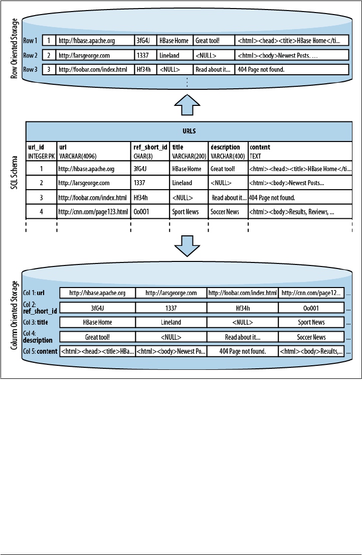
Column-Oriented Databases
Column-oriented databases save their data grouped by columns. Subsequent column
values are stored contiguously on disk. This differs from the usual row-oriented
approach of traditional databases, which store entire rows contiguously—see
Figure 1-1 for a visualization of the different physical layouts.
The reason to store values on a per-column basis instead is based on the assumption
that, for specific queries, not all of the values are needed. This is often the case in
analytical databases in particular, and therefore they are good candidates for this dif-
ferent storage schema.
Reduced I/O is one of the primary reasons for this new layout, but it offers additional
advantages playing into the same category: since the values of one column are often
very similar in nature or even vary only slightly between logical rows, they are often
much better suited for compression than the heterogeneous values of a row-oriented
record structure; most compression algorithms only look at a finite window.
Specialized algorithms—for example, delta and/or prefix compression—selected based
on the type of the column (i.e., on the data stored) can yield huge improvements in
compression ratios. Better ratios result in more efficient bandwidth usage.
Note, though, that HBase is not a column-oriented database in the typical RDBMS
sense, but utilizes an on-disk column storage format. This is also where the majority
of similarities end, because although HBase stores data on disk in a column-oriented
format, it is distinctly different from traditional columnar databases: whereas columnar
databases excel at providing real-time analytical access to data, HBase excels at pro-
viding key-based access to a specific cell of data, or a sequential range of cells.
The speed at which data is created today is already greatly increased, compared to only
just a few years back. We can take for granted that this is only going to increase further,
and with the rapid pace of globalization the problem is only exacerbated. Websites like
Google, Amazon, eBay, and Facebook now reach the majority of people on this planet.
The term planet-size web application comes to mind, and in this case it is fitting.
Facebook, for example, is adding more than 15 TB of data into its Hadoop cluster every
day‖ and is subsequently processing it all. One source of this data is click-stream log-
ging, saving every step a user performs on its website, or on sites that use the social
plug-ins offered by Facebook. This is an ideal case in which batch processing to build
machine learning models for predictions and recommendations is appropriate.
Facebook also has a real-time component, which is its messaging system, including
chat, wall posts, and email. This amounts to 135+ billion messages per month,# and
‖See this note published by Facebook.
The Dawn of Big Data | 3
storing this data over a certain number of months creates a huge tail that needs to be
handled efficiently. Even though larger parts of emails—for example, attachments—
are stored in a secondary system,* the amount of data generated by all these messages
is mind-boggling. If we were to take 140 bytes per message, as used by Twitter, it would
Figure 1-1. Column-oriented and row-oriented storage layouts
#See this blog post, as well as this one, by the Facebook engineering team. Wall messages count for 15 billion
and chat for 120 billion, totaling 135 billion messages a month. Then they also add SMS and others to create
an even larger number.
* Facebook uses Haystack, which provides an optimized storage infrastructure for large binary objects, such
as photos.
4 | Chapter 1: Introduction

total more than 17 TB every month. Even before the transition to HBase, the existing
system had to handle more than 25 TB a month.†
In addition, less web-oriented companies from across all major industries are collecting
an ever-increasing amount of data. For example:
Financial
Such as data generated by stock tickers
Bioinformatics
Such as the Global Biodiversity Information Facility (http://www.gbif.org/)
Smart grid
Such as the OpenPDC (http://openpdc.codeplex.com/) project
Sales
Such as the data generated by point-of-sale (POS) or stock/inventory systems
Genomics
Such as the Crossbow (http://bowtie-bio.sourceforge.net/crossbow/index.shtml)
project
Cellular services, military, environmental
Which all collect a tremendous amount of data as well
Storing petabytes of data efficiently so that updates and retrieval are still performed
well is no easy feat. We will now look deeper into some of the challenges.
The Problem with Relational Database Systems
RDBMSes have typically played (and, for the foreseeable future at least, will play) an
integral role when designing and implementing business applications. As soon as you
have to retain information about your users, products, sessions, orders, and so on, you
are typically going to use some storage backend providing a persistence layer for the
frontend application server. This works well for a limited number of records, but with
the dramatic increase of data being retained, some of the architectural implementation
details of common database systems show signs of weakness.
Let us use Hush, the HBase URL Shortener mentioned earlier, as an example. Assume
that you are building this system so that it initially handles a few thousand users, and
that your task is to do so with a reasonable budget—in other words, use free software.
The typical scenario here is to use the open source LAMP‡ stack to quickly build out
a prototype for the business idea.
The relational database model normalizes the data into a user table, which is accom-
panied by a url, shorturl, and click table that link to the former by means of a foreign
† See this presentation, given by Facebook employee and HBase committer, Nicolas Spiegelberg.
‡ Short for Linux, Apache, MySQL, and PHP (or Perl and Python).
The Problem with Relational Database Systems | 5

key. The tables also have indexes so that you can look up URLs by their short ID, or
the users by their username. If you need to find all the shortened URLs for a particular
list of customers, you could run an SQL JOIN over both tables to get a comprehensive
list of URLs for each customer that contains not just the shortened URL but also the
customer details you need.
In addition, you are making use of built-in features of the database: for example, stored
procedures, which allow you to consistently update data from multiple clients while
the database system guarantees that there is always coherent data stored in the various
tables.
Transactions make it possible to update multiple tables in an atomic fashion so that
either all modifications are visible or none are visible. The RDBMS gives you the so-
called ACID§ properties, which means your data is strongly consistent (we will address
this in greater detail in “Consistency Models” on page 9). Referential integrity takes
care of enforcing relationships between various table schemas, and you get a domain-
specific language, namely SQL, that lets you form complex queries over everything.
Finally, you do not have to deal with how data is actually stored, but only with higher-
level concepts such as table schemas, which define a fixed layout your application code
can reference.
This usually works very well and will serve its purpose for quite some time. If you are
lucky, you may be the next hot topic on the Internet, with more and more users joining
your site every day. As your user numbers grow, you start to experience an increasing
amount of pressure on your shared database server. Adding more application servers
is relatively easy, as they share their state only with the central database. Your CPU and
I/O load goes up and you start to wonder how long you can sustain this growth rate.
The first step to ease the pressure is to add slave database servers that are used to being
read from in parallel. You still have a single master, but that is now only taking writes,
and those are much fewer compared to the many reads your website users generate.
But what if that starts to fail as well, or slows down as your user count steadily increases?
A common next step is to add a cache—for example, Memcached.‖ Now you can off-
load the reads to a very fast, in-memory system—however, you are losing consistency
guarantees, as you will have to invalidate the cache on modifications of the original
value in the database, and you have to do this fast enough to keep the time where the
cache and the database views are inconsistent to a minimum.
While this may help you with the amount of reads, you have not yet addressed the
writes. Once the master database server is hit too hard with writes, you may replace it
with a beefed-up server—scaling up vertically—which simply has more cores, more
memory, and faster disks... and costs a lot more money than the initial one. Also note
§ Short for Atomicity, Consistency, Isolation, and Durability. See “ACID” on Wikipedia.
‖Memcached is an in-memory, nonpersistent, nondistributed key/value store. See the Memcached project
home page.
6 | Chapter 1: Introduction

that if you already opted for the master/slave setup mentioned earlier, you need to make
the slaves as powerful as the master or the imbalance may mean the slaves fail to keep
up with the master’s update rate. This is going to double or triple the cost, if not more.
With more site popularity, you are asked to add more features to your application,
which translates into more queries to your database. The SQL JOINs you were happy
to run in the past are suddenly slowing down and are simply not performing well
enough at scale. You will have to denormalize your schemas. If things get even worse,
you will also have to cease your use of stored procedures, as they are also simply be-
coming too slow to complete. Essentially, you reduce the database to just storing your
data in a way that is optimized for your access patterns.
Your load continues to increase as more and more users join your site, so another logical
step is to prematerialize the most costly queries from time to time so that you can serve
the data to your customers faster. Finally, you start dropping secondary indexes as their
maintenance becomes too much of a burden and slows down the database too much.
You end up with queries that can only use the primary key and nothing else.
Where do you go from here? What if your load is expected to increase by another order
of magnitude or more over the next few months? You could start sharding (see the
sidebar titled “Sharding”) your data across many databases, but this turns into an op-
erational nightmare, is very costly, and still does not give you a truly fitting solution.
You essentially make do with the RDBMS for lack of an alternative.
Sharding
The term sharding describes the logical separation of records into horizontal partitions.
The idea is to spread data across multiple storage files—or servers—as opposed to
having each stored contiguously.
The separation of values into those partitions is performed on fixed boundaries: you
have to set fixed rules ahead of time to route values to their appropriate store. With it
comes the inherent difficulty of having to reshard the data when one of the horizontal
partitions exceeds its capacity.
Resharding is a very costly operation, since the storage layout has to be rewritten. This
entails defining new boundaries and then horizontally splitting the rows across them.
Massive copy operations can take a huge toll on I/O performance as well as temporarily
elevated storage requirements. And you may still take on updates from the client ap-
plications and need to negotiate updates during the resharding process.
This can be mitigated by using virtual shards, which define a much larger key parti-
tioning range, with each server assigned an equal number of these shards. When you
add more servers, you can reassign shards to the new server. This still requires that the
data be moved over to the added server.
Sharding is often a simple afterthought or is completely left to the operator. Without
proper support from the database system, this can wreak havoc on production systems.
The Problem with Relational Database Systems | 7

Let us stop here, though, and, to be fair, mention that a lot of companies are using
RDBMSes successfully as part of their technology stack. For example, Facebook—and
also Google—has a very large MySQL setup, and for its purposes it works sufficiently.
This database farm suits the given business goal and may not be replaced anytime soon.
The question here is if you were to start working on implementing a new product and
knew that it needed to scale very fast, wouldn’t you want to have all the options avail-
able instead of using something you know has certain constraints?
Nonrelational Database Systems, Not-Only SQL or NoSQL?
Over the past four or five years, the pace of innovation to fill that exact problem space
has gone from slow to insanely fast. It seems that every week another framework or
project is announced to fit a related need. We saw the advent of the so-called NoSQL
solutions, a term coined by Eric Evans in response to a question from Johan Oskarsson,
who was trying to find a name for an event in that very emerging, new data storage
system space.#
The term quickly rose to fame as there was simply no other name for this new class of
products. It was (and is) discussed heavily, as it was also deemed the nemesis of
“SQL”—or was meant to bring the plague to anyone still considering using traditional
RDBMSes... just kidding!
The actual idea of different data store architectures for specific problem
sets is not new at all. Systems like Berkeley DB, Coherence, GT.M, and
object-oriented database systems have been around for years, with some
dating back to the early 1980s, and they fall into the NoSQL group by
definition as well.
The tagword is actually a good fit: it is true that most new storage systems do not
provide SQL as a means to query data, but rather a different, often simpler, API-like
interface to the data.
On the other hand, tools are available that provide SQL dialects to NoSQL data stores,
and they can be used to form the same complex queries you know from relational
databases. So, limitations in querying no longer differentiate RDBMSes from their
nonrelational kin.
The difference is actually on a lower level, especially when it comes to schemas or ACID-
like transactional features, but also regarding the actual storage architecture. A lot of
these new kinds of systems do one thing first: throw out the limiting factors in truly
scalable systems (a topic that is discussed in “Dimensions” on page 10).
For example, they often have no support for transactions or secondary indexes. More
#See “NoSQL” on Wikipedia.
8 | Chapter 1: Introduction

importantly, they often have no fixed schemas so that the storage can evolve with the
application using it.
Consistency Models
It seems fitting to talk about consistency a bit more since it is mentioned often through-
out this book. On the outset, consistency is about guaranteeing that a database always
appears truthful to its clients. Every operation on the database must carry its state from
one consistent state to the next. How this is achieved or implemented is not specified
explicitly so that a system has multiple choices. In the end, it has to get to the next
consistent state, or return to the previous consistent state, to fulfill its obligation.
Consistency can be classified in, for example, decreasing order of its properties, or
guarantees offered to clients. Here is an informal list:
Strict
The changes to the data are atomic and appear to take effect instantaneously. This
is the highest form of consistency.
Sequential
Every client sees all changes in the same order they were applied.
Causal
All changes that are causally related are observed in the same order by all clients.
Eventual
When no updates occur for a period of time, eventually all updates will propagate
through the system and all replicas will be consistent.
Weak
No guarantee is made that all updates will propagate and changes may appear out
of order to various clients.
The class of system adhering to eventual consistency can be even further divided into
subtler sets, where those sets can also coexist. Werner Vogels, CTO of Amazon, lists
them in his post titled “Eventually Consistent”. The article also picks up on the topic
of the CAP theorem,* which states that a distributed system can only achieve two out
of the following three properties: consistency, availability, and partition tolerance. The
CAP theorem is a highly discussed topic, and is certainly not the only way to classify,
but it does point out that distributed systems are not easy to develop given certain
requirements. Vogels, for example, mentions:
An important observation is that in larger distributed scale systems, network par-
titions are a given and as such consistency and availability cannot be achieved at
the same time. This means that one has two choices on what to drop; relaxing
consistency will allow the system to remain highly available [...] and prioritizing
consistency means that under certain conditions the system will not be available.
* See Eric Brewer’s original paper on this topic and the follow-up post by Coda Hale, as well as this PDF
by Gilbert and Lynch.
Nonrelational Database Systems, Not-Only SQL or NoSQL? | 9

Relaxing consistency, while at the same time gaining availability, is a powerful propo-
sition. However, it can force handling inconsistencies into the application layer and
may increase complexity.
There are many overlapping features within the group of nonrelational databases, but
some of these features also overlap with traditional storage solutions. So the new sys-
tems are not really revolutionary, but rather, from an engineering perspective, are more
evolutionary.
Even projects like memcached are lumped into the NoSQL category, as if anything that
is not an RDBMS is automatically NoSQL. This creates a kind of false dichotomy that
obscures the exciting technical possibilities these systems have to offer. And there are
many; within the NoSQL category, there are numerous dimensions you could use to
classify where the strong points of a particular system lie.
Dimensions
Let us take a look at a handful of those dimensions here. Note that this is not a com-
prehensive list, or the only way to classify them.
Data model
There are many variations in how the data is stored, which include key/value stores
(compare to a HashMap), semistructured, column-oriented stores, and document-
oriented stores. How is your application accessing the data? Can the schema evolve
over time?
Storage model
In-memory or persistent? This is fairly easy to decide since we are comparing with
RDBMSes, which usually persist their data to permanent storage, such as physical
disks. But you may explicitly need a purely in-memory solution, and there are
choices for that too. As far as persistent storage is concerned, does this affect your
access pattern in any way?
Consistency model
Strictly or eventually consistent? The question is, how does the storage system
achieve its goals: does it have to weaken the consistency guarantees? While this
seems like a cursory question, it can make all the difference in certain use cases. It
may especially affect latency, that is, how fast the system can respond to read and
write requests. This is often measured in harvest and yield.†
Physical model
Distributed or single machine? What does the architecture look like—is it built
from distributed machines or does it only run on single machines with the distri-
bution handled client-side, that is, in your own code? Maybe the distribution is
† See Brewer: “Lessons from giant-scale services.” Internet Computing, IEEE (2001) vol. 5 (4) pp. 46–55 (http:
//ieeexplore.ieee.org/xpl/freeabs_all.jsp?arnumber=939450).
10 | Chapter 1: Introduction

only an afterthought and could cause problems once you need to scale the system.
And if it does offer scalability, does it imply specific steps to do so? The easiest
solution would be to add one machine at a time, while sharded setups (especially
those not supporting virtual shards) sometimes require for each shard to be in-
creased simultaneously because each partition needs to be equally powerful.
Read/write performance
You have to understand what your application’s access patterns look like. Are you
designing something that is written to a few times, but is read much more often?
Or are you expecting an equal load between reads and writes? Or are you taking
in a lot of writes and just a few reads? Does it support range scans or is it better
suited doing random reads? Some of the available systems are advantageous for
only one of these operations, while others may do well in all of them.
Secondary indexes
Secondary indexes allow you to sort and access tables based on different fields and
sorting orders. The options here range from systems that have absolutely no sec-
ondary indexes and no guaranteed sorting order (like a HashMap, i.e., you need
to know the keys) to some that weakly support them, all the way to those that offer
them out of the box. Can your application cope, or emulate, if this feature is
missing?
Failure handling
It is a fact that machines crash, and you need to have a mitigation plan in place
that addresses machine failures (also refer to the discussion of the CAP theorem in
“Consistency Models” on page 9). How does each data store handle server failures?
Is it able to continue operating? This is related to the “Consistency model” dimen-
sion discussed earlier, as losing a machine may cause holes in your data store, or
even worse, make it completely unavailable. And if you are replacing the server,
how easy will it be to get back to being 100% operational? Another scenario is
decommissioning a server in a clustered setup, which would most likely be handled
the same way.
Compression
When you have to store terabytes of data, especially of the kind that consists of
prose or human-readable text, it is advantageous to be able to compress the data
to gain substantial savings in required raw storage. Some compression algorithms
can achieve a 10:1 reduction in storage space needed. Is the compression method
pluggable? What types are available?
Load balancing
Given that you have a high read or write rate, you may want to invest in a storage
system that transparently balances itself while the load shifts over time. It may not
be the full answer to your problems, but it may help you to ease into a high-
throughput application design.
Nonrelational Database Systems, Not-Only SQL or NoSQL? | 11

Atomic read-modify-write
While RDBMSes offer you a lot of these operations directly (because you are talking
to a central, single server), they can be more difficult to achieve in distributed
systems. They allow you to prevent race conditions in multithreaded or shared-
nothing application server design. Having these compare and swap (CAS) or check
and set operations available can reduce client-side complexity.
Locking, waits, and deadlocks
It is a known fact that complex transactional processing, like two-phase commits,
can increase the possibility of multiple clients waiting for a resource to become
available. In a worst-case scenario, this can lead to deadlocks, which are hard to
resolve. What kind of locking model does the system you are looking at support?
Can it be free of waits, and therefore deadlocks?
We will look back at these dimensions later on to see where HBase fits
and where its strengths lie. For now, let us say that you need to carefully
select the dimensions that are best suited to the issues at hand. Be prag-
matic about the solution, and be aware that there is no hard and fast
rule, in cases where an RDBMS is not working ideally, that a NoSQL
system is the perfect match. Evaluate your options, choose wisely, and
mix and match if needed.
An interesting term to describe this issue is impedance match, which
describes the need to find the ideal solution for a given problem. Instead
of using a “one-size-fits-all” approach, you should know what else is
available. Try to use the system that solves your problem best.
Scalability
While the performance of RDBMSes is well suited for transactional processing, it is less
so for very large-scale analytical processing. This refers to very large queries that scan
wide ranges of records or entire tables. Analytical databases may contain hundreds or
thousands of terabytes, causing queries to exceed what can be done on a single server
in a reasonable amount of time. Scaling that server vertically—that is, adding more
cores or disks—is simply not good enough.
What is even worse is that with RDBMSes, waits and deadlocks are increasing
nonlinearly with the size of the transactions and concurrency—that is, the square of
concurrency and the third or even fifth power of the transaction size.‡ Sharding is often
an impractical solution, as it has to be done within the application layer, and may
involve complex and costly (re)partitioning procedures.
Commercial RDBMSes are available that solve many of these issues, but they are often
specialized and only cover certain aspects. Above all, they are very, very expensive.
‡ See “FT 101” by Jim Gray et al.
12 | Chapter 1: Introduction

Looking at open source alternatives in the RDBMS space, you will likely have to give
up many or all relational features, such as secondary indexes, to gain some level of
performance.
The question is, wouldn’t it be good to trade relational features permanently for per-
formance? You could denormalize (see the next section) the data model and avoid waits
and deadlocks by minimizing necessary locking. How about built-in horizontal scala-
bility without the need to repartition as your data grows? Finally, throw in fault toler-
ance and data availability, using the same mechanisms that allow scalability, and what
you get is a NoSQL solution—more specifically, one that matches what HBase has to
offer.
Database (De-)Normalization
At scale, it is often a requirement that we design schema differently, and a good term
to describe this principle is Denormalization, Duplication, and Intelligent Keys
(DDI).§ It is about rethinking how data is stored in Bigtable-like storage systems, and
how to make use of it in an appropriate way.
Part of the principle is to denormalize schemas by, for example, duplicating data in
more than one table so that, at read time, no further aggregation is required. Or the
related prematerialization of required views, once again optimizing for fast reads with-
out any further processing.
There is much more on this topic in Chapter 9, where you will find many ideas on how
to design solutions that make the best use of the features HBase provides. Let us look
at an example to understand the basic principles of converting a classic relational
database model to one that fits the columnar nature of HBase much better.
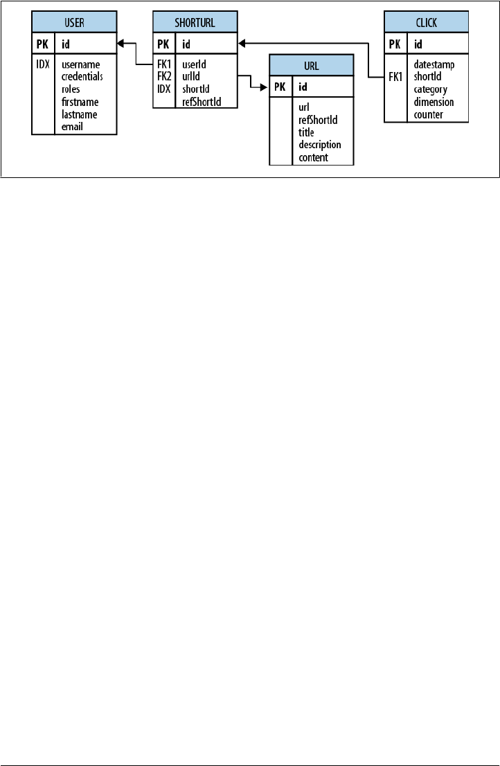
Consider the HBase URL Shortener, Hush, which allows us to map long URLs to short
URLs. The entity relationship diagram (ERD) can be seen in Figure 1-2. The full SQL
schema can be found in Appendix E.‖
The shortened URL, stored in the shorturl table, can then be given to others that
subsequently click on it to open the linked full URL. Each click is tracked, recording
the number of times it was used, and, for example, the country the click came from.
This is stored in the click table, which aggregates the usage on a daily basis, similar to
a counter.
Users, stored in the user table, can sign up with Hush to create their own list of short-
ened URLs, which can be edited to add a description. This links the user and short
url tables with a foreign key relationship.
§ The term DDI was coined in the paper “Cloud Data Structure Diagramming Techniques and Design Patterns”
by D. Salmen et al. (2009).
‖Note, though, that this is provided purely for demonstration purposes, so the schema is deliberately kept
simple.
Nonrelational Database Systems, Not-Only SQL or NoSQL? | 13
The system also downloads the linked page in the background, and extracts, for in-
stance, the TITLE tag from the HTML, if present. The entire page is saved for later
processing with asynchronous batch jobs, for analysis purposes. This is represented by
the url table.
Every linked page is only stored once, but since many users may link to the same long
URL, yet want to maintain their own details, such as the usage statistics, a separate
entry in the shorturl is created. This links the url, shorturl, and click tables.
This also allows you to aggregate statistics to the original short ID, refShortId, so that
you can see the overall usage of any short URL to map to the same long URL. The
shortId and refShortId are the hashed IDs assigned uniquely to each shortened URL.
For example, in
http://hush.li/a23eg
the ID is a23eg.
Figure 1-3 shows how the same schema could be represented in HBase. Every shortened
URL is stored in a separate table, shorturl, which also contains the usage statistics,
storing various time ranges in separate column families, with distinct time-to-live
settings. The columns form the actual counters, and their name is a combination of the
date, plus an optional dimensional postfix—for example, the country code.
The downloaded page, and the extracted details, are stored in the url table. This table
uses compression to minimize the storage requirements, because the pages are mostly
HTML, which is inherently verbose and contains a lot of text.
The user-shorturl table acts as a lookup so that you can quickly find all short IDs for
a given user. This is used on the user’s home page, once she has logged in. The user
table stores the actual user details.
We still have the same number of tables, but their meaning has changed: the clicks
table has been absorbed by the shorturl table, while the statistics columns use the date
as their key, formatted as YYYYMMDD—for instance, 20110502—so that they can be ac-
Figure 1-2. The Hush schema expressed as an ERD
14 | Chapter 1: Introduction
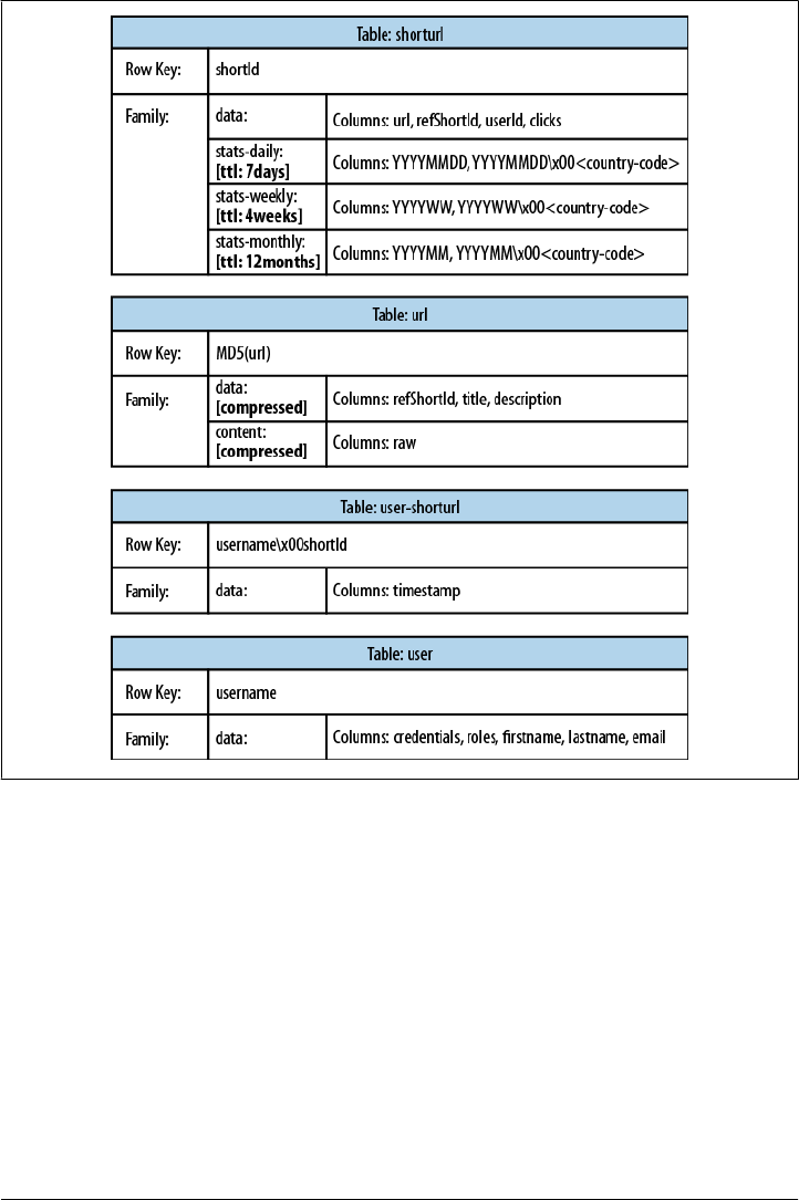
cessed sequentially. The additional user-shorturl table is replacing the foreign key
relationship, making user-related lookups faster.
There are various approaches to converting one-to-one, one-to-many, and many-to-
many relationships to fit the underlying architecture of HBase. You could implement
even this simple example in different ways. You need to understand the full potential
of HBase storage design to make an educated decision regarding which approach to
take.
The support for sparse, wide tables and column-oriented design often eliminates the
need to normalize data and, in the process, the costly JOIN operations needed to
aggregate the data at query time. Use of intelligent keys gives you fine-grained control
over how—and where—data is stored. Partial key lookups are possible, and when
Figure 1-3. The Hush schema in HBase
Nonrelational Database Systems, Not-Only SQL or NoSQL? | 15

combined with compound keys, they have the same properties as leading, left-edge
indexes. Designing the schemas properly enables you to grow the data from 10 entries
to 10 million entries, while still retaining the same write and read performance.
Building Blocks
This section provides you with an overview of the architecture behind HBase. After
giving you some background information on its lineage, the section will introduce the
general concepts of the data model and the available storage API, and presents a high-
level overview on implementation.
Backdrop
In 2003, Google published a paper titled “The Google File System”. This scalable dis-
tributed file system, abbreviated as GFS, uses a cluster of commodity hardware to store
huge amounts of data. The filesystem handled data replication between nodes so that
losing a storage server would have no effect on data availability. It was also optimized
for streaming reads so that data could be read for processing later on.
Shortly afterward, another paper by Google was published, titled “MapReduce: Sim-
plified Data Processing on Large Clusters”. MapReduce was the missing piece to the
GFS architecture, as it made use of the vast number of CPUs each commodity server
in the GFS cluster provides. MapReduce plus GFS forms the backbone for processing
massive amounts of data, including the entire search index Google owns.
What is missing, though, is the ability to access data randomly and in close to real-time
(meaning good enough to drive a web service, for example). Another drawback of the
GFS design is that it is good with a few very, very large files, but not as good with
millions of tiny files, because the data retained in memory by the master node is ulti-
mately bound to the number of files. The more files, the higher the pressure on the
memory of the master.
So, Google was trying to find a solution that could drive interactive applications, such
as Mail or Analytics, while making use of the same infrastructure and relying on GFS
for replication and data availability. The data stored should be composed of much
smaller entities, and the system would transparently take care of aggregating the small
records into very large storage files and offer some sort of indexing that allows the user
to retrieve data with a minimal number of disk seeks. Finally, it should be able to store
the entire web crawl and work with MapReduce to build the entire search index in a
timely manner.
Being aware of the shortcomings of RDBMSes at scale (see “Seek Versus Trans-
fer” on page 315 for a discussion of one fundamental issue), the engineers approached
this problem differently: forfeit relational features and use a simple API that has basic
create, read, update, and delete (or CRUD) operations, plus a scan function to iterate
16 | Chapter 1: Introduction

over larger key ranges or entire tables. The culmination of these efforts was published
in 2006 in a paper titled “Bigtable: A Distributed Storage System for Structured Data”,
two excerpts from which follow:
Bigtable is a distributed storage system for managing structured data that is designed to
scale to a very large size: petabytes of data across thousands of commodity servers.
…a sparse, distributed, persistent multi-dimensional sorted map.
It is highly recommended that everyone interested in HBase read that paper. It describes
a lot of reasoning behind the design of Bigtable and, ultimately, HBase. We will, how-
ever, go through the basic concepts, since they apply directly to the rest of this book.
HBase is implementing the Bigtable storage architecture very faithfully so that we can
explain everything using HBase. Appendix F provides an overview of where the two
systems differ.
Tables, Rows, Columns, and Cells
First, a quick summary: the most basic unit is a column. One or more columns form a
row that is addressed uniquely by a row key. A number of rows, in turn, form a table,
and there can be many of them. Each column may have multiple versions, with each
distinct value contained in a separate cell.
This sounds like a reasonable description for a typical database, but with the extra
dimension of allowing multiple versions of each cells. But obviously there is a bit more
to it.
All rows are always sorted lexicographically by their row key. Example 1-1 shows how
this will look when adding a few rows with different keys.
Example 1-1. The sorting of rows done lexicographically by their key
hbase(main):001:0> scan 'table1'
ROW COLUMN+CELL
row-1 column=cf1:, timestamp=1297073325971 ...
row-10 column=cf1:, timestamp=1297073337383 ...
row-11 column=cf1:, timestamp=1297073340493 ...
row-2 column=cf1:, timestamp=1297073329851 ...
row-22 column=cf1:, timestamp=1297073344482 ...
row-3 column=cf1:, timestamp=1297073333504 ...
row-abc column=cf1:, timestamp=1297073349875 ...
7 row(s) in 0.1100 seconds
Note how the numbering is not in sequence as you may have expected it. You may have
to pad keys to get a proper sorting order. In lexicographical sorting, each key is com-
pared on a binary level, byte by byte, from left to right. Since row-1... is less than
row-2..., no matter what follows, it is sorted first.
Having the row keys always sorted can give you something like a primary key index
known from RDBMSes. It is also always unique, that is, you can have each row key
Building Blocks | 17

only once, or you are updating the same row. While the original Bigtable paper only
considers a single index, HBase adds support for secondary indexes (see “Secondary
Indexes” on page 370). The row keys can be any arbitrary array of bytes and are not
necessarily human-readable.
Rows are composed of columns, and those, in turn, are grouped into column families.
This helps in building semantical or topical boundaries between the data, and also in
applying certain features to them—for example, compression—or denoting them to
stay in-memory. All columns in a column family are stored together in the same low-
level storage file, called an HFile.
Column families need to be defined when the table is created and should not be changed
too often, nor should there be too many of them. There are a few known shortcomings
in the current implementation that force the count to be limited to the low tens, but in
practice it is often a much smaller number (see Chapter 9 for details). The name of the
column family must be composed of printable characters, a notable difference from all
other names or values.
Columns are often referenced as family:qualifier with the qualifier being any arbitrary
array of bytes.# As opposed to the limit on column families, there is no such thing for
the number of columns: you could have millions of columns in a particular column
family. There is also no type nor length boundary on the column values.
Figure 1-4 helps to visualize how different rows are in a normal database as opposed
to the column-oriented design of HBase. You should think about rows and columns
not being arranged like the classic spreadsheet model, but rather use a tag metaphor,
that is, information is available under a specific tag.
The "NULL?" in Figure 1-4 indicates that, for a database with a fixed
schema, you have to store NULLs where there is no value, but for HBase’s
storage architectures, you simply omit the whole column; in other
words, NULLs are free of any cost: they do not occupy any storage space.
All rows and columns are defined in the context of a table, adding a few more concepts
across all included column families, which we will discuss shortly.
Every column value, or cell, either is timestamped implicitly by the system or can be
set explicitly by the user. This can be used, for example, to save multiple versions of a
value as it changes over time. Different versions of a cell are stored in decreasing time-
stamp order, allowing you to read the newest value first. This is an optimization aimed
at read patterns that favor more current values over historical ones.
The user can specify how many versions of a value should be kept. In addition, there
is support for predicate deletions (see “Log-Structured Merge-Trees” on page 316 for
#You will see in “Column Families” on page 212 that the qualifier also may be left unset.
18 | Chapter 1: Introduction
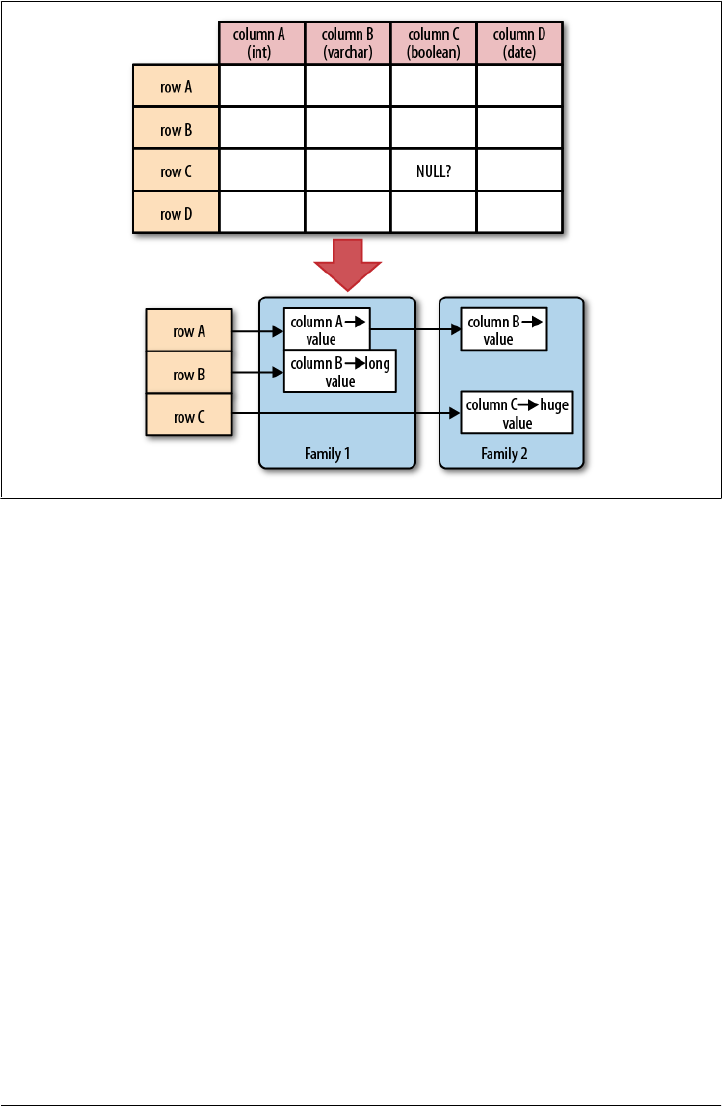
the concepts behind them) allowing you to keep, for example, only values written in
the past week. The values (or cells) are also just uninterpreted arrays of bytes, that the
client needs to know how to handle.
If you recall from the quote earlier, the Bigtable model, as implemented by HBase, is a
sparse, distributed, persistent, multidimensional map, which is indexed by row key,
column key, and a timestamp. Putting this together, we can express the access to data
like so:
(Table, RowKey, Family, Column, Timestamp) → Value
In a more programming language style, this may be expressed as:
SortedMap<
RowKey, List<
SortedMap<
Column, List<
Value, Timestamp
>
>
>
>
or all in one line:
SortedMap<RowKey, List<SortedMap<Column, List<Value, Timestamp>>>>
Figure 1-4. Rows and columns in HBase
Building Blocks | 19
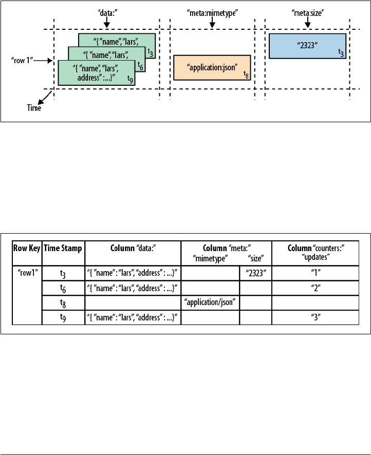
The first SortedMap is the table, containing a List of column families. The families
contain another SortedMap, which represents the columns, and their associated values.
These values are in the final List that holds the value and the timestamp it was set.
An interesting feature of the model is that cells may exist in multiple versions, and
different columns have been written at different times. The API, by default, provides
you with a coherent view of all columns wherein it automatically picks the most current
value of each cell. Figure 1-5 shows a piece of one specific row in an example table.
Figure 1-5. A time-oriented view into parts of a row
The diagram visualizes the time component using tn as the timestamp when the cell
was written. The ascending index shows that the values have been added at different
times. Figure 1-6 is another way to look at the data, this time in a more spreadsheet-
like layout wherein the timestamp was added to its own column.
Figure 1-6. The same parts of the row rendered as a spreadsheet
Although they have been added at different times and exist in multiple versions, you
would still see the row as the combination of all columns and their most current
versions—in other words, the highest tn from each column. There is a way to ask for
values at (or before) a specific timestamp, or more than one version at a time, which
we will see a little bit later in Chapter 3.
20 | Chapter 1: Introduction
The Webtable
The canonical use case of Bigtable and HBase is the webtable, that is, the web pages
stored while crawling the Internet.
The row key is the reversed URL of the page—for example, org.hbase.www. There is a
column family storing the actual HTML code, the contents family, as well as others
like anchor, which is used to store outgoing links, another one to store inbound links,
and yet another for metadata like language.
Using multiple versions for the contents family allows you to store a few older copies
of the HTML, and is helpful when you want to analyze how often a page changes, for
example. The timestamps used are the actual times when they were fetched from the
crawled website.
Access to row data is atomic and includes any number of columns being read or written
to. There is no further guarantee or transactional feature that spans multiple rows or
across tables. The atomic access is also a contributing factor to this architecture being
strictly consistent, as each concurrent reader and writer can make safe assumptions
about the state of a row.
Using multiversioning and timestamping can help with application layer consistency
issues as well.
Auto-Sharding
The basic unit of scalability and load balancing in HBase is called a region. Regions are
essentially contiguous ranges of rows stored together. They are dynamically split by
the system when they become too large. Alternatively, they may also be merged to
reduce their number and required storage files.*
The HBase regions are equivalent to range partitions as used in database
sharding. They can be spread across many physical servers, thus dis-
tributing the load, and therefore providing scalability.
Initially there is only one region for a table, and as you start adding data to it, the system
is monitoring it to ensure that you do not exceed a configured maximum size. If you
exceed the limit, the region is split into two at the middle key—the row key in the middle
of the region—creating two roughly equal halves (more details in Chapter 8).
Each region is served by exactly one region server, and each of these servers can serve
many regions at any time. Figure 1-7 shows how the logical view of a table is actually
a set of regions hosted by many region servers.
* Although HBase does not support online region merging, there are tools to do this offline. See “Merging
Regions” on page 433.
Building Blocks | 21
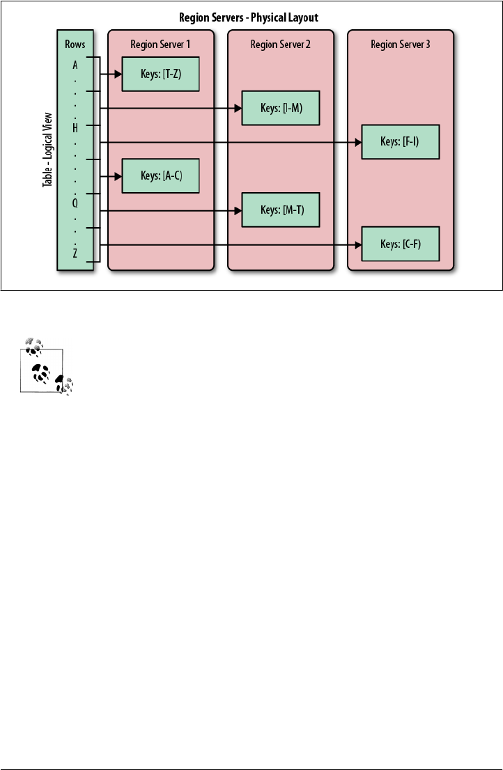
Figure 1-7. Rows grouped in regions and served by different servers
The Bigtable paper notes that the aim is to keep the region count be-
tween 10 and 1,000 per server and each at roughly 100 MB to 200 MB
in size. This refers to the hardware in use in 2006 (and earlier). For HBase
and modern hardware, the number would be more like 10 to 1,000
regions per server, but each between 1 GB and 2 GB in size.
But, while the numbers have increased, the basic principle is the same:
the number of regions per server, and their respective sizes, depend on
what can be handled sufficiently by a single server.
Splitting and serving regions can be thought of as autosharding, as offered by other
systems. The regions allow for fast recovery when a server fails, and fine-grained load
balancing since they can be moved between servers when the load of the server currently
serving the region is under pressure, or if that server becomes unavailable because of a
failure or because it is being decommissioned.
Splitting is also very fast—close to instantaneous—because the split regions simply
read from the original storage files until a compaction rewrites them into separate ones
asynchronously. This is explained in detail in Chapter 8.
Storage API
Bigtable does not support a full relational data model; instead, it provides clients with a
simple data model that supports dynamic control over data layout and format [...]
22 | Chapter 1: Introduction

The API offers operations to create and delete tables and column families. In addition,
it has functions to change the table and column family metadata, such as compression
or block sizes. Furthermore, there are the usual operations for clients to create or delete
values as well as retrieving them with a given row key.
A scan API allows you to efficiently iterate over ranges of rows and be able to limit
which columns are returned or the number of versions of each cell. You can match
columns using filters and select versions using time ranges, specifying start and end
times.
On top of this basic functionality are more advanced features. The system has support
for single-row transactions, and with this support it implements atomic read-modify-
write sequences on data stored under a single row key. Although there are no
cross-row or cross-table transactions, the client can batch operations for performance
reasons.
Cell values can be interpreted as counters and updated atomically. These counters can
be read and modified in one operation so that, despite the distributed nature of the
architecture, clients can use this mechanism to implement global, strictly consistent,
sequential counters.
There is also the option to run client-supplied code in the address space of the server.
The server-side framework to support this is called coprocessors. The code has access
to the server local data and can be used to implement lightweight batch jobs, or use
expressions to analyze or summarize data based on a variety of operators.
Coprocessors were added to HBase in version 0.91.0.
Finally, the system is integrated with the MapReduce framework by supplying wrappers
that convert tables into input source and output targets for MapReduce jobs.
Unlike in the RDBMS landscape, there is no domain-specific language, such as SQL,
to query data. Access is not done declaratively, but purely imperatively through the
client-side API. For HBase, this is mostly Java code, but there are many other choices
to access the data from other programming languages.
Implementation
Bigtable [...] allows clients to reason about the locality properties of the data represented
in the underlying storage.
The data is stored in store files, called HFiles, which are persistent and ordered immut-
able maps from keys to values. Internally, the files are sequences of blocks with a block
index stored at the end. The index is loaded when the HFile is opened and kept in
Building Blocks | 23
memory. The default block size is 64 KB but can be configured differently if required.
The store files provide an API to access specific values as well as to scan ranges of values
given a start and end key.
Implementation is discussed in great detail in Chapter 8. The text here
is an introduction only, while the full details are discussed in the refer-
enced chapter(s).
Since every HFile has a block index, lookups can be performed with a single disk seek.
First, the block possibly containing the given key is determined by doing a binary search
in the in-memory block index, followed by a block read from disk to find the actual key.
The store files are typically saved in the Hadoop Distributed File System (HDFS), which
provides a scalable, persistent, replicated storage layer for HBase. It guarantees that
data is never lost by writing the changes across a configurable number of physical
servers.
When data is updated it is first written to a commit log, called a write-ahead log (WAL)
in HBase, and then stored in the in-memory memstore. Once the data in memory has
exceeded a given maximum value, it is flushed as an HFile to disk. After the flush, the
commit logs can be discarded up to the last unflushed modification. While the system
is flushing the memstore to disk, it can continue to serve readers and writers without
having to block them. This is achieved by rolling the memstore in memory where the
new/empty one is taking the updates, while the old/full one is converted into a file.
Note that the data in the memstores is already sorted by keys matching exactly what
HFiles represent on disk, so no sorting or other special processing has to be performed.
We can now start to make sense of what the locality properties are,
mentioned in the Bigtable quote at the beginning of this section. Since
all files contain sorted key/value pairs, ordered by the key, and are op-
timized for block operations such as reading these pairs sequentially,
you should specify keys to keep related data together. Referring back to
the webtable example earlier, you may have noted that the key used is
the reversed FQDN (the domain name part of the URL), such as
org.hbase.www. The reason is to store all pages from hbase.org close to
one another, and reversing the URL puts the most important part of the
URL first, that is, the top-level domain (TLD). Pages under
blog.hbase.org would then be sorted with those from www.hbase.org—
or in the actual key format, org.hbase.blog sorts next to org.hbase.www.
Because store files are immutable, you cannot simply delete values by removing the
key/value pair from them. Instead, a delete marker (also known as a tombstone marker)
is written to indicate the fact that the given key has been deleted. During the retrieval
24 | Chapter 1: Introduction

process, these delete markers mask out the actual values and hide them from reading
clients.
Reading data back involves a merge of what is stored in the memstores, that is, the data
that has not been written to disk, and the on-disk store files. Note that the WAL is
never used during data retrieval, but solely for recovery purposes when a server has
crashed before writing the in-memory data to disk.
Since flushing memstores to disk causes more and more HFiles to be created, HBase
has a housekeeping mechanism that merges the files into larger ones using compac-
tion. There are two types of compaction: minor compactions and major compactions.
The former reduce the number of storage files by rewriting smaller files into fewer but
larger ones, performing an n-way merge. Since all the data is already sorted in each
HFile, that merge is fast and bound only by disk I/O performance.
The major compactions rewrite all files within a column family for a region into a single
new one. They also have another distinct feature compared to the minor compactions:
based on the fact that they scan all key/value pairs, they can drop deleted entries in-
cluding their deletion marker. Predicate deletes are handled here as well—for example,
removing values that have expired according to the configured time-to-live or when
there are too many versions.
This architecture is taken from LSM-trees (see “Log-Structured Merge-
Trees” on page 316). The only difference is that LSM-trees are storing
data in multipage blocks that are arranged in a B-tree-like structure on
disk. They are updated, or merged, in a rotating fashion, while in
Bigtable the update is more course-grained and the whole memstore is
saved as a new store file and not merged right away. You could call
HBase’s architecture “Log-Structured Sort-and-Merge-Maps.” The
background compactions correspond to the merges in LSM-trees, but
are occurring on a store file level instead of the partial tree updates,
giving the LSM-trees their name.
There are three major components to HBase: the client library, one master server, and
many region servers. The region servers can be added or removed while the system is
up and running to accommodate changing workloads. The master is responsible for
assigning regions to region servers and uses Apache ZooKeeper, a reliable, highly avail-
able, persistent and distributed coordination service, to facilitate that task.
Apache ZooKeeper
ZooKeeper† is a separate open source project, and is also part of the Apache Software
Foundation. ZooKeeper is the comparable system to Google’s use of Chubby for
Bigtable. It offers filesystem-like access with directories and files (called znodes) that
† For more information on Apache ZooKeeper, please refer to the official project website.
Building Blocks | 25
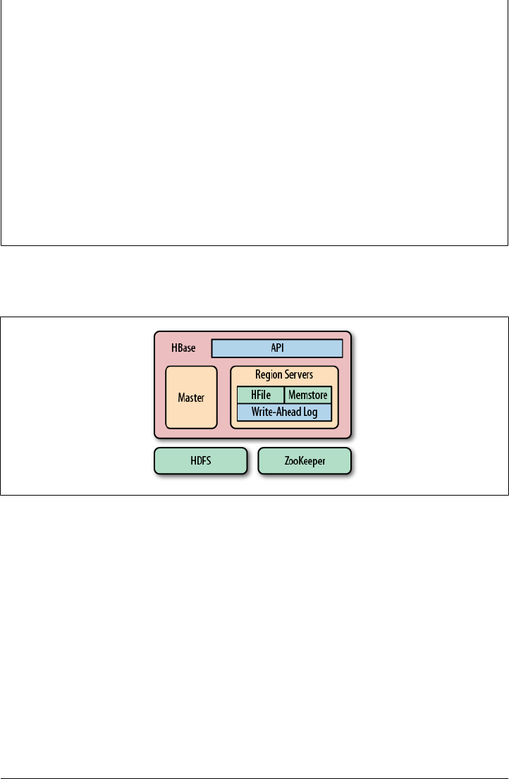
distributed systems can use to negotiate ownership, register services, or watch for
updates.
Every region server creates its own ephemeral node in ZooKeeper, which the master,
in turn, uses to discover available servers. They are also used to track server failures or
network partitions.
Ephemeral nodes are bound to the session between ZooKeeper and the client which
created it. The session has a heartbeat keepalive mechanism that, once it fails to report,
is declared lost by ZooKeeper and the associated ephemeral nodes are deleted.
HBase uses ZooKeeper also to ensure that there is only one master running, to store
the bootstrap location for region discovery, as a registry for region servers, as well as
for other purposes. ZooKeeper is a critical component, and without it HBase is not
operational. This is mitigated by ZooKeeper’s distributed design using an assemble of
servers and the Zab protocol to keep its state consistent.
Figure 1-8 shows how the various components of HBase are orchestrated to make use
of existing system, like HDFS and ZooKeeper, but also adding its own layers to form
a complete platform.
Figure 1-8. HBase using its own components while leveraging existing systems
The master server is also responsible for handling load balancing of regions across
region servers, to unload busy servers and move regions to less occupied ones. The
master is not part of the actual data storage or retrieval path. It negotiates load balancing
and maintains the state of the cluster, but never provides any data services to either the
region servers or the clients, and is therefore lightly loaded in practice. In addition, it
takes care of schema changes and other metadata operations, such as creation of tables
and column families.
Region servers are responsible for all read and write requests for all regions they serve,
and also split regions that have exceeded the configured region size thresholds. Clients
communicate directly with them to handle all data-related operations.
“Region Lookups” on page 345 has more details on how clients perform the region
lookup.
26 | Chapter 1: Introduction

Summary
Billions of rows * millions of columns * thousands of versions = terabytes or petabytes of
storage
We have seen how the Bigtable storage architecture is using many servers to distribute
ranges of rows sorted by their key for load-balancing purposes, and can scale to peta-
bytes of data on thousands of machines. The storage format used is ideal for reading
adjacent key/value pairs and is optimized for block I/O operations that can saturate
disk transfer channels.
Table scans run in linear time and row key lookups or mutations are performed in
logarithmic order—or, in extreme cases, even constant order (using Bloom filters).
Designing the schema in a way to completely avoid explicit locking, combined with
row-level atomicity, gives you the ability to scale your system without any notable effect
on read or write performance.
The column-oriented architecture allows for huge, wide, sparse tables as storing
NULLs is free. Because each row is served by exactly one server, HBase is strongly con-
sistent, and using its multiversioning can help you to avoid edit conflicts caused by
concurrent decoupled processes or retain a history of changes.
The actual Bigtable has been in production at Google since at least 2005, and it has
been in use for a variety of different use cases, from batch-oriented processing to real-
time data-serving. The stored data varies from very small (like URLs) to quite large
(e.g., web pages and satellite imagery) and yet successfully provides a flexible, high-
performance solution for many well-known Google products, such as Google Earth,
Google Reader, Google Finance, and Google Analytics.
HBase: The Hadoop Database
Having looked at the Bigtable architecture, we could simply state that HBase is a faith-
ful, open source implementation of Google’s Bigtable. But that would be a bit too
simplistic, and there are a few (mostly subtle) differences worth addressing.
History
HBase was created in 2007 at Powerset‡ and was initially part of the contributions in
Hadoop. Since then, it has become its own top-level project under the Apache Software
Foundation umbrella. It is available under the Apache Software License, version 2.0.
‡ Powerset is a company based in San Francisco that was developing a natural language search engine for the
Internet. On July 1, 2008, Microsoft acquired Powerset, and subsequent support for HBase development was
abandoned.
HBase: The Hadoop Database | 27

The project home page is http://hbase.apache.org/, where you can find links to the doc-
umentation, wiki, and source repository, as well as download sites for the binary and
source releases.
Here is a short overview of how HBase has evolved over time:
November 2006
Google releases paper on BigTable
February 2007
Initial HBase prototype created as Hadoop contrib§
October 2007
First “usable” HBase (Hadoop 0.15.0)
January 2008
Hadoop becomes an Apache top-level project, HBase becomes subproject
October 2008
HBase 0.18.1 released
January 2009
HBase 0.19.0 released
September 2009
HBase 0.20.0 released, the performance release
May 2010
HBase becomes an Apache top-level project
June 2010
HBase 0.89.20100621, first developer release
January 2011
HBase 0.90.0 released, the durability and stability release
Mid 2011
HBase 0.92.0 released, tagged as coprocessor and security release
Around May 2010, the developers decided to break with the version
numbering that was used to be in lockstep with the Hadoop releases.
The rationale was that HBase had a much faster release cycle and was
also approaching a version 1.0 level sooner than what was expected from
Hadoop.
To that effect, the jump was made quite obvious, going from 0.20.x to
0.89.x. In addition, a decision was made to title 0.89.x the early access
version for developers and bleeding-edge integrators. Version 0.89 was
eventually released as 0.90 for everyone as the next stable release.
§ For an interesting flash back in time, see HBASE-287 on the Apache JIRA, the issue tracking system. You
can see how Mike Cafarella did a code drop that was then quickly picked up by Jim Kellerman, who was
with Powerset back then.
28 | Chapter 1: Introduction

Nomenclature
One of the biggest differences between HBase and Bigtable concerns naming, as you
can see in Table 1-1, which lists the various terms and what they correspond to in each
system.
Table 1-1. Differences in naming
HBase Bigtable
Region Tablet
RegionServer Tablet server
Flush Minor compaction
Minor compaction Merging compaction
Major compaction Major compaction
Write-ahead log Commit log
HDFS GFS
Hadoop MapReduce MapReduce
MemStore memtable
HFile SSTable
ZooKeeper Chubby
More differences are described in Appendix F.
Summary
Let us now circle back to “Dimensions” on page 10, and how dimensions can be used
to classify HBase. HBase is a distributed, persistent, strictly consistent storage system
with near-optimal write—in terms of I/O channel saturation—and excellent read per-
formance, and it makes efficient use of disk space by supporting pluggable compression
algorithms that can be selected based on the nature of the data in specific column
families.
HBase extends the Bigtable model, which only considers a single index, similar to a
primary key in the RDBMS world, offering the server-side hooks to implement flexible
secondary index solutions. In addition, it provides push-down predicates, that is, fil-
ters, reducing data transferred over the network.
There is no declarative query language as part of the core implementation, and it has
limited support for transactions. Row atomicity and read-modify-write operations
make up for this in practice, as they cover most use cases and remove the wait or
deadlock-related pauses experienced with other systems.
HBase handles shifting load and failures gracefully and transparently to the clients.
Scalability is built in, and clusters can be grown or shrunk while the system is in pro-
HBase: The Hadoop Database | 29

duction. Changing the cluster does not involve any complicated rebalancing or re-
sharding procedure, but is completely automated.
30 | Chapter 1: Introduction
CHAPTER 2
Installation
In this chapter, we will look at how HBase is installed and initially configured. We will
see how HBase can be used from the command line for basic operations, such as adding,
retrieving, and deleting data.
All of the following assumes you have the Java Runtime Environment
(JRE) installed. Hadoop and also HBase require at least version 1.6 (also
called Java 6), and the recommended choice is the one provided by
Oracle (formerly by Sun), which can be found at http://www.java.com/
download/. If you do not have Java already or are running into issues
using it, please see “Java” on page 46.
Quick-Start Guide
Let us get started with the “tl;dr” section of this book: you want to know how to run
HBase and you want to know it now! Nothing is easier than that because all you have
to do is download the most recent release of HBase from the Apache HBase release
page and unpack the contents into a suitable directory, such as /usr/local or /opt, like so:
$ cd /usr/local
$ tar -zxvf hbase-x.y.z.tar.gz
Setting the Data Directory
At this point, you are ready to start HBase. But before you do so, it is advisable to set
the data directory to a proper location. You need to edit the configuration file conf/
hbase-site.xml and set the directory you want HBase to write to by assigning a value to
the property key named hbase.rootdir:
<?xml version="1.0"?>
<?xml-stylesheet type="text/xsl" href="configuration.xsl"?>
<configuration>
<property>
<name>hbase.rootdir</name>
<value>file:///<PATH>/hbase</value>
31
</property>
</configuration>
Replace <PATH> in the preceding example configuration file with a path to a directory
where you want HBase to store its data. By default, hbase.rootdir is set to /tmp/hbase-
${user.name}, which could mean you lose all your data whenever your server reboots
because a lot of operating systems (OSes) clear out /tmp during a restart.
With that in place, we can start HBase and try our first interaction with it. We will use
the interactive shell to enter the status command at the prompt (complete the com-
mand by pressing the Return key):
$ cd /usr/local/hbase-0.91.0-SNAPSHOT
$ bin/start-hbase.sh
starting master, logging to \
/usr/local/hbase-0.91.0-SNAPSHOT/bin/../logs/hbase-<username>-master-localhost.out
$ bin/hbase shell
HBase Shell; enter 'help<RETURN>' for list of supported commands.
Type "exit<RETURN>" to leave the HBase Shell
Version 0.91.0-SNAPSHOT, r1130916, Sat Jul 23 12:44:34 CEST 2011
hbase(main):001:0> status
1 servers, 0 dead, 2.0000 average load
This confirms that HBase is up and running, so we will now issue a few commands to
show that we can put data into it and retrieve the same data subsequently.
It may not be clear, but what we are doing right now is similar to sitting
in a car with its brakes engaged and in neutral while turning the ignition
key. There is much more that you need to configure and understand
before you can use HBase in a production-like environment. But it lets
you get started with some basic HBase commands and become familiar
with top-level concepts.
We are currently running in the so-called Standalone Mode. We will look
into the available modes later on (see “Run Modes” on page 58), but
for now it’s important to know that in this mode everything is run in a
single Java process and all files are stored in /tmp by default—unless you
did heed the important advice given earlier to change it to something
different. Many people have lost their test data during a reboot, only to
learn that they kept the default path. Once it is deleted by the OS, there
is no going back!
32 | Chapter 2: Installation

Let us now create a simple table and add a few rows with some data:
hbase(main):002:0> create 'testtable', 'colfam1'
0 row(s) in 0.2930 seconds
hbase(main):003:0> list 'testtable'
TABLE
testtable
1 row(s) in 0.0520 seconds
hbase(main):004:0> put 'testtable', 'myrow-1', 'colfam1:q1', 'value-1'
0 row(s) in 0.1020 seconds
hbase(main):005:0> put 'testtable', 'myrow-2', 'colfam1:q2', 'value-2'
0 row(s) in 0.0410 seconds
hbase(main):006:0> put 'testtable', 'myrow-2', 'colfam1:q3', 'value-3'
0 row(s) in 0.0380 seconds
After we create the table with one column family, we verify that it actually exists by
issuing a list command. You can see how it outputs the testtable name as the only
table currently known. Subsequently, we are putting data into a number of rows. If you
read the example carefully, you can see that we are adding data to two different rows
with the keys myrow-1 and myrow-2. As we discussed in Chapter 1, we have one column
family named colfam1, and can add an arbitrary qualifier to form actual columns, here
colfam1:q1, colfam1:q2, and colfam1:q3.
Next we want to check if the data we added can be retrieved. We are using a scan
operation to do so:
hbase(main):007:0> scan 'testtable'
ROW COLUMN+CELL
myrow-1 column=colfam1:q1, timestamp=1297345476469, value=value-1
myrow-2 column=colfam1:q2, timestamp=1297345495663, value=value-2
myrow-2 column=colfam1:q3, timestamp=1297345508999, value=value-3
2 row(s) in 0.1100 seconds
You can observe how HBase is printing the data in a cell-oriented way by outputting
each column separately. It prints out myrow-2 twice, as expected, and shows the actual
value for each column next to it.
If we want to get exactly one row back, we can also use the get command. It has many
more options, which we will look at later, but for now simply try the following:
hbase(main):008:0> get 'testtable', 'myrow-1'
COLUMN CELL
colfam1:q1 timestamp=1297345476469, value=value-1
1 row(s) in 0.0480 seconds
Quick-Start Guide | 33

What is missing in our basic set of operations is to delete a value. Again, delete offers
many options, but for now we just delete one specific cell and check that it is gone:
hbase(main):009:0> delete 'testtable', 'myrow-2', 'colfam1:q2'
0 row(s) in 0.0390 seconds
hbase(main):010:0> scan 'testtable'
ROW COLUMN+CELL
myrow-1 column=colfam1:q1, timestamp=1297345476469, value=value-1
myrow-2 column=colfam1:q3, timestamp=1297345508999, value=value-3
2 row(s) in 0.0620 seconds
Before we conclude this simple exercise, we have to clean up by first disabling and then
dropping the test table:
hbase(main):011:0> disable 'testtable'
0 row(s) in 2.1250 seconds
hbase(main):012:0> drop 'testtable'
0 row(s) in 1.2780 seconds
Finally, we close the shell by means of the exit command and return to our command-
line prompt:
hbase(main):013:0> exit
$ _
The last thing to do is stop HBase on our local system. We do this by running the stop-
hbase.sh script:
$ bin/stop-hbase.sh
stopping hbase.....
That is all there is to it. We have successfully created a table, added, retrieved, and
deleted data, and eventually dropped the table using the HBase Shell.
Requirements
Not all of the following requirements are needed for specific run modes HBase
supports. For purely local testing, you only need Java, as mentioned in “Quick-Start
Guide” on page 31.
Hardware
It is difficult to specify a particular server type that is recommended for HBase. In fact,
the opposite is more appropriate, as HBase runs on many, very different hardware
configurations. The usual description is commodity hardware. But what does that
mean?
For starters, we are not talking about desktop PCs, but server-grade machines. Given
that HBase is written in Java, you at least need support for a current Java Runtime, and
34 | Chapter 2: Installation

since the majority of the memory needed per region server is for internal structures—
for example, the memstores and the block cache—you will have to install a 64-bit
operating system to be able to address enough memory, that is, more than 4 GB.
In practice, a lot of HBase setups are collocated with Hadoop, to make use of locality
using HDFS as well as MapReduce. This can significantly reduce the required network
I/O and boost processing speeds. Running Hadoop and HBase on the same server
results in at least three Java processes running (data node, task tracker, and region
server) and may spike to much higher numbers when executing MapReduce jobs. All
of these processes need a minimum amount of memory, disk, and CPU resources to
run sufficiently.
It is assumed that you have a reasonably good understanding of Ha-
doop, since it is used as the backing store for HBase in all known pro-
duction systems (as of this writing). If you are completely new to HBase
and Hadoop, it is recommended that you get familiar with Hadoop first,
even on a very basic level. For example, read the recommended Hadoop:
The Definitive Guide (Second Edition) by Tom White (O’Reilly), and
set up a working HDFS and MapReduce cluster.
Giving all the available memory to the Java processes is also not a good idea, as most
operating systems need some spare resources to work more effectively—for example,
disk I/O buffers maintained by Linux kernels. HBase indirectly takes advantage of this
because the already local disk I/O, given that you collocate the systems on the same
server, will perform even better when the OS can keep its own block cache.
We can separate the requirements into two categories: servers and networking. We will
look at the server hardware first and then into the requirements for the networking
setup subsequently.
Servers
In HBase and Hadoop there are two types of machines: masters (the HDFS NameNode,
the MapReduce JobTracker, and the HBase Master) and slaves (the HDFS DataNodes,
the MapReduce TaskTrackers, and the HBase RegionServers). They do benefit from
slightly different hardware specifications when possible. It is also quite common to use
exactly the same hardware for both (out of convenience), but the master does not need
that much storage, so it makes sense to not add too many disks. And since the masters
are also more important than the slaves, you could beef them up with redundant hard-
ware components. We will address the differences between the two where necessary.
Since Java runs in user land, you can run it on top of every operating system that sup-
ports a Java Runtime—though there are recommended ones, and those where it does
not run without user intervention (more on this in “Operating system” on page 40).
It allows you to select from a wide variety of vendors, or even build your own hardware.
It comes down to more generic requirements like the following:
Requirements | 35

CPU
It makes no sense to run three or more Java processes, plus the services provided
by the operating system itself, on single-core CPU machines. For production use,
it is typical that you use multicore processors.* Quad-core are state of the art and
affordable, while hexa-core processors are also becoming more popular. Most
server hardware supports more than one CPU so that you can use two quad-core
CPUs for a total of eight cores. This allows for each basic Java process to run on
its own core while the background tasks like Java garbage collection can be exe-
cuted in parallel. In addition, there is hyperthreading, which adds to their overall
performance.
As far as CPU is concerned, you should spec the master and slave machines the
same.
Node type Recommendation
Master Dual quad-core CPUs, 2.0-2.5 GHz
Slave Dual quad-core CPUs, 2.0-2.5 GHz
Memory
The question really is: is there too much memory? In theory, no, but in practice, it
has been empirically determined that when using Java you should not set the
amount of memory given to a single process too high. Memory (called heap in Java
terms) can start to get fragmented, and in a worst-case scenario, the entire heap
would need rewriting—this is similar to the well-known disk fragmentation, but
it cannot run in the background. The Java Runtime pauses all processing to clean
up the mess, which can lead to quite a few problems (more on this later). The larger
you have set the heap, the longer this process will take. Processes that do not need
a lot of memory should only be given their required amount to avoid this scenario,
but with the region servers and their block cache there is, in theory, no upper limit.
You need to find a sweet spot depending on your access pattern.
At the time of this writing, setting the heap of the region servers to
larger than 16 GB is considered dangerous. Once a stop-the-world
garbage collection is required, it simply takes too long to rewrite
the fragmented heap. Your server could be considered dead by the
master and be removed from the working set.
This may change sometime as this is ultimately bound to the Java
Runtime Environment used, and there is development going on to
implement JREs that do not stop the running Java processes when
performing garbage collections.
* See “Multi-core processor” on Wikipedia.
36 | Chapter 2: Installation
Table 2-1 shows a very basic distribution of memory to specific processes. Please
note that this is an example only and highly depends on the size of your cluster
and how much data you put in, but also on your access pattern, such as interactive
access only or a combination of interactive and batch use (using MapReduce).
Table 2-1. Exemplary memory allocation per Java process for a cluster with 800 TB of raw disk
storage space
Process Heap Description
NameNode 8 GB About 1 GB of heap for every 100 TB of raw data stored, or per every million
files/inodes
SecondaryNameNode 8 GB Applies the edits in memory, and therefore needs about the same amount
as the NameNode
JobTracker 2 GB Moderate requirements
HBase Master 4 GB Usually lightly loaded, moderate requirements only
DataNode 1 GB Moderate requirements
TaskTracker 1 GB Moderate requirements
HBase RegionServer 12 GB Majority of available memory, while leaving enough room for the operating
system (for the buffer cache), and for the Task Attempt processes
Task Attempts 1 GB (ea.) Multiply by the maximum number you allow for each
ZooKeeper 1 GB Moderate requirements
An exemplary setup could be as such: for the master machine, running the Name-
Node, SecondaryNameNode, JobTracker, and HBase Master, 24 GB of memory;
and for the slaves, running the DataNodes, TaskTrackers, and HBase RegionServ-
ers, 24 GB or more.
Node type Recommendation
Master 24 GB
Slave 24 GB (and up)
It is recommended that you optimize your RAM for the memory
channel width of your server. For example, when using dual-
channel memory, each machine should be configured with pairs of
DIMMs. With triple-channel memory, each server should have
triplets of DIMMs. This could mean that a server has 18 GB (9 ×
2GB) of RAM instead of 16 GB (4 × 4GB).
Also make sure that not just the server’s motherboard supports this
feature, but also your CPU: some CPUs only support dual-channel
memory, and therefore, even if you put in triple-channel DIIMMs,
they will only be used in dual-channel mode.
Requirements | 37

Disks
The data is stored on the slave machines, and therefore it is those servers that need
plenty of capacity. Depending on whether you are more read/write- or processing-
oriented, you need to balance the number of disks with the number of CPU cores
available. Typically, you should have at least one core per disk, so in an eight-core
server, adding six disks is good, but adding more might not be giving you optimal
performance.
RAID or JBOD?
A common question concerns how to attach the disks to the server. Here is where
we can draw a line between the master server and the slaves. For the slaves, you
should not use RAID,† but rather what is called JBOD.‡ RAID is slower than
separate disks because of the administrative overhead and pipelined writes, and
depending on the RAID level (usually RAID 0 to be able to use the entire raw
capacity), entire data nodes can become unavailable when a single disk fails.
For the master nodes, on the other hand, it does make sense to use a RAID disk
setup to protect the crucial filesystem data. A common configuration is RAID 1+0,
or RAID 0+1.
For both servers, though, make sure to use disks with RAID firmware. The differ-
ence between these and consumer-grade disks is that the RAID firmware will fail
fast if there is a hardware error, and therefore will not freeze the DataNode in disk
wait for a long time.
Some consideration should be given regarding the type of drives—for example,
2.5” versus 3.5” drives or SATA versus SAS. In general, SATA drives are recom-
mended over SAS since they are more cost-effective, and since the nodes are all
redundantly storing replicas of the data across multiple servers, you can safely use
the more affordable disks. On the other hand, 3.5” disks are more reliable com-
pared to 2.5” disks, but depending on the server chassis you may need to go with
the latter.
The disk capacity is usually 1 TB per disk, but you can also use 2 TB drives
if necessary. Using from six to 12 high-density servers with 1 TB to 2 TB drives is
good, as you get a lot of storage capacity and the JBOD setup with enough cores
can saturate the disk bandwidth nicely.
Node type Recommendation
Master 4 × 1 TB SATA, RAID 0+1 (2 TB usable)
Slave 6 × 1 TB SATA, JBOD
† See “RAID” on Wikipedia.
‡ See “JBOD” on Wikipedia.
38 | Chapter 2: Installation

IOPS
The size of the disks is also an important vector to determine the overall I/O
operations per second (IOPS) you can achieve with your server setup. For example,
4 × 1 TB drives is good for a general recommendation, which means the node can
sustain about 400 IOPS and 400 MB/second transfer throughput for cold data
accesses.§
What if you need more? You could use 8 × 500 GB drives, for 800 IOPS/second
and near GigE network line rate for the disk throughput per node. Depending on
your requirements, you need to make sure to combine the right number of disks
to achieve your goals.
Chassis
The actual server chassis is not that crucial, as most servers in a specific price
bracket provide very similar features. It is often better to shy away from special
hardware that offers proprietary functionality and opt for generic servers so that
they can be easily combined over time as you extend the capacity of the cluster.
As far as networking is concerned, it is recommended that you use a two-port
Gigabit Ethernet card—or two channel-bonded cards. If you already have support
for 10 Gigabit Ethernet or InfiniBand, you should use it.
For the slave servers, a single power supply unit (PSU) is sufficient, but for the
master node you should use redundant PSUs, such as the optional dual PSUs
available for many servers.
In terms of density, it is advisable to select server hardware that fits into a low
number of rack units (abbreviated as “U”). Typically, 1U or 2U servers are used in
19” racks or cabinets. A consideration while choosing the size is how many disks
they can hold and their power consumption. Usually a 1U server is limited to a
lower number of disks or forces you to use 2.5” disks to get the capacity you want.
Node type Recommendation
Master Gigabit Ethernet, dual PSU, 1U or 2U
Slave Gigabit Ethernet, single PSU, 1U or 2U
Networking
In a data center, servers are typically mounted into 19” racks or cabinets with 40U or
more in height. You could fit up to 40 machines (although with half-depth servers,
some companies have up to 80 machines in a single rack, 40 machines on either side)
and link them together with a top-of-rack (ToR) switch. Given the Gigabit speed per
server, you need to ensure that the ToR switch is fast enough to handle the throughput
these servers can create. Often the backplane of a switch cannot handle all ports at line
§ This assumes 100 IOPS per drive, and 100 MB/second per drive.
Requirements | 39

rate or is oversubscribed—in other words, promising you something in theory it cannot
do in reality.
Switches often have 24 or 48 ports, and with the aforementioned channel-bonding or
two-port cards, you need to size the networking large enough to provide enough band-
width. Installing 40 1U servers would need 80 network ports; so, in practice, you may
need a staggered setup where you use multiple rack switches and then aggregate to a
much larger core aggregation switch (CaS). This results in a two-tier architecture, where
the distribution is handled by the ToR switch and the aggregation by the CaS.
While we cannot address all the considerations for large-scale setups, we can still notice
that this is a common design pattern. Given that the operations team is part of the
planning, and it is known how much data is going to be stored and how many clients
are expected to read and write concurrently, this involves basic math to compute the
number of servers needed—which also drives the networking considerations.
When users have reported issues with HBase on the public mailing list or on other
channels, especially regarding slower-than-expected I/O performance bulk inserting
huge amounts of data, it became clear that networking was either the main or a con-
tributing issue. This ranges from misconfigured or faulty network interface cards
(NICs) to completely oversubscribed switches in the I/O path. Please make sure that
you verify every component in the cluster to avoid sudden operational problems—the
kind that could have been avoided by sizing the hardware appropriately.
Finally, given the current status of built-in security in Hadoop and HBase, it is common
for the entire cluster to be located in its own network, possibly protected by a firewall
to control access to the few required, client-facing ports.
Software
After considering the hardware and purchasing the server machines, it’s time to con-
sider software. This can range from the operating system itself to filesystem choices
and configuration of various auxiliary services.
Most of the requirements listed are independent of HBase and have to
be applied on a very low, operational level. You may have to advise with
your administrator to get everything applied and verified.
Operating system
Recommending an operating system (OS) is a tough call, especially in the open source
realm. In terms of the past two to three years, it seems there is a preference for using
Linux with HBase. In fact, Hadoop and HBase are inherently designed to work with
Linux, or any other Unix-like system, or with Unix. While you are free to run either
one on a different OS as long as it supports Java—for example, Windows—they have
40 | Chapter 2: Installation

only been tested with Unix-like systems. The supplied start and stop scripts, for ex-
ample, expect a command-line shell as provided by Linux or Unix.
Within the Unix and Unix-like group you can also differentiate between those that are
free (as in they cost no money) and those you have to pay for. Again, both will work
and your choice is often limited by company-wide regulations. Here is a short list of
operating systems that are commonly found as a basis for HBase clusters:
CentOS
CentOS is a community-supported, free software operating system, based on Red
Hat Enterprise Linux (as RHEL). It mirrors RHEL in terms of functionality, fea-
tures, and package release levels as it is using the source code packages Red Hat
provides for its own enterprise product to create CentOS-branded counterparts.
Like RHEL, it provides the packages in RPM format.
It is also focused on enterprise usage, and therefore does not adopt new features
or newer versions of existing packages too quickly. The goal is to provide an OS
that can be rolled out across a large-scale infrastructure while not having to deal
with short-term gains of small, incremental package updates.
Fedora
Fedora is also a community-supported, free and open source operating system, and
is sponsored by Red Hat. But compared to RHEL and CentOS, it is more a play-
ground for new technologies and strives to advance new ideas and features. Because
of that, it has a much shorter life cycle compared to enterprise-oriented products.
An average maintenance period for a Fedora release is around 13 months.
The fact that it is aimed at workstations and has been enhanced with many new
features has made Fedora a quite popular choice, only beaten by more desktop-
oriented operating systems.‖ For production use, you may want to take into ac-
count the reduced life cycle that counteracts the freshness of this distribution. You
may also want to consider not using the latest Fedora release, but trailing by one
version to be able to rely on some feedback from the community as far as stability
and other issues are concerned.
Debian
Debian is another Linux-kernel-based OS that has software packages released as
free and open source software. It can be used for desktop and server systems and
has a conservative approach when it comes to package updates. Releases are only
published after all included packages have been sufficiently tested and deemed
stable.
As opposed to other distributions, Debian is not backed by a commercial entity,
but rather is solely governed by its own project rules. It also uses its own packaging
‖DistroWatch has a list of popular Linux and Unix-like operating systems and maintains a ranking by
popularity.
Requirements | 41

system that supports DEB packages only. Debian is known to run on many hard-
ware platforms as well as having a very large repository of packages.
Ubuntu
Ubuntu is a Linux distribution based on Debian. It is distributed as free and open
source software, and backed by Canonical Ltd., which is not charging for the OS
but is selling technical support for Ubuntu.
The life cycle is split into a longer- and a shorter-term release. The long-term
support (LTS) releases are supported for three years on the desktop and five years
on the server. The packages are also DEB format and are based on the unstable
branch of Debian: Ubuntu, in a sense, is for Debian what Fedora is for Red Hat
Linux. Using Ubuntu as a server operating system is made more difficult as the
update cycle for critical components is very frequent.
Solaris
Solaris is offered by Oracle, and is available for a limited number of architecture
platforms. It is a descendant of Unix System V Release 4, and therefore, the most
different OS in this list. Some of the source code is available as open source while
the rest is closed source. Solaris is a commercial product and needs to be purchased.
The commercial support for each release is maintained for 10 to 12 years.
Red Hat Enterprise Linux
Abbreviated as RHEL, Red Hat’s Linux distribution is aimed at commercial and
enterprise-level customers. The OS is available as a server and a desktop version.
The license comes with offerings for official support, training, and a certification
program.
The package format for RHEL is called RPM (the Red Hat Package Manager), and
it consists of the software packaged in the .rpm file format, and the package man-
ager itself.
Being commercially supported and maintained, RHEL has a very long life cycle of
7 to 10 years.
You have a choice when it comes to the operating system you are going
to use on your servers. A sensible approach is to choose one you feel
comfortable with and that fits into your existing infrastructure.
As for a recommendation, many production systems running HBase are
on top of CentOS, or RHEL.
42 | Chapter 2: Installation
Filesystem
With the operating system selected, you will have a few choices of filesystems to use
with your disks. There is not a lot of publicly available empirical data in regard to
comparing different filesystems and their effect on HBase, though. The common sys-
tems in use are ext3, ext4, and XFS, but you may be able to use others as well. For some
there are HBase users reporting on their findings, while for more exotic ones you would
need to run enough tests before using it on your production cluster.
Note that the selection of filesystems is for the HDFS data nodes. HBase
is directly impacted when using HDFS as its backing store.
Here are some notes on the more commonly used filesystems:
ext3
One of the most ubiquitous filesystems on the Linux operating system is ext3
(see http://en.wikipedia.org/wiki/Ext3 for details). It has been proven stable and
reliable, meaning it is a safe bet in terms of setting up your cluster with it. Being
part of Linux since 2001, it has been steadily improved over time and has been the
default filesystem for years.
There are a few optimizations you should keep in mind when using ext3. First, you
should set the noatime option when mounting the filesystem to reduce the admin-
istrative overhead required for the kernel to keep the access time for each file. It is
not needed or even used by HBase, and disabling it speeds up the disk’s read
performance.
Disabling the last access time gives you a performance boost and
is a recommended optimization. Mount options are typically speci-
fied in a configuration file called /etc/fstab. Here is a Linux example
line where the noatime option is specified:
/dev/sdd1 /data ext3 defaults,noatime 0 0
Note that this also implies the nodiratime option.
Another optimization is to make better use of the disk space provided by ext3. By
default, it reserves a specific number of bytes in blocks for situations where a disk
fills up but crucial system processes need this space to continue to function. This
is really useful for critical disks—for example, the one hosting the operating
system—but it is less useful for the storage drives, and in a large enough cluster it
can have a significant impact on available storage capacities.
Requirements | 43

You can reduce the number of reserved blocks and gain more usa-
ble disk space by using the tune2fs command-line tool that comes
with ext3 and Linux. By default, it is set to 5% but can safely be
reduced to 1% (or even 0%) for the data drives. This is done with
the following command:
tune2fs -m 1 <device-name>
Replace <device-name> with the disk you want to adjust—for ex-
ample, /dev/sdd1. Do this for all disks on which you want to store
data. The -m 1 defines the percentage, so use -m 0, for example, to
set the reserved block count to zero.
A final word of caution: only do this for your data disk, NOT for
the disk hosting the OS nor for any drive on the master node!
Yahoo! has publicly stated that it is using ext3 as its filesystem of choice on its large
Hadoop cluster farm. This shows that, although it is by far not the most current
or modern filesystem, it does very well in large clusters. In fact, you are more likely
to saturate your I/O on other levels of the stack before reaching the limits of ext3.
The biggest drawback of ext3 is that during the bootstrap process of the servers it
requires the largest amount of time. Formatting a disk with ext3 can take minutes
to complete and may become a nuisance when spinning up machines dynamically
on a regular basis—although that is not a very common practice.
ext4
The successor to ext3 is called ext4 (see http://en.wikipedia.org/wiki/Ext4 for
details) and initially was based on the same code but was subsequently moved into
its own project. It has been officially part of the Linux kernel since the end of 2008.
To that extent, it has had only a few years to prove its stability and reliability.
Nevertheless, Google has announced plans# to upgrade its storage infrastructure
from ext2 to ext4. This can be considered a strong endorsement, but also shows
the advantage of the extended filesystem (the ext in ext3, ext4, etc.) lineage to be
upgradable in place. Choosing an entirely different filesystem like XFS would have
made this impossible.
Performance-wise, ext4 does beat ext3 and allegedly comes close to the high-
performance XFS. It also has many advanced features that allow it to store files up
to 16 TB in size and support volumes up to 1 exabyte (i.e., 1018 bytes).
A more critical feature is the so-called delayed allocation, and it is recommended
that you turn it off for Hadoop and HBase use. Delayed allocation keeps the data
in memory and reserves the required number of blocks until the data is finally
flushed to disk. It helps in keeping blocks for files together and can at times write
the entire file into a contiguous set of blocks. This reduces fragmentation and im-
#See this post on the Ars Technica website. Google hired the main developer of ext4, Theodore Ts’o, who
announced plans to keep working on ext4 as well as other Linux kernel features.
44 | Chapter 2: Installation

proves performance when reading the file subsequently. On the other hand, it
increases the possibility of data loss in case of a server crash.
XFS
XFS (see http://en.wikipedia.org/wiki/Xfs for details) became available on Linux at
about the same time as ext3. It was originally developed by Silicon Graphics in
1993. Most Linux distributions today have XFS support included.
Its features are similar to those of ext4; for example, both have extents (grouping
contiguous blocks together, reducing the number of blocks required to maintain
per file) and the aforementioned delayed allocation.
A great advantage of XFS during bootstrapping a server is the fact that it formats
the entire drive in virtually no time. This can significantly reduce the time required
to provision new servers with many storage disks.
On the other hand, there are some drawbacks to using XFS. There is a known
shortcoming in the design that impacts metadata operations, such as deleting a
large number of files. The developers have picked up on the issue and applied
various fixes to improve the situation. You will have to check how you use HBase
to determine if this might affect you. For normal use, you should not have a prob-
lem with this limitation of XFS, as HBase operates on fewer but larger files.
ZFS
Introduced in 2005, ZFS (see http://en.wikipedia.org/wiki/ZFS for details) was de-
veloped by Sun Microsystems. The name is an abbreviation for zettabyte filesys-
tem, as it has the ability to store 258 zettabytes (which, in turn, is 1021 bytes).
ZFS is primarily supported on Solaris and has advanced features that may be useful
in combination with HBase. It has built-in compression support that could be used
as a replacement for the pluggable compression codecs in HBase.
It seems that choosing a filesystem is analogous to choosing an operating system: pick
one that you feel comfortable with and that fits into your existing infrastructure. Simply
picking one over the other based on plain numbers is difficult without proper testing
and comparison. If you have a choice, it seems to make sense to opt for a more modern
system like ext4 or XFS, as sooner or later they will replace ext3 and are already much
more scalable and perform better than their older sibling.
Installing different filesystems on a single server is not recommended.
This can have adverse effects on performance as the kernel may have to
split buffer caches to support the different filesystems. It has been re-
ported that, for certain operating systems, this can have a devastating
performance impact. Make sure you test this issue carefully if you have
to mix filesystems.
Requirements | 45

Java
It was mentioned in the note on page 31 that you do need Java for HBase. Not just any
version of Java, but version 6, a.k.a. 1.6, or later. The recommended choice is the one
provided by Oracle (formerly by Sun), which can be found at http://www.java.com/
download/.
You also should make sure the java binary is executable and can be found on your
path. Try entering java -version on the command line and verify that it works and that
it prints out the version number indicating it is version 1.6 or later—for example, java
version "1.6.0_22". You usually want the latest update level, but sometimes you may
find unexpected problems (version 1.6.0_18, for example, is known to cause random
JVM crashes) and it may be worth trying an older release to verify.
If you do not have Java on the command-line path or if HBase fails to start with a
warning that it was not able to find it (see Example 2-1), edit the conf/hbase-env.sh file
by commenting out the JAVA_HOME line and changing its value to where your Java is
installed.
Example 2-1. Error message printed by HBase when no Java executable was found
+======================================================================+
| Error: JAVA_HOME is not set and Java could not be found |
+----------------------------------------------------------------------+
| Please download the latest Sun JDK from the Sun Java web site |
| > http://java.sun.com/javase/downloads/ < |
| |
| HBase requires Java 1.6 or later. |
| NOTE: This script will find Sun Java whether you install using the |
| binary or the RPM based installer. |
+======================================================================+
The supplied scripts try many default locations for Java, so there is a
good chance HBase will find it automatically. If it does not, you most
likely have no Java Runtime installed at all. Start with the download link
provided at the beginning of this subsection and read the manuals of
your operating system to find out how to install it.
Hadoop
Currently, HBase is bound to work only with the specific version of Hadoop it was
built against. One of the reasons for this behavior concerns the remote procedure call
(RPC) API between HBase and Hadoop. The wire protocol is versioned and needs to
match up; even small differences can cause a broken communication between them.
46 | Chapter 2: Installation

The current version of HBase will only run on Hadoop 0.20.x. It will not run on Hadoop
0.21.x (nor 0.22.x) as of this writing. HBase may lose data in a catastrophic event unless
it is running on an HDFS that has durable sync support. Hadoop 0.20.2 and Hadoop
0.20.203.0 do not have this support. Currently, only the branch-0.20-append branch
has this attribute.* No official releases have been made from this branch up to now, so
you will have to build your own Hadoop from the tip of this branch. Scroll down in
the Hadoop How To Release to the “Build Requirements” section for instructions on
how to build Hadoop.†
Another option, if you do not want to build your own version of Hadoop, is to use a
distribution that has the patches already applied. You could use Cloudera’s CDH3.
CDH has the 0.20-append patches needed to add a durable sync. We will discuss this
in more detail in “Cloudera’s Distribution Including Apache Hadoop” on page 493.
Because HBase depends on Hadoop, it bundles an instance of the Hadoop JAR under
its lib directory. The bundled Hadoop was made from the Apache branch-0.20-append
branch at the time of HBase’s release. It is critical that the version of Hadoop that is in
use on your cluster matches what is used by HBase. Replace the Hadoop JAR found in
the HBase lib directory with the hadoop-xyz.jar you are running on your cluster to avoid
version mismatch issues. Make sure you replace the JAR on all servers in your cluster
that run HBase. Version mismatch issues have various manifestations, but often the
result is the same: HBase does not throw an error, but simply blocks indefinitely.
The bundled JAR that ships with HBase is considered only for use in
standalone mode.
A different approach is to install a vanilla Hadoop 0.20.2 and then replace the vanilla
Hadoop JAR with the one supplied by HBase. This is not tested extensively but seems
to work. Your mileage may vary.
* See CHANGES.txt in branch-0.20-append to see a list of patches involved in adding append on the Hadoop
0.20 branch.
† This is very likely to change after this book is printed. Consult with the online configuration guide for the
latest details; especially the section on Hadoop.
Requirements | 47
HBase will run on any Hadoop 0.20.x that incorporates Hadoop secur-
ity features—for example, CDH3—as long as you do as suggested in
the preceding text and replace the Hadoop JAR that ships with HBase
with the secure version.
SSH
Note that ssh must be installed and sshd must be running if you want to use the supplied
scripts to manage remote Hadoop and HBase daemons. A commonly used software
package providing these commands is OpenSSH, available from http://www.openssh
.com/. Check with your operating system manuals first, as many OSes have mechanisms
to install an already compiled binary release package as opposed to having to build it
yourself. On a Ubuntu workstation, for example, you can use:
$ sudo apt-get install openssh-client
On the servers, you would install the matching server package:
$ sudo apt-get install openssh-server
You must be able to ssh to all nodes, including your local node, using passwordless
login. You will need to have a public key pair—you can either use the one you already
use (see the .ssh directory located in your home directory) or you will have to generate
one—and add your public key on each server so that the scripts can access the remote
servers without further intervention.
The supplied shell scripts make use of SSH to send commands to each
server in the cluster. It is strongly advised that you not use simple
password authentication. Instead, you should use public key authenti-
cation—only!
When you create your key pair, also add a passphrase to protect your
private key. To avoid the hassle of being asked for the passphrase for
every single command sent to a remote server, it is recommended that
you use ssh-agent, a helper that comes with SSH. It lets you enter the
passphrase only once and then takes care of all subsequent requests to
provide it.
Ideally, you would also use the agent forwarding that is built in to log
in to other remote servers from your cluster nodes.
Domain Name Service
HBase uses the local hostname to self-report its IP address. Both forward and reverse
DNS resolving should work. You can verify if the setup is correct for forward DNS
lookups by running the following command:
$ ping -c 1 $(hostname)
48 | Chapter 2: Installation

You need to make sure that it reports the public IP address of the server and not the
loopback address 127.0.0.1. A typical reason for this not to work concerns an incor-
rect /etc/hosts file, containing a mapping of the machine name to the loopback address.
If your machine has multiple interfaces, HBase will use the interface that the primary
hostname resolves to. If this is insufficient, you can set hbase.regionserver.dns.inter
face (see “Configuration” on page 63 for information on how to do this) to indicate
the primary interface. This only works if your cluster configuration is consistent and
every host has the same network interface configuration.
Another alternative is to set hbase.regionserver.dns.nameserver to choose a different
name server than the system-wide default.
Synchronized time
The clocks on cluster nodes should be in basic alignment. Some skew is tolerable, but
wild skew can generate odd behaviors. Even differences of only one minute can cause
unexplainable behavior. Run NTP on your cluster, or an equivalent application, to
synchronize the time on all servers.
If you are having problems querying data, or you are seeing weird behavior running
cluster operations, check the system time!
File handles and process limits
HBase is a database, so it uses a lot of files at the same time. The default ulimit -n of
1024 on most Unix or other Unix-like systems is insufficient. Any significant amount
of loading will lead to I/O errors stating the obvious: java.io.IOException: Too many
open files. You may also notice errors such as the following:
2010-04-06 03:04:37,542 INFO org.apache.hadoop.hdfs.DFSClient: Exception
in createBlockOutputStream java.io.EOFException
2010-04-06 03:04:37,542 INFO org.apache.hadoop.hdfs.DFSClient: Abandoning
block blk_-6935524980745310745_1391901
These errors are usually found in the logfiles. See “Analyzing the
Logs” on page 468 for details on their location, and how to analyze their
content.
You need to change the upper bound on the number of file descriptors. Set it to a
number larger than 10,000. To be clear, upping the file descriptors for the user who is
running the HBase process is an operating system configuration, not an HBase config-
uration. Also, a common mistake is that administrators will increase the file descriptors
for a particular user but HBase is running with a different user account.
Requirements | 49

You can estimate the number of required file handles roughly as follows.
Per column family, there is at least one storage file, and possibly up to
five or six if a region is under load; on average, though, there are three
storage files per column family. To determine the number of required
file handles, you multiply the number of column families by the number
of regions per region server. For example, say you have a schema of 3
column families per region and you have 100 regions per region server.
The JVM will open 3 × 3 × 100 storage files = 900 file descriptors, not
counting open JAR files, configuration files, CRC32 files, and so on.
Run lsof -p REGIONSERVER_PID to see the accurate number.
As the first line in its logs, HBase prints the ulimit it is seeing. Ensure that it’s correctly
reporting the increased limit.‡ See “Analyzing the Logs” on page 468 for details on
how to find this information in the logs, as well as other details that can help you find—
and solve—problems with an HBase setup.
You may also need to edit /etc/sysctl.conf and adjust the fs.file-max value. See this
post on Server Fault for details.
Example: Setting File Handles on Ubuntu
If you are on Ubuntu, you will need to make the following changes.
In the file /etc/security/limits.conf add this line:
hadoop - nofile 32768
Replace hadoop with whatever user is running Hadoop and HBase. If you have separate
users, you will need two entries, one for each user.
In the file /etc/pam.d/common-session add the following as the last line in the file:
session required pam_limits.so
Otherwise, the changes in /etc/security/limits.conf won’t be applied.
Don’t forget to log out and back in again for the changes to take effect!
‡ A useful document on setting configuration values on your Hadoop cluster is Aaron Kimball’s “Configuration
Parameters: What can you just ignore?”.
50 | Chapter 2: Installation

You should also consider increasing the number of processes allowed by adjusting the
nproc value in the same /etc/security/limits.conf file referenced earlier. With a low limit
and a server under duress, you could see OutOfMemoryError exceptions, which will
eventually cause the entire Java process to end. As with the file handles, you need to
make sure this value is set for the appropriate user account running the process.
Datanode handlers
A Hadoop HDFS data node has an upper bound on the number of files that it will serve
at any one time. The upper bound parameter is called xcievers (yes, this is misspelled).
Again, before doing any loading, make sure you have configured Hadoop’s conf/hdfs-
site.xml file, setting the xcievers value to at least the following:
<property>
<name>dfs.datanode.max.xcievers</name>
<value>4096</value>
</property>
Be sure to restart your HDFS after making the preceding configuration
changes.
Not having this configuration in place makes for strange-looking failures. Eventually,
you will see a complaint in the datanode logs about the xcievers limit being exceeded,
but on the run up to this one manifestation is a complaint about missing blocks. For
example:
10/12/08 20:10:31 INFO hdfs.DFSClient: Could not obtain block
blk_XXXXXXXXXXXXXXXXXXXXXX_YYYYYYYY from any node: java.io.IOException:
No live nodes contain current block. Will get new block locations from
namenode and retry...
Swappiness
You need to prevent your servers from running out of memory over time. We already
discussed one way to do this: setting the heap sizes small enough that they give the
operating system enough room for its own processes. Once you get close to the phys-
ically available memory, the OS starts to use the configured swap space. This is typically
located on disk in its own partition and is used to page out processes and their allocated
memory until it is needed again.
Swapping—while being a good thing on workstations—is something to be avoided at
all costs on servers. Once the server starts swapping, performance is reduced signifi-
cantly, up to a point where you may not even be able to log in to such a system because
the remote access process (e.g., SSHD) is coming to a grinding halt.
Requirements | 51

HBase needs guaranteed CPU cycles and must obey certain freshness guarantees—for
example, to renew the ZooKeeper sessions. It has been observed over and over again
that swapping servers start to miss renewing their leases and are considered lost sub-
sequently by the ZooKeeper ensemble. The regions on these servers are redeployed on
other servers, which now take extra pressure and may fall into the same trap.
Even worse are scenarios where the swapping server wakes up and now needs to realize
it is considered dead by the master node. It will report for duty as if nothing has
happened and receive a YouAreDeadException in the process, telling it that it has missed
its chance to continue, and therefore terminates itself. There are quite a few implicit
issues with this scenario—for example, pending updates, which we will address later.
Suffice it to say that this is not good.
You can tune down the swappiness of the server by adding this line to the /etc/
sysctl.conf configuration file on Linux and Unix-like systems:
vm.swappiness=5
You can try values like 0 or 5 to reduce the system’s likelihood to use swap space.
Some more radical operators have turned off swapping completely (see swappoff on
Linux), and would rather have their systems run “against the wall” than deal with
swapping issues. Choose something you feel comfortable with, but make sure you keep
an eye on this problem.
Finally, you may have to reboot the server for the changes to take effect, as a simple
sysctl -p
might not suffice. This obviously is for Unix-like systems and you will have to adjust
this for your operating system.
Windows
HBase running on Windows has not been tested to a great extent. Running a production
install of HBase on top of Windows is not recommended.
If you are running HBase on Windows, you must install Cygwin to have a Unix-like
environment for the shell scripts. The full details are explained in the Windows Instal-
lation guide on the HBase website.
Filesystems for HBase
The most common filesystem used with HBase is HDFS. But you are not locked into
HDFS because the FileSystem used by HBase has a pluggable architecture and can be
used to replace HDFS with any other supported system. In fact, you could go as far as
implementing your own filesystem—maybe even on top of another database. The pos-
sibilities are endless and waiting for the brave at heart.
52 | Chapter 2: Installation
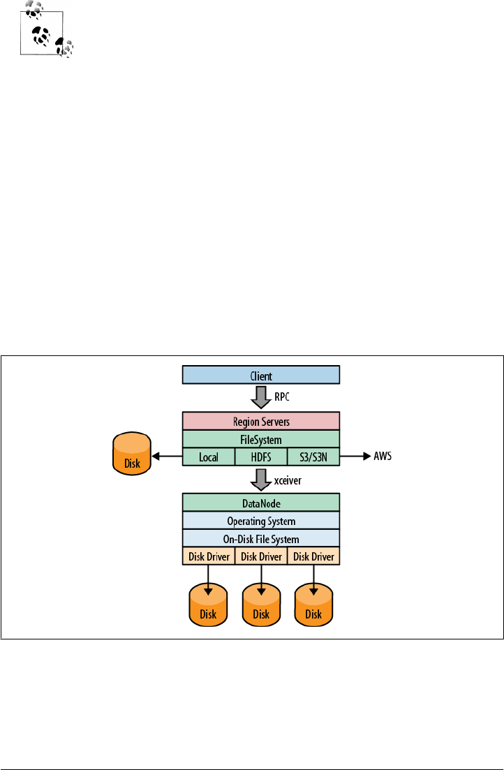
In this section, we are not talking about the low-level filesystems used
by the operating system (see “Filesystem” on page 43 for that), but the
storage layer filesystems. These are abstractions that define higher-level
features and APIs, which are then used by Hadoop to store the data.
The data is eventually stored on a disk, at which point the OS filesystem
is used.
HDFS is the most used and tested filesystem in production. Almost all production
clusters use it as the underlying storage layer. It is proven stable and reliable, so devi-
ating from it may impose its own risks and subsequent problems.
The primary reason HDFS is so popular is its built-in replication, fault tolerance, and
scalability. Choosing a different filesystem should provide the same guarantees, as
HBase implicitly assumes that data is stored in a reliable manner by the filesystem. It
has no added means to replicate data or even maintain copies of its own storage files.
This functionality must be provided by the lower-level system.
You can select a different filesystem implementation by using a URI§ pattern, where
the scheme (the part before the first “:”, i.e., the colon) part of the URI identifies the
driver to be used. Figure 2-1 shows how the Hadoop filesystem is different from the
low-level OS filesystems for the actual disks.
Figure 2-1. The filesystem negotiating transparently where data is stored
§ See “Uniform Resource Identifier” on Wikipedia.
Filesystems for HBase | 53

You can use a filesystem that is already supplied by Hadoop: it ships with a list of
filesystems,‖ which you may want to try out first. As a last resort—or if you’re an
experienced developer—you can also write your own filesystem implementation.
Local
The local filesystem actually bypasses Hadoop entirely, that is, you do not need to have
an HDFS or any other cluster at all. It is handled all in the FileSystem class used by
HBase to connect to the filesystem implementation. The supplied ChecksumFileSys
tem class is loaded by the client and uses local disk paths to store all the data.
The beauty of this approach is that HBase is unaware that it is not talking to a distrib-
uted filesystem on a remote or collocated cluster, but actually is using the local filesys-
tem directly. The standalone mode of HBase uses this feature to run HBase only. You
can select it by using the following scheme:
file:///<path>
Similar to the URIs used in a web browser, the file: scheme addresses local files.
HDFS
The Hadoop Distributed File System (HDFS) is the default filesystem when deploying
a fully distributed cluster. For HBase, HDFS is the filesystem of choice, as it has all the
required features. As we discussed earlier, HDFS is built to work with MapReduce,
taking full advantage of its parallel, streaming access support. The scalability, fail safety,
and automatic replication functionality is ideal for storing files reliably. HBase adds the
random access layer missing from HDFS and ideally complements Hadoop. Using
MapReduce, you can do bulk imports, creating the storage files at disk-transfer speeds.
The URI to access HDFS uses the following scheme:
hdfs://<namenode>:<port>/<path>
S3
Amazon’s Simple Storage Service (S3)# is a storage system that is primarily used in
combination with dynamic servers running on Amazon’s complementary service
named Elastic Compute Cloud (EC2).*
S3 can be used directly and without EC2, but the bandwidth used to transfer data in
and out of S3 is going to be cost-prohibitive in practice. Transferring between EC2 and
‖A full list was compiled by Tom White in his post “Get to Know Hadoop Filesystems”.
#See “Amazon S3” for more background information.
* See “EC2” on Wikipedia.
54 | Chapter 2: Installation

S3 is free, and therefore a viable option. One way to start an EC2-based cluster is shown
in “Apache Whirr” on page 69.
The S3 FileSystem implementation provided by Hadoop supports two different modes:
the raw (or native) mode, and the block-based mode. The raw mode uses the s3n: URI
scheme and writes the data directly into S3, similar to the local filesystem. You can see
all the files in your bucket the same way as you would on your local disk.
The s3: scheme is the block-based mode and was used to overcome S3’s former max-
imum file size limit of 5 GB. This has since been changed, and therefore the selection
is now more difficult—or easy: opt for s3n: if you are not going to exceed 5 GB per file.
The block mode emulates the HDFS filesystem on top of S3. It makes browsing the
bucket content more difficult as only the internal block files are visible, and the HBase
storage files are stored arbitrarily inside these blocks and strewn across them. You can
select the filesystem using these URIs:
s3://<bucket-name>
s3n://<bucket-name>
Other Filesystems
There are other filesystems, and one that deserves mention is CloudStore (formerly
known as the Kosmos filesystem, abbreviated as KFS and the namesake of the URI
scheme shown at the end of the next paragraph). It is an open source, distributed, high-
performance filesystem written in C++, with similar features to HDFS. Find more
information about it at the CloudStore website.
It is available for Solaris and Linux, originally developed by Kosmix and released as
open source in 2007. To select CloudStore as the filesystem for HBase use the following
URI format:
kfs:///<path>
Installation Choices
Once you have decided on the basic OS-related options, you must somehow get HBase
onto your servers. You have a couple of choices, which we will look into next. Also see
Appendix D for even more options.
Apache Binary Release
The canonical installation process of most Apache projects is to download a release,
usually provided as an archive containing all the required files. Some projects have
separate archives for a binary and source release—the former intended to have every-
thing needed to run the release and the latter containing all files needed to build the
project yourself. HBase comes as a single package, containing binary and source files
Installation Choices | 55

together. For more information on HBase releases, you may also want to check out the
Release Notes† page. Another interesting page is titled Change Log,‡ and it lists every-
thing that was added, fixed, or changed in any form for each release version.
You can download the most recent release of HBase from the Apache HBase release
page and unpack the contents into a suitable directory, such as /usr/local or /opt, like so:
$ cd /usr/local
$ tar -zxvf hbase-x.y.z.tar.gz
Once you have extracted all the files, you can make yourself familiar with what is in
the project’s directory. The content may look like this:
$ ls -lr
-rw-r--r-- 1 larsgeorge staff 192809 Feb 15 01:54 CHANGES.txt
-rw-r--r-- 1 larsgeorge staff 11358 Feb 9 01:23 LICENSE.txt
-rw-r--r-- 1 larsgeorge staff 293 Feb 9 01:23 NOTICE.txt
-rw-r--r-- 1 larsgeorge staff 1358 Feb 9 01:23 README.txt
drwxr-xr-x 23 larsgeorge staff 782 Feb 9 01:23 bin
drwxr-xr-x 7 larsgeorge staff 238 Feb 9 01:23 conf
drwxr-xr-x 64 larsgeorge staff 2176 Feb 15 01:56 docs
-rwxr-xr-x 1 larsgeorge staff 905762 Feb 15 01:56 hbase-0.90.1-tests.jar
-rwxr-xr-x 1 larsgeorge staff 2242043 Feb 15 01:56 hbase-0.90.1.jar
drwxr-xr-x 5 larsgeorge staff 170 Feb 15 01:55 hbase-webapps
drwxr-xr-x 32 larsgeorge staff 1088 Mar 3 12:07 lib
-rw-r--r-- 1 larsgeorge staff 29669 Feb 15 01:28 pom.xml
drwxr-xr-x 9 larsgeorge staff 306 Feb 9 01:23 src
The root of it only contains a few text files, stating the license terms (LICENSE.txt and
NOTICE.txt) and some general information on how to find your way around
(README.txt). The CHANGES.txt file is a static snapshot of the change log page
mentioned earlier. It contains all the changes that went into the current release you
downloaded.
You will also find the Java archive, or JAR files, that contain the compiled Java code
plus all other necessary resources. There are two variations of the JAR file, one with
just the name and version number and one with a postfix of tests. This file contains the
code required to run the tests provided by HBase. These are functional unit tests that
the developers use to verify a release is fully operational and that there are no
regressions.
The last file found is named pom.xml and is the Maven project file needed to build
HBase from the sources. See “Building from Source” on page 58.
The remainder of the content in the root directory consists of other directories, which
are explained in the following list:
†https://issues.apache.org/jira/browse/HBASE?report=com.atlassian.jira.plugin.system.project:changelog
-panel.
‡https://issues.apache.org/jira/browse/HBASE?report=com.atlassian.jira.plugin.system.project:changelog-panel
#selectedTab=com.atlassian.jira.plugin.system.project%3Achangelog-panel.
56 | Chapter 2: Installation

bin
The bin—or binaries—directory contains the scripts supplied by HBase to start
and stop HBase, run separate daemons,§ or start additional master nodes. See
“Running and Confirming Your Installation” on page 71 for information on how
to use them.
conf
The configuration directory contains the files that define how HBase is set up.
“Configuration” on page 63 explains the contained files in great detail.
docs
This directory contains a copy of the HBase project website, including the docu-
mentation for all the tools, the API, and the project itself. Open your web browser
of choice and open the docs/index.html file by either dragging it into the browser,
double-clicking that file, or using the File→Open (or similarly named) menu.
hbase-webapps
HBase has web-based user interfaces which are implemented as Java web applica-
tions, using the files located in this directory. Most likely you will never have to
touch this directory when working with or deploying HBase into production.
lib
Java-based applications are usually an assembly of many auxiliary libraries plus
the JAR file containing the actual program. All of these libraries are located in the
lib directory.
logs
Since the HBase processes are started as daemons (i.e., they are running in the
background of the operating system performing their duty), they use logfiles to
report their state, progress, and optionally, errors that occur during their life cycle.
“Analyzing the Logs” on page 468 explains how to make sense of their rather
cryptic content.
Initially, there may be no logs directory, as it is created when you
start HBase for the first time. The logging framework used by
HBase is creating the directory and logfiles dynamically.
src
In case you plan to build your own binary package (see “Building from
Source” on page 58 for information on how to do that), or you decide you would
like to join the international team of developers working on HBase, you will need
this source directory, containing everything required to roll your own release.
§ Processes that are started and then run in the background to perform their task are often referred to as
daemons.
Installation Choices | 57

Since you have unpacked a release archive, you can now move on to “Run
Modes” on page 58 to decide how you want to run HBase.
Building from Source
HBase uses Maven to build the binary packages. You therefore need a working Maven
installation, plus a full Java Development Kit (JDK)—not just a Java Runtime as used
in “Quick-Start Guide” on page 31.
This section is important only if you want to build HBase from its
sources. This might be necessary if you want to apply patches, which
can add new functionality you may be requiring.
Once you have confirmed that both are set up properly, you can build the binary pack-
ages using the following command:
$ mvn assembly:assembly
Note that the tests for HBase need more than one hour to complete. If you trust the
code to be operational, or you are not willing to wait, you can also skip the test phase,
adding a command-line switch like so:
$ mvn -DskipTests assembly:assembly
This process will take a few minutes to complete—and if you have not turned off the
test phase, this goes into the tens of minutes—while creating a target directory in the
HBase project home directory. Once the build completes with a Build Successful
message, you can find the compiled and packaged tarball archive in the target directory.
With that archive you can go back to “Apache Binary Release” on page 55 and follow
the steps outlined there to install your own, private release on your servers.
Run Modes
HBase has two run modes: standalone and distributed. Out of the box, HBase runs in
standalone mode, as seen in “Quick-Start Guide” on page 31. To set up HBase in
distributed mode, you will need to edit files in the HBase conf directory.
Whatever your mode, you may need to edit conf/hbase-env.sh to tell HBase which
java to use. In this file, you set HBase environment variables such as the heap size and
other options for the JVM, the preferred location for logfiles, and so on. Set
JAVA_HOME to point at the root of your java installation.
58 | Chapter 2: Installation

Standalone Mode
This is the default mode, as described and used in “Quick-Start Guide” on page 31. In
standalone mode, HBase does not use HDFS—it uses the local filesystem instead—and
it runs all HBase daemons and a local ZooKeeper in the same JVM process. ZooKeeper
binds to a well-known port so that clients may talk to HBase.
Distributed Mode
The distributed mode can be further subdivided into pseudodistributed—all daemons
run on a single node—and fully distributed—where the daemons are spread across
multiple, physical servers in the cluster.‖
Distributed modes require an instance of the Hadoop Distributed File System (HDFS).
See the Hadoop requirements and instructions for how to set up an HDFS. Before
proceeding, ensure that you have an appropriate, working HDFS.
The following subsections describe the different distributed setups. Starting, verifying,
and exploring of your install, whether a pseudodistributed or fully distributed configu-
ration, is described in “Running and Confirming Your Installation” on page 71. The
same verification script applies to both deploy types.
Pseudodistributed mode
A pseudodistributed mode is simply a distributed mode that is run on a single host.
Use this configuration for testing and prototyping on HBase. Do not use this configu-
ration for production or for evaluating HBase performance.
Once you have confirmed your HDFS setup, edit conf/hbase-site.xml. This is the file
into which you add local customizations and overrides for the default HBase
configuration values (see Appendix A for the full list, and “HDFS-Related Configura-
tion” on page 64). Point HBase at the running Hadoop HDFS instance by setting
the hbase.rootdir property. For example, adding the following properties to your
hbase-site.xml file says that HBase should use the /hbase directory in the HDFS whose
name node is at port 9000 on your local machine, and that it should run with one replica
only (recommended for pseudodistributed mode):
<configuration>
...
<property>
<name>hbase.rootdir</name>
<value>hdfs://localhost:9000/hbase</value>
</property>
<property>
<name>dfs.replication</name>
<value>1</value>
</property>
‖The pseudodistributed versus fully distributed nomenclature comes from Hadoop.
Run Modes | 59

...
</configuration>
In the example configuration, the server binds to localhost. This means
that a remote client cannot connect. Amend accordingly, if you want to
connect from a remote location.
If all you want to try for now is the pseudodistributed mode, you can skip to “Running
and Confirming Your Installation” on page 71 for details on how to start and verify
your setup. See Chapter 12 for information on how to start extra master and region
servers when running in pseudodistributed mode.
Fully distributed mode
For running a fully distributed operation on more than one host, you need to use the
following configurations. In hbase-site.xml, add the hbase.cluster.distributed prop-
erty and set it to true, and point the HBase hbase.rootdir at the appropriate HDFS
name node and location in HDFS where you would like HBase to write data. For ex-
ample, if your name node is running at a server with the hostname namenode.foo.com
on port 9000 and you want to home your HBase in HDFS at /hbase, use the following
configuration:
<configuration>
...
<property>
<name>hbase.rootdir</name>
<value>hdfs://namenode.foo.com:9000/hbase</value>
</property>
<property>
<name>hbase.cluster.distributed</name>
<value>true</value>
</property>
...
</configuration>
In addition, a fully distributed mode requires that you modify the
conf/regionservers file. It lists all the hosts on which you want to run HRegionServer
daemons. Specify one host per line (this file in HBase is like the Hadoop slaves file). All
servers listed in this file will be started and stopped when the HBase cluster start or
stop scripts are run.
A distributed HBase depends on a running ZooKeeper cluster. All par-
ticipating nodes and clients need to be able to access the running ZooKeeper ensemble.
HBase, by default, manages a ZooKeeper cluster (which can be as low as a single node)
for you. It will start and stop the ZooKeeper ensemble as part of the HBase start and
stop process. You can also manage the ZooKeeper ensemble independent of HBase and
just point HBase at the cluster it should use. To toggle HBase management of Zoo-
Keeper, use the HBASE_MANAGES_ZK variable in conf/hbase-env.sh. This variable, which
Specifying region servers.
ZooKeeper setup.
60 | Chapter 2: Installation

defaults to true, tells HBase whether to start and stop the ZooKeeper ensemble servers
as part of the start and stop commands supplied by HBase.
When HBase manages the ZooKeeper ensemble, you can specify the ZooKeeper con-
figuration using its native zoo.cfg file, or just specify the ZooKeeper options directly in
conf/hbase-site.xml. You can set a ZooKeeper configuration option as a property in the
HBase hbase-site.xml XML configuration file by prefixing the ZooKeeper option name
with hbase.zookeeper.property. For example, you can change the clientPort setting
in ZooKeeper by setting the hbase.zookeeper.property.clientPort property. For all
default values used by HBase, including ZooKeeper configuration, see Appendix A.
Look for the hbase.zookeeper.property prefix.#
zoo.cfg Versus hbase-site.xml
There is some confusion concerning the usage of zoo.cfg and hbase-site.xml in combi-
nation with ZooKeeper settings. For starters, if there is a zoo.cfg on the classpath
(meaning it can be found by the Java process), it takes precedence over all settings in
hbase-site.xml—but only those starting with the hbase.zookeeper.property prefix, plus
a few others.
There are some ZooKeeper client settings that are not read from zoo.cfg but must be
set in hbase-site.xml. This includes, for example, the important client session timeout
value set with zookeeper.session.timeout. The following table describes the depend-
encies in more detail.
Property zoo.cfg + hbase-site.xml hbase-site.xml only
hbase.zookeeper.quorum Constructed from server.n lines as
specified in zoo.cfg. Overrides any
setting in hbase-site.xml.
Used as specified.
hbase.zookeeper.property.* All values from zoo.cfg override any
value specified in hbase-site.xml.
Used as specified.
zookeeper.* Only taken from hbase-site.xml. Only taken from hbase-site.xml.
To avoid any confusion during deployment, it is highly recommended that you not use
a zoo.cfg file with HBase, and instead use only the hbase-site.xml file. Especially in a
fully distributed setup where you have your own ZooKeeper servers, it is not practical
to copy the configuration from the ZooKeeper nodes to the HBase servers.
If you are using the hbase-site.xml approach to specify all ZooKeeper settings, you must
at least set the ensemble servers with the hbase.zookeeper.quorum property. It otherwise
defaults to a single ensemble member at localhost, which is not suitable for a fully
#For the full list of ZooKeeper configurations, see ZooKeeper’s zoo.cfg. HBase does not ship with that file, so
you will need to browse the conf directory in an appropriate ZooKeeper download.
Run Modes | 61

distributed HBase (it binds to the local machine only and remote clients will not be
able to connect).
How Many ZooKeepers Should I Run?
You can run a ZooKeeper ensemble that comprises one node only, but in production
it is recommended that you run a ZooKeeper ensemble of three, five, or seven machines;
the more members an ensemble has, the more tolerant the ensemble is of host failures.
Also, run an odd number of machines, since running an even count does not make for
an extra server building consensus—you need a majority vote, and if you have three or
four servers, for example, both would have a majority with three nodes. Using an odd
number allows you to have two servers fail, as opposed to only one with even numbers.
Give each ZooKeeper server around 1 GB of RAM, and if possible, its own dedicated
disk (a dedicated disk is the best thing you can do to ensure a performant ZooKeeper
ensemble). For very heavily loaded clusters, run ZooKeeper servers on separate ma-
chines from RegionServers, DataNodes, and TaskTrackers.
For example, in order to have HBase manage a ZooKeeper quorum on nodes
rs{1,2,3,4,5}.foo.com, bound to port 2222 (the default is 2181), you must ensure that
HBASE_MANAGE_ZK is commented out or set to true in conf/hbase-env.sh and then edit
conf/hbase-site.xml and set hbase.zookeeper.property.clientPort and hbase.zoo
keeper.quorum. You should also set hbase.zookeeper.property.dataDir to something
other than the default, as the default has ZooKeeper persist data under /tmp, which is
often cleared on system restart. In the following example, we have ZooKeeper persist
to /var/zookeeper:
<configuration>
...
<property>
<name>hbase.zookeeper.property.clientPort</name>
<value>2222</value>
</property>
<property>
<name>hbase.zookeeper.quorum</name>
<value>rs1.foo.com,rs2.foo.com,rs3.foo.com,rs4.foo.com,rs5.foo.com</value>
</property>
<property>
<name>hbase.zookeeper.property.dataDir</name>
<value>/var/zookeeper</value>
</property>
...
</configuration>
To point HBase at an existing ZooKeeper cluster, one
that is not managed by HBase, set HBASE_MANAGES_ZK in conf/hbase-env.sh to false:
...
# Tell HBase whether it should manage it's own instance of Zookeeper or not.
export HBASE_MANAGES_ZK=false
Using the existing ZooKeeper ensemble.
62 | Chapter 2: Installation

Next, set the ensemble locations and client port, if nonstandard, in hbase-site.xml, or
add a suitably configured zoo.cfg to HBase’s CLASSPATH. HBase will prefer the con-
figuration found in zoo.cfg over any settings in hbase-site.xml.
When HBase manages ZooKeeper, it will start/stop the ZooKeeper servers as a part of
the regular start/stop scripts. If you would like to run ZooKeeper yourself, independent
of HBase start/stop, do the following:
${HBASE_HOME}/bin/hbase-daemons.sh {start,stop} zookeeper
Note that you can use HBase in this manner to spin up a ZooKeeper cluster, unrelated
to HBase. Just make sure to set HBASE_MANAGES_ZK to false if you want it to stay up
across HBase restarts so that when HBase shuts down, it doesn’t take ZooKeeper down
with it.
For more information about running a distinct ZooKeeper cluster, see the ZooKeeper
Getting Started Guide. Additionally, see the ZooKeeper wiki, or the ZooKeeper docu-
mentation for more information on ZooKeeper sizing.
Configuration
Now that the basics are out of the way (we’ve looked at all the choices when it comes
to selecting the filesystem, discussed the run modes, and fine-tuned the operating sys-
tem parameters), we can look at how to configure HBase itself. Similar to Hadoop, all
configuration parameters are stored in files located in the conf directory. These are
simple text files either in XML format arranged as a set of properties, or in simple flat
files listing one option per line.
For more details on how to modify your configuration files for specific
workloads refer to “Configuration” on page 436.
Configuring an HBase setup entails editing a file with environment variables, named
conf/hbase-env.sh, which is used mostly by the shell scripts (see “Operating a Clus-
ter” on page 71) to start or stop a cluster. You also need to add configuration
properties to an XML file* named conf/hbase-site.xml to, for example, override HBase
defaults, tell HBase what filesystem to use, and tell HBase the location of the ZooKeeper
ensemble.
When running in distributed mode, after you make an edit to an HBase configuration
file, make sure you copy the content of the conf directory to all nodes of the cluster.
HBase will not do this for you.
* Be careful when editing XML. Make sure you close all elements. Check your file using a tool like xmlint, or
something similar, to ensure well-formedness of your document after an edit session.
Configuration | 63
There are many ways to synchronize your configuration files across
your cluster. The easiest is to use a tool like rsync. There are many more
elaborate ways, and you will see a selection in “Deploy-
ment” on page 68.
hbase-site.xml and hbase-default.xml
Just as in Hadoop where you add site-specific HDFS configurations to the
hdfs-site.xml file, for HBase, site-specific customizations go into the file conf/hbase-
site.xml. For the list of configurable properties, see Appendix A, or view the raw hbase-
default.xml source file in the HBase source code at src/main/resources. The doc directory
also has a static HTML page that lists the configuration options.
Not all configuration options make it out to hbase-default.xml. Config-
urations that users would rarely change can exist only in code; the only
way to turn up such configurations is to read the source code itself.
The servers always read the hbase-default.xml file first and subsequently merge it with
the hbase-site.xml file content—if present. The properties set in hbase-site.xml always
take precedence over the default values loaded from hbase-default.xml.
Any modifications in your site file require a cluster restart for HBase to notice the
changes.
HDFS-Related Configuration
If you have made HDFS-related configuration changes on your Hadoop cluster—in
other words, properties you want the HDFS clients to use as opposed to the server-side
configuration—HBase will not see these properties unless you do one of the following:
• Add a pointer to your HADOOP_CONF_DIR to the HBASE_CLASSPATH environment vari-
able in hbase-env.sh.
• Add a copy of hdfs-site.xml (or hadoop-site.xml) or, better, symbolic links, under
${HBASE_HOME}/conf.
• Add them to hbase-site.xml directly.
An example of such an HDFS client property is dfs.replication. If, for example, you
want to run with a replication factor of 5, HBase will create files with the default of 3
unless you do one of the above to make the configuration available to HBase.
When you add Hadoop configuration files to HBase, they will always take the lowest
priority. In other words, the properties contained in any of the HBase-related
configuration files, that is, the default and site files, take precedence over any Hadoop
configuration file containing a property with the same name. This allows you to over-
ride Hadoop properties in your HBase configuration file.
64 | Chapter 2: Installation

hbase-env.sh
You set HBase environment variables in this file. Examples include options to pass to
the JVM when an HBase daemon starts, such as Java heap size and garbage collector
configurations. You also set options for HBase configuration, log directories, niceness,
SSH options, where to locate process pid files, and so on. Open the file at conf/hbase-
env.sh and peruse its content. Each option is fairly well documented. Add your own
environment variables here if you want them read when an HBase daemon is started.
Changes here will require a cluster restart for HBase to notice the change.†
regionserver
This file lists all the known region server names. It is a flat text file that has one hostname
per line. The list is used by the HBase maintenance script to be able to iterate over all
the servers to start the region server process.
If you used previous versions of HBase, you may miss the masters file,
available in the 0.20.x line. It has been removed as it is no longer needed.
The list of masters is now dynamically maintained in ZooKeeper and
each master registers itself when started.
log4j.properties
Edit this file to change the rate at which HBase files are rolled and to change the level
at which HBase logs messages. Changes here will require a cluster restart for HBase to
notice the change, though log levels can be changed for particular daemons via the
HBase UI. See “Changing Logging Levels” on page 466 for information on this topic,
and “Analyzing the Logs” on page 468 for details on how to use the logfiles to find and
solve problems.
Example Configuration
Here is an example configuration for a distributed 10-node cluster. The nodes are
named master.foo.com, host1.foo.com, and so on, through node host9.foo.com. The
HBase Master and the HDFS name node are running on the node master.foo.com.
Region servers run on nodes host1.foo.com to host9.foo.com. A three-node ZooKeeper
ensemble runs on zk1.foo.com, zk2.foo.com, and zk3.foo.com on the default ports.
ZooKeeper data is persisted to the directory /var/zookeeper. The following subsections
show what the main configuration files—hbase-site.xml, regionservers, and hbase-
env.sh—found in the HBase conf directory might look like.
† As of this writing, you have to restart the server. However, work is being done to enable online schema and
configuration changes, so this will change over time.
Configuration | 65

hbase-site.xml
The hbase-site.xml file contains the essential configuration properties, defining the
HBase cluster setup.
<?xml version="1.0"?>
<?xml-stylesheet type="text/xsl" href="configuration.xsl"?>
<configuration>
<property>
<name>hbase.zookeeper.quorum</name>
<value>zk1.foo.com,zk2.foo.com,zk3.foo.com</value>
</property>
<property>
<name>hbase.zookeeper.property.dataDir</name>
<value>/var/zookeeper</value>
</property>
<property>
<name>hbase.rootdir</name>
<value>hdfs://master.foo.com:9000/hbase</value>
</property>
<property>
<name>hbase.cluster.distributed</name>
<value>true</value>
</property>
</configuration>
regionservers
In this file, you list the nodes that will run region servers. In our example, we run region
servers on all but the head node master.foo.com, which is carrying the HBase Master
and the HDFS name node.
host1.foo.com
host2.foo.com
host3.foo.com
host4.foo.com
host5.foo.com
host6.foo.com
host7.foo.com
host8.foo.com
host9.foo.com
hbase-env.sh
Here are the lines that were changed from the default in the supplied hbase-env.sh file.
Here we are setting the HBase heap to be 4 GB instead of the default 1 GB:
...
# export HBASE_HEAPSIZE=1000
export HBASE_HEAPSIZE=4096
...
Once you have edited the configuration files, you need to distribute them across all
servers in the cluster. One option to copy the content of the conf directory to all servers
66 | Chapter 2: Installation
in the cluster is to use the rsync command on Unix and Unix-like platforms. This ap-
proach and others are explained in “Deployment” on page 68.
“Configuration” on page 436 discusses the settings you are most likely
to change first when you start scaling your cluster.
Client Configuration
Since the HBase Master may move around between physical machines (see “Adding a
backup master” on page 450 for details), clients start by requesting the vital informa-
tion from ZooKeeper—something visualized in “Region Lookups” on page 345. For
that reason, clients require the ZooKeeper quorum information in an hbase-site.xml file
that is on their Java CLASSPATH.
You can also set the hbase.zookeeper.quorum configuration key in your
code. Doing so would lead to clients that need no external configuration
files. This is explained in “Put Method” on page 76.
If you are configuring an IDE to run an HBase client, you could include the conf/
directory on your classpath. That would make the configuration files discoverable by
the client code.
Minimally, a Java client needs the following JAR files specified in its CLASSPATH, when
connecting to HBase: hbase, hadoop-core, zookeeper, log4j, commons-logging, and
commons-lang. All of these JAR files come with HBase and are usually postfixed with
the a version number of the required release. Ideally, you use the supplied JARs and do
not acquire them somewhere else because even minor release changes could cause
problems when running the client against a remote HBase cluster.
A basic example hbase-site.xml file for client applications might contain the following
properties:
<?xml version="1.0"?>
<?xml-stylesheet type="text/xsl" href="configuration.xsl"?>
<configuration>
<property>
<name>hbase.zookeeper.quorum</name>
<value>zk1.foo.com,zk2.foo.com,zk3.foo.com</value>
</property>
</configuration>
Configuration | 67

Deployment
After you have configured HBase, the next thing you need to do is to think about
deploying it on your cluster. There are many ways to do that, and since Hadoop and
HBase are written in Java, there are only a few necessary requirements to look out for.
You can simply copy all the files from server to server, since they usually share the same
configuration. Here are some ideas on how to do that. Please note that you would need
to make sure that all the suggested selections and adjustments discussed in “Require-
ments” on page 34 have been applied—or are applied at the same time when provi-
sioning new servers.
Script-Based
Using a script-based approach seems archaic compared to the more advanced ap-
proaches listed shortly. But they serve their purpose and do a good job for small to even
medium-size clusters. It is not so much the size of the cluster but the number of people
maintaining it. In a larger operations group, you want to have repeatable deployment
procedures, and not deal with someone having to run scripts to update the cluster.
The scripts make use of the fact that the regionservers configuration file has a list of all
servers in the cluster. Example 2-2 shows a very simple script that could be used to
copy a new release of HBase from the master node to all slave nodes.
Example 2-2. Example Script to copy the HBase files across a cluster
#!/bin/bash
# Rsyncs HBase files across all slaves. Must run on master. Assumes
# all files are located in /usr/local
if [ "$#" != "2" ]; then
echo "usage: $(basename $0) <dir-name> <ln-name>"
echo " example: $(basename $0) hbase-0.1 hbase"
exit 1
fi
SRC_PATH="/usr/local/$1/conf/regionservers"
for srv in $(cat $SRC_PATH); do
echo "Sending command to $srv...";
rsync -vaz --exclude='logs/*' /usr/local/$1 $srv:/usr/local/
ssh $srv "rm -fR /usr/local/$2 ; ln -s /usr/local/$1 /usr/local/$2"
done
echo "done."
Another simple script is shown in Example 2-3; it can be used to copy the configuration
files of HBase from the master node to all slave nodes. It assumes you are editing the
configuration files on the master in such a way that the master can be copied across to
all region servers.
68 | Chapter 2: Installation

Example 2-3. Example Script to copy configurations across a cluster
#!/bin/bash
# Rsync's HBase config files across all region servers. Must run on master.
for srv in $(cat /usr/local/hbase/conf/regionservers); do
echo "Sending command to $srv...";
rsync -vaz --delete --exclude='logs/*' /usr/local/hadoop/ $srv:/usr/local/hadoop/
rsync -vaz --delete --exclude='logs/*' /usr/local/hbase/ $srv:/usr/local/hbase/
done
echo "done."
The second script uses rsync just like the first script, but adds the --delete option to
make sure the region servers do not have any older files remaining but have an exact
copy of what is on the originating server.
There are obviously many ways to do this, and the preceding examples are simply for
your perusal and to get you started. Ask your administrator to help you set up mech-
anisms to synchronize the configuration files appropriately. Many beginners in HBase
have run into a problem that was ultimately caused by inconsistent configurations
among the cluster nodes. Also, do not forget to restart the servers when making changes.
If you want to update settings while the cluster is in production, please refer to “Rolling
Restarts” on page 447.
Apache Whirr
Recently, we have seen an increase in the number of users who want to run their cluster
in dynamic environments, such as the public cloud offerings by Amazon’s EC2, or
Rackspace Cloud Servers, as well as in private server farms, using open source tools
like Eucalyptus.
The advantage is to be able to quickly provision servers and run analytical workloads
and, once the result has been retrieved, to simply shut down the entire cluster, or reuse
the servers for other dynamic loads. Since it is not trivial to program against each of the
APIs providing dynamic cluster infrastructures, it would be useful to abstract the pro-
visioning part and, once the cluster is operational, simply launch the MapReduce jobs
the same way you would on a local, static cluster. This is where Apache Whirr comes in.
Whirr—available at http://incubator.apache.org/whirr/‡—has support for a variety of
public and private cloud APIs and allows you to provision clusters running a range of
services. One of those is HBase, giving you the ability to quickly deploy a fully opera-
tional HBase cluster on dynamic setups.
‡ Please note that Whirr is still part of the incubator program of the Apache Software Foundation. Once it is
accepted and promoted to a full member, its URL is going to change to a permanent place.
Deployment | 69

You can download the latest Whirr release from the aforementioned site and find pre-
configured configuration files in the recipes directory. Use it as a starting point to deploy
your own dynamic clusters.
The basic concept of Whirr is to use very simple machine images that already provide
the operating system (see “Operating system” on page 40) and SSH access. The rest is
handled by Whirr using services that represent, for example, Hadoop or HBase. Each
service executes every required step on each remote server to set up the user accounts,
download and install the required software packages, write out configuration files for
them, and so on. This is all highly customizable and you can add extra steps as needed.
Puppet and Chef
Similar to Whirr, there are other deployment frameworks for dedicated machines.
Puppet by Puppet Labs and Chef by Opscode are two such offerings.
Both work similar to Whirr in that they have a central provisioning server that stores
all the configurations, combined with client software, executed on each server, which
communicates with the central server to receive updates and apply them locally.
Also similar to Whirr, both have the notion of recipes, which essentially translate to
scripts or commands executed on each node.§ In fact, it is quite possible to replace the
scripting employed by Whirr with a Puppet- or Chef-based process.
While Whirr solely handles the bootstrapping, Puppet and Chef have further support
for changing running clusters. Their master process monitors the configuration repo-
sitory and, upon updates, triggers the appropriate remote action. This can be used to
reconfigure clusters on-the-fly or push out new releases, do rolling restarts, and so on.
It can be summarized as configuration management, rather than just provisioning.
You heard it before: select an approach you like and maybe even are
familiar with already. In the end, they achieve the same goal: installing
everything you need on your cluster nodes. If you need a full configu-
ration management solution with live updates, a Puppet- or Chef-based
approach—maybe in combination with Whirr for the server provision-
ing—is the right choice.
§ Some of the available recipe packages are an adaption of early EC2 scripts, used to deploy HBase to dynamic,
cloud-based server. For Chef, you can find HBase-related examples at http://cookbooks.opscode.com/
cookbooks/hbase. For Puppet, please refer to http://hstack.org/hstack-automated-deployment-using-puppet/
and the repository with the recipes at http://github.com/hstack/puppet.
70 | Chapter 2: Installation

Operating a Cluster
Now that you have set up the servers, configured the operating system and filesystem,
and edited the configuration files, you are ready to start your HBase cluster for the first
time.
Running and Confirming Your Installation
Make sure HDFS is running first. Start and stop the Hadoop HDFS daemons by running
bin/start-dfs.sh over in the HADOOP_HOME directory. You can ensure that it started
properly by testing the put and get of files into the Hadoop filesystem. HBase does not
normally use the MapReduce daemons. You only need to start them for actual Map-
Reduce jobs, something we will look into in detail in Chapter 7.
If you are managing your own ZooKeeper, start it and confirm that it is running: oth-
erwise, HBase will start up ZooKeeper for you as part of its start process.
Just as you started the standalone mode in “Quick-Start Guide” on page 31, you start
a fully distributed HBase with the following command:
bin/start-hbase.sh
Run the preceding command from the HBASE_HOME directory. You should now have
a running HBase instance. The HBase logfiles can be found in the logs subdirectory. If
you find that HBase is not working as expected, please refer to “Analyzing the
Logs” on page 468 for help finding the problem.
Once HBase has started, see “Quick-Start Guide” for information on how to create
tables, add data, scan your insertions, and finally, disable and drop your tables.
Web-based UI Introduction
HBase also starts a web-based user interface (UI) listing vital attributes. By default, it
is deployed on the master host at port 60010 (HBase region servers use 60030 by de-
fault). If the master is running on a host named master.foo.com on the default port, to
see the master’s home page you can point your browser at http://master.foo.com:
60010. Figure 2-2 is an example of how the resultant page should look. You can find a
more detailed explanation in “Web-based UI” on page 277.
From this page you can access a variety of status information about your HBase cluster.
The page is separated into multiple sections. The top part has the attributes pertaining
to the cluster setup. You can see the currently running tasks—if there are any. The
catalog and user tables list details about the available tables. For the user table you also
see the table schema.
The lower part of the page has the region servers table, giving you access to all the
currently registered servers. Finally, the region in transition list informs you about re-
gions that are currently being maintained by the system.
Operating a Cluster | 71
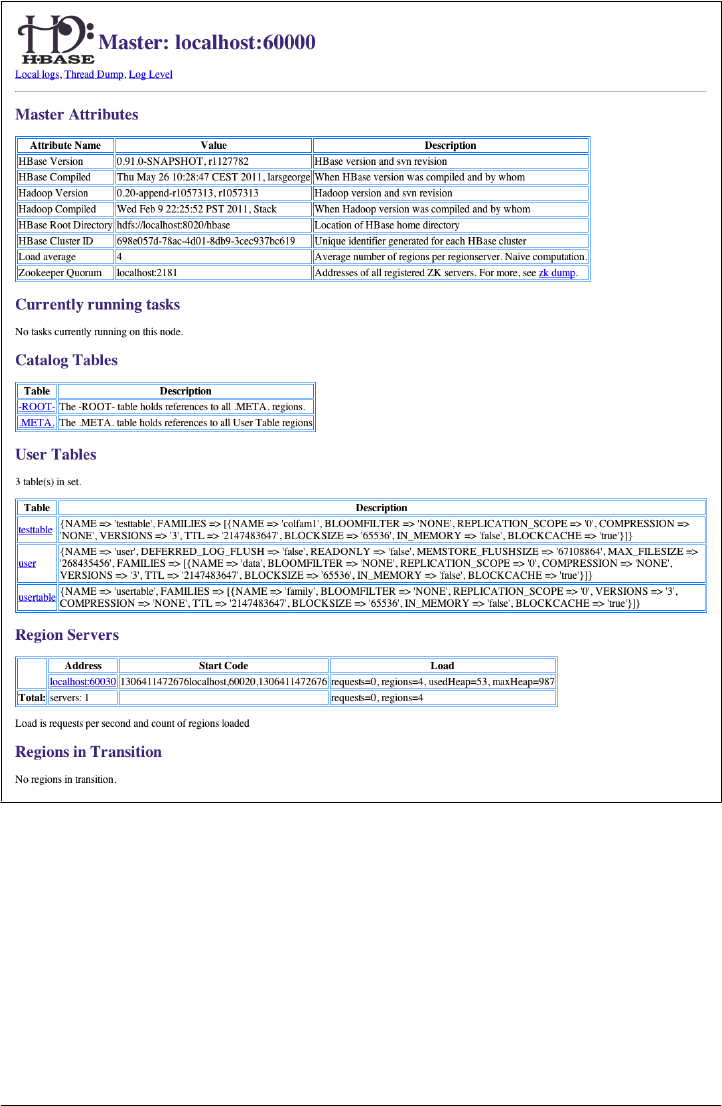
After you have started the cluster, you should verify that all the region servers have
registered themselves with the master and appear in the appropriate table with the
expected hostnames (that a client can connect to). Also verify that you are indeed run-
ning the correct version of HBase and Hadoop.
Figure 2-2. The HBase Master user interface
72 | Chapter 2: Installation

Shell Introduction
You already used the command-line shell that comes with HBase when you went
through “Quick-Start Guide” on page 31. You saw how to create a table, add and
retrieve data, and eventually drop the table.
The HBase Shell is (J)Ruby’s IRB with some HBase-related commands added. Anything
you can do in IRB, you should be able to do in the HBase Shell. You can start the shell
with the following command:
$ $HBASE_HOME/bin/hbase shell
HBase Shell; enter 'help<RETURN>' for list of supported commands.
Type "exit<RETURN>" to leave the HBase Shell
Version 0.91.0-SNAPSHOT, r1130916, Sat Jul 23 12:44:34 CEST 2011
hbase(main):001:0>
Type help and then press Return to see a listing of shell commands and options. Browse
at least the paragraphs at the end of the help text for the gist of how variables and
command arguments are entered into the HBase Shell; in particular, note how table
names, rows, and columns, must be quoted. Find the full description of the shell in
“Shell” on page 268.
Since the shell is JRuby-based, you can mix Ruby with HBase commands, which enables
you to do things like this:
hbase(main):001:0> create 'testtable', 'colfam1'
hbase(main):002:0> for i in 'a'..'z' do for j in 'a'..'z' do \
put 'testtable', "row-#{i}#{j}", "colfam1:#{j}", "#{j}" end end
The first command is creating a new table named testtable, with one column family
called colfam1, using default values (see “Column Families” on page 212 for what that
means). The second command uses a Ruby loop to create rows with columns in the
newly created tables. It creates row keys starting with row-aa, row-ab, all the way to
row-zz.
Stopping the Cluster
To stop HBase, enter the following command. Once you have started the script, you
will see a message stating that the cluster is being stopped, followed by “.” (period)
characters printed in regular intervals (just to indicate that the process is still running,
not to give you any percentage feedback, or some other hidden meaning):
$ ./bin/stop-hbase.sh
stopping hbase...............
Shutdown can take several minutes to complete. It can take longer if your cluster is
composed of many machines. If you are running a distributed operation, be sure to
wait until HBase has shut down completely before stopping the Hadoop daemons.
Operating a Cluster | 73


CHAPTER 3
Client API: The Basics
This chapter will discuss the client APIs provided by HBase. As noted earlier, HBase is
written in Java and so is its native API. This does not mean, though, that you must use
Java to access HBase. In fact, Chapter 6 will show how you can use other programming
languages.
General Notes
The primary client interface to HBase is the HTable class in the org.apache.hadoop.
hbase.client package. It provides the user with all the functionality needed to store
and retrieve data from HBase as well as delete obsolete values and so on. Before looking
at the various methods this class provides, let us address some general aspects of its
usage.
All operations that mutate data are guaranteed to be atomic on a per-row basis. This
affects all other concurrent readers and writers of that same row. In other words, it does
not matter if another client or thread is reading from or writing to the same row: they
either read a consistent last mutation, or may have to wait before being able to apply
their change.* More on this in Chapter 8.
Suffice it to say for now that during normal operations and load, a reading client will
not be affected by another updating a particular row since their contention is nearly
negligible. There is, however, an issue with many clients trying to update the same row
at the same time. Try to batch updates together to reduce the number of separate op-
erations on the same row as much as possible.
It also does not matter how many columns are written for the particular row; all of
them are covered by this guarantee of atomicity.
* The region servers use a multiversion concurrency control mechanism, implemented internally by the
ReadWriteConsistencyControl (RWCC) class, to guarantee that readers can read without having to wait for
writers. Writers do need to wait for other writers to complete, though, before they can continue.
75

Finally, creating HTable instances is not without cost. Each instantiation involves scan-
ning the .META. table to check if the table actually exists and if it is enabled, as well as
a few other operations that make this call quite costly. Therefore, it is recommended
that you create HTable instances only once—and one per thread—and reuse that in-
stance for the rest of the lifetime of your client application.
As soon as you need multiple instances of HTable, consider using the HTablePool class
(see “HTablePool” on page 199), which provides you with a convenient way to reuse
multiple instances.
Here is a summary of the points we just discussed:
• Create HTable instances only once, usually when your application
starts.
• Create a separate HTable instance for every thread you execute (or
use HTablePool).
• Updates are atomic on a per-row basis.
CRUD Operations
The initial set of basic operations are often referred to as CRUD, which stands for create,
read, update, and delete. HBase has a set of those and we will look into each of them
subsequently. They are provided by the HTable class, and the remainder of this chapter
will refer directly to the methods without specifically mentioning the containing class
again.
Most of the following operations are often seemingly self-explanatory, but the subtle
details warrant a close look. However, this means you will start to see a pattern of
repeating functionality so that we do not have to explain them again and again.
The examples you will see in partial source code can be found in full
detail in the publicly available GitHub repository at https://github.com/
larsgeorge/hbase-book. For details on how to compile them, see “Build-
ing the Examples” on page xxi.
Initially you will see the import statements, but they will be subsequently
omitted for the sake of brevity. Also, specific parts of the code are not
listed if they do not immediately help with the topic explained. Refer to
the full source if in doubt.
Put Method
This group of operations can be split into separate types: those that work on single
rows and those that work on lists of rows. Since the latter involves some more
76 | Chapter 3: Client API: The Basics

complexity, we will look at each group separately. Along the way, you will also be
introduced to accompanying client API features.
Single Puts
The very first method you may want to know about is one that lets you store data in
HBase. Here is the call that lets you do that:
void put(Put put) throws IOException
It expects one or a list of Put objects that, in turn, are created with one of these
constructors:
Put(byte[] row)
Put(byte[] row, RowLock rowLock)
Put(byte[] row, long ts)
Put(byte[] row, long ts, RowLock rowLock)
You need to supply a row to create a Put instance. A row in HBase is identified by a
unique row key and—as is the case with most values in HBase—this is a Java byte[]
array. You are free to choose any row key you like, but please also note that Chap-
ter 9 provides a whole section on row key design (see “Key Design” on page 357). For
now, we assume this can be anything, and often it represents a fact from the physical
world—for example, a username or an order ID. These can be simple numbers but also
UUIDs† and so on.
HBase is kind enough to provide us with a helper class that has many static methods
to convert Java types into byte[] arrays. Example 3-1 provides a short list of what it
offers.
Example 3-1. Methods provided by the Bytes class
static byte[] toBytes(ByteBuffer bb)
static byte[] toBytes(String s)
static byte[] toBytes(boolean b)
static byte[] toBytes(long val)
static byte[] toBytes(float f)
static byte[] toBytes(int val)
...
Once you have created the Put instance you can add data to it. This is done using these
methods:
Put add(byte[] family, byte[] qualifier, byte[] value)
Put add(byte[] family, byte[] qualifier, long ts, byte[] value)
Put add(KeyValue kv) throws IOException
Each call to add() specifies exactly one column, or, in combination with an optional
timestamp, one single cell. Note that if you do not specify the timestamp with the
† Universally Unique Identifier; see http://en.wikipedia.org/wiki/Universally_unique_identifier for details.
CRUD Operations | 77
add() call, the Put instance will use the optional timestamp parameter from the con-
structor (also called ts) and you should leave it to the region server to set it.
The variant that takes an existing KeyValue instance is for advanced users that have
learned how to retrieve, or create, this internal class. It represents a single, unique cell;
like a coordination system used with maps it is addressed by the row key, column
family, column qualifier, and timestamp, pointing to one value in a three-dimensional,
cube-like system—where time is the third dimension.
One way to come across the internal KeyValue type is by using the reverse methods to
add(), aptly named get():
List<KeyValue> get(byte[] family, byte[] qualifier)
Map<byte[], List<KeyValue>> getFamilyMap()
These two calls retrieve what you have added earlier, while having converted the unique
cells into KeyValue instances. You can retrieve all cells for either an entire column family,
a specific column within a family, or everything. The latter is the getFamilyMap() call,
which you can then iterate over to check the details contained in each available Key
Value.
Every KeyValue instance contains its full address—the row key, column
family, qualifier, timestamp, and so on—as well as the actual data. It is
the lowest-level class in HBase with respect to the storage architecture.
“Storage” on page 319 explains this in great detail. As for the available
functionality in regard to the KeyValue class from the client API, see
“The KeyValue class” on page 83.
Instead of having to iterate to check for the existence of specific cells, you can use the
following set of methods:
boolean has(byte[] family, byte[] qualifier)
boolean has(byte[] family, byte[] qualifier, long ts)
boolean has(byte[] family, byte[] qualifier, byte[] value)
boolean has(byte[] family, byte[] qualifier, long ts, byte[] value)
They increasingly ask for more specific details and return true if a match can be found.
The first method simply checks for the presence of a column. The others add the option
to check for a timestamp, a given value, or both.
There are more methods provided by the Put class, summarized in Table 3-1.
Note that the getters listed in Table 3-1 for the Put class only retrieve
what you have set beforehand. They are rarely used, and make sense
only when you, for example, prepare a Put instance in a private method
in your code, and inspect the values in another place.
78 | Chapter 3: Client API: The Basics
Table 3-1. Quick overview of additional methods provided by the Put class
Method Description
getRow() Returns the row key as specified when creating the Put instance.
getRowLock() Returns the row RowLock instance for the current Put instance.
getLockId() Returns the optional lock ID handed into the constructor using the rowLock parameter. Will
be -1L if not set.
setWriteToWAL() Allows you to disable the default functionality of writing the data to the server-side write-ahead
log.
getWriteToWAL() Indicates if the data will be written to the write-ahead log.
getTimeStamp() Retrieves the associated timestamp of the Put instance. Can be optionally set using the con-
structor’s ts parameter. If not set, may return Long.MAX_VALUE.
heapSize() Computes the heap space required for the current Put instance. This includes all contained data
and space needed for internal structures.
isEmpty() Checks if the family map contains any KeyValue instances.
numFamilies() Convenience method to retrieve the size of the family map, containing all KeyValue instances.
size() Returns the number of KeyValue instances that will be added with this Put.
Example 3-2 shows how all this is put together (no pun intended) into a basic
application.
The examples in this chapter use a very limited, but exact, set of data.
When you look at the full source code you will notice that it uses an
internal class named HBaseHelper. It is used to create a test table with a
very specific number of rows and columns. This makes it much easier
to compare the before and after.
Feel free to run the code as-is against a standalone HBase instance on
your local machine for testing—or against a fully deployed cluster.
“Building the Examples” on page xxi explains how to compile the ex-
amples. Also, be adventurous and modify them to get a good feel for the
functionality they demonstrate.
The example code usually first removes all data from a previous execu-
tion by dropping the table it has created. If you run the examples against
a production cluster, please make sure that you have no name collisions.
Usually the table is testtable to indicate its purpose.
Example 3-2. Application inserting data into HBase
import org.apache.hadoop.conf.Configuration;
import org.apache.hadoop.hbase.HBaseConfiguration;
import org.apache.hadoop.hbase.client.HTable;
import org.apache.hadoop.hbase.client.Put;
import org.apache.hadoop.hbase.util.Bytes;
CRUD Operations | 79
import java.io.IOException;
public class PutExample {
public static void main(String[] args) throws IOException {
Configuration conf = HBaseConfiguration.create();
HTable table = new HTable(conf, "testtable");
Put put = new Put(Bytes.toBytes("row1"));
put.add(Bytes.toBytes("colfam1"), Bytes.toBytes("qual1"),
Bytes.toBytes("val1"));
put.add(Bytes.toBytes("colfam1"), Bytes.toBytes("qual2"),
Bytes.toBytes("val2"));
table.put(put);
}
}
Create the required configuration.
Instantiate a new client.
Create Put with specific row.
Add a column, whose name is “colfam1:qual1”, to the Put.
Add another column, whose name is “colfam1:qual2”, to the Put.
Store the row with the column into the HBase table.
This is a (nearly) full representation of the code used and every line is explained. The
following examples will omit more and more of the boilerplate code so that you can
focus on the important parts.
Accessing Configuration Files from Client Code
“Client Configuration” on page 67 introduced the configuration files used by HBase
client applications. They need access to the hbase-site.xml file to learn where the cluster
resides—or you need to specify this location in your code.
Either way, you need to use an HBaseConfiguration class within your code to handle
the configuration properties. This is done using one of the following static methods,
provided by that class:
static Configuration create()
static Configuration create(Configuration that)
Example 3-2 is using create() to retrieve a Configuration instance. The second method
allows you to hand in an existing configuration to merge with the HBase-specific one.
When you call any of the static create() methods, the code behind it will attempt to
load two configuration files, hbase-default.xml and hbase-site.xml, using the current
Java classpath.
80 | Chapter 3: Client API: The Basics

If you specify an existing configuration, using create(Configuration that), it will take
the highest precedence over the configuration files loaded from the classpath.
The HBaseConfiguration class actually extends the Hadoop Configuration class, but is
still compatible with it: you could hand in a Hadoop configuration instance and it
would be merged just fine.
After you have retrieved an HBaseConfiguration instance, you will have a merged con-
figuration composed of the default values and anything that was overridden in the
hbase-site.xml configuration file—and optionally the existing configuration you have
handed in. You are then free to modify this configuration in any way you like, before
you use it with your HTable instances. For example, you could override the ZooKeeper
quorum address, to point to a different cluster:
Configuration config = HBaseConfiguration.create();
config.set("hbase.zookeeper.quorum", "zk1.foo.com,zk2.foo.com");
In other words, you could simply omit any external, client-side configuration file by
setting the quorum property in code. That way, you create a client that needs no extra
configuration.
You should share the configuration instance for the reasons explained in “Connection
Handling” on page 203.
You can, once again, make use of the command-line shell (see “Quick-Start
Guide” on page 31) to verify that our insert has succeeded:
hbase(main):001:0> list
TABLE
testtable
1 row(s) in 0.0400 seconds
hbase(main):002:0> scan 'testtable'
ROW COLUMN+CELL
row1 column=colfam1:qual1, timestamp=1294065304642, value=val1
1 row(s) in 0.2050 seconds
Another optional parameter while creating a Put instance is called ts, or timestamp. It
allows you to store a value at a particular version in the HBase table.
Versioning of Data
A special feature of HBase is the possibility to store multiple versions of each cell (the
value of a particular column). This is achieved by using timestamps for each of the
versions and storing them in descending order. Each timestamp is a long integer value
measured in milliseconds. It records the time that has passed since midnight, January
1, 1970 UTC—also known as Unix time‡ or Unix epoch. Most operating systems pro-
vide a timer that can be read from programming languages. In Java, for example, you
could use the System.currentTimeMillis() function.
‡ See “Unix time” on Wikipedia.
CRUD Operations | 81

When you put a value into HBase, you have the choice of either explicitly providing a
timestamp or omitting that value, which in turn is then filled in by the RegionServer
when the put operation is performed.
As noted in “Requirements” on page 34, you must make sure your servers have the
proper time and are synchronized with one another. Clients might be outside your
control, and therefore have a different time, possibly different by hours or sometimes
even years.
As long as you do not specify the time in the client API calls, the server time will prevail.
But once you allow or have to deal with explicit timestamps, you need to make sure
you are not in for unpleasant surprises. Clients could insert values at unexpected time-
stamps and cause seemingly unordered version histories.
While most applications never worry about versioning and rely on the built-in handling
of the timestamps by HBase, you should be aware of a few peculiarities when using
them explicitly.
Here is a larger example of inserting multiple versions of a cell and how to retrieve them:
hbase(main):001:0> create 'test', 'cf1'
0 row(s) in 0.9810 seconds
hbase(main):002:0> put 'test', 'row1', 'cf1', 'val1'
0 row(s) in 0.0720 seconds
hbase(main):003:0> put 'test', 'row1', 'cf1', 'val2'
0 row(s) in 0.0520 seconds
hbase(main):004:0> scan 'test'
ROW COLUMN+CELL
row1 column=cf1:, timestamp=1297853125623, value=val2
1 row(s) in 0.0790 seconds
hbase(main):005:0> scan 'test', { VERSIONS => 3 }
ROW COLUMN+CELL
row1 column=cf1:, timestamp=1297853125623, value=val2
row1 column=cf1:, timestamp=1297853122412, value=val1
1 row(s) in 0.0640 seconds
The example creates a table named test with one column family named cf1. Then two
put commands are issued with the same row and column key, but two different values:
val1 and val2, respectively. Then a scan operation is used to see the full content of the
table. You may not be surprised to see only val2, as you could assume you have simply
replaced val1 with the second put call.
But that is not the case in HBase. By default, it keeps three versions of a value and you
can use this fact to slightly modify the scan operation to get all available values (i.e.,
versions) instead. The last call in the example lists both versions you have saved. Note
how the row key stays the same in the output; you get all cells as separate lines in the
shell’s output.
For both operations, scan and get, you only get the latest (also referred to as the new-
est) version, because HBase saves versions in time descending order and is set to return
only one version by default. Adding the maximum version parameter to the calls allows
82 | Chapter 3: Client API: The Basics

you to retrieve more than one. Set it to the aforementioned Integer.MAX_VALUE and you
get all available versions.
The term maximum versions stems from the fact that you may have fewer versions in a
particular cell. The example sets VERSIONS (a shortcut for MAX_VERSIONS) to “3”, but since
only two are stored, that is all that is shown.
Another option to retrieve more versions is to use the time range parameter these
calls expose. They let you specify a start and end time and will retrieve all versions
matching the time range. More on this in “Get Method” on page 95 and
“Scans” on page 122.
There are many more subtle (and not so subtle) issues with versioning and we will
discuss them in “Read Path” on page 342, as well as revisit the advanced concepts and
nonstandard behavior in “Versioning” on page 381.
When you do not specify that parameter, it is implicitly set to the current time of the
RegionServer responsible for the given row at the moment it is added to the underlying
storage.
The constructors of the Put class have another optional parameter, called rowLock. It
gives you the ability to hand in an external row lock, something discussed in “Row
Locks” on page 118. Suffice it to say for now that you can create your own RowLock
instance that can be used to prevent other clients from accessing specific rows while
you are modifying it repeatedly.
The KeyValue class
From your code you may have to deal with KeyValue instances directly. As you may
recall from our discussion earlier in this book, these instances contain the data as well
as the coordinates of one specific cell. The coordinates are the row key, name of the
column family, column qualifier, and timestamp. The class provides a plethora of con-
structors that allow you to combine all of these in many variations. The fully specified
constructor looks like this:
KeyValue(byte[] row, int roffset, int rlength,
byte[] family, int foffset, int flength, byte[] qualifier, int qoffset,
int qlength, long timestamp, Type type, byte[] value, int voffset,
int vlength)
Be advised that the KeyValue class, and its accompanying comparators,
are designed for internal use. They are available in a few places in the
client API to give you access to the raw data so that extra copy operations
can be avoided. They also allow byte-level comparisons, rather than
having to rely on a slower, class-level comparison.
The data as well as the coordinates are stored as a Java byte[], that is, as a byte array.
The design behind this type of low-level storage is to allow for arbitrary data, but also
CRUD Operations | 83

to be able to efficiently store only the required bytes, keeping the overhead of internal
data structures to a minimum. This is also the reason that there is an offset and
length parameter for each byte array paremeter. They allow you to pass in existing byte
arrays while doing very fast byte-level operations.
For every member of the coordinates, there is a getter that can retrieve the byte arrays
and their given offset and length. This also can be accessed at the topmost level, that
is, the underlying byte buffer:
byte[] getBuffer()
int getOffset()
int getLength()
They return the full byte array details backing the current KeyValue instance. There will
be few occasions where you will ever have to go that far. But it is available and you can
make use of it—if need be.
Two very interesting methods to know are:
byte [] getRow()
byte [] getKey()
The question you may ask yourself is: what is the difference between a row and a key?
While you will learn about the difference in “Storage” on page 319, for now just re-
member that the row is what we have been referring to alternatively as the row key,
that is, the row parameter of the Put constructor, and the key is what was previously
introduced as the coordinates of a cell—in their raw, byte array format. In practice, you
hardly ever have to use getKey() but will be more likely to use getRow().
The KeyValue class also provides a large list of internal classes implementing the Compa
rator interface. They can be used in your own code to do the same comparisons as
done inside HBase. This is useful when retrieving KeyValue instances using the API and
further sorting or processing them in order. They are listed in Table 3-2.
Table 3-2. Brief overview of comparators provided by the KeyValue class
Comparator Description
KeyComparator Compares two KeyValue keys, i.e., what is returned by the getKey() method, in their raw,
byte array format.
KVComparator Wraps the raw KeyComparator, providing the same functionality based on two given Key
Value instances.
RowComparator Compares the row key (returned by getRow()) of two KeyValue instances.
MetaKeyComparator Compares two keys of .META. entries in their raw, byte array format.
MetaComparator Special version of the KVComparator class for the entries in the .META. catalog table. Wraps
the MetaKeyComparator.
RootKeyComparator Compares two keys of -ROOT- entries in their raw, byte array format.
RootComparator Special version of the KVComparator class for the entries in the -ROOT- catalog table. Wraps
the RootKeyComparator.
84 | Chapter 3: Client API: The Basics

The KeyValue class exports most of these comparators as a static instance for each class.
For example, there is a public field named KEY_COMPARATOR, giving access to a KeyCompa
rator instance. The COMPARATOR field is pointing to an instance of the more frequently
used KVComparator class. So instead of creating your own instances, you could use a
provided one—for example, when creating a set holding KeyValue instances that should
be sorted in the same order that HBase is using internally:
TreeSet<KeyValue> set =
new TreeSet<KeyValue>(KeyValue.COMPARATOR)
There is one more field per KeyValue instance that is representing an additional dimen-
sion for its unique coordinates: the type. Table 3-3 lists the possible values.
Table 3-3. The possible type values for a given KeyValue instance
Type Description
Put The KeyValue instance represents a normal Put operation.
Delete This instance of KeyValue represents a Delete operation, also known as a tombstone marker.
DeleteColumn This is the same as Delete, but more broadly deletes an entire column.
DeleteFamily This is the same as Delete, but more broadly deletes an entire column family, including all
contained columns.
You can see the type of an existing KeyValue instance by, for example, using another
provided call:
String toString()
This prints out the meta information of the current KeyValue instance, and has the
following format:
<row-key>/<family>:<qualifier>/<version>/<type>/<value-length>
This is used by some of the example code for this book to check if data has been set or
retrieved, and what the meta information is.
The class has many more convenience methods that allow you to compare parts of the
stored data, as well as check what type it is, get its computed heap size, clone or copy
it, and more. There are static methods to create special instances of KeyValue that can
be used for comparisons, or when manipulating data on that low of a level within
HBase. You should consult the provided Java documentation to learn more about
them.§ Also see “Storage” on page 319 for a detailed explanation of the raw, binary
format.
§ See the API documentation for the KeyValue class for a complete description.
CRUD Operations | 85

Client-side write buffer
Each put operation is effectively an RPC‖ that is transferring data from the client to the
server and back. This is OK for a low number of operations, but not for applications
that need to store thousands of values per second into a table.
The importance of reducing the number of separate RPC calls is tied to
the round-trip time, which is the time it takes for a client to send a request
and the server to send a response over the network. This does not in-
clude the time required for the data transfer. It simply is the overhead
of sending packages over the wire. On average, these take about 1ms on
a LAN, which means you can handle 1,000 round-trips per second only.
The other important factor is the message size: if you send large requests
over the network, you already need a much lower number of round-
trips, as most of the time is spent transferring data. But when doing, for
example, counter increments, which are small in size, you will see better
performance when batching updates into fewer requests.
The HBase API comes with a built-in client-side write buffer that collects put operations
so that they are sent in one RPC call to the server(s). The global switch to control if it
is used or not is represented by the following methods:
void setAutoFlush(boolean autoFlush)
boolean isAutoFlush()
By default, the client-side buffer is not enabled. You activate the buffer by setting auto-
flush to false, by invoking:
table.setAutoFlush(false)
This will enable the client-side buffering mechanism, and you can check the state of
the flag respectively with the isAutoFlush() method. It will return true when you ini-
tially create the HTable instance. Otherwise, it will obviously return the current state as
set by your code.
Once you have activated the buffer, you can store data into HBase as shown in “Single
Puts” on page 77. You do not cause any RPCs to occur, though, because the Put in-
stances you stored are kept in memory in your client process. When you want to force
the data to be written, you can call another API function:
void flushCommits() throws IOException
The flushCommits() method ships all the modifications to the remote server(s). The
buffered Put instances can span many different rows. The client is smart enough to
batch these updates accordingly and send them to the appropriate region server(s). Just
as with the single put() call, you do not have to worry about where data resides, as this
‖See “Remote procedure call” on Wikipedia.
86 | Chapter 3: Client API: The Basics
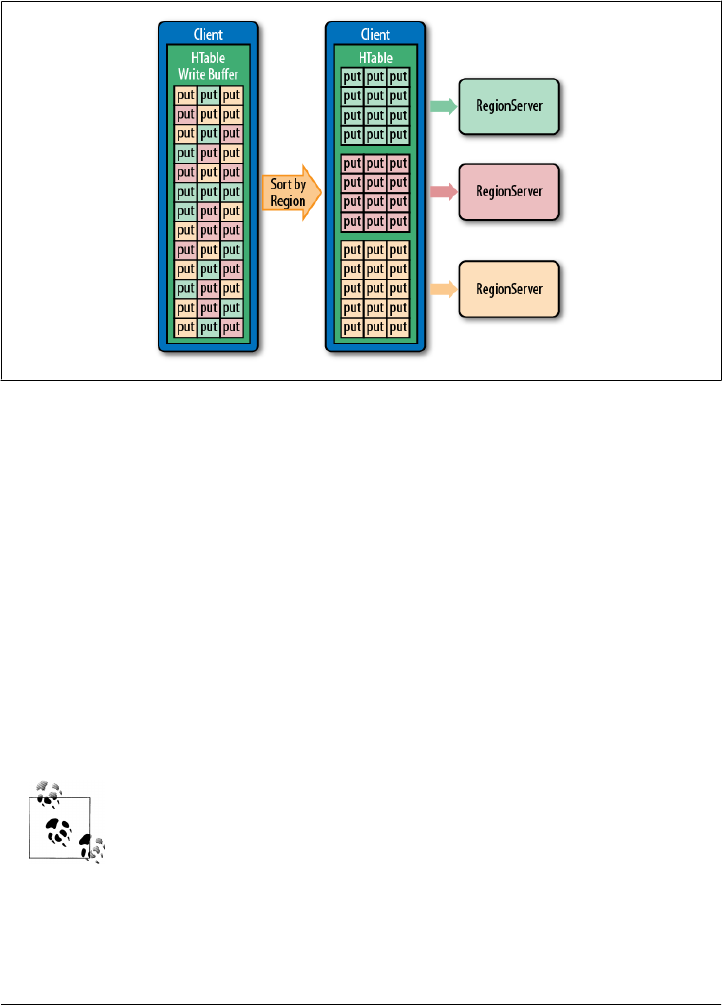
is handled transparently for you by the HBase client. Figure 3-1 shows how the oper-
ations are sorted and grouped before they are shipped over the network, with one single
RPC per region server.
Figure 3-1. The client-side puts sorted and grouped by region server
While you can force a flush of the buffer, this is usually not necessary, as the API tracks
how much data you are buffering by counting the required heap size of every instance
you have added. This tracks the entire overhead of your data, also including necessary
internal data structures. Once you go over a specific limit, the client will call the flush
command for you implicitly. You can control the configured maximum allowed client-
side write buffer size with these calls:
long getWriteBufferSize()
void setWriteBufferSize(long writeBufferSize) throws IOException
The default size is a moderate 2 MB (or 2,097,152 bytes) and assumes you are inserting
reasonably small records into HBase, that is, each a fraction of that buffer size. If you
were to store larger data, you may want to consider increasing this value to allow your
client to efficiently group together a certain number of records per RPC.
Setting this value for every HTable instance you create may seem cum-
bersome and can be avoided by adding a higher value to your local
hbase-site.xml configuration file—for example, adding:
<property>
<name>hbase.client.write.buffer</name>
<value>20971520</value>
</property>
This will increase the limit to 20 MB.
CRUD Operations | 87
The buffer is only ever flushed on two occasions:
Explicit flush
Use the flushCommits() call to send the data to the servers for permanent storage.
Implicit flush
This is triggered when you call put() or setWriteBufferSize(). Both calls compare
the currently used buffer size with the configured limit and optionally invoke the
flushCommits() method. In case the entire buffer is disabled, setting setAuto
Flush(true) will force the client to call the flush method for every invocation of
put().
Another call triggering the flush implicitly and unconditionally is the close()
method of HTable.
Example 3-3 shows how the write buffer is controlled from the client API.
Example 3-3. Using the client-side write buffer
HTable table = new HTable(conf, "testtable");
System.out.println("Auto flush: " + table.isAutoFlush());
table.setAutoFlush(false);
Put put1 = new Put(Bytes.toBytes("row1"));
put1.add(Bytes.toBytes("colfam1"), Bytes.toBytes("qual1"),
Bytes.toBytes("val1"));
table.put(put1);
Put put2 = new Put(Bytes.toBytes("row2"));
put2.add(Bytes.toBytes("colfam1"), Bytes.toBytes("qual1"),
Bytes.toBytes("val2"));
table.put(put2);
Put put3 = new Put(Bytes.toBytes("row3"));
put3.add(Bytes.toBytes("colfam1"), Bytes.toBytes("qual1"),
Bytes.toBytes("val3"));
table.put(put3);
Get get = new Get(Bytes.toBytes("row1"));
Result res1 = table.get(get);
System.out.println("Result: " + res1);
table.flushCommits();
Result res2 = table.get(get);
System.out.println("Result: " + res2);
Check what the auto flush flag is set to; should print “Auto flush: true”.
Set the auto flush to false to enable the client-side write buffer.
Store some rows with columns into HBase.
Try to load previously stored row. This will print “Result: keyvalues=NONE”.
88 | Chapter 3: Client API: The Basics
Force a flush. This causes an RPC to occur.
Now the row is persisted and can be loaded.
This example also shows a specific behavior of the buffer that you may not anticipate.
Let’s see what it prints out when executed:
Auto flush: true
Result: keyvalues=NONE
Result: keyvalues={row1/colfam1:qual1/1300267114099/Put/vlen=4}
While you have not seen the get() operation yet, you should still be able to correctly
infer what it does, that is, reading data back from the servers. But for the first get() in
the example, the API returns a NONE value—what does that mean? It is caused by the
fact that the client write buffer is an in-memory structure that is literally holding back
any unflushed records. Nothing was sent to the servers yet, and therefore you cannot
access it.
If you were ever required to access the write buffer content, you would
find that ArrayList<Put> getWriteBuffer() can be used to get the in-
ternal list of buffered Put instances you have added so far calling
table.put(put).
I mentioned earlier that it is exactly that list that makes HTable not safe
for multithreaded use. Be very careful with what you do to that list when
accessing it directly. You are bypassing the heap size checks, or you
might modify it while a flush is in progress!
Since the client buffer is a simple list retained in the local process mem-
ory, you need to be careful not to run into a problem that terminates
the process mid-flight. If that were to happen, any data that has not yet
been flushed will be lost! The servers will have never received that data,
and therefore there will be no copy of it that can be used to recover from
this situation.
Also note that a bigger buffer takes more memory—on both the client
and server side since the server instantiates the passed write buffer to
process it. On the other hand, a larger buffer size reduces the number
of RPCs made. For an estimate of server-side memory-used, evaluate
hbase.client.write.buffer * hbase.regionserver.handler.count *
number of region server.
Referring to the round-trip time again, if you only store large cells, the
local buffer is less useful, since the transfer is then dominated by
the transfer time. In this case, you are better advised to not increase the
client buffer size.
CRUD Operations | 89
List of Puts
The client API has the ability to insert single Put instances as shown earlier, but it also
has the advanced feature of batching operations together. This comes in the form of
the following call:
void put(List<Put> puts) throws IOException
You will have to create a list of Put instances and hand it to this call. Example 3-4
updates the previous example by creating a list to hold the mutations and eventually
calling the list-based put() method.
Example 3-4. Inserting data into HBase using a list
List<Put> puts = new ArrayList<Put>();
Put put1 = new Put(Bytes.toBytes("row1"));
put1.add(Bytes.toBytes("colfam1"), Bytes.toBytes("qual1"),
Bytes.toBytes("val1"));
puts.add(put1);
Put put2 = new Put(Bytes.toBytes("row2"));
put2.add(Bytes.toBytes("colfam1"), Bytes.toBytes("qual1"),
Bytes.toBytes("val2"));
puts.add(put2);
Put put3 = new Put(Bytes.toBytes("row2"));
put3.add(Bytes.toBytes("colfam1"), Bytes.toBytes("qual2"),
Bytes.toBytes("val3"));
puts.add(put3);
table.put(puts);
Create a list that holds the Put instances.
Add a Put to the list.
Add another Put to the list.
Add a third Put to the list.
Store multiple rows with columns into HBase.
A quick check with the HBase Shell reveals that the rows were stored as expected. Note
that the example actually modified three columns, but in two rows only. It added two
columns into the row with the key row2, using two separate qualifiers, qual1 and
qual2, creating two uniquely named columns in the same row.
hbase(main):001:0> scan 'testtable'
ROW COLUMN+CELL
row1 column=colfam1:qual1, timestamp=1300108258094, value=val1
row2 column=colfam1:qual1, timestamp=1300108258094, value=val2
row2 column=colfam1:qual2, timestamp=1300108258098, value=val3
2 row(s) in 0.1590 seconds
90 | Chapter 3: Client API: The Basics

Since you are issuing a list of row mutations to possibly many different rows, there is
a chance that not all of them will succeed. This could be due to a few reasons—for
example, when there is an issue with one of the region servers and the client-side retry
mechanism needs to give up because the number of retries has exceeded the configured
maximum. If there is problem with any of the put calls on the remote servers, the error
is reported back to you subsequently in the form of an IOException.
Example 3-5 uses a bogus column family name to insert a column. Since the client is
not aware of the structure of the remote table—it could have been altered since it was
created—this check is done on the server side.
Example 3-5. Inserting a faulty column family into HBase
Put put1 = new Put(Bytes.toBytes("row1"));
put1.add(Bytes.toBytes("colfam1"), Bytes.toBytes("qual1"),
Bytes.toBytes("val1"));
puts.add(put1);
Put put2 = new Put(Bytes.toBytes("row2"));
put2.add(Bytes.toBytes("BOGUS"), Bytes.toBytes("qual1"),
Bytes.toBytes("val2"));
puts.add(put2);
Put put3 = new Put(Bytes.toBytes("row2"));
put3.add(Bytes.toBytes("colfam1"), Bytes.toBytes("qual2"),
Bytes.toBytes("val3"));
puts.add(put3);
table.put(puts);
Add a Put with a nonexistent family to the list.
Store multiple rows with columns into HBase.
The call to put() fails with the following (or similar) error message:
org.apache.hadoop.hbase.client.RetriesExhaustedWithDetailsException:
Failed 1 action: NoSuchColumnFamilyException: 1 time,
servers with issues: 10.0.0.57:51640,
You may wonder what happened to the other, nonfaulty puts in the list. Using the shell
again you should see that the two correct puts have been applied:
hbase(main):001:0> scan 'testtable'
ROW COLUMN+CELL
row1 column=colfam1:qual1, timestamp=1300108925848, value=val1
row2 column=colfam1:qual2, timestamp=1300108925848, value=val3
2 row(s) in 0.0640 seconds
The servers iterate over all operations and try to apply them. The failed ones are
returned and the client reports the remote error using the RetriesExhausted
WithDetailsException, giving you insight into how many operations have failed, with
what error, and how many times it has retried to apply the erroneous modification. It
is interesting to note that, for the bogus column family, the retry is automatically set
CRUD Operations | 91
to 1 (see the NoSuchColumnFamilyException: 1 time), as this is an error from which
HBase cannot recover.
Those Put instances that have failed on the server side are kept in the local write buffer.
They will be retried the next time the buffer is flushed. You can also access them using
the getWriteBuffer() method of HTable and take, for example, evasive actions.
Some checks are done on the client side, though—for example, to ensure that the put
has a column specified or that it is completely empty. In that event, the client is throwing
an exception that leaves the operations preceding the faulty one in the client buffer.
The list-based put() call uses the client-side write buffer to insert all puts
into the local buffer and then to call flushCache() implicitly. While in-
serting each instance of Put, the client API performs the mentioned
check. If it fails, for example, at the third put out of five—the first two
are added to the buffer while the last two are not. It also then does not
trigger the flush command at all.
You could catch the exception and flush the write buffer manually to apply those mod-
ifications. Example 3-6 shows one approach to handle this.
Example 3-6. Inserting an empty Put instance into HBase
Put put1 = new Put(Bytes.toBytes("row1"));
put1.add(Bytes.toBytes("colfam1"), Bytes.toBytes("qual1"),
Bytes.toBytes("val1"));
puts.add(put1);
Put put2 = new Put(Bytes.toBytes("row2"));
put2.add(Bytes.toBytes("BOGUS"), Bytes.toBytes("qual1"),
Bytes.toBytes("val2"));
puts.add(put2);
Put put3 = new Put(Bytes.toBytes("row2"));
put3.add(Bytes.toBytes("colfam1"), Bytes.toBytes("qual2"),
Bytes.toBytes("val3"));
puts.add(put3);
Put put4 = new Put(Bytes.toBytes("row2"));
puts.add(put4);
try {
table.put(puts);
} catch (Exception e) {
System.err.println("Error: " + e);
table.flushCommits();
}
Add a put with no content at all to the list.
Catch a local exception and commit queued updates.
The example code this time should give you two errors, similar to:
Error: java.lang.IllegalArgumentException: No columns to insert
Exception in thread "main"
92 | Chapter 3: Client API: The Basics

org.apache.hadoop.hbase.client.RetriesExhaustedWithDetailsException:
Failed 1 action: NoSuchColumnFamilyException: 1 time,
servers with issues: 10.0.0.57:51640,
The first Error is the client-side check, while the second is the remote exception that
now is caused by calling
table.flushCommits()
in the try/catch block.
Since you possibly have the client-side write buffer enabled—refer to
“Client-side write buffer” on page 86—you will find that the exception
is not reported right away, but is delayed until the buffer is flushed.
You need to watch out for a peculiarity using the list-based put call: you cannot control
the order in which the puts are applied on the server side, which implies that the order
in which the servers are called is also not under your control. Use this call with caution
if you have to guarantee a specific order—in the worst case, you need to create smaller
batches and explicitly flush the client-side write cache to enforce that they are sent to
the remote servers.
Atomic compare-and-set
There is a special variation of the put calls that warrants its own section: check and
put. The method signature is:
boolean checkAndPut(byte[] row, byte[] family, byte[] qualifier,
byte[] value, Put put) throws IOException
This call allows you to issue atomic, server-side mutations that are guarded by an
accompanying check. If the check passes successfully, the put operation is executed;
otherwise, it aborts the operation completely. It can be used to update data based on
current, possibly related, values.
Such guarded operations are often used in systems that handle, for example, account
balances, state transitions, or data processing. The basic principle is that you read data
at one point in time and process it. Once you are ready to write back the result, you
want to make sure that no other client has done the same already. You use the atomic
check to compare that the value is not modified and therefore apply your value.
A special type of check can be performed using the checkAndPut() call:
only update if another value is not already present. This is achieved by
setting the value parameter to null. In that case, the operation would
succeed when the specified column is nonexistent.
CRUD Operations | 93
The call returns a boolean result value, indicating whether the Put has been applied or
not, returning true or false, respectively. Example 3-7 shows the interactions between
the client and the server, returning the expected results.
Example 3-7. Application using the atomic compare-and-set operations
Put put1 = new Put(Bytes.toBytes("row1"));
put1.add(Bytes.toBytes("colfam1"), Bytes.toBytes("qual1"),
Bytes.toBytes("val1"));
boolean res1 = table.checkAndPut(Bytes.toBytes("row1"),
Bytes.toBytes("colfam1"), Bytes.toBytes("qual1"), null, put1);
System.out.println("Put applied: " + res1);
boolean res2 = table.checkAndPut(Bytes.toBytes("row1"),
Bytes.toBytes("colfam1"), Bytes.toBytes("qual1"), null, put1);
System.out.println("Put applied: " + res2);
Put put2 = new Put(Bytes.toBytes("row1"));
put2.add(Bytes.toBytes("colfam1"), Bytes.toBytes("qual2"),
Bytes.toBytes("val2"));
boolean res3 = table.checkAndPut(Bytes.toBytes("row1"),
Bytes.toBytes("colfam1"), Bytes.toBytes("qual1"),
Bytes.toBytes("val1"), put2);
System.out.println("Put applied: " + res3);
Put put3 = new Put(Bytes.toBytes("row2"));
put3.add(Bytes.toBytes("colfam1"), Bytes.toBytes("qual1"),
Bytes.toBytes("val3"));
boolean res4 = table.checkAndPut(Bytes.toBytes("row1"),
Bytes.toBytes("colfam1"), Bytes.toBytes("qual1"),
Bytes.toBytes("val1"), put3);
System.out.println("Put applied: " + res4);
Create a new Put instance.
Check if the column does not exist and perform an optional put operation.
Print out the result; it should be “Put applied: true.”
Attempt to store the same cell again.
Print out the result; it should be “Put applied: false”, as the column now already
exists.
Create another Put instance, but using a different column qualifier.
Store new data only if the previous data has been saved.
Print out the result; it should be “Put applied: true”, as the checked column already
exists.
Create yet another Put instance, but using a different row.
94 | Chapter 3: Client API: The Basics
Store new data while checking a different row.
We will not get here, as an exception is thrown beforehand!
The last call in the example will throw the following error:
Exception in thread "main" org.apache.hadoop.hbase.DoNotRetryIOException:
Action's getRow must match the passed row
The compare-and-set operations provided by HBase rely on checking
and modifying the same row! As with other operations only providing
atomicity guarantees on single rows, this also applies for this call. Trying
to check and modify two different rows will return an exception.
Compare-and-set (CAS) operations are very powerful, especially in distributed systems,
with even more decoupled client processes. In providing these calls, HBase sets itself
apart from other architectures that give no means to reason about concurrent updates
performed by multiple, independent clients.
Get Method
The next step in a client API is to retrieve what was just saved. For that the HTable is
providing you with the Get call and matching classes. The operations are split into those
that operate on a single row and those that retrieve multiple rows in one call.
Single Gets
First, the method that is used to retrieve specific values from an HBase table:
Result get(Get get) throws IOException
Similar to the Put class for the put() call, there is a matching Get class used by the
aforementioned get() function. As another similarity, you will have to provide a row
key when creating an instance of Get, using one of these constructors:
Get(byte[] row)
Get(byte[] row, RowLock rowLock)
A get() operation is bound to one specific row, but can retrieve any
number of columns and/or cells contained therein.
Each constructor takes a row parameter specifying the row you want to access, while
the second constructor adds an optional rowLock parameter, allowing you to hand in
your own locks. And, similar to the put operations, you have methods to specify rather
broad criteria to find what you are looking for—or to specify everything down to exact
coordinates for a single cell:
CRUD Operations | 95

Get addFamily(byte[] family)
Get addColumn(byte[] family, byte[] qualifier)
Get setTimeRange(long minStamp, long maxStamp) throws IOException
Get setTimeStamp(long timestamp)
Get setMaxVersions()
Get setMaxVersions(int maxVersions) throws IOException
The addFamily() call narrows the request down to the given column family. It can be
called multiple times to add more than one family. The same is true for the
addColumn() call. Here you can add an even narrower address space: the specific
column. Then there are methods that let you set the exact timestamp you are looking
for—or a time range to match those cells that fall inside it.
Lastly, there are methods that allow you to specify how many versions you want to
retrieve, given that you have not set an exact timestamp. By default, this is set to 1,
meaning that the get() call returns the most current match only. If you are in doubt,
use getMaxVersions() to check what it is set to. The setMaxVersions() without a pa-
rameter sets the number of versions to return to Integer.MAX_VALUE—which is also the
maximum number of versions you can configure in the column family descriptor, and
therefore tells the API to return every available version of all matching cells (in other
words, up to what is set at the column family level).
The Get class provides additional calls, which are listed in Table 3-4 for your perusal.
Table 3-4. Quick overview of additional methods provided by the Get class
Method Description
getRow() Returns the row key as specified when creating the Get instance.
getRowLock() Returns the row RowLock instance for the current Get instance.
getLockId() Returns the optional lock ID handed into the constructor using the rowLock
parameter. Will be -1L if not set.
getTimeRange() Retrieves the associated timestamp or time range of the Get instance. Note that
there is no getTimeStamp() since the API converts a value assigned with set
TimeStamp() into a TimeRange instance internally, setting the minimum and
maximum values to the given timestamp.
setFilter()/getFilter() Special filter instances can be used to select certain columns or cells, based on a wide
variety of conditions. You can get and set them with these methods.
See “Filters” on page 137 for details.
setCacheBlocks()/
getCacheBlocks()
Each HBase region server has a block cache that efficiently retains recently accessed
data for subsequent reads of contiguous information. In some events it is better to
not engage the cache to avoid too much churn when doing completely random gets.
These methods give you control over this feature.
numFamilies() Convenience method to retrieve the size of the family map, containing the families
added using the addFamily() or addColumn() calls.
hasFamilies() Another helper to check if a family—or column—has been added to the current
instance of the Get class.
96 | Chapter 3: Client API: The Basics
Method Description
familySet()/getFamilyMap() These methods give you access to the column families and specific columns, as added
by the addFamily() and/or addColumn() calls. The family map is a map where
the key is the family name and the value a list of added column qualifiers for this
particular family. The familySet() returns the Set of all stored families, i.e., a
set containing only the family names.
The getters listed in Table 3-4 for the Get class only retrieve what you
have set beforehand. They are rarely used, and make sense only when
you, for example, prepare a Get instance in a private method in your
code, and inspect the values in another place.
As mentioned earlier, HBase provides us with a helper class named Bytes that has many
static methods to convert Java types into byte[] arrays. It also can do the same in
reverse: as you are retrieving data from HBase—for example, one of the rows stored
previously—you can make use of these helper functions to convert the byte[] data
back into Java types. Here is a short list of what it offers, continued from the earlier
discussion:
static String toString(byte[] b)
static boolean toBoolean(byte[] b)
static long toLong(byte[] bytes)
static float toFloat(byte[] bytes)
static int toInt(byte[] bytes)
...
Example 3-8 shows how this is all put together.
Example 3-8. Application retrieving data from HBase
Configuration conf = HBaseConfiguration.create();
HTable table = new HTable(conf, "testtable");
Get get = new Get(Bytes.toBytes("row1"));
get.addColumn(Bytes.toBytes("colfam1"), Bytes.toBytes("qual1"));
Result result = table.get(get);
byte[] val = result.getValue(Bytes.toBytes("colfam1"),
Bytes.toBytes("qual1"));
System.out.println("Value: " + Bytes.toString(val));
Create the configuration.
Instantiate a new table reference.
Create a Get with a specific row.
Add a column to the Get.
Retrieve a row with selected columns from HBase.
Get a specific value for the given column.
Print out the value while converting it back.
CRUD Operations | 97

If you are running this example after, say Example 3-2, you should get this as the output:
Value: val1
The output is not very spectacular, but it shows that the basic operation works. The
example also only adds the specific column to retrieve, relying on the default for max-
imum versions being returned set to 1. The call to get() returns an instance of the
Result class, which you will learn about next.
The Result class
When you retrieve data using the get() calls, you receive an instance of the Result class
that contains all the matching cells. It provides you with the means to access everything
that was returned from the server for the given row and matching the specified query,
such as column family, column qualifier, timestamp, and so on.
There are utility methods you can use to ask for specific results—just as Example 3-8
used earlier—using more concrete dimensions. If you have, for example, asked the
server to return all columns of one specific column family, you can now ask for specific
columns within that family. In other words, you need to call get() with just enough
concrete information to be able to process the matching data on the client side. The
functions provided are:
byte[] getValue(byte[] family, byte[] qualifier)
byte[] value()
byte[] getRow()
int size()
boolean isEmpty()
KeyValue[] raw()
List<KeyValue> list()
The getValue() call allows you to get the data for a specific cell stored in HBase. As you
cannot specify what timestamp—in other words, version—you want, you get the new-
est one. The value() call makes this even easier by returning the data for the newest
cell in the first column found. Since columns are also sorted lexicographically on the
server, this would return the value of the column with the column name (including
family and qualifier) sorted first.
You saw getRow() before: it returns the row key, as specified when creating the current
instance of the Get class. size() is returning the number of KeyValue instances the server
has returned. You may use this call—or isEmpty(), which checks if size() returns a
number greater than zero—to check in your own client code if the retrieval call returned
any matches.
Access to the raw, low-level KeyValue instances is provided by the raw() method,
returning the array of KeyValue instances backing the current Result instance. The
list() call simply converts the array returned by raw() into a List instance, giving you
convenience by providing iterator access, for example. The created list is backed by the
original array of KeyValue instances.
98 | Chapter 3: Client API: The Basics
The array returned by raw() is already lexicographically sorted, taking
the full coordinates of the KeyValue instances into account. So it is sorted
first by column family, then within each family by qualifier, then by
timestamp, and finally by type.
Another set of accessors is provided which are more column-oriented:
List<KeyValue> getColumn(byte[] family, byte[] qualifier)
KeyValue getColumnLatest(byte[] family, byte[] qualifier)
boolean containsColumn(byte[] family, byte[] qualifier)
Here you ask for multiple values of a specific column, which solves the issue pointed
out earlier, that is, how to get multiple versions of a given column. The number returned
obviously is bound to the maximum number of versions you have specified when con-
figuring the Get instance, before the call to get(), with the default being set to 1. In
other words, the returned list contains zero (in case the column has no value for the
given row) or one entry, which is the newest version of the value. If you have specified
a value greater than the default of 1 version to be returned, it could be any number, up
to the specified maximum.
The getColumnLatest() method is returning the newest cell of the specified column,
but in contrast to getValue(), it does not return the raw byte array of the value but the
full KeyValue instance instead. This may be useful when you need more than just the
data. The containsColumn() is a convenience method to check if there was any cell
returned in the specified column.
These methods all support the fact that the qualifier can be left unspe-
cified—setting it to null—and therefore matching the special column
with no name.
Using no qualifier means that there is no label to the column. When
looking at the table from, for example, the HBase Shell, you need to
know what it contains. A rare case where you might want to consider
using the empty qualifier is in column families that only ever contain a
single column. Then the family name might indicate its purpose.
There is a third set of methods that provide access to the returned data from the get
request. These are map-oriented and look like this:
NavigableMap<byte[], NavigableMap<byte[],
NavigableMap<Long, byte[]>>> getMap()
NavigableMap<byte[],
NavigableMap<byte[], byte[]>> getNoVersionMap()
NavigableMap<byte[], byte[]> getFamilyMap(byte[] family)
The most generic call, named getMap(), returns the entire result set in a Java Map class
instance that you can iterate over to access all the values. The getNoVersionMap() does
the same while only including the latest cell for each column. Finally, the getFamily
CRUD Operations | 99
Map() lets you select the KeyValue instances for a specific column family only—but
including all versions, if specified.
Use whichever access method of Result matches your access pattern; the data has al-
ready been moved across the network from the server to your client process, so it is not
incurring any other performance or resource penalties.
Dump the Contents
All Java objects have a toString() method, which, when overridden by a class, can be
used to convert the data of an instance into a text representation. This is not for seri-
alization purposes, but is most often used for debugging.
The Result class has such an implementation of toString(), dumping the result of a
read call as a string. The output looks like this:
keyvalues={row-2/colfam1:col-5/1300802024293/Put/vlen=7,
row-2/colfam2:col-33/1300802024325/Put/vlen=8}
It simply prints all contained KeyValue instances, that is, calling KeyValue.toString()
respectively. If the Result instance is empty, the output will be:
keyvalues=NONE
This indicates that there were no KeyValue instances returned. The code examples in
this book make use of the toString() method to quickly print the results of previous
read operations.
List of Gets
Another similarity to the put() calls is that you can ask for more than one row using a
single request. This allows you to quickly and efficiently retrieve related—but also
completely random, if required—data from the remote servers.
As shown in Figure 3-1, the request may actually go to more than one
server, but for all intents and purposes, it looks like a single call from
the client code.
The method provided by the API has the following signature:
Result[] get(List<Get> gets) throws IOException
Using this call is straightforward, with the same approach as seen earlier: you need to
create a list that holds all instances of the Get class you have prepared. This list is handed
into the call and you will be returned an array of equal size holding the matching
Result instances. Example 3-9 brings this together, showing two different approaches
to accessing the data.
100 | Chapter 3: Client API: The Basics
Example 3-9. Retrieving data from HBase using lists of Get instances
byte[] cf1 = Bytes.toBytes("colfam1");
byte[] qf1 = Bytes.toBytes("qual1");
byte[] qf2 = Bytes.toBytes("qual2");
byte[] row1 = Bytes.toBytes("row1");
byte[] row2 = Bytes.toBytes("row2");
List<Get> gets = new ArrayList<Get>();
Get get1 = new Get(row1);
get1.addColumn(cf1, qf1);
gets.add(get1);
Get get2 = new Get(row2);
get2.addColumn(cf1, qf1);
gets.add(get2);
Get get3 = new Get(row2);
get3.addColumn(cf1, qf2);
gets.add(get3);
Result[] results = table.get(gets);
System.out.println("First iteration...");
for (Result result : results) {
String row = Bytes.toString(result.getRow());
System.out.print("Row: " + row + " ");
byte[] val = null;
if (result.containsColumn(cf1, qf1)) {
val = result.getValue(cf1, qf1);
System.out.println("Value: " + Bytes.toString(val));
}
if (result.containsColumn(cf1, qf2)) {
val = result.getValue(cf1, qf2);
System.out.println("Value: " + Bytes.toString(val));
}
}
System.out.println("Second iteration...");
for (Result result : results) {
for (KeyValue kv : result.raw()) {
System.out.println("Row: " + Bytes.toString(kv.getRow()) +
" Value: " + Bytes.toString(kv.getValue()));
}
}
Prepare commonly used byte arrays.
Create a list that holds the Get instances.
Add the Get instances to the list.
Retrieve rows with selected columns from HBase.
Iterate over the results and check what values are available.
CRUD Operations | 101
Iterate over the results again, printing out all values.
Assuming that you execute Example 3-4 just before you run Example 3-9, you should
see something like this on the command line:
First iteration...
Row: row1 Value: val1
Row: row2 Value: val2
Row: row2 Value: val3
Second iteration...
Row: row1 Value: val1
Row: row2 Value: val2
Row: row2 Value: val3
Both iterations return the same values, showing that you have a number of choices on
how to access them, once you have received the results. What you have not yet seen is
how errors are reported back to you. This differs from what you learned in “List of
Puts” on page 90. The get() call either returns the said array, matching the same size
as the given list by the gets parameter, or throws an exception. Example 3-10 showcases
this behavior.
Example 3-10. Trying to read an erroneous column family
List<Get> gets = new ArrayList<Get>();
Get get1 = new Get(row1);
get1.addColumn(cf1, qf1);
gets.add(get1);
Get get2 = new Get(row2);
get2.addColumn(cf1, qf1);
gets.add(get2);
Get get3 = new Get(row2);
get3.addColumn(cf1, qf2);
gets.add(get3);
Get get4 = new Get(row2);
get4.addColumn(Bytes.toBytes("BOGUS"), qf2);
gets.add(get4);
Result[] results = table.get(gets);
System.out.println("Result count: " + results.length);
Add the Get instances to the list.
Add the bogus column family Get.
An exception is thrown and the process is aborted.
This line will never be reached!
102 | Chapter 3: Client API: The Basics
Executing this example will abort the entire get() operation, throwing the following
(or similar) error, and not returning a result at all:
org.apache.hadoop.hbase.client.RetriesExhaustedWithDetailsException:
Failed 1 action: NoSuchColumnFamilyException: 1 time,
servers with issues: 10.0.0.57:51640,
One way to have more control over how the API handles partial faults is to use the
batch() operations discussed in “Batch Operations” on page 114.
Related retrieval methods
There are a few more calls that you can use from your code to retrieve or check your
stored data. The first is:
boolean exists(Get get) throws IOException
You can set up a Get instance, just like you do when using the get() calls of HTable.
Instead of having to retrieve the data from the remote servers, using an RPC, to verify
that it actually exists, you can employ this call because it only returns a boolean flag
indicating that same fact.
Using exists() involves the same lookup semantics on the region serv-
ers, including loading file blocks to check if a row or column actually
exists. You only avoid shipping the data over the network—but that is
very useful if you are checking very large columns, or do so very
frequently.
Sometimes it might be necessary to find a specific row, or the one just before the re-
quested row, when retrieving data. The following call can help you find a row using
these semantics:
Result getRowOrBefore(byte[] row, byte[] family) throws IOException
You need to specify the row you are looking for, and a column family. The latter is
required because, in HBase, which is a column-oriented database, there is no row if
there are no columns. Specifying a family name tells the servers to check if the row
searched for has any values in a column contained in the given family.
Be careful to specify an existing column family name when using the
getRowOrBefore() method, or you will get a Java NullPointerException
back from the server. This is caused by the server trying to access a
nonexistent storage file.
The returned instance of the Result class can be used to retrieve the found row key.
This should be either the exact row you were asking for, or the one preceding it. If there
is no match at all, the call returns null. Example 3-11 uses the call to find the rows you
created using the put examples earlier.
CRUD Operations | 103
Example 3-11. Using a special retrieval method
Result result1 = table.getRowOrBefore(Bytes.toBytes("row1"),
Bytes.toBytes("colfam1"));
System.out.println("Found: " + Bytes.toString(result1.getRow()));
Result result2 = table.getRowOrBefore(Bytes.toBytes("row99"),
Bytes.toBytes("colfam1"));
System.out.println("Found: " + Bytes.toString(result2.getRow()));
for (KeyValue kv : result2.raw()) {
System.out.println(" Col: " + Bytes.toString(kv.getFamily()) +
"/" + Bytes.toString(kv.getQualifier()) +
", Value: " + Bytes.toString(kv.getValue()));
}
Result result3 = table.getRowOrBefore(Bytes.toBytes("abc"),
Bytes.toBytes("colfam1"));
System.out.println("Found: " + result3);
Attempt to find an existing row.
Print what was found.
Attempt to find a nonexistent row.
Returns the row that was sorted at the end of the table.
Print the returned values.
Attempt to find a row before the test rows.
Should return “null” since there is no match.
Assuming you ran Example 3-4 just before this code, you should see output similar or
equal to the following:
Found: row1
Found: row2
Col: colfam1/qual1, Value: val2
Col: colfam1/qual2, Value: val3
Found: null
The first call tries to find a matching row and succeeds. The second call uses a large
number postfix to find the last stored row, starting with the prefix row-. It did find
row-2 accordingly. Lastly, the example tries to find row abc, which sorts before the rows
the put example added, using the row- prefix, and therefore does not exist, nor matches
any previous row keys. The returned result is then null and indicates the missed lookup.
What is interesting is the loop to print out the data that was returned along with the
matching row. You can see from the preceding code that all columns of the specified
column family were returned, including their latest values. You could use this call to
quickly retrieve all the latest values from an entire column family—in other words, all
columns contained in the given column family—based on a specific sorting pattern.
For example, assume our put() example, which is using row- as the prefix for all keys.
104 | Chapter 3: Client API: The Basics

Calling getRowOrBefore() with a row set to row-999999999 will always return the row
that is, based on the lexicographical sorting, placed at the end of the table.
Delete Method
You are now able to create, read, and update data in HBase tables. What is left is the
ability to delete from it. And surely you may have guessed by now that the HTable
provides you with a method of exactly that name, along with a matching class aptly
named Delete.
Single Deletes
The variant of the delete() call that takes a single Delete instance is:
void delete(Delete delete) throws IOException
Just as with the get() and put() calls you saw already, you will have to create a
Delete instance and then add details about the data you want to remove. The con-
structors are:
Delete(byte[] row)
Delete(byte[] row, long timestamp, RowLock rowLock)
You need to provide the row you want to modify, and optionally provide a rowLock, an
instance of RowLock to specify your own lock details, in case you want to modify the
same row more than once subsequently. Otherwise, you would be wise to narrow down
what you want to remove from the given row, using one of the following methods:
Delete deleteFamily(byte[] family)
Delete deleteFamily(byte[] family, long timestamp)
Delete deleteColumns(byte[] family, byte[] qualifier)
Delete deleteColumns(byte[] family, byte[] qualifier, long timestamp)
Delete deleteColumn(byte[] family, byte[] qualifier)
Delete deleteColumn(byte[] family, byte[] qualifier, long timestamp)
void setTimestamp(long timestamp)
You do have a choice to narrow in on what to remove using four types of calls. First
you can use the deleteFamily() methods to remove an entire column family, including
all contained columns. You have the option to specify a timestamp that triggers more
specific filtering of cell versions. If specified, the timestamp matches the same and all
older versions of all columns.
The next type is deleteColumns(), which operates on exactly one column and deletes
either all versions of that cell when no timestamp is given, or all matching and older
versions when a timestamp is specified.
The third type is similar, using deleteColumn(). It also operates on a specific, given
column only, but deletes either the most current or the specified version, that is, the
one with the matching timestamp.
CRUD Operations | 105

Finally, there is setTimestamp(), which is not considered when using any of the other
three types of calls. But if you do not specify either a family or a column, this call can
make the difference between deleting the entire row or just all contained columns, in
all column families, that match or have an older timestamp compared to the given one.
Table 3-5 shows the functionality in a matrix to make the semantics more readable.
Table 3-5. Functionality matrix of the delete() calls
Method Deletes without timestamp Deletes with timestamp
none Entire row, i.e., all columns, all versions. All versions of all columns in all column families, whose
timestamp is equal to or older than the given timestamp.
deleteColumn() Only the latest version of the given
column; older versions are kept.
Only exactly the specified version of the given column,
with the matching timestamp. If nonexistent, nothing is
deleted.
deleteColumns() All versions of the given column. Versions equal to or older than the given timestamp of
the given column.
deleteFamily() All columns (including all versions) of
the given family.
Versions equal to or older than the given timestamp of
all columns of the given family.
The Delete class provides additional calls, which are listed in Table 3-6 for your
reference.
Table 3-6. Quick overview of additional methods provided by the Delete class
Method Description
getRow() Returns the row key as specified when creating the Delete instance.
getRowLock() Returns the row RowLock instance for the current Delete instance.
getLockId() Returns the optional lock ID handed into the constructor using the rowLock parameter. Will be
-1L if not set.
getTimeStamp() Retrieves the associated timestamp of the Delete instance.
isEmpty() Checks if the family map contains any entries. In other words, if you specified any column family,
or column qualifier, that should be deleted.
getFamilyMap() Gives you access to the added column families and specific columns, as added by the delete
Family() and/or deleteColumn()/deleteColumns() calls. The returned map uses the
family name as the key, and the value it points to is a list of added column qualifiers for this
particular family.
Example 3-12 shows how to use the single delete() call from client code.
Example 3-12. Application deleting data from HBase
Delete delete = new Delete(Bytes.toBytes("row1"));
delete.setTimestamp(1);
106 | Chapter 3: Client API: The Basics
delete.deleteColumn(Bytes.toBytes("colfam1"), Bytes.toBytes("qual1"), 1);
delete.deleteColumns(Bytes.toBytes("colfam2"), Bytes.toBytes("qual1"));
delete.deleteColumns(Bytes.toBytes("colfam2"), Bytes.toBytes("qual3"), 15);
delete.deleteFamily(Bytes.toBytes("colfam3"));
delete.deleteFamily(Bytes.toBytes("colfam3"), 3);
table.delete(delete);
table.close();
Create a Delete with a specific row.
Set a timestamp for row deletes.
Delete a specific version in one column.
Delete all versions in one column.
Delete the given and all older versions in one column.
Delete the entire family, all columns and versions.
Delete the given and all older versions in the entire column family, that is, from all
columns therein.
Delete the data from the HBase table.
The example lists all the different calls you can use to parameterize the delete() oper-
ation. It does not make too much sense to call them all one after another like this. Feel
free to comment out the various delete calls to see what is printed on the console.
Setting the timestamp for the deletes has the effect of only matching the exact cell, that
is, the matching column and value with the exact timestamp. On the other hand, not
setting the timestamp forces the server to retrieve the latest timestamp on the server
side on your behalf. This is slower than performing a delete with an explicit timestamp.
If you attempt to delete a cell with a timestamp that does not exist, nothing happens.
For example, given that you have two versions of a column, one at version 10 and one
at version 20, deleting from this column with version 15 will not affect either existing
version.
Another note to be made about the example is that it showcases custom versioning.
Instead of relying on timestamps, implicit or explicit ones, it uses sequential numbers,
starting with 1. This is perfectly valid, although you are forced to always set the version
yourself, since the servers do not know about your schema and would use epoch-based
timestamps instead.
As of this writing, using custom versioning is not recommended. It will
very likely work, but is not tested very well. Make sure you carefully
evaluate your options before using this technique.
CRUD Operations | 107
Another example of using custom versioning can be found in “Search Integra-
tion” on page 373.
List of Deletes
The list-based delete() call works very similarly to the list-based put(). You need to
create a list of Delete instances, configure them, and call the following method:
void delete(List<Delete> deletes) throws IOException
Example 3-13 shows where three different rows are affected during the operation, de-
leting various details they contain. When you run this example, you will see a printout
of the before and after states of the delete. The output is printing the raw KeyValue
instances, using KeyValue.toString().
Just as with the other list-based operation, you cannot make any as-
sumption regarding the order in which the deletes are applied on the
remote servers. The API is free to reorder them to make efficient use of
the single RPC per affected region server. If you need to enforce specific
orders of how operations are applied, you would need to batch those
calls into smaller groups and ensure that they contain the operations in
the desired order across the batches. In a worst-case scenario, you would
need to send separate delete calls altogether.
Example 3-13. Application deleting a list of values
List<Delete> deletes = new ArrayList<Delete>();
Delete delete1 = new Delete(Bytes.toBytes("row1"));
delete1.setTimestamp(4);
deletes.add(delete1);
Delete delete2 = new Delete(Bytes.toBytes("row2"));
delete2.deleteColumn(Bytes.toBytes("colfam1"), Bytes.toBytes("qual1"));
delete2.deleteColumns(Bytes.toBytes("colfam2"), Bytes.toBytes("qual3"), 5);
deletes.add(delete2);
Delete delete3 = new Delete(Bytes.toBytes("row3"));
delete3.deleteFamily(Bytes.toBytes("colfam1"));
delete3.deleteFamily(Bytes.toBytes("colfam2"), 3);
deletes.add(delete3);
table.delete(deletes);
table.close();
Create a list that holds the Delete instances.
Set a timestamp for row deletes.
Delete the latest version only in one column.
108 | Chapter 3: Client API: The Basics

Delete the given and all older versions in another column.
Delete the entire family, all columns and versions.
Delete the given and all older versions in the entire column family, that is, from all
columns therein.
Delete the data from multiple rows in the HBase table.
The output you should see is:#
Before delete call...
KV: row1/colfam1:qual1/2/Put/vlen=4, Value: val2
KV: row1/colfam1:qual1/1/Put/vlen=4, Value: val1
KV: row1/colfam1:qual2/4/Put/vlen=4, Value: val4
KV: row1/colfam1:qual2/3/Put/vlen=4, Value: val3
KV: row1/colfam1:qual3/6/Put/vlen=4, Value: val6
KV: row1/colfam1:qual3/5/Put/vlen=4, Value: val5
KV: row1/colfam2:qual1/2/Put/vlen=4, Value: val2
KV: row1/colfam2:qual1/1/Put/vlen=4, Value: val1
KV: row1/colfam2:qual2/4/Put/vlen=4, Value: val4
KV: row1/colfam2:qual2/3/Put/vlen=4, Value: val3
KV: row1/colfam2:qual3/6/Put/vlen=4, Value: val6
KV: row1/colfam2:qual3/5/Put/vlen=4, Value: val5
KV: row2/colfam1:qual1/2/Put/vlen=4, Value: val2
KV: row2/colfam1:qual1/1/Put/vlen=4, Value: val1
KV: row2/colfam1:qual2/4/Put/vlen=4, Value: val4
KV: row2/colfam1:qual2/3/Put/vlen=4, Value: val3
KV: row2/colfam1:qual3/6/Put/vlen=4, Value: val6
KV: row2/colfam1:qual3/5/Put/vlen=4, Value: val5
KV: row2/colfam2:qual1/2/Put/vlen=4, Value: val2
KV: row2/colfam2:qual1/1/Put/vlen=4, Value: val1
KV: row2/colfam2:qual2/4/Put/vlen=4, Value: val4
KV: row2/colfam2:qual2/3/Put/vlen=4, Value: val3
KV: row2/colfam2:qual3/6/Put/vlen=4, Value: val6
KV: row2/colfam2:qual3/5/Put/vlen=4, Value: val5
KV: row3/colfam1:qual1/2/Put/vlen=4, Value: val2
KV: row3/colfam1:qual1/1/Put/vlen=4, Value: val1
KV: row3/colfam1:qual2/4/Put/vlen=4, Value: val4
KV: row3/colfam1:qual2/3/Put/vlen=4, Value: val3
KV: row3/colfam1:qual3/6/Put/vlen=4, Value: val6
KV: row3/colfam1:qual3/5/Put/vlen=4, Value: val5
KV: row3/colfam2:qual1/2/Put/vlen=4, Value: val2
KV: row3/colfam2:qual1/1/Put/vlen=4, Value: val1
KV: row3/colfam2:qual2/4/Put/vlen=4, Value: val4
KV: row3/colfam2:qual2/3/Put/vlen=4, Value: val3
KV: row3/colfam2:qual3/6/Put/vlen=4, Value: val6
KV: row3/colfam2:qual3/5/Put/vlen=4, Value: val5
#For easier readability, the related details were broken up into groups using blank lines.
CRUD Operations | 109

After delete call...
KV: row1/colfam1:qual3/6/Put/vlen=4, Value: val6
KV: row1/colfam1:qual3/5/Put/vlen=4, Value: val5
KV: row1/colfam2:qual3/6/Put/vlen=4, Value: val6
KV: row1/colfam2:qual3/5/Put/vlen=4, Value: val5
KV: row2/colfam1:qual1/1/Put/vlen=4, Value: val1
KV: row2/colfam1:qual2/4/Put/vlen=4, Value: val4
KV: row2/colfam1:qual2/3/Put/vlen=4, Value: val3
KV: row2/colfam1:qual3/6/Put/vlen=4, Value: val6
KV: row2/colfam1:qual3/5/Put/vlen=4, Value: val5
KV: row2/colfam2:qual1/2/Put/vlen=4, Value: val2
KV: row2/colfam2:qual1/1/Put/vlen=4, Value: val1
KV: row2/colfam2:qual2/4/Put/vlen=4, Value: val4
KV: row2/colfam2:qual2/3/Put/vlen=4, Value: val3
KV: row2/colfam2:qual3/6/Put/vlen=4, Value: val6
KV: row3/colfam2:qual2/4/Put/vlen=4, Value: val4
KV: row3/colfam2:qual3/6/Put/vlen=4, Value: val6
KV: row3/colfam2:qual3/5/Put/vlen=4, Value: val5
The deleted original data is highlighted in the Before delete call... block. All three rows
contain the same data, composed of two column families, three columns in each family,
and two versions for each column.
The example code first deletes, from the entire row, everything up to version 4. This
leaves the columns with versions 5 and 6 as the remainder of the row content.
It then goes about and uses the two different column-related delete calls on row2 to
remove the newest cell in the column named colfam1:qual1, and subsequently every
cell with a version of 5 and older—in other words, those with a lower version number—
from colfam1:qual3. Here you have only one matching cell, which is removed as ex-
pected in due course.
Lastly, operating on row-3, the code removes the entire column family colfam1, and
then everything with a version of 3 or less from colfam2. During the execution of the
example code, you will see the printed KeyValue details, using something like this:
System.out.println("KV: " + kv.toString() +
", Value: " + Bytes.toString(kv.getValue()))
By now you are familiar with the usage of the Bytes class, which is used to print out
the value of the KeyValue instance, as returned by the getValue() method. This is nec-
essary because the KeyValue.toString() output (as explained in “The KeyValue
class” on page 83) is not printing out the actual value, but rather the key part only. The
toString() does not print the value since it could be very large.
Here, the example code inserts the column values, and therefore knows that these are
short and human-readable; hence it is safe to print them out on the console as shown.
You could use the same mechanism in your own code for debugging purposes.
110 | Chapter 3: Client API: The Basics
Please refer to the entire example code in the accompanying source code repository for
this book. You will see how the data is inserted and retrieved to generate the discussed
output.
What is left to talk about is the error handling of the list-based delete() call. The
handed-in deletes parameter, that is, the list of Delete instances, is modified to only
contain the failed delete instances when the call returns. In other words, when every-
thing has succeeded, the list will be empty. The call also throws the exception—if there
was one—reported from the remote servers. You will have to guard the call using a
try/catch, for example, and react accordingly. Example 3-14 may serve as a starting
point.
Example 3-14. Deleting faulty data from HBase
Delete delete4 = new Delete(Bytes.toBytes("row2"));
delete4.deleteColumn(Bytes.toBytes("BOGUS"), Bytes.toBytes("qual1"));
deletes.add(delete4);
try {
table.delete(deletes);
} catch (Exception e) {
System.err.println("Error: " + e);
}
table.close();
System.out.println("Deletes length: " + deletes.size());
for (Delete delete : deletes) {
System.out.println(delete);
}
Add the bogus column family to trigger an error.
Delete the data from multiple rows in the HBase table.
Guard against remote exceptions.
Check the length of the list after the call.
Print out the failed delete for debugging purposes.
Example 3-14 modifies Example 3-13 but adds an erroneous delete detail: it inserts a
BOGUS column family name. The output is the same as that for Example 3-13, but has
some additional details printed out in the middle part:
Before delete call...
KV: row1/colfam1:qual1/2/Put/vlen=4, Value: val2
KV: row1/colfam1:qual1/1/Put/vlen=4, Value: val1
...
KV: row3/colfam2:qual3/6/Put/vlen=4, Value: val6
KV: row3/colfam2:qual3/5/Put/vlen=4, Value: val5
Error: org.apache.hadoop.hbase.client.RetriesExhaustedWithDetailsException:
Failed 1 action: NoSuchColumnFamilyException: 1 time,
servers with issues: 10.0.0.43:59057,
CRUD Operations | 111

Deletes length: 1
row=row2, ts=9223372036854775807, families={(family=BOGUS, keyvalues= \
(row2/BOGUS:qual1/9223372036854775807/Delete/vlen=0)}
After delete call...
KV: row1/colfam1:qual3/6/Put/vlen=4, Value: val6
KV: row1/colfam1:qual3/5/Put/vlen=4, Value: val5
...
KV: row3/colfam2:qual3/6/Put/vlen=4, Value: val6
KV: row3/colfam2:qual3/5/Put/vlen=4, Value: val5
As expected, the list contains one remaining Delete instance: the one with the bogus
column family. Printing out the instance—Java uses the implicit toString() method
when printing an object—reveals the internal details of the failed delete. The important
part is the family name being the obvious reason for the failure. You can use this tech-
nique in your own code to check why an operation has failed. Often the reasons are
rather obvious indeed.
Finally, note the exception that was caught and printed out in the catch statement of
the example. It is the same RetriesExhaustedWithDetailsException you saw twice al-
ready. It reports the number of failed actions plus how often it did retry to apply them,
and on which server. An advanced task that you will learn about in later chapters is
how to verify and monitor servers so that the given server address could be useful to
find the root cause of the failure.
Atomic compare-and-delete
You saw in “Atomic compare-and-set” on page 93 how to use an atomic, conditional
operation to insert data into a table. There is an equivalent call for deletes that gives
you access to server-side, read-and-modify functionality:
boolean checkAndDelete(byte[] row, byte[] family, byte[] qualifier,
byte[] value, Delete delete) throws IOException
You need to specify the row key, column family, qualifier, and value to check before
the actual delete operation is performed. Should the test fail, nothing is deleted and the
call returns a false. If the check is successful, the delete is applied and true is returned.
Example 3-15 shows this in context.
Example 3-15. Application deleting values using the atomic compare-and-set operations
Delete delete1 = new Delete(Bytes.toBytes("row1"));
delete1.deleteColumns(Bytes.toBytes("colfam1"), Bytes.toBytes("qual3"));
boolean res1 = table.checkAndDelete(Bytes.toBytes("row1"),
Bytes.toBytes("colfam2"), Bytes.toBytes("qual3"), null, delete1);
System.out.println("Delete successful: " + res1);
Delete delete2 = new Delete(Bytes.toBytes("row1"));
delete2.deleteColumns(Bytes.toBytes("colfam2"), Bytes.toBytes("qual3"));
table.delete(delete2);
112 | Chapter 3: Client API: The Basics
boolean res2 = table.checkAndDelete(Bytes.toBytes("row1"),
Bytes.toBytes("colfam2"), Bytes.toBytes("qual3"), null, delete1);
System.out.println("Delete successful: " + res2);
Delete delete3 = new Delete(Bytes.toBytes("row2"));
delete3.deleteFamily(Bytes.toBytes("colfam1"));
try{
boolean res4 = table.checkAndDelete(Bytes.toBytes("row1"),
Bytes.toBytes("colfam1"), Bytes.toBytes("qual1"),
Bytes.toBytes("val1"), delete3);
System.out.println("Delete successful: " + res4);
} catch (Exception e) {
System.err.println("Error: " + e);
}
Create a new Delete instance.
Check if the column does not exist and perform an optional delete operation.
Print out the result; it should be “Delete successful: false.”
Delete the checked column manually.
Attempt to delete the same cell again.
Print out the result; it should be “Delete successful: true,” as the column now already
exists.
Create yet another Delete instance, but using a different row.
Try to delete it while checking a different row.
We will not get here, as an exception is thrown beforehand!
The entire output of the example should look like this:
Before delete call...
KV: row1/colfam1:qual1/2/Put/vlen=4, Value: val2
KV: row1/colfam1:qual1/1/Put/vlen=4, Value: val1
KV: row1/colfam1:qual2/4/Put/vlen=4, Value: val4
KV: row1/colfam1:qual2/3/Put/vlen=4, Value: val3
KV: row1/colfam1:qual3/6/Put/vlen=4, Value: val6
KV: row1/colfam1:qual3/5/Put/vlen=4, Value: val5
KV: row1/colfam2:qual1/2/Put/vlen=4, Value: val2
KV: row1/colfam2:qual1/1/Put/vlen=4, Value: val1
KV: row1/colfam2:qual2/4/Put/vlen=4, Value: val4
KV: row1/colfam2:qual2/3/Put/vlen=4, Value: val3
KV: row1/colfam2:qual3/6/Put/vlen=4, Value: val6
KV: row1/colfam2:qual3/5/Put/vlen=4, Value: val5
Delete successful: false
Delete successful: true
After delete call...
KV: row1/colfam1:qual1/2/Put/vlen=4, Value: val2
KV: row1/colfam1:qual1/1/Put/vlen=4, Value: val1
KV: row1/colfam1:qual2/4/Put/vlen=4, Value: val4
KV: row1/colfam1:qual2/3/Put/vlen=4, Value: val3
CRUD Operations | 113

KV: row1/colfam2:qual1/2/Put/vlen=4, Value: val2
KV: row1/colfam2:qual1/1/Put/vlen=4, Value: val1
KV: row1/colfam2:qual2/4/Put/vlen=4, Value: val4
KV: row1/colfam2:qual2/3/Put/vlen=4, Value: val3
Error: org.apache.hadoop.hbase.DoNotRetryIOException:
org.apache.hadoop.hbase.DoNotRetryIOException:
Action's getRow must match the passed row
...
Using null as the value parameter triggers the nonexistence test, that is, the check is
successful if the column specified does not exist. Since the example code inserts the
checked column before the check is performed, the test will initially fail, returning
false and aborting the delete operation.
The column is then deleted by hand and the check-and-modify call is run again. This
time the check succeeds and the delete is applied, returning true as the overall result.
Just as with the put-related CAS call, you can only perform the check-and-modify on
the same row. The example attempts to check on one row key while the supplied in-
stance of Delete points to another. An exception is thrown accordingly, once the check
is performed. It is allowed, though, to check across column families—for example, to
have one set of columns control how the filtering is done for another set of columns.
This example cannot justify the importance of the check-and-delete operation. In dis-
tributed systems, it is inherently difficult to perform such operations reliably, and
without incurring performance penalties caused by external locking approaches, that
is, where the atomicity is guaranteed by the client taking out exclusive locks on the
entire row. When the client goes away during the locked phase the server has to rely
on lease recovery mechanisms ensuring that these rows are eventually unlocked again.
They also cause additional RPCs to occur, which will be slower than a single, server-
side operation.
Batch Operations
You have seen how you can add, retrieve, and remove data from a table using single or
list-based operations. In this section, we will look at API calls to batch different oper-
ations across multiple rows.
In fact, a lot of the internal functionality of the list-based calls, such as
delete(List<Delete> deletes) or get(List<Get> gets), is based on the
batch() call. They are more or less legacy calls and kept for convenience.
If you start fresh, it is recommended that you use the batch() calls for
all your operations.
The following methods of the client API represent the available batch operations. You
may note the introduction of a new class type named Row, which is the ancestor, or
parent class, for Put, Get, and Delete.
114 | Chapter 3: Client API: The Basics
void batch(List<Row> actions, Object[] results)
throws IOException, InterruptedException
Object[] batch(List<Row> actions)
throws IOException, InterruptedException
Using the same parent class allows for polymorphic list items, representing any of these
three operations. It is equally easy to use these calls, just like the list-based methods
you saw earlier. Example 3-16 shows how you can mix the operations and then send
them off as one server call.
Be aware that you should not mix a Delete and Put operation for the
same row in one batch call. The operations will be applied in a different
order that guarantees the best performance, but also causes unpredict-
able results. In some cases, you may see fluctuating results due to race
conditions.
Example 3-16. Application using batch operations
private final static byte[] ROW1 = Bytes.toBytes("row1");
private final static byte[] ROW2 = Bytes.toBytes("row2");
private final static byte[] COLFAM1 = Bytes.toBytes("colfam1");
private final static byte[] COLFAM2 = Bytes.toBytes("colfam2");
private final static byte[] QUAL1 = Bytes.toBytes("qual1");
private final static byte[] QUAL2 = Bytes.toBytes("qual2");
List<Row> batch = new ArrayList<Row>();
Put put = new Put(ROW2);
put.add(COLFAM2, QUAL1, Bytes.toBytes("val5"));
batch.add(put);
Get get1 = new Get(ROW1);
get1.addColumn(COLFAM1, QUAL1);
batch.add(get1);
Delete delete = new Delete(ROW1);
delete.deleteColumns(COLFAM1, QUAL2);
batch.add(delete);
Get get2 = new Get(ROW2);
get2.addFamily(Bytes.toBytes("BOGUS"));
batch.add(get2);
Object[] results = new Object[batch.size()];
try {
table.batch(batch, results);
} catch (Exception e) {
System.err.println("Error: " + e);
}
for (int i = 0; i < results.length; i++) {
System.out.println("Result[" + i + "]: " + results[i]);
}
Batch Operations | 115

Use constants for easy reuse.
Create a list to hold all values.
Add a Put instance.
Add a Get instance for a different row.
Add a Delete instance.
Add a Get instance that will fail.
Create a result array.
Print an error that was caught.
Print all results.
You should see the following output on the console:
Before batch call...
KV: row1/colfam1:qual1/1/Put/vlen=4, Value: val1
KV: row1/colfam1:qual2/2/Put/vlen=4, Value: val2
KV: row1/colfam1:qual3/3/Put/vlen=4, Value: val3
Result[0]: keyvalues=NONE
Result[1]: keyvalues={row1/colfam1:qual1/1/Put/vlen=4}
Result[2]: keyvalues=NONE
Result[3]: org.apache.hadoop.hbase.regionserver.NoSuchColumnFamilyException:
org.apache.hadoop.hbase.regionserver.NoSuchColumnFamilyException:
Column family BOGUS does not exist in ...
After batch call...
KV: row1/colfam1:qual1/1/Put/vlen=4, Value: val1
KV: row1/colfam1:qual3/3/Put/vlen=4, Value: val3
KV: row2/colfam2:qual1/1308836506340/Put/vlen=4, Value: val5
Error: org.apache.hadoop.hbase.client.RetriesExhaustedWithDetailsException:
Failed 1 action: NoSuchColumnFamilyException: 1 time,
servers with issues: 10.0.0.43:60020,
As with the previous examples, there is some wiring behind the printed lines of code
that inserts a test row before executing the batch calls. The content is printed first, then
you will see the output from the example code, and finally the dump of the rows
after everything else. The deleted column was indeed removed, and the new column
was added to the row as expected.
Finding the result of the Get operation requires you to investigate the middle part of
the output, that is, the lines printed by the example code. The lines starting with
Result[n]—with n ranging from zero to 3—is where you see the outcome of the cor-
responding operation in the actions parameter. The first operation in the example is a
Put, and the result is an empty Result instance, containing no KeyValue instances. This
is the general contract of the batch calls; they return a best match result per input action,
and the possible types are listed in Table 3-7.
116 | Chapter 3: Client API: The Basics
Table 3-7. Possible result values returned by the batch() calls
Result Description
null The operation has failed to communicate with the remote server.
Empty Result Returned for successful Put and Delete operations.
Result Returned for successful Get operations, but may also be empty when there was no matching row or column.
Throwable In case the servers return an exception for the operation it is returned to the client as-is. You can use it to
check what went wrong and maybe handle the problem automatically in your code.
Looking further through the returned result array in the console output you can see the
empty Result instances printing keyvalues=NONE. The Get call succeeded and found a
match, returning the KeyValue instances accordingly. Finally, the operation with the
BOGUS column family has the exception for your perusal.
When you use the batch() functionality, the included Put instances will
not be buffered using the client-side write buffer. The batch() calls are
synchronous and send the operations directly to the servers; no delay
or other intermediate processing is used. This is obviously different
compared to the put() calls, so choose which one you want to use care-
fully.
There are two different batch calls that look very similar. The difference is that one
needs to have the array handed into the call, while the other creates it for you. So why
do you need both, and what—if any—semantical differences do they expose? Both
throw the RetriesExhaustedWithDetailsException that you saw already, so the crucial
difference is that
void batch(List<Row> actions, Object[] results)
throws IOException, InterruptedException
gives you access to the partial results, while
Object[] batch(List<Row> actions)
throws IOException, InterruptedException
does not! The latter throws the exception and nothing is returned to you since the
control flow of the code is interrupted before the new result array is returned.
The former function fills your given array and then throws the exception. The code in
Example 3-16 makes use of that fact and hands in the results array. Summarizing the
features, you can say the following about the batch() functions:
Both calls
Supports gets, puts, and deletes. If there is a problem executing any of them, a
client-side exception is thrown, reporting the issues. The client-side write buffer is
not used.
Batch Operations | 117

void batch(actions, results)
Gives access to the results of all succeeded operations, and the remote exceptions
for those that failed.
Object[] batch(actions)
Only returns the client-side exception; no access to partial results is possible.
All batch operations are executed before the results are checked: even
if you receive an error for one of the actions, all the other ones have been
applied. In a worst-case scenario, all actions might return faults, though.
On the other hand, the batch code is aware of transient errors, such as
the NotServingRegionException (indicating, for instance, that a region
has been moved), and is trying to apply the action multiple times. The
hbase.client.retries.number configuration property (by default set to
10) can be adjusted to increase, or reduce, the number of retries.
Row Locks
Mutating operations—like put(), delete(), checkAndPut(), and so on—are executed
exclusively, which means in a serial fashion, for each row, to guarantee row-level
atomicity. The region servers provide a row lock feature ensuring that only a client
holding the matching lock can modify a row. In practice, though, most client applica-
tions do not provide an explicit lock, but rather rely on the mechanism in place that
guards each operation separately.
You should avoid using row locks whenever possible. Just as with
RDBMSes, you can end up in a situation where two clients create a
deadlock by waiting on a locked row, with the lock held by the other
client.
While the locks wait to time out, these two blocked clients are holding
on to a handler, which is a scarce resource. If this happens on a heavily
used row, many other clients will lock the remaining few handlers and
block access to the complete server for all other clients: the server will
not be able to serve any row of any region it hosts.
To reiterate: do not use row locks if you do not have to. And if you do,
use them sparingly!
When you send, for example, a put() call to the server with an instance of Put, created
with the following constructor:
Put(byte[] row)
which is not providing a RowLock instance parameter, the servers will create a lock on
your behalf, just for the duration of the call. In fact, from the client API you cannot
even retrieve this short-lived, server-side lock instance.
118 | Chapter 3: Client API: The Basics

Instead of relying on the implicit, server-side locking to occur, clients can also acquire
explicit locks and use them across multiple operations on the same row. This is done
using the following calls:
RowLock lockRow(byte[] row) throws IOException
void unlockRow(RowLock rl) throws IOException
The first call, lockRow(), takes a row key and returns an instance of RowLock, which you
can hand in to the constructors of Put or Delete subsequently. Once you no longer
require the lock, you must release it with the accompanying unlockRow() call.
Each unique lock, provided by the server for you, or handed in by you through the
client API, guards the row it pertains to against any other lock that attempts to access
the same row. In other words, locks must be taken out against an entire row, specifying
its row key, and—once it has been acquired—will protect it against any other concur-
rent modification.
While a lock on a row is held by someone—whether by the server briefly or a client
explicitly—all other clients trying to acquire another lock on that very same row will
stall, until either the current lock has been released, or the lease on the lock has expired.
The latter case is a safeguard against faulty processes holding a lock for too long—or
possibly indefinitely.
The default timeout on locks is one minute, but can be configured
system-wide by adding the following property key to the hbase-
site.xml file and setting the value to a different, millisecond-based
timeout:
<property>
<name>hbase.regionserver.lease.period</name>
<value>120000</value>
</property>
Adding the preceding code would double the timeout to 120 seconds,
or two minutes, instead. Be careful not to set this value too high, since
every client trying to acquire an already locked row will have to block
for up to that timeout for the lock in limbo to be recovered.
Example 3-17 shows how a user-generated lock on a row will block all concurrent
readers.
Example 3-17. Using row locks explicitly
static class UnlockedPut implements Runnable {
@Override
public void run() {
try {
HTable table = new HTable(conf, "testtable");
Put put = new Put(ROW1);
put.add(COLFAM1, QUAL1, VAL3);
long time = System.currentTimeMillis();
Row Locks | 119
System.out.println("Thread trying to put same row now...");
table.put(put);
System.out.println("Wait time: " +
(System.currentTimeMillis() - time) + "ms");
} catch (IOException e) {
System.err.println("Thread error: " + e);
}
}
}
System.out.println("Taking out lock...");
RowLock lock = table.lockRow(ROW1);
System.out.println("Lock ID: " + lock.getLockId());
Thread thread = new Thread(new UnlockedPut());
thread.start();
try {
System.out.println("Sleeping 5secs in main()...");
Thread.sleep(5000);
} catch (InterruptedException e) {
// ignore
}
try {
Put put1 = new Put(ROW1, lock);
put1.add(COLFAM1, QUAL1, VAL1);
table.put(put1);
Put put2 = new Put(ROW1, lock);
put2.add(COLFAM1, QUAL1, VAL2);
table.put(put2);
} catch (Exception e) {
System.err.println("Error: " + e);
} finally {
System.out.println("Releasing lock...");
table.unlockRow(lock);
}
Use an asynchronous thread to update the same row, but without a lock.
The put() call will block until the lock is released.
Lock the entire row.
Start the asynchronous thread, which will block.
Sleep for some time to block other writers.
Create a Put using its own lock.
Create another Put using its own lock.
Release the lock, which will make the thread continue.
When you run the example code, you should see the following output on the console:
120 | Chapter 3: Client API: The Basics

Taking out lock...
Lock ID: 4751274798057238718
Sleeping 5secs in main()...
Thread trying to put same row now...
Releasing lock...
Wait time: 5007ms
After thread ended...
KV: row1/colfam1:qual1/1300775520118/Put/vlen=4, Value: val2
KV: row1/colfam1:qual1/1300775520113/Put/vlen=4, Value: val1
KV: row1/colfam1:qual1/1300775515116/Put/vlen=4, Value: val3
You can see how the explicit lock blocks the thread using a different, implicit lock. The
main thread sleeps for five seconds, and once it wakes up, it calls put() twice, setting
the same column to two different values, respectively.
Once the main thread releases the lock, the thread’s run() method continues to execute
and applies the third put call. An interesting observation is how the puts are applied
on the server side. Notice that the timestamps of the KeyValue instances show the third
put having the lowest timestamp, even though the put was seemingly applied last. This
is caused by the fact that the put() call in the thread was executed before the two puts
in the main thread, after it had slept for five seconds. Once a put is sent to the servers,
it is assigned a timestamp—assuming you have not provided your own—and then tries
to acquire the implicit lock. But the example code has already taken out the lock on
that row, and therefore the server-side processing stalls until the lock is released, five
seconds and a tad more later. In the preceding output, you can also see that it took
seven milliseconds to execute the two put calls in the main thread and to unlock the row.
Do Gets Require a Lock?
It makes sense to lock rows for any row mutation, but what about retrieving data? The
Get class has a constructor that lets you specify an explicit lock:
Get(byte[] row, RowLock rowLock)
This is actually legacy and not used at all on the server side. In fact, the servers do not
take out any locks during the get operation. They instead apply a multiversion concur-
rency control-style* mechanism ensuring that row-level read operations, such as get()
calls, never return half-written data—for example, what is written by another thread
or client.
Think of this like a small-scale transactional system: only after a mutation has been
applied to the entire row can clients read the changes. While a mutation is in progress,
all reading clients will be seeing the previous state of all columns.
When you try to use an explicit row lock that you have acquired earlier but failed to
use within the lease recovery time range, you will receive an error from the servers, in
the form of an UnknownRowLockException. It tells you that the server has already
* See “MVCC” on Wikipedia.
Row Locks | 121

discarded the lock you are trying to use. Drop it in your code and acquire a new one to
recover from this state.
Scans
Now that we have discussed the basic CRUD-type operations, it is time to take a look
at scans, a technique akin to cursors† in database systems, which make use of the
underlying sequential, sorted storage layout HBase is providing.
Introduction
Use of the scan operations is very similar to the get() methods. And again, similar to
all the other functions, there is also a supporting class, named Scan. But since scans are
similar to iterators, you do not have a scan() call, but rather a getScanner(), which
returns the actual scanner instance you need to iterate over. The available methods are:
ResultScanner getScanner(Scan scan) throws IOException
ResultScanner getScanner(byte[] family) throws IOException
ResultScanner getScanner(byte[] family, byte[] qualifier)
throws IOException
The latter two are for your convenience, implicitly creating an instance of Scan on your
behalf, and subsequently calling the getScanner(Scan scan) method.
The Scan class has the following constructors:
Scan()
Scan(byte[] startRow, Filter filter)
Scan(byte[] startRow)
Scan(byte[] startRow, byte[] stopRow)
The difference between this and the Get class is immediately obvious: instead of spec-
ifying a single row key, you now can optionally provide a startRow parameter—defining
the row key where the scan begins to read from the HBase table. The optional
stopRow parameter can be used to limit the scan to a specific row key where it should
conclude the reading.
The start row is always inclusive, while the end row is exclusive. This is
often expressed as [startRow, stopRow) in the interval notation.
A special feature that scans offer is that you do not need to have an exact match for
either of these rows. Instead, the scan will match the first row key that is equal to or
† Scans are similar to nonscrollable cursors. You need to declare, open, fetch, and eventually close a database
cursor. While scans do not need the declaration step, they are otherwise used in the same way. See
“Cursors” on Wikipedia.
122 | Chapter 3: Client API: The Basics

larger than the given start row. If no start row was specified, it will start at the beginning
of the table.
It will also end its work when the current row key is equal to or greater than the optional
stop row. If no stop row was specified, the scan will run to the end of the table.
There is another optional parameter, named filter, referring to a Filter instance.
Often, though, the Scan instance is simply created using the empty constructor, as all
of the optional parameters also have matching getter and setter methods that can be
used instead.
Once you have created the Scan instance, you may want to add more limiting details
to it—but you are also allowed to use the empty scan, which would read the entire
table, including all column families and their columns. You can narrow down the read
data using various methods:
Scan addFamily(byte [] family)
Scan addColumn(byte[] family, byte[] qualifier)
There is a lot of similar functionality compared to the Get class: you may limit the
data returned by the scan in setting the column families to specific ones using
addFamily(), or, even more constraining, to only include certain columns with the
addColumn() call.
If you only need subsets of the data, narrowing the scan’s scope is play-
ing into the strengths of HBase, since data is stored in column families
and omitting entire families from the scan results in those storage files
not being read at all. This is the power of column-oriented architecture
at its best.
Scan setTimeRange(long minStamp, long maxStamp) throws IOException
Scan setTimeStamp(long timestamp)
Scan setMaxVersions()
Scan setMaxVersions(int maxVersions)
A further limiting detail you can add is to set the specific timestamp you want, using
setTimestamp(), or a wider time range with setTimeRange(). The same applies to set
MaxVersions(), allowing you to have the scan only return a specific number of versions
per column, or return them all.
Scan setStartRow(byte[] startRow)
Scan setStopRow(byte[] stopRow)
Scan setFilter(Filter filter)
boolean hasFilter()
Using setStartRow(), setStopRow(), and setFilter(), you can define the same param-
eters the constructors exposed, all of them limiting the returned data even further, as
explained earlier. The additional hasFilter() can be used to check that a filter has been
assigned.
Scans | 123

There are a few more related methods, listed in Table 3-8.
Table 3-8. Quick overview of additional methods provided by the Scan class
Method Description
getStartRow()/getStopRow() Can be used to retrieve the currently assigned values.
getTimeRange() Retrieves the associated timestamp or time range of the Get instance. Note
that there is no getTimeStamp() since the API converts a value assigned
with setTimeStamp() into a TimeRange instance internally, setting the
minimum and maximum values to the given timestamp.
getMaxVersions() Returns the currently configured number of versions that should be retrieved
from the table for every column.
getFilter() Special filter instances can be used to select certain columns or cells, based
on a wide variety of conditions. You can get the currently assigned filter using
this method. It may return null if none was previously set.
See “Filters” on page 137 for details.
setCacheBlocks()/getCache
Blocks()
Each HBase region server has a block cache that efficiently retains recently
accessed data for subsequent reads of contiguous information. In some events
it is better to not engage the cache to avoid too much churn when doing full
table scans. These methods give you control over this feature.
numFamilies() Convenience method to retrieve the size of the family map, containing the
families added using the addFamily() or addColumn() calls.
hasFamilies() Another helper to check if a family—or column—has been added to the
current instance of the Scan class.
getFamilies()/setFamilyMap()/
getFamilyMap()
These methods give you access to the column families and specific columns,
as added by the addFamily() and/or addColumn() calls. The family
map is a map where the key is the family name and the value is a list of added
column qualifiers for this particular family. The getFamilies() returns
an array of all stored families, i.e., containing only the family names (as
byte[] arrays).
Once you have configured the Scan instance, you can call the HTable method, named
getScanner(), to retrieve the ResultScanner instance. We will discuss this class in more
detail in the next section.
The ResultScanner Class
Scans do not ship all the matching rows in one RPC to the client, but instead do this
on a row basis. This obviously makes sense as rows could be very large and sending
thousands, and most likely more, of them in one call would use up too many resources,
and take a long time.
The ResultScanner converts the scan into a get-like operation, wrapping the Result
instance for each row into an iterator functionality. It has a few methods of its own:
124 | Chapter 3: Client API: The Basics

Result next() throws IOException
Result[] next(int nbRows) throws IOException
void close()
You have two types of next() calls at your disposal. The close() call is required to
release all the resources a scan may hold explicitly.
Scanner Leases
Make sure you release a scanner instance as quickly as possible. An open scanner holds
quite a few resources on the server side, which could accumulate to a large amount of
heap space being occupied. When you are done with the current scan call close(), and
consider adding this into a try/finally construct to ensure it is called, even if there are
exceptions or errors during the iterations.
The example code does not follow this advice for the sake of brevity only.
Like row locks, scanners are protected against stray clients blocking resources for too
long, using the same lease-based mechanisms. You need to set the same configuration
property to modify the timeout threshold (in milliseconds):
<property>
<name>hbase.regionserver.lease.period</name>
<value>120000</value>
</property>
You need to make sure that the property is set to an appropriate value that makes sense
for locks and the scanner leases.
The next() calls return a single instance of Result representing the next available row.
Alternatively, you can fetch a larger number of rows using the next(int nbRows) call,
which returns an array of up to nbRows items, each an instance of Result, representing
a unique row. The resultant array may be shorter if there were not enough rows left.
This obviously can happen just before you reach the end of the table, or the stop row.
Otherwise, refer to “The Result class” on page 98 for details on how to make use of the
Result instances. This works exactly like you saw in “Get Method” on page 95.
Example 3-18 brings together the explained functionality to scan a table, while access-
ing the column data stored in a row.
Example 3-18. Using a scanner to access data in a table
Scan scan1 = new Scan();
ResultScanner scanner1 = table.getScanner(scan1);
for (Result res : scanner1) {
System.out.println(res);
}
scanner1.close();
Scan scan2 = new Scan();
scan2.addFamily(Bytes.toBytes("colfam1"));
ResultScanner scanner2 = table.getScanner(scan2);
Scans | 125
for (Result res : scanner2) {
System.out.println(res);
}
scanner2.close();
Scan scan3 = new Scan();
scan3.addColumn(Bytes.toBytes("colfam1"), Bytes.toBytes("col-5")).
addColumn(Bytes.toBytes("colfam2"), Bytes.toBytes("col-33")).
setStartRow(Bytes.toBytes("row-10")).
setStopRow(Bytes.toBytes("row-20"));
ResultScanner scanner3 = table.getScanner(scan3);
for (Result res : scanner3) {
System.out.println(res);
}
scanner3.close();
Create an empty Scan instance.
Get a scanner to iterate over the rows.
Print the row’s content.
Close the scanner to free remote resources.
Add one column family only; this will suppress the retrieval of “colfam2”.
Use a builder pattern to add very specific details to the Scan.
The code inserts 100 rows with two column families, each containing 100 columns.
The scans performed vary from the full table scan, to one that only scans one column
family, and finally to a very restrictive scan, limiting the row range, and only asking for
two very specific columns. The output should look like this:
Scanning table #3...
keyvalues={row-10/colfam1:col-5/1300803775078/Put/vlen=8,
row-10/colfam2:col-33/1300803775099/Put/vlen=9}
keyvalues={row-100/colfam1:col-5/1300803780079/Put/vlen=9,
row-100/colfam2:col-33/1300803780095/Put/vlen=10}
keyvalues={row-11/colfam1:col-5/1300803775152/Put/vlen=8,
row-11/colfam2:col-33/1300803775170/Put/vlen=9}
keyvalues={row-12/colfam1:col-5/1300803775212/Put/vlen=8,
row-12/colfam2:col-33/1300803775246/Put/vlen=9}
keyvalues={row-13/colfam1:col-5/1300803775345/Put/vlen=8,
row-13/colfam2:col-33/1300803775376/Put/vlen=9}
keyvalues={row-14/colfam1:col-5/1300803775479/Put/vlen=8,
row-14/colfam2:col-33/1300803775498/Put/vlen=9}
keyvalues={row-15/colfam1:col-5/1300803775554/Put/vlen=8,
row-15/colfam2:col-33/1300803775582/Put/vlen=9}
keyvalues={row-16/colfam1:col-5/1300803775665/Put/vlen=8,
row-16/colfam2:col-33/1300803775687/Put/vlen=9}
keyvalues={row-17/colfam1:col-5/1300803775734/Put/vlen=8,
row-17/colfam2:col-33/1300803775748/Put/vlen=9}
keyvalues={row-18/colfam1:col-5/1300803775791/Put/vlen=8,
row-18/colfam2:col-33/1300803775805/Put/vlen=9}
keyvalues={row-19/colfam1:col-5/1300803775843/Put/vlen=8,
row-19/colfam2:col-33/1300803775859/Put/vlen=9}
126 | Chapter 3: Client API: The Basics

keyvalues={row-2/colfam1:col-5/1300803774463/Put/vlen=7,
row-2/colfam2:col-33/1300803774485/Put/vlen=8}
Once again, note the actual rows that have been matched. The lexicographical sorting
of the keys makes for interesting results. You could simply pad the numbers with zeros,
which would result in a more human-readable sort order. This is completely under your
control, so choose carefully what you need.
Caching Versus Batching
So far, each call to next() will be a separate RPC for each row—even when you use the
next(int nbRows) method, because it is nothing else but a client-side loop over
next() calls. Obviously, this is not very good for performance when dealing with small
cells (see “Client-side write buffer” on page 86 for a discussion). Thus it would make
sense to fetch more than one row per RPC if possible. This is called scanner caching
and is disabled by default.
You can enable it at two different levels: on the table level, to be effective for all scan
instances, or at the scan level, only affecting the current scan. You can set the table-
wide scanner caching using these HTable calls:
void setScannerCaching(int scannerCaching)
int getScannerCaching()
You can also change the default value of 1 for the entire HBase setup.
You do this by adding the following configuration key to the hbase-
site.xml configuration file:
<property>
<name>hbase.client.scanner.caching</name>
<value>10</value>
</property>
This would set the scanner caching to 10 for all instances of Scan. You
can still override the value at the table and scan levels, but you would
need to do so explicitly.
The setScannerCaching() call sets the value, while getScannerCaching() retrieves the
current value. Every time you call getScanner(scan) thereafter, the API will assign the
set value to the scan instance—unless you use the scan-level settings, which take highest
precedence. This is done with the following methods of the Scan class:
void setCaching(int caching)
int getCaching()
They work the same way as the table-wide settings, giving you control over how many
rows are retrieved with every RPC. Both types of next() calls take these settings into
account.
Scans | 127
You may need to find a sweet spot between a low number of RPCs and the memory
used on the client and server. Setting the scanner caching higher will improve scanning
performance most of the time, but setting it too high can have adverse effects as well:
each call to next() will take longer as more data is fetched and needs to be transported
to the client, and once you exceed the maximum heap the client process has available
it may terminate with an OutOfMemoryException.
When the time taken to transfer the rows to the client, or to process the
data on the client, exceeds the configured scanner lease threshold, you
will end up receiving a lease expired error, in the form of a Scan
nerTimeoutException being thrown.
Example 3-19 showcases the issue with the scanner leases.
Example 3-19. Timeout while using a scanner
Scan scan = new Scan();
ResultScanner scanner = table.getScanner(scan);
int scannerTimeout = (int) conf.getLong(
HConstants.HBASE_REGIONSERVER_LEASE_PERIOD_KEY, -1);
try {
Thread.sleep(scannerTimeout + 5000);
} catch (InterruptedException e) {
// ignore
}
while (true){
try {
Result result = scanner.next();
if (result == null) break;
System.out.println(result);
} catch (Exception e) {
e.printStackTrace();
break;
}
}
scanner.close();
Get the currently configured lease timeout.
Sleep a little longer than the lease allows.
Print the row’s content.
The code gets the currently configured lease period value and sleeps a little longer to
trigger the lease recovery on the server side. The console output (abbreviated for the
sake of readability) should look similar to this:
Adding rows to table...
Current (local) lease period: 60000
Sleeping now for 65000ms...
Attempting to iterate over scanner...
Exception in thread "main" java.lang.RuntimeException:
128 | Chapter 3: Client API: The Basics

org.apache.hadoop.hbase.client.ScannerTimeoutException: 65094ms passed
since the last invocation, timeout is currently set to 60000
at org.apache.hadoop.hbase.client.HTable$ClientScanner$1.hasNext
at ScanTimeoutExample.main
Caused by: org.apache.hadoop.hbase.client.ScannerTimeoutException: 65094ms
passed since the last invocation, timeout is currently set to 60000
at org.apache.hadoop.hbase.client.HTable$ClientScanner.next
at org.apache.hadoop.hbase.client.HTable$ClientScanner$1.hasNext
... 1 more
Caused by: org.apache.hadoop.hbase.UnknownScannerException:
org.apache.hadoop.hbase.UnknownScannerException: Name: -315058406354472427
at org.apache.hadoop.hbase.regionserver.HRegionServer.next
...
The example code prints its progress and, after sleeping for the specified time, attempts
to iterate over the rows the scanner should provide. This triggers the said timeout ex-
ception, while reporting the configured values.
You might be tempted to add the following into your code:
Configuration conf = HBaseConfiguration.create()
conf.setLong(HConstants.HBASE_REGIONSERVER_LEASE_PERIOD_KEY, 120000)
assuming this increases the lease threshold (in this example, to two mi-
nutes). But that is not going to work as the value is configured on the
remote region servers, not your client application. Your value is not
being sent to the servers, and therefore will have no effect.
If you want to change the lease period setting you need to add the ap-
propriate configuration key to the hbase-site.xml file on the region serv-
ers—while not forgetting to restart them for the changes to take effect!
The stack trace in the console output also shows how the ScannerTimeoutException is
a wrapper around an UnknownScannerException. It means that the next() call is using a
scanner ID that has since expired and been removed in due course. In other words, the
ID your client has memorized is now unknown to the region servers—which is the name
of the exception.
So far you have learned to use client-side scanner caching to make better use of bulk
transfers between your client application and the remote region’s servers. There is an
issue, though, that was mentioned in passing earlier: very large rows. Those—
potentially—do not fit into the memory of the client process. HBase and its client API
have an answer for that: batching. You can control batching using these calls:
void setBatch(int batch)
int getBatch()
As opposed to caching, which operates on a row level, batching works on the column
level instead. It controls how many columns are retrieved for every call to any of the
next() functions provided by the ResultScanner instance. For example, setting the scan
to use setBatch(5) would return five columns per Result instance.
Scans | 129

When a row contains more columns than the value you used for the
batch, you will get the entire row piece by piece, with each next
Result returned by the scanner.
The last Result may include fewer columns, when the total number of
columns in that row is not divisible by whatever batch it is set to. For
example, if your row has 17 columns and you set the batch to 5, you get
four Result instances, with 5, 5, 5, and the remaining two columns
within.
The combination of scanner caching and batch size can be used to control the number
of RPCs required to scan the row key range selected. Example 3-20 uses the two
parameters to fine-tune the size of each Result instance in relation to the number of
requests needed.
Example 3-20. Using caching and batch parameters for scans
private static void scan(int caching, int batch) throws IOException {
Logger log = Logger.getLogger("org.apache.hadoop");
final int[] counters = {0, 0};
Appender appender = new AppenderSkeleton() {
@Override
protected void append(LoggingEvent event) {
String msg = event.getMessage().toString();
if (msg != null && msg.contains("Call: next")) {
counters[0]++;
}
}
@Override
public void close() {}
@Override
public boolean requiresLayout() {
return false;
}
};
log.removeAllAppenders();
log.setAdditivity(false);
log.addAppender(appender);
log.setLevel(Level.DEBUG);
Scan scan = new Scan();
scan.setCaching(caching);
scan.setBatch(batch);
ResultScanner scanner = table.getScanner(scan);
for (Result result : scanner) {
counters[1]++;
}
scanner.close();
System.out.println("Caching: " + caching + ", Batch: " + batch +
", Results: " + counters[1] + ", RPCs: " + counters[0]);
}
130 | Chapter 3: Client API: The Basics

public static void main(String[] args) throws IOException {
scan(1, 1);
scan(200, 1);
scan(2000, 100);
scan(2, 100);
scan(2, 10);
scan(5, 100);
scan(5, 20);
scan(10, 10);
}
Set caching and batch parameters.
Count the number of Results available.
Test various combinations.
The code prints out the values used for caching and batching, the number of results
returned by the servers, and how many RPCs were needed to get them. For example:
Caching: 1, Batch: 1, Results: 200, RPCs: 201
Caching: 200, Batch: 1, Results: 200, RPCs: 2
Caching: 2000, Batch: 100, Results: 10, RPCs: 1
Caching: 2, Batch: 100, Results: 10, RPCs: 6
Caching: 2, Batch: 10, Results: 20, RPCs: 11
Caching: 5, Batch: 100, Results: 10, RPCs: 3
Caching: 5, Batch: 20, Results: 10, RPCs: 3
Caching: 10, Batch: 10, Results: 20, RPCs: 3
You can tweak the two numbers to see how they affect the outcome. Table 3-9 lists a
few selected combinations. The numbers relate to Example 3-20, which creates a table
with two column families, adds 10 rows, with 10 columns per family in each row. This
means there are a total of 200 columns—or cells, as there is only one version for each
column—with 20 columns per row.
Table 3-9. Example settings and their effects
Caching Batch Results RPCs Notes
1 1 200 201 Each column is returned as a separate Result instance. One more
RPC is needed to realize the scan is complete.
200 1 200 2 Each column is a separate Result, but they are all transferred in one
RPC (plus the extra check).
2 10 20 11 The batch is half the row width, so 200 divided by 10 is 20
Results needed. 10 RPCs (plus the check) to transfer them.
5 100 10 3 The batch is too large for each row, so all 20 columns are batched. This
requires 10 Result instances. Caching brings the number of RPCs
down to two (plus the check).
5 20 10 3 This is the same as above, but this time the batch matches the columns
available. The outcome is the same.
10 10 20 3 This divides the table into smaller Result instances, but larger
caching also means only two RPCs are needed.
Scans | 131
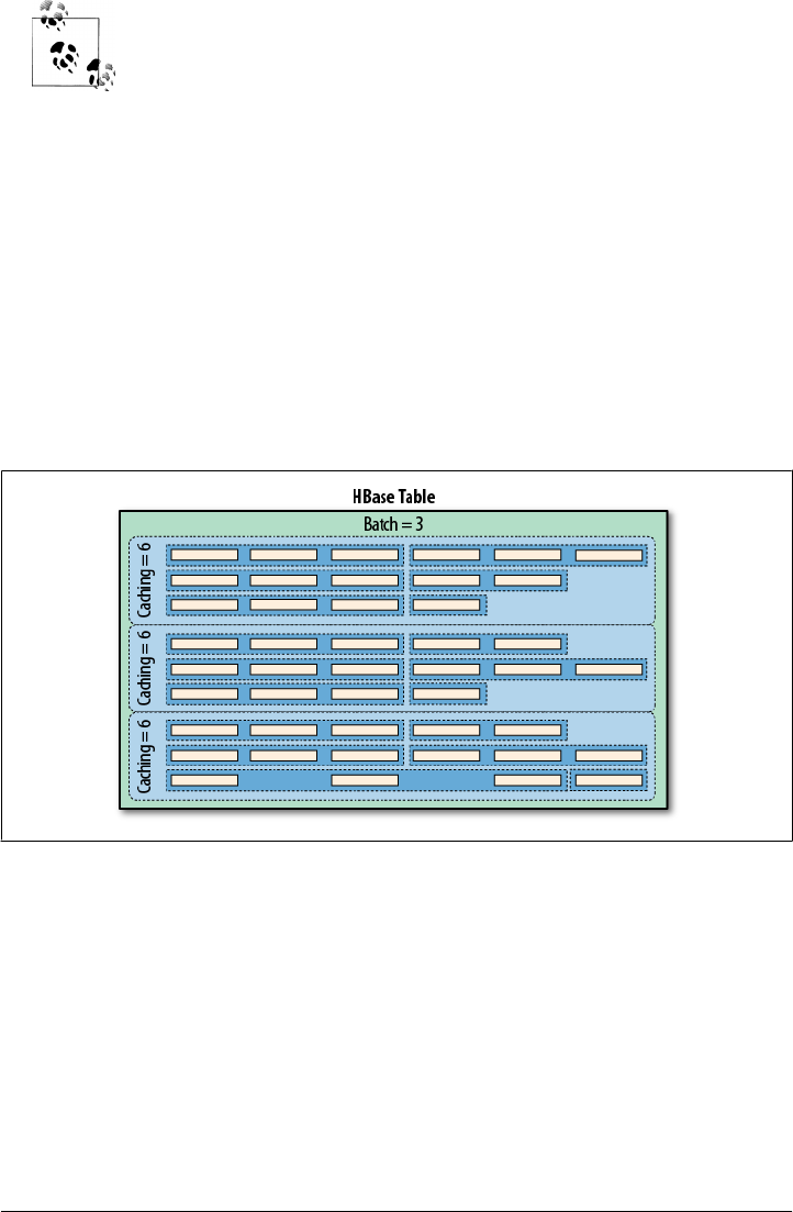
To compute the number of RPCs required for a scan, you need to first
multiply the number of rows with the number of columns per row (at
least some approximation). Then you divide that number by the smaller
value of either the batch size or the columns per row. Finally, divide that
number by the scanner caching value. In mathematical terms this could
be expressed like so:
RPCs = (Rows * Cols per Row) / Min(Cols per Row, Batch Size) /
Scanner Caching
In addition, RPCs are also required to open and close the scanner. You
would need to add these two calls to get the overall total of remote calls
when dealing with scanners.
Figure 3-2 shows how the caching and batching works in tandem. It has a table with
nine rows, each containing a number of columns. Using a scanner caching of six, and
a batch set to three, you can see that three RPCs are necessary to ship the data across
the network (the dashed, rounded-corner boxes).
Figure 3-2. The scanner caching and batching controlling the number of RPCs
The small batch value causes the servers to group three columns into one Result, while
the scanner caching of six causes one RPC to transfer six rows—or, more precisely,
results—sent in the batch. When the batch size is not specified but scanner caching is
specified, the result of the call will contain complete rows, because each row will be
contained in one Result instance. Only when you start to use the batch mode are you
getting access to the intra-row scanning functionality.
You may not have to worry about the consequences of using scanner caching and batch
mode initially, but once you try to squeeze the optimal performance out of your setup,
you should keep all of this in mind and find the sweet spot for both values.
132 | Chapter 3: Client API: The Basics

Miscellaneous Features
Before looking into more involved features that clients can use, let us first wrap up a
handful of miscellaneous features and functionality provided by HBase and its client
API.
The HTable Utility Methods
The client API is represented by an instance of the HTable class and gives you access to
an existing HBase table. Apart from the major features we already discussed, there are
a few more notable methods of this class that you should be aware of:
void close()
This method was mentioned before, but for the sake of completeness, and its im-
portance, it warrants repeating. Call close() once you have completed your work
with a table. It will flush any buffered write operations: the close() call implicitly
invokes the flushCache() method.
byte[] getTableName()
This is a convenience method to retrieve the table name.
Configuration getConfiguration()
This allows you to access the configuration in use by the HTable instance. Since this
is handed out by reference, you can make changes that are effective immediately.
HTableDescriptor getTableDescriptor()
As explained in “Tables” on page 207, each table is defined using an instance of
the HTableDescriptor class. You gain access to the underlying definition using
getTableDescriptor().
static boolean isTableEnabled(table)
There are four variants of this static helper method. They all need either an explicit
configuration—if one is not provided, it will create one implicitly using the default
values, and the configuration found on your application’s classpath—and a table
name. It checks if the table in question is marked as enabled in ZooKeeper.
byte[][] getStartKeys()
byte[][] getEndKeys()
Pair<byte[][],byte[][]> getStartEndKeys()
These calls give you access to the current physical layout of the table—this is likely
to change when you are adding more data to it. The calls give you the start and/or
end keys of all the regions of the table. They are returned as arrays of byte arrays.
You can use Bytes.toStringBinary(), for example, to print out the keys.
Miscellaneous Features | 133

void clearRegionCache()
HRegionLocation getRegionLocation(row)
Map<HRegionInfo, HServerAddress> getRegionsInfo()
This set of methods lets you retrieve more details regarding where a row lives, that
is, in what region, and the entire map of the region information. You can also clear
out the cache if you wish to do so. These calls are only for advanced users that wish
to make use of this information to, for example, route traffic or perform work close
to where the data resides.
void prewarmRegionCache(Map<HRegionInfo, HServerAddress> regionMap)
static void setRegionCachePrefetch(table, enable)
static boolean getRegionCachePrefetch(table)
Again, this is a group of methods for advanced usage. In “Implementa-
tion” on page 23 it was mentioned that it would make sense to prefetch region
information on the client to avoid more costly lookups for every row—until the
local cache is stable. Using these calls, you can either warm up the region cache
while providing a list of regions—you could, for example, use getRegionsInfo() to
gain access to the list, and then process it—or switch on region prefetching for the
entire table.
The Bytes Class
You saw how this class was used to convert native Java types, such as String, or long,
into the raw, byte array format HBase supports natively. There are a few more notes
that are worth mentioning about the class and its functionality.
Most methods come in three variations, for example:
static long toLong(byte[] bytes)
static long toLong(byte[] bytes, int offset)
static long toLong(byte[] bytes, int offset, int length)
You hand in just a byte array, or an array and an offset, or an array, an offset, and a
length value. The usage depends on the originating byte array you have. If it was created
by toBytes() beforehand, you can safely use the first variant, and simply hand in the
array and nothing else. All the array contains is the converted value.
The API, and HBase internally, store data in larger arrays, though, using, for example,
the following call:
static int putLong(byte[] bytes, int offset, long val)
This call allows you to write the long value into a given byte array, at a specific offset.
If you want to access the data in that larger byte array you can make use of the latter
two toLong() calls instead.
The Bytes class has support to convert from and to the following native Java types:
String, boolean, short, int, long, double, and float. Apart from that, there are some
noteworthy methods, which are listed in Table 3-10.
134 | Chapter 3: Client API: The Basics

Table 3-10. Overview of additional methods provided by the Bytes class
Method Description
toStringBinary() While working very similar to toString(), this variant has an extra safeguard to convert
nonprintable data into their human-readable hexadecimal numbers. Whenever you are not
sure what a byte array contains you should use this method to print its content, for example, to
the console, or into a logfile.
compareTo()/equals() These methods allow you to compare two byte[], that is, byte arrays. The former gives you a
comparison result and the latter a boolean value, indicating whether the given arrays are equal
to each other.
add()/head()/tail() You can use these to add two byte arrays to each other, resulting in a new, concatenated array,
or to get the first, or last, few bytes of the given byte array.
binarySearch() This performs a binary search in the given array of values. It operates on byte arrays for the values
and the key you are searching for.
incrementBytes() This increments a long value in its byte array representation, as if you had used
toBytes(long) to create it. You can decrement using a negative amount parameter.
There is some overlap of the Bytes class to the Java-provided ByteBuffer. The difference
is that the former does all operations without creating new class instances. In a way it
is an optimization, because the provided methods are called many times within HBase,
while avoiding possibly costly garbage collection issues.
For the full documentation, please consult the JavaDoc-based API documentation.‡
‡ See the Bytes documentation online.
Miscellaneous Features | 135

CHAPTER 4
Client API: Advanced Features
Now that you understand the basic client API, we will discuss the advanced features
that HBase offers to clients.
Filters
HBase filters are a powerful feature that can greatly enhance your effectiveness when
working with data stored in tables. You will find predefined filters, already provided
by HBase for your use, as well as a framework you can use to implement your own.
You will now be introduced to both.
Introduction to Filters
The two prominent read functions for HBase are get() and scan(), both supporting
either direct access to data or the use of a start and end key, respectively. You can limit
the data retrieved by progressively adding more limiting selectors to the query. These
include column families, column qualifiers, timestamps or ranges, as well as version
number.
While this gives you control over what is included, it is missing more fine-grained
features, such as selection of keys, or values, based on regular expressions. Both classes
support filters for exactly these reasons: what cannot be solved with the provided API
functionality to filter row or column keys, or values, can be achieved with filters. The
base interface is aptly named Filter, and there is a list of concrete classes supplied by
HBase that you can use without doing any programming.
You can, on the other hand, extend the Filter classes to implement your own require-
ments. All the filters are actually applied on the server side, also called predicate push-
down. This ensures the most efficient selection of the data that needs to be transported
back to the client. You could implement most of the filter functionality in your client
code as well, but you would have to transfer much more data—something you need to
avoid at scale.
137
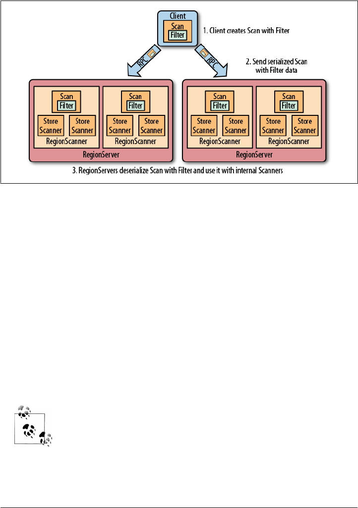
Figure 4-1 shows how the filters are configured on the client, then serialized over the
network, and then applied on the server.
Figure 4-1. The filters created on the client side, sent through the RPC, and executed on the server side
The filter hierarchy
The lowest level in the filter hierarchy is the Filter interface, and the abstract Filter
Base class that implements an empty shell, or skeleton, that is used by the actual filter
classes to avoid having the same boilerplate code in each of them.
Most concrete filter classes are direct descendants of FilterBase, but a few use another,
intermediate ancestor class. They all work the same way: you define a new instance of
the filter you want to apply and hand it to the Get or Scan instances, using:
setFilter(filter)
While you initialize the filter instance itself, you often have to supply parameters for
whatever the filter is designed for. There is a special subset of filters, based on
CompareFilter, that ask you for at least two specific parameters, since they are used by
the base class to perform its task. You will learn about the two parameter types next so
that you can use them in context.
Filters have access to the entire row they are applied to. This means that
they can decide the fate of a row based on any available information.
This includes the row key, column qualifiers, actual value of a column,
timestamps, and so on.
When referring to values, or comparisons, as we will discuss shortly, this
can be applied to any of these details. Specific filter implementations are
available that consider only one of those criteria each.
138 | Chapter 4: Client API: Advanced Features

Comparison operators
As CompareFilter-based filters add one more feature to the base FilterBase class,
namely the compare() operation, it has to have a user-supplied operator type that defines
how the result of the comparison is interpreted. The values are listed in Table 4-1.
Table 4-1. The possible comparison operators for CompareFilter-based filters
Operator Description
LESS Match values less than the provided one.
LESS_OR_EQUAL Match values less than or equal to the provided one.
EQUAL Do an exact match on the value and the provided one.
NOT_EQUAL Include everything that does not match the provided value.
GREATER_OR_EQUAL Match values that are equal to or greater than the provided one.
GREATER Only include values greater than the provided one.
NO_OP Exclude everything.
The comparison operators define what is included, or excluded, when the filter is ap-
plied. This allows you to select the data that you want as either a range, subset, or exact
and single match.
Comparators
The second type that you need to provide to CompareFilter-related classes is a compa-
rator, which is needed to compare various values and keys in different ways. They
are derived from WritableByteArrayComparable, which implements Writable, and
Comparable. You do not have to go into the details if you just want to use an imple-
mentation provided by HBase and listed in Table 4-2. The constructors usually take
the control value, that is, the one to compare each table value against.
Table 4-2. The HBase-supplied comparators, used with CompareFilter-based filters
Comparator Description
BinaryComparator Uses Bytes.compareTo() to compare the current with the provided value.
BinaryPrefixComparator Similar to the above, but does a lefthand, prefix-based match using
Bytes.compareTo().
NullComparator Does not compare against an actual value but whether a given one is null, or not null.
BitComparator Performs a bitwise comparison, providing a BitwiseOp class with AND, OR, and XOR
operators.
RegexStringComparator Given a regular expression at instantiation this comparator does a pattern match on the
table data.
SubstringComparator Treats the value and table data as String instances and performs a contains() check.
Filters | 139
The last three comparators listed in Table 4-2—the BitComparator,
RegexStringComparator, and SubstringComparator—only work with the
EQUAL and NOT_EQUAL operators, as the compareTo() of these comparators
returns 0 for a match or 1 when there is no match. Using them in a LESS or
GREATER comparison will yield erroneous results.
Each of the comparators usually has a constructor that takes the comparison value. In
other words, you need to define a value you compare each cell against. Some of these
constructors take a byte[], a byte array, to do the binary comparison, for example,
while others take a String parameter—since the data point compared against is
assumed to be some sort of readable text. Example 4-1 shows some of these in action.
The string-based comparators, RegexStringComparator and Substring
Comparator, are more expensive in comparison to the purely byte-based
version, as they need to convert a given value into a String first. The
subsequent string or regular expression operation also adds to the
overall cost.
Comparison Filters
The first type of supplied filter implementations are the comparison filters. They take
the comparison operator and comparator instance as described earlier. The constructor
of each of them has the same signature, inherited from CompareFilter:
CompareFilter(CompareOp valueCompareOp,
WritableByteArrayComparable valueComparator)
You need to supply this comparison operator and comparison class for the filters to do
their work. Next you will see the actual filters implementing a specific comparison.
Please keep in mind that the general contract of the HBase filter API
means you are filtering out information—filtered data is omitted from
the results returned to the client. The filter is not specifying what you
want to have, but rather what you do not want to have returned when
reading data.
In contrast, all filters based on CompareFilter are doing the opposite, in
that they include the matching values. In other words, be careful when
choosing the comparison operator, as it makes the difference in regard
to what the server returns. For example, instead of using LESS to skip
some information, you may need to use GREATER_OR_EQUAL to include the
desired data points.
140 | Chapter 4: Client API: Advanced Features
RowFilter
This filter gives you the ability to filter data based on row keys.
Example 4-1 shows how the filter can use different comparator instances to get the
desired results. It also uses various operators to include the row keys, while omitting
others. Feel free to modify the code, changing the operators to see the possible results.
Example 4-1. Using a filter to select specific rows
Scan scan = new Scan();
scan.addColumn(Bytes.toBytes("colfam1"), Bytes.toBytes("col-0"));
Filter filter1 = new RowFilter(CompareFilter.CompareOp.LESS_OR_EQUAL,
new BinaryComparator(Bytes.toBytes("row-22")));
scan.setFilter(filter1);
ResultScanner scanner1 = table.getScanner(scan);
for (Result res : scanner1) {
System.out.println(res);
}
scanner1.close();
Filter filter2 = new RowFilter(CompareFilter.CompareOp.EQUAL,
new RegexStringComparator(".*-.5"));
scan.setFilter(filter2);
ResultScanner scanner2 = table.getScanner(scan);
for (Result res : scanner2) {
System.out.println(res);
}
scanner2.close();
Filter filter3 = new RowFilter(CompareFilter.CompareOp.EQUAL,
new SubstringComparator("-5"));
scan.setFilter(filter3);
ResultScanner scanner3 = table.getScanner(scan);
for (Result res : scanner3) {
System.out.println(res);
}
scanner3.close();
Create a filter, while specifying the comparison operator and comparator. Here an
exact match is needed.
Another filter is created, this time using a regular expression to match the row keys.
The third filter uses a substring match approach.
Here is the full printout of the example on the console:
Adding rows to table...
Scanning table #1...
keyvalues={row-1/colfam1:col-0/1301043190260/Put/vlen=7}
keyvalues={row-10/colfam1:col-0/1301043190908/Put/vlen=8}
keyvalues={row-100/colfam1:col-0/1301043195275/Put/vlen=9}
keyvalues={row-11/colfam1:col-0/1301043190982/Put/vlen=8}
keyvalues={row-12/colfam1:col-0/1301043191040/Put/vlen=8}
Filters | 141

keyvalues={row-13/colfam1:col-0/1301043191172/Put/vlen=8}
keyvalues={row-14/colfam1:col-0/1301043191318/Put/vlen=8}
keyvalues={row-15/colfam1:col-0/1301043191429/Put/vlen=8}
keyvalues={row-16/colfam1:col-0/1301043191509/Put/vlen=8}
keyvalues={row-17/colfam1:col-0/1301043191593/Put/vlen=8}
keyvalues={row-18/colfam1:col-0/1301043191673/Put/vlen=8}
keyvalues={row-19/colfam1:col-0/1301043191771/Put/vlen=8}
keyvalues={row-2/colfam1:col-0/1301043190346/Put/vlen=7}
keyvalues={row-20/colfam1:col-0/1301043191841/Put/vlen=8}
keyvalues={row-21/colfam1:col-0/1301043191933/Put/vlen=8}
keyvalues={row-22/colfam1:col-0/1301043191998/Put/vlen=8}
Scanning table #2...
keyvalues={row-15/colfam1:col-0/1301043191429/Put/vlen=8}
keyvalues={row-25/colfam1:col-0/1301043192140/Put/vlen=8}
keyvalues={row-35/colfam1:col-0/1301043192665/Put/vlen=8}
keyvalues={row-45/colfam1:col-0/1301043193138/Put/vlen=8}
keyvalues={row-55/colfam1:col-0/1301043193729/Put/vlen=8}
keyvalues={row-65/colfam1:col-0/1301043194092/Put/vlen=8}
keyvalues={row-75/colfam1:col-0/1301043194457/Put/vlen=8}
keyvalues={row-85/colfam1:col-0/1301043194806/Put/vlen=8}
keyvalues={row-95/colfam1:col-0/1301043195121/Put/vlen=8}
Scanning table #3...
keyvalues={row-5/colfam1:col-0/1301043190562/Put/vlen=7}
keyvalues={row-50/colfam1:col-0/1301043193332/Put/vlen=8}
keyvalues={row-51/colfam1:col-0/1301043193514/Put/vlen=8}
keyvalues={row-52/colfam1:col-0/1301043193603/Put/vlen=8}
keyvalues={row-53/colfam1:col-0/1301043193654/Put/vlen=8}
keyvalues={row-54/colfam1:col-0/1301043193696/Put/vlen=8}
keyvalues={row-55/colfam1:col-0/1301043193729/Put/vlen=8}
keyvalues={row-56/colfam1:col-0/1301043193766/Put/vlen=8}
keyvalues={row-57/colfam1:col-0/1301043193802/Put/vlen=8}
keyvalues={row-58/colfam1:col-0/1301043193842/Put/vlen=8}
keyvalues={row-59/colfam1:col-0/1301043193889/Put/vlen=8}
You can see how the first filter did an exact match on the row key, including all of those
rows that have a key, equal to or less than the given one. Note once again the lexico-
graphical sorting and comparison, and how it filters the row keys.
The second filter does a regular expression match, while the third uses a substring
match approach. The results show that the filters work as advertised.
FamilyFilter
This filter works very similar to the RowFilter, but applies the comparison to the column
families available in a row—as opposed to the row key. Using the available combina-
tions of operators and comparators you can filter what is included in the retrieved data
on a column family level. Example 4-2 shows how to use this.
Example 4-2. Using a filter to include only specific column families
Filter filter1 = new FamilyFilter(CompareFilter.CompareOp.LESS,
new BinaryComparator(Bytes.toBytes("colfam3")));
Scan scan = new Scan();
142 | Chapter 4: Client API: Advanced Features
scan.setFilter(filter1);
ResultScanner scanner = table.getScanner(scan);
for (Result result : scanner) {
System.out.println(result);
}
scanner.close();
Get get1 = new Get(Bytes.toBytes("row-5"));
get1.setFilter(filter1);
Result result1 = table.get(get1);
System.out.println("Result of get(): " + result1);
Filter filter2 = new FamilyFilter(CompareFilter.CompareOp.EQUAL,
new BinaryComparator(Bytes.toBytes("colfam3")));
Get get2 = new Get(Bytes.toBytes("row-5"));
get2.addFamily(Bytes.toBytes("colfam1"));
get2.setFilter(filter2);
Result result2 = table.get(get2);
System.out.println("Result of get(): " + result2);
Create a filter, while specifying the comparison operator and comparator.
Scan over the table while applying the filter.
Get a row while applying the same filter.
Create a filter on one column family while trying to retrieve another.
Get the same row while applying the new filter; this will return “NONE”.
The output—reformatted and abbreviated for the sake of readability—shows the filter
in action. The input data has four column families, with two columns each, and 10
rows in total.
Adding rows to table...
Scanning table...
keyvalues={row-1/colfam1:col-0/1303721790522/Put/vlen=7,
row-1/colfam1:col-1/1303721790574/Put/vlen=7,
row-1/colfam2:col-0/1303721790522/Put/vlen=7,
row-1/colfam2:col-1/1303721790574/Put/vlen=7}
keyvalues={row-10/colfam1:col-0/1303721790785/Put/vlen=8,
row-10/colfam1:col-1/1303721790792/Put/vlen=8,
row-10/colfam2:col-0/1303721790785/Put/vlen=8,
row-10/colfam2:col-1/1303721790792/Put/vlen=8}
...
keyvalues={row-9/colfam1:col-0/1303721790778/Put/vlen=7,
row-9/colfam1:col-1/1303721790781/Put/vlen=7,
row-9/colfam2:col-0/1303721790778/Put/vlen=7,
row-9/colfam2:col-1/1303721790781/Put/vlen=7}
Result of get(): keyvalues={row-5/colfam1:col-0/1303721790652/Put/vlen=7,
row-5/colfam1:col-1/1303721790664/Put/vlen=7,
row-5/colfam2:col-0/1303721790652/Put/vlen=7,
row-5/colfam2:col-1/1303721790664/Put/vlen=7}
Result of get(): keyvalues=NONE
Filters | 143
The last get() shows that you can (inadvertently) create an empty set by applying a
filter for exactly one column family, while specifying a different column family selector
using addFamily().
QualifierFilter
Example 4-3 shows how the same logic is applied on the column qualifier level. This
allows you to filter specific columns from the table.
Example 4-3. Using a filter to include only specific column qualifiers
Filter filter = new QualifierFilter(CompareFilter.CompareOp.LESS_OR_EQUAL,
new BinaryComparator(Bytes.toBytes("col-2")));
Scan scan = new Scan();
scan.setFilter(filter);
ResultScanner scanner = table.getScanner(scan);
for (Result result : scanner) {
System.out.println(result);
}
scanner.close();
Get get = new Get(Bytes.toBytes("row-5"));
get.setFilter(filter);
Result result = table.get(get);
System.out.println("Result of get(): " + result);
ValueFilter
This filter makes it possible to include only columns that have a specific value. Com-
bined with the RegexStringComparator, for example, this can filter using powerful ex-
pression syntax. Example 4-4 showcases this feature. Note, though, that with certain
comparators—as explained earlier—you can only employ a subset of the operators.
Here a substring match is performed and this must be combined with an EQUAL, or
NOT_EQUAL, operator.
Example 4-4. Using the value-based filter
Filter filter = new ValueFilter(CompareFilter.CompareOp.EQUAL,
new SubstringComparator(".4"));
Scan scan = new Scan();
scan.setFilter(filter);
ResultScanner scanner = table.getScanner(scan);
for (Result result : scanner) {
for (KeyValue kv : result.raw()) {
System.out.println("KV: " + kv + ", Value: " +
Bytes.toString(kv.getValue()));
}
}
scanner.close();
Get get = new Get(Bytes.toBytes("row-5"));
144 | Chapter 4: Client API: Advanced Features

get.setFilter(filter);
Result result = table.get(get);
for (KeyValue kv : result.raw()) {
System.out.println("KV: " + kv + ", Value: " +
Bytes.toString(kv.getValue()));
}
Create a filter, while specifying the comparison operator and comparator.
Set the filter for the scan.
Print out the value to check that the filter works.
Assign the same filter to the Get instance.
DependentColumnFilter
Here you have a more complex filter that does not simply filter out data based on
directly available information. Rather, it lets you specify a dependent column—or
reference column—that controls how other columns are filtered. It uses the timestamp
of the reference column and includes all other columns that have the same timestamp.
Here are the constructors provided:
DependentColumnFilter(byte[] family, byte[] qualifier)
DependentColumnFilter(byte[] family, byte[] qualifier,
boolean dropDependentColumn)
DependentColumnFilter(byte[] family, byte[] qualifier,
boolean dropDependentColumn, CompareOp valueCompareOp,
WritableByteArrayComparable valueComparator)
Since it is based on CompareFilter, it also offers you to further select columns, but
for this filter it does so based on their values. Think of it as a combination of a
ValueFilter and a filter selecting on a reference timestamp. You can optionally hand
in your own operator and comparator pair to enable this feature. The class provides
constructors, though, that let you omit the operator and comparator and disable the
value filtering, including all columns by default, that is, performing the timestamp filter
based on the reference column only.
Example 4-5 shows the filter in use. You can see how the optional values can be handed
in as well. The dropDependentColumn parameter is giving you additional control over
how the reference column is handled: it is either included or dropped by the filter,
setting this parameter to false or true, respectively.
Example 4-5. Using a filter to include only specific column families
private static void filter(boolean drop,
CompareFilter.CompareOp operator,
WritableByteArrayComparable comparator)
throws IOException {
Filter filter;
if (comparator != null) {
filter = new DependentColumnFilter(Bytes.toBytes("colfam1"),
Bytes.toBytes("col-5"), drop, operator, comparator);
Filters | 145
} else {
filter = new DependentColumnFilter(Bytes.toBytes("colfam1"),
Bytes.toBytes("col-5"), drop);
}
Scan scan = new Scan();
scan.setFilter(filter);
ResultScanner scanner = table.getScanner(scan);
for (Result result : scanner) {
for (KeyValue kv : result.raw()) {
System.out.println("KV: " + kv + ", Value: " +
Bytes.toString(kv.getValue()));
}
}
scanner.close();
Get get = new Get(Bytes.toBytes("row-5"));
get.setFilter(filter);
Result result = table.get(get);
for (KeyValue kv : result.raw()) {
System.out.println("KV: " + kv + ", Value: " +
Bytes.toString(kv.getValue()));
}
}
public static void main(String[] args) throws IOException {
filter(true, CompareFilter.CompareOp.NO_OP, null);
filter(false, CompareFilter.CompareOp.NO_OP, null);
filter(true, CompareFilter.CompareOp.EQUAL,
new BinaryPrefixComparator(Bytes.toBytes("val-5")));
filter(false, CompareFilter.CompareOp.EQUAL,
new BinaryPrefixComparator(Bytes.toBytes("val-5")));
filter(true, CompareFilter.CompareOp.EQUAL,
new RegexStringComparator(".*\\.5"));
filter(false, CompareFilter.CompareOp.EQUAL,
new RegexStringComparator(".*\\.5"));
}
Create the filter with various options.
Call the filter method with various options.
This filter is not compatible with the batch feature of the scan opera-
tions, that is, setting Scan.setBatch() to a number larger than zero. The
filter needs to see the entire row to do its work, and using batching will
not carry the reference column timestamp over and would result in
erroneous results.
If you try to enable the batch mode nevertheless, you will get an error:
Exception org.apache.hadoop.hbase.filter.IncompatibleFilterException:
Cannot set batch on a scan using a filter that returns true for
filter.hasFilterRow
146 | Chapter 4: Client API: Advanced Features

The example also proceeds slightly differently compared to the earlier filters, as it sets
the version to the column number for a more reproducible result. The implicit time-
stamps that the servers use as the version could result in fluctuating results as you
cannot guarantee them using the exact time, down to the millisecond.
The filter() method used is called with different parameter combinations, showing
how using the built-in value filter and the drop flag is affecting the returned data set.
Dedicated Filters
The second type of supplied filters are based directly on FilterBase and implement
more specific use cases. Many of these filters are only really applicable when performing
scan operations, since they filter out entire rows. For get() calls, this is often too
restrictive and would result in a very harsh filter approach: include the whole row or
nothing at all.
SingleColumnValueFilter
You can use this filter when you have exactly one column that decides if an entire row
should be returned or not. You need to first specify the column you want to track, and
then some value to check against. The constructors offered are:
SingleColumnValueFilter(byte[] family, byte[] qualifier,
CompareOp compareOp, byte[] value)
SingleColumnValueFilter(byte[] family, byte[] qualifier,
CompareOp compareOp, WritableByteArrayComparable comparator)
The first one is a convenience function as it simply creates a BinaryComparator instance
internally on your behalf. The second takes the same parameters we used for the
CompareFilter-based classes. Although the SingleColumnValueFilter does not inherit
from the CompareFilter directly, it still uses the same parameter types.
The filter class also exposes a few auxiliary methods you can use to fine-tune its
behavior:
boolean getFilterIfMissing()
void setFilterIfMissing(boolean filterIfMissing)
boolean getLatestVersionOnly()
void setLatestVersionOnly(boolean latestVersionOnly)
The former controls what happens to rows that do not have the column at all. By
default, they are included in the result, but you can use setFilterIfMissing(true) to
reverse that behavior, that is, all rows that do not have the reference column are dropped
from the result.
Filters | 147

You must include the column you want to filter by, in other words, the
reference column, into the families you query for—using addColumn(),
for example. If you fail to do so, the column is considered missing and
the result is either empty, or contains all rows, based on the getFilter
IfMissing() result.
By using setLatestVersionOnly(false)—the default is true—you can change the de-
fault behavior of the filter, which is only to check the newest version of the reference
column, to instead include previous versions in the check as well. Example 4-6 com-
bines these features to select a specific set of rows only.
Example 4-6. Using a filter to return only rows with a given value in a given column
SingleColumnValueFilter filter = new SingleColumnValueFilter(
Bytes.toBytes("colfam1"),
Bytes.toBytes("col-5"),
CompareFilter.CompareOp.NOT_EQUAL,
new SubstringComparator("val-5"));
filter.setFilterIfMissing(true);
Scan scan = new Scan();
scan.setFilter(filter);
ResultScanner scanner = table.getScanner(scan);
for (Result result : scanner) {
for (KeyValue kv : result.raw()) {
System.out.println("KV: " + kv + ", Value: " +
Bytes.toString(kv.getValue()));
}
}
scanner.close();
Get get = new Get(Bytes.toBytes("row-6"));
get.setFilter(filter);
Result result = table.get(get);
System.out.println("Result of get: ");
for (KeyValue kv : result.raw()) {
System.out.println("KV: " + kv + ", Value: " +
Bytes.toString(kv.getValue()));
}
SingleColumnValueExcludeFilter
The SingleColumnValueFilter we just discussed is extended in this class to provide
slightly different semantics: the reference column, as handed into the constructor, is
omitted from the result. In other words, you have the same features, constructors, and
methods to control how this filter works. The only difference is that you will never get
the column you are checking against as part of the Result instance(s) on the client side.
148 | Chapter 4: Client API: Advanced Features

PrefixFilter
Given a prefix, specified when you instantiate the filter instance, all rows that match
this prefix are returned to the client. The constructor is:
public PrefixFilter(byte[] prefix)
Example 4-7 has this applied to the usual test data set.
Example 4-7. Using the prefix-based filter
Filter filter = new PrefixFilter(Bytes.toBytes("row-1"));
Scan scan = new Scan();
scan.setFilter(filter);
ResultScanner scanner = table.getScanner(scan);
for (Result result : scanner) {
for (KeyValue kv : result.raw()) {
System.out.println("KV: " + kv + ", Value: " +
Bytes.toString(kv.getValue()));
}
}
scanner.close();
Get get = new Get(Bytes.toBytes("row-5"));
get.setFilter(filter);
Result result = table.get(get);
for (KeyValue kv : result.raw()) {
System.out.println("KV: " + kv + ", Value: " +
Bytes.toString(kv.getValue()));
}
It is interesting to see how the get() call fails to return anything, because it is asking
for a row that does not match the filter prefix. This filter does not make much sense
when doing get() calls but is highly useful for scan operations.
The scan also is actively ended when the filter encounters a row key that is larger than
the prefix. In this way, and combining this with a start row, for example, the filter is
improving the overall performance of the scan as it has knowledge of when to skip the
rest of the rows altogether.
PageFilter
You paginate through rows by employing this filter. When you create the instance, you
specify a pageSize parameter, which controls how many rows per page should be
returned.
Filters | 149

There is a fundamental issue with filtering on physically separate serv-
ers. Filters run on different region servers in parallel and cannot retain
or communicate their current state across those boundaries. Thus, each
filter is required to scan at least up to pageCount rows before ending the
scan. This means a slight inefficiency is given for the PageFilter as more
rows are reported to the client than necessary. The final consolidation
on the client obviously has visibility into all results and can reduce what
is accessible through the API accordingly.
The client code would need to remember the last row that was returned, and then,
when another iteration is about to start, set the start row of the scan accordingly, while
retaining the same filter properties.
Because pagination is setting a strict limit on the number of rows to be returned, it is
possible for the filter to early out the entire scan, once the limit is reached or exceeded.
Filters have a facility to indicate that fact and the region servers make use of this hint
to stop any further processing.
Example 4-8 puts this together, showing how a client can reset the scan to a new start
row on the subsequent iterations.
Example 4-8. Using a filter to paginate through rows
Filter filter = new PageFilter(15);
int totalRows = 0;
byte[] lastRow = null;
while (true) {
Scan scan = new Scan();
scan.setFilter(filter);
if (lastRow != null) {
byte[] startRow = Bytes.add(lastRow, POSTFIX);
System.out.println("start row: " +
Bytes.toStringBinary(startRow));
scan.setStartRow(startRow);
}
ResultScanner scanner = table.getScanner(scan);
int localRows = 0;
Result result;
while ((result = scanner.next()) != null) {
System.out.println(localRows++ + ": " + result);
totalRows++;
lastRow = result.getRow();
}
scanner.close();
if (localRows == 0) break;
}
System.out.println("total rows: " + totalRows);
Because of the lexicographical sorting of the row keys by HBase and the comparison
taking care of finding the row keys in order, and the fact that the start key on a scan is
150 | Chapter 4: Client API: Advanced Features

always inclusive, you need to add an extra zero byte to the previous key. This will ensure
that the last seen row key is skipped and the next, in sorting order, is found. The zero
byte is the smallest increment, and therefore is safe to use when resetting the scan
boundaries. Even if there were a row that would match the previous plus the extra zero
byte, the scan would be correctly doing the next iteration—this is because the start
key is inclusive.
KeyOnlyFilter
Some applications need to access just the keys of each KeyValue, while omitting the
actual data. The KeyOnlyFilter provides this functionality by applying the filter’s ability
to modify the processed columns and cells, as they pass through. It does so by applying
the KeyValue.convertToKeyOnly(boolean) call that strips out the data part.
The constructor of this filter has a boolean parameter, named lenAsVal. It is handed to
the convertToKeyOnly() call as-is, controlling what happens to the value part of each
KeyValue instance processed. The default false simply sets the value to zero length,
while the opposite true sets the value to the number representing the length of the
original value.
The latter may be useful to your application when quickly iterating over columns, where
the keys already convey meaning and the length can be used to perform a secondary
sort, for example. “Client API: Best Practices” on page 434 has an example.
FirstKeyOnlyFilter
If you need to access the first column—as sorted implicitly by HBase—in each row,
this filter will provide this feature. Typically this is used by row counter type applications
that only need to check if a row exists. Recall that in column-oriented databases a row
really is composed of columns, and if there are none, the row ceases to exist.
Another possible use case is relying on the column sorting in lexicographical order, and
setting the column qualifier to an epoch value. This would sort the column with the
oldest timestamp name as the first to be retrieved. Combined with this filter, it is pos-
sible to retrieve the oldest column from every row using a single scan.
This class makes use of another optimization feature provided by the filter framework:
it indicates to the region server applying the filter that the current row is done and that
it should skip to the next one. This improves the overall performance of the scan,
compared to a full table scan.
InclusiveStopFilter
The row boundaries of a scan are inclusive for the start row, yet exclusive for the stop
row. You can overcome the stop row semantics using this filter, which includes the
specified stop row. Example 4-9 uses the filter to start at row-3, and stop at row-5
inclusively.
Filters | 151

Example 4-9. Using a filter to include a stop row
Filter filter = new InclusiveStopFilter(Bytes.toBytes("row-5"));
Scan scan = new Scan();
scan.setStartRow(Bytes.toBytes("row-3"));
scan.setFilter(filter);
ResultScanner scanner = table.getScanner(scan);
for (Result result : scanner) {
System.out.println(result);
}
scanner.close();
The output on the console, when running the example code, confirms that the filter
works as advertised:
Adding rows to table...
Results of scan:
keyvalues={row-3/colfam1:col-0/1301337961569/Put/vlen=7}
keyvalues={row-30/colfam1:col-0/1301337961610/Put/vlen=8}
keyvalues={row-31/colfam1:col-0/1301337961612/Put/vlen=8}
keyvalues={row-32/colfam1:col-0/1301337961613/Put/vlen=8}
keyvalues={row-33/colfam1:col-0/1301337961614/Put/vlen=8}
keyvalues={row-34/colfam1:col-0/1301337961615/Put/vlen=8}
keyvalues={row-35/colfam1:col-0/1301337961616/Put/vlen=8}
keyvalues={row-36/colfam1:col-0/1301337961617/Put/vlen=8}
keyvalues={row-37/colfam1:col-0/1301337961618/Put/vlen=8}
keyvalues={row-38/colfam1:col-0/1301337961619/Put/vlen=8}
keyvalues={row-39/colfam1:col-0/1301337961620/Put/vlen=8}
keyvalues={row-4/colfam1:col-0/1301337961571/Put/vlen=7}
keyvalues={row-40/colfam1:col-0/1301337961621/Put/vlen=8}
keyvalues={row-41/colfam1:col-0/1301337961622/Put/vlen=8}
keyvalues={row-42/colfam1:col-0/1301337961623/Put/vlen=8}
keyvalues={row-43/colfam1:col-0/1301337961624/Put/vlen=8}
keyvalues={row-44/colfam1:col-0/1301337961625/Put/vlen=8}
keyvalues={row-45/colfam1:col-0/1301337961626/Put/vlen=8}
keyvalues={row-46/colfam1:col-0/1301337961627/Put/vlen=8}
keyvalues={row-47/colfam1:col-0/1301337961628/Put/vlen=8}
keyvalues={row-48/colfam1:col-0/1301337961629/Put/vlen=8}
keyvalues={row-49/colfam1:col-0/1301337961630/Put/vlen=8}
keyvalues={row-5/colfam1:col-0/1301337961573/Put/vlen=7}
TimestampsFilter
When you need fine-grained control over what versions are included in the scan result,
this filter provides the means. You have to hand in a List of timestamps:
TimestampsFilter(List<Long> timestamps)
As you have seen throughout the book so far, a version is a specific value
of a column at a unique point in time, denoted with a timestamp. When
the filter is asking for a list of timestamps, it will attempt to retrieve the
column versions with the matching timestamps.
152 | Chapter 4: Client API: Advanced Features
Example 4-10 sets up a filter with three timestamps and adds a time range to the second
scan.
Example 4-10. Filtering data by timestamps
List<Long> ts = new ArrayList<Long>();
ts.add(new Long(5));
ts.add(new Long(10));
ts.add(new Long(15));
Filter filter = new TimestampsFilter(ts);
Scan scan1 = new Scan();
scan1.setFilter(filter);
ResultScanner scanner1 = table.getScanner(scan1);
for (Result result : scanner1) {
System.out.println(result);
}
scanner1.close();
Scan scan2 = new Scan();
scan2.setFilter(filter);
scan2.setTimeRange(8, 12);
ResultScanner scanner2 = table.getScanner(scan2);
for (Result result : scanner2) {
System.out.println(result);
}
scanner2.close();
Add timestamps to the list.
Add the filter to an otherwise default Scan instance.
Also add a time range to verify how it affects the filter.
Here is the output on the console in an abbreviated form:
Adding rows to table...
Results of scan #1:
keyvalues={row-1/colfam1:col-10/10/Put/vlen=8,
row-1/colfam1:col-15/15/Put/vlen=8,
row-1/colfam1:col-5/5/Put/vlen=7}
keyvalues={row-10/colfam1:col-10/10/Put/vlen=9,
row-10/colfam1:col-15/15/Put/vlen=9,
row-10/colfam1:col-5/5/Put/vlen=8}
keyvalues={row-100/colfam1:col-10/10/Put/vlen=10,
row-100/colfam1:col-15/15/Put/vlen=10,
row-100/colfam1:col-5/5/Put/vlen=9}
...
Results of scan #2:
keyvalues={row-1/colfam1:col-10/10/Put/vlen=8}
keyvalues={row-10/colfam1:col-10/10/Put/vlen=9}
keyvalues={row-100/colfam1:col-10/10/Put/vlen=10}
keyvalues={row-11/colfam1:col-10/10/Put/vlen=9}
...
Filters | 153

The first scan, only using the filter, is outputting the column values for all three specified
timestamps as expected. The second scan only returns the timestamp that fell into the
time range specified when the scan was set up. Both time-based restrictions, the filter
and the scanner time range, are doing their job and the result is a combination of both.
ColumnCountGetFilter
You can use this filter to only retrieve a specific maximum number of columns per row.
You can set the number using the constructor of the filter:
ColumnCountGetFilter(int n)
Since this filter stops the entire scan once a row has been found that matches the max-
imum number of columns configured, it is not useful for scan operations, and in fact,
it was written to test filters in get() calls.
ColumnPaginationFilter
Similar to the PageFilter, this one can be used to page through columns in a row. Its
constructor has two parameters:
ColumnPaginationFilter(int limit, int offset)
It skips all columns up to the number given as offset, and then includes limit columns
afterward. Example 4-11 has this applied to a normal scan.
Example 4-11. Paginating through columns in a row
Filter filter = new ColumnPaginationFilter(5, 15);
Scan scan = new Scan();
scan.setFilter(filter);
ResultScanner scanner = table.getScanner(scan);
for (Result result : scanner) {
System.out.println(result);
}
scanner.close();
Running this example should render the following output:
Adding rows to table...
Results of scan:
keyvalues={row-01/colfam1:col-15/15/Put/vlen=9,
row-01/colfam1:col-16/16/Put/vlen=9,
row-01/colfam1:col-17/17/Put/vlen=9,
row-01/colfam1:col-18/18/Put/vlen=9,
row-01/colfam1:col-19/19/Put/vlen=9}
keyvalues={row-02/colfam1:col-15/15/Put/vlen=9,
row-02/colfam1:col-16/16/Put/vlen=9,
row-02/colfam1:col-17/17/Put/vlen=9,
row-02/colfam1:col-18/18/Put/vlen=9,
row-02/colfam1:col-19/19/Put/vlen=9}
...
154 | Chapter 4: Client API: Advanced Features

This example slightly changes the way the rows and columns are num-
bered by adding a padding to the numeric counters. For example, the
first row is padded to be row-01. This also shows how padding can be
used to get a more human-readable style of sorting, for example—as
known from a dictionary or telephone book.
The result includes all 10 rows, starting each row at column (offset = 15) and printing
five columns (limit = 5).
ColumnPrefixFilter
Analog to the PrefixFilter, which worked by filtering on row key prefixes, this filter
does the same for columns. You specify a prefix when creating the filter:
ColumnPrefixFilter(byte[] prefix)
All columns that have the given prefix are then included in the result.
RandomRowFilter
Finally, there is a filter that shows what is also possible using the API: including random
rows into the result. The constructor is given a parameter named chance, which repre-
sents a value between 0.0 and 1.0:
RandomRowFilter(float chance)
Internally, this class is using a Java Random.nextFloat() call to randomize the row in-
clusion, and then compares the value with the chance given. Giving it a negative chance
value will make the filter exclude all rows, while a value larger than 1.0 will make it
include all rows.
Decorating Filters
While the provided filters are already very powerful, sometimes it can be useful to
modify, or extend, the behavior of a filter to gain additional control over the returned
data. Some of this additional control is not dependent on the filter itself, but can be
applied to any of them. This is what the decorating filter group of classes is about.
SkipFilter
This filter wraps a given filter and extends it to exclude an entire row, when the wrapped
filter hints for a KeyValue to be skipped. In other words, as soon as a filter indicates that
a column in a row is omitted, the entire row is omitted.
Filters | 155
The wrapped filter must implement the filterKeyValue() method, or
the SkipFilter will not work as expected.* This is because the SkipFil
ter is only checking the results of that method to decide how to handle
the current row. See Table 4-5 on page 167 for an overview of compat-
ible filters.
Example 4-12 combines the SkipFilter with a ValueFilter to first select all columns
that have no zero-valued column, and subsequently drops all other partial rows that
do not have a matching value.
Example 4-12. Using a filter to skip entire rows based on another filter’s results
Filter filter1 = new ValueFilter(CompareFilter.CompareOp.NOT_EQUAL,
new BinaryComparator(Bytes.toBytes("val-0")));
Scan scan = new Scan();
scan.setFilter(filter1);
ResultScanner scanner1 = table.getScanner(scan);
for (Result result : scanner1) {
for (KeyValue kv : result.raw()) {
System.out.println("KV: " + kv + ", Value: " +
Bytes.toString(kv.getValue()));
}
}
scanner1.close();
Filter filter2 = new SkipFilter(filter1);
scan.setFilter(filter2);
ResultScanner scanner2 = table.getScanner(scan);
for (Result result : scanner2) {
for (KeyValue kv : result.raw()) {
System.out.println("KV: " + kv + ", Value: " +
Bytes.toString(kv.getValue()));
}
}
scanner2.close();
Only add the ValueFilter to the first scan.
Add the decorating skip filter for the second scan.
The example code should print roughly the following results when you execute it—
note, though, that the values are randomized, so you should get a slightly different
result for every invocation:
Adding rows to table...
Results of scan #1:
KV: row-01/colfam1:col-00/0/Put/vlen=5, Value: val-4
KV: row-01/colfam1:col-01/1/Put/vlen=5, Value: val-2
* The various filter methods are discussed in “Custom Filters” on page 160.
156 | Chapter 4: Client API: Advanced Features

KV: row-01/colfam1:col-02/2/Put/vlen=5, Value: val-4
KV: row-01/colfam1:col-03/3/Put/vlen=5, Value: val-3
KV: row-01/colfam1:col-04/4/Put/vlen=5, Value: val-1
KV: row-02/colfam1:col-00/0/Put/vlen=5, Value: val-3
KV: row-02/colfam1:col-01/1/Put/vlen=5, Value: val-1
KV: row-02/colfam1:col-03/3/Put/vlen=5, Value: val-4
KV: row-02/colfam1:col-04/4/Put/vlen=5, Value: val-1
...
Total KeyValue count for scan #1: 122
Results of scan #2:
KV: row-01/colfam1:col-00/0/Put/vlen=5, Value: val-4
KV: row-01/colfam1:col-01/1/Put/vlen=5, Value: val-2
KV: row-01/colfam1:col-02/2/Put/vlen=5, Value: val-4
KV: row-01/colfam1:col-03/3/Put/vlen=5, Value: val-3
KV: row-01/colfam1:col-04/4/Put/vlen=5, Value: val-1
KV: row-07/colfam1:col-00/0/Put/vlen=5, Value: val-4
KV: row-07/colfam1:col-01/1/Put/vlen=5, Value: val-1
KV: row-07/colfam1:col-02/2/Put/vlen=5, Value: val-1
KV: row-07/colfam1:col-03/3/Put/vlen=5, Value: val-2
KV: row-07/colfam1:col-04/4/Put/vlen=5, Value: val-4
...
Total KeyValue count for scan #2: 50
The first scan returns all columns that are not zero valued. Since the value is assigned
at random, there is a high probability that you will get at least one or more columns of
each possible row. Some rows will miss a column—these are the omitted zero-valued
ones.
The second scan, on the other hand, wraps the first filter and forces all partial rows to
be dropped. You can see from the console output how only complete rows are emitted,
that is, those with all five columns the example code creates initially. The total Key
Value count for each scan confirms the more restrictive behavior of the SkipFilter
variant.
WhileMatchFilter
This second decorating filter type works somewhat similarly to the previous one, but
aborts the entire scan once a piece of information is filtered. This works by checking
the wrapped filter and seeing if it skips a row by its key, or a column of a row because
of a KeyValue check.†
Example 4-13 is a slight variation of the previous example, using different filters to
show how the decorating class works.
Example 4-13. Using a filter to skip entire rows based on another filter’s results
Filter filter1 = new RowFilter(CompareFilter.CompareOp.NOT_EQUAL,
new BinaryComparator(Bytes.toBytes("row-05")));
† See Table 4-5 for an overview of compatible filters.
Filters | 157

Scan scan = new Scan();
scan.setFilter(filter1);
ResultScanner scanner1 = table.getScanner(scan);
for (Result result : scanner1) {
for (KeyValue kv : result.raw()) {
System.out.println("KV: " + kv + ", Value: " +
Bytes.toString(kv.getValue()));
}
}
scanner1.close();
Filter filter2 = new WhileMatchFilter(filter1);
scan.setFilter(filter2);
ResultScanner scanner2 = table.getScanner(scan);
for (Result result : scanner2) {
for (KeyValue kv : result.raw()) {
System.out.println("KV: " + kv + ", Value: " +
Bytes.toString(kv.getValue()));
}
}
scanner2.close();
Once you run the example code, you should get this output on the console:
Adding rows to table...
Results of scan #1:
KV: row-01/colfam1:col-00/0/Put/vlen=9, Value: val-01.00
KV: row-02/colfam1:col-00/0/Put/vlen=9, Value: val-02.00
KV: row-03/colfam1:col-00/0/Put/vlen=9, Value: val-03.00
KV: row-04/colfam1:col-00/0/Put/vlen=9, Value: val-04.00
KV: row-06/colfam1:col-00/0/Put/vlen=9, Value: val-06.00
KV: row-07/colfam1:col-00/0/Put/vlen=9, Value: val-07.00
KV: row-08/colfam1:col-00/0/Put/vlen=9, Value: val-08.00
KV: row-09/colfam1:col-00/0/Put/vlen=9, Value: val-09.00
KV: row-10/colfam1:col-00/0/Put/vlen=9, Value: val-10.00
Total KeyValue count for scan #1: 9
Results of scan #2:
KV: row-01/colfam1:col-00/0/Put/vlen=9, Value: val-01.00
KV: row-02/colfam1:col-00/0/Put/vlen=9, Value: val-02.00
KV: row-03/colfam1:col-00/0/Put/vlen=9, Value: val-03.00
KV: row-04/colfam1:col-00/0/Put/vlen=9, Value: val-04.00
Total KeyValue count for scan #2: 4
The first scan used just the RowFilter to skip one out of 10 rows; the rest is returned to
the client. Adding the WhileMatchFilter for the second scan shows its behavior to stop
the entire scan operation, once the wrapped filter omits a row or column. In the example
this is row-05, triggering the end of the scan.
Decorating filters implement the same Filter interface, just like any
other single-purpose filter. In doing so, they can be used as a drop-in
replacement for those filters, while combining their behavior with the
wrapped filter instance.
158 | Chapter 4: Client API: Advanced Features

FilterList
So far you have seen how filters—on their own, or decorated—are doing the work of
filtering out various dimensions of a table, ranging from rows, to columns, and all the
way to versions of values within a column. In practice, though, you may want to have
more than one filter being applied to reduce the data returned to your client application.
This is what the FilterList is for.
The FilterList class implements the same Filter interface, just like any
other single-purpose filter. In doing so, it can be used as a drop-in re-
placement for those filters, while combining the effects of each included
instance.
You can create an instance of FilterList while providing various parameters at
instantiation time, using one of these constructors:
FilterList(List<Filter> rowFilters)
FilterList(Operator operator)
FilterList(Operator operator, List<Filter> rowFilters
The rowFilters parameter specifies the list of filters that are assessed together, using
an operator to combine their results. Table 4-3 lists the possible choices of operators.
The default is MUST_PASS_ALL, and can therefore be omitted from the constructor when
you do not need a different one.
Table 4-3. Possible values for the FilterList.Operator enumeration
Operator Description
MUST_PASS_ALL A value is only included in the result when all filters agree to do so, i.e., no filter is omitting the value.
MUST_PASS_ONE As soon as a value was allowed to pass one of the filters, it is included in the overall result.
Adding filters, after the FilterList instance has been created, can be done with:
void addFilter(Filter filter)
You can only specify one operator per FilterList, but you are free to add other Filter
List instances to an existing FilterList, thus creating a hierarchy of filters, combined
with the operators you need.
You can further control the execution order of the included filters by carefully choosing
the List implementation you require. For example, using ArrayList would guarantee
that the filters are applied in the order they were added to the list. This is shown in
Example 4-14.
Example 4-14. Using a filter list to combine single-purpose filters
List<Filter> filters = new ArrayList<Filter>();
Filter filter1 = new RowFilter(CompareFilter.CompareOp.GREATER_OR_EQUAL,
Filters | 159

new BinaryComparator(Bytes.toBytes("row-03")));
filters.add(filter1);
Filter filter2 = new RowFilter(CompareFilter.CompareOp.LESS_OR_EQUAL,
new BinaryComparator(Bytes.toBytes("row-06")));
filters.add(filter2);
Filter filter3 = new QualifierFilter(CompareFilter.CompareOp.EQUAL,
new RegexStringComparator("col-0[03]"));
filters.add(filter3);
FilterList filterList1 = new FilterList(filters);
Scan scan = new Scan();
scan.setFilter(filterList1);
ResultScanner scanner1 = table.getScanner(scan);
for (Result result : scanner1) {
for (KeyValue kv : result.raw()) {
System.out.println("KV: " + kv + ", Value: " +
Bytes.toString(kv.getValue()));
}
}
scanner1.close();
FilterList filterList2 = new FilterList(
FilterList.Operator.MUST_PASS_ONE, filters);
scan.setFilter(filterList2);
ResultScanner scanner2 = table.getScanner(scan);
for (Result result : scanner2) {
for (KeyValue kv : result.raw()) {
System.out.println("KV: " + kv + ", Value: " +
Bytes.toString(kv.getValue()));
}
}
scanner2.close();
The first scan filters out a lot of details, as at least one of the filters in the list excludes
some information. Only where they all let the information pass is it returned to the
client.
In contrast, the second scan includes all rows and columns in the result. This is caused
by setting the FilterList operator to MUST_PASS_ONE, which includes all the information
as soon as a single filter lets it pass. And in this scenario, all values are passed by at least
one of them, including everything.
Custom Filters
Eventually, you may exhaust the list of supplied filter types and need to implement
your own. This can be done by either implementing the Filter interface, or extending
the provided FilterBase class. The latter provides default implementations for all
methods that are members of the interface.
160 | Chapter 4: Client API: Advanced Features
The Filter interface has the following structure:
public interface Filter extends Writable {
public enum ReturnCode {
INCLUDE, SKIP, NEXT_COL, NEXT_ROW, SEEK_NEXT_USING_HINT
}
public void reset()
public boolean filterRowKey(byte[] buffer, int offset, int length)
public boolean filterAllRemaining()
public ReturnCode filterKeyValue(KeyValue v)
public void filterRow(List<KeyValue> kvs)
public boolean hasFilterRow()
public boolean filterRow()
public KeyValue getNextKeyHint(KeyValue currentKV)
The interface provides a public enumeration type, named ReturnCode, that is used by
the filterKeyValue() method to indicate what the execution framework should do
next. Instead of blindly iterating over all values, the filter has the ability to skip a value,
the remainder of a column, or the rest of the entire row. This helps tremendously in
terms of improving performance while retrieving data.
The servers may still need to scan the entire row to find matching data,
but the optimizations provided by the filterKeyValue() return code can
reduce the work required to do so.
Table 4-4 lists the possible values and their meaning.
Table 4-4. Possible values for the Filter.ReturnCode enumeration
Return code Description
INCLUDE Include the given KeyValue instance in the result.
SKIP Skip the current KeyValue and proceed to the next.
NEXT_COL Skip the remainder of the current column, proceeding to the next. This is used by the
TimestampsFilter, for example.
NEXT_ROW Similar to the previous, but skips the remainder of the current row, moving to the next. The
RowFilter makes use of this return code, for example.
SEEK_NEXT_USING_HINT Some filters want to skip a variable number of values and use this return code to indicate that
the framework should use the getNextKeyHint() method to determine where to skip to.
The ColumnPrefixFilter, for example, uses this feature.
Most of the provided methods are called at various stages in the process of retrieving
a row for a client—for example, during a scan operation. Putting them in call order,
you can expect them to be executed in the following sequence:
Filters | 161

filterRowKey(byte[] buffer, int offset, int length)
The next check is against the row key, using this method of the Filter implemen-
tation. You can use it to skip an entire row from being further processed. The
RowFilter uses it to suppress entire rows being returned to the client.
filterKeyValue(KeyValue v)
When a row is not filtered (yet), the framework proceeds to invoke this method
for every KeyValue that is part of the current row. The ReturnCode indicates what
should happen with the current value.
filterRow(List<KeyValue> kvs)
Once all row and value checks have been performed, this method of the filter is
called, giving you access to the list of KeyValue instances that have been included
by the previous filter methods. The DependentColumnFilter uses it to drop those
columns that do not match the reference column.
filterRow()
After everything else was checked and invoked, the final inspection is performed
using filterRow(). A filter that uses this functionality is the PageFilter, checking
if the number of rows to be returned for one iteration in the pagination process is
reached, returning true afterward. The default false would include the current
row in the result.
reset()
This resets the filter for every new row the scan is iterating over. It is called by the
server, after a row is read, implicitly. This applies to get and scan operations, al-
though obviously it has no effect for the former, as gets only read a single row.
filterAllRemaining()
This method can be used to stop the scan, by returning true. It is used by filters to
provide the early out optimizations mentioned earlier. If a filter returns false, the
scan is continued, and the aforementioned methods are called.
Obviously, this also implies that for get operations this call is not useful.
filterRow() and Batch Mode
A filter using filterRow() to filter out an entire row, or filterRow(List) to modify the
final list of included values, must also override the hasRowFilter() function to return
true.
The framework is using this flag to ensure that a given filter is compatible with the
selected scan parameters. In particular, these filter methods collide with the scanner’s
batch mode: when the scanner is using batches to ship partial rows to the client, the
previous methods are not called for every batch, but only at the actual end of the current
row.
162 | Chapter 4: Client API: Advanced Features

Example 4-15 implements a custom filter, using the methods provided by FilterBase,
overriding only those methods that need to be changed.
The filter first assumes all rows should be filtered, that is, removed from the result.
Only when there is a value in any column that matches the given reference does it
include the row, so that it is sent back to the client.
Example 4-15. Implementing a filter that lets certain rows pass
public class CustomFilter extends FilterBase{
private byte[] value = null;
private boolean filterRow = true;
public CustomFilter() {
super();
}
public CustomFilter(byte[] value) {
this.value = value;
}
@Override
public void reset() {
this.filterRow = true;
}
@Override
public ReturnCode filterKeyValue(KeyValue kv) {
if (Bytes.compareTo(value, kv.getValue()) == 0) {
filterRow = false;
}
return ReturnCode.INCLUDE;
}
@Override
public boolean filterRow() {
return filterRow;
}
@Override
public void write(DataOutput dataOutput) throws IOException {
Bytes.writeByteArray(dataOutput, this.value);
}
@Override
public void readFields(DataInput dataInput) throws IOException {
this.value = Bytes.readByteArray(dataInput);
}
}
Set the value to compare against.
Reset the filter flag for each new row being tested.
164 | Chapter 4: Client API: Advanced Features

When there is a matching value, let the row pass.
Always include this, since the final decision is made later.
Here the actual decision is taking place, based on the flag status.
Write the given value out so that it can be sent to the servers.
Used by the servers to establish the filter instance with the correct values.
Deployment of Custom Filters
Once you have written your filter, you need to deploy it to your HBase setup. You need
to compile the class, pack it into a Java Archive (JAR) file, and make it available to the
region servers.
You can use the build system of your choice to prepare the JAR file for deployment,
and a configuration management system to actually provision the file to all servers.
Once you have uploaded the JAR file, you need to add it to the hbase-env.sh configu-
ration file, for example:
# Extra Java CLASSPATH elements. Optional.
# export HBASE_CLASSPATH=
export HBASE_CLASSPATH="/hbase-book/ch04/target/hbase-book-ch04-1.0.jar"
This is using the JAR file created by the Maven build as supplied by the source code
repository accompanying this book. It uses an absolute, local path since testing is done
on a standalone setup, in other words, with the development environment and HBase
running on the same physical machine.
Note that you must restart the HBase daemons so that the changes in the configuration
file are taking effect. Once this is done you can proceed to test the new filter.
Example 4-16 uses the new custom filter to find rows with specific values in it, also
using a FilterList.
Example 4-16. Using a custom filter
List<Filter> filters = new ArrayList<Filter>();
Filter filter1 = new CustomFilter(Bytes.toBytes("val-05.05"));
filters.add(filter1);
Filter filter2 = new CustomFilter(Bytes.toBytes("val-02.07"));
filters.add(filter2);
Filter filter3 = new CustomFilter(Bytes.toBytes("val-09.00"));
filters.add(filter3);
FilterList filterList = new FilterList(
FilterList.Operator.MUST_PASS_ONE, filters);
Scan scan = new Scan();
scan.setFilter(filterList);
Filters | 165

ResultScanner scanner = table.getScanner(scan);
for (Result result : scanner) {
for (KeyValue kv : result.raw()) {
System.out.println("KV: " + kv + ", Value: " +
Bytes.toString(kv.getValue()));
}
}
scanner.close();
Just as with the earlier examples, here is what should appear as output on the console
when executing this example:
Adding rows to table...
Results of scan:
KV: row-02/colfam1:col-00/1301507323088/Put/vlen=9, Value: val-02.00
KV: row-02/colfam1:col-01/1301507323090/Put/vlen=9, Value: val-02.01
KV: row-02/colfam1:col-02/1301507323092/Put/vlen=9, Value: val-02.02
KV: row-02/colfam1:col-03/1301507323093/Put/vlen=9, Value: val-02.03
KV: row-02/colfam1:col-04/1301507323096/Put/vlen=9, Value: val-02.04
KV: row-02/colfam1:col-05/1301507323104/Put/vlen=9, Value: val-02.05
KV: row-02/colfam1:col-06/1301507323108/Put/vlen=9, Value: val-02.06
KV: row-02/colfam1:col-07/1301507323110/Put/vlen=9, Value: val-02.07
KV: row-02/colfam1:col-08/1301507323112/Put/vlen=9, Value: val-02.08
KV: row-02/colfam1:col-09/1301507323113/Put/vlen=9, Value: val-02.09
KV: row-05/colfam1:col-00/1301507323148/Put/vlen=9, Value: val-05.00
KV: row-05/colfam1:col-01/1301507323150/Put/vlen=9, Value: val-05.01
KV: row-05/colfam1:col-02/1301507323152/Put/vlen=9, Value: val-05.02
KV: row-05/colfam1:col-03/1301507323153/Put/vlen=9, Value: val-05.03
KV: row-05/colfam1:col-04/1301507323154/Put/vlen=9, Value: val-05.04
KV: row-05/colfam1:col-05/1301507323155/Put/vlen=9, Value: val-05.05
KV: row-05/colfam1:col-06/1301507323157/Put/vlen=9, Value: val-05.06
KV: row-05/colfam1:col-07/1301507323158/Put/vlen=9, Value: val-05.07
KV: row-05/colfam1:col-08/1301507323158/Put/vlen=9, Value: val-05.08
KV: row-05/colfam1:col-09/1301507323159/Put/vlen=9, Value: val-05.09
KV: row-09/colfam1:col-00/1301507323192/Put/vlen=9, Value: val-09.00
KV: row-09/colfam1:col-01/1301507323194/Put/vlen=9, Value: val-09.01
KV: row-09/colfam1:col-02/1301507323196/Put/vlen=9, Value: val-09.02
KV: row-09/colfam1:col-03/1301507323199/Put/vlen=9, Value: val-09.03
KV: row-09/colfam1:col-04/1301507323201/Put/vlen=9, Value: val-09.04
KV: row-09/colfam1:col-05/1301507323202/Put/vlen=9, Value: val-09.05
KV: row-09/colfam1:col-06/1301507323203/Put/vlen=9, Value: val-09.06
KV: row-09/colfam1:col-07/1301507323204/Put/vlen=9, Value: val-09.07
KV: row-09/colfam1:col-08/1301507323205/Put/vlen=9, Value: val-09.08
KV: row-09/colfam1:col-09/1301507323206/Put/vlen=9, Value: val-09.09
As expected, the entire row that has a column with the value matching one of the
references is included in the result.
166 | Chapter 4: Client API: Advanced Features

Filters Summary
Table 4-5 summarizes some of the features and compatibilities related to the provided
filter implementations. The ✓ symbol means the feature is available, while ✗ indi-
cates it is missing.
Table 4-5. Summary of filter features and compatibilities between them
Filter BatchaSkipbWhile-
MatchcListdEarly
OuteGetsfScansg
RowFilter ✓✓✓✓✓✗✓
FamilyFilter ✓✓✓✓✗✓ ✓
QualifierFilter ✓✓✓✓✗✓ ✓
ValueFilter ✓✓✓✓✗✓ ✓
DependentColumnFilter ✗✓✓✓✗✓ ✓
SingleColumnValueFilter ✓✓✓✓✗✗✓
SingleColumnValue
ExcludeFilter
✓✓✓✓✗✗✓
PrefixFilter ✓✗✓✓✓✗✓
PageFilter ✓✗✓✓✓✗✓
KeyOnlyFilter ✓✓✓✓✗✓ ✓
FirstKeyOnlyFilter ✓✓✓✓✗✓ ✓
InclusiveStopFilter ✓✗✓✓✓✗✓
TimestampsFilter ✓✓✓✓✗✓ ✓
ColumnCountGetFilter ✓✓✓✓✗✓✗
ColumnPaginationFilter ✓✓✓✓✗✓ ✓
ColumnPrefixFilter ✓✓✓✓✗✓ ✓
RandomRowFilter ✓✓✓✓✗✗✓
SkipFilter ✓ ✓/✗h✓/✗h✓✗✗✓
WhileMatchFilter ✓ ✓/✗h✓/✗h✓✓✗✓
FilterList ✓/✗h✓/✗h✓/✗h✓ ✓/✗h✓ ✓
aFilter supports Scan.setBatch(), i.e., the scanner batch mode.
bFilter can be used with the decorating SkipFilter class.
cFilter can be used with the decorating WhileMatchFilter class.
dFilter can be used with the combining FilterList class.
eFilter has optimizations to stop a scan early, once there are no more matching rows ahead.
fFilter can be usefully applied to Get instances.
gFilter can be usefully applied to Scan instances.
hDepends on the included filters.
Filters | 167

Counters
In addition to the functionality we already discussed, HBase offers another advanced
feature: counters. Many applications that collect statistics—such as clicks or views in
online advertising—were used to collect the data in logfiles that would subsequently
be analyzed. Using counters offers the potential of switching to live accounting, fore-
going the delayed batch processing step completely.
Introduction to Counters
In addition to the check-and-modify operations you saw earlier, HBase also has a
mechanism to treat columns as counters. Otherwise, you would have to lock a row,
read the value, increment it, write it back, and eventually unlock the row for other
writers to be able to access it subsequently. This can cause a lot of contention, and in
the event of a client process, crashing it could leave the row locked until the lease
recovery kicks in—which could be disastrous in a heavily loaded system.
The client API provides specialized methods to do the read-and-modify operation
atomically in a single client-side call. Earlier versions of HBase only had calls that would
involve an RPC for every counter update, while newer versions started to add the same
mechanisms used by the CRUD operations—as explained in “CRUD Opera-
tions” on page 76—which can bundle multiple counter updates in a single RPC.
While you can update multiple counters, you are still limited to single
rows. Updating counters in multiple rows would require separate API—
and therefore RPC—calls. The batch() calls currently do not support
the Increment instance, though this should change in the near future.
Before we discuss each type separately, you need to have a few more details regarding
how counters work on the column level. Here is an example using the shell that creates
a table, increments a counter twice, and then queries the current value:
hbase(main):001:0> create 'counters', 'daily', 'weekly', 'monthly'
0 row(s) in 1.1930 seconds
hbase(main):002:0> incr 'counters', '20110101', 'daily:hits', 1
COUNTER VALUE = 1
hbase(main):003:0> incr 'counters', '20110101', 'daily:hits', 1
COUNTER VALUE = 2
hbase(main):04:0> get_counter 'counters', '20110101', 'daily:hits'
COUNTER VALUE = 2
Every call to incr returns the new value of the counter. The final check using get_coun
ter shows the current value as expected.
168 | Chapter 4: Client API: Advanced Features

The format of the shell’s incr command is as follows:
incr '<table>', '<row>', '<column>', [<increment-value>]
Initializing Counters
You should not initialize counters, as they are automatically assumed to be zero when
you first use a new counter, that is, a column qualifier that does not yet exist. The first
increment call to a new counter will return 1—or the increment value, if you have
specified one—as its result.
You can read and write to a counter directly, but you must use
Bytes.toLong()
to decode the value and
Bytes.toBytes(long)
for the encoding of the stored value. The latter, in particular, can be tricky, as you need
to make sure you are using a long number when using the toBytes() method. You might
want to consider typecasting the variable or number you are using to a long explicitly,
like so:
byte[] b1 = Bytes.toBytes(1L)
byte[] b2 = Bytes.toBytes((long) var)
If you were to try to erroneously initialize a counter using the put method in the HBase
Shell, you might be tempted to do this:
hbase(main):001:0> put 'counters', '20110101', 'daily:clicks', '1'
0 row(s) in 0.0540 seconds
But when you are going to use the increment method, you would get this result instead:
hbase(main):013:0> incr 'counters', '20110101', 'daily:clicks', 1
COUNTER VALUE = 3530822107858468865
That is not the expected value of 2! This is caused by the put call storing the counter in
the wrong format: the value is the character 1, a single byte, not the byte array repre-
sentation of a Java long value—which is composed of eight bytes.
As a side note: the single byte the shell did store is interpreted as a byte array, with the
highest byte set to 49—which is the ASCII code for the character 1 that the Ruby-based
shell received from your input. Incrementing this value in the lowest byte and convert-
ing it to long gives the very large—and unexpected—number, shown as the COUNTER
VALUE in the preceding code:
hbase(main):001:0> include_class org.apache.hadoop.hbase.util.Bytes
=> Java::OrgApacheHadoopHbaseUtil::Bytes
hbase(main):002:0> Bytes::toLong([49,0,0,0,0,0,0,1].to_java :byte)
=> 3530822107858468865
Counters | 169

You can also access the counter with a get call, giving you this result:
hbase(main):005:0> get 'counters', '20110101'
COLUMN CELL
daily:hits timestamp=1301570823471, value=\x00\x00\x00\x00\x00\x00\x00\x02
1 row(s) in 0.0600 seconds
This is obviously not very readable, but it shows that a counter is simply a column, like
any other. You can also specify a larger increment value:
hbase(main):006:0> incr 'counters',
'20110101', 'daily:hits', 20
COUNTER VALUE = 22
hbase(main):007:0> get 'counters', '20110101'
COLUMN CELL
daily:hits timestamp=1301574412848, value=\x00\x00\x00\x00\x00\x00\x00\x16
1 row(s) in 0.0400 seconds
hbase(main):008:0> get_counter 'counters',
'20110101', 'daily:hits'
COUNTER VALUE = 22
Accessing the counter directly gives you the byte array representation, with the shell
printing the separate bytes as hexadecimal values. Using the get_counter once again
shows the current value in a more human-readable format, and confirms that variable
increments are possible and work as expected.
Finally, you can use the increment value of the incr call to not only increase the counter,
but also retrieve the current value, and decrease it as well. In fact, you can omit it
completely and the default of 1 is assumed:
hbase(main):004:0> incr 'counters', '20110101',
'daily:hits'
COUNTER VALUE = 3
hbase(main):005:0> incr 'counters', '20110101', 'daily:hits'
COUNTER VALUE = 4
hbase(main):006:0> incr 'counters', '20110101', 'daily:hits', 0
COUNTER VALUE = 4
hbase(main):007:0> incr 'counters', '20110101', 'daily:hits', -1
COUNTER VALUE = 3
hbase(main):008:0> incr 'counters', '20110101', 'daily:hits', -1
COUNTER VALUE = 2
Using the increment value—the last parameter of the incr command—you can achieve
the behavior shown in Table 4-6.
170 | Chapter 4: Client API: Advanced Features

Table 4-6. The increment value and its effect on counter increments
Value Effect
greater than zero Increase the counter by the given value.
zero Retrieve the current value of the counter. Same as using the get_counter shell command.
less than zero Decrease the counter by the given value.
Obviously, using the shell’s incr command only allows you to increase a single counter.
You can do the same using the client API, described next.
Single Counters
The first type of increment call is for single counters only: you need to specify the exact
column you want to use. The methods, provided by HTable, are as such:
long incrementColumnValue(byte[] row, byte[] family, byte[] qualifier,
long amount) throws IOException
long incrementColumnValue(byte[] row, byte[] family, byte[] qualifier,
long amount, boolean writeToWAL) throws IOException
Given the coordinates of a column, and the increment account, these methods only
differ by the optional writeToWAL parameter—which works the same way as the Put.set
WriteToWAL() method.
Omitting writeToWAL uses the default value of true, meaning the write-ahead log is
active.
Apart from that, you can use them easily, as shown in Example 4-17.
Example 4-17. Using the single counter increment methods
HTable table = new HTable(conf, "counters");
long cnt1 = table.incrementColumnValue(Bytes.toBytes("20110101"),
Bytes.toBytes("daily"), Bytes.toBytes("hits"), 1);
long cnt2 = table.incrementColumnValue(Bytes.toBytes("20110101"),
Bytes.toBytes("daily"), Bytes.toBytes("hits"), 1);
long current = table.incrementColumnValue(Bytes.toBytes("20110101"),
Bytes.toBytes("daily"), Bytes.toBytes("hits"), 0);
long cnt3 = table.incrementColumnValue(Bytes.toBytes("20110101"),
Bytes.toBytes("daily"), Bytes.toBytes("hits"), -1);
Increase the counter by one.
Increase the counter by one a second time.
Get the current value of the counter without increasing it.
Decrease the counter by one.
Counters | 171

The output on the console is:
cnt1: 1, cnt2: 2, current: 2, cnt3: 1
Just as with the shell commands used earlier, the API calls have the same effect: they
increment the counter when using a positive increment value, retrieve the current value
when using zero for the increment, and eventually decrease the counter by using a
negative increment value.
Multiple Counters
Another way to increment counters is provided by the increment() call of HTable. It
works similarly to the CRUD-type operations discussed earlier, using the following
method to do the increment:
Result increment(Increment increment) throws IOException
You must create an instance of the Increment class and fill it with the appropriate
details—for example, the counter coordinates. The constructors provided by this class
are:
Increment() {}
Increment(byte[] row)
Increment(byte[] row, RowLock rowLock)
You must provide a row key when instantiating an Increment, which sets the row con-
taining all the counters that the subsequent call to increment() should modify.
The optional parameter rowLock specifies a custom row lock instance, allowing you to
run the entire operation under your exclusive control—for example, when you want
to modify the same row a few times while protecting it against updates from other
writers.
While you can guard the increment operation against other writers, you
currently cannot do this for readers. In fact, there is no atomicity guar-
antee made for readers.
Since readers are not taking out locks on rows that are incremented, it
may happen that they have access to some counters—within one row—
that are already updated, and some that are not! This applies to scan
and get operations equally.
Once you have decided which row to update and created the Increment instance, you
need to add the actual counters—meaning columns—you want to increment, using
this method:
Increment addColumn(byte[] family, byte[] qualifier, long amount)
The difference here, as compared to the Put methods, is that there is no option to specify
a version—or timestamp—when dealing with increments: versions are handled im-
plicitly. Furthermore, there is no addFamily() equivalent, because counters are specific
172 | Chapter 4: Client API: Advanced Features

columns, and they need to be specified as such. It therefore makes no sense to add a
column family alone.
A special feature of the Increment class is the ability to take an optional time range:
Increment setTimeRange(long minStamp, long maxStamp)
throws IOException
Setting a time range for a set of counter increments seems odd in light of the fact that
versions are handled implicitly. The time range is actually passed on to the servers to
restrict the internal get operation from retrieving the current counter values. You can
use it to expire counters, for example, to partition them by time: when you set the time
range to be restrictive enough, you can mask out older counters from the internal get,
making them look like they are nonexistent. An increment would assume they are unset
and start at 1 again.
The Increment class provides additional methods, which are summarized in Table 4-7.
Table 4-7. Quick overview of additional methods provided by the Increment class
Method Description
getRow() Returns the row key as specified when creating the Increment instance.
getRowLock() Returns the row RowLock instance for the current Increment instance.
getLockId() Returns the optional lock ID handed into the constructor using the rowLock parameter. Will be
-1L if not set.
setWriteToWAL() Allows you to disable the default functionality of writing the data to the server-side write-ahead log.
getWriteToWAL() Indicates if the data will be written to the write-ahead log.
getTimeRange() Retrieves the associated time range of the Increment instance—as assigned using the
setTimeStamp() method.
numFamilies() Convenience method to retrieve the size of the family map, containing all column families of the
added columns.
numColumns() Returns the number of columns that will be incremented.
hasFamilies() Another helper to check if a family—or column—has been added to the current instance of the
Increment class.
familySet()/
getFamilyMap()
Give you access to the specific columns, as added by the addColumn() call. The family map is a
map where the key is the family name and the value a list of added column qualifiers for this
particular family. The familySet() returns the Set of all stored families, i.e., a set containing
only the family names.
Similar to the shell example shown earlier, Example 4-18 uses various increment values
to increment, retrieve, and decrement the given counters.
Example 4-18. Incrementing multiple counters in one row
Increment increment1 = new Increment(Bytes.toBytes("20110101"));
increment1.addColumn(Bytes.toBytes("daily"), Bytes.toBytes("clicks"), 1);
Counters | 173
increment1.addColumn(Bytes.toBytes("daily"), Bytes.toBytes("hits"), 1);
increment1.addColumn(Bytes.toBytes("weekly"), Bytes.toBytes("clicks"), 10);
increment1.addColumn(Bytes.toBytes("weekly"), Bytes.toBytes("hits"), 10);
Result result1 = table.increment(increment1);
for (KeyValue kv : result1.raw()) {
System.out.println("KV: " + kv +
" Value: " + Bytes.toLong(kv.getValue()));
}
Increment increment2 = new Increment(Bytes.toBytes("20110101"));
increment2.addColumn(Bytes.toBytes("daily"), Bytes.toBytes("clicks"), 5);
increment2.addColumn(Bytes.toBytes("daily"), Bytes.toBytes("hits"), 1);
increment2.addColumn(Bytes.toBytes("weekly"), Bytes.toBytes("clicks"), 0);
increment2.addColumn(Bytes.toBytes("weekly"), Bytes.toBytes("hits"), -5);
Result result2 = table.increment(increment2);
for (KeyValue kv : result2.raw()) {
System.out.println("KV: " + kv +
" Value: " + Bytes.toLong(kv.getValue()));
}
Increment the counters with various values.
Call the actual increment method with the earlier counter updates and receive the
results.
Print the KeyValue and returned the counter value.
Use positive, negative, and zero increment values to achieve the desired counter
changes.
When you run the example, the following is output on the console:
KV: 20110101/daily:clicks/1301948275827/Put/vlen=8 Value: 1
KV: 20110101/daily:hits/1301948275827/Put/vlen=8 Value: 1
KV: 20110101/weekly:clicks/1301948275827/Put/vlen=8 Value: 10
KV: 20110101/weekly:hits/1301948275827/Put/vlen=8 Value: 10
KV: 20110101/daily:clicks/1301948275829/Put/vlen=8 Value: 6
KV: 20110101/daily:hits/1301948275829/Put/vlen=8 Value: 2
KV: 20110101/weekly:clicks/1301948275829/Put/vlen=8 Value: 10
KV: 20110101/weekly:hits/1301948275829/Put/vlen=8 Value: 5
When you compare the two sets of increment results, you will notice that this works
as expected.
174 | Chapter 4: Client API: Advanced Features

Coprocessors
Earlier we discussed how you can use filters to reduce the amount of data being sent
over the network from the servers to the client. With the coprocessor feature in HBase,
you can even move part of the computation to where the data lives.
Introduction to Coprocessors
Using the client API, combined with specific selector mechanisms, such as filters, or
column family scoping, it is possible to limit what data is transferred to the client. It
would be good, though, to take this further and, for example, perform certain opera-
tions directly on the server side while only returning a small result set. Think of this as
a small MapReduce framework that distributes work across the entire cluster.
A coprocessor enables you to run arbitrary code directly on each region server. More
precisely, it executes the code on a per-region basis, giving you trigger-like
functionality—similar to stored procedures in the RDBMS world. From the client side,
you do not have to take specific actions, as the framework handles the distributed
nature transparently.
There is a set of implicit events that you can use to hook into, performing auxiliary
tasks. If this is not enough, you can also extend the RPC protocol to introduce your
own set of calls, which are invoked from your client and executed on the server on your
behalf.
Just as with the custom filters (see “Custom Filters” on page 160), you need to create
special Java classes that implement specific interfaces. Once they are compiled, you
make these classes available to the servers in the form of a JAR file. The region server
process can instantiate these classes and execute them in the correct environment. In
contrast to the filters, though, coprocessors can be loaded dynamically as well. This
allows you to extend the functionality of a running HBase cluster.
Use cases for coprocessors are, for instance, using hooks into row mutation operations
to maintain secondary indexes, or implementing some kind of referential integrity.
Filters could be enhanced to become stateful, and therefore make decisions across row
boundaries. Aggregate functions, such as sum(), or avg(), known from RDBMSes and
SQL, could be moved to the servers to scan the data locally and only returning the single
number result across the network.
Another good use case for coprocessors is access control. The authen-
tication, authorization, and auditing features added in HBase version
0.92 are based on coprocessors. They are loaded at system startup and
use the provided trigger-like hooks to check if a user is authenticated,
and authorized to access specific values stored in tables.
Coprocessors | 175

The framework already provides classes, based on the coprocessor framework, which
you can use to extend from when implementing your own functionality. They fall into
two main groups: observer and endpoint. Here is a brief overview of their purpose:
Observer
This type of coprocessor is comparable to triggers: callback functions (also referred
to here as hooks) are executed when certain events occur. This includes user-
generated, but also server-internal, automated events.
The interfaces provided by the coprocessor framework are:
RegionObserver
You can handle data manipulation events with this kind of observer. They are
closely bound to the regions of a table.
MasterObserver
This can be used to react to administrative or DDL-type operations. These are
cluster-wide events.
WALObserver
This provides hooks into the write-ahead log processing.
Observers provide you with well-defined event callbacks, for every operation a
cluster server may handle.
Endpoint
Next to event handling there is also a need to add custom operations to a cluster.
User code can be deployed to the servers hosting the data to, for example, perform
server-local computations.
Endpoints are dynamic extensions to the RPC protocol, adding callable remote
procedures. Think of them as stored procedures, as known from RDBMSes. They
may be combined with observer implementations to directly interact with the
server-side state.
All of these interfaces are based on the Coprocessor interface to gain common features,
but then implement their own specific functionality.
Finally, coprocessors can be chained, very similar to what the Java Servlet API does
with request filters. The following section discusses the various types available in the
coprocessor framework.
The Coprocessor Class
All coprocessor classes must be based on this interface. It defines the basic contract of
a coprocessor and facilitates the management by the framework itself. The interface
provides two enumerations, which are used throughout the framework: Priority and
State. Table 4-8 explains the priority values.
176 | Chapter 4: Client API: Advanced Features
Table 4-8. Priorities as defined by the Coprocessor.Priority enumeration
Value Description
SYSTEM Highest priority, defines coprocessors that are executed first
USER Defines all other coprocessors, which are executed subsequently
The priority of a coprocessor defines in what order the coprocessors are executed:
system-level instances are called before the user-level coprocessors are executed.
Within each priority level, there is also the notion of a sequence num-
ber, which keeps track of the order in which the coprocessors were
loaded. The number starts with zero, and is increased by one thereafter.
The number itself is not very helpful, but you can rely on the framework
to order the coprocessors—in each priority group—ascending by se-
quence number. This defines their execution order.
Coprocessors are managed by the framework in their own life cycle. To that effect, the
Coprocessor interface offers two calls:
void start(CoprocessorEnvironment env) throws IOException;
void stop(CoprocessorEnvironment env) throws IOException;
These two methods are called when the coprocessor class is started, and eventually
when it is decommissioned. The provided CoprocessorEnvironment instance is used to
retain the state across the lifespan of the coprocessor instance. A coprocessor instance
is always contained in a provided environment. Table 4-9 lists the methods available
from it.
Table 4-9. Methods provided by the CoprocessorEnvironment class
Method Description
String getHBaseVersion() Returns the HBase version identification string.
int getVersion() Returns the version of the Coprocessor interface.
Coprocessor getInstance() Returns the loaded coprocessor instance.
Coprocessor.Priority getPriority() Provides the priority level of the coprocessor.
int getLoadSequence() The sequence number of the coprocessor. This is set when the
instance is loaded and reflects the execution order.
HTableInterface getTable(byte[] tableName) Returns an HTable instance for the given table name. This
allows the coprocessor to access the actual table data.
Coprocessors should only deal with what they have been given by their environment.
There is a good reason for that, mainly to guarantee that there is no back door for
malicious code to harm your data.
Coprocessors | 177

Coprocessor implementations should be using the getTable() method
to access tables. Note that this class adds certain safety measures to the
default HTable class. For example, coprocessors are not allowed to lock
a row.
While there is currently nothing that can stop you from creating your
own HTable instances inside your coprocessor code, this is likely to be
checked against in the future and possibly denied.
The start() and stop() methods of the Coprocessor interface are invoked implicitly by
the framework as the instance is going through its life cycle. Each step in the process
has a well-known state. Table 4-10 lists the life-cycle state values as provided by the
coprocessor interface.
Table 4-10. The states as defined by the Coprocessor.State enumeration
Value Description
UNINSTALLED The coprocessor is in its initial state. It has no environment yet, nor is it initialized.
INSTALLED The instance is installed into its environment.
STARTING This state indicates that the coprocessor is about to be started, i.e., its start() method is about
to be invoked.
ACTIVE Once the start() call returns, the state is set to active.
STOPPING The state set just before the stop() method is called.
STOPPED Once stop() returns control to the framework, the state of the coprocessor is set to stopped.
The final piece of the puzzle is the CoprocessorHost class that maintains all the copro-
cessor instances and their dedicated environments. There are specific subclasses, de-
pending on where the host is used, in other words, on the master, region server, and
so on.
The trinity of Coprocessor, CoprocessorEnvironment, and CoprocessorHost forms the
basis for the classes that implement the advanced functionality of HBase, depending
on where they are used. They provide the life-cycle support for the coprocessors, man-
age their state, and offer the environment for them to execute as expected. In addition,
these classes provide an abstraction layer that developers can use to easily build their
own custom implementation.
Figure 4-3 shows how the calls from a client are flowing through the list of coprocessors.
Note how the order is the same on the incoming and outgoing sides: first are the system-
level ones, and then the user ones in the order they were loaded.
178 | Chapter 4: Client API: Advanced Features
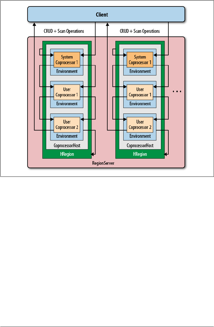
Coprocessor Loading
Coprocessors are loaded in a variety of ways. Before we discuss the actual coprocessor
types and how to implement your own, we will talk about how to deploy them so that
you can try the provided examples.
You can either configure coprocessors to be loaded in a static way, or load them dy-
namically while the cluster is running. The static method uses the configuration files
and table schemas—and is discussed next. Unfortunately, there is not yet an exposed
API to load them dynamically.‡
Figure 4-3. Coprocessors executed sequentially, in their environment, and per region
‡ Coprocessors are a fairly recent addition to HBase, and are therefore still in flux. Check with the online
documentation and issue tracking system to see what is not yet implemented, or planned to be added.
Coprocessors | 179
Loading from the configuration
You can configure globally which coprocessors are loaded when HBase starts. This is
done by adding one, or more, of the following to the hbase-site.xml configuration file:
<property>
<name>hbase.coprocessor.region.classes</name>
<value>coprocessor.RegionObserverExample, coprocessor.AnotherCoprocessor</value>
</property>
<property>
<name>hbase.coprocessor.master.classes</name>
<value>coprocessor.MasterObserverExample</value>
</property>
<property>
<name>hbase.coprocessor.wal.classes</name>
<value>coprocessor.WALObserverExample, bar.foo.MyWALObserver</value>
</property>
Replace the example class names with your own ones!
The order of the classes in each configuration property is important, as it defines the
execution order. All of these coprocessors are loaded with the system priority. You
should configure all globally active classes here so that they are executed first and have
a chance to take authoritative actions. Security coprocessors are loaded this way, for
example.
The configuration file is the first to be examined as HBase starts.
Although you can define additional system-level coprocessors in other
places, the ones here are executed first.
Only one of the three possible configuration keys is read by the matching
CoprocessorHost implementation. For example, the coprocessors
defined in hbase.coprocessor.master.classes are loaded by the
MasterCoprocessorHost class.
Table 4-11 shows where each configuration property is used.
Table 4-11. Possible configuration properties and where they are used
Property Coprocessor host Server type
hbase.coprocessor.master.classes MasterCoprocessorHost Master server
hbase.coprocessor.region.classes RegionCoprocessorHost Region server
hbase.coprocessor.wal.classes WALCoprocessorHost Region server
180 | Chapter 4: Client API: Advanced Features

The coprocessors defined with hbase.coprocessor.region.classes are loaded as
defaults when a region is opened for a table. Note that you cannot specify for which
table, or region, they are loaded: the default coprocessors are loaded for every table and
region. You need to keep this in mind when designing your own coprocessors.
Loading from the table descriptor
The other option to define what coprocessors to load is the table descriptor. As this is
per table, the coprocessors defined here are only loaded for regions of that table—and
only by the region servers. In other words, you can only use this approach for region-
related coprocessors, not for master or WAL-related ones.
Since they are loaded in the context of a table, they are more targeted compared to the
configuration loaded ones, which apply to all tables.
You need to add their definition to the table descriptor using the HTableDescriptor.set
Value() method. The key must start with COPROCESSOR, and the value has to conform to
the following format:
<path-to-jar>|<classname>|<priority>
Here is an example that defines two coprocessors, one with system-level priority, the
other with user-level priority:
'COPROCESSOR$1' => \
'hdfs://localhost:8020/users/leon/test.jar|coprocessor.Test|SYSTEM'
'COPROCESSOR$2' => \
'/Users/laura/test2.jar|coprocessor.AnotherTest|USER'
The path-to-jar can either be a fully specified HDFS location, or any other path sup-
ported by the Hadoop FileSystem class. The second coprocessor definition, for exam-
ple, uses a local path instead.
The classname defines the actual implementation class. While the JAR may contain
many coprocessor classes, only one can be specified per table attribute. Use the stand-
ard Java package name conventions to specify the class.
The priority must be either SYSTEM or USER. This is case-sensitive and must be specified
exactly this way.
Avoid using extra whitespace characters in the coprocessor definition.
The parsing is quite strict, and adding leading, trailing, or spacing char-
acters will render the entire entry invalid.
Using the $<number> postfix for the key enforces the order in which the definitions, and
therefore the coprocessors, are loaded. Although only the prefix of COPROCESSOR is
checked, using the numbered postfix is the advised way to define them.
Example 4-19 shows how this can be done using the administrative API for HBase.
Coprocessors | 181
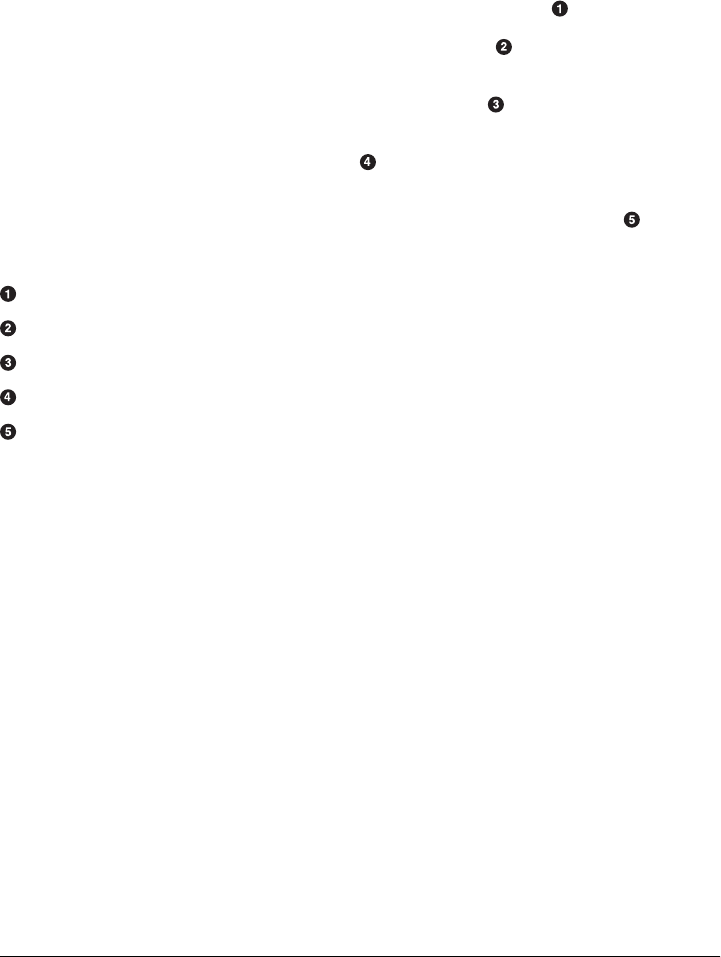
Example 4-19. Region observer checking for special get requests
public class LoadWithTableDescriptorExample {
public static void main(String[] args) throws IOException {
Configuration conf = HBaseConfiguration.create();
FileSystem fs = FileSystem.get(conf);
Path path = new Path(fs.getUri() + Path.SEPARATOR + "test.jar");
HTableDescriptor htd = new HTableDescriptor("testtable");
htd.addFamily(new HColumnDescriptor("colfam1"));
htd.setValue("COPROCESSOR$1", path.toString() +
"|" + RegionObserverExample.class.getCanonicalName() +
"|" + Coprocessor.Priority.USER);
HBaseAdmin admin = new HBaseAdmin(conf);
admin.createTable(htd);
System.out.println(admin.getTableDescriptor(Bytes.toBytes("testtable")));
}
}
Get the location of the JAR file containing the coprocessor implementation.
Define a table descriptor.
Add the coprocessor definition to the descriptor.
Instantiate an administrative API to the cluster and add the table.
Verify if the definition has been applied as expected.
The final check should show you the following result when running this example
against a local, standalone HBase cluster:
{NAME => 'testtable', COPROCESSOR$1 => \
'file:/test.jar|coprocessor.RegionObserverExample|USER', FAMILIES => \
[{NAME => 'colfam1', BLOOMFILTER => 'NONE', REPLICATION_SCOPE => '0', \
COMPRESSION => 'NONE', VERSIONS => '3', TTL => '2147483647', BLOCKSIZE \
=> '65536', IN_MEMORY => 'false', BLOCKCACHE => 'true'}]}
The coprocessor definition has been successfully applied to the table schema. Once the
table is enabled and the regions are opened, the framework will first load the configu-
ration coprocessors and then the ones defined in the table descriptor.
The RegionObserver Class
The first subclass of Coprocessor we will look into is the one used at the region level:
the RegionObserver class. You can learn from its name that it belongs to the group of
observer coprocessors: they have hooks that trigger when a specific region-level
operation occurs.
182 | Chapter 4: Client API: Advanced Features
These operations can be divided into two groups as well: region life-cycle changes and
client API calls. We will look into both in that order.
Handling region life-cycle events
While “The Region Life Cycle” on page 348 explains the region life-cycle, Figure 4-4
shows a simplified form.
Figure 4-4. The coprocessor reacting to life-cycle state changes of a region
The observers have the opportunity to hook into the pending open, open, and pending
close state changes. For each of them there is a set of hooks that are called implicitly by
the framework.
For the sake of brevity, all parameters and exceptions are omitted when
referring to the observer calls. Read the online documentation for the
full specification.§ Note, though, that all calls have a special first
parameter:
ObserverContext<RegionCoprocessorEnvironment> c
This special CoprocessorEnvironment wrapper gives you additional con-
trol over what should happen after the hook execution. See “The Re-
gionCoprocessorEnvironment class” on page 185 and “The Observer-
Context class” on page 186 for the details.
A region is in this state when it is about to be opened. Observing
coprocessors can either piggyback or fail this process. To do so, the following calls are
available:
void preOpen(...) / void postOpen(...)
These methods are called just before the region is opened, and just after it was opened.
Your coprocessor implementation can use them, for instance, to indicate to the frame-
work—in the preOpen() call—that it should abort the opening process. Or hook into
the postOpen() call to trigger a cache warm up, and so on.
State: pending open.
§ See http://hbase.apache.org/apidocs/org/apache/hadoop/hbase/coprocessor/RegionObserver.html.
Coprocessors | 183

After the pending open, but just before the open state, the region server may have to
apply records from the write-ahead log (WAL). This, in turn, invokes the following
methods of the observer:
void preWALRestore(...) / void postWALRestore(...)
Hooking into these calls gives you fine-grained control over what mutation is applied
during the log replay process. You get access to the edit record, which you can use to
inspect what is being applied.
A region is considered open when it is deployed to a region server and fully
operational. At this point, all the operations discussed throughout the book can take
place; for example, the region’s in-memory store could be flushed to disk, or the region
could be split when it has grown too large. The possible hooks are:
void preFlush(...) / void postFlush(...)
void preCompact(...) / void postCompact(...)
void preSplit(...) / void postSplit(...)
This should be quite intuitive by now: the pre calls are executed before, while the
post calls are executed after the respective operation. For example, using the pre
Split() hook, you could effectively disable the built-in region splitting process and
perform these operations manually.
The last group of hooks for the observers is for regions that go into
the pending close state. This occurs when the region transitions from open to closed.
Just before, and after, the region is closed the following hooks are executed:
void preClose(..., boolean abortRequested) /
void postClose(..., boolean abortRequested)
The abortRequested parameter indicates why a region was closed. Usually regions are
closed during normal operation, when, for example, the region is moved to a different
region server for load-balancing reasons. But there also is the possibility for a region
server to have gone rogue and be aborted to avoid any side effects. When this happens,
all hosted regions are also aborted, and you can see from the given parameter if that
was the case.
Handling client API events
As opposed to the life-cycle events, all client API calls are explicitly sent from a client
application to the region server. You have the opportunity to hook into these calls just
before they are applied, and just thereafter. Here is the list of the available calls:
void preGet(...) / void postGet(...)
Called before and after a client makes an HTable.get() request
void prePut(...) / void postPut(...)
Called before and after a client makes an HTable.put() request
void preDelete(...) / void postDelete(...)
Called before and after a client makes an HTable.delete() request
State: open.
State: pending close.
184 | Chapter 4: Client API: Advanced Features

boolean preCheckAndPut(...) / boolean postCheckAndPut(...)
Called before and after a client invokes an HTable.checkAndPut() call
boolean preCheckAndDelete(...) / boolean postCheckAndDelete(...)
Called before and after a client invokes an HTable.checkAndDelete() call
void preGetClosestRowBefore(...) / void postGetClosestRowBefore(...)
Called before and after a client invokes an HTable.getClosestRowBefore() call
boolean preExists(...) / boolean postExists(...)
Called before and after a client invokes an HTable.exists() call
long preIncrementColumnValue(...) / long postIncrementColumnValue(...)
Called before and after a client invokes an HTable.incrementColumnValue() call
void preIncrement(...) / void postIncrement(...)
Called before and after a client invokes an HTable.increment() call
InternalScanner preScannerOpen(...) / InternalScanner postScannerOpen(...)
Called before and after a client invokes an HTable.getScanner() call
boolean preScannerNext(...) / boolean postScannerNext(...)
Called before and after a client invokes a ResultScanner.next() call
void preScannerClose(...) / void postScannerClose(...)
Called before and after a client invokes a ResultScanner.close() call
The RegionCoprocessorEnvironment class
The environment instances provided to a coprocessor that is implementing the
RegionObserver interface are based on the RegionCoprocessorEnvironment class—which
in turn is implementing the CoprocessorEnvironment interface. The latter was discussed
in “The Coprocessor Class” on page 176.
On top of the provided methods, the more specific, region-oriented subclass is adding
the methods described in Table 4-12.
Table 4-12. Methods provided by the RegionCoprocessorEnvironment class, in addition to the
inherited one
Method Description
HRegion getRegion() Returns a reference to the region the current observer is associated with
RegionServerServices
getRegionServerServices()
Provides access to the shared RegionServerServices instance
The getRegion() call can be used to get a reference to the hosting HRegion instance, and
to invoke calls this class provides. In addition, your code can access the shared region
server services instance, which is explained in Table 4-13.
Coprocessors | 185
Table 4-13. Methods provided by the RegionServerServices class
Method Description
boolean isStopping() Returns true when the region server is stopping.
HLog getWAL() Provides access to the write-ahead log instance.
CompactionRequestor
getCompactionRequester()
Provides access to the shared CompactionRequestor instance. This can
be used to initiate compactions from within the coprocessor.
FlushRequester
getFlushRequester()
Provides access to the shared FlushRequester instance. This can be used
to initiate memstore flushes.
RegionServerAccounting
getRegionServerAccounting()
Provides access to the shared RegionServerAccounting instance. It
allows you to check on what the server currently has allocated—for
example, the global memstore size.
postOpenDeployTasks(HRegion r,
CatalogTracker ct, final boolean
daughter)
An internal call, invoked inside the region server.
HBaseRpcMetrics getRpcMetrics() Provides access to the shared HBaseRpcMetrics instance. It has details
on the RPC statistics for the current server.
I will not be discussing all the details on the provided functionality, and instead refer
you to the Java API documentation.‖
The ObserverContext class
For the callbacks provided by the RegionObserver class, there is a special context handed
in as the first parameter to all calls: the ObserverContext class. It provides access to the
current environment, but also adds the crucial ability to indicate to the coprocessor
framework what it should do after a callback is completed.
The context instance is the same for all coprocessors in the execution
chain, but with the environment swapped out for each coprocessor.
Table 4-14 lists the methods as provided by the context class.
‖The Java HBase classes are documented online at http://hbase.apache.org/apidocs/.
186 | Chapter 4: Client API: Advanced Features

Table 4-14. Methods provided by the ObserverContext class
Method Description
E getEnvironment() Returns the reference to the current coprocessor environment.
void bypass() When your code invokes this method, the framework is going to use your provided
value, as opposed to what usually is returned.
void complete() Indicates to the framework that any further processing can be skipped, skipping
the remaining coprocessors in the execution chain. It implies that this coproces-
sor’s response is definitive.
boolean shouldBypass() Used internally by the framework to check on the flag.
boolean shouldComplete() Used internally by the framework to check on the flag.
void prepare(E env) Prepares the context with the specified environment. This is used internally only.
It is used by the static createAndPrepare() method.
static <T extends Coprocessor
Environment> ObserverCon
text<T> createAndPrepare( T
env, ObserverContext<T> con
text)
Static function to initialize a context. When the provided context is null, it
will create a new instance.
The important context functions are bypass() and complete(). These functions give
your coprocessor implementation the option to control the subsequent behavior of the
framework. The complete() call influences the execution chain of the coprocessors,
while the bypass() call stops any further default processing on the server. Use it with
the earlier example of avoiding automated region splits like so:
@Override
public void preSplit(ObserverContext<RegionCoprocessorEnvironment> e) {
e.bypass();
}
Instead of having to implement your own RegionObserver, based on the interface, you
can use the following base class to only implement what is needed.
The BaseRegionObserver class
This class can be used as the basis for all your observer-type coprocessors. It has
placeholders for all methods required by the RegionObserver interface. They are all left
blank, so by default nothing is done when extending this class. You must override all
the callbacks that you are interested in to add the required functionality.
Example 4-20 is an observer that handles specific row key requests.
Coprocessors | 187
Example 4-20. Region observer checking for special get requests
public class RegionObserverExample extends BaseRegionObserver {
public static final byte[] FIXED_ROW = Bytes.toBytes("@@@GETTIME@@@");
@Override
public void preGet(final ObserverContext<RegionCoprocessorEnvironment> e,
final Get get, final List<KeyValue> results) throws IOException {
if (Bytes.equals(get.getRow(), FIXED_ROW)) {
KeyValue kv = new KeyValue(get.getRow(), FIXED_ROW, FIXED_ROW,
Bytes.toBytes(System.currentTimeMillis()));
results.add(kv);
}
}
}
Check if the request row key matches a well-known one.
Create a special KeyValue instance containing just the current time on the server.
The following was added to the hbase-site.xml file to enable the copro-
cessor:
<property>
<name>hbase.coprocessor.region.classes</name>
<value>coprocessor.RegionObserverExample</value>
</property>
The class is available to the region server’s Java Runtime Environment
because we have already added the JAR of the compiled repository to
the HBASE_CLASSPATH variable in hbase-env.sh—see “Deployment of Cus-
tom Filters” on page 165 for reference.
Do not forget to restart HBase, though, to make the changes to the static
configuration files active.
The row key @@@GETTIME@@@ is handled by the observer’s preGet() hook, inserting the
current time of the server. Using the HBase Shell—after deploying the code to servers—
you can see this in action:
hbase(main):001:0> get 'testtable', '@@@GETTIME@@@'
COLUMN CELL
@@@GETTIME@@@:@@@GETTIME@@@ timestamp=9223372036854775807, \
value=\x00\x00\x01/s@3\xD8
1 row(s) in 0.0410 seconds
hbase(main):002:0> Time.at(Bytes.toLong( \
"\x00\x00\x01/s@3\xD8".to_java_bytes) / 1000)
=> Wed Apr 20 16:11:18 +0200 2011
This requires an existing table, because trying to issue a get call to a nonexistent table
will raise an error, before the actual get operation is executed. Also, the example does
not set the bypass flag, in which case something like the following could happen:
188 | Chapter 4: Client API: Advanced Features
hbase(main):003:0> create 'testtable2', 'colfam1'
0 row(s) in 1.3070 seconds
hbase(main):004:0> put 'testtable2', '@@@GETTIME@@@', \
'colfam1:qual1', 'Hello there!'
0 row(s) in 0.1360 seconds
hbase(main):005:0> get 'testtable2', '@@@GETTIME@@@'
COLUMN CELL
@@@GETTIME@@@:@@@GETTIME@@@ timestamp=9223372036854775807, \
value=\x00\x00\x01/sJ\xBC\xEC
colfam1:qual1 timestamp=1303309353184, value=Hello there!
2 row(s) in 0.0450 seconds
A new table is created and a row with the special row key is inserted. Subsequently, the
row is retrieved. You can see how the artificial column is mixed with the actual one
stored earlier. To avoid this issue, Example 4-21 adds the necessary e.bypass() call.
Example 4-21. Region observer checking for special get requests and bypassing further processing
if (Bytes.equals(get.getRow(), FIXED_ROW)) {
KeyValue kv = new KeyValue(get.getRow(), FIXED_ROW, FIXED_ROW,
Bytes.toBytes(System.currentTimeMillis()));
results.add(kv);
e.bypass();
}
Once the special KeyValue is inserted, all further processing is skipped.
You need to adjust the hbase-site.xml file to point to the new example:
<property>
<name>hbase.coprocessor.region.classes</name>
<value>coprocessor.RegionObserverWithBypassExample</value>
</property>
Just as before, please restart HBase after making these adjustments.
As expected, and using the shell once more, the result is now different:
hbase(main):069:0> get 'testtable2', '@@@GETTIME@@@'
COLUMN CELL
@@@GETTIME@@@:@@@GETTIME@@@ timestamp=9223372036854775807, \
value=\x00\x00\x01/s]\x1D4
1 row(s) in 0.0470 seconds
Only the artificial column is returned, and since the default get operation is bypassed,
it is the only column retrieved. Also note how the timestamp of this column is
9223372036854775807—which is Long.MAX_VALUE on purpose. Since the example creates
the KeyValue instance without specifying a timestamp, it is set to
HConstants.LATEST_TIMESTAMP by default, and that is, in turn, set to Long.MAX_VALUE.
You can amend the example by adding a timestamp and see how that would be printed
when using the shell (an exercise left to you).
Coprocessors | 189

The MasterObserver Class
The second subclass of Coprocessor discussed handles all possible callbacks the master
server may initiate. The operations and API calls are explained in Chapter 5, though
they can be classified as data-manipulation operations, similar to DDL used in rela-
tional database systems. For that reason, the MasterObserver class provides the follow-
ing hooks:
void preCreateTable(...) / void postCreateTable(...)
Called before and after a table is created.
void preDeleteTable(...) / void postDeleteTable(...)
Called before and after a table is deleted.
void preModifyTable(...) / void postModifyTable(...)
Called before and after a table is altered.
void preAddColumn(...) / void postAddColumn(...)
Called before and after a column is added to a table.
void preModifyColumn(...) / void postModifyColumn(...)
Called before and after a column is altered.
void preDeleteColumn(...) / void postDeleteColumn(...)
Called before and after a column is deleted from a table.
void preEnableTable(...) / void postEnableTable(...)
Called before and after a table is enabled.
void preDisableTable(...) / void postDisableTable(...)
Called before and after a table is disabled.
void preMove(...) / void postMove(...)
Called before and after a region is moved.
void preAssign(...) / void postAssign(...)
Called before and after a region is assigned.
void preUnassign(...) / void postUnassign(...)
Called before and after a region is unassigned.
void preBalance(...) / void postBalance(...)
Called before and after the regions are balanced.
boolean preBalanceSwitch(...) / void postBalanceSwitch(...)
Called before and after the flag for the balancer is changed.
void preShutdown(...)
Called before the cluster shutdown is initiated. There is no post hook, because after
the shutdown, there is no longer a cluster to invoke the callback.
void preStopMaster(...)
Called before the master process is stopped. There is no post hook, because after
the master has stopped, there is no longer a process to invoke the callback.
190 | Chapter 4: Client API: Advanced Features

The MasterCoprocessorEnvironment class
Similar to how the RegionCoprocessorEnvironment is enclosing a single
RegionObserver coprocessor, the MasterCoprocessorEnvironment is wrapping MasterOb
server instances. It also implements the CoprocessorEnvironment interface, thus giving
you, for instance, access to the getTable() call to access data from within your own
implementation.
On top of the provided methods, the more specific, master-oriented subclass adds the
one method described in Table 4-15.
Table 4-15. The method provided by the MasterCoprocessorEnvironment class, in addition to the
inherited one
Method Description
MasterServices getMasterServices() Provides access to the shared MasterServices instance
Your code can access the shared master services instance, the methods of which are
listed and described in Table 4-16.
Table 4-16. Methods provided by the MasterServices class
Method Description
AssignmentManager getAssignmentManager() Gives you access to the assignment manager instance.
It is responsible for all region assignment operations,
such as assign, unassign, balance, and so on.
MasterFileSystem getMasterFileSystem() Provides you with an abstraction layer for all
filesystem-related operations the master is involved
in—for example, creating directories for table files
and logfiles.
ServerManager getServerManager() Returns the server manager instance. With it you have
access to the list of servers, live or considered dead,
and more.
ExecutorService getExecutorService() Used by the master to schedule system-wide events.
void checkTableModifiable(byte[] tableName) Convenient to check if a table exists and is offline so
that it can be altered.
I will not be discussing all the details on the provided functionality, and instead refer
you to the Java API documentation once more.#
#The Java HBase classes are documented online at http://hbase.apache.org/apidocs/.
Coprocessors | 191
The BaseMasterObserver class
Either you can base your efforts to implement a MasterObserver on the interface directly,
or you can extend the BaseMasterObserver class instead. It implements the interface
while leaving all callback functions empty. If you were to use this class unchanged, it
would not yield any kind of reaction.
Adding functionality is achieved by overriding the appropriate event methods. You
have the choice of hooking your code into the pre and/or post calls.
Example 4-22 uses the post hook after a table was created to perform additional tasks.
Example 4-22. Master observer that creates a separate directory on the filesystem when a table is
created
public class MasterObserverExample extends BaseMasterObserver {
@Override
public void postCreateTable(
ObserverContext<MasterCoprocessorEnvironment> env,
HRegionInfo[] regions, boolean sync)
throws IOException {
String tableName = regions[0].getTableDesc().getNameAsString();
MasterServices services = env.getEnvironment().getMasterServices();
MasterFileSystem masterFileSystem = services.getMasterFileSystem();
FileSystem fileSystem = masterFileSystem.getFileSystem();
Path blobPath = new Path(tableName + "-blobs");
fileSystem.mkdirs(blobPath);
}
}
Get the new table’s name from the table descriptor.
Get the available services and retrieve a reference to the actual filesystem.
Create a new directory that will store binary data from the client application.
You need to add the following to the hbase-site.xml file for the
coprocessor to be loaded by the master process:
<property>
<name>hbase.coprocessor.master.classes</name>
<value>coprocessor.MasterObserverExample</value>
</property>
Just as before, restart HBase after making these adjustments.
Once you have activated the coprocessor, it is listening to the said events and will trigger
your code automatically. The example is using the supplied services to create a directory
192 | Chapter 4: Client API: Advanced Features

on the filesystem. A fictitious application, for instance, could use it to store very large
binary objects (known as blobs) outside of HBase.
To trigger the event, you can use the shell like so:
hbase(main):001:0> create 'testtable', 'colfam1'
0 row(s) in 0.4300 seconds
This creates the table and afterward calls the coprocessor’s postCreateTable() method.
The Hadoop command-line tool can be used to verify the results:
$ bin/hadoop dfs -ls
Found 1 items
drwxr-xr-x - larsgeorge supergroup 0 ... /user/larsgeorge/testtable-blobs
There are many things you can implement with the MasterObserver coprocessor. Since
you have access to most of the shared master resources through the MasterServices
instance, you should be careful what you do, as it can potentially wreak havoc.
Finally, because the environment is wrapped in an ObserverContext, you have the same
extra flow controls, exposed by the bypass() and complete() methods. You can use
them to explicitly disable certain operations or skip subsequent coprocessor execution,
respectively.
Endpoints
The earlier RegionObserver example used a well-known row key to add a computed
column during a get request. It seems that this could suffice to implement other func-
tionality as well—for example, aggregation functions that return the sum of all values
in a specific column.
Unfortunately, this does not work, as the row key defines which region is handling the
request, therefore only sending the computation request to a single server. What we
want, though, is a mechanism to send such a request to all regions, and therefore all
region servers, so that they can build the sum of the columns they have access to locally.
Once each region has returned its partial result, we can aggregate the total on the client
side much more easily. If you were to have 1,000 regions and 1 million columns, you
would receive 1,000 decimal numbers on the client side—one for each region. This is
fast to aggregate for the final result.
If you were to scan the entire table using a purely client API approach, in a worst-case
scenario you would transfer all 1 million numbers to build the sum. Moving such com-
putation to the servers where the data resides is a much better option. HBase, though,
does not know what you may need, so to overcome this limitation, the coprocessor
framework provides you with a dynamic call implementation, represented by the end-
point concept.
Coprocessors | 193

The CoprocessorProtocol interface
In order to provide a custom RPC protocol to clients, a coprocessor implementation
defines an interface that extends CoprocessorProtocol. The interface can define any
methods that the coprocessor wishes to expose. Using this protocol, you can commu-
nicate with the coprocessor instances via the following calls, provided by HTable:
<T extends CoprocessorProtocol> T coprocessorProxy(
Class<T> protocol, byte[] row)
<T extends CoprocessorProtocol, R> Map<byte[],R> coprocessorExec(
Class<T> protocol, byte[] startKey, byte[] endKey,
Batch.Call<T,R> callable)
<T extends CoprocessorProtocol, R> void coprocessorExec(
Class<T> protocol, byte[] startKey, byte[] endKey,
Batch.Call<T,R> callable, Batch.Callback<R> callback)
Since CoprocessorProtocol instances are associated with individual regions within the
table, the client RPC calls must ultimately identify which regions should be used in the
CoprocessorProtocol method invocations. Though regions are seldom handled directly
in client code and the region names may change over time, the coprocessor RPC calls
use row keys to identify which regions should be used for the method invocations.
Clients can call CoprocessorProtocol methods against one of the following:
Single region
This is done by calling coprocessorProxy() with a single row key. This returns a
dynamic proxy of the CoprocessorProtocol interface, which uses the region con-
taining the given row key—even if the row does not exist—as the RPC endpoint.
Range of regions
You can call coprocessorExec() with a start row key and an end row key. All regions
in the table from the one containing the start row key to the one containing the
end row key (inclusive) will be used as the RPC endpoints.
The row keys passed as parameters to the HTable methods are not passed
to the CoprocessorProtocol implementations. They are only used to
identify the regions for endpoints of the remote calls.
The Batch class defines two interfaces used for CoprocessorProtocol invocations against
multiple regions: clients implement Batch.Call to call methods of the actual
CoprocessorProtocol instance. The interface’s call() method will be called once per
selected region, passing the CoprocessorProtocol instance for the region as a parameter.
Clients can optionally implement Batch.Callback to be notified of the results from each
region invocation as they complete. The instance’s
void update(byte[] region, byte[] row, R result)
method will be called with the value returned by R call(T instance) from each region.
194 | Chapter 4: Client API: Advanced Features

The BaseEndpointCoprocessor class
Implementing an endpoint involves the following two steps:
1. Extend the CoprocessorProtocol interface.
This specifies the communication details for the new endpoint: it defines the RPC
protocol between the client and the servers.
2. Extend the BaseEndpointCoprocessor class.
You need to provide the actual implementation of the endpoint by extending both
the abstract BaseEndpointCoprocessor class and the protocol interface provided in
step 1, defining your endpoint protocol.
Example 4-23 implements the CoprocessorProtocol to add custom functions to HBase.
A client can invoke these remote calls to retrieve the number of rows and KeyValues in
each region where it is running.
Example 4-23. Endpoint protocol, adding a row and KeyValue count method
public interface RowCountProtocol extends CoprocessorProtocol {
long getRowCount() throws IOException;
long getRowCount(Filter filter) throws IOException;
long getKeyValueCount() throws IOException;
}
Step 2 is to combine this new protocol interface with a class that also extends BaseEnd
pointCoprocessor. Example 4-24 uses the environment provided to access the data us-
ing an InternalScanner instance.
Example 4-24. Endpoint implementation, adding a row and KeyValue count method
public class RowCountEndpoint extends BaseEndpointCoprocessor
implements RowCountProtocol {
private long getCount(Filter filter, boolean countKeyValues)
throws IOException {
Scan scan = new Scan();
scan.setMaxVersions(1);
if (filter != null) {
scan.setFilter(filter);
}
RegionCoprocessorEnvironment environment =
(RegionCoprocessorEnvironment) getEnvironment();
// use an internal scanner to perform scanning.
InternalScanner scanner = environment.getRegion().getScanner(scan);
int result = 0;
try {
List<KeyValue> curVals = new ArrayList<KeyValue>();
boolean done = false;
do {
curVals.clear();
Coprocessors | 195
done = scanner.next(curVals);
result += countKeyValues ? curVals.size() : 1;
} while (done);
} finally {
scanner.close();
}
return result;
}
@Override
public long getRowCount() throws IOException {
return getRowCount(new FirstKeyOnlyFilter());
}
@Override
public long getRowCount(Filter filter) throws IOException {
return getCount(filter, false);
}
@Override
public long getKeyValueCount() throws IOException {
return getCount(null, true);
}
}
Note how the FirstKeyOnlyFilter is used to reduce the number of columns being
scanned.
You need to add (or amend from the previous examples) the following
to the hbase-site.xml file for the endpoint coprocessor to be loaded by
the region server process:
<property>
<name>hbase.coprocessor.region.classes</name>
<value>coprocessor.RowCountEndpoint</value>
</property>
Just as before, restart HBase after making these adjustments.
Example 4-25 showcases how a client can use the provided calls of HTable to execute
the deployed coprocessor endpoint functions. Since the calls are sent to each region
separately, there is a need to summarize the total number at the end.
Example 4-25. Using the custom row-count endpoint
public class EndpointExample {
public static void main(String[] args) throws IOException {
Configuration conf = HBaseConfiguration.create();
HTable table = new HTable(conf, "testtable");
try {
Map<byte[], Long> results = table.coprocessorExec(
RowCountProtocol.class,
196 | Chapter 4: Client API: Advanced Features

null, null,
new Batch.Call<RowCountProtocol, Long>() {
@Override
public Long call(RowCountProtocol counter) throws IOException {
return counter.getRowCount();
}
});
long total = 0;
for (Map.Entry<byte[], Long> entry : results.entrySet()) {
total += entry.getValue().longValue();
System.out.println("Region: " + Bytes.toString(entry.getKey()) +
", Count: " + entry.getValue());
}
System.out.println("Total Count: " + total);
} catch (Throwable throwable) {
throwable.printStackTrace();
}
}
}
Define the protocol interface being invoked.
Set start and end row keys to “null” to count all rows.
Create an anonymous class to be sent to all region servers.
The call() method is executing the endpoint functions.
Iterate over the returned map, containing the result for each region separately.
The code emits the region names, the count for each of them, and eventually the grand
total:
Region: testtable,,1303417572005.51f9e2251c29ccb2...cbcb0c66858f., Count: 2
Region: testtable,row3,1303417572005.7f3df4dcba3f...dbc99fce5d87., Count: 3
Total Count: 5
The Batch class also offers a more convenient way to access the remote endpoint: using
Batch.forMethod(), you can retrieve a fully configured Batch.Call instance, ready to be
sent to the region servers. Example 4-26 amends the previous example to make use of
this shortcut.
Example 4-26. One way in which Batch.forMethod() can reduce the client code size
Batch.Call call = Batch.forMethod(RowCountProtocol.class,
"getKeyValueCount");
Map<byte[], Long> results = table.coprocessorExec(
RowCountProtocol.class, null, null, call);
The forMethod() call uses the Java reflection API to retrieve the named method. The
returned Batch.Call instance will execute the endpoint function and return the same
data types as defined by the protocol for this method.
Coprocessors | 197

However, if you want to perform additional processing on the results, implementing
Batch.Call directly will provide more power and flexibility. This can be seen in Exam-
ple 4-27, which combines the row and key-value count for each region.
Example 4-27. Extending the batch call to execute multiple endpoint calls
Map<byte[], Pair<Long, Long>> results = table.coprocessorExec(
RowCountProtocol.class,
null, null,
new Batch.Call<RowCountProtocol, Pair<Long, Long>>() {
public Pair<Long, Long> call(RowCountProtocol counter)
throws IOException {
return new Pair(counter.getRowCount(),
counter.getKeyValueCount());
}
});
long totalRows = 0;
long totalKeyValues = 0;
for (Map.Entry<byte[], Pair<Long, Long>> entry : results.entrySet()) {
totalRows += entry.getValue().getFirst().longValue();
totalKeyValues += entry.getValue().getSecond().longValue();
System.out.println("Region: " + Bytes.toString(entry.getKey()) +
", Count: " + entry.getValue());
}
System.out.println("Total Row Count: " + totalRows);
System.out.println("Total KeyValue Count: " + totalKeyValues);
Running the code will yield the following output:
Region: testtable,,1303420252525.9c336bd2b294a...0647a1f2d13b., Count: {2,4}
Region: testtable,row3,1303420252525.6d7c95de8a7...386cfec7f2., Count: {3,6}
Total Row Count: 5
Total KeyValue Count: 10
The examples so far all used the coprocessorExec() calls to batch the requests across
all regions, matching the given start and end row keys. Example 4-28 uses the
coprocessorProxy() call to get a local, client-side proxy of the endpoint. Since a row
key is specified, the client API will route the proxy calls to the region—and to the server
currently hosting it—that contains the given key, regardless of whether it actually
exists: regions are specified with a start and end key only, so the match is done by range
only.
Example 4-28. Using the proxy call of HTable to invoke an endpoint on a single region
RowCountProtocol protocol = table.coprocessorProxy(
RowCountProtocol.class, Bytes.toBytes("row4"));
long rowsInRegion = protocol.getRowCount();
System.out.println("Region Row Count: " + rowsInRegion);
With the proxy reference, you can invoke any remote function defined in your
CoprocessorProtocol implementation from within client code, and it returns the result
198 | Chapter 4: Client API: Advanced Features
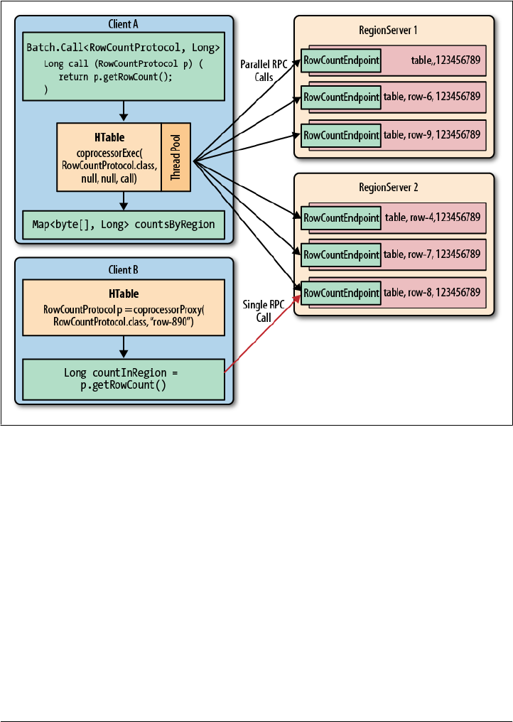
for the region that served the request. Figure 4-5 shows the difference between the two
approaches.
Figure 4-5. Coprocessor calls batched and executed in parallel, and addressing a single region only
HTablePool
Instead of creating an HTable instance for every request from your client application, it
makes much more sense to create one initially and subsequently reuse them.
The primary reason for doing so is that creating an HTable instance is a fairly expensive
operation that takes a few seconds to complete. In a highly contended environment
with thousands of requests per second, you would not be able to use this approach at
all—creating the HTable instance would be too slow. You need to create the instance
at startup and use it for the duration of your client’s life cycle.
There is an additional issue with the HTable being reused by multiple threads within
the same process.
HTablePool | 199

The HTable class is not thread-safe, that is, the local write buffer is not
guarded against concurrent modifications. Even if you were to use
setAutoFlush(true) (which is the default currently; see “Client-side
write buffer” on page 86) this is not advisable. Instead, you should use
one instance of HTable for each thread you are running in your client
application.
Clients can solve this problem using the HTablePool class. It only serves one purpose,
namely to pool client API instances to the HBase cluster. Creating the pool is accom-
plished using one of these constructors:
HTablePool()
HTablePool(Configuration config, int maxSize)
HTablePool(Configuration config, int maxSize,
HTableInterfaceFactory tableFactory)
The default constructor—the one without any parameters—creates a pool with the
configuration found in the classpath, while setting the maximum size to unlimited. This
equals calling the second constructor like so:
Configuration conf = HBaseConfiguration.create()
HTablePool pool = new HTablePool(conf, Integer.MAX_VALUE)
Setting the maxSize parameter gives you control over how many HTable instances a pool
is allowed to contain. The optional tableFactory parameter can be used to hand in a
custom factory class that creates the actual HTable instances.
The HTableInterfaceFactory Interface
You can create your own factory class to, for example, prepare the HTable instances
with specific settings. Or you could use the instance to perform some initial operations,
such as adding some rows, or updating counters. If you want to implement your own
HTableInterfaceFactory you need to implement two methods:
HTableInterface createHTableInterface(Configuration config,
byte[] tableName)
void releaseHTableInterface(HTableInterface table)
The first creates the HTable instance, while the second releases it. Take any actions you
require in these calls to prepare an instance, or clean up afterward. The client-side write
buffer, in particular, is a concern when sharing the table references. The releaseHTa
bleInterface() is the ideal place to handle implicit actions, such as flushing the write
buffer, calling flushCommits() in the process.
There is a default implementation of the factory class, called HTableFactory, which does
exactly that: it creates HTable instances, when the create method of the factory is
called—while calling HTable.close(), when the client invokes the release method.
If you do not specify your own HTableInterfaceFactory, the default HTableFactory is
created and assigned implicitly.
200 | Chapter 4: Client API: Advanced Features
Using the pool is a matter of employing the following calls:
HTableInterface getTable(String tableName)
HTableInterface getTable(byte[] tableName)
void putTable(HTableInterface table)
The getTable() calls retrieve an HTable instance from the pool, while the putTable()
returns it after you are done using it. Both internally defer some of the work to the
mentioned HTableInterfaceFactory instance the pool is configured with.
Setting the maxSize parameter during the construction of a pool does
not impose an upper limit on the number of HTableInterface instances
the pool is allowing you to retrieve. You can call getTable() as much as
you like to get a valid table reference.
The maximum size of the pool only sets the number of HTableInter
face instances retained within the pool, for a given table name. For ex-
ample, when you set the size to 5, but then call getTable() 10 times, you
have created 10 HTable instances (assuming you use the default). Upon
returning them using the putTable() method, five are kept for subse-
quent use, while the additional five you requested are simply ignored.
More importantly, the release mechanisms of the factory are not
invoked.
Finally, there are calls to close the pool for specific tables:
void closeTablePool(String tableName)
void closeTablePool(byte[] tableName)
Obviously, both do the same thing, with one allowing you to specify a String, and the
other a byte array—use whatever is more convenient for you.
The close call of the pool iterates over the list of retained references for a specific table,
invoking the release mechanism provided by the factory. This is useful for freeing all
resources for a named table, and starting all over again. Keep in mind that for all re-
sources to be released, you would need to call these methods for every table name you
have used so far.
Example 4-29 uses these methods to create and use a pool.
Example 4-29. Using the HTablePool class to share HTable instances
Configuration conf = HBaseConfiguration.create();
HTablePool pool = new HTablePool(conf, 5);
HTableInterface[] tables = new HTableInterface[10];
for (int n = 0; n < 10; n++) {
tables[n] = pool.getTable("testtable");
System.out.println(Bytes.toString(tables[n].getTableName()));
}
for (int n = 0; n < 5; n++) {
HTablePool | 201

pool.putTable(tables[n]);
}
pool.closeTablePool("testtable");
Create the pool, allowing five HTables to be retained.
Get 10 HTable references, which is more than the pool is retaining.
Return HTable instances to the pool. Five will be kept, while the additional five will
be dropped.
Close the entire pool, releasing all retained table references.
You should receive the following output on the console:
Acquiring tables...
testtable
testtable
testtable
testtable
testtable
testtable
testtable
testtable
testtable
testtable
Releasing tables...
Closing pool...
Note that using more than the configured maximum size of the pool works as we dis-
cussed earlier: we receive more references than were configured. Returning the tables
to the pool is not yielding any logging or printout, though, doing its work behind the
scenes.
Use Case: Hush
All of the tables in Hush are acquired through a shared table pool. The code below
provides the pool to calling classes:
private ResourceManager(Configuration conf) throws IOException {
this.conf = conf;
this.pool = new HTablePool(conf, 10);
/* ... */
}
public HTable getTable(byte[] tableName) throws IOException {
return (HTable) pool.getTable(tableName);
}
public void putTable(HTable table) throws IOException {
if (table != null) {
pool.putTable(table);
}
}
202 | Chapter 4: Client API: Advanced Features

The next code block shows how these methods are called in context. The table is
retrieved from the pool and used. Once the operations are concluded, the table is re-
turned to the pool subsequently.
public void createUser(String username, String firstName, String lastName,
String email, String password, String roles) throws IOException {
HTable table = rm.getTable(UserTable.NAME);
Put put = new Put(Bytes.toBytes(username));
put.add(UserTable.DATA_FAMILY, UserTable.FIRSTNAME,
Bytes.toBytes(firstName));
put.add(UserTable.DATA_FAMILY, UserTable.LASTNAME, Bytes.toBytes(lastName));
put.add(UserTable.DATA_FAMILY, UserTable.EMAIL, Bytes.toBytes(email));
put.add(UserTable.DATA_FAMILY, UserTable.CREDENTIALS,
Bytes.toBytes(password));
put.add(UserTable.DATA_FAMILY, UserTable.ROLES, Bytes.toBytes(roles));
table.put(put);
table.flushCommits();
rm.putTable(table);
}
Connection Handling
Every instance of HTable requires a connection to the remote servers. This is internally
represented by the HConnection class, and more importantly managed process-wide by
the shared HConnectionManager class. From a user perspective, there is usually no
immediate need to deal with either of these two classes; instead, you simply create a
new Configuration instance, and use that with your client API calls.
Internally, the connections are keyed in a map, where the key is the Configuration
instance you are using. In other words, if you create a number of HTable instances while
providing the same configuration reference, they all share the same underlying
HConnection instance. There are good reasons for this to happen:
Share ZooKeeper connections
As each client eventually needs a connection to the ZooKeeper ensemble to perform
the initial lookup of where user table regions are located, it makes sense to share
this connection once it is established, with all subsequent client instances.
Cache common resources
Every lookup performed through ZooKeeper, or the -ROOT-, or .META. table, of
where user table regions are located requires network round-trips. The location is
then cached on the client side to reduce the amount of network traffic, and to speed
up the lookup process.
Since this list is the same for every local client connecting to a remote cluster, it is
equally useful to share it among multiple clients running in the same process. This
is accomplished by the shared HConnection instance.
In addition, when a lookup fails—for instance, when a region was split—the con-
nection has the built-in retry mechanism to refresh the stale cache information.
Connection Handling | 203

This is then immediately available to all other clients sharing the same connection
reference, thus further reducing the number of network round-trips initiated by a
client.
Another class that benefits from the same advantages is the HTablePool: all of the pooled
HTable instances automatically share the provided configuration instances, and there-
fore also the shared connection it references to. This also means you should always
create your own configuration, whenever you plan to instantiate more than one
HTable instance. For example:
HTable table1 = new HTable("table1");
//...
HTable table2 = new HTable("table2");
is less efficient than the following code:
Configuration conf = HBaseConfiguration.create();
HTable table1 = new HTable(conf, "table1");
//...
HTable table2 = new HTable(conf, "table2");
The latter implicitly uses the connection sharing, as provided by the HBase client-side
API classes.
There are no known performance implications for sharing a connection,
even for heavily multithreaded applications.
The drawback of sharing a connection is the cleanup: when you do not explicitly close
a connection, it is kept open until the client process exits. This can result in many
connections that remain open to ZooKeeper, especially for heavily distributed appli-
cations, such as MapReduce jobs talking to HBase. In a worst-case scenario, you can
run out of available connections, and receive an IOException instead.
You can avoid this problem by explicitly closing the shared connection, when you are
done using it. This is accomplished with the close() method provided by HTable. The
call decreases an internal reference count and eventually closes all shared resources,
such as the connection to the ZooKeeper ensemble, and removes the connection ref-
erence from the internal list.
Every time you reuse a Configuration instance, the connection manager internally in-
creases the reference count, so you only have to make sure you call the close() method
to trigger the cleanup. There is also an explicit call to clear out a connection, or all open
connections:
static void deleteConnection(Configuration conf, boolean stopProxy)
static void deleteAllConnections(boolean stopProxy)
204 | Chapter 4: Client API: Advanced Features

Since all shared connections are internally keyed by the configuration instance, you
need to provide that instance to close the associated connection. The boolean stop
Proxy parameter lets you further enforce the cleanup of the entire RPC stack of the
client—which is its umbilical cord to the remote servers. Only use true when you do
not need any further communication with the server to take place.
The deleteAllConnections() call only requires the boolean stopProxy flag; it simply
iterates over the entire list of shared connections known to the connection manager
and closes them.
If you are ever in need of using a connection explicitly, you can make use of the get
Connection() call like so:
Configuration newConfig = new Configuration(originalConf);
HConnection connection = HConnectionManager.getConnection(newConfig);
// Use the connection to your hearts' delight and then when done...
HConnectionManager.deleteConnection(newConfig, true);
The advantage is that you are the sole user of that connection, but you must make sure
you close it out properly as well.
Connection Handling | 205

CHAPTER 5
Client API: Administrative Features
Apart from the client API used to deal with data manipulation features, HBase also
exposes a data definition-like API. This is similar to the separation into DDL and DML
found in RDBMSes. First we will look at the classes required to define the data schemas
and subsequently see the API that makes use of it to, for example, create a new HBase
table.
Schema Definition
Creating a table in HBase implicitly involves the definition of a table schema, as well
as the schemas for all contained column families. They define the pertinent character-
istics of how—and when—the data inside the table and columns is ultimately stored.
Tables
Everything stored in HBase is ultimately grouped into one or more tables. The primary
reason to have tables is to be able to control certain features that all columns in this
table share. The typical things you will want to define for a table are column families.
The constructor of the table descriptor in Java looks like the following:
HTableDescriptor();
HTableDescriptor(String name);
HTableDescriptor(byte[] name);
HTableDescriptor(HTableDescriptor desc);
Writable and the Parameterless Constructor
You will find that most classes provided by the API and discussed throughout this
chapter do possess a special constructor, one that does not take any parameters. This
is attributed to these classes implementing the Hadoop Writable interface.
Every communication between remote disjoint systems—for example, the client talk-
ing to the servers, but also the servers talking with one another—is done using the
207

Hadoop RPC framework. It employs the Writable class to denote objects that can be
sent over the network. Those objects implement the two Writable methods required:
void write(DataOutput out) throws IOException;
void readFields(DataInput in) throws IOException;
They are invoked by the framework to write the object’s data into the output stream,
and subsequently read it back on the receiving system. For that the framework calls
write() on the sending side, serializing the object’s fields—while the framework is
taking care of noting the class name and other details on their behalf.
On the receiving server the framework reads the metadata, and will create an empty
instance of the class, then call readFields() of the newly created instance. This will
read back the field data and leave you with a fully working and initialized copy of the
sending object.
Since the receiver needs to create the class using reflection, it is implied that it must
have access to the matching, compiled class. Usually that is the case, as both the servers
and clients are using the same HBase Java archive file, or JAR.
But if you develop your own extensions to HBase—for example, filters and coproces-
sors, as we discussed in Chapter 4—you must ensure that your custom class follows
these rules:
• It is available on both sides of the RPC communication channel, that is, the sending
and receiving processes.
• It implements the Writable interface, along with its write() and readFields()
methods.
• It has the parameterless constructor, that is, one without any parameters.
Failing to provide the special constructor will result in a runtime error. And calling the
constructor explicitly from your code is also a futile exercise, since it leaves you with
an uninitialized instance that most definitely does not behave as expected.
As a client API developer, you should simply acknowledge the underlying dependency
on RPC, and how it manifests itself. As an advanced developer extending HBase, you
need to implement and deploy your custom code appropriately. “Custom Fil-
ters” on page 160 has an example and further notes.
You either create a table with a name or an existing descriptor. The constructor without
any parameters is only for deserialization purposes and should not be used directly.
You can specify the name of the table as a Java String or byte[], a byte array. Many
functions in the HBase Java API have these two choices. The string version is plainly
for convenience and converts the string internally into the usual byte array represen-
tation as HBase treats everything as such. You can achieve the same using the supplied
Bytes class:
byte[] name = Bytes.toBytes("test");
HTableDescriptor desc = new HTableDescriptor(name);
208 | Chapter 5: Client API: Administrative Features
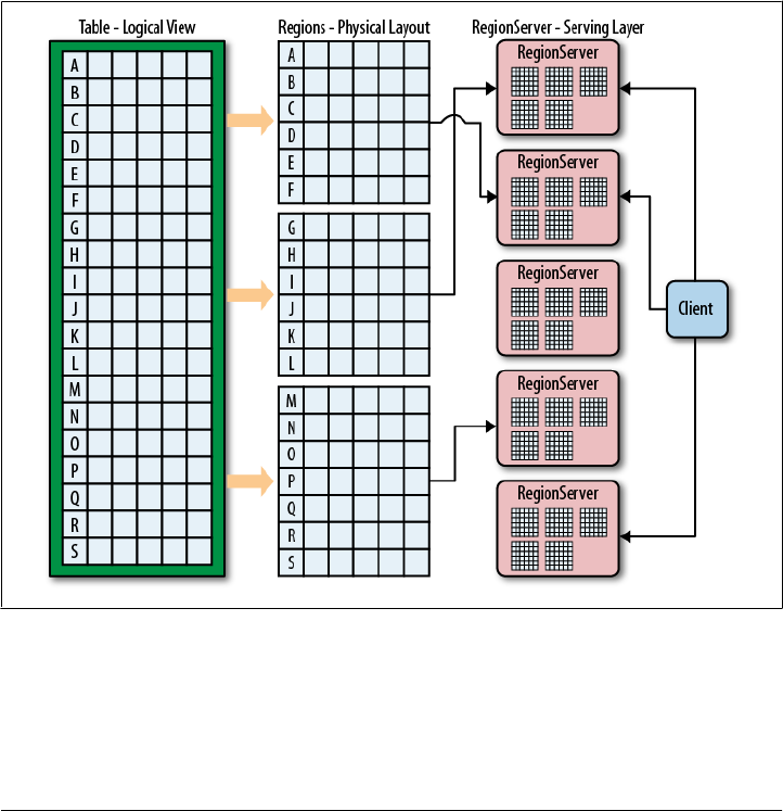
There are certain restrictions on the characters you can use to create a table name. The
name is used as part of the path to the actual storage files, and therefore complies with
filename rules. You can later browse the low-level storage system—for example,
HDFS—to see the tables as separate directories—in case you ever need to.
The column-oriented storage format of HBase allows you to store many details into the
same table, which, under relational database modeling, would be divided into many
separate tables. The usual database normalization* rules do not apply directly to HBase,
and therefore the number of tables is usually very low. More on this is discussed in
“Database (De-)Normalization” on page 13.
Although conceptually a table is a collection of rows with columns in HBase, physically
they are stored in separate partitions called regions. Figure 5-1 shows the difference
between the logical and physical layout of the stored data. Every region is served by
exactly one region server, which in turn serve the stored values directly to clients.
Figure 5-1. Logical and physical layout of rows within regions
* See “Database normalization” on Wikipedia.
Schema Definition | 209

Table Properties
The table descriptor offers getters and setters† to set other options of the table. In prac-
tice, a lot are not used very often, but it is important to know them all, as they can be
used to fine-tune the table’s performance.
Name
The constructor already had the parameter to specify the table name. The Java API
has additional methods to access the name or change it.
byte[] getName();
String getNameAsString();
void setName(byte[] name);
The name of a table must not start with a “.” (period) or a “-”
(hyphen). Furthermore, it can only contain Latin letters or num-
bers, as well as “_” (underscore), “-” (hyphen), or “.” (period). In
regular expression syntax, this could be expressed as [a-zA-
Z_0-9-.].
For example, .testtable is wrong, but test.table is allowed.
Refer to “Column Families” on page 212 for more details, and Figure 5-2 for an
example of how the table name is used to form a filesystem path.
Column families
This is the most important part of defining a table. You need to specify the column
families you want to use with the table you are creating.
void addFamily(HColumnDescriptor family);
boolean hasFamily(byte[] c);
HColumnDescriptor[] getColumnFamilies();
HColumnDescriptor getFamily(byte[]column);
HColumnDescriptor removeFamily(byte[] column);
You have the option of adding a family, checking if it exists based on its name,
getting a list of all known families, and getting or removing a specific one. More
on how to define the required HColumnDescriptor is explained in “Column Fami-
lies” on page 212.
Maximum file size
This parameter is specifying the maximum size a region within the table can grow
to. The size is specified in bytes and is read and set using the following methods:
long getMaxFileSize();
void setMaxFileSize(long maxFileSize);
† Getters and setters in Java are methods of a class that expose internal fields in a controlled manner. They are
usually named like the field, prefixed with get and set, respectively—for example, getName() and setName().
210 | Chapter 5: Client API: Administrative Features

Maximum file size is actually a misnomer, as it really is about the
maximum size of each store, that is, all the files belonging to each
column family. If one single column family exceeds this maximum
size, the region is split. Since in practice, this involves multiple files,
the better name would be maxStoreSize.
The maximum size is helping the system to split regions when they reach this
configured size. As discussed in “Building Blocks” on page 16, the unit of scalability
and load balancing in HBase is the region. You need to determine what a good
number for the size is, though. By default, it is set to 256 MB, which is good for
many use cases, but a larger value may be required when you have a lot of data.
Please note that this is more or less a desired maximum size and that, given certain
conditions, this size can be exceeded and actually be completely rendered without
effect. As an example, you could set the maximum file size to 10 MB and insert a
20 MB cell in one row. Since a row cannot be split across regions, you end up with
a region of at least 20 MB in size, and the system cannot do anything about it.
Read-only
By default, all tables are writable, but it may make sense to specify the read-only
option for specific tables. If the flag is set to true, you can only read from the table
and not modify it at all. The flag is set and read by these methods:
boolean isReadOnly();
void setReadOnly(boolean readOnly);
Memstore flush size
We discussed the storage model earlier and identified how HBase uses an in-
memory store to buffer values before writing them to disk as a new storage file in
an operation called flush. This parameter of the table controls when this is going
to happen and is specified in bytes. It is controlled by the following calls:
long getMemStoreFlushSize();
void setMemStoreFlushSize(long memstoreFlushSize);
As you do with the aforementioned maximum file size, you need to check your
requirements before setting this value to something other than the default 64
MB. A larger size means you are generating larger store files, which is good. On the
other hand, you might run into the problem of longer blocking periods, if the region
server cannot keep up with flushing the added data. Also, it increases the time
needed to replay the write-ahead log (the WAL) if the server crashes and all in-
memory updates are lost.
Deferred log flush
We will look into log flushing in great detail in “Write-Ahead Log” on page 333,
where this option is explained. For now, note that HBase uses one of two different
approaches to save write-ahead-log entries to disk. You either use deferred log
Schema Definition | 211

flushing or not. This is a boolean option and is, by default, set to false. Here is
how to access this parameter through the Java API:
synchronized boolean isDeferredLogFlush();
void setDeferredLogFlush(boolean isDeferredLogFlush);
Miscellaneous options
In addition to those already mentioned, there are methods that let you set arbitrary
key/value pairs:
byte[] getValue(byte[] key) {
String getValue(String key)
Map<ImmutableBytesWritable, ImmutableBytesWritable> getValues()
void setValue(byte[] key, byte[] value)
void setValue(String key, String value)
void remove(byte[] key)
They are stored with the table definition and can be retrieved if necessary.
One actual use case within HBase is the loading of coprocessors, as detailed in
“Coprocessor Loading” on page 179. You have a few choices in terms of how to
specify the key and value, either as a String, or as a byte array. Internally, they are
stored as ImmutableBytesWritable, which is needed for serialization purposes (see
“Writable and the Parameterless Constructor” on page 207).
Column Families
We just saw how the HTableDescriptor exposes methods to add column families to a
table. Similar to this is a class called HColumnDescriptor that wraps each column family’s
settings into a dedicated Java class. In other programming languages, you may find the
same concept or some other means of specifying the column family properties.
The class in Java is somewhat of a misnomer. A more appropriate name
would be HColumnFamilyDescriptor, which would indicate its purpose
to define column family parameters as opposed to actual columns.
Column families define shared features that apply to all columns that are created within
them. The client can create an arbitrary number of columns by simply using new column
qualifiers on the fly. Columns are addressed as a combination of the column family
name and the column qualifier (or sometimes also called the column key), divided by
a colon:
family:qualifier
The column family name must be composed of printable characters: the qualifier can
be composed of any arbitrary binary characters. Recall the Bytes class mentioned ear-
lier, which you can use to convert your chosen names to byte arrays. The reason why
the family name must be printable is that because the name is used as part of the
212 | Chapter 5: Client API: Administrative Features
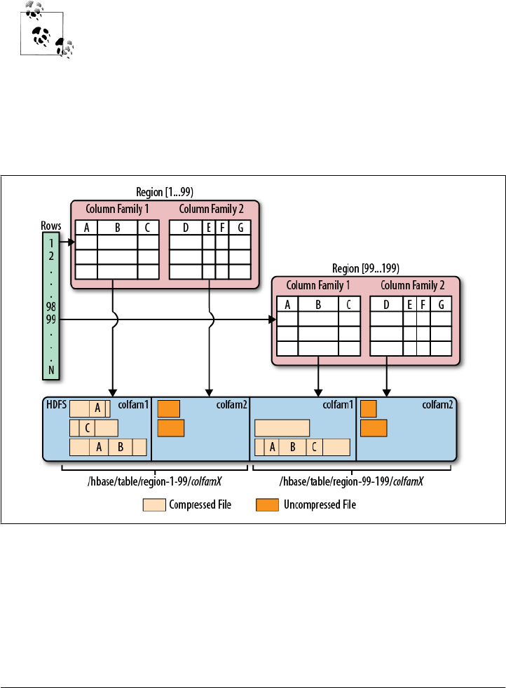
directory name by the lower-level storage layer. Figure 5-2 visualizes how the families
are mapped to storage files. The family name is added to the path and must comply
with filename standards. The advantage is that you can easily access families on the
filesystem level as you have the name in a human-readable format.
You should also be aware of the empty column qualifier. You can simply
omit the qualifier and specify just the column family name. HBase then
creates a column with the special empty qualifier. You can write and
read that column like any other, but obviously there is only one of those,
and you will have to name the other columns to distinguish them.
For simple applications, using no qualifier is an option, but it also carries
no meaning when looking at the data—for example, using the HBase
Shell. You should get used to naming your columns and do this from
the start, because you cannot simply rename them later.
Figure 5-2. Column families mapping to separate storage files
When you create a column family, you can specify a variety of parameters that control
all of its features. The Java class has many constructors that allow you to specify most
parameters while creating an instance. Here are the choices:
HColumnDescriptor();
HColumnDescriptor(String familyName),
HColumnDescriptor(byte[] familyName);
Schema Definition | 213
HColumnDescriptor(HColumnDescriptor desc);
HColumnDescriptor(byte[] familyName, int maxVersions, String compression,
boolean inMemory, boolean blockCacheEnabled, int timeToLive,
String bloomFilter);
HColumnDescriptor(byte [] familyName, int maxVersions, String compression,
boolean inMemory, boolean blockCacheEnabled, int blocksize,
int timeToLive, String bloomFilter, int scope);
The first one is only used internally for deserialization again. The next two simply take
a name as a String or byte[], the usual byte array we have seen many times now. There
is another one that takes an existing HColumnDescriptor and then two more that list all
available parameters.
Instead of using the constructor, you can also use the getters and setters to specify the
various details. We will now discuss each of them.
Name
Each column family has a name, and you can use the following methods to retrieve
it from an existing HColumnDescriptor instance:
byte[] getName();
String getNameAsString();
A column family cannot be renamed. The common approach to
rename a family is to create a new family with the desired name
and copy the data over, using the API.
You cannot set the name, but you have to use these constructors to hand it in. Keep
in mind the requirement for the name to be printable characters.
The name of a column family must not start with a “.” (period) and
not contain “:” (colon), “/” (slash), or ISO control characters, in
other words, if its code is in the range \u0000 through \u001F or in
the range \u007F through \u009F.
Maximum versions
Per family, you can specify how many versions of each value you want to keep.
Recall the predicate deletion mentioned earlier where the housekeeping of HBase
removes values that exceed the set maximum. Getting and setting the value is done
using the following API calls:
int getMaxVersions();
void setMaxVersions(int maxVersions);
The default value is 3, but you may reduce it to 1, for example, in case you know
for sure that you will never want to look at older values.
214 | Chapter 5: Client API: Administrative Features

Compression
HBase has pluggable compression algorithm support (you can find more on this
topic in “Compression” on page 424) that allows you to choose the best com-
pression—or none—for the data stored in a particular column family. The possible
algorithms are listed in Table 5-1.
Table 5-1. Supported compression algorithms
Value Description
NONE Disables compression (default)
GZ Uses the Java-supplied or native GZip compression
LZO Enables LZO compression; must be installed separately
SNAPPY Enables Snappy compression; binaries must be installed separately
The default value is NONE—in other words, no compression is enabled when you
create a column family. Once you deal with the Java API and a column descriptor,
you can use these methods to change the value:
Compression.Algorithm getCompression();
Compression.Algorithm getCompressionType();
void setCompressionType(Compression.Algorithm type);
Compression.Algorithm getCompactionCompression();
Compression.Algorithm getCompactionCompressionType();
void setCompactionCompressionType(Compression.Algorithm type);
Note how the value is not a String, but rather a Compression.Algorithm enumera-
tion that exposes the same values as listed in Table 5-1. The constructor of HCo
lumnDescriptor takes the same values as a string, though.
Another observation is that there are two sets of methods, one for the general
compression setting and another for the compaction compression setting. Also,
each group has a getCompression() and getCompressionType() (or
getCompactionCompression() and getCompactionCompressionType(), respectively)
returning the same type of value. They are indeed redundant, and you can use either
to retrieve the current compression algorithm type.‡
We will look into this topic in much greater detail in “Compression”
on page 424.
Block size
All stored files in HBase are divided into smaller blocks that are loaded during a
get or scan operation, analogous to pages in RDBMSes. The default is set to
64 KB and can be adjusted with these methods:
synchronized int getBlocksize();
void setBlocksize(int s);
‡ After all, this is open source and a redundancy like this is often caused by legacy code being carried forward.
Please feel free to help clean this up and to contribute back to the HBase project.
Schema Definition | 215

The value is specified in bytes and can be used to control how much data HBase
is required to read from the storage files during retrieval as well as what is cached
in memory for subsequent accesses. How this can be used to fine-tune your setup
can be found in “Configuration” on page 436.
There is an important distinction between the column family block
size, or HFile block size, and the block size specified on the HDFS
level. Hadoop, and HDFS specifically, is using a block size of—by
default—64 MB to split up large files for distributed, parallel pro-
cessing using the MapReduce framework. For HBase the HFile
block size is—again by default—64 KB, or one 1024th of the HDFS
block size. The storage files used by HBase are using this much
more fine-grained size to efficiently load and cache data in block
operations. It is independent from the HDFS block size and only
used internally. See “Storage” on page 319 for more details, espe-
cially Figure 8-3, which shows the two different block types.
Block cache
As HBase reads entire blocks of data for efficient I/O usage, it retains these blocks
in an in-memory cache so that subsequent reads do not need any disk operation.
The default of true enables the block cache for every read operation. But if your
use case only ever has sequential reads on a particular column family, it is advisable
that you disable it from polluting the block cache by setting the block cache-
enabled flag to false. Here is how the API can be used to change this flag:
boolean isBlockCacheEnabled();
void setBlockCacheEnabled(boolean blockCacheEnabled);
There are other options you can use to influence how the block cache is used, for
example, during a scan operation. This is useful during full table scans so that you
do not cause a major churn on the cache. See “Configuration” for more information
about this feature.
Time-to-live
HBase supports predicate deletions on the number of versions kept for each value,
but also on specific times. The time-to-live (or TTL) sets a threshold based on the
timestamp of a value and the internal housekeeping is checking automatically if a
value exceeds its TTL. If that is the case, it is dropped during major compactions.
The API provides the following getter and setter to read and write the TTL:
int getTimeToLive();
void setTimeToLive(int timeToLive);
The value is specified in seconds and is, by default, set to Integer.MAX_VALUE or
2,147,483,647 seconds. The default value also is treated as the special case of
keeping the values forever, that is, any positive value less than the default enables
this feature.
216 | Chapter 5: Client API: Administrative Features

In-memory
We mentioned the block cache and how HBase is using it to keep entire blocks of
data in memory for efficient sequential access to values. The in-memory flag de-
faults to false but can be modified with these methods:
boolean isInMemory();
void setInMemory(boolean inMemory);
Setting it to true is not a guarantee that all blocks of a family are loaded into memory
nor that they stay there. Think of it as a promise, or elevated priority, to keep them
in memory as soon as they are loaded during a normal retrieval operation, and until
the pressure on the heap (the memory available to the Java-based server processes)
is too high, at which time they need to be discarded by force.
In general, this setting is good for small column families with few values, such as
the passwords of a user table, so that logins can be processed very fast.
Bloom filter
An advanced feature available in HBase is Bloom filters,§ allowing you to improve
lookup times given you have a specific access pattern (see “Bloom Fil-
ters” on page 377 for details). Since they add overhead in terms of storage and
memory, they are turned off by default. Table 5-2 shows the possible options.
Table 5-2. Supported Bloom filter types
Type Description
NONE Disables the filter (default)
ROW Use the row key for the filter
ROWCOL Use the row key and column key (family+qualifier) for the filter
Because there are many more columns than rows (unless you only have a single
column in each row), the last option, ROWCOL, requires the largest amount of space.
It is more fine-grained, though, since it knows about each row/column combina-
tion, as opposed to just rows.
The Bloom filter can be changed and retrieved with these calls:
StoreFile.BloomType getBloomFilterType();
void setBloomFilterType(StoreFile.BloomType bt);
As with the compression value, these methods take a StoreFile.BloomType type,
while the constructor for the column descriptor lets you specify the aforementioned
types as a string. The letter casing is not important, so you can, for example, use
“row”. “Bloom Filters” has more on the Bloom filters and how to use them best.
§ See “Bloom filter” on Wikipedia.
Schema Definition | 217

Replication scope
Another more advanced feature coming with HBase is replication. It enables you
to have multiple clusters that ship local updates across the network so that they
are applied to the remote copies.
By default, replication is disabled and the replication scope is set to 0, meaning it is
disabled. You can change the scope with these functions:
int getScope();
void setScope(int scope);
The only other supported value (as of this writing) is 1, which enables replication
to a remote cluster. There may be more scope values in the future. See Table 5-3
for a list of supported values.
Table 5-3. Supported replication scopes
Scope Description
0 Local scope, i.e., no replication for this family (default)
1 Global scope, i.e., replicate family to a remote cluster
The full details can be found in “Replication” on page 462.
Finally, the Java class has a helper method to check if a family name is valid:
static byte[] isLegalFamilyName(byte[] b);
Use it in your program to verify user-provided input conforming to the specifications
that are required for the name. It does not return a boolean flag, but throws an
IllegalArgumentException when the name is malformed. Otherwise, it returns the given
parameter value unchanged. The fully specified constructors shown earlier use this
method internally to verify the given name; in this case, you do not need to call the
method beforehand.
HBaseAdmin
Just as with the client API, you also have an API for administrative tasks at your disposal.
Compare this to the Data Definition Language (DDL) found in RDBMSes—while the
client API is more an analog to the Data Manipulation Language (DML).
It provides operations to create tables with specific column families, check for table
existence, alter table and column family definitions, drop tables, and much more. The
provided functions can be grouped into related operations; they’re discussed separately
on the following pages.
218 | Chapter 5: Client API: Administrative Features
Basic Operations
Before you can use the administrative API, you will have to create an instance of the
HBaseAdmin class. The constructor is straightforward:
HBaseAdmin(Configuration conf)
throws MasterNotRunningException, ZooKeeperConnectionException
This section omits the fact that most methods may throw either an
IOException (or an exception that inherits from it), or an
InterruptedException. The former is usually a result of a communica-
tion error between your client application and the remote servers. The
latter is caused by an event that interrupts a running operation, for ex-
ample, when the region server executing the command is shut down
before being able to complete it.
Handing in an existing configuration instance gives enough details to the API to find
the cluster using the ZooKeeper quorum, just like the client API does. Use the admin-
istrative API instance for the operation required and discard it afterward. In other
words, you should not hold on to the instance for too long.
The HBaseAdmin instances should be short-lived as they do not, for ex-
ample, handle master failover gracefully right now.
The class implements the Abortable interface, adding the following call to it:
void abort(String why, Throwable e)
This method is called by the framework implicitly—for example, when there is a fatal
connectivity issue and the API should be stopped. You should not call it directly, but
rely on the system taking care of invoking it, in case of dire emergencies, that require
a complete shutdown—and possible restart—of the API instance.
You can get access to the remote master using:
HMasterInterface getMaster()
throws MasterNotRunningException, ZooKeeperConnectionException
This will return an RPC proxy instance of HMasterInterface, allowing you to commu-
nicate directly with the master server. This is not required because the HBaseAdmin class
provides a convenient wrapper to all calls exposed by the master interface.
HBaseAdmin | 219

Do not use the HMasterInterface returned by getMaster() directly, un-
less you are sure what you are doing. The wrapper functions in
HBaseAdmin perform additional work—for example, checking that the
input parameters are valid, converting remote exceptions to client ex-
ceptions, or adding the ability to run inherently asynchronous opera-
tions as if they were synchronous.
In addition, the HBaseAdmin class also exports these basic calls:
boolean isMasterRunning()
Checks if the master server is running. You may use it from your client application
to verify that you can communicate with the master, before instantiating the
HBaseAdmin class.
HConnection getConnection()
Returns a connection instance. See “Connection Handling” on page 203 for details
on the returned class type.
Configuration getConfiguration()
Gives you access to the configuration that was used to create the current
HBaseAdmin instance. You can use it to modify the configuration for a running ad-
ministrative API instance.
close()
Closes all resources kept by the current HBaseAdmin instance. This includes the
connection to the remote servers.
Table Operations
After the first set of basic operations, there is a group of calls related to HBase tables.
These calls help when working with the tables themselves, not the actual schemas
inside. The commands addressing this are in “Schema Operations” on page 228.
Before you can do anything with HBase, you need to create tables. Here is the set of
functions to do so:
void createTable(HTableDescriptor desc)
void createTable(HTableDescriptor desc, byte[] startKey,
byte[] endKey, int numRegions)
void createTable(HTableDescriptor desc, byte[][] splitKeys)
void createTableAsync(HTableDescriptor desc, byte[][] splitKeys)
All of these calls must be given an instance of HTableDescriptor, as described in detail
in “Tables” on page 207. It holds the details of the table to be created, including the
column families. Example 5-1 uses the simple variant of createTable() that just takes
a table name.
220 | Chapter 5: Client API: Administrative Features
Example 5-1. Using the administrative API to create a table
Configuration conf = HBaseConfiguration.create();
HBaseAdmin admin = new HBaseAdmin(conf);
HTableDescriptor desc = new HTableDescriptor(
Bytes.toBytes("testtable"));
HColumnDescriptor coldef = new HColumnDescriptor(
Bytes.toBytes("colfam1"));
desc.addFamily(coldef);
admin.createTable(desc);
boolean avail = admin.isTableAvailable(Bytes.toBytes("testtable"));
System.out.println("Table available: " + avail);
Create an administrative API instance.
Create the table descriptor instance.
Create a column family descriptor and add it to the table descriptor.
Call the createTable() method to do the actual work.
Check if the table is available.
The other createTable() versions have an additional—yet more advanced—feature set:
they allow you to create tables that are already populated with specific regions. The
code in Example 5-2 uses both possible ways to specify your own set of region
boundaries.
Example 5-2. Using the administrative API to create a table with predefined regions
private static void printTableRegions(String tableName) throws IOException {
System.out.println("Printing regions of table: " + tableName);
HTable table = new HTable(Bytes.toBytes(tableName));
Pair<byte[][], byte[][]> pair = table.getStartEndKeys();
for (int n = 0; n < pair.getFirst().length; n++) {
byte[] sk = pair.getFirst()[n];
byte[] ek = pair.getSecond()[n];
System.out.println("[" + (n + 1) + "]" +
" start key: " +
(sk.length == 8 ? Bytes.toLong(sk) : Bytes.toStringBinary(sk)) +
", end key: " +
(ek.length == 8 ? Bytes.toLong(ek) : Bytes.toStringBinary(ek)));
}
}
public static void main(String[] args) throws IOException, InterruptedException {
Configuration conf = HBaseConfiguration.create();
HBaseAdmin admin = new HBaseAdmin(conf);
HTableDescriptor desc = new HTableDescriptor(
Bytes.toBytes("testtable1"));
HColumnDescriptor coldef = new HColumnDescriptor(
HBaseAdmin | 221
Bytes.toBytes("colfam1"));
desc.addFamily(coldef);
admin.createTable(desc, Bytes.toBytes(1L), Bytes.toBytes(100L), 10);
printTableRegions("testtable1");
byte[][] regions = new byte[][] {
Bytes.toBytes("A"),
Bytes.toBytes("D"),
Bytes.toBytes("G"),
Bytes.toBytes("K"),
Bytes.toBytes("O"),
Bytes.toBytes("T")
};
desc.setName(Bytes.toBytes("testtable2"));
admin.createTable(desc, regions);
printTableRegions("testtable2");
}
Helper method to print the regions of a table.
Retrieve the start and end keys from the newly created table.
Print the key, but guarding against the empty start (and end) key.
Call the createTable() method while also specifying the region boundaries.
Manually create region split keys.
Call the createTable() method again, with a new table name and the list of region
split keys.
Running the example should yield the following output on the console:
Printing regions of table: testtable1
[1] start key: , end key: 1
[2] start key: 1, end key: 13
[3] start key: 13, end key: 25
[4] start key: 25, end key: 37
[5] start key: 37, end key: 49
[6] start key: 49, end key: 61
[7] start key: 61, end key: 73
[8] start key: 73, end key: 85
[9] start key: 85, end key: 100
[10] start key: 100, end key:
Printing regions of table: testtable2
[1] start key: , end key: A
[2] start key: A, end key: D
[3] start key: D, end key: G
[4] start key: G, end key: K
[5] start key: K, end key: O
[6] start key: O, end key: T
[7] start key: T, end key:
The example uses a method of the HTable class that you saw earlier, getStartEnd
Keys(), to retrieve the region boundaries. The first start and the last end keys are empty,
222 | Chapter 5: Client API: Administrative Features
as is customary with HBase regions. In between the keys are either the computed, or
the provided split keys. Note how the end key of a region is also the start key of the
subsequent one—just that it is exclusive for the former, and inclusive for the latter,
respectively.
The createTable(HTableDescriptor desc, byte[] startKey, byte[] endKey, int num
Regions) call takes a start and end key, which is interpreted as numbers. You must
provide a start value that is less than the end value, and a numRegions that is at least 3:
otherwise, the call will return with an exception. This is to ensure that you end up with
at least a minimum set of regions.
The start and end key values are subtracted and divided by the given number of regions
to compute the region boundaries. In the example, you can see how we end up with
the correct number of regions, while the computed keys are filling in the range.
The createTable(HTableDescriptor desc, byte[][] splitKeys) method used in the
second part of the example, on the other hand, is expecting an already set array of split
keys: they form the start and end keys of the regions created. The output of the example
demonstrates this as expected.
The createTable() calls are, in fact, related. The createTable(HTable
Descriptor desc, byte[] startKey, byte[] endKey, int numRegions)
method is calculating the region keys implicitly for you, using the
Bytes.split() method to use your given parameters to compute the
boundaries. It then proceeds to call the createTable(HTableDescriptor
desc, byte[][] splitKeys), doing the actual table creation.
Finally, there is the createTableAsync(HTableDescriptor desc, byte[][] splitKeys)
method that is taking the table descriptor, and region keys, to asynchronously perform
the same task as the createTable() call.
Most of the table-related administrative API functions are asynchronous
in nature, which is useful, as you can send off a command and not have
to deal with waiting for a result. For a client application, though, it is
often necessary to know if a command has succeeded before moving on
with other operations. For that, the calls are provided in
asynchronous—using the Async postfix—and synchronous versions.
In fact, the synchronous commands are simply a wrapper around the
asynchronous ones, adding a loop at the end of the call to repeatedly
check for the command to have done its task. The createTable()
method, for example, wraps the createTableAsync() method, while
adding a loop that waits for the table to be created on the remote servers
before yielding control back to the caller.
HBaseAdmin | 223

Once you have created a table, you can use the following helper functions to retrieve
the list of tables, retrieve the descriptor for an existing table, or check if a table exists:
boolean tableExists(String tableName)
boolean tableExists(byte[] tableName)
HTableDescriptor[] listTables()
HTableDescriptor getTableDescriptor(byte[] tableName)
Example 5-1 uses the tableExists() method to check if the previous command to create
the table has succeeded. The listTables() returns a list of HTableDescriptor instances
for every table that HBase knows about, while the getTableDescriptor() method is
returning it for a specific one. Example 5-3 uses both to show what is returned by the
administrative API.
Example 5-3. Listing the existing tables and their descriptors
HBaseAdmin admin = new HBaseAdmin(conf);
HTableDescriptor[] htds = admin.listTables();
for (HTableDescriptor htd : htds) {
System.out.println(htd);
}
HTableDescriptor htd1 = admin.getTableDescriptor(
Bytes.toBytes("testtable1"));
System.out.println(htd1);
HTableDescriptor htd2 = admin.getTableDescriptor(
Bytes.toBytes("testtable10"));
System.out.println(htd2);
The console output is quite long, since every table descriptor is printed, including every
possible property. Here is an abbreviated version:
Printing all tables...
{NAME => 'testtable1', FAMILIES => [{NAME => 'colfam1', BLOOMFILTER =>
'NONE', REPLICATION_SCOPE => '0', COMPRESSION => 'NONE', VERSIONS => '3',
TTL => '2147483647', BLOCKSIZE => '65536', IN_MEMORY => 'false', BLOCKCACHE
=> 'true'}, {NAME => 'colfam2', BLOOMFILTER => 'NONE', REPLICATION_SCOPE
=> '0', COMPRESSION => 'NONE', VERSIONS => '3', TTL => '2147483647',
BLOCKSIZE => '65536', IN_MEMORY => 'false', BLOCKCACHE => 'true'}, {NAME =>
'colfam3', BLOOMFILTER => 'NONE', REPLICATION_SCOPE => '0', COMPRESSION =>
'NONE', VERSIONS => '3', TTL => '2147483647', BLOCKSIZE => '65536',
IN_MEMORY => 'false', BLOCKCACHE => 'true'}]}
...
Exception org.apache.hadoop.hbase.TableNotFoundException: testtable10
...
at ListTablesExample.main(ListTablesExample.java)
The interesting part is the exception you should see being printed as well. The example
uses a nonexistent table name to showcase the fact that you must be using existing table
names—or wrap the call into a try/catch guard, handling the exception more
gracefully.
224 | Chapter 5: Client API: Administrative Features

After creating a table, it is time to also be able to delete them. The HBaseAdmin calls to
do so are:
void deleteTable(String tableName)
void deleteTable(byte[] tableName)
Hand in a table name as a String, or a byte array, and the rest is taken care of: the table
is removed from the servers, and all data deleted.
But before you can delete a table, you need to ensure that it is first disabled, using the
following methods:
void disableTable(String tableName)
void disableTable(byte[] tableName)
void disableTableAsync(String tableName)
void disableTableAsync(byte[] tableName)
Disabling the table first tells every region server to flush any uncommitted changes to
disk, close all the regions, and update the .META. table to reflect that no region of this
table is not deployed to any servers.
The choices are again between doing this asynchronously, or synchronously, and sup-
plying the table name in various formats for convenience.
Disabling a table can potentially take a very long time, up to several
minutes. This depends on how much data is residual in the server’s
memory and not yet persisted to disk. Undeploying a region requires all
the data to be written to disk first, and if you have a large heap value set
for the servers this may result in megabytes, if not even gigabytes, of
data being saved. In a heavily loaded system this could contend with
other processes writing to disk, and therefore require time to complete.
Once a table has been disabled, but not deleted, you can enable it again:
void enableTable(String tableName)
void enableTable(byte[] tableName)
void enableTableAsync(String tableName)
void enableTableAsync(byte[] tableName)
This call—again available in the usual flavors—reverses the disable operation by de-
ploying the regions of the given table to the active region servers. Finally, there is a set
of calls to check on the status of a table:
boolean isTableEnabled(String tableName)
boolean isTableEnabled(byte[] tableName)
boolean isTableDisabled(String tableName)
boolean isTableDisabled(byte[] tableName)
boolean isTableAvailable(byte[] tableName)
boolean isTableAvailable(String tableName)
Example 5-4 uses various combinations of the preceding calls to create, delete, disable,
and check the state of a table.
HBaseAdmin | 225

Example 5-4. Using the various calls to disable, enable, and check the status of a table
HBaseAdmin admin = new HBaseAdmin(conf);
HTableDescriptor desc = new HTableDescriptor(
Bytes.toBytes("testtable"));
HColumnDescriptor coldef = new HColumnDescriptor(
Bytes.toBytes("colfam1"));
desc.addFamily(coldef);
admin.createTable(desc);
try {
admin.deleteTable(Bytes.toBytes("testtable"));
} catch (IOException e) {
System.err.println("Error deleting table: " + e.getMessage());
}
admin.disableTable(Bytes.toBytes("testtable"));
boolean isDisabled = admin.isTableDisabled(Bytes.toBytes("testtable"));
System.out.println("Table is disabled: " + isDisabled);
boolean avail1 = admin.isTableAvailable(Bytes.toBytes("testtable"));
System.out.println("Table available: " + avail1);
admin.deleteTable(Bytes.toBytes("testtable"));
boolean avail2 = admin.isTableAvailable(Bytes.toBytes("testtable"));
System.out.println("Table available: " + avail2);
admin.createTable(desc);
boolean isEnabled = admin.isTableEnabled(Bytes.toBytes("testtable"));
System.out.println("Table is enabled: " + isEnabled);
The output on the console should look like this (the exception printout was abbrevi-
ated, for the sake of brevity):
Creating table...
Deleting enabled table...
Error deleting table:
org.apache.hadoop.hbase.TableNotDisabledException: testtable
...
Disabling table...
Table is disabled: true
Table available: true
Deleting disabled table...
Table available: false
Creating table again...
Table is enabled: true
The error thrown when trying to delete an enabled table shows that you either disable
it first, or handle the exception gracefully in case that is what your client application
requires. You could prompt the user to disable the table explicitly and retry the
operation.
226 | Chapter 5: Client API: Administrative Features
Also note how the isTableAvailable() is returning true, even when the table is disabled.
In other words, this method checks if the table is physically present, no matter what
its state is. Use the other two functions, isTableEnabled() and isTableDisabled(), to
check for the state of the table.
After creating your tables with the specified schema, you must either delete the newly
created table to change the details, or use the following method to alter its structure:
void modifyTable(byte[] tableName, HTableDescriptor htd)
As with the aforementioned deleteTable() commands, you must first disable the table
to be able to modify it. Example 5-5 does create a table, and subsequently modifies it.
Example 5-5. Modifying the structure of an existing table
byte[] name = Bytes.toBytes("testtable");
HBaseAdmin admin = new HBaseAdmin(conf);
HTableDescriptor desc = new HTableDescriptor(name);
HColumnDescriptor coldef1 = new HColumnDescriptor(
Bytes.toBytes("colfam1"));
desc.addFamily(coldef1);
admin.createTable(desc);
HTableDescriptor htd1 = admin.getTableDescriptor(name);
HColumnDescriptor coldef2 = new HColumnDescriptor(
Bytes.toBytes("colfam2"));
htd1.addFamily(coldef2);
htd1.setMaxFileSize(1024 * 1024 * 1024L);
admin.disableTable(name);
admin.modifyTable(name, htd1);
admin.enableTable(name);
HTableDescriptor htd2 = admin.getTableDescriptor(name);
System.out.println("Equals: " + htd1.equals(htd2));
System.out.println("New schema: " + htd2);
Create the table with the original structure.
Get the schema, and update by adding a new family and changing the maximum file
size property.
Disable, modify, and enable the table.
Check if the table schema matches the new one created locally.
The output shows that both the schema modified in the client code and the final schema
retrieved from the server after the modification are consistent:
Equals: true
New schema: {NAME => 'testtable', MAX_FILESIZE => '1073741824', FAMILIES =>
[{NAME => 'colfam1', BLOOMFILTER => 'NONE', REPLICATION_SCOPE => '0',
COMPRESSION => 'NONE', VERSIONS => '3', TTL => '2147483647', BLOCKSIZE =>
'65536', IN_MEMORY => 'false', BLOCKCACHE => 'true'}, {NAME => 'colfam2',
HBaseAdmin | 227

BLOOMFILTER => 'NONE', REPLICATION_SCOPE => '0', COMPRESSION => 'NONE',
VERSIONS => '3', TTL => '2147483647', BLOCKSIZE => '65536', IN_MEMORY =>
'false', BLOCKCACHE => 'true'}]}
Calling the equals() method on the HTableDescriptor class compares the current with
the specified instance and returns true if they match in all properties, also including
the contained column families and their respective settings.
The modifyTable() call is asynchronous, and there is no synchronous
variant. If you want to make sure that changes have been propagated to
all the servers and applied accordingly, you should use the
getTableDescriptor() call and loop over it in your client code until the
schema you sent matches up with the remote schema.
Schema Operations
Besides using the modifyTable() call, there are dedicated methods provided by the
HBaseAdmin class to modify specific aspects of the current table schema. As usual, you
need to make sure the table to be modified is disabled first.
The whole set of column-related methods is as follows:
void addColumn(String tableName, HColumnDescriptor column)
void addColumn(byte[] tableName, HColumnDescriptor column)
void deleteColumn(String tableName, String columnName)
void deleteColumn(byte[] tableName, byte[] columnName)
void modifyColumn(String tableName, HColumnDescriptor descriptor)
void modifyColumn(byte[] tableName, HColumnDescriptor descriptor)
You can add, delete, and modify columns. Adding or modifying a column requires that
you first prepare an HColumnDescriptor instance, as described in detail in “Column
Families” on page 212. Alternatively, you could use the getTableDescriptor() call to
retrieve the current table schema, and subsequently invoke getColumnFamilies() on the
returned HTableDescriptor instance to retrieve the existing columns.
Otherwise, you supply the table name—and optionally the column name for the delete
calls—in one of the common format variations to eventually invoke the method of
choice. All of these calls are asynchronous, so as mentioned before, caveat emptor.
Use Case: Hush
An interesting use case for the administrative API is to create and alter tables and their
schemas based on an external configuration file. Hush is making use of this idea and
defines the table and column descriptors in an XML file, which is read and the contained
schema compared with the current table definitions. If there are any differences they
are applied accordingly. The following example has the core of the code that does this
task:
private void createOrChangeTable(final TableSchema schema)
throws IOException {
228 | Chapter 5: Client API: Administrative Features
HTableDescriptor desc = null;
if (tableExists(schema.getName(), false)) {
desc = getTable(schema.getName(), false);
LOG.info("Checking table " + desc.getNameAsString() + "...");
final HTableDescriptor d = convertSchemaToDescriptor(schema);
final List<HColumnDescriptor> modCols =
new ArrayList<HColumnDescriptor>();
for (final HColumnDescriptor cd : desc.getFamilies()) {
final HColumnDescriptor cd2 = d.getFamily(cd.getName());
if (cd2 != null && !cd.equals(cd2)) {
modCols.add(cd2);
}
}
final List<HColumnDescriptor> delCols =
new ArrayList<HColumnDescriptor>(desc.getFamilies());
delCols.removeAll(d.getFamilies());
final List<HColumnDescriptor> addCols =
new ArrayList<HColumnDescriptor>(d.getFamilies());
addCols.removeAll(desc.getFamilies());
if (modCols.size() > 0 || addCols.size() > 0 || delCols.size() > 0 ||
!hasSameProperties(desc, d)) {
LOG.info("Disabling table...");
hbaseAdmin.disableTable(schema.getName());
if (modCols.size() > 0 || addCols.size() > 0 || delCols.size() > 0) {
for (final HColumnDescriptor col : modCols) {
LOG.info("Found different column -> " + col);
hbaseAdmin.modifyColumn(schema.getName(), col.getNameAsString(),
col);
}
for (final HColumnDescriptor col : addCols) {
LOG.info("Found new column -> " + col);
hbaseAdmin.addColumn(schema.getName(), col);
}
for (final HColumnDescriptor col : delCols) {
LOG.info("Found removed column -> " + col);
hbaseAdmin.deleteColumn(schema.getName(), col.getNameAsString());
}
} else if (!hasSameProperties(desc, d)) {
LOG.info("Found different table properties...");
hbaseAdmin.modifyTable(Bytes.toBytes(schema.getName()), d);
}
LOG.info("Enabling table...");
hbaseAdmin.enableTable(schema.getName());
LOG.info("Table enabled");
desc = getTable(schema.getName(), false);
LOG.info("Table changed");
} else {
LOG.info("No changes detected!");
}
} else {
desc = convertSchemaToDescriptor(schema);
LOG.info("Creating table " + desc.getNameAsString() + "...");
hbaseAdmin.createTable(desc);
LOG.info("Table created");
}
}
HBaseAdmin | 229

Compute the differences between the XML-based schema and what is currently in
HBase.
See if there are any differences in the column and table definitions.
Alter the columns that have changed. The table was properly disabled first.
Add newly defined columns.
Delete removed columns.
Alter the table itself, if there are any differences found.
If the table did not exist yet, create it now.
Cluster Operations
The last group of operations the HBaseAdmin class exposes is related to cluster opera-
tions. They allow you to check the status of the cluster, and perform tasks on tables
and/or regions. “The Region Life Cycle” on page 348 has the details on regions and
their life cycle.
Many of the following operations are for advanced users, so please han-
dle with care.
static void checkHBaseAvailable(Configuration conf)
ClusterStatus getClusterStatus()
You can use checkHBaseAvailable() to verify that your client application can com-
municate with the remote HBase cluster, as specified in the given configuration
file. If it fails to do so, an exception is thrown—in other words, this method does
not return a boolean flag, but either silently succeeds, or throws said error.
The getClusterStatus() call allows you to retrieve an instance of the Clus
terStatus class, containing detailed information about the cluster status. See
“Cluster Status Information” on page 233 for what you are provided with.
void closeRegion(String regionname, String hostAndPort)
void closeRegion(byte[] regionname, String hostAndPort)
Use these calls to close regions that have previously been deployed to region servers.
Any enabled table has all regions enabled, so you could actively close and undeploy
a region.
You need to supply the exact regionname as stored in the .META. table. Further, you
may optionally supply the hostAndPort parameter, that overrides the server assign-
ment as found in the .META. as well.
Using this close call does bypass any master notification, that is, the region is di-
rectly closed by the region server, unseen by the master node.
230 | Chapter 5: Client API: Administrative Features

void flush(String tableNameOrRegionName)
void flush(byte[] tableNameOrRegionName)
As updates to a region (and the table in general) accumulate the MemStore instances
of the region, servers fill with unflushed modifications. A client application
can use these synchronous methods to flush such pending records to disk, before
they are implicitly written by hitting the memstore flush size (see “Table Proper-
ties” on page 210) at a later time.
The method takes either a region name, or a table name. The value provided by
your code is tested to see if it matches an existing table; if it does, it is assumed to
be a table, otherwise it is treated as a region name. If you specify neither a proper
table nor a region name, an UnknownRegionException is thrown.
void compact(String tableNameOrRegionName)
void compact(byte[] tableNameOrRegionName)
Similar to the preceding operations, you must give either a table or a region name.
The call itself is asynchronous, as compactions can potentially take a long time to
complete. Invoking this method queues the table, or region, for compaction, which
is executed in the background by the server hosting the named region, or by all
servers hosting any region of the given table (see “Auto-Sharding” on page 21 for
details on compactions).
void majorCompact(String tableNameOrRegionName)
void majorCompact(byte[] tableNameOrRegionName)
These are the same as the compact() calls, but they queue the region, or table, for
a major compaction instead. In case a table name is given, the administrative API
iterates over all regions of the table and invokes the compaction call implicitly for
each of them.
void split(String tableNameOrRegionName)
void split(byte[] tableNameOrRegionName)
void split(String tableNameOrRegionName, String splitPoint)
void split(byte[] tableNameOrRegionName, byte[] splitPoint)
Using these calls allows you to split a specific region, or table. In case a table name
is given, it iterates over all regions of that table and implicitly invokes the split
command on each of them.
A noted exception to this rule is when the splitPoint parameter is given. In that
case, the split() command will try to split the given region at the provided row
key. In the case of specifying a table name, all regions are checked and the one
containing the splitPoint is split at the given key.
The splitPoint must be a valid row key, and—in case you specify a region
name—be part of the region to be split. It also must be greater than the region’s
start key, since splitting a region at its start key would make no sense. If you fail to
give the correct row key, the split request is ignored without reporting back to the
client. The region server currently hosting the region will log this locally with the
following message:
HBaseAdmin | 231

Split row is not inside region key range or is equal to startkey:
<split row>
void assign(byte[] regionName, boolean force)
void unassign(byte[] regionName, boolean force)
When a client requires a region to be deployed or undeployed from the region
servers, it can invoke these calls. The first would assign a region, based on the
overall assignment plan, while the second would unassign the given region.
The force parameter set to true has different meanings for each of the calls: first,
for assign(), it forces the region to be marked as unassigned in ZooKeeper before
continuing in its attempt to assign the region to a new region server. Be careful
when using this on already-assigned regions.
Second, for unassign(), it means that a region already marked to be unassigned—
for example, from a previous call to unassign()—is forced to be unassigned again.
If force were set to false, this would have no effect.
void move(byte[] encodedRegionName, byte[] destServerName)
Using the move() call enables a client to actively control which server is hosting
what regions. You can move a region from its current region server to a new one.
The destServerName parameter can be set to null to pick a new server at random;
otherwise, it must be a valid server name, running a region server process. If the
server name is wrong, or currently not responding, the region is deployed to a
different server instead. In a worst-case scenario, the move could fail and leave the
region unassigned.
boolean balanceSwitch(boolean b)
boolean balancer()
The first method allows you to switch the region balancer on or off. When the
balancer is enabled, a call to balancer() will start the process of moving regions
from the servers, with more deployed to those with less deployed regions. “Load
Balancing” on page 432 explains how this works in detail.
void shutdown()
void stopMaster() {
void stopRegionServer(String hostnamePort)
These calls either shut down the entire cluster, stop the master server, or stop a
particular region server only. Once invoked, the affected servers will be stopped,
that is, there is no delay nor a way to revert the process.
Chapters 8 and 11 have more information on these advanced—yet very powerful—
features. Use with utmost care!
232 | Chapter 5: Client API: Administrative Features

Cluster Status Information
When you query the cluster status using the HBaseAdmin.getClusterStatus() call, you
will be given a ClusterStatus instance, containing all the information the master server
has about the current state of the cluster. Note that this class also has setters—methods
starting with set, allowing you to modify the information they contain—but since you
will be given a copy of the current state, it is impractical to call the setters, unless you
want to modify your local-only copy.
Table 5-4 lists the methods of the ClusterStatus class.
Table 5-4. Quick overview of the information provided by the ClusterStatus class
Method Description
int getServersSize() The number of region servers currently live as known to the master server. The number
does not include the number of dead servers.
Collection<ServerName>
getServers()
The list of live servers. The names in the collection are ServerName instances, which
contain the hostname, RPC port, and start code.
int getDeadServers() The number of servers listed as dead. This does not contain the live servers.
Collection<ServerName>
getDeadServerNames()
A list of all server names currently considered dead. The names in the collection are
ServerName instances, which contain the hostname, RPC port, and start code.
double getAverageLoad() The total average number of regions per region server. This is the same currently as
getRegionsCount()/getServers().
int getRegionsCount() The total number of regions in the cluster.
int getRequestsCount() The current number of requests across all regions’ servers in the cluster.
String getHBaseVersion() Returns the HBase version identification string.
byte getVersion() Returns the version of the ClusterStatus instance. This is used during the serial-
ization process of sending an instance over RPC.
String getClusterId() Returns the unique identifier for the cluster. This is a UUID generated when HBase starts
with an empty storage directory. It is stored in hbase.id under the root directory.
Map<String, RegionState>
getRegionsInTransition()
Gives you access to a map of all regions currently in transition, e.g., being moved,
assigned, or unassigned. The key of the map is the encoded region name (as returned
by HRegionInfo.getEncodedName(), for example), while the value is an in-
stance of RegionState.a
HServerLoad get
Load(ServerName sn)
Retrieves the status information available for the given server name.
aSee “The Region Life Cycle” on page 348 for the details.
Accessing the overall cluster status gives you a high-level view of what is going on with
your servers—as a whole. Using the getServers() array, and the returned ServerName
instances, lets you drill further into each actual live server, and see what it is doing
currently. Table 5-5 lists the available methods.
HBaseAdmin | 233

Table 5-5. Quick overview of the information provided by the ServerName class
Method Description
String getHostname() Returns the hostname of the server. This might resolve to the IP address, when the
hostname cannot be looked up.
String getHostAndPort() Concatenates the hostname and RPC port, divided by a colon:
<hostname>:<rpc-port>.
long getStartcode() The start code is the epoch time in milliseconds of when the server was started, as
returned by System.currentTimeMillis().
String getServerName() The server name, consisting of <hostname>,<rpc-port>,<start-code>.
int getPort() Specifies the port used by the server for the RPCs.
Each server also exposes details about its load, by offering an HServerLoad instance,
returned by the getLoad() method of the ClusterStatus instance. Using the aforemen-
tioned ServerName, as returned by the getServers() call, you can iterate over all live
servers and retrieve their current details. The HServerLoad class gives you access to not
just the load of the server itself, but also for each hosted region. Table 5-6 lists the
provided methods.
Table 5-6. Quick overview of the information provided by the HServerLoad class
Method Description
byte getVersion() Returns the version of the HServerLoad instance. This is used
during the serialization process of sending an instance over RPC.
int getLoad() Currently returns the same value as getNumberOfRegions().
int getNumberOfRegions() The number of regions on the current server.
int getNumberOfRequests() Returns the number of requests accumulated within the last
hbase.regionserver.msginterval time frame. It is reset
at the end of this time frame, and counts all API requests, such as
gets, puts, increments, deletes, and so on.
int getUsedHeapMB() The currently used Java Runtime heap size in megabytes.
int getMaxHeapMB() The configured maximum Java Runtime heap size in megabytes.
int getStorefiles() The number of store files in use by the server. This is across all regions
it hosts.
int getStorefileSizeInMB() The total size in megabytes of the used store files.
int getStorefileIndexSizeInMB() The total size in megabytes of the indexes—the block and meta
index, to be precise—across all store files in use by this server.
int getMemStoreSizeInMB() The total size of the in-memory stores, across all regions hosted by
this server.
Map<byte[], RegionLoad> getRegions
Load()
Returns a map containing the load details for each hosted region of
the current server. The key is the region name and the value an
instance of the RegionsLoad class, discussed next.
234 | Chapter 5: Client API: Administrative Features

Finally, there is a dedicated class for the region load, aptly named RegionLoad. See
Table 5-7 for the list of provided information.
Table 5-7. Quick overview of the information provided by the RegionLoad class
Method Description
byte[] getName() The region name in its raw, byte[] byte array form.
String getNameAsString() Converts the raw region name into a String for convenience.
int getStores() The number of stores in this region.
int getStorefiles() The number of store files, across all stores of this region.
int getStorefileSizeMB() The size in megabytes of the store files for this region.
int getStorefileIndexSizeMB() The size of the indexes for all store files, in megabytes, for this region.
int getMemStoreSizeMB() The heap size in megabytes as used by the MemStore of the current region.
long getRequestsCount() The number of requests for the current region.
long getReadRequestsCount() The number of read requests for this region, since it was deployed to the
region server. This counter is not reset.
long getWriteRequestsCount() The number of write requests for this region, since it was deployed to the
region server. This counter is not reset.
Example 5-6 shows all of the getters in action.
Example 5-6. Reporting the status of a cluster
HBaseAdmin admin = new HBaseAdmin(conf);
ClusterStatus status = admin.getClusterStatus();
System.out.println("Cluster Status:\n--------------");
System.out.println("HBase Version: " + status.getHBaseVersion());
System.out.println("Version: " + status.getVersion());
System.out.println("No. Live Servers: " + status.getServersSize());
System.out.println("Cluster ID: " + status.getClusterId());
System.out.println("Servers: " + status.getServers());
System.out.println("No. Dead Servers: " + status.getDeadServers());
System.out.println("Dead Servers: " + status.getDeadServerNames());
System.out.println("No. Regions: " + status.getRegionsCount());
System.out.println("Regions in Transition: " +
status.getRegionsInTransition());
System.out.println("No. Requests: " + status.getRequestsCount());
System.out.println("Avg Load: " + status.getAverageLoad());
System.out.println("\nServer Info:\n--------------");
for (ServerName server : status.getServers()) {
System.out.println("Hostname: " + server.getHostname());
System.out.println("Host and Port: " + server.getHostAndPort());
System.out.println("Server Name: " + server.getServerName());
System.out.println("RPC Port: " + server.getPort());
System.out.println("Start Code: " + server.getStartcode());
HBaseAdmin | 235
HServerLoad load = status.getLoad(server);
System.out.println("\nServer Load:\n--------------");
System.out.println("Load: " + load.getLoad());
System.out.println("Max Heap (MB): " + load.getMaxHeapMB());
System.out.println("Memstore Size (MB): " + load.getMemStoreSizeInMB());
System.out.println("No. Regions: " + load.getNumberOfRegions());
System.out.println("No. Requests: " + load.getNumberOfRequests());
System.out.println("Storefile Index Size (MB): " +
load.getStorefileIndexSizeInMB());
System.out.println("No. Storefiles: " + load.getStorefiles());
System.out.println("Storefile Size (MB): " + load.getStorefileSizeInMB());
System.out.println("Used Heap (MB): " + load.getUsedHeapMB());
System.out.println("\nRegion Load:\n--------------");
for (Map.Entry<byte[], HServerLoad.RegionLoad> entry :
load.getRegionsLoad().entrySet()) {
System.out.println("Region: " + Bytes.toStringBinary(entry.getKey()));
HServerLoad.RegionLoad regionLoad = entry.getValue();
System.out.println("Name: " + Bytes.toStringBinary(
regionLoad.getName()));
System.out.println("No. Stores: " + regionLoad.getStores());
System.out.println("No. Storefiles: " + regionLoad.getStorefiles());
System.out.println("Storefile Size (MB): " +
regionLoad.getStorefileSizeMB());
System.out.println("Storefile Index Size (MB): " +
regionLoad.getStorefileIndexSizeMB());
System.out.println("Memstore Size (MB): " +
regionLoad.getMemStoreSizeMB());
System.out.println("No. Requests: " + regionLoad.getRequestsCount());
System.out.println("No. Read Requests: " +
regionLoad.getReadRequestsCount());
System.out.println("No. Write Requests: " +
regionLoad.getWriteRequestsCount());
System.out.println();
}
}
Get the cluster status.
Iterate over the included server instances.
Retrieve the load details for the current server.
Iterate over the region details of the current server.
Get the load details for the current region.
On a standalone setup, and having run the earlier examples in the book, you should
see something like this:
Cluster Status:
--------------
Avg Load: 12.0
236 | Chapter 5: Client API: Administrative Features

HBase Version: 0.91.0-SNAPSHOT
Version: 2
No. Servers: [10.0.0.64,60020,1304929650573]
No. Dead Servers: 0
Dead Servers: []
No. Regions: 12
No. Requests: 0
Server Info:
--------------
Hostname: 10.0.0.64
Host and Port: 10.0.0.64:60020
Server Name: 10.0.0.64,60020,1304929650573
RPC Port: 60020
Start Code: 1304929650573
Server Load:
--------------
Load: 12
Max Heap (MB): 987
Memstore Size (MB): 0
No. Regions: 12
No. Requests: 0
Storefile Index Size (MB): 0
No. Storefiles: 3
Storefile Size (MB): 0
Used Heap (MB): 62
Region Load:
--------------
Region: -ROOT-,,0
Name: -ROOT-,,0
No. Stores: 1
No. Storefiles: 1
Storefile Size (MB): 0
Storefile Index Size (MB): 0
Memstore Size (MB): 0
No. Requests: 52
No. Read Requests: 51
No. Write Requests: 1
Region: .META.,,1
Name: .META.,,1
No. Stores: 1
No. Storefiles: 0
Storefile Size (MB): 0
Storefile Index Size (MB): 0
Memstore Size (MB): 0
No. Requests: 4764
No. Read Requests: 4734
No. Write Requests: 30
Region: hush,,1304930393059.1ae3ea168c42fa9c855051c888ed36d4.
Name: hush,,1304930393059.1ae3ea168c42fa9c855051c888ed36d4.
No. Stores: 1
HBaseAdmin | 237

No. Storefiles: 0
Storefile Size (MB): 0
Storefile Index Size (MB): 0
Memstore Size (MB): 0
No. Requests: 20
No. Read Requests: 14
No. Write Requests: 6
Region: ldom,,1304930390882.520fc727a3ce79749bcbbad51e138fff.
Name: ldom,,1304930390882.520fc727a3ce79749bcbbad51e138fff.
No. Stores: 1
No. Storefiles: 0
Storefile Size (MB): 0
Storefile Index Size (MB): 0
Memstore Size (MB): 0
No. Requests: 14
No. Read Requests: 6
No. Write Requests: 8
Region: sdom,,1304930389795.4a49f5ba47e4466d284cea27629c26cc.
Name: sdom,,1304930389795.4a49f5ba47e4466d284cea27629c26cc.
No. Stores: 1
No. Storefiles: 0
Storefile Size (MB): 0
Storefile Index Size (MB): 0
Memstore Size (MB): 0
No. Requests: 8
No. Read Requests: 0
No. Write Requests: 8
Region: surl,,1304930386482.c965c89368951cf97d2339a05bc4bad5.
Name: surl,,1304930386482.c965c89368951cf97d2339a05bc4bad5.
No. Stores: 4
No. Storefiles: 0
Storefile Size (MB): 0
Storefile Index Size (MB): 0
Memstore Size (MB): 0
No. Requests: 1329
No. Read Requests: 1226
No. Write Requests: 103
Region: testtable,,1304930621191.962abda0515c910ed91f7520e71ba101.
Name: testtable,,1304930621191.962abda0515c910ed91f7520e71ba101.
No. Stores: 2
No. Storefiles: 0
Storefile Size (MB): 0
Storefile Index Size (MB): 0
Memstore Size (MB): 0
No. Requests: 29
No. Read Requests: 0
No. Write Requests: 29
Region: testtable,row-030,1304930621191.0535bb40b407321d499d65bab9d3b2d7.
Name: testtable,row-030,1304930621191.0535bb40b407321d499d65bab9d3b2d7.
No. Stores: 2
238 | Chapter 5: Client API: Administrative Features

No. Storefiles: 2
Storefile Size (MB): 0
Storefile Index Size (MB): 0
Memstore Size (MB): 0
No. Requests: 6
No. Read Requests: 6
No. Write Requests: 0
Region: testtable,row-060,1304930621191.81b04004d72bd28cc877cb1514dbab35.
Name: testtable,row-060,1304930621191.81b04004d72bd28cc877cb1514dbab35.
No. Stores: 2
No. Storefiles: 0
Storefile Size (MB): 0
Storefile Index Size (MB): 0
Memstore Size (MB): 0
No. Requests: 41
No. Read Requests: 0
No. Write Requests: 41
Region: url,,1304930387617.a39d16967d51b020bb4dad13a80a1a02.
Name: url,,1304930387617.a39d16967d51b020bb4dad13a80a1a02.
No. Stores: 1
No. Storefiles: 0
Storefile Size (MB): 0
Storefile Index Size (MB): 0
Memstore Size (MB): 0
No. Requests: 11
No. Read Requests: 8
No. Write Requests: 3
Region: user,,1304930388702.60bae27e577a620ae4b59bc830486233.
Name: user,,1304930388702.60bae27e577a620ae4b59bc830486233.
No. Stores: 1
No. Storefiles: 0
Storefile Size (MB): 0
Storefile Index Size (MB): 0
Memstore Size (MB): 0
No. Requests: 11
No. Read Requests: 9
No. Write Requests: 2
Region: user-surl,,1304930391974.71b9cecc9c111a5217bd1a81bde60418.
Name: user-surl,,1304930391974.71b9cecc9c111a5217bd1a81bde60418.
No. Stores: 1
No. Storefiles: 0
Storefile Size (MB): 0
Storefile Index Size (MB): 0
Memstore Size (MB): 0
No. Requests: 24
No. Read Requests: 21
No. Write Requests: 3
HBaseAdmin | 239

CHAPTER 6
Available Clients
HBase comes with a variety of clients that can be used from various programming
languages. This chapter will give you an overview of what is available.
Introduction to REST, Thrift, and Avro
Access to HBase is possible from virtually every popular programming language and
environment. You either use the client API directly, or access it through some sort of
proxy that translates your request into an API call. These proxies wrap the native Java
API into other protocol APIs so that clients can be written in any language the external
API provides. Typically, the external API is implemented in a dedicated Java-based
server that can internally use the provided HTable client API. This simplifies the imple-
mentation and maintenance of these gateway servers.
The protocol between the gateways and the clients is then driven by the available
choices and requirements of the remote client. An obvious choice is Representational
State Transfer (REST),* which is based on existing web-based technologies. The actual
transport is typically HTTP—which is the standard protocol for web applications. This
makes REST ideal for communicating between heterogeneous systems: the protocol
layer takes care of transporting the data in an interoperable format.
REST defines the semantics so that the protocol can be used in a generic way to address
remote resources. By not changing the protocol, REST is compatible with existing
technologies, such as web servers, and proxies. Resources are uniquely specified as part
of the request URI—which is the opposite of, for example, SOAP-based† services,
which define a new protocol that conforms to a standard.
* See “Architectural Styles and the Design of Network-based Software Architectures” (http://www.ics.uci.edu/
~fielding/pubs/dissertation/top.htm) by Roy T. Fielding, 2000.
† See the official SOAP specification online (http://www.w3.org/TR/soap/). SOAP—or Simple Object Access
Protocol—also uses HTTP as the underlying transport protocol, but exposes a different API for every service.
241

However, both REST and SOAP suffer from the verbosity level of the protocol. Human-
readable text, be it plain or XML-based, is used to communicate between client and
server. Transparent compression of the data sent over the network can mitigate this
problem to a certain extent.
As a result, companies with very large server farms, extensive bandwidth usage, and
many disjoint services felt the need to reduce the overhead and implemented their own
RPC layers. One of them was Google, which implemented Protocol Buffers.‡ Since the
implementation was initially not published, Facebook developed its own version,
named Thrift.§ The Hadoop project founders started a third project, Apache Avro,‖
providing an alternative implementation.
All of them have similar feature sets, vary in the number of languages they support, and
have (arguably) slightly better or worse levels of encoding efficiencies. The key differ-
ence with Protocol Buffers when compared to Thrift and Avro is that it has no RPC
stack of its own; rather, it generates the RPC definitions, which have to be used with
other RPC libraries subsequently.
HBase ships with auxiliary servers for REST, Thrift, and Avro. They are implemented
as standalone gateway servers, which can run on shared or dedicated machines. Since
Thrift and Avro have their own RPC implementation, the gateway servers simply pro-
vide a wrapper around them. For REST, HBase has its own implementation, offering
access to the stored data.
The supplied RESTServer actually supports Protocol Buffers. Instead of
implementing a separate RPC server, it leverages the Accept header of
HTTP to send and receive the data encoded in Protocol Buffers. See
“REST” on page 244 for details.
Figure 6-1 shows how dedicated gateway servers are used to provide endpoints for
various remote clients.
Internally, these servers use the common HTable-based client API to access the tables.
You can see how they are started on top of the region server processes, sharing the same
physical machine. There is no one true recommendation for how to place the gateway
servers. You may want to collocate them, or have them on dedicated machines.
Another approach is to run them directly on the client nodes. For example, when you
have web servers constructing the resultant HTML pages using PHP, it is advantageous
to run the gateway process on the same server. That way, the communication between
‡ See the official Protocol Buffer project website.
§ See the Thrift project website.
‖See the Apache Avro project website.
242 | Chapter 6: Available Clients
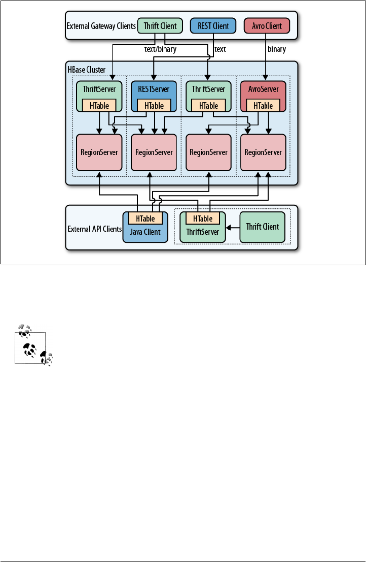
the client and gateway is local, while the RPC between the gateway and HBase is using
the native protocol.
Check carefully how you access HBase from your client, to place the
gateway servers on the appropriate physical machine. This is influenced
by the load on each machine, as well as the amount of data being trans-
ferred: make sure you are not starving either process for resources, such
as CPU cycles, or network bandwidth.
The advantage of using a server as opposed to creating a new connection for every
request goes back to when we discussed “HTablePool” on page 199—you need to reuse
connections to gain maximum performance. Short-lived processes would spend more
time setting up the connection and preparing the metadata than in the actual operation
itself. The caching of region information in the server, in particular, makes the reuse
important; otherwise, every client would have to perform a full row-to-region lookup
for every bit of data they want to access.
Selecting one server type over the others is a nontrivial task, as it depends on your use
case. The initial argument over REST in comparison to the more efficient Thrift, or
similar serialization formats, shows that for high-throughput scenarios it is
Figure 6-1. Clients connected through gateway servers
Introduction to REST, Thrift, and Avro | 243

advantageous to use a purely binary format. However, if you have few requests, but
they are large in size, REST is interesting. A rough separation could look like this:
REST use case
Since REST supports existing web-based infrastructure, it will fit nicely into setups
with reverse proxies and other caching technologies. Plan to run many REST serv-
ers in parallel, to distribute the load across them. For example, run a server on
every application server you have, building a single-app-to-server relationship.
Thrift/Avro use case
Use the compact binary protocols when you need the best performance in terms
of throughput. You can run fewer servers—for example, one per region server—
with a many-apps-to-server cardinality.
Interactive Clients
The first group of clients consists of the interactive ones, those that send client API calls
on demand, such as get, put, or delete, to servers. Based on your choice of protocol,
you can use the supplied gateway servers to gain access from your applications.
Native Java
The native Java API was discussed in Chapters 3 and 4. There is no need to start any
gateway server, as your client using HTable is directly communicating with the HBase
servers, via the native RPC calls. Refer to the aforementioned chapters to implement a
native Java client.
REST
HBase ships with a powerful REST server, which supports the complete client and
administrative API. It also provides support for different message formats, offering
many choices for a client application to communicate with the server.
Operation
For REST-based clients to be able to connect to HBase, you need to start the appropriate
gateway server. This is done using the supplied scripts. The following commands
show you how to get the command-line help, and then start the REST server in a non-
daemonized mode:
$ bin/hbase rest
usage: bin/hbase rest start [-p <arg>] [-ro]
-p,--port <arg> Port to bind to [default: 8080]
-ro,--readonly Respond only to GET HTTP method requests [default:
false]
To run the REST server as a daemon, execute bin/hbase-daemon.sh start|stop
244 | Chapter 6: Available Clients

rest [-p <port>] [-ro]
$ bin/hbase rest start
^C
You need to press Ctrl-C to quit the process. The help stated that you need to run the
server using a different script to start it as a background process:
$ bin/hbase-daemon.sh start rest
starting rest, logging to /var/lib/hbase/logs/hbase-larsgeorge-rest-<servername>.out
Once the server is started you can use curl# on the command line to verify that it is
operational:
$ curl http://<servername>:8080/
testtable
$ curl http://<servername>:8080/version
rest 0.0.2 [JVM: Apple Inc. 1.6.0_24-19.1-b02-334] [OS: Mac OS X 10.6.7 \
x86_64] [Server: jetty/6.1.26] [Jersey: 1.4]
Retrieving the root URL, that is "/" (slash), returns the list of available tables, here
testtable. Using "/version" retrieves the REST server version, along with details about
the machine it is running on.
Stopping the REST server, and running as a daemon, involves the same script, just
replacing start with stop:
$ bin/hbase-daemon.sh stop rest
stopping rest..
The REST server gives you all the operations required to work with HBase tables.
The current documentation for the REST server is online at http://hbase
.apache.org/apidocs/org/apache/hadoop/hbase/rest/package-summary
.html. Please refer to it for all the provided operations. Also, be sure to
carefully read the XML schemas documentation on that page. It explains
the schemas you need to use when requesting information, as well as
those returned by the server.
You can start as many REST servers as you like, and, for example, use a load balancer
to route the traffic between them. Since they are stateless—any state required is carried
as part of the request—you can use a round-robin (or similar) approach to distribute
the load.
Finally, use the -p, or --port, parameter to specify a different port for the server to listen
on. The default is 8080.
#curl is a command-line tool for transferring data with URL syntax, supporting a large variety of protocols.
See the project’s website for details.
Interactive Clients | 245

Supported formats
Using the HTTP Content-Type and Accept headers, you can switch between different
formats being sent or returned to the caller. As an example, you can create a table and
row in HBase using the shell like so:
hbase(main):001:0> create 'testtable', 'colfam1'
0 row(s) in 1.1790 seconds
hbase(main):002:0> put 'testtable', "\x01\x02\x03", 'colfam1:col1', 'value1'
0 row(s) in 0.0990 seconds
hbase(main):003:0> scan 'testtable'
ROW COLUMN+CELL
\x01\x02\x03 column=colfam1:col1, timestamp=1306140523371, value=value1
1 row(s) in 0.0730 seconds
This inserts a row with the binary row key 0x01 0x02 0x03 (in hexadecimal numbers),
with one column, in one column family, that contains the value value1.
For some operations it is permissible to have the data returned as plain
text. One example is the aforementioned /version operation:
$ curl -H "Accept: text/plain" http://<servername>:8080/version
rest 0.0.2 [JVM: Apple Inc. 1.6.0_24-19.1-b02-334] [OS: Mac OS X 10.6.7 \
x86_64] [Server: jetty/6.1.26] [Jersey: 1.4]
On the other hand, using plain text with more complex return values is not going to
work as expected:
$ curl -H "Accept: text/plain" \
http://<servername>:8080/testtable/%01%02%03/colfam1:col1
<html> http://<servername>:8080/testtable/%01%02%03/colfam1:col1
<head>
<meta http-equiv="Content-Type" content="text/html; charset=ISO-8859-1"/>
<title>Error 406 Not Acceptable</title>
</head>
<body><h2>HTTP ERROR 406</h2>
<p>Problem accessing /testtable/%01%02%03/colfam1:col1. Reason:
<pre> Not Acceptable</pre></p><hr /><i><small>Powered by Jetty://</small></i><br/>
<br/>
...
</body>
</html>
This is caused by the fact that the server cannot make any assumptions regarding how
to format a complex result value in plain text. You need to use a format that allows you
to express nested information natively.
Plain (text/plain).
246 | Chapter 6: Available Clients

As per the example table created in the previous text, the row key is a
binary one, consisting of three bytes. You can use REST to access those
bytes by encoding the key using URL encoding,* which in this case results
in %01%02%03. The entire URL to retrieve a cell is then:
http://<servername>:8080/testtable/%01%02%03/colfam1:col1
See the online documentation referred to earlier for the entire syntax.
When storing or retrieving data, XML is considered the default format.
For example, when retrieving the example row with no particular Accept header, you
receive:
$ curl http://<servername>:8080/testtable/%01%02%03/colfam1:col1
<?xml version="1.0" encoding="UTF-8" standalone="yes"?>
<CellSet>
<Row key="AQID">
<Cell timestamp="1306140523371" \
column="Y29sZmFtMTpjb2wx">dmFsdWUx</Cell>
</Row>
</CellSet>
The returned format defaults to XML. The column name and the actual value are en-
coded in Base64,† as explained in the online schema documentation. Here is the
excerpt:
<complexType name="Row">
<sequence>
<element name="key" type="base64Binary"></element>
<element name="cell" type="tns:Cell" maxOccurs="unbounded" \
minOccurs="1"></element>
</sequence>
</complexType>
<element name="Cell" type="tns:Cell"></element>
<complexType name="Cell">
<sequence>
<element name="value" maxOccurs="1" minOccurs="1">
<simpleType><restriction base="base64Binary">
</simpleType>
</element>
</sequence>
<attribute name="column" type="base64Binary" />
<attribute name="timestamp" type="int" />
</complexType>
XML (text/xml).
* The basic idea is to encode any unsafe or unprintable character code as “%” + ASCII Code.
Because it uses the percent sign as the prefix, it is also called percent encoding. See the Wikipedia
page on percent encoding for details.
† See the Wikipedia page on Base64 for details.
Interactive Clients | 247
All occurrences of base64Binary are where the REST server returns the encoded data.
This is done to safely transport the binary data that can be contained in the keys, or
the value.
This is also true for data that is sent to the REST server. Make sure to
read the schema documentation to encode the data appropriately, in-
cluding the payload, in other words, the actual data, but also the column
name, row key, and so on.
A quick test on the console using the base64 command reveals the proper content:
$ echo AQID | base64 -d | hexdump
0000000 01 02 03
$ echo Y29sZmFtMTpjb2wx | base64 -d
colfam1:col1
$ echo dmFsdWUx | base64 -d
value1l
This is obviously useful only to verify the details on the command line. From within
your code you can use any available Base64 implementation to decode the returned
values.
Similar to XML, requesting (or setting) the data in JSON simply
requires setting the Accept header:
$ curl -H "Accept: application/json" \
http://<servername>:8080/testtable/%01%02%03/colfam1:col1
{
"Row": [{
"key": "AQID",
"Cell": [{
"timestamp": 1306140523371,
"column": "Y29sZmFtMTpjb2wx",
"$": "dmFsdWUx"
}]
}]
}
The preceding JSON result was reformatted to be easier to read. Usually
the result on the console is returned as a single line, for example:
{"Row":[{"key":"AQID","Cell":[{"timestamp":1306140523371,"column": \
"Y29sZmFtMTpjb2wx","$":"dmFsdWUx"}]}]}
The encoding of the values is the same as for XML, that is, Base64 is used to encode
any value that potentially contains binary data. An important distinction to XML is
that JSON does not have nameless data fields. In XML the cell data is returned between
JSON (application/json).
248 | Chapter 6: Available Clients

Cell tags, but JSON must specify key/value pairs, so there is no immediate counterpart
available. For that reason, JSON has a special field called “$” (the dollar sign). The
value of the dollar field is the cell data. In the preceding example, you can see it being
used:
...
"$":"dmFsdWUx"
...
You need to query the dollar field to get the Base64-encoded data.
An interesting application of REST is to be able to
switch encodings. Since Protocol Buffers have no native RPC stack, the HBase REST
server offers support for its encoding. The schemas are documented online for your
perusal.
Getting the results returned in Protocol Buffer encoding requires the matching Accept
header:
$ curl -H "Accept: application/x-protobuf" \
http://<servername>:8080/testtable/%01%02%03/colfam1:col1 | hexdump -C
00000000 0a 24 0a 03 01 02 03 12 1d 12 0c 63 6f 6c 66 61 |.$.........colfa|
00000010 6d 31 3a 63 6f 6c 31 18 eb f6 aa e0 81 26 22 06 |m1:col1......&".|
00000020 76 61 6c 75 65 31 |value1|
The use of hexdump allows you to print out the encoded message in its binary format.
You need a Protocol Buffer decoder to actually access the data in a structured way. The
ASCII printout on the righthand side of the output shows the column name and cell
value for the example row.
Finally, you can dump the data in its raw form, while
omitting structural data. In the following console command, only the data is returned,
as stored in the cell.
$ curl -H "Accept: application/octet-stream" \
http://<servername>:8080/testtable/%01%02%03/colfam1:col1 | hexdump -C
00000000 76 61 6c 75 65 31 |value1|
Depending on the format request, the REST server puts structural data
into a custom header. For example, for the raw get request in the pre-
ceding paragraph, the headers look like this (adding -D- to the curl
command):
HTTP/1.1 200 OK
Content-Length: 6
X-Timestamp: 1306140523371
Content-Type: application/octet-stream
The timestamp of the cell has been moved to the header as X-Time
stamp. Since the row and column keys are part of the request URI, they
are omitted from the response to prevent unnecessary data from being
transferred.
Protocol Buffer (application/x-protobuf).
Raw binary (application/octet-stream).
Interactive Clients | 249
REST Java client
The REST server also comes with a comprehensive Java client API. It is located in the
org.apache.hadoop.hbase.rest.client package. The central classes are RemoteHTable
and RemoteAdmin. Example 6-1 shows the use of the RemoteHTable class.
Example 6-1. Using the REST client classes
Cluster cluster = new Cluster();
cluster.add("localhost", 8080);
Client client = new Client(cluster);
RemoteHTable table = new RemoteHTable(client, "testtable");
Get get = new Get(Bytes.toBytes("row-30"));
get.addColumn(Bytes.toBytes("colfam1"), Bytes.toBytes("col-3"));
Result result1 = table.get(get);
System.out.println("Get result1: " + result1);
Scan scan = new Scan();
scan.setStartRow(Bytes.toBytes("row-10"));
scan.setStopRow(Bytes.toBytes("row-15"));
scan.addColumn(Bytes.toBytes("colfam1"), Bytes.toBytes("col-5"));
ResultScanner scanner = table.getScanner(scan);
for (Result result2 : scanner) {
System.out.println("Scan row[" + Bytes.toString(result2.getRow()) +
"]: " + result2);
}
Set up a cluster list adding all known REST server hosts.
Create the client handling the HTTP communication.
Create a remote table instance, wrapping the REST access into a familiar interface.
Perform a get() operation as if it were a direct HBase connection.
Scan the table; again, this is the same approach as if using the native Java API.
Running the example requires that the REST server has been started and is listening on
the specified port. If you are running the server on a different machine and/or port, you
need to first adjust the value added to the Cluster instance.
Here is what is printed on the console when running the example:
Adding rows to table...
Get result1: keyvalues={row-30/colfam1:col-3/1306157569144/Put/vlen=8}
Scan row[row-10]: keyvalues={row-10/colfam1:col-5/1306157568822/Put/vlen=8}
Scan row[row-100]: keyvalues={row-100/colfam1:col-5/1306157570225/Put/vlen=9}
Scan row[row-11]: keyvalues={row-11/colfam1:col-5/1306157568841/Put/vlen=8}
Scan row[row-12]: keyvalues={row-12/colfam1:col-5/1306157568857/Put/vlen=8}
Scan row[row-13]: keyvalues={row-13/colfam1:col-5/1306157568875/Put/vlen=8}
Scan row[row-14]: keyvalues={row-14/colfam1:col-5/1306157568890/Put/vlen=8}
250 | Chapter 6: Available Clients

Due to the lexicographical sorting of row keys, you will receive the preceding rows.
The selected columns have been included as expected.
The RemoteHTable is a convenient way to talk to a number of REST servers, while being
able to use the normal Java client API classes, such as Get or Scan.
The current implementation of the Java REST client is using the Protocol
Buffer encoding internally to communicate with the remote REST
server. It is the most compact protocol the server supports, and therefore
provides the best bandwidth efficiency.
Thrift
Apache Thrift is written in C++, but provides schema compilers for many programming
languages, including Java, C++, Perl, PHP, Python, Ruby, and more. Once you have
compiled a schema, you can exchange messages transparently between systems imple-
mented in one or more of those languages.
Installation
Before you can use Thrift, you need to install it, which is preferably done using a binary
distribution package for your operating system. If that is not an option, you need to
compile it from its sources.
Download the source tarball from the website, and unpack it into a common location:
$ wget http://www.apache.org/dist/thrift/0.6.0/thrift-0.6.0.tar.gz
$ tar -xzvf thrift-0.6.0.tar.gz -C /opt
$ rm thrift-0.6.0.tar.gz
Install the dependencies, which are Automake, LibTool, Flex, Bison, and the Boost li-
braries:
$ sudo apt-get install build-essential automake libtool flex bison libboost
Now you can build and install the Thrift binaries like so:
$ cd /opt/thrift-0.6.0
$ ./configure
$ make
$ sudo make install
You can verify that everything succeeded by calling the main thrift executable:
$ thrift -version
Thrift version 0.6.0
Once you have Thrift installed, you need to compile a schema into the programming
language of your choice. HBase comes with a schema file for its client and administra-
tive API. You need to use the Thrift binary to create the wrappers for your development
environment.
Interactive Clients | 251

The supplied schema file exposes the majority of the API functionality,
but is lacking in a few areas. It was created when HBase had a different
API and that is noticeable when using it. Newer implementations of
features—for example, filters—are not supported at all.
An example of the differences in API calls is the mutateRow() call the
Thrift schema is using, while the new API has the appropriate get() call.
Work is being done in HBASE-1744 to port the Thrift schema file to the
current API, while adding all missing features. Once this is complete, it
will be added as the thrift2 package so that you can maintain your ex-
isting code using the older schema, while working on porting it over to
the new schema.
Before you can access HBase using Thrift, though, you also have to start the supplied
ThriftServer.
Operation
Starting the Thrift server is accomplished by using the supplied scripts. You can get the
command-line help by adding the -h switch, or omitting all options:
$ bin/hbase thrift
usage: Thrift [-b <arg>] [-c] [-f] [-h] [-hsha | -nonblocking |
-threadpool] [-p <arg>]
-b,--bind <arg> Address to bind the Thrift server to. Not supported by
the Nonblocking and HsHa server [default: 0.0.0.0]
-c,--compact Use the compact protocol
-f,--framed Use framed transport
-h,--help Print help information
-hsha Use the THsHaServer. This implies the framed transport.
-nonblocking Use the TNonblockingServer. This implies the framed
transport.
-p,--port <arg> Port to bind to [default: 9090]
-threadpool Use the TThreadPoolServer. This is the default.
To start the Thrift server run 'bin/hbase-daemon.sh start thrift'
To shutdown the thrift server run 'bin/hbase-daemon.sh stop thrift' or
send a kill signal to the thrift server pid
There are many options to choose from. The type of server, protocol, and transport
used is usually enforced by the client, since not all language implementations have
support for them. From the command-line help you can see that, for example, using
the nonblocking server implies the framed transport.
Using the defaults, you can start the Thrift server in nondaemonized mode:
$ bin/hbase thrift start
^C
You need to press Ctrl-C to quit the process. The help stated that you need to run the
server using a different script to start it as a background process:
252 | Chapter 6: Available Clients

$ bin/hbase-daemon.sh start thrift
starting thrift, logging to /var/lib/hbase/logs/ \
hbase-larsgeorge-thrift-<servername>.out
Stopping the Thrift server, running as a daemon, involves the same script, just replacing
start with stop:
$ bin/hbase-daemon.sh stop thrift
stopping thrift..
The Thrift server gives you all the operations required to work with HBase tables.
The current documentation for the Thrift server is online at http://wiki
.apache.org/hadoop/Hbase/ThriftApi. You should refer to it for all the
provided operations. It is also advisable to read the provided
$HBASE_HOME/src/main/resources/org/apache/hadoop/hbase/thrift/
Hbase.thrift schema definition file for the full documentation of the
available functionality.
You can start as many Thrift servers as you like, and, for example, use a load balancer
to route the traffic between them. Since they are stateless, you can use a round-robin
(or similar) approach to distribute the load.
Finally, use the -p, or --port, parameter to specify a different port for the server to listen
on. The default is 9090.
Example: PHP
HBase not only ships with the required Thrift schema file, but also with an example
client for many programming languages. Here we will enable the PHP implementation
to demonstrate the required steps.
You need to enable PHP support for your web server! Follow your server
documentation to do so.
The first step is to copy the supplied schema file and compile the necessary PHP source
files for it:
$ cp -r $HBASE_HOME/src/main/resources/org/apache/hadoop/hbase/thrift ~/thrift_src
$ cd thrift_src/
$ thrift -gen php Hbase.thrift
The call to thrift should complete with no error or other output on the command line.
Inside the thrift_src directory you will now find a directory named gen-php containing
the two generated PHP files required to access HBase:
$ ls -l gen-php/Hbase/
total 616
Interactive Clients | 253

-rw-r--r-- 1 larsgeorge staff 285433 May 24 10:08 Hbase.php
-rw-r--r-- 1 larsgeorge staff 27426 May 24 10:08 Hbase_types.php
These generated files require the Thrift-supplied PHP harness to be available as well.
They need to be copied into your web server’s document root directory, along with the
generated files:
$ cd /opt/thrift-0.6.0
$ sudo cp lib/php/src $DOCUMENT_ROOT/thrift
$ sudo mkdir $DOCUMENT_ROOT/thrift/packages
$ sudo cp -r ~/thrift_src/gen-php/Hbase $DOCUMENT_ROOT/thrift/packages/
The generated PHP files are copied into a packages subdirectory, as per the Thrift doc-
umentation, which needs to be created if it does not exist yet.
The $DOCUMENT_ROOT in the preceding code could be /var/www, for
example, on a Linux system using Apache, or /Library/WebServer/
Documents/ on an Apple Mac OS 10.6 machine. Check your web server
configuration for the appropriate location.
HBase ships with a DemoClient.php file that uses the generated files to communicate
with the servers. This file is copied into the same document root directory of the web
server:
$ sudo cp $HBASE_HOME/src/examples/thrift/DemoClient.php $DOCUMENT_ROOT/
You need to edit the DemoClient.php file and adjust the following fields at the beginning
of the file:
# Change this to match your thrift root
$GLOBALS['THRIFT_ROOT'] = 'thrift';
...
# According to the thrift documentation, compiled PHP thrift libraries should
# reside under the THRIFT_ROOT/packages directory. If these compiled libraries
# are not present in this directory, move them there from gen-php/.
require_once( $GLOBALS['THRIFT_ROOT'].'/packages/Hbase/Hbase.php' );
...
$socket = new TSocket( 'localhost', 9090 );
...
Usually, editing the first line is enough to set the THRIFT_ROOT path. Since the Demo-
Client.php file is also located in the document root directory, it is sufficient to set the
variable to thrift, that is, the directory copied from the Thrift sources earlier.
The last line in the preceding excerpt has a hardcoded server name and port. If you set
up the example in a distributed environment, you need to adjust this line to match your
environment as well.
After everything has been put into place and adjusted appropriately, you can open a
browser and point it to the demo page. For example:
http://<webserver-address>/DemoClient.php
254 | Chapter 6: Available Clients

This should load the page and output the following details (abbreviated here for the
sake of brevity):
scanning tables...
found: testtable
creating table: demo_table
column families in demo_table:
column: entry:, maxVer: 10
column: unused:, maxVer: 3
Starting scanner...
...
The same client is also available in C++, Java, Perl, Python, and Ruby. Follow the same
steps to start the Thrift server, compile the schema definition into the necessary lan-
guage, and start the client. Depending on the language, you will need to put the gen-
erated code into the appropriate location first.
HBase already ships with the generated Java classes to communicate with the Thrift
server. You can always regenerate them again from the schema file, but for convenience
they are already included.
Avro
Apache Avro, like Thrift, provides schema compilers for many programming languages,
including Java, C++, PHP, Python, Ruby, and more. Once you have compiled a schema,
you can exchange messages transparently between systems implemented in one or more
of those languages.
Installation
Before you can use Avro, you need to install it, which is preferably done using a binary
distribution package for your operating system. If that is not an option, you need to
compile it from its sources.
Once you have Avro installed, you need to compile a schema into the programming
language of your choice. HBase comes with a schema file for its client and administra-
tive API. You need to use the Avro tools to create the wrappers for your development
environment.
Before you can access HBase using Avro, though, you also have to start the supplied
AvroServer.
Operation
Starting the Avro server is accomplished by using the supplied scripts. You can get the
command-line help by adding the -h switch, or omitting all options:
$ bin/hbase avro
Usage: java org.apache.hadoop.hbase.avro.AvroServer --help | [--port=PORT] start
Arguments:
start Start Avro server
Interactive Clients | 255

stop Stop Avro server
Options:
port Port to listen on. Default: 9090
help Print this message and exit
You can start the Avro server in nondaemonized mode using the following command:
$ bin/hbase avro start
^C
You need to press Ctrl-C to quit the process. You need to run the server using a different
script to start it as a background process:
$ bin/hbase-daemon.sh start avro
starting avro, logging to /var/lib/hbase/logs/hbase-larsgeorge-avro-<servername>.out
Stopping the Avro server, running as a daemon, involves the same script, just replacing
start with stop:
$ bin/hbase-daemon.sh stop avro
stopping avro..
The Avro server gives you all the operations required to work with HBase tables.
The current documentation for the Avro server is available online at
http://hbase.apache.org/apidocs/org/apache/hadoop/hbase/avro/package
-summary.html. Please refer to it for all the provided operations. You
are also advised to read the provided $HBASE_HOME/src/main/java/
org/apache/hadoop/hbase/avro/hbase.avpr schema definition file for the
full documentation of the available functionality.
You can start as many Avro servers as you like, and, for example, use a load balancer
to route the traffic between them. Since they are stateless, you can use a round-robin
(or similar) approach to distribute the load.
Finally, use the -p, or --port, parameter to specify a different port for the server to listen
on. The default is 9090.
Other Clients
There are other client libraries that allow you to access an HBase cluster. They can
roughly be divided into those that run directly on the Java Virtual Machine, and those
that use the gateway servers to communicate with an HBase cluster. Here are some
examples:
JRuby
The HBase Shell is an example of using a JVM-based language to access the Java-
based API. It comes with the full source code, so you can use it to add the same
features to your own JRuby code.
256 | Chapter 6: Available Clients

HBql
HBql adds an SQL-like syntax on top of HBase, while adding the extensions needed
where HBase has unique features. See the project’s website for details.
HBase-DSL
This project gives you dedicated classes that help when formulating queries against
an HBase cluster. Using a builder-like style, you can quickly assemble all the op-
tions and parameters necessary. See its wiki online for more information.
JPA/JPO
You can use, for example, DataNucleus to put a JPA/JPO access layer on top of
HBase.
PyHBase
The PyHBase project (https://github.com/hammer/pyhbase/) offers an HBase client
through the Avro gateway server.
AsyncHBase
AsyncHBase offers a completely asynchronous, nonblocking, and thread-safe
client to access HBase clusters. It uses the native RPC protocol to talk directly to
the various servers. See the project’s website for details.
Note that some of these projects have not seen any activity for quite
some time. They usually were created to fill a need of the authors, and
since then have been made public. You can use them as a starting point
for your own projects.
Batch Clients
The opposite use case of interactive clients is batch access to data. The difference is that
these clients usually run asynchronously in the background, scanning large amounts
of data to build, for example, search indexes, machine-learning-based mathematical
models, or statistics needed for reporting.
Access is less user-driven, and therefore, SLAs are geared more toward overall runtime,
as opposed to per-request latencies. The majority of the batch frameworks reading and
writing from and to HBase are MapReduce-based.
MapReduce
The Hadoop MapReduce framework is built to process petabytes of data, in a reliable,
deterministic, yet easy-to-program way. There are a variety of ways to include HBase
as a source and target for MapReduce jobs.
Native Java
The Java-based MapReduce API for HBase is discussed in Chapter 7.
Batch Clients | 257

Clojure
The HBase-Runner project (https://github.com/mudphone/hbase-runner/) offers sup-
port for HBase from the functional programming language Clojure. You can write
MapReduce jobs in Clojure while accessing HBase tables.
Hive
The Apache Hive project‡ offers a data warehouse infrastructure atop Hadoop. It was
initially developed at Facebook, but is now part of the open source Hadoop ecosystem.
Hive offers an SQL-like query language, called HiveQL, which allows you to query the
semistructured data stored in Hadoop. The query is eventually turned into a MapRe-
duce job, executed either locally or on a distributed MapReduce cluster. The data is
parsed at job execution time and Hive employs a storage handler§ abstraction layer that
allows for data not to just reside in HDFS, but other data sources as well. A storage
handler transparently makes arbitrarily stored information available to the HiveQL-
based user queries.
Since version 0.6.0, Hive also comes with a handler for HBase.‖ You can define Hive
tables that are backed by HBase tables, mapping columns as required. The row key can
be exposed as another column when needed.
HBase Version Support
As of this writing, version 0.7.0 of Hive includes support for HBase 0.89.0-SNAPSHOT
only, though this is likely to change soon. The implication is that you cannot run the
HBase integration against a more current version, since the RPC is very sensitive to
version changes and will bail out at even minor differences.
The only way currently is to replace the HBase JARs with the newer ones and recompile
Hive from source. You either need to update the Ivy settings to include the version of
HBase (and probably Hadoop) you need, or try to build Hive, then copy the newer
JARs into the $HIVE_HOME/src/build/dist/lib directory and compile again (YMMV).
The better approach is to let Ivy load the appropriate version from the remote reposi-
tories, and then compile Hive normally. To get started, download the source tarball
from the website and unpack it into a common location:
$ wget http://www.apache.org/dist//hive/hive-0.7.0/hive-0.7.0.tar.gz
$ tar -xzvf hive-0.7.0.tar.gz -C /opt
Then edit the Ivy library configuration file:
$ cd /opt/hive-0.7.0/src
$ vim ivy/libraries.properties
‡http://hive.apache.org/
§ See the Hive wiki for more details on storage handlers.
‖The Hive wiki has a full explanation of the HBase integration into Hive.
258 | Chapter 6: Available Clients

...
#hbase.version=0.89.0-SNAPSHOT
#hbase-test.version=0.89.0-SNAPSHOT
hbase.version=0.91.0-SNAPSHOT
hbase-test.version=0.91.0-SNAPSHOT
...
You can now build Hive from the sources using ant, but not before you have set the
environment variable for the Hadoop version you are building against:
$ export HADOOP_HOME="/<your-path>/hadoop-0.20.2"
$ ant package
Buildfile: /opt/hive-0.7.0/src/build.xml
jar:
create-dirs:
compile-ant-tasks:
...
package:
[echo] Deploying Hive jars to /opt/hive-0.7.0/src/build/dist
BUILD SUCCESSFUL
The build process will take awhile, since Ivy needs to download all required libraries,
and that depends on your Internet connection speed. Once the build is complete, you
can start using the HBase handler with the new version of HBase.
In some cases, you need to slightly edit all files in src/hbase-handler/src/java/org/apache/
hadoop/hive/hbase/ and replace the way the configuration is created, from:
HBaseConfiguration hbaseConf = new HBaseConfiguration(hiveConf);
to the newer style, using a static factory method:
Configuration hbaseConf = HBaseConfiguration.create(hiveConf);
After you have installed Hive itself, you have to edit its configuration files so that it has
access to the HBase JAR file, and the accompanying configuration. Modify
$HIVE_HOME/conf/hive-env.sh to contain these lines:
# Set HADOOP_HOME to point to a specific hadoop install directory
HADOOP_HOME=/usr/local/hadoop
HBASE_HOME=/usr/local/hbase
# Hive Configuration Directory can be controlled by:
# export HIVE_CONF_DIR=
export HIVE_CLASSPATH=/etc/hbase/conf
# Folder containing extra libraries required for hive compilation/execution
# can be controlled by:
export HIVE_AUX_JARS_PATH=/usr/local/hbase/hbase-0.91.0-SNAPSHOT.jar
Batch Clients | 259

You may have to copy the supplied $HIVE_HOME/conf/hive-
env.sh.template file, and save it in the same directory, but without
the .template extension. Once you have copied the file, you can edit it
as described.
Once Hive is installed and operational, you can start using the new handler. First start
the Hive command-line interface, create a native Hive table, and insert data from the
supplied example files:
$ build/dist/bin/hive
Hive history file=/tmp/larsgeorge/hive_job_log_larsgeorge_201105251455_2009910117.txt
hive> CREATE TABLE pokes (foo INT, bar STRING);
OK
Time taken: 3.381 seconds
hive> LOAD DATA LOCAL INPATH '/opt/hive-0.7.0/examples/files/kv1.txt'
OVERWRITE INTO TABLE pokes;
Copying data from file:/opt/hive-0.7.0/examples/files/kv1.txt
Copying file: file:/opt/hive-0.7.0/examples/files/kv1.txt
Loading data to table default.pokes
Deleted file:/user/hive/warehouse/pokes
OK
Time taken: 0.266 seconds
This is using the pokes table, as described in the Hive guide at http://wiki.apache.org/
hadoop/Hive/GettingStarted. Next you create an HBase-backed table like so:
hive> CREATE TABLE hbase_table_1(key int, value string)
STORED BY 'org.apache.hadoop.hive.hbase.HBaseStorageHandler'
WITH SERDEPROPERTIES ("hbase.columns.mapping" = ":key,cf1:val")
TBLPROPERTIES ("hbase.table.name" = "hbase_table_1");
OK
Time taken: 0.144 seconds
This DDL statement maps the HBase table, defined using the TBLPROPERTIES, and
SERDEPROPERTIES, using the new HBase handler, to a Hive table named hbase_table_1.
The hbase.columns.mapping has a special feature, which is mapping the column with
the name ":key" to the HBase row key. You can place this special column to perform
row key mapping anywhere in your definition. Here it is placed as the first column,
thus mapping the values in the key column of the Hive table to be the row key in the
HBase table.
260 | Chapter 6: Available Clients

The hbase.table.name in the table properties is optional and only needed when you
want to use different names for the tables in Hive and HBase. Here it is set to the same
value, and therefore could be omitted.
Loading the table from the previously filled pokes Hive table is done next. According
to the mapping, this will save the pokes.foo values in the row key, and the pokes.bar
in the column cf1:val:
hive> INSERT OVERWRITE TABLE hbase_table_1 SELECT * FROM pokes;
Total MapReduce jobs = 1
Launching Job 1 out of 1
Number of reduce tasks is set to 0 since there's no reduce operator
Execution log at: /tmp/larsgeorge/larsgeorge_20110525152020_de5f67d1-9411- \
446f-99bb-35621e1b259d.log
Job running in-process (local Hadoop)
2011-05-25 15:20:31,031 null map = 100%, reduce = 0%
Ended Job = job_local_0001
OK
Time taken: 3.925 seconds
This starts the first MapReduce job in this example. You can see how the Hive command
line prints out the values it is using. The job copies the values from the internal Hive
table into the HBase-backed one.
In certain setups, especially in the local, pseudodistributed mode, the
Hive job may fail with an obscure error message. Before trying to figure
out the details, try running the job in Hive local MapReduce mode. In
the Hive CLI enter:
hive> SET mapred.job.tracker=local;
Then execute the job again. This mode was added in Hive 0.7.0, and
may not be available to you. If it is, try to use it, since it avoids using the
Hadoop MapReduce framework—which means you have one less part
to worry about when debugging a failed Hive job.
The following counts the rows in the pokes and hbase_table_1 tables (the CLI output
of the job details are omitted for the second and all subsequent queries):
hive> select count(*) from pokes;
Total MapReduce jobs = 1
Launching Job 1 out of 1
Number of reduce tasks determined at compile time: 1
In order to change the average load for a reducer (in bytes):
set hive.exec.reducers.bytes.per.reducer=<number>
In order to limit the maximum number of reducers:
set hive.exec.reducers.max=<number>
In order to set a constant number of reducers:
set mapred.reduce.tasks=<number>
Execution log at: /tmp/larsgeorge/larsgeorge_20110525152323_418769e6-1716- \
48ee-a0ab-dacd59e55da8.log
Job running in-process (local Hadoop)
Batch Clients | 261

2011-05-25 15:23:07,058 null map = 100%, reduce = 100%
Ended Job = job_local_0001
OK
500
Time taken: 3.627 seconds
hive> select count(*) from hbase_table_1;
...
OK
309
Time taken: 4.542 seconds
What is interesting to note is the difference in the actual count for each table. They
differ by more than 100 rows, where the HBase-backed table is the shorter one. What
could be the reason for this? In HBase, you cannot have duplicate row keys, so every
row that was copied over, and which had the same value in the originating pokes.foo
column, is saved as the same row. This is the same as performing a SELECT DISTINCT on
the source table:
hive> select count(distinct foo) from pokes;
...
OK
309
Time taken: 3.525 seconds
This is now the same outcome and proves that the previous results are correct. Finally,
drop both tables, which also removes the underlying HBase table:
hive> drop table pokes;
OK
Time taken: 0.741 seconds
hive> drop table hbase_table_1;
OK
Time taken: 3.132 seconds
hive> exit;
You can also map an existing HBase table into Hive, or even map the table into multiple
Hive tables. This is useful when you have very distinct column families, and querying
them is done separately. This will improve the performance of the query significantly,
since it uses a Scan internally, selecting only the mapped column families. If you have
a sparsely set family, this will only scan the much smaller files on disk, as opposed to
running a job that has to scan everything just to filter out the sparse data.
Mapping an existing table requires the Hive EXTERNAL keyword, which is also used in
other places to access data stored in unmanaged Hive tables, that is, those that are not
under Hive’s control:
hive> CREATE EXTERNAL TABLE hbase_table_2(key int, value string)
STORED BY 'org.apache.hadoop.hive.hbase.HBaseStorageHandler'
WITH SERDEPROPERTIES ("hbase.columns.mapping" = ":key,cf1:val")
TBLPROPERTIES("hbase.table.name" = "<existing-table-name>");
262 | Chapter 6: Available Clients

External tables are not deleted when the table is dropped within Hive. This simply
removes the metadata information about the table.
You have the option to map any HBase column directly to a Hive column, or you can
map an entire column family to a Hive MAP type. This is useful when you do not know
the column qualifiers ahead of time: map the family and iterate over the columns from
within the Hive query instead.
HBase columns you do not map into Hive are not accessible for Hive
queries.
Since storage handlers work transparently for the higher-level layers in Hive, you can
also use any user-defined function (UDF) supplied with Hive—or your own custom
functions.
There are a few shortcomings in the current version, though:
No custom serialization
HBase only stores byte[] arrays, so Hive is simply converting every column value
to String, and serializes it from there. For example, an INT column set to 12 in Hive
would be stored as if using Bytes.toBytes("12").
No version support
There is currently no way to specify any version details when handling HBase ta-
bles. Hive always returns the most recent version.
Check with the Hive project site to see if these features have since been added.
Pig
The Apache Pig project# provides a platform to analyze large amounts of data. It has
its own high-level query language, called Pig Latin, which uses an imperative program-
ming style to formulate the steps involved in transforming the input data to the final
output. This is the opposite of Hive’s declarative approach to emulate SQL.
The nature of Pig Latin, in comparison to HiveQL, appeals to everyone with a proce-
dural programming background, but also lends itself to significant parallelization.
When it is combined with the power of Hadoop and the MapReduce framework, you
can process massive amounts of data in reasonable time frames.
Version 0.7.0 of Pig introduced the LoadFunc/StoreFunc classes and functionality, which
allows you to load and store data from sources other than the usual HDFS. One of
those sources is HBase, implemented in the HBaseStorage class.
#http://pig.apache.org/
Batch Clients | 263

Pigs’ support for HBase includes reading and writing to existing tables. You can map
table columns as Pig tuples, which optionally include the row key as the first field for
read operations. For writes, the first field is always used as the row key.
The storage also supports basic filtering, working on the row level, and providing the
comparison operators explained in “Comparison operators” on page 139.*
Pig Installation
You should try to install the prebuilt binary packages for the operating system distri-
bution of your choice. If this is not possible, you can download the source from the
project website and build it locally. For example, on a Linux-based system you could
perform the following steps.†
Download the source tarball from the website, and unpack it into a common location:
$ wget http://www.apache.org/dist//pig/pig-0.8.1/pig-0.8.1.tar.gz
$ tar -xzvf pig-0.8.1.tar.gz -C /opt
$ rm pig-0.8.1.tar.gz
Add the pig script to the shell’s search path, and set the PIG_HOME environment variable
like so:
$ export PATH=/opt/pig-0.8.1/bin:$PATH
$ export PIG_HOME=/opt/pig-0.8.1
After that, you can try to see if the installation is working:
$ pig -version
Apache Pig version 0.8.1
compiled May 27 2011, 14:58:51
You can use the supplied tutorial code and data to experiment with Pig and HBase.
You do have to create the table in the HBase Shell first to work with it from within Pig:
hbase(main):001:0> create 'excite', 'colfam1'
Starting the Pig Shell, aptly called Grunt, requires the pig script. For local testing add
the -x local switch:
$ pig -x local
grunt>
Local mode implies that Pig is not using a separate MapReduce installation, but uses
the LocalJobRunner that comes as part of Hadoop. It runs the resultant MapReduce jobs
within the same process. This is useful for testing and prototyping, but should not be
used for larger data sets.
* Internally it uses the RowFilter class; see “RowFilter” on page 141.
† The full details can be found on the Pig setup page.
264 | Chapter 6: Available Clients

You have the option to write the script beforehand in an editor of your choice, and
subsequently specify it when you invoke the pig script. Or you can use Grunt, the Pig
Shell, to enter the Pig Latin statements interactively. Ultimately, the statements are
translated into one or more MapReduce jobs, but not all statements trigger the
execution. Instead, you first define the steps line by line, and a call to DUMP or STORE will
eventually set the job in motion.
The Pig Latin functions are case-insensitive, though commonly they are
written in uppercase. Names and fields you define are case-sensitive,
and so are the Pig Latin functions.
The Pig tutorial comes with a small data set that was published by Excite, and contains
an anonymous user ID, a timestamp, and the search terms used on its site. The first
step is to load the data into HBase using a slight transformation to generate a compound
key. This is needed to enforce uniqueness for each entry:
grunt> raw = LOAD 'tutorial/data/excite-small.log' \
USING PigStorage('\t') AS (user, time, query);
T = FOREACH raw GENERATE CONCAT(CONCAT(user, '\u0000'), time), query;
grunt> STORE T INTO 'excite' USING \
org.apache.pig.backend.hadoop.hbase.HBaseStorage('colfam1:query');
...
2011-05-27 22:55:29,717 [main] INFO org.apache.pig.backend.hadoop. \
executionengine.mapReduceLayer.MapReduceLauncher - 100% complete
2011-05-27 22:55:29,717 [main] INFO org.apache.pig.tools.pigstats.PigStats \
- Detected Local mode. Stats reported below may be incomplete
2011-05-27 22:55:29,718 [main] INFO org.apache.pig.tools.pigstats.PigStats \
- Script Statistics:
HadoopVersion PigVersion UserId StartedAt FinishedAt Features
0.20.2 0.8.1 larsgeorge 2011-05-27 22:55:22 2011-05-27 22:55:29 UNKNOWN
Success!
Job Stats (time in seconds):
JobId Alias Feature Outputs
job_local_0002 T,raw MAP_ONLY excite,
Input(s):
Successfully read records from: "file:///opt/pig-0.8.1/tutorial/data/excite-small.log"
Output(s):
Successfully stored records in: "excite"
Job DAG:
job_local_0002
Batch Clients | 265

You can use the DEFINE statement to abbreviate the long Java package
reference for the HBaseStorage class. For example:
grunt> DEFINE LoadHBaseUser org.apache.pig.backend.hadoop.hbase.HBaseStorage( \
'data:roles', '-loadKey');
grunt> U = LOAD 'user' USING LoadHBaseUser;
grunt> DUMP U;
...
This is useful if you are going to reuse the specific load or store function.
The STORE statement started a MapReduce job that read the data from the given logfile
and copied it into the HBase table. The statement in between is changing the relation
to generate a compound row key—which is the first field specified in the STORE state-
ment afterward—which is the user and time fields, separated by a zero byte.
Accessing the data involves another LOAD statement, this time using the HBaseStorage
class:
grunt> R = LOAD 'excite' USING \
org.apache.pig.backend.hadoop.hbase.HBaseStorage('colfam1:query', '-loadKey') \
AS (key: chararray, query: chararray);
The parameters in the brackets define the column to field mapping, as well as the extra
option to load the row key as the first field in relation R. The AS part explicitly defines
that the row key and the colfam1:query column are converted to chararray, which is
Pig’s string type. By default, they are returned as bytearray, matching the way they are
stored in the HBase table. Converting the data type allows you, for example, to subse-
quently split the row key.
You can test the statements entered so far by dumping the content of R, which is the
result of the previous statement.
grunt> DUMP R;
...
Success!
...
(002BB5A52580A8ED970916150445,margaret laurence the stone angel)
(002BB5A52580A8ED970916150505,margaret laurence the stone angel)
...
The row key, placed as the first field in the tuple, is the concatenated representation
created during the initial copying of the data from the file into HBase. It can now be
split back into two fields so that the original layout of the text file is re-created:
grunt> S = foreach R generate FLATTEN(STRSPLIT(key, '\u0000', 2)) AS \
(user: chararray, time: long), query;
grunt> DESCRIBE S;
S: {user: chararray,time: long,query: chararray}
266 | Chapter 6: Available Clients

Using DUMP once more, this time using relation S, shows the final result:
grunt> DUMP S;
(002BB5A52580A8ED,970916150445,margaret laurence the stone angel)
(002BB5A52580A8ED,970916150505,margaret laurence the stone angel)
...
With this in place, you can proceed to the remainder of the Pig tutorial, while replacing
the LOAD and STORE statements with the preceding code. Concluding this example, type
in QUIT to finally exit the Grunt shell:
grunt> QUIT;
$
Pig’s support for HBase has a few shortcomings in the current version, though:
No version support
There is currently no way to specify any version details when handling HBase cells.
Pig always returns the most recent version.
Fixed column mapping
The row key must be the first field and cannot be placed anywhere else. This can
be overcome, though, with a subsequent FOREACH...GENERATE statement, reordering
the relation layout.
Check with the Pig project site to see if these features have since been added.
Cascading
Cascading is an alternative API to MapReduce. Under the covers, it uses MapReduce
during execution, but during development, users don’t have to think in MapReduce to
create solutions for execution on Hadoop.
The model used is similar to a real-world pipe assembly, where data sources are taps,
and outputs are sinks. These are piped together to form the processing flow, where data
passes through the pipe and is transformed in the process. Pipes can be connected to
larger pipe assemblies to form more complex processing pipelines from existing pipes.
Data then streams through the pipeline and can be split, merged, grouped, or joined.
The data is represented as tuples, forming a tuple stream through the assembly. This
very visually oriented model makes building MapReduce jobs more like construction
work, while abstracting the complexity of the actual work involved.
Cascading (as of version 1.0.1) has support for reading and writing data to and from
an HBase cluster. Detailed information and access to the source code can be found on
the Cascading Modules page (http://www.cascading.org/modules.html).
Example 6-2 shows how to sink data into an HBase cluster. See the GitHub repository,
linked from the modules page, for more up-to-date API information.
Batch Clients | 267

Example 6-2. Using Cascading to insert data into HBase
// read data from the default filesystem
// emits two fields: "offset" and "line"
Tap source = new Hfs(new TextLine(), inputFileLhs);
// store data in an HBase cluster, accepts fields "num", "lower", and "upper"
// will automatically scope incoming fields to their proper familyname,
// "left" or "right"
Fields keyFields = new Fields("num");
String[] familyNames = {"left", "right"};
Fields[] valueFields = new Fields[] {new Fields("lower"),
new Fields("upper") };
Tap hBaseTap = new HBaseTap("multitable", new HBaseScheme(keyFields,
familyNames, valueFields), SinkMode.REPLACE);
// a simple pipe assembly to parse the input into fields
// a real app would likely chain multiple Pipes together for more complex
// processing
Pipe parsePipe = new Each("insert", new Fields("line"),
new RegexSplitter(new Fields("num", "lower", "upper"), " "));
// "plan" a cluster executable Flow
// this connects the source Tap and hBaseTap (the sink Tap) to the parsePipe
Flow parseFlow = new FlowConnector(properties).connect(source, hBaseTap,
parsePipe);
// start the flow, and block until complete
parseFlow.complete();
// open an iterator on the HBase table we stuffed data into
TupleEntryIterator iterator = parseFlow.openSink();
while(iterator.hasNext()) {
// print out each tuple from HBase
System.out.println( "iterator.next() = " + iterator.next() );
}
iterator.close();
Cascading to Hive and Pig offers a Java API, as opposed to the domain-specific
languages (DSLs) provided by the others. There are add-on projects that provide DSLs
on top of Cascading.
Shell
The HBase Shell is the command-line interface to your HBase cluster(s). You can use
it to connect to local or remote servers and interact with them. The shell provides both
client and administrative operations, mirroring the APIs discussed in the earlier chap-
ters of this book.
268 | Chapter 6: Available Clients
Basics
The first step to experience the shell is to start it:
$ $HBASE_HOME/bin/hbase shell
HBase Shell; enter 'help<RETURN>' for list of supported commands.
Type "exit<RETURN>" to leave the HBase Shell
Version 0.91.0-SNAPSHOT, r1130916, Sat Jul 23 12:44:34 CEST 2011
hbase(main):001:0>
The shell is based on JRuby, the Java Virtual Machine-based implementation of
Ruby.‡ More specifically, it uses the Interactive Ruby Shell (IRB), which is used to enter
Ruby commands and get an immediate response. HBase ships with Ruby scripts that
extend the IRB with specific commands, related to the Java-based APIs. It inherits the
built-in support for command history and completion, as well as all Ruby commands.
There is no need to install Ruby on your machines, as HBase ships with
the required JAR files to execute the JRuby shell. You use the supplied
script to start the shell on top of Java, which is already a necessary
requirement.
Once started, you can type in help, and then press Return, to get the help text (abbre-
viated in the following code sample):
hbase(main):001:0> help
HBase Shell, version 0.91.0-SNAPSHOT, r1130916, Sat Jul 23 12:44:34 CEST 2011
Type 'help "COMMAND"', (e.g. 'help "get"' -- the quotes are necessary) for
help on a specific command. Commands are grouped. Type 'help "COMMAND_GROUP"',
(e.g. 'help "general"') for help on a command group.
COMMAND GROUPS:
Group name: general
Commands: status, version
Group name: ddl
Commands: alter, create, describe, disable, drop, enable, exists,
is_disabled, is_enabled, list
...
SHELL USAGE:
Quote all names in HBase Shell such as table and column names. Commas delimit
command parameters. Type <RETURN> after entering a command to run it.
Dictionaries of configuration used in the creation and alteration of tables are
Ruby Hashes. They look like this:
...
‡ Visit the Ruby website (http://www.ruby-lang.org/) for details.
Shell | 269

As stated, you can request help for a specific command by adding the command when
invoking help, or print out the help of all commands for a specific group when using
the group name with the help command. The command or group name has the enclosed
in quotes.
You can leave the shell by entering exit, or quit:
hbase(main):002:0> exit
$
The shell also has specific command-line options, which you can see when adding the
-h, or --help, switch to the command:
$ $HBASE_HOME/bin.hbase shell -h
HBase Shell command-line options:
format Formatter for outputting results: console | html. Default: console
-d | --debug Set DEBUG log levels.
Debugging
Adding the -d, or --debug switch, to the shell’s start command enables the debug mode,
which switches the logging levels to DEBUG, and lets the shell print out any backtrace
information—which is similar to stacktraces in Java.
Once you are inside the shell, you can use the debug command to toggle the debug
mode:
hbase(main):001:0> debug
Debug mode is ON
hbase(main):002:0> debug
Debug mode is OFF
You can check the status with the debug? command:
hbase(main):003:0> debug?
Debug mode is OFF
Without the debug mode, the shell is set to print only ERROR-level messages, and no
backtrace details at all, on the console.
There is an option to switch the formatting being used by the shell. As of this writing,
only console is available, though.
The shell start script automatically uses the configuration directory located in the same
$HBASE_HOME directory. You can override the location to use other settings, but most
importantly to connect to different clusters. Set up a separate directory that contains
an hbase-site.xml file, with an hbase.zookeeper.quorum property pointing to another
cluster, and start the shell like so:
$ HBASE_CONF_DIR="/<your-other-config-dir>/" bin/hbase shell
Note that you have to specify an entire directory, not just the hbase-site.xml file.
270 | Chapter 6: Available Clients

Commands
The commands are grouped into five different categories, representing their semantic
relationships. When entering commands, you have to follow a few guidelines:
Quote names
Commands that require a table or column name expect the name to be quoted in
either single or double quotes.
Quote values
The shell supports the output and input of binary values using a hexadecimal—or
octal—representation. You must use double quotes or the shell will interpret them
as literals.
hbase> get 't1', "key\x00\x6c\x65\x6f\x6e"
hbase> get 't1', "key\000\154\141\165\162\141"
hbase> put 't1', "test\xef\xff", 'f1:', "\x01\x33\x70"
Note the mixture of quotes: you need to make sure you use the correct ones, or
the result might not be what you had expected. Text in single quotes is treated as
a literal, whereas double-quoted text is interpolated, that is, it transforms the octal,
or hexadecimal, values into bytes.
Comma delimiters for parameters
Separate command parameters using commas. For example:
hbase(main):001:0> get 'testtable', 'row-1',
'colfam1:qual1'
Ruby hashes for properties
For some commands, you need to hand in a map with key/value properties. This
is done using Ruby hashes:
{'key1' => 'value1', 'key2' => 'value2', ...}
The keys/values are wrapped in curly braces, and in turn are separated by "=>".
Usually keys are predefined constants such as NAME, VERSIONS, or COMPRESSION, and
do not need to be quoted. For example:
hbase(main):001:0> create 'testtable', {NAME =>
'colfam1', VERSIONS => 1, \
TTL => 2592000, BLOCKCACHE => true}
Restricting Output
The get command has an optional parameter that you can use to restrict the printed
values by length. This is useful if you have many columns with values of varying length.
To get a quick overview of the actual columns, you could suppress any longer value
being printed in full—which on the console can get unwieldy very quickly otherwise.
In the following example, a very long value is inserted and subsequently retrieved with
a restricted length, using the MAXLENGTH parameter:
Shell | 271

hbase(main):001:0> put
'testtable','rowlong','colfam1:qual1','abcdefghijklmnopqrstuvwxyzabcdefghi \
jklmnopqrstuvwxyzabcdefghijklmnopqrstuvwxyzabcdefghijklmnopqrstuvwxyzabcde \
...
xyzabcdefghijklmnopqrstuvwxyzabcdefghijklmnopqrstuvwxyz'
hbase(main):018:0> get 'testtable', 'rowlong', MAXLENGTH => 60
COLUMN CELL
colfam1:qual1 timestamp=1306424577316, value=abcdefghijklmnopqrstuvwxyzabc
The MAXLENGTH is counted from the start of the row (i.e., it includes the column name).
Set it to the width (or slightly less) of your console to fit each column into one line.
For any command, you can get detailed help by typing in help '<command>'. Here’s an
example:
hbase(main):001:0> help 'status'
Show cluster status. Can be 'summary', 'simple', or 'detailed'. The
default is 'summary'. Examples:
hbase> status
hbase> status 'simple'
hbase> status 'summary'
hbase> status 'detailed'
The majority of commands have a direct match with a method provided by either the
client or administrative API. Next is a brief overview of each command and the match-
ing API functionality.
General
The general commands are listed in Table 6-1. They allow you to retrieve details about
the status of the cluster itself, and the version of HBase it is running. See the Cluster
Status class in “Cluster Status Information” on page 233 for details.
Table 6-1. General shell commands
Command Description
status Returns various levels of information contained in the ClusterStatus class. See the help to get
the simple, summary, and detailed status information.
version Returns the current version, repository revision, and compilation date of your HBase cluster. See
ClusterStatus.getHBaseVersion() in Table 5-4.
272 | Chapter 6: Available Clients

Data definition
The data definition commands are listed in Table 6-2. Most of them stem from the
administrative API, as described in Chapter 5.
Table 6-2. Data definition shell commands
Command Description
alter Modifies an existing table schema using modifyTable().
See “Schema Operations” on page 228 for details.
create Creates a new table. See the createTable() call in “Table Operations” on page 220 for details.
describe Prints the HTableDescriptor. See “Tables” on page 207 for details.
disable Disables a table. See “Table Operations” and the disableTable() method.
drop Drops a table. See the deleteTable() method in “Table Operations”.
enable Enables a table. See the enableTable() call in “Table Operations” for details.
exists Checks if a table exists. It uses the tableExists() call; see “Table Operations”.
is_disabled Checks if a table is disabled. See the isTableDisabled() method in “Table Operations”.
is_enabled Checks if a table is enabled. See the isTableEnabled() method in “Table Operations”.
list Returns a list of all user tables. Uses the listTables() method, described in “Table Operations”.
Data manipulation
The data manipulation commands are listed in Table 6-3. Most of them are provided
by the client API, as described in Chapters 3 and 4.
Table 6-3. Data manipulation shell commands
Command Description
count Counts the rows in a table. Uses a Scan internally, as described in “Scans” on page 122.
delete Deletes a cell. See “Delete Method” on page 105 and the Delete class.
deleteall Similar to delete but does not require a column. Deletes an entire family or row. See “Delete
Method” and the Delete class.
get Retrieves a cell. See the Get class in “Get Method” on page 95.
get_counter Retrieves a counter value. Same as the get command but converts the raw counter value into a readable
number. See the Get class in “Get Method”.
incr Increments a counter. Uses the Increment class; see “Counters” on page 168 for details.
put Stores a cell. Uses the Put class, as described in “Put Method” on page 76.
scan Scans a range of rows. Relies on the Scan class. See “Scans” on page 122 for details.
truncate Truncates a table, which is the same as executing the disable and drop commands, followed by a
create, using the same schema.
Shell | 273

Tools
The tools commands are listed in Table 6-4. These commands are provided by the
administrative API; see “Cluster Operations” on page 230 for details.
Table 6-4. Tools shell commands
Command Description
assign Assigns a region to a server. See “Cluster Operations” on page 230 and the assign() method.
balance_switch Toggles the balancer switch. See “Cluster Operations” and the balanceSwitch() method.
balancer Starts the balancer. See “Cluster Operations” and the balancer() method.
close_region Closes a region. Uses the closeRegion() method, as described in “Cluster Operations”.
compact Starts the asynchronous compaction of a region or table. Uses compact(), as described in “Cluster
Operations”.
flush Starts the asynchronous flush of a region or table. Uses flush(), as described in “Cluster Operations”.
major_compact Starts the asynchronous major compaction of a region or table. Uses majorCompact(), as described
in “Cluster Operations”.
move Moves a region to a different server. See the move() call, and “Cluster Operations” for details.
split Splits a region or table. See the split() call, and “Cluster Operations” for details.
unassign Unassigns a region. See the unassign() call, and “Cluster Operations” for details.
zk_dump Dumps the ZooKeeper details pertaining to HBase. This is a special function offered by an internal class.
The web-based UI of the HBase Master exposes the same information.
Replication
The replication commands are listed in Table 6-5.
Table 6-5. Replication shell commands
Command Description
add_peer Adds a replication peer
disable_peer Disables a replication peer
enable_peer Enables a replication peer
remove_peer Removes a replication peer
start_replication Starts the replication process
stop_replication Stops the replications process
Scripting
Inside the shell, you can execute the provided commands interactively, getting imme-
diate feedback. Sometimes, though, you just want to send one command, and possibly
script this call from the scheduled maintenance system (e.g., cron or at). Or you want
274 | Chapter 6: Available Clients

to send a command in response to a check run in Nagios, or another monitoring tool.
You can do this by piping the command into the shell:
$ echo "status" | bin/hbase shell
HBase Shell; enter 'help<RETURN>' for list of supported commands.
Type "exit<RETURN>" to leave the HBase Shell
Version 0.91.0-SNAPSHOT, r1130916, Sat Jul 23 12:44:34 CEST 2011
status
1 servers, 0 dead, 44.0000 average load
Once the command is complete, the shell is closed and control is given back to the
caller. Finally, you can hand in an entire script to be executed by the shell at startup:
$ cat ~/hbase-shell-status.rb
status
$ bin/hbase shell ~/hbase-shell-status.rb
1 servers, 0 dead, 44.0000 average load
HBase Shell; enter 'help<RETURN>' for list of supported commands.
Type "exit<RETURN>" to leave the HBase Shell
Version 0.91.0-SNAPSHOT, r1130916, Sat Jul 23 12:44:34 CEST 2011
hbase(main):001:0> exit
Once the script has completed, you can continue to work in the shell or exit it as usual.
There is also an option to execute a script using the raw JRuby interpreter, which
involves running it directly as a Java application. Using the hbase script sets up the
classpath to be able to use any Java class necessary. The following example simply
retrieves the list of tables from the remote cluster:
$ cat ~/hbase-shell-status-2.rb
include Java
import org.apache.hadoop.hbase.HBaseConfiguration
import org.apache.hadoop.hbase.client.HBaseAdmin
conf = HBaseConfiguration.new
admin = HBaseAdmin.new(conf)
tables = admin.listTables
tables.each { |table| puts table.getNameAsString() }
$ bin/hbase org.jruby.Main ~/hbase-shell-status-2.rb
testtable
Since the shell is based on JRuby’s IRB, you can use its built-in features, such as com-
mand completion and history. Enabling them is a matter of creating an .irbrc in your
home directory, which is read when the shell starts:
$ cat ~/.irbrc
require 'irb/ext/save-history'
IRB.conf[:SAVE_HISTORY] = 100
IRB.conf[:HISTORY_FILE] = "#{ENV['HOME']}/.irb-save-history"
This enables the command history to save across shell starts. The command completion
is already enabled by the HBase scripts.
Shell | 275

Another advantage of the interactive interpreter is that you can use the HBase classes
and functions to perform, for example, something that would otherwise require you to
write a Java application. Here is an example of binary output received from a
Bytes.toBytes() call that is converted into an integer value:
hbase(main):001:0>
org.apache.hadoop.hbase.util.Bytes.toInt( \
"\x00\x01\x06[".to_java_bytes)
=> 67163
Note how the shell encoded the first three unprintable characters as
hexadecimal values, while the fourth, the "[", was printed as a character.
Another example is to convert a date into a Linux epoch number, and back into a
human-readable date:
hbase(main):002:0> java.text.SimpleDateFormat.new("yyyy/MM/dd HH:mm:ss").parse( \
"2011/05/30 20:56:29").getTime()
=> 1306781789000
hbase(main):002:0> java.util.Date.new(1306781789000).toString()
=> "Mon May 30 20:56:29 CEST 2011"
Finally, you can also add many cells in a loop—for example, to populate a table with
test data:
hbase(main):003:0> for i in 'a'..'z' do for j in
'a'..'z' do put 'testtable', \
"row-#{i}#{j}", "colfam1:#{j}", "#{j}" end end
A more elaborate loop to populate counters could look like this:
hbase(main):004:0> require 'date';
import java.lang.Long
import org.apache.hadoop.hbase.util.Bytes
(Date.new(2011, 01, 01)..Date.today).each { |x| put "testtable", "daily", \
"colfam1:" + x.strftime("%Y%m%d"), Bytes.toBytes(Long.new(rand * \
4000).longValue).to_a.pack("CCCCCCCC") }
Obviously, this is getting very much into Ruby itself. But even with a little bit of pro-
gramming skills in another language, you might be able to use the features of the
IRB-based shell to your advantage. Start easy and progress from there.
276 | Chapter 6: Available Clients

Web-based UI
The HBase processes expose a web-based user interface (UI), which you can use to gain
insight into the cluster’s state, as well as the tables it hosts. The majority of the func-
tionality is read-only, but a few selected operations can be triggered through the UI.
Master UI
HBase also starts a web-based listing of vital attributes. By default, it is deployed on
the master host at port 60010, while region servers use 60030. If the master is running
on a host named master.foo.com on the default port, to see the master’s home page,
you can point your browser at http://master.foo.com:60010.
The ports used by the servers can be set in the hbase-site.xml configu-
ration file. The properties to change are:
hbase.master.info.port
hbase.regionserver.info.port
Main page
The first page you will see when opening the master’s web UI is shown in Figure 6-2.
It consists of multiple sections that give you insight into the cluster status itself, the
tables it serves, what the region servers are, and so on.
The details can be broken up into the following groups:
Master attributes
You will find cluster-wide details in a table at the top of the page. It has information
on the version of HBase and Hadoop that you are using, where the root directory
is located,§ the overall load average, and the ZooKeeper quorum used.
There is also a link in the description for the ZooKeeper quorum allowing you to
see the information for your current HBase cluster stored in ZooKeeper. “Zoo-
Keeper page” on page 282 discusses its content.
Running tasks
The next group of details on the master’s main page is the list of currently running
tasks. Every internal operation performed by the master is listed here while it is
running, and for another minute after its completion. Entries with a white back-
ground are currently running, a green background indicates successful completion
of the task, and a yellow background means the task was aborted. The latter can
happen when an operation failed due to an inconsistent state. Figure 6-3 shows a
completed, a running, and a failed task.
§ Recall that this should better not be starting with /tmp, or you may lose your data during a machine restart.
Refer to “Quick-Start Guide” on page 31 for details.
Web-based UI | 277
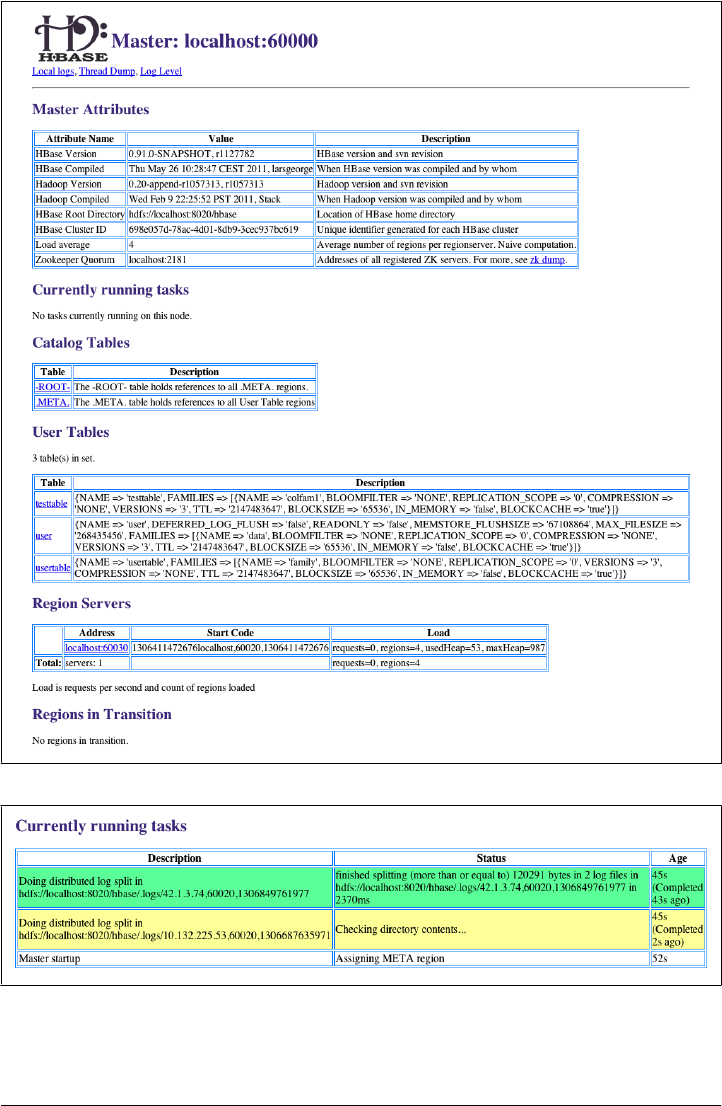
Figure 6-3. The list of currently running tasks on the master
Figure 6-2. The HBase Master user interface
278 | Chapter 6: Available Clients
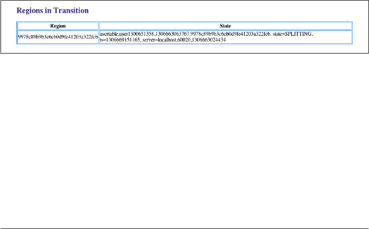
Catalog tables
This section list the two catalog tables, .META. and -ROOT-. You can click on the
name of the table to see more details on the table regions—for example, on what
server they are currently hosted.
User tables
Here you will see the list of all tables known to your HBase cluster. These are the
ones you—or your users—have created using the API, or the HBase Shell. The
description column in the list gives you a printout of the current table descriptor,
including all column descriptors; see “Schema Definition” on page 207 for an ex-
planation of how to read them.
The table names are links to another page with details on the selected table. See
“User Table page” on page 279 for an explanation of the contained information.
Region servers
The next section lists the actual region servers the master knows about. The table
lists the address, which you can click on to see more details. It also states the server
start code, a timestamp representing an ID for each server, and finally, the load of
the server. For information on the values listed refer to “Cluster Status Informa-
tion” on page 233, and especially the HServerLoad class.
Regions in transition
As regions are managed by the master and region servers to, for example, balance
the load across servers, they go through short phases of transition. This applies to
opening, closing, and splitting a region. Before the operation is performed, the
region is added to the list, and once the operation is complete, it is removed. “The
Region Life Cycle” on page 348 describes the possible states a region can be in.
Figure 6-4 shows a region that is currently split.
Figure 6-4. The Regions in Transitions table provided by the master web UI
User Table page
When you click on the name of a user table in the master’s web-based user interface,
you have access to the information pertaining to the selected table. Figure 6-5 shows
an abbreviated version of a User Table page (it has a shortened list of regions for the
sake of space).
Web-based UI | 279
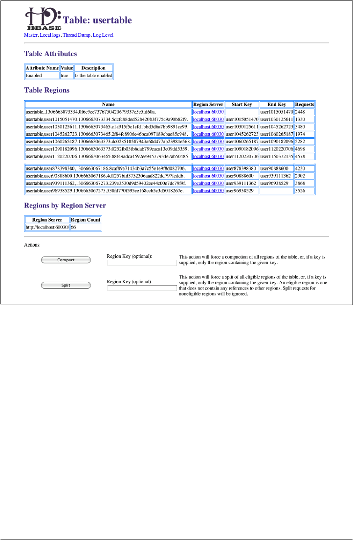
Figure 6-5. The User Table page with details about the selected table
The following groups of information are available in the User Table page:
Table attributes
Here you can find details about the table itself. As of this writing, this section only
lists the table status (i.e., it indicates if it is enabled or not). See “Table Opera-
tions” on page 220, and the disableTable() call especially.
The boolean value states whether the table is enabled, so when you see a true in
the Value column, this is the case. On the other hand, a value of false would mean
the table is currently disabled.
Table regions
This list can be rather large and shows all regions of a table. The Name column has
the region name itself, and the Region Server column has a link to the server hosting
the region. Clicking on the link takes you to the page explained in “Region Server
UI” on page 283.
280 | Chapter 6: Available Clients
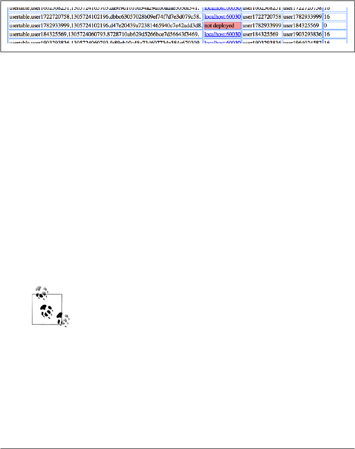
Sometimes you may see the words not deployed where the server name should be.
This happens when a user table region is not currently served by any region server.
Figure 6-6 shows an example of this situation.
The Start Key and End Key columns show the region’s start and end keys as ex-
pected. Finally, the Requests column shows the total number of requests, including
all read (e.g., get or scan) and write (e.g., put or delete) operations, since the region
was deployed to the server.
Figure 6-6. Example of a region that has not been assigned to a server and is listed as not deployed
Regions by region server
The last group on the User Table page lists which region server is hosting how
many regions of the selected table. This number is usually distributed evenly across
all available servers. If not, you can use the HBase Shell or administrative API to
initiate the balancer, or use the move command to manually balance the table re-
gions (see “Cluster Operations” on page 230).
The User Table page also offers a form that can be used to trigger administrative
operations on a specific region, or the entire table. See “Cluster Operations” again for
details, and “Optimizing Splits and Compactions” on page 429 for information on
when you want to use them. The available operations are:
Compact
This triggers the compact functionality, which is asynchronously running in the
background. Specify the optional name of a region to run the operation more se-
lectively. The name of the region can be taken from the table above, that is, the
entries in the Name column of the Table Regions table.
Make sure to copy the entire region name as-is. This includes the
trailing "." (the dot)!
If you do not specify a region name, the operation is performed on all regions of
the table instead.
Split
Similar to the compact action, the split form action triggers the split command,
operating on a table or region scope. Not all regions may be splittable—for
example, those that contain no, or very few, cells, or one that has already been
split, but which has not been compacted to complete the process.
Web-based UI | 281
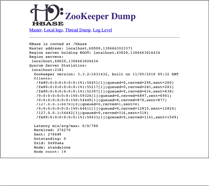
Once you trigger one of the operations, you will receive a confirmation page; for ex-
ample, for a split invocation, you will see:
Split request accepted.
Reload.
Use the Back button of your web browser to go back to the previous page, showing the
user table details.
ZooKeeper page
There is also a link in the description column that lets you dump the content of all the
nodes stored in ZooKeeper by HBase. This is useful when trying to solve problems with
the cluster setup (see “Troubleshooting” on page 467).
The page shows the same information as invoking the zk_dump command of the HBase
Shell. It shows you the root directory HBase is using inside the configured filesystem.
You also can see the currently assigned master, which region server is hosting the
-ROOT- catalog table, the list of region servers that have registered with the master, as
well as ZooKeeper internal details. Figure 6-7 shows an exemplary output available on
the ZooKeeper page.
Figure 6-7. The ZooKeeper page, listing HBase and ZooKeeper details, which is useful when debugging
HBase installations
282 | Chapter 6: Available Clients

Region Server UI
The region servers have their own web-based UI, which you usually access through the
master UI, by clicking on the server name links provided. You can access the page
directly by entering
http://<region-server-address>:60030
into your browser (while making sure to use the configured port, here using the default
of 60030).
Main page
The main page of the region servers has details about the server, the tasks, and regions
it is hosting. Figure 6-8 shows an abbreviated example of this page (the list of tasks and
regions is shortened for the sake of space).
The page can be broken up into the following groups of distinct information:
Region server attributes
This group of information contains the version of HBase you are running, when it
was compiled, a printout of the server metrics, and the ZooKeeper quorum used.
The metrics are explained in “Region Server Metrics” on page 394.
Running tasks
The table lists all currently running tasks, using a white background for running
tasks, a yellow one for failed tasks, and a green one for completed tasks. Failed or
completed tasks are removed after one minute.
Online regions
Here you can see all the regions hosted by the currently selected region server. The
table has the region name, the start and end keys, as well as the region metrics.
Shared Pages
On the top of the master, region server, and table pages there are also a few generic
links that lead to subsequent pages, displaying or controlling additional details of your
setup:
Local logs
This link provides a quick way to access the logfiles without requiring access to the
server itself. It firsts list the contents of the log directory where you can select the
logfile you want to see. Click on a log to reveal its content. “Analyzing the
Logs” on page 468 helps you to make sense of what you may see. Figure 6-9 shows
an example page.
Web-based UI | 283
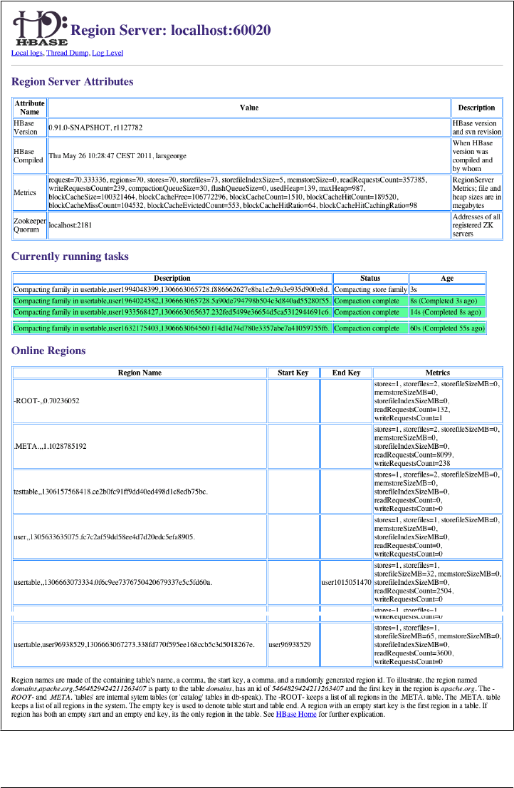
Figure 6-8. The Region Server main page
284 | Chapter 6: Available Clients
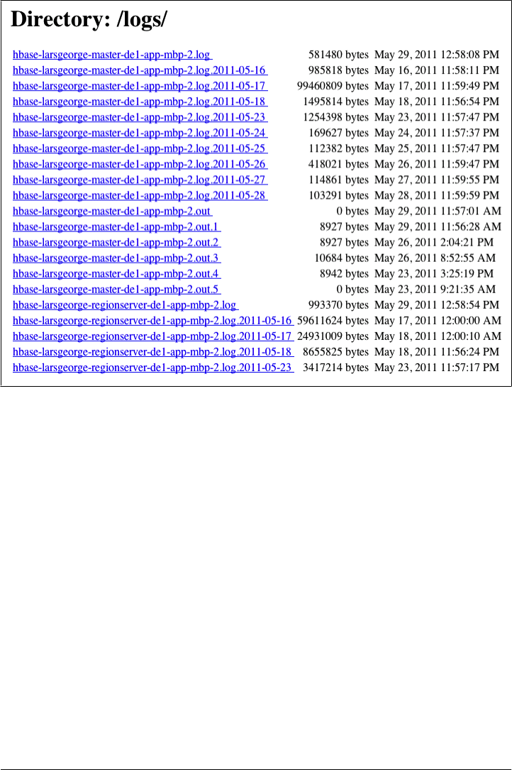
Thread dumps
For debugging purposes, you can use this link to dump the Java stacktraces of
the running HBase processes. You can find more details in “Troubleshoot-
ing” on page 467. Figure 6-10 shows example output.
Log level
This link leads you to a small form that allows you to retrieve and set the logging
levels used by the HBase processes. More on this is provided in “Changing Logging
Levels” on page 466. Figure 6-11 shows the form when it is loaded afresh.
When you enter, for example, org.apache.hadoop.hbase into the first input field,
and click on the Get Log Level button, you should see a result similar to that shown
in Figure 6-12.
The web-based UI provided by the HBase servers is a good way to quickly gain insight
into the cluster, the hosted tables, the status of regions and tables, and so on. The
majority of the information can also be accessed using the HBase Shell, but that requires
console access to the cluster.
Figure 6-9. The Local Logs page
Web-based UI | 285
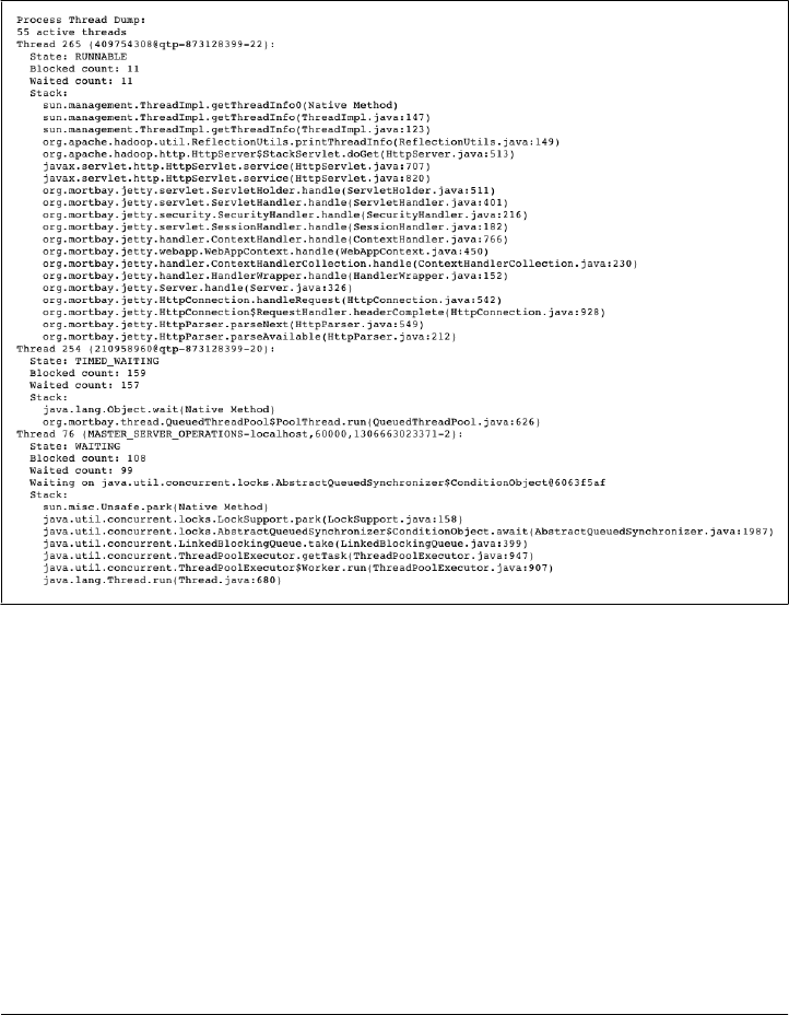
You can use the UI to trigger selected administrative operations; therefore, it might not
be advisable to give everyone access to it: similar to the shell, the UI should be used by
the operators and administrators of the cluster.
If you want your users to create, delete, and display their own tables, you will need an
additional layer on top of HBase, possibly using Thrift or REST as the gateway server,
to offer this functionality to end users.
Figure 6-10. The Thread Dump page
286 | Chapter 6: Available Clients
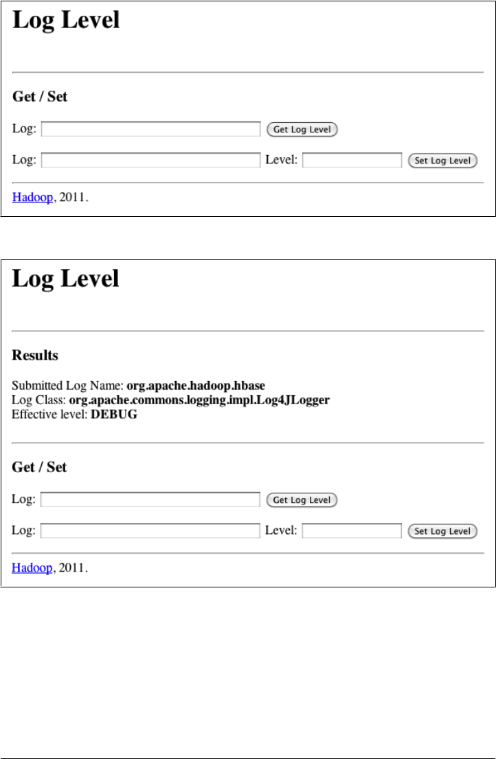
Figure 6-11. The Log Level page
Figure 6-12. The Log Level Result page
Web-based UI | 287

CHAPTER 7
MapReduce Integration
One of the great features of HBase is its tight integration with Hadoop’s MapReduce
framework. Here you will see how this can be leveraged and how unique traits of HBase
can be used advantageously in the process.
Framework
Before going into the application of HBase with MapReduce, we will first have a look
at the building blocks.
MapReduce Introduction
MapReduce as a process was designed to solve the problem of processing in excess of
terabytes of data in a scalable way. There should be a way to build such a system that
increases in performance linearly with the number of physical machines added. That
is what MapReduce strives to do. It follows a divide-and-conquer approach by splitting
the data located on a distributed filesystem so that the servers (or rather CPUs, or more
modern “cores”) available can access these chunks of data and process them as fast as
they can. The problem with this approach is that you will have to consolidate the data
at the end. Again, MapReduce has this built right into it. Figure 7-1 gives a high-level
overview of the process.
This (rather simplified) figure of the MapReduce process shows you how the data is
processed. The first thing that happens is the split, which is responsible for dividing the
input data into reasonably sized chunks that are then processed by one server at a time.
This splitting has to be done in a somewhat smart way to make best use of available
servers and the infrastructure in general. In this example, the data may be a very large
logfile that is divided into pieces of equal size. This is good, for example, for Apache
logfiles. Input data may also be binary, though, in which case you may have to write
your own getSplits() method—but more on that shortly.
289
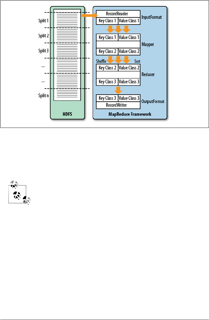
Classes
Figure 7-1 also shows you the classes that are involved in the Hadoop implementation
of MapReduce. Let us look at them and also at the specific implementations that HBase
provides on top of them.
Hadoop version 0.20.0 introduced a new MapReduce API. Its classes
are located in the package named mapreduce, while the existing classes
for the previous API are located in mapred. The older API was deprecated
and should have been dropped in version 0.21.0—but that did not hap-
pen. In fact, the old API was undeprecated since the adoption of the new
one was hindered by its incompleteness.
HBase also has these two packages, which only differ slightly. The new
API has more support by the community, and writing jobs against it is
not impacted by the Hadoop changes. This chapter will only refer to the
new API.
InputFormat
The first class to deal with is the InputFormat class (Figure 7-2). It is responsible for two
things. First it splits the input data, and then it returns a RecordReader instance that
defines the classes of the key and value objects, and provides a next() method that is
used to iterate over each input record.
Figure 7-1. The MapReduce process
290 | Chapter 7: MapReduce Integration
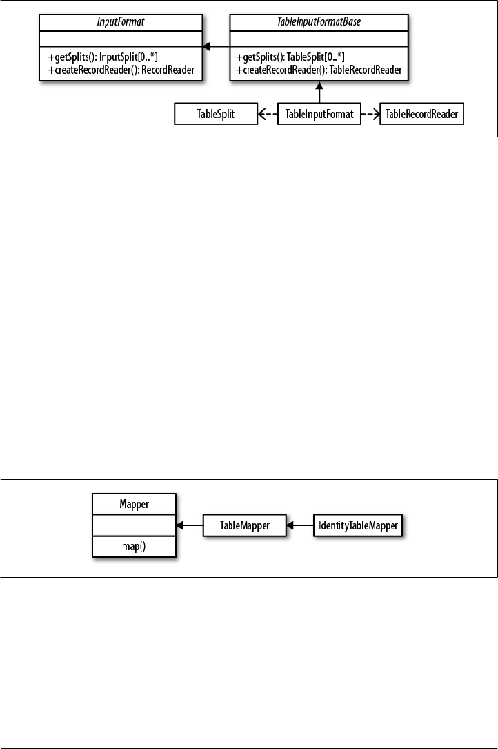
As far as HBase is concerned, there is a special implementation called TableInput
FormatBase whose subclass is TableInputFormat. The former implements the majority
of the functionality but remains abstract. The subclass is a lightweight concrete version
of TableInputFormat and is used by many supplied samples and real MapReduce classes.
These classes implement the full turnkey solution to scan an HBase table. You have to
provide a Scan instance that you can prepare in any way you want: specify start
and stop keys, add filters, specify the number of versions, and so on. The
TableInputFormat splits the table into proper blocks for you and hands them over to
the subsequent classes in the MapReduce process. See “Table Splits” on page 294 for
details on how the table is split.
Mapper
The Mapper class(es) is for the next stage of the MapReduce process and one of its
namesakes (Figure 7-3). In this step, each record read using the RecordReader is pro-
cessed using the map() method. Figure 7-1 also shows that the Mapper reads a specific
type of key/value pair, but emits possibly another type. This is handy for converting
the raw data into something more useful for further processing.
Figure 7-3. The Mapper hierarchy
HBase provides the TableMapper class that enforces key class 1 to be an ImmutableBytes
Writable, and value class 1 to be a Result type—since that is what the
TableRecordReader is returning.
One specific implementation of the TableMapper is the IdentityTableMapper, which is
also a good example of how to add your own functionality to the supplied classes. The
TableMapper class itself does not implement anything but only adds the signatures of
Figure 7-2. The InputFormat hierarchy
Framework | 291
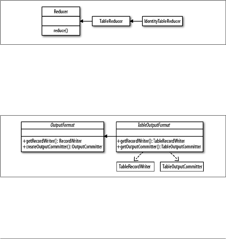
the actual key/value pair classes. The IdentityTableMapper is simply passing on the
keys/values to the next stage of processing.
Reducer
The Reducer stage and class hierarchy (Figure 7-4) is very similar to the Mapper stage.
This time we get the output of a Mapper class and process it after the data has been
shuffled and sorted.
In the implicit shuffle between the Mapper and Reducer stages, the intermediate data is
copied from different Map servers to the Reduce servers and the sort combines the
shuffled (copied) data so that the Reducer sees the intermediate data as a nicely sorted
set where each unique key is now associated with all of the possible values it was found
with.
Figure 7-4. The Reducer hierarchy
OutputFormat
The final stage is the OutputFormat class (Figure 7-5), and its job is to persist the data
in various locations. There are specific implementations that allow output to files, or
to HBase tables in the case of the TableOutputFormat class. It uses a TableRecord
Writer to write the data into the specific HBase output table.
Figure 7-5. The OutputFormat hierarchy
It is important to note the cardinality as well. Although many Mappers are handing
records to many Reducers, only one OutputFormat takes each output record from its
Reducer subsequently. It is the final class that handles the key/value pairs and writes
them to their final destination, this being a file or a table.
292 | Chapter 7: MapReduce Integration

The TableOutputCommitter class is required for the Hadoop classes to do their job. For
HBase integration, this class is not needed. In fact, it is a dummy and does not do
anything. Other implementations of OutputFormat do require it.
The name of the output table is specified when the job is created. Otherwise, the
TableOutputFormat does not add much more complexity. One rather significant thing
it does do is to set the table’s autoflush to false and handle the buffer flushing implicitly.
This helps a lot in terms of speeding up the import of large data sets. Also see “Client
API: Best Practices” on page 434 for information on how to optimize your scan
performance.
Supporting Classes
The MapReduce support comes with the TableMapReduceUtil class that helps in setting
up MapReduce jobs over HBase. It has static methods that configure a job so that you
can run it with HBase as the source and/or the target.
MapReduce Locality
One of the more ambiguous things in Hadoop is block replication: it happens auto-
matically and you should not have to worry about it. HBase relies on it to provide
durability as it stores its files into the distributed filesystem. Although block replication
works completely transparently, users sometimes ask how it affects performance.
This question usually arises when the user starts writing MapReduce jobs against either
HBase or Hadoop directly. Especially when larger amounts of data are being stored in
HBase, how does the system take care of placing the data close to where it is needed?
This concept is referred to as data locality, and in the case of HBase using the Hadoop
filesystem (HDFS), users may have doubts as to whether it is working.
First let us see how Hadoop handles this: the MapReduce documentation states that
tasks run close to the data they process. This is achieved by breaking up large files in
HDFS into smaller chunks, or blocks, with a default setting of 64 MB (128 MB and
larger is very common in practice).
Each block is assigned to a map task to process the contained data. This means larger
block sizes equal fewer map tasks to run as the number of mappers is driven by the
number of blocks that need processing. Hadoop knows where blocks are located, and
runs the map tasks directly on the node that hosts the block. Since block replication
ensures that we have (by default) three copies on three different physical servers, the
framework has the choice of executing the code on any of those three, which it uses to
balance workloads. This is how it guarantees data locality during the MapReduce
process.
Back to HBase. Once you understand that Hadoop can process data locally, you may
start to question how this may work with HBase. As discussed in
Framework | 293

“Storage” on page 319, HBase transparently stores files in HDFS. It does so for the
actual data files (HFile) as well as the log (WAL). And if you look into the code, it uses
the Hadoop API call FileSystem.create(Path path) to create these files.
If you do not co-share your cluster with Hadoop and HBase, but instead
employ a separate Hadoop as well as a standalone HBase cluster, there
is no data locality—there can’t be. This is the same as running a separate
MapReduce cluster that would not be able to execute tasks directly on
the data node. It is imperative for data locality to have the Hadoop and
HBase processes running on the same cluster—end of line.
How does Hadoop figure out where data is located as HBase accesses it? The most
important factor is that HBase servers are not restarted frequently and that they perform
housekeeping on a regular basis. These so-called compactions rewrite files as new data
is added over time. All files in HDFS, once written, are immutable (for all sorts of
reasons). Because of that, data is written into new files, and as their number grows,
HBase compacts them into another set of new, consolidated files.
And here is the kicker: HDFS is smart enough to put the data where it is needed! It has
a block placement policy in place that enforces all blocks to be written first on a col-
located server. The receiving data node compares the server name of the writer with its
own, and if they match, the block is written to the local filesystem. Then a replica is
sent to a server within the same rack, and another to a remote rack—assuming you are
using rack awareness in HDFS. If not, the additional copies get placed on the least
loaded data node in the cluster.
If you have configured a higher replication factor, more replicas are stored on distinct
machines. The important factor here, though, is that you now have a local copy of the
block available. For HBase, this means that if the region server stays up for long enough
(which is what you want), after a major compaction on all tables—which can be in-
voked manually or is triggered by a configuration setting—it has the files stored locally
on the same host. The data node that shares the same physical host has a copy of all
data the region server requires. If you are running a scan or get or any other use case,
you can be sure to get the best performance.
An issue to be aware of is region movements during load balancing, or server failures.
In that case, the data is no longer local, but over time it will be once again. The master
also takes this into consideration when a cluster is restarted: it assigns all regions to the
original region servers. If one of them is missing, it has to fall back to the random region
assignment approach.
Table Splits
When running a MapReduce job in which you read from a table, you are typically using
the TableInputFormat. It fits into the framework by overriding the required public
294 | Chapter 7: MapReduce Integration

methods getSplits() and createRecordReader(). Before a job is executed, the frame-
work calls getSplit() to determine how the data is to be separated into chunks, because
it sets the number of map tasks the job requires.
For HBase, the TableInputFormat uses the information about the table it represents—
based on the Scan instance you provided—to divide the table at region boundaries.
Since it has no direct knowledge of the effect of the optional filter, it uses the start and
stop keys to narrow down the number of regions. The number of splits, therefore, is
equal to all regions between the start and stop keys. If you do not set the start and/or
stop key, all are included.
When the job starts, the framework is calling createRecordReader() as many times as
it has splits. It iterates over the splits and creates a new TableRecordReader by calling
createRecordReader() with the current split. In other words, each TableRecordReader
handles exactly one region, reading and mapping every row between the region’s start
and end keys.
The split also contains the server name hosting the region. This is what drives locality
for MapReduce jobs over HBase: the framework checks the server name, and if a
task tracker is running on the same machine, it will preferably run it on that server.
Because the region server is also collocated with the data node on that same node, the
scan of the region will be able to retrieve all data from the local disk.
When running MapReduce over HBase, it is strongly advised that you
turn off speculative execution mode. It will only create more load on the
same region and server, and also works against locality: the speculative
task is executed on a different machine, and therefore will not have the
region server local, which is hosting the region. This results in all data
being sent over the network, adding to the overall I/O load.
MapReduce over HBase
The following sections will introduce you to using HBase in combination with Map-
Reduce. Before you can use HBase as a source or sink, or both, for data processing jobs,
you have to first decide how you want to prepare the support by Hadoop.
Preparation
To run a MapReduce job that needs classes from libraries not shipped with Hadoop or
the MapReduce framework, you'll need to make those libraries available before the job
is executed. You have two choices: static preparation of all task nodes, or supplying
everything needed with the job.
MapReduce over HBase | 295

Static Provisioning
For a library that is used often, it is useful to permanently install its JAR file(s) locally
on the task tracker machines, that is, those machines that run the MapReduce tasks.
This is done by doing the following:
1. Copy the JAR files into a common location on all nodes.
2. Add the JAR files with full location into the hadoop-env.sh configuration file, into
the HADOOP_CLASSPATH variable:
# Extra Java CLASSPATH elements. Optional.
# export HADOOP_CLASSPATH="<extra_entries>:$HADOOP_CLASSPATH"
3. Restart all task trackers for the changes to be effective.
Obviously this technique is quite static, and every update (e.g., to add new libraries)
requires a restart of the task tracker daemons. Adding HBase support requires at least
the HBase and ZooKeeper JARs. Edit the hadoop-env.sh to contain the following:
export HADOOP_CLASSPATH="$HBASE_HOME/hbase-0.91.0-SNAPSHOT.jar: \
$ZK_HOME/zookeeper-3.3.2.jar:$HADOOP_CLASSPATH"
This assumes you have defined the two $XYZ_HOME environment variables to point to
the location of where you have installed the respective packages.*
Note that this fixes the versions of these globally provided libraries to
whatever is specified on the servers and in their configuration files.
The issue of locking into specific versions of required libraries can be circumvented
with the dynamic provisioning approach, explained next.
Dynamic Provisioning
In case you need to provide different libraries to each job you want to run, or you want
to update the library versions along with your job classes, then using the dynamic
provisioning approach is more useful.
For this, Hadoop has a special feature: it reads all libraries from an optional /lib directory
contained in the job JAR. You can use this feature to generate so-called fat JAR files,
as they ship not just with the actual job code, but also with all libraries needed. This
results in considerably larger job JAR files, but on the other hand, represents a complete,
self-contained processing job.
* You can use an absolute path as well.
296 | Chapter 7: MapReduce Integration

Using Maven
The example code for this book uses Maven to build the JAR files (see “Building the
Examples” on page xxi). Maven allows you to create the JAR files not just with
the example code, but also to build the enhanced fat JAR file that can be deployed to
the MapReduce framework as-is. This avoids editing the server-side configuration files.
Maven has support for so-called profiles, which can be used to customize the build
process. The pom.xml for this chapter makes use of this feature to add a fatjar profile
that creates the required /lib directory inside the final job JAR, and copies all required
libraries into it. For this to work properly, some of the dependencies need to be defined
with a scope of provided so that they are not included in the copy operation. This is
done by adding the appropriate tag to all libraries that are already available on the
server, for instance, the Hadoop JARs:
<dependency>
<groupId>org.apache.hadoop</groupId>
<artifactId>hadoop-core</artifactId>
<version>0.20-append-r1044525</version>
<scope>provided</scope>
...
</dependency>
This is done in the parent POM file, located in the root directory of the book repository,
as well as inside the POM for the chapter, depending on where a dependency is added.
One example is the Apache Commons CLI library, which is also part of Hadoop.
The fatjar profile uses the Maven Assembly plug-in with an accompanying src/main/
assembly/job.xml file that specifies what should, and what should not, be included in
the generated target JAR (e.g., it skips the provided libraries). With the profile in place,
you can compile a lean JAR—one that only contains the job classes and would need
an updated server configuration to include the HBase and ZooKeeper JARs—like so:
<ch07>$ mvn package
This will build a JAR that can be used to execute any of the included MapReduce, using
the hadoop jar command:
<ch07>$ hadoop jar target/hbase-book-ch07-1.0.jar
An example program must be given as the first argument.
Valid program names are:
AnalyzeData: Analyze imported JSON
ImportFromFile: Import from file
ParseJson: Parse JSON into columns
ParseJson2: Parse JSON into columns (map only)
...
The command will list all possible job names. It makes use of the Hadoop Program
Driver class, which is prepared with all known job classes and their names. The Maven
build takes care of adding the Driver class—which is the one wrapping the Program
Driver instance—as the main class of the JAR file; hence, it is automatically executed
by the hadoop jar command.
Building a fat JAR only requires the addition of the profile name:
MapReduce over HBase | 297

<ch07>$ mvn package -Dfatjar
The generated JAR file has an added postfix to distinguish it, but that is just a matter
of taste (you can simply override the lean JAR if you prefer, although I refrain from
explaining it here):
<ch07>$ hadoop jar target/hbase-book-ch07-1.0-job.jar
It behaves exactly like the lean JAR, and you can launch the same jobs with the same
parameters. The difference is that it includes the required libraries, avoiding the con-
figuration change on the servers:
$ unzip -l target/hbase-book-ch07-1.0-job.jar
Archive: target/hbase-book-ch07-1.0-job.jar
Length Date Time Name
-------- ---- ---- ----
0 07-14-11 12:01 META-INF/
159 07-14-11 12:01 META-INF/MANIFEST.MF
0 07-13-11 15:01 mapreduce/
0 07-13-11 10:06 util/
740 07-13-11 10:06 mapreduce/Driver.class
3547 07-14-11 12:01 mapreduce/ImportFromFile$ImportMapper.class
5326 07-14-11 12:01 mapreduce/ImportFromFile.class
...
8739 07-13-11 10:06 util/HBaseHelper.class
0 07-14-11 12:01 lib/
16046 05-06-10 16:08 lib/json-simple-1.1.jar
58160 05-06-10 16:06 lib/commons-codec-1.4.jar
598364 11-22-10 21:43 lib/zookeeper-3.3.2.jar
2731371 07-02-11 15:20 lib/hbase-0.91.0-SNAPSHOT.jar
14837 07-14-11 12:01 lib/hbase-book-ch07-1.0.jar
-------- -------
3445231 16 files
Maven is not the only way to generate different job JARs; you can also use Apache Ant,
for example. What matters is not how you build the JARs, but that they contain the
necessary information (either just the code, or the code and its required libraries).
Another option to dynamically provide the necessary libraries is the libjars feature of
Hadoop’s MapReduce framework. When you create a MapReduce job using the sup-
plied GenericOptionsParser harness, you get support for the libjar parameter for free.
Here is the documentation of the parser class:
GenericOptionsParser is a utility to parse command line arguments generic to
the Hadoop framework. GenericOptionsParser recognizes several standarad
command line arguments, enabling applications to easily specify a namenode,
a jobtracker, additional configuration resources etc.
Generic Options
The supported generic options are:
-conf <configuration file> specify a configuration file
-D <property=value> use value for given property
-fs <local|namenode:port> specify a namenode
-jt <local|jobtracker:port> specify a job tracker
-files <comma separated list of files> specify comma separated
298 | Chapter 7: MapReduce Integration

files to be copied to the map reduce cluster
-libjars <comma separated list of jars> specify comma separated
jar files to include in the classpath.
-archives <comma separated list of archives> specify comma
separated archives to be unarchived on the compute machines.
The general command line syntax is:
bin/hadoop command [genericOptions] [commandOptions]
The reason to carefully read the documentation is that it not only states the libjars
parameter, but also how and where to specify it on the command line. Failing to add
the libjars parameter properly will result in the MapReduce job to fail. This can be
seen from the job’s logfiles, for every task attempt. The errors are also reported when
starting the job on the command line, for example:
$ HADOOP_CLASSPATH=$HBASE_HOME/target/hbase-0.91.0-SNAPSHOT.jar: \
$ZK_HOME/zookeeper-3.3.2.jar hadoop jar target/hbase-book-ch07-1.0.jar \
ImportFromFile -t testtable -i test-data.txt -c data:json
...
11/08/08 11:13:17 INFO mapred.JobClient: Running job: job_201108081021_0003
11/08/08 11:13:18 INFO mapred.JobClient: map 0% reduce 0%
11/08/08 11:13:29 INFO mapred.JobClient: Task Id : \
attempt_201108081021_0003_m_000002_0, Status : FAILED
java.lang.RuntimeException: java.lang.ClassNotFoundException: \
org.apache.hadoop.hbase.mapreduce.TableOutputFormat
at org.apache.hadoop.conf.Configuration.getClass(Configuration.java:809)
at org.apache.hadoop.mapreduce.JobContext.getOutputFormatClass(JobContext.java:197)
at org.apache.hadoop.mapred.Task.initialize(Task.java:413)
at org.apache.hadoop.mapred.MapTask.run(MapTask.java:288)
at org.apache.hadoop.mapred.Child.main(Child.java:170)
The leading HADOOP_CLASSPATH assignment is also required to be able to launch the job
from the command line. The Driver class setting up the job needs to have access to the
HBase and ZooKeeper classes. Fixing the above error requires the libjars parameter
to be added, like so:
$ HADOOP_CLASSPATH=$HBASE_HOME/target/hbase-0.91.0-SNAPSHOT.jar: \
$ZK_HOME/zookeeper-3.3.2.jar hadoop jar target/hbase-bk-ch07-1.0.jar \
ImportFromFile -libjars $HBASE_HOME/target/hbase-0.91.0-SNAPSHOT.jar, \
$ZK_HOME/zookeeper-3.3.2.jar -t testtable -i test-data.txt -c data:json
...
11/08/08 11:19:38 INFO mapred.JobClient: Running job: job_201108081021_0006
11/08/08 11:19:39 INFO mapred.JobClient: map 0% reduce 0%
11/08/08 11:19:48 INFO mapred.JobClient: map 100% reduce 0%
11/08/08 11:19:50 INFO mapred.JobClient: Job complete: job_201108081021_0006
Finally, the HBase helper class TableMapReduceUtil comes with a method that you can
use from your own code to dynamically provision additional JAR and configuration
files with your job:
static void addDependencyJars(Job job) throws IOException;
static void addDependencyJars(Configuration conf, Class... classes)
throws IOException;
MapReduce over HBase | 299

The former uses the latter function to add all the necessary HBase, ZooKeeper, and job
classes:
addDependencyJars(job.getConfiguration(),
org.apache.zookeeper.ZooKeeper.class,
job.getMapOutputKeyClass(),
job.getMapOutputValueClass(),
job.getInputFormatClass(),
job.getOutputKeyClass(),
job.getOutputValueClass(),
job.getOutputFormatClass(),
job.getPartitionerClass(),
job.getCombinerClass());
You can see in the source code of the ImportTsv class how this is used:
public static Job createSubmittableJob(Configuration conf, String[] args)
throws IOException, ClassNotFoundException {
...
Job job = new Job(conf, NAME + "_" + tableName);
...
TableMapReduceUtil.addDependencyJars(job);
TableMapReduceUtil.addDependencyJars(job.getConfiguration(),
com.google.common.base.Function.class /* Guava used by TsvParser */);
return job;
}
The first call to addDependencyJars() adds the job and its necessary classes, including
the input and output format, the various key and value types, and so on. The second
call adds the Google Guava JAR, which is needed on top of the others already added.
Note how this method does not require you to specify the actual JAR file. It uses the
Java ClassLoader API to determine the name of the JAR containing the class in question.
This might resolve to the same JAR, but that is irrelevant in this context. It is important
that you have access to these classes in your Java CLASSPATH; otherwise, these calls will
fail with a ClassNotFoundException error, similar to what you have seen already. You
are still required to at least add the HADOOP_CLASSPATH to the command line for an un-
prepared Hadoop setup, or else you will not be able to run the job.
Which approach you take is your choice. The fat JAR has the advantage
of containing everything that is needed for the job to run on a generic
Hadoop setup. The other approaches require at least a prepared
classpath.
As far as this book is concerned, we will be using the fat JAR to build
and launch MapReduce jobs.
300 | Chapter 7: MapReduce Integration
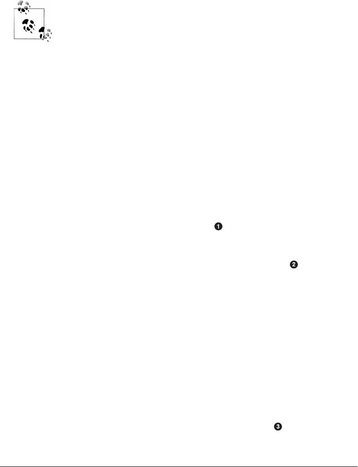
Data Sink
Subsequently, we will go through various MapReduce jobs that use HBase to read from,
or write to, as part of the process. The first use case explained is using HBase as a data
sink. This is facilitated by the TableOutputFormat class and demonstrated in Exam-
ple 7-1.
The example data used is based on the public RSS feed offered by De-
licious (http://delicious.com). Arvind Narayanan used the feed to collect
a sample data set, which he published on his blog.
There is no inherent need to acquire the data set, or capture the RSS
feed (http://feeds.delicious.com/v2/rss/recent); if you prefer, you can use
any other source, including JSON records. On the other hand, the De-
licious data set provides records that can be used nicely with Hush: every
entry has a link, user name, date, categories, and so on.
The test-data.txt included in the book’s repository is a small subset of
the public data set. For testing, this subset is sufficient, but you can
obviously execute the jobs with the full data set just as well.
The code, shown here in nearly complete form, includes some sort of standard tem-
plate, and the subsequent examples will not show these boilerplate parts. This includes,
for example, the command line parameter parsing.
Example 7-1. MapReduce job that reads from a file and writes into a table
public class ImportFromFile {
public static final String NAME = "ImportFromFile";
public enum Counters { LINES }
static class ImportMapper
extends Mapper<LongWritable, Text, ImmutableBytesWritable, Writable> {
private byte[] family = null;
private byte[] qualifier = null;
@Override
protected void setup(Context context)
throws IOException, InterruptedException {
String column = context.getConfiguration().get("conf.column");
byte[][] colkey = KeyValue.parseColumn(Bytes.toBytes(column));
family = colkey[0];
if (colkey.length > 1) {
qualifier = colkey[1];
}
}
@Override
public void map(LongWritable offset, Text line, Context context)
throws IOException {
MapReduce over HBase | 301

try {
String lineString = line.toString();
byte[] rowkey = DigestUtils.md5(lineString);
Put put = new Put(rowkey);
put.add(family, qualifier, Bytes.toBytes(lineString));
context.write(new ImmutableBytesWritable(rowkey), put);
context.getCounter(Counters.LINES).increment(1);
} catch (Exception e) {
e.printStackTrace();
}
}
}
private static CommandLine parseArgs(String[] args) throws ParseException {
Options options = new Options();
Option o = new Option("t", "table", true,
"table to import into (must exist)");
o.setArgName("table-name");
o.setRequired(true);
options.addOption(o);
o = new Option("c", "column", true,
"column to store row data into (must exist)");
o.setArgName("family:qualifier");
o.setRequired(true);
options.addOption(o);
o = new Option("i", "input", true,
"the directory or file to read from");
o.setArgName("path-in-HDFS");
o.setRequired(true);
options.addOption(o);
options.addOption("d", "debug", false, "switch on DEBUG log level");
CommandLineParser parser = new PosixParser();
CommandLine cmd = null;
try {
cmd = parser.parse(options, args);
} catch (Exception e) {
System.err.println("ERROR: " + e.getMessage() + "\n");
HelpFormatter formatter = new HelpFormatter();
formatter.printHelp(NAME + " ", options, true);
System.exit(-1);
}
return cmd;
}
public static void main(String[] args) throws Exception {
Configuration conf = HBaseConfiguration.create();
String[] otherArgs =
new GenericOptionsParser(conf, args).getRemainingArgs();
CommandLine cmd = parseArgs(otherArgs);
String table = cmd.getOptionValue("t");
String input = cmd.getOptionValue("i");
String column = cmd.getOptionValue("c");
conf.set("conf.column", column);
Job job = new Job(conf, "Import from file " + input + " into table " + table);
302 | Chapter 7: MapReduce Integration
job.setJarByClass(ImportFromFile.class);
job.setMapperClass(ImportMapper.class);
job.setOutputFormatClass(TableOutputFormat.class);
job.getConfiguration().set(TableOutputFormat.OUTPUT_TABLE, table);
job.setOutputKeyClass(ImmutableBytesWritable.class);
job.setOutputValueClass(Writable.class);
job.setNumReduceTasks(0);
FileInputFormat.addInputPath(job, new Path(input));
System.exit(job.waitForCompletion(true) ? 0 : 1);
}
}
Define a job name for later use.
Define the mapper class, extending the provided Hadoop class.
The map() function transforms the key/value provided by the InputFormat to what
is needed by the OutputFormat.
The row key is the MD5 hash of the line to generate a random key.
Store the original data in a column in the given table.
Parse the command line parameters using the Apache Commons CLI classes. These
are already part of HBase and therefore are handy to process the job specific
parameters.
Give the command line arguments to the generic parser first to handle "-Dxyz"
properties.
Define the job with the required classes.
This is a map only job; therefore, tell the framework to bypass the reduce step.
The code sets up the MapReduce job in its main() class by first parsing the command
line, which determines the target table name and column, as well as the name of the
input file. This could be hardcoded here as well, but it is good practice to write your
code in a configurable way.
The next step is setting up the job instance, assigning the variable details from the
command line, as well as all fixed parameters, such as class names. One of those is the
mapper class, set to ImportMapper. This class is defined in the same source code file,
defining what should be done during the map phase of the job.
The main() code also assigns the output format class, which is the aforementioned
TableOutputFormat class. It is provided by HBase and allows the job to easily write data
into a table. The key and value types needed by this class is implicitly fixed to
ImmutableBytesWritable for the key, and Writable for the value.
MapReduce over HBase | 303

Before you can execute the job, you first have to create a target table, for example, using
the HBase Shell:
hbase(main):001:0> create 'testtable', 'data'
0 row(s) in 0.5330 seconds
Once the table is ready you can launch the job:
$ hadoop dfs -put /projects/private/hbase-book-code/ch07/test-data.txt .
$ hadoop jar target/hbase-book-ch07-1.0-job.jar ImportFromFile \
-t testtable -i test-data.txt -c data:json
...
11/08/08 12:35:01 INFO mapreduce.TableOutputFormat: \
Created table instance for testtable
11/08/08 12:35:01 INFO input.FileInputFormat: Total input paths to process : 1
11/08/08 12:35:02 INFO mapred.JobClient: Running job: job_201108081021_0007
11/08/08 12:35:03 INFO mapred.JobClient: map 0% reduce 0%
11/08/08 12:35:10 INFO mapred.JobClient: map 100% reduce 0%
11/08/08 12:35:12 INFO mapred.JobClient: Job complete: job_201108081021_0007
The first command, hadoop dfs -put, stores the sample data in the user’s home directory
in HDFS. The second command launches the job itself, which completes in a short
amount of time. The data is read using the default TextInputFormat, as provided by
Hadoop and its MapReduce framework. This input format can read text files that have
newline characters at the end of each line. For every line read, it calls the map() function
of the defined mapper class. This triggers our ImportMapper.map() function.
As shown in Example 7-1, the ImportMapper defines two methods, overriding the ones
with the same name from the parent Mapper class.
Override Woes
It is highly recommended to add @Override annotations to your methods, so that wrong
signatures can be detected at compile time. Otherwise, the implicit map() or reduce()
methods might be called and do an identity function. For example, consider this
reduce() method:
public void reduce(Writable key, Iterator<Writable> values,
Context context) throws IOException, InterruptedException {
...
}
While this looks correct, it does not, in fact, override the reduce() method of the
Reducer class, but instead defines a new version of the method. The MapReduce frame-
work will silently ignore this method and execute the default implementation as
provided by the Reducer class.
The reason is that the actual signature of the method is this:
protected void reduce(KEYIN key, Iterable<VALUEIN> values, \
Context context) throws IOException, InterruptedException
This is a common mistake; the Iterable was erroneously replaced by an Iterator class.
This is all it takes to make for a new signature. Adding the @Override annotation to an
304 | Chapter 7: MapReduce Integration

overridden method in your code will make the compiler (and hopefully your back-
ground compilation check of your IDE) throw an error—before you run into what you
might perceive asstrange behavior during the job execution. Adding the annotation to
the previous example:
@Override
public void reduce(Writable key, Iterator<Writable> values,
Context context) throws IOException, InterruptedException {
...
}
The IDE you are using should already display an error, but at a minimum the compiler
will report the mistake:
...
[INFO] ---------------------------------------------------------------------
[ERROR] BUILD FAILURE
[INFO] ---------------------------------------------------------------------
[INFO] Compilation failure
ch07/src/main/java/mapreduce/InvalidReducerOverride.java:[18,4] method does
not override or implement a method from a supertype
The setup() method of ImportMapper overrides the method called once when the class
is instantiated by the framework. Here it is used to parse the given column into a column
family and qualifier.
The map() of that same class is doing the actual work. As noted, it is called for every
row in the input text file, each containing a JSON record. The code creates an HBase
row key by using an MD5 hash of the line content. It then stores the line content as-is
in the provided column, titled data:json.
The example makes use of the implicit write buffer set up by the TableOutputFormat
class. The call to context.write() issues an internal table.put() with the given instance
of Put. The TableOutputFormat takes care of calling flushCommits() when the job is
complete—saving the remaining data in the write buffer.
The map() method writes Put instances to store the input data. You can
also write Delete instances to delete data from the target table. This is
also the reason why the output key format of the job is set to Writable,
instead of the explicit Put class.
The TableOutputFormat can (currently) only handle Put and Delete in-
stances. Passing anything else will raise an IOException with the message
set to Pass a Delete or a Put.
Finally, note how the job is just using the map phase, and no reduce is needed. This is
fairly typical with MapReduce jobs in combination with HBase: since data is already
stored in sorted tables, or the raw data already has unique keys, you can avoid the more
costly sort, shuffle, and reduce phases in the process.
MapReduce over HBase | 305
Data Source
After importing the raw data into the table, we can use the contained data to parse the
JSON records and extract information from it. This is accomplished using the
TableInputFormat class, the counterpart to TableOutputFormat. It sets up a table as an
input to the MapReduce process. Example 7-2 makes use of the provided InputFor
mat class.
Example 7-2. MapReduce job that reads the imported data and analyzes it
static class AnalyzeMapper extends TableMapper<Text, IntWritable> {
private JSONParser parser = new JSONParser();
private IntWritable ONE = new IntWritable(1);
@Override
public void map(ImmutableBytesWritable row, Result columns, Context context)
throws IOException {
context.getCounter(Counters.ROWS).increment(1);
String value = null;
try {
for (KeyValue kv : columns.list()) {
context.getCounter(Counters.COLS).increment(1);
value = Bytes.toStringBinary(kv.getValue());
JSONObject json = (JSONObject) parser.parse(value);
String author = (String) json.get("author");
context.write(new Text(author), ONE);
context.getCounter(Counters.VALID).increment(1);
}
} catch (Exception e) {
e.printStackTrace();
System.err.println("Row: " + Bytes.toStringBinary(row.get()) +
", JSON: " + value);
context.getCounter(Counters.ERROR).increment(1);
}
}
}
static class AnalyzeReducer
extends Reducer<Text, IntWritable, Text, IntWritable> {
@Override
protected void reduce(Text key, Iterable<IntWritable> values,
Context context) throws IOException, InterruptedException {
int count = 0;
for (IntWritable one : values) count++;
context.write(key, new IntWritable(count));
}
}
public static void main(String[] args) throws Exception {
...
Scan scan = new Scan();
if (column != null) {
306 | Chapter 7: MapReduce Integration
byte[][] colkey = KeyValue.parseColumn(Bytes.toBytes(column));
if (colkey.length > 1) {
scan.addColumn(colkey[0], colkey[1]);
} else {
scan.addFamily(colkey[0]);
}
}
Job job = new Job(conf, "Analyze data in " + table);
job.setJarByClass(AnalyzeData.class);
TableMapReduceUtil.initTableMapperJob(table, scan, AnalyzeMapper.class,
Text.class, IntWritable.class, job);
job.setReducerClass(AnalyzeReducer.class);
job.setOutputKeyClass(Text.class);
job.setOutputValueClass(IntWritable.class);
job.setNumReduceTasks(1);
FileOutputFormat.setOutputPath(job, new Path(output));
System.exit(job.waitForCompletion(true) ? 0 : 1);
}
Extend the supplied TableMapper class, setting your own output key and value types.
Parse the JSON data, extract the author, and count the occurrence.
Extend a Hadoop Reducer class, assigning the proper types.
Count the occurrences and emit a sum.
Create and configure a Scan instance.
Set up the table mapper phase using the supplied utility.
Configure the reduce phase using the normal Hadoop syntax.
This job runs as a full MapReduce process, where the map phase is reading the JSON
data from the input table, and the reduce phase is aggregating the counts for every user.
This is very similar to the WordCount example† that ships with Hadoop: the mapper
emits counts of ONE, while the reducer counts those up to the sum per key (which in
Example 7-2 is the Author). Executing the job on the command line is done like so:
$ hadoop jar target/hbase-book-ch07-1.0-job.jar AnalyzeData \
-t testtable -c data:json -o analyze1
11/08/08 15:36:37 INFO mapred.JobClient: Running job: job_201108081021_0021
11/08/08 15:36:38 INFO mapred.JobClient: map 0% reduce 0%
11/08/08 15:36:45 INFO mapred.JobClient: map 100% reduce 0%
11/08/08 15:36:57 INFO mapred.JobClient: map 100% reduce 100%
11/08/08 15:36:59 INFO mapred.JobClient: Job complete: job_201108081021_0021
11/08/08 15:36:59 INFO mapred.JobClient: Counters: 19
...
11/08/08 15:36:59 INFO mapred.JobClient: mapreduce.AnalyzeData$Counters
11/08/08 15:36:59 INFO mapred.JobClient: ROWS=993
11/08/08 15:36:59 INFO mapred.JobClient: COLS=993
† See the Hadoop wiki page for details.
MapReduce over HBase | 307

11/08/08 15:36:59 INFO mapred.JobClient: VALID=993
...
The end result is a list of counts per author, and can be accessed from the command
line using, for example, the hadoop dfs -text command:
$ hadoop dfs -text analyze1/part-r-00000
10sr 1
13tohl 1
14bcps 1
21721725 1
2centime 1
33rpm 1
...
The example also shows how to use the TableMapReduceUtil class, with its static meth-
ods, to quickly configure a job with all the required classes. Since the job also needs a
reduce phase, the main() code adds the Reducer classes as required, once again making
implicit use of the default value when no other is specified (in this case, the TextOut
putFormat class).
Obviously, this is a simple example, and in practice you will have to perform more
involved analytical processing. But even so, the template shown in the example stays
the same: you read from a table, extract the required information, and eventually output
the results to a specific target.
Data Source and Sink
As already shown, the source or target of a MapReduce job can be a HBase table, but
it is also possible for a job to use HBase as both input and output. In other words, a
third kind of MapReduce template uses a table for the input and output types. This
involves setting the TableInputFormat and TableOutputFormat classes into the respective
fields of the job configuration. This also implies the various key and value types, as
shown before. Example 7-3 shows this in context.
Example 7-3. MapReduce job that parses the raw data into separate columns
static class ParseMapper
extends TableMapper<ImmutableBytesWritable, Writable> {
private JSONParser parser = new JSONParser();
private byte[] columnFamily = null;
@Override
protected void setup(Context context)
throws IOException, InterruptedException {
columnFamily = Bytes.toBytes(
context.getConfiguration().get("conf.columnfamily"));
}
@Override
public void map(ImmutableBytesWritable row, Result columns, Context context)
308 | Chapter 7: MapReduce Integration
throws IOException {
context.getCounter(Counters.ROWS).increment(1);
String value = null;
try {
Put put = new Put(row.get());
for (KeyValue kv : columns.list()) {
context.getCounter(Counters.COLS).increment(1);
value = Bytes.toStringBinary(kv.getValue());
JSONObject json = (JSONObject) parser.parse(value);
for (Object key : json.keySet()) {
Object val = json.get(key);
put.add(columnFamily, Bytes.toBytes(key.toString()),
Bytes.toBytes(val.toString()));
}
}
context.write(row, put);
context.getCounter(Counters.VALID).increment(1);
} catch (Exception e) {
e.printStackTrace();
System.err.println("Error: " + e.getMessage() + ", Row: " +
Bytes.toStringBinary(row.get()) + ", JSON: " + value);
context.getCounter(Counters.ERROR).increment(1);
}
}
}
public static void main(String[] args) throws Exception {
...
Scan scan = new Scan();
if (column != null) {
byte[][] colkey = KeyValue.parseColumn(Bytes.toBytes(column));
if (colkey.length > 1) {
scan.addColumn(colkey[0], colkey[1]);
conf.set("conf.columnfamily", Bytes.toStringBinary(colkey[0]));
conf.set("conf.columnqualifier", Bytes.toStringBinary(colkey[1]));
} else {
scan.addFamily(colkey[0]);
conf.set("conf.columnfamily", Bytes.toStringBinary(colkey[0]));
}
}
Job job = new Job(conf, "Parse data in " + input + ", write to " + output);
job.setJarByClass(ParseJson.class);
TableMapReduceUtil.initTableMapperJob(input, scan, ParseMapper.class,
ImmutableBytesWritable.class, Put.class, job);
TableMapReduceUtil.initTableReducerJob(output,
IdentityTableReducer.class, job);
System.exit(job.waitForCompletion(true) ? 0 : 1);
}
Store the top-level JSON keys as columns, with their value set as the column value.
Store the column family in the configuration for later use in the mapper.
Set up map phase details using the utility method.
MapReduce over HBase | 309

Configure an identity reducer to store the parsed data.
The example uses the utility methods to configure the map and reduce phases, speci-
fying the ParseMapper, which extracts the details from the raw JSON, and an Identity
TableReducer to store the data in the target table. Note that both—that is, the input
and output table—can be the same. Launching the job from the command line can be
done like this:
$ hadoop jar target/hbase-book-ch07-1.0-job.jar ParseJson \
-i testtable -c data:json -o testtable
11/08/08 17:44:33 INFO mapreduce.TableOutputFormat: \
Created table instance for testtable
11/08/08 17:44:33 INFO mapred.JobClient: Running job: job_201108081021_0026
11/08/08 17:44:34 INFO mapred.JobClient: map 0% reduce 0%
11/08/08 17:44:41 INFO mapred.JobClient: map 100% reduce 0%
11/08/08 17:44:50 INFO mapred.JobClient: map 100% reduce 100%
11/08/08 17:44:52 INFO mapred.JobClient: Job complete: job_201108081021_0026
...
The percentages show that both the map and reduce phases have been completed, and
that the job overall completed subsequently. Using the IdentityTableReducer to store
the extracted data is not necessary, and in fact the same code with one additional line
turns the job into a map-only one. Example 7-4 shows the added line.
Example 7-4. MapReduce job that parses the raw data into separate columns (map phase only)
...
Job job = new Job(conf, "Parse data in " + input + ", write to " + output +
"(map only)");
job.setJarByClass(ParseJson2.class);
TableMapReduceUtil.initTableMapperJob(input, scan, ParseMapper.class,
ImmutableBytesWritable.class, Put.class, job);
TableMapReduceUtil.initTableReducerJob(output,
IdentityTableReducer.class, job);
job.setNumReduceTasks(0);
...
Running the job from the command line shows that the reduce phase has been skipped:
$ hadoop jar target/hbase-book-ch07-1.0-job.jar ParseJson2 \
-i testtable -c data:json -o testtable
11/08/08 18:38:10 INFO mapreduce.TableOutputFormat: \
Created table instance for testtable
11/08/08 18:38:11 INFO mapred.JobClient: Running job: job_201108081021_0029
11/08/08 18:38:12 INFO mapred.JobClient: map 0% reduce 0%
11/08/08 18:38:20 INFO mapred.JobClient: map 100% reduce 0%
11/08/08 18:38:22 INFO mapred.JobClient: Job complete: job_201108081021_0029
...
The reduce stays at 0%, even when the job has completed. You can also use the Hadoop
MapReduce UI to confirm that no reduce task have been executed for this job. The
advantage of bypassing the reduce phase is that the job will complete much faster, since
no additional processing of the data by the framework is required.
310 | Chapter 7: MapReduce Integration

Both variations of the ParseJson job performed the same work. The result can be seen
using the HBase Shell (omitting the repetitive row key output for the sake of space):
hbase(main):001:0> scan 'testtable'
...
\xFB!Nn\x8F\x89}\xD8\x91+\xB9o9\xB3E\xD0
column=data:author, timestamp=1312821497945, value=bookrdr3
column=data:comments, timestamp=1312821497945,
value=http://delicious.com/url/409839abddbce807e4db07bf7d9cd7ad
column=data:guidislink, timestamp=1312821497945, value=false
column=data:id, timestamp=1312821497945,
value=http://delicious.com/url/409839abddbce807e4db07bf7d9cd7ad#bookrdr3
column=data:link, timestamp=1312821497945,
value=http://sweetsassafras.org/2008/01/27/how-to-alter-a-wool-sweater
...
column=data:updated, timestamp=1312821497945,
value=Mon, 07 Sep 2009 18:22:21 +0000
...
993 row(s) in 1.7070 seconds
The import makes use of the arbitrary column names supported by HBase: the JSON
keys are converted into qualifiers, and form new columns on the fly.
Custom Processing
You do not have to use any classes supplied by HBase to read and/or write to a table.
In fact, these classes are quite lightweight and only act as helpers to make dealing with
tables easier. Example 7-5 converts the previous example code to split the parsed JSON
data into two target tables. The link key and its value is stored in a separate table,
named linktable, while all other fields are stored in the table named infotable.
Example 7-5. MapReduce job that parses the raw data into separate tables
static class ParseMapper
extends TableMapper<ImmutableBytesWritable, Writable> {
private HTable infoTable = null;
private HTable linkTable = null;
private JSONParser parser = new JSONParser();
private byte[] columnFamily = null;
@Override
protected void setup(Context context)
throws IOException, InterruptedException {
infoTable = new HTable(context.getConfiguration(),
context.getConfiguration().get("conf.infotable"));
infoTable.setAutoFlush(false);
linkTable = new HTable(context.getConfiguration(),
context.getConfiguration().get("conf.linktable"));
linkTable.setAutoFlush(false);
columnFamily = Bytes.toBytes(
context.getConfiguration().get("conf.columnfamily"));
}
MapReduce over HBase | 311

@Override
protected void cleanup(Context context)
throws IOException, InterruptedException {
infoTable.flushCommits();
linkTable.flushCommits();
}
@Override
public void map(ImmutableBytesWritable row, Result columns, Context context)
throws IOException {
context.getCounter(Counters.ROWS).increment(1);
String value = null;
try {
Put infoPut = new Put(row.get());
Put linkPut = new Put(row.get());
for (KeyValue kv : columns.list()) {
context.getCounter(Counters.COLS).increment(1);
value = Bytes.toStringBinary(kv.getValue());
JSONObject json = (JSONObject) parser.parse(value);
for (Object key : json.keySet()) {
Object val = json.get(key);
if ("link".equals(key)) {
linkPut.add(columnFamily, Bytes.toBytes(key.toString()),
Bytes.toBytes(val.toString()));
} else {
infoPut.add(columnFamily, Bytes.toBytes(key.toString()),
Bytes.toBytes(val.toString()));
}
}
}
infoTable.put(infoPut);
linkTable.put(linkPut);
context.getCounter(Counters.VALID).increment(1);
} catch (Exception e) {
e.printStackTrace();
System.err.println("Error: " + e.getMessage() + ", Row: " +
Bytes.toStringBinary(row.get()) + ", JSON: " + value);
context.getCounter(Counters.ERROR).increment(1);
}
}
}
public static void main(String[] args) throws Exception {
...
conf.set("conf.infotable", cmd.getOptionValue("o"));
conf.set("conf.linktable", cmd.getOptionValue("l"));
...
Job job = new Job(conf, "Parse data in " + input + ", into two tables");
job.setJarByClass(ParseJsonMulti.class);
TableMapReduceUtil.initTableMapperJob(input, scan, ParseMapper.class,
ImmutableBytesWritable.class, Put.class, job);
job.setOutputFormatClass(NullOutputFormat.class);
job.setNumReduceTasks(0);
312 | Chapter 7: MapReduce Integration
System.exit(job.waitForCompletion(true) ? 0 : 1);
}
Create and configure both target tables in the setup() method.
Flush all pending commits when the task is complete.
Save parsed values into two separate tables.
Store table names in configuration for later use in the mapper.
Set the output format to be ignored by the framework.
You need to create two more tables, using, for example, the HBase Shell:
hbase(main):001:0> create 'infotable', 'data'
hbase(main):002:0> create 'linktable', 'data'
These two new tables will be used as the target tables for the current
example.
Executing the job is done on the command line, and emits the following output:
$ hadoop jar target/hbase-book-ch07-1.0-job.jar ParseJsonMulti \
-i testtable -c data:json -o infotable -l linktable
11/08/08 21:13:57 INFO mapred.JobClient: Running job: job_201108081021_0033
11/08/08 21:13:58 INFO mapred.JobClient: map 0% reduce 0%
11/08/08 21:14:06 INFO mapred.JobClient: map 100% reduce 0%
11/08/08 21:14:08 INFO mapred.JobClient: Job complete: job_201108081021_0033
...
So far, this is the same as the previous ParseJson examples. The difference is the re-
sulting tables, and their content. You can use the HBase Shell and the scan command
to list the content of each table after the job has completed. You should see that the
link table contains only the links, while the info table contains the remaining fields of
the original JSON.
Writing your own MapReduce code allows you to perform whatever is needed during
the job execution. You can, for example, read lookup values from a different table while
storing a combined result in yet another table. There is no limit as to where you read
from, or where you write to. The supplied classes are helpers, nothing more or less,
and serve well for a large number of use cases. If you find yourself limited by their
functionality, simply extend them, or implement generic MapReduce code and use the
API to access HBase tables in any shape or form.
MapReduce over HBase | 313
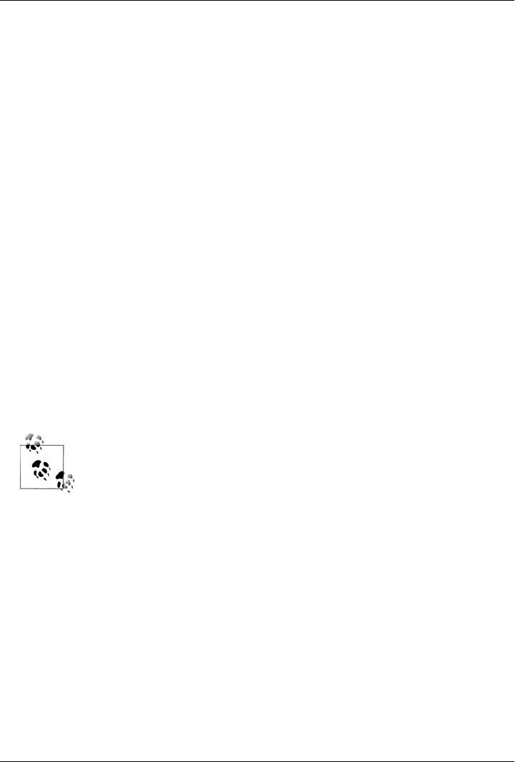
CHAPTER 8
Architecture
It is quite useful for advanced users (or those who are just plain adventurous) to fully
comprehend how a system of their choice works behind the scenes. This chapter ex-
plains the various moving parts of HBase and how they work together.
Seek Versus Transfer
Before we look into the architecture itself, however, we will first address a more fun-
damental difference between typical RDBMS storage structures and alternative ones.
Specifically, we will look briefly at B-trees, or rather B+ trees,* as they are commonly
used in relational storage engines, and Log-Structured Merge Trees,† which (to some
extent) form the basis for Bigtable’s storage architecture, as discussed in “Building
Blocks” on page 16.
Note that RDBMSes do not use B-tree-type structures exclusively, nor
do all NoSQL solutions use different architectures. You will find a col-
orful variety of mix-and-match technologies, but with one common
objective: use the best strategy for the problem at hand.
B+ Trees
B+ trees have some specific features that allow for efficient insertion, lookup, and de-
letion of records that are identified by keys. They represent dynamic, multilevel indexes
with lower and upper bounds as far as the number of keys in each segment (also called
page) is concerned. Using these segments, they achieve a much higher fanout compared
to binary trees, resulting in a much lower number of I/O operations to find a specific
key.
* See “B+ trees” on Wikipedia.
† See “LSM-Tree” (http://citeseerx.ist.psu.edu/viewdoc/summary?doi=10.1.1.44.2782), O’Neil et al., 1996.
315
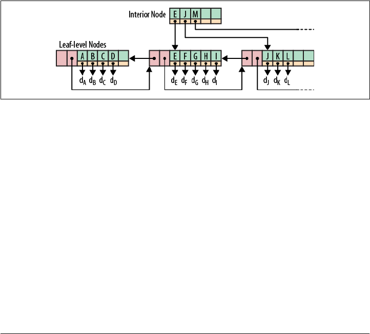
In addition, they also enable you to do range scans very efficiently, since the leaf nodes
in the tree are linked and represent an in-order list of all keys, avoiding more costly tree
traversals. That is one of the reasons why they are used for indexes in relational database
systems.
In a B+ tree index, you get locality on a page level (where “page” is synonymous with
“block” in other systems). For example, the leaf pages look something like this:
[link to previous page]
[link to next page]
key1 → rowid
key2 → rowid
key3 → rowid
In order to insert a new index entry, say key1.5, it will update the leaf page with a new
key1.5 → rowid entry. That is not a problem until the page, which has a fixed size,
exceeds its capacity. Then it has to split the page into two new ones, and update the
parent in the tree to point to the two new half-full pages. See Figure 8-1 for an example
of a page that is full and would need to be split when adding another key.
Figure 8-1. An example B+ tree with one full page
The issue here is that the new pages aren’t necessarily next to each other on disk. So
now if you ask to query a range from key 1 to key 3, it’s going to have to read two leaf
pages that could be far apart from each other. That is also the reason why you will find
an OPTIMIZE TABLE command in most layouts based on B+ trees—it basically rewrites
the table in-order so that range queries become ranges on disk again.
Log-Structured Merge-Trees
Log-structured merge-trees, also known as LSM-trees, follow a different approach.
Incoming data is stored in a logfile first, completely sequentially. Once the log has the
modification saved, it then updates an in-memory store that holds the most recent
updates for fast lookup.
When the system has accrued enough updates and starts to fill up the in-memory store,
it flushes the sorted list of key → record pairs to disk, creating a new store file. At this
316 | Chapter 8: Architecture
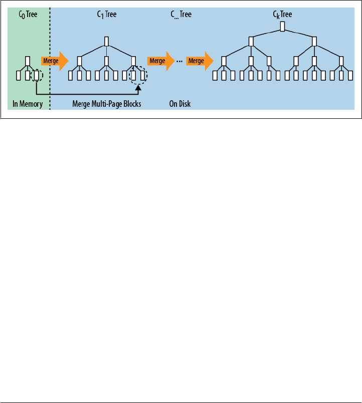
point, the updates to the log can be thrown away, as all modifications have been
persisted.
The store files are arranged similar to B-trees, but are optimized for sequential disk
access where all nodes are completely filled and stored as either single-page or multi-
page blocks. Updating the store files is done in a rolling merge fashion, that is, the system
packs existing on-disk multipage blocks together with the flushed in-memory data until
the block reaches its full capacity, at which point a new one is started.
Figure 8-2 shows how a multipage block is merged from the in-memory tree into the
next on-disk tree. Merging writes out a new block with the combined result. Eventually,
the trees are merged into the larger blocks.
Figure 8-2. Multipage blocks iteratively merged across LSM-trees
As more flushes are taking place over time, creating many store files, a background
process aggregates the files into larger ones so that disk seeks are limited to only a few
store files. The on-disk tree can also be split into separate trees to spread updates across
multiple store files. All of the stores are always sorted by key, so no reordering is re-
quired to fit new keys in between existing ones.
Lookups are done in a merging fashion in which the in-memory store is searched first,
and then the on-disk store files are searched next. That way, all the stored data, no
matter where it currently resides, forms a consistent view from a client’s perspective.
Deletes are a special case of update wherein a delete marker is stored and is used during
the lookup to skip “deleted” keys. When the pages are rewritten asynchronously, the
delete markers and the key they mask are eventually dropped.
An additional feature of the background processing for housekeeping is the ability to
support predicate deletions. These are triggered by setting a time-to-live (TTL) value
that retires entries, for example, after 20 days. The merge processes will check the
predicate and, if true, drop the record from the rewritten blocks.
The fundamental difference between B-trees and LSM-trees, though, is how their ar-
chitecture is making use of modern hardware, especially disk drives.
Seek Versus Transfer | 317

Seek Versus Sort and Merge in Numbers‡
For our large-scale scenarios, computation is dominated by disk transfers. Although
CPU, RAM, and disk size double every 18–24 months, seek time remains nearly con-
stant at around a 5% increase in speed per year.
As discussed at the beginning of this chapter, there are two different database para-
digms: one is seek and the other is transfer. Seek is typically found in RDBMSes and is
caused by the B-tree or B+ tree structures used to store the data. It operates at the disk
seek rate, resulting in log(N) seeks per access.
Transfer, on the other hand, as used by LSM-trees, sorts and merges files while oper-
ating at transfer rates, and takes log(updates) operations. This results in the following
comparison given these values:
– 10 MB/second transfer bandwidth
– 10 milliseconds disk seek time
– 100 bytes per entry (10 billion entries)
– 10 KB per page (1 billion pages)
When updating 1% of entries (100,000,000), it takes:
– 1,000 days with random B-tree updates
– 100 days with batched B-tree updates
– 1 day with sort and merge
We can safely conclude that, at scale seek, is inefficient compared to transfer.
To compare B+ trees and LSM-trees you need to understand their relative strengths
and weaknesses. B+ trees work well until there are too many modifications, because
they force you to perform costly optimizations to retain that advantage for a limited
amount of time. The more and faster you add data at random locations, the faster the
pages become fragmented again. Eventually, you may take in data at a higher rate than
the optimization process takes to rewrite the existing files. The updates and deletes are
done at disk seek rates, rather than disk transfer rates.
LSM-trees work at disk transfer rates and scale much better to handle large amounts
of data. They also guarantee a very consistent insert rate, as they transform random
writes into sequential writes using the logfile plus in-memory store. The reads are in-
dependent from the writes, so you also get no contention between these two operations.
The stored data is always in an optimized layout. So, you have a predictable and con-
sistent boundary on the number of disk seeks to access a key, and reading any number
of records following that key doesn’t incur any extra seeks. In general, what could be
emphasized about an LSM-tree-based system is cost transparency: you know that if
‡ From “Open Source Search” by Doug Cutting, December 5, 2005.
318 | Chapter 8: Architecture

you have five storage files, access will take a maximum of five disk seeks, whereas you
have no way to determine the number of disk seeks an RDBMS query will take, even if
it is indexed.
Finally, HBase is an LSM-tree-based system, just like Bigtable. The next sections will
explain the storage architecture, while referring back to earlier sections of the book
where appropriate.
Storage
One of the least-known aspects of HBase is how data is actually stored. While the
majority of users may never have to bother with this, you may have to get up to speed
when you want to learn the meaning of the various advanced configuration options
you have at your disposal. Chapter 11 lists the more common ones and Appendix A
has the full reference list.
You may also want to know more about file storage if, for whatever reason, disaster
strikes and you have to recover an HBase installation. At that point, it is important to
know where all the data is stored and how to access it on the HDFS level. Of course,
this shall not happen, but who can guarantee that?
Overview
The first step in understanding the various moving parts in the storage layer of HBase
is to understand the high-level picture. Figure 8-3 shows an overview of how HBase
and Hadoop’s filesystem are combined to store data.
The figure shows that HBase handles basically two kinds of file types: one is used for
the write-ahead log and the other for the actual data storage. The files are primarily
handled by the HRegionServers. In certain cases, the HMaster will also have to perform
low-level file operations. You may also notice that the actual files are divided into blocks
when stored within HDFS. This is also one of the areas where you can configure the
system to handle larger or smaller data records better. More on that in “HFile For-
mat” on page 329.
The general communication flow is that a new client contacts the ZooKeeper ensemble
(a separate cluster of ZooKeeper nodes) first when trying to access a particular row. It
does so by retrieving the server name (i.e., hostname) that hosts the -ROOT- region from
ZooKeeper. With this information it can query that region server to get the server name
that hosts the .META. table region containing the row key in question. Both of these
details are cached and only looked up once. Lastly, it can query the reported .META.
server and retrieve the server name that has the region containing the row key the client
is looking for.
Once it has been told in what region the row resides, it caches this information as well
and contacts the HRegionServer hosting that region directly. So, over time, the client
Storage | 319
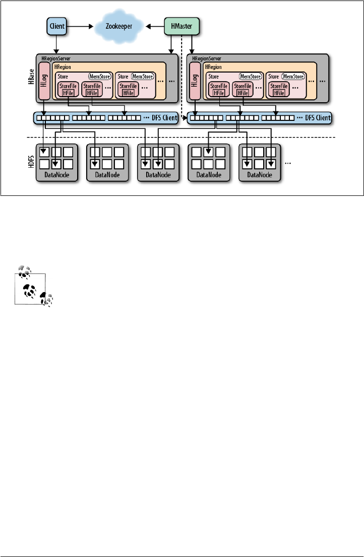
has a pretty complete picture of where to get rows without needing to query
the .META. server again. See “Region Lookups” on page 345 for more details.
The HMaster is responsible for assigning the regions to each HRegion
Server when you start HBase. This also includes the special -ROOT-
and .META. tables. See “The Region Life Cycle” on page 348 for details.
The HRegionServer opens the region and creates a corresponding HRegion object. When
the HRegion is opened it sets up a Store instance for each HColumnFamily for every table
as defined by the user beforehand. Each Store instance can, in turn, have one or more
StoreFile instances, which are lightweight wrappers around the actual storage file
called HFile. A Store also has a MemStore, and the HRegionServer a shared HLog in-
stance (see “Write-Ahead Log” on page 333).
Write Path
The client issues an HTable.put(Put) request to the HRegionServer, which hands the
details to the matching HRegion instance. The first step is to write the data to the write-
ahead log (the WAL), represented by the HLog class.§ The WAL is a standard Hadoop
SequenceFile and it stores HLogKey instances. These keys contain a sequential number
Figure 8-3. Overview of how HBase handles files in the filesystem, which stores them transparently
in HDFS
§ In extreme cases, you may turn off this step by setting a flag using the Put.setWriteToWAL(boolean) method.
This is not recommended as this will disable durability.
320 | Chapter 8: Architecture

as well as the actual data and are used to replay not-yet-persisted data after a server
crash.
Once the data is written to the WAL, it is placed in the MemStore. At the same time, it
is checked to see if the MemStore is full and, if so, a flush to disk is requested. The request
is served by a separate thread in the HRegionServer, which writes the data to a new
HFile located in HDFS. It also saves the last written sequence number so that the system
knows what was persisted so far.
Preflushing on Stop
There is a second reason for memstores to be flushed: preflushing. When a region server
is asked to stop it checks the memstores, and any that has more data than what is
configured with the hbase.hregion.preclose.flush.size property (set to 5 MB by de-
fault) is first flushed to disk before blocking access to the region for a final round of
flushing to close the hosted regions.
In other words, stopping the region servers forces all memstores to be written to disk,
no matter how full they are compared to the configured maximum size, set with the
hbase.hregion.memstore.flush.size property (the default is 64 MB), or when creating
the table (see the “Maximum file size” list item in “Table Properties” on page 210).
Once all memstores are flushed, the regions can be closed and no subsequent logfile
replaying is needed when the regions are reopened by a different server.
Using the extra round of preflushing extends availability for the regions: during the
preflush, the server and its regions are still available. This is similar to issuing a flush
shell command or API call. Only when the remaining smaller memstores are flushed
in the second round do the regions stop taking any further requests. This round also
takes care of all modifications that came in to any memstore that was preflushed al-
ready. It guarantees that the server can exit cleanly.
Files
HBase has a configurable root directory in HDFS, with the default set to "/hbase".
“Coexisting Clusters” on page 464 shows how to use a different root directory when
sharing a central HDFS cluster. You can use the hadoop dfs -lsr command to look at
the various files HBase stores. Before doing this, let us first create and fill a table with
a handful of regions:
hbase(main):001:0> create 'testtable', 'colfam1', \
{ SPLITS => ['row-300', 'row-500', 'row-700' , 'row-900'] }
0 row(s) in 0.1910 seconds
hbase(main):002:0> for i in '0'..'9' do for j in '0'..'9' do \
for k in '0'..'9' do put 'testtable', "row-#{i}#{j}#{k}", \
"colfam1:#{j}#{k}", "#{j}#{k}" end end end
0 row(s) in 1.0710 seconds
0 row(s) in 0.0280 seconds
0 row(s) in 0.0260 seconds
Storage | 321

...
hbase(main):003:0> flush 'testtable'
0 row(s) in 0.3310 seconds
hbase(main):004:0> for i in '0'..'9' do for j in '0'..'9' do \
for k in '0'..'9' do put 'testtable', "row-#{i}#{j}#{k}", \
"colfam1:#{j}#{k}", "#{j}#{k}" end end end
0 row(s) in 1.0710 seconds
0 row(s) in 0.0280 seconds
0 row(s) in 0.0260 seconds
...
The flush command writes the in-memory data to the store files; otherwise, we would
have had to wait until more than the configured flush size of data was inserted into the
stores. The last round of looping over the put command is to fill the write-ahead log
again.
Here is the content of the HBase root directory afterward:
$ $HADOOP_HOME/bin/hadoop dfs -lsr /hbase
...
0 /hbase/.logs
0 /hbase/.logs/foo.internal,60020,1309812147645
0 /hbase/.logs/foo.internal,60020,1309812147645/ \
foo.internal%2C60020%2C1309812147645.1309812151180
0 /hbase/.oldlogs
38 /hbase/hbase.id
3 /hbase/hbase.version
0 /hbase/testtable
487 /hbase/testtable/.tableinfo
0 /hbase/testtable/.tmp
0 /hbase/testtable/1d562c9c4d3b8810b3dbeb21f5746855
0 /hbase/testtable/1d562c9c4d3b8810b3dbeb21f5746855/.oldlogs
124 /hbase/testtable/1d562c9c4d3b8810b3dbeb21f5746855/.oldlogs/ \
hlog.1309812163957
282 /hbase/testtable/1d562c9c4d3b8810b3dbeb21f5746855/.regioninfo
0 /hbase/testtable/1d562c9c4d3b8810b3dbeb21f5746855/.tmp
0 /hbase/testtable/1d562c9c4d3b8810b3dbeb21f5746855/colfam1
11773 /hbase/testtable/1d562c9c4d3b8810b3dbeb21f5746855/colfam1/ \
646297264540129145
0 /hbase/testtable/66b4d2adcc25f1643da5e6260c7f7b26
311 /hbase/testtable/66b4d2adcc25f1643da5e6260c7f7b26/.regioninfo
0 /hbase/testtable/66b4d2adcc25f1643da5e6260c7f7b26/.tmp
0 /hbase/testtable/66b4d2adcc25f1643da5e6260c7f7b26/colfam1
7973 /hbase/testtable/66b4d2adcc25f1643da5e6260c7f7b26/colfam1/ \
3673316899703710654
0 /hbase/testtable/99c0716d66e536d927b479af4502bc91
297 /hbase/testtable/99c0716d66e536d927b479af4502bc91/.regioninfo
0 /hbase/testtable/99c0716d66e536d927b479af4502bc91/.tmp
0 /hbase/testtable/99c0716d66e536d927b479af4502bc91/colfam1
4173 /hbase/testtable/99c0716d66e536d927b479af4502bc91/colfam1/ \
1337830525545548148
0 /hbase/testtable/d240e0e57dcf4a7e11f4c0b106a33827
311 /hbase/testtable/d240e0e57dcf4a7e11f4c0b106a33827/.regioninfo
322 | Chapter 8: Architecture

0 /hbase/testtable/d240e0e57dcf4a7e11f4c0b106a33827/.tmp
0 /hbase/testtable/d240e0e57dcf4a7e11f4c0b106a33827/colfam1
7973 /hbase/testtable/d240e0e57dcf4a7e11f4c0b106a33827/colfam1/ \
316417188262456922
0 /hbase/testtable/d9ffc3a5cd016ae58e23d7a6cb937949
311 /hbase/testtable/d9ffc3a5cd016ae58e23d7a6cb937949/.regioninfo
0 /hbase/testtable/d9ffc3a5cd016ae58e23d7a6cb937949/.tmp
0 /hbase/testtable/d9ffc3a5cd016ae58e23d7a6cb937949/colfam1
7973 /hbase/testtable/d9ffc3a5cd016ae58e23d7a6cb937949/colfam1/ \
4238940159225512178
The output was reduced to include just the file size and name to fit the
available space. When you run the command on your cluster you will
see more details.
The files can be divided into those that reside directly under the HBase root directory,
and those that are in the per-table directories.
Root-level files
The first set of files are the write-ahead log files handled by the HLog instances, created
in a directory called .logs underneath the HBase root directory. The .logs directory
contains a subdirectory for each HRegionServer. In each subdirectory, there are several
HLog files (because of log rotation). All regions from that region server share the same
HLog files.
An interesting observation is that the logfile is reported to have a size of 0. This is fairly
typical when the file was created recently, as HDFS is using built-in append support to
write to this file, and only complete blocks are made available to readers—including
the hadoop dfs -lsr command. Although the data of the put operations is safely persisted,
the size of the logfile that is currently being written to is slightly off.
After, for example, waiting for an hour so that the logfile is rolled (see “LogRoller
Class” on page 338 for all reasons when logfiles are rolled), you will see the existing
logfile reported with its proper size, since it is closed now and HDFS can state the
“correct” size. The new logfile next to it again starts at zero size:
249962 /hbase/.logs/foo.internal,60020,1309812147645/ \
foo.internal%2C60020%2C1309812147645.1309812151180
0 /hbase/.logs/foo.internal,60020,1309812147645/ \
foo.internal%2C60020%2C1309812147645.1309815751223
When a logfile is are no longer needed because all of the contained edits have been
persisted into store files, it is decommissioned into the .oldlogs directory under the root
HBase directory. This is triggered when the logfile is rolled based on the configured
thresholds.
The old logfiles are deleted by the master after 10 minutes (by default), set with the
hbase.master.logcleaner.ttl property. The master checks every minute (by default
Storage | 323

again) for those files. This is configured with the hbase.master.cleaner.interval
property.
The behavior for expired logfiles is pluggable. This is used, for instance,
by the replication feature (see “Replication” on page 351) to have access
to persisted modifications.
The hbase.id and hbase.version files contain the unique ID of the cluster, and the file
format version:
$ hadoop dfs -cat /hbase/hbase.id
$e627e130-0ae2-448d-8bb5-117a8af06e97
$ hadoop dfs -cat /hbase/hbase.version
7
They are used internally and are otherwise not very interesting. In addition, there are
a few more root-level directories that appear over time. The splitlog and .corrupt folders
are used by the log split process to store the intermediate split files and the corrupted
logs, respectively. For example:
0 /hbase/.corrupt
0 /hbase/splitlog/foo.internal,60020,1309851880898_hdfs%3A%2F%2F \
localhost%2Fhbase%2F.logs%2Ffoo.internal%2C60020%2C1309850971208%2F \
foo.internal%252C60020%252C1309850971208.1309851641956/testtable/ \
d9ffc3a5cd016ae58e23d7a6cb937949/recovered.edits/0000000000000002352
There are no corrupt logfiles in this example, but there is one staged split file. The log
splitting process is explained in “Replay” on page 338.
Table-level files
Every table in HBase has its own directory, located under the HBase root directory in
the filesystem. Each table directory contains a top-level file named .tableinfo, which
stores the serialized HTableDescriptor (see “Tables” on page 207 for details) for the
table. This includes the table and column family schemas, and can be read, for example,
by tools to gain insight on what the table looks like. The .tmp directory contains tem-
porary data, and is used, for example, when the .tableinfo file is updated.
Region-level files
Inside each table directory, there is a separate directory for every region comprising the
table. The names of these directories are the MD5 hash portion of a region name. For
example, the following is taken from the master’s web UI, after clicking on the testta
ble link in the User Tables section:
testtable,row-500,1309812163930.d9ffc3a5cd016ae58e23d7a6cb937949.
The MD5 hash is d9ffc3a5cd016ae58e23d7a6cb937949 and is generated by encoding
everything before the hash in the region name (minus the dividing dot), that is,
324 | Chapter 8: Architecture
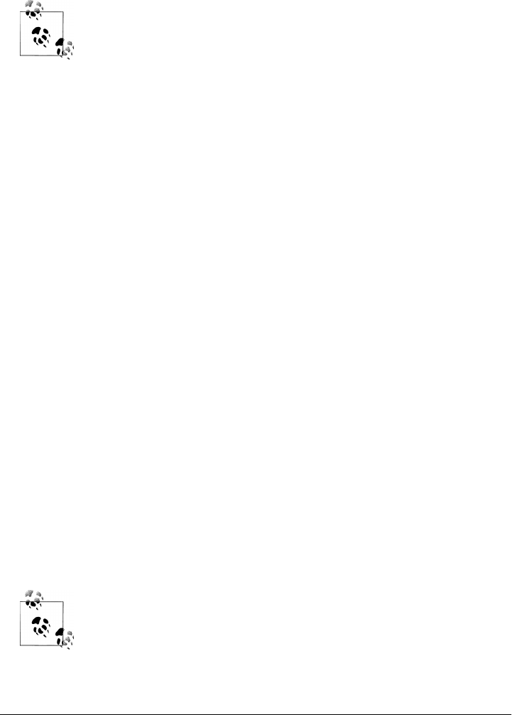
testtable,row-500,1309812163930. The final dot after the hash is part of the complete
region name: it indicates that this is a new style name. In previous versions of HBase,
the region names did not include the hash.
The -ROOT- and .META. catalog tables are still using the old style format,
that is, their region names include no hash, and therefore end without
the trailing dot:
.META.,,1.1028785192
The encoding of the region names for the on-disk directories is also
different: they use a Jenkins hash to encode the region name.
The hash guarantees that the directory names are always valid, in terms of filesystem
rules: they do not contain any special character, such as the slash (“/”), which is used
to divide the path. The overall layout for region files is then:
/<hbase-root-dir>/<tablename>/<encoded-regionname>/<column-family>/<filename>
In each column-family directory, you can see the actual data files, explained in “HFile
Format” on page 329. Their name is just an arbitrary number, based on the Java built-
in random generator. The code is smart enough to check for collisions, that is, where
a file with a newly generated number already exists. It loops until it finds an unused
one and uses that instead.
The region directory also has a .regioninfo file, which contains the serialized information
of the HRegionInfo instance for the given region. Similar to the .tableinfo file, it can be
used by external tools to gain insight into the metadata of a region. The hbase hbck tool
uses this to generate missing meta table entries, for example.
The optional .tmp directory is created on demand, and is used to hold temporary files—
for example, the rewritten files from a compaction. These are usually moved out into
the region directory once the process has completed. In rare circumstances, you might
find leftover files, which are cleaned out when the region is reopened.
During the replay of the write-ahead log, any edit that has not been committed is written
into a separate file per region. These are staged first (see the splitlog directory in “Root-
level files” on page 323) and then—assuming the log splitting process has completed
successfully—moved into the optional recovered.edits directory atomically. When the
region is opened the region server will see the recovery file and replay the entries
accordingly.
There is a clear distinction between the splitting of write-ahead logs
(“Replay” on page 338) and the splitting of regions (“Region
splits” on page 326). Sometimes it is difficult to distinguish the file and
directory names in the filesystem, because both might refer to the term
splits. Make sure you carefully identify their purpose to avoid
confusion—or mistakes.
Storage | 325

Once the region needs to split because it has exceeded the maximum configured region
size, a matching splits directory is created, which is used to stage the two new daughter
regions. If this process is successful—usually this happens in a few seconds or less—
they are moved up into the table directory to form the two new regions, each
representing one-half of the original region.
In other words, when you see a region directory that has no .tmp directory, no com-
paction has been performed for it yet. When it has no recovered.edits file, no write-
ahead log replay has occurred for it yet.
In HBase versions before 0.90.x there were additional files, which are
now obsolete. One is oldlogfile.log, which contained the replayed write-
ahead log edits for the given region. The oldlogfile.log.old file (note the
extra .old extension) indicated that there was already an existing old-
logfile.log file when the new one was put into place.
Another noteworthy file is the compaction.dir file in older versions of
HBase, which is now replaced by the .tmp directory.
This concludes the list of what is commonly contained in the various directories inside
the HBase root folder. There are more intermediate files, created by the region split
process. They are discussed separately in the next section.
Region splits
When a store file within a region grows larger than the configured
hbase.hregion.max.filesize—or what is configured at the column family level using
HColumnDescriptor—the region is split in two. This is done initially very quickly because
the system simply creates two reference files for the new regions (also called daugh-
ters), which each hosting half of the original region (referred to as the parent).
The region server accomplishes this by creating the splits directory in the parent region.
Next, it closes the region so that it does not take on anymore requests.
The region server then prepares the new daughter regions (using multiple threads) by
setting up the necessary file structures inside the splits directory. This includes the new
region directories and the reference files. If this process completes successfully, it moves
the two new region directories into the table directory. The .META. table is updated for
the parent to state that it is now split, and what the two daughter regions are. This
prevents it from being reopened by accident. Here is an example of how this looks in
the .META. table:
row: testtable,row-500,1309812163930.d9ffc3a5cd016ae58e23d7a6cb937949.
column=info:regioninfo, timestamp=1309872211559, value=REGION => {NAME => \
'testtable,row-500,1309812163930.d9ffc3a5cd016ae58e23d7a6cb937949. \
TableName => 'testtable', STARTKEY => 'row-500', ENDKEY => 'row-700', \
ENCODED => d9ffc3a5cd016ae58e23d7a6cb937949, OFFLINE => true,
326 | Chapter 8: Architecture

SPLIT => true,}
column=info:splitA, timestamp=1309872211559, value=REGION => {NAME => \
'testtable,row-500,1309872211320.d5a127167c6e2dc5106f066cc84506f8. \
TableName => 'testtable', STARTKEY => 'row-500', ENDKEY => 'row-550', \
ENCODED => d5a127167c6e2dc5106f066cc84506f8,}
column=info:splitB, timestamp=1309872211559, value=REGION => {NAME => \
'testtable,row-550,1309872211320.de27e14ffc1f3fff65ce424fcf14ae42. \
TableName => [B@62892cc5', STARTKEY => 'row-550', ENDKEY => 'row-700', \
ENCODED => de27e14ffc1f3fff65ce424fcf14ae42,}
You can see how the original region was split into two regions, separated at row-550.
The SPLIT => true in the info:regioninfo column value also indicates that this region
is now split into the regions referred to in info:splitA and info:splitB.
The name of the reference file is another random number, but with the hash of the
referenced region as a postfix, for instance:
/hbase/testtable/d5a127167c6e2dc5106f066cc84506f8/colfam1/ \
6630747383202842155.d9ffc3a5cd016ae58e23d7a6cb937949
This reference file represents one-half of the original region with the hash
d9ffc3a5cd016ae58e23d7a6cb937949, which is the region shown in the preceding exam-
ple. The reference files only hold a little information: the key the original region was
split at, and whether it is the top or bottom reference. Of note is that these references
are then used by the HalfHFileReader class (which was omitted from the earlier overview
as it is only used temporarily) to read the original region data files, and either the top
or the bottom half of the files.
Both daughter regions are now ready and will be opened in parallel by the same server.
This includes updating the .META. table to list both regions as available regions—just
like any other. After that, the regions are online and start serving requests.
The opening of the daughters also schedules a compaction for both—which rewrites
the store files in the background from the parent region into the two halves, while
replacing the reference files. This takes place in the .tmp directory of the daughter
regions. Once the files have been generated, they atomically replace the reference.
The parent is eventually cleaned up when there are no more references to it, which
means it is removed as the parent from the .META. table, and all of its files on disk are
deleted. Finally, the master is informed about the split and can schedule for the new
regions to be moved off to other servers for load balancing reasons.
All of the steps involved in the split are tracked in ZooKeeper. This
allows for other processes to reason about the state of a region in case
of a server failure.
Storage | 327
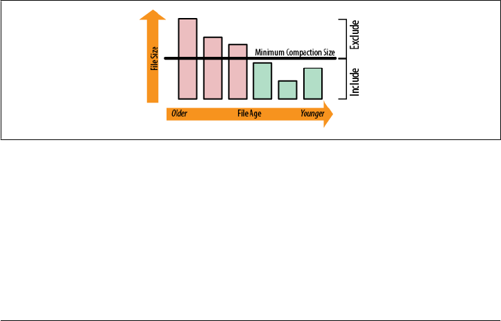
Compactions
The store files are monitored by a background thread to keep them under control. The
flushes of memstores slowly build up an increasing number of on-disk files. If there are
enough of them, the compaction process will combine them to a few, larger files. This
goes on until the largest of these files exceeds the configured maximum store file size
and triggers a region split (see “Region splits” on page 326).
Compactions come in two varieties: minor and major. Minor compactions are respon-
sible for rewriting the last few files into one larger one. The number of files is set
with the hbase.hstore.compaction.min property (which was previously called
hbase.hstore.compactionThreshold, and although deprecated is still supported). It is
set to 3 by default, and needs to be at least 2 or more. A number too large would delay
minor compactions, but also would require more resources and take longer once the
compactions start.
The maximum number of files to include in a minor compaction is set to 10, and is
configured with hbase.hstore.compaction.max. The list is further narrowed down by
the hbase.hstore.compaction.min.size (set to the configured memstore flush size for
the region), and the hbase.hstore.compaction.max.size (defaults to Long.MAX_VALUE)
configuration properties. Any file larger than the maximum compaction size is always
excluded. The minimum compaction size works slightly differently: it is a threshold
rather than a per-file limit. It includes all files that are under that limit, up to the total
number of files per compaction allowed.
Figure 8-4 shows an example set of store files. All files that fit under the minimum
compaction threshold are included in the compaction process.
Figure 8-4. A set of store files showing the minimum compaction threshold
The algorithm uses hbase.hstore.compaction.ratio (defaults to 1.2, or 120%) to ensure
that it does include enough files in the selection process. The ratio will also select files
that are up to that size compared to the sum of the store file sizes of all newer files. The
evaluation always checks the files from the oldest to the newest. This ensures that older
files are compacted first. The combination of these properties allows you to fine-tune
how many files are included in a minor compaction.
328 | Chapter 8: Architecture
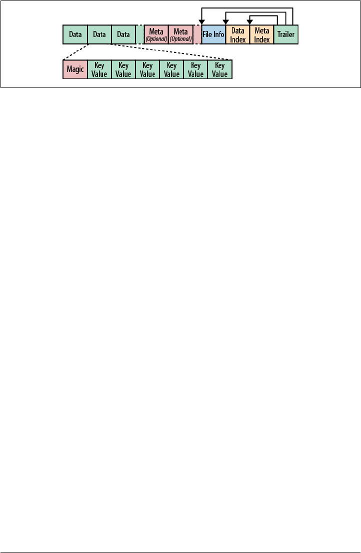
In contrast to minor compactions, major compactions compact all files into a single
file. Which compaction type is run is automatically determined when the compaction
check is executed. The check is triggered either after a memstore has been flushed to
disk, after the compact or major_compact shell commands or corresponding API calls
have been invoked, or by a background thread. This background thread is called the
CompactionChecker and each region server runs a single instance. It runs a check on a
regular basis, controlled by hbase.server.thread.wakefrequency (and multiplied by
hbase.server.thread.wakefrequency.multiplier, set to 1000, to run it less often than
the other thread-based tasks).
If you call the major_compact shell command, or the majorCompact() API call, you force
the major compaction to run. Otherwise, the server checks first if the major compaction
is due, based on hbase.hregion.majorcompaction (set to 24 hours) from the first time it
ran. The hbase.hregion.majorcompaction.jitter (set to 0.2, in other words, 20%) cau-
ses this time to be spread out for the stores. Without the jitter, all stores would run a
major compaction at the same time, every 24 hours. See “Managed Split-
ting” on page 429 for information on why this is a bad idea and how to manage this
better.
If no major compaction is due, a minor compaction is assumed. Based on the afore-
mentioned configuration properties, the server determines if enough files for a minor
compaction are available and continues if that is the case.
Minor compactions might be promoted to major compactions when the former would
include all store files, and there are less than the configured maximum files per
compaction.
HFile Format
The actual storage files are implemented by the HFile class, which was specifically
created to serve one purpose: store HBase’s data efficiently. They are based on Ha-
doop’s TFile class,‖ and mimic the SSTable format used in Google’s Bigtable architec-
ture. The previous use of Hadoop’s MapFile class in HBase proved to be insufficient in
terms of performance. Figure 8-5 shows the file format details.
‖See the JIRA issue HADOOP-3315 for details.
Figure 8-5. The HFile structure
Storage | 329

The files contain a variable number of blocks, where the only fixed ones are the file
info and trailer blocks. As Figure 8-5 shows, the trailer has the pointers to the other
blocks. It is written after the data has been persisted to the file, finalizing the now
immutable data store. The index blocks record the offsets of the data and meta blocks.
Both the data and the meta blocks are actually optional. But considering how HBase
uses the data files, you will almost always find at least data blocks in the store files.
The block size is configured by the HColumnDescriptor, which, in turn, is specified at
table creation time by the user, or defaults to reasonable standard values. Here is an
example as shown in the master web-based interface:
{NAME => 'testtable', FAMILIES => [{NAME => 'colfam1',
BLOOMFILTER => 'NONE', REPLICATION_SCOPE => '0', VERSIONS => '3',
COMPRESSION \=> 'NONE', TTL => '2147483647', BLOCKSIZE => '65536',
IN_MEMORY => 'false', BLOCKCACHE => 'true'}]}
The default is 64 KB (or 65,535 bytes). Here is what the HFile JavaDoc explains:
Minimum block size. We recommend a setting of minimum block size between 8KB to
1MB for general usage. Larger block size is preferred if files are primarily for sequential
access. However, it would lead to inefficient random access (because there are more data
to decompress). Smaller blocks are good for random access, but require more memory
to hold the block index, and may be slower to create (because we must flush the com-
pressor stream at the conclusion of each data block, which leads to an FS I/O flush).
Further, due to the internal caching in Compression codec, the smallest possible block
size would be around 20KB-30KB.
Each block contains a magic header, and a number of serialized KeyValue instances (see
“KeyValue Format” on page 332 for their format). If you are not using a compression
algorithm, each block is about as large as the configured block size. This is not an exact
science, as the writer has to fit whatever you give it: if you store a KeyValue that is larger
than the block size, the writer has to accept that. But even with smaller values, the check
for the block size is done after the last value was written, so in practice, the majority of
blocks will be slightly larger.
When you are using a compression algorithm you will not have much control over
block size. Compression codecs work best if they can decide how much data is enough
to achieve an efficient compression ratio. For example, setting the block size to 256 KB
and using LZO compression ensures that blocks will always be written to be less than
or equal to 256 KB to suit the LZO internal buffer size.
Many compression libraries come with a set of configuration properties
you can use to specify the buffer size, and other options. Refer to the
source code of the JNI library to find out what is available to you.
The writer does not know if you have a compression algorithm selected or not: it follows
the block size limit to write out raw data close to the configured amount. If you have
compression enabled, less data will be saved less. This means the final store file will
330 | Chapter 8: Architecture
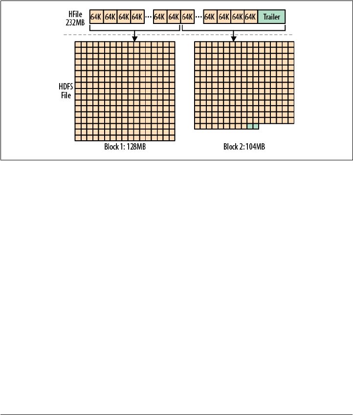
contain the same number of blocks, but the total size will be smaller since each block
is smaller.
One thing you may notice is that the default block size for files in HDFS is 64 MB,
which is 1,024 times the HFile default block size. As such, the HBase storage file blocks
do not match the Hadoop blocks. In fact, there is no correlation between these two
block types. HBase stores its files transparently into a filesystem. The fact that HDFS
uses blocks is a coincidence. And HDFS also does not know what HBase stores; it only
sees binary files. Figure 8-6 demonstrates how the HFile content is simply spread across
HDFS blocks.
Figure 8-6. HFile content spread across HDFS blocks when many smaller HFile blocks are
transparently stored in two HDFS blocks that are much larger
Sometimes it is necessary to be able to access an HFile directly, bypassing HBase, for
example, to check its health, or to dump its contents. The HFile.main() method pro-
vides the tools to do that:
$ ./bin/hbase org.apache.hadoop.hbase.io.hfile.HFile
usage: HFile [-a] [-b] [-e] [-f <arg>] [-k] [-m] [-p] [-r <arg>] [-v]
-a,--checkfamily Enable family check
-b,--printblocks Print block index meta data
-e,--printkey Print keys
-f,--file <arg> File to scan. Pass full-path; e.g.
hdfs://a:9000/hbase/.META./12/34
-k,--checkrow Enable row order check; looks for out-of-order keys
-m,--printmeta Print meta data of file
-p,--printkv Print key/value pairs
-r,--region <arg> Region to scan. Pass region name; e.g. '.META.,,1'
-v,--verbose Verbose output; emits file and meta data delimiters
Here is an example of what the output will look like (shortened):
$ ./bin/hbase org.apache.hadoop.hbase.io.hfile.HFile -f \
/hbase/testtable/de27e14ffc1f3fff65ce424fcf14ae42/colfam1/2518469459313898451 \
Storage | 331

-v -m -p
Scanning -> /hbase/testtable/de27e14ffc1f3fff65ce424fcf14ae42/colfam1/ \
2518469459313898451
K: row-550/colfam1:50/1309813948188/Put/vlen=2 V: 50
K: row-550/colfam1:50/1309812287166/Put/vlen=2 V: 50
K: row-551/colfam1:51/1309813948222/Put/vlen=2 V: 51
K: row-551/colfam1:51/1309812287200/Put/vlen=2 V: 51
K: row-552/colfam1:52/1309813948256/Put/vlen=2 V: 52
...
K: row-698/colfam1:98/1309813953680/Put/vlen=2 V: 98
K: row-698/colfam1:98/1309812292594/Put/vlen=2 V: 98
K: row-699/colfam1:99/1309813953720/Put/vlen=2 V: 99
K: row-699/colfam1:99/1309812292635/Put/vlen=2 V: 99
Scanned kv count -> 300
Block index size as per heapsize: 208
reader=/hbase/testtable/de27e14ffc1f3fff65ce424fcf14ae42/colfam1/ \
2518469459313898451, compression=none, inMemory=false, \
firstKey=row-550/colfam1:50/1309813948188/Put, \
lastKey=row-699/colfam1:99/1309812292635/Put, avgKeyLen=28, avgValueLen=2, \
entries=300, length=11773
fileinfoOffset=11408, dataIndexOffset=11664, dataIndexCount=1, \
metaIndexOffset=0, metaIndexCount=0, totalBytes=11408, entryCount=300, \
version=1
Fileinfo:
MAJOR_COMPACTION_KEY = \xFF
MAX_SEQ_ID_KEY = 2020
TIMERANGE = 1309812287166....1309813953720
hfile.AVG_KEY_LEN = 28
hfile.AVG_VALUE_LEN = 2
hfile.COMPARATOR = org.apache.hadoop.hbase.KeyValue$KeyComparator
hfile.LASTKEY = \x00\x07row-699\x07colfam199\x00\x00\x010\xF6\xE5|\x1B\x04
Could not get bloom data from meta block
The first part of the output is the actual data stored as serialized KeyValue instances.
The second part dumps the internal HFile.Reader properties, as well as the trailer block
details. The last part, starting with Fileinfo, is the file info block values.
The provided information is valuable to, for example, confirm whether a file is com-
pressed or not, and with what compression type. It also shows you how many cells you
have stored, as well as the average size of their keys and values. In the preceding ex-
ample, the key is much larger than the value. This is caused by the overhead required
by the KeyValue class to store the necessary data, explained next.
KeyValue Format
In essence, each KeyValue in the HFile is a low-level byte array that allows for zero-
copy access to the data. Figure 8-7 shows the layout of the contained data.
332 | Chapter 8: Architecture
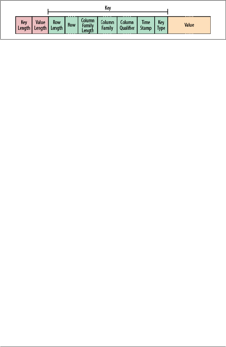
Figure 8-7. The KeyValue format
The structure starts with two fixed-length numbers indicating the size and value of the
key. With that information, you can offset into the array to, for example, get direct
access to the value, ignoring the key. Otherwise, you can get the required information
from the key. Once the information is parsed into a KeyValue Java instance, you can
use getters to access the details, as explained in “The KeyValue class” on page 83.
The reason the average key in the preceding example is larger than the value has to do
with the fields that make up the key part of a KeyValue. The key holds the row key, the
column family name, the column qualifier, and so on. For a small payload, this results
in quite a considerable overhead. If you deal with small values, try to keep the key small
as well. Choose a short row and column key (the family name with a single byte, and
the qualifier equally short) to keep the ratio in check.
On the other hand, compression should help mitigate the overwhelming key size prob-
lem, as it looks at finite windows of data, and all repeating data should compress well.
The sorting of all KeyValues in the store file helps to keep similar keys (and possibly
values too, in case you are using versioning) close together.
Write-Ahead Log
The region servers keep data in-memory until enough is collected to warrant a flush to
disk, avoiding the creation of too many very small files. While the data resides in mem-
ory it is volatile, meaning it could be lost if the server loses power, for example. This is
a likely occurrence when operating at large scale, as explained in “Seek Versus Trans-
fer” on page 315.
A common approach to solving this issue is write-ahead logging:# Each update (also
called an “edit”) is written to a log, and only if the update has succeeded is the client
informed that the operation has succeeded. The server then has the liberty to batch or
aggregate the data in memory as needed.
Overview
The WAL is the lifeline that is needed when disaster strikes. Similar to a binary log in
MySQL, the WAL records all changes to the data. This is important in case something
#For information on the term itself, read “Write-ahead logging” on Wikipedia.
Write-Ahead Log | 333
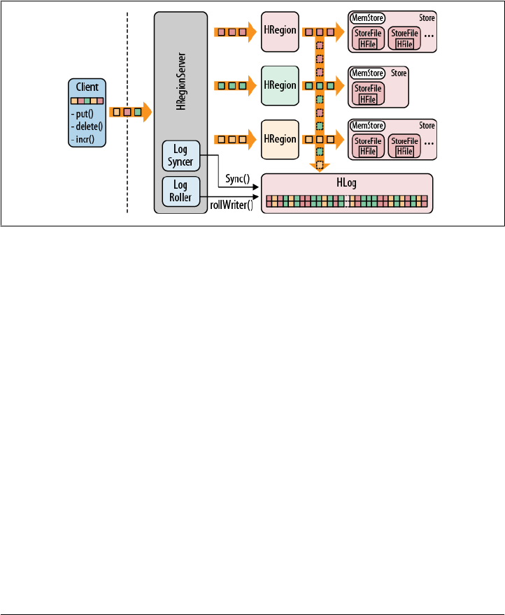
happens to the primary storage. If the server crashes, the WAL can effectively replay
the log to get everything up to where the server should have been just before the crash.
It also means that if writing the record to the WAL fails, the whole operation must be
considered a failure.
“Overview” on page 319 shows how the WAL fits into the overall architecture of HBase.
Since it is shared by all regions hosted by the same region server, it acts as a central
logging backbone for every modification. Figure 8-8 shows how the flow of edits is split
between the memstores and the WAL.
Figure 8-8. All modifications saved to the WAL, and then passed on to the memstores
The process is as follows: first the client initiates an action that modifies data. This can
be, for example, a call to put(), delete(), and increment(). Each of these modifications
is wrapped into a KeyValue object instance and sent over the wire using RPC calls. The
calls are (ideally) batched to the HRegionServer that serves the matching regions.
Once the KeyValue instances arrive, they are routed to the HRegion instances that are
responsible for the given rows. The data is written to the WAL, and then put into the
MemStore of the actual Store that holds the record. This is, in essence, the write path of
HBase.
334 | Chapter 8: Architecture

Eventually, when the memstores get to a certain size, or after a specific time, the data
is persisted in the background to the filesystem. During that time, data is stored in a
volatile state in memory. The WAL guarantees that the data is never lost, even if the
server fails. Keep in mind that the actual log resides on HDFS, which is a replicated
filesystem. Any other server can open the log and start replaying the edits—nothing on
the failed physical server is needed to effect a full recovery.
HLog Class
The class that implements the WAL is called HLog. When an HRegion is instantiated, the
single HLog instance that runs inside each region server is passed on as a parameter to
the constructor of HRegion. When a region receives an update operation, it can save the
data directly to the shared WAL instance.
The core of the HLog functionality is the append() method. Note that for performance
reasons there is an option for Put, Delete, and Increment to be called with an extra
parameter set: setWriteToWAL(false). If you invoke this method while setting up, for
example, a Put instance, the writing to the WAL is bypassed! That is also why the
downward arrow in Figure 8-8 was created with a dashed line to indicate the optional
step. By default, you certainly want the WAL, no doubt about that. But say you run a
large bulk import MapReduce job that you can rerun at any time. You gain extra per-
formance when you disable the WAL, but at the cost of having to take extra care that
no data was lost during the import.
You are strongly advised not to lightheartedly turn off writing edits to
the WAL. If you do so, you will lose data sooner or later. And no, HBase
cannot recover data that is lost and that has not been written to the log
first.
Another important feature of HLog is the ability to keep track of changes. It does this
by using a sequence number. It uses an AtomicLong internally to be thread-safe and starts
at either zero, or the last known number persisted to the filesystem: as the region is
opening its storage files, it reads the highest sequence number, which is stored as a meta
field in each HFile and sets the HLog sequence number to that value if it is higher than
what was recorded before. So, after it has opened all the storage files, the HLog is ini-
tialized to reflect where persisting ended and where to continue.
Figure 8-9 shows three different regions, hosted on the same region server, with each
of them covering a different row key range. Each region shares the same single instance
of HLog. This means the data is written to the WAL in the order it arrives. This means
some extra work is needed when a log needs to be replayed (see “Re-
play” on page 338). But since this happens rather seldomly, the WAL is optimized to
store data sequentially, giving it the best I/O performance.
Write-Ahead Log | 335
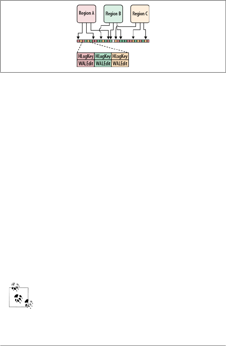
Figure 8-9. The WAL saving edits in the order they arrive, spanning all regions of the same server
HLogKey Class
Currently, the WAL uses a Hadoop SequenceFile, which stores records as sets of key/
values. For the WAL, the value is simply the modification(s) sent from the client. The
key is represented by an HLogKey instance: since the KeyValue only represents the row
key, column family, column qualifier, timestamp, type, and value, there has to be a
place to store what the KeyValue belongs to, in other words, the region and table name.
That information is stored in the HLogKey. Also stored is the aforementioned sequence
number. That number is incremented with each edit in order to keep a sequential order
of edits.
This class also records the write time, which is a timestamp that denotes when the edit
was written to the log. Finally, it stores the cluster ID, which is needed for replication
across clusters.
WALEdit Class
Every modification sent by a client is wrapped into a WALEdit instance, which takes care
of atomicity at the log level. Assume you update 10 columns in one row. Each column,
or cell, is represented as a separate KeyValue instance. If the server writes five of them
to the WAL and then fails, you will end up with a half-persisted row mutation.
Atomicity is guaranteed by bundling all updates that comprise multiple cells into a
single WALEdit instance. This group of edits is then written in a single operation, en-
suring that the row mutation is applied in full or not at all.
Before version 0.90.x, HBase did save the KeyValue instances separately.
336 | Chapter 8: Architecture

LogSyncer Class
The table descriptor allows you to set the so-called deferred log flush flag, as explained
in “Table Properties” on page 210. The default is false and it means that every time
an edit is sent to the servers, it will call the log writer’s sync() method. It is the call that
forces the update to the log to be acknowledged by the filesystem so that you have
durability.
Unfortunately, calling this method involves a pipelined write to N servers (where N is
the replication factor set for the write-ahead log files). Since this is a rather costly op-
eration, you have the option to slightly delay the call, and have it executed in a back-
ground process instead. Keep in mind that without the call to sync(), there is a chance
of data loss in case of a server failure. Use this option carefully.
Pipeline Versus n-Way Writes
The current implementation of sync() is a pipelined write, which means when the edit
is written, it is sent to the first data node to persist it. Once that has succeeded, it is
sent by that data node to another data node to do the same thing, and so on. Only when
all three have acknowledged the write operation is the client allowed to proceed.
Another approach to saving edits durably is the n-way write, where the write is sent to
three machines at the same time. When all acknowledge the write, the client can
continue.
The difference between pipelined and n-way writes is that a pipelined write needs time
to complete, and therefore has a higher latency. But it can saturate the network band-
width better. An n-way write has lower latency, as the client only needs to wait for the
slowest data node to acknowledge (assuming the others have already reported back
success). However, an n-way write needs to share the network bandwidth of the sending
server, which can cause a bottleneck for heavily loaded systems.
There is work in progress to have support for both in HDFS, giving you the choice to
use the one that performs best for your application.
Setting the deferred log flush flag to true causes the edits to be buffered on the region
server, and the LogSyncer class, running as a background thread on the server, is re-
sponsible for calling the sync() method at a very short interval. The default is one
second and is configured by the hbase.regionserver.optionallogflushinterval
property.
Note that this only applies to user tables: all catalog tables are always synced right away.
Write-Ahead Log | 337

LogRoller Class
There are size restrictions when it comes to the logs that are written. The LogRoller
class runs as a background thread and takes care of rolling logfiles at certain intervals.
This is controlled by the hbase.regionserver.logroll.period property, set by default
to one hour.
Every 60 minutes the log is closed and a new one is started. Over time, the system
accumulates an increasing number of logfiles that need to be managed as well. The
HLog.rollWriter() method, which is called by the LogRoller to roll the current logfile,
takes care of that as well by subsequently calling HLog.cleanOldLogs().
It checks what the highest sequence number written to a storage file is. This is the edit
sequence number of the last edit persisted out to the filesystem. It then checks if there
is a log left that has edits that are all less than that number. If that is the case, it moves
said logs into the .oldlogs directory, and leaves the remaining ones in place.
You might see the following obscure message in your logs:
2011-06-15 01:45:48,427 INFO org.apache.hadoop.hbase.regionserver.HLog: \
Too many hlogs: logs=130, maxlogs=96; forcing flush of 8 region(s):
testtable,row-500,1309872211320.d5a127167c6e2dc5106f066cc84506f8., ...
This message is printed because the configured maximum number of
logfiles to keep exceeds the number of logfiles that are required to be
kept because they still contain outstanding edits that have not yet been
persisted. This can occur when you stress out the filesystem to such an
extent that it cannot persist the data at the rate at which new data is
added. Otherwise, memstore flushes should take care of this.
Note, though, that when this message is printed the server goes into a
special mode trying to force edits to be flushed out to reduce the number
of outstanding WAL files.
The other parameters controlling log rolling are hbase.regionserver.hlog.blocksize
(set to the filesystem default block size, or fs.local.block.size, defaulting to 32 MB)
and hbase.regionserver.logroll.multiplier (set to 0.95), which will rotate logs when
they are at 95% of the block size. So logs are switched out when they are considered
full, or when a certain amount of time has passed—whatever comes first.
Replay
The master and region servers need to orchestrate the handling of logfiles carefully,
especially when it comes to recovering from server failures. The WAL is responsible
for retaining the edits safely; replaying the WAL to restore a consistent state is a much
more complex exercise.
338 | Chapter 8: Architecture

Single log
Since all edits are written to one HLog-based logfile per region server, you might ask:
why is that the case? Why not write all edits for a specific region into its own logfile?
Here is the related quote from the Bigtable paper:
If we kept the commit log for each tablet in a separate logfile, a very large number of files
would be written concurrently in GFS. Depending on the underlying file system imple-
mentation on each GFS server, these writes could cause a large number of disk seeks to
write to the different physical log files.
HBase followed that principle for pretty much the same reasons: writing too many files
at the same time, plus the number of rolled logs that need to be kept, does not scale well.
What is the drawback, though? If you have to split a log because of a server crash, you
need to divide it into suitable pieces, as described in the next section. The master cannot
redeploy any region from a crashed server until the logs for that very server have been
split. This can potentially take a considerable amount of time.
Log splitting
There are two situations in which logfiles have to be replayed: when the cluster starts,
or when a server fails. When the master starts—and this includes a backup master
taking over duty—it checks if there are any logfiles, in the .logs directory under the
HBase root on the filesystem, that have no region server assigned to them. The logs’
names contain not just the server name, but also the start code of the server. This num-
ber is reset every time a region server restarts, and the master can use this number to
verify whether a log has been abandoned—for example, due to a server crash.
The master is responsible for monitoring the servers using ZooKeeper, and if it detects
a server failure, it immediately starts the process of recovering its logfiles, before reas-
signing the regions to new servers. This happens in the ServerShutdownHandler class.
Before the edits in the log can be replayed, they need to be separated into one logfile
per region. This process is called log splitting: the combined log is read and all entries
are grouped by the region they belong to. These grouped edits are then stored in a file
next to the target region for subsequent recovery.
The actual process of splitting the logs is different in nearly every version of HBase:
early versions would read the file in a single thread, directly on the master. This was
improved to at least write the grouped edits per region in multiple threads. Version
0.92.0 finally introduces the concept of distributed log splitting, which removes the
burden of doing the actual work from the master to all region servers.
Consider a larger cluster with many region servers and many (rather large) logfiles. In
the past, the master had to recover each logfile separately, and—so it would not over-
load in terms of I/O as well as memory usage—it would do this sequentially. This meant
that, for any region that had pending edits, it had to be blocked from opening until the
log split and recovery had been completed.
Write-Ahead Log | 339

The new distributed mode uses ZooKeeper to hand out each abandoned logfile to a
region server. They monitor ZooKeeper for available work, and if the master indicates
that a log is available for processing, they race to accept the task. The winning region
server then proceeds to read and split the logfiles in a single thread (so as not to overload
the already busy region server).
You can turn the new distributed log splitting off by means of the
hbase.master.distributed.log.splitting configuration property. Set-
ting this property to false disables distributed splitting, and falls back
to doing the work directly on the master only.
In nondistributed mode the writers are multithreaded, controlled by
the hbase.regionserver.hlog.splitlog.writer.threads property, which
is set to 3 by default. You need to be careful when increasing this num-
ber, as you are likely bound by the performance of the single log reader.
The split process writes the edits first into the splitlog staging directory under the HBase
root folder. They are placed in the same path that is needed for the target region. For
example:
0 /hbase/.corrupt
0 /hbase/splitlog/foo.internal,60020,1309851880898_hdfs%3A%2F%2F \
localhost%2Fhbase%2F.logs%2Ffoo.internal%2C60020%2C1309850971208%2F \
foo.internal%252C60020%252C1309850971208.1309851641956/testtable/ \
d9ffc3a5cd016ae58e23d7a6cb937949/recovered.edits/0000000000000002352
The path contains the logfile name itself to distinguish it from other, possibly concur-
rently executed, log split output. The path also contains the table name, region name
(hash), and recovered.edits directory. Lastly, the name of the split file is the sequence
ID of the first edit for the particular region.
The .corrupt directory contains any logfile that could not be parsed. This is influenced
by the hbase.hlog.split.skip.errors property, which is set to true by default. It means
that any edit that could not be read from a file causes the entire log to be moved to
the .corrupt folder. If you set the flag to false, an IOExecption is thrown and the en-
tire log splitting process is stopped.
Once a log has been split successfully, the per-region files are moved into the actual
region directories. They are now ready to be recovered by the region itself. This is also
why the splitting has to stall opening the affected regions, since it first has to provide
the pending edits for replay.
340 | Chapter 8: Architecture

Edits recovery
When a region is opened, either because the cluster is started or because it has been
moved from one region server to another, it first checks for the presence of the recov-
ered.edits directory. If it exists, it opens the contained files and starts reading the edits
they contain. The files are sorted by their name, which contains the sequence ID. This
allows the region to recover the edits in order.
Any edit that has a sequence ID that is less than or equal to what has been persisted in
the on-disk store files is ignored, because it has already been applied. All other edits
are applied to the matching memstore of the region to recover the previous state. At
the end, a flush of the memstores is forced to write the current state to disk.
The files in the recovered.edits folder are removed once they have been read and their
edits persisted to disk. If a file cannot be read, the hbase.skip.errors property defines
what happens next: the default value is false and causes the entire region recovery to
fail. If this property is set to true, the file is renamed to the original filename
plus .<currentTimeMillis>. Either way, you need to carefully check your logfiles to
determine why the recovery has had issues and fix the problem to continue.
Durability
You want to be able to rely on the system to save all your data, no matter what new-
fangled algorithms are employed behind the scenes. As far as HBase and the log are
concerned, you can set the log flush times to be as low as you want, or sync them for
every edit—you are still dependent on the underlying filesystem as mentioned earlier;
the stream used to store the data is flushed, but is it written to disk yet? We are talking
about fsync style issues. Now for HBase we are most likely dealing with Hadoop’s HDFS
as being the filesystem that is persisted to.
At this point, it should be abundantly clear that the log is what keeps data safe. It is
being kept open for up to an hour (or more if configured to do so), and as data arrives
a new key/value pair is written to the SequenceFile. Eventually, the log is rolled and a
new one is created.
But that is not how Hadoop was designed to work. Hadoop provides an API tailored
to MapReduce that allows you to open a file, write data into it (preferably a lot), and
close it right away, leaving an immutable file for everyone else to read many times.
Only after a file is closed is it visible and readable to others. If a process dies while
writing the data, the file is considered lost. For HBase to be able to work properly, what
is required is a feature that allows you to read the log up to the point where the crashed
server has written it. This was added to HDFS in later versions and is referred to as
append.
Write-Ahead Log | 341

Interlude: HDFS append, hflush, hsync, sync...
Append is the feature needed by HBase to guarantee durability, but previous versions
of Hadoop did not offer it. Support was added over a longer period of time and in a list
of patches. It all started with HADOOP-1700. It was committed in Hadoop 0.19.0 and
was meant to solve the problem. But that was not the case: the append in Hadoop
0.19.0 was so badly suited that a hadoop fsck / would report the HDFS as being corrupt
because of the open logfiles HBase kept.
So the issue was tackled again in HADOOP-4379, a.k.a. HDFS-200, and implemented
syncFs() to make the process of syncing changes to a file more reliable. For a while we
had custom code—see HBASE-1470—that detected a patched Hadoop that exposed
the API.
Then came HDFS-265, which revisits the append idea in general. It also introduces a
Syncable interface that exposes hsync() and hflush().
Of note is that SequenceFile.Writer.sync() is not the same as the aforementioned sync
method: it writes a synchronization marker into the file, which helps when reading it
later—or recovers data from a corrupted sequence file.
HBase currently detects whether the underlying Hadoop library has support for
syncFs() or hflush(). If a sync() is triggered on the log writer, it calls either method
internally—or none if HBase runs in a nondurable setup. The sync() is using the pipe-
lined write process described in “LogSyncer Class” on page 337 to guarantee the du-
rability of the edits in the logfile. In case of a server crash, the system can safely read
the abandoned logfile up to the last edits.
In summary, without Hadoop 0.21.0 and later, or a specially prepared 0.20.x with
append support backported to it, you can very well face data loss. See “Ha-
doop” on page 46 for more information.
Read Path
HBase uses multiple store files per column family, which contain the actual cells, or
KeyValue instances. These files are created over time as modifications aggregated in the
memstores are eventually flushed as store files to disk. The background process of
compactions keeps the number of files under control by rewriting smaller files into
larger ones. Major compactions eventually compact the entire set of files into a single
one, after which the flushes start adding smaller files again.
Since all store files are immutable, there is no way to delete a particular value out of
them, nor does it make sense to keep rewriting large store files to remove the deleted
cells one by one. Instead, a tombstone marker is written, which masks out the “deleted”
information—which can be a single cell, a range of cells, or entire rows.
342 | Chapter 8: Architecture

Consider you are writing a column in a given row today. You keep adding data in other
rows over a few more days, then you write a different column in the given row. The
question is, given that the original column value has been persisted as a KeyValue on
disk for quite some time, while the newly written column for the same row is still in
the memstore, or has been flushed to disk, where does the logical row reside?
In other words, when you are using the shell to perform a get command on that row,
how does the system know what to return? As a client, you want to see both columns
being returned—as if they were stored in a single entity. But in reality, the data lives as
separate KeyValue instances, spread across any number of store files.
If you are deleting the initial column value, and you perform the get again, you expect
the value to be gone, when in fact it still exists somewhere, but the tombstone marker
is indicating that you have deleted it. But that marker is most likely stored far away
from the value it “buries.” A more formal explanation of the architecture behind this
approach is provided in “Seek Versus Transfer” on page 315.
HBase solves the problem by using a QueryMatcher in combination with a
ColumnTracker, which comes in a few variations: one for explicit matching, for when
you specify a list of columns to retrieve, and another that includes all columns. Both
allow you to set the maximum number of versions to match. They keep track of what
needs to be included in the final result.
Why Gets Are Scans
In previous versions of HBase, the Get method was implemented as a separate code
path. This was changed in recent versions and completely replaced internally by the
same code that the Scan API uses.
You may wonder why that was done since a straight Get should be faster than a Scan.
A separate code path could take care of some sort of special knowledge to quickly access
the data the user is asking for.
That is where the architecture of HBase comes into play. There are no index files that
allow such direct access of a particular row or column. The smallest unit is a block in
an HFile, and to find the requested data the RegionServer code and its underlying
Store instances must load a block that could potentially have that data stored and scan
through it. And that is exactly what a Scan does anyway.
In other words, a Get is nothing but a scan of a single row. It is as though you have
created a Scan, and set the start row to what you are looking for and the end row to
start row + 1.
Before all the store files are read to find a matching entry, a quick exclusion check is
conducted, which uses the timestamps and optional Bloom filter to skip files that
definitely have no KeyValue belonging to the row in question. The remaining store files,
including the memstore, are then scanned to find a matching key.
Read Path | 343
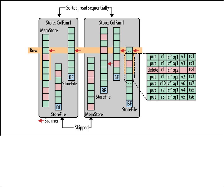
The scan is implemented by the RegionScanner class, which retrieves a StoreScanner for
every Store instance—each representing a column family. If the read operation ex-
cludes certain column families, their stores are omitted as well.
The StoreScanner class combines the store files and memstore that the Store instance
contains. It is also where the exclusion happens, based on the Bloom filter, or the
timestamp. If you are asking for versions that are not more than 30 minutes old, for
example, you can skip all storage files that are older than one hour: they will not contain
anything of interest. See “Key Design” on page 357 for details on the exclusion, and
how to make use of it.
The StoreScanner class also has the QueryMatcher (here the ScanQueryMatcher class),
which will keep track of which KeyValues to include in the final result.
The RegionScanner internally is using a KeyValueHeap class to arrange all store scanners
ordered by timestamps. The StoreScanner is using the same to order the stores the same
way. This guarantees that you are reading KeyValues in their correct order (e.g.,
descending by timestamp).
When the store scanners are opened, they will position themselves at the requested row
key, or—in the case of a get() call—on the next nonmatching row key. The scanner is
now ready to read data. Figure 8-10 shows an example of what this looks like.
Figure 8-10. Rows stored and scanned across different stores, on disk or in memory
For a get() call, all the server has to do is to call next() on the RegionScanner. The call
internally reads everything that should be part of the result. This includes all of the
versions requested. Consider a column that has three versions, and you are requesting
344 | Chapter 8: Architecture

to retrieve all of them. The three KeyValue instances could be spread across any store,
on disk or in memory. The next() call keeps reading from all store files until either the
next row is reached, or enough versions have been found.
At the same time, it keeps track of delete markers too. As it scans through the Key
Values of the current row, it will come across these delete markers and note that any-
thing with a timestamp that is less than or equal to the marker is considered erased.
Figure 8-10 also shows the logical row as a list of KeyValues, some in the same store file,
some on other files, spanning multiple column families. A store file and a memstore
were skipped because of the timestamp and Bloom filter exclusion process. The delete
marker in the last store file is masking out entries, but they are still all part of the same
row. The scanners—depicted as an arrow next to the stores—are either on the first
matching entry in the file, or on the one that would follow the requested key, in case
the store has no direct match.
Only scanners that are on the proper row are considered during the call to next(). The
internal loop would read the KeyValues from the first and last stores one after the other,
in time-descending order, until they also exceed the requested row key.
For scan operations, this is repeated by calling next() on the ResultScanner until either
the stop row has been found, the end of the table has been reached, or enough rows
have been read for the current batch (as set via scanner caching).
The final result is a list of KeyValue instances that matched the given get or scan oper-
ation. The list is sent back to the client, which can then use the API methods to access
the contained columns.
Region Lookups
For the clients to be able to find the region server hosting a specific row key range,
HBase provides two special catalog tables, called -ROOT- and .META..*
The -ROOT- table is used to refer to all regions in the .META. table. The design considers
only one root region, that is, the root region is never split to guarantee a three-level, B+
tree-like lookup scheme: the first level is a node stored in ZooKeeper that contains the
location of the root table’s region—in other words, the name of the region server host-
ing that specific region. The second level is the lookup of a matching meta region from
the -ROOT- table, and the third is the retrieval of the user table region from the .META.
table.
The row keys in the catalog tables are the region names, which are a concatenation of
the region’s table name, its start row, and an ID (usually the current time in millisec-
onds). As of HBase 0.90.0 these keys may have another hashed value attached to them.
* Subsequently, they are referred to interchangeably as root table and meta table, respectively, since, for
example, "-ROOT-" is how the table is actually named in HBase and calling it a root table is stating its purpose.
Region Lookups | 345

This is currently only used for user tables. See “Region-level files” on page 324 for an
example.
Avoiding any concerns about the three-level location scheme, the
Bigtable paper states that with average limits on the .META. region size
at 128 MB it can address 234 regions, or 261 bytes in 128 MB regions.
Since the size of the regions can be increased without any impact on the
location scheme, this is a conservative number and can be increased as
needed.
Although clients cache region locations, there is an initial need to figure out where to
send requests when looking for a specific row key—or when the cache is stale and a
region has since been split, merged, or moved. The client library uses a recursive dis-
covery process moving up in the hierarchy to find the current information. It asks the
corresponding region server hosting the matching .META. region for the given row key
and retrieves the address. If that information is invalid, it backs out, asking the root
table where the .META. region is. Eventually, if all else fails, it has to do a read of the
ZooKeeper node to find the root table region.
In a worst-case scenario, it would need six network round-trips to discover the user
region, since stale entries in the cache are only discovered when the lookup fails, be-
cause it is assumed that assignments, especially of meta regions, do not change too
often. When the cache is empty, the client needs three network round-trips to update
its cache. One way to mitigate future round-trips is to prefetch location information in
a single request, thus updating the client cache ahead of time. Refer to “Miscellaneous
Features” on page 133 for details on how to influence this using the client-side API.
Figure 8-11 shows the mapping of user table regions, through meta, and finally to the
root table information. Once the user table region is known, it can be accessed directly
without any further lookups. The lookups are numbered and assume an empty cache.
However, if the cache were filled with only stale details, the client would fail on all three
lookups, requiring a refresh of all three and resulting in the aforementioned six network
round-trips.
346 | Chapter 8: Architecture
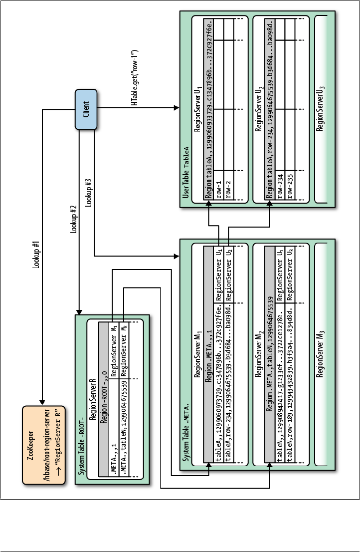
Figure 8-11. Mapping of user table regions, starting with an empty cache and then performing three
lookups
Region Lookups | 347

The Region Life Cycle
The state of a region is tracked by the master, using the AssignmentManager class. It
follows the region from its offline state, all the way through its life cycle. Table 8-1 lists
the possible states of a region.
Table 8-1. Possible states of a region
State Description
Offline The region is offline.
Pending Open A request to open the region was sent to the server.
Opening The server has started opening the region.
Open The region is open and fully operational.
Pending Close A request to close the region has been sent to the server.
Closing The server is in the process of closing the region.
Closed The region is closed.
Splitting The server started splitting the region.
Split The region has been split by the server.
The transitions between states are commonly initiated by the master, but may also be
initiated by the region server hosting the region. For example, the master assigns a
region to a server, which is then opened by the assignee. On the other hand, the region
server starts the split process, which in itself triggers multiple region close and open
events.
Because of the distributed nature of these events, the servers are using ZooKeeper to
track specific states in a dedicated znode.
ZooKeeper
Since version 0.20.x, HBase has been using ZooKeeper as its distributed coordination
service. This includes tracking of region servers, where the root region is hosted, and
more. Version 0.90.x introduced a new master implementation which has an even
tighter integration with ZooKeeper. It enables HBase to remove critical heartbeat mes-
sages that needed to be sent between the master and the region servers. These are now
moved into ZooKeeper, which informs either party of changes whenever they occur,
as opposed to the fixed intervals that were used before.
HBase creates a list of znodes under its root node. The default is /hbase and is configured
with the zookeeper.znode.parent property. Here is the list of the contained znodes and
their purposes:
348 | Chapter 8: Architecture

The examples use the ZooKeeper command-line interface (CLI) to issue
the commands. You can start it with:
$ $ZK_HOME/bin/zkCli.sh -server <quorum-server>
The output of each command was shortened by the ZooKeeper internal
details.
/hbase/hbaseid
Contains the cluster ID, as stored in the hbase.id file on HDFS. For example:
[zk: localhost(CONNECTED) 1] get /hbase/hbaseid
e627e130-0ae2-448d-8bb5-117a8af06e97
/hbase/master
Holds the server name (see “Cluster Status Information” on page 233 for details).
For example:
[zk: localhost(CONNECTED) 2] get /hbase/master
foo.internal,60000,1309859972983
/hbase/replication
Contains replication details. See “Internals” on page 353 for details.
/hbase/root-region-server
Contains the server name of the region server hosting the -ROOT- regions. This is
used during the region lookup (see “Region Lookups” on page 345). For instance:
[zk: localhost(CONNECTED) 3] get /hbase/root-region-server
rs1.internal,60000,1309859972983
/hbase/rs
Acts as the root node for all region servers to list themselves when they start. It is
used to track server failures. Each znode inside is ephemeral and its name is the
server name of the region server. For example:
[zk: localhost(CONNECTED) 4] ls /hbase/rs
[rs1.internal,60000,1309859972983,rs2.internal,60000,1309859345233]
/hbase/shutdown
Is used to track the cluster state. It contains the time when the cluster was started,
and is empty when it was shut down. For example:
[zk: localhost(CONNECTED) 5] get /hbase/shutdown
Tue Jul 05 11:59:33 CEST 2011
/hbase/splitlog
The parent znode for all log-splitting-related coordination (see “Log split-
ting” on page 339 for details). For example:
[zk: localhost(CONNECTED) 6] ls /hbase/splitlog
[hdfs%3A%2F%2Flocalhost%2Fhbase%2F.logs%2Ffoo.internal%2C60020%2C \
1309850971208%2Ffoo.internal%252C60020%252C1309850971208.1309851636647,
hdfs%3A%2F%2Flocalhost%2Fhbase%2F.logs%2Ffoo.internal%2C60020%2C \
ZooKeeper | 349

1309850971208%2Ffoo.internal%252C60020%252C1309850971208.1309851641956,
...
hdfs%3A%2F%2Flocalhost%2Fhbase%2F.logs%2Ffoo.internal%2C60020%2C \
1309850971208%2Ffoo.internal%252C60020%252C1309850971208.1309851784396]
[zk: localhost(CONNECTED) 7] get /hbase/splitlog/ \
\hdfs%3A%2F%2Flocalhost%2Fhbase%2F.logs%2Fmemcache1.internal%2C \
60020%2C1309850971208%2Fmemcache1.internal%252C60020%252C1309850971208. \
1309851784396
unassigned foo.internal,60000,1309851879862
[zk: localhost(CONNECTED) 8] get /hbase/splitlog/ \
\hdfs%3A%2F%2Flocalhost%2Fhbase%2F.logs%2Fmemcache1.internal%2C \
60020%2C1309850971208%2Fmemcache1.internal%252C60020%252C1309850971208. \
1309851784396
owned foo.internal,60000,1309851879862
[zk: localhost(CONNECTED) 9] ls /hbase/splitlog
[RESCAN0000293834, hdfs%3A%2F%2Flocalhost%2Fhbase%2F.logs%2Fmemcache1. \
internal%2C60020%2C1309850971208%2Fmemcache1.internal%252C \
60020%252C1309850971208.1309851681118, RESCAN0000293827, RESCAN0000293828, \
RESCAN0000293829, RESCAN0000293838, RESCAN0000293837]
These examples list various things: you can see how a log to be split was first
unassigned, and then owned by a region server. The RESCAN nodes are signifying
that the workers, that is, the region server, is supposed to check for more work, in
case a split has failed on another machine.
/hbase/table
The znode to which a disabled table is added as its parent. The name of the table
is the newly created znode, and its content is the word DISABLED. For example:
[zk: localhost(CONNECTED) 10] ls /hbase/table
[testtable]
[zk: localhost(CONNECTED) 11] get /hbase/table/testtable
DISABLED
/hbase/unassigned
Is used by the AssignmentManager to track region states across the entire cluster. It
contains znodes for those regions that are not open, but are in a transitional state.
The name of the znode is the hash of the region. For example:
[zk: localhost(CONNECTED) 11] ls /hbase/unassigned
[8438203023b8cbba347eb6fc118312a7]
350 | Chapter 8: Architecture
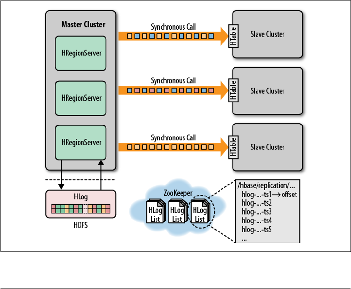
Replication
HBase replication is a way to copy data between HBase deployments. It can serve as a
disaster recovery solution and can contribute to provide higher availability at the HBase
layer. It can also serve a more practical purpose; for example, as a way to easily copy
edits from a web-facing cluster to a MapReduce cluster that will process old and new
data and ship back the results automatically.
The basic architecture pattern used for HBase replication is “(HBase cluster) master-
push”; this pattern makes it much easier to keep track of what is currently being repli-
cated since each region server has its own write-ahead log (WAL or HLog), just like other
well-known solutions, such as MySQL master/slave replication, where there is only
one binary log to keep track of. One master cluster can replicate to any number of slave
clusters, and each region server will participate to replicate its own stream of edits.
The replication is done asynchronously, meaning that the clusters can be geographically
distant, the links between them can be offline for some time, and rows inserted on the
master cluster will not be available at the same time on the slave clusters (eventual
consistency).
Figure 8-12 shows an overview of how replication works.
Figure 8-12. Overview of the replication architecture
Replication | 351

The replication format used in this design is conceptually the same as MySQL’s state-
ment-based replication.† Instead of SQL statements, whole WALEdits (consisting of
multiple cell inserts coming from the clients’ Put and Delete) are replicated in order to
maintain atomicity.
The HLogs from each region server are the basis of HBase replication, and must be kept
in HDFS as long as they are needed to replicate data to any slave cluster. Each region
server reads from the oldest log it needs to replicate and keeps the current position
inside ZooKeeper to simplify failure recovery. That position can be different for every
slave cluster, as can the queue of HLogs to process.
The clusters participating in replication can be of asymmetric sizes and the master
cluster will do its best effort to balance the stream of replication on the slave clusters
by relying on randomization.
Life of a Log Edit
The following sections describe the life of a single edit going from a client that com-
municates with a master cluster all the way to a single slave cluster.
Normal processing
The client uses an HBase API that sends a Put, Delete, or Increment to a region server.
The key/values are transformed into a WALEdit by the region server and the WALEdit is
inspected by the replication code that, for each family that is scoped for replication,
adds the scope to the edit. The edit is appended to the current WAL and is then applied
to its MemStore.
In a separate thread, the edit is read from the log (as part of a batch) and only the
KeyValues that are replicable are kept (i.e., they are part of a family that is scoped as
GLOBAL in the family’s schema and are noncatalog so it is not .META. or -ROOT-). When
the buffer is filled, or the reader hits the end of the file, the buffer is sent to a random
region server on the slave cluster.
Synchronously, the region server that receives the edits reads them sequentially and
separates each of them into buffers, one per table. Once all edits are read, each buffer
is flushed using the normal HBase client (HTables managed by an HTablePool). This is
done in order to leverage parallel insertion (MultiPut).
Back in the master cluster’s region server, the offset for the current WAL that is being
replicated is registered in ZooKeeper.
† See the online manual for details.
352 | Chapter 8: Architecture

Non-Responding slave clusters
The edit is inserted in the same way. In a separate thread, the region server reads, filters,
and buffers the log edits the same way as is done during normal processing. The slave
region server that is contacted does not answer to the RPC, so the master region server
will sleep and retry up to a configured number of times. If the slave region server still
is not available, the master cluster region server will select a new subset of the region
server to replicate to and will try to send the buffer of edits again.
In the meantime, the WALs will be rolled and stored in a queue in ZooKeeper. Logs
that are archived by their region server (archiving is basically moving a log from the
region server’s logs directory to a central logs archive directory) will update their paths
in the in-memory queue of the replicating thread.
When the slave cluster is finally available, the buffer will be applied the same way as
during normal processing. The master cluster region server will then replicate the
backlog of logs.
Internals
This section describes in depth how each of the replication’s internal features operates.
Choosing region servers to replicate to
When a master cluster region server initiates a replication source to a slave cluster, it
first connects to the slave’s ZooKeeper ensemble using the provided cluster key (that
key is composed of the value of hbase.zookeeper.quorum, zookeeper.znode.parent, and
hbase.zookeeper.property.clientPort). It then scans the /hbase/rs directory to discover
all the available sinks (region servers that are accepting incoming streams of edits to
replicate) and will randomly choose a subset of them using a configured ratio (which
has a default value of 10%). For example, if a slave cluster has 150 machines, 15 will
be chosen as potential recipients for edits that this master cluster region server will be
sending. Since this is done by all master cluster region servers, the probability that all
slave region servers are used is very high, and this method works for clusters of any
size. For example, a master cluster of 10 machines replicating to a slave cluster of five
machines with a ratio of 10% means that the master cluster region servers will choose
one machine each at random; thus the chance of overlapping and full usage of the slave
cluster is higher.
Keeping track of logs
Every master cluster region server has its own znode in the replication znodes hierarchy.
The parent znode contains one znode per peer cluster (if there are five slave clusters,
five znodes are created), and each of these contains a queue of HLogs to process. Each
of these queues will track the HLogs created by that region server, but they can differ in
size. For example, if one slave cluster becomes unavailable for some time, the HLogs
Replication | 353

should not be deleted, and thus they need to stay in the queue (while the others are
processed). See “Region server failover” on page 355 for an example.
When a source is instantiated, it contains the current HLog that the region server is
writing to. During log rolling, the new file is added to the queue of each slave cluster’s
znode just before it is made available. This ensures that all the sources are aware that
a new log exists before HLog is able to append edits into it, but this operation is now
more expensive. The queue items are discarded when the replication thread cannot
read more entries from a file (because it reached the end of the last block) and that there
are other files in the queue. This means that if a source is up-to-date and replicates from
the log that the region server writes to, reading up to the “end” of the current file will
not delete the item in the queue.
When a log is archived (because it is not used anymore or because there are too many
of them per hbase.regionserver.maxlogs, typically because the insertion rate is faster
than the region flushing rate), it will notify the source threads that the path for that log
changed. If a particular source was already done with it, it will just ignore the message.
If it is in the queue, the path will be updated in memory. If the log is currently being
replicated, the change will be done atomically so that the reader does not try to open
the file when it is already moved. Also, moving a file is a NameNode operation; so, if
the reader is currently reading the log, it will not generate any exceptions.
Reading, filtering, and sending edits
By default, a source will try to read from a logfile and ship log entries as quickly as
possible to a sink. This is first limited by the filtering of log entries; only KeyValues that
are scoped GLOBAL and that do not belong to catalog tables will be retained. A second
limit is imposed on the total size of the list of edits to replicate per slave, which by
default is 64 MB. This means that a master cluster region server with three slaves will
use, at most, 192 MB to store data to replicate. This does not take into account the data
that was filtered but was not garbage-collected.
Once the maximum number of edits has been buffered or the reader has hit the end of
the logfile, the source thread will stop reading and will randomly choose a sink to
replicate to (from the list that was generated by keeping only a subset of slave region
servers). It will directly issue an RPC to the chosen machine and will wait for the method
to return. If it is successful, the source will determine if the current file is emptied or if
it should continue to read from it. If the former, it will delete the znode in the queue.
If the latter, it will register the new offset in the log’s znode. If the RPC threw an ex-
ception, the source will retry 10 times until trying to find a different sink.
Cleaning logs
If replication is not enabled, the master’s log cleaning thread will delete old logs using
a configured TTL. This does not work well with replication since archived logs that are
past their TTL may still be in a queue. Thus, the default behavior is augmented so that
354 | Chapter 8: Architecture

if a log is past its TTL, the cleaning thread will look up every queue until it finds the
log (while caching the ones it finds). If it is not found, the log will be deleted. The next
time it has to look for a log, it will first use its cache.
Region server failover
As long as region servers do not fail, keeping track of the logs in ZooKeeper does not
add any value. Unfortunately, they do fail, so since ZooKeeper is highly available, we
can count on it and its semantics to help us manage the transfer of the queues.
All the master cluster region servers keep a watcher on one another to be notified when
one dies (just like the master does). When this happens, they all race to create a znode
called lock inside the dead region server’s znode that contains its queues. The one that
creates it successfully will proceed by transferring all the queues to its own znode (one
by one, since ZooKeeper does not support the rename operation) and will delete all the
old ones when it is done. The recovered queues’ znodes will be named with the ID of
the slave cluster appended with the name of the dead server.
Once that is done, the master cluster region server will create one new source thread
per copied queue, and each of them will follow the read/filter/ship pattern. The main
difference is that those queues will never have new data since they do not belong to
their new region server, which means that when the reader hits the end of the last log,
the queue’s znode will be deleted and the master cluster region server will close that
replication source.
For example, consider a master cluster with three region servers that is replicating to a
single slave with an ID of 2. The following hierarchy represents what the znodes’ layout
could be at some point in time. We can see that the region servers’ znodes all contain
a peers znode that contains a single queue. The znode names in the queues represent
the actual filenames on HDFS in the form address,port.timestamp.
/hbase/replication/rs/
1.1.1.1,60020,123456780/
peers/
2/
1.1.1.1,60020.1234 (Contains a position)
1.1.1.1,60020.1265
1.1.1.2,60020,123456790/
peers/
2/
1.1.1.2,60020.1214 (Contains a position)
1.1.1.2,60020.1248
1.1.1.2,60020.1312
1.1.1.3,60020, 123456630/
peers/
2/
1.1.1.3,60020.1280 (Contains a position)
Now let’s say that 1.1.1.2 loses its ZooKeeper session. The survivors will race to create
a lock, and for some reason 1.1.1.3 wins. It will then start transferring all the queues
Replication | 355

to its local peers znode by appending the name of the dead server. Right before
1.1.1.3 is able to clean up the old znodes, the layout will look like the following:
/hbase/replication/rs/
1.1.1.1,60020,123456780/
peers/
2/
1.1.1.1,60020.1234 (Contains a position)
1.1.1.1,60020.1265
1.1.1.2,60020,123456790/
lock
peers/
2/
1.1.1.2,60020.1214 (Contains a position)
1.1.1.2,60020.1248
1.1.1.2,60020.1312
1.1.1.3,60020,123456630/
peers/
2/
1.1.1.3,60020.1280 (Contains a position)
2-1.1.1.2,60020,123456790/
1.1.1.2,60020.1214 (Contains a position)
1.1.1.2,60020.1248
1.1.1.2,60020.1312
Sometime later, but before 1.1.1.3 is able to finish replicating the last HLog from
1.1.1.2, let’s say that it dies too (also, some new logs were created in the normal
queues). The last region server will then try to lock 1.1.1.3’s znode and will begin
transferring all the queues. The new layout will be:
/hbase/replication/rs/
1.1.1.1,60020,123456780/
peers/
2/
1.1.1.1,60020.1378 (Contains a position)
2-1.1.1.3,60020,123456630/
1.1.1.3,60020.1325 (Contains a position)
1.1.1.3,60020.1401
2-1.1.1.2,60020,123456790-1.1.1.3,60020,123456630/
1.1.1.2,60020.1312 (Contains a position)
1.1.1.3,60020,123456630/
lock
peers/
2/
1.1.1.3,60020.1325 (Contains a position)
1.1.1.3,60020.1401
2-1.1.1.2,60020,123456790/
1.1.1.2,60020.1312 (Contains a position)
Replication is still considered to be an experimental feature. Carefully evaluate whether
it works for your use case before you consider using it.
356 | Chapter 8: Architecture

CHAPTER 9
Advanced Usage
This chapter goes deeper into the various design implications imposed by HBase’s
storage architecture. It is important to have a good understanding of how to design
tables, row keys, column names, and so on, to take full advantage of the architecture.
Key Design
HBase has two fundamental key structures: the row key and the column key. Both can
be used to convey meaning, by either the data they store, or by exploiting their sorting
order. In the following sections, we will use these keys to solve commonly found prob-
lems when designing storage solutions.
Concepts
The first concept to explain in more detail is the logical layout of a table, compared to
on-disk storage. HBase’s main unit of separation within a table is the column family—
not the actual columns as expected from a column-oriented database in their traditional
sense. Figure 9-1 shows the fact that, although you store cells in a table format logically,
in reality these rows are stored as linear sets of the actual cells, which in turn contain
all the vital information inside them.
The top-left part of the figure shows the logical layout of your data—you have rows
and columns. The columns are the typical HBase combination of a column family name
and a column qualifier, forming the column key. The rows also have a row key so that
you can address all columns in one logical row.
The top-right hand side shows how the logical layout is folded into the actual physical
storage layout. The cells of each row are stored one after the other, in a separate storage
file per column family. In other words, on disk you will have all cells of one family in
a StoreFile, and all cells of another in a different file.
Since HBase is not storing any unset cells (also referred to as NULL values by RDBMSes)
from the table, the on-disk file only contains the data that has been explicitly set. It
357
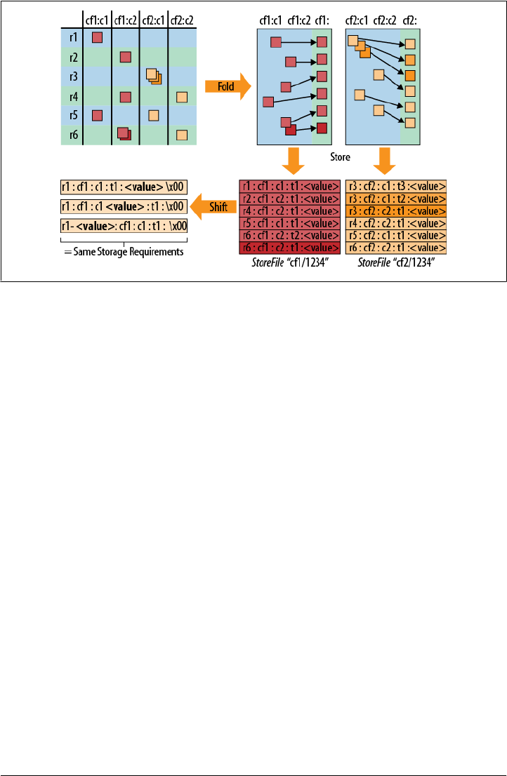
therefore has to also store the row key and column key with every cell so that it can
retain this vital piece of information.
In addition, multiple versions of the same cell are stored as separate, consecutive cells,
adding the required timestamp of when the cell was stored. The cells are sorted in
descending order by that timestamp so that a reader of the data will see the newest
value first—which is the canonical access pattern for the data.
The entire cell, with the added structural information, is called KeyValue in HBase
terms. It has not just the column and actual value, but also the row key and timestamp,
stored for every cell for which you have set a value. The KeyValues are sorted by row
key first, and then by column key in case you have more than one cell per row in one
column family.
The lower-right part of the figure shows the resultant layout of the logical table inside
the physical storage files. The HBase API has various means of querying the stored data,
with decreasing granularity from left to right: you can select rows by row keys and
effectively reduce the amount of data that needs to be scanned when looking for a
specific row, or a range of rows. Specifying the column family as part of the query can
eliminate the need to search the separate storage files. If you only need the data of one
family, it is highly recommended that you specify the family for your read operation.
Although the timestamp—or version—of a cell is farther to the right, it is another im-
portant selection criterion. The store files retain the timestamp range for all stored cells,
so if you are asking for a cell that was changed in the past two hours, but a particular
store file only has data that is four or more hours old it can be skipped completely. See
also “Read Path” on page 342 for details.
Figure 9-1. Rows stored as linear sets of actual cells, which contain all the vital information
358 | Chapter 9: Advanced Usage
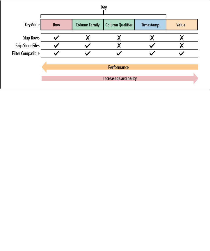
The next level of query granularity is the column qualifier. You can employ exact column
lookups when reading data, or define filters that can include or exclude the columns
you need to access. But as you will have to look at each KeyValue to check if it should
be included, there is only a minor performance gain.
The value remains the last, and broadest, selection criterion, equaling the column
qualifier’s effectiveness: you need to look at each cell to determine if it matches the read
parameters. You can only use a filter to specify a matching rule, making it the least
efficient query option. Figure 9-2 summarizes the effects of using the KeyValue fields.
Figure 9-2. Retrieval performance decreasing from left to right
The crucial part of Figure 9-1 shows is the shift in the lower-lefthand side. Since the
effectiveness of selection criteria greatly diminishes from left to right for a KeyValue,
you can move all, or partial, details of the value into a more significant place—without
changing how much data is stored.
Tall-Narrow Versus Flat-Wide Tables
At this time, you may be asking yourself where and how you should store your data.
The two choices are tall-narrow and flat-wide. The former is a table with few columns
but many rows, while the latter has fewer rows but many columns. Given the explained
query granularity of the KeyValue information, it seems to be advisable to store parts of
the cell’s data—especially the parts needed to query it—in the row key, as it has the
highest cardinality.
In addition, HBase can only split at row boundaries, which also enforces the recom-
mendation to go with tall-narrow tables. Imagine you have all emails of a user in a single
row. This will work for the majority of users, but there will be outliers that will have
magnitudes of emails more in their inbox—so many, in fact, that a single row could
outgrow the maximum file/region size and work against the region split facility.
Key Design | 359

The better approach would be to store each email of a user in a separate row, where
the row key is a combination of the user ID and the message ID. Looking at
Figure 9-1 you can see that, on disk, this makes no difference: if the message ID is in
the column qualifier, or in the row key, each cell still contains a single email message.
Here is the flat-wide layout on disk, including some examples:
<userId> : <colfam> : <messageId> : <timestamp> : <email-message>
12345 : data : 5fc38314-e290-ae5da5fc375d : 1307097848 : "Hi Lars, ..."
12345 : data : 725aae5f-d72e-f90f3f070419 : 1307099848 : "Welcome, and ..."
12345 : data : cc6775b3-f249-c6dd2b1a7467 : 1307101848 : "To Whom It ..."
12345 : data : dcbee495-6d5e-6ed48124632c : 1307103848 : "Hi, how are ..."
The same information stored as a tall-narrow table has virtually the same footprint
when stored on disk:
<userId>-<messageId> : <colfam> : <qualifier> : <timestamp> : <email-message>
12345-5fc38314-e290-ae5da5fc375d : data : : 1307097848 : "Hi Lars, ..."
12345-725aae5f-d72e-f90f3f070419 : data : : 1307099848 : "Welcome, and ..."
12345-cc6775b3-f249-c6dd2b1a7467 : data : : 1307101848 : "To Whom It ..."
12345-dcbee495-6d5e-6ed48124632c : data : : 1307103848 : "Hi, how are ..."
This layout makes use of the empty qualifier (see “Column Families” on page 212). The
message ID is simply moved to the left, making it more significant when querying
the data, but also transforming each email into a separate logical row. This results in a
table that is easily splittable, with the additional benefit of having a more fine-grained
query granularity.
Partial Key Scans
The scan functionality of HBase, and the HTable-based client API, offers the second
crucial part for transforming a table into a tall-narrow one, without losing query gran-
ularity: partial key scans.
In the preceding example, you have a separate row for each message, across all users.
Before you had one row per user, so a particular inbox was a single row and could be
accessed as a whole. Each column was an email message of the users’ inbox. The exact
row key would be used to match the user ID when loading the data.
With the tall-narrow layout an arbitrary message ID is now postfixed to the user ID in
each row key. If you do not have an exact combination of these two IDs you cannot
retrieve a particular message. The way to get around this complication is to use partial
key scans: you can specify a start and end key that is set to the exact user ID only, with
the stop key set to userId + 1.
360 | Chapter 9: Advanced Usage
The start key of a scan is inclusive, while the stop key is exclusive. Setting the start key
to the user ID triggers the internal lexicographic comparison mechanism of the scan to
find the exact row key, or the one sorting just after it. Since the table does not have an
exact match for the user ID, it positions the scan at the next row, which is:
<userId>-<lowest-messageId>
In other words, it is the row key with the lowest (in terms of sorting) user ID and message
ID combination. The scan will then iterate over all the messages of a user and you can
parse the row key to extract the message ID.
The partial key scan mechanism is quite powerful, as you can use it as a lefthand index,
with each added field adding to its cardinality. Consider the following row key
structure:
<userId>-<date>-<messageId>-<attachmentId>
Make sure that you pad the value of each field in the composite row key
so that the lexicographical (binary, and ascending) sorting works as ex-
pected. You will need a fixed-length field structure to guarantee that the
rows are sorted by each field, going from left to right.*
You can, with increasing precision, construct a start and stop key for the scan that
selects the required rows. Usually you only create the start key and set the stop key to
the same value as the start key, while increasing the least significant byte of its first field
by one. For the preceding inbox example, the start key could be 12345, and the stop
key 123456.
Table 9-1 shows the possible start keys and what they translate into.
Table 9-1. Possible start keys and their meaning
Command Description
<userId> Scan over all messages for a given user ID.
<userId>-<date> Scan over all messages on a given date for the given user ID.
<userId>-<date>-<messageId> Scan over all parts of a message for a given user ID and date.
<userId>-<date>-<messageId>-<attachmentId> Scan over all attachments of a message for a given user ID
and date.
* You could, for example, use Orderly to generate the composite row keys.
Key Design | 361
These composite row keys are similar to what RDBMSes offer, yet you can control the
sort order for each field separately. For example, you could do a bitwise inversion of
the date expressed as a long value (the Linux epoch). This would then sort the rows in
descending order by date. Another approach is to compute the following:
Long.MAX_VALUE - <date-as-long>
This will reverse the dates and guarantee that the sorting order of the date field is
descending.
In the preceding example, you have the date as the second field in the composite index
for the row key. This is only one way to express such a combination. If you were to
never query by date, you would want to drop the date from the key—and/or possibly
use another, more suitable, dimension instead.
While it seems like a good idea to always implement a composite row
key as discussed in the preceding text, there is one major drawback to
doing so: atomicity. Since the data is now spanning many rows for a
single inbox, it is not possible to modify it in one operation. If you are
not concerned with updating the entire inbox with all the user messages
in an atomic fashion, the aforementioned design is appropriate. But if
you need to have such guarantees, you may have to go back to flat-wide
table design.
Pagination
Using the partial key scan approach, it is possible to iterate over subsets of rows. The
principle is the same: you have to specify an appropriate start and stop key to limit the
overall number of rows scanned. Then you take an offset and limit parameter, applying
them to the rows on the client side.
You can also use the “PageFilter” on page 149, or “ColumnPagination-
Filter” on page 154 to achieve pagination. The approach shown here is
mainly to explain the concept of what a dedicated row key design can
achieve.
For pure pagination, the ColumnPaginationFilter is also the recommen-
ded approach, as it avoids sending unnecessary data over the network
to the client.
The steps are the following:
1. Open a scanner at the start row.
2. Skip offset rows.
3. Read the next limit rows and return to the caller.
4. Close the scanner.
362 | Chapter 9: Advanced Usage

Applying this to the inbox example, it is possible to paginate through all of the emails
of a user. Assuming an average user has a few hundred emails in his inbox, it is quite
common for a web-based email client to show only the first, for example, 50 emails.
The remainder of the emails are then accessed by clicking the Next button to load the
next page.
The client would set the start row to the user ID, and the stop row to the user ID + 1.
The remainder of the process would follow the approach we just discussed, so for the
first page, where the offset is zero, you can read the next 50 emails. When the user
clicks the Next button, you would set the offset to 50, therefore skipping those first 50
rows, returning row 51 to 100, and so on.
This approach works well for a low number of pages. If you were to page through
thousands of pages, a different approach would be required. You could add a sequential
ID into the row key to directly position the start key at the right offset. Or you could
use the date field of the key—if you are using one—to remember the date of the last
displayed item and add the date to the start key, but probably dropping the hour part
of it. If you were using epochs, you could compute the value for midnight of the last
seen date. That way you can rescan that entire day and make a more knowledgeable
decision regarding what to return.
There are many ways to design the row key to allow for efficient selection of subranges
and enable pagination through records, such as the emails in the user inbox example.
Using the composite row key with the user ID and date gives you a natural order,
displaying the newest messages first, sorting them in descending order by date. But
what if you also want to offer sorting by different fields so that the user can switch at
will? One way to do this is discussed in “Secondary Indexes” on page 370.
Time Series Data
When dealing with stream processing of events, the most common use case is time
series data. Such data could be coming from a sensor in a power grid, a stock exchange,
or a monitoring system for computer systems. Its salient feature is that its row key
represents the event time. This imposes a problem with the way HBase is arranging its
rows: they are all stored sorted in a distinct range, namely regions with specific start
and stop keys.
The sequential, monotonously increasing nature of time series data causes all incoming
data to be written to the same region. And since this region is hosted by a single server,
all the updates will only tax this one machine. This can cause regions to really run hot
with the number of accesses, and in the process slow down the perceived overall per-
formance of the cluster, because inserting data is now bound to the performance of a
single machine.
Key Design | 363

It is easy to overcome this problem by ensuring that data is spread over all region servers
instead. This can be done, for example, by prefixing the row key with a nonsequential
prefix. Common choices include:
Salting
You can use a salting prefix to the key that guarantees a spread of all rows across
all region servers. For example:
byte prefix = (byte) (Long.hashCode(timestamp) % <number of region
servers>);
byte[] rowkey = Bytes.add(Bytes.toBytes(prefix), Bytes.toBytes(timestamp);
This formula will generate enough prefix numbers to ensure that rows are sent to
all region servers. Of course, the formula assumes a specific number of servers, and
if you are planning to grow your cluster you should set this number to a multiple
instead. The generated row keys might look like this:
0myrowkey-1, 1myrowkey-2, 2myrowkey-3, 0myrowkey-4, 1myrowkey-5, \
2myrowkey-6, ...
When these keys are sorted and sent to the various regions the order would be:
0myrowkey-1
0myrowkey-4
1myrowkey-2
1myrowkey-5
...
In other words, the updates for row keys 0myrowkey-1 and 0myrowkey-4 would be
sent to one region (assuming they do not overlap two regions, in which case there
would be an even broader spread), and 1myrowkey-2 and 1myrowkey-5 are sent to
another.
The drawback of this approach is that access to a range of rows must be fanned
out in your own code and read with <number of region servers> get or scan calls.
On the upside, you could use multiple threads to read this data from distinct serv-
ers, therefore parallelizing read access. This is akin to a small map-only MapReduce
job, and should result in increased I/O performance.
Use Case: Mozilla Socorro
The Mozilla organization has built a crash reporter—named Socorro†—for Firefox
and Thunderbird, which stores all the pertinent details pertaining to when a client
asks its user to report a program anomaly. These reports are subsequently read
and analyzed by the Mozilla development team to make their software more reli-
able on the vast number of machines and configurations on which it is used.
The code is open source, available online, and contains the Python-based client
code that communicates with the HBase cluster using Thrift. Here is an example
† See the Mozilla wiki page on Socorro for details.
364 | Chapter 9: Advanced Usage

(as of the time of this writing) of how the client is merging the previously salted,
sequential keys when doing a scan operation:
def merge_scan_with_prefix(self,table,prefix,columns):
"""
A generator based iterator that yields totally ordered rows starting with a
given prefix. The implementation opens up 16 scanners (one for each leading
hex character of the salt) simultaneously and then yields the next row in
order from the pool on each iteration.
"""
iterators = []
next_items_queue = []
for salt in '0123456789abcdef':
salted_prefix = "%s%s" % (salt,prefix)
scanner = self.client.scannerOpenWithPrefix(table, salted_prefix, columns)
iterators.append(salted_scanner_iterable(self.logger,self.client,
self._make_row_nice,salted_prefix,scanner))
# The i below is so we can advance whichever scanner delivers us the polled
# item.
for i,it in enumerate(iterators):
try:
next = it.next
next_items_queue.append([next(),i,next])
except StopIteration:
pass
heapq.heapify(next_items_queue)
while 1:
try:
while 1:
row_tuple,iter_index,next = s = next_items_queue[0]
#tuple[1] is the actual nice row.
yield row_tuple[1]
s[0] = next()
heapq.heapreplace(next_items_queue, s)
except StopIteration:
heapq.heappop(next_items_queue)
except IndexError:
return
The Python code opens the required number of scanners, adding the salt prefix,
which here is composed of a fixed set of single-letter prefixes—16 different ones
all together. Note that an additional heapq object is used that manages the actual
merging of the scanner results against the global sorting order.
Field swap/promotion
Using the same approach as described in “Partial Key Scans” on page 360, you can
move the timestamp field of the row key or prefix it with another field. This ap-
proach uses the composite row key concept to move the sequential, monotonously
increasing timestamp to a secondary position in the row key.
If you already have a row key with more than one field, you can swap them. If you
have only the timestamp as the current row key, you need to promote another field
from the column keys, or even the value, into the row key.
Key Design | 365

There is also a drawback to moving the time to the righthand side in the composite
key: you can only access data, especially time ranges, for a given swapped or pro-
moted field.
Use Case: OpenTSDB
The OpenTSDB‡ project provides a time series database used to store metrics about
servers and services, gathered by external collection agents. All of the data is stored
in HBase, and using the supplied user interface (UI) enables users to query various
metrics, combining and/or downsampling them—all in real time.
The schema promotes the metric ID into the row key, forming the following
structure:
<metric-id><base-timestamp>...
Since a production system will have a considerable number of metrics, but their
IDs will be spread across a range and all updates occurring across them, you end
up with an access pattern akin to the salted prefix: the reads and writes are spread
across the metric IDs.
This approach is ideal for a system that queries primarily by the leading field of
the composite key. In the case of OpenTSDB this makes sense, since the UI asks
the users to select from one or more metrics, and then displays the data points of
those metrics ordered by time.
Randomization
A totally different approach is to randomize the row key using, for example:
byte[] rowkey = MD5(timestamp)
Using a hash function like MD5 will give you a random distribution of the key
across all available region servers. For time series data, this approach is obviously
less than ideal, since there is no way to scan entire ranges of consecutive
timestamps.
On the other hand, since you can re-create the row key by hashing the timestamp
requested, it still is very suitable for random lookups of single rows. When your
data is not scanned in ranges but accessed randomly, you can use this strategy.
Summarizing the various approaches, you can see that it is not trivial to find the right
balance between optimizing for read and write performance. It depends on your access
pattern, which ultimately drives the decision on how to structure your row keys.
Figure 9-3 shows the various solutions and how they affect sequential read and write
performance.
‡ See the OpenTSDB project website for details. In particular, the page that discusses the project’s
schema is a recommended read, as it adds advanced key design concepts for an efficient storage format
that also allows for high-performance querying of the stored data.
366 | Chapter 9: Advanced Usage
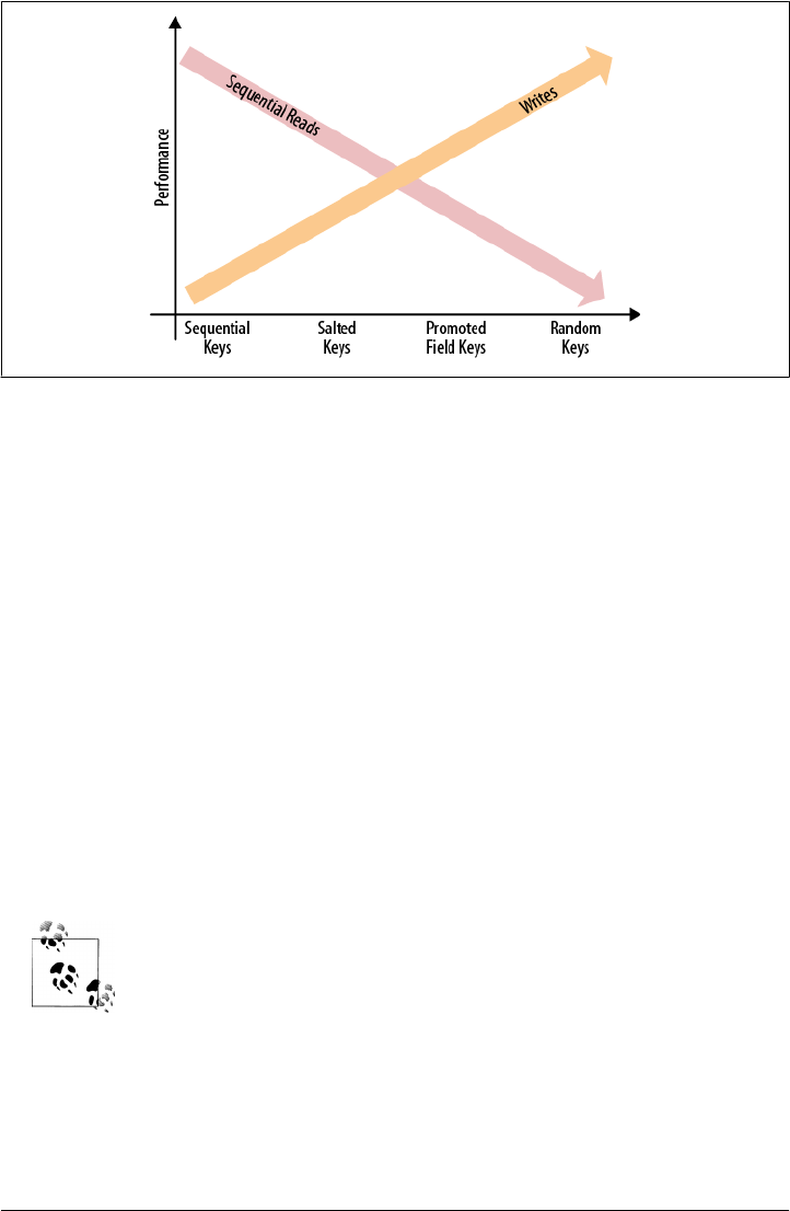
Using the salted or promoted field keys can strike a good balance of distribution for
write performance, and sequential subsets of keys for read performance. If you are only
doing random reads, it makes most sense to use random keys: this will avoid creating
region hot-spots.
Time-Ordered Relations
In our preceding discussion, the time series data dealt with inserting new events as
separate rows. However, you can also store related, time-ordered data: using the col-
umns of a table. Since all of the columns are sorted per column family, you can treat
this sorting as a replacement for a secondary index, as available in RDBMSes. Multiple
secondary indexes can be emulated by using multiple column families—although that
is not the recommended way of designing a schema. But for a small number of indexes,
this might be what you need.
Consider the earlier example of the user inbox, which stores all of the emails of a user
in a single row. Since you want to display the emails in the order they were received,
but, for example, also sorted by subject, you can make use of column-based sorting to
achieve the different views of the user inbox.
Given the advice to keep the number of column families in a table low—
especially when mixing large families with small ones (in terms of stored
data)—you could store the inbox inside one table, and the secondary
indexes in another table. The drawback is that you cannot make use of
the provided per-table row-level atomicity. Also see “Secondary In-
dexes” on page 370 for strategies to overcome this limitation.
The first decision to make concerns what the primary sorting order is, in other words,
how the majority of users have set the view of their inbox. Assuming they have set the
Figure 9-3. Finding the right balance between sequential read and write performance
Key Design | 367

view in descending order by date, you can use the same approach mentioned earlier,
which reverses the timestamp of the email, effectively sorting all of them in descending
order by time:
Long.MAX_VALUE - <date-as-long>
The email itself is stored in the main column family, while the sort indexes are in sep-
arate column families. You can extract the subject from the email address and add it
to the column key to build the secondary sorting order. If you need descending sorting
as well, you would need another family.
To circumvent the proliferation of column families, you can alternatively store all sec-
ondary indexes in a single column family that is separate from the main column family.
Once again, you would make use of implicit sorting by prefixing the values with an
index ID—for example, idx-subject-desc, idx-to-asc, and so on. Next, you would
have to attach the actual sort value. The actual value of the cell is the key of the main
index, which also stores the message. This also implies that you need to either load the
message details from the main table, display only the information stored in the secon-
dary index, or store the display details redundantly in the index, avoiding the random
lookup on the main information source. Recall that denormalization is quite common
in HBase to reduce the required read operations in favor of vastly improved user-facing
responsiveness.
Putting the aforementioned schema into action might result in something like this:
12345 : data : 5fc38314-e290-ae5da5fc375d : 1307097848 : "Hi Lars, ..."
12345 : data : 725aae5f-d72e-f90f3f070419 : 1307099848 : "Welcome, and ..."
12345 : data : cc6775b3-f249-c6dd2b1a7467 : 1307101848 : "To Whom It ..."
12345 : data : dcbee495-6d5e-6ed48124632c : 1307103848 : "Hi, how are ..."
...
12345 : index : idx-from-asc-mary@foobar.com : 1307099848 : 725aae5f-d72e...
12345 : index : idx-from-asc-paul@foobar.com : 1307103848 : dcbee495-6d5e...
12345 : index : idx-from-asc-pete@foobar.com : 1307097848 : 5fc38314-e290...
12345 : index : idx-from-asc-sales@ignore.me : 1307101848 : cc6775b3-f249...
...
12345 : index : idx-subject-desc-\xa8\x90\x8d\x93\x9b\xde : \
1307103848 : dcbee495-6d5e-6ed48124632c
12345 : index : idx-subject-desc-\xb7\x9a\x93\x93\x90\xd3 : \
1307099848 : 725aae5f-d72e-f90f3f070419
...
In the preceding code, one index (idx-from-asc) is sorting the emails in ascending order
by from address, and another (idx-subject-desc) in descending order by subject. The
subject itself is not readable anymore as it was bit-inversed to achieve the descending
sorting order. For example:
% String s = "Hello,";
% for (int i = 0; i < s.length(); i++) {
print(Integer.toString(s.charAt(i) ^ 0xFF, 16));
}
b7 9a 93 93 90 d3
368 | Chapter 9: Advanced Usage

All of the index values are stored in the column family index, using the prefixes men-
tioned earlier. A client application can read the entire column family and cache the
content to let the user quickly switch the sorting order. Or, if the number of values is
large, the client can read the first 10 columns starting with idx-subject-desc to show
the first 10 email messages sorted in ascending order by the email subject lines. Using
a scan with intra-row batching (see “Caching Versus Batching” on page 127) enables
you to efficiently paginate through the subindexes. Another option is the
ColumnPaginationFilter, combined with the ColumnPrefixFilter to iterate over an in-
dex page by page.
Advanced Schemas
So far we have discussed how to use the provided table schemas to map data into the
column-oriented layout HBase supports. You will have to decide how to structure your
row and column keys to access data in a way that is optimized for your application.
Each column value is then an actual data point, stored as an arbitrary array of bytes.
While this type of schema, combined with the ability to create columns with arbitrary
keys when needed, enables you to evolve with new client application releases, there are
use cases that require more formal support of a more feature-rich, evolveable seriali-
zation API, where each value is a compact representation of a more complex, nestable
record structure.
Possible solutions include the already discussed serialization packages—see “Intro-
duction to REST, Thrift, and Avro” on page 241 for details—listed here as examples:
Avro
An exemplary project using Avro to store complex records in each column is
HAvroBase.§ This project facilitates Avro’s interface definition language (IDL) to
define the actual schema, which is then used to store records in their serialized
form within arbitrary table columns.
Protocol Buffers
Similar to Avro, you can use the Protocol Buffer’s IDL to define an external schema,
which is then used to serialize complex data structures into HBase columns.
The idea behind this approach is that you get a definition language that allows you to
define an initial schema, which you can then update by adding or removing fields. The
serialization API takes care of reading older schemas with newer ones. Missing fields
are ignored or filled in with defaults.
§ See the HAvroBase GitHub project page.
Advanced Schemas | 369

Secondary Indexes
Although HBase has no native support for secondary indexes, there are use cases that
need them. The requirements are usually that you can look up a cell with not just the
primary coordinates—the row key, column family name, and qualifier—but also an
alternative coordinate. In addition, you can scan a range of rows from the main table,
but ordered by the secondary index.
Similar to an index in RDBMSes, secondary indexes store a mapping between the new
coordinates and the existing ones. Here is a list of possible solutions:
Client-managed
Moving the responsibility completely into the application layer, this approach typ-
ically combines a data table and one (or more) lookup/mapping tables. Whenever
the code writes into the data table it also updates the lookup tables. Reading data
requires either a direct lookup in the main table, or, if the key is from a secondary
index, a lookup of the main row key, and then retrieval of the data in a second
operation.
There are advantages and disadvantages to this approach. First, since the entire
logic is handled in the client code, you have all the freedom to map the keys exactly
the way they are needed. The list of shortcomings is longer, though: since you have
no cross-row atomicity, for example, in the form of transactions, you cannot guar-
antee consistency of the main and dependent tables. This can be partially overcome
using regular pruning jobs, for instance, using MapReduce to scan the tables and
remove obsolete—or add missing—entries.
The missing transactional support could result in data being stored in the data
table, but with no mapping in the secondary index tables, because the operation
failed after the main table was updated, but before the index tables were written.
This can be alleviated by writing to the secondary index tables first, and to the data
table at the end of the operation. Should anything fail in the process, you are left
with orphaned mappings, but those are subsequently removed by the asynchro-
nous, regular pruning jobs.
Having all the freedom to design the mapping between the primary and secondary
indexes comes with the drawback of having to implement all the necessary wiring
to store and look up the data. External keys need to be identified to access the
correct table, for example:
myrowkey-1
@myrowkey-2
The first key denotes a direct data table lookup, while the second, using the prefix,
is a mapping that has to be performed through a secondary index table. The name
of the table could be also encoded as a number and added to the prefix. The flip
side is this is hardcoded in your application and needs to evolve with overall schema
changes, and new requirements.
370 | Chapter 9: Advanced Usage

Indexed-Transactional HBase
A different solution is offered by the open source Indexed-Transactional HBase
(ITHBase) project.‖ This solution extends HBase by adding special implementa-
tions of the client and server-side classes.
The core extension is the addition of transactions, which are used to guarantee that
all secondary index updates are consistent. On top of this it adds index support,
by providing a client-side IndexedTableDescriptor, defining how a data table is
backed by a secondary index table.
Most client and server classes are replaced by ones that handle indexing support.
For example, HTable is replaced with IndexedTable on the client side. It has a new
method called getIndexedScanner(), which enables the iteration over rows in the
data table using the ordering of a secondary index.
Just as with the client-managed index described earlier, this index stores the map-
pings between the primary and secondary keys in separate tables. In contrast,
though, these are automatically created, and maintained, based on the descriptor.
Combined with the transactional updates of these indexes, this solution provides
a complete implementation of secondary indexes for HBase.
The drawback is that it may not support the latest version of HBase available, as
it is not tied to its release cycle. It also adds a considerable amount of synchroni-
zation overhead that results in decreased performance, so you need to benchmark
carefully.
Indexed HBase
Another solution that allows you to add secondary indexes to HBase is Indexed
HBase (IHBase).# This solution forfeits the use of separate tables for each index
but maintains them purely in memory. The indexes are generated when a region
is opened for the first time, or when a memstore is flushed to disk—involving an
entire region’s scan to build the index. Depending on your configured region size,
this can take a considerable amount of time and I/O resources.
Only the on-disk information is indexed; the in-memory data is searched as-is: it
uses the memstore data directly to search for index-related details. The advantage
of this solution is that the index is never out of sync, and no explicit transactional
control is necessary.
In comparison to table-based indexing, using this approach is very fast, as it has
all the required details in memory and can perform a fast binary search to find
matching rows. However, it requires a lot of extra heap to maintain the index.
‖The ITHBase project started as a contrib module for HBase. It was subsequently moved to an external
repository allowing it to address different versions of HBase, and to develop at its own pace. See the GitHub
project page for details.
#Similar to ITHBase, IHBase started as a contrib project within HBase. It was moved to an external repository
for the same reasons. See the GitHub project page for details. The original documentation of the JIRA issue
is online at HBASE-2037.
Secondary Indexes | 371

Depending on your requirements and the amount of data you want to index, you
might run into a situation where IHBase cannot keep all the indexes you need.
The in-memory indexes are typed and allow for more fine-grained sorting, as well
as more memory-efficient storage. There is support for BYTE, CHAR, SHORT, INT, LONG,
FLOAT, DOUBLE, BIG_DECIMAL, BYTE_ARRAY, and CHAR_ARRAY. There is no explicit control
over the sorting order; thus data is always stored in ascending order. You will need
to do the bitwise inversion of the value described earlier to sort in descending order.
The definition of an index revolves around the IdxIndexDescriptor class that de-
fines the specific column of the data table that holds the index, and the type of the
values it contains, taken from the list in the preceding paragraph.
Accessing an index is handled by the client-side IdxScan class, which extends the
normal Scan class by adding support to define Expressions. A scan without an
explicit expression defaults to normal scan behavior. Expressions provide basic
boolean logic with an And and Or construct. For example:
Expression expression = Expression
.or(
Expression.comparison(columnFamily1, qualifer1, operator1, value1)
)
.or(
Expression.and()
.and(Expression.comparison(columnFamily2, qualifer2, operator2, value2))
.and(Expression.comparison(columnFamily3, qualifer3, operator3, value3))
);
The preceding example uses builder-style helper methods to generate a complex
expression that combines three separate indexes. The lowest level of an expression
is the Comparison, which allows you to specify the actual index, and a filter-like
syntax to select values that match a comparison value and operator. Table 9-2 list
the possible operator choices.
Table 9-2. Possible values for the Comparison.Operator enumeration
Operator Description
EQ The equals operator
GT The greater than operator
GTE The greater than or equals operator
LT The less than operator
LTE The less than or equals operator
NEQ The not equals operator
You have to specify a columnFamily, and a qualifier of an existing index, or else
an IllegalStateException will be thrown.
The Comparison class has an optional includeMissing parameter, which works sim-
ilarly to filterIfMissing, described in “SingleColumnValueFilter” on page 147.
372 | Chapter 9: Advanced Usage

You can use it to fine-tune what is included in the scan depending on how the
expression is evaluated.
The sorting order is defined by the first evaluated index in the expression, while
the other indexes are used to intersect (for the and) or unite (for the or) the possible
keys with the first index. In other words, using complex expressions is predictable
only when using the same index, but with various comparisons.
The benefit of IHBase over ITHBase, for example, is that it achieves the same
guarantees—namely maintaining a consistent index based on an existing column
in a data table—but without the need to employ extra tables. It shares the same
drawbacks, for the following reasons:
• It is quite intrusive, as its installation requires additional JAR files plus a con-
figuration that replaces vital client- and server-side classes.
• It needs extra resources, although it trades memory for extra I/O requirements.
• It does random lookups on the data table, based on the sorting order defined
by the secondary index.
• It may not be available for the latest version of HBase.*
Coprocessor
There is work being done to implement an indexing solution based on coproces-
sors.† Using the server-side hooks provided by the coprocessor framework, it is
possible to implement indexing similar to ITHBase, as well as IHBase while not
having to replace any client- and server-side classes. The coprocessor would load
the indexing layer for every region, which would subsequently handle the main-
tenance of the indexes.
The code can make use of the scanner hooks to transparently iterate over a normal
data table, or an index-backed view on the same. The definition of the index would
need to go into an external schema that is read by the coprocessor-based classes,
or it could make use of the generic attributes a column family can store.
Since this is in its early stages, there is not much that can be docu-
mented at this time. Watch the online issue tracking system for
updates on the work if you are interested.
Search Integration
Using indexes gives you the ability to iterate over a data table in more than the implicit
row key order. You are still confined to the available keys and need to use either filters
or straight iterations to find the values you are looking for. A very common use case is
* As of this writing, IHBase only supports HBase version 0.20.5.
† See HBASE-2038 in the JIRA issue tracking system for details.
Search Integration | 373

to combine the arbitrary nature of keys with a search-based lookup, often backed by
full search engine integration.
Common choices are the Apache Lucene-based solutions, such as Lucene itself, or Solr,
a high-performance enterprise search server.‡ Similar to the indexing solutions, there
are a few possible approaches:
Client-managed
These range from implementations using HBase as the data store, and using Map-
Reduce jobs to build the search index, to those that use HBase as the backing store
for Lucene. Another approach is to route every update of the data table to the
adjacent search index. Implementing support for search indexes in combination
with HBase is primarily driven by how the data is accessed, and if HBase is used
as the data store, or as the index store.
A prominent implementation of a client-managed solution is the Facebook inbox
search. The schema is built roughly like this:
• Every row is a single inbox, that is, every user has a single row in the search table.
• The columns are the terms indexed from the messages.
• The versions are the message IDs.
• The values contain additional information, such as the position of the term in
the document.
With this schema it is easy to search a user’s inbox for messages containing specific
words. Boolean operators, such as and or or, can be implemented in the client code,
merging the lists of documents found. You can also efficiently implement type-
ahead queries: the user can start typing a word and the search finds all messages
that contain words that match the user’s input as a prefix.
Lucene
Using Lucene—or a derived solution—separately from HBase involves building
the index using a MapReduce job. An externally hosted project§ provides the
BuildTableIndex class, which was formerly part of the contrib modules shipping
with HBase. This class scans an entire table and builds the Lucene indexes, which
ultimately end up as directories on HDFS—their count depends on the number of
reducers used. These indexes can be downloaded to a Lucene-based server, and
accessed locally using, for example, a MultiSearcher class, provided by Lucene.
Another approach is to merge the index parts by either running the MapReduce
job with a single reducer, or using the index merge tool that comes with Lucene.
A merged index usually provides better performance, but the time required to
build, merge, and eventually serve the index is longer.
‡ Solr is based on Lucene, but extends it to provide a fully featured search server. See the project’s website for
details on either project.
§ See the GitHub project page for details and to access the code.
374 | Chapter 9: Advanced Usage

In general, this approach uses HBase only to store the data. If a search is performed
through Lucene, usually only the matching row keys are returned. A random
lookup into the data table is required to display the document. Depending on the
number of lookups, this can take a considerable amount of time. A better solution
would be something that combines the search directly with the stored data, thus
avoiding the additional random lookup.
HBasene
The approach chosen by HBasene‖ is to build an entire search index directly inside
HBase, while supporting the well-established Lucene API. The schema used stores
each document field, or term, in a separate row, with the documents containing
the term stored as columns inside that row.
The schema also reuses the same table to store various other details required to
implement full Lucene support. It implements an IndexWriter that stores the docu-
ments directly into the HBase table, as they are inserted using the normal Lucene
API. Searching is then done using the Lucene search API. Here is an example taken
from the test class that comes with HBasene:
private static final String[] AIRPORTS = { "NYC", "JFK", "EWR", "SEA",
"SFO", "OAK", "SJC" };
private final Map<String, List<Integer>> airportMap =
new TreeMap<String, List<Integer>>();
protected HTablePool tablePool;
protected void doInitDocs() throws CorruptIndexException, IOException {
Configuration conf = HBaseConfiguration.create();
HBaseIndexStore.createLuceneIndexTable("idxtbl", conf, true);
tablePool = new HTablePool(conf, 10);
HBaseIndexStore hbaseIndex = new HBaseIndexStore(tablePool, conf,
"idxtbl");
HBaseIndexWriter indexWriter = new HBaseIndexWriter(hbaseIndex, "id")
for (int i = 100; i >= 0; --i) {
Document doc = getDocument(i);
indexWriter.addDocument(doc, new StandardAnalyzer(Version.LUCENE_30));
}
}
private Document getDocument(int i) {
Document doc = new Document();
doc.add(new Field("id", "doc" + i, Field.Store.YES, Field.Index.NO));
int randomIndex = (int) (Math.random() * 7.0f);
doc.add(new Field("airport", AIRPORTS[randomIndex], Field.Store.NO,
Field.Index.ANALYZED_NO_NORMS));
doc.add(new Field("searchterm", Math.random() > 0.5f ?
"always" : "never",
Field.Store.NO, Field.Index.ANALYZED_NO_NORMS));
return doc;
‖The GitHub page has the details, and source code.
Search Integration | 375
}
public TopDocs search() throws IOException {
HBaseIndexReader indexReader = new HBaseIndexReader(tablePool, "idxtbl",
"id");
HBaseIndexSearcher indexSearcher = new HBaseIndexSearcher(indexReader);
TermQuery termQuery = new TermQuery(new Term("searchterm", "always"));
Sort sort = new Sort(new SortField("airport", SortField.STRING));
TopDocs docs = this.indexSearcher.search(termQuery
.createWeight(indexSearcher), null, 25, sort, false);
return docs;
}
public static void main(String[] args) throws IOException {
doInitDocs();
TopDocs docs = search();
// use the returned documents...
}
The example creates a small test index and subsequently searches it. You may note
that there is a lot of Lucene API usage, with small amendments to support the
HBase-backed index writer.
The project—as of this writing—is more a proof of concept than a
production-ready implementation.
Coprocessors
Yet another approach to complement a data table with Lucene-based search func-
tionality, and currently in development,# is based on coprocessors. It uses the
provided hooks to maintain the index, which is stored directly on HDFS. Every
region has its own index and search is distributed across them to gather the full
result.
This is only one example of what is possible with coprocessors. Similar to the use
of coprocessors to build secondary indexes, you have the choice of where to store
the actual index: either in another table, or externally. The framework offers the
enabling technology; the implementing code has the choice of how to use it.
Transactions
It seems somewhat counterintuitive to talk about transactions in regard to HBase.
However, the secondary index example showed that for some use cases it is beneficial
to abandon the simplified data model HBase offers, and in fact introduce concepts that
are usually seen in traditional database systems.
#HBASE-3529
376 | Chapter 9: Advanced Usage

One of those concepts is transactions, offering ACID compliance across more than one
row, and more than one table. This is necessary in lieu of a matching schema pattern
in HBase. For example, updating the main data table and the secondary index table
requires transactions to be reliably consistent.
Often, transactions are not needed, as normalized data schemas can be folded into a
single table and row design that does not need the overhead of distributed transaction
support. If you cannot do without this extra control, here are a few possible solutions:
Transactional HBase
The Indexed Transactional HBase project comes with a set of extended classes that
replace the default client- and server-side classes, while adding support for trans-
actions across row and table boundaries. The region servers, and more precisely,
each region, keeps a list of transactions, which are initiated with a beginTransac
tion() call, and are finalized with the matching commit() call. Every read and write
operation then takes a transaction ID to guard the call against other transactions.
ZooKeeper
HBase requires a ZooKeeper ensemble to be present, acting as the seed, or boot-
strap mechanism, for cluster setup. There are templates, or recipes, available that
show how ZooKeeper can also be used as a transaction control backend. For ex-
ample, the Cages project offers an abstraction to implement locks across multiple
resources, and is scheduled to add a specialized transactions class—using Zoo-
Keeper as the distributed coordination system.
ZooKeeper also comes with a lock recipe that can be used to implement a two-
phase commit protocol. It uses a specific znode representing the transaction, and
a child znode for every participating client. The clients can use their znodes to flag
whether their part of the transaction was successful or failed. The other clients can
monitor the peer znodes and take the appropriate action.*
Bloom Filters
“Column Families” on page 212 introduced the syntax to declare Bloom filters at the
column family level, and discussed specific use cases in which it makes sense to use
them.
The reason to use Bloom filters at all is that the default mechanisms to decide if a store
file contains a specific row key are limited to the available block index, which is, in
turn, fairly coarse-grained: the index stores the start row key of each contained block
only. Given the default block size of 64 KB, and a store file of, for example, 1 GB, you
end up with 16,384 blocks, and the same amount of indexed row keys.
If we further assume your cell size is an average of 200 bytes, you will have more than
5 million of them stored in that single file. Given a random row key you are looking
* More details can be found on the ZooKeeper project page.
Bloom Filters | 377
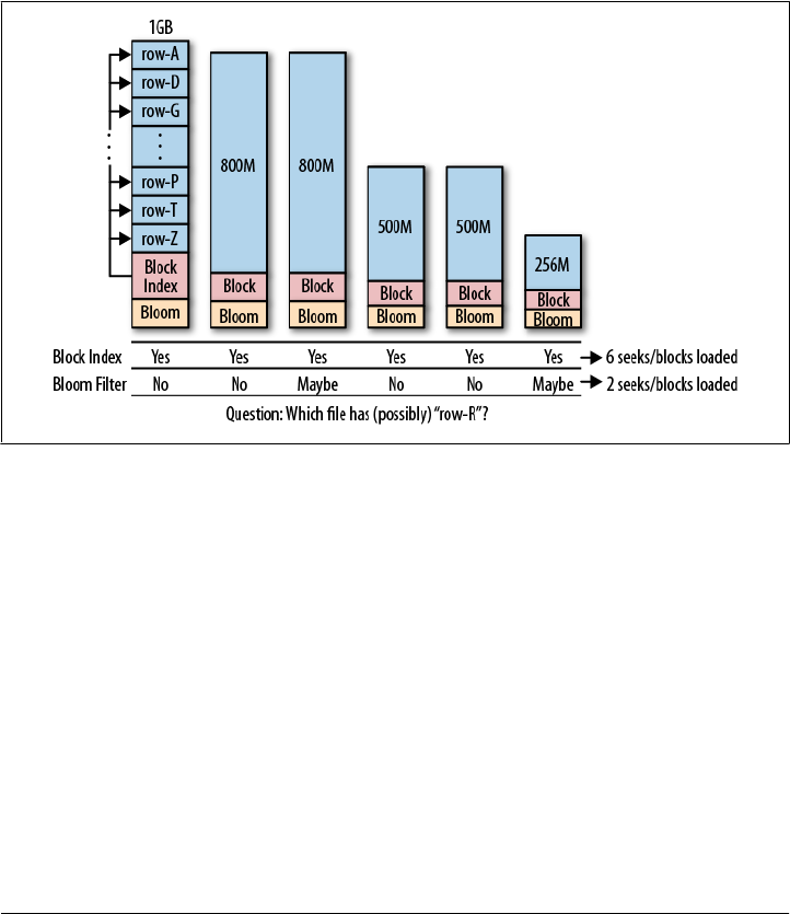
for, it is very likely that this key will fall in between two block start keys. The only way
for HBase to figure out if the key actually exists is by loading the block and scanning it
to find the key.
This problem is compounded by the fact that, for a typical application, you will expect
a certain update rate, which results in flushing in-memory data to disk, and subsequent
compactions aggregating them into larger store files. Since minor compactions only
combine the last few store files, and only up to a configured maximum size, you will
end up with a number of store files, all acting as possible candidates to have some cells
of the requested row key. Consider the example in Figure 9-4.
Figure 9-4. Using Bloom filters to help reduce the number of I/O operations
The files are all from one column family and have a similar spread in row keys, although
only a few really hold an update to a specific row. The block index has a spread across
the entire row key range, and therefore always reports positive to contain a random
row. The region server would need to load every block to check if the block actually
contains a cell of the row or not.
On the other hand, enabling the Bloom filter does give you the immediate advantage
of knowing if a file contains a particular row key or not. The nature of the filter is that
it can give you a definitive answer if the file does not contain the row—but might report
a false positive, claiming the file contains the data, where in reality it does not. The
number of false positives can be tuned and is usually set to 1%, meaning that in 1% of
all reports by the filter that a file contains a requested row, it is wrong—and a block is
loaded and checked erroneously.
378 | Chapter 9: Advanced Usage

This does not translate into an immediate performance gain on indi-
vidual get operations, since HBase does the reads in parallel, and is
ultimately bound by disk read latency. Reducing the number of unnec-
essary block loads improves the overall throughput of the cluster.
You can see from the example, however, that the number of block loads is greatly
reduced, which can make a big difference in a heavily loaded system. For this to be
efficient, you must also match a specific update pattern: if you modify all of the rows
on a regular basis, the majority of the store files will have a piece of the row you are
looking for, and therefore would not be a good use case for Bloom filters. But if you
update data in batches so that each row is written into only a few store files at a time,
the filter is a great feature to reduce the overall number of I/O operations.
Another place where you will find this to be advantageous is in the block cache. The
hit rate of the cache should improve as loading fewer blocks results in less churn. Since
the server is now loading blocks that contain the requested data most of the time, related
data has a greater chance to remain in the block cache and subsequent read operations
can make use of it.
Besides the update pattern, another driving factor to decide if a Bloom filter makes
sense for your use case is the overhead it adds. Every entry in the filter requires about
one byte of storage. Going back to the earlier example store file that was 1 GB in size,
assuming you store only counters (i.e., long values encoded as eight bytes), and adding
the overhead of the KeyValue information—which is its coordinates, or, the row key,
column family name, column qualifier, timestamp, and type—then every cell is about
20 bytes (further assuming you use very short keys) in size. Then the Bloom filter would
be 1/20th of your file, or about 51 MB.
Now assume your cells are, on average, 1 KB in size; in this case, the filter needs only
1 MB. Taking into account further optimizations, you often end up with a row-level
Bloom filter of a few hundred kilobytes for a store file of one or more gigabyte. In that
case, it seems that it would always be to enable the filter.
The final question is whether to use a row or a row+column Bloom filter. The answer
depends on your usage pattern. If you are doing only row scans, having the more specific
row+column filter will not help at all: having a row-level Bloom filter enables you to
narrow down the number of files that need to be checked, even when you do row
+column read operations, but not the other way around.
The row+column Bloom filter is useful when you cannot batch updates for a specific
row, and end up with store files which all contain parts of the row. The more specific
row+column filter can then identify which of the files contain the data you are re-
questing. Obviously, if you always load the entire row, this filter is once again hardly
useful, as the region server will need to load the matching block out of each file anyway.
Bloom Filters | 379
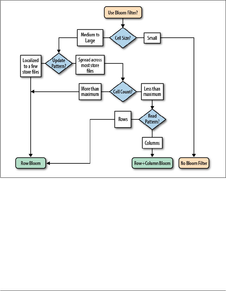
Since the row+column filter will require more storage, you need to do the math to
determine whether it is worth the extra resources. It is also interesting to know that
there is a maximum number of elements a Bloom filter can hold. If you have too many
cells in your store file, you might exceed that number and would need to fall back to
the row-level filter.
Figure 9-5 summarizes the selection criteria for the different Bloom filter levels.
Figure 9-5. Selection criteria for deciding what Bloom filter to use
Depending on your use case, it may be useful to enable Bloom filters, to increase the
overall performance of your system. If possible, you should try to use the row-level
Bloom filter, as it strikes a good balance between the additional space requirements
and the gain in performance coming from its store file selection filtering. Only resort
to the more costly row+column Bloom filter when you would otherwise gain no ad-
vantage from using the row-level one.
380 | Chapter 9: Advanced Usage

Versioning
Now that we have seen how data is stored and retrieved in HBase, it is time to revisit
the subject of versioning. There are a few advanced techniques when using timestamps
that—given that you understand their behavior—may be an option for specific use
cases. They also expose a few intricacies you should be aware of.
Implicit Versioning
I pointed out before that you should ensure that the clock on your servers is synchron-
ized. Otherwise, when you store data in multiple rows across different servers, using
the implicit timestamps, you may end up with completely different time settings.
For example, say you use the HBase URL Shortener and store three new shortened
URLs for an existing user. All of the keys are considered fully distributed, so all three
of the new rows end up on a different region server. Further, assuming that these servers
are all one hour apart, if you were to scan from the client side to get the list of new
shortened URLs within the past hour, you would miss a few, as they have been saved
with a timestamp that is more than an hour different from what the client considers
current.
This can be avoided by setting an agreed, or shared, timestamp when storing these
values. The put operation allows you to set a client-side timestamp that is used instead,
therefore overriding the server time. Obviously, the better approach is to rely on the
servers doing this work for you, but you might be required to use this approach in some
circumstances.†
Another issue with servers not being aligned by time is exposed by region splits. Assume
you have saved a value on a server that is one hour ahead all other servers in the cluster,
using the implicit timestamp of the server. Ten minutes later the region is split and the
half with your update is moved to another server. Five minutes later you are inserting
a new value for the same column, again using the automatic server time. The new value
is now considered older than the initial one, because the first version has a timestamp
one hour ahead of the current server’s time. If you do a standard get call to retrieve the
newest version of the value, you will get the one that was stored first.
Once you have all the servers synchronized, there are a few more interesting side effects
you should know about. First, it is possible—for a specific time—to make versions of
a column reappear. This happens when you store more versions than are configured at
the column family level. The default is to keep the last three versions of a cell, or value.
If you insert a new value 10 times into the same column, and request a complete list of
all versions retained, using the setMaxVersions() call of the Get class, you will only ever
† One example, although very uncommon, is based on virtualized servers. See http://support.ntp.org/bin/view/
Support/KnownOsIssues#Section_9.2.2, which lists an issue with NTP, the commonly used Network Time
Protocol, on virtual machines.
Versioning | 381
receive up to what is configured in the table schema, that is, the last three versions by
default.
But what would happen when you explicitly delete the last two versions? Exam-
ple 9-1 demonstrates this.
Example 9-1. Application deleting with explicit timestamps
for (int count = 1; count <= 6; count++) {
Put put = new Put(ROW1);
put.add(COLFAM1, QUAL1, count, Bytes.toBytes("val-" + count));
table.put(put);
}
Delete delete = new Delete(ROW1);
delete.deleteColumn(COLFAM1, QUAL1, 5);
delete.deleteColumn(COLFAM1, QUAL1, 6);
table.delete(delete);
Store the same column six times.
The version is set to a specific value, using the loop variable.
Delete the newest two versions.
When you run the example, you should see the following output:
After put calls...
KV: row1/colfam1:qual1/6/Put/vlen=5, Value: val-6
KV: row1/colfam1:qual1/5/Put/vlen=5, Value: val-5
KV: row1/colfam1:qual1/4/Put/vlen=5, Value: val-4
After delete call...
KV: row1/colfam1:qual1/4/Put/vlen=5, Value: val-4
KV: row1/colfam1:qual1/3/Put/vlen=5, Value: val-3
KV: row1/colfam1:qual1/2/Put/vlen=5, Value: val-2
An interesting observation is that you have resurrected versions 2 and 3! This is caused
by the fact that the servers delay the housekeeping to occur at well-defined times. The
older versions of the column are still kept, so deleting newer versions makes the older
versions come back.
This is only possible until a major compaction has been performed, after which the
older versions are removed forever, using the predicate delete based on the configured
maximum versions to retain.
The example code has some commented-out code you can enable to
enforce a flush and major compaction. If you rerun the example, you
will see this result instead:
After put calls...
KV: row1/colfam1:qual1/6/Put/vlen=5, Value: val-6
KV: row1/colfam1:qual1/5/Put/vlen=5, Value: val-5
KV: row1/colfam1:qual1/4/Put/vlen=5, Value: val-4
382 | Chapter 9: Advanced Usage
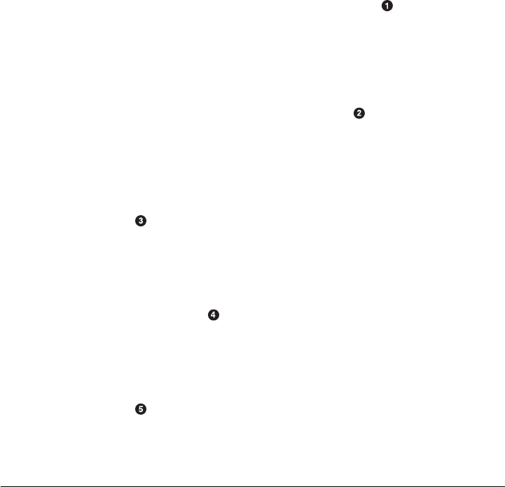
After delete call...
KV: row1/colfam1:qual1/4/Put/vlen=5, Value: val-4
Since the older versions have been removed, they do not reappear any-
more.
Finally, when dealing with timestamps, there is another issue to watch out for: delete
markers. This refers to the fact that, in HBase, a delete is actually adding a tombstone
marker into the store that has a specific timestamp. Based on that, it masks out versions
that are either a direct match, or, in the case of a column delete marker, anything that
is older than the given timestamp. Example 9-2 shows this using the shell.
Example 9-2. Deletes mask puts with explicit timestamps in the past
hbase(main):001:0> create 'testtable', 'colfam1'
0 row(s) in 1.1100 seconds
hbase(main):002:0> Time.now.to_i
=> 1308900346
hbase(main):003:0> put 'testtable', 'row1', 'colfam1:qual1', 'val1'
0 row(s) in 0.0290 seconds
hbase(main):004:0> scan 'testtable'
ROW COLUMN+CELL
row1 column=colfam1:qual1, timestamp=1308900355026, value=val1
1 row(s) in 0.0360 seconds
hbase(main):005:0> delete 'testtable', 'row1', 'colfam1:qual1'
0 row(s) in 0.0280 seconds
hbase(main):006:0> scan 'testtable'
ROW COLUMN+CELL
0 row(s) in 0.0260 seconds
hbase(main):007:0> put 'testtable', 'row1', 'colfam1:qual1', 'val1', \
Time.now.to_i - 50000
0 row(s) in 0.0260 seconds
hbase(main):008:0> scan 'testtable'
ROW COLUMN+CELL
0 row(s) in 0.0260 seconds
hbase(main):009:0> flush 'testtable'
0 row(s) in 0.2720 seconds
hbase(main):010:0> major_compact 'testtable'
0 row(s) in 0.0420 seconds
hbase(main):011:0> put 'testtable', 'row1', 'colfam1:qual1', 'val1', \
Time.now.to_i - 50000
0 row(s) in 0.0280 seconds
hbase(main):012:0> scan 'testtable'
Versioning | 383

ROW COLUMN+CELL
row1 column=colfam1:qual1, timestamp=1308900423953, value=val1
1 row(s) in 0.0290 seconds
Store a value into the column of the newly created table, and run a scan to verify.
Delete all values from the column. This sets the delete marker with a timestamp of
now.
Store the value again into the column, but use a time in the past. The subsequent
scan fails to return the masked value.
Flush and conduct a major compaction of the table to remove the delete marker.
Store the value with the time in the past again. The subsequent scan now shows it
as expected.
The example shows that there are sometimes situations where you might see something
you do not expect to see. But this behavior is explained by the architecture of HBase,
and is deterministic.
Custom Versioning
Since you can specify your own timestamp values—and therefore create your own
versioning scheme—while overriding the server-side timestamp generation based on
the synchronized server time, you are free to not use epoch-based versions at all.
For example, you could use the timestamp with a global number generator‡ that sup-
plies you with ever increasing, sequential numbers starting at 1. Every time you insert
a new value you retrieve a new number and use that when calling the put function.
You must do this for every put operation, or the server will insert an epoch-based
timestamp instead. There is a flag in the table or column descriptors that indicates your
use of custom timestamp values; in other words, your own versioning. If you fail to set
the value, it is silently replaced with the server timestamp.
When using your own timestamp values, you need to test your solution
thoroughly, as this approach has not been used widely in production.
Be aware that negative timestamp values are untested and, while they
have been discussed a few times in HBase developer circles, they have
never been confirmed to work properly.
Make sure to avoid collisions by using the same value for two separate
updates to the same cell. Usually the last saved value is visible afterward.
With these warnings out of the way, here are a few use cases that show how a custom
versioning scheme can be beneficial in the overall concept of table schema design:
‡ As an example for a number generator based on ZooKeeper, see the zk_idgen project.
384 | Chapter 9: Advanced Usage

Record IDs
A prominent example using this technique was discussed in “Search Integra-
tion” on page 373, that is, the Facebook inbox search. It uses the timestamp value
to hold the message ID. Since these IDs are increasing over time, and the implicit
sort order of versions in HBase is descending, you can retrieve, for example, the
last 10 versions of a matching search term column to get the latest 10 messages,
sorted by time, that contain said term.
Number generator
This follows on with the initially given example, making use of a distributed num-
ber generator. It may seem that a number generator would do the same thing as
epoch-based timestamps do: sort all values ascending by a monotonously increas-
ing value. The difference is subtler, because the resolution of the Java timer used
is down to the millisecond, which means it is quite unlikely to store two values at
the exact same time—but that can happen. If you were to require a solution in
which you need an absolutely unique versioning scheme, using the number gen-
erator can solve this issue.
Using the time component of HBase is an interesting way to exploit this extra dimension
offered by the architecture. You have less freedom, as it only accepts long values, as
opposed to arbitrary binary keys supported by row and column keys. Nevertheless, it
could solve your specific use case.
Versioning | 385

CHAPTER 10
Cluster Monitoring
Once you have your HBase cluster up and running, it is essential to continuously ensure
that it is operating as expected. This chapter explains how to monitor the status of the
cluster with a variety of tools.
Introduction
Just as it is vital to monitor production systems, which typically expose a large number
of metrics that provide details regarding their current status, it is vital that you monitor
HBase.
HBase actually inherits its monitoring APIs from Hadoop. But while Hadoop is a batch-
oriented system, and therefore often is not immediately user-facing, HBase is user-
facing, as it serves random access requests to, for example, drive a website. The response
times of these requests should stay within specific limits to guarantee a positive user
experience—also commonly referred to as a service-level agreement (SLA).
With distributed systems the administrator is facing the difficult task of making sense
of the overall status of the system, while looking at each server separately. And even
with a single server system it is difficult to know what is going on when all you have to
go by is a handful of raw logfiles. When disaster strikes it would be good to see where—
and when—it all started. But digging through mega-, giga-, or even terabytes of text-
based files to find the needle in the haystack, so to speak, is something only a few people
have mastered. And even if you have mad log-reading skills, it will take time to draw
and test hypotheses to eventually arrive at the cause of the disruption.
This is obviously not something new, and viable solutions have been around for years.
These solutions fall into the groups of graphing and monitoring—with some tools cov-
ering only one of these groups, while others cover both. Graphing captures the exposed
metrics of a system and displays them in visual charts, typically with a range of time
filters—for example, daily, monthly, and yearly time frames. This is good, as it can
quickly show you what your system has been doing lately—like they say, a picture
speaks a thousand words.
387

The graphs are good for historical, quantitative data, but with a rather large time gran-
ularity it is also difficult to see what a system is doing right now. This is where quali-
tative data is needed, which is handled by the monitoring kind of support systems. They
keep an ear out on your behalf to verify that each data point, or metric, exposed is
within a specified range. Often, the support tools already supply a significant set of
checks, so you only have to tweak them for your own purposes. Checks that are missing
can be added in the form of plug-ins, or simple script-based extensions. You can also
fine-tune how often the checks are run, which can range from seconds to days.
Whenever a check indicates a problem, or outright failure, evasive actions could be
taken automatically: servers could be decommissioned, restarted, or otherwise re-
paired. When a problem persists there are rules to escalate the issue to, for example,
the administrators to handle it manually. This could be done by sending out emails to
various recipients, or SMS messages to telephones.
While there are many possible support systems you can choose from, the Java-based
nature of HBase, and its affinity to Hadoop, narrow down your choices to a more
limited set of systems, which also have been proven to work reliably in combination.
For graphing, the system supported natively by HBase is Ganglia. For monitoring, you
need a system that can handle the JMX*-based metrics API as exposed by the HBase
processes. A common example in this category is Nagios.
You should set up the complete support system framework that you
want to use in production, even when prototyping a solution, or work-
ing on a proof-of-concept study based on HBase. That way you have a
head start in making sense of the numbers and configuring the system
checks accordingly. Using a cluster without monitoring and metrics is
the same as driving a car while blindfolded.
It is great to run load tests against your HBase cluster, but you need to
correlate the cluster’s performance with what the system is doing under
the hood. Graphing the performance lets you line up events across ma-
chines and subsystems, which is an invaluable when it comes to under-
standing test results.
The Metrics Framework
Every HBase process, including the master and region servers, exposes a specific set of
metrics. These are subsequently made available to the various monitoring APIs and
tools, including JMX and Ganglia. For each kind of server there are multiple groups of
metrics, usually pertaining to a subsystem within each server. For example, one group
of metrics is provided by the Java Virtual Machine (JVM) itself, giving insight into
* JMX is an acronym for Java Management Extensions, a Java-based technology that helps in building solutions
to monitor and manage applications. See the project’s website for more details, and “JMX” on page 408.—
388 | Chapter 10: Cluster Monitoring

many interesting details of the current process, such as garbage collection statistics and
memory usage.
Contexts, Records, and Metrics
HBase employs the Hadoop metrics framework, inheriting all of its classes and features.
This framework is based on the MetricsContext interface to handle the generation of
data points for monitoring and graphing. Here is a list of available implementations:
GangliaContext
Used to push metrics to Ganglia; see “Ganglia” on page 400 for details.
FileContext
Writes the metrics to a file on disk.
TimeStampingFileContext
Also writes the metrics to a file on disk, but adds a timestamp prefix to each metric
emitted. This results in a more log-like formatting inside the file.
CompositeContext
Allows you to emit metrics to more than one context. You can specify, for example,
a Ganglia and file context at the same time.
NullContext
The Off switch for the metrics framework. When using this context, nothing is
emitted, nor aggregated, at all.
NullContextWithUpdateThread
Does not emit any metrics, but starts the aggregation thread. This is needed when
retrieving the metrics through JMX. See “JMX” on page 408 for details.
Each context has a unique name, specified in the external configuration file (see
“HBase-related steps” on page 404), which is also used to define various properties
and the actual implementing class of the MetricsContext interface.
Another artifact of HBase inheriting the metrics framework from Ha-
doop is that it uses the supplied ContextFactory, which loads the various
context classes. The configuration filename is hardcoded in this class to
hadoop-metrics.properties—which is the reason HBase uses the exact
same filename as Hadoop, as opposed to the more intuitive hbase-
metrics.properties you might have expected.
Multiple metrics are grouped into a MetricsRecord, which describes, for example, one
specific subsystem. HBase uses these groups to keep the statistics for the master, region
server, and so on. Each group also has a unique name, which is combined with the
context and the actual metric name to form the fully qualified metric:
<context-name>.<record-name>.<metric-name>
The Metrics Framework | 389

The contexts have a built-in timer that triggers the push of the metrics on regular in-
tervals to whatever the target is—which can be a file, Ganglia, or your own custom
solution if you choose to build one. The configuration file enabling the context has a
period property per context that is used to specify the interval period in seconds for the
context to push its updates. Specific context implementations might have additional
properties that control their behavior. Figure 10-1 shows a sequence diagram with all
the involved classes.
The metrics are internally tracked by container classes, based on MetricsBase, which
have various update and/or increment methods that are called when an event occurs.
The framework, in turn, tracks the number of events for every known metric and cor-
relates it to the time elapsed since it was last polled.
The following list summarizes the available metric types in the Hadoop and HBase
metrics framework, associating abbreviations with each. These are referenced in the
remainder of this chapter.
Integer value (IV)
Tracks an integer counter. The metric is only updated when the value changes.
Long value (LV)
Tracks a long counter. The metric is only updated when the value changes.
Rate (R)
A float value representing a rate, that is, the number of operations/events per sec-
ond. It provides an increment method that is called to track the number of opera-
tions. It also has a last polled timestamp that is used to track the elapsed time. When
the metric is polled, the following happens:
1. The rate is calculated as number of operations / elapsed time in seconds.
2. The rate is stored in the previous value field.
3. The internal counter is reset to zero.
4. The last polled timestamp is set to the current time.
5. The computed rate is returned to the caller.
String (S)
A metric type for static, text-based information. It is used to report the HBase
version number, build date, and so on. It is never reset nor changed—once set, it
remains the same while the process is running.
Time varying integer (TVI)
A metric type in which the context keeps aggregating the value, making it a mo-
notonously increasing counter. The metric has a simple increment method that is
used by the framework to count various kinds of events. When the value is polled
it returns the accrued integer value, and resets to zero, until it is polled again.
Time varying long (TVL)
Same as TVI, but operates on a long value for faster incrementing counters, that
could otherwise exceed the maximum integer value. Also resets upon its retrieval.
390 | Chapter 10: Cluster Monitoring
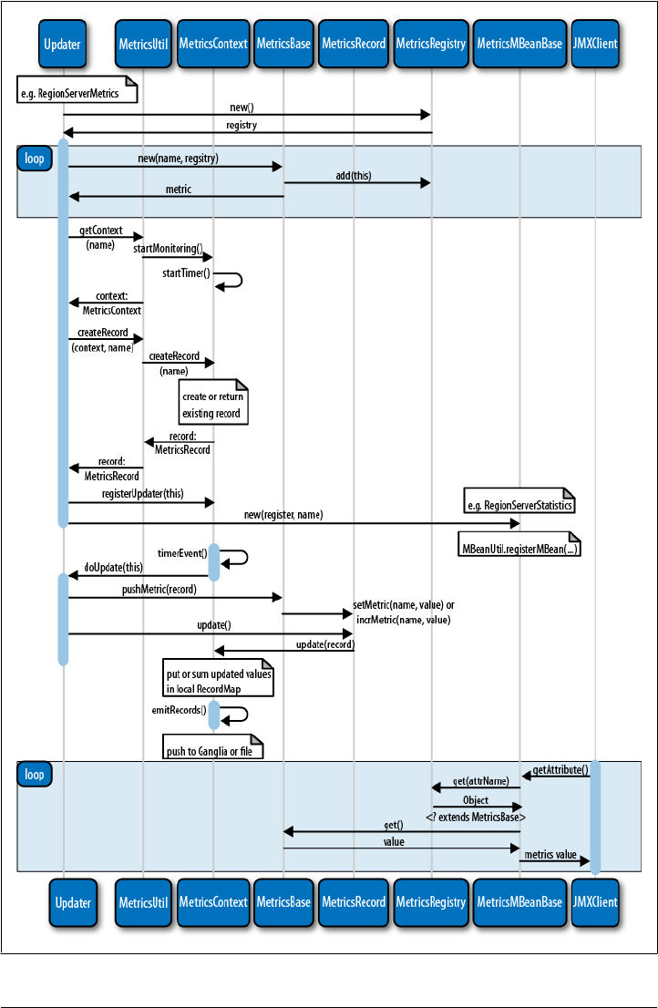
Figure 10-1. Sequence diagram of the classes involved in preparing the metrics
The Metrics Framework | 391

Time varying rate (TVR)
Tracks the number of operations or events and the time they required to complete.
This is used to compute the average time for an operation to finish. The metric also
tracks the minimum and maximum time per operation observed. Table 10-1 shows
how the values are exported under the same name, but with different postfixes.
The values in the Short column are postfixes that are attached to the actual metric
name. For instance, when you retrieve the metric for the increment() calls, as pro-
vided by HTable, you will see four values, named incrementNumOps, incrementMin
Time, incrementMaxTime, and incrementAvgTime.
This is not evident in all places, though. For example, the context-based metrics
only expose the AvgTime and NumOps values, while JMX gives access to all four.
Note that the values for operation count and time accrued are reset once the metric
is polled. The number of operations is aggregated by the polling context, though,
making it a monotonously increasing counter. In contrast, the average time is set
as an absolute value. It is computed when the metric is retrieved at the end of a
polling interval.
The minimum and maximum observed time per operation is not reset and is kept
until the resetMinMax() call is invoked. This can be done through JMX (see
“JMX” on page 408), or it can be triggered for some metrics by the extended pe-
riod property implicitly.
Persistent time varying rate (PTVR)
An extension to the TVR. This metric adds the necessary support for the extended
period metrics: since these long-running metrics are not reset for every poll they
need to be reported differently.
Table 10-1. Values exposed by metrics based on time varying rate
Value name Short Description
Number Operations NumOps The actual number of events since the last poll.
Mininum Time MinTime The shortest time reported for an event to complete.
Maximum Time MaxTime The longest time reported for an event to complete.
Average Time AvgTime The average time for completing events; this is computed as the sum of the
reported times per event, divided by the number of events.
When we subsequently discuss the different metrics provided by HBase you will find
the type abbreviation next to it for reference, in case you are writing your own support
tool. Keep in mind that these metrics behave differently when they are retrieved through
a metrics context, or via JMX.
392 | Chapter 10: Cluster Monitoring
Some of the metrics—for example, the time varying ones—are reset once they are pol-
led, but the containing context aggregates them as monotonously increasing counters.
Accessing the same values through JMX will reveal their reset behavior, since JMX
accesses the values directly, not through a metric context.
A prominent example is the NumOps component of a TVR metric. Reading it through a
metric context gives you an ever increasing value, while JMX would only give you the
absolute number of the last poll period.
Other metrics are only emitting data when the value has changed since the last update.
Again, this is evident when using the contexts, but not when using JMX. The latter will
simply retrieve the values from the last poll. If you do not set a poll period, the JMX
values will never change. More on this in “JMX” on page 408. Figure 10-2 shows how,
over each metric period, the different metric types are updated and emitted. JMX always
accesses the raw metrics, which results in a different behavior compared to context-
based aggregation.
Figure 10-2. Various metric types collected and (optionally) reset differently
The Metrics Framework | 393

HBase also has some exceptional rate metrics that span across specific time frames,
overriding the usual update intervals.
There are a few long-running processes in HBase that require some
metrics to be kept until the process has completed. This is controlled
by the hbase.extendedperiod property, specified in seconds. The default
is no expiration, but the supplied configuration sets it to a moderate
3600 seconds, or one hour.
Currently, this extended period is applied to the time and size rate
metrics for compactions, flushes, and splits for the region servers and
master, respectively. On the region server it also triggers a reset of all
other-rate based metrics, including the read, write, and sync latencies.
Master Metrics
The master process exposes all metrics relating to its role in a cluster. Since the master
is relatively lightweight and only involved in a few cluster-wide operations, it does
expose only a limited set of information (in comparison to the region server, for ex-
ample). Table 10-2 lists them.
Table 10-2. Metrics exposed by the master
Metric Description
Cluster requests (R) The total number of requests to the cluster, aggregated across all region servers
Split time (PTVR) The time it took to split the write-ahead log files after a restart
Split size (PTVR) The total size of the write-ahead log files that were split
Region Server Metrics
The region servers are part of the actual data read and write path, and therefore collect
a substantial number of metrics. These include details about different parts of the over-
all architecture inside the server—for example, the block cache and in-memory store.
Instead of listing all possible metrics, we will discuss them in groups, since it is more
important to understand their meaning as opposed to the separate data point. Within
each group the meaning is quite obvious and needs only a few more notes, if at all.
Block cache metrics
The block cache holds the loaded storage blocks from the low-level HFiles, read
from HDFS. Given that you have allowed for a block to be cached, it is kept in
memory until there is no more room, at which point it is evicted.
The count (LV) metric reflects the number of blocks currently in the cache, while
the size (LV) is the occupied Java heap space. The free (LV) metric is the remaining
heap for the cache, and evicted (LV) counts the number of blocks that had to be
removed because of heap size constraints.
394 | Chapter 10: Cluster Monitoring
The block cache keeps track of the cache hit (LV) and miss (LV) counts, as well as
the hit ratio (IV), which is the number of cache hits in relation to the total number
of requests to the cache.
Finally, the more ominous hit caching count is similar to the hit ratio, but only takes
into account requests and hits of operations that had requested for the block cache
to be used (see, e.g., the setCacheBlocks() method in “Single Gets” on page 95).
All read operations will try to use the cache, regardless of whether
retaining the block in the cache has been requested. Use of
setCacheBlocks() only influences the retainment policy of the re-
quest.
Compaction metrics
When the region server has to perform the asynchronous (or manually invoked)
housekeeping task of compacting the storage files, it reports its status in a different
metric. The compaction size (PTVR) and compaction time (PTVR) give details re-
garding the total size (in bytes) of the storage files that have been compacted, and
how long that operation took, respectively. Note that this is reported after a com-
pleted compaction run, because only then are both values known.
The compaction queue size (IV) can be used to check how many files a region server
has queued up for compaction currently.
The compaction queue size is another recommended early indica-
tor of trouble that should be closely monitored. Usually the number
is quite low, and varies between zero and somewhere in the low
tens. When you have I/O issues, you usually see this number rise
sharply. See Figure 10-5 on page 407 for an example.
Keep in mind that major compactions will also cause a sharp rise as
they queue up all storage files. You need to account for this when
looking at the graphs.
Memstore metrics
Mutations are kept in the memstore on the region server, and will subsequently be
written to disk via a flush. The memstore metrics expose the memstore size MB
metric (IV), which is the total heap space occupied by all memstores for the server
in megabytes. It is the sum of all memstores across all online regions.
The flush queue size (IV) is the number of enqueued regions that are being flushed
next. The flush size (PTVR) and flush time (PTVR) give details regarding the total size
(in bytes) of the memstore that has been flushed, and the time it took to do so,
respectively.
The Metrics Framework | 395

Just as with the compaction metrics, these last two metrics are updated after the
flush has completed. So the reported values slightly trail the actual value, as it is
missing what is currently in progress.
Similar to the compaction queue you will see a sharp rise in count
for the flush queue when, for example, your servers are under I/O
duress. Monitor the value to find the usual range—which should
be a fairly low number as well—and set sensible limits to trigger
warnings when it rises above these thresholds.
Store metrics
The store files (IV) metric states the total number of storage files, spread across all
stores—and therefore regions—managed by the current server. The stores (IV)
metric gives you the total number of stores for the server, across all regions it cur-
rently serves. The store file index size MB metric (IV) is the sum of the block index,
and optional meta index, for all store files in megabytes.
I/O metrics
The region server keeps track of I/O performance with three latency metrics, all of
them keeping their numbers in milliseconds. The fs read latency (TVR) reports the
filesystem read latency—for example, the time it takes to load a block from the
storage files. The fs write latency (TVR) is the same for write operations, but com-
bined for all writers, including the storage files and write-ahead log.
Finally, the fs sync latency (TVR) measures the latency to sync the write-ahead log
records to the filesystem. The latency metrics provide information about the low-
level I/O performance and should be closely monitored.
Miscellaneous metrics
In addition to the preceding metrics, the region servers also provide global coun-
ters, exposed as metrics. The read request count (LV) and write request count (LV)
report the total number of read (such as get()) and write (such as put()) operations,
respectively, summed up for all online regions this server hosts.
The requests (R) metric is the actual request rate per second encountered since it
was last polled. Finally, the regions (IV) metric gives the number of regions that
are currently online and hosted by this region server.
RPC Metrics
Both the master and region servers also provide metrics from the RPC subsystem. The
subsystem automatically tracks every operation possible between the different servers
and clients. This includes the master RPCs, as well as those exposed by region servers.
396 | Chapter 10: Cluster Monitoring
The RPC metrics for the master and region servers are shared—in other
words, you will see the same metrics exposed on either server type. The
difference is that the servers update the metrics for the operations
the process invokes. On the master, for example, you will not see up-
dates to the metrics for increment() operations, since those are related
to the region server. On the other hand, you do see all the metrics for
all of the administrative calls, like enableTable or compactRegion.
Since the metrics relate directly to the client and administrative APIs, you can infer their
meaning from the corresponding API calls. The naming is not completely consistent,
though, to remove arbitration. A notable pattern is the addition of the Region postfix
to the region-related API calls—for example, the split() call provided by HBaseAdmin
maps to the splitRegion metric. Only a handful of metrics have no API counterpart,
and these are listed in Table 10-3. These are metrics provided by the RPC subsystem
itself.
Table 10-3. Non-API metrics exposed by the RPC subsystem
Metric Description
RPC Processing Time This is the time it took to process the RPCs on the server side. As this spans all possible RPC calls,
it averages across them.
RPC Queue Time Since RPC employs a queuing system that lines up calls to be processed, there might be a delay
between the time the call arrived and when it is actually processed, which is the queue time.
Monitoring the queue time is a good idea, as it indicates the load on the
server. You could use thresholds to trigger warnings if this number goes
over a certain limit. These are early indicators of future problems.
The remaining metrics are from the RPC API between the master and the region servers,
including regionServerStartup() and regionServerReport. They are invoked when a
region server initially reports for duty at its assigned master node, and for regular status
reports, respectively.
JVM Metrics
When it comes to optimizing your HBase setup, tuning the JVM settings requires expert
skills. You will learn how to do this in “Garbage Collection Tuning” on page 419. This
section discusses what you can retrieve from each server process using the metrics
framework. Every HBase process collects and exposes JVM-related details that are
helpful to correlate, for example, server performance with underlying JVM internals.
This information, in turn, is used when tuning your HBase cluster setup.
The Metrics Framework | 397

The provided metrics can be grouped into related categories:
Memory usage metrics
You can retrieve the used memory and the committed memory† in megabytes for
both heap and nonheap usage. The former is the space that is maintained by the
JVM on your behalf and garbage-collected at regular intervals. The latter is memory
required for JVM internal purposes.
Garbage collection metrics
The JVM is maintaining the heap on your behalf by running garbage collections.
The gc count metric is the number of garbage collections, and the gc time millis is
the accumulated time spent in garbage collection since the last poll.
Certain steps in the garbage collection process cause so-called
stop-the-world pauses, which are inherently difficult to handle
when a system is bound by tight SLAs.
Usually these pauses are only a few milliseconds in length, but
sometimes they can increase to multiple seconds. Problems arise
when these pauses approach the multiminute range, because this
can cause a region server to miss its ZooKeeper lease renewal—
forcing the master to take evasive actions.‡
Use the garbage collection metric to track what the server is cur-
rently doing and how long the collections take. As soon as you see
a sharp increase, be prepared to investigate. Any pause that is
greater than the zookeeper.session.timeout configuration value
should be considered a fault.
Thread metrics
This group of metrics reports a variety of numbers related to Java threads. You can
see the count for each possible thread state, including new, runnable, blocked, and
so on.
System event metrics
Finally, the events group contains metrics that are collected from the logging sub-
system, but are subsumed under the JVM metrics category (for lack of a better
place). System event metrics provide counts for various log-level events. For ex-
ample, the log error metric provides the number of log events that occured on the
† See the official documentation on MemoryUsage for details on what used versus committed memory means.
‡ “The HBase development team has affectionately dubbed this scenario a Juliet Pause—the
master (Romeo) presumes the region server (Juliet) is dead when it’s really just sleeping, and
thus takes some drastic action (recovery). When the server wakes up, it sees that a great mistake
has been made and takes its own life. Makes for a good play, but a pretty awful failure scenario!”
(http://www.cloudera.com/blog/2011/02/avoiding-full-gcs-in-hbase-with-memstore-local
-allocation-buffers-part-1/)
398 | Chapter 10: Cluster Monitoring

error level, since the last time the metric was polled. In fact, all log event counters
show you the counts accumulated during the last poll period.
Using these metrics, you are able to feed support systems that either graph the values
over time, or trigger warnings based on definable thresholds. It is really important to
understand the values and their usual ranges so that you can make use of them in
production.
Info Metrics
The HBase processes also expose a group of metrics called info metrics. They contain
rather fixed information about the processes, and are provided so that you can check
these values in an automated fashion. Table 10-4 lists these metrics and provides a
description of each. Note that these metrics are only accessible through JMX.
Table 10-4. Metrics exposed by the info group
Metric Description
date The date HBase was built
version The HBase version
revision The repository revision used for the build
url The repository URL
user The user that built HBase
hdfsDate The date HDFS was built
hdfsVersion The HDFS version currently in use
hdfsRevision The repository revision used to build HDFS
hdfsUrl The HDFS repository URL
hdfsUser The user that built HDFS
HDFS refers to the hadoop-core-<X.Y-nnnn>.jar file that is currently in use by HBase.
This usually is the supplied JAR file, but it could be a custom file, depending on your
installation. The values returned could look like this:
date:Wed May 18 15:29:52 CEST 2011
version:0.91.0-SNAPSHOT
revision:1100427
url:https://svn.apache.org/repos/asf/hbase/trunk
user:larsgeorge
hdfsDate:Wed Feb 9 22:25:52 PST 2011
hdfsVersion:0.20-append-r1057313
hdfsRevision:1057313
hdfsUrl:http://svn.apache.org/repos/asf/hadoop/common/branches/branch-0.20-append
hdfsUser:Stack
The Metrics Framework | 399

The values are obviously not useful for graphing, but they can be used by an adminis-
trator to verify the running configuration.
Ganglia
HBase inherits its native support for Ganglia§ directly from Hadoop, providing a con-
text that can push the metrics directly to it.
As of this writing, HBase only supports the 3.0.x line of Ganglia ver-
sions. This is due to the changes in the network protocol used by the
newer 3.1.x releases. The GangliaContext class is therefore not compat-
ible with the 3.1.x Ganglia releases. This was addressed in
HADOOP-4675 and committed in Hadoop 0.22.0. In other words, fu-
ture versions of HBase will support the newly introduced GangliaCon
text31 and work with the newer Ganglia releases.
Advanced users also have the option to apply the patch themselves and
replace the stock Hadoop JAR with their own. Some distributions for
Hadoop—for example, CDH3 from Cloudera—have this patch already
applied.
Ganglia consists of three components:
Ganglia monitoring daemon (gmond)
The monitoring daemon needs to run on every machine that is monitored. It collects
the local data and prepares the statistics to be polled by other systems. It actively
monitors the host for changes, which it will announce using uni- or multicast net-
work messages. If configured in multicast mode, each monitoring daemon has the
complete cluster state—of all servers with the same multicast address—present.
Ganglia meta daemon (gmetad)
The meta daemon is installed on a central node and acts as the federation node to
the entire cluster. The meta daemon polls from one or more monitoring daemons
to receive the current cluster status, and saves it in a round-robin, time-series
database, using RRDtool.‖ The data is made available in XML format to other
clients—for example, the web frontend.
Ganglia also supports a hierarchy of reporting daemons, where at each node of the
hierarchy tree a meta daemon is aggregating the results of its assigned monitoring
daemons. The meta daemons on a higher level then aggregate the statistics for
multiple clusters polling the status from their assigned, lower-level meta daemons.
§ Ganglia is a distributed, scalable monitoring system suitable for large cluster systems. See its project
website for more details on its history and goals.
‖See the RRDtool project website for details.
400 | Chapter 10: Cluster Monitoring

Ganglia PHP web frontend
The web frontend, supplied by Ganglia, retrieves the combined statistics from the
meta daemon and presents it as HTML. It uses RRDtool to render the stored time-
series data in graphs.
Installation
Ganglia setup requires two steps: first you need to set up and configure Ganglia itself,
and then have HBase send the metrics to it.
Ganglia-related steps
You should try to install prebuilt binary packages for the operating system distribution
of your choice. If this is not possible, you can download the source from the project
website and build it locally. For example, on a Debian-based system you could perform
the following steps.
Perform the following on all nodes you want to monitor.
Add a dedicated user account:
$ sudo adduser --disabled-login --no-create-home ganglia
Download the source tarball from the website, and unpack it into a common location:
$ wget http://downloads.sourceforge.net/project/ganglia/ \
ganglia%20monitoring%20core/3.0.7%20%28Fossett%29/ganglia-3.0.7.tar.gz
$ tar -xzvf ganglia-3.0.7.tar.gz -C /opt
$ rm ganglia-3.0.7.tar.gz
Install the dependencies:
$ sudo apt-get -y install build-essential libapr1-dev \
libconfuse-dev libexpat1-dev python-dev
Now you can build and install the binaries like so:
$ cd /opt/ganglia-3.0.7
$ ./configure
$ make
$ sudo make install
The next step is to set up the configuration. This can be fast-tracked by generating a
default file:
$ gmond --default_config > /etc/gmond.conf
Change the following in the /etc/gmond.conf file:
globals {
user = ganglia
}
cluster {
name = HBase
Ganglia monitoring daemon.
Ganglia | 401

owner = "Foo Company"
url = "http://foo.com/"
}
The global section defines the user account created earlier. The cluster section defines
details about your cluster. By default, Ganglia is configured to use multicast UDP
messages with the IP address 239.2.11.71 to communicate—which is a good for clusters
less than ~120 nodes.
Multicast Versus Unicast
While the default communication method between monitoring daemons (gmond) is
UDP multicast messages, you may encounter environments where multicast is either
not possible or a limiting factor. The former is true, for example, when using Amazon’s
cloud-based server offerings, called EC2.
Another known issue is that multicast only works reliably in clusters of up to ~120
nodes. If either is true for you, you can switch from multicast to unicast messages
instead. In the /etc/gmond.conf file, change these options:
udp_send_channel {
# mcast_join = 239.2.11.71
host = host0.foo.com
port = 8649
# ttl = 1
}
udp_recv_channel {
# mcast_join = 239.2.11.71
port = 8649
# bind = 239.2.11.71
}
This example assumes you dedicate the gmond on the master node to receive the updates
from all other gmond processes running on the rest of the machines.
The host0.foo.com would need to be replaced by the hostname or IP address of the
master node. In larger clusters, you can have multiple dedicated gmond processes on
separate physical machines. That way you can avoid having only a single gmond handling
the updates.
You also need to adjust the /etc/gmetad.conf file to point to the dedicated node. See the
note in this chapter that discusses the use of unicast mode for details.
Start the monitoring daemon with:
$ sudo gmond
402 | Chapter 10: Cluster Monitoring
Test the daemon by connecting to it locally:
$ nc localhost 8649
This should print out the raw XML based cluster status. Stopping the
daemon is accomplished by using the kill command.
Perform the following on all nodes you want to use as meta daemon
servers, aggregating the downstream monitoring statistics. Usually this is only one ma-
chine for clusters less than 100 nodes. Note that the server has to create the graphs,
and therefore needs some decent processing capabilities.
Add a dedicated user account:
$ sudo adduser --disabled-login --no-create-home ganglia
Download the source tarball from the website, and unpack it into a common location:
$ wget http://downloads.sourceforge.net/project/ganglia/ \
ganglia%20monitoring%20core/3.0.7%20%28Fossett%29/ganglia-3.0.7.tar.gz
$ tar -xzvf ganglia-3.0.7.tar.gz -C /opt
$ rm ganglia-3.0.7.tar.gz
Install the dependencies:
$ sudo apt-get -y install build-essential libapr1-dev libconfuse-dev \
libexpat1-dev python-dev librrd2-dev
Now you can build and install the binaries like so:
$ cd /opt/ganglia-3.0.7
$ ./configure --with-gmetad
$ make
$ sudo make install
Note the extra --with-gmetad, which is required to build the binary we will need. The
next step is to set up the configuration, copying the supplied default gmetad.conf file
like so:
$ cp /opt/ganglia-3.0.7/gmetad/gmetad.conf /etc/gmetad.conf
Change the following in /etc/gmetad.conf:
setuid_username "ganglia"
data_source "HBase" host0.foo.com
gridname "<Your-Grid-Name>"
The data_source line must contain the hostname or IP address of one or more gmonds.
When you are using unicast mode you need to point your data_source
to the server that acts as the dedicated gmond server. If you have more
than one, you can list them all, which adds failover safety.
Ganglia meta daemon.
Ganglia | 403

Now create the required directories. These are used to store the collected data in round-
robin databases.
$ mkdir -p /var/lib/ganglia/rrds/
$ chown -R ganglia:ganglia /var/lib/ganglia/
Now start the daemon:
$ gmetad
Stopping the daemon requires the use of the kill command.
The last part of the setup concerns the web-based frontend. A com-
mon scenario is to install it on the same machine that runs the gmetad process. At a
minimum, it needs to have access to the round-robin, time-series database created by
gmetad.
First install the required libraries:
$ sudo apt-get -y install rrdtool apache2 php5-mysql libapache2-mod-php5 php5-gd
Ganglia comes fully equipped with all the required PHP files. You can copy them in
place like so:
$ cp -r /opt/ganglia-3.0.7/web /var/www/ganglia
Now restart Apache:
$ sudo /etc/init.d/apache2 restart
You should now be able to browse the web frontend using http://ganglia.foo.com/
ganglia—assuming you have pointed the ganglia subdomain name to the host running
gmetad first. You will only see the basic graph of the servers, since you still need to set
up HBase to push its metrics to Ganglia, which is discussed next.
HBase-related steps
The central part of HBase and Ganglia integration is provided by the GangliaContext
class, which sends the metrics collected in each server process to the Ganglia monitoring
daemons. In addition, there is the hadoop-metrics.properties configuration file, located
in the conf/ directory, which needs to be amended to enable the context. Edit the file
like so:
# HBase-specific configuration to reset long-running stats
# (e.g. compactions). If this variable is left out, then the default
# is no expiration.
hbase.extendedperiod = 3600
# Configuration of the "hbase" context for ganglia
# Pick one: Ganglia 3.0 (former) or Ganglia 3.1 (latter)
hbase.class=org.apache.hadoop.metrics.ganglia.GangliaContext
#hbase.class=org.apache.hadoop.metrics.ganglia.GangliaContext31
hbase.period=10
hbase.servers=239.2.11.71:8649
Ganglia web frontend.
404 | Chapter 10: Cluster Monitoring

jvm.class=org.apache.hadoop.metrics.ganglia.GangliaContext
#jvm.class=org.apache.hadoop.metrics.ganglia.GangliaContext31
jvm.period=10
jvm.servers=239.2.11.71:8649
rpc.class=org.apache.hadoop.metrics.ganglia.GangliaContext
#rpc.class=org.apache.hadoop.metrics.ganglia.GangliaContext31
rpc.period=10
rpc.servers=239.2.11.71:8649
I mentioned that HBase currently (as of version 0.91.x) only supports
Ganglia 3.0.x, so why is there a choice between GangliaContext and
GangliaContext31? Some repackaged versions of HBase already include
patches to support Ganglia 3.1.x. Use this context only if you are certain
that your version of HBase supports it (CDH3 does, for example).
When you are using Unicast messages, the 239.2.11.71 default multicast address needs
to be changed to the dedicated gmond hostname or IP address. For example:
...
hbase.class=org.apache.hadoop.metrics.ganglia.GangliaContext
hbase.period=10
hbase.servers=host0.yourcompany.com:8649
jvm.class=org.apache.hadoop.metrics.ganglia.GangliaContext
jvm.period=10
jvm.servers=host0.yourcompany.com:8649
rpc.class=org.apache.hadoop.metrics.ganglia.GangliaContext
rpc.period=10
rpc.servers=host0.yourcompany.com:8649
Once you have edited the configuration file you need to restart the HBase cluster pro-
cesses. No further changes are required. Ganglia will automatically pick up all the
metrics.
Usage
Once you refresh the web-based UI frontend you should see the Ganglia home page,
shown in Figure 10-3.
You can change the metric, time span, and sorting on that page; it will reload auto-
matically. On an underpowered machine, you might have to wait a little bit for all the
graphs to be rendered. Figure 10-4 shows the drop-down selection for the available
metrics.
Finally, Figure 10-5 shows an example of how the metrics can be correlated to find root
causes of problems. The graphs show how, at around midnight, the garbage collection
time sharply rose for a heavily loaded server. This caused the compaction queue to
increase significantly as well.
Ganglia | 405
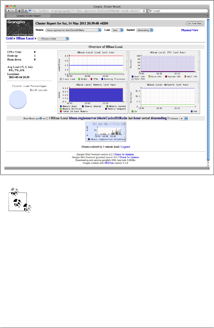
It seems obvious that write-heavy loads cause a lot of I/O churn, but
keep in mind that you can see the same behavior (though not as often)
for more read-heavy access patterns. For example, major compactions
that run in the background could have accrued many storage files that
all have to be rewritten. This can have an adverse effect on read latencies
without an explicit write load from the clients.
Ganglia and its graphs are a great tool to go back in time and find what caused a
problem. However, they are only helpful when dealing with quantitative data—for
example, for performing postmortem analysis of a cluster problem. In the next section,
you will see how to complement the graphing with a qualitative support system.
Figure 10-3. The Ganglia web-based frontend that gives access to all graphs
406 | Chapter 10: Cluster Monitoring
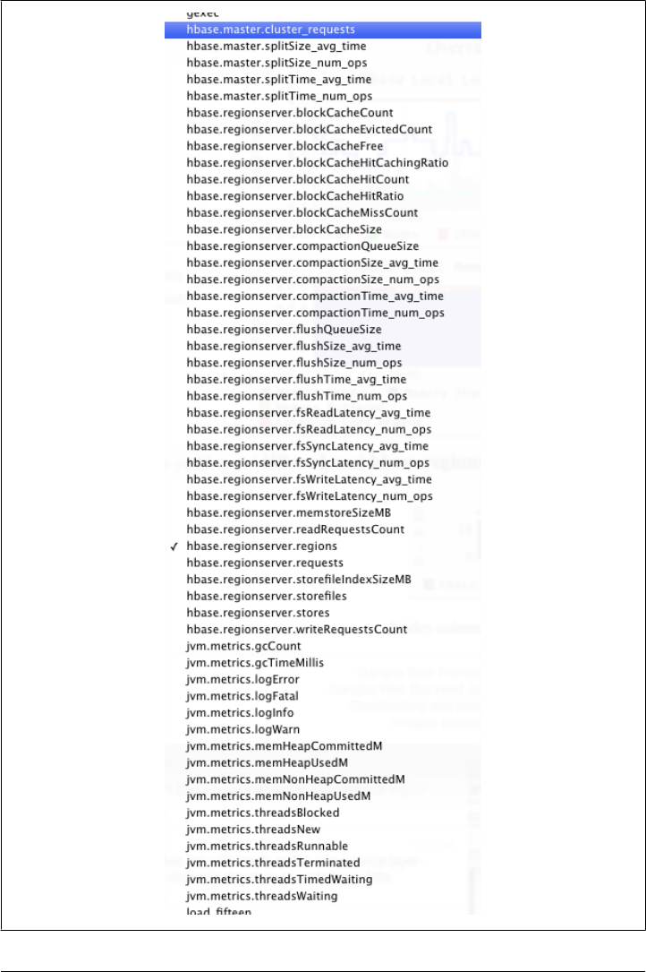
Figure 10-4. The drop-down box that provides access to the list of metrics
Ganglia | 407
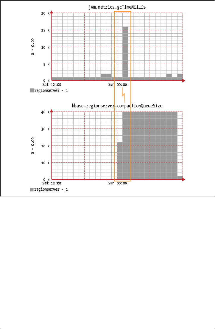
Figure 10-5. Graphs that can help align problems with related events
JMX
The Java Management Extensions technology is the standard for Java applications to
export their status. In addition to what we have discussed so far regarding Ganglia and
the metrics context, JMX also has the ability to provide operations. These allow you to
remotely trigger functionality on any JMX-enabled Java process.
Before you can access HBase processes using JMX, you need to enable it. This is
accomplished in the $HABASE_HOME/conf/hbase-env.sh configuration file by un-
commenting—and amending—the following lines:
408 | Chapter 10: Cluster Monitoring

# Uncomment and adjust to enable JMX exporting
# See jmxremote.password and jmxremote.access in $JRE_HOME/lib/management to
# configure remote password access. More details at:
# http://java.sun.com/javase/6/docs/technotes/guides/management/agent.html
#
export HBASE_JMX_BASE="-Dcom.sun.management.jmxremote.ssl=false \
-Dcom.sun.management.jmxremote.authenticate=false"
export HBASE_MASTER_OPTS="$HBASE_JMX_BASE \
-Dcom.sun.management.jmxremote.port=10101"
export HBASE_REGIONSERVER_OPTS="$HBASE_JMX_BASE \
-Dcom.sun.management.jmxremote.port=10102"
export HBASE_THRIFT_OPTS="$HBASE_JMX_BASE \
-Dcom.sun.management.jmxremote.port=10103"
export HBASE_ZOOKEEPER_OPTS="$HBASE_JMX_BASE \
-Dcom.sun.management.jmxremote.port=10104"
This enables JMX with remote access support, but with no security credentials. It is
assumed that, in most cases, the HBase cluster servers are not accessible outside a
firewall anyway, and therefore no authentication is needed. You can enable authenti-
cation if you want to, which makes the setup only slightly more complex.# You also
need to restart HBase for these changes to become active.
When a server starts, it not only registers its metrics with the appropriate context, it
also exports them as so-called JMX attributes. I mentioned already that when you want
to use JMX to access the metrics, you need to at least enable the NullContext
WithUpdateThread with an appropriate value for period—for example, a minimal ha-
doop-metrics.properties file could contain:
hbase.class=org.apache.hadoop.metrics.spi.NullContextWithUpdateThread
hbase.period=60
jvm.class=org.apache.hadoop.metrics.spi.NullContextWithUpdateThread
jvm.period=60
rpc.class=org.apache.hadoop.metrics.spi.NullContextWithUpdateThread
rpc.period=60
This would ensure that all metrics are updated every 10 seconds, and therefore would
be retrievable as JMX attributes. Failing to do so would yield all JMX attributes useless.
You could still use the JMX operations, though. Obviously, if you already have another
context enabled—for example, the GangliaContext—this is adequate.
JMX uses the notion of managed beans, or MBeans, which expose a specific set of
attributes and operations. There is a loose overlap between the metric context, as pro-
vided by the metrics framework, and the MBeans exposed over JMX. These MBeans
are addressed in the form:
hadoop:service=<service-name>,name=<mbean-name>
The following MBeans are provided by the various HBase processes:
#The HBase page metrics has information on how to add the password and access credentials files.
JMX | 409

hadoop:service=Master,name=MasterStatistics
Provides access to the master metrics, as described in “Master Met-
rics” on page 394.
hadoop:service=RegionServer,name=RegionServerStatistics
Provides access to the region metrics, as described in “Region Server Metrics”.
hadoop:service=HBase,name=RPCStatistics- <port>
Provides access to the RPC metrics, as described in “RPC Metrics” on page 396.
Note that the port in the name is dynamic and may change when you reconfigure
where the master, or region server, binds to.
hadoop:service=HBase,name=Info
Provides access to the info metrics, as described in “Info Metrics” on page 399.
The MasterStatistics, RegionServerStatistics, and RPCStatistics MBeans also pro-
vide one operation: resetAllMinMax. Use this operation to reset the minimal and max-
imal observed completion times to time varying rate (TVR) metrics.
You have a few options to access the JMX attributes and operations, two of which are
described next.
JConsole
Java ships with a helper application called JConsole, which can be used to connect to
local and remote Java processes. Given that you have the $JAVA_HOME directory in your
search path, you can start it like so:
$ jconsole
Once the application opens, it shows you a dialog that lets you choose whether to
connect to a local or a remote process. Figure 10-6 shows the dialog.
Since you have configured all HBase processes to listen to specific ports, it is advisable
to use those and treat them as remote processes—one advantage is that you can re-
connect to a server, even when the process ID has changed. With the local connection
method this is not possible, as it is ultimately bound to said ID.
410 | Chapter 10: Cluster Monitoring
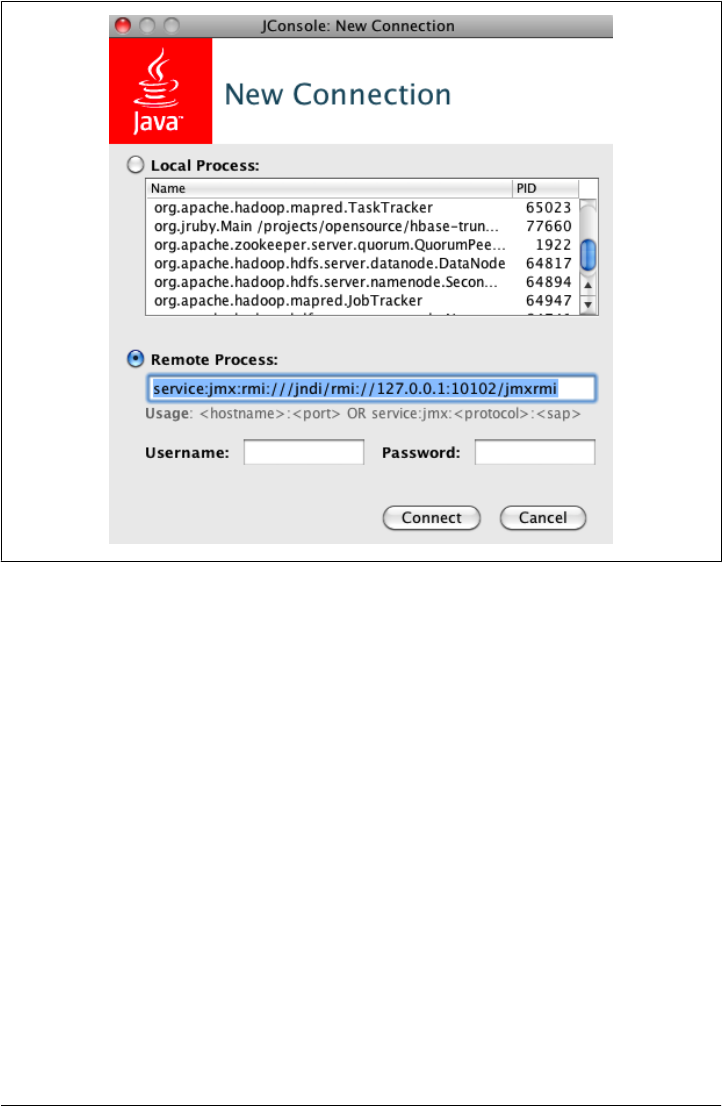
Connecting to a remote HBase process is accomplished by using JMX Service URLs,
which follow this format:
service:jmx:rmi:///jndi/rmi://<server-address>:<port>/jmxrmi
This uses the Java Naming and Directory Interface (JNDI) registry to look up the re-
quired details. Adjust the <port> to the process you want to connect to. In some cases,
you may have multiple Java processes running on the same physical machine—for
example, the Hadoop name node and the HBase Master—so that each of them requires
a unique port assignment. See the hbase-env.sh file contents shown earlier, which sets
a port for every process. The master, for example, listens on port 10101, the region server
on port 10102, and so on. Since you can only run one region server per physical machine,
it is valid to use the same port for all of them, as in this case, the <server-address>—
which is the hostname or IP address—changes to form a unique address:port pair.
Once you connect to the process, you will see a tabbed window with various details
in it. Figure 10-7 shows the initial screen after you have connected to a process.
The constantly updated graphs are especially useful for seeing what a server is currently
up to.
Figure 10-6. Connecting to local or remote processes when JConsole starts
JMX | 411
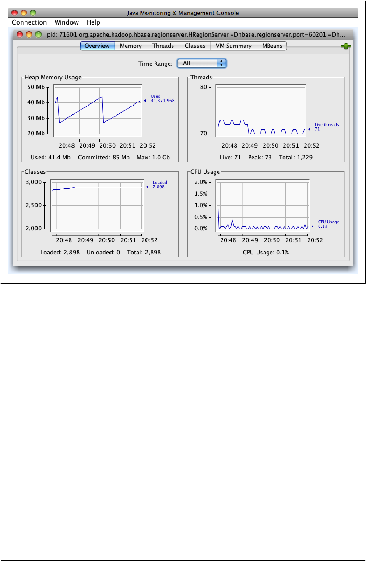
Figure 10-7. The JConsole application, which provides insight into a running Java process
Figure 10-8 is a screenshot of the MBeans tab that allows you to access the attributes
and operations exposed by the registered managed beans. Here you see the compaction
QueueSize metric.
See the official documentation for all the possible options, and an explanation of each
tab with its content.
412 | Chapter 10: Cluster Monitoring
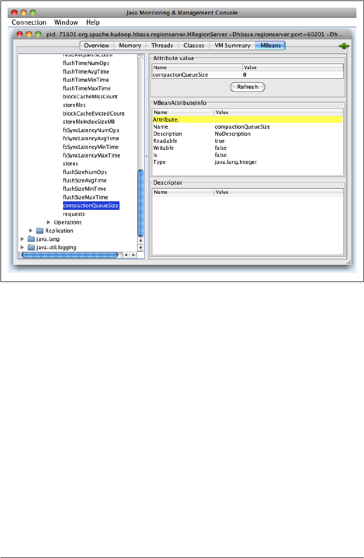
Figure 10-8. The MBeans tab, from which you can access any HBase process metric.
JMX Remote API
Another way to get the same information is the JMX Remote API, using remote method
invocation or RMI.* Many tools are available that implement a client to access the re-
mote managed Java processes. Even the Hadoop project is working on adding some
basic support for it.†
As an example, we are going to use the JMXToolkit, also available in source code online
(https://github.com/larsgeorge/jmxtoolkit). You will need the git command-line tools,
and Apache Ant. Clone the repository and build the tool:
$ git clone git://github.com/larsgeorge/jmxtoolkit.git
Initialized empty Git repository in jmxtoolkit/.git/
...
$ cd jmxtoolkit
$ ant
Buildfile: jmxtoolkit/build.xml
* See the official documentation for details.
† See HADOOP-4756 for details.
JMX | 413

...
jar:
[jar] Building jar: /private/tmp/jmxtoolkit/build/hbase-jmxtoolkit.jar
BUILD SUCCESSFUL
Total time: 2 seconds
After the building process is complete (and successful), you can see the provided op-
tions by invoking the -h switch like so:
$ java -cp build/hbase-jmxtoolkit.jar \
org.apache.hadoop.hbase.jmxtoolkit.JMXToolkit -h
Usage: JMXToolkit [-a <action>] [-c <user>] [-p <password>]
[-u url] [-f <config>] [-o <object>] [-e regexp]
[-i <extends>] [-q <attr-oper>] [-w <check>]
[-m <message>] [-x] [-l] [-v] [-h]
-a <action> Action to perform, can be one of the following
(default: query)
create Scan a JMX object for available attributes
query Query a set of attributes from the given objects
check Checks a given value to be in a valid range (see -w below)
encode Helps creating the encoded messages (see -m and -w below)
walk Walk the entire remote object list
...
-h Prints this help
You can use the JMXToolkit to walk, or print, the entire collection of available attrib-
utes and operations. You do have to know the exact names of the MBean and the
attribute or operation you want to get. Since this is not an easy task, because you do
not have this list yet, it makes sense to set up a basic configuration file that will help in
subsequently retrieving the full list. Create a properties file with the following content:
$ vim hbase.properties
$ cat hbase.properties
; HBase Master
[hbaseMasterStatistics]
@object=hadoop:name=MasterStatistics,service=Master
@url=service:jmx:rmi:///jndi/rmi://${HOSTNAME1|localhost}:10101/jmxrmi
@user=${USER|controlRole}
@password=${PASSWORD|password}
[hbaseRPCMaster]
@object=hadoop:name=RPCStatistics-60000,service=HBase
@url=service:jmx:rmi:///jndi/rmi://${HOSTNAME1|localhost}:10101/jmxrmi
@user=${USER|controlRole}
@password=${PASSWORD|password}
; HBase RegionServer
[hbaseRegionServerStatistics]
@object=hadoop:name=RegionServerStatistics,service=RegionServer
@url=service:jmx:rmi:///jndi/rmi://${HOSTNAME2|localhost}:10102/jmxrmi
@user=${USER|controlRole}
@password=${PASSWORD|password}
414 | Chapter 10: Cluster Monitoring

[hbaseRPCRegionServer]
@object=hadoop:name=RPCStatistics-60020,service=HBase
@url=service:jmx:rmi:///jndi/rmi://${HOSTNAME2|localhost}:10102/jmxrmi
@user=${USER|controlRole}
@password=${PASSWORD|password}
; HBase Info
[hbaseInfo]
@object=hadoop:name=Info,service=HBase
@url=service:jmx:rmi:///jndi/rmi://${HOSTNAME1|localhost}:10101/jmxrmi
@user=${USER|controlRole}
@password=${PASSWORD|password}
; EOF
This configuration can be fed into the tool to retrieve all the attributes and operations
of the listed MBeans. The result is saved in myjmx.properties:
$ java -cp build/hbase-jmxtoolkit.jar \
org.apache.hadoop.hbase.jmxtoolkit.JMXToolkit \
-f hbase.properties -a create -x > myjmx.properties
$ cat myjmx.properties
[hbaseMasterStatistics]
@object=hadoop:name=MasterStatistics,service=Master
@url=service:jmx:rmi:///jndi/rmi://${HOSTNAME1|localhost}:10101/jmxrmi
@user=${USER|controlRole}
@password=${PASSWORD|password}
splitTimeNumOps=INTEGER
splitTimeAvgTime=LONG
splitTimeMinTime=LONG
splitTimeMaxTime=LONG
splitSizeNumOps=INTEGER
splitSizeAvgTime=LONG
splitSizeMinTime=LONG
splitSizeMaxTime=LONG
cluster_requests=FLOAT
*resetAllMinMax=VOID
...
These commands assume you are running them against a pseuodistrib-
uted, local HBase instance. When you need to run them against a remote
set of servers, simply set the variables included in the template properties
file. For example, adding the following lines to the earlier command will
specify the hostnames (or IP addresses) for the master and a slave node:
-DHOSTNAME1=master.foo.com -DHOSTNAME2=slave1.foo.com
When you look into the newly created myjmx.properties file you will see all the metrics
you have seen already. The operations are prefixed with a * (i.e., the star charater).
JMX | 415

You can now start requesting metric values on the command line using the toolkit and
the populated properties file. The first query is for an attribute value, while the second
is triggering an operation (which in this case does not return a value):
$ java -cp build/hbase-jmxtoolkit.jar \
org.apache.hadoop.hbase.jmxtoolkit.JMXToolkit \
-f myjmx.properties -o hbaseRegionServerStatistics -q compactionQueueSize
compactionQueueSize:0
$ java -cp build/hbase-jmxtoolkit.jar \
org.apache.hadoop.hbase.jmxtoolkit.JMXToolkit \
-f myjmx.properties -o hbaseRegionServerStatistics -q *resetAllMinMax
Once you have created the properties files, you can retrieve a single value, all values of
an entire MBean, trigger operations, and so on. The toolkit is great for quickly scanning
a managed process and documenting all the available information, thereby taking the
guesswork out of querying JMX MBeans.
JMXToolkit and Cacti
Once the JMXToolkit JAR is built, it can be used on a Cacti server. The first step is to
copy the JAR into the Cacti scripts directory (which can vary between installs, so make
sure you know what you are doing). Next, extract the scripts:
$ cd $CACTI_HOME/scripts
$ unzip hbase-jmxtoolkit.jar bin/*
$ chmod +x bin/*
Once the scripts are in place, you can test the basic functionality:
$ bin/jmxtkcacti-hbase.sh host0.foo.com hbaseMasterStatistics
splitTimeNumOps:0 splitTimeAvgTime:0 splitTimeMinTime:-1 splitTimeMaxTime:0 \
splitSizeNumOps:0 splitSizeAvgTime:0 splitSizeMinTime:-1 splitSizeMaxTime:0 \
cluster_requests:0.0
The JAR also includes a set of Cacti templates‡ that you can import into it, and use as
a starting point to graph various values exposed by Hadoop’s and HBase’s JMX
MBeans. Note that these templates use the preceding script to get the metrics via JMX.
Setting up the graphs in Cacti is much more involved compared to Ganglia, which
dynamically adds the pushed metrics from the monitoring daemons. Cacti comes with
a set of PHP scripts that can be used to script the addition (and updates) of cluster
servers as a bulk operation.
‡ As of this writing, the templates are slightly outdated, but should work for newer versions of HBase.
416 | Chapter 10: Cluster Monitoring

Nagios
Nagios is a very commonly used support tool for gaining qualitative data regarding
cluster status. It polls current metrics on a regular basis and compares them with given
thresholds. Once the thresholds are exceededing it will start evasive actions, ranging
from sending out emails, or SMS messages to telephones, all the way to triggering
scripts, or even physically rebooting the server when necessary.
Typical checks in Nagios are either the supplied ones, those added as plug-ins, or cus-
tom scripts that have to return a specific exit code and print the outcome to the standard
output. Integrating Nagios with HBase is typically done using JMX. There are many
choices for doing so, including the already discussed JMXToolkit.
The advantage of JMXToolkit is that once you have built your properties file with
all the attributes and operations in it, you can add Nagios thresholds to it. (You can
also use a different monitoring tool if you’d like, so long as it uses the same exit code
and/or standard output message approach as Nagios.) These are subsequently execu-
ted, and changing the check to, for example, different values is just a matter of editing
the properties file. For example:
attributeXYZ=INTEGER|0:OK%3A%20%7B0%7D|2:WARN%3A%20%7B0%7D:80:<| \
1:FAILED%3A%20%7B0%7D:95:<
*operationABC=FLOAT|0|2::0.1:>=|1::0.5:>
You can follow the same steps described earlier in the Cacti install. You can then wire
the Nagios checks to the supplied JMXToolkit script. If you have checks defined in the
properties file, you only specify the object and attribute or operation to query. If not,
you can specify the check within Nagios like so:
$ bin/jmxtknagios-hbase.sh host0.foo.com hbaseRegionServerStatistics \
compactionQueueSize "0:OK%3A%20%7B0%7D|2:WARN%3A%20%7B0%7D:10:>=| \
1:FAIL%3A%20%7B0%7D:100:>"
OK: 0
Note that JMXToolkit also comes with an action to encode text into the appropriate
format.
Obviously, using JMXToolkit is only one of many choices. The crucial point, though,
is that monitoring and graphing are essential to not only maintain a cluster, but also
be able to track down issues much more easily. It is highly recommended that you
implement both monitoring and graphing early in your project. It is also vital that you
test your system with a load that reflects your real workload, because then you can
become familiar with the graphs, and how to read them. Set thresholds and find sensible
upper and lower limits—it may save you a lot of grief when going into production
later on.
Nagios | 417

CHAPTER 11
Performance Tuning
Thus far, you have seen how to set up a cluster and make use of it. Using HBase in
production often requires that you turn many knobs to make it hum as expected. This
chapter covers various advanced techniques for tuning a cluster and testing it repeatedly
to verify its performance.
Garbage Collection Tuning
One of the lower-level settings you need to adjust is the garbage collection parameters
for the region server processes. Note that the master is not a problem here as it does
not handle any heavy loads, and data does not pass through it. These parameters only
need to be added to the region servers.
You might wonder why you have to tune the garbage collection parameters to run
HBase efficiently. The problem is that the Java Runtime Environment comes with basic
assumptions regarding what your programs are doing, how they create objects, how
they allocate the heap to handle data, and so on. These assumptions work well in a lot
of cases. In addition, the JRE has heuristic algorithms that adjust these assumptions as
your process is running. Even with those in place, the JRE is limited to the implemen-
tation of such heuristics and can handle some use cases better than others.
The bottom line is that the JRE does not handle region servers very well. This is caused
by certain workloads, especially write-heavy ones, stressing the memory allocation
mechanisms to a degree that it cannot safely rely on the JRE assumptions alone: you
need to use the provided JRE options to tweak the garbage collection strategies to suit
the workload.
For write-heavy use cases, the memstores are creating and discarding objects at various
times, and in varying sizes. As the data is collected in the in-memory buffers, it needs
to remain there until it has outgrown the configured minimum flush size, set with
hbase.hregion.memstore.flush.size or at the table level.
419
Once the data is greater than that number, it is flushed to disk, creating a new store
file. Since the data that is written to disk mostly resides in different locations in the
Java heap—assuming it was written by the client at different times—it leaves holes in
the heap.
Depending on how long the data was in memory, it resided in different locations in the
generational architecture of the Java heap: data that was inserted rapidly and is flushed
equally fast is often still in the so-called young generation (also called new generation)
of the heap. The space can be reclaimed quickly and no harm is done.
However, if the data stays in memory for a longer period of time—for example, within
a column family that is less rapidly inserted into—it is promoted to the old generation
(or tenured generation). The difference between the young and old generations is pri-
marily size: the young generation is between 128 MB and 512 MB, while the old gen-
eration holds the remaining available heap, which is usually many gigabytes of memory.
You can set the following garbage collection-related options by adding
them in the hbase-env.sh configuration file to the HBASE_OPTS or the
HBASE_REGIONSERVER_OPTS variable. The latter only affects the region
server process (as opposed to the master, for example), and is
the recommended way to set these options.
You can specify the young generation size like so:
-XX:MaxNewSize=128m -XX:NewSize=128m
Or you can use the newer and shorter specification which combines the preceding code
into one convenient option:
-Xmn128m
Using 128 MB is a good starting point, and further observation of the
JVM metrics should be conducted to confirm satisfactory use of the new
generation of the heap.
Note that the default value is too low for any serious region server load
and must be increased. If you do not do this, you might notice a steep
increase in CPU load on your servers, as they spend most of their time
collecting objects from the new generation space.
Both generations need to be maintained by the JRE, to reuse the holes created by data
that has been written to disk (and obviously any other object that was created and
discarded subsequently). If the application ever requests a size of heap that does not fit
into one of those holes, the JRE needs to compact the fragmented heap. This includes
implicit requests, such as the promotion of longer-living objects from the young to the
old generation. If this fails, you will see a promotion failure in your garbage collection
logs.
420 | Chapter 11: Performance Tuning

It is highly recommended that you enable the JRE’s log output for gar-
bage collection details. This is done by adding the following JRE
options:
-verbose:gc -XX:+PrintGCDetails -XX:+PrintGCTimeStamps \
-Xloggc:$HBASE_HOME/logs/gc-$(hostname)-hbase.log"
Once the log is enabled, you can monitor it for occurrences of "concur
rent mode failure" or "promotion failed" messages, which oftentimes
precede long pauses.
Note that the logfile is not rolled like the other files are; you need to take
care of this manually (e.g., by using a cron-based daily log roll task).
The process to rewrite the heap generation in question is called a garbage collection,
and there are parameters for the JRE that you can use to specify different garbage col-
lection implementations. The recommended values are:
-XX:+UseParNewGC and -XX:+UseConcMarkSweepGC
The first option is setting the garbage collection strategy for the young generation to
use the Parallel New Collector: it stops the entire Java process to clean up the young
generation heap. Since its size is small in comparison, this process does not take a long
time, usually less than a few hundred milliseconds.
This is acceptable for the smaller young generation, but not for the old generation: in
a worst-case scenario this can result in processes being stopped for seconds, if not
minutes. Once you reach the configured ZooKeeper session timeout, this server is con-
sidered lost by the master and it is abandoned. Once it comes back from the garbage
collection-induced stop, it is notified that it is abandoned and shuts itself down.
This is mitigated by using the Concurrent Mark-Sweep Collector (CMS), enabled with
the latter option shown earlier. It works differently in that it tries to do as much work
concurrently as possible, without stopping the Java process. This takes extra effort and
an increased CPU load, but avoids the required stops to rewrite a fragmented old gen-
eration heap—until you hit the promotion error, which forces the garbage collector to
stop everything and clean up the mess.
The CMS has an additional switch, which controls when it starts doing its concurrent
mark and sweep check. This value can be set with this option:
-XX:CMSInitiatingOccupancyFraction=70
The value is a percentage that specifies when the background process starts, and it
needs to be set to a level that avoids another issue: the concurrent mode failure. This
occurs when the background process to mark and sweep the heap for collection is still
running when the heap runs out of usable space (recall the holes analogy). In this case,
the JRE must stop the Java process and free the space by forcefully removing discarded
objects, or tenuring those that are old enough.
Garbage Collection Tuning | 421

Setting the initiating occupancy fraction to 70% means that it is slightly larger than the
configured 60% of heap usage by the region servers, which is the combination of the
default 20% block cache and 40% memstore limits. It will start the concurrent collec-
tion process early enough before the heap runs out of space, but also not too early for
it to run too often.
Putting the preceding settings together, you can use the following as a starting point
for your configuration:
export HBASE_REGIONSERVER_OPTS="-Xmx8g -Xms8g -Xmn128m -XX:+UseParNewGC \
-XX:+UseConcMarkSweepGC -XX:CMSInitiatingOccupancyFraction=70 -verbose:gc \
-XX:+PrintGCDetails -XX:+PrintGCTimeStamps \
-Xloggc:$HBASE_HOME/logs/gc-$(hostname)-hbase.log"
Note that -XX:+CMSIncrementalMode is not recommended on actual
server hardware.
These settings combine the current best practices at the time of this writing. If you use
a newer version than Java 6, make sure you carefully evaluate the new garbage collection
implementations and choose one that fits your use case.
It is important to size the young generation space so that the tenuring of longer-living
objects is not causing the older generation heap to fragment too quickly. On the other
hand, it should not be too large either, as this might cause too many short pauses.
Although this will not cause your region servers to be abandoned, it does affect the
latency of your servers, as they frequently stop for a few hundred milliseconds.
Also, when tuning the block cache and memstore size, make sure you set the initiating
occupancy fraction value to something slightly larger. In addition, you must not specify
these two values to go over a reasonable value, but definitely make sure they are less
than 100%. You need to account for general Java class management overhead, so the
default total of 60% is reasonable. More on this in “Configuration” on page 436.
Memstore-Local Allocation Buffer
Version 0.90 of HBase introduced an advanced mechanism to mitigate the issue of heap
fragmentation due to too much churn on the memstore instances of a region server:
the memstore-local allocation buffers, or MSLAB for short.
The preceding section explained how tenured KeyValue instances, once they are flushed
to disk, cause holes in the old generation heap. Once there is no longer enough space
for a new allocation caused by the fragmentation, the JRE falls back to the stop-the-
world garbage collector, which rewrites the entire heap space and compacts it to the
remaining active objects.
422 | Chapter 11: Performance Tuning

The key to reducing these compacting collections is to reduce fragmentation, and the
MSLABs were built to help with that. The idea behind them is that only objects of
exactly the same size should be allocated from the heap. Once these objects tenure and
eventually get collected, they leave holes in the heap of a specific size. Subsequent
allocations of new objects of the exact same size will always reuse these holes: there is
no promotion error, and therefore no stop-the-world compacting collection is required.
The MSLABs are buffers of fixed sizes containing KeyValue instances of varying sizes.
Whenever a buffer cannot completely fit a newly added KeyValue, it is considered full
and a new buffer is created, once again of the given fixed size.
The feature is enabled by default in version 0.92, and disabled in version 0.90 of HBase.
You can use the hbase.hregion.memstore.mslab.enabled configuration property to
override it either way. It is recommended that you thoroughly test your setup with this
new feature, as it might delay the inevitable only longer—which is a good thing—and
therefore you still have to deal with long garbage collection pauses. If you are still
experiencing these pauses, you could plan to restart the servers every few days, or
weeks, before the pause happens.
As of this writing, this feature is not yet widely tested in long-running
production environments. Due diligence is advised.
The size of each allocated, fixed-sized buffer is controlled by the hbase.hregion.mem
store.mslab.chunksize property. The default is 2 MB and is a sensible starting point.
Based on your KeyValue instances, you may have to adjust this value: if you store larger
cells, for example, 100 KB in size, you need to increase the MSLAB size to fit more than
just a few cells.
There is also an upper boundary of what is stored in the buffers. It is set by the
hbase.hregion.memstore.mslab.max.allocation property and defaults to 256 KB. Any
cell that is larger will be directly allocated in the Java heap. If you are storing a lot of
KeyValue instances that are larger than this upper limit, you will run into fragmentation-
related pauses earlier.
The MSLABs do not come without a cost: they are more wasteful in regard to heap
usage, as you will most likely not fill every buffer to the last byte. The remaining unused
capacity of the buffer is wasted. Once again, it’s about striking a balance: you need to
decide if you should use MSLABs and benefit from better garbage collection but incur
the extra space that is required, or not use MSLABs and benefit from better memory
efficiency but deal with the problem caused by garbage collection pauses.
Finally, because the buffers require an additional byte array copy operation, they are
also slightly slower, compared to directly using the KeyValue instances. Measure the
impact on your workload and see if it has no adverse effect.
Memstore-Local Allocation Buffer | 423
Compression
HBase comes with support for a number of compression algorithms that can be enabled
at the column family level. It is recommended that you enable compression unless you
have a reason not to do so—for example, when using already compressed content, such
as JPEG images. For every other use case, compression usually will yield overall better
performance, because the overhead of the CPU performing the compression and de-
compression is less than what is required to read more data from disk.
Available Codecs
You can choose from a fixed list of supported compression algorithms. They have dif-
ferent qualities when it comes to compression ratio, as well as CPU and installation
requirements.
Currently there is no support for pluggable compression algorithms.
The provided ones either are part of Java itself or are added on the
operating-system level. They require support libraries which are either
built or shipped with HBase.
Before looking into each available compression algorithm, refer to Table 11-1 to see
the compression algorithm comparison Google published in 2005.* While the numbers
are old, they still can be used to compare the qualities of the algorithms.
Table 11-1. Comparison of compression algorithms
Algorithm % remaining Encoding Decoding
GZIP 13.4% 21 MB/s 118 MB/s
LZO 20.5% 135 MB/s 410 MB/s
Zippy/Snappy 22.2% 172 MB/s 409 MB/s
Note that some of the algorithms have a better compression ratio while others are faster
during encoding, and a lot faster during decoding. Depending on your use case, you
can choose one that suits you best.
* The video of the presentation is available online.
424 | Chapter 11: Performance Tuning

Before Snappy was made available in 2011, the recommended algorithm
was LZO, even if it did not have the best compression ratio. GZIP is very
CPU-intensive and its slight advantage in storage savings is usually not
worth the slower performance and CPU usage it exposes.
Snappy has similar qualities as LZO, it comes with a compatible license,
and first tests have shown that it slightly outperforms LZO when used
with Hadoop and HBase. Thus, as of this writing, you should consider
Snappy over LZO.
Snappy
With Snappy, released by Google under the BSD License, you have access to the same
compression used by Bigtable (where it is called Zippy). It is optimized to provide high
speeds and reasonable compression, as opposed to being compatible with other com-
pression libraries.
The code is written in C++, and HBase—as of version 0.92—ships with the required
JNI† libraries to be able to use it. It requires that you first install the native executable
binaries, by either using a packet manager, such as apt, rpm, or yum, or building them
from the source code and installing them so that the JNI library can find them.
When setting up support for Snappy, you must install the native binary library on all
region servers. Only then are they usable by the libraries.
LZO
Lempel-Ziv-Oberhumer (LZO) is a lossless data compression algorithm that is focused
on decompression speed, and written in ANSI C. Similar to Snappy, it requires a JNI
library for HBase to be able to use it.
Unfortunately, HBase cannot ship with LZO because of licensing issues: HBase uses
the Apache License, while LZO is using the incompatible GNU General Public License
(GPL). This means that the LZO installation needs to be performed separately, after
HBase has been installed.‡
GZIP
The GZIP compression algorithm will generally compress better than Snappy or LZO,
but is slower in comparison. While this seems like a disadvantage, it comes with an
additional savings in storage space.
The performance issue can be mitigated to some degree by using the native GZIP li-
braries that are available on your operating system. The libraries used by HBase (which
† Java uses the Java Native Interface (JNI) to integrate native libraries and applications.
‡ See the wiki page “Using LZO Compression” (http://wiki.apache.org/hadoop/UsingLzoCompression) for
information on how to make LZO work with HBase.
Compression | 425

are provided by Hadoop) automatically check if the native libraries are available§ and
will make use of them. If not, you will see this message in your logfiles: "Got brand-new
compressor". This indicates a failure to load the native version while falling back to the
Java code implementation instead. The compression will still work, but is slightly
slower.
An additional disadvantage is that GZIP needs a considerable amount of CPU resour-
ces. This can put unwanted load on your servers and needs to be carefully monitored.
Verifying Installation
Once you have installed a supported compression algorithm, it is highly recommended
that you check if the installation was successful. There are a few mechanisms in HBase
to do that.
Compression test tool
HBase includes a tool to test if compression is set up properly. To run it, type ./bin/
hbase org.apache.hadoop.hbase.util.CompressionTest. This will return information
on how to run the tool:
$ ./bin/hbase org.apache.hadoop.hbase.util.CompressionTest
Usage: CompressionTest <path> none|gz|lzo|snappy
For example:
hbase class org.apache.hadoop.hbase.util.CompressionTest file:///tmp/testfile gz
You need to specify a file that the tool will create and test in combination with the
selected compression algorithm. For example, using a test file in HDFS and checking
if GZIP is installed, you can run:
$ ./bin/hbase org.apache.hadoop.hbase.util.CompressionTest \
/user/larsgeorge/test.gz gz
11/07/01 20:27:43 WARN util.NativeCodeLoader: Unable to load native-hadoop \
library for your platform... using builtin-java classes where applicable
11/07/01 20:27:43 INFO compress.CodecPool: Got brand-new compressor
11/07/01 20:27:43 INFO compress.CodecPool: Got brand-new compressor
SUCCESS
The tool reports SUCCESS, and therefore confirms that you can use this compression
type for a column family definition. Note how it also prints the "Got brand-new com
pressor" message explained earlier: the server did not find the native GZIP libraries,
but it can fall back to the Java code-based library.
Trying the same tool with a compression type that is not properly installed will raise
an exception:
§ The Hadoop project has a page describing the required steps to build and/or install the native libraries, which
includes the GZIP support.
426 | Chapter 11: Performance Tuning

$ ./bin/hbase org.apache.hadoop.hbase.util.CompressionTest \
file:///tmp/test.lzo lzo
Exception in thread "main" java.lang.RuntimeException: \
java.lang.ClassNotFoundException: com.hadoop.compression.lzo.LzoCodec
at org.apache.hadoop.hbase.io.hfile.Compression$Algorithm$1.getCodec)
at org.apache.hadoop.hbase.io.hfile.Compression$Algorithm.getCompressor
If this happens, you need to go back and check the installation again. You also may
have to restart the servers after you installed the JNI and/or native compression
libraries.
Startup check
Even if the compression test tool reports success and confirms the proper installation
of a compression library, you can still run into problems later on: since JNI requires
that you first install the native libraries, it can happen that while you provision a new
machine you miss this step. Subsequently, the server fails to open regions that contain
column families using the native libraries (see “Basic setup checklist” on page 471).
This can be mitigated by specifying the (by default unset) hbase.regionserver.codecs
property to list all of the required JNI libraries. Should one of them fail to find its native
counterpart, it will prevent the entire region server from starting up. This way you get
a fast failing setup where you notice the missing libraries, instead of running into issues
later.
For example, this will check that the Snappy and LZO compression libraries are prop-
erly installed when the region server starts:
<property>
<name>hbase.regionserver.codecs</name>
<value>snappy,lzo</value>
</property>
If, for any reason, the JNI libraries fail to load the matching native ones, the server will
abort at startup with an IOException stating "Compression codec <codec-name> not sup
ported, aborting RS construction". Repair the setup and try to start the region server
daemon again.
You can conduct this test for every compression algorithm supported by HBase. Do
not forget to copy the changed configuration file to all region servers and to restart
them afterward.
Enabling Compression
Enabling compression requires installation of the JNI and native compression libraries
(unless you only want to use the Java code-based GZIP compression), as described
earlier, and specifying the chosen algorithm in the column family schema.
One way to accomplish this is during table creation. The possible values are listed in
“Column Families” on page 212.
Compression | 427

hbase(main):001:0> create 'testtable', { NAME => 'colfam1', COMPRESSION => 'GZ' }
0 row(s) in 1.1920 seconds
hbase(main):012:0> describe 'testtable'
DESCRIPTION ENABLED
{NAME => 'testtable', FAMILIES => [{NAME => 'colfam1', true
BLOOMFILTER => 'NONE', REPLICATION_SCOPE => '0', VERSIONS
=> '3', COMPRESSION => 'GZ', TTL => '2147483647', BLOCKSIZE
=> '65536', IN_MEMORY => 'false', BLOCKCACHE => 'true'}]}
1 row(s) in 0.0400 seconds
The describe shell command is used to read back the schema of the newly created table.
You can see the compression is set to GZIP (using the shorter GZ value as required).
Another option to enable—or change, or disable—the compression algorithm is to use
the alter command for existing tables:
hbase(main):013:0> create 'testtable2', 'colfam1'
0 row(s) in 1.1920 seconds
hbase(main):014:0> disable 'testtable2'
0 row(s) in 2.0650 seconds
hbase(main):016:0> alter 'testtable2', { NAME => 'colfam1', COMPRESSION => 'GZ' }
0 row(s) in 0.2190 seconds
hbase(main):017:0> enable 'testtable2'
0 row(s) in 2.0410 seconds
Note how the table was first disabled. This is necessary to perform the alteration of the
column family definition. The final enable command brings the table back online.
Changing the compression format to NONE will disable the compression for the given
column family.
Delayed Action
Note that although you enable, disable, or change the compression algorithm, nothing
happens right away. All the store files are still compressed with the previously used
algorithm—or not compressed at all. All newly flushed store files after the change will
use the new compression format.
If you want to force that all existing files are rewritten with the newly selected format,
issue a major_compact '<tablename>' in the shell to start a major compaction process
in the background. It will rewrite all files, and therefore use the new settings. Keep in
mind that this might be very resource-intensive, and therefore should only be forcefully
done when you are sure that you have the required resources available. Also note that
the major compaction will run for a while, depending on the number and size of the
store files. Be patient!
428 | Chapter 11: Performance Tuning

Optimizing Splits and Compactions
The built-in mechanisms of HBase to handle splits and compactions have sensible de-
faults and perform their duty as expected. Sometimes, though, it is useful to change
their behavior to gain additional performance.
Managed Splitting
Usually HBase handles the splitting of regions automatically: once the regions reach
the configured maximum size, they are split into two halves, which then can start taking
on more data and grow from there. This is the default behavior and is sufficient for the
majority of use cases.
There is one known problematic scenario, though, that can cause what is called split/
compaction storms: when you grow your regions roughly at the same rate, eventually
they all need to be split at about the same time, causing a large spike in disk I/O because
of the required compactions to rewrite the split regions.
Rather than relying on HBase to handle the splitting, you can turn it off and manually
invoke the split and major_compact commands. This is accomplished by setting the
hbase.hregion.max.filesize for the entire cluster, or when defining your table schema
at the column family level, to a very high number. Setting it to Long.MAX_VALUE is not
recommended in case the manual splits fail to run. It is better to set this value to a
reasonable upper boundary, such as 100 GB (which would result in a one-hour major
compaction if triggered).
The advantage of running the commands to split and compact your regions manually
is that you can time-control them. Running them staggered across all regions spreads
the I/O load as much as possible, avoiding any split/compaction storm. You will need
to implement a client that uses the administrative API to call the split() and majorCom
pact() methods. Alternatively, you can use the shell to invoke the commands interac-
tively, or script their call using cron, for instance. Also see the RegionSplitter (added
in version 0.90.2), discussed shortly, for another way to split existing regions: it has a
rolling split feature you can use to carefully split the existing regions while waiting long
enough for the involved compactions to complete (see the -r and -o command-line
options).
An additional advantage to managing the splits manually is that you have better control
over which regions are available at any time. This is good in the rare case that you have
to do very low-level debugging, to, for example, see why a certain region had problems.
With automated splits it might happen that by the time you want to check into a specific
region, it has already been replaced with two daughter regions. These regions have new
names and tracing the evolution of the original region over longer periods of time makes
it much more difficult to find the information you require.
Optimizing Splits and Compactions | 429

Region Hotspotting
Using the metrics discussed in “Region Server Metrics” on page 394,‖ you can determine
if you are dealing with a write pattern that is causing a specific region to run hot.
If this is the case, refer to the approaches discussed in Chapter 9, especially those dis-
cussed in “Key Design” on page 357: you may need to salt the keys, or use random keys
to distribute the load across all servers evenly.
The only way to alleviate the situation is to manually split a hot region into one or more
new regions, at exact boundaries. This will divide the region’s load over multiple region
servers. As you split a region you can specify a split key, that is, the row key where you
can split the given region into two. You can specify any row key within that region so
that you are also able to generate halves that are completely different in size.
This might help only when you are not dealing with completely sequential key ranges,
because those are always going to hit one region for a considerable amount of time.
Table Hotspotting
Sometimes an existing table with many regions is not distributed well—in other words,
most of its regions are located on the same region server.# This means that, although
you insert data with random keys, you still load one region server much more often
than the others. You can use the move() function, as explained in “Cluster Opera-
tions” on page 230, from the HBase Shell, or use the HBaseAdmin class to explicitly move
the server’s table regions to other servers. Alternatively, you can use the unassign()
method or shell command to simply remove a region of the affected table from the
current server. The master will immediately deploy it on another available server.
Presplitting Regions
Managing the splits is useful to tightly control when load is going to increase on your
cluster. You still face the problem that when initially loading a table, you need to split
the regions rather often, since you usually start out with a single region per table.
Growing this single region to a very large size is not recommended; therefore, it is better
to start with a larger number of regions right from the start. This is done by presplit-
ting the regions of an existing table, or by creating a table with the required number of
regions.
The createTable() method of the administrative API, as well as the shell’s create com-
mand, both take a list of split keys, which can be used to presplit a table when it is
‖As an alternative, you can also look at the number of requests values reported on the master UI page; see
“Main page” on page 277.
#Work has been done to improve this situation in HBase 0.92.0.
430 | Chapter 11: Performance Tuning

created. HBase also ships with a utility called RegionSplitter, which you can use to
create a presplit table. Starting it without a parameter will show usage information:
$ ./bin/hbase org.apache.hadoop.hbase.util.RegionSplitter
usage: RegionSplitter <TABLE>
-c <region count> Create a new table with a pre-split number of
regions
-D <property=value> Override HBase Configuration Settings
-f <family:family:...> Column Families to create with new table.
Required with -c
-h Print this usage help
-o <count> Max outstanding splits that have unfinished
major compactions
-r Perform a rolling split of an existing region
--risky Skip verification steps to complete
quickly.STRONGLY DISCOURAGED for production
systems.
By default, it used the MD5StringSplit class to partition the row keys into ranges. You
can define your own algorithm by implementing the SplitAlgorithm interface provided,
and handing it into the utility using the -D split.algorithm=<your-algorithm-class>
parameter. An example of using the supplied split algorithm class and creating a presplit
table is:
$ ./bin/hbase org.apache.hadoop.hbase.util.RegionSplitter \
-c 10 testtable -f colfam1
In the web UI of the master, you can click on the link with the newly created table name
to see the generated regions:
testtable,,1309766006467.c0937d09f1da31f2a6c2950537a61093.
testtable,0ccccccc,1309766006467.83a0a6a949a6150c5680f39695450d8a.
testtable,19999998,1309766006467.1eba79c27eb9d5c2f89c3571f0d87a92.
testtable,26666664,1309766006467.7882cd50eb22652849491c08a6180258.
testtable,33333330,1309766006467.cef2853e36bd250c1b9324bac03e4bc9.
testtable,3ffffffc,1309766006467.00365940761359fee14d41db6a73ffc5.
testtable,4cccccc8,1309766006467.f0c5045c304c2ff5338be27e81ae698e.
testtable,59999994,1309766006467.2d854f337aa6c09232409f0ba1d4964b.
testtable,66666660,1309766006467.b1ec9df9fd90d91f54cb18da5edc2581.
testtable,7333332c,1309766006468.42e179b78663b64401079a8601d9bd06.
Or you can use the shell’s create command:
hbase(main):001:0> create 'testtable', 'colfam1', \
{ SPLITS => ['row-100', 'row-200', 'row-300', 'row-400'] }
0 row(s) in 1.1670 seconds
This generates the following regions:
testtable,,1309768272330.37377c4ab0a944a326ba8b6596a29396.
testtable,row-100,1309768272331.e6092cc777f58a08c61bf081aba14916.
testtable,row-200,1309768272331.63c9630a79b37ebce7b58cde0235dfe5.
testtable,row-300,1309768272331.eead6ad2ff3303ffe6a3126e0df3ff7a.
testtable,row-400,1309768272331.2bee7417fa67e4ac8c7210ce7325708e.
Optimizing Splits and Compactions | 431

As for the number of presplit regions to use, you can start low with 10 presplit regions
per server and watch as data grows over time. It is better to err on the side of too few
regions and using a rolling split later, as having too many regions is usually not ideal
in regard to overall cluster performance.
Alternatively, you can determine how many presplit regions to use based on the largest
store file in your region: with a growing data size, this will get larger over time, and
you want the largest region to be just big enough so that is not selected for major
compaction—or you might face the mentioned compaction storms.
If you presplit your regions too thin, you can increase the major compaction interval
by increasing the value for the hbase.hregion.majorcompaction configuration property.
If your data size grows too large, use the RegionSplitter utility to perform a network
I/O safe rolling split of all regions.
Use of manual splits and presplit regions is an advanced concept that requires a lot of
planning and careful monitoring. On the other hand, it can help you to avoid the com-
paction storms that can happen for uniform data growth, or to shed load of hot regions
by splitting them manually.
Load Balancing
The master has a built-in feature, called the balancer. By default, the balancer runs every
five minutes, and it is configured by the hbase.balancer.period property. Once the
balancer is started, it will attempt to equal out the number of assigned regions per region
server so that they are within one region of the average number per server. The call first
determines a new assignment plan, which describes which regions should be moved
where. Then it starts the process of moving the regions by calling the unassign() method
of the administrative API iteratively.
The balancer has an upper limit on how long it is allowed to run, which is configured
using the hbase.balancer.max.balancing property and defaults to half of the balancer
period value, or two and a half minutes.
You can control the balancer by means of the balancer switch: either use the shell’s
balance_switch command to toggle the balancer status between enabled and disabled,
or use the balanceSwitch() API method to do the same. When you disable the balancer,
it no longer runs as expected.
The balancer can be explicitly started using the shell’s balancer command, or using the
balancer() API method. The time-controlled invocation mentioned previously calls
this method implicitly. It will determine if there is any work to be done and return
true if that is the case. The return value of false means that it was not able to run the
balancer, because either it was switched off, there was no work to be done (all is bal-
anced), or something else was prohibiting the process. One example for this is the
432 | Chapter 11: Performance Tuning

region in transition list (see “Main page” on page 277): if there is a region currently in
transition, the balancer will be skipped.
Instead of relying on the balancer to do its work properly, you can use the move com-
mand and API method to assign regions to other servers. This is useful when you want
to control where the regions of a particular table are assigned. See “Region Hotspot-
ting” on page 430 for an example.
Merging Regions
While it is much more common for regions to split automatically over time as you are
adding data to the corresponding table, sometimes you may need to merge regions—
for example, after you have removed a large amount of data and you want to reduce
the number of regions hosted by each server.
HBase ships with a tool that allows you to merge two adjacent regions as long as the
cluster is not online. You can use the command-line tool to get the usage details:
$ ./bin/hbase org.apache.hadoop.hbase.util.Merge
Usage: bin/hbase merge <table-name> <region-1> <region-2>
Here is an example of a table that has more than one region, all of which are subse-
quently merged:
$ ./bin/hbase shell
hbase(main):001:0> create 'testtable', 'colfam1', \
{SPLITS => ['row-10','row-20','row-30','row-40','row-50']}
0 row(s) in 0.2640 seconds
hbase(main):002:0> for i in '0'..'9' do for j in '0'..'9' do \
put 'testtable', "row-#{i}#{j}", "colfam1:#{j}", "#{j}" end end
0 row(s) in 1.0450 seconds
hbase(main):003:0> flush 'testtable'
0 row(s) in 0.2000 seconds
hbase(main):004:0> scan '.META.', { COLUMNS => ['info:regioninfo']}
ROW COLUMN+CELL
testtable,,1309614509037.612d1e0112 column=info:regioninfo, timestamp=130...
406e6c2bb482eeaec57322. STARTKEY => '', ENDKEY => 'row-10'
testtable,row-10,1309614509040.2fba column=info:regioninfo, timestamp=130...
fcc9bc6afac94c465ce5dcabc5d1. STARTKEY => 'row-10', ENDKEY => 'row-20'
testtable,row-20,1309614509041.e7c1 column=info:regioninfo, timestamp=130...
6267eb30e147e5d988c63d40f982. STARTKEY => 'row-20', ENDKEY => 'row-30'
testtable,row-30,1309614509041.a9cd column=info:regioninfo, timestamp=130...
e1cbc7d1a21b1aca2ac7fda30ad8. STARTKEY => 'row-30', ENDKEY => 'row-40'
testtable,row-40,1309614509041.d458 column=info:regioninfo, timestamp=130...
236feae097efcf33477e7acc51d4. STARTKEY => 'row-40', ENDKEY => 'row-50'
testtable,row-50,1309614509041.74a5 column=info:regioninfo, timestamp=130...
7dc7e3e9602d9229b15d4c0357d1. STARTKEY => 'row-50', ENDKEY => ''
6 row(s) in 0.0440 seconds
Merging Regions | 433

hbase(main):005:0> exit
$ ./bin/stop-hbase.sh
$ ./bin/hbase org.apache.hadoop.hbase.util.Merge testtable \
testtable,row-20,1309614509041.e7c16267eb30e147e5d988c63d40f982. \
testtable,row-30,1309614509041.a9cde1cbc7d1a21b1aca2ac7fda30ad8.
The example creates a table with five split points, resulting in six regions. It then inserts
some rows and flushes the data to ensure that there are store files for the subsequent
merge. The scan is used to get the names of the regions, but you can also use the web
UI of the master: click on the table name in the User Tables section to get the same list
of regions.
Note how the shell wraps the values in each column. The region name
is split over two lines, which you need to copy and paste separately. The
web UI is easier to use in that respect, as it has the names in one column
and in a single line.
The content of the column values is abbreviated to the start and end keys. You can see
how the create command using the split keys has created the regions. The example goes
on to exit the shell, and stop the HBase cluster. Note that HDFS still needs to run for
the merge to work, as it needs to read the store files of each region and merge them into
a new, combined one.
Client API: Best Practices
When reading or writing data from a client using the API, there are a handful of opti-
mizations you should consider to gain the best performance. Here is a list of the best
practice options:
Disable auto-flush
When performing a lot of put operations, make sure the auto-flush feature of
HTable is set to false, using the setAutoFlush(false) method. Otherwise, the Put
instances will be sent one at a time to the region server. Puts added via
HTable.add(Put) and HTable.add( <List> Put) wind up in the same write buffer.
If auto-flushing is disabled, these operations are not sent until the write buffer is
filled. To explicitly flush the messages, call flushCommits(). Calling close on the
HTable instance will implicitly invoke flushCommits().
Use scanner-caching
If HBase is used as an input source for a MapReduce job, for example, make sure
the input Scan instance to the MapReduce job has setCaching() set to something
greater than the default of 1. Using the default value means that the map task will
make callbacks to the region server for every record processed. Setting this value
to 500, for example, will transfer 500 rows at a time to the client to be processed.
434 | Chapter 11: Performance Tuning

There is a cost to having the cache value be large because it costs more in memory
for both the client and region servers, so bigger is not always better.
Limit scan scope
Whenever a Scan is used to process large numbers of rows (and especially when
used as a MapReduce source), be aware of which attributes are selected. If Scan.add
Family() is called, all of the columns in the specified column family will be returned
to the client. If only a small number of the available columns are to be processed,
only those should be specified in the input scan because column overselection
incurs a nontrivial performance penalty over large data sets.
Close ResultScanners
This isn’t so much about improving performance, but rather avoiding performance
problems. If you forget to close ResultScanner instances, as returned by
HTable,getScanner(), you can cause problems on the region servers.
Always have ResultScanner processing enclosed in try/catch blocks, for example:
Scan scan = new Scan();
// configure scan instance
ResultScanner scanner = table.getScanner(scan);
try {
for (Result result : scanner) {
// process result...
} finally {
scanner.close(); // always close the scanner!
}
table.close();
Block cache usage
Scan instances can be set to use the block cache in the region server via the
setCacheBlocks() method. For scans used with MapReduce jobs, this should be
false. For frequently accessed rows, it is advisable to use the block cache.
Optimal loading of row keys
When performing a table scan where only the row keys are needed (no families,
qualifiers, values, or timestamps), add a FilterList with a MUST_PASS_ALL operator
to the scanner using setFilter(). The filter list should include both a First
KeyOnlyFilter and a KeyOnlyFilter instance, as explained in “Dedicated Fil-
ters” on page 147. Using this filter combination will cause the region server to only
load the row key of the first KeyValue (i.e., from the first column) found and return
it to the client, resulting in minimized network traffic.
Turn off WAL on Puts
A frequently discussed option for increasing throughput on Puts is to call write
ToWAL(false). Turning this off means that the region server will not write the Put
to the write-ahead log, but rather only into the memstore. However, the conse-
quence is that if there is a region server failure there will be data loss. If you use
writeToWAL(false), do so with extreme caution. You may find that it actually makes
little difference if your load is well distributed across the cluster.
Client API: Best Practices | 435

In general, it is best to use the WAL for Puts, and where loading throughput is a
concern to use the bulk loading techniques instead, as explained in “Bulk Im-
port” on page 459.
Configuration
Many configuration properties are available for you to use to fine-tune your cluster
setup. “Configuration” on page 63 listed the ones you need to change or set to get your
cluster up and running. There are advanced options you can consider adjusting based
on your use case. Here is a list of the more commonly changed ones, and how to adjust
them.
The majority of the settings are properties in the hbase-site.xml config-
uration file. Edit the file, copy it to all servers in the cluster, and restart
the servers to effect the changes.
Decrease ZooKeeper timeout
The default timeout between a region server and the ZooKeeper quorum is three
minutes (specified in milliseconds), and is configured with the
zookeeper.session.timeout property. This means that if a server crashes, it will be
three minutes before the master notices this fact and starts recovery. You can tune
the timeout down to a minute, or even less, so the master notices failures sooner.
Before changing this value, be sure you have your JVM garbage collection config-
uration under control, because otherwise, a long garbage collection that lasts be-
yond the ZooKeeper session timeout will take out your region server. You might
be fine with this: you probably want recovery to start if a region server has been in
a garbage collection-induced pause for a long period of time.
The reason for the default value being rather high is that it avoids problems during
very large imports: such imports put a lot of stress on the servers, thereby increasing
the likelihood that they will run into the garbage collection pause problem. Also
see “Stability issues” on page 472 for information on how to detect such pauses.
Increase handlers
The hbase.regionserver.handler.count configuration property defines the num-
ber of threads that are kept open to answer incoming requests to user tables. The
default of 10 is rather low in order to prevent users from overloading their region
servers when using large write buffers with a high number of concurrent clients.
The rule of thumb is to keep this number low when the payload per request ap-
proaches megabytes (e.g., big puts, scans using a large cache) and high when the
payload is small (e.g., gets, small puts, increments, deletes).
436 | Chapter 11: Performance Tuning

It is safe to set that number to the maximum number of incoming clients if their
payloads are small, the typical example being a cluster that serves a website, since
puts are typically not buffered, and most of the operations are gets.
The reason why it is dangerous to keep this setting high is that the aggregate size
of all the puts that are currently happening in a region server may impose too much
pressure on the server’s memory, or even trigger an OutOfMemoryError exception.
A region server running on low memory will trigger its JVM’s garbage collector to
run more frequently up to a point where pauses become noticeable (the reason
being that all the memory used to keep all the requests’ payloads cannot be col-
lected, no matter how hard the garbage collector tries). After some time, the overall
cluster throughput is affected since every request that hits that region server will
take longer, which exacerbates the problem.
Increase heap settings
HBase ships with a reasonable, conservative configuration that will work on nearly
all machine types that people might want to test with. If you have larger machines—
for example, where you can assign 8 GB or more to HBase—you should adjust the
HBASE_HEAPSIZE setting in your hbase-env.sh file.
Consider using HBASE_REGIONSERVER_OPTS instead of changing the global HBASE_HEAP
SIZE: this way the master will run with the default 1 GB heap, while you can increase
the region server heap as needed independently.
This option is set in hbase-env.sh, as opposed to the hbase-site.xml file used for
most of the other options.
Enable data compression
You should enable compression for the storage files—in particular, Snappy or
LZO. It’s near-frictionless and, in most cases, boosts performance. See “Compres-
sion” on page 424 for information on all the compression algorithms.
Increase region size
Consider going to larger regions to cut down on the total number of regions on
your cluster. Generally, fewer regions to manage makes for a smoother-running
cluster. You can always manually split the big regions later should one prove hot
and you want to spread the request load over the cluster. “Optimizing Splits and
Compactions” on page 429 has the details.
By default, regions are 256 MB in size. You could run with 1 GB, or even larger
regions. Keep in mind that this needs to be carefully assessed, since a large region
also can mean longer pauses under high pressure, due to compactions.
Adjust hbase.hregion.max.filesize in your hbase-site.xml configuration file.
Adjust block cache size
The amount of heap used for the block cache is specified as a percentage, expressed
as a float value, and defaults to 20% (set as 0.2). The property to change this
percentage is perf.hfile.block.cache.size. Carefully monitor your block cache
Configuration | 437

usage (see “Region Server Metrics” on page 394) to see if you are encountering
many block evictions. In this case, you could increase the cache to fit more blocks.
Another reason to increase the block cache size is if you have mainly reading work-
loads. Then the block cache is what is needed most, and increasing it will help to
cache more data.
The total value of the block cache percentage and the upper limit
of the memstore should not be 100%. You need to leave room for
other purposes, or you will cause the server to run out of memory.
The default total percentage is 60%, which is a reasonable value.
Only go above that percentage when you are absolutely sure it will
help you—and that it will have no adverse effect later on.
Adjust memstore limits
Memstore heap usage is set with the hbase.regionserver.global.memstore.upper
Limit property, and it defaults to 40% (set to 0.4). In addition, the hbase.region
server.global.memstore.lowerLimit property (set to 35%, or 0.35) is used to con-
trol the amount of flushing that will take place once the server is required to free
heap space. Keep the upper and lower limits close to each other to avoid excessive
flushing.
When you are dealing with mainly read-oriented workloads, you can consider re-
ducing both limits to make more room for the block cache. On the other hand,
when you are handling many writes, you should check the logfiles (or use the region
server metrics as explained in “Region Server Metrics” on page 394) if the flushes
are mostly done at a very small size—for example, 5 MB—and increase the mem-
store limits to reduce the excessive amount of I/O this causes.
Increase blocking store files
This value, set with the hbase.hstore.blockingStoreFiles property, defines when
the region servers block further updates from clients to give compactions time to
reduce the number of files. When you have a workload that sometimes spikes in
regard to inserts, you should increase this value slightly—the default is seven
files—to account for these spikes.
Use monitoring to graph the number of store files maintained by the region servers.
If this number is consistently high, you might not want to increase this value, as
you are only delaying the inevitable problems of overloading your servers.
Increase block multiplier
The property hbase.hregion.memstore.block.multiplier, set by default to 2, is a
safety latch that blocks any further updates from clients when the memstores ex-
ceed the multiplier * flush size limit.
When you have enough memory at your disposal, you can increase this value to
handle spikes more gracefully: instead of blocking updates to wait for the flush to
complete, you can temporarily accept more data.
438 | Chapter 11: Performance Tuning

Decrease maximum logfiles
Setting the hbase.regionserver.maxlogs property allows you to control how often
flushes occur based on the number of WAL files on disk. The default is 32, which
can be high in a write-heavy use case. Lower it to force the servers to flush data
more often to disk so that these logs can be subsequently discarded.
Load Tests
After installing your cluster, it is advisable to run performance tests to verify its func-
tionality. These tests give you a baseline which you can refer to after making changes
to the configuration of the cluster, or the schemas of your tables. Doing a burn-in of
your cluster will show you how much you can gain from it, but this does not replace a
test with the load as expected from your use case.
Performance Evaluation
HBase ships with its own tool to execute a performance evaluation. It is aptly named
Performance Evaluation (PE) and its usage details can be gained from using it with no
command-line parameters:
$ ./bin/hbase org.apache.hadoop.hbase.PerformanceEvaluation
Usage: java org.apache.hadoop.hbase.PerformanceEvaluation \
[--miniCluster] [--nomapred] [--rows=ROWS] <command> <nclients>
Options:
miniCluster Run the test on an HBaseMiniCluster
nomapred Run multiple clients using threads (rather than use mapreduce)
rows Rows each client runs. Default: One million
flushCommits Used to determine if the test should flush the table.
Default: false
writeToWAL Set writeToWAL on puts. Default: True
Command:
filterScan Run scan test using a filter to find a specific row based
on it's value (make sure to use --rows=20)
randomRead Run random read test
randomSeekScan Run random seek and scan 100 test
randomWrite Run random write test
scan Run scan test (read every row)
scanRange10 Run random seek scan with both start and stop row (max 10 rows)
scanRange100 Run random seek scan with both start and stop row (max 100 rows)
scanRange1000 Run random seek scan with both start and stop row (max 1000 rows)
scanRange10000 Run random seek scan with both start and stop row (max 10000 rows)
sequentialRead Run sequential read test
sequentialWrite Run sequential write test
Args:
nclients Integer. Required. Total number of clients (and HRegionServers)
running: 1 <= value <= 500
Examples:
Load Tests | 439

To run a single evaluation client:
$ bin/hbase org.apache.hadoop.hbase.PerformanceEvaluation sequentialWrite 1
By default, the PE is executed as a MapReduce job—unless you specify for it to use 1
client, or because you used the --nomapred parameter. You can see the default values
from the usage information in the preceding code sample, which are reasonable starting
points, and the command to run a test is given as well:
$ ./bin/hbase org.apache.hadoop.hbase.PerformanceEvaluation sequentialWrite 1
11/07/03 13:18:34 INFO hbase.PerformanceEvaluation: Start class \
org.apache.hadoop.hbase.PerformanceEvaluation$SequentialWriteTest at \
offset 0 for 1048576 rows
...
11/07/03 13:18:41 INFO hbase.PerformanceEvaluation: 0/104857/1048576
...
11/07/03 13:18:45 INFO hbase.PerformanceEvaluation: 0/209714/1048576
...
11/07/03 13:20:03 INFO hbase.PerformanceEvaluation: 0/1048570/1048576
11/07/03 13:20:03 INFO hbase.PerformanceEvaluation: Finished class \
org.apache.hadoop.hbase.PerformanceEvaluation$SequentialWriteTest \
in 89062ms at offset 0 for 1048576 rows
The command starts a single client and performs a sequential write test. The output of
the command shows the progress, until the final results are printed. You need to in-
crease the number of clients (i.e., threads or MapReduce tasks) to a reasonable number,
while making sure you are not overloading the client machine.
There is no need to specify a table name, nor a column family, as the PE code is gen-
erating its own schema: a table named TestTable with a family called info.
The read tests require that you have previously executed the write tests.
This will generate the table and insert the data to read subsequently.
Using the random or sequential read and write tests allows you to emulate these specific
workloads. You cannot mix them, though, which means you must execute each test
separately.
YCSB
The Yahoo! Cloud Serving Benchmark* (YCSB) is a suite of tools that can be used to
run comparable workloads against different storage systems. While primarily built to
compare various systems, it is also a reasonable tool for performing an HBase cluster
burn-in—or performance test.
* See the project’s GitHub repository for details.
440 | Chapter 11: Performance Tuning

Installation
YCSB is available in an online repository only, and you need to compile a binary version
yourself. The first thing to do is to clone the repository:
$ git clone http://github.com/brianfrankcooper/YCSB.git
Initialized empty Git repository in /private/tmp/YCSB/.git/
...
Resolving deltas: 100% (475/475), done.
This will create a local YCSB directory in your current path. The next step is to change
into the newly created directory, copy the required libraries for HBase, and compile the
executable code:
$ cd YCSB/
$ cp $HBASE_HOME/hbase*.jar db/hbase/lib/
$ cp $HBASE_HOME/lib/*.jar db/hbase/lib/
$ ant
Buildfile: /private/tmp/YCSB/build.xml
...
makejar:
[jar] Building jar: /private/tmp/YCSB/build/ycsb.jar
BUILD SUCCESSFUL
Total time: 1 second
$ ant dbcompile-hbase
...
BUILD SUCCESSFUL
Total time: 1 second
This process only takes seconds and leaves you with an executable JAR file in the
build directory.
Before you can use YCSB you need to create the required test table, named usertable.
While the name of the table is hardcoded, you are free to create a column family with
a name of your choice. For example:
$ ./bin/hbase shell
hbase(main):001:0> create 'usertable', 'family'
0 row(s) in 0.3420 seconds
Starting YCSB without any options gives you its usage information:
$ java -cp build/ycsb.jar:db/hbase/lib/* com.yahoo.ycsb.Client
Usage: java com.yahoo.ycsb.Client [options]
Options:
-threads n: execute using n threads (default: 1) - can also be specified as the
"threadcount" property using -p
-target n: attempt to do n operations per second (default: unlimited) - can also
be specified as the "target" property using -p
-load: run the loading phase of the workload
-t: run the transactions phase of the workload (default)
-db dbname: specify the name of the DB to use (default: com.yahoo.ycsb.BasicDB) -
can also be specified as the "db" property using -p
Load Tests | 441

-P propertyfile: load properties from the given file. Multiple files can
be specified, and will be processed in the order specified
-p name=value: specify a property to be passed to the DB and workloads;
multiple properties can be specified, and override any
values in the propertyfile
-s: show status during run (default: no status)
-l label: use label for status (e.g. to label one experiment out of a whole
batch)
Required properties:
workload: the name of the workload class to use
(e.g. com.yahoo.ycsb.workloads.CoreWorkload)
To run the transaction phase from multiple servers, start a separate client
on each. To run the load phase from multiple servers, start a separate client
on each; additionally, use the "insertcount" and "insertstart" properties to
divide up the records to be inserted
The first step to test a running HBase cluster is to load it with a number of rows, which
are subsequently used to modify the same rows, or to add new rows to the existing table:
$ java -cp $HBASE_HOME/conf:build/ycsb.jar:db/hbase/lib/* \
com.yahoo.ycsb.Client -load -db com.yahoo.ycsb.db.HBaseClient \
-P workloads/workloada -p columnfamily=family -p recordcount=100000000 \
-s > ycsb-load.log
This will run for a while and create the rows. The layout of the row is controlled by the
given workload file, here workloada, containing these settings:
$ cat workloads/workloada
# Yahoo! Cloud System Benchmark
# Workload A: Update heavy workload
# Application example: Session store recording recent actions
#
# Read/update ratio: 50/50
# Default data size: 1 KB records (10 fields, 100 bytes each, plus key)
# Request distribution: zipfian
recordcount=1000
operationcount=1000
workload=com.yahoo.ycsb.workloads.CoreWorkload
readallfields=true
readproportion=0.5
updateproportion=0.5
scanproportion=0
insertproportion=0
requestdistribution=zipfian
Refer to the online documentation of the YCSB project for details on how to modify,
or set up your own, workloads. The description specifies the data size and number of
columns that are created during the load phase. The output of the tool is redirected
into a logfile, which will contain lines like these:
442 | Chapter 11: Performance Tuning

YCSB Client 0.1
Command line: -load -db com.yahoo.ycsb.db.HBaseClient -P workloads/workloada \
-p columnfamily=family -p recordcount=100000000 -s
[OVERALL], RunTime(ms), 915.0
[OVERALL], Throughput(ops/sec), 1092.896174863388
[INSERT], Operations, 1000
[INSERT], AverageLatency(ms), 0.457
[INSERT], MinLatency(ms), 0
[INSERT], MaxLatency(ms), 314
[INSERT], 95thPercentileLatency(ms), 1
[INSERT], 99thPercentileLatency(ms), 1
[INSERT], Return=0, 1000
[INSERT], 0, 856
[INSERT], 1, 143
[INSERT], 2, 0
[INSERT], 3, 0
[INSERT], 4, 0
...
This is useful to keep, as it states the observed write performance for the initial set of
rows. The default record count of 1000 was increased to reflect a more real-world
number. You can override any of the workload configuration options on the command
line. If you are running the same workloads more often, create your own and refer to
it on the command line using the -P parameter.
The second step for a YCSB performance test is to execute the workload on the prepared
table. For example:
$ java -cp $HBASE_HOME:build/ycsb.jar:db/hbase/lib/* \
com.yahoo.ycsb.Client -t -db com.yahoo.ycsb.db.HBaseClient \
-P workloads/workloada -p columnfamily=family -p operationcount=1000000 -s \
-threads 10 > ycsb-test.log
As with the loading step shown earlier, you need to override a few values to make this
test useful: increase (or use your own modified workload file) the number of operations
to test, and set the number of concurrent threads that should perform them to some-
thing reasonable. If you use too many threads you may overload the test machine (the
one you run YCSB on). In this case, it is more useful to run the same test at the same
time from different physical machines.
The output is also redirected into a logfile so that you can evaluate the test run after-
ward. The output will contain lines like these:
]$ cat transactions.dat
YCSB Client 0.1
Command line: -t -db com.yahoo.ycsb.db.HBaseClient -P workloads/workloada -p \
columnfamily=family -p operationcount=1000 -s -threads 10
[OVERALL], RunTime(ms), 575.0
[OVERALL], Throughput(ops/sec), 1739.1304347826087
[UPDATE], Operations, 507
[UPDATE], AverageLatency(ms), 2.546351084812623
[UPDATE], MinLatency(ms), 0
[UPDATE], MaxLatency(ms), 414
[UPDATE], 95thPercentileLatency(ms), 1
Load Tests | 443

[UPDATE], 99thPercentileLatency(ms), 1
[UPDATE], Return=0, 507
[UPDATE], 0, 455
[UPDATE], 1, 49
[UPDATE], 2, 0
[UPDATE], 3, 0
...
[UPDATE], 997, 0
[UPDATE], 998, 0
[UPDATE], 999, 0
[UPDATE], >1000, 0
[READ], Operations, 493
[READ], AverageLatency(ms), 7.711967545638945
[READ], MinLatency(ms), 0
[READ], MaxLatency(ms), 417
[READ], 95thPercentileLatency(ms), 3
[READ], 99thPercentileLatency(ms), 416
[READ], Return=0, 493
[READ], 0, 1
[READ], 1, 165
[READ], 2, 257
[READ], 3, 48
[READ], 4, 11
[READ], 5, 4
[READ], 6, 0
...
[READ], 998, 0
[READ], 999, 0
[READ], >1000, 0
Note that YCSB can hardly emulate the workload you will see in your use case, but it
can still be useful to test a varying set of loads on your cluster. Use the supplied work-
loads, or create your own, to emulate cases that are bound to read, write, or both kinds
of operations.
Also consider running YCSB while you are running batch jobs, such as a MapReduce
process that scans subsets, or entire tables. This will allow you to measure the impact
of either on the other.
As of this writing, using YCSB is preferred over the HBase-supplied
Performance Evaluation. It offers more options, and can combine read
and write workloads.
444 | Chapter 11: Performance Tuning

CHAPTER 12
Cluster Administration
Once a cluster is in operation, it may become necessary to change its size or add extra
measures for failover scenarios, all while the cluster is in use. Data should be backed
up and/or moved between distinct clusters. In this chapter, we will look how this can
be done with minimal to no interruption.
Operational Tasks
This section introduces the various tasks necessary while operating a cluster, including
adding and removing nodes.
Node Decommissioning
You can stop an individual region server by running the following script in the HBase
directory on the particular server:
$ ./bin/hbase-daemon.sh stop regionserver
The region server will first close all regions and then shut itself down. On shutdown,
its ephemeral node in ZooKeeper will expire. The master will notice that the region
server is gone and will treat it as a crashed server: it will reassign the regions the server
was carrying.
Disabling the Load Balancer Before Decommissioning a Node
If the load balancer runs while a node is shutting down, there could be contention
between the load balancer and the master’s recovery of the just-decommissioned region
server. Avoid any problems by disabling the balancer first: use the shell to disable the
balancer like so:
hbase(main):001:0> balance_switch false
true
0 row(s) in 0.3590 seconds
This turns the balancer off. To reenable it, enter the following:
445
hbase(main):002:0> balance_switch true
false
0 row(s) in 0.3590 seconds
A downside to this method of stopping a region server is that regions could be offline
for a good period of time—up to the configured ZooKeeper timeout period. Regions
are closed in order: if there are many regions on the server, the first region to close may
not be back online until all regions close and after the master notices the region server’s
ZooKeeper znode being removed.
HBase 0.90.2 introduced the ability for a node to gradually shed its load and then shut
itself down. This is accomplished with the graceful_stop.sh script. When you invoke
this script without any parameters, you are presented with an explanation of its usage:
$ ./bin/graceful_stop.sh
Usage: graceful_stop.sh [--config &conf-dir>] [--restart] [--reload] \
[--thrift] [--rest] &hostname>
thrift If we should stop/start thrift before/after the hbase stop/start
rest If we should stop/start rest before/after the hbase stop/start
restart If we should restart after graceful stop
reload Move offloaded regions back on to the stopped server
debug Move offloaded regions back on to the stopped server
hostname Hostname of server we are to stop
When you want to decommission a loaded region server, run the following:
$ ./bin/graceful_stop.sh HOSTNAME
where HOSTNAME is the host carrying the region server you want to decommission.
The HOSTNAME passed to graceful_stop.sh must match the hostname that
HBase is using to identify region servers. Check the list of region servers
in the master UI for how HBase is referring to each server. It is usually
hostname, but it can also be an FQDN, such as hostname.foobar.com.
Whatever HBase is using, this is what you should pass the grace-
ful_stop.sh decommission script.
If you pass IP addresses, the script is not (yet) smart enough to make a
hostname (or FQDN) out of it and will fail when it checks if the server is
currently running: the graceful unloading of regions will not run.
The graceful_stop.sh script will move the regions off the decommissioned region server
one at a time to minimize region churn. It will verify the region deployed in the new
location before it moves the next region, and so on, until the decommissioned server
is carrying no more regions.
At this point, the graceful_stop.sh script tells the region server to stop. The master will
notice the region server gone but all regions will have already been redeployed, and
because the region server went down cleanly, there will be no WALs to split.
446 | Chapter 12: Cluster Administration

Rolling Restarts
You can also use the graceful_stop.sh script to restart a region server after the shutdown
and move its old regions back into place. (You might do the latter to retain data locality.)
A primitive rolling restart might be effected by running something like the following:
$ for i in `cat conf/regionservers|sort`; do ./bin/graceful_stop.sh \
--restart --reload --debug $i; done &> /tmp/log.txt &
Tail the output of /tmp/log.txt to follow the script’s progress. The preceding code per-
tains to region servers only. Be sure to disable the load balancer before using this code.
You will need to perform the master update separately, and it is recommended that you
do the rolling restart of the region servers. Here are some steps you can follow to ac-
complish a rolling restart:
1. Unpack your release, make sure of its configuration, and then rsync it across
the cluster. If you are using version 0.90.2, patch it with HBASE-3744 and
HBASE-3756.
2. Run hbck to ensure the cluster is consistent:
$ ./bin/hbase hbck
Effect repairs if inconsistent.
3. Restart the master:
$ ./bin/hbase-daemon.sh stop master; ./bin/hbase-daemon.sh start master
4. Disable the region balancer:
$ echo "balance_switch false" | ./bin/hbase shell
5. Run the graceful_stop.sh script per region server. For example:
$ for i in `cat conf/regionservers|sort`; do ./bin/graceful_stop.sh \
--restart --reload --debug $i; done &> /tmp/log.txt &
If you are running Thrift or REST servers on the region server, pass the --thrift
or --rest option, as per the script’s usage instructions, shown earlier (i.e., run it
without any commandline options to get the instructions).
6. Restart the master again. This will clear out the dead servers list and reenable the
balancer.
7. Run hbck to ensure the cluster is consistent.
Adding Servers
One of the major features HBase offers is built-in scalability. As the load on your cluster
increases, you need to be able to add new servers to compensate for the new require-
ments. Adding new servers is a straightforward process and can be done for clusters
running in any of the distribution modes, as explained in “Distributed
Mode” on page 59.
Operational Tasks | 447

Pseudodistributed mode
It seems paradoxical to scale an HBase cluster in an all-local mode, even when all dae-
mons are run in separate processes. However, pseudodistributed mode is the closest
you can get to a real cluster setup, and during development or prototyping it is advan-
tageous to be able to replicate a fully distributed setup on a single machine.
Since the processes have to share all the local resources, adding more processes obvi-
ously will not make your test cluster perform any better. In fact, pseudodistributed
mode is really suitable only for a very small amount of data. However, it allows you to
test most of the architectural features HBase has to offer.
For example, you can experiment with master failover scenarios, or regions being
moved from one server to another. Obviously, this does not replace testing at scale on
the real cluster hardware, with the load expected during production. However, it does
help you to come to terms with the administrative functionality offered by the HBase
Shell, for example.
Or you can use the administrative API as discussed in Chapter 5. Use it to develop tools
that maintain schemas, or to handle shifting server loads. There are many applications
for this in a production environment, and being able to develop and test a tool locally
first is tremendously helpful.
You need to have set up a pseudodistributed installation before you can
add any servers in psuedodistributed mode, and it must be running to
use the following commands. They add to the existing processes, but
do not take care of spinning up the local cluster itself.
Starting a local backup master process is accomplished by
using the local-master-backup.sh script in the bin directory, like so:
$ ./bin/local-master-backup.sh start 1
The number at the end of the command signifies an offset that is added to the default
ports of 60000 for RPC and 60010 for the web-based UI. In this example, a new master
process would be started that reads the same configuration files as usual, but would
listen on ports 60001 and 60011, respectively.
In other words, the parameter is required and does not represent a number of servers
to start, but where their ports are bound to. Starting more than one is also possible:
$./bin/local-master-backup.sh start 1 3 5
This starts three backup masters on ports 60001, 60003, and 60005 for RPC, plus 60011,
60013, and 60015 for the web UIs.
Adding a local backup master.
448 | Chapter 12: Cluster Administration

Make sure you do not specify an offset that could collide with a port
that is already in use by another process. For example, it is a bad idea
to use 30 for the offset, since this would result in a master RPC port on
60030—which is usually already assigned to the first region server as its
UI port.
The start script also adds the offset to the name of the logfile the process is using, thus
differentiating it from the logfiles used by the other local processes. For an offset of 1,
it would set the logfile name to be:
logs/hbase-${USER}-1-master-${HOSTNAME}.log
Note the added 1 in the name. Using an offset of, for instance, 10 would add that number
into the logfile name.
Stopping the backup master(s) involves the same command, but replacing the start
command with the aptly named stop, like so:
$ ./bin/local-master-backup.sh stop 1
You need to specify the offsets of those backup masters you want to stop, and you have
the option to stop only one, or any other number, up to all of the ones you started:
whatever offset you specify is used to stop the master matching that number.
In a similar vein, you are allowed to start additional local region
servers. The script provided is called local-regionservers.sh, and it takes the same pa-
rameters as the related local-master-backup.sh script: you specify the command, that
is, if you want to start or stop the server, and a list of offsets.
The difference is that these offsets are added to 60200 for RPC, and 60300 for the web
UIs. For example:
$ ./bin/local-regionservers.sh start 1
This command will start an additional region server using port 60201 for RPC, and
60301 for the web UI. The logfile name has the offset added to it, and would result in:
logs/hbase-${USER}-1-regionserver-${HOSTNAME}.log
The same concerns apply: you need to ensure that you are specifying an offset that
results in a port that is not already in use by another process, or you will receive a
java.net.BindException: Address already in use exception—as expected.
Starting more than one region server is accomplished by adding more offsets:
$ ./bin/local-regionservers.sh start 1 2 3
You do not have to start with an offset of 1. Since these are added to the
base port numbers, you are free to specify any offset you prefer.
Adding a local region server.
Operational Tasks | 449

Stopping any additional region server involves replacing the start command with the
stop command:
$ ./bin/local-regionservers.sh stop 1
This would stop the region server using offset 1, or ports 60201 and 60301. If you specify
the offsets of all previously started region servers, they will all be stopped.
Fully distributed cluster
Operating an HBase cluster typically involves adding new servers over time. This is
more common for the region servers, as they are doing all the heavy lifting. For the
master, you have the option to start backup instances.
To prevent an HBase cluster master server from being the single
point of failure, you can add backup masters. These are typically located on separate
physical machines so that in a worst-case scenario, where the machine currently hosting
the active master is failing, the system can fall back to a backup master.
The master process uses ZooKeeper to negotiate which is the currently active master:
there is a dedicated ZooKeeper znode that all master processes race to create, and the
first one to create it wins. This happens at startup and the winning process moves on
to become the current master. All other machines simply loop around the znode check
and wait for it to disappear—triggering the race again.
The /hbase/master znode is ephemeral, and is the same kind the region servers use to
report their presence. When the master process that created the znode fails, ZooKeeper
will notice the end of the session with that server and remove the znode accordingly,
triggering the election process.
Starting a server on multiple machines requires that it is configured just like the rest of
the HBase cluster (see “Configuration” on page 63 for details). The master servers
usually share the same configuration with the other servers in the cluster. Once you
have confirmed that this is set up appropriately, you can run the following command
on a server that is supposed to host the backup master:
$ ./bin/hbase-daemon.sh start master
Assuming you already had a master running, this command will bring up the new
master to the point where it waits for the znode to be removed.* If you want to start
many masters in an automated fashion and dedicate a specific server to host the current
one, while all the others are considered backup masters, you can add the --backup
switch like so:
$ ./bin/hbase-daemon.sh start master --backup
Adding a backup master.
* As of this writing, the newly started master also has no web-based UI available. In other words, accessing the
master info port on that server will not yield any results.
450 | Chapter 12: Cluster Administration

This forces the newly started master to wait for the dedicated one—which is the one
that was started using the normal start-hbase.sh script, or by the previous command
but without the --backup parameter—to create the /hbase/master znode in ZooKeeper.
Once this has happened, they move on to the master election loop. Since now there is
already a master present, they go into idle mode as explained.
If you started more than one master, and you experienced failovers,
there is no easy way to tell which master is currently active. This causes
a slight problem in that there is no way for you to know where the
master’s web-based UI is located. You will need to try the http://host
name:60010 URL on all possible master servers to find the active one.†
Since HBase 0.90.x, there is also the option of creating a backup-masters file in the
conf directory. This is akin to the regionservers file, listing one hostname per line that
is supposed to start a backup master. For the example in “Example Configura-
tion” on page 65, we could assume that we have three backup masters running on the
ZooKeeper servers. In that case, the conf/backup-masters, would contain these entries:
zk1.foo.com
zk2.foo.com
zk3.foo.com
Adding these processes to the ZooKeeper machines is useful in a small cluster, as the
master is more a coordinator in the overall design, and therefore does not need a lot of
resources.
You should start as many backup masters as you feel satisfies your re-
quirements to handle machine failures. There is no harm in starting too
many, but having too few might leave you with a weak spot in the setup.
This is mitigated by the use of monitoring solutions that report the first
master to fail. You can take action by repairing the server and adding it
back to the cluster. Overall, having two or three backup masters seems
a reasonable number.
Note that the servers listed in backup-masters are what the backup master processes
are started on, while using the --backup switch. This happens as the start-hbase.sh script
starts the primary master, the region servers, and eventually the backup masters. Al-
ternatively, you can invoke the hbase-backup.sh script to initiate the start of the
backup masters.
† There is an entry in the issue tracking system to rectify this inconvenience, which means it will
improve over time. For now, you could use a script that reads the current master’s hostname
from ZooKeeper and updates a DNS entry pointing a generic hostname to it.
Operational Tasks | 451

Adding a new region server is one of the more common procedures
you will perform on a cluster. The first thing you should do is to edit the re-
gionservers file in the conf directory, to enable the launcher scripts to automat the server
start and stop procedure.‡ Simply add a new line to the file specifying the hostname to
add.
Once you have updated the file, you need to copy it across all machines in the cluster.
You also need to ensure that the newly added machine has HBase installed, and that
the configuration is current.
Then you have a few choices to start the new region server process. One option is to
run the start-hbase.sh script on the master machine. It will skip all machines that have
a process already running. Since the new machine fails this check, it will appropriately
start the region server daemon.
Another option is to use the launcher script directly on the new server. This is done
like so:
$ ./bin/hbase-daemon.sh start regionserver
This must be run on the server on which you want to start the new region
server process.
The region server process will start and register itself by creating a znode with its host-
name in ZooKeeper. It subsequently joins the collective and is assigned regions.
Data Tasks
When dealing with an HBase cluster, you also will deal with a lot of data, spread over
one or more tables. Sometimes you may be required to move the data as a whole—or
in parts—to either archive data for backup purposes or to bootstrap another cluster.
The following describes the possible ways in which you can accomplish this task.
Import and Export Tools
HBase ships with a handful of useful tools, two of which are the Import and Export
MapReduce jobs. They can be used to write subsets, or an entire table, to files in HDFS,
and subsequently load them again. They are contained in the HBase JAR file and you
need the hadoop jar command to get a list of the tools:
$ hadoop jar $HBASE_HOME/hbase-0.91.0-SNAPSHOT.jar
An example program must be given as the first argument.
Adding a region server.
‡ Note that some distributions for HBase do not require this, since they do not make use of the supplied start-
hbase.sh script.
452 | Chapter 12: Cluster Administration

Valid program names are:
CellCounter: Count cells in HBase table
completebulkload: Complete a bulk data load.
copytable: Export a table from local cluster to peer cluster
export: Write table data to HDFS.
import: Import data written by Export.
importtsv: Import data in TSV format.
rowcounter: Count rows in HBase table
verifyrep: Compare the data from tables in two different clusters.
WARNING: It doesn't work for incrementColumnValues'd cells since the
timestamp is changed after being appended to the log.
Adding the export program name then displays the options for its usage:
$ hadoop jar $HBASE_HOME/hbase-0.91.0-SNAPSHOT.jar export
ERROR: Wrong number of arguments: 0
Usage: Export [-D <property=value>]* <tablename> <outputdir> \
[<versions> [<starttime> [<endtime>]] \
[^[regex pattern] or [Prefix] to filter]]
Note: -D properties will be applied to the conf used.
For example:
-D mapred.output.compress=true
-D mapred.output.compression.codec=org.apache.hadoop.io.compress.GzipCodec
-D mapred.output.compression.type=BLOCK
Additionally, the following SCAN properties can be specified
to control/limit what is exported..
-D hbase.mapreduce.scan.column.family=<familyName>
You can see how you can supply various options. The only two required parameters
are tablename and outputdir. The others are optional and can be added as required. §
Table 12-1 lists the possible options.
Table 12-1. Parameters for the Export tool
Name Description
tablename The name of the table to export.
outputdir The location in HDFS to store the exported data.
versions The number of versions per column to store. Default is 1.
starttime The start time, further limiting the versions saved. See “Introduction” on page 122 for details
on the setTimeRange() method that is used.
endtime The matching end time for the time range of the scan used.
regexp/prefix When starting with ^ it is treated as a regular expression pattern, matching row keys; otherwise,
it is treated as a row key prefix.
§ There is an entry open in the issue tracking system to replace the parameter parsing with a more modern
command-line parser. This will change the how the job is parameterized in the future.
Data Tasks | 453

The regexp parameter makes use of the RowFilter and RegexStringCom
parator, as explained in “RowFilter” on page 141, and the prefix ver-
sion uses the PrefixFilter, discussed in “PrefixFilter” on page 149.
You do need to specify the parameters from left to right, and you cannot omit any
inbetween. In other words, if you want to specify a row key filter, you must specify
the versions, as well as the start and end times. If you do not need them, set them to
their minimum and maximum values—for example, 0 for the start and
9223372036854775807 (since the time is given as a long value) for the end timestamp.
This will ensure that the time range is not taken into consideration.
Although you are supplying the HBase JAR file, there are a few extra
dependencies that need to be satisfied before you can run this
MapReduce job successfully. MapReduce requires access to the follow-
ing JAR files: zookeeper-xyz.jar, guava-xyz.jar, and google-collec
tions-xyz.jar. You need to make them available in such a way that the
MapReduce task attempt has access to them. One way is to add them
to HADOOP_CLASSPATH variable in the $HADOOP_HOME/conf/hadoop-
env.sh.
Running the command will start the MapReduce job and print out the progress:
$ hadoop jar $HBASE_HOME/hbase-0.91.0-SNAPSHOT.jar export \
testtable /user/larsgeorge/backup-testtable
11/06/25 15:58:29 INFO mapred.JobClient: Running job: job_201106251558_0001
11/06/25 15:58:30 INFO mapred.JobClient: map 0% reduce 0%
11/06/25 15:58:52 INFO mapred.JobClient: map 6% reduce 0%
11/06/25 15:58:55 INFO mapred.JobClient: map 9% reduce 0%
11/06/25 15:58:58 INFO mapred.JobClient: map 15% reduce 0%
11/06/25 15:59:01 INFO mapred.JobClient: map 21% reduce 0%
11/06/25 15:59:04 INFO mapred.JobClient: map 28% reduce 0%
11/06/25 15:59:07 INFO mapred.JobClient: map 34% reduce 0%
11/06/25 15:59:10 INFO mapred.JobClient: map 40% reduce 0%
11/06/25 15:59:13 INFO mapred.JobClient: map 46% reduce 0%
11/06/25 15:59:16 INFO mapred.JobClient: map 53% reduce 0%
11/06/25 15:59:19 INFO mapred.JobClient: map 59% reduce 0%
11/06/25 15:59:22 INFO mapred.JobClient: map 65% reduce 0%
11/06/25 15:59:25 INFO mapred.JobClient: map 71% reduce 0%
11/06/25 15:59:28 INFO mapred.JobClient: map 78% reduce 0%
11/06/25 15:59:31 INFO mapred.JobClient: map 84% reduce 0%
11/06/25 15:59:34 INFO mapred.JobClient: map 90% reduce 0%
11/06/25 15:59:37 INFO mapred.JobClient: map 96% reduce 0%
11/06/25 15:59:40 INFO mapred.JobClient: map 100% reduce 0%
11/06/25 15:59:42 INFO mapred.JobClient: Job complete: job_201106251558_0001
11/06/25 15:59:42 INFO mapred.JobClient: Counters: 6
11/06/25 15:59:42 INFO mapred.JobClient: Job Counters
11/06/25 15:59:42 INFO mapred.JobClient: Rack-local map tasks=32
11/06/25 15:59:42 INFO mapred.JobClient: Launched map tasks=32
454 | Chapter 12: Cluster Administration

11/06/25 15:59:42 INFO mapred.JobClient: FileSystemCounters
11/06/25 15:59:42 INFO mapred.JobClient: HDFS_BYTES_WRITTEN=3648
11/06/25 15:59:42 INFO mapred.JobClient: Map-Reduce Framework
11/06/25 15:59:42 INFO mapred.JobClient: Map input records=0
11/06/25 15:59:42 INFO mapred.JobClient: Spilled Records=0
11/06/25 15:59:42 INFO mapred.JobClient: Map output records=0
Once the job is complete, you can check the filesystem for the exported data. Use the
hadoop dfs command (the lines have been shortened to fit horizontally):
$ hadoop dfs -lsr /user/larsgeorge/backup-testtable
drwxr-xr-x - ... 0 2011-06-25 15:58 _logs
-rw-r--r-- 1 ... 114 2011-06-25 15:58 part-m-00000
-rw-r--r-- 1 ... 114 2011-06-25 15:58 part-m-00001
-rw-r--r-- 1 ... 114 2011-06-25 15:58 part-m-00002
-rw-r--r-- 1 ... 114 2011-06-25 15:58 part-m-00003
-rw-r--r-- 1 ... 114 2011-06-25 15:58 part-m-00004
-rw-r--r-- 1 ... 114 2011-06-25 15:58 part-m-00005
-rw-r--r-- 1 ... 114 2011-06-25 15:58 part-m-00006
-rw-r--r-- 1 ... 114 2011-06-25 15:58 part-m-00007
-rw-r--r-- 1 ... 114 2011-06-25 15:58 part-m-00008
-rw-r--r-- 1 ... 114 2011-06-25 15:59 part-m-00009
-rw-r--r-- 1 ... 114 2011-06-25 15:59 part-m-00010
-rw-r--r-- 1 ... 114 2011-06-25 15:59 part-m-00011
-rw-r--r-- 1 ... 114 2011-06-25 15:59 part-m-00012
-rw-r--r-- 1 ... 114 2011-06-25 15:59 part-m-00013
-rw-r--r-- 1 ... 114 2011-06-25 15:59 part-m-00014
-rw-r--r-- 1 ... 114 2011-06-25 15:59 part-m-00015
-rw-r--r-- 1 ... 114 2011-06-25 15:59 part-m-00016
-rw-r--r-- 1 ... 114 2011-06-25 15:59 part-m-00017
-rw-r--r-- 1 ... 114 2011-06-25 15:59 part-m-00018
-rw-r--r-- 1 ... 114 2011-06-25 15:59 part-m-00019
-rw-r--r-- 1 ... 114 2011-06-25 15:59 part-m-00020
-rw-r--r-- 1 ... 114 2011-06-25 15:59 part-m-00021
-rw-r--r-- 1 ... 114 2011-06-25 15:59 part-m-00022
-rw-r--r-- 1 ... 114 2011-06-25 15:59 part-m-00023
-rw-r--r-- 1 ... 114 2011-06-25 15:59 part-m-00024
-rw-r--r-- 1 ... 114 2011-06-25 15:59 part-m-00025
-rw-r--r-- 1 ... 114 2011-06-25 15:59 part-m-00026
-rw-r--r-- 1 ... 114 2011-06-25 15:59 part-m-00027
-rw-r--r-- 1 ... 114 2011-06-25 15:59 part-m-00028
-rw-r--r-- 1 ... 114 2011-06-25 15:59 part-m-00029
-rw-r--r-- 1 ... 114 2011-06-25 15:59 part-m-00030
-rw-r--r-- 1 ... 114 2011-06-25 15:59 part-m-00031
Each part-m-nnnnn file contains a piece of the exported data, and together they form
the full backup of the table. You can now, for example, use the hadoop distcp command
to move the directory from one cluster to another, and perform the import there.
Also, using the optional parameters, you can implement an incremental backup proc-
ess: set the start time to the value of the last backup. The job will still scan the entire
table, but only export what has been modified since.
Data Tasks | 455

It is usually OK to only export the last version of a column value, but if you want a
complete table backup, set the number of versions to 2147483647, which means all of
them.
Importing the data is the reverse operation. First we can get the usage details by invoking
the command without any parameters, and then we can start the job with the table
name and inputdir (the directory containing the exported files):
$ hadoop jar $HBASE_HOME/hbase-0.91.0-SNAPSHOT.jar import
ERROR: Wrong number of arguments: 0
Usage: Import <tablename> <inputdir>
$ hadoop jar $HBASE_HOME/hbase-0.91.0-SNAPSHOT.jar import \
testtable /user/larsgeorge/backup-testtable
11/06/25 17:09:48 INFO mapreduce.TableOutputFormat: Created table instance \
for testtable
11/06/25 17:09:48 INFO input.FileInputFormat: Total input paths to process : 32
11/06/25 17:09:49 INFO mapred.JobClient: Running job: job_201106251558_0003
11/06/25 17:09:50 INFO mapred.JobClient: map 0% reduce 0%
11/06/25 17:10:04 INFO mapred.JobClient: map 6% reduce 0%
11/06/25 17:10:07 INFO mapred.JobClient: map 12% reduce 0%
11/06/25 17:10:10 INFO mapred.JobClient: map 18% reduce 0%
11/06/25 17:10:13 INFO mapred.JobClient: map 25% reduce 0%
11/06/25 17:10:16 INFO mapred.JobClient: map 31% reduce 0%
11/06/25 17:10:19 INFO mapred.JobClient: map 37% reduce 0%
11/06/25 17:10:22 INFO mapred.JobClient: map 43% reduce 0%
11/06/25 17:10:25 INFO mapred.JobClient: map 50% reduce 0%
11/06/25 17:10:28 INFO mapred.JobClient: map 56% reduce 0%
11/06/25 17:10:31 INFO mapred.JobClient: map 62% reduce 0%
11/06/25 17:10:34 INFO mapred.JobClient: map 68% reduce 0%
11/06/25 17:10:37 INFO mapred.JobClient: map 75% reduce 0%
11/06/25 17:10:40 INFO mapred.JobClient: map 81% reduce 0%
11/06/25 17:10:43 INFO mapred.JobClient: map 87% reduce 0%
11/06/25 17:10:46 INFO mapred.JobClient: map 93% reduce 0%
11/06/25 17:10:49 INFO mapred.JobClient: map 100% reduce 0%
11/06/25 17:10:51 INFO mapred.JobClient: Job complete: job_201106251558_0003
11/06/25 17:10:51 INFO mapred.JobClient: Counters: 6
11/06/25 17:10:51 INFO mapred.JobClient: Job Counters
11/06/25 17:10:51 INFO mapred.JobClient: Launched map tasks=32
11/06/25 17:10:51 INFO mapred.JobClient: Data-local map tasks=32
11/06/25 17:10:51 INFO mapred.JobClient: FileSystemCounters
11/06/25 17:10:51 INFO mapred.JobClient: HDFS_BYTES_READ=3648
11/06/25 17:10:51 INFO mapred.JobClient: Map-Reduce Framework
11/06/25 17:10:51 INFO mapred.JobClient: Map input records=0
11/06/25 17:10:51 INFO mapred.JobClient: Spilled Records=0
11/06/25 17:10:51 INFO mapred.JobClient: Map output records=0
You can also use the Import job to store the data in a different table. As
long as it has the same schema, you are free to specify a different table
name on the command line.
456 | Chapter 12: Cluster Administration

The data from the exported files was read by the MapReduce job and stored in the
specified table. Finally, this Export/Import combination is per-table only. If you have
more than one table, you need to run them separately.
Using DistCp
You need to use a tool supplied by HBase to operate on a table. It seems tempting to
use the hadoop distcp command to copy the entire /hbase directory in HDFS. This is
not a recommended procedure—in fact, it copies files without regard for their state:
you may copy store files that are halfway through a memstore flush operation, leaving
you with a mix of new and old files.
You also ignore the in-memory data that has not been flushed yet. The low-level copy
operation only sees the persisted data. One way to overcome this is to disallow write
operations to a table, flush its memstores explicitly, and then copy the HDFS files.
Even with this approach, you would need to carefully monitor how far the flush oper-
ation has proceeded, which is questionable, to say the least. Be warned!
CopyTable Tool
Another supplied tool is CopyTable, which is primarily designed to bootstrap cluster
replication. You can use is it to make a copy of an existing table from the master cluster
to the slave cluster. Here are its command-line options:
$ hadoop jar $HBASE_HOME/hbase-0.91.0-SNAPSHOT.jar copytable
Usage: CopyTable [--rs.class=CLASS] [--rs.impl=IMPL] [--starttime=X]
[--endtime=Y] [--new.name=NEW] [--peer.adr=ADR] <tablename>
Options:
rs.class hbase.regionserver.class of the peer cluster
specify if different from current cluster
rs.impl hbase.regionserver.impl of the peer cluster
starttime beginning of the time range
without endtime means from starttime to forever
endtime end of the time range
new.name new table's name
peer.adr Address of the peer cluster given in the format
hbase.zookeeer.quorum:hbase.zookeeper.client.port:zookeeper.znode.parent
families comma-seperated list of families to copy
Args:
tablename Name of the table to copy
Examples:
To copy 'TestTable' to a cluster that uses replication for a 1 hour window:
$ bin/hbase org.apache.hadoop.hbase.mapreduce.CopyTable \
--rs.class=org.apache.hadoop.hbase.ipc.ReplicationRegionInterface
--rs.impl=org.apache.hadoop.hbase.regionserver.replication.ReplicationRegionServer
--starttime=1265875194289 --endtime=1265878794289
--peer.adr=server1,server2,server3:2181:/hbase TestTable
Data Tasks | 457

CopyTable comes with an example command at the end of the usage output, which
you can use to set up your own copy process. The parameters are all documented in
the output too, and you may notice that you also have the start and end time options,
which you can use the same way as explained earlier for the Export/Import tool.
In addition, you can use the families parameter to limit the number of column families
that are included in the copy. The copy only considers the latest version of a column
value. Here is an example of copying a table within the same cluster:
$ hadoop jar $HBASE_HOME/hbase-0.91.0-SNAPSHOT.jar copytable \
--new.name=testtable3 testtable
11/06/26 15:20:07 INFO mapreduce.TableOutputFormat: Created table instance for \
testtable3
11/06/26 15:20:07 INFO mapred.JobClient: Running job: job_201106261454_0003
11/06/26 15:20:08 INFO mapred.JobClient: map 0% reduce 0%
11/06/26 15:20:19 INFO mapred.JobClient: map 6% reduce 0%
11/06/26 15:20:22 INFO mapred.JobClient: map 12% reduce 0%
11/06/26 15:20:25 INFO mapred.JobClient: map 18% reduce 0%
11/06/26 15:20:28 INFO mapred.JobClient: map 25% reduce 0%
11/06/26 15:20:31 INFO mapred.JobClient: map 31% reduce 0%
11/06/26 15:20:34 INFO mapred.JobClient: map 37% reduce 0%
11/06/26 15:20:37 INFO mapred.JobClient: map 43% reduce 0%
11/06/26 15:20:40 INFO mapred.JobClient: map 50% reduce 0%
11/06/26 15:20:43 INFO mapred.JobClient: map 56% reduce 0%
11/06/26 15:20:46 INFO mapred.JobClient: map 62% reduce 0%
11/06/26 15:20:49 INFO mapred.JobClient: map 68% reduce 0%
11/06/26 15:20:52 INFO mapred.JobClient: map 75% reduce 0%
11/06/26 15:20:55 INFO mapred.JobClient: map 81% reduce 0%
11/06/26 15:20:58 INFO mapred.JobClient: map 87% reduce 0%
11/06/26 15:21:01 INFO mapred.JobClient: map 93% reduce 0%
11/06/26 15:21:04 INFO mapred.JobClient: map 100% reduce 0%
11/06/26 15:21:06 INFO mapred.JobClient: Job complete: job_201106261454_0003
11/06/26 15:21:06 INFO mapred.JobClient: Counters: 5
11/06/26 15:21:06 INFO mapred.JobClient: Job Counters
11/06/26 15:21:06 INFO mapred.JobClient: Launched map tasks=32
11/06/26 15:21:06 INFO mapred.JobClient: Data-local map tasks=32
11/06/26 15:21:06 INFO mapred.JobClient: Map-Reduce Framework
11/06/26 15:21:06 INFO mapred.JobClient: Map input records=0
11/06/26 15:21:06 INFO mapred.JobClient: Spilled Records=0
11/06/26 15:21:06 INFO mapred.JobClient: Map output records=0
The copy process requires for the target table to exist: use the shell to get the definition
of the source table, and create the target table using the same. You can omit the families
you do not include in the copy command.
The example also uses the optional new.name parameter, which allows you to specify a
table name that is different from the original. The copy of the table is stored on the
same cluster, since the peer.adr parameter was not used.
458 | Chapter 12: Cluster Administration
Note that for both the CopyTable and Export/Import tools you can only
rely on row-level atomicity. In other words, if you export or copy a table
while it is being modified by other clients, you may not be able to tell
exactly what has been copied to the new location.
Especially when dealing with more than one table, such as the secondary
indexes, you need to ensure from the client side that you have copied a
consistent view of all tables. One way to handle this is to use the start
and end time parameters. This will allow you to run a second update
job that only addresses the recently updated data.
Bulk Import
HBase includes several methods of loading data into tables. The most straightforward
method is to either use the TableOutputFormat class from a MapReduce job (see Chap-
ter 7), or use the normal client APIs; however, these are not always the most efficient
methods.
Another way to efficiently load large amounts of data is via a bulkimport. The bulk load
feature uses a MapReduce job to output table data in HBase’s internal data format, and
then directly loads the data files into a running cluster. This feature uses less CPU and
network resources than simply using the HBase API.
A problem with loading data into HBase is that often this must be done
in short bursts, but with those bursts being potentially very large. This
will put additional stress on your cluster, and might overload it subse-
quently. Bulk imports are a way to alleviate this problem by not causing
unnecessary churn on region servers.
Bulk load procedure
The HBase bulk load process consists of two main steps:
Preparation of data
The first step of a bulk load is to generate HBase data files from a MapReduce job
using HFileOutputFormat. This output format writes out data in HBase’s internal
storage format so that it can be later loaded very efficiently into the cluster.
In order to function efficiently, HFileOutputFormat must be configured such that
each output HFile fits within a single region: jobs whose output will be bulk-loaded
into HBase use Hadoop’s TotalOrderPartitioner class to partition the map output
into disjoint ranges of the key space, corresponding to the key ranges of the regions
in the table.
HFileOutputFormat includes a convenience function, configureIncrementalLoad(),
which automatically sets up a TotalOrderPartitioner based on the current region
boundaries of a table.
Data Tasks | 459

Load data
After the data has been prepared using HFileOutputFormat, it is loaded into the
cluster using the completebulkload tool. This tool iterates through the prepared
data files, and for each one it determines the region the file belongs to. It then
contacts the appropriate region server which adopts the HFile, moving it into its
storage directory and making the data available to clients.
If the region boundaries have changed during the course of bulk load preparation,
or between the preparation and completion steps, the completebulkload tool will
automatically split the data files into pieces corresponding to the new boundaries.
This process is not optimally efficient, so you should take care to minimize the
delay between preparing a bulk load and importing it into the cluster, especially if
other clients are simultaneously loading data through other means.
This mechanism makes use of the merge read already in place on the servers to scan
memstores and on-disk file stores for KeyValue entries of a row. Adding the newly gen-
erated files from the bulk import adds an additional file to handle—similar to new store
files generated by a memstore flush.
What is even more important is that all of these files are sorted by the timestamps the
matching KeyValue instances have (see “Read Path” on page 342). In other words, you
can bulk-import newer and older versions of a column value, while the region servers
sort them appropriately. The end result is that you immediately have a consistent and
coherent view of the stored rows.
Using the importtsv tool
HBase ships with a command-line tool called importtsv which, when given files con-
taining data in tab-separated value (TSV) format, can prepare this data for bulk import
into HBase. This tool uses the HBase put() API by default to insert data into HBase
one row at a time.
Alternatively, you can use the importtsv.bulk.output option so that importtsv will in-
stead generate files using HFileOutputFormat. These can subsequently be bulk-loaded
into HBase. Running the tool with no arguments prints brief usage information:
$ hadoop jar $HBASE_HOME/hbase-0.91.0-SNAPSHOT.jar importtsv
Usage: importtsv -Dimporttsv.columns=a,b,c <tablename> <inputdir>
Imports the given input directory of TSV data into the specified table.
The column names of the TSV data must be specified using the -Dimporttsv.columns
option. This option takes the form of comma-separated column names, where each
column name is either a simple column family, or a columnfamily:qualifier. The
special column name HBASE_ROW_KEY is used to designate that this column should
be used as the row key for each imported record. You must specify exactly one
column to be the row key, and you must specify a column name for every column
that exists in the input data.
By default importtsv will load data directly into HBase. To instead generate
460 | Chapter 12: Cluster Administration

HFiles of data to prepare for a bulk data load, pass the option:
-Dimporttsv.bulk.output=/path/for/output
Note: if you do not use this option, then the target table must already
exist in HBase
Other options that may be specified with -D include:
-Dimporttsv.skip.bad.lines=false - fail if encountering an invalid line
'-Dimporttsv.separator=|' - eg separate on pipes instead of tabs
-Dimporttsv.timestamp=currentTimeAsLong - use the specified timestamp for the import
-Dimporttsv.mapper.class=my.Mapper - A user-defined Mapper to use instead \
of org.apache.hadoop.hbase.mapreduce.TsvImporterMapper
The usage information is self-explanatory, so you simply need to run the tool, while
specifying the option it requires. It will start a job that reads the files from HDFS and
prepare the bulk import store files.
Using the completebulkload Tool
After a data import has been prepared, either by using the importtsv tool with the
importtsv.bulk.output option, or by some other MapReduce job using the
HFileOutputFormat, the completebulkload tool is used to import the data into the run-
ning cluster.
The completebulkload tool simply takes the output path where importtsv or your Map-
Reduce job put its results, and the table name to import into. For example:
$ hadoop jar $HBASE_HOME/hbase-0.91.0-SNAPSHOT.jar completebulkload \
-conf ~/my-hbase-site.xml /user/larsgeorge/myoutput mytable
The optional -conf config-file parameter can be used to specify a file containing the
appropriate HBase parameters, if not supplied already on the CLASSPATH. In addition,
the CLASSPATH must contain the directory that has the ZooKeeper configuration file, if
ZooKeeper is not managed by HBase.
If the target table does not already exist in HBase, this tool will create it
for you.
The completebulkload tool completes quickly, after which point the new data will be
visible in the cluster.
Advanced usage
Although the importtsv tool is useful in many cases, advanced users may want to gen-
erate data programatically, or import data from other formats. To get started doing so,
peruse the ImportTsv.java class, and check the JavaDoc for HFileOutputFormat.
The import step of the bulk load can also be done from within your code: see the
LoadIncrementalHFiles class for more information.
Data Tasks | 461

Replication
The architecture of the HBase replication feature was discussed in “Replica-
tion” on page 351. Here we will look at what is required to enable replication of a table
between two clusters.
The first step is to edit the hbase-site.xml configuration file in the conf directory to turn
the feature on for the entire cluster:
<configuration>
<property>
<name>hbase.zookeeper.quorum</name>
<value>zk1.foo.com,zk2.foo.com,zk3.foo.com</value>
</property>
<property>
<name>hbase.rootdir</name>
<value>hdfs://master.foo.com:8020/hbase</value>
</property>
<property>
<name>hbase.cluster.distributed</name>
<value>true</value>
</property>
<property>
<name>hbase.replication</name>
<value>true</value>
</property>
</configuration>
This example adds the new hbase.replication property, where setting it to true enables
replication support. This puts certain low-level features into place that are required.
Otherwise, you will not see any changes to your cluster setup and functionality. Do not
forget to copy the changed configuration file to all machines in your cluster, and to
restart the servers.
Now you can either alter an existing table—you need to disable it before you can do
that—or create a new one with the replication scope set to 1 (also see “Column Fami-
lies” on page 212 for its value range):
hbase(main):001:0> create 'testtable1', 'colfam1'
hbase(main):002:0> disable 'testtable1'
hbase(main):003:0> alter 'testtable1', NAME => 'colfam1', \
REPLICATION_SCOPE => '1'
hbase(main):004:0> enable 'testtable1'
hbase(main):005:0> create 'testtable2', { NAME => 'colfam1', \
REPLICATION_SCOPE => 1}
Setting the scope further prepares the master cluster for its role as the replication source.
Now it is time to add a slave—here also called a peer—cluster and start the replication:
hbase(main):006:0> add_peer '1', 'slave-zk1:2181:/hbase'
hbase(main):007:0> start_replication
462 | Chapter 12: Cluster Administration

The first command adds the ZooKeeper quorum details for the peer cluster so that
modifications can be shipped to it subsequently. The second command starts the actual
shipping of modification records to the peer cluster. For this to work as expected, you
need to make sure that you have already created an identical copy of the table on the
peer cluster: it can be empty, but it needs to have the same schema definition and table
name.
For development and prototyping, you can use the approach of running
two local clusters, described in “Coexisting Clusters” on page 464, and
configure the peer address to point to the second local cluster:
hbase(main):006:0> add_peer '1', 'localhost:2181:/hbase-2'
There is one more change you need to apply to the hbase-site.xml file in
the conf.2 directory on the secondary cluster:
<property>
<name>hbase.replication</name>
<value>true</value>
</property>
Adding this flag will allow for it to act as a peer for the master replication
cluster.
Since replication is now enabled, you can add data into the master cluster, and within
a few moments see the data appear in the peer cluster table with the same name.
No further changes need to be applied to the peer cluster. The replication feature uses
the normal client API on the peer cluster to apply the changes locally. Removing a peer
and stopping the translation is equally done, using the reverse commands:
hbase(main):008:0> stop_replication
hbase(main):009:0> remove_peer '1'
Note that stopping the replication will still complete the shipping of all queued mod-
ifications to the peer, but all further processing is ended.
Finally, verifying the replicated data on two clusters is easy to do in the shell when
looking only at a few rows, but doing a systematic comparison requires more computing
power. This is why the Verify Replication tool is provided; it is available as verifyrep
using the hadoop jar command once more:
$ hadoop jar $HBASE_HOME/hbase-0.91.0-SNAPSHOT.jar verifyrep
Usage: verifyrep [--starttime=X] [--stoptime=Y] [--families=A] <peerid>
<tablename>
Options:
starttime beginning of the time range
without endtime means from starttime to forever
stoptime end of the time range
families comma-separated list of families to copy
Data Tasks | 463

Args:
peerid Id of the peer used for verification, must match the one given
for replication
tablename Name of the table to verify
Examples:
To verify the data replicated from TestTable for a 1 hour window with peer #5
$ bin/hbase org.apache.hadoop.hbase.mapreduce.replication.VerifyReplication \
--starttime=1265875194289 --stoptime=1265878794289 5 TestTable
T has to be run on the master cluster and needs to be provided with a peer ID (the one
provided when establishing a replication stream) and a table name. Other options let
you specify a time range and specific families.
Additional Tasks
On top of the operational and data tasks, there are additional tasks you may need to
perform when setting up or running a test or production HBase cluster. We will discuss
these tasks in the following subsections.
Coexisting Clusters
For testing purposes, it is useful to be able to run HBase in two separate instances, but
on the same physical machine. This can be helpful, for example, when you want to
prototype replication on your development machine.
Running multiple instances of HBase, including any of its daemons, on
a distributed cluster is not recommended, and is not tested at all. None
of HBase’s processes is designed to share the same server in production,
nor is doing so part of its design. Be warned!
Presuming you have set up a local installation of HBase, as described in Chapter 2, and
configured it to run in standalone mode, you can first make a copy of the configuration
directory like so:
$ cd $HBASE_HOME
$ cp -pR conf conf.2
The next step is to edit the hbase-env.sh file in the new conf.2 directory:
# Where log files are stored. $HBASE_HOME/logs by default.
export HBASE_LOG_DIR=${HBASE_HOME}/logs.2
# A string representing this instance of hbase. $USER by default.
export HBASE_IDENT_STRING=${USER}.2
This is required to have no overlap in local filenames. Lastly, you need to adjust the
hbase-site.xml file:
464 | Chapter 12: Cluster Administration

<configuration>
<property>
<name>hbase.zookeeper.quorum</name>
<value>localhost</value>
</property>
<property>
<name>hbase.rootdir</name>
<value>hdfs://localhost:8020/hbase-2</value>
</property>
<property>
<name>hbase.tmp.dir</name>
<value>/tmp/hbase-2-${user.name}</value>
</property>
<property>
<name>hbase.cluster.distributed</name>
<value>true</value>
</property>
<property>
<name>zookeeper.znode.parent</name>
<value>/hbase-2</value>
</property>
<property>
<name>hbase.master.port</name>
<value>60100</value>
</property>
<property>
<name>hbase.master.info.port</name>
<value>60110</value>
</property>
<property>
<name>hbase.regionserver.port</name>
<value>60120</value>
</property>
<property>
<name>hbase.regionserver.info.port</name>
<value>60130</value>
</property>
</configuration>
The highlighted properties contain the required changes. You need to assign all ports
differently so that you have a clear distinction between the two cluster instances.
Operating the secondary cluster requires specification of the new configuration
directory:
$ HBASE_CONF_DIR=conf.2 bin/start-hbase.sh
$ HBASE_CONF_DIR=conf.2 ./bin/hbase shell
$ HBASE_CONF_DIR=conf.2 ./bin/stop-hbase.sh
The first command starts the secondary local cluster, the middle one starts a shell con-
necting to it, and the last command stops the cluster.
Additional Tasks | 465

Required Ports
The HBase processes, when started, bind to two separate ports: one for the RPCs, and
another for the web-based UI. This applies to both the master and each region server.
Since you are running each process type on one machine only, you need to consider
two ports per server type—unless you run in a nondistributed setup. Table 12-2 lists
the default ports.
Table 12-2. Default ports used by the HBase daemons
Node type Port Description
Master 60000 The RPC port the master listens on for client requests. Can be configured
with the hbase.master.port configuration property.
Master 60010 The web-based UI port the master process listens on. Can be configured with
the hbase.master.info.port configuration property.
Region server 60020 The RPC port the region server listens on for client requests. Can be configured
with the hbase.regionserver.port configuration property.
Region server 60030 The web-based UI port the region server listens on. Can be configured with
the hbase.regionserver.info.port configuration property.
In addition, if you want to configure a firewall, for example, you also have to ensure
that the ports for the Hadoop subsystems, that is, MapReduce and HDFS, are config-
ured so that the HBase daemons have access to them.‖
Changing Logging Levels
By default, HBase ships with a configuration which sets the log level of its processes to
DEBUG, which is useful if you are in the installation and prototyping phase. It allows you
to search through the files in case something goes wrong, as discussed in “Analyzing
the Logs” on page 468.
For a production environment, you can switch to a less verbose level, such as INFO, or
even WARN. This is accomplished by editing the log4j.properties file in the conf directory.
Here is an example with the modified level for the HBase classes:
...
# Custom Logging levels
log4j.logger.org.apache.zookeeper=INFO
#log4j.logger.org.apache.hadoop.fs.FSNamesystem=DEBUG
log4j.logger.org.apache.hadoop.hbase=INFO
# Make these two classes INFO-level. Make them DEBUG to see more zk debug.
log4j.logger.org.apache.hadoop.hbase.zookeeper.ZKUtil=INFO
log4j.logger.org.apache.hadoop.hbase.zookeeper.ZooKeeperWatcher=INFO
‖Hadoop uses a similar layout for the port assignments, but since it has more process types it also has additional
ports. See this blog post for more information.
466 | Chapter 12: Cluster Administration

#log4j.logger.org.apache.hadoop.dfs=DEBUG
# Set this class to log INFO only otherwise its OTT
...
This file needs to be copied to all servers, which need to be restarted subsequently for
the changes to take effect.
Another option to either temporarily change the level, or when you have made changes
to the properties file and want to delay the restart, use the web-based UIs and their log-
level page. This is discussed and shown in “Shared Pages” on page 283. Since the UI
log-level change is only affecting the server it is loaded from, you will need to adjust
the level separately for every server in your cluster.
Troubleshooting
This section deals with the things you can do to heal a cluster that does not work as
expected.
HBase Fsck
HBase comes with a tool called hbck which is implemented by the HBaseFsck class. It
provides various command-line switches that influence its behavior. You can get a full
list of its usage information by running it with -h:
$ ./bin/hbase hbck -h
Unknown command line option : -h
Usage: fsck [opts]
where [opts] are:
-details Display full report of all regions.
-timelag {timeInSeconds} Process only regions that have not experienced
any metadata updates in the last {{timeInSeconds} seconds.
-fix Try to fix some of the errors.
-sleepBeforeRerun {timeInSeconds} Sleep this many seconds before checking
if the fix worked if run with -fix
-summary Print only summary of the tables and status.
The details switch prints out the most information when running hbck, while sum
mary prints out the least. No option at all invokes the normal output detail, for example:
$ ./bin/hbase hbck
Number of Tables: 40
Number of live region servers: 19
Number of dead region servers: 0
Number of empty REGIONINFO_QUALIFIER rows in .META.: 0
Summary:
-ROOT- is okay.
Number of regions: 1
Deployed on: host1.foo.com:60020
.META. is okay.
Number of regions: 1
Deployed on: host4.foo.com:60020
testtable is okay.
Troubleshooting | 467

Number of regions: 15
Deployed on: host7.foo.com:60020 host14.foo.com:60020
...
testtable2 is okay.
Number of regions: 1
Deployed on: host11.foo.com:60020
0 inconsistencies detected.
Status: OK
The extra parameters, such as timelag and sleepBeforeRerun, are explained in the usage
details in the preceding code. They allow you to check subsets of data, as well as delay
the eventual re-check run, to report any remaining issues.
Once started, the hbck tool will scan the .META. table to gather all the pertinent infor-
mation it holds. It also scans the HDFS root directory HBase is configured to use. It
then proceeds to compare the collected details to report on inconsistencies and integrity
issues.
Consistency check
This check applies to a region on its own. It is checked whether the region is listed
in .META. and exists in HDFS, as well as if it is assigned to exactly one region server.
Integrity check
This concerns a table as a whole. It compares the regions with the table details to
find missing regions, or those that have holes or overlaps in their row key ranges.
The fix option allows you to repair a list of these issues. Over time, this feature is going
to be enhanced so that more problems can be fixed. As of this writing, the fix option
can handle the following problems:
• Assign .META. to a single new server if it is unassigned.
• Reassign .META. to a single new server if it is assigned to multiple servers.
• Assign a user table region to a new server if it is unassigned.
• Reassign a user table region to a single new server if it is assigned to multiple servers.
• Reassign a user table region to a new server if the current server does not match
what the .META. table refers to.
Be aware that sometimes hbck reports inconsistencies which are tem-
poral, or transitional only. For example, when regions are unavailable
for short periods of time during the internal housekeeping process,
hbck will report those as inconsistencies too. Add the details switch to
get more information on what is going on and rerun the tool a few times
to confirm a permanent problem.
Analyzing the Logs
In rare cases it is necessary to directly access the logfiles created by the various HBase
processes. They contain a mix of messages, some of which are printed for informational
468 | Chapter 12: Cluster Administration

purposes and others representing internal warnings or error messages. While some of
these messages are temporary, and do not mean that there is a permanent issue with
the cluster, others state a system failure and are printed just before the process is force-
fully ended.
Table 12-3 lists the various default HBase, ZooKeeper, and Hadoop logfiles. user is
replaced with the user ID the process is started by, and hostname is the name of the
machine the process is running on.
Table 12-3. The various server types and the logfiles they create
Server type Logfile
HBase Master $HBASE_HOME/logs/hbase-<user>-master-<hostname>.log
HBase RegionServer $HBASE_HOME/logs/hbase-<user>-regionserver-<hostname>.log
ZooKeeper Console log output only
NameNode $HADOOP_HOME/logs/hadoop-<user>-namenode-<hostname>.log
DataNode $HADOOP_HOME/logs/hadoop-<user>-datanode-<hostname>.log
JobTracker $HADOOP_HOME/logs/hadoop-<user>-jobtracker-<hostname>.log
TaskTracker $HADOOP_HOME/logs/hadoop-<user>-jobtracker-<hostname>.log
Obviously, this can be modified by editing the configuration files for either of these
systems.
When you start analyzing the logfiles, it is useful to begin with the master logfile first,
as it acts as the coordinator service of the entire cluster. It contains informational mes-
sages, such as the balancer printing out its background processing:
2011-06-03 09:12:55,448 INFO org.apache.hadoop.hbase.master.HMaster: balance \
hri=testtable,mykey1,1308610119005.dbccd6310dd7326f28ac09b60170a84c., \
src=host1.foo.com,60020,1308239280769, dest=host3.foo.com,60020,1308239274789
or when a region is split on a region server, duly reporting back the event:
2011-06-03 09:12:55,344 INFO org.apache.hadoop.hbase.master.ServerManager: \
Received REGION_SPLIT:
testtable,myrowkey5,1308647333895.0b8eeffeba8e2168dc7c06148d93dfcf.:
Daughters; testtable,myrowkey5,1308647572030.bc7cc0055a3a4fd7a5f56df6f27a696b.,
testtable,myrowkey9,1308647572030.87882799b2d58020990041f588b6b31c.
from host5.foo.com,60020,1308239280769
Many of these messages at the INFO level show you how your cluster evolved over time.
You can use them to go back in time and see what happened earlier on. Typically the
master is simply printing these messages on a regular basis, so when you look at specific
time ranges you will see the common patterns.
If something fails, though, these patterns will change: the log messages are interrupted
by others at the WARN (short for warning) or even ERROR level. You should find those
patterns and reset just before the common pattern was disturbed.
Troubleshooting | 469

An interesting metric you can use as a gauge for where to start is
discussed in “JVM Metrics” on page 397, under System Event Metrics:
the error log event metric. It gives you a graph showing you where the
server(s) started logging an increasing number of error messages in
the logfiles. Find the time before this graph started rising and use it as
the entry point into your logs.
Once you have found where the processes began logging ERROR level messages, you
should be able to identify the root cause. A lot of subsequent messages are often col-
lateral damage: they are a side effect of the original problem.
Not all of the logged messages that indicate a pattern change are using an elevated log
level. Here is an example of a region that has been in the transition table for too long:
2011-06-21 09:19:20,218 INFO org.apache.hadoop.hbase.master.AssignmentManager:
Regions in transition timed out:
testtable,myrowkey123,1308610119005.dbccd6310dd7326f28ac09b60170a84c.
state=CLOSING, ts=1308647575449
2011-06-21 09:19:20,218 INFO org.apache.hadoop.hbase.master.AssignmentManager:
Region has been CLOSING for too long, this should eventually complete or the
server will expire, doing nothing
The message is logged on the info level because the system will eventually recover from
it. But it could indicate the beginning of larger problems—for example, when the serv-
ers start to get overloaded. Make sure you reset your log analysis to where the normal
patterns are disrupted.
Once you have investigated the master logs, move on to the region server logs. Use the
monitoring metrics to see if any of them shows an increase in log messages, and scru-
tinize that server first.
If you find an error message, use the online resources to search#for the message in the
public mailing lists (see http://hbase.apache.org/mail-lists.html). There is a good chance
that this has been reported or discussed before, especially with recurring issues, such
as the mentioned server overload scenarios: even errors follow a pattern at times.
Here is an example error message, caused by session loss between the region server and
the ZooKeeper quorum:
2011-06-09 15:28:34,836 ERROR
org.apache.hadoop.hbase.regionserver.HRegionServer:
ZooKeeper session expired
2011-06-09 15:28:34,837 ERROR
org.apache.hadoop.hbase.regionserver.HRegionServer:
java.io.IOException: Server not running, aborting
...
#A dedicated service you can use is Search Hadoop.
470 | Chapter 12: Cluster Administration

You can search in the logfiles for occurrences of "ERROR" and "aborting" to find clues
about the reasons the server in question stopped working.
Common Issues
The following gives you a list to run through when you encounter problems with your
cluster setup.
Basic setup checklist
This section provides a checklist of things you should confirm for your cluster, before
going into a deeper analysis in case of problems or performance issues.
The ulimit -n for the DataNode processes and the HBase processes should
be set high. To verify the current ulimit setting you can also run the following:
$ cat /proc/<PID of JVM>/limits
You should see that the limit on the number of files is set reasonably high—it is safest
to just bump this up to 32000, or even more. “File handles and process lim-
its” on page 49 has the full details on how to configure this value.
The DataNodes should be configured with a large number of
transceivers—at least 4,096, but potentially more. There’s no particular harm in setting
it up to as high as 16,000 or so. See “Datanode handlers” on page 51 for more infor-
mation.
Compression should almost always be on, unless you are storing precom-
pressed data. “Compression” on page 424 discusses the details. Make sure that you
have verified the installation so that all region servers can load the required compression
libraries. If not, you will see errors like this:
hbase(main):007:0> create 'testtable', { NAME => 'colfam1', COMPRESSION => 'LZO' }
ERROR: org.apache.hadoop.hbase.client.NoServerForRegionException: \
No server address listed in .META. for region \
testtable2,,1309713043529.8ec02f811f75d2178ad098dc40b4efcf.
In the logfiles of the servers, you will see the root cause for this problem (abbreviated
and line-wrapped to fit the available width):
2011-07-03 19:10:43,725 INFO org.apache.hadoop.hbase.regionserver.HRegion: \
Setting up tabledescriptor config now ...
2011-07-03 19:10:43,725 DEBUG org.apache.hadoop.hbase.regionserver.HRegion: \
Instantiated testtable,,1309713043529.8ec02f811f75d2178ad098dc40b4efcf.
2011-07-03 19:10:43,839 ERROR org.apache.hadoop.hbase.regionserver.handler. \
OpenRegionHandler: Failed open of region=testtable,,1309713043529. \
8ec02f811f75d2178ad098dc40b4efcf.
java.io.IOException: java.lang.RuntimeException: \
java.lang.ClassNotFoundException: com.hadoop.compression.lzo.LzoCodec
at org.apache.hadoop.hbase.util.CompressionTest.testCompression
at org.apache.hadoop.hbase.regionserver.HRegion.checkCompressionCodecs
...
File handles.
DataNode connections.
Compression.
Troubleshooting | 471

The missing compression library triggers an error when the region server tries to open
the region with the column family configured to use LZO compression.
We discussed the common Java garbage collector set-
tings in “Garbage Collection Tuning” on page 419. If enough memory is available, you
should increase the region server heap up to at least 4 GB, preferably more like 8 GB.
The recommended garbage collection settings ought to work for any heap size.
Also, if you are colocating the region server and MapReduce task tracker, be mindful
of resource contention on the shared system. Edit the mapred-site.xml file to reduce the
number of slots for nodes running with ZooKeeper, so you can allocate a good share
of memory to the region server. Do the math on memory allocation, accounting for
memory allocated to the task tracker and region server, as well as memory allocated
for each child task (from mapred-site.xml and hadoop-env.sh) to make sure you are
leaving enough memory for the region server but you’re not oversubscribing the system.
Refer to the discussion in “Requirements” on page 34. You might want to consider
separating MapReduce and HBase functionality if you are otherwise strapped for
resources.
Lastly, HBase is also CPU-intensive. So even if you have enough memory, check your
CPU utilization to determine if slots need to be reduced, using a simple Unix command
such as top, or the monitoring described in Chapter 10.
Stability issues
In rare cases, a region server may shut itself down, or its process may be terminated
unexpectedly. You can check the following:
• Double-check that the JVM version is not 1.6.0u18 (which is known to have det-
rimental effects on running HBase processes).
• Check the last lines of the region server logs—they probably have a message con-
taining the word "aborting" (or "abort"), hopefully with a reason.
The latter is often an issue when the server is losing its ZooKeeper session. If that is the
case, you can look into the following:
It is vital to ensure that ZooKeeper can perform its tasks as the co-
ordination service for HBase. It is also important for the HBase processes to be able to
communicate with ZooKeeper on a regular basis. Here is a checklist you can use to
ensure that your do not run into commonly known problems with ZooKeeper:
Check that the region server and ZooKeeper machines do not swap
If machines start swapping, certain resources start to time out and the region servers
will lose their ZooKeeper session, causing them to abort themselves. You can use
Ganglia, for example, to graph the machines’ swap usage, or execute
$ vmstat 20
Garbage collection/memory tuning.
ZooKeeper problems.
472 | Chapter 12: Cluster Administration

on the server(s) while running load against the cluster (e.g., a MapReduce job):
make sure the "si" and "so" columns stay at 0. These columns show the amount
of data swapped in or out. Also execute
$ free -m
to make sure that no swap space is used (the swap column should state 0). Also
consider tuning the kernel’s swappiness value (/proc/sys/vm/swappiness) down to
5 or 10. This should help if the total memory allocation adds up to less than the
box’s available memory, yet swap is happening anyway.
Check network issues
If the network is flaky, region servers will lose their connections to ZooKeeper and
abort.
Check ZooKeeper machine deployment
ZooKeeper should never be codeployed with task trackers or data nodes. It is per-
missible to deploy ZooKeeper with the name node, secondary name node, and job
tracker on small clusters (e.g., fewer than 40 nodes).
It is preferable to deploy just one ZooKeeper peer shared with the name node/job
tracker than to deploy three that are collocated with other processes: the other
processes will stress the machine and ZooKeeper will start timing out.
Check pauses related to garbage collection
Check the region server’s logfiles for a message containing "slept"; for example,
you might see something like "We slept 65000ms instead of 10000ms". If you see
this, it is probably due to either garbage collection pauses or heavy swapping. If
they are garbage collection pauses, refer to the tuning options mentioned in “Basic
setup checklist” on page 471.
Monitor slow disks
HBase does not degrade well when reading or writing a block on a data node with
a slow disk. This problem can affect the entire cluster if the block holds data from
the META region, causing compactions to slow and back up. Again, use monitor-
ing to carefully keep these vital metrics under control.
Often, this is the xceiver problem, discussed in “Basic setup
checklist”. Double-check the configured xceivers value. Also check the data node for
log messages containing "exceeds the limit", which would indicate the xceiver issue.
Check both the data node and region server log for "Too many open files" errors.
“Could not obtain block” errors.
Troubleshooting | 473
APPENDIX A
HBase Configuration Properties
This appendix lists all configuration properties HBase supports with their default values
and a description of how they are used. Use it to reference what you need to put into
the hbase-site.xml file. The following list is sorted alphabetically for easier lookup. See
“Configuration” on page 436 for details on how to tune the more important properties.
The description for each property is taken as-is from the hbase-
default.xml file. The Type, Default, and Unit fields were added for your
convenience.
hbase.balancer.period
Period at which the region balancer runs in the master.
Type: int
Default: 300000 (5 mins)
Unit: milliseconds
hbase.client.keyvalue.maxsize
Specifies the combined maximum allowed size of a KeyValue instance. This is to
set an upper boundary for a single entry saved in a storage file. Since they cannot
be split, it helps avoiding that a region cannot be split any further because the data
is too large. It seems wise to set this to a fraction of the maximum region size.
Setting it to zero or less disables the check.
Type: int
Default: 10485760
Unit: bytes
hbase.client.pause
General client pause value. Used mostly as value to wait before running a retry of
a failed get, region lookup, etc.
475

Type: long
Default: 1000 (1 sec)
Unit: milliseconds
hbase.client.retries.number
Maximum retries. Used as maximum for all retryable operations such as fetching
of the root region from root region server, getting a cell’s value, starting a row
update, etc.
Type: int
Default: 10
Unit: number
hbase.client.scanner.caching
Number of rows that will be fetched when calling next on a scanner if it is not
served from (local, client) memory. Higher caching values will enable faster scan-
ners but will eat up more memory and some calls of next may take longer and
longer time when the cache is empty. Do not set this value such that the time
between invocations is greater than the scanner timeout; i.e. hbase.region
server.lease.period.
Type: int
Default: 1
Unit: number
hbase.client.write.buffer
Default size of the HTable client write buffer in bytes. A bigger buffer takes more
memory—on both the client and server side since server instantiates the passed
write buffer to process it—but a larger buffer size reduces the number of RPCs
made. For an estimate of server-side memory-used, evaluate hbase.cli
ent.write.buffer * hbase.regionserver.handler.count.
Type: long
Default: 2097152
Unit: bytes
hbase.cluster.distributed
The mode the cluster will be in. Possible values are false for standalone mode and
true for distributed mode. If false, startup will run all HBase and ZooKeeper dae-
mons together in the one JVM.
Type: boolean
Default: false
hbase.coprocessor.master.classes
A comma-separated list of org.apache.hadoop.hbase.coprocessor.MasterObserver
coprocessors that are loaded by default on the active HMaster process. For any
implemented coprocessor methods, the listed classes will be called in order. After
476 | Appendix A: HBase Configuration Properties

implementing your own MasterObserver, just put it in HBase’s classpath and add
the fully qualified class name here.
Type: class names
Default: <empty>
hbase.coprocessor.region.classes
A comma-separated list of Coprocessors that are loaded by default on all tables.
For any override coprocessor method, these classes will be called in order. After
implementing your own Coprocessor, just put it in HBase’s classpath and add the
fully qualified class name here. A coprocessor can also be loaded on demand by
setting HTableDescriptor.
Type: class names
Default: <empty>
hbase.defaults.for.version.skip
Set to true to skip the hbase.defaults.for.version check. Setting this to true can
be useful in contexts other than the other side of a maven generation; i.e., running
in an IDE. You’ll want to set this boolean to true to avoid seeing the Run-
timeException complaint "hbase-default.xml file seems to be for an old ver
sion of HBase (@@@VERSION@@@), this version is X.X.X-SNAPSHOT".
Type: boolean
Default: false
hbase.hash.type
The hashing algorithm for use in HashFunction. Two values are supported now:
murmur (MurmurHash) and jenkins (JenkinsHash). Used by Bloom filters.
Type: string
Default: murmur
hbase.hregion.majorcompaction
The time (in milliseconds) between major compactions of all HStoreFiles in a re-
gion. Default: 1 day. Set to 0 to disable automated major compactions.
Type: long
Default: 86400000 (1 day)
Unit: milliseconds
hbase.hregion.max.filesize
Maximum HStoreFile size. If any one of a column families’ HStoreFiles has grown
to exceed this value, the hosting HRegion is split in two.
Type: long
Default: 268435456 (256 * 1024 * 1024)
Unit: bytes
HBase Configuration Properties | 477

hbase.hregion.memstore.block.multiplier
Block updates if memstore has hbase.hregion.block.memstore time
hbase.hregion.flush.size bytes. Useful for preventing runaway memstore during
spikes in update traffic. Without an upper bound, the memstore fills such that
when it flushes, the resultant flush files take a long time to compact or split, or
worse, we OOME.
Type: int
Default: 2
Unit: number
hbase.hregion.memstore.flush.size
Memstore will be flushed to disk if size of the memstore exceeds this number of
bytes. Value is checked by a thread that runs every hbase.server.thread.wakefre
quency.
Type: long
Default: 67108864 (1024*1024*64L)
Unit: bytes
hbase.hregion.memstore.mslab.enabled
Enables the MemStore-Local Allocation Buffer, a feature which works to prevent
heap fragmentation under heavy write loads. This can reduce the frequency of stop-
the-world GC pauses on large heaps.
Type: boolean
Default: true
hbase.hregion.preclose.flush.size
If the memstores in a region are this size or larger when we go to close, run a “pre-
flush” to clear out memstores before we put up the region closed flag and take the
region offline. On close, a flush is run under the close flag to empty memory. During
this time the region is offline and we are not taking on any writes. If the memstore
content is large, this flush could take a long time to complete. The preflush is meant
to clean out the bulk of the memstore before putting up the close flag and taking
the region offline so the flush that runs under the close flag has little to do.
Type: long
Default: 5242880 (1024 * 1024 * 5)
Unit: bytes
hbase.hstore.blockingStoreFiles
If more than this number of StoreFiles in any one Store (one StoreFile is written
per flush of MemStore) then updates are blocked for this HRegion until a compaction
is completed, or until hbase.hstore.blockingWaitTime has been exceeded.
Type: int
Default: 7, hardcoded: -1
478 | Appendix A: HBase Configuration Properties

Unit: number
hbase.hstore.blockingWaitTime
The time an HRegion will block updates for after hitting the StoreFile limit defined
by hbase.hstore.blockingStoreFiles. After this time has elapsed, the HRegion will
stop blocking updates even if a compaction has not been completed.
Type: int
Default: 90000
Unit: milliseconds
hbase.hstore.compaction.max
Max number of HStoreFiles to compact per minor compaction.
Type: int
Default: 10
Unit: number
hbase.hstore.compactionThreshold
If more than this number of HStoreFiles in any one HStore (one HStoreFile is writ-
ten per flush of memstore) then a compaction is run to rewrite all HStoreFiles files
as one. Larger numbers put off compaction, but when it runs, it takes longer to
complete.
Type: int
Default: 3, hardcoded: 2
Unit: number
hbase.mapreduce.hfileoutputformat.blocksize
The mapreduce HFileOutputFormat writes store files/HFiles. This is the minimum
HFile blocksize to emit. Usually in HBase, when writing HFiles, the blocksize is
gotten from the table schema (HColumnDescriptor) but in the MapReduce output
format context, we don’t have access to the schema, so we get the blocksize from
the configuation. The smaller you make the blocksize, the bigger your index will
be and the less you will fetch on a random access. Set the blocksize down if you
have small cells and want faster random access of individual cells.
Type: int
Default: 65536
Unit: bytes
hbase.master.dns.interface
The name of the network interface from which a master should report its IP address.
Type: string
Default: “default”
HBase Configuration Properties | 479

hbase.master.dns.nameserver
The hostname or IP address of the name server (DNS) which a master should use
to determine the hostname used for communication and display purposes.
Type: string
Default: “default”
hbase.master.info.bindAddress
The bind address for the HBase Master web UI.
Type: String
Default: 0.0.0.0
hbase.master.info.port
The port for the HBase Master web UI. Set to -1 if you do not want a UI instance run.
Type: int
Default: 60010
Unit: number
hbase.master.kerberos.principal
Example: “hbase/_HOST@EXAMPLE.COM”. The Kerberos principal name that
should be used to run the HMaster process. The principal name should be in the
form: user/hostname@DOMAIN. If “_HOST” is used as the hostname portion, it
will be replaced with the actual hostname of the running instance.
Type: string
Default:
hbase.master.keytab.file
Full path to the Kerberos keytab file to use for logging in the configured HMaster
server principal.
Type: string
Default:
hbase.master.logcleaner.plugins
A comma-separated list of LogCleanerDelegates invoked by the LogsCleaner serv-
ice. These WAL/HLog cleaners are called in order, so put the HLog cleaner that
prunes the most HLog files in front. To implement your own LogCleanerDele
gate, just put it in HBase’s classpath and add the fully qualified class name here.
Always add the above default log cleaners in the list.
Type: string
Default: org.apache.hadoop.hbase.master.TimeToLiveLogCleaner
hbase.master.logcleaner.ttl
Maximum time an HLog can stay in the .oldlogdir directory, after which it will be
cleaned by a master thread.
Type: long
480 | Appendix A: HBase Configuration Properties

Default: 600000
Unit: milliseconds
hbase.master.port
The port the HBase Master should bind to.
Type: int
Default: 60000
Unit: number
hbase.regions.slop
Rebalance if any region server has average + (average * slop) regions. Default is
20% slop.
Type:
Default: 0.2
Unit: float (percent)
hbase.regionserver.class
The RegionServer interface to use. Used by the client opening proxy to remote
region server.
Type: class name
Default: org.apache.hadoop.hbase.ipc.HRegionInterface
hbase.regionserver.dns.interface
The name of the network interface from which a region server should report its IP
address.
Type: string
Default: “default”
hbase.regionserver.dns.nameserver
The hostname or IP address of the name server (DNS) which a region server should
use to determine the hostname used by the master for communication and display
purposes.
Type: string
Default: “default”
hbase.regionserver.global.memstore.lowerLimit
When memstores are being forced to flush to make room in memory, keep flushing
until we hit this mark. Defaults to 35% of heap. This value equal to hbase.region
server.global.memstore.upperLimit causes the minimum possible flushing to oc-
cur when updates are blocked due to memstore limiting.
Type: float
Default: 0.35, hardcoded: 0.25
Unit: float (percent)
HBase Configuration Properties | 481

hbase.regionserver.global.memstore.upperLimit
Maximum size of all memstores in a region server before new updates are blocked
and flushes are forced. Defaults to 40% of heap.
Type: float
Default: 0.4
Unit: float (percent)
hbase.regionserver.handler.count
Count of RPC Listener instances spun up on RegionServers. The same property is
used by the master for count of master handlers.
Type: int
Default: 10
Unit: number
hbase.regionserver.hlog.reader.impl
The HLog file reader implementation.
Type: class name
Default: org.apache.hadoop.hbase.regionserver.wal.SequenceFileLogReader
hbase.regionserver.hlog.writer.impl
The HLog file writer implementation.
Type: class name
Default: org.apache.hadoop.hbase.regionserver.wal.SequenceFileLogWriter
hbase.regionserver.info.bindAddress
The address for the HBase RegionServer web UI.
Type: string
Default: 0.0.0.0
hbase.regionserver.info.port
The port for the HBase RegionServer web UI. Set to -1 if you do not want the
RegionServer UI to run.
Type: int
Default: 60030
Unit: number
hbase.regionserver.info.port.auto
Whether or not the Master or RegionServer UI should search for a port to bind to.
Enables automatic port search if hbase.regionserver.info.port is already in use.
Useful for testing; turned off by default.
Type: boolean
Default: false
482 | Appendix A: HBase Configuration Properties

hbase.regionserver.kerberos.principal
Example: “hbase/_HOST@EXAMPLE.COM”. The Kerberos principal name that
should be used to run the HRegionServer process. The principal name should be
in the form user/hostname@DOMAIN. If “_HOST” is used as the hostname por-
tion, it will be replaced with the actual hostname of the running instance. An entry
for this principal must exist in the file specified in hbase.regionserver.keytab.file.
Type: string
Default: <empty>
hbase.regionserver.keytab.file
Full path to the Kerberos keytab file to use for logging in the configured HRegion-
Server server principal.
Type: string
Default: <empty>
hbase.regionserver.lease.period
HRegion server lease period in milliseconds. Default is 60 seconds. Clients must
report in within this period else they are considered dead.
Type: long
Default: 60000 (1 min)
Unit: milliseconds
hbase.regionserver.logroll.period
Period at which we will roll the commit log regardless of how many edits it has.
Type: long
Default: 3600000
Unit: milliseconds
hbase.regionserver.msginterval
Interval between messages from the RegionServer to the HBase Master in milli-
seconds.
Type: int
Default: 3000 (3 secs)
Unit: milliseconds
hbase.regionserver.nbreservationblocks
The number of reservoir blocks of memory released on OOME so we can clean up
properly before server shutdown.
Type: int
Default: 4
Unit: number
HBase Configuration Properties | 483

hbase.regionserver.optionallogflushinterval
Sync the HLog to the HDFS after this interval if it has not accumulated enough
entries to trigger a sync.
Type: long
Default: 1000 (1 sec)
Unit: milliseconds
hbase.regionserver.port
The port the HBase RegionServer binds to.
Type: int
Default: 60020
Unit: number
hbase.regionserver.regionSplitLimit
Limit for the number of regions after which no more region splitting should take
place. This is not a hard limit for the number of regions, but acts as a guideline for
the RegionServer to stop splitting after a certain limit. Default is set to MAX_INT; that
is, do not block splitting.
Type: int
Default: 2147483647
Unit: number
hbase.rest.port
The port for the HBase REST server.
Type: int
Default: 8080, hardcoded: 9090
Unit: number
hbase.rest.readonly
Defines the mode the REST server will be started in. Possible values are false,
which means all HTTP methods are permitted (GET, PUT, POST, and DELETE); and
true, which means only the GET method is permitted.
Type: boolean
Default: false
hbase.rootdir
The directory shared by region servers and into which HBase persists. The URL
should be fully qualified to include the filesystem scheme. For example, to specify
the HDFS directory /hbase where the HDFS instance’s namenode is running at
namenode.example.org on port 9000, set this value to hdfs://namenode.exam
ple.org:9000/hbase. By default, HBase writes into /tmp. Change this configuration
else all data will be lost on machine restart.
Type: string
484 | Appendix A: HBase Configuration Properties

Default: file:///tmp/hbase-${user.name}/hbase
hbase.rpc.engine
Implementation of org.apache.hadoop.hbase.ipc.RpcEngine to be used for client/
server RPC call marshaling.
Type: class name
Default: org.apache.hadoop.hbase.ipc.WritableRpcEngine
hbase.server.thread.wakefrequency
Time to sleep in between searches for work (in milliseconds). Used as sleep interval
by service threads such as log roller.
Type: int
Default: 10000 (10 secs)
Unit: milliseconds
hbase.tmp.dir
Temporary directory on the local filesystem. Change this setting to point to a lo-
cation more permanent than /tmp (the /tmp directory is often cleared on machine
restart).
Type: string
Default: /tmp/hbase-${user.name}
hbase.zookeeper.dns.interface
The name of the network interface from which a ZooKeeper server should report
its IP address.
Type: string
Default: “default”
hbase.zookeeper.dns.nameserver
The hostname or IP address of the name server (DNS) which a ZooKeeper server
should use to determine the hostname used by the master for communication and
display purposes.
Type: string
Default: “default”
hbase.zookeeper.leaderport
Port used by ZooKeeper for leader election. See http://hadoop.apache.org/zoo-
keeper/docs/r3.1.1/zookeeperStarted.html#sc_RunningReplicatedZooKeeper for
more information.
Type: int
Default: 3888
Unit: number
HBase Configuration Properties | 485

hbase.zookeeper.peerport
Port used by ZooKeeper peers to talk to each other. See http://hadoop.apache.org/
zookeeper/docs/r3.1.1/zookeeperStarted.html#sc_RunningReplicatedZooKeeper
for more information.
Type: int
Default: 2888
Unit: number
hbase.zookeeper.property.clientPort
Property from ZooKeeper’s zoo.cfg configuration file. The port at which the clients
will connect.
Type: int
Default: 2181
Unit: number
hbase.zookeeper.property.dataDir
Property from ZooKeeper’s zoo.cfg configuration file. The directory where the
snapshot is stored.
Type: string
Default: ${hbase.tmp.dir}/zookeeper
hbase.zookeeper.property.initLimit
Property from ZooKeeper’s zoo.cfg configuration file. The number of ticks that the
initial synchronization phase can take.
Type: int
Default: 10
Unit: number
hbase.zookeeper.property.maxClientCnxns
Property from ZooKeeper’s zoo.cfg configuration file. Limit on number of concur-
rent connections (at the socket level) that a single client, identified by IP address,
may make to a single member of the ZooKeeper ensemble. Set high to avoid Zoo-
Keeper connection issues running standalone and pseudodistributed.
Type: int
Default: 30
Unit: number
hbase.zookeeper.property.syncLimit
Property from ZooKeeper’s zoo.cfg configuration file. The number of ticks that can
pass between sending a request and getting an acknowledgment.
Type: int
Default: 5
Unit: number
486 | Appendix A: HBase Configuration Properties

hbase.zookeeper.quorum
Comma-separated list of servers in the ZooKeeper Quorum. For example, by de-
fault, “host1.mydomain.com,host2.mydomain.com,host3.mydomain.com” is set
to localhost for local and pseudodistributed modes of operation. For a fully dis-
tributed setup, this should be set to a full list of ZooKeeper quorum servers. If
HBASE_MANAGES_ZK is set in hbase-env.sh, this is the list of servers on which we will
start/stop ZooKeeper.
Type: string
Default: localhost
hfile.block.cache.size
Percentage of maximum heap (-Xmx setting) to allocate to block cache used by
HFile/StoreFile. Default of 0.2 means allocate 20%. Set to 0 to disable.
Type: float
Default: 0.2
Unit: float (percent)
zookeeper.session.timeout
ZooKeeper session timeout. HBase passes this to the ZooKeeper quorum as the
suggested maximum time for a session (this setting becomes ZooKeeper’s maxSes
sionTimeout). See http://hadoop.apache.org/zookeeper/docs/current/zookeeperProg
rammers.html#ch_zkSessions. “The client sends a requested timeout, the server
responds with the timeout that it can give the client.”
Type: int
Default: 180000
Unit: milliseconds
zookeeper.znode.parent
Root znode for HBase in ZooKeeper. All of HBase’s ZooKeeper files that are con-
figured with a relative path will go under this node. By default, all of HBase’s
ZooKeeper file paths are configured with a relative path, so they will all go under
this directory unless changed.
Type: string
Default: /hbase
zookeeper.znode.rootserver
Path to znode holding root region location. This is written by the master and read
by clients and region servers. If a relative path is given, the parent folder will be $
{zookeeper.znode.parent}. By default, this means the root location is stored at /
hbase/root-region-server.
Type: string
Default: root-region-server
HBase Configuration Properties | 487

APPENDIX B
Road Map
HBase is still being heavily developed. Here is a road map of what is planned in the
next releases.
HBase 0.92.0
This upcoming version is being called the Coprocessor Release. The planned availability
date is Q3 2011. It adds the following major features:
Coprocessors
Coprocessors represent a major new feature in HBase. Coprocessors enable users
to write code that runs within each region, accessing data directly where it resides.
See “Coprocessors” on page 175 for details.
Distributed log splitting
The write-ahead log (WAL) is now split completely distributed on all region servers
in parallel. This brings HBase on a par with Bigtable.
Running tasks in the UI
Previously it was difficult to know what the servers were working on in the back-
ground, such as compactions or splits. This is now visualized in the web-based UIs
that the master and region servers provide. See “Web-based UI” on page 277 for
details.
Performance improvements
Many miscellaneous performance enhancements were added to this release to
make it the best performing HBase ever. More than 260 fixes went into 0.92.0 (see
https://issues.apache.org/jira/browse/HBASE/fixforversion/12314223 for the full
list).
Development for 0.92.0 is still ongoing, even while this book is going into print. Check
with the aforementioned link online to see the complete list of features once this version
is released.
489

HBase 0.94.0
Current plans for this version, which is preliminarily being called the Security Re-
lease, call for an early 2012 release date. This version is scheduled to include the fol-
lowing new features. See https://issues.apache.org/jira/browse/HBASE/fixforversion/
12316419 for more information.
Security
This release will add Kerberos integration to HBase.
Secondary indexes
This coprocessor-backed extension allows you to create and maintain secondary
indexes based on columns of tables.
Search integration
This feature lets you create and maintain a search index, for example, based on
Apache Lucene, per region, so that you can perform searches on rows and columns.
HFile v2
This introduces a new storage format to overcome current limitations with the
existing file format.
Other interesting issues are also being worked on and may find their way into this
release. One of them is the pluggable block cache feature: it allows you to facilitate a
memory manager outside the Java JRE heap. This will reduce the amount of garbage
collection churn a large heap causes—which is one of the concerns when running a
large-scale HBase cluster with heavy read and write loads.
490 | Appendix B: Road Map
APPENDIX C
Upgrade from Previous Releases
Upgrading HBase involves careful planning, especially when the cluster is currently in
production. With the addition of rolling restarts (see “Rolling Restarts” on page 447),
it has become much easier to update HBase with no downtime.
Depending on the version of HBase you are using or upgrading to, you
may need to upgrade the underlying Hadoop version first so that it
matches the required version for the new version of HBase you are in-
stalling. Follow the upgrade guide found on the Hadoop website.
Upgrading to HBase 0.90.x
Depending on the versions you are upgrading from, a different set of steps might be
necessary to update your existing cluster to a newer version. The following subsections
address the more common update scenarios.
From 0.20.x or 0.89.x
This version of 0.90.x HBase can be started on data written by HBase 0.20.x or HBase
0.89.x, and there is no need for a migration step. HBase 0.89.x and 0.90.x do write out
the names of region directories differently—they name them with an MD5 hash of the
region name rather than a Jenkins hash, which means that once you have started, there
is no going back to HBase 0.20.x.
Be sure to remove the hbase-default.xml file from your conf directory when you upgrade.
A 0.20.x version of this file will have suboptimal configurations for HBase 0.90.x. The
hbase-default.xml file is now bundled into the HBase JAR and read from there. If you
would like to review the content of this file, you can find it in the src directory at
$HBASE_HOME/src/main/resources/hbase-default.xml or see Appendix A.
491

Finally, if upgrading from 0.20.x, check your .META. schema in the shell. In the past, it
was recommended that users run with a 16 KB MEMSTORE_FLUSHSIZE. Execute
hbase(main):001:0> scan '-ROOT-'
in the shell. This will output the current .META. schema. Check if the MEMSTORE_FLUSH
SIZE size is set to 16 KB (16384). If that is the case, you will need to change this. The
new default value is 64 MB (67108864). Run the script $HBASE_HOME/bin/
set_meta_memstore_size.rb. This will make the necessary changes to your .META.
schema. Failure to run this change will cause your cluster to run more slowly.*
Within 0.90.x
You can use a rolling restart during any of the minor upgrades. Simply install the new
version and restart the region servers using the procedure described in “Rolling Re-
starts” on page 447.
Upgrading to HBase 0.92.0
No rolling restart is possible, as the wire protocol has changed between versions. You
need to prepare the installation in parallel, then shut down the cluster and start the
new version of HBase. No migration is needed otherwise.
* See “HBASE-3499 Users upgrading to 0.90.0 need to have their .META. table updated with the right
MEMSTORE_SIZE” (http://issues.apache.org/jira/browse/HBASE-3499) for details.
492 | Appendix C: Upgrade from Previous Releases

APPENDIX D
Distributions
There are more choices to install HBase than using the Apache releases. Here we list
what is available alternatively.
Cloudera’s Distribution Including Apache Hadoop
Cloudera’s Distribution including Apache Hadoop (hereafter CDH) is based on the most
recent stable version of Apache Hadoop with numerous patches, backports, and up-
dates. Cloudera makes the distribution available in a number of different formats:
source and binary tar files, RPMs, Debian packages, VMware images, and scripts for
running CDH in the cloud. CDH is free, released under the Apache 2.0 license and
available at http://www.cloudera.com/hadoop/.
To simplify deployment, Cloudera hosts packages on public yum and apt repositories.
CDH enables you to install and configure Hadoop, and HBase, on each machine using
a single command. Kickstart users can commission entire Hadoop clusters without
manual intervention.
CDH manages cross-component versions and provides a stable platform with a com-
patible set of packages that work together. As of CDH3, the following packages are
included, many of which are covered elsewhere in this book:
HDFS Self-healing distributed filesystem
MapReduce Powerful, parallel data processing framework
Hadoop
Common
A set of utilities that support the Hadoop subprojects
HBase Hadoop database for random read/write access
Hive SQL-like queries and tables on large data sets
Pig Dataflow language and compiler
Oozie Workflow for interdependent Hadoop jobs
Sqoop Integrates databases and data warehouses with Hadoop
493

Flume Highly reliable, configurable streaming data collection
ZooKeeper Coordination service for distributed applications
Hue User interface framework and SDK for visual Hadoop applications
Whirr Library for running Hadoop, and HBase, in the cloud
In regard to HBase, CDH solves the issue of running a truly reliable cluster setup, as it
has all the required HDFS patches to enable durability. The Hadoop project itself has
no officially supported release in the 0.20.x family that has the required additions to
guarantee that no data is lost in case of a server crash.
To download CDH, visit http://www.cloudera.com/downloads/.
494 | Appendix D: Distributions

APPENDIX E
Hush SQL Schema
Here is the HBase URL Shortener, or Hush, schema expressed in SQL:
CREATE TABLE user (
id INTEGER UNSIGNED NOT NULL AUTO_INCREMENT,
username CHAR(20) NOT NULL,
credentials CHAR(12) NOT NULL,
roles CHAR(10) NOT NULL, // could be a separate table "userroles", but \
for the sake of brevity it is folded in here, eg. "AU" == "Admin,User"
firstname CHAR(20),
lastname CHAR(30),
email VARCHAR(60),
CONSTRAINT pk_user PRIMARY KEY (id),
CONSTRAINT idx_user_username UNIQUE INDEX (username)
);
CREATE TABLE url (
id INTEGER UNSIGNED NOT NULL AUTO_INCREMENT,
url VARCHAR(4096) NOT NULL,
refShortId CHAR(8),
title VARCHAR(200),
description VARCHAR(400),
content TEXT,
CONSTRAINT pk_url (id),
)
CREATE TABLE shorturl (
id INTEGER UNSIGNED NOT NULL AUTO_INCREMENT,
userId INTEGER,
urlId INTEGER,
shortId CHAR(8) NOT NULL,
refShortId CHAR(8),
description VARCHAR(400),
CONSTRAINT pk_shorturl (id),
CONSTRAINT idx_shorturl_shortid UNIQUE INDEX (shortId),
FOREIGN KEY fk_user (userId) REFERENCES user (id),
FOREIGN KEY fk_url (urlId) REFERENCES url (id)
)
CREATE TABLE click (
495

id INTEGER UNSIGNED NOT NULL AUTO_INCREMENT,
datestamp DATETIME,
shortId CHAR(8) NOT NULL,
category CHAR(2),
dimension CHAR(4),
counter INTEGER UNSIGNED,
CONSTRAINT pk_clicks (id),
FOREIGN KEY fk_shortid (shortId) REFERENCES shortid (id);
)
496 | Appendix E: Hush SQL Schema

APPENDIX F
HBase Versus Bigtable
Overall, HBase implements close to all of the features described in Chapter 1. Where
it differs, it may have to because either the Bigtable paper was not very clear to begin
with, or it relies on other open source projects to provide various services and those
simply work differently.
HBase stores timestamps in milliseconds—as opposed to Bigtable, which uses micro-
seconds. This is not much of an issue and can possibly be attributed to C and Java
having different preferred timer resolutions.
While we have not yet addressed the specific details, it should be pointed out that both
also use different compression algorithms. HBase uses those supplied in Java, but can
also use LZO (with a bit of work; we will look into this later).* Bigtable has a two-phase
compression using BMDiff and Zippy.
HBase has coprocessors that are different from what Sawzall, the scripting language
used in Bigtable to filter or aggregate data, or the Bigtable Coprocessor framework,†
provides. The details on Google’s coprocessor implementation are rather sketchy, so
if there are more differences, they are unknown. On the other hand, HBase has support
for server-side filters that help reduce the amount of data being moved from the server
to the client.
HBase does primarily work with the Hadoop Distributed File System (HDFS), while
Bigtable uses GFS. But HBase can also work on other filesystems thanks to the pluggable
FileSystem class provided by Hadoop. There are implementations for Amazon S3 (raw
or emulated HDFS), as well as EBS.
HBase cannot map storage files into memory, something that is available in Bigtable.
There is ongoing work in HBase to optimize I/O performance, and with the addition
* While writing this book, Google made Zippy available under the Apache license and the name Snappy. The
work to integrate it with HBase is still in progress. See the project’s online repository for details.
† Jeff Dean gave a talk at LADIS ’09 (pages 66-67) mentioning coprocessors.
497

of more widespread use of Java’s New I/O (NIO), it may be something that could be
enhanced.
Bigtable has a concept called locality groups, which allow the client to group specific
column families together and apply shared features, such as compression. This is also
useful when the contained columns are accessed together, as all the data is stored in
the same storage files. Column families in Bigtable are used for accounting and access
control. In HBase, on the other hand, there is only the concept of column families,
combining the features that Bigtable has in two distinct concepts.
Apart from the block cache that both systems have, Bigtable also implements a key/
value cache, probably for cells that are accessed a lot.
The handling and implementation of the commit log also differs slightly. Bigtable has
two commit logs to handle slow writes and is able to switch between them to com-
pensate for that. This could be implemented in HBase, but it does not seem to be a
topic for discussion, and therefore is omitted for the time being.
In contrast, HBase has an option to skip the commit log completely on writes for per-
formance reasons and when the possibility of not being able to replay those logs after
a server crash is acceptable.
The METADATA table in Bigtable is also used to store secondary information such as log
events related to each tablet. This historical data can be used to analyze tablet transi-
tions, splits, and/or merges. HBase had the notion of a historian in earlier versions that
implemented the same concept, but its performance was not good enough and it has
been removed.
While splitting regions/tablets is the same for both, merging is handled differently.
HBase has a tool that helps you to merge regions manually, while in Bigtable this is
handled automatically by the master. Merging in HBase is a delicate operation and
currently is left to the operator to decide what is best.
Another very minor difference is that the master in Bigtable is doing the garbage col-
lection of obsolete storage files. One reason for this could be the fact that, in Bigtable,
the storage files are tracked in the METADATA table. For HBase, the cleanup is done by
the region server that has done the split and no file location is recorded explicitly.
Bigtable can memory-map entire storage files and use them to perform lookups without
a single disk seek. HBase has an in-memory option per column family and uses its LRU
cache‡ to retain blocks for subsequent use.
There are also some differences in the compaction algorithms. For example, a merging
compaction also includes a memtable flush. Mostly, though, they are the same and
simply use different names.
‡ See Cache algorithms on Wikipedia.
498 | Appendix F: HBase Versus Bigtable

Region names, as stored in the meta table in HBase, are a combination of the table
name, the start row key, and an ID. In Bigtable, the corresponding tablet names consist
of the table identifier and the end row. This has a few implications when it comes to
locating data in the storage files (see “Read Path” on page 342).
Finally, it can be noted that HBase has two separate catalog tables, -ROOT-
and .META., while in Bigtable the root table, since in both systems it only ever consists
of one single region/tablet, is stored as part of the meta table. The first tablet in the
METADATA table is the root tablet, and all subsequent ones are the meta tablets. This is
just an implementation detail.
HBase Versus Bigtable | 499

Index
A
abort() method, HBaseAdmin class, 219
Abortable interface, 219
Accept header, switching REST formats, 246,
248, 249
access control
Bigtable column families for, 498
coprocessors for, 175
ACID properties, 6
add() method, Bytes class, 135
add() method, Put class, 77
addColumn() method, Get class, 95
addColumn() method, HBaseAdmin class,
228
addColumn() method, Increment class, 172
addColumn() method, Scan class, 123
addFamily() method, Get class, 95
addFamily() method, HTableDescriptor class,
210
addFamily() method, Scan class, 123, 435
add_peer command, HBase Shell, 274
alter command, HBase Shell, 273
Amazon
data requirements of, 2
S3 (Simple Storage Service), 54–55
Apache Avro (see Avro)
Apache binary release for HBase, 55–58
Apache HBase (see HBase)
Apache Hive (see Hive)
Apache Lucene, 374
Apache Maven (see Maven)
Apache Pig (see Pig)
Apache Solr, 374
Apache Whirr, deployment using, 69–70
Apache ZooKeeper (see ZooKeeper)
API (see client API)
append feature, for durability, 341
append() method, HLog class, 335
architecture, storage (see storage architecture)
assign command, HBase Shell, 274
assign() method, HBaseAdmin class, 232
AssignmentManager class, 348
AsyncHBase client, 257
atomic read-modify-write, 12
compare-and-delete operations, 112–114
compare-and-set, for put operations, 93–
95
per-row basis for, 21, 23, 75
row locks for, 118
for WAL edits, 336
auto-sharding, 21–22
Avro, 242–244, 255–256
documentation for, 256
installing, 255
port used by, 256
schema compilers for, 255
schema used by, 369
starting server for, 255
stopping, 256
B
B+ trees, 315–316
backup masters, adding, 448, 450–451
balancer, 432–433, 445
balancer command, HBase Shell, 274, 432
balancer() method, HBaseAdmin class, 232,
432
balanceSwitch() method, HBaseAdmin class,
232, 432
We’d like to hear your suggestions for improving our indexes. Send email to index@oreilly.com.
501

balance_switch command, HBase Shell, 274,
432, 445
base64 command, 248
Base64 encoding, with REST, 247, 248
BaseEndpointCoprocessor class, 195–199
BaseMasterObserver class, 192–193
BaseRegionObserver class, 187–189
Batch class, 194, 197
batch clients, 257
batch operations
for scans, 129–132, 162
on tables, 114–118
batch() method, HTable class, 114–118, 168
Bigtable storage architecture, 17, 27, 29, 497–
499
“Bigtable: A Distributed Storage System for
Structured Data” (paper, by Google),
xix, 17
bin directory, 57
BinaryComparator class, 139
BinaryPrefixComparator class, 139
binarySearch() method, Bytes class, 135
bioinformatics, data requirements of, 5
BitComparator class, 139
block cache, 216
Bloom filters affecting, 379
controlling use of, 96, 124, 435
enabling and disabling, 216
metrics for, 394
settings for, 437
block replication, 293–294
blocks, 330–332
compressing, 330
size of, 215, 330
Bloom filters, 217, 377–380
bypass() method, ObserverContext class, 187
Bytes class, 77, 97, 134–135
C
caching, 127
(see also block cache; Memcached)
regions, 134
for scan operations, 127–132, 434, 476
Cacti server, JMXToolkit on, 416
call() method, Batch class, 194
CAP (consistency, availability, and partition
tolerance) theorem, 9
CAS (compare-and-set)
for delete operations, 112
for put operations, 93–95
CaS (core aggregation switch), 40
Cascading, 267–268
causal consistency, 9
CDH3 Hadoop distribution, 47, 493–494
cells, 17–21
timestamp for (see versioning)
cellular services, data requirements of, 5
CentOS, 41
checkAndDelete() method, HTable class, 112–
114
checkAndPut() method, HTable class, 93–95
checkHBaseAvailable() method, HBaseAdmin
class, 230
checkTableModifiable() method,
MasterServices class, 191
Chef, deployment using, 70
CLASSPATH variable, 67
clearRegionCache() method, HTable class,
134
client API, 23, 75
batch operations, 114–118
byte conversion operations, 134–135
connection handling, 203–205
coprocessors, 175–199
counters, 168–174
delete method, 105–114
filters, 137–167
get method, 95–105
HTablePool class, 199–202
put method, 76–95
row locks, 118–122
scan operations, 122–132
utility methods, 133–134
client library, 25
client-managed search integration, 374
client-managed secondary indexes, 370
client-side write buffer (see write buffer)
clients, 241–244
(see also HBase Shell; web-based UI for
HBase)
batch, 257–268
configuration for, 67
interactive, 244–257
Clojure-based MapReduce API, 258
close() method, HBaseAdmin class, 220
close() method, HTable class, 133
close() method, ResultScanner class, 124
502 | Index

closeRegion() method, HBaseAdmin class,
230
closeTablePool() method, HTablePool class,
201
close_region command, HBase Shell, 274
Cloudera’s Distribution including Apache
Hadoop, 493–494
CloudStore filesystem, 55
cluster
monitoring (see monitoring systems)
operations on, 230–232
shutting down, 232
starting, 32, 71
status information for, 71, 233–236, 277–
279
status of, 230
stopping, 34, 73
two, coexisting, 464–465
ClusterStatus class, 233, 272
CMS (Concurrent Mark-Sweep Collector),
421
Codd’s 12 rules, 2
column families, 18, 210, 357–359
adding, 228
block cache for, 216
block size for, 215
Bloom filters for, 217
compression for, 215
deleting, 228, 273
in-memory blocks for, 217
maximum number of versions for, 214
modifying structure of, 228
name for, 212, 214, 218
replication scope for, 218
time-to-live (TTL) for, 216
column family descriptors, 212–218, 228
column keys, 357, 367–369
column qualifiers, 212, 359
column-oriented databases, 3
ColumnCountGetFilter class, 154, 167
ColumnPaginationFilter class, 154–155, 167,
362
ColumnPrefixFilter class, 155, 167
columns, 17–21
commas, in HBase Shell, 271
commit log (see WAL)
commodity hardware, 34
compact command, HBase Shell, 274
compact() method, HBaseAdmin class, 231
compacting collections, reducing, 423
compaction, 25, 328–329
major compaction, 25, 328, 428
managed, with splitting, 429
metrics for, 395
minor compaction, 25, 328
performing, 231, 274, 281
properties for, 477, 479
compaction.dir file, 326
comparators, for filters, 139–140
CompareFilter class, 138, 140
compareTo() method, Bytes class, 135
comparison filters, 140–147
comparison operators, for filters, 139
complete() method, ObserverContext class,
187
completebulkload tool, 460, 461
CompositeContext class, 389
compression, 11, 424–428
algorithms for, 424–426
for column families, 215
enabling, 427–428
settings for, 471
verifying installation of, 426–427
CompressionTest tool, 426
Concurrent Mark-Sweep Collector (CMS),
421
concurrent mode failure, 421
conf directory, 57
configuration, 63–67
accessing from client code, 80, 133
caching, 127
client-side write buffer, 87
clients, 67
coexisting clusters, 464
coprocessors
enabling, 188
loading, 180–181
data directory, 31
file descriptor limits, 50
fully distributed mode, 60
garbage collection, 420
HBase Shell, 270
Java, 46, 58
lock timeout, 119
performance tuning, 436–439
ports, for web-based UI, 277
properties, list of, 475–487
pseudodistributed mode, 59
Index | 503

replication, 462
swapping, 51
ZooKeeper, 60, 62, 436
Configuration class, 81
configureIncrementalLoad() method,
HFileOutputFormat class, 459
connection handling, 203–205
consistency models, 9, 10
(see also CAP theorem)
constructors, parameterless, 207
contact information for this book, xxvii
containsColumn() method, Result class, 99
Content-Type header, switching REST formats
in, 246
conventions used in this book, xxv
Coprocessor interface, 176–178
CoprocessorEnvironment class, 177
coprocessorExec() method, HTable class, 194
CoprocessorProtocol interface, 194
coprocessorProxy() method, HTable class,
194
coprocessors, 23, 175–199
endpoint coprocessors, 176, 193–199
loading, 179–182
observer coprocessors, 176, 182–193
priority of, 176
search integration using, 376
secondary indexes using, 373
state of, 178
CopyTable tool, 457–459
core aggregation switch (CaS), 40
.corrupt directory, 324, 340
count command, HBase Shell, 273
counters, 168–174
encoding and decoding, 169
incrementing, 168, 170, 171, 172–174, 273
initializing, 169
multiple counters, 172–174
retrieving, 168, 170, 273
single counters, 171–172
CPU
requirements for, 36
utilization of, 472
create command, HBase Shell, 33, 73, 273,
430
create() method, HBaseConfiguration class,
80
createAndPrepare() method, ObserverContext
class, 187
createRecordReader() method,
TableInputFormat class, 294
createTable() method, HBaseAdmin class,
220–223, 430
createTableAsync() method, HBaseAdmin
class, 220, 223
Crossbow project, 5
CRUD operations, 76–114
delete method, 105–114
get method, 95–105
put method, 76–95
curl command, 245
D
data directory, setting, 31
data locality, 293–294
data models, 10
database normalization, 209
databases
access requirements for, 2–3
classifying, dimensions for, 10–12
column-oriented (see column-oriented
databases)
consistency models for, 9
denormalizing, 13, 368
nonrelational (see NoSQL database
systems)
quantity requirements for, 1–5
relational (see RDBMS)
scalability of, 12–13
sharding, 7, 12, 21–22
datanode handlers, 51, 471
DDI (Denormalization, Duplication, and
Intelligent Keys), 13
deadlocks, 12
Debian, 41
debug command, HBase Shell, 270
DEBUG logging level, 466
debugging, 466
(see also troubleshooting)
debug mode for, 270
logging level for, 466
text representations of data for, 100
thread dumps for, 285
decorating filters, 155–158
dedicated filters, 147–155
Delete class, 105–107
delete command, HBase Shell, 34, 273
delete marker, 24, 317
504 | Index

Delete type, KeyValue class, 85
delete() method, HTable class, 105–114
(see also checkAndDelete() method, HTable
class)
for multiple operations, 108–112
for single operations, 105–108
deleteall command, HBase Shell, 273
deleteAllConnections() method,
HConnectionManager class, 204
DeleteColumn type, KeyValue class, 85
deleteColumn() method, Delete class, 105
deleteColumn() method, HBaseAdmin class,
228
deleteColumns() method, Delete class, 105
deleteConnection() method,
HConnectionManager class, 204
DeleteFamily type, KeyValue class, 85
deleteFamily() method, Delete class, 105
deleteTable() method, HBaseAdmin class, 225
Delicious RSS feed, 301
Denormalization, Duplication, and Intelligent
Keys (see DDI)
DependentColumnFilter class, 145–147, 167
describe command, HBase Shell, 273
disable command, HBase Shell, 34, 273
disableTable() method, HBaseAdmin class,
225
disableTableAsync() method, HBaseAdmin
class, 225
disable_peer command, HBase Shell, 274
disks, requirements for, 38
distcp command, Hadoop, 457
distributed mode, 58, 59–63
adding servers in, 450–452
distributions of HBase, 493
DNS (Domain Name Service), requirements
for, 48
docs directory, 57
drop command, HBase Shell, 34, 273
durability of data, 341–342
dynamic provisioning, for MapReduce, 296–
300
E
empty qualifier, 360
enable command, HBase Shell, 273
enableTable() method, HBaseAdmin class,
225
enableTableAsync() method, HBaseAdmin
class, 225
enable_peer command, HBase Shell, 274
endpoint coprocessors, 176, 193–199
environmental companies, data requirements
of, 5
EQUAL operator, 139
equals() method, Bytes class, 135
equals() method, HTableDescriptor class, 228
ERD (entity relationship diagram), for Hush,
13–14
error messages in logfiles, 468–471
Ethernet card, requirements for, 39
Evans, Eric (coined “NoSQL”), 8
eventual consistency, 9
“Eventually Consistent” (article, by Werner
Vogels), 9
examples in this book, xxi–xxiii
(see also Hush (HBase URL Shortener))
building, xxi–xxiii
location of, xxi
permission to use, xxvi
running, xxiii
exists command, HBase Shell, 273
exists() method, HTable class, 103
exit command, HBase Shell, 34, 270
Export tool, 452–456
ext3 filesystem, 43
ext4 filesystem, 44
F
Facebook
data requirements of, 3
Thrift (see Thrift)
failure handling, 11
FamilyFilter class, 142–144, 167
familySet() method, Get class, 97
familySet() method, Increment class, 173
Fedora, 41
file handles, 49–51, 471
file info blocks, 330
FileContext class, 389
filesystem
for HBase, 53–55
for operating system, 43–45
Filter interface, 137–138, 161–163
filterAllRemaining() method, Filter interface,
162
FilterBase class, 138
Index | 505

filterKeyValue() method, Filter interface, 162
FilterList class, 159–160, 167
filterRow() method, Filter interface, 162
filterRowKey() method, Filter interface, 162
filters, 137–167
Bloom filters, 217
comparators for, 139–140
comparison filters, 140–147
comparison operators for, 139
custom, 160–166
decorating filters, 155–158
dedicated filters, 147–155
list of, showing features, 167
multiple, applying to data, 159–160
financial companies, data requirements of, 5
FirstKeyOnlyFilter class, 151, 167
flush command, HBase Shell, 274
flush() method, HBaseAdmin class, 231
flushCommits() method, HTable class, 86,
434
fonts used in this book, xxv
for loop, 73
forMethod() method, Batch class, 197
fully distributed mode, 60–63
G
Ganglia, 388, 400–406
installing, 401–405
versions of, 400
web-based frontend, 405–406
web-based frontend for, 401, 404
GangliaContext class, 389, 404–405
garbage collection
CPU requirements for, 36
metrics for, 398
performance tuning for, 419–422, 472
genomics, data requirements of, 5
Get class, 95–98
(see also Result class)
get command, HBase Shell, 33, 271, 273
get operations, 95–105, 342–345
(see also scan operations)
get() method, HTable class, 95–100
filters for (see filters)
list-based, 100–103
get() method, Put class, 78
getAssignmentManager() method,
MasterServices class, 191
getAverageLoad() method, ClusterStatus class,
233
getBatch() method, Scan class, 129
getBlocksize() method, HColumnDescriptor
class, 215
getBloomFilterType() method,
HColumnDescriptor class, 217
getBuffer() method, KeyValue class, 84
getCacheBlocks() method, Get class, 96
getCacheBlocks() method, Scan class, 124
getCaching() method, Scan class, 127
getClusterId() method, ClusterStatus class,
233
getClusterStatus() method, HBaseAdmin class,
230, 233
getColumn() method, Result class, 99
getColumnFamilies() method,
HTableDescriptor class, 210
getColumnLatest() method, Result class, 99
getCompactionCompression() method,
HColumnDescriptor class, 215
getCompactionCompressionType() method,
HColumnDescriptor class, 215
getCompactionRequester() method,
RegionServerServices class, 186
getCompression() method,
HColumnDescriptor class, 215
getCompressionType() method,
HColumnDescriptor class, 215
getConfiguration() method, HBaseAdmin
class, 220
getConfiguration() method, HTable class, 133
getConnection() method, HBaseAdmin class,
220
getConnection() method,
HConnectionManager class, 205
getDeadServerNames() method, ClusterStatus
class, 233
getDeadServers() method, ClusterStatus class,
233
getEndKeys() method, HTable class, 133
getEnvironment() method, ObserverContext
class, 187
getExecutorService() method, MasterServices
class, 191
getFamilies() method, Scan class, 124
getFamily() method, HTableDescriptor class,
210
getFamilyMap() method, Delete class, 106
506 | Index

getFamilyMap() method, Get class, 97
getFamilyMap() method, Increment class, 173
getFamilyMap() method, Put class, 78
getFamilyMap() method, Result class, 99
getFamilyMap() method, Scan class, 124
getFilter() method, Get class, 96
getFilter() method, Scan class, 124
getFlushRequester() method,
RegionServerServices class, 186
getHBaseVersion() method, ClusterStatus
class, 233
getHBaseVersion() method,
CoprocessorEnvironment class, 177
getHostAndPort() method, ServerName class,
234
getHostname() method, ServerName class,
234
getInstance() method,
CoprocessorEnvironment class, 177
getKey() method, KeyValue class, 84
getLength() method, KeyValue class, 84
getLoad() method, ClusterStatus class, 233,
234
getLoad() method, HServerLoad class, 234
getLoadSequence() method,
CoprocessorEnvironment class, 177
getLockId() method, Delete class, 106
getLockId() method, Get class, 96
getLockId() method, Increment class, 173
getLockId() method, Put class, 79
getMap() method, Result class, 99
getMaster() method, HBaseAdmin class, 219
getMasterFileSystem() method, MasterServices
class, 191
getMasterServices() method,
MasterCoprocessorEnvironment
class, 191
getMaxFileSize() method, HTableDescriptor
class, 210
getMaxHeapMB() method, HServerLoad class,
234
getMaxVersions() method,
HColumnDescriptor class, 214
getMaxVersions() method, Scan class, 124
getMemStoreFlushSize() method,
HTableDescriptor class, 211
getMemStoreSizeInMB() method,
HServerLoad class, 234
getMemStoreSizeMB() method, RegionLoad
class, 235
getName() method, HTableDescriptor class,
210
getName() method, RegionLoad class, 235
getNameAsString() method, RegionLoad class,
235
getNoVersionMap() method, Result class, 99
getNumberofRegions() method, HServerLoad
class, 234
getNumberOfRequests() method,
HServerLoad class, 234
getOffset() method, KeyValue class, 84
getPort() method, ServerName class, 234
getPriority() method,
CoprocessorEnvironment class, 177
getReadRequestsCount() method, RegionLoad
class, 235
getRegion() method,
RegionCoprocessorEnvironment
class, 185
getRegionCachePrefetch() method, HTable
class, 134
getRegionLocation() method, HTable class,
134
getRegionsCount() method, ClusterStatus
class, 233
getRegionServerAccounting() method,
RegionServerServices class, 186
getRegionServerServices() method,
RegionCoprocessorEnvironment
class, 185
getRegionsInfo() method, HTable class, 134
getRegionsInTransition() method,
ClusterStatus class, 233
getRegionsLoad() method, HServerLoad class,
234
getRequestsCount() method, ClusterStatus
class, 233
getRequestsCount() method, RegionLoad
class, 235
getRow() method, Delete class, 106
getRow() method, Get class, 96
getRow() method, Increment class, 173
getRow() method, KeyValue class, 84
getRow() method, Put class, 79
getRow() method, Result class, 98
getRowLock() method, Delete class, 106
getRowLock() method, Get class, 96
Index | 507

getRowLock() method, Increment class, 173
getRowLock() method, Put class, 79
getRowOrBefore() method, HTable class, 103
getRpcMetrics() method, RegionServerServices
class, 186
getScanner() method, HTable class, 122
getScannerCaching() method, HTable class,
127
getScope() method, HColumnDescriptor class,
218
getServerManager() method, MasterServices
class, 191
getServerName() method, ServerName class,
234
getServers() method, ClusterStatus class, 233
getServersSize() method, ClusterStatus class,
233
getSplits() method, TableInputFormat class,
294
getStartcode() method, ServerName class, 234
getStartEndKeys() method, HTable class, 133
getStartKeys() method, HTable class, 133
getStartRow() method, Scan class, 124
getStorefileIndexSizeInMB() method,
HServerLoad class, 234
getStorefileIndexSizeMB() method,
RegionLoad class, 235
getStorefiles() method, HServerLoad class,
234
getStorefiles() method, RegionLoad class, 235
getStorefileSizeInMB() method, HServerLoad
class, 234
getStorefileSizeMB() method, RegionLoad
class, 235
getStores() method, RegionLoad class, 235
getTable() method, CoprocessorEnvironment
class, 177
getTable() method, HTablePool class, 201
getTableDescriptor() method, HBaseAdmin
class, 224
getTableDescriptor() method, HTable class,
133
getTableName() method, HTable class, 133
getters, 210
getTimeRange() method, Get class, 96
getTimeRange() method, Increment class, 173
getTimeRange() method, Scan class, 124
getTimeStamp() method, Delete class, 106
getTimeStamp() method, Put class, 79
getUsedHeapMB() method, HServerLoad
class, 234
getValue() method, HTableDescriptor class,
212
getValue() method, Result class, 98
getVersion() method, ClusterStatus class, 233
getVersion() method,
CoprocessorEnvironment class, 177
getVersion() method, HServerLoad class, 234
getWAL() method, RegionServerServices class,
186
getWriteBuffer() method, HTable class, 92
getWriteRequestsCount() method,
RegionLoad class, 235
getWriteToWAL() method, Increment class,
173
getWriteToWAL() method, Put class, 79
get_counter command, 168
get_counter command, HBase Shell, 273
GFS (Google File System), 16
Git, requirements for, xxi
GitHub, xxi
Global Biodiversity Information Facility, 5
gmetad (Ganglia meta daemon), 400, 403–404
gmond (Ganglia monitoring daemon), 400,
401–403
Google
“Bigtable: A Distributed Storage System for
Structured Data” (paper), 17
data requirements of, 2
file system developed by, 16
“The Google File System” (paper), 16
“MapReduce: Simplified Data Processing on
Large Clusters” (paper), 16
Protocol Buffers (see Protocol Buffers)
“Bigtable: A Distributed Storage System for
Structured Data” (paper), xix
graphing tools, 387
(see also Ganglia)
GREATER operator, 139
GREATER_OR_EQUAL operator, 139
Grunt shell, 264–267
GZIP algorithm, 424, 425
H
Hadoop, 1–5
building, 47
requirements for, 46–48
Hadoop Distributed File System (see HDFS)
508 | Index

hadoop-env.sh file, 296
Hadoop: The Definitive Guide (O’Reilly), 35
hard drives, requirements for, 38
hardware requirements, 34–40
has() method, Put class, 78
hasFamilies() method, Get class, 96
hasFamilies() method, Increment class, 173
hasFamilies() method, Scan class, 124
hasFamily() method, HTableDescriptor class,
210
HAvroBase, 369
HBase, 16–30
(see also client API; cluster; configuration)
building from source, 58
compared to Bigtable, 497–499
configuration, 63–67
deployment, 68–70
distributed mode, 58, 59–63
distributions of, 493
hardware requirements for, 34–40
history of, 16–17, 27–28
implementation of, 23–26
installing, 31–34, 55–58
nomenclature of, compared to Bigtable, 29
software requirements, 40–52
standalone mode, 32, 58, 59
starting, 32, 71
stopping, 34, 73
storage architecture, 319–333
structural units of, 17–22
upgrading from previous releases, 491–492
versions of, 489–490
determining, 233
in this book, xx
metrics for, 399
numbering of, 28
supported by Hive, 258
web-based UI for, 71, 277–286
HBase Shell, 32, 73, 268–276
administrative commands, 274
cluster status, 272
command syntax, 271
command-line options, 270
commas in, 271
configuration, 270
data definition commands, 273
data manipulation commands, 273
debug mode, 270
exiting, 270
formatting for, 270
help for, 269, 272
parameters in, 271
quotes in, 271
replication commands, 274
restricting output from, 271
Ruby hashes in, 271
scripting in, 274–276
starting, 269
version of cluster, 272
hbase-default.xml file, 64, 80
(see also configuration)
HBase-DSL client, 257
hbase-env.sh file, 63, 65, 66
(see also configuration)
HBase-Runner project, 258
hbase-site.xml file, 61, 64, 66, 80, 475–487
(see also configuration)
hbase-webapps directory, 57
hbase.balancer.max.balancing property, 432
hbase.balancer.period property, 432, 475
hbase.client.keyvalue.maxsize property, 475
hbase.client.pause property, 475
hbase.client.retries.number property, 118, 476
hbase.client.scanner.caching property, 476
hbase.client.write.buffer property, 89, 476
hbase.cluster.distributed property, 60, 476
hbase.coprocessor.master.classes property,
180, 476
hbase.coprocessor.region.classes property,
180, 477
hbase.coprocessor.wal.classes property, 180
hbase.defaults.for.version.skip property, 477
hbase.extendedperiod property, 394
hbase.hash.type property, 477
hbase.hlog.split.skip.errors property, 340
hbase.hregion.majorcompaction property,
329, 432, 477
hbase.hregion.majorcompaction.jitter
property, 329
hbase.hregion.max.filesize property, 326, 429,
437, 477
hbase.hregion.memstore.block.multiplier
property, 438, 478
hbase.hregion.memstore.flush.size property,
321, 419, 478
hbase.hregion.memstore.mslab.chunksize
property, 423
Index | 509

hbase.hregion.memstore.mslab.enabled
property, 423, 478
hbase.hregion.memstore.mslab.max.allocatio
n property, 423
hbase.hregion.preclose.flush.size property,
321, 478
hbase.hstore.blockingStoreFiles property, 438,
478
hbase.hstore.blockingWaitTime property, 479
hbase.hstore.compaction.max property, 328,
479
hbase.hstore.compaction.max.size property,
328
hbase.hstore.compaction.min property, 328
hbase.hstore.compaction.min.size property,
328
hbase.hstore.compaction.ratio property, 328
hbase.hstore.compactionThreshold property,
328, 479
hbase.id file, 324
hbase.mapreduce.hfileoutputformat.blocksize
property, 479
hbase.master.cleaner.interval property, 324
hbase.master.distributed.log.splitting
property, 340
hbase.master.dns.interface property, 479
hbase.master.dns.nameserver property, 480
hbase.master.info.bindAddress property, 480
hbase.master.info.port property, 466, 480
hbase.master.kerberos.principal property, 480
hbase.master.keytab.file property, 480
hbase.master.logcleaner.plugins property, 480
hbase.master.logcleaner.ttl property, 323, 480
hbase.master.port property, 466, 481
hbase.regions.slop property, 481
hbase.regionserver.class property, 481
hbase.regionserver.codecs property, 427
hbase.regionserver.dns.interface property, 49,
481
hbase.regionserver.dns.nameserver property,
49, 481
hbase.regionserver.global.memstore.lowerLim
it property, 438, 481
hbase.regionserver.global.memstore.upperLim
it property, 438, 482
hbase.regionserver.handler.count property, 89,
436, 482
hbase.regionserver.hlog.blocksize property,
338
hbase.regionserver.hlog.reader.impl property,
482
hbase.regionserver.hlog.splitlog.writer.threads
property, 340
hbase.regionserver.hlog.writer.impl property,
482
hbase.regionserver.info.bindAddress property,
482
hbase.regionserver.info.port property, 466,
482
hbase.regionserver.info.port.auto property,
482
hbase.regionserver.kerberos.principal
property, 483
hbase.regionserver.keytab.file property, 483
hbase.regionserver.lease.period property, 483
hbase.regionserver.logroll.multiplier property,
338
hbase.regionserver.logroll.period property,
338, 483
hbase.regionserver.maxlogs property, 354,
439
hbase.regionserver.msginterval property, 234,
483
hbase.regionserver.nbreservationblocks
property, 483
hbase.regionserver.optionallogflushinterval
property, 337, 484
hbase.regionserver.port property, 466, 484
hbase.regionserver.regionSplitLimit property,
484
hbase.replication property, 462
hbase.rest.port property, 484
hbase.rest.readonly property, 484
hbase.rootdir property, 31, 59, 484
hbase.rpc.engine property, 485
hbase.server.thread.wakefrequency property,
329, 485
hbase.server.thread.wakefrequency.multiplier
property, 329
hbase.skip.errors property, 341
hbase.tmp.dir property, 485
hbase.version file, 324
hbase.zookeeper.dns.interface property, 485
hbase.zookeeper.dns.nameserver property,
485
hbase.zookeeper.leaderport property, 485
hbase.zookeeper.peerport property, 486
hbase.zookeeper.property property prefix, 61
510 | Index

hbase.zookeeper.property.clientPort property,
61, 62, 353, 486
hbase.zookeeper.property.dataDir property,
62, 486
hbase.zookeeper.property.initLimit property,
486
hbase.zookeeper.property.maxClientCnxns
property, 486
hbase.zookeeper.property.syncLimit property,
486
hbase.zookeeper.quorum property, 61, 62, 67,
270, 353, 487
HBaseAdmin class, 218–236
HBaseConfiguration class, 80
HBaseFsck class, 467
HBaseHelper class
used in examples, xxi
HBasene, 375–376
HBaseStorage class, 263
HBASE_CLASSPATH variable, 64
HBASE_HEAPSIZE variable, 437
HBASE_MANAGER_ZK variable, 60
HBASE_MANAGES_ZK variable, 62
HBASE_OPTS variable, 420
HBASE_REGIONSERVER_OPTS variable,
420, 437
hbck tool, 467–468
HBql client, 257
HColumnDescriptor class, 212–218
HConnection class, 203–205
HConnectionManager class, 203–205
HDFS (Hadoop Distributed File System), 24,
52–53, 54, 319–320
files in, 321–329
HFile format for, 329–332
KeyValue format for, 332–333
requirements for, 59
starting, 71
version of, metrics for, 399
write path, 320–321
hdfs-site.xml file, 51
head() method, Bytes class, 135
heap
for block cache, 437
generational architecture of, 420
memory requirements for, 36–37
for memstore, 438
for Put, determining, 79
for scanner leases, 125
settings for, 66, 437, 472
status information for, 234, 235, 394, 395,
398
heapSize() method, Put class, 79
help command, HBase Shell, 73, 269, 272
HFile class, 329–332
hfile.block.cache.size property, 487
HFileOutputFormat class, 459
HFiles (see store files)
Hive, 258–263
command-line interface for, 260–263
configuring, 259
documentation for, 260
HBase versions supported, 258
unsupported features, 263
HiveQL, 258
HLog class, 320, 335, 352
HLogKey class, 336
HMasterInterface class, 219
HServerLoad class, 234
HTable class, 75–76
HTableDescriptor class, 181, 207
HTableFactory class, 200
HTableInterfaceFactory interface, 200
HTablePool class, 76, 199–202, 204
Hush (HBase URL Shortener), xxiii–xxiv
building, xxv
ERD for, 13–14
HBase schema for, 14–16
RDBMS implementation of, 5–7
running, xxv
schema for, 495
table and column descriptors, modifying,
228
table pools used by, 202
I
I/O metrics, 396
IdentityTableReducer class, 310
IHBase (Indexed HBase), 371–373
impedance match, 12
Import tool, 452, 456–457
importing data
bulk import, 459–461
Import tool, 452, 456–457
importtsv tool, 460
ImportTsv.java class, 461
InclusiveStopFilter class, 151–152, 167
incr command, 168
Index | 511

incr command, HBase Shell, 273
Increment class, 172–173
increment() method, HTable class, 172–174
incrementBytes() method, Bytes class, 135
incrementColumnValue() method, HTable
class, 171–172
index blocks, 330
Indexed HBase (IHBase), 371–373
Indexed-Transactional HBase (ITHBase)
project, 371, 377
indexes, secondary, 11, 370–373
INFO logging level, 466
InputFormat class, 290–291
Integer value (IV) metric type, 390
intelligent keys (see DDI)
interactive clients, 244–257
IOPS (I/O operations per second), 39
IRB, compared to HBase Shell, 73
isAutoFlush() method, HTable class, 86
isBlockCacheEnabled() method,
HColumnDescriptor class, 216
isDeferredLogFlush() method,
HTableDescriptor class, 211
isEmpty() method, Delete class, 106
isEmpty() method, Put class, 79
isEmpty() method, Result class, 98
isInMemory() method, HColumnDescriptor
class, 217
isLegalFamilyName() method,
HColumnDescriptor class, 218
isMasterRunning() method, HBaseAdmin
class, 220
isReadOnly() method, HTableDescriptor class,
211
isStopping() method, RegionServerServices
class, 186
isTableAvailable() method, HBaseAdmin class,
225
isTableDisabled() method, HBaseAdmin class,
225
isTableEnabled() method, HBaseAdmin class,
225
isTableEnabled() method, HTable class, 133
is_disabled command, HBase Shell, 273
is_enabled command, HBase Shell, 273
ITHBase (Indexed-Transactional HBase)
project, 371
IV (Integer value) metric type, 390
J
Java client
for REST, 250–251
native (see client API)
Java Development Kit (JDK), requirements for,
58
Java heap (see heap)
Java Management Extensions (see JMX)
Java Runtime Environment (see JRE)
Java, requirements for, xxi, 46
Java-based MapReduce API, 257
JAVA_HOME variable, 46, 58
JBOD, 38
JConsole, 410–412
JDiff, for this book, xx
JDK (Java Development Kit), requirements for,
58
JMX (Java Management Extensions), 388, 408–
416
enabling, 408
JConsole for, 410–412
remote API for, 413–416
JMXToolkit, 413–416, 417
JPA/JPO client, 257
JRE (Java Runtime Environment)
garbage collection handling by, 419, 420,
421, 422
requirements for, 31
(J)Ruby, in HBase Shell commands, 73
JRuby client, 256
JSON format, with REST, 248–249
JVM metrics, 397–399
K
key structures
column keys, 357
field swap and promotion of row key, 365
pagination with, 362–363
partial key scans with, 360–362
randomization of row key, 366
row keys, 357
salting prefix for row key, 364
time series data with, 363–367
time-ordered relations with, 367–369
KeyComparator class, 84
KeyOnlyFilter class, 151, 167
KeyValue array, 332–333, 358
KeyValue class, 83–85
512 | Index

KFS (Kosmos filesystem) (see CloudStore
filesystem)
Kimball, Ralph (quotation regarding data
assets), 2
L
Lempel-Ziv-Oberhumer (LZO) algorithm, 424,
425
LESS operator, 139
LESS_OR_EQUAL operator, 139
lib directory, 57
libjars, in MapReduce, 298
limits.conf file, 50
Linux, 40–42
list command, HBase Shell, 33, 273
list() method, Result class, 98
listTables() method, HBaseAdmin class, 224
load balancing, 11, 432–433, 445
load tests, 439–444
LoadIncrementalHFiles class, 461
local filesystem, 54
locality properties, 24
lockRow() method, HTable class, 119
locks, 12
on rows, 79, 83, 95, 96, 105, 106, 118–122,
172
timeout for, 119
Log-Structured Merge-Trees (see LSM-trees)
Log-Structured Sort-and-Merge-Maps, 25
log4j.properties file, 65, 466
(see also configuration)
logfiles, 469
(see also WAL (write-ahead log))
accessing, 283
analyzing, 468–471
level of, changing, 270, 285, 466
location of, 57, 323
properties for, 65, 466
rolling of, 323–324
logging metrics, 398
LogRoller class, 338
logs directory, 57, 323
LogSyncer class, 337
Long value (LV) metric type, 390
LSM-trees, 25, 316–319
Lucene, 374
LV (Long value) metric type, 390
LZO (Lempel-Ziv-Oberhumer) algorithm, 424,
425
M
majorCompact() method, HBaseAdmin class,
231, 429
major_compact command, HBase Shell, 274,
429
managed beans (MBeans), 409
Mapper class, 291–292
mapred package, 290
mapred-site.xml file, 472
MapReduce, 16, 23, 257–258, 289
classes for, 290–293
custom processing for, 311–313
data locality, 293–294
dynamic provisioning for, 296–300
HBase as both data source and sink, 308–
311
HBase as data sink for, 301–305
HBase as data source for, 306–308
libjars, 298
persisting data, 292–293
reading data, 291–292
shuffling and sorting data, 292
splitting data, 289, 290–291, 294–295
static provisioning for, 296
versions of, 290
mapreduce package, 290
“MapReduce: Simplified Data Processing on
Large Clusters” (paper, by Google),
16
massively parallel processing (MPP) databases,
2
master server, 6, 25
backup, adding, 450
communication with, from API, 219
local backup, adding, 448
logfiles created by, 469
metrics exposed by, 394
ports for, 466
properties for, 479–481
requirements for, 35–39
running tasks on, status of, 277
stopping, 232
MasterCoprocessorEnvironment class, 191
MasterObserver class, 190–193
Maven
profiles, 297–298
requirements for, xxi, 58
MBeans (managed beans), 409
Memcached, 6, 10
Index | 513

memory, 36
(see also heap)
requirements for, 36
usage metrics for, 398
memstore, 24, 321
flush size for, 211
flushing, 24, 184, 186, 231, 316, 321, 322
limits of, 438
metrics for, 395
performance of, 419
memstore-local allocation buffer (MSLAB),
422–423
.META. table, 345, 468
MetaComparator class, 84
MetaKeyComparator class, 84
metrics (see monitoring systems)
MetricsBase class, 390
MetricsContext interface, 389–390
MetricsRecord class, 389
military, data requirements of, 5
modifyColumn() method, HBaseAdmin class,
228
modifyTable() method, HBaseAdmin class,
227
monitoring systems, 387–400
(see also hbck tool; logfiles)
Ganglia, 388, 400–406
importance of, 387–388
info metrics, 399–400
JMX, 388, 408–416
JVM metrics, 397–399
master server metrics, 394
metric types, 390–393
metrics for, 388–400
Nagios, 417
for prototyping, 388
region server metrics, 394–396
RPC metrics, 396–397
types of, 387–388
move command, HBase Shell, 274
move() method, HBaseAdmin class, 232
Mozilla Socorro, 364
MPP (massively parallel processing) databases,
2
MSLAB (memstore-local allocation buffer),
422–423
multicast messages, 402
multicore processors, 36
multiversion concurrency control, 121
MUST_PASS_ALL operator, 159
MUST_PASS_ONE operator, 159
N
n-way writes, 337
Nagios, 388, 417
Narayanan, Arvind (developer, sample data
set), 301
native Java API (see client API)
Network Time Protocol (NTP), 49
networking, hardware requirements for, 39–
40
new (young) generation of heap, 420
next() method, ResultScanner class, 124
NoSQL database systems, 8–10
NOT_EQUAL operator, 139
NO_OP operator, 139
NTP (Network Time Protocol), 49
NullComparator class, 139
NullContext class, 389
NullContextWithUpdateThread class, 389
number generators, custom versioning for,
385
numColumns() method, Increment class, 173
numFamilies() method, Get class, 96
numFamilies() method, Increment class, 173
numFamilies() method, Put class, 79
numFamilies() method, Scan class, 124
O
observer coprocessors, 176, 182–193
ObserverContext class, 186–187
old (tenured) generation of heap, 420
oldlogfile.log file, 326
oldlogfile.log.old file, 326
oldlogs directory, 323
OpenPDC project, 5
OpenSSH, 48
OpenTSDB project, 366
OS (operating system), requirements for, 40–
42, 52
OutputFormat class, 292–293
@Override, for methods, 304
P
PageFilter class, 149–151, 167
pagination, 362–363
Parallel New Collector, 421
514 | Index

parameterless constructors, 207
partial key scans, 360–362
partition tolerance, 9
PE (Performance Evaluation) tool, 439–440
perf.hfile.block.cache.size property, 437
performance
best practices for, 434–436
block replication and, 293–294
load tests for, 439–444
seek compared to transfer operations, 318
tuning
compression, 424–428
configuration for, 436–439
garbage collection, 419–422
load balancing, 432–433
managed splitting, 429
memstore-local allocation buffer, 422–
423
merging regions, 433–434
presplitting regions, 430–432
region hotspotting, 430
Performance Evaluation (PE) tool, 439–440
Persistent time varying rate (PTVR) metric rate,
392
physical models, 10
Pig, 263–267
Grunt shell for, 264–267
installing, 264
Pig Latin query language for, 263
pipelined writes, 337
piping commands into HBase Shell, 274–276
planet-sized web applications, 3
POM (Project Object Model), xxi
pom.xml file, 297
ports
for Avro, 256
required for each server, 466
for REST, 245
for Thrift, 253
for web-based UI, 277, 448
postAddColumn() method, MasterObserver
class, 190
postAssign() method, MasterObserver class,
190
postBalance() method, MasterObserver class,
190
postBalanceSwitch() method, MasterObserver
class, 190
postCheckAndDelete, 185
postCheckAndPut() method, RegionObserver
class, 185
postCreateTable() method, MasterObserver
class, 190
postDelete() method, RegionObserver class,
184
postDeleteColumn() method, MasterObserver
class, 190
postDeleteTable() method, MasterObserver
class, 190
postDisableTable() method, MasterObserver
class, 190
postEnableTable() method, MasterObserver
class, 190
postExists() method, RegionObserver class,
185
postGet() method, RegionObserver class, 184
postGetClosestRowBefore() method,
RegionObserver class, 185
postIncrement() method, RegionObserver
class, 185
postIncrementColumnValue() method,
RegionObserver class, 185
postModifyColumn() method,
MasterObserver class, 190
postModifyTable() method, MasterObserver
class, 190
postMove() method, MasterObserver class,
190
postOpenDeployTasks() method,
RegionServerServices class, 186
postPut() method, RegionObserver class, 184
postScannerClose() method, RegionObserver
class, 185
postScannerNext() method, RegionObserver
class, 185
postScannerOpen() method, RegionObserver
class, 185
postUnassign() method, MasterObserver class,
190
power supply unit (PSU), requirements for, 39
preAddColumn() method, MasterObserver
class, 190
preAssign() method, MasterObserver class,
190
preBalance() method, MasterObserver class,
190
preBalanceSwitch() method, MasterObserver
class, 190
Index | 515

preCheckAndDelete() method,
RegionObserver class, 185
preCheckAndPut() method, RegionObserver
class, 185
preClose() method, RegionObserver class, 184
preCompact() method, RegionObserver class,
184
preCreateTable() method, MasterObserver
class, 190
preDelete() method, RegionObserver class,
184
preDeleteColumn() method, MasterObserver
class, 190
preDeleteTable() method, MasterObserver
class, 190
predicate deletions, 18, 317
predicate pushdown, 137
preDisableTable() method, MasterObserver
class, 190
preEnableTable() method, MasterObserver
class, 190
preExists() method, RegionObserver class,
185
PrefixFilter class, 149, 167
preFlush() method, RegionObserver class, 184
preGet() method, RegionObserver class, 184
preGetClosestRowBefore() method,
RegionObserver class, 185
preIncrement() method, RegionObserver class,
185
preIncrementColumnValue() method,
RegionObserver class, 185
preModifyColumn() method, MasterObserver
class, 190
preModifyTable() method, MasterObserver
class, 190
preMove() method, MasterObserver class, 190
preOpen() method, RegionObserver class, 183
prepare() method, ObserverContext class, 187
prePut() method, RegionObserver class, 184
preScannerClose() method, RegionObserver
class, 185
preScannerNext() method, RegionObserver
class, 185
preScannerOpen() method, RegionObserver
class, 185
preShutdown() method, MasterObserver class,
190
preSplit() method, RegionObserver class, 184
preStopMaster() method, MasterObserver
class, 190
preUnassign() method, MasterObserver class,
190
preWALRestore() method, RegionObserver
class, 184
prewarmRegionCache() method, HTable class,
134
process limits, 49–51
processors (see CPU)
profiles, Maven, 297–298
Project Object Model (see POM)
properties, for configuration, 475–487
Protocol Buffers, 242
encoding for REST, 249
schema used by, 369
pseudodistributed mode, 59, 448–450
PSU (power supply unit), requirements for, 39
PTVR (Persistent time varying rate), 392
Puppet, deployment using, 70
Put class, 77–80
put command, HBase Shell, 33, 273
Put type, KeyValue class, 85
put() method, HTable class, 76–95
(see also checkAndPut() method, HTable
class)
list-based, 90–93
for multiple operations, 86–93
for single operations, 77–83
putLong() method, Bytes class, 134
putTable() method, HTablePool class, 201
PyHBase client, 257
Q
QualifierFilter class, 144, 167
quit command, HBase Shell, 270
quotes, in HBase Shell, 271
R
RAID, 38
RAM (see memory)
RandomRowFilter class, 155, 167
range partitions, 21
Rate (R) metric type, 390
raw() method, Result class, 98
RDBMS (Relational Database Management
System)
converting to HBase, 13–16
516 | Index

limitations of, 2–3, 5–8
read-only tables, 211
read/write performance, 11
readFields() method, Writable interface, 208
record IDs, custom versioning for, 385
RecordReader class, 290
recovered.edits directory, 325, 340, 341
Red Hat Enterprise Linux (see RHEL)
Red Hat Package Manager (see RPM)
Reducer class, 292
referential integrity, 6
RegexStringComparator class, 139
region hotspotting, 430
region servers, 21, 25
adding, 452
for fully distributed mode, 60
heap for, 472
local, adding, 449
logfiles created by, 469
metrics exposed by, 394–396
ports for, 466
properties for, 481–484
rolling restart for, 447
shutting down, troubleshooting, 472–473
startup check for, 427
status information for, 71, 233, 279, 283
stopping, 232, 445–446
workloads of, handling, 419
RegionCoprocessorEnvironment class, 185
.regioninfo file, 325
RegionLoad class, 235
RegionObserver class, 182–189
regions, 21–22, 209
assigning to a server, 274
cache for, 134
closing, 230, 274
compacting, 231, 274, 281, 328–329
deploying or undeploying, 232
files for, 324–326
flushing, 231, 274
life-cycle state changes, 183–184, 348
listing, 280, 281
lookups for, 345
map of, 134
merging, 433–434
moving to a different server, 232, 274
presplitting, 430–432
reassigning to a new server, 468
size of, increasing, 437
splitting, 21, 231, 274, 281, 326–327, 429
status information for, 233, 235
in transition, map of, 233, 279
unassigning, 274
RegionScanner class, 344
regionservers file, 60, 65, 66, 68
(see also configuration)
RegionSplitter utility, 431
Relational Database Management System (see
RDBMS)
remote method invocation (RMI), 413
remote procedure call (see RPC)
RemoteAdmin class, 250
RemoteHTable class, 250–251
remove() method, HTableDescriptor class,
212
removeFamily() method, HTableDescriptor
class, 210
remove_peer command, HBase Shell, 274
replication, 351–356, 462–464
for column families, 218
in HBase Shell, 274
Representational State Transfer (see REST)
requests, current number of, 233
reset() method, Filter interface, 162
REST (Representational State Transfer), 241–
244–251, 484
Base64 encoding used in, 247, 248
documentation for, 245
formats supported by, 246–249
Java client for, 250–251
JSON format for, 248–249
plain text format for, 246–247
port for, 245
Protocol Buffer format for, 249
raw binary format for, 249
starting gateway server for, 244
stopping, 245
verifying operation of, 245
XML format for, 247–248
Result class, 98–100
ResultScanner class, 124–127, 435
RHEL (Red Hat Enterprise Linux), 42
RMI (remote method invocation), 413
rolling restarts, 447
-ROOT- table, 345
RootComparator class, 84
RootKeyComparator class, 84
round-trip time, 86
Index | 517

row keys, 17–18, 357
field swap and promotion of, 365
for pagination, 362
for partial key scans, 360
randomization of, 366
salting prefix for, 364
RowComparator class, 84
RowCountProtocol interface, 195
RowFilter class, 141–142, 167
RowLock class, 83
rows, 17–21
adding, 273
multiple operations, 86–93
single operations, 77–83
batch operations on, 114–118
counting, 273
deleting, 273
multiple operations, 108–112
single operations, 105–108
getting, 273
multiple operations, 100–103
single operations, 95–100
locking, 79, 83, 95, 96, 105, 106, 118–122,
172
scanning, 122–132, 273
RPC (remote procedure call)
metrics for, 396–397
put operations as, 86
RPM (Red Hat Package Manager), 42
Ruby hashes, in HBase Shell, 271
RVComparator class, 84
S
S (String) metric type, 390
S3 (Simple Storage Service), 54–55
Safari Books Online, xxvi
sales, data requirements of, 5
salting, 364
scalability, 12–13
Scan class, 122–124, 122
scan command, HBase Shell, 33, 273
scan operations, 122–132, 342
(see also get operations)
batching, 129–132
caching, 127–132
leases for, 125
pagination, 362–363
partial key scans, 360–362
scan() method, HTable class
filters for (see filters)
schema, 207–218
column families, 212–218
tables, 207–212
script-based deployment, 68–69
scripting, in HBase Shell, 274–276
search integration, 373–376
secondary indexes, 11, 370–373
seek operations, compared to transfer
operations, 318
sequential consistency, 9
ServerName class, 233
servers, 35
(see also master server; region servers)
adding, 447–452
requirements for, 35–39
status information for, 233
status of, 233–234
setAutoFlush() method, HTable class, 86, 434
setBatch() method, Scan class, 129
setBlockCacheEnabled() method,
HColumnDescriptor class, 216
setBlockSize() method, HColumnDescriptor
class, 215
setBloomFilterType() method,
HColumnDescriptor class, 217
setCacheBlocks() method, Get class, 96
setCacheBlocks() method, Scan class, 124,
435
setCaching() method, Scan class, 127, 434
setCompactionCompressionType() method,
HColumnDescriptor class, 215
setCompressionType() method,
HColumnDescriptor class, 215
setDeferredLogFlush() method,
HTableDescriptor class, 211
setFamilyMap() method, Scan class, 124
setFilter() method, Get class, 96
setFilter() method, Get or Scan class, 138
setFilter() method, Scan class, 435
setInMemory() method, HColumnDescriptor
class, 217
setMaxFileSize() method, HTableDescriptor
class, 210
setMaxVersions() method, Get class, 95
setMaxVersions() method,
HColumnDescriptor class, 214
setMaxVersions() method, Scan class, 123
518 | Index

setMemStoreFlushSize() method,
HTableDescriptor class, 211
setReadOnly() method, HTableDescriptor
class, 211
setRegionCachePrefetch() method, HTable
class, 134
setScannerCaching() method, HTable class,
127
setScope() method, HColumnDescriptor class,
218
setters, 210
setTimeRange() method, Get class, 95
setTimeRange() method, Increment class, 173
setTimeRange() method, Scan class, 123
setTimeStamp() method, Delete class, 105
setTimeStamp() method, Get class, 95
setTimeStamp() method, Scan class, 123
setValue() method, HTableDescriptor class,
181, 212
setWriteToWAL() method, Increment class,
173
setWriteToWAL() method, Put class, 79
sharding, 7, 12, 21–22
Shell, HBase (see HBase Shell)
shouldBypass() method, ObserverContext
class, 187
shouldComplete() method, ObserverContext
class, 187
shutdown() method, HBaseAdmin class, 232
Simple Object Access Protocol (see SOAP)
Simple Storage Service (see S3)
SingleColumnValueExcludeFilter class, 167
SingleColumnValueFilter class, 147–148, 167
size() method, Put class, 79
size() method, Result class, 98
SkipFilter class, 155–157, 167
slave servers, 6, 35–39
(see also region servers)
smart grid, data requirements of, 5
Snappy algorithm, 424, 425
SOAP (Simple Object Access Protocol), 241–
242
Socorro, Mozilla, 364
software requirements, 40–52, 58
Solaris, 42
Solr, 374
sort and merge operations, compared to seek
operations, 318
speculative execution mode, MapReduce, 295
split command, HBase Shell, 274, 429
split() method, HBaseAdmin class, 231, 429
split/compaction storms, 429
SplitAlgorithm interface, 431
splitlog directory, 324, 325, 340
splits directory, 326
src directory, 57
SSH, requirements for, 48
standalone mode, 58, 59
for HBase, 32
start key, for partial key scans, 361
start() method, Coprocessor interface, 177
start_replication command, HBase Shell, 274
static provisioning, for MapReduce, 296
status command, HBase Shell, 32, 272
stop key, for partial key scans, 361
stop() method, Coprocessor interface, 177
stopMaster() method, HBaseAdmin class, 232
stopRegionServer() method, HBaseAdmin
class, 232
stop_replication command, HBase Shell, 274
storage API (see client API)
storage architecture, 319–333
accessing data, 317, 319
column families, 357–359
deleting data, 317
files in, 321–329
HFile format, 329–332
KeyValue format, 332–333
LSM-trees for, 316–319
read path, 342–345
tables, 359
WAL (write-ahead log), 333–342
writing data, 316
writing path, 320–321
storage models, 10
store files (HFiles), 18, 23–25
(see also storage architecture)
compaction of (see compaction)
compression of (see compression)
creation of, 320
in LSM-trees, 316
metrics for, 396
properties for, 478–479
status information about, 234, 235
stored procedures, 6
StoreScanner class, 344
strict consistency, 9
String (S) metric type, 390
Index | 519

SubstringComparator class, 139
swapping, configuring, 51
synchronized time, 49
sysctl.conf file, 50, 52
system event metrics, 398
system requirements, 34–52
system time, synchronized, 49
T
tab-separated value (TSV) data, importing,
460
table descriptors, 207–212
loading coprocessors, 181–182
modifying, 228
retrieving, 224, 273
table hotspotting, 430
tableExists() method, HBaseAdmin class, 224
.tableinfo file, 324
TableInputFormat class, 291, 294, 306, 308
TableMapper class, 291
TableMapReduceUtil class, 293
TableOutputCommitter class, 293
TableOutputFormat class, 292, 303, 308
TableRecordReader class, 295
TableRecordWriter class, 292
tables, 17–21
altering structure of, 227, 273
closing, 133
compacting, 231, 274, 281, 328–329
copying, 457–459
creating, 33, 73, 220–223, 273
deferred log flushing for, 211
deleting, 225
disabling, 225, 273
dropping, 34, 273
enabling, 225, 273
files for, 324
flat-wide layout, 359
flushing, 231, 274
keyvalue pairs for, setting, 212
listing, 224
maximum file size for, 211
memstore flush size for, 211
name for, 133, 208, 210
properties of, 210–212
read-only, 211
replication of, 462–464
splitting, 231, 274, 281, 294–295
status information for, 279–282
tall-narrow layout, 359
truncating, 273
tail() method, Bytes class, 135
tenured (old) generation of heap, 420
thread metrics, 398
Thrift, 242–244, 251–255
documentation for, 253
installing, 251–252
PHP schema compiler for, 253–255
port used by, 253
schema compilers for, 253, 255
schema for, 251
starting server for, 252
stopping, 253
time series data, 363–367
Time varying integer (TVI) metric type, 390
Time varying long (TVL) metric type, 390
Time varying rate (TVR) metric type, 392–393
time-ordered, related, data, 367–369
time-to-live (TTL), 216, 317, 323, 354
timestamp, for cells (see versioning)
TimestampFilter class, 152–154
TimeStampingFileContext class, 389
TimestampsFilter class, 167
.tmp directory, 325, 327
toBoolean() method, Bytes class, 97
toBytes() method, Bytes class, 77
toFloat() method, Bytes class, 97
toInt() method, Bytes class, 97
toLong() method, Bytes class, 97, 134
tombstone marker (see delete marker)
ToR (top-of-rack) switch, 39
toString() method, Bytes class, 97, 110
toString() method, Result class, 100
toStringBinary() method, Bytes class, 135
trailer blocks, 330
Transactional HBase project, 377
transactions, 6, 371, 376–377
transfer operations, compared to seek
operations, 318
troubleshooting, 467
(see also debugging)
checklist for, 471–473
hbck tool, 467–468
logfiles, analyzing, 468–471
region servers shutting down, 472–473
ZooKeeper problems, 472–473
truncate command, HBase Shell, 273
520 | Index

TSV (tab-separated value) data, importing,
460
TTL (time-to-live), 216, 317, 323, 354
TVI (Time varying integer) metric type, 390
TVL (Time varying long) metric type, 390
TVR (Time varying rate) metric type, 392–393
U
Ubuntu, 42, 50
UDP multicast messages, 402
UDP unicast messages, 402
ulimit setting, 471
unassign command, HBase Shell, 274
unassign() method, HBaseAdmin class, 232
unicast messages, 402
Unix, 40–42
Unix epoch, 81
Unix time, 81
unlockRow() method, HTable class, 119
update() method, Batch class, 194
URL encoding, 247
URLs, shortening (see Hush (HBase URL
Shortener))
V
value() method, Result class, 98
ValueFilter class, 144–145, 167
verifyrep tool, 463
version command, HBase Shell, 272
versioning, 18–20, 81–83, 381–385
custom, 384–385
implicit, 381–384
incrementing counters based on, 173
retrieving timestamp for Get, 96
retrieving timestamp for Put, 79
setting timestamp for Delete, 106, 107
setting timestamp for Get, 95
setting timestamp for Put, 121
setting timestamp for Scan, 123
storage architecture for, 358
versions of HBase, 489–490
determining, 233
in this book, xx
metrics for, 399
numbering of, 28
supported by Hive, 258
upgrading from previous releases, 491–492
virtual shards, 7
Vogels, Werner (author, “Eventually
Consistent”), 9
W
waits (from locking), 12
WAL (write-ahead log), 24, 333–342
(see also logfiles)
appending data to, 335
deferred flushing for, 211, 337
durability of data with, 341–342
keys in, 336
location of, 323–324
number of, decreasing, 439
recovering edits, 341
replaying, 338–341
rolling, 338
splitting, 339–340
writing data to, 320
WALEdit class, 336, 352
WARN logging level, 466
weak consistency, 9
web-based companies, data requirements of, 1–
5
web-based UI
ports for, 448
web-based UI for HBase, 277–286
accessing, 277
cluster information, 277–279
logfiles, accessing from web-based UI, 283
logging levels, 285
ports used by, 277
region server information, 283
table information, 279–282
thread dumps, 285
ZooKeeper information, 282
website resources
Avro server documentation, 256
Bigtable, 17
Cascading, 267
Chef, 70
Cloudera’s Distribution including Apache
Hadoop, 494
CloudStore, 55
companies using HBase, list of, xx
Crossbow project, 5
Delicious RSS feed, 301
error messages, 470
ext3 filesystem, 43
ext4 filesystem, 44
Index | 521

for this book, xx, xxi, xxvii, 76
GFS (Google File System), 16
GitHub, xxi
Global Biodiversity Information Facility, 5
Hadoop, 47
HBase, 28, 31, 56
HBase-Runner project, 258
HDFS, 59
Hive documentation, 260
Java, 46
JConsole documentation, 412
JMXToolkit, 413
JRE (Java Runtime Environment), 31
(J)Ruby, 73
Linux file descriptor limit, 50
MapReduce, 16
Mozilla Socorro, 364
NTP, 49
OpenPDC project, 5
OpenSSH, 48
Puppet, 70
REST documentation, 245
Safari Books Online, xxvi
Thrift server documentation, 253
Whirr, 69
Windows Installation guide, 52
XFS filesystem, 45
ZFS filesystem, 45
Zookeeper, 63
webtable, 21
WhileMatchFilter class, 157–158, 167
Whirr, deployment using, 69–70
White, Tom (author, Hadoop: The Definitive
Guide), 35
Windows, 52
Writable interface, 207
write buffer, 86–89
concurrent modifications in, 200
flushing, 86–89, 92–93, 200, 305, 434
size of, 476
write() method, Writable interface, 208
write-ahead log (see WAL)
writeToWAL() method, Put class, 435
X
XFS filesystem, 45
XML format, with REST, 247–248
-XX:+CMSIncrementalMode option, 422
-XX:CMSInitiatingOccupancyFraction option,
421
-XX:MaxNewSize option, 420
-XX:NewSize option, 420
-XX:+PrintGCDetails option, 421
-XX:+PrintGCTimeStamps options, 421
-XX:+UseConcMarkSweepGC option, 421
-XX:+UseParNewGC option, 421
Y
YCSB (Yahoo! Cloud Serving Benchmark),
440–444
young (new) generation of heap, 420
Z
ZFS filesystem, 45
Zippy algorithm, 424, 425
zk_dump command, HBase Shell, 274
zoo.cfg file, 61
ZooKeeper, 25
existing cluster, setting up for HBase, 62
information about, retrieving, 274, 277,
282
number of members to run, 62
properties for, 485–487
role in data access, 319
setup for fully distributed mode, 60–63
sharing connections to, 203
splits tracked by, 327
starting, 71
timeout for, 436
for transactions, 377
troubleshooting, 472–473
znodes for, 348–350
zookeeper.session.timeout property, 61, 398,
436, 487
zookeeper.znode.parent property, 348, 353,
487
zookeeper.znode.rootserver property, 487
522 | Index

About the Author
Lars George has been involved with HBase since 2007, and became a full HBase com-
mitter in 2009. He has spoken at various Hadoop User Group meetings, as well as large
conferences such as FOSDEM in Brussels. He also started the Munich OpenHUG
meetings. He now works for Cloudera as a Solutions Architect to support Hadoop and
HBase in and around Europe through technical support, consulting work, and training.
Colophon
The animal on the cover of HBase: The Definitive Guide is a Clydesdale horse. Named
for the district in Scotland where it originates, the breed dates back to the early nine-
teenth century, when local mares were crossed with imported Flemish stallions. The
horse was bred to fulfill the needs of farmers within the district, as well as to carry coal
and other heavy haulage throughout the country. Due to its reliability as a heavy draft
horse, by the early twentieth century, the Clydesdale was exported to many countries,
including Australia, New Zealand, Canada, and the United States. The mechanical age
brought a decline in the breed, and although the late twentieth century saw a slight rise
in popularity and numbers, the horse is still considered vulnerable to extinction.
The modern Clydesdale is slightly larger than the original Scottish horse, with breed
standards dictating that the height should range between 16 and 18 hands (about 64
to 72 inches) and the weight between 1,600 and 2,200 pounds. However, the appear-
ance of the horse has mostly remained the same throughout its history. Especially
compared to other draft breeds, the Clydesdale has very distinctive characteristics,
marked particularly by its feathered legs and high-stepping gait. It is usually bay, brown,
or black in color, and often roan, or white hair scattered throughout the coat, is also
seen. Its darkly colored body stands in contrast to its bright white face and legs, though
it is not uncommon for the legs to be black. The horse is also well known for the size
of its feet, which are fitted into horseshoes comparable in size to dinner plates.
Although largely replaced by the tractor, Clydesdales remain an indispensable asset for
some agricultural work, and are also ridden and shown, used for carriage services, and
kept for pleasure in many places. In the United States, the best-known ambassadors
for the breed are perhaps the horses that make up the team used in marketing campaigns
for the Anheuser-Busch Brewing Company.
The cover image is from Wood’s Animate Creation. The cover font is Adobe ITC Ga-
ramond. The text font is Linotype Birka; the heading font is Adobe Myriad Condensed;
and the code font is LucasFont’s TheSansMonoCondensed.
