HSPICE Reference Manual: Commands And Control Options Manual Options, Version I 2013.12
HSPICE%20Reference%20Manual%20Commands%20and%20Control%20Options%2C%20version%20I-2013.12
User Manual:
Open the PDF directly: View PDF ![]() .
.
Page Count: 736 [warning: Documents this large are best viewed by clicking the View PDF Link!]
- Contents
- Related Products and Trademarks
- Conventions
- Customer Support
- 1 HSPICE Commands Introduction
- 2 HSPICE Simulation Command Reference
- .AC
- .ACMATCH
- .ACPHASENOISE
- .ALIAS
- .ALTER
- .APPENDMODEL
- .BA_ACHECK
- .BIASCHK
- .CFL_PROTOTYPE
- .CHECK EDGE
- .CHECK FALL
- .CHECK GLOBAL_LEVEL
- .CHECK HOLD
- .CHECK IRDROP
- .CHECK RISE
- .CHECK SETUP
- .CHECK SLEW
- .CLFLIB
- .CONNECT
- .DATA
- .DC
- .DCMATCH
- .DCSENS
- .DCVOLT
- .DEL LIB
- .DEL MODULE
- .DEL MODULEVAR
- .DESIGN_EXPLORATION
- .DISTO
- .DOUT
- .EBD
- .ELSE
- .ELSEIF
- .END
- .ENDDATA
- .ENDIF
- .ENDL / ENDLIB
- .ENDMODULE
- .ENDMODULEVAR
- .ENDS
- .ENV
- .ENVFFT
- .ENVOSC
- .EOM
- .FFT
- .FLAT
- .FOUR
- .FSOPTIONS
- .GLOBAL
- .HB
- .HBAC
- .HBLIN
- .HBLSP
- .HBNOISE
- .HBOSC
- .HBXF
- .HDL
- .IBIS
- .IC
- .ICM
- .IF
- .INCLUDE / INC / INCL
- .IVDMARGIN
- .IVTH
- .LAYERSTACK
- .LIB
- .LIN
- .LOAD
- .LPRINT
- .LSTB
- .MACRO
- .MALIAS
- .MATERIAL
- .MEASURE / MEAS
- .MEASURE (Rise, Fall, Delay, and Power Measurements)
- .MEASURE (FIND and WHEN)
- .MEASURE (Continuous Results)
- .MEASURE (Equation Evaluation/Arithmetic Expression)
- .MEASURE (AVG, EM_AVG, INTEG, MIN, MAX, PP, and RMS)
- .MEASURE (Integral Function)
- .MEASURE (Derivative Function)
- .MEASURE (Error Function)
- .MEASURE PHASENOISE
- .MEASURE PTDNOISE
- .MEASURE (Pushout Bisection)
- .MEASURE (ACMATCH)
- .MEASURE (DCMATCH)
- .MEASURE FFT
- .MEASURE LSTB
- .MODEL
- .MODEL_INFO
- .MODULE
- .MODULEVAR
- .MOSRA
- .MOSRA_SUBCKT_PIN_VOLT
- .MOSRAPRINT
- .NODESET
- .NOISE
- .OP
- .OPTION / OPTIONS
- .PARAM / PARAMETER / PARAMETERS
- .PAT
- .PHASENOISE
- .PKG
- .PORT_INFO
- .POWER
- .POWERDC
- .PROBE
- .PROTECT / PROT
- .PRUNE
- .PTDNOISE
- .PZ
- .SAMPLE
- .SAVE
- .SENS
- .SET_SAMPLE_TIME
- .SHAPE
- .SHAPE (Rectangles)
- .SHAPE (Circles)
- .SHAPE (Polygons)
- .SHAPE (Strip Polygons)
- .SHAPE (Trapezoids)
- .SN
- .SNAC
- .SNFT
- .SNNOISE
- .SNOSC
- .SNXF
- .STATEYE
- .STIM
- .STORE
- .SUBCKT
- .SURGE
- .SWEEPBLOCK
- .TEMP / TEMPERATURE
- .TF
- .TITLE
- .TRAN
- .TRANNOISE
- .UNPROTECT / UNPROT
- .VARIATION
- .VEC
- CHECK_WINDOW
- ENABLE
- IDELAY
- IO
- MASK
- ODELAY
- OUT / OUTZ
- PERIOD
- RADIX
- SLOPE
- STOP_AT_ERROR
- TDELAY
- TFALL
- TRISE
- TRIZ
- TSKIP
- TUNIT
- VCHK_IGNORE
- VIH
- VIL
- VNAME
- VOH
- VOL
- VREF
- VTH
- 3 HSPICE Simulation Control Options Reference
- .DESIGN_EXPLORATION
- .OPTION (X0R,X0I)
- .OPTION (X1R,X1I)
- .OPTION (X2R,X21)
- .OPTION ABSH
- .OPTION ABSI
- .OPTION ABSIN
- .OPTION ABSMOS
- .OPTION ABSTOL
- .OPTION ABSV
- .OPTION ABSVAR
- .OPTION ABSVDC
- .OPTION ACCURATE
- .OPTION ALTCC
- .OPTION ALTCHK
- .OPTION ALTER_SELECT
- .OPTION APPENDALL
- .OPTION ARTIST
- .OPTION ASPEC
- .OPTION AUTO_INC_OFF
- .OPTION AUTOSTOP / AUTOST
- .OPTION BA_ACTIVE
- .OPTION BA_ACTIVEHIER
- .OPTION BA_ADDPARAM
- .OPTION BA_COUPLING
- .OPTION BA_DPFPFX
- .OPTION BA_ERROR
- .OPTION BA_FILE
- .OPTION BA_FINGERDELIM
- .OPTION BA_GEOSHRINK
- .OPTION BA_HIERDELIM
- .OPTION BA_IDEALPFX
- .OPTION BA_MERGEPORT
- .OPTION BA_NETFMT
- .OPTION BA_PRINT
- .OPTION BA_SCALE
- .OPTION BA_TERMINAL
- .OPTION BADCHR
- .OPTION BDFATOL
- .OPTION BDFRTOL
- .OPTION BEEP
- .OPTION BIASFILE
- .OPTION BIASINTERVAL
- .OPTION BIASNODE
- .OPTION BIASPARALLEL
- .OPTION BIAWARN
- .OPTION BINPRNT
- .OPTION BPNMATCHTOL
- .OPTION BSIM4PDS
- .OPTION BYPASS
- .OPTION BYTOL
- .OPTION CAPTAB
- .OPTION CFLFLAG
- .OPTION CHGTOL
- .OPTION CMIFLAG
- .OPTION CMIMCFLAG
- .OPTION CMIPATH
- .OPTION CMIUSRFLAG
- .OPTION CMIVTH
- .OPTION CONVERGE
- .OPTION CPTIME
- .OPTION CSCAL
- .OPTION CSDF
- .OPTION CSHDC
- .OPTION CSHUNT
- .OPTION CUSTCMI
- .OPTION CVTOL
- .OPTION D_IBIS
- .OPTION DCAP
- .OPTION DCCAP
- .OPTION DCFOR
- .OPTION DCHOLD
- .OPTION DCIC
- .OPTION DCON
- .OPTION DCTRAN
- .OPTION DEFAD
- .OPTION DEFAS
- .OPTION DEFL
- .OPTION DEFNRD
- .OPTION DEFNRS
- .OPTION DEFPD
- .OPTION DEFPS
- .OPTION DEFSA
- .OPTION DEFSB
- .OPTION DEFSD
- .OPTION DEFW
- .OPTION DEGF
- .OPTION DEGFN
- .OPTION DEGFP
- .OPTION DELMAX
- .OPTION DI
- .OPTION DIAGNOSTIC / DIAGNO
- .OPTION DLENCSDF
- .OPTION DP_FAST
- .OPTION DUMPCFL
- .OPTION DV
- .OPTION DVDT
- .OPTION DVTR
- .OPTION DYNACC
- .OPTION EM_RECOVERY
- .OPTION EPSMIN
- .OPTION EQN_ANALYTICAL_DERIV
- .OPTION EXPLI
- .OPTION EXPMAX
- .OPTION EXTERNAL_FILE
- .OPTION EXT_OP
- .OPTION FAST
- .OPTION FFT_ACCURATE
- .OPTION FFTOUT
- .OPTION FMAX
- .OPTION FS
- .OPTION FSCAL
- .OPTION FSDB
- .OPTION FT
- .OPTION GDCPATH
- .OPTION GEN_CUR_POL
- .OPTION GENK
- .OPTION GEOCHECK
- .OPTION GEOSHRINK
- .OPTION GMAX
- .OPTION GMB_CLAMP
- .OPTION GMIN
- .OPTION GMINDC
- .OPTION GRAMP
- .OPTION GSCAL
- .OPTION GSHDC
- .OPTION GSHUNT
- .OPTION HB_GIBBS
- .OPTION HBACKRYLOVDIM
- .OPTION HBACKRYLOVITER / HBAC_KRYLOV_ITER
- .OPTION HBACTOL
- .OPTION HBCONTINUE
- .OPTION HBFREQABSTOL
- .OPTION HBFREQRELTOL
- .OPTION HBJREUSE
- .OPTION HBJREUSETOL
- .OPTION HBKRYLOVDIM
- .OPTION HBKRYLOVTOL
- .OPTION HBKRYLOVMAXITER / HB_KRYLOV_MAXITER
- .OPTION HBLINESEARCHFAC
- .OPTION HBMAXITER / HB_MAXITER
- .OPTION HBOSCMAXITER / HBOSC_MAXITER
- .OPTION HBPROBETOL
- .OPTION HBSOLVER
- .OPTION HBTOL
- .OPTION HBTRANFREQSEARCH
- .OPTION HBTRANINIT
- .OPTION HBTRANPTS
- .OPTION HBTRANSTEP
- .OPTION HBTROUT
- .OPTION HIER_DELIM
- .OPTION HIER_SCALE
- .OPTION IC_ACCURATE
- .OPTION ICSWEEP
- .OPTION IMAX
- .OPTION IMIN
- .OPTION INGOLD
- .OPTION INTERP
- .OPTION IPROP
- .OPTION ITL1
- .OPTION ITL2
- .OPTION ITL3
- .OPTION ITL4
- .OPTION ITL5
- .OPTION ITLPTRAN
- .OPTION ITLPZ
- .OPTION ITRPRT
- .OPTION IVDMARGIN
- .OPTION IVTH
- .OPTION IVTH_MODEL
- .OPTION KCLTEST
- .OPTION KLIM
- .OPTION LA_FREQ
- .OPTION LA_MAXR
- .OPTION LA_MINC
- .OPTION LA_SPLC
- .OPTION LA_TIME
- .OPTION LA_TOL
- .OPTION LENNAM
- .OPTION LIMPTS
- .OPTION LIMTIM
- .OPTION LIS_NEW
- .OPTION LISLVL
- .OPTION LIST
- .OPTION LOADHB
- .OPTION LOADSNINIT
- .OPTION LSCAL
- .OPTION LVLTIM
- .OPTION MACMOD
- .OPTION MAXAMP
- .OPTION MAXORD
- .OPTION MAXWARNS
- .OPTION MBYPASS
- .OPTION MC_FAST
- .OPTION MCBRIEF
- .OPTION MEASDGT
- .OPTION MEASFAIL
- .OPTION MEASFILE
- .OPTION MEASFORM
- .OPTION MEASOUT
- .OPTION MESSAGE_LIMIT
- .OPTION METHOD
- .OPTION MINVAL
- .OPTION MIXED_NUM_FORMAT
- .OPTION MODMONTE
- .OPTION MODPARCHK
- .OPTION MODPRT
- .OPTION MONTECON
- .OPTION MOSRALIFE
- .OPTION MOSRASORT
- .OPTION MRAAPI
- .OPTION MRAEXT
- .OPTION MRAPAGED
- .OPTION MRA00PATH, MRA01PATH, MRA02PATH, MRA03PATH
- .OPTION MTTHRESH
- .OPTION MU
- .OPTION NCFILTER
- .OPTION NCWARN
- .OPTION NEWTOL
- .OPTION NODE
- .OPTION NOELCK
- .OPTION NOISEMINFREQ
- .OPTION NOISUM
- .OPTION NOMOD
- .OPTION NOPIV
- .OPTION NOTOP
- .OPTION NOWARN
- .OPTION NUMDGT
- .OPTION NUMERICAL_DERIVATIVES
- .OPTION NXX
- .OPTION OFF
- .OPTION OPFILE
- .OPTION OPTCON
- .OPTION OPTLST
- .OPTION OPTPARHIER
- .OPTION OPTS
- .OPTION PARHIER / PARHIE
- .OPTION PATHNUM
- .OPTION PCB_SCALE_FORMAT
- .OPTION PHASENOISEKRYLOVDIM / PHASENOISE_KRYLOV_DIM
- .OPTION PHASENOISEKRYLOVITR / PHASENOISE_KRYLOV_ITR
- .OPTION PHASENOISETOL
- .OPTION PHASETOLI
- .OPTION PHASETOLV
- .OPTION PHD
- .OPTION PHNOISEAMPM
- .OPTION PHNOISELORENTZ / PHNOISE_LORENTZ
- .OPTION PIVOT
- .OPTION PIVTOL
- .OPTION POST
- .OPTION POSTLVL
- .OPTION POST_VERSION
- .OPTION POSTTOP
- .OPTION PROBE
- .OPTION PSF
- .OPTION PURETP
- .OPTION PUTMEAS
- .OPTION PZABS
- .OPTION PZTOL
- .OPTION RADEGFILE
- .OPTION RADEGOUTPUT
- .OPTION RANDGEN
- .OPTION REDEFMODEL
- .OPTION REDEFSUB
- .OPTION RELH
- .OPTION RELI
- .OPTION RELIN
- .OPTION RELMOS
- .OPTION RELQ
- .OPTION RELTOL
- .OPTION RELV
- .OPTION RELVAR
- .OPTION RELVDC
- .OPTION REPLICATES
- .OPTION RES_BITS
- .OPTION RESMIN
- .OPTION RISETIME / RISETI
- .OPTION RITOL
- .OPTION RM_CMAX
- .OPTION RM_CMIN
- .OPTION RM_CNEG
- .OPTION RM_RMAX
- .OPTION RM_RMIN
- .OPTION RM_RNEG
- .OPTION RMAX
- .OPTION RMIN
- .OPTION RUNLVL
- .OPTION SAMPLING_METHOD
- .OPTION SAVEHB
- .OPTION SAVESNINIT
- .OPTION SCALE
- .OPTION SCALM
- .OPTION SEARCH
- .OPTION SEED
- .OPTION SET_MISSING_VALUES
- .OPTION SHRINK
- .OPTION SI_SCALE_SYMBOLS
- .OPTION SIM_ACCURACY
- .OPTION SIM_DELTAI
- .OPTION SIM_DELTAV
- .OPTION SIM_DSPF
- .OPTION SIM_DSPF_ACTIVE
- .OPTION SIM_DSPF_INSERROR
- .OPTION SIM_DSPF_LUMPCAPS
- .OPTION SIM_DSPF_MAX_ITER
- .OPTION SIM_DSPF_RAIL
- .OPTION SIM_DSPF_SCALEC
- .OPTION SIM_DSPF_SCALER
- .OPTION SIM_DSPF_VTOL
- .OPTION SIM_LA
- .OPTION SIM_LA_FREQ
- .OPTION SIM_LA_MAXR
- .OPTION SIM_LA_MINC
- .OPTION SIM_LA_TIME
- .OPTION SIM_LA_TOL
- .OPTION SIM_ORDER
- .OPTION SIM_OSC_DETECT_TOL
- .OPTION SIM_POSTAT
- .OPTION SIM_POSTDOWN
- .OPTION SIM_POSTSCOPE
- .OPTION SIM_POSTSKIP
- .OPTION SIM_POSTTOP
- .OPTION SIM_POWER_ANALYSIS
- .OPTION SIM_POWER_TOP
- .OPTION SIM_POWERDC_ACCURACY
- .OPTION SIM_POWERDC_HSPICE
- .OPTION SIM_POWERPOST
- .OPTION SIM_POWERSTART
- .OPTION SIM_POWERSTOP
- .OPTION SIM_SPEF
- .OPTION SIM_SPEF_ACTIVE
- .OPTION SIM_SPEF_INSERROR
- .OPTION SIM_SPEF_LUMPCAPS
- .OPTION SIM_SPEF_MAX_ITER
- .OPTION SIM_SPEF_PARVALUE
- .OPTION SIM_SPEF_RAIL
- .OPTION SIM_SPEF_SCALEC
- .OPTION SIM_SPEF_SCALER
- .OPTION SIM_SPEF_VTOL
- .OPTION SIM_TG_THETA
- .OPTION SIM_TRAP
- .OPTION SLOPETOL
- .OPTION SNACCURACY
- .OPTION SNCONTINUE
- .OPTION SNINITOUT
- .OPTION SNMAXITER / SN_MAXITER
- .OPTION SNTMPFILE
- .OPTION SOIQ0
- .OPTION SPLIT_DP
- .OPTION SPMODEL
- .OPTION STATFL
- .OPTION STRICT_CHECK
- .OPTION SX_FACTOR
- .OPTION SYMB
- .OPTION TIMERES
- .OPTION TMEVTHMD
- .OPTION TMIFLAG
- .OPTION TMIPATH
- .OPTION TMIVERSION
- .OPTION TMPLT_POL
- .OPTION TNOM
- .OPTION TRANFORHB
- .OPTION TRCON
- .OPTION TRTOL
- .OPTION UNWRAP
- .OPTION USE_TEMP
- .OPTION VAMODEL
- .OPTION VECBUS
- .OPTION VER_CONTROL
- .OPTION VERIFY
- .OPTION VFLOOR
- .OPTION VNTOL
- .OPTION VPD
- .OPTION WACC
- .OPTION WARN
- .OPTION WARN_SEP
- .OPTION WARNLIMIT / WARNLIM
- .OPTION WAVE_POP
- .OPTION WDELAYOPT
- .OPTION WDF
- .OPTION WINCLUDEGDIMAG
- .OPTION WL
- .OPTION WNFLAG
- .OPTION XDTEMP
- .OPTION XMULT_IN_EXP
- .VARIATION Block Control Options
- A HSPICE Control Options Behavioral Notes
- Index

HSPICE® Reference
Manual: Commands and
Control Options
Version I-2013.12, December 2013

ii HSPICE® Reference Manual: Commands and Control Options
I-2013.12
Copyright and Proprietary Information Notice
© 2013 Synopsys, Inc. All rights reserved. This software and documentation contain confidential and proprietary information that is
the property of Synopsys, Inc. The software and documentation are furnished under a license agreement and may be used or
copied only in accordance with the terms of the license agreement. No part of the software and documentation may be reproduced,
transmitted, or translated, in any form or by any means, electronic, mechanical, manual, optical, or otherwise, without prior written
permission of Synopsys, Inc., or as expressly provided by the license agreement.
Destination Control Statement
All technical data contained in this publication is subject to the export control laws of the United States of America.
Disclosure to nationals of other countries contrary to United States law is prohibited. It is the reader’s responsibility to
determine the applicable regulations and to comply with them.
Disclaimer
SYNOPSYS, INC., AND ITS LICENSORS MAKE NO WARRANTY OF ANY KIND, EXPRESS OR IMPLIED, WITH
REGARD TO THIS MATERIAL, INCLUDING, BUT NOT LIMITED TO, THE IMPLIED WARRANTIES OF
MERCHANTABILITY AND FITNESS FOR A PARTICULAR PURPOSE.
Trademarks
Synopsys and certain Synopsys product names are trademarks of Synopsys, as set forth at
http://www.synopsys.com/Company/Pages/Trademarks.aspx.
All other product or company names may be trademarks of their respective owners.
Synopsys, Inc.
700 E. Middlefield Road
Mountain View, CA 94043
www.synopsys.com

iii
Contents
Related Products and Trademarks. . . . . . . . . . . . . . . . . . . . . . . . . . . . . . . . . . xxiii
Conventions . . . . . . . . . . . . . . . . . . . . . . . . . . . . . . . . . . . . . . . . . . . . . . . . . . . xxiii
Customer Support . . . . . . . . . . . . . . . . . . . . . . . . . . . . . . . . . . . . . . . . . . . . . . xxiv
1. HSPICE Commands Introduction . . . . . . . . . . . . . . . . . . . . . . . . . . . . . . . . . 1
Invoking HSPICE . . . . . . . . . . . . . . . . . . . . . . . . . . . . . . . . . . . . . . . . . . . . . . . 1
Starting HSPICE - Examples . . . . . . . . . . . . . . . . . . . . . . . . . . . . . . . . . . . . . . 8
Viewing Online Help Topics from the Command-Line . . . . . . . . . . . . . . . . . . . 10
Interpreting Default Values of .OPTION in HSPICE. . . . . . . . . . . . . . . . . . . . . 12
Using the Example Syntax. . . . . . . . . . . . . . . . . . . . . . . . . . . . . . . . . . . . . . . . 13
Using HSPICE for Calculating New Measurements. . . . . . . . . . . . . . . . . . . . . 13
2. HSPICE Simulation Command Reference . . . . . . . . . . . . . . . . . . . . . . . . . . 15
.AC . . . . . . . . . . . . . . . . . . . . . . . . . . . . . . . . . . . . . . . . . . . . . . . . . . . . . . . . . . 30
.ACMATCH. . . . . . . . . . . . . . . . . . . . . . . . . . . . . . . . . . . . . . . . . . . . . . . . . . . . 33
.ACPHASENOISE . . . . . . . . . . . . . . . . . . . . . . . . . . . . . . . . . . . . . . . . . . . . . . 35
.ALIAS . . . . . . . . . . . . . . . . . . . . . . . . . . . . . . . . . . . . . . . . . . . . . . . . . . . . . . . 36
.ALTER. . . . . . . . . . . . . . . . . . . . . . . . . . . . . . . . . . . . . . . . . . . . . . . . . . . . . . . 38
.APPENDMODEL . . . . . . . . . . . . . . . . . . . . . . . . . . . . . . . . . . . . . . . . . . . . . . 40
.BA_ACHECK . . . . . . . . . . . . . . . . . . . . . . . . . . . . . . . . . . . . . . . . . . . . . . . . . 42
.BIASCHK . . . . . . . . . . . . . . . . . . . . . . . . . . . . . . . . . . . . . . . . . . . . . . . . . . . . 44
.CFL_PROTOTYPE . . . . . . . . . . . . . . . . . . . . . . . . . . . . . . . . . . . . . . . . . . . . . 54
.CHECK EDGE . . . . . . . . . . . . . . . . . . . . . . . . . . . . . . . . . . . . . . . . . . . . . . . . 58
.CHECK FALL . . . . . . . . . . . . . . . . . . . . . . . . . . . . . . . . . . . . . . . . . . . . . . . . . 59
.CHECK GLOBAL_LEVEL. . . . . . . . . . . . . . . . . . . . . . . . . . . . . . . . . . . . . . . . 60
.CHECK HOLD . . . . . . . . . . . . . . . . . . . . . . . . . . . . . . . . . . . . . . . . . . . . . . . . 61
.CHECK IRDROP . . . . . . . . . . . . . . . . . . . . . . . . . . . . . . . . . . . . . . . . . . . . . . 62

iv
Contents
.CHECK RISE . . . . . . . . . . . . . . . . . . . . . . . . . . . . . . . . . . . . . . . . . . . . . . . . . 64
.CHECK SETUP . . . . . . . . . . . . . . . . . . . . . . . . . . . . . . . . . . . . . . . . . . . . . . . 65
.CHECK SLEW . . . . . . . . . . . . . . . . . . . . . . . . . . . . . . . . . . . . . . . . . . . . . . . . 66
.CLFLIB . . . . . . . . . . . . . . . . . . . . . . . . . . . . . . . . . . . . . . . . . . . . . . . . . . . . . . 68
.CONNECT . . . . . . . . . . . . . . . . . . . . . . . . . . . . . . . . . . . . . . . . . . . . . . . . . . . 68
.DATA . . . . . . . . . . . . . . . . . . . . . . . . . . . . . . . . . . . . . . . . . . . . . . . . . . . . . . . . 73
.DC. . . . . . . . . . . . . . . . . . . . . . . . . . . . . . . . . . . . . . . . . . . . . . . . . . . . . . . . . . 80
.DCMATCH . . . . . . . . . . . . . . . . . . . . . . . . . . . . . . . . . . . . . . . . . . . . . . . . . . . 85
.DCSENS. . . . . . . . . . . . . . . . . . . . . . . . . . . . . . . . . . . . . . . . . . . . . . . . . . . . . 86
.DCVOLT . . . . . . . . . . . . . . . . . . . . . . . . . . . . . . . . . . . . . . . . . . . . . . . . . . . . . 88
.DEL LIB. . . . . . . . . . . . . . . . . . . . . . . . . . . . . . . . . . . . . . . . . . . . . . . . . . . . . . 89
.DEL MODULE. . . . . . . . . . . . . . . . . . . . . . . . . . . . . . . . . . . . . . . . . . . . . . . . . 92
.DEL MODULEVAR . . . . . . . . . . . . . . . . . . . . . . . . . . . . . . . . . . . . . . . . . . . . . 94
.DESIGN_EXPLORATION . . . . . . . . . . . . . . . . . . . . . . . . . . . . . . . . . . . . . . . . 95
.DISTO . . . . . . . . . . . . . . . . . . . . . . . . . . . . . . . . . . . . . . . . . . . . . . . . . . . . . . 97
.DOUT . . . . . . . . . . . . . . . . . . . . . . . . . . . . . . . . . . . . . . . . . . . . . . . . . . . . . . . 99
.EBD. . . . . . . . . . . . . . . . . . . . . . . . . . . . . . . . . . . . . . . . . . . . . . . . . . . . . . . . . 101
.ELSE . . . . . . . . . . . . . . . . . . . . . . . . . . . . . . . . . . . . . . . . . . . . . . . . . . . . . . . 104
.ELSEIF . . . . . . . . . . . . . . . . . . . . . . . . . . . . . . . . . . . . . . . . . . . . . . . . . . . . . . 104
.END . . . . . . . . . . . . . . . . . . . . . . . . . . . . . . . . . . . . . . . . . . . . . . . . . . . . . . . . 105
.ENDDATA . . . . . . . . . . . . . . . . . . . . . . . . . . . . . . . . . . . . . . . . . . . . . . . . . . . . 106
.ENDIF . . . . . . . . . . . . . . . . . . . . . . . . . . . . . . . . . . . . . . . . . . . . . . . . . . . . . . 107
.ENDL / ENDLIB . . . . . . . . . . . . . . . . . . . . . . . . . . . . . . . . . . . . . . . . . . . . . . . 107
.ENDMODULE . . . . . . . . . . . . . . . . . . . . . . . . . . . . . . . . . . . . . . . . . . . . . . . . . 108
.ENDMODULEVAR . . . . . . . . . . . . . . . . . . . . . . . . . . . . . . . . . . . . . . . . . . . . . 108
.ENDS . . . . . . . . . . . . . . . . . . . . . . . . . . . . . . . . . . . . . . . . . . . . . . . . . . . . . . . 109
.ENV. . . . . . . . . . . . . . . . . . . . . . . . . . . . . . . . . . . . . . . . . . . . . . . . . . . . . . . . . 110
.ENVFFT . . . . . . . . . . . . . . . . . . . . . . . . . . . . . . . . . . . . . . . . . . . . . . . . . . . . . 111
.ENVOSC . . . . . . . . . . . . . . . . . . . . . . . . . . . . . . . . . . . . . . . . . . . . . . . . . . . . 112
.EOM . . . . . . . . . . . . . . . . . . . . . . . . . . . . . . . . . . . . . . . . . . . . . . . . . . . . . . . . 113
.FFT . . . . . . . . . . . . . . . . . . . . . . . . . . . . . . . . . . . . . . . . . . . . . . . . . . . . . . . . . 114

v
Contents
.FLAT . . . . . . . . . . . . . . . . . . . . . . . . . . . . . . . . . . . . . . . . . . . . . . . . . . . . . . . . 118
.FOUR . . . . . . . . . . . . . . . . . . . . . . . . . . . . . . . . . . . . . . . . . . . . . . . . . . . . . . . 120
.FSOPTIONS . . . . . . . . . . . . . . . . . . . . . . . . . . . . . . . . . . . . . . . . . . . . . . . . . . 121
.GLOBAL . . . . . . . . . . . . . . . . . . . . . . . . . . . . . . . . . . . . . . . . . . . . . . . . . . . . . 123
.HB . . . . . . . . . . . . . . . . . . . . . . . . . . . . . . . . . . . . . . . . . . . . . . . . . . . . . . . . . 124
.HBAC . . . . . . . . . . . . . . . . . . . . . . . . . . . . . . . . . . . . . . . . . . . . . . . . . . . . . . . 129
.HBLIN . . . . . . . . . . . . . . . . . . . . . . . . . . . . . . . . . . . . . . . . . . . . . . . . . . . . . . 130
.HBLSP . . . . . . . . . . . . . . . . . . . . . . . . . . . . . . . . . . . . . . . . . . . . . . . . . . . . . . 132
.HBNOISE . . . . . . . . . . . . . . . . . . . . . . . . . . . . . . . . . . . . . . . . . . . . . . . . . . . . 134
.HBOSC . . . . . . . . . . . . . . . . . . . . . . . . . . . . . . . . . . . . . . . . . . . . . . . . . . . . . . 136
.HBXF . . . . . . . . . . . . . . . . . . . . . . . . . . . . . . . . . . . . . . . . . . . . . . . . . . . . . . . 142
.HDL. . . . . . . . . . . . . . . . . . . . . . . . . . . . . . . . . . . . . . . . . . . . . . . . . . . . . . . . . 143
.IBIS . . . . . . . . . . . . . . . . . . . . . . . . . . . . . . . . . . . . . . . . . . . . . . . . . . . . . . . . . 145
.IC . . . . . . . . . . . . . . . . . . . . . . . . . . . . . . . . . . . . . . . . . . . . . . . . . . . . . . . . . . 149
.ICM . . . . . . . . . . . . . . . . . . . . . . . . . . . . . . . . . . . . . . . . . . . . . . . . . . . . . . . . 151
.IF. . . . . . . . . . . . . . . . . . . . . . . . . . . . . . . . . . . . . . . . . . . . . . . . . . . . . . . . . . . 153
.INCLUDE / INC / INCL . . . . . . . . . . . . . . . . . . . . . . . . . . . . . . . . . . . . . . . . . . 154
.IVDMARGIN . . . . . . . . . . . . . . . . . . . . . . . . . . . . . . . . . . . . . . . . . . . . . . . . . . 156
.IVTH . . . . . . . . . . . . . . . . . . . . . . . . . . . . . . . . . . . . . . . . . . . . . . . . . . . . . . . . 158
.LAYERSTACK . . . . . . . . . . . . . . . . . . . . . . . . . . . . . . . . . . . . . . . . . . . . . . . . . 159
.LIB . . . . . . . . . . . . . . . . . . . . . . . . . . . . . . . . . . . . . . . . . . . . . . . . . . . . . . . . . 161
.LIN . . . . . . . . . . . . . . . . . . . . . . . . . . . . . . . . . . . . . . . . . . . . . . . . . . . . . . . . . 164
.LOAD . . . . . . . . . . . . . . . . . . . . . . . . . . . . . . . . . . . . . . . . . . . . . . . . . . . . . . . 168
.LPRINT . . . . . . . . . . . . . . . . . . . . . . . . . . . . . . . . . . . . . . . . . . . . . . . . . . . . . 170
.LSTB. . . . . . . . . . . . . . . . . . . . . . . . . . . . . . . . . . . . . . . . . . . . . . . . . . . . . . . . 170
.MACRO . . . . . . . . . . . . . . . . . . . . . . . . . . . . . . . . . . . . . . . . . . . . . . . . . . . . . 174
.MALIAS . . . . . . . . . . . . . . . . . . . . . . . . . . . . . . . . . . . . . . . . . . . . . . . . . . . . . 176
.MATERIAL . . . . . . . . . . . . . . . . . . . . . . . . . . . . . . . . . . . . . . . . . . . . . . . . . . . 177
.MEASURE / MEAS . . . . . . . . . . . . . . . . . . . . . . . . . . . . . . . . . . . . . . . . . . . . . 178
.MEASURE (Rise, Fall, Delay, and Power Measurements) . . . . . . . . . . . . . . . 180
.MEASURE (FIND and WHEN) . . . . . . . . . . . . . . . . . . . . . . . . . . . . . . . . . . . . 186

vi
Contents
.MEASURE (Continuous Results) . . . . . . . . . . . . . . . . . . . . . . . . . . . . . . . . . . 190
.MEASURE (Equation Evaluation/Arithmetic Expression) . . . . . . . . . . . . . . . . 193
.MEASURE (AVG, EM_AVG, INTEG, MIN, MAX, PP, and RMS) . . . . . . . . . . 195
.MEASURE (Integral Function) . . . . . . . . . . . . . . . . . . . . . . . . . . . . . . . . . . . . 199
.MEASURE (Derivative Function) . . . . . . . . . . . . . . . . . . . . . . . . . . . . . . . . . . 201
.MEASURE (Error Function) . . . . . . . . . . . . . . . . . . . . . . . . . . . . . . . . . . . . . . 204
.MEASURE PHASENOISE . . . . . . . . . . . . . . . . . . . . . . . . . . . . . . . . . . . . . . . 206
.MEASURE PTDNOISE. . . . . . . . . . . . . . . . . . . . . . . . . . . . . . . . . . . . . . . . . . 210
.MEASURE (Pushout Bisection) . . . . . . . . . . . . . . . . . . . . . . . . . . . . . . . . . . . 211
.MEASURE (ACMATCH) . . . . . . . . . . . . . . . . . . . . . . . . . . . . . . . . . . . . . . . . . 213
.MEASURE (DCMATCH) . . . . . . . . . . . . . . . . . . . . . . . . . . . . . . . . . . . . . . . . . 214
.MEASURE FFT. . . . . . . . . . . . . . . . . . . . . . . . . . . . . . . . . . . . . . . . . . . . . . . . 216
.MEASURE LSTB . . . . . . . . . . . . . . . . . . . . . . . . . . . . . . . . . . . . . . . . . . . . . . 219
.MODEL . . . . . . . . . . . . . . . . . . . . . . . . . . . . . . . . . . . . . . . . . . . . . . . . . . . . . . 221
.MODEL_INFO. . . . . . . . . . . . . . . . . . . . . . . . . . . . . . . . . . . . . . . . . . . . . . . . . 228
.MODULE. . . . . . . . . . . . . . . . . . . . . . . . . . . . . . . . . . . . . . . . . . . . . . . . . . . . . 229
.MODULEVAR . . . . . . . . . . . . . . . . . . . . . . . . . . . . . . . . . . . . . . . . . . . . . . . . . 234
.MOSRA. . . . . . . . . . . . . . . . . . . . . . . . . . . . . . . . . . . . . . . . . . . . . . . . . . . . . . 237
.MOSRA_SUBCKT_PIN_VOLT . . . . . . . . . . . . . . . . . . . . . . . . . . . . . . . . . . . . 243
.MOSRAPRINT . . . . . . . . . . . . . . . . . . . . . . . . . . . . . . . . . . . . . . . . . . . . . . . . 244
.NODESET. . . . . . . . . . . . . . . . . . . . . . . . . . . . . . . . . . . . . . . . . . . . . . . . . . . . 246
.NOISE. . . . . . . . . . . . . . . . . . . . . . . . . . . . . . . . . . . . . . . . . . . . . . . . . . . . . . . 248
.OP. . . . . . . . . . . . . . . . . . . . . . . . . . . . . . . . . . . . . . . . . . . . . . . . . . . . . . . . . . 250
.OPTION / OPTIONS . . . . . . . . . . . . . . . . . . . . . . . . . . . . . . . . . . . . . . . . . . . . 253
.PARAM / PARAMETER / PARAMETERS . . . . . . . . . . . . . . . . . . . . . . . . . . . . 254
.PAT . . . . . . . . . . . . . . . . . . . . . . . . . . . . . . . . . . . . . . . . . . . . . . . . . . . . . . . . . 258
.PHASENOISE. . . . . . . . . . . . . . . . . . . . . . . . . . . . . . . . . . . . . . . . . . . . . . . . . 261
.PKG . . . . . . . . . . . . . . . . . . . . . . . . . . . . . . . . . . . . . . . . . . . . . . . . . . . . . . . . 264
.PORT_INFO . . . . . . . . . . . . . . . . . . . . . . . . . . . . . . . . . . . . . . . . . . . . . . . . . . 266
.POWER . . . . . . . . . . . . . . . . . . . . . . . . . . . . . . . . . . . . . . . . . . . . . . . . . . . . . 267
.POWERDC . . . . . . . . . . . . . . . . . . . . . . . . . . . . . . . . . . . . . . . . . . . . . . . . . . 268

vii
Contents
.PRINT . . . . . . . . . . . . . . . . . . . . . . . . . . . . . . . . . . . . . . . . . . . . . . . . . . . . . . . 269
.PROBE . . . . . . . . . . . . . . . . . . . . . . . . . . . . . . . . . . . . . . . . . . . . . . . . . . . . . . 273
.PROTECT / PROT . . . . . . . . . . . . . . . . . . . . . . . . . . . . . . . . . . . . . . . . . . . . . 277
.PRUNE . . . . . . . . . . . . . . . . . . . . . . . . . . . . . . . . . . . . . . . . . . . . . . . . . . . . . . 278
.PTDNOISE . . . . . . . . . . . . . . . . . . . . . . . . . . . . . . . . . . . . . . . . . . . . . . . . . . . 279
.PZ . . . . . . . . . . . . . . . . . . . . . . . . . . . . . . . . . . . . . . . . . . . . . . . . . . . . . . . . . . 282
.SAMPLE . . . . . . . . . . . . . . . . . . . . . . . . . . . . . . . . . . . . . . . . . . . . . . . . . . . . . 284
.SAVE . . . . . . . . . . . . . . . . . . . . . . . . . . . . . . . . . . . . . . . . . . . . . . . . . . . . . . . 285
.SENS . . . . . . . . . . . . . . . . . . . . . . . . . . . . . . . . . . . . . . . . . . . . . . . . . . . . . . . 287
.SET_SAMPLE_TIME . . . . . . . . . . . . . . . . . . . . . . . . . . . . . . . . . . . . . . . . . . . 289
.SHAPE . . . . . . . . . . . . . . . . . . . . . . . . . . . . . . . . . . . . . . . . . . . . . . . . . . . . . . 290
.SHAPE (Rectangles) . . . . . . . . . . . . . . . . . . . . . . . . . . . . . . . . . . . . . . . . . . . 291
.SHAPE (Circles) . . . . . . . . . . . . . . . . . . . . . . . . . . . . . . . . . . . . . . . . . . . . . . . 292
.SHAPE (Polygons) . . . . . . . . . . . . . . . . . . . . . . . . . . . . . . . . . . . . . . . . . . . . . 293
.SHAPE (Strip Polygons) . . . . . . . . . . . . . . . . . . . . . . . . . . . . . . . . . . . . . . . . . 294
.SHAPE (Trapezoids) . . . . . . . . . . . . . . . . . . . . . . . . . . . . . . . . . . . . . . . . . . . . 295
.SN. . . . . . . . . . . . . . . . . . . . . . . . . . . . . . . . . . . . . . . . . . . . . . . . . . . . . . . . . . 296
.SNAC . . . . . . . . . . . . . . . . . . . . . . . . . . . . . . . . . . . . . . . . . . . . . . . . . . . . . . . 299
.SNFT. . . . . . . . . . . . . . . . . . . . . . . . . . . . . . . . . . . . . . . . . . . . . . . . . . . . . . . . 300
.SNNOISE . . . . . . . . . . . . . . . . . . . . . . . . . . . . . . . . . . . . . . . . . . . . . . . . . . . . 303
.SNOSC . . . . . . . . . . . . . . . . . . . . . . . . . . . . . . . . . . . . . . . . . . . . . . . . . . . . . . 304
.SNXF . . . . . . . . . . . . . . . . . . . . . . . . . . . . . . . . . . . . . . . . . . . . . . . . . . . . . . . 307
.STATEYE . . . . . . . . . . . . . . . . . . . . . . . . . . . . . . . . . . . . . . . . . . . . . . . . . . . . 308
.STIM . . . . . . . . . . . . . . . . . . . . . . . . . . . . . . . . . . . . . . . . . . . . . . . . . . . . . . . . 314
.STORE . . . . . . . . . . . . . . . . . . . . . . . . . . . . . . . . . . . . . . . . . . . . . . . . . . . . . . 317
.SUBCKT . . . . . . . . . . . . . . . . . . . . . . . . . . . . . . . . . . . . . . . . . . . . . . . . . . . . . 320
.SURGE . . . . . . . . . . . . . . . . . . . . . . . . . . . . . . . . . . . . . . . . . . . . . . . . . . . . . . 325
.SWEEPBLOCK . . . . . . . . . . . . . . . . . . . . . . . . . . . . . . . . . . . . . . . . . . . . . . . 327
.TEMP / TEMPERATURE . . . . . . . . . . . . . . . . . . . . . . . . . . . . . . . . . . . . . . . . 328
.TF . . . . . . . . . . . . . . . . . . . . . . . . . . . . . . . . . . . . . . . . . . . . . . . . . . . . . . . . . . 330
.TITLE . . . . . . . . . . . . . . . . . . . . . . . . . . . . . . . . . . . . . . . . . . . . . . . . . . . . . . . 331

viii
Contents
.TRAN . . . . . . . . . . . . . . . . . . . . . . . . . . . . . . . . . . . . . . . . . . . . . . . . . . . . . . . 332
.TRANNOISE . . . . . . . . . . . . . . . . . . . . . . . . . . . . . . . . . . . . . . . . . . . . . . . . . . 341
.UNPROTECT / UNPROT . . . . . . . . . . . . . . . . . . . . . . . . . . . . . . . . . . . . . . . . 346
.VARIATION . . . . . . . . . . . . . . . . . . . . . . . . . . . . . . . . . . . . . . . . . . . . . . . . . . 347
.VEC. . . . . . . . . . . . . . . . . . . . . . . . . . . . . . . . . . . . . . . . . . . . . . . . . . . . . . . . . 349
CHECK_WINDOW. . . . . . . . . . . . . . . . . . . . . . . . . . . . . . . . . . . . . . . . . . . . . . 350
ENABLE. . . . . . . . . . . . . . . . . . . . . . . . . . . . . . . . . . . . . . . . . . . . . . . . . . . . . . 352
IDELAY . . . . . . . . . . . . . . . . . . . . . . . . . . . . . . . . . . . . . . . . . . . . . . . . . . . . . . 353
IO . . . . . . . . . . . . . . . . . . . . . . . . . . . . . . . . . . . . . . . . . . . . . . . . . . . . . . . . . . . 354
MASK. . . . . . . . . . . . . . . . . . . . . . . . . . . . . . . . . . . . . . . . . . . . . . . . . . . . . . . . 355
ODELAY. . . . . . . . . . . . . . . . . . . . . . . . . . . . . . . . . . . . . . . . . . . . . . . . . . . . . . 356
OUT / OUTZ. . . . . . . . . . . . . . . . . . . . . . . . . . . . . . . . . . . . . . . . . . . . . . . . . . . 358
PERIOD . . . . . . . . . . . . . . . . . . . . . . . . . . . . . . . . . . . . . . . . . . . . . . . . . . . . . . 359
RADIX . . . . . . . . . . . . . . . . . . . . . . . . . . . . . . . . . . . . . . . . . . . . . . . . . . . . . . . 359
SLOPE. . . . . . . . . . . . . . . . . . . . . . . . . . . . . . . . . . . . . . . . . . . . . . . . . . . . . . . 361
STOP_AT_ERROR . . . . . . . . . . . . . . . . . . . . . . . . . . . . . . . . . . . . . . . . . . . . . 362
TDELAY . . . . . . . . . . . . . . . . . . . . . . . . . . . . . . . . . . . . . . . . . . . . . . . . . . . . . . 362
TFALL . . . . . . . . . . . . . . . . . . . . . . . . . . . . . . . . . . . . . . . . . . . . . . . . . . . . . . . 364
TRISE . . . . . . . . . . . . . . . . . . . . . . . . . . . . . . . . . . . . . . . . . . . . . . . . . . . . . . . 365
TRIZ. . . . . . . . . . . . . . . . . . . . . . . . . . . . . . . . . . . . . . . . . . . . . . . . . . . . . . . . . 366
TSKIP. . . . . . . . . . . . . . . . . . . . . . . . . . . . . . . . . . . . . . . . . . . . . . . . . . . . . . . . 367
TUNIT . . . . . . . . . . . . . . . . . . . . . . . . . . . . . . . . . . . . . . . . . . . . . . . . . . . . . . . 368
VCHK_IGNORE. . . . . . . . . . . . . . . . . . . . . . . . . . . . . . . . . . . . . . . . . . . . . . . . 370
VIH. . . . . . . . . . . . . . . . . . . . . . . . . . . . . . . . . . . . . . . . . . . . . . . . . . . . . . . . . . 370
VIL . . . . . . . . . . . . . . . . . . . . . . . . . . . . . . . . . . . . . . . . . . . . . . . . . . . . . . . . . . 371
VNAME . . . . . . . . . . . . . . . . . . . . . . . . . . . . . . . . . . . . . . . . . . . . . . . . . . . . . . 372
VOH . . . . . . . . . . . . . . . . . . . . . . . . . . . . . . . . . . . . . . . . . . . . . . . . . . . . . . . . . 374
VOL . . . . . . . . . . . . . . . . . . . . . . . . . . . . . . . . . . . . . . . . . . . . . . . . . . . . . . . . . 376
VREF . . . . . . . . . . . . . . . . . . . . . . . . . . . . . . . . . . . . . . . . . . . . . . . . . . . . . . . . 377
VTH . . . . . . . . . . . . . . . . . . . . . . . . . . . . . . . . . . . . . . . . . . . . . . . . . . . . . . . . . 378

ix
Contents
3. HSPICE Simulation Control Options Reference . . . . . . . . . . . . . . . . . . . . . 381
.DESIGN_EXPLORATION . . . . . . . . . . . . . . . . . . . . . . . . . . . . . . . . . . . . . . . . 410
.OPTION (X0R,X0I) . . . . . . . . . . . . . . . . . . . . . . . . . . . . . . . . . . . . . . . . . . . . 412
.OPTION (X1R,X1I) . . . . . . . . . . . . . . . . . . . . . . . . . . . . . . . . . . . . . . . . . . . . 412
.OPTION (X2R,X21) . . . . . . . . . . . . . . . . . . . . . . . . . . . . . . . . . . . . . . . . . . . . 413
.OPTION ABSH . . . . . . . . . . . . . . . . . . . . . . . . . . . . . . . . . . . . . . . . . . . . . . . 414
.OPTION ABSI. . . . . . . . . . . . . . . . . . . . . . . . . . . . . . . . . . . . . . . . . . . . . . . . . 414
.OPTION ABSIN . . . . . . . . . . . . . . . . . . . . . . . . . . . . . . . . . . . . . . . . . . . . . . . 415
.OPTION ABSMOS . . . . . . . . . . . . . . . . . . . . . . . . . . . . . . . . . . . . . . . . . . . . . 416
.OPTION ABSTOL . . . . . . . . . . . . . . . . . . . . . . . . . . . . . . . . . . . . . . . . . . . . . 416
.OPTION ABSV . . . . . . . . . . . . . . . . . . . . . . . . . . . . . . . . . . . . . . . . . . . . . . . . 417
.OPTION ABSVAR . . . . . . . . . . . . . . . . . . . . . . . . . . . . . . . . . . . . . . . . . . . . . 418
.OPTION ABSVDC . . . . . . . . . . . . . . . . . . . . . . . . . . . . . . . . . . . . . . . . . . . . . 418
.OPTION ACCURATE . . . . . . . . . . . . . . . . . . . . . . . . . . . . . . . . . . . . . . . . . . . 419
.OPTION ALTCC . . . . . . . . . . . . . . . . . . . . . . . . . . . . . . . . . . . . . . . . . . . . . . . 420
.OPTION ALTCHK . . . . . . . . . . . . . . . . . . . . . . . . . . . . . . . . . . . . . . . . . . . . . 420
.OPTION ALTER_SELECT . . . . . . . . . . . . . . . . . . . . . . . . . . . . . . . . . . . . . . . 421
.OPTION APPENDALL . . . . . . . . . . . . . . . . . . . . . . . . . . . . . . . . . . . . . . . . . . 422
.OPTION ARTIST . . . . . . . . . . . . . . . . . . . . . . . . . . . . . . . . . . . . . . . . . . . . . . 423
.OPTION ASPEC. . . . . . . . . . . . . . . . . . . . . . . . . . . . . . . . . . . . . . . . . . . . . . . 424
.OPTION AUTO_INC_OFF . . . . . . . . . . . . . . . . . . . . . . . . . . . . . . . . . . . . . . . 425
.OPTION AUTOSTOP / AUTOST. . . . . . . . . . . . . . . . . . . . . . . . . . . . . . . . . . . 425
.OPTION BA_ACTIVE . . . . . . . . . . . . . . . . . . . . . . . . . . . . . . . . . . . . . . . . . . . 427
.OPTION BA_ACTIVEHIER. . . . . . . . . . . . . . . . . . . . . . . . . . . . . . . . . . . . . . . 427
.OPTION BA_ADDPARAM . . . . . . . . . . . . . . . . . . . . . . . . . . . . . . . . . . . . . . . 428
.OPTION BA_COUPLING . . . . . . . . . . . . . . . . . . . . . . . . . . . . . . . . . . . . . . . . 429
.OPTION BA_DPFPFX . . . . . . . . . . . . . . . . . . . . . . . . . . . . . . . . . . . . . . . . . . 429
.OPTION BA_ERROR . . . . . . . . . . . . . . . . . . . . . . . . . . . . . . . . . . . . . . . . . . . 430
.OPTION BA_FILE. . . . . . . . . . . . . . . . . . . . . . . . . . . . . . . . . . . . . . . . . . . . . . 431
.OPTION BA_FINGERDELIM . . . . . . . . . . . . . . . . . . . . . . . . . . . . . . . . . . . . . 432

x
Contents
.OPTION BA_GEOSHRINK. . . . . . . . . . . . . . . . . . . . . . . . . . . . . . . . . . . . . . . 432
.OPTION BA_HIERDELIM. . . . . . . . . . . . . . . . . . . . . . . . . . . . . . . . . . . . . . . . 433
.OPTION BA_IDEALPFX . . . . . . . . . . . . . . . . . . . . . . . . . . . . . . . . . . . . . . . . . 433
.OPTION BA_MERGEPORT . . . . . . . . . . . . . . . . . . . . . . . . . . . . . . . . . . . . . . 434
.OPTION BA_NETFMT . . . . . . . . . . . . . . . . . . . . . . . . . . . . . . . . . . . . . . . . . . 434
.OPTION BA_PRINT . . . . . . . . . . . . . . . . . . . . . . . . . . . . . . . . . . . . . . . . . . . . 435
.OPTION BA_SCALE. . . . . . . . . . . . . . . . . . . . . . . . . . . . . . . . . . . . . . . . . . . . 436
.OPTION BA_TERMINAL . . . . . . . . . . . . . . . . . . . . . . . . . . . . . . . . . . . . . . . . 436
.OPTION BADCHR . . . . . . . . . . . . . . . . . . . . . . . . . . . . . . . . . . . . . . . . . . . . . 438
.OPTION BDFATOL . . . . . . . . . . . . . . . . . . . . . . . . . . . . . . . . . . . . . . . . . . . . . 438
.OPTION BDFRTOL. . . . . . . . . . . . . . . . . . . . . . . . . . . . . . . . . . . . . . . . . . . . . 440
.OPTION BEEP . . . . . . . . . . . . . . . . . . . . . . . . . . . . . . . . . . . . . . . . . . . . . . . . 441
.OPTION BIASFILE . . . . . . . . . . . . . . . . . . . . . . . . . . . . . . . . . . . . . . . . . . . . . 441
.OPTION BIASINTERVAL . . . . . . . . . . . . . . . . . . . . . . . . . . . . . . . . . . . . . . . . 442
.OPTION BIASNODE. . . . . . . . . . . . . . . . . . . . . . . . . . . . . . . . . . . . . . . . . . . . 442
.OPTION BIASPARALLEL . . . . . . . . . . . . . . . . . . . . . . . . . . . . . . . . . . . . . . . . 443
.OPTION BIAWARN. . . . . . . . . . . . . . . . . . . . . . . . . . . . . . . . . . . . . . . . . . . . . 444
.OPTION BINPRNT . . . . . . . . . . . . . . . . . . . . . . . . . . . . . . . . . . . . . . . . . . . . . 444
.OPTION BPNMATCHTOL . . . . . . . . . . . . . . . . . . . . . . . . . . . . . . . . . . . . . . . 445
.OPTION BSIM4PDS . . . . . . . . . . . . . . . . . . . . . . . . . . . . . . . . . . . . . . . . . . . . 445
.OPTION BYPASS . . . . . . . . . . . . . . . . . . . . . . . . . . . . . . . . . . . . . . . . . . . . . . 446
.OPTION BYTOL . . . . . . . . . . . . . . . . . . . . . . . . . . . . . . . . . . . . . . . . . . . . . . 446
.OPTION CAPTAB . . . . . . . . . . . . . . . . . . . . . . . . . . . . . . . . . . . . . . . . . . . . . 447
.OPTION CFLFLAG . . . . . . . . . . . . . . . . . . . . . . . . . . . . . . . . . . . . . . . . . . . . . 447
.OPTION CHGTOL . . . . . . . . . . . . . . . . . . . . . . . . . . . . . . . . . . . . . . . . . . . . . 448
.OPTION CMIFLAG . . . . . . . . . . . . . . . . . . . . . . . . . . . . . . . . . . . . . . . . . . . . . 448
.OPTION CMIMCFLAG . . . . . . . . . . . . . . . . . . . . . . . . . . . . . . . . . . . . . . . . . . 449
.OPTION CMIPATH . . . . . . . . . . . . . . . . . . . . . . . . . . . . . . . . . . . . . . . . . . . . . 450
.OPTION CMIUSRFLAG . . . . . . . . . . . . . . . . . . . . . . . . . . . . . . . . . . . . . . . . . 451
.OPTION CMIVTH . . . . . . . . . . . . . . . . . . . . . . . . . . . . . . . . . . . . . . . . . . . . . . 452
.OPTION CONVERGE. . . . . . . . . . . . . . . . . . . . . . . . . . . . . . . . . . . . . . . . . . . 452

xi
Contents
.OPTION CPTIME . . . . . . . . . . . . . . . . . . . . . . . . . . . . . . . . . . . . . . . . . . . . . . 453
.OPTION CSCAL . . . . . . . . . . . . . . . . . . . . . . . . . . . . . . . . . . . . . . . . . . . . . . . 454
.OPTION CSDF . . . . . . . . . . . . . . . . . . . . . . . . . . . . . . . . . . . . . . . . . . . . . . . . 454
.OPTION CSHDC . . . . . . . . . . . . . . . . . . . . . . . . . . . . . . . . . . . . . . . . . . . . . . 455
.OPTION CSHUNT . . . . . . . . . . . . . . . . . . . . . . . . . . . . . . . . . . . . . . . . . . . . . 455
.OPTION CUSTCMI. . . . . . . . . . . . . . . . . . . . . . . . . . . . . . . . . . . . . . . . . . . . . 456
.OPTION CVTOL . . . . . . . . . . . . . . . . . . . . . . . . . . . . . . . . . . . . . . . . . . . . . . . 457
.OPTION D_IBIS . . . . . . . . . . . . . . . . . . . . . . . . . . . . . . . . . . . . . . . . . . . . . . . 457
.OPTION DCAP . . . . . . . . . . . . . . . . . . . . . . . . . . . . . . . . . . . . . . . . . . . . . . . . 458
.OPTION DCCAP . . . . . . . . . . . . . . . . . . . . . . . . . . . . . . . . . . . . . . . . . . . . . . 458
.OPTION DCFOR . . . . . . . . . . . . . . . . . . . . . . . . . . . . . . . . . . . . . . . . . . . . . . 459
.OPTION DCHOLD . . . . . . . . . . . . . . . . . . . . . . . . . . . . . . . . . . . . . . . . . . . . . 460
.OPTION DCIC . . . . . . . . . . . . . . . . . . . . . . . . . . . . . . . . . . . . . . . . . . . . . . . . 460
.OPTION DCON . . . . . . . . . . . . . . . . . . . . . . . . . . . . . . . . . . . . . . . . . . . . . . . 461
.OPTION DCTRAN . . . . . . . . . . . . . . . . . . . . . . . . . . . . . . . . . . . . . . . . . . . . . 462
.OPTION DEFAD . . . . . . . . . . . . . . . . . . . . . . . . . . . . . . . . . . . . . . . . . . . . . . . 462
.OPTION DEFAS . . . . . . . . . . . . . . . . . . . . . . . . . . . . . . . . . . . . . . . . . . . . . . . 463
.OPTION DEFL . . . . . . . . . . . . . . . . . . . . . . . . . . . . . . . . . . . . . . . . . . . . . . . . 463
.OPTION DEFNRD . . . . . . . . . . . . . . . . . . . . . . . . . . . . . . . . . . . . . . . . . . . . . 463
.OPTION DEFNRS . . . . . . . . . . . . . . . . . . . . . . . . . . . . . . . . . . . . . . . . . . . . . 464
.OPTION DEFPD . . . . . . . . . . . . . . . . . . . . . . . . . . . . . . . . . . . . . . . . . . . . . . . 464
.OPTION DEFPS . . . . . . . . . . . . . . . . . . . . . . . . . . . . . . . . . . . . . . . . . . . . . . . 464
.OPTION DEFSA . . . . . . . . . . . . . . . . . . . . . . . . . . . . . . . . . . . . . . . . . . . . . . . 465
.OPTION DEFSB . . . . . . . . . . . . . . . . . . . . . . . . . . . . . . . . . . . . . . . . . . . . . . . 465
.OPTION DEFSD . . . . . . . . . . . . . . . . . . . . . . . . . . . . . . . . . . . . . . . . . . . . . . . 465
.OPTION DEFW. . . . . . . . . . . . . . . . . . . . . . . . . . . . . . . . . . . . . . . . . . . . . . . . 466
.OPTION DEGF . . . . . . . . . . . . . . . . . . . . . . . . . . . . . . . . . . . . . . . . . . . . . . . . 466
.OPTION DEGFN. . . . . . . . . . . . . . . . . . . . . . . . . . . . . . . . . . . . . . . . . . . . . . . 466
.OPTION DEGFP. . . . . . . . . . . . . . . . . . . . . . . . . . . . . . . . . . . . . . . . . . . . . . . 467
.OPTION DELMAX . . . . . . . . . . . . . . . . . . . . . . . . . . . . . . . . . . . . . . . . . . . . . 467
.OPTION DI . . . . . . . . . . . . . . . . . . . . . . . . . . . . . . . . . . . . . . . . . . . . . . . . . . . 468

xii
Contents
.OPTION DIAGNOSTIC / DIAGNO . . . . . . . . . . . . . . . . . . . . . . . . . . . . . . . . . 469
.OPTION DLENCSDF . . . . . . . . . . . . . . . . . . . . . . . . . . . . . . . . . . . . . . . . . . . 469
.OPTION DP_FAST . . . . . . . . . . . . . . . . . . . . . . . . . . . . . . . . . . . . . . . . . . . . . 470
.OPTION DUMPCFL . . . . . . . . . . . . . . . . . . . . . . . . . . . . . . . . . . . . . . . . . . . . 470
.OPTION DV . . . . . . . . . . . . . . . . . . . . . . . . . . . . . . . . . . . . . . . . . . . . . . . . . . 471
.OPTION DVDT . . . . . . . . . . . . . . . . . . . . . . . . . . . . . . . . . . . . . . . . . . . . . . . . 472
.OPTION DVTR . . . . . . . . . . . . . . . . . . . . . . . . . . . . . . . . . . . . . . . . . . . . . . . . 473
.OPTION DYNACC . . . . . . . . . . . . . . . . . . . . . . . . . . . . . . . . . . . . . . . . . . . . . 473
.OPTION EM_RECOVERY . . . . . . . . . . . . . . . . . . . . . . . . . . . . . . . . . . . . . . . 474
.OPTION EPSMIN . . . . . . . . . . . . . . . . . . . . . . . . . . . . . . . . . . . . . . . . . . . . . . 474
.OPTION EQN_ANALYTICAL_DERIV. . . . . . . . . . . . . . . . . . . . . . . . . . . . . . . 475
.OPTION EXPLI. . . . . . . . . . . . . . . . . . . . . . . . . . . . . . . . . . . . . . . . . . . . . . . . 475
.OPTION EXPMAX . . . . . . . . . . . . . . . . . . . . . . . . . . . . . . . . . . . . . . . . . . . . . 476
.OPTION EXTERNAL_FILE. . . . . . . . . . . . . . . . . . . . . . . . . . . . . . . . . . . . . . . 476
.OPTION EXT_OP . . . . . . . . . . . . . . . . . . . . . . . . . . . . . . . . . . . . . . . . . . . . . . 477
.OPTION FAST . . . . . . . . . . . . . . . . . . . . . . . . . . . . . . . . . . . . . . . . . . . . . . . . 477
.OPTION FFT_ACCURATE . . . . . . . . . . . . . . . . . . . . . . . . . . . . . . . . . . . . . . . 478
.OPTION FFTOUT . . . . . . . . . . . . . . . . . . . . . . . . . . . . . . . . . . . . . . . . . . . . . 483
.OPTION FMAX . . . . . . . . . . . . . . . . . . . . . . . . . . . . . . . . . . . . . . . . . . . . . . . . 484
.OPTION FS . . . . . . . . . . . . . . . . . . . . . . . . . . . . . . . . . . . . . . . . . . . . . . . . . . 484
.OPTION FSCAL . . . . . . . . . . . . . . . . . . . . . . . . . . . . . . . . . . . . . . . . . . . . . . . 485
.OPTION FSDB . . . . . . . . . . . . . . . . . . . . . . . . . . . . . . . . . . . . . . . . . . . . . . . . 485
.OPTION FT . . . . . . . . . . . . . . . . . . . . . . . . . . . . . . . . . . . . . . . . . . . . . . . . . . 486
.OPTION GDCPATH . . . . . . . . . . . . . . . . . . . . . . . . . . . . . . . . . . . . . . . . . . . . 487
.OPTION GEN_CUR_POL . . . . . . . . . . . . . . . . . . . . . . . . . . . . . . . . . . . . . . . 487
.OPTION GENK . . . . . . . . . . . . . . . . . . . . . . . . . . . . . . . . . . . . . . . . . . . . . . . . 488
.OPTION GEOCHECK. . . . . . . . . . . . . . . . . . . . . . . . . . . . . . . . . . . . . . . . . . . 488
.OPTION GEOSHRINK . . . . . . . . . . . . . . . . . . . . . . . . . . . . . . . . . . . . . . . . . . 489
.OPTION GMAX . . . . . . . . . . . . . . . . . . . . . . . . . . . . . . . . . . . . . . . . . . . . . . . 490
.OPTION GMB_CLAMP. . . . . . . . . . . . . . . . . . . . . . . . . . . . . . . . . . . . . . . . . . 491
.OPTION GMIN . . . . . . . . . . . . . . . . . . . . . . . . . . . . . . . . . . . . . . . . . . . . . . . . 491

xiii
Contents
.OPTION GMINDC . . . . . . . . . . . . . . . . . . . . . . . . . . . . . . . . . . . . . . . . . . . . . 492
.OPTION GRAMP . . . . . . . . . . . . . . . . . . . . . . . . . . . . . . . . . . . . . . . . . . . . . . 492
.OPTION GSCAL . . . . . . . . . . . . . . . . . . . . . . . . . . . . . . . . . . . . . . . . . . . . . . . 493
.OPTION GSHDC . . . . . . . . . . . . . . . . . . . . . . . . . . . . . . . . . . . . . . . . . . . . . . 494
.OPTION GSHUNT . . . . . . . . . . . . . . . . . . . . . . . . . . . . . . . . . . . . . . . . . . . . . 494
.OPTION HB_GIBBS . . . . . . . . . . . . . . . . . . . . . . . . . . . . . . . . . . . . . . . . . . . . 495
.OPTION HBACKRYLOVDIM . . . . . . . . . . . . . . . . . . . . . . . . . . . . . . . . . . . . . 496
.OPTION HBACKRYLOVITER / HBAC_KRYLOV_ITER . . . . . . . . . . . . . . . . . 496
.OPTION HBACTOL . . . . . . . . . . . . . . . . . . . . . . . . . . . . . . . . . . . . . . . . . . . . 497
.OPTION HBCONTINUE . . . . . . . . . . . . . . . . . . . . . . . . . . . . . . . . . . . . . . . . . 497
.OPTION HBFREQABSTOL . . . . . . . . . . . . . . . . . . . . . . . . . . . . . . . . . . . . . . 498
.OPTION HBFREQRELTOL. . . . . . . . . . . . . . . . . . . . . . . . . . . . . . . . . . . . . . . 498
.OPTION HBJREUSE . . . . . . . . . . . . . . . . . . . . . . . . . . . . . . . . . . . . . . . . . . . 498
.OPTION HBJREUSETOL . . . . . . . . . . . . . . . . . . . . . . . . . . . . . . . . . . . . . . . . 499
.OPTION HBKRYLOVDIM . . . . . . . . . . . . . . . . . . . . . . . . . . . . . . . . . . . . . . . 499
.OPTION HBKRYLOVTOL . . . . . . . . . . . . . . . . . . . . . . . . . . . . . . . . . . . . . . . 500
.OPTION HBKRYLOVMAXITER / HB_KRYLOV_MAXITER . . . . . . . . . . . . . . 500
.OPTION HBLINESEARCHFAC . . . . . . . . . . . . . . . . . . . . . . . . . . . . . . . . . . . 501
.OPTION HBMAXITER / HB_MAXITER . . . . . . . . . . . . . . . . . . . . . . . . . . . . . 501
.OPTION HBOSCMAXITER / HBOSC_MAXITER. . . . . . . . . . . . . . . . . . . . . . 502
.OPTION HBPROBETOL . . . . . . . . . . . . . . . . . . . . . . . . . . . . . . . . . . . . . . . . 502
.OPTION HBSOLVER . . . . . . . . . . . . . . . . . . . . . . . . . . . . . . . . . . . . . . . . . . . 502
.OPTION HBTOL . . . . . . . . . . . . . . . . . . . . . . . . . . . . . . . . . . . . . . . . . . . . . . 503
.OPTION HBTRANFREQSEARCH . . . . . . . . . . . . . . . . . . . . . . . . . . . . . . . . 503
.OPTION HBTRANINIT . . . . . . . . . . . . . . . . . . . . . . . . . . . . . . . . . . . . . . . . . . 504
.OPTION HBTRANPTS . . . . . . . . . . . . . . . . . . . . . . . . . . . . . . . . . . . . . . . . . 504
.OPTION HBTRANSTEP . . . . . . . . . . . . . . . . . . . . . . . . . . . . . . . . . . . . . . . . 505
.OPTION HBTROUT . . . . . . . . . . . . . . . . . . . . . . . . . . . . . . . . . . . . . . . . . . . . 506
.OPTION HIER_DELIM . . . . . . . . . . . . . . . . . . . . . . . . . . . . . . . . . . . . . . . . . . 506
.OPTION HIER_SCALE. . . . . . . . . . . . . . . . . . . . . . . . . . . . . . . . . . . . . . . . . . 507
.OPTION IC_ACCURATE . . . . . . . . . . . . . . . . . . . . . . . . . . . . . . . . . . . . . . . . 508

xiv
Contents
.OPTION ICSWEEP . . . . . . . . . . . . . . . . . . . . . . . . . . . . . . . . . . . . . . . . . . . . 509
.OPTION IMAX . . . . . . . . . . . . . . . . . . . . . . . . . . . . . . . . . . . . . . . . . . . . . . . . 509
.OPTION IMIN . . . . . . . . . . . . . . . . . . . . . . . . . . . . . . . . . . . . . . . . . . . . . . . . . 510
.OPTION INGOLD . . . . . . . . . . . . . . . . . . . . . . . . . . . . . . . . . . . . . . . . . . . . . . 510
.OPTION INTERP . . . . . . . . . . . . . . . . . . . . . . . . . . . . . . . . . . . . . . . . . . . . . . 512
.OPTION IPROP . . . . . . . . . . . . . . . . . . . . . . . . . . . . . . . . . . . . . . . . . . . . . . . 512
.OPTION ITL1 . . . . . . . . . . . . . . . . . . . . . . . . . . . . . . . . . . . . . . . . . . . . . . . . . 513
.OPTION ITL2 . . . . . . . . . . . . . . . . . . . . . . . . . . . . . . . . . . . . . . . . . . . . . . . . . 513
.OPTION ITL3 . . . . . . . . . . . . . . . . . . . . . . . . . . . . . . . . . . . . . . . . . . . . . . . . . 514
.OPTION ITL4 . . . . . . . . . . . . . . . . . . . . . . . . . . . . . . . . . . . . . . . . . . . . . . . . . 514
.OPTION ITL5 . . . . . . . . . . . . . . . . . . . . . . . . . . . . . . . . . . . . . . . . . . . . . . . . . 515
.OPTION ITLPTRAN . . . . . . . . . . . . . . . . . . . . . . . . . . . . . . . . . . . . . . . . . . . . 515
.OPTION ITLPZ . . . . . . . . . . . . . . . . . . . . . . . . . . . . . . . . . . . . . . . . . . . . . . . 516
.OPTION ITRPRT . . . . . . . . . . . . . . . . . . . . . . . . . . . . . . . . . . . . . . . . . . . . . . 516
.OPTION IVDMARGIN. . . . . . . . . . . . . . . . . . . . . . . . . . . . . . . . . . . . . . . . . . . 516
.OPTION IVTH . . . . . . . . . . . . . . . . . . . . . . . . . . . . . . . . . . . . . . . . . . . . . . . . . 518
.OPTION IVTH_MODEL . . . . . . . . . . . . . . . . . . . . . . . . . . . . . . . . . . . . . . . . . 519
.OPTION KCLTEST . . . . . . . . . . . . . . . . . . . . . . . . . . . . . . . . . . . . . . . . . . . . 519
.OPTION KLIM. . . . . . . . . . . . . . . . . . . . . . . . . . . . . . . . . . . . . . . . . . . . . . . . . 520
.OPTION LA_FREQ . . . . . . . . . . . . . . . . . . . . . . . . . . . . . . . . . . . . . . . . . . . . 520
.OPTION LA_MAXR . . . . . . . . . . . . . . . . . . . . . . . . . . . . . . . . . . . . . . . . . . . . 521
.OPTION LA_MINC . . . . . . . . . . . . . . . . . . . . . . . . . . . . . . . . . . . . . . . . . . . . . 521
.OPTION LA_SPLC . . . . . . . . . . . . . . . . . . . . . . . . . . . . . . . . . . . . . . . . . . . . . 522
.OPTION LA_TIME . . . . . . . . . . . . . . . . . . . . . . . . . . . . . . . . . . . . . . . . . . . . . 522
.OPTION LA_TOL . . . . . . . . . . . . . . . . . . . . . . . . . . . . . . . . . . . . . . . . . . . . . . 523
.OPTION LENNAM . . . . . . . . . . . . . . . . . . . . . . . . . . . . . . . . . . . . . . . . . . . . . 524
.OPTION LIMPTS . . . . . . . . . . . . . . . . . . . . . . . . . . . . . . . . . . . . . . . . . . . . . . 524
.OPTION LIMTIM. . . . . . . . . . . . . . . . . . . . . . . . . . . . . . . . . . . . . . . . . . . . . . . 525
.OPTION LIS_NEW . . . . . . . . . . . . . . . . . . . . . . . . . . . . . . . . . . . . . . . . . . . . . 525
.OPTION LISLVL . . . . . . . . . . . . . . . . . . . . . . . . . . . . . . . . . . . . . . . . . . . . . . . 526
.OPTION LIST . . . . . . . . . . . . . . . . . . . . . . . . . . . . . . . . . . . . . . . . . . . . . . . . . 527

xv
Contents
.OPTION LOADHB . . . . . . . . . . . . . . . . . . . . . . . . . . . . . . . . . . . . . . . . . . . . . 528
.OPTION LOADSNINIT . . . . . . . . . . . . . . . . . . . . . . . . . . . . . . . . . . . . . . . . . . 528
.OPTION LSCAL . . . . . . . . . . . . . . . . . . . . . . . . . . . . . . . . . . . . . . . . . . . . . . . 528
.OPTION LVLTIM . . . . . . . . . . . . . . . . . . . . . . . . . . . . . . . . . . . . . . . . . . . . . . . 530
.OPTION MACMOD. . . . . . . . . . . . . . . . . . . . . . . . . . . . . . . . . . . . . . . . . . . . . 531
.OPTION MAXAMP . . . . . . . . . . . . . . . . . . . . . . . . . . . . . . . . . . . . . . . . . . . . . 532
.OPTION MAXORD . . . . . . . . . . . . . . . . . . . . . . . . . . . . . . . . . . . . . . . . . . . . 532
.OPTION MAXWARNS . . . . . . . . . . . . . . . . . . . . . . . . . . . . . . . . . . . . . . . . . . 533
.OPTION MBYPASS . . . . . . . . . . . . . . . . . . . . . . . . . . . . . . . . . . . . . . . . . . . . 533
.OPTION MC_FAST. . . . . . . . . . . . . . . . . . . . . . . . . . . . . . . . . . . . . . . . . . . . . 534
.OPTION MCBRIEF. . . . . . . . . . . . . . . . . . . . . . . . . . . . . . . . . . . . . . . . . . . . . 535
.OPTION MEASDGT . . . . . . . . . . . . . . . . . . . . . . . . . . . . . . . . . . . . . . . . . . . . 536
.OPTION MEASFAIL . . . . . . . . . . . . . . . . . . . . . . . . . . . . . . . . . . . . . . . . . . . . 537
.OPTION MEASFILE . . . . . . . . . . . . . . . . . . . . . . . . . . . . . . . . . . . . . . . . . . . . 537
.OPTION MEASFORM . . . . . . . . . . . . . . . . . . . . . . . . . . . . . . . . . . . . . . . . . . 538
.OPTION MEASOUT . . . . . . . . . . . . . . . . . . . . . . . . . . . . . . . . . . . . . . . . . . . . 540
.OPTION MESSAGE_LIMIT . . . . . . . . . . . . . . . . . . . . . . . . . . . . . . . . . . . . . . 541
.OPTION METHOD . . . . . . . . . . . . . . . . . . . . . . . . . . . . . . . . . . . . . . . . . . . . . 542
.OPTION MINVAL . . . . . . . . . . . . . . . . . . . . . . . . . . . . . . . . . . . . . . . . . . . . . . 544
.OPTION MIXED_NUM_FORMAT. . . . . . . . . . . . . . . . . . . . . . . . . . . . . . . . . . 545
.OPTION MODMONTE . . . . . . . . . . . . . . . . . . . . . . . . . . . . . . . . . . . . . . . . . . 546
.OPTION MODPARCHK . . . . . . . . . . . . . . . . . . . . . . . . . . . . . . . . . . . . . . . . . 547
.OPTION MODPRT . . . . . . . . . . . . . . . . . . . . . . . . . . . . . . . . . . . . . . . . . . . . . 548
.OPTION MONTECON . . . . . . . . . . . . . . . . . . . . . . . . . . . . . . . . . . . . . . . . . . 550
.OPTION MOSRALIFE . . . . . . . . . . . . . . . . . . . . . . . . . . . . . . . . . . . . . . . . . . 550
.OPTION MOSRASORT . . . . . . . . . . . . . . . . . . . . . . . . . . . . . . . . . . . . . . . . . 551
.OPTION MRAAPI . . . . . . . . . . . . . . . . . . . . . . . . . . . . . . . . . . . . . . . . . . . . . . 552
.OPTION MRAEXT . . . . . . . . . . . . . . . . . . . . . . . . . . . . . . . . . . . . . . . . . . . . . 552
.OPTION MRAPAGED . . . . . . . . . . . . . . . . . . . . . . . . . . . . . . . . . . . . . . . . . . . 553
.OPTION MRA00PATH, MRA01PATH, MRA02PATH, MRA03PATH . . . . . . . . 553
.OPTION MTTHRESH . . . . . . . . . . . . . . . . . . . . . . . . . . . . . . . . . . . . . . . . . . . 554

xvi
Contents
.OPTION MU . . . . . . . . . . . . . . . . . . . . . . . . . . . . . . . . . . . . . . . . . . . . . . . . . . 555
.OPTION NCFILTER . . . . . . . . . . . . . . . . . . . . . . . . . . . . . . . . . . . . . . . . . . . . 555
.OPTION NCWARN . . . . . . . . . . . . . . . . . . . . . . . . . . . . . . . . . . . . . . . . . . . . . 556
.OPTION NEWTOL . . . . . . . . . . . . . . . . . . . . . . . . . . . . . . . . . . . . . . . . . . . . . 556
.OPTION NODE. . . . . . . . . . . . . . . . . . . . . . . . . . . . . . . . . . . . . . . . . . . . . . . . 557
.OPTION NOELCK . . . . . . . . . . . . . . . . . . . . . . . . . . . . . . . . . . . . . . . . . . . . . 557
.OPTION NOISEMINFREQ . . . . . . . . . . . . . . . . . . . . . . . . . . . . . . . . . . . . . . . 558
.OPTION NOISUM. . . . . . . . . . . . . . . . . . . . . . . . . . . . . . . . . . . . . . . . . . . . . . 559
.OPTION NOMOD . . . . . . . . . . . . . . . . . . . . . . . . . . . . . . . . . . . . . . . . . . . . . . 560
.OPTION NOPIV . . . . . . . . . . . . . . . . . . . . . . . . . . . . . . . . . . . . . . . . . . . . . . . 560
.OPTION NOTOP. . . . . . . . . . . . . . . . . . . . . . . . . . . . . . . . . . . . . . . . . . . . . . . 560
.OPTION NOWARN . . . . . . . . . . . . . . . . . . . . . . . . . . . . . . . . . . . . . . . . . . . . 561
.OPTION NUMDGT . . . . . . . . . . . . . . . . . . . . . . . . . . . . . . . . . . . . . . . . . . . . . 562
.OPTION NUMERICAL_DERIVATIVES. . . . . . . . . . . . . . . . . . . . . . . . . . . . . . 562
.OPTION NXX . . . . . . . . . . . . . . . . . . . . . . . . . . . . . . . . . . . . . . . . . . . . . . . . . 563
.OPTION OFF . . . . . . . . . . . . . . . . . . . . . . . . . . . . . . . . . . . . . . . . . . . . . . . . . 564
.OPTION OPFILE . . . . . . . . . . . . . . . . . . . . . . . . . . . . . . . . . . . . . . . . . . . . . . 564
.OPTION OPTCON . . . . . . . . . . . . . . . . . . . . . . . . . . . . . . . . . . . . . . . . . . . . . 566
.OPTION OPTLST . . . . . . . . . . . . . . . . . . . . . . . . . . . . . . . . . . . . . . . . . . . . . . 567
.OPTION OPTPARHIER . . . . . . . . . . . . . . . . . . . . . . . . . . . . . . . . . . . . . . . . . 568
.OPTION OPTS . . . . . . . . . . . . . . . . . . . . . . . . . . . . . . . . . . . . . . . . . . . . . . . . 568
.OPTION PARHIER / PARHIE . . . . . . . . . . . . . . . . . . . . . . . . . . . . . . . . . . . . . 569
.OPTION PATHNUM . . . . . . . . . . . . . . . . . . . . . . . . . . . . . . . . . . . . . . . . . . . . 570
.OPTION PCB_SCALE_FORMAT . . . . . . . . . . . . . . . . . . . . . . . . . . . . . . . . . . 571
.OPTION PHASENOISEKRYLOVDIM / PHASENOISE_KRYLOV_DIM . . . . . 572
.OPTION PHASENOISEKRYLOVITR / PHASENOISE_KRYLOV_ITR . . . . . . 572
.OPTION PHASENOISETOL . . . . . . . . . . . . . . . . . . . . . . . . . . . . . . . . . . . . . 573
.OPTION PHASETOLI . . . . . . . . . . . . . . . . . . . . . . . . . . . . . . . . . . . . . . . . . . . 573
.OPTION PHASETOLV . . . . . . . . . . . . . . . . . . . . . . . . . . . . . . . . . . . . . . . . . . 574
.OPTION PHD . . . . . . . . . . . . . . . . . . . . . . . . . . . . . . . . . . . . . . . . . . . . . . . . . 574
.OPTION PHNOISEAMPM . . . . . . . . . . . . . . . . . . . . . . . . . . . . . . . . . . . . . . . 575

xvii
Contents
.OPTION PHNOISELORENTZ / PHNOISE_LORENTZ . . . . . . . . . . . . . . . . . 576
.OPTION PIVOT . . . . . . . . . . . . . . . . . . . . . . . . . . . . . . . . . . . . . . . . . . . . . . . 576
.OPTION PIVTOL . . . . . . . . . . . . . . . . . . . . . . . . . . . . . . . . . . . . . . . . . . . . . . 577
.OPTION POST . . . . . . . . . . . . . . . . . . . . . . . . . . . . . . . . . . . . . . . . . . . . . . . . 578
.OPTION POSTLVL . . . . . . . . . . . . . . . . . . . . . . . . . . . . . . . . . . . . . . . . . . . . . 580
.OPTION POST_VERSION . . . . . . . . . . . . . . . . . . . . . . . . . . . . . . . . . . . . . . . 581
.OPTION POSTTOP . . . . . . . . . . . . . . . . . . . . . . . . . . . . . . . . . . . . . . . . . . . . 582
.OPTION PROBE. . . . . . . . . . . . . . . . . . . . . . . . . . . . . . . . . . . . . . . . . . . . . . . 582
.OPTION PSF . . . . . . . . . . . . . . . . . . . . . . . . . . . . . . . . . . . . . . . . . . . . . . . . . 584
.OPTION PURETP. . . . . . . . . . . . . . . . . . . . . . . . . . . . . . . . . . . . . . . . . . . . . . 585
.OPTION PUTMEAS . . . . . . . . . . . . . . . . . . . . . . . . . . . . . . . . . . . . . . . . . . . . 586
.OPTION PZABS . . . . . . . . . . . . . . . . . . . . . . . . . . . . . . . . . . . . . . . . . . . . . . . 586
.OPTION PZTOL . . . . . . . . . . . . . . . . . . . . . . . . . . . . . . . . . . . . . . . . . . . . . . . 587
.OPTION RADEGFILE. . . . . . . . . . . . . . . . . . . . . . . . . . . . . . . . . . . . . . . . . . . 587
.OPTION RADEGOUTPUT . . . . . . . . . . . . . . . . . . . . . . . . . . . . . . . . . . . . . . . 588
.OPTION RANDGEN . . . . . . . . . . . . . . . . . . . . . . . . . . . . . . . . . . . . . . . . . . . . 588
.OPTION REDEFMODEL . . . . . . . . . . . . . . . . . . . . . . . . . . . . . . . . . . . . . . . . 589
.OPTION REDEFSUB . . . . . . . . . . . . . . . . . . . . . . . . . . . . . . . . . . . . . . . . . . . 590
.OPTION RELH . . . . . . . . . . . . . . . . . . . . . . . . . . . . . . . . . . . . . . . . . . . . . . . . 590
.OPTION RELI . . . . . . . . . . . . . . . . . . . . . . . . . . . . . . . . . . . . . . . . . . . . . . . . 591
.OPTION RELIN. . . . . . . . . . . . . . . . . . . . . . . . . . . . . . . . . . . . . . . . . . . . . . . . 591
.OPTION RELMOS . . . . . . . . . . . . . . . . . . . . . . . . . . . . . . . . . . . . . . . . . . . . . 592
.OPTION RELQ . . . . . . . . . . . . . . . . . . . . . . . . . . . . . . . . . . . . . . . . . . . . . . . 592
.OPTION RELTOL . . . . . . . . . . . . . . . . . . . . . . . . . . . . . . . . . . . . . . . . . . . . . . 593
.OPTION RELV . . . . . . . . . . . . . . . . . . . . . . . . . . . . . . . . . . . . . . . . . . . . . . . . 593
.OPTION RELVAR . . . . . . . . . . . . . . . . . . . . . . . . . . . . . . . . . . . . . . . . . . . . . 594
.OPTION RELVDC . . . . . . . . . . . . . . . . . . . . . . . . . . . . . . . . . . . . . . . . . . . . . . 594
.OPTION REPLICATES . . . . . . . . . . . . . . . . . . . . . . . . . . . . . . . . . . . . . . . . . . 595
.OPTION RES_BITS . . . . . . . . . . . . . . . . . . . . . . . . . . . . . . . . . . . . . . . . . . . . 596
.OPTION RESMIN . . . . . . . . . . . . . . . . . . . . . . . . . . . . . . . . . . . . . . . . . . . . . 596
.OPTION RISETIME / RISETI . . . . . . . . . . . . . . . . . . . . . . . . . . . . . . . . . . . . . 597

xviii
Contents
.OPTION RITOL. . . . . . . . . . . . . . . . . . . . . . . . . . . . . . . . . . . . . . . . . . . . . . . . 598
.OPTION RM_CMAX . . . . . . . . . . . . . . . . . . . . . . . . . . . . . . . . . . . . . . . . . . . . 599
.OPTION RM_CMIN . . . . . . . . . . . . . . . . . . . . . . . . . . . . . . . . . . . . . . . . . . . . 599
.OPTION RM_CNEG . . . . . . . . . . . . . . . . . . . . . . . . . . . . . . . . . . . . . . . . . . . . 600
.OPTION RM_RMAX . . . . . . . . . . . . . . . . . . . . . . . . . . . . . . . . . . . . . . . . . . . . 600
.OPTION RM_RMIN . . . . . . . . . . . . . . . . . . . . . . . . . . . . . . . . . . . . . . . . . . . . 601
.OPTION RM_RNEG . . . . . . . . . . . . . . . . . . . . . . . . . . . . . . . . . . . . . . . . . . . . 602
.OPTION RMAX. . . . . . . . . . . . . . . . . . . . . . . . . . . . . . . . . . . . . . . . . . . . . . . . 603
.OPTION RMIN . . . . . . . . . . . . . . . . . . . . . . . . . . . . . . . . . . . . . . . . . . . . . . . . 603
.OPTION RUNLVL . . . . . . . . . . . . . . . . . . . . . . . . . . . . . . . . . . . . . . . . . . . . . 604
.OPTION SAMPLING_METHOD . . . . . . . . . . . . . . . . . . . . . . . . . . . . . . . . . . . 607
.OPTION SAVEHB . . . . . . . . . . . . . . . . . . . . . . . . . . . . . . . . . . . . . . . . . . . . . 608
.OPTION SAVESNINIT . . . . . . . . . . . . . . . . . . . . . . . . . . . . . . . . . . . . . . . . . . 609
.OPTION SCALE . . . . . . . . . . . . . . . . . . . . . . . . . . . . . . . . . . . . . . . . . . . . . . . 609
.OPTION SCALM. . . . . . . . . . . . . . . . . . . . . . . . . . . . . . . . . . . . . . . . . . . . . . . 610
.OPTION SEARCH . . . . . . . . . . . . . . . . . . . . . . . . . . . . . . . . . . . . . . . . . . . . . 611
.OPTION SEED . . . . . . . . . . . . . . . . . . . . . . . . . . . . . . . . . . . . . . . . . . . . . . . 612
.OPTION SET_MISSING_VALUES . . . . . . . . . . . . . . . . . . . . . . . . . . . . . . . . . 612
.OPTION SHRINK . . . . . . . . . . . . . . . . . . . . . . . . . . . . . . . . . . . . . . . . . . . . . . 613
.OPTION SI_SCALE_SYMBOLS. . . . . . . . . . . . . . . . . . . . . . . . . . . . . . . . . . . 613
.OPTION SIM_ACCURACY . . . . . . . . . . . . . . . . . . . . . . . . . . . . . . . . . . . . . . 615
.OPTION SIM_DELTAI . . . . . . . . . . . . . . . . . . . . . . . . . . . . . . . . . . . . . . . . . . 615
.OPTION SIM_DELTAV . . . . . . . . . . . . . . . . . . . . . . . . . . . . . . . . . . . . . . . . . . 616
.OPTION SIM_DSPF . . . . . . . . . . . . . . . . . . . . . . . . . . . . . . . . . . . . . . . . . . . 617
.OPTION SIM_DSPF_ACTIVE . . . . . . . . . . . . . . . . . . . . . . . . . . . . . . . . . . . . 619
.OPTION SIM_DSPF_INSERROR . . . . . . . . . . . . . . . . . . . . . . . . . . . . . . . . . 620
.OPTION SIM_DSPF_LUMPCAPS . . . . . . . . . . . . . . . . . . . . . . . . . . . . . . . . 620
.OPTION SIM_DSPF_MAX_ITER . . . . . . . . . . . . . . . . . . . . . . . . . . . . . . . . . 621
.OPTION SIM_DSPF_RAIL . . . . . . . . . . . . . . . . . . . . . . . . . . . . . . . . . . . . . . 622
.OPTION SIM_DSPF_SCALEC . . . . . . . . . . . . . . . . . . . . . . . . . . . . . . . . . . . 622
.OPTION SIM_DSPF_SCALER . . . . . . . . . . . . . . . . . . . . . . . . . . . . . . . . . . . 623

xix
Contents
.OPTION SIM_DSPF_VTOL . . . . . . . . . . . . . . . . . . . . . . . . . . . . . . . . . . . . . . 623
.OPTION SIM_LA . . . . . . . . . . . . . . . . . . . . . . . . . . . . . . . . . . . . . . . . . . . . . . 625
.OPTION SIM_LA_FREQ . . . . . . . . . . . . . . . . . . . . . . . . . . . . . . . . . . . . . . . . 626
.OPTION SIM_LA_MAXR . . . . . . . . . . . . . . . . . . . . . . . . . . . . . . . . . . . . . . . . 626
.OPTION SIM_LA_MINC . . . . . . . . . . . . . . . . . . . . . . . . . . . . . . . . . . . . . . . . 627
.OPTION SIM_LA_TIME . . . . . . . . . . . . . . . . . . . . . . . . . . . . . . . . . . . . . . . . . 627
.OPTION SIM_LA_TOL . . . . . . . . . . . . . . . . . . . . . . . . . . . . . . . . . . . . . . . . . 628
.OPTION SIM_ORDER . . . . . . . . . . . . . . . . . . . . . . . . . . . . . . . . . . . . . . . . . . 629
.OPTION SIM_OSC_DETECT_TOL . . . . . . . . . . . . . . . . . . . . . . . . . . . . . . . . 630
.OPTION SIM_POSTAT . . . . . . . . . . . . . . . . . . . . . . . . . . . . . . . . . . . . . . . . . 630
.OPTION SIM_POSTDOWN . . . . . . . . . . . . . . . . . . . . . . . . . . . . . . . . . . . . . . 632
.OPTION SIM_POSTSCOPE . . . . . . . . . . . . . . . . . . . . . . . . . . . . . . . . . . . . . 632
.OPTION SIM_POSTSKIP . . . . . . . . . . . . . . . . . . . . . . . . . . . . . . . . . . . . . . . 633
.OPTION SIM_POSTTOP . . . . . . . . . . . . . . . . . . . . . . . . . . . . . . . . . . . . . . . . 634
.OPTION SIM_POWER_ANALYSIS . . . . . . . . . . . . . . . . . . . . . . . . . . . . . . . . 635
.OPTION SIM_POWER_TOP . . . . . . . . . . . . . . . . . . . . . . . . . . . . . . . . . . . . . 636
.OPTION SIM_POWERDC_ACCURACY . . . . . . . . . . . . . . . . . . . . . . . . . . . . 636
.OPTION SIM_POWERDC_HSPICE . . . . . . . . . . . . . . . . . . . . . . . . . . . . . . . 637
.OPTION SIM_POWERPOST . . . . . . . . . . . . . . . . . . . . . . . . . . . . . . . . . . . . 637
.OPTION SIM_POWERSTART . . . . . . . . . . . . . . . . . . . . . . . . . . . . . . . . . . . . 638
.OPTION SIM_POWERSTOP . . . . . . . . . . . . . . . . . . . . . . . . . . . . . . . . . . . . . 638
.OPTION SIM_SPEF . . . . . . . . . . . . . . . . . . . . . . . . . . . . . . . . . . . . . . . . . . . 639
.OPTION SIM_SPEF_ACTIVE . . . . . . . . . . . . . . . . . . . . . . . . . . . . . . . . . . . . 640
.OPTION SIM_SPEF_INSERROR . . . . . . . . . . . . . . . . . . . . . . . . . . . . . . . . . 641
.OPTION SIM_SPEF_LUMPCAPS . . . . . . . . . . . . . . . . . . . . . . . . . . . . . . . . . 641
.OPTION SIM_SPEF_MAX_ITER . . . . . . . . . . . . . . . . . . . . . . . . . . . . . . . . . 642
.OPTION SIM_SPEF_PARVALUE . . . . . . . . . . . . . . . . . . . . . . . . . . . . . . . . . 642
.OPTION SIM_SPEF_RAIL . . . . . . . . . . . . . . . . . . . . . . . . . . . . . . . . . . . . . . 643
.OPTION SIM_SPEF_SCALEC . . . . . . . . . . . . . . . . . . . . . . . . . . . . . . . . . . . 643
.OPTION SIM_SPEF_SCALER . . . . . . . . . . . . . . . . . . . . . . . . . . . . . . . . . . . 644
.OPTION SIM_SPEF_VTOL . . . . . . . . . . . . . . . . . . . . . . . . . . . . . . . . . . . . . . 645

xx
Contents
.OPTION SIM_TG_THETA . . . . . . . . . . . . . . . . . . . . . . . . . . . . . . . . . . . . . . . 645
.OPTION SIM_TRAP . . . . . . . . . . . . . . . . . . . . . . . . . . . . . . . . . . . . . . . . . . . 646
.OPTION SLOPETOL . . . . . . . . . . . . . . . . . . . . . . . . . . . . . . . . . . . . . . . . . . . 647
.OPTION SNACCURACY . . . . . . . . . . . . . . . . . . . . . . . . . . . . . . . . . . . . . . . . 647
.OPTION SNCONTINUE . . . . . . . . . . . . . . . . . . . . . . . . . . . . . . . . . . . . . . . . . 648
.OPTION SNINITOUT . . . . . . . . . . . . . . . . . . . . . . . . . . . . . . . . . . . . . . . . . . . 648
.OPTION SNMAXITER / SN_MAXITER . . . . . . . . . . . . . . . . . . . . . . . . . . . . . 649
.OPTION SNTMPFILE . . . . . . . . . . . . . . . . . . . . . . . . . . . . . . . . . . . . . . . . . . . 649
.OPTION SOIQ0 . . . . . . . . . . . . . . . . . . . . . . . . . . . . . . . . . . . . . . . . . . . . . . . 650
.OPTION SPLIT_DP . . . . . . . . . . . . . . . . . . . . . . . . . . . . . . . . . . . . . . . . . . . . 650
.OPTION SPMODEL . . . . . . . . . . . . . . . . . . . . . . . . . . . . . . . . . . . . . . . . . . . . 652
.OPTION STATFL. . . . . . . . . . . . . . . . . . . . . . . . . . . . . . . . . . . . . . . . . . . . . . . 652
.OPTION STRICT_CHECK . . . . . . . . . . . . . . . . . . . . . . . . . . . . . . . . . . . . . . . 653
.OPTION SX_FACTOR . . . . . . . . . . . . . . . . . . . . . . . . . . . . . . . . . . . . . . . . . . 654
.OPTION SYMB . . . . . . . . . . . . . . . . . . . . . . . . . . . . . . . . . . . . . . . . . . . . . . . 654
.OPTION TIMERES . . . . . . . . . . . . . . . . . . . . . . . . . . . . . . . . . . . . . . . . . . . . 655
.OPTION TMEVTHMD. . . . . . . . . . . . . . . . . . . . . . . . . . . . . . . . . . . . . . . . . . . 655
.OPTION TMIFLAG . . . . . . . . . . . . . . . . . . . . . . . . . . . . . . . . . . . . . . . . . . . . . 655
.OPTION TMIPATH . . . . . . . . . . . . . . . . . . . . . . . . . . . . . . . . . . . . . . . . . . . . . 656
.OPTION TMIVERSION. . . . . . . . . . . . . . . . . . . . . . . . . . . . . . . . . . . . . . . . . . 657
.OPTION TMPLT_POL. . . . . . . . . . . . . . . . . . . . . . . . . . . . . . . . . . . . . . . . . . . 657
.OPTION TNOM. . . . . . . . . . . . . . . . . . . . . . . . . . . . . . . . . . . . . . . . . . . . . . . . 657
.OPTION TRANFORHB . . . . . . . . . . . . . . . . . . . . . . . . . . . . . . . . . . . . . . . . . 658
.OPTION TRCON . . . . . . . . . . . . . . . . . . . . . . . . . . . . . . . . . . . . . . . . . . . . . . 659
.OPTION TRTOL . . . . . . . . . . . . . . . . . . . . . . . . . . . . . . . . . . . . . . . . . . . . . . . 659
.OPTION UNWRAP . . . . . . . . . . . . . . . . . . . . . . . . . . . . . . . . . . . . . . . . . . . . 660
.OPTION USE_TEMP . . . . . . . . . . . . . . . . . . . . . . . . . . . . . . . . . . . . . . . . . . . 661
.OPTION VAMODEL . . . . . . . . . . . . . . . . . . . . . . . . . . . . . . . . . . . . . . . . . . . . 662
.OPTION VECBUS . . . . . . . . . . . . . . . . . . . . . . . . . . . . . . . . . . . . . . . . . . . . . 662
.OPTION VER_CONTROL . . . . . . . . . . . . . . . . . . . . . . . . . . . . . . . . . . . . . . . 663
.OPTION VERIFY . . . . . . . . . . . . . . . . . . . . . . . . . . . . . . . . . . . . . . . . . . . . . . 664

xxi
Contents
.OPTION VFLOOR . . . . . . . . . . . . . . . . . . . . . . . . . . . . . . . . . . . . . . . . . . . . . 664
.OPTION VNTOL . . . . . . . . . . . . . . . . . . . . . . . . . . . . . . . . . . . . . . . . . . . . . . 664
.OPTION VPD . . . . . . . . . . . . . . . . . . . . . . . . . . . . . . . . . . . . . . . . . . . . . . . . . 665
.OPTION WACC . . . . . . . . . . . . . . . . . . . . . . . . . . . . . . . . . . . . . . . . . . . . . . . 665
.OPTION WARN . . . . . . . . . . . . . . . . . . . . . . . . . . . . . . . . . . . . . . . . . . . . . . . 666
.OPTION WARN_SEP . . . . . . . . . . . . . . . . . . . . . . . . . . . . . . . . . . . . . . . . . . . 667
.OPTION WARNLIMIT / WARNLIM . . . . . . . . . . . . . . . . . . . . . . . . . . . . . . . . 668
.OPTION WAVE_POP . . . . . . . . . . . . . . . . . . . . . . . . . . . . . . . . . . . . . . . . . . . 668
.OPTION WDELAYOPT . . . . . . . . . . . . . . . . . . . . . . . . . . . . . . . . . . . . . . . . . 669
.OPTION WDF . . . . . . . . . . . . . . . . . . . . . . . . . . . . . . . . . . . . . . . . . . . . . . . . . 670
.OPTION WINCLUDEGDIMAG . . . . . . . . . . . . . . . . . . . . . . . . . . . . . . . . . . . . 671
.OPTION WL . . . . . . . . . . . . . . . . . . . . . . . . . . . . . . . . . . . . . . . . . . . . . . . . . . 672
.OPTION WNFLAG . . . . . . . . . . . . . . . . . . . . . . . . . . . . . . . . . . . . . . . . . . . . . 673
.OPTION XDTEMP . . . . . . . . . . . . . . . . . . . . . . . . . . . . . . . . . . . . . . . . . . . . . 673
.OPTION XMULT_IN_EXP. . . . . . . . . . . . . . . . . . . . . . . . . . . . . . . . . . . . . . . . 674
.VARIATION Block Control Options . . . . . . . . . . . . . . . . . . . . . . . . . . . . . . . . . 675
A. HSPICE Control Options Behavioral Notes . . . . . . . . . . . . . . . . . . . . . . . . . 681
Influence of an Option on Other Options . . . . . . . . . . . . . . . . . . . . . . . . . . . . . 681
Control Options - Aliases and Defaults . . . . . . . . . . . . . . . . . . . . . . . . . . . . . . 685
RUNLVL Control Option Notes. . . . . . . . . . . . . . . . . . . . . . . . . . . . . . . . . . . . . 686
Golden Reference for Control Options. . . . . . . . . . . . . . . . . . . . . . . . . . . . . . . 687
Index . . . . . . . . . . . . . . . . . . . . . . . . . . . . . . . . . . . . . . . . . . . . . . . . . . . . . . . . . . . . 689

xxii
Contents

HSPICE® Reference Manual: Commands and Control Options xxiii
I-2013.12
About this Manual
This manual describes the individual HSPICE commands you can use to
simulate and analyze your circuit designs.
Related Products and Trademarks
This manual refers to the following products:
Cadence® Virtuoso® Analog Design Environment
Synopsys HSPICE®
Synopsys SolvNet® support site
Conventions
The following conventions are used in Synopsys documentation.
Convention Description
Courier Indicates command syntax.
Italic Indicates a user-defined value, such as object_name.
Purple ■Within an example, indicates information of special
interest.
■Within a command-syntax section, indicates a default
value, such as:
include_enclosing = true | false
Bold ■Within syntax and examples, indicates user input—text
you type verbatim.
■Indicates a graphical user interface (GUI) element that has
an action associated with it.

xxiv HSPICE® Reference Manual: Commands and Control Options
I-2013.12
Customer Support
Customer Support
Customer support is available through the Synopsys SolvNet customer support
website and by contacting the Synopsys support center.
Accessing SolvNet
The SolvNet support site includes an electronic knowledge base of technical
articles and answers to frequently asked questions about Synopsys tools. The
site also gives you access to a wide range of Synopsys online services, which
include downloading software, viewing documentation, and entering a call to
the Support Center.
To access the SolvNet site:
1. Go to the web page at https://solvnet.synopsys.com.
[ ] Denotes optional parameters, such as:
write_file [-f filename]
... Indicates that parameters can be repeated as many times as
necessary:
pin1 pin2 ... pinN
|Indicates a choice among alternatives, such as
low | medium | high
\Indicates a continuation of a command line.
/Indicates levels of directory structure.
Edit > Copy Indicates a path to a menu command, such as opening the
Edit menu and choosing Copy.
Ctrl+C Indicates a keyboard combination, such as holding down the
Ctrl key and pressing the C key.
Convention Description

HSPICE® Reference Manual: Commands and Control Options xxv
I-2013.12
Customer Support
2. If prompted, enter your user name and password. (If you do not have a
Synopsys user name and password, follow the instructions to register.)
If you need help using the site, click Help on the menu bar.
Contacting Synopsys Support
If you have problems, questions, or suggestions, you can contact Synopsys
support in the following ways:
■Go to the Synopsys Global Support site on synopsys.com. There you can
find e-mail addresses and telephone numbers for Synopsys support centers
throughout the world.
■Go to either the Synopsys SolvNet site or the Synopsys Global Support site
and open a case online (Synopsys user name and password required).

xxvi HSPICE® Reference Manual: Commands and Control Options
I-2013.12
Customer Support

HSPICE® Reference Manual: Commands and Control Options 1
I-2013.12
1
1HSPICE Commands Introduction
Describes the commands you use to start HSPICE, including syntax,
arguments, and examples.
This chapter provides the syntax and arguments for the hspice application
commands. You can enter these commands at the command-line prompt to
start HSPICE on all primary platforms.
The following sections show you how to invoke:
■Invoking HSPICE
■Starting HSPICE - Examples
■Viewing Online Help Topics from the Command-Line
■Interpreting Default Values of .OPTION in HSPICE
■Using the Example Syntax
■Using HSPICE for Calculating New Measurements
Invoking HSPICE
The following is the syntax for invoking HSPICE from the command-line
prompt:
hspice [-i path/input_file]
[-o path/output_file]
[-preprocess]
[-n number]
[-html path/html_file]
[-gz]
[-d]
[-C path/input_file]

2 HSPICE® Reference Manual: Commands and Control Options
I-2013.12
Chapter 1: HSPICE Commands Introduction
Invoking HSPICE
[-CC path/input_file]
[-I]
[-K]
[-L command_file]
[-S]
[-case 0|1]
[-datamining -i datamining.cfg [-o outname]]
[-dp [#num]
[-dpconfig dp_configuration_file]
[-dplocation NFS|TMP]
[-merge]
[-dpgui]]
[-mp process_count]
[-mt thread_count]
[-hpp]
[-meas measure_file]
[-mrasim [0|1|2|3]]
[-top subcktname]
[-restore checkpoint_file]
[-hdl file_name]
[-hdlpath pathname]
[-vamodel name]
[-vamodel name2...]
[-help]
[-doc]
[-h]
[-v]
Argument Description
-i path/input_file Input netlist file name for which an extension *.ext is optional. If you do
not specify an input file name extension in the command, HSPICE
searches
■for a *.sp# file, or
■for a *.tr#,*.ac#, or *.sw# file (PSF files are not supported).
HSPICE uses the input file name as the root for the output files. To
exceed 256 character use the -i longpath_exceed256/filename
command. HSPICE also checks for an initial conditions file (.ic) that has
the input file root name. The following is an example of an input file
name: /usr/sim/work/rb_design.sp
In this file name:
■/usr/sim/work/ is the directory path to the design
■rb_design is the design root name
■.sp is the file name suffix

3 HSPICE® Reference Manual: Commands and Control Options
I-2013.12
Chapter 1: HSPICE Commands Introduction
Invoking HSPICE
-o path/output_file Name of the output file. Here, output_file is the root name of the
output file. HSPICE appends the .lis extension to all output files. For
example:
■For the output log file: output_file.lis
■For transient waveform: output_file.tr0
■For transient measurement: output_file.mt0
Everything up to the last period is the root file name and everything after
the last period is the file name extension.
■If you either do not use this option or you use it without specifying a
file name, HSPICE uses the output root file name specified in the -
html option. To turn off the html popup, use the -o following the input
file name.
■If you include the .lis extension in the file name that you enter using
this option, then HSPICE does not append another .lis extension
to the root file name of the output file.
■If you do not specify an output file name, HSPICE directs output to
stdout.
For the .meas option, some case results differ from the measure result
HSPICE produces. To exceed 256 character use the -o
longpath_exceed256/filename command.
-n number Starting number for numbering output data file revisions
(output_file.tr#, output_file.ac#, output_file.sw#, where
# is between 0 and 9999.).
-html path/html_file HTML output file.
■If a path is unspecified, HSPICE saves the HTML output file in the
same directory that you specified in the -o option.
■If you do not specify an -o option, HSPICE saves the HTML output in
the working directory.
■If you do not specify an output file name in either the
-o or -html option, then HSPICE uses the input root file name as
the output file root file name.
If you add .OPTION ITRPRT = 1 to your netlist to print output variables
at their internal time points, and you use the -html option when invoking
HSPICE, then HSPICE prints the values to a separate file
(*.printtr0).
-gz Generates compression output on analysis results for these output types:
.tr#, .ac#, .sw# .ma# .mt# .ms# .mc#.
-d (UNIX) Displays the content of .st0 files on screen while running
HSPICE. For example, to show the status during simulation.
-C path/input_file Client/Server (C/S) mode.
■Entering hspice -C checks out an HSPICE license and starts client/
server mode.
■Entering hspice -C path/input_file simulates your netlist.
■Entering hspice -C -K releases the HSPICE license and exits.
For additional information, see Using HSPICE in Client-Server Mode in
the HSPICE User Guide: Basic Simulation and Analysis.
Argument Description

4 HSPICE® Reference Manual: Commands and Control Options
I-2013.12
Chapter 1: HSPICE Commands Introduction
Invoking HSPICE
-CC path/input_file Advanced Client/Server mode.
■Entering hspice -CC checks out an HSPICE license and starts the
advanced client/server mode.
■Entering hspice -CC path/input_file simulates your netlist.
■Adding -mp [process_count] enables multiprocessing in the file
containing Alter, Transient sweeps, or Monte Carlo trials.
■Entering hspice -CC -share common.sp -o output redirects
share file to avoid issues with *.lis file for the shared model file
while running the multiple servers on a farm or multi-CPU machine.
■Entering hspice -CC -K releases the HSPICE license and exits.
For additional information, see Launching the Advanced Client-Server
Mode (-CC) in the HSPICE User Guide: Basic Simulation and Analysis
-I Interactive mode.
■Entering hspice -I invokes interactive mode.
■Entering help at the HSPICE prompt lists supported commands.
■Entering hspice -I -L file_name runs a command file.
■Entering quit at the hspice prompt exits interactive mode.
For additional information, see Using Interactive Mode in the HSPICE
User Guide: Basic Simulation and Analysis.
-K Used with -C option to terminate client/server mode and exit.
-L file_name Used with -I option to run commands contained in a command file.
-S Performs as a server. Accepts data from SPEED2000, simulates the
circuit, and returns results to SPEED2000.
■On UNIX and Linux, HSPICE waits for successive simulations after
invocation.
■On Windows you must re-invoke for each successive simulation.
-case 0|1 ■0: (default) case sensitivity disabled
■1: case sensitivity enabled
Enables case sensitivity only for the following items (HSPICE commands
and control options continue to be case-insensitive):
■Parameter Names
■Node Names
■Instance Names
■Model Names
■Subcircuit Names
■Data Names
■Measure Names
■File Names and Paths (case sensitive by default)
■Library Entry Names
Argument Description

5 HSPICE® Reference Manual: Commands and Control Options
I-2013.12
Chapter 1: HSPICE Commands Introduction
Invoking HSPICE
-datamining -i
datamining.cfg
[-o outname]
HSPICE skips netlist readin, errchk, and simulation, and only does
standalone data mining. The configuration file content includes:
■*comments/description
■*Required records
■.sampleFile input.mct
■.measFile input .mt0 input .mt0A input.mt0B …
■.Option Screening_Method = Pearson | Spearman
See Monte Carlo Data Mining
-dp [#num] Invokes DP and specifies the number of workers. The workers can be
distributed on one multiple core machine or multiple machines across the
network. If you are running -dp on one multiple core machine, #num
cannot be greater than the core count of the machine. If you do not
specify #num, then DP defaults to the core count of the machine. When
running -dp with -dpconfig on multiple machines across the network,
you must specify #num.
For details see Running Distributed Processing (DP) on a Network Grid
in the HSPICE User Guide: Basic Simulation and Analysis.
[-dpconfig
dp_configuration_file]
Specifies the configuration file for DP. Refer to the CDPL Users Manual
for details about the configuration file.
Note: If -dp is triggered without specifying the -dpconfig
dp_configuration_file option, all the distributions are
run on the same machine.
[-dplocation NFS|TMP] By default, all the results files are written to the /tmp folder, and then
move whatever output is needed to the -o HSPICE output.Otherwise,
specify the location of where to write all the intermediate files during
simulation such as /my_location/tmp.
[-merge] Merges the output files from HSPICE only if you specify this option.
[-dpgui] Launches the DP manager to monitor the status of the DP run.
For more information on using DP Manager, See $installdir/
hspice/cdpl/doc/DPManagerUserGuide.pdf
-mp [process_count] Activates multiprocessing while running ALTER cases, transient sweeps,
and Monte Carlo analyses on one machine with multiple processors/
cores. If you specify the number of CPUs you can limit the number of
CPUs to avoid overtaxing performance scalability. If a CPU number is not
specified, HSPICE auto-determines the child processes by the number of
available CPUs. For details see the HSPICE User Guide: Basic
Simulation and Analysis.
For additional information, see Running Multi-threading (MT) and
Distributed Processing (DP) Concurrently in the HSPICE User Guide:
Basic Simulation and Analysis.
Argument Description

6 HSPICE® Reference Manual: Commands and Control Options
I-2013.12
Chapter 1: HSPICE Commands Introduction
Invoking HSPICE
-mt thread_count Invokes multithreading and specifies the number of processors for a
multi-threaded simulation. If thread_count is not entered, HSPICE
issues an error.
For additional information, see Running Multi-threading (MT) and
Distributed Processing (DP) Concurrently in the HSPICE User Guide:
Basic Simulation and Analysis. See also .OPTION MTTHRESH in this
manual.
-hpp Enables HSPICE Precision Parallel. The multi-core algorithm can be
applied without multithreading (-mt), but for best performance, use -hpp
-mt N, together, where N is number of threads. For details, see the
HSPICE User Guide: Basic Simulation and Analysis, Chapter 3, Startup
and Simulation, section HSPICE Precision Parallel (-hpp).
-meas measure_file Re-invokes the measure file to calculate new measurements from a
previous simulation. The format of measure_file is similar to the HSPICE
netlist format. The first line is a comment line and the last line is an .END
command. The following netlist commands are supported.
■.MEASURE
■.PARAM
■.TEMP
■.OPTION
■.DATA
■.ENDDATA
■.FFT
■.MEASURE FFT
■.END
Note: The .DATA command in the measure file must be consistent
with the .DATA command in the wavefile.
The following types of .OPTION commands are supported:
■MEASFAIL
■MEASFORM
■NUMDGT
■INGOLD
■MEASDGT
■EM_RECOVERY
Warnings are issued if other options or commands are used.
Syntax to perform spectrum analysis measurements from previous
simulation results:
hspice -i *.tr0 -meas measure_file
-mrasim [0|1|2|3] Overwrites the value of SimMode in a .MOSRA command card:
■0: Selects pre-stress simulation only
■1: Selects post-stress simulation only
■2: Selects both pre- and post-stress simulation
■3: Selects continual degradation integration through .ALTERs
For example: hspice -i input.sp -o run1 -mrasim 2
Argument Description

HSPICE® Reference Manual: Commands and Control Options 7
I-2013.12
Chapter 1: HSPICE Commands Introduction
Invoking HSPICE
-top subcktname Top level subcircuit name. Effectively eliminates .subckt subcktname
and corresponding .ends statements. Users do not need to instantiate
top-level SUBCKT using “X” syntax of HSPICE.
-restore
checkpoint_file
The checkpoint_file specifies from which simulation the checkpoint
data is to be restored.
The restore operation should be submitted on a machine that has the
same kernel version as the machine used to store, otherwise, a failure
may occur.
Any output files generated by the previous simulation should not be
removed. After the restore simulation is done, the output files will be
updated. For example:
hspice -i test.sp -restore test.1e-7.ic0 -o test.
The simulation starts from the time point that data was stored at in the
previously interrupted simulation. See Storing and Restoring Checkpoint
Files for full details.
-hdl file_name Verilog-A module. The Verilog-A file is assumed to have a *.va extension
when only a prefix is provided. One -hdl option can include one Verilog-
A file, use multiple -hdl options if multiple Verilog-A files are needed. This
example loads the amp.va Verilog-A source file:
hspice amp.sp -hdl amp.va
When a module to be loaded has the same name as a previously-loaded
module or the names differ in case only, the latter one is ignored and the
simulator issues a warning message.
If a Verilog-A module file is not found or the Compiled Model Library file
has an incompatible version, the simulation exits and an error message
is issued.
-hdlpath pathname Search path for a Verilog-A file if HSPICE cannot find it in the current
working directory. The search order for Verilog-A files is:
1. Current working directory
2. Path defined by command-line argument -hdlpath
3. Path defined by environment variable HSP_HDL_PATH
The path defined by either -hdlpath or HSP_HDL_PATH can consist a
set of directory names. The path separator must follow HSPICE
conventions or platform conventions (“;” on UNIX). Path entries that do
not exist are ignored and no error/warning messages are issued.
This example first searches the current working directory and when a
*.va file is not found, the relative location ./my_modules directory is
searched: hspice amp.sp -hdlpath ./my_modules
-vamodel name
-vamodel name2...
Cell names for Verilog-A definitions. name is the cell name that uses a
Verilog-A definition rather than a subcircuit definition when both exist.
Each -vamodel option can take no more than one name. Repeat this
option if multiple Verilog-A modules are defined. If no name is supplied
after -vamodel, then the Verilog-A definition will be used whenever it is
available.
Argument Description

8 HSPICE® Reference Manual: Commands and Control Options
I-2013.12
Chapter 1: HSPICE Commands Introduction
Starting HSPICE - Examples
Starting HSPICE - Examples
The following are more examples of commands to start running HSPICE.
■hspice demo.sp -n 7 > demo.out
This command redirects output to a file instead of stdout. demo.sp is the
input netlist file. The .sp extension is optional. The -n 7 starts the output
data file revision numbers at 7; for example: demo.tr7, demo.ac7,
demo.sw7, and so forth. The > redirects the program output listing to file
demo.out.
■hspice -i demo.sp
demo is the root input file name. Without the -o argument and without
redirection, HSPICE does not generate an output listing file.
■hspice -i demo.sp -o demo
demo is the output file root name (designated with the -o option). Output
files are named demo.lis, demo.tr0, demo.st0, and demo.ic0.
■hspice -i rbdir/demo.sp
demo is the input root file name. HSPICE writes the demo.lis, demo.tr0, and
demo.st0 output files into the directory where you executed the HSPICE
command. It also writes the demo.ic0 output file into the same directory as
the input source—that is, rbdir.
■hspice -i a.b.sp
-help Searchable browser-based help system for HSPICE. An html browser
must be installed on your machine to access this help system.
For more information, see Viewing Online Help Topics from the
Command-Line section.
-doc PDF documentation set user manuals for HSPICE. It is recommended
that you have Adobe Acrobat Reader or another PDF format reader
installed on your system. You can do full text searches of the
documentation set. See the Release Notes for instructions.
-h Displays a help message and exits.
-v Outputs version information and exits.
Argument Description

HSPICE® Reference Manual: Commands and Control Options 9
I-2013.12
Chapter 1: HSPICE Commands Introduction
Starting HSPICE - Examples
a.b is the root name. The output files are ./a.b.lis, ./a.b.tr0, ./a.b.st0, and ./
a.b.ic0.
■hspice -i a.b -o d.e
a.b is the root name for the input file. d.e is the root output file name,
except for the .ic file to which HSPICE assigns the a.b input file root name.
The output files are d.e.lis, d.e.tr0, d.e.st0, and a.b.ic0.
■hspice -i a.b.sp -o outdir/d.e
HSPICE writes the output files as: outdir/d.e.lis, outdir/d.e.tr0,
outdir/d.e.st0, and outdir/d.e.ic0.
■ hspice -i indir/a.b.sp -o outdir/d.e.lis
a.b is the root for the .ic file. HSPICE writes the .ic0 file into a file named
indir/a.b.ic0. d.e is the root for the output files.
■hspice test.sp -o test.lis -html test.html
This command creates output file in both .lis and .html format after
simulating the test.sp input netlist.
■hspice test.sp -html test.html
This command creates only a .html output file after simulating the test.sp
input netlist.
■hspice test.sp -o test.lis
This command creates only a .lis output file after simulating the test.sp input
netlist.
■hspice -i test.sp -o -html outdir/a.html
This command creates output files in both .lis and .html format. Both files
are in the outdir directory and their root file name is a.
■hspice -i test.sp -o out1/a.lis -html out2/b.html
This command creates output files in both .lis and .html format. The .lis file
is in the out1 directory and its root file name is a. The .html file is in the out2
directory and its root file name is b.
■hspice -i test.sp -o test -x
This command launches a full parasitic back-annotation for the file named
test.sp.

10 HSPICE® Reference Manual: Commands and Control Options
I-2013.12
Chapter 1: HSPICE Commands Introduction
Viewing Online Help Topics from the Command-Line
Viewing Online Help Topics from the Command-Line
You can use the -help option from the command-line to access the online help
topics:
List of Keywords for Generic Online help Topics
The following table lists the keyword and the corresponding topics that are
displayed when you use one of the keywords in the -help expression:
Topic Type Syntax Example Notes
Command hspice -help <command> hspice -help .AC When issuing Digital
Vector related
commands, prefix
the command with
.VEC_
Control Option hspice -help .OPTION_<option>hspice -help .OPTION_ABSH You must
concatenate the
.OPTION and
control name with an
underscore “_” for
the help topic to
launch.
General hspice -help <keyword> hspice -help bsim3v3 See List of Keywords
for Generic Online
help Topics
Keyword Topic
3DIC Multi technology simulation of 3D integrated circuits
AC Using the .AC Statement
ACMatch ACMatch Analysis
Back_Annotation Post-Layout Back-Annotation
Bisection Timing Analysis Using Bisection
BJT BJT Models
BSIM-CMG BSIM-CMG MOSFET Model
BSIM3v3 Level 49 and 53 BSIM3v3 MOS Models

HSPICE® Reference Manual: Commands and Control Options 11
I-2013.12
Chapter 1: HSPICE Commands Introduction
Viewing Online Help Topics from the Command-Line
BSIM4 BSIM4 Model
DC .DC Statement—DC Sweeps
DCMatch DCMatch Analysis
Diodes Diode Models
dp Multiple Simulations, DP, and HPP
Element_Templates Element Template Listings
Exploration_Block Exploration Block
FFT .FFT Analysis
Field-Solver Using the field solver to extract transmission lines
FinFET BSIM-CMG MOSFET/FINFET Model
HB Steady-State Harmonic Balance Analysis
HBAC Multitone Harmonic Balance AC Analysis (.HBAC)
HBOSC Harmonic Balance Oscillator Analysis (.HBOSC)
HiSIM-HV HSPICE HiSIM-LDMOS/HiSIM-HV Model
HiSIM2 STARC HiSIM2 Model
HPP HSPICE Precision Parallel (-hpp)
IBIS Modeling Input/output Buffers Using IBIS Files
IBIS-AMI Using IBIS-AMI Equalizer Models with StatEye
JFET_MESFET JFET and MESFET Models
LIN LIN Analysis
LSTB Using .LSTB for Loop Stability Analysis
Monte_Carlo Monte Carlo—Traditional Flow Statistical Analysis
MOSFET_Output_Templates MOSFET Output Templates
MOSRA MOSFET Model Reliability Analysis (MOSRA)
Keyword Topic

12 HSPICE® Reference Manual: Commands and Control Options
I-2013.12
Chapter 1: HSPICE Commands Introduction
Interpreting Default Values of .OPTION in HSPICE
Interpreting Default Values of .OPTION in HSPICE
The typical behavior for options is:
■Option not specified: value is default value, typically “OFF” or 0.
■Option specified but without value: typically turns the option “ON” or to a
value of 1.
If an option has more than two values allowed, specifying it without a value sets
it to 1, if appropriate.In most cases, options without values are allowed only for
flags that can be on or off, and specifying the option without a value turns it on.
There are a few options (such as POST), where there are more than two values
NOISE Using .NOISE for Small-Signal Noise Analysis
Phase_Noise Phase Noise Analysis (.PHASENOISE)
Pole-Zero Pole Zero Analysis
PSP PSP100 DFM Support Series Model
S-Parameter S-parameter Modeling Using the S-element
SI Signal integrity
SN Steady-State Shooting Newton Analysis
SNAC Shooting Newton AC Analysis (.SNAC)
SNOSC Oscillator Analysis Using Shooting Newton (.SNOSC)
SPUTIL S-parameter Standalone Manipulation Utility (SPutil)
StatEye Statistical Eye Analysis
TFT TFT Model
TRAN Transient Analysis
Transient_Noise Transient Noise Analysis
Verilog-A Using Verilog-A
Keyword Topic

HSPICE® Reference Manual: Commands and Control Options 13
I-2013.12
Chapter 1: HSPICE Commands Introduction
Using the Example Syntax
allowed, but you can still specify it without a value. Usually, you should expect it
to be 1.
Using the Example Syntax
To copy and paste proven syntax use the demonstration files shipped with your
installation of HSPICE (see Listing of Demonstration Input Files). Attempting to
copy and paste from the book or help documentation may present unexpected
results, as text used in formatting may include hidden characters, and white
space for visual clarity.
Using HSPICE for Calculating New Measurements
When you want to calculate new measurements from previous simulation
results produced by HSPICE you can use the following mode to rerun HSPICE
without having to do another simulation:
hspice -meas measurefile -i wavefile -o outputfile -h -v

14 HSPICE® Reference Manual: Commands and Control Options
I-2013.12
Chapter 1: HSPICE Commands Introduction
Using HSPICE for Calculating New Measurements
See the following table for arguments and descriptions:
Argument Description
-meas measurefile This format is similar to the HSPICE netlist format. The first line is a comment line
and the last line is an .END command. The following netlist commands are
supported:
■.MEASURE
■.PARAM
■.TEMP
■.OPTION
■.DATA
■.ENDDATA
■.END
Note: The .DATA command in the measure file must be consistent with the
.DATA command in the waveform file.
The .OPTION command supports the following types:
■MEASFAIL
■MEASFORM
■NUMDGT
■INGOLD
■MEASDGT
Warnings are issued if other options or commands are used.
-i wavefile *.tr#,*.ac#, and *.sw# waveform files are produced by HSPICE.
If a plot fails to open, it is due to one of the following reasons:
■Waveform file format is not supported.
■File format is not understood.
■File is not found.
■File larger than max size of x.
Note: “x” depends on any file size limitation of your application. For example,
a 2GB file size limitation exists on 32-bit HSPICE Linux, SuSe versions
when reading the waveforms. Solaris has no such limitation.
-o outputfile Same output files as HSPICE. Some case results are different from the measure
result HSPICE produces due to an accuracy problem.
Note: If there is sweep analysis, PSF format waveform file is named as
*@sweep_num# and the measure result file is named as *mt/*ma/
*ms*@sweep_num#.
-h Displays a help message and exits.
-v Outputs version information and exits.

HSPICE® Reference Manual: Commands and Control Options 15
I-2013.12
2
2HSPICE Simulation Command Reference
Presents reference information for each of the HSPICE commands.
This chapter provides the list of HSPICE commands in an alphabetical order,
followed by detailed descriptions of the individual commands and control
options.
Command Description Category Control Options
.AC Performs several types of AC
analyses.
Analysis -
.ACMATCH Calculates the effects of
variations in device
characteristics and parasitic
capacitance sensitivities on a
circuit's AC response.
Analysis .OPTION POST
.ACPHASENOISE Helps you interpret signal and
noise quantities as phase
variables for accumulated jitter
for closed-loop PLL analysis.
Analysis -
.ALIAS Renames a model or library
containing a model; deletes an
entire library of models.
Model and
Variation
-
.ALTER Reruns an HSPICE simulation
using different parameters and
data.
Alter Block .OPTION ALTCC
.OPTION MEASFILE
.OPTION OPTCON
.APPENDMODEL Appends the .MOSRA
parameters to a model card.
Model and
Variation
.OPTION APPENDALL
.BA_ACHECK Specifies the rule for detecting
node activity in back-
annotation.
Output Porting -

16 HSPICE® Reference Manual: Commands and Control Options
I-2013.12
Chapter 2: HSPICE Simulation Command Reference
.BIASCHK Monitors device voltage bias,
current, size, expression,
region, or temperature.
Output Porting .OPTION BIASFILE
.OPTION BIASINTERVAL
.OPTION BIASNODE
.OPTION BIASPARALLEL
.OPTION BIAWARN
.CFL_PROTOTYPE Specifies function protocol type
for the Compiled Function
Library capability.
Library
Management
-
.CHECK EDGE Verifies that a triggering event
provokes an appropriate RISE
or FALL action in HSPICE.
Analysis -
.CHECK FALL Verifies that a fall time occurs
within a specified time window
in HSPICE.
Analysis -
.CHECK GLOBAL_LEVEL Globally sets specified high and
low definitions for all CHECK
commands in HSPICE.
Analysis -
.CHECK HOLD Ensures that specified signals
do not switch for a specified
period of time in HSPICE.
Analysis -
.CHECK IRDROP Verifies that IR drop does not
fall below or exceed a specified
value in HSPICE.
Analysis -
.CHECK RISE Verifies that a rise time occurs
within a specified time window
in HSPICE.
Analysis -
.CHECK SETUP Verifies that specified signals
do not switch for a specified
time-period in HSPICE.
Analysis -
.CHECK SLEW Verifies that a slew rate occurs
within a specified time window
in HSPICE.
Analysis -
.CLFLIB Enables automatic selection for
HSPICE Compiled Function
Library function
Library
Management
-
.CONNECT Connects two nodes together;
the first node replaces the
second node in the simulation.
Node Naming .OPTION NODE
Command Description Category Control Options

HSPICE® Reference Manual: Commands and Control Options 17
I-2013.12
Chapter 2: HSPICE Simulation Command Reference
.DATA Concatenates or column-
laminates data sets to optimize
measured I-V, C-V, transient, or
S-parameter data.
Setup -
.DC Performs several types of
sweeps during DC analysis.
Analysis .OPTION DCIC
.DCMATCH Calculates the effects of
variations on a circuit's DC
characteristics.
Analysis -
.DCSENS Invokes DC sensitivity analysis
using variation definitions as
specified in the Variation Block.
Analysis .OPTION OPFILE
.DCVOLT Sets initial conditions in
HSPICE.
Setup -
.DEL LIB Removes library data from
memory for HSPICE.
Alter Block,
Library
Management
-
.DEL MODULE .ALTER block instance
statement removal/
replacement scheme for
previously defined instances in
a .MODULE construct.
3D-IC -
.DEL MODULEVAR .ALTER block instance
statement replacement scheme
for previously defined instances
in a .MODULEVAR construct
used for a 3D-IC simulation.
3D-IC -
.DESIGN_EXPLORATION Creates an Exploration Block to
extract the parameters suitable
for exploration from a netlist.
3D-IC -
.DISTO Computes the distortion
characteristics of the circuit in
an AC analysis.
Analysis -
.DOUT Specifies the expected final
state of an output signal.
Output Porting -
.EBD Invokes IBIS Electronic Board
Description (EBD) functionality.
IBIS -
Command Description Category Control Options

18 HSPICE® Reference Manual: Commands and Control Options
I-2013.12
Chapter 2: HSPICE Simulation Command Reference
.ELSE Precedes commands to be
executed in a conditional block
when preceding .IF and
.ELSEIF conditions are false.
Conditional
Block
-
.ELSEIF Specifies conditions that
determine whether HSPICE
executes subsequent
commands in a conditional
block.
Conditional
Block
-
.END Ends a simulation run in an
input netlist file.
Simulation
Runs
-
.ENDDATA Ends a .DATA block in an
HSPICE input netlist file.
Setup -
.ENDIF Ends a conditional block of
commands in an HSPICE input
netlist file.
Conditional
Block
-
.ENDLIB Ends a .LIB command in an
HSPICE input netlist file.
Library
Management
-
.ENDMODULE Completes a .MODULE block in
a 3D-IC netlist.
3D-IC
.ENDMODULEVAR Signifies completion of a
.MODULEVAR block in a 3D-IC
netlist.
3D-IC
.ENDS Ends a subcircuit definition
(.SUBCKT) in an HSPICE input
netlist file.
Subcircuits -
.ENV Performs standard envelope
simulation in HSPICE.
Analysis -
.ENVFFT Performs Fast Fourier
Transform (FFT) on envelope
output in HSPICE.
Analysis -
.ENVOSC Performs envelope simulation
for oscillator startup or
shutdown in HSPICE.
Analysis -
.EOM Ends a .MACRO command. Subcircuits -
Command Description Category Control Options

HSPICE® Reference Manual: Commands and Control Options 19
I-2013.12
Chapter 2: HSPICE Simulation Command Reference
.FFT Calculates the Discrete Fourier
Transform (DFT) value used for
spectrum analysis. Numerical
parameters (excluding string
parameters) can be passed to
the .FFT command.
Analysis -
.FLAT Provides subcircuit OP back
annotation when a device is
modeled as a subckt.
Subcircuits
.FOUR Performs a Fourier analysis as
part of the transient analysis.
Analysis -
.FSOPTIONS Sets various options for the
HSPICE Field Solver.
Field Solver -
.GLOBAL Globally assigns a node name. Setup, Node
Naming
-
.HB Invokes the single and
multi-tone harmonic balance
algorithm for periodic steady
state analysis.
Analysis .OPTION HBCONTINUE
.OPTION HBJREUSE
.OPTION HBJREUSETOL
.OPTION HBKRYLOVDIM
.OPTION HBKRYLOVTOL
.OPTION HBLINESEARCHFAC
.OPTION HBMAXITER
.OPTION HBKRYLOVMAXITER
.OPTION HBSOLVER
.OPTION HBTOL
.OPTION LOADHB
.OPTION SAVEHB
.OPTION TRANFORHB
.HBAC Performs harmonic-balance–
based periodic AC analysis on
circuits operating in a large-
signal periodic steady state.
Analysis .OPTION HBACTOL
.OPTION HBACKRYLOVDIM
.HBLIN Extracts frequency translation
S-parameters and noise
figures.
Analysis -
.HBLSP Performs periodically driven
nonlinear circuit analyses for
power-dependent
S-parameters.
Analysis -
Command Description Category Control Options

20 HSPICE® Reference Manual: Commands and Control Options
I-2013.12
Chapter 2: HSPICE Simulation Command Reference
.HBNOISE Performs cyclo-stationary noise
analysis on circuits operating in
a large-signal periodic steady
state.
Analysis -
.HBOSC Performs oscillator analysis on
autonomous (oscillator)
circuits.
Analysis .OPTION HBFREQABSTOL
.OPTION HBFREQRELTOL
.OPTION HBOSCMAXITER
.OPTION HBPROBETOL
.OPTION
HBTRANFREQSEARCH
.OPTION HBTRANINIT
.OPTION HBTRANPTS
.OPTION HBTRANSTEP
.HBXF Calculates transfer from the
given source in the circuit to the
designated output.
Analysis -
.HDL Specifies the Verilog-A source
name and path.
Verilog-A -
.IBIS Provides IBIS functionality by
specifying an IBIS file and
component and optional
keywords.
IBIS -
.IC Sets transient initial conditions
in HSPICE.
Setup .OPTION DCIC
.OPTION GMAX
.OPTION IC_ACCURATE
.ICM Automatically creates port
names that reference the pin
name of an ICM model and
generate a series of element
nodes on the pin.
IBIS -
.IF Specifies conditions that
determine whether HSPICE
executes subsequent
commands in conditional block.
Conditional
Block
-
.INCLUDE Includes another netlist as a
subcircuit of the current netlist.
Subcircuits,
Library
Management
.OPTION PARHIER
Command Description Category Control Options

HSPICE® Reference Manual: Commands and Control Options 21
I-2013.12
Chapter 2: HSPICE Simulation Command Reference
.IVDMARGIN Helps characterize Vdmargin
using terminal I-V at MOSFET
external nodes.
Library
Management
.OPTION IVDMARGIN
.IVTH Invokes the constant-current
based threshold voltage
characterization.
Library
Management
.OPTION IVTH
.LAYERSTACK Defines a stack of dielectric or
metal layers.
Field Solver -
.LIB Creates and reads from
libraries of commonly used
commands, device models,
subcircuit analyses, and
commands.
Library
Management
-
.LIN Extracts noise and linear
transfer parameters for a
general multi-port network.
Analysis -
.LOAD Uses the operating point
information of a file previously
created with a .SAVE
command.
Setup, Library
Management
-
.LPRINT Produces output in VCD file
format from transient analysis in
HSPICE.
Analysis -
.LSTB Invokes linear loop stability
analysis.
Analysis .OPTION UNWRAP
.MACRO Defines a subcircuit in your
netlist.
Subcircuits -
.MALIAS Assigns an alias to a diode,
BJT, JFET, or MOSFET model
that you defined in a .MODEL
command.
Model and
Variation
-
.MATERIAL Specifies material to be used
with the HSPICE field solver.
Field Solver -
.MEASURE (ACMATCH) Introduces special keywords to
access results for ACMatch
analysis.
Output Porting -
.MEASURE (AVG,
EM_AVG, INTEG, MIN,
MAX, PP, and RMS)
Reports statistical functions of
the output variable (voltage,
current, or power).
Output Porting .OPTION AUTOSTOP
.OPTION EM_RECOVERY
Command Description Category Control Options

22 HSPICE® Reference Manual: Commands and Control Options
I-2013.12
Chapter 2: HSPICE Simulation Command Reference
.MEASURE (Continuous
Results)
Measures continuous results
for TRIG-TARG and FIND-
WHEN functions.
Output Porting .OPTION AUTOSTOP
.MEASURE (DCMATCH) Introduces special keywords to
access the different types of
results for DCMatch analysis.
Output Porting -
.MEASURE (Derivative
Function)
Provides the derivative of an
output signal or sweep variable.
Output Porting .OPTION AUTOSTOP
.MEASURE (Equation
Evaluation/Arithmetic
Expression)
Evaluates an equation that is a
function of the results of
previous .MEASURE
commands.
Output Porting .OPTION AUTOSTOP
.MEASURE (Error Function) Reports the relative difference
between two output variables.
Output Porting .OPTION AUTOSTOP
.MEASURE (FIND and
WHEN)
Measures independent and
dependent variables (as well as
derivatives of dependent
variables if a specific event
occurs).
Output Porting .OPTION AUTOSTOP
.MEASURE (Integral
Function)
Reports the real time
integration (instantaneous time
integral) of an output variable
over a specified period.
Output Porting .OPTION AUTOSTOP
.MEASURE (Pushout
Bisection)
Specifies a maximum allowed
pushout time to control the
distance from failure in
bisection analysis.
Output Porting -
.MEASURE (Rise, Fall,
Delay, and Power
Measurements)
Measures independent-
variable differentials such as
rise time, fall time, and slew
rate.
Output Porting .OPTION AUTOSTOP
.MEASURE Modifies information to define
the results of successive
simulations.
Output Porting .OPTION NCWARN
.OPTION MEASFAIL
.OPTION MEASFILE
.OPTION MEASOUT
.MEASURE FFT Specifies measurement of FFT
results.
Output Porting -
Command Description Category Control Options

HSPICE® Reference Manual: Commands and Control Options 23
I-2013.12
Chapter 2: HSPICE Simulation Command Reference
.MEASURE LSTB Enables the measurement of
lstb output variables similar to
any other common ac variable.
Output Porting -
.MEASURE PHASENOISE Enables measurement of
phase noise at various
frequency points in HSPICE.
Output Porting .OPTION PHNOISEAMPM
.OPTION AUTOSTOP
.MEASURE PTDNOISE Allows for the measurement of
integrated phase noise, time-
point, tdelta-value, slewrate,
and strobed jitter parameters in
HSPICE.
Output Porting -
.MODEL Includes an instance of a
predefined HSPICE model in
an input netlist.
Model and
Variation,
Subcircuits
-
.MODEL_INFO Enables printout of all or
specified MOSFET model
parameters for each simulation.
Model and
Variation,
Subcircuits
-
.MODULE Helps you create a 3D-IC netlist
to simulate multiple facets when
two or more layers of active
electronic components are
integrated both vertically and
horizontally into a single circuit.
3D-IC .OPTION TNOM
.OPTION SCALE
.OPTION GEOSHRINK
.MODULEVAR The .MODULEVAR and
.ENDMODULEVAR block
enables you to define the
unique IC module entities for
each top-level instance
instantiation.
3D-IC -
.MOSRA Starts HSPICE HCI and/or BTI
reliability analysis for HSPICE.
Model and
Variation
-
.MOSRA_SUBCKT_PIN_V
OLT
Starts HSPICE HCI and/or BTI
reliability analysis for HSPICE.
Model and
Variation
-
.MOSRAPRINT Provides .PRINT/.PROBE
capability for the electrical
degradation elements.
Model and
Variation
.OPTION MEASFORM
.NODESET Initializes specified nodal
voltages for DC operating point
analysis and corrects
convergence problems in DC
analysis.
Setup .OPTION DCHOLD
Command Description Category Control Options

24 HSPICE® Reference Manual: Commands and Control Options
I-2013.12
Chapter 2: HSPICE Simulation Command Reference
.NOISE Controls the noise analysis of
the circuit.
Analysis -
.OP Calculates the DC operating
point of the circuit; saves circuit
voltages at multiple timesteps.
Analysis .OPTION OPFILE
.OPTION Modifies various aspects of an
HSPICE simulation; individual
options for HSPICE commands
are described in Chapter 3,
HSPICE Simulation Control
Options Reference.
Setup -
.PARAMETER Defines parameters in HSPICE. Setup .OPTION LIST
.PAT Specifies predefined pattern
names to be used in a pattern
source; also defines new
pattern names.
Analysis -
.PHASENOISE Performs phase noise analysis
on autonomous (oscillator)
circuits in HSPICE.
Analysis .OPTION PHNOISEAMPM
.OPTION BPNMATCHTOL
.OPTION
PHASENOISEKRYLOVDIM
.OPTION
PHASENOISEKRYLOVITR
.OPTION PHASENOISETOL
.OPTION PHNOISELORENTZ
.PKG Provides the IBIS Package
Model feature; automatically
creates a series of W-elements
or discrete R, L and C
components.
IBIS -
.PORT_INFO Provides an all-inclusive card
type with a sub-command to
perform different and extensible
annotations.
Subcircuits -
.POWER Prints a table containing the
AVG, RMS, MAX, and MIN
measurements for specified
signals in HSPICE.
Analysis .OPTION
SIM_POWER_ANALYSIS
.OPTION SIM_POWER_TOP
.OPTION SIM_POWERPOST
.OPTION SIM_POWERSTART
.OPTION SIM_POWERSTOP
Command Description Category Control Options

HSPICE® Reference Manual: Commands and Control Options 25
I-2013.12
Chapter 2: HSPICE Simulation Command Reference
.POWERDC Calculates the DC leakage
current in the design hierarchy.
Analysis .OPTION
SIM_POWERDC_ACCURACY
.OPTION
SIM_POWERDC_HSPICE
.PRINT Prints the values of specified
output variables.
Output Porting -
.PROBE Saves output variables to
interface and graph data files.
Output Porting .OPTION PROBE
.OPTION PUTMEAS
.PROTECT Keeps models and cell libraries
private as part of the encryption
process in HSPICE.
Encryption .OPTION LIS_NEW
.PRUNE Removes parasitics to speed
up characterization flow by
using the active-net file or
inactive-net file.
Simulation
Runs
-
.PTDNOISE Calculates the noise spectrum
and total noise at a point in time
for HSPICE.
Analysis -
.PZ Performs pole/zero analysis. Analysis -
.SAMPLE Analyzes data sampling noise. Analysis -
.SAVE Stores the operating point of a
circuit in a file that you specify in
HSPICE.
Setup -
.SENS Determines DC small-signal
sensitivities of output variables
for circuit parameters.
Analysis -
.SET_SAMPLE_TIME Forces HSPICE to compute the
data points with a fixed time
step. It is available only for
transient analysis.
Analysis -
.SHAPE Defines a shape to be used by
the HSPICE field solver.
Field Solver -
.SHAPE (Circles) Defines a circle to be used by
the HSPICE field solver.
Field Solver -
.SHAPE (Polygons) Defines a polygon to be used by
the HSPICE field solver.
Field Solver -
Command Description Category Control Options

26 HSPICE® Reference Manual: Commands and Control Options
I-2013.12
Chapter 2: HSPICE Simulation Command Reference
.SHAPE (Rectangles) Defines a rectangle to be used
by the HSPICE field solver.
Field Solver -
.SHAPE (Strip Polygons) Defines a strip polygon to be
used by the HSPICE field
solver.
Field Solver -
.SHAPE (Trapezoids) Defines a trapezoid to be used
by the HSPICE field solver.
Field Solver -
.SN Performs Shooting Newton
analysis. Supports both Time-
Domain and Frequency-
Domain sources and
measurements.
Analysis .OPTION LOADSNINIT
.OPTION SAVESNINIT
.OPTION SNACCURACY
.OPTION SNCONTINUE
.OPTION SNMAXITER
.SNAC Runs a frequency sweep
across a range for the input
signal based on a Shooting
Newton algorithm.
Analysis -
.SNFT Calculates the Discrete Fourier
Transform (DFT) value used for
Shooting Newton analysis.
Analysis -
.SNNOISE Runs a periodic, time-varying
AC noise analysis based on a
Shooting Newton algorithm.
Analysis -
.SNOSC Performs oscillator analysis on
autonomous (oscillator)
circuits. As with regular
Shooting Newton analysis,
input might be specified in
terms of time or frequency
values.
Analysis .OPTION HBFREQABSTOL
.OPTION HBFREQRELTOL
.OPTION HBOSCMAXITER
.OPTION HBPROBETOL
.OPTION
HBTRANFREQSEARCH
.OPTION HBTRANINIT
.OPTION HBTRANPTS
.OPTION HBTRANSTEP
.SNXF Calculates the transfer function
from the given source in the
circuit to the designated output.
Analysis -
.STATEYE Enables use of statistical eye
diagram analysis.
Analysis -
Command Description Category Control Options

HSPICE® Reference Manual: Commands and Control Options 27
I-2013.12
Chapter 2: HSPICE Simulation Command Reference
.STIM Uses the results (output) of one
simulation as input stimuli in a
new simulation in HSPICE.
Output Porting -
.STORE Starts a store operation to
create checkpoint files
describing a running process
during transient analysis.
Setup -
.SUBCKT Defines a subcircuit in a netlist. Subcircuits .OPTION LIST
.OPTION PARHIER
.SURGE Automatically detects and
reports a current surge that
exceeds the specified surge
tolerance in HSPICE.
Analysis -
.SWEEPBLOCK Creates a sweep whose set of
values is the union of a set of
linear, logarithmic, and point
sweeps in HSPICE.
Analysis -
.TEMPERATURE Specifies the circuit
temperature for an HSPICE
simulation.
Alter Block,
Analysis,
Simulation
Runs
.OPTION TNOM
.OPTION USE_TEMP
.TF Calculates DC small-signal
values for transfer functions.
Analysis -
.TITLE Sets the simulation title. Setup,
Simulation
Runs
-
.TRAN Starts a transient analysis that
simulates a circuit at a specific
time.
Analysis .OPTION DELMAX
.TRANNOISE Activates transient noise
analysis to compute the
additional noise variables over
a standard .TRAN analysis.
Analysis .OPTION MCBRIEF
.OPTION MACMOD
.OPTION MODMONTE
.OPTION MONTECON
.OPTION RANDGEN
.OPTION SEED
Command Description Category Control Options

28 HSPICE® Reference Manual: Commands and Control Options
I-2013.12
Chapter 2: HSPICE Simulation Command Reference
.UNPROTECT Restores normal output
functions previously restricted
by a .PROTECT command as
part of the encryption process
in HSPICE.
Encryption .OPTION LIS_NEW
.VARIATION Specifies global and local
variations on model parameters
in HSPICE.
Model and
Variation
-
.VEC Calls a digital vector file from a
HSPICE netlist.
Files -
CHECK_WINDOW Defines a time window around
the vector strobe time or user-
defined first_time such that the
output comparison, for signals
specified as output in the.IO
statement, is checked over this
time window.
Digital Vector -
ENABLE Specifies the controlling
signal(s) for bidirectional
signals.
Digital Vector -
IDELAY Defines an input delay time for
bidirectional signals.
Digital Vector -
IO Defines the type for each
vector: input, bidirectional,
output, or unused.
Digital Vector -
MASK Allows a mask value to be
assigned to variable and that
variable can used in place of a
mask value.
Digital Vector -
ODELAY Defines an output delay time for
bidirectional signals.
Digital Vector -
OUT Specifies output resistance for
each signal for which the mask
applies.
Digital Vector -
PERIOD Defines the time interval for the
Tabular Data section.
Digital Vector -
RADIX Specifies the number of bits
associated with each vector.
Digital Vector -
Command Description Category Control Options

HSPICE® Reference Manual: Commands and Control Options 29
I-2013.12
Chapter 2: HSPICE Simulation Command Reference
SLOPE Specifies the rise/fall time for
the input signal.
Digital Vector -
STOP_AT_ERROR Stop circuit simulation if output
comparisons are performed
resulting in mismatched
outputs.
Digital Vector -
TDELAY Defines the delay time for both
input and output signals in the
Tabular Data section.
Digital Vector -
TFALL Specifies the fall time of each
input signal for which the mask
applies.
Digital Vector -
TRISE Specifies the rise time of each
input signal for which the mask
applies.
Digital Vector -
TRIZ Specifies the output impedance
when the signal for which the
mask applies is in tristate.
Digital Vector -
TSKIP Causes HSPICE to ignore the
absolute time field in the tabular
data.
Digital Vector -
TUNIT Defines the time unit for
PERIOD, TDELAY, IDELAY,
ODELAY, SLOPE, TRISE,
TFALL, and absolute time.
Digital Vector -
VCHK_IGNORE Causes HSPICE to ignore
checking for all nodes specified
when you use the optional
mask between times specified
by t1 and t2.
Digital Vector -
VIH Specifies the logic-high voltage
for each input signal to which
the mask applies.
Digital Vector -
VIL Specifies the logic-low voltage
for each input signal to which
the mask applies.
Digital Vector -
VNAME Defines the name of each
vector.
Digital Vector -
Command Description Category Control Options

30 HSPICE® Reference Manual: Commands and Control Options
I-2013.12
Chapter 2: HSPICE Simulation Command Reference
.AC
Performs several types of AC analyses.
Syntax
Single or Double Sweep
.AC type np fstart fstop
.AC type np fstart fstop [SWEEP var [START=]start
+ [STOP=]stop [STEP=]incr]
.AC type np fstart fstop [SWEEP var type np start stop]
.AC type np fstart fstop
+ [SWEEP var START=”param_expr1”
+ STOP=”param_expr2” STEP=”param_expr3”]
.AC type np fstart fstop [SWEEP var start_expr
+ stop_expr step_expr]
Sweep Using Parameters
.AC type np fstart fstop [SWEEP DATA=datanm(Nums)]
.AC DATA=datanm
.AC DATA=datanm [SWEEP var [START=]start [STOP=]stop
+ [STEP=]incr]
.AC DATA=datanm [SWEEP var type np start stop]
.AC DATA=datanm [SWEEP var START="param_expr"
VOH Specifies the logic-high
threshold voltage for each
output signal to which the mask
applies.
Digital Vector -
VOL Specifies the logic-low
threshold voltage for each
output signal to which the mask
applies.
Digital Vector -
VREF Specifies the name of the
reference voltage for each input
vector to which the mask
applies.
Digital Vector -
VTH Specifies the logic threshold
voltage for each output signal to
which the mask applies.
Digital Vector -
Command Description Category Control Options

HSPICE® Reference Manual: Commands and Control Options 31
I-2013.12
Chapter 2: HSPICE Simulation Command Reference
+ STOP="param_expr2" STEP="param_expr3"]
.AC DATA=datanm [SWEEP var start_expr stop_expr
+ step_expr]
Optimization
.AC DATA=datanm OPTIMIZE=opt_par_fun
+ RESULTS=measnames MODEL=optmod
Monte Carlo
.AC type np fstart fstop [SWEEP MONTE=MCcommand]
Argument Description
DATA=datanm(Nums)Data name, referenced in the .AC command, where (Nums) can be any
of the following to allow selective runs for a .DATA structure:
■One signal number to specify the sample number to execute. For
example:
.ac .1n 1n sweep data=datanm(4)
■Sequence of signals as follows - (num1:num2 num3 num4:num5),
where : Samples from num1 to num2, sample num3, and samples from
num4 to num5 are executed. For example:
.ac 0.1n 1n sweep data=datanm(1:2 3 4:5)
incr Increment value of the voltage, current, element, or model parameter. If
you use type variation, specify the np (number of points) instead of incr.
fstart Starting frequency. If you use POI (list of points) type variation, use a list
of frequency values, not fstart fstop.
fstop Final frequency.
MONTE=
MCcommand
Where MCcommand can be any of the following:
■val Specifies the number of random samples to produce.
■val firstrun=num Specifies the sample number on which the simulation
starts.
■list num Specifies the sample number to execute.
■list(num1:num2 num3 num4:num5) Samples from num1 to num2,
sample num3, and samples from num4 to num5 are executed
(parentheses are optional).
np Number of points or points per decade or octave, depending on which
keyword precedes it.

32 HSPICE® Reference Manual: Commands and Control Options
I-2013.12
Chapter 2: HSPICE Simulation Command Reference
Description
The.AC command is usable in several different formats, depending on the
application as shown in the examples. You can also use the .AC command to
perform data-driven analysis in HSPICE.
If the input file includes an .AC command, HSPICE runs AC analysis for the
circuit over a selected frequency range for each parameter in the second
sweep.
start Starting voltage or current or any parameter value for an element or
model.
stop Final voltage or current or any parameter value for an element or a model.
SWEEP Second sweep.
TEMP Temperature sweep
type Any of the following keywords:
■DEC – decade variation.
■OCT – octave variation.
■LIN – linear variation.
■POI – list of points.
var Name of an independent voltage or current source, element or model
parameter or the TEMP (temperature sweep) keyword. HSPICE supports
source value sweep, referring to the source name (SPICE style). If you
select a parameter sweep, a .DATA command and a temperature sweep,
then you must choose a parameter name for the source value. You must
also later refer to it in the .AC command. The parameter name cannot
start with V or I.
firstrun The val value specifies the number of Monte Carlo iterations to perform.
The firstrun value specifies the desired number of iterations. HSPICE runs
from num to num+val-1.
list Iterations at which HSPICE performs a Monte Carlo analysis. You can
write more than one number after a list. The colon represents “from ...
to ...". Specifying only one number causes to HSPICE run at only the
specified point.
Argument Description

HSPICE® Reference Manual: Commands and Control Options 33
I-2013.12
Chapter 2: HSPICE Simulation Command Reference
For AC analysis, the data file must include at least one independent AC source
element command (for example, VI INPUT GND AC 1V). HSPICE checks for
this condition and reports a fatal error if you did not specify such AC sources.
Command Group
Analysis
Examples
.AC DEC 10 1K 100MEG
This example performs a frequency sweep by 10 points per decade from 1kHz
to 100MHz.
See Also
.DC
.DISTO
.LSTB
.NOISE
.TRAN
AC Small-Signal and Noise Analysis
BJT and Diode Examples for the paths to the demo files mextram_ac.sp
and vbic99_ac.sp, which use the .AC command.
Device Optimization Examples for paths to the demo netlists bjtopt.sp
and bjtopt2.sp which use .AC sweep keywords.
MOSFET Device Examples for paths to the demo netlists calcap.sp and
cascode.sp for use of the .AC command.
Applications of General Interest Examples for the paths to the demo files
alm124.sp and quickAC.sp, for.AC command usage.
Transmission (W-element) Line Examples for the paths to the demo files
ex1.sp, ex2.sp, ex3.sp, rlgc.sp, and umodel.sp for .AC command
usage.
.ACMATCH
Calculates the effects of variations in device characteristics and parasitic
capacitance sensitivities on a circuit's AC response.
Syntax
.ACMATCH OUTVAR [THRESHOLD=T] [FILE=string] [INTERVAL=Int]
+ [Virtual_Sensitivity=Yes|No] [Sens_threshold=x]
+ [Sens_node=(nodei_name,nodej_name),…,

34 HSPICE® Reference Manual: Commands and Control Options
I-2013.12
Chapter 2: HSPICE Simulation Command Reference
+ (nodem_name,noden_name)]
Description
Use to calculate the effects of variations in device characteristics on a circuit's
AC response. ACMatch allows for calculation of parasitic capacitor sensitivities
whose nominal values are “zero” in the original design. Such analysis is useful
for high precision (differential) analog circuits and switched capacitor filters. If
more than one ACMatch analysis is specified per simulation, only the last
command is executed. dB syntax is supported in .ACMatch for Vdb and Idb,
for local, global, and element variation.
Note: ACMatch does not support Spatial Variations.
Argument Description
OutVar OutputVariable can be one or several output voltages, difference
voltages, or branch current through an independent voltage source.
The voltage or current specifier is followed by an identifier of the AC
quantity of interest: M: magnitude P: phase R: real part I: imaginary
part
Threshold Only devices with variation contributions above Threshold are reported
in the table. Results for all devices are displayed if Threshold=0 is set.
The maximum value for Threshold is 1.0, but at least 10 devices (or all)
are displayed. Default is 0.01.
File Valid file name for the output tables. Default is basename.am#, where
# is the regular HSPICE sequence number.
Interval This option applies to the frequency sweep definition in he .AC
command. A table is printed at the first sweep point, then for each
subsequent increment of SweepValue, and at the final sweep point.
Virtual_Sensitivity Invokes ACmatch computation and output of virtual sensitivity;
sensitivity table is printed even if variation block does not exist in netlist.
Default: Yes
Sens_Threshold=x Only nodes with sensitivity above x are reported. At least 10
sensitivities (or all) are displayed. This avoids generation of null output
if you specify too large a value for x. Default: 1e-6
Sens_Node Output all sensitivities associated with the requested nodes. The node
name should appear in pairs. (See examples below.)

HSPICE® Reference Manual: Commands and Control Options 35
I-2013.12
Chapter 2: HSPICE Simulation Command Reference
Control Options
The following netlist control options are available for this command:
Command Group
Analysis
Examples
.ACMATCH VM(out) VP(out) IM(x1.r1) IP(x1.r1) IM(c1) IP(c1)
.AC dec 10 1k 10Meg interval=10
When using the virtual capacitance sensitivity option Sens_Node multiple
name pairs are supported with one comma between node names, but commas
are optional between node name pairs. Either of the following specifications is
valid in HSPICE:
.ACmatch v(out) virtual_sens=yes
+ sens_node= (out, xi82.net044),
+ (0,out), (xi82.net044,xi82.net031) sens_threshold=1e-6
OR
.ACmatch v(out) virtual_sens=yes
+ sens_node= (out, xi82.net044)
+ (0,out) (xi82.net044,xi82.net031) sens_threshold=1e-6
See Also
.AC
.MEASURE / MEAS
.MEASURE (ACMATCH)
.OPTION POST
ACMatch Analysis
.ACPHASENOISE
Helps you interpret signal and noise quantities as phase variables for
accumulated jitter for closed-loop PLL analysis.
Option Description
.OPTION POST Saves simulation results for viewing by an interactive waveform viewer.

36 HSPICE® Reference Manual: Commands and Control Options
I-2013.12
Chapter 2: HSPICE Simulation Command Reference
Syntax
.ACPHASENOISE output input [interval] carrier=freq
+ [listfreq=(frequencies|none|all)]
+ [listcount=val] [listfloor=val]
+ [listsources=(1|0)]
Description
The .ACPHASENOISE command aids in the ability to compute “Accumulated
Jitter” or “Timing Jitter” for the closed loop PLL. The accumulated jitter
response is essentially an integral transformation of the closed-loop PLL
response. The .ACPHASENOISE analysis outputs raw data to *.pn0 and
*.printpn0 files. The PHNOISE data is given in units of dBc/Hz, i.e., dB
relative to the carrier, per Hz, across the output nodes specified by the
.ACPHASENOISE command. The data plot is a function of offset frequency. If
the “JITTER” keyword is present, .ACPHASENOISE also outputs the
accumulated TIE jitter data to *.jt0 and *.printjt0 data files. These data
are plotted as a function of time in units of seconds. The Timing Jitter data itself
has units of seconds. The timing jitter calculations make use of the parameters
given in the .ACPHASENOISE syntax, such as “freq” and “interval”.
For details, see Small-Signal Phase-Domain Noise Analysis
(.ACPHASENOISE) in the HSPICE User Guide: Advanced Analog Simulation
and Analysis.
Command Group
Analysis
.ALIAS
Renames a model or library containing a model; deletes an entire library of
models.
Syntax
.ALIAS model_name1 model_name2
Description
Use in instances when you have used .ALTER commands to rename a model,
to rename a library containing a model, or to delete an entire library of models
in HSPICE. If your netlist references the old model name, then after you use
one of these types of .ALTER commands, HSPICE no longer finds this model.

HSPICE® Reference Manual: Commands and Control Options 37
I-2013.12
Chapter 2: HSPICE Simulation Command Reference
For example, if you use .DEL LIB in the .ALTER block to delete a library, the
.ALTER command deletes all models in this library. If your netlist references
one or more models in the deleted library, then HSPICE no longer finds the
models.
To resolve this issue, HSPICE provides an .ALIAS command to let you keep
the old model name that HSPICE can find in the existing model libraries.
Command Group
Model and Variation
Examples
Example 1 For a scenario in which you delete a library named poweramp that
contains a model named pa1, while another library contains an
equivalent model named par: You can then convert the pa1 model name
to the par1 model name.
.ALIAS pa1 par1
Example 2 During simulation when HSPICE encounters a model named pa1 in your
netlist, it initially cannot find this model because you used an .ALTER
command to delete the library that contained the model. However,
the .ALIAS command indicates to use the par1 model in place of the old
pa1 model and HSPICE does find this new model in another library so
simulation continues.You must specify an old model name and a new
model name to use in its place. You cannot use .ALIAS without any model
names:
.ALIAS
or with only one model name:
.ALIAS pa1
Example 3 You also cannot alias a model name to more than one model name
because the simulator cannot determine which of these new models to
use in place of the deleted or renamed model. For the same reason, you
cannot substitute a model name to a second model name and then
substitute the second model name to a third model name.
.ALIAS pa1 par1 par2
Example 4 If your netlist does not contain an .ALTER command and if the .ALIAS
does not report a usage error, then the .ALIAS does not affect the
simulation results.
.ALIAS pa1 par1
.ALIAS par1 par2

38 HSPICE® Reference Manual: Commands and Control Options
I-2013.12
Chapter 2: HSPICE Simulation Command Reference
Your netlist might contain the command:
.ALIAS myfet nfet
Without an .ALTER command, HSPICE does not use nfet to replace myfet
during simulation.
If your netlist contains one or more .ALTER commands, the first simulation
uses the original myfet model. After the first simulation if the netlist references
myfet from a deleted library, .ALIAS substitutes nfet in place of the missing
model.
■If HSPICE finds model definitions for both myfet and nfet, it reports an
error and aborts.
■If HSPICE finds a model definition for myfet, but not for nfet, it reports a
warning and simulation continues by using the original myfet model.
■If HSPICE finds a model definition for nfet, but not for myfet, it reports a
“replacement successful” message.
See Also
.ALTER
.MALIAS
.ALTER
Reruns an HSPICE simulation using different parameters and data.
Syntax
.ALTER title_string
Description
Use this command to rerun an HSPICE simulation using different parameters
and data. Use parameter (variable) values for .PRINT commands before you
alter them. The .ALTER block cannot include .PRINT, or any other input/
Argument Description
title_string Any string up to 80 characters. HSPICE prints the appropriate title
string for each .ALTER run in each section heading of the output listing
and in the graphical data (.tr#) files.

HSPICE® Reference Manual: Commands and Control Options 39
I-2013.12
Chapter 2: HSPICE Simulation Command Reference
output commands. You can include analysis commands (.DC,.AC,.TRAN,
.FOUR,.DISTO,.PZ, and so on) in a .ALTER block in an input netlist file.
However, if you change only the analysis type and you do not change the circuit
itself, then the simulation runs faster if you specify all analysis types in one
block, instead of using separate .ALTER blocks for each analysis type.
To activate multiprocessing while running .ALTER cases, enter hspice -mp on
the command line. While running in parallel mode, HSPICE checks if the input
case has .ALTER commands. If it has, HSPICE splits the input case into
several subcases, then fork HSPICE processes to run each subcase at the
same time. After all HSPICE processes finish running the subcases, HSPICE
merges all the output files of the subcases.
Note: Following are some important notes.
■Reloading the same files in .ALTER blocks can lead to
slowdowns in performance.
■When using an .INCLUDE command within an
.ALTER statement, the purpose of this feature is to
enable you to slightly modify the original netlist; i.e.,
adding some elements/nodes without changing or
deleting any elements/nodes that were already defined
in the original .INC. This feature is not intended or able
to significantly modify elements/nodes to the previously
existing circuit topology. Using .INC statements within
an .ALTER that disregard this limitation will yield
simulation results that are unlikely to reflect the reality
of the intended netlist.
■HSPICE reports the elapsed time for the top level
simulation and each .ALTER block separately.
The .ALTER sequence or block can contain:
■Element commands (except E, F, G, H, I, and V source elements)
■.AC commands
■.ALIAS commands
■.DATA commands
■.DC commands
■.DEL LIB commands
■.HDL commands

40 HSPICE® Reference Manual: Commands and Control Options
I-2013.12
Chapter 2: HSPICE Simulation Command Reference
■.IC (initial condition) commands
■.INCLUDE / INC / INCL commands
■.LIB commands
■.MODEL commands
■.NODESET commands
■.OP commands
■.OPTION / OPTIONS commands
■.PARAM / PARAMETER / PARAMETERS commands
■.TEMP / TEMPERATURE commands
■.TF commands
■.TRAN commands
■.VARIATION commands
Control Options
The following netlist control options are available for this command:
Command Group
Alter Block
Examples
.ALTER simulation_run2
.APPENDMODEL
Appends the .MOSRA (model reliability) parameters to a model card.
Option Description
.OPTION ALTCC Sets onetime reading of the input netlist for multiple .ALTER commands.
.OPTION MEASFILE Controls whether measure information outputs to single or multiple files
when an .ALTER command is present in the netlist.
.OPTION OPTCON Continues running a bisection analysis (with multiple .ALTER commands)
even if optimization failed.

HSPICE® Reference Manual: Commands and Control Options 41
I-2013.12
Chapter 2: HSPICE Simulation Command Reference
Syntax
.APPENDMODEL SrcModel ModelKeyword1 DestModel ModelKeyword2
Description
Appends the parameter values from the source model card (SrcModel) to the
destination model card (DestModel). All arguments are required. Wildcards are
supported for the .APPENDMODEL command. In addition, the .OPTION
APPENDALL enables the top hierarchical level to use the .APPENDMODEL
command even if the MOSFET model is embedded in a subcircuit.
Control Options
The following netlist control options are available for this command:
Command Group
Model and Variation
Examples
Example 1 Appending the content of the model card hci_1 to the b3_nch BSIM3
model card.
.appendmodel hci_1 mosra b3_nch nmos
Example 2 Model p1_ra is appended to all of the pmos models. Quotation marks are
required if the model name is defined only by a wildcard.
.appendmodel p1_ra mosra “*” pmos
Argument Description
SrcModel Source model name, e.g., the name of the MOSRA model.
ModelKeyword Model type for SrcModel. For example, the keyword mosra.
DestModel Destination model name, e.g, the original model in the model library.
ModelKeyword2 Model type for DestModel. For example, 'nmos'.
Option Description
.OPTION APPENDALL Allows the top hierarchical level to use the .APPENDMODEL command
even if the MOSFET model is embedded in a subcircuit.

42 HSPICE® Reference Manual: Commands and Control Options
I-2013.12
Chapter 2: HSPICE Simulation Command Reference
Example 3 The model p1_ra is appended to all of the pmos models that are named
pch* (pch1, pch2, pch_tt, etc.).
.appendmodel p1_ra mosra pch* pmos
See Also
.MODEL
.MOSRA
.BA_ACHECK
Specifies the rule for detecting node activity in back-annotation.
Syntax
.BA_ACHECK [include=node_pattern]
+ [exclude=node_pattern] [level=val2 0|1|n]
+ [dv=val] [start=start_time] [stop=stop_time]
+ [save_dir="path"]
Argument Description
include=
node_pattern
Defines the signal node name(s) which can be the node name of a single node
or a node name containing wildcard character '*' representing a group of node
names. The node name with wildcard character must be quoted by single
quotation marks as 'node_name', because in HSPICE syntax, all characters
after unquoted '*' are treated as comments and are ignored.
exclude=
node_pattern
Defines the signal node name(s) which are excluded from the list of nodes that
need to be checked. Wildcard characters can be used and need to be quoted
such as: 'a*'.
level=val2 The level value val2 specifies the number of hierarchical depth levels when
checking node activity.
■When val2 is set to 0 (default), all subckt levels are considered for node
activity.
■When val2 is set to 1, only nodes in the root circuit are considered for node
activity.
■When val2 is set to n, nodes in the range from the root circuit to nth level
subckt are considered for node activity.

HSPICE® Reference Manual: Commands and Control Options 43
I-2013.12
Chapter 2: HSPICE Simulation Command Reference
Description
Use this option to specify the rule for detecting node activity. A node is
considered active if its voltage change exceeds the specified threshold during
the simulation time.
Note: The .BA_ACHECK command is similar to the HSIM command:
acheck.
Command Group
Output Porting
Examples
In the following example when you run HSPICE you can access the active
back-annotation file from the specified save path (note quotes).
.ba_acheck dv=1 tstart=0 tstop=1u exclude='x*'
+ save_dir="/remote/hsp_build6/xyzuser/"
See Also
Post-Layout Back-Annotation
Back-Annotation Demo Cases
dv=val Defines the threshold of voltage variation. A node is considered active when the
voltage change, compared to the initial value of the node, is larger than val.
DEFAULT of val is 0.1 volt.
start=
start_time,
stop=
stop_time
Specifies the start_time and stop_time in the time window. The activity is
checked at the time within the specified time. If no time window is specified, the
check is performed from the time 0 ns to the end of simulation.
save_dir=
"path"
Use to set output path for back-annotation active file.
Argument Description

44 HSPICE® Reference Manual: Commands and Control Options
I-2013.12
Chapter 2: HSPICE Simulation Command Reference
.BIASCHK
Monitors device voltage bias, current, size, expression, region, or temperature.
Syntax
As an expression monitor
.BIASCHK 'expression' [limit=lim] [noise=ns] [max=max]
+ [min=min] [simulation=op|dc|tr|all] [monitor=v|i|w|l]
+ [tstart=time1] [tstop=time2] [autostop]
+ [interval=time] [BIASNAME=val]
As an element and model monitor
.BIASCHK type terminal1=t1 [terminal2=t2] [monitor=v|i]
+ [limit=lim] [noise=ns] [max=max] [min=min]
+ [simulation=op|dc|tr|all]
+ [name=name1,name2,...]
+ [mname=modname_1,modname_2,...]
+ [tstart=time1] [tstop=time2] [autostop]
+ [except=name_1,name_2,...]
+ [interval=time] [sname=subckt_name1,subckt_name2,...]
+ [device=active|off]
+ [BIASNAME=val][message=”string”]
Or
.BIASCHK type monitor=param
+ [limit=lim] [noise=ns] [max=max] [min=min]
+ [simulation=op|dc|tr|all]
+ [name=name1,name2,...]
+ [mname=modname_1,modname_2,...]
+ [tstart=time1] [tstop=time2] [autostop]
+ [except=name_1,name_2,...]
+ [interval=time] [sname=subckt_name1,subckt_name2,...]
+ [device=active|off]
+ [BIASNAME=val][message=”string”]
As an element or model expression monitor
.BIASCHK type expr=’real_expression’
+ [condition=’logical_expression’]
+ [max=max] [min=min]
+ [simulation=op|dc|tr|all]
+ [name=name1,name2,...]
+ [mname=modname_1,modname_2,...]

HSPICE® Reference Manual: Commands and Control Options 45
I-2013.12
Chapter 2: HSPICE Simulation Command Reference
+ [tstart=time1] [tstop=time2] [autostop]
+ [except=name_1,name_2,...]
+ [interval=time] [sname=subckt_name1,subckt_name2,...]
+ [BIASNAME=val][message=”string”]
As a region monitor
.BIASCHK MOS [region=cutoff|linear|saturation]
+ [simulation=op|dc|tr|all]
+ [name=name1,name2,...]
+ [mname=modname_1,modname_2,...]
+ [tstart=time1] [tstop=time2] [autostop]
+ [except=name1,name2,...]
+ [interval=time] [sname=subckt_name1,subckt_name2,...]
+ [BIASNAME=val][message=”string”]
As a length and width monitor
.BIASCHK type monitor=w|l
+ [limit=lim] [noise=ns] [max=max] [min=min]
+ [simulation=op|dc|tr|all]
+ [name=devname_1,devname_2,...]
+ [name=devname_n,devname_n+1,...]
+ [mname=modelname_1,modelname_2,...]
+ [tstart=time1] [tstop=time2] [autostop]
+ [interval=time] [sname=subckt_name1,subckt_name2,...]
+ [BIASNAME=val] [message=”string”]
As a temperature monitor
.BIASCHK type monitor=temp
+ [limit=lim] [max=max] [min=min]
+ [simulation=op|dc|tr|all]
+ [name=devname_1,devname_2,...]
+ [mname=modelname_1,modelname_2,...]
+ [sname=subckt_name1, subckt_name2, ...]
+ [tstart=time1] [tstop=time2] [autostop]
+ [message="string"]
Argument Description
type Element type to check. MOS (C, BJT, ...) For a monitor, type can be
DIODE, BIPOLAR, BJT, JFET, MOS, NMOS, PMOS, R, or C. When used
with REGION, type can be MOS only.

46 HSPICE® Reference Manual: Commands and Control Options
I-2013.12
Chapter 2: HSPICE Simulation Command Reference
expr Specify the expression to be checked for the Device. The expression can
contain HSPICE output signals like LV1(*), vth(*). For the geometry
parameters of a device, use the HSPICE template output. For example,
lv1(*) for effective L length of a MOSFET. The wildcard character * can
be used in conjunction with device categories, for example: VGS(*) and
vth(*).
Note: Please note the following limitations when using expr and
condition options:
1. condition='expression' only works for expr='expression'.
2. condtion='expression' and expr='expression' does not
work for HPP.
condition Define the condition for expr=‘expression’. When the condition is
true, the .biaschk is enabled. If no condition is set, the .biaschk is
always enabled.
The expression can contain HSPICE output signals like LV1(*), vth(*).
For the geometry parameters of a device, use the HSPICE template
output. For example, lv1(*) for effective L length of a MOSFET. The
wildcard character * can be used in conjunction with device categories,
for example: VGS(*) and vth(*).
Note: Please note the following limitations when using expr and
condition options:
1. condition='expression' only works for expr='expression'.
2. condtion='expression' and expr='expression' does not
work for HPP.
terminal 1, 2 Terminals between which HSPICE checks (that is, checks between
terminal1 and terminal2):
■For MOS level 57: nd, ng, ns, ne, np, n6
■For MOS level 58: nd, ngf, ns, ngb
■For MOS level 59: nd, ng, ns, ne, np
■For other MOS level: nd, ng, ns, nb
■For resistor: n1, n2
■For capacitor: n1, n2
■For diode: np, nn
■For bipolar: nc, nb, ne, ns
■For JFET: nd, ng, ns, nb
For type=subckt, the terminal names are those pins defined by the
subcircuit definition of mname.
Argument Description

HSPICE® Reference Manual: Commands and Control Options 47
I-2013.12
Chapter 2: HSPICE Simulation Command Reference
limit Bias check limit that you define. Reports an error if the bias voltage
(between appointed terminals of appointed elements and models) is
larger than the limit.
noise Bias check noise that you define. The default is 0.1v. Noise-filter some of
the results (the local maximum bias voltage that is larger than the limit).
The next local max replaces the local max if all of the following conditions
are satisfied: local_max-local_min < noise, next local_max
-local_min < noise and this local max is smaller than the next local
max.
For a parasitic diode, HSPICE ignores the smaller local max biased
voltage and does not output this voltage. To disable this feature, set the
noise detection level to 0.
Note: noise works only with limit method.
max Maximum value.
min Minimum value.
name Element name to check. If name and mname are not both set for the
element type, the elements of this type are all checked. You can define
more than one element name in keyword name with a comma (,)
delimiter.If doing bias checking for subcircuits:
■When both mname and name are defined while multiple name
definitions are allowed if a name is also an instance of mname, then
only those names are checked, others will be ignored.
■This command is ignored if no name is an instance of mname.
■For name definitions which are not of the type defined in mname will
be ignored.
■If a mname is not defined, the subcircuit type is determined by the first
name definition.
Argument Description

48 HSPICE® Reference Manual: Commands and Control Options
I-2013.12
Chapter 2: HSPICE Simulation Command Reference
mname Model name. If you are doing bias checking for a subcircuit, it is the
subcircuit definition name. HSPICE checks elements of the model for
bias. If you define mname, then HSPICE checks all devices of this model.
You can define more than one model name in the keyword mname with
the comma (,) delimiter. If mname and name are not both set for the
element type, the elements of this type are all checked. If doing bias
checking for subcircuits:
■Once there is one and only one mname defined, the terminal names
for this command are those pins defined by the subckt definition of
mname.
■Multiple mname definitions are not allowed.
■Wildcards are supported for mname.
■If only mname is specified in a subckt bias check, then all subcircuits
will be checked.
See also sname below.
region Values can be cutoff, linear, or saturation. HSPICE monitors when the
MOS device, defined in the .BIASCHK command, transitions to and from
the specified region (such as cutoff).
simulation Simulation type you want to monitor. You can specify op, dc, tr (transient),
and all (op, dc, and tr). The tr option is the default simulation type.
Argument Description

HSPICE® Reference Manual: Commands and Control Options 49
I-2013.12
Chapter 2: HSPICE Simulation Command Reference
monitor Type of value you want to monitor. You can specify v(voltage), i(current),
w/l (device size for the element type/temperature), and param, where
param can be:
■Ic-Collector current of a BJT
■Ie-Emitter current of a BJT
■Id-Drain current of MOSFET or JFET
■Ig-Gate current of a MOSFET or JFET
■Is-Source current of a MOSFET, BJT, or JFET
■Ib-Bulk current of a MOSFET or base current of a BJT
■Vbe-Base/emitter voltage difference of a BJT (Vb-Ve)
■Veb-Emitter/base voltage difference of a BJT (Ve-Vb)
■Vbc-Base/collector voltage difference of a BJT (Vb-Vc)
■Vcb-Collector/base voltage difference of a BJT (Vc-Vb)
■Ves-Emitter/source voltage difference of a BJT (Ve-Vs)
■Vse-Source/emitter voltage difference of a BJT (Vs-Ve)
■Vcs-Collector/source voltage difference of a BJT (Vc-Vs)
■Vsc-Source/collector voltage difference of a BJT (Vs-Vc)
■Vce-Collector/emitter voltage difference of a BJT (Vc-Ve)
■Vec-Emitter/collector voltage difference of a BJT (Ve-Vc)
■Vbd-Bulk/drain voltage difference of a MOSFET or JFET (Vb-Vd)
■Vdb-Drain/bulk voltage difference of a MOSFET or JFET (Vd-Vb)
■Vds-Drain/source voltage difference of a MOSFET or JFET (Vd-Vs)
■Vsd-Source/drain voltage difference of a MOSFET or JFET (Vs-Vd)
■Vgb-Gate/bulk voltage difference of a MOSFET or JFET (Vg-Vb)
■Vbg-Bulk/gate voltage difference of a MOSFET or JFET (Vb-Vg)
■Vgd-Gate/drain voltage difference of a MOSFET or JFET (Vg-Vd)
■Vdg-Drain/gate voltage difference of a MOSFET or JFET (Vd-Vg)
■Vgs-Gate/source voltage difference of a MOSFET or JFET (Vg-Vs)
■Vsg-Gate/source voltage difference of a MOSFET or JFET (Vs-Vg)
■Vbs-Bulk/source voltage difference of a MOSFET or base/source
voltage difference of a BJT (Vb-Vs)
■Vsb - Source/bulk voltage difference of a MOSFET or source/base
voltage difference of a BJT (Vs-Vb)
■Vs-Source voltage of a MOSFET, JFET or BJT
■VD-Drain voltage of a MOSFET/JFET
■VB-Bulk voltage of a MOSFET, JFET or BJT
■VG-Gate voltage of a MOSFET/JFET
■VC-Collector/base voltage of a BJT
■VE-Emitter voltage of a BJT
Argument Description

50 HSPICE® Reference Manual: Commands and Control Options
I-2013.12
Chapter 2: HSPICE Simulation Command Reference
Description
Use this command to monitor the voltage bias, current, device size, expression,
region, or temperature during analysis. The output reports:
monitor ■Vneg-Cathode voltage of a DIODE or low-voltage terminal voltage of
RESISTOR or CAPACITOR
■Vpos-Anode voltage of a DIODE or high-voltage terminal voltage of
RESISTOR or CAPACITOR
■Vdip-Anode/Cathode voltage difference of a DIODE or high-voltage
terminal/low-voltage terminal voltage difference of RESISTOR or
CAPACITOR
tstart Bias check start time during transient analysis. The default is 0.
tstop Bias check end time during transient analysis. The analysis ends on its
own by default if you do not set this parameter.
autostop When set, HSPICE supports an autostop for a biaschk card so that it can
report error messages and stop the simulation immediately.
except Specify the element or instance that you do not want to bias check.
interval Active when .OPTION BIASINTERVAL is set to a nonzero value. This
argument prevents reporting intervals that are less than or equal to the
time specified.
device Additional condition when using bias check method such as limit/
min/max for MOS monitor.
sname Name of the subcircuit definition that the type of element of lies in.
HSPICE checks all elements in this subcircuit for bias. You can define
more than one subcircuit name in the keyword sname with a comma (,)
delimiter. If you are doing bias checking for a subcircuit, sname = the X-
element name.
biasname Keyword to organize multiple .biaschk commands and their outputs in
final bias check results file for viewing violation details in GUI applications
such as SAE and HAI.
message "string" is a user-defined warning message for any issue
that .BIASCHK monitors. The issue is reported in the *.lis file,
including the string you specify. See Example 9.
Argument Description

HSPICE® Reference Manual: Commands and Control Options 51
I-2013.12
Chapter 2: HSPICE Simulation Command Reference
■Element (instance) name
■Time
■Terminals
■Bias that exceeds the limit
■Number of times the bias exceeds the limit for an element
■User-defined warning message for monitored temperature exceeding limits
HSPICE saves the information as both a warning and a bias check summary in
the *.lis file or a file you define in the BIASFILE option. You can use this
command only for active elements, resistors, capacitors, and subcircuits.
More than one simulation type or all simulation types can be set in a
single .BIASCHK command. Also, more than one region can be set in a
single .BIASCHK command.
After a simulation that uses the .BIASCHK command runs, HSPICE outputs a
results summary including the element name, time, terminals, model name,
and the number of times the bias exceeded the limit for a specified element.
The keywords name, mname, and sname act as OR'd filters for element
selection. Also, if type is subckt in a .BIASCHK command that tries to check
the ports of a subcircuit, the keyword sname then behaves identically to the
name keyword.
Element and model names can contain wildcards, either “?” (stands for one
character) or “*” (stands for 0 or more characters).
If a model name that is referenced in an active element command contains a
period (.), then .BIASCHK reports an error. This occurs because it is unclear
whether a reference such as x.123 is a model name or a subcircuit name (123
model in “x” subcircuit). With version F-2011.09-SP1, you can conduct node
voltage error checks within model subcircuits instead of defining these in a
netlist (top-level).
If you do not specify an element and model name, HSPICE checks all elements
of this type for bias voltage (you must include type in the BIASCHK card).
However, if type is subckt at least one element or model name must be
specified in the .BIASCHK command; otherwise, a warning message is issued
and this command is ignored.
Note: To perform a complete bias check and print all results in the
Outputs Biaschk Report, do not use .protect/.unprotect in
the netlist for the part that is used in .biaschk. For example: If

52 HSPICE® Reference Manual: Commands and Control Options
I-2013.12
Chapter 2: HSPICE Simulation Command Reference
a model definition such as model nch is contained within
.prot/.unprot commands, in the *.lis you'll see a warning
message as follows: **warning** : model nch defined
in .biaschk cannot be found in netlist--ignored
Control Options
The following netlist control options are available for this command:
Command Group
Output Porting
Examples
Example 1 Check the MOSFET expression when the Vds of some MOSFET is larger
than -0.4 and is less than 0.4.
.biasck MOS expr=‘vds(*)-vth(*)’ max=0.2 min=-0.1
+ condition=’’vds(*) > -0.4 && vds(*)<0.4’
Example 2 Check the absolute value of node voltage when the Vds of some
MOSFET is not less than 0.4 or when the Vds of some MOSFET is not
larger than -0.4.
.biaschk MOS expr='abs(V(2))' min=1.81
+ condition='(Vds(*)<=-0.4 || Vds(*)>=0.4)'
Example 3 Check the MOSFET whose bias voltage exceeds -0.1 and filter some
results with noise 0.05.
.biaschk nmos terminal1=nb terminal2=ns limit=-0.1 noise=0.05
Example 4 Monitoring an expression:
.biaschk 'v(1)' min='v(2)*2' simulation= op
Option Description
.OPTION BIASFILE Sends .BIASCHK command results to a specified file.
.OPTION BIASINTERVAL Controls the level of information output during transient analysis.
.OPTION BIASNODE Specifies whether to use node names or port names in element
commands.
.OPTION BIASPARALLEL Controls whether .BIASCHK sweeps the parallel elements being
monitored.
.OPTION BIAWARN Controls whether HSPICE outputs warning messages when local max bias
voltage exceeds limit during transient analysis.

HSPICE® Reference Manual: Commands and Control Options 53
I-2013.12
Chapter 2: HSPICE Simulation Command Reference
Example 5 Element and model monitor: Violations when Vds exceed 5.1 v and the
device is on
.biaschk mos terminal1=nd terminal2=ns simulation=tr mname=n33
+ limit=5.1 device=active
Example 6 Monitoring element m1 and model types between two specified
terminals.
.biaschk nmos terminal1=ng terminal2=ns simulation=tr name=m1
Example 7 Monitoring MOSFET model m1 whose bias voltage exceeds 2.5 V and
interval exceeds 5 ns.
.biaschk nmos terminal1=nb terminal2=ng limit=2.5
+ mname=m1 interval=5n
Example 8 The following two examples use .BIASCHK commands that do not
require terminal specifications. Example 4 monitors the MOS transistor
region of operation
.biaschk mos region=saturation name=x1.m1 mname=nch name=m2
Example 9 Monitors MOS transistor length and width.
.biaschk mos monitor=l mname=m* p* min=1u simulation=op
Example 10 Temperature monitoring
*Monitor temperature (main netlist)
.temp 180
x1 c b e vpb4u area=4
*Model file
.subckt vpb4u 1 2 3 …
q0 c b e n_bjt DTEMP=30
.model n_bjt npn
.ends vpb4u
.biaschk subckt monitor=temp max=200 min=-40 mname=vpb4u
Output in *.lis file
**warning** (test.sp: 4) Element temperature of vpb4u.q0, 210,
has exceeded max or min limit.
Example 11 User defined message
.biaschk nmos terminal1=nd monitor=i limit=-1u
+ message=' mosfet terminal current exceeds max value'

54 HSPICE® Reference Manual: Commands and Control Options
I-2013.12
Chapter 2: HSPICE Simulation Command Reference
The *.lis file reports the following warning:
**warning** (t1.sp:33) mosfet terminal current exceeds max value
type terminals time Vbias method model-name element-name
subckt-name nmos i(nd) 0. 905.7552n limit nmos x1.mn inv
For a full example netlist go to:
$installdir/demo/hspice/apps/biaschk.sp
.CFL_PROTOTYPE
Specifies function protocol type for the Compiled Function Library capability.
Syntax
.CFL_PROTOTYPE function_name(arg1_type, arg2 type,...,
+ argn type)
Description
This command specifies a function type.
Function types include:
■A predefined parameter value
■A mathematical expression of multiple predefined parameter values
■A built-in mathematical function in the standard library
■An output of another evaluated CFL function
The CFL function can re-assign local and global parameter values. Only local
functions with the parameters in the argument list are updated with the new
local values. The global functions are updated with the new global values.
Argument Description
function_name CFL function name
arg_type input argument type; it can be
■double: (default) keyword argument passed to C library as C
language's “double” type for C code used in C-based file (not
HSPICE netlist); used to generate the *.so file (CFL library file)
■param: parameter storage reference as output only

HSPICE® Reference Manual: Commands and Control Options 55
I-2013.12
Chapter 2: HSPICE Simulation Command Reference
The following rules apply:
■CFL functions cannot be used in .PRINT, .PROBE and .MEASURE
statements.
■Only a single compiled CFL *.so file is allowed in the simulation input
netlist.
■Parameter definition must be order-dependent when using multiple return
values for the CFL functions (unlike the current HSPICE order-independent
parameter definition requirement).
■If the CFL function name is same as the user-defined function (UDF), the
UDF is used and CFL is not called.
Note: In the C code, the protocol type of C library must be
func(argc,argv), where argc is argument number, and
argv is the argument array. See Examples 2 and 3 for sample
CFL function syntax.
The CFL feature requires setting an environment variable,
CFL_COMPILED_LIB CFL_library_file_name, (*.so file) and use of the
.OPTION CFLFLAG to enable it in a netlist. For other descriptive information on
the Compiled Library Function see Features in the HSPICE User Guide: Basic
Simulation and Analysis.
Command Group
Library Management
Examples
Example 1 Note the use of the “&” notation that signifies the bidirectional nature of
an argument which means the value of the argument is updated upon
returning from the function. The example presents multiple return values
for the CFL functions:
.CFL_PROTOTYPE xyz_eval (double, param)
.param p1=5
.param p2=9
.param p3= xyz_eval(p1, &p2)

56 HSPICE® Reference Manual: Commands and Control Options
I-2013.12
Chapter 2: HSPICE Simulation Command Reference
Example 2 In this Sample CFL function, the content of the “return” parameters does
not affect the calculated return values from the function with the same
arguments. Parameters passed into the functions as references are used
only as return values and do not contribute to the calculation inside the
CFL function in any form.
double func1 (int argc, long **argv)
{
double a1 = *(double*)argv[0];
double *a2 = (double*)argv[1];
return eval1_func(a1, a2);
}
double eval1_func (double arg1, double *arg2)
{
double val = 0;
*arg2 = arg1 + 2;
val = (*arg2) * (arg1 + 4)
return val
}
In Example 2, CFL C-code Function Implementation, CFL functions are an
arbitrary number of function arguments with any combination of the argument
base type as either “double” or parameter address. Example 3 is the function
prototype:
Example 3 Netlist Showing Redefinition of User Functions
static double
eval1_func(double a1, double *a2)
{
*a2 = a1 + 10;
return a1 - 4;}
double xyz_eval 1(int argc, long **argv)
{
double a1 = *(double *)(argv[0]);
double *a2 = (double*)argv[1];
return eval1_func(a1, a2);
}
static double
eval2_func(double *a1, double a2, double *a3)
{
*a1 = a2 + 2;
*a3 = a2 - 3;
return a2 - 1;
}
double xyz_eval_2(int argc, long **argv)
{
double *a1 = (double*)(argv[0]);
double a2 = *(double *)argv[1];

HSPICE® Reference Manual: Commands and Control Options 57
I-2013.12
Chapter 2: HSPICE Simulation Command Reference
double *a3 = (double *)argv[2];
return eval2_func(a1, a2, a3);
}
Example 4 Redefinition following evaluations
.param p2 = 10
.param p1 = 2
.param p3 = func1 (p1, &p2)
After returning from evaluating func1(), p3=24, and user function are
redefined to p2=4.
.subckt INV
.param p1 = 3
.param p2 = 3
.param p3 = func1(p1, &p2)
After returning from evaluating func1(), the user function p1=3 is redefined
to p2=5 while p3=35.
.param p3 = 0
.param p4 = func1(p2, &p3)
After the evaluation of func1(), p2=5 and p3=7 & p4=63.
.ends INV
Example 5 Sample Netlist
*
.cfl_prototype zyz_eval_1(double, param)
.cfl_prototpye xyz_eval_2(param, double, param)
*
.param p1 = 5
.param p2 = 8
.param p3 = 9
.param p4 = 7
.param p5 = 10
*
.param p7 = xyz_eval_1(p1, &p2) * p2 = 15 ; p7 = 1
.param p8 = xyz_eval_2(&p3, p4, &p5) * p3 = 9; p5 = 4; p8 = 6
.param p9 = p8 + p5 - p3 + p2
*
R1 n1 A r="p2" * R = 15
R2 n3 B r="p7" * R = 1
M1 n1 n2 n3 NMOS w=5u l=6u bqi="p9" * bqi = 16
See Also
.OPTION CFLFLAG

58 HSPICE® Reference Manual: Commands and Control Options
I-2013.12
Chapter 2: HSPICE Simulation Command Reference
.CHECK EDGE
Verifies that a triggering event provokes an appropriate RISE or FALL action in
HSPICE.
Syntax
.CHECK EDGE (ref RISE | FALL minmax RISE | FALL)
+ node1 [node2 ...] (hi lo hi_th low_th)
Description
Use a .CHECK EDGE command to verify that a triggering event provokes an
appropriate RISE or FALL action within the specified time window.
Note: This option is active only when HSPICE advanced analog
functions are used.
Command Group
Analysis
Examples
This example sets the condition that the rising action of the clock (clk) triggers
the falling edge of VOUTA within 1 to 3 ns, as shown in Figure 1:
.CHECK EDGE (clk RISE 1ns 3ns FALL) VOUTA
Values for hi, lo, and the thresholds were defined in a .CHECK GLOBAL_LEVEL
command placed earlier in the netlist.
Argument Description
ref Name of the reference signal.
min Minimum time.
max Maximum time.
node1 node2 ... List of nodes to which you apply the edge condition.
hi lo hi_th lo_th Logic levels for the timing check.

HSPICE® Reference Manual: Commands and Control Options 59
I-2013.12
Chapter 2: HSPICE Simulation Command Reference
Figure 1 EDGE Example
See Also
.CHECK HOLD
.CHECK GLOBAL_LEVEL
.CHECK SETUP
.CHECK FALL
Verifies that a fall time occurs within a specified time window in HSPICE.
Syntax
.CHECK FALL (minmax) node1 [node2 ...]
(hi lo hi_th lo_th)
Description
Use a .CHECK FALL command verifies that a fall time occurs within the
specified window of time.
Note: This option is active only when HSPICE advanced analog
functions are used.
Argument Description
min Lower boundary for the time window.
max Upper limit for the time window.
node1 node2 ... List of all nodes to check.
hi lo hi_th lo_th Logic levels for the timing check.
HI
HI_thresh
LO
LO_thresh
CLKvoutA
1ns < t < 3 ns

60 HSPICE® Reference Manual: Commands and Control Options
I-2013.12
Chapter 2: HSPICE Simulation Command Reference
Command Group
Analysis
See Also
.CHECK GLOBAL_LEVEL
.CHECK RISE
.CHECK SLEW
.CHECK GLOBAL_LEVEL
Globally sets specified high and low definitions for all CHECK commands in
HSPICE.
Syntax
.CHECK GLOBAL_LEVEL (hi lo hi_th lo_th)
Description
Use this command to globally set the desired high and low definitions for all
CHECK commands. The high and low definitions can be either numbers or
expressions, and hi_th and lo_th can be either absolute values or percentages
if punctuated with the % symbol. You can also locally set different logic levels
for individual timing checks.
Note: This option is active only when HSPICE advanced analog
functions are used.
Command Group
Analysis
Argument Description
hi Value for logic high.
lo Value for logic low.
hi_th Is the minimum value considered high.
lo_th Is the maximum value considered low.

HSPICE® Reference Manual: Commands and Control Options 61
I-2013.12
Chapter 2: HSPICE Simulation Command Reference
Examples
Example 1 Defines a logic high as 5 volts and a logic low as 0 volts. A voltage value
as small as 4 V is considered high, while a value up to 1 V is low.
.CHECK GLOBAL_LEVEL (5 0 4 1)
Example 2 Illustrates an alternative definition for the first example.
.CHECK GLOBAL_LEVEL (5 0 80% 20%)
See Also
.CHECK EDGE
.CHECK FALL
.CHECK HOLD
.CHECK IRDROP
.CHECK RISE
.CHECK SLEW
.CHECK HOLD
Ensures that specified signals do not switch for a specified period of time in
HSPICE.
Syntax
.CHECK HOLD (ref RISE | FALL duration RISE | FALL)
+ node1 [node2 ...] (hi lo hi_th low_th)
Description
Use this command to ensure that the specified signals do not switch for a
specific period of time.
Argument Description
ref Reference or trigger signal.
duration Minimum time required after the triggering event before the
specified nodes can rise or fall.
node1 node2 ... List of nodes for which the HOLD condition applies.
hi lo hi_th lo_th Logic levels for the timing check.
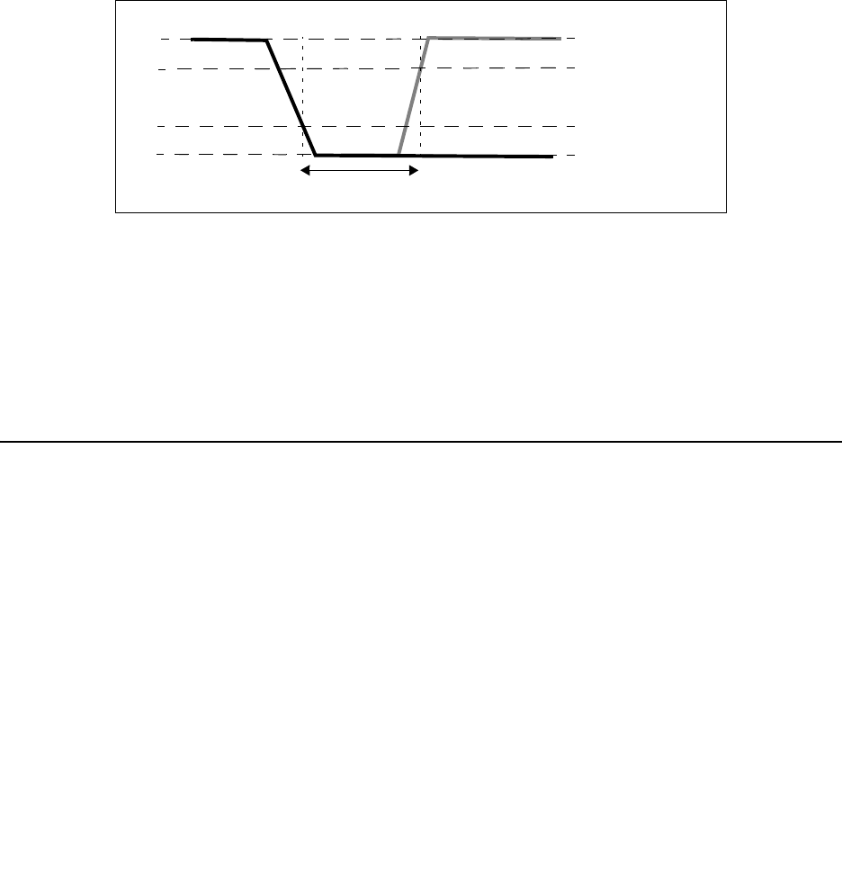
62 HSPICE® Reference Manual: Commands and Control Options
I-2013.12
Chapter 2: HSPICE Simulation Command Reference
Note: This option is active only when HSPICE advanced analog
functions are used.
Command Group
Analysis
Examples
This example specifies that vin* (such as vin1, vin2, and so on), must not
switch for 2ns after every falling edge of nodeA (see Figure 2).
.CHECK HOLD (nodeA FALL 2ns RISE) vin*
Figure 2 HOLD Example
See Also
.CHECK EDGE
.CHECK GLOBAL_LEVEL
.CHECK SETUP
.CHECK IRDROP
Verifies that IR drop does not fall below or exceed a specified value in HSPICE.
Syntax
.CHECK IRDROP (volt_valtimeduration) node1 [node2 ...]
+ (hi lo hi_th low_th)
HI
HI_thresh
LO
LO_thresh
nodeA vin*
t >=2ns
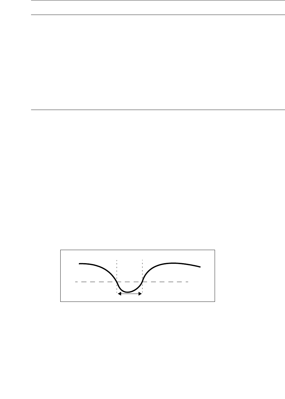
HSPICE® Reference Manual: Commands and Control Options 63
I-2013.12
Chapter 2: HSPICE Simulation Command Reference
Description
Use this command to verify that the IR drop does not fall below or exceed a
specified value for a specified duration.
Note: This option is active only when HSPICE advanced analog
functions are used.
Command Group
Analysis
Examples
This example specifies that v1 must not fall below -2 volts for any duration
exceeding 1ns (see Figure 3).
.CHECK IRDROP (-2 1ns) v1
Figure 3 IR Drop Example
See Also
.CHECK EDGE
Argument Description
volt_val Limiting voltage value.
■A positive volt_val (voltage value) indicates ground bounce
checking.
■A negative volt_val denotes VDD drop.
duration Maximum allowable time. If you set duration to 0, then HSPICE
reports every glitch that strays beyond the specified volt_val.
node1 [node2 ...] List of nodes for which the IR drop checking applies.
hi lo hi_th lo_th Logic levels for the timing check.
t <=1ns
v1
-2 volts

64 HSPICE® Reference Manual: Commands and Control Options
I-2013.12
Chapter 2: HSPICE Simulation Command Reference
.CHECK GLOBAL_LEVEL
.CHECK SETUP
.CHECK RISE
Verifies that a rise time occurs within a specified time window in HSPICE.
Syntax
.CHECK RISE (minmax) node1 [node2 ...] (hi lo hi_th lo_th)
Description
Use this command to verify that a rise time occurs within the specified window
of time.
Note: This option is active only when HSPICE advanced analog
functions are used.
Command Group
Analysis
Examples
This example defines a window between 1.5ns and 2.2ns wide, in which the va
and vb signals must complete their rise transition (see Figure 4). Values for the
HI, LO, and the thresholds were defined in a .CHECK GLOBAL_LEVEL
command placed earlier in the netlist.
.CHECK RISE (1.5ns 2.2ns) va vb
Argument Description
min Lower boundary for the time window.
max Upper limit for the time window.
node1 node2 ... List of all nodes to check.
hi lo hi_th lo_th Logic levels for the timing check.

HSPICE® Reference Manual: Commands and Control Options 65
I-2013.12
Chapter 2: HSPICE Simulation Command Reference
Figure 4 RISE Time Example
See Also
.CHECK GLOBAL_LEVEL
.CHECK FALL
.CHECK SLEW
.CHECK SETUP
Verifies that specified signals do not switch for a specified time-period when
using the advanced analog feature.
Syntax
.CHECK SETUP (ref RISE | FALL duration RISE | FALL)
+ node1 [node2 ...] (hi lo hi_th low_th)
Description
Use to verify that specified signals do not switch for a specified period of time.
Argument Description
ref Reference or trigger signal.
duration Minimum time before the triggering event during which the
specified nodes cannot rise or fall
node1 [node2 ...] List of nodes for which the HOLD condition applies.
hi lo hi_th lo_th Logic levels for the timing check.
HI
HI_thresh
LO
LO_thresh
1.5 ns < t < 2.2 ns
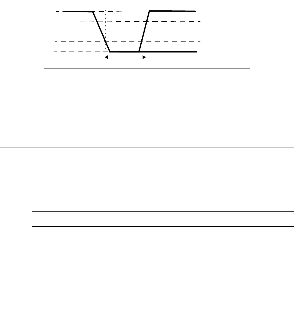
66 HSPICE® Reference Manual: Commands and Control Options
I-2013.12
Chapter 2: HSPICE Simulation Command Reference
Note: This option is active only when HSPICE advanced analog
functions are used.
Command Group
Analysis
Examples
This example specifies that v1 and v2 must not switch for 2 ns before every
rising edge of nodeA (see Figure 5).
.CHECK SETUP (nodeA RISE 2ns FALL) v1 v2
Figure 5 SETUP Example
See Also
.CHECK EDGE
.CHECK GLOBAL_LEVEL
.CHECK HOLD
.CHECK SLEW
Verifies that a slew rate occurs within a specified time window in HSPICE.
Syntax
.CHECK SLEW (minmax) node1 [node2 ...](hi lo hi_th lo_th)
Argument Description
min Lower boundary for the time window.
max Upper limit for the time window.
HI
HI_thresh
LO
LO_thresh
nodeA
v1
t >=2ns
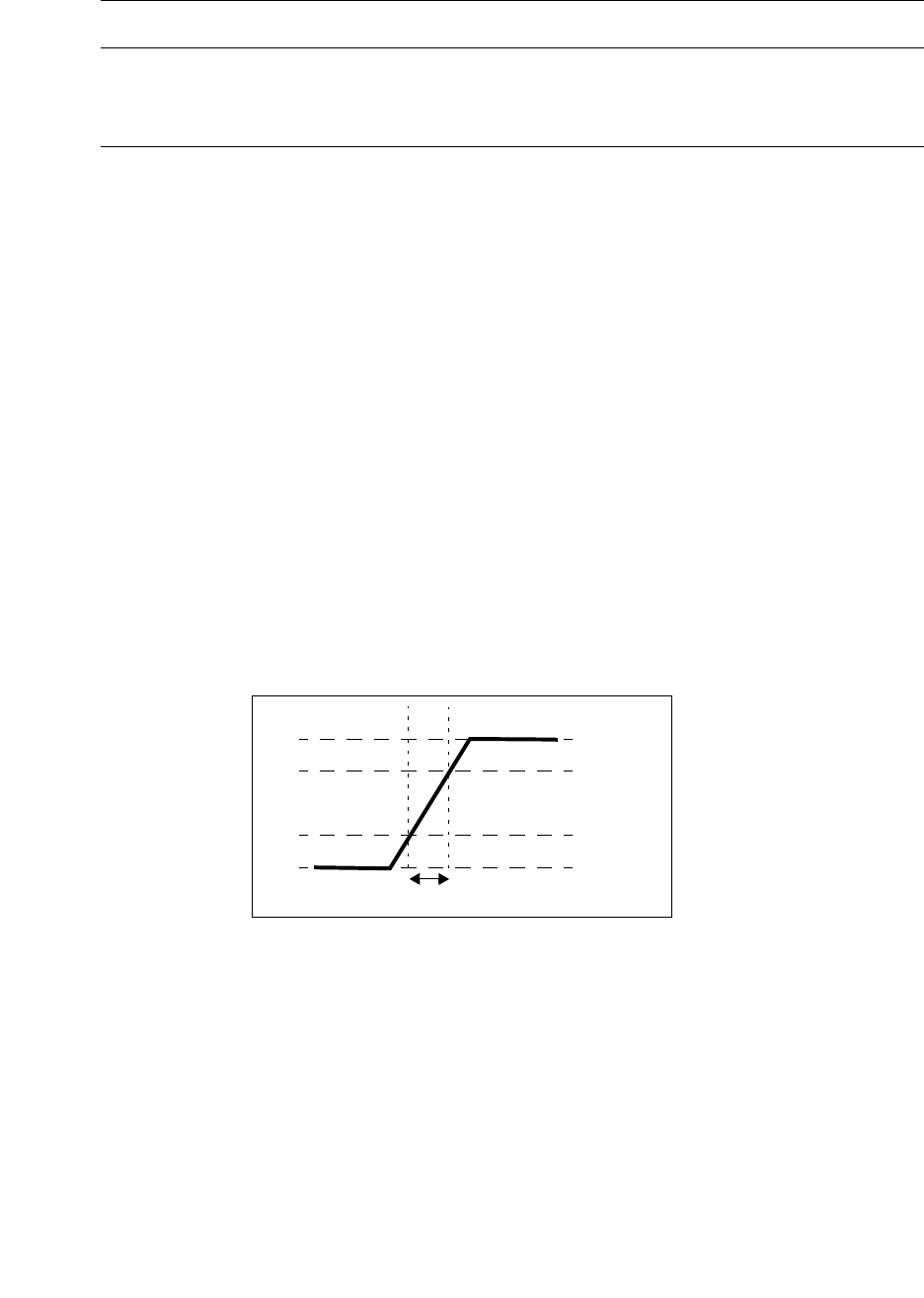
HSPICE® Reference Manual: Commands and Control Options 67
I-2013.12
Chapter 2: HSPICE Simulation Command Reference
Description
Use this command to verify that a slew rate occurs within specified time range.
Note: This option is active only when HSPICE advanced analog
functions are used.
Command Group
Analysis
Examples
This example sets the condition that nodes starting with a* nodes must have a
slew rate between (HI_thresh - LO_thresh)/3ns and (HI_thresh - LO_thresh)/
1ns. If either node has a slew rate greater than that defined in the .CHECK
SLEW command, HSPICE reports the violation in the .err file.
.CHECK SLEW (1ns 3ns) a* (3.3 0 2.6 0.7)
The slew rate check in Figure 6 defines its own hi, lo, and corresponding
threshold values, as indicated by the four values after the node names.
Figure 6 SLEW Example
See Also
.CHECK FALL
.CHECK GLOBAL_LEVEL
.CHECK RISE
node1 node2 ... List of all nodes to check.
hi lo hi_th lo_th Logic levels for the timing check.
Argument Description
3.3
2.6
0.0
0.7
1ns < t < 3ns

68 HSPICE® Reference Manual: Commands and Control Options
I-2013.12
Chapter 2: HSPICE Simulation Command Reference
.CLFLIB
Enables automatic selection for HSPICE Compiled Function Library function.
Syntax
.CFLLIB "%platform/func.so"
Description
Add this command and string to the netlist to automatically select the platform
for CFL functions. This feature works similarly to that of HSIMPlus.
You can select the platform from any of the following:
■x86sol64
■x86sol32
■sparc64
■sparcOS5
■amd64
■linux
■suse64
■suse32
■unknown (when the platform does not match any of the above platforms)
Command Group
Library Management
.CONNECT
Connects two nodes together; the first node replaces the second node in the
simulation.
Syntax
.CONNECT node1[.[global_node_label]]
+ node2[.global_node_label]

HSPICE® Reference Manual: Commands and Control Options 69
I-2013.12
Chapter 2: HSPICE Simulation Command Reference
Description
Use this command to connect two nodes together in your netlist. This causes
the simulation to evaluate the two nodes as if they were only one node that
uses the name of the first node. The name of the second node is not
recognized in the simulation. Both nodes must be at the same level in the circuit
design that you are simulating: you cannot connect nodes that belong to
different subcircuits.
Note: The .CONNECT command is not supported inside of a subckt
definition.
Control Options
The following netlist control options are available for this command:
Command Group
Node Naming
Argument Description
node1 Name of the first of two nodes to connect together.
node2 Name of the second of two nodes to connect together. This node
is replaced by Node1, which is the first node, in the simulation.
[global_node_label] This option is available only when you are simulating a 3D-IC
netlist. Use this option to access the global node inside a module
from the top level or access the module based global nodes that
are connected with the top level global nodes.
By default, multiple instantiation with the same IC module does not
make the module based global nodes connected together. You
need to explicitly connect them as required.
For more information on defining multiple tier IC module
definitions, see .MODULE command.
Option Description
.OPTION NODE Prints a node cross-reference table.

70 HSPICE® Reference Manual: Commands and Control Options
I-2013.12
Chapter 2: HSPICE Simulation Command Reference
Examples
Example 1 A is the name of the first of two nodes to connect together and VSS is
the name of the second of two nodes to connect together. A, the first
node, replaces the second node, VSS, in the simulation.
.CONNECT A VSS
...
.subckt eye_diagram node1 node2 ...
.connect node1 node2
...
.ends
Example 2 Example 1 now is the same as the following:
...
.subckt eye_diagram node1 node1 ...
...
.ends
...
HSPICE reports the following error message:
**error**: subcircuit definition duplicates node node1
To apply any HSPICE command to node2, apply it to node1, instead. Then, to
change the netlist construction to recognize node2, use an .ALTER command.
HSPICE reports the following error message:
**error**: subcircuit definition duplicates node node1
To apply any HSPICE command to node2, apply it to node1, instead. Then, to
change the netlist construction to recognize node2, use an .ALTER command.
In the following variation of the example, node1 node2 are not be the same in
this situation and the duplicated node error message will not be issued.
.connect node1 node2
.subckt eye_diagram node1 node2 ...
...
.ends

HSPICE® Reference Manual: Commands and Control Options 71
I-2013.12
Chapter 2: HSPICE Simulation Command Reference
Example 3 The first .TRAN simulation includes two resistors. Later simulations have
only one resistor because r2 is short-circuited by connecting cc with 1.
v(1) does not print out, but v(cc) prints out instead.
*example for .connect
vcc 0 cc 5v
r1 0 1 5k
r2 1 cc 5k
.tran 1n 10n
.print i(vcc) v(1)
.alter
.connect cc 1
.end
Example 4 Shows how to use multiple .CONNECT commands to connect several
nodes together. This example connects both node2 and node3 to node1.
All connected nodes must be in the same subcircuit or all in the main
circuit. The first HSPICE simulation evaluates only node1; node2 and
node3 are the same node as node1. Use .ALTER commands to simulate
node2 and node3.
.CONNECT node1 node2
.CONNECT node2 node3
If you set .OPTION NODE, then HSPICE prints out a node connection table.
vcc cc 0 5v
r1 cc net1 5k
r2 net1 net2 5k
c1 net2 0 1n
.tran 1n 10n
.connect net2 0
.print i(vcc) v(net2)
.end
This causes the circuit elements to be connected as shown in Example 5:
Example 5
vcc cc net2 5v
r1 cc net1 5k
r2 net1 net2 5k
c1 net2 net2 1n
.tran 1n 10n
.connect net2 0
.print i(vcc) v(net2)
.end

72 HSPICE® Reference Manual: Commands and Control Options
I-2013.12
Chapter 2: HSPICE Simulation Command Reference
For Example 5, HSPICE reports the following error message for the elements
vcc r1 and r2, since there is now no ground node in the netlist.
**error** no dc path to ground from node
Example 6 The correct way to connect net2 to ground is to specify the .CONNECT
command as follows:
.connect 0 net2
3D IC Netlist - Module Based Global Node Reference Examples
In this example, even though the xtop1 and xtop2 references to the same top
subckt inside the IC module tmod, the vdd in the xtop1 is not connected to
vdd in the xtop2 by default. It requires explicit definitions to connect the nodes
if it is the intention. In this example, the vdd for both xtop1 and xtop2 are
connected together with the .connect command.
Xtop1 … tmod::top
Xtop2 … tmod::top
.connect xtop1.vdd xtop2.vdd
.module tmod
.global vdd
.subckt top
…
.ends
.endmodule
In this example, the top level vdd and xtop1.vdd are connected together.
.global vdd
Xtop1 … tmod::top
.connect vdd xtop1.vdd
.module tmod
.global vdd
.subckt top
…
.ends
.endmodule
See Also
.ALTER

HSPICE® Reference Manual: Commands and Control Options 73
I-2013.12
Chapter 2: HSPICE Simulation Command Reference
.DATA
Concatenates or column-laminates data sets to optimize measured I-V, C-V,
transient, or S-parameter data.
Syntax
Inline command
.DATA datanm pnam1 [pnam2 pnam3 ... pnamxxx]
+pval1 [pval2 pval3 ... pvalxxx]
+pval1’ [pval2’ pval3’ ... pvalxxx’]
.ENDDATA
External File command for concatenated data files
.DATA datanm MER
+ FILE=’filename1’ pname1=col_num [pname2=col_num ...]
+ [FILE=’filename2’ pname1=col_num
+ [pname2=col_num ...] ... [OUT=’fileout’]
.ENDDATA
Column Laminated command (not available for HSPICE advanced analog
analyses).
.DATA datanm LAM
+ FILE=’filename1’ pname1=col_num
+ [pname2=col_num ...]
+ [FILE=’filename2’ pname1=col_num
+ pname2=col_num ...] ... [OUT=’fileout’]
.ENDDATA
Argument Description
col_num Column number in the data file for the parameter value. The column
does not need to be the same between files.
datanm Data name—referenced in the .TRAN,.DC, or .AC command.
filenamei Data file to read. HSPICE concatenates files in the order they appear
in the .DATA command. You can specify up to 10 files.
fileouti Data file name, where simulation writes concatenated data. This file
contains the full syntax for an inline .DATA command and can replace
the .DATA command that created it in the netlist. You can output the
file and use it to generate one data file from many.

74 HSPICE® Reference Manual: Commands and Control Options
I-2013.12
Chapter 2: HSPICE Simulation Command Reference
Description
Use the .DATA command to concatenate or column-laminate data sets to
optimize measured I-V, C-V, transient, or S-parameter data. Up to 1000
variables (columns) can be displayed.
You can also use the .DATA command for a first or second sweep variable
when you characterize cells and test worst-case corners. Simulation reads data
measured in a lab, such as transistor I-V data, one transistor at a time in an
outer analysis loop. Within the outer loop, the analysis reads data for each
transistor (IDS curve, GDS curve, and so on), one curve at a time in an inner
analysis loop.
Data-driven analysis syntax requires a .DATA command and an analysis
command that contains a DATA=dataname keyword.
The .DATA command specifies parameters that change values, and the sets of
values to assign during each simulation. The required simulations run as an
internal loop. This bypasses reading-in the netlist and setting-up the simulation,
which saves computing time. In internal loop simulation you can also plot
simulation results against each other and print them in a single output.
You can enter any number of parameters in a .DATA block. The .AC,.DC,
and .TRAN commands can use external and inline data provided in .DATA
commands. For example, to specify the circuit temperature for an HSPICE
simulation you can use the .TEMP command, the TEMP parameter in the .DC,
.AC, and .TRAN commands, or the TEMP/TEMPER parameter in the first
column of the .DATA command.The number of data values per line does not
need to correspond to the number of parameters. For example, you do not
need to enter 20 values on each line in the .DATA block if each simulation pass
requires 20 parameters: the program reads 20 values on each pass, however
the values are formatted.
Each .DATA command can contain up to 1000 parameters.
LAM Column-laminated (parallel merging) data files to use.
MER Concatenated (series merging) data files to use.
pnami Parameter names—used for source value, element value, device size,
model parameter value, and so on. You must declare these names in
a.PARAM command.
pvali Parameter value.
Argument Description

HSPICE® Reference Manual: Commands and Control Options 75
I-2013.12
Chapter 2: HSPICE Simulation Command Reference
HSPICE refers to .DATA commands by their data names so each data name
must be unique. HSPICE supports three .DATA command formats:
■Inline data, which is parameter data, listed in a .DATA command block. The
datanm parameter in a .DC,.AC, or .TRAN analysis command, calls this
command. The number of parameters that HSPICE reads determines the
number of columns of data. The physical number of data numbers per line
does not need to correspond to the number of parameters. For example, if
the simulation needs 20 parameters you do not need 20 numbers per line.
■Concatenated data from external files. Concatenated data files are files with
the same number of columns, placed one after another.
■Data that is Column-laminated data from external files. Column-laminated
data are columns of files with the same number of rows, arranged side-by-
side.
To use external files with the .DATA format:
■Use the MER and LAM keywords to prepare HSPICE for external file data,
rather than inline data.
■Use the FILE keyword to specify the external filename.
■Use simple file names, such as out.dat without single or double quotation
marks ( ‘ ’ or “ ”), but use quotation marks when file names start with
numbers, such as “1234.dat”.
■Use the proper case, since file names are case sensitive on UNIX systems.
For data-driven analysis, specify the start time (time 0) in the analysis
command so that the analysis correctly calculates the stop time.
The following shows how different types of analyses use .DATA
commands: .DC DATA=dataname
Operating point: .DC vin 1 5 .25 SWEEP DATA=dataname
DC sweep: .DC vin 1 5 .25 SWEEP DATA=dataname
AC sweep: AC dec 10 100 10meg SWEEP DATA=dataname
TRAN sweep: .TRAN 1n 10n SWEEP DATA=dataname
With the release of F-2011.09-SP2, HSPICE supports a second selective data
sweep, by using syntax as follows:
■.DC var1 type np start1 stop1 SWEEP DATA=datanm(nums)
■.AC type np fstart fstop SWEEP DATA=datanm(nums)

76 HSPICE® Reference Manual: Commands and Control Options
I-2013.12
Chapter 2: HSPICE Simulation Command Reference
■.TRAN tstep1 tstop1 [tstep2 tstop2 ...tstepN tstopN]
+ [START=val] [UIC] SWEEP DATA=datanm(nums)
Where nums can be either of following:
• one signal num, to specify the sample number to execute; for example:
.tran 0.1n 1n sweep data=datanm(4)
•num1:num2 num3 num4:num5 — to execute samples from num1 to
num2, sample num3, and samples from num4 to num5; for example:
.tran 0.1n 1n sweep data=datanm(2 4:5 7)
Command Group
Setup
Examples
Example 1 HSPICE performs these analyses for each set of parameter values
defined in the .DATA command. For example, the program first uses the
width=50u, length=30u, thresh=1.2v, and cap=1.2pf parameters to
perform .TRAN, .AC, and .DC analyses. HSPICE then repeats the
analyses for width=25u, length=15u, thresh=1.0v, and cap=0.8pf, and
again for the values on each subsequent line in the .DATA block.
* Inline .DATA statement
.TRAN 1n 100n SWEEP DATA=devinf
.AC DEC 10 1hz 10khz SWEEP DATA=devinf
.DC TEMP -55 125 10 SWEEP DATA=devinf
.DATA devinf width length thresh cap
+ 50u 30u 1.2v 1.2pf
+ 25u 15u 1.0v 0.8pf
+ 5u 2u 0.7v 0.6pf
.ENDDATA

HSPICE® Reference Manual: Commands and Control Options 77
I-2013.12
Chapter 2: HSPICE Simulation Command Reference
Example 2 HSPICE performs a DC sweep analysis for each set of VBS, VDS, and L
parameters in the .DATA vdot block. That is, HSPICE runs eight DC
analyses one for each line of parameter values in the .DATA block.
* .DATA as the inner sweep
M1 1 2 3 0 N W=50u L=LN
VGS 2 0 0.0v
VBS 3 0 VBS
VDS 1 0 VDS
.PARAM VDS=0 VBS=0 L=1.0u
.DC DATA=vdot
.DATA vdot
VBS VDS L
0 0.1 1.5u
0 0.1 1.0u
0 0.1 0.8u
-1 0.1 1.0u
-2 0.1 1.0u
-3 0.1 1.0u
0 1.0 1.0u
0 5.0 1.0u
.ENDDATA
Example 3 These values result in transient analyses at every time value from 0 to
100 ns in steps of 1 ns by using the first set of parameter values in
the .DATA d1 block. Then HSPICE reads the next set of parameter values
and does another 100 transient analyses. It sweeps time from 0 to 100
ns in 1 ns steps. The outer sweep is time and the inner sweep varies the
parameter values. HSPICE performs 200 analyses: 100 time increments,
times 2 sets of parameter values.
* .DATA as the outer sweep
.PARAM W1=50u W2=50u L=1u CAP=0
.TRAN 1n 100n SWEEP DATA=d1
.DATA d1
W1 W2 L CAP
50u 40u 1.0u 1.2pf
25u 20u 0.8u 0.9pf
.ENDDATA
Example 4 This example shows the external file .DATA for concatenated data files.
* External File .DATA for concatenated data files
.DATA datanm MER
+ FILE=filename1 pname1 = colnum
+ pname2=colnum ...
+ FILE=filename2 pname1=colnum
+ pname2=colnum ...
+ ...
+ OUT=fileout
.ENDDATA

78 HSPICE® Reference Manual: Commands and Control Options
I-2013.12
Chapter 2: HSPICE Simulation Command Reference
If you concatenate the three files (file1, file2, and file3).
file1 file2 file3
a a a b b b c c c
a a a b b b c c c
a a a
The data appears as follows:
Example 5
a a a
a a a
a a a
b b b
b b b
c c c
c c c
The number of lines (rows) of data in each file does not need to be the same.
The simulator assumes that the associated parameter of each column of the A
file is the same as each column of the other files. The .DATA command for this
example is:
* External File .DATA statement
.DATA inputdata MER
FILE=‘file1’ p1=1 p2=3 p3=4
FILE=‘file2’ p1=1
FILE=‘file3’
.ENDDATA
This example listing concatenates file1, file2, and file3 to form the inputdata
data set. The data in file1 is at the top of the file, followed by the data in file2,
and file3. The inputdata in the .DATA command references the data name
specified in either the .DC,.AC, or .TRAN analysis commands. The parameter
fields specify the column that contains the parameters (you must already have
defined the parameter names in .PARAM commands). For example, the values
for the p1 parameter are in column 1 of file1 and file2. The values for the p2
parameter are in column 3 of file1. For data files with fewer columns than
others, HSPICE assigns values of zero to the missing parameters.

HSPICE® Reference Manual: Commands and Control Options 79
I-2013.12
Chapter 2: HSPICE Simulation Command Reference
(Not valid for advanced analog functions) In Example 5 three files (D, E, and F)
contain the following columns of data:
Example 6
File D File E File F
d1 d2 d3 e4 e5 f6
d1 d2 d3 e4 e5 f6
d1 d2 d3 e4 e5 f6
The laminated data appears as follows:
d1 d2 d3 e4 e5 f6
d1 d2 d3 e4 e5 f6
d1 d2 d3 e4 e5 f6
The number of columns of data does not need to be the same in the three files.
The number of lines (rows) of data in each file does not need to be the same.
HSPICE interprets missing data points as zero.
The .DATA command for this example is:
* Column-Laminated .DATA statement
.DATA dataname LAM
FILE=‘file1’ p1=1 p2=2 p3=3
FILE=‘file2’ p4=1 p5=2
OUT=‘fileout’
.ENDDATA
This listing laminates columns from file1 and file2 into the fileout output file.
Columns one, two, and three of file1 and columns one and two of file2 are
designated as the columns to place in the output file. You can specify up to 10
files per .DATA command.
If you run HSPICE on a different machine than the one on which the input data
files reside (such as when you work over a network), use full path names
instead of aliases. Aliases might have different definitions on different
machines.
Example 7 HSPICE dumps separate plot files for each DATA sweep index by using
distributed processing. For example:
.DATA PAM_SWP C_LOAD
10p
20p
.ENDDATA
When you submit the HSPICE job with the distributed processing switch -dp as
follows:

80 HSPICE® Reference Manual: Commands and Control Options
I-2013.12
Chapter 2: HSPICE Simulation Command Reference
hspice -i test.sp -o test -dp 2
... then HSPICE dumps separate plot files and they are stored under task#/
*.tr#. HSPICE actually distributes two data sweep indexes into two tasks,
named task0 and task1 here. Individual plot files are stored under each task.
See Also
.AC
.DC
.ENDDATA
.PARAM / PARAMETER / PARAMETERS
.TRAN
.DC
Performs several types of sweeps during DC analysis.
Syntax
Sweep or Parameterized Sweep:
.DC var1 START=start1 STOP=stop1 STEP=incr1
.DC var1 START=[param_expr1]
+ STOP=[param_expr2] STEP=[param_expr3]
.DC var1 start1 stop1 incr1
+ [SWEEP var2 type np start2 stop2]
.DC var1 start1 stop1 incr1 [var2 start2 stop2 incr2]
Data-Driven Sweep:
.DC var1 type np start1 stop1 [SWEEP DATA=datanm(Nums)]
.DC DATA=datanm [SWEEP var2 start2 stop2 incr2]
.DC DATA=datanm(Nums)
Monte Carlo and Corners Analysis:
.DC var1 type np start1 stop1 [SWEEP MONTE=MCcommand]
.DC MONTE=McCommand
.DC var1 type np start1 stop1 [SWEEP MONTE=MCcommand]
[corner_percentile=val]
Optimization:
.DC DATA=datanm OPTIMIZE=opt_par_fun
+ RESULTS=measnames MODEL=optmod
.DC var1 start1 stop1 SWEEP OPTIMIZE=OPTxxx

HSPICE® Reference Manual: Commands and Control Options 81
I-2013.12
Chapter 2: HSPICE Simulation Command Reference
+ RESULTS=measname MODEL=optmod
Argument Description
DATA=datanm(Nums)Data name, referenced from a .DATA command in the .DC
command, where (Nums) can be any of the following to allow
selective runs for a .DATA structure:
■One signal number to specify the sample number to execute. For
example:
.DC .1n 1n sweep data=datanm(4)
■Sequence of signals as follows - (num1:num2 num3 num4:num5),
where : Samples from num1 to num2, sample num3, and samples
from num4 to num5 are executed. For example:
.DC 0.1n 1n sweep data=datanm(1:2 3 4:5)
incr1... Voltage, current, element, or model parameters; or temperature
increments.
MODEL Optimization reference name. The .MODEL OPT command uses this
name in an optimization analysis
MONTE=MCcommand Where MCcommand can be any of the following:
■val Specifies the number of random samples to produce.
■val firstrun=num Specifies the sample number on which the
simulation starts.
■list num Specifies the sample number to execute.
■list(num1:num2 num3 num4:num5) Samples from num1 to num2,
sample num3, and samples from num4 to num5 are executed
(parentheses are optional).
corner_percentile Default 0.0. This option specifies the percentiles used to find corners.
The value field is a non-negative number in the range (0.0~0.5). For
example, if value=0.1, then HSPICE will sort the measure results, and
choose the points below the 10th percentile and those above the 90th
percentile as corners. If the value = 0.0, then HSPICE will use the
maximum and minimum values as corners.
np Number of points per decade or per octave or just number of points,
based on which keyword precedes it.
OPTIMIZE Specifies the parameter reference name, used for optimization in
the .PARAM command
RESULTS Measure name used for optimization in the .MEASURE command

82 HSPICE® Reference Manual: Commands and Control Options
I-2013.12
Chapter 2: HSPICE Simulation Command Reference
Description
You can use the .DC command in DC analysis to:
start1 ... Starting voltage, current, element, or model parameters; or
temperature values. If you use the POI (list of points) variation type,
specify a list of parameter values, instead of start stop. When using
HSPICE advanced analog functions, the start and stop syntax is not
supported.
stop1 ... Final voltage, current, any element, model parameter, or temperature
values.
SWEEP Second sweep has a different type of variation (DEC, OCT, LIN, POI,
or DATA command; or MONTE=val).
TEMP Temperature sweep.
type Can be any of the following keywords:
■DEC — decade variation
■OCT — octave variation
■LIN — linear variation
■POI — list of points
var1 ... ■Name of an independent voltage or current source, or
■Name of any element or model parameter, or
■TEMP keyword (indicating a temperature sweep).
HSPICE supports a source value sweep, which refers to the source
name (SPICE style). However, if you select a parameter sweep,
a.DATA command, and a temperature sweep, then you must select
a parameter name for the source value. A later .DC command must
refer to this name. The parameter must not start with the TEMP
keyword. The var1 parameter should be defined in advance using
the.PARAM command.
firstrun The val value specifies the number of Monte Carlo iterations to
perform. The firstrun value specifies the desired number of iterations.
HSPICE runs from num1 to num1+val-1.
list The iterations at which HSPICE performs a Monte Carlo analysis. You
can write more than one number after list. The colon represents
“from ... to ...". Specifying only one number makes HSPICE run at
only the specified point.
Argument Description

HSPICE® Reference Manual: Commands and Control Options 83
I-2013.12
Chapter 2: HSPICE Simulation Command Reference
■Sweep any parameter value.
■Sweep any source value.
■Sweep temperature range.
■Perform a DC Monte Carlo (random sweep) analysis.
■Perform a data-driven sweep.
■Perform a DC circuit optimization for a data-driven sweep.
■Perform a DC circuit optimization by using start and stop.
■Perform a DC model characterization.
The format for the .DC command depends on the application that uses it. The
DC sweep functionality is enhanced by use of the GSHUNT algorithm.
Control Options
The following netlist control options are available for this command:
Command Group
Analysis
Examples
Example 1 Sweeps the value of the VIN voltage source from 0.25 volts to 5.0 volts in
increments of 0.25 volts.
.DC VIN 0.25 5.0 0.25
Example 2 Sweeps the drain-to-source voltage from 0 to 10 v in 0.5 v increments at
VGS values of 0, 1, 2, 3, 4, and 5 v.
.DC VDS 0 10 0.5 VGS 0 5 1
Example 3 Starts a DC analysis of the circuit from -55
°
C to 125
°
C in 10
°
C
increments.
.DC TEMP -55 125 10
Example 4 Script runs a DC analysis at five temperatures: 0, 30, 50, 100, and 125
°
C.
.DC XVAL 1K 10K .5K SWEEP TEMP LIN 5 25 125
Option Description
.OPTION DCIC Specifies whether to use or ignore commands in the netlist.

84 HSPICE® Reference Manual: Commands and Control Options
I-2013.12
Chapter 2: HSPICE Simulation Command Reference
Example 5 Runs a DC analysis on the circuit at each temperature value. The
temperatures result from a linear temperature sweep from 25
°
C to
125
°
C (five points), which sweeps a resistor value named xval from 1 k
to 10 k in 0.5 k increments.
.DC XVAL 1K 10K .5K SWEEP TEMP LIN 5 25 125
Example 6 Specifies a sweep of the par1 value from 1 k to 100 k in increments of 10
points per decade.
.DC DATA=DATANM SWEEP PAR1 DEC 10 1K 100K
Example 7 Requests a DC analysis at specified parameters in the .DATA DATANM
command. It also sweeps the par1 parameter from 1k to 100k in
increments of 10 points per decade.
.DC PAR1 DEC 10 1K 100K SWEEP DATA=DATANM
Example 8 Invokes a DC sweep of the par1 parameter from 1k to 100k by 10 points
per decade by using 30 randomly generated (Monte Carlo) values.
.DC PAR1 DEC 10 1K 100K SWEEP MONTE=30
Example 9 Schmitt Trigger script.
*file: bjtschmt.sp bipolar schmitt trigger
.OPTION post=2
vcc 6 0 dc 12
vin 1 0 dc 0 pwl(0,0 2.5u,12 5u,0)
cb1 2 4 .1pf
rc1 6 2 1k
rc2 6 5 1k
rb1 2 4 5.6k
rb2 4 0 4.7k
re 3 0 .47k
diode 0 1 dmod
q1 2 1 3 bmod 1 ic=0,8
q2 5 4 3 bmod 1 ic=.5,0.2
.dc vin 0,12,.1
.model dmod d is=1e-15 rs=10
.model bmod npn is=1e-15 bf=80 tf=1n
+ cjc=2pf cje=1pf rc=50 rb=100 vaf=200
.probe v(1) v(5)
.print
.end
Example 10 Invokes a DC sweep of the par1 parameter from 1k to 100k by 10 points
per decade and uses 10 Monte Carlo) values from 11th to 20th trials.
.DC par1 DEC 10 1k 100k SWEEP MONTE=list(10 20:30 35:40 50)

HSPICE® Reference Manual: Commands and Control Options 85
I-2013.12
Chapter 2: HSPICE Simulation Command Reference
Example 11 Invokes a DC sweep of the par1 parameter from 1k to 100k by 10 points
per decade and a Monte Carlo analysis at the 10th trial, then from the
20th to the 30th trials, followed by the 35th to 40th trials and finally at the
50th trial.
.DC par1 DEC 10 1k 100k SWEEP MONTE=list(10 20:30 35:40 50)
See Also
.MODEL
.OPTION DCIC
.PARAM / PARAMETER / PARAMETERS
Behavioral Application Examples for the path to the demo file
inv_vin_vout.sp
.DCMATCH
Calculates the effects of variations on a circuit's DC characteristics.
Syntax
.DCMATCH OUTVAR [THRESHOLD=T] [FILE=string] [INTERVAL=Int]
Argument Description
OUTVAR One or more node voltages, voltage differences for a node pair, or
currents through an independent voltage source or currents through
a resistor, a capacitor, or an inductor.
THRESHOLD Report devices with a relative contribution above Threshold in the
summary table.
■T=0: reports results for all devices
■T<0: suppresses table output; however, individual results are still
available through .PROBE or .MEASURE commands.
The upper limit for T is 1, but at least 10 devices are reported or all if
there are less than 10. Default value is 0.01.
FILE Valid file name for the output tables. Default is basename.dm# where
“#” is the usual sequence number for HSPICE output files.
INTERVAL Applies only if a DC sweep is specified. Int is a positive integer. A
summary is printed at the first sweep point, then for each subsequent
increment of Int and then if not already printed at the final sweep point.
Only single sweeps are supported.

86 HSPICE® Reference Manual: Commands and Control Options
I-2013.12
Chapter 2: HSPICE Simulation Command Reference
Description
Use this command to calculate the effects of variations in device characteristics
on the DC solution of a circuit.
You can perform only one DCMATCH analysis per simulation. Only the last
.DCMATCH command is used in case more than one in present. The others are
discarded with warnings.
Command Group
Analysis
Examples
Example 1 HSPICE reports DCMatch variations on the voltage of node 9, the
voltage difference between nodes 4 and 2, and on the current through the
source VCC and on the current through resister x1.r1.
.DCMatch V(9) V(4,2) I(VCC) I(x1.r1)
Example 2 The variable XVal is being swept in the .DC command. It takes nine
values in sequence from 1k to 9k in increments of 1k. Tabular output for
the.DCMATCH command is only generated for the set XVal={1k, 4k, 7k,
9k}.
.DC XVal Start=1K Stop=9K Step=1K
.DCMATCH V(vcc) interval=3
See Also
.DC
.MEASURE (DCMATCH)
.PROBE
DCMatch Analysis
.DCSENS
Invokes DC sensitivity analysis using variation definitions as specified in the
Variation Block.
Syntax
.DCSENS Output_Variable [File=string] [Perturbation=x]
+ [Interval=SweepValue] [Threshold=x] [GroupByDevice=0|1]

HSPICE® Reference Manual: Commands and Control Options 87
I-2013.12
Chapter 2: HSPICE Simulation Command Reference
Description
Use this command to calculate the parameter sensitivity in the following
instances:
■Global variation
■Local variation
■Local element variation with model type and model parameters that are
permitted for DCmatch, including subckt variation
Argument Description
Output_Variable Response with regard to the parameters designated in Sensitivity
Block. Similar to the .DCMATCH command, the Output_Variable
can be node voltage or branch current in a circuit.
File=string Valid file name for the output tables. Default=basename.ds#
where “#” is a number in the style of ds0, ds1, etc. If multiple
dcsweep commands are specified in the netlist, then sensitivity
analysis table results for each dcsweep are listed in *.ds# files. If
.OPTION OPFILE specified, sensitivity result tables on operating
points are listed in *.dp# files, otherwise, these tables are listed
in the *.lis file.
Perturbation=xPerturbations of x standard deviation are used in computing the
finite difference approximations to device derivatives. The valid
range for the parameter is 0.0001 to 1.0 with a default value of
0.05.
Interval=SweepValue This option only applies to one dimensional sweeps. The
SweepValue fields are positive integers. A summary is printed at
the first sweep point, then for each subsequent increment of
SweepValue, and then, if not already printed, at the final sweep
point. The Interval key is ignored with a warning if a sweep is not
being carried out.
The option only controls the printed summary table. The analysis
may be carried out at additional sweep values if required by other
forms of output such as Probe and Measure statements.
Threshold=xOnly devices with absolute sensitivity value above x are reported.
Results for all devices are displayed if Threshold=0 is set.
Default=10u.
GroupByDevice = 0|1 Alternate mode of generating sensitivity result tables; Default=0

88 HSPICE® Reference Manual: Commands and Control Options
I-2013.12
Chapter 2: HSPICE Simulation Command Reference
The methodology is based on using a finite difference approximation algorithm.
DC sensitivity analysis combines the device derivatives, the DC solution, and
the adjoint variables to get the sensitivity. DC sensitivity analysis enables you to
compute sensitivity of any model parameter and many more models than
traditional HSPICE sensitivity analysis. In addition, the analysis supports
sensitivity for Probe and Measure output statements and for DC sweeps.
Note: .DCSENS does not support spatial variation and global element
variation.
Control Options
The following netlist control options are available for this command:
Command Group
Analysis
Examples
In the following example, the variable XVal is being swept in the DC command.
It takes nine values in sequence from 1K to 9K in increments of 1K. Tabular
output for the sensitivity command is only generated for the set XVal={1K, 4K,
7K, 9K}.
.DC XVal Start=1K Stop=9K Step=1K
.DCsens V(vcc) Interval=3
See Also
DC Sensitivity Analysis and Variation Block
.DCVOLT
Sets initial conditions in HSPICE.
Syntax
.DCVOLT V(node1)=val1 V(node2)=val2 ...
.DCVOLT V node1val1 [node2val2 ...]
Option Description
.OPTION OPFILE Outputs the operating point information to a file.

HSPICE® Reference Manual: Commands and Control Options 89
I-2013.12
Chapter 2: HSPICE Simulation Command Reference
Description
Use the .IC command or the .DCVOLT command to set transient initial
conditions in HSPICE. How it initializes depends on whether the .TRAN
analysis command includes the UIC parameter.
If you specify the UIC parameter in the .TRAN command, HSPICE does not
calculate the initial DC operating point but directly enters transient analysis.
Transient analysis uses the .IC initialization values as part of the solution for
timepoint zero (calculating the zero timepoint applies a fixed equivalent voltage
source). The .IC command is equivalent to specifying the IC parameter on
each element command but is more convenient. You can still specify the IC
parameter, but it does not take precedence over values set in the .IC
command.
If you do not specify the UIC parameter in the .TRAN command, HSPICE
computes the DC operating point solution before the transient analysis. The
node voltages that you specify in the .IC command are fixed to determine the
DC operating point. Transient analysis releases the initialized nodes to
calculate the second and later time points.
Command Group
Setup
Examples
.DCVOLT 11 5 4 -5 2 2.2
See Also
.IC
.TRAN
.DEL LIB
Removes library data from memory for HSPICE.
Argument Description
val1 ... Voltages. The significance of these voltages depends on whether you
specify the UIC parameter in the .TRAN command.
node1 ... Node numbers or names can include full paths or circuit numbers.

90 HSPICE® Reference Manual: Commands and Control Options
I-2013.12
Chapter 2: HSPICE Simulation Command Reference
Syntax
.DEL LIB ‘[file_path]file_name’ entry_name
.DEL LIB libnumber entryname
.DEL LIB All
Description
Use this command to remove library data from memory. The next time you run
a simulation, the .DEL LIB command removes the .LIB call command with
the same library number and entry name from memory. You can then use
a.LIB command to replace the deleted library. In this way, .DEL LIB helps
you avoid name conflicts.
You can use the .DEL LIB command with the .ALTER command.
Command Group
Alter Block and Library Management
Examples
Example 1 Calculates a DC transfer function for a CMOS inverter using these steps:
1. HSPICE simulates the device by using the NORMAL inverter model
from the MOS.LIB library.
2. Using the .ALTER block and the .LIB command, HSPICE substitutes
a faster CMOS inverter, FAST for NORMAL.
3. HSPICE then resimulates the circuit.
4. Using the second .ALTER block, HSPICE executes DC transfer
analysis simulations at three different temperatures and with an n-
Argument Description
entry_name Name of entry used in the library call command to delete.
file_name Name of a file to delete from the data file; the file path, plus the file
name, can be up to 256 characters long. You can use any file name that
is valid for the operating system that you use. Enclose the file path and
file name in single or double quotation marks.
file_path Path name of a file if the operating system supports tree-structured
directories.
libnumber Library number, used in the library call command to delete.
all Deletes all loaded libraries.

HSPICE® Reference Manual: Commands and Control Options 91
I-2013.12
Chapter 2: HSPICE Simulation Command Reference
channel width of 100 mm, instead of 15 mm.
5. HSPICE also runs a transient analysis in the second .ALTER block
and uses a .MEASURE command to measure the rise time of the inverter.
FILE1: ALTER1 TEST CMOS INVERTER
.OPTION ACCT LIST
.TEMP 125
.PARAM WVAL=15U VDD=5
*
.OP
.DC VIN 0 5 0.1
.PRINT DC V(3) V(2)
*
VDD 1 0 VDD
VIN 2 0
*
M1 3 2 1 1 P 6U 15U
M2 3 2 0 0 N 6U W=WVAL
*
.LIB 'MOS.LIB' NORMAL
.ALTER
.DEL LIB 'MOS.LIB' NORMAL $removes LIB from memory
.DEL LIB 'MOS.LIB' NORMAL $removes normal library from memory
.LIB 'MOS.LIB' FAST $get fast model library
.ALTER
.OPTION NOMOD OPTS $suppress printing model
$parameters and print the
$option summary
.TEMP -50 0 50 $run with different temperatures
.PARAM WVAL=100U VDD=5.5 $change the parameters using
VDD 1 0 5.5 $VDD 1 0 5.5 to change the power
$supply VDD value doesn't work
VIN 2 0 PWL 0NS 0 2NS 5 4NS 0 5NS 5
$change the input source
.OP VOL $node voltage table of
$operating points
.TRAN 1NS 5NS $run with transient also
M2 3 2 0 0 N 6U WVAL $change channel width
.MEAS SW2 TRIG V(3) VAL=2.5 RISE=1 TARG V(3)
+ VAL=VDD CROSS=2 $measure output
*
.END

92 HSPICE® Reference Manual: Commands and Control Options
I-2013.12
Chapter 2: HSPICE Simulation Command Reference
Example 2 The .ALTER block adds a resistor and capacitor network to the circuit.
The network connects to the output of the inverter and HSPICE simulates
a DC small-signal transfer function.
FILE2: ALTER2.SP CMOS INVERTER USING SUBCIRCUIT
.OPTION LIST ACCT
.MACRO INV 1 2 3
M1 3 2 1 1 P 6U 15U
M2 3 2 0 0 N 6U 8U
.LIB 'MOS.LIB' NORMAL
.EOM INV
XINV 1 2 3 INV
VDD 1 0 5
VIN 2 0
.DC VIN 0 5 0. 1
.PRINT V(3) V(2)
.ALTER
.DEL LIB 'MOS.LIB' NORMAL
.TF V(3) VIN $DC small-signal transfer
$function
*
.MACRO INV 1 2 3 $change data within
$subcircuit def
M1 4 2 1 1 P 100U 100U $change channel length,width,also
$topology
M2 4 2 0 0 N 6U 8U $change topology
R4 4 3 100 $add the new element
C3 3 0 10P $add the new element
.LIB 'MOS.LIB' SLOW $set slow model library
$.INC 'MOS2.DAT' $not allowed to be used
$inside subcircuit, allowed
$outside subcircuit
.EOM INV
.END
See Also
.ALTER
.LIB
.DEL MODULE
.ALTER block instance statement removal/replacement scheme for previously
defined instances in a .MODULE construct.

HSPICE® Reference Manual: Commands and Control Options 93
I-2013.12
Chapter 2: HSPICE Simulation Command Reference
Syntax
.DEL MODULE existing_module_label
Description
The .DEL MODULE command undefines the previously defined .MODULE
construct and prepares it for redefinition. The .DELMODULE construct can only
be defined inside .ALTER blocks and all the contents previously defined with
the specified .MODULE label are no longer referenced.
Command Group
3D-IC
Examples
This example redefines the top label.
.module top
.subckt inv
m1…
m2…
.ends inv
.endmodule
xtop … top::inv
.alter s1
.del module top * Undefine the "top" IC module.
* Redefine the "top" IC module
.module top
.subckt inv
xm1 … nch
xm2 … pch
.ends inv
.subckt nch
…
.ends
.subckt pch
…
.ends
.endmodule
.end
See Also
.ALTER
Argument Description
existing_module_label Name of original label used in a .MODULE statement which
contains instances, parameters, etc. for a 3D-IC simulation.

94 HSPICE® Reference Manual: Commands and Control Options
I-2013.12
Chapter 2: HSPICE Simulation Command Reference
.MODULE
.DEL MODULEVAR
Multi-Technology Simulation of 3D Integrated Circuit
.DEL MODULEVAR
.ALTER block instance statement replacement scheme for previously defined
instances in a .MODULEVAR construct used for a 3D-IC simulation.
Syntax
.DELMODULEVAR existing_modulevar_label
Description
In a 3D-IC simulation, the .DEL MODULEVAR command undefines the
previously defined .MODULEVAR construct and prepares it for redefinition. The
.DEL MODULEVAR construct can only be defined inside .ALTER blocks and all
the contents previously defined with the specified .MODULEVAR label are no
longer referenced.
Command Group
3D-IC
Argument Description
existing_modulevar_label Name of original label used in a .MODULE statement which
contains instances, parameters, etc. for a 3D-IC simulation.

HSPICE® Reference Manual: Commands and Control Options 95
I-2013.12
Chapter 2: HSPICE Simulation Command Reference
Examples
This example shows the parameter p=0.06u redefined to p=0.06u for this
.ALTER run s2.
.module top
.subckt inv
m1… w=p l=0.02u
.ends inv
.endmodule
.modulevar ic1
.param p=0.05u
.endmodulevar
.param p=0.06u
xtop … top::inv modulevar="ic1"
.alter s1
.del modulevar ic1 * "xtop.m1" will have "0.06u" as
width.
.alter s2
.del modulevar ic1
.modulevar ic1
.param p=0.07u * "xtop.m1" will have "0.07u" as width.
.endmodulevar
.end
See Also
.ALTER
.MODULEVAR
Multi-Technology Simulation of 3D Integrated Circuit
.DESIGN_EXPLORATION
Creates an Exploration Block to extract the parameters suitable for exploration
from a netlist.
Syntax
.Design_Exploration
Options
Parameter Parameter_Name = value
Parameter Parameter_Name = expression
.Data BlockName

96 HSPICE® Reference Manual: Commands and Control Options
I-2013.12
Chapter 2: HSPICE Simulation Command Reference
Index Name Name, …
…
.EndData
.End_Design_Exploration
Description
Use the command to create an exploration block to extract prearrangers from a
netlist to explore in the early stages of designing integrated circuits in CMOS
technology.
Argument Option Description
Option Explore_only Subckts=
SubcktList
This command is executed hierarchically—the
specified subcircuits and all instantiated subcircuits
and elements underneath are affected. Thus, if an
inverter with name INV1 is placed in a digital control
block called DIGITAL and in an analog block ANALOG,
and Option Explore_only Subckts = ANALOG,
then the perturbations only affect the INV1 in the
analog block. You must create a new inverter
INV1analog, with the new device sizes.
Option Do_not_explore Subckts=
SubcktList
Excludes listed subcircuits.
Option Export=yes Exports extraction data and runs one simulation with
the original netlist
Option Export=no (Default) Runs a simulation with Exploration data
Option Exploration_method=
external Block_name=
Block_name
The block_name is the same as the name specified in
the .DATA block; HSPICE will sweep the row content
with the EXCommand.
Option Ignore_exploration=
yes|no
(Default=no) HSPICE ignores the content in the
design_exploration block, when
Ignore_exploration=yes.
Option Secondary_param= yes|no (Default = no) If Secondary_param= yes, HSPICE
exports the MOSFET secondary instance parameters
to a *.mex file (created when option export=yes),
and also permits the secondary parameters to be
imported as a column header in the .DATA block
(option export=no).

HSPICE® Reference Manual: Commands and Control Options 97
I-2013.12
Chapter 2: HSPICE Simulation Command Reference
Exploration is currently supported for:
■Independent sources: DC value
■MOS devices: W, L, M, dtemp
■Resistors: R or W, L, M, dtemp
■Capacitors: C or W, L, M, dtemp
When designing circuits, the multiplicity factor M is always a positive integer, but
the Exploration tool can request arbitrary positive values.
To preserve relationships which have been previously defined through
expressions, exploration can only be applied to parameters which are defined
with numerical values.
The Export and non-export modes of exploration are distinguished by setting
Export either yes or no.
The perturbation types are selected by setting any of the last three option listed
in the Argument section.
For a detailed description of the Exploration Block usage, see Exploration Block
in the HSPICE User Guide: Basic Simulation and Analysis.
Command Group
Exploration
.DISTO
Computes the distortion characteristics of the circuit in an AC analysis (Not
valid for advanced analog functions).
Syntax
.DISTO Rload [inter [skw2 [refpwr spwf]]]
Argument Description
Rload Resistor element name of the output load resistor into which the output
power feeds.

98 HSPICE® Reference Manual: Commands and Control Options
I-2013.12
Chapter 2: HSPICE Simulation Command Reference
Description
Use the .DISTO command to calculate the distortion characteristics of the
circuit in an AC small-signal, sinusoidal, steady-state analysis. The program
computes and reports five distortion measures at the specified load resistor.
The analysis assumes that the input uses one or two signal frequencies.
■HSPICE uses the first frequency (F1, the nominal analysis frequency) to
calculate harmonic distortion. The .AC command frequency-sweep sets it.
■HSPICE uses the optional second input frequency (F2) to calculate
intermodulation distortion. To set it implicitly, specify the skw2 parameter,
which is the F2/F1 ratio
HSPICE performs only one distortion analysis per simulation. If your design
contains more than one .DISTO command, HSPICE runs only the last
inter Interval at which HSPICE prints a distortion-measure summary.
Specifies a number of frequency points in the AC sweep (see the np
parameter in the .AC command).
■If you omit inter or set it to zero, HSPICE does not print a summary.
To print or plot the distortion measures, use the .PRINT command.
■If you set inter to 1 or higher, HSPICE prints a summary of the first
frequency and of each subsequent inter-frequency increment.
To obtain a summary printout for only the first and last frequencies, set
inter equal to the total number of increments needed to reach fstop in
the .AC command. For a summary printout of only the first frequency,
set inter to greater than the total number of increments required to
reach fstop.
HSPICE prints an extensive summary from the distortion analysis for
each frequency listed. Use the inter parameter in the .DISTO
command to limit the amount of output generated.
skw2 Ratio of the second frequency (F2) to the nominal analysis frequency
(F1) in the range 1e-3 < skw2 < 0.999. If you omit skw2, the default
value is 0.9.
refpwr Reference power level—used to compute the distortion products. If you
omit refpwr, the default value is 1mW—measured in decibels
magnitude (dbM). The value must be ≥ 1e-10.
spwf Amplitude of the second frequency (F2). The value must be ≥ 1e-3. The
default is 1.0.
Argument Description

HSPICE® Reference Manual: Commands and Control Options 99
I-2013.12
Chapter 2: HSPICE Simulation Command Reference
command. The .DISTO command calculates distortions for diodes, BJTs
(levels 1, 2, 3, and 4), and MOSFETs (Level49 and Level53, Version 3.22). You
can use the .DISTO command only with the .AC command.
Command Group
Analysis
Examples
.DISTO RL 2 0.95 1.0E-3 0.75
See Also
.AC
.DOUT
Specifies the expected final state of an output signal.
Syntax
.DOUT nd VTH (time state [time state])
.DOUT nd VLO VHI (time state [timestate])
Description
Use .DOUT to specify the expected final state of an output signal. During
simulation, HSPICE compares simulation results with the expected output. If
the states are different, an error report results.
Argument Description
nd Node name
time Absolute time point (maximum 60)
state Expected condition of the nd node at the specified time:
■0: Expect ZERO,LOW.
■1: Expect ONE,HIGH.
■Else: Do not care.
VTH Single voltage threshold
VLO Voltage of the logic-low state
VHI Voltage of the logic-high state

100 HSPICE® Reference Manual: Commands and Control Options
I-2013.12
Chapter 2: HSPICE Simulation Command Reference
For both syntax cases, the time, state pair describes the expected output.
During simulation, the simulated results are compared against the expected
output vector.
.DOUT State values are 0, 1, X, x, U, u, Z, z. Legal values for state are:
■0: Expect zero
■1: Expect one
■X, x: Do not care
■U, u: Do not care
■Z, z: Expect high impedance (do not care)
In addition, HSPICE supports multiple nodes in the .DOUT statement. This
enables you to verify signals at the same time point in a single.DOUT
statement.
Command Group
Output Porting
Examples
Example 1 The .PARAM command in this example sets the VTH variable value to 3.
The .DOUT command, operating on the node1 node, uses VTH as its
threshold voltage.
When node1 is above 3V, it is a logic 1; otherwise, it is a logic 0.
At 0ns, the expected state of node1 is logic-low.
At 2ns, 3ns, and 4ns, the expected state is “do not care.”
At 5ns, the expected state is again logic low.
.PARAM VTH=3.0
.DOUT node1 VTH(0.0n 0 1.0n 1
+ 2.0n X 3.0n U 4.0n Z 5.0n 0)
Example 2 Multiple nodes: verifying signals at the same time point
.DOUT B C D (0n 1 1 0 5n 0 0 0)
See Also
.MEASURE / MEAS
.PARAM / PARAMETER / PARAMETERS
.PRINT
.PROBE
.STIM

HSPICE® Reference Manual: Commands and Control Options 101
I-2013.12
Chapter 2: HSPICE Simulation Command Reference
.EBD
Invokes IBIS Electronic Board Description (EBD) functionality.
Syntax
.EBD ebdname
+ file = ’filename’
+ component = ’comp_or_ebd_name:reference_designator’
+ {component
=’comp_or_ebd_name:reference_designator’...}
+ {usemap = package_value}
Description
Enter the .EBD command to use the IBIS EBD feature. HSPICE uses the EBD
file when simulating the line connected with the reference_designator. When
the keyword 'usemap' is added to the .EDB command, new components are
added into the circuit according to the [Reference Designator Map]. The new
component names are: 'Comp'+referenceName+'_'+ebdName
In Figure 7, CompU22_ebd and CompU23_ebd are added if U22 and U23
occur in [Reference Designator Map].
Figure 7 Circuit Connection for EBD Example
Argument Description
comp_or_ebd_name Name after the .IBIS command that describes a component
or r name after the .EBD command that describes an electronic
board.
reference_designator Reference designator that maps the component.
package_value Value=0,1, 2,or 3 sets the package value (the same as option
'package' of .IBIS) of all components in [Reference
Designator Map]. Default=0.
Pin2
U22
J25
Len=0.5 Len=0.5 Len=0.5
Pin1
U21
Pin3
U23

102 HSPICE® Reference Manual: Commands and Control Options
I-2013.12
Chapter 2: HSPICE Simulation Command Reference
If a component is associated with both the keywords component and usemap,
then the mapping relation defined by component only is used. The format of
the node name on the EBD side is ebdName_pinName. For example, the name
J25 is ebd_J25
Note: If a component pin is not found and it is not a terminal node in the
EBD path, then the name is used to designate the related node.
For example, in Figure 7 on page 101, if U22_2 (here, 2 is the pin
name) does not exist, then the node name will be ebd_U22_2.
If the component pin is a terminal node in the EBD path and is
not found, then the node and the associated section will not be
added into circuit. For example, in Figure 7, if U23_3 does not
exist, then the section between Pin2 and Pin3 will be ignored and
U22_2 is the terminal node.
Command Group
Input/Output Buffer Information Specification (IBIS)
Examples
Example 1 This example corresponds to the .ebd file that follows. See Figure 7 on
page 101 for the circuit connection.
.ebd ebd
+ file = ’test.ebd’
+ model = ’16Meg X 8 SIMM Module’
+ component = ’cmpnt:u21’
* + usemap = 0
.ibis cmpnt
+ file = ’ebd.ibs’
+ component = ’SIMM’
+ nowarn
...................
[Begin Board Description] 16Meg X 8 SIMM Module
..................
[Pin List] signal_name
J25 POWER5
[Path Description] CAS_2
Pin J25
Len=0.5 L=8.35n C=3.34p R=0.01 /
Node u21.1
Len=0.5 L=8.35n C=3.34p R=0.01 /
Node u22.2
Len=0.5 L=8.35n C=3.34p R=0.01 /
Node u23.3

HSPICE® Reference Manual: Commands and Control Options 103
I-2013.12
Chapter 2: HSPICE Simulation Command Reference
Example 2 This example corresponds to the following two .ebd files below:
.ebd ebd1
+ file = 'testebd1.ebd'
+ model = 'testebd1'
+ component = 'cmp1:u2'
+ component = 'ebd2:u20'
.ebd ebd2
+ file = 'testebd2.ebd'
+ model = 'testebd2'
+ component = 'cmp1:u2'
.ibis cmp1
+ file = 'testibis.ibs'
+ component = 'testibis'
+ nowarn
[Begin Board Description] testebd1
[Manufacturer] Test
|...
[Pin List] signal_name
12 RDQ8
[Path Description] 12
Pin 12
Len=0.10604 L=8.39999e-009 C=2.74272e-012 R=0.25139 /
Len=0 R=15.00000 /
Fork
Len=0.07935 L=8.39999e-009 C=2.74272e-012 R=0.25139 /
Node U2.C8
Endfork
Len=0.07063 L=8.39999e-009 C=2.74272e-012 R=0.25139 /
Node U20.A13
[Begin Board Description] testebd2
[Manufacturer] Test
|...
[Pin List] signal_name
A13 DQ1
[Path Description] A13
Pin A13
Len=0.18690 L=8.38871e-009 C=2.32868e-012 R=0.12121 /
Node U2.C8
See Also
.IBIS
.PKG
IBIS Examples and see .EBD command use in ebd.sp and pinmap.sp

104 HSPICE® Reference Manual: Commands and Control Options
I-2013.12
Chapter 2: HSPICE Simulation Command Reference
.ELSE
Precedes commands to be executed in a conditional block when preceding .IF
and .ELSEIF conditions are false (Not valid for advanced analog functions).
Syntax
.ELSE
Description
Use this command to precede one or more commands in a conditional block
after the last .ELSEIF command, but before the .ENDIF command.
HSPICE executes these commands by default if the conditions are all false in
the preceding .IF command and in all of the preceding .ELSEIF commands
in the same conditional block.
For the syntax and a description of how to use the .ELSE command within the
context of a conditional block, see the .IF command.
For information on use of conditional blocks with the Exploration Block, see,
Specifying Constraints in the HSPICE User Guide: Basic Simulation and
Analysis.
Command Group
Conditional Block
See Also
.ELSEIF
.ENDIF
.IF
.ELSEIF
Specifies conditions that determine whether HSPICE executes subsequent
commands in a conditional block.
Syntax
.ELSEIF (condition)

HSPICE® Reference Manual: Commands and Control Options 105
I-2013.12
Chapter 2: HSPICE Simulation Command Reference
Description
HSPICE executes the commands that follow the first.ELSEIF command only if
condition1 in the preceding .IF command is false and condition2 in the
first .ELSEIF command is true.
If condition1 in the .IF command and condition2 in the first .ELSEIF
command are both false, then HSPICE moves on to the next .ELSEIF
command if there is one.
If this second .ELSEIF condition is true, HSPICE executes the commands that
follow the second .ELSEIF command, instead of the commands after the
first .ELSEIF command.
HSPICE ignores the commands in all false .IF and .ELSEIF commands, until
it reaches the first .ELSEIF condition that is true. If no .IF or .ELSEIF
condition is true, HSPICE continues to the .ELSE command.
For the syntax and a description of how to use the .ELSEIF command within
the context of a conditional block, see the .IF command.
For information on use of conditional blocks with the Exploration Block, see,
Specifying Constraints in the HSPICE User Guide: Basic Simulation and
Analysis.
Command Group
Conditional Block
See Also
.ELSE
.ENDIF
.IF
.END
Ends a simulation run in an input netlist file.
Syntax
.END [comment]
Argument Description
comment Can be any comment. Typically, the comment is the name of the netlist
file or of the simulation run that this command terminates.

106 HSPICE® Reference Manual: Commands and Control Options
I-2013.12
Chapter 2: HSPICE Simulation Command Reference
Description
An .END command must be the last command in the input netlist file. The
period preceding END is required. Text that follows the .END command is
regarded as a comment only. An input file that contains more than one
simulation run must include an .END command for each simulation run. You
can concatenate several simulations into a single file.
Command Group
Simulation Runs
Examples
MOS OUTPUT
.OPTION NODE NOPAGE
VDS 3 0
VGS 2 0
M1 1 2 0 0 MOD1 L=4U W=6U AD=10P AS=10P
.MODEL MOD1 NMOS VTO=-2 NSUB=1.0E15 TOX=1000
+ UO=550
VIDS 3 1
.DC VDS 0 10 0.5 VGS 0 5 1
.PRINT DC I(M1) V(2)
.END MOS OUTPUT
MOS CAPS
.OPTION SCALE=1U SCALM=1U WL ACCT
.OP
.TRAN .1 6
V1 1 0 PWL 0 -1.5V 6 4.5V
V2 2 0 1.5VOLTS
MODN1 2 1 0 0 M 10 3
.MODEL M NMOS VTO=1 NSUB=1E15 TOX=1000
+ UO=800 LEVEL=1 CAPOP=2
.PRINT TRAN V(1) (0,5) LX18(M1) LX19(M1) LX20(M1)
+ (0,6E-13)
.END MOS CAPS
.ENDDATA
Ends a .DATA block in an HSPICE input netlist file.
Syntax
.ENDDATA
Description
Use this command to terminate a .DATA block in an HSPICE input netlist.

HSPICE® Reference Manual: Commands and Control Options 107
I-2013.12
Chapter 2: HSPICE Simulation Command Reference
Command Group
Setup
See Also
.DATA
.ENDIF
Ends a conditional block of commands in an HSPICE (only) input netlist file.
Syntax
.ENDIF
Description
Use this command to terminate a conditional block of commands that begins
with an .IF command.
For the syntax and a description of how to use the .ENDIF command within the
context of a conditional block, see the .IF command.
Command Group
Conditional Block
See Also
.ELSE
.ELSEIF
.IF
.ENDL / ENDLIB
Ends a .LIB command in an HSPICE input netlist file.
Syntax
.ENDL entry_name
Description
Use this command to terminate a .LIB command in an HSPICE input netlist.
Command Group
Library Management

108 HSPICE® Reference Manual: Commands and Control Options
I-2013.12
Chapter 2: HSPICE Simulation Command Reference
Examples
Either the .ENDL command or the .ENDL command with the entry_name
specified is valid for ending a .LIB statement.
.lib tt
.param vth=0.1
.include 'model_tt.sp'
.endl tt
or
.lib tt
.param vth=0.1
.include 'model_tt.sp'
.endl
See Also
.LIB
.ENDMODULE
Completes a .MODULE block in a 3D-IC netlist.
Syntax
.ENDMODULE [label]
Description
Use this command to complete a .MODULE block when simulating 3D-IC
circuits.
Command Group
3D-IC
See Also
.MODULE
.ENDMODULEVAR
Signifies completion of a .MODULEVAR block in a 3D-IC netlist.

HSPICE® Reference Manual: Commands and Control Options 109
I-2013.12
Chapter 2: HSPICE Simulation Command Reference
Syntax
.ENDMODULEVAR [label]
Description
Use this command to complete a .MODULE block when simulating 3D-IC
circuits.
Command Group
3D-IC
See Also
.MODULEVAR
.ENDS
Ends a subcircuit definition (.SUBCKT) in an HSPICE input netlist file.
Syntax
.ENDS subckt_name
Description
Use this command to terminate a .SUBCKT command. This command must be
the last for any subcircuit definition that starts with a .SUBCKT command. You
can nest subcircuit references (calls) within subcircuits in HSPICE.
Note: Using -top subck_name on the command line effectively
eliminates the need for the .subckt subckt_name and
.ends subckt_name
Command Group
Subcircuits
Examples
Example 1 Terminates a subcircuit named mos_circuit.
.ENDS mos_circuit
Argument Description
subckt_name Subcircuit name definition to end a command that begins with
a.SUBCKT command.

110 HSPICE® Reference Manual: Commands and Control Options
I-2013.12
Chapter 2: HSPICE Simulation Command Reference
Example 2 Terminates all subcircuit definitions that begin with a .SUBCKT
command.
.ENDS
See Also
.SUBCKT
.ENV
Performs standard envelope simulation in HSPICE.
Syntax
.ENV TONES=f1 [f2...fn] NHARMS=h1[h2...hn]
+ ENV_STEP=tstep ENV_STOP=tstop
Description
Use this command to perform standard envelope simulation.
The simulation proceeds just as it does in standard transient simulation,
starting at time=0 and continuing until time=env_stop. An HB analysis is
performed at each step in time. You can use Backward-Euler (BE), trapezoidal
(TRAP), or level-2 Gear (GEAR) integration.
■For BE integration, set .OPTION SIM_ORDER=1.
■For TRAP, set .OPTION SIM_ORDER=2 (default) METHOD=TRAP (default).
■For GEAR, set .OPTION SIM_ORDER=2 (default) METHOD=GEAR.
Command Group
Analysis
See Also
.ENVOSC
Argument Description
TONES Carrier frequencies, in hertz
NHARMS Number of harmonics
ENV_STEP Envelope step size, in seconds
ENV_STOP Envelope stop time, in seconds

HSPICE® Reference Manual: Commands and Control Options 111
I-2013.12
Chapter 2: HSPICE Simulation Command Reference
.HB
.PRINT
.PROBE
.ENVFFT
Performs Fast Fourier Transform (FFT) on envelope output in HSPICE.
Syntax
.ENVFFT output_var NP=value FORMAT=keyword
+ WINDOW=keyword ALFA=value
Description
Use this command to perform Fast Fourier Transform (FFT) on envelope
output. This command is similar to the .FFT command. In HSPICE the data
Argument Description
output_var Any valid output variable.
NP Number of points to use in the FFT analysis. NP must be a power
of 2. If not a power of 2, then it is automatically adjusted to the
closest higher number that is a power of 2. The default is 1024.
FORMAT Output format:
NORM= normalized magnitude
UNORM=unnormalized magnitude (default)
WINDOW Window type to use:
■RECT=simple rectangular truncation window (default)
■BART=Bartlett (triangular) window
■HANN=Hanning window
■HAMM=Hamming window
■BLACK=Blackman window
■HARRIS=Blackman-Harris window
■GAUSS=Gaussian window
■KAISER=Kaiser-Bessel window
ALFA Controls the highest side-lobe level and bandwidth for GAUSS and
KAISER windows. The default is 3.0.

112 HSPICE® Reference Manual: Commands and Control Options
I-2013.12
Chapter 2: HSPICE Simulation Command Reference
being transformed is complex. You usually want to do this for a specific
harmonic of a voltage, current, or power signal.
Command Group
Analysis
See Also
.ENV
.ENVOSC
.FFT
.ENVOSC
Performs envelope simulation for oscillator startup or shutdown in HSPICE.
Syntax
.ENVOSC TONE=f1 NHARMS=h1 ENV_STEP=tstep ENV_STOP=tstop
+ PROBENODE=n1,n2,vosc [FSPTS=num, min, max]
Description
Use .EVOSC to perform envelope simulation for oscillator startup or shutdown.
Oscillator startup or shutdown analysis must be helped along by converting a
bias source from a DC description to a PWL description that either:
Argument Description
TONES Carrier frequencies, in hertz.
NHARMS Number of harmonics.
ENV_STEP Envelope step size, in seconds.
ENV_STOP Envelope stop time, in seconds.
PROBENODE Defines the nodes used for oscillator conditions and the initial probe
voltage value.
FSPTS Specifies the frequency search points used in the initial small-signal
frequency search. Usage depends on oscillator type.

HSPICE® Reference Manual: Commands and Control Options 113
I-2013.12
Chapter 2: HSPICE Simulation Command Reference
■Starts at a low value that supports oscillation and ramps up to a final value
(startup simulation)
■Starts at the DC value and ramps down to zero (shutdown simulation).
In addition to computing the state variables at each envelope time point, the
.ENVOSC command also computes the frequency. This command is applied to
high-Q oscillators that take a long time to reach steady-state. For these circuits,
standard transient analysis is too costly. Low-Q oscillators, such as typical ring
oscillators are more efficiently simulated with standard transient analysis.
Command Group
Analysis
See Also
.ENV
.ENVFFT
.EOM
Ends a .MACRO command.
Syntax
.EOM subckt_name
Description
Use this command to terminate a .MACRO command..EOM must be the last for
any subcircuit definition that starts with a .MACRO command. You can nest
subcircuit references (calls) within subcircuits.
Command Group
Subcircuits
Examples
Example 1 Terminates a subcircuit named diode_circuit.
.EOM diode_circuit
ArgumentArgument DescriptionDescription
subckt_name Subcircuit name definition to end a macro that begins with
a.SUBCKT command.

114 HSPICE® Reference Manual: Commands and Control Options
I-2013.12
Chapter 2: HSPICE Simulation Command Reference
Example 2 If you omit the subcircuit name as in this second example, this command
terminates all subcircuit definitions that begin with a .MACRO command.
.EOM
See Also
.MACRO
.FFT
Calculates the Discrete Fourier Transform (DFT) value used for spectrum
analysis. Numerical parameters (excluding string parameters) can be passed
to the .FFT command.
Syntax
Syntax # 1 Alphanumeric input
.FFT output_var [START=value] [STOP=value]
+ NP=value [FORMAT=keyword]
+ [WINDOW=keyword] [ALFA=value]
+ [FREQ=value] [FMIN=value] [FMAX=value]
Syntax #2 Numerics and expressions
.FFT [output_var] [START=param_expr1] [STOP=param_expr2]
+ [NP=param_expr3] [FORMAT=keyword]
+ [WINDOW=keyword] [ALFA=param_expr4]
+ [FREQ=param_expr5] [FMIN=param_expr6] [FMAX=param_expr7]
Syntax # Verilog-A Blocks
.FFT VAblock:SigName StartIdx=n1 StartIdx=n2
+ SamplePeriod=val
+ ...
Argument Description
output_var Any valid output variable, such as voltage, current, or power.
START Start of the output variable waveform to analyze. Defaults to the START value
in the .TRAN command (tstart), which defaults to 0.
FROM An alias for START in .FFT commands.

HSPICE® Reference Manual: Commands and Control Options 115
I-2013.12
Chapter 2: HSPICE Simulation Command Reference
STOP End of the output variable waveform to analyze. Defaults to the TSTOP value
in the .TRAN command.
TO An alias for STOP, in .FFT commands.
NP Number of points to use in the FFT analysis. NP must be a power of 2. If NP
is not a power of 2, HSPICE automatically adjusts it to the closest higher
number that is a power of 2. The default is 1024.
FORMAT Output format:
■NORM= normalized magnitude (default)
■UNORM=unnormalized magnitude
WINDOW Window can be one of the following types:
■RECT=simple rectangular truncation window (default).
■BART=Bartlett (triangular) window.
■HANN=Hanning window.
■HAMM=Hamming window.
■BLACK=Blackman window.
■HARRIS=Blackman-Harris window.
■GAUSS=Gaussian window.
■KAISER=Kaiser-Bessel window.
ALFA Parameter to use in GAUSS and KAISER windows to control the highest side-
lobe level, bandwidth, and so on.
1.0 <= ALFA <= 20.0
The default is 3.0
FREQ Frequency to analyze. If FREQ is non-zero, the output lists only the harmonics
of this frequency, based on FMIN and FMAX. HSPICE also prints the THD for
these harmonics. The default is 1.0/(STOP-START) (Hz).
FMIN Minimum frequency for which HSPICE prints FFT output into the listing file.
THD calculations also use this frequency.
T=(STOP-START)
The default is 1.0/T (Hz).
FMAX Maximum frequency for which HSPICE prints FFT output into the listing file.
THD calculations also use this frequency. The default is 0.5*NP*FM IN (Hz).
VAblock Name of the Verilog-A block.
Argument Description

116 HSPICE® Reference Manual: Commands and Control Options
I-2013.12
Chapter 2: HSPICE Simulation Command Reference
Description
Use this command to calculate the Discrete Fourier Transform (DFT) values for
spectrum analysis. .FFT uses internal time point values to calculate these
values. A DFT uses sequences of time values to determine the frequency
content of analog signals in circuit simulation. You can pass numerical
parameters/expressions (but no string parameters) to the .FFT command.
Output variables for .FFT can be voltage, current, or power, followed by a
parenthesis containing the instance name. If it is power, for example, you need
to write the signal’s name in the format p(instance_name).
You can specify only one output variable in an .FFT command. The following is
an incorrect use of the command because it contains two variables in
one .FFT command:
For an .FFT analysis using a Verilog A-block, the FFT time window is:
TimeWindow = SamplePeriod*(stopidx-startidx)
A FFT process requires sampling the waveform with equally spaced time
points, and the total point number must be 2N (N: integer). Therefore, the start/
stop time points, fundamental frequency, sampling rate, and total point number
are not independent of each other. They need to satisfy the following
relationship:
SigName Parameter name of the series output from Verilog-A. It should have the
following type definition in Verilog-A block:
(* desc="SigName" *) real SigName[n1:n2];
StartIdx Start index of the series for FFT.
StopIdx End index of the series for FFT; it must be greater than StartIdx; otherwise,
HSPICE uses the whole series for the FFT process.
SamplePeriod Time interval between two samples inside the series. It must be a positive
value, the default value is 1 second.
Argument Description
point_number
tstop tstart
–
------------------------------------ sample rate where point_number 2N
Ffund
M
tstop tstart
–
---------------------------where Mis an integer number,
=
=
,=

HSPICE® Reference Manual: Commands and Control Options 117
I-2013.12
Chapter 2: HSPICE Simulation Command Reference
If that relationship is compromised, conflicts between parameters may arise. To
avoid such conflicts, HSPICE conducts an error check process according to the
following:
An embedded .FFT command in a measure_file can be called to perform
FFT measurements from previous simulation results as follows:
HSPICE -i *.tr0 -meas measure_file
Command Group
Analysis
Examples
.FFT v(1)
.FFT v(1,2) np=1024 start=0.3m stop=0.5m freq=5.0k
+ window=kaiser alfa=2.5
.FFT I(rload) start=0m to=2.0m fmin=100k fmax=120k
+ format=unorm
.FFT par(‘v(1) + v(2)’) from=0.2u stop=1.2u
+ window=harris
Parameter Check if input... Adjust if input... Set if not input...
START Error if < tstart (start point in .TRAN) N/A =tstart (start point in
.TRAN
STOP Error if > tstop (stop point in .TRAN) N/A =tstop (stop point in .TRAN
NP Error if NP< 4Error if NP > 227 Is not a power of 2; adjust
to nearest power of 2, issue
warning and final value
Default value (1024)
FREQ
Error if <
If not integer multiple of 1/
(STOP-START)), adjust to
nearest multiple of
1/(STOP-START), issue
warning and final value
SamplePeriod Error if non-positive Use default value: 1s 1 second
StartIdx Error if StopIdx N/A Start index of the VA array
StopIdx Error if StartIdx N/A Stop index of the VA array
1
STOP START–
---------------------------------------
1
STOP START–
---------------------------------------
≥
≤

118 HSPICE® Reference Manual: Commands and Control Options
I-2013.12
Chapter 2: HSPICE Simulation Command Reference
The example below generates an .ft0 file for the FFT of v(1) and an .ft1 file
for the FFT of v(2).
.FFT v(1) np=1024
.FFT v(2) np=1024
See Also
.TRAN
.MEASURE FFT
Spectrum Analysis
Fourier Analysis Examples for demo files on window weighting including
•gauss.sp
•hamm.sp
•hann.sp
•harris.sp
•kaiser.sp
•rect.sp
Fourier Analysis Examples, netlists demonstrating use of the .FFT
command:
•fft5.sp (data-driven with transient analysis)
•fft6.sp and sine.sp (sine source)
•intermod.sp (intermodulation distortion)
•mod.sp (modulated pulse)
•pulse.sp (pulse source)
•pwl.sp (PWL source)
•sffm.sp (single-frequency FM source)
•swcap5.sp (fifth-order elliptic, switched-capacitor filter)
.FLAT
Provides subcircuit OP back annotation when a device is modeled as a subckt.
Syntax
If defined in subckt definition block:
.FLAT element_name

HSPICE® Reference Manual: Commands and Control Options 119
I-2013.12
Chapter 2: HSPICE Simulation Command Reference
If defined in main circuit:
.FLAT subckt_nameelement_name
Description
This command enables subcircuit OP back annotation when a device is
modeled as a subckt.
Note: subckt_name is the name appearing in a .subckt definition
statement; element_name is a simple element name which is
defined in the same subckt definition block.
When a device is modeled as a subcircuit rather than as .MODEL, using the
.FLAT command within a subcircuit allows the writing of a results file with
proper values for the device. Back-annotation is done by retrieving results from
the input.op0 (for DC) and input.op1 (for transient) results files. The
.FLAT command works for *.wdf format, *.psf, and *.tr0 files.
If the .FLAT command is in both the subckt definition block and main circuit,
the subckt block .FLAT takes priority. If more than one .FLAT is defined for the
same subckt, the last one takes priority.
Command Group
Subcircuits
Examples
.subckt nmossub D G S B l=l w=w
M1 D_int G_int S_int B nch l=l w=w
M2 D_int G_int S_int B nch l=l w=w
RD D D_int 100
RG G G_int 10
RS S S_int 400
.flat M1
.ends nmossub
X1 1 2 0 0 nmossub
This subckt file ...is equal to
.subckt nmos_sub d g s b
m0 d g s b nmos 10u 10u
r0 int_d d 100
.flat m0
.model nmos nmos level=49
.ends nmos_sub
.flat nmos_sub m0
.subckt nmos_sub d g s b
m0 d g s b nmos 10u 10u
r0 int_d d 100
.model nmos nmos level=49
.ends nmos_sub

120 HSPICE® Reference Manual: Commands and Control Options
I-2013.12
Chapter 2: HSPICE Simulation Command Reference
.FOUR
Performs a Fourier analysis as part of the transient analysis.
Syntax
.FOUR freq ov1 [ov2 ov3 ...]
Description
Use this command to perform a Fourier analysis as part of the transient
analysis. You can use this command in HSPICE to perform the Fourier analysis
over the interval (tstop-fperiod, tstop), where:
■tstop is the final time, specified for the transient analysis.
■fperiod is a fundamental frequency period (freq parameter).
HSPICE performs Fourier analysis on 501 points of transient analysis data on
the last 1/f time period, where f is the fundamental Fourier frequency. HSPICE
interpolates transient data to fit on 501 points, running from (tstop-1/f) to tstop.
To calculate the phase, the normalized component and the Fourier component,
HSPICE uses 10 frequency bins. The Fourier analysis determines the DC
component and the first nine AC components. For improved accuracy,
the .FOUR command can use non-linear, instead of linear interpolation.
You can use a .FOUR command only with a .TRAN command.
Command Group
Analysis
Examples
.FOUR 100K V(5)
See Also
.TRAN
.FFT
Argument Description
freq Fundamental frequency
ov1 ... Output variables to analyze

HSPICE® Reference Manual: Commands and Control Options 121
I-2013.12
Chapter 2: HSPICE Simulation Command Reference
.FSOPTIONS
Sets various options for the HSPICE Field Solver.
Syntax
.FSOPTIONS name [ACCURACY=HIGH|MEDIUM|LOW]
+ [GRIDFACTOR=val] [COMPUTE_GO=YES|NO]
+ [COMPUTE_GD=YES|NO] [COMPUTE_RO=YES|NO]
+ [COMPUTE_RS=YES|NO|DIRECT|ITER]
+ [COMPUTE_TABLE=FREQENCY_SWEEP]
+ [PRINTDATA=YES|NO|APPEND]
Argument Description
name Option name.
ACCURACY Determines the number of segments used by the boundary
element method field solver for each conductor shape. Solver
accuracy is one of the following:
■HIGH (Default)
■MEDIUM
■LOW
GRIDFACTOR Multiplication factor (integer) to determine the final number of
segments used to define the shape.
If you set COMPUTE_RS=yes, the field solver does not use this
parameter to compute Ro and Rs values.
COMPUTE_GO
[or]
COMPUTEGO
Computes the static conductance matrix.
COMPUTE_GD
[or]
COMPUTEGD
Computes the dielectric loss matrix.
COMPUTE_RO
[or]
COMPUTERO
Computes the DC resistance matrix.

122 HSPICE® Reference Manual: Commands and Control Options
I-2013.12
Chapter 2: HSPICE Simulation Command Reference
Description
Use the .FSOPTIONS command to set various options for the field solver. The
following rules apply to the field solver when specifying options with
the .FSOPTIONS command:
■The field solver always computes the L and C matrixes.
■If COMPUTE_RS=YES, the field solver starts and calculates Lo, Ro, and Rs.
■For each accuracy mode, the field solver uses either the predefined number
of segments or the number of segments that you specified. It then multiplies
this number times the GRIDFACTOR to obtain the final number of segments.
Because a wide range of applications are available, the predefined accuracy
level might not be accurate enough for some applications. If you need a higher
accuracy than the value that the HIGH option sets, then increase either the
GRIDFACTOR value or the N, NH, or NW values to increase the mesh density. NW
and NH quantities are used for rectangles and N is used for circles, polygons
and strips. See the .SHAPE commands in this chapter for the complete syntax
for each shape.
Note: The forms of the following arguments are interchangeable:
COMPUTE_RS
[or]
COMPUTERS
Activates and chooses filament solver to compute Ro and Rs. The
solver computes the skin-effect resistance matrix.
■YES: activate filament solver with direct matrix solver
■NO: (Default) Does not perform filament solver
■DIRECT: Activate filament solver with direct matrix solver
(same as “YES”)
■ITER: Activates filament solver with iterative matrix solver
COMPUTE_TABLE
[or]
COMPUTETABLE
Specifies a type of frequency sweep for extracting RLGC Tabular
Model. You can specify either LIN, DEC, OCT, POI. Specify the
nsteps, start, and stop values using the following syntax for each
type of sweep:
■LIN nsteps start stop
■DEC nsteps start stop
■OCT nsteps start stop
■POI nsteps freq_values
PRINTDATA When PRINTDATA=APPEND, RLGC model output is appended
to the specified output file.
Argument Description

HSPICE® Reference Manual: Commands and Control Options 123
I-2013.12
Chapter 2: HSPICE Simulation Command Reference
COMPUTE_GO : COMPUTEGO
COMPUTE_GD : COMPUTEGD
COMPUTE_RO : COMPUTERO
COMPUTE_RS : COMPUTERS
COMPUTE_TABLE : COMPUTETABLE
See the HSPICE User Guide: Signal Integrity Modeling and Analysis for more
information on Extracting Transmission Line Parameters (Field Solver).
Command Group
Field Solver
Examples
// LU solver
*.fsoptions printem printdata=yes compute_rs=direct
compute_gd=yes
// GMRES solver
.fsoptions printem printdata=yes compute_rs=iter compute_gd=yes
See Also
.LAYERSTACK
.MATERIAL
.SHAPE
Transmission (W-element) Line Examples
Using the Field Solver to Extract a RLGC Tabular Model
.GLOBAL
Globally assigns a node name.
Syntax
.GLOBAL node1 node2 node3 ...
Description
Use this command to globally assign a node name in HSPICE. This means that
all references to a global node name, used at any level of the hierarchy in the
circuit, connect to the same node.
Argument Description
node1, node2... Name of a global nodes, such as supply and clock names; overrides
local subcircuit definitions.

124 HSPICE® Reference Manual: Commands and Control Options
I-2013.12
Chapter 2: HSPICE Simulation Command Reference
The most common use of a .GLOBAL command is if your netlist file includes
subcircuits. This command assigns a common node name to subcircuit nodes.
Another common use of .GLOBAL commands is to assign power supply
connections of all subcircuits. For example, .GLOBAL VCC connects all
subcircuits with the internal node name VCC.
Typically, in a subcircuit, the node name consists of the circuit number
concatenated to the node name. When you use a .GLOBAL command,
HSPICE does not concatenate the node name with the circuit number and
assigns only the global name. You can then exclude the power node name in
the subcircuit or macro call.
Command Group
Setup and Node Naming
Examples
This example shows global definitions for VDD and input_sig nodes.
.GLOBAL VDD input_sig
.HB
Invokes the single and multi-tone harmonic balance algorithm for periodic
steady state analysis.
Syntax
Syntax # 1 without SS_TONE
.HB TONES=F1 [F2 … FN] [SUBHARMS=SH]
+ [NHARMS=H1, H2 … HN] [INTMODMAX=n]
+ [SWEEP parameter_sweep]
Syntax#2 with SS_TONE
.HB TONES=F1 [F2 … FN] [SUBHARMS=SH]
+ [NHARMS=H1, H2 … HN] [INTMODMAX=n]
+ [SS_TONE=n] [SWEEP parameter_sweep]
Argument Description
TONES Fundamental frequencies.
SUBHARMS Allows subharmonics in the analysis spectrum. The minimum non-DC frequency
in the analysis spectrum is f/subharms, where f is the frequency of oscillation.

HSPICE® Reference Manual: Commands and Control Options 125
I-2013.12
Chapter 2: HSPICE Simulation Command Reference
Description
Use this command to invoke the single and multi-tone harmonic balance
algorithm for periodic steady state analysis.
The NHARMS and INTMODMAX input parameters define the spectrum.
■If INTMODMAX=N, the spectrum consists of all f=a*f1+b*f2+...+n*fn
frequencies so that f>=0 and |a|+|b|+...+|n|<=N. The a,b,...,n
coefficients are integers with absolute value <=N.
■If you do not specify INTMODMAX, it defaults to the largest value in the
NHARMS list.
■If entries in the NHARMS list are > INTMODMAX, HSPICE advanced analog
analyses adds the m*fk frequencies to the spectrum, where fk is the
corresponding tone, and m is a value <= the NHARMS entry.
Example 1 The resulting HB analysis spectrum={dc, f1, f2}
.hb tones=f1, f2 intmodmax=1
NHARMS Number of harmonics to use for each tone. Must have the same number of entries
as TONES. You must specify NHARMS, INTMODMAX or both.
INTMODMAX INTMODMAX is the maximum intermodulation product order that you can specify
in the analysis spectrum. You must specify NHARMS, INTMODMAX or both.
SWEEP Type of sweep. You can sweep up to three variables. You can specify either LIN,
DEC, OCT, POI, SWEEPBLOCK, DATA, OPTIMIZE or MONTE. Specify the
nsteps, start, and stop times using the following syntax for each type of sweep:
■LIN nsteps start stop
■DEC nsteps start stop
■OCT nsteps start stop
■POI nsteps freq_values
■SWEEPBLOCK nsteps freq1 freq2 ... freqn
■DATA=dataname
■OPTIMIZE=OPTxxx
■MONTE=val
SS_TONE Small-signal tone number for HBLIN analysis. The value must be an integer
number. The default value is 0, indicating that no small signal tone is specified.
Argument Description

126 HSPICE® Reference Manual: Commands and Control Options
I-2013.12
Chapter 2: HSPICE Simulation Command Reference
Example 2 The resulting HB analysis spectrum={dc, f1, f2, f1+f2, f1-f2, 2*f1, 2*f2}
.hb tones=f1, f2 intmodmax=2
Example 3 The resulting HB analysis spectrum={dc, f1, f2, f1+f2, f1-f2, 2*f1, 2*f2,
2*f1+f2, 2*f1-f2, 2*f2+f1, 2*f2-f1, 3*f1, 3*f2}
.hb tones=f1, f2 intmodmax=3
Example 4 The resulting HB analysis spectrum={dc, f1, f2, f1+f2, f1-f2, 2*f1, 2*f2}
.hb tones=f1, f2 nharms=2,2
Example 5 The resulting HB analysis spectrum={dc, f1, f2, f1+f2, f1-f2, 2*f1, 2*f2, 2*f1-
f2, 2*f1+f2, 2*f2-f1, 2*f2+f1}
hb tones=f1, f2 nharms=2,2 intmodmax=3
Example 6 The resulting HB analysis spectrum={dc, f1, f2, f1+f2, f1-f2, 2*f1, 2*f2, 2*f1-
f2, 2*f1+f2, 2*f2-f1, 2*f2+f1, 3*f1, 3*f2, 4*f1, 4*f2, 5*f1, 5*f2}
.hb tones=f1, f2 nharms=5,5 intmodmax=3
For detailed discussion of HBLIN analysis, see Frequency Translation
S-Parameter (HBLIN) Extraction in the HSPICE User Guide: Advanced Analog
Simulation and Analysis.
Control Options
The following netlist control options are available for this command:
Option Description
.OPTION HBCONTINUE Specifies whether to use the sweep solution from the previous
simulation as the initial guess for the present simulation.
■HBCONTINUE=1 (default): Use solution from previous simulation
as the initial guess.
■HBCONTINUE=0: Start each simulation in a sweep from the DC
solution.
.OPTION HBJREUSE Controls when to recalculate the Jacobian matrix:
■HBJREUSE=0 recalculates the Jacobian matrix at each iteration.
■HBJREUSE=1 reuses the Jacobian matrix for several iterations,
after sufficient error reduction.
The default is 0 if HBSOLVER=1 or 2, or 1 if HBSOLVER=0.

HSPICE® Reference Manual: Commands and Control Options 127
I-2013.12
Chapter 2: HSPICE Simulation Command Reference
.OPTION HBJREUSETOL Determines when to recalculate Jacobian matrix (if HBJREUSE=1).
The percentage by which HSPICE advanced analog analyses must
reduce the error from the last iteration so you can use the Jacobian
matrix for the next iteration. Must be a real number, between 0 and 1.
The default is 0.05.
.OPTION HBKRYLOVDIM Dimension of the Krylov subspace that the Krylov solver uses. Must
be an integer, greater than zero. Default is 40.
.OPTION HBKRYLOVTOL The error tolerance for the Krylov solver. Must be a real number,
greater than zero. The default is 0.01.
.OPTION HBLINESEARCHFAC The line search factor. If Newton iteration produces a new vector of
HB unknowns with a higher error than the last iteration, then scale the
update step by HBLINESEARCHFAC, and try again. Must be a real
number, between 0 and 1. The default is 0.35.
.OPTION HBMAXITER Specifies the maximum number of Newton-Raphson iterations that
the HB engine performs. Analysis stops when the number of
iterations reaches this value. The default is 10000.
.OPTION HBKRYLOVMAXITER Specifies the maximum number of GMRES solver iterations
performed by the HB engine.
.OPTION HBSOLVER Specifies a pre-conditioner to solve nonlinear circuits.
■HBSOLVER=0: invokes the direct solver.
■HBSOLVER=1 (default): invokes the matrix-free Krylov solver.
■HBSOLVER=2: invokes the two-level hybrid time-frequency
domain solver.
.OPTION HBTOL The absolute error tolerance for determining convergence. Must be a
real number that is greater than zero. The default is 1.e-9.
.OPTION LOADHB LOADHB = “filename” loads the state variable information contained
in the specified file. These values initialize the HB simulation.
.OPTION SAVEHB SAVEHB = “filename”’ saves the final state (that is, the no sweep
point or the steady state of the first sweep point) variable values from
a HB simulation in the specified file. Load this file as the starting point
for another simulation by using a LOADHB option.
.OPTION TRANFORHB ■TRANFORHB=1: forces HB to recognize V/I sources that include
SIN, PULSE, VMRF, and PWL transient descriptions, and to use
them in analysis. However, if the source also has an HB
description, analysis uses the HB description instead.
■TRANFORHB=0: forces HB to ignore transient descriptions of V/
I sources, and to use only HB descriptions.
To override this option, specify TRANFORHB in the source
description.
Option Description

128 HSPICE® Reference Manual: Commands and Control Options
I-2013.12
Chapter 2: HSPICE Simulation Command Reference
Command Group
Analysis
Examples
In Example 1, the resulting HB analysis spectrum={dc, f1, f2}.
Example 7
.hb tones=f1, f2 intmodmax=1
In Example 2, the HB analysis spectrum={dc, f1, f2, f1+f2, f1-f2, 2*f1, 2*f2}.
Example 8
.hb tones=f1, f2 intmodmax=2
In Example 3, the resulting HB analysis spectrum={dc, f1, f2, f1+f2, f1-f2, 2*f1,
2*f2, 2*f1+f2, 2*f1-f2, 2*f2+f1, 2*f2-f1, 3*f1, 3*f2}.
Example 9
.hb tones=f1, f2 intmodmax=3
In Example 4, the resulting HB analysis spectrum={dc, f1, f2, f1+f2, f1-f2,
2*f1,2*f2}.
Example 10
.hb tones=f1, f2 nharms=2,2
In Example 5, the resulting HB analysis spectrum={dc, f1, f2, f1+f2, f1-f2, 2*f1,
2*f2, 2*f1-f2, 2*f1+f2, 2*f2-f1, 2*f2+f1}.
Example 11
hb tones=f1, f2 nharms=2,2 intmodmax=3
The resulting HB analysis spectrum={dc, f1, f2, f1+f2, f1-f2, 2*f1, 2*f2, 2*f1-f2,
2*f1+f2, 2*f2-f1, 2*f2+f1, 3*f1, 3*f2, 4*f1, 4*f2, 5*f1, 5*f2}.
Example 12
.hb tones=f1, f2 nharms=5,5 intmodmax=3
See Also
.ENV
.HBAC
.HBLIN

HSPICE® Reference Manual: Commands and Control Options 129
I-2013.12
Chapter 2: HSPICE Simulation Command Reference
.HBNOISE
.HBOSC
.OPTION HBCONTINUE
.OPTION HBJREUSE
.OPTION HBJREUSETOL
.OPTION HBACKRYLOVDIM
.OPTION HBKRYLOVTOL
.OPTION HBLINESEARCHFAC
.OPTION HBMAXITER / HB_MAXITER
.OPTION HBSOLVER
.OPTION HBTOL
.OPTION LOADHB
.OPTION SAVEHB
.OPTION TRANFORHB
.PRINT
.PROBE
.HBAC
Performs harmonic-balance–based periodic AC analysis on circuits operating
in a large-signal periodic steady state.
Syntax
.HBAC frequency_sweep
Argument Description
frequency_sweep Frequency sweep range for the input signal (also refer to as
the input frequency band (IFB) or fin). You can specify LIN,
DEC, OCT, POI, SWEEPBLOCK, or DATA. Specify the
nsteps, start and stop times using the following syntax for
each type of sweep:
■LIN nsteps start stop
■DEC nsteps start stop
■OCT nsteps start stop
■POI nsteps freq_values
■SWEEPBLOCK nsteps freq1 freq2 ... freqn
■DATA=dataname

130 HSPICE® Reference Manual: Commands and Control Options
I-2013.12
Chapter 2: HSPICE Simulation Command Reference
Description
Use this command to invoke a harmonic balance-based periodic AC analysis to
analyze small-signal perturbations on circuits operating in a large-signal
periodic steady state.
Control Options
The following netlist control options are available for this command:
Command Group
Analysis
See Also
.HB
.HBNOISE
.HBOSC
.OPTION HBACTOL
.OPTION HBACKRYLOVDIM
.PRINT
.PROBE
.HBLIN
Extracts frequency translation S-parameters and noise figures.
Syntax
Without SS_TONE
.HBLIN frequency_sweep
+ [NOISECALC=1|0|yes|no] [FILENAME=file_name]
+ [DATAFORMAT=ri|ma|db]
+ [MIXEDMODE2PORT=dd|cc|cd|dc|sd|sc|cs|ds]
With SS_TONE
.HBLIN [NOISECALC=1|0|yes|no] [FILENAME=file_name]
Option Description
.OPTION HBACTOL Specifies the absolute error tolerance for determining convergence.
.OPTION HBACKRYLOVDIM Specifies the dimension of the Krylov subspace used by the Krylov
solver.

HSPICE® Reference Manual: Commands and Control Options 131
I-2013.12
Chapter 2: HSPICE Simulation Command Reference
+ [DATAFORMAT=ri|ma|db]
+ [MIXEDMODE2PORT=dd|cc|cd|dc|sd|sc|cs|ds]
Argument Description
frequency_sweep Frequency sweep range for the input signal (also referred to as
the input frequency band (IFB) or fin). You can specify LIN,
DEC, OCT, POI, SWEEPBLOCK, or DATA. Specify the nsteps,
start, and stop times using the following syntax for each type of
sweep:
■LIN nsteps start stop
■DEC nsteps start stop
■OCT nsteps start stop
■POI nsteps freq_values
■SWEEPBLOCK nsteps freq1 freq2 ... freqn
■DATA=dataname
NOISECALC Enables calculating the noise figure. The default is no (0).
FILENAME Output file name for the extracted S-parameters or the object
name after the -o command-line option. The default is the
netlist file name.
DATAFORMAT Format of the output data file.
■dataformat=RI, real-imaginary. This is the default for .sc#/
citi file.
■dataformat=MA, magnitude-phase. This is the default format
for Touchstone file.
■dataformat=DB, DB(magnitude)-phase.

132 HSPICE® Reference Manual: Commands and Control Options
I-2013.12
Chapter 2: HSPICE Simulation Command Reference
Description
Use this command in HSPICE to extract frequency translation S-parameters
and noise figures.
Command Group
Analysis
See Also
.HB
.HBAC
.PRINT
.PROBE
.HBLSP
Performs periodically driven nonlinear circuit analyses for power-dependent
S parameters.
Syntax
.HBLSP NHARMS=nh [POWERUNIT=dbm|watt]
+ [SSPCALC=1|0|YES|NO] [NOISECALC=1|0|YES|NO]
+ [FILENAME=file_name] [DATAFORMAT=ri|ma|db]
MIXEDMODE2PORT Mixed-mode data map of output mixed mode S-parameter
matrix. The availability and default value for this keyword
depends on the first two port (P element) configuration as
follows:
■case 1: p1=p2=single-ended (standard-mode P element)
available: ss
default: ss
■case 2: p1=p2=balanced (mixed-mode P element)
available: dd, cd, dc, cc
default: dd
■case 3: p1=balanced p2=single-ended
available: ds, cs
default: ds
■case 4: p1=single p2=balanced
available: sd, sc
default: sd
Argument Description

HSPICE® Reference Manual: Commands and Control Options 133
I-2013.12
Chapter 2: HSPICE Simulation Command Reference
+ FREQSWEEP freq_sweep POWERSWEEP power_sweep
Description
Use this command in HSPICE to invoke periodically driven nonlinear circuit
analyses for power-dependent S-parameters.
For details, see the HSPICE User Guide: Advanced Analog Simulation and
Analysis, Large-Signal S-parameter (HBLSP) Analysis.
Argument Description
NHARMS Number of harmonics in the HB analysis triggered by the .HBLSP
command.
POWERUNIT Power unit. Default is watt.
SSPCALC Extract small-signal S-parameters. Default is 0 (NO).
NOISECALC Perform small-signal 2-port noise analysis. Default is 0 (NO).
FILENAME Output data .p2d# filename. Default is the netlist name or the
object name after the -o command-line option.
DATAFORMAT Format of the output data file. Default is ma (magnitude, angle).
FREQSWEEP Frequency sweep specification. A sweep of type LIN, DEC, OCT,
POI, or SWEEPBLOCK. Specify the nsteps, start, and stop times
using the following syntax for each type of sweep:
■LIN nsteps start stop
■DEC nsteps start stop
■OCT nsteps start stop
■POI nsteps freq_values
■SWEEPBLOCK=blockname
This keyword must appear before the POWERSWEEP keyword.
POWERSWEEP Power sweep specification. A sweep of type LIN, DEC, OCT,POI, or
SWEEPBLOCK. Specify the nsteps, start, and stop times using the
following syntax for each type of sweep:
■LIN nsteps start stop
■DEC nsteps start stop
■OCT nsteps start stop
■POI nsteps power_values
■SWEEPBLOCK=blockname
This keyword must follow the FREQSWEEP keyword.

134 HSPICE® Reference Manual: Commands and Control Options
I-2013.12
Chapter 2: HSPICE Simulation Command Reference
Command Group
Analysis
See Also
.HB
.PRINT
.PROBE
.HBNOISE
Performs cyclo-stationary noise analysis on circuits operating in a large-signal
periodic steady state.
Syntax
.HBNOISE output insrc parameter_sweep
+ [n1, n2, …, nk,+/-1]
+ [listfreq=(frequencies|none|all)] [listcount=val]
+ [listfloor=val] [listsources=on|off]
Argument Description
output Output node, pair of nodes, or 2-terminal element. HSPICE references
equivalent noise output to this node (or pair of nodes). Specify a pair of nodes
as V(n+,n-). If you specify only one node, V(n+), then HSPICE assumes that
the second node is ground. You can also specify a 2-terminal element name
that refers to an existing element in the netlist.
insrc Input source. If this is a resistor, HSPICE uses it as a reference noise source
to determine the noise figure. If the resistance value is 0, the result is an
infinite noise figure.

HSPICE® Reference Manual: Commands and Control Options 135
I-2013.12
Chapter 2: HSPICE Simulation Command Reference
parameter_sweep Frequency sweep range for the input signal. Also referred to as the input
frequency band (IFB) or fin). You can specify LIN, DEC, OCT, POI,
SWEEPBLOCK, DATA, MONTE, or OPTIMIZE sweeps. Specify the nsteps,
start, and stop frequencies using the following syntax for each type of sweep:
■LIN nsteps start stop
■DEC nsteps start stop
■OCT nsteps start stop
■POI nsteps freq_values
■SWEEPBLOCK nsteps freq1 freq2 ... freqn
■DATA dataname
■MONTE niterations
■OPTIMIZE optxxx
n1,n2,...,nk, +/-1 Index term defining the output frequency band (OFB or fout) at which the
noise is evaluated. Generally, fout=ABS(n1*f1+n2*f2+...+nk*fk+/-fin) where:
■f1,f2,...,fk are the first through kth steady-state tones determined from the
harmonic balance solution
■n1,n2,...,nk are the associated harmonic multipliers
■fin is the IFB defined by parameter_sweep.
The default index term is [1,1,...1,-1]. For a single tone analysis, the default
mode is consistent with simulating a low-side, down conversion mixer where
the RF signal is specified by the IFB and the noise is measured at a down-
converted frequency that the OFB specifies. In general, you can use the
[n1,n2,...,nk,+/-1] index term to specify an arbitrary offset. The noise figure
measurement is also dependent on this index term.
listfreq Prints the element noise value to the .lis file. You can specify at which
frequencies the element noise value is printed. The frequencies must match
the sweep_frequency values defined in the parameter_sweep, otherwise
they are ignored.In the element noise output, the elements that contribute the
largest noise are printed first. The frequency values can be specified with the
NONE or ALL keyword, which either prints no frequencies or every frequency
defined in parameter_sweep. Frequency values must be enclosed in
parentheses. For example:listfreq=(none) listfreq=(all)
listfreq=(1.0G) listfreq=(1.0G, 2.0G)The default value is
NONE.
Argument Description

136 HSPICE® Reference Manual: Commands and Control Options
I-2013.12
Chapter 2: HSPICE Simulation Command Reference
Description
Use this command to invoke cyclo-stationary noise analysis on circuits
operating in a large-signal periodic steady state.
Command Group
Analysis
See Also
.HB
.HBAC
.HBOSC
.PRINT
.PROBE
.HBOSC
Performs oscillator analysis on autonomous (oscillator) circuits. The input
syntax for HBOSC analysis supports two different formats, depending on
listcount Prints the element noise value to the .lis file, which is sorted from the largest
to smallest value. You do not need to print every noise element; instead, you
can define listcount to print the number of element noise frequencies. For
example, listcount=5 means that only the top 5 noise contributors are
printed. The default value is 1.
listfloor Prints the element noise value to the .lis file and defines a minimum
meaningful noise value (in V/Hz1/2 units). Only those elements with noise
values larger than listfloor are printed. The default value is 1.0e-14 V/
Hz1/2.
listsources Prints the element noise value to the .lis file when the element has multiple
noise sources, such as a FET, which contains the thermal, shot, and 1/f noise
sources. You can specify either ON or OFF: ON Prints the contribution from
each noise source and OFF does not. The default value is OFF.
When .OPTION PSF=2 ARTIST=2 is specified in the netlist and the
listsources is turned-on, the element noise sources attribute will also be
output into .pn# file.
Argument Description

HSPICE® Reference Manual: Commands and Control Options 137
I-2013.12
Chapter 2: HSPICE Simulation Command Reference
whether the PROBENODE location is specified using a circuit element (current
source) or using the HBOSC PROBENODE parameters:
Syntax
Syntax #1
.HBOSC TONE=F1 NHARMS=H1
+ PROBENODE=N1,N2,VP
+[FSPTS=NUM, MIN, MAX] [STABILITY=(-2|-1|0|1|2)]
+[SWEEP PARAMETER_SWEEP] [SUBHARMS=I]
Syntax #2 (Uses current source to set PROBENODE)
ISRC N1N2 HBOSCVPROBE=VP
.HBOSC TONE=F1 NHARMS=H1
+[FSPTS=NUM, MIN, MAX] [STABILITY=(-2|-1|0|1|2)]
+[SWEEP PARAMETER_SWEEP] [SUBHARMS=I]
Argument Description
TONE Approximate value for oscillation frequency (Hz). The search for an
exact oscillation frequency begins from this value unless you
specify an FSPTS range or transient initialization.
NHARMS Number of harmonics to use for oscillator HB analysis.
PROBENODE Circuit nodes that are probed for oscillation conditions.
■N1 and N2 are the positive and negative nodes for a voltage
probe inserted in the circuit to search for oscillation conditions.
■VP is the initial probe voltage value (suggested: 1/2 the supply
voltage).
The phase of the probe voltage is forced to zero; all other phases
are relative to the probe phase. HSPICE uses this probe to
calculate small-signal admittance for the initial frequency
estimates. It should be connected near the “heart” of the oscillator
(near resonators, inside the ring of a ring oscillator, and so on).
Note: The PROBENODE pins and approximate voltage value can
also be set by using a zero amp current source that uses the
HBOSCVPROBE keyword.
HBOSCVPROBE=
VP
Sets PROBENODE with a current source. If a current source with
HBOSCVPROBE is used, the PROBENODE syntax is not
necessary.

138 HSPICE® Reference Manual: Commands and Control Options
I-2013.12
Chapter 2: HSPICE Simulation Command Reference
FSPTS Frequency search points that HSPICE uses in its initial small-signal
frequency search to find an oscillation frequency. Optional, but
recommended for high-Q and most LC oscillators.
■NUM is an integer.
■MIN and MAX are frequency values in units of Hz.
If the FSPTS analysis finds an approximate oscillation frequency,
the TONE parameter is ignored. An option for FSPTS
Argument Description

HSPICE® Reference Manual: Commands and Control Options 139
I-2013.12
Chapter 2: HSPICE Simulation Command Reference
STABILITY When used with FSPTS, activates the additional oscillator stability
analyses depending on the following values:
■0: A single point oscillator frequency-search stability analysis is
performed. The FSPTS search is executed, and the first
successful linear oscillation frequency value found is used as
the starting point for the two-tier Newton nonlinear oscillator
analysis. The probenode vp value specified is used as the
starting amplitude for the Newton solver.
■1: (default) A single point oscillator frequency-search stability
analysis, plus an estimate of oscillator amplitude, is performed.
The FSPTS search is executed, and the first successful linear
oscillation frequency value found is used as the starting point for
the two-tier Newton nonlinear oscillator analysis. An additional
analysis for automatically estimating the probenode amplitude is
also performed, and this value is used as the starting amplitude
for the two-tier Newton solver.
■–1: A single point oscillator frequency-search stability analysis,
plus an estimate of oscillator amplitude, is performed. The
FSPTS search is executed, and the first successful linear
oscillation frequency value found is accurately computed and
reported. An additional analysis for automatically estimating the
probenode amplitude is also performed, and this value is also
reported. The analysis aborts without attempting the two-tier
Newton nonlinear oscillator analysis. By using STABILITY=–1, a
check can be made if any linear oscillation conditions are found,
before attempting the nonlinear oscillator analysis.
■2: A multipoint frequency-search stability analysis is performed.
The FSPTS search is executed, and all successful linear
oscillation frequency values found over the entire FSPTS search
range are reported. For each potential oscillation frequency
found, an additional analysis for estimating the probenode
amplitude is also performed. All frequency and amplitude values
are reported. The frequency value that has the largest predicted
amplitude is used as the starting point for the two-tier Newton
nonlinear oscillator analysis.
■–2: A multipoint frequency-search stability analysis is
performed. The FSPTS search is executed, and all successful
linear oscillation frequency values found over the entire FSPTS
search range are reported. For each potential oscillation
frequency found, an additional analysis for estimating the
probenode amplitude is also performed. All frequency and
amplitude values are reported. The analysis aborts without
attempting the two-tier Newton nonlinear oscillator analysis. By
using STABILITY=–2, a check can be made if any linear
oscillation conditions are found, before attempting the nonlinear
oscillator analysis.
Argument Description

140 HSPICE® Reference Manual: Commands and Control Options
I-2013.12
Chapter 2: HSPICE Simulation Command Reference
Description
Use this command to invoke oscillator analysis on autonomous (oscillator)
circuits.
Control Options
The following netlist control options are available for this command:
SWEEP Type of sweep. You can sweep up to three variables. You can
specify either LIN, DEC, OCT, POI, SWEEPBLOCK, DATA,
OPTIMIZE, or MONTE. Specify the nsteps, start, and stop
frequencies using the following syntax for each type of sweep:
■LIN nsteps start stop
■DEC nsteps start stop
■OCT nsteps start stop
■POI nsteps freq_values
■SWEEPBLOCK nsteps freq1 freq2 ... freqn
■DATA=dataname
■OPTIMIZE=OPTxxx
■MONTE=val
SUBHARMS Subharmonics in the analysis spectrum. The minimum non-DC
frequency in the analysis spectrum is f/subharms, where f is the
frequency of oscillation. Use this option if your oscillator circuit
includes a divider or prescaler that result in frequency terms that
are subharmonics of the fundamental oscillation frequency
Option Description
.OPTION HBFREQABSTOL Specifies the maximum absolute change in frequency between
solver iterations for convergence.
.OPTION HBFREQRELTOL Specifies the maximum relative change in frequency between
solver iterations for convergence.
.OPTION HBOSCMAXITER /
HBOSC_MAXITER
Specifies the maximum number of outer-loop iterations for
oscillator analysis.
.OPTION HBPROBETOL Searches for a probe voltage at which the probe current is less
than the specified value.
.OPTION HBTRANFREQSEARCH Specifies the frequency source for the HB analysis of a ring
oscillator.
Argument Description

HSPICE® Reference Manual: Commands and Control Options 141
I-2013.12
Chapter 2: HSPICE Simulation Command Reference
Command Group
Analysis
Examples
Example 1 Performs an oscillator analysis searching for frequencies in the vicinity of
900 MHz. This example uses nine harmonics with the probe inserted
between the gate and gnd nodes. The probe voltage estimate is 0.65 V.
.HBOSC tone=900MEG nharms=9 probenode=gate,gnd,0.65
Example 2 Performs an oscillator analysis searching for frequencies in the vicinity of
2.4 GHz. This example uses 11 harmonics with the probe inserted
between the drainP and drainN nodes. The probe voltage estimate is 1.0
V.
.HBOSC tone=2400MEG nharms=11
+ probenode=drainP,drainN,1.0 fspts=20,2100MEG,2700MEG
Another means to define the probenode information is through a zero-current
source. Examples 3 and 4 shows two methods define an equivalent .HBOSC
command.
Example 3 Method 1
.HBOSC tone = 2.4G nharms = 10
+ probenode = drainP, drainN, 1.0
+ fspts = 20, 2.1G, 2.7G
In Method 2, the PROBENODE information is defined by a current source in the
circuit. Only one such current source is needed, and its current must be 0.0
.OPTION HBTRANINIT Selects transient analysis for initializing all state variables for HB
analysis of a ring oscillator.
.OPTION HBTRANPTS Specifies the number of points per period for converting time-
domain data results into the frequency domain for HB analysis
of a ring oscillator.
.OPTION HBTRANSTEP Specifies transient analysis step size for the HB analysis of a
ring oscillator.
Option Description

142 HSPICE® Reference Manual: Commands and Control Options
I-2013.12
Chapter 2: HSPICE Simulation Command Reference
with the HBOSC PROBENODE voltage defined through its HBOSCVPROBE
property.
Example 4 Method 2
ISRC drainP drainN 0 HBOSCVPROBE = 1.0
.HBOSC tone = 2.4G nharms = 10
+ fspts = 20, 2.1G, 2.7G
See Also
.HB
.OPTION HBFREQABSTOL
.OPTION HBFREQRELTOL
.OPTION HBOSCMAXITER / HBOSC_MAXITER
.OPTION HBPROBETOL
.OPTION HBTRANFREQSEARCH
.OPTION HBTRANINIT
.OPTION HBTRANPTS
.OPTION HBTRANSTEP
.PRINT
.PROBE
.HBXF
Calculates transfer from the given source in the circuit to the designated output.
Syntax
.HBXF out_varfreq_sweep
Argument Description
out_var Specify i(2_port_elem) or V(n1<,n2>)

HSPICE® Reference Manual: Commands and Control Options 143
I-2013.12
Chapter 2: HSPICE Simulation Command Reference
Description
Calculates the transfer function from the given source in the circuit to the
designated output.
Command Group
Analysis
Examples
Here, trans-impedance from isrc to v(1)is calculated based on HB analysis.
.hb tones=1e9 nharms=4
.hbxf v(1) lin 10 1e8 1.2e8
.print hbxf tfv(isrc) tfi(n3)
See Also
.HB
.HBAC
.HBNOISE
.HBOSC
.SNXF
.HDL
Specifies the Verilog-A source name and path.
Syntax
.HDL "file_name" [module_name] [module_alias]
freq_sweep A sweep of type LIN, DEC, OCT, POI, or SWEEPBLOCK. Specify
nsteps, start/stop times the syntax below for each type of sweep:
■LIN nsteps start stop
■DEC nsteps start stop
■OCT nsteps start stop
■POI nsteps freq_values
■SWEEPBLOCK = BlockName
Specify the frequency sweep range for the output signal. HSPICE
determines the offset frequency in the input sidebands; for example,f1 =
abs(fout - k*f0) s.t. f1<=f0/2The f0 is the steady-state fundamental tone
and f1 is the input frequency.
Argument Description

144 HSPICE® Reference Manual: Commands and Control Options
I-2013.12
Chapter 2: HSPICE Simulation Command Reference
Description
Use .HDL commands to specify the Verilog-A or compiled model library (CML)
source name and path within a netlist. The Verilog-A file is assumed to have
a*.va extension only when a prefix is provided. You can also use .HDL
commands in .ALTER blocks to vary simulation behavior. For example, to
compare multiple variations of Verilog-A modules.
In .MODEL commands you must add the Verilog-A type of model cards. Every
Verilog-A module can have one or more associated model cards. The type of
model cards should be the same as the Verilog-A module name. Verilog-A
module names cannot conflict with HSPICE built-in device keywords. If a
conflict occurs, HSPICE issues a warning message and the Verilog-A module
definition is ignored.
The module_name and module_alias arguments can be specified without
quotes or with single or double quotes. Any tokens after the module alias are
ignored.
The same Verilog-A case insensitivity rules used for module and parameter
names apply to both the module_name and module_alias arguments, and
the same module override logic applies.
Command Group
Verilog-A
Argument Description
file_name Verilog-A or CML file.
module_name Optional module name. If a module is specified, then only that
module is loaded from the specified Verilog-A or CML file. If the
module is not found or if the module specification is not uniquely
case-insensitive inside, then an error is generated. (Not valid for
advanced analog functions).
module_alias If specified (in addition to a module name), then that module is
loaded into the system using the alias in place of the module name
defined in the Verilog-A source file. Thereafter, any reference to the
module is made using its alias. The system behaves as if the
module had the alias as its module name. A module might be
loaded with any number of aliases in addition to being loaded
without an alias. This argument is useful when loading modules of
the same name from different files. See Example 4 below. (Not valid
for advanced analog functions)

HSPICE® Reference Manual: Commands and Control Options 145
I-2013.12
Chapter 2: HSPICE Simulation Command Reference
Examples
Example 1 loads the res.va Verilog-A model file from the directory /
myhome/Verilog_A_lib.
Example 1
.HDL "/myhome/Verilog_A_lib/res.va"
Example 2 loads the va_models.va Verilog-A model file (not va_model file)
from the current working directory.
Example 2
.HDL "va_models"
Example 3 loads the module called va_amp from the amp_one.va file for the
first simulation run. For the second run, HSPICE loads the va_amp module
from the amp_two.va file.
Example 3
* simple .alter test
.hdl amp_one.va
v1 1 0 10
x1 1 0 va_amp
.tran 10n 100n
.alter alter1
.hdl amp_two.va
.end
See Also
.ALTER
.MODEL
Using Verilog-A Modules Within the .MODULE Scope (for 3D-IC simulation)
.MODULE
.IBIS
Provides IBIS functionality by specifying an IBIS file and component and
optional keywords.
Syntax
.IBIS 'ibis_name'
+ file='ibis_file_name'
+ component='component_name' [time_control=0|1]

146 HSPICE® Reference Manual: Commands and Control Options
I-2013.12
Chapter 2: HSPICE Simulation Command Reference
+ [mod_sel='sel1=mod1,sel2=mod2,...']
+ [package=0|1|2|3] [pkgfile='pkg_file_name']
+ [typ={typ|min|max}]
+ [nowarn]
+ rlclen=0|1
+ ...
Argument (Keyword) Description
ibis_name Instance name of this ibis command.
file Name of ibis (*.ibs) file.
component or
cname
Component name.
time_control Invokes an HSPICE time-control algorithm to achieve greater
accuracy for high speed digital signal buffers:
■0: (default) Time step algorithm will not take effect.
■1: Launches the time-step algorithm.
mod_sel Assigns special model for model selector, here model selector
can be used for series model. If model selector is used for a pin
of a component, but mod_sel is not set in the .ibis command,
then the first model under the corresponding [Model Selector]
will be selected as default.
package When package equals:
0, then the package is not added into the component.
1, then RLC of [Package] (in the .ibs file) is added.
2, then RLC of [Pin] (in the .ibs file) is added.
3 (default), and if [Package Model] is defined, set package with
a package model.
If the [Package Model] is not defined, set the package with [Pin].
If the package information is not set in [Pin], set the package with
[Package] as a default.
You can define the [Package Model] in an IBIS file specified by
the file keyword or a PKG file specified by the pkgfile keyword.
The pkgfile keyword is useful only when package =3
typ The value of the typ signifies a column in the IBIS file from which
the current simulation extracts data. The default is typ=typ. If min
or max data are not available, typ data are used instead.

HSPICE® Reference Manual: Commands and Control Options 147
I-2013.12
Chapter 2: HSPICE Simulation Command Reference
Description
The general syntax above shows the .IBIS command when used with a
component. The optional keywords are in square brackets.
Command Group
Input/Output Buffer Information Specification (IBIS)
Examples
.ibis cmpnt
+ file = ’ebd.ibs’
+ component = ’SIMM’
+ hsp_ver=2002.4 nowarn package=2
This example corresponds to the following ebd.ibs file:
[Component] SIMM
[Manufacturer] TEST
[Package]
R_pkg 200m NA NA
L_pkg 7.0nH NA NA
C_pkg 1.5pF NA NA
|
[Pin] signal_name model_name R_pin L_pin C_pin
|
1 ND1 ECL 40.0m 2n 0.4p
2 ND2 NMOS 50.0m 3n 0.5p
...................
nowarn The nowarn keyword suppresses warning messages from the
IBIS parser.
rlclen Sets the length of W element for R,L,C matrix based package
model. Valid values are 0 (default) and 1. If rlclen=0, HSPICE
creates lumped R,L,C instances for package with data from
R,L,C matrixes in package model.
Argument (Keyword) Description
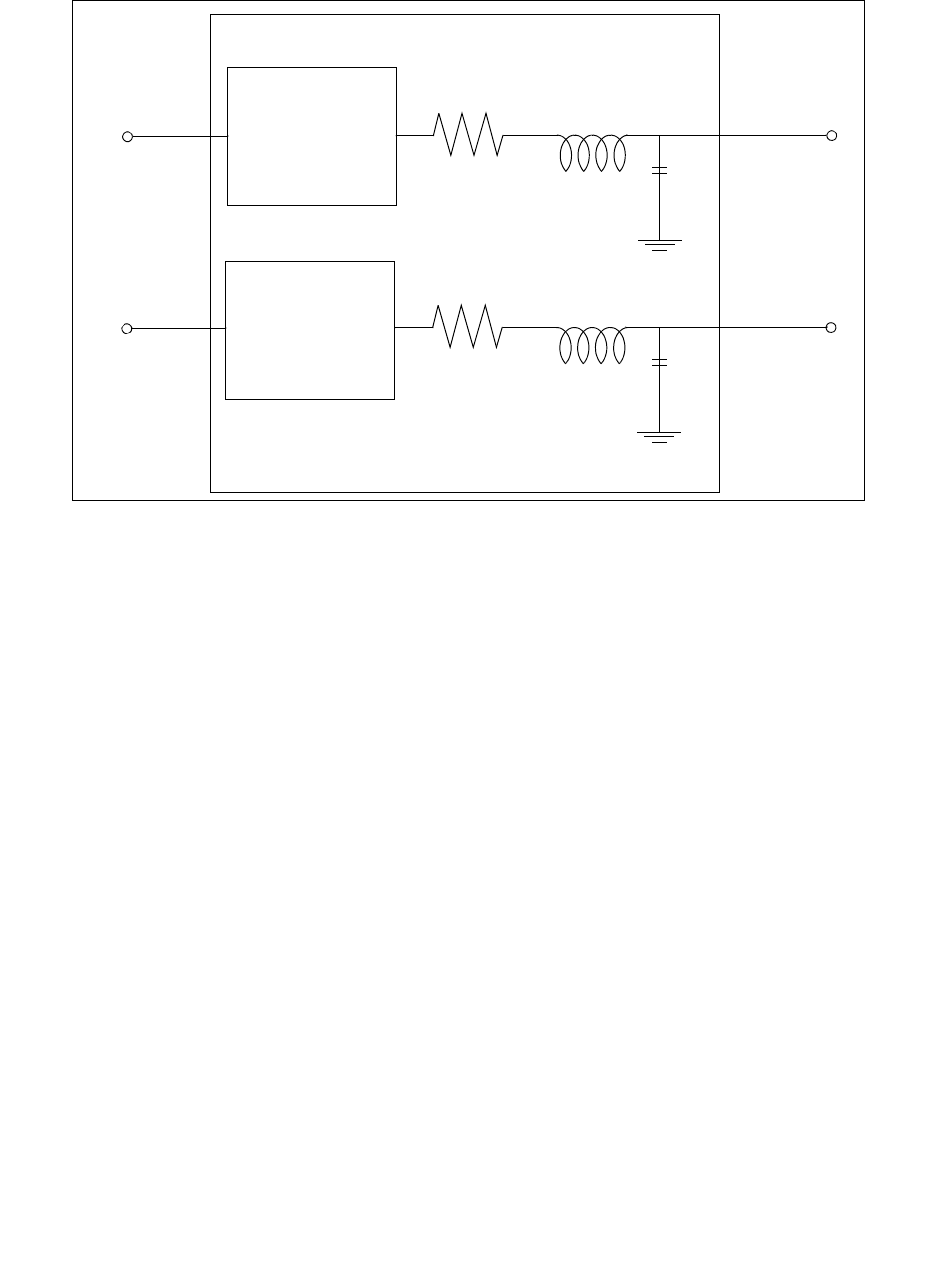
148 HSPICE® Reference Manual: Commands and Control Options
I-2013.12
Chapter 2: HSPICE Simulation Command Reference
Figure 8 Equivalent Circuit for IBIS Component Example
.IBIS cmpt1
+ file='example.ibs'
+ component='EXAMPLE'
+ mod_sel = 'DQ = DQ_FULL'
In the following example, the model DQ_FULL will be used for all pins that use
the model name DQ.The corresponding IBIS file, example.ibs, contains the
following [Model Selector] section:
|***********************MODEL SELECTOR***********************
|
Model Selector] DQ
|
DQ_FULL Full-Strength IO Driver
DQ_HALF 54% Reduced Drive Strength IO Driver
*
See Also
.EBD
.PKG
IBIS Examples (iob_ex1.sp) for demonstration files and see .IBIS
command use in ebd.sp and pinmap.sp
Component cmpnt
cmpnt_1
cmpnt_2
buffer cmpnt_nd1
buffer cmpnt_nd2
cmpnt_1_i
cmpnt_2_i
40.0m
50.0m
2n
3n
gnd
0.4p
0.5p
gnd

HSPICE® Reference Manual: Commands and Control Options 149
I-2013.12
Chapter 2: HSPICE Simulation Command Reference
.IC
Sets transient initial conditions in HSPICE.
Syntax
.IC V(node1)=val1 V(node2)=val2 ... [subckt=sub_name]
Description
Use the .IC command or the .DCVOLT command to set transient initial
conditions in HSPICE. How it initializes depends on whether the .TRAN
analysis command includes the UIC parameter. This command is less
preferred compared to using the.NODESET command in many cases.
The value set by an .IC statement is a Norton equivalent circuit that contains
the finite conductance value of GMAX (100 mhos by default). For most cases,
this model has good performance and accuracy. If a Norton equivalent circuit
created by that source is comparable with the conductance of other parts of the
circuit, the DC node voltages will deviate from those specified in the .IC
statement. To counteract such deviance, use .OPTION IC_ACCURATE=1.
When using the .IC command, forcing circuits are connected to the .IC nodes
for the duration of DC convergence. After DC convergence is obtained, the
forcing circuits are removed for all further analysis. The DC operating point for
each .IC'd node should be very close to the voltage specified in the .IC
command. If a node is not, then that node has a DC conductance to ground
comparable to GMAX. This is almost certainly an error condition. In the rare
case that it is not, GMAX can be increased to prevent appreciable current
division. Example: .OPTION GMAX=1000
Argument Description
val1 ... Specifies voltages. The significance of these voltages depends on
whether you specify the UIC parameter in the .TRAN command.
node1 ... Node numbers or names can include full paths or circuit numbers.
subckt=sub_name Initial condition is set to the specified node name(s) within all instances
of the specified subcircuit name. This subckt setting is equivalent to
placing the .IC statement within the subcircuit definition.

150 HSPICE® Reference Manual: Commands and Control Options
I-2013.12
Chapter 2: HSPICE Simulation Command Reference
Note: In nearly all applications, .NODESET should be used to ensure a
true DC operating point is obtained. Intentionally floating (or very
high impedance) nodes should be set to a known good voltage
using .IC.
If you do not specify the UIC parameter in the .TRAN command, HSPICE
computes the DC operating point solution before the transient analysis. The
node voltages that you specify in the .IC command are fixed to determine the
DC operating point. They are used only in the first iteration to set an initial
guess for the DC operating point analysis. The .IC command is equivalent to
specifying the IC parameter on each element command, but is more
convenient.
If you specify the UIC parameter in the .TRAN command, HSPICE does not
calculate the initial DC operating point, but directly enters transient analysis.
When you use .TRAN UIC, the .TRAN node values (at time zero) are
determined by searching for the first value found in this order: from .IC value,
then IC parameter on an element command, then .NODESET value, otherwise
use a voltage of zero.
Note that forcing a node value of the dc operating point may not satisfy KVL
and KCL. In this event you may likely see activity during the initial part of the
simulation.This may happen if UIC is used and some node values left
unspecified, when too many (conflicting) .IC values are specified, or when
node values are forced and the topology changes. In this event you may likely
see activity during the initial part of the simulation. Forcing a node voltage
applies a fixed equivalent voltage source during DC analysis and transient
analysis removes the voltage sources to calculate the second and later time
points.
Therefore, to correct DC convergence problems use .NODESETs (without
.TRAN UIC) liberally (when a good guess can be provided) and use .ICs
sparingly (when the exact node voltage is known).
In addition, you can use wildcards in the .IC command. See Using Wildcards
on Node Names in the HSPICE User Guide: Basic Simulation and Analysis.
Control Options
The following netlist control options are available for this command:
Option Description
.OPTION DCIC Specifies whether to use or ignore .IC commands in the netlist.

HSPICE® Reference Manual: Commands and Control Options 151
I-2013.12
Chapter 2: HSPICE Simulation Command Reference
Command Group
Setup
Examples
Example 1
.IC V(11)=5 V(4)=-5 V(2)=2.2
Example 2 All settings in this statement are applied to subckt my_ff.
.IC V(in)=0.9 subckt=my_ff
See Also
.DCVOLT
.TRAN
.NODESET
.ICM
Automatically creates port names that reference the pin name of an ICM model
and generate a series of element nodes on the pin.
Syntax
.ICM icmname
+ file='icmfilename'
+ model='icmmodelname'
.OPTION GMAX Specifies the maximum conductance in parallel with a current source for
.IC and .NODESET initialization circuitry.
.OPTION IC_ACCURATE Improves the accuracy of the .IC command.
Argument Description
icmname .ICM command card name.
icmfilename Name of an *.icm file that contains an ICM model.
icmmodelname Working model in an *.icm file.
Option Description

152 HSPICE® Reference Manual: Commands and Control Options
I-2013.12
Chapter 2: HSPICE Simulation Command Reference
Description
Use this command to automatically create port names that reference the pin
name of an ICM model and generate a series of element (W/S/RLGCK) nodes
on the pin when one of the following conditions occur:
■If the model is described using [Nodal Path Description]
'icmname'_'nodemapname'_'sidename'_'pinname'
■If the model is described using [Tree Path Description]
'icmname'_'pinmapname'_'sidename'_'pinname'
Note: If a side subparameter is not used in an ICM file, then
'sidename'_ (above) should be removed.
Command Group
Input/Output Buffer Information Specification (IBIS)
Examples
.ICM icm1
+ file='test1.icm'
+ model='FourLineModel1'
The following example shows how to reference a pin of the ICM model in a
HSPICE netlist.
icm1_NodeMap1_SideName1_pin1, icm1_NodeMap2_SideName2_pin1,
icm1_NodeMap2_SideName2_pin2, ...
See Also
IBIS Examples for .ICM command usage (RLGC approach—/icm/
nodepath_rlgc/bga_1.sp), (S-element approach—/icm/
nodepath_sele/test1.sp), (treepath—test1.sp), and treepath swath
matrix expansion (/icm/treepath_swath/complex.sp)
nodemapname Name of the [ICM node map] keyword in an .icm file.
pinmapname Name of the [ICM pin map] keyword in an .icm file.
pinname Name of the first column of entries of the [ICM node map] or [ICM
pin map].
sidename Name of the side subparameter
Argument Description

HSPICE® Reference Manual: Commands and Control Options 153
I-2013.12
Chapter 2: HSPICE Simulation Command Reference
.IF
Specifies conditions that determine whether HSPICE executes subsequent
commands in conditional block.
Syntax
.IF (condition1)...
+ [.ELSEIF (condition2)...]
+ [.ELSE ...]
.ENDIF
Description
HSPICE executes the commands that follow the first.ELSEIF command only if
condition1 in the preceding .IF command is false and condition2 in the
first .ELSEIF command is true.
If condition1 in the .IF command and condition2 in the first .ELSEIF
command are both false, then HSPICE moves on to the next .ELSEIF
command if there is one. If this second .ELSEIF condition is true, HSPICE
executes the commands that follow the second .ELSEIF command, instead of
the commands after the first .ELSEIF command.
HSPICE ignores the commands in all false .IF and .ELSEIF commands, until
it reaches the first .ELSEIF condition that is true. If no .IF or .ELSEIF
condition is true, HSPICE continues to the .ELSE command.
.ELSE precedes one or more commands in a conditional block after the
last .ELSEIF command, but before the .ENDIF command. HSPICE executes
these commands by default if the conditions in the preceding .IF command
Argument Description
condition1 Condition that must be true before HSPICE executes the commands
that follow the .IF command.
condition2 Condition that must be true before HSPICE executes the commands
that follow the .ELSEIF command. HSPICE executes the commands
that follow condition2 only if condition1 is false and condition2 is true.
(def(flag)) This function allows for checking whether a parameter exists (is
defined), and with the if-else construct allows for including certain
parts of a model or library, if the parameter has been defined elsewhere
in the netlist, or omit the part, if the parameter does not exist. The flag
can be the parameterName. See example 2 for syntax.

154 HSPICE® Reference Manual: Commands and Control Options
I-2013.12
Chapter 2: HSPICE Simulation Command Reference
and in all of the preceding .ELSEIF commands in the same conditional block
all false.
The .ENDIF command ends a conditional block of commands that begins with
an .IF command.
For information on use of conditional blocks with the Exploration Block, see,
Specifying Constraints in the HSPICE User Guide: Basic Simulation and
Analysis.
Command Group
Conditional Block
Examples
Example 1
.IF (a==b)
.INCLUDE /myhome/subcircuits/diode_circuit1
...
.ELSEIF (a==c)
.INCLUDE /myhome/subcircuits/diode_circuit2
...
.ELSE
.INCLUDE /myhome/subcircuits/diode_circuit3
...
.ENDIF
Example 2 Using the def (Defined) parameter so that if parameterName is available
it is included; if not it is excluded without generating an error.
.if (def(flag))
.inc "file1.dat"
.else
.inc "file2.dat"
.endif
See Also
.ELSE
.ELSEIF
.ENDIF
.INCLUDE / INC / INCL
Includes another netlist as a subcircuit of the current netlist.

HSPICE® Reference Manual: Commands and Control Options 155
I-2013.12
Chapter 2: HSPICE Simulation Command Reference
Syntax
.INCLUDE ‘file_pathfile_name’
Description
Use this command to include another netlist in the current netlist. You can
include a netlist as a subcircuit in one or more other netlists. You must enclose
the file path and file name in single or double quotation marks. Otherwise, an
error message is generated. Any file name following an .INC command is case
sensitive beginning with the 2009.09 release. You can define the models inside
of a subcircuit using .INCLUDE statements. The parameters defined in the
included models are global by default but you want any parameters defined in
the included file to be local to the subcircuit if you want to define a model that is
specific to only one subcircuit. This means that you will also need to set
.OPTION PARHIER=LOCAL so that parameter scoping rules are correct for
this case.
This command can be used as part of a compressed (.gzip) netlist file.
Control Options
The following netlist control options are available for this command:
Command Group
Subcircuits and Library Management
Argument Description
file_path Path name of a file for computer operating systems that support tree-
structured directories.
An include file can contain nested .INCLUDE calls to itself or to
another include file. If you use a relative path in a nested .INCLUDE
call, the path starts from the directory of the parent .INCLUDE file, not
from the current working directory. If the path starts from the current
working directory, HSPICE can also find the .INCLUDE file, but prints
a warning.
file_name Name of a file to include in the data file. The file path, plus the file
name, can be up to 16 characters long. You can use any valid file name
for the computer’s operating system.
Option Description
.OPTION PARHIER / PARHIE Specifies scoping rules for netlist parameters.

156 HSPICE® Reference Manual: Commands and Control Options
I-2013.12
Chapter 2: HSPICE Simulation Command Reference
Examples
Example 1 Simple syntax example
.INCLUDE `/myhome/subcircuits/diode_circuit´
Example 2 Showing use of .OPTION PARHIER
...
.option PARHIER=LOCAL
.subckt INV IN OUT
.include 'weak_ model.inc'
M1 ...
M2 ...
.ends INV
..
X1 IN OUT INV
..
See Also
.SUBCKT
.IVDMARGIN
Helps characterize Vdmargin using terminal I-V at MOSFET external nodes.
Syntax
.IVDMARGIN instance_name|macromodel_name DELTAGD=val
Description
Vdmargin, as shown in the following plot, is defined as the MOSFET drain
voltage range within which the change in the MOSFET drain conductance
Argument Description
instance_name When specified, this element uses the command-line specified
DELTAGD value for the iVdmargin calculation.
macromodel_name When specified, all the elements in the subcircuit use the command-
line specified DELTAGDS value for iVdmargin calculation.
DELTAGD Default=0.1. A positive variable in double type to define the relative
gd change on the right side of the equation. DELTAGD is typically in
a range of 0 to 1. If not specified, HSPICE uses DELTAGD=0.1.
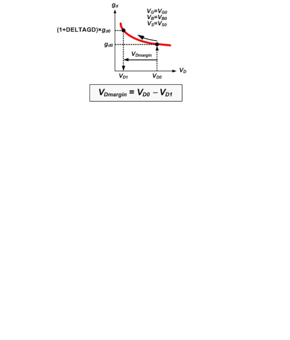
HSPICE® Reference Manual: Commands and Control Options 157
I-2013.12
Chapter 2: HSPICE Simulation Command Reference
(with repect to reference (the gd value at operating point) is
smaller than a user-specified target. It provides a heuristic measure of how
much the drain voltage can be reduced, particularly in the saturation region of
MOSFET operation, beyond which the MOSFET drain conductance has
degraded beyond a user-specified tolerance.
Command Group
Library Management
Examples
Example 1 The M3 instance uses DELTAGD=0.3.
.iVdmargin M3 DELTAGD=0.3
Example 2 Both M1 and M2 use DELTAGD=0.2.
.iVdmargin XM5 DELTAGD=0.2
XM5 n00 n01 vdd vss inv
.subckt inv in out vdd vss
M1 out in vss vss nch w=1e-6 l=0.3e-6
M2 out in vdd vdd pch w=1e-6 l=0.3e-6
.ends
gd ld•
vd•
---------------
=

158 HSPICE® Reference Manual: Commands and Control Options
I-2013.12
Chapter 2: HSPICE Simulation Command Reference
See Also
.OPTION IVDMARGIN
.IVTH
Invokes the constant-current based threshold voltage characterization.
Syntax
.IVTH model_name Ivth0=val DW=val DL=val VDSMIN=val
+ [.OPTION SX_factor=x]
Description
Use this command to enable constant current-based threshold voltage
characterization. The threshold voltage reported by iVth characterization is
defined as the MOSFET's gate-to-source voltage at which the drain terminal
current reaches the user-defined constant current value. The drain and body
biases of the device are set to their corresponding bias conditions in the circuit.
For example, in DCOP, the drain and body bias of the device is set to its
operating point condition. In DC sweep or transient analysis, drain and body
bias of the device is set to its solution at each sweep or time point.
The constant current for each MOSFET is given as follows:
Ivth=Ivth0 * (Wdrawn * SX_factor + DW)/(Ldrawn * SX_factor + DL)
Argument Description
model_name Model name that iVth characterization applies to.
Ivth0=val Constant drain terminal current density.
DW=val Width offset for iVth current calculation.
DL=val Length offset for iVth current calculation.
VDSMIN=val User-defined minimum vds value.
.OPTION SX_factor A special option, .OPTION SX_factor, is provided to scale the
width and length specifically for iVth characterization.

HSPICE® Reference Manual: Commands and Control Options 159
I-2013.12
Chapter 2: HSPICE Simulation Command Reference
VDSMIN provides a user-defined minimum Vds value and invokes a special
characterization method for small Vds bias to ensure continuation and
meaningful characterization result.
If VDSMIN is not given, the same iVth characterization methodology is applied
for all vds bias regions. If VDSMIN is not given, VDSMIN=0.05. If Vds is
smaller than VDSMIN, then:
1. Simulate Vth_op(Vdsmin) and Vth_ivth(Vdsmin) where: Vth_op() is the
threshold voltage acquired from model formulation, and vth_ivth() is the
threshold voltage acquired from iVth method.
2. Calculate DeltaVth = Vth_op(Vdsmin) - Vth_ivth(Vdsmin)
3. Simulate Vth_op(Vds)
4. Calculate Vth_ivth(Vds) = Vth_op(Vds) - DeltaVth
Multiple ivth commands can be added in a netlist to invoke characterization of
different models.
Command Group
Library Management
Examples
.ivth nch Ivth0=1.5e-7 DW=2e-8 DL=1e-8 VDSMIN=0.06
.ivth pch Ivth0=1e-7 DW=2e-8 DL=1e-8 VDSMIN=0.06
In OP analysis, a constant current based vth is reported in the OP output. In
addition, the element region operation check and Vod output are based on the
new vth.
During transient or DC analysis, template output of LX142(m*) or ivth(m*)
could be used for the new vth output.
.LAYERSTACK
Defines a stack of dielectric or metal layers.
Syntax
.LAYERSTACK sname [BACKGROUND=mname]
+ [LAYER=(mname,thickness) ...]

160 HSPICE® Reference Manual: Commands and Control Options
I-2013.12
Chapter 2: HSPICE Simulation Command Reference
Description
Use this command to define a stack of dielectric or metal layers. You must
associate each transmission line system with only one layer stack. However,
you can associate a single-layer stack with many transmission line systems.
In the layer stack:
■Layers are listed from bottom to top.
■Metal layers (ground planes) can be located only at the bottom, only at the
top, or both at the top and bottom.
■Layers are stacked in the y-direction; the bottom of a layer stack is at y=0.
■All conductors must be located above y=0.
■Background material must be dielectric.
The following limiting cases apply to the .LAYERSTACK command:
■Free space without ground:
.LAYERSTACK mystack
■Free space with a (bottom) ground plane where a predefined metal name =
perfect electrical conductor (PEC):
.LAYERSTACK halfSpace PEC 0.1mm
Command Group
Field Solver
See Also
.FSOPTIONS
.MATERIAL
.SHAPE
Transmission (W-element) Line Examples
Argument Description
sname Layer stack name.
mname Material name.
BACKGROUND Background dielectric material name. By default, the field solver
assumes AIR for the background.
thickness Layer thickness.

HSPICE® Reference Manual: Commands and Control Options 161
I-2013.12
Chapter 2: HSPICE Simulation Command Reference
.LIB
Creates and reads from libraries of commonly used commands, device models,
subcircuit analyses, and commands.
Syntax
Use the following syntax for library calls:
.LIB ‘[file_path] file_name’ entry_name
Use the following syntax to define library files:
.LIB entry_name1
. $ ANY VALID SET OF HSPICE STATEMENTS
.ENDL entry_name1
.LIB entry_name2
.
. $ ANY VALID SET OF HSPICE STATEMENTS
.ENDL entry_name2
.LIB entry_name3
.
. $ ANY VALID SET OF HSPICE STATEMENTS
.ENDL entry_name3
Description
Use the .LIB call command to read from libraries of commonly used
commands, device models, subcircuit analyses, and commands (library calls)
Argument Description
file_path Path to a file. Used where a computer supports tree-structured directories. When
the LIB file (or alias) is in the same directory where you run HSPICE you do not
need to specify a directory path; the netlist runs on any machine. Use “../” syntax
in the file_path to designate the parent directory of the current directory.
entry_name Entry name for the section of the library file to include. The first character of an
entry_name cannot be an integer. If more than one entry with the same name is
encountered in a file, only the first one is loaded.
file_name Name of a file to include in the data file. The combination of filepath plus
file_name can be up to 256 characters long, structured as any filename that is
valid for the computer’s operating system. Enclose the file path and file name in
single or double quotation marks. Use “../” syntax in the filename to designate
the parent directory of the current directory.

162 HSPICE® Reference Manual: Commands and Control Options
I-2013.12
Chapter 2: HSPICE Simulation Command Reference
in library files. Note that as HSPICE encounters each .LIB call name in the
main data file, it reads the corresponding entry from the designated library file,
until it finds an .ENDL command.
You can also place a .LIB call command in an .ALTER block.
To build libraries (library file definition), use the .LIB command in a library file.
For each macro in a library, use a library definition command (.LIB
entry_name) and an .ENDL command. The .LIB command begins the
library macro and the .ENDL command ends the library macro. The text after a
library file entry name must consist of HSPICE commands. Library calls can
call other libraries (nested library calls) if they are different files. You can nest
library calls to any depth. Use nesting with the .ALTER command to create a
sequence of model runs. Each run can consist of similar components by using
different model parameters without duplicating the entire input file.
The simulator uses the .LIB command and the .INCLUDE command to
access the models and skew parameters. The library contains parameters that
modify .MODEL commands.
You must enclose the file path and file name in single or double quotation
marks. Otherwise, an error message is generated. Any file name following
a.LIB command is case sensitive beginning with the 2009.09 release. To
terminate the .LIB command use .ENDL or .ENDL entry_name.
This command can be used as part of a compressed (.gzip) netlist file.
Command Group
Library Management
Examples
Example 1 is a simple library call.
* Library call
.LIB 'MODELS' cmos1
Example 2 shows the syntax of using any valid set of advanced analog
commands.
.LIB MOS7
$ Any valid set of HSPICE commands
.
.
.
.ENDL MOS7

HSPICE® Reference Manual: Commands and Control Options 163
I-2013.12
Chapter 2: HSPICE Simulation Command Reference
Example 3 is an example of illegal nested .LIB commands for the file3
library.
.LIB MOS7
...
.LIB 'file3' MOS7 $ This call is illegal in MOS7 library
...
.ENDL
Example 4 is a .LIB call command of model skew parameters and features
both worst-case and statistical distribution data. The statistical distribution
median value is the default for all non-Monte Carlo analyses. The model is in
the /usr/meta/lib/cmos1_mod.dat include file.
.LIB TT
$TYPICAL P-CHANNEL AND N-CHANNEL CMOS LIBRARY
$ PROCESS: 1.0U CMOS, FAB7
$ following distributions are 3 sigma ABSOLUTE GAUSSIAN
.PARAM TOX=AGAUSS(200,20,3) $ 200 angstrom +/- 20a
+ XL=AGAUSS(0.1u,0.13u,3) $ polysilicon CD
+ DELVTON=AGAUSS(0.0,.2V,3) $ n-ch threshold change
+ DELVTOP=AGAUSS(0.0,.15V,3)
$ p-ch threshold change
.INC ‘/usr/meta/lib/cmos1_mod.dat’
$ model include file
.ENDL TT
.LIB FF
$HIGH GAIN P-CH AND N-CH CMOS LIBRARY 3SIGMA VALUES
.PARAM TOX=220 XL=-0.03 DELVTON=-.2V
+ DELVTOP=-0.15V
.INC ‘/usr/meta/lib/cmos1_mod.dat’
$ model include file
.ENDL FF
In example 5, the .MODEL keyword (left side) equates to the skew parameter
(right side). A .MODEL keyword can be the same as a skew parameter.
.MODEL NCH NMOS LEVEL=2 XL=XL TOX=TOX
+ DELVTO=DELVTON .....
.MODEL PCH PMOS LEVEL=2 XL=XL TOX=TOX
+ DELVTO=DELVTOP .....
See Also
.ALTER
.ENDL / ENDLIB
.INCLUDE / INC / INCL

164 HSPICE® Reference Manual: Commands and Control Options
I-2013.12
Chapter 2: HSPICE Simulation Command Reference
.LIN
Extracts noise and linear transfer parameters for a general multiport network.
Syntax
Multiport Syntax
.LIN [sparcalc=[1|0] [modelname = modelname]]
+ [filename = filename]
+ [format=selem|citi|touchstone | touchstone2]
+ [noisecalc=[1|0] [gdcalc=[1|0]]
+ [mixedmode2port=dd|dc|ds|cd|cc|cs|sd|sc|ss]
+ [dataformat=ri|ma|db]
Two-Port Syntax
.LIN [sparcalc=1|0 [modelname = modelname]]
+ [filename = filename]
+ [format=selem|citi|touchstone | touchstone2]
+ [noisecalc=1|0] [gdcalc=1|0]
+ [mixedmode2port=dd|dc|ds|cd|cc|cs|sd|sc|ss]
+ [dataformat=ri|ma|db] [FREQDIGIT=x] [SPARDIGIT=x]
+ [listfreq=(frequencies|none|all|freq1 freq2...)]
+ [listcount=num] [listfloor=val] [listsources=1|0|yes|no]
Argument Description
sparcalc If 1, extract S parameters (default).
modelname Model name to be listed in the .MODEL command in the .sc#
model output file.
filename Output file name (The default is netlist name).
format Output file format:
■selem: S-element .sc# format, which you can include in
the netlist.
■citi:CITIfile format.
■touchstone and touchstone2:TOUCHSTONE v1.0 and v2.0
format, respectively.

HSPICE® Reference Manual: Commands and Control Options 165
I-2013.12
Chapter 2: HSPICE Simulation Command Reference
noisecalc Specifies level of N-port noise wave correlation matrix
extraction.
If 1, extract noise parameters (perform 2-port noise analysis).
The default is 0.
gdcalc If 1, extract group delay (perform group delay analysis). The
default is 0.
mixedmode2port The mixedmode2port keyword describes the mixed-mode
data map of output mixed mode S-parameter matrix. The
availability and default value for this keyword depends on the
first two port (P-element) configuration as follows:
■case 1: p1=p2=single (standard mode P element)
available: ss
default: ss
■case 2: p1=p2=balanced (mixed mode P element)
available: dd, cd, dc, cc
default: dd
■case 3: p1=balanced p2=single
available: ds, cs
default: ds
■case 4: p1=single p2=balanced
available: sd, sc
default: sd
dataformat The dataformat keyword describes the data format output to
the .sc#/touchstone1.0|2.0/citi file.
■dataformat=RI, real-imaginary. This is the default for
the .sc#/citi file.
■dataformat=MA, magnitude-phase. This is the default
format for touchstone file.
■dataformat=DB, DB(magnitude)-phase.
HSPICE uses six digits for both frequency and S-parameters
in HSPICE generated data files (.sc#/touchstone/citifile). The
number of digits for noise parameters are five in .sc# and
Touchstone files and six in CITIfiles.
Note: The lower limit of DB output is -300.
FREQDIGIT Sets the numerical precision (number of digits) for frequency
output in Touchstone, Citi, or sc# files. The default is 6.
Argument Description

166 HSPICE® Reference Manual: Commands and Control Options
I-2013.12
Chapter 2: HSPICE Simulation Command Reference
Description
Use this command to extract noise and linear transfer parameters for a general
multiport network.
When used with P- (port) element(s) and .AC commands, .LIN makes
available a broad set of linear port-wise measurements:
SPARDIGIT Sets the numerical precision (number of digits) for S
parameter output in Touchstone, Citi, or sc# files. The default
is 6.
listfreq=
(none|all|freq1req2....)
Dumps the element noise figure contribution to the total NF in
the *.lis file. You can specify at which frequencies HSPICE
dumps the element noise figure contribution. The elements
that contribute the largest noise figure are dumped first. The
frequency values can be specified by the NONE or ALL
keyword, which either dumps no frequencies or every
frequency defined in the AC sweep.
■ALL: Output all of the frequency points (default, if LIST* is
required).
■NONE - Do not output any of the frequency points.
■freq1 freq2...: Output the information on the specified
frequency points.
For example:
listfreq=none
listfreq=all
listfreq=1.0G
listfreq=1.0G 2.0G
listcount=num Outputs the first few noise elements that make the biggest
contribution to NF. The number is specified by num. The
default is to output all of the noise element contribution to NF.
The NF contribution is calculated with the source impedance
equal to the Zo of the first port.
listfloor=val Lists elements whose noise contribution to NF (in dB) are
higher than value specified in dB to .lis file. Default is 0.
listsources=[1|0|yes|no] Defines whether or not to output the contribution of each noise
source of each noise element. Default is no/0.
Argument Description

HSPICE® Reference Manual: Commands and Control Options 167
I-2013.12
Chapter 2: HSPICE Simulation Command Reference
■standard and mixed-mode multiport S- (scattering) parameters
■standard and mixed-mode multiport Y/Z parameters
■standard mode multiport H-parameter
■standard mode two-port noise parameters
■standard and mixed-mode group delays
■standard mode stability factors
■standard mode gain factors
■standard mode matching coefficients
The .LIN command computes the S-(scattering), Y-(admittance), Z-
(impedance) parameters directly, and H-(hybrid) parameters directly based on
the location of the port (P) elements in your circuit, and the specified values for
their reference impedances. The .LIN command also supports mixed-mode
transfer parameters calculation and group delay analysis when used together
with mixed-mode P elements.
To calculate the insertion and return loss for the high speed differential signal
on my PCB board you can use the .LIN command with a port (P) element at
input and output, where Port=1 defines the input and Port=2 defines the output.
The return loss in dB is |S111(DB)| and the insertion loss in dB is
|S21(DB)|.
By default, the .LIN command creates a .sc# file with the same base name as
your netlist. This file contains S-parameter, noise parameter, and group delay
data as a function of the frequency. You can use this file as model data for the
S-element. Noise contributor tables are generated for every frequency point
and every circuit device. The last four arguments allow users to better control
the output information. If the LIST* arguments are not set, .LIN 2port noise
analysis will output to .lis file with the older format. If any of the LIST*
arguments is set, the output information follows the syntax noted in the
arguments section.
Command Group
Analysis
Examples
This example extracts linear transfer parameters for a general multiport
network, performs a 2-port noise analysis and a group-delay analysis for a

168 HSPICE® Reference Manual: Commands and Control Options
I-2013.12
Chapter 2: HSPICE Simulation Command Reference
model named my_custom_model. The output is in the mydesign Touchstone
format output file. The data format in the Touchstone file is real-imaginary.
.LIN sparcalc=1 modelname=my_custom_model
+ filename=mydesign format=touchstone noisecalc=1
+ gdcalc=1 dataformat=ri
See Also
Filters Examples, fbpnet.sp, for a bandpass LCR filter demo using the
.LIN command
.LOAD
Uses the operating point information of a file previously created with a .SAVE
command (Not valid for advanced analog functions).
Syntax
.LOAD [FILE=load_file] [RUN=PREVIOUS|CURRENT]
Description
Use this command to input the contents of a file that you stored using
the .SAVE command. Files stored with the .SAVE command contain operating
point information for the point in the analysis at which you executed .SAVE.
Do not use the .LOAD command for concatenated netlist files.
This command can be used as part of a compressed (.gzip) netlist file.
Command Group
Setup and Library Management
Argument Description
load_file Name of the file in which .SAVE saved an operating point for the
circuit under simulation.The format of the file name is design.ic#.
Default is design.ic0, where design is the root name of the design.
RUN The format of file name is design.ic#. Used only outside of .ALTER
commands in a netlist that contains .ALTER commands.
■PREVIOUS: Each .ALTER uses the saved operating point from the
previous .ALTER run in the current simulation run.
■CURRENT: Each .ALTER uses the saved operating point from the
corresponding .ALTER run in the previous simulation run.

HSPICE® Reference Manual: Commands and Control Options 169
I-2013.12
Chapter 2: HSPICE Simulation Command Reference
Examples
Example 1 loads a file name design.ic0, which you previously saved using
a.SAVE command.
Example 1
.SAVE FILE=design.ic0
.LOAD FILE=design.ic0
$load--design.ic0 save--design.ic0
.alter
... $load--none save--design.ic1
.alter
... $load--none save--design.ic2
.end
Example 2 runs a previously saved and loaded design.
Example 2
.SAVE FILE=design.ic
.LOAD FILE=design.ic RUN=PREVIOUS
$load--none save--design.ic0
.alter
... $load--design.ic0 save--design.ic1
.alter
... $load--design.ic1 save--design.ic2
.end
Example 3 runs the current design.
Example 3
.SAVE FILE=design.ic
.LOAD FILE=design.ic RUN=CURRENT
$load--design.ic0 save--design.ic0
.alter
... $load--design.ic1 save--design.ic1
.alter
... $load--design.ic2 save--design.ic2
.end
See Also
.ALTER
.SAVE

170 HSPICE® Reference Manual: Commands and Control Options
I-2013.12
Chapter 2: HSPICE Simulation Command Reference
.LPRINT
Produces output in VCD (Value Change Dump) file format from transient
analysis in HSPICE. (Valid only for advanced analog functions and -HPP).
Syntax
.LPRINT (v1,v2) output_varable_list
Description
Use this command to produce output in VCD (Value Change Dump) file format
from transient analysis.
Command Group
Analysis
Examples
In this example, the .LPRINT command sets threshold values to 0.5 and 4.5,
and the voltage level at voltage source VIN.
.LPRINT (0.5,4.5) v(VIN)
See Also
.PRINT
.LSTB
Invokes linear loop stability analysis.
Syntax
Vxxx drv fbk 0
.LSTB mode=[single|diff|comm]
+ vsource=[vlstb|vlstbp,vlstbn]
.PRINT|PROBE AC
Argument Description
v1, v2 Threshold values for digital output. Values less than v1 are output
as digital 0. Values greater than 1 are output as digital 1.
output_varable_list Output variables to .PRINT. These are variables from a DC, AC,
TRAN, or NOISE analysis).

HSPICE® Reference Manual: Commands and Control Options 171
I-2013.12
Chapter 2: HSPICE Simulation Command Reference
+ LSTB|LSTB(DB)|LSTB(M)|LSTB(P)|LSTB(R)|LSTB(I)
Description
The .LSTB command measures the loop gain by successive injection
(Middlebrook’s Technique). A 0V voltage source is placed in series in the loop:
one pin of the voltage loop must be connected to the loop input, the other pin to
the loop output. The orientation of inserted voltage sources in differential and
common-mode testing is significant. It is required that the positive terminal of
both voltage sources go to the input of amplifier or go to the output of amplifier.
The first 3 characters of the mode type are effective (sin, dif or com). For single-
ended (default mode) test: place one 0V DC voltage source in series and
specify its name in the loop of interest, then add the .LSTB statement and
specify single as mode. For differential and common-mode loop analysis, set
diff or comm as the mode and specify the names of two 0V DC voltage
sources.
Argument Description
Vxxx The 0V voltage source(s) indicating the insertion point of test circuit. Note that
the direction of Vxxx is of significance in diff/comm mode analysis.
■drv: Driving node (i.e., input of amplifier)
■fbk: Feedback node (i.e., output of amplifier)
mode ■Single: (default) single-ended test. Single mode analysis is used to deal
with feedback circuit with only one single signal path.
■Diff: differential mode test.
■Comm: common mode test.
If the feedback loop has a differential amplifier, then there are two signal paths.
In this situation, diff and comm mode should be used, respectively, to calculate
the differential and common mode loop gain.
Vsource ■Vlstb: The only one vsource for single-ended mode test.
■Vlstbp: One of the two vsources for differential or common mode test.
■Vlstpn: The other one of the two vsources for differential or common mode
test.
LSTB Output all results: dB, magnitude, phase, real and imaginary part of loop gain.
LSTB(x) ■x=DB: Output the dB values of loop gain.
■X=M: Output magnitude of loop gain.
■X=P: Output phase of loop gain.
■X=R: Output real part of loop gain.
■X=I: Output imaginary part of loop gain.

172 HSPICE® Reference Manual: Commands and Control Options
I-2013.12
Chapter 2: HSPICE Simulation Command Reference
.MEASURE statements are supported similar to any ac output variables. The
feature can be used with .ALTER to generate multiple loop analyses. (See
examples below.)
The outputs for loop stability analysis are as follows:
■The gain margin (GM), phase margin (PM), unity gain frequency (FU) and
gain at minimum frequency (ADC) are reported in the *.lis file.
■The Loop Gain is reported to the *.cx# file, which is always produced for
.LSTB analysis. The *.cx# file is a general file for all the complex number
outputs. It contains the data for waveforms as complex vectors.
■If you specify.probe ac lstb(db) lstb(mag) lstb(real)
lstb(imag) lstb(phase), the specific format of loop gain goes to the
*.ac# file for viewing.
■If an *.ac# file is produced with .probe ac lstb, then both *.ac# and
*.cx# file could be used to view magnitude, phase, real, and imaginary
versus frequency as complex vectors.
Considerations regarding loop stability analysis include the following:
■.LSTB analysis is based on a linearized circuit at a given DC operating
point. It does not guarantee a stable condition for large signal condition. As
a final stability check, designers should perform transient analysis; i.e.,inject
a slow sinusoid superimposed with a series of fast pulses into the loop; the
amount of ringing indicates the degree of stability for the circuit.
■All other independent AC voltage sources are disabled automatically
when.LSTB is enabled.
■.OPTION UNWRAP is set to 1 and if phase wrapping is found, the phase is
corrected by 180 degrees.
■If phase/gain margin is not found in the given ac analysis frequency range,
a warning message is issued.
Control Options
The following netlist control options are available for this command:
Option Description
.OPTION UNWRAP Displays phase results for AC analysis in unwrapped form.

HSPICE® Reference Manual: Commands and Control Options 173
I-2013.12
Chapter 2: HSPICE Simulation Command Reference
Command Group
Analysis
Examples
Example 1 This example shows a sample portion of a netlist where the first two lines
are the 0 voltage sources indicating the insertion point of circuit under
test; line 3 sets the .LSTB analysis using the differential mode and
specifies the two vsources; line 4 sets the .AC analysis, and the last three
lines specify post-processing (printing, plotting, and measurements).
V1 n1 n2 0
V2 n3 n4 0
.LSTB mode=diff vsource=v1,v2
.AC DEC 10 1K 1MEG
.PRINT AC LSTB(DB) LSTB(M) LSTB(P) LSTB(R) LSTB(I)
.PROBE AC LSTB(DB) LSTB(M) LSTB(P) LSTB(R) LSTB(I)
.MEASURE AC phase_margin FIND LSTB(P) when LSTB(DB)=0
Example 2 The .MEASURE statement is supported such as any common ac output
variable.
.measure ac phase_margin FIND lstb(P) when lstb(db)=0
.measure ac integ1 INTEGRAL lstb(P) FROM=1k TO=100k
Example 3 In this example, the lstb scalars are measured in which lstb is the type
name, out1-out4 are names for output, followed by scalar variable
keywords:
.measure lstb out1 gain_margin
.measure lstb out2 phase_margin
.measure lstb out3 unity_gain_freq
.measure lstb out4 loop_gain_minifreq
Example 4 A series of loop stability analyses are supported by the .alter command.
V3 n3 n4 0
.lstb mode=single vsource=V3
.alter
V4 n5 n6 0
V5 n7 n8 0
.lstb mode=common vsource=v4, v5
See Also
.AC
.ALTER
.MEASURE LSTB
.PRINT

174 HSPICE® Reference Manual: Commands and Control Options
I-2013.12
Chapter 2: HSPICE Simulation Command Reference
.PROBE
Using .LSTB for Loop Stability Analysis
.MACRO
Defines a subcircuit in your netlist.
Syntax
.MACRO subckt_namen1 [n2n3...] [parnam=val]
.EOM
Description
Use this command to define a subcircuit in your netlist (effectively the same as
the .SUBCKT command). You can create a subcircuit description for a
commonly used circuit and include one or more references to the subcircuit in
your netlist. Use the .EOM command to terminate a .MACRO command.
Command Group
Subcircuits
Examples
Example 1 defines two subcircuits: SUB1 and SUB2. These are resistor divider
networks, whose resistance values are parameters (variables). The X1, X2,
Argument Description
subckt_nam reference name for the subcircuit model call.
n1 ... Node numbers for external reference; cannot be the ground node
(zero). Any element nodes that are in the subcircuit, but are not in
this list strictly local with three exceptions:
■Ground node (zero).
■Nodes assigned using BULK=node in MOSFET or BJT models.
■Nodes assigned using the .GLOBAL command.
parnam Parameter name set to a value. Use only in the subcircuit. To
override this value, assign it in the subcircuit call or set a value in
a.PARAM command.
SubDefaultsList SubParam1=Expression
[SubParam2=Expression...]

HSPICE® Reference Manual: Commands and Control Options 175
I-2013.12
Chapter 2: HSPICE Simulation Command Reference
and X3 commands call these subcircuits. Because the resistor values are
different in each call, these three calls produce different subcircuits.
Example 1
*FILE SUB2.SP TEST OF SUBCIRCUITS
.OPTION LIST ACCT
V1 1 0 1
.PARAM P5=5 P2=10
.SUBCKT SUB1 1 2 P4=4
R1 1 0 P4
R2 2 0 P5
X1 1 2 SUB2 P6=7
X2 1 2 SUB2
.ENDS
*
.MACRO SUB2 1 2 P6=11
R1 1 2 P6
R2 2 0 P2
.EOM
X1 1 2 SUB1 P4=6
X2 3 4 SUB1 P6=15
X3 3 4 SUB2
*
.MODEL DA D CJA=CAJA CJP=CAJP VRB=-20 IS=7.62E-18
+ PHI=.5 EXA=.5 EXP=.33
.PARAM CAJA=2.535E-16 CAJP=2.53E-16
.END
Example 2 implements an inverter that uses a Strength parameter. By default,
the inverter can drive three devices. Enter a new value for the Strength
parameter in the element line to select larger or smaller inverters for the
application.
Example 2
.SUBCKT Inv a y Strength=3
Mp1 <MosPinList> pMosMod L=1.2u W=’Strength * 2u’
Mn1 <MosPinList> nMosMod L=1.2u W=’Strength * 1u’
.ENDS
...
xInv0 a y0 Inv $ Default devices: p device=6u,
$ n device=3u
xInv1 a y1 Inv Strength=5 $ p device=10u, n device=5u
xInv2 a y2 Inv Strength=1 $ p device= 2u, n device=1u
...
See Also
.ENDS

176 HSPICE® Reference Manual: Commands and Control Options
I-2013.12
Chapter 2: HSPICE Simulation Command Reference
.EOM
.SUBCKT
.MALIAS
Assigns an alias to a diode, BJT, JFET, or MOSFET model that you defined in
a.MODEL command.
Syntax
.MALIAS model_name=alias_name1 [alias_name2 ...]
Description
Use this command to assign an alias (another name) to a diode, BJT, JFET, or
MOSFET model that you defined in a .MODEL command.
.MALIAS differs from .ALIAS in two ways:
■A model can define the alias in an .ALIAS command, but not the alias in
a.MALIAS command. The .MALIAS command applies to an element (an
instance of the model), not to the model itself.
■The .ALIAS command works only if you include .ALTER in the netlist. You
can use .MALIAS without .ALTER.
You can use .MALIAS to alias to a model name that you defined in a .MODEL
command or to alias to a subcircuit name that you defined in a .SUBCKT
command. The syntax for .MALIAS is the same in either usage.
Note: The .MALIAS command is supported for diode, BJT, JFET, and
MOSFET models in .Global_Variation and
.Local_Variation blocks.
Command Group
Model and Variation
Argument Description
model_name Model name defined in the .MODEL card
alias_name1... Alias that an instance (element) of the model references

HSPICE® Reference Manual: Commands and Control Options 177
I-2013.12
Chapter 2: HSPICE Simulation Command Reference
Examples
■zendef is a diode model
■zen and zend are its aliases.
■The zendef model points to both the zen and zend aliases.
*file: test malias statement
.OPTION acct tnom=50 list gmin=1e-14 post
.temp 0.0 25
.tran .1 2
vdd 2 0 pwl 0 -1 1 1
d1 2 1 zend dtemp=25
d2 1 0 zen dtemp=25
* malias statements
.malias zendef=zen zend
* model definition
.model zendef d (vj=.8 is=1e-16 ibv=1e-9 bv=6.0 rs=10
+ tt=0.11n n=1.0 eg=1.11 m=.5 cjo=1pf tref=50)
.end
See Also
.ALIAS
.MODEL
.MATERIAL
Specifies material to be used with the HSPICE field solver.
Syntax
.MATERIAL mname METAL|DIELECTRIC [ER=val]
+ [UR=val] [CONDUCTIVITY=val] [LOSSTANGENT=val]
+ ROUGHNESS=val
Argument Description
mname Material name.
METAL|DIELECTRIC Material type: METAL or DIELECTRIC.
ER Dielectric constant (relative permittivity).
UR Relative permeability.

178 HSPICE® Reference Manual: Commands and Control Options
I-2013.12
Chapter 2: HSPICE Simulation Command Reference
Description
The field solver assigns the following default values for metal:
CONDUCTIVITY=-1 (perfect conductor), ER=1, UR=1.
PEC (perfect electrical conductor) is a predefined metal name. You cannot
redefine its default values.The field solver assigns default values for dielectrics:
■CONDUCTIVITY=0 (lossless dielectric)
■LOSSTANGENT=0 (lossless dielectric)
■ER=1
■UR=1
AIR is a predefined dielectric name. You cannot redefine its default values.
Because the field solver does not currently support magnetic materials, it
ignores UR values.
Command Group
Field Solver
See Also
.LAYERSTACK
.FSOPTIONS
Transmission (W-element) Line Examples
.MEASURE / MEAS
Modifies information to define the results of successive simulations.
Syntax
See the links below for the various syntaxes.
CONDUCTIVITY Static field conductivity of conductor or lossy dielectric (S/m).
LOSSTANGENT Alternating field loss tangent of dielectric (tan ).
ROUGHNESS RMS surface roughness height, used when scaling the field
solver.
Argument Description
δ

HSPICE® Reference Manual: Commands and Control Options 179
I-2013.12
Chapter 2: HSPICE Simulation Command Reference
Description
Use this command to modify information and to define the results of successive
HSPICE simulations. The .MEASURE command prints user-defined electrical
specifications of a circuit. Optimization uses .MEASURE commands extensively.
You can shorten the command name to .MEAS. The specifications include:
■Propagation
■Delay
■RIse time
■Fall time
■Peak-to-peak voltage
■Minimum and maximum voltage over a specified period
■Other user-defined variables
You can also use .MEASURE with either the error function (ERRfun) or GOAL
parameter to optimize circuit component values, and to curve-fit measured data
to model parameters.
The .MEASURE command can use several different formats, depending on the
application. You can use it for DC sweep, and AC or transient analyses.
Note: If a .measure command uses the result of previous .meas
command, then the calculation starts when the previous result is
found. Until the previous result is found, it outputs zero.
Control Options
The following netlist control options are available for this command:
Option Description
.OPTION NCWARN Allows turning on a switch to report a warning message for
negative conductance on MOSFETs.
.OPTION MEASFAIL Specifies where to print the failed measurement output.
.OPTION MEASFILE Controls whether measure information outputs to single or
multiple files when an .ALTER command is present in the netlist.
.OPTION MEASOUT Outputs .MEASURE / MEAS command values and sweep
parameters into an ASCII file.

180 HSPICE® Reference Manual: Commands and Control Options
I-2013.12
Chapter 2: HSPICE Simulation Command Reference
Command Group
Output Porting
Examples
To measure the difference between two different nodes in a dc analysis:
.MEAS dc V1 MAX V(1)
.MEAS dc V2 MAX V(2)
.MEAS VARG PARAM="(V2 - V1)"
See Also
.MEASURE (Rise, Fall, Delay, and Power Measurements)
.MEASURE (FIND and WHEN)
.MEASURE (Equation Evaluation/Arithmetic Expression)
.MEASURE (AVG, EM_AVG, INTEG, MIN, MAX, PP, and RMS)
.MEASURE (Integral Function)
.MEASURE (Derivative Function)
.MEASURE (Error Function)
.MEASURE (Pushout Bisection)
.MEASURE (ACMATCH)
.MEASURE (DCMATCH)
.MEASURE FFT
.MEASURE LSTB
.AC
.DC
.DCMATCH
.DOUT
.PRINT
.PROBE
.STIM
.TRAN
Measuring Total Noise
Measuring the Value of MOSFET Model Card Parameters
.MEASURE (Rise, Fall, Delay, and Power
Measurements)
Measures independent-variable differentials such as rise time, fall time, and
slew rate.

HSPICE® Reference Manual: Commands and Control Options 181
I-2013.12
Chapter 2: HSPICE Simulation Command Reference
Syntax
The following are parameters for the TRIG and TARG subcommands.
Trigger and Target Subcommands
.MEASURE [DC|AC|TRAN] ResultName TRIG TrigSpec TARG TargSpec
+ [GOAL=val][MINVAL=val][WEIGHT=val][PRINT 0|1][FROM=val]
+ [TO=val]
For example:
.MEASURE TRAN TCLK2BL7R_1 TRIG V(CLK)='VAL50' FALL=2
+ TARG V(XI0.BL7_bot_L_E)='VAL50' RISE=1 FROM=TBR1 TO=TBR2
The input syntax for delay, rise time, and fall time in HSPICE is:
.MEASURE [TRAN] varname TRIG_SPECTARG_SPEC
In this syntax, varname is the user-defined variable name for the measurement
(the time difference between TRIG and TARG events). The input syntax for
TRIG_SPEC and TARG_SPEC is:
TRIG var VAL=val [TD=time] [CROSS=c|LAST]
+ [RISE=r|LAST] [FALL=f|LAST][TRIG AT=time]
TARG var VAL=val [TD=time-delay] [CROSS=c|LAST|PREVIOUS]
+ [RISE=r|LAST|PREVIOUS] [FALL=f|LAST|PREVIOUS]
+ [REVERSE][TARG AT=time]
Argument Description
DC | AC | TRAN Analysis type of the measurement. If you omit this
parameter, HSPICE uses the last analysis mode that you
requested.
result Name associated with the measured value in the HSPICE
output, can be up to 16 characters long. This example
measures the independent variable, beginning at the trigger
and ending at the target:
■Transient analysis measures time.
■AC analysis measures frequency.
■DC analysis measures the DC sweep variable.
If simulation reaches the target before the trigger activates,
the resulting value is negative.Do not use DC, TRAN, or AC
as the result name.
TRIG Beginning of trigger specifications.

182 HSPICE® Reference Manual: Commands and Control Options
I-2013.12
Chapter 2: HSPICE Simulation Command Reference
TAR G Beginning of the target specification.
TrigSpec OutputVar VAL={Number|'Expression'}
[TD={Numeric|'Expression'}] where: NumericExpression=
{FloatingPointNumber|'AlgebraicExpression'} See Using
Algebraic Expressions for information on algebra in output
statements.
Tar g Sp e c OutputVar VAL={Numeric|'Expression'}
[TD={Number|'Expression'}] where: NumericExpression:=
{FloatingPointNumber|'AlgebraicExpression'} See Using
Algebraic Expressions for information on algebra in output
statements. If a time-delay is not specified for the Target, the
TD is inherited from the Trigger value.
GOAL=val Desired measure value in ERR calculation for optimization.
To calculate the error, the simulation uses the equation:
.
MINVAL If the absolute value of GOAL is less than MINVAL, the
MINVAL replaces the GOAL value in the denominator of the
ERRfun expression. Used only in ERR calculation for
optimization. The default is 1.0e-12.
WEIGHT Multiplies the calculated error by the weight value. Used only
in ERR calculation for optimization. The default is 1.0.
PRINT ■print=0 prevents the printing a measure result into the
measure output file
■print=1 (Default) prints the measure result into the output
file
FROM... TO... Allows adding single XRANGE conditions for TRIG/TARG
measurements.
trig_var Value of trig_var, which increments the counter by one for
crossings, rises, or falls. See Using Algebraic Expressions
for information on algebra in output statements.
Argument Description
ERRfun GOAL result–()GOAL⁄=

HSPICE® Reference Manual: Commands and Control Options 183
I-2013.12
Chapter 2: HSPICE Simulation Command Reference
Description
Use the Rise, Fall, and Delay form of the .MEASURE command to measure
independent-variable (time, frequency, or any parameter or temperature)
differentials such as rise time, fall time, slew rate, or any measurement that
requires determining independent variable values. This format specifies TRIG
and TARG subcommands. These two commands specify the beginning and end
of a voltage or current amplitude measurement.
trig_var Specifies the name of the output variable that determines the
logical beginning of a measurement. If HSPICE reaches the
target before the trigger activates, .MEASURE reports a
negative value. See Using Algebraic Expressions for
information on algebra in output statements.
PREVIOUS Use the PREVIOUS keyword as an alternative to targ
xnumber. If PREVIOUS is set, the last possible target event
previous to the trigger event is computed.
REVERSE The REVERSE keyword is used to reverse the direction of the
measure. For any measure where RISE, FALL or CROSS is
used, the REVERSE keyword allows the measure to start at
the end of the simulation time and end at time=0 or the
delay time defined by TD.
TD Amount of simulation time that must elapse before HSPICE
enables the measurement. Simulation counts the number of
crossings, rises, or falls only after the time_delay value.
Default trigger delay is zero. If a time-delay is not specified
for the Target, the TD is inherited from the Trigger value.
AT=va l Special case for trigger specification. val is:
■Time for TRAN analysis.
■Frequency for AC analysis.
■Parameter for DC analysis.
■SweepValue from .DC mismatch analysis.
The trigger determines where measurement takes place.
Argument Description

184 HSPICE® Reference Manual: Commands and Control Options
I-2013.12
Chapter 2: HSPICE Simulation Command Reference
Control Options
The following netlist control options are available for this command:
Command Group
Output Porting
Examples
Example 1 HSPICE automatically measures T_prop using the .MEASURE
command. This reference file contains .MEAS commands for rising edge
and falling edge measurements. The time delay is measured and saved
during simulation in an *.mt0 file. Note that if a falling edge simulation is
run, the rising edge measurements are invalid. Similarly, if a rising edge
simulation is run, the falling edge measurements are invalid. (Remember
this when referring to the *.mt0 file after a simulation.) In this sample
file, .MEASURE statements are provided to measure T_prop from the
ref_50pf waveform to each of ten loads. Since each load is measured, the
worst-case T_prop for a given configuration can be quickly determined by
finding the largest value. The .MEASURE commands work by “triggering”
on the ref_50pf signal as it crosses 1.5 volts, and ending the
measurement when the “target” waveform, crosses the specified voltage
for the last time. For rising edge measurements, this value is 2.0 Volts.
For falling edge measurements, the value is 0.8 Volt. Examples from a
sample file are listed here.
***************************************************************
* Rising edge T_prop measurements *
***************************************************************
.MEAS tran tr1_val TRIG V(ref_50pf) val=1.5v td=’per/2’ cross=1
+ TARG V(load1) val=2.0v rise=last
.MEAS tran tr2_val TRIG B(ref_50pf) val=1.5v td=’per/2’ cross=1
+TARG V(load2) val=2.0v rise=last
.
.
.
.MEAS tran tr10_val TRIG V(ref_50pf) val=1.5v td=’per/2 cross=1
+ TARG V(load10) val=2.0v rise=last
***************************************************************
* Falling edge T_prop measurements *
***************************************************************
.MEAS tran tf1_val TRIG V(ref_50pf val=1.5v td=’per/2’ cross=1
+TARG V(load1) val=0.8v fall=last
.
.
Option Description
.OPTION AUTOSTOP / AUTOST Stops a transient analysis in HSPICE after calculating all
TRIG-TARG, FIND-WHEN, and FROM-TO measure functions.

HSPICE® Reference Manual: Commands and Control Options 185
I-2013.12
Chapter 2: HSPICE Simulation Command Reference
.
.MEAS tran tf10_vasl TRIG V(ref_50pf) vbal=1.5v td=’per/2’ cross=1
+ TARFG V(load10) val=0.8v fall=last
Example 2 Measures the propagation delay between nodes 1 and 2 for a transient
analysis. HSPICE measures the delay from the second rising edge of the
voltage at node 1 to the second falling edge of node 2. Measurement
begins when the second rising voltage at node 1 is 2.5 V and ends when
the second falling voltage at node 2 is 2.5 V. The TD=10n parameter
counts the crossings after 10 ns have elapsed. HSPICE prints results as
tdlay=value.
* Example of rise/fall/delay measurement
.MEASURE TRAN tdlay TRIG V(1) VAL=2.5 TD=10n
+ RISE=2 TARG V(2) VAL=2.5 FALL=2
Example 3 TRIG AT=10n starts measuring time at t=10 ns in the transient analysis.
The TARG parameters terminate time measurement when V(IN) = 2.5 V
on the third crossing. pwidth is the printed output variable. If you use
the .TRAN analysis command with a .MEAS command, do not use a
non-zero start time in the .TRAN command to avoid incorrect .MEAS
results.
.MEASURE TRAN riset TRIG I(Q1) VAL=0.5m RISE=3
+ TARG I(Q1) VAL=4.5m RISE=3
* Rise/fall/delay measure with TRIG and TARG specs
.MEASURE pwidth TRIG AT=10n TARG V(IN) VAL=2.5
+ CROSS=3
Example 4 This excample shows a target delayed until the trigger time before the
target counts the edges.
.MEAS TRAN TDEL12 TRIG V(signal1) VAL='VDD/2'
+ RISE=10 TARG V(signal2) VAL='VDD/2' RISE=1 TD=TRIG
Example 5 This example uses the cross keyword to calculate the final settled value
when you do not know how many times the signal crosses the final value.
.meas tran tim2 when v(out)='final_value' cross=last
Example 6 In this example, print=0 prevents the printing of Vmax to the *.mt0 and
*.lis files. Delay is output into *.mt# file and *.lis file.
.meas tran Vmax max v(out) print=0
.meas tran delay trig V(in) val=’vmax/2’ rise=1 targ v(out)
+ val=’vmax/2’ rise=1
See Also
Filters Examples, fbp_1.sp, for a bandpass LCR filter measurement demo
netlist

186 HSPICE® Reference Manual: Commands and Control Options
I-2013.12
Chapter 2: HSPICE Simulation Command Reference
.MEASURE (FIND and WHEN)
Measures independent and dependent variables (as well as derivatives of
dependent variables if a specific event occurs).
Syntax
.MEASURE [DC|AC|TRAN] result WHEN out_var=val [TD=val]
+ [FROM=val] [TO=val]
+ [RISE=r|LAST][FALL=f|LAST][CROSS=c|LAST][REVERSE]
+ [[GOAL=val]|GOALMAX|GOALMIN] [MINVAL=val] [WEIGHT=val]
+ [PRINT 0|1]
.MEASURE [DC|AC|TRAN] result
+ WHEN out_var1=out_var2 [TD=val] [RISE=r|LAST]
+ [FALL=f|LAST] [CROSS=c|LAST]
+ [[GOAL=val] [GOALMAX|GOALMIN] [MINVAL=val]
+ [WEIGHT=val] [PRINT 0|1]
.MEASURE [DC|AC|TRAN] result FIND out_var1
+ WHEN out_var2=val [TD=val] [FROM=val] [TO=val]
+ [RISE=r|LAST][FALL=f|LAST] [CROSS=c|LAST] [REVERSE]
+ [[GOAL=val]|GOALMAX|GOALMIN][MINVAL=val] [WEIGHT=val]
+ [PRINT 0|1]
.MEASURE [DC|AC|TRAN] result FIND out_var1
+ WHEN out_var2=out_var3 [TD=val]
+ [RISE=r|LAST] [FALL=f|LAST] [REVERSE] [CROSS=c|LAST]
+ [[GOAL=val]|GOALMAX|GOALMIN] [MINVAL=val] [WEIGHT=val]
+ [PRINT 0|1]
.MEASURE [DC|AC|TRAN] result FIND out_var1
+ AT=val [FROM=val] [TO=val]
+[[GOAL=val]|GOALMAX|GOALMIN][MINVAL=val]
+[WEIGHT=val] [PRINT 0|1]
Argument Description
DC | AC | TRAN Analysis type of the measurement. If you omit this
parameter, HSPICE uses the last analysis mode that you
requested.
result Name of a measured value in the HSPICE output.

HSPICE® Reference Manual: Commands and Control Options 187
I-2013.12
Chapter 2: HSPICE Simulation Command Reference
WHEN WHEN function.
out_var(1,2,3) Variables that establish conditions to start a
measurement.
TD Time at which measurement starts.
FROM... TO... Allows adding multiple trigger conditions to some WHEN
measurements.
CROSS=c
RISE=r
FALL=f
Numbers indicate which CROSS, FALL, or RISE event to
measure. For example:
.meas tran tdlay trig v(1) val=1.5 td=10n
+ rise=2 targ v(2) val=1.5 fall=2
In this example, rise=2 specifies the measure of the v(1)
voltage only on the first two rising edges of the waveform.
The value of these first two rising edges is 1. However, trig
v(1) val=1.5 indicates to trigger when the voltage on the
rising edge voltage is 1.5, which never occurs on these
first two rising edges. So the v(1) voltage measurement
never finds a trigger.
RISE=r, the WHEN condition is met and measurement
occurs after the designated signal has risen r rise times.
FALL =f, measurement occurs when the designated signal
has fallen f fall times.
A crossing is either a rise or a fall so for CROSS=c,
measurement occurs when the designated signal has
achieved a total of c crossing times as a result of either
rising or falling.
For TARG, the LAST keyword specifies the last event.
LAST HSPICE measures when the last CROSS, FALL, or RISE
event occurs.
■CROSS=LAST, measurement occurs the last time the
WHEN condition is true for a rising or falling signal.
■FALL=LAST, measurement occurs the last time the
WHEN condition is true for a falling signal.
■RISE=LAST, measurement occurs the last time the
WHEN condition is true for a rising signal.
LAST is a reserved word; you cannot use it as a parameter
name in the above .MEASURE commands.
Argument Description

188 HSPICE® Reference Manual: Commands and Control Options
I-2013.12
Chapter 2: HSPICE Simulation Command Reference
REVERSE The REVERSE keyword is used to reverse the direction of
the measure. For any measure where RISE, FALL or
CROSS is used, the REVERSE keyword allows the measure
to start at the end of the simulation time and end at
time=0 or the delay time defined by TD.
GOAL=val Desired .MEASURE value. Optimization uses this value in
ERR calculation. The following equation calculates the
error:
In HSPICE output you cannot apply .MEASURE to
waveforms generated from another .MEASURE command
in a parameter sweep.
GOALMAX | GOALMIN Use bisection method to get maximum/minimum measure
value.
MINVAL If the absolute value of GOAL is less than MINVAL, then
MINVAL replaces the GOAL value in the denominator of
the ERRfun expression. Used only in ERR calculation for
optimization. The default is 1.0e-12.
WEIGHT Calculated error multiplied by the weight value. Used only
in ERR calculation for optimization. The default is 1.0.
PRINT ■print=0 prevents the printing a measure result into the
measure output file
■print=1 (Default) prints the measure result into the
output file
FIND FIND function.
AT=va l Special case for trigger specification. val is:
■Time for TRAN analysis.
■Frequency for AC analysis.
■Parameter for DC analysis.
■SweepValue from .DC mismatch analysis.
The trigger determines where measurement takes place.
Argument Description
ERRfun GOAL result–()GOAL⁄=

HSPICE® Reference Manual: Commands and Control Options 189
I-2013.12
Chapter 2: HSPICE Simulation Command Reference
Description
The FIND and WHEN functions of the .MEASURE command measure:
■Any independent variables (time, frequency, parameter).
■Any dependent variables (voltage or current, for example).
■A derivative of a dependent variable if a specific event occurs.
Control Options
The following netlist control options are available for this command:
Command Group
Output Porting
Examples
Example 1 Calculating Voltage: Here, the first measurement, TRT, calculates the
difference between V(3) and V(4) when V(1) is half the voltage of V(2) at
the last rise event. The second measurement, STIME, finds the time
when V(4) is 2.5V at the third rise-fall event. A CROSS event is a rising
or falling edge.
* MEASURE statement using FIND/WHEN
.MEAS TRAN TRT FIND PAR(‘V(3)-V(4)’)
+ WHEN V(1)=PAR(‘V(2)/2’) RISE=LAST
.MEAS STIME WHEN V(4)=2.5 CROSS=3
PRINT ■print=0 prevents the printing a measure result into the
measure output file
■print=1 (Default) prints the measure result into the
output file
Option Description
.OPTION AUTOSTOP / AUTOST Stops a transient analysis in HSPICE after calculating all
TRIG-TARG, FIND-WHEN, and FROM-TO measure functions.
Argument Description

190 HSPICE® Reference Manual: Commands and Control Options
I-2013.12
Chapter 2: HSPICE Simulation Command Reference
Example 2 Using a DC Sweep Variable: By adding par() to the sweep variable it can
be used in a .MEASURE command.
* sweep measure
v0 1 0 3
r0 1 0 x
.dc x 1 5 1
.meas res find par(x) when i(r0)=2
.end
Example 3 This example calculates capacitance from node to node.
.meas tran pct_5 when v(out)='vddr*0.05' rise=1
.meas tran pct_95 when v(out)='vddr*0.95' rise=1
.meas tran avg_rout_n avg par('v(out)/i(xinv.mn)')
+ from=pct_5 to=pct_95
.MEASURE (Continuous Results)
Measures continuous results for TRIG-TARG and FIND-WHEN functions.
Syntax
.MEASURE [DC_CONT|AC_CONT|TRAN_CONT] result TRIG … TARG …
+ [[GOAL=val]|GOALMAX|GOALMIN] [MINVAL=val]
+ [WEIGHT=val][PRINT 0|1]
.MEASURE [DC_CONT|AC_CONT|TRAN_CONT] result
+ WHEN out_var=val [TD=val]
+ [RISE=r | LAST] [FALL=f| LAST][CROSS=c | LAST]
+ [[GOAL=val]|GOALMAX|GOALMIN] [MINVAL=val]
+ [WEIGHT=val] [PRINT 0|1]
.MEASURE [DC_CONT|AC_CONT|TRAN_CONT] result
+ WHEN out_var1=out_var2 [TD=val]
+ [RISE=r | LAST] [FALL=f | LAST] [CROSS=c|LAST]
+ [[GOAL=val]|GOALMAX|GOALMIN] [MINVAL=val] [WEIGHT=val]
.MEASURE [DC_CONT|AC_CONT|TRAN_CONT] result FIND out_var1
+ WHEN out_var2=val [TD=val] [RISE=r | LAST]
+ [FALL=f|LAST] [CROSS=c|LAST] [[GOAL=val]|GOALMAX|GOALMIN]
+ [MINVAL=val] [WEIGHT=val] [PRINT 0|1]
.MEASURE [DC_CONT|AC_CONT|TRAN_CONT] result FIND out_var1
+ WHEN out_var2=out_var3 [TD=val] [RISE=r | LAST]
+ [FALL=f|LAST] [CROSS=c|LAST] [[GOAL=val]|GOALMAX|GOALMIN]

HSPICE® Reference Manual: Commands and Control Options 191
I-2013.12
Chapter 2: HSPICE Simulation Command Reference
+ [MINVAL=val] [WEIGHT=val] [PRINT 0|1]
Argument Description
DC_CONT AC_CONT
TRAN_CONT
Analysis type of the continuous measurement.
result Name of a measured value in the HSPICE output.
TRIG... Beginning of trigger specifications.
TARG... Beginning of the target specification.
GOAL=val Desired .MEASURE value. Optimization uses this value in
ERR calculation. The following equation calculates the error:
In HSPICE output you cannot apply .MEASURE to
waveforms generated from another .MEASURE command in
a parameter sweep.
GOALMAX | GOALMIN Use bisection method to get maximum/minimum measure
value.
MINVAL If the absolute value of GOAL is less than MINVAL, then
MINVAL replaces the GOAL value in the denominator of the
ERRfun expression. Used only in ERR calculation for
optimization. The default is 1.0e-12.
WEIGHT Calculated error multiplied by the weight value. Used only in
ERR calculation for optimization. The default is 1.0.
PRINT ■print=0 prevents the printing a measure result into the
measure output file
■print=1 (Default) prints the measure result into the output
file
WHEN WHEN function.
out_var(1,2,3) Variables that establish conditions to start a measurement.
TD Time at which measurement starts.
ERRfun GOAL result–()GOAL⁄=

192 HSPICE® Reference Manual: Commands and Control Options
I-2013.12
Chapter 2: HSPICE Simulation Command Reference
Description
Enables HSPICE to give multiple results during the measurement of DC, AC,
and transient analysis data. For example, it gives all the time points at which
two signals cross each other. Similar to HSIM, this command uses the same
syntax. The standalone measure utility also supports this feature. The
CROSS=c RISE=r
FALL=f
Numbers indicate which CROSS, FALL, or RISE event to
measure. For example:.meas tran tdlay trig v(1)
val=1.5 td=10n + rise=2 targ v(2) val=1.5
fall=2 In this example, rise=2 specifies the measure of the
v(1) voltage only on the first two rising edges of the
waveform. The value of these first two rising edges is 1.
However, trig v(1) val=1.5 indicates to trigger when the
voltage on the rising edge voltage is 1.5, which never occurs
on these first two rising edges. So the v(1) voltage
measurement never finds a trigger.RISE=r, the WHEN
condition is met and measurement occurs after the
designated signal has risen r rise times.FALL =f,
measurement occurs when the designated signal has fallen
f fall times.A crossing is either a rise or a fall so for
CROSS=c, measurement occurs when the designated
signal has achieved a total of c crossing times as a result of
either rising or falling. For TARG, the LAST keyword specifies
the last event.
LAST HSPICE measures when the last CROSS, FALL, or RISE
event occurs.
■CROSS=LAST, measurement occurs the last time the
WHEN condition is true for a rising or falling signal.
■FALL=LAST, measurement occurs the last time the
WHEN condition is true for a falling signal.
■RISE=LAST, measurement occurs the last time the
WHEN condition is true for a rising signal.
LAST is a reserved word; you cannot use it as a parameter
name in the above .MEASURE commands.
FIND FIND function.
PRINT ■print=0 prevents the printing a measure result into the
measure output file
■print=1 (Default) prints the measure result into the output
file
Argument Description

HSPICE® Reference Manual: Commands and Control Options 193
I-2013.12
Chapter 2: HSPICE Simulation Command Reference
continuous measurement feature only applies to TRIG-TARG and FIND-WHEN
functions. Results of continuous measurement are only written to *.mt, *.ms,
or *.ma files (not to the *.lis file).
Control Options
The following netlist control options are available for this command:
Command Group
Output Porting
Examples
Example 1 The .measure statement continuously reports the voltage out1 when the
voltage value of node a1 reaches 2.5 starting from the first falling edge.
.measure tran_cont vout1 find v(out1) when v(a1)=2.5 fall=1
Example 2 The .measure statement continuously reports the time when the voltage
value of node a1 reaches 2.5V, starting from the second falling edge.
.measure tran_cont cont_vout1 when v(a1)=2.5 fall=2
.MEASURE (Equation Evaluation/Arithmetic
Expression)
Evaluates an equation that is a function of the results of previous .MEASURE
commands.
Syntax
.MEASURE [DC|TRAN|AC] result PARAM=’equation’
+ [[GOAL=val]|GOALMAX|GOALMIN] [MINVAL=val] [PRINT 0|1]
.MEASURE TRAN varname PARAM="expression"
Option Description
.OPTION AUTOSTOP / AUTOST Stops a transient analysis in HSPICE after calculating all
TRIG-TARG, FIND-WHEN, and FROM-TO measure functions.
Argument Description
DC | AC | TRAN Analysis type of the measurement. If you omit this parameter,
HSPICE uses the last analysis mode that you requested.

194 HSPICE® Reference Manual: Commands and Control Options
I-2013.12
Chapter 2: HSPICE Simulation Command Reference
Description
Use the Equation Evaluation form of the .MEASURE command to evaluate an
equation that is a function of the results of previous .MEASURE commands. The
equation must not be a function of node voltages or branch currents.
The expression option is an arithmetic expression that uses results from other
prior .MEASURE commands.
Expressions used in arithmetic expression must not be a function of node
voltages or branch currents. Expressions used in all other .MEASURE
commands can contain either node voltages or branch currents, but must not
use results from other .MEASURE commands.
result Name of a measured value in the HSPICE output.
PARAM=’equation’ Equation wrapped in single quotes, a function of the results of
previous .MEASURE commands.
GOAL=val Desired .MEASURE value. In HSPICE output you cannot
apply .MEASURE to waveforms generated from
another .MEASURE command in a parameter sweep.
GOALMAX | GOALMIN Use bisection method to get maximum/minimum measure
value.
MINVAL If the absolute value of GOAL is less than MINVAL, then
MINVAL replaces the GOAL value in the denominator of the
ERRfun expression. Used only in ERR calculation for
optimization. The default is 1.0e-12.
TRAN Transient analysis results.
varname Name of variable to be used in evaluation.
PARAM=”expression” Arithmetic expression that uses results from other
prior .MEASURE commands.
PRINT ■print=0 prevents the printing a measure result into the
measure output file
■print=1 (Default) prints the measure result into the output
file
Argument Description

HSPICE® Reference Manual: Commands and Control Options 195
I-2013.12
Chapter 2: HSPICE Simulation Command Reference
When using formulas in a .MEAS command, use the PAR( ) keyword to
designate the formula.
Control Options
The following netlist control options are available for this command:
Command Group
Output Porting
Examples
In Example 1, he first two measurements, V3MAX and V2MIN, set up the
variables for the third .MEASURE command.
■V3MAX is the maximum voltage of V(3) between 0ns and 100ns of the
simulation.
■V2MIN is the minimum voltage of V(2) during that same interval.
■VARG is the mathematical average of the V3MAX and V2MIN measurements.
Example 1
.MEAS TRAN V3MAX MAX V(3) FROM 0NS TO 100NS
.MEAS TRAN V2MIN MIN V(2) FROM 0NS TO 100NS
.MEAS VARG PARAM=‘(V2MIN + V3MAX)/2’
Example 2 illustrates use of the par() keyword to measure the integral of a
formula.
Example 2
.meas i1 integ par('v(a)+v(b)')
.MEASURE (AVG, EM_AVG, INTEG, MIN, MAX, PP, and
RMS)
Reports statistical functions of the output variable (voltage, current, or power).
Option Description
.OPTION AUTOSTOP / AUTOST Stops a transient analysis in HSPICE after calculating all
TRIG-TARG, FIND-WHEN, and FROM-TO measure functions.

196 HSPICE® Reference Manual: Commands and Control Options
I-2013.12
Chapter 2: HSPICE Simulation Command Reference
Syntax
.MEASURE [DC|AC|TRAN] result func out_var
+ [FROM=val] [TO=val] [[GOAL=val]|GOALMAX|GOALMIN]
+ MINVAL=val] [WEIGHT=val] [PRINT 0|1]
Argument Description
DC|AC|TRAN Analysis type for the measurement. If you omit this
parameter, HSPICE defaults to the last analysis mode that
you requested.
result Name of the measured value in the output, can be up to 16
characters long. The value is a function of the variable
(out_var) and func.
func Indicates one of the following measure function types:
■AVG (average): Calculates the area under the out_var,
divided by the periods of interest.
■INTEG (Integral function): Reports the integral of an
output variable over a specified period.
■MIN (minimum): Reports the minimum value of the
out_var over the specified interval.
■MAX (maximum): Reports the maximum value of the
out_var over the specified interval.
■PP (peak-to-peak): Reports the maximum value, minus
the minimum value of the out_var over the specified
interval.
■RMS (root mean squared): Calculates the square root of
the area under the out_var2 curve, divided by the period
of interest.
■EM_AVG: Calculates the average electromigration
current. For a symmetric bipolar waveform, the current is:
I_avg (0, T/2) - R*Iavg (T/2, T), where R is the recovery
factor specified using .option em_recovery.
Wildcards are also supported during this measurement.
out_var Name of any output variable whose function (func) the
simulation measures (voltage, current, or power). An output
variable can be any dependent variable (voltage, current, or
power).
FROM Initial value for the INTEG calculation.
TO End of the INTEG calculation.

HSPICE® Reference Manual: Commands and Control Options 197
I-2013.12
Chapter 2: HSPICE Simulation Command Reference
Description
Average (AVG), EM_AVG,RMS, MIN, MAX, and peak-to-peak (PP) measurement
modes report statistical functions of the output variable, rather than analysis
values. Output variables are voltage, current, or power. Wildcards are
supported for the From-To functions for AVG, EM_AVG, RMS, MIN, MAX and PP
measurement (unlike other measurement functions).
AVG, RMS, and INTEG have no meaning in a DC data sweep so if you use them,
HSPICE issues a warning message.
Control Options
The following netlist control options are available for this command:
Command Group
Output Porting
GOAL=val .MEASURE value. Optimization uses this value for ERR
calculation. This equation calculates the error:
In HSPICE simulation output you cannot apply .MEASURE
to waveforms generated from another .MEASURE command
in a parameter sweep.
GOALMAX | GOALMIN Use bisection method to get maximum/minimum measure
value.
WEIGHT Calculated error multiplied by the weight value. Used only in
ERR calculation for optimization. The default is 1.0.
PRINT ■print=0 prevents the printing a measure result into the
measure output file
■print=1 (Default) prints the measure result into the output
file
Option Description
.OPTION AUTOSTOP / AUTOST Stops a transient analysis in HSPICE after calculating all
TRIG-TARG, FIND-WHEN, and FROM-TO measure functions.
.OPTION EM_RECOVERY Provides a coefficient value for measuring “recovered” average
current such as electro-migration for bipolar currents.
Argument Description
ERRfun GOAL result–()GOAL⁄=

198 HSPICE® Reference Manual: Commands and Control Options
I-2013.12
Chapter 2: HSPICE Simulation Command Reference
Examples
Example 1 Calculates the average nodal voltage value for node 10 during the
transient sweep from the time 10ns to 55ns. It prints out the result as
avgval
.MEAS TRAN avgval AVG V(10) FROM=10ns TO=55ns
Example 2 Finds the maximum voltage difference between nodes 1 and 2 for the
time period from 15 ns to 100 ns.
.MEAS TRAN MAXVAL MAX V(1,2) FROM=15ns TO=100ns
Example 3 The first command finds the minimum voltage difference between nodes
1 and 2 over the time period 15 ns to 100 ns. The second command
measures the peak to peak current through transistor M1 from 10ns to
100ns.
.MEAS TRAN MINVAL MIN V(1,2) FROM=15ns TO=100ns
.MEAS TRAN P2PVAL PP I(M1) FROM=10ns TO=100ns
Example 4 The coefficient value is set by .option em_recovery=val. The
electromagnetic migration average is measured from 5 ns to 10.2 ns.
.option em_recovery=0.2
.measure tran vout_1 EM_AVG v(5) from=5ns to=10.2ns
Example 5 These commands measure result parameter currents over specified
ranges.
.measure tran em1 em_avg i(rload) from=1n to=3.5n
.measure tran em2 em_avg i(rload) from=4n to=9n
Example 6 Finds the average of all the positive currents (Ipos_avg) from 5ns to 50ns.
.MEASURE TRAN EM_AVG I(OUT) FROM=5N TO=50N
Example 7 The .MEASURE command calculates the RMS voltage of the OUT node
from 0ns to 10ns. It then labels the result RMSVAL.
.MEAS TRAN RMSVAL RMS V(OUT) FROM=0NS TO=10NS
Example 8 The .MEASURE command finds the maximum current of the VDD voltage
supply between 10ns and 200ns. The result is called MAXCUR.
.MEAS MAXCUR MAX I(VDD) FROM=10NS TO=200NS
Example 9 The .MEASURE command uses the ratio of V(OUT) and V(IN) to find the
peak-to-peak value in the interval of 0ns to 200ns.
.MEAS P2P PP PAR(‘V(OUT)/V(IN)’) FROM=0NS TO=200NS

HSPICE® Reference Manual: Commands and Control Options 199
I-2013.12
Chapter 2: HSPICE Simulation Command Reference
Example 10 Power measurement supplied by source vdd
.MEAS P(VDD)
Example 11 Three commands measuring power
.MEAS TRAN avg_cur avg par('-I(vh)')
.MEAS TRAN total_cur integ par('-I(vh)') from=0n to=3n
.MEAS TRAN total_pwr PARAM='total_cur*V(vdda)'
.MEASURE (Integral Function)
Reports the real time integration (instantaneous time integral) of an output
variable over a specified period.
Syntax
.MEASURE [DC|AC|TRAN] result INTEG[RAL] out_var
+ [FROM=val] [TO=val] [[GOAL=val]|GOALMAX|GOALMIN]
+ [MINVAL=val] [WEIGHT=val] [PRINT 0|1]
Argument Description
DC | AC | TRAN Analysis type of the measurement. If you omit this parameter,
HSPICE uses the last analysis mode that you requested.
result Name of a measured value in the HSPICE output.
INTEG Integral function to find an output variable over a specified
period.
outvar Name of any output variable whose function the simulation
measures.
FROM Initial value for the func calculation. For transient analysis, this
value is in units of time.
TO End of the func calculation.
GOAL=val Desired .MEASURE value.
In HSPICE output you cannot apply .MEASURE to waveforms
generated from another .MEASURE command in a parameter
sweep.

200 HSPICE® Reference Manual: Commands and Control Options
I-2013.12
Chapter 2: HSPICE Simulation Command Reference
Description
The INTEGRAL function reports the integral of an output variable over a
specified period. The INTEGRAL function uses the same syntax as the AVG
(average), RMS, MIN, MAX and peak-to-peak (PP) measurement modes.
Control Options
The following netlist control options are available for this command:
Command Group
Output Porting
Examples
This example calculates the integral of I(cload) from 10ns to 100ns.
.MEAS TRAN charge INTEG I(cload) FROM=10ns TO=100ns
The following .MEASURE command calculates the integral of I(R1) from 50ns
to 200ns.
.MEASURE TRAN integ_i INTEGRAL I(r1) FROM=50ns TO=200ns
GOALMAX | GOALMIN Use bisection method to get maximum/minimum measure
value.
MINVAL If the absolute value of GOAL is less than MINVAL, then
MINVAL replaces the GOAL value in the denominator of the
ERRfun expression. Used only in ERR calculation for
optimization. The default is 1.0e-12.
PRINT ■print=0 prevents the printing a measure result into the
measure output file
■print=1 (Default) prints the measure result into the output
file
Option Description
.OPTION AUTOSTOP / AUTOST Stops a transient analysis in HSPICE after calculating all
TRIG-TARG, FIND-WHEN, and FROM-TO measure functions.
Argument Description

HSPICE® Reference Manual: Commands and Control Options 201
I-2013.12
Chapter 2: HSPICE Simulation Command Reference
.MEASURE (Derivative Function)
Provides the derivative of an output signal or sweep variable.
Syntax
.MEASURE [DC|AC|TRAN result DERIV[ATIVE] (’out_var’)
+ [FROM=val] [TO=val] AT=val [[GOAL=val]|GOALMAX|GOALMIN]
+ [MINVAL=val] [WEIGHT=val] [PRINT 0|1]
.MEASURE [DC|AC|TRAN] result DERIV[ATIVE] (’out_var’)
+ [FROM=val TO=val] WHEN var2=val [RISE=r|LAST]
+ [FALL=f|LAST] [CROSS=c|LAST] [TD=tdval]
+ [[GOAL=val]|GOALMAX|GOALMIN] [MINVAL=minval] [WEIGHT=val]
+ [PRINT 0|1]
.MEASURE [DC|AC|TRAN] result DERIV[ATIVE] (’out_var’)
+ [FROM=val] [TO=val] WHEN var2=var3 [RISE=r|LAST]
+ [FALL=f|LAST] [CROSS=c|LAST] [TD=tdval]
+ [[GOAL=val]|GOALMAX|GOALMIN] [MINVAL=val] [WEIGHT=val]
+ [PRINT 0|1]
Argument Description
DC | AC | TRAN Analysis type of the measurement. If you omit this parameter,
HSPICE uses the last analysis mode that you requested.
result Name of the measured value in the output.
DERIVATIVE Derivative function (measure of how a function changes as its
input changes).
out_var Output signal variable for which HSPICE finds the derivative.
FROM=val TO=val Specifies a range to measure, such as time window.
var(2,3) Variables establish the conditions to start a measurement.
AT=val Value of out_var at which the derivative is found.

202 HSPICE® Reference Manual: Commands and Control Options
I-2013.12
Chapter 2: HSPICE Simulation Command Reference
GOAL=val Specifies the desired .MEASURE value. Optimization uses
this value for ERR calculation. This equation calculates the
error:
In HSPICE output you cannot apply .MEASURE to waveforms
generated from another .MEASURE command in a
parameter sweep.
GOALMAX | GOALMIN Use bisection method to get maximum/minimum measure
value.
MINVAL If the absolute value of GOAL is less than MINVAL, MINVAL
replaces the GOAL value in the denominator of the ERRfun
expression. Used only in ERR calculation for optimization.
The default is 1.0e-12.
WEIGHT Calculates the error between result and GOAL by multiplied
by the weight value. Used only in ERR calculation for
optimization. The default is 1.0.
WHEN WHEN function.
RISE=r FALL=f
CROSS=c
Numbers indicate which occurrence of a CROSS, FALL, or
RISE event starts a measurement.
■For RISE=r when the designated signal has risen r rise
times, the WHEN condition is met and measurement
starts.
■For FALL=f, measurement starts when the designated
signal has fallen f fall times.
■A crossing is either a rise or a fall so for CROSS=c,
measurement starts when the designated signal has
achieved a total of c crossing times as a result of either
rising or falling.
Argument Description
ERRfun GOAL result–()GOAL⁄=

HSPICE® Reference Manual: Commands and Control Options 203
I-2013.12
Chapter 2: HSPICE Simulation Command Reference
Description
The DERIV function provides the derivative of:
■An output variable signal at a specified time or frequency.
■Any sweep variable, depending on the type of analysis.
■A specified output variable when some specific event occurs.
Control Options
The following netlist control options are available for this command:
Command Group
Output Porting
Examples
Example 1 Calculates the derivative of V(out) at 25 ns.
.MEAS TRAN slew rate DERIV (’V(out)’) AT=25ns
LAST Last CROSS, FALL, or RISE event.
■CROSS=LAST, measures the last time the WHEN
condition is true for a rising or falling signal.
■FALL=LAST, measures the last time WHEN is true for a
falling signal.
■RISE=LAST, measures the last time WHEN is true for a
rising signal.
LAST is a reserved word; do not use it as a parameter name
in the above .MEASURE commands.
TD Time when measurement starts.
PRINT ■print=0 prevents the printing a measure result into the
measure output file
■print=1 (Default) prints the measure result into the output
file
Option Description
.OPTION AUTOSTOP / AUTOST Stops a transient analysis in HSPICE after calculating all
TRIG-TARG, FIND-WHEN, and FROM-TO measure functions.
Argument Description

204 HSPICE® Reference Manual: Commands and Control Options
I-2013.12
Chapter 2: HSPICE Simulation Command Reference
Example 2 Calculates the derivative of VP(output)/360.0 when the frequency is 10
kHz.
.MEAS AC delay DERIV (’VP(output)/360.0’) AT=10khz
Example 3 Measures the derivative of a nodal waveform.
.meas tran Marg_r_far_left
+ FIND PAR('v(x1.xi0.bit)-v(x1.xi0.xi1.net021)')
+ WHEN DERIV ('i3(x1.xi0.xi1.xmm1.main)')= 0 TD=15ns
Example 4 If you plot result from the command you get the dV(out)/dTemperature vs
Temperature plot.
.MEAS DC result deriv v(out) …
Example 5 Measures and finds when the maximum derivative of a signal occurs. The
example shows (1) a probe of the derivative of the signal, (2) the
maximum value of the derivative, and (3) when the maximum value of the
derivative occurred.
.probe dt=deriv("v(out)")
.meas m0 max par(dt)
.meas m1 when par(dt)=m0
.MEASURE (Error Function)
Reports the relative difference between two output variables.
Syntax
.MEASURE [DC|AC|TRAN] result
+ ERRfun meas_varcalc_var
+ [MINVAL=val] [IGNOR|YMIN=val]
+ [YMAX=val] [WEIGHT=val] [FROM=val] [TO=val] [PRINT 0|1]
Argument Description
DC|AC|TRAN Analysis type for the measurement. If you omit this parameter, HSPICE
defaults to the last analysis mode requested.
result Name of the measured result in the output.
ERRfun Error function to use: ERR, ERR1, ERR2, or ERR3.
meas_var Name of any output variable or parameter in the data command. M
denotes the meas_var in the error equation.

HSPICE® Reference Manual: Commands and Control Options 205
I-2013.12
Chapter 2: HSPICE Simulation Command Reference
Description
The relative error function reports the relative difference between two output
variables. You can use this format in optimization and curve-fitting of measured
data. The relative error format specifies the variable to measure and calculate
from the .PARAM variable. To calculate the relative error between the two,
HSPICE uses the ERR, ERR1, ERR2, or ERR3 functions. With this format you
can specify a group of parameters to vary to match the calculated value and the
measured data.
calc_var Name of the simulated output variable or parameter in the .MEASURE
command to compare with meas_var. C is the calc_var in the error
equation.
MINVAL If the absolute value of meas_var is less than MINVAL, MINVAL
replaces the meas_var value in the denominator of the ERRfun
expression. Used only in ERR calculation for optimization. Default:
1.0e-12.
IGNOR|YMIN If the absolute value of meas_var is less than the IGNOR value, then
the ERRfun calculation does not consider this point. Default: 1.0e-15.
YMAX If the absolute value of meas_var is greater than the YMAX value, then
the ERRfun calculation does not consider this point. Default: 1.0e+15.
WEIGHT Calculates error multiplied weight value. Used only in ERR calculation
for optimization. The default is 1.0.
FROM Specifies the beginning of the ERRfun calculation. For transient
analysis, the FROM value is in units of time. Defaults to the first value
of the sweep variable.
TO End of the ERRfun calculation. Default is last value of the sweep
variable.
PRINT ■print=0 prevents printing a measure result into the measure output
file
■print=1 (Default) prints the measure result into the output file
Argument Description

206 HSPICE® Reference Manual: Commands and Control Options
I-2013.12
Chapter 2: HSPICE Simulation Command Reference
Control Options
The following netlist control options are available for this command:
Command Group
Output Porting
Examples
.measure ac comp1 err1 par(s11m) s11(m)
.measure tran re1 err1 par(out2) v(out) from=1u to=2u
.MEASURE PHASENOISE
Enables measurement of phase noise at various frequency points in HSPICE.
Syntax
FIND-WHEN ... Phase Noise
.MEASURE PHASENOISE result FIND phnoise At = IFB_value
+ [PRINT 0|1]
.MEASURE PHASENOISE result WHEN phnoise=value [PRINT 0|1]
RMS, average, min, max, and peak-to-peak Phase Noise
.MEASURE PHASENOISE result funcphnoise + [FROM = IFB1] [TO
= IFB2] [PRINT 0|1]
Integral Evaluation of Phase Noise
.MEASURE PHASENOISE result INTEGRAL phnoise + [FROM = IFB1]
[TO = IFB2] [PRINT 0|1]
Derivative Evaluation of Phase noise
.MEASURE PHASENOISE result DERIV[ATIVE] phnoise AT = IFB1
+ [PRINT 0|1]
Amplitude modulation noise
.MEASURE phasenoise result AM[NOISE] phnoise
+ [FROM = IFB1] [TO = IFB2] [PRINT 0|1]
Option Description
.OPTION AUTOSTOP / AUTOST Stops a transient analysis in HSPICE after calculating all
TRIG-TARG, FIND-WHEN, and FROM-TO measure functions.

HSPICE® Reference Manual: Commands and Control Options 207
I-2013.12
Chapter 2: HSPICE Simulation Command Reference
Phase modulation noise
.MEASURE phasenoise result PM[NOISE] phnoise
+ [FROM = IFB1] [TO = IFB2] [PRINT 0|1]
Argument Description
FIND Selects the FIND function
result Name of the measured result in the output.
phnoise .MEASURE PHASENOISE value for phase noise
WHEN Selects the WHEN function
IFB_value Input frequency band point value
func Indicates one of the measure command types:
■AVG (average): Calculates the phase noise over the frequency
range.
■MAX (maximum): Reports the maximum value of the phase noise
over the specified frequency range.
■MIN (minimum): Reports the minimum value of the phase noise over
the specified frequency range.
■PP (peak-to-peak): Reports the maximum value, minus the
minimum value of the phase noise over the specified frequency
range.
■RMS (root mean squared): Calculates the square root of the phase
noise over the specified frequency range.
FROM...TO Optional range for input frequency bands (IFB)
INTEGRAL Integrates the phase noise value from the first to the second IFB
frequency points
DERIVATIVE Finds the derivative of the phase noise at the first IFB frequency point
PM[NOISE] Measures the phase modulation noise from the specified first to the
second IFB frequency points (when .OPTION PHASENOISEAMPM=1)
AM[NOISE] Measures the amplitude modulation noise from the specified first to the
second IFB frequency points (when .OPTION PHASENOISEAMPM=1)

208 HSPICE® Reference Manual: Commands and Control Options
I-2013.12
Chapter 2: HSPICE Simulation Command Reference
Description
This command enables measurement of phase noise at various frequency
points in HSPICE.
The .MEASURE PHASENOISE syntax supports yielding the following phase
noise instances in dbc/Hz:
■Yields the phase noise using FIND or WHEN functions: at a specified input
frequency band (FIND), or phase noise found at a specified input frequency
point (WHEN).
■Yields the average, RMS, minimum, maximum, or peak-to-peak value of the
phase noise from frequency IFB1 to frequency IFB2, where the value of
func can be RMS, AVG, MIN, MAX or PP. If FROM and TO are not specified,
the value will be calculated over the frequency range specified in the
.PHASENOISE command.
■Integrates the phase noise value from the IFB1 frequency to the IFB2
frequency.
■Finds the derivative of phase noise at the IFB1 frequency point.
Note: The .MEASURE PHASENOISE command cannot contain an
expression that uses a phase noise variable as an argument. You
also cannot use .MEASURE PHASENOISE for error
measurement and expression evaluation of PHASENOISE.
The HSPICE optimization flow can read the measured data from a .MEASURE
PHASENOISE analysis. This flow can be combined in the HSPICE optimization
routine with a .MEASURE HBTR analysis.
Control Options
The following netlist control options are available for this command:
PRINT ■print=0 prevents printing a measure result into the measure output
file
■print=1 (Default) prints the measure result into the output file
Option Description
.OPTION PHNOISEAMPM Allows you to separate amplitude modulation and phase
modulation components in a phase noise simulation.
Argument Description

HSPICE® Reference Manual: Commands and Control Options 209
I-2013.12
Chapter 2: HSPICE Simulation Command Reference
Command Group
Output Porting
Examples
Example 1 The FIND keyword yields the result of a variable value at a specific input
frequency band (IFB) point.
.MEASURE PHASENOISE np1 find PHNOISE at=100K
Example 2 The WHEN keyword yields the input frequency point at a specific phase
noise value.
.MEASURE PHASENOISE fcorn1 WHEN PHNOISE=-120
Example 3 The following sample command find functions such as the RMS, AVG,
MIN, MAX, or PP over the frequency range.
.measure PHASENOISE rn1 RMS phnoise
.measure PHASENOISE agn1 AVG phnoise from=100k to=10meg
.measure PHASENOISE nmin MIN phnoise
Example 4 The INTEGRAL command integrates the phase noise across the two
specified Input frequency band points.
.measure PHASENOISE inns1 INTEGRAL phnoise
.measure PHASENOISE rns1 INTEGRAL phnoise from=50k to 500k
Example 5 These DERIV sample commands find the derivative of the phase noise
at one input frequency band point.
.measure PHASENOISE dnf1 DERIVATIVE phnoise at=100k
.measure PHASENOISE fdn1 DERIVATIVE phnoise at=10meg
Example 6 These AM/PM sample commands find the amplitude modulation (AM)
and phase modulation (PM) noise across the specified input frequency
range.
.measure PHASENOISE amp1 AM phnoise from=100k to 400k
.measure PHASENOISE pmp1 PM phnoise from=10meg to=30meg
See Also
.PHASENOISE
.MEASURE PTDNOISE
.MEASURE (FIND and WHEN)
.OPTION AUTOSTOP / AUTOST Stops a transient analysis in HSPICE after calculating all
TRIG-TARG, FIND-WHEN, and FROM-TO measure functions.
Option Description

210 HSPICE® Reference Manual: Commands and Control Options
I-2013.12
Chapter 2: HSPICE Simulation Command Reference
.MEASURE (AVG, EM_AVG, INTEG, MIN, MAX, PP, and RMS)
.MEASURE (Integral Function)
.MEASURE (Derivative Function)
Measuring Phase Noise with .MEASURE PHASENOISE
.HB
.OPTION PHNOISEAMPM
.OPTION AUTOSTOP / AUTOST
.MEASURE PTDNOISE
Allows for the measurement of integrated phase noise, time-point, tdelta-value,
slewrate, and strobed jitter parameters in HSPICE.
Syntax
.MEASURE PTDNOISE meas_name STROBEJITTER onoisefreq_sweep
+[PRINT 0|1]
Description
Use to obtain strobed jitter or other parameters in large signal periodic time-
dependent noise analysis. For more information, see the HSPICE User Guide:
Advanced Analog Simulation and Analysis section on Periodic Time-
Dependent Noise Analysis (.PTDNOISE).
Argument Description
strobed jitter Calculated from the noise voltage (integrated over the frequency range
specified by frequency_range), divided by the slewrate at the same
node(s), at the time point specified by time_value. While only
STROBEJITTER can be specified, all of the parameters listed below are
also output to the *.msnptn# file. Unit: sec
integptdnoise Unit: V
timepoint Unit: sec
tdelta-value Unit: sec
slewrate Unit: V/sec
PRINT ■print=0 prevents printing a measure result into the measure output file
■print=1 (Default) prints the measure result into the output file

HSPICE® Reference Manual: Commands and Control Options 211
I-2013.12
Chapter 2: HSPICE Simulation Command Reference
Command Group
Output Porting
Examples
Example 1 Using measure results for the time value: The first line of this example
measures the first crossing of the output; the second line uses the
measured value, edge, as the time point.
.measure sn edge when v(div1out)='v(vdddiv)/2' cross=1
.ptdnoise v(div1out) time=edge dec 10 100 100e6
See Also
.PTDNOISE
.MEASURE Syntax and File Format
.MEASURE (Pushout Bisection)
Specifies a maximum allowed pushout time to control the distance from failure
in bisection analysis.
Syntax
Absolute Pushout Syntax
.MEASURE TRAN result MeasureClause PUSHOUT=time
+ [lower|upper] [POSITIVE|NEGATIVE] [PRINT 0|1]
Relative Pushout Syntax
.MEASURE TRAN result MeasureClause PUSHOUT_PER=percentage
+ [lower|upper] [POSITIVE|NEGATIVE] [PRINT 0|1]
Argument Description
result Name associated with the measured value in the HSPICE output, can be up
to 16 characters long.
MeasureClause Measurement type; can be either TARG-TRIG or WHEN. For GOAL you can
specify GOAL=val|GOALMAX|GOALMIN.
PUSHOUT=time The absolute time to obtain the pushout result. PUSHOUT in the absolute
pushout syntax is not unitless, it is in the unit of time.

212 HSPICE® Reference Manual: Commands and Control Options
I-2013.12
Chapter 2: HSPICE Simulation Command Reference
Description
Pushout is used only in bisection analysis. Instead of finding the last point just
before failure, you specify a maximum pushout time to control the distance from
failure. To limit the range, add both absolute and relative pushout together. Note
the comma-separated syntax.
For example:
.Measure Tran pushout When v(D_Output)='vih/2'
+ rise=1 pushout=20p,50p pushout_per=0.1
The final measure result for the preceding example should be in the range of:
| measresult-goldmeas | < Min (pushout_max, pushout_per*goldmeas)
...or, the final measure result should satisfy,
Max(pushout_per*goldmeas, pushout_min)
Command Group
Output Porting
PUSHOUT_PER=
percentage
Relative error. If you specify a 0.1 relative error, the T_lower or T_upper and
T_pushout have more than a 10% difference in value. This causes the
iteration to stop and output the optimized parameter.
lower|upper (Optional) Parameter boundary values for pushout comparison. If the
parameter is defined as
.PARAM ParamName= OPTxxx(Initial, min, max)
then “lower” means the lower bound “min”, and “upper” means the upper
bound “max”. Default: lower.
POSITIVE Pushout constraints only take effect when the measured results are larger
than the golden measure.
NEGATIVE Pushout constraints only take effect when the measured results are smaller
than the golden measure.
PRINT 0|1 ■print=0 prevents printing a measure result into the measure output file
■print=1 (Default) prints the measure result into the output file
Argument Description

HSPICE® Reference Manual: Commands and Control Options 213
I-2013.12
Chapter 2: HSPICE Simulation Command Reference
Examples
Example 1 Delaytime is set for optimization; the evaluation goal is setup_prop.
pushout=1.5n lower specifies the setup_prop of the final solution is not
1.5n far from the setup_prop of the lower bound of the parameter (0.0n).
.Param DelayTime=Opt1 ( 0.0n, 0.0n , 5.0n )
.Tran 1n 8n Sweep Optimize=Opt1 Result=setup_prop Model=OptMod
.Measure Tran setup_prop Trig v(data)
+ Val='v(Vdd) 2' fall=1 Targ v(D_Output)
+ Val='v(Vdd)' rise=1 pushout=1.5n lower
Example 2 The differences between the setup_prop of the final solution and that of
the lower bound of the parameter (0.0n) is not more than 10%.
.Measure Tran setup_prop Trig v(data) Val='v(Vdd)/2' fall=1
+ Targ v(D_Output) Val='v(Vdd)' rise=1 pushout_per=0.1 lower
Example 3 Pushout constraints only take effect when the measuring results are
larger than the golden measure.
.MEASURE TRAN result MeasureClause pushout=time
+ pushout_per 0.01 POSITIVE
Example 4 Pushout constraints only take effect when the measuring results are
smaller than the golden measure.
.MEASURE TRAN delay When v(D_Output)='vih/2' rise=1
+ pushout_per 0.01n NEGATIVE
See Also
Pushout Bisection Methodology
.MEASURE (ACMATCH)
Introduces special keywords to access results for ACMatch analysis.
Syntax
.MEASURE AC result [MAX][ACM_Total|ACM_Global|
+ ACM_Global(par)|ACM_Local|ACM_Local(dev)] [PRINT 0|1]
Argument DescriptionDescription
results Name associated with the measured values in the HSPICE output, can be up
to 16 characters long.

214 HSPICE® Reference Manual: Commands and Control Options
I-2013.12
Chapter 2: HSPICE Simulation Command Reference
Description
ACMatch analysis saves results using .MEASURE commands, with AC type
(M,P,R,I) for an output variable, as specified on the .ACMatch command. If you
specify multiple output variables the command issues a result for the last one
only. You must specify an AC sweep to produce these kinds of outputs; a single
point sweep is sufficient. ACMatch uses the special keywords shown above to
access the results from the different variation types. For usable keywords with
the .PROBE command, see Output from .PROBE and .MEASURE Commands
for ACMatch in the HSPICE User Guide: Basic Simulation and Analysis.
Command Group
Output Porting
See Also
.AC
.MEASURE (ACMATCH)
.PROBE
.MEASURE (DCMATCH)
Introduces special keywords to access the different types of results for
DCMatch analysis in HSPICE.
MAX Sample function; Instead of “MAX” other functions can be used which select
one out of multiple results.
ACM_Total Output sigma due to global, local, and spatial variations.
ACM_Global Output sigma due to global variations.
ACM_Global(par) Contribution of parameter (par) to output sigma due to global variations.
ACM_Local Output sigma due to local variations.
ACM_Local(dev) Contribution of device (dev) to output sigma due to local variations.
PRINT ■print=0 prevents printing a measure result into the measure output file
■print=1 (Default) prints the measure result into the output file
Argument DescriptionDescription

HSPICE® Reference Manual: Commands and Control Options 215
I-2013.12
Chapter 2: HSPICE Simulation Command Reference
Syntax
.MEASURE DC result [MAX] [DCM_Total | DCM_global |
+ DCM_Global(par) | DCM_Local | DCM_Local(dev) |
+ DCM_Spatial | DCM_Spatial(par)] [PRINT 0|1]
Description
DCMatch analysis uses special keywords to access the different types of
results. You can save the different results produced by a DCMatch analysis
using the .MEASURE command for the output variable specified on the
.DCMatch command. For keywords to be used with the .PROBE command,
see Syntax for .PROBE Command for DCMatch in the HSPICE User Guide:
Basic Simulation and Analysis. If you specify multiple output variables, the
command produces a result for the last one only. You must specify a DC sweep
to produce these kinds of outputs; a single point sweep is sufficient.
Command Group
Output Porting
Argument Description
result Name associated with the measured values in the HSPICE output, can be up
to 16 characters long.
MAX Sample function. Instead of “MAX,” other functions can be used which select
one out of multiple results.
DCM_Total Output sigma due to global, local, and spatial variations.
DCM_Global Output sigma due to global variations.
DCM_Global(par) Contribution of parameter (par) to output sigma due to global variations.
DCM_Local Output sigma due to local variations.
DCM_Local(dev) Contribution of device (dev) to output sigma due to local variations.
DCM_Spatial Output sigma due to local variations.
DCM_Spatial(par) Contribution of parameter (par) to output sigma due to spatial variations.
PRINT ■print=0 prevents printing a measure result into the measure output file
■print=1 (Default) prints the measure result into the output file

216 HSPICE® Reference Manual: Commands and Control Options
I-2013.12
Chapter 2: HSPICE Simulation Command Reference
Examples
In this example, the result systoffset reports the systematic offset of the
amplifier; the result matchoffset reports the variation due to mismatch; and
the result maxoffset reports the maximum (3-sigma) offset of the amplifier.
.MEAS DC systoffset avg V(inp,inn)
.MEAS DC matchoffset avg DCm_local
.MEAS DC maxoffset
param='abs(systoffset)+3.0*matchoffset'
See Also
.DC
.PROBE
.MEASURE FFT
Specifies measurement of FFT results.
Syntax
Syntax #1
.MEASURE FFT result
+ Find [vm|vp|vr|vi|vdb|im|ip|ir|ii|idb](signal) AT=freq
+ [PRINT 0|1]
Syntax #2
.MEASURE FFT result THD signal_name [nbharm=num]
[PRINT 0|1]
Syntax #3
.MEASURE FFT result[SNR|SNDR|ENOB] signal_name
+ [nbharm=num|maxfreq=val] [BINSIZ=num] [PRINT 0|1]
Syntax #4
.MEASURE FFT result SFDR signal_name
+ [minfreq=val][maxfreq=val] [PRINT 0|1]
Argument Description
result Name associated with the measured values in the FFT output, can be up to
16 characters long.

HSPICE® Reference Manual: Commands and Control Options 217
I-2013.12
Chapter 2: HSPICE Simulation Command Reference
Description
Four syntaxes are provided for finding measurements of several types for FFT
results.
Find FIND function.
At Value of the frequency at which the component frequency and signal are
found
frequency
component/signal
Can be any of the following: vm|vp|vr|vi|vdb|im|ip|ir|ii|idb
freq Specified frequency
THD Total harmonic distortion
signal_name User-supplied name of signal
nbharm Harmonic up to which to carry out the measurement. Default: highest
harmonic in FFT result.
maxfreq Higher limit of frequency range to carrying out the measurement. Default:
maximum frequency in an FFT result.
minfreq Lower limit of frequency range to calculate SFDR.
SNR Signal to noise ratio.
SNDR Signal to noise-plus-distortion ratio.
ENOB Effective number of bits.
BINSIZ Filters out noise component within the bin; the noise component is calculated
from the index of “fundamental_freq_idx+BINSIZ+1”. Default=0.
SFDR Spurious free dynamic range.
PRINT ■print=0 prevents printing a measure result into the measure output file
■print=1 (Default) prints the measure result into the output file
Argument Description

218 HSPICE® Reference Manual: Commands and Control Options
I-2013.12
Chapter 2: HSPICE Simulation Command Reference
See examples below for sample usage.
■Syntax #1: Measures a frequency component at certain frequency.
■Syntax #2: Measures THD of a signal spectrum up to a specified harmonic;
Default: nbharm=maximum harmonic in FFT result
■Syntax # 3: Measures SNR/SNDR/ENOB of a signal up to a specified
frequency; Defaults: nbharm=maximum harmonic in FFT result;
maxfreq=maximum frequency in FFT result; BINSIZ=0.
■Syntax # 4: Measures SFDR of a signal from minfreq to maxfreq;
searches the frequency component with maximum magnitude from
minfreq to maxfreq.
An embedded .MEASURE FFT command in a measure file can be called to
perform FFT measurements from previous simulation results as follows:
HSPICE -i *.tr0 -meas measure_file
Command Group
Output Porting
Examples
Example 1 Measures frequency component at certain frequency.
.meas FFT v12 Find vm(1,2)at=20k
Example 2 Measures THD of a signal spectrum up to a specified harmonic.
.meas FFT thd56 THD V(node5, node6) nbharm=10
Example 3 Measures SNR/SNDR/ENOB of a signal up to a specified frequency.
.meas FFT snr12 SNDR V(node1, node2) maxfreq=1G
Example 4 Measures SFDR of a signal from minfreq to maxfreq and searching the
frequency component with maximum magnitude from minfreq to
maxfreq.
.meas FFT sfdr9 SFDR V(node9)
Example 5 Filters out the noise component within the bin.
.meas fft snrsrc SNR v(out) BINSIZ=10

HSPICE® Reference Manual: Commands and Control Options 219
I-2013.12
Chapter 2: HSPICE Simulation Command Reference
Example 6 This extended example measures the spectral energy in the fft across a
frequency band.
*
.FFT v(outp,outn) np=32768
.measure fft tone1 find vdb(outp,outn) at=169950
.measure fft tone2 find vdb(outp,outn) at=192000
.measure fft tone3 find vdb(outp,outn) at=200000
.measure fft tone_3.072e06_500e06_1 integ vdb(outp,outn)
+ from=169950 to=191980
.measure fft tone_3.072e06_500e06_2 integ vdb(outp,outn)
+ from=361950 to=383980
.measure fft tone_tot_3.072e06_500e06_1
+ param='tone_3.072e06_500e06_1'
.measure fft tone_tot_3.072e06_500e06_2
+ param='tone_3.072e06_500e06_2 + tone_tot_3.072e06_500e06_1
.end
See Also
.FFT
Spectrum Analysis
.MEASURE LSTB
Enables the measurement of lstb output variables similar to any other common
ac variable.
Syntax
.MEASURE AC Result FIND LSTB(x) WHEN LSTB(x)=val
.MEASURE AC Result LSTB(x) FROM=val TO=val [PRINT 0|1]
Argument Description
AC AC analysis result
Result Result name of an .AC .LSTB analysis
LSTB Output loop gain as complex numbers

220 HSPICE® Reference Manual: Commands and Control Options
I-2013.12
Chapter 2: HSPICE Simulation Command Reference
Description
Use the .MEASURE LSTB statement to measure linear loop stability outputs in
a similar manner to any common ac output variable. Measure phase margin,
gain margin, unity gain frequency, dc gain, etc... from the return ratio waveform
that is generated in the .LSTB analysis. The lstb scalars can be measured as
follows:
.measure lstb out1 gain_margin
.measure lstb out2
.measure lstb out3 phase_margin_freq
.measure lstb out4 loop_gain_at_minifreq
.measure lstb out5 gain_margin_freq
in which out1 - out4 are names for measured output, lstb is the type name,
and gain_margin, gain_margin_freq, phase_margin,
phase_margin_freq, and loop_gain_at_minifreq are keywords of
scalar variables.
Command Group
Output Porting
Examples
Example 1 Finds the measurement for the output phase of loop gain of phase margin
when the decibel output is 0.
.MEASURE AC PHASE_MARGIN FIND LSTB(P) WHEN LSTB(DB)=0
LSTB(x) ■x=DB: Output the dB values of loop gain
■x=M: Output magnitude of loop gain
■x=P: Output phase of loop gain
■x=R: Output real part of loop gain
■x=I: Output imaginary part of loop gain
FIND...WHEN Selects the Find and When functions
FROM...TO Selects the range of measurement
PRINT ■print=0 prevents printing a measure result into the measure
output file
■print=1 (Default) prints the measure result into the output file
Argument Description

HSPICE® Reference Manual: Commands and Control Options 221
I-2013.12
Chapter 2: HSPICE Simulation Command Reference
Example 2 Measures the first output phase of loop gain Integral across a range of 1
to 100k.
.MEASURE AC INTEG1 INTEGRAL LSTB(P) FROM=1k TO=100k
See Also
.LSTB
.MODEL
Includes an instance of a predefined HSPICE model in an input netlist.
Syntax
Passive and active device model syntax
.MODEL mname type [level=num]
+ [pname1=val1pname2=val2 ...]
See specific element type for supported model parameter information.
Optimization model syntax
.MODEL mname OPT [METHOD=BISECTION|PASSFAIL] [close=num]
+ [max] [cut=val] [difsiz=val] [grad=val] [parmin=val]
+ [relin=val] [relout=val] [absout=val)
+ [itrop=val] [absin=val]
+ [DYNACC=0|1] [cendif=num]
Syntax used for a Monte Carlo analysis
.MODEL mname ModelType ([level=val]
+ [keyword1=val1][keyword2=val2]
+ [keyword3=val3][LOT distribution value]
+ [DEV distribution value]...)
Syntax used for model reliability analysis
.model mname mosra
+ level|mosralevel value
+ [relmodelparam]
Argument Description
mname Model name reference. Elements must use this name to refer to the model. If
model names contain periods (.), the automatic model selector might fail. When
used with .MOSRA it is the user-defined MOSFET reliability model name.

222 HSPICE® Reference Manual: Commands and Control Options
I-2013.12
Chapter 2: HSPICE Simulation Command Reference
type Model type. Must be one of the following.:
■AMP—operational amplifier model
■C—capacitor model
■CORE—magnetic core model
■D—diode model
■L—inductor model or magnetic core mutual inductor model
■NJF—n-channel JFET model
■NMOS—n-channel MOSFET model
■NPN—npn BJT model
■OPT—optimization model
■PJF—p-channel JFET model
■PLOTQ—plot model for the .GRAPH command (obsolete)
■PMOS—p-channel MOSFET model
■PNP—pnp BJT model
■R—resistor model
■U—lossy transmission line model (lumped)
■W—lossy transmission line model
■S—S-parameter
level Model level.
■For optimization model, LEVEL=1 specifies the Modified Levenberg-
Marquardt method. Use this setting with multiple optimization parameters
and goals.
■Only Level=1 is available in HSPICE. See below: This argument is ignored
when METHOD has been specified.
■LEVEL=2 (advanced analog function) specifies the BISECTION method in
HSPICE. You would use this setting with one optimization parameter.
■LEVEL=3 (advanced analog function) specifies the PASSFAIL method. You
would use this setting with two optimization parameters.
■For transistors, diodes, and some passive element models, see the HSPICE
Reference Manual, Elements and Device Models.
■For MOSFET Models, see the HSPICE Reference Manual: MOSFET
Models.
■To use custom MOSRA models and for discussion of LEVEL values, refer to
the HSPICE User Guide: Implementation of MOSRA API. Contact your
Synopsys technical support team for more information.
Argument Description

HSPICE® Reference Manual: Commands and Control Options 223
I-2013.12
Chapter 2: HSPICE Simulation Command Reference
pname1 ... Parameter name. Assign a model parameter name (pname1) from the
parameter names for the appropriate model type. Each model section provides
default values. For legibility, enclose the parameter assignment list in
parentheses and use either blanks or commas to separate each assignment.
Use a plus sign (+) to start a continuation line.
OPT Keyword to indicate the definition model is for optimization analysis.
METHOD Specifies an optimization method.
■METHOD=BISECTION specifies the Bisection method. When the difference
between the two latest test input values is within the error tolerance and the
latest measured value exceeds the goal, bisection has succeeded and then
ends. This process reports the optimized parameter that corresponded to the
test value that satisfies this error tolerance and this goal (passes).
■METHOD=PASSFAIL specifies the PASSFAIL method. When the difference
between the last two optimization parameter test values is less than the error
tolerance and the associated goal measurement fails for one of the values
and passes for the other, bisection has succeeded and then ends. The
process reports the optimization parameter test value associated with the
last passing measurement. “Pass” is defined as a condition in which the
associated goal measurement can produce a valid result. “Fail” is defined as
a condition in which the associated goal measurement is unable to produce
a valid result.
You can also monitor multiple measurement results and find the parameter
value at which all measurements begin to succeed. For example:
.tran 1p 100n sweep optimize=opt1 result=delq,delqn
model=optmod
close (Optimization) Initial estimate of how close parameter initial value estimates are
to the solution. The close argument multiplies changes in new parameter
estimates. If you use a large close value, the optimizer takes large steps toward
the solution. For a small value, the optimizer takes smaller steps toward the
solution. You can use a smaller value for close parameter estimates and a larger
value for rough initial guesses. The default is 1.0.
■If close is greater than 100, the steepest descent in the Levenburg-
Marquardt algorithm dominates.
■If close is less than 1, the Gauss-Newton method dominates.
For more details, see L. Spruiell, “Optimization Error Surfaces,” Meta-Software
Journal, Volume 1, Number 4, December 1994.
max (Optimization) Upper limit on close. Use values > 100. The default is 6.0e+5.
Argument Description

224 HSPICE® Reference Manual: Commands and Control Options
I-2013.12
Chapter 2: HSPICE Simulation Command Reference
cut (Optimization) Modifies close, depending on how successful iterations are
toward the solution. If the last iteration succeeds, descent toward the close
solution decreases by the cut value. That is, close=close / cut
If the last iteration was not a successful descent to the solution, close increases
by cut squared. That is, close=close * cut * cut.
Cut drives close up or down, depending on the relative success in finding the
solution. The cut value must be > 1. The default is 2.0.
difsiz (Optimization) Increment change in a parameter value for gradient calculations
(Δx=DIFSIZ ⋅ MAX(x, 0.1) ). If you specify delta in a .PARAM command, then
Δx=delta. The default is 1e-3.
grad (Optimization) Represents possible convergence if the gradient of the
RESULTS function is less than GRAD. Most applications use values of 1e-6 to
1e-5. Too large a value can stop the optimizer before finding the best solution.
Too small a value requires more iterations. The default is 1.0e-6.
parmin (Optimization) Allows better control of incremental parameter changes during
error calculations. The default is 0.1. This produces more control over the trade-
off between simulation time and optimization result accuracy. To calculate
parameter increments, HSPICE uses the relationship:
Δpar_val=ΔIFSIZ ⋅ MAX(par_val, PARMIN)
relin (Optimization) Relative input parameter (delta_par_val / MAX(par_val,1e-6)) for
convergence. If all optimizing input parameters vary by no more than RELIN
between iterations, the solution converges. RELIN is a relative variance test so
that a value of 0.001 implies that optimizing parameters vary by less than 0.1%
from one iteration to the next. The default is 0.001.
relout (Optimization) Relative tolerance to finish optimization. For relout=0.001: if the
relative difference in the RESULTS functions from one iteration to the next is
less than 0.001, then optimization is finished. The default is 0.001.
absout (Bisection) Absolute tolerance to finish bisection. For absout=0.001, if the
absolute difference in the RESULTS functions from one iteration to the next, is
less than 0.001, then bisection is completed. The default is 0.0, which means
inactive, and use relout.
itropt (Optimization) Maximum number of iterations. Typically, you need no more than
20-40 iterations to find a solution. Too many iterations can imply that the relin,
grad, or relout values are too small. The default is 20.
Argument Description

HSPICE® Reference Manual: Commands and Control Options 225
I-2013.12
Chapter 2: HSPICE Simulation Command Reference
absin (Optimization) Overrides relin parameter and ignores relout and itropt; there is
no default value
DYNACC (Optimization) Dynamic accuracy tolerance setting to accelerate bisection
simulation. The default is 0.
When DYNACC=1, if HSPICE is in accuracy mode, it uses reduced accuracy
simulations to narrow the bisection window, then switches to the original
accuracy algorithm to refine the solution. This method reduces simulation time
by doing the majority of simulations at lower accuracy, which run faster by taking
fewer time steps.
cendif (Optimization) Point at which more accurate derivatives are desired.
keyword (Monte Carlo) Model parameter keyword.
distribution (Monte Carlo) The distribution function name, which must be specified as
GAUSS, AGAUSS, LIMIT, UNIF, or AUNIF. If you do not set the distribution
function, the default distribution function is used. The default distribution
function is UNIFORM distribution.
DEV (Monte Carlo) DEV tolerance, which is independent (each device varies
independently).
LOT (Monte Carlo) The LOT tolerance, which requires all devices that refer to the
same model use the same adjustments to the model parameter.
mosra Keyword to indicate the definition model is for MOSRA analysis.
level (alias:
mosralevel)
To use the Synopsys MOSRA model, set LEVEL=1. For compatibility with
HSIM, in the .MODEL statement, 'LEVEL=' can be replaced with
'MOSRALEVEL='. HSPICE will consider them equivalent. Example: The
following two lines will be interpreted the same by HSPICE.
.MODEL my_mod MOSRA LEVEL=1
.MODEL my_mod MOSRA MOSRALEVEL=1
To use custom MOSRA models and for discussion of LEVEL values, refer to the
HSPICE Application Note: Unified Custom Reliability Modeling API (MOSRA
API). Contact your Synopsys technical support team for more information.
Argument Description

226 HSPICE® Reference Manual: Commands and Control Options
I-2013.12
Chapter 2: HSPICE Simulation Command Reference
Description
Use this command to include an instance (element) of a predefined HSPICE
model in your input netlist.
For each optimization within a data file, specify a .MODEL command. HSPICE
can then execute more than one optimization per simulation run. The .MODEL
optimization command defines:
■Convergence criteria: (Bisection accuracy is controlled by the parameters:
relin, relout, absin, and itropt. The relin parameter (default 1e-3)
times the bisection window size is the goal accuracy. This goal accuracy is
also influenced by relout (default 1e-3, the difference ratio between last
two iterations) and itropt (default 20 iterations). To keep the same
bisection accuracy, these three parameters need to change accordingly with
a changing bisection window size. You can override the relin value by
using the absin option which has no default (see .OPTION ABSIN.) The
absin parameter also ignores itropt and relout.
■Number of iterations
■Derivative methods
Command Group
Subcircuits, Model and Variation
RelMode HSPICE reliability mode level; selects whether a simulation accounts for both
HCI and NBTI effects or either one of them. If the RelMode in the .MOSRA
command is defined as 1 or 2, it takes higher priority and applies to all MOSRA
models. If RelMode in the .MOSRA command is not set or set to 0, then the
RelMode inside individual MOSRA models take precedence for that MOSRA
model only; the rest of the MOSRA models take the RelMode value from
the .MOSRA command. If any other value is set, except 0, 1, or 2, a warning is
issued, and RelMode is automatically set to the default value 0.
■0: both HCI and NBTI, Default.
■1: HCI only
■2: NBTI only
relmodelparam Model parameter for HCI or BTI, when doing a reliability MOSFET device
analysis. See Level 1 MOSRA BTI and HCI Model Parameters in the HSPICE
User Guide: Basic Simulation and Analysis for listing of HCI and NBTI
parameters. Contact Synopsys Technical Support for access to the MOSRA
API.
Argument Description

HSPICE® Reference Manual: Commands and Control Options 227
I-2013.12
Chapter 2: HSPICE Simulation Command Reference
Examples
Example 1 A standard .model statement.
.MODEL MOD1 NPN BF=50 IS=1E-13 VBF=50 AREA=2 PJ=3 N=1.05
Example 2 Shows the addition of the DYNACC=1 option in an optimization model
card to invoke bisection speedup.
.MODEL optmod OPT METHOD=BISECTION ITROPT=20 dynacc=1 relout=1e20
Example 3 Model command used for a Monte Carlo analysis.
.model m1 nmos level=6 bulk=2 vt=0.7 dev/2 0.1
+ tox=520 lot/gauss 0.3 a1=.5 a2=1.5 cdb=10e-16
+ csb=10e-16 tcv=.0024
Example 4 Transistors M1 through M3 have the same random vto model parameter
for each of the five Monte Carlo runs through the use of the LOT
construct.
...
.model mname nmos level=53 vto=0.4 LOT/agauss 0.1 version=3.22
M1 11 21 31 41 mname W=20u L=0.3u
M2 12 22 32 42 mname W=20u L=0.3u
M3 13 23 33 43 mname W=20u L=0.3u
...
.dc v1 0 vdd 0.1 sweep monte=5
.end
Example 5 Transistors M1 through M3 have different values of the vto model
parameter for each of the Monte Carlo runs through the use of the DEV
construct.
...
.model mname nmos level=54 vto=0.4 DEV/agauss 0.1
M1 11 21 31 41 mname W=20u L=0.3u
M2 12 22 32 42 mname W=20u L=0.3u
M3 13 23 33 43 mname W=20u L=0.3u
...
.dc v1 0 vdd 0.1 sweep monte=5
.end
Example 6 Establishes a MOS reliability model card.
.model NCH_RA mosra
+ level=1
+ a_hci=1e-2
+ n_hci=1

228 HSPICE® Reference Manual: Commands and Control Options
I-2013.12
Chapter 2: HSPICE Simulation Command Reference
See Also
Cell Characterization Examples for demo files of .MODEL opt
Method=bisection or passfail
BJT and Diode Examples for all listed *.sp files in the demo group which
use the .MODEL command for npn transistors.
.MODEL_INFO
Enables printout of all or specified MOSFET model parameters for each
simulation.
Syntax
.MODEL_INFO ALL | instance_name1, instance_name2, …,
Description
This command generates a text format file with the suffix *.model_info#.
Note: If the arguments ALL and instance_name are specified
together, ALL will take higher priority.
Command Group
Library Management
Examples
Example 1 Prints all MOSFET instances' model parameters.
.MODEL_INFO ALL
Example 2 Prints the model parameters for devices.
.model_info main x1.m1 x2.m2
Argument Description
ALL Prints all MOSFET instances.
intance_name1...
instance_name2
Specific MOSFET instance. If the MOSFET instance is in a
.SUBCKT command, it must be written in the full hierarchical
path, e.g.: x1.x2.main.

HSPICE® Reference Manual: Commands and Control Options 229
I-2013.12
Chapter 2: HSPICE Simulation Command Reference
Example 3 Prints all MOSFET instances' model parameters. (“ALL” takes higher
priority over instances.)
.MODEL_INFO ALL x1.m1
See Also
Using .MODEL_INFO to Print Model Parameters
.MODULE
Helps you create a 3D-IC netlist to simulate multiple facets when two or more
layers of active electronic components are integrated both vertically and
horizontally into a single circuit.
Syntax
.MODULE label [BASE=base_module_label]

230 HSPICE® Reference Manual: Commands and Control Options
I-2013.12
Chapter 2: HSPICE Simulation Command Reference
Argument Description
label Can be:
■File inclusion commands, such as .LIB and
.INCLUDE.
■.SUBCKT constructs that contain legal netlist
commands.
■.HDL (Verilog-A) commands.
■.PARAM commands.
■.MODEL commands.
■ .OPTION SCALE and .OPTION GEOSHRINK - Scaling
control options that define the device scaling factor for
each IC module such that all instances below the
subckts carry these properties.
■.TEMP and .OPTION TNOM - These commands define
the simulation temperature for each IC module such
that all instances below the subcircuit carry these
properties.
■.GLOBAL command - Defines the global node for each
IC module. Thus, all nodes below the subckts carry this
node definition connected to this node within the IC
module. For example, if .GLOBAL defines a node within
the .MODULE construct, only the instances inside the
subckts (defined within the same .MODULE construct)
and subsequent nodes below the subckts can connect
to the defined node without connecting through subckt
ports.
Note: Even though the .GLOBAL nodes are defined for
each IC module, HSPICE only limits its reference within
the IC module. The nodes can be referenced from top
level through the following syntax:
instance_name.global_node_label

HSPICE® Reference Manual: Commands and Control Options 231
I-2013.12
Chapter 2: HSPICE Simulation Command Reference
label ■.OPTION PARHIER=[global|local]- When you
specify this option inside the .MODULE command, it
defines the parameter passing-scheme for all the
instances below the subckt which carry this option.
Thus, .OPTION PARHIER defines the top level
instance parameter passing-scheme outside
the.MODULE and .MODULEVAR constructs, or by the
netlist default. The definition inside the .MODULEVAR
overrides the option that is defined inside the .MODULE
construct.
■.OPTION MACMOD=[1|2|3|0]- If you declare this
option inside the .MODULE command, it defines the
MOS device recognition with either a leading “X” or “M”
character such that all the subckts defined inside the
.MODULE construct are controlled by this option setup.
■.IVTH: If you declare this command inside the
.MODULE block, it applies to the model card defined
within the same .MODULE construct only.
[BASE=base_module_label]The base_module_label argument allows you to define
and inherit all of the content of the base module in the
derived IC module without any IC module label. The
derived IC module content can overwrite the base IC
module content.
You can connect the module based global nodes explicitly
at the top level such that, all instances instantiated with the
IC module top subckt could have different top level
connection.
For more information on accessing the global node inside
a module from the top level, see .CONNECT command.
Note:
1. Multiple base inheritance is not allowed. Only one base
module can be specified with the BASE= argument.
2. The referenced IC module label must be defined before
referenced by any new IC module construct with the
BASE= argument.
3. Multiple level inheritance is not allowed.
4. The .CONNECT command is not supported inside of a
subckt definition.
Argument Description

232 HSPICE® Reference Manual: Commands and Control Options
I-2013.12
Chapter 2: HSPICE Simulation Command Reference
Description
The .MODULE command enables you to define the unique IC module entities
without name labels or circuit properties and thus avoid collision between
different IC modules. You can define the model reference static scope unique
for the given IC module and define the unique IC module default entities and
circuit properties. The module block begins with the .MODULE command and
ends with the .ENDMODULE command.
Control Options
The following netlist control options are available for this command:
Command Group
3D-IC
Examples
In this example, default control and parameters and default single IC memory
properties are drawn from the memory.lib “TT” section. Models for the circuit
elaborations in the memory circuit are drawn from the memory.lib file
“models” section. Netlist definitions from the original single IC circuit are drawn
from the included memory.sp file.
.module 1GMem
.lib "memory.lib" TT
.temp 25
…
.lib "memory.lib" models
.include "memory.sp"
.endmodule 1GMem
In this example, the xtop1.x1.m1 instance will take the device length as 3e-6
from IC module tmod instead of the 2e-6 in the base IC module bmod. Also,
Option Description
.OPTION TNOM Sets the reference temperature for the simulation.
.OPTION SCALE Sets the element scaling factor for HSPICE.
.OPTION GEOSHRINK Element scaling factor used with .OPTION SCALE.

HSPICE® Reference Manual: Commands and Control Options 233
I-2013.12
Chapter 2: HSPICE Simulation Command Reference
the model card referenced by the xtop1.x1.m1 would be the one defined in
the tmod.
Xtop1 … tmod::top1
.module bmod
.param ptop=2e-6
.subckt top1 …
X1 … inv
…
.ends
.endmodule bmod
.module tmod base=bmod
.param ptop=3e-6
.subckt inv
M1 … mmod l="ptop" w=2.7e-6
…
.ends
.endmodule tmod
In this example, the xtop1 and xtop2 reference to different top subckt inside
the IC module tmod1 and tmod2 respectively. This example uses the
xtop1.vdd and xtop2.vdd to reference each IC module global node
separately for the r1 connection at the top level.
Xtop1 … tmod1::top
Xtop2 … tmod2::top
R1 xtop1.vdd xtop2.vdd r=10
.module tmod1
.global vdd
.subckt top
…
.ends
.endmodule
.module tmod2
.global vdd
.subckt top
…
.ends
.endmodule
See Also
Multi-Technology Simulation of 3D Integrated Circuit
.ALTER
.MODULEVAR
.DEL MODULE
.DEL MODULEVAR
.ENDMODULE

234 HSPICE® Reference Manual: Commands and Control Options
I-2013.12
Chapter 2: HSPICE Simulation Command Reference
.ENDMODULEVAR
.LIB
.INCLUDE / INC / INCL
.PARAM / PARAMETER / PARAMETERS
.MODEL
.SUBCKT
.GLOBAL
.TEMP / TEMPERATURE
.OPTION TNOM
.HDL
.IVTH
.OPTION SCALE
.OPTION GEOSHRINK
.MODULEVAR
The .modulevar and .endmodulevar block enables you to define the
unique IC module entities for each top-level instance instantiation.
Syntax
.MODULEVAR label
Description
Use the .MODULEVAR command when you need to reference unique IC
module entities specifications such as parameters, include and library file
values, temperature, and so forth for your simulation.
The .modulevar label can only be referenced by the modulevar= parameter
as part of the "Xinstance_name" statement.
Valid .MODULEVAR label argument(s) are legal netlist statements and
constructs, such as:
■.PARAM
■.OPTION
■.TEMP
■.LIB and .INCLUDE to include files containing legal statements inside the
.MODULEVAR construct

HSPICE® Reference Manual: Commands and Control Options 235
I-2013.12
Chapter 2: HSPICE Simulation Command Reference
The overall circuit properties reference precedence is the following order:
1. Defined inside the .modulevar construct.
2. Defined inside the .module construct.
3. Defined at the top-level netlist (outside any .module construct).
4. Any circuit properties not defined inside the lower precedence scope, are
treated as additional circuit properties for the referenced IC module.
The top-level IC module instance can overwrite any circuit properties with
predefined a .modulevar construct label.
Command Group
3D-IC
Examples
Example 1: This netlist shows top-down parameter passing (.option
parhier=global) of the following properties:
And the bottom-up parameter passing of the following properties using
.OPTION PARHIER=local.
xtop1 … tmod::top modulevar="top-inst"
xtop2 … tmod::top modulevar="top-inst"
+ ptop=4e-008
xtop3 … tmod::top
Instance Nominal Temperature Device Length
xtop1.m1 25 3e-008
xtop2.m1 25 5e-008
xtop3.m1 40 5e-008
xtop4.m1 40 1e-008
xtop5.m1 25 1e-008
xtop6.m1 25 8e-008
xtop7.m1 10 4e-008
xtop8.m1 10 8e-008
Instance Nominal Temperature Device Length
xtop1.m1 25 8e-008
xtop2.m1 25 4e-008
xtop3.m1 40 8e-008
xtop4.m1 40 6e-008
xtop5.m1 25 7e-008
xtop6.m1 25 2e-008
xtop7.m1 10 7e-008
xtop8.m1 10 9e-008

236 HSPICE® Reference Manual: Commands and Control Options
I-2013.12
Chapter 2: HSPICE Simulation Command Reference
xtop4 … tmod::top ptop=6e-008
xtop5 … top modulevar="top-inst"
xtop6 … top modulevar="top-inst"
+ ptop=2e-008
xtop7 … top
xtop8 … top ptop=9e-008
.temp 10
.param ptop=1e-008
.module tmod
.temp 40
.param ptop=3e-008
.subckt top …
.param ptop=8e-008
m1 … nmod l="ptop" w=2.7e-006 …
.ends top
.endmodule tmod
.modulevar top-inst
.temp 25
.param ptop=5e-008
.endmodulevar top-inst
.subckt top …
.param ptop=7e-008
m1 … nmod l="ptop" w=3.7e-006 …
.ends top
Example 2: References instance-specific properties as follows:
xtop1 … tmod::top modulevar="top-inst"
xtop2 … tmod::top
xtop3 … top modulevar="top-inst"
xtop4 … top
.temp 10
.param ptop=1e-008
.module tmod
.temp 40
Instance Nominal Temperature Device Length
xtop1.m1 25 5e-008
xtop2.m1 40 3e-008
xtop3.m1 25 5e-008
xtop4.m1 10 1e-008

HSPICE® Reference Manual: Commands and Control Options 237
I-2013.12
Chapter 2: HSPICE Simulation Command Reference
.param ptop=3e-008
.subckt top …
m1 … nmod l="ptop" w=2.7e-006 …
.ends top
.endmodule tmod
.modulevar top-inst
.temp 25
.param ptop=5e-008
.endmodulevar top-inst
See Also
.MODULE
.ENDMODULEVAR
.MOSRA
Starts HSPICE HCI and/or BTI reliability analysis for HSPICE.
Syntax
.MOSRA RelTotalTime=time_value
+ [RelStartTime=time_value] [DEC=value] [LIN=value]
+ [RelStep=time_value] [RelMode=0|1|2] SimMode=[0|1|2|3]
+ [AgingStart=time_value] [AgingStop=time_value]
+ [AgingPeriod=time_value] [AgingWidth=time_value]
+ [AgingInst="inst_name"]
+ [Integmod=0|1|2] [Xpolatemod=0|1|2]
+ [Tsample1=value] [Tsample2=value]
+ [Agethreshold=value] [DegradationTime=value]
+ [MosraLlife=degradation_type_keyword] [DegF=value]
+ [DegFN=value] [DegFP=value]
+ [Frequency=value]
+ [hci=0|1] [bti=0|1] [tddb=0|1]
+ [circuit_report=0|1] [trelax=value] [area_scaling=value]

238 HSPICE® Reference Manual: Commands and Control Options
I-2013.12
Chapter 2: HSPICE Simulation Command Reference
Argument Description
RelTotalTime Final reliability test time to use in post-stress simulation phase. Required
argument where time_value can be in units of:
■sec (default with no unit entry required)
■min
■hr
■day
■yr
RelStartTime Time point of the first post-stress simulation. Default is 0.
DEC Specifies number of post-stress time points simulated per decade.
LIN Linear post-stress time points from RelStartTme to RelTotalTime.
RelStep Post-stress simulation phase on time= RelStep, 2* RelStep, 3* RelStep, …
until it achieves the RelTotalTime; the default is equal to RelTotalTime.
Value is ignored if DEC or LIN value is set.
RelMode HSPICE reliability model mode selects whether a simulation accounts for
both HCI and BTI effects or either one of them. If the RelMode in
the .MOSRA command is defined as 1 or 2, it takes higher priority and
applies to all MOSRA models. If RelMode in the .MOSRA command is not
set or set to 0, then the RelMode inside individual MOSRA models take
precedence for that MOSRA model only; the rest of the MOSRA models
take the RelMode value from the .MOSRA command. If any other value is
set, except 0, 1, or 2, a warning is issued, and RelMode is automatically
set to the default value 0.
■0: both HCI and BTI, Default
■1: HCI only
■2: BTI only

HSPICE® Reference Manual: Commands and Control Options 239
I-2013.12
Chapter 2: HSPICE Simulation Command Reference
SimMode ■0: Select pre-stress simulation only
■1: Select post-stress simulation only
■2: Select both pre- and post-stress simulation, Default
■3: Select continual degradation integration through .ALTERs
When SimMode=1
■HSPICE reads in the *.radeg0 file and uses it to update the device
model for reliability analysis; new transient output is generated in a
*.tr1 waveform file.
■The *.radeg file and input netlist must be in the same directory.
■The netlist stimuli could be different from the SimMode=0 netlist that
generated the *.radeg file.
When SimMode=3
■If you do not specify .option radegfile in the top level netlist, the
simulation does not start from a fresh device.
■If you specify .option radegfile in the top level netlist, HSPICE
reads in the last suite degradation to the radeg file, and continues the
degradation integration/extrapolation from the corresponding circuit
time in the radeg file.
■In consecutive alters, HSPICE reads in the radeg generated from the
previous .ALTER run.
Note: You can use the command-line option -mrasim to overwrite the
value of SimMode in a .MOSRA command card. Possible values are:
■0: Selects pre-stress simulation only
■1: Selects post-stress simulation only
■2: Selects both pre- and post-stress simulation
■3: Selects continual degradation integration through .ALTERs
AgingStart Optionally defines time when HSPICE starts stress effect calculation
during transient simulation. Default is 0.0.
AgingStop Optionally defines time when HSPICE stops stress effect calculation
during transient simulation. Default is tstop in .TRAN command.
AgingPeriod Stress period. Scales the total degradation over time.
AgingWidth The AgingWidth (circuit time “on”) argument works with the AgingPeriod
argument. For example: if you specify AgingPeriod=1.0s and
AgingWidth=0.5s, then the circuit is turned on for 0.5s, and turned off for
0.5s. (The period is 1.0s.)
Argument Description

240 HSPICE® Reference Manual: Commands and Control Options
I-2013.12
Chapter 2: HSPICE Simulation Command Reference
AgingInst Selects MOSFET devices to which HSPICE applies HCI and/or BTI
analysis. The default is all MOSFET devices with reliability model
appended. The name must be surrounded by quotes. Multiple names
allowed/wildcards supported.
Integmod The flag is used to select the integration method and function.
■0 (default): User-defined integration function in MOSRA API
■1: Linearized integration method (support non-constant n coefficient)
■2: True derivation and integration method
Xpolatemod The flag is used to select the extrapolation method and function.
■0 (default): User-defined extrapolation function in MOSRA API
■1: Linearization extrapolation method (support non-constant n
coefficient)
■2: Two-point fitting extraction and extrapolation method
Tsample1 First simulation time point of stress_total sampling for Xpolatemod=2
Tsample2 Second simulation time point of stress_total sampling for Xpolatemod=2
Agethreshold Only when the degradation value >= Agethreshold, the MOSFET
information is printed in the MOSRA output file *.radeg or *.cvs file.
Default is 0.
DegradationTime If you specify this argument, the MOSRA API calculates the degradation at
the degradation time, and generates a .degradation output file.
MosraLife Argument to compute device lifetime for the degradation type specified.
This argument has the same function as .OPTION MOSRALIFE.
If .OPTION MOSRALIFE is specified, it takes precedence over .MOSRA
MOSRALIFE.
DegF Sets the MOSFET’s failure criteria for lifetime computation. This argument
has the same function as .option degf. If .option degf is specified,
it takes precedence over .MOSRA DegF.
DegFN Sets the NMOS's failure criteria for lifetime computation. This argument
has the same function as .option degfn. If .option degfn is
specified, it takes precedence over .mosra degfn.
Argument Description

HSPICE® Reference Manual: Commands and Control Options 241
I-2013.12
Chapter 2: HSPICE Simulation Command Reference
Description
Use the .MOSRA command to initiate HCI and BTI analysis for the following
models: Level 49, Level 53, Level 54, Level 57, Level 66, Level 69, Level 70,
Level 71, Level 73, and external CMI MOSFET models. This is a two-phase
simulation, the fresh simulation phase and the post stress simulation phase.
During the fresh simulation phase, HSPICE computes the electron age/stress
of selected MOS transistors in the circuit based on circuit behavior and the
HSPICE built-in stress model including HCI and/or BTI effect. During the post
stress simulation phase, HSPICE simulates the degradation effect on circuit
performance, based on the stress information produced during the fresh
DegFP Sets the PMOS's failure criteria for lifetime computation. This argument
has the same function as .option degfp. If .option degfp is
specified, it takes precedence over .mosra degfp.
Frequency User-specified frequency of the signal for BTI frequency-dependent
recovery effect calculus. If not specified, the value will be automatically
calculated.
hci Control flag to invoke HCI model in API.
■0 (Default): HCI off
■1: on
bti Control flag to invoke BTI model in API.
■0 (Default): BTI off
■1: on
tddb Control flag to invoke TDDB model in API.
■0 (Default): TDDB off
■1: on
circuit_report Control flag to indicate if there is user defined aging report to be generated
in the model in API.
■0 (Default): no report
■1: yes
trelax User-defined relaxation time for models in API. Default is 0.0.
area_scaling User-defined area scaling coefficient for models in API. Default is 1.0.
Argument Description

242 HSPICE® Reference Manual: Commands and Control Options
I-2013.12
Chapter 2: HSPICE Simulation Command Reference
simulation phase. If you specify either DEC or LIN, the RelStep value is
ignored.
For a full description refer to the HSPICE User Guide: Basic Simulation and
Analysis: MOSFET Model Reliability Analysis (MOSRA).
Command Group
Model and Variation
Examples
Example 1 Basic reliability test.
.mosra reltotaltime=6.3e+8 relstep=6.3e+7
+ agingstart=5n agingstop=100n
+ aginginst="x1.*"

HSPICE® Reference Manual: Commands and Control Options 243
I-2013.12
Chapter 2: HSPICE Simulation Command Reference
Example 2 Full example showing how for general MOSRA, the degradation is printed
in *.radeg or *.csv files when >=agethreshold.
* test circuit using demo MOSRA API model
.temp 27
.option runlvl=6 bypass=0 accurate=1 delmax=1p
vdd 1 0 pvdd
mp1 3 2 1 1 p1 l=0.1u w=10u ad=5p pd=6u as=5p ps=6u
mn1 3 2 0 0 n1 l=0.1u w=5u ad=5p pd=6u as=5p ps=6u
mp2 4 3 1 1 p1 l=0.1u w=10u ad=5p pd=6u as=5p ps=6u
mn2 4 3 0 0 n1 l=0.1u w=5u ad=5p pd=6u as=5p ps=6u
mp3 2 4 1 1 p1 l=0.1u w=10u ad=5p pd=6u as=5p ps=6u
mn3 2 4 0 0 n1 l=0.1u w=5u ad=5p pd=6u as=5p ps=6u
c1 2 0 .1p
.ic v(2)=pvdd
.include ./mosramodel.inc
.tran 1n 10n
.options post
*.option mraext=1
* mosra command
.mosra reltotaltime=5yr Aginginst='*' relstep=2.5yr
+ agethreshold = 2.7E-02
.option radegoutput=csv
*.param hsimradegoutput=csv
.alter
.mosra reltotaltime=5yr Aginginst='*' relstep=2.5yr
+ agethreshold = 0
.alter
.mosra reltotaltime=5yr agethreshold = -0.1
.alter
.mosra reltotaltime=5yr agethreshold = 0.1
.end
See Also
.APPENDMODEL
.MODEL
.MOSRA_SUBCKT_PIN_VOLT
When a MOSFET is wrapped by a subckt-based macro model, this command
specifies the subckt terminal voltages used by MOSRA model evaluation.
Syntax
.MOSRA_SUBCKT_PIN_VOLT subckt_name1, subckt_name2,...

244 HSPICE® Reference Manual: Commands and Control Options
I-2013.12
Chapter 2: HSPICE Simulation Command Reference
Description
Use this command to specify subckt-based macro terminal voltages HSPICE
will use for MOSRA model evaluation.
subckt: The subcircuit name whose terminal voltages to be used for MOSRA
model evaluation.
Note: There is a limitation to this capability. The subckt-based macro
model can contain only one MOSFET, and the number and
definition of subckt terminals must be consistent with HSPICE
MOSFET terminal number and definition.
Command Group
Subcircuits
Examples
In this example, HSPICE will use subckt sub1's terminal voltages v(d)/v(g)/
v(s)/v(b), instead of the MOSFET M1's terminal voltages, v(d1)/v(g1)/v(s1)/
v(b1), v(d1)/v(g1)/v(s1)/v(b) for MOSRA model evaluation.
.subckt sub1 d g s b ...
M1 d1 g1 s1 b ...
Rd d d1 1k
Rs s s1 1k
Rg g g1 1k
.model ...
.ends
.mosra_subckt_pin_volt sub1
...
.end
.MOSRAPRINT
Provides .PRINT/.PROBE capability for the electrical degradation elements.
Syntax
.MOSRAPRINT output_nameoutput_type(element_name, vds=exp1,
vgs=exp2, vbs=exp3)

HSPICE® Reference Manual: Commands and Control Options 245
I-2013.12
Chapter 2: HSPICE Simulation Command Reference
Description
The .MOSRAPRINT command supports the following models: B3SOI, B4SOI,
PSP, BSIM3, BSIM4, HVMOS, HiSIM-HV, UTSOI, BSIM-CMG, and Custom
CMI MOSFETS.
This command provides access to device degradation information. The vds,
vgs and vbs are user-specified bias conditions used to characterize the device
electrical property as specified by the output type. There is no order
requirement for vds, vgs, and vbs. Wildcards '?' and '*' are supported in
element_name. The output variable dids reports the percent change of ids
between post-stress simulation and fresh-simulation. dvth reports the change
of vth between post-stress simulation and fresh-simulation. The output file
format is the same as the measurement file format with file extension *.ra.
You can use .OPTION MEASFORM with this command to produce *.cvs files
suitable for Microsoft Excel output.
.MOSRAPRINT does approximate calculation to get the ids.
Control Options
The following netlist control options are available for this command:
Command Group
Model and Variation
Argument Description
output_name User-defined output variable; this output_name@element_name is used as
the as output variable name in the output file.
output_type One of the following output variable types: vth, gm, gds, ids, dids or dvth
element_name The element name that the .MOSRAPRINT command applies.
Option Description
.OPTION MEASFORM Enables writing of measurement output files to Excel or HSIM
formats, as well as the traditional HSPICE *.mt# format.

246 HSPICE® Reference Manual: Commands and Control Options
I-2013.12
Chapter 2: HSPICE Simulation Command Reference
Examples
The following syntax prints the ids value of the MOSFET m1, when vds =
5vgs=5, vbs=0, at each reltime point.
.MOSRA reltotaltime=5e+7 relstep=1e+7
.MOSRAPRINT ids(m1, vds=5, vgs=5, vbs=0)
See Also
.MOSRA
.NODESET
Initializes specified nodal voltages for DC operating point analysis and corrects
convergence problems in DC analysis.
Syntax
.NODESET V(node1)=val1 V(node2)=val2 ... [subckt=sub_name]
-or-
.NODESET node1val1node2val2 [subckt=sub_name]
Description
Use the .NODESET command to set a seed value for the iterative DC
convergence algorithm for all specified nodal voltages. Use this to correct
convergence problems in DC analysis. How it behaves depends on whether the
.TRAN analysis command includes the UIC parameter.
Forcing circuits are connected to the .NODESET nodes for the first iteration of
DC convergence. To increase the number of held iterations, see .OPTION
DCHOLD. The forcing circuits are then removed and Newton Raphson
iterations continued until DC convergence is obtained. The .NODESET nodes
can move to their true DC operating points. For this reason, .NODESET should
Argument Description
node1 ... Node numbers or names can include full paths or circuit numbers.
val1 Voltages.
subckt=sub_
name
Initial condition is set to the specified node name(s) within all instances
of the specified subcircuit name. This subckt setting is equivalent to
placing the .NODESET command within the subcircuit definition.

HSPICE® Reference Manual: Commands and Control Options 247
I-2013.12
Chapter 2: HSPICE Simulation Command Reference
be used to provide initial guesses to either speed up convergence, aid non-
convergence, or to set the preferred DC state of multi-stable nodes. If the DC
operating voltage of a .NODESET node is appreciably different than the voltage
in the .NODESET command you should investigate the circuit to determine why.
It is a likely error condition.
Note: In nearly all applications you should use .NODESET to ensure a
true DC operating point. Set intentionally floating (or very high
impedance) nodes to a known good voltage using .IC.
If you do not specify the UIC parameter in the .TRAN command then use
.NODESET to set seed values for an initial guess for DC operating point
analysis. If the node value is close to the DC solution then you will enhance
convergence of the simulation.
If you specify the UIC parameter in the .TRAN command, HSPICE does not
calculate the initial DC operating point, but directly enters transient analysis.
When you use .TRAN UIC, the .TRAN node values (at time zero) are
determined by searching for the first value found in this order: from .IC value,
then IC parameter on an element command, then .NODESET value, otherwise
use a voltage of zero.
Note that forcing a node value of the DC operating point might not satisfy KVL
and KCL. In this event you might see activity during the initial part of the
simulation. This might happen if you use UIC and do not specify some node
values, when you specify too many conflicting .IC values, or when you force
node values and topology changes. Forcing a node voltage applies a fixed
equivalent voltage source during DC analysis and transient analysis removes
the voltage sources to calculate the second and later time points.Therefore to
correct DC convergence problems use .NODESETs (without .TRAN UIC)
liberally (when a good guess can be provided) and use .ICs sparingly (when
the exact node voltage is known).
In addition, you can use wildcards in the .NODESET command. See Using
Wildcards on Node Names in the HSPICE User Guide: Basic Simulation and
Analysis.

248 HSPICE® Reference Manual: Commands and Control Options
I-2013.12
Chapter 2: HSPICE Simulation Command Reference
Control Options
The following netlist control options are available for this command:
Command Group
Setup
Examples
Example 1
.NODESET V(5:SETX)=3.5V V(X1.X2.VINT)=1V
.NODESET V(12)=4.5 V(4)=2.23
.NODESET 12 4.5 4 2.23 1 1
Example 2 All settings in this statement are applied to subckt my_ff.
.NODESET V(in)=0.9 subckt=my_ff
See Also
.DC
.IC
.TRAN
.NOISE
Controls the noise analysis of the circuit.
Syntax
.NOISE v(out) vin [interval|inter=x]
+ [listckt=[1|0]]
+ [listfreq=frequencies|none|all]
+ [listcount=num] [listfloor=val]
+ [listsources=1|0|yes|no]]
Option Description
.OPTION DCHOLD Specifies how many iterations to hold a node at the .NODESET
voltage values.

HSPICE® Reference Manual: Commands and Control Options 249
I-2013.12
Chapter 2: HSPICE Simulation Command Reference
Argument Description
v(out) Nodal voltage or branch current output variable. Defines the node or branch
at which HSPICE sums the noise.
vin Independent voltage source to use as the noise input reference
interval | inter Interval at which HSPICE prints a noise analysis summary. inter specifies
how many frequency points to summarize in the AC sweep. If you omit inter
or set it to zero, HSPICE does not print a summary. If inter is equal to or
greater than one, HSPICE prints summary for the first frequency, and once
for each subsequent increment of the interval frequency. The noise report is
sorted according to the contribution of each node to the overall noise level. If
any of the LIST* arguments below are specified, the output information will
follow the format required by LIST*, and interval does not influence the
output information for later sweeps.
listckt= [1|0] ■1: The contribution of each subcircuit is listed in the .lis file and you can
view the subcircuit noise contribution curve in WaveView.
■0: (default) HSPICE does not list the noise contribution of any subcircuits.
listfreq=
(none|all|freq1
freq2....)
Dumps the element noise figure value to the .lis file. You can specify which
frequencies the element phase noise value dumps. The frequencies must
match the sweep_frequency values defined in the parameter_sweep,
otherwise they are ignored. In the element phase noise output, the elements
that contribute the largest phase noise are dumped first. The frequency
values can be specified with the NONE or ALL keyword, which either dumps
no frequencies or every frequency defined in the parameter_sweep.
■ALL: output all of the frequency points (default, if LIST* is required.)
■NONE: do not output any of the frequency points
■freq1 freq2...: output the information on the specified frequency points
Frequency values must be enclosed in parentheses. For example:
listfreq=(none)listfreq=(all)listfreq=(1.0G)listfreq=(1
.0G, 2.0G)
listcount=num Outputs the first few noise elements that make the biggest contribution to NF.
The number is specified by num. The default is to output all of the noise
element contribution to NF. The NF contribution is calculated with the source
impedance equal to the Zo of the first port.
listfloor=val Contribution to the output noise power greater than the value specified by
LISTFLOOR. Default is to output all the noise elements. The unit of
LISTFLOOR is V2/hz

250 HSPICE® Reference Manual: Commands and Control Options
I-2013.12
Chapter 2: HSPICE Simulation Command Reference
Description
Use this command and .AC commands to control the noise analysis of the
circuit. You can use this command only with an .AC command. Noise
contributor tables are generated for every frequency point and every circuit
device. The last four arguments allow users to better control the output
information.
Command Group
Analysis
Examples
Example 1 This example sums the output noise voltage at the node 5 by using the
voltage source VIN as the noise input reference and prints a noise
analysis summary every 10 frequency points.
.NOISE V(5) VIN 10
Example 2 Sums the output noise current at the r2 branch by using the voltage
source VIN as the noise input reference and prints a noise analysis
summary every 5 frequency points.
.NOISE I(r2) VIN 5
Example 3 Shows the list subcircuit option turned on and sample results:
***************************************************************
subcircuit squared noise voltages (sq v/hz)
x1 total 1.90546e-20
x7 total 7.14403e-19
x1.x3 total 1.90546e-20
***************************************************************
See Also
.AC
.OP
Calculates the DC operating point of the circuit; saves circuit voltages at
multiple timesteps.
listsources=
[1|0|yes|no]
Defines whether or not to output the contribution of each noise source of
each noise element. Default is no/0.
Argument Description

HSPICE® Reference Manual: Commands and Control Options 251
I-2013.12
Chapter 2: HSPICE Simulation Command Reference
Syntax
.OP format time format time... [interpolation]
...
.op voltage time1 time2...
Description
Use this command to calculate the DC operating point of the circuit. You can
also use the .OP command to produce an operating point during a transient
analysis. You can include only one .OP command in a simulation.
If an analysis requires calculating an operating point you do not need to specify
the .OP command; HSPICE calculates an operating point. If you use a .OP
command and if you include the UIC parameter in a .TRAN analysis command,
then simulation omits the time=0 operating point analysis and issues a
warning in the output listing.
Argument Description
format Any of the following keywords. Only the first letter is required. The default is ALL
■ALL: Full operating point, including voltage, currents, conductances, and
capacitances. This parameter outputs voltage/current for the specified time.
■BRIEF: One-line summary of each element’s voltage, current, and power.
Current is stated in milliamperes and power in milliwatts.
■CURRENT: Voltage table with a brief summary of element currents and power.
■DEBUG: Usually invoked only if a simulation does not converge. Debug prints
the non-convergent nodes with the new voltage, old voltage, and the tolerance
(degree of non-convergence). It also prints the non-convergent elements with
their tolerance values.
■NONE: Inhibits node and element printouts, but performs additional analysis
that you specify.
■VOLTAGE: Voltage table only.
The preceding keywords are mutually-exclusive; use only one at a time.
time Time at which HSPICE prints the report.
interpolation Interpolation method for .OP time points during transient analysis or no
interpolation. Only the first character is required; that is, typing i has the same
effect as typing interpolation. Default is not active.If you specify interpolation, all
of the time points in the .OP command (except time=0) use the interpolation
method to calculate the OP value during the transient analysis. If you use this
keyword, it must be at the end of the .OP command. HSPICE ignores any word
after this keyword.

252 HSPICE® Reference Manual: Commands and Control Options
I-2013.12
Chapter 2: HSPICE Simulation Command Reference
Use .OP to output circuit node voltages at different timesteps to *.ic0 files.
You can replace use of the .SAVE command to save node voltages. The *.ic0
files are identical to those created by the .SAVE command. (Remove.SAVE
commands to avoid conflict with the .OP command used to save node
voltages.)
If you want to generate *.dp# files for your transient simulations, use .OPTION
OPFILE in your netlist.
Note: The following notes apply to the .OP command.
1. Without .OP in the netlist, HSPICE does not create an
*.op0 file.
2. Operating point information is printed in *.lis, *.op0
and .psf format files.
3. With the F-2011.09 release you can use .PRINT/
.PROBE to output operating point data.
4. HICUM level 0 information is also supported.
Control Options
The following netlist control options are available for this command:
Command Group
Analysis
Examples
Example 1 calculates:
■Operating point at .5ns.
■Currents at 10 ns for the transient analysis.
■Voltages at 17.5 ns, 20 ns and 25 ns for the transient analysis.
Example 1
.OP .5NS CUR 10NS VOL 17.5NS 20NS 25NS
Option Description
.OPTION OPFILE Outputs the operating point information to a file.

HSPICE® Reference Manual: Commands and Control Options 253
I-2013.12
Chapter 2: HSPICE Simulation Command Reference
Example 2 calculates a complete DC operating point solution.
Example 2
.OP
See Also
.TRAN
.OPTION / OPTIONS
Modifies various aspects of an HSPICE simulation; individual options for
HSPICE commands are described in Chapter 3, HSPICE Simulation Control
Options Reference.
Syntax
.OPTION opt1 [opt2 opt3 ...]
Description
Use this command to modify various aspects of an HSPICE simulation,
including:
■output types
■accuracy
■speed
■convergence
You can set any number of options in one .OPTION command, and you can
include any number of .OPTION commands in an input netlist file. Most options
default to 0 (OFF) when you do not assign a value by using either .OPTION
opt=val or the option with no assignment: .OPTION opt.
To reset options, set them to 0 (.OPTION opt=0). To redefine an option, enter
a new .OPTION command; HSPICE uses the last definition.
You can use the following types of options with this command. For detailed
information on individual options, see Chapter 3, HSPICE Simulation Control
Argument Description
opt1 ... Input control options. Many options are in the form opt=x, where opt is the
option name and x is the value assigned to that option.

254 HSPICE® Reference Manual: Commands and Control Options
I-2013.12
Chapter 2: HSPICE Simulation Command Reference
Options Reference.
Note: Option values cannot be parameterized. In other words, the
following is illegal and generates an error:
.param cmin = 1f
.option CSHUNT = 'cmin'
For instructions on how to use options that are relevant to a specific simulation
type, see the appropriate analysis chapters in the HSPICE User Guide: Basic
Simulation and Analysis for:
■Initializing DC-Operating Point Analysis
■Pole-Zero Analysis
■Spectrum Analysis
■Transient Analysis
■AC Small-Signal and Noise Analysis
■Linear Network Parameter Analysis
■Timing Analysis Using Bisection
■Monte Carlo - Traditional Flow Statistical Analysis
■Variability Analysis Using the Variation Block
■Monte Carlo Analysis — Variation Block Flow
■Mismatch Analyses
■Optimization
■RC Reduction and Post-Layout Simulation
■MOSFET Model Reliability Analysis (MOSRA)
Command Group
Setup
.PARAM / PARAMETER / PARAMETERS
Defines parameters in HSPICE.

HSPICE® Reference Manual: Commands and Control Options 255
I-2013.12
Chapter 2: HSPICE Simulation Command Reference
Syntax
Simple parameter assignment:
.PARAM ParamName=RealNumber
Algebraic parameter assignments:
.PARAM ParamName=’AlgebraicExpression’
.PARAM ParamName1=ParamName2
User-defined functions:
.PARAM ParamName(pv1[pv2])=’Expression’
Redefined analysis functions—Variability definitions (see .PARAM Distribution
Function:
.PARAM ParamName=DistributionFunction(Arguments)
Optimization parameter assignment:
.PARAM ParamName=OPTxxx (initial_guess, low_limit,
+ upper_limit)
.PARAM ParamName=OPTxxx (initial_guess, low_limit,
+ upper_limit, delta)
String parameter assignment, including subcircuits and models:
.PARAM ParamName=str('string')
Argument Description
parameter Parameter to vary.
■Initial value estimate.
■Lower limit.
■Upper limit.
If the optimizer does not find the best solution within these constraints, it attempts to
find the best solution without constraints.
OPTxxx Optimization parameter reference name. The associated optimization analysis
references this name. Must agree with the OPTxxx name in the analysis command
associated with an OPTIMIZE keyname.
delta The final parameter value is the initial guess ± (n⋅delta). If you do not specify delta,
the final parameter value is between low_limit and upper_limit. For example, you can
use this parameter to optimize transistor drawn widths and lengths, which must be
quantized.

256 HSPICE® Reference Manual: Commands and Control Options
I-2013.12
Chapter 2: HSPICE Simulation Command Reference
Description
Use this command to define parameters. Parameters in HSPICE are names
that have associated numeric values.
Note: A .PARAM statement with no definition is illegal.
A parameter definition always uses the last value found in the input netlist
(subject to global parameter rules).
Use any of the following methods to define parameters:
■A simple parameter assignment is a constant real number. The parameter
keeps this value unless a later definition changes its value or an algebraic
expression assigns a new value during simulation. HSPICE does not warn
you if it reassigns a parameter.
■An algebraic parameter (equation) is an algebraic expression of real values,
a predefined or user-defined function or circuit or model values. Enclose a
complex expression in single quotes to invoke the algebraic processor,
unless the expression begins with an alphabetic character and contains no
spaces. A simple expression consists of a single parameter name. To use
an algebraic expression as an output variable in a .PRINT, or .PROBE
command, use the PARAM keyword.
■A user-defined function assignment is similar to an algebraic parameter.
HSPICE extends the algebraic parameter definition to include function
parameters, used in the algebraic that defines the function. You can nest
user-defined functions up to three levels deep.
■A predefined analysis function. HSPICE provides several specialized
analysis types, which require a way to control the analysis:
• Temperature functions (fn)
• Optimization guess/range
HSPICE also supports the following predefined parameter types:
■Frequency
■Time
■Monte Carlo functions
Note: To print the final evaluated values of all .PARAM commands in the
netlist, use .OPTION LIST. This helps you avoid seeing the
same value for every time point if you run a transient analysis.

HSPICE® Reference Manual: Commands and Control Options 257
I-2013.12
Chapter 2: HSPICE Simulation Command Reference
Control Options
The following netlist control options are available for this command:
Command Group
Setup
Examples
Example 1 Examples 1-3 illustrate predefined analysis function
.PARAM mcVar=Agauss(1.0,0.1,1)
Example 2 In this example, uox and vtx are the variable model parameters, which
optimize a model for a selected set of electrical specifications. The
estimated initial value for the vtx parameter is 0.7 volts. You can vary this
value within the limits of 0.3 and 1.0 volts for the optimization procedure.
The optimization parameter reference name (OPT1) references the
associated optimization analysis command (not shown).
PARAM vtx=OPT1(.7,.3,1.0) uox=OPT1(650,400,900)
Example 3
.PARAM fltmod=str('bpfmodel')
s1 n1 n2 n3 n_ref fqmodel=fltmod zo=50 fbase=25e6 fmax=1e9
Example 4 Simple parameter assignment
.PARAM power_cylces=256
Example 5 Numerical parameter assignment
.PARAM TermValue=1g
rTerm Bit0 0 TermValue
rTerm Bit1 0 TermValue
...
Option Description
.OPTION LIST Prints a list of netlist elements, node connections, and values for
components, voltage and current sources, parameters, and more.

258 HSPICE® Reference Manual: Commands and Control Options
I-2013.12
Chapter 2: HSPICE Simulation Command Reference
Example 6 Parameter assignment using expressions
.PARAM Pi =’355/113’
.PARAM Pi2 =’2*Pi’
.PARAM npRatio =2.1
.PARAM nWidth =3u
.PARAM pWidth =’nWidth * npRatio’
Mp1 ... pModelName W=pWidth
Mn1 ... nModelName W=nWidth
...
Example 7 Algebraic parameter
.param x=cos(2)+sin(2)
Example 8 String to parametrize .TEMP
.PARAM T1=30
.TEMP T1 '10+T1' '10+T1*2'
Example 9 Algebraic expression as an output variable
.PRINT DC v(3) gain=PAR(‘v(3)/v(2)’)
+ PAR(‘V(4)/V(2)’)
Example 10 User-defined functions
.PARAM MyFunc(x, y )=‘Sqrt((x*x)+(y*y))’
.PARAM CentToFar (c) =’(((c*9)/5)+32)’
.PARAM F(p1,p2) =’Log(Cos(p1)*Sin(p2))’
.PARAM SqrdProd (a,b) =’(a*a)*(b*b)’
Example 11 Undefined .PARAM statement results in a warning requesting parameter
variables with their respective values or expressions.
.PARAM $ Illegal as a standalone netlist command.
.PAT
Specifies predefined pattern names to be used in a pattern source; also
defines new pattern names.
Syntax
.PAT PatName=data [RB=val][R=int]
.PAT patName=[component 1... component n] [RB=val]
+ [R=repeat]

HSPICE® Reference Manual: Commands and Control Options 259
I-2013.12
Chapter 2: HSPICE Simulation Command Reference
[or]
.PAT PatName=data [RB=param_expr1] [R=param_expr2]
.PAT patName=[component 1 ... component n] [RB=param_expr1]
+ [R=param_expr2]
Description
When the .PAT command is used in an input file, some patnames are
predefined and can be used in a pattern source. Patnames can associate a b-
string or nested structure, two different types of pattern sources. In this case, a
b-string is a series of 1, 0, m, and z states. The nested structure is a
combination of a b-string and another netlisted structure defined in the .PAT
command. The .PAT command can also be used to define a new patname,
which can be a b-string or nested structure.
Avoid using a predefined patname to define another patname to lessen the
occurrence of a circular definition for which HSPICE issues an error report.
Argument Description
data String of 1, 0, M, or Z that represents a pattern source. The first letter
must be B to represent it as a binary bit stream. This series is called
b-string. A 1 represents the high voltage or current value, and a 0 is
the low voltage or current value. An M represents the value that is
equal to 0.5*(vhi+vlo), and a Z represents the high impedance state
(only for voltage source).
PatName Pattern name that has an associated b-string or nested structure.
component Elements that make up a nested structure. Components can be b-
strings or a patname defined in other .PAT commands.
RB=val Starting component of a repetition. The repeat data starts from the
component or bit indicated by RB. RB must be an integer. If RB is
larger than the length of the NS or b-string, an error is issued. If it is
less than 1, it is automatically set to 1.
R=repeat Specifies how many times the repeating operation is executed. With
no argument, the source repeats from the beginning of the nested
structure or b-string. If R=-1, the repeating operation continues
infinitely. The R must be an integer. If it is less than -1, it is
automatically set to 0.

260 HSPICE® Reference Manual: Commands and Control Options
I-2013.12
Chapter 2: HSPICE Simulation Command Reference
Nested structures must use brackets “[ ]”, but HSPICE does not support using
multiple brackets in one command. If you need to use another nested structure
as a component, define it in a new .PAT command.
Command Group
Analysis
Examples
Example 1 Shows eight instances of the .PAT command used for a b-string.
.PAT a1=b1010 r=1 rb=1
.PAT a1=b10101010
.PAT a1=b1010 b0011 r=1 rb=2
.PAT a1=b1010 b0011011
.PAT a1=b1010 r=1 rb=1 b0011 r=1 rb=2
.PAT a1=b10101010 b0011011
.PAT a1=b1010 b0011 r=2 rb=2
.PAT a1=b1010 b0011011011
Example 2 Shows four instances of how an existing patname is used to define a new
patname:
.PAT a1=b1010 r=1 rb=1
.PAT a2=a1
.PAT a1=b1010 r=1 rb=1
.PAT a2=b1010 r=1 rb=1
Example 3 Shows a nested structure:
.PAT a1=[b1010 r=1 rb=2 b1100]
Example 4 Shows several instances of how a predefined nested structure is used as
a component in a new nested structure:
.PAT a1=[b1010 r=1 rb=2 b1100] r=1 rb=1
.PAT a2=[a1 b0m0m] r=2 rb=1
.PAT a1=[b1010 r=1 rb=2 b1100] r=1 rb=1
.PAT a2=a1 b0m0m a1 b0m0m a1 b0m0m
.PAT a1=b1010 r=1 rb=2 b1100 b1010 r=1 rb=2 b1100
.PAT a2=b1010 r=1 rb=2 b1100 b1010 r=1 rb=2 b1100 b0m0m
+ b1010 r=1 rb=2 b1100 b1010 r=1 rb=2 b1100 b0m0m
+ b1010 r=1 rb=2 b1100 b1010 r=1 rb=2 b1100 b0m0m

HSPICE® Reference Manual: Commands and Control Options 261
I-2013.12
Chapter 2: HSPICE Simulation Command Reference
Example 5 Shows several instances of how a predefined nested structure is used as
a component in a new nested structure:
.PAT a1=[b1010 r=1 rb=2 b1100] r=1 rb=2
.PAT a2=[a1 b0m0m] r=2 rb=2
.PAT a1=[b1010 r=1 rb=2 b1100] r=1 rb=2
.PAT a2=a1 b0m0m b0m0m b0m0m
.PAT a1=b1010 r=1 rb=2 b1100 b1100
.PAT a2=b1010 r=1 rb=2 b1100 b1100 b0m0m b0m0m b0m0m
.PHASENOISE
Performs phase noise analysis on autonomous (oscillator) circuits in HSPICE.
Syntax
.PHASENOISE output frequency_sweep [method=0|1|2]
+ [carrierindex=int] [listfreq=(frequencies|none|all)]
+ [listcount=val] [listfloor=val] [listsources=on|off]
+ [spurious=0|1]
Argument Description
output Output node, pair of nodes, or 2-terminal element. HSPICE
references phase noise calculations to this node (or pair of nodes).
Specify a pair of nodes as V(n+,n-). If you specify only one node,
V(n+), then HSPICE assumes that the second node is ground. You
can also specify a 2-terminal element.
frequency_sweep Sweep of type LIN, OCT, DEC, POI, or SWEEPBLOCK. Specify the
type, nsteps, and start and stop time for each sweep type, where:
■type = Frequency sweep type, such as OCT, DEC, or LIN.
■nsteps = Number of steps per decade or total number of steps.
■start = Starting frequency.
■stop = Ending frequency.
The four parameters determine the offset frequency sweep about
the carrier used for the phase noise analysis.
■LIN type nsteps start stop
■OCT type nsteps start stop
■DEC type nsteps start stop
■POI type nsteps start stop
■SWEEPBLOCK freq1 freq2 ... freqn

262 HSPICE® Reference Manual: Commands and Control Options
I-2013.12
Chapter 2: HSPICE Simulation Command Reference
METHOD ■METHOD=0 selects the Nonlinear Perturbation (NLP)
algorithm, which is used for low-offset frequencies.
■METHOD=1 (default) selects the Periodic AC (PAC) algorithm,
which is used for high-offset frequencies.
■METHOD=2 selects the Broadband Phase Noise (BPN)
algorithm, which you can use to span low and high offset
frequencies.
You can use METHOD to specify any single method.
carrierindex Harmonic index of the carrier at which HSPICE computes the
phase noise (optional). The phase noise output is normalized to
this carrier harmonic. The default is 1.
listfreq Element phase noise value written to the .lis file. You can specify
which frequencies the element phase noise value dumps. The
frequencies must match the sweep_frequency values defined in the
parameter_sweep, otherwise they are ignored.In the element
phase noise output, the elements that contribute the largest phase
noise are dumped first. The frequency values can be specified with
the NONE or ALL keyword, which either dumps no frequencies or
every frequency defined in the parameter_sweep. Frequency
values must be enclosed in parentheses. For example:
listfreq=(none) listfreq=(all) listfreq=(1.0G) listfreq=(1.0G,
2.0G)The default value is the first frequency value.
listcount Dumps the element phase noise value to the .lis file, which is
sorted from the largest to smallest value. You do not need to dump
every noise element; instead, you can define listcount to dump the
number of element phase-noise frequencies. For example,
listcount=5 means that only the top 5 noise contributors are
dumped. The default value is 20.
listfloor Dumps the element phase noise value to the .lis file and defines a
minimum meaningful noise value (in dBc/Hz units). Only those
elements with phase-noise values larger than the listfloor value are
dumped. For example, listfloor=-200 means that all noise values
below -200 (dbc/Hz) are not dumped. The default value is -300 dbc/
Hz.
Argument Description

HSPICE® Reference Manual: Commands and Control Options 263
I-2013.12
Chapter 2: HSPICE Simulation Command Reference
Description
Use this command to invoke phase noise analysis on autonomous (oscillator)
circuits.
Control Options
The following netlist control options are available for this command:
listsources Writes the element phase-noise value to the .lis file. When the
element has multiple noise sources, such as a level 54 MOSFET,
which contains the thermal, shot, and 1/f noise sources. When
dumping the element phase-noise value you can decide if you need
to dump the contribution from each noise source. You can specify
either ON or OFF: ON dumps the contribution from each noise
source and OFF does not. The default value is OFF.
When .OPTION PSF=2 ARTIST=2 is specified in the netlist and
the listsources is turned-on, the element noise sources attribute will
also be output into .pn# file.
spurious Additional .HBAC analysis that predicts the spurious contributions
to the phase noise. Spurs result from deterministic signals present
within the circuit. In most cases, the spurs are very small signals
and do not interfere with the steady-state operation of the oscillator
but do add energy to the output spectrum of the oscillator. The
energy that the spurs adds might need to be included in jitter
measurements. 0 - No spurious analysis (default)1 - Initiates a
spurious noise analysis
Option Description
.OPTION PHNOISEAMPM Allows you to separate amplitude modulation and phase modulation
components in a phase noise simulation.
.OPTION BPNMATCHTOL Determines the minimum required match between the NLP and PAC
phase noise algorithms. An acceptable range is 0.05dB to 5dB. The
default is 0.5dB.
.OPTION
PHASENOISEKRYLOVDIM
Specifies the dimension of the Krylov subspace that the Krylov solver
uses. This must be an integer greater than zero. The default is 500.
.OPTION
PHASENOISEKRYLOVITR
Specifies the maximum number of Krylov iterations that the phase noise
Krylov solver takes. Analysis stops when the number of iterations
reaches this value. The default is 1000.
Argument Description

264 HSPICE® Reference Manual: Commands and Control Options
I-2013.12
Chapter 2: HSPICE Simulation Command Reference
Command Group
Analysis
See Also
.HB
.HBAC
.HBOSC
.SN
.SNAC
.SNOSC
.PRINT
.PROBE
Identifying Phase Noise Spurious Signals
.PKG
Provides the IBIS Package Model feature; automatically creates a series of W-
elements or discrete R, L and C components.
Syntax
.PKG pkgname
+ file = ’pkgfilename’
+ model = ’pkgmodelname’
+ rlclen = 0|1
.OPTION PHASENOISETOL Specifies the error tolerance for the phase noise solver. This must be a
real number greater than zero. The default is 1e-8.
.OPTION PHNOISELORENTZ Turns on a Lorentzian model for the phase noise analysis.
■val=0: (default) uses a linear approximation to a Lorentzian model
and avoids phasenoise values >0dB for low offsets
■val=1: applies a Lorentzian model to all noise sources
■val=2: applies a Lorentzian model to all non-frequency dependent
noise sources
■val=3: Lorentzian model applied to white noise source, Gaussian
model applied to flicker noise sources.
Argument Description
pkgname Package card name
Option Description

HSPICE® Reference Manual: Commands and Control Options 265
I-2013.12
Chapter 2: HSPICE Simulation Command Reference
Description
The .PKG command provides the IBIS Package Model feature. It supports both
sections and matrixes.
The .PKG command automatically creates a series of W-elements or discrete
R, L and C components. The following nodes are referenced in the netlist:
■Nodes on the die side:
’pkgname’_’pinname’_dia
■Nodes on the pin side:
’pkgname’_’pinname’
See Example 2 for how pin1 is referenced.
■If package = 0 in the .IBIS card, then no package information is added.
■If package = 1 or 2, then the package information in the .ibs file is added.
■If package = 3, then the package information in the .pkg file is added.
Command Group
Input/Output Buffer Information Specification (IBIS)
Examples
Example 1 Illustrates a typical .PKG statement.
.pkg p_test
+ file=’processor_clk_ff.ibs’
+ model=’FCPGA_FF_PKG’
Example 2 Shows how pin1 is referenced.
p_test_pin1_dia and p_test_pin1
pkgfilename Name of a .pkg or .ibs file that contains package models.
pkgmodelname Working model in the .pkg file
rlclen Sets the length of W element for R,L,C matrix based package
model. Valid values are 0 (default) and 1. If rlclen=0, HSPICE
creates lumped R,L,C instances for package with data from R,L,C
matrixes in package model.
Argument Description

266 HSPICE® Reference Manual: Commands and Control Options
I-2013.12
Chapter 2: HSPICE Simulation Command Reference
Example 3 The element name becomes:
w_p_test_pin1_? ? or r_p_test_pin1_? ? ...
See Also
.EBD
.IBIS
.PORT_INFO
Provides an all-inclusive card type with a sub-command to perform different
and extensible annotations.
Syntax
.PORT_INFO port_type port_name1 port_name2 ...
Description
This command provides a syntax checked by the HSPICE parser for using an
HSPICE netlist with non-simulation tools, such as routers. For example, this
eliminates the need to use comments to annotate pin direction.
Command Group
Subcircuits
Examples
.subckt opamp vbias in_p in_n out vdd vss
.port_info input in_p in_n vdd vss
.port_info output out
.port_info inout vbias
.port_info supply vdd vss
...
.ends
Argument Description
port_type Tag of the subckt port. The value can be input, output,
inout, supply, or power.
port_name1 ... Name of subckt port.

HSPICE® Reference Manual: Commands and Control Options 267
I-2013.12
Chapter 2: HSPICE Simulation Command Reference
.POWER
Prints a table containing the AVG, RMS, MAX, and MIN measurements for
specified signals in HSPICE.
Syntax
.POWER signal [REF=vname FROM=start_time TO=end_time]
Description
Use this command to print a table containing the AVG, RMS, MAX, and MIN
measurements for every signal specified.
By default, the scope of these measurements are set from 0 to the maximum
timepoint specified in the .TRAN command.
For additional information, see POWER Analysis in the HSPICE User Guide:
Advanced Analog Simulation and Analysis.
Note: This option is active only when HSPICE advanced analog
functions are used.
Control Options
The following netlist control options are available for this command:
Argument Description
signal Signal name.
vname Reference name.
start_time Start time of power analysis period. You can also use parameters to define
time.
end_time End time of power analysis period. You can also use parameters to define
time.
Option Description
.OPTION SIM_POWER_ANALYSIS Prints a list of signals matching the tolerance setting at a
specified point in time.
.OPTION SIM_POWER_TOP Controls the number of hierarchy levels on which power
analysis is performed.

268 HSPICE® Reference Manual: Commands and Control Options
I-2013.12
Chapter 2: HSPICE Simulation Command Reference
Command Group
Analysis
Examples
Example 1 No simulation start and stop time is specified for the x1.in signal, so the
simulation scope for this signal runs from the start (0ps) to the last .tran
time (100ps).
.power x1.in
.tran 4ps 100ps
Example 2 shows how you can use the FROM and TO times to specify a
separate measurement start and stop time for each signal. In this example.
■The scope for simulating the x2.in signal is from 20ps to 80ps.
■The scope for simulating the x0.in signal is from 30ps to 70ps.
Example 2
.param myendtime=80ps
.power x2.in REF=a123 from=20ps to=80ps
.power x0.in REF=abc from=30ps to=’myendtime - 10ps’
See Also
.TRAN
.POWERDC
Calculates the DC leakage current in the design hierarchy.
Syntax
.POWERDC keywordsubckt_name1...
.OPTION SIM_POWERPOST Controls power analysis waveform dumping.
.OPTION SIM_POWERSTART Specifies a default start time for measuring signals during
simulation.
.OPTION SIM_POWERSTOP Specifies a default stop time for measuring signals during
simulation.
Option Description

HSPICE® Reference Manual: Commands and Control Options 269
I-2013.12
Chapter 2: HSPICE Simulation Command Reference
Description
Use this command to calculate the DC leakage current in the design hierarchy.
This option prints a table containing the measurements for AVG, MAX, and MIN
values for the current of every instance in the subcircuit. This table also lists the
sum of the power of each port in the subcircuit.
For additional information, see POWER Analysis in the HSPICE User Guide:
Advanced Analog Simulation and Analysis.
You can use the SIM_POWERDC_HSPICE and SIM_POWERDC_ACCURACY
options to increase the accuracy of the .POWERDC command.
Note: This option is active only when HSPICE advanced analog
functions are used.
Control Options
The following netlist control options are available for this command:
Command Group
Analysis
.PRINT
Prints the values of specified output variables.
Argument Description
keyword One of these keywords:
■TOP – prints the power for top-level instances
■ALL (default) – prints the power for all instances
subckt_name# Prints the power of all instances in this subcircuit definition
Option Description
.OPTION
SIM_POWERDC_ACCURACY
Increases the accuracy of operating point calculations for
POWERDC analysis.
.OPTION SIM_POWERDC_HSPICE Increases the accuracy of operating point calculations for
POWERDC analysis.

270 HSPICE® Reference Manual: Commands and Control Options
I-2013.12
Chapter 2: HSPICE Simulation Command Reference
Syntax
.PRINT antype ov1 [ov2 ... ][filter=pattern][level=val2]
+ [isub(subcircuit_node_path)]
Description
Use this command to print the values of specified output variables. You can
include wildcards in .PRINT commands. You can also use the iall keyword
in a .PRINT command to print all branch currents of all diode, BJT, JFET, or
MOSFET elements in your circuit design. By default, the .PRINT command
prints out simulation data at a time interval of tstep of .TRAN command, so the
number of points for this output data reported in the *.lis are the “# points”
shown at the end of *.lis file.
Argument Description
antype Type of analysis for outputs. Can be one of the following types:
DC, AC, TRAN, NOISE, OP, or DISTO. All HSPICE phase noise output
files can be specified using the .PRINT command (see HSPICE User
Guide Advanced Analog Simulation and Analysis).
ov1 ... Output variables to print. These are voltage, current, or element template
variables from a DC, AC, TRAN, NOISE, OP, or DISTO analysis.
filter=pattern When printing node voltage(s) and/or element current(s) that are specified
by wildcard patterns such as: .print v(x1.x2.*), nodes/elements
that match the pattern specified in the filter clause are not printed. Each
filter applies to all wildcard voltages/currents being printed on the .print
statement. See Example 13 on page 272.
level=val2 This setting is effective only when the wildcard character is specified in the
output variable. The level value val2 specifies the number of hierarchical
depth levels when the wildcard node/element name matches.
■val2 = 1: The wildcard match applies to the same depth level where the
.print statement is located.
■val2 = 2: Applies to the same level and to one level below the current
level where .print is located.
■val2 = -1: The wildcard match applies to all the depth levels below and
including the current level of .print statement. The default value of
val2 is -1
isub() Use to print/probe subcircuit currents. (Not valid for advanced analog
functions)

HSPICE® Reference Manual: Commands and Control Options 271
I-2013.12
Chapter 2: HSPICE Simulation Command Reference
Command Group
Output Porting
Examples
Example 1 Three cases of invoking the print function:
In Case 1, if you replace the .PRINT command with: .print TRAN
v(din)i(mnx), then all three cases have identical .sw0 and .tr0 files.
If you replace the .printcommand with: .print DC v(din) i(mnx), then
the .sw0 and .tr0 files are different.
* CASE 1
.print v(din) i(mxn18)
.dc vdin 0 5.0 0.05
.tran 1ns 60ns
* CASE 2
.dc vdin 0 5.0 0.05
.tran 1ns 60ns
.print v(din) i(mxn18)
* CASE 3
.dc vdin 0 5.0 0.05
.print v(din) i(mxn18)
.tran 1ns 60ns
Example 2 Example 2 prints the results of a transient analysis for the nodal voltage
named 4. It also prints the current through the voltage source named VIN.
It also prints the ratio of the nodal voltage at the OUT and IN nodes.
.PRINT TRAN V (4) I(VIN) PAR(`V(OUT)/V(IN)')
Example 3 In Example 3:
Depending on the value of the ACOUT option, VM(4,2) prints the AC
magnitude of the voltage difference, or the difference of the voltage
magnitudes between nodes 4 and 2.
VR(7) prints the real part of the AC voltage between node 7 and ground.
Depending on the ACOUT value, VP(8,3) prints the phase of the voltage
difference between nodes 8 and 3, or the difference of the phase of
voltage at node 8 and voltage at node 3.
II(R1) prints the imaginary part of the current through R1.
.PRINT AC VM(4,2) VR(7) VP(8,3) II(R1)
Example 4 This example prints:
The magnitude of the input impedance.
The phase of the output admittance.
Several S and Z parameters.
.PRINT AC ZIN YOUT(P) S11(DB) S12(M) Z11(R)

272 HSPICE® Reference Manual: Commands and Control Options
I-2013.12
Chapter 2: HSPICE Simulation Command Reference
Example 5 This example prints the DC analysis results for several different nodal
voltages and currents through:
The resistor named R1.
The voltage source named VSRC.
The drain-to-source current of the MOSFET named M1.
.PRINT DC V(2) I(VSRC) V(23,17) I1(R1) I1(M1)
Example 6 Prints the equivalent input noise.
.PRINT NOISE INOISE
Example 7 Prints the magnitude of third-order harmonic distortion, and the dB value
of the intermodulation distortion sum through the load resistor that you
specify in the .DISTO command.
.PRINT DISTO HD3 SIM2(DB)
Example 8 The command in Example 8 includes NOISE, DISTO, and AC output
variables in the same .PRINT statement.
.PRINT AC INOISE ONOISE VM(OUT) HD3
Example 9 Prints the value of pj1 with the specified function. (HSPICE
ignores .PRINT command references to nonexistent netlist part names,
and prints those names in a warning.)
.PRINT pj1=par(‘p(rd) +p(rs)‘)
Example 10 The commands in Example 10 illustrate print statements for a derivative
function and an integrative function. The parameter can be a node
voltage or a reasonable expression.
.PRINT der=deriv('v(NodeX)')
.PRINT int=integ('v(NodeX)')
Example 11 Shows how you can use p1 and p2 as parameters in netlist. The p1 value
is 3; the p2 value is 15. You can use p1 and p2 as parameters in netlist.
.param p1=3
.print par('p1')
.print p2=par("p1*5")
Example 12 Shows the syntax for outputting the length and width of a polygon in
template format for the following models: BSIM3, BSIM4, BSIM3SOI,
BSIM4SOI, and PSP.
.print ac wpoly() lpoly()
Example 13 Filter/pattern: This syntax example prints the voltages of all nodes in
subckt x1.x2 that do not start with n or a, and the current of all elements
in subckt x1.x2 that do not start with either n or a.
.print v(x1.x2.*) i(x1.x2.*) filter=’x1.x2.n*’ filter=’x1.x2.a*’

HSPICE® Reference Manual: Commands and Control Options 273
I-2013.12
Chapter 2: HSPICE Simulation Command Reference
Example 14 Printing subcircuit currents
.print isub(node1)
See Also
.AC
.DC
.DCMATCH
.DISTO
.DOUT
.MEASURE / MEAS
.NOISE
.PROBE
.STIM
.TRAN
Measuring the Value of MOSFET Model Card Parameters
.PROBE
Saves output variables to interface and waveform data files.
Syntax
.PROBE analysis_type ov1 [ov2 ...]
+ [filter=pattern]
.PROBE analysis_type v(inst_name.subckt_port_name)
+ [isub()]
Argument Description
analysis_type Type of analysis for the specified plots. Analysis types are: DC, OP, AC,
TRAN, NOISE, or DISTO for HSPICE; ENV, HB, HBAC, HBLSP, HBNOISE,
HBTR, HBTRAN, HBXF, NOISE, or PHASENOISE for advanced analog
analyses.
ov1... Output variables to plot: voltage, current, or element template (HSPICE-
only variables from a DC, OP, DCMATCH, AC, ACMATCH, TRAN, NOISE,
or DISTO analysis. .PROBE can include more than one output variable.
HSPICE advanced analog analyses include: ENV, HB, HBAC, HBLSP,
HBNOISE, HBTR, HBTRAN, HBXF, NOISE, or PHASENOISE analysis.

274 HSPICE® Reference Manual: Commands and Control Options
I-2013.12
Chapter 2: HSPICE Simulation Command Reference
Description
Use this command to save output variables and print to interface and graph
data files. Parameters can be node voltages, currents, elements, reasonable
expressions, and node probe instances and ports. You can include wildcards
in .PROBE commands. To save instance port nodes, you need to set .OPTION
PROBE. The .PROBE command outputs the signals to waveform files no matter
how .OPTION PROBE and .OPTION PUTMEAS are set. (See .OPTION
PROBE for inportant notes.) For any .PROBE commands, however, you must
specify the analysis type to generate waveforms if there is no analysis defined
before the .PROBE command. For example, the following results in a warning
message:
.PROBE v(out) v(gate)
.DC nd1 5 0 -1
.TRAN 10p 10n
To avoid such an occurrence, write your netlist command as follows:
.PROBE DC v(out) v(gate)
filter=pattern When printing node voltage(s) and/or element current(s) that are specified
by wildcard patterns such as: .probe v(x1.x2.*), nodes/elements that
match the pattern specified in the filter clause are not probed. Each filter
applies to all wildcard voltages/currents being probed on the .probe
statement. See Example 4 on page 275.
level=val2 This setting is effective only when the wildcard character is specified in the
output variable. The level value val2 specifies the number of hierarchical
depth levels when the wildcard node/element name matches.
■val2 = 1: The wildcard match applies to the same depth level where the
.probe statement is located.
■val2 = 2: Applies to the same level and to one level below the current level
where .probe is located.
■val2 = -1 (default): The wildcard match applies to all the depth levels
below and including the current level of .probe statement.
inst_name Specifies instance name.
subckt_port_name Specifies subcircuit port name.
isub() Use to probe subcircuit current.
Argument Description

HSPICE® Reference Manual: Commands and Control Options 275
I-2013.12
Chapter 2: HSPICE Simulation Command Reference
Note: For AC analysis in HSPICE, only the magnitude is saved to the
waveform file unless a complex quantity is explicitly specified.
Control Options
The following netlist control options are available for this command:
Command Group
Output Porting
Examples
Example 1 Saves several node voltages and an expression.
.PROBE DC V(4) V(5) V(1) beta=PAR(`I1(Q1)/I2(Q1)')
Example 2 This syntax probes the voltage of the net connected with the Gate of
XINST1.MN0.
PROBE TRAN V2(XINST1.MN0)
Example 3 Illustrates saving derivative and integrative functions.
* Derivative function
.PROBE der=deriv('v(NodeX)')
* Integrate function
.PROBE int=integ('v(NodeX)')
Example 4 Filter/pattern: This syntax example probes the voltages of all nodes in
subckt x1.x2 that do not start with n or a, and the current of all elements
in subckt x1.x2 that do not start with either n or a.
.probe v(x1.x2.*) i(x1.x2.*) filter=’x1.x2.n*’ filter=’x1.x2.a*’
Example 5 Probes one level below x4 but does not probe names that have 'r2' in it.
.probe v(x12.x4.*) level=1 filter='r2'
Option Description
.OPTION PROBE Limits post-analysis output to only variables specified in .PROBE and
.PRINT commands for HSPICE.
.OPTION PUTMEAS Controls the output variables listed in the .MEASURE / MEAS command.

276 HSPICE® Reference Manual: Commands and Control Options
I-2013.12
Chapter 2: HSPICE Simulation Command Reference
Example 6 Last section of a netlist to generate a NAND circuit, illustrating printing of
subcircuit node instances and ports. Adding .OPTION POST PROBE
limits the output to the *.lis file.
...
.subckt nand0 data clk out vdd
mna n_mid data 0 0 n w=2u l=1u
mnb out clk n_mid 0 n w=2u l=1u
mpa out clk vdd vdd p w=2u l=1u
mpb out data vdd vdd p w=2u l=1u
.ends
xa data clk out vdd nand5
v1 vdd 0 3
vdata data 0 pwl 0 0 5n 0 5.01n 3
vclk clk 0 pwl 0 0 12n 0 12.01n 3
.tran 1p 200n
.probe tran v(xa.x5x4.x4x3.clk)
.probe tran v(xa.x5x1.x4x1.clk)
.probe tran v(xa.x5x1.x4x3.data)
.opt post probe lis_new
.end
See Also
.AC
.ACMATCH
.DC
.DCMATCH
.DISTO
.DOUT
.ENV
.HB
.HBAC
.HBLSP
.HBNOISE
.HBOSC
.HBXF
.MEASURE / MEAS
.NOISE
.PHASENOISE
.PRINT
.STIM
.TRAN
Measuring the Value of MOSFET Model Card Parameters

HSPICE® Reference Manual: Commands and Control Options 277
I-2013.12
Chapter 2: HSPICE Simulation Command Reference
.PROTECT / PROT
Keeps models and cell libraries private as part of the encryption process in
HSPICE.
Syntax
.PROTECT
Description
Use this command to designate the start of the file section to be encrypted
when using Metaencrypt.
■Use .UNPROTECT to end the file section that will be encrypted.
■Any elements and models located between a .PROTECT and
an .UNPROTECT command inhibit the element and model listing from the
LIST option.
■The .OPTION NODE nodal cross-reference and the .OP operating point
printout do not list any nodes that are contained between the .PROTECT
and .UNPROTECT commands.
Note: If you use.prot/.unprot in a library or file that is not
encrypted you will get warnings that the file is encrypted and the
file or library is treated as a “black box.”
Note: To perform a complete bias check and print all results in the
Outputs Biaschk Report, do not use .protect/.unprotect in
the netlist for the part that is used in .biaschk. For example: If
a model definition such as model nch is contained within
.prot/.unprot commands, in the *.lis you'll see a warning
message as follows: **warning** : model nch defined
in .biaschk cannot be found in netlist--ignored
Usage Note: The .prot/.unprot feature is meant for the encryption process
and not netlist echo suppression. Netlist and model echo suppression is on by
default since HSPICE C-2009.03. For a compact and better formatted output
(*.lis) file, use .OPTION LIS_NEW

278 HSPICE® Reference Manual: Commands and Control Options
I-2013.12
Chapter 2: HSPICE Simulation Command Reference
Control Options
The following netlist control options are available for this command:
Command Group
Encryption
See Also
.UNPROTECT / UNPROT
.PRUNE
Removes parasitics to speed up characterization flow by using the active-net
file or inactive-net file.
Syntax
.PRUNE “post-layout_flat_netlist_file” “active_net_file”
or
.PRUNE DSPF_FILE="post-layout_flat_netlist_file"
+[ACTIVE_FILE="active_net_file"|
+ INACTIVE_FILE="inactive_net_file"]
Description
This command enables you to create active (or inactive) net file and use it to
remove parasitics only for all nets that are not part of active nets or a part of
inactive nets.
Option Description
.OPTION LIS_NEW Enables streamlining improvements to the *.lis file.
Argument Description
post-layout_flat_netlist_file *.DSPF format file
active-net_file Format defined by Star-RC or Star-RCXT
inactive-net file Format defined by Star-RC or Star-RCXT

HSPICE® Reference Manual: Commands and Control Options 279
I-2013.12
Chapter 2: HSPICE Simulation Command Reference
The command allows removal of parasitic components in the active nets
including:
■Resistors
■Capacitors (non-coupling and coupling)
You can keep or remove coupling capacitors as follows:
• Keep if connected to an active net
• Remove if connected to an inactive net
Command Group
Exploration
Examples
.PRUNE "input.spf" "input.rcxt"
.PRUNE dspf_file="input.spf" active_file="act.rcxt"
.PRUNE dspf_file="input.spf" inactive_file="inact.rcxt"
See Also
Pruning Parasitics from a Post-Layout Flat Netlist in the HSPICE User
Guide: Basic Simulation and Analysis.
.PTDNOISE
Calculates the noise spectrum and total noise at a point in time for HSPICE.
Syntax
.PTDNOISE output TIME=[val|meas|sweep]
+ [TDELTA=time_delta]
+ frequency_sweep
+ [listfreq=(frequencies|none|all)] [listcount=val]
+ [listfloor=val] [listsources=on|off]

280 HSPICE® Reference Manual: Commands and Control Options
I-2013.12
Chapter 2: HSPICE Simulation Command Reference
Argument Description
output An output node, pair of nodes, or 2-terminal elements. HSPICE references the
equivalent noise output to this node (or pair of nodes). Specify a pair of nodes as
V(n+,n-); only one node as V(n+, n-). If you specify only one node, V(n+), then
HSPICE assumes the second node is ground. You can also specify a 2-terminal
element name that refers to an existing element in the netlist.
TIME Time point at which time domain noise is evaluated. Specify either a time point
explicitly, such as: TIME=value, where value is either numerical or a parameter
name or a .MEASURE name associated with a time domain .MEASURE
command located in the netlist.
PTDNOISE uses the time point generated from the .MEASURE command to
evaluate the noise characteristics. This is useful if you want to evaluate noise or
jitter when a signal reaches some threshold value.
TDELTA A time value used to determine the slew rate of the time-domain output signal.
Specified as TDELTA=value. The signal slew rate is then determined by the
output signal at TIME +/- TDELTA and dividing this difference by 2 x TDELTA.
This slew rate is then used in the calculation of the strobed jitter. If this term is
omitted a default value of 0.01 x the .SN period is assumed.
frequency_sweep Frequency sweep range for the output noise spectrum. The upper and lower
limits also specify the integral range in calculating the integrated noise value.
Specify LIN,DEC, OCT, POI, SWEEPBLOCK, DATA sweeps. Specify the nsteps,
start, and stop frequencies using the following syntax for each type of sweep:
■LIN nsteps start stop
■DECnsteps start stop
■OCT nsteps start stop
■POI nsteps freq_values
■SWEEPBLOCK nsteps freq1 freq2 ... freqn
■DATA data_name

HSPICE® Reference Manual: Commands and Control Options 281
I-2013.12
Chapter 2: HSPICE Simulation Command Reference
Description
Periodic Time-Dependent noise analysis (PTDNOISE) calculates the noise
spectrum and the total noise at a point in time. Jitter in a digital threshold circuit
can then be determined from the total noise and the digital signal slew rate.
.MEASURE PTDNOISE allows for the measurement of these parameters:
integnoise, time-point, tdelta-value, slewrate, and strobed jitter. See Periodic
listfreq Prints the element noise value to the .lis file. This information is only printed if
a noise spectrum is requested in a PRINT or PROBE statement. (See
PTDNOISE Output Syntax and File Format.) You can specify which frequencies
the element noise is printed. The frequencies must match the sweep_frequency
values defined in the frequency_sweep, otherwise they are ignored.
In the element noise output, the elements that contribute the largest noise are
printed first. The frequency values can be specified with the NONE or ALL
keyword, which either prints no frequencies or every frequency defined in
frequency_sweep. Frequency values must be enclosed in parentheses. For
example:
■listfreq=(none)
■listfreq=(all)
■listfreq=(1.0)
■listfreq=(1.0G, 2.0G)
The default value is NONE.
listcount Prints the element noise value to the .lis file, which is sorted from the largest
to smallest value. You do not need to print every noise element; instead, you can
define listcount to print the number of element noise frequencies. For
example, listcount=5 means that only the top 5 noise contributors are
printed. The default value is 1.
listfloor Prints the element noise value to the .lis file and defines a minimum
meaningful noise value (in V/Hz1/2 units). Only those elements with noise values
larger than listfloor are printed. The default value is 1.0e-14 V/Hz1/2.
listsources Prints the element noise value to the .lis file when the element has multiple
noise sources, such as a MOSFET, which contains the thermal, shot, and 1/f
noise sources. You can specify either ON or OFF: ON prints the contribution from
each noise source and OFF does not. The default value is OFF.
When .OPTION PSF=2 ARTIST=2 is specified in the netlist and the listsources
is turned-on, the element noise sources attribute will also be output into
.snptn# file.
Argument Description

282 HSPICE® Reference Manual: Commands and Control Options
I-2013.12
Chapter 2: HSPICE Simulation Command Reference
Time-Dependent Noise Analysis (.PTDNOISE) in the HSPICE User Guide:
Advanced Analog Simulation and Analysis for details.
Command Group
Analysis
Examples
Example 1 The following example does a time point sweep. Note that the dec 5 1e5
1e10 refers to the frequency sweep.
.param f0 = 5.0e8
.sn tones=f0 nharms=4 trinit=10n
.PTDNOISE v(out1) TIME=lin 3 0 2n TDELTA=.1n dec 5 1e5 1e10
+ listfreq=(1e6,1e8)
+ listcount=1
+ listsources=ON
...
Example 2 Using measure results for the time value: The first line of this example
measures the first crossing of the output; the second line uses the
measured value, edge, as the time point.
.measure sn edge when v(div1out)='v(vdddiv)/2' cross=1
.ptdnoise v(div1out) time=edge dec 10 100 100e6
See Also
.HBNOISE
.SNNOISE
.MEASURE PTDNOISE
.PZ
Performs pole/zero analysis.
Syntax
.PZ output input
.PZ ovsrcname
Argument Description
input Input source; the name of any independent voltage or current source.

HSPICE® Reference Manual: Commands and Control Options 283
I-2013.12
Chapter 2: HSPICE Simulation Command Reference
Description
Use to perform Pole/Zero analysis. You do not need to specify .OP because the
simulator automatically invokes an operating point calculation. See Pole/Zero
Analysis in the HSPICE User Guide: Basic Simulation and Analysis for
complete information about pole/zero analysis.
Command Group
Analysis
Examples
.PZ V(10) VIN
.PZ I(RL) ISORC
■In the first pole/zero analysis, the output is the voltage for node 10 and the
input is the VIN independent voltage source.
■In the second pole/zero analysis, the output is the branch current for the RL
branch and the input is the ISORC independent current source.
See Also
.DC
Filters Examples, for full demo netlists using the .PZ command, including:
•fbp_2.sp (bandpass LCR filter, pole/zero)
•ninth.sp (active low pass filter using Laplace elements)
•fhp4th.sp (high-pass LCR, fourth-order Butterworth filter, pole-zero
analysis)
•fkerwin.sp (pole/zero analysis of Kerwin’s circuit)
•flp5th.sp (low-pass, fifth-order filter, pole-zero analysis)
output Output variables, which can be:
■Any node voltage, V(n).
■Any branch current, I(branch_name).
ov Output variable:
■a node voltage V(n), or a branch current I(element)
srcnam Input source:
■an independent voltage or a current source name
Argument Description

284 HSPICE® Reference Manual: Commands and Control Options
I-2013.12
Chapter 2: HSPICE Simulation Command Reference
•flp9th.sp (low-pass, ninth-order FNDR, with ideal op-amps, pole-
zero analysis)
.SAMPLE
Analyzes data sampling noise.
Syntax
.SAMPLE FS=freq [TOL=val] [NUMF=val]
+ [MAXFLD=val] [BETA=0|1]
Description
Use this command to acquire data from analog signals. It is used with
the .NOISE and .AC commands to analyze data sampling noise in HSPICE.
The SAMPLE analysis performs a noise-folding analysis at the output node.
Command Group
Analysis
Argument Description
FS=freq Sample frequency in hertz.
TOL Sampling-error tolerance: the ratio of the noise power (in the highest
folding interval) to the noise power (in baseband). The default is
1.0e-3.
NUMF Maximum number of frequencies that you can specify. The algorithm
requires about ten times this number of internally-generated
frequencies so keep this value small. The default is 100.
MAXFLD Maximum number of folding intervals (The default is 10.0). The
highest frequency (in hertz) that you can specify is: FMAX=MAXFLD
⋅ FS
BETA Optional noise integrator (duty cycle) at the sampling node:
■BETA=0 no integrator
■BETA=1 simple integrator (default)
If you clock the integrator (integrates during a fraction of the 1/FS
sampling interval), then set BETA to the duty cycle of the integrator.

HSPICE® Reference Manual: Commands and Control Options 285
I-2013.12
Chapter 2: HSPICE Simulation Command Reference
See Also
.AC
.NOISE
.SAVE
Stores the operating point of a circuit in a file that you specify in HSPICE (only).
Syntax
.SAVE [TYPE=type_keyword] [FILE=save_file]
+ [LEVEL=level_keyword] [TIME=save_time]
Argument Description
TYPE=
type_keyword
Storage method for saving the operating point. The type can be one of
the following. Default is NODESET.
■NODESET: Stores the operating point as a NODESET command.
Later simulations initialize all node voltages to these values if you
use the .LOAD command. If circuit conditions change
incrementally, DC converges within a few iterations.
■IC: Stores the operating point as an IC command. Later
simulations initialize node voltages to these values if the netlist
includes the .LOAD commands.
save_file Name of the file that stores DC operating point data. The file name
format is save_file.ic#. Default is design.ic0.
level_keyword Circuit level at which you save the operating point. The level can be
one of the following.
■ALL (default): Saves all nodes from the top to the lowest circuit
level. This option offers the greatest improvement in simulation
time.
■TOP: Saves only nodes in the top-level design. Does not save
subcircuit nodes.
■SELECT: Enables you to select nodes that you would like to be
reported using .PRINT or .PROBE statements.
■NONE: Does not save the operating point.
save_time Time during transient analysis when HSPICE saves the operating
point. HSPICE requires a valid transient analysis command to save a
DC operating point. The default is 0.

286 HSPICE® Reference Manual: Commands and Control Options
I-2013.12
Chapter 2: HSPICE Simulation Command Reference
Description
Use this command to store the operating point of a circuit in a file that you
specify. For quick DC convergence in subsequent simulations, use the .LOAD
command to input the contents of this file. HSPICE saves the operating point by
default, even if the HSPICE input file does not contain a .SAVE command. To
not save the operating point, specify .SAVELEVEL=NONE. You can save the
operating point data as either an .IC or a .NODESET command. A parameter
or temperature sweep saves only the first operating point.
The .SAVE command only saves one bias point to a file.
Note: To save multiple node voltages at different timesteps, it is
preferable to use the .OP command.
MP and DP do not support saving and loading *.ic files. If a netlist contains
.save or .load commands, then -mp and -dp are disabled.
Command Group
Setup
Examples
Example 1 This example saves the operating point corresponding to .TEMP -25 to a
file named my_design.ic0.
.TEMP -25 0 25
.SAVE TYPE=NODESET FILE=my_design.ic0 LEVEL=ALL
+ TIME=0
Example 2 In this example statement, only the four specified signals are printed in
the test.ic0 file.
.SAVE LEVEL=SELECT FILE='test.ic0'
.probe v(in) v(x1.clk) v(x1.xpll.4gout) v(out_n)
Example 3 This example appears in a file where there are eight end's where there
are .SAVE lines in every other .end (four total). The save_file flag is
6230_lrmf.ic’. The resultant files are:
6230_lrmf.ic0
6230_lrmf.ic1
6230_lrmf.ic2
6230_lrmf.ic3
.SAVE TYPE=IC TIME=1.72323e-09 FILE='6230_lmrf.ic'
See Also
.IC
.LOAD

HSPICE® Reference Manual: Commands and Control Options 287
I-2013.12
Chapter 2: HSPICE Simulation Command Reference
.NODESET
.OP
.PRINT
.PROBE
.SENS
Determines DC small-signal sensitivities of output variables for circuit
parameters.
Syntax
.SENS ov1 [ov2 ...]
Description
Use this command to determine DC small-signal sensitivities of output
variables for circuit parameters.
If the input file includes a .SENS command, HSPICE determines DC small-
signal sensitivities for each specified output variable relative to every circuit
parameter. The sensitivity measurement is the partial derivative of each output
variable for a specified circuit element measured at the operating point and
normalized to the total change in output magnitude. Therefore, the sum of the
sensitivities of all elements is 100%. DC small-signal sensitivities are
calculated for:
■resistors
■voltage sources
■current sources
■diodes
■BJTs (including Level 4, the VBIC95 model)
■MOSFETs (Level49 and Level53, Version=3.22).
Argument Description
ov1 ov2 ... Branch currents or nodal voltage for DC component-sensitivity
analysis

288 HSPICE® Reference Manual: Commands and Control Options
I-2013.12
Chapter 2: HSPICE Simulation Command Reference
Note: The only BSIM3 model version supported in sensitivity analysis
is the BSIM3V3.22 model. BSIMV3.2, BSIM3V3.24, and
BSIM3V3.3 models are not supported.
You can perform only one .SENS analysis per simulation. Only the last .SENS
command is used in case more than one is present. The others are discarded
with warnings. The amount of output generated from a .SENS analysis is
dependent on the size of the circuit.
Command Group
Analysis
Examples
In Example 1, the .SENS v(2) command is used to find out how sensitive the
voltage at node 2 is to change at any element value.
For sensitivity analysis only one element is changed at a time while all other
element values are retained at their original value. The output of the .SENS
v(2) command appears in the list file as follows:
Example 1
v1 1 0 1
r1 1 2 1k
r2 2 0 1k
.SENS v(2)
.end
In Example 2, the element sensitivity column lists the absolute change in V(2)
when the element value is changed by unity. As shown, an element sensitivity
of -250.0000u for element r1 indicates that v(2) decreases by 250uv when R1
is increased from 1000 ohms to 1001 ohms. Similarly, an element sensitivity of
500.0000m for element v1 indicates that v(2)increases by 500mv when v1
increases by 1V.
The normalized sensitivity column lists the absolute change in v(2) when the
element value is increased by 1%. As shown for element r1, the normalized

HSPICE® Reference Manual: Commands and Control Options 289
I-2013.12
Chapter 2: HSPICE Simulation Command Reference
sensitivity of -2.5000m indicates that v(2) decreases by 2.5mv when the value
of r1 is increased by 1%.
Example 2
dc sensitivities of output v(2)
element element element normalized
name value sensitivity sensitivity
(volts/unit) (volts/percent)
0:r1 1.0000k -250.0000u -2.5000m
0:r2 1.0000k 250.0000u 2.5000m
0:v1 1.0000 500.0000m 5.0000m
Note: In both columns, a negative sign indicates a decrease and a
positive sign indicates an increase in the output variable (in this
case, v(2)).
See Also
.DC
.SET_SAMPLE_TIME
Forces HSPICE to compute the data points with a fixed time step. It is available
only for transient analysis.
Syntax
.SET_SAMPLE_TIME twindow start_time stop_time [[start_time
stop_time]...] period period_value
Argument Description
start_time Sets the start time of the sampling point.
stop_time Sets the stop time of the sampling point.
period_value Sets the period between sampling points. If you specify multiple
start_time and stop_time arguments, the period applies
to all the twindow values.

290 HSPICE® Reference Manual: Commands and Control Options
I-2013.12
Chapter 2: HSPICE Simulation Command Reference
Description
This command forces HSPICE to compute the data points with a fixed time
step. This prevents any interpolation errors and maximizes the precision of
waveform and measurement.
Command Group
Analysis
Examples
The following example starts the first sample at 10u, the end of the sampling
time is 20u, and a sample point occurs at 10u, 10.1u, 10.2u, 10.3u, and so
forth.
.SET_SAMPLE_TIME twindow 10u 20u period 100n
.SHAPE
Defines a shape to be used by the HSPICE field solver.
Syntax
.SHAPE snameShape_Descriptor
Description
Use this command to define a shape. The field solver uses the shape to
describe a cross-section of the conductor.
Command Group
Field Solver
Argument Description
sname Shape name.
Shape_Descriptor One of the following:
■Rectangle
■Circle
■Strip
■Polygon
■Trapezoid

HSPICE® Reference Manual: Commands and Control Options 291
I-2013.12
Chapter 2: HSPICE Simulation Command Reference
See Also
.SHAPE (Rectangles)
.SHAPE (Circles)
.SHAPE (Polygons)
.SHAPE (Strip Polygons)
.SHAPE (Trapezoids)
.FSOPTIONS
.LAYERSTACK
.MATERIAL
Transmission (W-element) Line Examples
.SHAPE (Rectangles)
Defines a rectangle to be used by the HSPICE field solver.
Syntax
.SHAPE RECTANGLE WIDTH=val HEIGHT=val [NW=val] [NH=val]
Description
Use this keyword to define a rectangle. Normally, you do not need to specify the
NW and NH values because the field solver automatically sets these values,
depending on the accuracy mode. You can specify both values or only one of
these values and let the solver determine the other.
Argument Description
WIDTH Width of the rectangle (size in the x-direction).
HEIGHT Height of the rectangle (size in the y-direction).
NW Number of horizontal (x) segments in a rectangle with a specified width.
NH Number of vertical (y) segments in a rectangle with a specified height.

292 HSPICE® Reference Manual: Commands and Control Options
I-2013.12
Chapter 2: HSPICE Simulation Command Reference
Figure 9 Coordinates of a Rectangle
Command Group
Field Solver
.SHAPE (Circles)
Defines a circle to be used by the HSPICE field solver.
Syntax
.SHAPE CIRCLE RADIUS=val [N=val]
Description
Use this keyword to define a circle in the field solver. The field solver
approximates a circle as an inscribed regular polygon with N edges. The more
edges, the more accurate the circle approximation is.
Do not use the CIRCLE descriptor to model actual polygons; instead use the
POLYGON descriptor.
Normally, you do not need to specify the N value because the field solver
automatically sets this value, depending on the accuracy mode. But you can
specify this value if you need to
Argument Description
RADIUS Radius of the circle.
NNumber of segments to approximate a circle with a specified radius.
(0,0)
Origin
Width
Height
x
y

HSPICE® Reference Manual: Commands and Control Options 293
I-2013.12
Chapter 2: HSPICE Simulation Command Reference
Figure 10 Coordinates of a Circle
Command Group
Field Solver
.SHAPE (Polygons)
Defines a polygon to be used by the HSPICE field solver.
Syntax
.SHAPE POLYGON VERTEX=(x1y1x2y2 ...)
+ [N=(n1,n2,...)]
Description
Use this command to define a polygon in a field solver. The specified
coordinates are within the local coordinate with respect to the origin of a
conductor.
Argument Description
VERTEX (x, y) coordinates of vertices. Listed either in clockwise or counter-
clockwise direction.
NNumber of segments that define the polygon with the specified x and y
coordinates. You can specify a different N value for each edge. If you
specify only one N value, then the field solver uses this value for all
edges.For example, the first value of N, n1, corresponds to the number of
segments for the edge from (x1 y1) to (x2 y2).
(0,0)
Origin Radius
x
y
Starting vertex
of the inscribed
polygon
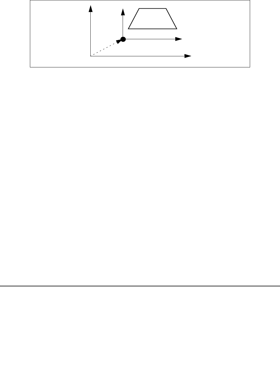
294 HSPICE® Reference Manual: Commands and Control Options
I-2013.12
Chapter 2: HSPICE Simulation Command Reference
Figure 11 Coordinates of a Polygon
Command Group
Field Solver
Examples
Example 1 demonstrates a rectangular polygon using the default number of
segments.
Example 1
.SHAPE POLYGON VERTEX=(1 10 1 11 5 11 5 10)
The rectangular polygon specified in Example 2 uses five segments for each
edge.
Example 2
.SHAPE POLYGON VERTEX=(1 10 1 11 5 11 5 10)
+ N=5
Example 3 shows how rectangular polygon uses different number of segments
for each edge.
Example 3
.SHAPE POLYGON VERTEX=(1 10 1 11 5 11 5 10)
+ N=(5 3 5 3)
.SHAPE (Strip Polygons)
Defines a strip polygon to be used by the HSPICE field solver.
Syntax
.SHAPE STRIP WIDTH=val [N=val]
(0,0)
Origin
x
y
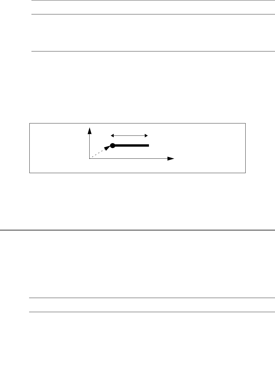
HSPICE® Reference Manual: Commands and Control Options 295
I-2013.12
Chapter 2: HSPICE Simulation Command Reference
Description
Use this command to define a strip polygon in a field solver. Normally, you do
not need to specify the N value because the field solver automatically sets this
value, depending on the accuracy mode. But you can specify this value if you
need to.
The field solver (filament method) does not support this shape.
Figure 12 Coordinates of a Strip Polygon
Command Group
Field Solver
.SHAPE (Trapezoids)
Defines a trapezoid to be used by the HSPICE field solver.
Syntax
.SHAPE TRAPEZOID TOP=val BOTTOM=val HEIGHT=val
+ [NW=val] [NH=val]
Argument Description
WIDTH Width of the strip (size in the x-direction).
NNumber of segments that define the strip shape with the specified
width.
Argument Description
TOP Top edge length of the trapezoid (size in the x-direction).
BOTTOM Bottom edge length of the trapezoid (size in the x-direction).
(0,0)
Origin
Width
x
y
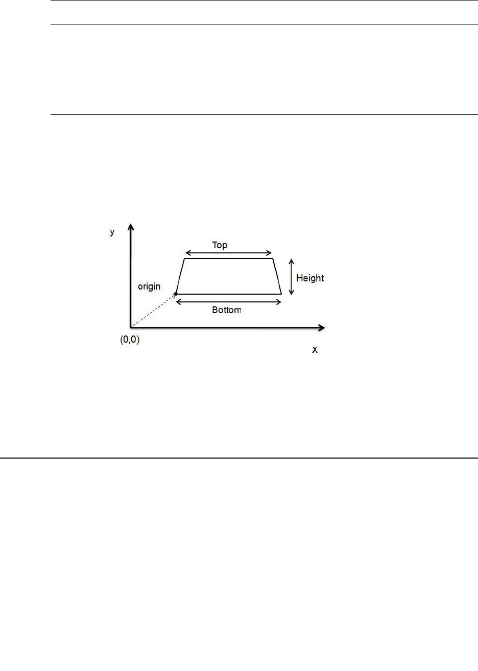
296 HSPICE® Reference Manual: Commands and Control Options
I-2013.12
Chapter 2: HSPICE Simulation Command Reference
Description
Use this keyword to define a trapezoid. Normally, you do not need to specify the
NW and NH values because the field solver automatically sets these values,
depending on the accuracy mode. You can specify both values or only one of
these values to let the solver determine the other.
Figure 13 Coordinates of a Trapezoid
Command Group
Field Solver
.SN
In HSPICE, Shooting Newton provides two syntaxes. Syntax #1 is
recommended when you are using/making Time Domain sources and
measurements (for example, going from .TRAN to .SN). Syntax #2 effectively
supports Frequency Domain sources and measurements (and should be used,
for example, when going from .HB to .SN).
HEIGHT Height of the trapezoid (size in the y-direction).
NW Number of horizontal (x) segments in a trapezoid with a specified top and
bottom.
NH Number of vertical (y) segments in a trapezoid with a specified height.
Argument Description

HSPICE® Reference Manual: Commands and Control Options 297
I-2013.12
Chapter 2: HSPICE Simulation Command Reference
Syntax
Syntax #1
.SN TRES=Tr PERIOD=T [TRINIT=Ti]
+ [SWEEP parameter_sweep][MAXTRINITCYCLES=integer]
+ [NUMPEROUT=val]
Syntax #2
.SN TONE=F1 NHARMS=N [TRINIT=Ti]
+ [SWEEP parameter_sweep] [MAXTRINITCYCLES=integer]
+ [NUMPEROUT=val]
Argument Description
TRES Time resolution to be computed for the steady-state waveforms
(in seconds).
PERIOD Expected period T (seconds) of the steady-state waveforms.
Enter an approximate value when using for oscillator analysis.
The period of the steady-state waveform may be entered either
as PERIOD or its reciprocal, TONE.
TONE The fundamental frequency (in Hz).
NHARMS Specifies the number of high-frequency harmonic components to
include in the analysis. NHARMS defaults to PERIOD/TRES
rounded to nearest integer. NHARMS is required to run
subsequent SNAC, SNNOISE, SNXF, and PHASENOISE
analyses. When using Syntax #1, NHARMS is computed
automatically as NHARMS=Round(PERIOD/TRES).
TRINIT Transient initialization time. If not specified, the transient
initialization time will be equal to the period (for Syntax 1) or the
reciprocal of the tone (for Syntax 2).
SWEEP Parameter sweep. As in all main analyses in HSPICE such
as .TRAN, .HB, etc., you can specify LIN, DEC, OCT, POI,
SWEEPBLOCK, DATA, MONTE, or OPTIMIZE.
MAXTRINITCYCLES SN stabilization simulation and frequency detection is stopped
when the simulator detects that maxtrinitcycles have been
reached in the oscnode signal, or when time=trinit, whichever
comes first. Minimum cycles is 1.

298 HSPICE® Reference Manual: Commands and Control Options
I-2013.12
Chapter 2: HSPICE Simulation Command Reference
Description
Shooting-Newton adds analysis capabilities for PLL components, digital
circuits/logic, such as ring oscillators, frequency dividers, phase/frequency
detectors (PFDs), and for other digital logic circuits and advanced analog
components that require steady-state analysis, but operate with waveforms that
are more square wave than sinusoidal. Refer to the HSPICE User Guide:
Advanced Analog Analysis, Steady-State Shooting Newton Analysis.
In addition to all .TRAN options, .SN analysis supports the following options:
■.OPTION LOADSNINIT
■.OPTION SAVESNINIT
■.OPTION SNACCURACY
■.OPTION SNMAXITER
■.OPTION SNCONTINUE
Control Options
The following netlist control options are available for this command:
NUMPEROUT Allows you to dump more than one period of output to ease
waveform viewing. (Your eye doesn’t have to struggle in the
viewer to connect the end of a waveform period to its beginning.)
By default, SN analysis only dumps one period of output.
Option Description
.OPTION LOADSNINIT Loads the operating point saved at the end of SN initialization
which is used as initial conditions for the Shooting-Newton
method.
.OPTION SAVESNINIT Saves the operating point at the end of SN initialization (sninit).
.OPTION SNACCURACY Similar to the sim_accuracy definition in.TRAN, i.e., larger
values of snaccuracy result in a more accurate solution but
may require more time points. Because Shooting-Newton must
store derivative information at every time point, the memory
requirements may be significant if the number of time points is
very large. Default is 10.
The maximum integer value is 50.
Argument Description

HSPICE® Reference Manual: Commands and Control Options 299
I-2013.12
Chapter 2: HSPICE Simulation Command Reference
Command Group
Analysis
See Also
.SNAC
.SNFT
.SNNOISE
.SNOSC
.SNXF
.SNAC
Runs a frequency sweep across a range for the input signal based on a
Shooting Newton algorithm.
Syntax
.SNAC frequency_sweep
.OPTION SNMAXITER Sets the maximum number of iterations for a Shooting Newton
analysis. Default is 40.
.OPTION SNCONTINUE Specifies whether to use the sweep solution from the previous
simulation as the initial guess for the present simulation.
Default is 1.
■SNCONTINUE=1 (default): Use solution from previous
simulation as the initial guess.
■HBCONTINUE=0: Start each simulation in a sweep from
the DC solution.
Argument Description
frequency_sweep Frequency sweep range for the input signal (also referred to as the
input frequency band (IFB) or fin). You can specify LIN, DEC, OCT,
POI, or SWEEPBLOCK. Specify the nsteps, start, and stop times
using the following syntax for each type of sweep:
■LIN nsteps start stop
■DEC nsteps start stop
■OCT nsteps start stop
■POI nsteps freq_values
■SWEEPBLOCK nsteps freq1 freq2 ... freqn
Option Description

300 HSPICE® Reference Manual: Commands and Control Options
I-2013.12
Chapter 2: HSPICE Simulation Command Reference
Description
The frequency_sweep runs across a range for the input signal based on a
Shooting Newton algorithm. For more information, see Shooting Newton AC
Analysis (.SNAC) in the HSPICE User Guide: Advanced Analog Simulation and
Analysis.
Command Group
Analysis
Examples
VSRC node1 node2 0 SNAC 1 45
.SNAC DEC 10 1k 10K
See Also
.HBAC
.SN
.SNNOISE
.SNFT
Calculates the Discrete Fourier Transform (DFT) value used for Shooting
Newton analysis. Numerical parameters (excluding string parameters) can be
passed to the .SNFT command.
Syntax
Syntax # 1 Alphanumeric input
.SNFT output_var [START=value] [STOP=value]
+ [NP=value] [FORMAT=keyword]
+ [WINDOW=keyword] [ALFA=value]
+ [FREQ=value] [FMIN=value] [FMAX=value]
Syntax #2 Numerics and expressions
.SNFT output_var [START=param_expr1] [STOP=param_expr2]
+ [NP=param_expr3] [FORMAT=keyword]
+ [WINDOW=keyword] [ALFA=param_expr4]
+ [FREQ=param_expr5] [FMIN=param_expr6] [FMAX=param_expr7]
Argument Description
output_var Any valid output variable, such as voltage, current, or power.

HSPICE® Reference Manual: Commands and Control Options 301
I-2013.12
Chapter 2: HSPICE Simulation Command Reference
START Start of the output variable waveform to analyze. Defaults to the START
value in the .SN command, which defaults to 0.
FROM Alias for START in .SNFT commands.
STOP End of the output variable waveform to analyze. Defaults to the TSTOP
value in the .SN command.
TO Alias for STOP, in .SNFT commands.
NP Number of points to use in the SNFT analysis. NP must be a power of 2.
If NP is not a power of 2, HSPICE automatically adjusts it to the closest
higher number that is a power of 2. The default is 1024.
FORMAT Output format:
■NORM= normalized magnitude (default)
■UNORM=unnormalized magnitude
WINDOW Window type to use:
■RECT=simple rectangular truncation window (default).
■BART=Bartlett (triangular) window.
■HANN=Hanning window.
■HAMM=Hamming window.
■BLACK=Blackman window.
■HARRIS=Blackman-Harris window.
■GAUSS=Gaussian window.
■KAISER=Kaiser-Bessel window.
ALFA Parameter to use in GAUSS and KAISER windows to control the highest
side-lobe level, bandwidth, and so on. 1.0 <= ALFA <= 20.0The default
is 3.0
FREQ Frequency to analyze. If FREQ is non-zero, the output lists only the
harmonics of this frequency, based on FMIN and FMAX. HSPICE also
prints the THD for these harmonics. The default is 0.0 (Hz).
FMIN Minimum frequency for which HSPICE prints SNFT output into the listing
file. THD calculations also use this frequency. T=(STOP-START) The
default is 1.0/T (Hz).
Argument Description

302 HSPICE® Reference Manual: Commands and Control Options
I-2013.12
Chapter 2: HSPICE Simulation Command Reference
Description
Use this command to calculate the Discrete Fourier Transform (DFT) spectrum
analysis values for Shooting Newton analysis. It uses internal time point values
to calculate these values. A DFT uses sequences of time values to determine
the frequency content of analog signals in circuit simulation. You can pass
numerical parameters/expressions (but no string parameters) to the .SNFT
command. The output goes to a file with extension .snft#.
You can specify only one output variable in an .SNFT command. The following
is an incorrect use of the command because it contains two variables in
one .SNFT command:
Command Group
Analysis
Examples
Example 1 Correctly designates the variables per .SNFT command.
.SNFT v(1)
.SNFT v(1,2) np=1024 start=0.3m stop=0.5m freq=5.0k
+ window=kaiser alfa=2.5
.SNFT I(rload) start=0m to=2.0m fmin=100k fmax=120k
+ format=unorm
.SNFT par(‘v(1) + v(2)’) from=0.2u stop=1.2u
+ window=harris
Example 2 Generates a .snft0 file for the SNFT of v(1) and a .snft1 file for the SNFT
of v(2).
.SNFT v(1) np=1024
.SNFT v(2) np=1024
See Also
.SN
FMAX Maximum frequency for which HSPICE prints SNFT output into the listing
file. THD calculations also use this frequency. The default is 0.5*NP*FM
IN (Hz).
Argument Description

HSPICE® Reference Manual: Commands and Control Options 303
I-2013.12
Chapter 2: HSPICE Simulation Command Reference
.SNNOISE
Runs a periodic, time-varying AC noise analysis based on a Shooting Newton
algorithm.
Syntax
.SNNOISE output insrc frequency_sweep
+[[n1, +/-1]]
+[listfreq=(frequencies|none|all)> [listcount=val]
+[listfloor=val] [listsources=on|off]
Argument Description
output Output node, pair of nodes, or 2-terminal element that the
equivalent noise output references.
insrc Input source.
frequency_sweep Frequency sweep range for the input signal. You can specify LIN,
DEC, OCT, POI, SWEEPBLOCK, DATA, MONTE, or OPTIMIZE
sweeps.
n1, +/- Index term defining the output frequency band at which the noise
is evaluated. The output frequency is computed according to
fout=|n1*f1 +/- fin|, where f1 is the fundamental tone (inverse of
fundamental period) and fin is from the frequency sweep.
listfreq Prints the element noise value to the .lis file; the default is
none.
listcount Prints the element noise value to the .lis file, sorted from the
largest to smallest value.
listfloor Prints the element noise value to the .lis file and defines a
minimum meaningful noise value. Only those elements with
noise values larger than listfloor are printed. The default value is
1.0e-14 V/sqrt(Hz).
listsources Prints the element noise value to the .lis file when the
element has multiple noise sources. The default is off.
When .OPTION PSF=2 ARTIST=2 is specified in the netlist
and the listsources is turned-on, the element noise sources
attribute will also be output into .snpn# file.

304 HSPICE® Reference Manual: Commands and Control Options
I-2013.12
Chapter 2: HSPICE Simulation Command Reference
Description
The functionality for the .SNNOISE command to is similar to the Harmonic
Balance (HBNOISE command) for periodic, time-varying AC noise analysis, but
the Shooting Newton-based algorithm completes the analysis in a much faster
run time with the same result.
Command Group
Analysis
Examples
.SNNOISE V(n1,n2) RIN DEC 10 1k 10k 0 -1
See Also
.HBNOISE
.SN
.SNAC
.SNOSC
Performs oscillator analysis on autonomous (oscillator) circuits. As with regular
Shooting Newton analysis, input might be specified in terms of time or
frequency values.
Syntax
Syntax #1
.SNOSC TONE=F1 NHARMS=H1 [TRINIT=Ti] OSCNODE=N1
+[MAXTRINITCYCLES=N][SWEEP PARAMETER_SWEEP]
Syntax #2
.SNOSC TRES=Tr PERIOD=Tp [TRINIT=Tr] OSCNODE=N1
+[MAXTRINITCYCLES=I] SWEEP PARAMETER_SWEEP
Argument Description
TONE Approximate value for oscillation frequency (Hz). The search
for an exact oscillation frequency begins from this value.
NHARMS Number of harmonics to be used for oscillator SN analysis.

HSPICE® Reference Manual: Commands and Control Options 305
I-2013.12
Chapter 2: HSPICE Simulation Command Reference
Description
Use this command to invoke oscillator analysis on autonomous (oscillator)
circuits. The SNOSC command is very effective for ring oscillator circuits, and
oscillators that operate with piecewise linear waveforms (HBOSC is superior for
OSCNODE Node used to probe for oscillation conditions. This node is
automatically analyzed to search for periodic behavior near
the TONE or PERIOD value specified.
TRINIT Transient initialization time. If not specified, the transient
initialization time is equal to the period (for Syntax 1) or the
reciprocal of the tone (for Syntax 2). For oscillators we
recommend specifying a transient initialization time since the
default initialization time is usually too short to effectively
stabilize the circuit.
MAXTRINITCYCLES SN stabilization simulation and frequency detection is
stopped when the simulator detects that
MAXTRINITCYCLES have been reached in the oscnode
signal, or when time=trinit, whichever comes first.
Minimum cycles is 1.
TRES Time resolution to be computed for the steady-state
waveforms (in seconds). The period of the steady-state
waveform may be entered either as PERIOD or its reciprocal,
TONE.
PERIOD Expected period T (seconds) of the steady-state waveforms.
Enter an approximate value when using for oscillator analysis.
SWEEP Type of sweep. You can sweep up to three variables. You can
specify either LIN, DEC, OCT, POI, SWEEPBLOCK, DATA,
OPTIMIZE, or MONTE. Specify the nsteps, start, and stop
frequencies using the following syntax for each type of sweep:
■LIN nsteps start stop
■DEC nsteps start stop
■OCT nsteps start stop
■POI nsteps freq_values
■SWEEPBLOCK nsteps freq1 freq2 ... freqn
■DATA=dataname
■OPTIMIZE=OPTxxx
■MONTE=val
Argument Description

306 HSPICE® Reference Manual: Commands and Control Options
I-2013.12
Chapter 2: HSPICE Simulation Command Reference
sinusoidal waveforms). As with the Harmonic Balance approach, the goal is to
solve for the additional unknown oscillation frequency. This is accomplished in
Shooting Newton by considering the period of the waveform as an additional
unknown, and solving the boundary conditions at the waveform endpoints that
coincide with steady-state operation. As with regular Shooting Newton
analysis, input might be specified in terms of time or frequency values. See the
examples, below.
Control Options
The following netlist control options are available for this command:
Command Group
Analysis
Examples
Example 1 Performs an oscillator analysis searching for periodic behavior after an
initial transient analysis of 10 ns. This example uses nine harmonics
while searching for a oscillation at the gate node.
.SNOSC tone=900Meg nharms=9 trinit=10n oscnode=gate
Option Description
.OPTION HBFREQABSTOL Specifies the maximum absolute change in frequency between
solver iterations for convergence.
.OPTION HBFREQRELTOL Specifies the maximum relative change in frequency between
solver iterations for convergence.
.OPTION HBOSCMAXITER /
HBOSC_MAXITER
Specifies the maximum number of outer-loop iterations for
oscillator analysis.
.OPTION HBPROBETOL Searches for a probe voltage at which the probe current is less
than the specified value.
.OPTION HBTRANFREQSEARCH Specifies the frequency source for the HB analysis of a ring
oscillator.
.OPTION HBTRANINIT Selects transient analysis for initializing all state variables for
HB analysis of a ring oscillator.
.OPTION HBTRANPTS Specifies the number of points per period for converting time-
domain data results into the frequency domain for HB analysis
of a ring oscillator.
.OPTION HBTRANSTEP Specifies transient analysis step size for the HB analysis of a
ring oscillator.

HSPICE® Reference Manual: Commands and Control Options 307
I-2013.12
Chapter 2: HSPICE Simulation Command Reference
Example 2 Performs an oscillator analysis searching for frequencies in the vicinity of
2.4 Ghz. This example uses 11 harmonics and a search at the drainP.
.SNOSC tone=2400MEG nharms=11 trinit=20n oscnode=drainP
Example 3 Presents another equivalent method to define the OSCNODE
information through a zero-current source. Example 3 is identical to
Example 2, except that the OSCNODE information is defined by a current
source in the circuit. Only one such current source is needed and its
current source must be 0.0 with the SNOSC OSCNODE identified by the
SNOSCVPROBE keyword.
ISRC drainP 0 SNOSCVPROBE
.SNOSC tone = 2.4 G nharms = 1 trinit=20n
See Also
.HB
.PRINT
.PROBE
.SNXF
Calculates the transfer function from the given source in the circuit to the
designated output.
Syntax
.SNXF out_varfreq_sweep
Argument Description
out_var I(2_port_elem) or V(n1<,n2>)
freq_sweep Sweep of type LIN, DEC, OCT, POI, or SWEEPBLOCK. Specify the
nsteps, start, and stop times using the following syntax for each
type of sweep:
■LIN nsteps start stop
■DEC nsteps start stop
■OCT nsteps start stop
■POI nsteps freq_values
■SWEEPBLOCK = BlockName
Specify the frequency sweep range for the output signal. HSPICE
determines the offset frequency in the input sidebands; for
example,f1 = abs(fout - k*f0) s.t. f1<=f0/2The f0 is the steady-state
fundamental tone and f1 is the input frequency.

308 HSPICE® Reference Manual: Commands and Control Options
I-2013.12
Chapter 2: HSPICE Simulation Command Reference
Description
Use this command in HSPICE to calculate the transfer function from the given
source in the circuit to the designated output. The functionality for the .SNXF
command is similar to the Harmonic Balance (.HBXF) command for periodic,
time-varying AC noise analysis, but the Shooting Newton based algorithm
completes the analysis in a much faster run time with the same result.
Command Group
Analysis
Examples
In this example, the trans-impedance from isrc to v(1)is calculated based on
the HB analysis.
.hb tones=1e9 nharms=4
.snxf v(1) lin 10 1e8 1.2e8
.print snxf tfv(isrc) tfi(n3)
See Also
.HB
.HBAC
.HBNOISE
.HBOSC
.PRINT
.PROBE
.STATEYE
Enables use of statistical eye diagram analysis.
Syntax
.STATEYE T=time_interval Trf=rise_fall_time
+ [Tr=rise_time] [Tf=fall_time]
+ Incident_port=idx1, [idx2, ... idxN]
+ Probe_port=idx1, [idx2, ... idxN]
+ [Tran_init=n_periods]
+ [V_low=val] [V_high=val]
+ [TD_In=val] [TD_Probe=val][TD_Probe_AMI=val]
+ [TW_Reltol=val]
+ [Initial_Low=val]
+ [T_resolution=n] [V_resolution=n]
+ [VD_range=val] [TD_NUI=n] [Edge=1|2|4|8]

HSPICE® Reference Manual: Commands and Control Options 309
I-2013.12
Chapter 2: HSPICE Simulation Command Reference
+ [MAX_PATTERN=n] [Pattern_repeat=n]
+ [Save_tr=ascii] [Load_tr=ascii]
+ [Save_Dir=string] [Load_Dir=string]
+ [Ignore_Bits=n]
+ [AMIInit_Use_Impulse=0|1]
+ [Xtalk_Type = SYNC|ASYNC|DDP|NO]
+ [MODE=EDGE|TRAN]
+ [TRAN_BIT_SEG=val]
+ [Unfold_Length=n]
Argument Description
TTime (in seconds) of single bit width of the incident signal,
normally referred as Unit Interval (UI)
Trf Single value (in seconds) to set both the rise and fall times of
the incident pulse
Tr Rise time (in seconds) of the incident port
Tf Fall time (in seconds) of the incident port
Incident_port An array of the index numbers of the incident port elements
Probe_port An array of the index numbers of the probing port elements
V_low Low voltage level of the incident pulse. The value is used when
the voltage level is not specified in the incident port(s). Default:
-1.0
V_high High voltage level of the incident pulse. The value is used when
the voltage level is not specified in the incident port(s). Default:
1.0
Tran_init An integer number that specifies the numbers of unit intervals
(T) that is used by the initial transient analysis to determine the
response of the system. Default value is 60.
T_resolution An integer number used to specify the probability density
function (PDF) image resolution of the time axis. Default value
is 200.
V_resolution An integer number used to specify the probability density
function (PDF) image resolution of the voltage axis. Default
value is 200.

310 HSPICE® Reference Manual: Commands and Control Options
I-2013.12
Chapter 2: HSPICE Simulation Command Reference
TD_In Applies specified time delay to the incident pulse/step in the
initial transient analysis. Default value is 0 (no delay).
TD_Probe When a positive time value is specified, StatEye only uses
initial transient analysis waveforms after the specified time for
the eye diagram generation. Default value is 0.
TD_Probe_AMI Similar to TD_Probe keyword. StatEye only uses AMI filtered
waveform after the specified time for the eye diagram
generation. Default value is 0.
TW_RELTOL Relative tolerance used to determine the output waveform
transition time window.
StatEye considers the output settled when the output voltage
reaches the value of the maximum output swing multiplied by
TW_RELTOL. Default is 0.01.
Initial_Low Forces all the edge input to begin at a low state for specified
time. For edges which begin at a high state, the input ramps up
to a high state at the specified time and then proceeds to the
given edge shape. When this keyword is specified, TD_In
defaults to 2*Initial_Low, so the edge transition begins
after the specified Initial_Low period. TD_Probe and
TD_Probe_AMI also default to TD_In, so the edge response
during the Initial_Low period is ignored.
VD_range Specifies voltage display (output data) range. By default,
the .StatEye analysis engine automatically determines the
optimum voltage display range. Specifying VD_range can
enlarge the display range.
TD_NUI An integer number to specify time display range relative to the
unit interval. Default value is 2 to display a single eye. TD_NUI
value may be from 1 to 5. The higher value requires a larger
data size.
Argument Description

HSPICE® Reference Manual: Commands and Control Options 311
I-2013.12
Chapter 2: HSPICE Simulation Command Reference
EDGE Number of edges to be used.
■1: Conventional statistical eye generation using the single
pulse response (default).
■2: Double-edge mode. The rising and falling edges are
evaluated separately.
■4: Four edge patterns are modeled. Aids in increasing
accuracy for transmission line systems’ linear memory
effect.
■8: Eight edge patterns are modeled for greater accuracy in
nonlinearity. As the number of edge patterns increases,
higher nonlinearity can be modeled accurately.
MAX_PATTERN=nLimits the number of bits to be examined for a custom bit
pattern specified with LFSR/PAT in incident Port-element(s).
For example, if MAX_PATTERN=100 is specified, StatEye
examines only the first 100 bits in the LFSR/PAT sources. This
keyword is especially effective when LFSR is used with very
high (over 20-bit) feedback tap(s) since it generates an
extremely long bit stream.
The default value of the MAX_PATTERN is 1000 for mode=tran
and 221 when mode=tran with edge=<n> modes. When you
specify MAX_PATTERN=0 StatEye examines all the given
patterns.
PATTERN_REPEAT When a positive number, n, is specified, .StatEye repeats
pattern examination n times until the number of bits hits the
MAX_PATTERN value. Default=0 (no repeats).
SAVE_TR=ascii Saves initial transient data in text files.
LOAD_TR=ascii Loads initial transient data from text files when available.
SAVE_DIR=string Specifies a target directory other than the one specified by the
-o command option for the SAVE_TR and LOAD_TR transient
files. In saving initial transient result, HSPICE creates
netlist.save0/ directory under the specified SAVE_DIR
directory. For example, SAVE_DIR = my_dir is specified in
my_netlist.sp, “my_dir/my_netlist.save0/”
directory will be the target of SAVE_TR and LOAD_TR
operations.
Argument Description

312 HSPICE® Reference Manual: Commands and Control Options
I-2013.12
Chapter 2: HSPICE Simulation Command Reference
LOAD_DIR=string LOAD_DIR works the same as SAVE_DIR but LOAD_DIR can
be used to specify different directory target than SAVE_DIR for
initial transient data read in. LOAD_DIR defaults to SAVE_DIR.
Ignore_Bits=nWhen a positive number is specified, StatEye's pattern-specific
eye diagram generation process ignores the first n bits. The
value is overridden by one specified in the AMI parameter file
when one exists for each probe port.
AMIInit_Use_Impu
lse=0|1
Specifies the waveform input for the AMI_Init function:
■0: (default) edge (pulse/step/etc) responses are used for the
AMI_Init function call.
■1: StatEye extracts system impulse response from edge
responses then uses it for the AMI_Init function call.
Xtalk_Type Specifies type of crosstalk.
■ SYNC: (Default) Crosstalk aggressors and victims are in
sync under single system clock.
■ASYNC: Crosstalk noises are considered asynchronous.
■DDP: Input data dependent crosstalk. This mode requires
input bit patterns for both aggressor and victim lines.
■NO: No crosstalk.
MODE=EDGE|TRAN Specifies StatEye simulation mode. By default, MODE=EDGE is
used.
■EDGE: Conventional statistical eye generation using the
number of edges specified by the EDGE keyword.
■TRAN: StatEye uses full transient analysis mode instead of
edge mode. The EDGE keyword will be ignored when full
transient analysis mode is specified.
Argument Description

HSPICE® Reference Manual: Commands and Control Options 313
I-2013.12
Chapter 2: HSPICE Simulation Command Reference
Description
Use this command to perform statistical eye analysis to evaluate high-speed
serial interfaces. (This analysis requires two HSPICE licenses.)
The statistical eye diagram is a fundamental performance metric for high-speed
serial interfaces in the bit error rate (BER). When setting up a Statistical Eye
Analysis, the Port element is used to designate the incident (input) and probe
(output) ports for the system to be analyzed. Ports can be specified as single-
ended or mixed mode. Random jitter can be applied to each incident and probe
point in the system.Each incident port acts as random bit pattern source with
specified voltage magnitude. If an incident port element does not have a time
domain voltage magnitude specification, the default values, V_high=1.0,
V_low=-1.0 are used.Probe ports are used as observation points where
.PRINT, .PROBE, and .MEASURE commands can be defined.
Command Group
Analysis
Examples
.STATEYE T=400p Trf=20p
+ incident_port= 1, 2
+ probe_port= 3, 4
See Also
.MEASURE / MEAS
Tran_Bit_Seg=n Specifies the number of bits per each eye diagram generation
process.
When AMI objects are used, AMI_GetWave is called at each
Tran_Bit_Seg bits. For example, when a given pattern has
10,000 bits and Tran_Bit_Seg=1000, StatEye sequentially
calls AMI_GetWave 10 times with stream waveform of 1000
bits.
Also in MODE=TRAN mode, StatEye processes transient
waveforms at each Tran_Bit_Seg bits. The default values
are: 200 for MODE=TRAN mode and 1000 for MODE=EDGE
mode. For more details about AMI_GetWave, see chapter 10
of the IBIS version 5.0 specification.
Unfold_Length=nSpecifies the bit pattern length of the unfold eye probe/print.
Default value is 200.
Argument Description

314 HSPICE® Reference Manual: Commands and Control Options
I-2013.12
Chapter 2: HSPICE Simulation Command Reference
.PRINT
.PROBE
Statistical Eye Analysis
.STIM
Uses the results (output) of one simulation as input stimuli in a new simulation
in HSPICE.
Syntax
General Syntax:
.STIM [tran|ac|dc] PWL|DATA|VEC
+ [filename=output_filename ...]
PWL Source Syntax (Transient Analysis Only)
.STIM [tran] PWL [filename=output_filename]
+ [name1=] ovar1 [node1=n+] [node2=n-]
+ [[name2=]ovar2 [node1=n+] [node2=n-] ...]
+ [from=val] [to=val] [npoints=val]
.STIM [tran] PWL [filename=output_filename]
+ [name1=] ovar1 [node1=n+] [node2=n-]
+ [[name2=]ovar2 [node1=n+] [node2=n-] ...]
+ indepvar=[(]t1 [t2 ...[)]]
Data Card Syntax
.STIM [tran|ac|dc] DATA [filename=output_filename]
+ dataname [name1=] ovar1
+ [[name2=]ovar2 ...] [from=val] [to=val]
+ [npoints=val] [indepout=val]
.STIM [tran | ac | dc] DATA [filename=output_filename]
+ dataname [name1=] ovar1
+[[name2=]ovar2 ...] indepvar=[(]t1 [t2 ...[)]]
+ [indepout=val]
Digital Vector File Syntax (Transient Analysis Only)
.STIM [tran] VEC [filename=output_filename]
+vth=val vtl=val [voh=val] [vol=val]
+ [name1=] ovar1 [[name2=] ovar2 ...]
+ [from=val] [to=val] [npoints=val]
.STIM [tran] VEC [filename=output_filename]

HSPICE® Reference Manual: Commands and Control Options 315
I-2013.12
Chapter 2: HSPICE Simulation Command Reference
+vth=val vtl=val [voh=val] [vol=val]
+ [name1=] ovar1 [[name2=] ovar2 ...]
+ indepvar=[(]t1 [t2 ...[)]]
Argument Description
tran | ac | dc Simulation type: transient, AC, or DC.
filename Output file name. If you do not specify a file, HSPICE uses the input
filename.
name1 PWL Source Name that you specify. The name must start with V (for a
voltage source) or I (for a current source). Or—Name of a parameter of
the data card to generate.
ovar1 Output variable that you specify. ovar can be:
■Node voltage.
■Element current.
■Parameter string. If using a parameter string you must specify name1.
For example: v(1), i(r1), v(2,1), par(’v(1)+v(2)’)
dataname Name of the data card to generate.
node1 Positive terminal node name.
node2 Negative terminal node name.
from Time to start output of simulation results. For transient analysis, it uses
the time units that you specified. Cannot use with indepvar.
npoints Number of output time points or independent-variable points.
to Time to terminate output of simulation results. For transient analysis, it
uses the time units that you specified. The from value can be greater than
the to value. Cannot use with indepvar.
indepvar Dispersed (independent-variable) time points. Specify dispersed time
points in increasing order. Replaces the “from” and “to” construct.

316 HSPICE® Reference Manual: Commands and Control Options
I-2013.12
Chapter 2: HSPICE Simulation Command Reference
Description
Use this command to reuse the results (output) of one simulation as input
stimuli in a new simulation.
The .STIM command specifies:
■Expected stimulus (PWL Source, DATA CARD, or VEC FILE).
■Signals to transform.
■Independent variables.
One .STIM command produces one corresponding output file.
For additional information, see “Reusing Simulation Output as Input Stimuli” in
the HSPICE User Guide: Basic Simulation and Analysis.
Command Group
Output Porting
Examples
In Example 1, the .STIM command creates a file “test.pwl0_tr0”, having a
voltage source “v0” applied between nodes neg and 0 (ground). It has a PWL
source function based on the voltage of node n0 during the time 0.0ns to 5.0ns
with 10 points.
Example 1
.stim tran pwl filename=test v0=v(n0) node1=neg
+ node2=0 from=0.0ns to=5ns npoints=10
indepout Indicates whether to generate the independent variable column.
■indepout, indepout=1, or on, produces the independent variable
column. You can specify the independent-variables in any order.
■indepout= 0 or off (default) does not create an independent variable
column.
You can place the indepout field anywhere after the ovar1 field.
vth High voltage threshold.
vtl Low voltage threshold.
voh Logic-high voltage for each output signal.
vol Logic-low voltage for each output signal.
Argument Description

HSPICE® Reference Manual: Commands and Control Options 317
I-2013.12
Chapter 2: HSPICE Simulation Command Reference
Example 2: In this example the “from and to” construct is used:
.stim tran data filename=new PWL v(2) from=start to=end
Example 3: In this example, the indepvar construct replaces “from and to”;
using both constructs results in an error.
.stim tran pwl filename=new v(2) indepvar=(2n 3n 4n)
See Also
.DOUT
.MEASURE / MEAS
.PRINT
.PROBE
.STORE
Starts a store operation to create checkpoint files describing a running process
during transient analysis.
Syntax
.STORE [TYPE=IC/MEMDUMP]
+ [FILE=save_file_prefix]
+ [TIME=time1][TIME=time2]...[TIME=timeN]
+ [REPEAT=period]
+ [TRANTIME=0/1]
+ [SAVE_ON_KILL=0/1]
Argument Description
TYPE=IC/MEMDUMP Stores checkpoint data to either an IC type or a memory
dump file.If unspecified, the default checkpoint file is of the
TYPE=IC and the name prefix is same as the HSPICE
output file.
FILE=save_file_prefix Changes the prefix of the output file names.
TIME=time1,time2,...timeN Collects checkpoint data beginning at time1 after the start of
transient analysis. It then updates the checkpoint data every
21,600 wall-clock seconds if no checkpoint period is
specified.

318 HSPICE® Reference Manual: Commands and Control Options
I-2013.12
Chapter 2: HSPICE Simulation Command Reference
Description
Use this command in a netlist to trigger a restore operation by creating
checkpoint files describing a running process during transient analysis; the
operating system can later reconstruct the process from the contents of this
file. This feature is not supported in when HSPICE advanced analog functions
are used.
The shortest repeat period for a checkpoint period is 7,200 seconds, anything
shorter than that defaults to 7,200 seconds automatically.
If the netlist contains more than one .store statement, only the last statement
takes effect.
The restore operation is done on the command-line with the -restore
keyword. See Chapter 1, HSPICE Commands Introduction for more
information. For usage requirements and additional information, see Storing
and Restoring Checkpoint Files in the HSPICE User Guide: Basic Simulation
and Analysis.
Types of output files with TYPE=IC
The following output files are generated with TYPE=IC:
Contains node voltage and inductor current data in ASCII format:
Test.<time>.ic# or Test.save.ic#
REPEAT=period If you specify a nonzero period, new checkpoint data is
collected at every period, starting at transient time=0 and
overwriting previous interval checkpoint data. If a nonzero
time1 is specified, checkpoint data is collected at time1 +
period * n, where n is an integer. Period is always calculated
based on time1. If repeat=0, the store operation is disabled.
If you set both time=0 and repeat=0, checkpoint data is
saved at transient time=0 only.
TRANTIME=0/1 ■If set to 0, time1 and period are taken as wall-clock time.
■If set to 1, time1 and period are transient times or times
is smaller than TSTOP.
Note: If TYPE=MEMDUMP, TRANTIME is ignored.
SAVE_ON_KILL=0/1 If set to 1, the checkpoint data is saved on kill and halts the
simulation.
Argument Description

HSPICE® Reference Manual: Commands and Control Options 319
I-2013.12
Chapter 2: HSPICE Simulation Command Reference
Contains node dv/dt voltage and di/dt for inductor current ASCII format:
Test.<time>.ic#.sup or Test.save.ic#.sup
If TIME or REPEAT is specified:
test.<time>.ic# and .sup files
If SAVE_ON_KILL or wall time is specified:
Test.save.ic# and .sup files
If a .alter/sweep exists in the simulation:
Test.<sweepNum>.ic<alterNum>
If a VA instance exists in the simulation:
Test.<time>.ic#.pva and test.<time>.ic.pvaoff
*.ic#.pva $ Contains all pVA rtl flags, state values of DIS,
I/O buffer and so on in binary format.
*.ic#.pvaoff $ Contains saved instance names and file-positions
in ASCII format. It is necessary since pVA might not have the
exact instance order during the restore phase.
Command Group
Output Porting
Examples
$ Transient seconds since lower than tstop value.
.STORE [TYPE=IC] TIME=45n
$ Wall seconds since higher than tstop value.
.STORE [TYPE=IC] TIME='60*60*3'
$ Wall seconds since lower than tstop value.
.STORE [TYPE=IC] REPEAT=50n
$ Transient seconds since higher than tstop value.
.STORE [TYPE=IC] REPEAT='60*60*3'
$ Repeat every 100ns, starting at 45ns (ignoring the other time
entries).
.STORE TIME=45n TIME=66n REPEAT=100n
$ Save every 10ns, starting at 0.
.STORE REPEAT=10n
$ Save starting at 10ns, ending at 90ns.
.STORE TIME=10n TIME=20n… TIME=90n

320 HSPICE® Reference Manual: Commands and Control Options
I-2013.12
Chapter 2: HSPICE Simulation Command Reference
$ generate file named hsp_save_file.8e-09.ic0.
.STORE TIME=80n FILE=”hsp_save_file”
See Also
.TRAN
.SUBCKT
Defines a subcircuit in a netlist.
Syntax
Nodes and Parameters
.SUBCKT subnam n1 n2 n3 ... [param=val]
.ENDS
.SUBCKT SubNamePinList [SubDefaultsList]
.ENDS
Parameter String
.SUBCKT subnam n1 n2 n3 ... [param=str('string')]
.ENDS
Isomorphic Analyses
.SUBCKT analyses_sb [start=p1 stop=p2 steps=p3]
.DC …
.AC …
.TRAN …
.ENDS analyses_sb
...followed by
x1 analyses_sb [start=a1] [stop=a2] [steps=a3]
x2 analyses_sb [start=b1] [stop=b2] [steps=b3]
Argument Description
subnam Reference name for the subcircuit model call.

HSPICE® Reference Manual: Commands and Control Options 321
I-2013.12
Chapter 2: HSPICE Simulation Command Reference
Description
Use this command to define a subcircuit in your netlist. You can create a
subcircuit description for a commonly used circuit and include one or more
references to the subcircuit in your netlist.
When you use hierarchical subcircuits, you can pick default values for circuit
elements in a .SUBCKT command. You can use this feature in cell definitions to
simulate the circuit with typical values.
The isomorphic analyses feature enables you to run unrelated analyses (.DC,
.AC, and .TRAN) many times during a simulation by grouping the set of
analyses into a subcircuit, which performs multiple analyses in one simulation
with calls to the subcircuit. The usage model is: Specify the analyses
commands within the subckt definition block and then instantiate the subckt to
perform the analyses. Each call of the subcircuit is treated as an individual
analysis with its own set of parameters.
In cases where you have multiple subcircuits in your design and would like to
define a model for one instance at the top level you can define a model that is
specific to only one subcircuit. You can define the models inside of a subcircuit
using .INCLUDE statements and using .OPTION PARHIER=LOCAL. See
Example 5 for more information.
n1... Node numbers for external reference; cannot be the ground node
(0, gnd, ground, gnd!). Any element nodes that are in the
subcircuit, but are not in this list are strictly local with three
exceptions:
■Ground node (0, gnd, ground, gnd!).
■Nodes assigned using BULK=node in MOSFET or BJT
models.
■Nodes assigned using the .GLOBAL command.
parnam Parameter name set to a value. Use only in the subcircuit. To
override this value, assign it in the subcircuit call or set a value in
a .PARAM command.
SubDefaultsList SubParam1=Expression [SubParam2=Expression...]
analysis_sb Reference name for the isomorphic analyses that can be run in a
subckt block.
p1...p2...p3 Parameters specified for the start, stop, and number of steps.
Argument Description

322 HSPICE® Reference Manual: Commands and Control Options
I-2013.12
Chapter 2: HSPICE Simulation Command Reference
Use the .ENDS command to terminate a .SUBCKT command.
Note: Using -top subck_name on the command line effectively
eliminates the need for the .subckt subckt_name and
.ends subckt_name.
Control Options
The following netlist control options are available for this command:
Command Group
Subcircuits
Option Description
.OPTION LIST Prints a list of netlist elements, node connections, and values for
components, voltage and current sources, parameters, and more.
.OPTION PARHIER / PARHIE Specifies scoping rules for netlist parameters.

HSPICE® Reference Manual: Commands and Control Options 323
I-2013.12
Chapter 2: HSPICE Simulation Command Reference
Examples
Example 1 Defining two subcircuits: SUB1 and SUB2. These are resistor-divider
networks, whose resistance values are parameters (variables). The X1,
X2, and X3 commands call these subcircuits. Because the resistor values
are different in each call, these three calls produce different subcircuits.
*FILE SUB2.SP TEST OF SUBCIRCUITS
.OPTION LIST ACCT
V1 1 0 1
.PARAM P5=5 P2=10
.SUBCKT SUB1 1 2 P4=4
R1 1 0 P4
R2 2 0 P5
X1 1 2 SUB2 P6=7
X2 1 2 SUB2
.ENDS
*
.MACRO SUB2 1 2 P6=11
R1 1 2 P6
R2 2 0 P2
.EOM
X1 1 2 SUB1 P4=6
X2 3 4 SUB1 P6=15
X3 3 4 SUB2
*
.MODEL DA D CJA=CAJA CJP=CAJP VRB=-20
IS=7.62E-18
+ PHI=.5 EXA=.5 EXP=.33
.PARAM CAJA=2.535E-16 CAJP=2.53E-16
.END

324 HSPICE® Reference Manual: Commands and Control Options
I-2013.12
Chapter 2: HSPICE Simulation Command Reference
Example 2 Implementing an inverter that uses a Strength parameter. By default, the
inverter can drive three devices. Enter a new value for the Strength
parameter in the element line to select larger or smaller inverters for the
application.
.SUBCKT Inv a y Strength=3
Mp1 MosPinList pMosMod L=1.2u
W=’Strength * 2u’
Mn1 MosPinList nMosMod L=1.2u
W=’Strength * 1u’
.ENDS
...
xInv0 a y0 Inv $ Default devices: p device=6u,
$ n device=3u
xInv1 a y1 Inv Strength=5 $ p device=10u,
n device=5u
xInv2 a y2 Inv Strength=1 $ p device= 2u,
n device=1u
...
Example 3 Implementing an IBIS model (in HSPICE only) that uses string
parameters to specify the IBIS file name and IBIS model name.
* Using string parameters
.subckt IBIS vccq vss out in
+ IBIS_FILE=str('file.ibs')
+ IBIS_MODEL=str('ibis_model')
ven en 0 vcc
B1 vccq vss out in en v0dq0 vccq vss
+ file= str(IBIS_FILE) model=str(IBIS_MODEL)
.ends
Example 4 Specifying Isomorphic Analyses
.subckt analyses_sb start_dc=-25 stop_dc=25 steps_dc=5
+ steps_tran=1n stop_tran=10n
.DC TEMP start_dc stop_dc steps_dc
.TRAN steps_tran stop_tran
.ends analyses_sb
...
x1 analyses_sb start_dc=25 stop_dc=75 steps_dc=10
x2 analyses_sb steps_tran=2n
x3 analyses_sb
Example 4 specifies both .DC and .TRAN analyses within the subckt. To
invoke these analyses you can call the subckts.

HSPICE® Reference Manual: Commands and Control Options 325
I-2013.12
Chapter 2: HSPICE Simulation Command Reference
■Each subckt call will perform DC and Transient analysis.
■Parameters defined in the subcircuit calls will override the default values
specified in the subcircuit definition.
■If parameters are not defined in the subckt calls they will take the default
values given in the subcircuit.
Example 5 If you have multiple subcircuits in your design and would like to define a
model for one instance at the top level. You can define a model that is
specific to only one subcircuit as follows: Define the models inside of a
subcircuit using .INCLUDE statements. The parameters defined in the
included models are global by default but you want any parameters
defined in the included file to be local to the subcircuit. This means that
you will also need to set .OPTION PARHIER=LOCAL so that parameter
scoping rules are correct for this case.
...
.option PARHIER=LOCAL
.subckt INV IN OUT
.include 'weak_ model.inc'
M1 ...
M2 ...
.ends INV
...
X1 IN OUT INV
...
See Also
.ENDS
.EOM
.MACRO
.MODEL
.PARAM / PARAMETER / PARAMETERS
.INCLUDE / INC / INCL
Isomorphic Analyses in Subckt Blocks
.SURGE
Automatically detects and reports a current surge that exceeds the specified
surge tolerance in HSPICE.
Syntax
.SURGE surge_thresholdsurge_widthnode1 [node2 ...noden]

326 HSPICE® Reference Manual: Commands and Control Options
I-2013.12
Chapter 2: HSPICE Simulation Command Reference
Description
Use this command to automatically detect and report a current surge that
exceeds the specified surge tolerance. The command reports any current
surge that is greater than surge_threshold for a duration of more than
surge_width.
Surge current is defined as the current flowing into or out of a node to the lower
subcircuit hierarchy.
Note: This option is active only when HSPICE advanced analog
functions are used.
Command Group
Analysis
Examples
In this example, the .SURGE command detects any current surge that has an
absolute amplitude of more than 1mA, and that exceeds 100ns, x(xm.x1.a),
x(xm.x2.c), and x(xn.y).
.SUBCKT sa a b
...
.ENDS
.SUBCKT sb c d
...
.ENDS
.SUBCKT sx x y
x1 x y sa
x2 x a sb
.ENDS
xm 1 2 sx
xn 2 a sx
.SURGE 1mA 100ns xm.x1.a xm.x2.c xn.y
Argument Description
surge_threshold Minimum absolute surge current.
surge_width Defines the minimum duration of a surge.
noden Any valid node name at current or lower subcircuit level.

HSPICE® Reference Manual: Commands and Control Options 327
I-2013.12
Chapter 2: HSPICE Simulation Command Reference
.SWEEPBLOCK
Creates a sweep whose set of values is the union of a set of linear, logarithmic,
and point sweeps when HSPICE advanced analog functions are used.
Syntax
.SWEEPBLOCK swblocknamesweepspec [sweepspec
+ [sweepspec [...]]]
Description
Use this command to create a sweep whose set of values is the union of a set
of linear, logarithmic, and point sweeps.
You can use this command to specify DC sweeps, parameter sweeps, AC, and
HBAC frequency sweeps, or wherever HSPICE accepts sweeps.
For additional information, see “SWEEPBLOCK in Sweep Analyses” in the
HSPICE User Guide: Advanced Analog Simulation and Analysis.
Command Group
Analysis
Examples
The following example specifies a logarithmic sweep from 1 to 1e9 with more
resolution from 1e6 to 1e7:
.sweepblock freqsweep dec 10 1 1g dec 1000 1meg 10meg
See Also
.AC
.DC
.ENV
.HB
.HBAC
.HBLSP
Argument Description
swblockname Assigns a name to SWEEPBLOCK.
sweepspec You can specify an unlimited number of sweepspec parameters. Each
sweepspec can specify a linear, logarithmic, or point sweep by using one of the
following forms:start stop increment lin npoints start stop dec npoints start stop
oct npoints start stop poi npoints p1 p2 ...

328 HSPICE® Reference Manual: Commands and Control Options
I-2013.12
Chapter 2: HSPICE Simulation Command Reference
.HBNOISE
.HBOSC
.HBXF
.PHASENOISE
.TRAN
.TEMP / TEMPERATURE
Specifies the circuit temperature for an HSPICE simulation.
Syntax
.TEMP t1 [t2t3 ...]
Description
Use this command to specify the circuit temperature for an HSPICE simulation.
You can use either the .TEMP command or the TEMP parameter in
the .DC,.AC, and .TRAN commands. HSPICE compares the circuit simulation
temperature against the reference temperature in the TNOM option. HSPICE
uses the difference between the circuit simulation temperature and the TNOM
reference temperature to define derating factors for component values.
When using HSPICE advanced analog functions, only one .TEMP command in
a netlist is supported. If you use multiple .TEMP commands, only the last one
will be used.
Note: HSPICE allows multiple .TEMP commands in a netlist and
performs multiple DC, AC or TRAN analyses for each
temperature. If you are not using .ALTER blocks, make sure that
the netlist does not contain two .TEMP commands as it causes
the simulation to run twice with the same result. HSPICE allows
multiple .TEMP commands in a netlist and performs any
specified analysis for each temperature. If you have multiple
.TEMP commands that set the same temperature the simulation
results will be identical. See .OPTION USE_TEMP for simulation
flexibility.
Argument Description
t1 t2 Temperatures in ×C at when HSPICE simulates the circuit.

HSPICE® Reference Manual: Commands and Control Options 329
I-2013.12
Chapter 2: HSPICE Simulation Command Reference
When you use multiple temperature values in a .TEMP
command, and use advanced analog commands, HSPICE
performs multiple HB, SN, PHASENOISE, etc. analyses for each
temperature. The simulation results for the different temperature
values saved use a file naming convention consistent with
.ALTER commands.
Control Options
The following netlist control options are available for this command:
Command Group
Alter Block, Analysis, and Simulation Runs
Examples
In Example 1, the .TEMP command sets the circuit temperatures for the entire
circuit simulation. To simulate the circuit by using individual elements or model
temperatures, HSPICE uses:
■Temperature as set in the .TEMP command.
■.OPTION TNOM setting (or the TREF model parameter).
■DTEMP element temperature.
Example 1
.TEMP -55.0 25.0 125.0
In Example 2:
■The .TEMP command sets the circuit simulation temperature to 1000C.
■You do not specify .OPTION TNOM so it defaults to 250C.
■The temperature of the diode is 300C above the circuit temperature as set
in the DTEMP parameter.
Option Description
.OPTION TNOM Sets the reference temperature for the simulation.
.OPTION USE_TEMP Checks the values of the temperature when a netlist contains multiple
defined .TEMP / TEMPERATURE statements.

330 HSPICE® Reference Manual: Commands and Control Options
I-2013.12
Chapter 2: HSPICE Simulation Command Reference
That is:
■D1temp=1000C + 300C=1300C.
■HSPICE simulates the D2 diode at 1000C.
■R1 simulates at 700C.
Because the diode model command specifies TREF at 600C, HSPICE derates
the specified model parameters by:
■700C (1300C - 600C) for the D1 diode.
■400C (1000C - 600C) for the D2 diode.
■450C (700C - TNOM) for the R1 resistor.
Example 2
.TEMP 100
D1 N1 N2 DMOD DTEMP=30
D2 NA NC DMOD
R1 NP NN 100 TC1=1 DTEMP=-30
.MODEL DMOD D IS=1E-15 VJ=0.6 CJA=1.2E-13
+ CJP=1.3E-14 TREF=60.0
In Example 3, parameterized .TEMP is also supported.
Example 3
.param mytemp =0
.temp '105 + 3*mytemp'
See Also
.AC
.DC
.TRAN
.TF
Calculates DC small-signal values for transfer functions.
Syntax
.TF ov srcnam

HSPICE® Reference Manual: Commands and Control Options 331
I-2013.12
Chapter 2: HSPICE Simulation Command Reference
Description
Use this command to calculate DC small-signal values for transfer functions
(ratio of output variable to input source). You do not need to specify .OP.
The .TF command defines small-signal output and input for DC small-signal
analysis. When you use this command, HSPICE computes:
■DC small-signal value of the transfer function (output/input)
■Input resistance
■Output resistance
Command Group
Analysis
Examples
.TF V(5,3) VIN
.TF I(VLOAD) VIN
For the first example, HSPICE computes the ratio of V(5,3) to VIN. This is the
ratio of small-signal input resistance at VIN to the small-signal output
resistance (measured across nodes 5 and 3). If you specify more than one .TF
command in a single simulation, HSPICE runs only the last .TF command.
See Also
.DC
.TITLE
Sets the simulation title.
Syntax
.TITLE string_of_up_to_73_characters
Or, if .TITLE is not used
string_of_up_to_80_characters
Argument Description
ov Small-signal output variable.
srcnam Small-signal input source.

332 HSPICE® Reference Manual: Commands and Control Options
I-2013.12
Chapter 2: HSPICE Simulation Command Reference
Description
Use this command to set the simulation title in the first line of the input file. This
line is read and used as the title of the simulation, regardless of the line’s
contents. The simulation prints the title verbatim in each section heading of the
output listing file.
To set the title you can place a .TITLE command on the first line of the netlist.
However, the .TITLE syntax is not required.
In the second form of the syntax, the string is the first line of the input file. The
first line of the input file is always the implicit title. If any command appears as
the first line in a file, simulation interprets it as a title and does not execute it.
An .ALTER command does not support using the .TITLE command. To
change a title for a .ALTER command, place the title content in the .ALTER
command itself.
Command Group
Setup, Simulation Runs
Examples
.TITLE my-design_netlist
See Also
.ALTER
.TRAN
Starts a transient analysis that simulates a circuit at a specific time.
Syntax
Syntax for Single-Point Analysis:
.TRAN tstep1 tstop1 [START=val] [UIC]
Syntax for Double-Point Analysis:
.TRAN tstep1 tstop1 [tstep2 tstop2]
+ [START=val] [UIC] [SWEEP var type np pstart pstop]
.TRAN tstep1 tstop1 [tstep2 tstop2]
Argument Description
string Any character string up to 73 (or 80 if .TITLE is omitted) characters long.

HSPICE® Reference Manual: Commands and Control Options 333
I-2013.12
Chapter 2: HSPICE Simulation Command Reference
+ [START=val] [UIC] [SWEEP var START="param_expr1"
+ STOP="param_expr2" STEP="param_expr3"]
.TRAN tstep1 tstop1 [tstep2tstop2] [START=val] [UIC]
+ [SWEEP var start_expr stop_expr step_expr]
Syntax for Multipoint Analysis:
.TRAN tstep1 tstop1 [tstep2 tstop2 ...tstepN tstopN]
+ RUNLVL =(time1 runlvl1 time2 runlvl2...timeN runlvlN)
+ [START=val] [UIC] [SWEEP var type np pstart pstop]
.TRAN tstep1 tstop1 [tstep2 tstop2 ...tstepN tstopN]
+ [START=val] [UIC] [SWEEP var START="param_expr1"
+ STOP="param_expr2" STEP="param_expr3"]
+ [START=val] [UIC]
+ [SWEEP var start_expr stop_expr step_expr]
Syntax for Interval-based Generic RUNLVL setting:
.TRAN tstep tstop [RUNLVL=(time1 runlvl1...timeN runlvlN)]
Syntax for Interval-based Sub-Circuit/Instance RUNLVL setting:
.TRAN tstep tstop
+ [-INST inst_expression1
RUNLVL=(time11 runlvl11...time1N runlvl1N)]
+ [-SUBCKT subckt_expression2
RUNLVL=(time21 runlvl21...time2N runlvl2N)]
+ [-INST inst_expression3 -SUBCKT subckt_expression3
RUNLVL=(time31 runlvl31...time3N runlvl3N)]
+ [-SUBCKT subckt_expression4 -INST inst_expression4
RUNLVL=(time41 runlvl41...time4N runlvl4N)]
Syntax for Temperature Sweep:
.TRAN tstep tstop [tempvec=(t1 Temp1 t2 Temp2 t3 Temp3...)
+[tempstep=val]]
Syntax for Data-Driven Sweep:
.TRAN DATA=datanm
.TRAN tstep1 tstop1 [tstep2 tstop2 ...tstepN tstopN]
+ [START=val] [UIC] [SWEEP DATA=datanm(Nums)]
.TRAN DATA=datanm [SWEEP var type np pstart pstop]
.TRAN DATA=datanm [SWEEP var START="param_expr1"
+ STOP="param_expr2" STEP="param_expr3"]
.TRAN DATA=datanm
+ [SWEEP var start_expr stop_expr step_expr]

334 HSPICE® Reference Manual: Commands and Control Options
I-2013.12
Chapter 2: HSPICE Simulation Command Reference
Syntax for Monte Carlo Analysis, Corner Analysis:
.TRAN tstep1 tstop1 [tstep2 tstop2 ...tstepN tstopN]
+ [START=val] [UIC] [SWEEP MONTE=MCcommand]
.TRAN tstep1 tstop1 [tstep2 tstop2 ...tstepN tstopN]
+ [START=val] [UIC] [SWEEP MONTE = dc_corner]
+ MONTE = dc_corner
Syntax for Optimization:
.TRAN DATA=datanm OPTIMIZE=opt_par_fun
+ RESULTS=measnames MODEL=optmod
.TRAN [DATA=filename] SWEEP OPTIMIZE=OPTxxx
+ RESULTS=ierr1 ... ierrn MODEL=optmod
Argument Description
DATA=datanm(Nums)Data name, referenced in the .TRAN command from a .DATA
command.
MONTE=
MCcommand
Where MCcommand can be any of the following:
■val
Specifies the number of random samples to produce.
■val firstrun=num
Specifies the sample number on which the simulation starts.
■list num
Specifies the sample number to execute.
■list(num1:num2 num3 num4:num5)
Samples from num1 to num2, sample num3, and samples from
num4 to num5 are executed (parentheses are optional).
■dc_corner is keyword only for Monte Carlo simulation; it works
with the transient Monte Carlo command only. With this option,
HPSICE reuses corners generated in the DC Monte Carlo and
runs transient analysis with these random values.
np Number of points or number of points per decade or octave,
depending on what keyword precedes it.
param_expr... Expressions you specify: param_expr1...param_exprN.
pincr Voltage, current, element, or model parameter; or any
temperature increment value. If you set the type variation, use np
(number of points), not pincr.

HSPICE® Reference Manual: Commands and Control Options 335
I-2013.12
Chapter 2: HSPICE Simulation Command Reference
pstart Starting voltage, current, or temperature; or any element or model
parameter value. If you set the type variation to POI (list of points),
use a list of parameter values, instead of pstart pstop.
pstop Final value: voltage, current, temperature; element or model
param.
START Time when printing or plotting begins.
Caution: If you use .TRAN with a .MEASURE command, a non-zero
START time can cause incorrect .MEASURE results. Do not use
non-zero START times in .TRAN commands when you also
use .MEASURE.
SWEEP Indicates that .TRAN specifies a second sweep.
tstep1... Printing or plotting increment for printer output and the suggested
computing increment for post-processing. This argument is
always a positive value.
tstop1... Time when a transient analysis stops incrementing by the first
specified time increment (tstep1). If another tstep-tstop pair
follows, analysis continues with a new increment. This argument
is always a positive value.
-INST inst_expression All the instances matched with the inst_expresison will use
the following RUNLVL=(time1 runlvl1 time2 runlvl2…).
-SUBCKT
subckt_expression
All the subckt X instance that model name matched with the
subckt_expression will use the following RUNLVL=(time1
runlvl1 time2 runlvl2…).
Argument Description

336 HSPICE® Reference Manual: Commands and Control Options
I-2013.12
Chapter 2: HSPICE Simulation Command Reference
-SUBCKT
subckt_expression
-INST inst_expression
or
-INST inst_expression
-SUBCKT
subckt_expression
When both keywords –SUBCKT and –INST exist, the instances
under a subckt (the subckt model name should matched with
subckt_expression) whose local instance name matched with
the inst_expression will use the following RUNLVL=(time1
runlvl1 time2 runvll2…).
The order for keyword –INST and –SUBCKT is interchangeable.
Wildcard “*” and “?” are supported for both the
inst_expression and subckt_expression.
When multi instance/subckt based runlvl statements are specified,
the strictest runlvl will be applied for the matched instances during
time internal.
RUNLVL Sets different RUNLVL values in the user-defined simulation
periods.
Note:
■If RUNLVL is not specified anywhere in the netlist, the default
value is 3.
■The .option RUNLVL<=value> overrides the default
RUNLVL=3 if different.
■The last .option RUNLVL is considered when multiple
RUNLVL options are specified.
■When .option ACCURATE exists, it increases the RUNLVL to
5 if the RUNLVL option value is lower than 5. This is
independent of the netlist order.
■RUNLVL values defined for a specific transient periods in a
.TRAN command overrides the RUNLVL value set by the
.option RUNLVL or .option ACCURATE.
tempvec=(t1 Temp1 t2
Temp2 t3 Temp3...)
Sets different temperature change values (Temp1, Temp2,...) at
the user-defined time points (t1, t2,...).
tempstep Defines time interval of temperature update. If tempstep=1n,
temperature will be updated at following timepoints: t1, t1+1n,
… ,t1+1n*N, t2, t2+1n, …, t2+1n*M, t3, …, and the
corresponding temperature value are given by linear interpolation.
Argument Description

HSPICE® Reference Manual: Commands and Control Options 337
I-2013.12
Chapter 2: HSPICE Simulation Command Reference
UIC If you specify the UIC parameter in the .TRAN command, HSPICE
does not calculate the initial DC operating point, but directly enters
transient analysis. When you use .TRAN UIC, the .TRAN node
values (at time zero) are determined by searching for the first
value found in this order: from .IC value, then IC parameter on an
element command, then .NODESET value, otherwise use a
voltage of zero.
Note that forcing a node value of the DC operating point might not
satisfy KVL and KCL. In this event you might see activity during
the initial part of the simulation. This might happen if you use UIC
and do not specify some node values, when you specify too many
(conflicting) .IC values are specified, or when you force node
values and the topology changes. Forcing a node voltage applies
a fixed equivalent voltage source during DC analysis and transient
analysis removes the voltage sources to calculate the second and
later time points.
Therefore, to correct DC convergence problems use .NODESETs
(without .TRAN UIC) liberally (when a good guess can be
provided) and use .ICs sparingly (when the exact node voltage is
known).
type Any of the following keywords:
■DEC – decade variation.
■OCT – octave variation (the value of the designated variable is
eight times its previous value).
■LIN – linear variation.
■POI – list of points.
var Name of an independent voltage or current source, any element
or model parameter, or the TEMP keyword (indicating a
temperature sweep). You can use a source value sweep, referring
to the source name (SPICE style). However, if you specify a
parameter sweep, a .DATA command, or a temperature sweep you
must choose a parameter name for the source value and
subsequently refer to it in the .TRAN command. The parameter
must not start with TEMP and should be defined in advance using
the .PARAM command.
firstrun MONTE=val value specifies the number of Monte Carlo iterations
to perform. This argument specifies the desired number of
iterations. HSPICE runs from num1 to num1+val-1.
Argument Description

338 HSPICE® Reference Manual: Commands and Control Options
I-2013.12
Chapter 2: HSPICE Simulation Command Reference
Description
Use to start a transient analysis that simulates a circuit at a specific time.
For single-point analysis, the values of the tstep, tstop, and START
arguments should obey the following rules:
START < tstop
tstep <= tstop - START
For double-point analysis, the values of the tstep1, tstop1, tstep2,
tstop2, and START arguments should obey the following rules:
START < tstop < tstop2
tstep1 <= tstop1 - START
tstep2 <= tstop2 - tstop1
In double-point analysis, if tstep2 < tstop1, tstop2 < tstop1, and START
is not explicitly set, the command is interpreted as:
.TRAN tstep tstop start delmax
There can be three different “DELMAX” values involved in a .TRAN command:
■.OPTION DELMAX (value specified with this .OPTION)
■delmax (value that can be specified with the .TRAN command)
■“auto” DELMAX (value that is computed automatically)
When column 4 is interpreted as delmax, this command has a higher priority
than the DELMAX option. The maximum internal timestep taken by HSPICE
during transient analysis is referred to as . Its value is normally computed
automatically based on several timestep control settings. If you wish to override
the automatically computed value, and force the maximum step size to be a
specific value, you can do so with .OPTION DELMAX, or by specifying a
list Iterations at which HSPICE performs a Monte Carlo analysis. You
can write more than one number after list. The colon represents
“from... to...”. Specifying only one number makes HSPICE run at
only the specified point.
OPTIMIZE When used with .TRAN and SWEEP, this argument is either
opt_par_fun or OPTxxx for a bisection/Monte Carlo analysis in
HSPICE.
Argument Description
Δtmax

HSPICE® Reference Manual: Commands and Control Options 339
I-2013.12
Chapter 2: HSPICE Simulation Command Reference
delmax value with the .TRAN command. If not specified, HSPICE
automatically computes a DELMAX “auto” value, based on timestep control
factors such as FS and RMAX. (For a complete list of timestep control factors,
see Transient Control Options in the HSPICE User Guide: Basic Simulation and
Analysis.)
For multipoint analysis, the values of the tstep1, tstop1,..., tstepN,
tstopN, and START arguments should obey the following rules:
START < tstop < tstop2 < ... < tstopN
tstep1 <= tstop1 - START
tstep2 <= tstop2 - tstop1
...
tstepN <= tstopN - tstop(N-1)
The following syntax shows multiple timestep increments in HSPICE transient
analysis:
.tran tstep1 tend1 tstep2 tend2 tstep3 tend3 ...
or
.tran tstep tend tstart delmax
The following limitation applies for HSPICE:
The ratio between tstop and tstep must be 1e09. For example, .TRAN 8n
8 is permissible, but .TRAN 0.1n 8 is not.
You can initiate a store/restore operation that creates checkpoint files
describing a running process during transient analysis; the operating system
can later reconstruct the process from the contents of this file. This function is
available in HSPICE only on Redhat Linux/SuSE Linux platforms for the current
release.
Control Options
The following netlist control options are available for this command:
Option Description
.OPTION DELMAX Sets the maximum allowable step size of the timesteps taken during
transient analysis in HSPICE.

340 HSPICE® Reference Manual: Commands and Control Options
I-2013.12
Chapter 2: HSPICE Simulation Command Reference
Command Group
Analysis
Examples
Example 1 Changes the temperature during the transient analysis.
.TRAN 1n 100n tempvec=(0n 25 50n 50 100n 100) tempstep = 10n
Example 2 Prints the transient analysis every 1 ns for 100 ns.
.TRAN 1NS 100NS
Example 3 Calculates every 0.1 ns for the first 25 ns; and then every 1 ns until 40 ns.
Printing and plotting begin at 10 ns.
.TRAN .1NS 25NS 1NS 40NS START=10NS
Example 4 Calculates every 0.1 ns for 25 ns; and then every 1 ns for 40 ns; and then
every 2 ns until 100 ns. Printing and plotting begin at 10 ns.
.TRAN .1NS 25NS 1NS 40NS 2NS 100NS START = 10NS
Example 5 Calculates every 10 ns for 1
μ
s. This example bypasses the initial DC
operating point calculation. It uses the nodal voltages specified in the .IC
command (or by IC parameters in element commands) to calculate the
initial conditions.
.TRAN 10NS 1US UIC
Example 6 Increases the temperature by 100C through the range -550C to 750C. It
also performs transient analysis for each temperature.
.TRAN 10NS 1US UIC SWEEP TEMP -55 75 10
Example 7 Analyzes each load parameter value at 1 pF, 5 pF, and 10 pF.
.TRAN 10NS 1US SWEEP load POI 3 1pf 5pf 10pf
Example 8 Uses a data file as the sweep input. If the parameters in the data
command are controlling sources, then a piecewise linear specification
must reference them.
.TRAN data=dataname
Example 9 Calculates every 10ns for 1us from the 11th to 20th Monte Carlo trials.
.TRAN 10NS 1US SWEEP MONTE=10 firstrun=11
Example 10 Calculates every 10ns for 1us at the 10th trial, then from the 20th to the
30th trial, followed by the 35th to the 40th trial and finally at the 50th
Monte Carlo trial.
.TRAN 10NS 1US SWEEP MONTE=list(10 20:30 35:40 50)

HSPICE® Reference Manual: Commands and Control Options 341
I-2013.12
Chapter 2: HSPICE Simulation Command Reference
To probe temperature changes in transient simulation, add the following lines:
.param ckt_temp=temper
.probe tran par(ckt_temp)
See Also
.DC
.IC
.NODESET
.STORE
Timing Analysis Using Bisection
Transient Analysis
Corner Analysis - DC Monte Carlo/Transient Analysis
Signal Integrity Examples for netlists using .TRAN including iotran.sp,
qa8.sp, and qabounce.sp. See also ipopt.sp for an optimization
example using .TRAN.
Behavioral Application Examples for the path to the demo file invb_op.sp
demonstrating use of .TRAN with OPTIMIZE to optimize a CMOS
macromodel inverter.
.TRANNOISE
Activates transient noise analysis to compute the additional noise variables
over a standard .TRAN analysis. Important: FMAX has a dramatic effect on
TRANNOISE, since it controls the amount of energy each noise source can
emit. Huge values of FMAX (such as 100G) can result in huge instantaneous
noise levels. FMIN sets the low frequency limit for flicker noise, and therefore
controls the energy in flicker noise sources. You can expect some significant
differences with FMAX and FMIN changes: Noise power will increase linearly
with FMAX; Flicker noise power can scale as 1/FMIN.
Syntax
Monte Carlo Single Sample Approach
.TRANNOISE output [METHOD=MC] [SEED=val] [START=val]
+ [FMIN=val] [FMAX=val] [SCALE=val]
+ [AUTOCORRELATION=0|1|2|off|on]
+ [PHASENOISE=0|1|2]
+ [JITTER=0|1|2]
+ [REF=srcName]

342 HSPICE® Reference Manual: Commands and Control Options
I-2013.12
Chapter 2: HSPICE Simulation Command Reference
Monte Carlo Multi-Sample Approaches
.TRANNOISE output [METHOD=MC] SAMPLES=val [SEED=val]
+ [START=val] [FMIN=val][FMAX=val][SCALE=val]
+ [AUTOCORRELATION=0|1|2|off|on]
+ [PHASENOISE=0|1|2]
+ [JITTER=0|1|2]
+ [REF=srcName]
or
.TRANNOISE output [METHOD=MC] [SAMPLES=List(…)]
+ [START=val][FMIN=val][FMAX=val][SCALE=val]
+ [AUTOCORRELATION=0|1|2|off|on]
+ [PHASENOISE=0|1|2]
+ [JITTER=0|1|2]
+ [REF=srcName]
Input Syntax—SDE Approach
.TRANNOISE output METHOD=SDE
+ [TIME=all|val]
+ [FMIN=val] [FMAX=val] [SCALE=val]
Argument Description
output (Required) Output node, pair of nodes, or 2-terminal element. Noise
calculations are referenced to this node (or node pair). Specify a pair of
nodes as V(n+,n-). If you specify only one node, V(n+), then HSPICE
reads the second node as ground. If you specify a 2-terminal element,
the noise voltage across this element is treated as the output.
METHOD=
MC | SDE
Specifies Monte Carlo or SDE transient noise analysis method. The
default, or, if METHOD is not specified, is the single-sample Monte Carlo
method. Specifying METHOD=SDE is required to select the transient
noise analysis SDE method.
METHOD=MC | SDE is position independent.
SEED=val (Optional) Specifies the beginning simulation sample. Default=2, if value
for SEED is not specified. Setting SEED=1 causes a noiseless
simulation to be performed.
SAMPLES=val Specifies the number of Monte Carlo samples to use for the analysis.
The default, or if SAMPLES is not specified, is 1, the single-sample
Monte Carlo method. For the multi-sample Monte Carlo method,
SAMPLES must be specified as greater than 1.

HSPICE® Reference Manual: Commands and Control Options 343
I-2013.12
Chapter 2: HSPICE Simulation Command Reference
SAMPLES=List(...) Where List can be of the form:
■LIST (num1, num2, num3, …) A list of sample SEED values to
execute.
■ LIST(<num1:num2><num3><num4:num5>) A list of sample SEED
value ranges; for example: from num1 to num2, sample num3, and
samples from num4 to num5 are executed.
START (Default=0) Start time during transient analysis when noise sources are
activated.
TIME (Optional) Used to specify additional time points (breakpoints) where
time-domain noise should be evaluated in addition to those time points
that will be evaluated as part of the normal time-stepping algorithm.Use
this parameter to force noise evaluation at important time points of
interest (such as rising/falling edges). TIME=all: (default) causes time-
domain noise ONOISE values to be computed and available for output at
all time points selected by the .TRAN command time-step
algorithm.TIME=val: Specifies a single additional time point at which
time domain noise is measured. The value can be numeric or a
parameter. A .TRAN analysis at this time point will be forced. Note that
time-domain noise calculations require an accompanying .TRAN
analysis at each time point. The TIME parameter may therefore add
transient analysis time-points (breakpoints) as needed while values
given outside the range of the .TRAN command constraints are ignored.
FMIN (Optional) Base frequency used for modeling frequency dependent noise
sources. Sets bandwidth for contributing noise sources. (Default: 1/
TSTOP) See Note below.
FMAX (Optional) Maximum frequency used for modeling frequency dependent
noise sources. Sets bandwidth for contributing noise sources. Default: 1/
TSTEP; See Note below.
SCALE Scale factor that can be applied to uniformly amplify the intensity of all
device noise sources to exaggerate their contributions. Default: 1.0
Argument Description

344 HSPICE® Reference Manual: Commands and Control Options
I-2013.12
Chapter 2: HSPICE Simulation Command Reference
Description
Use to analyze time-variant noise for circuits driven with non-periodic
waveforms. Transient noise analysis requires an accompanying .TRAN
analysis to determine the time-sampling, matrix solutions, and deterministic
output waveforms. .TRANNOISE activates transient noise and computes the
additional noise variables. This is consistent with how .NOISE computes
additional noise outputs when added to an .AC analysis. The Monte Carlo
approach can capture very nonlinear noise behaviors. This is useful when the
responses of circuits with noise are known to have non-Gaussian variations
about their noiseless simulations. For details, see Transient Noise Analysis in
the HSPICE User Guide: Advanced Analog Simulation and Analysis.
Command Group
Analysis
AUTOCORRELATION (Optional for MC approaches) Used to enable the autocorrelation
function calculation at the specified output.
■AUTOCORRELATION=0 (OFF) - (default) Does not calculate
autocorrelation function.
■AUTOCORRELATION=1 (ON) - Calculates autocorrelation function
at the specified output.
■AUTOCORRELATION=2 - Calculates autocorrelation function at the
specified output, with normalization applied over the simulation
interval.
PHASENOISE=0|1|2 ■PHASENOISE=0: (default) Phase noise calculations are disabled.
■PHASENOISE=1: Uses Delay-Line measurement approach to
compute phase noise.
■PHASENOISE=2: Uses Phase Detector method for phase noise
calculations.
JITTER=0|1|2 ■JITTER=0: (default) Phase noise calculations are disabled.
■JITTER=1: Use phase noise method to compute jitter.
■JITTER=2: Use phase detector method to compute jitter.
REF=srcName Where srcName can be either:
■AUTO (default): Detected automatically.
■SIN: A SIN voltage or current source.
■PULSE: A PULSE voltage or current source.
The rises edges of the SIN or PULSE source are used to establish the
phase reference for jitter calculations.
Argument Description

HSPICE® Reference Manual: Commands and Control Options 345
I-2013.12
Chapter 2: HSPICE Simulation Command Reference
Examples
Example 1 Generates 30 Monte Carlo noise simulations beginning with a noiseless
(index=1) simulation.
.TRANNOISE v(out) METHOD=MC SAMPLES=30
Example 2 Generates 20 Monte Carlo noise simulations starting with the seed value
(i.e., index) of 31 for the first simulation.
.TRANNOISE v(out) METHOD=MC SAMPLES=20 SEED=31
Example 3 Generates a single noise simulation, with seed value of 50, with all noise
sources amplified by a factor of 10.
.TRANNOISE v(out) SEED=50 SCALE=10.0
Example 4 Generates six Monte Carlo transient noise simulations with seed values
of 1, 3, 4, 5, 9 and 10. Normalized autocorrelation is computed for each
v(out) output.
.TRANNOISE v(out) SAMPLES=LIST(1,3:5,9:10) AUTOCORRELATION=2
Example 5 Activates SDE noise analysis, and dumps the ONOISE output to the *.tr0
file:
.TRANNOISE v(out)METHOD=SDE
.PROBE TRANNOISE ONOISE
Example 6 Activates SDE noise analysis, placing a lower bound on flicker noise to
be 10kHz, and an upper bound on all noise power at 100MHz:
.TRANNOISE v(out) METHOD=SDE FMIN=10k FMAX=100MEG
Example 7 Starts .TRANNOISE analysis at 200n of the transient simulation.
****************
* .Tran Setup
*
.option wl post accurate
.tran 10p 250n
*.trannoise v(fout) SWEEP MONTE=1 FIRSTRUN=2 FMAX=50G $ FIRSTRUN=2
* this not working for single run:
*.trannoise v(fout) SAMPLES=1 SEED=2 FMAX=50G START=200n
.trannoise v(lfin) SAMPLES=1 SEED=2 FMAX=50G START=200n
.probe tran v(fin) v(lfin) v(fb) v(xin) v(fout)
.probe trannoise onoise
**********************************
See Also
.TRAN
.NOISE

346 HSPICE® Reference Manual: Commands and Control Options
I-2013.12
Chapter 2: HSPICE Simulation Command Reference
.PTDNOISE
.OPTION MCBRIEF
.OPTION MACMOD
.OPTION MODMONTE
.OPTION MONTECON
.OPTION RANDGEN
.OPTION SEED
Transient Noise Analysis
.UNPROTECT / UNPROT
Restores normal output functions previously restricted by a .PROTECT
command as part of the encryption process in HSPICE.
Syntax
.UNPROTECT
Description
Use this command to restore normal output functions previously restricted by
a.PROTECT command.
■Any elements and models located between .PROTECT and .UNPROTECT
commands, inhibit the element and model listing from the LIST option.
■Neither the .OPTION NODE cross-reference, nor the .OP operating point
printout list any nodes within the .PROTECT and .UNPROTECT commands.
■The .UNPROTECT command is encrypted during the encryption process.
Note: The following are usage notes:
■If you use.prot/.unprot in a library or file that is not
encrypted warnings are issued that the file is encrypted
and the file or library is treated as a “black box.”
■To perform a complete bias check and print all results
in the Outputs Biaschk Report, do not use .protect/
.unprotect in the netlist for the part that is used in
.biaschk. For example: If a model definition such as
model nch is contained within .prot/.unprot
commands, in the *.lis you'll see a warning message

HSPICE® Reference Manual: Commands and Control Options 347
I-2013.12
Chapter 2: HSPICE Simulation Command Reference
as follows: **warning** : model nch defined
in .biaschk cannot be found in netlist--
ignored
■The .prot/.unprot feature is meant for the
encryption process and not netlist echo suppression.
Netlist and model echo suppression is on by default
since HSPICE C-2009.03. For a compact and better
formatted output (*.lis) file, use .OPTION LIS_NEW
Control Options
The following netlist control options are available for this command:
Command Group
Encryption
See Also
.PROTECT / PROT
.VARIATION
Specifies global and local variations on model parameters in HSPICE.
Syntax
.Variation
Define options
Define common parameters that apply to all subblocks
.Global_Variation
Define the univariate independent random variables
Define additional random variables through
transformation
Define variations of model parameters
.End_Global_Variation
.Local_Variation
Define the univariate independent random variables
Define additional random variables through
transformation
Option Description
.OPTION LIS_NEW Enables streamlining improvements to the *.lis file.

348 HSPICE® Reference Manual: Commands and Control Options
I-2013.12
Chapter 2: HSPICE Simulation Command Reference
Define variations of model parameters
.Element_Variation
Define variations of element parameters
.End_Element_Variation
.End_Local_Variation
.Spatial_Variation
Define the univariate independent random variables
Define additional random variables through
transformation
Define variations of model parameters
.End_Spatial_Variation
.End_Variation
Description
Use this command to specify global, local, and spatial variations on model
parameters, resulting from variations in materials and manufacturing. If a
Variation Block is read as part of .ALTER processing, then the contents are
treated as additive. If the same parameters are redefined, HSPICE considers
this an error.
The following are parameters and options available to the Variation Block:
■Constant parameter—definition which can be referenced anywhere within
the Variation Block:
parameter PARAM=val
■Univariate Independent Random Variable normal, uniform, and
cumulative distributions below, respectively:
parameter IVarName=N()
parameter IVarName=U()
parameter IVarName=CDF(xn,yn)
■Transformed Random Variable
parameter TVarName=expression(IVarNameIVarName)
■Variation Definition for Model Parameter
modelType modelName paramName=Expression_For_Sigma
■Variation Definition for Element Parameter
modelType paramName=Expression_For_Sigma
modelType(condition) paramName=Expression_For_Sigma

HSPICE® Reference Manual: Commands and Control Options 349
I-2013.12
Chapter 2: HSPICE Simulation Command Reference
■Expression_For_Sigma
■Access Function
■Options: For a detailed description of the Variation Block and usage
examples, see Variability Analysis Using the Variation Block in the HSPICE
User Guide: Basic Simulation and Analysis and for Variation Block options,
see Control Options and Syntax.
Command Group
Model and Variation
.VEC
Calls a digital vector file from an HSPICE netlist.
Referencing a previously defined Random Variable
perturb('expression(IVarName|TVarNameIVarName TVarName)') absolute
perturb('expression(IVarName|TVarNameIVarName TVarName)') % relative
Referencing a previously defined Random Variable
perturb('expression(IVarName|TVarNameIVarName TVarName)') absolute
perturb('expression(IVarName|TVarNameIVarName TVarName)') % relative
For element parameter (for example w, l, x, y):
get_E(elementParameter)
For netlist parameter (for example .param vdd, temper):
get_P(Parameter)
For model parameter (for example Get_M(u0)):
get_M(Model_Parameter)

350 HSPICE® Reference Manual: Commands and Control Options
I-2013.12
Chapter 2: HSPICE Simulation Command Reference
Syntax
.VEC ‘digital_vector_file’
Description
Use this command to call a digital vector file from an HSPICE netlist. A digital
vector file consists of three sections:
■Vector Pattern Definition
■Waveform Characteristics
■Tabu l a r D a ta
The .VEC file must be a text file. If you transfer the file between UNIX/Linux and
Windows, use text mode.
Command Group
Digital Vector
Examples
This is a fragment from a netlist with a call to a digital vector file.
*file: mos2bit_v.sp - adder - 2 bit all-nand-gate binary adder
*uses digital vector input
.options post nomod
.option opts fast
*
.tran .5ns 60ns
*
.vec 'digstim.vec'
...
CHECK_WINDOW
Defines a time window around the vector strobe time or user-defined first_time
such that the output comparison, for signals specified as output in the.IO
statement, is checked over this time window.
Syntax
CHECK_WINDOW start_offset stop_offset steady 0|1|
+ [mask_name]
or
CHECK_WINDOW start_offset stop_offset steady 2|3
+ period_time first_time [mask_name]

HSPICE® Reference Manual: Commands and Control Options 351
I-2013.12
Chapter 2: HSPICE Simulation Command Reference
Description
In the first syntax statement, the values specified by start_offset and
stop_offset define the time window as [t-start_offset,
t+stop_offset] where t is the vector stop time. The unit of time for
start_offset and stop_offset is nanosecond. When you specify
steady as 1, the comparison check passes if the output state matches the
expected state throughout the time window period. When you specify steady as
0, the output comparison passes as long as the output state ever reaches the
expected state at any time within the window. mask_name is optional. When
you specify a mask_name, check_window applies to the signals defined
under mask_name only.
In the second syntax statement , the values you specify for start_offset
and stop_offset define the time window as [t-start_offset,
t+stop_offset] where t (in nanoseconds) is the first time. The checking is
repeated every period_time. The unit of time for start_offset,
stop_offset, period_time, and first_time is nanosecond. When you
specify steady as 3, the comparison check passes if the output state matches
the expected state throughout the time window period.
When you specify steady as 2, the, output comparison passes as long as the
output state reaches the expected state at any time within the time window.
The mask_name keyword is optional. When you specify mask_name,
check_window applies to the signals defined under mask_name only.
Command Group
Digital Vector
Examples
Example 1
signal a b c d
radix 1 1 1 1
io i o o i
check_window 1.5 2.0 1
1 1 0 1
Example 2 The output comparison on signal D2 passes if the logic state of D2 is 0
between 3.8 ns to 4.2 ns, and the logic state of D2 is 1 between 13.8 ns
to 14.2 ns, and so on.
signal clk D2 D3
radix 1 1 1
io i o o
mask m1 D2

352 HSPICE® Reference Manual: Commands and Control Options
I-2013.12
Chapter 2: HSPICE Simulation Command Reference
check_window 0.2 0.2 3 10 4 m1
0 0 X X
5 1 0 1
6.5 1 1 1
8 1 0 0
10 0 0 1
10.2 0 1 0
15 1 1 0
15.2 1 0 1
17.3 1 1 1
18.6 1 0 0
20 0 0 0
. . . .
See Also
IO
ENABLE
Specifies the controlling signal(s) for bidirectional signals.
Syntax
ENABLE controlling_signalname mask
Description
Use this command to specify the controlling signal(s) for bidirectional signals.
All bidirectional signals require an ENABLE command. If you specify more than
one ENABLE command, the last command overrides the previous command
and HSPICE issues a warning message:
[Warning]:[line 6] resetting enable signal to WENB for
bit ’XYZ’
Argument Description
controlling_signalname Controlling signal for bidirectional signals. Must be an input
signal with a radix of 1. The bidirectional signals become
output when the controlling signal is at state 1 (or high). To
reverse this default control logic, start the control signal
name with a tilde (~).
mask Defines the bidirectional signals to which ENABLE applies.

HSPICE® Reference Manual: Commands and Control Options 353
I-2013.12
Chapter 2: HSPICE Simulation Command Reference
Command Group
Digital Vector
Examples
radix 144
io ibb
vname a x[[3:0]] y[[3:0]]
enable a 0 F 0
enable ~a 0 0 F
In this example, the x and y signals are bidirectional as defined by the b in the
io line.
■The first enable command indicates that x (as defined by the position of F)
becomes output when the a signal is 1.
■The second enable specifies that the y bidirectional bus becomes output
when the a signal is 0.
IDELAY
Defines an input delay time for bidirectional signals.
Syntax
IDELAY delay_value [mask]
Description
Use this command to define an input delay time for bidirectional signals relative
to the absolute time of each row in the Tabular Data section. HSPICE ignores
IDELAY settings on output signals and issues a warning message.
You can specify more than one TDELAY, IDELAY, or ODELAY command.
Argument Description
delay_value Time delay to apply to the signals.
mask Signals to which the delay applies. If you do not provide a mask value,
the delay value applies to all signals.

354 HSPICE® Reference Manual: Commands and Control Options
I-2013.12
Chapter 2: HSPICE Simulation Command Reference
■If you apply more than one TDELAY (IDELAY, ODELAY) command to a
signal, the last command overrides the previous commands and HSPICE
issues a warning.
■If you do not specify the signal delays in a TDELAY, IDELAY, or ODELAY
command, HSPICE defaults to zero.
Command Group
Digital Vector
Examples
RADIX 1 1 4 1234 11111111
IO i i o iiib iiiiiiii
VNAME V1 V2 VX[[3:0]] V4 V5[[1:0]] V6[[0:2]] V7[[0:3]]
+ V8 V9 V10 V11 V12 V13 V14 V15
TDELAY 1.0
TDELAY -1.2 0 1 F 0000 00000000
TDELAY 1.5 0 0 0 1370 00000000
IDELAY 2.0 0 0 0 000F 00000000
ODELAY 3.0 0 0 0 000F 00000000
This example does not specify the TUNIT command so HSPICE uses the
default, ns, as the time unit for this example. The first TDELAY command
indicates that all signals have the same delay time of 1.0ns. Subsequent
TDELAY, IDELAY, or ODELAY commands overrule the delay time of some
signals.
■The delay time for the V2 and Vx signals is -1.2.
■The delay time for the V4, V5[0:1], and V6[0:2] signals is 1.5.
■The input delay time for the V7[0:3] signals is 2.0, and the output delay time
is 3.0.
See Also
ODELAY
TDELAY
TUNIT
IO
Defines the type for each vector: input, bidirectional, output, or unused.
Syntax
IO I | O | B | U [I | O | B | U ...]

HSPICE® Reference Manual: Commands and Control Options 355
I-2013.12
Chapter 2: HSPICE Simulation Command Reference
Description
Use this command to define the type for each vector. The line starts with the IO
keyword followed by a string of i, b, o, or u definitions. These definitions indicate
whether each corresponding vector is an input (i), bidirectional (b), output (o),
or unused (u) vector.
■If you do not specify the IO command, HSPICE assumes that all signals are
input signals.
■If you define more than one IO command, the last command overrides
previous commands.
Command Group
Digital Vector
Examples
io i i i bbbb iiiioouu
MASK
Allows a mask value to be assigned to variable and that variable can used in
place of a mask value.
Syntax
MASK mask_name dddd dddd ...
MASK mask_name node1 [node2 ... ]
Description
Use this command when signals require values other than the globally defined
ones. You can specify the mask pattern to define those selected signals. The
mask command defines the mask name to represent the mask pattern.
Argument Description
i Input that HSPICE uses to stimulate the circuit.
o Expected output that HSPICE compares with the simulated outputs.
b Bidirectional vector.
u Unused vector that HSPICE ignores.

356 HSPICE® Reference Manual: Commands and Control Options
I-2013.12
Chapter 2: HSPICE Simulation Command Reference
The statement starts with a keyword MASK, followed by a mask name and then
the mask pattern. The mask pattern can be specified by either the values or the
signal nodes. If the signal nodes are used to describe the mask pattern, a logic
1 is set to each signal node at the corresponding column location. Any
unspecified column is defaulted to logic 0.
Command Group
Digital Vector
Examples
Example 1 The following specifies that both m1 and m2 have a mask pattern of 0101.
signal a b c d
mask m1 01 0 1
mask m2 b d
Example 2 For those statements which take an optional mask pattern, you can
specify the pattern by either the values or the predefined mask name.
The following defines the logic 1 voltage for signals a, d, e[0-7] and e[12-
15] as 3.0V. The logic 1 voltage for b[0-3] is 2.5V. The logic 1 voltage for
signals c and e[8-11] is 2.8V. The mask pattern for m3 is 001000f0.
signal a b[0-3] c d e[0-15]
radix 14114444
logichv 3.0
logichv 2.5 0f000000
logichv 2.8 m3
ODELAY
Defines an output delay time for bidirectional signals.
Syntax
ODELAY delay_value [mask]
Argument Description
delay_value Time delay to apply to the signals.
mask Signals to which the delay applies. If you do not provide a mask
value, the delay value applies to all signals.

HSPICE® Reference Manual: Commands and Control Options 357
I-2013.12
Chapter 2: HSPICE Simulation Command Reference
Description
Use this command to define an output delay time for bidirectional signals
relative to the absolute time of each row in the Tabular Data section.
HSPICE ignores ODELAY settings on input signals and issues a warning
message.
You can specify more than one TDELAY, IDELAY, or ODELAY command.
■If you apply more than one TDELAY (IDELAY, ODELAY) command to a
signal, the last command overrides the previous commands and HSPICE
issues a warning.
■If you do not specify the signal delays in a TDELAY, IDELAY, or ODELAY
command, HSPICE defaults to zero.
Command Group
Digital Vector
Examples
RADIX 1 1 4 1234 11111111
IO i i o iiib iiiiiiii
VNAME V1 V2 VX[[3:0]] V4 V5[[1:0]] V6[[0:2]] V7[[0:3]]
+ V8 V9 V10 V11 V12 V13 V14 V15
TDELAY 1.0
TDELAY -1.2 0 1 F 0000 00000000
TDELAY 1.5 0 0 0 1370 00000000
IDELAY 2.0 0 0 0 000F 00000000
ODELAY 3.0 0 0 0 000F 00000000
This example does not specify the TUNIT command so HSPICE uses the
default, ns, as the time unit for this example. The first TDELAY command
indicates that all signals have the same delay time of 1.0ns. Subsequent
TDELAY, IDELAY, or ODELAY commands overrule the delay time of some
signals.
■The delay time for the V2 and Vx signals is -1.2.
■The delay time for the V4, V5[0:1], and V6[0:2] signals is 1.5.
■The input delay time for the V7[0:3] signals is 2.0 and the output delay time
is 3.0.
See Also
IDELAY
TDELAY
TUNIT

358 HSPICE® Reference Manual: Commands and Control Options
I-2013.12
Chapter 2: HSPICE Simulation Command Reference
OUT / OUTZ
Specifies output resistance for each signal for which the mask applies. OUT and
OUTZ are equivalent.
Syntax
OUT output_resistance [mask]
Description
The OUT and OUTZ keywords are equivalent: use these commands to specify
output resistance for each signal (for which the mask applies). OUT or OUTZ
applies to input signals only.
■If you do not specify the output resistance of a signal in an OUT (or OUTZ)
command, HSPICE uses the default (zero).
■If you specify more than one OUT (or OUTZ) command for a signal, the last
command overrides the previous commands and HSPICE issues a warning
message.
The OUT (or OUTZ) commands have no effect on the expected output signals.
Command Group
Digital Vector
Examples
OUT 15.1
OUT 150 1 1 1 0000 00000000
OUTZ 50.5 0 0 0 137F 00000000
The first OUT command in this example creates a 15.1 ohm resistor to place in
series with all vector inputs. The next OUT command sets the resistance to 150
ohms for vectors 1 to 3. The OUTZ command changes the resistance to 50.5
ohms for vectors 4 through 7.
Argument Description
output_resistance Output resistance for an input signal. The default is 0.
mask Signals to which the output resistance applies. If you do not
provide a mask value, the output resistance value applies to all
input signals.

HSPICE® Reference Manual: Commands and Control Options 359
I-2013.12
Chapter 2: HSPICE Simulation Command Reference
PERIOD
Defines the time interval for the Tabular Data section.
Syntax
PERIOD time_interval
Description
Use this command to define the time interval for the Tabular Data section. You
do not need to specify the absolute time at every time point. If you use a
PERIOD command without the TSKIP command, the Tabular Data section
contains only signal values, not absolute times. The TUNIT command defines
the time unit of the PERIOD.
Command Group
Digital Vector
Examples
radix 1111 1111
period 10
1000 1000
1100 1100
1010 1001
■The first row of the tabular data (1000 1000) is at time 0ns.
■The second row (1100 1100) is at 10ns.
■The third row (1010 1001) is at 20ns.
See Also
TSKIP
TUNIT
RADIX
Specifies the number of bits associated with each vector.
Argument Description
time_interval Time interval for the Tabular Data.

360 HSPICE® Reference Manual: Commands and Control Options
I-2013.12
Chapter 2: HSPICE Simulation Command Reference
Syntax
RADIX number_of_bits [number_of_bits...]
Description
Use this command to specify the number of bits associated with each vector.
Valid values for the number of bits range from 1 to 4.
A digital vector file must contain only one RADIX command and it must be the
first non-comment line in the file.
Command Group
Digital Vector
Examples
; start of Vector Pattern Definition section
RADIX 1 1 4 1234 1111 1111
VNAME A B C[[3:0]] I9 I[[8:7]] I[[6:4]] I[[3:0]] O7 O6 O5 O4
+ O3 O2 O1 O0
IO I I I IIII OOOO OOOO
This example illustrates two 1-bit signals followed by a 4-bit signal, followed by
one each 1-bit, 2-bit, 3-bit, and 4-bit signals, and finally eight 1-bit signals.
Argument Description
number_of_bits Specifies the number of bits in one vector in the digital vector
file. You must include a separate number_of_bits argument in
the RADIX command for each vector listed in the file.
Table 1 Valid Values for the RADIX command
# bits Radix Number System Valid Digits
1 2 Binary 0, 1
2 4 – 0 – 3
3 8 Octal 0 – 7
416 Hexadecimal 0 – F

HSPICE® Reference Manual: Commands and Control Options 361
I-2013.12
Chapter 2: HSPICE Simulation Command Reference
SLOPE
Specifies the rise/fall time for the input signal.
Syntax
SLOPE [input_rise_time | input_fall_time] [mask]
Description
Use this command to specify the rise/fall time for the input signal. Use the
TUNIT command to define the time unit for this command.
■If you do not specify the SLOPE command, the default slope value is 0.1 ns.
■If you specify more than one SLOPE command, the last command overrides
the previous commands and HSPICE issues a warning message.
The SLOPE command has no effect on the expected output signals. You can
specify the optional TRISE and TFALL commands to overrule the rise time and
fall time of a signal.
Command Group
Digital Vector
Examples
In the following example, the rising and falling times of all signals are 1.2 ns.
Example 1
SLOPE 1.2
In the following example, the rising/falling time is 1.1 ns for the first, second,
sixth, and seventh signals.
Example 2
SLOPE 1.1 1100 0110
Argument Description
input_rise_time Rise time of the input signal.
input_fall_time Fall time of the input signal.
mask Name of a signal to which the SLOPE command applies. If you
do not specify a mask value, the SLOPE command applies to
all signals.

362 HSPICE® Reference Manual: Commands and Control Options
I-2013.12
Chapter 2: HSPICE Simulation Command Reference
See Also
TFALL
TRISE
TUNIT
STOP_AT_ERROR
Stop circuit simulation if output comparisons are performed resulting in
mismatched outputs.
Syntax
STOP_AT_ERROR
Description
Use STOP_AT_ERROR to stop circuit simulation whenever output comparisons
are performed and mismatched outputs occur.
Command Group
Digital Vector
See Also
CHECK_WINDOW
TDELAY
Defines the delay time for both input and output signals in the Tabular Data
section.
Syntax
TDELAY delay_value [mask]
Argument Description
delay_value Time delay to apply to the signals.
mask Signals to which the delay applies. If you do not provide a mask
value, the delay value applies to all signals.

HSPICE® Reference Manual: Commands and Control Options 363
I-2013.12
Chapter 2: HSPICE Simulation Command Reference
Description
Use this command to define the delay time of both input and output signals
relative to the absolute time of each row in the Tabular Data section.
You can specify more than one TDELAY, IDELAY, or ODELAY command.
■If you apply more than one TDELAY (IDELAY, ODELAY) command to a
signal, the last command overrides the previous commands and HSPICE
issues a warning.
■If you do not specify the signal delays in a TDELAY, IDELAY, or ODELAY
command, HSPICE defaults to zero.
Command Group
Analysis
Examples
RADIX 1 1 4 1234 11111111
IO i i o iiib iiiiiiii
VNAME V1 V2 VX[[3:0]] V4 V5[[1:0]] V6[[0:2]] V7[[0:3]]
+ V8 V9 V10 V11 V12 V13 V14 V15
TDELAY 1.0
TDELAY -1.2 0 1 F 0000 00000000
TDELAY 1.5 0 0 0 1370 00000000
IDELAY 2.0 0 0 0 000F 00000000
ODELAY 3.0 0 0 0 000F 00000000
This example does not specify the TUNIT command so HSPICE uses the
default, ns, as the time unit for this example. The first TDELAY command
indicates that all signals have the same delay time of 1.0ns. Subsequent
TDELAY, IDELAY, or ODELAY commands overrule the delay time of some
signals.
■The delay time for the V2 and Vx signals is -1.2.
■The delay time for the V4, V5[0:1], and V6[0:2] signals is 1.5.
■The input delay time for the V7[0:3] signals is 2.0, and the output delay time
is 3.0.
See Also
IDELAY
ODELAY
TUNIT

364 HSPICE® Reference Manual: Commands and Control Options
I-2013.12
Chapter 2: HSPICE Simulation Command Reference
TFALL
Specifies the fall time of each input signal for which the mask applies.
Syntax
TFALL input_fall_time [mask]
Description
Use this command to specify the fall time of each input signal for which the
mask applies. The TUNIT command defines the time unit of TFALL.
■If you do not use any TFALL command to specify the fall time of the signals,
HSPICE uses the value defined in the slope command.
■If you apply more than one TFALL command to a signal, the last command
overrides the previous commands and HSPICE issues a warning message.
TFALL commands have no effect on the expected output signals.
Command Group
Digital Vector
Examples
In Example1, the TFALL command assigns a fall time of 0.5 time units to all
vectors.
Example 1
TFALL 0.5
In the following example, the TFALL command assigns a fall time of 0.3 time
units overriding the older setting of 0.5 to vectors 2, 3, and 4 to 7.
Example 2
TFALL 0.3 0 1 1 137F 00000000
Argument Description
input_fall_time Fall time of the input signal.
mask Name of a signal to which the TFALL command applies. If you do not
specify a mask value, the TFALL command applies to all input
signals.

HSPICE® Reference Manual: Commands and Control Options 365
I-2013.12
Chapter 2: HSPICE Simulation Command Reference
In the following example, the TFALL command assigns a fall time of 0.9 time
units to vectors 8 through 11.
TFALL 0.9 0 0 0 0000 11110000
See Also
TRISE
TUNIT
TRISE
Specifies the rise time of each input signal for which the mask applies.
Syntax
TRISE input_rise_time [mask]
Description
Use this command to specify the rise time of each input signal for which the
mask applies. The TUNIT command defines the time unit of TRISE.
■If you do not use any TRISE command to specify the rising time of the
signals, HSPICE uses the value defined in the slope command.
■If you apply more than one TRISE command to a signal, the last command
overrides the previous commands and HSPICE issues a warning message.
TRISE commands have no effect on the expected output signals.
Command Group
Digital Vector
Argument Description
input_rise_time Rise time of the input signal.
mask Name of a signal to which the TRISE command applies. If you
do not specify a mask value, the TRISE command applies to all
input signals.

366 HSPICE® Reference Manual: Commands and Control Options
I-2013.12
Chapter 2: HSPICE Simulation Command Reference
Examples
In this example, the TRISE command assigns a rise time of 0.3 time units to all
vectors.
Example 1
TRISE 0.3
In this example, the TRISE command assigns a rise time of 0.5 time units
overriding the older setting of 0.3 in at least some of the bits in vectors 2, 3, and
4 through 7.
Example 2
TRISE 0.5 0 1 1 137F 00000000
In Example 3, the TRISE command assigns a rise time of 0.8 time units to
vectors 8 through 11.
Example 3
TRISE 0.8 0 0 0 0000 11110000
See Also
TFALL
TUNIT
TRIZ
Specifies the output impedance when the signal for which the mask applies is
in tristate.
Syntax
TRIZ output_impedance [mask]
Argument Description
output_impedance Output impedance of the input signal.
mask Name of a signal to which the TRIZ command applies. If
you do not specify a mask value, the TRIZ command
applies to all input signals.

HSPICE® Reference Manual: Commands and Control Options 367
I-2013.12
Chapter 2: HSPICE Simulation Command Reference
Description
Use this command to specify the output impedance when the signal (for which
the mask applies) is in tristate; TRIZ applies only to the input signals.
■If you do not specify the tristate impedance of a signal, in a TRIZ command,
HSPICE assumes 1000M.
■If you apply more than one TRIZ command to a signal, the last command
overrides the previous commands and HSPICE issues a warning.
TRIZ commands have no effect on the expected output signals.
Command Group
Digital Vector
Examples
TRIZ 15.1Meg
TRIZ 150Meg 1 1 1 0000 00000000
TRIZ 50.5Meg 0 0 0 137F 00000000
■The first TRIZ command sets the high impedance resistance globally at
15.1 Mohms.
■The second TRIZ command increases the value to 150 Mohms for vectors
1 to 3.
■The last TRIZ command increases the value to 50.5 Mohms for vectors 4
through 7.
TSKIP
Causes HSPICE to ignore the absolute time field in the tabular data.
Syntax
TSKIP absolute_time tabular_data ...
Argument Description
absolute_time Absolute time.
tabular_data Data captured at absolute_time.

368 HSPICE® Reference Manual: Commands and Control Options
I-2013.12
Chapter 2: HSPICE Simulation Command Reference
Description
Use this command to cause HSPICE to ignore the absolute time field in the
tabular data. You can then keep, but ignore, the absolute time field for each row
in the tabular data when you use the .PERIOD command.
You might do this, for example, if for testing reasons the absolute times are not
perfectly periodic. Another reason might be that a path in the circuit does not
meet timing, but you might still use it as part of a test bench. Initially, HSPICE
writes to the vector file using absolute time. After you fix the circuit, you might
want to use periodic data.
Command Group
Digital Vector
Examples
radix 1111 1111
period 10
tskip
11.0 1000 1000
20.0 1100 1100
33.0 1010 1001
HSPICE ignores the absolute times 11.0, 20.0 and 33.0, but HSPICE does
process the tabular data on the same lines as those absolute times.
See Also
PERIOD
TUNIT
Defines the time unit for PERIOD, TDELAY,IDELAY, ODELAY, SLOPE, TRISE,
TFALL, and absolute time.
Syntax
TUNIT [fs|ps|ns|us|ms]
Argument Description
fs femtosecond
ps picosecond

HSPICE® Reference Manual: Commands and Control Options 369
I-2013.12
Chapter 2: HSPICE Simulation Command Reference
Description
Use this command to define the time unit in the digital vector file for PERIOD,
TDELAY, IDELAY, ODELAY, SLOPE, TRISE, TFALL, and absolute time.
■If you do not specify the TUNIT command, the default time unit value is ns.
■If you define more than one TUNIT command, the last command overrides
the previous command.
Command Group
Digital Vector
Examples
The TUNIT command in this example specifies that the absolute times in the
Tabular Data section are 11.0ns, 20.0ns, and 33.0ns.
TUNIT ns
11.0 1000 1000
20.0 1100 1100
33.0 1010 1001
The following are legal ways to write the time values.
tunit 999ns
tunit .99ps
tunit .99e+6ps
tunit 999 ns
tunit .99 ps
The following are examples of wrong syntax which will result in an error
message:
tunit .99eps
tunit .99 e+6ps
tunit .99 eps
See Also
IDELAY
ODELAY
ns nanosecond (default)
us microsecond
ms millisecond
Argument Description

370 HSPICE® Reference Manual: Commands and Control Options
I-2013.12
Chapter 2: HSPICE Simulation Command Reference
PERIOD
SLOPE
TDELAY
TFALL
TRISE
VCHK_IGNORE
Causes HSPICE to ignore checking for all nodes specified when yoiu use the
optional mask between times specified by t1 and t2.
Syntax
VCHK_IGNORE t1 t2 [mask]
Description
If mask is not specified, HSPICE ignores all signals between t1 and t2. To
ignore selected signals over the entire time period, specify the t1 start and t2
ending times. This command can be repeated for cumulative effect.
Command Group
Digital Vector
Examples
This example applies t2 to the specified mask from 0 to 2 ns.
vchk_ignore 0 2 0101
VIH
Specifies the logic-high voltage for each input signal to which the mask applies.
Syntax
VIH logic-high_voltage [mask]
Argument Description
logic-high_voltage Logic-high voltage for an input signal. The default is 3.3.

HSPICE® Reference Manual: Commands and Control Options 371
I-2013.12
Chapter 2: HSPICE Simulation Command Reference
Description
Use this command to specify the logic-high voltage for each input signal to
which the mask applies.
■If you do not specify the logic high voltage of the signals in a VIH command,
HSPICE assumes 3.3.
■If you use more than one VIH command for a signal, the last command
overrides previous commands and HSPICE issues a warning.
VIH commands have no effect on the expected output signals.
Command Group
Digital Vector
Examples
VIH 5.0
VIH 3.5 0 0 0 0000 11111111
■The first VIH command sets all input vectors to 5V when they are high.
■The last VIH command changes the logic-high voltage from 5V to 3.5V for
the last eight vectors.
See Also
VIL
VOH
VOL
VTH
VIL
Specifies the logic-low voltage for each input signal to which the mask applies.
Syntax
VIL logic-low_voltage [mask]
mask Name of a signal to which the VIH command applies. If you
do not specify a mask value, the VIH command applies to all
input signals.
Argument Description

372 HSPICE® Reference Manual: Commands and Control Options
I-2013.12
Chapter 2: HSPICE Simulation Command Reference
Description
Use this command to specify the logic-low voltage for each input signal to
which the mask applies.
■If you do not specify the logic-low voltage of the signals in a VIL command,
HSPICE assumes 0.0.
■If you use more than one VIL command for a signal, the last command
overrides previous commands and HSPICE issues a warning.
VIL commands have no effect on the expected output signals.
Command Group
Digital Vector
Examples
VIL 0.0
VIL 0.5 0 0 0 0000 11111111
■The first VIL command sets the logic-low voltage to 0V for all vectors.
■The second VIL command changes the logic-low voltage to 0.5V for the last
eight vectors.
See Also
VIH
VOH
VOL
VTH
VNAME
Defines the name of each vector.
Argument Description
logic-low_voltage Logic-low voltage for an input signal. The default is 0.0.
mask Name of a signal to which the VIL command applies. If you
do not specify a mask value, the VIL command applies to all
input signals.

HSPICE® Reference Manual: Commands and Control Options 373
I-2013.12
Chapter 2: HSPICE Simulation Command Reference
Syntax
VNAME vector_name [[starting_index:ending_index]]
Description
Use this command to define the name of each vector. If you do not specify
VNAME, HSPICE assigns a default name to each signal: V1, V2, V3, and so on.
If you define more than one VNAME command, the last command overrides the
previous command.
Command Group
Digital Vector
Examples
Auto-defined names for each signal.
Example 1
RADIX 1 1 1 1 1 1 1 1 1 1 1 1
VNAME V1 V2 V3 V4 V5 V6 V7 V8 V9 V10 V11 V12
Example 2 represents a0, a1, a2, and a3, in that order. HSPICE does not
reverse the order to make a3 the first bit. The bit order is MSB:LSB, which
means most significant bit to least significant bit. For example, you can
represent a 5-bit bus such as: {a4 a3 a2 a1 a0}, using this notation: a[[4:0]].
The high bit is a4, which represents 24. It is the largest value and therefore is
the MSB.
Example 2
VNAME a[[0:3]]
Argument Description
vector_name Name of the vector, or range of vectors.
starting_index First bit in a range of vector names.
ending_index Last bit in a range of vector names. You can associate a single name
with multiple bits (such as bus notation).
The opening and closing brackets and the colon are required; they
indicate that this is a range. The vector name must correlate with the
number of bits available.
You can nest the bus definition inside other grouping symbols, such
as { }, ( ), [ ], and so on. The bus indices expand in the specified order

374 HSPICE® Reference Manual: Commands and Control Options
I-2013.12
Chapter 2: HSPICE Simulation Command Reference
HSPICE generates voltage sources with the following names:
VA0 VA1 VB4 VB3 VB2 VB1
■VA0 and VB4 are the MSBs.
■VA1 and VB1 are the LSBs.
Example 3
RADIX 2 4
VNAME VA[[0:1]] VB[[4:1]]
For Example 4, HSPICE generates voltage sources with the following names:
VA[0] VA[1] VB<4> VB<3> VB<2> VB<1>
Example 4
VNAME VA[[0:1]] VB<[4:1]>
Example 5 specifies a single bit of a bus. This range creates a voltage source
named VA [2].
Example 5
VNAME VA[[2:2]]
Example 6 generates signals named A0, A1, A2, ... A23.
Example 6
RADIX 444444
VNAME A[[0:23]]
VOH
Specifies the logic-high threshold voltage for each output signal to which the
mask applies.
Syntax
VOH logic-high_threshold_voltage [mask]
Argument Description
logic-high_threshold_voltage Logic-high threshold voltage for an output vector. The
default is 2.66.

HSPICE® Reference Manual: Commands and Control Options 375
I-2013.12
Chapter 2: HSPICE Simulation Command Reference
Description
Use this command to specify the logic-high threshold voltage for each output
signal to which the mask applies.
■If you do not specify the logic-high threshold voltage in a VOH command,
HSPICE assumes 2.64.
■If you apply more than one VOH command to a signal, the last command
overrides the previous commands and HSPICE issues a warning.
VOH commands have no effect on input signals.
Command Group
Digital Vector
Examples
VOH 4.75
VOH 4.5 1 1 1 137F 00000000
VOH 3.5 0 0 0 0000 11111111
■The first line tries to set a logic-high threshold output voltage of 4.75V, but it
is redundant.
■The second line changes the voltage level to 4.5V for the first seven vectors.
■The last line changes the last eight vectors to a 3.5V logic-high threshold
output.
These second and third lines completely override the first VOH command.
If you do not define either VOH or VOL, HSPICE uses VTH (default or defined).
See Also
VIH
VIL
VOL
VTH
mask Name of a signal to which the VOH command applies. If you
do not specify a mask value, the VOH command applies to
all output signals.
Argument Description

376 HSPICE® Reference Manual: Commands and Control Options
I-2013.12
Chapter 2: HSPICE Simulation Command Reference
VOL
Specifies the logic-low threshold voltage for each output signal to which the
mask applies.
Syntax
VOL logic-low_threshold_voltage [mask]
Description
Use this command to specify the logic-low threshold voltage for each output
signal to which the mask applies.
■If you do not specify the logic-low threshold voltage in a VOL command,
HSPICE assumes 0.66.
■If you apply more than one VOL command to a signal, the last command
overrides the previous commands and HSPICE issues a warning.
Command Group
Digital Vector
Examples
VOL 0.0
VOL 0.2 0 0 0 137F 00000000
VOL 0.5 1 1 1 0000 00000000
■The first VOL command sets the logic-low threshold output to 0V.
■The second VOL command sets the output voltage to 0.2V for the fourth
through seventh vectors.
■The last command increases the voltage further to 0.5V for the first three
vectors.
These second and third lines completely override the first VOL command.
If you do not define either VOH or VOL, HSPICE uses VTH (default or defined).
Argument Description
logic-low_voltage Logic-low threshold voltage for an output vector. The
default is 0.64.
mask Name of a signal to which the VOL command applies.
If you do not specify a mask value, the VOL command
applies to all output signals.

HSPICE® Reference Manual: Commands and Control Options 377
I-2013.12
Chapter 2: HSPICE Simulation Command Reference
See Also
VIH
VIL
VOH
VTH
VREF
Specifies the name of the reference voltage for each input vector to which the
mask applies.
Syntax
VREF reference_voltage
Description
Use this command to specify the name of the reference voltage for each input
vector to which the mask applies. Similar to the TDELAY command, the VREF
command applies only to input signals.
■If you do not specify the reference voltage name of the signals in a VREF
command, HSPICE assumes 0.
■If you apply more than one VREF command, the last command overrides the
previous commands and HSPICE issues a warning.
VREF commands have no effect on the output signals.
Command Group
Digital Vector
Examples
VNAME v1 v2 v3 v4 v5[[1:0]] v6[[2:0]] v7[[0:3]] v8 v9 v10
VREF 0
VREF 0 111 137F 000
VREF vss 0 0 0 0000 111
When HSPICE implements these commands into the netlist, the voltage source
realizes v1:
Argument Description
reference_voltage Reference voltage for each input vector. The default is 0.

378 HSPICE® Reference Manual: Commands and Control Options
I-2013.12
Chapter 2: HSPICE Simulation Command Reference
v1 V1 0 pwl(......)
as well as v2, v3, v4, v5, v6, and v7.
However, v8 is realized by
V8 V8 vss pwl(......)
v9 and v10 use a syntax similar to v8.
See Also
TDELAY
VTH
Specifies the logic threshold voltage for each output signal to which the mask
applies.
Syntax
VTH logic-threshold_voltage
Description
Use this command to specify the logic threshold voltage for each output signal
to which the mask applies. It is similar to the TDELAY command. The threshold
voltage determines the logic state of output signals for comparison with the
expected output signals.
■If you do not specify the threshold voltage of the signals in a VTH command,
HSPICE assumes 1.65.
■If you apply more than one VTH command to a signal, the last command
overrides the previous commands and HSPICE issues a warning.
VTH commands have no effect on the input signals.
Command Group
Digital Vector
Argument Description
logic-threshold_voltage Logic-threshold voltage for an output vector. The
default is 1.65.

HSPICE® Reference Manual: Commands and Control Options 379
I-2013.12
Chapter 2: HSPICE Simulation Command Reference
Examples
VTH 1.75
VTH 2.5 1 1 1 137F 00000000
VTH 1.75 0 0 0 0000 11111111
■The first VTH command sets the logic threshold voltage at 1.75V.
■The next line changes that threshold to 2.5V for the first 7 vectors.
■The last line changes that threshold to 1.75V for the last 8 vectors.
All of these examples apply the same vector pattern and both output and input
control commands, so the vectors are all bidirectional.
See Also
TDELAY
VIH
VIL
VOH
VOL

380 HSPICE® Reference Manual: Commands and Control Options
I-2013.12
Chapter 2: HSPICE Simulation Command Reference

HSPICE® Reference Manual: Commands and Control Options 381
I-2013.12
3
3HSPICE Simulation Control Options Reference
Presents simulation control options you can set using various forms of
the .OPTION command.
You can set HSPICE simulation control options using the .OPTION command.
This chapter provides the list of simulation control options in an alphabetical
order, followed by detailed descriptions of the individual options. In a few
instances, an option has different functionality, depending on which mode
(HSPICE) has been invoked. The description of the command notes the
differences.
Control Option Description Category Associated Command
.DESIGN_EXPLORATION Several options can be applied when
doing .DESIGN_EXPLORATION
analysis. Note that no leading period
is allowed with variation control
options:
Exploration .DESIGN_EXPLORATION
.OPTION (X0R,X0I) The first of three complex starting-
trial points in the Muller algorithm
used in Pole/Zero analysis.
Analysis .PZ
.OPTION (X1R,X1I) The second of three complex
starting-trial points in the Muller
algorithm used in Pole/Zero analysis.
Analysis .PZ
.OPTION (X2R,X21) The third of three complex starting-
trial points in the Muller algorithm
used in Pole/Zero analysis.
Analysis .PZ
.OPTION ABSH Sets the absolute current change
through voltage-defined branches.
Error
To l e ra n c e
-

382 HSPICE® Reference Manual: Commands and Control Options
I-2013.12
Chapter 3: HSPICE Simulation Control Options Reference
.OPTION ABSI Sets the absolute error tolerance for
branch currents in diodes, BJTs, and
JFETs during DC and transient
analysis.
Error
To l e ra n c e
.AC
.TRAN
.OPTION ABSIN Convergence criteria for bisection/
passfail optimization.
Error
To l e ra n c e
.MODEL
.OPTION ABSMOS Specifies the current error tolerance
for MOSFET devices in DC or
transient analysis.
Error
To l e ra n c e
.DC
.TRAN
.OPTION ABSTOL Sets the absolute error tolerance for
branch currents in DC and transient
analysis.
Error
To l e ra n c e
.DC
.TRAN
.OPTION ABSV Sets the absolute minimum voltage
for DC and transient analysis.
Error
To l e ra n c e
.DC
.TRAN
.OPTION ABSVAR Sets the absolute limit for maximum
voltage change between time points.
Error
To l e ra n c e
-
.OPTION ABSVDC Sets the minimum voltage for DC and
transient analysis.
Error
To l e ra n c e
.DC
.TRAN
.OPTION ACCURATE Selects a time algorithm for circuits
such as high-gain comparators.
Speed and
Accuracy
-
.OPTION ALTCC Sets onetime reading of the input
netlist for multiple .ALTER
commands.
Netlist Parser .ALTER
.LIB
.OPTION ALTCHK Disables (or re-enables) topology
checking in redefined elements (in
altered netlists).
Netlist Parser .ALTER
.OPTION ALTER_SELECT Enables selection of one or more
alters from a list of alters.
Netlist Parser -
.OPTION APPENDALL Allows the top hierarchical level to
use the .APPENDMODEL command
even if the MOSFET model is
embedded in a subcircuit.
Model
Analysis
.APPENDMODEL
.MODEL
.MOSRA
.OPTION ARTIST Enables the Cadence Virtuoso
Analog Design Environment
interface.
Interface
Control
-
.OPTION ASPEC Sets HSPICE to
ASPEC-compatibility mode.
Model
Analysis
-
Control Option Description Category Associated Command

HSPICE® Reference Manual: Commands and Control Options 383
I-2013.12
Chapter 3: HSPICE Simulation Control Options Reference
.OPTION AUTO_INC_OFF Suppresses automatic search for
model/subckt.inc files when they are
not explicitly included.
Transient
Control Limit
-
.OPTION AUTOSTOP Stops a transient analysis in HSPICE
after calculating all TRIG-TARG,
FIND-WHEN, and FROM-TO
measure functions.
Transient
Control Limit
.MEASURE (Rise, Fall,
Delay, and Power
Measurements)
.MEASURE (FIND and
WHEN)
.MEASURE (Continuous
Results)
.MEASURE (AVG,
EM_AVG, INTEG, MIN,
MAX, PP, and RMS)
.MEASURE (Integral
Function)
.MEASURE (Derivative
Function)
.MEASURE (Error
Function)
.MEASURE
PHASENOISE
.OPTION BA_ACTIVE Specifies the active net file name(s)
selective net back-annotation.
Back
Annotation
-
.OPTION BA_ACTIVEHIER Annotate full hierarchical net names
that are specified for BA_ACTIVE
files.
Back
Annotation
-
.OPTION BA_ADDPARAM Specifies extra parameters to be
scaled by .OPTION BA_SCALE /
.OPTION BA_GEOSHRINK.
Back
Annotation
-
.OPTION BA_COUPLING Controls how to treat cutoff coupling
capacitors when invoking selective
net back-annotation.
Back
Annotation
-
.OPTION BA_DPFPFX Remove the prefix of the instance
names in the post-layout file (DSPF)
when running back annotation.
Back
Annotation
-
.OPTION BA_ERROR Mode for handling error on nets. Back
Annotation
-
.OPTION BA_FILE Launches DPF parasitic back-
annotation.
Back
Annotation
-
Control Option Description Category Associated Command

384 HSPICE® Reference Manual: Commands and Control Options
I-2013.12
Chapter 3: HSPICE Simulation Control Options Reference
.OPTION BA_FINGERDELIM Explicitly specifies the delimiter
character used for finger devices.
Back
Annotation
-
.OPTION BA_GEOSHRINK Element scaling factor used with
.OPTION BA_SCALE option.
Back
Annotation
-
.OPTION BA_HIERDELIM Specifies the hierarchical separator
in the DPF file.
Back
Annotation
-
.OPTION BA_IDEALPFX Instructs HSPICE to prefix the
instance names in the post-layout file
(DSPF) with the specified string while
running back annotation.
Back
Annotation
-
.OPTION BA_MERGEPORT Controls whether to merge net ports
into one node.
Back
Annotation
-
.OPTION BA_NETFMT Specifies the format of Active Net file. Back
Annotation
-
.OPTION BA_PRINT Controls whether to output nodes
and resistors/capacitors introduced
by back-annotation.
Back
Annotation
-
.OPTION BA_SCALE Sets the element scaling factor for
instances in the DPF file separately.
Back
Annotation
-
.OPTION BA_TERMINAL Specifies mapping characters for
back annotation terminal name.
Back
Annotation
-
.OPTION BADCHR Generates a warning on finding a
non-printable character in an input
file.
Netlist Parser -
.OPTION BDFATOL Sets the absolute tolerance for the
global accuracy control of the
Backward Differentiation Formulae
integration method.
Speed and
Accuracy
-
.OPTION BDFRTOL Sets the relative tolerance for the
global accuracy control of the
Backward Differentiation Formulae
integration method.
Speed and
Accuracy
-
.OPTION BEEP Enables or disables audible alert
tone when simulation returns a
message.
Input/Output -
.OPTION BIASFILE Sends .BIASCHK command results
to a specified file.
BIASCHK .BIASCHK
Control Option Description Category Associated Command

HSPICE® Reference Manual: Commands and Control Options 385
I-2013.12
Chapter 3: HSPICE Simulation Control Options Reference
.OPTION BIASINTERVAL Controls the level of information
output during transient analysis.
BIASCHK .BIASCHK
.OPTION BIASNODE Specifies whether to use node
names or port names in element
commands.
BIASCHK .BIASCHK
.OPTION BIASPARALLEL Controls whether .BIASCHK sweeps
the parallel elements being
monitored.
BIASCHK .BIASCHK
.OPTION BIAWARN Controls whether HSPICE outputs
warning messages when local max
bias voltage exceeds limit during
transient analysis.
BIASCHK .TRAN
.OPTION BINPRNT Outputs the binning parameters of
the CMI MOSFET model.
Input/Output -
.OPTION BPNMATCHTOL Determines the minimum required
match between the NLP and PAC
phase noise algorithms in HSPICE.
Phase Noise
Analysis
.PHASENOISE
.OPTION BSIM4PDS Flag to control the BSIM4 Pseff
(effective source perimeter) and Pdeff
(effective drain perimeter) model
equation calculation.
Model
Analysis
-
.OPTION BYPASS Bypasses model evaluations if the
terminal voltages stay constant.
Bypass -
.OPTION BYTOL Sets a voltage tolerance at which a
MOSFET, MESFET, JFET, BJT, or
diode becomes latent.
Bypass -
.OPTION CAPTAB Adds up all the capacitances
attached to a node and prints a table
of single-plate node capacitances.
Output
Listing
-
.OPTION CFLFLAG Activates the Compiled Function
Library (CFL) feature in HSPICE.
Custom
Models
.CFL_PROTOTYPE
.PARAMETER
.OPTION CHGTOL Sets a charge error tolerance. Error
To l e ra n c e
-
.OPTION CMIFLAG Loads and links the dynamically
linked Common Model Interface
(CMI) library.
Custom
Models
-
Control Option Description Category Associated Command

386 HSPICE® Reference Manual: Commands and Control Options
I-2013.12
Chapter 3: HSPICE Simulation Control Options Reference
.OPTION CMIMCFLAG Restricted: for specified users only.
Enables model memory allocation for
each element.
Custom
Models
-
.OPTION CMIPATH Enables automatic selection of
correct Custom CMI. For information
on the HSPICE CMI, contact your
Synopsys technical support team.
Custom
Models
-
.OPTION CMIUSRFLAG Flag to control.OPTION SCALE
parsing into the External Common
Model Interface (CMI).
Custom
Models
-
.OPTION CMIVTH For Custom CMI MOSFET model
only, invokes one additional CMI
model function call when
convergence criteria is met.
Custom
Models
-
.OPTION CONVERGE Invokes various methods for solving
non-convergence problems.
Error
To l e ra n c e
-
.OPTION CPTIME Sets the maximum CPU time allotted
for a simulation.
Analysis -
.OPTION CSCAL Sets the capacitance scale for Pole/
Zero analysis.
Analysis -
.OPTION CSDF Selects the Common Simulation
Data Format (Viewlogic-compatible
graph data file format).
Interface
Control
-
.OPTION CSHDC Adds capacitance from each node to
ground; used only with the
CONVERGE option.
Analysis -
.OPTION CSHUNT Adds capacitance from each node to
ground.
Speed and
Accuracy
-
.OPTION CUSTCMI Turns on gate direct tunneling current
modeling and additional instance
parameter support.
Custom
Models
-
.OPTION CVTOL Changes the number of numerical
integration steps when calculating
the gate capacitor charge for a
MOSFET.
Speed and
Accuracy
-
.OPTION D_IBIS Specifies the directory containing the
IBIS files.
Input/Output -
Control Option Description Category Associated Command

HSPICE® Reference Manual: Commands and Control Options 387
I-2013.12
Chapter 3: HSPICE Simulation Control Options Reference
.OPTION DCAP Specifies equations used to calculate
depletion capacitance for Level 1 and
3 diodes and BJTs.
Model
Analysis
-
.OPTION DCCAP Generates C-V plots. Output
Listing
.DC
.OPTION DCFOR Sets the number of iterations to
calculate after a circuit converges in
the steady state.
Analysis .DC
.NODESET
.OPTION DCHOLD Specifies how many iterations to hold
a node at the .NODESET voltage
values.
Analysis .DC
.NODESET
.OPTION DCIC Specifies whether to use or ignore .IC
commands in the netlist.
Analysis .IC
.DC
.OPTION DCON Aids in the auto-convergence
routines; can also disable
auto-converge routines when set to
=-1.
Convergence -
.OPTION DCTRAN Invokes different methods to solve
non-convergence problems.
Convergence -
.OPTION DEFAD Sets the default MOSFET drain diode
area.
Model
Analysis
-
.OPTION DEFAS Sets the default MOSFET source
diode area.
Model
Analysis
-
.OPTION DEFL Sets the default MOSFET channel
length.
Model
Analysis
-
.OPTION DEFNRD Sets the default number of squares
for the drain resistor on a MOSFET.
Model
Analysis
-
.OPTION DEFNRS Sets the default number of squares
for the source resistor on a MOSFET.
Model
Analysis
-
.OPTION DEFPD Sets the default MOSFET drain diode
perimeter.
Model
Analysis
-
.OPTION DEFPS Sets the default MOSFET source
diode perimeter.
Model
Analysis
-
.OPTION DEFSA Sets the default BSIM4 MOSFET SA
parameter in HSPICE.
Model
Analysis
-
Control Option Description Category Associated Command

388 HSPICE® Reference Manual: Commands and Control Options
I-2013.12
Chapter 3: HSPICE Simulation Control Options Reference
.OPTION DEFSB Sets the default BSIM4 MOSFET SB
parameter.
Model
Analysis
-
.OPTION DEFSD Sets default for BSIM4 MOSFET SD
parameter.
Model
Analysis
-
.OPTION DEFW Sets the default MOSFET channel
width.
Model
Analysis
-
.OPTION DEGF Sets the device’s failure criteria for
lifetime computation when using the
MOSRA API if no values are set for
.OPTION DEGFN or .OPTION
DEGFP.
Model
Analysis
-
.OPTION DEGFN Sets the NMOS's failure criteria for
lifetime computation when using the
MOSRA API.
Model
Analysis
-
.OPTION DEGFP Sets the PMOS's failure criteria for
lifetime computation when using the
MOSRA API.
Model
Analysis
-
.OPTION DELMAX Sets the maximum allowable step
size of the timesteps taken during
transient analysis in HSPICE.
Speed and
Accuracy
.TRAN
.OPTION DI Sets the maximum iteration to
iteration current change in HSPICE.
Speed and
Accuracy
-
.OPTION DIAGNOSTIC Logs the occurrence of negative
model conductances.
Netlist Parser -
.OPTION DLENCSDF Specifies how many digits to include
in scientific notation (exponents) or to
the right of the decimal point when
using Common Simulation Data
Format.
Interface
Control
-
.OPTION DP_FAST When turned on (=Yes) sets
MC_Fast=Yes and uses several
other options to reduce the number
and size of the output files.
Analysis -
.OPTION DUMPCFL Prints all the internal variables for
HSPICE-CFL simulations.
Output
Listing
.DC
.TRAN
Control Option Description Category Associated Command

HSPICE® Reference Manual: Commands and Control Options 389
I-2013.12
Chapter 3: HSPICE Simulation Control Options Reference
.OPTION DV Specifies maximum iteration to
iteration voltage change for all circuit
nodes in both DC and transient
analyses.
Analysis .DC
.TRAN
.OPTION DVDT Adjusts the timestep based on rates
of change for node voltage.
Speed and
Accuracy
-
.OPTION DVTR Limits the voltage in transient
analysis.
Speed and
Accuracy
-
.OPTION DYNACC (Optimization) Dynamic accuracy
tolerance setting to accelerate
bisection simulation.
Speed and
Accuracy
.MODEL
.OPTION EM_RECOVERY Provides a coefficient value for
measuring “recovered” average
current such as electro-migration for
bipolar currents.
Error
To l e ra n c e
.MEASURE (AVG,
EM_AVG, INTEG, MIN,
MAX, PP, and RMS)
.OPTION EPSMIN Specifies the smallest number a
computer can add or subtract.
Error
To l e ra n c e
-
.OPTION
EQN_ANALYTICAL_DERIV
Enables analytical derivative
computation for expression-based
element evaluations in HPP analysis
and advanced analog analyses.
HB Options -
.OPTION EXPLI Enables the current-explosion model
parameter.
Diode and
BJT
-
.OPTION EXPMAX Specifies the largest exponent that
you can use for an exponential before
overflow occurs.
Diode and
BJT
-
.OPTION EXTERNAL_FILE Avoids read-in of entire external block
at front end.
Variation -
.OPTION EXT_OP Enable additional OP information
output in HSPICE
Output
Listing
-
.OPTION FAST Disables status updates for latent
devices; this speeds up simulation.
Speed and
Accuracy
-
.OPTION FFT_ACCURATE Produces a computed time point at
each FFT sampling time location.
The FFT measurement is calculated
based on the computed time points.
Any post-processing utility such as
WaveView can also use these time
points for FFT measurement.
Spectral
Analysis
Controls
-
Control Option Description Category Associated Command

390 HSPICE® Reference Manual: Commands and Control Options
I-2013.12
Chapter 3: HSPICE Simulation Control Options Reference
.OPTION FFTOUT Prints 30 harmonic fundamentals. Spectral
Analysis
Controls
.FFT
.OPTION FMAX Sets the maximum frequency value
of angular velocity, for poles and
zeros.
Analysis .PZ
.OPTION FS Decreases FS value to help circuits
that have timestep convergence
difficulties.
Speed and
Accuracy
.TRAN
.OPTION FSCAL Sets the frequency scale for Pole/
Zero analysis.
Analysis .PZ
.OPTION FSDB Enables HSPICE to output a
transient waveform file (*.tr#) in
FSDB format.
Output
Listing
-
.OPTION FT Decreases delta by a specified
fraction of a timestep for iteration set
that does not converge.
Speed and
Accuracy
.TRAN
.OPTION GDCPATH Adds conductance to nodes having
no DC path to ground.
Analysis -
.OPTION GEN_CUR_POL Enables specifying that the generic
current polarity maintain backward
compatibility with HSPICE simulation
files.
Analysis -
.OPTION GENK Automatically computes
second-order mutual inductance for
several coupled inductors.
Inductor and
Mutual
Inductors
-
.OPTION GEOCHECK Checks MOSFET geometry range in
global models.
Model
Analysis
-
.OPTION GEOSHRINK Element scaling factor used with
.OPTION SCALE.
Model
Analysis
-
.OPTION GMAX Specifies the maximum conductance
in parallel with a current source for
.IC and .NODESET initialization
circuitry.
Analysis .TRAN
.NODESET
.OPTION GMB_CLAMP Disables negative conductance
clamping.
Analysis -
Control Option Description Category Associated Command

HSPICE® Reference Manual: Commands and Control Options 391
I-2013.12
Chapter 3: HSPICE Simulation Control Options Reference
.OPTION GMIN Specifies the minimum conductance
added to all PN junctions for a time
sweep in transient analysis for
HSPICE.
Speed and
Accuracy
-
.OPTION GMINDC Specifies conductance in parallel for
PN junctions and MOSFET nodes in
DC analysis.
Analysis .DC
.OPTION GRAMP Specifies a conductance range over
which DC operating point analysis
sweeps GMINDC.
Analysis .DC
.OPTION GSCAL Sets the conductance scale for Pole/
Zero analysis.
Analysis .PZ
.OPTION GSHDC Adds conductance from each node to
ground when calculating the DC
operating point of the circuit.
Analysis -
.OPTION GSHUNT Adds conductance from each node to
ground.
Analysis -
.OPTION HB_GIBBS Option for HBTRAN output to
minimize Gibbs’ phenomena.
HB Options -
.OPTION HBACKRYLOVDIM Specifies the dimension of the Krylov
subspace used by the Krylov solver.
HB Options .HB
.OPTION HBACKRYLOVITER Specifies the number of GMRES
solver iterations performed by the HB
engine.
HB Options .HBAC
.OPTION HBACTOL Specifies the absolute error
tolerance for determining
convergence.
HB Options .HB
.OPTION HBCONTINUE Specifies whether to use the sweep
solution from the previous simulation
as the initial guess for the present
simulation.
HB Options .HB
.OPTION HBFREQABSTOL Specifies the maximum absolute
change in frequency between solver
iterations for convergence.
HB Options .HBOSC
.OPTION HBFREQRELTOL Specifies the maximum relative
change in frequency between solver
iterations for convergence.
HB Options .HBOSC
Control Option Description Category Associated Command

392 HSPICE® Reference Manual: Commands and Control Options
I-2013.12
Chapter 3: HSPICE Simulation Control Options Reference
.OPTION HBJREUSE Controls when to recalculate the
Jacobson matrix.
HB Options .HB
.OPTION HBJREUSETOL Determines when to recalculate
Jacobian matrix if HBJREUSE=1.0.
HB Options .HB
.OPTION HBKRYLOVDIM Specifies the dimension of the
subspace used by the Krylov solver.
HB Options .HB
.OPTION
HBKRYLOVMAXITER
Specifies the maximum number of
GMRES solver iterations performed
by the HB engine.
HB Options .HB
.OPTION HBKRYLOVTOL Specifies the error tolerance for the
Krylov solver.
HB Options .HB
.OPTION HBLINESEARCHFAC Specifies the line search factor. HB Options .HB
.OPTION HBMAXITER Specifies the maximum number of
Newton-Raphson iterations
performed by the HB engine.
HB Options .HB
.OPTION HBOSCMAXITER Specifies the maximum number of
outer-loop iterations for oscillator
analysis.
HB Options .HBOSC
.OPTION HBPROBETOL Searches for a probe voltage at
which the probe current is less than
the specified value.
HB Options .HBOSC
.OPTION HBSOLVER Specifies a pre-conditioner for
solving nonlinear circuits.
HB Options .HBOSC
.OPTION HBTOL Specifies the absolute error
tolerance for determining
convergence.
HB Options .HB
.OPTION
HBTRANFREQSEARCH
Specifies the frequency source for
the HB analysis of a ring oscillator.
HB Options .HB
.HBOSC
.OPTION HBTRANINIT Selects transient analysis for
initializing all state variables for HB
analysis of a ring oscillator.
HB Options .HB
.HBOSC
.OPTION HBTRANPTS Specifies the number of points per
period for converting time-domain
data results into the frequency
domain for HB analysis of a ring
oscillator.
HB Options .HB
.HBOSC
Control Option Description Category Associated Command

HSPICE® Reference Manual: Commands and Control Options 393
I-2013.12
Chapter 3: HSPICE Simulation Control Options Reference
.OPTION HBTRANSTEP Specifies transient analysis step size
for the HB analysis of a ring oscillator.
HB Options .HB
.HBOSC
.OPTION HBTROUT Turn-on or turn-off generation of
HBTRANINIT initialization output.
HB Options .HB
.HBOSC
.OPTION HIER_DELIM Replaces the caret delimiter with a
period (for output control only) when
used for HSPICE/ADE only.
Model
Control
-
.OPTION HIER_SCALE Uses the parameter S to scale
subcircuits.
Model
Control
-
.OPTION IC_ACCURATE Improves the accuracy of the .IC
command.
Speed and
Accuracy
.IC
.OPTION ICSWEEP Saves the current analysis result of a
parameter or temperature sweep as
the starting point in the next analysis.
Speed and
Accuracy
-
.OPTION IMAX Specifies the maximum timestep in
timestep algorithms for transient
analysis.
Speed and
Accuracy
-
.OPTION IMIN Specifies the minimum timestep in
timestep algorithms for transient
analysis.
Speed and
Accuracy
-
.OPTION INGOLD Controls whether HSPICE prints
*.lis file output in exponential form
or engineering notation in HSPICE.
Output
Listing
-
.OPTION INTERP Limits output to only the .TRAN
timestep intervals for post-analysis
tools.
Input/Output .TRAN
.OPTION IPROP Controls whether to treat all of the
circuit information as IP protected.
Speed and
Accuracy
-
.OPTION ITL1 Specifies the maximum DC iteration
limit.
Speed and
Accuracy
.DC
.OPTION ITL2 Specifies the iteration limit for the DC
transfer curve.
Speed and
Accuracy
.DC
.OPTION ITL3 Specifies minimum timestep in
timestep algorithms for transient
analysis.
Speed and
Accuracy
.TRAN
Control Option Description Category Associated Command

394 HSPICE® Reference Manual: Commands and Control Options
I-2013.12
Chapter 3: HSPICE Simulation Control Options Reference
.OPTION ITL4 Specifies maximum timestep in
timestep algorithms for transient
analysis in HSPICE.
Speed and
Accuracy
.TRAN
.OPTION ITL5 Sets an iteration limit for transient
analysis.
Speed and
Accuracy
.TRAN
.OPTION ITLPTRAN Controls iteration limit used in the
final try of the pseudo-transient
method.
Speed and
Accuracy
.DC
.OP
.OPTION ITLPZ Sets the iteration limit for pole/zero
analysis.
Speed and
Accuracy
.PZ
.OPTION ITRPRT Enables printing of output variables
at their internal time points.
Input/Output -
.OPTION IVDMARGIN Helps characterize Vdmargin using
terminal I-V at MOSFET external
nodes.
3D-IC .IVDMARGIN
.OPTION IVTH Invokes a constant-current threshold
voltage probing and characterization
function for BSIM4 models.
3D-IC -
.OPTION IVTH_MODEL Foundry defined constant-current
threshold voltage probing and
characterization function for
BSIM-CMG models.
3D-IC -
.OPTION KCLTEST Activates the KCL (Kirchhoff’s
Current Law) test.
Error
To l e ra n c e
-
.OPTION KLIM Sets the minimum mutual
inductance.
Inductor and
Mutual
Inductors
-
.OPTION LA_FREQ Specifies the upper frequency for
which accuracy must be preserved.
RC
Reduction
-
.OPTION LA_MAXR Specifies the maximum resistance
for linear matrix reduction.
RC
Reduction
-
.OPTION LA_MINC Specifies the minimum capacitance
for linear matrix reduction.
RC
Reduction
-
.OPTION LA_SPLC Helps reduce RC post-processing
time.
RC
Reduction
-
Control Option Description Category Associated Command

HSPICE® Reference Manual: Commands and Control Options 395
I-2013.12
Chapter 3: HSPICE Simulation Control Options Reference
.OPTION LA_TIME Specifies the minimum time for which
accuracy must be preserved.
RC
Reduction
-
.OPTION LA_TOL Specifies the error tolerance for the
PACT algorithm.
RC
Reduction
-
.OPTION LENNAM Specifies maximum name length for
printing operating point analysis
results.
Output
Listing
-
.OPTION LIMPTS Specifies the number of points to
print in AC analysis.
Output
Listing
.AC
.DC
.TRAN
.OPTION LIMTIM Specifies the amount of CPU time
reserved to generate prints.
Output
Listing
-
.OPTION LIS_NEW Enables streamlining improvements
to the *.lis file.
Output
Listing
.LIB
.NOISE
.OP
.OPTION LISLVL Controls whether of not HSPICE
suppresses the circuit number to
circuit hierarchy information in the
listing file.
Output
Listing
-
.OPTION LIST Prints a list of netlist elements, node
connections, and values for
components, voltage and current
sources, parameters, and more.
Output
Listing
-
.OPTION LOADHB Loads state variable information from
a specified file.
HB Options .HB
.OPTION LOADSNINIT Loads the operating point saved at
the end of Shooting Newton analysis
initialization.
Shooting
Newton
-
.OPTION LSCAL Sets the inductance scale for Pole/
Zero analysis.
Analysis .PZ
.OPTION LVLTIM Selects the timestep algorithm for
transient analysis.
Transient
Control
Integration
-
Control Option Description Category Associated Command

396 HSPICE® Reference Manual: Commands and Control Options
I-2013.12
Chapter 3: HSPICE Simulation Control Options Reference
.OPTION MACMOD Enables HSPICE to access the
subcircuit definition for MOSFETs,
diodes, and BJTs, when there is no
matching model reference; also
enables an HSPICE X-element to
access the model reference when
there is no matching subcircuit
definition.
Model
Control
-
.OPTION MAXAMP Sets the maximum current through
voltage-defined branches.
Error
To l e ra n c e
-
.OPTION MAXORD Specifies the maximum order of
integration for the GEAR method.
Transient
Control
Integration
-
.OPTION MAXWARNS Specifies maximum number of safe
operating area (SOA) warning
messages.
Transient
Control
Integration
-
.OPTION MBYPASS Computes the default value of the
BYTOL control option.
Bypass -
.OPTION MC_FAST Helps reduce size of output files
when distributed processing (-DP)
includes Monte Carlo simulation.
Analysis -
.OPTION MCBRIEF Controls how HSPICE outputs Monte
Carlo parameters.
Output
Listing
-
.OPTION MEASDGT Formats the .MEASURE command
output of significant digits in both the
listing file and the .MEASURE output
files.
.MEAS
Options
.MEASURE
.OPTION MEASFAIL Specifies where to print the failed
measurement output.
.MEAS
Options
.MEASURE
.OPTION MEASFILE Controls whether measure
information outputs to single or
multiple files when an .ALTER
command is present in the netlist.
.MEAS
Options
.ALTER
.MEASURE
.OPTION MEASFORM Enables writing of measurement
output files to Excel or HSIM formats,
as well as the traditional HSPICE
*.mt# format.
.MEAS
Options
.MEASURE
Control Option Description Category Associated Command

HSPICE® Reference Manual: Commands and Control Options 397
I-2013.12
Chapter 3: HSPICE Simulation Control Options Reference
.OPTION MEASOUT Outputs .MEASURE / MEAS
command values and sweep
parameters into an ASCII file.
.MEAS
Options
.ALTER
.MEASURE
.TEMPERATURE
.OPTION MESSAGE_LIMIT Limits how many times a certain type
warning can appear in the output
listing based on the message index.
Output
Listing
-
.OPTION METHOD Sets the numerical integration
method for a transient analysis for
HSPICE.
Transient
Control
Integration
-
.OPTION MINVAL Provides flexibility in changing values
from defaults for specified options in
a netlist.
Transient
Control
Integration
-
.OPTION
MIXED_NUM_FORMAT
Enables use of mixed exponential
and engineering key letter number
format.
Transient
Control
Integration
-
.OPTION MODMONTE Controls how random values are
assigned to parameters with Monte
Carlo definitions.
Model
Control
.MODEL
.OPTION MODPARCHK Determines whether HSPICE aborts
a simulation if it encounters fatal-
errors in model side parameter
checking.
Model
Control
-
.OPTION MODPRT Invokes model pre-processing and
parameter flattening.
Model
Control
-
.OPTION MONTECON Continues a Monte Carlo analysis in
HSPICE by retrieving the next
random value, even if non-
convergence occurs.
Input/Output -
.OPTION MOSRALIFE Invokes the MOSRA “lifetime”
computation.
Model
Control
-
.OPTION MOSRASORT Enables the descending sort for
reliability degradation (RADEG)
output.
Model
Control
.MOSRA
.OPTION MRA0xPATH These options support file path
access in MOSRA API functions.
Model
Control
-
.OPTION MRAAPI Loads and links the dynamically
linked MOSRA API library.
Model
Control
-
Control Option Description Category Associated Command

398 HSPICE® Reference Manual: Commands and Control Options
I-2013.12
Chapter 3: HSPICE Simulation Control Options Reference
.OPTION MRAEXT Enables access to MOSRA API
extension functions.
Model
Control
-
.OPTION MRAPAGED Enables the MOSRA API to enable
two modes of model parameter
degradation.
Model
Control
-
.OPTION MTTHRESH Reduces the default active device
limit for multithreading.
Multithreadin
g Option
-
.OPTION MU Defines the integration method
coefficient.
Transient
Control
Integration
-
.OPTION NCFILTER Filters negative conductance
warning messages according to the
setting value.
Transient
Control
Integration
-
.OPTION NCWARN Allows turning on a switch to report a
warning message for negative
conductance on MOSFETs.
Model
Analysis
-
.OPTION NEWTOL Calculates one or more iterations
past convergence for every
calculated DC solution and time point
circuit solution.
Speed and
Accuracy
-
.OPTION NODE Prints a node cross-reference table. Output
Listing
-
.OPTION NOELCK Bypasses element checking to
reduce preprocessing time for very
large files.
Netlist Parser -
.OPTION NOISEMINFREQ Specifies the minimum frequency of
noise analysis in HSPICE.
AC/Noise -
.OPTION NOISUM Control the noise summary table
output format.
Output
Listing
-
.OPTION NOMOD Suppresses the printout of model
parameters.
Netlist Parser -
.OPTION NOPIV Controls whether HSPICE
automatically switches to pivoting
matrix factors.
Netlist Parser -
.OPTION NOTOP Suppresses topology checks to
increase preprocessing speed.
Netlist Parser -
Control Option Description Category Associated Command

HSPICE® Reference Manual: Commands and Control Options 399
I-2013.12
Chapter 3: HSPICE Simulation Control Options Reference
.OPTION NOWARN Suppresses parameter conflict
warning messages.
Netlist Parser .ALTER
.OPTION NUMDGT Controls the listing printout accuracy. Output
Listing
-
.OPTION
NUMERICAL_DERIVATIVES
Diagnostic-only option for checking a
problem with the device models.
Output
Listing
-
.OPTION NXX Stops echoing (print back) of the data
file to stdout.
Output
Listing
-
.OPTION OFF Initializes terminal voltages to zero
for active devices not initialized to
other values.
Output
Listing
.DC
.IC
.NODESET
.OPTION OPFILE Outputs the operating point
information to a file.
Input/Output .OP
.OPTION OPTCON Continues running a bisection
analysis (with multiple .ALTER
commands) even if optimization
failed.
Analysis .ALTER
.OPTION OPTLST Outputs additional optimization
information.
Output
Listing
-
.OPTION OPTPARHIER Specifies scoping rules to options. Output
Listing
.SUBCKT
.OPTION OPTS Prints current settings for all control
options.
Output
Listing
-
.OPTION PARHIER Specifies scoping rules for netlist
parameters.
Netlist Parser .SUBCKT
.OPTION PATHNUM Prints subcircuit path numbers
instead of path names; overrides 8-
character model name limitation.
Output
Listing
-
.OPTION
PCB_SCALE_FORMAT
Extends support for using a scaling
factor in place of the decimal point for
PCB part number formats during
case-sensitive simulation.
Output
Listing
-
.OPTION
PHASENOISEKRYLOVDIM
Specifies the dimension of the Krylov
subspace that the Krylov solver uses.
Phase Noise
Analysis
.PHASENOISE
Control Option Description Category Associated Command

400 HSPICE® Reference Manual: Commands and Control Options
I-2013.12
Chapter 3: HSPICE Simulation Control Options Reference
.OPTION
PHASENOISEKRYLOVITR
Specifies the maximum number of
Krylov iterations that the phase noise
Krylov solver takes.
Phase Noise
Analysis
.PHASENOISE
.OPTION PHASENOISETOL Specifies the error tolerance for the
phase noise solver.
Phase Noise
Analysis
.PHASENOISE
.OPTION PHASETOLI For HB output, aids in reporting when
magnitude of phase current is very
small.
Phase Noise
Analysis
.HB
.HBAC
.HBLIN
.HBLSP
.HBNOISE
.HBOSC
.HBXF
.OPTION PHASETOLV For HB output, aids in reporting when
magnitude of phase voltage is very
small.
Phase Noise
Analysis
.HB
.HBAC
.HBLIN
.HBLSP
.HBNOISE
.HBOSC
.HBXF
.OPTION PHD Facilitates fast OP convergence for
BSIM4 testcases.
Phase Noise
Analysis
-
.OPTION PHNOISEAMPM Allows you to separate amplitude
modulation and phase modulation
components in a phase noise
simulation.
Phase Noise
Analysis
.PHASENOISE
.OPTION PHNOISELORENTZ Turns on a Lorentzian model for the
phase noise analysis.
Phase Noise
Analysis
.PHASENOISE
.OPTION PIVOT Selects a pivot algorithm. Model
Control
-
.OPTION PIVTOL Sets the absolute minimum value for
which HSPICE accepts a matrix
entry as a pivot.
Model
Control
-
.OPTION POST Saves simulation results for viewing
by an interactive waveform viewer.
Input/Output -
.OPTION POST_VERSION Specifies the post-processing output
version for HSPICE.
Input/Output -
Control Option Description Category Associated Command

HSPICE® Reference Manual: Commands and Control Options 401
I-2013.12
Chapter 3: HSPICE Simulation Control Options Reference
.OPTION POSTLVL Limits the data written to your
waveform file to a specified level of
nodes.
Input/Output -
.OPTION POSTTOP Limits the data written to the
waveform file to data from only the
top n level nodes.
Input/Output -
.OPTION PROBE Limits post-analysis output to only
variables specified in .PROBE and
.PRINT commands for HSPICE.
Input/Output .PRINT
.OPTION PSF Specifies whether the output is
binary (Parameter Storage Format)
or ASCII.
Interface
Control
-
.OPTION PURETP Specifies the integration method to
use for reversal time point in
HSPICE.
Transient
Control
Integration
-
.OPTION PUTMEAS Controls the output variables listed in
the .MEASURE command.
.MEAS
Options
.MEASURE
.OPTION PZABS Sets absolute tolerances for poles
and zeros.
Analysis -
.OPTION PZTOL Sets the relative tolerance for poles
and zeros.
Analysis -
.OPTION RADEGFILE Use to specify a MOSRA degradation
file name to be used with
SIMMODE=1.
Output
Listing
.MOSRA
.OPTION RADEGOUTPUT Outputs the MOSRA degradation
information to the Word Excel CSV
format.
Output
Listing
-
.OPTION RANDGEN Specifies the random number
generator used in traditional Monte
Carlo analysis.
Error
To l e ra n c e
-
.OPTION REDEFMODEL Allows redefinition of a model in a
netlist.
Error
To l e ra n c e
-
.OPTION REDEFSUB Allows redefinition of a subckt in a
netlist.
Error
To l e ra n c e
-
.OPTION RELH Sets the relative current tolerance
from iteration to iteration through
voltage-defined branches.
Error
To l e ra n c e
-
Control Option Description Category Associated Command

402 HSPICE® Reference Manual: Commands and Control Options
I-2013.12
Chapter 3: HSPICE Simulation Control Options Reference
.OPTION RELI Sets the relative error/tolerance
change from iteration to iteration.
Error
To l e ra n c e
-
.OPTION RELIN (Optimization) Relative input
parameter (delta_par_val /
MAX(par_val,1e-6)) for
convergence.
Error
To l e ra n c e
.MODEL
.OPTION RELMOS Sets the relative error tolerance for
drain-to-source current from iteration
to iteration.
Error
To l e ra n c e
-
.OPTION RELQ Sets the timestep size from iteration
to iteration.
Error
To l e ra n c e
-
.OPTION RELTOL Sets the relative error tolerance for
voltages from iteration to iteration.
-
.OPTION RELV Sets the relative error tolerance for
voltages from iteration to iteration.
Error
To l e ra n c e
-
.OPTION RELVAR Sets the relative voltage change for
LVLTIM=1 or 3 from iteration to
iteration.
Error
To l e ra n c e
-
.OPTION RELVDC Sets the relative error tolerance for
voltages from iteration to iteration.
Error
To l e ra n c e
-
.OPTION REPLICATES Runs replicates of the Latin
Hypercube samples.
Error
To l e ra n c e
-
.OPTION RES_BITS Tightens tolerances when using HPP
(High Performance Parallel) in
transient simulations.
Error
To l e ra n c e
-
.OPTION RESMIN Specifies the minimum resistance for
all resistors.
Resistance -
.OPTION RISETIME Specifies the smallest signal risetime
to be supported in elements and
analyses that are sensitive to
frequency bandwidth and time scale
constraints.
Speed and
Accuracy
.MODEL
.OPTION RITOL Sets the minimum ratio value for the
(real/imaginary) or (imaginary/real)
parts of the poles or zeros.
Speed and
Accuracy
.PZ
Control Option Description Category Associated Command

HSPICE® Reference Manual: Commands and Control Options 403
I-2013.12
Chapter 3: HSPICE Simulation Control Options Reference
.OPTION RM_CMAX Enables you to set a value above
which HSPICE removes capacitors
from the circuit.
Speed and
Accuracy
-
.OPTION RM_CMIN Enables you to set a value below
which HSPICE ignores capacitors.
Speed and
Accuracy
-
.OPTION RM_CNEG Removes all negative capacitors. Speed and
Accuracy
-
.OPTION RM_RMAX Enables you to set a value above
which HSPICE removes resistors
from the circuit.
Speed and
Accuracy
-
.OPTION RM_RMIN Enables you to set a value below
which HSPICE ignores resistors.
Speed and
Accuracy
-
.OPTION RM_RNEG Resets all negative resistors to
.OPTION RESMIN setting.
Speed and
Accuracy
-
.OPTION RMAX Sets the TSTEP multiplier, which
controls the maximum value for the
internal timestep delta for HSPICE.
Transient
Control Limit
-
.OPTION RMIN Sets the minimum value of delta
(internal timestep).
Speed and
Accuracy
-
.OPTION RUNLVL Controls runtime speed and
simulation accuracy.
Speed and
Accuracy
.PZ
.OPTION
SAMPLING_METHOD
Enables use of advanced sampling
methods with traditional Gaussian
Monte Carlo trials.
Speed and
Accuracy
-
.OPTION SAVEHB Saves the final-state variable values
from an HB simulation.
HB Options .HB
.OPTION SAVESNINIT Saves the operating point at the end
of Shooting Newton initialization.
Shooting
Newton
.SN
.OPTION SCALE Sets the element scaling factor for
HSPICE.
Scaling -
.OPTION SCALM Sets the model scaling factor. Scaling .MODEL
.OPTION SEARCH Automatically accesses a library,
Verilog-A, or individual vendor files.
Netlist Parser -
Control Option Description Category Associated Command

404 HSPICE® Reference Manual: Commands and Control Options
I-2013.12
Chapter 3: HSPICE Simulation Control Options Reference
.OPTION SEED Specifies the starting seed for the
random-number generator in Monte
Carlo analysis.
Model
Control
-
.OPTION
SET_MISSING_VALUES
Sub-option to
SAMPLING_METHOD=External
option, limits reporting of missing
independent random variables.
Model
Control
-
.OPTION SHRINK Scales the final constant capacitance
value (only works with .OPTION
CMIUSRFLAG=3).
Model
Control
-
.OPTION
SI_SCALE_SYMBOLS
Controls whether the scale factors
are HSPICE attributes or
International System of Units (SI)
when case sensitivity is invoked.
Model
Control
-
.OPTION SIM_ACCURACY Sets and modifies the size of time
steps.
Transient
Accuracy
Options
-
.OPTION SIM_DELTAI Sets the selection criteria for current
waveforms in WDB and NW format.
DSPF
Options
-
.OPTION SIM_DELTAV Sets the selection criteria for current
waveforms in WDB and NW format.
DSPF
Options
-
.OPTION SIM_DSPF Runs simulation with standard DSPF
expansion of all nets from one or
more DSPF files.
DSPF
Options
-
.OPTION SIM_DSPF_ACTIVE Runs simulation with selective DSPF
expansion of active nets from one or
more DSPF files.
DSPF
Options
-
.OPTION
SIM_DSPF_INSERROR
Skips unmatched instances. DSPF
Options
-
.OPTION
SIM_DSPF_LUMPCAPS
Connects a lumped capacitor with a
value equal to the net capacitance for
instances missing in the hierarchical
netlist.
DSPF
Options
-
.OPTION
SIM_DSPF_MAX_ITER
Specifies the maximum number of
simulation runs for the second
selective DSPF expansion pass.
DSPF
Options
-
.OPTION SIM_DSPF_RAIL Controls whether power-net
parasitics are back-annotated
DSPF
Options
-
Control Option Description Category Associated Command

HSPICE® Reference Manual: Commands and Control Options 405
I-2013.12
Chapter 3: HSPICE Simulation Control Options Reference
.OPTION SIM_DSPF_SCALEC Scales the capacitance values in a
DSPF file for a standard DSPF
expansion flow.
DSPF
Options
-
.OPTION SIM_DSPF_SCALER Scales the resistance values in a
DSPF file for a standard DSPF
expansion flow.
DSPF
Options
-
.OPTION SIM_DSPF_VTOL Specifies multiple DSPF active
thresholds.
DSPF
Options
-
.OPTION SIM_LA Activates linear matrix (RC) reduction
for HSPICE.
RC
Reduction
-
.OPTION SIM_LA_FREQ Specifies the upper frequency for
which accuracy must be preserved.
RC Network
Reduction
-
.OPTION SIM_LA_MAXR Specifies the maximum resistance
for linear matrix reduction.
RC Network
Reduction
-
.OPTION SIM_LA_MINC Specifies the minimum capacitance
for linear matrix reduction.
RC Network
Reduction
-
.OPTION SIM_LA_TIME Specifies the minimum time for which
accuracy must be preserved.
RC Network
Reduction
-
.OPTION SIM_LA_TOL Specifies the error tolerance for the
PACT algorithm.
RC Network
Reduction
-
.OPTION SIM_ORDER Controls the amount of Backward-
Euler (BE) method to mix with the
Trapezoidal (TRAP) method for
hybrid integration.
Transient
Accuracy
Options
-
.OPTION
SIM_OSC_DETECT_TOL
Specifies the tolerance for detecting
numerical oscillations.
Transient
Accuracy
Options
-
.OPTION SIM_POSTAT Specifies waveform output to nodes
in the specified subcircuit instance
only.
Simulation
Output
-
.OPTION SIM_POSTDOWN Limits waveform output to nodes in
the specified subcircuit instance and
their children.
Simulation
Output
-
.OPTION SIM_POSTSCOPE Specifies the signal types to probe
from within a scope.
Simulation
Output
-
Control Option Description Category Associated Command

406 HSPICE® Reference Manual: Commands and Control Options
I-2013.12
Chapter 3: HSPICE Simulation Control Options Reference
.OPTION SIM_POSTSKIP Causes the SIM_POSTTOP option to
skip subckt_definition instances.
Simulation
Output
-
.OPTION SIM_POSTTOP Limits data written to your waveform
file to data from only the top n level
nodes.
Simulation
Output
-
.OPTION
SIM_POWER_ANALYSIS
Prints a list of signals matching the
tolerance setting at a specified point
in time.
Power
Analysis
.POWER
.OPTION SIM_POWER_TOP Controls the number of hierarchy
levels on which power analysis is
performed.
Power
Analysis
.POWER
.OPTION
SIM_POWERDC_ACCURACY
Increases the accuracy of operating
point calculations for POWERDC
analysis.
Power
Analysis
.POWERDC
.OPTION
SIM_POWERDC_HSPICE
Increases the accuracy of operating
point calculations for POWERDC
analysis.
Power
Analysis
.POWERDC
.OPTION SIM_POWERPOST Controls power analysis waveform
dumping.
Power
Analysis
.POWER
.OPTION SIM_POWERSTART Specifies a default start time for
measuring signals during simulation.
Power
Analysis
-
.OPTION SIM_POWERSTOP Specifies a default stop time for
measuring signals during simulation.
Power
Analysis
.POWERDC
.OPTION SIM_SPEF Runs simulation with SPEF
expansion of all nets from one or
more SPEF files.
SPEF
Options
-
.OPTION SIM_SPEF_ACTIVE Runs simulation with selective SPEF
expansion of active nets from one or
more DSPF files.
SPEF
Options
-
.OPTION
SIM_SPEF_INSERROR
Skips unmatched instances. SPEF
Options
-
.OPTION
SIM_SPEF_LUMPCAPS
Connects a lumped capacitor with a
value equal to the net capacitance for
instances missing in the hierarchical
netlist.
SPEF
Options
-
Control Option Description Category Associated Command

HSPICE® Reference Manual: Commands and Control Options 407
I-2013.12
Chapter 3: HSPICE Simulation Control Options Reference
.OPTION
SIM_SPEF_MAX_ITER
Specifies the maximum number of
simulation runs for the second
selective SPEF expansion pass.
SPEF
Options
-
.OPTION
SIM_SPEF_PARVALUE
Interprets triplet format
float:float:float values in SPEF files
as best: average: worst.
SPEF
Options
-
.OPTION SIM_SPEF_RAIL Controls whether power-net
parasitics are back-annotated.
SPEF
Options
-
.OPTION SIM_SPEF_SCALEC Scales the capacitance values in a
SPEF file for a standard SPEF
expansion flow.
SPEF
Options
-
.OPTION SIM_SPEF_SCALER Scales the resistance values in a
SPEF file for a standard SPEF
expansion flow.
SPEF
Options
-
.OPTION SIM_SPEF_VTOL Specifies multiple SPEF active
thresholds.
SPEF
Options
-
.OPTION SIM_TG_THETA Controls the amount of second-order
Gear method to mix with Trapezoidal
integration for the hybrid TRAPGEAR
method.
Transient
Accuracy
Options
-
.OPTION SIM_TRAP Changes the default
SIM_TG_THETA=0 so that
METHOD=TRAPGEAR acts like
METHOD=TRAP.
Transient
Accuracy
Options
-
.OPTION SLOPETOL Specifies the minimum value for
breakpoint table entries in a
piecewise linear (PWL) analysis.
Speed and
Accuracy
-
.OPTION SNACCURACY Sets and modifies the size of
timesteps.
Shooting
Newton
-
.OPTION SNCONTINUE Specifies whether to use the sweep
solution from the previous simulation
as the initial guess for the present
simulation.
Shooting
Newton
.SN
.OPTION SNINITOUT Turn-on or turn-off generation of SN
initialization output.
Shooting
Newton
.SN
.OPTION SNMAXITER Sets the maximum number of
iterations for a Shooting Newton
analysis.
Shooting
Newton
.SN
Control Option Description Category Associated Command

408 HSPICE® Reference Manual: Commands and Control Options
I-2013.12
Chapter 3: HSPICE Simulation Control Options Reference
.OPTION SNTMPFILE Specifies whether Shooting Newton
analysis stores intermediate solution
data to disk or memory.
Shooting
Newton
.SN
.OPTION SOIQ0 Invokes the body charge initialization
(BQI) algorithm.
Model
Analysis
.DC
.OP
.TRAN
.OPTION SPLIT_DP Enables the writing of multiple
operating points in separate files.
Model
Analysis
.OP
.OPTION SPMODEL Disables the previous .OPTION
VAMODEL.
Verilog-A -
.OPTION STATFL Controls whether HSPICE creates a
.st0 file.
Output
Listing
-
.OPTION STRICT_CHECK Turns a subset of HSPICE netlist
syntax warnings into terminal
(abortive) syntax errors.
Model
Analysis
-
.OPTION SX_FACTOR External shrink factor, only used for
Ivthx calculation with the .IVTH
command.
3D-IC .IVTH
.OPTION SYMB Uses a symbolic operating point
algorithm to get initial guesses before
calculating operating points.
Speed and
Accuracy
-
.OPTION TIMERES Sets the minimum separation
between breakpoint values for the
breakpoint table.
Speed and
Accuracy
-
.OPTION TMEVTHMD Foundry defined constant-current
threshold voltage probing and
characterization function for
BSIM-CMG models.
3D-IC -
.OPTION TMIFLAG Invokes the TMI flow and specifies
TMI version.
Custom
Models
-
.OPTION TMIPATH Points to a TMI *.so (compiled library)
file location.
Custom
Models
-
.OPTION TMIVERSION Specifies TMI version. Custom
Models
-
.OPTION TMPLT_POL Enables HSPICE to print PMOS
template output voltage polarity as
real bias.
Custom
Models
-
Control Option Description Category Associated Command

HSPICE® Reference Manual: Commands and Control Options 409
I-2013.12
Chapter 3: HSPICE Simulation Control Options Reference
.OPTION TNOM Sets the reference temperature for
the simulation.
Temperature .TEMP / TEMPERATURE
.OPTION TRANFORHB Forces HB analysis to recognize or
ignore specific V/I sources.
HB Options .HB
.OPTION TRCON Controls the automatic convergence
process of transient simulation.
Speed and
Accuracy
-
.OPTION TRTOL Estimates the amount of error
introduced when the timestep
algorithm truncates the Taylor series
expansion.
Error
To l e ra n c e
-
.OPTION UNWRAP Displays phase results for AC
analysis in unwrapped form.
Output
Listing
-
.OPTION USE_TEMP Checks the values of the temperature
when a netlist contains multiple
defined .TEMPERATURE
statements.
Netlist Parser .TEMPERATURE
.OPTION VAMODEL Specifies that name is the cell name
that uses a Verilog-A definition rather
than the subcircuit definition when
both exist (for use in HSPICE with
Verilog-A).
Verilog-A -
.OPTION VECBUS Enables backward compatibility in a
vector file for bus mode.
-
.OPTION VER_CONTROL Determines whether to continue the
simulation when encountering non-
supported model versions.
-
.OPTION VERIFY Duplicates the LIST option. -
.OPTION VFLOOR Sets the minimum voltage to print in
the output listing for DC and transient
analysis.
Output
Listing
-
.OPTION VNTOL Duplicates the ABSV option. Error
To l e ra n c e
-
.OPTION WACC Activates the dynamic step control
algorithm for a W-element transient
analysis.
Transmission
Lines
-
.OPTION WARN Enables or turns off SOA voltage
warning message.
Output
Listing
-
Control Option Description Category Associated Command

410 HSPICE® Reference Manual: Commands and Control Options
I-2013.12
Chapter 3: HSPICE Simulation Control Options Reference
.DESIGN_EXPLORATION
The following options can be applied when doing .DESIGN_EXPLORATION
analysis. Note that no leading period is allowed with variation control options:
Syntax
Option Explore_only Subckts= SubcktList
.OPTION WARN_SEP Separates out warnings to a file,
while suppressing them in the *.lis
file.
Output
Listing
-
.OPTION WARNLIMIT Limits how many times certain
warnings appear in the output listing.
Output
Listing
-
.OPTION WAVE_POP Enables setting of buffer flush interval
for .tr0 and .wdf files.
Output
Listing
-
.OPTION WDELAYOPT Globally applies the DELAYOPT
keyword to a W-element transient
analysis.
Output
Listing
-
.OPTION WDF Enables HSPICE to produce
waveform files in WDF format.
Output
Listing
.PRINT
.PROBE
.OPTION WINCLUDEGDIMAG Globally activates the complex
dielectric loss model in W-element
analysis.
Output
Listing
-
.OPTION WL Reverses the order of the VSIZE
MOS element.
Model
Analysis
-
.OPTION WNFLAG Controls whether bin is selected
based on w or w/nf.
Model
Analysis
-
.OPTION XDTEMP Defines how HSPICE interprets the
DTEMP parameter.
Temperature -
.OPTION XMULT_IN_EXP Allows X multiplier in right side of
expression within a subcircuit.
Model
Analysis
-
.VARIATION Block Control
Options
Several options can be applied when
doing a .VARIATION analysis. Note
that no leading period is allowed with
Variation Block control options.
Variation
Analysis
-
Control Option Description Category Associated Command

HSPICE® Reference Manual: Commands and Control Options 411
I-2013.12
Chapter 3: HSPICE Simulation Control Options Reference
Option Do_not_explore Subckts= SubcktList
Option Export=yes|no
Option Exploration_method=external Block_name=Block_name
Option Ignore_exploration= yes|no
Option Secondary_param= yes|no
Description
The Design Exploration control options are described below:
■Option Explore_only Subckts= SubcktList This command is
executed hierarchically — the specified subcircuits and all instantiated
subcircuits and elements underneath are affected. Thus, if an inverter with
name INV1 is placed in a digital control block called DIGITAL and in an
analog block ANALOG, and OptionExplore_only Subckts = ANALOG,
then the perturbations only affect the INV1 in the analog block. You must
create a new inverter, INV1analog, with the new device sizes.
■Option Do_not_explore Subckts= SubcktList Excludes listed
subcircuits.
■Option Export=yes|no If yes, exports extraction data and runs a
simulation with the original netlist. If no (default), runs a simulation with
Exploration data.
■Option MexFileOnly=yes|no If yes, generates a *.mex file without
running a simulation. If no (default), generates a *.mex file only after a
simulation is run. Option Export=yes must precede this option.
■Option Exploration_method=external
Block_name=Block_name The Block_name is the same as the name
specified in the .DATA block; HSPICE will sweep the row content with the
EXCommandexplore.
■Option Ignore_exploration= yes|no (Default=no) HSPICE ignores
the content in the design_exploration block, when
Ignore_exploration=yes.
■Option Secondary_param= yes|no (Default=no) If
Secondary_param=yes, HSPICE exports the MOSFET secondary
instance parameters to a *.mex file (created when option export=yes),
and also permits the secondary parameters to be imported as a column
header in the .DATA block (option export=no).
See Also
.DESIGN_EXPLORATION
Exploration Block

412 HSPICE® Reference Manual: Commands and Control Options
I-2013.12
Chapter 3: HSPICE Simulation Control Options Reference
.OPTION (X0R,X0I)
The first of three complex starting-trial points in the Muller algorithm used in
Pole/Zero analysis.
Syntax
.OPTION (X0R,X0I)= x,x
Default X0R=-1.23456e6 X0I=0.0
Description
Use this option in Pole/Zero analysis if you need to change scale factors and
modify the initial Muller points, (X0R, X0I), (X1R, X1I) and (X2R, X2I). HSPICE
multiplies these initial points, and FMAX, by FSCAL.
Scale factors must satisfy the following relations:
See Also
.OPTION CSCAL
.OPTION FMAX
.OPTION FSCAL
.OPTION GSCAL
.OPTION ITLPZ
.OPTION LSCAL
.OPTION PZABS
.OPTION PZTOL
.PZ
.OPTION (X1R,X1I)
The second of three complex starting-trial points in the Muller algorithm used in
Pole/Zero analysis.
Syntax
.OPTION (X1R,X1I)= x,x
Default X1R=1.23456e5 X1I=0.0
GSCAL CSCAL FSCAL⋅=
GSCAL 1
LSCAL FSCAL⋅
---------------------------------------------
=

HSPICE® Reference Manual: Commands and Control Options 413
I-2013.12
Chapter 3: HSPICE Simulation Control Options Reference
Description
Use this option in Pole/Zero analysis if you need to change scale factors and
modify the initial Muller points, (X0R, X0I), (X1R, X1I) and (X2R, X2I). HSPICE
multiplies these initial points, and FMAX, by FSCAL.
Scale factors must satisfy the following relations:
See Also
.OPTION CSCAL
.OPTION FMAX
.OPTION FSCAL
.OPTION GSCAL
.OPTION ITLPZ
.OPTION LSCAL
.OPTION PZABS
.OPTION PZTOL
.PZ
.OPTION (X2R,X21)
The third of three complex starting-trial points in the Muller algorithm used in
Pole/Zero analysis.
Syntax
.OPTION (X2R,X2I)= x,x
Default X2R=+1.23456e6 X2I=0.0
Description
Use this option in Pole/Zero analysis if you need to change scale factors and
modify the initial Muller points, (X0R, X0I), (X1R, X1I) and (X2R, X2I). HSPICE
multiplies these initial points, and FMAX, by FSCAL.
Scale factors must satisfy the following relations:
GSCAL CSCAL FSCAL⋅=
GSCAL 1
LSCAL FSCAL⋅
---------------------------------------------
=
GSCAL CSCAL FSCAL⋅=
GSCAL 1
LSCAL FSCAL⋅
---------------------------------------------
=

414 HSPICE® Reference Manual: Commands and Control Options
I-2013.12
Chapter 3: HSPICE Simulation Control Options Reference
See Also
.OPTION CSCAL
.OPTION FMAX
.OPTION FSCAL
.OPTION GSCAL
.OPTION ITLPZ
.OPTION LSCAL
.OPTION PZABS
.OPTION PZTOL
.PZ
.OPTION ABSH
Sets the absolute current change through voltage-defined branches.
Syntax
.OPTION ABSH=x
Default 0.0
Description
Use this option to set the absolute current change through voltage-defined
branches (voltage sources and inductors). Use this option with options DI and
RELH to check for current convergence.
See Also
.OPTION DI
.OPTION RELH
.OPTION ABSI
Sets the absolute error tolerance for branch currents in diodes, BJTs, and
JFETs during DC and transient analysis.
Syntax
.OPTION ABSI=x
Default 1e-9 when KCLTEST=0 or 1e-6 when KCLTEST=1.

HSPICE® Reference Manual: Commands and Control Options 415
I-2013.12
Chapter 3: HSPICE Simulation Control Options Reference
Description
Use this option to set the absolute error tolerance for branch currents in diodes,
BJTs, and JFETs during DC and transient analysis. Decrease ABSI if accuracy
is more important than convergence time.
To analyze currents less than 1 nanoamp, change ABSI to a value at least two
orders of magnitude smaller than the minimum expected current. Min value: 1e-
25; Max value: 10.
See Also
.AC
.OPTION ABSMOS
.OPTION KCLTEST
.TRAN
.OPTION ABSIN
Convergence criteria for bisection/passfail optimization.
Syntax
.OPTION ABSIN=val
Default None
Description
This option invokes the absolute input parameter value and takes effect only for
bisection methods bisection or passfail. When set as .OPTION ABSIN,
it overrides all optimization model card accuracy settings and ignores the
relout and itropt parameters; when set in the model card, absin takes
effect only for the specified model. In cases where both absin and relin are
set, absin takes higher priority and dominates the simulation.
Examples
.OPTION ABSIN=5.0e-11
For use in a model card:
.MODEL optmod opt absin=5.0e-11
See Also
.MODEL

416 HSPICE® Reference Manual: Commands and Control Options
I-2013.12
Chapter 3: HSPICE Simulation Control Options Reference
.OPTION ABSMOS
Specifies the current error tolerance for MOSFET devices in DC or transient
analysis.
Syntax
.OPTION ABSMOS=x
Default 1uA
Description
Use this option to specify the current error tolerance for MOSFET devices in
DC or transient analysis. The ABSMOS setting determines whether the drain-to-
source current solution has converged. The drain-to-source current converged
if:
■The difference between the drain-to-source current in the last iteration and
the current iteration is less than ABSMOS, or
■This difference is greater than ABSMOS, but the percent change is less than
RELMOS.
Min value: 1e-15; Max value 10.
If other accuracy tolerances also indicate convergence, HSPICE solves the
circuit at that timepoint and calculates the next timepoint solution.
For single transistor and small circuits sensitive to leakage current, set
ABSMOS=1e-12.
See Also
.DC
.OPTION RELMOS
.TRAN
.OPTION ABSTOL
Sets the absolute error tolerance for branch currents in DC and transient
analysis.
Syntax
.OPTION ABSTOL=x
Default 1e-9

HSPICE® Reference Manual: Commands and Control Options 417
I-2013.12
Chapter 3: HSPICE Simulation Control Options Reference
Description
Use this option to set the absolute error tolerance for branch currents in DC and
transient analysis. Decrease ABSTOL if accuracy is more important than
convergence time. ABSTOL is the same as ABSI. Min value: 1e-25; Max value:
10.
See Also
.DC
.OPTION ABSI
.OPTION ABSMOS
.TRAN
.OPTION ABSV
Sets the absolute minimum voltage for DC and transient analysis.
Syntax
.OPTION ABSV=x
Default 50 uV
Description
Use this option to set the absolute minimum voltage for DC and transient
analysis.ABSV is the same as VNTOL.
■If accuracy is more critical than convergence, decrease ABSV.
■If you need voltages less than 50 uV, reduce ABSV to two orders of
magnitude less than the smallest desired voltage. This ensures at least two
significant digits.
Typically, you do not need to change ABSV, except to simulate a high-voltage
circuit. A reasonable value for 1000-volt circuits is 5 to 50 uV. Default value: 5e-
05; Min value: 0; Max value: 10.
See Also
.DC
.OPTION VNTOL
.TRAN

418 HSPICE® Reference Manual: Commands and Control Options
I-2013.12
Chapter 3: HSPICE Simulation Control Options Reference
.OPTION ABSVAR
Sets the absolute limit for maximum voltage change between time points.
Syntax
.OPTION ABSVAR=volts
Default 0.5 (volts)
Description
Use this option to set the absolute limit for the maximum voltage change from
one time point to the next. Use this option with .OPTION DVDT. If the simulator
produces a convergent solution that is greater than ABSVAR, HSPICE discards
the solution, sets the timestep to a smaller value and recalculates the solution.
This is called a timestep reversal.
For additional information, see “DVDT Dynamic Timestep” in the HSPICE User
Guide: Basic Simulation and Analysis.
See Also
.OPTION DVDT
.OPTION ABSVDC
Sets the minimum voltage for DC and transient analysis.
Syntax
.OPTION ABSVDC=volts
Default 50uV.
Description
Use this option to set the minimum voltage for DC and transient analysis. If
accuracy is more critical than convergence, decrease ABSVDC. If you need
voltages less than 50 uV, reduce ABSVDC to two orders of magnitude less than
the smallest voltage. This ensures at least two digits of significance. Typically,
you do not need to change ABSVDC unless you simulate a high-voltage circuit.
For 1000-volt circuits, a reasonable value is 5 to 50 uV.
See Also
.DC

HSPICE® Reference Manual: Commands and Control Options 419
I-2013.12
Chapter 3: HSPICE Simulation Control Options Reference
.OPTION VNTOL
.TRAN
.OPTION ACCURATE
Selects a time algorithm for circuits such as high-gain comparators.
Syntax
.OPTION ACCURATE=[0|1]
Default Value if option is not specified in the netlist: 0
Value if option name is specified without a corresponding value: 1
Description
Use this option to select a time algorithm that uses LVLTIM=3 and DVDT=2 for
circuits such as high-gain comparators. Use this option with circuits that
combine high gain and large dynamic range to guarantee accurate solutions in
HSPICE. When set to 1, this option sets these control options:
The default does not set the above control options.
When used with HSPICE advanced analog functions, this option turns on
.OPTION FFT_ACCURATE and is subordinate to .OPTION SIM_ACCURACY.
To see how use of the ACCURATE option impacts the value settings when
used with .METHOD=GEAR, and other options, see Appendix A, HSPICE
Control Options Behavioral Notes.
See Also
.OPTION ABSVAR
.OPTION DVDT
.OPTION FFT_ACCURATE
.OPTION FT
.OPTION LVLTIM
.OPTION METHOD
.OPTION RELMOS
.OPTION RELVAR
.OPTION SIM_ACCURACY

420 HSPICE® Reference Manual: Commands and Control Options
I-2013.12
Chapter 3: HSPICE Simulation Control Options Reference
.OPTION ALTCC
Sets onetime reading of the input netlist for multiple .ALTER commands.
Syntax
.OPTION ALTCC=[-1|0|1]
Default 0
Description
Use this option to enable HSPICE to read the input netlist only once for multiple
.ALTER commands.
■ALTCC=1 reads input netlist only once for multiple .ALTER commands.
■ALTCC=0 or -1 disables this option. HSPICE does not output a warning
message during transient analysis. Results are output following analysis.
.OPTION ALTCC or .OPTION ALTCC=1 ignores parsing of an input netlist
before an .ALTER command during standard cell library characterization only
when an .ALTER command changes parameters, source stimulus, analysis, or
passive elements. Otherwise, this option is ignored.
See Also
.ALTER
.LIB
.OPTION ALTCHK
Disables (or re-enables) topology checking in redefined elements (in altered
netlists).
Syntax
.OPTION ALTCHK=0|1
Default Value if option is not specified in the netlist: 0
Value if option name is specified without a corresponding value: 1
Description
By default, HSPICE automatically reports topology errors in the latest elements
in your top-level netlist. It does not report errors in elements that you redefine
by using the .ALTER command (altered netlist).

HSPICE® Reference Manual: Commands and Control Options 421
I-2013.12
Chapter 3: HSPICE Simulation Control Options Reference
To enable topology checking redefined elements in the .ALTER block, set:
.OPTION ALTCHK=1or .OPTION ALTCHK
To disable topology checking in redefined elements (that is, to check topology
only in the top-level netlist, not in the altered netlist), set:
.OPTION ALTCHK=0
See Also
.ALTER
.OPTION ALTER_SELECT
Enables selection of one or more alters from a list of alters.
Syntax
.OPTION ALTER_SELECT="list_command"
Description
Use this option to run specific selected alters from a list of alters where
list_command can be either:
■"list num": Specifies one or more .alters to execute
or
■"list(num1:num2 num3 num4:num5)": Executes samples from num1
to num2, sample num3, and samples from num4 to num5 (parentheses are
optional).
Note: Either single or double quotation marks are required around the
"list_command".
Examples
Example 1 This example simulates .ALTER # 5 and #18.
.OPTION ALTER_SELECT="list 5 18"
Example 2 This example simulates .ALTERs 1, 2, 3, 6, 10, and 11.
.OPTION ALTER_SELECT=’list(1:3 6 10:11)’ $ Parentheses optional

422 HSPICE® Reference Manual: Commands and Control Options
I-2013.12
Chapter 3: HSPICE Simulation Control Options Reference
.OPTION APPENDALL
Allows the top hierarchical level to use the .APPENDMODEL command even if
the MOSFET model is embedded in a subcircuit.
Syntax
.OPTION APPENDALL
Default Value if option is not specified in the netlist: 0 Value if option name is
specified without a corresponding value: 1
Description
Use this option when, for example, MOSFET model cards from fabs might be
embedded in subcircuit definitions. The option ends the need to edit fab model
files to include .APPENDMODEL commands in subcircuit definitions.When this
option is declared above the .APPENDMODEL command, then the main
(uppermost) circuit level hierarchy can be used, even if the MOSFET model is
embedded in a subcircuit. With this option, if the .APPENDMODEL command
appears both in the main circuit and in a subcircuit, the .APPENDMODEL in the
subcircuit takes priority.Without this option, the rules of .APPENDMODEL remain
unchanged.
Examples
In this example, the .APPENDMODEL in the main circuit is used.
.option appendall
.appendmodel n_ra mosra nch nmos
.SUBCKT mosra_test 1 2 3 4
M1 1 2 3 4 nch L=PL W=PW
.model nch nmos level= ...
.ENDS
In this example, the .APPENDMODEL in the subcircuit is used.
.option appendall
.appendmodel n_ra mosra nch nmos
.SUBCKT mosra_test 1 2 3 4
M1 1 2 3 4 nch L=PL W=PW
.model nch nmos level= ...
.appendmodel n_ra1 mosra nch nmos
.ENDS
See Also
.APPENDMODEL

HSPICE® Reference Manual: Commands and Control Options 423
I-2013.12
Chapter 3: HSPICE Simulation Control Options Reference
.MODEL
.MOSRA
.OPTION ARTIST
Enables the Cadence Virtuoso Analog Design Environment interface.
Syntax
.OPTION ARTIST=[0|1|2]
Default Value if option is not specified in the netlist: 0
Value if option name is specified without a corresponding value: 2
Description
Enables the Virtuoso® Analog Design Environment if ARTIST=2. This option
requires a specific license.
This option is generally used together with .OPTION PSF. If you use .OPTION
PSF=1 or 2 with ARTIST=1 or 2 then the output format is always binary
(Parameter Storage Format) and you need to use the Cadence ADE converter
utility to change the binary format to ASCII format. When ARTIST=2 PSF=2,
no *.dp# files are generated, nor is OP information output in the *.lis file. If
.OPTION OPFILE=1 is in a netlist when ARTIST=2/PSF=2, the OPFILE=1 is
ignored.

424 HSPICE® Reference Manual: Commands and Control Options
I-2013.12
Chapter 3: HSPICE Simulation Control Options Reference
The combinations shown in the below table produce the following output file
format:
Note: The PSF format is only supported on Sun/SPARC, Red Hat/
SUSE Linux and IBM AIX platforms, as well as the 64-bit
versions.
The syntax is:
ADE_install_dir/platform/tools/dfII/bin/psf -i input_file
-o output_file
See Also
.OPTION PSF
.OPTION OPFILE
.OPTION ASPEC
Sets HSPICE to ASPEC-compatibility mode.
Syntax
.OPTION ASPEC=0|1
Default Value if option is not specified in the netlist: 0 Value if option name is
specified without a corresponding value: 1
Description
Use this option to set the application to ASPEC-compatibility mode. When you
set this option to 1, the simulator reads ASPEC models and netlists, and the
results are compatible.
PSF Value ARTIST Value Output File Format
1 0 Binary
1 1 Binary
1 2 Binary
2 0 ASCII
2 1 Binary
2 2 Binary

HSPICE® Reference Manual: Commands and Control Options 425
I-2013.12
Chapter 3: HSPICE Simulation Control Options Reference
If you set ASPEC, the following model parameters default to ASPEC values:
■ACM=1: Changes the default values for CJ, IS, NSUB, TOX, U0, and UTRA.
■Diode Model: TLEV=1 affects temperature compensation for PB.
■MOSFET Model: TLEV=1 affects PB, PHB, VTO, and PHI.
■SCALM, SCALE: Sets the model scale factor to microns for length
dimensions.
■WL: Reverses implicit order for stating width and length in a MOSFET
command. The default (WL=0) assigns the length first, then the width.
See Also
.OPTION SCALE
.OPTION SCALM
.OPTION WL
.OPTION AUTO_INC_OFF
Suppresses automatic search for model/subckt.inc files when they are not
explicitly included.
Syntax
.OPTION AUTO_INC_OFF=0|1
Default 0
Description
Set .OPTION AUTO_INC_OFF=1 to disable the HSPICE automatic search for
model/subckt.inc files when your netlist does not explicitly include them.
The default value, 0, allows HSPICE automatically to search by default for
model/subckt.inc files even when they are not explicitly included.
.OPTION AUTOSTOP / AUTOST
Stops a transient analysis in HSPICE after calculating all TRIG-TARG,
FIND-WHEN, and FROM-TO measure functions.
Syntax
.OPTION AUTOSTOP

426 HSPICE® Reference Manual: Commands and Control Options
I-2013.12
Chapter 3: HSPICE Simulation Control Options Reference
-or-
.OPTION AUTOSTOP=’expression’
Default Value if option is not specified in the netlist: 0 Value if option name is
specified without a corresponding value: 1
Description
Use this option to terminate a transient analysis in HSPICE after calculating all
TRIG-TARG, FIND-WHEN, and FROM-TO measure functions. This option can
substantially reduce CPU time. You can use the AUTOSTOP option with any
measure type. You can also use the result of the preceding measurement as
the next measured parameter.
When using .OPTION AUTOSTOP=’expression’, the ‘expression’ can only
involve measure results, a logical AND (&&) or a logical OR(||). Using these
types of expressions ends the simulation if any one of a set of .MEASURE
commands succeeds, even if the others are not completed.
Also terminates the simulation after completing all .MEASURE commands. This
is of special interest when testing corners.
Examples
.option autostop='m1&&m2||m4'
.meas tran m1 trig v(bd_a0) val='ddv/2' fall=1 targ v(re_bd)
+ val='ddv/2' rise=1
.meas tran m2 trig v(bd_a0) val='ddv/2' fall=2 targ v(re_bd)
+ val='ddv/2' rise=2
.meas tran m3 trig v(bd_a0) val='ddv/2' rise=2 targ v(re_bd)
+ val='ddv/2' rise=3
.meas tran m4 trig v(bd_a0) val='ddv/2' fall=3 targ v(re_bd)
+ val='ddv/2' rise=4
.meas tran m5 trig v(bd_a0) val='ddv/2' rise=3 targ v(re_bd)
+ val='ddv/2' rise=5
In this example, when either m1 and m2 are obtained or just m4 is obtained,
the transient analysis ends.
See Also
.MEASURE (Rise, Fall, Delay, and Power Measurements)
.MEASURE (FIND and WHEN)
.MEASURE (Continuous Results)
.MEASURE (AVG, EM_AVG, INTEG, MIN, MAX, PP, and RMS)
.MEASURE (Integral Function)
.MEASURE (Derivative Function)
.MEASURE (Error Function)
.MEASURE PHASENOISE

HSPICE® Reference Manual: Commands and Control Options 427
I-2013.12
Chapter 3: HSPICE Simulation Control Options Reference
.OPTION BA_ACTIVE
Specifies the active net file name(s) selective net back-annotation.
Syntax
.OPTION BA_ACTIVE = "FILENAME [;FILENAME2; FILENAME3...]"
Description
Conducts selective back-annotation. The active net file name contains the
selected nets in the format defined by Star-RC or Star-RCXT. If no file is
supplied, all nets (nodes) are selected for annotation. Multiple active net files
can be specified, with each other being delimited by semicolon.
You must use this option with BA_FILE, or it has no effect. To view examples of
active net files used in a format for Star-RC/Star-RCXT, see Selective Net
Back-Annotation in the HSPICE User Guide: Basic Simulation and Analysis.
Examples
.option ba_active = "./hspice/NETLIST/DSPF/active.rcxt"
See Also
.OPTION BA_ACTIVEHIER
.OPTION BA_FILE
Back-Annotation Demo Cases
.OPTION BA_ACTIVEHIER
Annotate full hierarchical net names that are specified for BA_ACTIVE files.
Syntax
.OPTION BA_ACTIVEHIER = 0|1
Default 0
Description
Setting this option to 1 annotates the full hierarchical net names that are
specified in BA_ACTIVE files, instead of the name starting from last period (.).
For example, in an active net file, if the net name is xi1.xi2.net_name, by
default, HSPICE truncates this name from the last period and identifies the net
name as 'net_name'. If you set ba_activehier=1, HSPICE use the full net
name.

428 HSPICE® Reference Manual: Commands and Control Options
I-2013.12
Chapter 3: HSPICE Simulation Control Options Reference
See Also
.OPTION BA_ACTIVE
Post-Layout Back-Annotation
Back-Annotation Demo Cases
.OPTION BA_ADDPARAM
Specifies extra parameters to be scaled by .OPTIONS BA_SCALE/
BA_GEOSHRINK.
Syntax
.OPTION BA_ADDPARAM = "LINEAR: PARAM [PARAM2 …];
+ QUAD: PARAM [PARAM2 …]"
Description
.OPTION BA_SCALE/BA_GEOSHRINK is usually applied only to common
elements (M/D/R/C/J) and common parameters needed for scaling (L/W/AD/
AS/PD/PS/AREA …). At times, extra, unusual parameters need to be scaled
by BA_SCALE/BA_GEOSHRINK as well, such as the variation of common
parameters from a subckt wrapping a type of element. For example, see a
subckt wrapping a MOSFET with parameters wr/lr, which stands for width/
length of the wrapped MOSFET in the following example.
Examples
.OPTION BA_ADDPARAM = "LINEAR: WR LR; QUAD: ASR AREAR"
See Also
.OPTION BA_SCALE
.OPTION BA_GEOSHRINK
Argument Description
LINEAR/QUAD Keywords to indicate how the following parameters to be scaled
for instances in the DPF file, i.e., to be scaled linearly/
quadratically.
PARAM Parameter to be scaled by .OPTIONS BA_SCALE/
BA_GEOSHRINK. Multiple parameters can be specified, with
each other being delimited by blank space. The parameter
groups (LINEAR/QUAD) are delimited by semicolon.

HSPICE® Reference Manual: Commands and Control Options 429
I-2013.12
Chapter 3: HSPICE Simulation Control Options Reference
.OPTION BA_COUPLING
Controls how to treat cutoff coupling capacitors when invoking selective net
back-annotation.
Syntax
.OPTION BA_COUPLING = 0|1|2
Default 0
Description
Coupling capacitors across two nets are very common in parasitic netlists. For
example, assume one coupling capacitor CC with terminals connected to two
nodes belonging to nets A and B, respectively. When selective net back-
annotation is launched and net A is active while net B is inactive, then CC is cut
off from the node under net B and the terminal becomes a dangling node.
.OPTION BA COUPLING allows three methods to deal with the cutoff coupling
capacitor, with BA_COUPLING assigned a value listed below:
■0: Just discards this coupling capacitor (a warning is issued).
■1: Let the cutoff terminal connect to the node defined by *|GROUND_NET.
■2: Let the cutoff terminal connect to the unexpanded inactive node (node B
in the example above).
Examples
.OPTION BA_COUPLING = 2
See Also
Post-Layout Back-Annotation
Back-Annotation Demo Cases
.OPTION BA_DPFPFX
Remove the prefix of the instance names in the post-layout file (DSPF) when
running back annotation.
Syntax
.OPTION BA_DPFPFX="prefix_string"
Default the first character

430 HSPICE® Reference Manual: Commands and Control Options
I-2013.12
Chapter 3: HSPICE Simulation Control Options Reference
Description
HSPICE removes the prefix (the string defined by BA_DPFPFX) of the instance
names in the post-layout file (DSPF) in order to match the instance names in
the pre-layout netlist during back annotation. If BA_DPFPFX is not specified,
the first character of the instance names in the post-layout file (DSPF) will be
removed.
If BA_DPFPFX alone cannot help HSPICE to match pre-layout netlist instances
with post-layout instances, please see .OPTION BA_IDEALPFX for more
information.
Examples
In the pre-layout netlist, instance names have prefix, such as M1; In the
post-layout file (DSPF), instance names have different prefix, such as M_mM1.
.option ba_dpfpfx="M_m"
See Also
.OPTION BA_IDEALPFX
Back-Annotation Demo Cases
.OPTION BA_ERROR
Mode for handling error on nets.
Syntax
.OPTION BA_Error=0|1|2
Default 1 (LUMPCAP)
Description
Specifies means to handle an error on nets, where:
■0: EXIT — Terminates the simulation with an error message
■1: LUMPCAP — Adds only the total lumped net capacitance
■2: YES — Expands whatever can be expanded
Examples
.OPTION BA_ERROR = 2
See Also
Post-Layout Back-Annotation

HSPICE® Reference Manual: Commands and Control Options 431
I-2013.12
Chapter 3: HSPICE Simulation Control Options Reference
.OPTION BA_FILE
Launches DPF parasitic back-annotation.
Syntax
.OPTION BA_FILE = “FILENAME [;FILENAME2; FILENAME3 …]”
Description
This option enables you to specify the DPF file and invoke DPF back-
annotation. This option expands usage so that a DSP file does
not have to be embedded in a DSPF file as the “Instance
Section.”
FILENAME is the name of the file that contains parasitic information in SPEF or
DSPF format. Multiple parasitic netlists can be specified, with each other being
delimited by semicolon. These parasitic netlists must be independent but
cannot cross-reference each other. The advantage of DPF back-annotation is
that the pre-layout hierarchy is maintained for simulation.
For MOSFET devices, the supported DPF parameters are: L, W, AD, AS, PD,
PS, NRD, NRS, SA, SB, SD, NF, DELVTO, MULU0, RGEOMOD, RDC, RSC,
SCA, SCB, SCC, SA1, SA2, SA3, SA4, SA5, SA6, SA7, SA8, SA9, SA10, SB1,
SB2, SB3, SB4, SB5, SB6, SB7, SB8, SB9, SB10, SW1, SW2, SW3, SW4,
SW5, SW6, SW7, SW8, SW9, SW10.
Use .OPTION BA_ACTIVE with .OPTION BA_FILE to launch selective
parasitic expansion. To view examples of the SPEF and DSPF file structures,
see DSPF and SPEF File Structures in the HSPICE User Guide: Basic
Simulation and Analysis.
Examples
Example 1 Single Parasitic Netlist
.OPTION BA_FILE = "./hspice/NETLIST/DSPF/add4.spf"
Example 2 Multiple Parasitic Netlists
.OPTION BA_FILE = "./ba_file1.spf; ba_file2.spf; ba_file3.spef"
See Also
Full Back-Annotation
Back-Annotation Demo Cases

432 HSPICE® Reference Manual: Commands and Control Options
I-2013.12
Chapter 3: HSPICE Simulation Control Options Reference
.OPTION BA_FINGERDELIM
Explicitly specifies the delimiter character used for finger devices.
Syntax
.OPTION BA_FINGERDELIM=character
Default @
Description
Use this option to specify delimiter characters used on fingered devices.
See Also
Back-Annotation Demo Cases
.OPTION BA_GEOSHRINK
Element scaling factor used with .OPTION BA_SCALE.
Syntax
.OPTION BA_GEOSHRINK=X
Default Same as .OPTION GEOSHRINK (or its default value)
Description
In addition to .OPTION BA_SCALE, use this option to further scale geometric
parameters of element instances in the DPF file separately, whose default units
are meters. By default the instances in the DPF file are scaled by .OPTION
GEOSHRINK (and SCALE), no difference with instances in the ideal netlist.
When .OPTION BA_GEOSHRINK is specified, the .OPTION GEOSHRINK is
then disabled for instances in the DPF file and BA_GEOSHRINK is applied to
them separately.
The final instance geometric parameters are then calculated as:
final_dimension = original_dimension * BA_SCALE *
BA_GEOSHRINK
The effective scaling factor is the product of the two parameters; HSPICE uses
ba_scale*ba_geoshrink to scale the parameters/dimensions in the DPF
file.
See Also
.OPTION BA_SCALE

HSPICE® Reference Manual: Commands and Control Options 433
I-2013.12
Chapter 3: HSPICE Simulation Control Options Reference
.OPTION SCALE
.OPTION GEOSHRINK
.OPTION BA_HIERDELIM
Specifies the hierarchical separator in the DPF file.
Syntax
.OPTION BA_HIERDELIM=character
Description
If the hierarchical separator used in a DPF file is different from
BA_HIERDELIM, the hierarchical separator must be specified with
BA_HIERDELIM.
Examples
.OPTION BA_HIERDELIM=/
See Also
Back-Annotation Demo Cases
.OPTION BA_IDEALPFX
Instructs HSPICE to prefix the instance names in the post-layout file (DSPF)
with the specified string while running back annotation.
Syntax
.OPTION BA_IDEALPFX = “prefix_string“
Default “X”, “M”, “X_”, “M_”, “D”, “D_”, “Q”, “Q_”, “R”, “R_”
Description
BA_IDEALPFX specifies the prefix string, and instructs HSPICE to prefix the
instance names (including Q and R prefixes) in the post-layout file (DSPF)
when matching pre and post layout instances during back annotation. Note that
a different purpose is served here than using .OPTION BA_DPFPFX.
BA_DPFPFX is used to indicate the prefix that needs to be removed in the
post-layout file (DSPF). HSPICE executes BA_DPFPFX before BA_IDEALPFX,
if both options are given.

434 HSPICE® Reference Manual: Commands and Control Options
I-2013.12
Chapter 3: HSPICE Simulation Control Options Reference
Examples
In the pre-layout netlist, instance names have prefix, such as “xmM1”; In the
post-layout file (DSPF), instance names have different prefix, such as “mM1”.
By default, BA_DPFPFX will remove the first character of “mM1”, it becomes
“M1”. Therefore, specify:
.option ba_idealpfx="xm"
See Also
.OPTION BA_DPFPFX
Back-Annotation Demo Cases
.OPTION BA_MERGEPORT
Controls whether to merge net ports into one node.
Syntax
.OPTION BA_MERGEPORT = 0|1
Default 1
Description
Merging net ports into one node may introduce some small inaccuracy. To
separate the net ports, set BA_MERGEPORT = 0.
Examples
.OPTION BA_MERGEPORT = 0
See Also
Post-Layout Back-Annotation
Back-Annotation Demo Cases
.OPTION BA_NETFMT
Specifies the format of Active Net file.
Syntax
.OPTION BA_NETFMT=[0|1]
Default 0

HSPICE® Reference Manual: Commands and Control Options 435
I-2013.12
Chapter 3: HSPICE Simulation Control Options Reference
Description
Enables HSPICE to output active nodes in HSIMBA format or STAR-RCXT
format.
.OPTION BA_PRINT
Controls whether to output nodes and resistors/capacitors introduced by back-
annotation.
Syntax
.OPTION BA_PRINT = IDEAL|ALL
Default IDEAL
Description
Specify this option to control the output of nodes and resistors/capacitors
added by back-annotation.
After back-annotation many nodes and resistors/capacitors are introduced in
the output files, which can distract from the effective and useful information. By
setting BA_PRINT=IDEAL, the newly-added nodes and resistors/capacitors by
back-annotation are filtered from the *.lis, *.ic# and *.tr#. To switch on
the output of these nodes and RCs, set BA_PRINT=ALL.
Examples
.OPTION BA_PRINT=IDEAL
See Also
Post-Layout Back-Annotation
Back-Annotation Demo Cases
Argument Description
0Reports active nets in HSIM Back-Annotation (*.hsimba) format for the
Selective Net Back-Annotation Flow.
1Reports active nets in StarRC (*.rcxt) format for the Selective Net
Extraction Flow.

436 HSPICE® Reference Manual: Commands and Control Options
I-2013.12
Chapter 3: HSPICE Simulation Control Options Reference
.OPTION BA_SCALE
Sets the element scaling factor for instances in the DPF file separately.
Syntax
.OPTION BA_SCALE=X
Default Same as .OPTION SCALE (or its default value)
Description
Use this option to scale geometric parameters of element instances in the DPF
file separately, whose default unit is meters. By default the instances in the DPF
file are scaled by .OPTION SCALE, no difference with instances in the ideal
netlist. When .OPTION BA_SCALE is specified, the .OPTION SCALE is then
disabled for instances in the DPF file and BA_SCALE is applied to them
separately.
You can also use this option with .OPTION BA_GEOSHRINK to scale an
element even more finely. The effective scaling factor is the product of the two
parameters; HSPICE uses ba_scale*ba_geoshrink to scale the
parameters/dimensions in the DPF file.
See Also
.OPTION BA_GEOSHRINK
.OPTION SCALE
.OPTION GEOSHRINK
.OPTION BA_TERMINAL
Specifies mapping characters for back annotation terminal name.
Syntax
.OPTION BA_TERMINAL = “TERMINAL= ALIAS [; TERMINAL2= ALIAS2;
+ TERMINAL3=ALIAS3 …]”
Argument Description
TERMINAL Terminal name used in the parasitic netlist.
ALIAS Common terminal name recognized by the simulator, or user-defined/
tool-specific terminal name used in the ideal netlist.

HSPICE® Reference Manual: Commands and Control Options 437
I-2013.12
Chapter 3: HSPICE Simulation Control Options Reference
Description
Specifies the terminal name mapping between the parasitic netlist and the
terminal names recognized by the simulator. You can specify multiple
TERMINAL=ALIAS pairs, with each delimited by semicolon. Generally, terminal
names used in the parasitic netlist and ideal netlist are same. These terminals
are widely accepted by various simulators, as listed in the following table.
HPSICE uses the first character and optional subsequent characters listed
above to determine which terminal is referred to.
However, sometimes terminal names referenced in the parasitic netlist are
user-defined/tool-specific and different from above default terminal characters.
Another case is the terminal names employed in the parasitic netlist follow the
default rules, but are different from the ones used in ideal netlist, which are
user-defined/tool-specific. This is especially common for elements of subckt
type. That's what BA_TERMINAL is intended for.
.OPTION BA_TERMINAL is used to set up the terminal name mapping
between the parasitic netlist and ideal netlist. Of the TERMINAL ALIAS pair,
the first entry is the terminal name used in the parasitic netlist, and the second
entry is the corresponding terminal name used in the ideal netlist.
Note: Consider the following limitation for BA_TERMINAL. All terminal
mapping pairs specified are of global scope, not only applied for
specific elements/blocks, but applicable for all un-found terminal
names. Besides, if multiple mapping pairs have the same first
Table 2 Default rules for element terminal names
Term.
Index
M (MOS) Q (BJT) R,C,D (Resistor, Capacitor,
Diode)
1D [R] [A] [I] [N] C [O] [L] [L] [E] [C] [T] [O] [R] A [N] [O] [D] [E],
P [L] [U] [S],
P [O] [S] [I] [T] [I] [V] [E]
2G [A] [T] [E] B [A] [S] [E] C [A] [T] [H] [O] [D [E],
M [I] [N] [U] [S],
N [E] [G] [A] [T] [I] [V] [E]
3S [O] [U] [R] [C] [E] E [M] [I] [T] [T] [E] [R] S [U] [B] [S] [T] [R] [A] [T] [E]
4B [U] [L] [K] S [U] [B] [S] [T] [R] [A] [T] [E] N/A

438 HSPICE® Reference Manual: Commands and Control Options
I-2013.12
Chapter 3: HSPICE Simulation Control Options Reference
entry (key), e.g., .OPTION BA_TERMINAL = "N1 UDRN; N2
UDRN", then the latter pair will hide the previous one and take
effect.
Examples
Example 1 This example maps user-defined terminals (UDRN, UGATE) in the
parasitic netlist to default terminal characters (D, G).
.OPTION BA_TERMINAL="D UDRN ;G UGATE"
Example 2 This example maps widely accepted terminal characters (D, G, S) in the
parasitic netlist to subckt-defined node list (SUBCKT_N1, SUBCKT_N2,
SUBCKT_N3) in the ideal netlist.
.OPTION BA_TERMINAL="D SUBCKT_N1;G SUBCKT_N2; S SUBCKT_N3"
See Also
Post-Layout Back-Annotation
Back-Annotation Demo Cases
.OPTION BADCHR
Generates a warning on finding a non-printable character in an input file.
Syntax
.OPTION BADCHR=[0|1]
Default Value if option is not specified in the netlist: 0 Value if option name is
specified without a corresponding value: 1
Description
Use this option to generate a warning on finding a non-printable character in an
input file by setting to 1.
.OPTION BDFATOL
Sets the absolute tolerance for the global accuracy control of the Backward
Differentiation Formulae integration method.
Syntax
.OPTION BDFATOL=val

HSPICE® Reference Manual: Commands and Control Options 439
I-2013.12
Chapter 3: HSPICE Simulation Control Options Reference
Default 1e-3
Description
Use this option to set the absolute tolerance of the circuit convergence
integration method BDF (a higher order integration algorithm than Backward-
Euler, Gear, or Trapezoidal).
The option operates independent of .OPTIONS RUNLVL and ACCURATE
settings with the following exception:
If either .OPTION RUNLVL or ACCURATE follows an .OPTION BDFATOL or
BDFRTOL value, the RUNLVL or ACCURATE setting overrides the tolerance of
the BDF algorithm. If ACCURATE is set with or without RUNLVL, the default for
BDFATOL will always set to 1.e-5.
The option appears in the .lis file.
Examples
.OPTION METHOD=BDF
+.OPTIONS BDFATOL=1e-4 BDFRTOL=1e-4
See Also
.OPTION METHOD
.OPTION BDFRTOL
RUNLVL BDFATOL
01e-4
11e-2
21e-2
31e-3
41e-4
51e-4
61e-5

440 HSPICE® Reference Manual: Commands and Control Options
I-2013.12
Chapter 3: HSPICE Simulation Control Options Reference
.OPTION BDFRTOL
Sets the relative tolerance for the global accuracy control of the Backward
Differentiation Formulae integration method.
Syntax
.OPTION BDFRTOL=val
Default 1e-3
Description
Use this option to set the relative tolerance of the circuit convergence
integration method BDF (a higher order integration algorithm than Backward-
Euler, Gear, or Trapezoidal).
The option operates independent of .OPTIONS RUNLVL and ACCURATE
settings with the following exception:
If .OPTION RUNLVL or ACCURATE follows an .OPTION BDFATOL or
BDFRTOL value, the RUNLVL or ACCURATE setting overrides the tolerance of
the BDF algorithm. If ACCURATE is set with or without RUNLVL, the default for
BDFRTOL will always reset to 1.e-5.
The value of the option appears in the .lis file.
Examples
.OPTION METHOD=BDF
+.OPTIONS BDFRTOL=1e-4 BDFATOL=1e-4
RUNLVL BDFRTOL
01e-4
11e-2
21e-2
31e-3
41e-4
51e-4
61e-5

HSPICE® Reference Manual: Commands and Control Options 441
I-2013.12
Chapter 3: HSPICE Simulation Control Options Reference
See Also
.OPTION METHOD
.OPTION BDFATOL
.OPTION BEEP
Enables or disables audible alert tone when simulation returns a message.
Syntax
.OPTION BEEP=[0|1]
Default Value if option is not specified in the netlist: 0 Value if option name is
specified without a corresponding value: 1
Description
Use this option to enable or disable the audible alert tone when simulation
returns a message.
■BEEP=1 Turns on an audible tone when simulation returns a message (such
as HSPICE job completed).
■BEEP=0 Turns off the audible tone.
.OPTION BIASFILE
Sends .BIASCHK command results to a specified file.
Syntax
.OPTION BIASFILE=’file_name’
Default *.lis
Description
Use this option to output the results of all .BIASCHK commands to a file that
you specify. If you do not set this option, HSPICE outputs the .BIASCHK
results to the *.lis file. If you do not enter a file name between the quotation
marks, HSPICE generates a file named output_filename.bias and the file
follows hspice -o behavior.
Examples
.OPTION BIASFILE=’biaschk/mos.bias’

442 HSPICE® Reference Manual: Commands and Control Options
I-2013.12
Chapter 3: HSPICE Simulation Control Options Reference
See Also
.BIASCHK
.OPTION BIASINTERVAL
Controls the level of information output during transient analysis.
Syntax
.OPTION BIASINTERVAL=[0|1|2|3]
Default 3
Description
Use this option with the .BIASCHKinterval argument to control the level of
information output during transient analysis.
■BIASINTERVAL=0: Ignores the interval argument on .biaschk
statement.
■BIASINTERVAL=1: Only output the total number of suppressed violations
for those elements being monitored.
■BIASINTERVAL=2: Output detailed information of suppressed violations
(less than INTERVAL). This includes element information, start time, stop
time, and peak values.
■BIASINTERVAL=3: Output detailed information of actual violations (larger
than INTERVAL).
Examples
.OPTION BIASINTERVAL=1
See Also
.BIASCHK
.OPTION BIASNODE
Specifies whether to use node names or port names in element commands.
Syntax
.OPTION BIASNODE=[0|1]

HSPICE® Reference Manual: Commands and Control Options 443
I-2013.12
Chapter 3: HSPICE Simulation Control Options Reference
Default Value if option is not specified in the netlist: 0 Value if option name is
specified without a corresponding value: 1
Description
Use this option to specify whether to use node names or port names in element
commands in .BIASCHK warning messages.
■BIASNODE=1: use node names instead of port names
■BIASNODE=0: use port names (for example, ng of MOS element)
Examples
.OPTION BIASNODE=1
See Also
.BIASCHK
.OPTION BIASPARALLEL
Controls whether .BIASCHK sweeps the parallel elements being monitored.
Syntax
.OPTION BIASPARALLEL=[0|1]
Default Value if option is not specified in the netlist: 0 Value if option name is
specified without a corresponding value: 1
Description
Use this option with the .BIASCHKmname argument to control whether
.BIASCHK sweeps the parallel elements being monitored.
■BIASPARALLEL=1: sweep parallel elements. If node voltage is also being
monitored, only the first element is used to generate warning messages.
■BIASPARALLEL=0: do not sweep parallel elements.
Examples
.OPTION BIASPARALLEL=1
See Also
.BIASCHK

444 HSPICE® Reference Manual: Commands and Control Options
I-2013.12
Chapter 3: HSPICE Simulation Control Options Reference
.OPTION BIAWARN
Controls whether HSPICE outputs warning messages when local max bias
voltage exceeds limit during transient analysis.
Syntax
.OPTION BIAWARN=[0|1]
Default Value if option is not specified in the netlist: 0
Value if option name is specified without a corresponding value: 1
Description
Use this option to control whether HSPICE outputs warning messages when a
local max bias voltage exceeds the limit during transient analysis.
■BIAWARN=1: Output warning messages. When transient analysis is
completed, the results are output as filtered by noise.
■BIAWARN=0: Do not output a warning message. When the transient
analysis is completed, output the results.
Examples
.OPTION BIAWARN=1
See Also
.TRAN
.OPTION BINPRNT
Outputs the binning parameters of the CMI MOSFET model.
Syntax
.OPTION BINPRNT=[0|1]
Default Value if option is not specified in the netlist: 0 Value if option name is
specified without a corresponding value: 1
Description
Use this option to output the binning parameters of the CMI MOSFET model.
Currently available only for Level 57.

HSPICE® Reference Manual: Commands and Control Options 445
I-2013.12
Chapter 3: HSPICE Simulation Control Options Reference
.OPTION BPNMATCHTOL
Determines the minimum required match between the NLP and PAC phase
noise algorithms in HSPICE.
Syntax
.OPTION BPNMATCHTOL=val
Default 0.5dB
Description
Use this option to determines the minimum required match between the NLP
and PAC phase noise algorithms. An acceptable range is 0.05dB to 5dB.
See Also
.OPTION PHASENOISEKRYLOVDIM / PHASENOISE_KRYLOV_DIM
.OPTION PHASENOISEKRYLOVITR / PHASENOISE_KRYLOV_ITR
.OPTION PHASENOISETOL
.OPTION PHNOISELORENTZ / PHNOISE_LORENTZ
.OPTION BSIM4PDS
Flag to control the BSIM4 Pseff (effective source perimeter) and Pdeff (effective
drain perimeter) model equation calculation.
Syntax
.OPTION BSIM4PDS=0|1
Default Value if option is not specified in the netlist: 0 Value if option name is
specified without a corresponding value: 1
Description
Setting BSIM4PDS=1 enhances the pseff and pdeff calculation, so that when the
calculated pseff and pdeff is negative, HSPICE uses the PAeffGeo function to
recalculate it. (This option solves the issue of negative pseff and pdeff causing
potential non-convergence issues.) When BSIM4PDS=0, HSPICE strictly
follows the UCB code, and results in no recalculation if negative pseff or pdeff
occurs.
Note: This option is only available for BSIM4 (Level 54).

446 HSPICE® Reference Manual: Commands and Control Options
I-2013.12
Chapter 3: HSPICE Simulation Control Options Reference
.OPTION BYPASS
Bypasses model evaluations if the terminal voltages stay constant.
Syntax
.OPTION BYPASS=[0|1|2]
Default 1 for MESFETs, JFETs, or BJTs; 2 for MOSFETs and diodes
Description
Use this option to bypass model evaluations if the terminal voltages do not
change or are within tolerance. Values can be 0 (off), 1 (old algorithm), or 2
(advanced algorithm).
To speed up simulation, BYPASS=1 does not update the status of latent
devices. BYPASS=2 uses linear prediction to update the devices and balance
speed and accuracy.
See Also
.OPTION ACCURATE
.OPTION RUNLVL
.OPTION BYTOL
Sets a voltage tolerance at which a MOSFET, MESFET, JFET, BJT, or diode
becomes latent.
Syntax
.OPTION BYTOL=x
Default 100.00u
Description
Use this option to specify a voltage tolerance at which a MOSFET, MESFET,
JFET, BJT, or diode becomes latent. HSPICE does not update status of latent
devices. The default=MBYPASS x VNTOL.
See Also
.OPTION MBYPASS
.OPTION VNTOL

HSPICE® Reference Manual: Commands and Control Options 447
I-2013.12
Chapter 3: HSPICE Simulation Control Options Reference
.OPTION CAPTAB
Adds up all the capacitances attached to a node and prints a table of single-
plate node capacitances.
Syntax
.OPTION CAPTAB=[0|1]
Default Value if option is not specified in the netlist: 0 Value if option name is
specified without a corresponding value: 1
Description
Use this option to print a compiled table of single-plate node capacitances for
diodes, BJTs, MOSFETs, JFETs, and passive capacitors at each operating
point.
Note: When .OPTION CAPTAB is used to estimate the equivalent
capacitance of the circuit nodes, HSPICE can give a zero
capacitance values for some nodes when a resistance is
connected to that node. The reason for getting 0 is that the
capacitance is a dynamic, frequency-dependent capacitance
and not a static capacitance. You need to run an AC analysis to
see a non-zero node capacitance.
.OPTION CFLFLAG
Activates the Compiled Function Library (CFL) feature in HSPICE.
Syntax
.OPTION CFLFLAG=[0|1]
Default Value if option is not specified in the netlist: 0 Value if option name is
specified without a corresponding value: 1
Description
Use this option to turn on the CFL capability and pass arguments
(mathematical or user-defined functions written in C that can be dynamically
linked to HSPICE during run time). See the Features section of the HSPICE
User Guide: Basic Simulation and Analysis for more information.

448 HSPICE® Reference Manual: Commands and Control Options
I-2013.12
Chapter 3: HSPICE Simulation Control Options Reference
Examples
In the following example, mysqrt(x) and func(arg1, arg2) are a coded
as a CFL function. The functions mysqrt and func are called in the netlist as
follows:
.option CFLflag
.param area = 4u*u
.param p1 = mysqrt(area)
.param p2 = mysqrt(area/2)
.param p3 = func(p1, p2)
See Also
.CFL_PROTOTYPE
.PARAM / PARAMETER / PARAMETERS
.OPTION CHGTOL
Sets a charge error tolerance.
Syntax
.OPTION CHGTOL=x
Default 1.00f
Description
Use this option to set a charge error tolerance if you set LVLTIM=2. Use
CHGTOL with RELQ to set the absolute and relative charge tolerance for all
HSPICE capacitances. The default is 1e-15 (coulomb). Min value: 1e-20; Max
value: 10.
See Also
.OPTION CHGTOL
.OPTION LVLTIM
.OPTION RELQ
.OPTION CMIFLAG
Loads and links the dynamically linked Common Model Interface (CMI) library.

HSPICE® Reference Manual: Commands and Control Options 449
I-2013.12
Chapter 3: HSPICE Simulation Control Options Reference
Syntax
.OPTION CMIFLAG=0|1
Default Value if option is not specified in the netlist: 0 Value if option name is
specified without a corresponding value: 1
Description
Use this option to load and link the compiled CMI object .so file to HSPICE
during simulation runs. If this option parameter is set with no value or to 1, then
the CMI .so file is loaded as a dynamically-linked object file. If this option
parameter does not exist (deemed as default) in the netlist, or is explicitly set to
0, no loading or linking takes place.
If CMIFLAG is set, model parameter CMIMODEL can be used to enable “hybrid”
model usage, i.e., you can determine if a built-in model or model from custom
CMI library is to be used in the simulation.
CMIMODEL=0|1|2|undefined
Model parameter CMIMODEL values are as follows:
■0: HSPICE searches for the model from built-in models. If not found, an error
message is issued and HSPICE aborts.
■1: HSPICE searches for the model from the Custom CMI. If not found, a
warning message is issued and HSPICE then searches for the model from
built-in models.
■2: Invokes the CMI2 mode.
■undefined: HSPICE proceeds as if CMIMODEL=1.
If .OPTION CMIFLAG is not set, model parameter CMIMODEL is ignored.
See Also
.OPTION CUSTCMI
.OPTION CMIMCFLAG
Restricted: for specified users only. Enables model memory allocation for each
element.
Syntax
.OPTION CMIMCFLAG=0|1
Default 0

450 HSPICE® Reference Manual: Commands and Control Options
I-2013.12
Chapter 3: HSPICE Simulation Control Options Reference
Description
For restricted use: Setting this option to 1, changes the method for storing
instance-specific local variation information. With use of this flag, during the
instance reset process model memory is allocated for each element. Each
instance will have its own model structure to store the local variation
information.
Note: Users employing conventional public domain models where
many model parameters exist should not use this option to avoid
memory issues.
.OPTION CMIPATH
Enables automatic selection of correct Custom CMI .so library platform. For
information on the HSPICE CMI, contact your Synopsys technical support
team.
Syntax
.OPTION CMIPATH='LIB_DIRECTORY'
Description
This option allows you to automatically select the correct custom CMI .so
library platform, even though you might not have the right information about the
platform HSPICE is running on. This functionality eliminates the need to
manually search for the correct platform and allows for efficient CMI .so library
distribution and customer applications. The solution to this issue keeps the
environment variable hspice_lib_models backward compatible in its usage
model, but users can add the control option .OPTION
CMIPATH='LIB_DIRECTORY' to the model file.
For the UNIX OS, HSPICE provides two scripts, hspice and hspice64 to
invoke the right HSPICE executable for the platform on which HSPICE is being
invoked to run. These scripts are enhanced to recognize the correct machine
and platform for automatic CMI .so library selection. For the Windows OS, no
HSPICE script is required, since all Windows platforms share the same single
CMI .so library:LIB_DIRECTORY/WIN for all Windows platforms.

HSPICE® Reference Manual: Commands and Control Options 451
I-2013.12
Chapter 3: HSPICE Simulation Control Options Reference
.OPTION CMIUSRFLAG
Flag to control.OPTION SCALE parsing into the External Common Model
Interface (CMI).
Syntax
.OPTION CMIUSRFLAG=0|1|2|3
Default 0
Description
Controls the CMI element instance parameter value (unit) scaling. This option
is only available for custom CMI MOS Level 101. It permits users and/or
foundry model development teams to choose desired scaling for the instance
parameters of the MOSFET devices that call a foundry’s CMI model libraries.
The CMIUSRFLAG values are as follows:
■0: Turns off other functions of the CMIUSRFLAG option.
■1: Passes scale*geoshrink value to custom CMI through artificial
instance parameter “scale”. If set with no value or to 1, the products of option
parameters SCALE and GEOSHRINK are passed and made available to
scale the CMI model instance parameter values.
■2: Turns on dynamic model bin selection for custom CMI and turns off other
functions.
■3 HSPICE will pass options SHRINK, SCALE and M into Custom CMI (both
MOSFET model with BSIM4-like topology and DIODE model), using string
names "optshrink", "optscale", and "mult", respectively. In
addition, final constant capacitance value (for capacitors) will be scaled by
.OPTION SHRINK.
If the CMIUSRFLAG option parameter does not exist in the netlist (default), or is
explicitly set to 0, then the option parameters SCALE and GEOSHRINK are not
accessible in the CMI; and the element instance parameter scaling is not
activated for the foundry CMI models and libraries.

452 HSPICE® Reference Manual: Commands and Control Options
I-2013.12
Chapter 3: HSPICE Simulation Control Options Reference
Examples
In this example, the value scale*geoshrink=0.9e-6 is parsed to the
external CMI.
.option cmiflag=1
.option scale=1e-6 geoshrink=0.9 cmiusrflag=1
...
.model nch nmos level=101 ...
See Also
.OPTION SCALE
.OPTION GEOSHRINK
.OPTION SHRINK
.OPTION CMIVTH
For Custom CMI MOSFET model only, invokes one additional CMI model
function call when convergence criteria is met.
Syntax
.OPTION CMIVTH=0|1
Default Value if option is not specified in the netlist: 0
Value if option name is specified without a corresponding value: 1
Description
Use this option to enable the following operation: when CMIVTH is set, the
simulator calls the CMI model function one more time and passes an internal
flag, initf=100, into CMI to indicate that this is the last iteration. This option
supports DC/OP/TRAN analysis.
.OPTION CONVERGE
Invokes various methods for solving non-convergence problems.
Syntax
.OPTION CONVERGE=[-1|0|1|2|3|4|5|100]

HSPICE® Reference Manual: Commands and Control Options 453
I-2013.12
Chapter 3: HSPICE Simulation Control Options Reference
Description
Use this option to run different methods for solving non-convergence issues.
This option is part of the auto-converge flow.
Note: When HSPICE advanced analog functions are used, this option
is ignored because it is replaced by automated algorithms
■CONVERGE=-1: Use with DCON=-1 to disable auto-convergence.
■CONVERGE=0: Auto-convergence.
■CONVERGE=1: Use the Damped Pseudo Transient algorithm. If simulation
does not converge within the set CPU time (in the CPTIME control option),
then simulation halts.
■CONVERGE=2: Use a combination of DCSTEP and GMINDC ramping. Not
used in the auto-convergence flow.
■CONVERGE=3: Invoke the source-stepping method. Not used in the auto-
convergence flow.
■CONVERGE=4: Use the gmath ramping method.
■CONVERGE=5: Use the gshunt ramping method. Even you did not set it in
an .OPTION command, the CONVERGE option activates if a matrix floating-
point overflows or if HSPICE reports a “timestep too small” error. The default
is 0. If a matrix floating-point overflows, then CONVERGE=1.
■CONVERGE=100 Adaptive option control for auto-convergence; this value
requires less dependence on convergence option settings, such as DV,
ITL1, GRAMP, SYMB, and DCON.
See Also
.OPTION DCON
.OPTION GMINDC
.OPTION DV
.OPTION GRAMP
.OPTION ITL1
.OPTION SYMB
.OPTION CPTIME
Sets the maximum CPU time allotted for a simulation.

454 HSPICE® Reference Manual: Commands and Control Options
I-2013.12
Chapter 3: HSPICE Simulation Control Options Reference
Syntax
.OPTION CPTIME=x
Default 10.00x
Description
Use this option to set the maximum CPU time, in seconds, allotted for this
simulation job. When the time allowed for the job exceeds CPTIME, HSPICE
prints or plots the results up to that point and concludes the job. Use this option
if you are uncertain how long the simulation takes, especially when you debug
new data files. The default is 1e7 (400 days).
.OPTION CSCAL
Sets the capacitance scale for Pole/Zero analysis.
Syntax
.OPTION CSCAL=x
Default 1.0e+12
Description
Use this option to set the capacitance scale for Pole/Zero analysis. HSPICE
multiplies capacitances by CSCAL.
See Also
.OPTION FMAX
.OPTION GSCAL
.OPTION ITLPZ
.OPTION LSCAL
.OPTION PZABS
.OPTION CSDF
Selects the Common Simulation Data Format (Viewlogic-compatible graph
data file format).
Syntax
.OPTION CSDF=0|1

HSPICE® Reference Manual: Commands and Control Options 455
I-2013.12
Chapter 3: HSPICE Simulation Control Options Reference
Default Value if option is not specified in the netlist: 0 Value if option name is
specified without a corresponding value: 1
Description
Use this option to specify whether HSPICE outputs CSDF data when you run a
HSPICE simulation.
■If CSDF=0, CSDF output is disabled.If CSDF=1, HSPICE produces CSDF
output.
See Also
.OPTION POST
.OPTION CSHDC
Adds capacitance from each node to ground; used only with the CONVERGE
option.
Syntax
.OPTION CSHDC=x
Description
Use this option to add capacitance from each node to ground. This is the same
option as CSHUNT; use CSHDC only with the CONVERGE option. When
defined, .OPTION CSHDC is the same as .OPTION CSHUNT, except that
CSHDC becomes invalid after DC OP analysis, while CSHUNT stays in both
DC OP and transient analysis.
See Also
.OPTION CONVERGE
.OPTION CSHUNT
.OPTION CSHUNT
Adds capacitance from each node to ground.
Syntax
.OPTION CSHUNT=x
Default 0

456 HSPICE® Reference Manual: Commands and Control Options
I-2013.12
Chapter 3: HSPICE Simulation Control Options Reference
Description
Use this option to add capacitance from each node to ground. Add a small
CSHUNT to each node to solve internal “timestep too small” timestep problems
caused by high frequency oscillations or numerical noise. When defined,
.OPTION CSHUNT is the same as .OPTION CSHDC, except that CSHDC
becomes invalid after DC OP analysis, while CSHUNT stays in both DC OP and
transient analysis.
Examples
.option gshunt=1e-13 cshunt=1e-17
.option gshunt=1e-12 cshunt=1e-16
.option gshunt=1e-11 cshunt=5e-15
.option gshunt=1e-10 cshunt=1e-15
.option gshunt=1e-9 cshunt=1e-14
See Also
.OPTION CSHDC
.OPTION GSHUNT
.OPTION CUSTCMI
Turns on gate direct tunneling current modeling and additional instance
parameter support.
Syntax
.OPTION CUSTCMI= 0|1
Default Value if option is not specified in the netlist: 0 Value if option name is
specified without a corresponding value: 1
Description
Use this option to turn on gate direct tunneling current modeling and instance
parameter support. Set .OPTION CUSTCMI=1 jointly with .OPTION CMIFLAG
to turn on gate direct tunneling current modeling and instance parameters.
.OPTION CUSTCMI=0 to turns off the feature.
The existing HSPICE BSIM4-like instance parameters include: geomod,
acnqsmod, delk1, delnfct, deltox, min, mulu0, nf, rbdb, rbodymod, rbpb, rbpd,
rbps, rbsb, rgatemod, sa, sa1, sa10,sa2, sa3, sa4, sa5, sa6, sa7,sa8, sa9, sb,
sb1, sb10, sb2,sb3, sb4, sb5, sb6, sb7, sb8,sb9, sd, stimod, sw1, sw10, sw2,
sw3, sw4, sw5, sw6, sw7, sw8, sw9, and trnqsmod.

HSPICE® Reference Manual: Commands and Control Options 457
I-2013.12
Chapter 3: HSPICE Simulation Control Options Reference
.OPTION CUSTCMI=1 also supports the six integer instance model flags:
insflg1, insflg2, insflg3, insflg4, insflg5, and insflg6 and the
ten double precision instance parameters supported for customer CMI:
insprm1, insprm2, insprm3, insprm4,...,insprm10.
See Also
.OPTION CMIFLAG
.OPTION CVTOL
Changes the number of numerical integration steps when calculating the gate
capacitor charge for a MOSFET.
Syntax
.OPTION CVTOL=x
Description
Use this option to change the number of numerical integration steps when
calculating the gate capacitor charge for a MOSFET by using CAPOP=3. See
the discussion of CAPOP=3 in the “Overview of MOSFET Models” chapter of
the HSPICE Reference Manual: MOSFET Models for explicit equations and
discussion.
.OPTION D_IBIS
Specifies the directory containing the IBIS files.
Syntax
.OPTION D_IBIS=’ibis_files_directory’
Description
Use this option to specify the directory containing the IBIS files. If you specify
several directories, the simulation looks for IBIS files in the local directory (the
directory from which you run the simulation). It then checks the directories
specified through .OPTIOND_IBIS in the order that .OPTION cards appear in
the netlist. You can use the D_IBIS option to specify up to 40 directories.
Examples
.OPTION d_ibis='/home/user/ibis/models'

458 HSPICE® Reference Manual: Commands and Control Options
I-2013.12
Chapter 3: HSPICE Simulation Control Options Reference
.OPTION DCAP
Specifies equations used to calculate depletion capacitance for Level 1 and 3
diodes and BJTs.
Syntax
.OPTION DCAP
Description
Use this option to specify equations for HSPICE to use when calculating
depletion capacitance for Level 1 and 3 diodes and BJTs. The HSPICE
Reference Manual: Elements and Device Models describes these equations in
the section Using Diode Capacitance Equations.
.OPTION DCCAP
Generates C-V plots.
Syntax
.OPTION DCCAP=0|1
Default Value if option is not specified in the netlist: 0 Value if option name is
specified without a corresponding value: 1
Description
Use this option to generate C-V plots. Prints capacitance values of a circuit
(both model and element) during a DC analysis. You can use a DC sweep of
the capacitor to generate C-V plots. If not set, MOS device or voltage-variable
capacitance values are not evaluated and the printed value is zero. When doing
C-V curves for devices, make sure you set .OPTION DCCAP so that the
capacitance values can be output. Depending on the MOS model level you are
using, make sure that you use the appropriate model templates for the models.

HSPICE® Reference Manual: Commands and Control Options 459
I-2013.12
Chapter 3: HSPICE Simulation Control Options Reference
Examples
In the following example, which uses an output template that reports results for
a transient analysis, the DCCAP=1 option enforces the printing of the
capacitance calculation in a DC analysis.
m1 vdd g 0 0 nch l=2u w=10u
vdd vdd 0 3
vg g 0 3
.model nch nmos level=49
.print tran lx23(m1)
.print dc lx23(m1)
.op
.tran 1n 10n
.dc vg 0 3 0.5
.option dccap=1
.end
See Also
.DC
MOSFET Device Examples, for paths to demo files gatecap.sp and
mosivcv.sp.
.OPTION DCFOR
Sets the number of iterations to calculate after a circuit converges in the steady
state.
Syntax
.OPTION DCFOR=x
Default 0
Description
Use this option to set the number of iterations to calculate after a circuit
converges in the steady state. The number of iterations after convergence is
usually zero, so DCFOR adds iterations (and computation time) to the DC circuit
solution. DCFOR ensures that a circuit actually, not falsely, converges.
Use this option with .OPTIONDCHOLD and the .NODESET command to
enhance DC convergence.
See Also
.DC

460 HSPICE® Reference Manual: Commands and Control Options
I-2013.12
Chapter 3: HSPICE Simulation Control Options Reference
.NODESET
.OPTION DCHOLD
.OPTION DCHOLD
Specifies how many iterations to hold a node at the .NODESET voltage values.
Syntax
.OPTION DCHOLD=n
Default 1
Description
Use this option to specify how many iterations to hold a node at the .NODESET
voltage values.
Note: When HSPICE advanced analog functions are used, this option
is ignored because it is replaced by automated algorithms
Use DCFOR and DCHOLD together to initialize DC analysis.DCFOR and DCHOLD
enhance the convergence properties of a DC simulation. DCFOR and DCHOLD
work with the .NODESET command. The effects of DCHOLD on convergence
differ, according to the DCHOLD value and the number of iterations before DC
convergence.
If a circuit converges in the steady state in fewer than DCHOLD iterations, the
DC solution includes the values set in .NODESET.
If a circuit requires more than DCHOLD iterations to converge, HSPICE ignores
the values set in the .NODESET command, and calculates the DC solution by
setting the .NODESET fixed-source voltages as open circuited.
See Also
.DC
.NODESET
.OPTION DCFOR
.OPTION DCIC
Specifies whether to use or ignore .IC commands in the netlist.

HSPICE® Reference Manual: Commands and Control Options 461
I-2013.12
Chapter 3: HSPICE Simulation Control Options Reference
Syntax
.OPTION DCIC=0|1
Description
Use this option to specify whether to use or ignore .IC commands in the
netlist.
■DCIC=1 (default): Each point in a DC sweep analysis acts like an operating
point and all .IC commands in the netlist are used.
■DCIC=0: .IC commands in the netlist are ignored for DC sweep analysis.
See Also
.IC
.DC
.OPTION DCON
Aids in the auto-convergence routines; can also disable autoconverge routines
when set to =-1.
Syntax
.OPTION DCON=x
Default Value if option is not specified in the netlist: 0
Value if option name is specified without a corresponding value: 1
Description
This option aids in the auto-convergence routines.
When DCON equals
■-1: Disables convergence routines, Steps 2 and 3 of the HSPICE auto-
converge process (when DCON=-1 and .OPTION CONVERGE=-1).
■0: Enables autoconvergence routines as designed
■1: If a circuit cannot converge using Newton-Raphson, HSPICE
automatically sets DCON=1 and calculates the following:
, if DV =1000
DV max 0.1 Vmax
50
-----------
,
⎝⎠
⎛⎞
=

462 HSPICE® Reference Manual: Commands and Control Options
I-2013.12
Chapter 3: HSPICE Simulation Control Options Reference
■2: If the circuit still cannot converge, HSPICE sets DCON=2, which sets
DV=1e6.
See Also
.OPTION CONVERGE
.OPTION DV
Autoconverge Process
.OPTION DCTRAN
Invokes different methods to solve nonconvergence problems.
Syntax
.OPTION DCTRAN=x
Description
Use this option to run different methods to solve non-convergence problems.
DCTRAN is an alias for CONVERGE.
See Also
.OPTION CONVERGE
.OPTION DEFAD
Sets the default MOSFET drain diode area.
Syntax
.OPTION DEFAD=0|1
Default Value if option is not specified in the netlist: 0 Value if option name is
specified without a corresponding value: 1
Description
Use this option to set the default MOSFET drain diode area.
GRAMP max 6log
10
Imax
GMINDC
-------------------------
⎝⎠
⎛⎞
,
⎝⎠
⎛⎞
=
ITL1ITL120 GRAMP⋅+=

HSPICE® Reference Manual: Commands and Control Options 463
I-2013.12
Chapter 3: HSPICE Simulation Control Options Reference
.OPTION DEFAS
Sets the default MOSFET source diode area.
Syntax
.OPTION DEFAS=x
Default Value if option is not specified in the netlist: 0 Value if option name is
specified without a corresponding value: 1
Description
Use this option to set the default MOSFET source diode area.
.OPTION DEFL
Sets the default MOSFET channel length.
Syntax
.OPTION DEFL=x
Default 100.00u
Description
Use this option to set the default MOSFET channel length.
.OPTION DEFNRD
Sets the default number of squares for the drain resistor on a MOSFET.
Syntax
.OPTION DEFNRD=n
Default 0
Description
Use this option to set the default number of squares for the drain resistor on a
MOSFET.

464 HSPICE® Reference Manual: Commands and Control Options
I-2013.12
Chapter 3: HSPICE Simulation Control Options Reference
.OPTION DEFNRS
Sets the default number of squares for the source resistor on a MOSFET.
Syntax
.OPTION DEFNRS= n
Default 0
Description
Use this option to set the default number of squares for the source resistor on a
MOSFET.
.OPTION DEFPD
Sets the default MOSFET drain diode perimeter.
Syntax
.OPTION DEFPD=n
Default 0
Description
Use this option to set the default MOSFET drain diode perimeter.
.OPTION DEFPS
Sets the default MOSFET source diode perimeter.
Syntax
.OPTION DEFPS=x
Default 0
Description
Use this option to set the default MOSFET source diode perimeter.

HSPICE® Reference Manual: Commands and Control Options 465
I-2013.12
Chapter 3: HSPICE Simulation Control Options Reference
.OPTION DEFSA
Sets the default BSIM4 MOSFET SA parameter in HSPICE.
Syntax
.OPTION DEFSA=x
Default 0.0
Description
Use this option to set the default distance between the S/D diffusion edge to the
poly gate edge from one side in the BSIM STI/LOD model.
.OPTION DEFSB
Sets the default BSIM4 MOSFET SB parameter.
Syntax
.OPTION DEFSB=x
Default 0.0
Description
Use this option to set the default distance between the S/D diffusion edge to the
poly gate edge from side opposite the SA side in the BSIM STI/LOD model.
.OPTION DEFSD
Sets default for BSIM4 MOSFET SD parameter.
Syntax
.OPTION DEFSD=x
Default 0.0
Description
Use this option to set the default for the distance between neighboring fingers
(SD parameter) in a BSIM STI/LOD model.

466 HSPICE® Reference Manual: Commands and Control Options
I-2013.12
Chapter 3: HSPICE Simulation Control Options Reference
.OPTION DEFW
Sets the default MOSFET channel width.
Syntax
.OPTION DEFW=x
Default 100.00u
Description
Use this option to set the default MOSFET channel width. The default is 1e-4m.
.OPTION DEGF
Sets the device’s failure criteria for lifetime computation when using the
MOSRA API if no values are set for .OPTIONS DEGFN or DEGFP.
Syntax
.OPTION DEGF=val
Description
This option is used in conjunction with .OPTION MOSRALIFE. For NMOS,
DEGFN is used. If DEGFN is not defined, DEGF is used instead.
For PMOS, DEGFP is used. If DEGFP is not defined, DEGF is used instead. This
option sets the device’s degradation value at lifetime. The options apply to all
MOSFETs. The lifetime values are printed in the RADEG file.
See Also
.OPTION DEGFN
.OPTION DEGFP
.OPTION MOSRALIFE
.OPTION DEGFN
Sets the NMOS's failure criteria for lifetime computation when using the
MOSRA API.

HSPICE® Reference Manual: Commands and Control Options 467
I-2013.12
Chapter 3: HSPICE Simulation Control Options Reference
Syntax
.option DEGFN=val
Description
This option is used in conjunction with .OPTION MOSRALIFE. This option sets
the PMOS's degradation value at lifetime. If the option is not specified or the
keyword can not be identified by the MRAlifetimeDeg function, HSPICE
substitutes .OPTION DEGF for lifetime computation. The options apply to all
MOSFETs. The lifetime values are printed in the RADEG file.
See Also
.OPTION DEGF
.OPTION DEGFP
.OPTION MOSRALIFE
.OPTION DEGFP
Sets the PMOS's failure criteria for lifetime computation when using the
MOSRA API.
Syntax
.option DEGFP= val
Description
This option is used in conjunction with .OPTION MOSRALIFE. This option sets
the PMOS's degradation value at lifetime. If the option is not specified or the
keyword can not be identified by the MRAlifetimeDeg function, HSPICE
substitutes .OPTION DEGF for lifetime computation. The options apply to all
MOSFETs. The lifetime values are printed in the RADEG file.
See Also
.OPTION DEGF
.OPTION DEGFN
.OPTION MOSRALIFE
.OPTION DELMAX
Sets the maximum allowable step size of the timesteps taken during transient
analysis in HSPICE.

468 HSPICE® Reference Manual: Commands and Control Options
I-2013.12
Chapter 3: HSPICE Simulation Control Options Reference
Syntax
.OPTION DELMAX=x
Default (Computed automatically)
Description
Use this option to set the maximum allowable step size of the internal timestep.
The maximum internal timestep taken by HSPICE during transient analysis is
referred to as . Its value is normally computed automatically based on
several timestep control settings. If you wish to override the automatically
computed value, and force the maximum step size to be a specific value, you
can do so with .OPTION DELMAX, or by specifying a delmax value with the
.TRAN command. If not specified, HSPICE automatically computes a DELMAX
“auto” value, based on timestep control factors such as FS and RMAX.
The initial calculated DELMAX “auto” value, shown in the output listing, is
generally not the value used for simulation. The calculated DELMAX value is
automatically adjusted by the timestep control methods, DVDT, RUNLVL and
LVLTIM.
If DELMAX is defined in an .OPTION command, its priority is higher than the
value given with a .TRAN command and it overrides the DELMAX “auto” value
calculations. Min value: -1e10; Max value 1e10.
See Also
.TRAN
.OPTION DVDT
.OPTION RUNLVL
.OPTION LVLTIM
.OPTION FS
.OPTION RMAX
Appendix A, HSPICE Control Options Behavioral Notes
.OPTION DI
Sets the maximum iteration to iteration current change in HSPICE.
Syntax
.OPTION DI=n
Default 100.00
Δtmax

HSPICE® Reference Manual: Commands and Control Options 469
I-2013.12
Chapter 3: HSPICE Simulation Control Options Reference
Description
Use this option to set the maximum iteration to iteration current change through
voltage-defined branches (voltage sources and inductors). Use this option only
if the value of the ABSH control option is greater than 0.
See Also
.OPTION ABSH
.OPTION DIAGNOSTIC / DIAGNO
Logs the occurrence of negative model conductances.
Syntax
.OPTION DIAGNOSTIC
Description
Use this option to log the occurrence of negative model conductances.
.OPTION DLENCSDF
Specifies how many digits to include in scientific notation (exponents) or to the
right of the decimal point when using Common Simulation Data Format.
Syntax
.OPTION DLENCSDF=x
Default 5
Description
If you use the Common Simulation Data Format (Viewlogic graph data file
format) as the output format, this digit length option specifies how many digits
to include in scientific notation (exponents) or to the right of the decimal point.
Valid values are any integer from 1 to 10.
If you assign a floating decimal point or if you specify less than 1 or more than
10 digits, HSPICE uses the default. For example, it places 5 digits to the right of
a decimal point.

470 HSPICE® Reference Manual: Commands and Control Options
I-2013.12
Chapter 3: HSPICE Simulation Control Options Reference
.OPTION DP_FAST
When turned on (=Yes) sets MC_Fast=Yes and uses several other options to
reduce the number and size of the output files.
Syntax
.OPTION DP_FAST=No|Yes
Default No
Description
Minimizes the size and number of output files generated by the worker
machines in a distributed processing array, including the listing file.
Note: The sub-options listed below are subject to change.
HSPICE automatically sets the following option values:
■.OPTION MC_FAST=Yes
■.OPTION BADCHR=0
■.OPTION INGOLD=2
■.OPTION LISLVL=1
■.OPTION LIST=0
■.OPTION NOMOD=1
■.OPTION OPFILE=0
■.OPTION PATHNUM=0
■.OPTION WARN_SEP=1
■.OPTION WARNLIMIT=2
See Also
.OPTION MC_FAST
.OPTION DUMPCFL
Prints all the internal variables for HSPICE-CFL simulations.

HSPICE® Reference Manual: Commands and Control Options 471
I-2013.12
Chapter 3: HSPICE Simulation Control Options Reference
Syntax
.OPTION DUMPCFL=0|1
Default 0. Do not print variable values passed to CFL functions
Description
Use this option to print all internal variables for HSPICE-CFL simulations. The
default is 0.
■0: Does not print variable values passed to CFL functions.
■1: Prints variable values passed to CFL functions. The variable values are
output in a separate file named as *.cflprt# which is similar to HSIM
output.
Examples
Here is an example of the contents of a *.cflprt# file:
xx033.xcm1.cgnd1 =
calculatecgnd(array1,lr1,wr1,sp1,layer1,density1,fgnd1,fcpl1)+1
==> calculatecgnd( 0., 25.0600, 0.1720, 0.2480, 3.0000,
3.0000, -0.2164, -0.2095)
==> 2.982e-16
xx033.xcx1.ccpl1 =
calculateccpl(array1,lr1,wr1,sp1,layer1,density1,fgnd1,fcpl1)
==> calculateccpl( 0., 25.0600, 0.1720, 0.2480, 3.0000,
3.0000, -0.2164, -0.2095)
==> 8.703e-16
xx032.xcm1.cgnd1 =
calculatecgnd(array1,lr1,wr1,sp1,layer1,density1,fgnd1,fcpl1)+1
==> calculatecgnd( 0., 25.0600, 0.1720, 0.2480, 3.0000,
2.0000, -0.2164, -0.2095)
==> 2.860e-16
......
See Also
.DC
.OPTION DCON
.TRAN
.OPTION DV
Specifies maximum iteration to iteration voltage change for all circuit nodes in
both DC and transient analyses.

472 HSPICE® Reference Manual: Commands and Control Options
I-2013.12
Chapter 3: HSPICE Simulation Control Options Reference
Syntax
.OPTION DV=x
Default 1.00k
Description
Use this option to specify maximum iteration to iteration voltage change for all
circuit nodes in both DC and transient analysis. High-gain bipolar amplifiers can
require values of 0.5 to 5.0 to achieve a stable DC operating point. Large
CMOS digital circuits frequently require about 1 V. The default is 1000 (or 1e6 if
DCON=2).
See Also
.DC
.OPTION DCON
.TRAN
.OPTION DVDT
Adjusts the timestep based on rates of change for node voltage.
Syntax
.OPTION DVDT=0|1|2|3|4
Default 4 (regardless of runlvl setting)
Description
Use this option to adjust the timestep based on rates of change for node
voltage.
■0: Original algorithm
■1: Fast
■2: Accurate
■3, 4: Balance speed and accuracy
■The ACCURATE option also increases the accuracy of the results.
For additional information, see “DVDT Dynamic Timestep” in the HSPICE User
Guide: Basic Simulation and Analysis.
For information on how DVDT values impact other options, see Appendix A,
HSPICE Control Options Behavioral Notes.

HSPICE® Reference Manual: Commands and Control Options 473
I-2013.12
Chapter 3: HSPICE Simulation Control Options Reference
See Also
.OPTION ACCURATE
.OPTION DELMAX
.OPTION DVTR
Limits the voltage in transient analysis.
Syntax
.OPTION DVTR=x
Default 1.00k
Description
Use this option to limit the voltage in transient analysis. The default is 1000.
.OPTION DYNACC
(Optimization) Dynamic accuracy tolerance setting to accelerate bisection
simulation.
Syntax
.OPTION DYNACC = 0|1
Default Value if option is not specified in the netlist: 0 Value if option name is
specified without a corresponding value: 1
Description
When DYNACC=1, if HSPICE is in accuracy mode, it uses reduced accuracy
simulations to narrow the bisection window, then switches to the original
accuracy algorithm to refine the solution. This method reduces simulation time
by doing the majority of simulations at lower accuracy, which run faster by
taking fewer time steps.If DYNACC is set using the .OPTION command, the
setting of DYNACC in .model card is overridden.
See Also
.MODEL

474 HSPICE® Reference Manual: Commands and Control Options
I-2013.12
Chapter 3: HSPICE Simulation Control Options Reference
.OPTION EM_RECOVERY
Provides a coefficient value for measuring “recovered” average current such as
electro-migration for bipolar currents.
Syntax
.OPTION EM_RECOVERY=value
Default 1
Description
This option is used in a transient analysis with the .MEAS keyword em_avg
(electromigration average) using the From-To function. .OPTION
EM_RECOVERY assists in measuring “recovered” average current from an
electromigration perspective. The option can have a coefficient value between
0.0 and 1.0. Recovered average current is especially meaningful for bipolar
currents (for example output of the inverter), as the mathematical average for
such a waveform is zero.
Examples
.option em_recovery=0.9
See Also
.MEASURE (AVG, EM_AVG, INTEG, MIN, MAX, PP, and RMS)
.OPTION EPSMIN
Specifies the smallest number a computer can add or subtract.
Syntax
.OPTION EPSMIN=x
Default 1e-28
Description
Use this option to specify the smallest number that a computer can add or
subtract, a constant value. This options helps avoid zero denominator issues.

HSPICE® Reference Manual: Commands and Control Options 475
I-2013.12
Chapter 3: HSPICE Simulation Control Options Reference
.OPTION EQN_ANALYTICAL_DERIV
Enables analytical derivative computation for expression-based element
evaluations in HPP analysis and advanced analog analyses.
Syntax
.OPTION EQN_ANALYTICAL_DERIV=1|0
Default Value if option is not specified in the netlist: 0
Value if option name is specified without a corresponding value: 1
Description
By default, HSPICE Performance Parallel (HPP) and advanced analog
analyses use numerical derivative computations for elements with
mathematical expressions. This option enables analytical derivative
computation for expression-based element evaluations (for these analyses
only).
When EQN_ANALYTICAL_DERIV is set to 1, HSPICE computes analytical
derivatives in element evaluations for extensive accuracy with slight additional
computational cost.
.OPTION EXPLI
Enables the current-explosion model parameter.
Syntax
.OPTION EXPLI=x
Default 0 (amp/area effective)
Description
Use this option to enable the current-explosion model parameter. PN junction
characteristics, above the explosion current are linear. HSPICE determines the
slope at the explosion point. This improves simulation speed and convergence.
See Also
BJT and Diode Examples for the path to the demo file bjtgm.sp, which
uses .OPTION EXPLI=10.

476 HSPICE® Reference Manual: Commands and Control Options
I-2013.12
Chapter 3: HSPICE Simulation Control Options Reference
.OPTION EXPMAX
Specifies the largest exponent that you can use for an exponential before
overflow occurs.
Syntax
.OPTION EXPMAX=x
Default 80.00
Description
Use this option to specify the largest exponent for build-in EXP() function
before overflow occurs. It also limits the exponent of Diode, BJT exponential
equation.
.OPTION EXTERNAL_FILE
Avoids read-in of entire external block at front end.
Syntax
.OPTION EXTERNAL_FILE=filename
Description
Use this command to enable read-in of external block line-by line-during the
simulation stage. This command distributes memory consumption and avoids
overtaxing front-end with block containing large samples. This option is also
available for DP with Monte Carlo.
Examples
.OPTION SAMPLING_METHOD=External Block_Name=extern_data
+ EXTERNAL_FILE=extern.mc0
.DATA extern_data
...
.ENDDATA
See Also
.VARIATION Block Control Options

HSPICE® Reference Manual: Commands and Control Options 477
I-2013.12
Chapter 3: HSPICE Simulation Control Options Reference
.OPTION EXT_OP
Enable additional OP information output in HSPICE.
Syntax
.OPTION EXT_OP=0|1
Default Default Value if option is not specified in the netlist: 0
Description
Set this option to 1 to enable HSPICE to output additional OP information for
BSIM3, BSIM4, PSP, and BSIMCMG.
.OPTION FAST
Disables status updates for latent devices; this speeds up simulation.
Syntax
.OPTION FAST=[0|1]
Default Value if option is not specified in the netlist: 0 Value if option name is
specified without a corresponding value: 1
Description
Use this option to set additional options, which increase simulation speed with
minimal loss of accuracy.
To speed up simulation, this option disables status updates for latent devices.
Use this option for MOSFETs, MESFETs, JFETs, BJTs, and diodes.
A device is latent if its node voltage variation (from one iteration to the next) is
less than the value of either the BYTOL control option or the BYPASSTOL
element parameter. (If FAST is on, HSPICE sets BYTOL to different values for
different types of device models.)
Besides the FAST option, you can also use the NOTOP and NOELCK options to
reduce input preprocessing time. Increasing the value of the MBYPASS or
BYTOL option, also helps simulations to run faster, but can reduce accuracy. To
see how use of FAST impacts the value settings of other options, see Appendix
A, HSPICE Control Options Behavioral Notes.
See Also
.OPTION BYTOL

478 HSPICE® Reference Manual: Commands and Control Options
I-2013.12
Chapter 3: HSPICE Simulation Control Options Reference
.OPTION MBYPASS
.OPTION NOELCK
.OPTION NOTOP
.OPTION FFT_ACCURATE
Produces a computed time point at each FFT sampling time location. The FFT
measurement is calculated based on the computed time points. Any
post-processing utility such as WaveView can also use these time points for
FFT measurement.
Syntax
.OPTION FFT_ACCURATE=[0|1|2]
Default Value if option is not specified in the netlist: 0 Value if option name is
specified without a corresponding value: 1
Description
Use this option to dynamically adjust the time step so that each FFT point is a
real simulation point. This eliminates interpolation error and provides the
highest FFT accuracy with minimal overhead in simulation time.
Note: This option is active by default only when .FFT is used.
Important: Time point location is stored as single precision numerical
data and round-off errors may be introduced when
resolving pico-second resolution in a millisecond transient
simulation. In this case, it is recommended to store the data
as double precision numerical data by setting .OPTION
POST_VERSION = 2001.
Argument Description
FFT_ACCURATE=0 No forced time points for FFT in transient analysis.
FFT_ACCURATE=1 (default) Forces time points evaluated at FFT required points.
FFT_ACCURATE=2 Additional time points are added to not only the FFT
time period, but also several periods ahead of the FFT
time period.

HSPICE® Reference Manual: Commands and Control Options 479
I-2013.12
Chapter 3: HSPICE Simulation Control Options Reference
FFT Measurement Based on Different Methods
The following table shows the FFT measurement based on different methods:
Method THD (dB)
HSPICE .FFT Measurement -28.0396
HSPICE .FFT Measurement with FFT_ACCURATE -28.0346
WaveView FFT Tool Post-Processing *.tr0 -28.0238
WaveView FFT Tool Post-Processing *.tr0 (with FFT_ACCURATE)-28.0346
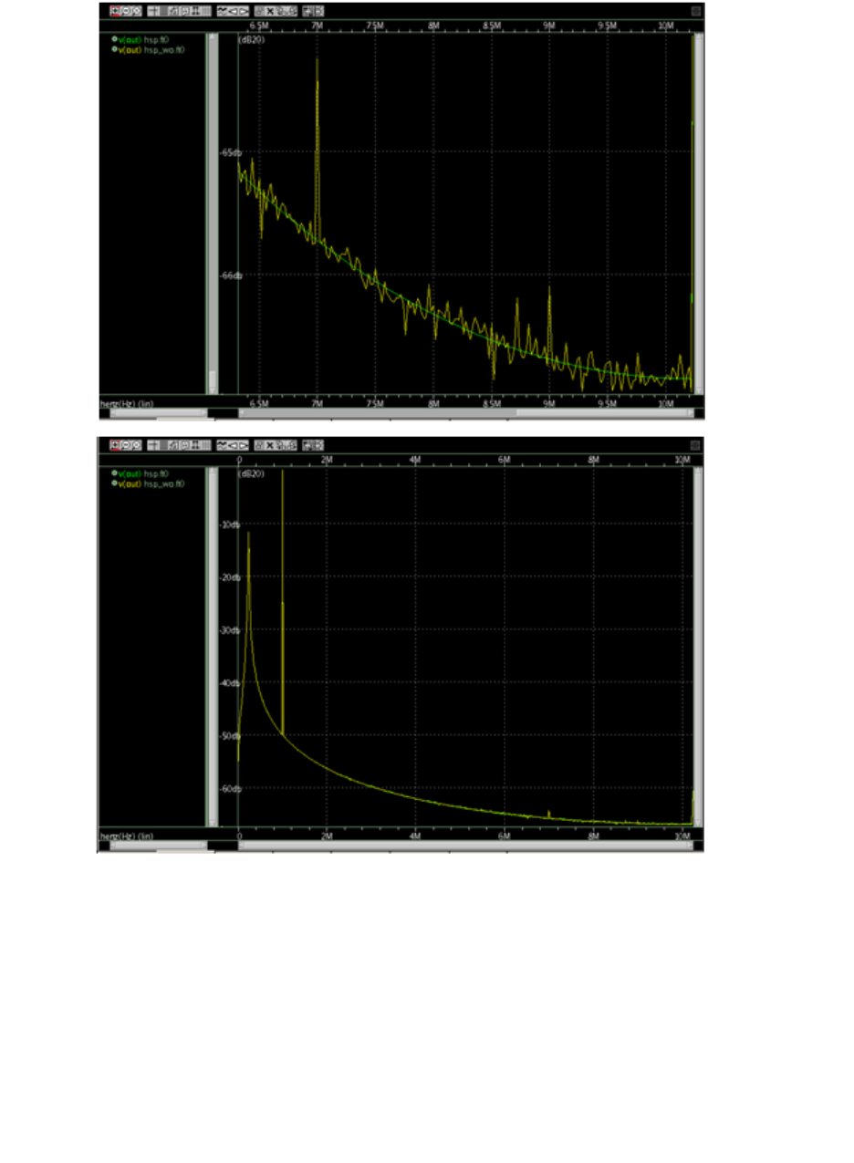
480 HSPICE® Reference Manual: Commands and Control Options
I-2013.12
Chapter 3: HSPICE Simulation Control Options Reference
FFT results from HSPICE .FFT output file (*.ft0)
Green curve indicates HSPICE .FFT with FFT_ACCURATE; Yellow curve
indicates HSPICE .FFT without FFT_ACCURATE showing noises due to
interpolation error.
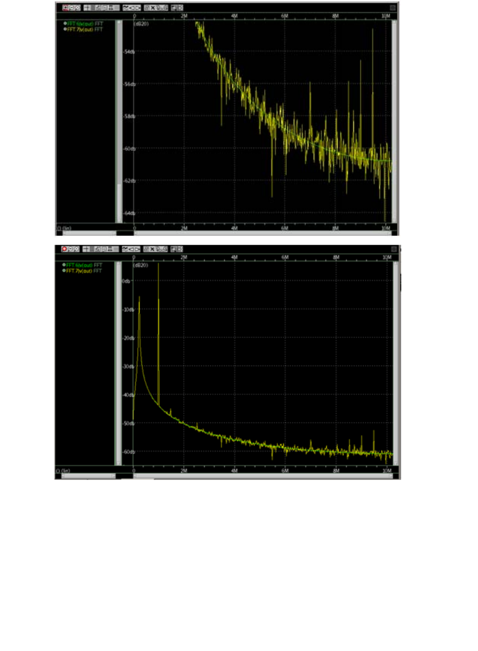
HSPICE® Reference Manual: Commands and Control Options 481
I-2013.12
Chapter 3: HSPICE Simulation Control Options Reference
FFT results using Waveview to post-process HSPICE output file (*.tr0)
Green curve indicates HSPICE .FFT with FFT_ACCURATE; Yellow curve
indicates HSPICE .FFT without FFT_ACCURATE showing noises due to
interpolation error.
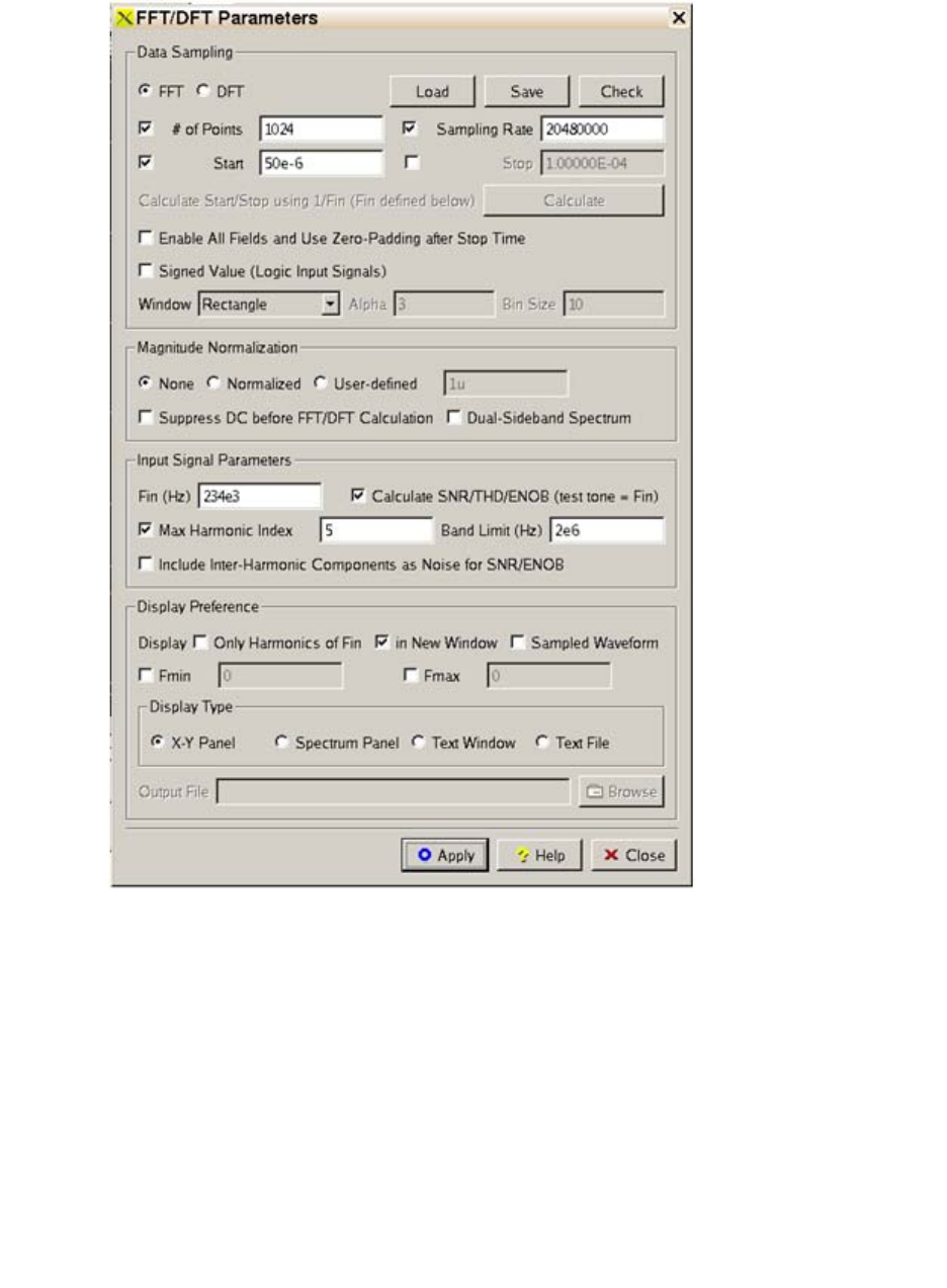
482 HSPICE® Reference Manual: Commands and Control Options
I-2013.12
Chapter 3: HSPICE Simulation Control Options Reference
FFT parameters used for post-processing HSPICE output file (*.tr0)

HSPICE® Reference Manual: Commands and Control Options 483
I-2013.12
Chapter 3: HSPICE Simulation Control Options Reference
Examples
The following example illustrates the usage of .FFT with the FFT_ACCURATE
option:
*Netlist
vin in 0 sin 0 1 1e6
vind ind_ 0 sin 0 0.3 234e3
Emulti inm 0 vcvs in ind_ 2
rin inm out 0 1k
cout out 0 1p
.tran 1p 100u
.fft v(out) start=50e-6 stop=100e-6 np=1024 freq=234e3
.option fft_accurate
.MEASURE FFT sin_thd THD v(out) NBHARM=5 maxfreq=2e6
.option post
.end
See Also
.OPTION ACCURATE
.OPTION SIM_ACCURACY
.OPTION FFTOUT
Prints 30 harmonic fundamentals.
Syntax
.OPTION FFTOUT=0|1
Default Value if option is not specified in the netlist: 0 Value if option name is
specified without a corresponding value: 1
Description
Use this option to print 30 harmonic fundamentals sorted by size, THD, SNR,
and SFDR, but only if you specify a FFTOUT option and a .FFT freq=xxx
command.
See Also
.FFT

484 HSPICE® Reference Manual: Commands and Control Options
I-2013.12
Chapter 3: HSPICE Simulation Control Options Reference
.OPTION FMAX
Sets the maximum frequency value of angular velocity, for poles and zeros.
Syntax
.OPTION FMAX=x
Default 1.0e+12
Description
Use this option to set the maximum frequency value of angular velocity for Pole/
Zero analysis. The units of value are in rad/sec.
See Also
.OPTION CSCAL
.OPTION FSCAL
.OPTION GSCAL
.OPTION ITLPZ
.OPTION LSCAL
.OPTION PZABS
.OPTION PZTOL
.OPTION RITOL
.PZ
.OPTION FS
Decreases FS value to help circuits that have timestep convergence difficulties.
Syntax
.OPTION FS=x
Description
Use this option to decrease delta (internal timestep) by the specified fraction of
a timestep (TSTEP) for the first time point of a transient. Decreases the FS
value to help circuits that have timestep convergence difficulties. DVDT=3 uses
FS to control the timestep.
■You specify DELMAX.
■BKPT is related to the breakpoint of the source.
■The .TRAN command sets TSTEP.
Delta FS MIN TSTEP DELMAX BKPT,,()[⋅=

HSPICE® Reference Manual: Commands and Control Options 485
I-2013.12
Chapter 3: HSPICE Simulation Control Options Reference
See Also
.OPTION DELMAX
.OPTION DVDT
.TRAN
.OPTION FSCAL
Sets the frequency scale for Pole/Zero analysis.
Syntax
.OPTION FSCAL=x
Default 1e-9
Description
Use this option to set the frequency scale for Pole/Zero analysis. HSPICE
multiplies capacitances by FSCAL.
See Also
.OPTION CSCAL
.OPTION FMAX
.OPTION GSCAL
.OPTION ITLPZ
.OPTION LSCAL
.OPTION PZABS
.OPTION PZTOL
.OPTION RITOL
.PZ
.OPTION FSDB
Enables HSPICE to output a transient waveform file (*.tr#) in FSDB format.
Syntax
.OPTION FSDB= [0|1]
Default The value if the option is not specified in the netlist is 0. If the option
name is specified without a corresponding value, the default is 1.

486 HSPICE® Reference Manual: Commands and Control Options
I-2013.12
Chapter 3: HSPICE Simulation Control Options Reference
Description
This option generates a transient waveform file in Fast Signal Database (FSDB)
format.
Important: The latest FSDB version supported by HSPICE is 5.0.
The options are as follows:
■FSDB=0 – Disables the option.
■FSDB=1 – Causes HSPICE to output the transient waveform file in FSDB
format with the suffix: *.tr#.fsdb.
Note: Following are some important notes:
■If you specify both the FSDB and POST options in the
same netlist, the last one declared is effective. Make
sure the FSDB option appears after a POST option in the
netlist file if you prefer the FSDB output format.
■FSDB does not support AC analysis. You will have to
reset the FSDB option to POST for AC output.
.OPTION FT
Decreases delta by a specified fraction of a timestep for iteration set that does
not converge.
Syntax
.OPTION FT=x
Description
Use this option to decrease delta (the internal timestep) by a specified fraction
of a timestep (TSTEP) for an iteration set that does not converge. If DVDT=2 or
DVDT=4, FT controls the timestep.
See Also
.OPTION DVDT
.TRAN

HSPICE® Reference Manual: Commands and Control Options 487
I-2013.12
Chapter 3: HSPICE Simulation Control Options Reference
.OPTION GDCPATH
Adds conductance to nodes having no DC path to ground.
Syntax
.OPTION GDCPATH[=x]
Default 1e-12
Description
Use this option to add conductance to nodes having no DC path to ground.
.OPTION GEN_CUR_POL
Enables specifying that the generic current polarity maintain backward
compatibility with HSPICE simulation files.
Syntax
.OPTION GEN_CUR_POL=ON|OFF
Default OFF
Description
When .OPTION GEN_CUR_POL=ON, the i2() and i3() direction is changed
to use a generic direction rule, that is: the current in is positive, and the current
out is negative. The HSPICE current direction rule is more device-aware.
However, for primitive devices and devices with macro models (subcircuit
definitions), support of a more generic current direction rule enables ease of
use with the Synopsys Galaxy Custom Designer®.
HSPICE current .PRINT/.PROBE statements as in (Wwww), Iall(Wwww) and
Izn(Wwww) work with this option.
This option can be used with the following elements:
■MOSFETs (N and P)
■BJTs (NPN and PNP)
■JFETs (N and P)
■Diodes (D)
■Sources (V and I)
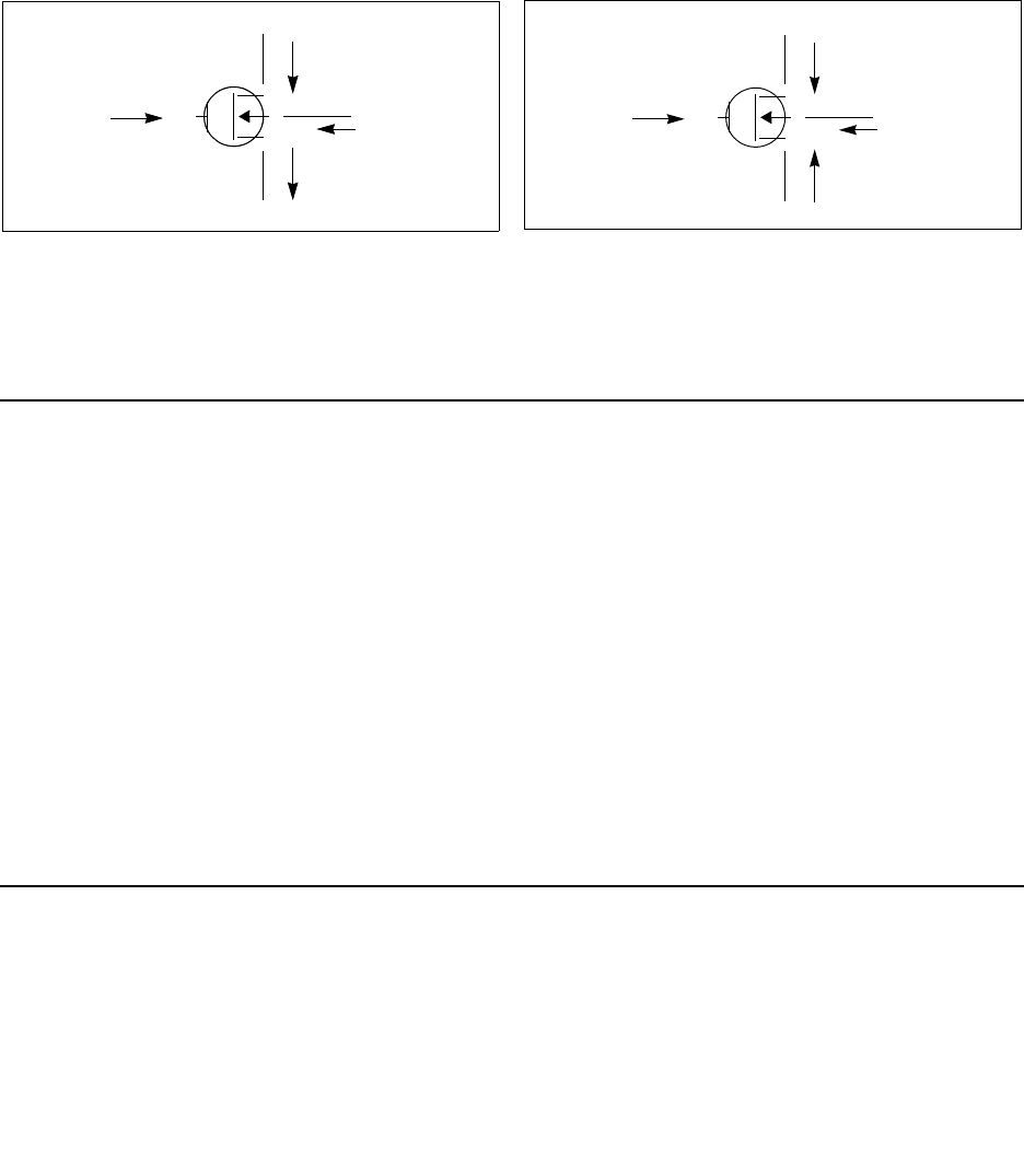
488 HSPICE® Reference Manual: Commands and Control Options
I-2013.12
Chapter 3: HSPICE Simulation Control Options Reference
■Passive elements (L, R and C)
■Behavioral elements (E, F, G and H)
The following elements are not affected by this option and are a limitation of the
F-2011.09 release: W-, U-, T-, P-, and S-elements and IBIS models.
Examples
Figure 14 Direction of current: default HSPICE behavior (left), generic rule (right)
.OPTION GENK
Automatically computes second-order mutual inductance for several coupled
inductors.
Syntax
.OPTION GENK= 0|1
Default Value if option is not specified in the netlist: 1
Value if option name is specified without a corresponding value: 0
Description
Use this option to automatically calculate second-order mutual inductance for
several coupled inductors. The default (1) enables the calculation.
.OPTION GEOCHECK
Checks MOSFET geometry range in global models.
node1 (drain node)
I1 (M1)
node2 (gate node)
I2 (M1)
node3 (source node)
I3 (M1)
node4 (substrate node)
I4 (M1)
node1 (drain node)
I1 (M1)
node2 (gate node)
I2 (M1)
node3 (source node)
I3 (M1)
node4 (substrate node)
I4 (M1)
node1 (drain node)
I1 (M1)
node2 (gate node)
I2 (M1)
node3 (source node)
I3 (M1)
node4 (substrate node)
I4 (M1)
.OPTION GEN_CUR_POL=ON
.OPTION GEN_CUR_POL=OFF (default)

HSPICE® Reference Manual: Commands and Control Options 489
I-2013.12
Chapter 3: HSPICE Simulation Control Options Reference
Syntax
.OPTION GEOCHECK=[0|1|2]
Default 0
Description
Use .OPTION GEOCHECK to validate the geometry range in a global model.
The option checks wmin/lmin/wmax/lmax parameters in the model card.
■0: Suppresses check of MOSFET geometry range in a global model card.
■1: Checks MOSFET geometry range in the global model card that contains
wmin/lmin/wmax/lmax parameters and issues a warning if the device falls
out of range.
■2: Checks MOSFET geometry range in the global model card that contains
wmin/lmin/wmax/lmax parameters and issues an error message if the
device falls out of range.
** warning ** or ** error ** (filename: linenumber) Mosfet
xxx: Instance length or width does not fit the lmin/lmax,
wmin/wmax range for the model xxx. The instance
Length=xxx' Width=xxx. The model range is Lmin=xxx,
Lmax=xxx, Wmin=xxx, Wmax=xxx.
If you declare .OPTION GEOCHECK with no value it is equivalent to .OPTION
GEOCHECK=1.
.OPTION GEOSHRINK
Element scaling factor used with .OPTION SCALE.
Syntax
.OPTION GEOSHRINK=x
Description
Use this option as a global model to apply to all elements. In addition
to .OPTION SCALE, use this option (usually through a technology file) on top of
the existing scale option to further scale geometric element instance
parameters whose default units are meters. The final instance geometric
parameters are then calculated as:
final_dimension = original_dimension * SCALE * GEOSHRINK
The effective scaling factor is the product of the two parameters.

490 HSPICE® Reference Manual: Commands and Control Options
I-2013.12
Chapter 3: HSPICE Simulation Control Options Reference
The default value for both SCALE and GEOSHRINK is 1.
If a model library contains devices other that MOSFET, such as R, L, C, diode,
bjt... etc., and/or the netlist is a post-layout design with RCs, the shrink factor is
applied to all elements.
Examples
Example 1: If there is more than one geoshrink option set, only the last
geoshrink is used.
.option geoshrink=0.8
.option geoshrink=0.9
Then the final_dimension = original_dimension * SCALE * 0.9
Example 2: If there is more than one geoshrink and scale in the model
card, only the last scale and the last geoshrink are used.
.option scale=2u
.option scale=1u
.option geoshrink=0.8
.option geoshrink=0.9
Then the final_dimension = original_dimension * 1u * 0.9
See Also
.OPTION SCALE
.OPTION CMIUSRFLAG
.OPTION GMAX
Specifies the maximum conductance in parallel with a current source for .IC
and .NODESET initialization circuitry.
Syntax
.OPTION GMAX=x
Default 100.00 (mho)
Description
Use this option to specify the maximum conductance in parallel with a current
source for .IC and .NODESET initialization circuitry. Some large bipolar circuits
require you to set GMAX=1 for convergence.

HSPICE® Reference Manual: Commands and Control Options 491
I-2013.12
Chapter 3: HSPICE Simulation Control Options Reference
See Also
.IC
.NODESET
.OPTION IC_ACCURATE
.OPTION GMB_CLAMP
Disables negative conductance clamping.
Syntax
.OPTION GMB_CLAMP=0|1
Default 1
Description
This option allows you to disable gmbs clamping to 0 (for some MOSFET
models, such as Level 54 - BSIM4, when gmbs turns negative, it is
automatically set to 0).
■If .OPTION GMB_CLAMP=0: HSPICE prevents gmbs output from clamping
at zero.
■If GMB_CLAMP=1: conductance is clamped at zero (disallows negative
values).
.OPTION GMIN
Specifies the minimum conductance added to all PN junctions for a time sweep
in transient analysis for HSPICE.
Syntax
.OPTION GMIN=x
Default 1e-12
Description
Use this option to specify the minimum conductance added to all PN junctions
for a time sweep in transient analysis. Min value: 1e-30; Max value: 100.
For BSIM-CMG, GMIN default is 1e-15, and HSPICE scale down user specified
option GMIN by 1e-3.

492 HSPICE® Reference Manual: Commands and Control Options
I-2013.12
Chapter 3: HSPICE Simulation Control Options Reference
See Also
.OPTION GMINDC
.OPTION GMINDC
Specifies conductance in parallel for PN junctions and MOSFET nodes in DC
analysis.
Syntax
.OPTION GMINDC=x
Description
Use this option to specify conductance in parallel for all PN junctions and
MOSFET nodes except gates in DC analysis.GMINDC helps overcome DC
convergence problems caused by low values of off-conductance for PN
junctions and MOSFETs.
Large values of GMINDC can cause unreasonable circuit response. If your
circuit requires large values to converge, suspect a bad model or circuit.
For BSIM-CMG, GMINDC default is 1e-15, and HSPICE scale down user
specified option GMINDC by 1e-3.
See Also
.DC
.OPTION GRAMP
.OPTION PIVTOL
.OPTION GRAMP
Specifies a conductance range over which DC operating point analysis sweeps
GMINDC.
Syntax
.OPTION GRAMP=0|1
Default Value if option is not specified in the netlist: 0 Value if option name is
specified without a corresponding value: 1

HSPICE® Reference Manual: Commands and Control Options 493
I-2013.12
Chapter 3: HSPICE Simulation Control Options Reference
Description
Use this option to specify a conductance range over which the DC operating
point analysis sweeps GMINDC. HSPICE sets this value during auto-
convergence. Use GRAMP with the GMINDC option to find the smallest GMINDC
value that results in DC convergence.
GRAMP specifies a conductance range over which the DC operating point
analysis sweeps GMINDC. HSPICE replaces GMINDC values over this range,
simulates each value, and uses the lowest GMINDC value where the circuit
converges in a steady state.
If you sweep GMINDC between 1e-12 mhos (default) and 1e-6 mhos, GRAMP
is 6 (value of the exponent difference between the default and the maximum
conductance limit). In this example:
■HSPICE first sets GMINDC to 1e-6 mhos and simulates the circuit.
■If circuit simulation converges, HSPICE sets GMINDC to 1e-7 mhos and
simulates the circuit.
■The sweep continues until HSPICE simulates all values of the GRAMP ramp.
If the combined GMINDC and GRAMP conductance is greater than 1e-3 mho,
false convergence can occur.
Min value: 0; Max value: 1000.
See Also
.DC
.OPTION GMINDC
.OPTION GSCAL
Sets the conductance scale for Pole/Zero analysis.
Syntax
.OPTION GSCAL=x
Default 1e+3
Description
Use this option to set the conductance scale for Pole/Zero analysis. HSPICE
multiplies the conductance and divides the resistance by GSCAL.

494 HSPICE® Reference Manual: Commands and Control Options
I-2013.12
Chapter 3: HSPICE Simulation Control Options Reference
See Also
.OPTION CSCAL
.OPTION FMAX
.OPTION FMAX
.OPTION FSCAL
.OPTION GSCAL
.OPTION LSCAL
.OPTION PZABS
.OPTION PZTOL
.OPTION RITOL
.PZ
.OPTION GSHDC
Adds conductance from each node to ground when calculating the DC
operating point of the circuit.
Syntax
.OPTION GSHDC=x
Default 0
Description
Use this option to add conductance from each node to ground when calculating
the DC operating point of the circuit (.OP) to help solve convergence issues.
Examples
.option gshdc=1e-13
See Also
.OPTION GSHUNT
.OPTION GSHUNT
Adds conductance from each node to ground.
Syntax
.OPTION GSHUNT=x
Default 0

HSPICE® Reference Manual: Commands and Control Options 495
I-2013.12
Chapter 3: HSPICE Simulation Control Options Reference
Description
Use this option to add conductance from each node to ground. Add a small
GSHUNT to each node to help solve “timestep too small” problems caused by
either high-frequency oscillations or numerical noise.
Examples
.option gshunt=1e-13 cshunt=1e-17
.option gshunt=1e-12 cshunt=1e-16
.option gshunt=1e-11 cshunt=5e-15
.option gshunt=1e-10 cshunt=1e-15
.option gshunt=1e-9 cshunt=1e-14
See Also
.OPTION CSHUNT
.OPTION GSHDC
.OPTION HB_GIBBS
Option for HBTRAN output to minimize Gibbs’ phenomena.
Syntax
.OPTION HB_GIBBS=n
Default 0
Description
Minimize any Gibbs' phenomenon that may occur in transforming a square-
wave signal from the frequency domain to the time domain. < n >=0 (defaults to
zero, which is equivalent to not using it at all). The result is that the HBTRAN
waveforms are filtered by a function before being transformed to the
time domain via FFT. This option applies only to single-tone output.
Examples
.option hb_gibbs = 2
...
.print hbtran v(2)
See Also
The HSPICE User Guide: Advanced Analog Simulation and Analysis,
Minimizing Gibbs Phenomenon
cx()sin()
N

496 HSPICE® Reference Manual: Commands and Control Options
I-2013.12
Chapter 3: HSPICE Simulation Control Options Reference
.OPTION HBACKRYLOVDIM
Specifies the dimension of the Krylov subspace used by the Krylov solver.
Syntax
.OPTION HBACKRYLOVDIM=value
Default 300
Description
Use this option to specify the dimension of the Krylov subspace that the Krylov
solver uses.
The value parameter must specify an integer greater than zero. The range is 1
to infinity.
This option overrides the corresponding PAC option if specified in the netlist.
When this option is not specified in the netlist if HBACKRYLOVDIM <
HBKRYLOVDIM, then HBACKRYLOVDIM = HBKRYLOVDIM.
See Also
.HB
.OPTION HBACKRYLOVITER / HBAC_KRYLOV_ITER
Specifies the number of GMRES solver iterations performed by the HB engine.
Syntax
.OPTION HBACKRYLOVITER | HBAC_KRYLOV_ITER = value
Description
Use this option to specify the number of Generalized Minimum Residual
(GMRES) solver iterations that the HB engine performs.
The value parameter must specify an integer greater than zero. The range is 1
to infinity.
This option overrides the corresponding PAC option if specified in the netlist.
See Also
.HBAC
.OPTION HBKRYLOVDIM

HSPICE® Reference Manual: Commands and Control Options 497
I-2013.12
Chapter 3: HSPICE Simulation Control Options Reference
.OPTION HBACTOL
Specifies the absolute error tolerance for determining convergence.
Syntax
.OPTION HBACTOL=value
Default 1.e-8
Description
Use this option to specify the absolute error tolerance for determining
convergence. The value parameter must specify a real number greater than
zero. The range is 1.e-14 to infinity.
This option overrides the corresponding PAC option if specified in the netlist.
When this option is not specified in the netlist if HBACTOL > HBTOL, then
HBACTOL = HBTOL.
See Also
.HB
.OPTION HBCONTINUE
Specifies whether to use the sweep solution from the previous simulation as
the initial guess for the present simulation.
Syntax
.OPTION HBCONTINUE= 0|1
Default 1
Description
Use this option to specify whether to use the sweep solution from the previous
simulation as the initial guess for the present simulation.
■HBCONTINUE=1 Use solution from previous simulation as the initial guess.
■HBCONTINUE=0: Start each simulation in a sweep from the DC solution.
See Also
.HB

498 HSPICE® Reference Manual: Commands and Control Options
I-2013.12
Chapter 3: HSPICE Simulation Control Options Reference
.OPTION HBFREQABSTOL
Specifies the maximum absolute change in frequency between solver iterations
for convergence.
Syntax
.OPTION HBFREQABSTOL=value
Default 1Hz
Description
Use this option to specify the maximum absolute change in frequency between
solver iterations for convergence.
This option is an additional convergence criterion for oscillator analysis.
See Also
.HBOSC
.OPTION HBFREQRELTOL
Specifies the maximum relative change in frequency between solver iterations
for convergence.
Syntax
.OPTION HBFREQRELTOL=value
Description
Use this option to specify the maximum relative change in frequency between
solver iterations for convergence.
This option is an additional convergence criterion for oscillator analysis.
See Also
.HBOSC
.OPTION HBJREUSE
Controls when to recalculate the Jacobson matrix.

HSPICE® Reference Manual: Commands and Control Options 499
I-2013.12
Chapter 3: HSPICE Simulation Control Options Reference
Syntax
.OPTION HBJREUSE=0|1
Default Conditional, see below
Description
Use this option to control when to recalculate the Jacobson matrix.
■HBJREUSE=0: Recalculates the Jacobian matrix at each iteration. This is
the default if HBSOLVER=1.
■HBJREUSE=1: Reuses the Jacobian matrix for several iterations if the error
is sufficiently reduced. This is the default if HBSOLVER=0.
See Also
.HB
.OPTION HBJREUSETOL
Determines when to recalculate Jacobian matrix if HBJREUSE=1.0.
Syntax
.OPTION HBJREUSETOL=value
Description
Determines when to recalculate Jacobian matrix (if HBJREUSE=1.0).
This is the percentage by which HSPICE must reduce the error from the last
iteration so you can use the Jacobian matrix for the next iteration. The value
parameter must specify a real number between 0 and 1.
See Also
.HB
.OPTION HBKRYLOVDIM
Specifies the dimension of the subspace used by the Krylov solver.
Syntax
.OPTION HBKRYLOVDIM=value

500 HSPICE® Reference Manual: Commands and Control Options
I-2013.12
Chapter 3: HSPICE Simulation Control Options Reference
Description
Use this option to specify the dimension of the Krylov subspace that the Krylov
solver uses.
The value parameter must specify an integer greater than zero.
See Also
.HB
.OPTION HBKRYLOVTOL
Specifies the error tolerance for the Krylov solver.
Syntax
.OPTION HBKRYLOVTOL=value
Default 0.01
Description
Use this option to specify the error tolerance for the Krylov solver.
The value parameter must specify a real number greater than zero.
See Also
.HB
.OPTION HBKRYLOVMAXITER /
HB_KRYLOV_MAXITER
Specifies the maximum number of GMRES solver iterations performed by the
HB engine.
Syntax
.OPTION HBKRYLOVMAXITER | HB_KRYLOV_MAXITER =value
Default 500
Description
Use this option to specify the maximum number of Generalized Minimum
Residual (GMRES) solver iterations that the HB engine performs.
Analysis stops when the number of iterations reaches this value.

HSPICE® Reference Manual: Commands and Control Options 501
I-2013.12
Chapter 3: HSPICE Simulation Control Options Reference
See Also
.HB
.OPTION HBLINESEARCHFAC
Specifies the line search factor.
Syntax
.OPTION HBLINESEARCHFAC=value
Default 0.35
Description
Use this option to specify the line search factor.
If Newton iteration produces a new vector of HB unknowns with a higher error
than the last iteration, then scale the update step by this value and try again.
The value parameter must specify a real number between 0 and 1.
See Also
.HB
.OPTION HBMAXITER / HB_MAXITER
Specifies the maximum number of Newton-Raphson iterations performed by
the HB engine.
Syntax
.OPTION HBMAXITER | HB_MAXITER=value
Default 10000
Description
Use this option to specify the maximum number of Newton-Raphson iterations
that the HB engine performs.
Analysis stops when the number of iterations reaches this value.
See Also
.HB

502 HSPICE® Reference Manual: Commands and Control Options
I-2013.12
Chapter 3: HSPICE Simulation Control Options Reference
.OPTION HBOSCMAXITER / HBOSC_MAXITER
Specifies the maximum number of outer-loop iterations for oscillator analysis.
Syntax
.OPTION HBOSCMAXITER | HBOSC_MAXITER=value
Default 10000
Description
Use this option to specify the maximum number of outer-loop iterations for
oscillator analysis.
See Also
.HBOSC
.OPTION HBPROBETOL
Searches for a probe voltage at which the probe current is less than the
specified value.
Syntax
.OPTION HBPROBETOL=value
Default 1.e-9
Description
Use this option to cause oscillator analysis to try to find a probe voltage at
which the probe current is less than the specified value.
This option defaults to the value of the HBTOL option, which defaults to 1.e-9.
See Also
.HBOSC
.OPTION HBTOL
.OPTION HBSOLVER
Specifies a pre-conditioner for solving nonlinear circuits.

HSPICE® Reference Manual: Commands and Control Options 503
I-2013.12
Chapter 3: HSPICE Simulation Control Options Reference
Syntax
.OPTION HBSOLVER=0|1|2
Default 1
Description
Use this option to specify a preconditioner for solving nonlinear circuits.
■HBSOLVER=0: Invokes the direct solver.
■HBSOLVER=1 Invokes the matrix-free Krylov solver.
■HBSOLVER=2: Invokes the two-level hybrid time-frequency domain solver.
See Also
.HBOSC
.OPTION HBTOL
Specifies the absolute error tolerance for determining convergence.
Syntax
.OPTION HBTOL=value
Default 1.e-9
Description
Use this option to specify the absolute error tolerance for determining
convergence.
The value parameter must specify a real number greater than zero.
See Also
.HB
.OPTION HBTRANFREQSEARCH
Specifies the frequency source for the HB analysis of a ring oscillator.
Syntax
.OPTION HBTRANFREQSEARCH=[1|0]
Default 1

504 HSPICE® Reference Manual: Commands and Control Options
I-2013.12
Chapter 3: HSPICE Simulation Control Options Reference
Description
Use this option to specify the frequency source for the HB analysis of a ring
oscillator.
■HBTRANFREQSEARCH=1: HB analysis calculates the oscillation frequency
from the transient analysis
■HBTRANFREQSEARCH=0: HB analysis assumes that the period is 1/f, where
f is the frequency specified in the tones description.
See Also
.HB
.HBOSC
.OPTION HBTOL
.OPTION HBTRANINIT
Selects transient analysis for initializing all state variables for HB analysis of a
ring oscillator.
Syntax
.OPTION HBTRANINIT=time
Description
Use this option to cause HB to use transient analysis to initialize all state
variables for HB analysis of a ring oscillator.
The time parameter is defined by when the circuit has reached (or is near)
steady-state. The default is 0.
See Also
.HB
.HBOSC
.OPTION HBTRANPTS
Specifies the number of points per period for converting time-domain data
results into the frequency domain for HB analysis of a ring oscillator.

HSPICE® Reference Manual: Commands and Control Options 505
I-2013.12
Chapter 3: HSPICE Simulation Control Options Reference
Syntax
.OPTION HBTRANPTS=npts
Default 4*nh
Description
Use this option to specify the number of points per period for converting the
time-domain data results from transient analysis into the frequency domain for
HB analysis of a ring oscillator.
The npts parameter must be set to an integer greater than 0. The units are in
nharms (nh).
This option is relevant only if you set .OPTION HBTRANINIT. You can specify
either .OPTION HBTRANPTS or .OPTION HBTRANSTEP, but not both.
See Also
.HB
.HBOSC
.OPTION HBTRANINIT
.OPTION HBTRANSTEP
.OPTION HBTRANSTEP
Specifies transient analysis step size for the HB analysis of a ring oscillator.
Syntax
.OPTION HBTRANSTEP=stepsize
Description
Use this option to specify transient analysis step size for the HB analysis of a
ring oscillator.
The stepsize parameter must be set to a real number. The default is 1/
(4*nh*f0), where nh is the nharms value and f0 is the oscillation frequency.
This option is relevant only if you set .OPTION HBTRANINIT.
Note: You can specify either .OPTION HBTRANPTS or .OPTION
HBTRANSTEP, but not both.
See Also
.HB

506 HSPICE® Reference Manual: Commands and Control Options
I-2013.12
Chapter 3: HSPICE Simulation Control Options Reference
.HBOSC
.OPTION HBTRANINIT
.OPTION HBTRANPTS
.OPTION HBTROUT
Turn-on or turn-off generation of HBTRANINIT initialization output.
Syntax
.OPTION HBTROUT = 0|1
Default 0
Description
Use this option to either turn-on or turn-off generation of HBTRANINIT
initialization data output. The result is a file with the extension *.hbtr0.
■HBTROUT=0: Turns-off the generation of HBTRANINIT initialization output.
■HBTROUT=1: Turns-on the generation of HBTRANINIT initialization output
and the results are stored in a *.hbtr0 file.
See Also
.HB
.HBOSC
.OPTION HBTRANINIT
.OPTION HBTRANPTS
.OPTION HIER_DELIM
Replaces the caret delimiter with a period (for output control only) when used
for HSPICE-ADE only.
Syntax
.OPTION HIER_DELIM= 0|1|2
Default Value if option is not specified in the netlist: 0
Value if option name is specified without a corresponding value: 1

HSPICE® Reference Manual: Commands and Control Options 507
I-2013.12
Chapter 3: HSPICE Simulation Control Options Reference
Description
Use .OPTION HIER_DELIM to change the hierarchy delimiter from a caret (^)
to a period (.) only with for the HSPICE integration to Cadence Virtuoso ADE.
When .OPTION HIER_DELIM=1, a caret (^) is changed to a period(.). This
option works with .OPTION PSF and .OPTION ARTIST.
■0: Maintains the caret.
■1: Replaces the caret with a period.
■2: Use “/” character as a delimiter.
See Also
.OPTION ARTIST
.OPTION PSF
.OPTION HIER_SCALE
Uses the parameter S to scale subcircuits.
Syntax
.OPTION HIER_SCALE=[0|1]
Default Value if option is not specified in the netlist: 0 Value if option name is
specified without a corresponding value: 1
Description
Use this option so you can use the parameter S to scale subcircuits.
■0 Interprets S as a user-defined parameter.
■1 Interprets S as a scale parameter.
This option enables you to selectively scale the required instance. See the
example below.
Examples
Assume you have an encrypted subcircuit from an IP vendor A which has
.option SCALE=1e-6 defined. You have another encrypted subcircuit (from
another IP vendor B), which has the units defined as microns and does not
need to be scaled. When you simulate the circuit, HSPICE applies the SCALE

508 HSPICE® Reference Manual: Commands and Control Options
I-2013.12
Chapter 3: HSPICE Simulation Control Options Reference
option globally and the subcircuit from IP vendor B is scaled again. You can
selectively apply the SCALE option so that this does not happen, as follows:
* Top level netlist
.option hier_scale=1
.include "subckt_a.inc" $ subcircuit from IP vendor A
.include "subckt_b.inc" $ subcircuit from IP vendor B
vin in 0 5
x1 in 2 subckt_a $ uses .option scale=1e-6 defined in subckt_a.inc
file
x2 2 0 subckt_b S=1e6 $ scale option is not required
.tran 100p 10n
.end
The subckt_a.inc file has .option scale=1u defined and this is applied
globally. When .option hier_scale=1 is used and the subcircuit instance,
X2 contains S=1e6, the global scaling is offset.If W=10u is used in subcircuit
instance X2 and hier_scale is used, then:
W="10u*SCALE*S"="10u*1u*1e6"=10u
If W=10 is used in subcircuit instance X1 and “S” is not used, then only the
global .option SCALE=1e-6 is applied and the value of W is 10u.
.OPTION IC_ACCURATE
Improves the accuracy of the .IC command.
Syntax
.OPTION IC_ACCURATE=0|1
Default Value if option is not specified in the netlist: 0
Value if option name is specified without a corresponding value: 1
Description
When .OPTION IC_ACCURATE=1 the .IC command accuracy is increased
for cases requiring tighter precision (for example, when the GMAX value is too
large) than is used to set the maximum conductance in parallel with a current
source for .IC and .NODESET initialization circuitry. The option overrides the
approximating method used by the .IC command with only slight performance
cost. If the option is not set or it equals 0, then the default .IC method is used.

HSPICE® Reference Manual: Commands and Control Options 509
I-2013.12
Chapter 3: HSPICE Simulation Control Options Reference
See Also
.IC
.OPTION GMAX
.OPTION ICSWEEP
Saves the current analysis result of a parameter or temperature sweep as the
starting point in the next analysis.
Syntax
.OPTION ICSWEEP=0|1|2
Default 1
Description
Use this option to save the current analysis result of a parameter or
temperature sweep as the starting point in the next analysis in the sweep.
■If ICSWEEP=0, the next analysis does not use the results of the current
analysis.
■If ICSWEEP=1, the next analysis uses the current results.
■If ICSWEEP=2, the operating point will be re-used between each
optimization sweep. (The next analysis skips the OP operation during a
transient sweep if the operating point is always same.) Use this setting if the
OP has not changed during the transient sweep to speed up the simulation.
.OPTION IMAX
Specifies the maximum timestep in timestep algorithms for transient analysis.
Syntax
.OPTION IMAX=x
Description
Use this option to specify the maximum timestep in algorithms for transient
analysis.IMAX sets the maximum iterations to obtain a convergent solution at a
timepoint. If the number of iterations needed is greater than IMAX, the internal
timestep (delta) decreases by a factor equal to the FT transient control option.

510 HSPICE® Reference Manual: Commands and Control Options
I-2013.12
Chapter 3: HSPICE Simulation Control Options Reference
The new timestep calculates a new solution. IMAX also works with the IMIN
transient control option. IMAX is the same as ITL4.
See Also
.OPTION FT
.OPTION IMIN
.OPTION ITL4
.OPTION IMIN
Specifies the minimum timestep in timestep algorithms for transient analysis.
Syntax
.OPTION IMIN=x
Description
Use this option to specify the minimum number of iterations required to obtain
convergence for transient analysis. If the number of iterations is less than
IMIN, the internal timestep (delta) doubles.
Use this option to decrease simulation times in circuits where the nodes are
stable most of the time (such as digital circuits). If the number of iterations is
greater than IMIN, the timestep stays the same unless the timestep exceeds
the IMAX option. IMIN is the same as ITL3.
See Also
.OPTION IMAX
.OPTION ITL3
.OPTION INGOLD
Controls whether HSPICE prints *.lis file output in exponential form or
engineering notation in HSPICE.
Syntax
.OPTION INGOLD=[0|1|2]
Default Value if option is not specified in the netlist: 0
Value if option name is specified without a corresponding value: 1

HSPICE® Reference Manual: Commands and Control Options 511
I-2013.12
Chapter 3: HSPICE Simulation Control Options Reference
Description
Use this option to control if HSPICE prints output in exponential form (scientific
notation) or engineering notation. Engineering notation provides two to four
extra significant digits and aligns columns to facilitate comparison, as:
F=1e-15 M=1e-3
P=1e-12 K=1e3
N=1e-9 X=1e6
U=1e-6 G=1e9
When using HSPICE advanced analog functions variable values in engineering
notation is printed by default. To use the exponential form, specify .OPTION
INGOLD=1 or 2. To print variable values in exponential form, specify .OPTION
INGOLD=1 or 2.
.OPTION INGOLD does not control the number format in measure files (*.mt#/
*.ms#/*.ma#). If you specify a measure output file using .OPTION
MEASFORM, HSPICE automatically resets an INGOLD=0 setting to INGOLD=1,
which allows the measure file to be imported to Excel when .OPTION
MEASFORM=1.
For DCMatch and ACMatch results, with the G-2012.06-SP1 release,
significant digits is increased to a default of four. For example:
> Output 1-sigma due to total variations = 317.9979uA
< Output 1-sigma due to global variations = 224.86uA
---
> Output 1-sigma due to global variations = 224.8585uA
< Output 1-sigma due to local variations = 224.86uA
---
> Output 1-sigma due to local variations = 224.8585uA
Examples
.OPTION INGOLD=2
Argument Description
INGOLD=0 Engineering Format; defaults 1.234K, 123M
INGOLD=1 G Format (fixed and exponential); defaults 1.234e+03, .123
INGOLD=2 E Format (exponential SPICE); defaults 1.234e+03, .123e-1

512 HSPICE® Reference Manual: Commands and Control Options
I-2013.12
Chapter 3: HSPICE Simulation Control Options Reference
See Also
.OPTION MEASDGT
.OPTION MEASFORM
.OPTION INTERP
Limits output to only the .TRAN timestep intervals for post-analysis tools.
Syntax
.OPTION INTERP=0|1
Default Value if option is not specified in the netlist: 0 (engineering notation)
Value if option name is specified without a corresponding value: 1
Description
Use to limit output for post-analysis tools to only the .TRAN timestep intervals
for some post-analysis tools. This option can be used to reduce the size of the
post-processing output. By default, HSPICE outputs data at internal timepoints.
In some cases, INTERP produces a much larger design .tr# file, especially
for smaller timesteps, and it also leads to longer runtime. When using INTERP,
make sure you set TSTEP to the intervals you need the simulation data printed
at.
Note: Since HSPICE uses the post-processing output to compute the
.MEASURE command results, interpolation errors result if you
use the INTERP option and your netlist also contains .MEASURE
commands. Using the INTERP option with .MEASURE
commands is not recommended.
When you run data-driven transient analysis (.TRAN DATA) in an optimization
routine, HSPICE forces INTERP=1. All measurement results are at the time
points specified in the data-driven sweep.
See Also
.TRAN
.OPTION IPROP
Controls whether to treat all of the circuit information as IP protected.

HSPICE® Reference Manual: Commands and Control Options 513
I-2013.12
Chapter 3: HSPICE Simulation Control Options Reference
Syntax
.OPTION IPROP 0|1
Default Value if option is not specified in the netlist: 0 Value if option name is
specified without a corresponding value: 1
Description
Use to control whether to treat all of the circuit information as IP protected and
not output this information during simulation.
■0= Output information (IP not protected)
■1=Do not output information (IP protected)
.OPTION ITL1
Specifies the maximum DC iteration limit.
Syntax
.OPTION ITL1=n
Description
Use this option to specify the maximum DC iteration limit. Increasing this value
rarely improves convergence in small circuits. Values as high as 400 have
resulted in convergence for some large circuits with feedback (such as
operational amplifiers and sense amplifiers). However, most models do not
require more than 100 iterations to converge.
See Also
.DC
.OPTION ITL2
Specifies the iteration limit for the DC transfer curve.
Syntax
.OPTION ITL2=n
Description
Use this option to specify the iteration limit for the DC transfer curve. Increasing
this limit improves convergence only for very large circuits.

514 HSPICE® Reference Manual: Commands and Control Options
I-2013.12
Chapter 3: HSPICE Simulation Control Options Reference
See Also
.DC
.OPTION ITL3
Specifies minimum timestep in timestep algorithms for transient analysis.
Syntax
.OPTION ITL3=x
Description
Use this option to specify the minimum timestep in timestep algorithms for
transient analysis.ITL3 is the minimum number of iterations required to obtain
convergence. If the number of iterations is less than ITL3, the internal timestep
(delta) doubles.
Use this option to decrease simulation times in circuits where the nodes are
stable most of the time (such as digital circuits). If the number of iterations is
greater than IMIN, the timestep stays the same unless the timestep exceeds
the IMAX option. ITL3 is the same as IMIN.
See Also
.OPTION IMAX
.OPTION IMIN
.OPTION ITL4
Specifies maximum timestep in timestep algorithms for transient analysis in
HSPICE.
Syntax
.OPTION ITL4=x
Default 8
Description
Use this option to specify the maximum timestep in timestep algorithms for
transient analysis.ITL4 sets the maximum iterations to obtain a convergent
solution at a timepoint. If the number of iterations needed is greater than ITL4,
the internal timestep (delta) decreases by a factor equal to the FT transient

HSPICE® Reference Manual: Commands and Control Options 515
I-2013.12
Chapter 3: HSPICE Simulation Control Options Reference
control option. HSPICE uses the new timestep to calculate a new solution.
ITL4 also works with the IMIN transient control option. For HSPICE, ITL4 is
the same as IMAX.
See Also
.OPTION FT
.OPTION IMAX
.OPTION IMIN
.OPTION ITL5
Sets an iteration limit for transient analysis.
Syntax
.OPTION ITL5=x
Default 0 (infinite number of iterations)
Description
Use this option to set an iteration limit for a transient analysis. If a circuit uses
more than ITL5 iterations, the program prints all results up to that point.
.OPTION ITLPTRAN
Controls iteration limit used in the final try of the pseudo-transient method.
Syntax
.OPTION ITLPTRAN=x
Default 30
Description
Use this option to control the iteration limit used in the final try of the pseudo-
transient method in OP or DC analysis. If a simulation fails in the final try of the
pseudo-transient method, provide a higher value.
See Also
.DC
.OP

516 HSPICE® Reference Manual: Commands and Control Options
I-2013.12
Chapter 3: HSPICE Simulation Control Options Reference
.OPTION ITLPZ
Sets the iteration limit for pole/zero analysis.
Syntax
.OPTION ITLPZ=x
Default 100
Description
Use this option to set the iteration limit for pole/zero analysis.
See Also
.OPTION CSCAL
.OPTION GSCAL
.PZ
.OPTION FMAX
.OPTION ITRPRT
Enables printing of output variables at their internal time points.
Syntax
.OPTION ITRPRT 0|1
Default Value if option is not specified in the netlist: 0 Value if option name is
specified without a corresponding value: 1
Description
Use this option to enable printing of output variables at their internal time
points.
When set to 1, HSPICE prints output variables at their internal transient
simulation time points. In addition, if you use the -html option when invoking
HSPICE, then HSPICE prints the values to a separate file (*.printtr0).
.OPTION IVDMARGIN
Helps characterize Vdmargin using terminal I-V at MOSFET external nodes.
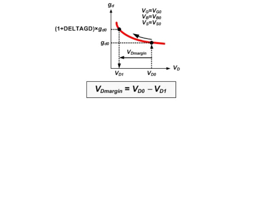
HSPICE® Reference Manual: Commands and Control Options 517
I-2013.12
Chapter 3: HSPICE Simulation Control Options Reference
Syntax
.OPTION IVDMARGIN=x
Default 0.1
Description
X is a positive variable in double type to define the relative gd change target for
vdmargin calculation. X is typically in a range of 0 to 1. An alternative to the
command.IVDMARGIN, this option is only available for BSIM4 MOSFETs.
Wildcards (*) can be used to specify FETs. If no FET is specified, then the
value applies to all FETs in the simulation by default.
Vdmargin, as shown in the following plot, is defined as the MOSFET drain
voltage range within which the change in the MOSFET drain conductance
(with respect to reference (the gd value at operating point) is
smaller than a user-specified target. It provides a heuristic measure of how
much the drain voltage can be reduced, particularly in the saturation region of
MOSFET operation, beyond which the MOSFET drain conductance has
degraded beyond a user-specified tolerance.
■If the option is not set, HSPICE does not invoke Vdmargin characterization.
■If the option is given with a non-zero X, Vdmargin simulation is invoked with
X as the target of gd change. For example, .OPTION iVdmargin=X
■If the option is given with no argument specified, Vdmargin is invoked and
uses X = 0.1
■iVdmargin=0 is equivalent to turning off the Vdmargin simulation.
gd ld•
vd•
---------------
=

518 HSPICE® Reference Manual: Commands and Control Options
I-2013.12
Chapter 3: HSPICE Simulation Control Options Reference
Note: If both the .IVDMARGIN command and .OPTION IVDMARGIN
are both set in a netlist, HSPICE ignores the option.
See Also
.IVDMARGIN
Vdmargin Output
.OPTION IVTH
Invokes a constant-current threshold voltage probing and characterization
function for BSIM4 models.
Syntax
.OPTION IVTH=val | IVTHN=val | IVTHP=val
Description
Specifies the ivth constant drain terminal current density, to be multiplied by
the ratio of transistor width (W) and length (L). The value must be greater than
zero to enable the function; the IVTH option should always be set to a positive
value for both PMOS and NMOS.
.OPTION IVTH supports HSPICE BSIM4 (level 54), BSIMSOI4.x (level 70),
and PSP (level 69) and BSIM-CMG (level72). .OPTION IVTHN and IVTHP
support NMOS and PMOS, respectively.
Note: The val should be a constant.
In OP analysis, a constant current based vth is reported in the OP output. In
addition, the element region operation check and Vod output are based on the
new vth. During transient or DC analysis, a template output of LX142
accesses the new vth value. You can use LX142(m*) or ivth(m*) for the
new vth output. This methodology is based on the monotony Id/Vgs curve.
If Vds is smaller than 0.05V, HSPICE invokes a special characterization method
for small Vds bias to ensure continuation and a meaningful characterization
result. Here is the method:
1. Simulate Vth_op(Vdsmin) and Vth_ivth(Vdsmin) where: Vth_op() is the
threshold voltage acquired from model formulation, and vth_ivth() is the
threshold voltage acquired from iVth method.
2. Calculate DeltaVth = Vth_op(Vdsmin) - Vth_ivth(Vdsmin)

HSPICE® Reference Manual: Commands and Control Options 519
I-2013.12
Chapter 3: HSPICE Simulation Control Options Reference
3. Simulate Vth_op(Vds)
4. Calculate Vth_ivth(Vds) = Vth_op(Vds) - DeltaVth
.OPTION IVTH_MODEL
Foundry defined specific constant-current threshold voltage probing and
characterization.
Syntax
.OPTION IVTH_MODEL=0|1
Default Value if option is not specified in the netlist: 0
Value if option name is specified without a corresponding value: 1
Description
Foundry defined specific constant-current threshold voltage probing and
characterization.
.OPTION KCLTEST
Activates the KCL (Kirchhoff’s Current Law) test.
Syntax
.OPTION KCLTEST=0|1
Default Value if option is not specified in the netlist: 0 Value if option name is
specified without a corresponding value: 1
Description
Use this option to activate the KCL test. This increases simulation time,
especially for large circuits, but checks the solution with a high degree of
accuracy.
If you set this value to 1, HSPICE sets these options:
■Sets RELMOS and ABSMOS options to 0 (off).
■Sets ABSI to 1e-6 A.
■Sets RELI to 1e-6.
To satisfy the KCL test, each node must satisfy this condition:

520 HSPICE® Reference Manual: Commands and Control Options
I-2013.12
Chapter 3: HSPICE Simulation Control Options Reference
In this equation, the ibs are the node currents.
See Also
.OPTION ABSI
.OPTION ABSMOS
.OPTION RELI
.OPTION RELMOS
.OPTION KLIM
Sets the minimum mutual inductance.
Syntax
.OPTION KLIM=x
Description
Use this option to set the minimum mutual inductance below which automatic
second-order mutual inductance calculation no longer proceeds. KLIM is
unitless (analogous to coupling strength, specified in the K-element). Typical
KLIM values are between .5 and 0.0.
.OPTION LA_FREQ
Specifies the upper frequency for which accuracy must be preserved.
Syntax
.OPTION LA_FREQ=value
Default 1GHz
Description
Use this option to specify the upper frequency for which accuracy must be
preserved.
The value parameter specifies the upper frequency for which the PACT
algorithm must preserve accuracy. If value is 0, the algorithm drops all
capacitors because only DC is of interest.
ΣibRELI Σib
⋅< ABSI+

HSPICE® Reference Manual: Commands and Control Options 521
I-2013.12
Chapter 3: HSPICE Simulation Control Options Reference
The maximum frequency required for accurate reduction depends on both the
technology of the circuit and the time scale of interest. In general, the faster the
circuit, the higher the maximum frequency.
For additional information, see “Linear Acceleration” in the HSPICE User
Guide: Basic Simulation and Analysis.
See Also
.OPTION SIM_LA
.OPTION LA_TIME
.OPTION LA_MAXR
Specifies the maximum resistance for linear matrix reduction.
Syntax
.OPTION LA_MAXR=value
Default 1e15 ohms
Description
Use this option to specify the maximum resistance for linear matrix reduction.
The value parameter specifies the maximum resistance preserved in the
reduction. The linear matrix reduction process assumes that any resistor
greater than value has an infinite resistance and drops the resistor after
reduction is completed.
For additional information, see “Linear Acceleration” in the HSPICE User
Guide: Basic Simulation and Analysis.
See Also
.OPTION SIM_LA
.OPTION LA_MINC
Specifies the minimum capacitance for linear matrix reduction.
Syntax
.OPTION LA_MINC=val
Default 1e-16 farads

522 HSPICE® Reference Manual: Commands and Control Options
I-2013.12
Chapter 3: HSPICE Simulation Control Options Reference
Description
Removes any capacitor in the original netlist less than the value of LA_MINC
prior to reduction. For additional information, see “Linear Acceleration” in the
HSPICE User Guide: Basic Simulation and Analysis.
See Also
.OPTION SIM_LA
.OPTION LA_FREQ
.OPTION LA_MAXR
.OPTION LA_TIME
.OPTION LA_TOL
.OPTION LA_SPLC
Helps reduce RC post-processing time.
Syntax
.OPTION LA_SPLC=0|1
Default 0
Description
As an adjunct to .OPTION SIM_LA, .OPTION LA_SPLC=1 turns on capacitor
splitting. Cap splitting skips the matrix reservation for coupling entries of the
capacitor. This option works only in conjunction with .OPTION SIM_LA. For
additional information, see “Linear Acceleration” in the HSPICE User Guide:
Basic Simulation and Analysis.
See Also
.OPTION SIM_LA
.OPTION LA_TIME
Specifies the minimum time for which accuracy must be preserved.
Syntax
.OPTION LA_TIME=value

HSPICE® Reference Manual: Commands and Control Options 523
I-2013.12
Chapter 3: HSPICE Simulation Control Options Reference
Description
Use this option to specify the minimum time for which accuracy must be
preserved. The value parameter specifies the minimum switching time for
which the PACT algorithm preserves accuracy.
Waveforms that occur more rapidly than the minimum switching time are not
accurately represented.
This option is simply an alternative to .OPTION LA_FREQ. The default is
equivalent to setting LA_FREQ=1GHz.
Note: Higher frequencies (smaller times) increase accuracy, but only
up to the minimum time step used in HSPICE.
For additional information, see “Linear Acceleration” in the HSPICE User
Guide: Basic Simulation and Analysis.
Examples
For a circuit having a typical rise time of 1ns, either set the maximum frequency
to 1 GHz, or set the minimum switching time to 1ns:
.OPTION LA_FREQ=1GHz
-or-
.OPTION LA_TIME=1ns
However, if spikes occur in 0.1ns, HSPICE does not accurately simulate them.
To capture the behavior of the spikes, use:
.OPTION LA_FREQ=10GHz
-or-
.OPTION LA_TIME=0.1ns
See Also
.OPTION SIM_LA
.OPTION LA_FREQ
.OPTION LA_TOL
Specifies the error tolerance for the PACT algorithm.
Syntax
.OPTION LA_TOL=value
Default 0.05

524 HSPICE® Reference Manual: Commands and Control Options
I-2013.12
Chapter 3: HSPICE Simulation Control Options Reference
Description
Use this option to specify the error tolerance for the PACT algorithm.
The value parameter must specify a real number between 0.0 and 1.0.
For additional information, see “Linear Acceleration” in the HSPICE User
Guide: Basic Simulation and Analysis.
See Also
.OPTION SIM_LA
.OPTION LENNAM
Specifies maximum name length for printing operating point analysis results.
Syntax
.OPTION LENNAM=x
Default 8 (characters)
Description
Use this option to specify the maximum length of names in the printout of
operating point analysis results. The maximum value is 1024. .OPTION
LENNAME prints the full related name of the transistor in the noise tables and
OP tables.
Examples
...
.OPTIONS POST=1 LENNAM=40
...
.OPTION LIMPTS
Specifies the number of points to print in AC analysis.
Syntax
.OPTION LIMPTS=x
Default 2001

HSPICE® Reference Manual: Commands and Control Options 525
I-2013.12
Chapter 3: HSPICE Simulation Control Options Reference
Description
Use this option to specify the number of points to print or plot in AC analysis.
You do not need to set LIMPTS for a DC or transient analysis. HSPICE spools
the output file to disk.
See Also
.AC
.DC
.TRAN
.OPTION LIMTIM
Specifies the amount of CPU time reserved to generate prints.
Syntax
.OPTION LIMTIM=x
Default 2 (seconds)
Description
Use this option to specify the amount of CPU time reserved to generate prints
and plots if a CPU time limit (CPTIME=x) terminates simulation. Default is
normally sufficient for short printouts.
See Also
.OPTION CPTIME
.OPTION LIS_NEW
Enables streamlining improvements to the *.lis file.
Syntax
.OPTION LIS_NEW=0|1
Default Value if option is not specified in the netlist: 0
Value if option name is specified without a corresponding value: 1

526 HSPICE® Reference Manual: Commands and Control Options
I-2013.12
Chapter 3: HSPICE Simulation Control Options Reference
Description
Use .OPTION LIS_NEW to activate several streamlining improvements to the
*.lis file as noted below. A value of 0 disables the following functions. A value
of 1 enables the following:
■Moves .PRINT data and .NOISE analysis data to separate files,
■Suppresses operating point node voltage table that exists in the *.ic# file.
■Prints loading information for input files.
■Invokes console printing of simulation progress percentage.
■Adds a convergence status update to *.lis.
■Increments every 10% of analysis update to *.lis.
■Reports analysis output file with analysis-specific format.
■Prints Improved format of circuit statistics information.
■Any .PRINT statement in your netlist generates a text file containing the
simulation results. For a transient analysis, the file has the extension,
.printtr#.
■Operating point analysis information is separated to file if .OP is used in
netlist (LIS_NEW=1 automatically sets .OPTION OPFILE=1).
■Model related information is suppressed (LIS_NEW=1 automatically sets
.OPTION NOMOD=1). Circuit hierarchy to number mapping information is
not printed to *.lis file and LIS_NEW=1 nullifies .OPTION LISLVL.
See Also
.OPTION LIST
.LIB
.NOISE
.OPTION LISLVL
.OPTION NOMOD
.OPTION OPFILE
.OP
.OPTION LISLVL
Controls whether of not HSPICE suppresses the circuit number to circuit
hierarchy information in the listing file.

HSPICE® Reference Manual: Commands and Control Options 527
I-2013.12
Chapter 3: HSPICE Simulation Control Options Reference
Syntax
LISLVL=0|1
Default Value if option is not specified in the netlist: 0
Value if option name is specified without a corresponding value: 1
Description
LISLVL=0 prints the circuit name directory information in the .lis file.If the
value is 1, the circuit number and circuit hierarchy information is not output to
the .lis file.
.OPTION LIST
Prints a list of netlist elements, node connections, and values for components,
voltage and current sources, parameters, and more.
Syntax
.OPTION LIST=0|1|2|3
Default Value if option is not specified in the netlist: 0
Value if option name is specified without a corresponding value: 1
Description
Use this option as follows:
■0 | NONE: None of below supported
■1 | ALL: Print circuit element summary table and parameter definitions
■2 | ELEMENT: Print circuit element summary table only
■3 | PARAMETER: Print circuit parameter definitions only
The LIST option also prints effective sizes of elements as follows, and key
values: when LIST=1 or List=2, element information files *.el0 are
generated (if .OPTION ARTIST=2 and .OPTION PSF are used in a netlist.
Otherwise, *.el0 files are suppressed and element information is not reported
in the log file.
See Also
.OPTION ARTIST
.OPTION LIS_NEW
.OPTION PSF

528 HSPICE® Reference Manual: Commands and Control Options
I-2013.12
Chapter 3: HSPICE Simulation Control Options Reference
.OPTION UNWRAP
.OPTION VFLOOR
.OPTION LOADHB
Loads state variable information from a specified file.
Syntax
.OPTION LOADHB=’filename’
Description
Use this option to load the state variable information contained in the specified
file. These values are used to initialize the HB simulation.
See Also
.HB
.OPTION LOADSNINIT
Loads the operating point saved at the end of Shooting Newton analysis
initialization.
Syntax
.OPTION LOADSNINIT="filename"
Description
Use this option to load the operating point file saved at the end of SN
initialization, which is used as initial conditions for the Shooting-Newton
method.
.OPTION LSCAL
Sets the inductance scale for Pole/Zero analysis.
Syntax
.OPTION LSCAL=x
Default 1e+6

HSPICE® Reference Manual: Commands and Control Options 529
I-2013.12
Chapter 3: HSPICE Simulation Control Options Reference
Description
Use this option to set the inductance scale for Pole/Zero analysis. HSPICE
multiplies inductance by LSCAL.
Note: Scale factors must satisfy the following
relations:
If you change scale factors, you might need to modify the initial
Muller points, (X0R, X0I), (X1R, X1I) and (X2R, X2I), even
though HSPICE internally multiplies the initial values by (1.0e-9/
GSCAL).
The three complex starting-trial points, in the Muller (x1R,X1I) algorithm for
pole/zero analysis are listed below with their defaults. HSPICE multiplies these
initial points, and FMAX, by FSCAL.
See Also
.OPTION CSCAL
.OPTION FMAX
.OPTION FSCAL
.OPTION GSCAL
.OPTION ITLPZ
.OPTION PZABS
.OPTION PZTOL
.OPTION RITOL
.OPTION (X0R,X0I)
.OPTION (X1R,X1I)
.OPTION (X2R,X21)
.PZ
Starting-Trial Points Defaults
.OPTION (X0R,X0I) X0R=-1.23456e6 X0I=0.0
.OPTION (X1R,X1I) X1R=1.23456e5 X1I=0.0
.OPTION (X2R,X21) X2R=+1.23456e6 X2I=0.0
GSCAL CSCAL FSCAL⋅=
GSCAL 1
LSCAL FSCAL⋅
---------------------------------------------
=

530 HSPICE® Reference Manual: Commands and Control Options
I-2013.12
Chapter 3: HSPICE Simulation Control Options Reference
.OPTION LVLTIM
Selects the timestep algorithm for transient analysis.
Syntax
.OPTION LVLTIM=[1|2|3]|4]
Default 1
Description
Use this option, (levels 1-3, only) to select the timestep algorithm for transient
analysis.
■LVLTIM=1 (default) uses the DVDT timestep control algorithm.
■LVLTIM=2 uses the local truncation error (LTE) timestep control method.
You can apply LVLTIM=2 to the TRAP method.
■LVLTIM=3 uses the DVDT timestep control method with timestep reversal.
■LVLTIM=4 is invalid if set by user; it is invoked by the RUNLVL option only
to enhance the LTE time step control method used by the latest RUNLVL
algorithm.
The local truncation algorithm LVLTIM=2 (LTE) provides a higher degree of
accuracy than LVLTIM=1 or 3 (DVDT). If you use this option, errors do not
propagate from time point to time point, which can result in an unstable
solution.
Selecting the GEAR method changes the value of LVLTIM to 2 automatically.
For information on how LVLTIM values impact other options, see Appendix A,
HSPICE Control Options Behavioral Notes.
See Also
.OPTION CHGTOL
.OPTION DVDT
.OPTION FS
.OPTION FT
.OPTION RELQ

HSPICE® Reference Manual: Commands and Control Options 531
I-2013.12
Chapter 3: HSPICE Simulation Control Options Reference
.OPTION MACMOD
Enables HSPICE to access the subcircuit definition for MOSFETs, diodes, and
BJTs, when there is no matching model reference; also enables an HSPICE X-
element to access the model reference when there is no matching subcircuit
definition.
Syntax
.OPTION MACMOD=[1|2|3|0]
Default Value if option is not specified in the netlist: 0 Value if option name is
specified without a corresponding value: 1
Description
The following describes .OPTION MACMOD characteristics:
■When macmod=1, HSPICE seeks a subckt definition for the M/Q/D***
element if no model reference exists. The desired subckt name must match
(case insensitive) the mname field in the M/Q/D*** instance command. In
addition, the number of terminals of the subckt must match the M/Q/D***
element referencing it; otherwise HSPICE exits the simulation based on lack
of definition for the M/Q/D*** element. Moreover, the M instance can call
Verilog-A models when macmod=1.
■When macmod=2, HSPICE seeks a model definition when it cannot find a
matching subckt or Verilog-A definition for an X-element. The targeted
MODEL card could be either an HSPICE built-in model or CMI model. If the
model card that matched the X-element reference name is not a type of M/
Q/D model, the simulator exits and displays an error message indicating that
the reference is “not found.”
■When macmod=3, HSPICE enables the same features as when macmod=1.
HSPICE seeks a .subckt definition for an M/Q/D-element if there is no
matching model reference; HSPICE seeks a .model definition for an X-
element if there is no matching .subckt or Verilog-A definition. Usage
considerations and limitations remain the same for both features,
respectively.
If .OPTION TMIFLAG 1, .OPTION MACMOD automatically equals 3.
When macmod=0: if there is no .OPTION MACMOD in the input files or
MACMOD=0, then neither of the features is enabled. HSPICE ignores the option
MACMOD when any value other than 1|2|3|0 is set.The MACMOD option is a
≥

532 HSPICE® Reference Manual: Commands and Control Options
I-2013.12
Chapter 3: HSPICE Simulation Control Options Reference
global option; if there are multiple MACMOD options in one simulation, HSPICE
uses the value of the last MACMOD option.
For examples and detailed discussion, see MOSFET Element Support
Using .OPTION MACMOD in the HSPICE User Guide: Basic Simulation and
Analysis.
See Also
.OPTION TMIFLAG
.OPTION MAXAMP
Sets the maximum current through voltage-defined branches.
Syntax
.OPTION MAXAMP=x
Description
Use this option to set the maximum current through voltage-defined branches
(voltage sources and inductors). If the current exceeds the MAXAMP value,
HSPICE reports an error.
.OPTION MAXORD
Specifies the maximum order of integration for the GEAR method.
Syntax
.OPTION MAXORD=[1|2|3]
Description
Use this option to specify the maximum order of integration for the GEAR
method. When the GEAR method is used, based on the circuit type, HSPICE
automatically switches the GEAR order on the fly. If this option is not
specifically set, HSPICE automatically selects the BDF or GEAR integration
method based on circuit type when METHOD=GEAR.
The value of the parameter can be either 1, 2, or 3:

HSPICE® Reference Manual: Commands and Control Options 533
I-2013.12
Chapter 3: HSPICE Simulation Control Options Reference
■MAXORD=1 selects the first-order GEAR (Backward-Euler) integration (and
prohibits GEAR from switching to BDF).
■MAXORD=2 selects the second-order GEAR (Gear-2), which is more stable
and accurate than MAXORD=1.
■MAXORD=3 selects the third-order or high GEAR (Gear-3), which is most
accurate, since it uses 3 previous time points to estimate the next time point.
Examples
This example selects the Backward-Euler integration method.
.OPTION MAXORD=1 METHOD=GEAR
See Also
.OPTION METHOD
.OPTION RUNLVL
.OPTION MAXWARNS
Specifies maximum number of safe operating area (SOA) warning messages.
Syntax
.OPTION MAXWARNS=n
Default 5
Description
Use this option to specify the maximum number of SOA warning messages
when terminal voltages of a device (MOSFET, BJT, Diode, Resistor, Capacitor
etc…) exceed a safe operating area. This option is used with .OPTION WARN.
See Also
.OPTION WARN
Safe Operating Area (SOA) Warnings
.OPTION MBYPASS
Computes the default value of the BYTOL control option.

534 HSPICE® Reference Manual: Commands and Control Options
I-2013.12
Chapter 3: HSPICE Simulation Control Options Reference
Syntax
.OPTION MBYPASS=x
Description
Use this option to calculate the default value of the BYTOL control option:
Also multiplies the RELV voltage tolerance. Set MBYPASS to about 0.1 for
precision analog circuits.
■Default is 1 for DVDT=0, 1, 2, or 3.
■Default is 2 for DVDT=4.
See Also
.OPTION BYTOL
.OPTION DVDT
.OPTION RELV
.OPTION MC_FAST
Helps reduce size of output files when distributed processing (-DP) includes
Monte Carlo simulation.
Syntax
.OPTION MC_FAST=No|Yes
Default No
Description
When set to this option is set to Yes, HSPICE takes actions to reduce size of
output files.
Note: The sub-options listed below are subject to change.
The following operations and outputs are affected:
■Operating point
• Uses operating point at sweep index 1 as a nodeset for other sweep
points (DC, TR)
• Sets the store state internally in scalar mode and as a binary file
(including internal device nodes) in DP

HSPICE® Reference Manual: Commands and Control Options 535
I-2013.12
Chapter 3: HSPICE Simulation Control Options Reference
• Disables convergence options after sweep point 1 and sets
.OPTION DCON=1
■Disables probe, print, capacitance tables, and model information
■Sets .OPTION AUTOSTOP=1 to terminate transient early
■Sets .OPTION STATFL=1 and .OPTION MEASFORM=1
See Also
.OPTION DP_FAST
.OPTION MCBRIEF
Controls how HSPICE outputs Monte Carlo parameters.
Syntax
.OPTION MCBRIEF=0|1|2|3|4|5
Default Value in sequential run: 0; Value in DP: 5.
Description
Use this option to control how HSPICE outputs Monte Carlo parameters:
■MCBRIEF=0: Outputs all Monte Carlo parameters
■MCBRIEF=1: Suppresses Monte Carlo parameters in *.mt# and *.lis
files; also suppresses generation of *.mc?#,*.mpp#,*.annotate,
and *.corner files.
■MCBRIEF=2: Outputs the Monte Carlo parameters into a *.lis file only
■MCBRIEF=3: Outputs the Monte Carlo parameters into the measure files
only
■MCBRIEF=4: Changes outputs as follows:
• Eliminates all Monte Carlo information in *.lis file (suppresses
measure and parameter information, and statistical analysis results)
• Eliminates all IRVs in *.mt file
• Generates an *.mc file
■MCBRIEF=5: (Default) Reduces output by suppressing the following:
• All information output in *.lis file
• All IRV information in *.mt file

536 HSPICE® Reference Manual: Commands and Control Options
I-2013.12
Chapter 3: HSPICE Simulation Control Options Reference
• Does not block generation of *.mc0, *.corner, or *.annotate files
• Suppresses sensitivity sections in *.mpp0 file
Note that the MCBRIEF option only works for parameters defined in a netlist,
and not for measurement results.
See Also
.OPTION DP_FAST
.OPTION MC_FAST
.OPTION MEASDGT
Formats the .MEASURE command output of significant digits in both the listing
file and the .MEASURE output files.
Syntax
.OPTION MEASDGT=x
Default 4
Description
Use this option to format the .MEASURE command output’s significant digits in
both the listing file and the .MEASURE output files (.ma0,.mt0,.ms0, and so
on).
The value of x is typically between 1 and 7 significant digits, although you can
set it as high as 10.
Use MEASDGT with .OPTION INGOLD=x to control the output data format.
Examples
For example, if MEASDGT=5, then .MEASURE displays numbers as:
■Five decimal digits for numbers in scientific notation.
■Five digits to the right of the decimal for numbers between 0.1 and 999.
In the listing (.lis) file, all .MEASURE output values are in scientific notation
so .OPTION MEASDGT=5 results in five decimal digits.
See Also
.OPTION INGOLD
.MEASURE / MEAS

HSPICE® Reference Manual: Commands and Control Options 537
I-2013.12
Chapter 3: HSPICE Simulation Control Options Reference
.OPTION MEASFAIL
Specifies where to print the failed measurement output.
Syntax
.OPTION MEASFAIL=0|1
Default 1
Description
Use this option to specify where to print the failed measurement output. You
can assign this option the following values:
■MEASFAIL=0, outputs “0” into the .mt#,.ms#, or .ma# file, and prints
“failed” in the .lis file.
■MEASFAIL=1, prints “failed” in the .mt#,.ms#, or .ma# file, and in
the .lis file.
See Also
.MEASURE / MEAS
.OPTION MEASFILE
Controls whether measure information outputs to single or multiple files when
an .ALTER command is present in the netlist.
Syntax
.OPTION MEASFILE=0|1
Default Value if option is not specified in the netlist: 0
Value if option name is specified without a corresponding value: 1
Description
Use this option to control whether the measure information outputs to a single
or multiple files when an .ALTER command is present in the netlist. You can
assign this option the following values:
■MEASFILE=0, outputs measure information to several files.
■MEASFILE=1, outputs measure information to a single file.

538 HSPICE® Reference Manual: Commands and Control Options
I-2013.12
Chapter 3: HSPICE Simulation Control Options Reference
Note: .OPTION MEASFILE is only supported in combination with
.ALTER statements. If no .ALTER statements are in the netlist,
the following warning message is displayed:
**warning** option measfile is disabled due to no .alter in
the netlist
See Also
.ALTER
.MEASURE / MEAS
.OPTION MEASFORM
Enables writing of measurement output files to Excel or HSIM formats, as well
as the traditional HSPICE *.mt#, *.ms#, and *.ma# formats.
Syntax
.OPTION MEASFORM=0|1|2|3|4
Default 0
Description
This option allows specification of file formats other than the traditional HSPICE
*.mt#, *.ms#, and *.ma# measure output files to include Excel or HSIM file
formats. In addition this option and all of its values can be used with the
.MOSRAPRINT command for *.ra file output.
■0: Writes measure file in traditional default HSPICE output style. (Example
1)
■1: Writes space-separated style which can be imported as data into Excel
and Microsoft products (requires manual steps in Excel). (Example 2)
■2: Writes the HSIM style in name=value format. Easy to read, but difficult to
import into standard post-processing tools. (Does not work for *.mc?# files
[see value 3 below] and defaults to HSPICE default output style). (Example
3)

HSPICE® Reference Manual: Commands and Control Options 539
I-2013.12
Chapter 3: HSPICE Simulation Control Options Reference
■3: Writes the comma separated style with suffix *.csv and this format
includes *.m?#, *.mc?# , and *.corner files. This style and suffix is
understood by Windows to be an Excel file and can be opened directly in
Excel by double-clicking the file name. (Example 4)
■4: Writes the output trig-targ, from-to information into the *.mt#,
*.ms#, and *.ma# files. (Example 5)
Note: For the *.mc file, .OPTION MEASFORM is automatically set to 1
if the option had been set to 0 or 2 in a netlist.
Examples
Results Example 1: Default (Traditional) Measure Format (.option
measform=0)
.TITLE '***inverter circuit***'
delayf delayr delay temper alter#
9.187e-10 5.487e-10 7.337e-10 -25.0000 1.0000
Results Example 2: Excel Format (.option measform=1)
.TITLE '***inverter circuit***'
delayf delayr delay temper alter#
9.187e-10 5.487e-10 7.337e-10 -25.0000 1.0000
Results Example 3: HSIM Format (.option measform=2)
.TITLE '***inverter circuit***'
delayf = 9.187e-10
delayr = 5.487e-10
delay = 7.337e-10
temper =-25.0000
alter# = 1.0000
Results Example 4: CSV-Excel Format (.option measform=3)
*** File name opampmc.ms0_D.csv***

540 HSPICE® Reference Manual: Commands and Control Options
I-2013.12
Chapter 3: HSPICE Simulation Control Options Reference
Results Example 5: trig-targ and from-to information (.option measform=4)
$DATA1 SOURCE='HSPICE' VERSION='I-2013.12-BETA 32-BIT'
$OPTION MEASFORM=4
.TITLE '*'
m0 = failed trig= failed targ= failed
m1 = 1.0000 from= 2.0000 to= 5.0000
m2 = 1.0000
m3 = 1.0000
temper = 25.0000
alter# = 1
See Also
.OPTION INGOLD
.MEASURE / MEAS
.OPTION MEASOUT
Outputs .MEASURE command values and sweep parameters into an ASCII file.
Syntax
.OPTION MEASOUT=1(default)|0
Default Value if option is not specified in the netlist:1; Value if option name is
specified without a corresponding value: 1
Description
Use this option to output .MEASURE command values and sweep parameters
into an ASCII file. Post-analysis processing (WaveView or other analysis tools)
uses this design.mt# file, where # increments for each .TEMP or .ALTER
block.

HSPICE® Reference Manual: Commands and Control Options 541
I-2013.12
Chapter 3: HSPICE Simulation Control Options Reference
For example, for a parameter sweep of an output load, which measures the
delay, the .mt# file contains data for a delay-versus-fanout plot. You can set this
option to 0 (off) in the hspice.ini file.
See Also
.ALTER
.MEASURE / MEAS
.TEMP / TEMPERATURE
.OPTION MESSAGE_LIMIT
Limits how many times a certain type warning can appear in the output listing
based on the message index.
Syntax
.OPTION MESSAGE_LIMIT 'message_index:number'
Description
Use this option to set the number of display times for a certain warning type
based on its message index number.
■The message_index parameter specifies the message index listed in the
Warning Message Index [00001-10076] or Error Message Index [20001-
20024], located in the HSPICE User Guide: Basic Simulation and Analysis,
Chapter 34, Warning/Error Messages.
■The number parameter specifies the display times.
.OPTION MESSAGE_LIMIT has a higher priority than OPTION WARNLIMIT
and increases the coverage of types messages to be limited.
See Also
.OPTION WARNLIMIT / WARNLIM
.OPTION STRICT_CHECK
Argument Description
message_index Specifies the message index linked below
number Specifies the limiting number of displays of the message

542 HSPICE® Reference Manual: Commands and Control Options
I-2013.12
Chapter 3: HSPICE Simulation Control Options Reference
.OPTION METHOD
Sets the numerical integration method for a transient analysis for HSPICE.
Syntax
.OPTION METHOD=GEAR | TRAP [PURETP] | BDF
Default TRAP
Description
Use this option to set the numerical integration method for a transient analysis.
■TRAP selects trapezoidal rule integration. This method inserts occasional
Backward-Euler timesteps to avoid numerical oscillations. You can use the
PURETP option to turn this oscillation damping feature off.
■TRAP PURETP selects pure trapezoidal rule integration. This method is
recommended for high-Q LC oscillators and crystal oscillators.
■GEAR selects BDF integration or GEAR integration based on circuit type.
■GEAR MAXORD=2|3 selects GEAR integration.
■GEAR MAXORD=1 prohibits GEAR from selecting BDF.
■GEAR MU=0 selects Backward-Euler integration.
■BDF selects the high order integration method based on the backward
differentiation formulation.
Note: To change LVLTIM from 2 to 1 or 3, set LVLTIM=1 or 3 after
the METHOD=GEAR option. This overrides METHOD=GEAR,
which sets LVLTIM=2.
TRAP (trapezoidal) integration usually reduces program execution time with
more accurate results. However, this method can introduce an apparent
oscillation on printed or plotted nodes, which might not result from circuit
behavior. To test this, run a transient analysis by using a small timestep. If
oscillation disappears, the cause is the trapezoidal method.
The GEAR method is a filter, removing oscillations that occur in the trapezoidal
method. Highly non-linear circuits (such as operational amplifiers) can require
very long execution times when you use the GEAR method. Circuits that do not
converge in trapezoidal integration, often converge if you use GEAR.
The BDF method is a high order integration method based on the backward
differentiation formulae. Two tolerance options are available to the user for the

HSPICE® Reference Manual: Commands and Control Options 543
I-2013.12
Chapter 3: HSPICE Simulation Control Options Reference
BDF method: .OPTIONS BDFRTOL (relative) and BDFATOL (absolute); each
has a default of 1e-3. BDF can provide a speed enhancement to mixed-signal
circuit simulation, especially for circuits with a large number of devices. The
BDF method currently provides no advantage for use with small circuits in
standard cell characterization. The BDF supported models/devices/elements
and limitations are listed. METHOD=BDF supports the following:
■Bulk MOSFET, levels 1-54
■SOI MOSFET, levels 57, 70
■BJT, levels 1, 2, 3
■Diodes, all
■Resistors, all
■Capacitors (excludes DC block)
■Independent sources: V and I
■Dependent sources: E/F/G/H
■L (excludes AC choke)
■K (excludes magnetic core, ideal transformer)
■Signal integrity elements: B (IBIS buffer)/S/ W/ T
Note: BDF issues a warning in the .lis file if it encounters an
unsupported model. The message is similar to: WARNING!!!,
netlist contains ‘unsupported models’, HSP-BDF
is disabled.
When RUNLVL is turned off (=0), method=GEAR sets bypass=0; the user can
reset bypass value by using .option bypass=value. Also, when RUNLVL
is turned off, there is an order dependency with GEAR and ACCURATE
options; if method=GEAR is set after the ACCURATE option, then the
ACCURATE option does not take effect; if method=GEAR is set before the
ACCURATE option, then both GEAR and ACCURATE take effect.
If GEAR is used with RUNLVL, then GEAR only determines the numeric
integration method; anything else is controlled by RUNLVL; there is no order
dependency with RUNLVL and GEAR. Since there is no order dependency with
RUNLVL and GEAR, or RUNLVL and ACCURATE, then:
is equivalent to
To see how use of the GEAR method impacts the value settings of ACCURATE
and other options, see Appendix A, HSPICE Control Options Behavioral Notes.

544 HSPICE® Reference Manual: Commands and Control Options
I-2013.12
Chapter 3: HSPICE Simulation Control Options Reference
Examples
Example 1 sets pure trapezoidal method integration. No Gear-2 or Backward-
Euler is mixed in. Use this setting when you simulate harmonic oscillators.
.option method=trap puretp
Example 2 sets pure Backward-Euler integration.
.option method=gear maxord=1
Example 3 sets pure Gear-2 integration.
.option method=gear
Example 4 sets the higher order backward differentiation formulation
integration for supported models.
.option method=bdf
See Also
.OPTION ACCURATE
.OPTION LVLTIM
.OPTION MAXORD
.OPTION MTTHRESH
.OPTION PURETP
.OPTION MU
.OPTION RUNLVL
.OPTION BDFATOL
.OPTION BDFRTOL
.OPTION MINVAL
Provides flexibility in changing values from defaults for specified options in a
netlist.
Syntax
.OPTION MINVAL=val
Description
Use this option to control values for the following options: gmin, gmindc,
gdcpath (insert the value from NODE to GND if no dc path is found),
ncfilter (negative: report negative conductance less than the value), and
minval (.measure parameter). For example, if option minval or .option

HSPICE® Reference Manual: Commands and Control Options 545
I-2013.12
Chapter 3: HSPICE Simulation Control Options Reference
minval=xxx is specified in the netlist, then {gmin, gmindc, gdcpath,
ncfilter, minval(.meas)} will be set to 1e-15 or “xxx”.
But if you add a line .option gmin=sss (for example, in the netlist after the
line .option minval, then gmin will be set to sss separately, and others will
keep their default 1e-15, since the last option statement takes the highest
priority in HSPICE.
Examples
To set {minval(.meas)} to 1e-15, but set {gmin, gmindc, gdcpath,
ncfilter} at 1e-13, include the following statements in your netlist
.option minval=1e-15
.option gmin=1e-13 gmindc=1e-13 gdcpath=1e-13 ncfilter=-1e-13
See Also
.OPTION GMIN
.OPTION GMINDC
.OPTION GSHDC
.OPTION NCFILTER
.OPTION MIXED_NUM_FORMAT
Enables use of mixed exponential and engineering key letter number format.
Syntax
.OPTION MIXED_NUM_FORMAT=0|1
Default Value if option is not specified in the netlist: 0
Value if option name is specified without a corresponding value: 1
Description
Use this option to support mixed exponential and engineering key letter number
formats. Specifying =1 is optional for the mixed number format to take effect.
The mixed sequence enables the exponential number followed by the
engineering key letter. This option enables compatibility with HSIM and
traditional SPICE. (You can write numbers that use either exponential format or
engineering key letter format (1e-12 or 1p) only, when .OPTION
MIXED_NUM_FORMAT=0 or is not included in a netlist. To use both formats, you
must specify .OPTION MIXED_NUM_FORMAT.)

546 HSPICE® Reference Manual: Commands and Control Options
I-2013.12
Chapter 3: HSPICE Simulation Control Options Reference
Examples
.OPTION MIXED_NUM_FORMAT=1
.param a=1e-5u
.param b='1p+1e-05u'
.OPTION MODMONTE
Controls how random values are assigned to parameters with Monte Carlo
definitions.
Syntax
.OPTION MODMONTE=0|1
Default Value if option is not specified in the netlist: 0
Value if option name is specified without a corresponding value: 1
Description
Ordinarily, the assignment of a random value is only done once, then used
several times. The exception to this rule is for model parameters. Since a model
definition is only done once, the behavior described above would assign the
same parameter value to all devices referencing that model. To overcome
this, .OPTION MODMONTE lets you decide if all instances of a device should get
the same or unique model parameters. Use this option to control how random
values are assigned to parameters with Monte Carlo definitions.
■If MODMONTE=1, then within a single simulation run, each device that shares
the same model card and is in the same Monte Carlo index receives a
different random value for parameters that have a Monte Carlo definition.
■If MODMONTE=0, then within a single simulation run, each device that shares
the same model card and is in the same Monte Carlo index receives the
same random value for its parameters that have a Monte Carlo definition.
Examples
In the following example, transistors M1 through M3 have the same random
vto model parameter for each of the five Monte Carlo runs through the use of
the MODMONTE option.

HSPICE® Reference Manual: Commands and Control Options 547
I-2013.12
Chapter 3: HSPICE Simulation Control Options Reference
...
.option MODMONTE=0 $$ MODMONTE defaults to 0;OK to omit this line.
.param vto_par=agauss(0.4, 0.1, 3)
.model mname nmos level=53 vto=vto_par version=3.22
M1 11 21 31 41 mname W=20u L=0.3u
M2 12 22 32 42 mname W=20u L=0.3u
M3 13 23 33 43 mname W=20u L=0.3u
...
.dc v1 0 vdd 0.1 sweep monte=5
.end
In Example 2, transistors M1 through M3 have different values of the vto
model parameter for each of the Monte Carlo runs by the means of setting
.option MODMONTE=1.
Example 1
...
.option MODMONTE=1
.param vto_par=agauss(0.4, 0.1, 3)
.model mname nmos level=54 vto=vto_par
M1 11 21 31 41 mname W=20u L=0.3u
M2 12 22 32 42 mname W=20u L=0.3u
M3 13 23 33 43 mname W=20u L=0.3u
...
.dc v1 0 vdd 0.1 sweep monte=5
.end
See Also
.MODEL
.OPTION MODPARCHK
Determines whether HSPICE aborts a simulation if it encounters fatal-errors in
model side parameter checking.
Syntax
.OPTION MODPARCHK=1|0
Default 1, when option is not specified in the netlist or if option name is
specified without a corresponding value.
Description
Use this option to determine whether a simulation aborts when it encounters
fatal-errors in model side parameter checking.

548 HSPICE® Reference Manual: Commands and Control Options
I-2013.12
Chapter 3: HSPICE Simulation Control Options Reference
■When MODPARCHK=1 the simulation aborts if it encounters a fatal error
during parameter checking and reports the error.
■When MODPARCHK=0 Checks limited model parameters and resets them to
avoid fatal errors (in BSIM-CMG and BSIM6, limited model and instance
parameters are checked, but the parameters are not reset, and the errors
are reported); simulation runs to conclusion.
Note: This option is only available for BSIM4, BSIM6, and BSIM-CMG.
.OPTION MODPRT
Invokes model pre-processing and parameter flattening.
Syntax
.OPTION MODPRT=[0|1]
Default 0 (Off)
Description
When .OPTION MODPRT=1 the following takes place:
■Model information is written to a file called reduced.models, readable by
standard HSPICE.
■Information for each model occupies a single physical record to facilitate
further processing necessary to link the new models to the cell library.
■Comments can appear between the model records (to help tracing).
■Values are printed to 17 digits to simplify validation.
■Fields that are missing on the original model record are not be printed (to
avoid warnings and potential errors in HSPICE).
■Fields for which the values equal the default values for the particular level/
version are not printed, thus reducing the size of the file; all other fields
appearing on the original model card are printed.
■Since each MOSFET has its own model in the reduced.models file, the
bin designator is replaced by the index of the MOSFET. For example, a
model name is pch_27 because the device belongs to bin 27.

HSPICE® Reference Manual: Commands and Control Options 549
I-2013.12
Chapter 3: HSPICE Simulation Control Options Reference
■Since the models are non-binned, the extra fields: lmin, lmax, wmin, wmax
(and similar fields, if any), are deleted.
■A reduced.instances file is generated in cases where additional
information is required for the instance. For example, for the main n1 … call
inside the subckt, the parameters on the MOSFET need not be the same as
what were specified on the subckt invocation. The reduced.instances
file reports the MOSFET records with the resolved values for the
parameters.
See the examples below for additional information.
Examples
Example 1 Original Netlist: In the case below, it is assumed that:
(1) X_1 and X_2 use the same bin model card pch.26, while there are
some different parameters values in model cards (because instance
parameters will affect the model parameters values);
(2) X_3 and X_4 could share the model card with X_1;
(3) X_5 could not share model card with other instance, and it uses the
pch_4 model card;
X_1 1 2 0 0 pch_mac W=… L=…
X_2 1 2 0 0 nch_mac W=… L=…
X_3 1 2 0 0 pch_mac W=… L=…
X_4 1 2 0 0 nch_mac W=… L=…
X_5 1 2 0 0 pch_mac W=… L=…
Example 2 reduced.models output file for Example 1: This file prints unique model
cards and adds instance name information on model card name.
.model X_1_pch_26 level = 54 ……
.model X_2_pch_26 level = 54 ……
.model X_5_pch_4 level = 54 …..
Example 3 reduced.instance file: this file connects the model information with
instance information as shown below.
X_1 X_1_pch_26 W = …… L = ……
X_2 X_2_pch_26 W = …… L = ……
X_3 X_1_pch_26 W = …… L = ……
X_4 X_1_pch_26 W = …… L = ……
X_5 X_5_pch_4 W = …… L = ……
1. In the reduced.instance file, he "." characters by are replaced by "_" in
the model names; a model card name X_1_pch_26 includes two parts:
■Instance name (X_1)
■Bin model name (pch_26)

550 HSPICE® Reference Manual: Commands and Control Options
I-2013.12
Chapter 3: HSPICE Simulation Control Options Reference
the first part is the instance name (X_1) and the second part is the bin
2. The reduced.instance file does not print the d/g/s/b connecting
information; the format is:
instance name model name solved parameter values
X_1 X_1_pch_26 W = …… L = ……
3. The reduced.instance file contains all the fields as they become
resolved inside the macro, not just the ones on the original “X” record.
4. For each model, the information is printed to be a single physical record in
reduced.models (not continued across multiple records with “+”
continuation).
.OPTION MONTECON
Continues a Monte Carlo analysis in HSPICE by retrieving the next random
value, even if non-convergence occurs.
Syntax
.OPTION MONTECON=0|1
Default 1
Description
Use this option to retrieve the next random value, even if non-convergence
occurs. A random value can be too large or too small to cause convergence to
fail. Other types of analyses can use this Monte Carlo random value.
.OPTION MOSRALIFE
Invokes the MOSRA “lifetime” computation.
Syntax
.OPTION MOSRALIFE=degradation_type_keyword
Description
Use this option to compute device lifetime calculation for the degradation type
specified.

HSPICE® Reference Manual: Commands and Control Options 551
I-2013.12
Chapter 3: HSPICE Simulation Control Options Reference
The option is used in conjunction with .OPTION DegF=valwhen no values are
set for either .OPTION DegFN=val or .OPTION DegFP=val, the designated
NMOS's or PMOS’s failure criteria for lifetime computation, respectively. The
options apply to all MOSFETs. The lifetime value is printed in the RADEG file.
Lifetime calculus is supported with the Synopsys built-in MOSRA Model Level 1
and with the MOSRA API models. (For the implementation of the lifetime
function in the API models see the HSPICE User Guide: Implementing the
MOSRA API, available by contacting the HSPICE technical support team.)
See Also
.OPTION DEGF
.OPTION DEGFN
.OPTION DEGFP
.OPTION RADEGFILE
.OPTION RADEGOUTPUT
.OPTION MOSRASORT
Enables the descending sort for reliability degradation (RADEG) output.
Syntax
.OPTION MOSRASORT=degradation_type_keyword
Default delvth0
Description
Use this option mosrasort to enable the descending sort for reliability
degradation (RADEG) output.
If the mosrasort option is not specified, or the degradation type keyword is
not recognized, HSPICE does not do the sorting. (Degradation type keywords
are listed in the HSPICE Application Note: Unified Custom Reliability Modeling
API (MOSRA API), available by contacting the HSPICE technical support
team.)
If you only specify the option mosrasort, and do not specify the degradation
type keyword, HSPICE sorts RADEG by the delvth0 keyword.
HSPICE sorts the output in two separate lists, one for NMOS devices, another
for PMOS device. HSPICE prints the NMOS device list first, and then the
PMOS device list.

552 HSPICE® Reference Manual: Commands and Control Options
I-2013.12
Chapter 3: HSPICE Simulation Control Options Reference
Examples
In the following usage, the option does a descending sort for RADEG output on
delvth0’s value.
.option mosrasort=delvth0
See Also
.MOSRA
MOSFET Model Reliability Analysis (MOSRA)
.OPTION MRAAPI
Loads and links the dynamically linked MOSRA API library.
Syntax
.OPTION MRAAPI=0|1
Default Value if option is not specified in the netlist: 0 Value if option name is
specified without a corresponding value: 1
Description
Use this option to load and link the compiled MOSRA API .so library file to
HSPICE during simulation. If this option parameter is set with no value or to 1,
then the MOSRA API .so library file is loaded as a dynamically-linked object
file.
If this option parameter does not exist in the netlist, or is explicitly set to 0, the
MOSRA API .so library will not be used.
.OPTION MRAEXT
Enables access to MOSRA API extension functions.
Syntax
.OPTION MRAEXT 0|1
Default Value if option is not specified in the netlist: 0 Value if option name is
specified without a corresponding value: 1

HSPICE® Reference Manual: Commands and Control Options 553
I-2013.12
Chapter 3: HSPICE Simulation Control Options Reference
Description
Use this option to control the access to the MOSRAAPI extension functions.
When MRAEXT=1, HSPICE can access the extension functions. Details are in
the HSPICE User Guide: Implementing the MOSRA API. Contact HSPICE
Technical Support for more information.
.OPTION MRAPAGED
Enables the MOSRA API to enable two modes of model parameter
degradation.
Syntax
.OPTION MRAPAGED=0|1
Default 0
Description
If this option parameter does not exist (deemed as default) in the netlist, or is
explicitly set to 0, degradation from the MOSRA API model is the parameter
value shift with regard to the fresh model, delta_P. If this option parameter is set
to 1, then the degradation from the MOSRA API model is the degraded model
parameter, P+delta_P.
■0: delta_P mode
■1: Degraded model parameter
.OPTION MRA00PATH, MRA01PATH, MRA02PATH,
MRA03PATH
These options support file path access in MOSRA API functions.
Syntax
.OPTION MRA00PATH ='file_path1'
.option MRA01PATH ='file_path2'
.option MRA02PATH ='file_path3'
.option MRA03PATH ='file_path4'

554 HSPICE® Reference Manual: Commands and Control Options
I-2013.12
Chapter 3: HSPICE Simulation Control Options Reference
Default NULL for each path
Description
Use these options to enable global string type variables such as user-defined
paths. This option is for API model developers to access the MOSRA API
functions.
.OPTION MTTHRESH
Reduces the default active device limit for multithreading.
Syntax
.OPTION MTTHRESH=N
Default 64
Description
Use .OPTION MTTHRESH only for model evaluation threading. For
multithreading to be effective in model evaluation, the number of active devices
or elements should meet certain requirements.
The condition for model evaluation to be multithreaded is ONE of the following:
■MOSFET >= 64
■BJT >= 128
■Diode >= 128
■G-element >= 128
■E-element >= 128
■F-element >= 128
■H-element >= 128
■or parameter expressions >= 64
If the circuit lacks the required number of active devices, HSPICE automatically
uses a single thread. You can manually enforce multithreading on model
evaluation by using .OPTION MTTHRESH. The default MTTHRESH value is 64.
You can set it to any positive integer number equal to or greater than 2. This
option has no effect on matrix solving. MTTHRESH must = 2 or more. Otherwise,
HSPICE MT defaults to 64.

HSPICE® Reference Manual: Commands and Control Options 555
I-2013.12
Chapter 3: HSPICE Simulation Control Options Reference
Examples
If MTTHRESH=50, model evaluation of MOSFETs would be threaded if the
number of MOSFETs is greater than 50. Similarly, a diode model evaluation
would receive benefit from multithreading if the circuit contains more than 100
(50 x 2) diodes.
.OPTION MU
Defines the integration method coefficient.
Syntax
.OPTION MU=x
Default 0.5
Description
Use this option to define the integration method coefficient. The value range is
0.0 to 0.5. The default integration method is trapezoidal which corresponds to
the default coefficient value of 0.5. If the value is set to 0, then the integration
method becomes backward-Euler. A value between 0 and 0.5 is a blend of the
trapezoidal and backward-Euler integration methods.
See Also
.OPTION METHOD
.OPTION NCFILTER
Filters negative conductance warning messages according to the setting value.
Syntax
.OPTION NCFILTER=val
Default –1e–12
Description
When .option ncwarn is set, use this option to filter the negative
conductance warning messages according to the setting value. If gds, gm,
gmbs < value, a warning message is reported. When ncwarn is set, this filter is
automatically enabled. The legal range of val is –1e20 to 0.

556 HSPICE® Reference Manual: Commands and Control Options
I-2013.12
Chapter 3: HSPICE Simulation Control Options Reference
See Also
.OPTION NCWARN
.OPTION NCWARN
Allows turning on a switch to report a warning message for negative
conductance on MOSFETs.
Syntax
.OPTION NCWARN=0|1
Default Value if option is not specified in the netlist: 0 Value if option name is
specified without a corresponding value: 1
Description
Use the option to turn on (.option NCWARN=1), printing out of the first
occurrence of MOSFET related “negative conductance” in the listing file; if you
want to check the entire negative conductance on MOSFETs, use.option
DIAGNOSTIC to print all these warning messages.NCWARN=0 (default) turns off
all warning messages on negative conductance.
See Also
.OPTION DIAGNOSTIC / DIAGNO
.OPTION NCFILTER
.OPTION NEWTOL
Calculates one or more iterations past convergence for every calculated DC
solution and timepoint circuit solution.
Syntax
.OPTION NEWTOL=x
Description
Use this option to calculate one or more iterations past convergence for every
calculated DC solution and timepoint circuit solution. If you do not set NEWTOL
after HSPICE determines convergence the convergence routine ends and the
next program step begins.

HSPICE® Reference Manual: Commands and Control Options 557
I-2013.12
Chapter 3: HSPICE Simulation Control Options Reference
.OPTION NODE
Prints a node cross-reference table.
Syntax
.OPTION NODE=x
Description
Use this option to print a node cross-reference table. The table lists each node
and all elements connected to it. A code indicates the terminal of each element.
A colon (:) separates the code from the element name.
The codes are:
+ — Diode anode
- — Diode cathode
B — BJT base
B — MOSFET or JFET bulk
C — BJT collector
D — MOSFET or JFET drain
E — BJT emitter
G — MOSFET or JFET gate
S — BJT substrate
S — MOSFET or JFET source
Examples
This sample indicates that the voltage source v1, the gate of the MOSFET
mpfet, the gate of the MOSFET mnfet are all connected to node in.
****** element node table
...
in v1 mpfet:g mnfet:g
...
.OPTION NOELCK
Bypasses element checking to reduce preprocessing time for very large files.
Syntax
.OPTION NOELCK 0|1

558 HSPICE® Reference Manual: Commands and Control Options
I-2013.12
Chapter 3: HSPICE Simulation Control Options Reference
Default Value if option is not specified in the netlist: 0
Value if option name is specified without a corresponding value: 1
Description
Use this option to bypass element checking to reduce preprocessing time for
very large files. HSPICE typically checks for duplicate element definitions. If
.option NOELCK is set (1), HSPICE skips the element checking and the
simulation runs even if there is a duplicate element definition. For the duplicate
elements, HSPICE uses the last definition it finds.
When NOELCHK is not turned on, if HSPICE finds a duplicate element
definition, it issues an error and aborts the simulation.
Note: Subcircuit redefinition is not supported by this option.
Examples
In the following netlist:
R1 1 2 1k
R2 2 0 1k
C1 2 end 1p
C1 2 0 1n
...unless .option NOELCHK is set to 1, HSPICE aborts the simulation and
issue an error message.
**error** attempts to redefine c1 at line xx and line yy
.OPTION NOISEMINFREQ
Specifies the minimum frequency of noise analysis in HSPICE.
Syntax
.OPTION NOISEMINFREQ=x
Description
Use this option to specify the minimum frequency of noise analysis. If the
frequency of noise analysis is smaller than the minimum frequency, then
HSPICE automatically sets the frequency for NOISEMINFREQ.

HSPICE® Reference Manual: Commands and Control Options 559
I-2013.12
Chapter 3: HSPICE Simulation Control Options Reference
.OPTION NOISUM
Control the noise summary table output format.
Syntax
.OPTION NOISUM 0|1
Default 0
Description
When NOISUM=1 HSPICE generates a noise summary showing total noise
contribution and total percent for each element at each frequency. The noise
summary report is always output to the *.noise# file regardless of whether
.OPTION LIS_NEW is set or not. When NOISUM=0,.OPTION LIS_NEW
settings control noise output.
Examples
Resulting contents of a *.noise file
See Also
.OPTION LIS_NEW
frequency = 1.0000k hz
total output noise voltage = 1.6336E-18 sq v/hz equivalent input noise = 2.1821E-09 rt/hz
Element Name Parameter Contribution (V^2/Hz) Total %
r34 total 1.61133e-18 98.6385
xi27.xm18sat.main total 1.45156e-21 0.0888579
xi27.xm19sat.main total 1.45156e-21 0.0888579
xi26.xldopa.xld_out.xr32.r4 total 8.36745e-22 0.0512218
xi26.xldopa.xld_out.xr30.r1 total 8.36745e-22 0.0512218
xi26.xldopa.xld_out.xr32.r1 total 8.36744e-22 0.0512218
xi26.xldopa.xld_out.xr30.r4 total 8.36744e-22 0.0512218
xi26.xldopa.xld_out.xr32.r2 total 8.36744e-22 0.0512218
xi26.xldopa.xld_out.xr30.r3 total 8.36744e-22 0.0512218
xi26.xldopa.xld_out.xr32.r3 total 8.36744e-22 0.0512218
xi26.xldopa.xld_out.xr30.r2 total 8.36744e-22 0.0512218

560 HSPICE® Reference Manual: Commands and Control Options
I-2013.12
Chapter 3: HSPICE Simulation Control Options Reference
.OPTION NOMOD
Suppresses the printout of model parameters.
Syntax
.OPTION NOMOD=[0|1]
Default Value if option is not specified in the netlist: 0
Value if option name is specified without a corresponding value: 1
Description
Use this option to suppress the printout of model parameters.
.OPTION NOPIV
Controls whether HSPICE automatically switches to pivoting matrix factors.
Syntax
.OPTION NOPIV=0|1
Default Value if option is not specified in the netlist: 0
Value if option name is specified without a corresponding value: 1
Description
Use this option to prevent HSPICE from automatically switching to pivoting
matrix factors if a nodal conductance is less than PIVTOL. NOPIV=1 inhibits
pivoting.
See Also
.OPTION PIVTOL
.OPTION NOTOP
Suppresses topology checks to increase preprocessing speed.
Syntax
.OPTION NOTOP=0|1
Default Value if option is not specified in the netlist: 0
Value if option name is specified without a corresponding value: 1

HSPICE® Reference Manual: Commands and Control Options 561
I-2013.12
Chapter 3: HSPICE Simulation Control Options Reference
Description
Use this option to suppress topology checks to increase the speed for
preprocessing very large files. HSPICE normally checks the netlist topology
and reports a warning or error message. The different topologies that HSPICE
checks includes inductor/voltage loops, dangling nodes, stacked current
sources and current sources in a closed capacitor loop. If you set the NOTOP
option to 1, these checks will not be performed and there will be no warning or
error messages issued for these topologies.
Examples
If you run the following netlist:
R1 1 2 1k
R2 2 0 1k
C1 2 end 1p
...the dangling node check function causes HSPICE to issue a warning in
the .lis file.
only 1 connection at node 0:end ...
If .option NOTOP is set, the topology check is skipped and you will not get
the warning.
.OPTION NOWARN
Suppresses parameter conflict warning messages.
Syntax
.OPTION NOWARN=0|1
Default Value if option is not specified in the netlist: 0
Value if option name is specified without a corresponding value: 1
Description
Use this option to suppress all conflicting parameter warning messages, except
those generated from commands in .ALTER blocks.
.OPTION WARNLIMIT can be used to limit the number of a same warning
message.
Note: This option only suppresses warnings about conflicting
parameters, not model-related or other warnings.

562 HSPICE® Reference Manual: Commands and Control Options
I-2013.12
Chapter 3: HSPICE Simulation Control Options Reference
See Also
.ALTER
.OPTION WARNLIMIT / WARNLIM
.OPTION NUMDGT
Controls the listing printout accuracy.
Syntax
.OPTION NUMDGT=x
Description
Use this option to control the listing printout (.lis) accuracy. The value of x is
typically between 1 and 7, although you can set it as high as 10. This option
does not affect the accuracy of the simulation.
With the G-2012.06-SP1 release, .OPTION NUMDGT can apply to ACMatch
and DCMatch results up to four digits.
This option does, however, affect the results files (ASCII and binary) if you use
the .OPTION POST_VERSION=2001 setting. The default setting is 5 digits for
results for printout accuracy when using POST_VERSION=2001.
Range:
Range is from 1 to 10.
Default:
The default is 5.
See Also
.OPTION POST_VERSION
.OPTION INGOLD
.OPTION NUMERICAL_DERIVATIVES
Diagnostic-only option for checking a problem with the device models.

HSPICE® Reference Manual: Commands and Control Options 563
I-2013.12
Chapter 3: HSPICE Simulation Control Options Reference
Syntax
.OPTION NUMERICAL_DERIVATIVES=0|1
Default Value if option is not specified in the netlist: 0 Value if option name is
specified without a corresponding value: 1
Description
This option can be used to help diagnose convergence problems or suspected
inaccuracies in small-signal analyses such as HBAC, HBNOISE, or
PHASENOISE. If a convergence or accuracy problem stems from an
inaccuracy in the current or charge derivatives returned by a transistor or diode
model, setting this option to 1 will resolve the problem, although with a
performance decrease.
If NUMERICAL_DERIVATIVES=1 resolves the problem, please contact
Synopsys support so that the underlying transistor model issue can be
resolved.
If you are confident that the models are providing accurate derivatives, do not
use this option.
.OPTION NXX
Stops echoing (printback) of the data file to stdout.
Syntax
.OPTION NXX=[0|1]
Default Value if option is not specified in the netlist: 0
Value if option name is specified without a corresponding value: 1
Description
Use this option to terminate echoing (printback) of the data file to stdout until
HSPICE finds the .END command. It also resets the LIST, NODE and OPTS
options and sets NOMOD.
See Also
.OPTION LIST
.OPTION NODE
.OPTION OPTS

564 HSPICE® Reference Manual: Commands and Control Options
I-2013.12
Chapter 3: HSPICE Simulation Control Options Reference
.OPTION OFF
Initializes terminal voltages to zero for active devices not initialized to other
values.
Syntax
.OPTION OFF=[0|1]
Default Value if option is not specified in the netlist: 0
Value if option name is specified without a corresponding value: 1
Description
Use this option to initialize terminal voltages to zero if you did not initialize them
to other values for all active devices. For example, if you did not initialize both
drain and source nodes of a transistor (using .NODESET, .IC commands, or
connecting them to sources), then OFF initializes all nodes of the transistor to 0.
HSPICE checks the OFF option before element IC parameters. If you assigned
an element IC parameter to a node, simulation initializes the node to the
element IC parameter value, even if the OFF option previously set it to 0.
You can use the OFF element parameter to initialize terminal voltages to 0 for
specific active devices. Use the OFF option to help find exact DC operating-
point solutions for large circuits.
See Also
.DC
.IC
.NODESET
.OPTION OPFILE
Outputs the operating point information to a file.
Syntax
.OPTION OPFILE=[0|1]
Default Value if option is not specified in the netlist: 0
Value if option name is specified without a corresponding value: 1

HSPICE® Reference Manual: Commands and Control Options 565
I-2013.12
Chapter 3: HSPICE Simulation Control Options Reference
Description
Use this option to output the operating point information to a file. When
back-annotating the operating point information for the Custom Designer, use
this option =1 in conjunction with .OPTION SPLIT_DP=1.
For a 1D sweep, the OP analysis is run for each sweep and the operating point
information is written to separate files for each sweep.
For 2D Monte Carlo, the OP analysis is run for each Monte Carlo and the
number of OP files will be *.dp#@sweep_number@sample_number.
For transient Monte Carlo the operating point information is written to a
*_wdf.op0@MC_index file.
For AC Monte Carlo, the operating point information is written to a
*_wdf.op0@ac@MC_index file.
For DC Monte Carlo, no matter sweep type is 1D or 2D, only one output file for
each Monte Carlo sample is generated (*_wdf.op0@dc@MC_index).
Note: .OPTION OPFILE=1 with SPLIT_DP=1 supports ASCII
waveform format.
.OPTION OPFILE=1 with SPLIT_DP=2 supports PSF/WDF
waveform format.
See Also
.OP
If... then...
.OPTION OPFILE=0 the operating point information is written to the stdout.
.OPTION OPFILE=0 and
.OPTION SPLIT_DP=0
the SPLIT_DP option is ignored and the operating point information is
written to a *.op file for one operation point.
.OPTION OPFILE=1 and
.OPTION SPLIT_DP=0
the operating point information for all Monte Carlo points specified in
the .OP statement is written to a single .dp0 file.
■For a 1D Monte Carlo, the OP points are MC_sample
■For a 2D Monte Carlo, the OP points are
MC_sample*parameter_sweep
.OPTION OPFILE=1 and
.OPTION SPLIT_DP=1
the operating point information in written to a separate file for each
sample point specified in the .OP statement.
For a 2D Monte Carlo, the file name is *.dp#@sample_number,
each OP file contains number of parameter sweeps OP point
information.

566 HSPICE® Reference Manual: Commands and Control Options
I-2013.12
Chapter 3: HSPICE Simulation Control Options Reference
.OPTION SPLIT_DP
.OPTION ARTIST
.OPTION OPTCON
Continues running a bisection analysis (with multiple .ALTER commands) even
if optimization failed.
Syntax
.OPTION OPTCON=0|1
Default Value if option is not specified in the netlist: 0
Value if option name is specified without a corresponding value: 1
Description
Use this option to override how HSPICE treats bisection measure failure. With
this option turned on, Instead of issuing an error and exiting the simulation,
HSPICE treats a bisection search failure like a measurement failure and
completes the simulation, or continues if .ALTER commands are specified.
Examples
.option optcon=1
r1 1 0 2000
v1 1 0 3
.param target=0.5
.param x=opt1(0, 0, 1)
.model opt_model opt method=bisection relout=1e6
relin=0.0005
.meas tran y param = x goal = target
.tran 1.0e-10 1.0e-9 sweep optimize=opt1 results=y
model=opt_model
.alter target=1.5
.param target=1.5
.alter target=0.75
.param target=0.75
.end

HSPICE® Reference Manual: Commands and Control Options 567
I-2013.12
Chapter 3: HSPICE Simulation Control Options Reference
If a bisection search fails because of endpoints having the same sign, for
example, screen output might appear as follows:
>info: ***** hspice job concluded
the maximum number of iterations ( 14)was
exceeded. however, results might be accurate.
x = 3.556e-09
y = 1.7103E+00
>info: ***** hspice job concluded
**Warning** endpoints have same sign in bisection
x = failed
y = failed
>info: ***** hspice job concluded
Output stored in file => test.lis
See Also
.ALTER
.OPTION MEASFAIL
.OPTION OPTLST
Outputs additional optimization information.
Syntax
.OPTION OPTLST=0|1|2|3
Default 0
Description
Use this option to output additional optimization information:
■OPTLST=0: No information (default).
■OPTLST=1: Prints parameter, Broyden update and bisection results
information.
■OPTLST=2: Prints gradient, error, Hessian, and iteration information.
■OPTLST=3: Prints all of the above and Jacobian.
Since the results of each iteration during an optimization do not meet the
defined electrical specifications, HSPICE does not allow you to probe the
results at each optimization iteration. However, you can use .OPTION
OPTLST=3 to get the useful information about each iteration.

568 HSPICE® Reference Manual: Commands and Control Options
I-2013.12
Chapter 3: HSPICE Simulation Control Options Reference
.OPTION OPTPARHIER
Specifies scoping rules to options.
Syntax
.OPTION OPTPARHIER=[GLOBAL|LOCAL]
Description
Use this option to specify scoping rules to options to support local GEOSHRINK
and SCALE options within .SUBCKT commands. As shown in the example
below, when OPTPARHIER=GLOBAL, SCALE=2u GEOSHRINK=0.8 will be valid
in subcircuits.
When OPTPARHIER=LOCAL, SCALE=1e-6 GEOSHRINK=0.9 is valid in
subcircuits.
Examples
This example explicitly shows the difference between local and global scoping
for using options in subcircuits.
.OPTION OPTPARHIER=[global | local]
.OPTION SCALE=2u GEOSHRINK=0.8
.PARAM DefPwid=1u
.SUBCKT Inv a y DefPwid=2u DefNwid=1u
.OPTIONS SCALE=1e-6 GEOSHRINK=0.9
Mp1 MosPinList pMosMod L=1.2u W=DefPwid
Mn1 MosPinList nMosMod L=1.2u W=DefNwid
.ENDS
See Also
.OPTION GEOSHRINK
.OPTION SCALE
.SUBCKT
.OPTION OPTS
Prints current settings for all control options.
Syntax
.OPTION OPTS

HSPICE® Reference Manual: Commands and Control Options 569
I-2013.12
Chapter 3: HSPICE Simulation Control Options Reference
Description
Use this option to print the current settings for all control options. If you change
any of the default values of the options, the OPTS option prints the values that
the simulation actually uses.
Note: All SIM_LA* printed settings are shown as LA_*.
.OPTION PARHIER / PARHIE
Specifies scoping rules for netlist parameters.
Syntax
.OPTION PARHIER=GLOBAL|LOCAL
Default Value if option is not specified in the netlist: GLOBAL
Description
Use this option to specify scoping rules for netlist parameters.
If PARHIER is LOCAL, then all parameters defined in the context of a subcircuit
definition remain local to that subcircuit (the lines between .SUBCKT and
.ENDS). This applies to any parameters defined in .INCLUDE or .LIB
commands referenced within the subcircuit name space.
If PARHIER is GLOBAL, then all parameters not defined on the .SUBCKT line
either refer to, or are created in, the global name space. SUBCKT parameters
(or instance parameters) are always local to the SUBCKT name space.
Examples
This example defines the models inside of a subcircuit using an .INCLUDE
command. The parameters defined in included models are global by default.
Because you want parameters defined in the included file to be local to the
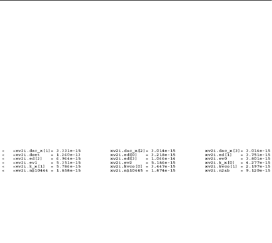
570 HSPICE® Reference Manual: Commands and Control Options
I-2013.12
Chapter 3: HSPICE Simulation Control Options Reference
subcircuit, set .OPTION PARHIER=LOCAL so that parameter scoping rules are
correct for this case.
...
.option PARHIER=LOCAL
.subckt INV IN OUT
.include 'weak_ model.inc'
M1 ..
M2 ..
.ends INV
..
X1 IN OUT INV
..
See Also
.INCLUDE / INC / INCL
.SUBCKT
.OPTION PATHNUM
Prints subcircuit path numbers instead of path names; overrides 8-character
model name limitation.
Syntax
.OPTION PATHNUM=[0|1|2]
Default Value if option is not specified in the netlist: 0
Value if option name is specified without a corresponding value: 1
Description
When set to 1, this option prints subcircuit path numbers instead of path
names. When set to 2, the complete model name (no truncation) is printed to
the *.lis file; without this setting, model names are limited to eight
characters. In addition, a full nodal hierarchy table is printed. For example, the
following captab nodal hierarchy appears as:

HSPICE® Reference Manual: Commands and Control Options 571
I-2013.12
Chapter 3: HSPICE Simulation Control Options Reference
.OPTION PCB_SCALE_FORMAT
Extends support for using a scaling factor in place of the decimal point for PCB
part number formats during case-sensitive simulation.
Syntax
.OPTION PCB_SCALE_FORMAT=[0|1]
Default Value if option is not specified in the netlist: 0
Value if option name is specified without a corresponding value: 1
Description
Allows both uppercase and lowercase number formats to be supported when
case sensitive simulations are run for parts places on a PCB. This option
maintains backward compatibility for those who use a number format that is
common for parts placed on a PCB, where the scaling factor is used instead of
the decimal point (e.g., 3k3 -> 3.3k).
Setting .OPTION PCB_SCALE_FORMAT= 1 when case-sensitivity is turned on
allows the 3k3 number format to be usable in an expression.
This option adds a new scaling factor, “r” or “R,” which is the multiplying factor
1e0 (often used for resistors).
Examples
Example 1 Decimal converted to Expression
.option pcb_scale_format=1
.param a='3k3 +2k/2'
As seen in the examples below, backward compatibility with the features of
HSPICE numbers is maintained (such as optional trailing units and scaling
symbols). The examples below show how the values 0 or 1 affect the output.
Example 2 .OPTION PCB_SCALE_FORMAT=0:
1) 0u1 / 0U1 / 0u1farads / 0.1u / 0u1farads / 0.1ufarads -> 0.1u
2) 5R6 / 5r6 / 5600m0 / 5600M0 / 5600m -> 5.6
3) 5MEG35 / 5meg35 / 5.35Meg -> 5.35e6
Example 3 .OPTION PCB_SCALE_FORMAT=1:
a) 0u1 / 0u1farads / 0.1u -> 0.1u
b) 5R6 / 5r6 / 5600m0 / 0M0000056-> 5.6
c) 5MEG35 / 5meg35 -> 5.35e6

572 HSPICE® Reference Manual: Commands and Control Options
I-2013.12
Chapter 3: HSPICE Simulation Control Options Reference
See Also
.OPTION SI_SCALE_SYMBOLS
.OPTION PHASENOISEKRYLOVDIM /
PHASENOISE_KRYLOV_DIM
Specifies the dimension of the Krylov subspace that the Krylov solver uses.
Syntax
.OPTION PHASENOISEKRYLOVDIM | PHASENOISE_KRYLOV_DIM
Default 500
Description
Specifies the dimension of the Krylov subspace that the Krylov solver uses.
This must be an integer greater than zero.
See Also
.OPTION BPNMATCHTOL
.OPTION PHASENOISEKRYLOVITR / PHASENOISE_KRYLOV_ITR
.OPTION PHASENOISETOL
.OPTION PHNOISELORENTZ / PHNOISE_LORENTZ
.OPTION PHASENOISEKRYLOVITR /
PHASENOISE_KRYLOV_ITR
Specifies the maximum number of Krylov iterations that the phase noise Krylov
solver takes.
Syntax
.OPTION PHASENOISEKRYLOVITR | PHASENOISE_KRYLOV_ITR
Default 1000
Description
Specifies the maximum number of Krylov iterations that the phase noise Krylov
solver takes. Analysis stops when the number of iterations reaches this value.

HSPICE® Reference Manual: Commands and Control Options 573
I-2013.12
Chapter 3: HSPICE Simulation Control Options Reference
See Also
.OPTION BPNMATCHTOL
.OPTION PHASENOISEKRYLOVDIM / PHASENOISE_KRYLOV_DIM
.OPTION PHASENOISETOL
.OPTION PHNOISELORENTZ / PHNOISE_LORENTZ
.OPTION PHASENOISETOL
Specifies the error tolerance for the phase noise solver.
Syntax
.OPTION PHASENOISETOL
Default 1e-8
Description
Specifies the error tolerance for the phase noise solver. This must be a real
number greater than zero.
See Also
.OPTION BPNMATCHTOL
.OPTION PHASENOISEKRYLOVDIM / PHASENOISE_KRYLOV_DIM
.OPTION PHASENOISEKRYLOVITR / PHASENOISE_KRYLOV_ITR
.OPTION PHNOISELORENTZ / PHNOISE_LORENTZ
.OPTION PHASETOLI
For HB output, aids in reporting when magnitude of phase current is very small.
Syntax
.OPTION PHASETOLI=val
Default 1.e-15
Description
Use this option in a harmonic balance analysis to report the output of the
magnitude of a current phasor as zero. If the current phasor is less than the
PHASETOLI value, then zero phase is reported. (If the magnitude of a current
value is very small, the phase does not matter at all.)

574 HSPICE® Reference Manual: Commands and Control Options
I-2013.12
Chapter 3: HSPICE Simulation Control Options Reference
See Also
.OPTION PHASETOLV
.HB
.HBAC
.HBLIN
.HBLSP
.HBNOISE
.HBOSC
.HBXF
.OPTION PHASETOLV
For HB output, aids in reporting when magnitude of phase voltage is very small.
Syntax
.OPTION PHASETOLV=val
Default 1.e-15
Description
Use this option in a harmonic balance analysis to report the output of the
magnitude of a voltage phasor as zero. If the voltage phasor is less than the
PHASETOLV value, the phase of that phasor is output as zero. (If the magnitude
of a voltage value is very small, the phase does not matter at all.)
See Also
.OPTION PHASETOLI
.HB
.HBAC
.HBLIN
.HBLSP
.HBNOISE
.HBOSC
.HBXF
.OPTION PHD
Facilitates fast OP convergence for BSIM4 testcases.

HSPICE® Reference Manual: Commands and Control Options 575
I-2013.12
Chapter 3: HSPICE Simulation Control Options Reference
Syntax
.OPTION PHD=[0|1]
Default Value if option is not specified in the netlist: 0 Value if option name is
specified without a corresponding value: 1
Description
When PHD is set to 1 (ON), this option facilitates fast OP convergence for
BSIM4 test cases. The PHD flow may show performance improvement in
simulations that require large DC OP convergence iterations. When PHD is on
but fails to converge, the simulation exits.
.OPTION PHNOISEAMPM
Allows you to separate amplitude modulation and phase modulation
components in a phase noise simulation.
Syntax
.OPTION PHNOISEAMPM=0|1
Default Value if option is not specified in the netlist: 0 Value if option name is
specified without a corresponding value: 1
Description
Use this option to enable HSPICE to calculate separate amplitude (am) and
phase modulation (pm) components using the output and measure syntax of
a .PHASENOISE simulation. A value of 0 sets the Periodic AC (PAC) phase
noise amplitude modulation (AM) component to zero and the results will be
identical to earlier releases. A value of 1 calculates separate AM and phase
noise components. When .OPTION PHNOISEAMPM=1, then
.MEASURE PHASENOISE extends output variables to the set:<am[noise]>
<pm[noise]>
Examples
The following explicitly sets the calculation for separate am and pm calculation.
.opt phnoiseampm=1
See Also
.PHASENOISE
Amplitude Modulation/Phase Modulation Separation

576 HSPICE® Reference Manual: Commands and Control Options
I-2013.12
Chapter 3: HSPICE Simulation Control Options Reference
.OPTION PHNOISELORENTZ / PHNOISE_LORENTZ
Turns on a Lorentzian model for the phase noise analysis.
Syntax
.OPTION PHNOISELORENTZ | PHNOISE_LORENTZ = 0|1|2|3
Default 0
Description
Allows you to select a Lorentzian model type for the phase noise analysis.
■0: (default) Uses a linear approximation to a Lorentzian model and avoids
phasenoise values >0dB for low offsets
■1: Applies a Lorentzian model to all noise sources
■2: Applies a Lorentzian model to all non-frequency dependent noise
sources
■3: Lorentzian model applied to white noise source, Gaussian model applied
to flicker noise sources.
See Also
.OPTION BPNMATCHTOL
.OPTION PHASENOISEKRYLOVDIM / PHASENOISE_KRYLOV_DIM
.OPTION PHASENOISEKRYLOVITR / PHASENOISE_KRYLOV_ITR
.OPTION PHASENOISETOL
.OPTION PIVOT
Selects a pivot algorithm.
Syntax
.OPTION PIVOT=0|1
Default Value if option is not specified in the netlist: 0
Value if option name is specified without a corresponding value: 1
Description
Set this option to 1 to select a pivot algorithm to achieve convergence in circuits
that produce hard-to-solve matrix equations. PIVOTselects the numerical
pivoting algorithm that is used to manipulate the matrices. Pivoting affects both

HSPICE® Reference Manual: Commands and Control Options 577
I-2013.12
Chapter 3: HSPICE Simulation Control Options Reference
DC and transient analysis. Usually the reason for choosing a pivot method
other than the default 0 is that the circuit contains both very large and very
small conductances.
If PIV0T=0, HSPICE automatically changes from a non-pivoting to pivot
strategy if it detects any diagonal-matrix entry less than PIVTOL. This strategy
provides the time and memory advantages of non-pivoting inversion and avoids
unstable simulations and incorrect results. Use .OPTION NOPIV to prevent
HSPICE from pivoting.
The SPARSE option is the same as PIVOT.
See Also
.OPTION NOPIV
.OPTION PIVTOL
.OPTION PIVTOL
Sets the absolute minimum value for which HSPICE accepts a matrix entry as
a pivot.
Syntax
.OPTION PIVTOL=x
Description
Use this option to set the absolute minimum value for which HSPICE accepts a
matrix entry as a pivot. PIVTOL is used to prevent numeric overflow conditions
like divide by 0. If the conductance is less than the value of PIVTOL, HSPICE
rebuilds the matrix and chooses the PIVOT algorithm. If the conductance is
greater than the value of PIVTOL, the PIVTOL value replaces the conductance
in the matrix. When a non-pivot algorithm is selected by setting PIVOT=0, then
pivtol is the minimum conductance in the matrix and not a pivot.
The default value of PIVTOL is 1e-15 and the range of PIVTOL is Min:1e-35,
Max:1, excluding 0. The value of PIVTOL must be less than GMIN or GMINDC.
Values that approach 1 increase the pivot. The example below shows how you
can correct a “maximum conductance on node error.”
Note: If PIVTOL is set too small, you run the risk of creating an overflow
condition and a convergence problem. If you set the value to 0,
an out-of-bounds error is reported.

578 HSPICE® Reference Manual: Commands and Control Options
I-2013.12
Chapter 3: HSPICE Simulation Control Options Reference
Examples
If you get an error message such as:
**error** maximum conductance on node 1:v75 } =( 9.2414D-23) is
less than pivtol in transient analysis.
Check hookup for this node, set smaller option pivtol and rerun.
—the error message informs that the node conductance value is less than the
value of PIVTOL. Decrease the PIVTOL value so that it is less than the value in
the error message. The valid range of pivtol values is between 1e-35 to 1,
excluding 0. For this case a setting PIVTOL to 1e-25 resolves the error.
See Also
.OPTION GMIN
.OPTION GMINDC
.OPTION PIVOT
.OPTION POST
Saves simulation results for viewing by an interactive waveform viewer.
Syntax
HSPICE Syntax
.OPTION POST=[0|1|2|3|ASCII|BINARY|CSDF]
HSPICE Advanced Analog Syntax
.OPTION POST=[0|1|2|3|ASCII|BINARY|CSDF|NW|P|TW|UT|WDBA]
Default Value if option is not specified in the netlist: 0
Value if option name is specified without a corresponding value: 1
Description
Use this option to save simulation results for viewing by an interactive waveform
viewer and to provide output without specifying other parameters.
Note: The behavior for .OPTION POST when HSPICE advanced
analog functions are used is different from the same option used
in HSPICE.
The defaults for the POST option supply usable data to most parameters:

HSPICE® Reference Manual: Commands and Control Options 579
I-2013.12
Chapter 3: HSPICE Simulation Control Options Reference
■POST=0: Does not output simulation results.
■POST=1, BINARY: (Default if POST is declared without a value) Output
format is binary.
■POST=2, ASCII: Output format is ASCII. When you set .option POST=2
HSPICE increases the spacing between points after writing out 100k time
points. The simulation accuracy is not affected, but the ASCII output
waveform file is. To resolve this, either add .option
POST_VERSION=2001 to the netlist to output all time points as double-
precision numbers, or use .option POST=1 in the netlist to create a binary
output file.
■POST=3: Output format is New Wave binary (which enables you to
generate .tr0 files that are larger than 2 gigabytes on Linux platforms).
■POST=CSDF: Output format is Common Simulation Data Format (Viewlogic-
compatible graph data file format).
Options available when HSPICE advanced analog functions are used:
■POST=NW: Output format is XP/AvanWaves.
■POST=TW: Output format is TurboWave.
■POST=UT: Output format is Veritools Undertow.
■POST=WDBA: Output format is XP/Custom WaveView.
■POST=XP: Output format is XP/AvanWaves/Custom WaveView.
By default, HSPICE outputs single precision for both time and signal data. If
you want to get double precision data, in the netlist set:
.OPTION POST POST_VERSION=2001
Note: .OPTION POST in HSPICE is not a global option to dump output
in general and then use other options to specify another format.
Other options such as PSF, CSDF, SDA, ZUKEN override POST if
they are specified after POST, and vice versa. This is unlike when
HSPICE advanced analog functions are used, which allows
values beyond [0|1|2|3|ASCII|BINARY|CSDF].
HSPICE uses the last output control option if multiple output control options are
specified in the netlist.
In POST format, only the inductor OP information is output into a *.lis file or a
*.dp# file (when opfile=1). For inductor and capacitor information see
.OPTION PSF and .OPTION WDF formats.

580 HSPICE® Reference Manual: Commands and Control Options
I-2013.12
Chapter 3: HSPICE Simulation Control Options Reference
Examples
In this example the option post overrides the options artist/PSF.
.option artist=2 psf=2
.option post
In this example, the options artist/PSF override the option post.
.option post
.option artist=2 psf=2
See Also
.OPTION POST_VERSION
.OPTION POSTLVL
Limits the data written to your waveform file to a specified level of nodes.
Syntax
.OPTION POSTLVL=n
Description
Limits the data written to your waveform file to the level of nodes specified by
the n parameter. This option differs from POSTSTOP in that it specifies the
signals of one given level at any level.
Note: In a netlist, .OPTION POSTLVL overrides.OPTION PROBE.
Examples
.OPTION POSTLVL=2
This example limits the data written to the waveform file to only the second-
level nodes (voltage and current).
See Also
.OPTION POSTTOP
.OPTION PROBE

HSPICE® Reference Manual: Commands and Control Options 581
I-2013.12
Chapter 3: HSPICE Simulation Control Options Reference
.OPTION POST_VERSION
Specifies the post-processing output version for HSPICE.
Syntax
.OPTION POST_VERSION=x
Default 9601
Description
Use this option to set the post-processing output version:
■x=9007 truncates the node name in the post-processor output file to a
maximum of 16 characters.
■x=9601 sets the node name length for the output file consistent with input
restrictions (1024 characters) and limits the number of output variables to
9999.
■x=2001 uses an output file header that displays the correct number of
output variables when the number exceeds 9999. This option also changes
the digit-number precision in results files to match the value of .OPTION
NUMDGT (when < 5).
■x=2013 outputs the time / frequency / dc variable data with double precision
and output the signals data in single precision.
By default, HSPICE outputs single precision for both time and signal data. If
you want to get double precision data, in the netlist set:
.OPTION POST POST_VERSION=2001
If you set .OPTION POST_VERSION=2001 POST=2 in the netlist, HSPICE
returns more accurate ASCII results.
Examples
If you need to probe more than 9999 signals, set the POST_VERSION option to
2001; for example,
.OPTION POST_VERSION=2001
HSPICE now outputs all the signals into a waveform file and the correct number
of output signals is shown rather than **** when the number of signals exceeds
9999. You can load this waveform file in WaveView to view the signals.

582 HSPICE® Reference Manual: Commands and Control Options
I-2013.12
Chapter 3: HSPICE Simulation Control Options Reference
See Also
.OPTION NUMDGT
.OPTION POST
.OPTION POSTTOP
Limits the data written to the waveform file to data from only the top n level
nodes.
Syntax
.OPTION POSTTOP=n
Description
Use this option to limit the data written to your waveform file to data from only
the top n level nodes. This option outputs instances up to n levels deep. If you
do not specify either the PROBE or the POSTTOP options, HSPICE outputs all
levels. To enable the waveform display interface, you also need to specify the
.OPTIONPOST option. This option differs from .OPTION POSTLVL in that it
specifies the signals of one or multiple levels from the top level down.
Note: In a netlist, .OPTION POSTTOP overrides.OPTION PROBE.
Examples
This example limits the data written to the waveform file to only the three top-
level nodes (voltage and current).
POSTTOP=3
See Also
.OPTION POST
.OPTION PROBE
.OPTION POSTLVL
.OPTION PROBE
Limits post-analysis output to only variables specified in .PROBE and .PRINT
commands for HSPICE.

HSPICE® Reference Manual: Commands and Control Options 583
I-2013.12
Chapter 3: HSPICE Simulation Control Options Reference
Syntax
.OPTION PROBE=0|1
Default Value if option is not specified in the netlist: 0
Value if option name is specified without a corresponding value: 1
Description
When turned on (1), allows you to set post-analysis output to only variables
specified in .PROBE, and PRINT commands. 0=off.By default, HSPICE
outputs all voltages and power supply currents in addition to variables listed
in .PROBE, and .PRINT commands. Using this option can significantly
decrease the sizes of simulation output files.
If .OPTION PROBE is not set:
■All node voltage/source currents output to *.tr#, *.ac#, *.sw# files.
■If measured, the resistor or MOSFET current is also output to *.tr#,
*.ac#, or *.sw# files.
■If the resistor or MOSFET current are determined by measurement
variables, and .OPTION PUTMEAS is reset (set to 0), these measurement
variables are not output to waveform files.
Important: .OPTION PROBE is ignored if any of .OPTIONS POSTTOP,
POSTLVL, SIM_POSTTOP, SIM_POSTAT, or
SIM_POSTDOWN is also set in the netlist. .OPTION
POSTTOP, POSTLVL, SIM_POSTTOP, SIM_POSTAT, or
SIM_POSTDOWN each overrides.OPTION PROBE.
See Also
.PRINT
.PROBE
.OPTION PUTMEAS
.OPTION POSTLVL
.OPTION POSTTOP
.OPTION SIM_POSTAT
.OPTION SIM_POSTDOWN
.OPTION SIM_POSTTOP

584 HSPICE® Reference Manual: Commands and Control Options
I-2013.12
Chapter 3: HSPICE Simulation Control Options Reference
.OPTION PSF
In a standalone HSPICE simulation, specifies whether the output is binary
(Parameter Storage Format) or ASCII. When used with HSPICE, specifies
whether binary or ASCII data is output when you run an HSPICE simulation
from the Cadence Virtuoso Analog Design Environment.
Syntax
.OPTION PSF=0|1|2
Default Value if option is not specified in the netlist: 0
Value if option name is specified without a corresponding value: 1
Description
Use this option to specify whether HSPICE outputs binary (Parameter Storage
Format—*.PSF) or ASCII data when you run an HSPICE simulation through
the Cadence Virtuoso Analog Design Environment.
The combinations shown in the below table produce the following output file
format:
When ARTIST=2 PSF=2, no *.dp# files are generated, nor is OP information
output in the *.lis file. If .OPTION OPFILE=1 is in a netlist when PSF=2, the
OPFILE=1 is ignored.
In PSF or WDF format, the inductor and capacitor OP information are both
output into *.op# files.
PSF Value ARTIST Value Output File Format
1 0 Binary
1 1 Binary
1 2 Binary
2 0 ASCII
2 1 Binary
2 2 Binary

HSPICE® Reference Manual: Commands and Control Options 585
I-2013.12
Chapter 3: HSPICE Simulation Control Options Reference
When the netlist contains .option psf=2 and a .tran analysis statement
(with no .op statement in the netlist file), HSPICE creates the following output
files:
■.op0 — dc node voltage and dc operating points
■.op1 — transient voltage and transient operating points for the transient
end time.
Ordinarily, PSF output is directed to a directory named ./psf to accommodate
the Analog Design Environment. However, HSPICE and Custom Designer
users can redirect PSF output by setting the HSPICE command line option -o
to a directory other than ./psf (for example: -o ../results/input).
Note: The PSF format is supported on Sun/SPARC, Red Hat/SUSE
Linux, x86, and IBM AIX platforms, as well as 64-bit versions.
See Also
.OPTION ARTIST
.OPTION OPFILE
.OPTION PURETP
Specifies the integration method to use for reversal time point in HSPICE.
Syntax
.OPTION PURETP=[0|1]
Default Value if option is not specified in the netlist: 0
Value if option name is specified without a corresponding value: 1
Description
Use this option to specify the integration method to use for reversal time point.
If you set PURETP=1 and HSPICE finds non-convergence, it uses TRAP
(instead of Bbackward-Euler) for the reversed time point.
Use this option with an .OPTION METHOD=TRAP command to help some
oscillating circuits to oscillate if the default simulation process cannot satisfy the
result.
See Also
.OPTION METHOD

586 HSPICE® Reference Manual: Commands and Control Options
I-2013.12
Chapter 3: HSPICE Simulation Control Options Reference
.OPTION PUTMEAS
Controls the output variables listed in the .MEASURE command.
Syntax
.OPTION PUTMEAS=0|1
Default 1
Description
Use this option to control the output variables listed in the .MEASURE
command.
■0: Does not save variable values listed in the .MEASURE command into the
corresponding output file (such as .tr#,.ac# or .sw#). This option
decreases the size of the output file.
■1: Default. Saves variable values listed in the .MEASURE command to the
corresponding output file (such as .tr#,.ac# or .sw#). This option is
similar to the output of HSPICE 2000.4.
See Also
.MEASURE / MEAS
.OPTION PZABS
Sets absolute tolerances for poles and zeros.
Syntax
.OPTION PZABS=x
Default 1.0e-2
Description
Use this option to set absolute tolerances for poles and zeros in Pole/Zero
analysis. Use this option as follows: If , then
. You can also use this option for convergence tests.
See Also
.OPTION CSCAL
.OPTION FMAX
.OPTION FSCAL
Xreal Xreal
+PZABS<()
Xreal and Ximag 0=

HSPICE® Reference Manual: Commands and Control Options 587
I-2013.12
Chapter 3: HSPICE Simulation Control Options Reference
.OPTION GSCAL
.OPTION LSCAL
.OPTION PZTOL
.OPTION RITOL
.OPTION PZTOL
Sets the relative tolerance for poles and zeros.
Syntax
.OPTION PZTOL=x
Default 1.0e-6
Description
Use this option to set relative tolerances for poles and zeros in Pole/Zero
analysis.
See Also
.OPTION CSCAL
.OPTION FMAX
.OPTION FSCAL
.OPTION GSCAL
.OPTION LSCAL
.OPTION PZABS
.OPTION RITOL
.OPTION RADEGFILE
Use to specify a MOSRA degradation file name to be used with SIMMODE=1.
Syntax
.OPTION RADEGFILE=file_name
Description
Use this option to specify a MOSRA degradation file name to be used with
SIMMODE=1. HSPICE will read in the degradation information in the specified
file and do a MOSRA post-stress simulation.

588 HSPICE® Reference Manual: Commands and Control Options
I-2013.12
Chapter 3: HSPICE Simulation Control Options Reference
Examples
.mosra reltotaltime='10*365*24*60*60' lin=11 simmode=1
.option radegfile = '1.radeg0'
See Also
.MOSRA
.OPTION RADEGOUTPUT
.OPTION RADEGOUTPUT
Outputs the MOSRA degradation information to the Word Excel CSV format.
Syntax
.OPTION RADEGOUTPUT=CSV
Description
Use this option to output the MOSRA degradation information to the Microsoft
Excel CSV format. If the CSV value is not specified no CSV file is generated.
See Also
.OPTION RADEGFILE
.OPTION RANDGEN
Specifies the random number generator used in traditional Monte Carlo
analysis.
Syntax
.OPTION RANDGEN=[0|1|2|3|4|3lc|moa|uvs|mcg|wh]
Default Value if option is not specified in the netlist: 0
Value if option name is specified without a corresponding value: 1

HSPICE® Reference Manual: Commands and Control Options 589
I-2013.12
Chapter 3: HSPICE Simulation Control Options Reference
Description
Use this option to specify the random number generator used in HSPICE
traditional Monte Carlo analysis.
For the generators of mcg and wh, there is almost no time cost to skip random
number, no matter how large the number is following the keyword firstrun.
Note: The .OPTION SEED command is also valid for the new random
number generator without usage change.
See Also
.OPTION RUNLVL
.OPTION SEED
.OPTION REDEFMODEL
Allows redefinition of a model in a netlist.
Syntax
.OPTION REDEFMODEL=[0|1|2]
Default 0
Description
This option enables you to redefine a model in a netlist.
■0: Issues an error message for multiple definitions
■1: Uses the last declared definition
■2: Uses the first definition
RANDGEN Option Description
3lc | 0 A traditional random number generator is used.
moa | 1 A multiply-with-carry type random number generator with longer cycle is used.
uvs | 2 A 64-bit universal random number generator with longer cycle is used.
mcg | 3 A multiplicative congruential generator with longer cycle is used.
wh | 4 Another longer cycle is used.

590 HSPICE® Reference Manual: Commands and Control Options
I-2013.12
Chapter 3: HSPICE Simulation Control Options Reference
.OPTION REDEFMODEL without a value equals .OPTION REDEFMODEL=0. If
you do not specify REDEFMODEL, HSPICE errors out on a duplicate model.
.OPTION REDEFSUB
Allows redefinition of a subckt in a netlist.
Syntax
.OPTION REDEFSUB =[0|1|2]
Default 0
Description
Enables the redefinition of a subcircuit in a netlist.
■0: Issues an error message for multiple definitions
■1: Uses the last declared definition
■2: Uses the first definition
.OPTION REDEFSUB without a value equals .OPTION REDEFSUB=1.
.OPTION RELH
Sets the relative current tolerance from iteration to iteration through voltage-
defined branches.
Syntax
.OPTION RELH=x
Description
Use this option to set the relative current tolerance through voltage-defined
branches (voltage sources and inductors) from iteration to iteration.
This option can also be used to check current convergence, but only if the value
of the ABSH option is greater than zero.
See Also
.OPTION ABSH

HSPICE® Reference Manual: Commands and Control Options 591
I-2013.12
Chapter 3: HSPICE Simulation Control Options Reference
.OPTION RELI
Sets the relative error/tolerance change from iteration to iteration.
Syntax
.OPTION RELI=x
Description
Use this option to set the relative error/tolerance change from iteration to
iteration.
This option determines convergence for all currents in diode, BJT, and JFET
devices. (RELMOS sets tolerance for MOSFETs). This value is the change in
current from the value calculated at the previous timepoint.
■Default=0.01 for .OPTION KCLTEST=0.
■Default=1e-6 for .OPTION KCLTEST=1.
See Also
.OPTION RELMOS
.OPTION KCLTEST
.OPTION RELIN
(Optimization) Relative input parameter (delta_par_val / MAX(par_val,1e-6)) for
convergence.
Syntax
.OPTION RELIN=value
Default 0.001
Description
(Optimization) Relative input parameter (delta_par_val / MAX(par_val, 1e-6))
for convergence. If all optimizing input parameters vary by no more than RELIN
between iterations, the solution converges. RELIN is a relative variance test so
a value of 0.001 implies that optimizing parameters vary by less than 0.1% from
one iteration to the next. If RELIN is set in .OPTION, the setting of RELIN in the
.model card will be overridden.
Examples
.option RELIN=1e-6 DYNACC

592 HSPICE® Reference Manual: Commands and Control Options
I-2013.12
Chapter 3: HSPICE Simulation Control Options Reference
See Also
.MODEL
.OPTION RELMOS
Sets the relative error tolerance for drain-to-source current from iteration to
iteration.
Syntax
.OPTION RELMOS=x
Description
Use this option to set the relative error tolerance for drain-to-source current
from iteration to iteration.
This option determines convergence for currents in MOSFET devices while
.OPTION RELI sets the tolerance for other active devices.
This option also sets the change in current from the value calculated at the
previous timepoint. HSPICE uses the .OPTION RELMOS value only if the
current is greater than the .OPTION ABSMOS floor value.
Min value: 1e-07; Max value 10.
See Also
.OPTION ABSMOS
.OPTION RELI
.OPTION RELMOS
.OPTION RELQ
Sets the timestep size from iteration to iteration.
Syntax
.OPTION RELQ=x
Description
Use this option in the timestep algorithm for local truncation error (LVLTIM=2).
If the capacitor charge calculation in the present iteration exceeds that of the

HSPICE® Reference Manual: Commands and Control Options 593
I-2013.12
Chapter 3: HSPICE Simulation Control Options Reference
past iteration by a percentage greater than the RELQ value, then HSPICE
reduces the internal timestep (delta). The default is 0.01.
See Also
.OPTION LVLTIM
.OPTION RELTOL
Sets the relative error tolerance for voltages from iteration to iteration.
Syntax
.OPTION RELTOL=x
Default 1e-3
Description
Use this option to set the relative error tolerance for voltages from iteration to
iteration. Min value: 1e-20; Max value: 10.
Use this option with the ABSV option to determine voltage convergence.
Increasing x increases the relative error. This option is the same as the RELV
option. The RELI and RELVDC options default to the RELTOL value.
See Also
.OPTION ABSV
.OPTION RELI
.OPTION RELV
.OPTION RELVDC
.OPTION RELV
Sets the relative error tolerance for voltages from iteration to iteration.
Syntax
.OPTION RELV=x
Default 1e-3
Description
Use this option to set the relative error tolerance for voltages from iteration to
iteration.

594 HSPICE® Reference Manual: Commands and Control Options
I-2013.12
Chapter 3: HSPICE Simulation Control Options Reference
If voltage or current exceeds the absolute tolerances, a RELV test determines
convergence. Increasing x increases the relative error. You should generally
maintain this option at its default value. It conserves simulator charge. For
voltages, this option is the same as the RELTOL option. Min value: 1e-20; Max
value: 10.
See Also
.OPTION RELTOL
.OPTION RELVAR
Sets the relative voltage change for LVLTIM=1 or 3 from iteration to iteration.
Syntax
.OPTION RELVAR=x
Description
Use this option to set the relative voltage change for LVLTIM=1 or 3 from
iteration to iteration.
Use this option with the ABSVAR and DVDT timestep algorithm. If the node
voltage at the current timepoint exceeds the node voltage at the previous
timepoint by RELVAR, then HSPICE reduces the timestep and calculates a new
solution at a new timepoint. The default is 0.30, or 30 percent.
For additional information, see “DVDT Dynamic Timestep” in the HSPICE User
Guide: Basic Simulation and Analysis.
See Also
.OPTION ABSVAR
.OPTION DVDT
.OPTION LVLTIM
.OPTION RELVDC
Sets the relative error tolerance for voltages from iteration to iteration.
Syntax
.OPTION RELVDC=x

HSPICE® Reference Manual: Commands and Control Options 595
I-2013.12
Chapter 3: HSPICE Simulation Control Options Reference
Description
Use this option to set the relative error tolerance for voltages from iteration to
iteration.
If voltages or currents exceed their absolute tolerances, the RELVDC test
determines convergence. Increasing the x parameter value increases the
relative error. You should generally maintain RELVDC at its default value to
conserve simulator charge.
See Also
.OPTION RELTOL
.OPTION REPLICATES
Runs replicates of the Latin Hypercube samples.
Syntax
.OPTION REPLICATES=number
Description
When the advanced sampling method Latin Hypercube is used with traditional
Monte Carlo simulation, you can add this option following
.OPTION SAMPLING _METHOD=LHS. This option runs replicates of the Latin
Hypercube samples. The sample with nominal conditions is simulated once.
HSPICE repeats the LHS run the number of times specified by number. For
example, if, in a regular run, you have 10+1 (including nominal value) iterations,
if you set .OPTION REPLICATES=2, you generate 21 (or 2* Value +1) Latin
Hypercube samples.
Examples
.OPTION SAMPLING_METHOD=LHS
.OPTION REPLICATES=2
See Also
.OPTION SAMPLING_METHOD

596 HSPICE® Reference Manual: Commands and Control Options
I-2013.12
Chapter 3: HSPICE Simulation Control Options Reference
.OPTION RES_BITS
Tightens tolerances when using HPP (High Performance Parallel) in transient
simulations.
Syntax
.OPTION RES_BITS=n
Default 0
Description
When running a multi-thread operation in a transient simulation using HPP
(only) this option can be used to tighten convergence tolerances. Tightening
convergence tolerances enable resolving the least significant bit in an n-bit
converter.
Note: Setting this option may result in increased number of iterations
and, sometimes, slightly increased number of time steps.
Examples
The following example, for a 14-bit A-to-D converter, is set as:
.option res_bits=14
.OPTION RESMIN
Specifies the minimum resistance for all resistors.
Syntax
.OPTION RESMIN=x
Default 1E-05
Description
Use this option to specify the minimum resistance for all resistors. Any
resistance (including parasitic, inductive resistors, and those in the transistor
models) smaller than the specified RESMIN is reset to the RESMIN value. No
resistor reduction is involved. The default is 1E-05. Users can specify a bigger
value up to 10 ohms.

HSPICE® Reference Manual: Commands and Control Options 597
I-2013.12
Chapter 3: HSPICE Simulation Control Options Reference
See Also
.OPTION RM_RMIN
.OPTION RM_RMAX
.OPTION RISETIME / RISETI
Specifies the smallest signal risetime to be supported in elements and
analyses that are sensitive to frequency bandwidth and time scale constraints.
Syntax
.OPTION RISETIME=x
Default Calculated automatically (see below)
Description
Use this option to specify the smallest signal risetime to be anticipated when
analyzing certain elements that have frequency dependencies. Several
HSPICE elements require some knowledge regarding either their maximum
frequency of operation, or the minimum signal rise time to be expected. This is
particularly true of elements that are described in the frequency domain, yet
require time-domain simulation. The RISETIME option is used to establish time
scale and frequency scale information needed for inverse Fourier transform
and convolution calculations.
In the W-element (transmission line) model, RISETIME is used to determine
the maximum signal frequency to be taken into account for frequency
dependencies such as skin effect, and dielectric loss (non-zero Rs or Gd).
In the S-element (scattering-parameter) based model, the reciprocal of
RISETIME sets the maximum signal frequency (FMAX) value used for the S-
parameter analysis.
In the U-element (lumped transmission line) model, RISETIME is used to set
the number of lumps according to the equation:
where, TDeff is the end-to-end delay in a transmission line.
#lumps M=IN 20 1 20 TDeff
RISETIME
----------------------------
⎝⎠
⎛⎞
⋅+,

598 HSPICE® Reference Manual: Commands and Control Options
I-2013.12
Chapter 3: HSPICE Simulation Control Options Reference
When needed, HSPICE automatically calculates a default value for RISETIME
as follows:
■25% of the tstep value specified with the .TRAN command.
■The time corresponding to a 90-degree phase shift for the highest frequency
specified in SIN, SFFM, and AM sources.
■The smallest delay time, rise time, fall time, or time increment used in
PULSE, EXP, and PWL sources.
See Also
.MODEL
.OPTION WACC
.OPTION WDELAYOPT
.OPTION RITOL
Sets the minimum ratio value for the (real/imaginary) or (imaginary/real) parts
of the poles or zeros.
Syntax
.OPTION RITOL=x
Default 1.0e-2
Description
Use this option to set the minimum ratio value for the (real/imaginary) or
(imaginary/real) parts of the poles or zeros. Use the RITOL option as follows.
if: , then . If , then
.
See Also
.OPTION CSCAL
.OPTION FMAX
.OPTION FSCAL
.OPTION GSCAL
.OPTION LSCAL
.OPTION PZABS
.OPTION PZTOL
.PZ
Ximag RITOL Xreal
⋅≤
Ximag 0=
Xreal RITOL Ximag
⋅≤
Xreal 0=

HSPICE® Reference Manual: Commands and Control Options 599
I-2013.12
Chapter 3: HSPICE Simulation Control Options Reference
.OPTION RM_CMAX
Enables you to set a value above which HSPICE removes capacitors from the
circuit.
Syntax
.OPTION RM_CMAX=val
Default O (Disabled)
Description
Use this option to specify a threshold at which linear capacitors are removed.
This option is especially useful with extracted netlists containing numerous
capacitors. Specifying such a threshold can speed up simulation.
All capacitors that encounter an |R value| > RM_CMAX are immediately
removed. If a negative value is set, HSPICE issues a warning message and the
simulation ignores the option.
Minimum value: 0, Maximum value: 1e+20.
Examples
In the following example, capacitors greater than 1e12 are removed from the
circuit.
.opt rm_cmax=1e12
See Also
.OPTION RM_CMIN
.OPTION RM_CNEG
.OPTION RM_CMIN
Enables you to set a value below which HSPICE ignores capacitors.
Syntax
.OPTION RM_CMIN=val
Default 0 (Disabled)

600 HSPICE® Reference Manual: Commands and Control Options
I-2013.12
Chapter 3: HSPICE Simulation Control Options Reference
Description
Use this option to specify a threshold at which linear capacitors are ignored.
This option is especially useful with extracted netlists containing numerous very
small capacitors. Specifying such a threshold helps to speed up simulation.
If a negative value is set, HSPICE issues a warning message and the
simulation ignores the option.
Minimum value: 0, Maximum value: 100.
Examples
In the following example, capacitors less than 1e-3 are removed from the
circuit.
.opt rm_cmin=1e-3
See Also
.OPTION RM_CMAX
.OPTION RM_CNEG
.OPTION RM_CNEG
Removes all negative capacitors.
Syntax
.OPTION RM_CNEG=0|1
Default 0
Description
Use this option to remove all negative capacitors in the netlist.
See Also
.OPTION RM_CMAX
.OPTION RM_CMIN
.OPTION RM_RMAX
Enables you to set a value above which HSPICE removes resistors from the
circuit.

HSPICE® Reference Manual: Commands and Control Options 601
I-2013.12
Chapter 3: HSPICE Simulation Control Options Reference
Syntax
.OPTION RM_RMAX=val
Default 0 (Disabled)
Description
Use this option to specify a threshold at which resistors are removed. This
option is especially useful with extracted netlists containing numerous resistors.
Specifying such a threshold can speed up simulation.
All linear resistors that encounter an |R value| > RM_RMAX are immediately
removed. The priority of .OPTION RM_RMAX is higher than .OPTION RESMIN
or .OPTION RM_RMIN.
If a negative value is set, HSPICE issues a warning message and the
simulation ignores the option.
Minimum value: 0, Maximum value: 1e+20.
Examples
In the following example, resistors smaller than 1e-3 are shorted (ignored) and
the resistors greater than 1e12 are removed from the circuit.
.opt rm_rmin=1e-3 rm_rmax=1e12
See Also
.OPTION RM_RMIN
.OPTION RESMIN
.OPTION RM_RMIN
Enables you to set a value below which HSPICE ignores resistors.
Syntax
.OPTION RM_RMIN=val
Default 1e-5
Description
Use this option to specify a threshold at which resistors are ignored. This option
is especially useful with extracted netlists containing numerous very small
resistors. Specifying such a threshold helps to speed up simulation.

602 HSPICE® Reference Manual: Commands and Control Options
I-2013.12
Chapter 3: HSPICE Simulation Control Options Reference
All linear resistors that encounter an |R value|< RM_RMIN shorts the wire. Its
priority is higher than .OPTION RESMIN. To disable the option, set the value to
0.
If a negative value is set, HSPICE issues a warning message and the
simulation ignores the option.
Minimum value: 0, Maximum value: 100.
Examples
In the following example, resistors smaller than 1e-3 are shorted (ignored) and
the resistors greater than 1e12 are removed from the circuit.
.opt rm_rmin=1e-3 rm_rmax=1e12
See Also
.OPTION RM_RMAX
.OPTION RESMIN
.OPTION RM_RNEG
.OPTION RM_RNEG
Resets all negative resistors to .OPTION RESMIN setting.
Syntax
.OPTION RM_RNEG=0|1
Default 0
Description
Use this option to reset all negative resistors in the netlist o that specified by
.OPTION RESMIN. This option’s priority is higher than RESMIN, and lower than
RM_RMIN, or RM_RMAX. i.e. priorities are RM_RMAX > RM_RMIN > RM_RNEG >
RESMIN.
See Also
.OPTION RESMIN
.OPTION RM_RMAX
.OPTION RM_RMIN

HSPICE® Reference Manual: Commands and Control Options 603
I-2013.12
Chapter 3: HSPICE Simulation Control Options Reference
.OPTION RMAX
Sets the TSTEP multiplier, which controls the maximum value for the internal
timestep delta for HSPICE.
Syntax
.OPTION RMAX=x
Description
Use this option to set the TSTEP multiplier, which controls the maximum value
(DELMAX) for the delta of the internal timestep:
DELMAX=TSTEP x RMAX
■The default is 5 if DVDT is 4 and LVLTIM is 1.
■Otherwise, the default is 2.
Min value: 1e-9; Max value: 1e+9. The RMAX value cannot be smaller than
RMIN.
See Also
.OPTION DELMAX
.OPTION DVDT
.OPTION LVLTIM
.OPTION RMIN
Sets the minimum value of delta (internal timestep).
Syntax
.OPTION RMIN=x
Description
Use this option to set the minimum value of delta (internal timestep). An
internal timestep smaller than RMIN x TSTEP, terminates the transient analysis,
and reports an internal “timestep too small” error. If the circuit does not
converge in IMAX iterations, delta decreases by the amount you set in the FT
option. The default is 1.0e-9. Min value: 1e-15.
See Also
.OPTION FT
.OPTION IMAX

604 HSPICE® Reference Manual: Commands and Control Options
I-2013.12
Chapter 3: HSPICE Simulation Control Options Reference
.OPTION RUNLVL
Controls runtime speed and simulation accuracy.
Syntax
.OPTION RUNLVL= 1|2|3|4|5|6
Description
Higher values of RUNLVL result in higher accuracy and longer simulation
runtimes; lower values result in lower accuracy and faster simulation runtimes.
For HSPICE:
The RUNLVL option setting controls the scaling of all simulator tolerances
simultaneously, affecting timestep control, transient analysis convergence, and
model bypass tolerances all at once. Higher values of RUNLVL result in smaller
timestep sizes and could result in more Newton-Raphson iterations to meet
stricter error tolerances. RUNLVL settings affect transient analysis only.
RUNLVL can be set to 0 (to disable) 1, 2, 3, 4, 5, or 6:
■1: Lowest simulation runtime
■2: More accurate than RUNLVL=1 and faster than RUNLVL=3
■3: Default value, similar to HSPICE’s original default mode
■4: More accurate than RUNLVL=3 and faster than RUNLVL=5
■5 or 6: Corresponds to HSPICE’s standard accurate mode for most circuits:
•5 is similar to the standard accurate mode in HSPICE
•6 has the highest accuracy
If RUNLVL is specified in the netlist without a value, the value is the default, 3.
If .OPTION ACCURATE is specified in the netlist together with RUNLVL, the
value of RUNLVL is limited to 5 or 6; specifying a specifying a RUNLVL value of
1, 2, 3, or 4 defaults to 5.
If .OPTION RUNLVL is not turned off, there is no dependency with GEAR and
ACCURATE options, and
.OPTION ACCURATE method=GEAR RUNLVL
is equivalent to
.OPTION method=GEAR ACCURATE RUNLVL

HSPICE® Reference Manual: Commands and Control Options 605
I-2013.12
Chapter 3: HSPICE Simulation Control Options Reference
The RUNLVL option interacts with other options as follows:
■Regardless of its position in the netlist, RUNLVL ignores the following step
control-related options (which are replaced by automated algorithms):
LVLTIM DVDT FT FAST TRTOL ABSVARRELVAR RELQ CHGTOL DVTR
IMIN ITL3
■See the notes to the table below for discussion of options ACCURATE and
BYPASS in relation to RUNLVL if it is specified in the netlist.
■The tstep value specified with the .TRAN command affects timestep
control when a RUNLVL option is used. Timestep values larger than
tstep*RMAX use a tighter timestep control tolerance.
For information on how RUNLVL values affect other options, see the following
section, and also see Appendix A, HSPICE Control Options Behavioral Notes.
For HSPICE Advanced Analog functions:
When using HSPICE advanced analog functions, the SIM_ACCURACY option
gives you a more continuous range of settings. You can use .OPTION RUNLVL
to control runtime speed and simulation accuracy. As in HSPICE, higher values
of RUNLVL result in higher accuracy and longer simulations; lower values result
in lower accuracy and faster simulation.
.OPTION RUNLVL maps to .OPTION SIM_ACCURACY as follows:
■RUNLVL=1: SIM_ACCURACY=0.5
■RUNLVL=2: SIM_ACCURACY=0.75
■RUNLVL=3: SIM_ACCURACY=1
■RUNLVL=4: SIM_ACCURACY=5
■RUNLVL=5: SIM_ACCURACY=10
■RUNLVL=6: SIM_ACCURACY=20
Interactions Between .OPTION RUNLVL and Other Options
Since the latest algorithm invoked by RUNLVL sets the timestep and error
tolerance internally, many transient error tolerance and timestep control options
are no longer valid; furthermore, to assure the most efficiency of the new
RUNLVL algorithm, you should let the new engine manage everything itself.
Options that are recommended not to tune are listed in the table, as well.

606 HSPICE® Reference Manual: Commands and Control Options
I-2013.12
Chapter 3: HSPICE Simulation Control Options Reference
Note: Once RUNLV is set, it does not = 0.
Option Default value
when RUNLVL=0
Default value with
RUNLVL=3
User definition
ignored
Recommend not
to tune
ABSV/VNTOL 50u 50u - x
ABSVAR 500m 500m x-
ACCURATE 10 0 - -
BYPASS a22 for RUNLVL=1-6 - -
CHGTOL 1.0f 1.0f x-
DI 100 100 - x
DVDT 4 4 x -
DVTR 1.0k 1.0k x-
FAST 20 0 x -
FS 250m 250m - x
FT 250m 250m x-
IMIN/ITL3 3 3 x -
LVLTIM 1 4 x -
METHOD 3TRAP TRAP - -
RELQ 10m 10m x-
RELTOL 1.0m 1.0m - x
RELV 1.0m 1.0m - x
RELVAR 300.0m 300.0m x-
RMAX 5 5 x -
RMIN 1.0n 1.0n - x
TRTOL 7 7 x -

HSPICE® Reference Manual: Commands and Control Options 607
I-2013.12
Chapter 3: HSPICE Simulation Control Options Reference
See Also
.OPTION ACCURATE
.OPTION BYPASS
.OPTION DVDT
.OPTION LVLTIM
.OPTION METHOD
.OPTION RELTOL
.TRAN
.OPTION SIM_ACCURACY
.OPTION SAMPLING_METHOD
Enables use of advanced sampling methods with traditional Gaussian Monte
Carlo trials.
Syntax
.OPTION SAMPLING_METHOD=SRS|LHS|Factorial|OFAT|Sobol|
+ Niederreiter
Default SRS
1. ACCURATE and BYPASS notes:
1. If .option ACCURATE is set, then the RUNLVL value is limited to 5 or 6. Specifying a RUNLVL less than
5 results in a simulation at RUNLVL=5. When both ACCURATE and RUNLVL are set, the RUNLVL algorithm
will be used.
2. When RUNLVL is set, BYPASS is set to 2. Users can redefine the BYPASS value by setting .option
BYPASS=value; this behavior is independent of the order of RUNLVL and BYPASS;
2. The FAST option is disabled by the RUNLVL option; setting the RUNLVL value to 1 is comparable to
setting the FAST option.
3. RUNLVL can work with METHOD=GEAR; in cases where GEAR only determines the numeric
integration method during transient analysis, the other options that were previously set by GEAR (when
there is no RUNLVL) now are determined by the RUNLVL mode. This behavior is independent of the order
of RUNLVL and METHOD. See below.
Argument Description
SRS Simple random sampling performed in traditional HSPICE Monte Carlo method
LHS Latin Hypercube sampling; efficient for large number of variable parameters
(used with .OPTION REPLICATES)

608 HSPICE® Reference Manual: Commands and Control Options
I-2013.12
Chapter 3: HSPICE Simulation Control Options Reference
Description
This option enables use of sampling methods other than Gaussian techniques
available in traditional HSPICE Monte Carlo simulation. For a full discussion
about advanced sampling methods see Comparison of Sampling Methods in
the HSPICE User Guide: Basic Simulation and Analysis. These methods are
also available in the HSPICE Variation Block functionality.
See Also
.OPTION REPLICATES
.OPTION SAVEHB
Saves the final-state variable values from an HB simulation.
Syntax
.OPTION SAVEHB=’filename’
Description
Use this option to save the final state (that is, the no-sweep point or the steady
state of the first sweep point) variable values from an HB simulation to the
specified file.
This file can be loaded as the starting point for another simulation by using a
LOADHB option.
Factorial Factorial sampling;
■Evaluates the circuit response at the extremes of variable ranges to get an
idea of the worst and best case behavior.
■Creates polynomial response surface approximations.
OFAT One-Factor-At-a-Time sampling; useful for sensitivity studies and for
constructing low order response surface approximations.
Sobol Sobol sampling uses low discrepancy sequences (LDS); LDS sample points
are more frequently distributed compared to LHS and the sampling error is
lower. Sobol is used with a sampling dimension of 40 or less.
Niederreiter LDS sampling sequence useful as a sampling method for cases of a sampling
dimension up to 318. If that number is exceeded, HSPICE switches to the
default SRS sampling method.
Argument Description

HSPICE® Reference Manual: Commands and Control Options 609
I-2013.12
Chapter 3: HSPICE Simulation Control Options Reference
See Also
.HB
.OPTION LOADHB
.OPTION SAVESNINIT
Saves the operating point at the end of Shooting Newton initialization (sninit).
Syntax
.OPTION SAVESNINIT="filename"
Description
Use this option to save an operating point file at the end of a SN initialization for
use as initial conditions for another Shooting Newton analysis. For more
information, see SN Steady-State Time Domain Analysis in the HSPICE User
Guide: Advanced Analog Simulation and Analysis.
See Also
.SN
.OPTION LOADSNINIT
.OPTION SAVESNINIT
.OPTION SNACCURACY
.OPTION SNMAXITER / SN_MAXITER
.OPTION SCALE
Sets the element scaling factor for HSPICE.
Syntax
.OPTION SCALE=x
Description
Use this option to scale geometric element instance parameters whose default
unit is meters. You can also use this option with .OPTION GEOSHRINK to scale
an element even more finely (usually through a technology file). The effective
scaling factor is the product of the two parameters; HSPICE will use
scale*geoshrink to scale the parameters/dimensions.

610 HSPICE® Reference Manual: Commands and Control Options
I-2013.12
Chapter 3: HSPICE Simulation Control Options Reference
In HSPICE, the possible geometrical instance parameters include width,
length, or area for both passive and active devices, in addition to the commonly
known MOSFET parameters such as AS, AD, PS, PD, and so on.
■For active elements, the geometric parameters scaled by the SCALE and
GEOSHRINK options are:
• Diode — W, L, Area
• JFET/MESFET — W, L, Area
• MOSFET — W, L, AS, AD, PS, PD, SA, SB, SC, SD
■For passive elements having values calculated as a function geometry, the
geometric parameters are:
• Resistor — W, L
• Capacitor — W, L
In cases where you want to selectively scale a required instance, such as in an
encrypted file, you can use .OPTION HIER_SCALE.
See Also
.OPTION GEOSHRINK
.OPTION BA_SCALE
.OPTION CMIUSRFLAG
.OPTION HIER_SCALE
.OPTION SCALM
Sets the model scaling factor.
Syntax
.OPTION SCALM=x
Description
Use this option to set the scaling factor defined in a .MODEL command for an
element. See the HSPICE Elements and Device Models Manual for parameters
that this option scales. For MOSFET devices, this option is ignored in Level 49
and higher model levels. See the HSPICE Reference Manual: MOSFET
Models for levels available to the SCALM option.
See Also
.MODEL
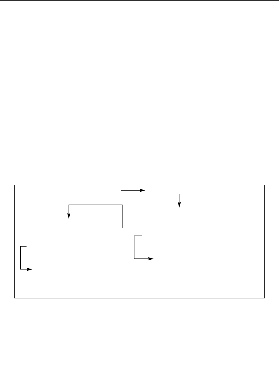
HSPICE® Reference Manual: Commands and Control Options 611
I-2013.12
Chapter 3: HSPICE Simulation Control Options Reference
.OPTION SEARCH
Automatically accesses a library, Verilog-A, or individual vendor files.
Syntax
.OPTION SEARCH=‘directory_path’ [path_name]
Description
Use this option to auto-access a library, or, using path_name, to search for
library (*.lib) files. Typically, vendors supply part files containing a single
subcircuit. The name of the file is the same as the subcircuit with the file
extension *.inc. The commands .LIB.INC, and .LOAD search for the file. In
addition, HSPICE supports .OPTION SEARCH for .VEC commands and
Verilog-A files. The path can be '/remote/home1/aa' or as '../'.
Examples
.OPTION SEARCH=‘$installdir/parts/vendor’
This example searches for models in the vendor subdirectory, under the
$installdir/parts installation directory (see Figure 15). The parts
directory contains the DDL subdirectories.
Figure 15 Vendor Library Usage
See Also
Signal Integrity Examples for netlists using .OPTION SEARCH including
iotran.sp, qa8.sp, and qabounce.sp.
$installdir/parts/vendor/buffer_f.inc
.macro buffer_f in out vdd vss
.inc ‘$installdir/parts/vendor/buffer.inc’
.eom
.lib ‘$installdir/parts/vendor/skew.dat’ ff
$installdir/parts/vendor/skew.dat
.lib ff $ fast model
.param vendor_xl=-.1u
.inc ‘$installdir/parts/vendor/model.dat’
.endl ff
$installdir/parts/vendor/model.dat
.model nch nmos level=28
+ xl=vendor_xl ...
$installdir/parts/vendor/buffer.inc
.macro buffer in out vdd vss
m1 out in vdd vdd nch w=10 l=1
...
x1 in out vdd vss buffer_f .OPTION search=’$installdir/parts/vendor’
Note: The ‘/usr’ directory is in the HSPICE install directory.

612 HSPICE® Reference Manual: Commands and Control Options
I-2013.12
Chapter 3: HSPICE Simulation Control Options Reference
.OPTION SEED
Specifies the starting seed for the random-number generator in Monte Carlo
analysis.
Syntax
.OPTION SEED=x | ‘random’
Description
Use this option to specify the starting seed for the random-number generator in
HSPICE Monte Carlo analysis. The minimum value is 1; the maximum value is
a positive integer of 259200. If SEED='random', HSPICE assigns a random
number between 1 and 259200 according to the system clock and prints it in
the .lis file for you to debug. An equivalent Option Seed can be used in the
Variation Block flow for AGUASS Monte Carlo usage with advanced sampling
methods.
See Also
.OPTION RANDGEN
.OPTION SET_MISSING_VALUES
Sub-option to SAMPLING_METHOD=External option, limits reporting of
missing independent random variables.
Syntax
OPTION SET_MISSING_VALUES = Random|Zero
Default Random
Description
Use this option to control missing random values in a .data block for external
sampling:
■Set_Missing_Values=Random — HSPICE generates its own random
values for the missing random variables in a .data block.
■Set_Missing_Values=Zero —HSPICE generates zero values for those
missing random variables in .data block in external sampling table.

HSPICE® Reference Manual: Commands and Control Options 613
I-2013.12
Chapter 3: HSPICE Simulation Control Options Reference
Examples
The following is an example of syntax use for this option.
.option Sampling_Method = External Block_Name = XXXX
+ File_Name = YYYY Set_Missing_Values = Random|Zero
.OPTION SHRINK
Scales the final constant capacitance value (only works with .OPTION
CMIUSRFLAG=3).
Syntax
.OPTION SHRINK= val
Description
Use this option to scale the final constant capacitance value. The default
setting overrides .OPTION SHRINK before applying shrink*shrink scaling
to constant capacitance value. The following is the usage of .OPTION SHRINK
and instance parameter shrink:
■1: If both .OPTION SHRINK and the shrink instance are not set in the
netlist, do nothing.
■2: If only .OPTION SHRINK is set in the netlist, use it to scale the final
constant capacitance value.
■3: If the instance parameter shrink is set in the netlist, use the instance
shrink to scale the final constant capacitance value.
See Also
.OPTION CMIUSRFLAG
.OPTION SI_SCALE_SYMBOLS
Controls whether the scale factors are HSPICE attributes or International
System of Units (SI) when case sensitivity is invoked.
Syntax
SI_SCALE_SYMBOLS=0|1
Default Value if option is not specified in the netlist: 0

614 HSPICE® Reference Manual: Commands and Control Options
I-2013.12
Chapter 3: HSPICE Simulation Control Options Reference
Value if option name is specified without a corresponding value: 1
Description
SI_SCALE_SYMBOLS=1 changes the scaling factors from the HSPICE
standard (default) to the International System of Units (SI) to enable you to use
case sensitive scaling symbols. (Using the (=1) setting assures consistency
with spice scale factors for downstream tools.)
Note: This option is enabled when case-sensitivity is on (-case 1).
See Also
.OPTION PCB_SCALE_FORMAT
Multiplying
Factors
Description .OPTION_SCALE_SYMBOLS=S
%> hspice -case C
S=0, C=0 (default) S=0, C=1
(Same as
S=0, C=0)
S=1, C=1 S=1, C=0
Same as
S=0,C=0
1e12 Tera T, t T, t
1e9 Giga G, g G, g
1e6 Mega MEG, meg, X, x M, MEG, meg, X, X
1e3 Kilo K, k K, k
1e-3 Milli M or m m
25.4e-6 1,000(s) of an
inch
MIL, mil MIL, mil
1e-6 Mico U, u U, u
1e-9 Nano N, n N, n
1e-12 Pico P, p P, p
1e-15 Femto F, f F, f
1e-18 Atto A, a A, a

HSPICE® Reference Manual: Commands and Control Options 615
I-2013.12
Chapter 3: HSPICE Simulation Control Options Reference
.OPTION SIM_ACCURACY
Sets and modifies the size of time steps.
Syntax
.OPTION SIM_ACCURACY=value
Default Conditional, see below
Description
Use this option to set and modify the size of time steps. This option applies to
all modes and tightens all tolerances, such as Newton-Raphson tolerance,
local truncation error, and other errors. The value must be a positive number.
The default is 1. If you specify .OPTION ACCURATE, the default value is 10;
you can use .option sim_accuracy=10 instead of .option accurate.
They are interchangeable. You can set .option sim_accuracy=10 if you
have not set previous sim_accuracy settings that are 10 or greater or have
previously set .option accurate. To set global accuracy, use .OPTION
SIM_ACCURACY=n, where n is a number greater than 0. You can specify
SIM_ACCURACY=100 for greatest granularity. SIM_ACCURACY maps to
several .OPTION RUNLVL settings.
You can apply different accuracy settings to different blocks or time intervals.
The syntax to set accuracy on a block, instance, or time interval is similar to the
settings used for a power supply.
Note: This option is active only when HSPICE advanced analog
functions are used.
See Also
.OPTION FFT_ACCURATE
.OPTION ACCURATE
.OPTION RUNLVL
.OPTION SIM_DELTAI
Sets the selection criteria for current waveforms in WDB and NW format.
Syntax
.OPTION SIM_DELTAI=value

616 HSPICE® Reference Manual: Commands and Control Options
I-2013.12
Chapter 3: HSPICE Simulation Control Options Reference
Default 0 amps
Description
Use this option to set the selection criteria for advanced analog current
waveforms in WDB and NW format. The value parameter specifies the amount
of change.
Note: This option is active only when HSPICE advanced analog
functions are used.
Examples
In this example, at the n timestep, HSPICE saves only data points that change
by more than 0 amps from previous values at the n-1 timestep.
.OPTION SIM_DELTAI = 0amps
See Also
.OPTION SIM_DELTAV
.OPTION SIM_DELTAV
Sets the selection criteria for current waveforms in WDB and NW format.
Syntax
.OPTION SIM_DELTAV=value
Default 1 mv
Description
Sets the selection criteria for current waveforms in WDB and NW format.
The value parameter specifies the amount of change.
Note: This option is active only when HSPICE advanced analog
functions are used.
Examples
In this example, at the n timestep, HSPICE saves only data points that change
by more than 1 mV from their previous values at the n-1 timestep.
.OPTION SIM_DELTAV = 1mv

HSPICE® Reference Manual: Commands and Control Options 617
I-2013.12
Chapter 3: HSPICE Simulation Control Options Reference
See Also
.OPTION SIM_DELTAI
.OPTION SIM_DSPF
Runs simulation with standard DSPF expansion of all nets from one or more
DSPF files.
Syntax
.OPTION SIM_DSPF=“[scope] dspf_filename”
Description
Use this option to run simulation with standard DSPF expansion of all nets from
one or more DSPF files.
scope can be a subcircuit definition or an instance. If you do not specify
scope, it defaults to the top-level definition.
You can repeat this option to include more DSPF files.
This option can accelerate simulation by more than 100%. You can further
reduce total CPU time by including the .OPTION SIM_LA in the netlist.
For designs of 5K transistors or more, including .OPTION SIM_DSPF_ACTIVE
in your netlist to expand only active nodes also provides a performance gain.
Note: HSPICE requires both a DSPF file and an ideal extracted netlist.
Only flat DSPF files are supported; hierarchy commands, such
as .SUBCKT and .x1 are ignored.
For additional information, see “Post-Layout Back-Annotation” in the HSPICE
User Guide: Advanced Analog Simulation and Analysis.
Note: This option is active only when HSPICE advanced analog
features are used.

618 HSPICE® Reference Manual: Commands and Control Options
I-2013.12
Chapter 3: HSPICE Simulation Control Options Reference
Examples
In Example 1, the parasitics in the DSPF file are mapped into the hierarchical
ideal netlist.
Example 1
$ models
.MODEL p pmos
.MODEL n nmos
.INCLUDE add4.dspf
.OPTION SIM_DSPF="add4.dspf"
.VEC "dspf_adder.vec"
.TRAN 1n 5u
vdd vdd 0 3.3
.OPTION POST
.END
In Example 2, the SIM_DSPF option accelerates the simulation by more than
100%. By using the SIM_LA option at the same time, you can further reduce
the total CPU time:
Example 2
$ models
.MODEL p pmos
.MODEL n nmos
.INCLUDE add4.dspf
.OPTION SIM_DSPF="add4.dspf"
.OPTION SIM_LA=PACT
.VEC "dspf_adder.vec"
.TRAN 1n 5u
vdd vdd 0 3.3
.OPTION POST
.END
Example 3, the x1.spf DSPF file is back-annotated to the x1 top-level instance.
It also back-annotates the inv.spf DSPF file to the inv subcircuit.
Example 3
.OPTION SIM_DSPF = "x1 x1.spf"
.OPTION SIM_DSPF = "inv inv.spf"
See Also
.OPTION SIM_LA
.OPTION SIM_DSPF_ACTIVE
.OPTION SIM_DSPF_SCALEC

HSPICE® Reference Manual: Commands and Control Options 619
I-2013.12
Chapter 3: HSPICE Simulation Control Options Reference
.OPTION SIM_DSPF_SCALER
.OPTION SIM_SPEF
.OPTION SIM_DSPF_ACTIVE
Runs simulation with selective DSPF expansion of active nets from one or more
DSPF files.
Syntax
.OPTION SIM_DSPF_ACTIVE=”active_node”
Description
Use this option to run simulation with selective DSPF expansion of active nets
from one or more DSPF files. HSPICE performs a preliminary verification run to
determine the activity of the nodes and generates two ASCII files:
active_node.rc and active_node.rcxt. These files save all active node
information in both Star-RC and Star-RCXT formats. If an active_node file is
not generated from the preliminary run, no nets are expanded. Active nets are
added to the file as they are identified in the subsequent transient simulation. A
second simulation run using the same file and option causes only the nets
listed in the active_node file to be expanded. Activity changes may be due to
timing changes caused by expansion of the active nets. In this case, additional
nets are listed in the active_node file and a warning is issued.
HSPICE uses the active_node file and the DSPF file with the ideal netlist to
expand only the active portions of the circuit. If a net is latent, then HSPICE
does not expand it, which saves memory and CPU time.
For additional information, see “Selective Post-Layout Flow” in the HSPICE
User Guide: Advanced Analog Simulation and Analysis.
Note: This option is active only when HSPICE advanced analog
functions are used.
Examples
In the following example, an active net in which the tolerance of the voltage
change is greater than 0.5V is saved to both the active.rc and active.rcxt files.
Based on these files, HSPICE back-annotates only the active parasitics from
x1.spf and s2.spf to the x1 and x2 top-level instances.

620 HSPICE® Reference Manual: Commands and Control Options
I-2013.12
Chapter 3: HSPICE Simulation Control Options Reference
.OPTION SIM_DSPF = "x1 x1.spf"
.OPTION SIM_DSPF = "x2 x2.spf"
.OPTION SIM_DSPF_ACTIVE = "active"
.OPTION SIM_DSPF_VTOL = 0.5V
See Also
.OPTION SIM_DSPF
.OPTION SIM_DSPF_MAX_ITER
.OPTION SIM_DSPF_VTOL
.OPTION SIM_SPEF_ACTIVE
.OPTION SIM_DSPF_INSERROR
Skips unmatched instances.
Syntax
.OPTION SIM_DSPF_INSERROR=ON | OFF
Default OFF
Description
Use this option to skip unmatched instances.
■ON: Skips unmatched instances
■OFF: Does not skip unmatched instances.
For additional information, see “Additional Post-Layout Options” in the HSPICE
User Guide: Advanced Analog Simulation and Analysis.
Note: This option is active only when HSPICE advanced analog
functions are used.
.OPTION SIM_DSPF_LUMPCAPS
Connects a lumped capacitor with a value equal to the net capacitance for
instances missing in the hierarchical netlist.
Syntax
.OPTION SIM_DSPF_LUMPCAPS=ON | OFF
Default ON

HSPICE® Reference Manual: Commands and Control Options 621
I-2013.12
Chapter 3: HSPICE Simulation Control Options Reference
Description
Use this option to connect a lumped capacitor with a value equal to the net
capacitance for instances missing in the hierarchical netlist.
■ON (default): Adds lumped capacitance while ignoring other net contents
■OFF: Uses net contents
For additional information, see “Additional Post-Layout Options” in the HSPICE
User Guide: Advanced Analog Simulation and Analysis.
Note: This option is active only when HSPICE advanced analog
functions are used.
.OPTION SIM_DSPF_MAX_ITER
Specifies the maximum number of simulation runs for the second selective
DSPF expansion pass.
Syntax
.OPTION SIM_DSPF_MAX_ITER=value
Default 1
Description
Use this option to specify the maximum number of simulation runs for the
second selective DSPF expansion pass.
The value parameter specifies the number of iterations for the second
simulation run.
Some of the latent nets might turn active after the first iteration of the second
simulation run. In this case:
■Resimulate the netlist to ensure the accuracy of the post-layout simulation.
■Use this option to set the maximum number of iterations for the second run.
If the active_node remains the same after the second simulation run,
HSPICE ignores these options.
For details, see “Selective Post-Layout Flow” HSPICE User Guide: Advanced
Analog Simulation and Analysis.
Note: This option is active only when HSPICE advanced analog
functions are used.

622 HSPICE® Reference Manual: Commands and Control Options
I-2013.12
Chapter 3: HSPICE Simulation Control Options Reference
See Also
.OPTION SIM_DSPF_ACTIVE
.OPTION SIM_DSPF_VTOL
.OPTION SIM_DSPF_RAIL
Controls whether power-net parasitics are back-annotated
Syntax
.OPTION SIM_DSPF_RAIL=ON | OFF
Default OFF
Description
Use this option to control whether power-net parasitics are back-annotated.
■OFF: Do not back-annotate nets in a power rail
■ON: Back-annotate nets in a power rail
For additional information, see “Additional Post-Layout Options” in the HSPICE
User Guide: Advanced Analog Simulation and Analysis.
Note: This option is active only when HSPICE advanced analog
functions are used.
.OPTION SIM_DSPF_SCALEC
Scales the capacitance values in a DSPF file for a standard DSPF expansion
flow.
Syntax
.OPTION SIM_DSPF_SCALEC=scaleC
Description
Use this option to scale the capacitance values in a DSPF file for a standard
DSPF expansion flow.
The scaleC parameter specifies the scale factor.
For additional information, see “Additional Post-Layout Options” in the HSPICE
User Guide: Advanced Analog Simulation and Analysis.

HSPICE® Reference Manual: Commands and Control Options 623
I-2013.12
Chapter 3: HSPICE Simulation Control Options Reference
Note: This option is active only when HSPICE advanced analog
functions are used.
See Also
.OPTION SIM_LA
.OPTION SIM_DSPF_ACTIVE
.OPTION SIM_DSPF_SCALER
Scales the resistance values in a DSPF file for a standard DSPF expansion
flow.
Syntax
.OPTION SIM_DSPF_SCALER=scaleR
Description
Use this option to scale the resistance values in a DSPF file for a standard
DSPF expansion flow.
The scaleR specifies the scale factor.
For additional information, see “Additional Post-Layout Options” in the HSPICE
User Guide: Advanced Analog Simulation and Analysis.
Note: This option is active only when HSPICE advanced analog
functions are used.
See Also
.OPTION SIM_LA
.OPTION SIM_DSPF_ACTIVE
.OPTION SIM_DSPF_VTOL
Specifies multiple DSPF active thresholds.
Syntax
.OPTION SIM_DSPF_VTOL=“value | scope1 scope2 ...
+ scopen”
Default 0.1V

624 HSPICE® Reference Manual: Commands and Control Options
I-2013.12
Chapter 3: HSPICE Simulation Control Options Reference
Description
Use this option to specify multiple DSPF active thresholds.
■The value parameter specifies the tolerance of voltage change. This value
should be relatively small compared to the operating range of the circuit or
smaller than the supply voltage.
■scopen can be a subcircuit definition that uses a prefix of “@” or a subcircuit
instance.
HSPICE performs a second simulation run by using the active_node file, the
DSPF, and the hierarchical LVS ideal netlist to back-annotate only active
portions of the circuit. If a net is latent, HSPICE does not expand the net. This
saves simulation runtime and memory.
By default, HSPICE performs only one iteration of the second simulation run.
Use the SIM_DSPF_MAX_ITER option to change this setting.
For additional information, see “Selective Post-Layout Flow” in the HSPICE
User Guide: Advanced Analog Simulation and Analysis.
Note: This option is active only when HSPICE advanced analog
functions are used.
Examples
Example 1 The first line sets the sensitivity voltage to 0.01V. Subcircuit definition
snsamp and the subcircuit instance xvco have full parasitics if their nodes
move more than 0.01V during active nodes generation. In the second
line, xand and xff are less sensitive than the default, indicating that they
are not sensitive to parasitics
.OPTION SIM_DSPF_VTOL=“0.01 | @snsamp xvco”
.OPTION SIM_DSPF_VTOL=“0.25 | xand xff”
Example 2 The sense amp circuit uses full parasitics if their nodes move more than
0.01V during active-node generation. The inv subcircuit definition is less
sensitive than the default so the nodes are less sensitive to the parasitics.
.OPTION SIM_DSPF = "inv inv.spf"
.OPTION SIM_DSPF = "senseamp senseamp.spf"
.OPTION SIM_DSPF_ACTIVE = "activenet"
.OPTION SIM_DSPF_VTOL = "0.15 | @inv"
.OPTION SIM_DSPF_VTOL = "0.01 | @senseamp"
See Also
.OPTION SIM_DSPF_ACTIVE
.OPTION SIM_DSPF_MAX_ITER

HSPICE® Reference Manual: Commands and Control Options 625
I-2013.12
Chapter 3: HSPICE Simulation Control Options Reference
.OPTION SIM_LA
Activates linear matrix (RC) reduction for HSPICE.
Syntax
.OPTION SIM_LA=[ PACT | PI | LNE [0|1|2|3]]
Default Value if option is not specified in the netlist: 0
Value if option name is specified without a corresponding value: 1
Description
Use this option to activate linear matrix reduction. SIM_LA does not reduce a
node used by any analysis command, such as .PROBE,.MEASURE, and so on
This option accelerates the simulation of circuits that include large linear RC
networks by reducing all matrixes that represent RC networks.
■0 turns off SIM_LA
■1 is the equivalent of PACT, which selects the Pole Analysis via Congruence
Transforms (PACT) algorithm to reduce RC networks in a well-conditioned
manner, while preserving network stability.
■2 invokes the PI algorithm to create a PI model analyzing the small signal
behavior of bipolar junction and field effect transistors. The model can be
quite accurate for low-frequency circuits and can easily be adapted for
higher frequency circuits with the addition of appropriate inter-electrode
capacitances and other parasitic elements. models of the RC networks.
■3 invokes the LNE (Linear Node Elimination) algorithm to speed up the
simulation of circuits with huge numbers of coupling capacitors.
■If SIM_LA is not specified in the input file, the lis file returns SIM_LA=0.
■If SIM_LA is specified with no value or SIM_LA=PACT, the lis file returns
SIM_LA=1.
■If SIM_LA=PI, the lis file returns SIM_LA=2.
■If SIM_LA=LNE, the lis file returns SIM_LA=3.
For additional information, see “Linear Acceleration” in the HSPICE User
Guide: Basic Simulation and Analysis or “Linear Acceleration” in the HSPICE
User Guide: Advanced Analog Simulation and Analysis.
See Also
.OPTION SIM_DSPF
.OPTION LA_FREQ

626 HSPICE® Reference Manual: Commands and Control Options
I-2013.12
Chapter 3: HSPICE Simulation Control Options Reference
.OPTION LA_MAXR
.OPTION LA_MINC
.OPTION LA_TIME
.OPTION LA_TOL
.OPTION SIM_LA_FREQ
Specifies the upper frequency for which accuracy must be preserved.
Syntax
.OPTION SIM_LA_FREQ=value
Default 1GHz
Description
Use this option to specify the upper frequency for which accuracy must be
preserved. The value parameter specifies the upper frequency for which the
PACT algorithm must preserve accuracy. If value is 0, the algorithm drops all
capacitors because only DC is of interest.
The maximum frequency required for accurate reduction depends on both the
technology of the circuit and the time scale of interest. In general, the faster the
circuit, the higher the maximum frequency. For additional information, see
“Linear Acceleration” in the HSPICE User Guide: Advanced Analog Simulation
and Analysis.
See Also
.OPTION SIM_LA
.OPTION SIM_LA_TIME
.OPTION SIM_LA_MAXR
Specifies the maximum resistance for linear matrix reduction.
Syntax
.OPTION SIM_LA_MAXR=value
Default 1e15 ohms

HSPICE® Reference Manual: Commands and Control Options 627
I-2013.12
Chapter 3: HSPICE Simulation Control Options Reference
Description
Use this option to specify the maximum resistance for linear matrix reduction.
The value parameter specifies the maximum resistance preserved in the
reduction. The linear matrix reduction process assumes that any resistor
greater than value has an infinite resistance and drops the resistor after
reduction completes. For additional information, see “Linear Acceleration” in
the HSPICE User Guide: Advanced Analog Simulation and Analysis.
See Also
.OPTION SIM_LA
.OPTION SIM_LA_MINC
Specifies the minimum capacitance for linear matrix reduction.
Syntax
.OPTION SIM_LA_MINC=value
Default 1e-16 farads
Description
Use this option to specify the minimum capacitance for linear matrix reduction.
The value parameter specifies the minimum capacitance preserved in the
reduction.
The linear matrix reduction process lumps any capacitor smaller than value to
ground after the reduction completes.
For additional information, see “Linear Acceleration” in the HSPICE User
Guide: Advanced Analog Simulation and Analysis.
See Also
.OPTION SIM_LA
.OPTION SIM_LA_TIME
Specifies the minimum time for which accuracy must be preserved.
Syntax
.OPTION SIM_LA_TIME=value

628 HSPICE® Reference Manual: Commands and Control Options
I-2013.12
Chapter 3: HSPICE Simulation Control Options Reference
Default 1ns.
Description
Use this option to specify the minimum time for which accuracy must be
preserved.
The value parameter specifies the minimum switching time for which the PACT
algorithm preserves accuracy.
Waveforms that occur more rapidly than the minimum switching time are not
accurately represented.
This option is simply an alternative to .OPTION SIM_LA_FREQ. The default is
equivalent to setting SIM_LA_FREQ=1GHz.
Note: Higher frequencies (smaller times) increase accuracy, but only
up to the minimum time step used in HSPICE.
For additional information, see “Linear Acceleration” in the HSPICE User
Guide: Advanced Analog Simulation and Analysis.
Examples
For a circuit having a typical rise time of 1ns, either set the maximum frequency
to 1 GHz, or set the minimum switching time to 1ns:
.OPTION SIM_LA_FREQ=1GHz
-or-
.OPTION SIM_LA_TIME=1ns
However, if spikes occur in 0.1ns, HSPICE does not accurately simulate them.
To capture the behavior of the spikes, use:
.OPTION SIM_LA_FREQ=10GHz
-or-
.OPTION SIM_LA_TIME=0.1ns
See Also
.OPTION SIM_LA
.OPTION SIM_LA_FREQ
.OPTION SIM_LA_TOL
Specifies the error tolerance for the PACT algorithm.

HSPICE® Reference Manual: Commands and Control Options 629
I-2013.12
Chapter 3: HSPICE Simulation Control Options Reference
Syntax
.OPTION SIM_LA_TOL=value
Default 0.05ns.
Description
Use this option to specify the error tolerance for the PACT algorithm.
The value parameter must specify a real number between 0.0 and 1.0.
For additional information, see “Linear Acceleration” in the HSPICE User
Guide: Advanced Analog Simulation and Analysis.
See Also
.OPTION SIM_LA
.OPTION SIM_ORDER
Controls the amount of Backward-Euler (BE) method to mix with the
Trapezoidal (TRAP) method for hybrid integration.
Syntax
.OPTION SIM_ORDER=x
Default 1.9
Description
Use this option to control the amount of Backward-Euler (BE) method to mix
with the Trapezoidal (TRAP) method for hybrid integration.
The x parameter must specify a real number between 1.0 and 2.0.
■SIM_ORDER=1.0 selects BE
■SIM_ORDER=2.0 selects TRAP.
Note: .OPTION SIM_ORDER has precedence over .OPTION
SIM_TRAP.
A higher order is more accurate, especially with inductors (such as crystal
oscillators), which need SIM_ORDER=2.0. A lower order has more damping.
This option affects time stepping when you set .OPTION METHOD to TRAP or
TRAPGEAR.

630 HSPICE® Reference Manual: Commands and Control Options
I-2013.12
Chapter 3: HSPICE Simulation Control Options Reference
Note: This option is active only when HSPICE advanced analog
functions are used.
Examples
This example causes a mixture of 10% Gear-2 and 90% BE-trapezoidal hybrid
integration. The BE-trapezoidal part is 10% BE.
.option sim_order=1.9
See Also
.OPTION METHOD
.OPTION SIM_TRAP
.OPTION SIM_OSC_DETECT_TOL
Specifies the tolerance for detecting numerical oscillations.
Syntax
.OPTION SIM_OSC_DETECT_TOL=value
Default 10^8
Description
Use this option to specify the tolerance for detecting numerical oscillations. If
HSPICE detects numerical oscillations, it inserts Backward-Euler (BE) steps.
Smaller values of this tolerance result in fewer BE steps.
Note: This option is active only when HSPICE advanced analog
functions are used.
See Also
.OPTION METHOD
.OPTION SIM_POSTAT
Specifies waveform output to nodes in the specified subcircuit instance only.
Syntax
.OPTION SIM_POSTAT=instance

HSPICE® Reference Manual: Commands and Control Options 631
I-2013.12
Chapter 3: HSPICE Simulation Control Options Reference
Description
Use this option to limit waveform output to nodes in the specified subcircuit
instance only in HSPICE and HPP. SIM_POSTAT is available for both HSPICE.
Wildcards are supported. This option is equivalent to .OPTION POSTAT.
Each of these options, SIM_POSTTOP, SIM_POSTAT, SIM_POSTDOWN,
SIM_POSTSKIP works for both default output (.option probe=0) and
.probe/.print v(*).
Examples
Example 1 The following example outputs X1.X4 node signals only; see Figure 16.
.OPTION SIM_POSTAT=X1.X4
Figure 16 Node Hierarchy
Example 2 Without .OPTION PROBE, HSPICE plots all voltages of subcircuit x1.x1.
.option post
.option sim_postat = x1.x1
Example 3 With .OPTION PROBE, HSPICE plots all voltages of subcircuit x1.x1.
.option post
.option probe
.option sim_postat = x1.x1
Example 4 With a .PROBE statement, HSPICE plots all voltages of subcircuit x1.x1.
.option post
.option probe
.option sim_postat = x1.x1
.probe v(*)
X3 X4 X5 X6
X1 X2 X1 X2
top
X1(ADD) X2(SUB)

632 HSPICE® Reference Manual: Commands and Control Options
I-2013.12
Chapter 3: HSPICE Simulation Control Options Reference
See Also
.OPTION SIM_POSTSKIP
.OPTION SIM_POSTTOP
.OPTION POSTTOP
.OPTION SIM_POSTDOWN
Limits waveform output to nodes in the specified subcircuit instance and their
children.
Syntax
.OPTION SIM_POSTDOWN=instance
Description
Use this option with .OPTION SIM_POSTTOP and it takes precedence over
.OPTION SIM_POSTSKIP.
Wildcards are supported.
Each of these options, SIM_POSTTOP, SIM_POSTAT, SIM_POSTDOWN,
SIM_POSTSKIP works for both default output (.option probe=0) and
.probe/.print v(*).
Examples
The following example outputs top, X1, X1.X4, X1.X4.X1, X1.X4.X2, and X2.
(See Figure 16 on page 631.)
.OPTION SIM_POSTTOP=2
.OPTION SIM_POSTDOWN=X1.X4
See Also
.OPTION SIM_POSTAT
.OPTION SIM_POSTSKIP
.OPTION SIM_POSTTOP
.OPTION SIM_POSTSCOPE
Specifies the signal types to probe from within a scope.

HSPICE® Reference Manual: Commands and Control Options 633
I-2013.12
Chapter 3: HSPICE Simulation Control Options Reference
Syntax
.OPTION SIM_POSTSCOPE= net | port | all
Description
Use this option to specify the signal types to probe from within a scope.
■net: Outputs only nets in the scope
■port: Outputs both nets and ports
■all: Outputs nets, ports, and global variables.
See Also
.OPTION POST
.OPTION SIM_POSTSKIP
.OPTION SIM_POSTTOP
.OPTION SIM_POSTSKIP
Causes the SIM_POSTTOP option to skip subckt_definition instances.
Syntax
.OPTION SIM_POSTSKIP=subckt_definition
Description
Use this option to cause the SIM_POSTTOP option to skip any instances and
their children that are defined by the subckt_definition parameter. To specify
more than one subcircuit definition, issue this option once for each definition
you want to skip. SIM_POSTSKIP is available for both HSPICE. Wildcards are
supported.
Each of these options, SIM_POSTTOP, SIM_POSTAT, SIM_POSTDOWN,
SIM_POSTSKIP works for both default output (.option probe=0) and
.probe/.print v(*).
Examples
The following example outputs top, and skips X2. X1 because they are
instances of the ADD subcircuit. (See Figure 16 on page 631.)
.OPTION SIM_POSTTOP=2
.OPTION SIM_POSTSKIP=ADD
See Also
.OPTION SIM_POSTTOP

634 HSPICE® Reference Manual: Commands and Control Options
I-2013.12
Chapter 3: HSPICE Simulation Control Options Reference
.OPTION SIM_POSTTOP
Limits data written to your waveform file to data from only the top n level nodes.
Syntax
.OPTION SIM_POSTTOP=n
Description
Limits the data written to your waveform file to data from only the top n level
nodes. SIM_POSTAT is available for both HSPICE.
This option outputs instances to n levels deep.
■SIM_POSTTOP=3: Outputs instances from 3 levels deep
■SIM_POSTTOP=1: Outputs instances from only the top-level signals.
Specifying the PROBE option without specifying a SIM_POSTTOP option
HSPICE sets the SIM_POSTTOP=0. HSPICE outputs all levels if you do not
specify the PROBE option or a SIM_POSTTOP option. Wildcards are supported.
Note: Specify the POST option to enable a waveform display interface.
SIM_POSTTOP is equivalent to POSTTOP used in HSPICE.
Each of these options, SIM_POSTTOP, SIM_POSTAT, SIM_POSTDOWN,
SIM_POSTSKIP works for both default output (.option probe=0) and
.probe/.print v(*).
Examples
Example 1 Outputs top, X1, and X2. (See Figure 16 on page 631.)
.OPTION SIM_POSTTOP=2
The following example outputs top, X1, X2,and X4, X1and X2. (See Figure 16
on page 631.)
Example 2
.OPTION SIM_POSTTOP=2
.OPTION SIM_POSTDOWN=X1.X4
See Also
.OPTION POST
.OPTION PROBE
.OPTION SIM_POSTSKIP

HSPICE® Reference Manual: Commands and Control Options 635
I-2013.12
Chapter 3: HSPICE Simulation Control Options Reference
.OPTION SIM_POWER_ANALYSIS
Prints a list of signals matching the tolerance setting at a specified point in time.
Syntax
.OPTION SIM_POWER_ANALYSIS=“time_pointtol”
.OPTION SIM_POWER_ANALYSIS=“bottom time_pointtol”
Description
Use this option to print a list of signals matching the tolerance (tol) setting at
a specified point in time.
The first syntax produces a list of signals that consume more current than tol
at time point, in this format:
The second syntax produces the list of lowest-level signals, known as leaf
subcircuits that consume more than tol at time point. The output is similar
to this:
For additional information, see “Power Analysis Output Format” in the HSPICE
User Guide: Advanced Analog Simulation and Analysis.
Note: This option is active only when HSPICE advanced analog
functions are used.
Examples
In this example, print the names of leaf subcircuits that use more than 100uA at
100ns into the simulation are printed.
.OPTION SIM_POWER_ANALYSIS=“bottom 100ns 100ua”
.POWER VDD
See Also
.POWER
Argument Description
time_point Time when HSPICE detects signals where the port current is larger
than the tolerance value.
tol Tolerance value for the signal defined in the .POWER command.
bottom Signal at the lowest hierarchy level, also called a leaf subcircuit.

636 HSPICE® Reference Manual: Commands and Control Options
I-2013.12
Chapter 3: HSPICE Simulation Control Options Reference
.OPTION SIM_POWER_TOP
Controls the number of hierarchy levels on which power analysis is performed.
Syntax
.OPTION SIM_POWER_TOP=value
Description
Use this option to control the number of hierarchy levels on which power
analysis is performed.
By default, power analysis is performed on the top levels of hierarchy.
Note: This option is active only when HSPICE advanced analog
functions are used.
Examples
In the following example, HSPICE produces .POWER command results for top-
level and first-level subcircuits (the subcircuit children of the top-level
subcircuits).
.OPTION SIM_POWER_TOP=2
See Also
.POWER
.OPTION SIM_POWERDC_ACCURACY
Increases the accuracy of operating point calculations for POWERDC analysis.
Syntax
.OPTION SIM_POWERDC_ACCURACY=value
Description
Use this option to increase the accuracy of operating point calculations for
POWERDC analysis.
A higher value results in greater accuracy, but more time to complete the
calculation.
Note: This option is active only when HSPICE advanced analog
functions are used.

HSPICE® Reference Manual: Commands and Control Options 637
I-2013.12
Chapter 3: HSPICE Simulation Control Options Reference
See Also
.POWERDC
.OPTION SIM_POWERDC_HSPICE
.OPTION SIM_POWERDC_HSPICE
Increases the accuracy of operating point calculations for POWERDC analysis.
Syntax
.OPTION SIM_POWERDC_HSPICE
Description
Use this option to increase the accuracy of operating point calculations for
POWERDC analysis.
Note: This option is active only when HSPICE advanced analog
functions are used.
See Also
.POWERDC
.OPTION SIM_POWERDC_ACCURACY
.OPTION SIM_POWERPOST
Controls power analysis waveform dumping.
Syntax
.OPTION SIM_POWERPOST=ON|OFF
Description
Use this option to enable or disable power analysis waveform dumping.
Note: This option is active only when HSPICE advanced analog
functions are used.
See Also
.POWER

638 HSPICE® Reference Manual: Commands and Control Options
I-2013.12
Chapter 3: HSPICE Simulation Control Options Reference
.OPTION SIM_POWERSTART
Specifies a default start time for measuring signals during simulation.
Syntax
.OPTION SIM_POWERSTART=time
Description
Use this option with a .POWER command to specify a default start time for
measuring signals during simulation. This default time applies to all signals that
do not have their own FROM measurement time. This option together with the
.OPTION SIM_POWERSTOP control the power measurement scope for an
entire simulation.
Note: This option is active only when HSPICE advanced analog
functions are used.
Examples
In this example, the scope for simulating the x1.in signal is from 10 ps to 90 ps.
.OPTION SIM_POWERSTART=10ps
.OPTION SIM_POWERSTOP=90ps
.power x1.in
See Also
.OPTION SIM_POWERSTOP
.OPTION SIM_POWERSTART
.OPTION SIM_POWERSTOP
Specifies a default stop time for measuring signals during simulation.
Syntax
.OPTION SIM_POWERSTOP=time
Description
Use this option with a .POWER command to specify a default stop time for
measuring signals during simulation. This default time applies to all signals that
do not have their own TO measurement time. This option together with the
.OPTION SIM_POWERSTART control the power measurement scope for an
entire simulation.

HSPICE® Reference Manual: Commands and Control Options 639
I-2013.12
Chapter 3: HSPICE Simulation Control Options Reference
Note: This option is active only when HSPICE advanced analog
functions are used.
See Also
.OPTION SIM_POWERSTART
.POWER
.OPTION SIM_SPEF
Runs simulation with SPEF expansion of all nets from one or more SPEF files.
Syntax
.OPTION SIM_SPEF=“spec_filename”
Description
Use this option to run simulation with SPEF expansion of all nets from one or
more SPEF files.
You can repeat this option to include more SPEF files.
For additional information, see “Post-Layout Back-Annotation” in the HSPICE
User Guide: Advanced Analog Simulation and Analysis.
Note: This option is active only when HSPICE advanced analog
functions are used.
Examples
In this example, the senseamp.spf SPEF file is back-annotated to the sense
amp circuit.
.OPTION SIM_SPEF = "senseamp.spf"
See Also
.OPTION SIM_SPEF_ACTIVE
.OPTION SIM_SPEF_SCALEC
.OPTION SIM_SPEF_SCALER

640 HSPICE® Reference Manual: Commands and Control Options
I-2013.12
Chapter 3: HSPICE Simulation Control Options Reference
.OPTION SIM_SPEF_ACTIVE
Runs simulation with selective SPEF expansion of active nets from one or more
DSPF files.
Syntax
.OPTION SIM_SPEF_ACTIVE=”active_node”
Description
Use this option to run simulation with selective SPEF expansion of active nets
from one or more DSPF files.
HSPICE performs a preliminary verification run to determine the activity of the
nodes and generates two ASCII files: active_node.rc and
active_node.rcxt. These files save all active node information in both Star-
RC and Star-RCXT formats.
If an active_node file is not generated from the preliminary run, no nets are
expanded. Active nets are added to the file as they are identified in the
subsequent transient simulation. A second simulation run using the same file
and option causes only the nets listed in the active_node file to be
expanded. It is possible that activity changes are due to timing changes caused
by expansion of the active nets. In this case, additional nets are listed in the
active_node file and a warning is issued.
By default, a node is considered active if the voltage varies by more than 0.1 V.
You can use the SIM_SPEF_VTOL option to change this value.
HSPICE uses the active_node file and the DSPF file with the ideal netlist to
expand only the active portions of the circuit. If a net is latent, then HSPICE
does not expand it, which saves memory and CPU time.
For additional information, see “Selective Post-Layout Flow” in the HSPICE
User Guide: Advanced Analog Simulation and Analysis.
Note: This option is active only when HSPICE advanced analog
functions are used.
See Also
.OPTION SIM_SPEF_VTOL

HSPICE® Reference Manual: Commands and Control Options 641
I-2013.12
Chapter 3: HSPICE Simulation Control Options Reference
.OPTION SIM_SPEF_INSERROR
Skips unmatched instances.
Syntax
.OPTION SIM_SPEF_INSERROR=ON | OFF
Description
Use this option to skip unmatched instances.
■ON: Skips unmatched instances.
■OFF: Does not skip unmatched instances.
For more information, see “Additional Post-Layout Options” in the HSPICE
User Guide: Advanced Analog Simulation and Analysis.
Note: This option is active only when HSPICE advanced analog
functions are used.
.OPTION SIM_SPEF_LUMPCAPS
Connects a lumped capacitor with a value equal to the net capacitance for
instances missing in the hierarchical netlist.
Syntax
.OPTION SIM_SPEF_LUMPCAPS=ON | OFF
Description
Use this option to connect a lumped capacitor with a value equal to the net
capacitance for instances missing in the hierarchical netlist.
■ON: Adds lumped capacitance while ignoring other net contents.
■OFF: Uses net contents.
For additional information, see “Additional Post-Layout Options” in the HSPICE
User Guide: Advanced Analog Simulation and Analysis.
Note: This option is active only when HSPICE advanced analog
functions are used.

642 HSPICE® Reference Manual: Commands and Control Options
I-2013.12
Chapter 3: HSPICE Simulation Control Options Reference
.OPTION SIM_SPEF_MAX_ITER
Specifies the maximum number of simulation runs for the second selective
SPEF expansion pass.
Syntax
.OPTION SIM_SPEF_MAX_ITER=value
Description
Use this option to specify the maximum number of simulation runs for the
second selective SPEF expansion pass.
The value parameter specifies the number of iterations for the second
simulation run.
Some of the latent nets might turn active after the first iteration of the second
simulation run. In this case:
■Re simulate the netlist to ensure the accuracy of the post-layout simulation.
■Use this option to set the maximum number of iterations for the second run.
If the active_node remains the same after the second simulation run,
HSPICE ignores these options.
For additional information, see “Selective Post-Layout Flow” in the HSPICE
User Guide: Advanced Analog Simulation and Analysis.
Note: This option is active only when HSPICE advanced analog
functions are used.
See Also
.OPTION SIM_SPEF_ACTIVE
.OPTION SIM_SPEF_VTOL
.OPTION SIM_SPEF_PARVALUE
Interprets triplet format float:float:float values in SPEF files as best: average:
worst.
Syntax
.OPTION SIM_SPEF_PARVALUE=1|2|3

HSPICE® Reference Manual: Commands and Control Options 643
I-2013.12
Chapter 3: HSPICE Simulation Control Options Reference
Description
Use this option to interpret triplet format float:float:float values in SPEF files as
best: average: worst.
■SIM_SPEF_PARVALUE = 1: Use best.
■SIM_SPEF_PARVALUE = 2: Use average.
■SIM_SPEF_PARVALUE = 3: Use worst.
For further information, see “Additional Post-Layout Options” in the HSPICE
User Guide: Advanced Analog Simulation and Analysis.
Note: This option is active only when HSPICE advanced analog
functions are used.
.OPTION SIM_SPEF_RAIL
Controls whether power-net parasitics are back-annotated.
Syntax
.OPTION SIM_SPEF_RAIL=ON | OFF
Description
Use this option to control whether power-net parasitics are back-annotated.
■OFF: Do not back-annotate nets in a power rail.
■ON: Back-annotate nets in a power rail.
For further information, see “Additional Post-Layout Options” in the HSPICE
User Guide: Advanced Analog Simulation and Analysis.
Note: This option is active only when HSPICE advanced analog
functions are used.
.OPTION SIM_SPEF_SCALEC
Scales the capacitance values in a SPEF file for a standard SPEF expansion
flow.

644 HSPICE® Reference Manual: Commands and Control Options
I-2013.12
Chapter 3: HSPICE Simulation Control Options Reference
Syntax
.OPTION SIM_SPEF_SCALEC=scaleC
Description
Use this option to scale the capacitance values in a SPEF file for a standard
SPEF expansion flow.
The scaleC parameter specifies the scale factor.
See “Additional Post-Layout Options” in the HSPICE User Guide: Advanced
Analog Simulation and Analysis.
Note: This option is active only when HSPICE advanced analog
functions are used.
See Also
.OPTION SIM_SPEF_ACTIVE
.OPTION SIM_SPEF_SCALER
Scales the resistance values in a SPEF file for a standard SPEF expansion
flow.
Syntax
.OPTION SIM_SPEF_SCALER=scaleR
Description
Use this option to scale the resistance values in a SPEF file for a standard
SPEF expansion flow.
The scaleR parameter specifies the scale factor.
For more information, see “Additional Post-Layout Options” in the HSPICE
User Guide: Advanced Analog Simulation and Analysis.
Note: This option is active only when HSPICE advanced analog
functions are used.
See Also
.OPTION SIM_SPEF_ACTIVE

HSPICE® Reference Manual: Commands and Control Options 645
I-2013.12
Chapter 3: HSPICE Simulation Control Options Reference
.OPTION SIM_SPEF_VTOL
Specifies multiple SPEF active thresholds.
Syntax
.OPTION SIM_SPEF_VTOL=“value | scope1 scope2...
+ scopen”
Description
Use this option to specify multiple SPEF active thresholds.
■The value parameter specifies the tolerance of voltage change. This value
should be relatively small compared to the operating range of the circuit, or
smaller than the supply voltage.
■The scopen parameter can be a subcircuit definition that uses a prefix of “@”
or a subcircuit instance.
HSPICE performs a second simulation run by using the active_node file, the
SPEF, and the hierarchical LVS ideal netlist to back-annotate only active
portions of the circuit. If a net is latent, then HSPICE does not expand the net.
This saves simulation runtime and memory.
By default, HSPICE performs only one iteration of the second simulation run.
Use the SIM_SPEF_MAX_ITER option to change it.
For additional information, see “Selective Post-Layout Flow” in the HSPICE
User Guide: Advanced Analog Simulation and Analysis.
Note: This option is active only when HSPICE advanced analog
functions are used.
See Also
.OPTION SIM_SPEF_ACTIVE
.OPTION SIM_SPEF_MAX_ITER
.OPTION SIM_TG_THETA
Controls the amount of second-order Gear method to mix with Trapezoidal
integration for the hybrid TRAPGEAR method.

646 HSPICE® Reference Manual: Commands and Control Options
I-2013.12
Chapter 3: HSPICE Simulation Control Options Reference
Syntax
.OPTION SIM_TG_THETA=[0|1]
Default Value if option is not specified in the netlist: 0
Value if option name is specified without a corresponding value: 1
Description
Use this option to control the amount of second-order Gear (Gear-2) method to
mix with Trapezoidal (TRAP) integration for the hybrid TRAPGEAR method.
The value parameter must specify a value between 0.0 and 1.0. The default
is 0.1.
■SIM_TG_THETA=0 selects TRAP without Gear-2.
■SIM_TG_THETA=1 selects pure Gear-2.
Note: This option is active only when HSPICE advanced analog
functions are used.
See Also
.OPTION METHOD
.OPTION SIM_TRAP
Changes the default SIM_TG_THETA=0 so that METHOD=TRAPGEAR acts like
METHOD=TRAP.
Syntax
.OPTION SIM_TRAP=x
Description
Use this option to change the default SIM_TG_THETA=0 so that
METHOD=TRAPGEAR acts like METHOD=TRAP.
The x parameter must specify a value between 0.0 and 1.0.
Note: This option is active only when HSPICE advanced analog
functions are used.
See Also
.OPTION METHOD
.OPTION SIM_TG_THETA

HSPICE® Reference Manual: Commands and Control Options 647
I-2013.12
Chapter 3: HSPICE Simulation Control Options Reference
.OPTION SLOPETOL
Specifies the minimum value for breakpoint table entries in a piecewise linear
(PWL) analysis.
Syntax
.OPTION SLOPETOL=x
Description
Use this option to specify the minimum value for breakpoint table entries in a
piecewise linear (PWL) analysis. If the difference in the slopes of two
consecutive PWL segments is less than the SLOPETOL value, HSPICE ignores
the breakpoint for the point between the segments. Min value: 0; Max value: 2.
.OPTION SNACCURACY
Sets and modifies the size of timesteps.
Syntax
.OPTION SNACCURACY=integer
Default 10
Description
Use this option to set and modify the size of timesteps. Larger values of
snaccuracy result in a more accurate solution but might require more time
points. Because Shooting-Newton must store derivative information at every
time point, the memory requirements might be significant if the number of time
points is very large. The maximum integer value is 50.
For additional information, see SN Steady-State Time Domain Analysis in the
HSPICE User Guide: Advanced Analog Simulation and Analysis.
See Also
.OPTION SIM_ACCURACY
.OPTION SNMAXITER / SN_MAXITER

648 HSPICE® Reference Manual: Commands and Control Options
I-2013.12
Chapter 3: HSPICE Simulation Control Options Reference
.OPTION SNCONTINUE
Specifies whether to use the sweep solution from the previous simulation as
the initial guess for the present simulation.
Syntax
.OPTION SNCONTINUE= 0|1
Default 1
Description
Use this option to specify whether to use the sweep solution from the previous
simulation as the initial guess for the present simulation.
■SNCONTINUE=1: Use solution from previous simulation as the initial guess.
■SNCONTINUE=0: Start each simulation in a sweep from the DC solution.
See Also
.SN
.OPTION SNINITOUT
Turn-on or turn-off generation of SN initialization output.
Syntax
.OPTION SNINITOUT = 0|1
Default 0
Description
Use this option to either turn-on or turn-off generation of SN initialization data
output. The result is a file with the extension .sntr0.
■SNINITOUT=0: Turns-off the generation of SN initialization data output.
■SNINITOUT=1: Turns-on the generation of SN initialization data output and
the results are stored in a *.sntr0 file.
See Also
.SN

HSPICE® Reference Manual: Commands and Control Options 649
I-2013.12
Chapter 3: HSPICE Simulation Control Options Reference
.OPTION SNMAXITER / SN_MAXITER
Sets the maximum number of iterations for a Shooting Newton analysis.
Syntax
.OPTION SNMAXITER | SN_MAXITER=integer
Description
Use this option to limit the number of SN iterations. For more information, see
Steady-State Shooting Newton Analysis in the HSPICE User Guide: Advanced
Analog Simulation and Analysis.
See Also
.SN
.OPTION SNTMPFILE
Specifies whether Shooting Newton analysis stores intermediate solution data
to disk or memory.
Syntax
.OPTION SNTMPFILE=0|1
Default 0
Description
Use this option to control how Shooting Newton (.SN) analysis stores
intermediate solution data. Storing data to disk, using temporary files, can
significantly reduce the analysis memory footprint, and allow the analysis of
larger circuits. Storing to memory tends to result in faster simulations.
■SNTMPFILE=0: Store intermediate results in memory.
■SNTMPFILE=1: Store intermediate results to disk, using temporary files.
See Also
.SN
Steady-State Shooting Newton Analysis in the HSPICE User Guide:
Advanced Analog Simulation and Analysis.

650 HSPICE® Reference Manual: Commands and Control Options
I-2013.12
Chapter 3: HSPICE Simulation Control Options Reference
.OPTION SOIQ0
Invokes the body charge initialization (BQI) algorithm.
Syntax
.OPTION SOIQ0=[0|1]
Default Value if option is not specified in the netlist: 0 Value if option name is
specified without a corresponding value: 1
Description
Use this option to invoke the BQI algorithm for floating body SOI transistors.
This option is to be used in conjunction with instance parameter soiq0.
The BQI algorithm allows users to specify a SOI device initial state for
simulation to start with the initial state. The initial body charge can be provided
by CFL function calls.
The BQI algorithm is applied to SOI models (Levels: 57, 60, and 70). For
additional information, see MOSFET Models (BSIM): Levels 47 through 72 in
the HSPICE Reference Manual: MOSFET Models.
See Also
.DC
.OP
.TRAN
.OPTION SPLIT_DP
Enables the writing of multiple operating points in separate files.
Syntax
.OPTION SPLIT_DP=0|1|2
Default Value if option is not specified in the netlist: 0
Value if option name is specified without a corresponding value: 1

HSPICE® Reference Manual: Commands and Control Options 651
I-2013.12
Chapter 3: HSPICE Simulation Control Options Reference
Description
Use this option in conjunction with .OPTION OPFILE when back annotating
the operating point information for the Custom Designer.
Note: .OPTION OPFILE=1 with SPLIT_DP=1 supports ASCII
waveform format.
.OPTION OPFILE=1 with SPLIT_DP=2 supports PSF/WDF
waveform format.
Examples
The following command, these files below are returned:
.option opfile=1 split_dp=2
*.op0
*.dp0
*.op@timepoint@sweep_index
*.dp@timepoint@sweep_index
With .op timepoint1 timepoint2... in the netlist,
.tran '1n' '2n' start='0' sweep monte=10 firstrun=1
.option opfile=1 split_dp=1
The resulting files are generated:
*.op0
*.dp0
*.dp@timepoint@sweep_index
If... then...
.OPTION OPFILE=0 and
.OPTION SPLIT_DP=0
the SPLIT_DP option is ignored and the operating point information is
written to a *.op file for one operation point.
.OPTION OPFILE=1 and
.OPTION SPLIT_DP=0
the operating point information for all Monte Carlo points specified in
the .OP statement is written to a single .dp0 file.
■For a 1D Monte Carlo, the OP points are MC_sample
■For a 2D Monte Carlo, the OP points are
MC_sample*parameter_sweep
.OPTION OPFILE=1 and
.OPTION SPLIT_DP=1
the operating point information in written to a separate file for each
sample point specified in the .OP statement.
For a 2D Monte Carlo, the file name is *.dp#@sample_number,
each OP file contains number of parameter sweeps OP point
information.

652 HSPICE® Reference Manual: Commands and Control Options
I-2013.12
Chapter 3: HSPICE Simulation Control Options Reference
See Also
.OPTION OPFILE
.OPTION WDF
.OP
.OPTION SPMODEL
Disables the previous .OPTION VAMODEL.
Syntax
.OPTION SPMODEL [= name]
Description
Use this option to disable a previously issued VAMODEL option. In this option,
the name is the cell name that uses a SPICE definition. Each SPMODEL option
can take no more than one name. Multiple names need multiple SPMODEL
options.
Examples
Example 1 disables the previous .OPTIONVAMODEL but has no effect on the
other VAMODEL options if they are specified for the individual cells. For
example, if .OPTIONVAMODEL=vco has been set, the vco cell uses the
Verilog-A definition whenever it is available until .OPTIONSPMODEL=vco
disables it.
.OPTION SPMODEL
This example disables the previous .OPTIONVAMODEL=chargepump, which
causes all instantiations of chargepump to now use the subcircuit definition
again.
.option spmodel=chargepump
See Also
.OPTION VAMODEL
.OPTION STATFL
Controls whether HSPICE creates a .st0 file.

HSPICE® Reference Manual: Commands and Control Options 653
I-2013.12
Chapter 3: HSPICE Simulation Control Options Reference
Syntax
.OPTION STATFL=0|1
Default Value if option is not specified in the netlist: 0
Value if option name is specified without a corresponding value: 1
Description
Use this option to control whether HSPICE creates a .st0 file.
■STATFL=0 Outputs a .st0 file.
■STATFL=1 Suppresses the .st0 file.
.OPTION STRICT_CHECK
Turns a subset of HSPICE netlist syntax warnings into terminal (abortive)
syntax errors.
Syntax
.OPTION STRICT_CHECK 0|1
Default Value if option is not specified in the netlist: 0
Value if option name is specified without a corresponding value: 1
Description
When enabled (set to 1), netlist conditions listed below will abort HSPICE with
an error message. When disabled (set to 0), HSPICE will make assumptions
and continue to run with only a warning message.
For more information, see Warning Message Index [00001-10076] located in
the HSPICE User Guide: Basic Simulation and Analysis, Chapter 34, Warning/
Error Messages.
Note: .OPTION STRICT_CHECK=1 also ignores all parameters that
start with the keyword “HSIM”.
See Also
.OPTION MESSAGE_LIMIT

654 HSPICE® Reference Manual: Commands and Control Options
I-2013.12
Chapter 3: HSPICE Simulation Control Options Reference
.OPTION SX_FACTOR
External shrink factor, only used for Ivthx calculation with the .IVTH command.
Syntax
.IVTH model_name Ivth0=x DW=x DL=x
.OPTION SX_factor=x
Description
This option is only used with the IVTH command as shown in the Syntax
section. It is restricted to use for ivthx calculation only.
See Also
.IVTH
.OPTION SYMB
Uses a symbolic operating point algorithm to get initial guesses before
calculating operating points.
Syntax
.OPTION SYMB=0|1
Default Value if option is not specified in the netlist: 0 Value if option name is
specified without a corresponding value: 1
Description
Use this option to calculate the operating point. When SYMB is set to 1,
HSPICE operates with a symbolic operating point algorithm to get initial
guesses before calculating operating points. SYMB assumes the circuit is digital
and assigns a low/high state to all nodes that set a reasonable initial voltage
guess. This option improves DC convergence for oscillators, logic, and mixed-
signal circuits.
.OPTION SYMB does not have any effect on the transient analysis if you set
UIC in the .TRAN command.

HSPICE® Reference Manual: Commands and Control Options 655
I-2013.12
Chapter 3: HSPICE Simulation Control Options Reference
.OPTION TIMERES
Sets the minimum separation between breakpoint values for the breakpoint
table.
Syntax
.OPTION TIMERES=x
Description
Use this option to set the minimum separation between breakpoint values for
the breakpoint table. If two breakpoints are closer together in time than the
TIMERES value, HSPICE enters only one of them in the breakpoint table.
.OPTION TMEVTHMD
Foundry defined specific constant-current threshold voltage probing and
characterization.
Syntax
.OPTION TMEVTHMOD=0|1
Default Value if option is not specified in the netlist: 0
Value if option name is specified without a corresponding value: 1
Description
Foundry defined specific constant-current threshold voltage probing and
characterization.
.OPTION TMIFLAG
Invokes the TMI flow and specifies TMI version.
Syntax
.OPTION TMIFLAG=0|1.00|2.00|2.01
Default Value if option is not specified in the netlist: 0
Value if option name is specified without a corresponding value: the latest
version supported by simulator.

656 HSPICE® Reference Manual: Commands and Control Options
I-2013.12
Chapter 3: HSPICE Simulation Control Options Reference
Description
Use this option to invoke the TMI flow. The TMIFLAG option must equal 1 or
greater to enable a TMI flow. If the TMIFLAG is set to a value greater than the
highest version supported by simulator, the simulator will abort.
To distinguish a TMI device from simulator built-in devices, the model
parameter TMIMODEL can be used.
■If model parameter TMIMODEL=0 (default), HSPICE uses the built-in model
for the simulation.
■If model parameter TMIMODEL=1, HSPICE uses the TMI model for the
simulation.
When .OPTION TMIFLAG 1,.OPTION MACMOD automatically equals 3 to
enable the mapping of an instance name starting with “x” to “m.”
(Contact the Compact Model Council for the detailed specification of TMI.)
See Also
.OPTION TMIPATH
.OPTION MACMOD
.OPTION TMIPATH
Points to a TMI *.so (compiled library) file location.
Syntax
.OPTION TMIPATH=‘tmifilename_dir’
Description
Use this option to point to a TSMC Model Interface (TMI) *.so file location.
The path must be enclosed in single quotation marks. This option supports
both relative and absolute paths.
Examples
.option tmipath=‘tmi_v0d03_dir’
See Also
.OPTION TMIFLAG
≥

HSPICE® Reference Manual: Commands and Control Options 657
I-2013.12
Chapter 3: HSPICE Simulation Control Options Reference
.OPTION TMIVERSION
Specifies TMI version.
Syntax
.OPTION TMIVERSION=1.0|2.0
Default 1.0
Description
Use this option to select the TMI version:
■1.0: Compatible with version TMI 1. HSPICE passes the model level and
model type id (e.g., TMI_MOS_MODEL in tmiDef.h) to TMI for TMI model
selection
■2.0: Compatible with TMI 2 and CMC TMI. HSPICE passes model name id
(e.g,. TMI_MOS_BSIM4, TMI_MOS_PSP... defined in tmiDef.h) to TMI
for TMI model selection.
.OPTION TMPLT_POL
Enables HSPICE to print PMOS template output voltage polarity as real bias.
Syntax
.OPTION TMPLT_POL=0|1
Default Value if option is not specified in the netlist: 0
Value if option name is specified without a corresponding value: 1
Description
Use .OPTION TMPLT_POL=1 to output the real bias of PMOS template
voltage. (The default PMOS template voltage output is taken as NMOS.) This
option applies to the following output templates:
MOSFET LX0/LX1/LX2/LX3/LV9/LX133/LX134
.OPTION TNOM
Sets the reference temperature for the simulation.

658 HSPICE® Reference Manual: Commands and Control Options
I-2013.12
Chapter 3: HSPICE Simulation Control Options Reference
Syntax
.OPTION TNOM=x
Default 25°C
Description
Use this option to set the reference temperature for the HSPICE simulation. At
this temperature, component derating is zero.
Note: The reference temperature defaults to the analysis temperature
if you do not explicitly specify a reference temperature.
See Also
.TEMP / TEMPERATURE
.OPTION TRANFORHB
Forces HB analysis to recognize or ignore specific V/I sources.
Syntax
.OPTION TRANFORHB=[0|1]
Default Value if option is not specified in the netlist: 0 Value if option name is
specified without a corresponding value: 1
Description
This option forces HB analysis to recognize or ignore specific V/I sources.
■TRANFORHB=1: Forces HB analysis to recognize V/I sources that include
SIN, PULSE, VMRF, and PWL transient descriptions, and to use them in
analysis. However, if the source also has an HB description, analysis uses
the HB description instead.
■TRANFORHB=0: Forces HB to ignore transient descriptions of V/I sources
and to use only HB descriptions.
To override this option, specify TRANFORHB in the source description.
See Also
.HB

HSPICE® Reference Manual: Commands and Control Options 659
I-2013.12
Chapter 3: HSPICE Simulation Control Options Reference
.OPTION TRCON
Controls the automatic convergence process of transient simulation.
Syntax
.OPTION TRCON=[0|1|2]
Default 1
Description
Use this option to control auto-convergence of transient simulations. If the
circuit fails to converge using the default trapezoidal (TRAP) numerical
integration method (for example because of trapezoidal oscillation), HSPICE
sets the GEAR method to run the transient simulation again from time=0. This
process is auto-convergence. If HSPICE fails to converge, an “internal timestep
too small” error is issued.
■TRCON=0: Disables auto-convergence.
■TRCON=1: Enables auto-convergence for transient simulation only when the
accumulated CPU time of the current simulation is less than 1 hour.
■TRCON=2: Enables auto-convergence with no restriction; in addition, a
simulation enters into transient analysis without a converged operating
point.
.OPTION TRTOL
Estimates the amount of error introduced when the timestep algorithm
truncates the Taylor series expansion.
Syntax
.OPTION TRTOL=x
Description
Use this option timestep algorithm for local truncation error (LVLTIM=2).
HSPICE multiplies TRTOL by the internal timestep, which is generated by the
timestep algorithm for the local truncation error. TRTOL reduces simulation time
and maintains accuracy. It estimates the amount of error introduced when the
algorithm truncates the Taylor series expansion. This error reflects the
minimum timestep to reduce simulation time and maintain accuracy.

660 HSPICE® Reference Manual: Commands and Control Options
I-2013.12
Chapter 3: HSPICE Simulation Control Options Reference
The range of TRTOL is 0.01 to 100; typical values are 1 to 10. If you set TRTOL
to 1, HSPICE uses a very small timestep. As you increase the TRTOL setting,
the timestep size increases.
See Also
.OPTION LVLTIM
.OPTION UNWRAP
Displays phase results for AC analysis in unwrapped form.
Syntax
.OPTION UNWRAP=0|1
Default Value if option is not specified in the netlist: 0 Value if option name is
specified without a corresponding value: 1
Description
Use this option to display phase results for AC analysis in unwrapped form
(with a continuous phase plot).HSPICE uses these results to accurately
calculate group delay. HSPICE also uses unwrapped phase results to compute
group delay, even if you do not set UNWRAP. By default, HSPICE calculates the
unwrapped phase first and then converts it to wrapped phase. The convention
is to normalize the phase output from -180 degrees to +180 degrees. A phase
of -181 degrees is the same as a phase of +179 degrees.Below is an example
to illustrate how HSPICE wraps the phase.
Examples
Default Method (Without)
Freq Phase
3.16228k --> -167.7243
3.98107k --> 178.7844
If you use .OPTION UNWRAP = 1
3.16228k --> -167.7243
3.98107k --> -181.2156
If the phase value goes beyond -180, then it wraps to a positive value. At the
frequency 3.98107kHz the actual value is -181.2156, but by default, it is
wrapped to +178.7844.

HSPICE® Reference Manual: Commands and Control Options 661
I-2013.12
Chapter 3: HSPICE Simulation Control Options Reference
HSPICE does the following calculation to wrap the phase:
-181.2156
+180.0000
----------
-1.2156
+180.0000
-1.2156
----------
178.7844
.OPTION USE_TEMP
Checks the values of the temperature when a netlist contains multiple defined
.TEMP statements.
Syntax
.OPTION USE_TEMP = FIRST|LAST|ALL
Default ALL
Description
Use this option to check the values of the temperature when more than
one.TEMP command is used in a netlist.
Choose from the following options:
■ALL (default) - Run simulation for all defined .TEMP statements. If
USE_TEMP is not defined, or defined without an argument, then run
simulation for all defined .TEMP statements.
■LAST - Run simulation using the last .TEMP statement found in the netlist.
■FIRST - Run simulation using the first .TEMP statement found in the netlist.
This option can be used for both HSPICE and HPP.
HSPICE checks duplicate temperature values for .TEMP statements and
reports a warning in the *.lis file:
** warning ** duplicate temperature xxx is defined in .temp. Only
the first one will be used.
See Also
.TEMP / TEMPERATURE

662 HSPICE® Reference Manual: Commands and Control Options
I-2013.12
Chapter 3: HSPICE Simulation Control Options Reference
.OPTION VAMODEL
Specifies that name is the cell name that uses a Verilog-A definition rather than
the subcircuit definition when both exist (for use in HSPICE with Verilog-A).
Syntax
.OPTION VAMODEL [=name]
Description
Use this option to specify that name is the cell name that uses a Verilog-A
definition rather than the subcircuit definition when both exist. Each VAMODEL
option can take no more than one name. Multiple names need multiple
VAMODEL options.
If a name is not provided for the VAMODEL option, HSPICE uses the Verilog-A
definition whenever it is available. The VAMODEL option works on cell-based
instances only. Instance-based overriding is not allowed.
Examples
The following example specifies a Verilog-A definition for all instantiations of the
cell vco.
Example 1
.option vamodel=vco
Example 2 specifies a Verilog-A definition for all instantiations of the vco and
chargepump cells.
Example 2
.option vamodel=vco vamodel=chargepump
The following example instructs HSPICE to always use the Verilog-A definition
whenever it is available.
Example 3
.option vamodel
.OPTION VECBUS
Enables backward compatibility in a vector file for bus mode.

HSPICE® Reference Manual: Commands and Control Options 663
I-2013.12
Chapter 3: HSPICE Simulation Control Options Reference
Syntax
.OPTION VECBUS=0|1
Default 0
Description
This option enables both backward compatibility of VEC file bus notation written
as sig[1:2] and new bus name resolution. Using the new convention, this
signal searches for nodes sig[1] and sig[2]. The old format (single bit
mode) is valid when VECBUS=0 and the bus resolves as sig[1] and sig[2].
■VECBUS=0: Backward compatibility, use previous bus name resolution
■VECBUS=1: Use new bus name resolution
For example: formerly, a bus with a vname of a[2:0] would look for nodes
named a2, a1, and a0 in the netlist to associate the stimulus. Starting in
2010.12-SP2, the same bus notation resolves to a[2], a[1], and a[0]. This
makes the HSPICE handling of bus name resolution in vector files consistent
with the Synopsys CustomSim®simulator.
.OPTION VER_CONTROL
Determines whether to continue the simulation when encountering
non-supported model versions.
Syntax
.OPTION VER_CONTROL [0|1]
Default Value if option is not specified in the netlist: 0
Description
Use this option to determine whether HSPICE should continue the simulation
when encountering non-supported model versions.
■VER_CONTROL=1 The simulation aborts for non-supported versions.
■VER_CONTROL=0 Turns off version control.
Note: This option is only available for BSIM4 (level54), BSIMSOI
(level57), BSIM6(level77), BSIM-CMG (level72), and PSP
(level69).

664 HSPICE® Reference Manual: Commands and Control Options
I-2013.12
Chapter 3: HSPICE Simulation Control Options Reference
.OPTION VERIFY
Duplicates the LIST option.
Syntax
.OPTION VERIFY=[0|1]
Default Value if option is not specified in the netlist: 0 Value if option name is
specified without a corresponding value: 1
Description
Use this option as an alias for the LIST option.
See Also
.OPTION LIST
.OPTION VFLOOR
Sets the minimum voltage to print in the output listing for DC and transient
analysis.
Syntax
.OPTION VFLOOR=x
Default 0.5e-6
Description
Use this option to set the minimum voltage to print in the output listing. All
voltages lower than VFLOOR print as 0. Affects only the printed output listing for
DC and TRAN analysis.
.OPTION VNTOL
Duplicates the ABSV option.
Syntax
.OPTION VNTOL=x
Default 5e-05

HSPICE® Reference Manual: Commands and Control Options 665
I-2013.12
Chapter 3: HSPICE Simulation Control Options Reference
Description
Use this option as an alias for the ABSV option. Min value: 0; Max value: 10.
See Also
.OPTION ABSV
.OPTION VPD
Enables generation of VPD files with analog and digital information.
Syntax
.OPTION 1|2
Default 1 (analog data)
Description
For HSPICE-VCS co-simulation:
■Set .OPTION VPD =1 (instead of .OPTION POST=1(or others, such as:
.OPTION CSDF) to specify the output format for analog signals to generate
a VPD format file.
■Set .OPTION VPD=2 to generate a merged VPD file containing both analog
and digital signals. After you set .OPTION VPD[=1], split VPD files are
generated.
The merged VPD file takes the name determined by VCS, which can be
either of the following:
• The VCS default name
• The file name specified by the $vcdplusfile() system task in Verilog
.OPTION WACC
Activates the dynamic step control algorithm for a W-element transient
analysis.
Syntax
.OPTION WACC=x
Default -1 (variable, see below)

666 HSPICE® Reference Manual: Commands and Control Options
I-2013.12
Chapter 3: HSPICE Simulation Control Options Reference
Description
Use this option to activate the dynamic step control algorithm for a W-element
transient analysis. WACC is a non-negative real value that can be set between
0.0 and 10.0. The WACC value influences a series of tolerances for W-element
simulation. The default value of WACC is determined by HSPICE, according to
the transmission line properties, such as loss and delay. Therefore, for different
transmission line, the default WACC value is different. It is suggested that you
not give a WACC value in the .option line, because it will give a constant value
to all the transmission lines in the netlist.HSPICE assigns WACC -1 if you do
not set a WACC option, or if you set .OPTION WACC. When a value of 1 is
specified, HSPICE assigns WACC a positive value. If a non-negative value is set
in the .option line (.OPTION WACC=XXX), HSPICE uses the specified WACC
value for all the W-elements. When WACC=0, HSPICE uses static breakpoint
with the interval between each two as the transmission line system delay.
Otherwise, when a positive value is set, W element uses dynamic time step
control, which may improve the performance, especially for short delay cases.
A large WACC value results in loose tolerance and bigger time steps, while small
values result in tight tolerances and smaller time steps.
The following refers to HSPICE only: For cases containing IBIS, PKG, EBD, or
ICM blocks, HSPICE turns WACC off automatically. If you want to use the
dynamic time step control algorithm for IBIS-related cases, you must set it
explicitly in the netlist. For example:
.option WACC $ Make HSPICE use automatically generated
WACC value for each W element
or
.option WACC=value $ Use this value for all the W
elements
See Also
Using Dynamic Time-Step Control in the HSPICE User Guide: Signal
Integrity Modeling and Analysis.
.OPTION WARN
Enables or turns off SOA voltage warning message.
Syntax
.OPTION WARN=1|0

HSPICE® Reference Manual: Commands and Control Options 667
I-2013.12
Chapter 3: HSPICE Simulation Control Options Reference
Default 1 or unspecified
Description
Use this option to enable or disable HSPICE warning messages when terminal
voltages of a device (MOSFET, BJT, Diode, Resistor, Capacitor, etc…) exceed
safe operating area (SOA).
The warning message is as follows:
**warning**(filename:line number): node_voltage_name =val
has exceeded node_voltage_name max =val
Control the number of warnings issued by using .OPTION MAXWARNS=n
See Also
.OPTION MAXWARNS
Safe Operating Area (SOA) Warnings
.OPTION WARN_SEP
Separates out warnings to a file, while suppressing them in the *.lis file.
Syntax
.OPTION WARN_SEP [0|1]
Default Value if option is not specified in the netlist: 0 Value if option name is
specified without a corresponding value: 1
Description
Setting a value of 1 for this option separates error and warning messages from
the *.lis file into a separate file (.warnlog). This file reports error and
warning message subheadings, contents, and summaries. This option also
prints message types to the terminal.
Argument Description
1 or
unspecified
Tur n s on the warning message
0Tur n s off the warning message

668 HSPICE® Reference Manual: Commands and Control Options
I-2013.12
Chapter 3: HSPICE Simulation Control Options Reference
See Also
.OPTION WARNLIMIT / WARNLIM
.OPTION LIS_NEW
.OPTION WARNLIMIT / WARNLIM
Limits how many times certain warnings appear in the output listing.
Syntax
.OPTION WARNLIMIT=n
Description
Use this option to limit how many times the same warning appears in the output
listing. This reduces the output listing file size. The n parameter specifies the
maximum number of warnings for each warning type.
This limit applies to the following warning messages:
■MOSFET has negative conductance.
■Node conductance is zero.
■Saturation current is too small.
■Inductance or capacitance is too large.
See Also
.OPTION NOWARN
.OPTION MESSAGE_LIMIT
.OPTION WAVE_POP
Enables setting of buffer flush interval for .tr0 and .wdf files (Not supported
when HSPICE advanced analog functions are used).
Syntax
.OPTION WAVE_POP=val
Default 0.1 (10%)

HSPICE® Reference Manual: Commands and Control Options 669
I-2013.12
Chapter 3: HSPICE Simulation Control Options Reference
Description
Sets waveform buffer flush interval as a percentage of the total simulation time.
The value can be set from 0.001 to 1, where 0.001 is 1% and 1 is 100% of the
total transient run time. .OPTION WAVE_POP values can also work when
.OPTION PSF is set. If the option is not set, then the waveform buffer will be
flushed at every 10% of the total simulation time.
Examples
In this example, the waveform buffer is flushed at every 5% of the total
simulation time.
.OPTION WAVE_POP=0.05
.OPTION WDELAYOPT
Globally applies the DELAYOPT keyword to a W-element transient analysis.
Syntax
.OPTION WDELAYOPT=[0|1|2|3]
Default 0
Description
Use this option as a global option which applies to all W-elements in a netlist.
.OPTION WDELAYOPT can be overridden by the DELAYOPT keyword for a
specified W-element.
■In cases where WDELAYOPT is set in the .OPTION and the DELAYOPT
keyword is not specially set for Wxxx, the WDELAYOPT keyword is auto-set
for Wxxx.
■In cases where the DELAYOPT keyword is already set for Wxxx, .OPTION
WDELAYOPT is overridden for the Wxxx.
■In cases where neither .OPTION WDELAYOPT nor the DELAYOPT keyword
is set, the DELAYOPT keyword defaults to 0.
.OPTION WDELAYOPT helps construct a W-element transient (recursive
convolution) model with a higher level of accuracy. By specifying this option,
you can add the DELAYOPT keyword to the W-element instance line.
You can use DELAYOPT=0|1|2 to deactivate, activate, and automatically
determine, respectively.

670 HSPICE® Reference Manual: Commands and Control Options
I-2013.12
Chapter 3: HSPICE Simulation Control Options Reference
Use DELAYOPT=3 to achieve a level of accuracy up to a tens of GHz operation
and involve harmonics up to THz order. With this option, line length limits are
removed, which frees the simulation from segmenting and allows
independence in the behavior of the RISETIME option setting. A setting of
WDELAYOPT=3 automatically detects whether or not frequency-dependent
phenomena need to be recorded, which makes it identical to the DELAYOPT=0
setting if it produces a high enough accuracy.
See Use DELAYOPT Keyword for Higher Frequency Ranges in the HSPICE
User Guide: Signal Integrity Modeling and Analysis
See Also
.OPTION WINCLUDEGDIMAG
.OPTION RISETIME / RISETI
.OPTION WDF
Enables HSPICE to produce waveform files in WDF format.
Syntax
.OPTION WDF=0|1
Default Value if option is not specified in the netlist: 0 Value if option name is
specified without a corresponding value: 1
Description
Use this option to enable HSPICE to produce waveform files in WDF format.
The WDF (Waveform Data File) format is a proprietary waveform storage
format. The WDF format compresses analog and logic waveform data, and
facilitates fast waveform access for large data files. Only lossless compression
is supported. Use this option with the .PRINT or .PROBE command.
■.option WDF=0—Disables this option
■.option WDF or .option WDF=1—Enables HSPICE to produce the
waveform file in WDF format. When WDF=1, no *.dp# files are generated,
nor is OP information output in the *.lis file. If .OPTION OPFILE=1 is in
a netlist when WDF=1, the OPFILE=1 is ignored.
In PSF or WDF format, the inductor and capacitor OP information are both
output into *.op# files.

HSPICE® Reference Manual: Commands and Control Options 671
I-2013.12
Chapter 3: HSPICE Simulation Control Options Reference
For the WDF waveform file, HSPICE automatically appends _wdf into the
output file root name to specify that it is in WDF format. The file names appear
as: *_wdf.tr#, *_wdf.sw#, or *_wdf.ac#.
For example, the WDF waveform output file will be named: design_wdf.tr0.
The WDF format is available to HSPICE for .AC, .DC, and .TRAN analyses.
When the netlist contains .option wdf=1 and a .tran analysis statement
(with no .op statement in the netlist file), HSPICE creates the following output
files. See examples below.
■.op0 — dc node voltage and dc operating points.
■.op1 — transient voltage and transient operating points for the transient
end time.
Examples
Example 1 In this example, HSPICE creates these output files:
input_wdf.op0
input.dp0@timepoint@spweep_index
.option WDF=1 opfile=1 split_dp=1
.tran '1n' '2n' start='0' sweep monte=10 firstrun=1
.op All 0.5n 1n 1.5n
Example 2 In this example, HSPICE outputs:
input_wdf.op0@timepoint@sweep_index
input.dp0@timepoint@spweep_index
.option WDF=1 opfile=1 split_dp=2
See Also
.PRINT
.PROBE
.OPTION OPFILE
.OPTION SPLIT_DP
.OPTION WINCLUDEGDIMAG
Globally activates the complex dielectric loss model in W-element analysis.
Syntax
.OPTION WINCLUDEGIMAG=[YES|NO]
Default NO

672 HSPICE® Reference Manual: Commands and Control Options
I-2013.12
Chapter 3: HSPICE Simulation Control Options Reference
Description
Use this option as a global option to activate the complex dielectric loss model
for all W-elements a netlist by introducing an imaginary term of the skin effect to
be considered. If WINCLUDEGDIMAG=YESand there is no wp input, the W-
element regards the Gd matrix as the conventional model and then
automatically extracts constants for the complex dielectric model.
The .OPTION WINCLUDEGIMAG operates with the .OPTION WDELAYOPT
option.
■In cases where WINCLUDEGDIMAG is set in the .OPTION and the
INCLUDEGDIMAG keyword is not specially set for Wxxx, the
INCLUDEGDIMAG is auto-set for Wxxx.
■In cases where the INCLUDEGDIMAG keyword is already set for Wxxx,
.OPTION WINCLUDEGDIMAG is overridden for the Wxxx.
■In cases where neither .OPTION WINCLUDEGDIMAG nor the
INCLUDEGDIMAG keyword is set, the INCLUDEGDIMAG keyword defaults to
N0.
For details about the INCLUDEGDIMAG keyword, see Fitting Procedure
Triggered by INCLUDEGDIMAG Keyword in the HSPICE User Guide: Signal
Integrity Modeling and Analysis.
See Also
.OPTION WDELAYOPT
.OPTION RISETIME / RISETI
.OPTION WL
Reverses the order of the VSIZE MOS element.
Syntax
.OPTION WL=0|1
Default Value if option is not specified in the netlist: 0 Value if option name is
specified without a corresponding value: 1
Description
Use this option to reverse the order of the MOS element VSIZE. The default
order is length-width; this option changes the order to width-length.

HSPICE® Reference Manual: Commands and Control Options 673
I-2013.12
Chapter 3: HSPICE Simulation Control Options Reference
.OPTION WNFLAG
Controls whether bin is selected based on w or w/nf.
Syntax
.OPTION WNFLAG=[0|1]
Default 1 (global)
Description
Use this option to control whether HSPICE selects the bin based on the total
device width (WNFLAG=0) or based on the width of one finger of a multi fingered
device (WNFLAG=1).
For devices which are using a BSIM4 model, an element parameter
wnflag=[0|1] can be set, with the same effect as the option, and this
element parameter overrides the option setting on an element basis.
Examples
For All Levels:
.option wnflag
M1 out in vdd vdd pmos w=10u l=1u nf=5
For BSIM4 models only:
M1 out in vdd vdd pmos w=10u l=1u nf=5 wnflag=1
.OPTION XDTEMP
Defines how HSPICE interprets the DTEMP parameter.
Syntax
.OPTION XDTEMP=0|1
Default Value if option is not specified in the netlist: 0 (user-defined
parameter) Value if option name is specified without a corresponding value: 1
Description
Use this option to define how HSPICE interprets the DTEMP parameter, where
value is either:

674 HSPICE® Reference Manual: Commands and Control Options
I-2013.12
Chapter 3: HSPICE Simulation Control Options Reference
■0: Indicates a user-defined parameter
■1: Indicates a temperature difference parameter
If you set .OPTION XDTEMP to 1, HSPICE adds the DTEMP value in the
subcircuit call command to all elements within the subcircuit that use the
DTEMP keyword syntax. The DTEMP parameter is cumulative throughout the
design hierarchy.
Examples
.OPTION XDTEMP
X1 2 0 SUB1 DTEMP=2
.SUBCKT SUB1 A B
R1 A B 1K DTEMP=3
C1 A B 1P
X2 A B sub2 DTEMP=4
.ENDS
.SUBCKT SUB2 A B
R2 A B 1K
.ENDS
In this example:
■X1 sets a temperature difference (2 degrees Celsius) between the elements
within the subcircuit SUB1.
■X2 (a subcircuit instance of X1) sets a temperature difference by the DTEMP
value of both X1 and X2 (2+4=6 degrees Celsius) between the elements
within the SUB2 subcircuit. The DTEMP value of each element in this
example is:
Elements DTEMP Value (Celsius)
X1 2
X1.R1 2+3 =5
X1.C1 2
X2 2+4=6
X2.R2 6
.OPTION XMULT_IN_EXP
Allows X multiplier in right side of expression within a subcircuit.
Syntax
.OPTION XMULT_IN_EXP=Yes|No
Default No

HSPICE® Reference Manual: Commands and Control Options 675
I-2013.12
Chapter 3: HSPICE Simulation Control Options Reference
Description
This option permits the M-factor to appear on the right side of expressions for
backward compatibility.
When .OPTION XMULT_IN_EXP=YES, the Multiplier of the x element can be
used in the right side of expression within .SUBCKT. The M in X element works
as both a multiplier and as a user-defined parameter.
When .OPTION XMULT_IN_EXP=NO, the Multiplier of the x element cannot be
used in the right side of expression within .SUBCKT. The M in X element works
only as a multiplier.
Examples
When .OPTION XMULT_IN_EXP=YES, x1.l='M*1e-6'='2*1e-6'=2e-6.
X d g s b M=2 // Here, M is a keyword (m-factor)
.subckt sub1 d g s b M=1 //Here, M is a user-defined parameter,
and it cannot be overriden by the M in X element by default
.param l=’M*1e-6’ // l=1e-6 by default
M1 d g s b pch l=l w=…
.ends
.VARIATION Block Control Options
The following options can be applied when doing .VARIATION analysis. Note
that no leading period is allowed with Variation Block control options.
Syntax
[Option Normal_Limit=val]
[Option Ignore_Variation_Block=Yes]
[Option Ignore_Local_Variation=Yes]
[Option Ignore_Global_Variation=Yes]
[Option Ignore_Spatial_Variation=Yes]
[Option Ignore_Interconnect_Variation=Yes]
[Option Output_Sigma_Value=Value]
[Option Vary_Only Subckts=SubcktList]
[Option Do_Not_Vary Subckts=SubcktList]
[Option Vary_Only instances=instance1, instance2...]
[Option Do_Not_Vary instances=instance1, instance2...]
[Option MC_File_only=Sample_Number]
[Option External_File=filename]
[OPTION SET_MISSING_VALUES=Random|Zero]

676 HSPICE® Reference Manual: Commands and Control Options
I-2013.12
Chapter 3: HSPICE Simulation Control Options Reference
Monte Carlo-Specific Options Using the Variation Block
[Option Random_Generator=[Default|MSG]]
[Option Stream=[x|Random|Default]]
[Option Use_Agauss_Format=Yes|No]
[Option Normal_Limit=Value]
[Option Output_Sigma_Value=Value]
[Option Vary_Only instances=instance1, instance2...]
[Option Do_Not_Vary instances=instance1, instance2...]
[Option Print_Only Subckts=SubcktList]
[Option Do_Not_Print Subckts=SubcktList]
[Option MC_File_only=Sample_Number]
[Option External_File=filename]
[Option Seed=x|random]
[Option Add_Variation=yes]
[Option Other_Percentiles]
[Option Mirror_Components=instanceList]
[Option large_scale_mc=no|yes]
[Option measure_file=no|yes]
[Option tail_samples=100|#]
[Option histogram_bins=800|#]
Description
The following describes the available options:
■Option Use_Agauss_Format=Yes Allows use of Gaussian sampling
methods as well as advanced sampling formats in a Variation Block. Default
is yes.
■Option Normal_Limit=[val] Limits the range for the numbers
generated by the random number generator for standard normal
distributions. The default value is 4. For example, numbers in the range -/+4
are created. The allowed range for the option is 0.1 to 20. Negative values
are automatically reset to 4.
■Option Ignore_Variation_Block=Yes Ignores the Variation Block
and executes earlier style variations (traditional Monte Carlo analysis). By
default, the contents of the variation block are executed and other definitions
(AGAUSS, GAUSS, AUNIF, UNIF, LOT, and DEV) are ignored. Previous
methods of specifying variations on parameters and models are not
compatible with the Variation Block. By default, the contents of the Variation
Block are used and all other specifications are ignored. Thus no changes
are required in existing netlists other than adding the Variation Block.
■Option Ignore_Local_Variation=Yes Excludes effects of local
variations in simulation. Default is No.

HSPICE® Reference Manual: Commands and Control Options 677
I-2013.12
Chapter 3: HSPICE Simulation Control Options Reference
■Option Ignore_Global_Variation=Yes Excludes effects of global
variations in simulation. Default is No.
■Option Ignore_Spatial_Variation=Yes Excludes effects of spatial
variations in simulation. Default is No.
■Option Ignore_Interconnect_Variation=Yes Excludes effects of
interconnect variations in simulation. Default is No. (See Interconnect
Variation in Star-RC with the HSPICE Flow.)
■Option Output_Sigma_Value=Value Use to specify the sigma value of
the results of Monte Carlo, DCMatch, and ACMatch analyses. Default is 1,
range is 1 to 10. Note that this option only changes the output listings and
that the input sigma is not affected.
■Option Vary_Only Subckts=SubcktList Use this option to either
limit variation to the specified subcircuits or the one below, but not both.
Actual subcircuit names are specified here (hierarchical names are also
supported).
■Option Do_Not_Vary Subckts=SubcktList Excludes variation on
the specified subcircuits. Use this option to either limit variation to the
specified subcircuits or the one above, but not both. Actual subcircuit names
are specified here (hierarchical names are also supported).
■Option Vary_Only instances=instance_1, instance_2... Use
this option to limit the variations on the specified elements only.
■Option Do_Not_Vary_instances=instance_1, instance_2...
Use this option to exclude the specified elements varying during the Monte
Carlo Simulation.
Both AGAUSS type variation and variation block local and element variation
are supported. All sampling methods except external data block are
supported. Wildcards are supported in the instance list.
Limitation: .DCMATCH and .ACMATCH analyses are not
supported and global variations would still be applied all
the elements.
Example 1 In this example, all xi10.mn* instances will be varied during the Monte
Carlo analysis
.variation
.option vary_only instances=xi10.mn*
.end_variation

678 HSPICE® Reference Manual: Commands and Control Options
I-2013.12
Chapter 3: HSPICE Simulation Control Options Reference
Example 2 In this example, Instance xi1.mp1 and xi2.mp2 will not be varied during
the Monte Carlo analysis
.variation
.option do_not_vary instances=xi1.mp1,xi2.mp1
.end_variation
■Option MC_File_Only=yes|no Use this option to generate a random
number sample file (*.mc0) without invoking any analysis. This is applicable
to AGAUSS style too. The feature is useful for external block sampling
simulation where you want to modify the samples before running the Monte
Carlo simulation. If the netlist has a Monte Carlo command, then the
sampling number is taken from the MC command; if the netlist has no MC
command, then the sampling number is zero.
■Option Screening_Method = Pearson|Spearman HSPICE
calculates the variables screened by importance using the Pearson or
Spearman algorithm. Default: Pearson.
■Option MC_File_Only=yes|no Use this option to generate a random
number sample file (*.mc0) without invoking any analysis (applicable to
AGAUSS style also). The feature is useful for an external block sampling
simulation when you want to modify the samples before running the Monte
Carlo simulation. If the netlist has a Monte Carlo command, then the MC
command provides the number of samples; if the netlist has no MC
command, then the number of samples is zero.
■Option Stream =[x | Random | Default]
Specifies an integer stream number for random number generator (only for
Variation Block). The minimum value of x is 1, the maximum value of x is 20;
If Stream=Random, HSPICE creates a random stream number between 1
and 20 according to the system clock, and prints it in the *.lis file for the
user for later use. Stream=Default is equivalent to Stream=1.
■Option Seed=x|random Where x is a positive integer from 1to 259200.
Setting Random allows HSPICE to select an integer from the range. This
option also works for AGAUSS-style Monte Carlo when you use advanced
sampling methods.
Note: Option Seed is only valid for the random number generator
of MOA and overrides the setting of Option Stream. Use
Stream only when Seed is not set.
■Option Add_Variation=yes

HSPICE® Reference Manual: Commands and Control Options 679
I-2013.12
Chapter 3: HSPICE Simulation Control Options Reference
In this example, the first four lines are variations provided by the foundry.
Option Add_Variation=yes and .Option Sampling_Method are user-
supplied required options and nmos nch_mac.nch toxe= 10% is the VB
global variation where nch_mac is the subckt name and nch is the binned
model name.
.lib ’mismatch_totalflag_b.l’ stat
.lib ’mismatch_totalflag_b.l’ global
.lib ’mismatch_totalflag_b.l’ total
.lib ’mismatch_totalflag_b.l’ tt
.Variation
Option_Add_Variation=yes
.Global_Variation
nmos nch_mac.nch= 10%
.End_Global_Variation
.Local_Variation
nmos nch_mac.nch toxe= 10%
.End_Local_Variation
.End_Variation
■Option Other_Percentile=data_block_name
Use this option to specify quantiles lower than 1 percent. This option allows
you to help to see how much impact there is from trailing data points, or to
count samples near the absolute minimum for a sample set. Refer to Using
the Other_Percentiles Option in Chapter 26, Monte Carlo Data Mining for
more information.
■Option Mirror_Components = instanceList Use this option to
specify the list of instances. The instance list uses the same set of random
values in Monte Carlo simulation. This option does not support external
sampling, the sampling values in external data block always has higher
priority. This option supports SRS, LHS, Factorial, OFAT, Sobel, Niederreiter
sampling methods. This option also supports wildcard instance name
matching.
Note: This option is supported in:
■VB local/element and AGAUSS local type variation
only.
■User needs to set .OPTION SAMPLING_METHOD=SRS
(or other supported sampling methods) in the netlist
with traditional or AGAUSS type variation definitions.

680 HSPICE® Reference Manual: Commands and Control Options
I-2013.12
Chapter 3: HSPICE Simulation Control Options Reference
■Option External_File=filename where this command enables
read-in of external block line-by line-during the simulation stage. This
command distributes memory consumption and avoids overtaxing front-end
with block containing large samples. This option is also available for DP+ DC
Monte Carlo.
■.OPTION SET_MISSING_VALUES = Random | Zero (sub-option of
Option External_File to limit external file IRV output. See .OPTION
SET_MISSING_VALUES
■Option large_scale_mc=no|yes (default) no, if sample size<1m; yes,
if sample size>=1m. When sample size is larger than 1M, HSPICE will evoke
streaming algorithm for Monte Carlo automatically and the following warning
message is issued:
**warning** The Monte Carlo sample size >=, one million
and HSPICE is switching to the large sample mode, (option
Large_Scale_MC = Yes) for efficient computations and
lower disk space requirements. If you do not want this
feature, please set Large_Scale_MC = No in variation
block.
■Option measure_file=no|yes Essential for validation of the results
and for initial deployment. You can get all the simulations done in one pass
with large_sacle_mc=Yes and measure_file=Yes. Default is no.
■Option tail_samples=100|# Controls the tail samples to be retained.
Default is 100.
■Option histogram_bins=800|# Controls the resolution of histograms.
Default is 800.
See Also
Variability Analysis Using the Variation Block
Monte Carlo Analysis — Variation Block Flow

HSPICE® Reference Manual: Commands and Control Options 681
I-2013.12
A
AHSPICE Control Options Behavioral Notes
Describes the effects of specifying control options on other options in the netlist.
This chapter covers the following topics:
■Influence of an Option on Other Options
■Control Options - Aliases and Defaults
■RUNLVL Control Option Notes
■Golden Reference for Control Options
Influence of an Option on Other Options
The following options either impact or are impacted by the specifying of other
.OPTION parameters:
Specifying... Sets the values of other options as follows...
.OPTION METHOD=GEAR BYPASS = 0
BYTOL = 50u
DVDT = 3
LVLTIM = 2
MBYPASS = 1.0
METHOD = 2
RMAX = 2.0
SLOPETOL = 500m

682 HSPICE® Reference Manual: Commands and Control Options
I-2013.12
Appendix A: HSPICE Control Options Behavioral Notes
Influence of an Option on Other Options
.OPTION ACCURATE=[0|1] ABSVAR = 0.2
ACCURATE = 1
BYPASS = 2
DVDT = 2
FFT_ACCU = 1
FT = 0.2
LVLTIM = 3
RELMOS = 0.01
RELVAR = 0.2
.OPTION FAST=[0|1] BYTOL = 50u
DVDT = 3
BYPASS = 0
DVDT = 2
FAST = 1
MBYPASS = 1.0
RMAX = 2.0
SLOPETOL = 500m
.OPTION METHOD=GEAR first followed
by.OPTION ACCURATE=[0|1]
ABSVAR = 0.2
ACCURATE =1
BYPASS = 2
BYTOL = 50u
DVDT = 2
FFT_ACCU = 1
FT = 0.2
LVLTIM = 3
MBYPASS = 1.0
METHOD = 2
RELMOS = 0.01
RELVAR = 0.2
RMAX = 2
SLOPETOL = 500m
Specifying... Sets the values of other options as follows...

HSPICE® Reference Manual: Commands and Control Options 683
I-2013.12
Appendix A: HSPICE Control Options Behavioral Notes
Influence of an Option on Other Options
.OPTION ACCURATE=[0|1]first followed
by .OPTION METHOD=GEAR
ABSVAR = 0.2
ACCURATE =1
BYPASS = 2
BYTOL = 50u
DVDT = 3
FFT_ACCU = 1
FT = 0.2
LVLTIM = 2
MBYPASS = 1.0
METHOD = 2
RELMOS = 0.01
RELVAR = 0.2
RMAX = 2
SLOPETOL = 500m
.OPTION ACCURATE=[0|1] with
.OPTION FAST=[0|1]
ABSVAR = 0.2
ACCURATE =1
BYPASS = 2
BYTOL = 50u
DVDT = 2
FAST = 1
FFT_ACCU = 1
FT = 0.2
LVLTIM = 3
MBYPASS = 1.0
RELMOS = 0.01
RELVAR = 0.2
RMAX = 2
SLOPETOL = 500m
Note: The .OPTION ACCURATE and .OPTION FAST options are
order-independent.
Specifying... Sets the values of other options as follows...

684 HSPICE® Reference Manual: Commands and Control Options
I-2013.12
Appendix A: HSPICE Control Options Behavioral Notes
Influence of an Option on Other Options
.OPTION METHOD=GEAR with .OPTION
FAST=[0|1]
BYTOL = 50u
DVDT = 3
FAST = 1
LVLTIM = 2
MBYPASS = 2
METHOD = 0.01
RMAX = 2
SLOPETOL = 500m
Note: The .OPTION METHOD=GEAR and .OPTION FAST options
are order-independent.
.OPTION METHOD=GEAR with .OPTION
ACCURATE=[0|1] and .OPTION
FAST=[0|1]
ABSVAR = 0.2
ACCURATE =1
BYPASS = 2
BYTOL = 50u
DVDT = 2
FAST = 1
FFT_ACCU = 1
FT = 0.2
LVLTIM = 3
METHOD = 2
MBYPASS = 1.0
RELMOS = 0.01
RELVAR = 0.2
RMAX = 2
SLOPETOL = 500m
Note: If .OPTION METHOD=GEAR is specified first followed by
.OPTION ACCURATE and .OPTION FAST, then DVDT=2
and LVLTIM=3 else all the options are order-independent.
.OPTION RUNLVL=1|2|3|4|5|6 BYPASS = 2
Note: If .OPTION METHOD=GEAR with RUNLVL=0, then
BYPASS=0.
DVDT = 3
LVLTIM = 4
RUNLVL = N
SLOPETOL = 500m
Specifying... Sets the values of other options as follows...

HSPICE® Reference Manual: Commands and Control Options 685
I-2013.12
Appendix A: HSPICE Control Options Behavioral Notes
Control Options - Aliases and Defaults
Control Options - Aliases and Defaults
■ABSTOL aliases ABSI
■VNTOL aliases ABSV
■If ABSVDC is not set, VNTOL sets it.
■DCTRAN aliases CONVERGE
■GMIN does not overwrite GMINDC, nor does GMINDC overwrite GMIN
■RELH only takes effect when ABSH is non-zero
■RELTOL aliases RELV
■RELVDC defaults to RELTOL
■If RELTOL < BYTOL then BYTOL = RELTOL
.OPTION RUNLVL=1|2|3|4|5|6 with
.OPTION ACCURATE=[0|1], .OPTION
FAST=[0|1], and .OPTION
METHOD=GEAR
RUNLVL option (LVLTIM = 4) is always on.
GEAR method is always selected.
RUNLVL = 5 is always selected.
FAST has no effect on RUNLVL.
Note: All the options are order-independent.
.OPTION DVDT=1|2|3 BYPASS = 0
BYTOL = 50u
MBYPASS = 1.0
RMAX = 2
SLOPETOL = 500m
.OPTION LVLTIM=[1|2|3] BYPASS = 0
BYTOL = 50u
MBYPASS = 1.0
RMAX = 2
SLOPETOL = 500m
Note: The DVDT value is ignored if LVLTIM = 2.
.OPTION KCLTEST=0|1 ABSTOL = 1u
RELI = 1u
Note: KCLTEST is order-dependent with ABSTOL and RELI.
Specifying... Sets the values of other options as follows...

686 HSPICE® Reference Manual: Commands and Control Options
I-2013.12
Appendix A: HSPICE Control Options Behavioral Notes
RUNLVL Control Option Notes
■RELVAR applies to LVLTIM = 1|3 only
■CHGTOL, RELQ, and TRTOL are the only error tolerance options for
LVLTIM = 2 (LTE)
■The DVDT algorithm works with LVLTIM = 1 and 3
RUNLVL Control Option Notes
If RUNLVL is invoked, you can disable it by:
■Adding .OPTION RUNLVL=0 to your current simulation job.
■Copying $installdir/hspice.ini to your HOME directory and
customize it by adding .OPTION RUNLVL=0, which disables it for all of your
simulation jobs.
■Re-invoking the $installdir/bin/config program and deselecting the
option RUNLVL setting in box "hspice.ini" which disables it for the
whole group of simulation jobs.
If RUNLVL is invoked, some options are ignored or automatically set:
Options below are automatically set (user setting will overwrite them):
■ If RUNLVL=1|2|3|4|5, then .OPTION BYPASS=2
■The following options are ignored; they are replaced by automated
algorithms: LVLTIM, DVDT, FT, FAST, TRTOL, ABSVAR, RELVAR,
RELQ, CHGTOL, DVTR, IMIN, ITL3, and RMAX
If RUNLVL is invoked, actual values of options used by HSPICE are:
■RUNLVL = 3
■BYPASS = 2
■MBYPASS = 2.00
■BYTOL = 100.00u
■BDFATOL = 1e-3
■BDFRTOL = 1e-3

HSPICE® Reference Manual: Commands and Control Options 687
I-2013.12
Appendix A: HSPICE Control Options Behavioral Notes
Golden Reference for Control Options
Golden Reference for Control Options
When trying to determine the acceptable trade-off between HSPICE accuracy
and transient analysis simulation performance, it is important to first establish a
reference value for the measurements you are using to evaluate the
performance (speed and accuracy) of a given HSPICE configuration. There are
multiple ways to configure HSPICE for higher accuracy. The following is a good
starting point that you might want to modify for your specific application:
.OPTION RUNLVL=6 ACCURATE KCLTEST DELMAX=a_small_value
The options are described as follows:
Options Description
.OPTION RUNLVL Invokes the RUNLVL algorithm and sets tolerances to their tightest values.
.OPTION ACCURATE Sets even more HSPICE OPTIONs to tighter tolerances.
.OPTION KCLTEST Activates Kirchhoff's Current Law testing for every circuit node.
.OPTION DELMAX Sets the largest timestep that HSPICE is allowed to take. It should be set to the
smallest value (1ps, for example) that still allows the simulation to finish in a
reasonable amount of time. Typically, it should be set approximately
1/(20*highest-frequency-activity-in-the-circuit)
Warning: This option can create very large tr0 files. Be careful to only probe
the needed nodes (use .OPTION PROBE combined with .PROBE).

688 HSPICE® Reference Manual: Commands and Control Options
I-2013.12
Appendix A: HSPICE Control Options Behavioral Notes
Golden Reference for Control Options

689
Index
Symbols
545
(X0R, X0I) option 412
(X1R, X1I) option 412
(X2R, X2I) option 413
A
AAUTO_INC_OFF option 425
ABSH option 414
ABSI option 414, 415, 519
ABSIN option 415
ABSMOS option 416, 519
ABSOUT optimization bisection parameter 224
ABSTOL option 416
ABSV option 417
ABSVAR option 418
ABSVDC option 418
AC analysis
optimization 31
.AC command 30
external data 74
ACCURATE option 419
.ACMATCH command 33
algorithms
DVDT 418, 530
local truncation error 530, 592, 659
pivoting 576
timestep control 472
transient analysis timestep 530
trapezoidal integration 542
.ALIAS command 36
ALL keyword 251, 285
ALTCC option 420
ALTCHK option 420
ALTER cases, multiprocessing 5
.ALTER command 38, 90
ALTER_SELECT option 421
APPENDALL option 422
.APPENDMODEL 40
arguments, command-line
hspice 1
arithmetic expression 193
ARTIST option 423
ASCII output data 541
ASPEC option 424
AT key wo r d 183, 188
AUTOSTOP option 425, 426
average nodal voltage, with .MEASURE 195
average value, measuring 197
AVG keyword 196, 207
B
BA_ACTIVE option 427
BA_ACTIVEHIER option 427
BA_ADDPARAM option 428
BA_COUPLING option 429
BA_ERROR option 430
BA_FILE option 431
BA_FINGERDELIM option 432
BA_GEOSHRINK option 432
BA_HIERDELIM option 433
BA_IDEALPFX option 433
BA_MERGEPORT option 434
BA_NETFMT option 435
BA_PRINT option 435
BA_SCALE option 436
BA_TERMINAL option 437
BADCHAR option 438
BADCHR option 438
BDFATOL option 438
BDFRTOL option 440
BEEP option 441
BETA keyword 284
.BIASCHK command 44
BIASFILE option 441
BIASINTERVAL option 442
BIASNODE option 442
BIASPARALLEL option 443

690
Index
C
BIAWARN option 444
BINPRNT option 444
bisection
pushout 211
BPNMATCHTOL option 445
branch current error 415
BRIEF option 251, 569
BSIM4PDS option 445
bus notation 373
BYPASS option 446
BYTOL option 446
C
capacitanc, pole-zero 454
capacitance
charge tolerance, setting 448
CSHUNT node-to-ground 456
table of values 447
capacitor, models 222
CAPTAB option 447
.CFL_PROTOTYPE 54
CFLFLAG option 447
.CFLLIB command
commands
.CFLIB 68
C-function library 54
characterization of models 83
charge tolerance, setting 448
.CHECK EDGE command 58
.CHECK FALL command 59
.CHECK GLOBAL_LEVEL command 60
.CHECK HOLD command 61
.CHECK IRDROP command 62
.CHECK RISE command 64
.CHECK SLEW command 66
CHECK_WINDOW command 351
CHGTOL option 448
CLOSE optimization parameter 223
CMIFLAG option 448
CMIMCFLAG option 450
CMIPATH option
options CMIPATH 450
CMIUSRFLAG option 451
CO option 332, 338
column laminated data 79
command-line arguments
hspice 1
commands
.AC 30
.ACMATCH 33
.ALIAS 36
.ALTER 38, 90
.APPENDMODEL 40
.BIASCHK 44
.CFL_PROTOTYPE 54
.CHECK EDGE 58
.CHECK FALL 59
.CHECK GLOBAL_LEVEL 60
.CHECK HOLD 61
.CHECK IRDROP 62
.CHECK RISE 64
.CHECK SLEW 66
.CONNECT 68
.DATA 73
.DC 80
.DCMATCH 85
.DCVOLT 88
.DEL LIB 89
.DISTO 97
.DOUT 99
.EBD 101
.ELSE 104
.ELSEIF 104
.END 105
.ENDDATA 106
.ENDIF 107
.ENDL 107
.ENDS 109
.ENV 110
.ENVFFT 111
.ENVOSC 112
.EOM 113
.FFT 114
.FLAT 118, 119
.FOUR 120
.FSOPTIONS 121
.GLOBAL 123
.HB 124
.HBAC 129
.HBLIN 130
.HBLSP 132
.HBNOISE 134
.HBOSC 136
.HBXF 142

691
Index
C
.HDL 143
.IBIS 145
.IC 149
.ICM 151
.IF 153
.INCLUDE 154
.LAYERSTACK 159
.LIB 161
.LIN 164
.LOAD 168
.LPRINT 170
.MACRO 174
.MALIAS 176
.MATERIAL 177
.MEASURE 178
.MEASURE PHASENOISE 206, 208
.MEASURE(ACMATCH) 213
.MEASURE(DCMATCH) 214
.MODEL 221
.MOSRA 237
.MOSRAPRINT 244
.NODESET 246
.NOISE 248
.OP 250
.OPTION 253
.PARAM 254
.PAT 258
.PHASENOISE 261
.PKG 264
.POWER 267
.POWERDC 268
.PRINT 269
.PROBE 273
.PROTECT 277
.PTDNOISE 279
.PZ 282
.SAVE 285
.SENS 287
.SHAPE 290
.SNFT 300
.SNOSC 304
.SNXF 307
.STATEYE 308
.STIM 314
.SUBCKT 320
.SURGE 325
.SWEEPBLOCK 327
.TEMP (or) .TEMPERATURE 328
.TF 330
.TITLE 331
.TRAN 332
.UNPROTECT 346
.VARIATION 347
.VEC 349
Common Simulation Data Format 469
concatenated data files 78
conductance
current source, initialization 490
minimum, setting 491
negative, logging 469
node-to-ground 495
sweeping 493
.CONNECT command 68
control options
printing 569
transient analysis
limit 664
CONVERGE option 452, 453, 462
convergence
for optimization 224
problems
changing integration algorithm 542
CONVERGE option 453, 462
DCON setting 461
decreasing the timestep 484
operating point Debug mode 251
steady state 493
CPTIME option 453
CPU time, reducing 558
CROSS keyword 187, 192
CSCAL option 454
CSDF option 454
CSHDC option 455
CSHUNT option 455
current
ABSMOS floor value for convergence 592
branch 415
operating point table 251
CURRENT keyword 251
current threshold option 518
CUSTCMI option 456
CUT optimization parameter 224
CVTOL option 457

692
Index
D
D
-d argument 3
D_IBIS option 457
.DATA command 73
datanames 75
external file 73
for sweep data 74
inline data 75
DATA keyword 31, 74, 81, 334
datanames 75, 315
DC
analysis
decade variation 82
initialization 460
iteration limit 513
linear variation 82
list of points 82
octave variation 82
optimization 80
.DC command 80, 82
external data with .DATA 74
DCAP option 458
DCCAP option 458
DCFOR option 459
DCHOLD option 460
DCIC option 460
.DCMATCH command 85
DCON option 461
DCTRAN option 462
.DCVOLT command 88, 89, 149
DEBUG keyword 251
DEC keyword 32, 82, 337
DEFAD option 462
DEFAS option 463
default settings all control options (.OPTION OPTS)
568
DEFL option 463
DEFNRD option 463
DEFNRS option 464
DEFPD option 464
DEFPS option 464
DEFSA option 465
DEFSB option 465
DEFSD option 465
DEFW option 466
DEGF option 466
DEGFN option 467
DEGFP option 467
.DEL LIB command 89
with .ALTER 90
with .LIB 90
delays
group 660
DELMAX option 467, 603
DELTA internal timestep
See also timestep
demo files
MOSFETs 33
transmission (W-element) lines 123, 160, 178,
291
derivative function 201
DERIVATIVE keyword 201
derivatives, measuring 189
DI option 468
DIAGNOSTIC option 469
DIFSIZ optimization parameters 224
digits, significant 536
diode models 222
.DISTO command 97
DLENCSDF option 469
.DOUT command 99
dp file-size reduction 534
DP_FAST option 470
DUMPCFL option 471
DV option 461, 470, 471, 472
DVDT
algorithm 418
option 472, 530
DVDT option 472
DVTR option 473
DYNACC option 473
E
.EBD command 101
element
checking, suppression of 558
OFF parameter 564
.ELSE command 104
.ELSEIF command 104
EM_RECOVERY option 474
ENABLE command 352
.END command 105

693
Index
F
for multiple HSPICE runs 106
location 106
.ENDDATA command 106
ENDDATA keyword 73, 77
.ENDIF command 107
.ENDL command 107, 162
.ENDS command 109
.ENV command 110
envelope simulation 110
FFT on output 111
oscillator startup, shutdown 112
.ENVFFT command 111
.ENVOSC command 112
.EOM command 113
EPSMIN option 474
EQN_ANALYTICAL_DERIV option 475
equation 193
ERR function 204, 205
ERR1 function 204
ERR2 function 204
ERR3 function 204
error function 204
errors
branch current 415
internal timestep too small 456, 603
optimization goal 182
tolerances
ABSMOS 416
branch current 415
RELMOS 416
EXPLI option 475
EXPMAX option 476
expression, arithmetic 193
external data files 75
EXTERNAL_FILE option 476
F
FALL keyword 187, 192
fall time
verification 59
FAST option 477
.FFT command 114
FFTOUT option 483
FIL keyword 75
files
column lamination 79
concatenated data files 78
filenames 75
hspice.ini 541
include files 155, 163
input 2
multiple simulation runs 106
FIND keyword 189
FIND, using with .MEASURE 186
.FLAT command 118, 119
floating point overflow
CONVERGE setting 453
FMAX option 484
.FOUR command 120
frequency
ratio 98
sweep 33
FROM parameter 205
FS option 284, 484
FSCAL option 485
FSDB option 486
.FSOPTIONS command 121
FT option 486
functions
ERR 205
ERR1 204
ERR2 204
ERR3 204
error 204
G
GDCPATH option 487
GEN_CUR_POL option 487
GENK option 488
GEOCHECK option 489
GEOSHRINK option 489
.GLOBAL command 123
global node names 123
GMAX option 490
GMB_CLAMP option 491
GMIN option 491
GMINDC option 492
GOAL keyword 197
GRAD optimization parameter 224
GRAMP
calculation 462
GRAMP option 492

694
Index
H
graph data file (Viewlogic format) 469
ground bounce checking 63
group delay, calculating 660
GSCAL option 493
GSHDC option 494
GSHUNT option 494, 495
H
harmonic balance analysis 125
harmonic balance noise analysis 136
harmonic balance transfer analysis 143, 308
harmonic balance-based periodic AC analysis 129,
130
.HB command 124
HB_GIBBS option 495
.HBAC command 129
HBACKRYLOVDIM option 496
HBACKRYLOVITER option 496
HBACTOL option 497
HBCONTINUE option 497
HBFREQABSTOL option 498
HBFREQRELTOL option 498
HBJREUSE option 498
HBJREUSETOL option 499
HBKRYLOVDIM option 499
HBKRYLOVMAXITER option 500
HBKRYLOVTOL option 500
.HBLIN command 130
HBLINESEARCHFAC option 501
.HBLSP command 132
HBMAXITER option 501
.HBNOISE command 134
.HBOSC command 136
HBOSCMAXITER option 502
HBPROBETOL option 502
HBSOLVER option 502
HBTOL option 503
HBTRANFREQSEARCH option 503
HBTRANINIT option 504
HBTRANPTS option 504
HBTRANSTEP option 505
.HBXF command 142
HCI and NBTI analysis 241
.HDL command 143
HIER_DELIM option 506
HIER_SCALE option 507
hspice
arguments 1
command 1
hspice.ini file 541
-html argument 3
I
-I argument 4
-i argument 2
.IBIS command 145
.IC command 89, 149
from .SAVE 286
IC keyword 285
IC parameter 89
IC_ACCURATE option 508
.ICM command 151
ICSWEEP option 509
IDELAY command 353
.IF command 153
IGNOR keyword 205
IMAX option 509, 514
IMIN option 510
.INCLUDE command 154
include files 155, 163
indepout 316
indepvar 315
inductors, mutual model 222
INGOLD option 510, 536
initial conditions
saving and reusing 509
initialization 564
inline data 75
input
data
adding library data 90
column laminated 79
concatenated data files 78
deleting library data 90
external, with .DATA command 74
filenames on networks 79
formats 75, 78, 79
include files 155
file names 2
netlist file 106

695
Index
J
INTEG keyword 196, 200, 207
used with .MEASURE 195
integral function 199
integration
backward Euler method 533
INTERP option 512
IO command 355
iterations
limit 513
maximum number of 515
ITL1 option 513
ITL2 option 513
ITL3 option 514
ITL4 option 514
ITL5 option 515
ITLPTRAN option 515
ITLPZ option 516
ITROPT optimization parameter 224
ITRPRT option 516
IVDMARGIN option 517
IVTH option 518
J
Jacobian data, printing 567
K
KCLTEST option 519
keywords
.AC command parameter 31, 81
ALL 251, 285
AT 183, 188
AVG 196, 207
BETA 284
CROSS 187, 192
CURRENT 251
DATA 31, 74, 81, 334
.DATA command parameter 74
DEBUG 251
DEC 32, 82, 337
DERIVATIVE 201
ENDDATA 73, 77
FALL 187, 192
FIL 75
FIND 189
FS 284
IGNOR 205
INTEG 195, 196, 200, 207
LAM 75, 79
LAST 187, 192
LIN 32, 82, 337
MAXFLD 284
.MEASUREMENT command parameter 196,
207
MER 75, 78
MINVAL 205
MODEL 81
MONTE 31, 81, 334
NONE 251, 285
NUMF 284
OCT 32, 82, 337
OPTIMIZE 81
POI 32, 82, 337
PP 196, 207
RESULTS 81
RISE 187, 192
START 335
SWEEP 32, 82, 335
target syntax 183, 188
TO 196, 199, 205
TOL 284
TOP 285
.TRAN command parameter 334
TRIG 181
VOLTAGE 251
WEIGHT 197, 205
weight 197
WHEN 189
Kirchhoff’s Current Law (KCL) test 519
KLIM option 520
L
LA_FREQ option 520
LA_MAXR option 521
LA_MINC option 521
LA_SPLC option 522
LA_TIME option 522
LA_TOL option 523
LAM keyword 75, 79
laminated data 79
LAST keyword 187, 192
latent devices
excluding 477
.LAYERSTACK command 159

696
Index
M
LENNAM option 524
.LIB command 161
call command 162
in .ALTER blocks 162
nesting 162
with .DEL LIB 90
libraries
adding with .LIB 90
building 162
deleting 89
private 277
protecting 277
LIMPTS option 524, 525
LIMTIM option 525
.LIN command 164
LIN keyword 32, 82, 337
LIS_NEW option 526
LISLVL option 527
LIST option 527
listing, suppressing 277
.LOAD command 168
LOADHB option 528
LOADSNINIT option 528
local truncation error algorithm 530, 592, 659
.LPRINT command 170
LSCAL option 528
LVLTIM option 530, 659
M
MACMOD option 531
.MACRO command 174
macros 90
magnetic core models 222
.MALIAS command 176
MASK command 355
.MATERIAL command 177
matrix
minimum pivot values 577
MAX 195
MAX parameter 196, 207, 223
MAXAMP option 532
MAXFLD keyword 284
maximum value, measuring 197
MAXORD option 532
MAXWARNS option 533
MBYPASS option 533, 534
MC_FAST option 534
MCBRIEF option 535
MEASDGT option 536
MEASFAIL option 537
MEASFILE option 537
MEASFORM option 538
MEASOUT option 540, 541
.MEASURE
output formats 538
.MEASURE command 178, 536, 541
average nodal voltage 195
expression 194
propogation delay 180
.MEASURE PHASENOISE 206, 208
.MEASURE(ACMATCH) command 213
.MEASURE(DCMATCH) command 214
measuring average values 197
measuring derivatives 189
MER keyword 75, 78
MESSAGE_LIMIT option 541
messages
See also errors, warnings
METHOD option 542
MIN 195
MIN parameter 196, 207
minimum value, measuring 197
MINVAL keyword 205
MINVAL option 544
.MODEL command 221
ABSOUTT 224
CLOSE 223
CUT 224
DEV 225
DIFSIZ 224
distribution 225
GRAD 224
ITROPT 224
keyword 225
LOT 225
MAX 223
model name 221
PA R M I N 224
RELIN 224
RELOUT 224
type 222
MODEL keyword 81

697
Index
N
model parameters
suppressing printout of 560
TEMP 328
models
BJTs 222
capacitors 222
characterization 83
diode 222
JFETs 222
magnetic core 222
MOSFETs 222
mutual inductors 222
names 221
npn BJT 222
op-amps 222
optimization 222
plot 222
private 277
protecting 277
simulator access 162
types 222
models, diode 222
MODMONTE option 546
MODPARCHK option 547
MODPRT option 548
Monte Carlo
AC analysis 31
DC analysis 80
.MODEL parameters 225
time analysis 334
MONTE keyword 31, 81, 334
MONTECON option 550
.MOSRA command 237
MOSRALIFE option 550
.MOSRAPRINT command 244
MOSRASORT option 551
MRAAPI option 552
MRAEXT option 552
MRAPAGED option 553
MR Axx PATH o pt i on 554
-mt argument 5, 6
MTTHRESH option 554
MU option 555
multiprocessing, ALTER cases 5
multithreading, lowering device number threshold
554
N
-n argument 3
namei 315
NBTI and HCI analysis 241
NCFILTER option 555
n-channel, MOSFET’s models 222
NCWARN option 556
negative conductance, logging 469
nested library calls 162
network
filenames 79
NEWTOL option 556
NODE option 557
nodes
cross-reference table 557
global versus local 123
printing 557
.NODESET command 246
from .SAVE 286
NODESET keyword 285
NOELCK option 557, 558
noise
folding 284
numerical 456
sampling 284
.NOISE command 248
NOISEMINFREQ option 558
NOISUM option 559
NOMOD option 560
NONE keyword 251, 285
NOPIV option 560
NOTOP option 560
NOWARN option 561
npn BJT models 222
npoints 315
NUMDGT option 562
numerical integration algorithms 542
numerical noise 456, 495
NUMERICAL_DERIVATIVES option 562
NUMF keyword 284
NXX option 563
O
OCT keyword 32, 82, 337
ODELAY command 356

698
Index
O
OFF option
options
OFF 564
.OP command 250
op-amps model, names 222
operating point
capacitance 447
.IC command initialization 89
restoring 168
solution 564
voltage table 251
OPFILE option 564
OPTCON option 566
optimization
AC analysis 31
DC analysis 80
error function 182
iterations 224
models 222
time
analysis 334
optimization parameter, DIFSIZ 224
OPTIMIZE keyword 81
option
HBJREUSETOL 499
.OPTION (X0R, X0I) 412
.OPTION (X1R, X1I) 412
.OPTION (X2R, X2I) 413
.OPTION ABSH 414
.OPTION ABSI 414
.OPTION ABSIN 415
.OPTION ABSMOS 416
.OPTION ABSTOL 416
.OPTION ABSV 417
.OPTION ABSVAR 418
.OPTION ABSVDC 418
.OPTION ACCURATE 419
.OPTION ALTCC 420
.OPTION ALTCHK 420
.OPTION ALTER_SELECT 421
.OPTION APPENDALL 422
.OPTION ARTIST 423
.OPTION ASPEC 424
.OPTION AUTO_INC_OFF 425
.OPTION AUTOSTOP 425
.OPTION BA_ACTIVE 427
.OPTION BA_ACTIVEHIER 427
.OPTION BA_ADDPARAM 428
.OPTION BA_COUPLING 429
.OPTION BA_ERROR 430
.OPTION BA_FILE 431
.OPTION BA_FINGERDELIM 432
.OPTION BA_GEOSHRINK 432
.OPTION BA_HIERDELIM 433
.OPTION BA_IDEALPFX 433
.OPTION BA_MERGEPORT 434
.OPTION BA_NETFMT 435
.OPTION BA_PRINT 435
.OPTION BA_SCALE 436
.OPTION BA_TERMINAL 437
.OPTION BADCHAR 438
.OPTION BADCHR 438
.OPTION BDFATOL 438
.OPTION BDFRTOL 440
.OPTION BEEP 441
.OPTION BIASFILE 441
.OPTION BIASINTERVAL 442
.OPTION BIASNODE 442
.OPTION BIASPARALLEL 443
.OPTION BIAWARN 444
.OPTION BINPRNT 444
.OPTION BPNMATCHTOL 445
.OPTION BRIEF 251, 569
.OPTION BSIM4PDS 445
.OPTION BYPASS 446
.OPTION BYTOL 446
.OPTION CAPTAB 447
.OPTION CFLFLAG 447
.OPTION CHGTOL 448
.OPTION CMIFLAG 448
.OPTION CMIMCFLAG 450
.OPTION CMIPATH 450
.OPTION CMIUSRFLAG 451
.OPTION CMIVTH 452
.OPTION CO 332, 338
.OPTION command 253
.OPTION CONVERGE 452
.OPTION CPTIME 453
.OPTION CSCAL 454
.OPTION CSDF 454
.OPTION CSHDC 455
.OPTION CSHUNT 455

699
Index
O
.OPTION CUSTCMI 456
.OPTION CVTOL 457
.OPTION D_IBIS 457
.OPTION DCAP 458
.OPTION DCCAP 458
.OPTION DCFOR 459
.OPTION DCHOLD 460
.OPTION DCIC 460
.OPTION DCTRAN 462
.OPTION DEFAD 462
.OPTION DEFAS 463
.OPTION DEFL 463
.OPTION DEFNRD 463
.OPTION DEFNRS 464
.OPTION DEFPD 464
.OPTION DEFPS 464
.OPTION DEFSA 465
.OPTION DEFSB 465
.OPTION DEFSD 465
.OPTION DEFW 466
.OPTION DEGF 466
.OPTION DEGFN 467
.OPTION DEGFP 467
.OPTION DELMAX 467
.OPTION DI 468
.OPTION DIAGNOSTIC 469
.OPTION DLENCSDF 469
.OPTION DP_FAST 470
.OPTION DV 470, 471
.OPTION DVDT 472
.OPTION DVTR 473
.OPTION DYNACC 473
.OPTION EM_RECOVERY 474
.OPTION EPSMIN 474
.OPTION EQN_ANALYTICAL_DERIV 475
.OPTION EXPLI 475
.OPTION EXPMAX 476
.OPTION EXTERNAL_FILE 476
.OPTION FAST 477
.OPTION FFTOUT 483
.OPTION FMAX 484
.OPTION FS 484
.OPTION FSCAL 485
.OPTION FSDB 486
.OPTION FT 486
.OPTION GDCPATH 487
.OPTION GENK 488
.OPTION GEOCHECK 489
.OPTION GEOSHRINK 489
.OPTION GMAX 490
.OPTION GMB_CLAMP 491
.OPTION GMIN 491
.OPTION GMINDC 492
.OPTION GRAMP 492
.OPTION GSCAL 493
.OPTION GSHDC 494
.OPTION GSHUNT 494
.OPTION HB_GIBBS 495
.OPTION HBACKRYLOVDIM 496
.OPTION HBACKRYLOVITER 496
.OPTION HBACTOL 497
.OPTION HBCONTINUE 497
.OPTION HBFREQABSTOL 498
.OPTION HBFREQRELTOL 498
.OPTION HBJREUSE 498
.OPTION HBJREUSETOL 499
.OPTION HBKRYLOVDIM 499
.OPTION HBKRYLOVMAXITER 500
.OPTION HBKRYLOVTOL 500
.OPTION HBLINESEARCHFAC 501
.OPTION HBMAXITER 501
.OPTION HBOSCMAXITER 502
.OPTION HBPROBETOL 502
.OPTION HBSOLVER 502
.OPTION HBTOL 503
.OPTION HBTRANFREQSEARCH 503
.OPTION HBTRANINIT 504
.OPTION HBTRANPTS 504
.OPTION HBTRANSTEP 505
.OPTION HIER_DELIM 506
.OPTION HIER_SCALE 507
.OPTION IC_ACCURATE 508
.OPTION ICSWEEP 509
.OPTION IMAX 509
.OPTION IMIN 510
.OPTION INGOLD 510
.OPTION INTERP 512
.OPTION ITL1 513
.OPTION ITL2 513
.OPTION ITL3 514

700
Index
O
.OPTION ITL4 514
.OPTION ITL5 515
.OPTION ITLPTRAN 515
.OPTION ITLPZ 516
.OPTION ITRPRT 516
.OPTION IVDMARGIN 517
.OPTION IVTH 518
.OPTION KCLTEST 519
.OPTION KLIM 520
.OPTION LA_FREQ 520
.OPTION LA_MAXR 521
.OPTION LA_MINC 521
.OPTION LA_SPLC 522
.OPTION LA_TIME 522
.OPTION LA_TOL 523
.OPTION LENNAM 524
.OPTION LIMPTS 524
.OPTION LIMTIM 525
.OPTION LIS_NEWL 526
.OPTION LISLVL 527
.OPTION LIST 527
.OPTION LOADHB 528
.OPTION LOADSNINIT 528
.OPTION LSCAL 528
.OPTION LVLTIM 530
.OPTION MACMOD 531
.OPTION MAXAMP 532
.OPTION MAXORD 532
.OPTION MAXWARNS 533
.OPTION MBYPASS 533
.OPTION MC_FAST 534
.OPTION MCBRIEF 535
.OPTION MEASDGT 536
.OPTION MEASFAIL 537
.OPTION MEASFILE 537
.OPTION MEASFORM 538
.OPTION MEASOUT 540
.OPTION MESSAGE_LIMIT 541
.OPTION METHOD 542
.OPTION MINVAL 544
.OPTION MIXED_NUM_FORMAT 545
.OPTION MODMONTE 546
.OPTION MODPARCHK 547
.OPTION MODPARKCHK 547
.OPTION MODPRT 548
.OPTION MONTECON 550
.OPTION MOSRASORT 551
.OPTION MRAAPI 552
.OPTION MRAEXTI 552
.OPTION MRAPAGED 553
.OPTION MRAxxPATH 554
.OPTION MTTHRESH 554
.OPTION MU 555
.OPTION NCFILTER 555
.OPTION NCWARN 556
.OPTION NEWTOL 556
.OPTION NODE 557
.OPTION NOELCK 557, 558
.OPTION NOISEMINFREQ 558
.OPTION NOISUM 559
.OPTION NOMOD 560
.OPTION NOPIV 560
.OPTION NOTOP 560
.OPTION NOWARN 561
.OPTION NUMDGT 562
.OPTION NUMERICAL_DERIVATIVES 562
.OPTION NXX 563
.OPTION OFF 564
.OPTION OPFILE 564
.OPTION OPTCON 566
.OPTION OPTLST 567
.OPTION OPTS 568
.OPTION PARHIER 569
.OPTION PATHNUM 570
.OPTION PCB_SCALE_FORMAT 571
.OPTION PHASENOISEAMPM 575
.OPTION PHASENOISEKRYLOVDIM 572
.OPTION PHASENOISEKRYLOVITER 572
.OPTION PHASENOISETOL 573
.OPTION PHD 575
.OPTION PHNOISELORENTZ 576
.OPTION PIVOT 576
.OPTION PIVTOL 577
.OPTION POST 578
.OPTION POST_VERSION 581
.OPTION POSTLVL 580
.OPTION POSTTOP 582
.OPTION PROBE 582
.OPTION PSF 584
.OPTION PURETP 585

701
Index
O
.OPTION PUTMEAS 586
.OPTION PZABS 586
.OPTION PZTOL 587
.OPTION RADEGFILE 587, 588
.OPTION RADEGOUTPUT 588
.OPTION RANDGEN 588
.OPTION RELH 590
.OPTION RELI 591
.OPTION RELMOS 592
.OPTION RELQ 592
.OPTION RELTOL 593
.OPTION RELV 593
.OPTION RELVAR 594
.OPTION RELVDC 594
.OPTION RESMIN 596
.OPTION RISETIME 597
.OPTION RITOL 598
.OPTION RMAX 603
.OPTION RMIN 603
.OPTION RUNLVL 604
.OPTION SAVEHB 608
.OPTION SAVESNINIT 609
.OPTION SCALE 609
.OPTION SCALM 610
.OPTION SEARCH 611
.OPTION SEED 612
.OPTION SIM_ACCURACY 615
.OPTION SIM_DELTAI 615
.OPTION SIM_DELTAV 616
.OPTION SIM_DSPF 617
.OPTION SIM_DSPF_ACTIVE 619
.OPTION SIM_DSPF_INSERROR 620
.OPTION SIM_DSPF_LUMPCAPS 620
.OPTION SIM_DSPF_MAX_ITER 621
.OPTION SIM_DSPF_RAIL 622
.OPTION SIM_DSPF_SCALEC 622
.OPTION SIM_DSPF_SCALER 623
.OPTION SIM_DSPF_VTOL 623
.OPTION SIM_LA 625
.OPTION SIM_LA_FREQ 626
.OPTION SIM_LA_MAXR 626
.OPTION SIM_LA_MINC 627
.OPTION SIM_LA_TIME 627
.OPTION SIM_LA_TOL 628
.OPTION SIM_ORDER 629
.OPTION SIM_OSC_DETECT_TOL 630
.OPTION SIM_POSTAT 630
.OPTION SIM_POSTDOWN 632
.OPTION SIM_POSTSCOPE 632
.OPTION SIM_POSTSKIP 633
.OPTION SIM_POSTTOP 634
.OPTION SIM_POWER_ANALYSIS 635
.OPTION SIM_POWER_TOP 636
.OPTION SIM_POWERDC_ACCURACY 636
.OPTION SIM_POWERDC_HSPICE 637
.OPTION SIM_POWERPOST 637
.OPTION SIM_POWERSTART 638
.OPTION SIM_POWERSTOP 638
.OPTION SIM_SPEF 639
.OPTION SIM_SPEF_ACTIVE 640
.OPTION SIM_SPEF_INSERROR 641
.OPTION SIM_SPEF_LUMPCAPS 641
.OPTION SIM_SPEF_MAX_ITER 642
.OPTION SIM_SPEF_PARVALUE 642
.OPTION SIM_SPEF_RAIL 643
.OPTION SIM_SPEF_SCALEC 643
.OPTION SIM_SPEF_SCALER 644
.OPTION SIM_SPEF_VTOL 645
.OPTION SIM_TG_THETA 645
.OPTION SIM_TRAP 646
.OPTION SLOPETOL 647
.OPTION SNACCURACY 647
.OPTION SNCONTINUE 506, 648
.OPTION SNMAXITER 649
.OPTION SPLIT_DP 651
.OPTION SPMODEL 652
.OPTION STATFL 652
.OPTION SYMB 654
.OPTION TIMERES 655
.OPTION TMPLT_POL 657
.OPTION TNOM 657
.OPTION TRANFORHB 658
.OPTION TRCON 659
.OPTION TRTOL 659
.OPTION UNWRAP 660
.OPTION VAMODEL 662
.OPTION VECBUS 662
.OPTION VER_CONTROL 663
.OPTION VERIFY 664
.OPTION VFLOOR 664

702
Index
O
.OPTION VNTOL 664
.OPTION WACC 665
.OPTION WARN 667
.OPTION WARNLIMIT 668
.OPTION WDELAYOPT 669
.OPTION WDF 670
.OPTION WINCLUDEGDIMAG 671
.OPTION WL 672
.OPTION WNFLAG 673
.OPTION XDTEMP 673
.OPTIONDCON 461
.options
CMIVTH 452
MOSRALIFE 550
options
ABSIN 415
ALTER_SELECT 421
AUTO_INC_OFF 425
BA_ACTIVE 427
BA_ACTIVEHIER 427
BA_ADDPARAM 428
BA_COUPLIN 429
BA_ERROR 430
BA_FILE 431
BA_FINGERDELIM 432
BA_GEOSHRINK 432
BA_HIERDELIM 433
BA_IDEALPFX 433
BA_MERGEPORT 434
BA_NETFMT 435
BA_PRINT 435
BA_SCALE 436
BA_TERMINAL 437
BADCHAR 438
BDFATOL 438
BDFRTOL 440
BEEP 441
BIASFILE 441
BIASINTERVAL 442
BIASNODE 442
BIASPARALLEL 443
BIAWARN 444
BINPRNT 444
BPNMATCHTOL 445
BSIM$PDS 445
BYPASS 446
BYTOL 446
CAPTAB 447
CFLFLAG 447
CHGTOL 448
CMIFLAG 448
CMIMCFLAG 450
CMIUSRFLAG 451
CMIVTH 452
CONVERGE 452
CPTIME 453
CSCAL 454
CSDF 454
CSHDC 455
CSHUNT 455
CVTOL 457
D_IBIS 457
DCAP 458
DCCAP 458
DCFOR 459
DCHOLD 460
DCIC 460
DCON 461
DCTRAN 462
DEFAS 463
DEFL 463
DEFNRD 463
DEFNRS 464
DEFPD 464
DEFPS 464
DEFSA 465
DEFSB 465
DEFSD 465
DEFW 466
DEGF 466
DEGFN 467
DEGFP 467
DELMAX 467
DFAD 462
DI 468
DIAGNOSTIC 469
DLENCSDF 469
DP_FAST 470
DV 470, 471
DVDT 472
DVTR 473
DYNACC 473
EM_RECOVERY 474
EPSMIN 474
EQN_ANALYTICAL_DERIV 475
EXPLI 475

703
Index
O
EXPMAX 476
EXTERNAL_FILE 476
FAST 477
FFTOUT 483
FMAX 484
FSCAL 485
FSDB 486
FT 486
GD CPATH 487
GEN_CUR_POL 487
GENK 488
GEOCHECK 489
GEOSHRINK 489
GMAX 490
GMB_CLAMP 491
GMIN 491
GMINDC 492
GRAMP 492
GSCAL 493
GSHDC 494
GSHUNT 494
HB_GIBBS 495
HBACKRYLOVDIM 496
HBACKRYLOVITER 496
HBACTOL 497
HBCONTINUE 497
HBFREQABSTOL 498
HBFREQRELTOL 498
HBJREUSE 498
HBKRYLOVDIM 499
HBKRYLOVMAXITER 500
HBKRYLOVTOL 500
HBLINESEARCHFAC 501
HBMAXITER 501
HBOSCMAXITER 502
HBPROBETOL 502
HBSOLVER 502
HBTOL 503
HBTRANFREQSEARCH 503
HBTRANINIT 504
HBTRANPTS 504
HBTRANSTEP 505, 506
HIER_SCALE 507
IC_ACCURATE 508
ICSWEEP 509
IMAX 509
IMIN 510
INGOLD 510
INTERP 512
ITL1 513
ITL2 513
ITL3 514
ITL4 514
ITL5 515
ITLPTRAN 515
ITLPZ 516
ITRPRT 516
IVDMARGIN 517
IVTH 518
KCLTEST 519
KLIM 520
LA_FREQ 520
LA_MAXR 521
LA_MINC 521
LA_SPLC 522
LA_TIME 522
LA_TOL 523
LENNAM 524
LIMPTS 524
LIMTIM 525
LIS_NEWL 526
LISLVL 527
LIST 527
LOADHB 528
LOADSNINIT 528
LSCAL 528
LVLTIM 530
MACMOD 531
MAXAMP 532
MAXORD 532
MAXWARNS 533
MBYPASS 533
MC_FAST 534
MCBRIEF 535
MEASDGT 536
MEASFAIL 537
MEASFILE 537
MEASFORM 538
MEASOUT 540
MESSAGE_LIMIT 541
METHOD 542
MINVAL 544
MIXED_NUM_FORMAT 545
MODMONTE 546
MODPARCHK 547
MODPRT 548

704
Index
P
MOSRALIFE 550
MOSRASORT 551
MRAAPI 552
MRAEXT 552
MRAPAGED 553
MR A xx PATH 554
MTTHRESH 554
MU 555
NCFILTERr 555
NCWARN 556
NEWTOL 556
NODE 557
NOELCK 557
NOISEMINFREQ 558
NOISUM 559
NOMOD 560
NOPIV 560
NOTOP 560
NOWARN 561
NUMDGT 562
NUMERICAL_DERIVATIVES 562
NXX 563
OPFILE 564
OPTCON 566
OPTLST 567
PA R H I E R 569
PATHNUM 570
PCB_SCALE_FORMAT 571
PHASENOISEAMPM 575
PHASENOISEKRYLOVDIM 572
PHASENOISEKRYLOVITER 572
PHASENOISETOL 573
PHD 575
PHNOISELORENTZ 576
PIVOT 576
PIVTOL 577
POST 578
POST_VERSION 581
POSTLVL 580
POSTTOP 582
PROBE 582
PSF 584
PURETP 585
PUTMEAS 586
PZABS 586
PZTOL 587
RADEGFILE 587, 588
RADEGOUTPUT 588
SPLIT_DP 651
TMPLT_POL 657
VER_CONTROL 663
WARN (SOA) 667
WDF 670
options CUSTCMI 456
options MONTECON 550
options VECBUS 662
options VER_CONTROL 663
OPTLST option 567
OPTS option
options
OPTS 568
oscillation, eliminating 542
oscillator analysis 140, 263
OUT, OUTZ command 358
output
data
format 536
limiting 512
significant digits specification 562
specifying 525
storing 541
data, redirecting 8
files
reducing size of 668
version number, specifying 3
.MEASURE results 179
printing 271–??
printout format 511
redirecting 8
variables
printing 516
probing 273
specifying significant digits for 562
output format
.OP 250
OPFILE (*.dp) 564
SPLIT_DP 651
WDF 670
output formats
POST 578
PSF 584
ovari 315
P
.PARAM command 254
parameters

705
Index
P
ABSOUT optimization bisection 224
AC sweep 30
DC sweep 80
defaults 569
FROM 205
IC 89
inheritance 569
ITROPT optimization 224
names
.MODEL command parameter name 223
simulator access 162
skew, assigning 163
UIC 89, 149
PARHIER option 569
PARMIN optimization parameter 224
.PAT c om man d 258
path names 570
path numbers, printing 570
PATH N U M opt i on 570
PCB_SCALE_FORMAT option 571
p-channel
JFETs models 222
MOSFET’s models 222
peak-to-peak value
measuring 195
PERIOD command 359
PERIOD statement 359
periodic pime-dependent noise analysis 281
.PHASENOISE command 261
PHASENOISEAMPM option 575
PHASENOISEKRYLOVDIM option 572
PHASENOISEKRYLOVITER option 572
PHASENOISETOL option 573
PHD option 575
PHNOISELORENTZ option 576
pivot
algorithm, selecting 576
PIVOT option 576
pivot option 576
PIVTOL option 577
.PKG command 264
plot
models 222
.PLOT command
in .ALTER block 38
pnp BJT models 222
POI keyword 32, 82, 337
pole-zero
(X0R, X0I) option 412
(X1R, X1I) option 412
(X2R, X2I) option 413
FSCAL option 485
GSCAL option 493
LSCAL option 528
PZABS option 586
PZTOL option 587
RITOL option 598
pole-zero analysis
FMAX option 484
maximum iterations 516
pole-zero capacitance 454
polygon, defining 295
POST option 578
POST_VERSION option 581
POSTLVL option 580
POSTTOP option 582
.POWER command 267
power operating point table 251
.POWERDC command 268
power-dependent S parameter extraction 133
PP 195, 200
PP keyword 196, 207
.PRINT command 269
in .ALTER 38
printing
Jacobian data 567
printout
suppressing 277
.PROBE command 273
PROBE option 582
propogation delays
measuring 183
with .MEASURE 180
.PROTECT command 277
protecting data 277
PSF option 584
PTDNOISE
overview 281
.PTDNOISE command 279
PURETP option 585
pushout bisection 211
PUTMEAS option 586
.PZ command 282
PZABS option 586

706
Index
R
PZTOL option 587
R
RADEGFILE option 587, 588
RADEGOUTPUT option 588
RADIX scommand 360
RANDGEN option 588
reference temperature 328
RELH option 590
RELI option 519, 591
RELIN optimization parameter 224
RELMOS option 416, 519, 592
RELOUT optimization parameter 224
RELQ option 592
RELTOL option 448
RELTOLoption 593
RELV option 477, 534, 593, 594
RELVAR option 594
RELVDC option 594
RESMIN option 596
RESULTS keyword 81
Rise 180
rise and fall times 183
RISE keyword 187, 192
rise time
example 65
specify 364, 365
verify 64
RISETIME option 597, 598
RITOL option 598
RMAX option 603
RMIN option 603
RMS keyword 196, 207
RUNLVL option 604
S
safe operating warnings 533, 667
.SAMPLE 284
.SAMPLE command 284
sampling noise 284
.SAVE command 285
SAVEHB option 608
SAVESNINIT option 609
SCALE option 609
SCALM option 610
SEARCH option 611
SEED option 612
.SENS command 287
.SHAPE command 290
Defining Circles 292
Defining Polygons 293
Defining Rectangles 291
Defining Strip Polygons 294
Shooting Newton syntaxes 296
significant digits 536
SIM_ACCURACY option 615
SIM_DSPF option 617
SIM_DSPF_ACTIVE option 619
SIM_DSPF_DELTAI option 615
SIM_DSPF_DELTAV option 616
SIM_DSPF_INSERROR option 620
SIM_DSPF_LUMPCAPS option 620
SIM_DSPF_MAX_ITER option 621
SIM_DSPF_RAIL option 622
SIM_DSPF_SCALEC option 622
SIM_DSPF_SCALER option 623
SIM_DSPF_VTOL option 623
SIM_LA option 625
SIM_LA_FREQ option 626
SIM_LA_MAXR option 626
SIM_LA_MINC option 627
SIM_LA_TIME option 627
SIM_LA_TOL option 628
SIM_ORDER option 629
SIM_OSC_DETECT_TOL option 630
SIM_POSTAT option 630
SIM_POSTDOWN option 632
SIM_POSTSCOPE option 632
SIM_POSTSKIP option 633
SIM_POSTTOP option 634
SIM_POWER_ANALYSIS option 635
SIM_POWER_TOP option 636
SIM_POWERDC_ACCURACY option 636
SIM_POWERDC_HSPICE option 637
SIM_POWERPOST option 637
SIM_POWERSTART option 638
SIM_POWERSTOP option 638
SIM_SPEF option 639
SIM_SPEF_ACTIVE option 640

707
Index
S
SIM_SPEF_INSERROR option 641
SIM_SPEF_LUMPCAPS option 641
SIM_SPEF_MAX_ITER option 642
SIM_SPEF_PARVALUE option 642
SIM_SPEF_RAIL option 643
SIM_SPEF_SCALEC option 643
SIM_SPEF_SCALER option 644
SIM_SPEF_VTOL option 645
SIM_TG_THETA option 645
SIM_TG_TRAP option 646
simulation
accuracy 419, 530
accuracy improvement 472
multiple analyses, .ALTER command 38
multiple runs 106
reducing time 74, 426, 472, 510, 514, 647, 659
results
printing 271
specifying 179
title 332
skew, parameters 163
slew rate
verification 66, 67
SLEW, .CHECK command 67
SLOPE command 361
SLOPETOL option 647
small-signal, DC sensitivity 287
.SN command 296
SNACCURACY option 647
SNCONTINUE option 506, 648
.SNFT command 300
SNMAXITER option 649
.SNOSC command 304
.SNXF command 307
SOA warnings 533, 667
source
AC sweep 30
DC sweep 80
S-parameter, model type 222
SPLIT_DP option 651
SPMODEL option 652
START keyword 335
statements
.AC 30
.ACMATCH 33
.ALIAS 36
.ALTER 38, 90
.BIASCHK 44
.CHECK EDGE 58
.CHECK FALL 59
.CHECK GLOBAL_LEVEL 60
.CHECK HOLD 61
.CHECK IRDROP 62
.CHECK RISE 64
.CHECK SLEW 66
.CONNECT 68
.DATA 73
external file 73
inline 73
.DC 80, 82
.DCMATCH 85
.DCVOLT 88, 89, 149
.DEL LIB 89
.DISTO 97, 99
.DOUT 99
.EBD 101
.ELSE 104
.ELSEIF 104, 105
.END 105
.ENDDATA 106
.ENDIF 107
.ENDL 107, 162
.ENDS 109, 113
.ENV 110
.ENVFFT 111
.ENVOSC 112
.EOM 113
.FFT 114
.FOUR 120
.FSOPTIONS 121
.GLOBAL 123, 124
.HB 124
.HBAC 129
.HBLIN 130
.HBLSP 132
.HBNOISE 134
.HBOSC 136
.HBXF 142
.HDL 143
.IBIS 145
.IC 89, 149
.ICM 151
.IF 153
.INCLUDE 104, 106, 154, 155, 286
.LAYERSTACK 159

708
Index
T
.LIB 161, 162
nesting 162
.LIN 164
.LOAD 168
.LPRINT 170
.MACRO 174
.MALIAS 176
.MATERIAL 177
.MEASURE 178, 179, 536, 541
.MODEL 221
.MOSRA 237
.MOSRAPRINT 244
.NODESET 246
.NOISE 248
.OP 250, 251
.PARAM 254
.PAT 258
.PERIOD 359
.PHASENOISE 261
.PKG 264
.POWER 267
.POWERDC 268
.PRINT 269
.PROBE 273
.PROTECT 277
.PZ 282
.SAMPLE 284
.SAVE 285
.SENS 287
.SHAPE 290
.SNFT 300
.SNOSC 304
.SNXF 307
.STIM 314
.SUBCKT 320
.SURGE 325
.SWEEPBLOCK 327
.TEMP 328
.TF 330
.TITLE 331
.TRAN 332
.UNPROTECT 346
.VARIATION 347
.VEC 349
.STATEYE command 308
STATFL option 652
statistical eye diagram analysis 308
.STIM command 314
STOP_AT_ERROR command 362
subcircuits
calling 175, 322
global versus local nodes 123
names 174, 320
node numbers 174, 321
parameter 109, 113, 174, 175, 321, 322
printing path numbers 570
.SUBCKT command 320
.SURGE command 325
sweep
data 541
frequency 33
SWEEP keyword 32, 82, 335
.SWEEPBLOCK command 327
SYMB option 654
T
Tabular Data section
time interval 359
TAR G _SP EC 181
target specification 181, 191
TDELAY command 363
TEMP
keyword 32, 82
model parameter 328
.TEMP (or) .TEMPERATURE command 328
temperature
AC sweep 30
DC sweep 80
derating 328, 330
reference 328
.TF command 330
TFALL command 364
time 251
See also CPU time
TIMERES option 655
timestep
algorithms 472
calculation for DVDT=3 484
changing size 592
control 484, 594, 659
maximum 509, 514, 603
minimum 510, 514, 603
reversal 418
transient analysis algorithm 530
.TITLE command 331

709
Index
U
title for simulation 332
TMPLT_POL option 657
TNOM option 328, 657
TO keyword 196, 199, 205
TOL keyword 284
TOP keyword 285
.TRAN command 332
TRANFORHB option 658
transient analysis
Fourier analysis 120
initial conditions 89, 149
number of iterations 515
TRAP algorithm
See trapezoidal integration
TRCON option 659
TRIG keyword 181
TRIG_SPEC 181
trigger specification 181, 191
TRISE command 364, 365
TRIZ command 367
TRTOL option 659
TSKIP command 368
TSTEP
multiplier 603
option 603
TUNIT command 369
U
UIC
parameter 89, 149
U-lement, transmission line model 222
.UNPROTECT command 346
UNWRAP option 660
V
VAMODEL option 662
.VARIATION command 347
VCHK_IGNORE command 370
.VEC command 349
VEC commands
CHECK_WINDOW 351
ENABLE 352
IDELAY 353
IO 355
MASK 355
ODELAY 356
OUT, OUTZ 358
PERIOD 359
RADIX 360
SLOPE 361
TDELAY 363
TFALL 364
TRISE 365
TRIZ 367
TSKIP 368
TUNIT 369
VCHK_IGNORE 370
VIH 371
VIL 372
VNAME 373
VOH 375
VOL 376
VREF 377
VTH 378
VEC commandsSTOP_AT_ERROR 362
VECBUS option 662
VERIFY option 664
VFLOOR option 664
Viewlogic graph data file 469
VIH command 371
VIL command 372
VNAME command 373
VNTOL option 477, 664
VOH command 375, 376
VOL command 376
voltage
initial conditions 89, 149
iteration-to-iteration change 472
logic high 371, 375
logic low 372
logic low threshold 376
maximum change 418
minimum
DC analysis 418
transient analysis 417
minimum listing 664
operating point table 251
tolerance
MBYPASS multiplier 534
value for BYPASS 446
VOLTAGE keyword 251
VREF command 377
VREF statement 377

710
Index
W
VTH command 378
W
WACC option 665
WARN option 667
warnings
limiting repetitions 668
suppressing 561
WARNLIMIT option 668
WDELAYOPT option 669
WDF option 670
WEIGHT keyword 197, 205
W-elements transmission line model 222
WHEN keyword 189
WHEN, using with .MEASURE 186
WINCLUDEGDIMAG option 671
WL option 672
WNFLAG option 673
X
XDTEMP option 673
Y
YMAX parameter 205
YMIN parameter 205
