HYPRE Usr Manual
User Manual:
Open the PDF directly: View PDF ![]() .
.
Page Count: 86
- 1 Introduction
- 2 Structured-Grid System Interface (Struct)
- 3 Semi-Structured-Grid System Interface (SStruct)
- 4 Finite Element Interface
- 5 Linear-Algebraic System Interface (IJ)
- 6 Solvers and Preconditioners
- 7 General Information

User’s Manual
Software Version: 2.15.0
Date: 2018/09/21
Center for Applied Scientific Computing
Lawrence Livermore National Laboratory
Copyright (c) 2008, Lawrence Livermore National Security, LLC. Produced at the Lawrence Liv-
ermore National Laboratory. This file is part of HYPRE. See file COPYRIGHT for details.
HYPRE is free software; you can redistribute it and/or modify it under the terms of the GNU
Lesser General Public License (as published by the Free Software Foundation) version 2.1 dated
February 1999.
Contents
1 Introduction 1
1.1 OverviewofFeatures.................................... 1
1.2 GettingMoreInformation................................. 2
1.3 Howtogetstarted ..................................... 3
1.3.1 Installing hypre ................................... 3
1.3.2 Choosing a conceptual interface . . . . . . . . . . . . . . . . . . . . . . . . . . 3
1.3.3 Writingyourcode ................................. 5
2 Structured-Grid System Interface (Struct) 7
2.1 SettingUptheStructGrid ................................ 8
2.2 Setting Up the Struct Stencil . . . . . . . . . . . . . . . . . . . . . . . . . . . . . . . 10
2.3 Setting Up the Struct Matrix . . . . . . . . . . . . . . . . . . . . . . . . . . . . . . . 10
2.4 Setting Up the Struct Right-Hand-Side Vector . . . . . . . . . . . . . . . . . . . . . 13
2.5 SymmetricMatrices .................................... 14
3 Semi-Structured-Grid System Interface (SStruct) 17
3.1 Block-Structured Grids with Stencils . . . . . . . . . . . . . . . . . . . . . . . . . . . 18
3.2 Block-Structured Grids with Finite Elements . . . . . . . . . . . . . . . . . . . . . . 23
3.3 Structured Adaptive Mesh Refinement . . . . . . . . . . . . . . . . . . . . . . . . . . 26
4 Finite Element Interface 29
4.1 Introduction......................................... 29
4.2 A Brief Description of the Finite Element Interface . . . . . . . . . . . . . . . . . . . 30
5 Linear-Algebraic System Interface (IJ) 33
5.1 IJMatrixInterface..................................... 33
5.2 IJVectorInterface ..................................... 35
5.3 AScalableInterface .................................... 36
6 Solvers and Preconditioners 37
6.1 SMG............................................. 39
6.2 PFMG............................................ 40
6.3 SysPFMG.......................................... 40
i
ii CONTENTS
6.4 SplitSolve .......................................... 40
6.5 FAC ............................................. 40
6.6 Maxwell........................................... 41
6.7 Hybrid............................................ 43
6.8 BoomerAMG ........................................ 43
6.8.1 ParameterOptions................................. 43
6.8.2 CoarseningOptions ................................ 44
6.8.3 Interpolation Options . . . . . . . . . . . . . . . . . . . . . . . . . . . . . . . 44
6.8.4 Non-GalerkinOptions ............................... 45
6.8.5 SmootherOptions ................................. 45
6.8.6 AMG for systems of PDEs . . . . . . . . . . . . . . . . . . . . . . . . . . . . 46
6.8.7 SpecialAMGCycles................................ 46
6.8.8 Miscellaneous.................................... 46
6.9 AMS............................................. 46
6.9.1 Overview ...................................... 47
6.9.2 SampleUsage.................................... 48
6.9.3 High-order Discretizations . . . . . . . . . . . . . . . . . . . . . . . . . . . . . 51
6.9.4 Non-conforming AMR Grids . . . . . . . . . . . . . . . . . . . . . . . . . . . 52
6.10ADS ............................................. 53
6.10.1 Overview ...................................... 53
6.10.2 SampleUsage.................................... 54
6.10.3 High-order Discretizations . . . . . . . . . . . . . . . . . . . . . . . . . . . . . 56
6.11TheMLIPackage...................................... 57
6.12 Multigrid Reduction (MGR) . . . . . . . . . . . . . . . . . . . . . . . . . . . . . . . . 58
6.13ParaSails .......................................... 59
6.13.1 ParameterSettings................................. 59
6.13.2 Preconditioning Nearly Symmetric Matrices . . . . . . . . . . . . . . . . . . . 60
6.14Euclid ............................................ 60
6.14.1 Overview ...................................... 61
6.14.2 Setting Options: Examples . . . . . . . . . . . . . . . . . . . . . . . . . . . . 62
6.14.3 OptionsSummary ................................. 63
6.15 PILUT: Parallel Incomplete Factorization . . . . . . . . . . . . . . . . . . . . . . . . 64
6.16LOBPCGEigensolver ................................... 65
6.17FEISolvers ......................................... 65
6.17.1 Solvers Available Only through the FEI . . . . . . . . . . . . . . . . . . . . . 66
7 General Information 69
7.1 GettingtheSourceCode.................................. 69
7.2 BuildingtheLibrary .................................... 69
7.2.1 ConfigureOptions ................................. 70
7.2.2 MakeTargets.................................... 71
7.3 TestingtheLibrary..................................... 71
CONTENTS iii
7.4 LinkingtotheLibrary................................... 72
7.5 ErrorFlags ......................................... 72
7.6 Bug Reporting and General Support . . . . . . . . . . . . . . . . . . . . . . . . . . . 73
7.7 Using HYPRE in External FEI Implementations . . . . . . . . . . . . . . . . . . . . 73
7.8 Calling HYPRE from Other Languages . . . . . . . . . . . . . . . . . . . . . . . . . 74
iv CONTENTS
Chapter 1
Introduction
This manual describes hypre, a software library of high performance preconditioners and solvers
for the solution of large, sparse linear systems of equations on massively parallel computers [14].
The hypre library was created with the primary goal of providing users with advanced parallel
preconditioners. The library features parallel multigrid solvers for both structured and unstructured
grid problems. For ease of use, these solvers are accessed from the application code via hypre’s
conceptual linear system interfaces [13] (abbreviated to conceptual interfaces throughout much of
this manual), which allow a variety of natural problem descriptions.
This introductory chapter provides an overview of the various features in hypre, discusses further
sources of information on hypre, and offers suggestions on how to get started.
1.1 Overview of Features
•Scalable preconditioners provide efficient solution on today’s and tomorrow’s sys-
tems: hypre contains several families of preconditioner algorithms focused on the scalable
solution of very large sparse linear systems. (Note that small linear systems, systems that are
solvable on a sequential computer, and dense systems are all better addressed by other libraries
that are designed specifically for them.) hypre includes “grey-box” algorithms that use more
than just the matrix to solve certain classes of problems more efficiently than general-purpose
libraries. This includes algorithms such as structured multigrid.
•Suite of common iterative methods provides options for a spectrum of problems:
hypre provides several of the most commonly used Krylov-based iterative methods to be used
in conjunction with its scalable preconditioners. This includes methods for nonsymmetric
systems such as GMRES and methods for symmetric matrices such as Conjugate Gradient.
•Intuitive grid-centric interfaces obviate need for complicated data structures and
provide access to advanced solvers: hypre has made a major step forward in usability
from earlier generations of sparse linear solver libraries in that users do not have to learn
complicated sparse matrix data structures. Instead, hypre does the work of building these
data structures for the user through a variety of conceptual interfaces, each appropriate to
1
2CHAPTER 1. INTRODUCTION
different classes of users. These include stencil-based structured/semi-structured interfaces
most appropriate for finite-difference applications; a finite-element based unstructured inter-
face; and a linear-algebra based interface. Each conceptual interface provides access to several
solvers without the need to write new interface code.
•User options accommodate beginners through experts: hypre allows a spectrum of
expertise to be applied by users. The beginning user can get up and running with a minimal
amount of effort. More expert users can take further control of the solution process through
various parameters.
•Configuration options to suit your computing system: hypre allows a simple and
flexible installation on a wide variety of computing systems. Users can tailor the installation
to match their computing system. Options include debug and optimized modes, the ability
to change required libraries such as MPI and BLAS, a sequential mode, and modes enabling
threads for certain solvers. On most systems, however, hypre can be built by simply typing
configure followed by make, or by using CMake [8].
•Interfaces in multiple languages provide greater flexibility for applications: hypre
is written in C (with the exception of the FEI interface, which is written in C++) and provides
an interface for Fortran users.
1.2 Getting More Information
This user’s manual consists of chapters describing each conceptual interface, a chapter detailing
the various linear solver options available, and detailed installation information. In addition to this
manual, a number of other information sources for hypre are available.
•Reference Manual: The reference manual comprehensively lists all of the interface and
solver functions available in hypre. The reference manual is ideal for determining the various
options available for a particular solver or for viewing the functions provided to describe a
problem for a particular interface.
•Example Problems: A suite of example problems is provided with the hypre installation.
These examples reside in the examples subdirectory and demonstrate various features of the
hypre library. Associated documentation may be accessed by viewing the README.html file
in that same directory.
•Papers, Presentations, etc.: Articles and presentations related to the hypre software
library and the solvers available in the library are available from the hypre web page at
http://www.llnl.gov/CASC/hypre/.
•Mailing List: The mailing list hypre-announce can be subscribed to through the hypre
web page at http://www.llnl.gov/CASC/hypre/. The development team uses this list to
announce new releases of hypre. It cannot be posted to by users.
1.3. HOW TO GET STARTED 3
1.3 How to get started
1.3.1 Installing hypre
As previously noted, on most systems hypre can be built by simply typing configure followed
by make in the top-level source directory. Alternatively, the CMake system [8] can be used, and
is the best approach for building hypre on Windows systems in particular. For more detailed
instructions, read the INSTALL file provided with the hypre distribution or refer to the last chapter
in this manual. Note the following requirements:
•To run in parallel, hypre requires an installation of MPI.
•Configuration of hypre with threads requires an implementation of OpenMP. Currently, only
a subset of hypre is threaded.
•The hypre library currently does not directly support complex-valued systems.
1.3.2 Choosing a conceptual interface
An important decision to make before writing any code is to choose an appropriate conceptual
interface. These conceptual interfaces are intended to represent the way that applications developers
naturally think of their linear problem and to provide natural interfaces for them to pass the
data that defines their linear system into hypre. Essentially, these conceptual interfaces can be
considered convenient utilities for helping a user build a matrix data structure for hypre solvers
and preconditioners. The top row of Figure 1.1 illustrates a number of conceptual interfaces.
Generally, the conceptual interfaces are denoted by different types of computational grids, but
other application features might also be used, such as geometrical information. For example,
applications that use structured grids (such as in the left-most interface in the Figure 1.1) typically
view their linear problems in terms of stencils and grids. On the other hand, applications that use
unstructured grids and finite elements typically view their linear problems in terms of elements and
element stiffness matrices. Finally, the right-most interface is the standard linear-algebraic (matrix
rows/columns) way of viewing the linear problem.
The hypre library currently supports four conceptual interfaces, and typically the appropriate
choice for a given problem is fairly obvious, e.g. a structured-grid interface is clearly inappropriate
for an unstructured-grid application.
•Structured-Grid System Interface (Struct): This interface is appropriate for applica-
tions whose grids consist of unions of logically rectangular grids with a fixed stencil pattern
of nonzeros at each grid point. This interface supports only a single unknown per grid point.
See Chapter 2 for details.
•Semi-Structured-Grid System Interface (SStruct): This interface is appropriate for
applications whose grids are mostly structured, but with some unstructured features. Exam-
ples include block-structured grids, composite grids in structured adaptive mesh refinement
(AMR) applications, and overset grids. This interface supports multiple unknowns per cell.
See Chapter 3 for details.

4CHAPTER 1. INTRODUCTION
Data Layout
structured composite block-struc unstruc CSR
Linear Solvers
GMG, ... FAC, ... Hybrid, ... AMGe, ... ILU, ...
Linear System Interfaces
Figure 1.1: Graphic illustrating the notion of conceptual interfaces.
•Finite Element Interface (FEI): This is appropriate for users who form their linear sys-
tems from a finite element discretization. The interface mirrors typical finite element data
structures, including element stiffness matrices. Though this interface is provided in hypre,
its definition was determined elsewhere (please email to Alan Williams william@sandia.gov
for more information). See Chapter 4 for details.
•Linear-Algebraic System Interface (IJ): This is the traditional linear-algebraic inter-
face. It can be used as a last resort by users for whom the other grid-based interfaces are
not appropriate. It requires more work on the user’s part, though still less than building par-
allel sparse data structures. General solvers and preconditioners are available through this
interface, but not specialized solvers which need more information. Our experience is that
users with legacy codes, in which they already have code for building matrices in particular
formats, find the IJ interface relatively easy to use. See Chapter 5 for details.
Generally, a user should choose the most specific interface that matches their application, be-
cause this will allow them to use specialized and more efficient solvers and preconditioners without
losing access to more general solvers. For example, the second row of Figure 1.1 is a set of linear
solver algorithms. Each linear solver group requires different information from the user through the
conceptual interfaces. So, the geometric multigrid algorithm (GMG) listed in the left-most box,
for example, can only be used with the left-most conceptual interface. On the other hand, the ILU
algorithm in the right-most box may be used with any conceptual interface. Matrix requirements
for each solver and preconditioner are provided in Chapter 6 and in the hypre Reference Manual.
Your desired solver strategy may influence your choice of conceptual interface. A typical user will
select a single Krylov method and a single preconditioner to solve their system.
The third row of Figure 1.1 is a list of data layouts or matrix/vector storage schemes. The
1.3. HOW TO GET STARTED 5
relationship between linear solver and storage scheme is similar to that of the conceptual interface
and linear solver. Note that some of the interfaces in hypre currently only support one matrix/vector
storage scheme choice. The conceptual interface, the desired solvers and preconditioners, and the
matrix storage class must all be compatible.
1.3.3 Writing your code
As discussed in the previous section, the following decisions should be made before writing any
code:
1. Choose a conceptual interface.
2. Choose your desired solver strategy.
3. Look up matrix requirements for each solver and preconditioner.
4. Choose a matrix storage class that is compatible with your solvers and preconditioners and
your conceptual interface.
Once the previous decisions have been made, it is time to code your application to call hypre.
At this point, reviewing the previously mentioned example codes provided with the hypre library
may prove very helpful. The example codes demonstrate the following general structure of the
application calls to hypre:
1. Build any necessary auxiliary structures for your chosen conceptual interface. This
includes, e.g., the grid and stencil structures if you are using the structured-grid interface.
2. Build the matrix, solution vector, and right-hand-side vector through your chosen
conceptual interface. Each conceptual interface provides a series of calls for entering
information about your problem into hypre.
3. Build solvers and preconditioners and set solver parameters (optional). Some
parameters like convergence tolerance are the same across solvers, while others are solver
specific.
4. Call the solve function for the solver.
5. Retrieve desired information from solver. Depending on your application, there may be
different things you may want to do with the solution vector. Also, performance information
such as number of iterations is typically available, though it may differ from solver to solver.
The subsequent chapters of this User’s Manual provide the details needed to more fully under-
stand the function of each conceptual interface and each solver. Remember that a comprehensive
list of all available functions is provided in the hypre Reference Manual, and the provided example
codes may prove helpful as templates for your specific application.
6CHAPTER 1. INTRODUCTION
Chapter 2
Structured-Grid System Interface
(Struct)
In order to get access to the most efficient and scalable solvers for scalar structured-grid applications,
users should use the Struct interface described in this chapter. This interface will also provide
access (this is not yet supported) to solvers in hypre that were designed for unstructured-grid
applications and sparse linear systems in general. These additional solvers are usually provided via
the unstructured-grid interface (FEI) or the linear-algebraic interface (IJ) described in Chapters 4
and 5.
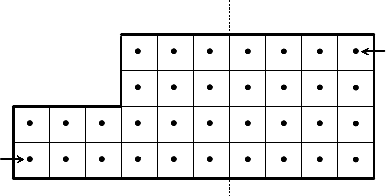
Figure 2.1 gives an example of the type of grid currently supported by the Struct interface.
The interface uses a finite-difference or finite-volume style, and currently supports only scalar PDEs
(i.e., one unknown per gridpoint). There are four basic steps involved in setting up the linear system
to be solved:
1. set up the grid,
2. set up the stencil,
3. set up the matrix,
4. set up the right-hand-side vector.
(-3,1)
(6,4)
process 0 process 1
Figure 2.1: An example 2D structured grid, distributed accross two processors.
7
8CHAPTER 2. STRUCTURED-GRID SYSTEM INTERFACE (STRUCT)
(-3,2)
(6,11)
(7,3) (15,8)
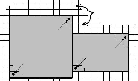
Index Space
Figure 2.2: A box is a collection of abstract cell-centered indices, described by its minimum and
maximum indices. Here, two boxes are illustrated.
To describe each of these steps in more detail, consider solving the 2D Laplacian problem
(∇2u=f, in the domain,
u= 0,on the boundary.(2.1)
Assume (2.1) is discretized using standard 5-pt finite-volumes on the uniform grid pictured in 2.1,
and assume that the problem data is distributed across two processes as depicted.
2.1 Setting Up the Struct Grid
The grid is described via a global index space, i.e., via integer singles in 1D, tuples in 2D, or triples
in 3D (see Figure 2.2). The integers may have any value, negative or positive. The global indexes
allow hypre to discern how data is related spatially, and how it is distributed across the parallel
machine. The basic component of the grid is a box: a collection of abstract cell-centered indices in
index space, described by its “lower” and “upper” corner indices. The scalar grid data is always
associated with cell centers, unlike the more general SStruct interface which allows data to be
associated with box indices in several different ways.
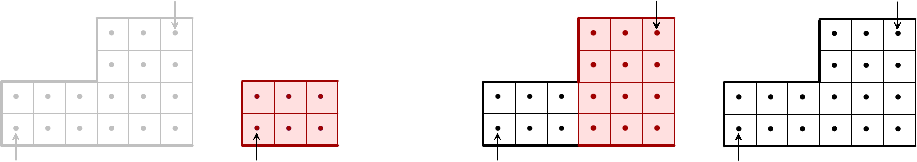
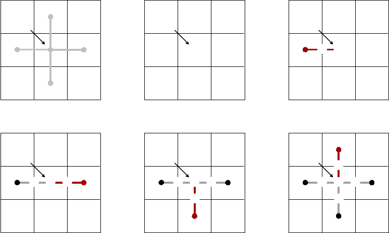
Each process describes that portion of the grid that it “owns”, one box at a time. For example,
the global grid in Figure 2.1 can be described in terms of three boxes, two owned by process 0, and
one owned by process 1. Figure 2.3 shows the code for setting up the grid on process 0 (the code for
process 1 is similar). The “icons” at the top of the figure illustrate the result of the numbered lines
of code. The Create() routine creates an empty 2D grid object that lives on the MPI_COMM_WORLD
communicator. The SetExtents() routine adds a new box to the grid. The Assemble() routine
is a collective call (i.e., must be called on all processes from a common synchronization point), and
finalizes the grid assembly, making the grid “ready to use”.
2.1. SETTING UP THE STRUCT GRID 9
(-3,1)
(2,4)
1
(-3,1)
2
(-3,1)
(2,4)
3
(-3,1)
(2,4)
4
HYPRE_StructGrid grid;
int ndim = 2;
int ilower[][2] = {{-3,1}, {0,1}};
int iupper[][2] = {{-1,2}, {2,4}};
/* Create the grid object */
1: HYPRE_StructGridCreate(MPI_COMM_WORLD, ndim, &grid);
/* Set grid extents for the first box */
2: HYPRE_StructGridSetExtents(grid, ilower[0], iupper[0]);
/* Set grid extents for the second box */
3: HYPRE_StructGridSetExtents(grid, ilower[1], iupper[1]);
/* Assemble the grid */
4: HYPRE_StructGridAssemble(grid);
Figure 2.3: Code on process 0 for setting up the grid in Figure 2.1.
10 CHAPTER 2. STRUCTURED-GRID SYSTEM INTERFACE (STRUCT)
0
1
2
3
4
( 0, 0)
(-1, 0)
( 1, 0)
( 0,-1)
( 0, 1)
stencil entries
offsets
(-1,-1)
(0,0)
0
1
4
2
3
Figure 2.4: Representation of the 5-point discretization stencil for the example problem.
2.2 Setting Up the Struct Stencil
The geometry of the discretization stencil is described by an array of indexes, each representing a
relative offset from any given gridpoint on the grid. For example, the geometry of the 5-pt stencil
for the example problem being considered can be represented by the list of index offsets shown in
Figure 2.4. Here, the (0,0) entry represents the “center” coefficient, and is the 0th stencil entry.
The (0,−1) entry represents the “south” coefficient, and is the 3rd stencil entry. And so on.
On process 0 or 1, the code in Figure 2.5 will set up the stencil in Figure 2.4. The stencil must
be the same on all processes. The Create() routine creates an empty 2D, 5-pt stencil object. The
SetElement() routine defines the geometry of the stencil and assigns the stencil numbers for each
of the stencil entries. None of the calls are collective calls.
2.3 Setting Up the Struct Matrix
The matrix is set up in terms of the grid and stencil objects described in Sections 2.1 and 2.2.
The coefficients associated with each stencil entry will typically vary from gridpoint to gridpoint,
but in the example problem being considered, they are as follows over the entire grid (except at
boundaries; see below):
−1
−1 4 −1
−1
.(2.2)
On process 0, the code in Figure 2.6 will set up matrix values associated with the center (entry
0) and south (entry 3) stencil entries as given by 2.2 and Figure 2.6 (boundaries are ignored here
temporarily). The Create() routine creates an empty matrix object. The Initialize() routine
indicates that the matrix coefficients (or values) are ready to be set. This routine may or may
not involve the allocation of memory for the coefficient data, depending on the implementation.
The optional Set routines mentioned later in this chapter and in the Reference Manual, should
be called before this step. The SetBoxValues() routine sets the matrix coefficients for some set
of stencil entries over the gridpoints in some box. Note that the box need not correspond to any
of the boxes used to create the grid, but values should be set for all gridpoints that this process
2.3. SETTING UP THE STRUCT MATRIX 11
(-1,-1)
(0,0)
1
(-1,-1)
(0,0)
0
2
(-1,-1)
(0,0)
0
1
3
(-1,-1)
(0,0)
0
1 2
4
(-1,-1)
(0,0)
0
1 2
3
5
(-1,-1)
(0,0)
0
1
4
2
3
6
HYPRE_StructStencil stencil;
int ndim = 2;
int size = 5;
int entry;
int offsets[][2] = {{0,0}, {-1,0}, {1,0}, {0,-1}, {0,1}};
/* Create the stencil object */
1: HYPRE_StructStencilCreate(ndim, size, &stencil);
/* Set stencil entries */
for (entry = 0; entry < size; entry++)
{
2-6: HYPRE_StructStencilSetElement(stencil, entry, offsets[entry]);
}
/* Thats it! There is no assemble routine */
Figure 2.5: Code for setting up the stencil in Figure 2.4.
12 CHAPTER 2. STRUCTURED-GRID SYSTEM INTERFACE (STRUCT)
HYPRE_StructMatrix A;
double values[36];
int stencil_indices[2] = {0,3};
int i;
HYPRE_StructMatrixCreate(MPI_COMM_WORLD, grid, stencil, &A);
HYPRE_StructMatrixInitialize(A);
for (i = 0; i < 36; i += 2)
{
values[i] = 4.0;
values[i+1] = -1.0;
}
HYPRE_StructMatrixSetBoxValues(A, ilower[0], iupper[0], 2,
stencil_indices, values);
HYPRE_StructMatrixSetBoxValues(A, ilower[1], iupper[1], 2,
stencil_indices, values);
/* set boundary conditions */
...
HYPRE_StructMatrixAssemble(A);
Figure 2.6: Code for setting up matrix values associated with stencil entries 0 and 3 as given by
2.2 and Figure 2.4.
2.4. SETTING UP THE STRUCT RIGHT-HAND-SIDE VECTOR 13
int ilower[2] = {-3, 1};
int iupper[2] = { 2, 1};
/* create matrix and set interior coefficients */
...
/* implement boundary conditions */
...
for (i = 0; i < 12; i++)
{
values[i] = 0.0;
}
i = 3;
HYPRE_StructMatrixSetBoxValues(A, ilower, iupper, 1, &i, values);
/* complete implementation of boundary conditions */
...
Figure 2.7: Code for adjusting boundary conditions along the lower grid boundary in Figure 2.1.
“owns”. The Assemble() routine is a collective call, and finalizes the matrix assembly, making the
matrix “ready to use”.
Matrix coefficients that reach outside of the boundary should be set to zero. For efficiency
reasons, hypre does not do this automatically. The most natural time to insure this is when the
boundary conditions are being set, and this is most naturally done after the coefficients on the
grid’s interior have been set. For example, during the implementation of the Dirichlet boundary
condition on the lower boundary of the grid in Figure 2.1, the “south” coefficient must be set to
zero. To do this on process 0, the code in Figure 2.7 could be used:
2.4 Setting Up the Struct Right-Hand-Side Vector
The right-hand-side vector is set up similarly to the matrix set up described in Section 2.3 above.
The main difference is that there is no stencil (note that a stencil currently does appear in the
interface, but this will eventually be removed).
On process 0, the code in Figure 2.8 will set up the right-hand-side vector values. The Create()
routine creates an empty vector object. The Initialize() routine indicates that the vector co-
efficients (or values) are ready to be set. This routine follows the same rules as its corresponding
Matrix routine. The SetBoxValues() routine sets the vector coefficients over the gridpoints in
some box, and again, follows the same rules as its corresponding Matrix routine. The Assemble()
14 CHAPTER 2. STRUCTURED-GRID SYSTEM INTERFACE (STRUCT)
HYPRE_StructVector b;
double values[18];
int i;
HYPRE_StructVectorCreate(MPI_COMM_WORLD, grid, &b);
HYPRE_StructVectorInitialize(b);
for (i = 0; i < 18; i++)
{
values[i] = 0.0;
}
HYPRE_StructVectorSetBoxValues(b, ilower[0], iupper[0], values);
HYPRE_StructVectorSetBoxValues(b, ilower[1], iupper[1], values);
HYPRE_StructVectorAssemble(b);
Figure 2.8: Code for setting up right-hand-side vector values.
routine is a collective call, and finalizes the vector assembly, making the vector “ready to use”.
2.5 Symmetric Matrices
Some solvers and matrix storage schemes provide capabilities for significantly reducing memory
usage when the coefficient matrix is symmetric. In this situation, each off-diagonal coefficient
appears twice in the matrix, but only one copy needs to be stored. The Struct interface provides
support for matrix and solver implementations that use symmetric storage via the SetSymmetric()
routine.
To describe this in more detail, consider again the 5-pt finite-volume discretization of (2.1) on
the grid pictured in Figure 2.1. Because the discretization is symmetric, only half of the off-diagonal
coefficients need to be stored. To turn symmetric storage on, the following line of code needs to be
inserted somewhere between the Create() and Initialize() calls.
HYPRE_StructMatrixSetSymmetric(A, 1);
The coefficients for the entire stencil can be passed in as before. Note that symmetric storage may
or may not actually be used, depending on the underlying storage scheme. Currently in hypre, the
Struct interface always uses symmetric storage.
To most efficiently utilize the Struct interface for symmetric matrices, notice that only half of
the off-diagonal coefficients need to be set. To do this for the example being considered, we simply
2.5. SYMMETRIC MATRICES 15
need to redefine the 5-pt stencil of Section 2.2 to an “appropriate” 3-pt stencil, then set matrix
coefficients (as in Section 2.3) for these three stencil elements only. For example, we could use the
following stencil
(0,1)
(0,0) (1,0)
.(2.3)
This 3-pt stencil provides enough information to recover the full 5-pt stencil geometry and associated
matrix coefficients.
16 CHAPTER 2. STRUCTURED-GRID SYSTEM INTERFACE (STRUCT)
Chapter 3
Semi-Structured-Grid System
Interface (SStruct)
The SStruct interface is appropriate for applications with grids that are mostly—but not entirely—
structured, e.g. block-structured grids (see Figure 3.2), composite grids in structured adaptive
mesh refinement (AMR) applications (see Figure 3.9), and overset grids. In addition, it supports
more general PDEs than the Struct interface by allowing multiple variables (system PDEs) and
multiple variable types (e.g. cell-centered, face-centered, etc.). The interface provides access to
data structures and linear solvers in hypre that are designed for semi-structured grid problems, but
also to the most general data structures and solvers.
The SStruct grid is composed out of a number of structured grid parts, where the physical inter-
relationship between the parts is arbitrary. Each part is constructed out of two basic components:
boxes (see Figure 2.2) and variables. Variables represent the actual unknown quantities in the
grid, and are associated with the box indices in a variety of ways, depending on their types. In
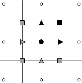
hypre, variables may be cell-centered, node-centered, face-centered, or edge-centered. Face-centered
variables are split into x-face, y-face, and z-face, and edge-centered variables are split into x-edge,
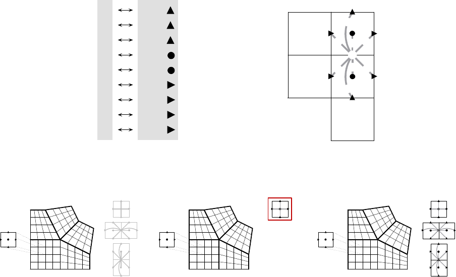
y-edge, and z-edge. See Figure 3.1 for an illustration in 2D.
The SStruct interface uses a graph to allow nearly arbitrary relationships between part data.
The graph is constructed from stencils or finite element stiffness matrices plus some additional data-
coupling information set by the GraphAddEntries() routine. Two other methods for relating part
data are the GridSetNeighborPart() and GridSetSharedPart() routines, which are particularly
well suited for block-structured grid problems. The latter is useful for finite element codes.
There are five basic steps involved in setting up the linear system to be solved:
1. set up the grid,
2. set up the stencils (if needed),
3. set up the graph,
4. set up the matrix,
5. set up the right-hand-side vector.
17
18 CHAPTER 3. SEMI-STRUCTURED-GRID SYSTEM INTERFACE (SSTRUCT)
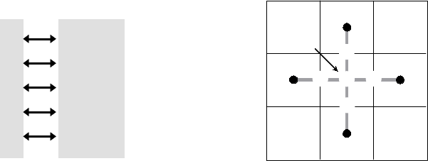
(i,j)
Figure 3.1: Grid variables in hypre are referenced by the abstract cell-centered index to the left
and down in 2D (analogously in 3D). In the figure, index (i, j) is used to reference the variables in
black. The variables in grey—although contained in the pictured cell—are not referenced by the
(i, j) index.
3.1 Block-Structured Grids with Stencils
In this section, we describe how to use the SStruct interface to define block-structured grid prob-
lems. We do this primarily by example, paying particular attention to the construction of stencils
and the use of the GridSetNeighborPart() interface routine.
Consider the solution of the diffusion equation
−∇ · (D∇u) + σu =f(3.1)
on the block-structured grid in Figure 3.2, where Dis a scalar diffusion coefficient, and σ≥0.
The discretization [29] introduces three different types of variables: cell-centered, x-face, and y-
face. The three discretization stencils that couple these variables are also given in the figure. The
information in this figure is essentially all that is needed to describe the nonzero structure of the
linear system we wish to solve.
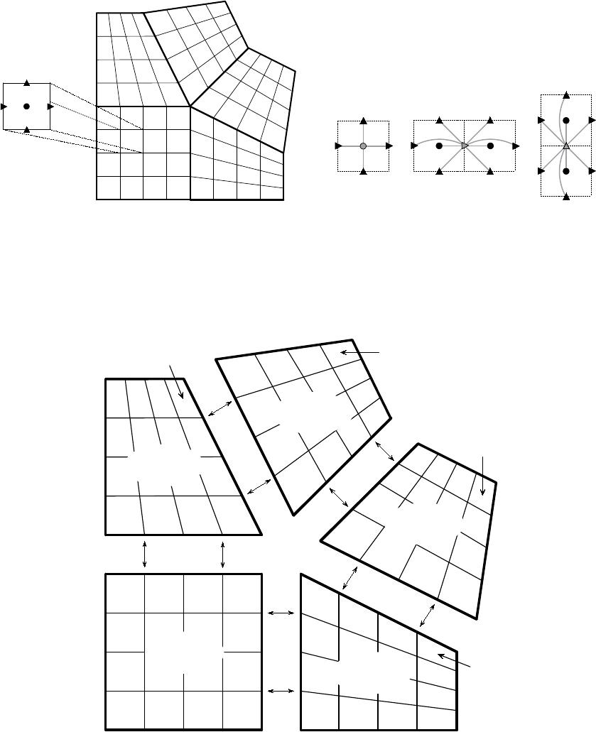
The grid in Figure 3.2 is defined in terms of five separate logically-rectangular parts as shown in
Figure 3.3, and each part is given a unique label between 0 and 4. Each part consists of a single box
with lower index (1,1) and upper index (4,4) (see Section 2.1), and the grid data is distributed on
five processes such that data associated with part plives on process p. Note that in general, parts
may be composed out of arbitrary unions of boxes, and indices may consist of non-positive integers
(see Figure 2.2). Also note that the SStruct interface expects a domain-based data distribution
by boxes, but the actual distribution is determined by the user and simply described (in parallel)
through the interface.
As with the Struct interface, each process describes that portion of the grid that it “owns”,
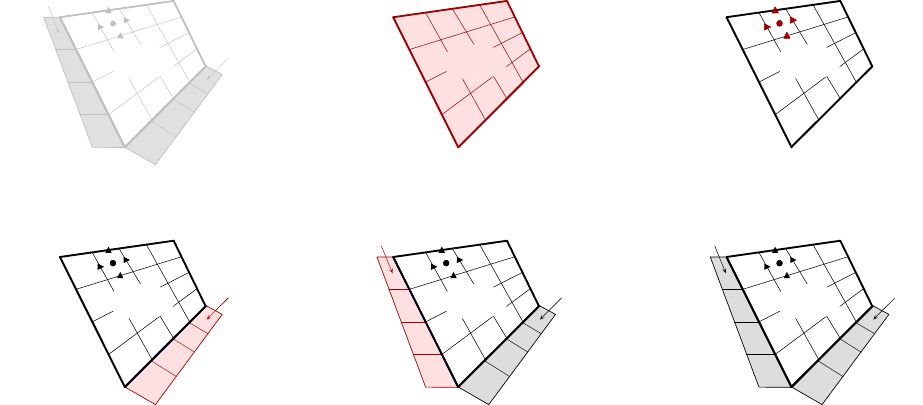
one box at a time. Figure 3.4 shows the code for setting up the grid on process 3 (the code for the
other processes is similar). The “icons” at the top of the figure illustrate the result of the numbered
lines of code. Process 3 needs to describe the data pictured in the bottom-right of the figure. That
is, it needs to describe part 3 plus some additional neighbor information that ties part 3 together
3.1. BLOCK-STRUCTURED GRIDS WITH STENCILS 19
Figure 3.2: Example of a block-structured grid with five logically-rectangular blocks and three
variables types: cell-centered, x-face, and y-face. Discretization stencils for the cell-centered (left),
x-face (middle), and y-face (right) variables are also pictured.
(1,1) (1,1)
(1,1)
(1,1)
(1,1)
(4,4)
(4,4)
(4,4)
(4,4)
part 0
part 1
part 2
part 3
part 4
(4,4)
Figure 3.3: One possible labeling of the grid in Figure 3.2.
20 CHAPTER 3. SEMI-STRUCTURED-GRID SYSTEM INTERFACE (SSTRUCT)
(1,1)
(1,4)
(4,1)
(4,4)
(1,1)
(4,4)
part 2
part 3
part 4
1
(1,1)
(4,4)
part 3
(1,1)
(4,4)
part 3
2
(1,1)
(4,4)
part 3
(1,1)
(4,4)
part 3
3
(1,1)
(1,4)
(1,1)
(4,4)
part 2
part 3
(1,1)
(1,4)
(1,1)
(4,4)
part 2
part 3
4
(1,1)
(1,4)
(4,1)
(4,4)
(1,1)
(4,4)
part 2
part 3
part 4
(1,1)
(1,4)
(4,1)
(4,4)
(1,1)
(4,4)
part 2
part 3
part 4
5
(1,1)
(1,4)
(4,1)
(4,4)
(1,1)
(4,4)
part 2
part 3
part 4
(1,1)
(1,4)
(4,1)
(4,4)
(1,1)
(4,4)
part 2
part 3
part 4
6
HYPRE_SStructGrid grid;
int ndim = 2, nparts = 5, nvars = 3, part = 3;
int extents[][2] = {{1,1}, {4,4}};
int vartypes[] = {HYPRE_SSTRUCT_VARIABLE_CELL,
HYPRE_SSTRUCT_VARIABLE_XFACE,
HYPRE_SSTRUCT_VARIABLE_YFACE};
int nb2_n_part = 2, nb4_n_part = 4;
int nb2_exts[][2] = {{1,0}, {4,0}}, nb4_exts[][2] = {{0,1}, {0,4}};
int nb2_n_exts[][2] = {{1,1}, {1,4}}, nb4_n_exts[][2] = {{4,1}, {4,4}};
int nb2_map[2] = {1,0}, nb4_map[2] = {0,1};
int nb2_dir[2] = {1,-1}, nb4_dir[2] = {1,1};
1: HYPRE_SStructGridCreate(MPI_COMM_WORLD, ndim, nparts, &grid);
/* Set grid extents and grid variables for part 3 */
2: HYPRE_SStructGridSetExtents(grid, part, extents[0], extents[1]);
3: HYPRE_SStructGridSetVariables(grid, part, nvars, vartypes);
/* Set spatial relationship between parts 3 and 2, then parts 3 and 4 */
4: HYPRE_SStructGridSetNeighborPart(grid, part, nb2_exts[0], nb2_exts[1],
nb2_n_part, nb2_n_exts[0], nb2_n_exts[1], nb2_map, nb2_dir);
5: HYPRE_SStructGridSetNeighborPart(grid, part, nb4_exts[0], nb4_exts[1],
nb4_n_part, nb4_n_exts[0], nb4_n_exts[1], nb4_map, nb4_dir);
6: HYPRE_SStructGridAssemble(grid);
Figure 3.4: Code on process 3 for setting up the grid in Figure 3.2.
3.1. BLOCK-STRUCTURED GRIDS WITH STENCILS 21
with the rest of the grid. The Create() routine creates an empty 2D grid object with five parts
that lives on the MPI_COMM_WORLD communicator. The SetExtents() routine adds a new box to
the grid. The SetVariables() routine associates three variables of type cell-centered, x-face, and
y-face with part 3.
At this stage, the description of the data on part 3 is complete. However, the spatial relationship
between this data and the data on neighboring parts is not yet defined. To do this, we need to relate
the index space for part 3 with the index spaces of parts 2 and 4. More specifically, we need to
tell the interface that the two grey boxes neighboring part 3 in the bottom-right of Figure 3.4 also
correspond to boxes on parts 2 and 4. This is done through the two calls to the SetNeighborPart()
routine. We discuss only the first call, which describes the grey box on the right of the figure. Note
that this grey box lives outside of the box extents for the grid on part 3, but it can still be
described using the index-space for part 3 (recall Figure 2.2). That is, the grey box has extents
(1,0) and (4,0) on part 3’s index-space, which is outside of part 3’s grid. The arguments for the
SetNeighborPart() call are simply the lower and upper indices on part 3 and the corresponding
indices on part 2. The final two arguments to the routine indicate that the positive x-direction on
part 3 (i.e., the icomponent of the tuple (i, j)) corresponds to the positive y-direction on part 2
and that the positive y-direction on part 3 corresponds to the positive x-direction on part 2.
The Assemble() routine is a collective call (i.e., must be called on all processes from a common
synchronization point), and finalizes the grid assembly, making the grid “ready to use”.
With the neighbor information, it is now possible to determine where off-part stencil entries
couple. Take, for example, any shared part boundary such as the boundary between parts 2 and 3.
Along these boundaries, some stencil entries reach outside of the part. If no neighbor information
is given, these entries are effectively zeroed out, i.e., they don’t participate in the discretization.
However, with the additional neighbor information, when a stencil entry reaches into a neighbor
box it is then coupled to the part described by that neighbor box information.
Another important consequence of the use of the SetNeighborPart() routine is that it can de-
clare variables on different parts as being the same. For example, the face variables on the boundary
of parts 2 and 3 are recognized as being shared by both parts (prior to the SetNeighborPart()
call, there were two distinct sets of variables). Note also that these variables are of different types
on the two parts; on part 2 they are x-face variables, but on part 3 they are y-face variables.
For brevity, we consider only the description of the y-face stencil in Figure 3.2, i.e. the third
stencil in the figure. To do this, the stencil entries are assigned unique labels between 0 and 8 and
their “offsets” are described relative to the “center” of the stencil. This process is illustrated in
Figure 3.5. Nine calls are made to the routine HYPRE_SStructStencilSetEntry(). As an example,
the call that describes stencil entry 5 in the figure is given the entry number 5, the offset (−1,0),
and the identifier for the x-face variable (the variable to which this entry couples). Recall from
Figure 3.1 the convention used for referencing variables of different types. The geometry description
uses the same convention, but with indices numbered relative to the referencing index (0,0) for the
stencil’s center. Figure 3.6 shows the code for setting up the graph .
With the above, we now have a complete description of the nonzero structure for the matrix. The
matrix coefficients are then easily set in a manner similar to what is described in Section 2.3 using
routines MatrixSetValues() and MatrixSetBoxValues() in the SStruct interface. As before,
22 CHAPTER 3. SEMI-STRUCTURED-GRID SYSTEM INTERFACE (SSTRUCT)
0
1
2
3
4
5
6
7
8
(0,0);
(0,-1);
(0,1);
(0,0);
(0,1);
(-1,0);
(0,0);
(-1,1);
(0,1);
stencil entries
offsets
(-1,1)
(-1,0)
(0,-1)
0
1
2
3
4
5 6
7 8
Figure 3.5: Assignment of labels and geometries to the y-face stencil in Figure 3.2.
1 2 3
HYPRE_SStructGraph graph;
HYPRE_SStructStencil c_stencil, x_stencil, y_stencil;
int c_var = 0, x_var = 1, y_var = 2;
int part;
1: HYPRE_SStructGraphCreate(MPI_COMM_WORLD, grid, &graph);
/* Set the cell-centered, x-face, and y-face stencils for each part */
for (part = 0; part < 5; part++)
{
2: HYPRE_SStructGraphSetStencil(graph, part, c_var, c_stencil);
HYPRE_SStructGraphSetStencil(graph, part, x_var, x_stencil);
HYPRE_SStructGraphSetStencil(graph, part, y_var, y_stencil);
}
3: HYPRE_SStructGraphAssemble(graph);
Figure 3.6: Code on process 3 for setting up the graph for Figure 3.2.
3.2. BLOCK-STRUCTURED GRIDS WITH FINITE ELEMENTS 23
there are also AddTo variants of these routines. Likewise, setting up the right-hand-side is similar
to what is described in Section 2.4. See the hypre reference manual for details.
An alternative approach for describing the above problem through the interface is to use the
GraphAddEntries() routine instead of the GridSetNeighborPart() routine. In this approach,
the five parts would be explicitly “sewn” together by adding non-stencil couplings to the matrix
graph. The main downside to this approach for block-structured grid problems is that variables
along block boundaries are no longer considered to be the same variables on the corresponding
parts that share these boundaries. For example, any face variable along the boundary between
parts 2 and 3 in Figure 3.2 would represent two different variables that live on different parts.
To “sew” the parts together correctly, we would need to explicitly select one of these variables as
the representative that participates in the discretization, and make the other variable a dummy
variable that is decoupled from the discretization by zeroing out appropriate entries in the matrix.
All of these complications are avoided by using the GridSetNeighborPart() for this example.
3.2 Block-Structured Grids with Finite Elements
In this section, we describe how to use the SStruct interface to define block-structured grid prob-
lems with finite elements. We again do this by example, paying particular attention to the use of
the FEM interface routines and the GridSetSharedPart() routine. See example code ex14.c for a
complete implementation.
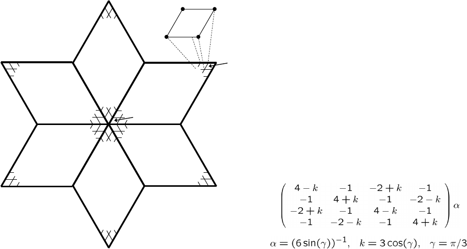
Consider a nodal finite element (FEM) discretization of the Laplace equation on the star-shaped
grid in Figure 3.7. The local FEM stiffness matrix in the figure describes the coupling between the
grid variables. Although we could still describe this problem using stencils as in Section 3.1, an
FEM-based approach (available in hypre version 2.6.0b and later) is a more natural alternative.
The grid in Figure 3.7 is defined in terms of six separate logically-rectangular parts, and each
part is given a unique label between 0 and 5. Each part consists of a single box with lower index
(1,1) and upper index (9,9), and the grid data is distributed on six processes such that data
associated with part plives on process p.
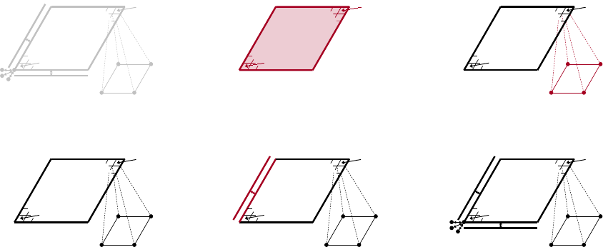
As in Section 3.1, each process describes that portion of the grid that it “owns”, one box at
a time. Figure 3.8 shows the code for setting up the grid on process 0 (the code for the other
processes is similar). The “icons” at the top of the figure illustrate the result of the numbered lines
of code. Process 0 needs to describe the data pictured in the bottom-right of the figure. That is,
it needs to describe part 0 plus some additional information about shared data with other parts
on the grid. The SetFEMOrdering() routine sets the ordering of the unknowns in an element (an
element is always a grid cell in hypre). This determines the ordering of the data passed into the
routines MatrixAddFEMValues() and VectorAddFEMValues() discussed later.
At this point, the layout of the data on part 0 is complete, but there is no relationship to the rest
of the grid. To couple the parts, we need to tell hypre that some of the boundary variables on part 0
are shared with other parts, i.e., they are the same as some of the variables on other parts. This is
done through five calls to the SetSharedPart() routine. Only the first call is shown in the figure;
the other four calls are similar. The arguments to this routine are the same as SetNeighborPart()
with the addition of two new offset arguments, named offset and s_offset in the figure. Each
24 CHAPTER 3. SEMI-STRUCTURED-GRID SYSTEM INTERFACE (SSTRUCT)
part 0
part 1
part 2
part 3
part 4
part 5
(9,9)
(1,1)
01
2
3
0 1 2 3
0
1
2
3
Figure 3.7: Example of a star-shaped grid with six logically-rectangular blocks and one nodal
variable. Each block has an angle at the origin given by γ=π/3. The finite element stiffness
matrix (right) is given in terms of the pictured variable ordering (left).
offset represents a pointer from the cell center to one of the following: all variables in the cell (no
nonzeros in offset); all variables on a face (only 1 nonzero); all variables on an edge (2 nonzeros);
all variables at a point (3 nonzeros). The two offsets must be consistent with each other.
The graph is set up similarly to Figure 3.6, except that the stencil calls are replaced by calls to
GraphSetFEM(). The nonzero pattern of the stiffness matrix can also be set by calling the optional
routine GraphSetFEMSparsity().
Matrix and vector values are set one element at a time. For the example in this section, calls
on part 0 would have the following form:
int part = 0;
int index[2] = {i,j};
double m_values[16] = {...};
double v_values[4] = {...};
HYPRE_SStructMatrixAddFEMValues(A, part, index, m_values);
HYPRE_SStructVectorAddFEMValues(v, part, index, v_values);
Here, m_values contains local stiffness matrix values and v_values contains local variable values.
The global matrix and vector are assembled internally by hypre, using the shared variables to
couple the parts.
3.2. BLOCK-STRUCTURED GRIDS WITH FINITE ELEMENTS 25
part 1
part 2
part 3
part 4part 5
part 0
(9,9)
(1,1)
01
2
3
1
part 0
(9,9)
(1,1)
2
part 0
(9,9)
(1,1)
3
part 0
(9,9)
(1,1)
01
2
3
4
part 1part 0
(9,9)
(1,1)
01
2
3
5
part 1
part 2
part 3
part 4part 5
part 0
(9,9)
(1,1)
01
2
3
6
HYPRE_SStructGrid grid;
int ndim = 2, nparts = 6, nvars = 1, part = 0;
int ilower[2] = {1,1}, iupper[2] = {9,9};
int vartypes[] = {HYPRE_SSTRUCT_VARIABLE_NODE};
int ordering[12] = {0,-1,-1, 0,+1,-1, 0,+1,+1, 0,-1,+1};
int s_part = 2;
int ilo[2] = {1,1}, iup[2] = {1,9}, offset[2] = {-1,0};
int s_ilo[2] = {1,1}, s_iup[2] = {9,1}, s_offset[2] = {0,-1};
int map[2] = {1,0};
int dir[2] = {-1,1};
1: HYPRE_SStructGridCreate(MPI_COMM_WORLD, ndim, nparts, &grid);
/* Set grid extents, grid variables, and FEM ordering for part 0 */
2: HYPRE_SStructGridSetExtents(grid, part, ilower, iupper);
3: HYPRE_SStructGridSetVariables(grid, part, nvars, vartypes);
4: HYPRE_SStructGridSetFEMOrdering(grid, part, ordering);
/* Set shared variables for parts 0 and 1 (0 and 2/3/4/5 not shown) */
5: HYPRE_SStructGridSetSharedPart(grid, part, ilo, iup, offset,
s_part, s_ilo, s_iup, s_offset, map, dir);
6: HYPRE_SStructGridAssemble(grid);
Figure 3.8: Code on process 0 for setting up the grid in Figure 3.7.
26 CHAPTER 3. SEMI-STRUCTURED-GRID SYSTEM INTERFACE (SSTRUCT)
(4,4)
(1,1)
(2,4)
(3,1)
(9,9)
(6,6)
(7,9)
(8,6)
part 0
part 1
Figure 3.9: Structured AMR grid example. Shaded regions correspond to process 0, unshaded to
process 1. The grey dots are dummy variables.
3.3 Structured Adaptive Mesh Refinement
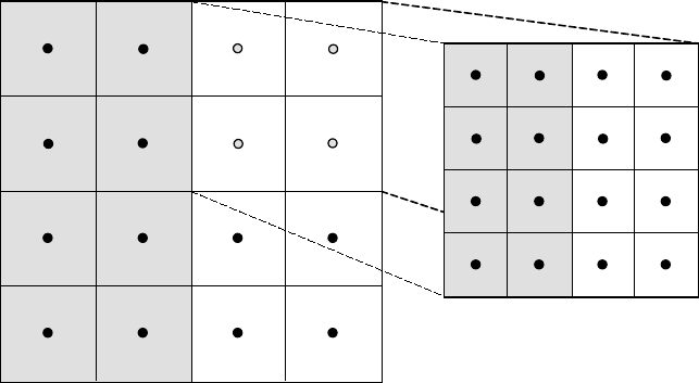
We now briefly discuss how to use the SStruct interface in a structured AMR application. Consider
Poisson’s equation on the simple cell-centered example grid illustrated in Figure 3.9. For structured
AMR applications, each refinement level should be defined as a unique part. There are two parts
in this example: part 0 is the global coarse grid and part 1 is the single refinement patch. Note
that the coarse unknowns underneath the refinement patch (gray dots in Figure 3.9) are not real
physical unknowns; the solution in this region is given by the values on the refinement patch. In
setting up the composite grid matrix [28] for hypre the equations for these “dummy” unknowns
should be uncoupled from the other unknowns (this can easily be done by setting all off-diagonal
couplings to zero in this region).
In the example, parts are distributed across the same two processes with process 0 having
the “left” half of both parts. The composite grid is then set up part-by-part by making calls to
GridSetExtents() just as was done in Section 3.1 and Figure 3.4 (no SetNeighborPart calls are
made in this example). Note that in the interface there is no required rule relating the indexing on
the refinement patch to that on the global coarse grid; they are separate parts and thus each has
its own index space. In this example, we have chosen the indexing such that refinement cell (2i, 2j)
lies in the lower left quadrant of coarse cell (i, j). Then the stencil is set up. In this example we
are using a finite volume approach resulting in the standard 5-point stencil in Figure 2.5 in both
parts.
The grid and stencil are used to define all intra-part coupling in the graph, the non-zero pattern
of the composite grid matrix. The inter-part coupling at the coarse-fine interface is described by
GraphAddEntries() calls. This coupling in the composite grid matrix is typically the composition
3.3. STRUCTURED ADAPTIVE MESH REFINEMENT 27
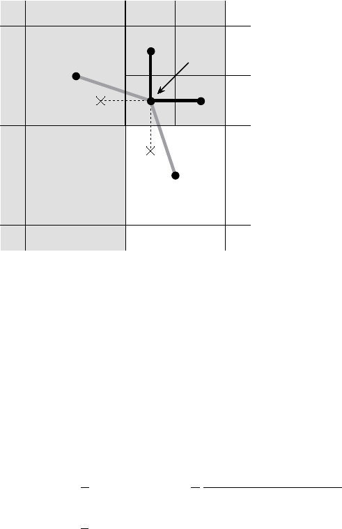
(3,2)
(2,3) (6,6)
Figure 3.10: Coupling for equation at corner of refinement patch. Black lines (solid and broken)
are stencil couplings. Gray line are non-stencil couplings.
of an interpolation rule and a discretization formula. In this example, we use a simple piecewise
constant interpolation, i.e. the solution value in a coarse cell is equal to the solution value at the cell
center. Then the flux across a portion of the coarse-fine interface is approximated by a difference
of the solution values on each side. As an example, consider approximating the flux across the
left interface of cell (6,6) in Figure 3.10. Let hbe the coarse grid mesh size, and consider a local
coordinate system with the origin at the center of cell (6,6). We approximate the flux as follows
Zh/4
−h/4
ux(−h/4, s)ds ≈h
2ux(−h/4,0) ≈h
2
u(0,0) −u(−3h/4,0)
3h/4(3.2)
≈2
3(u6,6−u2,3).
The first approximation uses the midpoint rule for the edge integral, the second uses a finite
difference formula for the derivative, and the third the piecewise constant interpolation to the
solution in the coarse cell. This means that the equation for the variable at cell (6,6) involves
not only the stencil couplings to (6,7) and (7,6) on part 1 but also non-stencil couplings to (2,3)
and (3,2) on part 0. These non-stencil couplings are described by GraphAddEntries() calls. The
syntax for this call is simply the part and index for both the variable whose equation is being defined
and the variable to which it couples. After these calls, the non-zero pattern of the matrix (and the
graph) is complete. Note that the “west” and “south” stencil couplings simply “drop off” the part,
and are effectively zeroed out (currently, this is only supported for the HYPRE_PARCSR object type,
and these values must be manually zeroed out for other object types; see MatrixSetObjectType()
in the reference manual).
The remaining step is to define the actual numerical values for the composite grid matrix.
This can be done by either MatrixSetValues() calls to set entries in a single equation, or by
28 CHAPTER 3. SEMI-STRUCTURED-GRID SYSTEM INTERFACE (SSTRUCT)
MatrixSetBoxValues() calls to set entries for a box of equations in a single call. The syntax for
the MatrixSetValues() call is a part and index for the variable whose equation is being set and an
array of entry numbers identifying which entries in that equation are being set. The entry numbers
may correspond to stencil entries or non-stencil entries.
Chapter 4
Finite Element Interface
4.1 Introduction
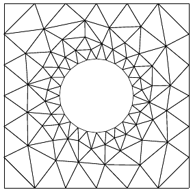
Many application codes use unstructured finite element meshes. This section describes an interface
for finite element problems, called the FEI, which is supported in hypre.
Figure 4.1: Example of an unstructured mesh.
FEI refers to a specific interface for black-box finite element solvers, originally developed in
Sandia National Lab, see [11]. It differs from the rest of the conceptual interfaces in hypre in two
important aspects: it is written in C++, and it does not separate the construction of the linear
system matrix from the solution process. A complete description of Sandia’s FEI implementation
can be obtained by contacting Alan Williams at Sandia (william@sandia.gov). A simplified version
of the FEI has been implemented at LLNL and is included in hypre. More details about this
implementation can be found in the header files of the FEI_mv/fei-base and FEI_mv/fei-hypre
directories.
29

30 CHAPTER 4. FINITE ELEMENT INTERFACE
4.2 A Brief Description of the Finite Element Interface
Typically, finite element codes contain data structures storing element connectivities, element stiff-
ness matrices, element loads, boundary conditions, nodal coordinates, etc. One of the purposes of
the FEI is to assemble the global linear system in parallel based on such local element data. We
illustrate this in the rest of the section and refer to example 10 (in the examples directory) for
more implementation details.
In hypre, one creates an instance of the FEI as follows:
LLNL_FEI_Impl *feiPtr = new LLNL_FEI_Impl(mpiComm);
Here mpiComm is an MPI communicator (e.g. MPI COMM WORLD). If Sandia’s FEI package is to be
used, one needs to define a hypre solver object first:
LinearSystemCore *solver = HYPRE_base_create(mpiComm);
FEI_Implementation *feiPtr = FEI_Implementation(solver,mpiComm,rank);
where rank is the number of the master processor (used only to identify which processor will
produce the screen outputs). The LinearSystemCore class is the part of the FEI which interfaces
with the linear solver library. It will be discussed later in Sections 6.17 and 7.7.
Local finite element information is passed to the FEI using several methods of the feiPtr object.
The first entity to be submitted is the field information. A field has an identifier called fieldID and
a rank or fieldSize (number of degree of freedom). For example, a discretization of the Navier
Stokes equations in 3D can consist of velocity vector having 3 degrees of freedom in every node
(vertex) of the mesh and a scalar pressure variable, which is constant over each element. If these
are the only variables, and if we assign fieldIDs 7 and 8 to them, respectively, then the finite
element field information can be set up by
nFields = 2; /* number of unknown fields */
fieldID = new int[nFields]; /* field identifiers */
fieldSize = new int[nFields]; /* vector dimension of each field */
/* velocity (a 3D vector) */
fieldID[0] = 7;
fieldSize[0] = 3;
/* pressure (a scalar function) */
fieldID[1] = 8;
fieldSize[1] = 1;
feiPtr -> initFields(nFields, fieldSize, fieldID);
Once the field information has been established, we are ready to initialize an element block.
An element block is characterized by the block identifier, the number of elements, the number of
nodes per element, the nodal fields and the element fields (fields that have been defined previously).
Suppose we use 1000 hexahedral elements in the element block 0, the setup consists of
4.2. A BRIEF DESCRIPTION OF THE FINITE ELEMENT INTERFACE 31
elemBlkID = 0; /* identifier for a block of elements */
nElems = 1000; /* number of elements in the block */
elemNNodes = 8; /* number of nodes per element */
/* nodal-based field for the velocity */
nodeNFields = 1;
nodeFieldIDs = new[nodeNFields];
nodeFieldIDs[0] = fieldID[0];
/* element-based field for the pressure */
elemNFields = 1;
elemFieldIDs = new[elemNFields];
elemFieldIDs[0] = fieldID[1];
feiPtr -> initElemBlock(elemBlkID, nElems, elemNNodes, nodeNFields,
nodeFieldIDs, elemNFields, elemFieldIDs, 0);
The last argument above specifies how the dependent variables are arranged in the element matrices.
A value of 0 indicates that each variable is to be arranged in a separate block (as opposed to
interleaving).
In a parallel environment, each processor has one or more element blocks. Unless the element
blocks are all disjoint, some of them share a common set of nodes on the subdomain boundaries. To
facilitate setting up interprocessor communications, shared nodes between subdomains on different
processors are to be identified and sent to the FEI. Hence, each node in the whole domain is assigned
a unique global identifier. The shared node list on each processor contains a subset of the global
node list corresponding to the local nodes that are shared with the other processors. The syntax
for setting up the shared nodes is
feiPtr -> initSharedNodes(nShared, sharedIDs, sharedLengs, sharedProcs);
This completes the initialization phase, and a completion signal is sent to the FEI via
feiPtr -> initComplete();
Next, we begin the load phase. The first entity for loading is the nodal boundary conditions.
Here we need to specify the number of boundary equations and the boundary values given by
alpha, beta, and gamma. Depending on whether the boundary conditions are Dirichlet, Neumann,
or mixed, the three values should be passed into the FEI accordingly.
feiPtr -> loadNodeBCs(nBCs, BCEqn, fieldID, alpha, beta, gamma);
The element stiffness matrices are to be loaded in the next step. We need to specify the element
number i, the element block to which element ibelongs, the element connectivity information, the
element load, and the element matrix format. The element connectivity specifies a set of 8 node
global IDs (for hexahedral elements), and the element load is the load or force for each degree of
freedom. The element format specifies how the equations are arranged (similar to the interleaving
scheme mentioned above). The calling sequence for loading element stiffness matrices is
32 CHAPTER 4. FINITE ELEMENT INTERFACE
for (i = 0; i < nElems; i++)
feiPtr -> sumInElem(elemBlkID, elemID, elemConn[i], elemStiff[i],
elemLoads[i], elemFormat);
To complete the assembling of the global stiffness matrix and the corresponding right hand side, a
signal is sent to the FEI via
feiPtr -> loadComplete();
Chapter 5
Linear-Algebraic System Interface
(IJ)
The IJ interface described in this chapter is the lowest common denominator for specifying linear
systems in hypre. This interface provides access to general sparse-matrix solvers in hypre, not to
the specialized solvers that require more problem information.
5.1 IJ Matrix Interface
As with the other interfaces in hypre, the IJ interface expects to get data in distributed form because
this is the only scalable approach for assembling matrices on thousands of processes. Matrices are
assumed to be distributed by blocks of rows as follows:
A0
A1
.
.
.
AP−1
(5.1)
In the above example, the matrix is distributed accross the Pprocesses, 0,1, ..., P −1 by blocks
of rows. Each submatrix Apis “owned” by a single process and its first and last row numbers are
given by the global indices ilower and iupper in the Create() call below.
The following example code illustrates the basic usage of the IJ interface for building matrices:
MPI_Comm comm;
HYPRE_IJMatrix ij_matrix;
HYPRE_ParCSRMatrix parcsr_matrix;
int ilower, iupper;
int jlower, jupper;
int nrows;
33
34 CHAPTER 5. LINEAR-ALGEBRAIC SYSTEM INTERFACE (IJ)
int *ncols;
int *rows;
int *cols;
double *values;
HYPRE_IJMatrixCreate(comm, ilower, iupper, jlower, jupper, &ij_matrix);
HYPRE_IJMatrixSetObjectType(ij_matrix, HYPRE_PARCSR);
HYPRE_IJMatrixInitialize(ij_matrix);
/* set matrix coefficients */
HYPRE_IJMatrixSetValues(ij_matrix, nrows, ncols, rows, cols, values);
...
/* add-to matrix cofficients, if desired */
HYPRE_IJMatrixAddToValues(ij_matrix, nrows, ncols, rows, cols, values);
...
HYPRE_IJMatrixAssemble(ij_matrix);
HYPRE_IJMatrixGetObject(ij_matrix, (void **) &parcsr_matrix);
The Create() routine creates an empty matrix object that lives on the comm communicator. This
is a collective call (i.e., must be called on all processes from a common synchronization point),
with each process passing its own row extents, ilower and iupper. The row partitioning must be
contiguous, i.e., iupper for process imust equal ilower−1 for process i+1. Note that this allows
matrices to have 0- or 1-based indexing. The parameters jlower and jupper define a column
partitioning, and should match ilower and iupper when solving square linear systems. See the
Reference Manual for more information.
The SetObjectType() routine sets the underlying matrix object type to HYPRE_PARCSR (this
is the only object type currently supported). The Initialize() routine indicates that the matrix
coefficients (or values) are ready to be set. This routine may or may not involve the allocation of
memory for the coefficient data, depending on the implementation. The optional SetRowSizes()
and SetDiagOffdSizes() routines mentioned later in this chapter and in the Reference Manual,
should be called before this step.
The SetValues() routine sets matrix values for some number of rows (nrows) and some number
of columns in each row (ncols). The actual row and column numbers of the matrix values to be
set are given by rows and cols. The coefficients can be modified with the AddToValues() routine.
If AddToValues() is used to add to a value that previously didn’t exist, it will set this value. Note
that while AddToValues() will add to values on other processors, SetValues() does not set values
on other processors. Instead if a user calls SetValues() on processor ito set a matrix coefficient
belonging to processor j, processor iwill erase all previous occurrences of this matrix coefficient,
so they will not contribute to this coefficient on processor j. The actual coefficient has to be set on
processor j.
The Assemble() routine is a collective call, and finalizes the matrix assembly, making the
5.2. IJ VECTOR INTERFACE 35
matrix “ready to use”. The GetObject() routine retrieves the built matrix object so that it can
be passed on to hypre solvers that use the ParCSR internal storage format. Note that this is not
an expensive routine; the matrix already exists in ParCSR storage format, and the routine simply
returns a “handle” or pointer to it. Although we currently only support one underlying data storage
format, in the future several different formats may be supported.
One can preset the row sizes of the matrix in order to reduce the execution time for the
matrix specification. One can specify the total number of coefficients for each row, the number of
coefficients in the row that couple the diagonal unknown to (Diag) unknowns in the same processor
domain, and the number of coefficients in the row that couple the diagonal unknown to (Offd)
unknowns in other processor domains:
HYPRE_IJMatrixSetRowSizes(ij_matrix, sizes);
HYPRE_IJMatrixSetDiagOffdSizes(matrix, diag_sizes, offdiag_sizes);
Once the matrix has been assembled, the sparsity pattern cannot be altered without completely
destroying the matrix object and starting from scratch. However, one can modify the matrix values
of an already assembled matrix. To do this, first call the Initialize() routine to re-initialize the
matrix, then set or add-to values as before, and call the Assemble() routine to re-assemble before
using the matrix. Re-initialization and re-assembly are very cheap, essentially a no-op in the current
implementation of the code.
5.2 IJ Vector Interface
The following example code illustrates the basic usage of the IJ interface for building vectors:
MPI_Comm comm;
HYPRE_IJVector ij_vector;
HYPRE_ParVector par_vector;
int jlower, jupper;
int nvalues;
int *indices;
double *values;
HYPRE_IJVectorCreate(comm, jlower, jupper, &ij_vector);
HYPRE_IJVectorSetObjectType(ij_vector, HYPRE_PARCSR);
HYPRE_IJVectorInitialize(ij_vector);
/* set vector values */
HYPRE_IJVectorSetValues(ij_vector, nvalues, indices, values);
...
36 CHAPTER 5. LINEAR-ALGEBRAIC SYSTEM INTERFACE (IJ)
HYPRE_IJVectorAssemble(ij_vector);
HYPRE_IJVectorGetObject(ij_vector, (void **) &par_vector);
The Create() routine creates an empty vector object that lives on the comm communicator. This is
a collective call, with each process passing its own index extents, jlower and jupper. The names
of these extent parameters begin with a jbecause we typically think of matrix-vector multiplies
as the fundamental operation involving both matrices and vectors. For matrix-vector multiplies,
the vector partitioning should match the column partitioning of the matrix (which also uses the j
notation). For linear system solves, these extents will typically match the row partitioning of the
matrix as well.
The SetObjectType() routine sets the underlying vector storage type to HYPRE_PARCSR (this
is the only storage type currently supported). The Initialize() routine indicates that the vector
coefficients (or values) are ready to be set. This routine may or may not involve the allocation of
memory for the coefficient data, depending on the implementation.
The SetValues() routine sets the vector values for some number (nvalues) of indices. The
values can be modified with the AddToValues() routine. Note that while AddToValues() will add
to values on other processors, SetValues() does not set values on other processors. Instead if
a user calls SetValues() on processor ito set a value belonging to processor j, processor iwill
erase all previous occurrences of this matrix coefficient, so they will not contribute to this value on
processor j. The actual value has to be set on processor j.
The Assemble() routine is a trivial collective call, and finalizes the vector assembly, making
the vector “ready to use”. The GetObject() routine retrieves the built vector object so that it can
be passed on to hypre solvers that use the ParVector internal storage format.
Vector values can be modified in much the same way as with matrices by first re-initializing the
vector with the Initialize() routine.
5.3 A Scalable Interface
As explained in the previous sections, problem data is passed to the hypre library in its distributed
form. However, as is typically the case for a parallel software library, some information regarding
the global distribution of the data will be needed for hypre to perform its function. In particular,
a solver algorithm requires that a processor obtain “nearby” data from other processors in order
to complete the solve. While a processor may easily determine what data it needs from other
processors, it may not know which processor owns the data it needs. Therefore, processors must
determine their communication partners, or neighbors.
The straightforward approach to determining neighbors involves constructing a global partition
of the data. This approach, however, requires O(P) storage and computations and is not scalable
for machines with tens of thousands of processors. The assumed partition algorithm was developed
to address this problem [4]. It is used by default in hypre and is recommended in general. For
modest numbers of processors (less than a hundred or so), a global partition may produce slightly
faster results and can be turned on by compiling the library as detailed in Section 7.2.1.
Chapter 6
Solvers and Preconditioners
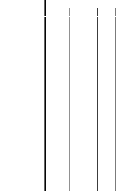
There are several solvers available in hypre via different conceptual interfaces (see Table 6.1). Note
that there are a few additional solvers and preconditioners not mentioned in the table that can be
used only through the FEI interface and are described in Paragraph 6.14. The procedure for setup
and use of solvers and preconditioners is largely the same. We will refer to them both as solvers
in the sequel except when noted. In normal usage, the preconditioner is chosen and constructed
before the solver, and then handed to the solver as part of the solver’s setup. In the following, we
assume the most common usage pattern in which a single linear system is set up and then solved
with a single righthand side. We comment later on considerations for other usage patterns.
Setup:
1. Pass to the solver the information defining the problem. In the typical user cycle, the
user has passed this information into a matrix through one of the conceptual interfaces prior
to setting up the solver. In this situation, the problem definition information is then passed
to the solver by passing the constructed matrix into the solver. As described before, the
matrix and solver must be compatible, in that the matrix must provide the services needed
by the solver. Krylov solvers, for example, need only a matrix-vector multiplication. Most
preconditioners, on the other hand, have additional requirements such as access to the matrix
coefficients.
2. Create the solver/preconditioner via the Create() routine.
3. Choose parameters for the preconditioner and/or solver. Parameters are chosen
through the Set() calls provided by the solver. Throughout hypre, we have made our best
effort to give all parameters reasonable defaults if not chosen. However, for some precondi-
tioners/solvers the best choices for parameters depend on the problem to be solved. We give
recommendations in the individual sections on how to choose these parameters. Note that in
hypre, convergence criteria can be chosen after the preconditioner/solver has been setup. For
a complete set of all available parameters see the Reference Manual.
37
38 CHAPTER 6. SOLVERS AND PRECONDITIONERS
System Interfaces
Solvers Struct SStruct FEI IJ
Jacobi X X
SMG X X
PFMG X X
Split X
SysPFMG X
FAC X
Maxwell X
BoomerAMG X X X
AMS X X X
ADS X X X
MLI X X X
MGR X
ParaSails X X X
Euclid X X X
PILUT X X X
PCG X X X X
GMRES X X X X
FlexGMRES X X X X
LGMRES X X X
BiCGSTAB X X X X
Hybrid X X X X
LOBPCG X X X
Table 6.1: Current solver availability via hypre conceptual interfaces.
4. Pass the preconditioner to the solver. For solvers that are not preconditioned, this step
is omitted. The preconditioner is passed through the SetPrecond() call.
5. Set up the solver. This is just the Setup() routine. At this point the matrix and right
hand side is passed into the solver or preconditioner. Note that the actual right hand side is
not used until the actual solve is performed.
At this point, the solver/preconditioner is fully constructed and ready for use.
Use:
1. Set convergence criteria. Convergence can be controlled by the number of iterations,
as well as various tolerances such as relative residual, preconditioned residual, etc. Like all
parameters, reasonable defaults are used. Users are free to change these, though care must be
taken. For example, if an iterative method is used as a preconditioner for a Krylov method,
a constant number of iterations is usually required.
6.1. SMG 39
2. Solve the system. This is just the Solve() routine.
Finalize:
1. Free the solver or preconditioner. This is done using the Destroy() routine.
Synopsis
In general, a solver (let’s call it SOLVER) is set up and run using the following routines, where A is
the matrix, b the right hand side and x the solution vector of the linear system to be solved:
/* Create Solver */
int HYPRE_SOLVERCreate(MPI_COMM_WORLD, &solver);
/* set certain parameters if desired */
HYPRE_SOLVERSetTol(solver, 1.e-8);
.
.
/* Set up Solver */
HYPRE_SOLVERSetup(solver, A, b, x);
/* Solve the system */
HYPRE_SOLVERSolve(solver, A, b, x);
/* Destroy the solver */
HYPRE_SOLVERDestroy(solver);
In the following sections, we will give brief descriptions of the available hypre solvers with some
suggestions on how to choose the parameters as well as references for users who are interested in
a more detailed description and analysis of the solvers. A complete list of all routines that are
available can be found in the reference manual.
6.1 SMG
SMG is a parallel semicoarsening multigrid solver for the linear systems arising from finite difference,
finite volume, or finite element discretizations of the diffusion equation,
∇ · (D∇u) + σu =f(6.1)
on logically rectangular grids. The code solves both 2D and 3D problems with discretization stencils
of up to 9-point in 2D and up to 27-point in 3D. See [31, 6, 12] for details on the algorithm and its
parallel implementation/performance.
SMG is a particularly robust method. The algorithm semicoarsens in the z-direction and uses
plane smoothing. The xy plane-solves are effected by one V-cycle of the 2D SMG algorithm, which
semicoarsens in the y-direction and uses line smoothing.
40 CHAPTER 6. SOLVERS AND PRECONDITIONERS
6.2 PFMG
PFMG is a parallel semicoarsening multigrid solver similar to SMG. See [1, 12] for details on the
algorithm and its parallel implementation/performance.
The main difference between the two methods is in the smoother: PFMG uses simple pointwise
smoothing. As a result, PFMG is not as robust as SMG, but is much more efficient per V-cycle.
6.3 SysPFMG
SysPFMG is a parallel semicoarsening multigrid solver for systems of elliptic PDEs. It is a gener-
alization of PFMG, with the interpolation defined only within the same variable. The relaxation is
of nodal type- all variables at a given point location are simultaneously solved for in the relaxation.
Although SysPFMG is implemented through the SStruct interface, it can be used only for
problems with one grid part. Ideally, the solver should handle any of the seven variable types (cell-,
node-, xface-, yface-, zface-, xedge-, yedge-, and zedge-based). However, it has been completed only
for cell-based variables.
6.4 SplitSolve
SplitSolve is a parallel block Gauss-Seidel solver for semi-structured problems with multiple parts.
For problems with only one variable, it can be viewed as a domain-decomposition solver with no
grid overlapping.
Consider a multiple part problem given by the linear system Ax =b. Matrix Acan be decom-
posed into a structured intra-variable block diagonal component Mand a component Nconsisting
of the inter-variable blocks and any unstructured connections between the parts. SplitSolve per-
forms the iteration
xk+1 =˜
M−1(b+Nxk),
where ˜
M−1is a decoupled block-diagonal V(1,1) cycle, a separate cycle for each part and variable
type. There are two V-cycle options, SMG and PFMG.
6.5 FAC
FAC is a parallel fast adaptive composite grid solver for finite volume, cell-centred discretizations of
smooth diffusion coefficient problems. To be precise, it is a FACx algorithm since the patch solves
consist of only relaxation sweeps. For details of the basic overall algorithms, see [28]. Algorithmic
particularities include formation of non-Galerkin coarse-grid operators (i.e., coarse-grid operators
underlying refinement patches are automatically generated) and non-stored linear/constant inter-
polation/restriction operators. Implementation particularities include a processor redistribution
of the generated coarse-grid operators so that intra-level communication between adaptive mesh
refinement (AMR) levels during the solve phase is kept to a minimum. This redistribution is hidden
from the user.

6.6. MAXWELL 41
The user input is essentially a linear system describing the composite operator, and the refine-
ment factors between the AMR levels. To form this composite linear system, the AMR grid is
described using semi-structured grid parts. Each AMR level grid corresponds to a separate part
so that this level grid is simply a collection of boxes, all with the same refinement factor, i.e., it is
a struct grid. However, several restrictions are imposed on the patch (box) refinements. First, a
refinement box must cover all underlying coarse cells- i.e., refinement of a partial coarse cell is not
permitted. Also, the refined/coarse indices must follow a mapping: with [r1, r2, r3] denoting the
refinement factor and [a1, a2, a3]×[b1, b2, b3] denoting the coarse subbox to be refined, the mapping
to the refined patch is
[r1∗a1, r2∗a2, r3∗a3]×[r1∗b1+r1−1, r2∗b2+r2−1, r3∗b3+r3−1].
With the AMR grid constructed under these restrictions, the composite matrix can be formed.
Since the AMR levels correspond to semi-structured grid parts, the composite matrix is a semi-
structured matrix consisting of structured components within each part, and unstructured com-
ponents describing the coarse-to-fine/fine-to-coarse connections. The structured and unstructured
components can be set using stencils and the HYPRE SStructGraphAddEntries routine, respec-
tively. The matrix coefficients can be filled after setting these non-zero patterns. Between each
pair of successive AMR levels, the coarse matrix underlying the refinement patch must be the
identity and the corresponding rows of the rhs must be zero. These can performed using routines
HYPRE SStructFACZeroCFSten (to zero off the stencil values reaching from coarse boxes into
refinement boxes), HYPRE SStructFACZeroFCSten (to zero off the stencil values reaching from
refinement boxes into coarse boxes), HYPRE SStructFACZeroAMRMatrixData (to set the identity
at coarse grid points underlying a refinement patch), and HYPRE SStructFACZeroAMRVectorData
(to zero off a vector at coarse grid points underlying a refinement patch). These routines can sim-
plify the user’s matrix setup. For example, consider two successive AMR levels with the coarser
level consisting of one box and the finer level consisting of a collection of boxes. Rather than dis-
tinguishly setting the stencil values and the identity in the appropriate locations, the user can set
the stencil values on the whole coarse grid using the HYPRE SStructMatrixSetBoxValues routine
and then zero off the appropriate values using the above zeroing routines.
The coarse matrix underlying these patches are algebraically generated by operator-collapsing
the refinement patch operator and the fine-to-coarse coefficients (this is why stencil values reaching
out of a part must be zeroed). This matrix is re-distributed so that each processor has all of its
coarse-grid operator.
To solve the coarsest AMR level, a PFMG V cycle is used. Note that a minimum of two AMR
levels are needed for this solver.
6.6 Maxwell
Maxwell is a parallel solver for edge finite element discretization of the curl-curl formulation of the
Maxwell equation
∇ × α∇ × E+βE =f, β > 0

42 CHAPTER 6. SOLVERS AND PRECONDITIONERS
on semi-structured grids. Details of the algorithm can be found in [23]. The solver can be viewed as
an operator-dependent multiple-coarsening algorithm for the Helmholtz decomposition of the error
correction. Input to this solver consist of only the linear system and a gradient operator. In fact,
if the orientation of the edge elements conforms to a lexicographical ordering of the nodes of the
grid, then the gradient operator can be generated with the routine HYPRE MaxwellGrad: at grid
points (i, j, k) and (i−1, j, k),the produced gradient operator takes values 1 and −1 respectively,
which is the correct gradient operator for the appropriate edge orientation. Since the gradient
operator is normalized (i.e., hindependent) the edge finite element must also be normalized in the
discretization.
This solver is currently developed for perfectly conducting boundary condition (Dirichlet).
Hence, the rows and columns of the matrix that corresponding to the grid boundary must be set to
the identity or zeroed off. This can be achieved with the routines HYPRE SStructMaxwellPhysBdy
and HYPRE SStructMaxwellEliminateRowsCols. The former identifies the ranks of the rows that
are located on the grid boundary, and the latter adjusts the boundary rows and cols. As usual,
the rhs of the linear system must also be zeroed off at the boundary rows. This can be done using
HYPRE SStructMaxwellZeroVector.
With the adjusted linear system and a gradient operator, the user can form the Maxwell
multigrid solver using several different edge interpolation schemes. For problems with smooth
coefficients, the natural Nedelec interpolation operator can be used. This is formed by calling
HYPRE SStructMaxwellSetConstantCoef with the flag>0 before setting up the solver, otherwise
the default edge interpolation is an operator-collapsing/element-agglomeration scheme. This is suit-
able for variable coefficients. Also, before setting up the solver, the user must pass the gradient oper-
ator, whether user or HYPRE MaxwellGrad generated, with HYPRE SStructMaxwellSetGrad. Af-
ter these preliminary calls, the Maxwell solver can be setup by calling HYPRE SStructMaxwellSetup.
There are two solver cycling schemes that can be used to solve the linear system. To describe
these, one needs to consider the augmented system operator
A="Aee Aen
Ane Ann #,(6.2)
where Aee is the stiffness matrix corresponding to the above curl-curl formulation, Ann is the nodal
Poisson operator created by taking the Galerkin product of Aee and the gradient operator, and
Ane and Aen are the nodal-edge coupling operators (see [23]). The algorithm for this Maxwell
solver is based on forming a multigrid hierarchy to this augmented system using the block-diagonal
interpolation operator
P="Pe0
0Pn#,
where Peand Pnare respectively the edge and nodal interpolation operators determined individ-
ually from Aee and Ann.Taking a Galerkin product between Aand Pproduces the next coarse
augmented operator, which also has the nodal-edge coupling operators. Applying this procedure re-
cursively produces nodal-edge coupling operators at all levels. Now, the first solver cycling scheme,

6.7. HYBRID 43
HYPRE SStructMaxwellSolve, keeps these coupling operators on all levels of the V-cycle. The
second, cheaper scheme, HYPRE SStructMaxwellSolve2, keeps the coupling operators only on the
finest level, i.e., separate edge and nodal V-cycles that couple only on the finest level.
6.7 Hybrid
The hybrid solver is designed to detect whether a multigrid preconditioner is needed when solving
a linear system and possibly avoid the expensive setup of a preconditioner if a system can be solved
efficiently with a diagonally scaled Krylov solver, e.g. a strongly diagonally dominant system.
It first uses a diagonally scaled Krylov solver, which can be chosen by the user (the default is
conjugate gradient, but one should use GMRES if the matrix of the linear system to be solved is
nonsymmetric). It monitors how fast the Krylov solver converges. If there is not sufficient progress,
the algorithm switches to a preconditioned Krylov solver.
If used through the Struct interface, the solver is called StructHybrid and can be used with the
preconditioners SMG and PFMG (default). It is called ParCSRHybrid, if used through the IJ inter-
face and is used here with BoomerAMG. The user can determine the average convergence speed by
setting a convergence tolerance 0 ≤θ < 1 via the routine HYPRE StructHybridSetConvergenceTol
or HYPRE StructParCSRHybridSetConvergenceTol. The default setting is 0.9.
The average convergence factor ρi=krik
kr0k1/i is monitored within the chosen Krylov solver,
where ri=b−Axiis the i-th residual. Convergence is considered too slow when
1−|ρi−ρi−1|
max(ρi, ρi−1)ρi> θ. (6.3)
When this condition is fulfilled the hybrid solver switches from a diagonally scaled Krylov solver
to a preconditioned solver.
6.8 BoomerAMG
BoomerAMG is a parallel implementation of the algebraic multigrid method [30]. It can be used
both as a solver or as a preconditioner. The user can choose between various different parallel coars-
ening techniques, interpolation and relaxation schemes. While the default settings work fairly well
for two-dimensional diffusion problems, for three-dimensional diffusion problems, it is recommended
to choose a lower complexity coarsening like HMIS or PMIS (coarsening 10 or 8) and combine it
with a distance-two interpolation (interpolation 6 or 7), that is also truncated to 4 or 5 elements
per row. Additional reduction in complexity and increased scalability can often be achieved using
one or two levels of aggressive coarsening.
6.8.1 Parameter Options
Various BoomerAMG functions and options are mentioned below. However, for a complete listing
and description of all available functions, see the reference manual.

44 CHAPTER 6. SOLVERS AND PRECONDITIONERS
BoomerAMG’s Create function differs from the synopsis in that it has only one parameter
HYPRE_BoomerAMGCreate(HYPRE_Solver *solver). It uses the communicator of the matrix A.
6.8.2 Coarsening Options
Coarsening can be set by the user using the function HYPRE BoomerAMGSetCoarsenType. A detailed
description of various coarsening techniques can be found in [19, 37].
Various coarsening techniques are available:
•the Cleary-Luby-Jones-Plassman (CLJP) coarsening,
•the Falgout coarsening which is a combination of CLJP and the classical RS coarsening
algorithm,
•CGC and CGC-E coarsenings [18, 17],
•PMIS and HMIS coarsening algorithms which lead to coarsenings with lower complexities [10]
as well as
•aggressive coarsening, which can be applied to any of the coarsening techniques mentioned
above and thus achieving much lower complexities and lower memory use [32].
To use aggressive coarsening the user has to set the number of levels to which he wants to apply
aggressive coarsening (starting with the finest level) via HYPRE_BoomerAMGSetAggNumLevels. Since
aggressive coarsening requires long range interpolation, multipass interpolation is always used on
levels with aggressive coarsening, unless the user specifies another long-range interpolation suitable
for aggressive coarsening.
Note that the default coarsening is HMIS [10].
6.8.3 Interpolation Options
Various interpolation techniques can be set using HYPRE_BoomerAMGSetInterpType:
•the “classical” interpolation as defined in [30],
•direct interpolation [32],
•standard interpolation [32],
•an extended “classical” interpolation, which is a long range interpolation and is recommended
to be used with PMIS and HMIS coarsening for harder problems [9],
•multipass interpolation [32],
•two-stage interpolation [38],
•Jacobi interpolation [32],
6.8. BOOMERAMG 45
•the “classical” interpolation modified for hyperbolic PDEs.
Jacobi interpolation is only use to improve certain interpolation operators and can be used with
HYPRE_BoomerAMGSetPostInterpType. Since some of the interpolation operators might generate
large stencils, it is often possible and recommended to control complexity and truncate the interpo-
lation operators using HYPRE_BoomerAMGSetTruncFactor and/or HYPRE_BoomerAMGSetPMaxElmts,
or HYPRE_BoomerAMGSetJacobiTruncTheshold (for Jacobi interpolation only).
Note that the default interpolation is extended+i interpolation [9] truncated to 4 elements per
row.
6.8.4 Non-Galerkin Options
In order to reduce communication, there is a non-Galerkin coarse grid sparsification option available
[15]. This option can be used by itself or with existing strategies to reduce communication such
as aggressive coarsening and HMIS coarsening. To use, call HYPRE_BoomerAMGSetNonGalerkTol,
which gives BoomerAMG a list of level specific non-Galerkin drop tolerances. It is common to
drop more aggressively on coarser levels. A common choice of drop-tolerances is [0.0,0.01,0.05]
where the value of 0.0 will skip the non-Galerkin process on the first coarse level (level 1), use a
drop-tolerance of 0.01 on the second coarse level (level 2) and then use 0.05 on all subsequent coarse
levels. While still experimental, this capability has significantly improved performance on a variety
of problems. See the ij driver for an example usage and the reference manual for more details.
6.8.5 Smoother Options
A good overview of parallel smoothers and their properties can be found in [2]. Various of the
described relaxation techniques are available:
•weighted Jacobi relaxation,
•a hybrid Gauss-Seidel / Jacobi relaxation scheme,
•a symmetric hybrid Gauss-Seidel / Jacobi relaxation scheme,
•l1-Gauss-Seidel or Jacobi,
•Chebyshev smoothers,
•hybrid block and Schwarz smoothers [36],
•ILU and approximate inverse smoothers.
Point relaxation schemes can be set using HYPRE_BoomerAMGSetRelaxType or, if one wants to specif-
ically set the up cycle, down cycle or the coarsest grid, with HYPRE_BoomerAMGSetCycleRelaxType.
To use the more complicated smoothers, e.g. block, Schwarz, ILU smoothers, it is necessary to use
HYPRE_BoomerAMGSetSmoothType and HYPRE_BoomerAMGSetSmoothNumLevels. There are further
parameter choices for the individual smoothers, which are described in the reference manual. The

46 CHAPTER 6. SOLVERS AND PRECONDITIONERS
default relaxation type is l1-Gauss-Seidel, using a forward solve on the down cycle and a backward
solve on the up-cycle, to keep symmetry. Note that if BoomerAMG is used as a preconditioner
for conjugate gradient, it is necessary to use a symmetric smoother. Other symmetric options are
weighted Jacobi or hybrid symmetric Gauss-Seidel.
6.8.6 AMG for systems of PDEs
If the users wants to solve systems of PDEs and can provide information on which variables
belong to which function, BoomerAMG’s systems AMG version can also be used. Functions
that enable the user to access the systems AMG version are HYPRE_BoomerAMGSetNumFunctions,
HYPRE_BoomerAMGSetDofFunc and HYPRE BoomerAMGSetNodal.
If the user can provide the near null-space vectors, such as the rigid body modes for linear elastic-
ity problems, an interpolation is available that will incorporate these vectors with HYPRE_BoomerAMGSetInterpVectors
and HYPRE_BoomerAMGSetInterpVecVariant. This can lead to improved convergence and scala-
bility [3].
6.8.7 Special AMG Cycles
The default cycle is a V(1,1)-cycle, however it is possible to change the number of sweeps of the
up- and down-cycle as well as the coare grid. One can also choose a W-cycle, however for parallel
processing this is not recommended, since it is not scalable.
BoomerAMG also provides an additive V(1,1)-cycle as well as a mult-additive V(1,1)-cycle and
a simplified versioni [35]. The additive variants can only be used with weighted Jacobi or l1-Jacobi
smoothing.
6.8.8 Miscellaneous
For best performance, it might be necessary to set certain parameters, which will affect both coars-
ening and interpolation. One important parameter is the strong threshold, which can be set using
the function HYPRE_BoomerAMGSetStrongThreshold. The default value is 0.25, which appears to
be a good choice for 2-dimensional problems and the low complexity coarsening algorithms. For
3-dimensional problems a better choice appears to be 0.5, when using the default coarsening al-
gorithm. However, the choice of the strength threshold is problem dependent and therefore there
could be better choices than the two suggested ones.
6.9 AMS
AMS (the Auxiliary-space Maxwell Solver) is a parallel unstructured Maxwell solver for edge finite
element discretizations of the variational problem
Find u∈Vh: (α∇ × u,∇ × v)+(βu,v) = (f,v),for all v∈Vh.(6.4)
Here Vhis the lowest order Nedelec (edge) finite element space, and α > 0 and β≥0 are scalar, or
SPD matrix coefficients. AMS was designed to be scalable on problems with variable coefficients,
6.9. AMS 47
and allows for βto be zero in part or the whole domain. In either case the resulting problem is
only semidefinite, and for solvability the right-hand side should be chosen to satisfy compatibility
conditions.
AMS is based on the auxiliary space methods for definite Maxwell problems proposed in [20].
For more details, see [27].
6.9.1 Overview
Let Aand bbe the stiffness matrix and the load vector corresponding to (6.4). Then the resulting
linear system of interest reads,
A x =b.(6.5)
The coefficients αand βare naturally associated with the “stiffness” and “mass” terms of A.
Besides Aand b, AMS requires the following additional user input:
1. The discrete gradient matrix Grepresenting the edges of the mesh in terms of its vertices.
Ghas as many rows as the number of edges in the mesh, with each row having two nonzero
entries: +1 and −1 in the columns corresponding to the vertices composing the edge. The sign
is determined based on the orientation of the edge. We require that Gincludes all (interior
and boundary) edges and vertices.
2. The representations of the constant vector fields (1,0,0),(0,1,0) and (0,0,1) in the Vhbasis,
given as three vectors: Gx,Gy, and Gz. Note that since no boundary conditions are imposed
on G, the above vectors can be computed as Gx=Gx,Gy=Gy and Gz=Gz, where x,y,
and zare vectors representing the coordinates of the vertices of the mesh.
In addition to the above quantities, AMS can utilize the following (optional) information:
(3.) The Poisson matrices Aαand Aβ, corresponding to assembling of the forms (α∇u, ∇v) +
(β∇u, ∇v) and (β∇u, ∇v) using standard linear finite elements on the same mesh.
Internally, AMS proceeds with the construction of the following additional objects:
•AG– a matrix associated with the mass term which is either GTAG, or the Poisson matrix
Aβ(if given).
•Π– the matrix representation of the interpolation operator from vector linear to edge finite
elements.
•AΠ– a matrix associated with the stiffness term which is either ΠTAΠ or a block-diagonal
matrix with diagonal blocks Aα(if given).
•BGand BΠ– efficient (AMG) solvers for AGand AΠ.
The solution procedure then is a three-level method using smoothing in the original edge space
and subspace corrections based on BGand BΠ. We can employ a number of options here utilizing
various combinations of the smoother and solvers in additive or multiplicative fashion. If βis
identically zero one can skip the subspace correction associated with G, in which case the solver is
a two-level method.
48 CHAPTER 6. SOLVERS AND PRECONDITIONERS
6.9.2 Sample Usage
AMS can be used either as a solver or as a preconditioner. Below we list the sequence of hypre calls
needed to create and use it as a solver. See example code ex15.c for a complete implementation.
We start with the allocation of the HYPRE_Solver object:
HYPRE_Solver solver;
HYPRE_AMSCreate(&solver);
Next, we set a number of solver parameters. Some of them are optional, while others are
necessary in order to perform the solver setup.
AMS offers the option to set the space dimension. By default we consider the dimension to be
3. The only other option is 2, and it can be set with the function given below. We note that a 3D
solver will still work for a 2D problem, but it will be slower and will require more memory than
necessary.
HYPRE_AMSSetDimension(solver, dim);
The user is required to provide the discrete gradient matrix G. AMS expects a matrix defined
on the whole mesh with no boundary edges/nodes excluded. It is essential to not impose any
boundary conditions on G. Regardless of which hypre conceptual interface was used to construct
G, one can obtain a ParCSR version of it. This is the expected format in the following function.
HYPRE_AMSSetDiscreteGradient(solver, G);
In addition to G, we need one additional piece of information in order to construct the solver.
The user has the option to choose either the coordinates of the vertices in the mesh or the repre-
sentations of the constant vector fields in the edge element basis. In both cases three hypre parallel
vectors should be provided. For 2D problems, the user can set the third vector to NULL. The
corresponding function calls read:
HYPRE_AMSSetCoordinateVectors(solver,x,y,z);
or
HYPRE_AMSSetEdgeConstantVectors(solver,
one_zero_zero,
zero_one_zero,
zero_zero_one);
The vectors one_zero_zero,zero_one_zero and zero_zero_one above correspond to the constant
vector fields (1,0,0), (0,1,0) and (0,0,1).
The remaining solver parameters are optional. For example, the user can choose a different
cycle type by calling
HYPRE_AMSSetCycleType(solver, cycle_type); /* default value: 1 */
The available cycle types in AMS are:
6.9. AMS 49
•cycle_type=1: multiplicative solver (01210)
•cycle_type=2: additive solver (0 + 1 + 2)
•cycle_type=3: multiplicative solver (02120)
•cycle_type=4: additive solver (010 + 2)
•cycle_type=5: multiplicative solver (0102010)
•cycle_type=6: additive solver (1 + 020)
•cycle_type=7: multiplicative solver (0201020)
•cycle_type=8: additive solver (0(1 + 2)0)
•cycle_type=11: multiplicative solver (013454310)
•cycle_type=12: additive solver (0 + 1 + 3 + 4 + 5)
•cycle_type=13: multiplicative solver (034515430)
•cycle_type=14: additive solver (01(3 + 4 + 5)10)
Here we use the following convention for the three subspace correction methods: 0 refers to smooth-
ing, 1 stands for BoomerAMG based on BG, and 2 refers to a call to BoomerAMG for BΠ. The
values 3, 4 and 5 refer to the scalar subspaces corresponding to the x,yand zcomponents of Π.
The abbreviation xyyz for x, y, z ∈ {0,1,2,3,4,5}refers to a multiplicative subspace correction
based on solvers x,y,y, and z(in that order). The abbreviation x+y+zstands for an additive sub-
space correction method based on x,yand zsolvers. The additive cycles are meant to be used only
when AMS is called as a preconditioner. In our experience the choices cycle_type=1,5,8,11,13
often produced fastest solution times, while cycle_type=7 resulted in smallest number of iterations.
Additional solver parameters, such as the maximum number of iterations, the convergence
tolerance and the output level, can be set with
HYPRE_AMSSetMaxIter(solver, maxit); /* default value: 20 */
HYPRE_AMSSetTol(solver, tol); /* default value: 1e-6 */
HYPRE_AMSSetPrintLevel(solver, print); /* default value: 1 */
More advanced parameters, affecting the smoothing and the internal AMG solvers, can be set
with the following three functions:
HYPRE_AMSSetSmoothingOptions(solver, 2, 1, 1.0, 1.0);
HYPRE_AMSSetAlphaAMGOptions(solver, 10, 1, 3, 0.25, 0, 0);
HYPRE_AMSSetBetaAMGOptions(solver, 10, 1, 3, 0.25, 0, 0);
For (singular) problems where β= 0 in the whole domain, different (in fact simpler) version of
the AMS solver is offered. To allow for this simplification, use the following hypre call
50 CHAPTER 6. SOLVERS AND PRECONDITIONERS
HYPRE_AMSSetBetaPoissonMatrix(solver, NULL);
If βis zero only in parts of the domain, the problem is still singular, but the AMS solver will
try to detect this and construct a non-singular preconditioner. Though this often works well in
practice, AMS also provides a more robust version for solving such singular problems to very low
convergence tolerances. This version takes advantage of additional information: the list of nodes
which are interior to a zero-conductivity region provided by the function
HYPRE_AMSSetInteriorNodes(solver, HYPRE_ParVector interior_nodes);
A node is interior, if its entry in the interior_nodes array is 1.0. Based on this array, a restricted
discrete gradient operator G0is constructed, and AMS is then defined based on the matrix A+
δGT
0G0which is non-singular, and a small δ > 0 perturbation of A. When iterating with this
preconditioner, it is advantageous to project on the compatible subspace Ker(GT
0). This can be
done periodically, or manually through the functions
HYPRE_AMSSetProjectionFrequency(solver, int projection_frequency);
HYPRE_AMSProjectOutGradients(solver, HYPRE_ParVector x);
Two additional matrices are constructed in the setup of the AMS method—one corresponding
to the coefficient αand another corresponding to β. This may lead to prohibitively high memory
requirements, and the next two function calls may help to save some memory. For example, if the
Poisson matrix with coefficient β(denoted by Abeta) is available then one can avoid one matrix
construction by calling
HYPRE_AMSSetBetaPoissonMatrix(solver, Abeta);
Similarly, if the Poisson matrix with coefficient αis available (denoted by Aalpha) the second
matrix construction can also be avoided by calling
HYPRE_AMSSetAlphaPoissonMatrix(solver, Aalpha);
Note the following regarding these functions:
•Both of them change their input. More specifically, the diagonal entries of the input matrix
corresponding to eliminated degrees of freedom (due to essential boundary conditions) are
penalized.
•It is assumed that their essential boundary conditions of A,Abeta and Aalpha are on the
same part of the boundary.
•HYPRE_AMSSetAlphaPoissonMatrix forces the AMS method to use a simpler, but weaker
(in terms of convergence) method. With this option, the multiplicative AMS cycle is not
guaranteed to converge with the default parameters. The reason for this is the fact the solver
is not variationally obtained from the original matrix (it utilizes the auxiliary Poisson–like
matrices Abeta and Aalpha). Therefore, it is recommended in this case to use AMS as
preconditioner only.
6.9. AMS 51
After the above calls, the solver is ready to be constructed. The user has to provide the stiffness
matrix A(in ParCSR format) and the hypre parallel vectors band x. (The vectors are actually
not used in the current AMS setup.) The setup call reads,
HYPRE_AMSSetup(solver, A, b, x);
It is important to note the order of the calling sequence. For example, do not call HYPRE_AMSSetup
before calling HYPRE_AMSSetDiscreteGradient and one of the functions HYPRE_AMSSetCoordinateVectors
or HYPRE_AMSSetEdgeConstantVectors.
Once the setup has completed, we can solve the linear system by calling
HYPRE_AMSSolve(solver, A, b, x);
Finally, the solver can be destroyed with
HYPRE_AMSDestroy(&solver);
More details can be found in the files ams.h and ams.c located in the parcsr_ls directory.
6.9.3 High-order Discretizations
In addition to the interface for the lowest-order Nedelec elements described in the previous subsec-
tions, AMS also provides support for (arbitrary) high-order Nedelec element discretizations. Since
the robustness of AMS depends on the performance of BoomerAMG on the associated (high-order)
auxiliary subspace problems, we note that the convergence may not be optimal for large polynomial
degrees k≥1.
In the high-order AMS interface, the user does not need to provide the coordinates of the vertices
(or the representations of the constant vector fields in the edge basis), but instead should construct
and pass the Nedelec interpolation matrix Πwhich maps (high-order) vector nodal finite elements
into the (high-order) Nedelec space. In other words, Πis the (parallel) matrix representation of the
interpolation mapping from P3
k/Q3
kinto NDk, see [20, 27]. We require this matrix as an input, since
in the high-order case its entries very much depend on the particular choice of the basis functions
in the edge and nodal spaces, as well as on the geometry of the mesh elements. The columns of
Πshould use a node-based numbering, where the x/y/zcomponents of the first node (vertex or
high-order degree of freedom) should be listed first, followed by the x/y/zcomponents of the second
node and so on (see the documentation of HYPRE_BoomerAMGSetDofFunc).
Similarly to the Nedelec interpolation, the discrete gradient matrix Gshould correspond to the
mapping ϕ∈P3
k/Q3
k7→ ∇ϕ∈NDk, so even though its values are still independent of the mesh
coordinates, they will not be ±1, but will be determined by the particular form of the high-order
basis functions and degrees of freedom.
With these matrices, the high-order setup procedure is simply
HYPRE_AMSSetDimension(solver, dim);
HYPRE_AMSSetDiscreteGradient(solver, G);
HYPRE_AMSSetInterpolations(solver, Pi, NULL, NULL, NULL);

52 CHAPTER 6. SOLVERS AND PRECONDITIONERS
We remark that the above interface calls can also be used in the lowest-order case (or even other
types of discretizations such as those based on the second family of Nedelec elements), but we
recommend calling the previously described HYPRE_AMSSetCoordinateVectors instead, since this
allows AMS to handle the construction and use of Πinternally.
Specifying the monolithic Πlimits the AMS cycle type options to those less than 10. Alterna-
tively one can separately specify the x,yand zcomponents of Π:
HYPRE_AMSSetInterpolations(solver, NULL, Pix, Piy, Piz);
which enables the use of AMS cycle types with index greater than 10. By definition, Πxϕ=
Π(ϕ, 0,0), and similarly for Πyand Πz. Each of these matrices has the same sparsity pattern as
G, but their entries depend on the coordinates of the mesh vertices.
Finally, both Πand its components can be passed to the solver:
HYPRE_AMSSetInterpolations(solver, Pi, Pix, Piy, Piz);
which will duplicate some memory, but allows for experimentation with all available AMS cycle
types.
6.9.4 Non-conforming AMR Grids
AMS could also be applied to problems with adaptive mesh refinement (AMR) posed on non-
conforming quadrilateral/hexahedral meshes, see [16] for more details.
On non-conforming grids (assuming also arbitrarily high-order elements), each finite element
space has two versions: a conforming one, e.g. Qc
k/NDc
k, where the hanging degrees of freedom are
constrained by the conforming (real) degrees of freedom, and a non-conforming one, e.g. Qnc
k/NDnc
k
where the non-conforming degrees of freedom (hanging and real) are unconstrained. These spaces
are related with the conforming prolongation and the pure restriction operators Pand R, as well
as the conforming and non-conforming version of the discrete gradient operator as follows:
Qc
k
Gc
//
PQ
NDc
k
PND
Qnc
k
Gnc
//
RQ
OO
NDnc
k
RND
OO
Since the linear system is posed on NDc
k, the user needs to provide the conforming discrete gra-
dient matrix Gcto AMS, using HYPRE_AMSSetDiscreteGradient. This matrix is defined by the
requirement that the above diagram commutes from Qc
kto NDnc
k, corresponding to the definition
Gc=RND Gnc PQ,
i.e. the conforming gradient is computed by starting with a conforming nodal Qkfunction, in-
terpolating it in the hanging nodes, computing the gradient locally and representing it in the
Nedelec space on each element (the non-conforming discrete gradient Gnc in the above formula),
and disregarding the values in the hanging NDkdegrees of freedom.
6.10. ADS 53
Similar considerations imply that the conforming Nedelec interpolation matrix Πcshould be
defined as
Πc=RND Πnc PQ3,
with Πnc computed element-wise as in the previous subsection. Note that in the low-order case, Πc
can be computed internally in AMS based only Gcand the conforming coordinates of the vertices
xc/yc/zc, see [16].
6.10 ADS
The Auxiliary-space Divergence Solver (ADS) is a parallel unstructured solver similar to AMS, but
targeting H(div) instead of H(curl) problems. Its usage and options are very similar to those of
AMS, and in general the relationship between ADS and AMS is analogous to that between AMS
and AMG.
Specifically ADS was designed for the scalable solution of linear systems arising in the finite
element discretization of the variational problem
Find u∈Wh: (α∇ · u,∇ · v)+(βu,v)=(f,v),for all v∈Wh,(6.6)
where Whis the lowest order Raviart-Thomas (face) finite element space, and α > 0 and β > 0 are
scalar, or SPD matrix variable coefficients. It is based on the auxiliary space methods for H(div)
problems proposed in [20].
6.10.1 Overview
Let Aand bbe the stiffness matrix and the load vector corresponding to (6.6). Then the resulting
linear system of interest reads,
A x =b.(6.7)
The coefficients αand βare naturally associated with the “stiffness” and “mass” terms of A.
Besides Aand b, ADS requires the following additional user input:
1. The discrete curl matrix Crepresenting the faces of the mesh in terms of its edges. Chas as
many rows as the number of faces in the mesh, with each row having nonzero entries +1 and
−1 in the columns corresponding to the edges composing the face. The sign is determined
based on the orientation of the edges relative to the face. We require that Cincludes all
(interior and boundary) faces and edges.
2. The discrete gradient matrix Grepresenting the edges of the mesh in terms of its vertices.
Ghas as many rows as the number of edges in the mesh, with each row having two nonzero
entries: +1 and −1 in the columns corresponding to the vertices composing the edge. The sign
is determined based on the orientation of the edge. We require that Gincludes all (interior
and boundary) edges and vertices.
3. Vectors x,y, and zrepresenting the coordinates of the vertices of the mesh.
54 CHAPTER 6. SOLVERS AND PRECONDITIONERS
Internally, ADS proceeds with the construction of the following additional objects:
•AC– the curl-curl matrix CTAC.
•Π– the matrix representation of the interpolation operator from vector linear to face finite
elements.
•AΠ– the vector nodal matrix ΠTAΠ.
•BCand BΠ– efficient (AMS/AMG) solvers for ACand AΠ.
The solution procedure then is a three-level method using smoothing in the original face space and
subspace corrections based on BCand BΠ. We can employ a number of options here utilizing
various combinations of the smoother and solvers in additive or multiplicative fashion.
6.10.2 Sample Usage
ADS can be used either as a solver or as a preconditioner. Below we list the sequence of hypre calls
needed to create and use it as a solver. We start with the allocation of the HYPRE_Solver object:
HYPRE_Solver solver;
HYPRE_ADSCreate(&solver);
Next, we set a number of solver parameters. Some of them are optional, while others are
necessary in order to perform the solver setup.
The user is required to provide the discrete curl and gradient matrices Cand G. ADS expects a
matrix defined on the whole mesh with no boundary faces, edges or nodes excluded. It is essential
to not impose any boundary conditions on Cor G. Regardless of which hypre conceptual interface
was used to construct the matrices, one can always obtain a ParCSR version of them. This is the
expected format in the following functions.
HYPRE_ADSSetDiscreteCurl(solver, C);
HYPRE_ADSSetDiscreteGradient(solver, G);
Next, ADS requires the coordinates of the vertices in the mesh as three hypre parallel vectors.
The corresponding function call reads:
HYPRE_ADSSetCoordinateVectors(solver, x, y, z);
The remaining solver parameters are optional. For example, the user can choose a different
cycle type by calling
HYPRE_ADSSetCycleType(solver, cycle_type); /* default value: 1 */
The available cycle types in ADS are:
•cycle_type=1: multiplicative solver (01210)
6.10. ADS 55
•cycle_type=2: additive solver (0 + 1 + 2)
•cycle_type=3: multiplicative solver (02120)
•cycle_type=4: additive solver (010 + 2)
•cycle_type=5: multiplicative solver (0102010)
•cycle_type=6: additive solver (1 + 020)
•cycle_type=7: multiplicative solver (0201020)
•cycle_type=8: additive solver (0(1 + 2)0)
•cycle_type=11: multiplicative solver (013454310)
•cycle_type=12: additive solver (0 + 1 + 3 + 4 + 5)
•cycle_type=13: multiplicative solver (034515430)
•cycle_type=14: additive solver (01(3 + 4 + 5)10)
Here we use the following convention for the three subspace correction methods: 0 refers to smooth-
ing, 1 stands for AMS based on BC, and 2 refers to a call to BoomerAMG for BΠ. The values 3,
4 and 5 refer to the scalar subspaces corresponding to the x,yand zcomponents of Π.
The abbreviation xyyz for x, y, z ∈ {0,1,2,3,4,5}refers to a multiplicative subspace correction
based on solvers x,y,y, and z(in that order). The abbreviation x+y+zstands for an additive sub-
space correction method based on x,yand zsolvers. The additive cycles are meant to be used only
when ADS is called as a preconditioner. In our experience the choices cycle_type=1,5,8,11,13
often produced fastest solution times, while cycle_type=7 resulted in smallest number of iterations.
Additional solver parameters, such as the maximum number of iterations, the convergence
tolerance and the output level, can be set with
HYPRE_ADSSetMaxIter(solver, maxit); /* default value: 20 */
HYPRE_ADSSetTol(solver, tol); /* default value: 1e-6 */
HYPRE_ADSSetPrintLevel(solver, print); /* default value: 1 */
More advanced parameters, affecting the smoothing and the internal AMS and AMG solvers,
can be set with the following three functions:
HYPRE_ADSSetSmoothingOptions(solver, 2, 1, 1.0, 1.0);
HYPRE_ADSSetAMSOptions(solver, 11, 10, 1, 3, 0.25, 0, 0);
HYPRE_ADSSetAMGOptions(solver, 10, 1, 3, 0.25, 0, 0);
We note that the AMS cycle type, which is the second parameter of HYPRE_ADSSetAMSOptions
should be greater than 10, unless the high-order interface of HYPRE_ADSSetInterpolations de-
scribed in the next subsection is being used.
After the above calls, the solver is ready to be constructed. The user has to provide the stiffness
matrix A(in ParCSR format) and the hypre parallel vectors band x. (The vectors are actually
not used in the current ADS setup.) The setup call reads,
56 CHAPTER 6. SOLVERS AND PRECONDITIONERS
HYPRE_ADSSetup(solver, A, b, x);
It is important to note the order of the calling sequence. For example, do not call HYPRE_ADSSetup
before calling each of the functions HYPRE_ADSSetDiscreteCurl,HYPRE_ADSSetDiscreteGradient
and HYPRE_ADSSetCoordinateVectors.
Once the setup has completed, we can solve the linear system by calling
HYPRE_ADSSolve(solver, A, b, x);
Finally, the solver can be destroyed with
HYPRE_ADSDestroy(&solver);
More details can be found in the files ads.h and ads.c located in the parcsr_ls directory.
6.10.3 High-order Discretizations
Similarly to AMS, ADS also provides support for (arbitrary) high-order H(div) discretizations.
Since the robustness of ADS depends on the performance of AMS and BoomerAMG on the asso-
ciated (high-order) auxiliary subspace problems, we note that the convergence may not be optimal
for large polynomial degrees k≥1.
In the high-order ADS interface, the user does not need to provide the coordinates of the vertices,
but instead should construct and pass the Raviart-Thomas and Nedelec interpolation matrices ΠRT
and ΠND which map (high-order) vector nodal finite elements into the (high-order) Raviart-Thomas
and Nedelec space. In other words, these are the (parallel) matrix representation of the interpolation
mappings from P3
k/Q3
kinto RTk−1and NDk, see [20, 27]. We require these matrices as inputs, since
in the high-order case their entries very much depend on the particular choice of the basis functions
in the finite element spaces, as well as on the geometry of the mesh elements. The columns of the Π
matrices should use a node-based numbering, where the x/y/zcomponents of the first node (vertex
or high-order degree of freedom) should be listed first, followed by the x/y/zcomponents of the
second node and so on (see the documentation of HYPRE_BoomerAMGSetDofFunc). Furthermore,
each interpolation matrix can be split into x,yand zcomponents by defining Πxϕ=Π(ϕ, 0,0),
and similarly for Πyand Πz.
The discrete gradient and curl matrices Gand Cshould correspond to the mappings ϕ∈
P3
k/Q3
k7→ ∇ϕ∈NDkand u∈NDk7→ ∇ × u∈RTk−1, so even though their values are still
independent of the mesh coordinates, they will not be ±1, but will be determined by the particular
form of the high-order basis functions and degrees of freedom.
With these matrices, the high-order setup procedure is simply
HYPRE_ADSSetDiscreteCurl(solver, C);
HYPRE_ADSSetDiscreteGradient(solver, G);
HYPRE_ADSSetInterpolations(solver, RT_Pi, NULL, NULL, NULL,
ND_Pi, NULL, NULL, NULL);
6.11. THE MLI PACKAGE 57
We remark that the above interface calls can also be used in the lowest-order case (or even other
types of discretizations), but we recommend calling the previously described HYPRE_ADSSetCoordinateVectors
instead, since this allows ADS to handle the construction and use of the interpolations internally.
Specifying the monolithic ΠRT limits the ADS cycle type options to those less than 10. Alter-
natively one can separately specify the x,yand zcomponents of ΠRT .
HYPRE_ADSSetInterpolations(solver, NULL, RT_Pix, RT_Piy, RT_Piz,
ND_Pi, NULL, NULL, NULL);
which enables the use of ADS cycle types with index greater than 10. The same holds for ΠND
and its components, e.g. to enable the subspace AMS cycle type greater then 10 we need to call
HYPRE_ADSSetInterpolations(solver, NULL, RT_Pix, RT_Piy, RT_Piz,
NULL, ND_Pix, ND_Piy, ND_Piz);
Finally, both Πand their components can be passed to the solver:
HYPRE_ADSSetInterpolations(solver, RT_Pi, RT_Pix, RT_Piy, RT_Piz
ND_Pi, ND_Pix, ND_Piy, ND_Piz);
which will duplicate some memory, but allows for experimentation with all available ADS and AMS
cycle types.
6.11 The MLI Package
MLI is an object-oriented module that implements the class of algebraic multigrid algorithms based
on Vanek and Brezina’s smoothed aggregation method [34, 33]. There are two main algorithms in
this module - the original smoothed aggregation algorithm and the modified version that uses the
finite element substructure matrices to construct the prolongation operators. As such, the later
algorithm can only be used in the finite element context via the finite element interface. In addition,
the nodal coordinates obtained via the finite element interface can be used to construct a better
prolongation operator than the pure translation modes.
Below is an example on how to set up MLI as a preconditioner for conjugate gradient.
HYPRE_LSI_MLICreate(MPI_COMM_WORLD, &pcg_precond);
HYPRE_LSI_MLISetParams(pcg_precond, "MLI strengthThreshold 0.08");
...
HYPRE_PCGSetPrecond(pcg_solver,
(HYPRE_PtrToSolverFcn) HYPRE_LSI_MLISolve,
(HYPRE_PtrToSolverFcn) HYPRE_LSI_MLISetup,
pcg_precond);
Note that parameters are set via HYPRE_LSI_MLISetParams. A list of valid parameters that can be
set using this routine can be found in the FEI section of the reference manual.

58 CHAPTER 6. SOLVERS AND PRECONDITIONERS
6.12 Multigrid Reduction (MGR)
MGR is a parallel multigrid reduction solver and preconditioner designed to take advantage of
use-provided information to solve systems of equations with multiple vatiable types. The algorithm
is similar to two-stage preconditioner strategies and other reduction techniques like ARMS, but in
a standard multigrid framework.
The MGR algorithm accepts information about the variables in block form from the user and
uses it to define the appropriate C/F splitting for the multigrid scheme. The linear system solve
proceeds with an F-relaxation solve on the F points, folowed by a coarse grid correction. The
coarse grid solve is handled by scalar AMG (BoomerAMG). MGR provides users with more control
over the coarsening process, and can potentially be a starting point for designing multigrid-based
physics-based preconditioners.
The following represents a minimal set of functions, and some optional functions, to call to use
the MGR solver. For simplicity, we ignore the function parameters here, and refer the reader to
the reference manual for more details on the parameters and their defaults.
•HYPRE MGRCreate: Create the MGR solver object.
•HYPRE MGRSetCpointsByBlock: Set up block data with information about coarse indexes for
reduction. Here, the user specifies the number of reduction levels, as well as the the coarse
nodes for each level of the reduction. These coarse nodes are indexed by their index in the
block of unknowns. This is used internally to tag the appropriate indexes of the linear system
matrix as coarse nodes.
•(Optional) HYPRE MGRSetReservedCoarseNodes: Prescribe a subset of nodes to be kept as
coarse nodes until the coarsest level. These nodes are transferred onto the coarsest grid of
the BoomerAMG coarse grid solver.
•(Optional) HYPRE MGRSetNonCpointsToFpoints: Set points not prescribed as C points to be
fixed as F points for intermediate levels. Setting this to 1 uses the user input to define the
C/F splitting. Otherwise, a BoomerAMG coarsening routine is used to determine the C/F
splitting for intermediate levels.
•(Optional) HYPRE MGRSetCoarseSolver: This function sets the BoomerAMG solver to be
used for the solve on the coarse grid. The user can define their own BoomerAMG solver with
their preferred options and pass this to the MGR solver. Otherwise, an internal BoomerAMG
solver is used as the coarse grid solver instead.
•HYPRE MGRSetup: Setup and MGR solver object.
•HYPRE MGRSolve: Solve the linear system.
•HYPRE MGRDestroy: Destroy the MGR solver object
For more details about additional solver options and parameters, please refer to the reference
manual. NOTE: The MGR solver is currently only supported by the IJ interface.
6.13. PARASAILS 59
6.13 ParaSails
ParaSails is a parallel implementation of a sparse approximate inverse preconditioner, using a
priori sparsity patterns and least-squares (Frobenius norm) minimization. Symmetric positive
definite (SPD) problems are handled using a factored SPD sparse approximate inverse. General
(nonsymmetric and/or indefinite) problems are handled with an unfactored sparse approximate
inverse. It is also possible to precondition nonsymmetric but definite matrices with a factored,
SPD preconditioner.
ParaSails uses a priori sparsity patterns that are patterns of powers of sparsified matrices.
ParaSails also uses a post-filtering technique to reduce the cost of applying the preconditioner. In
advanced usage not described here, the pattern of the preconditioner can also be reused to generate
preconditioners for different matrices in a sequence of linear solves.
For more details about the ParaSails algorithm, see [7].
6.13.1 Parameter Settings
The accuracy and cost of ParaSails are parametrized by the real thresh and integer nlevels param-
eters, 0 ≤thresh ≤1, 0 ≤nlevels. Lower values of thresh and higher values of nlevels lead to
more accurate, but more expensive preconditioners. More accurate preconditioners are also more
expensive per iteration. The default values are thresh = 0.1 and nlevels = 1. The parameters are
set using HYPRE_ParaSailsSetParams.
Mathematically, given a symmetric matrix A, the pattern of the approximate inverse is the
pattern of ˜
Amwhere ˜
Ais a matrix that has been sparsified from A. The sparsification is performed
by dropping all entries in a symmetrically diagonally scaled Awhose values are less than thresh in
magnitude. The parameter nlevel is equivalent to m+ 1. Filtering is a post-thresholding procedure.
For more details about the algorithm, see [7].
The storage required for the ParaSails preconditioner depends on the parameters thresh and
nlevels. The default parameters often produce a preconditioner that can be stored in less than the
space required to store the original matrix. ParaSails does not need a large amount of intermediate
storage in order to construct the preconditioner.
ParaSail’s Create function differs from the synopsis in the following way:
int HYPRE_ParaSailsCreate(MPI_Comm comm, HYPRE_Solver *solver,
int symmetry);
where comm is the MPI communicator.
The value of symmetry has the following meanings, to indicate the symmetry and definiteness
of the problem, and to specify the type of preconditioner to construct:
value meaning
0 nonsymmetric and/or indefinite problem, and nonsymmetric preconditioner
1 SPD problem, and SPD (factored) preconditioner
2 nonsymmetric, definite problem, and SPD (factored) preconditioner

60 CHAPTER 6. SOLVERS AND PRECONDITIONERS
For more information about the final case, see section 6.13.2.
Parameters for setting up the preconditioner are specified using
int HYPRE_ParaSailsSetParams(HYPRE_Solver solver,
double thresh, int nlevel, double filter);
The parameters are used to specify the sparsity pattern and filtering value (see above), and are
described with suggested values as follows:
parameter type range sug. values default meaning
nlevel integer nlevel ≥0 0, 1, 2 1 m=nlevel + 1
thresh real thresh ≥0 0, 0.1, 0.01 0.1 thresh =thresh
thresh <0 -0.75, -0.90 thresh selected automatically
filter real filter ≥0 0, 0.05, 0.001 0.05 filter value = filter
filter <0 -0.90 filter value selected automatically
When thresh <0, then a threshold is selected such that −thresh represents the fraction
of the nonzero elements that are dropped. For example, if thresh =−0.9 then ˜
Awill contain
approximately ten percent of the nonzeros in A.
When filter <0, then a filter value is selected such that −filter represents the fraction of
the nonzero elements that are dropped. For example, if filter =−0.9 then approximately 90
percent of the entries in the computed approximate inverse are dropped.
6.13.2 Preconditioning Nearly Symmetric Matrices
A nonsymmetric, but definite and nearly symmetric matrix Amay be preconditioned with a sym-
metric preconditioner M. Using a symmetric preconditioner has a few advantages, such as guar-
anteeing positive definiteness of the preconditioner, as well as being less expensive to construct.
The nonsymmetric matrix Amust be definite, i.e., (A+AT)/2 is SPD, and the a priori sparsity
pattern to be used must be symmetric. The latter may be guaranteed by 1) constructing the sparsity
pattern with a symmetric matrix, or 2) if the matrix is structurally symmetric (has symmetric
pattern), then thresholding to construct the pattern is not used (i.e., zero value of the thresh
parameter is used).
6.14 Euclid
The Euclid library is a scalable implementation of the Parallel ILU algorithm that was presented at
SC99 [21], and published in expanded form in the SIAM Journal on Scientific Computing [22]. By
scalable we mean that the factorization (setup) and application (triangular solve) timings remain
nearly constant when the global problem size is scaled in proportion to the number of processors.
As with all ILU preconditioning methods, the number of iterations is expected to increase with
global problem size.
Experimental results have shown that PILU preconditioning is in general more effective than
Block Jacobi preconditioning for minimizing total solution time. For scaled problems, the relative
6.14. EUCLID 61
advantage appears to increase as the number of processors is scaled upwards. Euclid may also be
used to good advantage as a smoother within multigrid methods.
6.14.1 Overview
Euclid is best thought of as an “extensible ILU preconditioning framework.” Extensible means
that Euclid can (and eventually will, time and contributing agencies permitting) support many
variants of ILU(k) and ILUT preconditioning. (The current release includes Block Jacobi ILU(k)
and Parallel ILU(k) methods.) Due to this extensibility, and also because Euclid was developed
independently of the hypre project, the methods by which one passes runtime parameters to Euclid
preconditioners differ in some respects from the hypre norm. While users can directly set options
within their code, options can also be passed to Euclid preconditioners via command line switches
and/or small text-based configuration files. The latter strategies have the advantage that users will
not need to alter their codes as Euclid’s capabilities are extended.
The following fragment illustrates the minimum coding required to invoke Euclid precondition-
ing within hypre application contexts. The next subsection provides examples of the various ways
in which Euclid’s options can be set. The final subsection lists the options, and provides guidance
as to the settings that (in our experience) will likely prove effective for minimizing execution time.
#include "HYPRE_parcsr_ls.h"
HYPRE_Solver eu;
HYPRE_Solver pcg_solver;
HYPRE_ParVector b, x;
HYPRE_ParCSRMatrix A;
//Instantiate the preconditioner.
HYPRE_EuclidCreate(comm, &eu);
//Optionally use the following three methods to set runtime options.
// 1. pass options from command line or string array.
HYPRE_EuclidSetParams(eu, argc, argv);
// 2. pass options from a configuration file.
HYPRE_EuclidSetParamsFromFile(eu, "filename");
// 3. pass options using interface functions.
HYPRE_EuclidSetLevel(eu, 3);
...
//Set Euclid as the preconditioning method for some
//other solver, using the function calls HYPRE_EuclidSetup
//and HYPRE_EuclidSolve. We assume that the pcg_solver

62 CHAPTER 6. SOLVERS AND PRECONDITIONERS
//has been properly initialized.
HYPRE_PCGSetPrecond(pcg_solver,
(HYPRE_PtrToSolverFcn) HYPRE_EuclidSolve,
(HYPRE_PtrToSolverFcn) HYPRE_EuclidSetup,
eu);
//Solve the system by calling the Setup and Solve methods for,
//in this case, the HYPRE_PCG solver. We assume that A, b, and x
//have been properly initialized.
HYPRE_PCGSetup(pcg_solver, (HYPRE_Matrix)A, (HYPRE_Vector)b, (HYPRE_Vector)x);
HYPRE_PCGSolve(pcg_solver, (HYPRE_Matrix)parcsr_A, (HYPRE_Vector)b, (HYPRE_Vector)x);
//Destroy the Euclid preconditioning object.
HYPRE_EuclidDestroy(eu);
6.14.2 Setting Options: Examples
For expositional purposes, assume you wish to set the ILU(k) factorization level to the value k= 3.
There are several methods of accomplishing this. Internal to Euclid, options are stored in a simple
database that contains (name, value) pairs. Various of Euclid’s internal (private) functions query
this database to determine, at runtime, what action the user has requested. If you enter the option
“-eu stats 1”, a report will be printed when Euclid’s destructor is called; this report lists (among
other statistics) the options that were in effect during the factorization phase.
Method 1. By default, Euclid always looks for a file titled “database” in the working directory.
If it finds such a file, it opens it and attempts to parse it as a configuration file. Configuration files
should be formatted as follows.
>cat database
#this is an optional comment
-level 3
Any line in a configuration file that contains a “#” character in the first column is ignored. All
other lines should begin with an option name, followed by one or more blanks, followed by the
option value. Note that option names always begin with a “-” character. If you include an option
name that is not recognized by Euclid, no harm should ensue.
Method 2. To pass options on the command line, call
HYPRE_EuclidSetParams(HYPRE_Solver solver, int argc, char *argv[]);
where argc and argv carry the usual connotation: main(int argc, char *argv[]). If your
hypre application is called phoo, you can then pass options on the command line per the following
example.
mpirun -np 2 phoo -level 3

6.14. EUCLID 63
Since Euclid looks for the “database” file when HYPRE EuclidCreate is called, and parses the
command line when HYPRE EuclidSetParams is called, option values passed on the command line
will override any similar settings that may be contained in the “database” file. Also, if same option
name appears more than once on the command line, the final appearance determines the setting.
Some options, such as “-bj” (see next subsection) are boolean. Euclid always treats these
options as the value “1” (true) or “0” (false). When passing boolean options from the command
line the value may be committed, in which case it assumed to be “1.” Note, however, that when
boolean options are contained in a configuration file, either the “1” or “0” must stated explicitly.
Method 3. There are two ways in which you can read in options from a file whose name is other
than “database.” First, you can call HYPRE EuclidSetParamsFromFile to specify a configuration
filename. Second, if you have passed the command line arguments as described above in Method
2, you can then specify the configuration filename on the command line using the -db filename
filename option, e.g.,
mpirun -np 2 phoo -db_filename ../myConfigFile
Method 4. One can also set parameters via interface functions, e.g
int HYPRE_EuclidSetLevel(HYPRE_Solver solver, int level);
For a full set of functions, see the reference manual.
6.14.3 Options Summary
-level hintiFactorization level for ILU(k). Default: 1. Guidance: for 2D convection-diffusion and
similar problems, fastest solution time is typically obtained with levels 4 through 8. For 3D
problems fastest solution time is typically obtained with level 1.
-bj Use Block Jacobi ILU preconditioning instead of PILU. Default: 0 (false). Guidance: if sub-
domains contain relatively few nodes (less than 1,000), or the problem is not well partitioned,
Block Jacobi ILU may give faster solution time than PILU.
-eu stats When Euclid’s destructor is called a summary of runtime settings and timing information
is printed to stdout. Default: 0 (false). The timing marks in the report are the maximum
over all processors in the MPI communicator.
-eu mem When Euclid’s destructor is called a summary of Euclid’s memory usage is printed to std-
out. Default: 0 (false). The statistics are for the processor whose rank in MPI COMM WORLD
is 0.
-printTestData This option is used in our autotest procedures, and should not normally be
invoked by users.
-sparseA hfloatiDrop-tolerance for ILU(k) factorization. Default: 0 (no dropping). Entries are
treated as zero if their absolute value is less than (sparseA * max), where “max” is the largest
absolute value of any entry in the row. Guidance: try this in conjunction with -rowScale.
64 CHAPTER 6. SOLVERS AND PRECONDITIONERS
CAUTION: If the coefficient matrix Ais symmetric, this setting is likely to cause the filled
matrix, F=L+U−I, to be unsymmetric. This setting has no effect when ILUT factorization
is selected.
-rowScale Scale values prior to factorization such that the largest value in any row is +1 or -1.
Default: 0 (false). CAUTION: If the coefficient matrix Ais symmetric, this setting is likely
to cause the filled matrix, F=L+U−I, to be unsymmetric. Guidance: if the matrix is
poorly scaled, turning on row scaling may help convergence.
-ilut hfloatiUse ILUT factorization instead of the default, ILU(k). Here, hfloatiis the drop
tolerance, which is relative to the largest absolute value of any entry in the row being factored.
CAUTION: If the coefficient matrix Ais symmetric, this setting is likely to cause the filled
matrix, F=L+U−I, to be unsymmetric. NOTE: this option can only be used sequentially!
6.15 PILUT: Parallel Incomplete Factorization
Note: this code is no longer supported by the hypre team. We recommend to use Euclid instead,
which is more versatile and in general more efficient, especially when used with many processors.
PILUT is a parallel preconditioner based on Saad’s dual-threshold incomplete factorization
algorithm. The original version of PILUT was done by Karypis and Kumar [24] in terms of the
Cray SHMEM library. The code was subsequently modified by the hypre team: SHMEM was
replaced by MPI; some algorithmic changes were made; and it was software engineered to be
interoperable with several matrix implementations, including hypre’s ParCSR format, PETSc’s
matrices, and ISIS++ RowMatrix. The algorithm produces an approximate factorization LU, with
the preconditioner Mdefined by M=LU .
Note: PILUT produces a nonsymmetric preconditioner even when the original matrix is sym-
metric. Thus, it is generally inappropriate for preconditioning symmetric methods such as Conju-
gate Gradient.
Parameters:
•SetMaxNonzerosPerRow( int LFIL ); (Default: 20) Set the maximum number of nonze-
ros to be retained in each row of Land U. This parameter can be used to control the amount
of memory that Land Uoccupy. Generally, the larger the value of LFIL, the longer it takes
to calculate the preconditioner and to apply the preconditioner and the larger the storage re-
quirements, but this trades off versus a higher quality preconditioner that reduces the number
of iterations.
•SetDropTolerance( double tol ); (Default: 0.0001) Set the tolerance (relative to the
2-norm of the row) below which entries in L and U are automatically dropped. PILUT first
drops entries based on the drop tolerance, and then retains the largest LFIL elements in each
6.16. LOBPCG EIGENSOLVER 65
row that remain. Smaller values of tol lead to more accurate preconditioners, but can also
lead to increases in the time to calculate the preconditioner.
6.16 LOBPCG Eigensolver
LOBPCG (Locally Optimal Block Preconditioned Conjugate Gradient) is a simple, yet very effi-
cient, algorithm suggested in [25, 26, 5] for computing several smallest eigenpairs of the symmetric
generalized eigenvalue problem Ax =λBx with large, possibly sparse, symmetric matrix Aand
symmetric positive definite matrix B. The matrix Ais not assumed to be positive, which also
allows one to use LOBPCG to compute the largest eigenpairs of Ax =λBx simply by solving
−Ax =µBx for the smallest eigenvalues µ=−λ.
LOBPCG simultaneously computes several eigenpairs together, which is controlled by the
blockSize parameter, see example ex11.c. The LOBCPG also allows one to impose constraints
on the eigenvectors of the form xTByi= 0 for a set of vectors yigiven to LOBPCG as input pa-
rameters. This makes it possible to compute, e.g., 50 eigenpairs by 5 subsequent calls to LOBPCG
with the blockSize=10, using deflation. LOBPCG can use preconditioning in two different ways:
by running an inner preconditioned PCG linear solver, or by applying the preconditioner directly
to the eigenvector residual (option -pcgitr 0). In all other respects, LOBPCG is similar to the
PCG linear solver.
The LOBPCG code is available for system interfaces: Struct, SStruct, and IJ. It is also used in
the Auxiliary-space Maxwell Eigensolver (AME). The LOBPCG setup is similar to the setup for
PCG.
6.17 FEI Solvers
After the FEI has been used to assemble the global linear system (as described in Chapter 4), a
number of hypre solvers can be called to perform the solution. This is straightforward, if hypre’s FEI
has been used. If an external FEI is employed, the user needs to link with hypre’s implementation
of the LinearSystemCore class, as described in Section 7.7.
Solver parameters are specified as an array of strings, and a complete list of the available options
can be found in the FEI section of the reference manual. They are passed to the FEI as in the
following example:
nParams = 5;
paramStrings = new char*[nParams];
for (i = 0; i < nParams; i++) }
paramStrings[i] = new char[100];
strcpy(paramStrings[0], "solver cg");
strcpy(paramStrings[1], "preconditioner diag");
strcpy(paramStrings[2], "maxiterations 100");
strcpy(paramStrings[3], "tolerance 1.0e-6");
66 CHAPTER 6. SOLVERS AND PRECONDITIONERS
strcpy(paramStrings[4], "outputLevel 1");
feiPtr -> parameters(nParams, paramStrings);
To solve the linear system of equations, we call
feiPtr -> solve(&status);
where the returned value status indicates whether the solve was successful.
Finally, the solution can be retrieved by the following function call:
feiPtr -> getBlockNodeSolution(elemBlkID, nNodes, nodeIDList,
solnOffsets, solnValues);
where nodeIDList is a list of nodes in element block elemBlkID, and solnOffsets[i] is the index
pointing to the first location where the variables at node iis returned in solnValues.
6.17.1 Solvers Available Only through the FEI
While most of the solvers from the previous sections are available through the FEI interface, there
are number of additional solvers and preconditioners that are accessible only through the FEI.
These solvers are briefly described in this section (see also the reference manual).
Sequential and Parallel Solvers
hypre currently has many iterative solvers. There is also internally a version of the sequential
SuperLU direct solver (developed at U.C. Berkeley) suitable to small problems (may be up to the
size of 10000). In the following we list some of these internal solvers.
1. Additional Krylov solvers (FGMRES, TFQMR, symmetric QMR),
2. SuperLU direct solver (sequential),
3. SuperLU direct solver with iterative refinement (sequential),
Parallel Preconditioners
The performance of the Krylov solvers can be improved by clever selection of preconditioners.
Besides those mentioned previously in this chapter, the following preconditioners are available via
the LinearSystemCore interface:
1. the modified version of MLI, which requires the finite element substructure matrices to con-
struct the prolongation operators,
2. parallel domain decomposition with inexact local solves (DDIlut),
3. least-squares polynomial preconditioner,
6.17. FEI SOLVERS 67
4. 2 ×2 block preconditioner, and
5. 2 ×2 Uzawa preconditioner.
Some of these preconditioners can be tuned by a number of internal parameters modifiable by
users. A description of these parameters is given in the reference manual.
Matrix Reduction
For some structural mechanics problems with multi-point constraints the discretization matrix is
indefinite (eigenvalues lie in both sides of the imaginary axis). Indefinite matrices are much more
difficult to solve than definite matrices. Methods have been developed to reduce these indefinite
matrices to definite matrices. Two matrix reduction algorithms have been implemented in hypre,
as presented in the following subsections.
Schur Complement Reduction
The incoming linear system of equations is assumed to be in the form :
"D B
BT0#" x1
x2#="b1
b2#
where Dis a diagonal matrix. After Schur complement reduction is applied, the resulting linear
system becomes
−BTD−1Bx2=b2−BTD−1b1.
Slide Surface Reduction
With the presence of slide surfaces, the matrix is in the same form as in the case of Schur complement
reduction. Here Arepresents the relationship between the master, slave, and other degrees of
freedom. The matrix block [BT0] corresponds to the constraint equations. The goal of reduction
is to eliminate the constraints. As proposed by Manteuffel, the trick is to re-order the system into
a 3 ×3 block matrix.
A11 A12 N
A21 A22 D
NTD0
="A11 ˆ
A12
ˆ
A21 ˆ
A22.#
The reduced system has the form :
(A11 −ˆ
A21 ˆ
A−1
22 ˆ
A12)x1=b1−ˆ
A21 ˆ
A−1
22 b2,
which is symmetric positive definite (SPD) if the original matrix is PD. In addition, ˆ
A−1
22 is easy to
compute.
There are three slide surface reduction algorithms in hypre. The first follows the matrix formu-
lation in this section. The second is similar except that it replaces the eliminated slave equations
with identity rows so that the degree of freedom at each node is preserved. This is essential for
68 CHAPTER 6. SOLVERS AND PRECONDITIONERS
certain block algorithms such as the smoothed aggregation multilevel preconditioners. The third is
similar to the second except that it is more general and can be applied to problems with intersecting
slide surfaces (sequential only for intersecting slide surfaces).
Other Features
To improve the efficiency of the hypre solvers, a few other features have been incorporated. We list
a few of these features below :
1. Preconditioner reuse - For multiple linear solves with matrices that are slightly perturbed
from each other, oftentimes the use of the same preconditioners can save preconditioner setup
times but suffer little convergence rate degradation.
2. Projection methods - For multiple solves that use the same matrix, previous solution vectors
can sometimes be used to give a better initial guess for subsequent solves. Two projection
schemes have been implemented in hypre - A-conjugate projection (for SPD matrices) and
minimal residual projection (for both SPD and non-SPD matrices).
3. The sparsity pattern of the matrix is in general not destroyed after it has been loaded to an
hypre matrix. But if the matrix is not to be reused, an option is provided to clean up this
pattern matrix to conserve memory usage.
Chapter 7
General Information
7.1 Getting the Source Code
The hypre distribution tar file is available from the Software link of the hypre web page, http:
//www.llnl.gov/CASC/hypre/. The hypre Software distribution page allows access to the tar files
of the latest and previous general and beta distributions as well as documentation.
7.2 Building the Library
In this and the following several sections, we discuss the steps to install and use hypre on a Unix-like
operating system, such as Linux, AIX, and Mac OS X. Alternatively, the CMake build system [8]
can be used, and is the best approach for building hypre on Windows systems in particular (see
the INSTALL file for details).
After unpacking the hypre tar file, the source code will be in the “src” sub-directory of a directory
named hypre-VERSION, where VERSION is the current version number (e.g., hypre-1.8.4, with a
“b” appended for a beta release).
Move to the “src” sub-directory to build hypre for the host platform. The simplest method is
to configure, compile and install the libraries in ./hypre/lib and ./hypre/include directories,
which is accomplished by:
./configure
make
NOTE: when executing on an IBM platform configure must be executed under the nopoe
script (./nopoe ./configure <option> ...<option>) to force a single task to be run on the
log-in node.
There are many options to configure and make to customize such things as installation direc-
tories, compilers used, compile and load flags, etc.
Executing configure results in the creation of platform specific files that are used when building
the library. The information may include such things as the system type being used for building
and executing, compilers being used, libraries being searched, option flags being set, etc. When all
69
70 CHAPTER 7. GENERAL INFORMATION
of the searching is done two files are left in the src directory; config.status contains information
to recreate the current configuration and config.log contains compiler messages which may help
in debugging configure errors.
Upon successful completion of configure the file config/Makefile.config is created from its
template config/Makefile.config.in and hypre is ready to be built.
Executing make, with or without targets being specified, in the src directory initiates compiling
of all of the source code and building of the hypre library. If any errors occur while compiling, the
user can edit the file config/Makefile.config directly then run make again; without having to
re-run configure.
When building hypre without the install target, the libraries and include files will be copied
into the default directories, src/hypre/lib and src/hypre/include, respectively.
When building hypre using the install target, the libraries and include files will be copied into
the directories that the user specified in the options to configure, e.g. --prefix=/usr/apps. If
none were specified the default directories, src/hypre/lib and src/hypre/include, are used.
7.2.1 Configure Options
There are many options to configure to allow the user to override and refine the defaults for any
system. The best way to find out what options are available is to display the help package, by
executing ./configure --help, which also includes the usage information. The user can mix and
match the configure options and variable settings to meet their needs.
Some of the commonly used options include:
--enable-debug Sets compiler flags to generate information
needed for debugging.
--enable-shared Build shared libraries.
NOTE: in order to use the resulting shared
libraries the user MUST have the path to
the libraries defined in the environment
variable LD_LIBRARY_PATH.
--with-print-errors Print HYPRE errors
--enable-global-partition Store a global partition of the data
NOTE: this option may produce faster code on
small numbers of processors (< 100), but
is not recommended in general.
The user can mix and match the configure options and variable settings to meet their needs. It
should be noted that hypre can be configured with external BLAS and LAPACK libraries, which
can be combined with any other option. This is done as follows (currently, both libraries must be
configured as external together):
./configure --with-blas-lib="blas-lib-name" --with-blas-lib-dirs="path-to-blas-lib" \
--with-lapack-lib="lapack-lib-name" --with-lapack-lib-dirs="path-to-lapack-lib"
7.3. TESTING THE LIBRARY 71
The output from configure is several pages long. It reports the system type being used for
building and executing, compilers being used, libraries being searched, option flags being set, etc.
7.2.2 Make Targets
The make step in building hypre is where the compiling, loading and creation of libraries occurs.
Make has several options that are called targets. These include:
help prints the details of each target
all default target in all directories
compile the entire library
does NOT rebuild documentation
clean deletes all files from the current directory that are
created by building the library
distclean deletes all files from the current directory that are created
by configuring or building the library
install compile the source code, build the library and copy executables,
libraries, etc to the appropriate directories for user access
uninstall deletes all files that the install target created
tags runs etags to create a tags table
file is named TAGS and is saved in the top-level directory
test depends on the all target to be completed
removes existing temporary installation directories
creates temporary installation directories
copies all libHYPRE* and *.h files to the temporary locations
builds the test drivers; linking to the temporary locations to
simulate how application codes will link to HYPRE
7.3 Testing the Library
The examples subdirectory contains several codes that can be used to test the newly created hypre
library. To create the executable versions, move into the examples subdirectory, enter make then
execute the codes as described in the initial comments section of each source code.

72 CHAPTER 7. GENERAL INFORMATION
7.4 Linking to the Library
An application code linking with hypre must be compiled with -I$PREFIX/include and linked
with -L$PREFIX/lib -lHYPRE, where $PREFIX is the directory where hypre is installed, default
is hypre, or as defined by the configure option --prefix=PREFIX. As noted above, if hypre was
built as a shared library the user MUST have its location defined in the environment variable
LD LIBRARY PATH.
As an example of linking with hypre, a user may refer to the Makefile in the examples sub-
directory. It is designed to build codes similar to user applications that link with and call hypre.
All include and linking flags are defined in the Makefile.config file by configure.
7.5 Error Flags
Every hypre function returns an integer, which is used to indicate errors during execution. Note
that the error flag returned by a given function reflects the errors from all previous calls to hypre
functions. In particular, a value of zero means that all hypre functions up to (and including)
the current one have completed successfully. This new error flag system is being implemented
throughout the library, but currently there are still functions that do not support it. The error flag
value is a combination of one or a few of the following error codes:
1. HYPRE ERROR GENERIC – describes a generic error
2. HYPRE ERROR MEMORY –hypre was unable to allocate memory
3. HYPRE ERROR ARG – error in one of the arguments of a hypre function
4. HYPRE ERROR CONV – a hypre solver did not converge as expected
One can use the HYPRE CheckError function to determine exactly which errors have occurred:
/* call some HYPRE functions */
hypre_ierr = HYPRE_Function();
/* check if the previously called hypre functions returned error(s) */
if (hypre_ierr)
/* check if the error with code HYPRE_ERROR_CODE has occurred */
if (HYPRE_CheckError(hypre_ierr,HYPRE_ERROR_CODE))
The corresponding FORTRAN code is
C header file with hypre error codes
include ’HYPRE_error_f.h’
C call some HYPRE functions
call HYPRE_Function(..., hypre_ierr);
C check if the previously called hypre functions returned error(s)
if (hypre_ierr .ne. 0) then

7.6. BUG REPORTING AND GENERAL SUPPORT 73
C check if the error with code HYPRE_ERROR_CODE has occurred
HYPRE_CheckError(hypre_ierr,HYPRE_ERROR_CODE,check)
if (check .ne. 0) then
The global error flag can also be obtained directly, between calls to other hypre functions, by
calling HYPRE GetError(). If an argument error (HYPRE ERROR ARG) has occurred, the argument
index (counting from 1) can be obtained from HYPRE GetErrorArg(). To get a character string
with a description of all errors in a given error flag, use
HYPRE_DescribeError(int hypre_ierr, char *descr);
The global error flag can be cleared manually by calling HYPRE ClearAllErrors(), which will
essentially ignore all previous hypre errors. To only clear a specific error code, the user can call
HYPRE ClearError(HYPRE ERROR CODE). Finally, if hypre was configured with --with-print-errors,
additional error information will be printed to the standard error during execution.
7.6 Bug Reporting and General Support
Simply send and email to hypre-support@llnl.gov to report bugs, request features, or ask general
usage questions. An issue number will be assigned to your email so that we can track progress (we
are using an issue tracking tool called Roundup to do this).
Users should include as much relevant information as possible in their issue emails, including
at a minimum, the hypre version number being used. For compile and runtime problems, please
also include the machine type, operating system, MPI implementation, compiler, and any error
messages produced.
7.7 Using HYPRE in External FEI Implementations
To set up hypre for use in external, e.g. Sandia’s, FEI implementations one needs to follow the
following steps:
1. obtain the hypre and Sandia’s FEI source codes,
2. compile Sandia’s FEI (fei-2.5.0) to create the fei base library.
3. compile hypre
(a) unpack the archive and go into the src directory
(b) do a ’configure’ with the --with-fei-inc-dir option set to the FEI include directory
plus other compile options
(c) compile with make install to create the HYPRE LSI library in hypre/lib.
4. call the FEI functions in your application code (as shown in Chapters 4 and 6)
(a) include cfei-hypre.h in your file

74 CHAPTER 7. GENERAL INFORMATION
(b) include FEI Implementation.h in your file
5. Modify your Makefile
(a) include hypre’s include and lib directories in the search paths.
(b) Link with -lfei_base -lHYPRE_LSI. Note that the order in which the libraries are
listed may be important.
Building an application executable often requires linking with many different software packages,
and many software packages use some LAPACK and/or BLAS functions. In order to alleviate the
problem of multiply defined functions at link time, it is recommended that all software libraries
are stripped of all LAPACK and BLAS function definitions. These LAPACK and BLAS functions
should then be resolved at link time by linking with the system LAPACK and BLAS libraries (e.g.
dxml on DEC cluster). Both hypre and SuperLU were built with this in mind. However, some
other software library files needed may have the BLAS functions defined in them. To avoid the
problem of multiply defined functions, it is recommended that the offending library files be stripped
of the BLAS functions.
7.8 Calling HYPRE from Other Languages
The hypre library currently supports two languages: C (native) and Fortran (in version 2.10.1 and
earlier, additional language interfaces were also provided through a tool called Babel). The Fortran
interface is manually supported to mirror the “native” C interface used throughout most of this
manual. We describe this interface next.
Typically, the Fortran subroutine name is the same as the C name, unless it is longer than
31 characters. In these situations, the name is condensed to 31 characters, usually by simple
truncation. For now, users should look at the Fortran test drivers (*.f codes) in the test directory
for the correct condensed names. In the future, this aspect of the interface conversion will be made
consistent and straightforward.
The Fortran subroutine argument list is always the same as the corresponding C routine, except
that the error return code ierr is always last. Conversion from C parameter types to Fortran
argument type is summarized in Table 7.1.
Array arguments in hypre are always of type (int *) or (double *), and the corresponding
Fortran types are simply integer or double precision arrays. Note that the Fortran arrays may
be indexed in any manner. For example, an integer array of length Nmay be declared in fortran as
either of the following:
integer array(N)
integer array(0:N-1)
hypre objects can usually be declared as in the table because integer*8 usually corresponds to
the length of a pointer. However, there may be some machines where this is not the case. On such
machines, the Fortran type for a hypre object should be an integer of the appropriate length.
This simple example illustrates the above information:

7.8. CALLING HYPRE FROM OTHER LANGUAGES 75
C parameter Fortran argument
int i integer i
double d double precision d
int *array integer array(*)
double *array double precision array(*)
char *string character string(*)
HYPRE Type object integer*8 object
HYPRE Type *object integer*8 object
Table 7.1: Conversion from C parameters to Fortran arguments
C prototype:
int HYPRE_IJMatrixSetValues(HYPRE_IJMatrix matrix,
int nrows, int *ncols,
const int *rows, const int *cols,
const double *values);
The corresponding Fortran code for calling this routine is as follows:
integer*8 matrix,
integer nrows, ncols(MAX_NCOLS)
integer rows(MAX_ROWS), cols(MAX_COLS)
double precision values(MAX_COLS)
integer ierr
call HYPRE_IJMatrixSetValues(matrix, nrows, ncols, rows, cols,
& values, ierr)
76 CHAPTER 7. GENERAL INFORMATION
Bibliography
[1] S. F. Ashby and R. D. Falgout. A parallel multigrid preconditioned conjugate gradient al-
gorithm for groundwater flow simulations. Nuclear Science and Engineering, 124(1):145–159,
September 1996. Also available as LLNL Technical Report UCRL-JC-122359. 40
[2] A. Baker, R. Falgout, T. Kolev, and U. M. Yang. Multigrid smoothers for ultra-parallel
computing. SIAM J. on Sci. Comp., 33:2864–2887, 2011. Also available as LLNL technical
report LLLNL-JRNL-473191. 45
[3] A. Baker, T. Kolev, and U. M. Yang. Improving algebraic multigrid interpolation operators
for linear elasticity problems. Numer. Linear Algebra Appl., 17:495–517, 2010. Also available
as LLNL technical report LLLNL-JRNL-412928. 46
[4] A.H. Baker, R.D. Falgout, and U.M. Yang. An assumed partition algorithm for determining
processor inter-communication. Parallel Computing, 32:394–414, 2006. 36
[5] BLOPEX, parallel preconditioned eigenvalue solvers. http://code.google.com/p/blopex/.
65
[6] P. N. Brown, R. D. Falgout, and J. E. Jones. Semicoarsening multigrid on distributed memory
machines. SIAM J. Sci. Comput., 21(5):1823–1834, 2000. Special issue on the Fifth Copper
Mountain Conference on Iterative Methods. Also available as LLNL technical report UCRL-
JC-130720. 39
[7] E. Chow. A priori sparsity patterns for parallel sparse approximate inverse preconditioners.
SIAM J. Sci. Comput., 21:1804–1822, 2000. 59
[8] CMake, a cross-platform open-source build system. http://www.cmake.org/. 2, 3, 69
[9] H. De Sterck, R. Falgout, J. Nolting, and U. M. Yang. Distance-two interpolation for parallel
algebraic multigrid. Numer. Linear Algebra Appl., 15:115–139, 2008. Also available as LLNL
technical report UCRL-JRNL-230844. 44, 45
[10] H. De Sterck, U. M. Yang, and J. Heys. Reducing complexity in parallel algebraic multigrid
preconditioners. SIAM Journal on Matrix Analysis and Applications, 27:1019–1039, 2006. Also
available as LLNL technical report UCRL-JRNL-206780. 44
77
78 BIBLIOGRAPHY
[11] R. L. Clay et al. An annotated reference guide to the Finite Element Interface (FEI) specifica-
tion, Version 1.0. Technical Report SAND99-8229, Sandia National Laboratories, Livermore,
CA, 1999. 29
[12] R. D. Falgout and J. E. Jones. Multigrid on massively parallel architectures. In E. Dick,
K. Riemslagh, and J. Vierendeels, editors, Multigrid Methods VI, volume 14 of Lecture Notes
in Computational Science and Engineering, pages 101–107, Berlin, 2000. Springer. Proc. of
the Sixth European Multigrid Conference held in Gent, Belgium, September 27-30, 1999. Also
available as LLNL technical report UCRL-JC-133948. 39, 40
[13] R. D. Falgout, J. E. Jones, and U. M. Yang. Conceptual interfaces in hypre.Future Generation
Computer Systems, 22:239–251, 2006. Special issue on PDE software. Also available as LLNL
technical report UCRL-JC-148957. 1
[14] R. D. Falgout, J. E. Jones, and U. M. Yang. The design and implementation of hypre, a
library of parallel high performance preconditioners. In A. M. Bruaset and A. Tveito, editors,
Numerical Solution of Partial Differential Equations on Parallel Computers, pages 267–294.
Springer–Verlag, 2006. Also available as LLNL technical report UCRL-JRNL-205459. 1
[15] Robert D. Falgout and Jacob B. Schroder. Non-galerkin coarse grids for algebraic multigrid.
SIAM J. Sci. Comput., 36(3):309–334, 2014. 45
[16] A. Grayver and Tz. Kolev. Large-scale 3D geo-electromagnetic modeling using parallel adaptive
high-order finite element method. Geophysics, (submitted). Also available as LLNL technical
report LLNL-JRNL-665742. 52, 53
[17] M. Griebel, B. Metsch, and M. A. Schweitzer. Coarse grid classification - Part II: Automatic
coarse grid agglomeration for parallel AMG. Preprint No. 271, Sonderforschungsbereich 611,
Universit¨at Bonn, 2006. 44
[18] M. Griebel, B. Metsch, and M. A. Schweitzer. Coarse grid classification: A parallel coarsening
scheme for algebraic multigrid methods. Numerical Linear Algebra with Applications, 13(2–
3):193–214, 2006. Also available as SFB 611 preprint No. 225, Universit¨at Bonn, 2005. 44
[19] V. E. Henson and U. M. Yang. BoomerAMG: a parallel algebraic multigrid solver and pre-
conditioner. Applied Numerical Mathematics, 41(5):155–177, 2002. Also available as LLNL
technical report UCRL-JC-141495. 44
[20] R. Hiptmair and J. Xu. Nodal auxiliary space preconditioning in H(curl) and H(div) spaces.
Numer. Math., 2006. to appear. 47, 51, 53, 56
[21] D. Hysom and A. Pothen. Efficient parallel computation of ILU(k) preconditioners. In Pro-
ceedings of Supercomputing ’99. ACM, November 1999. Published on CDROM, ISBN #1-
58113-091-0, ACM Order #415990, IEEE Computer Society Press Order # RS00197. 60
[22] D. Hysom and A. Pothen. A scalable parallel algorithm for incomplete factor preconditioning.
SIAM J. Sci. Comput., 22(6):2194–2215, 2001. 60
BIBLIOGRAPHY 79
[23] J. Jones and B. Lee. A multigrid method for variable coefficient maxwell’s equations. SIAM
J. Sci. Comput., 27:1689–1708, 2006. 42
[24] G. Karypis and V. Kumar. Parallel threshold-based ILU factorization. Technical Report
061, University of Minnesota, Department of Computer Science/Army HPC Research Center,
Minneapolis, MN 5455, 1998. 64
[25] A. Knyazev. Toward the optimal preconditioned eigensolver: Locally optimal block precondi-
tioned conjugate gradient method. SIAM J. Sci. Comput., 23(2):517–541, 2001. 65
[26] A. Knyazev, I. Lashuk, M. Argentati, and E. Ovchinnikov. Block locally optimal preconditioned
eigenvalue xolvers (blopex) in hypre and petsc. SIAM J. Sci. Comput., 25(5):2224–2239, 2007.
65
[27] Tz. Kolev and P. Vassilevski. Parallel auxiliary space AMG for H(curl) problems. J. Comput.
Math., 27:604–623, 2009. Special issue on Adaptive and Multilevel Methods in Electromag-
netics. UCRL-JRNL-237306. 47, 51, 56
[28] S. F. McCormick. Multilevel Adaptive Methods for Partial Differential Equations, volume 6 of
Frontiers in Applied Mathematics. SIAM Books, Philadelphia, 1989. 26, 40
[29] J.E. Morel, Randy M. Roberts, and Mikhail J. Shashkov. A local support-operators diffusion
discretization scheme for quadrilateral r-z meshes. J. Comp. Physics, 144:17–51, 1998. 18
[30] J. W. Ruge and K. St¨uben. Algebraic multigrid (AMG). In S. F. McCormick, editor, Multigrid
Methods, volume 3 of Frontiers in Applied Mathematics, pages 73–130. SIAM, Philadelphia,
PA, 1987. 43, 44
[31] S. Schaffer. A semi-coarsening multigrid method for elliptic partial differential equations with
highly discontinuous and anisotropic coefficients. SIAM J. Sci. Comput., 20(1):228–242, 1998.
39
[32] K. St¨uben. Algebraic multigrid (AMG): an introduction with applications. In U. Trottenberg,
C. Oosterlee, and A. Sch¨uller, editors, Multigrid. Academic Press, 2001. 44
[33] P. Vanek, M. Brezina, and J. Mandel. Convergence of algebraic multigrid based on smoothed
aggregation. Numerische Mathematik, 88:559–579, 2001. 57
[34] P. Vanˇek, J. Mandel, and M. Brezina. Algebraic multigrid based on smoothed aggregation for
second and fourth order problems. Computing, 56:179–196, 1996. 57
[35] P. Vassilevski and U. M. Yang. Reducing communication in algebraic multigrid using additive
variants. Numer. Linear Algebra Appl., 21:275–296, 2014. Also available as LLNL technical
report LLLNL-JRNL-637872. 46
[36] U. M. Yang. On the use of relaxation parameters in hybrid smoothers. Numerical Linear
Algebra with Applications, 11:155–172, 2004. 45
80 BIBLIOGRAPHY
[37] U. M. Yang. Parallel algebraic multigrid methods - high performance preconditioners. In
A. M. Bruaset and A. Tveito, editors, Numerical Solution of Partial Differential Equations on
Parallel Computers, pages 209–236. Springer-Verlag, 2006. Also available as LLNL technical
report UCRL-BOOK-208032. 44
[38] U. M. Yang. On long range interpolation operators for aggressive coarsening. Numer. Linear
Algebra Appl., 17:453–472, 2010. Also available as LLNL technical report LLLNL-JRNL-
417371. 44
