High Frequency Trading: A Practical Guide To Algorithmic Strategies And Trading Systems
Aldridge%20-%20High-Frequency%20Trading%20A%20Practical%20Guide%20to%20Algorithmic%20Strategies%20and%20Trading%20Systems
User Manual:
Open the PDF directly: View PDF ![]() .
.
Page Count: 354 [warning: Documents this large are best viewed by clicking the View PDF Link!]
- High-Frequency Trading: A Practical Guide to Algorithmic Strategies and Trading Systems
- Contents
- Acknowledgments
- Chapter 1: Introduction
- Chapter 2: Evolution of High-Frequency Trading
- Chapter 3: Overview of the Business of High-Frequency Trading
- Chapter 4: Financial Markets Suitable for High-Frequency Trading
- Chapter 5: Evaluating Performance of High-Frequency Strategies
- Chapter 6: Orders, Traders, and Their Applicability to High-Frequency Trading
- Chapter 7: Market Inefficiency and Profit Opportunities at Different Frequencies
- Chapter 8: Searching for High-Frequency Trading Opportunities
- Chapter 9: Working with Tick Data
- Chapter 10: Trading on Market Microstructure
- Chapter 11: Trading on Market Microstructure
- Chapter 12: Event Arbitrage
- Chapter 13: Statistical Arbitrage in High-Frequency Settings
- Chapter 14: Creating and Managing Portfolios of High-Frequency Strategies
- Chapter 15: Back-Testing Trading Models
- Chapter 16: Implementing High-Frequency Trading Systems
- Chapter 17: Risk Management
- Chapter 18: Executing and Monitoring High-Frequency Trading
- Chapter 19: Post-Trade Profitability Analysis
- References
- About the Web Site
- About the Author
- Index
P1: SBT
fm JWBT188-Aldridge October 29, 2009 16:50 Printer: Yet to come
iv

P1: SBT
fm JWBT188-Aldridge October 29, 2009 16:50 Printer: Yet to come
High-Frequency
Trading
A Practical Guide to Algorithmic
Strategies and Trading Systems
IRENE ALDRIDGE
John Wiley & Sons, Inc.
i
P1: SBT
fm JWBT188-Aldridge October 29, 2009 16:50 Printer: Yet to come
Copyright C
2010 by Irene Aldridge. All rights reserved.
Published by John Wiley & Sons, Inc., Hoboken, New Jersey.
Published simultaneously in Canada.
No part of this publication may be reproduced, stored in a retrieval system, or transmitted in
any form or by any means, electronic, mechanical, photocopying, recording, scanning, or
otherwise, except as permitted under Section 107 or 108 of the 1976 United States Copyright
Act, without either the prior written permission of the Publisher, or authorization through
payment of the appropriate per-copy fee to the Copyright Clearance Center, Inc., 222
Rosewood Drive, Danvers, MA 01923, (978) 750-8400, fax (978) 646-8600, or on the web at
www.copyright.com. Requests to the Publisher for permission should be addressed to the
Permissions Department, John Wiley & Sons, Inc., 111 River Street, Hoboken, NJ 07030, (201)
748-6011, fax (201) 748-6008, or online at http://www.wiley.com/go/permissions.
Limit of Liability/Disclaimer of Warranty: While the publisher and author have used their best
efforts in preparing this book, they make no representations or warranties with respect to the
accuracy or completeness of the contents of this book and specifically disclaim any implied
warranties of merchantability or fitness for a particular purpose. No warranty may be created
or extended by sales representatives or written sales materials. The advice and strategies
contained herein may not be suitable for your situation. You should consult with a
professional where appropriate. Neither the publisher nor author shall be liable for any loss of
profit or any other commercial damages, including but not limited to special, incidental,
consequential, or other damages.
For general information on our other products and services or for technical support, please
contact our Customer Care Department within the United States at (800) 762-2974, outside the
United States at (317) 572-3993 or fax (317) 572-4002.
Wiley also publishes its books in a variety of electronic formats. Some content that appears in
print may not be available in electronic books. For more information about Wiley products,
visit our web site at www.wiley.com.
Library of Congress Cataloging-in-Publication Data:
Aldridge, Irene, 1975–
High-frequency trading : a practical guide to algorithmic strategies and trading
system / Irene Aldridge.
p. cm. – (Wiley trading series)
Includes bibliographical references and index.
ISBN 978-0-470-56376-2 (cloth)
1. Investment analysis. 2. Portfolio management. 3. Securities. 4. Electronic
trading of securities. I. Title.
HG4529.A43 2010
332.64–dc22 2009029276
Printed in the United States of America
10987654321
ii
P1: SBT
fm JWBT188-Aldridge October 29, 2009 16:50 Printer: Yet to come
To my family
iii
P1: SBT
fm JWBT188-Aldridge October 29, 2009 16:50 Printer: Yet to come
iv

P1: SBT
fm JWBT188-Aldridge October 29, 2009 16:50 Printer: Yet to come
Contents
Acknowledgments xi
CHAPTER 1 Introduction 1
CHAPTER 2 Evolution of High-Frequency Trading 7
Financial Markets and Technological Innovation 7
Evolution of Trading Methodology 13
CHAPTER 3 Overview of the Business
of High-Frequency Trading 21
Comparison with Traditional Approaches to Trading 22
Market Participants 24
Operating Model 26
Economics 32
Capitalizing a High-Frequency Trading Business 34
Conclusion 35
CHAPTER 4 Financial Markets Suitable
for High-Frequency Trading 37
Financial Markets and Their Suitability
for High-Frequency Trading 38
Conclusion 47
v

P1: SBT
fm JWBT188-Aldridge October 29, 2009 16:50 Printer: Yet to come
vi CONTENTS
CHAPTER 5 Evaluating Performance
of High-Frequency Strategies 49
Basic Return Characteristics 49
Comparative Ratios 51
Performance Attribution 57
Other Considerations in Strategy Evaluation 58
Conclusion 60
CHAPTER 6 Orders, Traders, and Their
Applicability to High-Frequency
Trading 61
Order Types 61
Order Distributions 70
Conclusion 73
CHAPTER 7 Market Inefficiency and Profit
Opportunities at
Different Frequencies 75
Predictability of Price Moves at High Frequencies 78
Conclusion 89
CHAPTER 8 Searching for High-Frequency
Trading Opportunities 91
Statistical Properties of Returns 91
Linear Econometric Models 97
Volatility Modeling 102
Nonlinear Models 108
Conclusion 114
CHAPTER 9 Working with Tick Data 115
Properties of Tick Data 116
Quantity and Quality of Tick Data 117
Bid-Ask Spreads 118

P1: SBT
fm JWBT188-Aldridge October 29, 2009 16:50 Printer: Yet to come
Contents vii
Bid-Ask Bounce 120
Modeling Arrivals of Tick Data 121
Applying Traditional Econometric Techniques
to Tick Data 123
Conclusion 125
CHAPTER 10 Trading on Market Microstructure:
Inventory Models 127
Overview of Inventory Trading Strategies 129
Orders, Traders, and Liquidity 130
Profitable Market Making 134
Directional Liquidity Provision 139
Conclusion 143
CHAPTER 11 Trading on Market Microstructure:
Information Models 145
Measures of Asymmetric Information 146
Information-Based Trading Models 149
Conclusion 164
CHAPTER 12 Event Arbitrage 165
Developing Event Arbitrage Trading Strategies 165
What Constitutes an Event? 167
Forecasting Methodologies 168
Tradable News 173
Application of Event Arbitrage 175
Conclusion 184
CHAPTER 13 Statistical Arbitrage
in High-Frequency Settings 185
Mathematical Foundations 186
Practical Applications of Statistical Arbitrage 188
Conclusion 199

P1: SBT
fm JWBT188-Aldridge October 29, 2009 16:50 Printer: Yet to come
viii CONTENTS
CHAPTER 14 Creating and Managing Portfolios
of High-Frequency Strategies 201
Analytical Foundations of Portfolio Optimization 202
Effective Portfolio Management Practices 211
Conclusion 217
CHAPTER 15 Back-Testing Trading Models 219
Evaluating Point Forecasts 220
Evaluating Directional Forecasts 222
Conclusion 231
CHAPTER 16 Implementing High-Frequency
Trading Systems 233
Model Development Life Cycle 234
System Implementation 236
Testing Trading Systems 246
Conclusion 249
CHAPTER 17 Risk Management 251
Determining Risk Management Goals 252
Measuring Risk 253
Managing Risk 266
Conclusion 271
CHAPTER 18 Executing and Monitoring
High-Frequency Trading 273
Executing High-Frequency Trading Systems 274
Monitoring High-Frequency Execution 280
Conclusion 281

P1: SBT
fm JWBT188-Aldridge October 29, 2009 16:50 Printer: Yet to come
Contents ix
CHAPTER 19 Post-Trade Profitability Analysis 283
Post-Trade Cost Analysis 284
Post-Trade Performance Analysis 295
Conclusion 301
References 303
About the Web Site 323
About the Author 325
Index 327
P1: SBT
fm JWBT188-Aldridge October 29, 2009 16:50 Printer: Yet to come
x

P1: SBT
fm JWBT188-Aldridge October 29, 2009 16:50 Printer: Yet to come
Acknowledgments
This book was made possible by a terrific team at John Wiley & Sons: Deb
Englander, Laura Walsh, Bill Falloon, Tiffany Charbonier, Cristin Riffle-
Lash, and Michael Lisk. I am also immensely grateful to all reviewers for
their comments, and to my immediate family for their encouragement, ed-
its, and good cheer.
xi
P1: SBT
fm JWBT188-Aldridge October 29, 2009 16:50 Printer: Yet to come
xii

P1: SBT
c01 JWBT188-Aldridge October 22, 2009 18:28 Printer: Yet to come
CHAPTER 1
Introduction
High-frequency trading has been taking Wall Street by storm, and
for a good reason: its immense profitability. According to Alpha
magazine, the highest earning investment manager of 2008 was Jim
Simons of Renaissance Technologies Corp., a long-standing proponent of
high-frequency strategies. Dr. Simons reportedly earned $2.5 billion in 2008
alone. While no institution was thoroughly tracking performance of high-
frequency funds when this book was written, colloquial evidence suggests
that the majority of high-frequency managers delivered positive returns
in 2008, whereas 70 percent of low-frequency practitioners lost money,
according to the New York Times. The profitability of high-frequency en-
terprises is further corroborated by the exponential growth of the industry.
According to a February 2009 report from Aite Group, high-frequency trad-
ing now accounts for over 60 percent of trading volume coming through the
financial exchanges. High-frequency trading professionals are increasingly
in demand and reap top-dollar compensation. Even in the worst months
of the 2008 crisis, 50 percent of all open positions in finance involved ex-
pertise in high-frequency trading (Aldridge, 2008). Despite the demand for
information on this topic, little has been published to help investors under-
stand and implement high-frequency trading systems.
So what is high-frequency trading, and what is its allure? The main
innovation that separates high-frequency from low-frequency trading is a
high turnover of capital in rapid computer-driven responses to changing
market conditions. High-frequency trading strategies are characterized by
a higher number of trades and a lower average gain per trade. Many tra-
ditional money managers hold their trading positions for weeks or even
1
P1: SBT
c01 JWBT188-Aldridge October 22, 2009 18:28 Printer: Yet to come
2HIGH-FREQUENCY TRADING
months, generating a few percentage points in return per trade. By compar-
ison, high-frequency money managers execute multiple trades each day,
gaining a fraction of a percent return per trade, with few, if any, posi-
tions carried overnight. The absence of overnight positions is important to
investors and portfolio managers for three reasons:
1. The continuing globalization of capital markets extends most of the
trading activity to 24-hour cycles, and with the current volatility in
the markets, overnight positions can become particularly risky. High-
frequency strategies do away with overnight risk.
2. High-frequency strategies allow for full transparency of account hold-
ings and eliminate the need for capital lock-ups.
3. Overnight positions taken out on margin have to be paid for at the in-
terest rate referred to as an overnight carry rate. The overnight carry
rate is typically slightly above LIBOR. With volatility in LIBOR and
hyperinflation around the corner, however, overnight positions can
become increasingly expensive and therefore unprofitable for many
money managers. High-frequency strategies avoid the overnight carry,
creating considerable savings for investors in tight lending conditions
and in high-interest environments.
High-frequency trading has additional advantages. High-frequency
strategies have little or no correlation with traditional long-term buy
and hold strategies, making high-frequency strategies valuable diversifica-
tion tools for long-term portfolios. High-frequency strategies also require
shorter evaluation periods because of their statistical properties, which
are discussed in depth further along in this book. If an average monthly
strategy requires six months to two years of observation to establish the
strategy’s credibility, the performance of many high-frequency strategies
can be statistically ascertained within a month.
In addition to the investment benefits already listed, high-frequency
trading provides operational savings and numerous benefits to society.
From the operational perspective, the automated nature of high-frequency
trading delivers savings through reduced staff headcount as well as a lower
incidence of errors due to human hesitation and emotion.
Among the top societal benefits of high-frequency strategies are the
following:
rIncreased market efficiency
rAdded liquidity
rInnovation in computer technology
rStabilization of market systems
P1: SBT
c01 JWBT188-Aldridge October 22, 2009 18:28 Printer: Yet to come
Introduction 3
High-frequency strategies identify and trade away temporary market
inefficiencies and impound information into prices more quickly. Many
high-frequency strategies provide significant liquidity to the markets, mak-
ing the markets work more smoothly and with fewer frictional costs for all
investors. High-frequency traders encourage innovation in computer tech-
nology and facilitate new solutions to relieve Internet communication bot-
tlenecks. They also stimulate the invention of new processors that speed
up computation and digital communication. Finally, high-frequency trading
stabilizes market systems by flushing out toxic mispricing.
A fit analogy was developed by Richard Olsen, CEO of Oanda, Inc. At a
March 2009 FXWeek conference, Dr. Olsen suggested that if financial mar-
kets can be compared to a human body, then high-frequency trading is anal-
ogous to human blood that circulates throughout the body several times a
day flushing out toxins, healing wounds, and regulating temperature. Low-
frequency investment decisions, on the other hand, can be thought of as
actions that destabilize the circulatory system by reacting too slowly. Even
a simple decision to take a walk in the park exposes the body to infection
and other dangers, such as slips and falls. It is high-frequency trading that
provides quick reactions, such as a person rebalancing his footing, that can
stabilize markets’ reactions to shocks.
Many successful high-frequency strategies run on foreign exchange,
equities, futures, and derivatives. By its nature, high-frequency trading can
be applied to any sufficiently liquid financial instrument. (A “liquid instru-
ment” can be a financial security that has enough buyers and sellers to
trade at any time of the trading day.)
High-frequency trading strategies can be executed around the clock.
Electronic foreign exchange markets are open 24 hours, 5 days a week.
U.S. equities can now be traded “outside regular trading hours,” from 4 A.M.
EST to midnight EST every business day. Twenty-four-hour trading is also
being developed for selected futures and options.
Many high-frequency firms are based in New York, Connecticut,
London, Singapore, and Chicago. Many Chicago firms use their proximity
to the Chicago Mercantile Exchange to develop fast trading strategies for
futures, options, and commodities. New York and Connecticut firms tend
to be generalist, with a preference toward U.S. equities. European time
zones give Londoners an advantage in trading currencies, and Singapore
firms tend to specialize in Asian markets. While high-frequency strategies
can be run from any corner of the world at any time of day, natural affilia-
tions and talent clusters emerge at places most conducive to specific types
of financial securities.
The largest high-frequency names worldwide include Millennium,
DE Shaw, Worldquant, and Renaissance Technologies. Most of the high-
frequency firms are hedge funds or other proprietary investment vehicles

P1: SBT
c01 JWBT188-Aldridge October 22, 2009 18:28 Printer: Yet to come
4HIGH-FREQUENCY TRADING
TABLE 1.1 Classification of High-Frequency Strategies
Strategy Description
Typical
Holding Period
Automated liquidity
provision
Quantitative algorithms for optimal
pricing and execution of
market-making positions
<1 minute
Market microstructure
trading
Identifying trading party order flow
through reverse engineering of
observed quotes
<10 minutes
Event trading Short-term trading on macro events <1hour
Deviations arbitrage Statistical arbitrage of deviations
from equilibrium: triangle trades,
basis trades, and the like
<1day
that fly under the radar of many market participants. Proprietary trading
desks of major banks, too, dabble in high-frequency products, but often get
spun out into hedge fund structures once they are successful.
Currently, four classes of trading strategies are most popular in
the high-frequency category: automated liquidity provision, market mi-
crostructure trading, event trading, and deviations arbitrage. Table 1.1 sum-
marizes key properties of each type.
Developing high-frequency trading presents a set of challenges previ-
ously unknown to most money managers. The first is dealing with large
volumes of intra-day data. Unlike the daily data used in many traditional
investment analyses, intra-day data is much more voluminous and can be
irregularly spaced, requiring new tools and methodologies. As always, most
prudent money managers require any trading system to have at least two
years worth of back testing before they put money behind it. Working with
two or more years of intra-day data can already be a great challenge for
many. Credible systems usually require four or more years of data to allow
for full examination of potential pitfalls.
The second challenge is the precision of signals. Since gains may
quickly turn to losses if signals are misaligned, a signal must be precise
enough to trigger trades in a fraction of a second.
Speed of execution is the third challenge. Traditional phone-in orders
are not sustainable within the high-frequency framework. The only reliable
way to achieve the required speed and precision is computer automa-
tion of order generation and execution. Programming high-frequency com-
puter systems requires advanced skills in software development. Run-time
mistakes can be very costly; therefore, human supervision of trading in
production remains essential to ensure that the system is running within
P1: SBT
c01 JWBT188-Aldridge October 22, 2009 18:28 Printer: Yet to come
Introduction 5
prespecified risk boundaries. Such discretion is embedded in human su-
pervision. However, the intervention of the trader is limited to one decision
only: whether the system is performing within prespecified bounds, and if
it is not, whether it is the right time to pull the plug.
From the operational perspective, the high speed and low transparency
of computer-driven decisions requires a particular comfort level with
computer-driven execution. This comfort level may be further tested by
threats from Internet viruses and other computer security challenges that
could leave a system paralyzed.
Finally, just staying in the high-frequency game requires ongoing main-
tenance and upgrades to keep up with the “arms race” of information tech-
nology (IT) expenditures by banks and other financial institutions that are
allotted for developing the fastest computer hardware and execution en-
gines in the world.
Overall, high-frequency trading is a difficult but profitable endeavor
that can generate stable profits under various market conditions. Solid
footing in both theory and practice of finance and computer science are
the normal prerequisites for successful implementation of high-frequency
environments. Although past performance is never a guarantee of future
returns, solid investment management metrics delivered on auditable re-
turns net of transaction costs are likely to give investors a good indication
of a high-frequency manager’s abilities.
This book offers the first applied “how to do it” manual for building
high-frequency systems, covering the topic in sufficient depth to thor-
oughly pinpoint the issues at hand, yet leaving mathematical complexities
to their original publications, referenced throughout the book.
The following professions will find the book useful:
rSenior management in investment and broker-dealer functions seeking
to familiarize themselves with the business of high-frequency trading
rInstitutional investors, such as pension funds and funds of funds, desir-
ing to better understand high-frequency operations, returns, and risk
rQuantitative analysts looking for a synthesized guide to contemporary
academic literature and its applications to high-frequency trading
rIT staff tasked with supporting a high-frequency operation
rAcademics and business students interested in high-frequency trading
rIndividual investors looking for a new way to trade
rAspiring high-frequency traders, risk managers, and government regu-
lators
The book has five parts. The first part describes the history and busi-
ness environment of high-frequency trading systems. The second part re-
views the statistical and econometric foundations of the common types of
P1: SBT
c01 JWBT188-Aldridge October 22, 2009 18:28 Printer: Yet to come
6HIGH-FREQUENCY TRADING
high-frequency strategies. The third part addresses the details of modeling
high-frequency trading strategies. The fourth part describes the steps re-
quired to build a quality high-frequency trading system. The fifth and last
part addresses the issues of running, monitoring, and benchmarking high-
frequency trading systems.
The book includes numerous quantitative trading strategies with refer-
ences to the studies that first documented the ideas. The trading strate-
gies discussed illustrate practical considerations behind high-frequency
trading. Chapter 10 considers strategies of the highest frequency, with
position-holding periods of one minute or less. Chapter 11 looks into a class
of high-frequency strategies known as the market microstructure mod-
els, with typical holding periods seldom exceeding 10 minutes. Chapter 12
details strategies capturing abnormal returns around ad hoc events such
as announcements of economic figures. Such strategies, known as “event
arbitrage” strategies, work best with positions held from 30 minutes to
1 hour. Chapter 13 addresses a gamut of other strategies collectively known
as “statistical arbitrage” with positions often held up to one trading day.
Chapter 14 discusses the latest scientific thought in creating multistrategy
portfolios.
The strategies presented are based on published academic research
and can be readily implemented by trading professionals. It is worth keep-
ing in mind, however, that strategies made public soon become obsolete, as
many people rush in to trade upon them, erasing the margin potential in the
process. As a consequence, the best-performing strategies are the ones that
are kept in the strictest of confidence and seldom find their way into the
press, this book being no exception. The main purpose of this book is to il-
lustrate how established academic research can be applied to capture mar-
ket inefficiencies with the goal of stimulating readers’ own innovations in
the development of new, profitable trading strategies.

P1: SBT
c02 JWBT188-Aldridge October 22, 2009 19:3 Printer: Yet to come
CHAPTER 2
Evolution of
High-Frequency
Trading
Advances in computer technology have supercharged the transmis-
sion and execution of orders and have compressed the holding
periods required for investments. Once applied to quantitative sim-
ulations of market behavior conditioned on large sets of historical data, a
new investment discipline, called “high-frequency trading,” was born.
This chapter examines the historical evolution of trading to explain
how technological breakthroughs impacted financial markets and facili-
tated the emergence of high-frequency trading.
FINANCIAL MARKETS AND
TECHNOLOGICAL INNOVATION
Among the many developments affecting the operations of financial mar-
kets, technological innovation leaves the most persistent mark. While the
introduction of new market securities, such as EUR/USD in 1999, created
large-scale one-time disruptions in market routines, technological changes
have a subtle and continuous impact on the markets. Over the years, tech-
nology has improved the way news is disseminated, the quality of finan-
cial analysis, and the speed of communication among market participants.
While these changes have made the markets more transparent and reduced
the number of traditional market inefficiencies, technology has also made
available an entirely new set of arbitrage opportunities.
Many years ago, securities markets were run in an entirely manual
fashion. To request a quote on a financial security, a client would contact
7
P1: SBT
c02 JWBT188-Aldridge October 22, 2009 19:3 Printer: Yet to come
8HIGH-FREQUENCY TRADING
his sales representative in person or via messengers and later via telegraph
and telephone when telephony became available. The salesperson would
then walk over or shout to the trading representative a request for prices
on securities of interest to the client. The trader would report back the mar-
ket prices obtained from other brokers and exchanges. The process would
repeat itself when the client placed an order.
The process was slow, error-prone, and expensive, with the costs being
passed on to the client. Most errors arose from two sources:
1. Markets could move significantly between the time the market price
was set on an exchange and the time the client received the quote.
2. Errors were introduced in multiple levels of human communication, as
people misheard the market data being transmitted.
The communication chain was as costly as it was unreliable, as all the
links in the human chain were compensated for their efforts and market
participants absorbed the costs of errors.
It was not until the 1980s that the first electronic dealing systems ap-
peared and were immediately heralded as revolutionary. The systems ag-
gregated market data across multiple dealers and exchanges, distributed
information simultaneously to a multitude of market participants, allowed
parties with preapproved credits to trade with each other at the best avail-
able prices displayed on the systems, and created reliable information
and transaction logs. According to Leinweber (2007), designated order
turnaround (DOT), introduced by the New York Stock Exchange (NYSE),
was the first electronic execution system. DOT was accessible only to
NYSE floor specialists, making it useful only for facilitation of the NYSE’s
internal operations. Nasdaq’s computer-assisted execution system, avail-
able to broker-dealers, was rolled out in 1983, with the small-order execu-
tion system following in 1984.
While computer-based execution has been available on selected ex-
changes and networks since the mid-1980s, systematic trading did not gain
traction until the 1990s. According to Goodhart and O’Hara (1997), the
main reasons for the delay in adopting systematic trading were the high
costs of computing as well as the low throughput of electronic orders on
many exchanges. NASDAQ, for example, introduced its electronic execu-
tion capability in 1985, but made it available only for smaller orders of up
to 1,000 shares at a time. Exchanges such as the American Stock Exchange
(AMEX) and the NYSE developed hybrid electronic/floor markets that did
not fully utilize electronic trading capabilities.
Once new technologies are accepted by financial institutions, their ap-
plications tend to further increase demand for automated trading. To wit,
rapid increases in the proportion of systematic funds among all hedge
P1: SBT
c02 JWBT188-Aldridge October 22, 2009 19:3 Printer: Yet to come
Evolution of High-Frequency Trading 9
0
20
40
60
80
100
120
140
1990
1991
1992
1993
1994
1995
1996
1997
1998
1999
2000
2001
2002
2003
2004
2005
Date
No. of Systematic Funds
0.00%
0.50%
1.00%
1.50%
2.00%
2.50%
3.00%
3.50%
% of Systematic Funds
No. of Systematic Funds (left scale) % Systematic Funds (right scale)
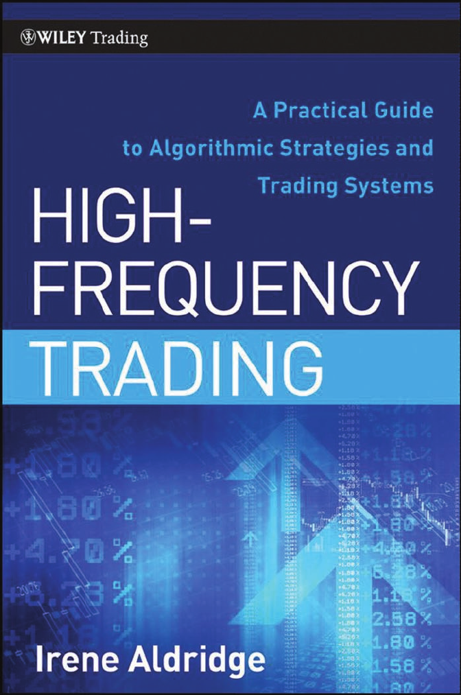
FIGURE 2.1 Absolute number and relative proportion of hedge funds identifying
themselves as “systematic.”
Source: Aldridge (2009b).
funds coincided with important developments in trading technology. As
Figure 2.1 shows, a notable rise in the number of systematic funds oc-
curred in the early 1990s. Coincidentally, in 1992 the Chicago Mercantile
Exchange (CME) launched its first electronic platform, Globex. Initially,
Globex traded only CME futures on the most liquid currency pairs:
Deutsche mark and Japanese yen. Electronic trading was subsequently ex-
tended to CME futures on British pounds, Swiss francs, and Australian and
Canadian dollars. In 1993, systematic trading was enabled for CME equity
futures. By October 2002, electronic trading on the CME reached an aver-
age daily volume of 1.2 million contracts, and innovation and expansion of
trading technology continued henceforth, causing an explosion in system-
atic trading in futures along the way.
The first fully electronic U.S. options exchange was launched in 2000
by the New York–based International Securities Exchange (ISE). As of
mid-2008, seven exchanges offered either fully electronic or a hybrid mix
of floor and electronic trading in options. These seven exchanges are
ISE, Chicago Board Options Exchange (CBOE), Boston Options Exchange
(BOX), AMEX, NYSE’s Arca Options, and Nasdaq Options Market (NOM).
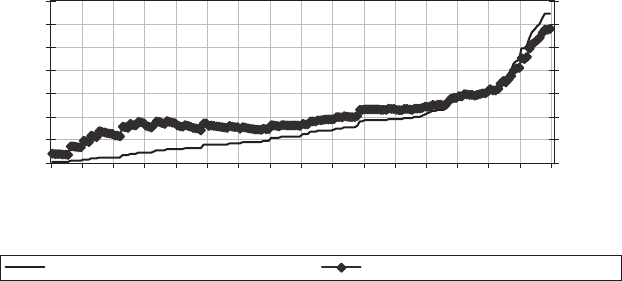
According to estimates conducted by Boston-based Aite Group, shown
in Figure 2.2, adoption of electronic trading has grown from 25 percent of
trading volume in 2001 to 85 percent in 2008. Close to 100 percent of equity
trading is expected to be performed over the electronic networks by 2010.
Technological developments markedly increased the daily trade vol-
ume. In 1923, 1 million shares traded per day on the NYSE, while just over
1 billion shares were traded per day on the NYSE in 2003, a 1,000-times
increase.
P1: SBT
c02 JWBT188-Aldridge October 22, 2009 19:3 Printer: Yet to come
10 HIGH-FREQUENCY TRADING
0%
20%
40%
60%
80%
100%
2001 2002 2003 2004 2005 2006 2007 2008 2009 2010
Year
Equities
Futures
Options
FX
Fixed Income
FIGURE 2.2 Adoption of electronic trading capabilities by asset class.
Source: Aite Group.
Technological advances have also changed the industry structure for fi-
nancial services from a rigid hierarchical structure popular through most of
the 20th century to a flat decentralized network that has become the stan-
dard since the late 1990s. The traditional 20th-century network of financial
services is illustrated in Figure 2.3. At the core are the exchanges or, in the
case of foreign exchange trading, inter-dealer networks. Exchanges are the
centralized marketplaces for transacting and clearing securities orders. In
decentralized foreign exchange markets, inter-dealer networks consist of
inter-dealer brokers, which, like exchanges, are organizations that ensure
liquidity in the markets and deal between their peers and broker-dealers.
Broker-dealers perform two functions—trading for their own accounts
(known as “proprietary trading” or “prop trading”) and transacting and
clearing trades for their customers. Broker-dealers use inter-dealer brokers
to quickly find the best price for a particular security among the network of
other broker-dealers. Occasionally, broker-dealers also deal directly with
other broker-dealers, particularly for less liquid instruments such as cus-
tomized option contracts. Broker-dealers’ transacting clients are invest-
ment banking clients (institutional clients), large corporations (corporate
clients), medium-sized firms (commercial clients), and high-net-worth in-
dividuals (HNW clients). Investment institutions can in turn be brokerages
providing trading access to other, smaller institutions and individuals with
smaller accounts (retail clients).
Until the late 1990s, it was the broker-dealers who played the central
and most profitable roles in the financial ecosystem; broker-dealers con-
trolled clients’ access to the exchanges and were compensated handsomely
for doing so. Multiple layers of brokers served different levels of investors.
The institutional investors, the well-capitalized professional investment
outfits, were served by the elite class of institutional sales brokers that
sought volume; the individual investors were assisted by the retail bro-
kers that charged higher commissions. This hierarchical structure existed
from the early 1920s through much of the 1990s when the advent of the
P1: SBT
c02 JWBT188-Aldridge October 22, 2009 19:3 Printer: Yet to come
Evolution of High-Frequency Trading 11
Exchanges
or
Inter-dealer Brokers
Investment Banking
Broker-Dealers
Institutional
Investors High-Net-Worth
Individuals
Corporate
Clients
Commercial
Clients
Retail Clients
Private Client
Services Private Bank
FIGURE 2.3 Twentieth-century structure of capital markets.
Internet uprooted the traditional order. At that time, a garden variety of
online broker-dealers sprung up, ready to offer direct connectivity to the
exchanges, and the broker structure flattened dramatically.
Dealers trade large lots by aggregating their client orders. To en-
sure speedy execution for their clients on demand, dealers typically “run
books”—inventories of securities that the dealers expand or shrink de-
pending on their expectation of future demand and market conditions.
To compensate for the risk of holding the inventory and the conve-
nience of transacting in lots as small as $100,000, the dealers charge their
clients a spread on top of the spread provided by the inter-broker dealers.
Because of the volume requirement, the clients of a dealer normally cannot
deal directly with exchanges or inter-dealer brokers. Similarly, due to vol-
ume requirements, retail clients cannot typically gain direct access either
to inter-dealer brokers or to dealers.
Today, financial markets are becoming increasingly decentralized.
Competing exchanges have sprung up to provide increased trading liq-
uidity in addition to the market stalwarts, such as NYSE and AMEX.
P1: SBT
c02 JWBT188-Aldridge October 22, 2009 19:3 Printer: Yet to come
12 HIGH-FREQUENCY TRADING
Following the advances in computer technology, the networks are flat-
tening, and exchanges and inter-dealer brokers are gradually giving way
to electronic communication networks (ECNs), also known as “liquidity
pools.” ECNs employ sophisticated algorithms to quickly transmit orders
and to optimally match buyers and sellers. In “dark” liquidity pools, trader
identities and orders remain anonymous.
Island is one of the largest ECNs, which traded about 10 percent of
NASDAQ’s volume in 2002. On Island, all market participants can post
their limit orders anonymously. Biais, Bisiere and Spatt (2003) find that the
higher the liquidity on NASDAQ, the higher the liquidity on Island, but the
reverse does not necessarily hold. Automated Trading Desk, LLC (ATD) is
an example of a dark pool. The customers of the pool do not see the identi-
ties or the market depth of their peers, ensuring anonymous liquidity. ATD
algorithms further screen for disruptive behaviors such as spread manip-
ulation. The identified culprits are financially penalized for inappropriate
behavior.
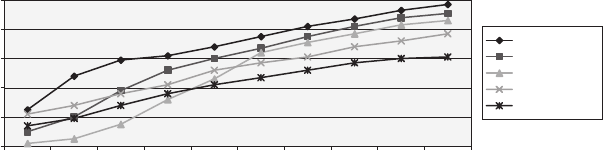
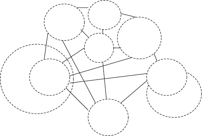
Figure 2.4 illustrates the resulting “distributed” nature of a typical
modern network incorporating ECNs and dark pool structures. The lines
connecting the network participants indicate possible dealing routes.
Typically, only exchanges, ECNs, dark pools, broker-dealers, and retail
brokerages have the ability to clear and settle the transactions, although
Exchange
ECN
Dark
Pool
Corporate
Clients
Commercial
Clients
Investment
Banking
Broker-
Dealers
High-Net-
Worth
Individuals
Retail
Brokerages
Retail Clients
Institutional
Clients
FIGURE 2.4 Contemporary trading networks.

P1: SBT
c02 JWBT188-Aldridge October 22, 2009 19:3 Printer: Yet to come
Evolution of High-Frequency Trading 13
selected institutional clients, such as Chicago-based Citadel, have recently
acquired broker-dealer arms of investment banks and are now able to clear
all the trades in-house.
EVOLUTION OF TRADING
METHODOLOGY
One of the earlier techniques that became popular with many traders was
technical analysis. Technical analysts sought to identify recurring patterns
in security prices. Many techniques used in technical analysis measure cur-
rent price levels relative to the rolling moving average of the price, or a
combination of the moving average and standard deviation of the price.
For example, a technical analysis technique known as moving average
convergence divergence (MACD) uses three exponential moving averages
to generate trading signals. Advanced technical analysts may look at se-
curity prices in conjunction with current market events or general market
conditions to obtain a fuller idea of where the prices may be moving next.
Technical analysis prospered through the first half of the 20th century,
when trading technology was in its telegraph and pneumatic-tube stages
and the trading complexity of major securities was considerably lower
than it is today. The inability to transmit information quickly limited the
number of shares that changed hands, curtailed the pace at which infor-
mation was incorporated into prices, and allowed charts to display latent
supply and demand of securities. The previous day’s trades appeared in
the next morning’s newspaper and were often sufficient for technical an-
alysts to successfully infer future movement of the prices based on pub-
lished information. In post-WWII decades, when trading technology began
to develop considerably, technical analysis developed into a self-fulfilling
prophecy.
If, for example, enough people believed that a “head-and-shoulders”
pattern would be followed by a steep sell-off in a particular instrument,
all the believers would place sell orders following a head-and-shoulders
pattern, thus indeed realizing the prediction. Subsequently, institutional
investors began modeling technical patterns using powerful computer
technology, and trading them away before they became apparent to the
naked eye. By now, technical analysis at low frequencies, such as daily or
weekly intervals, is marginalized to work only for the smallest, least liquid
securities, which are traded at very low frequencies—once or twice per day
or even per week. However, several researchers find that technical analysis
still has legs: Brock, Lakonishok, and LeBaron (1992) find that moving av-
erages can predict future abnormal returns, while Aldridge (2009a) shows
P1: SBT
c02 JWBT188-Aldridge October 22, 2009 19:3 Printer: Yet to come
14 HIGH-FREQUENCY TRADING
that moving averages, “stochastics” and relative strength indicators (RSI)
may succeed in generating profitable trading signals on intra-day data sam-
pled at hourly intervals.
In a way, technical analysis was a precursor of modern microstruc-
ture theory. Even though market microstructure applies at a much higher
frequency and with a much higher degree of sophistication than techni-
cal analysis, both market microstructure and technical analysis work to
infer market supply and demand from past price movements. Much of the
contemporary high-frequency trading is based on detecting latent market
information from the minute changes in the most recent price movements.
Not many of the predefined technical patterns, however, work consistently
in the high-frequency environment. Instead, high-frequency trading models
are built on probability-driven econometric inferences, often incorporating
fundamental analysis.
Fundamental analysis originated in equities, when traders noticed
that future cash flows, such as dividends, affected market price levels.
The cash flows were then discounted back to the present to obtain the
fair present market value of the security. Graham and Dodd (1934) were
one of the earliest purveyors of the methodology and their approach is
still popular. Over the years, the term fundamental analysis expanded
to include pricing of securities with no obvious cash flows based on
expected economic variables. For example, fundamental determination of
exchange rates today implies equilibrium valuation of the rates based on
macroeconomic theories.
Fundamental analysis developed through much of the 20th century.
Today, fundamental analysis refers to trading on the expectation that the
prices will move to the level predicted by supply and demand relation-
ships, the fundamentals of economic theory. In equities, microeconomic
models apply; equity prices are still most often determined as present val-
ues of future cash flows. In foreign exchange, macroeconomic models are
most prevalent; the models specify expected price levels using information
about inflation, trade balances of different countries, and other macroeco-
nomic variables. Derivatives are traded fundamentally through advanced
econometric models that incorporate statistical properties of price move-
ments of underlying instruments. Fundamental commodities trading ana-
lyzes and matches available supply and demand.
Various facets of the fundamental analysis are active inputs into
many high-frequency trading models, alongside market microstructure. For
example, event arbitrage consists of trading the momentum response ac-
companying the price adjustment of the security in response to new fun-
damental information. The date and time of the occurrence of the news
event is typically known in advance, and the content of the news is usually
revealed at the time of the news announcement. In high-frequency event
P1: SBT
c02 JWBT188-Aldridge October 22, 2009 19:3 Printer: Yet to come
Evolution of High-Frequency Trading 15
arbitrage, fundamental analysis can be used to forecast the fundamental
value of the economic variable to be announced, in order to further refine
the high-frequency process.
Technical and fundamental analyses coexisted through much of the
20th century, when an influx of the new breed of traders armed with
advanced degrees in physics and statistics arrived on Wall Street. These
warriors, dubbed quants, developed advanced mathematical models that
often had little to do with the traditional old-school fundamental and tech-
nical thinking. The new quant models gave rise to “quant trading,” a math-
ematical model–fueled trading methodology that was a radical departure
from established technical and fundamental trading styles. “Statistical ar-
bitrage” strategies (stat-arb for short) became the new stars in the money-
making arena. As the news of great stat-arb performances spread, their
techniques became widely popular, and the constant innovation arms race
ensued; the people who kept ahead of the pack were likely to reap the
highest gains.
The most obvious aspect of competition was speed. Whoever was able
to run a quant model the fastest was the first to identify and trade upon
a market inefficiency and was the one to capture the biggest gain. To in-
crease trading speed, traders began to rely on fast computers to make and
execute trading decisions. Technological progress enabled exchanges to
adapt to the new technology-driven culture and offer docking convenient
for trading. Computerized trading became known as “systematic trading”
after the computer systems that processed run-time data and made and
executed buy-and-sell decisions.
High-frequency trading developed in the 1990s in response to advances
in computer technology and the adoption of the new technology by the
exchanges. From the original rudimentary order processing to the cur-
rent state-of-the-art all-inclusive trading systems, high-frequency trading
has evolved into a billion-dollar industry.
To ensure optimal execution of systematic trading, algorithms were
designed to mimic established execution strategies of traditional traders.
To this day, the term “algorithmic trading” usually refers to the system-
atic execution process—that is, the optimization of buy-and-sell decisions
once these buy-and-sell decisions were made by another part of the system-
atic trading process or by a human portfolio manager. Algorithmic trading
may determine how to process an order given current market conditions:
whether to execute the order aggressively (on a price close to the market
price) or passively (on a limit price far removed from the current market
price), in one trade or split into several smaller “packets.” As mentioned
previously, algorithmic trading does not usually make portfolio allocation
decisions; the decisions about when to buy or sell which securities are as-
sumed to be exogenous.
P1: SBT
c02 JWBT188-Aldridge October 22, 2009 19:3 Printer: Yet to come
16 HIGH-FREQUENCY TRADING
High-frequency trading became a trading methodology defined as quan-
titative analysis embedded in computer systems processing data and mak-
ing trading decisions at high speeds and keeping no positions overnight.
The advances in computer technology over the past decades have en-
abled fully automated high-frequency trading, fueling the profitability of
trading desks and generating interest in pushing the technology even fur-
ther. Trading desks seized upon cost savings realized from replacing ex-
pensive trader headcount with less expensive trading algorithms along
with other advanced computer technology. Immediacy and accuracy of
execution and lack of hesitation offered by machines as compared with
human traders have also played a significant role in banks’ decisions to
switch away from traditional trading to systematic operations. Lack of
overnight positions has translated into immediate savings due to reduction
in overnight position carry costs, a particular issue in crisis-driven tight
lending conditions or high-interest environments.
Banks also developed and adopted high-frequency functionality in re-
sponse to demand from buy-side investors. Institutional investors, in turn,
have been encouraged to practice high-frequency trading by the influx of
capital following shorter lock-ups and daily disclosure to investors. Both
institutional and retail investors found that investment products based on
quantitative intra-day trading have little correlation with traditional buy-
and-hold strategies, adding pure return, or alpha, to their portfolios.
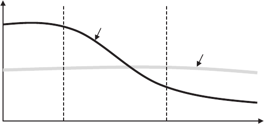
As computer technology develops further and drops in price, high-
frequency systems are bound to take on an even more active role. Special
care should be taken, however, to distinguish high-frequency trading from
electronic trading, algorithmic trading, and systematic trading. Figure 2.5
illustrates a schematic difference between high-frequency, systematic, and
traditional long-term investing styles.
Electronic trading refers to the ability to transmit the orders electron-
ically as opposed to telephone, mail, or in person. Since most orders in
today’s financial markets are transmitted via computer networks, the term
electronic trading is rapidly becoming obsolete.
Algorithmic trading is more complex than electronic trading and can
refer to a variety of algorithms spanning order-execution processes as well
as high-frequency portfolio allocation decisions. The execution algorithms
are designed to optimize trading execution once the buy-and-sell decisions
have been made elsewhere. Algorithmic execution makes decisions about
the best way to route the order to the exchange, the best point in time
to execute a submitted order if the order is not required to be executed
immediately, and the best sequence of sizes in which the order should
be optimally processed. Algorithms generating high-frequency trading sig-
nals make portfolio allocation decisions and decisions to enter or close a

P1: SBT
c02 JWBT188-Aldridge October 22, 2009 19:3 Printer: Yet to come
Evolution of High-Frequency Trading 17
Algorithmic or electronic trading (execution)
Position holding period
Short Long
Execution
latency
Low
High
Traditional long-
term investing
High-frequency
trading
FIGURE 2.5 High-frequency trading versus algorithmic (systematic) trading and
traditional long-term investing.
position in a particular security. For example, algorithmic execution may
determine that a received order to buy 1,000,000 shares of IBM is best han-
dled using increments of 100 share lots to prevent a sudden run-up in the
price. The decision fed to the execution algorithm, however, may or may
not be high-frequency. An algorithm deployed to generate high-frequency
trading signals, on the other hand, would generate the decision to buy the
1,000,000 shares of IBM. The high-frequency signals would then be passed
on to the execution algorithm that would determine the optimal timing and
routing of the order.
Successful implementation of high-frequency trading requires both
types of algorithms: those generating high-frequency trading signals and
those optimizing execution of trading decisions. Algorithms designed for
generation of trading signals tend to be much more complex than those
focusing on optimization of execution. Much of this book is devoted to
algorithms used to generate high-frequency trading signals. Common al-
gorithms used to optimize trade execution in algorithmic trading are dis-
cussed in detail in Chapter 18.
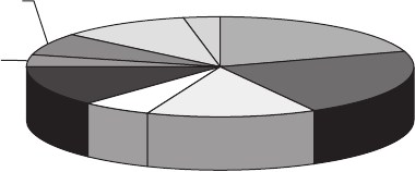
The intent of algorithmic execution is illustrated by the results of a
TRADE Group survey. Figure 2.6 shows the full spectrum of responses
from the TRADE survey. The proportion of buy-side traders using
algorithms in their trading increased from 9 percent in 2008 to 26 percent
in 2009, with algorithms at least partially managing over 40 percent of the
P1: SBT
c02 JWBT188-Aldridge October 22, 2009 19:3 Printer: Yet to come
18 HIGH-FREQUENCY TRADING
Cost
20%
Anonymity
22%
Trader productivity
14%
Execution
consistency
6%
Reduced market
impact 13%
Customization
4%
Ease of use
7%
Speed
11%
Other
3%
FIGURE 2.6 Reasons for using algorithms in trading.
Source: The TRADE Annual Algorithmic Survey.
total order flow, according to the 2009 Annual Algorithmic Trading Survey
conducted by the TRADE Group. In addition to the previously mentioned
factors related to adoption of algorithmic trading, such as productivity and
accuracy of traders, the buy-side managers also reported their use of the
algorithms to be driven by the anonymity of execution that the algorithmic
trading permits. Stealth execution allows large investors to hide their
trading intentions from other market participants, thus deflecting the
possibilities of order poaching and increasing overall profitability.
Systematic trading refers to computer-driven trading positions that
may be held a month or a day or a minute and therefore may or may not be
high-frequency. An example of systematic trading is a computer program
that runs daily, weekly, or even monthly; accepts daily closing prices; out-
puts portfolio allocation matrices; and places buy-and-sell orders. Such a
system is not a high-frequency system.
True high-frequency trading systems make a full range of decisions,
from identification of underpriced or overpriced securities, through opti-
mal portfolio allocation, to best execution. The distinguishing characteris-
tic of high-frequency trading is the short position holding times, one day or
shorter in duration, usually with no positions held overnight. Because of
their rapid execution nature, most high-frequency trading systems are fully
systematic and are also examples of systematic and algorithmic trading.
All systematic and algorithmic trading platforms, however, are not high-
frequency.
Ability to execute a security order algorithmically is a prerequisite for
high-frequency trading in a given security. As discussed in Chapter 4, some
markets are not yet suitable for high-frequency trading, inasmuch as most
trading in these markets is performed over the counter (OTC). According
to research conducted by Aite Group, equities are the most algorithmically
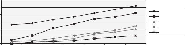
P1: SBT
c02 JWBT188-Aldridge October 22, 2009 19:3 Printer: Yet to come
Evolution of High-Frequency Trading 19
0%
10%
20%
30%
40%
50%
60%
2004 2005 2006 2007 2008 2009 2010
Year
Equities
Futures
Options
FX
Fixed Income
FIGURE 2.7 Adoption of algorithmic execution by asset class.
Source: Aite Group.
executed asset class, with over 50 percent of the total volume of equities
expected to be handled by algorithms by 2010. As Figure 2.7 shows, equi-
ties are closely followed by futures. Advances in algorithmic execution of
foreign exchange, options, and fixed income, however, have been less visi-
ble. As illustrated in Figure 2.7, the lag of fixed income instruments can be
explained by the relative tardiness of electronic trading development for
them, given that many of them are traded OTC and are difficult to synchro-
nize as a result.
While research dedicated to the performance of high-frequency trad-
ing is scarce, due to the unavailability of system performance data rel-
ative to data on long-term buy-and-hold strategies, anecdotal evidence
suggests that most computer-driven strategies are high-frequency strate-
gies. Systematic and algorithmic trading naturally lends itself to trading
applications demanding high speed and precision of execution, as well
as high-frequency analysis of volumes of tick data. Systematic trading, in
turn, has been shown to outperform human-led trading along several key
metrics. Aldridge (2009b), for example, shows that systematic funds con-
sistently outperform traditional trading operations when performance is
measured by Jensen’s alpha (Jensen, 1968), a metric of returns designed to
measure the unique skill of trading by abstracting performance from broad
market influences. Aldridge (2009b) also shows that the systematic funds
outperform nonsystematic funds in raw returns in times of crisis. That find-
ing can be attributed to the lack of emotion inherent in systematic trading
strategies as compared with emotion-driven human traders.
P1: SBT
c02 JWBT188-Aldridge October 22, 2009 19:3 Printer: Yet to come
20

P1: SBT
c03 JWBT188-Aldridge October 22, 2009 19:8 Printer: Yet to come
CHAPTER 3
Overview of the
Business of
High-Frequency
Trading
According to the Technology and High-Frequency Trading Survey
conducted by FINalternatives.com, a leading hedge fund publica-
tion, in June 2009, 90 percent of the 201 asset managers surveyed
thought that high-frequency trading had a bright future. In comparison,
only 50 percent believed that the investment management industry has fa-
vorable prospects, and only 42 percent considered the U.S. economy as
having a positive outlook.
The same respondents identified the following key characteristics of
high-frequency trading:
rTick-by-tick data processing
rHigh capital turnover
rIntra-day entry and exit of positions
rAlgorithmic trading
Tick-by-tick data processing and high capital turnover define much
of high-frequency trading. Identification of small changes in the quote
stream sends rapid-fire signals to open and close positions. The term “high-
frequency” itself refers to fast entry and exit of trading positions. An over-
whelming 86 percent of respondents in the FINalternatives survey thought
that the term “high-frequency trading” referred strictly to holding periods
of one day or less. (See Figure 3.1.)
Intra-day position management deployed in high-frequency trading re-
sults in considerable savings of overnight position carrying costs. The carry
is the cost of holding a margined position through the night; it is usually
21

P1: SBT
c03 JWBT188-Aldridge October 22, 2009 19:8 Printer: Yet to come
22 HIGH-FREQUENCY TRADING
0.0%
10.0%
20.0%
30.0%
40.0%
50.0%
60.0%
70.0%
< 1 second
1 second–
10 minutes
10 minutes–
1 hour
1 hour–
4 hours
4 hours–
1 day
1 day–
5 days
5 days–
1 month
1 month–
3 months
Over
3 months
Position-Holding Time Qualifying as High-Frequency Trading
FIGURE 3.1 Details of the FINalternatives July 2009 Technology and Trading
Survey responses to the question “What position-holding time qualifies as high-
frequency trading?”
computed on the margin portion of account holdings after the close of
the North American trading sessions. Overnight carry charges can substan-
tially cut into the trading bottom line in periods of tight lending or high
interest rates.
Closing down positions at the end of each trading day also reduces the
risk exposure resulting from the passive overnight positions. Smaller risk
exposure again results in considerable risk-adjusted savings.
Finally, algorithmic trading is a necessary component of high-
frequency trading platforms. Evaluating every tick of data separated by
milliseconds, processing market information, and making trading decisions
in a consistent continuous manner is not well suited for a human brain.
Affordable algorithms, on the other hand, can make fast, efficient, and
emotionless decisions, making algorithmic trading a requirement in high-
frequency operations.
COMPARISON WITH TRADITIONAL
APPROACHES TO TRADING
High-frequency trading is a relatively novel approach to investing. As
a result, confusion and questions often arise as to how high-frequency
trading relates to other, older investment styles. This section addresses
these issues.
Technical, Fundamental, or Quant?
As discussed in Chapter 2, technical trading is based on technical analysis,
the objective of which is to identify persistent price change patterns.
P1: SBT
c03 JWBT188-Aldridge October 22, 2009 19:8 Printer: Yet to come
Overview of the Business of High-Frequency Trading 23
Technical analysis may suggest that a price is too high or too low given
its past trajectory. Technical trading would then imply buying a security
the price of which was deemed too low in technical analysis, and selling
a security the price of which was deemed too high. Technical analysis can
be applied at any frequency and can be perfectly suitable in high-frequency
trading models.
Fundamental trading is based on fundamental analysis. Fundamental
analysis derives the equilibrium price levels, given available information
and economic equilibrium theories. As with technical trading, fundamen-
tal trading entails buying a security the price of which was deemed too
low relative to its analytically determined fundamental value and selling a
security the price of which is considered too high. Like technical trading,
fundamental trading can also be applied at any frequency, although price
formation or microstructure effects may result in price anomalies at ultra-
high frequencies.
Finally, quant (short for quantitative) trading refers to making port-
folio allocation decisions based on scientific principles. These principles
may be fundamental or technical or can be based on simple statistical re-
lationships. The main difference between quant analyses and technical or
fundamental styles is that quants use little or no discretionary judgments,
whereas fundamental analysts may exercise discretion in rating the man-
agement of the company, for example, and technical analysts may “see”
various shapes appearing in the charts. Given the availability of data, quant
analysis can be run in high-frequency settings.
Quant frameworks are best suited to high-frequency trading for one
simple reason: high-frequency generation of orders leaves little time for
traders to make subjective nonquantitative decisions and input them into
the system. Aside from their inability to incorporate discretionary inputs,
high-frequency trading systems can run on quant analyses based on both
technical and fundamental models.
Algorithmic, Systematic, Electronic,
or Low-Latency?
Much confusion exists among the terms “high-frequency trading” and
“algorithmic,” “systematic,” “electronic,” and “low-latency” trading.
High-frequency trading refers to fast reallocation or turnover of trading
capital. To ensure that such reallocation is feasible, most high-frequency
trading systems are built as algorithmic trading systems that use complex
computer algorithms to analyze quote data, make trading decisions, and
optimize trade execution. All algorithms are run electronically and, there-
fore, automatically fall into the “electronic trading” subset.
While all algorithmic trading qualifies as electronic trading, the reverse
does not have to be the case; many electronic trading systems only route

P1: SBT
c03 JWBT188-Aldridge October 22, 2009 19:8 Printer: Yet to come
24 HIGH-FREQUENCY TRADING
orders that may or may not be placed algorithmically. Similarly, while most
high-frequency trading systems are algorithmic, many algorithms are not
high-frequency.
“Low-latency trading” is another term that gets confused with “high-
frequency trading.” In practice, “low-latency” refers to the speed of execut-
ing an order that may or may not have been placed by a high-frequency
system; “low-latency trading” refers to the ability to quickly route and exe-
cute orders irrespective of their position-holding time. High-frequency, on
the other hand, refers to the fast turnover of capital that may require low-
latency execution capability. Low-latency can be a trading strategy in its
own right when the high speed of execution is used to arbitrage instanta-
neous price differences on the same security at different exchanges.
MARKET PARTICIPANTS
Competitors
High-frequency trading firms compete with other investment management
firms for quick access to market inefficiencies, for access to trading and
operations capital, and for recruiting of talented trading strategists. Com-
petitive investment management firms may be proprietary trading divi-
sions of investment banks, hedge funds, and independent proprietary trad-
ing operations. The largest independent firms deploying high-frequency
strategies are DE Shaw, Tower Research Capital, and Renaissance
Technologies.
Investors
Investors in high-frequency trading include fund of funds aiming to
diversify their portfolios, hedge funds eager to add new strategies to their
existing mix, and private equity firms seeing a sustainable opportunity to
create wealth. Most investment banks offer leverage through their “prime”
services.
Services and Technology Providers
Like any business, a high-frequency trading operation requires specific sup-
port services. This section identifies the most common and, in many cases,
critical providers to the high-frequency business community.
Electronic Execution High-frequency trading practitioners rely on
their executing brokers and electronic communication networks (ECNs)
P1: SBT
c03 JWBT188-Aldridge October 22, 2009 19:8 Printer: Yet to come
Overview of the Business of High-Frequency Trading 25
to quickly route and execute their trades. Goldman Sachs and Credit
Suisse are often cited as broker-dealers dominating electronic execution.
Today’s major ECN players are ICAP and Thomson/Reuters, along with
several others.
Custody and Clearing In addition to providing connectivity to
exchanges, broker-dealers typically offer special “prime” services that
include safekeeping of trading capital (known as custody) and trade
reconciliation (known as clearing). Both custody and clearing involve a
certain degree of risk. In a custody arrangement, the broker-dealer takes
the responsibility for the assets, whereas in clearing, the broker-dealer may
act as insurance against the default of trading counterparties. Transaction
cost mark-ups compensate broker-dealers for their custody and clearing
efforts and risk.
Software High-frequency trading operations deploy the following soft-
ware that may or may not be built in-house:
rComputerized generation of trading signals refers to the core function-
ality of a high-frequency trading system; the generator accepts and pro-
cesses tick data, generates portfolio allocations and trade signals, and
records profit and loss (P&L).
rComputer-aided analysis represents financial modeling software de-
ployed by high-frequency trading operations to build new trading
models. MatLab and R have emerged as the industry’s most popular
quantitative modeling choices.
rInternet-wide information-gathering software facilitates high-
frequency fundamental pricing of securities. Promptly capturing
rumors and news announcements enhances forecasts of short-term
price moves. Thomson/Reuters has a range of products that deliver
real-time news in a machine-readable format.
rTrading software incorporates optimal execution algorithms for
achieving the best execution price within a given time interval through
timing of trades, decisions on market aggressiveness, and sizing or-
ders into optimal lots. New York–based MarketFactory provides a suite
of software tools to help automated traders get an extra edge in the
market, help their models scale, increase their fill ratios, reduce slip-
page, and thereby improve profitability (P&L). Chapter 18 discusses
optimization of execution.
rRun-time risk management applications ensure that the system stays
within prespecified behavioral and P&L bounds. Such applications may
also be known as system-monitoring and fault-tolerance software.

P1: SBT
c03 JWBT188-Aldridge October 22, 2009 19:8 Printer: Yet to come
26 HIGH-FREQUENCY TRADING
rMobile applications suitable for monitoring performance of high-
frequency trading systems alert administration of any issues.
rReal-time third-party research can stream advanced information and
forecasts.
Legal, Accounting, and Other Professional Services Like any
business in the financial sector, high-frequency trading needs to make sure
that “all i’s are dotted and all t’s are crossed” in the legal and accounting
departments. Qualified legal and accounting assistance is therefore indis-
pensable for building a capable operation.
Government
In terms of government regulation, high-frequency trading falls under the
same umbrella as day trading. As such, the industry has to abide by
common trading rules—for example, no insider trading is allowed. An
unsuccessful attempt to introduce additional regulation through a sur-
charge on transaction costs was made in February 2009.
OPERATING MODEL
Overview
Surprisingly little has been published on the best practices to implement
high-frequency trading systems. This chapter presents an overview of the
business of high-frequency trading, complete with information on planning
the rollout of the system and the capital required to develop and deploy a
profitable operation.
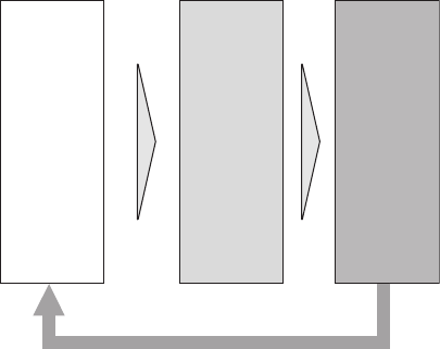
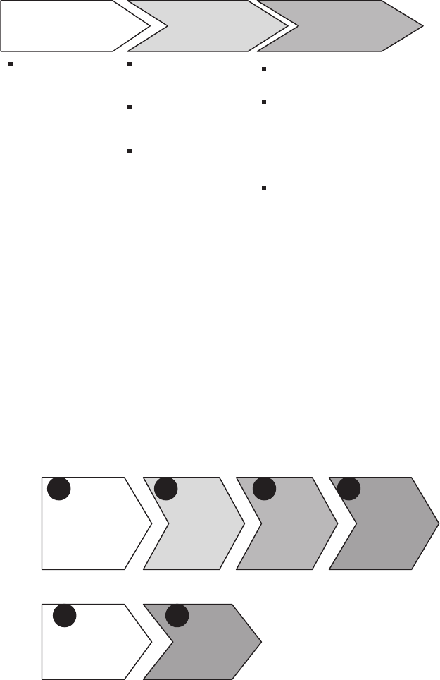
Three main components, shown in Figure 3.2, make up the business
cycle:
rHighly quantitative, econometric models that forecast short-term price
moves based on contemporary market conditions
rAdvanced computer systems built to quickly execute the complex
econometric models
rCapital applied and monitored within risk and cost-management
frameworks that are cautious and precise
The main difference between traditional investment management and
high-frequency trading is that the increased frequency of opening and clos-
ing positions in various securities allows the trading systems to profitably
P1: SBT
c03 JWBT188-Aldridge October 22, 2009 19:8 Printer: Yet to come
Overview of the Business of High-Frequency Trading 27
Models Systems Capital
Re-investment
FIGURE 3.2 Overview of the development cycle of a high-frequency trading
process.
capture small deviations in securities prices. When small gains are booked
repeatedly throughout the day, the end-of-day result is a reasonable gain.
Developing a high-frequency trading business follows a process un-
usual for most traditional financial institutions. Designing new high-
frequency trading strategies is very costly; executing and monitoring
finished high-frequency products costs close to nothing. By contrast, tradi-
tional proprietary trading businesses incur fixed costs from the moment an
experienced senior trader with a proven track record begins running the
trading desk and training promising young apprentices, through the time
when the trained apprentices replace their masters.
Figure 3.3 illustrates the cost curves for rolling out computerized and
traditional trading systems. The cost of traditional trading remains fairly
constant through time. With the exception of trader “burn-outs” necessi-
tating hiring and training new trader staff, costs of staffing the traditional
trading desk do not change. Developing computerized trading systems,
however, requires an up-front investment that is costly in terms of labor
and time. One successful trading system takes on average 18 months to
develop. The costs of computerized trading decline as the system moves
into production, ultimately requiring a small support staff that typically
includes a dedicated systems engineer and a performance monitoring
agent. Both the systems engineer and a monitoring agent can be respon-
sible for several trading systems simultaneously, driving the costs closer
to zero.
P1: SBT
c03 JWBT188-Aldridge October 22, 2009 19:8 Printer: Yet to come
28 HIGH-FREQUENCY TRADING
Cost
Time in development and use
High-frequency
trading
Traditional
trading
FIGURE 3.3 The economics of high-frequency versus traditional trading busi-
nesses.
Model Development
The development of a high-frequency trading business begins with the de-
velopment of the econometric models that document persistent relation-
ships among securities. These relationships are then tested on lengthy
spans of tick-by-tick data to verify the forecasting validity in various mar-
ket situations. This process of model verification is referred to as “back-
testing.” Standard back-testing practices require that the tests be run on
data of at least two years in duration. The typical modeling process is illus-
tratedinFigure3.4.
System Implementation
The models are often built in computer languages such as MatLab that pro-
vide a wide range of modeling tools but may not be suited perfectly for
high-speed applications. Thus, once the econometric relationships are as-
certained, the relationships are programmed for execution in a fast com-
puter language such as C++. Subsequently, the systems are tested in
“paper-trading” with make-believe capital to ensure that the systems work
as intended and any problems (known as “bugs”) are identified and fixed.
Once the systems are indeed performing as expected, they are switched to
live capital, where they are closely monitored to ensure proper execution
and profitability.
High-frequency execution systems tend to be complex entities that de-
tect and react to a variety of market conditions. Figure 3.5 documents the
standard workflow of a high-frequency trading system operating on live
capital.
P1: SBT
c03 JWBT188-Aldridge October 22, 2009 19:8 Printer: Yet to come
Overview of the Business of High-Frequency Trading 29
Academic
research and
proprietary
extensions
Ideas Tools Historical Data
Advanced econometric
modeling: MatLab or R
with custom libraries
C++ is necessary for
back tests and transition
into production
Computing “horsepower”
Tick data
–Most informative
Market depth
–Necessary for the highest-
frequency strategies,
liquidity provision
–Desirable for market
microstructure strategies
Real-time streaming data
–Broker-dealer data
–Reference data
(e.g., Reuters)
FIGURE 3.4 The process for development of econometric models for high-
frequency trading.
As Figure 3.5 shows, a typical high-frequency trading system in produc-
tion encompasses six major tasks, all of which are interrelated and operate
in unison.
rBlock A receives and archives real-time tick data on securities of
interest.
rBlock B applies back-tested econometric models to the tick data ob-
tained in Block A.
Run-time
Post-trade
Receive and
archive real-time
quotes
Manage
position
risk
A
Develop
buy and sell
signals from
the models
B
Keep track
of open
positions
and the
P&L
C D
Performance
evaluation
Cost
estimation
E F
FIGURE 3.5 Run-time and post-trade workflows of a typical high-frequency
operation.

P1: SBT
c03 JWBT188-Aldridge October 22, 2009 19:8 Printer: Yet to come
30 HIGH-FREQUENCY TRADING
rBlock C sends orders and keeps track of open positions and P&L
values.
rBlock D monitors run-time trading behavior, compares it with prede-
fined parameters, and uses the observations to manage the run-time
trading risk.
rBlock E evaluates trading performance relative to a host of predeter-
mined benchmarks.
rBlock F ensures that the trading costs incurred during execution are
within acceptable ranges.
Each of the six functional blocks is built with an independent alert
system that notifies the monitoring personnel of any problems or other un-
usual patterns, including unforeseen market behavior, disruptions in the
market data process, unexpectedly high trading costs, failure to transmit
orders or to receive acknowledgments, and the like.
Given the complexity of the execution process, the development
of the six tasks is hardly trivial. It is most successfully approached
using a continuous iterative implementation cycle whereby the execu-
tion capability is gradually expanded in scope. Figure 3.6 illustrates a
5. Production
and
Maintenance
4. Implementation
3. Design
2. Analysis
1. Planning
FIGURE 3.6 A typical implementation process of run-time high-frequency trading
systems.
P1: SBT
c03 JWBT188-Aldridge October 22, 2009 19:8 Printer: Yet to come
Overview of the Business of High-Frequency Trading 31
standard approach for designing and implementing high-frequency trading
systems.
The implementation of the run-time components of the high-frequency
trading systems begins with careful planning that establishes core func-
tionalities and budgets for the system. Once the planning phase is com-
plete, the process moves into the analysis phase, where the scope of the
initial iteration of the project is determined, feedback from all the rele-
vant stakeholders is aggregated, and senior management signs off on the
high-level project specifications. The next stage—the design—breaks the
system into manageable modules, outlines the functionality of each mod-
ule, and specifies the desired behavior. In the following stage (known as
the implementation stage) the modules are programmed by teams of dedi-
cated software engineers and are tested against specifications determined
in the design stage. Once behavior is found to be satisfactory, the project
moves into the production and maintenance phase, where deviations from
the desired behavior are addressed. When the project is considered sta-
ble, a new iteration of planning begins to incorporate enhancements and
other desired features into the project. See Chapter 16 for the details of
best practices in design and implementation of the high-frequency trading
systems.
Trading Platform
Most high-frequency trading systems today are built to be “platform-
independent”—that is, to incorporate flexible interfaces to multiple broker-
dealers, ECNs, and even exchanges. The independence is accomplished
through the use of FIX language, a special sequence of codes optimized for
exchange of financial trading data. With FIX, at a flip of a switch the trading
routing can be changed from one executing broker to another or to several
brokers simultaneously.
Risk Management
Competent risk management is key to the success of any high-frequency
trading system. A seemingly harmless glitch in the code, market data, mar-
ket conditions, or the like can throw off the trading dynamic and result in
large losses. The objective of risk management is to assess the extent of
potential damages and to create infrastructure to mitigate damaging con-
ditions during the system run-time. Risk management is discussed in detail
in Chapter 17.

P1: SBT
c03 JWBT188-Aldridge October 22, 2009 19:8 Printer: Yet to come
32 HIGH-FREQUENCY TRADING
ECONOMICS
Revenue Driven by Leverage and
the Sharpe Ratio
For the business to remain viable, revenues must be sufficient to cover ex-
penses of running the business. The business of high-frequency trading is
no exception. Accounting for trading costs, a portion of revenues (80 per-
cent on average) is paid out to investors in the trading operation, leaving
the management with “performance fees.” In addition, the management
may collect “management fees,” which are a fixed percentage of assets des-
ignated to cover administrative expenses of the trading business regardless
of performance.
Even the most cost-effective high-frequency trading operation has em-
ployee salaries, administrative services, and trading costs, as well as legal
and compliance expenses. The expenses easily run $100,000 per average
employee in base salaries and benefits, not considering a negotiated incen-
tive structure; this is in addition to the fixed cost overhead of office space
and related expenses.
To compensate for these expenses, what is the minimum level of re-
turn on capital that a high-frequency manager should generate each year
to remain a going concern? The answer depends on the leverage of the
trading platform. Consider a trading operation with five employees. Fixed
expenses of such a business may total $600,000 per year, including salaries
and office expenses. Suppose further that the business charges a 0.5 per-
cent management fee on its capital equity and a 20 percent incentive fee
on returns it produces above the previous high value, or “watermark.” The
minimum capital/return conditions for breaking even for such a trading
business under different leverage situations are shown in Figure 3.7. As il-
lustrated there, a $20 million unlevered fund with five employees needs to
generate at least a 12 percent return per year in order to break even, while
the same fund levered 500 percent (borrowing four times its investment
equity) needs to generate just 3 percent per year to survive.
Conventional wisdom, however, tells us that leverage increases the
risk of losses. To evaluate the risk associated with higher leverage, we
next consider the risks of losing at least 20 percent of the capital equity
of the business. As shown in Figures 3.7 and 3.8, the probability of severe
losses is much more dependent on the aggregate Sharpe ratio of the trading
strategies than it is on the leverage used by the hedge fund.
The Sharpe ratio of a high-frequency trading strategy, discussed in de-
tail in Chapter 5, is the ratio of the average annualized return of the strategy
to the annualized standard deviation of the strategy’s returns. The higher
the Sharpe ratio, the lower the probability of severe losses. As Figure 3.8
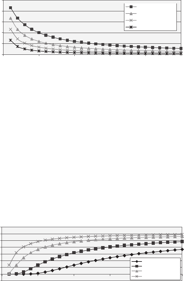
P1: SBT
c03 JWBT188-Aldridge October 22, 2009 19:8 Printer: Yet to come
Overview of the Business of High-Frequency Trading 33
Sample Break-Even Conditions for Different Leverage Values
0
20
40
60
80
100
0% 5% 10% 15% 20% 25%
Minimum Unlevered Return on Investment Required to Break Even
Investment Equity (MM)
Leverage 100%
Leverage 200%
Leverage 500%
Leverage 1000%
FIGURE 3.7 Sample break-even conditions for a high-frequency trading business
employing five workers.
shows, an annualized Sharpe ratio of 0.5 for an unlevered trading opera-
tion expecting to make 20 percent per year translates into a 15 percent risk
of losing at least one-fifth of the fund’s equity capital. Levering the same
fund nine-fold only doubles the risk of losing at least one-fifth of equity.
In comparison, the annualized Sharpe ratio of 2.0 for an unlevered trading
business expecting to make 20 percent per year translates into a miniscule
0.1 percent risk of losing at least one-fifth of the equity capital, and levering
the same trading business only increases the risk of losing at least one-fifth
of the fund to 1.5 percent, as shown in Figure 3.9.
Furthermore, as Figures 3.8 and 3.9 show, for any given Sharpe ratio,
the likelihood of severe losses actually increases with increasing expected
returns, reflecting the wider dispersion of returns. From an investor’s per-
spective, a 5 percent expected return with a Sharpe over 2 is much prefer-
able to a 35 percent expected return with a low Sharpe of, say, 0.5.
–5.0%
0.0%
5.0%
10.0%
15.0%
20.0%
25.0%
30.0%
35.0%
0% 5% 10% 15% 20% 25%
Expected return (unlevered)
Leverage = 100%
Leverage = 200%
Leverage = 500%
Leverage = 1000%
FIGURE 3.8 Probability of losing 20 percent or more of the investment capital
equity running strategies with Sharpe ratio of 0.5.
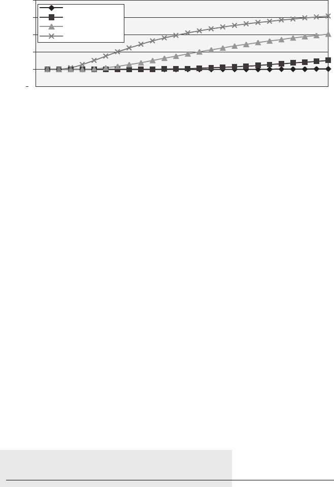
P1: SBT
c03 JWBT188-Aldridge October 22, 2009 19:8 Printer: Yet to come
34 HIGH-FREQUENCY TRADING
–0.5%
0.0%
0.5%
1.0%
1.5%
2.0%
0% 5% 10% 15% 20% 25%
Expected return (unlevered)
Leverage = 100%
Leverage = 200%
Leverage = 500%
Leverage = 1000%
FIGURE 3.9 Probability of losing 20 percent or more of the investment capital
equity running strategies with Sharpe ratio of 2.
In summary, a high-frequency trading operation is more likely to sur-
vive and prosper if it has leverage and high Sharpe ratios. High leverage in-
creases the likelihood of covering costs, and the high Sharpe ratio reduces
the risk of a catastrophic loss.
Transparent and Latent Costs
Understanding the cost structure of trading becomes especially important
in high-frequency settings, where the sheer number of transactions can
eliminate gains. As Chapter 19 notes, in addition to readily available or
transparent costs of trading, high-frequency operations should account for
a wide range of unobservable, or latent, costs. For details on various cost
types, please see Chapter 19.
Staffing
Initial development of high-frequency systems is both risky and pricey, and
the staff required to design trading models should understand PhD-level
quantitative research in finance and econometrics. In addition, program-
ming staff should be experienced enough to handle complex issues of sys-
tem inter-operability, computer security, and algorithmic efficiency.
CAPITALIZING A HIGH-FREQUENCY
TRADING BUSINESS
Capital used for trading in high-frequency operations comprises equity and
leverage. The equity normally comprises contributions from the founders

P1: SBT
c03 JWBT188-Aldridge October 22, 2009 19:8 Printer: Yet to come
Overview of the Business of High-Frequency Trading 35
of the firm, private equity capital, investor capital, or capital of the parent
company. Leverage is debt that can be obtained through a simple bank loan
or margin lending or through other loans offered by broker-dealers.
CONCLUSION
Developing a high-frequency business involves challenges that include is-
sues surrounding the “gray box” or “black box” nature of many systems.
The low transparency of fast and complex algorithm decisions may frus-
trate human traders accustomed to having a thorough understanding of
decisions prior to placing trades. High trading frequency may make it diffi-
cult to spot a malfunction with the algorithm. And we will not even go into
the whole issue of computer security!
Despite the complexity of successfully implementing high-frequency
operations, the end results make it all worthwhile. The deployment and
execution costs decrease considerably with time, leaving the profit-
generating engines operating consistently, with no emotion, sickness, or
other human factors. High-frequency trading is particularly well suited for
markets where traditional long-term investment strategies may not work
at all; high geopolitical and economic uncertainty may render many such
traditional investing venues unprofitable. Well-designed and -executed
high-frequency systems, capitalizing on multiple short-term moves of
security prices, are capable of generating solid profitability in highly
uncertain markets.
P1: SBT
c03 JWBT188-Aldridge October 22, 2009 19:8 Printer: Yet to come
36

P1: SBT
c04 JWBT188-Aldridge October 29, 2009 16:52 Printer: Yet to come
CHAPTER 4
Financial
Markets
Suitable for
High-Frequency
Trading
Awide range of securities and numerous market conditions fit the pro-
file for trading at high frequencies. Some securities markets, how-
ever, are more appropriate than others. This chapter examines the
topic of market suitability for high-frequency trading.
To be appropriate for this type of trading, two requirements must be
met: the ability to quickly move in and out of positions and sufficient mar-
ket volatility to ensure that changes in prices exceed transaction costs. The
volatilities of different markets have been shown to be highly interrelated
and dependent on the volume of macroeconomic news reaching the mar-
kets. The ability to quickly enter into positions as well as to close them
is in turn determined by two factors: market liquidity and availability of
electronic execution.
Liquid assets are characterized by readily available supply and de-
mand. Liquid securities such as major foreign exchange pairs are traded
24 hours a day, 5 days a week. Less liquid securities, such as penny stocks,
may trade only once every few days. Between trades, the prices on illiquid
assets may change substantially, making less liquid securities more risky
as compared with more liquid assets.
High-frequency strategies focus on the most liquid securities; a security
requiring a holding period of 10 minutes may not be able to find a timely
counterparty in illiquid markets. While longer-horizon investors can work
with either liquid or illiquid securities, Amihud and Mendelson (1986) show
that longer-horizon investors optimally hold less liquid assets. According to
these authors, the key issue is the risk/return consideration; longer-term
37

P1: SBT
c04 JWBT188-Aldridge October 29, 2009 16:52 Printer: Yet to come
38 HIGH-FREQUENCY TRADING
investors (already impervious to the adverse short-term market moves)
will obtain higher average gains by taking on more risk in less liquid
investments.
According to Bervas (2006), a perfectly liquid market is the one where
the quoted bid or ask price can be achieved irrespective of the quantities
traded. Market liquidity depends on the presence of trading counterparties
in the market, as well as the counterparties’ willingness to trade. The mar-
ket participants’ willingness to trade in turn depends on their risk aversions
and expectations of impending price movements, along with other market
information.
One way to compare the liquidity of different securities is to use the
average daily volume of each security as the measure of liquidity. In terms
of daily average trading volume, foreign exchange is the most liquid mar-
ket, followed by recently issued U.S. Treasury securities; then come equi-
ties, options, commodities, and futures. Of the most liquid securities, only
spot foreign exchange, equities, options, and futures markets have enabled
fully automated execution; the remaining markets still tend to negotiate
on a contract-by-contract basis over the counter (OTC), slowing down the
trading process. Table 4.1 enumerates current market volumes and exe-
cution methods for different securities. As the demand for high-frequency
trading increases, the development of electronic trading in the OTC mar-
kets may prove highly profitable. Figure 4.1 graphically illustrates optimal
trading frequencies for various securities where the optimal trading fre-
quency is a function of available market liquidity. The following sections
discuss the pros and cons of high-frequency trading in each security market
in detail.
FINANCIAL MARKETS AND
THEIR SUITABILITY FOR
HIGH-FREQUENCY TRADING
This section discusses the availability of various financial markets for high-
frequency trading. As discussed in the first section of this chapter, for a
market to be suitable, it must be both liquid and electronic to facilitate the
quick turnover of capital. In the following subsections, we consider three
key elements of each market:
rAvailable liquidity
rElectronic trading capability
rRegulatory considerations
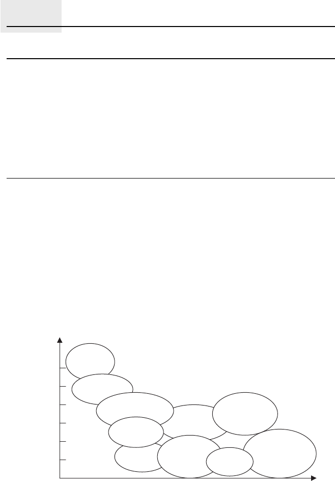
P1: SBT
c04 JWBT188-Aldridge October 29, 2009 16:52 Printer: Yet to come
Financial Markets Suitable for High-Frequency Trading 39
TABLE 4.1 Average Daily Volume and Dominant Execution Method for Major
Security Classes
Market
Average Daily
Volume (Billions)
Dominant
Execution Method
Foreign exchange swaps* 1,714.4 OTC
Foreign exchange spot* 1,004.9 Electronic
Foreign exchange outright forwards* 361.7 OTC
U.S. Treasury** 570.2 OTC
Agency MBS** 320.1 OTC
Federal agency securities** 83.0 OTC
Municipal** 25.0 OTC
Corporate debt** 24.3 OTC
NYSE*** 2.6 Electronic
Options**** 1.6 Electronic and OTC
*Information on the global volume of foreign exchange is for April 2007 as
reported in the Triennial Central Bank Survey.
**Information on the U.S. debt daily volume is quoted from 2007 data reported by
the Securities Industry and Financial Markets Association (SIFMA). By January 2009,
in the aftermath of the credit crisis, the average daily volume in U.S. Treasuries
decreased to USD 358 billion, Agency MBS volume increased to 358 billion, federal
agency securities volume decreased to 75 billion, municipal bonds to 12 billion,
and corporate debt to 12 billion.
***The average daily volume is computed for the month of April 2009 from the
daily volume reported by the NYSE.
****The trading volume for options is quoted from the average daily volume
reported by the Options Clearing Corporation for May 2009.
Optimal Trading Frequency
Instrument liquidity
(daily trading volume)
1 Second
1 Minute
1 Hour
1 Day
1 Month
1 Year
Private
Equity
Foreign
Exchange
Small-Cap
Equities
Large-Cap
Equities
Futures Exchange-
Traded
Options ETFs
Fixed-Income
Commodities
Options
FIGURE 4.1 Optimal trading frequency for various trading instruments, depend-
ing on the instrument’s liquidity.
P1: SBT
c04 JWBT188-Aldridge October 29, 2009 16:52 Printer: Yet to come
40 HIGH-FREQUENCY TRADING
Fixed-Income Markets
The fixed-income markets include the interest rate market and the bond
market. The interest rate market trades short- and long-term deposits, and
the bond market trades publicly issued debt obligations. Interest rate prod-
ucts and bonds are similar in that they both pay fixed or prespecified in-
come to their holders. Aside from their fixed-income quality, bonds and
interest rate products exhibit little similarity.
Both interest rate and bond markets use spot, futures, and swap con-
tracts. Spot trading in both interest rate products and bonds implies instan-
taneous or “on-the-spot” delivery and transfer of possession of the traded
security. Futures trading denotes delivery and transfer of possession at a
prespecified date. Swap trading is a contractual transfer of cash flows be-
tween two parties. Interest rate swaps may specify swapping of a fixed rate
for a floating rate; bond swaps refer mostly to a trading strategy whereby
the investor sells one bond and buys another at a comparable price, but
with different characteristics.
In fixed-income markets, many investors are focused on the product
payouts rather than on the prices of the investments themselves. High-
frequency traders taking advantage of short-term price deviations win, as
do longer-term investors.
Interest Rate Markets The spot interest rate market comprises
quotes offered by banks to other banks, and can be known as “spot in-
terest rates,” “cash interest rates,” or “interbank interest rates.” As other
financial products, interbank interest rates are quoted as a bid and an ask.
A bid interest rate is quoted to banks wanting to make a deposit, whereas
the ask quote is offered to banks to take a credit.
The quoted interest rates are not necessarily the rates at which banks
lend each other money. The actual lending rate is the quoted interest rate
plus a credit spread, where the credit spread is the amount that compen-
sates the lending bank for the risk it takes while lending. The risk of the
lending bank in turn depends on the creditworthiness of the borrowing
bank. The lower the creditworthiness of the borrowing bank, the higher the
risk that the lending bank takes by lending out the money, and the higher
the credit spread intended to compensate the lending bank for the risk of
lending.
Spot interest rates have fixed maturity periods denominated in days or
months. Current maturity periods constitute the following set:
rOvernight: O/N
rThe next business day after tomorrow, known as “tomorrow next”: T/N
rOne week: S/W

P1: SBT
c04 JWBT188-Aldridge October 29, 2009 16:52 Printer: Yet to come
Financial Markets Suitable for High-Frequency Trading 41
rOne month: 1M
rTwo months: 2M
rThree months: 3M
rSix months: 6M
rNine months: 9M
rOne year: 1Y
Interest rate futures are contracts to buy and sell underlying interest
rates in the future. Short-term interest rate futures are more liquid than
spot interest rate futures. The liquidity of the interest rate futures market is
reflected in the bid-ask spread of the interest rate futures; a bid-ask spread
on interest rate futures is on average one-tenth of the bid-ask spread on the
underlying spot interest rate.
Interest rate futures are commonly based on the 3-month deposit rate.
The actual quotation for a futures bid or ask prices, fbid and fask, respec-
tively, depends on the annualized bid or ask OTC forward rates, rbid and
rask, as follows:
fbid =100 1−rbid
100%
fask =100 1−rask
100%
A 3-percent forward rate, for example, results in a futures price of 97.00.
The forward rates underlying the futures contracts typically mature in
three months. The futures contracts usually have four standardized set-
tlements per year—in March, June, September, and December.
Unlike spot interest rates, interest rate futures do not vary according
to the creditworthiness of the borrower. Instead of pricing default risk
into the rate explicitly, exchanges trading interest rate futures require bor-
rowers to post collateral accounts that reflect the creditworthiness of the
borrower.
Swap products are the most populous interest rate category, yet most
still trade OTC. Selected swap products have made inroads into electronic
trading. CME Group, for example, has created electronic programs for 30-
day Fed Funds futures and CBOT 5-year, 10-year, and 30-year interest rate
swap futures; 30-day Fed Funds options; 2-year, 5-year and 10-year Trea-
sury note options; and Treasury bond options. As Table 4.2 shows, how-
ever, electronic trading volumes of interest rate products remain limited.
Bond Markets Bonds are publicly issued debt obligations. Bonds can
be issued by a virtual continuum of organizations ranging from federal gov-
ernments through local governments to publicly held corporations. Bonds

P1: SBT
c04 JWBT188-Aldridge October 29, 2009 16:52 Printer: Yet to come
42 HIGH-FREQUENCY TRADING
TABLE 4.2
Daily Dollar Volume in Most Active Interest Rate
Products on CME Electronic Trading (Globex) on
6/12/2009 Computed as Average Price Times
Total Contract Volume Reported by CME
Instrument
Futures Daily Volume
(in USD thousands)
Eurodollar deposits 196,689.9
LIBOR 163.5
30-Year Swap 934.5
5-Year Swap 1,295.2
10-Year Swap 978.6
30-Day Fed Funds 2,917.7
typically pay interest throughout their lifetimes and pay back the princi-
pal at the end of the bond contract, known as the maturity of the bond.
Bonds can also embed various options, to suit both the needs of the issuer
and the needs of the target buyer. For example, a company in the midst
of a turmoil may decide to issue bonds that embed an option to convert
the bond into the company’s stock at some later date. Such a bond type is
known as a convertible bond and is designed to give prospective investors
the security of preferred redemptions should the company be liquidated;
should the company fully recover, the bond gives investors the ability to
convert it into equity and thus obtain a higher return in the long run. In
addition to risk-averse investors, convertible bonds may attract investors
desiring a conservative investment profile at present and a riskier equity
profile in the long run.
Despite the advantageous breadth of the bond market, spot bonds are
transacted mostly OTC and do not generate a readily observable stream of
high-frequency data.
Unlike bonds that can be custom tailored to the buyer’s specifications,
bond futures contracts are standardized by the exchange and are often
electronic. (See Table 4.3.) Bond futures have characteristics similar to
those of the interest rate futures. Like interest rate futures, bond futures
settle four times a year—in March, June, September, and December. The
exact settlement and delivery rules vary from exchange to exchange.
Bond futures with the nearer expiry dates are more liquid than their
counterparts with longer maturities.
While interest rate futures are based on notional 3-month deposits,
bond futures are typically based on government bonds with multiyear ma-
turities. As such, bond futures register less influence from the central banks
that issue them. Bonds issued with maturity of less than two years are
referred to as “bills,” whereas bonds issued with maturity of two to ten
years are often called “notes.”

P1: SBT
c04 JWBT188-Aldridge October 29, 2009 16:52 Printer: Yet to come
Financial Markets Suitable for High-Frequency Trading 43
TABLE 4.3 Daily Dollar Volume in Most Active Bond Futures Products on CME
Electronic Trading (Globex) on 6/12/2009 Computed as Average
Price Times Total Contract Volume Reported by CME
Instrument
Futures Daily Volume
(in USD thousands)
30-Year U.S. Treasury Bond, Futures 19,486.6
10-Year U.S. Treasury Note, Futures 82,876.5
5-Year U.S. Treasury Note, Futures 31,103.0
2-Year U.S. Treasury Note, Futures 14,187.1
Foreign Exchange Markets
In a nutshell, a foreign exchange rate is a swap of interest rates denomi-
nated in different currencies. Foreign exchange trading originated in 1971
when the gold standard collapsed under the heft of U.S. debt. From 1971
until the late 1980s, foreign exchange traded entirely among commercial
banks that made deposit arrangements in different currencies. Commercial
banks had exclusive access to inter-dealer networks, consisting of loose
groups of third-party agents facilitating quick distribution of orders among
different commercial banking clients. Investment banks, such as Goldman
Sachs, had no direct access to the inter-dealer networks and transacted
their foreign exchange trades through commercial banks instead.
In the early 1990s, investment banks were able to gain access to broker-
dealer networks. In the late 1990s non-bank companies and non–U.S. in-
vestment banks connected directly to the inter-dealer pools. Since 2003,
hedge funds and proprietary trading funds have also been granted access
to the inter-dealer liquidity. Currently, spot, forward, and swap foreign ex-
change products trade through this decentralized and unregulated mecha-
nism. Only foreign exchange futures and selected options contracts can be
found on exchanges.
The decentralization of foreign exchange trading has had two key con-
sequences: the absence of “one price” and the absence of volume measures.
The absence of a single coherent price at any given time is a direct
consequence of decentralization. Different dealers receive different infor-
mation and price their securities accordingly. The lack of one price can
present substantial arbitrage opportunities at high trading frequencies. An-
other consequence of decentralization is that the market-wide measure of
volume at any given time in foreign exchange is not available. To monitor
developments in foreign exchange markets, central banks conduct finan-
cial institution surveys every three years. These surveys are then aggre-
gated and published by the Bank for International Settlements (BIS).
BIS estimates that the total foreign exchange (FX) market in 2007 had
a daily trading volume of $3 trillion. This includes the spot market and

P1: SBT
c04 JWBT188-Aldridge October 29, 2009 16:52 Printer: Yet to come
44 HIGH-FREQUENCY TRADING
forwards, futures, options, and swaps. The spot market accounts for about
33 percent of the total daily turnover or about $1 trillion. According to
BIS Triennial Surveys, the proportion of spot transactions among all FX
trades has been decreasing; in 1989, spot represented 59 percent of all FX
trades. In 1998, spot accounted for only 40 percent of all FX trades. Of the
$2 trillion of daily FX volume that is not spot, $1.7 trillion is contributed
by FX swaps.
Some FX futures and options are traded on exchanges. Table 4.4 shows
daily electronic trading volumes in most common foreign exchange futures
on CME.
Foreign exchange markets profitably accommodate three types of
players with distinct goals: high-frequency traders, longer-term investors,
and corporations. The main objective of high-frequency traders is to cap-
ture small intra-day price changes. The main objective of longer-term in-
vestors is to gain from global macro changes. Finally, the main objective
of corporate currency managers is usually hedging of cross-border flows
against adverse currency movements—for example, a Canadian firm sell-
ing in the United States may choose to hedge its revenue stream by pur-
chasing puts on USD/CAD futures. The flows of the three parties can be
quite distinct, as Table 4.5 illustrates.
Table 4.5 reports summary statistics for EUR/USD order flows ob-
served by Citibank and sampled at the weekly frequency between Jan-
uary 1993 and July 1999: A) statistics for weekly EUR/USD order flow
aggregated across Citibank’s corporate, trading, and investing customers;
and B) order flows from end-user segments cumulated over a week. The
last four columns on the right report autocorrelations iat lag iand p-values
for the null that (i=0). The summary statistics on the order flow data are
from Evans and Lyons (2007), who define order flow as the total value of
EUR/USD purchases (in USD millions) initiated against Citibank’s quotes.
TABLE 4.4 Daily Dollar Volume in Most Active Foreign Exchange Products on
CME Electronic Trading (Globex) on 6/12/2009 Computed as
Average Price Times Total Contract Volume Reported by CME
Currency
Futures Daily Volume
(in USD thousands)
Mini-Futures Daily Volume
(in USD thousands)
Australian Dollar 5,389.8 N/A
British Pound 17,575.6 N/A
Canadian Dollar 6,988.1 N/A
Euro 32,037.9 525.3
Japanese Yen 8,371.5 396.2
New Zealand Dollar 426.5 N/A
Swiss Franc 4,180.6 N/A

P1: SBT
c04 JWBT188-Aldridge October 29, 2009 16:52 Printer: Yet to come
TABLE 4.5 Summary Statistics of Weekly EUR/USD Order Flow observed by Citibank between January 1993 and July 1999
Summary Statistics (Citibank weekly EUR/USD order flow 1993–1999)
Autocorrelations Lag
Order Flow
Mean
Standard
Maximum
Minimum
Skewness or
Kurtosis*1248
−0.043 3.722 0.105 −0.061 0.027 0.025 −0.015
A: Total for EUR/USD 1.234 −3.715 3.204 (0.287) (0.603) (0.643) (0.789)
B: EUR/USD Order Flows
per Customer Type
−16.774 549.302 −0.696 −0.037 −0.04 0.028 −0.028
(i) Corporate U.S. 108.685 −529.055 9.246 (0.434) (0.608) (0.569) (0.562)
(ii) Corporate Non–U.S. −59.784 634.918 −0.005 0.072 0.089 −0.038 0.103
196.089 −692.419 3.908 (0.223) (0.124) (0.513) (0.091)
−4.119 1710.163 0.026 −0.021 0.024 0.126 −0.009
(iii) Traders U.S. 346.296 −2024.28 8.337 (0.735) (0.602) (0.101) (0.897)
11.187 972.106 0.392 −0.098 0.024 0.015 0.083
(iv) Traders Non–U.S. 183.36 −629.139 5.86 (0.072) (0.660) (0.747) (0.140)
(v) Investors U.S. 19.442 535.32 −1.079 0.096 −0.024 −0.03 −0.016
146.627 −874.15 11.226 (0.085) (0.568) (0.536) (0.690)
15.85 1881.284 0.931 0.061 0.107 −0.03 −0.014
(vi) Investors Non–U.S. 273.406 −718.895 9.253 (0.182) (0.041) (0.550) (0.825)
*Skewness of order flows measures whether the flows skew toward either the positive or the negative side of their mean, and
kurtosis indicates the likelihood of extremely large or small order flows. Statistical properties of skewness and kurtosis are
discussed in detail in Chapter 8.
45

P1: SBT
c04 JWBT188-Aldridge October 29, 2009 16:52 Printer: Yet to come
46 HIGH-FREQUENCY TRADING
TABLE 4.6 Daily Dollar Volume in Most Active Equity Futures on CME Electronic
Trading (Globex) on 6/12/2009 Computed as Average Price Times
Total Contract Volume Reported by CME
Instrument
Futures Daily Volume
(in USD thousands)
Mini-Futures Daily Volume
(in USD thousands)
S&P 500 2,331.6 N/A
Nasdaq100 172.4 N/A
E-mini 2,300,537.2 N/A
E-Mid-cap 40,820.9 N/A
E-Nasdaq 515,511.8 N/A
Nikkei 56,570.3 N/A
GSCI 211.0 N/A
MSCI EAFE 24,727.7 2,126.9
Equity Markets
Equity markets are popular among high-frequency players due to the
market inefficiencies presented by the markets’ sheer breadth; in 2006,
2,764 stocks were listed on NYSE alone. In addition to stocks, equity mar-
kets trade exchange-traded funds (ETFs), warrants, certificates, and even
structured products. There are stock futures and options, as well as index
futures and options. Most stock exchanges provide full electronic trading
functionality for all of their offerings. Table 4.6 documents sample daily
electronic trading volumes in most active equity futures trading on Globex.
Equity markets display diversity in investment objectives. Many equity
market participants invest in long-term buy-and-hold patterns. Short-term
opportunities for high-frequency traders abound.
Commodity Markets
Commodities products also include spot, futures, and options. Spot com-
modity contracts provide physical delivery of goods (e.g., a bushel of corn)
and are therefore ill suited for high-frequency trading. Electronically traded
and liquid commodity futures and options, on the other hand, can provide
viable and profitable trading strategies.
Like other types of futures, commodity futures are contracts to buy or
sell the underlying security—in this case a commodity, at a prespecified
point in time in the future. Futures of agricultural commodities may
have irregular expiry dates due to the seasonality of harvests. Commodity
futures contracts tend to be smaller than FX futures or interest rate futures
contracts.

P1: SBT
c04 JWBT188-Aldridge October 29, 2009 16:52 Printer: Yet to come
Financial Markets Suitable for High-Frequency Trading 47
TABLE 4.7 Daily Dollar Volume of Commodity Products in CME Electronic
Trading (Globex) on 6/12/2009 Computed as Average Price Times
Total Contract Volume Reported by CME
Commodity
Futures Daily Volume
(in USD thousands)
Mini-Futures Daily Volume
(in USD thousands)
Corn 121,920.9 178.0
Wheat 33,399.5 N/A
Soybeans 147,168.6 423.1
Soybean Meal 13,089.6 N/A
Soybean Oil 4,334.1 N/A
Oats 212.9 N/A
Rough Rice 447.0 N/A
Milk 12.9 N/A
Dry Milk 0.1 N/A
Cash Butter 14.3 N/A
Pork Belly 1.6 N/A
Lean Hog 1,385.0 N/A
Live Cattle 728.0 N/A
Feeder 179.8 N/A
Lumber 167.3 N/A
Ethanol 40.8 N/A
In 2009, CME offered electronic futures and options trading in com-
modities shown in Table 4.7. Table 4.7 also shows daily volumes on se-
lected electronically traded futures recorded on CME on June 12, 2009.
CONCLUSION
As previous sections have shown, electronic trading is rapidly advancing to
bring instantaneous execution to most securities. The advantages of high-
frequency trading in the developing electronic markets are two-fold:
rFirst-to-market high-frequency traders in the newly electronic markets
are likely to capture significant premiums on their speculative activity
simply because of the lack of competition.
rIn the long term, none of the markets is a zero-sum game. The diverse
nature of market participants ensures that all players are able to ex-
tract value according to their own metrics.
P1: SBT
c04 JWBT188-Aldridge October 29, 2009 16:52 Printer: Yet to come
48

P1: SBT
c05 JWBT188-Aldridge October 22, 2009 19:17 Printer: Yet to come
CHAPTER 5
Evaluating
Performance of
High-Frequency
Strategies
The field of strategy performance measurement is quite diverse. Many
different metrics have been developed over time to illuminate a strat-
egy’s performance. This chapter summarizes the most popular ap-
proaches for performance measurement and discusses strategy capacity
and the length of time required to evaluate a strategy.
BASIC RETURN CHARACTERISTICS
Trading strategies may come in all shapes and sizes, but they share one
characteristic that makes comparison across different strategies feasible—
return.
The return itself, however, can be measured across a wide array of
frequencies: hourly, daily, monthly, quarterly, and annually, among others.
Care should be exercised to ensure that all returns used for inter-strategy
comparisons are generated at the same frequency.
Returns of individual strategies can be compared using a variety of per-
formance measures. Average annual return is one such metric. An average
return value is a simplistic summary of the location of the mean of the re-
turn distribution. Higher average returns may be potentially more desirable
than lower returns; however, the average return itself says nothing about
dispersion of the distribution of returns around its mean, a measure that
can be critical for risk-averse investors.
Volatility of returns measures the dispersion of returns around the av-
erage return; it is most often computed as the standard deviation of returns.
49
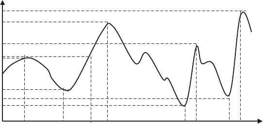
P1: SBT
c05 JWBT188-Aldridge October 22, 2009 19:17 Printer: Yet to come
50 HIGH-FREQUENCY TRADING
Volatility, or standard deviation, is often taken to proxy risk. Standard devi-
ation, however, summarizes the average deviation from the mean and does
not account for the risk of extreme negative effects that can wipe out years
of performance.
A measure of tail risk popular among practitioners that documents the
maximum severity of losses observed in historical data is maximum draw-
down. Maximum drawdown records the lowest peak-to-trough return from
the last global maximum to the minimum that occurred prior to the next
global maximum that supersedes the last global maximum. The global max-
imum measured on the past data at any point in time is known as “high
water mark.” A drawdown is then the lowest return in between two suc-
cessive high water marks. The lowest drawdown is known as the maximum
drawdown.
Figure 5.1 illustrates the concepts of high water mark and maximum
drawdown graphically. The graph presents an evolution of a sample cu-
mulative return of a particular investment model over time. At time tA,the
return RAis the highest cumulative return documented on the chart, so it is
our high water mark at time tA. The cumulative return subsequently drops
to level RBat time tB, but the value of our high water mark remains the
same: RA. Since RBat time tBpresents the lowest drop in cumulative re-
turn on record, the value (RB−RA) constitutes our maximum drawdown
at time tB.
Subsequently, the model reaches a new high water mark at time tA’
as soon as the cumulative return reached passes the previous high water
mark RA. The value of the high water mark continues to increase until point
C, where it reaches a peak value to date: RC. At this point, the maximum
drawdown remains (RB−RA).
Cumulative Return
A
B
C
D
E
F
G
tAtBtCtDtEtFtGtime
RG
RC
RE
RA
RB
RF
RD
tA’
FIGURE 5.1 Calculation of maximum drawdowns.

P1: SBT
c05 JWBT188-Aldridge October 22, 2009 19:17 Printer: Yet to come
Evaluating Performance of High-Frequency Strategies 51
Following point C, the cumulative return drops considerably, reaching
progressively lower troughs. The new maximum drawdown is computed
at a point X as soon as the following condition holds: RX−RC<RB−
RA. Point C and the corresponding cumulative return RCremain the high
water mark until it is exceeded at point G. Point D sets the new maximum
drawdown (RD−RC) that remains in effect for the duration of the time
shown in the graph.
The average return, volatility, and maximum drawdown over a pre-
specified window of time measured at a predefined frequency are the main-
stays of performance comparison and reporting for different trading strate-
gies. In addition to the average return, volatility, and maximum drawdown,
practitioners sometimes quote skewness and kurtosis of returns when de-
scribing the shape of their return distributions. As usual, skewness illus-
trates the position of the distribution relative to the return average; positive
skewness indicates prevalence of positive returns, while negative skew-
ness indicates that a large proportion of returns is negative. Kurtosis indi-
cates whether the tails of the distribution are normal; high kurtosis signifies
“fat tails,” a higher than normal probability of extreme positive or negative
events.
COMPARATIVE RATIOS
While average return, standard deviation, and maximum drawdown
present a picture of the performance of a particular trading strategy, the
measures do not lend to an easy point comparison among two or more
strategies. Several comparative performance metrics have been developed
in an attempt to summarize mean, variance, and tail risk in a single number
that can be used to compare different trading strategies. Table 5.1 summa-
rizes the most popular point measures.
The first generation of point performance measures were devel-
oped in the 1960s and include the Sharpe ratio, Jensen’s alpha, and the
Treynor ratio. The Sharpe ratio is probably the most widely used mea-
sure in comparative performance evaluation; it incorporates three desir-
able metrics—average return, standard deviation, and the cost of capital.
The Sharpe ratio was designed in 1966 by William Sharpe, later a win-
ner of the Nobel Memorial Prize in Economics; it is a remarkably enduring
concept used in the study and practice of finance. A textbook definition of
the Sharpe ratio is SR =¯
R−RF
σR, where ¯
Ris the annualized average return
from trading, σRis the annualized standard deviation of trading returns,
and RFis the risk-free rate (e.g., Fed Funds) that is included to capture
the opportunity cost as well as the position carrying costs associated with

P1: SBT
c05 JWBT188-Aldridge October 22, 2009 19:17 Printer: Yet to come
52 HIGH-FREQUENCY TRADING
TABLE 5.1 Performance Measure Summary
Sharpe Ratio
(Sharpe
[1966])
SR =E[r]−rf
σ[r],where
E[r]=r1+···+rT
T
σ[r]=(r1−E[r])2+···+(rT−E[r])2
T−1
The Sharpe ratio of
high-frequency trading
strategies: SR =E[r]
σ[r]
Adequate if returns are
normally distributed.
Treynor Ratio
(Treynor
[1965])
Treynori=E[ri]−rf
βi
βiis the regression
coefficient of trading
returns on returns of the
investor’s reference
portfolio, such as the
market portfolio.
Adequate if returns are
normally distributed and the
investor wishes to split his
holdings between one trading
strategy and the market
portfolio.
Jensen’s
Alpha
(Jensen
[1968])
αi=E[ri]−rf−βi(rM−rf)
βiis the regression
coefficient of trading
returns on returns of the
investor’s reference
portfolio, such as the
market portfolio.
Measures trading return in
excess of the return predicted
by CAPM. Adequate if returns
are normally distributed and
the investor wishes to split his
holdings between one trading
strategy and the market
portfolio, but can be
manipulated by leveraging
the trading strategy.
Measures based on lower partial moments (LPMs):
LPM of order nfor security i:
LPMni (τ)=1
T
T
t=1
max[τ−rit,0]n
where τis the minimal acceptable return;
nis the moment: n=0 is the shortfall probability, n=1 is the expected shortfall,
n=2forτ=E[r] is the semi-variance.
According to Eling and Schuhmacher (2007), more risk-averse investors should use
higher order n.
LPMs consider only negative deviations of returns from a minimal acceptable return.
As such, LPMs are deemed to be a better measure of risk than standard deviation,
which considers both positive and negative deviations (Sortino and van der Meer
[1991]). Minimal acceptable return can be 0, risk-free rate, or average return.

P1: SBT
c05 JWBT188-Aldridge October 22, 2009 19:17 Printer: Yet to come
Evaluating Performance of High-Frequency Strategies 53
TABLE 5.1 (Continued)
Omega (Shadwick
and Keating
[2002]), (Kaplan
and Knowles
[2004])
i=E[ri]−τ
LPM1i(τ)+1E[ri]−τis the average
return in excess of the
benchmark rate.
Sortino Ratio
(Sortino and van
der Meer [1991])
Sortinoi=E[ri]−τ
(LPM2i(τ))1/2
Kappa 3 (Kaplan
and Knowles
[2004])
K3i=E[ri]−τ
(LPM3i(τ))1/3
Upside Potential
Ratio (Sortino,
van der Meer, and
Plantinga [1999])
UPRi=HPM1i(τ)
LPM2i(τ)1/2where
HPM =higher partial moment
HPMni (τ)=1
T
T
t=1
max[rit −τ, 0]n
According to Eling and
Schuhmacher (2007), this
ratio gains from the
consistent application of
the minimal acceptable
return τin the numerator
as well as in the
denominator.
Measures based on drawdown: frequently used by CTAs, according to Eling and
Schuhmacher (2007, p. 5), “because these measures illustrate what the advisors are
supposed to do best—continually accumulating gains while consistently limiting
losses (see Lhabitant, 2004).” MDi1denotes the lowest maximum drawdown, MDi2
the second lowest maximum drawdown, and so on.
Calmar Ratio
(Young [1991])
Calmari=E[ri]−rf
−MDi1
MDi1is the maximum
drawdown.
Sterling Ratio
(Kestner [1996])
Sterlingi=E[ri]−rf
−1
N
N
k=1MDij −1
N
N
k=1
MDij is the
average maximum
drawdown.
Burke Ratio
(Burke [1994])
Burkei=E[ri]−rf
N
k=1MDij21/2N
k=1MDij21/2
is a type
of variance below the Nth
largest drawdown;
accounts for very large
losses.
Value-at-risk–based measures.
Value at risk (VaRi) describes the possible loss of an investment, which is not
exceeded with a given probability of 1 −αin a certain period. For normally
distributed returns, VaRi=−(E[ri]+zασi), where zαis the α-quantile of the
standard normal distribution.
(Continued)

P1: SBT
c05 JWBT188-Aldridge October 22, 2009 19:17 Printer: Yet to come
54 HIGH-FREQUENCY TRADING
TABLE 5.1 (Continued)
Excess return
on value at
risk (Dowd,
[2000])
Excess R on VaR =E[r]−rf
VaRi
Not suitable for
non-normal returns.
Conditional
Sharpe ratio
(Agarwal and
Naik [2004])
Conditional Sharpe =E[r]−rf
CVaRi
CVaRi=E[−rit|rit ≤−VaRi]
The advantage of
CVaR is that it
satisfies certain
plausible axioms
(Artzner et al.
[1999]).
Modified
Sharpe ratio
(Gregoriou
and Gueyie
[2003])
Modified Sharpe =E[r]−rf
MVaRi
Cornish-Fisher expansion is calculated
as follows:
MVaRi=−(E[ri]+σi(zα+(z2
α−1)Si/6
+(z3
α−3zα)EKi/24 −(2z3
α−5zα)S2
i/36))
where Si denotes skewness and EKi
the excess kurtosis for security i
Suitable for
non-normal returns.
the trading activity. It should be noted that in high-frequency trading with
no positions carried overnight, the position carrying costs are 0. Therefore,
the high-frequency Sharpe ratio is computed as follows:
SR =R
σR.
What makes the Sharpe ratio an appealing measure of performance, in
comparison with, say, raw absolute return? Surprisingly, the Sharpe ratio
is an effective metric for selecting mean-variance efficient securities.
Consider Figure 5.2, for example, which illustrates the classic mean-
variance frontier. In the figure, the Sharpe ratio is the slope of the line em-
anating from the risk-free rate and passing through a point corresponding
to a given portfolio (Mfor market portfolio), or trading strategy, or individ-
ual security. The bold line tangent to the mean-variance set of all portfolio
combinations is the efficient frontier itself. It has the highest slope and, cor-
respondingly, the highest Sharpe ratio of all the portfolios in the set. For
any other portfolio, trading strategy, or individual security A, the higher the
Sharpe ratio, the closer the security is to the efficient frontier.
Sharpe himself came up with the metric when developing a portfolio
optimization mechanism for a mutual fund for which he was consulting.
Sharpe’s mandate was to develop a portfolio selection framework for the
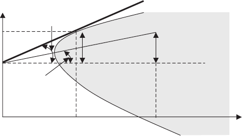
P1: SBT
c05 JWBT188-Aldridge October 22, 2009 19:17 Printer: Yet to come
Evaluating Performance of High-Frequency Strategies 55
Return
E [RM]
RF
σ
M
Ris
k
A
RF
E [RA]−
σ
A
RF
E [RM]−
Sharpe ratio of the
market portfolio
Sharpe ratio of
instrument A
FIGURE 5.2 Sharpe ratio as a mean-variance slope. The market portfolio has the
highest slope and, correspondingly, the highest Sharpe ratio.
fund with the following constraint: no more than 5 percent of the fund’s
portfolio could be allocated to a particular financial security. Sharpe then
created the following portfolio solution: he first ranked the security uni-
verse on what now is known as Sharpe ratio, then picked the 20 securities
with the best performance according to the Sharpe ratio measure, and in-
vested 5 percent of the fund into each of the 20 securities. Equally weighted
portfolio allocation in securities with the highest Sharpe ratios is just one
example of a successful Sharpe ratio application.
Jensen’s alpha is a measure of performance that abstracts from broad
market influences, CAPM-style. Jensen’s alpha implicitly takes into con-
sideration the variability of returns in co-movement with chosen market
indices.
The third ratio, the Treynor ratio, measures the average return in ex-
cess of the chosen benchmark per unit of risk proxied by beta from the
CAPM estimation.
While these three metrics remain popular, they do not take into ac-
count the tail risk of extreme adverse returns. Brooks and Kat (2002),
Mahdavi (2004), and Sharma (2004), for example, present cases against
using Sharpe ratios on non-normally distributed returns. The researchers’
primary concerns surrounding the use of the Sharpe ratio are linked to
the use of derivative instruments that result in an asymmetric return distri-
bution and fat tails. Ignoring deviations from normality may underestimate
risk and overestimate performance. New performance measures have been
subsequently developed to capture the tail risk inherent in the returns of
most trading strategies.
A natural extension of the Sharpe ratio is to change the measure of risk
from standard deviation to a drawdown-based methodology in an effort to
P1: SBT
c05 JWBT188-Aldridge October 22, 2009 19:17 Printer: Yet to come
56 HIGH-FREQUENCY TRADING
capture the tail risk of the strategies. The Calmar ratio, Sterling ratio, and
Burke ratio do precisely that. The Calmar ratio, developed by Young (1991),
uses the maximum drawdown as the measure of volatility. The Sterling
ratio, first described by Kestner (1996), uses the average drawdown as a
proxy for volatility. Finally, the Burke ratio, developed by Burke (1994),
uses the standard deviation of maximum drawdowns as a volatility metric.
In addition to ignoring the tail risk, the Sharpe ratio is also frequently
criticized for including positive returns in the volatility measure. The argu-
ment goes that only the negative returns are meaningful when estimating
and comparing performance of trading strategies. In response, a “Greek”
class of ratios extended the Sharpe ratio by replacing volatility with the av-
erage metrics of adverse returns only. These adverse return metrics are
known as lower partial moments (LPMs) and are computed as regular
moments of a distribution (i.e., mean, standard deviation, and skewness),
except that the data used in computation comprises returns below a speci-
fied benchmark only. Thus, a metric known as Omega, developed by Shad-
wick and Keating (2002) and Kaplan and Knowles (2004), replaces the
standard deviation of returns in the Sharpe ratio calculation with the first
lower partial moment, the average of the returns that fell below the se-
lected benchmark. The Sortino ratio, developed by Sortino and van der
Meer (1991), uses the standard deviation of the returns that fell short of the
benchmark, the second LPM, as a measure of return volatility in the Sharpe
ratio calculation. The Kappa 3 measure, developed by Kaplan and Knowles
(2004), replaces the standard deviation in the Sharpe ratio with the third
LPM of the returns, the skewness of the returns below the benchmark. Fi-
nally, the Upside Potential ratio, produced by Sortino, van der Meer, and
Plantinga (1999), measures the average return above the benchmark (the
first higher partial moment) per unit of standard deviation of returns below
the benchmark.
Value-at-risk (VaR) measures also gained considerable popularity as
metrics able to summarize the tail risk in a convenient point format within
a statistical framework. The VaR measure essentially identifies the 90 per-
cent, 95 percent, or 99 percent Z-score cutoff in distribution of returns (the
metric is also often used on real dollar distributions of daily profit and loss).
VaR companion measure, the conditional VaR (CVaR), also known as ex-
pected loss (EL), measures the average value of return within the cut-off
tail. Of course, the original VaR assumes normal distributions of returns,
whereas the returns are known to be fat-tailed. To address this issue, a
modified VaR (MVaR) measure was proposed by Gregoriou and Gueyie
(2003) and takes into account deviations from normality. Gregoriou and
Gueyie (2003) also suggest using MVaR in place of standard deviation in
Sharpe ratio calculations.
How do these performance metrics stack up against each other? It
turns out that all metrics deliver comparable rankings of trading strategies.

P1: SBT
c05 JWBT188-Aldridge October 22, 2009 19:17 Printer: Yet to come
Evaluating Performance of High-Frequency Strategies 57
Eling and Schuhmacher (2007) compare hedge fund ranking performance
of the 13 measures listed and conclude that the Sharpe ratio is an adequate
measure for hedge fund performance.
PERFORMANCE ATTRIBUTION
Performance attribution analysis, often referred to as “benchmarking,”
goes back to the arbitrage pricing theory of Ross (1977) and has been ap-
plied to trading strategy performance by Sharpe (1992) and Fung and Hsieh
(1997), among others. In a nutshell, performance attribution notes that
t-period return on strategy ithat invests into individual securities with re-
turns rjt in period t,withj=1, ...,J, has an underlying factor structure:
Rit =
j
xjtrjt (5.1)
where xjt is the relative weight of the jth financial security in the portfolio
at time t,
j
xjt =1. The jth financial security, in turn, has a period-treturn
that can be explained by Ksystematic factors:
rjt =
k
λjkFkt +εjt (5.2)
where Fkt is one of Kunderlying systematic factors in period t,k=1, ...,
K,λis the factor loading, and εjt is the security jidiosyncratic return in pe-
riod t. Following Sharpe (1992), factors can be assumed to be broad asset
classes, as well as individual stocks or other securities. Combining equa-
tions (1) and (2) we can express returns as follows:
Rit =
j,k
xjtλjk Fkt +
j
xjtεjt (5.3)
reducing the large number of financial securities potentially underlying
strategy i’s returns to a small group of global factors. Performance attri-
bution to various factors then involves regressing the strategy’s returns on
a basket of factors:
Rit =αi+
k
bik Fkt +uit (5.4)
where bkmeasures the performance of the strategy that can be attributed
to factor k,αimeasures the strategy’s persistent ability to generate
abnormal returns, and uit measures the strategy’s idiosyncratic return in
period t.

P1: SBT
c05 JWBT188-Aldridge October 22, 2009 19:17 Printer: Yet to come
58 HIGH-FREQUENCY TRADING
Performance attribution is a useful measure of strategy returns for the
following reasons:
rThe technique may accurately capture investment styles of black-box
strategies in addition to the details reported by the designer of the
strategy.
rPerformance attribution is a measure of true added value of the strat-
egy and lends itself to easy comparison with other strategies.
rNear-term persistence of trending factors allows forecasting of strat-
egy performance based on performance attribution (see, for example,
Jegadeesh and Titman [1993]).
In the performance attribution model, the idiosyncratic value-added of
the strategy is the strategy’s return in excess of the performance of the
basket of weighted strategy factors.
Fung and Hsieh (1997) find that the following eight global groups of
asset classes serve well as performance attribution benchmarks:
rThree equity classes: MSCI U.S. equities, MSCI non–U.S. equities, and
IFC emerging market equities
rTwo bond classes: JP Morgan U.S. government bonds and JP Morgan
non–U.S. government bonds
rOne-month Eurodollar deposit representing cash
rThe price of gold proxying commodities and the Federal Reserve’s
trade-weighted dollar index measuring currencies in aggregate.
OTHER CONSIDERATIONS IN
STRATEGY EVALUATION
Strategy Capacity
Strategy performance may vary with the amount of capital deployed. Size-
induced changes in observed performance are normally due to limits in
market liquidity for each trading instrument. Large position sizes consume
available pools of liquidity, driving market prices into adverse directions
and reducing the profitability of trading strategies. The capacity of individ-
ual strategies can be estimated through estimation of market impact, dis-
cussed in detail in Chapter 19. Extensive research on the impact of invest-
ment size on performance has been documented for hedge funds utilizing
portfolios of strategies. This section notes the key findings in the studies of
the impact of investment size on fund performance.
P1: SBT
c05 JWBT188-Aldridge October 22, 2009 19:17 Printer: Yet to come
Evaluating Performance of High-Frequency Strategies 59
Fransolet (2004) shows that fast increase in capital in the entire in-
dustry may erode capacities of many profitable strategies. In addition, per
Brown, Goetzmann, and Park (2004), strategy capacity may depend on a
manager’s skills. Furthermore, strategy capacity is a function of trading
costs and asset liquidity, as shown by Getmansky, Lo, and Makarov (2004).
As a result, Ding et al. (2008) conjecture that when the amount of capi-
tal deployed is lower than the strategy capacity, the strategy performance
may be positively related to its capitalization. However, once capitalization
exceeds strategy capacity, performance becomes negatively related to the
amount of capital involved.
Length of the Evaluation Period
for High-Frequency Strategies
Most portfolio managers face the following question in evaluating candi-
date trading strategies for inclusion in their portfolios: how long does one
need to monitor a strategy in order to gain confidence that the strategy
produces the Sharpe ratio advertised?
Some portfolio managers have adopted an arbitrarily long evaluation
period: six months to two years. Some investors require a track record of at
least six years. Yet others are content with just one month of daily perfor-
mance data. It turns out that, statistically, any of the previously mentioned
time frames is correct if it is properly matched with the Sharpe ratio it
is intended to verify. The higher the Sharpe ratio, the shorter the strategy
evaluation period needed to ascertain the validity of the Sharpe ratio.
If returns of the trading strategy can be assumed to be normal, Job-
son and Korkie (1981) showed that the error in Sharpe ratio estimation is
normally distributed with mean 0 and standard deviation
s=[(1/T)(1 +0.5SR2)]1/2
For a 90 percent confidence level, the claimed Sharpe ratio should be
at least 1.645 times greater than the standard deviation of the Sharpe ratio
errors, s. As a result, the minimum number of evaluation periods used for
Sharpe ratio verification is
Tmin =(1.6452/SR2)(1 +0.5SR2)
The Sharpe ratio SR used in the calculation of Tmin, however, should
correspond to the frequency of estimation periods. If the annual Sharpe
ratio claimed for a trading strategy is 2, and it is computed based on the
basis of monthly data, then the corresponding monthly Sharpe ratio SR
is 2/(12)0.5 =0.5774. On the other hand, if the claimed Sharpe ratio is
computed based on daily data, then the corresponding Sharpe ratio SR

P1: SBT
c05 JWBT188-Aldridge October 22, 2009 19:17 Printer: Yet to come
60 HIGH-FREQUENCY TRADING
TABLE 5.2 Minimum Trading Strategy Performance Evaluation Times Required
for Verification of Reported Sharpe Ratios
Claimed Annualized
Sharpe Ratio
No. of Months Required
(Monthly Performance Data)
No. of Months Required
(Daily Performance Data)
0.5 130.95 129.65
1.0 33.75 32.45
1.5 15.75 14.45
2.0 9.45 8.15
2.5 6.53 5.23
3.0 4.95 3.65
4.0 3.38 2.07
is 2/(250)0.5 =0.1054. The minimum number of monthly observations re-
quired to verify the claimed Sharpe ratio with 90 percent statistical con-
fidence is then just over nine months for monthly performance data and
just over eight months for daily performance data. For a claimed Sharpe
ratio of 6, less than one month of daily performance data is required to
verify the claim. Table 5.2 summarizes the minimum performance evalua-
tion times required for verification of performance data for key values of
Sharpe ratios.
CONCLUSION
Statistical tools for strategy evaluation allow managers to assess the feasi-
bility and appropriateness of high-frequency strategies to their portfolios.
Although several statistical strategy evaluation methods have been devel-
oped, the Sharpe ratio remains the most popular measure.

P1: SBT
c06 JWBT188-Aldridge October 22, 2009 19:20 Printer: Yet to come
CHAPTER 6
Orders, Traders,
and Their
Applicability to
High-Frequency
Trading
High-frequency trading aims to identify and arbitrage temporary mar-
ket inefficiencies that are created by the competing interests of
market participants. Understanding the types of orders that traders
can place to achieve their goals allows insights into the strategies of var-
ious traders. Ultimately, this understanding can inform the forecasting of
impending actions of market participants, which itself is key to success
in high-frequency trading. This chapter examines various types of orders
present in today’s markets.
ORDER TYPES
Contemporary exchanges and electronic communication networks (ECNs)
offer a vast diversity of ordering capabilities. The order types differ as to
execution price, timing, size, and even disclosure specifications. This sec-
tion considers each order characteristic in detail.
Order Price Specifications
Market Orders versus Limit Orders Orders can be executed at the
best available price or at a specified price. Orders to buy or sell a security
at the best available price when the order is placed are known as market
orders. Orders to buy or sell a security at a particular price are known as
limit orders.
61

P1: SBT
c06 JWBT188-Aldridge October 22, 2009 19:20 Printer: Yet to come
62 HIGH-FREQUENCY TRADING
When a market order arrives at an exchange or an ECN, the order is im-
mediately matched with the best available opposite order or several best
orders, depending on the size of the arriving order. For example, if a mar-
ket order to sell 100,000 shares of SPY arrives at an exchange, and the ex-
change has the following buy orders outstanding from best to worst: 10,000
shares at $935, 40,000 shares at $930, and 50,000 at $925, then the arriving
market sell order is “walked through the order book” until it is filled: the
first 10,000 shares are sold at $935, the next 40,000 shares at $930 and the
final 50,000 shares at $925, capturing the weighted-average price of $928
per share:
P=10,000 ×$935 +40,000 ×$930 +50,000 ×$925
100,000 =$928
Transaction costs, such as the broker-dealer and exchange fees, are ac-
counted for separately, further reducing the profitability of the trade. For
details on cost types and values, please see Chapter 19.
Limit orders are executed at a specified limit price or at a better price,
if one is available. When a limit order arrives at an exchange or an ECN,
the order is first compared with the best available opposite orders to de-
termine whether the newly arrived order can be filled immediately. For
example, when a limit order to sell SPY at 930 arrives at an exchange, the
exchange first checks whether the exchange already has matching orders
to buy SPY at or above 930. If orders to buy SPY at 930 or at a higher price
are present, the arriving order is treated as a regular market order; it is
filled immediately and charged the market order fees. If no matching or-
ders exist, the arriving limit order is placed in the limit order book, where
it remains until it becomes the best available order and is matched with an
incoming market order.
The aggregate size of limit orders available in the limit order book is
often thought to be the liquidity of the market. The total size of limit orders
available at a particular price is referred to as the market depth. The num-
ber of different price points at which limit orders exist in the limit order
book is known as the breadth of the market. Figure 6.1 illustrates compo-
nents of the liquidity in the limit order book, according to Bervas (2006).
Limit orders can be seen as pre-commitments to buy or sell a specified
number of shares of a particular security at a prespecified price, whereas
market orders are requests to trade the specified quantity of a given se-
curity as soon as possible at the best price available in the market. As
a result, market orders execute fast, with certainty, at uncertain prices
and relatively high transaction costs. Limit orders, on the other hand,
have a positive probability of no execution, lower transaction costs, and
P1: SBT
c06 JWBT188-Aldridge October 22, 2009 19:20 Printer: Yet to come
Orders, Traders, and Their Applicability to High-Frequency Trading 63
Price
Quantities QuantitiesAA´0
Sale Purchase
Ask Price Ap
Bp Bid Price
Resilience
Depth
Depth
Breadth
Resilience
FIGURE 6.1 Aspects of market liquidity (Bervas, 2006). The bid price and the ask
price are defined for liquidity quantities OA and OAthat represent market depths at
bid and ask prices, respectively.
encompass an option to resubmit the order at a different price. Table 6.1
key outlines key differences between market and limit orders.
Market orders specify the desired exchange for the order, the exchange
code of the security to be traded, the quantity of the security to be bought
or sold, and whether the order is to buy or to sell. Limit orders specify
the same parameters as do market orders along with the desired execution
price.
Profitability of Limit Orders A trader placing a buy limit order writes
a put option available freely, with no premium, to the market. Similarly,
a trader placing a sell limit order writes a free call option on the secu-
rity. In addition to foregoing the premium on the option, the limit trader
opens himself up to being “picked off” by better-informed traders. For
TABLE 6.1 Limit Orders versus Market Orders
Market Orders Limit Orders
Order Execution Guaranteed Uncertain
Time to Execution Short Uncertain
Execution Price Uncertain Certain
Order Resubmission None Infinite prior to execution
Transaction Costs High Low
P1: SBT
c06 JWBT188-Aldridge October 22, 2009 19:20 Printer: Yet to come
64 HIGH-FREQUENCY TRADING
example, suppose that the limit trader places a limit buy order on a secu-
rity at $30.00, and that another, better-informed, trader knows that $30.00
is the maximum price the security can reach within the time interval under
consideration. The better-informed trader then jumps at the opportunity
to sell the security to the limit trader, leaving the limit trader in a losing
position.
Despite the seeming lack of profitability of limit order traders, limit
trading has prospered. Most exchanges now offer limit order capabilities,
and limit order–based exchange alternatives known as the electronic com-
munication networks (ECNs) experience a boom. The ability of exchanges
and ECNs to attract numerous limit order traders suggests that limit order
trading is profitable for many market participants.
Handa and Schwartz (1996) examine the profitability of limit order
traders, also known as liquidity traders, and find that limit order strategies
can capture economic rents in excess of market order strategies. Specif-
ically, Handa and Schwartz (1996) find that the buy limit order strategies
allow limit traders to obtain a premium of 0.1 percent to 1.6 percent per
trade on average, depending on the type of the limit order strategy. Handa
and Schwartz (1996) consider four types of buy limit order strategies: those
with buy limit orders placed at prices 0.5 percent, 1 percent, 2 percent, and
3 percent below the corresponding market price.
To measure the profitability of limit order trades, Handa and Schwartz
(1996) conducted the following experiment:
rThe authors break down the trading data into equally spaced profitabil-
ity evaluation periods.
rIn every evaluation period, the simulated market trader executes all
trades at the opening price of the evaluation period.
rThe limit order trader sets limit orders at prices xpercent below the
market opening price.
rThe limit order is considered executed when it is crossed by the market
price.
rIf the limit orders are not executed within the evaluation period, the
limit trader is forced to execute his orders at the opening price of the
next evaluation period.
Handa and Schwartz (1996) measure the profitability of the limit order
strategy as the average difference between the prices obtained using the
limit order strategy and the prices obtained using the market order strategy
during each evaluation period.
The limit order strategy is profitable if the average cost of realized limit
orders is lower than that of realized market orders. The profitability of the

P1: SBT
c06 JWBT188-Aldridge October 22, 2009 19:20 Printer: Yet to come
Orders, Traders, and Their Applicability to High-Frequency Trading 65
buy limit order strategy within each evaluation period is then measured
according to equation (6.1):
t=Pt,M−Pt,L(6.1)
where tis the profitability of the buy limit order strategy in evaluation
period t,Pt,M is the opening price of the evaluation period at which the
market buy order is executed, and Pt,L is the obtained limit price—either
a price obtained when the market price crosses the best limit sell order
or the opening price of the next evaluation period, as defined previously.
The average buy limit order profitability is then computed as an average of
profitability for individual evaluation periods:
t=1
T
T
t=1
(Pt,M−Pt,L) (6.2)
Handa and Schwartz (1996) assess the performance of the following
buy limit orders: orders with prices set 0.5 percent, 1 percent, 2 percent,
and 3 percent below the opening market price in each evaluation period.
The authors run their experiments on stocks of 30 Dow Jones Industrial
firms that traded on the NYSE and find that, on average, limit order strate-
gies outperform market orders. Table 6.2 replicates the average results for
limit order strategies appearing in Handa and Schwartz (1996). The results
show the average percentage value by which the limit order strategy out-
performs the market order strategy.
In summary, limit order strategies can bring clear profitable outcomes
to traders. The limit order strategy works particularly well in the volatile
range-bound markets, such as those we are currently experiencing.
Delays in Limit Order Execution Limit orders, when executed,
are usually executed at prices more favorable than otherwise identical
TABLE 6.2 Average Profitability of Limit Order Strategies in Excess of the Market
Order Strategies
The Distance of Limit Order Prices Away (in the Favorable
Direction) from the Market Order Prices
0.5 percent 1 percent 2 percent 3 percent
Average
profitability
0.100 percent 0.361 percent* 0.516 percent* 1.605 percent*
*Indicates statistical significance at the 95 percent confidence level.
P1: SBT
c06 JWBT188-Aldridge October 22, 2009 19:20 Printer: Yet to come
66 HIGH-FREQUENCY TRADING
market orders that are executed with certainty in most cases. The time du-
ration of limit orders, however, is unpredictable; limit orders can be “hit”
by market orders right away or can fail to be executed if the market price
moves away from the price of the limit order. Failure to execute a limit
order can be quite costly when the limit order is placed to close a position,
particularly when the position is a loss that needs to be liquidated. For ex-
ample, consider a trading strategy that is currently long USD/CAD. Suppose
that the position was opened with a market buy order at 1.2005, the current
market price is 1.1955, and a stop-loss order arrives to close the position. If
the stop-loss order is placed as a market order, the order is executed with
probability 1 at or below the current market price. If the order is placed
as a limit order, and if the market price for USD/CAD suddenly drops, the
order never gets filled and the losses exacerbate dramatically. As a result,
stop-losses are most often executed at market to ensure that the negative
exposure is reliably limited.
Failure to execute a limit order can also be costly when the order is
placed to open a position, because the trading strategy incurs the oppor-
tunity cost corresponding to the average expected gain per trade. For ex-
ample, consider a trading strategy that is “flat,” or fully in cash, at time 0.
Suppose further that at time 1, a buy order arrives to buy USD/CAD while
USD/CAD is at 1.2005. If the buy order is placed as a market order, the
order will be executed with a probability of 100 percent but at 1.2005 at
best (latency in execution and other slippage issues may push the price
even further in the adverse direction). On the other hand, if the buy order
is placed as a limit order at 1.2000, the order may be executed at 1.2000 if
the market price drops to that level, or it may not be executed at all if the
market price stays above the limit level. If the limit order never gets hit, the
system loses the trade opportunity value equal to the gain from the trade
initiated at the market price.
Foucault (1999) and Parlour (1998) model dynamic conditions that en-
sure that limit orders get hit by market orders, while resulting in the prof-
itable outcome for the trader placing the limit orders. The main questions
answered by the two research articles are
1. At what prices will traders post limit orders?
2. How often do traders modify their limit orders?
Such issues in order flow dynamics impact the traders’ bargaining
power and affect their profitability through transaction costs. The main
finding of the studies is that limit orders are preferred to market orders
in high-volatility conditions. Thus, in high-volatility situations, the propor-
tion of limit orders in the marketplace increases, simultaneously reducing
cumulative profitability of agents resulting from a larger number of trades
P1: SBT
c06 JWBT188-Aldridge October 22, 2009 19:20 Printer: Yet to come
Orders, Traders, and Their Applicability to High-Frequency Trading 67
that are left not executed, as well as from the increased market bid-ask
spreads. Parlour (1998) further explains the diagonal effect observed in
Biais, Hillion and Spatt (1995): a market buy reduces the liquidity available
at the ask, inducing sellers to post additional limit sell orders instead of
market sell orders and subsequently triggering more market buy orders.
Thus, serial autocorrelation in order flow arises from liquidity dynamics in
addition to dynamics in informed trading. Ahn, Bae, and Chan (2001) find
that the volume of limit orders increases with increases in volatility on the
Stock Exchange of Hong Kong.
Both Foucault, Kadan, and Kandel (2005) and Rosu (2005) assume that
investors care about execution time and submit orders based on their ex-
pectations of execution time.
Kandel and Tkatch (2006) find that investors indeed take execution
delay into account when submitting limit orders on the Tel-Aviv Stock Ex-
change. The duration of limit orders appears to decrease with increases in
aggressiveness of the limit orders (the distance of the limit orders from the
current market price), as shown by survival analysis of Lo, MacKinlay, and
Zhang (2002).
Goettler, Parlour, and Rajan (2005) extend the analysis to a world
where investors can submit multiple limit orders, at different prices and
with different order quantities. Lo and Sapp (2005) test the influence of or-
der size along with order aggressiveness in the foreign exchange markets
and find that aggressiveness and size are negatively correlated.
Hasbrouck and Saar (2002) document that limit order traders may post
fleeting limit orders; according to Rosu (2005), the fleeting orders are offers
to split the difference made by patient investors on one side of the book to
the patient investors on the other side of the book.
Traders who are confident in their information may choose to place
limit orders during the time they expect their information to impact prices.
Keim and Madhavan (1995), for example, show that informed traders
whose information decays slowly tend to use limit orders. The proportion
of limit orders used by a particular trader or trading strategy, therefore,
can be used to measure the traders’ confidence in their information. The
confidence variable may then be used in extracting additional information
from the observed trading decisions and order flow of the traders.
Limit Orders and Bid-Ask Spreads A trader may also gear towards
limit orders whenever the bid-ask spreads are high. The bid-ask spread may
be a greater cost than the opportunity cost associated with non-execution
of position entry orders placed as limit orders. Biais, Hillion, and Spatt
(1995) show that on the Paris Bourse the traders indeed place limit or-
ders whenever the bid-ask spread is large and market orders whenever the
bid-ask spread is small. Chung, Van Ness, and Van Ness (1999) further show
P1: SBT
c06 JWBT188-Aldridge October 22, 2009 19:20 Printer: Yet to come
68 HIGH-FREQUENCY TRADING
that the proportion of traders entering limit orders increases whenever bid-
ask spreads are wide.
Limit Orders and Market Volatility Bae, Jang, and Park (2003)
examine traders’ propensity to place market and limit orders in varying
volatility conditions. They find that the number of limit orders increases
following a rise in intra-day market volatility, independently of the rela-
tive bid-ask spread size. Handa and Schwartz (1996) show that transitory
volatility, the volatility resulting from uninformed or noise trading, induces
a higher propensity of traders to place limit orders than do permanent
volatility changes, given that traders can get compensated for providing
liquidity while limiting the probability of being picked off. Foucault (1999),
however, finds that limit orders are always more optimal than market or-
ders, even when the probability of being picked off increases.
Order Timing Specifications
Both market and limit orders can be specified as valid for different lengths
of time and even at different times of the trading day. The “good till can-
celed” orders (GTC) remain active in the order book until completely filled.
The “good till date” orders (GTD) remain in the order book until completely
filled or until the specified expiry date. The GTC and GTD orders can be
“killed,” or canceled, by the exchange or the ECN after a predefined time
period (e.g., 90 days), whenever certain corporate actions are taken (e.g.,
bankruptcy or delisting), or as a result of structural changes on the ex-
change (e.g., a change in minimum order sizes).
The “day” orders, also known as the “good for the day” (GFD) orders,
remain in the order book until completely filled or until the end of the trad-
ing day, defined as the end of normal trading hours. The “good for the ex-
tended day” (GFE) orders allow the day orders to be executed until the end
of the extended trading session. Orders even shorter in duration that are
particularly well suited for high-frequency trading are the “good till time”
(GTT) orders. The GTT orders remain in the order book until completely
filled or until the specified expiry date and time and can be used to specify
short-term orders. The GTT orders are especially useful in markets where
order cancellation or order change fees are common, such as in the options
markets. When market conditions change, instead of canceling or changing
the order and thus incurring order cancellation or change fees, traders can
let their previous orders expire at a predetermined time and place new or-
ders instead.
Order Size Specifications
The straightforward or plain “vanilla,” order size specification in both limit
and market orders is a simple number of security contracts geared for
P1: SBT
c06 JWBT188-Aldridge October 22, 2009 19:20 Printer: Yet to come
Orders, Traders, and Their Applicability to High-Frequency Trading 69
execution. Vanilla order sizes are typically placed in “round lots”—that is,
the standard contract sizes traded on the exchange. For example, a round
lot for common stocks on the New York Stock Exchange (NYSE) is 100
shares. Smaller orders, known as “odd lots,” are filled by a designated odd
lot dealer (on a per-security basis), and are normally charged higher trans-
action costs than the round-lot orders. Both market and limit orders can be
odd lots.
Orders bigger than round lots, yet not in round-lot multiples, are known
as “mixed lots.” Mixed-lot orders are typically broken down into the round
lots and the odd lots on the exchange and are executed accordingly by a
regular dealer and the odd-lot dealer.
When large market orders are placed, there may not be enough liq-
uidity to fill the order, and subsequent liquidity may be attainable only
at prices unacceptable to the trader placing the market order. To address
the problem, most exchanges and ECNs accept “fill or kill” (FOK) orders
that specify that the order be filled immediately in full, or in part, with the
unfilled quantity killed in its entirety. If the partial fill of the market order
is unacceptable to the trader, the order can be specified as a “fill and kill”
(FAK) order, to be either filled immediately in full or killed in its entirety.
Alternatively, if the immediacy of the order execution is not the principal
concern but the size is, the order can be specified as an “all or none” (AON)
order. The AON orders remain in the order book with their original time
priorities until they can be filled in full.
Order Disclosure Specifications
The amount of order information that is disclosed varies from exchange
to exchange and from ECN to ECN. On some exchanges and ECNs, all
market and limit orders are executed with full transparency to all market
participants. Other exchanges, such as the NYSE, allow market makers to
decide how much of an incoming market order should be executed at a
given price. Other exchanges show limit orders only for a restricted set of
prices that are near the current market price. Still others permit “iceberg”
orders—that is, orders with only a portion of the order size observable to
other market participants.
A “standard iceberg” (SI) order is a limit order that specifies a total
size and a disclosed size. The disclosed size is revealed as a limit order.
Once the disclosed size is completely executed, the new quantity becomes
disclosed, and it is instantaneously made available for matching with time
priority corresponding to the release time.
An order is often placed anonymously, without disclosing the identity
of the trader or the trading institution to other market participants on the
given exchange or ECN. Anonymous orders are particularly attractive to

P1: SBT
c06 JWBT188-Aldridge October 22, 2009 19:20 Printer: Yet to come
70 HIGH-FREQUENCY TRADING
traders processing large orders, as any identifying information may trigger
adverse price offers from other market participants.
Stop-Loss and Take-Profit Orders
In addition to previously discussed specifications of order execution, some
exchanges offer stop-loss and take-profit order capability. Both the stop-
loss and take-profit orders become market or limit orders to buy or sell the
security if a specified price, known as the stop price, is reached, or passed.
Administrative Orders
A change order is an order to change a pending limit order, whether a limit
open or limits for take-profit or stop-loss. The change order can specify
the change in the limit price, the order type (buy or sell), and the number
of units to process. A change order can also be placed to cancel an ex-
isting limit order. Some execution counterparties may charge a fee for a
change order.
A margin call close order is one order traders probably want to avoid.
It is initiated by the executing counterparty whenever a trader trades on
margin and the amount of cash in the trader’s account is not sufficient to
cover two times the losses of all open positions. The margin call close is
executed at market at the end of day, which varies depending on the finan-
cial instrument traded.
Most broker-dealers and ECNs provide phone support for clients. If
customer computer system or network connectivity breaks down for what-
ever reason, a customer can phone in an order. Such phone-in orders are
sometimes referred to as “orders by hand,” and are often charged a trans-
action cost premium relative to the electronic ordering.
Finally, several cancel orders can be initiated either by the customer
or by the executing counterparty. An insufficient funds cancel can be en-
acted by the executing broker in the event that the customer does not have
enough funds to open a new position. Limit orders can be canceled if the
price of the underlying instrument moves outside the preselected bounds;
such orders are known as bound violation cancel orders.
ORDER DISTRIBUTIONS
Order statistics, such as Oanda’s FX Trade presented in Table 6.3, are sel-
dom, if ever, distributed to the public. It should be noted, however, that
the mean and median size of Oanda FXTrade transactions indicate that the

P1: SBT
c06 JWBT188-Aldridge October 22, 2009 19:20 Printer: Yet to come
Orders, Traders, and Their Applicability to High-Frequency Trading 71
majority of Oanda’s customers are retail and that the numbers are thus not
necessarily representative of order flows at broker-dealers and ECNs. Nev-
ertheless, the data offers an interesting point for comparison.
As Table 6.3 shows, on an average day between October 1, 2003
and May 14, 2004, the most common orders—both by number of orders
and by volume—were stop-loss or take-profit (22 percent and 23 percent,
TABLE 6.3 Daily Distributions of Trades per Trade Category in FX Spot of Oanda
FXTrade, a Toronto-Based Electronic FX Brokerage, as Documented
by Lechner and Nolte (2007)
Transaction Record
Percentage of
Orders per
Order Count
Mean Daily
Trading
Volume in EUR
Percentage of
Orders by
Trade Volume
Buy Market (open) 13.10 percent 167,096 14.13 percent
Sell Market (open) 10.61 percent 135,754 11.48 percent
Buy Market (close) 8.27 percent 110,461 9.34 percent
Sell Market (close) 10.27 percent 140,263 11.86 percent
Limit Order: Buy 5.41 percent 61,856 5.23 percent
Limit Order: Sell 4.76 percent 48,814 4.13 percent
Buy Limit Order
Executed (open)
3.22 percent 23,860 2.02 percent
Sell Limit Order
Executed (open)
2.92 percent 14,235 1.20 percent
Buy Limit Order
Executed (close)
0.46 percent 6,091 0.52 percent
Sell Limit Order
Executed (close)
0.46 percent 6,479 0.55 percent
Buy Take-Profit (close) 3.14 percent 12,858 1.09 percent
Sell Take-Profit (close) 3.49 percent 19,401 1.64 percent
Buy Stop-Loss (close) 2.18 percent 19,773 1.67 percent
Sell Stop-Loss (close) 2.55 percent 23,391 1.98 percent
Buy Margin Call (close) 0.12 percent 733 0.06 percent
Sell Margin Call (close) 0.17 percent 1,213 0.10 percent
Change Order 3.01 percent 61,229 5.18 percent
Change Stop-Loss or
Take-Profit
22.36 percent 268,568 22.71 percent
Cancel Order by Hand 2.41 percent 44,246 3.74 percent
Cancel Order:
Insufficient Funds
0.28 percent 10,747 0.91 percent
Cancel Order: Bound
Violation
0.20 percent 860 0.07 percent
Order Expired 0.65 percent 4,683 0.40 percent
Total: 100.04 percent 1,182,611 100.00 percent

P1: SBT
c06 JWBT188-Aldridge October 22, 2009 19:20 Printer: Yet to come
72 HIGH-FREQUENCY TRADING
TABLE 6.4 Popularity of Orders as a Percentage of Order Number and Total
Volume among Orders Recorded by Oanda between October 1, 2003
and May 14, 2004
Order Type
Number of Orders,
Daily Average
Total Volume
in EUR
Percent of All Open Orders That Are Buy
Orders
55 percent 55 percent
Percent of Market Orders That Are Buy
Orders
55 percent 55 percent
Percent of Open Buy Limit Orders Executed 60 percent 39 percent
Percent of Open Sell Limit Orders Executed 61 percent 29 percent
Total Long Positions Opened per Day 1,647 190,956
Closing the Long Position
Sell Market (close) 63 percent 73 percent
Sell Take-Profit (close) 21 percent 10 percent
Sell Stop-Loss (close) 16 percent 12 percent
Sell Limit Order Executed (close) 3 percent 3 percent
Sell Margin Call (close) 1 percent 1 percent
Total Short Positions Opened per Day 1,367 149,989
Closing the Short Position
Buy Market (close) 61 percent 74 percent
Buy Take-Profit (close) 23 percent 9 percent
Buy Stop-Loss (close) 16 percent 13 percent
Buy Limit Order Executed (close) 3 percent 4 percent
Buy Margin Call (close) 1 percent 0 percent
respectively), buy market open (13 percent and 14 percent), sell market
open (11 percent), and sell market close (10 percent and 12 percent by
order number and volume, respectively).
Aggregating the data by buy and sell order types provides insightful
statistics on the distribution of orders. As Table 6.3. further shows, 55 per-
cent of both market or limit open orders were buy orders. The numbers
reflect a slight preference of smaller customers to enter into long positions.
Out of the total number of open limit orders placed, 60 percent and 61
percent were “hit” or executed across both buy limit opens and sell limit
opens (three hits for every five orders). By volume, however, the hit per-
centage on limit orders was significantly lower. Out of all the buy limit
open orders, only 39 percent were hit (EUR 390 hit for every EUR 1,000
in buy limit open orders). Out of all the sell limit open orders, the hit rate

P1: SBT
c06 JWBT188-Aldridge October 22, 2009 19:20 Printer: Yet to come
Orders, Traders, and Their Applicability to High-Frequency Trading 73
was even lower: just 29 percent (EUR 290 hit out of every EUR 1,000 sell
limit open orders placed). The observed discrepancy probably reflects the
relative propensity of higher-volume traders to seek bargains—that is to
place limit open orders farther away from the market in the hope of enter-
ing a position at a lower buy or a higher sell.
Among the opened positions, long and short, discrepancies persisted
relating to the position closing method. A comparison of columns 2 and 3 in
Table 6.4 shows that larger customers were less likely to close their posi-
tions using take-profit and stop-loss orders than were smaller customers
and that larger customers preferred to close their positions using mar-
ket orders instead. This finding may reflect the relative sophistication of
larger customers: since all the take-profit and stop-loss orders may be artifi-
cially triggered by Oanda’s proprietary trading team, larger customers may
be posting well-timed market orders instead. However, among those cus-
tomers using take-profit and stop-loss provisions, smaller customers had a
higher success ratio: by the number of orders, customers took profit on 21
percent of orders and experienced stop-losses on 16 percent of orders. By
volume, customers took profit on only 9 percent of orders and experienced
stop-losses on 13 percent of orders.
CONCLUSION
Diversity of order types allows traders to build complex trading strategies
by changing price, timing, transparency, and other parameters of orders.
Still, simple market and limit orders retain their popularity in the trading
community because of their versatility and ease of use.
P1: SBT
c06 JWBT188-Aldridge October 22, 2009 19:20 Printer: Yet to come
74

P1: SBT
c07 JWBT188-Aldridge October 23, 2009 14:12 Printer: Yet to come
CHAPTER 7
Market Inefficiency
and Profit
Opportunities at
Different
Frequencies
The key feature that unites all types of high-frequency trading strate-
gies is persistence of the underlying tradable phenomena. This part
of the book addresses the ways to identify these persistent trading
opportunities.
High-frequency trading opportunities range from microsecond price
moves allowing a trader to benefit from market-making trades, to several-
minute-long strategies that trade on momentum forecasted by microstruc-
ture theories, to several-hour-long market moves surrounding recurring
events and deviations from statistical relationships. Dacorogna et al. (2001)
emphasize a standard academic approach to model development:
1. Document observed phenomena.
2. Develop a model that explains the phenomena.
3. Test the model’s predictive properties.
The development of high-frequency trading strategies begins with iden-
tification of recurrent profitable trading opportunities present in high-
frequency data. The discourse on what is the most profitable trading
frequency often ends once the question of data availability emerges and
researchers cannot quantify the returns of strategies run at different fre-
quencies. Traders that possess the data shun the public limelight because
they are using the data to successfully run high-frequency strategies. Other
sources tend to produce data from questionable strategies.
The profitability of a trading strategy is bound by the chosen trading
frequency. At the daily trading frequency, the maximum profit and loss are
75

P1: SBT
c07 JWBT188-Aldridge October 23, 2009 14:12 Printer: Yet to come
76 HIGH-FREQUENCY TRADING
limited by the daily range of price movements. At the hourly frequency, the
possible range of the price movement shrinks, but the number of hourly
ranges in the day increases to 7 in most equities and 24 in foreign exchange.
The total potential gain is then the sum of all intra-hour ranges recorded
during the day. At even higher frequencies, the ranges of price movements
tighten further, and the number of ranges increases to provide even higher
profitability.
Table 7.1 shows the maximum gain potential and other high-frequency
range statistics for SPY (S&P 500 Depository Receipts ETF) and EUR/USD
at different frequencies recorded for April 21, 2009. The maximum gain is
calculated as the sum of price ranges at each frequency. The maximum
gains of SPY and EUR/USD are then normalized by the daily open prices of
SPY and EUR/USD, respectively, to show the relative gain in percentages.
The maximum gain potential at every frequency is determined by the sum
of all per-period ranges at that frequency.
The gain potential in the high-frequency space is nothing short of re-
markable, as is the maximum potential loss, which is equal to the negative
maximum gain. Careful strategy design, extensive back testing, risk man-
agement, and implementation are needed to realize the high-frequency gain
potential.
The profitability of a trading strategy is often measured by Sharpe
ratios, a risk-adjusted return metric first proposed by Sharpe (1966). As
Table 7.2 shows, maximum Sharpe ratios increase with increases in trading
frequencies. From March 11, 2009, through March 22, 2009, the maximum
possible annualized Sharpe ratio for EUR/USD trading strategies with daily
position rebalancing was 37.3, while EUR/USD trading strategies that held
positions for 10 seconds could potentially score Sharpe ratios well over the
5,000 mark.
The maximum possible intra-day Sharpe ratio is computed as a sam-
ple period’s average range divided by the sample period’s standard devia-
tion of the range, adjusted by square root of the number of observations in
a year:
SR =E[Range]
σ[Range] ×(# Intra-day Periods) ×(# Trading Days in a Year)
(7.1)
Note that high-frequency strategies normally do not carry overnight posi-
tions and, therefore, do not incur the overnight carry cost often proxied by
the risk-free rate in Sharpe ratios of longer-term investments.
In practice, well-designed and -implemented strategies trading at the
highest frequencies tend to produce the highest profitability with the
double-digit Sharpe ratios. Real-life Sharpe ratios for well-executed strate-
gies with daily rebalancing typically fall in the 1–2 range.

P1: SBT
c07 JWBT188-Aldridge October 23, 2009 14:12 Printer: Yet to come
TABLE 7.1 Maximum Gain Potential and Other Range Statistics for SPY and EUR/USD at Different Frequencies on April 21, 2009
SPY
Period Duration
Statistic 10 sec 1 min 10 min 1 hour 1 day
Maximum Gain Potential per Day (Sum of
All per-Period Ranges)
96.33 percent 44.59 percent 13.96 percent 5.66 percent 1.09 percent
Average Range per Period 0.04 percent 0.11 percent 0.35 percent 0.81 percent 1.09 percent
Number of Intra-Day Periods 2340 390 39 7 1
EUR/USD
Period Duration
Statistic 10 sec 1 min 10 min 1 hour 1 day
Maximum Gain Potential per Day (Sum of
All per-Period Ranges)
319.23 percent 90.07 percent 18.48 percent 6.44 percent 0.57 percent
Average Range per Period 0.04 percent 0.06 percent 0.13 percent 0.27 percent 0.57 percent
Number of Intra-Day Periods 8640 1440 144 24 1
77

P1: SBT
c07 JWBT188-Aldridge October 23, 2009 14:12 Printer: Yet to come
78 HIGH-FREQUENCY TRADING
TABLE 7.2
Comparison of Maximum Sharpe Ratios Achievable by an Ideal
Strategy with Perfect Predictability of Intra-Period Price Movement in
EUR/USD. (The results are computed ex-post with 20/20 hindsight
on the data for 30 trading days from February 9, 2009 through
March 22, 2009.)
Average
Maximum Gain
(Range) per
Period
Range
Standard
Deviation
per Period
Number of
Observations
in the Sample
Period
Maximum
Annualized
Sharpe Ratio
10 seconds 0.04 percent 0.01 percent 2,592,000 5879.8
1 minute 0.06 percent 0.02 percent 43,200 1860.1
10 minutes 0.12 percent 0.09 percent 4,320 246.4
1 hour 0.30 percent 0.19 percent 720 122.13
1 day 1.79 percent 0.76 percent 30 37.3
PREDICTABILITY OF PRICE MOVES
AT HIGH FREQUENCIES
Predictability and Market Efficiency
Every trader and trading system aims to generate trading signals that re-
sult in consistently positive outcomes over a large number of trades. In
seeking such signals, both human traders and econometricians designing
systematic trading platforms are looking to uncover sources of predictabil-
ity of future price movements in selected securities. Predictability, both
in trading and statistics, is the opposite of randomness. It is, therefore,
the objective of every trading system to find ways to distinguish between
predictable and random price moves and then to act on the predictable
ones.
While the future is never certain, history can offer us some clues about
how the future may look given certain recurring events. All successful trad-
ing systems, therefore, are first tested on large amounts of past histori-
cal data. Technical analysts, for example, pore over historical price charts
to obtain insights into past price behaviors. Fundamental analysts often
run multiple regressions to determine how one fundamental factor influ-
ences another. High-frequency trading system developers run their models
through years of tick data to ascertain the validity of their trading signals.
A more scientific method for analyzing a particular financial security
may lie in determining whether price changes of the security are random
or not. If the price changes are indeed random, the probability of detecting
a consistently profitable trading opportunity for that particular security is
small. On the other hand, if the price changes are nonrandom, the financial
security has persistent predictability, and should be analyzed further.
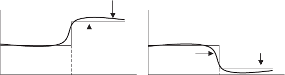
P1: SBT
c07 JWBT188-Aldridge October 23, 2009 14:12 Printer: Yet to come
Market Inefficiency and Profit Opportunities at Different Frequencies 79
Information arrival time Information arrival time
Panel (a):
Good news
Panel (b):
Bad news
Efficient
market
response
Inefficient
market
response
Efficient
market
response
Inefficient
market response
FIGURE 7.1 Incorporation of information in efficient and inefficient markets.
The relative availability of trading opportunities can be measured as
a degree of market inefficiency. An efficient market (Fama, 1970) should
instantaneously reflect all the available information in prices of the traded
securities. If the information is impounded into the securities slowly, then
arbitrage opportunities exist, and the market is considered to be inefficient.
Figure 7.1 illustrates the idea of efficient versus inefficient markets. To
identify markets with arbitrage opportunities is to find inefficient markets.
The arbitrage opportunities themselves are market inefficiencies.
In Figure 7.1, panel (a) shows efficient and inefficient market re-
sponses to “good” information that pushes the price of the security higher,
while panel (b) shows efficient and inefficient market responses to “bad”
information that lowers the price of the security. The price of the secu-
rity in the efficient market adjusts to the new level instantaneously at the
time the news comes out. The price of the security in the inefficient market
begins adjusting before the news becomes public (“information leakage”),
and usually temporarily overreacts (“overshoots”) once the news becomes
public. Many solid trading strategies exploit both the information leakage
and the overshooting to generate consistent profits.
Testing for Market Efficiency and Predictability
The more inefficient the market, the more predictable trading opportuni-
ties become available. Tests for market efficiency help discover the extent
of predictable trading opportunities. This chapter considers several tests
for market efficiency designed to help the researchers to select the most
profitable markets. The chapter by no means considers all the market ef-
ficiency tests that have been proposed in the academic literature; rather,
it summarizes key tests with varying degrees of complexity, from the sim-
plest to the most advanced.
The market efficiency hypothesis has several “levels”: weak, semi-
strong, and strong forms of market efficiency. Tests for the weak form of
market efficiency measure whether returns can be predicted by their past
P1: SBT
c07 JWBT188-Aldridge October 23, 2009 14:12 Printer: Yet to come
80 HIGH-FREQUENCY TRADING
prices and returns alone. Other forms of market efficiency restrict the kinds
of information that can be considered in forecasting prices. The strong
form deals with all kinds of public and nonpublic information; the semi-
strong form excludes nonpublic information from the information set. As
in most contemporary academic literature on market efficiency, we restrict
the tests to the weak form analysis only.
Non-Parametric Runs Test Several tests of market efficiency have
been developed over the years. The very first test, constructed by Louis
Bachelier in 1900, measured the probability of a number of consecutively
positive or consecutively negative price changes, or “runs.” As with tossing
a fair coin, the probability of two successive price changes of the same sign
(a positive change followed by a positive change, for example) is 1/(22)=
0.25. The probability of three successive price changes of the same sign is
1/(23)=0.125. Four successive price changes of the same sign are even
less likely, having the probability of 1/(24)=0.0625 or 6.25 percent. Several
price changes of the same sign in a row present a trading opportunity at
whichever frequency one chooses to consider, the only requirement being
the ability to overcome the transaction costs accompanying the trade.
Thetestworksasfollows:
1. Within a sample containing price moves of the desired frequency, note
the number of sequences consisting strictly of price moves of the same
sign. If the desired frequency is every tick, then a run can be a sequence
of strictly positive or strictly negative price increments from one tick
to the next. If the desired frequency is one minute, a run can be a se-
quence of strictly positive or strictly negative price increments mea-
sured at 1-minute intervals. Table 7.3 shows 1-minute changes in the
AUD/USD exchange rate that occurred from 16:00 GMT to 16:20 GMT
on June 8, 2009.
The 1-minute changes are calculated as follows: if the closing
price for AUD/USD recorded for a given minute is higher than that
for the previous minute, the change for the given minute is recorded
to be positive. If the closing price for AUD/USD recorded for a given
minute is lower than that for the previous minute, the change for the
given minute is recorded to be negative. As shown in Table 7.3, from
16:00 GMT to 16:20 GMT, there were in total nine minutes with positive
change in AUD/USD, eight minutes with negative change in AUD/USD,
and three minutes with 0 change in AUD/USD. Altogether, there were
six positive runs whereby the price of AUD/USD increased, and four
negative runs where the price of AUD/USD decreased. Positive runs
are marked “P” in the “Runs” column, and negative runs are marked
“N.” Thus, minutes marked “P2” correspond to the second run of

P1: SBT
c07 JWBT188-Aldridge October 23, 2009 14:12 Printer: Yet to come
Market Inefficiency and Profit Opportunities at Different Frequencies 81
sequential positive changes, and minutes marked “N1” correspond to
the first run of negative changes.
2. Denote the total number of runs, both positive and negative, observed
in the sample as u. Furthermore, denote as n1the number of posi-
tive 1-minute changes in the sample, and as n2the number of nega-
tive 1-minute changes in the sample. In the sample shown in Table 7.3,
u=10, n1=9, and n2=8.
3. If price changes were completely random, it can be shown that the
expected number of runs in a random sample is ¯x=2n1n2
n1+n2+1, with
the standard deviation of runs being
s=2n1n2(2n1n2−n1−n2)
(n1+n2)2(n1+n2−1).
In the example of Table 7.3, ¯x=9.47, and s=1.99.
TABLE 7.3 One-Minute Closing Price Data on AUD/USD Recorded on June 8,
2009, from 16:00 to 16:20 GMT
DATE TIME Close
1-Minute
Change
Sign of the
Change Runs
6/8/2009 16:00 0.7851
6/8/2009 16:01 0.7853 0.0002 +P1
6/8/2009 16:02 0.7848 −0.0005 −N1
6/8/2009 16:03 0.7841 −0.0007 −N1
6/8/2009 16:04 0.784 −1E-04 −N1
6/8/2009 16:05 0.7842 0.0002 +P2
6/8/2009 16:06 0.7844 0.0002 +P2
6/8/2009 16:07 0.7845 1E-04 +P2
6/8/2009 16:08 0.7845 0
6/8/2009 16:09 0.7847 0.0002 +P3
6/8/2009 16:10 0.7849 0.0002 +P3
6/8/2009 16:11 0.7846 −0.0003 −N2
6/8/2009 16:12 0.7845 −1E-04 −N2
6/8/2009 16:13 0.7839 −0.0006 −N2
6/8/2009 16:14 0.7841 0.0002 +P4
6/8/2009 16:15 0.7841 0
6/8/2009 16:16 0.7837 −0.0004 −N3
6/8/2009 16:17 0.7842 0.0005 +P5
6/8/2009 16:18 0.784 −0.0002 −N4
6/8/2009 16:19 0.784 0
6/8/2009 16:20 0.7842 0.0002 +P6

P1: SBT
c07 JWBT188-Aldridge October 23, 2009 14:12 Printer: Yet to come
82 HIGH-FREQUENCY TRADING
4. Next, we test whether the realized number of runs indicates statistical
nonrandomness. The runs at the selected frequency are deemed pre-
dictable, or nonrandom, with 95 percent statistical confidence if the
number of runs is at least 1.654 standard deviations saway from the
mean ¯x. The number of runs is not random if the two-tailed test based
on Z-score is rejected. The Z-score is computed as Z=|u−¯x|−0.5
s.In
other words, the randomness of runs is rejected with 95 percent statis-
tical confidence whenever Zis greater than 1.645. The randomness of
runs cannot be rejected if Z<1.645.
In the example of Table 7.3, Z=0.0147; therefore, randomness of 1-
minute changes in the sample cannot be rejected.
Table 7.4 summarizes runs test Z-scores obtained for several securi-
ties on data of different frequency for all data of June 8, 2009. As Table 7.4
shows, the runs test rejects randomness of price changes at 1-minute fre-
quencies, except for prices on S&P 500 Depository Receipts (SPY). The
results imply strong market inefficiency in 1-minute data for the securities
shown. Market inefficiency measured by runs test decreases or disappears
entirely at a frequency lower than 10 minutes.
Tests of Random Walks Other, more advanced tests for market
efficiency have been developed over the years. These tests help traders
evaluate the state of the markets and reallocate trading capital to the
markets with the most inefficiencies—that is, the most opportunities for
reaping profits.
When price changes are random, they are said to follow a “random
walk.” Formally, a random walk process is specified as follows:
ln Pt=ln Pt−1+εt(7.2)
where ln Ptis the logarithm of the price of the financial security of inter-
est at time t,lnPt-1is the logarithm of the price of the security one time
TABLE 7.4 Non-Parametric Runs Test Applied to Data on Various Securities and
Frequencies Recorded on June 8, 2009.
Ticker Data Frequency N1N2uZResult
SPY 1 minute 179 183 193 1.11 Random
SPY 10 minutes 21 17 20 −0.10 Random
T 1 minute 142 138 187 5.45 Predictable
T 10 minutes 18 17 20 0.35 Random
USD/JPY 1 minute 558 581 775 12.11 Predictable
USD/JPY 10 minutes 68 64 82 2.55 Predictable
XAU/USD 1 minute 685 631 778 6.61 Predictable
XAU/USD 10 minutes 75 66 76 0.73 Random

P1: SBT
c07 JWBT188-Aldridge October 23, 2009 14:12 Printer: Yet to come
Market Inefficiency and Profit Opportunities at Different Frequencies 83
interval removed at a predefined frequency (minute, hour, etc.), and εtis
the error term with mean 0. From equation (7.2), log price changes ln Pt
are obtained as follows:
ln Pt=ln Pt−ln Pt−1=εt
At any given time, the change in log price is equally likely to be positive and
negative. The logarithmic price specification ensures that the model does
not allow prices to become negative (logarithm of a negative number does
not exist).
The random walk process can drift, and be specified as shown in equa-
tion (7.3):
ln Pt=µ+ln Pt−1+εt(7.3)
In this case, the average change in prices equals the drift rather than 0,
since ln Pt=ln Pt−ln Pt−1=µ+εt. The drift can be due to a variety of
factors; persistent inflation, for example, would uniformly lower the value
of the U.S. dollar, inflicting a small positive drift on prices of all U.S. equi-
ties. At very high frequencies, however, drifts are seldom noticeable.
Lo and MacKinlay (1988) developed a popular test for whether or not a
given price follows a random walk. The test can be applied to processes
with or without drift. The test procedure is built around the following
principle: if price changes measured at a given frequency (e.g., one hour)
are random, then price changes measured at a lower frequency (e.g., two
hours) should also be random. Furthermore, the variances of the 1-hour
and 2-hour changes should be deterministically related. Note that the re-
verse does not apply; randomness in 1-hour price changes does not imply
randomness in 10-minute price changes, nor does it imply a relationship in
variances between the 1-hour and 10-minute samples.
The test itself is based on the following estimators:
ˆµ=1
2n
2n
k=1
(ln Pk−ln Pk−1)=1
2n(ln P2n−ln P0) (7.4)
ˆσ2
a=1
2n
2n
k=1
(ln Pk−ln Pk−1−ˆµ)2(7.5)
ˆσ2
b=1
2n
n
k=1
(ln P2k−ln P2k−2−2ˆµ)2(7.6)
If the error term εtin equations (7.2) or (7.3) is a sequence of indepen-
dent, identically normally distributed numbers with mean 0 and variance

P1: SBT
c07 JWBT188-Aldridge October 23, 2009 14:12 Printer: Yet to come
84 HIGH-FREQUENCY TRADING
σ2
0,ε
t∼i.i.d.N(0,σ2
0), then Lo and MacKinlay (1988) show that the differ-
ences in parameters σ2
0,ˆσ2
a(7.5), and ˆσ2
b(7.6) are asymptotically distributed
as follows:
√2n(ˆσ2
a−σ2
0)a
∼N(0,2σ4
0) (7.7)
√2n(ˆσ2
b−σ2
0)a
∼N(0,4σ4
0) (7.8)
The test for market efficiency is then performed as specified by equation
(7.9):
Jr≡ˆσ2
b
ˆσ2
a−1,√2nJr
a
∼N(0,2) (7.9)
Lo and MacKinlay (1988) subsequently use the test on daily, weekly,
and monthly equity data and conclude that while market efficiency cannot
be rejected for weekly and monthly frequency, daily equity prices are not
efficient.
Table 7.5 summarizes the results of the variance ratio test applied
to several foreign exchange instruments across different frequencies. The
rows represent the estimated values for the variance ratio test Jr, as de-
fined by equation (7.9). The parentheses show the value of the test statistic
measuring the deviation of Jrfrom 0. If the time series follows a random
walk, then the test statistic Jrwill have a normal distribution.
When applied to daily data of the S&P 500 index, the variance ratio test
produced mean Jrof 0.7360 with the corresponding test statistic of 13.84,
significant at 0.001 percent. As Table 7.5 shows, each of the six major USD
crosses are more efficient than the S&P 500: deviations of the variance ra-
tio test statistic, Jr, from 0 are less statistically significant for major USD
crosses and their derivatives than they are for S&P 500, even at high fre-
quencies. The relative inefficiency of S&P 500 signifies that S&P 500 has
more arbitrage opportunities than do the six USD currencies.
According to Table 7.5, daily spot in USD/CAD is the most efficient
currency pair with the fewest number of arbitrage opportunities among
the six major USD-crosses. USD/CAD together with USD/JPY are the most
efficient USD-based pairs in put options written on JPY/USD and CAD/USD
futures with the nearest expiration date.
As Table 7.5 shows, the efficiency of spot instruments decreases—that
is, the number of arbitrage opportunities increases—with increases in data
sampling frequency. For example, the inefficiency of EUR/USD daily spot
rate is higher when EUR/USD is measured at 1-hour intervals than when it
is measured at daily intervals, as evidenced by a higher t-statistic accom-
panying the daily and hourly estimates.

P1: SBT
c07 JWBT188-Aldridge October 23, 2009 14:12 Printer: Yet to come
TABLE 7.5
ThevarianceratiosJrdefined by equation (7.9) are reported in the rows, with the heteroscedasticity-robust test
statistics z*(q) given in parentheses immediately below each row. Under the random walk null hypothesis, the
value of Jris 0 and the test statistics have a standard normal distribution (asymptotically). Test statistics marked
with asterisks indicate that the corresponding variance ratios are statistically different from 0 at the 5 percent
level of significance. The estimation was conducted on data spanning the two-month period of November and
December 2008.
Currency Pair Daily Spot 5-min Spot 15-min Spot 1-Hr Spot
1-Hr
Futures
1-Hr Call
Options
1-Hr Put
Options
AUD/USD 0.6354
(2.27)*
0.7320
(8.74)*
0.7310
(9.21)*
0.7128
(4.90)*
0.7176
(5.48)*
0.6851
(3.72)*
0.6937
(3.75)*
USD/CAD 0.5672
(1.89)
0.7301
(7.97)*
0.7278
(8.61)*
0.7124
(4.90)*
0.7181
(5.48)*
0.6919
(3.87)*
0.6614
(2.98)*
USD/CHF 0.6356
(2.27)*
0.7325
(8.85)*
0.7315
(9.77)*
0.7123
(5.00)*
0.6952
(4.14)*
0.6796
(3.57)*
0.6850
(3.80)*
EUR/USD 0.6355
(2.27)*
0.7359
(15.07)*
0.7337
(10.08)*
0.7135
(5.00)*
0.7189
(5.57)*
0.6912
(3.87)*
0.6836
(3.77)*
GBP/USD 0.6658
(2.27)*
0.7346
(11.00)*
0.7263
(7.01)*
0.7068
(4.84)*
0.6927
(3.72)*
0.6962
(3.88)*
0.6871
(3.81)*
USD/JPY 0.6353
(2.27)*
0.7386
(17.37)*
0.7322
(9.83)*
0.7129
(5.00)*
0.7123
(5.36)*
0.6580
(2.88)*
0.6384
(2.61)*
85

P1: SBT
c07 JWBT188-Aldridge October 23, 2009 14:12 Printer: Yet to come
86 HIGH-FREQUENCY TRADING
As Table 7.5 further shows, spot foreign exchange rates at daily fre-
quencies have the fewest number of persistent trading opportunities. Sur-
prisingly, 1-hr put and call options have fewer trading opportunities than
do spot and futures at the same frequency. Higher frequency markets, how-
ever, show more persistent profit pockets, further strengthening the case
for already popular high-frequency trading styles.
As documented in Table 7.5, even in foreign exchange, value oppor-
tunities exist at high frequencies. Extracting that value requires much in-
genuity, speed, and precision and can be a time-consuming and expensive
process. The tests for market efficiency save traders time and money by
enabling the selection of the most profitable financial instruments and fre-
quencies prior to committing to development of trading models.
Autoregression-Based Tests Trading strategies perform best in the
least efficient markets, where abundant arbitrage opportunities exist. Per-
fectly efficient markets instantaneously incorporate all available market
information, allowing no dependencies from past price movements. One
way to measure the relative degree of market efficiency, therefore, is to
estimate the explanatory power of past prices. Mech (1993) and Hou and
Moskowitz (2005), for example, propose to measure market efficiency as
the difference between Adjusted R2coefficients of an unrestricted model
attempting to explain returns with lagged variables and of a restricted
model involving no past data.
The unrestricted model is specified as follows:
ri,t=αi+βi,1ri,t−1+βi,2ri,t−2+βi,3ri,t−3+βi,4ri,t−4+εi,t(7.10)
where ri,tis the return on security iat time t(see Chapter 8 for a detailed
discussion on the computation of returns).
The restricted model restricts all coefficients βi,jto be 0:
ri,t=αi+εi,t(7.11)
Market inefficiency is next calculated as the relative difference be-
tween Ordinary Least Squares (OLS) R2coefficients of the two models:
Market Inefficiency =1−R2
Restricted
R2
Unrestricted
(7.12)
The closer the difference is to 0, the smaller the influence of past price
movements and the higher the market efficiency.
Market Efficiency Tests Based on the Martingale Hypothesis A
classic definition of market efficiency in terms of security returns is due to
P1: SBT
c07 JWBT188-Aldridge October 23, 2009 14:12 Printer: Yet to come
Market Inefficiency and Profit Opportunities at Different Frequencies 87
Samuelson (1965), who showed that properly anticipated prices fluctuate
randomly in an efficient market. In other words, if all of the news is in-
corporated instantaneously into the price of a given financial security, the
expected price of the security given current information is always the cur-
rent price of the security itself. This relationship is known as a martingale.
Formally, a stochastic price process {Pt}is a martingale within informa-
tion set Itif the best forecast of Pt+1based on current information Itis
equal to Pt:
E[Pt+1|It]=Pt(7.13)
Applying the martingale hypothesis to changes in price levels, we can
express “abnormal,” or returns in excess of expected returns given current
information, as follows:
Zt+1=Pt+1−E[Pt+1|It] (7.14)
A market in a particular financial security or a portfolio of financial
securities is then said to be efficient when abnormal return Zt+1isa“fair
game”—that is,
E[Zt+1|It]=0 (7.15)
LeRoy (1989) provides an extensive summary of the literature on the
subject.
A financial securities market characterized by fair game returns is ef-
ficient as it lacks consistent profit opportunities. As Fama (1991) pointed
out, in a market with trading costs, equation (7.15) will hold within trading
cost deviations.
Fama (1991) also suggested that the efficient markets hypothesis is dif-
ficult to test for the following reason: the idea of a market fully reflect-
ing all available information contains a joint hypothesis. On the one hand,
expected values of returns are a function of information. On the other
hand, differences of realized returns from their expected values are ran-
dom. Incorporating both issues in the same test is difficult. Nevertheless,
martingale-based tests for market efficiencies exist.
Froot and Thaler (1990), for example, derive a specification for a test
of market efficiency of a foreign exchange rate. In equilibrium, foreign ex-
change markets follow the uncovered interest rate parity hypothesis that
formulates the price of a foreign exchange rate as a function of interest
rates in countries on either side of the interest rate. Under the uncovered
interest rate parity, an expected change in the equilibrium spot foreign ex-
change rate S, given that the information set Itis a function of the interest

P1: SBT
c07 JWBT188-Aldridge October 23, 2009 14:12 Printer: Yet to come
88 HIGH-FREQUENCY TRADING
rate differential between domestic and foreign interest rates, rt−rd
tand
risk premium ξtof the exchange rate:
E[St+1|It]=rt−rd
t+ξt(7.16)
where the risk premium ξtis zero for risk-neutral investors and is diversifi-
able to zero for others.
In addition, following the martingale hypothesis, realized spot ex-
change rate at time t+1, St+1is related to its ex-ante expectation E[St+1|It]
as follows:
St+1=E[St+1|It]+ut+1(7.17)
where E[ut+1|It]=0. Combining equations (7.16) and (7.17) yields the fol-
lowing, information-independent test for market efficiency of a foreign ex-
change rate:
St+1=rt−rd
t+εt+1(7.18)
where {εt}series is independent, identically distributed with mean 0.
Taking exponents of both sides of equation (7.18), the test can be spec-
ified in a forward-rate form as follows:
log St+1=log Ft+υt+1(7.19)
where mean of υtis E[υt]=0 and variance of υtis σ2
υ.
The specification of equation (7.19) produces a testable hypothesis at
low frequencies as forward contracts and their open market counterparts
(i.e., futures) typically mature once a quarter. Most low-frequency tests re-
ject predictability of spot rates with forward rates. For example, Hodrick
(1987) notes that none of the pre-1987 tests involving forward rates to
forecast spot rates fit the data. Engel (1996) supports Hodrick’s (1987) con-
clusions and further notes that even when the risk premium in the specifi-
cation of equation (7.18) is assumed to differ from 0, the risk premium fails
to explain the lack of predictability of the forward model. Alexakis and
Apergis (1996), however, find that the forward rates indeed accurately pre-
dict spot rates when predictability is measured in an ARCH specification
(ARCH is discussed in Chapter 8). A high-frequency specification, nonethe-
less, is easy to derive as a differential between two subsequent realizations
of equation (7.19):
log St+1
St=log Ft
Ft−1+υt+1(7.20)
with mean of υtis E[υt]=0 and variance of υtis 2σ2
υ.

P1: SBT
c07 JWBT188-Aldridge October 23, 2009 14:12 Printer: Yet to come
Market Inefficiency and Profit Opportunities at Different Frequencies 89
Cointegration-Based Tests of Market Efficiency Another test of
market efficiency is based on the Engle and Granger (1987) representa-
tion theorem that suggests that cointegration between two variables im-
plies systematic predictability. For example, if some market factor X, say
log forward rate, predicts spot exchange rate Saccording to specification
St=b0+b1Xt+εt, where εtis stationary (has a consistent distribution
over time) and E[εt]=0, then a cointegration-based test for ascertaining
dependency of Son Xhas the following specification:
St=α(b0+b1Xt−1−St−1)+βXt−1+γSt−1+ηt(7.21)
where ηtis an independent, identically distributed error term with mean
0, αmeasures the speed of the model’s adjustment to its long-term equi-
librium, and βand γmeasure short-term impact of lagged changes in X
and S.
Evidence of cointegration on daily closing rates of three or more cur-
rency pairs has been documented by Goodhart (1988), Hakkio and Rush
(1989), Coleman (1990), and Alexander and Johnson (1992), among others.
Literature on the efficient markets hypothesis in foreign exchange fur-
ther distinguishes between speculative and arbitraging efficiencies. The
speculative efficiency hypothesis due to Hansen and Hodrick (1980) pro-
poses that the expected rate of return from speculation in the forward mar-
ket conditioned on available information is zero. The arbitraging efficiency
hypothesis puts forward that the expected return on a portfolio composed
of long one unit of currency and short one future contract on that unit of
currency is zero. The arbitrage strategy of buying one unit of currency and
selling one futures contract is known as uncovered interest arbitrage. The
strategy attempts to arbitrage the uncovered interest parity.
CONCLUSION
The tests of market efficiency illuminate different aspects of a security’s
price and return dependency on other variables. Taking advantage of mar-
ket inefficiency requires an understanding of the different tests that identi-
fied the inefficiency in the first place.
The same security may be predictable at one frequency and fully ran-
dom at another frequency. Various combinations of securities may have
different levels of efficiency. While price changes of two or more securi-
ties may be random when securities are considered individually, the price
changes of a combination of those securities may be predictable, and
vice versa.
P1: SBT
c07 JWBT188-Aldridge October 23, 2009 14:12 Printer: Yet to come
90

P1: SBT
c08 JWBT188-Aldridge October 22, 2009 20:9 Printer: Yet to come
CHAPTER 8
Searching for
High-Frequency
Trading
Opportunities
This chapter reviews the most important econometric concepts used
in the subsequent parts of the book. The treatment of topics is by no
means exhaustive; it is instead intended as a high-level refresher on
the core econometric concepts applied to trading at high frequencies. Yet,
readers relying on software packages with preconfigured statistical proce-
dures may find the level of detail presented here to be sufficient for qual-
ity analysis of trading opportunities. The depth of the statistical content
should be also sufficient for readers to understand the models presented
throughout the remainder of this book. Readers interested in a more thor-
ough treatment of statistical models may refer to Tsay (2002); Campbell,
Lo, and MacKinlay (1997); and Gouri´
eroux and Jasiak (2001).
This chapter begins with a review of the fundamental statistical estima-
tors, moves on to linear dependency identification methods and volatility
modeling techniques, and concludes with standard nonlinear approaches
for identifying and modeling trading opportunities.
STATISTICAL PROPERTIES OF RETURNS
According to Dacorogna et al. (2001, p. 121), “high-frequency data opened
up a whole new field of exploration and brought to light some behaviors
that could not be observed at lower frequencies.” Summary statistics about
aggregate behavior of data, known as “stylized facts,” help distill particu-
larities of high-frequency data. Dacorogna et al. (2001) review stylized facts
91

P1: SBT
c08 JWBT188-Aldridge October 22, 2009 20:9 Printer: Yet to come
92 HIGH-FREQUENCY TRADING
for foreign exchange rates, interbank money market rates, and Eurofutures
(futures on Eurodollar deposits).
Financial data is typically analyzed using returns. A return is a differ-
ence between two subsequent price quotes normalized by the earlier price
level. Independent of the price level, returns are convenient for direct per-
formance comparisons across various financial instruments. A simple re-
turn measure can be computed as shown in equation (8.1):
Rt=Pt−Pt−1
Pt−1=Pt
Pt−1−1 (8.1)
where Rtis the return for period t,Ptis the price of the financial instrument
of interest in period t, and Pt−1is the price of the financial instrument
in period t−1. As discussed previously, determination of prices in high-
frequency data may not always be straightforward; quotes arrive at random
intervals, but the analysis demands that the data be equally spaced.
Despite the intuitiveness of simple returns, much of the financial liter-
ature relies on log returns. Log returns are defined as follows:
rt=ln (Rt)=ln (Pt)−ln (Pt−1)(8.2)
Log returns are often preferred to simple returns for the following
reasons:
1. If log returns are assumed to follow a normal distribution, then the
underlying simple returns and the asset prices used to compute simple
returns follow a lognormal distribution. Lognormal distributions better
reflect the actual distributions of asset prices than do normal distribu-
tions. For example, asset prices are generally positive. Lognormal dis-
tribution models this property perfectly, whereas normal distributions
allow values to be negative.
2. Like distributions of asset prices, lognormal distributions have fatter
tails than do normal distributions. Although lognormal distributions
typically fail to model the fatness of the tails of asset prices exactly,
lognormal distributions better approximate observed fat tails than do
normal distributions.
3. Once log prices have been computed, log returns are easy and fast to
manipulate.
Returns can be computed on bid prices, ask prices, last trade prices,
or mid prices. Mid prices can be taken to be just an arithmetic average,
or a mid-point between a bid and an ask price at any point in time. In the

P1: SBT
c08 JWBT188-Aldridge October 22, 2009 20:9 Printer: Yet to come
Searching for High-Frequency Trading Opportunities 93
absence of synchronous quotes, mid prices can be computed using the last
bid and ask quotes.
Both simple and log returns can be averaged over time to obtain lower-
frequency return estimates. An average of simple and log returns can be
computed as normal arithmetic averages:
E[R]=1
T
T
t=1
Rt(8.3)
µ=1
T
T
t=1
rt(8.4)
Variation in sequential returns is known as volatility. Volatility can
be measured in a variety of ways. The simplest measure of volatility is
variance of simple or log returns, computed according to equations (8.5)
and (8.6).
var [R]=1
T−1
T
t=1
(Rt−E[R])2(8.5)
σ2=1
T−1
T
t=1
(rt−µ)2(8.6)
Note that the division factor in volatility computation is (T−1), not T.The
reduced number of normalizing observations accounts for reduced num-
ber of degrees of freedom—the variance equation includes the average re-
turn, which in most cases is itself estimated from the sample data. Standard
deviation is a square root of the variance.
Other common statistics used to describe distributions of prices or
simple or log returns are skewness and kurtosis. Skewness measures
whether a distribution skews towards either the positive or the negative
side of the mean, as compared with the standardized normal distribution.
Skewness of the standardized normal distribution is 0. Skewness can be
measured as follows:
S[R]=1
T−1
T
t=1
(Rt−E[R])3
(var[R])3/2(8.7)
Kurtosis is a measure of fatness of the tails of a distribution. The fat-
ter the tails of a return distribution, the higher the chance of an extreme
positive or negative return. Extreme negative returns can be particularly
damaging to a trading strategy, potentially wiping out all previous profits

P1: SBT
c08 JWBT188-Aldridge October 22, 2009 20:9 Printer: Yet to come
94 HIGH-FREQUENCY TRADING
and even equity capital. The standardized normal distribution has a kurto-
sis of 3. Kurtosis can be computed as follows:
K[R]=1
T−1
T
t=1
(Rt−E[R])4
(var[R])2(8.8)
If returns indeed follow a lognormal distribution (i.e., log returns rt
are normally distributed with mean µand standard deviation σ2), then
the mean and the standard deviation of simple returns has the following
properties:
E[Rt]=exp µ−σ2
2−1
var[Rt]=exp 2µ+σ2exp(σ2)−1(8.9)
Table 8.1 shows statistics for log returns of EUR/USD. The log returns
are calculated from closing trade prices observed during each period at
different frequencies. If no trades are observed during a particular time
period, the closing trade price from the previous period is used in the es-
timation. As Table 8.1 illustrates, the higher the data frequency, the higher
the kurtosis of the data—that is, the fatter the tails of the data distribution.
Another metric useful to describe distributions of returns is autocor-
relation, which is a measure of serial dependence between subsequent
TABLE 8.1
Summary Statistics for Log Returns for Different Instruments of
EUR/USD at Various Frequencies and for Different Securities (The log
returns are computed from closing trade prices sampled at different
frequencies on data for August–November 2008.)
Frequency Mean Max Median Min
Standard
Deviation Skewness Kurtosis
Daily Spot −0.0003 0.0119 0.0001 −0.0179 0.0052 −0.4389 3.3051
5-min Spot −0.0001 0.0184 0.0000 −0.0225 0.0009 −1.4723 83.7906
15-min
Spot −0.0001 0.0186 0.0000 −0.0226 0.0015 −1.0278 32.6960
1-Hr Spot −0.0002 0.0213 −0.0001 −0.0228 0.0029 −0.8184 14.5028
1-Hr
Futures −0.0002 0.0213 −0.0001 −0.0300 0.0032 −0.7207 13.5256
1-Hr Call
Options −0.0001 0.6551 −0.0031 −0.6555 0.1411 0.3333 8.3108
1-Hr Put
Options
0.0000 2.1115 0.0022 −1.7717 0.1736 0.9859 51.8545

P1: SBT
c08 JWBT188-Aldridge October 22, 2009 20:9 Printer: Yet to come
Searching for High-Frequency Trading Opportunities 95
returns sampled at a specific frequency. For example, autocorrelation of
order 1 measures of 1-minute returns is a correlation of 1-minute returns
with 1-minute returns that occurred 1 minute earlier. Autocorrelation of
order 2 measures of 1-minute returns is a correlation of 1-minute returns
with 1-minute returns that occurred 2 minutes earlier. The autocorrelation
value of order pcan be determined as follows:
ρ(p)=
T
t=p+1(Rt−E[R])(Rt−p−E[R])
T
t=p+1
(Rt−E[R])1/2T
t=p+1
(Rt−p−E[R])1/2(8.10)
As any other correlation function, ρ(p) ranges from −1 to 1. Equation
(8.10) uses simple returns to compute autocorrelation, but returns of any
type can be used instead.
Autocorrelation is of interest because its results indicate a persistent
behavior in returns. For example, Dacorogna et al. (2001) report negative
first-order autocorrelation in 10-minute spot foreign exchange data as evi-
dence of persistent trends in price formation.
Autocorrelation allows us to check whether there are any persistent
momentum/reversal relationships in the data that we could trade upon. For
example, it is a well-known stylized fact that a large swing, or momentum,
in the price of a financial security is typically followed by a reversal. Using
autocorrelation at different frequencies we can actually establish whether
the patterns persist and whether we can trade upon them.
Autocorrelation, like any correlation function, can range from −1to1.
High autocorrelation, say 0.5 and higher, implies a significant positive re-
lationship between current and lagged observations. Low autocorrelation,
say −0.5 and lower, in turn implies a significant negative relationship be-
tween current and lagged observations. Thus, if a return today is positive
and the lag-1 autocorrelation is greater than 0.5, we can expect that the re-
turn tomorrow will be positive as well, at least 50 percent of the time. Thus,
if a return today is positive and the lag-1 autocorrelation is less than −0.5,
we can expect that the return tomorrow will be negative at least 50 per-
cent of the time. Little, if anything, can be said about lagged relationships
characterized by correlations closer to 0.
Of course, we cannot make sweeping inferences without first formally
testing the statistical significance of the observed autocorrelation. There
are two popular tests: (1) a t-ratio test allows us to check whether autocor-
relation is significant at a specific lag, and (2) the Portmanteau test and its
variation, the Ljung-Box test, allow us to determine the last significant au-
tocorrelation in the sequence, beginning with ρ(1). The Portmanteau and

P1: SBT
c08 JWBT188-Aldridge October 22, 2009 20:9 Printer: Yet to come
96 HIGH-FREQUENCY TRADING
Ljung-Box tests are useful in determining the number of lags necessary in
the autoregressive process, which is discussed in the following section.
To determine whether an individual ρ(l) is significant, we can apply
the following test:
t−ratio =ˆρl
(1 +2l−1
i=1ˆρi)/T
(8.11)
For a significance level of (100-α) percent, we reject the observed autocor-
relation ρ(l)if|t−ratio|>Zα/2, where Zα/2is the 100(1 −α/2)th percentile
of the standard normal distribution.
As the t-ratio test indicates, autocorrelation is only 90 percent+statis-
tically significant at lags 1 and 2, meaning that we can reliably use this anal-
ysis to make statistically accurate predictions for at most two days ahead.
To find the optimal number of autocorrelations or the number of lags
to use in forecasting future values, many researchers use the Portmanteau
test and its finite-sample enhancement, the Ljung-Box test. Unlike the
t-ratio test, which tests the statistical significance of an individual autocor-
relation at a particular lag, both the Portmanteau and Ljung-Box tests help
us determine whether correlations at lags 1, 2, ...,lare jointly significant.
The end-goal of the test is to find the lag mwhere autocorrelations
1, 2, ...,mare jointly significant, but autocorrelations 1, 2, ...,m,m+1
are no longer jointly significant. Such a lag m, once identified, signals the
optimal number of lags to be used in further modeling for the security un-
der consideration.
Both Portmanteau and Ljung-Box tests produce similar results when
the number of observations is large. The Ljung-Box test is optimized for
samples with at least 200 observations or 30 at the very minimum.
Formally, the tests are specified as follows: the null hypothesis is
that the mautocorrelations are not jointly statistically significant—that is,
H0:ρ1=...ρ
m=0, and the alternative hypothesis is Ha:ρi= 0 for some
i∈{1,...,m}. To establish that the mth autocorrelation is statistically sig-
nificant, we need to be able to reject the null hypothesis.
Portmanteau test (Box and Pierce [1970]): Q∗(m)=T
m
l=1
ˆρ2
l(8.12)
Ljung-Box test (Ljung and Box [1978]):
Q(m)=T(T+2)
m
l=1
ˆρ2
l
T−l(8.13)
Assuming that the underlying data sequence is independently and
identically distributed, both tests are asymptotically chi-squared random

P1: SBT
c08 JWBT188-Aldridge October 22, 2009 20:9 Printer: Yet to come
Searching for High-Frequency Trading Opportunities 97
TABLE 8.2 Critical Values for the Chi-Squared Distributions with Different
Degrees of Freedom
Statistical Significance
Degrees of
Freedom 90 percent 95 percent 99 percent 99.99 percent
1 2.705541 3.841455 6.634891 15.13429
2 4.605176 5.991476 9.210351 18.42474
3 6.251394 7.814725 11.34488 21.10402
4 7.779434 9.487728 13.2767 23.5064
5 9.236349 11.07048 15.08632 25.75065
6 10.64464 12.59158 16.81187 27.85266
7 12.01703 14.06713 18.47532 29.88138
8 13.36156 15.50731 20.09016 31.82683
9 14.68366 16.91896 21.66605 33.72467
10 15.98717 18.30703 23.20929 35.55716
11 17.27501 19.67515 24.72502 37.36475
12 18.54934 21.02606 26.21696 39.13058
13 19.81193 22.36203 27.68818 40.87346
14 21.06414 23.68478 29.14116 42.57523
15 22.30712 24.9958 30.57795 44.25964
16 23.54182 26.29622 31.99986 45.92551
17 24.76903 27.5871 33.40872 47.55914
18 25.98942 28.86932 34.80524 49.18533
19 27.20356 30.14351 36.19077 50.78726
20 28.41197 31.41042 37.56627 52.38323
variables with mdegrees of freedom. The decision rule is to reject the
null hypothesis at 100(1 −α) percent statistical significance if Q(m)>χ
2
α,
where χ2
αis the 100(1 −α)th percentile of a chi-squared distribution with
mdegrees of freedom. Table 8.2 lists cut-off values for the chi-squared dis-
tributions with different levels of α.
High-frequency trading relies on fast, almost instantaneous, execution
of orders. In this respect, high-frequency trading works best when all or-
ders are initiated, sent through, and executed via computer networks, by-
passing any human interference. Depending on the design of a particular
systematic trading mechanism, even a second’s worth of delay induced by
hesitation or distraction on the part of a human trader can substantially
reduce the system’s profitability.
LINEAR ECONOMETRIC MODELS
Linear econometric models forecast random variables as linear com-
binations of other contemporaneous or lagged random variables with
P1: SBT
c08 JWBT188-Aldridge October 22, 2009 20:9 Printer: Yet to come
98 HIGH-FREQUENCY TRADING
well-defined distributions. In equation terms, linear models can be ex-
pressed as follows:
yt=α+∞
i=0
βixt−i+∞
j=0
γjzt−i+···+εt(8.14)
where {yt}is the time series of random variables that are to be forecasted,
{xt}and {zt}are factors significant in forecasting {yt}, and α,β, and γare
coefficients to be estimated.
Technical analysts like to refer to periods of momentums and rever-
sals. While both can be readily observed on the charts, accurately predict-
ing when the next momentum or reversal begins or ends is not simple.
Autoregressive moving average (ARMA) is an estimation framework
designed to detect consistent momentum and reversal patterns in data of
selected frequencies.
Most linear models require that the distributional properties of data
remain approximately constant through time, or stationary.
Stationarity
Stationarity is measured on the residuals (error terms) of econometric
models. Stationarity requires that the distribution of the residuals remains
stable through time; it is a necessary condition of most linear models.
Stationarity describes the stability of a distribution of a random vari-
able. Distribution of a stationary time series does not change if shifted in
time or space. A number of stationarity tests have been developed, the few
examples of which are Choi (1992), Cochrane (1991), Dickey and Fuller
(1979), and Phillips and Perron (1988). The Augmented Dickey Fuller
(ADF) test frequently appears in the literature and tests several lags of au-
tocorrelation of the dependent variable for unit root (ρ=1). The absence
of unit root indicates stability in the inferences obtained in the estimation.
On the other hand, presence of the unit root suggests that the obtained
results may well be spurious and that the results are invalid.
Autoregressive (AR) Estimation
Autoregressive (AR) estimation models are regressions on the lagged val-
ues of the dependent variable:
yt=α+∞
i=0
βiyt−i+εt(8.15)
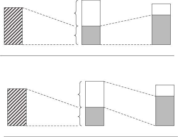
P1: SBT
c08 JWBT188-Aldridge October 22, 2009 20:9 Printer: Yet to come
Searching for High-Frequency Trading Opportunities 99
Coefficients obtained in autoregressions indicate momentum and reversal
patterns in the data. Positive and statistically significant βcoefficients, for
example, indicate positive serial dependence or momentum. Similarly, neg-
ative statistically significant βcoefficients indicate reversal.
Moving Average (MA) Estimation
Moving average (MA) models constitute another set of tools for forecast-
ing future movements of a financial instrument. While autoregressive AR
models estimate what proportion of past period data is likely to persist
in future periods, MA models focus on how future data reacts to innova-
tion in the past data. In other words, AR models estimate future responses
to the expected component realized in the past persistence, whereas MA
models measure future responses to the unexpected component realized
in the past data. Figure 8.1 illustrates the difference between AR and MA
estimation.
Unlike the AR models that can be estimated using ordinary least-
squares or OLS regressions, estimation of moving average models is more
complex. Many off-the-shelf packages provide built-in routines to assist
users in the process.
day 0 day 1 day 2
Expected
component
Unexpected
component
MA
estimation
Step 1 Step 2
day 0 day 1 day 2
Expected
component
Unexpected
component
AR
estimation
Step 1 Step 2
FIGURE 8.1 Illustration of differences between AR and MA estimation.
P1: SBT
c08 JWBT188-Aldridge October 22, 2009 20:9 Printer: Yet to come
100 HIGH-FREQUENCY TRADING
MA(q) model, with qlags, can be specified as follows:
rt=c0+at−θ1at−1−···−θqat−q(8.16)
where c0is the intercept, θlis the coefficient pertaining to lag l, and al
is the unexpected component of the return at lag l. The negative signs in
front of the θ’s are nothing more than a conventional notation of an MA
representation.
For the intrepid, there are two main approaches to estimating MA:
1. Assume that the initial unexpected component is 0 and then recur-
sively estimate other unexpected components using OLS.
2. Assume that the unexpected component is an additional parameter to
be estimated, and then estimate the model using a technique known as
maximum likelihood estimation (MLE).
Using the first approach, estimation proceeds as follows:
1. Run autocorrelation analysis to determine the last statistically signifi-
cant lag, q.
2. Estimate c0by running the following OLS regression of rton a vector of
1’s: rt=c0+at, assuming at∼N(0,σ2). Determine a1’s as at=rt−c0.
3. Estimate c0and θ1using the following OLS regression: rt=c0−θ1a1+
a2, where a1is as determined in Step 2. Find a2’s as a2=rt−c0+θ1a1.
4. Repeat Step 3 to find a3,...,aq, where qis as determined in Step 1.
5. Estimate MA(q) coefficients c0,θ1,θ2,...,θqin the equation rt=
c0−θ1at−1−θ2at−2−···−θqat−q+at, with at−i=aiestimated pre-
viously, and atan error term distributed with mean 0 and variance σ2
a.
Forecasting with MA models is a pretty straightforward exercise. For
a one-period forecast, we are seeking to find E[rt+1], which for MA(q)
model is
E[rt+1|It]=E[c0−θ1at−θ2at−1−···−θqat−q+at+1|It] (8.17)
where Itis the set of all information available at t. The key issue is to re-
member that forecasts for the unexpected components alhave the follow-
ing properties: E[at+1|It]=0, and Var[at+1|It]=σ2
a. Keeping these proper-
ties in mind, E[rt+1|It] now becomes
E[rt+1|It]=c0−θ1at−θ2at−1−···−θqat−q(8.18)
P1: SBT
c08 JWBT188-Aldridge October 22, 2009 20:9 Printer: Yet to come
Searching for High-Frequency Trading Opportunities 101
and the forecast error becomes e(1) =rt+1−E[rt+1|It]=at+1with vari-
ance Var[e(1)] =σ2
a. A two-step-ahead forecast can be computed as
follows: E[rt+2|It]=E[c0−θ1at+1−θ2at−···−θqat−q+1+at+2|It]=c0−
θ2at−···−θqat−q+1. Finally, an l-step ahead forecast for l>qis
E[rt+l|It]=c0.
Autoregressive Moving Average (ARMA)
Autoregressive moving average (ARMA) models combine the AR and MA
models in a single framework. ARMA(p,q), for example, is specified as
follows:
rt=α+
p
i=0
βirt−i−
q
i=0
θiat−i+εt(8.19)
Like MA models, ARMA models are estimated using maximum likelihood
(MLE).
Cointegration
Cointegration is a popular technique used for optimal portfolio construc-
tion, hedging, and risk management. Cointegration measures the con-
temporaneous or lagged effect of one variable on another variable. For
example, if both time series {x}and {y}represent price time series of two
financial securities, cointegration identifies a lead-lag relationship between
the two time series.
The simplest test for lead-lag relationships can be specified using the
following equation, first suggested by Engle and Granger (1987):
xt=α+βyt+εt(8.20)
Equation (8.20) can be estimated using OLS, with the residuals tested for
stationarity.
The cointegration specification of equation (8.20), however, does not
reveal whether one variable drives or causes another. To detect causality,
a technique known as error correction model (ECM) is often used. In the
simplest case with just two variables (e.g., log-price series), the ECM can
be specified as the following pair of simultaneous equations:
xt=α1+β1xt−1+β2yt−1+γ1zt−1+ε1(8.21)
yt=α2+β3xt−1+β4yt−1+γ2zt−1+ε2

P1: SBT
c08 JWBT188-Aldridge October 22, 2009 20:9 Printer: Yet to come
102 HIGH-FREQUENCY TRADING
where denotes the first difference operator and ztis a stationary cointe-
grating vector, zt=xt−α−βytfrom equation (8.20). Equations (8.21) are
then simultaneously estimated using OLS. Coefficients γ1and γ2constrain
deviations from long-run equilibrium specified by equation (8.20) and ex-
plain the “error correction” piece of the ECM.
If β2, the coefficient on the lagged yreturns in the xequation is found
to be significant, then changes in ylead changes in x. In Granger causality
terminology, y“causes” x. Both the direction and strength of causalities
may change over time.
Cointegration is widely used in testing for lead-lag relationships in gen-
erating cross-asset trading signals. Cointegration can also be an important
component of portfolio management and hedging applications.
VOLATILITY MODELING
Most of today’s uses of volatility modeling involve forecasting components
of future returns. The forecasts range from the point forecasts to quantiles
of returns to the probabilistic density of future returns. These forecasts
are used by portfolio managers to optimize the performance of their in-
vestment vehicles, by risk managers to limit their trading downside, and
by quantitative traders to develop superior trading models. According to
Engle and Patton (2001, p. 238):
A risk manager must know today the likelihood that his portfolio
will decline in the future. An option trader will want to know the
volatility that can be expected over the future life of the contract. To
hedge this contract he will also want to know the volatility of his
forecast. A portfolio manager may want to sell a stock or a portfolio
before it becomes too volatile. A market maker may want to set the
bid ask spread wider when the future is believed to be more volatile.
A good volatility model is the one that competently forecasts
volatility:
1. Volatility is persistent.
2. Volatility is mean-reverting.
3. Market returns may have asymmetric impact on volatility.
4. External (exogenous) variables may affect volatility.
Persistence of volatility is sometimes referred to as “volatility cluster-
ing.” The phenomenon describes the observed persistence in the levels of

P1: SBT
c08 JWBT188-Aldridge October 22, 2009 20:9 Printer: Yet to come
Searching for High-Frequency Trading Opportunities 103
volatility; if volatility is high today, it is likely to be high tomorrow. The
converse is also true; volatility that is low during the current observation
period is likely to remain low in the next observation period. The observed
volatility persistence implies that “shocks” (unusually large price moves)
will impact expected volatility measures many observation periods ahead.
According to Engle and Patton (2001), the impact of shocks on future
volatility expectations declines geometrically but can be seen in options
data as long as one year after the occurrence of the shock.
The mean-reversion properties of volatility describe the phenomenon
whereby volatility regresses to its optimal intrinsic levels. Thus, if volatility
is unusually high one period and, due to persistence, will remain high for
several observation periods, it will nevertheless eventually fall to its nor-
mal level. A useful tool for comparing volatility models is to compare the
models’ forecasts many periods ahead. According to the mean-reversion
property of volatility, long-term forecasts of all volatility models should
converge on the same intrinsic volatility value, a finite number.
Positive and negative shocks to market returns have been found to
impact subsequent volatility differently. Market crashes and other nega-
tive shocks have been shown to result in higher subsequent volatility lev-
els than rallies and other news favorable to the market. This asymmetric
property of volatility generates skews in volatility surfaces constructed
of option-implied volatilities for different option strike prices. Engle and
Patton (2001) cite the following example of volatility skews: the implied
volatilities of in-the-money put options are lower than those of at-the-
money put options. Furthermore, the implied volatilities of at-the-money
put options are lower than the implied volatilities of out-of-the-money
options.
Finally, volatility forecasts may be influenced by external events, such
as news announcements. In foreign exchange, for example, price and
return volatility of a particular currency pair increase markedly during
macroeconomic announcements pertaining to one or both sides of the cur-
rency pair.
Volatility can be forecasted in a number of ways. The simplest volatility
forecast assumes that the volatility remains constant through time and that,
as a result, future volatility will be equal to the volatility estimate obtained
from historical data. In this case, the forecast for future squared volatility,
σ2
t+1, is just the variance of the past returns of the security or portfolio
under consideration:
Etσ2
t+1=σ2
t=σ2=1
t−1
t
τ=1Rτ−R2(8.22)
Of course, volatility may change with time. Securities that exhibit time-
varying volatility are said to possess “heteroscedastic” properties, with the

P1: SBT
c08 JWBT188-Aldridge October 22, 2009 20:9 Printer: Yet to come
104 HIGH-FREQUENCY TRADING
term “heteroscedasticity” referring to the varying volatility; the term “ho-
moscedasticity” describes constant volatility.
One way to model volatility that changes with time is to assume that
it stays constant over short periods of time, known as volatility estimation
windows. To do so, the volatility is forecasted as the volatility over the time
window of returns on the security of interest:
Etσ2
t+1=1
T−1
t
τ=t−T+1Rτ−Rt2(8.23)
where Rt=1
T
t
τ=t−T+1
Rτ(8.24)
Similar to moving average estimation, the window used in volatility es-
timation is then moved through time to obtain the latest estimates. Accord-
ing to the central limit theorem, the return window used for estimation of
each individual volatility forecast should contain at least 30 observations.
The time spaces between subsequent returns used within the window can
be made as short as required—thirty 1-second returns can be used to esti-
mate intraminute volatility.
The moving window approach to volatility estimation places equal
weight on all the observations in the sample. The earliest changes in re-
turns are given the same weights as the latest changes, but the latest
changes may possess more relevance to the present time and forecasting of
future returns. To address this issue, several weighting schemes for returns
within a volatility estimation window have been proposed.
The simplest observation weighting scheme is linear or triangular
weighting: each of the Tobservations within the window is multiplied by
a coefficient that reflects the order of the observation within the window.
The earliest observation is given the lowest weight, and the latest observa-
tions are given the highest significance. The resulting forecast of variance
at time t+1 is then computed as follows:
Etσ2
t+1=
t
τ=t−T+1τ−t+T
TRτ−Rt2
(8.25)
where Rt=
t
τ=t−T+1
τ−t+T
TRτ(8.26)
An exponential weighting scheme also gives special significance to
later observations. The scheme uses a geometric coefficient, λ, for weight-
ing observations within the volatility estimation window. The geometric
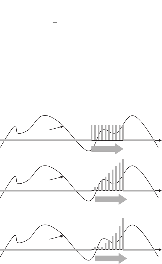
P1: SBT
c08 JWBT188-Aldridge October 22, 2009 20:9 Printer: Yet to come
Searching for High-Frequency Trading Opportunities 105
coefficient is known as the “smoothing parameter” and is used in estima-
tion as follows:
Etσ2
t+1=
t
τ=t−T+1λt−τ(1 −λ)Rτ−Rt2(8.27)
where Rt=
t
τ=t−T+1λt−τ(1 −λ)Rτ(8.28)
The smoothing parameter is normally estimated on historical data using
maximum likelihood. RiskMetricsTM estimates λto be 0.94, but λmay vary
from security to security and with changes in the number of observations,
T, used in the volatility estimation window.
Figure 8.2 graphically compares the shapes of the weights used in
volatility estimation under the simple, equally weighted moving window,
the triangular moving window, and the exponential moving window.
Panel A: Equally weighted estimation
Panel B: Triangular estimation
Panel C: Exponentially weighted estimation
Time
Security
Returns
Time
Security
Returns
Time
Security
Returns
FIGURE 8.2 Panel A: Equally weighted estimation.
P1: SBT
c08 JWBT188-Aldridge October 22, 2009 20:9 Printer: Yet to come
106 HIGH-FREQUENCY TRADING
The moving window estimators of volatility fail to model an important
characteristic of volatility—“volatility clustering.” Volatility clustering de-
scribes the phenomenon of volatility persistence. Current high volatility
does not typically revert to lower volatility levels instantaneously; instead,
high volatility persists for several time periods. The same observation holds
for low volatility; low volatility at present is likely to lead to low volatility
in the immediate future.
To model the observed volatility clustering, researchers use ARMA
technique on volatilities:
σ2
t=α0+
m
i=1
αia2
t−i+
s
j=1
βjσ2
t−j(8.29)
where at=σtzt, where {zt}is a sequence of independent, identically dis-
tributed random variables with mean 0 and variance 1. Additional station-
arity conditions include α0>0,α
i≥0,βj≥0,and max(m,s)
k=1(αk+βk)<1.
Such a volatility model is known as a generalized autoregressive condi-
tional heteroscedasticity (GARCH) process, proposed by Bollerslev (1986),
extending the ARCH specification of Engle (1982).
GARCH parameters are typically estimated recursively using maxi-
mum likelihood with the model’s observation σ0“seeded” with a window-
estimated volatility value. Various extensions to the GARCH specification
include additional explanatory right-hand side variables controlling for
external events, an exponential “EGARCH” specification that addresses
the asymmetric response of returns to positive and negative shocks (bad
news is typically accompanied by a higher volatility than good news), and
a “GARCH-M” model in which the return of a security depends on the
security’s volatility, among numerous other GARCH extensions.
In addition to the moving window and GARCH volatility estimators,
popular volatility measurements include the intraperiod volatility estima-
tor, known as the “realized volatility;” several measures based on the in-
traperiod range of prices; and a stochastic volatility model where volatility
is thought to be a random variable drawn from a prespecified distribu-
tion. The realized volatility due to Andersen, Bollerslev, Diebold, and Labys
(2001) is computed as the sum of squared intraperiod returns obtained by
breaking a time period into nsmaller time increments of equal duration:
RVt=
n
i=1
r2
t,i(8.30)
The range-based volatility measures are based on combinations of
open, high, low, and close prices for every period under consideration.

P1: SBT
c08 JWBT188-Aldridge October 22, 2009 20:9 Printer: Yet to come
Searching for High-Frequency Trading Opportunities 107
Garman and Klass (1980), for example, find that all of the following volatil-
ity estimators are less noisy than the conventional estimator based on the
variance of returns (Ot,Ht,Lt, and Ctdenote the open, high, low, and close
prices for period t, respectively):
ˆσ2
1,t=(Ot−Ct−1)2
2f+(Ct−Ot)2
2(1 −f),0<f<1 (8.31)
ˆσ2
2,t=(Ht−Lt)2
4ln(2) (8.32)
ˆσ2
3,t=0.17(Ot−Ct−1)2
f+0.83 (Ht−Lt)2
(1 −f)4 ln(2),0<f<1 (8.33)
ˆσ2
5,t=0.5(Ht−Lt)2−[2 ln(2) −1](Ct−Ot)2(8.34)
ˆσ2
6,t=0.12(Ot−Ct−1)2
f+0.88 ˆσ2
5,t
1−f,0<f<1 (8.35)
GARCH estimators assume that volatility is a deterministic function
of lagged observations and their variances. The deterministic condition
can be restrictive and fail to reflect the dynamic nature of volatility. A
different class of volatility estimators, known as stochastic volatility esti-
mators, have been developed to allow modeling of heteroscedasticity and
volatility clustering without the functional form restrictions on volatility
specification.
The simplest stochastic volatility estimator can be specified as follows:
vt=σtξt=ςexp(αt/2) ξt(8.36)
where αt=φαt−1+ηtis the parameter modeling volatility persistence,
|φ|<1, ξtis an identically and independently distributed random variable
with mean 0 and variance 1, and ζis a positive constant.
While stochastic volatility models reflect well the random nature un-
derlying volatility processes, stochastic volatility is difficult to estimate.
The parameters of equation (8.36) are often estimated using an economet-
ric technique known as maximum likelihood or its close cousins. Given the
randomness of the stochastic volatility estimator, the estimation process is
quite complex. Estimation of GARCH can seem trivial in comparison with
the estimation of stochastic volatility.

P1: SBT
c08 JWBT188-Aldridge October 22, 2009 20:9 Printer: Yet to come
108 HIGH-FREQUENCY TRADING
NONLINEAR MODELS
Overview
As their name implies, nonlinear models allow modeling of complex non-
trivial relationships in the data.
Unlike linear models discussed in the first section of this chapter, non-
linear models forecast random variables that cannot be expressed as linear
combinations of other, contemporaneous or lagged, random variables with
well-defined distributions. Instead, nonlinear models can be expressed as
some functions f(.) of other random variables. In mathematical terms, if a
linear model can be expressed as shown in equation (8.37), reprinted here
for convenience, then nonlinear models are best expressed as shown in
equation (8.38) which follows:
yt=α+∞
i=0
βixt−i+εt(8.37)
yt=f(xt,xt−1,xt−2,···) (8.38)
where {yt}is the time series of random variables that are to be forecasted,
{xt}is a factor significant in forecasting {yt}, and αand βare coefficients
to be estimated.
The one-step-ahead nonlinear forecast conditional on the information
available in the previous period is usually specified using a Brownian mo-
tion formulation, as shown in equation (8.39):
yt+1=µt+1+σt+1ξt+1(8.39)
where µt+1=Et[yt+1] is the one-period-ahead forecast of the mean of the
variable being forecasted, σt+1=vart[xt+1] is the one-period-ahead fore-
cast of the volatility of the variable being forecasted, and ξt+1is an iden-
tically and independently distributed random variable with mean 0 and
variance 1. The term ξt+1is often referred to as a standardized shock or
innovation.
The nonlinear estimation is often used in pricing derivatives and other
complex financial instruments. In fact, many readers will recognize equa-
tion (8.39) as the cornerstone equation of derivatives pricing models.
Here, we will briefly review the following nonlinear estimation
methods:
rTaylor series expansion (bilinear models)
rThreshold autoregressive model

P1: SBT
c08 JWBT188-Aldridge October 22, 2009 20:9 Printer: Yet to come
Searching for High-Frequency Trading Opportunities 109
rMarkov switching model
rNonparametric estimation
rNeural networks
For a detailed examination of nonlinear estimation, please see
Priestley (1988) and Tong (1990).
Taylor Series Expansion (Bilinear Models)
One of the simplest ways to deal with nonlinear functions is to linearize
them using the Taylor series expansion. The Taylor series expansion of a
univariate function f(x), for any xin the vicinity of some specific value a,
is a derivative-based approximation of the function f(x) and is defined as
follows:
f(x)=f(a)+(x−a)df(x)
dx x=a+1
2(x−a)2d2f(x)
dx2x=a+o(f(x))
(8.40)
where f(a) is the value of the function f(x) at point a,df(x)
dx |x=ais the slope
of the function f(x)atx=a,d2f(x)
dx2|x=ais the curvature of the function f(x)
at point a, and o(f(x)) are higher-order derivative terms of the function
f(x). The higher-order derivative terms o(f(x)) are generally small and are
routinely ignored in estimation.1
Granger and Andersen (1978) showed that equation (8.40) translates
into the following linear econometric equation:
yt=α+
p
i=1
φiyt−i−
q
j=1
θjxt−j+
m
i=1
s
j=1
βij yt−ixt−j+εt(8.42)
where p,q,m, and sare nonnegative integers.
1The Taylor series expansion of a bivariate function f(x,z), for any xin the vicinity
of some points x=aand z=b, includes a cross-derivative and is specified as
follows:
f(x,z)=f(a,b)+(x−a)df(x,z)
dx x=a+(z−b)df(x,z)
dz z=b
+1
2(x−a)2d2f(x,z)
dx2x=a+1
2(z−b)2d2f(x,z)
dz2z=b
(8.41)
+(x−a)(z−b)d2f(x,z)
dxdz x=a,z=b+o(f(x,z))
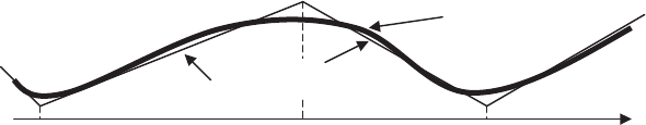
P1: SBT
c08 JWBT188-Aldridge October 22, 2009 20:9 Printer: Yet to come
110 HIGH-FREQUENCY TRADING
Taylor series expansions can be used in estimation of cross-market
derivative/underlying security arbitrage.
Threshold Autoregressive (TAR) Models
Threshold autoregressive (TAR) models approximate nonlinear functions
with piecewise linear estimation with thresholds defined on the dependent
variable. For example, the model may have different specifications for pos-
itive and negative values of the dependent variable, in addition to separate
linear models for large positive and large negative values. Such specifica-
tion can be used in estimation of statistical arbitrage models. Figure 8.3
illustrates the idea.
An example of the TAR of Figure 8.3 may be the following AR(1) spec-
ification:
yt=⎧
⎪
⎪
⎨
⎪
⎪
⎩
−5yt−1+εt,if y
t−1<Threshold 1
5yt−1+εt,if y
t−1∈(Threshold 1,Threshold 2)
−5yt−1+εt,if y
t−1∈(Threshold 2,Threshold 3)
5yt−1+εt,if y
t−1>Threshold 3
(8.43)
The major problem of the TAR models is the models’ discontinuity at
thresholds. Smooth transition AR (STAR) models have been proposed to
address the discontinuities of the TAR models. For detailed treatment of
STAR models, please see Chan and Tong (1986) and Ter¨
asvirta (1994).
Markov Switching Models
Markov models are models with a finite number of mutually exclusive
“states”; the states can be defined as value intervals between successive
thresholds as in TAR models discussed previously, or as some discrete
values potentially reflecting exogenous variables such as states of overall
economy and the like. Contrary to TAR models, in Markov models each
state has a discrete probability of transitioning into another state. The
Original
function
Threshold 1 Threshold 2 Threshold 3 yt–1
Piecewise linear
approximation
FIGURE 8.3 Piecewise linear approximation of a nonlinear function.
P1: SBT
c08 JWBT188-Aldridge October 22, 2009 20:9 Printer: Yet to come
Searching for High-Frequency Trading Opportunities 111
transition probabilities are often estimated from historical data or deter-
mined analytically from theory.
An example of a two-state Markov model with a linear AR(1) specifica-
tion in each state can be of the following nature:
yt=−5yt−1+εt,ifs
t=1
5yt−1+εt,ifs
t=2(8.44)
where stdenotes the “state” of yt, however the state is defined, and state
transition probabilities are specified as follows:
P(st=2|st−1=1) =p1
P(st=1|st−1=1) =1−p1
P(st=1|st−1=2) =p2
P(st=2|st−1=2) =1−p2
(8.45)
Using the advanced statistical properties of the Markov processes, it can be
shown that the expected proportion of time that the 2-state Markov process
spends in state 1 is 1/p1, while the expected proportion of time that the
2-state Markov process spends in state 2 is 1/p2.
Markov switching models can be used in estimation of inter-trade du-
rations and execution probabilities in limit order-based trading and other
optimizations of execution. Markov switching models can also be applied
in estimation of cross-market arbitrage opportunities.
Nonparametric Estimation of Nonlinear Models
Nonparametric estimation denotes a broad class of econometric models
that generally refers to econometric estimation without any assumptions
as to the distribution of estimation errors or the shape of the function relat-
ing dependent and independent variables. One subclass of nonparametric
models discussed here allows us to determine the functional relationship
between dependent and independent variables directly from the historical
data. Such nonparametric techniques boil down to smoothing the data into
a functional form.
The nonparametric estimation of nonlinear models is designed to esti-
mate the following function:
yt=f(xt)+εt(8.46)
where {εt}is the time series sequence of normally distributed errors and
f(.) is an arbitrary, smooth function to be estimated. The simple average
smoothing determines the value of f(x) at every point x=Xby taking the
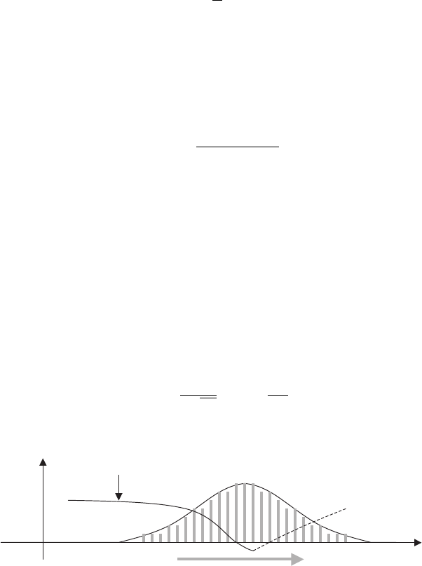
P1: SBT
c08 JWBT188-Aldridge October 22, 2009 20:9 Printer: Yet to come
112 HIGH-FREQUENCY TRADING
across-time averages of both sides of equation (8.46) and utilizing the fact
that E[ε]=0 by assumption:
E[y]=f(x)+E[ε]=f(x) (8.47)
or, equivalently,
f(x)=1
T
T
t=1
yt(8.48)
where Tis the size of the sample.
To make sure that the estimation of f(x) considers only the values
around xand not the values of the entire time series, the values of ytcan
be weighted by a weight function, wt(x). The weight function is determined
by another function, known as a “kernel function,” Kh(x):
wt(x)=Kh(x−xt)
T
t=1
Kh(x−xt)
(8.49)
The weight function, wt(x), defines the location of the filter window
that includes the yelements closest to the xbeing estimated at the mo-
ment and excludes all the y’s outside the filter window. The kernel func-
tion Kh(x) defines the shape of the filter window. As the window is moved
through the continuum of x’s, the yelements fall in and out of the estima-
tion window to reflect their relevance to the estimation. Since the weights
whave to add up to 1 for all values of yconsidered, K(x) can be de-
fined as the probability density function with Kh(x)≥0 and Kh(z)dz =1.
Figure 8.4 shows the process of kernel estimation using the Gaussian
kernel specified as the density of the normal distribution:
Kh(x)=1
h√2πexp −x2
2h2
x
y
**
**
*
**
* * **
**
****
*
The resulting smooth function
FIGURE 8.4 Kernel smoothing using a normal-density kernel.
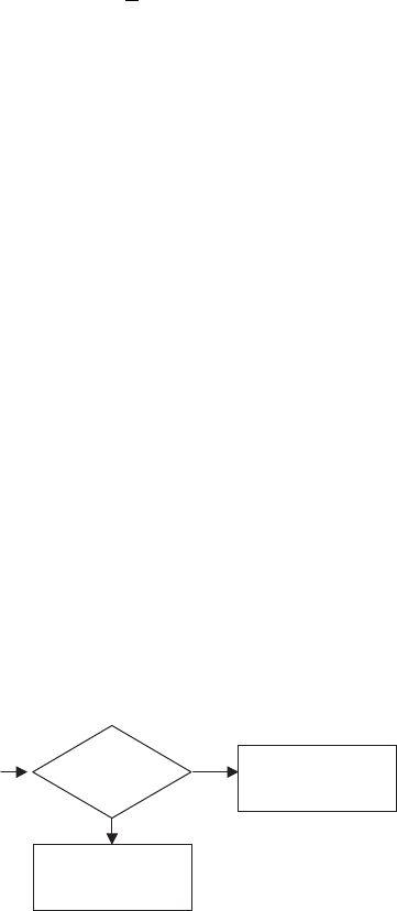
P1: SBT
c08 JWBT188-Aldridge October 22, 2009 20:9 Printer: Yet to come
Searching for High-Frequency Trading Opportunities 113
The width of the estimation window can be controlled through a pa-
rameter known as bandwidth that enters the kernel function as shown in
equation (8.50):
Kh(x)=1
hK(x/h) (8.50)
Fan and Yao (2003) determine the optimal bandwidth parameter hto be
1.06sT−0.2, where sis the sample standard error of xand Tis the total size
of the sample.
Kernel smoothing with different kernel functions is commonly used to
filter the data—that is, to eliminate outliers and other noise.
Neural Networks
Neural networks are an example of semiparametric estimation. The term
“neural network” is sometimes perceived to signal advanced complexity
of a high-frequency system. In reality, neural networks are built instead to
simplify algorithms dealing with econometric estimation.
A neural network is, in essence, a collection of interconnected rules
that are selectively and sequentially triggered, depending on which condi-
tions are satisfied in the real-time data. Caudill (1988, p. 53) defines a neu-
ral network as “a computing system made up of a number of simple, highly
interconnected processing elements, which process information by their
dynamic state response to external inputs.” The simplest neural network
can be built as shown in Figure 8.5.
Advanced neural networks can comprise multiple decisions based on
numerous simultaneous inputs. Neural networks can also incorporate feed-
back mechanisms whereby outputs of the previous periods are taken as
inputs, for example.
Security returns, rtIs rt > 0? Ye s
Forecast for rt+1:
ttt+1rr
εβα
++= 11
No
Forecast for rt+1:
t
rt
rt+1 =
α
2
εβ
++ 2
FIGURE 8.5 A simple neural network that forecasts return values on the basis of
the value of the previous return value. The forecast parameters ˆα1,ˆα2,ˆ
β1,ˆ
β2are
estimated from historical data.

P1: SBT
c08 JWBT188-Aldridge October 22, 2009 20:9 Printer: Yet to come
114 HIGH-FREQUENCY TRADING
The main advantage of neural networks is their simplified step-by-step
structure that can significantly speed up execution of the forecasting algo-
rithm. Neural networks are classified as semiparametric estimation tools,
given that the networks may incorporate both distributional assumptions
and rule-based systems in estimating and forecasting desired variables.
CONCLUSION
The field of econometrics provides a wide range of tools to model statistical
dependencies in the data. Linear models assume that data dependencies
are direct, or linear, while nonlinear models comprise a set of functions for
more involved relationships. Chapter 9 discusses additional high-frequency
estimation models.

P1: SBT
c09 JWBT188-Aldridge October 22, 2009 21:57 Printer: Yet to come
CHAPTER 9
Working with
Tick Data
Trading opportunities are largely a function of the data that identifies
them. As discussed in Chapter 7, the higher the data frequency, the
more arbitrage opportunities appear. When researching profitable op-
portunities, therefore, it is important to use data that is as granular as pos-
sible. Recent microstructure research and advances in econometric model-
ing have facilitated a common understanding of the unique characteristics
of tick data. In contrast to traditional low-frequency regularly spaced data,
tick data is irregularly spaced with quotes arriving randomly at very short
time intervals. The observed irregularities present researchers and traders
with a wealth of information not available in low-frequency data sets. Inter-
trade durations may signal changes in market volatility, liquidity, and other
variables, as discussed further along in this chapter.
In addition, the sheer volume of data allows researchers to produce
statistically precise inferences. As noted by Dacorogna et al. (2001), large
sets of data can support considerably wider ranges of input variables
(parameters) because of the expanded number of allowable degrees of
freedom.
Finally, the copious quantities of tick data allow researchers to use
short-term data samples to make statistically significant inferences pertain-
ing to the latest changes in the markets. Whereas a monthly set of daily data
is normally deemed too short a sample to make statistically viable predic-
tions, volumes of tick data in the same monthly sample can make such
short-term estimation practical. Other frequency-specific considerations,
such as intra-day seasonality, must be taken into account in assessing the
sufficient number of observations.
115

P1: SBT
c09 JWBT188-Aldridge October 22, 2009 21:57 Printer: Yet to come
116 HIGH-FREQUENCY TRADING
This chapter discusses the following topics:
rVarious properties of tick data
rEconometric techniques specific to tick data estimation
rHow trading systems can make better trading decisions using tick data
rHow trading systems can apply traditional econometric principles
PROPERTIES OF TICK DATA
The highest-frequency data is a collection of sequential “ticks,” arrivals
of the latest quote, trade, price, and volume information. Tick data usually
has the following properties:
rA timestamp
rA financial security identification code
rAn indicator of what information it carries:
rBid price
rAsk price
rAvailable bid volume
rAvailable ask volume
rLast trade price
rLast trade size
rOption-specific data, such as implied volatility
rThe market value information, such as the actual numerical value of
the price, available volume, or size
A timestamp records the date and time at which the quote originated.
It may be the time at which the exchange or the broker-dealer released
the quote, or the time when the trading system has received the quote.
The quote travel time from the exchange or the broker-dealer to the trad-
ing system can be as small as 20 milliseconds. All sophisticated systems,
therefore, include milliseconds as part of their timestamps.
Part of the quote is an identifier of the financial security. In equities, the
identification code can be a ticker, or, for tickers simultaneously traded on
multiple exchanges, a ticker followed by the exchange symbol. For futures,
the identification code can consist of the underlying security, futures expi-
ration date, and exchange code.
The last trade price shows the price at which the last trade in the se-
curity cleared. Last trade price can differ from the bid and ask. The dif-
ferences can arise when a customer posts a favorable limit order that is
immediately matched by the broker without broadcasting the customer’s
quote. Last trade size shows the actual size of the last executed trade.

P1: SBT
c09 JWBT188-Aldridge October 22, 2009 21:57 Printer: Yet to come
Working with Tick Data 117
The bid quote is the highest price available for sale of the security in the
market. The ask quote is the lowest price entered for buying the security at
any particular time. Both bid and ask quotes are provided by other market
participants through limit orders. A yet-to-be-executed limit order to buy
with the highest price becomes the market bid, and a limit order to sell
with the lowest price among other limit orders in the same book becomes
the market ask. Available bid and ask volumes indicate the total demand
and supply, respectively, at the bid and ask prices.
QUANTITY AND QUALITY OF TICK DATA
High-frequency data is voluminous. According to Dacorogna et al. (2001),
the number of observations in a single day of tick-by-tick data is equiva-
lent to 30 years of daily observations. The quality of data does not always
match its quantity. Centralized exchanges generally provide accurate data
on bids, asks, and volume of any trade with a reasonably timely timestamp.
The information on the limit order book is less commonly available. In de-
centralized markets, such as foreign exchange and the interbank money
market, no market-wide quotes are available at any given time. In such
markets, participants are aware of the current price levels, but each insti-
tution quotes its own prices adjusted for its order book. In decentralized
markets, each dealer provides his own tick data to his clients. As a result,
a specific quote on a given financial instrument at any given time may vary
from dealer to dealer. Reuters, Telerate, and Knight Ridder, among others,
collect quotes from different dealers and disseminate them back, improv-
ing the efficiency of the decentralized markets. There are generally thought
to be three anomalies in inter-dealer quote discrepancies.
Each dealer’s quotes reflect that dealer’s own inventory. For example,
a dealer that has just sold a customer $100 million of USD/CAD would
be eager to diversify the risk of his position and avoid selling any more
of USD/CAD. Most dealers are, however, obligated to transact with their
clients on tradeable quotes. To incite his clients to place sell orders on
USD/CAD, the dealer temporarily raises the bid quote on USD/CAD. At the
same time, to encourage his clients to withhold placing buy orders, the
dealer raises the ask quote on USD/CAD. Thus, dealers tend to raise both
bid and ask prices whenever they are short in a particular financial instru-
ment and lower both bid and ask prices whenever they are disproportion-
ally long in a financial instrument.
In an anonymous marketplace, such as a dark pool, dealers as well
as other market makers may “fish” for market information by sending in-
dicative quotes that are much off the previously quoted price to assess the
available demand or supply.
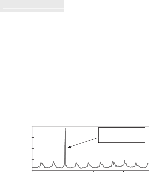
P1: SBT
c09 JWBT188-Aldridge October 22, 2009 21:57 Printer: Yet to come
118 HIGH-FREQUENCY TRADING
Dacorogna et al. (2001) note that some dealers’ quotes may lag real
market prices. The lag is thought to vary from milliseconds to a minute.
Some dealers quote moving averages of quotes of other dealers. The deal-
ers who provide delayed quotes usually do so to advertise their market
presence in the data feed. This was particularly true when most order
prices were negotiated over the telephone, allowing a considerable de-
lay between quotes and orders. Fast-paced electronic markets discourage
lagged quotes, improving the quality of markets.
BID-ASK SPREADS
The difference between the bid quote and the ask quote at any given time
is known as the bid-ask spread. The bid-ask spread is the cost of instan-
taneously buying and selling the security. The higher the bid-ask spread,
the higher a gain the security must produce in order to cover the spread
along with other transaction costs. Most low-frequency price changes are
large enough to make the bid-ask spread negligible in comparison. In tick
data, on the other hand, incremental price changes can be comparable or
smaller than the bid-ask spread.
Bid-ask spreads usually vary throughout the day. Figure 9.1 illustrates
the average bid-ask spread cycles observed in the institutional EUR/USD
market for the last two weeks of October 2008. As Figure 9.1 shows, the
average spread increases significantly during Tokyo trading hours when
the market is quiet. The spread then reaches its lowest levels during the
overlap of the London and New York trading sessions when the market has
many active buyers and sellers. The spike in the spread over the weekend
of October 18–19, 2008, reflects the market concern over the subpoenas
0
5
10
15
20
15-Oct-2008 17-Oct-2008 22-Oct-2008 24-Oct-2008
Dates
pips
Spread on the weekend
of Oct. 18, 2008–Oct. 19,
2008
FIGURE 9.1 Average hourly bid-ask spread on EUR/USD spot for the last two
weeks of October 2008 on a median transaction size of USD 5 million.
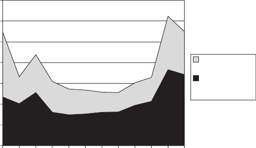
P1: SBT
c09 JWBT188-Aldridge October 22, 2009 21:57 Printer: Yet to come
Working with Tick Data 119
0.00
0.50
1.00
1.50
2.00
2.50
3.00
3.50
0-2
2-4
4-6
6-8
8-10
10-12
12-14
14-16
16-18
18-20
20-22
22-0
Hour of the Day (GMT)
Average Hourly Bid-Ask Spread of
EUR/USD, pips
Crisis Conditions,
Sept–Oct 2008
Normal Market
Conditions,
July–August 2008
FIGURE 9.2 Comparison of average bid-ask spreads for different hours of the
day during normal market conditions and crisis conditions.
issued on October 17, 2009, to senior Lehman executives in a case relating
to potential securities fraud at Lehman Brothers.
Bid-ask spreads typically increase during periods of market uncer-
tainty or instability. Figure 9.2, for example, compares average bid-ask
spreads on EUR/USD in the stable market conditions of July–August 2008
and the crisis conditions of September–October 2008. As Figure 9.2 shows,
the intra-day spread pattern is persistent in both crisis and normal market
conditions, but the spreads are significantly higher during crisis months
than during normal conditions at all hours of the day. As Figure 9.2 also
shows, the spread increase is not uniform at all hours of the day. The av-
erage hourly EUR/USD spreads increased by 0.0048% (0.48 basis points or
pips) between the hours of 12 GMT and 16 GMT, when the London and
New York trading sessions overlap. From 0 to 2 GMT, during the Tokyo
trading hours, the spread increased by 0.0156 percent, over three times the
average increase during the New York/London hours.
As a result of increasing bid-ask spreads during periods of uncer-
tainty and crises, the profitability of high-frequency strategies decreases
during those times. For example, high-frequency EUR/USD strategies run-
ning over Asian hours incurred significantly higher costs during September
and October 2008 as compared with normal market conditions. A strategy
that executed 100 trades during Asian hours alone resulted in 1.56 percent
evaporating from daily profits due to the increased spreads, while the same
strategy running during London and New York hours resulted in a smaller

P1: SBT
c09 JWBT188-Aldridge October 22, 2009 21:57 Printer: Yet to come
120 HIGH-FREQUENCY TRADING
but still significant daily profit decrease of 0.48 percent. The situation can
be even more severe for high-frequency strategies built for less liquid in-
struments. For example, bid-ask spreads for NZD/USD (not shown) on
average increased thrice during September–October in comparison with
market conditions of July–August 2008.
Future realizations of the bid-ask spread can be estimated using the
model of Roll (1984), where the price of an asset at time t,pt, is assumed
to equal an unobservable fundamental value, mt, offset by a value equal
to half of the bid-ask spread, s. The price offset is positive when the next
market order is a buy, and negative when the trade is a sell, as shown in
equation (9.1):
pt=mt+s
2It(9.1)
where
It=1,market buy at ask
−1,market sell at bid
If either a buy or a sell order can arrive next with equal probability,
then E[It]=0, and E[pt]=0, absent changes in the fundamental asset
value, mt. The covariance of subsequent price changes, however, is differ-
ent from 0:
cov [pt,pt+1]=E[ptpt+1]=−s2
4(9.2)
As a result, the future expected spread can be estimated as follows:
E[s]=2−cov [pt,pt+1]whenever cov [pt,pt+1]<0.
Numerous extensions of Roll’s model have been developed to account
for contemporary market conditions along with numerous other variables.
Hasbrouck (2007) provides a good summary of the models.
BID-ASK BOUNCE
While tick data carries information about market dynamics, it is also dis-
torted by the same processes that make the data so valuable in the first
place. Dacorogna et al. (2001) report that sequential trade price bounces
between the bid and ask quotes during market execution of orders intro-
duce significant distortions into estimation of high-frequency parameters.
Corsi, Zumbach, M¨
uller, and Dacorogna (2001), for example, show that the
bid-ask bounce introduces a considerable bias into volatility estimates. The

P1: SBT
c09 JWBT188-Aldridge October 22, 2009 21:57 Printer: Yet to come
Working with Tick Data 121
authors calculate that the bid-ask bounce on average results in –40 percent
negative first-order autocorrelation of tick data. Corsi et al. (2001) as well
as Voev and Lunde (2007) propose to remedy the bias by filtering the data
prior from the bid-ask noise prior to estimation.
MODELING ARRIVALS OF TICK DATA
Unlike low-frequency data, which is recorded at regular time periods, tick
data arrives at irregularly spaced intervals. Several researchers have stud-
ied whether the time distance between subsequent quote arrivals itself car-
ries information. Most researchers agree that inter-trade intervals indeed
carry information on securities for which short sales are disallowed; the
lower the inter-trade duration, the more likely the yet-to-be-observed good
news and the higher the impending price change.
The process of information arrivals is modeled using so-called duration
models. Duration models are used to estimate the factors affecting the du-
ration between any two sequential ticks. Such models are known as quote
processes and trade processes, respectively. Duration models are also used
to measure the time elapsed between price changes of a prespecified size,
as well as the time interval between predetermined trade volume incre-
ments. The models working with fixed price are known as price processes;
the models estimating variation in duration of fixed volume increments are
known as volume processes.
Durations are often modeled using Poisson processes. Poisson pro-
cesses assume that sequential events, like quote arrivals, occur indepen-
dently of one another. The number of arrivals between any two time points
tand (t+τ) is assumed to have a Poisson distribution.
In a Poisson process, λarrivals occur per unit time. In other words, the
arrivals occur at an average rate of (1/λ). The average arrival rate may be
assumed to hold constant, or it may vary with time. If the average arrival
rate is constant, the probability of observing exactly karrivals between
times tand (t+τ)is
P[(N(t+τ)−N(t)) =k]=1
k!e−λτ (λτ )k,k=0,1,2,... (9.3)
Diamond and Verrecchia (1987) and Easley and O’Hara (1992) were
the first to suggest that the duration between subsequent data arrivals car-
ries information. The models posit that in the presence of short-sale con-
straints, inter-trade duration can indicate the presence of good news; in
markets of securities where short selling is disallowed, the shorter the
inter-trade duration, the higher is the likelihood of unobserved good news.

P1: SBT
c09 JWBT188-Aldridge October 22, 2009 21:57 Printer: Yet to come
122 HIGH-FREQUENCY TRADING
The reverse also holds: in markets with limited short selling and normal
liquidity levels, the longer the duration between subsequent trade arrivals,
the higher the probability of yet-unobserved bad news. A complete absence
of trades, however, indicates a lack of news.
Easley and O’Hara (1992) further point out that trades that are sepa-
rated by a time interval have a much different information content than
trades occurring in close proximity. One of the implications of Easley and
O’Hara (1992) is that the entire price sequence conveys information and
should be used in its entirety whenever possible, strengthening the argu-
ment for high-frequency trading.
Table 9.1 shows summary statistics for a duration measure computed
on all trades recorded for S&P 500 Depository Receipts ETF (SPY) on
May 13, 2009. As Table 9.1 shows, the average inter-trade duration was the
longest outside of regular market hours, and the shortest during the hour
preceding the market close (3–4 P.M. ET).
Variation in duration between subsequent trades may be due to sev-
eral other causes. While the lack of trading may be due to a lack of new
information, trading inactivity may also be due to low levels of liquidity,
trading halts on exchanges, and strategic motivations of traders. Foucault,
Kadan, and Kandel (2005) consider that patiently providing liquidity using
limit orders may itself be a profitable trading strategy, as liquidity providers
TABLE 9.1 Hourly Distributions of Inter-Trade Duration Observed on May 13,
2009 for S&P 500 Depository Receipts ETF (SPY)
Inter-Trade Duration (milliseconds)
Hour (ET)
Number
of Trades Average Median Std Dev Skewness Kurtosis
4–5 AM 170 19074.58 5998 47985.39 8.430986 91.11571
5–6 AM 306 11556.95 4781.5 18567.83 3.687372 21.92054
6–7 AM 288 12606.81 4251 20524.15 3.208992 16.64422
7–8 AM 514 7096.512 2995 11706.72 4.288352 29.86546
8–9 AM 767 4690.699 1997 7110.478 3.775796 23.56566
9–10 AM 1089 2113.328 1934 24702.9 3.5185 24.6587
10–11 AM 1421 2531.204 1373 3409.889 3.959082 28.53834
11–12 PM 1145 3148.547 1526 4323.262 3.240606 17.24866
12–1 PM 749 4798.666 1882 7272.774 2.961139 13.63373
1–2 PM 982 3668.247 1739.5 5032.795 2.879833 13.82796
2–3 PM 1056 3408.969 1556 4867.061 3.691909 23.90667
3–4 PM 1721 2094.206 1004 2684.231 2.9568 15.03321
4–5 PM 423 8473.593 1500 24718.41 7.264483 69.82157
5–6 PM 47 73579.23 30763 113747.8 2.281743 7.870699
6–7 PM 3 1077663 19241 1849464 0.707025 1.5

P1: SBT
c09 JWBT188-Aldridge October 22, 2009 21:57 Printer: Yet to come
Working with Tick Data 123
should be compensated for their waiting. The compensation usually comes
in the form of a bid-ask spread and is a function of the waiting time until
the order limit is “hit” by liquidity takers; lower inter-trade durations induce
lower spreads. However, Dufour and Engle (2000) and Saar and Hasbrouck
(2002) find that spreads are actually higher when traders observe short du-
rations, contrasting the time-based limit order compensation hypothesis.
In addition to durations between subsequent trades and quotes, re-
searchers have also been modeling durations between fixed changes in
security prices and volumes. The time interval between subsequent price
changes of a specified magnitude is known as price duration. Price du-
ration has been shown to decrease with increases in volatility. Similarly,
the time interval between subsequent volume changes of a prespecified
size is known as the volume duration. Volume duration has been shown to
decrease with increases in liquidity.
The information content of quote, trade, price, and volume durations
introduces biases into the estimation process, however. If the available
information determines the time between subsequent trades, time itself
ceases to be an independent variable, introducing substantial endogeneity
bias into estimation. As a result, traditional estimates of variance of trans-
action prices are too high in comparison with the true variance of the price
series. The variance of the high-frequency data, however, can be consis-
tently estimated using the generalized autoregressive conditional hetero-
scedasticity (GARCH) process framework that can incorporate inter-trade
and inter-quote duration.
APPLYING TRADITIONAL ECONOMETRIC
TECHNIQUES TO TICK DATA
Most modern computational techniques have been developed to work with
regularly spaced data, presented in monthly, weekly, daily, hourly, or other
consistent intervals. The traditional reliance of researchers on fixed time
intervals is due to
rRelative availability of daily data (newspapers have published daily
quotes since the 1920s)
rRelative ease of processing regularly spaced data
rAn outdated view that “whatever drove security prices and returns, it
probably did not vary significantly over short time intervals.” (Good-
hart and O’Hara 1997, pp. 80–81)
The major difference between tick data and traditional, regularly
spaced data is that tick-by-tick observations are separated by varying time
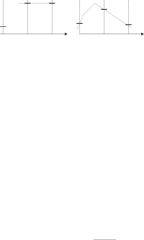
P1: SBT
c09 JWBT188-Aldridge October 22, 2009 21:57 Printer: Yet to come
124 HIGH-FREQUENCY TRADING
Minute 1 Minute 2 Minute 3 Time Minute 1 Minute 2 Minute 3 Time
*
*
*
*
*
*
**
FIGURE 9.3 Data-sampling methodologies.
intervals. One way to overcome the irregularities in the data is to sample
it at certain predetermined periods of time—for example, every hour or
minute.
Traditional financial literature samples closing prices. For example, if
the data is to be converted from tick data to minute “bars,” then under
the traditional approach, the bid or ask price for any given minute would
be determined as the last quote that arrived during that particular minute.
If no quotes arrived during a certain minute, then the previous minute’s
closing prices would be taken as the current minute’s closing prices, and
so on. Figure 9.3, panel (a) illustrates this idea. This approach implicitly
assumes that in the absence of new quotes, the prices stay constant, which
does not have to be the case.
Dacorogna et al. (2001) propose a potentially more precise way to sam-
ple quotes—linear time-weighted interpolation between adjacent quotes.
At the core of the interpolation technique is an assumption that at any given
time, unobserved quotes lie on a straight line that connects two neighbor-
ing observed quotes. Figure 9.3, panel (b) illustrates linear interpolation
sampling.
As shown in Figure 9.3 panels (a) and (b), the two quote-sampling
methods produce quite different results. Dacorogna et al. (2001) do not
provide or reference any studies that compare the performances of the two
sampling methods.
Mathematically, the two sampling methods can be expressed as
follows:
Quote sampling using closing prices: ˆqt=qt,last (9.4)
Quote sampling using linear interpolation:
ˆqt=qt,last +(qt,next −qt,last)t−tlast
tnext −tlast
(9.5)
where ˆqtis the resulting sampled quote, tis the desired sampling time (start
of a new minute, for example), tlast is the timestamp of the last observed

P1: SBT
c09 JWBT188-Aldridge October 22, 2009 21:57 Printer: Yet to come
Working with Tick Data 125
quote prior to the sampling time t,qt,last is the value of the last quote prior
to the sampling time t,tnext is the timestamp of the first observed quote
after the sampling time t, and qt,next is the value of the first quote after the
sampling time t.
Another way to assess the variability of the tick data is through mod-
eling the high-frequency distributions using the mixtures of distributions
model (MODM). Tauchen and Pitts (1983), for example, show that if
changes in the market prices are normally distributed, then aggregates of
price changes and volume of trades approximately form a jointly normal
distribution.
CONCLUSION
Tick data differs dramatically from low-frequency data. Utilization of tick
data creates a host of opportunities not available at lower frequencies.
P1: SBT
c09 JWBT188-Aldridge October 22, 2009 21:57 Printer: Yet to come
126

P1: SBT
c10 JWBT188-Aldridge October 29, 2009 16:53 Printer: Yet to come
CHAPTER 10
Trading on
Market
Microstructure
Inventory Models
Rational expectations and the efficient markets hypotheses imply that,
following a relevant news release, market prices adjust instanta-
neously. From the perspective of a long-term investor, holding posi-
tions for days or months, the adjustment may indeed seem instantaneous.
Anyone who has watched the markets surrounding a major news release,
however, has observed a different picture—a volatile price that eventually
settles within a specific price band. Note that the price eventually settles
within a price range and not at a constant price level, because a degree of
volatility, however small, accompanies all market conditions. The process
of the market finding its optimal post-announcement price band is often
referred to as tˆ
atonnement, from French for “trial and error.”
Figure 10.1 illustrates price adjustments as viewed at different fre-
quencies. At very high frequencies, the price adjustment process is hardly
instantaneous. The tˆ
atonnement toward a new optimal price happens
through the implicit negotiation among buyers and sellers that is occurring
in the order flow; the market participants develop individual security val-
uations given the news, which are reflected in their bids and asks. These
quotes provide market participants with information about other market
participants’ valuations. The process repeats until most market partici-
pants agree on a range of acceptable prices; the equilibrium price band can
then be considered achieved. The process of tˆ
atonnement, therefore, not
only incorporates information into prices but also shapes beliefs of market
participants through a form of collective bargaining process.
The discipline that studies the price formation process is known as
market microstructure. Trading on market microstructure is the holy grail
127
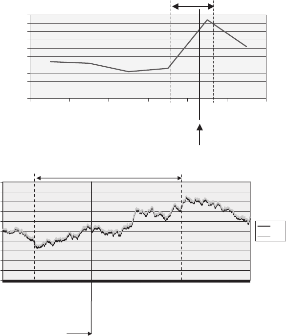
P1: SBT
c10 JWBT188-Aldridge October 29, 2009 16:53 Printer: Yet to come
128 HIGH-FREQUENCY TRADING
1.089
1.0895
1.09
1.0905
1.091
1.0915
1.092
1.0925
1.093
1.0935
1.094
2:00:01
3:00:01
4:00:01
5:00:01
6:00:01
7:00:01
Time (GMT)
USD/CHF Price Level
Price Adjustment Period
News release time
1.085
1.086
1.087
1.088
1.089
1.09
1.091
1.092
1.093
1.094
1.095
04:19:53:737
04:31:40:802
04:44:41:972
04:51:44:015
05:00:22:013
05:14:09:406
05:28:12:164
05:35:09:464
05:45:29:923
05:51:56:382
05:58:53:276
06:05:30:391
06:08:00:711
06:11:22:955
06:14:39:905
06:17:57:625
06:22:56:927
06:27:16:752
06:31:40:095
06:35:48:931
06:38:42:450
06:42:20:491
Time
USD/CHF Price Level
Bid
Ask
News Release Time
Price Adjustment Period
FIGURE 10.1 USD/CHF price adjustments to Swiss unemployment news,
recorded on July 8, 2009 at hourly (top panel) and tick-by-tick (bottom panel) fre-
quencies.
of high-frequency trading. The idea of market microstructure trading is to
extract information from the observable quote data and trade upon that
extracted information in order to obtain gains. Holding periods for posi-
tions in market microstructure trading can vary in duration from seconds
to hours.
The optimal holding period is influenced by the transaction costs faced
by the trader. A gross average gain for a position held just several seconds
will likely be in the range of several basis points (1 basis point =1bp=
1pip=0.01%), at most. To make such trading viable, the expected gain has

P1: SBT
c10 JWBT188-Aldridge October 29, 2009 16:53 Printer: Yet to come
Trading on Market Microstructure 129
to surpass the transaction costs. In an institutional setting (e.g., on a propri-
etary trading desk of a broker-dealer), a trader will often face transaction
costs of 1 bp or less on selected securities, making a seconds-based trading
strategy with an expected gain of at least 2 bps per trade quite profitable.
Other institutional players, such as hedge funds, can expect their transac-
tion costs to range anywhere from 3 bps to 30 bps per trade, mandating
strategies that call for longer holding periods.
According to Lyons (2001), the field of market microstructure encom-
passes two general types of models—inventory models and information
models. Information models are concerned with the process of impound-
ing information into prices in response to news. With information models,
order flow carries information that induces price changes. Inventory
models, on the other hand, explain transitory variations in prices in the
absence of news. As with information models, it is order flow that causes
these temporary variations. Unlike information models where order flow
is a result of end customers receiving and acting on information, inventory
models concern themselves with the order flow resulting from dealer book
imbalances.
This chapter reviews inventory models and their applications to high-
frequency trading. The following chapter, Chapter 11, discusses informa-
tion models.
OVERVIEW OF INVENTORY
TRADING STRATEGIES
Inventory trading, also known as liquidity provision or market making,
concerns itself with profitable management of inventory. Liquidity pro-
vision was once performed only by dedicated broker-dealers, known as
market makers. Market makers kept enough liquidity on hand to satisfy
supply and demand of any arriving traders. During the past decade, this
system changed. The proliferation of electronic transacting capability cou-
pled with the 1997 SEC order display rule enabled most traders to place
the short-term limit orders required to make markets. Several competitive
liquidity provision strategies have emerged to profitably capture liquidity
premiums available in the markets.
Inventory trading strategies possess the following key characteristics:
rThe strategies are executed predominantly using limit orders, although
an occasional market order is warranted to close a position.

P1: SBT
c10 JWBT188-Aldridge October 29, 2009 16:53 Printer: Yet to come
130 HIGH-FREQUENCY TRADING
rThe strategies rely on a multitude of very small realized gains; it is not
uncommon for these strategies to move in and out of positions 2,000
times per day.
rAs a result, these strategies operate at very high frequencies; short po-
sition holding time is what makes it possible to move capital in and out
of multiple trades, generating a large surplus at the end of each day.
rHigh-speed transmission of orders and low-latency execution are re-
quired for successful implementation of liquidity provision strategies.
ORDERS, TRADERS, AND LIQUIDITY
Orders Used in Microstructure Trading
Limit orders, first introduced in Chapter 6, are commitments to buy or sell
a particular security at a prespecified price. Limit orders can be seen as
ex-ante commitments to provide market liquidity. As noted by Demsetz
(1968), while limit orders are in queue, the trader who placed limit orders
incurs inventory and waiting costs. The inventory costs arise from the un-
certainty as to the market price of the securities that the trader may hold
in his portfolio while his limit orders are pending. The waiting costs are
the opportunity costs associated with the time between placing an order
and its execution. In addition, per Copeland and Galai (1983), limit orders
suffer from an informational disadvantage, whereby they are picked off by
better-informed investors.
Naturally, the probability of limit orders being executed depends on
the limit order price proximity to the current market price. Cohen, Maier,
Schwartz, and Whitcomb (1981), call this phenomenon a “gravitational
pull” of existing quotes. Limit orders placed at current market quotes are
likely to be executed, whereas the probability of execution for aggressive
limit orders is close to zero.
Trading with limit orders generates nonlinear payoffs; sometimes limit
orders execute and sometimes they do not. As a result, limit orders are diffi-
cult to model. As Parlour and Seppi (2008) point out, limit orders compete
with other limit orders, both existing and those submitted in the future.
Further, all limit orders execute against future market orders. Thus, when
selecting the price and quantity for a limit order, the trader must take into
account the future trading process, including the current limit order book,
as well as past histories of orders and trading outcomes.
Early limit order models, known as static equilibrium models, pre-
sumed that limit order traders were to be compensated for providing liq-
uidity. Examples of such models include Rock (1996), Glosten (1994),
and Seppi (1997). The longer the waiting time until order execution, the
P1: SBT
c10 JWBT188-Aldridge October 29, 2009 16:53 Printer: Yet to come
Trading on Market Microstructure 131
higher was the expected compensation to liquidity providers who did not
change their limit order specifications once they submitted the orders.
The assumptions behind the static equilibrium models reflected early ex-
change conditions. Changing the details of a limit order was prohibitively
costly, and market makers indeed expected a tidy compensation for bear-
ing the risk of ending up in an adverse position once their limit orders
were hit.
Static equilibrium models, however, have found little empirical sup-
port in the recent literature. In fact, Sandas (2001) in his study of limit or-
ders on actively traded stocks on the Stockholm Stock Exchange finds that
the expected profit on limit orders appears to decrease as the time dura-
tion between market orders increases, contradicting previously formulated
theory. The implicit outcome of empirical evidence is that the limit orders
are submitted by traders with active profit motives, rather than by market
makers interested strictly in providing liquidity.
Demand for trading immediacy can be fueled by the traders’ need for
capital and their risk aversion, among other factors. Traders strapped for
cash may choose to set the limit price close to the market to turn their
positions into cash as soon as possible. Risk-averse traders may choose
to set the limit price close to the market to ensure swift execution and to
minimize uncertainty.
An extension to static equilibrium models penalizes aggressive limit
orders with a non-execution cost. The cost can be considered a penalty
for deviating too far from the trading targets of active limit order traders.
Examples of such an approach include Kumar and Seppi (1994), who mod-
eled two types of limit order traders—value traders and liquidity traders.
Value traders submit limit orders to exploit undervalued limit orders but
have no other reason to trade. Liquidity traders submit limit orders to re-
spond to random liquidity shocks; randomness in their orders leads to price
risk for other traders’ market orders and execution risk in all limit orders.
Cao, Hansch, and Wang (2004) find cointegration of different orders in the
limit order book, supporting the existence of value traders.
Trader Types in Market Microstructure Trading
Harris (1998) identifies three types of traders:
1. Informed traders, who possess material information about an impend-
ing market move
2. Liquidity traders (also known as uninformed traders), who have no ma-
terial market insights and aim to profit from providing liquidity and
following short-term price momentum
P1: SBT
c10 JWBT188-Aldridge October 29, 2009 16:53 Printer: Yet to come
132 HIGH-FREQUENCY TRADING
3. Value-motivated traders, who wait for security prices to become cheap
relative to their proprietary valuations of security based on fundamen-
tal indicators
Informed traders possess private information that allows them to pre-
dict future price changes in a particular security. Private information can
include analyses from paid-for news sources, like Bloomberg, not yet avail-
able to the general public, and superior forecasts based on market mi-
crostructure. Informed traders are often high-frequency money managers
and other proprietary traders with superior access to information and skill
in assessing immediate market situations. The informed traders’ private
information can make a significant impact on the market. As a result, in-
formed traders are impatient and typically execute their orders at market
prices or at prices close to market (see Vega [2007]). Alam and Tkatch
(2007) find that institutional orders are more likely to be market orders
as opposed to limit orders, potentially reflecting advanced information and
skill of institutional money managers.
Liquidity (or uninformed) traders specialize in crafting order submis-
sion strategies in an effort to capture best prices for their customers.
These traders have little proprietary information about the true value of
the security they trade. Executing broker-dealers are examples of liquidity
traders.
Value traders run models to determine the fair value of each secu-
rity, based on the publicly available information. Value traders might be
traditional, low-frequency, institutional money managers; individual day-
traders; or high-frequency managers running high-frequency fundamental
models.
These three types of traders decide when to submit a market order as
opposed to a limit order and at what price to submit a limit order. Such
decisions are optimized to minimize trading costs and maximize portfolio
returns.
According to Harris (1998), market orders and aggressively priced limit
orders are placed by impatient traders, those with material market infor-
mation about to become public. Limit orders that are far away from the
current market price are typically placed by value traders, those seeking
to obtain bargain prices. The remaining limit orders are placed by unin-
formed liquidity traders who are attempting to profit from making markets
and from detecting and following short-term price momentum. Figure 10.2
illustrates the distributions of order aggressiveness and trader types rela-
tive to the market price in the limit order book. Harris (1998) considers a
market for a single security, so that no substitute securities can be traded
in place of an overpriced or illiquid security.
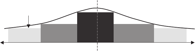
P1: SBT
c10 JWBT188-Aldridge October 29, 2009 16:53 Printer: Yet to come
Trading on Market Microstructure 133
High security price (asks)Low security price (bids) Market price
Informed
traders
Value traders
Liquidity traders
(Uninformed
traders)
Value traders
Liquidity traders
(Uninformed
traders)
Order
aggressiveness
FIGURE 10.2 A graphical representation of order aggressiveness and trader type
distributions in the limit order book.
Kaniel and Liu (2006) extend Angel (1992) and Harris (1998) to show
that informed investors may use limit orders whenever their private in-
formation has a sufficient degree of persistence. Bloomfield, O’Hara, and
Saar (2005) discuss how informed investors are natural liquidity providers.
Because the informed investors know the true value of an asset, they are
the first to know when the prices have adjusted to the levels at which the
limit orders cannot be picked off by other traders. Measures of aggressive-
ness of the order flow may capture informed traders’ information and facil-
itate generation of short-term profits.
Liquidity Provision
Limit orders provide market liquidity. As such, limit orders may fare better
in lower-liquidity markets. The extent of market liquidity available can be
assessed using one or more of the following measures:
1. The tightness of the bid-ask spread. The bid-ask spread indicates
the cost of instantaneous reversal of a given position for a standard
trading amount, or “clip.”
2. Market depth. The depth of the market is the size of all limit orders
posted at the current market price (the best limit price). Market depth
therefore indicates the size of the order that can be processed immedi-
ately at the current market price.
3. Market resilience. Market resilience is a measure of how quickly the
market price mean-reverts to its equilibrium level following a random
order flow.
4. Price sensitivity to block transactions. The sensitivity is most
often measured by what came to be known as “Kyle’s λ,” which is a

P1: SBT
c10 JWBT188-Aldridge October 29, 2009 16:53 Printer: Yet to come
134 HIGH-FREQUENCY TRADING
coefficient from OLS estimation of the following regression (Kyle,
1985):
Pt=α+λNVOLt+εt(10.1)
where Ptis the change in market price due to the market impact of
orders and NVOLtis the difference between the buy and sell market
depths in period t. The smaller the market sensitivity to transaction
size, λ, the larger the market’s capacity to absorb orders at the current
market price.
5. Illiquidity ratio of Amihud (2002). Amihud (2002) notes that illiq-
uid markets are characterized by more drastic relative price changes
per trade. Although changes in trade prices in the most liquid securities
can be as low as one tick (e.g., 0.005 of 1 percent in most currency mar-
kets), in illiquid markets the changes in trade prices can be as large as
20 percent per trade. Amihud (2002), therefore, proposes to measure
the degree of market illiquidity as the average ratio of relative price
change to quantity traded:
γt=1
Dt
Dt
d=1
|rd,t|
νd,t
(10.2)
where Dtis the number of trades executed during time period t,rd,t is
the relative price change following trade dduring trade period t, and
νd,t is the trade quantity executed within trade d.
Limit order books are also often characterized by the presence of
“holes”—that is, ranges of prices that are skipped by investors when sub-
mitting limit orders. Holes were empirically documented by Biais, Hillion
and Spatt (1995), among others.
PROFITABLE MARKET MAKING
Harrison and Kreps (1978) showed that the current value of an asset is de-
termined by its resale potential; as a result, high-frequency investors trad-
ing in multiple markets arbitrage away price discrepancies among markets.
The simplest profitable liquidity provision strategy involves identification
of mispricings on the same security across different markets and arbitrag-
ing away the difference. This is done by posting a limit order to buy just
below the market price in the low-priced market and a limit order to sell
just above market in the high-priced market, and then reversing the posi-
tions once transaction costs were overcome.

P1: SBT
c10 JWBT188-Aldridge October 29, 2009 16:53 Printer: Yet to come
Trading on Market Microstructure 135
Garman (1976) was the first to investigate the optimal market-making
conditions through modeling temporary imbalances between buy and sell
orders. These imbalances are due to differences between the individual
trader and the way a dealer optimizes his order flow, which may reflect un-
derlying differences in budgets, risk appetite, access to markets, and a host
of other idiosyncrasies. The individual trader optimization problems them-
selves are less important than the aggregated order imbalances that these
optimization differences help create. In the Garman (1976) model, the mar-
ket has one monopolistic market maker (dealer). The market maker is re-
sponsible for deciding on and then setting bid and ask prices, receiving all
orders, and clearing trades. The market maker’s objective is to maximize
profits while avoiding bankruptcy or failure. The latter arise whenever the
market maker has no inventory or cash. Both buy and sell orders arrive as
independent stochastic processes.
The model solution for optimal bid and ask prices lies in the estimation
of the rates at which a unit of cash (e.g., a dollar or a “clip” of 10 million
in FX) “arrives” to the market maker when a customer comes in to buy
securities (pays money to the dealer) and “departs” the market maker when
a customer comes in to sell (the dealer pays the customer). Suppose the
probability of an arrival, a customer order to buy a security at the market
ask price pais denoted λa. Correspondingly, the probability of departure
of a clip from the market maker to the customer, or a customer order to
sell securities to the market maker at the bid price pb, can be denoted λb.
Garman (1976) proposes a simple but effective model for the minimum bid-
ask spreads necessary in order for the market maker to remain viable.
The model’s solution is based on the solution to a classical problem
known as the Gambler’s Ruin Problem. In the dealer’s version of the Gam-
bler’s Ruin Problem, a gambler, or a dealer, starts out with a certain initial
wealth position and wagers (stays in business) until he loses all his money.
This version of the Gambler’s Ruin Problem is known as an unbounded
problem. The bounded problem assumes that the gambler bets until he ei-
ther loses all his money or reaches a certain level of wealth, at which point
he exits.
Under the Gambler’s Ruin Problem, the probability that the gambler
will lose all his money is
PrFailure =Pr(Loss) ×Loss
Pr(Gain) ×GainInitial Wealth
(10.3)
where Initial Wealth is the gambler’s start-up cash, Pr(Loss) is the proba-
bility of losing an amount (Loss) of the initial wealth, and Pr(Gain)isthe
probability of gaining an amount (Gain).

P1: SBT
c10 JWBT188-Aldridge October 29, 2009 16:53 Printer: Yet to come
136 HIGH-FREQUENCY TRADING
From the Gambler’s Ruin Problem, we can see that the probability of
failure is always positive. It can be further shown that failure is certain
whenever the probability of losing exceeds the probability of gaining. In
other words, the minimum condition for a positive probability of avoiding
failure in the long term is Pr(Gain)>Pr(Loss).
Garman (1976) applies the Gambler’s Ruin Problem to the market-
making business in the following two ways:
1. The market maker fails if he runs out of cash.
2. The market maker fails if he runs out of inventory and is unable to
satisfy client demand.
In modeling the Gambler’s Ruin Problem for the market maker’s ruin
through running out of inventory, we assume that both the Gain and Loss
variables are single units of the underlying financial asset. In other words,
Gain =1
Loss =1
In the case of equity, this unit may be a share of stock. In the case
of foreign exchange, the unit may be a clip. Then, from the market maker’s
perspective, the probability of “losing” one unit of inventory is the probabil-
ity of selling a unit of inventory, and it equals the probability λaof a buyer
arriving. By the same logic, the probability of gaining one unit of inven-
tory is λb, the probability of a seller arriving. The Gambler’s Ruin Problem
equation (1) now becomes
lim
t→∞ PrFailure(t)≈λa
λbInitial Wealth/E0(pa,pb)
,if λb>λ
a
=1,otherwise.
(10.4)
where E0(pa,pb) is the initial average price of an underlying unit of inven-
tory and
Initial Wealth
E0(pa,pb)
is the initial number of units of the financial instrument in possession of
the market maker.
The Gambler’s Ruin Problem is further applied to the market maker’s
probability of failure due to running out of cash. From the market maker’s
perspective, gaining a unit of cash—say a dollar—happens when a buyer
of the security arrives. As before, the arrival of a buyer willing to buy at

P1: SBT
c10 JWBT188-Aldridge October 29, 2009 16:53 Printer: Yet to come
Trading on Market Microstructure 137
price pahappens with probability λa. As a result, the market maker’s prob-
ability of gaining a dollar is pa. Similarly, the market maker’s probability
of “losing” or giving away a dollar to a seller of the security for selling the
security at price pbis λb. The Gambler’s Ruin Problem now takes the fol-
lowing shape:
lim
t→∞ PrFailure(t)≈λbpb
λapaInitial Wealth
,if λapa>λ
bpb
=1,otherwise
(10.5)
For a market maker to remain in business, the first conditions of equa-
tions (10.4) and (10.5) need to be satisfied simultaneously. In other words,
the following two inequalities have to hold contemporaneously:
λb>λ
aand λapa>λ
bpb
For both inequalities to hold at the same time, the following must be true
at all times: pa>pb, defining the bid-ask spread. The bid-ask spread al-
lows the market maker to earn cash while maintaining sufficient inventory
positions.
Other inventory models assume more detailed specifications for the
market maker’s objectives and constraints. For example, Stoll (1978) as-
sumes that the main objective of the dealer is not only to stay in business
but to effectively manage his portfolio in the face of market pressures. The
bid-ask spread is the market maker’s reward for bearing the costs of mar-
ket making. These costs arise from the following three sources:
1. Inventory costs—the market maker often is left holding a suboptimal
position in order to satisfy market demand for liquidity.
2. Order processing costs specific to the market maker’s own trading
mechanism—these costs may involve exchange fees, settlement and
trade clearing costs, and transfer taxes, among other charges.
3. The information asymmetry cost—a market maker trading with well-
informed traders may often be forced into a disadvantaged trading
position.
As a result, Stoll’s (1978) model predicts that the differences in bid-
ask spreads between different market makers are a function of the market
makers’ respective risk tolerances and execution set-ups.
In Ho and Stoll (1981), the market maker determines bid and ask prices
so as to maximize wealth while minimizing risk. The market maker controls
his starting wealth positions, as well as the amounts of cash and inventory
held on the book at any given time. As in Garman (1976), the arrival rates
P1: SBT
c10 JWBT188-Aldridge October 29, 2009 16:53 Printer: Yet to come
138 HIGH-FREQUENCY TRADING
of bid and ask orders are functions of bid and ask prices, respectively. In
the outcome of the Ho and Stoll (1981) model, the market maker’s spreads
depend on the his time horizon. For example, as the market maker nears
the end of the day, the possible changes in positions become smaller, and
consequently the market maker’s risk of carrying a position decreases.
Therefore, the market maker may lower the spread towards the end of the
day. On the other hand, when the market maker’s time horizon increases,
he increases the spread to be compensated for a higher probability of an
adverse movement to the market maker’s book positions.
Avellaneda and Stoikov (2008) transform Garman’s model into a quan-
titative market-making limit order book strategy that generates persistent
positive returns. Furthermore, the strategy outperforms the “best-bid-best-
ask” market-making strategy where the trader posts limit orders at the
best bid and ask available on the market. For fully rational, “risk-neutral”
traders, the strategy of Avellaneda and Stoikov (2008) also outperforms
the “symmetric” bid and ask strategy whereby the trader places bid and
ask limit orders that are equidistant from the current mid-market price.
Avellaneda and Stoikov (2008) focus on the effects of inventory risk
and derive the optimal bid and ask limit prices for the market maker, given
the following six parameters:
rThe frequency of new bid quotes, λb. For example, λbcan be five
per minute. The frequency of bid quotes can be thought of as demand
for a given security as it reflects the arrival of new sellers.
rThe frequency of new ask quotes, λa. The frequency of ask quotes
can be thought of as an indicator of supply of a given security and the
probability that new buyers will emerge.
rThe latest change in frequency of new bid quotes, λb. For ex-
ample, if 5 bid quotes arrived during the last minute, but 10 bid quotes
arrived during the previous minute, then the change in the bid arrival
frequency is λb=(5 −10)/10 =–0.5.
rThe latest change in frequency of new ask quotes, λa. For ex-
ample, if 5 ask quotes arrived during the last minute, and 5 ask quotes
arrived during the previous minute, then the change in the ask arrival
frequency is λa=(5 −5)/5 =0.
rThe relative risk aversion of the trader, γ. A small value of risk
aversion, γ∼0, represents a risk-neutral investor. A risk aversion of
0.5, on the other hand, represents a very risk-averse investor.
rThe trader’s reservation prices. These are the highest price at
which the trader is willing to buy a given security, rb, and the low-
est price at which the trader is willing to sell a given security, ra.Both
raand rbare determined from a partial differential equation with the
security price, s, trader’s inventory, q, and time, t, as inputs.

P1: SBT
c10 JWBT188-Aldridge October 29, 2009 16:53 Printer: Yet to come
Trading on Market Microstructure 139
The optimal limit bid price, b, and limit ask price, a, are then deter-
mined as follows:
b=rb−1
γln 1−γλb
λband a=ra−1
γln 1−γλa
λa
Avellaneda and Stoikov (2008) offer the following comparisons of their
inventory strategy with best bid/best ask and symmetric strategies for a
reasonable trader risk aversion of 0.1. As Figure 10.3 shows, the inventory
strategy proposed by Avellaneda and Stoikov (2008) has a narrow profit
distribution, resulting in a high Sharpe ratio trading performance.
DIRECTIONAL LIQUIDITY PROVISION
When the Limit Order Book Is Observable
One of the key observations of inventory models is that the shape of
the order book is predictive of impending changes in the market price.
Figure 10.4 illustrates the phenomenon identified by Cao, Hansch, and
Wang (2004). In panel (a), market price is “pushed” by a large concentra-
tion of conservative limit orders.
Cao, Hansch, and Wang (2004) find that the shape of the limit order
book is actively exploited by market-making traders. Cao, Hansch, and
Wang (2004) also find that the breadth and depth (also known as the length
and height) of the limit order book predicts 30 percent of the impending
price moves. Furthermore, the asymmetry in the order book generates ad-
ditional information. Handa, Schwartz, and Tiwari (2003) find that the bid-
ask spread is greater in “balanced” markets when the number of buyers
and sellers is comparable; conversely, the bid-ask spread is lower when-
ever the number of traders on one side of the trading equation exceeds the
number of traders on the other side. According to Handa, Schwartz, and
Tiwari (2003), this imbalance effect stems from the fact that the few traders
on the sparse trading side exert greater market power and obtain better
prices from the investors on the populous trading side who are desperate
to trade.
Rosu (2005) determines that the shape of the limit order book depends
on the probability distribution for arriving market orders. High probabil-
ities of large market orders lead to hump-shaped limit order books. Fou-
cault, Kadan, and Kandel (2005) model continuous-time markets as an
order-determination process on a multiprice grid with infinitely lived limit
orders. Rosu (2005) extends the research with cancelable limit orders.
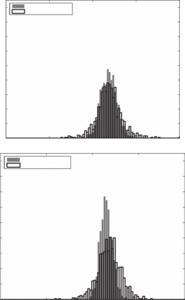
P1: SBT
c10 JWBT188-Aldridge October 29, 2009 16:53 Printer: Yet to come
140 HIGH-FREQUENCY TRADING
180 Inventory strategy
Symmetric strategy
160
140
120
100
80
60
40
20
0
–50 0 50 100 150
180 Inventory strategy
Symmetric strategy
160
140
120
100
80
60
40
20
0
–50 0 50 100 150
FIGURE 10.3 Comparison of performance of inventory, best bid/best ask, and
symmetric strategies per Avellaneda and Stoikov (2008).
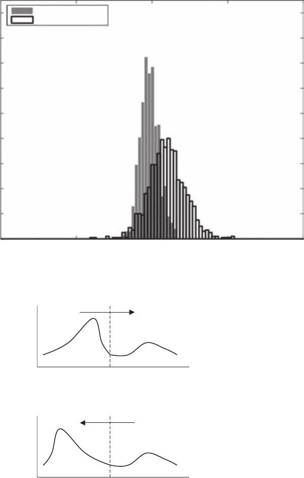
P1: SBT
c10 JWBT188-Aldridge October 29, 2009 16:53 Printer: Yet to come
Trading on Market Microstructure 141
180 Inventory strategy
Symmetric strategy
160
140
120
100
80
60
40
20
0
–50 0 50 100 150
FIGURE 10.3 (Continued)
Panel a): market price gets “pushed” by a large concentration
of conservative limit orders.
Direction of the near-term
movement in the market price
Current market price
Panel b): market price gets “pulled” by a large concentration
of aggressive limit orders.
Direction of the near-term
movement in the market price
Current market price
FIGURE 10.4 Limit book distribution and subsequent price moves.
P1: SBT
c10 JWBT188-Aldridge October 29, 2009 16:53 Printer: Yet to come
142 HIGH-FREQUENCY TRADING
Foucault, Moinas, and Theissen (2005) find that the depth of the limit
order book can forecast future volatility of asset prices. In Holden and
Subrahmanyam (1992), the more volatile the common valuation of the
traded asset, the lower the depth of the information that can be gleaned
from the limit order book. As a result, the limit order market multiplies the
changes in volatility of the traded asset; small changes in the volatility of
the value of the traded asset lead to large changes in volatility of transac-
tion prices, and informed traders are less likely to provide liquidity.
Berber and Caglio (2004) find that limit orders carry private informa-
tion around events such as earnings announcements.
The ability to observe the limit order book in full, however, can de-
liver unfair advantage to market makers. Harris and Panchapagesan (2005)
show that market makers able to fully observe the information in the limit
order book can extract abnormal returns, or “pick off” other limit traders.
When the Limit Order Book Is Not Observable
The directional strategy based on Cao, Hansch, and Wang (2004) requires
full transparency of the limit order book for the instrument of interest. In
many trading venues (e.g., dark pools), the limit order book is not avail-
able. This section discusses approaches for estimating the shape of the
order book.
Kavajecz and Odders-White (2004) show limit orders to be indicative
of future pockets of liquidity. Technical analysis has long been a friend
of traders and a bane of academics. The amount of resources dedicated
to technical analysis in the investment management industry, however,
continues to puzzle academics, who find little plausible explanation for
technical inferences in the science of economics. Most seem to agree that
technical analysis is a self-fulfilling prophecy; when enough people believe
that a particular pricing move is about to occur, they drive the price to
its target location. Yet, technical analysis is more popular in some markets
than in others; for example, many foreign exchange traders actively use
technical analysis, while proportionally fewer equity traders do.
An interesting new application of technical analysis has been uncov-
ered by Kavajecz and Odders-White (2004). The authors find that techni-
cal analysis may provide information about the shape of the limit book.
Specifically, Kavajecz and Odders-White (2004) find that traders are more
likely to place limit orders at the technical support and resistance lev-
els. Thus, the support and resistance indicators pinpoint the liquidity
peaks in the limit order book. This finding may be particularly helpful to
ultra–high-frequency traders working in opaque or dark markets.
In addition, Kavajecz and Odders-White (2004) find that indicators
based on moving averages help identify the skewness of the order book.

P1: SBT
c10 JWBT188-Aldridge October 29, 2009 16:53 Printer: Yet to come
Trading on Market Microstructure 143
When a short-run moving average rises above a long-run moving aver-
age, the buy-side liquidity pool in the limit order book moves closer to
the market price. In this sense, moving average indicators help determine
the skewness of the limit order book. Kavajecz and Odders-White (2004)
speculate that the popularity of technical analysis in foreign exchange is
driven by the absence of a centralized limit order book in the foreign ex-
change market. The authors believe that technical analysis helps traders
reverse-engineer limit order books and deploy profitable liquidity provision
strategies.
CONCLUSION
How does one take advantage of the opportunities present at ultra-high fre-
quencies? First, a thorough econometric analysis of past short-term price
and order book variability can be used to reveal a set of relationships that
can be traded upon. Next, traders can simultaneously submit vectors of
market and limit orders to promptly react to random fluctuations in buy-
ing and selling interest. The uncertainty in the timing of execution of limit
orders, however, must be competently managed because it leads to ran-
dom slippage in traders’ portfolios, introducing a potentially undesirable
stochastic dimension to their portfolio holdings.
Liquidity provision is not only profitable but is also an important func-
tion. As Parlour and Seppi (2008) note, valuation of publicly traded assets
is a “social activity,” strengthening the connection between liquidity and
asset prices. Thus, trading activity creates value to investors who wish to
reallocate their portfolios in response to changes in their personal valua-
tions of assets.
P1: SBT
c10 JWBT188-Aldridge October 29, 2009 16:53 Printer: Yet to come
144

P1: SBT
c11 JWBT188-Aldridge October 29, 2009 16:54 Printer: Yet to come
CHAPTER 11
Trading on
Market
Microstructure
Information Models
Inventory models, discussed in Chapter 10, propose ways in which a
market maker can set limit order prices based on characteristics of
the market maker such as inventory (limit order book) and risk prefer-
ences. As such, inventory models do not account for motivations of other
market participants. The dynamics relating to the trading rationale and ac-
tions of other market participants, however, can significantly influence the
market maker’s behavior.
Information models specifically address the intent and future actions
of various market participants. Information models include game-theoretic
approaches to reverse-engineer quote and trade flows to discover the infor-
mation a market maker possesses. Information models also use observed
or inferred order flow to make informed trading decisions.
At their core, information models describe trading on information flow
and possible informational asymmetries arising during the dissemination
of information. Differences in information flow persist in different mar-
kets. Information flow is comparably faster in transparent centralized mar-
kets, such as most equity markets and electronic markets, and slower in
the opaque markets, such as foreign exchange and OTC markets in bonds
and derivatives.
The main outcome of information models is that the bid-ask spreads
persist even when the market maker has unlimited inventory and is able
to absorb any trading request instantaneously. In fact, the spread is the
way that the market maker stays solvent in the presence of well-informed
traders. As the order flow from informed traders to the market maker
conveys information from traders to the market maker, the subsequent
145

P1: SBT
c11 JWBT188-Aldridge October 29, 2009 16:54 Printer: Yet to come
146 HIGH-FREQUENCY TRADING
changes in the bid-ask spread may also convey information from the mar-
ket maker to other market participants.
This chapter describes information-based microstructure trading
strategies.
MEASURES OF ASYMMETRIC
INFORMATION
Asymmetric information present in the markets leads to adverse selec-
tion, or the ability of informed traders to “pick off” uninformed market
participants. According to Dennis and Weston (2001) and Odders-White
and Ready (2006), the following measures of asymmetric information have
been proposed over the years:
rQuoted bid-ask spread
rEffective bid-ask spread
rInformation-based impact
rAdverse-selection components of the bid-ask spread
rProbability of informed trading
Quoted Bid-Ask Spread
The quoted bid-ask spread is the crudest, yet most readily observable mea-
sure of asymmetric information. First suggested by Bagehot (1971) and
later developed by numerous researchers, the bid-ask spread reflects the
expectations of market movements by the market maker using asymmet-
ric information. When the quoting dealer receives order flow that he sus-
pects may come from an informed trader and may leave the dealer at a
disadvantage relative to the market movements, the dealer increases the
spread he quotes in order to compensate himself against potentially ad-
verse uncertainty in price movements. As a result, the wider the quoted
bid-ask spread, the higher the dealer’s estimate of information asymmetry
between his clients and the dealer himself. Given that the dealer has the
same access to public information as do most of the dealer’s clients, the
quoted bid-ask spread may serve as a measure of asymmetric information
available in the market at large at any given point in time.
Effective Bid-Ask Spread
The effective bid-ask spread is computed as twice the difference between
the latest trade price and the midpoint between the quoted bid and ask

P1: SBT
c11 JWBT188-Aldridge October 29, 2009 16:54 Printer: Yet to come
Trading on Market Microstructure 147
prices, divided by the midpoint between the quoted bid and ask prices. The
effective spread, therefore, produces a measure that is virtually identical
to the quoted bid-ask spread but reflects the actual order book and allows
comparison among financial instruments with various price levels.
Information-Based Impact
The information-based impact measure of asymmetric information is at-
tributable to Hasbrouck (1991). Brennan and Subrahmanyam (1996) spec-
ify the following vector autoregressive (VAR) model for estimation of the
information-based impact measure, λ:
Vi,t=θi,0+
K
k=1
βi,kPi,t−k+
M
m=1
γi,mVi,t−m+τi,t(11.1)
Pi,t=φi,0+φi,1sign(Pi,t)+λiτi,t+εi,t(11.2)
where Pi,tis the change in price of security ifrom time t−1totimet,
Vi,t=sign(Pi,t)·vi,t, and vi,tis the volume recorded in trading the secu-
rity ifrom time t−1 to time t. Brennan and Subrahmanyam (1996) propose
five lags in estimation of equation (1): K=M=5.
Adverse Selection Components of the
Bid-Ask Spread
The adverse selection components of the bid-ask spread is attributable to
Glosten and Harris (1988). The model separates the bid-ask spread into the
following three components:
rAdverse selection risk
rOrder-processing costs
rInventory risk
Models in a similar spirit were proposed by Roll (1984); Stoll (1989);
and George, Kaul, and Nimalendran (1991). The version of the Glosten and
Harris (1988) model popularized by Huang and Stoll (1997) aggregates in-
ventory risk and order-processing costs and is specified as follows:
Pi,t=(1 −λi)Si,t
2sign(Pi,t)+λiSi,t
2sign(Pi,t)·vi,t+εi,t(11.3)
where Pi,tis the change in price of security ifrom time t−1totimet,
Vi,t=sign(Pi,t)·vi,t,vi,tis the volume recorded in trading the security i

P1: SBT
c11 JWBT188-Aldridge October 29, 2009 16:54 Printer: Yet to come
148 HIGH-FREQUENCY TRADING
from time t-1 to time t,Si,t is the effective bid-ask spread as defined previ-
ously, and λiis the fraction of the traded spread due to adverse selection.
Probability of Informed Trading
Easley, Kiefer, O’Hara, and Paperman (1996) propose a model to distill
the likelihood of informed trading from sequential quote data. The model
reverse-engineers the quote sequence provided by a dealer to obtain a prob-
abilistic idea of the order flow seen by the dealer.
The model is built on the following concept: Suppose an event occurs
that is bound to impact price levels but is observable only to a select group
of investors. Such an event may be a controlled release of selected infor-
mation or a research finding by a brilliant analyst. The probability of such
an event is α. Furthermore, suppose that if the event occurs, the probabil-
ity of its having a negative effect on prices is δand the probability of the
event having a positive effect on prices is (1-δ). When the event occurs, in-
formed investors know of the impact the event is likely to have on prices;
they then place trades according to their knowledge at a rate µ. Thus, all
the investors informed of the event will place orders on the same side of
the market—either buys or sells. At the same time, investors uninformed
of the event will keep placing orders on both sides of the market at a rate
ω. The probability of informed trading taking place is then determined as
follows:
PI =αµ
αµ +2ω(11.4)
The parameters α,µ, and ωare then estimated from the following likeli-
hood function over Tperiods of time:
L(B,S|α, µ, ω, δ)=
T
t=1
(B,S,t|α, µ, ω, δ) (11.5)
where (B,S,t|α, µ, ω, δ) is the daily likelihood of observing Bbuys and S
sells:
(B,S,t|α, µ, ω, δ)=(1 −α)exp(−ωT)(ωT)B
B!exp(−ωT)(ωT)S
S!
+α(1 −δ)exp(−(ω+µ)T)((ω+µ)T)B
B!exp(−ωT)(ωT)S
S!
+αδ exp(−ωT)(ωT)B
B!exp(−(ω+µ)T)((ω+µ)T)S
S!
(11.6)

P1: SBT
c11 JWBT188-Aldridge October 29, 2009 16:54 Printer: Yet to come
Trading on Market Microstructure 149
INFORMATION-BASED
TRADING MODELS
Trading on Information Contained in
Bid-Ask Spreads
Liquidity-providing market participants (or market makers) use bid-ask
spreads as compensation for bearing the costs of market making. These
costs arise from the following four sources:
1. Order-processing costs. Order-processing costs are specific to the
market maker’s own trading platform. These costs may involve ex-
change fees, settlement and trade clearing costs, transfer taxes, and
the like. To transfer the order-processing costs to their counterparties,
market makers simply increase the bid-ask spread by the amount it
costs market makers to process the orders.
2. Inventory costs. Market makers often find themselves holding sub-
optimal positions in order to satisfy market demand for liquidity. They
therefore increase the bid-ask spreads they quote to their counterpar-
ties to slow down further accumulation of adverse positions, at least
until they are able to distribute their inventory among other market
participants.
3. Information asymmetry costs. A market maker trading with well-
informed traders may often be forced into a disadvantageous trading
position. For example, if a well-informed trader is able to correctly
forecast that EUR/JPY is about to increase by 1 percent, then the well-
informed trader buys a certain amount of EUR/JPY from the market
maker, leaving the market maker holding a short position in EUR/JPY
in the face of rising EUR/JPY. To hedge his risk of ending up in such
situations, the market maker widens the bid-ask spreads for all of his
counterparties, informed and uninformed alike. The bid-ask spread
on average compensates for the market maker’s risk of being at a
disadvantage.
4. Time-horizon risk. Most market makers are evaluated on the basis of
their daily performance, with a typical trading day lasting eight hours.
At the end of each trading day, the market maker closes his position
book or transfers the book to another market maker who takes the
responsibility and makes decisions on all open positions. At the begin-
ning of each trading shift, a market maker faces the risk that each of
his open market positions may move considerably in the adverse di-
rection by the end of the day if left unattended. As the day progresses,
the market maker’s time horizon shrinks, and with it shrinks the risk
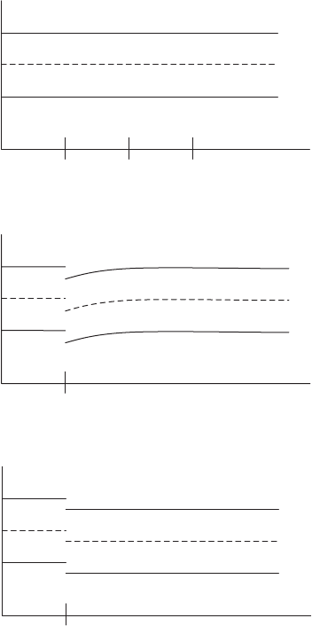
P1: SBT
c11 JWBT188-Aldridge October 29, 2009 16:54 Printer: Yet to come
150 HIGH-FREQUENCY TRADING
of a severely adverse move by the traded security. The market maker
uses the bid-ask spreads he quotes to his counterparties to hedge the
time-horizon risk of his own positions. The bid-ask spreads are great-
est at the beginning of the trading day and smallest at the end of each
trading day.
Figures 11.1–11.3 illustrate the first three dimensions per Lyons (2001).
If bid-ask spreads were to compensate the dealer for order process-
ing costs only, then the mid-price does not change in response to the
Askt
Bidt
Midt
*
*
*
Sell Buy Sell
Time
FIGURE 11.1 Order-processing costs.
Ask t
Bid t
Mid t
*
Sell
Time
FIGURE 11.2 Inventory costs.
Askt
Bidt
Midt
*
Sell
Time
FIGURE 11.3 Asymmetric information (adverse selection).
P1: SBT
c11 JWBT188-Aldridge October 29, 2009 16:54 Printer: Yet to come
Trading on Market Microstructure 151
order. If bid-ask spreads were to compensate the dealer for the risks as-
sociated with holding excess inventory, then any changes in prices would
be temporary. If all orders were to carry information that led to permanent
price changes, the bid-ask spreads would compensate the dealer for the
potential risk of encountering adverse asymmetric information.
Analyzing the bid-ask spreads of the market maker gives clues to the
position sizes of the market maker’s inventory and allows the market
maker to estimate the order flow faced by the market maker. Unexpectedly
widening spreads may signal that the market maker has received and is pro-
cessing large positions. These positions may be placed by well-informed
institutional traders and may indicate the direction of the security price
movement in the near future. Information about future price movements
extracted from the bid-ask spreads may then serve as reliable forecasts of
direction of upcoming price changes.
Gains achieved in the markets are due either to market activity or to
trading activity. Market gains, also referred to as capital gains, are com-
mon to most long-term investors. When markets go up, so do the gains of
most investors long in the markets; the opposite occurs when the markets
go down. Over time, as markets rise and fall, market investors expect to
receive the market rate of return on average. As first noted by Bagehot
(1971), however, the presence of short-term speculative traders may skew
the realized return values.
If a market maker knew for sure that a specific trader had superior
information, that market maker could raise the spread for that trader
alone. However, most traders trade on probabilities of specific events
occurring and cannot be distinguished ahead of closing their positions
from uninformed market participants. To compensate for the informed
trader–related losses, the market maker will extract higher margins from
all of his clients by raising the bid-ask spread. As a result, in the presence
of well-informed traders, both well-informed and less-informed market par-
ticipants bear higher bid-ask spreads.
Important research on the topic is documented in Glosten and
Milgrom (1985). The authors model how informed traders’ orders incor-
porate and distribute information within a competitive market. At the fun-
damental level, traders who have bad news about a particular financial se-
curity ahead of the market will sell that security, and traders with good
news will buy the security. However, well-informed traders may also buy
and sell to generate liquidity. Depending on the type of the order the mar-
ket maker receives (either a buy or a sell), the market maker will adjust his
beliefs about the impending direction of the market for a particular finan-
cial security. As a result, the market maker’s expected value of the security
changes, and the market maker subsequently adjusts the bid and the ask
prices he is willing to trade upon with his clients.
P1: SBT
c11 JWBT188-Aldridge October 29, 2009 16:54 Printer: Yet to come
152 HIGH-FREQUENCY TRADING
Glosten and Milgrom (1985) model the trading process as a sequence
of actions. First, some traders obtain superior information about the true
value of the financial security, V, while other market participants do not.
Informed traders probabilistically profit more often than do uninformed
traders and consequently are interested in trading as often as possible.
Because informed traders know the true value V, they will always gain
at the expense of the uninformed traders. The uninformed traders may
choose to trade for reasons other than short-term profits. For example,
market participants such as long-term investors uninformed of the true
value of the security one minute from now may have a pretty good idea
of the true value of the security one day from now. These uninformed in-
vestors are therefore willing to trade with an informed trader now even
though in just one minute the investors could get a better price, unbe-
knownst to them at present. In the foreign exchange market, uninformed
market participants such as multinational corporations may choose to
trade to hedge their foreign exchange exposure.
The informed traders’ information gets impounded into prices by the
market maker. When a market maker receives an order, the market maker
reevaluates his beliefs about the true value of the financial security based
on the parameters of the order. The order parameters may be the action
(buy or sell), limit price if any, order quantity, leverage or margin, and the
trader’s prior success rate, among other order characteristics. The process
of incorporating new information into prior beliefs that the market maker
undergoes with every order is often modeled according to the Bayes rule.
Updating beliefs according to the Bayes rule is known as Bayesian learning.
Computer algorithms employing Bayesian learning are often referred to as
genetic algorithms.
“In Praise of Bayes,” an article in the The Economist from September
40, 2000, describes Bayesian learning as follows:
The essence of the Bayesian approach is to provide a mathematical
rule explaining how you should change your existing beliefs in the
light of new evidence. In other words, it allows scientists to combine
new data with their existing knowledge or expertise. The canoni-
cal example is to imagine that a precocious newborn observes his
first sunset, and wonders whether the sun will rise again or not. He
assigns equal prior probabilities to both possible outcomes, and rep-
resents this by placing one white and one black marble into a bag.
The following day, when the sun rises, the child places another white
marble in the bag. The probability that a marble plucked randomly
from the bag will be white (i.e., the child’s degree of belief in future
sunrises) has thus gone from a half to two-thirds. After sunrise the
next day, the child adds another white marble, and the probability

P1: SBT
c11 JWBT188-Aldridge October 29, 2009 16:54 Printer: Yet to come
Trading on Market Microstructure 153
(and thus the degree of belief) goes from two-thirds to three-quarters.
And so on. Gradually, the initial belief that the sun is just as likely
as not to rise each morning is modified to become a near-certainty
that the sun will always rise.
Mathematically, the Bayes rule can be specified as follows:
Pr(seeing data) =Pr(seeing data |event occurred) Pr(event occurred)
+Pr(seeing data |no event) Pr(no event) (11.7)
where Pr(event) may refer to the probability of the sun rising again or the
probability of security prices rising, while seeing may refer to registering a
buy order or actually observing the sunrise. No event may refer to a lack of
buy orders or inability to observe a sunrise on a particular day—for exam-
ple, due to a cloudy sky. The probability of seeing data and registering an
event at the same time has the following symmetric property:
Pr(seeing data, event) =Pr(event|seeing data) Pr(seeing data)
=Pr(seeing data|event) Pr(event) (11.8)
Rearranging equation (11.8) to obtain expression for Pr(event|seeing data)
and then substituting Pr (seeing data)from equation (1) produces the
following result:
Pr(event|seeing data) =
Pr(seeing data|event) Pr(event)
Pr(seeing data|event) Pr(event) +Pr(seeing data|no event) Pr(no event)
(11.9)
Equation (11.9) is known as the Bayes rule, and it can be rewritten as
follows:
Posterior belief =Pr(event|seeing data)
=Prior belief ×Pr(seeing data|event)
Marginal likelihood of the data (11.10)
Market makers apply the Bayes rule after each order event, whether
they consciously calculate probabilities or unconsciously use their trad-
ing experience. For example, suppose that the market maker is in charge
of providing liquidity for the Australian dollar, AUD/USD. The current
mid-price, Vmid, for AUD/USD is 0.6731. Consequently, the market maker’s

P1: SBT
c11 JWBT188-Aldridge October 29, 2009 16:54 Printer: Yet to come
154 HIGH-FREQUENCY TRADING
initial belief about the true price for AUD/USD is 0.6731. At what level
should the market maker set bid and ask prices?
According to the Bayes rule, the market maker should set the new ask
price to the expected Vask, given the buy order: E[Vask|buy order]. Sup-
pose that the market maker cannot distinguish between informed and un-
informed traders and assigns a 50 percent probability to the event that a
market buy order will arrive from an informed trader and a 50 percent
probability to the event that a market buy order will arrive from an unin-
formed trader. In addition, suppose that any informed trader would place
a buy order only if the trader was certain he could make at least 5 pips
on each trade in excess of the bid-ask spread and that there are no other
transaction costs. If the average bid-ask spread on AUD/USD quoted by the
market maker is 2 pips, then an informed trader would place a buy order
only if he believes that the true value of AUD/USD is at least 0.6738. From
the market maker’s perspective, the Bayesian probability of the true value
of AUD/USD, Vask, being worth 0.6738 after observing a buy order is calcu-
lated as follows:
Pr(Vask =0.6738|buy order) =
Pr(Vask =0.6738) Pr(buy order|Vask =0.6738)
Pr(Vask =0.6731) Pr(buy order|Vask =0.6731)
+Pr(Vask =0.6738) Pr(buy order|Vask =0.6738)
(11.11)
If the true value Vask is indeed 0.6738, then an informed trader places
the buy order with certainty (a probability of 100 percent), while the unin-
formed trader may place a buy order with a probability of 50 percent (also
with a probability of 50 percent, the uninformed trader may place a sell
order instead). Thus, if the true price Vask =0.6738,
Pr(buy order|Vask =0.6738) =Pr(informed trader) ∗100 percent
+Pr(uninformed trader)∗50 percent
(11.12)
Since we previously assumed that the market maker cannot distinguish
between informed and uninformed traders and assigns equal probability to
either,
Pr(informed trader) =Pr(uninformed trader) =50 percent (11.13)
Combining equations (11.12) and (11.13), we obtain the following proba-
bility of the buy order being an indication of the buy order resulting from
higher true value Vask:

P1: SBT
c11 JWBT188-Aldridge October 29, 2009 16:54 Printer: Yet to come
Trading on Market Microstructure 155
Pr(buy order|Vask =0.6738) =50 percent∗100 percent
+50 percent∗50 percent (11.14)
=75 percent.
The probability of the buy order resulting from the lower, unchanged, true
value Vask is then
Pr(buy order|Vask =0.6731) =1−Pr(buy order|Vask =0.6738)
=25 percent.(11.15)
Assuming that the market maker has no indication where the market
is going—in other words, from the market maker’s perspective at the given
moment,
Pr(Vask =0.6738) =Pr(Vask =0.6731) =50 percent (11.16)
and substituting equations (11.13), (11.14), (11.15), and (11.16) into equa-
tion (11.11), we obtain the following probability of the true value of
AUD/USD being at least 0.6738 given that the buy order arrived:
Pr(Vask =0.6738|buy order) =50% ×75%
50% ×25% +50% ×75% =75%
By the same logic, Pr(Vask =0.6731|buy order) =25%.
Having calculated these probabilities, the market maker is now ready
to set market prices. He sets the price equal to the conditional expected
value as follows:
New ask price =E[V|buy order] =0.6731 ×Pr(Vask =0.6731)
+0.6738 ×Pr(Vask =0.6738) (11.17)
=0.6731 ×25% +0.6738 ×75% =0.6736
Similarly, a new bid price can be calculated as E[Vbid|sellorder] after ob-
serving a sell order. The resulting bid and ask values are tradable “regret-
free” quotes. When the market maker sells a unit of his inventory known as
a clip to the buyer at 0.6736, the market maker is protected against the loss
because of the buyer’s potentially superior information.
If a buy order at ask of 0.6738 actually arrives, the market maker then
recalculates his bid and ask prices as new conditional expected values.
The market maker’s new posterior probability of a buy coming from an in-
formed trader is 75 percent by the foregoing calculation. Furthermore, an
P1: SBT
c11 JWBT188-Aldridge October 29, 2009 16:54 Printer: Yet to come
156 HIGH-FREQUENCY TRADING
informed buyer would buy at 0.6738 only if the true value of AUD/USD less
the ask price exceeded the average spread and the trader’s minimum de-
sired gain. Suppose that, as before, the trader expects the minimum desired
gain to be 5 pips and the average spread to be 2 pips, making him willing
to buy at 0.6738 only if the true value of AUD/USD is at least 0.6745. The
market maker will now once again adjust his bid and ask prices conditional
on such expectation.
One outcome of Glosten and Milgrom (1985) is that in the presence of
a large number of informed traders, a market maker will set unreasonably
high spreads in order to break even. As a result, no trades will occur and
the market will shut down.
In Glosten and Milgrom (1985) all trades are done on one unit of the
financial security. Glosten and Milgrom (1985) do not consider the im-
pact that the trade size has on price. Easley and O’Hara (1987) extend the
Glosten and Milgrom model to incorporate varying trade sizes. Easley and
O’Hara (1987) further add one more level of complexity—information ar-
rives with probability α. Still, both Glosten and Milgrom (1985) and Easley
and O’Hara are models in which informed traders simply submit orders at
every trading opportunity until prices adjust to their new full-information
value. The traders do not strategically consider the optimal actions of mar-
ket makers and how market makers may act to reduce traders’ profitability.
By contrast, the class of models known as strategic models develop
conjectures about pricing policies of the market maker and incorporate
those conjectures into their trading actions. One such strategic model by
Kyle (1985) analyzes how a single informed trader could best take advan-
tage of his information in order to maximize his profits.
Kyle (1985) describes how information is incorporated into security
prices over time. A trader with exclusive information (e.g., a good pro-
prietary quantitative model) hides his orders among those of uninformed
traders to avoid provoking the market maker into increasing the spread or
otherwise adjusting the price in any adverse manner.
Mende, Menkhoff, and Osler (2006) note that the process of embedding
information into foreign exchange prices differs from the process of other
asset classes, say equities. Traditional microstructure theory observes four
components contributing to the bid-ask spread: adverse selection, inven-
tory risk, operating costs, and occasional monopoly power. Foreign ex-
change literature often excludes the possibility of monopolistic pricing in
the foreign exchange markets due to decentralization of competitive for-
eign exchange dealers. Some literature suggests that most bid-ask spreads
arise as a function of adverse selection; dealers charge the bid-ask spread
to neutralize the effects of losing trades in which the counterparties are bet-
ter informed than the dealer himself. As a result, dealers that can differen-
tiate between informed and uninformed customers charge higher spreads
P1: SBT
c11 JWBT188-Aldridge October 29, 2009 16:54 Printer: Yet to come
Trading on Market Microstructure 157
on trades with informed customers and lower spreads on trades with unin-
formed customers.
Mende, Menkhoff, and Osler (2006) note that in foreign exchange mar-
kets the reverse is true: uninformed customers, such as corporate and
commercial entities that transact foreign exchange as part of their oper-
ations, receive higher bid-ask spreads from dealers than do institutional
customers that transact foreign exchange for investment and speculative
purposes. Mende, Menkhoff, and Osler (2006) further suggest that the deal-
ers may be simply enjoying higher margins on corporate and commercial
entities than on institutional customers due to competitive pressures from
the electronic marketplace in the latter markets. Mende, Menkhoff, and
Osler (2006) attribute this phenomenon to the relative market power of
foreign exchange dealers among corporate and commercial enterprises.
In addition, Mende, Menkhoff, and Osler (2006) suggest that the deal-
ers may strategically subsidize the trades that carry information, as first
noted by Leach and Madhavan (1992, 1993) and Naik, Neuberkert, and
Viswanathan (1999). For example, the dealers may provide lower spreads
on large block orders in an effort to gather information and use it in their
own proprietary trades.
Mende, Menkhoff, and Osler (2006), however, emphasize that the ma-
jority of price variations in response to customer orders occurs through
dealer inventory management. When the dealer transacts with an informed
customer, the dealer immediately needs to diversify the risk of ending up
on the adverse side of the transaction. For example, if a dealer receives a
buy order from an informed customer, there is a high probability that the
market price is about to rise; still, the dealer has just sold his inventory to
the customer. To diversify his exposure, the dealer places a buy in the inter-
dealer markets. When the dealer receives a buy order from an uninformed
customer, on the other hand, the probability that the market price will rise
is low, and the dealer has no immediate need to diversify the exposure that
results from his trading with the uninformed customer.
Trading on Order Aggressiveness
Much of the success of microstructure trading is based on the trader’s abil-
ity to retrieve information from observed market data. The market data
can be publicly observed, as is real-time price and volume information.
The data can also be private, such as the information about client order
flow that can be seen only by the client’s broker.
To extract the market information from the publicly available data,
Vega (2007) proposes monitoring the aggressiveness of trades. Aggressive-
ness refers to the percentage of orders that are submitted at market prices,
as opposed to limit prices. The higher the percentage of market orders, the
P1: SBT
c11 JWBT188-Aldridge October 29, 2009 16:54 Printer: Yet to come
158 HIGH-FREQUENCY TRADING
more aggressive the trader in his bid to capture the best available price and
the more likely the trader is to believe that the price of the security is about
to move away from the market price.
The results of Vega (2007) are based on those of Foster and
Viswanathan (1996), who evaluate the average response of prices in a situa-
tion where different market participants are informed to a different degree.
For example, before an expected economic announcement is made, it is
common to see “a consensus forecast” that is developed by averaging fore-
casts of several market analysts. The consensus number is typically accom-
panied by a range of forecasts that measures the dispersion of forecasts by
all analysts under consideration. For example, prior to the announcement
of the January 2009 month-to-month change in retail sales in the United
States, Bloomberg LP reported the analysts’ consensus to be –0.8 percent,
while all the analysts’ estimates for the number ranged from –2.2 percent to
0.3 percent (the actual number revealed at 8:30 A.M. on February 12, 2009,
happened to be +1.0 percent).
Foster and Viswanathan (1996) show that the correlation in the degree
of informativeness of various market participants affects the speed with
which information is impounded into prices, impacts profits of traders pos-
sessing information, and also determines the ability of the market partici-
pants to learn from each other. In other words, the narrower the analysts’
forecast range, the faster the market arrives at fair market prices of se-
curities following a scheduled news release. The actual announcement in-
formation enters prices through active trading. Limit orders result in more
favorable execution prices than market orders; the price advantage, how-
ever, comes at a cost—the wait and the associated risk of non-execution.
Market orders, on the other hand, are executed immediately but can be
subject to adverse pricing. Market orders are used in aggressive trading,
when prices are moving rapidly and quick execution must be achieved to
capture and preserve trading gains. The better the trader’s information and
the more aggressive his trading, the faster the information enters prices.
As a result, aggressive orders may themselves convey information
about the impending direction of the security price move. If a trader exe-
cutes immediately instead of waiting for a more favorable price, the trader
may convey information about his beliefs about where the market is going.
Vega (2007) shows that better-informed market participants trade more ag-
gressively. Mimicking aggressive trades, therefore, may result in a consis-
tently profitable trading strategy. Measures of aggressiveness of the order
flow may further capture informed traders’ information and facilitate gen-
eration of short-term profits.
Anand, Chakravarty, and Martell (2005) find that on the NYSE,
institutional limit orders perform better than limit orders placed by

P1: SBT
c11 JWBT188-Aldridge October 29, 2009 16:54 Printer: Yet to come
Trading on Market Microstructure 159
individuals, orders at or better than market price perform better than
limit orders placed inside the bid-ask spread, and larger orders outperform
smaller orders. To evaluate the orders, Anand, Chakravarty, and Martell
(2005) sampled all orders and the execution details of a 3-month trading
audit trail on the NYSE, spanning November 1990 through January 1991.
Anand, Chakravarty, and Martell (2005) use the following regression
equation to estimate the impact of various order characteristics on the
price changes measured as Difft, the difference between the bid-ask mid-
points at times tand t+n:
Difft=β0+β1Sizet+β2Aggressivenesst+β3Institutionalt
+γ1D1t+···+γkDk−1,t+εt
where tis the time of the order submission, nequals 5 and then 60 minutes
after order submission. Size is the number of shares in the particular order
divided by the mean daily volume of shares traded in the particular stock
over the sample period. For buy orders, Aggressiveness is a dummy that
takes the value 1 if the order is placed at or better than the standing quote
and zero otherwise. Institutional is a dummy variable that takes the value
1 for institutional orders and 0 for individual orders. D1to Dk-1 are stock-
specific dummies associated with the particular stock that was traded.
TABLE 11.1 Difference in the Performance of Institutional and Individual Orders
Intercept Size Aggressiveness Institutional
Panel A: 97 stocks
5 min after order placement 0.005 0.010*0.016*0.004*
60 min after order placement 0.020** 0.020*0.012*0.006*
Panel B: 144 stocks
5 min after order placement 0.006 0.012*0.014*0.004*
60 min after order placement 0.021** 0.023*0.012*0.004*
This table, from Anand, Chakravarty, and Martell (2005), summarizes the results of
robustness regressions testing for a difference in the performance of institutional
and individual orders. The regression equation controls for stock selection by
institutional and individual traders. The dependent variable in the regression is the
change in the bid-ask midpoint 5 and then 60 minutes after order submission.
*t-test significant at 1 percent.
**t-test significant at 5 percent.
Reprinted from Journal of Financial Markets, 8/3 2005, Amber Anand, Sugato
Chakravarty, and Terrence Martell, “Empirical Evidence on the Evolution of
Liquidity: Choice of Market versus Limit Orders by Informed and Uninformed
Traders,” page 21, with permission from Elsevier.
P1: SBT
c11 JWBT188-Aldridge October 29, 2009 16:54 Printer: Yet to come
160 HIGH-FREQUENCY TRADING
According to several researchers, market aggressiveness exhibits auto-
correlation that can be used to forecast future realizations of market ag-
gressiveness. The autocorrelation of market aggressiveness is thought to
originate from either of the following sources:
rLarge institutional orders that are transmitted in smaller slices over an
extended period of time at comparable levels of market aggressiveness
rSimple price momentum
Research into detecting autocorrelation of market aggressiveness was
performed by Biais, Hillion, and Spatt (1995), who separated orders ob-
served on the Paris Bourse by the degree of aggressiveness—from the least
aggressive market orders that move prices to the most aggressive limit or-
ders outside the current book. The authors found that the distribution of
orders in terms of aggressiveness depends on the state of the market and
that order submissions are autocorrelated. The authors detected a “diag-
onal effect” whereby initial orders of a certain level of aggressiveness are
followed by other orders of the same level of aggressiveness. Subsequent
empirical research confirmed the findings for different stock exchanges.
See, for example, Griffiths, Smith, Turnbull, and White (2000) for the
Toronto Stock Exchange; Ranaldo (2004) for the Swiss Stock Exchange;
Cao, Hansch, and Wang (2004) for the Australian Stock Exchange; Ahn,
Bae, and Chan (2001) for the Stock Exchange of Hong Kong; and Handa,
Schwartz, and Tiwari (2003) for the CAC40 stocks traded on the Paris
Bourse.
Trading on Order Flow
Order Flow Overview Order flow is the difference between buyer-
initiated and seller-initiated trading volume. Order flow has lately been of
particular interest to both academics and practitioners studying the flow’s
informational content. According to Lyons (2001), order flow is informative
for three reasons:
1. Order flow can be thought of as market participants exposing their eq-
uity to their own forecasts. A decision to send an order can be costly to
market participants. Order flow therefore reflects market participants’
honest beliefs about the upcoming direction of the market.
2. Order flow data is decentralized with limited distribution; brokers see
the order flow of their clients and inter-dealer networks only. Clients
seldom see any direct order flow at all, but can partially infer the order
flow information from market data provided by their brokers using a
P1: SBT
c11 JWBT188-Aldridge October 29, 2009 16:54 Printer: Yet to come
Trading on Market Microstructure 161
complex and costly mechanism. Because the order flow is not available
to everyone, those who possess full order flow information are in a
unique position to exploit it before the information is impounded into
market prices.
3. Order flow shows large and nontrivial positions that will temporarily
move the market regardless of whether the originator of the trades pos-
sesses any superior information. Once again, an entity observing the
order flow is best positioned to capitalize on the market movements
surrounding the transaction.
Lyons (2001) further distinguishes between transparent and opaque or-
der flows, with transparent order flows providing immediate information,
and opaque order flows failing to produce useful data or subjective analy-
sis to extract market beliefs. According to Lyons (2001), order flow trans-
parency encompasses the following three dimensions:
rPre-trade versus post-trade information
rPrice versus quantity information
rPublic versus dealer information
Brokers observing the customer and inter-dealer flow firsthand have
access to the information pre-trade, can observe both the price and the
quantity of the trade, and can see both public and dealer information. On
the other hand, end customers can generally see only the post-trade price
information by the time it becomes public or available to all customers.
Undoubtedly, dealers are much better positioned to use the wealth of in-
formation embedded in the order flow to obtain superior returns, given the
appropriate resources to use the information efficiently.
Order flow information is easy to trade profitably. A disproportionately
large number of buy orders will inevitably push the price of the traded secu-
rity higher; placing a buy order at the time a large buy volume is observed
will result in positive gains. Similarly, a large number of sell orders will
depress prices, and a timely sell order placed when the sell order flow is
observed will generate positive results.
Order Flow Is Directly Observable As noted by Lyons (1995), Per-
raudin and Vitale (1996), and Evans and Lyons (2002), among others, or-
der flow is a centralized measure of information that was previously dis-
persed among market participants. Order flow for a particular financial
security at any given time is formally measured as the difference between
buyer-initiated and seller-initiated trading interest. Order flow is some-
times referred to as buying or selling pressures. When the trade sizes are

P1: SBT
c11 JWBT188-Aldridge October 29, 2009 16:54 Printer: Yet to come
162 HIGH-FREQUENCY TRADING
observable, the order flow can be computed as the difference between the
cumulative size of buyer-initiated trades and the cumulative size of seller-
initiated trades. When trade quantities are not directly observable, order
flow can be measured as the difference between the number of buyer-
initiated trades and seller-initiated trades in each specific time interval.
Both trade-size–based and number-of-trades–based measures of order
flow have been used in the empirical literature. The measures are compa-
rable since most orders are transmitted in “clips,” or parcels of a standard
size, primarily to avoid undue attention and price run-ups that would ac-
company larger trades. Jones, Kaul, and Lipson (1994) actually found that
order flow measured in number of trades predicts prices and volatility bet-
ter than order flow measured in aggregate size of trades.
The importance of order flow in arriving at a new price level follow-
ing a news announcement has been verified empirically. Love and Payne
(2008), for example, examine the order flow in foreign exchange surround-
ing macroeconomic news announcements and find that order flow directly
accounts for at least half of all the information impounded into market
prices.
Love and Payne (2008) studied the impact of order flow on three cur-
rency pairs: USD/EUR, GBP/EUR, and USD/GBP. The impact of the order
flow on the respective rates found by Love and Payne (2008) is shown
in Table 11.2. The authors measure order flow as the difference between
the number of buyer-initiated and the number of seller-initiated trades in
each 1-minute interval. Love and Payne (2008) document that at the time
of news release from Eurozone, each additional buyer-initiated trade in ex-
cess of seller-initiated trades causes USD/EUR to increase by 0.00626 or
0.626 percent.
TABLE 11.2 Average Changes in 1-Minute Currency Returns Following a Single
Trade Increase in the Number of Buyer-Initiated Trades in Excess of
Seller-Initiated Trades
USD/EUR
Return
GBP/EUR
Return
USD/GBP
Return
Flowtat a time coinciding with a news
release from Eurozone
0.00626*0.000544 0.00206
Flowtat a time coinciding with a news
release from the UK
0.000531 0.00339*** 0.00322***
Flowtat a time coinciding with a news
release from the U.S.
0.00701*** 0.00204 0.00342**
***,** and *denote 99.9 percent, 95 percent, and 90 percent statistical
significance, respectively.
P1: SBT
c11 JWBT188-Aldridge October 29, 2009 16:54 Printer: Yet to come
Trading on Market Microstructure 163
Order Flow Is Not Directly Observable Order flow is not necessar-
ily transparent to all market participants. For example, executing brokers
can directly observe buy-and-sell orders coming from their customers, but
generally the customers can see only the bid and offer prices, and, possibly,
the depth of the market.
As a result, various models have sprung up to extract order flow infor-
mation from the observable data. Most of these models are based on the
following principle: the aggregate number of buy orders dominates the ag-
gregate number of sell orders for a particular security whenever the price
of that security rises, and vice versa. Hasbrouck (1991) proposes the fol-
lowing identification of order flow, adjusted for orders placed in previous
time periods and conditioned on the time of day:
xi,t=αx+
K
k=1
βkri,t−k+
M
m=1
γmxt−m+
T
t=1
δDt+εi,t(11.18)
where xi,tis the aggregate order flow for a security iat time t, equal to
+1 for buys and –1 for sells; ri,tis a one-period return on the security i
from time t-1 to time t; and Dtis the dummy indicator controlling for the
time of day into which time tfalls. Hasbrouck (1991) considers nineteen Dt
operators corresponding to half-hour periods between 7:30 A.M. and 5:00
P.M.EST.
Autocorrelation of Order Flows Like market aggressiveness, order
flows exhibit autocorrelation, according to a number of articles including
those by Biais, Hillion, and Spatt (1995); Foucault (1999); Parlour (1998);
Foucault, Kadan, and Kandel (2005); Goettler, Parlour, and Rajan (2005,
2007); and Rosu (2005).
Ellul, Holden, Jain, and Jennings (2007) interpret short-term autocor-
relation in high-frequency order flows as waves of competing order flows
responding to current market events within liquidity depletion and replen-
ishment. Ellul, Holden, Jain, and Jennings (2007) confirm strong positive
serial correlation in order flow at high frequencies, but find negative order
firm correlation at lower frequencies on the New York Stock Exchange.
Hollifield, Miller, and Sandas (2004) test the relationship of the limit order
fill rate at different profitability conditions on a single Swedish stock. Like
Hedvall, Niemeyer, and Rosenqvist (1997) and Ranaldo (2004), Hollifield,
Miller, and Sandas (2004) find asymmetries in investor behavior on the two
sides of the market of the Finnish Stock Exchange. Foucault, Kadan, and
Kandel (2005) and Rosu (2005) make predictions about order flow autocor-
relations that support the diagonal autocorrelation effect first documented
in Biais, Hillion, and Spatt (1995).

P1: SBT
c11 JWBT188-Aldridge October 29, 2009 16:54 Printer: Yet to come
164 HIGH-FREQUENCY TRADING
CONCLUSION
Understanding the type and motivation of each market participant can un-
lock profitable trading strategies. For example, understanding whether a
particular market participant possesses information about impending mar-
ket movement may result in immediate profitability from either engaging
the trader if he is uninformed or following his moves if he has superior
information.

P1: SBT
c12 JWBT188-Aldridge October 23, 2009 20:5 Printer: Yet to come
CHAPTER 12
Event Arbitrage
With news reported instantly and trades placed on a tick-by-tick
basis, high-frequency strategies are now ideally positioned to
profit from the impact of announcements on markets. These high-
frequency strategies, which trade on the market movements surrounding
news announcements, are collectively referred to as event arbitrage. This
chapter investigates the mechanics of event arbitrage in the following
order:
rOverview of the development process
rGenerating a price forecast through statistical modeling of
rDirectional forecasts
rPoint forecasts
rApplying event arbitrage to corporate announcements, industry news,
and macroeconomic news
rDocumented effects of events on foreign exchange, equities, fixed in-
come, futures, emerging economies, commodities, and REIT markets
DEVELOPING EVENT ARBITRAGE
TRADING STRATEGIES
Event arbitrage refers to the group of trading strategies that place trades on
the basis of the markets’ reaction to events. The events may be economic
or industry-specific occurrences that consistently affect the securities of in-
terest time and time again. For example, unexpected increases in the Fed
165
P1: SBT
c12 JWBT188-Aldridge October 23, 2009 20:5 Printer: Yet to come
166 HIGH-FREQUENCY TRADING
Funds rates consistently raise the value of the U.S. dollar, simultaneously
raising the rate for USD/CAD and lowering the rate for AUD/USD. The an-
nouncements of the U.S. Fed Funds decisions, therefore, are events that
can be consistently and profitably arbitraged.
The goal of event arbitrage strategies is to identify portfolios that make
positive profit over the time window surrounding each event. The time win-
dow is typically a time period beginning just before the event and ending
shortly afterwards. For events anticipated ex-ante, such as scheduled eco-
nomic announcements, the portfolio positions may be opened ahead of the
announcement or just after the announcement. The portfolio is then fully
liquidated shortly after the announcement.
Trading positions can be held anywhere from a few seconds to several
hours and can result in consistently profitable outcomes with low volatili-
ties. The speed of response to an event often determines the trade gain; the
faster the response, the higher the probability that the strategy will be able
to profitably ride the momentum wave to the post-announcement equilib-
rium price level. As a result, event arbitrage strategies are well suited for
high-frequency applications and are most profitably executed in fully auto-
mated trading environments.
Developing an event arbitrage trading strategy harnesses research on
equilibrium pricing and leverages statistical tools that assess tick-by-tick
trading data and events the instant they are released. Further along in
this chapter, we will survey academic research on the impact of events on
prices; now we investigate the mechanics of developing an event arbitrage
strategy.
Most event arbitrage strategies follow a three-stage development
process:
1. For each event type, identify dates and times of past events in historical
data.
2. Compute historical price changes at desired frequencies pertaining to
securities of interest and surrounding the events identified in Step 1.
3. Estimate expected price responses based on historical price behavior
surrounding past events.
The sources of dates and times for specified events that occurred in
the past can be collected from various Internet sites. Most announcements
recur at the same time of day and make the job of collecting the data
much easier. U.S. unemployment announcements, for example, are always
released at 8:30 A.M. Eastern time. Some announcements, such as those of
the U.S. Federal Open Markets Committee interest rate changes, occur at
irregular times during the day and require greater diligence in collecting
the data.

P1: SBT
c12 JWBT188-Aldridge October 23, 2009 20:5 Printer: Yet to come
Event Arbitrage 167
WHAT CONSTITUTES AN EVENT?
The events used in event arbitrage strategies can be any releases of news
about economic activity, market disruptions, and other events that con-
sistently impact market prices. Classic financial theory tells us that in
efficient markets, the price adjusts to new information instantaneously fol-
lowing a news release. In practice, market participants form expectations
about inflation figures well before the formal statistics are announced.
Many financial economists are tasked with forecasting inflation figures
based on other continuously observed market variables, such as prices
on commodity futures and other market securities. When such forecasts
become available, market participants trade securities on the basis of the
forecasts, impounding their expectations into prices well before the formal
announcements occur.
All events do not have the same magnitude. Some events may have
positive and negative impacts on prices, and some events may have more
severe consequences than others. The magnitude of an event can be mea-
sured as a deviation of the realized event figures from the expectations
of the event. The price of a particular stock, for example, should adjust
to the net present value of its future cash flows following a higher- or
lower-than-expected earnings announcement. However, if earnings are in
line with investor expectations, the price should not move. Similarly, in
the foreign exchange market, the level of a foreign exchange pair should
change in response to an unexpected change—for example, in the level of
the consumer price index (CPI) of the domestic country. If, however, the
domestic CPI turns out to be in line with market expectations, little change
should occur.
The key objective in the estimation of news impact is the determi-
nation of what actually constitutes the unexpected change, or news. The
earliest macroeconomic event studies, such as those of Frenkel (1981) and
Edwards (1982), considered news to be an out-of-sample error based
on the one-step-ahead autoregressive forecasts of the macroeconomic
variable in question. The thinking went that most economic news develops
slowly over time, and the trend observed during the past several months
or quarters is the best predictor of the value to be released on the next
scheduled news release day. The news, or the unexpected component of
the news release, is then the difference between the value released in the
announcement and the expectation formed on the basis of autoregressive
analysis.
Researchers such as Eichenbaum and Evans (1993) and Grilli and
Roubini (1993) have been using the autoregressive framework to predict
the decisions of the central bankers, including the U.S. Federal Reserve.

P1: SBT
c12 JWBT188-Aldridge October 23, 2009 20:5 Printer: Yet to come
168 HIGH-FREQUENCY TRADING
Once again, the main rationale behind the autoregressive predictability of
the central bankers’ actions is that the central bankers are not at liberty
to make drastic changes to economic variables under their control, given
that major changes may trigger large-scale market disruptions. Instead, the
central bankers adopt and follow a longer-term course of action, gradu-
ally adjusting the figures in their control, such as interest rates and money
supply, to lead the economy in the intended direction.
The empirical evidence of the impact of news defined in the autore-
gressive fashion shows that the framework indeed can be used to pre-
dict future movements of securities. Yet the impact is best seen in shorter
terms—for example, on intra-day data. Almeida, Goodhart, and Payne
(1998) documented a significant effect of macroeconomic news announce-
ments on the USD/DEM exchange rate sampled at five-minute intervals.
The authors found that news announcements pertaining to the U.S. em-
ployment and trade balance were particularly significant predictors of ex-
change rates, but only within two hours following the announcement. On
the other hand, U.S. non-farm payroll and consumer confidence news an-
nouncements caused price momentum lasting 12 hours or more following
an announcement.
Lately, surprises in macroeconomic announcements have been mea-
sured relative to published averages of economists’ forecasts. For example,
every week Barron’s and the Wall Street Journal publish consensus fore-
casts for the coming week’s announcements. The forecasts are developed
from a survey of field economists.
FORECASTING METHODOLOGIES
Directional and point forecasts are the two approaches to estimating
the price response to an announcement. A directional forecast predicts
whether the price of a particular security will go up or down, whereas a
point forecast predicts the level to which the new price will go. The fol-
lowing two sections consider directional and point forecast methodologies
in detail. The last section of the chapter discusses event study results that
have been documented in the academic literature to date.
Directional Forecasts
Directional forecasts of the post-event price movement of the security
price can be created using the sign test. The sign test answers the follow-
ing question: does the security under consideration consistently move up
or down in response to announcements of a certain kind?

P1: SBT
c12 JWBT188-Aldridge October 23, 2009 20:5 Printer: Yet to come
Event Arbitrage 169
The sign test assumes that in the absence of the event, the price
change, or the return, is equally likely to be positive or negative. When an
event occurs, however, the return can be persistently positive or negative,
depending on the event. The sign test aims to estimate whether a persis-
tently positive or negative sign of the response to a specific event exists and
whether the response is statistically significant. If the sign test produces a
statistically significant result, an event arbitrage trading strategy is feasible.
MacKinlay (1997) specifies the following test hypotheses for the sign
test:
rThe null hypothesis, H0:p≤0.5, states that the event does not cause
consistent behavior in the price of interest—that is, the probability pof
the price moving consistently in one direction in response to the event
is less than or equal to 50 percent.
rThe alternative hypothesis, HA:p>0.5, is that the event does cause
consistent behavior in the price of the security of interest—in other
words, the probability pof the price moving consistently in one direc-
tion in response to the event is greater than 50 percent.
We next define Nto be the total number of events and let N+denote the
number of events that were accompanied by positive return of the security
under our consideration. The null hypothesis is rejected, and the price of
the security is determined to respond consistently to the event with statis-
tical confidence of (1 – α) if the asymptotic test statistic θ>
−1(α), where
θ=N+
N−0.5√N
0.5∼N(0,1).
Example: Trading USD/CAD on U.S. Inflation Announcements
The latest figures tracking U.S. inflation are released monthly at 8:30 A.M.
on prespecified dates. On release, USD/CAD spot and other USD crosses
undergo an instantaneous one-time adjustment, at least in theory. Identi-
fying when and how quickly the adjustments happen in practice, we can
construct profitable trading strategies that capture changes in price levels
following announcements of the latest inflation figures.
Even to a casual market observer, the movement of USD/CAD at the
time inflation figures are announced suggests that the price adjustment
may not be instantaneous and that profitable trading opportunities may ex-
ist surrounding U.S. inflation announcements. When the sign test is applied
to intra-day USD/CAD spot data, it indeed shows that profitable trading op-
portunities are plentiful. These opportunities, however, exist only at high
frequencies.
The first step in identification of profitable trading opportunities is to
define the time period from the announcement to the end of the trading

P1: SBT
c12 JWBT188-Aldridge October 23, 2009 20:5 Printer: Yet to come
170 HIGH-FREQUENCY TRADING
opportunity, known as the “event window.” We select data sample win-
dows surrounding the recent U.S. inflation announcements in the tick-
level data from January 2002 through August 2008. As all U.S. inflation
announcements occur at 8:30 A.M. EST, we define 8 A.M.to9A.M.asthe
trading window and download all of the quotes and trades recorded during
that time. We partition the data further into 5-minute, 1-minute, 30-second,
and 15-second blocks. We then measure the impact of the announcement
on the corresponding 5-minute, 1-minute, 30-second, and 15-second returns
of USD/CAD spot.
According to the purchasing power parity (PPP), a spot exchange rate
between domestic and foreign currencies is the ratio of the domestic and
foreign inflation rates. When the U.S. inflation rate changes, the deviation
disturbs the PPP equilibrium and the USD-based exchange rates adjust to
new levels. When the U.S. inflation rate rises, USD/CAD is expected to
increase instantaneously, and vice versa. To keep matters simple, in this
example we will consider the inflation news in the same fashion as it is
announced, ignoring the market’s pre-announcement adjustment to expec-
tations of inflation figures.
The sign test then tells us during which time intervals, if any, the
market properly and consistently responds to announcements during our
“trading window” from 8 to 9 A.M. The sample includes only days when
inflation rates were announced. The summary of the results is presented
in Table 12.1.
Looking at 5-minute intervals surrounding the U.S. inflation announce-
ments, it appears that USD/CAD reacts persistently only to decreases in
the U.S. inflation rate and that reaction is indeed instantaneous. USD/CAD
decreases during the 5-minute interval from 8:25 A.M.to8:30A.M.in
response to announcements of lower inflation with 95 percent statisti-
cal confidence. The response may potentially support the instantaneous
adjustment hypothesis; after all, the U.S. inflation news is released at
8:30 A.M., at which point the adjustment to drops in inflation appears to be
completed. No statistically significant response appears to occur following
rises in inflation.
TABLE 12.1 Number of Persistent Trading Opportunities in USD/CAD Following
the U.S. Inflation Rate Announcements
Estimation Frequency U.S. Inflation Up U.S. Inflation Down
5 minutes 0 0
1 minute 1 0
30 seconds 4 1
15 seconds 5 6
P1: SBT
c12 JWBT188-Aldridge October 23, 2009 20:5 Printer: Yet to come
Event Arbitrage 171
Higher-frequency intervals tell us a different story—the adjustments
occur in short-term bursts. At 1-minute intervals, for example, the adjust-
ment to increases in inflation can now be seen to consistently occur from
8:34 to 8:35 A.M. This post-announcement adjustment, therefore, presents a
consistent profit-taking opportunity.
Splitting the data into 30-second intervals, we observe that the num-
ber of tradable opportunities increases further. For announcements of
rising inflation, the price adjustment now occurs in four 30-second post-
announcement intervals. For the announcements showing a decrease in
inflation, the price adjustment occurs in one 30-second post-announcement
time interval.
Examining 15-second intervals, we note an even higher number of
time-persistent trading opportunities. For rising inflation announcements,
there are five 15-second periods during which USD/CAD consistently in-
creased in response to the inflation announcement between 8:30 and
9:00 A.M., presenting ready tradable opportunities. Six 15-second intervals
consistently accompany falling inflation announcements during the same
8:30 to 9:00 A.M. time frame.
In summary, as we look at shorter time intervals, we detect a larger
number of statistically significant currency movements in response to the
announcements. The short-term nature of the opportunities makes them
conducive to a systematic (i.e., black-box) approach, which, if imple-
mented knowledgeably, reduces risk of execution delays, carrying costs,
and expensive errors in human judgment.
Point Forecasts
Whereas directional forecasts provide insight about direction of trends,
point forecasts estimate the future value of price in equilibrium follow-
ing an announcement. Development of point forecasts involves performing
event studies on very specific trading data surrounding event announce-
ments of interest.
Event studies measure the quantitative impact of announcements on
the returns surrounding the news event and are usually conducted as
follows:
1. The announcement dates, times, and “surprise” changes are identified
and recorded. To create useful simulations, the database of events and
the prices of securities traded before and after the event should be very
detailed, with events categorized carefully and quotes and trades cap-
tured at high frequencies. The surprise component can be measured in
following ways:
rAs the difference between the realized value and the prediction
based on autoregressive analysis
P1: SBT
c12 JWBT188-Aldridge October 23, 2009 20:5 Printer: Yet to come
172 HIGH-FREQUENCY TRADING
rAs the difference between the realized value and the analyst forecast
consensus obtained from Bloomberg or Thomson Reuters.
2. The returns corresponding to the times of interest surrounding the
announcements are calculated for the securities under consideration.
For example, if the researcher is interested in evaluating the impact of
CPI announcements on the 5-minute change in USD/CAD, the 5-minute
change in USD/CAD is calculated from 8:30 A.M.to8:35A.M. on histori-
cal data on past CPI announcement days. (The 8:30 to 8:35 A.M. interval
is chosen for the 5-minute effect of CPI announcements, because the
U.S. CPI announcements are always released at 8:30 A.M. ET.)
3. The impact of the announcements is then estimated in a simple linear
regression:
Rt=α+βXt+εt
where Rtis the vector of returns surrounding the announcement for
the security of interest arranged in the order of announcements; Xt
is the vector of “surprise” changes in the announcements arranged in
the order of announcements; εtis the idiosyncratic error pertaining to
news announcements; αis the estimated intercept of the regression
that captures changes in returns due to factors other than announce-
ment surprises; and, finally, βmeasures the average impact of the an-
nouncement on the security under consideration.
Changes in equity prices are adjusted by changes in the overall market
prices to account for the impact of broader market influences on equity val-
ues. The adjustment is often performed using the market model of Sharpe
(1964):
Ra
t=Rt−ˆ
Rt(12.1)
where ˆ
Rtis the expected equity return estimated over historical data using
the market model:
Rt=α+βRm,t+εt(12.2)
The methodology was first developed by Ball and Brown (1968), and
the estimation method to this day delivers statistically significant trading
opportunities.
Event arbitrage trading strategies may track macroeconomic news an-
nouncements, earnings releases, and other recurring changes in the eco-
nomic information. During a typical trading day, numerous economic an-
nouncements are made around the world. The news announcements may

P1: SBT
c12 JWBT188-Aldridge October 23, 2009 20:5 Printer: Yet to come
Event Arbitrage 173
be related to a particular company, industry, or country; or, like macroe-
conomic news, they may have global consequences. Company news usu-
ally includes quarterly and annual earnings releases, mergers and acquisi-
tions announcements, new product launch announcements, and the like.
Industry news comprises industry regulation in a particular country, the
introduction of tariffs, and economic conditions particular to the indus-
try. Macroeconomic news contains interest rate announcements by major
central banks, economic indicators determined from government-collected
data, and regional gauges of economic performance.
With the development of information technology such as RSS feeds,
alerts, press wires, and news aggregation engines such as Google, it is now
feasible to capture announcements the instant they are released. A well-
developed automated event arbitrage system captures news, categorizes
events, and matches events to securities based on historical analysis.
TRADABLE NEWS
Corporate News
Corporate activity such as earnings announcements, both quarterly and
annual, significantly impacts equity prices of the firms releasing the an-
nouncements. Unexpectedly positive earnings typically lift equity prices,
and unexpectedly negative earnings often depress corporate stock valua-
tion.
Earnings announcements are preceded by analyst forecasts. The an-
nouncement that is materially different from the economists’ consensus
forecast results in a rapid adjustment of the security price to its new equi-
librium level. The unexpected component of the announcements is com-
puted as the difference between the announced value and the mean or me-
dian economists’ forecast. The unexpected component is the key variable
used in estimation of the impact of an event on prices.
Theoretically, equities are priced as present values of future cash flows
of the company, discounted at the appropriate interest rate determined by
Capital Asset Pricing Model (CAPM), the arbitrage pricing theory of Ross
(1976), or the investor-specific opportunity cost:
equity price =∞
t=1
E[Earningst]
(1 +Rt)t(12.3)
where E[Earningst] are the expected cash flows of the company at a future
time t, and Rtis the discount rate found appropriate for discounting time t
dividends to present. Unexpected changes to earnings generate rapid price
P1: SBT
c12 JWBT188-Aldridge October 23, 2009 20:5 Printer: Yet to come
174 HIGH-FREQUENCY TRADING
responses whereby equity prices quickly adjust to new information about
earnings.
Significant deviations of earnings from forecasted values can cause
large market movements and can even result in market disruptions. To pre-
vent large-scale impacts of earnings releases on the overall market, most
earnings announcements are made after the markets close.
Other firm-level news also affects equity prices. The effect of stock
splits, for example, has been documented by Fama, Fisher, Jensen, and
Roll (1969), who show that the share prices typically increase following a
split relative to their equilibrium price levels.
Event arbitrage models incorporate the observation that earnings an-
nouncements affect each company differently. The most widely docu-
mented firm-level factors for evaluation include the size of the firm market
capitalization (for details, see Atiase, 1985; Freeman, 1987; and Fan-fah,
Mohd, and Nasir, 2008).
Industry News
Industry news consists mostly of legal and regulatory decisions along
with announcements of new products. These announcements reverberate
throughout the entire sector and tend to move all securities in that market
in the same direction. Unlike macroeconomic news that is collected and
disseminated in a systematic fashion, industry news usually emerges in an
erratic fashion.
Empirical evidence on regulatory decisions suggests that decisions
relaxing rules governing activity of a particular industry result in higher
equity values, whereas the introduction of rules constricting activity
pushes equity values down. The evidence includes the findings of Navissi,
Bowman, and Emanuel (1999), who ascertained that announcements of re-
laxation or elimination of price controls resulted in an upswing in equity
values and that the introduction of price controls depressed equity prices.
Boscaljon (2005) found that the relaxation of advertising rules by the U.S.
Food and Drug Administration was accompanied by rising equity values.
Macroeconomic News
Macroeconomic decisions and some observations are made by government
agencies on a predetermined schedule. Interest rates, for example, are set
by economists at the central banks, such as the U.S. Federal Reserve or
the Bank of England. On the other hand, variables such as consumer price
indices (CPIs) are typically not set but are observed and reported by statis-
tics agencies affiliated with the countries’ central banks.

P1: SBT
c12 JWBT188-Aldridge October 23, 2009 20:5 Printer: Yet to come
Event Arbitrage 175
Other macroeconomic indices are developed by research departments
of both for-profit and nonprofit private companies. The ICSC Goldman
store sales index, for example, is calculated by the International Council
of Shopping Centers (ICSC) and is actively supported and promoted by
the Goldman Sachs Group. The index tracks weekly sales at sample retail-
ers and serves as an indicator of consumer confidence: the more confident
consumers are about the economy and their future earnings potential, the
higher their retail spending and the higher the value of the index. Other in-
dices measure different aspects of economic activity ranging from relative
prices of McDonalds’ hamburgers in different countries to oil supplies to
industry-specific employment levels.
Table 12.2 shows an ex-ante schedule of macroeconomic news an-
nouncements for Tuesday, March 3, 2009, a typical trading day. European
news is most often released in the morning of the European trading ses-
sion while North American markets are closed. Most macroeconomic an-
nouncements of the U.S. and Canadian governments are distributed in the
morning of the North American session that coincides with afternoon trad-
ing in Europe. Most announcements from the Asia Pacific region, which
includes Australia and New Zealand, are released during the morning trad-
ing hours in Asia.
Many announcements are accompanied by “consensus forecasts,”
which are aggregates of forecasts made by economists of various financial
institutions. The consensus figures are usually produced by major media
and data companies, such as Bloomberg LP, that poll various economists
every week and calculate average industry expectations.
Macroeconomic news arrives from every corner of the world. The im-
pact on currencies, commodities, equities, and fixed-income and derivative
instruments is usually estimated using event studies, a technique that mea-
sures the persistent impact of news on the prices of securities of interest.
APPLICATION OF EVENT ARBITRAGE
Foreign Exchange Markets
Market responses to macroeconomic announcements in foreign exchange
were studied by Almeida, Goodhart, and Payne (1998); Edison (1996);
Andersen, Bollerslev, Diebold, and Vega (2003); and Love and Payne
(2008), among many others.
Edison (1996) studied macroeconomic news impact on daily changes
in the USD-based foreign exchange rates and selected fixed-income secu-
rities, and finds that foreign exchange reacts most significantly to news
about real economic activity, such as non-farm payroll employment figures.

P1: SBT
c12 JWBT188-Aldridge October 23, 2009 20:5 Printer: Yet to come
176 HIGH-FREQUENCY TRADING
TABLE 12.2 Ex-Ante Schedule of Macroeconomic Announcements for
March 3, 2009
Time (ET) Event Prior Value
Consensus
Forecast Country
1:00 A.M. Norway Consumer
Confidence −13.3 Norway
1:45 A.M. GDP Q/Q 0.0 percent −0.8 percent Switzerland
1:45 A.M. GDP Y/Y 1.6 percent −0.1 percent Switzerland
2:00 A.M. Wholesale Price
Index M/M −3.0 percent −2.0 percent Germany
2:00 A.M. Wholesale Price
Index Y/Y −3.3 percent −6.3 percent Germany
3:00 A.M. Norway PMI SA 40.8 40.2 Norway
4:30 A.M. PMI Construction 34.5 34.2 UK
7:45 A.M. ICSC Goldman Store
Sales
U.S.
8:55 A.M. Redbook U.S.
9:00 A.M. Bank of Canada Rate 1.0 percent 0.5 percent Canada
10:00 A.M. Pending Home Sales 6.3 percent −3.0 percent U.S.
1:00 P.M. Four-Week Bill Auction U.S.
2:00 P.M. Total Car Sales 9.6M 9.6M U.S.
2:00 P.M. Domestic Car Sales 6.8M 6.9M U.S.
5:00 P.M. ABC/Washington Post
Consumer Confidence
v48 −47 U.S.
5:30 P.M. AIG Performance of
Service Index
41 Australia
7:00 P.M. Nationwide Consumer
Confidence
40 38 UK
7:30 P.M. GDP Q/Q 0.1 percent 0.1 percent Australia
7:30 P.M. GDP Y/Y 1.9 percent 1.1 percent Australia
9:00 P.M. ANZ Commodity Prices −4.3 percent New Zealand
“SA” stands for “seasonally adjusted”; “NSA” indicates non–seasonally adjusted data.
In particular, Edison (1996) shows that for every 100,000 surprise increases
in non-farm payroll employment, USD appreciates by 0.2 percent on aver-
age. At the same time, the author documents little impact of inflation on
foreign exchange rates.
Andersen, Bollerslev, Diebold, and Vega (2003) conducted their anal-
ysis on foreign exchange quotes interpolated based on timestamps to
create exact 5-minute intervals—the procedure outlined in Chapter 9 of
P1: SBT
c12 JWBT188-Aldridge October 23, 2009 20:5 Printer: Yet to come
Event Arbitrage 177
this book. The authors show that average exchange rate levels adjust
quickly and efficiently to new levels according to the information releases.
Volatility, however, takes longer to taper off after the spike surrounding
most news announcements. The authors also document that bad news usu-
ally has a more pronounced effect than good news.
Andersen, Bollerslev, Diebold, and Vega (2003) use the consensus
forecasts compiled by the International Money Market Services (MMS)
as the expected value for estimation of surprise component of news an-
nouncements. The authors then model the 5-minute changes in spot foreign
exchange rate Rtas follows:
Rt=β0+
I
i=1
βiRt−i+
K
k=1
J
j=0
βkjSk,t−j+εt,t=1,...,T(12.4)
where Rt-i is i-period lagged value of the 5-minute spot rate, Sk,t-j is the sur-
prise component of the kth fundamental variable lagged jperiods, and εt
is the time-varying volatility that incorporates intra-day seasonalities. An-
dersen, Bollerslev, Diebold, and Vega (2003) estimate the impact of the
following variables:
rGDP (advance, preliminary, and final figures)
rNon-farm payroll
rRetail sales
rIndustrial production
rCapacity utilization
rPersonal income
rConsumer credit
rPersonal consumption expenditures
rNew home sales
rDurable goods orders
rConstruction spending
rFactory orders
rBusiness inventories
rGovernment budget deficit
rTrade balance
rProducer price index
rConsumer price index
rConsumer confidence index
rInstitute for Supply Management (ISM) index (formerly, the National
Association of Purchasing Managers [NAPM] index)
rHousing starts
rIndex of leading indicators
rTarget Fed Funds rate
rInitial unemployment claims

P1: SBT
c12 JWBT188-Aldridge October 23, 2009 20:5 Printer: Yet to come
178 HIGH-FREQUENCY TRADING
rMoney supply (M1, M2, M3)
rEmployment
rManufacturing orders
rManufacturing output
rTrade balance
rCurrent account
rProducer prices
rWholesale price index
rImport prices
rMoney stock M3
Andersen, Bollerslev, Diebold, and Vega (2003) considered the fol-
lowing currency pairs: GBP/USD, USD/JPY, DEM/USD, CHF/USD, and
EUR/USD from January 3, 1992 through December 30, 1998. The authors
document that all currency pairs responded positively, with 99 percent sig-
nificance, to surprise increases in the following variables: non-farm payroll
employment, industrial production, durable goods orders, trade balance,
consumer confidence index, and NAPM index. All the currency pairs con-
sidered responded negatively to surprise increases in the initial unemploy-
ment claims and money stock M3.
Love and Payne (2008) document that macroeconomic news from dif-
ferent countries affects different currency pairs. Love and Payne (2008)
studied the impact of the macroeconomic news originating in the United
States, the Eurozone, and the UK on the EUR/USD, GBP/USD, and
EUR/GBP exchange-rate pairs. The authors find that the U.S. news has
the largest effect on the EUR/USD, while GBP/USD is most affected by
the news originating in the UK. Love and Payne (2008) also document the
specific impact of the type of news from the three regions on their respec-
tive currencies; their findings are shown in Table 12.3.
TABLE 12.3 Effect of Region-Specific News Announcements on the Respective
Currency, per Love and Payne (2008)
News Announcement Type
Region of News
Origination
Increase in Prices
or Money
Increase of Output Increase in Trade
Balance
Eurozone, Effect
on EUR
Appreciation Appreciation
UK, Effect on GBP Appreciation Appreciation Appreciation
U.S., Effect on
USD
Depreciation Appreciation Appreciation
P1: SBT
c12 JWBT188-Aldridge October 23, 2009 20:5 Printer: Yet to come
Event Arbitrage 179
Equity Markets
A typical trading day is filled with macroeconomic announcements, both
domestic and foreign. How does the macroeconomic news impact equity
markets?
According to classical financial theory, changes in equity prices are due
to two factors: changes in expected earnings of publicly traded firms, and
changes in the discount rates associated with those firms. Expected earn-
ings may be affected by changes in market conditions. For example, in-
creasing consumer confidence and consumer spending are likely to boost
retail sales, uplifting earnings prospects for retail outfits. Rising labor costs,
on the other hand, may signal tough business conditions and decrease earn-
ings expectations as a result.
The discount rate in classical finance is, at its bare minimum, deter-
mined by the level of the risk-free rate and the idiosyncratic riskiness of a
particular equity share. The risk-free rate pertinent to U.S. equities is often
proxied by the 3-month bill issued by the U.S. Treasury; the risk-free rate
significant to equities in another country is taken as the short-term target
interest rate announced by that country’s central bank. The lower the risk-
free rate, the lower the discount rate of equity earnings and the higher the
theoretical prices of equities.
How does macroeconomic news affect equities in practice? Ample
empirical evidence shows that equity prices respond strongly to interest
rate announcements and, in a less pronounced manner, to other macroe-
conomic news. Decreases in both long-term and short-term interest rates
indeed positively affect monthly stock returns with 90 percent statistical
confidence for long-term rates and 99 percent confidence for short-term
rates. Cutler, Poterba, and Summers (1989) analyzed monthly NYSE stock
returns and found that, specifically, for every 1 percent decrease in the
yield on 3-month Treasury bills, monthly equity returns on the NYSE in-
creased by 1.23 percent on average in the 1946–1985 sample.
Stock reaction to nonmonetary macroeconomic news is usually mixed.
Positive inflation shocks tend to induce lower stock returns independent
of other market conditions (see Pearce and Roley, 1983, 1985 for details).
Several other macroeconomic variables produce reactions conditional on
the contemporary state of the business cycle. Higher-than-expected indus-
trial production figures are good news for the stock market during reces-
sions but bad news during periods of high economic activity, according to
McQueen and Roley (1993).
Similarly, unexpected changes in unemployment statistics were found
to cause reactions dependent on the state of the economy. For example,
Orphanides (1992) finds that returns increase when unemployment rises,
but only during economic expansions. During economic contractions, re-
turns drop following news of rising unemployment. Orphanides (1992)
P1: SBT
c12 JWBT188-Aldridge October 23, 2009 20:5 Printer: Yet to come
180 HIGH-FREQUENCY TRADING
attributes the asymmetric response of equities to the overheating hypoth-
esis: when the economy is overheated, increase in unemployment ac-
tually presents good news. The findings have been confirmed by Boyd,
Hu, and Jagannathan (2005). The asymmetric response to macroeconomic
news is not limited to the U.S. markets. L¨
oflund and Nummelin (1997),
for instance, observe the asymmetric response to surprises in industrial
production figures in the Finnish equity market; they found that higher-
than-expected production growth bolsters stocks in sluggish states of the
economy.
Whether or not macroeconomic announcements move stock prices,
the announcements are usually surrounded by increases in market volatil-
ity. While Schwert (1989) pointed out that stock market volatility is not
necessarily related to volatility of other macroeconomic factors, surprises
in macroeconomic news have been shown to significantly increase mar-
ket volatility. Bernanke and Kuttner (2005), for example, show that an
unexpected component in the interest rate announcements of the U.S.
Federal Open Market Committee (FOMC) increase equity return volatil-
ity. Connolly and Stivers (2005) document spikes in the volatility of eq-
uities constituting the Dow Jones Industrial Average (DJIA) in response
to U.S. macroeconomic news. Higher volatility implies higher risk, and fi-
nancial theory tells us that higher risk should be accompanied by higher
returns. Indeed, Savor and Wilson (2008) show that equity returns on days
with major U.S. macroeconomic news announcements are higher than on
days when no major announcements are made. Savor and Wilson (2008)
consider news announcements to be “major” if they are announcements
of Consumer Price Index (CPI), Producer Price Index (PPI), employment
figures, or interest rate decisions of the FOMC. Veronesi (1999) shows
that investors are more sensitive to macroeconomic news during periods
of higher uncertainty, which drives asset price volatility. In the European
markets, Errunza and Hogan (1998) found that monetary and real macroe-
conomic news has considerable impact on the volatility of the largest
European stock markets.
Different sources of information appear to affect equities at differ-
ent frequencies. The macroeconomic impact on equity data appears to in-
crease with the increase in frequency of equity data. Chan, Karceski, and
Lakonishok (1998), for example, analyzed monthly returns for U.S. and
Japanese equities in an arbitrage pricing theory setting and found that
idiosyncratic characteristics of individual equities are most predictive of
future returns at low frequencies. By using factor-mimicking portfolios,
Chan, Karceski, and Lakonishok (1998) show that size, past return, book-
to-market ratio, and dividend yield of individual equities are the factors that
move in tandem (“covary”) most with returns of corresponding equities.
However, Chan, Karceski, and Lakonishok (1998, p. 182) document that
P1: SBT
c12 JWBT188-Aldridge October 23, 2009 20:5 Printer: Yet to come
Event Arbitrage 181
“the macroeconomic factors do a poor job in explaining return covariation”
at monthly return frequencies. Wasserfallen (1989) finds no impact of
macroeconomic news on quarterly equities data.
Flannery and Protopapadakis (2002) found that daily returns on the
U.S. equities are significantly impacted by several types of macroeconomic
news. The authors estimate a GARCH return model with independent vari-
ables and found that the following macroeconomic announcements have
significant influence on both equity returns and volatility: consumer price
index (CPI), producer price index (PPI), monetary aggregate, balance of
trade, employment report, and housing starts figures.
Ajayi and Mehdian (1995) document that foreign stock markets in
developed countries typically overreact to the macroeconomic news an-
nouncements from the United States. As a result, foreign equity markets
tend to be sensitive to the USD-based exchange rates and domestic account
balances. Sadeghi (1992), for example, notes that in the Australian markets,
equity returns increased in response to increases in the current account
deficit, the AUD/USD exchange rate, and the real GDP; equity returns de-
creased following news of rising domestic inflation or interest rates.
Stocks of companies from different industries have been shown to re-
act differently to macroeconomic announcements. Hardouvelis (1987), for
example, pointed out that stocks of financial institutions exhibited higher
sensitivity to announcements of monetary adjustments. The extent of mar-
ket capitalization appears to matter as well. Li and Hu (1998) show that
stocks with large market capitalization are more sensitive to macroeco-
nomic surprises than are small-cap stocks.
The size of the surprise component of the macroeconomic news im-
pacts equity prices. Aggarwal and Schirm (1992), for example, document
that small surprises, those within one standard deviation of the average,
caused larger changes in equities and foreign exchange markets than did
large surprises.
Fixed-Income Markets
Jones, Lamont, and Lumsdaine (1998) studied the effect of employment
and producer price index data on U.S. Treasury bonds. The authors find
that while the volatility of the bond prices increased markedly on the days
of the announcements, the volatility did not persist beyond the announce-
ment day, indicating that the announcement information is incorporated
promptly into prices.
Hardouvelis (1987) and Edison (1996) note that employment figures,
producer price index (PPI), and consumer price index (CPI) move bond
prices. Krueger (1996) documents that a decline in U.S. unemployment
causes higher yields in bills and bonds issued by the U.S. Treasury.

P1: SBT
c12 JWBT188-Aldridge October 23, 2009 20:5 Printer: Yet to come
182 HIGH-FREQUENCY TRADING
High-frequency studies of the bond market responses to macroeco-
nomic announcements include those by Ederington and Lee (1993); Flem-
ing and Remolona (1997, 1999); and Balduzzi, Elton and Green (2001).
Ederington and Lee (1993) and Fleming and Remolona (1999) show that
new information is fully incorporated in bond prices just two minutes
following its announcement. Fleming and Remolona (1999) estimate the
high-frequency impact of macroeconomic announcements on the entire
U.S. Treasury yield curve. Fleming and Remolona (1999) measure the im-
pact of 10 distinct announcement classes: consumer price index (CPI),
durable goods orders, gross domestic product (GDP), housing starts, job-
less rate, leading indicators, non-farm payrolls, producer price index (PPI),
retail sales, and trade balance. Fleming and Remolona (1999) define the
macroeconomic surprise to be the actual number released less the Thom-
son Reuters consensus forecast for the same news release.
All of the 10 macroeconomic news announcements studied by Fleming
and Remolona (1999) were released at 8:30 A.M. The authors then mea-
sure the significance of the impact of the news releases on the entire yield
curve from 8:30 A.M.to8:35A.M., and document statistically significant av-
erage changes in yields in response to a 1 percent positive surprise change
in the macro variable. The results are reproduced in Table 12.4. As Table
12.4 shows, a 1 percent “surprise” increase in the jobless rate led on aver-
age to a 0.9 percent drop in the yield of the 3-month bill with 95 percent
TABLE 12.4 Effects of Macroeconomic News Announcements Documented by
Fleming and Remolona (1999)
Announcement 3-Month Bill 2-Year Note 30-Year Bond
CPI 0.593* 1.472†1.296†
Durable Goods Orders 1.275†2.180†1.170†
GDP 0.277 0.379 0.167
Housing Starts 0.670†1.406†0.731†
Jobless Rate −0.939* −1.318†−0.158
Leading Indicators 0.411†0.525* 0.271*
Non-Farm Payrolls 3.831†6.124†2.679*
PPI 0.768†1.879†1.738
Retail Sales 0.582* 1.428†0.766†
Trade Balance −0.138 0.027 −0.062
The table shows the average change in percent in the yields of the 3-month U.S.
Treasury bill, the 2-year U.S. Treasury note, and the 30-year U.S. Treasury bond,
corresponding to a 1 percent “surprise” in each macroeconomic announcement.
*and †indicate statistical significance at the 95 percent and 99 percent confidence
levels, respectively. The estimates were conducted on data from July 1,1991 to
September 29,1995.
P1: SBT
c12 JWBT188-Aldridge October 23, 2009 20:5 Printer: Yet to come
Event Arbitrage 183
statistical confidence and a 1.3 percent drop in the yield of the 2-year note
with 99 percent confidence. The corresponding average drop in the yield of
the 30-year bond was not statistically significant.
Futures Markets
The impact of the macroeconomic announcements on the futures market
has been studied by Becker, Finnerty, and Kopecky (1996); Ederington and
Lee (1993); and Simpson and Ramchander (2004). Becker, Finnerty, and
Kopecky (1996) and Simpson and Ramchander (2004) document that news
announcements regarding the PPI, merchandise trade, non-farm payrolls,
and the CPI move prices of bond futures. Ederington and Lee (1993) find
that news-induced price adjustment of interest rate and foreign exchange
futures happens within the first minute after the news is released. News-
related volatility, however, may often persist for the following 15 minutes.
Emerging Economies
Several authors have considered the impact of macroeconomic news on
emerging economies. For example, Andritzky, Bannister, and Tamirisa
(2007) study how macroeconomic announcements affect bond spreads.
The authors found that the U.S. news had a major impact, whereas do-
mestic announcements did not generate much effect. On the other hand,
Nikkinen, Omran, Sahlstr¨
om, and ¨
Aij¨
o (2006) conducted similar analysis
on equity markets and found that while mature equity markets respond
almost instantaneously to U.S. macroeconomic announcements, emerging
equity markets are not affected. Kandir (2008) estimated macroeconomic
impact on monthly returns of equities trading on the Istambul Stock Ex-
change, and found that the Turkish Lira/USD exchange rate, the Turkish
interest rate, and the world market returns significantly affect Turkish eq-
uities, while domestic variables such as industrial production and money
supply had little effect. Muradoglu, Taskin, and Bigan (2000) found that
emerging markets were influenced by global macroeconomic variables, de-
pending on the size of the emerging market under consideration and the
degree of the market’s integration with the world economy.
ASEAN countries, however, appear to be influenced predominantly by
their domestic variables. Wongbangpo and Sharma (2002) find that local
GNPs, CPIs, money supplies, interest rates, and the USD-based exchange
rates of ASEAN countries (Indonesia, Malaysia, Philippines, Singapore, and
Thailand) significantly influence local stock markets. At the same time, Bai-
ley (1990) found no causal relation between the U.S. money supply and
stock returns of Asian Pacific markets.

P1: SBT
c12 JWBT188-Aldridge October 23, 2009 20:5 Printer: Yet to come
184 HIGH-FREQUENCY TRADING
Commodity Markets
Empirical evidence in the commodity markets includes the findings of
Gorton and Rouwenhorst (2006), who document that both real activity
and inflation affect commodity prices. The effect of the news announce-
ments, however, can be mixed; higher-than-expected real activity and in-
flation generally have a positive effect on commodity prices, except when
accompanied by rising interest rates, which have a cooling impact on com-
modity valuations. See Bond (1984), Chambers (1985), and Frankel (2006)
for more details on the relation between commodity prices and interest
rates.
Real Estate Investment Trusts (REITS)
Equity real estate investment trusts (REITs) are fairly novel publicly traded
securities, established by the U.S. Congress in 1960. The market capitaliza-
tion of all U.S.-based REITs was about $9 million in 1991 and steadily grew
to $300 billion by 2006. A REIT is traded like an ordinary equity, but it
is required to have the following peculiar structure: at least 75 percent of
the REIT’s assets should be invested in real estate, and the REIT must pay
out at least 90 percent of its taxable earnings as dividends. Because of their
high payout ratios, REITs may respond differently to macroeconomic news
announcements than would ordinary equities.
The impact of inflation on REIT performance has been documented by
Simpson, Ramchander, and Webb (2007). The authors found that the re-
turns on REITs increase when inflation unexpectedly falls as well as when
inflation unexpectedly rises. Bredin, O’Reilly, and Stevenson (2007) exam-
ine the response of REIT returns to unanticipated changes in U.S. monetary
policy. The authors find that the response of REITs is comparable to that
of equities—increase in the Federal Funds rates increases the volatility of
REIT prices while depressing the REIT prices themselves.
CONCLUSION
Event arbitrage strategies utilize high-frequency trading since price equi-
librium is reached only after market participants have reacted to the
news. Short trading windows and estimation of the impact of historical
announcements enable profitable trading decisions surrounding market
announcements.

P1: SBT
c13 JWBT188-Aldridge October 23, 2009 11:55 Printer: Yet to come
CHAPTER 13
Statistical
Arbitrage in
High-Frequency
Settings
Statistical arbitrage (stat-arb) exploded on the trading scene in the
late 1990s, with PhDs in physics and other “hard” sciences reaping
double-digit returns using simple statistical phenomena. Since then,
statistical arbitrage has been both hailed and derided. The advanced re-
turns generated before 2007 by many stat-arb shops popularized the tech-
nique. Yet some blame stat-arb traders for destabilizing the markets in the
2007 and 2008 crises. Stat-arb can lead to a boon in competent hands and a
bust in semi-proficient applications.
The technique is a modern cousin of a technical analysis strategy utiliz-
ing “Bollinger Bands” that was used to indicate maximum highs and lows
at any given point in time by plotting a two-standard deviation envelope
around the simple moving average of the price. Despite the recent explo-
sive popularity of stat-arb strategies, many misconceptions about the tech-
nique are prevalent. This chapter examines the stat-arb technique in detail.
At its core, stat-arb rests squarely on data mining. To begin with, stat-
arb analysts sift through volumes of historical data with the objective of
identifying a pervasive statistical relationship. Such a relationship may be
between the current price level of the security and the price level of the
same security in the recent past. The relationship may also be between
price levels of two different securities, or the price level of one security
and the volatility of another. The critical point in the identification process
is that the relationship has to hold with at least 90 percent statistical con-
fidence, 90 percent being the lowest acceptable confidence threshold in
most statistical analyses.
185

P1: SBT
c13 JWBT188-Aldridge October 23, 2009 11:55 Printer: Yet to come
186 HIGH-FREQUENCY TRADING
Once a statistically significant relationship is detected, a stat-arb trad-
ing model is built around the following assumption: if at any point in time
the statistical relationship is violated, the relationship will mean-revert to
its natural historical level and the trade should be placed in the mean-
reverting direction. The tendency to mean-revert is assumed to increase
whenever the relationship is violated to a large extent.
The degree of violation of the historical relationship can be measured
by the number of standard deviations the relationship has moved away
from the historical mean of values characterizing the relationship. For ex-
ample, if the variable of interest is price and the price level of USD/CAD
rises by two or more standard deviations above its average historical price
difference with the level of USD/CHF in a short period of time, the stat-
arb strategy assumes that the unusually large move of USD/CAD is likely
to reverse in the near future, and the trading strategy enters into a short
position in USD/CAD. If the mean-reversion indeed materializes, the strat-
egy captures a gain. Otherwise, a stop loss is triggered, and the strategy
books a loss.
MATHEMATICAL FOUNDATIONS
Mathematically, the steps involved in the development of stat-arb trad-
ing signals are based on a relationship between price levels or other vari-
ables characterizing any two securities. A relationship based on price levels
Si,tand Sj,tfor any two securities iand jcan be can be arrived at through
the following procedure:
1. Identify the universe of liquid securities—that is, securities that trade
at least once within the desired trading frequency unit. For example,
for hourly trading frequency choose securities that trade at least once
every hour.
2. Measure the difference between prices of every two securities, iand j,
identified in step (1) across time t:
Sij,t=Si,t−Sj,t,t∈[1,T] (13.1)
where Tis a sufficiently large number of daily observations. Accord-
ing to the central limit theorem (CLT) of statistics, 30 observations at
selected trading frequency constitute the bare minimum. The intra-day
data, however, has high seasonality—that is, persistent relationships
can be observed at specific hours of the day. Thus, a larger Tof at least
30 daily observations is strongly recommended. For robust inferences,
aTof 500 daily observations (two years) is desirable.

P1: SBT
c13 JWBT188-Aldridge October 23, 2009 11:55 Printer: Yet to come
Statistical Arbitrage in High-Frequency Settings 187
3. For each pair of securities, select the ones with the most stable rela-
tionship—security pairs that move together. To do this, Gatev, Goetz-
mann, and Rouwenhorst (2006) perform a simple minimization of the
historical differences in returns between every two liquid securities:
min
i,j
T
t=1
(Sij,t)2(13.2)
The stability of the relationship can also be assessed using cointe-
gration and other statistical techniques.
Next, for each security i, select the security jwith the minimum
sum of squares obtained in equation (13.2).
4. Estimate basic distributional properties of the difference as follows.
Mean or average of the difference:
E[St]=1
T
T
t=1
St
Standard deviation:
σ[St]=1
T−1
T
t=1
(St−E[St])2
5. Monitor and act upon differences in security prices:
At a particular time τ,if
Sτ=Si,τ −Sj,τ >E[Sτ]+2σ[Sτ]
sell security iand buy security j. On the other hand, if
Sτ=Si,τ −Sj,τ <E[Sτ]−2σ[Sτ]
buy security iand sell security j.
6. Once the gap in security prices reverses to achieve a desirable gain,
close out the positions. If the prices move against the predicted direc-
tion, activate stop loss.
Instead of detecting statistical anomalies in price levels, statistical ar-
bitrage can be applied to other variables, such as correlation between two
securities and traditional fundamental relationships. The details of imple-
mentation of statistical arbitrage based on fundamental factors are dis-
cussed in detail in the following text.
Stat-arb strategies can be trained to dynamically adjust to changing
market conditions. The mean of the variable under consideration, to which
the identified statistical relationships are assumed to tend, can be com-
puted as a moving weighted average with the latest observations being

P1: SBT
c13 JWBT188-Aldridge October 23, 2009 11:55 Printer: Yet to come
188 HIGH-FREQUENCY TRADING
given more weight than the earliest observations in the computation win-
dow. Similarly, the standard deviation used in computations can be com-
puted using a limited number of the most recent observations, reflecting
the latest economic environment.
The shortcomings of statistical arbitrage strategies are easy to see;
often enough, detected statistical relationships are random or “spurious”
and have little predictive staying power. Yet other statistical relationships,
those validated by academic research in economics and finance, have con-
sistently produced positive results for many traders. Thorough understand-
ing of economic theory helps quantitative analysts distinguish between
solid and arbitrary relationships and, in turn, improves the profitability of
trading operations that use stat-arb methodology.
In addition to the issues embedded in the estimation of statistical
relationships, statistical arbitrage strategies are influenced by numerous
adverse market conditions.
rThe strategies face a positive probability of bankruptcy of the parties
issuing one or both of the selected financial instruments. Tough market
conditions, an unexpected change in regulation, or terrorist events can
destroy credible public companies overnight.
rTransaction costs may wipe out all the profitability of stat-arb trading,
particularly for investors deploying high leverage or limited capital.
rThe bid-ask spread may be wide enough to cancel any gains obtained
from the strategy.
rFinally, the pair’s performance may be determined by the sizes of the
chosen stocks along with other market frictions—for example, price
jumps in response to earnings announcements.
Careful measurement and management of risks, however, can deliver
high stat-arb profitability. Gatev, Goetzmann, and Rouwenhorst (2006) doc-
ument that the out-of-sample back tests conducted on the daily equity data
from 1967 to 1997 using their stat-arb strategy delivered Sharpe ratios well
in excess of 4. High-frequency stat-arb delivers even higher performance
numbers.
PRACTICAL APPLICATIONS
OF STATISTICAL ARBITRAGE
General Considerations
Most common statistical arbitrage strategies relying solely on statistical
relationships with no economic background produce fair results, but these
P1: SBT
c13 JWBT188-Aldridge October 23, 2009 11:55 Printer: Yet to come
Statistical Arbitrage in High-Frequency Settings 189
relationships often prove to be random or spurious. A classic example of
a spurious relationship is the relationship between time as a continuous
variable and the return of a particular stock; all publicly listed firms are
expected to grow with time, and while the relationship produces a highly
significant statistical dependency, it can hardly be used to make meaningful
predictions about future values of equities. Another extreme example of a
potentially spurious statistical relationship is shown by Challe (2003), who
documents statistical significance between the occurrence of sunspots and
the predictability of asset returns.
High-frequency statistical arbitrage based on economic models has
ex-ante longer staying power, because it is based on solid economic princi-
ples. The stat-arb strategies arbitraging deviations in economic equations
can be called fundamental arbitrage models in that they exploit deviations
from fundamental economic principles.
The prices of the pair of securities traded often will be related in some
fashion or other, but they can nevertheless span a variety of asset classes
and individual names. In equities, the companies issuing securities may be-
long to the same industry and will therefore respond similarly to changes
in the broad market. Alternatively, the securities may actually be issued by
the same company. Companies often issue more than one class of shares,
and the shares typically differ by voting rights. Even shares of the same
class issued by the same company but trading on different exchanges may
have profitable intra-day deviations in prices. In foreign exchange, the pair
of securities chosen can be a foreign exchange rate and a derivative (e.g.,
a futures contract) on the same foreign exchange rate. The same underly-
ing derivative trading strategy may well apply to equities and fixed-income
securities. Passive indexes, such as infrequently rebalanced ETFs, can be
part of profitable trades when the index and its constituents exhibit tem-
porary price deviations from equilibrium. In options, the pair of securities
may be two options on the same underlying asset but with different times
to expiration.
This section discusses numerous examples of statistical arbitrage ap-
plied to various securities. Table 13.1 itemizes the strategies discussed sub-
sequently. The selected strategies are intended to illustrate the ideas of
fundamental arbitrage. The list is by no means exhaustive, and many addi-
tional fundamental arbitrage opportunities can be found.
Foreign Exchange
Foreign exchange has a number of classic models that have been shown
to work in the short term. This section summarizes statistical arbitrage
applied to triangular arbitrage and uncovered interest rate parity models.
Other fundamental foreign exchange models, such as the flexible price

P1: SBT
c13 JWBT188-Aldridge October 23, 2009 11:55 Printer: Yet to come
190 HIGH-FREQUENCY TRADING
TABLE 13.1 Summary of Fundamental Arbitrage Strategies by Asset Class
Presented in This Section
Asset Class Fundamental Arbitrage Strategy
Foreign Exchange Triangular Arbitrage
Foreign Exchange Uncovered Interest Parity (UIP) Arbitrage
Equities Different Equity Classes of the Same Issuer
Equities Market Neutral Arbitrage
Equities Liquidity Arbitrage
Equities Large-to-Small Information Spillovers
Futures and the Underlying Asset Basis Trading
Indexes and ETFs Index Composition Arbitrage
Options Volatility Curve Arbitrage
monetary model, the sticky price monetary model, and the portfolio model
can be used to generate consistently profitable trades in the statistical
arbitrage framework.
Triangular Arbitrage Triangular arbitrage exploits temporary devia-
tions from fair prices in three foreign exchange crosses. The following ex-
ample illustrates triangular arbitrage of EUR/CAD, following a triangular
arbitrage example described by Dacorogna et al. (2001). The strategy arbi-
trages mispricings between the market prices on EUR/CAD and “synthetic”
prices on EUR/CAD that are computed as follows:
EUR/CADSynthetic,bid =EUR/USDMarket,bid ×USD/CADMarket,bid
(13.3)
EUR/CADSynthetic,ask =EUR/USDMarket,ask ×USD/CADMarket,ask
(13.4)
If market ask for EUR/CAD is lower than synthetic bid for EUR/CAD,
the strategy is to buy market EUR/CAD, sell synthetic EUR/CAD, and wait
for the market and synthetic prices to align, then reverse the position, cap-
turing the profit. The difference between the market ask and the synthetic
bid should be high enough to at least overcome two spreads—on EUR/USD
and on USD/CAD. The USD-rate prices used to compute the synthetic rate
should be sampled simultaneously. Even a delay as small as one second
in price measurement can significantly distort the relationship as a result
of unobserved trades that affect the prices in the background; by the time
the dealer receives the order, the prices may have adjusted to their no-
arbitrage equilibrium levels.

P1: SBT
c13 JWBT188-Aldridge October 23, 2009 11:55 Printer: Yet to come
Statistical Arbitrage in High-Frequency Settings 191
Uncovered Interest Parity Arbitrage The uncovered interest parity
(UIP) is just one such relation. Chaboud and Wright (2005) find that the
UIP best predicts changes in foreign exchange rates at high frequencies
and daily rates when the computation is run between 4 P.M. ET and 9 P.M.
ET. The UIP is specified as follows:
1+it=(1 +i∗
t)Et[St+1]
St
(13.5)
where itis the one-period interest rate on the domestic currency deposits,
it*is the one-period interest rate on deposits denominated in a foreign cur-
rency, and Stis the spot foreign exchange price of one unit of foreign cur-
rency in units of domestic currency. Thus, for example, if domestic means
United States–based and foreign means Swiss, the UIP equation, equation
(13.5), can be used to calculate the equilibrium CHF/USD rate as follows:
1+it,USD =(1 +i∗
t,CHF)EtSt+1,CHF/USD
St,CHF/USD
(13.6)
The expression can be conveniently transformed to the following
regression form suitable for linear estimation:
ln(St+1,CHF/USD)−ln(St,CHF/USD)=α+β(ln(1 +it,USD)
−ln(1 +i∗
t,CHF)) +εt+1(13.7)
A statistical arbitrage of this relationship would look into the statistical
deviations of the two sides of equation (13.7) and make trading decisions
accordingly.
Equities
Examples of successful statistical arbitrage strategies involving fundamen-
tal equities models abound. This section reviews the following popular
trading pair trading strategies: different equity classes of the same issuer,
market-neutral pairs trading, liquidity arbitrage, and large-to-small infor-
mation spillovers.
Arbitraging Different Equity Classes of the Same Issuer It is
reasonable to expect stocks corresponding to two common equity classes
issued by the same company to be trading within a relatively constant price
range from each other. Different classes of common equity issued by the
same company typically diverge in the following two characteristics only:
voting rights and number of shares outstanding.
P1: SBT
c13 JWBT188-Aldridge October 23, 2009 11:55 Printer: Yet to come
192 HIGH-FREQUENCY TRADING
Shares with superior voting rights are usually worth more than the
shares with inferior voting rights or non-voting shares, given that shares
with wider voting privileges allow the shareholders to exercise a degree of
control over the direction of the company—see Horner (1988) and Smith
and Amoako-Adu (1995), for example. Nenova (2003) shows that the stock
price premium for voting privileges exists in most countries. The premium
varies substantially from country to country and depends on the legal en-
vironment, the degree of investor protection, and takeover regulations,
among other factors. In countries with the greatest transparency, such as
Finland, the voting premium is worth close to 0, whereas in South Korea,
the voting premium can be worth close to 50 percent of the voting stock’s
market value.
Stocks with a higher number of shares outstanding are usually more
liquid, prompting actively trading investors to value them more highly;
see Amihud and Mendelson (1986, 1989); Amihud (2002); Brennan and
Subrahmanyam (1996); Brennan, Chordia and Subrahmanyam (1998); and
Eleswarapu (1997). At the same time, the more liquid class of shares is
likely to incorporate market information significantly faster than the less
liquid share class, creating the potential for information arbitrage.
A typical trade may work as follows: if the price range widens to more
than two standard deviations of the average daily range without a suffi-
ciently good reason, it may be a fair bet that the range will narrow within
the following few hours.
The dual-class share strategy suffers from two main shortcomings and
may not work for funds with substantial assets under management (AUM).
1. The number of public companies that have dual share classes trading in
the open markets is severely limited, restricting the applicability of the
strategy. In January 2009, for example, Yahoo! Finance carried histor-
ical data for two equity classes for just eight companies trading on the
NYSE: Blockbuster, Inc.; Chipotle; Forest City Entertainment; Greif,
Inc.; John Wiley & Sons; K V Pharma; Lennar Corp.; and Moog, Inc.
2. The daily volume for the less liquid share class is often small, further
restricting the capacity of the strategy. Table 13.2 shows the closing
price and daily volume for dual-class shares registered on the NYSE on
January 6, 2009. For all names, Class B daily volume on January 6, 2009
does not reach even one million in shares and is too small to sustain a
trading strategy of any reasonable trading size.
Market-Neutral Arbitrage Market arbitrage refers to a class of
trading models that are based on classical equilibrium finance literature.
At core, most market arbitrage models are built on the capital asset pricing

P1: SBT
c13 JWBT188-Aldridge October 23, 2009 11:55 Printer: Yet to come
Statistical Arbitrage in High-Frequency Settings 193
TABLE 13.2 Closing Price and Daily Volume of Dual-Class Shares on NYSE on
January 6, 2009
Company Name
Ticker
Class A
Class A
Close
Class A
Volume
(MM
Shares)
Ticker
Class B
Class B
Close
Class B
Volume
(MM
Shares)
Blockbuster, Inc. BBI 1.59 2.947 BBI-B 0.88 0.423
Chipotle CMG 60.38 0.659 CMG-B 55.87 0.156
Forest City
Entertainment
FCE-A 8.49 1.573 FCE-B 8.41 0.008
Greif, Inc. GEF 35.42 0.378 GEF-B 35.15 0.016
John Wiley & Sons JW-A 36.82 0.237 JW-B 36.63 0.005
K V Pharma KV-A 3.68 0.973 KV-B 3.78 0.007
Lennar Corp. LEN 11.17 8.743 LEN-B 8.5 0.074
Moog, Inc. MOG-A 37.52 0.242 MOG-B 37.9 0.000
model (CAPM) developed by Sharpe (1964), Lintner (1965), and Black
(1972).
The CAPM is based on the idea that returns on all securities are influ-
enced by the broad market returns. The degree of the co-movement that
a particular security may experience with the market is different for each
individual security and can vary through time. For example, stocks of lux-
ury companies have been shown to produce positive returns whenever the
broad market produces positive returns as well, whereas breweries and
movie companies tend to produce higher positive returns whenever the
overall market returns are downward sloping.
The CAPM equation is specified as follows:
ri,t−rf,t=αi+βi(rM,t−rf,t)+εt(13.8)
where ri,tis the return on security iat time t,rM,tisthereturnonabroad
market index achieved in time period t, and rf,tis the risk-free interest
rate, such as Fed Funds rate, valid in time period t. The equation can be
estimated using Ordinary Least Squares (OLS) regression. The resulting
parameter estimates, ˆαand ˆ
β, measure the abnormal return that is intrinsic
to the security ( ˆα) and the security’s co-movement with the market ( ˆ
β).
The simplest example of CAPM-based pair arbitrage in equities is trad-
ing pairs with the same response to the changes in the broader market
conditions, or beta, but different intrinsic returns, or alpha. This type of
strategy is often referred to as a market-neutral strategy, with the idea that
going long and short, respectively, in two securities with similar beta would
neutralize the resulting portfolio from broad market exposure.

P1: SBT
c13 JWBT188-Aldridge October 23, 2009 11:55 Printer: Yet to come
194 HIGH-FREQUENCY TRADING
Often, the two securities used belong to the same or a similar indus-
try, although this is not mandatory. The alpha and beta for two securities
iand jare determined from the CAPM equation (13.8). Once the point esti-
mates for alphas and betas of the two securities are produced, along with
standard deviations of those point estimates, the statistical significance of
difference in alphas and betas is then determined using the difference in
the means test, described here for betas only:
ˆ
β=ˆ
βi−ˆ
βj(13.9)
ˆσβ =σ2
βi
ni+σ2
βj
nj
(13.10)
where niand njare the numbers of observations used in the estimation of
equation (13.8) for security iand security j, respectively.
The standard t-ratio statistic is then determined as follows:
Studentβ=ˆ
β
ˆσβ
(13.11)
The difference test for alphas follows the same procedure as the one out-
lined for betas in equations (13.9)–(13.11).
As with other t-test estimations, betas can be deemed to be statistically
similarifthetstatistic falls within one standard deviation interval:
tβ∈[ˆ
β−ˆσβ ,ˆ
β+ˆσβ ] (13.12)
At the same time, the difference in alphas has to be both economically
and statistically significant. The difference in alphas has to exceed trading
costs, TC, and the t-ratio has to indicate a solid statistical significance, with
95 percent typically considered the minimum:
ˆα>TC (13.13)
|tα|>[ˆα+2ˆσα ] (13.14)
Once a pair of securities satisfying equations (13.12)–(13.14) is identified,
the trader goes long in the security with the higher alpha and shorts the
security with the lower alpha. The position is held for the predetermined
horizon used in the forecast.
Variations on the basic market-neutral pair trading strategy include
strategies accounting for other security-specific factors, such as equity
P1: SBT
c13 JWBT188-Aldridge October 23, 2009 11:55 Printer: Yet to come
Statistical Arbitrage in High-Frequency Settings 195
fundamentals. For example, Fama and French (1993) show that the follow-
ing three-factor model can be successfully used in equity pair trading:
ri,t=αi+βMKT
iMKTt+βSMB
iSMBt+βHML
iHMLt+εt(13.15)
where ri,tis the return on stock iat time t,MKTtis the time-treturn on
a broad market index, SMBt(small minus big) is the time-tdifference in
returns between market indices or portfolios of small and big capitalization
stocks, and HMLt(high minus low) is the return on a portfolio constructed
by going long in stocks with comparatively high book-to-market ratios and
going short in stocks with comparatively low book-to-market ratios.
Liquidity Arbitrage In classical asset pricing literature, a financial se-
curity that offers some inconvenience to the prospective investors should
offer higher returns to compensate investors for the inconvenience. Lim-
ited liquidity is one such inconvenience; lower liquidity levels make it more
difficult for individual investors to unwind their positions, potentially lead-
ing to costly outcomes. On the flipside, if liquidity is indeed priced in asset
returns, then periods of limited liquidity may offer nimble investors highly
profitable trading opportunities.
In fact, several studies have documented that less liquid stocks have
higher average returns: see Amihud and Mendelson (1986); Brennan and
Subrahmanyam (1996); Brennan, Chordia, and Subrahmanyam (1998); and
Datar, Naik, and Radcliffe (1998). Trading the illiquid stocks based exclu-
sively on the information that they are illiquid, however, delivers no posi-
tive abnormal returns. The relatively high average returns simply compen-
sate prospective investors for the risks involved in holding these less liquid
securities.
P´
astor and Stambaugh (2003), however, recognize that at least a por-
tion of the observed illiquidity of financial securities may be attributed to
market-wide causes. If the market-wide liquidity is priced into individual
asset returns, then market illiquidity arbitrage strategies may well deliver
consistent positive abnormal returns on the risk-adjusted basis.
P´
astor and Stambaugh (2003) find that in equities, stocks whose re-
turns have higher exposure to variability in the market-wide liquidity in-
deed deliver higher returns than stocks that are insulated from the market-
wide liquidity. To measure sensitivity of stock ito market liquidity, P´
astor
and Stambaugh (2003) devise a metric γthat is estimated in the following
OLS specification:
re
i,t+1=θ+βri,t+γsign(re
i,t)·vi,t+τt+1(13.16)
where ri,tis the return on stock iat time t,vi,tis the dollar volume for
stock iat time t, and re
i,tis the return on stock iat time tin excess of the
P1: SBT
c13 JWBT188-Aldridge October 23, 2009 11:55 Printer: Yet to come
196 HIGH-FREQUENCY TRADING
market return at time t:re
i,t=ri,t−rm,t. The sign of the excess return re
i,t
proxies for the direction of the order flow at time t; when stock returns
are positive, it is reasonable to assume that the number of buy orders in
the market outweighs the number of sell orders, and vice versa. The prior
time-period return ri,tis included to capture the first-order autocorrelation
effects shown to be persistent in the return time series of most financial
securities.
Large-to-Small Information Spillovers Equity shares and other se-
curities with relatively limited market capitalization are considered to be
“small.” The precise cutoff for “smallness” varies from exchange to ex-
change. On the NYSE in 2002, for example, “small” stocks were those with
market capitalization below $1 billion; stocks with market capitalization of
$1 billion to $10 billion were considered to be “medium,” and “large” stocks
were those with market cap in excess of $10 billion.
Small stocks are known to react to news significantly more slowly than
large stocks. Lo and MacKinlay (1990), for example, found that returns on
smaller stocks follow returns on large stocks. One interpretation of this
phenomenon is that large stocks are traded more actively and absorb in-
formation more efficiently than small stocks. Hvidkjaer (2006) further doc-
uments “an extremely sluggish reaction” of small stocks to past returns of
large stocks and attributes this underreaction to the inefficient behavior of
small investors.
A proposed reason for the delay in the response of small stocks is
their relative unattractiveness to institutional investors who are the pri-
mary source of the information that gets impounded into market prices.
The small stocks are unattractive to institutional investors because of their
size. A typical size of a portfolio of a mid-career institutional manager is
$200 million; if a portfolio manager decides to invest into small stocks, even
a well-diversified share of an institutional portfolio will end up moving the
market for any small stock significantly, cutting into profitability and rais-
ing the liquidity risk of the position. In addition, ownership of 5 percent or
more of a particular U.S. stock must be reported to the SEC, further com-
plicating institutional investing in small stocks. As a result, small stocks
are traded mostly by small investors, many of whom use daily data and
traditional “low-tech” technical analysis to make trading decisions.
The market features of small stocks make the stocks illiquid and highly
inefficient, enabling profitable trading. Llorente, Michaely, Saar, and Wang
(2002) studied further informational content of trade volume and found
that stocks of smaller firms and stocks with large bid-ask spreads exhibit
momentum following high-volume periods. Stocks of large firms and firms
with small bid-ask spread, however, exhibit no momentum and sometimes
exhibit reversals following high-volume time periods. Profitable trading
P1: SBT
c13 JWBT188-Aldridge October 23, 2009 11:55 Printer: Yet to come
Statistical Arbitrage in High-Frequency Settings 197
strategies, therefore, involve trading small stocks based on the results of
correlation or cointegration with lagged returns of large stocks as well as
the volume of large and small stocks’ records during preceding periods.
Futures
Statistical arbitrage can also be applied to pairs consisting of a security
and its derivative. The derivative of choice is often a futures contract since
futures prices are linear functions of the underlying asset:
Ft=Stexp[rt(T−t)]
where Ftis the price of a futures contract at time t,Stis the price of the
underlying asset (e.g., equity share, foreign exchange rate, or interest rate)
also at time t,Tis the time the futures contract expires, and rtis the interest
rate at time t. For foreign exchange futures, rtis the differential between
domestic and foreign interest rates.
Basis Trading The statistical arbitrage between a futures contract and
the underlying asset is known as “basis trading.” As with equity pairs trad-
ing, the basis-trading process follows the following steps: estimation of the
distribution of the contemporaneous price differences, ongoing monitoring
of the price differences, and acting upon those differences.
Lyons (2001) documents results of a basis-trading strategy involving
six currency pairs: DEM/USD, USD/JPY, GBP/USD, USD/CHF, FRF/USD,
and USD/CAD. The strategy bets that the difference between the spot and
futures prices reverts to its mean or median values. The strategy works as
follows: sell foreign currency futures whenever the futures price exceeds
the spot price by a certain predetermined level or more, and buy foreign
currency futures whenever the futures price falls short of the spot price
by at least a prespecified difference. Lyons (2001) reports that when the
predetermined strategy trigger levels are computed as median basis values,
the strategy obtains a Sharpe ratio of 0.4–0.5.
Futures/Equity Arbitrage In response to macroeconomic news an-
nouncements, futures markets have been shown to adjust more quickly
than spot markets. Kawaller, Koch, and Koch (1993), for example, show
that prices of the S&P 500 futures react to news faster than prices of the
S&P 500 index itself, in the Granger causality specification. A similar ef-
fect was documented by Stoll and Whaley (1990): for returns measured in
5-minute intervals, both S&P 500 and money market index futures led stock
market returns by 5 to 10 minutes.
The quicker adjustment of the futures markets relative to the equi-
ties markets is likely due to the historical development of the futures and
P1: SBT
c13 JWBT188-Aldridge October 23, 2009 11:55 Printer: Yet to come
198 HIGH-FREQUENCY TRADING
equities markets. The Chicago Mercantile Exchange, the central clearing-
house for futures contracts in North America, rolled out a fully functional
electronic trading platform during the early 1990s; most equity exchanges
still relied on a hybrid clearing mechanism that involved both human
traders and machines up to the year 2005. As a result, faster information-
arbitraging strategies have been perfected for the futures market, while
systematic equity strategies remain underdeveloped to this day. By the time
this book was written, the lead-lag effect between futures and spot mar-
kets had decreased from the 5- to 10-minute period documented by Stoll
and Whaley (1990) to a 1- to 2-second advantage. However, profit-taking
opportunities still exist for powerful high-frequency trading systems with
low transaction costs.
Indexes and ETFs
Index arbitrage is driven by the relative mispricings of indexes and their
underlying components. Under the Law of One Price, index price should
be equal to the price of a portfolio of individual securities composing the
index, weighted according to their weights within the index. Occasion-
ally, relative prices of the index and the underlying securities deviate from
the Law of One Price and present the following arbitrage opportunities.
If the price of the index-mimicking portfolio net of transaction costs ex-
ceeds the price of the index itself, also net of transaction costs, sell the
index-mimicking portfolio, buy index, hold until the market corrects its in-
dex pricing, then realize gain. Similarly, if the price of the index-mimicking
portfolio is lower than that of the index itself, sell index, buy portfolio, and
close the position when the gains have been realized.
Alexander (1999) shows that cointegration-based index arbitrage
strategies deliver consistent positive returns and sets forth a cointegration-
based portfolio management technique step by step:
1. A portfolio manager selects or is assigned a benchmark. For a portfo-
lio manager investing in international equities, for example, the bench-
mark can be a European, Asian, or Far East (EAFE) Morgan Stanley
index and its constituent indexes. Outperforming the EAFE becomes
the objective of the portfolio manager.
2. The manager next determines which countries lead EAFE by running
the error-correcting model (ECM) with log(EAFE) as a dependent vari-
able and log prices of constituent indexes in local currencies as inde-
pendent (explanatory) variables:
EAFE
t=α+β1x1,t+...+βnxn,t+εt(13.17)

P1: SBT
c13 JWBT188-Aldridge October 23, 2009 11:55 Printer: Yet to come
Statistical Arbitrage in High-Frequency Settings 199
where the statistically significant β1...βncoefficients indicate optimal
allocations pertaining to their respective country indices x1...xn, and
αrepresents the expected outperformance of the EAFE benchmark if
the residual from the cointegrating regression is stationary. β1...βn
can be constrained in estimation, depending on investor preferences.
An absolute return strategy can further be obtained by going long in
the indexes in proportions identified in step 2 and shorting EAFE.
Options
In options and other derivative instruments with a nonlinear payoff struc-
ture, statistical arbitrage usually works between a pair of instruments writ-
ten on the same underlying asset but having one different characteristic.
The different characteristic is most often either the expiration date or the
strike price of the derivative. The strategy development proceeds along the
steps noted in the previous sections.
CONCLUSION
Statistical arbitrage is powerful in high-frequency settings as it provides a
simple set of clearly defined conditions that are easy to implement in a sys-
tematic fashion in high-frequency settings. Statistical arbitrage based on
solid economic theories is likely to have longer staying power than strate-
gies based purely on statistical phenomena.
P1: SBT
c13 JWBT188-Aldridge October 23, 2009 11:55 Printer: Yet to come
200

P1: SBT
c14 JWBT188-Aldridge October 23, 2009 11:57 Printer: Yet to come
CHAPTER 14
Creating and
Managing
Portfolios of
High-Frequency
Strategies
The portfolio management process allocates trading capital among the
best available trading strategies. These allocation decisions are made
with a two-pronged goal in mind:
1. Maximize returns on total capital deployed in the trading operation.
2. Minimize the overall risk.
High-frequency portfolio management tasks can range from instan-
taneous decisions to allocate capital among individual trading strategies
to weekly or monthly portfolio rebalancing among groups of trading
strategies. The groups of trading strategies can be formed on the basis
of the methodology deployed (e.g., event arbitrage), common underlying
instruments (e.g., equity strategies), trading frequency (e.g., one hour), or
other common strategy factors. One investment consultant estimates that
most successful funds run close to 25 trading strategies at any given time;
fewer strategies provide insufficient risk diversification, and managing a
greater number of strategies becomes unwieldy. Each strategy can, in turn,
simultaneously trade anywhere from one to several thousands of financial
securities.
This chapter reviews modern academic and practitioner approaches
to high-frequency portfolio optimization. As usual, effective management
begins with careful measurement of underlying performance; distributions
of returns of strategies composing the overall portfolio are the key inputs
into the portfolio optimization. This chapter discusses the theoretical un-
derpinnings of portfolio optimization once the distributions of returns of
201
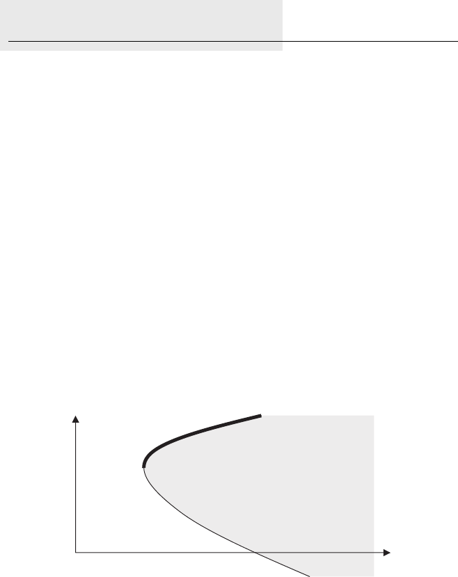
P1: SBT
c14 JWBT188-Aldridge October 23, 2009 11:57 Printer: Yet to come
202 HIGH-FREQUENCY TRADING
the underlying strategies have been estimated. It begins with a review of
classical portfolio theory and proceeds to consider the latest applications
in portfolio management.
ANALYTICAL FOUNDATIONS OF
PORTFOLIO OPTIMIZATION
Graphical Representation of the Portfolio
Optimization Problem
The dominant focus of any portfolio management exercise is minimizing
risks while maximizing returns. The discipline of portfolio optimization
originated from the seminal work of Markowitz (1952). The two dimen-
sions of a portfolio that he reviewed are the average return and risk of
the individual securities that compose the portfolio and of the portfolio
as a whole. Optimization is conducted by constructing an “efficient fron-
tier,” a set of optimal risk-return portfolio combinations for the various in-
struments under consideration. In the absence of leveraging opportunities
(opportunities to borrow and increase the total capital available as well as
opportunities to lend to facilitate leverage of others), the efficient frontier
is constructed as follows:
1. For every possible combination of security allocations, the risk and
return are plotted on a two-dimensional chart, as shown in Figure 14.1.
Due to the quadratic nature of the risk function, the resulting chart
takes the form of a hyperbola.
Return
Risk
FIGURE 14.1 Graphical representation of the risk-return optimization con-
structed in the absence of leveraging opportunities. The bold line indicates the effi-
cient frontier.
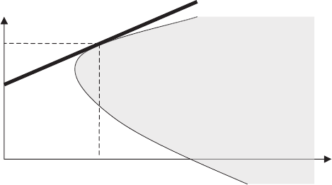
P1: SBT
c14 JWBT188-Aldridge October 23, 2009 11:57 Printer: Yet to come
Creating and Managing Portfolios of High-Frequency Strategies 203
2. The points with the highest level of return for every given level of risk
are selected as the efficient frontier. The same result is obtained if the
frontier is selected as the set of points with the lowest level of risk for
every given level of return. The bold segment highlights the efficient
frontier.
3. An individual investor then selects a portfolio on the efficient frontier
that corresponds to the investor’s risk appetite.
In the presence of leveraging, the efficient frontier shifts dramatically
upward to a straight line between the lending rate, approximated to be
risk free for the purposes of high-level analysis, and the “market” portfo-
lio, which is a portfolio lying on a line tangent to the efficient frontier of
Figure 14.2. Figure 14.2 shows the resulting efficient frontier.
An interpretation of the efficient frontier in the presence of the lever-
age rate RFproceeds as follows. If an investor can lend a portion of his
wealth at the rate RFto high-grade borrowers, he can reduce the risk of
his overall portfolio by reducing his risk exposure. The lending investor
then ends up on the bold line between RFand the market portfolio point
(σM,RM). The investor incurs two advantages by lending compared with
selecting a portfolio from the efficient set with no lending as represented
in Figure 14.1:
1. The investor may be able to attain lower risk than ever possible in the
no-lending situation.
Return
RM
RF
σ
MRisk
FIGURE 14.2 Graphical representation of the risk-return optimization con-
structed in the presence of leveraging opportunities. All leveraging is assumed to
be conducted at the risk-free rate RF. The bold line indicates the efficient frontier.
The point (σM,RM) corresponds to the “market portfolio” for the given RFand the
portfolio set.

P1: SBT
c14 JWBT188-Aldridge October 23, 2009 11:57 Printer: Yet to come
204 HIGH-FREQUENCY TRADING
2. With lending capabilities, the investor’s return gets scaled linearly to
his scaling of risk. In the no-lending situation, the investor’s return de-
creases faster than the investor’s decrease in risk.
Similarly, an investor who decides to borrow to increase the capital of
his portfolio ends up on the efficient frontier but to the right of the market
portfolio. The borrowing investor, too, enjoys the return, which increases
linearly with risk and is above the no-borrowing opportunity set.
Core Portfolio Optimization Framework
Analytical estimation of the efficient frontier requires an understanding of
the returns delivered by the strategies making up the portfolio. The return
of each strategy iis measured as a simple average return over the time
period t∈[1,...,T],
Ri=1
T
T
t=1
Rit (14.1)
where Rit is the return of strategy iin time period t,t∈[1,...,T]. The
annualized risk of each strategy i,σi2is often measured as a variance Vi,a
square of the standard deviation:
Vi=1
T−1
T
t=1
(Rit −Ri)2(14.2)
Note that in computation of the average return, Ri, the sum of returns
is divided by the total number of returns, T, whereas in computation of the
risk in equation (14.2), the sum of squared deviations from the mean is di-
vided by T−1 instead. The T−1 factor reflects the number of “degrees of
freedom” used in the computation of Vi. Every statistical equation counts
every independent variable (a raw number) as a degree of freedom; at the
same time, every estimate used in the statistical equation reduces the num-
ber of degrees of freedom by 1. Thus, in the estimation of Ri, the number
of independent variables is T, while in the estimation of Vi, the number of
independent variables is reduced by 1 since the equation (14.2) uses Ri,an
estimate itself.
The sample frequency of time period tshould match the frequency in-
tended for the analysis. In developing high-frequency trading frameworks,
it may be desirable to make all the inferences from returns at very high
intra-day frequencies—for example, a minute or a second. For investor

P1: SBT
c14 JWBT188-Aldridge October 23, 2009 11:57 Printer: Yet to come
Creating and Managing Portfolios of High-Frequency Strategies 205
relations purposes, daily or even monthly frequency of returns is often
sufficient.
If the portfolio comprises Istrategies, each represented by a propor-
tion xiwithin the portfolio, and each with the average annualized return
of Riand risk of Vi, the total risk and return of the portfolio can be deter-
mined as follows:
E[Rp]=
I
i=1
xiE[Ri] (14.3)
V[Rp]=
I
i=1
i
j=1
xixjcov[Ri,Rj] (14.4)
where xiis the proportion of the portfolio capital allocated to the strategy
iat any given time, E[Rp] and E[Ri] represent respective average annual-
ized returns of the combined portfolio and of the individual strategy i, and
cov[Ri,Rj] is the covariance between returns of strategy iand returns of
strategy j:
cov[Ri,Rj]=ρijV0.5
iV0.5
j=E[Ri]E[Rj]−E[RiRj] (14.5)
Additionally, the optimal portfolio should satisfy the following con-
straint: the sum of all allocations xiin the portfolio should add up to
100 percent of the portfolio:
I
i=1
xi=1 (14.6)
Note that the formulation (14.6) allows portfolio weights of individual
securities {xi}to be all real numbers, both positive and negative. Positive
numbers denote long positions, while negative numbers denote short
positions.
The basic portfolio optimization problem is then specified as follows:
min V[Rp],s.t.E[Rp]≥µ,
I
i=1
xi=1 (14.7)
where µis the minimal acceptable average return.
P1: SBT
c14 JWBT188-Aldridge October 23, 2009 11:57 Printer: Yet to come
206 HIGH-FREQUENCY TRADING
For a trading operation with the coefficient of risk aversion of λ,the
mean-variance optimization framework becomes the one shown in equa-
tion (14.8):
max
T
t=1
(E[Rp,t]−λV[Rp,t]),
I
i=1
xi=1 (14.8)
The value of the objective function of equation (14.8) resulting from the
optimization can be interpreted as “value added” to the particular investor
with risk aversion of λ. The risk aversion parameter λis taken to be about
0.5 for very risk-averse investors, 0 for risk-neutral investors, and negative
for risk-loving investors.
Furthermore, when the trading operation is tasked with outperforming
a particular benchmark, µ, the optimization problem is reformulated as
follows:
max
T
t=1
(E[Rp,t]−λV[Rp,t]),s.t.
T
t=1
E[Rp,t]≥µ,
I
i=1
xi=1 (14.9)
Portfolio Optimization in the Presence
of Transaction Costs
The portfolio optimization model considered in the previous section did
not account for transaction costs. Transaction costs, analyzed in detail in
Chapter 19, decrease returns and distort the portfolio risk profile; depend-
ing on the transaction costs’ correlation with the portfolio returns, trans-
action costs may increase overall portfolio risk. This section addresses the
portfolio optimization solution in the presence of transaction costs.
The trading cost minimization problem can be specified as follows:
min
s.t.V[TC]≤KE[TC] (14.10)
where E[TC] is the average of observed trading costs, V[TC] is the variance
of observed trading costs, and Kis the parameter that specifies the max-
imum trading cost variance. Changing the parameter Kallows us to trace
out the “efficient trading frontier,” a collection of minimum trading costs
for each level of dispersion of trading costs.
Alternatively, given the risk-aversion coefficient λof the investor or
portfolio manager, the target trading cost strategy can be determined from
the following optimization:
min E[TC]+λV[TC] (14.11)
P1: SBT
c14 JWBT188-Aldridge October 23, 2009 11:57 Printer: Yet to come
Creating and Managing Portfolios of High-Frequency Strategies 207
Both the efficient trading frontier and the target trading cost scenario can
be used as benchmarks to compare execution performance of individual
traders and executing broker-dealers. However, the cost optimization by
itself does not answer the question of portfolio optimization in the pres-
ence of trading costs.
Engle and Ferstenberg (2007) further propose an integrative frame-
work for portfolio and execution risk decisions. Using xit to denote the
proportion of the total portfolio value allocated to the security iat the end
of period t,pit to denote the price of security iat the end of period t, and
ctto denote the cash holdings in the portfolio at the end of period t, Engle
and Ferstenberg (2007) specify the portfolio value at the end of period tas
follows:
yt=
I
i=1
xit pit +ct(14.12)
If the portfolio rebalancing happens at the end of each period, the one-
period change in the portfolio value from time tto time t+1isthen
yt+1=yt+1−yt=I
i=1
xi,t(pi,t+1−pit)+I
i=1
(xi,t+1−xit)pi,t+1+(ct+1−ct)
=I
i=1
xi,tpi,t+1+I
i=1
xi,t+1pi,t+1+ct+1(14.13)
If the cash position bears no interest and there are no dividends, the
change in the cash position is strictly due to changes in portfolio composi-
tion executed at time tat transaction prices ˜pit for each security i:
ci,t+1=−
I
i=1
xi,t+1˜pi,t+1(14.14)
The negative sign on the right-hand side of equation (14.14) reflects the fact
that the increase in the holding position of security i,xit results in a de-
crease of cash available in the portfolio. Combining equations (14.13) and
(14.14) produces the following specification for the changes in the portfolio
at time t:
yt+1=
I
i=1
xitpi,t+1+
I
i=1
xi,t+1(pi,t+1−˜pi,t+1)=
I
i=1
xitpi,t+1−TCt+1
(14.15)
where I
i=1xitpi,t+1is the change in portfolio value due to the active port-
folio management and I
i=1xi,t+1(pi,t+1−˜pi,t+1) is due to trading costs.

P1: SBT
c14 JWBT188-Aldridge October 23, 2009 11:57 Printer: Yet to come
208 HIGH-FREQUENCY TRADING
Specifically, I
i=1xi,t+1(pi,t+1−˜pi,t+1) would equal 0 if all the trades were
executed at their target prices, pi,t+1.
The combined portfolio optimization problem in the presence of risk
aversion λ,maxE[yt+1]−λV[yt+1], can then be rewritten as follows for
each period t+1:
max EI
i=1
xitpi,t+1−TCt+1−λVI
i=1
xitpi,t+1−TCt+1(14.16)
where TCt=I
i=1xit(pit −˜pit), xit is the one-period change in port-
folio weight of security i,pit is the target execution price for trading of
security iat the end of period t, and ˜pit is the realized execution price for
security iat the end of period t.
In addition, the interaction between transaction costs and portfolio al-
locations can be captured as follows:
VI
i=1
xitpi,t+1−TCt+1=VI
i=1
xitpi,t+1
+V[TCt+1]−2 cov I
i=1
xitpi,t+1,TCt+1(14.17)
The resulting Sharpe ratio of the portfolio can be ex-ante computed as
follows:
Sharpe ratio =
EI
i=1
xipi−TC−Rf
√TVI
i=1
xitpi,t+1−TCt+1(14.18)
Portfolio Diversification with
Asymmetric Correlations
The portfolio optimization frameworks discussed previously assume that
the correlations between trading strategies behave comparably in rising
and falling markets. Ang and Chen (2002), however, show that this does not
have to be the case; the authors document that correlation of equity returns
often increases in falling markets, likely distorting correlations of trad-
ing strategies used in trading portfolios. Explicit modeling of time-varying
correlations of portfolio strategies may refine portfolio estimation and gen-
erate more consistent results.
P1: SBT
c14 JWBT188-Aldridge October 23, 2009 11:57 Printer: Yet to come
Creating and Managing Portfolios of High-Frequency Strategies 209
One way to model correlations is to follow the methodology developed
by Ang and Chen (2002). The authors’ methodology is based on examining
the distribution of correlations of returns: if correlations behave normally,
they are symmetrical; the correlations accompanying extreme negative re-
turns are equal to the correlations accompanying extreme positive returns.
Any asymmetry in correlations of extreme returns should be incorporated
in portfolio management solutions.
Dealing with Estimation Errors
in Portfolio Optimization
All portfolio optimization exercises involve estimates of average returns,
return variances, and correlations. The classic Markowitz (1952) method-
ology takes the estimated parameters as true distributional values and
ignores the estimation error. Frankfurter, Phillips, and Seagle (1971);
Dickenson (1979); and Best and Grauer (1991), among others, point out
that the estimation errors distort the portfolio selection process and result
in poor out-of-sample performance of the complete portfolio.
A common way to overcome estimation errors is to learn from them.
A mechanism known as the Bayesian approach proposes that the system
learns from its own estimation mistakes by comparing its realized perfor-
mance with its forecasts. The portfolio optimization system then corrects
its future estimates based on its own learnings. In a purely systematic en-
vironment, the self-correction process happens without any human inter-
vention. The Bayesian self-correction mechanism is often referred to as a
“genetic algorithm.”
In the Bayesian approach, the average return estimate of a particu-
lar security is considered to be a random variable and is viewed proba-
bilistically in the context of previously obtained information, or priors. All
expectations are subsequently developed with respect to the distribution
obtained for the estimate. Multiple priors, potentially representing multi-
ple investors or analysts, increase the accuracy of the distribution for the
estimate.
Under the Bayesian specification, all mean and variance-covariance es-
timates are associated with a confidence interval that measures the ac-
curacy of the forecast. An accurate forecast has a tight confidence inter-
val, while the inaccurate forecast has a wide confidence interval. After
the accuracy of the previous forecast has been determined, the portfolio
weight of a security is scaled depending on the width of the confidence
intervals of these securities. The wider the confidence intervals for param-
eter estimates, the smaller the portfolio weight for that security. When the
confidence intervals approach 0, the weights are similar to those of the
classic mean-variance optimization.

P1: SBT
c14 JWBT188-Aldridge October 23, 2009 11:57 Printer: Yet to come
210 HIGH-FREQUENCY TRADING
The traditional Bayesian approach, applied to mean-variance optimiza-
tion by Jorion (1986), works as follows: both mean and variance estimates
computed on a contemporary data sample are adjusted by lessons gleaned
from historical (prior) observations.
The dispersion of the distributions of the true mean and variance of
the distributions shrink as more observations are collected and analyzed
with time. If Rp,tis the portfolio return following the mean-variance op-
timization of equation (14.7) from time t−1totimet, and ˆ
E[Ri,t]isthe
average return estimate for security i,ˆ
E[Ri,t]=1
tt
τ=1Ri,τ , the “Bayes-
Stein shrinkage estimators” for expected return and variance of an indi-
vidual security ito be used in the mean-variance optimization for the next
period t+1, are computed as follows:
E[Ri,t+1]BS =(1 −φi,BS)ˆ
E[Ri,t]+φi,BSRp,t
V[Ri,t+1]BS =V[Ri,t]1+1
t+ν+v
t(t+1+ν)V[Ri,t]
where vis the precision of the mean estimates: v=(N−2)
t
V[Ri,t]
(Rp,t−ˆ
E[Ri,t])2,Nis
the number of observations in the sample at time t, and φBS is the shrink-
age factor for the mean: φBS =v
t+v. The case of zero precision (v=0) cor-
responds to completely diffuse estimates.
Some investors feel particularly strongly about the accuracy of a fore-
cast and would prefer to exclude systems generating inaccurate or ambigu-
ous forecasts from their trading tool belt. Garlappi, Uppal, and Wang (2007)
propose a Bayesian portfolio allocation methodology for such investors.
An ambiguity-averse investor may be one who relies on multiple informa-
tion sources and prefers to trade a particular financial security only when
those information sources are in agreement about the future movement of
that security. This ambiguity aversion is different from risk aversion. Risk
aversion measures the investor’s tolerance for variance in returns mea-
sured after the trades have been executed, or ex-post, whereas ambiguity
aversion measures the investor’s tolerance for dispersion in the trade out-
come forecasts before any trades have been executed, or ex-ante.
To specify the ambiguity aversion, Garlappi, Uppal, and Wang (2007)
add the following constraint to the standard mean-variance optimization:
f(E[R],ˆ
E[R],V[R]) ≤ε, where fis the uncertainty about forecasts of
expected returns, and εis the investor’s maximum tolerance for such
uncertainty:
f(E[R],ˆ
E[R],V[R]) =(E[R]−ˆ
E[R])2
V[R]/T(14.19)
where Tis the number of observations in the sample.

P1: SBT
c14 JWBT188-Aldridge October 23, 2009 11:57 Printer: Yet to come
Creating and Managing Portfolios of High-Frequency Strategies 211
The optimization problem of equation (14.7) over a one-period horizon
and multiple assets now becomes:
max(E[R]−λV[R]),s.t.
I
i=1
xi=1,E[R]≥µ, f(E[R],ˆ
E[R],V[R]) ≤ε
(14.20)
Garlappi, Uppal, and Wang (2007) show that the optimization of equation
(14.20) can be rewritten as follows:
max(E[R]−λV[R]−ξV[R]),s.t.
I
i=1
xi=1 (14.21)
where ξspecifies the multi-asset aversion to ambiguity:
(ˆ
E[R]−E[R])V[R]( ˆ
E[R]−E[R]) ≤ξ(14.22)
The methodology presented here documents analytical approaches
to portfolio optimization. The following sections discuss practical ap-
proaches to the estimation of portfolio optimization problems defined pre-
viously as well as to other aspects of effective portfolio management in
high-frequency trading operations.
EFFECTIVE PORTFOLIO
MANAGEMENT PRACTICES
Effective practical portfolio management involves making the following
key decisions:
1. How much leverage is appropriate within the portfolio?
2. What proportion of the portfolio should be invested into which trading
strategy?
This section presents best-practices answers for each of these
questions.
How Much Leverage Is Appropriate
within the Portfolio?
Two methodologies, option-based portfolio insurance (OBPI) and constant
proportion portfolio insurance (CPPI), address the leverage component of
P1: SBT
c14 JWBT188-Aldridge October 23, 2009 11:57 Printer: Yet to come
212 HIGH-FREQUENCY TRADING
the portfolio optimization process. Both methodologies require that a sub-
stantial proportion of the portfolio at any time be left in cash or invested in
risk-free bonds. Each methodology determines exactly what proportion of
the portfolio should be left in cash and what proportion should be levered
and then invested into risky securities. The OBPI method is static in nature,
while the CPPI allocation changes with changes in the market value of the
overall portfolio.
1. The OBPI methodology suggests that only a fixed proportion of the
portfolio (e.g., Xpercent, X<100 percent) be invested in risky instru-
ments. The technique was first developed by Leland and Rubenstein
(1976), who introduced the concept as options-based insurance. In
Leland and Rubenstein (1976), the portfolio is structured to preserve
(100 −X) percent of the original portfolio capital, while allowing the
portfolio to benefit from the potential upside of the Xpercent of the
portfolio invested in risky securities, such as options. Such portfolios
are now commonly securitized and marketed as “structured products.”
The proportion of the portfolio Xcan be determined through the cost-
benefit analysis of option and bond prices versus expected probabili-
ties of option payouts or, in high-frequency trading cases, the selling
price of the option.
2. CPPI is another popular portfolio allocation strategy that calls for dy-
namic adjustment of portfolio breakdown into cash and risky securi-
ties, unlike OBPI, in which the breakdown is static. Black and Jones
(1987) and Perold and Sharpe (1988) created CPPI as an extension of
OBPI that morphed into an automated method widely used by industry
practitioners today.
CPPI works in accordance with the following steps:
1. Management sets the absolute worst-case maximum drawdown, a floor
for the market value of the portfolio. If the market value of the portfolio
reaches the floor, the portfolio is fully liquidated into cash. Suppose
that the maximum allowable drawdown is L percent.
2. The “cushion” is the difference between the market value of the port-
folio and the floor. A proportion of the cushion is levered and invested
in risky securities. The exact proportion of the cushion invested in the
risky instruments is determined by a “multiplier,” M, set by manage-
ment. Common multipliers range from 3 to 6.
3. The risk capital allocated to the risky securities then becomes M×
Cushion. As an illustration, suppose that the total capital allocated to
a particular portfolio is $100 million, with 10 percent being the absolute
P1: SBT
c14 JWBT188-Aldridge October 23, 2009 11:57 Printer: Yet to come
Creating and Managing Portfolios of High-Frequency Strategies 213
maximum drawdown. The value of the cushion at this point is $10 mil-
lion. If the multiplier is set to 5 (M=5), the maximum actively invested
at-risk capital can be $50 million. However, this $50 million can be lev-
ered. Black and Jones (1987) and Perold and Sharpe (1988) assumed
that the leverage ratio on the cushion stays constant during the whole
life of the portfolio, leading to the “constant” term in CPPI. Modern
CPPI strategies allow for dynamic leverage strategies that scale lever-
age down in adverse market conditions.
The CPPI allocation ensures that the portfolio always has enough cash
to mitigate portfolio risks and to safeguard the investment principal. The
portfolio is periodically rebalanced to reflect the current market value of
the portfolio. The higher the market value of the portfolio, the more of its
proportion is allocated to risky assets. Conversely, the lower the market
value of the portfolio, the higher the proportion of the portfolio that is held
in cash or in nearly risk-free fixed-income securities.
What Proportion of the Portfolio Should Be
Invested into Which Trading Strategy?
After the performance of individual securities and trading strategies has
been assessed and the best performers identified, the composition of the
master portfolio is determined from the best-performing strategies. This
step of the process is known as asset allocation and involves determining
the relative weights of strategies within the master portfolio.
The easiest approach to portfolio optimization is to create an equally
weighted portfolio of the best-performing strategies. Although the equally
weighted framework diversifies the risk of the overall portfolio, it may not
diversify the risk as well as a thorough portfolio optimization process. As
the number of securities in the portfolio increases, however, determining
the optimal weights for each security becomes increasingly complex and
time-consuming—a real challenge in the high-frequency environment.
Several classes of algorithms have been proposed to simplify and
speed up setting the optimal portfolio weights. Optimization algorithms fall
into three classes:
1. The simultaneous equations framework is the algorithm that directly
follows the Markowitz (1952) specification. It has been shown to be
inefficient for optimization if the portfolio exceeds 10 strategies, and it
may produce highly erroneous forecasts when 20 or more assets are in-
volved. The forecast errors are due to the estimation errors that occur
when the average returns and variances are computed. The Bayesian
error-correction framework, discussed previously in this chapter,
P1: SBT
c14 JWBT188-Aldridge October 23, 2009 11:57 Printer: Yet to come
214 HIGH-FREQUENCY TRADING
alleviates some of the input estimation errors. Still, in addition to the
issues of forecast errors, the estimation time of this algorithm grows
exponentially with the number of trading strategies involved, making
this method hardly suitable for high-frequency trading of many assets.
2. Nonlinear programming is a class of optimizers popular in commer-
cial software. The nonlinear algorithms employ a variety of techniques
with the objective of maximizing or minimizing the target portfolio op-
timization function given specified parameters such as portfolio allo-
cation weights. Some of these algorithms employ a gradient technique
whereby they analyze the slope of the objective function at any given
point and select the fastest increasing or decreasing path to the target
maximum or minimum, respectively. The nonlinear programming algo-
rithms are equally sensitive to the estimation errors of the input means
and variances of the returns. Most often, the algorithms are too compu-
tationally complex to be feasible in the high-frequency environments.
A recent example of a nonlinear optimizer is provided by Steuer, Qi,
and Hirschberger (2006).
3. The critical line–optimizing algorithm was developed by Markowitz
(1959) to facilitate the computation of his own portfolio theory. The
algorithm is fast and comparatively easy to implement. Instead of pro-
viding point weights for each individual security considered in the
portfolio allocation, the critical line optimizer delivers a set of port-
folios on the efficient frontier, a drawback that has precluded many
commercial companies from adapting this method. A recent algorithm
by Markowitz and Todd (2000) addresses some of the issues. Accord-
ing to Niedermayer and Niedermayer (2007), the Markowitz and Todd
(2000) algorithm outperforms the algorithm designed by Steuer, Qi,
and Hirschberger (2006) by a factor of 10,000 for at least 2,000 assets
considered simultaneously.
The existing algorithms, whatever the complexity and accuracy of
their portfolio allocation outputs, may not be perfectly suited to the
high-frequency trading environment. First, in environments where a delay
of 1 second can result in a million-dollar loss, the optimization algorithms
in their current form still consume too much time and system power.
Second, these algorithms ignore the liquidity considerations pertinent
to the contemporary trading settings; most of the transactions occur in
blocks or “clips” of a prespecified size. Trades of larger-than-normal sizes
as well as trades of smaller blocks incur higher transaction costs that in
the high-frequency environment can put a serious strain on the system’s
profitability.
A simple high-frequency alternative to the complex optimization so-
lutions is a discrete pair-wise (DPW) optimization developed by Aldridge
P1: SBT
c14 JWBT188-Aldridge October 23, 2009 11:57 Printer: Yet to come
Creating and Managing Portfolios of High-Frequency Strategies 215
(2009c). The DPW algorithm is a fast compromise between the equally
weighted portfolio setting and a full-fledged optimization machine that out-
puts portfolio weights in discrete clips of the prespecified sizes. No frac-
tional weights are allowed. The algorithm works as follows:
1. Candidates for selection into the overall portfolio are ranked using
Sharpe ratios and sorted from the highest Sharpe ratio to the lowest.
This step of the estimation utilizes the fact that the Sharpe ratio itself
is a measure of where each individual strategy lies on the efficient
frontier.
2. An even number of strategies with the highest Sharpe ratios are se-
lected for inclusion into the portfolio. Half of the selected strategies
should have historically positive correlations with the market, and half
should have historically negative correlations with the market.
3. After the universe of financial instruments is selected on the basis of
the Sharpe ratio characteristics, all selected strategies are ranked ac-
cording to their current liquidity. The current liquidity can be measured
as the number of quotes or trades that have been recorded over the
past 10 minutes of trading activity, for example.
4. After all the strategies have been ranked on the basis of their liquid-
ity, the pairs are formed through the following process: the two strate-
gies within each pair have opposite historical correlation with the
market. Thus, strategies historically positively correlated with the mar-
ket are matched with strategies historically negatively correlated with
the market. Furthermore, the matching should occur according to
the strategy liquidity rank. The most liquid strategy positively corre-
lated with the market should be matched with the most liquid strat-
egy negatively correlated with the market, and so on until the least
liquid strategy positively correlated with the market is matched with
the least liquid strategy negatively correlated with the market. The
liquidity-based matching ensures that the high-frequency dynamic cap-
tured by correlation is due to idiosyncratic movements of the strategy
rather than the illiquidity conditions of one strategy.
5. Next, for each pair of strategies, the high-frequency volatility of a port-
folio of just the two strategies is computed for discrete position sizes
in either strategy. For example, in foreign exchange, where a stan-
dard transactional clip is $20 million, the discrete position sizes consid-
ered for the pair-wise optimization may be −$60 million, −$40 million,
−$20 million, 0, $20 million, $40 million, and $60 million, where the mi-
nus sign indicates the short position. Once the volatility for the various
portfolio combinations is selected within each pair of strategies, the
positions with the lowest portfolio volatility are selected.
P1: SBT
c14 JWBT188-Aldridge October 23, 2009 11:57 Printer: Yet to come
216 HIGH-FREQUENCY TRADING
6. The resulting pair portfolios are subsequently executed given the maxi-
mum allowable allocation constraints for each strategy. The maximum
long and short allocation is predetermined and constrained as follows:
the cumulative gross position in each strategy cannot exceed a cer-
tain size, and the cumulative net position cannot exceed another, sep-
arately set, limit that is smaller than the aggregate of the gross limits
for all strategies. The smaller net position clause ensures a degree of
market neutrality.
The DWP algorithm is particularly well suited to high-frequency envi-
ronments because it has the following properties:
rThe DPW algorithm avoids the brunt of the impact of input estimation
errors by reducing the number of strategies in each portfolio allocation
decision.
rThe negative historical correlation of input securities ensures that
within each pair of matched strategies, the minimum variance will re-
sult in long positions in both strategies most of the time. Long positions
in the strategies are shown to historically produce the highest returns
per unit of risk, as is determined during the Sharpe ratio ranking phase.
The times that the system results in short positions for one or more
strategy are likely due to idiosyncratic market events.
rThe algorithm is very fast in comparison with other portfolio optimiza-
tion algorithms. The speed of the algorithm comes from the following
“savings” in computational time:
rIf the total number of strategies selected in the Sharpe ratio ranking
phase is 2K, the DPW algorithm computes only Kcorrelations. Most
other portfolio optimization algorithms compute correlation among
every pair of strategies among the 2Ksecurities, requiring 2K(K−1)
correlation computations instead.
rThe grid search employed in seeking the optimal portfolio size for
each strategy within each portfolio pair optimizes only between two
strategies, or in two dimensions. A standard algorithm requires a
2K-dimensional optimization.
rFinally, the grid search allows only a few discrete portfolio weight
values. In the main example presented here, there are seven
allowable portfolio weights: −$60 MM; −$40 MM; −$20 MM; 0;
$20 MM; $40 MM; and $60 MM. This limits the number of iterations
and resulting computations from, potentially, infinity, to 72=49.
Alexander (1999) notes that correlation and volatility are not sufficient
to ensure long-term portfolio stability; both correlation and volatility are
typically computed using short-term returns, which only partially reflect

P1: SBT
c14 JWBT188-Aldridge October 23, 2009 11:57 Printer: Yet to come
Creating and Managing Portfolios of High-Frequency Strategies 217
dynamics in prices and necessitate frequent portfolio rebalancing. Instead,
Alexander (1999) suggests that in portfolio optimization more attention
should be paid to cointegration of constituent strategies. Auxiliary secu-
rities, such as options and futures, can be added into the portfolio mix
based on cointegration analysis to further strengthen the risk-return char-
acteristics of the trading operation. The cointegration-enhanced portfolios
can work particularly well in trading operations that are tasked with out-
performing specific financial benchmarks.
CONCLUSION
Competent portfolio management enhances the performance of high-
frequency strategies. Ultra-fast execution of portfolio optimization deci-
sions is difficult to achieve but is critical in high-frequency settings.
P1: SBT
c14 JWBT188-Aldridge October 23, 2009 11:57 Printer: Yet to come
218

P1: SBT
c15 JWBT188-Aldridge October 23, 2009 11:58 Printer: Yet to come
CHAPTER 15
Back-Testing
Trading Models
Once a trading idea is formed, it needs to be tested on historical
data. The testing process is known as a back test. This chapter
describes the key considerations for a successful and meaningful
back test.
The purpose of back tests is twofold. First, a back test validates the
performance of the trading model on large volumes of historical data
before being used for trading live capital. Second, the back test shows
how accurately the strategies capture available profit opportunities and
whether the strategies can be incrementally improved to capture higher
revenues.
Optimally, the trading idea itself is developed on a small set of his-
torical data. The performance from this sample is known as “in-sample”
performance. One month of data can be perfectly sufficient for in-sample
estimation, depending on the chosen strategy. To draw any statistically
significant inferences about the properties of the trading model at hand,
the trading idea should be verified on large amounts of data that was not
used in developing the trading model itself. Having a large reserve of his-
torical data (at least two years of continuous tick data) ensures that the
model minimizes the data-snooping bias, a condition that occurs when the
model overfits to a nonrecurring aberration in the data. Running the back
test on a fresh set of historical data is known as making “out-of-sample”
inferences.
Once the out-of-sample back-test results have been obtained, they
must be evaluated. At a minimum, the evaluation process should compute
219

P1: SBT
c15 JWBT188-Aldridge October 23, 2009 11:58 Printer: Yet to come
220 HIGH-FREQUENCY TRADING
basic statistical parameters of the trading idea’s performance: cumulative
and average returns, Sharpe ratio, and maximum drawdown, as explained
in Chapter 5.
For the purposes of accuracy analyses, trading systems can be grouped
into those that generate point forecasts and those that generate directional
forecasts. Point forecasts predict that the price of a security will reach a
certain level, or point. For example, a system that determines that the S&P
500 index will rise from the current 787 level to 800 within the following
week is a point forecast system; the point forecast in this case is the 800
number predicted for the S&P 500. Directional systems make decisions
to enter into positions based on expectations of the system going up or
down, without specific target forecasts. A directional system may predict
that USD/CAD will rise from its current level without making a specific
prediction about how far USD/CAD will rise.
EVALUATING POINT FORECASTS
The simplest way to evaluate the validity of point forecasts is to run a
regression of realized values from the historical data against the out-of-
sample forecasts. For example, suppose that the trading model predicts
future price levels of equities. Regressing the realized equity prices on the
forecasted ones shows the degree of usefulness of the forecast.
Specifically, the model evaluation regression is specified as follows:
Yt=α+βXt+εt(15.1)
where Y is the realized price level, X is the forecasted price level, αand β
are parameters estimated by the regression, and εis a normally distributed
error term. Whenever the forecast perfectly predicts the realized values,
β=1 and α=0. The deviation of the αand βparameters from the opti-
mal β=1 and α=0 itself indicates the reliability and usefulness of the
forecasting model. In addition, the R2coefficient obtained from the regres-
sion shows the percentage of realized observations explained by the fore-
casts. The higher the realized R2, the greater the accuracy of the forecasting
model.
The accuracy of point forecasts can also be evaluated by comparing
the forecasts with the realized values. Methods for forecast comparisons
include:
rMean squared error (MSE)
rMean absolute deviation (MAD)

P1: SBT
c15 JWBT188-Aldridge October 23, 2009 11:58 Printer: Yet to come
Back-Testing Trading Models 221
rMean absolute percentage error (MAPE)
rDistributional performance
rCumulative accuracy profiling
If the value of a financial security is forecasted to be xF,t at some fu-
ture time tand the realized value of the same security at time tis xR,t,the
forecast error for the given forecast, εF,t, is computed as follows:
εF,t=xF,t−xR,t(15.2)
The mean squared error (MSE) is then computed as the average of
squared forecast errors over Testimation periods, analogously to volatility
computation:
MSE =1
T
T
τ=1
ε2
F,τ (15.3)
The mean absolute deviation (MAD) and the mean absolute percentage
error (MAPE) also summarize properties of forecast errors:
MAD =1
T
T
τ=1|εF,τ |(15.4)
MAPE =1
T
T
τ=1
εF,τ
xR,τ (15.5)
Naturally, the lower each of the three metrics (MSE, MAD, and MAPE), the
better the forecasting performance of the trading system.
The distributional evaluation of forecast performance also examines
forecast errors εF,tnormalized by the realized value, xR,t. Unlike MSE,
MAD, and MAPE metrics, however, the distributional performance metric
seeks to establish whether the forecast errors are random. If the errors are
indeed random, there exists no consistent bias in either direction of price
movement, and the distribution of normalized errors εF,t
xR,tshould fall on
the uniform [0, 1] distribution. If the errors are nonrandom, the forecast
can be improved. One test that can be used to determine whether the er-
rors are random is a comparison of errors with the uniform distribution
using the Kolmogorov-Smirnov statistic.
The accuracy of models can be further considered in asymmetric situ-
ations. For example, does the MSE of negative forecast errors exceed the
MSE of positive errors? If so, the model tends to err by underestimating

P1: SBT
c15 JWBT188-Aldridge October 23, 2009 11:58 Printer: Yet to come
222 HIGH-FREQUENCY TRADING
the subsequently realized value and needs to be fine-tuned to address the
asymmetric nature of forecast accuracy. Similarly, the accuracy of fore-
cast errors can be examined when the errors are grouped based on various
market factors:
rMarket volatility at the time the errors were measured
rMagnitude of the errors
rUtilization rate of computer power in generating the forecasts, among
other possible factors
The objective of the exercise is to identify the conditions under which
the system persistently errs and to fix the error-generating issue.
EVALUATING DIRECTIONAL FORECASTS
Testing the accuracy of directional systems presents a greater challenge.
Yet, accuracy evaluation of the directional systems can be similar to that
of the point forecast systems, with binary values of 1 and 0 indicating
whether the direction of the forecast matches the direction of the realized
market movement or not. As with the forecasts themselves, directional ac-
curacy estimates are much less accurate than the accuracy estimates of the
point forecasts.
Aldridge (2009a) proposes the trading strategy accuracy (TSA) method
to measure the ability of a trading strategy to exploit the gain that opportu-
nities present to the strategy in the market. As such, the method evaluates
not only the market value of trading opportunities realized by the system
but the market value of trading opportunities that the system missed. The
methodology of the test is based on that of the cumulative accuracy profile,
also known as Gini curve or power curve. To the author’s best knowledge,
the cumulative accuracy profile has not been applied to the field of trading
strategy evaluation to date.
The TSA methodology evaluates trading strategies in back-testing—
that is, in observing the strategy run on historical data. The methodology
comprises the following three steps:
1. Determination of model-driven trade signals in the historical data
2. Ex-ante identification of successful and unsuccessful trades in the
historical data
3. Computation of the marginal probabilities of the trade signals obtained
in Step 2 predicting trading outcomes obtained in Step 1

P1: SBT
c15 JWBT188-Aldridge October 23, 2009 11:58 Printer: Yet to come
Back-Testing Trading Models 223
TABLE 15.1 Model-Generated Trading Behavior
Date Time
Buy a Unit
of Security?
Sell a Unit
of Security?
March 9, 2009 6:00 A.M.1 0
March 9, 2009 7:00 A.M.0 0
March 9, 2009 8:00 A.M.1 0
March 9, 2009 9:00 A.M.0 0
March 9, 2009 10:00 A.M.0 0
March 9, 2009 11:00 A.M.0 1
March 9, 2009 12:00 P.M.0 0
March 9, 2009 1:00 P.M.0 0
Determination of Model-Driven Trade Signals
This step is similar to a standard back test for a trading strategy on a sin-
gle security. The trading model is run on data of the selected frequency.
The buy and sell trading signals that the model generates are recorded in
Table 15.1, where 1 corresponds to a decision to execute a trade and 0
denotes the absence of such a decision.
Ex-Ante Identification of Successful and
Unsuccessful Trades in the Historical Data
This step involves dividing all trading opportunities in the historical data
into profitable and unprofitable buys and sells. At each trade evaluation
time, the evaluation process looks ahead in the historical data of a given
security to determine whether a buy or a sell entered into for the security
at that point in time is a success—that is, a profitable trade.
The frequency of the buy or sell decision times corresponds to the
frequency of the portfolio-rebalancing decisions in the trading strategy
being evaluated. Some strategies are designed to make portfolio rebal-
ancing decisions at the end of each day; other higher-frequency strategies
make decisions on whether to place a buy or a sell on the given security
following each quote tick. The ex-ante identification of successful and
unsuccessful trades proceeds in tandem with the frequency of the trading
strategy studied.
The trade’s profitability is determined based on the position closing
rules—the stop-gain and stop-loss parameters—decided on in advance.
The stop-gain parameter determines at what realized gain the system
should close the position. The stop-loss parameter determines the max-
imum allowable loss for each position and triggers liquidation of the

P1: SBT
c15 JWBT188-Aldridge October 23, 2009 11:58 Printer: Yet to come
224 HIGH-FREQUENCY TRADING
position whenever the trading strategy hits the stop-loss threshold. For
example, a stop gain of 40 pips (0.004) and a stop loss of 20 pips for a
long position in EUR/USD exchange rate entered at 1.2950 would result
in closing the position should EUR/USD either reach 1.2990 or trip 1.2930.
Identifying the trades with the desired characteristics entails separating
potential trades into those that encounter the stop gain prior to encoun-
tering the stop loss—the successful ones—and those that encounter a stop
loss prior to encountering stop gain.
In evaluating the trading opportunities based on regular time inter-
vals (e.g., one hour), care should be taken to ensure that the stop losses
are recorded whenever they are triggered, which can happen at times
other than when the closing prices are posted for the period. One way
to approach this issue is to evaluate the stop losses with the period
lows for long positions, and with the period highs for short positions.
Thus, a position in EUR/USD that opened with a buy at 1.2950 should be
considered stop-lossed whenever a low during any hour drops to 1.2930
or below.
The output of this step is shown in Table 15.2, where 1 indicates a trade
that hit the stop gain prior to tripping the stop loss.
Out of eight hours of profitability assessment in the example shown
in Table 15.2, three were entry points for profitable buy-initiated trades,
and one was an entry point for profitable sell-initiated trade for given lev-
els of stop-gain and stop-loss parameters. Based on these eight hours of
assessment, profitable buy trades existed 3/8 or 37.5 percent of time, and
profitable sell trades existed 1/8 or 12.5 percent of time.
Eight trades are hardly enough of a sample for meaningful characteri-
zation of trade opportunities, as the sample may not converge to a statisti-
cally significant description of potential trade population. Just as with back
TABLE 15.2 Trade Profitability Characterization
Date Time
Profitable
Buy Trade?
Profitable
Sell Trade?
March 9, 2009 6:00 A.M.1 0
March 9, 2009 7:00 A.M.1 0
March 9, 2009 8:00 A.M.0 0
March 9, 2009 9:00 A.M.0 0
March 9, 2009 10:00 A.M.1 0
March 9, 2009 11:00 A.M.0 1
March 9, 2009 12:00 P.M.0 0
March 9, 2009 1:00 P.M.0 0
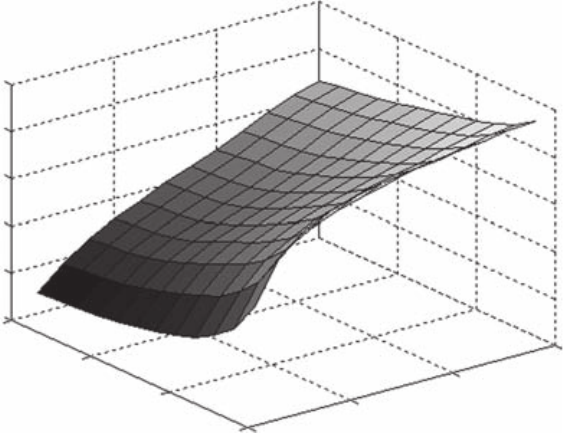
P1: SBT
c15 JWBT188-Aldridge October 23, 2009 11:58 Printer: Yet to come
Back-Testing Trading Models 225
tests, it is desirable to produce analysis on data of the desired frequency
spanning two years or more.
Figures 15.1–15.4 show the results of the potential profitability analysis
of EUR/USD on the hourly data sample ranging from January 2001 through
December 2008. Figures 15.1 and 15.2 show probabilities of successful buy
and sell trades in hourly EUR/USD data with values of stop-gain and stop-
loss parameters ranging from 25 to 300 pips (0.0025 to 0.03) in 25-pip inter-
vals. Figures 15.3 and 15.4 show the surface of the average gain per trade
for hourly EUR/USD buy and sell decisions for various stop-gain and stop-
loss values.
As Figures 15.1 and 15.2 show, the higher the absolute value of the
stop-loss parameter relative to the stop-gain, the higher the probability of
hitting a successful trade. However, high probabilities of a gain do not nec-
essarily turn into high average gain values per trade, as Figures 15.3 and
15.4 illustrate. Over the 2001–2008 sample period, long EUR/USD trades
with high stop-gain and stop-loss parameters achieved higher average gains
than short EUR/USD trades, the observation being due to the underlying
appreciation of EUR/USD over the period.
Probability of gain in long EUR/USD trades
1
0.8
0.6
0.4
0.2
0
300
200
100
00
100
200
300
Stop Loss (bps) Stop Gain (bps)
FIGURE 15.1 Probability of successful buy-initiated trades in hourly EUR/USD
data for different levels of stop-gain and stop-loss parameters.
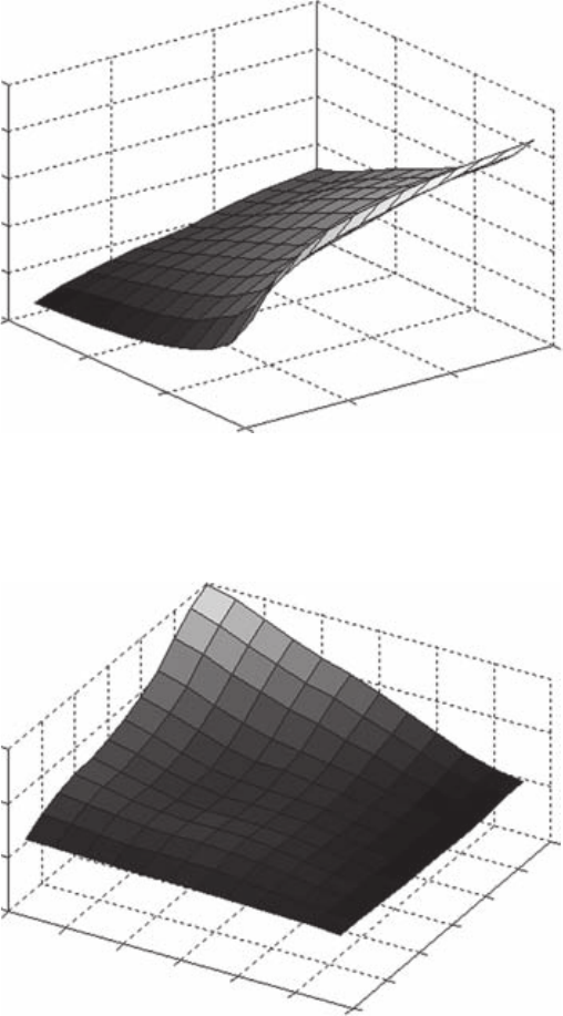
P1: SBT
c15 JWBT188-Aldridge October 23, 2009 11:58 Printer: Yet to come
226 HIGH-FREQUENCY TRADING
Probability of gain in short EUR/USD trades
1
0.8
0.6
0.4
0.2
0
300
200
100
00
100
200
300
Stop Loss (bps) Stop Gain (bps)
FIGURE 15.2 Probability of successful sell-initiated trades in hourly EUR/USD
data for different levels of stop-gain and stop-loss parameters.
Expected gain in long EUR/USD trades
100
50
0
–50
300
250
200
150
100
50
00
50
100
150
300
250
200
Stop Loss (bps)
Stop Gain (bps)
FIGURE 15.3 Average gain per buy-initiated trade in hourly EUR/USD data for
different levels of stop-gain and stop-loss parameters.
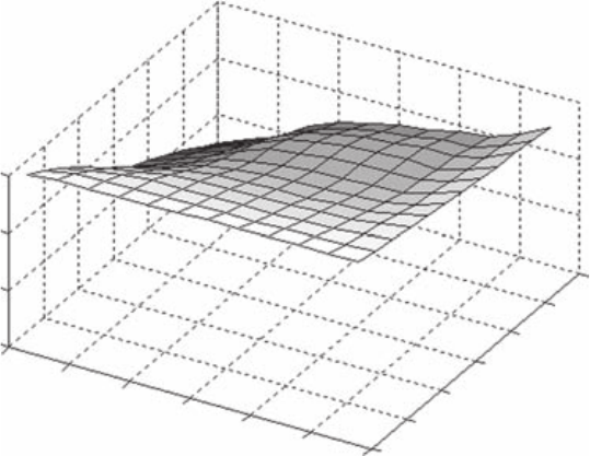
P1: SBT
c15 JWBT188-Aldridge October 23, 2009 11:58 Printer: Yet to come
Back-Testing Trading Models 227
Expected gain in short EUR/USD trades
0
–50
–100
–150
300
250 200
150
100
50
00
50
100
150
300
250
200
Stop Loss (bps)
Stop Gain (bps)
FIGURE 15.4 Average gain per sell-initiated trade in hourly EUR/USD data for
different levels of stop-gain and stop-loss parameters.
Computation of Marginal Probabilities
The next step involves matching the results of Steps 1 and 2 in the preced-
ing list to determine the percentage of trade signals that resulted in positive
gains as well as the percentage of positive gains that remained undetected
by the system. In its most basic approach, this task can be accomplished
as follows:
1. Compute the “hit ratio,” the percentage of trade signals that resulted
in the positive gain. To compute the hit ratio, sum up the number of
buy trades with positive outcomes determined in Step 2, the times
of which corresponded to the times of buy trades determined by the
model presented in Step 1 in the preceding list. Divide the matched
number of buy trades with positive outcomes by the total number of
buy trades generated by the model in Step 1. Repeat the process for
sell trades.
2. Compute the “miss ratio,” the percentage of positive outcomes deter-
mined in Step 2 that were not matched by trades in Step 1.
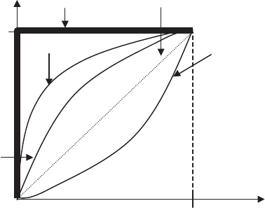
P1: SBT
c15 JWBT188-Aldridge October 23, 2009 11:58 Printer: Yet to come
228 HIGH-FREQUENCY TRADING
Although the hit and miss ratio statistics alone are indicative of the
relative capabilities of the trading model to exploit market conditions,
a graphical representation of trading strategy accuracy generates even
stronger and more intuitive comparative insights.
Accuracy Curves
Accuracy curves, also known as Lorenz, Power, or Gini curves, provide
a way to graphically compare the accuracy of probabilistic forecasts of
trade signals. An accuracy curve plots probabilistic hit rates of different
forecasting models versus the ideal (100 percent accurate) forecast.
The trading strategy accuracy (TSA) curves plot the cumulative dis-
tribution of the “hits” of the trading models versus the “miss” signals. A
“hit” is an outcome whereby the trade signal that generated the outcome is
a profitable trade. For example, if following a buy signal on EUR/USD, the
currency pair appreciates, allowing us to capture a predetermined gain, the
forecast was a “hit.” A “miss” outcome is the opposite situation; it is a trade
signal that led to a loss. The determination of whether the forecast was a
hit or a miss is carried out after the trade has been completed and the trade
profitability is fully observable.
Figure 15.5 shows sample accuracy curves. The thick black line ex-
tending from (0, 0), first vertically and then horizontally to (100, 100), is the
plot of the ideal forecast—that is, the forecast that would ex-ante identify
all the hits as hits and all the misses as misses.
The line bisecting the chart at the 45-degree angle corresponds to a
completely random forecast—a forecast that is equally likely to be a hit
Miss rate (%)
Hit rate (%)
0.0
100%
100
Random forecast
Model AModel C
Ideal forecast
Model B
FIGURE 15.5 Trade model evaluation using trading strategy accuracy (TSA)
curves.

P1: SBT
c15 JWBT188-Aldridge October 23, 2009 11:58 Printer: Yet to come
Back-Testing Trading Models 229
and a miss. All the other models are then evaluated by locations of their
TSA curves relative to the ideal and random forecasts. Model A, for exam-
ple, is worse than the random forecast. Model B is better than the random
forecast, and model C is even better (closer to the ideal) than model B.
A TSA curve is a plot of the cumulative distribution of correctly fore-
casted losses followed by one of correctly forecasted wins. An ideal model
will have a 100 percent hit ratio in all of its forecasts; all the gains will be
ex-ante forecasted as gains, and all the losses will be ex-ante forecasted as
losses. The model with the TSA curve closest to the ideal curve is the best
model. A TSA curve is generated as follows:
1. Gather information on all trade outcomes and their ex-ante forecasts.
A winning trade can be identified as a “1,” while a losing trade can be
identified as a “0.” Similarly, a hit ex-ante forecast that predicted a win
and resulted in a win can be identified as a “1,” and so can an ex-ante hit
predicting a loss and resulting in a loss. An ex-ante miss of either the
forecasted win resulting in a loss or a forecasted loss resulting in a win
can be identified as “0.” Table 15.3 shows the resulting data structure
for several sample trades.
2. Calculate the total number of hits, H, and misses, M, among all trade
outcomes. In our example, there were two hits and three misses. Next,
define Nas the maximum of the two numbers: N=max(H,M). In our
example, N=3.
3. Compute cumulative hit and miss rates for each trade. The cumulative
hit rate for the ith trade, Hiis determined as follows:
Hi=Hi−1+1/Nifith trade is a hit
Hi−1otherwise
Mi=Mi−1+1/Nifith trade is a miss
Mi−1otherwise
TABLE 15.3 Assessing Trade Outcomes and Forecast Hits and Misses
Trade
ID Date
Forecast/
Trade Open
Time
Ex-Ante
Forecast
Trade
Realization
Gain
(Loss)
MM
Trade
Outcome
Hit or
Miss
1 3/9/2009 6:00 A.M.ET Win Win 59 1 1
2 3/9/2009 7:00 A.M. ET Loss Win 70 1 0
3 3/9/2009 8:00 A.M. ET Win Loss (25) 0 0
4 3/9/2009 9:00 A.M. ET Loss Loss (66) 0 1
5 3/9/2009 10:00 A.M. ET Loss Win 30 1 0
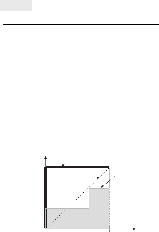
P1: SBT
c15 JWBT188-Aldridge October 23, 2009 11:58 Printer: Yet to come
230 HIGH-FREQUENCY TRADING
TABLE 15.4 Cumulative Hit and Miss Rates
Trade ID
Trade
Outcome Hit or Miss
Cumulative
Hit Rate
Cumulative
Miss Rate
1 1 1 33.3 percent 0 percent
2 1 0 33.3 percent 33.3 percent
3 0 0 33.3 percent 66.7 percent
4 0 1 66.7 percent 66.7 percent
5 1 0 66.7 percent 100 percent
Table 15.4 shows the cumulative hit and miss trades for our example.
Trade characteristics have been omitted to save space.
4. We are now ready to plot our sample TSA curve. On the chart, the cu-
mulative miss rate for each trade is plotted on the vertical axis, and
the cumulative hit rate is plotted on the vertical axis. Starting at the
lower-left corner, at point (0, 0), we now draw the line through the
points characterizing the hit and miss rate pairs in our example and
then continue the line to the upper-right corner (100 percent, 100 per-
cent) point. Figure 15.6 illustrates the outcome.
The accuracy of the forecast is determined as the total area under
the TSA curve. For our example, the area under the curve (shaded re-
gion) amounts to 44.4 percent of the total area of the box, indicating a
Example model
Hit rate (%)
0.0
100%
100
Random forecast
Ideal forecast
Miss rate (%)
FIGURE 15.6 Trading strategy accuracy (TSA) curve for the foregoing sample
trades.

P1: SBT
c15 JWBT188-Aldridge October 23, 2009 11:58 Printer: Yet to come
Back-Testing Trading Models 231
44.4 percent accuracy of our forecasts. Our sample forecasting model per-
forms worse than the random forecasting model, the diagonal. The random
forecasting model has an accuracy of 50 percent. Note that in small sam-
ples like our example, the accuracy of the estimation will depend on the
order of hits and misses within the sample. Depending on the order of hits
and misses, the accuracy will vary around its true value.
The TSA curve described here is of the simplest kind; it illustrates the
hit ratios without any consideration for the actual profitability of winning
versus losing trades. A more advanced version of the TSA curve remedies
the situation by splitting all gains into two or more buckets of profitability
and splitting all losses into comparable buckets of loss values.
In addition to comparisons of accuracy among different trading mod-
els, analyzing potential outcomes of trading systems helps to strengthen
and calibrate existing models as well as to evaluate the performance of a
combination of different models with mutually exclusive signals. Aldridge
(2009a) develops a quantitative methodology of applying hit and miss ratio
analyses to enhance the accuracy of predictions of trading models.
CONCLUSION
Various back-test procedures illuminate different aspects of strategy per-
formance on historical data and are performed before the trading strategy
is applied to live capital. Observing parameters of strategy performance in
back tests allows high-frequency managers to identify the best strategies
to include in their portfolio. The same parameters allow modelers to tweak
their strategies to obtain even more robust models. Care should be taken
to avoid “overfitting”—using the same data sample in repeated testing
of the model.
P1: SBT
c15 JWBT188-Aldridge October 23, 2009 11:58 Printer: Yet to come
232

P1: SBT
c16 JWBT188-Aldridge October 23, 2009 12:1 Printer: Yet to come
CHAPTER 16
Implementing
High-Frequency
Trading Systems
Once high-frequency trading models have been identified, the models
are back-tested to ensure their viability. The back-testing software
should be a “paper”-based prototype of the eventual live system.
The same code should be used in both, and the back-testing engine should
run on tick-by-tick data to reenact past market conditions. The main func-
tionality code from the back-testing modules should then be reused in the
live system.
To ensure statistically significant inferences, the model “training” pe-
riod Tshould be sufficiently large; according to the central limit theorem
(CLT), 30 observations is the bare minimum for any statistical significance,
and 200 observations is considered a reasonable number. Given strong sea-
sonality in intra-day data (recurrent price and volatility changes at specific
times throughout the day), benchmark high-frequency models are back-
tested on several years of tick-by-tick data.
The main difference between the live trading model and the back-test
model should be the origin of the quote data; the back-test system includes
a historical quote-streaming module that reads historical tick data from
archives and feeds it sequentially to the module that has the main function-
ality. In the live trading system, a different quote module receives real-time
tick data originating at the broker-dealers.
Except for differences in receiving quotes, both live and back-test sys-
tems should be identical; they can be built simultaneously and, ideally, can
use the same code samples for core functionality. This chapter reviews
233

P1: SBT
c16 JWBT188-Aldridge October 23, 2009 12:1 Printer: Yet to come
234 HIGH-FREQUENCY TRADING
the systems implementation process under the assumption that both back-
testing and live engines are built and tested in parallel.
MODEL DEVELOPMENT LIFE CYCLE
High-frequency trading systems, by their nature, require rapid hesitation-
free decision making and execution. Properly programmed computer
systems typically outperform human traders in these “mission-critical”
trading tasks, particularly under treacherous market conditions—see
Aldridge (2009), for example. As a result, computer trading systems are
rapidly replacing traditional human traders on trading desks around the
world.
The development of a fully automated trading system follows a path
similar to that of the standard software development process. The typical
life cycle of a development process is illustrated in Figure 16.1.
A sound development process normally consists of the following five
phases:
1. Planning
2. Analysis
3. Design
4. Implementation
5. Maintenance
Analysis
Design
Implementation
Maintenance
Planning
FIGURE 16.1 Typical development cycle of a trading system.
P1: SBT
c16 JWBT188-Aldridge October 23, 2009 12:1 Printer: Yet to come
Implementing High-Frequency Trading Systems 235
The circular nature of the process illustrates the continuous quality of
system development. When a version of the system appears to be complete,
new issues demand advanced modifications and enhancements that lead to
a new development cycle.
The purpose of the planning phase is to determine the goals of the
project as well as to generate a high-level view of what the completed
project may look like. The planning is accompanied by a feasibility study
that evaluates the project in terms of its economics, operating model, and
technical requirements. The economical considerations explore whether
the project has a sufficient profit and loss (P&L) potential, whereas oper-
ational and technical issues address the feasibility of the project from the
compliance, human resources, and other day-to-day points of view. The
outputs of the planning phase include concrete goals and targets set for
the project, established schedules, and estimated budgets for the entire
system.
During the analysis stage of the process, the team aggregates require-
ments for system functionality, determines the scope of the project (which
features are in and which features are out of the current release), and so-
licits initial feedback from users and management. The analysis stage is
arguably the most critical stage in the development process, because it is
here that stakeholders have the ultimate ability to shape the functionality
of the system given the allocated budget.
The design phase incorporates detailed specifications of functionality,
including process diagrams, business rules, and screenshots, along with
other output formats such as those of daily reports and other documents.
An objective of the design stage is to separate the whole project into dis-
crete components subsequently assigned to teams of software developers;
the discrete components will have well-specified interfaces that can lock
in seamlessly with other components designed by different teams of soft-
ware developers. Such early specification of software packaging of inter-
nal computer modules streamlines future communication among different
software development teams and enables smooth operation of the project
going forward. The design phase also outlines test cases—that is, the func-
tionality paths that are later used as blueprints to verify the correctness of
the completed code.
The implementation phase, finally, involves actual programming; the
software teams or individual programmers develop software modules ac-
cording to the specifications defined in the design stage. The individual
modules are then tested by the development teams themselves against the
predefined test cases. When the project management is satisfied that the
individual modules have been developed according to the specifications,
the project integration work begins. Integration, as its name implies, refers
to putting together the individual modules to create a functional system.

P1: SBT
c16 JWBT188-Aldridge October 23, 2009 12:1 Printer: Yet to come
236 HIGH-FREQUENCY TRADING
While successfully planned projects encounter little variance or prob-
lems in the integration stage, some work still remains. Scripts may have
to be written to ensure proper communication among various system
components, installation wrappers may have to be developed, and, most
importantly, the system has to be comprehensively tested to ensure proper
operation. The test process usually involves dedicated personnel other
than the people who developed the code. The test staff diligently monitors
the execution of each functionality according to testing procedures defined
in the design stage. The test personnel then documents any “bugs”—that
is, discrepancies between the prespecified test case performance and ob-
served performance. The bugs are then sent back over to the development
team for resolution and are subsequently returned to the testing teams.
Successful implementation is followed by the deployment and subse-
quent maintenance phase of the system. The maintenance phase addresses
system-wide deviations from planned performance, such as troubleshoot-
ing newly discovered bugs.
SYSTEM IMPLEMENTATION
Key Steps in Implementation
of High-Frequency Systems
Most systematic trading platforms are organized as shown in Figure 16.2.
One or several run-time processors contain the core logic of the trading
mechanism and perform the following functions:
rReceive, evaluate, and archive incoming quotes
rPerform run-time econometric analysis
rImplement run-time portfolio management
rInitiate and transmit buy and sell trading signals
rListen for and receive confirmation of execution
rCalculate run-time P&L
rDynamically manage risk based on current portfolio allocations and
market conditions
A successful high-frequency trading system adapts itself easily to con-
temporary market conditions. As a result, most high-frequency systems
accept, process, and archive volumes of quotes and other market data de-
livered at real-time frequency. Some systems may convert streaming real-
time data into equally spaced data intervals, such as seconds or minutes,
for use in their internal econometric analyses. Other systems may run on
the raw, irregularly spaced quotes. The decision whether to convert the
data should be based on the requirements of the run-time econometric
analysis.
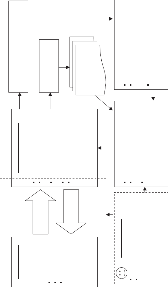
P1: SBT
c16 JWBT188-Aldridge October 23, 2009 12:1 Printer: Yet to come
Live Quotes
Buy/Sell
Orders
Electronic
Interface Generate order and fulfillment
record for future reconciliation
Archive all quotes
received
USD/CAD
Post-Trade Analysis
Proprietary software technology
Reconciles daily trades with
simulation results based on
archived data
Identifies slippages, anomalies,
and other discrepancies
Simulation Engine
Proprietary software technology
Generates and tests new
strategies
Enhances current trading
strategies based on the results
generated in the post-trade
analysis
Human Element
Run-time performance monitoring
Innovation in strategy
development/enhancement
Run-Time Processor
Proprietary software
technology
Process real-time quotes
Perform run-time
econometrics
Develop buy and sell
signals
Calculate run-time P&L
Risk management based on
pre-defined parameters
Broker-Dealer
Services:
Quotes
Order Processing
Trade
Reconciliation
FIGURE 16.2 Typical high-frequency process.
237
P1: SBT
c16 JWBT188-Aldridge October 23, 2009 12:1 Printer: Yet to come
238 HIGH-FREQUENCY TRADING
The run-time econometric analysis is a computer program that per-
forms the following three functions:
1. Accepts quotes and order acknowledgments
2. Uses the quotes as input to the core analysis engine
3. Outputs trading signals
The core analysis engine is typically based on the historical analysis
identified to generate consistent positive returns over a significant period
of time during the simulation and back-testing process. The development
of the core engine usually proceeds as follows. First, a quantitative ana-
lyst identifies a mispriced security, a market inefficiency, or a persistent
deviation from equilibrium. This first modeling step is often done using
the MatLab or R programming languages, which are designed to facilitate
mathematical operations.
Next, the quantitative analyst, usually in conjunction with technical
specialists, back-tests the model on several years of data. A back test of
several years (two at the very minimum) should produce a sample distribu-
tion of returns that is numerous enough to be close to the true distribution
of returns characterizing both past and future performance. If the model
delivers consistently positive results in the back test over several years,
the model is then programmed into its production state.
Most of the high-frequency production-bound systems are written in
C++, although some hedge funds and other investment management firms
are known to use Java. C++is often considered to be “lighter” and “faster”
than Java, meaning that C++ programs do not have the processing power
overhead required by Java; as a result, C++systems often work faster than
Java-based systems. C++ programmers, however, must be careful in their
utilization of the system’s run-time memory, whereas Java is designed to
take care of all run-time memory issues whether or not the programmer
remembers to do so.
The design and implementation of run-time portfolio management
reflects the core econometric engine. In addition to the raw quote inputs,
the portfolio management framework incorporates inputs from the econo-
metric model, current position sizes, and other information relevant to
portfolio diversification and maximization of portfolio returns, while mini-
mizing portfolio risk.
The core engine and the portfolio management framework then initiate
and transmit orders to the broker-dealer. Upon receiving and executing an
order, the broker-dealer sends back the order status and order-filling price
and size to the client. The system then calculates the P&L and assesses
risk management parameters that feed back into the portfolio management
piece.
P1: SBT
c16 JWBT188-Aldridge October 23, 2009 12:1 Printer: Yet to come
Implementing High-Frequency Trading Systems 239
Incoming quotes, along with outgoing orders and any other communi-
cation between a broker-dealer and a client or an exchange, are most often
transmitted via a Financial Information eXchange (FIX) protocol specifi-
cally designed for transmission of real-time financial information. Accord-
ing to the FIX industry website (http://www.fixprotocol.org), FIX emerged
in 1992 as a bilateral communications framework for equity trading be-
tween Fidelity Investments and Salomon Brothers. It has since become
the dominant communication method among various broker-dealers, ex-
changes, and transacting customers. In fact, according to a survey con-
ducted by fixprotocol.org, FIX was used for systematic trading by 75 per-
cent of buy-side firms, 80 percent of sell-side firms, and over 75 percent of
exchanges in 2006.
FIX is best described as a programming language that is overseen by
a global steering committee, consisting of representatives from banks,
broker-dealers, exchanges, industry utilities and associations, institutional
investors, and information technology providers from around the world.
Its standard is open and free. Implementation of communication process
via FIX, however, requires careful planning and dedicated resources and
may demand significant expense, much like any other system development
process.
A typical FIX message is composed of a header, a body, and a trailer.
The header always contains the following three fields: a string identifying
the beginning of a message (FIX field # 8), the number of characters in the
body of the message to follow the message header (FIX field # 9), and
the type of the message (FIX field # 35). Among many message types are
quotation and order execution directives and acknowledgments as well as
housekeeping messages designed to ensure that the system remains up and
running.
For example, MsgType =0 is the “Heartbeat” message—a message is
sent to the other communication party to ensure that the communication
connection remains operational and has not been lost as a result of any
unforeseen technical problems. The heartbeat message is typically sent af-
ter a prespecified number of seconds of inactivity. If either communication
party has not received a heartbeat message from the other party, it sends
a TestRequest message (MsgType =1) to “poll” the other communication
party. If no heartbeat message is received following a TestRequest mes-
sage, the connection is considered lost and steps are taken to restart it.
MsgType =6 is known as “Indication of Interest.” Exchanges and
broker-dealers use Indication of Interest messages to transmit their inter-
est in either buying or selling in either a proprietary or an agency capacity.
MsgType =R indicates a “Quote Request” message with which a client of
a broker-dealer requests a quote stream. Under normal circumstances, the
broker-dealer responds to the Quote Request message with a continuous
P1: SBT
c16 JWBT188-Aldridge October 23, 2009 12:1 Printer: Yet to come
240 HIGH-FREQUENCY TRADING
stream of Quote messages (MsgType =S) that carry actual quote informa-
tion, such as bid or ask prices.
Other message types include orders such as single-name orders, list
orders, day limit orders, multiday orders, various cancellation requests,
and acknowledgments. All fields in the body are included in the following
format:
[Field #] =[data]
For example, to communicate that the message carries the status of an
order, the following sequence is used:
35 =8|
All field sequences are terminated with a special character that has a com-
puter value of 0x01. The character looks like “|” when seen on-screen.
The body of the message contains the details of the message, whether
it is a quote request, a quote itself, or order and trade information. The
message body further specifies the exchange of interest, a timestamp that
includes milliseconds, a security symbol, and other necessary transaction
data. Like the header, all fields in the body are included in the following
format:
[Field #] =[data]
and each field sequence is terminated by a special computer character
0x01.
Finally, at the end of the body of every message is the “checksum”—a
sum of digital values of all the characters in the message included as a
verification of whether the message has arrived in full.
For example, a message carrying a quote for USD/CAD at 15:25:20 GMT
on July 31, 2007 looked like this:
8=FIX.4.2 | 9=309|35=S|49=ML-FIX-FX |
56=ECHO2-QTS-TEST | 34=5015 | 52=20070731-15:25:20 |
131=1185895365 | 117=ECHO2-QTS-
TEST.00043690C8A8D6B9.00043690D14044C6 | 301=0|
55=USD/CAD | 167=FOR|15=USD | 132=1.065450 |
133=1.065850 | 134=5000000.0 | 135=5000000.0 |
647=2000001.0 | 648=2000001.0 | 188=1.06545 |
190=1.06585 | 60=20070731-15:25:20 | 40=H|64=20070801
|10=178
Dissecting the message, we note the following fields:
8=FIX.4.2: Version of the FIX protocol used.
9=309: The body of the message is 309 characters long.
35=S: This message is carrying a quote.
P1: SBT
c16 JWBT188-Aldridge October 23, 2009 12:1 Printer: Yet to come
Implementing High-Frequency Trading Systems 241
49=ML-FIX-FX: internal identification of the sender of the message; in
this case, the sender is Merrill Lynch FX desk.
56=ECHO2-QTS-TEST: internal identification of the message recipient.
34=5015: sequential message number; this number is used to track all
the messages sent. Message sequencing makes it easy for the recip-
ient of the message to identify whether the recipient has received
all of the messages and whether they were received in order. Mes-
sage sequencing may help pinpoint problems with the communica-
tion link or message transmission and reception.
52=20070731-15:25:20: timestamp corresponding to the time
transmission originated. The timestamp consists of the date
(yyyymmdd) and time (hh:mm:dd). The time is usually quoted in
GMT.
131=1185895365: unique identifier corresponding to a message con-
taining an original quote request for a given security.
117=ECHO2-QTS-TEST.00043690C8A8D6B9.00043690D14044C6:
unique identifier for the quote. Note that the identifier contains
the recipient’s identification, making it possible for broker-dealers
to stream different quotes to clients with different profiles. For
example, the broker-dealer may increase spreads for a persistently
successful client.
301=0: level of response requested from recipient of the quote mes-
sage; valid responses are 0 =No Acknowledgment (default), 1
=Acknowledge only negative or erroneous quotes, and 2 =Ac-
knowledge each quote message. In our example, Merrill Lynch
does not expect any acknowledgment upon receipt of the quote.
55=USD/CAD: the ticker symbol of the quoted instrument.
167=FOR: the type of the security quoted. Valid values include ABS
=Asset-backed Securities, BN =Bank Notes, FUT =Future, and
OPT =Option, among many others.
15=USD: based currency used for price.
132=1.065450: bid price.
133=1.065850: offer or ask price.
134=5000000.0: bid quantity.
135=5000000.0: offer quantity.
647=2000001.0: minimum quantity for a bid.
648=2000001.0: minimum quantity for an offer.
188=1.06545: bid FX spot rate.
190=1.06585: offer FX spot rate.
60=20070731-15:25:20: timestamp of the quote creation.
40=H: available order types.
Order types may assume one of the following values: 1 =Market, 2 =
Limit, 3 =Stop/Stop Loss, 4 =Stop Limit, 5 =Market On Close (No
P1: SBT
c16 JWBT188-Aldridge October 23, 2009 12:1 Printer: Yet to come
242 HIGH-FREQUENCY TRADING
longer used), 6 =With Or Without, 7 =Limit Or Better, 8 =Limit
With Or Without, 9 =On Basis, A =On Close (No longer used), B
=Limit On Close (No longer used), C =Forex Market (No longer
used), D =Previously Quoted, E =Previously Indicated, F =Forex
Limit (No longer used), G =Forex Swap, H =Forex Previously
Quoted (No longer used), I =Funari (Limit day order with unexe-
cuted portion handles as Market On Close, e.g., Japan), J =Market
If Touched (MIT), K =Market With Left Over as Limit (market or-
der with unexecuted quantity becoming limit order at last price), L
=Previous Fund Valuation Point (Historic pricing; for CIV), M =
Next Fund Valuation Point (Forward pricing; for CIV), P =Pegged,
Q=Counter-order selection.
64=20070801: trade settlement date. If the order were to be executed
on July 31, 2007, the trade would be settled on 8/1/2007.
10=178: checksum, a sum of computer codes of all characters in the
message. The checksum is used to verify that the message arrived
intact.
The best high-frequency trading systems do not stop there. A post-
trade analysis engine reconciles production results with simulation results
run with the same code on the same data and updates distributions of re-
turns, trading costs, and risk management parameters to be fed back into
the main processing engine, portfolio optimization, and risk management
components.
The simulation engine is an independent module that tests new trad-
ing ideas on past and run-time data without actually executing the trades.
Unlike ideas that are still in early stages of development that are often
coded in MatLab or Excel, ideas tested in the simulation engine are typ-
ically coded in the production language (C++ or Java). Once coded for
production setup, the simulation engine is first run on a long sample of
historical data in a process known as back-testing. At this point, the sim-
ulation engine can be refined to incorporate any system tweaks and bug
fixes. Once the back test performs satisfactorily, the system is switched to
run on real-time data, the same data that feeds into the production system.
At this point, however, the system is still in the testing phase and the sys-
tem’s ability to send production orders is disabled. Instead, all orders that
would be sent to the broker-dealer are recorded in a text file. This testing
phase of the system on the real-time data is referred to as “paper-trading.”
Once paper-trading performance is satisfactory and comparable to that
of the back test, paper-trading is moved into production. Continuous hu-
man supervision of the system is required to ensure that the system does
not fall victim to some malicious activity such as a computer virus or a mar-
ket event unaccounted for in the model itself. The role of the human trader,
however, should normally be limited to making sure that the performance
P1: SBT
c16 JWBT188-Aldridge October 23, 2009 12:1 Printer: Yet to come
Implementing High-Frequency Trading Systems 243
of the system falls within specific bounds. Once the bounds are breached,
the human trader should have the authority to shut down trading for the
day or until the conditions causing the breach have been resolved.
Common Pitfalls in Systems Implementation
Time Distortion The simulation runs in its own time using quotes col-
lected and stored during a run-time of another process. The frequency of
the quotes recorded by the process that collected the data that is now his-
torical data can vary greatly, mostly because of the following two factors:
1. The number of financial instruments for which the original process col-
lected quotes
2. The speed of the computer system on which the original process ran
Their impact is due to the nature of the quote process and its realiza-
tion in most trading systems. Most systems comprise a client (the quote
collecting and/or trading application) that is geared to receive quotes and
the server (a broker-dealer application supplying the quotes). The client is
most often a “local” application that runs “locally”: on computer hardware
over which the trader has full control. The broker-dealer server is almost
always a remote application, meaning that the client has to communicate
with the server over a remote connection, such as the Internet. To receive
quotes, the client application usually has to perform the following commu-
nication with the server process:
1. The client sends the server a message or a series of messages with the
following information:
a. Client identification (given to the client by the broker-dealer that
houses the server)
b. Names of financial securities for which the quotes are requested
2. The server will respond, acknowledging the client’s message. The
server’s response will also indicate whether the client is not allowed
to receive any of the quotes requested for any reason.
3. The server will begin to stream the quotes to the client. The quotes are
typically streamed in an “asynchronous” manner—that is, the server
will send a quote to the client as soon as a new quote becomes avail-
able. Some securities have higher-frequency quotes than others. For
example, during high-volatility times surrounding economic announce-
ments, it is not unusual for the EUR/USD exchange rate to be accom-
panied by as many as 30 quotes per second. At the same time, some
obscure stock may generate only one quote per trading day. It is impor-
tant to keep in mind the expected frequency of quotes while designing
the quote-receiving part of the application.
P1: SBT
c16 JWBT188-Aldridge October 23, 2009 12:1 Printer: Yet to come
244 HIGH-FREQUENCY TRADING
4. Quote distortion often happens next. It is the responsibility of the
client to collect and process all the quotes as soon as they arrive at
the client’s computer. Here, several issues can occur. On the client’s
machine, all incoming quotes are placed into a queue in the order of
their arrival, with the earliest quotes located closest to the processor.
This queue can be thought of as a line for airport check-in. Unlike the
airport line, however, the queue often has a finite length or capacity;
therefore, any quote arrivals that find the queue full are discarded.
Hence the first issue: Quote time series may vary from client to client
if the client systems have queues of varying lengths, all other system
characteristics being equal.
Once the quotes are in the queue, the system picks the earliest
quote arrival from the queue for processing; then all the quotes in the
queue are shifted closer to the processing engine. As noted previously,
the quotes may arrive faster than the client is able to process them, fill-
ing up the queue and leading the system to discard new quote arrivals
until the older quotes are processed. Even a seemingly simple opera-
tion such as copying a quote to a file or a database stored on the com-
puter system takes computer time. While the quote-storing time may
be a tiny fraction of a second and thus negligible by human time stan-
dards, the time can be significant by computer clock, and slow down
the processing of incoming quotes.
A client system may assign the quote an arrival time on taking the
quote from its arrival queue. The timestamp may therefore differ from
the timestamp given to the quote by the server. Depending on the num-
ber of securities for which the quotes are collected and the market’s
volatility at any given time of day, the timestamp distortion may dif-
fer significantly as a result of the quote-processing delay alone. If the
quotes are further mathematically manipulated to generate trading sig-
nals, the distortions in timestamps may be even more considerable.
5. Naturally, systems running on computers with slower processing
power will encounter more timestamp distortion than systems running
on faster machines. Faster machines are quicker at processing sequen-
tial quotes and drop fewer quotes as a result. Even the slightest differ-
ences in system power can result in different quote streams that in turn
may produce different trading signals.
The reliability of quote delivery can be improved in the following four
ways:
1. Timestamping quotes immediately when each quote arrives before
putting the quote into the queue
2. Increasing the size of the quote queue
P1: SBT
c16 JWBT188-Aldridge October 23, 2009 12:1 Printer: Yet to come
Implementing High-Frequency Trading Systems 245
3. Increasing system memory to the largest size feasible given a cost/
benefit analysis
4. Reducing the number of securities for which the quotes are collected
on any given client
These four steps toward establishing greater quote reliability are fairly
easy to implement when the client application is designed and built from
scratch, and in particular when using the FIX protocol for quote delivery.
On the other hand, many off-the shelf clients, including those distributed by
executing brokers, may be difficult or impossible to customize. For firms
planning to use an off-the-shelf client, it may be prudent to ask the software
manufacturer how the preceding issues can be addressed in the client.
Speed of Execution Duration of execution can make or break high-
frequency trading models. Most strategies for arbitraging temporary mar-
ket mispricings, for example, depend on the ability to get the orders posted
with lightning speed. Whoever detects the mispricing and gets his order
posted on the exchange first is likely to generate the most profit.
Speed of execution is controlled by the following components of trad-
ing platforms:
rThe speed of applications generating trading signals
rThe proximity of applications generating trading signals to the execut-
ing broker
rThe speed of the executing broker’s platform in routing execution
requests
rThe proximity of the executing broker to the exchange
rThe speed of the exchange in processing the execution orders
Figure 16.3 illustrates the time-dependent flow of execution process.
To alleviate delays due to the physical transmission of trading signals
between clients and the broker and, again, between the broker and the
exchange, clients dependent on the speed of execution often choose to
locate their systems as close to the broker and the exchange as possible.
This practice of placing client computer systems next to the broker and the
exchange is known as “co-location.” Co-location does not require clients
to move their offices; instead, co-location can be achieved through a set of
production machines managed in a secure warehouse by an experienced
third-party administrator, with the client having a full remote, or “virtual,”
access to the production machines. Co-location services typically employ
systems administration staff that is capable of providing recovery services
in case of systems or power failure, making sure that the client applications
work at least 99.9 percent of time.
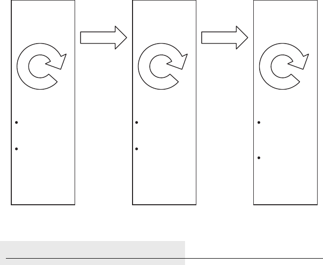
P1: SBT
c16 JWBT188-Aldridge October 23, 2009 12:1 Printer: Yet to come
246 HIGH-FREQUENCY TRADING
Trading signal
generation
(Buy-side Client)
Factors
influencing
speed:
Complexity
of trading
signals
Processing
power of
hardware
Order processing
and routing
(Executing
Broker)
Factors
influencing
speed:
Optimization
of routing
algorithms
Capacity to
process large
number of
orders in
parallel
Order Execution
(Exchange)
Factors
influencing
speed:
Optimization
of order-
matching
algorithms
Capacity to
process large
number of
orders in
parallel
Signal
travel
speed
~
signal
travel
distance
Signal
travel
speed
~
signal
travel
distance
FIGURE 16.3 Execution process.
TESTING TRADING SYSTEMS
The costs of rolling out a system that contains programmatic errors, or
bugs, can be substantial. Thorough testing of the system, therefore, is es-
sential prior to wide roll-out of the model. Testing has the following stages:
rData set testing
rUnit testing
rIntegration testing
rSystem testing
rRegression testing
rUse case testing
Data Set Testing
Data set testing refers to testing the validity of the data, whether historical
data used in a back test or real-time data obtained from a streaming data
provider. The objective of data testing is to ascertain that the system mini-
mizes undesirable influences and distortions in the data and to ensure that
the run-time analysis and trading signal generation work smoothly.
Data set testing is built on the premise that all data received for
a particular security should fall into a statistical distribution that is
P1: SBT
c16 JWBT188-Aldridge October 23, 2009 12:1 Printer: Yet to come
Implementing High-Frequency Trading Systems 247
consistent throughout time. The data should also exhibit consistent distri-
butional properties when sampled at different frequencies: 1-minute data
for USD/CAD, for example, should be consistent with historical 1-minute
data distribution for USD/CAD observed for the past year. Naturally, data
set testing should allow for distributions to change with time, but the ob-
served changes should not be drastic, unless they are caused by a large-
scale market disruption.
A popular procedure for testing data is based on testing for consistency
of autocorrelations. It is implemented as follows:
1. A data set is sampled at a given frequency—say, 10-second intervals.
2. Autocorrelations are estimated for a moving window of 30 to 1,000
observations.
3. The obtained autocorrelations are then mapped into a distribution;
outliers are identified, and their origin is examined. The distributional
properties can be analyzed further to answer the following questions:
rHave the properties of the distribution changed during the past
month, quarter, or year?
rAre these changes due to the version of the code or to the addition
or removal of programs on the production box?
The testing should be repeated at different sampling frequencies to en-
sure that no systemic deviations occur.
Unit Testing
Unit testing verifies that each individual software component of the system
works properly. A unit is a testable part of an application; the definition of a
unit can range from the code for the lowest function or method to the func-
tionality of a medium-level component—for example, a latency measure-
ment component of the post-trade analysis engine. Testing code in small
blocks from the ground up ensures that any errors are caught early in the
integration process, avoiding expensive system disruptions at later stages.
Integration Testing
Integration testing follows unit testing. As its name implies, integration
testing is a test of the interoperability of code components; the test is
administered to increasingly larger aggregates of code as the system is
being built up from modular pieces to its completed state. Testing modular
interoperability once again ensures that any code defects are caught and
fixed early.
P1: SBT
c16 JWBT188-Aldridge October 23, 2009 12:1 Printer: Yet to come
248 HIGH-FREQUENCY TRADING
System Testing
System testing is a post-integration test of the system as a whole. The sys-
tem testing incorporates several testing processes described as follows.
Graphical user interface (GUI) software testing ensures that the hu-
man interface of the system enables the user (e.g., the person responsible
for monitoring trading activity) to perform her tasks. GUI testing typically
ensures that all the buttons and displays that appear on screen are con-
nected with the proper functionality according to the specifications devel-
oped during the design phase of the development process.
Usability and performance testing is similar in nature to GUI testing but
is not limited to graphical user interfaces and may include such concerns
as the speed of a particular functionality. For example, how long does the
system take to process a “system shutdown” request? Is the timing accept-
able from a risk management perspective?
Stress testing is a critical component of the testing of high-frequency
trading systems. A stress-testing process attempts to document and, sub-
sequently, quantify the impact of extreme hypothetical scenarios on the
system’s performance. For example, how does the system react if the price
of a particular security drops 10 percent within a very short time? What
if an act of God occurs that shuts down the exchange, leaving the system
holding its positions? What other worst-case scenarios are there and how
will they affect the performance of the system and the subsequent P&L?
Security testing is another indispensable component of the testing pro-
cess that is often overlooked by organizations. Security testing is designed
to identify possible security breaches and to either provide a software so-
lution for overcoming the breaches or create a breach-detection mecha-
nism and a contingency plan in the event a breach occurs. High-frequency
trading systems can be vulnerable to security threats coming from the In-
ternet, where unscrupulous users may attempt to hijack account numbers,
passwords, and other confidential information in an attempt to steal trad-
ing capital. However, intra-organizational threats should not be underes-
timated; employees with malicious intent or disgruntled workers having
improper access to the trading system can wreak considerable and costly
havoc. All such possibilities must be tested and taken into account.
Scalability testing refers to testing the capacity of the system. How
many securities can the system profitably process at the same time with-
out incurring significant performance impact? The answer to this question
may appear trivial, but the matter is anything but trivial in reality. Every in-
cremental security measure added to the system requires an allocation of
computer power and Internet bandwidth. A large number of securities pro-
cessed simultaneously on the same machine may considerably slow down
system performance, distorting quotes, trading signals, and the P&L as a

P1: SBT
c16 JWBT188-Aldridge October 23, 2009 12:1 Printer: Yet to come
Implementing High-Frequency Trading Systems 249
result. A determination of the maximum permissible number of securities
will be based on the characteristics of each trading platform, including
available computing power.
Reliability testing determines the probable rate of failure of the sys-
tem. Reliability testing seeks to answer the following questions: What are
the conditions under which the system fails? How often can we expect
these conditions to occur? The failure conditions may include unexpected
system crashes, shutdowns due to insufficient memory space, and anything
else that leads the system to stop operating. The failure rate for any well-
designed high-frequency trading system should not exceed 0.01 percent
(i.e., the system should be guaranteed to remain operational 99.99 percent
of the time).
Recovery testing refers to verification that in an adverse event, whether
an act of God or a system crash, the documented recovery process en-
sures that the system’s integrity is restored and it is operational within a
prespecified time. The recovery testing also ensures that data integrity is
maintained through unexpected terminations of the system. Recovery test-
ing should include the following scenarios: When the application is running
and the computer system is suddenly restarted, the application should have
valid data upon restart. Similarly, the application should continue operat-
ing normally if the network cable should be unexpectedly unplugged and
then plugged back in.
Use Case Testing
The term use case testing refers to the process of testing the system ac-
cording to the system performance guidelines defined during the design
stage of the system development. In use case testing, a dedicated tester
follows the steps of using the system and documents any discrepancies be-
tween the observed behavior and the behavior that is supposed to occur.
Use case testing ensures that the system is operating within its parameters.
CONCLUSION
Implementation of high-frequency systems is a critical process, one in
which mistakes can be very costly. Outsourcing noncritical components
of the system may be a prudent strategy. However, code that implements
proprietary econometric models should be developed internally to ensure
maximum strategy capacity.
P1: SBT
c16 JWBT188-Aldridge October 23, 2009 12:1 Printer: Yet to come
250

P1: SBT
c17 JWBT188-Aldridge October 22, 2009 17:49 Printer: Yet to come
CHAPTER 17
Risk
Management
Effective risk management in a trading operation is as important as
the signals that motivate the trades. A well-designed and executed
risk management function is key to sustainable profitability in all
organizations. This chapter presents the leading approaches for managing
risk in high-frequency trading operations that are compliant with Basel II
risk management standards.1
As with any business decision, the process of building a risk manage-
ment system involves several distinct steps:
1. First, the overall organization-wide goals of risk management should
be clearly defined.
2. Next, potential risk exposure should be measured for each proposed
trading strategy and the overall portfolio of the trading operation.
3. Based on the goals and risk parameters determined in the two preced-
ing steps, a risk management system is put in place to detect abnormal
risk levels and to dynamically manage risk exposure.
The following sections in turn address each of these steps.
1Basel II is the set of recommendations on risk management in financial services
issued by the Basel Committee on Banking Supervision in June 2004 with the goal
of promoting economic stability.
251

P1: SBT
c17 JWBT188-Aldridge October 22, 2009 17:49 Printer: Yet to come
252 HIGH-FREQUENCY TRADING
DETERMINING RISK
MANAGEMENT GOALS
The primary objective of risk management is to limit potential losses. Com-
petent and thorough risk management in a high-frequency setting is es-
pecially important, given that large-scale losses can mount quickly at the
slightest shift in behavior of trading strategies. The losses may be due to a
wide range of events, such as unforeseen trading model shortcomings, mar-
ket disruptions, acts of God (earthquakes, fire, etc.), compliance breaches,
and similar adverse conditions.
Determining organizational goals for risk management is hardly a triv-
ial endeavor. To effectively manage risk, an organization first needs to
create clear and effective processes for measuring risk. The risk man-
agement goals, therefore, should set concrete risk measurement method-
ologies and quantitative benchmarks for risk tolerance associated with
different trading strategies as well as with the organization as a whole. Ex-
pressing the maximum allowable risk in numbers is difficult, and obtaining
organization-wide agreement on the subject is even more challenging, but
the process pays off over time through quick and efficient daily decisions
and the resulting low risk.
A thorough goal-setting exercise should achieve senior management
consensus with respect to the following questions:
rWhat are the sources of risk the organization faces?
rWhat is the extent of risk the organization is willing to undertake? What
risk/reward ratio should the organization target? What is the minimum
acceptable risk/reward ratio?
rWhat procedures should be followed if the acceptable risk thresholds
are breached?
The sources of risk should include the risk of trading losses, as well
as credit and counterparty risk, liquidity risk, operational risk, and legal
risk. The risk of trading losses, known as market risk, is the risk induced
by price movements of all market securities; credit and counterparty risk
addresses the ability and intent of trading counterparties to uphold their
obligations; liquidity risk measures the ability of the trading operation to
quickly unwind positions; operational risk enumerates possible financial
losses embedded in daily trading operations; and legal risk refers to all
types of contract frustration. A successful risk management practice iden-
tifies risks pertaining to each of these risk categories.
Every introductory finance textbook notes that higher returns, on aver-
age, are obtained with higher risk. Yet, while riskier returns are on average
higher across the entire investing population, some operations with risky
exposures obtain high gains and others suffer severe losses. A successful

P1: SBT
c17 JWBT188-Aldridge October 22, 2009 17:49 Printer: Yet to come
Risk Management 253
risk management process should establish the risk budget that the opera-
tion is willing to take in the event that the operation ends up on the losing
side of the equation. The risks should be quantified as worst-case scenario
losses tolerable per day, week, month, and year and should include opera-
tional costs, such as overhead and personnel costs. Examples of the worst-
case losses to be tolerated may be 10 percent of organizational equity per
month or a hard dollar amount—for example, $150 million per fiscal year.
Once senior management has agreed to the goals of risk management,
it becomes necessary to translate the goals into risk processes and or-
ganizational structures. Processes include development of a standardized
approach for review of individual trading strategies and the trading port-
folio as a whole. Structures include a risk committee that meets regularly,
reviews trading performance, and discusses the firm’s potential exposure
to risks from new products and market developments.
The procedures for dealing with breaches of established risk manage-
ment parameters should clearly document step-by-step actions. Corporate
officers should be appointed as designated risk supervisors responsible
to follow risk procedures. The procedures should be written for dealing
with situations not if, but when a risk breach occurs. Documented step-by-
step action guidelines are critical; academic research has shown that the
behavior of investment managers becomes even riskier when investment
managers are incurring losses. See, for example, Kahneman and Teversky
(1979), Kouwenberg and Ziemba (2007), and Carpenter (2000). Previously
agreed-on risk management procedures eliminate organizational conflicts
in times of crisis, when unified and speedy action is most necessary.
The following sections detail the quantification of risk exposure for dif-
ferent types of risk and document the best practices for ongoing oversight
of risk exposure.
MEASURING RISK
While all risk is quantifiable, the methodology for measuring risk depends
on the type of risk under consideration. The Basel Committee on Banking
Supervision2, an authority on risk management in financial services, iden-
tifies the following types of risk affecting financial securities:
1. Market risk—induced by price movements of market securities
2. Credit and counterparty risk—addresses the ability and intent of trad-
ing counterparties to uphold their obligations
2More information on the Basel Committee for Banking Supervision can be found
by visiting http://www.bis.org/bcbs/ on the Internet.
P1: SBT
c17 JWBT188-Aldridge October 22, 2009 17:49 Printer: Yet to come
254 HIGH-FREQUENCY TRADING
3. Liquidity risk—the ability of the trading operation to quickly unwind
positions
4. Operational risk—the risk of financial losses embedded in daily trading
operations
5. Legal risk—the risk of litigation expenses
All current risk measurement approaches fall into four categories:
rStatistical models
rScalar models
rScenario analysis
rCausal modeling
Statistical models generate predictions about worst-case future con-
ditions based on past information. The Value-at-Risk (VaR) methodology
is the most common statistical risk measurement tool, discussed in detail
in the sections that focus on market and liquidity risk estimation. Statis-
tical models are the preferred methodology of risk estimation whenever
statistical modeling is feasible.
Scalar models establish the maximum foreseeable loss levels as per-
centages of business parameters, such as revenues, operating costs, and
the like. The parameters can be computed as averages of several days,
weeks, months, or even years of a particular business variable, depend-
ing on the time frame most suitable for each parameter. Scalar models are
frequently used to estimate operational risk.
Scenario analysis determines the base, best, and worst cases for the
key risk indicators (KRIs). The values of KRIs for each scenario are deter-
mined as hard dollar quantities and are used to quantify all types of risk.
Scenario analysis is often referred to as the “stress test.”
Causal modeling involves identification of causes and effects of
potential losses. A dynamic simulation model incorporating relevant causal
drivers is developed based on expert opinions. The simulation model can
then be used to measure and manage credit and counterparty risk, as well
as operational and legal risks. The following sections discuss the measure-
ment of different types of risk.
Measuring Market Risk
Market risk refers to the probability of and the expected value of a decrease
in market value due to market movements. Market risk is present in every
trading system and must be competently and thoroughly estimated.
Market risk is the risk of loss of capital due to an adverse price move-
ment in any securities—equities, interest rates, or foreign exchange. Many
P1: SBT
c17 JWBT188-Aldridge October 22, 2009 17:49 Printer: Yet to come
Risk Management 255
securities can be affected by changes in prices of other, seemingly unre-
lated, securities. The capital invested in equity futures, for example, will
be affected by price changes in equities underlying the futures as well as
by the changes in interest rates used to value the time component of the
futures price. If the capital originates and is settled in EUR, but the invest-
ment is placed into equity futures in the U.S. market, then EUR/USD price
changes will also affect the value of the portfolio.
To accurately estimate the risk of a given trading system, it is neces-
sary to have a reasonably complete idea of the returns generated by the
trading system. The returns are normally described in terms of distribu-
tions. The preferred distributions of returns are obtained from running the
system on live capital. The back test obtained from running the model over
at least two years of tick data can also be used as a sample distribution of
trade returns. However, the back-test distribution alone may be mislead-
ing, because it may fail to account for all the extreme returns and hidden
costs that occur when the system is trading live. Once the return distribu-
tions have been obtained, the risk metrics are most often estimated using
statistical models and VaR in particular.
The concept of Value-at-Risk (VaR) has by now emerged as the dom-
inant metric in market risk management estimation. The VaR framework
spans two principal measures—VaR itself and the expected shortfall (ES).
VaR is the value of loss in case a negative scenario with the specified prob-
ability should occur. The probability of the scenario is determined as a
percentile of the distribution of historical scenarios that can be strategy
or portfolio returns. For example, if the scenarios are returns from a par-
ticular strategy and all the returns are arranged by their realized value in
ascending order from the worst to the best, then the 95 percent VaR corre-
sponds to the cutoff return at the lowest fifth percentile. In other words, if
100 sample observations are arranged from the lowest to the highest, then
VaR corresponds to the value of the fifth lowest observation.
The expected shortfall (ES) measure determines the average worst-
case scenario among all scenarios at or below the prespecified threshold.
For example, a 95 percent ES is the average return among all returns at the
5 percent or lower percentile. If 100 sample observations are arranged from
the lowest to the highest, the ES is the average of observations 1 through
5. Figure 17.1 illustrates the concepts of VaR and ES.
An analytical approximation to true VaR can be found by parameteriz-
ing the sample distribution. The parametric VaR assumes that the obser-
vations are distributed in a normal fashion. Specifically, the parametric
VaR assumes that the 5 percent in the left tail of the observations fall at
µ−1.65σof the distribution, where µand σrepresent the mean and stan-
dard deviation of the observations, respectively. The 95 percent parametric
VaR is then computed as µ−1.65σ, while the 95 percent parametric ES is
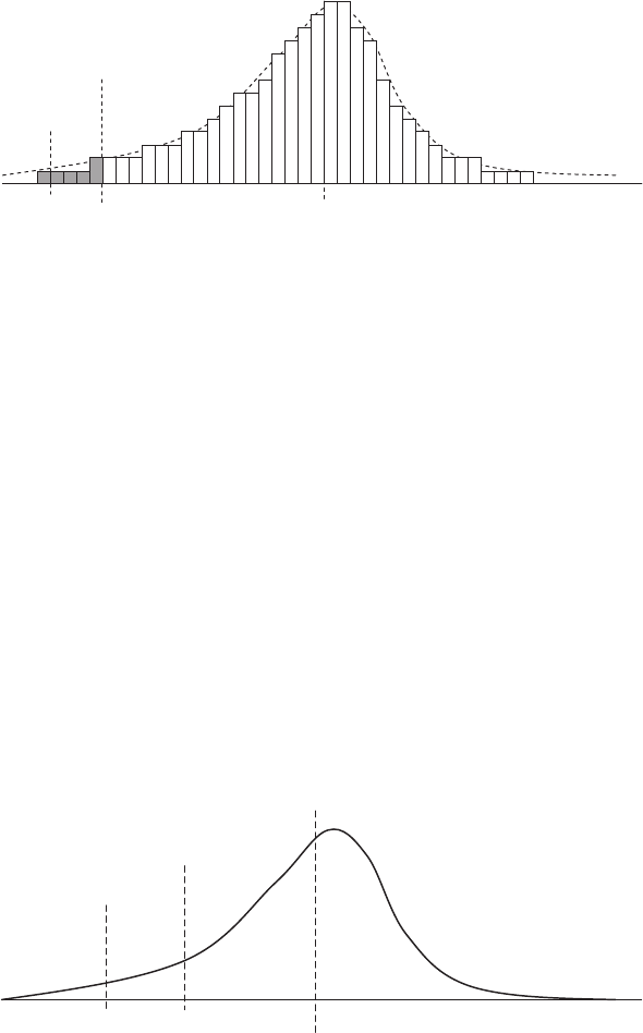
P1: SBT
c17 JWBT188-Aldridge October 22, 2009 17:49 Printer: Yet to come
256 HIGH-FREQUENCY TRADING
α = 1% µ
α = 5%
FIGURE 17.1 The 99 percent VaR (α=1 percent) and 95 percent VaR (α=5per-
cent) computed on the sample return population.
computed as the average of all distribution values from –∞to µ−1.65σ.
The average can be computed as an integral of the distribution function.
Similarly, the 99 percent parametric VaR is computed as µ−2.33σ, while
the 99 percent parametric ES is computed as the average of all distribution
values from −∞ to µ−1.65σ. The parametric VaR is an approximation of
the true VaR; the applicability of the parametric VaR depends on how close
the sample distribution resembles the normal distribution. Figure 17.2
illustrates this idea.
While the VaR and ES metrics summarize the location and the aver-
age of many worst-case scenarios, neither measure indicates the absolute
worst scenario that can destroy entire trading operations, banks, and mar-
kets. Most financial return distributions have fat tails, meaning that the very
extreme events lie beyond normal distribution bounds and can be truly
catastrophic.
The limitations of VaR methodology have hardly been a secret. In a
New York Times article published on January 2, 2009, David Einhorn, the
µ
– 2.33
σ
α
= 1%
µ
– 1.65
σ
µ
α
= 5%
FIGURE 17.2 The 95 percent parametric VaR corresponds to µ−1.65σof the
distribution, while the 99 percent parametric VaR corresponds to µ−2.33σof the
distribution.
P1: SBT
c17 JWBT188-Aldridge October 22, 2009 17:49 Printer: Yet to come
Risk Management 257
founder of the hedge fund Greenlight Capital, stated that VaR was “rela-
tively useless as a risk-management tool and potentially catastrophic when
its use creates a false sense of security among senior managers and watch-
dogs. This is like an air bag that works all the time, except when you have
a car accident.” The article also quoted Nassim Nicholas Taleb, the best-
selling author of The Black Swan, as calling VaR metrics “a fraud.” Jorion
(2000) points out that the VaR approach both presents a faulty measure of
risk and actively pushes strategists to bet on extreme events. Despite all
the criticism, VaR and ES have been mainstays of corporate risk manage-
ment for years, where they present convenient reporting numbers.
To alleviate the shortcomings of the VaR, many quantitative outfits
began to parameterize extreme tail distributions to develop fuller pictures
of extreme losses. Once the tail is parameterized based on the available
data, the worst-case extreme events can be determined analytically from
distributional functions, even though no extreme events of comparable
severity were ever observed in the sample data.
The parameterization of the tails is performed using the extreme value
theory (EVT). EVT is an umbrella term spanning a range of tail model-
ing functions. Dacorogna et al. (2001) note that all fat-tailed distributions
belong to the family of Pareto distributions. A Pareto distribution family is
described as follows:
G(x)=0x≤0
exp(−x−α)x>0,α >0(17.1)
where the tail index αis the parameter that needs to be estimated from the
return data. For raw security returns, the tail index varies from financial
security to financial security. Even for raw returns of the same financial
security, the tail index can vary from one quoting institution to another,
especially for really high-frequency estimations.
When the tail index αis determined, we can estimate the magnitude
and probability of all the extreme events that may occur, given the extreme
events that did occur in the sample. Figure 17.3 illustrates the process of
using tail parameterization:
1. Sample return observations obtained from either a back test or live
results are arranged in ascending order.
2. The tail index value is estimated on the bottom 5 percentile of the sam-
ple return distribution.
3. Using the distribution function obtained with the tail index, the prob-
abilities of observing the extreme events are estimated. According to
the tail index distribution function, a –7 percent return would occur
with a probability of 0.5 percent, while a return of –11 percent would
register with a probability of 0.001 percent.
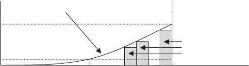
P1: SBT
c17 JWBT188-Aldridge October 22, 2009 17:49 Printer: Yet to come
258 HIGH-FREQUENCY TRADING
Tail index function is
fitted for observations of
the bottom 5% of the entire
sample distribution
Sample return observations
(back test and/or production)
Probability
Return
–1%–3%–4%
5%
0.5%
–7%–11%
FIGURE 17.3 Using tail index parameterization to predict extreme events.
The tail index approach allows us to deduce the unobserved return dis-
tributions from the sample distributions of observed returns. Although the
tail index approach is useful, it has its limitations. For one, the tail index
approach “fills in” the data for the observed returns with theoretical obser-
vations; if the sample tail distribution is sparse (and it usually is), the tail
index distribution function may not be representative of the actual extreme
returns. In such cases, a procedure known as “parametric bootstrapping”
may be applicable.
Parametric bootstrap simulates observations based on the properties
of the sample distribution. The technique “fills in” unobserved returns
based on observed sample returns. The parametric bootstrap process
works as follows:
1. The sample distribution of observed returns delivered by the manager
is decomposed into three components using a basic market model:
a. The manager’s skill, or alpha
b. The manager’s return due to the manager’s portfolio correlation
with the benchmark
c. The manager’s idiosyncratic error
The decomposition is performed using the standard market
model regression:
Ri,t=αi+βi,xRx,t+εt(17.2)
where Ri,t is the manager’s raw return in period t,Rx,t is the raw
return on the chosen benchmark in period t,αiis the measure of the
manager’s money management skill or alpha, and βi,x is a measure
of the dependency of the manager’s raw returns on the benchmark
returns.

P1: SBT
c17 JWBT188-Aldridge October 22, 2009 17:49 Printer: Yet to come
Risk Management 259
TABLE 17.1 Examples of Generated Bootstrap Components
Observation
No. Ri,t Rx,t ˆαiˆ
βi,xRx,tεi,t
1 0.015 –0.001 0.002 0.00005 0.01295
2 0.0062 0.0034 0.002 –0.00017 0.00403
2. Once parameters ˆαiand ˆ
βi,xare estimated using equation (17.2), three
pools of data are generated: one for ˆαi(constant for given manager,
benchmark, and return sample), ˆ
βi,xRx,t, and εi,t.3For example, if ˆαi
and ˆ
βi,xwere estimated to be 0.002 and –0.05, respectively, then the
component pools for a sample of raw returns and benchmarked re-
turns may look as shown in Table 17.1.
3. Next, the data is resampled as follows:
a. A value εS
i,tis drawn at random from the pool of idiosyncratic errors,
{εi,t}.
b. Similarly, a value ˆ
βi,xRS
x,tis drawn at random from the pool of
{βi,xRx,t}.
c. A new sample value is created as follows:
ˆ
RS
i,t=ˆαi+ˆ
βi,xRS
x,t+εS
t(17.3)
d. The sampled variables εS
tand ˆ
βi,xRS
x,tare returned to their pools
(not eliminated from the sample).
The resampling process outlined in steps a–d above is then
repeated a large number of times deemed sufficient to gain a better
perspective on the distribution of tails. As a rule of thumb, the resam-
pling process should be repeated at least as many times as there were
observations in the original sample. It is not uncommon for the boot-
strap process to be repeated thousands of times. The resampled values
ˆ
RS
i,tcan differ from the observed sample distribution, thus expanding
the sample data set with extra observations conforming to the proper-
ties of the original sample.
4. The new distribution values obtained through the parametric process
are now treated as were other sample values and are incorporated into
the tail index, VaR, and other risk management calculations.
3The “hat” notation on variables, as in ˆαiand ˆ
βi,x, denotes that the parameters were
estimated from a sample distribution, as opposed to comprising the true distribu-
tion values.
P1: SBT
c17 JWBT188-Aldridge October 22, 2009 17:49 Printer: Yet to come
260 HIGH-FREQUENCY TRADING
The parametric bootstrap relies on the assumption that the raw re-
turns’ dependence on a benchmark as well as the manager’s alpha remain
constant through time. This does not have to be the case. Managers with
dynamic strategies spanning different asset classes are likely to have time-
varying dependencies on several benchmarks. Despite this shortcoming,
the parametric bootstrap allows risk managers to glean a fuller notion of
the true distribution of returns given the distribution of returns observed
in the sample.
To incorporate portfolio managers’ benchmarks into the VaR frame-
work, Suleiman, Shapiro, and Tepla (2005) propose analyzing the “track-
ing error” of the manager’s return in excess of his benchmark. Suleiman,
Shapiro, and Tepla (2005) define tracking error as a contemporaneous dif-
ference between the manager’s return and the return on the manager’s
benchmark index:
TE
t=ln(Ri,t)−ln(RX,t) (17.4)
where Ri,t is the manager’s return at time tand Rx,t is return on the man-
ager’s benchmark, also at time t. The VaR parameters are then estimated
on the tracking error observations.
In addition to VaR, statistical models may include Monte Carlo
simulation–based methods to estimate future market values of capital at
risk. The Monte Carlo simulations are often used in determining deriva-
tives exposure. Scenario analyses and causal models can be used to esti-
mate market risk as well. These auxiliary types of market risk estimation,
however, rely excessively on qualitative assessment and can, as a result, be
misleading in comparison with VaR estimates, which are based on realized
historical performance.
Measuring Credit and Counterparty Risk
The credit and counterparty risk reflects the probability of financial loss
should one party in the trading equation not live up to its obligations. An
example of losses due to a counterparty failure is a situation in which a
fund’s money is custodied with a broker-dealer, and the broker-dealer goes
bankrupt. The collapse of Lehman Brothers in October 2008 was the most
spectacular counterparty failure in recent memory. According to Reuters,
close to $300 billion was frozen in bankruptcy proceedings as a result of
the bank’s collapse, pushing many prominent hedge funds to the brink of
insolvency. Credit risk is manifest in decisions to extend lines of credit or
margins. Credit risk determines the likelihood that creditors will default
on their margin calls, should they encounter any. In structured products,
P1: SBT
c17 JWBT188-Aldridge October 22, 2009 17:49 Printer: Yet to come
Risk Management 261
credit risk measures the likelihood and the impact of default of the product
underwriter, called the reference entity.
Until recently, the measurement of credit and counterparty risk was
delegated to dedicated third-party agencies that used statistical analysis
overlaid with scenario and causal modeling. The most prominent of these
agencies, Standard & Poor’s and Moody’s, came under fire during the credit
crisis of 2007–2008 because their ratings may have failed to capture the true
credit and counterparty risk, and it was revealed that in many instances
the rating agencies had cozy relationships with the firms they rated. As
credit and counterparty data becomes increasingly available, it may make
good sense for firms to statistically rate their counterparties internally. The
remainder of this section describes common techniques for measuring
credit and counterparty risk.
Entities with publicly traded debt are the easiest counterparties to
rank. The lower the creditworthiness of the entity, the lower the market
price on the senior debt issued by the entity and the higher the yield the
entity has to pay out to attract investors. The spread, or the difference
between the yield on the debt of the entity under consideration and the
yield on the government debt with comparable maturity, is a solid indi-
cator of the creditworthiness of the counterparty. The higher the spread,
the lower the creditworthiness of the counterparty. Because yields and
spreads are inversely related to the prices of the bonds, the creditworthi-
ness of a counterparty can also be measured on the basis of the relative
bond price of the firm: the lower the bond price, the higher the yield and
the lower the creditworthiness. Market prices of corporate debt provide
objective information about the issuer’s creditworthiness. The prices are
determined by numerous market participants analyzing the firms’ strate-
gies and financial prospects and arriving at their respective valuations.
Table 17.2 shows senior bond prices for selected firms and their rel-
ative creditworthiness rankings on May 15, 2009. A creditworthiness of
100 indicates solid ability to repay the debt, while a creditworthiness of
0 indicates the imminence of default. From the perspective of a fund decid-
ing on May 15, 2009 whether to use Morgan Stanley or Wells Fargo & Co.
as its prime broker, for example, Morgan Stanley may be a better choice in
that the firm shows higher creditworthiness and lower counterparty risk.
As discussed in the section on implementation of risk management frame-
works that follows, a diversification of counterparties is the best way to
protect the operation from credit and counterparty risk.
The creditworthiness of private entities with unobservable market val-
ues of obligations can be approximated as that of a public firm with match-
ing factors. The matching factors should include the industry, geographic
location, annual earnings of the firms to proxy for the firms’ sizes, and
various accounting ratios, such as the quick ratio to assess short-term

P1: SBT
c17 JWBT188-Aldridge October 22, 2009 17:49 Printer: Yet to come
262 HIGH-FREQUENCY TRADING
TABLE 17.2 Senior Bond Prices for Selected Firms and Their Relative
Creditworthiness Rank on May 15, 2009
Firm
Bond Ticker
Symbol
Bond Price
at Close on
5/15/2009
Relative
Creditworthiness
Rank
Coca Cola Enterprises, Inc. 191219AP9 131.07 80
Morgan Stanley 617446HD4 103.25 55
Wells Fargo & Co. 949746FS5 95.83 40
Marriott Int’l, Inc. (New) 571903AF0 90.43 30
American General Fin. Corp. 02635PRT2 47.18 5
solvency. Once a close match with publicly traded debt is found for the
private entity under evaluation, the spread on the senior debt of the pub-
licly traded firm is used in place of that for the evaluated entity.
In addition to the relative creditworthiness score, the firms may need
to obtain a VaR-like number to measure credit and counterparty risk.
This number is obtained as an average of exposure to each counterparty
weighted by the counterparty’s relative probability of default:
CCExposure =1
N
N
i=1
Exposurei×PDi(17.5)
where CCExposure is the total credit and counterparty exposure of the
organization, Nis the total number of counterparties of the organization,
Exposureiis the dollar exposure of the ith counterparty, and PDiis the
probability of default of the ith counterparty:
PDi=100 −(Creditworthiness Rank)i
100 % (17.6)
The total credit and counterparty exposure is then normalized by the capi-
tal of the firm and added to the aggregate VaR number.
Measuring Liquidity Risk
Liquidity risk measures the firm’s potential inability to unwind or hedge
positions in a timely manner at current market prices. The inability to close
out positions is normally due to low levels of market liquidity relative to
the position size. The lower the market liquidity available for a specific
instrument, the higher the liquidity risk associated with that instrument.
Levels of liquidity vary from instrument to instrument and depend on the
number of market participants willing to transact in the instrument under
P1: SBT
c17 JWBT188-Aldridge October 22, 2009 17:49 Printer: Yet to come
Risk Management 263
consideration. Bervas (2006) further suggests the distinction between the
trading liquidity risk and the balance sheet liquidity risk, the latter being
the inability to finance the shortfall in the balance sheet either through
liquidation or borrowing.
In mild cases, liquidity risk can result in minor price slippages due to
the delay in trade execution and can cause collapses of market systems
in its extreme. For example, the collapse of Long-Term Capital Manage-
ment (LTCM) in 1998 can be attributed to the firm’s inability to promptly
offload its holdings. The credit crisis of 2008 was another vivid example of
liquidity risk; as the credit crisis spread, seemingly high-quality debt instru-
ments such as high-grade CDOs lost most of their value when the markets
for these securities vanished. Many firms holding long positions in these
securities suffered severe losses. Another, simpler, example of liquidity
risk is provided by out-of-the-money options nearing expiration; the mar-
kets for out-of-the-money options about to become worthless disappear
entirely.
The number of transacting parties usually depends on the potential
profitability and degree of regulation in the trades of interest. No one is in-
clined to buy worthless options just before the options expire. In the case
of CDOs in the fall of 2008, the absence of markets was largely due to reg-
ulation FAS 133 enacted in 2007. FAS 133 mandates that all securities be
marked to their market prices. In the case of CDOs, for example, the mar-
ket price is the last trade price recorded for the security by the firm holding
CDOs in its portfolio. As a result of this regulation, the firms that held CDOs
at 100 percent of their face value on the books refused to sell a portion of
their CDOs at a lower price. The sale would result in devaluation of their
remaining CDOs at the lower market price, which would trigger devalua-
tion of the fund as a whole and would, in turn, result in increased investor
redemptions. At the same time, potential buyers of the CDOs faced a sim-
ilar problem: those already holding CDOs on their books at 100 percent of
face value would face sharp devaluations of their entire funds if they chose
to purchase new CDOs at significantly reduced prices. The recently pro-
posed taxation scheme of charging transaction costs on trading as a tax
may similarly destroy the liquidity of currently liquid instruments.
To properly assess the liquidity risk exposure of a portfolio, it is nec-
essary to take into account all potential portfolio liquidation costs, includ-
ing the opportunity costs associated with any delays in execution. While
liquidation costs are stable and are easy to estimate during periods with
little volatility, the liquidation costs can vary wildly during high-volatility
regimes. Bangia et al. (1999), for example, document that liquidity risk ac-
counted for 17 percent of the market risk in long USD/THB positions in
May 1997, and Le Saout (2002) estimates that liquidity risk can reach over
50 percent of total risk on selected securities in CAC40 stocks.

P1: SBT
c17 JWBT188-Aldridge October 22, 2009 17:49 Printer: Yet to come
264 HIGH-FREQUENCY TRADING
Bervas (2006) proposes the following liquidity-adjusted VaR measure:
VaRL=VaR +Liquidity Adjustment =VaR −µS+zασS(17.7)
where VaR is the market risk value-at-risk discussed previously in this
chapter, µSis the mean expected bid-ask spread, σSis the standard devia-
tion of the bid-ask spread, and zαis the confidence coefficient correspond-
ing to the desired α–percent of the VaR estimation. Both µSand σScan be
estimated either from raw spread data or from the Roll (1984) model.
Using Kyle’s λmeasure, the VaR liquidity adjustment can be similarly
computed through estimation of the mean and standard deviation of the
trade volume:
VaRL=VaR +Liquidity Adjustment
=VaR −ˆα+ˆ
λ(µNVOL +zασNVOL)(17.8)
where ˆαand ˆ
λare estimated using OLS regression following Kyle
(1985):
Pt=α+λNVOLt+εt(17.9)
Ptis the change in market price due to market impact of orders, and
NVOLtis the difference between the buy and sell market depths in period t.
Hasbrouck (2005) finds that the Amihud (2002) illiquidity measure best
indicates the impact of volume on prices. Similar to Kyle’s λadjustment to
VaR, the Amihud (2002) adjustment can be applied as follows:
VaRL=VaR +Liquidity Adjustment =VaR −(µγ+zασγ)(17.10)
where µγand σγare the mean and standard deviation of the Amihud (2002)
illiquidity measure γ,γt=1
DtDt
d=1|rd,t|
vd,t,Dtis the number of trades exe-
cuted during time period t,rd,t is the relative price change following trade d
during trade period t, and vd,t is the trade quantity executed within trade d.
Measuring Operational Risk
Operational risk is the risk of financial losses resulting from one or more
of the following situations:
rInadequate or failed internal controls, policies, or procedures
rFailure to comply with government regulations
rSystems failures
rFraud
rHuman error
rExternal catastrophes
P1: SBT
c17 JWBT188-Aldridge October 22, 2009 17:49 Printer: Yet to come
Risk Management 265
Operational risk can affect the firm in many ways. For example, a risk
of fraud can taint the reputation of the firm and will therefore become a
“reputation risk.” Systems failures may result in disrupted trading activity
and lost opportunity costs for capital allocation.
The Basel Committee for Bank Supervision has issued the following
examples of different types of operational risk:
rInternal fraud—misappropriation of assets, tax evasion, intentional
mismarking of positions, and bribery
rExternal fraud—theft of information, hacking damage, third-party
theft, and forgery
rEmployment practices and workplace safety—discrimination,
workers’ compensation, employee health and safety
rClients, products, and business practice—market manipulation,
antitrust, improper trade, product defects, fiduciary breaches, account
churning
rDamage to physical assets—natural disasters, terrorism, vandalism
rBusiness disruption and systems failures—utility disruptions, soft-
ware failures, hardware failures
rExecution, delivery, and process management—data entry errors,
accounting errors, failed mandatory reporting, negligent loss of client
assets
Few statistical frameworks have been developed for measurement of
operational risk; the risk is estimated using a combination of scalar and
scenario analyses. Quantification of operational risk begins with the devel-
opment of hypothetical scenarios of what can go wrong in the operation.
Each scenario is then quantified in terms of the dollar impact the scenario
will produce on the operation in the base, best, and worst cases. To align
the results of scenario analysis with the VaR results obtained from esti-
mates of other types of risk, the estimated worst-case dollar impact on
operations is then normalized by the capitalization of the trading operation
and added to the market VaR estimates.
Measuring Legal Risk
Legal risk measures the risk of breach of contractual obligations. Legal
risk addresses all kinds of potential contract frustration, including contract
formation, seniority of contractual agreements, and the like. An example
of legal risk might be two banks transacting foreign exchange between the
two of them, with one bank deciding that under its local laws, the signed
contract is void.

P1: SBT
c17 JWBT188-Aldridge October 22, 2009 17:49 Printer: Yet to come
266 HIGH-FREQUENCY TRADING
The estimation of legal risk is conducted by a legal expert affiliated
with the firm, primarily using a causal framework. The causal analysis iden-
tifies the key risk indicators embedded in the current legal contracts of the
firm and then works to quantify possible outcomes caused by changes in
the key risk indicators. As with other types of risk, the output of legal risk
analysis is a VaR number, a legal loss that has the potential to occur with
just a 5 percent probability for a 95 percent VaR estimate.
MANAGING RISK
Once market risk has been estimated, a market risk management frame-
work can be established to minimize the adverse impact of the market risk
on the trading operation. Most risk management systems work in the fol-
lowing two ways:
1. Stop losses—stop current transaction(s) to prevent further losses
2. Hedging—hedge risk exposure with complementary financial instru-
ments
Stop Losses
A stop loss is the crudest and most indispensable risk management tech-
nique to manage the risk of unexpected losses. In the case of market risk,
a stop loss is a threshold price of a given security, which, if crossed by
the market price, triggers liquidation of the current position. In credit and
counterparty risk, a stop loss is a level of counterparty creditworthiness be-
low which the trading operation makes a conscious decision to stop deal-
ing with the deteriorating counterparty. In liquidity risk, the stop loss is
the minimum level of liquidity that warrants opened positions in a given
security. In operations risk, the stop loss is a set of conditions according
to which a particular operational aspect is reviewed and terminated, if nec-
essary. For example, compromised Internet security may mandate a com-
plete shutdown of trading operations until the issue is resolved. Finally, a
stop loss in legal risk can be a settlement when otherwise incurred legal
expenses are on track to exceed the predetermined stop-loss level.
In market risk management, a simple stop loss defines a fixed level of
the threshold price. For example, if at 12:00 P.M. EST we bought USD/CAD
at 1.2000 and set a simple stop loss at 50 bps, the position will be liqui-
dated whenever the level of USD/CAD drops below 1.1950, provided the
position is not closed sooner for some other reason. Figure 17.4, panel (a)
illustrates the idea. A simple stop loss does not take into account any price
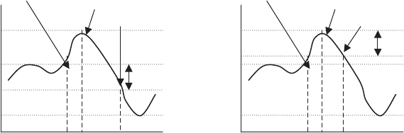
P1: SBT
c17 JWBT188-Aldridge October 22, 2009 17:49 Printer: Yet to come
Risk Management 267
Panel (a). Simple (fixed) stop loss. Panel (b). Trailing stop loss.
1.2000 1.2000
12:00 12:15
1.2067 1.2067 0.0050
0.0050
1.2017
1.1950
13:15 12:00 12:15 12:40
Buy here Max gain
Stop loss
Buy here Max gain
Stop loss
FIGURE 17.4 The difference between simple (fixed) and trailing stop-loss
thresholds.
movement from the time the position was open until the time the stop loss
was triggered, resulting in a realized loss of 50 bps.
A trailing stop, on the other hand, takes into account the movements of
the security’s market price from the time the trading position was opened.
As its name implies, the trailing stop “trails” the security’s market price.
Unlike the simple stop that defines a fixed price level at which to trigger
a stop loss, the trailing stop defines a fixed stop-loss differential relative
to the maximum gain attained in the position. For example, suppose we
again bought USD/CAD at 12:00 P.M. EST at 1.2000 and set a trailing stop
loss at 50 bps. Suppose further that by 12:15 P.M. EST the market price for
USD/CAD rose to 1.2067, but by 13:30 P.M. EST the market price dropped
down to 1.1940. The trailing stop loss would be triggered at 50 bps less the
market price corresponding to the highest local maximum of the gain func-
tion. In our example, the local maximum of gain appeared at 1.2067 when
the position gain was 1.2067−1.2000 =0.0067. The corresponding trailing
stop loss would be hit as soon as the market price for USD/CAD dipped
below 1.2067 –50 bps =1.2017, resulting in a realized profit of 17 bps, a big
improvement over performance with a simple stop loss. Figure 17.4, panel
(b) shows the process.
How does one determine the appropriate level of the stop-loss thresh-
old? If the stop-loss threshold is too narrow, the position may be closed
due to short-term variations in prices or even due to variation in the bid-ask
spread. If the stop-loss threshold is too wide, the position may be closed
too late, resulting in severe drawdowns. As a result, many trading practi-
tioners calibrate the stop-loss thresholds to the intrinsic volatility of the
traded security. For example, if a position is opened during high-volatility
conditions with price bouncing wildly, a trader will set wide stop losses. At
P1: SBT
c17 JWBT188-Aldridge October 22, 2009 17:49 Printer: Yet to come
268 HIGH-FREQUENCY TRADING
the same time, for positions opened during low-volatility conditions, nar-
row stop thresholds are required.
The actual determination of the stop-loss threshold based on market
volatility of the traded security is typically calibrated with the following
two factors in mind:
1. Average gain of the trading system without stop losses in place, E[G]
2. Average loss of the trading system without stop losses in place, E[L]
The probabilities of a particular position turning out positive also play
a role in determining the optimal stop-loss threshold, but their role is a
much smaller one than that of the averages. The main reason for the rel-
ative insignificance of probabilities of relative occurrence of gains and
losses is that per the Gambler’s Ruin Problem, the probability of a gain
must always exceed the probability of a loss on any given trade; otherwise,
the system faces the certainty of bankruptcy. Please refer to Chapter 10 for
details.
The information on average upside and downside is typically deter-
mined from the system’s back test. The back test normally spans at least
two years of data and produces a sample return distribution with a number
of observations sufficient to draw unbiased inferences about the distribu-
tion of the return population with the use of the techniques such as VaR, tail
parameterization, or benchmarked performance measurement, discussed
subsequently. Armed with distributional information about returns of the
trading system, we can estimate the maximum (trailing) loss allowed that
would keep our system consistently positive. The maximum trailing stop
loss, LM, has to satisfy the following three conditions:
1. In absolute terms, the maximum loss is always less than the average
gain, |LM|<E[G]; otherwise, the system can produce negative cumu-
lative results.
2. Also in absolute terms, the maximum loss is always less than the aver-
age loss, |LM|≤|E[L]|; otherwise, the system can deliver almost iden-
tical results with no stop losses.
3. After the introduction of stop losses, the probability of a gain still ex-
ceeds the probability of a loss in a back test.
Once the maximum stop loss is determined, the stop loss can be fur-
ther refined to tighten dynamically in response to different volatility con-
ditions. Dynamic calibration of stop losses to market volatility is more
art than science. Dacorogna et al. (2001), for example, describe a moving
average–based model with stop losses of low-volatility and high-volatility
P1: SBT
c17 JWBT188-Aldridge October 22, 2009 17:49 Printer: Yet to come
Risk Management 269
regimes. Dacorogna et al. (2001) use the absolute value of the gain or loss
as a proxy for “volatility” and consider “volatility” to be low if the absolute
gain or loss is less than 0.5 percent (50 bps). The model thresholds change
in accordance with the volatility conditions. In Dacorogna et al. (2001), for
example, the thresholds increase 10 times their low-volatility value when
the “volatility” defined previously exceeds 0.5 percent. The low-volatility
parameter is calibrated in the back test on the historical data.
The stop-loss thresholds in other types of risk are similarly determined
based on the expected market gain and total maximum loss considerations
presented previously.
Hedging Portfolio Exposure
Hedging is closely related to portfolio optimization: the objective of any
hedging operation is to create a portfolio that maximizes returns while
minimizing risk—downside risk in particular. Hedging can also be thought
of as a successful payoff matching: the negative payoffs of one security
“neutralized” by positive payoffs of another.
Hedging can be passive or dynamic. Passive risk hedging is most akin
to insurance. The manager enters into a position in a financial security with
the risk characteristics that offset the long-term negative returns of the
operation. For example, a manager whose main trading strategy involves
finding fortuitous times for being long in USD/CAD may want to go short
in the USD/CAD futures contract to offset his exposure to USD/CAD. As
always, detailed analysis of the risk characteristics of the two securities is
required to make such a decision.
Dynamic hedging is most often done through a series of short-term, po-
tentially overlapping, insurance-like contracts. The objective of the short-
term insurance contracts is to manage the short-term characteristics of
trading returns. In the case of market risk hedging, dynamic hedging may
be developed for a particular set of recurring market conditions, when
behaviors of the trading systems may repeat themselves. It may be possible
to find a set of financial securities or trading strategies the returns of which
would offset the downside of the primary trading strategy during these par-
ticular market conditions. For example, during a U.S. Fed announcement
about the level of interest rates, the USD/CAD exchange rate is likely to
rise following a rise in the U.S. interest rates, while U.S. bond prices are
likely to fall following the same announcement. Depending upon return
distributions for USD/CAD and U.S. bonds, it may make sense to trade the
two together during the U.S. interest rate announcements in order to off-
set the negative tail risk in either. Mapping out extensive distributions of
returns as described previously in this chapter would help in determining
the details of such a dynamic hedging operation.
P1: SBT
c17 JWBT188-Aldridge October 22, 2009 17:49 Printer: Yet to come
270 HIGH-FREQUENCY TRADING
As with mean-variance portfolio construction, a successful hedging
strategy solves the following optimization problem:
max xE[R]−Ax
Vx
s.t.xi=1(17.11)
where xiis the portfolio weight of security i,i∈[1,...,I], E[R] is a vector
of expected returns of Isecurities, Vis an I×Ivariance-covariance matrix
of returns, and Ais the coefficient reflecting the risk aversion of the trad-
ing operation. Ais commonly assumed to be 0.5 to simplify the solution.
A dynamic state-dependent hedging would repeat the process outlined in
equation (17.11), but only for returns pertaining to a specific market state.
Like market risk, other types of risk can be diversified through portfo-
lio risk management. The counterparty risk, for example, can be diversified
through establishment of several ongoing broker-dealer relationships. Citi
prime brokerage even markets itself as a secondary broker-dealer for funds
already transacting, or “priming,” with another broker-dealer.
Similarly, liquidity risk can be diversified away through using several
liquidity providers. The American Academy of Actuaries (2000) provided
the following guidance for companies seeking to diversify their liquidity
exposure: “While a company is in good financial shape, it may wish to es-
tablish durable, ever-green (i.e., always available) liquidity lines of credit.
The credit issuer should have an appropriately high credit rating to in-
crease the chances that the resources will be there when needed.” Accord-
ing to Bhaduri, Meissner, and Youn (2007), five derivative instruments can
be specifically used for hedging liquidity risk:
rWithdrawal option is a put on the illiquid underlying asset.
rBermudan-style return put option is a right to sell the underlying asset
at a specified strike on specific dates.
rReturn swap allows swapping the return on the underlying asset for
LIBOR.
rReturn swaption is an option to enter into the return swap.
rLiquidity option is a “knock-in” barrier option, where the barrier is a
liquidity metric.
Regular process reviews ensure that the operations are running within
predetermined guidelines on track to set goals, minimizing the probability
of failure of oversight, regulatory breaches, and other internal functions.
For example, the addition of new trading strategies into the trading portfo-
lio should undergo rigid product review processes that analyze the return
and risk profiles and other profitability and risk factors of proposed cap-
ital allocations, as described in Chapter 5. In addition to detailed process

P1: SBT
c17 JWBT188-Aldridge October 22, 2009 17:49 Printer: Yet to come
Risk Management 271
guidelines, operational risk can be hedged with insurance contracts offered
by specialty insurance firms and by entirely outsourcing noncritical busi-
ness processes to third-party vendors.
Legal risk is most effectively managed via the causal analysis used for
its measurement. The key risk indicators are continuously monitored, and
the effect of their changes is assessed according to the causal framework
developed in the estimation of legal risk.
CONCLUSION
This chapter has examined the best practices in risk management followed
by successful high-frequency operations. While the process of identifica-
tion, measurement, and management of risk can consume time and effort,
the process pays off by delivering business longevity and stability.
P1: SBT
c17 JWBT188-Aldridge October 22, 2009 17:49 Printer: Yet to come
272

P1: SBT
c18 JWBT188-Aldridge October 22, 2009 13:17 Printer: Yet to come
CHAPTER 18
Executing and
Monitoring
High-Frequency
Trading
Once a high-frequency trading system is designed and back-tested,
it is applied to live capital (i.e., executed). The execution process
can be complex, particularly as the capital allocated to the strat-
egy grows and the adverse cost of market impact begins to take effect. To
maximize trading performance and minimize costs, the best high-frequency
trading systems are executed through optimization algorithms. To ensure
that all algorithms of the trading system work as intended, a strict monitor-
ing process is deployed.
This chapter discusses the best contemporary practices in the execu-
tion and monitoring of high-frequency trading systems.
Execution optimization algorithms tackle the following questions:
rShould a particular order issued by the trading strategy be executed in
full or in smaller lots?
rShould the order be optimally processed as a market or a limit order?
rIs there an order-timing execution strategy that delivers a better-than-
expected order fill price, given current market conditions?
The optimization algorithms can be developed internally or purchased
off the shelf. Off-the-shelf algorithms are often cheaper, but they are less
transparent than internally developed platforms. Both external and internal
execution optimization systems, however advanced, may possess unex-
pected defects and other skews in performance and result in costly exe-
cution blunders.
To detect undesirable shifts in costs and other trading parameters dur-
ing execution, all execution processes must be closely monitored. Even the
273

P1: SBT
c18 JWBT188-Aldridge October 22, 2009 13:17 Printer: Yet to come
274 HIGH-FREQUENCY TRADING
most miniscule problems in execution may have fast and dramatic effects
on performance; timely identification of potential issues is a nonnegotiable
necessity in high-frequency operations.
EXECUTING HIGH-FREQUENCY
TRADING SYSTEMS
Overview of Execution Algorithms
Optimization of execution is becoming an increasingly important topic
in the modern high-frequency environment. Before the introduction of
computer-enabled trading optimization algorithms, investors desiring to
trade large blocks of equity shares or other financial instruments may have
hired a broker-dealer to find a counterparty for the entire order. Subse-
quently, broker-dealers developed “best execution” services that split up
the order to gradually process it with limited impact on the price. The ad-
vent of algorithmic trading allowed institutional traders to optimize trading
on their own, minimizing the dominance of broker-dealers and capturing a
greater profit margin as a result.
Optimization algorithms take into account a variety of current market
conditions as well as characteristics of the orders to be processed: order
type, size, and frequency. Bertsimas and Lo (1998) developed optimization
strategies to take advantage of contemporary price changes. Engle and
Ferstenberg (2007) examined the risks embedded in execution. Almgren
and Chriss (2000) and Alam and Tkatch (2007), among others, studied the
effects of “slicing” up orders into batches of smaller size. Obizhaeva and
Wang (2005) optimize execution, assuming that post-trade liquidity is not
replenished immediately. Kissell and Malamut (2006) adapt the speed of
order processing to traders’ current beliefs about the impending direction
of market prices.
In addition to algorithms optimizing the total execution cost of trad-
ing, algorithms have been developed to optimize liquidity supply, hedge
positions, and even to optimize the effort extended in monitoring position
changes in the marketplace. See Foucault, Roell and Sandas (2003) for an
example of the latter. In this chapter, we consider three common forms of
executing optimization algorithms:
1. Trading-aggressiveness selection algorithms, designed to choose
between market and limit orders for optimal execution
2. Price-scaling strategies, designed to select the best execution price
according to the prespecified trading benchmarks
P1: SBT
c18 JWBT188-Aldridge October 22, 2009 13:17 Printer: Yet to come
Executing and Monitoring High-Frequency Trading 275
3. Size-optimization algorithms that determine the optimal ways to break
down large trading lots into smaller parcels to minimize adverse costs
(e.g., the cost of market impact)
Market-Aggressiveness Selection
Aggressive execution refers to high trading frequency and to short trading
intervals that may lead to high market impact. Aggressive execution most
often skews toward the heavy use of market orders. Passive trading, on
the other hand, is lower frequency, depends more on limit orders, but may
be subject to non-execution risk should the market move adversely. To
balance passive and aggressive trading, Almgren and Chriss (1999) propose
the following optimization:
min
αCost(α)+λRisk(α) (18.1)
where αis the trading rate often calculated as a percentage of volume
(POV) or liquidity that the strategy absorbs during the trading period and λ
is the coefficient of risk aversion of the investor. Plotting cost/risk profiles
for various algorithms identifies efficient trading frontiers that are well-
suited for comparisons of algorithm efficiencies and for determining the
suitability of a particular algorithm to the trading needs of a particular
investor.
According to Kissell and Malamut (2005), market aggressiveness (POV
or α) can be varied using a combination of market and limit orders. Market
orders tend to increase the POV or α, whereas limit orders decrease market
aggressiveness.
The cost and risk functions used in the optimization equation (18.1)
are defined as follows:
Cost(α)=E0[P(α)−Pb](18.2)
Risk(α)=σ(ε(α)) (18.3)
P(α)=P+f(X,α)+g(X)+ε(α) (18.4)
where E0denotes the ex-ante expectation at the start of the trading
period,
Pbis the benchmark execution price,
P(α) is the realized execution price defined in equation (18.4),
ε(α) is a random deviation of the trading outcome, E[ε(α)] =
0, Var[ε(α)] =σ2(α).

P1: SBT
c18 JWBT188-Aldridge October 22, 2009 13:17 Printer: Yet to come
276 HIGH-FREQUENCY TRADING
Pis the market price at the time of order entry,
f(X,α) is a temporary market impact due to the liquidity
demand of trading, and
g(X) is the permanent price impact due to information leakage
during order execution.
Price-Scaling Strategies
The main objective of so-called price-scaling execution algorithms is to
obtain the best price for the strategy. The best price can be attained rel-
ative to a benchmark—for example, the average daily price for a given se-
curity. The best price can also be attained given the utility function of the
end investor or a target Sharpe ratio of a portfolio manager.
The algorithm that minimizes the cost of execution relative to a bench-
mark is known as a Strike algorithm. The Strike is designed to capture gains
in periods of favorable prices; the algorithm is aggressive (executes at mar-
ket prices) in times of favorable prices and passive (places limit orders) in
times of unfavorable prices. The Strike strategy dynamically adjusts the
percent of volume rate αused to process market orders of the strategy to
minimize the quadratic execution cost of the strategy:
min
αt
EtPt+1(αt)−Pb,t2(18.5)
where Pt+1(αt) is the realized price obtained using the trading aggressive-
ness level αtdecided upon at time t, and Pb,tis the benchmark price at time
tused to compare the trading performance.
The Plus algorithm maximizes the probability of outperforming a spec-
ified benchmark while minimizing risk. To do so, the algorithm maximizes
the following Sharpe ratio–like specification:
max
αt
EtPt+1(αt)−Pb,t
(V(Pt+1(αt)−Pb,t))1/2(18.6)
where, as before, Pb,tis the benchmark price at time tused to compare the
trading performance, and Pt+1(αt) is the realized price obtained using the
trading aggressiveness level αtdecided upon at time t.
Finally, the Wealth algorithm maximizes investor wealth in the pres-
ence of uncertainty. The Wealth algorithm is passive during periods of fa-
vorable prices, but acts aggressively during periods of unfavorable prices
with the goal of preserving the investor’s wealth in adverse conditions. The
Wealth strategy is obtained by optimizing the following expression:
max
αt
log Et[U(Pt+1(αt))](18.7)
P1: SBT
c18 JWBT188-Aldridge October 22, 2009 13:17 Printer: Yet to come
Executing and Monitoring High-Frequency Trading 277
where U(.) is a utility function approximating the risk-return preferences of
the investor. The utility function may be the one shown in equation (18.8):
U(x)=E[x]−λV[x] (18.8)
where xis the realized payoff and λis the risk aversion coefficient of the
investor. The risk-aversion coefficient λis 0 for a risk-neutral investor, or
an investor insensitive to risk. A risk-averse investor will have λgreater
than 0; λof 0.5 and above would characterize a highly risk-averse investor.
The profitability of execution algorithms depends on concurrent mar-
ket conditions. Kissell and Malamut (2005) compared the three execution
strategies in detail and found that all three strategies consistently outper-
form random, nonsystematic execution. Among the algorithms, the Strike
method delivers a lower average cost but ignores participation in favor-
able price conditions. The Plus strategy also delivers a low average cost,
but increases the risk of unfavorable prices. Finally, the Wealth strategy is
able to capture a greater proportion of favorable price conditions but at the
expense of higher average prices.
Slicing Large Orders
Kyle (1985) and Admati and Pfleiderer (1988) were the first to suggest that
for informed investors to profit from their information, they need to trade
in a fashion that precludes other market participants from recognizing the
informed investors’ order flow. Should other investors recognize the or-
der flow of informed investors, they could front-run the informed parties,
diluting their profitability. Barclay and Warner (1993) argue that for insti-
tutions to trade with their positions undetected, their large order packets
need to be broken up into parcels of medium size—not too big and not
too small—in order to minimize other trading participants’ ability to distin-
guish these orders from other, “noise,” orders. Chakravarty (2001) studies
the impact of stealth trading—that is, trading by breaking down large trad-
ing blocks into small order parcels with the intent of causing the least mar-
ket impact. Chakravarty (2001) finds that, consistent with the hypotheses
of Barclay and Warner (1993), medium-sized orders indeed are followed
by disproportionally large price changes, relative to all price and overall
proportion of trades and volume.
Alam and Tkatch (2007) analyzed data from the Tel-Aviv Stock Ex-
change to study the performance of institutional investors who slice their
orders into blocks of equal size in order to avoid being detected and picked
off by other traders. Alam and Tkatch (2007) detect these orders as groups
of equally sized, equally priced same-direction orders placed within two
P1: SBT
c18 JWBT188-Aldridge October 22, 2009 13:17 Printer: Yet to come
278 HIGH-FREQUENCY TRADING
minutes of each other. Alam and Tkatch (2007) report that sliced orders
have a median of four “slices” or consecutively streaming components.
Out of all the slice orders submitted, about 79 percent are executed and
20 percent are canceled by the trader prior to execution. The execution rate
of slice orders compares favorably with the execution rate of all orders;
only 63 percent of all orders, including sliced and non-sliced orders, are
executed.
Another metric of slice efficiency is order fill rate. The order fill rate
measures the proportion of the order that was “hit” or executed. Com-
pletely executed orders have a fill rate of 100 percent; the order that failed
to execute has a fill rate of 0 percent. Regular, non-sliced, orders may en-
counter a partial fill, depending on the order size. Alam and Tkatch (2007)
show that non-sliced orders have a fill rate of 40 percent, while sliced or-
ders have a fill rate of 48 percent. Slicing particularly improves the fill rate
of limit orders; regular limit orders have a fill rate of 42 percent, while sliced
limit orders have a fill rate of 77 percent.
Sliced orders are executed more quickly. Alam and Tkatch (2007)
report that the mean execution time for a fully filled sliced order is 3 min-
utes and 29 seconds, while the mean execution time for a regular order is
11 minutes and 54 seconds.
Execution is costly not only in terms of the average transaction costs
but in terms of risks associated with execution. The risk embedded in ex-
ecution comprises primarily two types of risk: (1) the uncertainty of the
price at which market orders are executed and (2) the uncertainty in the
timing of the execution of limit orders and the associated opportunity cost.
Extreme examples of such costs include the possible failure to execute a
limit order and an insufficient market depth at a reasonable range of prices
for market order execution.
Execution risk creates an additional dimension for portfolio
risk/return optimization and has to be taken into account. Engle and
Ferstenberg (2006) propose that the study of possible execution risks is
necessary to determine the following aspects of portfolio management:
rIs risk-neutral portfolio management optimal in the presence of execu-
tion risks?
rIs execution risk diversifiable in a portfolio of several financial instru-
ments?
rCan execution risk be hedged?
Instead of executing the total order size at the same time, institutions
employ strategies to minimize market impact by, for example, splitting
the total order size into discrete blocks executed over time, often sev-
eral days. The identification of impending trading periods with extensive
liquidity, therefore, becomes an important problem for optimization of
P1: SBT
c18 JWBT188-Aldridge October 22, 2009 13:17 Printer: Yet to come
Executing and Monitoring High-Frequency Trading 279
execution. Several recent studies have characterized properties of liquid-
ity that may assist managers in forecasting liquidity going forward; specif-
ically, liquidity has been shown to be time varying, yet persistent from
one period to the next. These studies include those of Chordia, Roll, and
Subrahmanyam (2001, 2002); Hasbrouck and Seppi (2001); and Huberman
and Halka (2001).
Obizhaeva and Wang (2005) analytically derive optimal execution sizes
depending on the execution horizon of the trade and the “speed of recov-
ery” of the limit order book for a given security. The speed of recovery
is a measure of how fast the limit order book absorbs the market impact
generated by the previous lot in the execution sequence. Obizhaeva and
Wang (2005) find that for securities with a reasonable speed of limit order
book recovery, the optimal trading strategy is to process large lots at the
beginning and at the end of the execution period with small lots spaced
in between. The spacing of smaller lots depends on whether the speed of
recovery for the traded security is uniform throughout the day. If the speed
of recovery is not uniform throughout the day, larger lots should be pro-
cessed at times with higher speeds of recovery.
Nevmyvaka, Kearns, Papandreou, and Sycara (2006) have developed
an algorithm for optimizing execution through a dynamic combination of
market and limit orders. The optimization is focused on a specific task:
to acquire Vshares of a particular financial security within Tseconds of
the order. The authors compare the following three market and limit order
execution scenarios to obtain a certain number of shares, V:
1. Submit a market order for Vshares immediately at the beginning of
the trading period, time 0. This approach guarantees execution, but
the liquidity required to fulfill the order may be costly; the trader may
need to explore the depth of the book at suboptimal prices and wide
bid-ask spreads.
2. Wait until the end of the trading period and submit a market order for V
shares at time T. This strategy may improve upon the obtained price,
but it is also subject to market volatility risks. Full bid-ask spread is
present.
3. Submit a limit order for Vshares at the beginning of the trading period
(time 0) and a market order for the unexecuted shares (if any) at the
end of the trading period (time T). This strategy avoids paying bid-ask
spread if the limit order is executed. The worst-case outcome of this
strategy is that presented in case 2.
In all three scenarios, the trading period ends with the same number
of shares, V. In each scenario, however, the Vshares can potentially be
obtained at a different cost.

P1: SBT
c18 JWBT188-Aldridge October 22, 2009 13:17 Printer: Yet to come
280 HIGH-FREQUENCY TRADING
Nevmyvaka, Kearns, Papandreou, and Sycara (2006) found that the
best strategy is strategy 3, with limit orders placed at the beginning of the
trading period and besting the market price by one tick size. For example,
if we want to buy 500 shares of IBM within 300 seconds, the current mar-
ket bid and offer prices are $93.63 and $93.67, and the minimum tick size
is $0.01, the optimal strategy will be to submit a limit buy order at $93.64,
one tick better than the best limit buy currently available on the market.
The unfilled portion of the order is then executed at market at the end of
the 300-second period.
MONITORING HIGH-FREQUENCY
EXECUTION
Monitoring high-frequency execution involves a two-part process:
rFirst, allowable ranges of trading and other run-time parameters are
identified through pre-trade analysis.
rNext, the run-time performance is continuously compared to the pre-
trade estimates; the decisions to shut down the system are made in
cases when the run-time parameters breach pre-trade guidelines.
The sections that follow detail the key considerations in pre-trade anal-
ysis and run-time monitoring.
Pre-Trade Analysis
Pre-trade analysis is designed to accomplish the following objectives:
rEstimate expected execution costs given current market conditions.
rEstimate expected execution risks:
rThe risk of non-execution at a desired price
rThe risk of non-execution due to insufficient liquidity
rThe risk of non-execution due to system breakdown
The estimates are then included in the determination of run-time stop-
gain and stop-loss parameters.
Solid high-frequency systems specify and monitor the following micro-
level deviations:
rAllowable versus realized deviations in price of the traded instrument
rAllowable versus realized deviations in market volume or security
volume
rMaximum allowable versus realized trade duration

P1: SBT
c18 JWBT188-Aldridge October 22, 2009 13:17 Printer: Yet to come
Executing and Monitoring High-Frequency Trading 281
Monitoring Run-Time Performance
High-frequency trading is particularly vulnerable to deviations of trad-
ing behavior from the expected norm. Even the smallest deviations in
trading costs, for example, can destroy the profitability of high-frequency
trading strategies capturing minute bursts of price movements. As a result,
run-time monitoring of trading conditions is critical to successful imple-
mentation of high-frequency strategies.
Monitoring trading performance can be delegated to a designated hu-
man trader armed with an array of dynamically updated performance
gauges. Kissell and Malamut (2005) list the following metrics of trading
performance as desirable tools for performance monitoring:
1. Allowable deviation in the price of the traded instrument from the tar-
get execution price ensures that the execution is suspended whenever
the market impact costs become too high for the strategy to remain
profitable. For example, a strategy with an average net per-trade gain
of 5 bps or pips can sustain the maximum market impact costs of 4 bps
or pips. A market impact cost of 5 bps or more renders the strategy
unprofitable.
2. Processing market orders in high-volume conditions limits the market
impact of the strategy and increases profitability. Specifying the mini-
mum level of volume allowable to run the strategy caps market impact
costs.
3. The longer the limit orders have been outstanding, the higher is the
probability that the market price has moved away from the limit or-
der prices, increasing the risk of non-execution. Specifying the maxi-
mum allowable duration of orders reduces the risk of non-execution:
if a limit order is not executed within the prespecified time period, the
order is either canceled or executed at market.
CONCLUSION
Successful execution is key to ensuring profitability of high-frequency
strategies. Various algorithms have been developed to optimize execution.
Furthermore, a human trader tasked with observing the trading parame-
ters should have strict directions for termination of outstanding positions.
Such oversight ensures smooth operation and swift reaction to disruptive
and potentially costly events.
P1: SBT
c18 JWBT188-Aldridge October 22, 2009 13:17 Printer: Yet to come
282

P1: SBT
c19 JWBT188-Aldridge October 23, 2009 12:3 Printer: Yet to come
CHAPTER 19
Post-Trade
Profitability
Analysis
Trading costs can make and break the profitability of a high-
frequency trading strategy. Transaction costs that may be negligible
for long-term strategies are amplified dramatically in a high-frequency
setting.
If market movements are compared to ocean wave patterns, long-term
investment strategies can be thought of as surfers riding the trough to
crest waves. High-frequency strategies are like pebbles thrown parallel to
the ocean floor and grazing small ripples near the shore. Small changes
in the wave pattern do not make a significant difference in the surfer’s
ability to tame large waves. On the other hand, a minute change in the
wave structure can alter the pebble’s trajectory. The smaller the pebble,
the higher the influence of the wave shape, size, and speed. Transaction
costs can be thought of as the market wave properties barely perceivable
to the low-frequency strategies seeking to ride large market movements.
At the same time, transaction costs substantially affect the profitability
of high-frequency trades, seeking to capture the smallest market ripples.
This chapter focuses on the transparent and latent costs that impact high-
frequency trading. The roles of inventory and liquidity on the structure
of a market and on realized execution are discussed, as are order slicing
and other trading-optimization techniques that allow traders to obtain the
best price. In addition to identification and management of trading costs,
the chapter also reviews common approaches to analyzing post-trade
performance.
283

P1: SBT
c19 JWBT188-Aldridge October 23, 2009 12:3 Printer: Yet to come
284 HIGH-FREQUENCY TRADING
Post-trade analysis has two parts:
1. Cost analysis—realized execution costs for all live trading strategies
2. Performance analysis—execution performance relative to a bench-
mark.
Post-trade analyses can be run after each trade, as well as at the end
of each trading day. The analyses are often programmed to start and run
automatically and to generate consistent daily reports. The reports are gen-
erated for each trading strategy and are studied by every portfolio manager
or strategist and every trader, if any are involved in the execution process.
Cost analysis and benchmarking analysis are discussed in the sections that
follow.
POST-TRADE COST ANALYSIS
Analysis of execution costs begins with identification and estimation of
costs by type and as they are incurred in an individual trade, in a trad-
ing strategy, by a portfolio manager, or by an execution trader. Execution
costs are the trading fees or commissions paid by either the buyer or the
seller but not received by the buyer or the seller. A novice may assume that
trading costs comprise only the broker commissions and exchange fees. In
reality, most trades incur at least nine types of cost, most of which are not
observable directly and require a rigorous estimation process. The most
common execution costs are the following:
rTransparent execution costs:
rBroker commissions—fixed and variable components
rExchange fees
rTaxes
rLatent execution costs:
rBid-ask spread
rInvestment delay
rPrice appreciation
rMarket impact
rTiming risk
rOpportunity cost
Costs known prior to trading activity are referred to as “transparent”
or “explicit,” and costs that have to be estimated are known as “latent” or
“implicit.” According to Kissell and Glantz (2003), while the transparent
P1: SBT
c19 JWBT188-Aldridge October 23, 2009 12:3 Printer: Yet to come
Post-Trade Profitability Analysis 285
costs are known with certainty prior to trading, latent costs can only be es-
timated from the costs’ historical distribution inferred from the data of past
trades. The goal of estimating latent cost values is to remove the pre-trade
uncertainty about these costs during execution. Once all applicable execu-
tion costs have been identified and estimated, cost information is relayed
to the trading team to find ways to deliver better, more cost-efficient execu-
tion. At a minimum, the cost analysis should produce cost estimates in the
format shown in Table 19.1. The mechanics of identification and estimation
of each type of execution cost are described in the following sections.
Transparent Execution Costs
Broker Commissions Brokers charge fees and commissions to cover
the costs of their businesses, which provide connectivity to different ex-
changes and inter-dealer networks. Broker commissions can have both
fixed and variable components. The fixed component can be a flat commis-
sion per month or a flat charge per trade, often with a per-trade minimum.
The variable component is typically proportional to the size of each trade,
with higher trade sizes incurring lower costs.
Brokers set custom price schedules to differentiate their businesses.
The differences in cost estimates from one executing broker to another
can be significant, because some brokers may quote lower fees for a par-
ticular set of securities while charging premium rates on other trading
instruments.
Broker commissions may also depend on the total business the broker
receives from a given firm, as well as on the extent of “soft-dollar” trans-
actions that the broker provides in addition to direct execution services.
Brokers’ commissions typically cover the following services:
rTrade commissions
rInterest and financing fees
rMarket data and news charges
rResearch
rOther miscellaneous fees
Some broker-dealers may charge their customers additional fees for
access to streaming market data and other premium information, such as
proprietary research. Others may charge separately for a host of incremen-
tal miscellaneous fees.
Broker commissions generally come in two forms—bundled and un-
bundled. Bundled commissions are fixed all-in prices per contract and may
include the fees of the exchanges through which equity, futures, or com-
modity trades are executed. For example, a fixed bundled fee can be USD

P1: SBT
c19 JWBT188-Aldridge October 23, 2009 12:3 Printer: Yet to come
TABLE 19.1 A Sample Cost Reporting Worksheet
Metric
Financial
Security
Strategy/
Portfolio
Manager
Executing
Broker
Characteristics
Mean Std Dev Skewness Kurtosis
Broker Fees and
Commissions
Exchange Fees
Taxes
Bid-Ask Spread
Investment Delay
Price Appreciation
Market Impact
Timing Risk
Opportunity Cost
286
P1: SBT
c19 JWBT188-Aldridge October 23, 2009 12:3 Printer: Yet to come
Post-Trade Profitability Analysis 287
0.10 per stock share. The unbundled fees account for exchange fees and
broker commissions separately. Since exchanges charge different rates,
the unbundled fee structures allow investors to minimize the commissions
they pay. Equity brokers charge USD 0.0001 to USD 0.003 commissions
per share of stock traded through them in addition to the exchange fees,
discussed in the following section. Similarly, in foreign exchange, some
broker-dealers offer “no commission” platforms by pricing all costs in the
increased bid-ask spreads. Others go to the opposite extreme and price all
trades according to the “unbundled” list of minute trade features.
Broker-dealers also differ on the interest they pay their clients on cash
accounts as well as on the financing fees they charge their clients for ser-
vices such as margin financing and other forms of leverage. The cash ac-
count is the portion of the total capital that is not deployed by the trading
strategy. For example, if the total size of the account a firm custodies with
a broker-dealer is $100,000,000, and out of this amount one actively trades
only $20,000,000, the remaining $80,000,000 remains “in cash” in the ac-
count. Brokers typically use this cash to advance loans to other customers.
Brokers pay the cash account owners interest on the passive cash balance;
the interest is often the benchmark rate less a fraction of a percent. The
benchmark rate is typically the Fed Funds rate for the USD-denominated
cash accounts and the central-bank equivalents for deposits in other cur-
rencies. A sample rate may be quoted as LIBOR minus 0.1 percent, for ex-
ample. Brokers usually charge the benchmark rate plus a spread (0.05 per-
cent – 1 percent) for financing borrowing investors’ leverage and generate
income on the spread between their borrowing and lending activities. The
spread ideally reflects the creditworthiness of the borrower.
Broker commissions are negotiated well in advance of execution.
Detailed understanding of broker commission costs allows optimization of
per-order cost structures by bundling orders for several strategies together
or by disaggregating orders into smaller chunks.
Exchange Fees Exchanges match orders from different broker-dealers
or electronic communication networks (ECNs) and charge fees for their
services. The core product of every exchange is the inventory of open buy
and sell interest that traders are looking to transact on the exchange. To
attract liquidity, exchanges charge higher fees for orders consuming liquid-
ity than for orders supplying liquidity. In an effort to attract liquidity, some
exchanges go as far as paying traders that supply liquidity, while charging
only the traders that consume liquidity.
Liquidity is created by open limit orders; limit buy orders placed at
prices below the current ask provide liquidity, as do limit sell orders placed
at prices above the current bid. Market orders, on the other hand, are
matched immediately with the best limit orders available on the exchange,
P1: SBT
c19 JWBT188-Aldridge October 23, 2009 12:3 Printer: Yet to come
288 HIGH-FREQUENCY TRADING
consuming liquidity. Limit orders can also consume liquidity; a limit buy
placed at or above the market ask price will be immediately matched with
the best available limit sell, thus removing the sell order from the exchange.
Similarly, a limit sell placed at or below the market bid price will be imme-
diately matched with the best available bid, as a market sell would.
Like broker commissions, exchange fees are negotiated in advance of
execution.
Taxes According to Benjamin Franklin, “In this world nothing can be
said to be certain, except death and taxes.” Taxes are charged from the net
profits of the trading operation by the appropriate jurisdiction in which
the operation is domiciled. High-frequency trading generates short-term
profits that are usually subject to the full tax rate, unlike investments of
one year or more, which fall under the reduced-tax capital gains umbrella
in most jurisdictions. A local certified or chartered accountant should be
able to provide a wealth of knowledge pertaining to proper taxation rates.
Appropriate tax rates can be determined in advance of trading activity.
Latent Execution Costs
Bid-Ask Spreads A bid-ask spread is the price differential between the
market bid (the highest price at which market participants are willing to
buy a given security) and the market ask (the lowest price at which the
market participants agree to sell the security). Most commonly, the bid-
ask spread compensates the market participants for the risk of serving as
counterparties and cushions the impact of adverse market moves. A full
discussion of the bid-ask spread is presented in detail in Chapters 6, 9,
and 10.
Bid-ask spreads are not known in advance. Instead, they are stochastic
or random variables that are best characterized by the shape of the distribu-
tion of their historical values. The objective of the cost analysis, therefore,
is to estimate the distributions of the bid-ask spreads that can be used to
increase the accuracy of bid-ask spread forecasts in future simulations and
live trading activity.
To understand the parameters of a bid-ask distribution, the trader
reviews key characteristics of bid-ask spreads, such as their mean and stan-
dard deviation. Approximate locations of the spreads based on historical
realizations are made by computing statistical characteristics of spreads
grouped by time of day, market conditions, and other factors potentially
affecting the value of the spread.
Investment Delay Costs The cost of investment delay, also referred
to as the latency cost, is the adverse change in the market price of the

P1: SBT
c19 JWBT188-Aldridge October 23, 2009 12:3 Printer: Yet to come
Post-Trade Profitability Analysis 289
traded security that occurs from the time an investment decision is made
until the time the trade is executed. The following example illustrates the
concept of the investment delay cost. The trading strategy identifies a stock
(e.g., IBM) to be a buy at $56.50, but by the time the market buy order
is executed, the market price moves up to $58.00. In this case, the $1.50
differential between the desired price and the price obtained on execution
is the cost of the investment delay.
In systematic high-frequency trading environments, investment delay
costs are generated by the following circumstances:
1. Interruptions in network communications may disrupt timely execu-
tion and can delay transmission of orders.
2. The clearing counterparty may experience an overload of simultane-
ous orders, resulting in an order-processing backlog and subsequent
delay in execution. Such situations most often occur in high-volatility
environments. In the absence of large-scale disruptions, delays due to
high trading volume can last for up to a few seconds.
The cost of investment delays can range from a few basis points in
less volatile markets to tens of basis points in very liquid and volatile se-
curities such as the EUR/USD exchange rate. The investment delay costs
are random and cannot be known with precision in advance of a trade.
Distribution of investment delay costs inferred from past trades, however,
can produce the expected cost value to be used within the trading strategy
development process.
While the investment delay costs cannot be fully eliminated, even with
current technology, the costs can be minimized. Backup communication
systems and continuous human supervision of trading activity can detect
network problems and route orders to their destinations along alter-
native backup channels, ensuring a continuous transmission of trading
information.
Price Appreciation Costs The price appreciation cost refers to the
loss of investment value during the execution of a large position. A position
of considerable size may not be immediately absorbed by the market and
may need to be “sliced” into smaller blocks.1The smaller blocks are then
executed one block at a time over a certain time period. During execution,
1Chan and Lakonishok (1995), for example, show that if a typical institutional trade
size were executed all at once, it would account for about 60 percent of the daily
trading volume, making simultaneous execution of the order expensive and diffi-
cult, if not impossible.
P1: SBT
c19 JWBT188-Aldridge October 23, 2009 12:3 Printer: Yet to come
290 HIGH-FREQUENCY TRADING
the price of the traded security may appreciate or depreciate as a result
of natural market movements, potentially causing an incremental loss in
value. Such loss in value is known as price appreciation cost and can be
estimated using information on past trades. The price appreciation cost
is different from the market impact cost, or the adverse change in price
generated by the trading activity itself, discussed subsequently.
For an example of the price appreciation cost, consider the following
EUR/USD trade. Suppose that a trading strategy determines that EUR/USD
is undervalued at 1.3560, and a buy order of $100 million EUR/USD is
placed that must be executed over the next three minutes. The forecast
turns out to be correct, and EUR/USD appreciates to 1.3660 over the fol-
lowing two minutes. The price appreciation cost is therefore 50 bps per
minute. Note that the price appreciation cost is due to the fundamental
appreciation of price, not the trading activity in EUR/USD.
Market Impact Costs Market impact cost measures the adverse
change in the market price due to the execution of a market order. More
precisely, the cost of market impact is the loss of investment value caused
by the reduction in liquidity following market order–driven trades.
Every market order reduces available liquidity and causes a change
in the price of the traded security. A market buy order reduces the avail-
able supply of the security and causes an instantaneous appreciation in
the price of the security. A market sell order decreases the demand for
the security and causes an instantaneous depreciation in the price of the
security.
The market impact may be due to the imbalances in inventories created
by the order, to the order pressures on the supply or demand, or to the
informational content of the trades signaling an undervalued security to
other market participants. Market impact is most pronounced when large
orders are executed. Breaking orders into smaller, standard-size “clips” or
“rounds” has been shown to alleviate the market impact. The properties of
market impact can be described as follows:
1. When the limit order book is not observable, ex-ante expectations of
market impact are the same for buy and sell orders in normal trading
conditions. In other words, in the absence of information it can with
reasonable accuracy be assumed that the number of limit buys out-
standing in the market equals the number of limit sells. However, if the
limit order book can be observed, market impact can be calculated pre-
cisely based on the limit orders present in the order book by “walking”
the order through the order book.
2. Market impact is proportional to the size of the trade relative to the
overall market volume at the time the trade is placed.

P1: SBT
c19 JWBT188-Aldridge October 23, 2009 12:3 Printer: Yet to come
Post-Trade Profitability Analysis 291
3. Market impact due to inventory effects is transient. In other words,
if any price appreciation following a buy order is due to our execut-
ing broker’s “digestion” of the order and not to market news, the price
is likely to revert to its normal levels after the executing broker has
finished “digesting” the order. Whether the market impact cost is tran-
sient or permanent depends on the beliefs and actions of other market
participants.
4. Market impact accompanies market orders only; limit orders do not
incur market impact costs.
5. The informational content of market impact is canceled out by oppos-
ing orders.
In ideal market conditions, the market impact cost is measured as the
difference in the market price of the security between two states of the
market:
State 1—the order was executed; execution was initiated at time t0,
and the execution was completed at time t1.
State 2—the order was not executed (the market was left undisturbed
by the order from t0to t1).
In real-life conditions, simultaneous observations of both the undis-
turbed market and the effects of the trade execution on the market are
hardly feasible, and the true value of the market impact may not be readily
available. Instead, according to Kissell and Glantz (2003), the market im-
pact is estimated as the difference between the market price at t0and the
average execution price from t0to t1:
MI =P0−1
N
N
Pτ,n(19.1)
where MI stands for “market impact,” P0is the market price immediately
prior to execution at time t0,Nis the total number of trades required to
process the entire position size from t0to t1, and Pτ,nis the price at which
the nth trade was executed at time τ,τ∈[t0,t1].
While the costs of market impact are difficult to measure both pre-
and post-trade, market impact costs can be estimated as a percentage of
the total market liquidity for a given security. The higher the percentage of
market liquidity the strategy consumes, the higher the adverse price move-
ment following the trades, and the higher the market impact cost incurred
by subsequent trades in the same direction.
Consumed liquidity can be approximated as a percentage of the ob-
served market volume that is directly due to market-order execution. Since

P1: SBT
c19 JWBT188-Aldridge October 23, 2009 12:3 Printer: Yet to come
292 HIGH-FREQUENCY TRADING
market orders are processed at the latest market prices, market orders con-
sume available liquidity and create market impact costs that may make sub-
sequent trades in the same direction more expensive. Limit orders, on the
other hand, supply liquidity, are executed only when “crossed” by a market
order, and generate little market impact at the time the order is executed.
Limit orders, however, may fail to execute and present a significant risk in
case the markets move adversely.
A combination of market and limit orders can help balance the costs
of market impact with the risks of non-execution. The optimal proportion
of market and limit orders may depend on the risk-aversion coefficient of
the trading strategy: Almgren and Chriss (1999), for example, specify the
market versus limit optimization problem as follows:
min
αMICost(α)+λRisk(α) (19.2)
where αis the trading rate calculated as a percentage of market volume due
to market orders placed by the strategy, λis the coefficient of risk aversion
of the strategy, and MICost stands for the market impact cost function.
As usual, a risk aversion of 0.5 corresponds to a strategy for a conserva-
tive wealth-preserving investor, while a risk aversion of 0 corresponds to
a risk-neutral strategy that is designed to maximize returns with little con-
sideration for risk. The optimization of equation (19.2) can be solved by
plotting MICost/Risk profiles for various strategies; the resulting efficient
trading frontier identifies the best execution strategies.
According to Kissell and Malamut (2005), market impact costs can also
be optimized using dynamic benchmarking, often referred to as “price-
scaling.” For example, a “strike” price–scaling strategy dictates that there
is an increase in the proportion of market orders whenever prices are bet-
ter than the benchmark and a decrease in market orders whenever prices
are worse than the benchmark. A feasible alternative strategy, known as
the “wealth” strategy, posts limit orders during favorable prices and mar-
ket orders during adverse market conditions to minimize exposure to the
adverse changes in the traded security. A “plus” strategy maximizes the
probability of outperforming a benchmark within a risk/return framework.
Each of the price-scaling strategies is discussed in detail in Chapter 18.
In dark pools of liquidity and similar trading environments where the
extent of the order book cannot be observed directly, Kissell and Glantz
(2003) propose to estimate the cost of market impact using the following
expression:
k(x)=I
X
j
x2
j
xj+0.5vj
(19.3)

P1: SBT
c19 JWBT188-Aldridge October 23, 2009 12:3 Printer: Yet to come
Post-Trade Profitability Analysis 293
where Iis the instantaneous market impact cost for security i,Xis the or-
der size for security i,xjis the order size of the parcel of security itraded
at time j(assuming that the total order was broken down into smaller
parcels), and vjis the expected volume for security iat time j. Equation
(19.3) accounts for the trade size relative to the total inventory of the secu-
rity; the smaller the size of an individual parcel order relative to the total
market volume of the security, the smaller the realized market impact of
the order. The 0.5 coefficient preceding the market volume at time j,vj,
reflects the na¨
ıve expectation of a balanced order book in the absence of
better order book details; a guess of an equal number of buy and sell orders
results in half the book being relevant for each trade parcel.
To estimate the ex-ante risk of the market impact for a portfolio of
several securities due to be executed simultaneously, Kissell and Glantz
(2003) compute liquidity risk as variance of the potential market impact as
follows:
σ2(k(x)) =
iIi
Xi2
j
x4
ijσ2(vij)
4(xij +0.5vij)4(19.4)
The term σ2(vij) in equation (19.4) refers to expected variance in volume
of security iat time j.
Other approaches, such as proposed by Lee and Ready (1991), are
available for estimation of potential market depth and the corresponding
market impact when the true market depth and market breadth values are
not observable.
Timing Risk Costs Timing risk costs are due to random, unforecasted
price movements of the traded security that occur while the execution
strategy is waiting to pinpoint or “hit” the optimal execution price. The
cost of timing risk describes by how much, on average, the price of the
traded security can randomly appreciate or depreciate within 1 second,
10 seconds, 1 minute and so on from the time an investment decision is
made until the market order is executed. The timing risk cost applies to
active market timing activity, usually executed using market orders. The
timing risk cost does not apply to limit orders. Timing risk captures several
sources of execution uncertainty:
rPrice volatility of the traded asset
rVolatility of liquidity of the asset
rUncertainty surrounding the potential market impact of the order
Like other costs that are due to the price movements of the underly-
ing security, timing risk costs can be estimated from historical trade data.
P1: SBT
c19 JWBT188-Aldridge October 23, 2009 12:3 Printer: Yet to come
294 HIGH-FREQUENCY TRADING
While the timing risk costs tend to average to zero, the costs nevertheless
impact the risk profile of trading strategies with their volatility. The tim-
ing risk is modeled as a distribution, with the worst-case scenarios being
estimated using the value-at-risk (VaR) framework.
Opportunity Costs The opportunity cost is the cost associated with
inability to complete an order. Most often, opportunity cost accompanies
limit order–based strategies, but it can also be present in market-order ex-
ecution. The inability to fulfill an order can be due to one of several factors:
rThe market price never crossed the limit price.
rThe market did not have the liquidity (demand or supply) sufficient to
fulfill the order at the desired price.
rThe price moved away so quickly that fulfilling the order would ren-
der the transaction unprofitable, and the transaction was canceled as
a result.
rThe opportunity cost is measured as the profit expected to be gener-
ated had the order been executed.
Cost Variance Analysis
Cost variance analysis summarizes deviations of realized costs from the
cost averages. The latest realized costs are compared against popula-
tion distributions of previously recorded costs with matching transaction
properties—same financial security, same strategy or portfolio manager,
and same executing broker. Over time, cost variance analysis gives portfo-
lio managers a thorough understanding of the cost process and improves
the system’s ability to manage trading costs during strategy run-time.
Suppose that a particular trade in USD/CAD driven by strategy iand
executed by broker jgenerated cost ςij, and that the population mean and
standard deviation for costs of all USD/CAD trades on record generated by
the same strategy iand executed by the same broker jis represented by
¯ςij and σς,ij, respectively. Then the deviation of the realized cost from its
population mean is ςij =ςij −¯ςij. Whenever the deviation of the realized
cost from population mean falls outside one standard deviation,
ςij /∈[¯ςij −σς,ij,¯ςij +σς,ij]
the reason for the deviation should be investigated and noted.
Often deviations can be due to unusual market conditions, such as an
unexpected interest rate cut that prompts exceptional market volatility.
High-cost conditions that occur independently of unusual market events
may signal issues at the broker-dealer’s and should be paid close attention.

P1: SBT
c19 JWBT188-Aldridge October 23, 2009 12:3 Printer: Yet to come
Post-Trade Profitability Analysis 295
Cost Analysis Summary
While transparent costs are readily measurable and easy to incorporate
into trading models, it is the costs that are latent and unobservable directly
that have the greatest impact on trading profitability, according to Chan
and Lakonishok (1995) and Keim and Madhavan (1995, 1996, and 1998),
among others. Understanding the full cost profile accompanying execution
of each security improves the ability to successfully model trading oppor-
tunities, leading to enhanced profitability of trading strategies.
POST-TRADE PERFORMANCE ANALYSIS
Efficient Trading Frontier
Transaction costs may vary from strategy to strategy, portfolio manager to
portfolio manager, and executing broker to executing broker. Some strate-
gies may be designed to execute in calm market conditions when slippage
is minimal. Other strategies may work in volatile markets, when latency
impact is palpable and makes up the bulk of transaction costs.
Performance can be further compared to differentiate value added and
non–value added execution. Almgren and Chriss (2000) propose that the
evaluation of execution be based on the “efficient trading frontier” method-
ology. Reminiscent of the efficient frontier of Markowitz (1952) used in
portfolio optimization, the efficient trading frontier (ETF) identifies the
lowest execution cost per level of market risk at the time the order was
executed. The ETF is computed for each security, strategy, executing bro-
ker, and cost type. Figure 19.1 illustrates this idea.
The efficient frontier is traced across all executed transactions in a
given security; it can be broken down by type of the transaction cost, strat-
egy, executing broker, and so forth. The goal of the exercise is to use
execution with the most optimal trading frontier going forward. Depend-
ing on the scope of the analysis, the transaction cost can be measured as
the implementation shortfall (IS) (discussed further along in this chapter)
or as an individual cost component as shown in Table 19.1. The market
risk at the time of execution can be measured as the volatility of an ag-
gregate market index, such as the S&P 500. Alternatively, the market risk
at the time of execution can be specific to each security traded and can
be measured in the following ways: as a historical volatility of the mid
price over a prespecified number of seconds or minutes, or as a size in
bid-ask spread during the time of execution, among other methods. The
bid-ask spread, while easy to estimate from the historical data, may be a bi-
ased measure specific to the executing broker (some brokers have higher
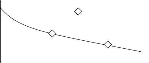
P1: SBT
c19 JWBT188-Aldridge October 23, 2009 12:3 Printer: Yet to come
296 HIGH-FREQUENCY TRADING
Transaction Cost
Market risk at the time of execution
A
B
C
FIGURE 19.1 Efficient trading frontier (ETF). Trades A and B span the efficient
frontier. Trade C is inefficient.
spreads than do other brokers throughout the entire spectrum of market
conditions).
In Figure 19.1, the efficient trading frontier is traced by trades A and B.
Trade C is not efficient, and the causes of the deviation of trade C from the
efficient trading frontier should be investigated. If trades A, B, and C are
recorded for the same security and strategy but different executing bro-
kers, the costs of the broker responsible for trade C should be addressed,
or the bulk of trading should be moved from the broker that traded C to
the brokers that traded A and B.
Benchmarked Analysis
In the benchmarked analysis, the dollar value of the executed position is
compared to the dollar value of the position executed at a certain price,
known as the benchmark price. The benchmarks typically fall into one of
the following categories:
rPre-trade
rPost-trade
rIntra-trade
The pre-trade benchmarks are known at the time the trading begins
and are usually the market prices at the outset of the trading period—or,
for lower trading frequencies, the daily opening prices. Pre-trade bench-
marks may also be based on the trade decision price, the price at which
the trading system makes the decision to execute the trade. Benchmarking
to the trade decision prices is often referred to as “implementation short-
fall,” and is discussed in detail later in this chapter.

P1: SBT
c19 JWBT188-Aldridge October 23, 2009 12:3 Printer: Yet to come
Post-Trade Profitability Analysis 297
The post-trading benchmarks can be any prices recorded after the trad-
ing period. A market price at the end of an intra-day trading period can be a
post-trading benchmark, as can be the daily close. Perold (1988) points out
that to the extent that the trading system places trades correctly—buys
a security that rises through the remainder of the trading period, for
example—comparing execution price with the closing price for the trad-
ing period will make execution look exceptionally, but unjustifiably,
good.
Intra-trading benchmarks include various weighted price averages.
The most popular benchmarks are the volume-weighted average price
(VWAP, pronounced “vee-wop”) and the time-weighted average price
(TWAP, pronounced “tee-wop”). Other benchmarks include averages of
the open, high, low, and close prices (OHLC) within the given trading inter-
val that are designed to proxy for the intra-period range of price movement
and measure the algorithm’s capability to navigate volatility.
Both the VWAP and the TWAP benchmarks can be based on daily,
hourly, or even higher-frequency price data surrounding the trade. The
VWAP for a particular security ion day Tis computed as follows:
VWAPi=
tvit pit
tvit ,{t}∈T(19.5)
where vit is the volume of security itraded at time t, and pit is the market
price of security iat time t.
VWAP is often thought to be a good indicator of market price through-
out the period under consideration (a minute, an hour, a day, etc.). Execu-
tion geared to outperform VWAP typically succeeds at minimizing market
impact, and VWAP-based performance measures reflect the success of cost
minimization strategies. On the other hand, VWAP-based performance met-
rics do not assess the performance of strategies trying to minimize risk or
other variables other than market cost.
TWAP benchmarking measures the ability of the execution algorithm
to time the market. TWAP benchmark price computes the price that would
be obtained if the order were split into equal-sized parcels and traded one
parcel at a time at equally spaced time intervals within the designated trad-
ing time period:
TWAPi=1
T
T
t=1
pit,{t}∈T(19.6)
where pit is the market price of security iat time t.

P1: SBT
c19 JWBT188-Aldridge October 23, 2009 12:3 Printer: Yet to come
298 HIGH-FREQUENCY TRADING
Finally, the OHLC benchmark is a simple average of the open, high,
low, and close prices recorded during the trading period of interest:
OHLCi=1
4pO
it +pH
it +pL
it +pC
it ,{t}∈T(19.7)
where pO
it ,pH
it ,pL
it and pC
it are the market open, high, low, and close prices
of security iduring the time interval t. The OHLC benchmark incorporates
the intra-period price volatility by including the high and low price values.
The OHLC benchmark does not, however, account for volume or liquidity
available on the market.
Kissell and Malamut (2005) point out that different investors may have
natural preferences for different benchmarks. Value investors may want to
execute at their decision price or better, mutual fund managers may need
to execute at the daily closing prices to facilitate the fund’s accounting,
and others may prefer VWAP, the below-average price for the pre-specified
trading period. It is informative to compare performance of an algorithm
against all benchmarks.
Overall, Kissell and Glantz (2003) caution that the benchmarked eval-
uation of execution performance may not be thoroughly useful for the
following reasons:
1. Benchmarked assessment does not lend itself to execution compar-
isons across asset classes, a comparison that may be desirable in as-
sessing performance of different executing brokers.
2. Benchmarked assessments are geared to minimization of execution
prices; other execution-related performance characteristics may be
plausible optimization candidates.
3. Furthermore, according to Kissell and Glantz (2003), benchmarked as-
sessment strategies can be manipulated to show better performance
than is warranted by the actual execution, making the portfolio man-
ager incur higher costs at the same time.
Relative Performance Measurement
To address the flaws of the benchmarked performance measurement,
Kissell and Glantz (2003) propose “relative performance measurement” as
an alternative to the benchmarked analysis. The relative performance mea-
sure is based on either volume or the number of trades and determines the
proportion of volume or trades for which the market price throughout
the trading time period (a minute, an hour, a day, etc.) was more favor-
able than the execution price. In other words, the relative performance
measure assesses at what percentage of volume or trades throughout the

P1: SBT
c19 JWBT188-Aldridge October 23, 2009 12:3 Printer: Yet to come
Post-Trade Profitability Analysis 299
specified period of time the trade could have been executed on even bet-
ter terms than it was actually executed. Specifically, relative performance
measure (RPM) is computed as follows:
RPM(volume) =Total volume |price better than execution price
Total volume
RPM(trades) =Total # of trades |price better than execution price
Total # of trades
(19.8)
According to Kissell and Glantz (2003), the relative performance mea-
sure allows a comparison of execution performance across different finan-
cial instruments as well as across time. Unlike the benchmarked approach
that produces performance assessments in dollars and cents, the rela-
tive performance measure outputs results in percentages ready for cross-
sectional comparisons. For example, suppose we would like to compare
performance of execution of two stocks, IBM and AAPL, within a given
hour. Suppose further that the benchmarked approach tells us that IBM
outperformed its VWAP by 0.04, whereas AAPL outperformed its VWAP by
0.01. The two measures are not comparable, as neither one takes into ac-
count the relative prices of the securities traded. The relative performance
measure, on the other hand, produces the following numbers—50 percent
for IBM and 5 percent for AAPL—and allows us to objectively deduce that
AAPL execution maximized its market advantage during the trading win-
dow, while execution of IBM can be improved further.
Implementation Shortfall
The implementation shortfall (IS) measure due to Perold (1988) measures
the efficiency of executing investment decisions. The IS is computed as the
difference between the realized trades and the trades recorded in paper
trading. The paper trading process usually runs in parallel with the live
process and records all the trades as if they were executed at desirable
price at optimal times.
The paper-trading system of Perold (1988) executes all trades at the
mid-point between the market bid and ask quotes, ignoring all transaction
costs (spreads, commissions, etc.). The paper-trading system also assumes
that unlimited volume can be processed at any point in time at the market
price, ignoring the market depth or liquidity constraints and the associated
slippage and market impact. The IS metric then measures the cost of run-
ning the trading system in real market conditions as compared to the costs
incurred in the idealized paper-trading environment.

P1: SBT
c19 JWBT188-Aldridge October 23, 2009 12:3 Printer: Yet to come
300 HIGH-FREQUENCY TRADING
As Perold (1988) notes, the observed IS can be due to several factors:
rLiquidity constraints
rPrice movement due to information imputed in market prices
rRandom price oscillations
rLatency in execution
rMarket impact
rCommissions
rFees
rSpreads
rTaxes
The IS delivers a bundled estimate of the component costs and the esti-
mate is difficult to disaggregate into individual cost centers. As a result, the
IS methodology of Perold (1988) has been subject to criticism. To measure
the costs of execution with greater precision, Wagner and Banks (1992)
and Wagner and Edwards (1993) adjust IS by known transaction costs.
Furthermore, the implementation shortfall analysis can help in calcu-
lating the cost of market impact. A paper-trading system run concurrently
with production can note two types of orders in parallel: (1) market orders
at the market prices when the order decisions are made and (2) limit or-
ders when the market price crosses the limit price. Such analysis will help
assess the probability of hitting a limit order for a particular strategy, as
shown by equation (19.9):
Pr(Limit Execution) =# of Executed Limit Orders
# of Orders Placed (19.9)
For example, if out of 75 orders placed as limit orders, only 25 were exe-
cuted, the probability of executing a limit order for a given strategy is 33
percent.
The analysis will also help describe the opportunity cost of missing
profits for limit orders that are never hit, as shown in equation (19.10):
Opp Cost per Limit Order =−GainMarket Orders −GainLimit Orders
# of Orders Placed (19.10)
Both the probability and the opportunity costs accompanying limit or-
ders are useful tools in designing and updating future trading systems. The
opportunity cost associated with a limit order failing to execute should be
taken into account when deciding whether to send a particular order as a

P1: SBT
c19 JWBT188-Aldridge October 23, 2009 12:3 Printer: Yet to come
Post-Trade Profitability Analysis 301
limit or as a market order. As usual, the decision should be based on the
expected gain of the limit order, computed as shown in equation (19.11):
E[GainLimit Orders]=(Opp Cost per Limit Order) ×
Pr(Limit Execution) +(1 −Pr(Limit Execution)) ×
GainLimit Orders
# of Executed Limit Orders (19.11)
An order should be executed on limit instead of on market if the expected
gain associated with limit orders is positive.
For example, suppose that a particular trading system on average ex-
ecutes two limit orders for every three limit orders placed. In this case,
Pr(LimitExecution)=66.7 percent. In addition, suppose that every exe-
cuted limit order on average gains 15 bps and every executed market order
gains 12 bps. Then the opportunity cost on 100 orders placed can be com-
puted as follows:
Opp Cost per Limit Order =
−12 bps ×100 orders −15 bps ×100 orders ×66.7%
100 orders =−2 bps
E[GainLimit Orders]=(−2 bps) ×66.7% +(1 −66.7%) ×15 bps =3.67 bps
The limit orders will continue being placed as limit orders (as opposed to
market orders) for as long as E[GainLimit Orders] remains positive.
Performance Analysis Summary
Both cost and performance analyses, performed post-trade, generate in-
sights critical to understanding the real-life trading behavior of trading
models. The results of the analyses provide key feedback ideas for improv-
ing existing trading methodologies.
CONCLUSION
Post-trade analysis is an important component of high-frequency trading.
At low trading frequencies, where the objective is to capture large gains
over extended periods of time, transaction costs and variations in ex-
ecution prices are negligible in comparison with the target trade gain.
High-frequency trading, however, is much more sensitive to increases
in costs and decreases in performance. At high frequencies, costs and
P1: SBT
c19 JWBT188-Aldridge October 23, 2009 12:3 Printer: Yet to come
302 HIGH-FREQUENCY TRADING
underperformance accumulate rapidly throughout the day, denting or out-
right eliminating trading profitability. Understanding, measuring, and man-
aging incurred costs and potential performance shortcomings become
paramount in the high-frequency setting.
The issues of costs and execution-related performance are bound to
become more pronounced as the field of high-frequency trading expands.
With multiple parties competing to ride the same short-term price oscilla-
tions, traders with the most efficient cost and performance structures will
realize the biggest gains.

P1: SBT
ref JWBT188-Aldridge October 29, 2009 16:59 Printer: Yet to come
References
Abel, A.B., 1990. “Asset Prices under Habit Formation and Catching Up with the
Joneses.” American Economic Review 80, 38–42.
Admati, A. and P. Pfleiderer, 1988. “A Theory of Intraday Patterns: Volume and Price
Variability.” Review of Financial Studies 1, 3–40.
Agarwal, V. and N.Y. Naik, 2004. “Risk and Portfolio Decisions Involving Hedge
Funds.” Review of Financial Studies 17 (1), 63–98.
Aggarwal, R. and D.C. Schirm, 1992. “Balance of Trade Announcements and Asset
Prices: Influence on Equity Prices, Exchange Rates, and Interest Rates.” Journal of
International Money and Finance 11, 80–95.
Ahn, H., K. Bae and K. Chan, 2001. “Limit Orders, Depth and Volatility: Evi-
dence from the Stock Exchange of Hong Kong.” Journal of Finance 56, 767–
788.
Aitken, M., N. Almeida, F. Harris and T. McInish, 2005. “Order Splitting and Order
Aggressiveness in Electronic Trading.” Working paper.
Ajayi, R.A. and S.M. Mehdian, 1995. “Global Reactions of Security Prices to Major
US-Induced Surprises: An Empirical Investigation.” Applied Financial Economics
5, 203–218.
Alam, Zinat Shaila and Isabel Tkatch, 2007. “Slice Order in TASE—Strategy to
Hide?” Working paper, Georgia State University.
Aldridge, Irene, 2008. “Systematic Funds Outperform Peers in Crisis.” HedgeWorld
(Thomson/Reuters), November 13, 2008.
Aldridge, Irene, 2009a. “Measuring Accuracy of Trading Strategies.” Journal of
Trading 4, Summer 2009, 17–25.
Aldridge, Irene, 2009b. “Systematic Funds Outperform Discretionary Funds.” Work-
ing paper.
Aldridge, Irene, 2009c. “High-Frequency Portfolio Optimization.” Working paper.
Alexander, Carol and A. Johnson, 1992. “Are Foreign Exchange Markets Really
Efficient?” Economics Letters 40, 449–453.
Alexander, Carol, 1999. “Optimal Hedging Using Cointegration.” Philosophical
Transactions of the Royal Society,Vol.357, No. 1758, 2039–2058.
303
P1: SBT
ref JWBT188-Aldridge October 29, 2009 16:59 Printer: Yet to come
304 REFERENCES
Alexakis, Panayotis and Nicholas Apergis, 1996. “ARCH Effects and Cointegration:
Is the Foreign Exchange Market Efficient?” Journal of Banking and Finance 20
(4), 687–97.
Almeida, Alvaro, Charles Goodhart and Richard Payne, 1998. “The Effect of Macro-
economic ‘News’ on High Frequency Exchange Rate Behaviour.” Journal of Finan-
cial and Quantitative Analysis 33, 1–47.
Almgren, R. and N. Chriss, 1999. “Value Under Liquidation.” Risk Magazine 12,
61–63.
Almgren, R. and N. Chriss, 2000. “Optimal Execution of Portfolio Transactions.”
Journal of Risk 12, 61–63.
Almgren, R.C. Thum, E. Hauptmann and H. Li, 2005. “Equity Market Impact.” Risk
18, 57–62.
Amenc, M., S. Curtis and L. Martellini, 2003. “The Alpha and Omega of Hedge Fund
Performance.” Working paper, Edhec/USC.
American Academy of Actuaries, 2000. “Report of the Life Liquidity Work Group of
the American Academy of Actuaries to the NAIC’s Life Liquidity Working Group.”
Boston, MA, December 2, 2000.
Amihud, Y., 2002. “Illiquidity and Stock Returns: Cross-Section and Time Series
Effects.” Journal of Financial Markets 5, 31–56.
Amihud, Y., B.J. Christensen and H. Mendelson, 1993. “Further Evidence on the
Risk-Return Relationship.” Working Paper, New York University.
Amihud, Y. and H. Mendelson, 1986. “Asset Pricing and the Bid-Ask Spread.” Jour-
nal of Financial Economics 17, 223–249.
Amihud, Y. and H. Mendelson, 1989. “The Effects of Beta, Bid-Ask Spread, Residual
Risk and Size on Stock Returns.” Journal of Finance 44, 479–486.
Amihud, Y. and H. Mendelson, 1991. “Liquidity, Maturity and the Yields on U.S. Gov-
ernment Securities.” Journal of Finance 46, 1411–1426.
Anand, Amber, Sugato Chakravarty and Terrence Martell, 2005. “Empirical Evi-
dence on the Evolution of Liquidity: Choice of Market versus Limit Orders by In-
formed and Uninformed Traders.” Journal of Financial Markets 8, 289–309.
Andersen, T.G., T. Bollerslev, F.X. Diebold and P. Labys, 2001. “The Distribution of
Realized Exchange Rate Volatility.” Journal of the American Statistical Associa-
tion 96, 42–55.
Andersen, T.G., T. Bollerslev, F.X. Diebold and P. Labys, 2001. “The Distribu-
tion of Realized Stock Return Volatility.” Journal of Financial Economics 61,
43–76.
Andersen, T.G., T. Bollerslev, F.X. Diebold and C. Vega, 2003. “Micro Effects of
Macro Announcements: Real-Time Price Discovery in Foreign Exchange.” Ameri-
can Economic Review 93, 38–62.
Andritzky, J.R., G.J. Bannister and N.T. Tamirisa, 2007. “The Impact of Macroeco-
nomic Announcements on Emerging Market Bonds.” Emerging Markets Review 8,
20–37.
P1: SBT
ref JWBT188-Aldridge October 29, 2009 16:59 Printer: Yet to come
References 305
Ang, A. and J. Chen, 2002. “Asymmetric Correlations of Equity Portfolios.” Journal
of Financial Economics, 443–494.
Angel, J., 1992. “Limit versus Market Orders.” Working paper, Georgetown Univer-
sity.
Artzner, P., F. Delbaen, J. Eber and D. Heath, 1997. “Thinking Coherently.” Risk
10(11), 68–71.
Atiase, R. 1985. “Predisclosure Information, Firm Capitalization and Security Price
Behavior around Earnings Announcements.” Journal of Accounting Research
21–36.
Avellaneda, Marco and Sasha Stoikov, 2008. “High-Frequency Trading in a Limit
Order Book.” Quantitative Finance,Vol.8, No. 3., 217–224.
Bae, Kee-Hong, Hasung Jang and Kyung Suh Park, 2003. “Traders’ Choice between
Limit and Market Orders: Evidence from NYSE Stocks.” Journal of Financial
Markets 6, 517–538.
Bagehot, W., (pseud.) 1971. “The Only Game in Town.” Financial Analysts Journal
27, 12–14, 22.
Bailey, W., 1990. “US Money Supply Announcements and Pacific Rim Stock Mar-
kets: Evidence and Implications.” Journal of International Money and Finance 9,
344–356.
Balduzzi, P., E.J. Elton and T.C. Green, 2001. “Economic News and Bond Prices:
Evidence From the U.S. Treasury Market.” Journal of Financial and Quantitative
Analysis 36, 523–543.
Bangia, A., F.X. Diebold, T. Schuermann and J.D. Stroughair, 1999. “Liquidity Risk,
with Implications for Traditional Market Risk Measurement and Management.”
Wharton School, Working Paper 99–06.
Banz, R.W., 1981. “The Relationship between Return and Market Value of Common
Stocks.” Journal of Financial Economics 9, 3–18.
Barclay, M.J. and J.B. Warner, 1993. “Stealth and Volatility: Which Trades Move
Prices?” Journal of Financial Economics 34, 281–306.
Basak, Suleiman, Alex Shapiro and Lucie Tepla, 2005. “Risk Management with
Benchmarking.” LBS Working Paper.
Basu, S., 1983. “The Relationship Between Earnings Yield, Market Value and the
Return for NYSE Common Stocks.” Journal of Financial Economics 12, 126–
156.
Bauwens, Luc, Walid Ben Omrane and Pierre Giot, 2005. “News Announcements,
Market Activity and Volatility in the Euro/Dollar Foreign Exchange Market.” Jour-
nal of International Money and Finance 24, 1108–1125.
Becker, Kent G., Joseph E. Finnerty and Kenneth J. Kopecky, 1996. “Macroeco-
nomic News and the Efficiency of International Bond Futures Markets.” Journal of
Futures Markets 16, 131–145.
Berber, A. and C. Caglio, 2004. “Order Submission Strategies and Information:
Empirical Evidence from the NYSE.” Working paper, University of Lausanne.
P1: SBT
ref JWBT188-Aldridge October 29, 2009 16:59 Printer: Yet to come
306 REFERENCES
Bernanke, Ben S. and Kenneth N. Kuttner, 2005. “What Explains the Stock Market’s
Reaction to Federal Reserve Policy?” Journal of Finance 60, 1221–1257.
Bertsimas, D. and A.W. Lo, 1998. “Optimal Control of Execution Costs.” Journal of
Financial Markets 1, 1–50.
Bervas, Arnaud, 2006. “Market Liquidity and Its Incorporation into Risk Manage-
ment.” Financial Stability Review 8, 63–79.
Best, M.J. and R.R. Grauer, 1991. “On the Sensitivity of Mean-Variance-Efficient
Portfolios to Changes in Asset Means: Some Analytical and Computational Results.”
Review of Financial Studies 4, 315–42.
Bhaduri, R., G. Meissner and J. Youn, 2007. “Hedging Liquidity Risk.” Journal of
Alternative Investments, 80–90.
Biais, Bruno, Christophe Bisiere and Chester Spatt, 2003. “Imperfect Competition in
Financial Markets: ISLAND vs NASDAQ.” GSIA Working Papers, Carnegie Mellon
University, Tepper School of Business, 2003-E41.
Biais, B., P. Hillion and C. Spatt, 1995. “An Empirical Analysis of the Limit Or-
der Book and the Order Flow in the Paris Bourse.” Journal of Finance 50, 1655–
1689.
Black, Fisher, 1972. “Capital Market Equilibrium with Restricted Borrowing.” Jour-
nal of Business 45, 444–455.
Black, F. and R. Jones, 1987. “Simplifying Portfolio Insurance.” Journal of Portfolio
Management 14, 48–51.
Black, Fischer and Myron Scholes (1973). “The Pricing of Options and Corporate
Liabilities.” Journal of Political Economy 81, 637–654.
Bloomfield, R., M. O’Hara and G. Saar, 2005. “The ‘Make or Take’ Decision in an
Electronic Market: Evidence on the Evolution of Liquidity.” Journal of Financial
Economics 75, 165–199.
Board, J. and C. Sutcliffe, 1995. “The Effects of Transparency in the London Stock
Exchange.” Report commissioned by the London Stock Exchange, January 1995.
Bollerslev, T., 1986. “Generalized Autoregressive Conditional Heteroscedasticity.”
Journal of Econometrics 31, 307–327.
Bond, G.E., 1984. “The Effects of Supply and Interest Rate Shocks in Commodity
Futures Markets.” American Journal of Agricultural Economics 66, 294–301.
Bos, T. and P. Newbold, 1984. “An Empirical Investigation of the Possibility of
Stochastic Systematic Risk in the Market Model.” Journal of Business 57, 35–41.
Boscaljon, Brian L., 2005. “Regulatory Changes in the Pharmaceutical Industry.”
International Journal of Business 10(2), 151–164.
Boyd, John H., Jian Hu and Ravi Jagannathan, 2005. “The Stock Market’s Reaction
to Unemployment News: Why Bad News Is Usually Good for Stocks.” Journal of
Finance 60, 649–672.
Bredin, Don, Gerard O’Reilly and Simon Stevenson, 2007. “Monetary Shocks and
REIT Returns.” The Journal of Real Estate Finance and Economics 35, 315–331.
P1: SBT
ref JWBT188-Aldridge October 29, 2009 16:59 Printer: Yet to come
References 307
Brennan, M.J., T. Chordia and A. Subrahmanyam, 1998. “Alternative Factor Spec-
ifications, Security Characteristics, and the Cross-Section of Expected Stock
Returns.” Journal of Financial Economics 49, 345–373.
Brennan, M.J. and A. Subrahmanyam, 1996. “Market Microstructure and Asset Pric-
ing: On the Compensation for Illiquidity in Stock Returns.” Journal of Financial
Economics 41, 441–464.
Brock, W.A., J. Lakonishok and B. LeBaron, 1992. “Simple Technical Trading Rules
and the Stochastic Properties of Stock Returns.” Journal of Finance 47, 1731–1764.
Brooks, C. and H.M. Kat, 2002. “The Statistical Properties of Hedge Fund Index
Returns and Their Implications for Investors.” Journal of Alternative Investments
5(Fall), 26–44.
Brown, S.J., W.N. Goetzmann and J.M. Park, 2004. “Conditions for Survival: Chang-
ing Risk and the Performance of Hedge Fund Managers and CTAs.” Yale School of
Management Working Papers.
Burke, G., 1994. “A Sharper Sharpe Ratio.” Futures 23 (3), 56.
Campbell, J.Y. and J.H. Cochrane, 1999. “By Force of Habit: A Consumption-Based
Explanation of Aggregate Stock Market Behaviour.” Journal of Political Economy
107, 205–251.
Campbell, John Y., Andrew W. Lo and A. Craig MacKinlay, 1997. The Econometrics
of Financial Markets. Princeton University Press.
Cao, C., O. Hansch and X. Wang, 2004. “The Informational Content of an Open Limit
Order Book.” Working paper, Pennsylvania State University.
Carpenter, J. “Does Option Compensation Increase Managerial Risk Appetite?”
Journal of Finance 55, 2000, 2311–2331.
Caudill, M., 1988. “Neural Networks Primer—Part I.” AI Expert 31, 53–59.
Chaboud, Alain P. and Jonathan H. Wright, 2005. “Uncovered Interest Parity: It
Works, but Not for Long.” Journal of International Economics 66, 349–362.
Chakravarty, Sugato, 2001. “Stealth Trading: Which Traders’ Trades Move Stock
Prices?” Journal of Financial Economics 61, 289–307.
Chakravarty, Sugato and C. Holden, 1995. “An Integrated Model of Market and Limit
Orders.” Journal of Financial Intermediation 4, 213–241.
Challe, Edouard, 2003. “Sunspots and Predictable Asset Returns.” Journal of Eco-
nomic Theory 115, 182–190.
Chambers, R.G., 1985. “Credit Constraints, Interest Rates and Agricultural Prices.”
American Journal of Agricultural Economics 67, 390–395.
Chan, K.S. and H. Tong, 1986. “On estimating Thresholds in Autoregressive Models.”
Journal of Time Series Analysis 7, 179–190.
Chan, L.K.C., Y. Hamao and J. Lakonishok, 1991. “Fundamentals and Stock Returns
in Japan.” Journal of Finance 46, 1739–1764.
Chan, L.K.C., J. Karceski and J. Lakonishok, 1998. “The Risk and Return from Fac-
tors.” Journal of Financial and Quantitative Analysis 33, 159–188.
P1: SBT
ref JWBT188-Aldridge October 29, 2009 16:59 Printer: Yet to come
308 REFERENCES
Chan, L. and J. Lakonishok, 1995. “The Behavior of Stock Price around Institutional
Trades.” Journal of Finance 50, 1147–1174.
Choi, B.S., 1992. ARMA Model Identification. Springer Series in Statistics, New
York.
Chordia, T., R. Roll and A. Subrahmanyam, 2001. “Market Liquidity and Trading
Activity.” Journal of Finance 56, 501–530.
Chordia, T., R. Roll and A. Subrahmanyam, 2002. “Commonality in Liquidity.” Jour-
nal of Financial Economics 56, 3–28.
Chung, K., B. Van Ness and B. Van Ness, 1999. “Limit Orders and the Bid-Ask
Spread.” Journal of Financial Economics 53, 255–287.
Clare, A.D., R. Priestley and S.H. Thomas, 1998. “Reports of Beta’s Death Are
Premature: Evidence from the UK.” Journal of Banking and Finance 22, 1207–
1229.
Cochrane, J., 2005. Asset Pricing (2nd edition). Princeton, NJ: Princeton University
Press.
Cohen, K., S. Maier, R. Schwartz and D. Whitcomb, 1981. “Transaction Costs, Order
Placement Strategy, and Existence of the Bid-Ask Spread.” Journal of Political
Economy 89, 287–305.
Colacito, Riccardo and Robert Engle, 2004. “Multiperiod Asset Allocation with
Dynamic Volatilities.” Working paper.
Coleman, M., 1990. “Cointegration-Based Tests of Daily Foreign Exchange Market
Efficiency.” Economic Letters 32, 53–59.
Connolly, Robert A. and Chris Stivers, 2005. “Macroeconomic News, Stock
Turnover, and Volatility Clustering in Daily Stock Returns.” Journal of Financial
Research 28, 235–259.
Constantinides, George, 1986. “Capital Market Equilibrium with Transaction
Costs.” Journal of Political Economy 94, 842–862.
Copeland, T. and D. Galai, 1983. “Information Effects on the Bid-Ask Spreads.”
Journal of Finance 38, 1457–1469.
Corsi, Fulvio, Gilles Zumbach, Ulrich M¨
uller and Michel Dacorogna, 2001. “Consis-
tent High-Precision Volatility from High-Frequency Data.” Economics Notes 30,No.
2, 183–204.
Cutler, David M., James M. Poterba and Lawrence H. Summers, 1989. “What Moves
Stock Prices?” Journal of Portfolio Management 15, 4–12.
Dacorogna, M.M., R. Gencay, U.A. M¨
uller, R. Olsen and O.V. Pictet, 2001. An Intro-
duction to High-Frequency Finance. Academic Press: San Diego, CA.
Dahl, C.M. and S. Hyllenberg, 1999. “Specifying Nonlinear Econometric Models by
Flexible Regression Models and Relative Forecast Performance.” Working paper,
Department of Economics, University of Aarhus, Denmark.
Datar, Vinay T., Narayan Y. Naik and Robert Radcliffe, 1998. “Liquidity and Asset
Returns: An Alternative Test.” Journal of Financial Markets 1, 203–219.
P1: SBT
ref JWBT188-Aldridge October 29, 2009 16:59 Printer: Yet to come
References 309
Demsetz, Harold, 1968. “The Cost of Transacting,” Quarterly Journal of Eco-
nomics, 33–53.
Dennis, Patrick J. and James P. Weston, 2001. “Who’s Informed? An Analysis of
Stock Ownership and Informed Trading.” Working paper.
Diamond, D.W. and R.E. Verrecchia, 1987. “Constraints on Short-Selling and
Asset Price Adjustment to Private Information.” Journal of Financial Economics
18, 277–311.
Dickenson, J.P., 1979. “The Reliability of Estimation Procedures in Portfolio Analy-
sis.” Journal of Financial and Quantitative Analysis 9, 447–462.
Dickey, D.A. and W.A. Fuller, 1979. “Distribution of the Estimators for Autoregres-
sive Time Series with a Unit Root.” Journal of the American Statistical Associa-
tion 74, 427–431.
Ding, B., H.A. Shawky and J. Tian, 2008. “Liquidity Shocks, Size and the Relative
Performance of Hedge Fund Strategies.” Working Paper, University of Albany.
Dowd, K., 2000. “Adjusting for Risk: An Improved Sharpe Ratio.” International
Review of Economics and Finance 9(3), 209–222.
Dufour, A. and R.F. Engle, 2000. “Time and the Price Impact of a Trade.” Journal of
Finance 55, 2467–2498.
Easley, David, Nicholas M. Kiefer, Maureen O’Hara and Joseph B. Paperman, 1996.
“Liquidity, Information, and Infrequently Traded Stocks.” Journal of Finance 51,
1405–1436.
Easley, David and Maureen O’Hara, 1987. “Price, Trade Size, and Information in
Securities Markets.” Journal of Financial Economics 19, 69–90.
Easley, David and Maureen O’Hara, 1992. “Time and the Process of Security Price
Adjustment.” Journal of Finance 47, 1992, 557–605.
Ederington, Louis H. and Jae Ha Lee, 1993. “How Markets Process Information:
News Releases and Volatility.” Journal of Finance 48, 1161–1191.
Edison, Hali J., 1996. “The Reaction of Exchange Rates and Interest Rates to
News Releases.” Board of Governors of the Federal Reserve System, International
Finance Discussion Paper No. 570 (October).
Edwards, F.R. and M. Caglayan, 2001. “Hedge Fund Performance and Manager
Skill,” Journal of Futures Markets 21(11), 1003–28.
Edwards, Sebastian, 1982. “Exchange Rates, Market Efficiency and New Informa-
tion.” Economics Letters 9, 377–382.
Eichenbaum, Martin and Charles Evans, 1993. “Some Empirical Evidence on the
Effects of Monetary Policy Shocks on Exchange Rates.” NBER Working Paper
No. 4271.
Eleswarapu, V.R., 1997. “Cost of Transacting and Expected Returns in the Nasdaq
Market.” Journal of Finance 52, 2113–2127.
Eling, M. and F. Schuhmacher, 2007. “Does the Choice of Performance Measure
Influence the Evaluation of Hedge Funds?” Journal of Banking and Finance 31,
2632–2647.
P1: SBT
ref JWBT188-Aldridge October 29, 2009 16:59 Printer: Yet to come
310 REFERENCES
Ellul, A., C. Holden, P. Jain and R. Jennings, 2007. “Determinants of Order Choice
on the New York Stock Exchange.” Working paper, Indiana University.
Engel, Charles, 1996. “The Forward Discount Anomaly and the Risk Premium: A
Survey of Recent Evidence.” Journal of Empirical Finance 3, 123–192.
Engel, Charles, 1999. “Accounting for US Real Exchange Rate Changes.” Journal of
Political Economy 107(3), 507.
Engle, R.F., 1982. “Autoregressive Conditional Heteroscedasticity with Estimates
of the Variance of United Kingdom Inflations.” Econometrica 50, 987–1007.
Engle, R.F., 2000. “The Econometrics of Ultra-High Frequency Data.” Econometrica
68, 1–22.
Engle, R. and R. Ferstenberg, 2007. “Execution Risk.” Journal of Portfolio Manage-
ment 33, 34–45.
Engle, R. and C. Granger, 1987. “Co-Integration and Error-Correction: Representa-
tion, Estimation, and Testing.” Econometrica 35, 251–276.
Engle, R.F. and J. Lange, 2001. “Predicting VNET: A Model of the Dynamics of
Market Depth.” Journal of Financial Markets 4, 113–142.
Engle, R.F. and A. Lunde, 2003. “Trades and Quotes: A Bivariate Point Process.”
Journal of Financial Econometrics 1, 159–188.
Engle, R.F. and A.J. Patton, 2001. “What Good is a Volatility Model?” Quantitative
Finance 1, 237–245.
Engle, R.F. and J.R. Russell, 1997. “Forecasting the Frequency of Changes in Quoted
Foreign Exchange Prices with the Autoregressive Conditional Duration Model.”
Journal of Empirical Finance 4, 187–212.
Engle, R.F. and J.R. Russell, 1998. “Autoregressive Conditional Duration: A New
Model for Irregularly Spaced Transactions Data.” Econometrica 66, 1127–1162.
Errunza, V. and K. Hogan, 1998. “Macroeconomic Determinants of European Stock
Market Volatility.” European Financial Management 4, 361–377.
Evans, M. and R.K. Lyons, 2002. “Order Flow and Exchange Rate Dynamics.” Jour-
nal of Political Economy 110, 170–180.
Evans, M.D.D. and R.K. Lyons, 2007. “Exchange Rate Fundamentals and Order
Flow.” NBER Working Paper No. 13151.
Evans, M.D.D., 2008. Foundations of Foreign Exchange. Princeton Series in Inter-
national Economics, Princeton University Press.
Fama, E., L. Fisher, M. Jensen and R. Roll, 1969. “The Adjustment of Stock Prices
to New Information.” International Economic Review 10, 1–21.
Fama, Eugene, 1970. “Efficient Capital Markets: A Review of Theory and Empirical
Work.” Journal of Finance 25, 383–417.
Fama, Eugene, 1984. “Forward and Spot Exchange Rates.” Journal of Monetary
Economics 14, 319–338.
Fama, Eugene, 1991. “Efficient Capital Markets: II.” The Journal of Finance XLVI
(5), 1575–1617.
P1: SBT
ref JWBT188-Aldridge October 29, 2009 16:59 Printer: Yet to come
References 311
Fama, Eugene F. and Kenneth R. French, 1993. “Common Risk Factors in the Re-
turns on Stocks and Bonds.” Journal of Financial Economics 33, 3–56.
Fama, E. and K. French, 1995. “Size and Book-to-Market Factors in Earnings and
Returns.” Journal of Finance 50, 131–156.
Fan-fah, C., S. Mohd and A. Nasir, 2008. “Earnings Announcements: The Impact of
Firm Size on Share Prices.” Journal of Money, Investment and Banking 36–46.
Fan, J. and Q. Yao, 2003. Nonlinear Time Series: Nonparametric and Parametric
Methods. Springer-Verlag, New York.
Fatum, R. and M.M. Hutchison, 2003. “Is Sterilized Foreign Exchange Intervention
Effective After All? An Event Study Approach.” Economic Journal, Royal Eco-
nomic Society, Vol. 113(487), 390–411, 04.
Flannery, M.J. and A.A. Protopapadakis, 2002. “Macroeconomic Factors Do Influ-
ence Aggregate Stock Returns.” Review of Financial Studies 15, 751–782.
Fleming, Michael J. and Eli M. Remolona, 1997. “What Moves the Bond Market?”
Federal Reserve Bank of New York Economic Policy Review 3, 31–50.
Fleming, Michael J. and Eli M. Remolona, 1999. “Price Formation and Liquidity in
the U.S. Treasury Market: The Response to Public Information.” Journal of Finance
54, 1901-1915.
Fleming, Michael J. and Eli M. Remolona, 1999. “The Term Structure of Announce-
ment Effects.” BIS Working paper No. 71.
Foster, F. and S. Viswanathan, 1996. “Strategic Trading When Agents Forecast the
Forecasts of Others.” Journal of Finance 51, 1437–1478.
Foucault, T., 1999. “Order Flow Composition and Trading Costs in a Dynamic Limit
Order Market.” Journal of Financial Markets 2, 99–134.
Foucault, T., O. Kadan and E. Kandel, 2005. “Limit Order Book As a Market for
Liquidity.” Review of Financial Studies 18, 1171–1217.
Foucault, T. and A. Menkveld, 2005. “Competition for Order Flow and Smart Order
Routing Systems.” Working paper, HEC.
Foucault, T., A. Roell and P. Sandas, 2003. “Market Making with Costly Monitor-
ing: An Analysis of the SOES Controversy.” Review of Financial Studies 16, 345–
384.
Foucault, T., S. Moinas and E. Theissen, 2007. “Does Anonymity Matter in Elec-
tronic Limit Order Markets?” Review of Financial Studies 20 (5), 1707–1747.
Frankel, Jeffrey, 2006. “The Effect of Monetary Policy on Real Commodity Prices.”
Asset Prices and Monetary Policy. John Campbell, ed., University of Chicago Press,
291–327.
Frankfurter, G.M., H.E. Philips and J.P. Seagle, 1971. “Portfolio Selection: The
Effects of Uncertain Means, Variances and Covariances.” Journal of Financial and
Quantitative Analysis 6, 1251–1262.
Fransolet, L., 2004. “Have 8000 hedge funds eroded market opportunities?” Euro-
pean Fixed Income Research, JP Morgan Securities Ltd., October 191–215.
P1: SBT
ref JWBT188-Aldridge October 29, 2009 16:59 Printer: Yet to come
312 REFERENCES
Freeman, R., 1987. “The Association Between Accounting Earnings and Secu-
rity Returns for Large and Small Firms.” Journal of Accounting and Economics.
195–228.
Frenkel, Jacob, 1981. “Flexible Exchange Rates, Prices and the Role of ‘News’:
Lessons from the 1970s.” Journal of Political Economy 89, 665–705.
Froot, K. and R. Thaler, 1990. “Anomalies: Foreign Exchange.” Journal of Eco-
nomic Perspectives 4(3), 179–192.
Fung, W. and D.A. Hsieh, 1997. “Empirical Characteristics of Dynamic Trading
Strategies: The Case of Hedge Funds.” Review of Financial Studies 10, 275–
302.
Garlappi, L., R. Uppal and T. Wang, 2007. “Portfolio Selection with Parameter and
Model Uncertainty: A Multi-Prior Approach.” The Review of Financial Studies 20,
41–81.
Garman, Mark, 1976. “Market Microstructure.” Journal of Financial Economics 3,
257–275.
Garman, M.B. and M.J. Klass, 1980. “On the Estimation of Security Price Volatilities
from Historical Data.” Journal of Business 53, 67–78.
Gatev, Evan, William N. Goetzmann and K. Geert Rouwenhorst, 2006. “Pairs Trad-
ing: Performance of a Relative-Value Arbitrage Rule,” Review of Financial Studies,
797–827.
George, T., G. Kaul and M. Nimalendran, 1991. “Estimation of the Bid-Ask Spread
and its Components: A New Approach.” The Review of Financial Studies 4(4),
623–656.
Getmansky, M., A.W. Lo and I. Makarov, 2004. “An Econometric Model of Serial
Correlation and Illiquidity in Hedge Fund Returns.” Journal of Financial Eco-
nomics 74 (3), 529–609.
Ghysels, E. and J. Jasiak, 1998. “GARCH for Irregularly Spaced Financial Data:
The ACD-GARCH Model.” Studies on Nonlinear Dynamics and Econometrics 2,
133–149.
Ghysels, E., C. Gouri´
eroux and J. Jasiak, 2004. “Stochastic Volatility Duration Mod-
els.” Journal of Econometrics 119, 413–433.
Glosten, Lawrence, 1994. “Is the Electronic Open Limit Order Book Inevitable?”
Journal of Finance 49, 1127–1161.
Glosten, Lawrence R. and Lawrence E. Harris, 1988. “Estimating the Components
of the Bid-Ask Spread.” Journal of Financial Economics 21, 123–142.
Glosten, Lawrence and P. Milgrom, 1985. “Bid, Ask, and Transaction Prices in a
Specialist Market with Heterogeneously Informed Traders.” Journal of Financial
Economics 13, 71–100.
Goettler, R., C. Parlour and U. Rajan, 2005. “Equilibrium in a Dynamic Limit Order
Market.” Journal of Finance 60, 2149–2192.
Goettler, R., C. Parlour and U. Rajan, 2007. “Microstructure Effects and Asset Pric-
ing.” Working paper, University of California—Berkeley.
P1: SBT
ref JWBT188-Aldridge October 29, 2009 16:59 Printer: Yet to come
References 313
Goodhart, Charles A.E., 1988. “The Foreign Exchange Market: A Random Walk with
a Dragging Anchor.” Economica 55, 437–460.
Goodhart, Charles A.E. and Maureen O’Hara, 1997. “High Frequency Data in Fi-
nancial Markets: Issues and Applications.” Journal of Empirical Finance 4, 73–
114.
Gorton, G. and G. Rouwenhorst, 2006. “Facts and Fantasies About Commodity Fu-
tures.” Financial Analysts Journal, March/April, 47–68.
Gouri´
eroux, C. and J. Jasiak, 2001. Financial Econometrics. Princeton, NJ: Prince-
ton University Press.
Gouri´
eroux, C., J. Jasiak and G. Le Fol, 1999. “Intraday Trading Activity.” Journal
of Financial Markets 2, 193–226.
Graham, Benjamin and David Dodd, 1934. Security Analysis.NewYork:The
McGraw-Hill Companies.
Granger, C., 1986. “Developments in the Study of Cointegrated Economic Vari-
ables.” Oxford Bulletin of Economics and Statistics 48, 213–228.
Granger, C. and A.P. Andersen, 1978. An Introduction to Bilinear Time Series
Models. Vandenhoek and Ruprecht, G¨
ottingen.
Granger, C. and P. Newbold, 1974. “Spurious Regressions in Econometrics.” Jour-
nal of Econometrics 2, 111–120.
Gregoriou, G.N. and J.-P. Gueyie, 2003. “Risk-Adjusted Performance of Funds of
Hedge Funds Using a Modified Sharpe Ratio.” Journal of Alternative Investments
6(Winter), 77–83.
Gregoriou, G.N. and F. Rouah, 2002. “Large versus Small Hedge Funds: Does Size
Affect Performance?” Journal of Alternative Investments 5, 75–77.
Griffiths, M., B. Smith, A. Turnbull and R. White, 2000. “The Costs and Determinants
of Order Aggressiveness.” Journal of Financial Economics 56, 65–88.
Grilli, Vittorio and Nouriel Roubini, 1993. “Liquidity and Exchange Rates: Puzzling
Evidence from the G-7 Countries.” Mimeo, Birkbeck College.
Groenewold, N. and P. Fraser, 1997. “Share Prices and Macroeconomic Factors.”
Journal of Business Finance and Accounting 24, 1367–1383.
Hakkio, C.S. and M. Rush, 1989. “Market Efficiency and Cointegration: An Appli-
cation to the Sterling and Deutsche Mark Exchange Markets.” Journal of Interna-
tional Money and Finance 8, 75–88.
Handa, Puneet and Robert A. Schwartz, 1996. “Limit Order Trading.” Journal of
Finance 51, 1835–1861.
Handa, P., R. Schwartz and A. Tiwari, 2003. “Quote Setting and Price Formation in
an Order Driven Market.” Journal of Financial Markets 6, 461–489.
Hansen L.P. and R.J. Hodrick, 1980. “Forward Exchange Rates as Optimal Predic-
tors of Future Spot Rates.” Journal of Political Economy, October, 829–853.
Hardouvelis, Gikas A., 1987. “Macroeconomic Information and Stock Prices.” Jour-
nal of Economics and Business 39, 131–140.
P1: SBT
ref JWBT188-Aldridge October 29, 2009 16:59 Printer: Yet to come
314 REFERENCES
Harris, L., 1998. “Optimal Dynamic Order Submission Strategies in Some Stylized
Trading Problems.” Financial Markets, Institutions & Instruments 7, 1–76.
Harris, L. and J. Hasbrouck, 1996. “Market vs. Limit Orders: The SuperDOT Ev-
idence on Order Submission Strategy.” Journal of Financial and Quantitative
Analysis 31, 213–231.
Harris, L. and V. Panchapagesan, 2005. “The Information Content of the Limit Order
Book: Evidence from NYSE Specialist Trading Decisions,” Journal of Financial
Market 8, 25–68.
Harrison, J. Michael and David M. Kreps, 1978. “Speculative Behavior in a Stock
Market with Heterogeneous Expectations.” The Quarterly Journal of Economics
92, 323–336.
Hasbrouck, J., 1991. “Measuring the Information Content of Stock Trades.” Journal
of Finance 46, 179–207.
Hasbrouck, J., 2005. “Trading Costs and Returns for US Equities: The Evidence from
Daily Data.” Working paper.
Hasbrouck, J., 2007. Empirical Market Microstructure: The Institutions, Eco-
nomics, and Econometrics of Securities Trading. Oxford University Press.
Hasbrouck, J. and G. Saar, 2002. “Limit Orders and Volatility in a Hybrid Market:
The Island ECN.” Working paper, New York University.
Hasbrouck, J. and D. Seppi, 2001. “Common Factors in Prices, Order Flows and
Liquidity.” Journal of Financial Economics 59, 383–411.
Hedges, R.J., 2003. “Size vs. Performance in the Hedge Fund Industry.” Journal of
Financial Transformation 10, 14–17.
Hedvall, K., J. Niemeyer and G. Rosenqvist, 1997. “Do Buyers and Sellers Behave
Similarly in a Limit Order Book? A High-Frequency Data Examination of the Finnish
Stock Exchange.” Journal of Empirical Finance 4, 279–293.
Ho, T. and H. Stoll, 1981. “Optimal Dealer Pricing Under Transactions and Return
Uncertainty.” Journal of Financial Economics 9, 47–73.
Hodrick, Robert J., 1987. The Empirical Evidence on the Efficiency of Forward
and Futures Foreign Exchange Markets. Harwood Academic Publishers GmbH,
Chur, Switzerland.
Hoffman, D. and D. Schlagenhauf, 1985. “The Impact of News and Alternative Theo-
ries of Exchange Rate Determination.” Journal of Money, Credit and Banking 17,
328–346.
Holden, C. and A. Subrahmanyam, 1992. “Long-Lived Private Information and
Imperfect Competition.” Journal of Finance 47, 247–270.
Hollifield, B., R. Miller and P. Sandas, 2004. “Empirical Analysis of Limit Order Mar-
kets.” Review of Economic Studies 71, 1027–1063.
Horner, Melchior R., 1988. “The Value of the Corporate Voting Right: Evidence from
Switzerland,” Journal of Banking and Finance 12 (1), 69–84.
Hou, K. and T.J. Moskowitz, 2005. “Market Frictions, Price Delay, and the Cross-
Section of Expected Returns.” Review of Financial Studies 18, 981–1020.
P1: SBT
ref JWBT188-Aldridge October 29, 2009 16:59 Printer: Yet to come
References 315
Howell, M.J., 2001. “Fund Age and Performance,” Journal of Alternative Invest-
ments 4. No. 2, 57–60.
Huang, R. and H. Stoll, 1997. “The Components of the Bid-ask Spread: A General
Approach.” Review of Financial Studies 10, 995–1034.
Huberman, G. and D. Halka, 2001. “Systematic Liquidity.” Journal of Financial
Research 24, 161–178.
Hvidkjaer, Soeren, 2006. “A Trade-Based Analysis of Momentum.” Review of
Financial Studies 19, 457–491.
Jarque, Carlos M. and Anil K. Bera (1980). “Efficient Tests for Normality,
Homoscedasticity and Serial Independence of Regression Residuals.” Economics
Letters 6(3), 255–259.
Jegadeesh, N. and S. Titman, 1993. “Returns to Buying Winners and Selling Losers:
Implications for Stock Market Efficiency.” Journal of Finance 48, 65–91.
Jagannathan, R. and Z. Wang, 1996. “The Conditional CAPM and the Cross-Section
of Expected Returns.” Journal of Finance 51, 3–53.
Jensen, Michael, 1968. “The Performance of Mutual Funds in the Period 1945–1968.”
Journal of Finance 23 (2), 389–416.
Jobson, J.D. and Korkie, B.M., “Performance Hypothesis Testing with the Sharpe
and Treynor Measures.” Journal of Finance 36, 889–908.
Jones, C., G. Kaul and M. Lipson, 1994. “Transactions, Volume and Volatility.” Re-
view of Financial Studies 7, 631–651.
Jones, C.M., O. Lamont and R.L. Lumsdaine, 1998. “Macroeconomic News and Bond
Market Volatility.” Journal of Financial Economics 47, 315–337.
Jorion, Philippe, 1986. “Bayes-Stein Estimation for Portfolio Analysis.” Journal of
Financial and Quantitative Analysis 21, 279–292.
Jorion, Philippe, 2000. “Risk Management Lessons from Long-Term Capital Man-
agement.” European Financial Management 6, Issue 3, 277–300.
Kahneman, D. and A. Tversky, 1979. “Prospect Theory: An Analysis of Decision
under Risk.” Econometrica 47, 263–291.
Kan, R. and C. Zhang, 1999. “Two-Pass Tests of Asset Pricing Models with Useless
Factors.” Journal of Finance 54, 203–235.
Kandel, E. and I. Tkatch, 2006. “Demand for the Immediacy of Execution: Time Is
Money.” Working paper, Georgia State University.
Kandir, Serkan Yilmaz, 2008. “Macroeconomic Variables, Firm Characteristics and
Stock Returns: Evidence from Turkey.” International Research Journal of Finance
and Economics 16, 35–45.
Kaniel, R. and H. Liu, 2006. “What Orders Do Informed Traders Use?” Journal of
Business 79, 1867–1913.
Kaplan, P.D. and J.A. Knowles, 2004. “Kappa: A Generalized Downside Risk-
Adjusted Performance Measure.” Journal of Performance Measurement 8, 42–54.
Kavajecz, K. and E. Odders-White, 2004. “Technical Analysis and Liquidity Provi-
sion.” Review of Financial Studies 17, 1043–1071.
P1: SBT
ref JWBT188-Aldridge October 29, 2009 16:59 Printer: Yet to come
316 REFERENCES
Kawaller, I.G, P.D. Koch and T.W. Koch, 1993. “Intraday Market Behavior and the
Extent of Feedback Between S&P 500 Futures Prices and the S&P 500 Index.” Jour-
nal of Financial Research 16, 107–121.
Keim, D. and A. Madhavan, 1995. “Anatomy of the Trading Process: Empirical Evi-
dence on the Behavior of Institutional Traders.” Journal of Financial Economics
37, 371–398.
Keim, D. and A. Madhavan, A., 1996. “The Upstairs Markets for Large-Block Trans-
actions: Analyses and Measurement of Price Effects.” Review of Financial Studies
9, 1–39.
Keim, D. and A. Madhavan, 1998. “Execution Costs and Investment Performance:
An Empirical Analysis of Institutional Equity Trades.” Working paper, University of
Southern California.
Kestner, L.N., 1996. “Getting a Handle on True Performance.” Futures 25 (1), 44–46.
Liang, B., 1999. “On the Performance of Hedge Funds.” Financial Analysts Journal
55, 72–85.
Kim, D., 1995. “The Errors in the Variables Problem in the Cross-Section of
Expected Stock Returns.” Journal of Finance 50, 1605–1634.
Kissell, Robert, 2008. “Transaction Cost Analysis: A Practical Framework to Mea-
sure Costs and Evaluate Performance.” Journal of Trading, Spring 2008.
Kissell, Robert and Morton Glantz, 2003. Optimal Trading Strategies. AMACOM,
New York.
Kissell, R. and R. Malamut, 2005. “Understanding the Profit and Loss Distribution of
Trading Algorithms.” Institutional Investor, Guide to Algorithmic Trading, Spring
2005.
Kissell, R. and R. Malamut, 2006. “Algorithmic Decision Making Framework.” Jour-
nal of Trading 1, 12–21.
Kothari, S.P., J. Shanken and R.G Sloan, 1995. “Another Look at the Cross-Section
of Expected Stock Returns.” Journal of Finance 50, 185–224.
Kouwenberg, R. and W.T. Ziemba, 2007. “Incentives and Risk Taking in Hedge
Funds.” Journal of Banking and Finance 31, 3291–3310.
Kreps, D. and E. Porteus, 1978. “Temporal Resolution of Uncertainty and Dynamic
Choice Theory.” Econometrica 46, 185–200.
Krueger, Anne B., 1996. “Do Markets Respond More to Reliable Labor Market Data?
A Test of Market Rationality.” NBER working paper 5769.
Kumar, P. and D. Seppi, 1994. “Limit and Market Orders with Optimizing Traders.”
Working paper, Carnegie Mellon University.
Kyle, A., 1985. “Continuous Auctions and Insider Trading,” Econometrica 53,
1315–1335.
Le Saout, E., 2002. “Int´
egration du Risque de Liquidit´
e dans les Mod`
eles de Valeur
en Risqu´
e.” Banque et March´
es, No. 61, November–December.
Leach, J. Chris and Ananth N. Madhavan, 1992. “Intertemporal Price Discovery by
Market Makers: Active versus Passive Learning.” Journal of Financial Intermedi-
ation 2, 207–235.
P1: SBT
ref JWBT188-Aldridge October 29, 2009 16:59 Printer: Yet to come
References 317
Leach, J. Chris and Ananth N. Madhavan, 1993. “Price Experimentation and Secu-
rity Market Structure.” Review of Financial Studies 6, 375–404.
Lechner, S. and I. Nolte, 2007. “Customer Trading in the Foreign Exchange Market:
Empirical Evidence from an Internet Trading Platform.” Working paper, University
of Konstanz.
Lee, C. and M. Ready, 1991. “Inferring Trade Direction from Intraday Data.” Journal
of Finance 46, 733–747.
Leinweber, D., 2007. “Algo vs. Algo,” Institutional Investor Alpha Magazine Febru-
ary 2007, 44–51.
Leland, H.E. and M. Rubinstein, 1976. “The Evolution of Portfolio Insurance.”
In: Luskin, D.L. (Ed.), Portfolio Insurance: A Guide to Dynamic Hedging.New
York: John Wiley & Sons.
LeRoy, S. 1989. “Efficient Capital Markets and Martingales.” Journal of Economic
Literature XXVII, 1583–1621.
Lhabitant, F.S., 2004. Hedge Funds: Quantitative Insights. John Wiley & Sons, Inc.,
England.
Li, Li and Zuliu F. Hu, 1998. “Responses of the Stock Market to Macroeconomic
Announcements across Economic States.” IMF Working Paper 98/79.
Liang, B. and H. Park, 2007. “Risk Measures for Hedge Funds: a Cross-Sectional
Approach.” European Financial Management 13, No. 2, 317–354
Lintner, John, 1965. “The Valuation of Risk Assets and the Selection of Risky Invest-
ments in Stock Portfolios and Capital Budgets.” Review of Economics and Statis-
tics 47, 13–37.
Llorente, Guillermo, Roni Michaely, Gideon Saar and Jiang Wang, 2002. “Dynamic
Volume-Return Relation of Individual Stocks.” The Review of Financial Studies
15, 1005–1047.
Lo, Andrew W. and A. Craig MacKinlay, 1988. “Stock Market Prices Do Not Follow
Random Walks: Evidence from a Simple Specification Test.” Review of Financial
Studies 1, 41–66.
Lo, Andrew W. and A. Craig MacKinlay, 1990. “When Are Contrarian Profits Due to
Stock Market Overreaction?” Review of Financial Studies 3, 175–208.
Lo, A., A. MacKinlay and J. Zhang, 2002. “Econometric Models of Limit-Order Exe-
cutions.” Journal of Financial Economics 65, 31–71.
Lo, I. and S. Sapp, 2005. “Price Aggressiveness and Quantity: How Are They Deter-
mined in a Limit Order Market?” Working paper.
L¨
oflund, A. and K. Nummelin, 1997. “On Stocks, Bonds and Business Conditions.”
Applied Financial Economics 7, 137–146.
Love, R. and R. Payne, 2008. “The Adjustment of Exchange Rates to Macroeco-
nomic Information: The Role of Order Flow.” Journal of Financial and Quantita-
tive Analysis 43, 467–488.
Lyons, Richard K., 1995. “Tests of Microstructural Hypotheses in the Foreign
Exchange Market.” Journal of Financial Economics 39, 321–351.
P1: SBT
ref JWBT188-Aldridge October 29, 2009 16:59 Printer: Yet to come
318 REFERENCES
Lyons, Richard K., 1996. “Optimal Transparency in a Dealer Market with an Appli-
cation to Foreign Exchange.” Journal of Financial Intermediation 5, 225–254.
Lyons, Richard K., 2001. The Microstructure Approach to Exchange Rates.MIT
Press.
MacKinlay, A.C., 1997. “Event Studies in Economics and Finance.” Journal of Eco-
nomic Literature XXXV, 13–39.
Mahdavi, M., 2004. “Risk-Adjusted Return When Returns Are Not Normally Dis-
tributed: Adjusted Sharpe Ratio.” Journal of Alternative Investments 6(Spring),
47–57.
Maki, A. and T. Sonoda, 2002. “A Solution to the Equity Premium and Riskfree
Rate Puzzles: An Empirical Investigation Using Japanese Data.” Applied Financial
Economics 12, 601–612.
Markowitz, Harry M., 1952. “Portfolio Selection,” Journal of Finance 7(1), 77–91.
Markowitz, Harry, 1959. Portfolio Selection: Efficient Diversification of Invest-
ments. New York: John Wiley & Sons. Second Edition, 1991,Cambridge, MA: Basil
Blackwell.
Markowitz, H.M. and P. Todd, 2000. Mean-Variance Analysis in Portfolio Choice
and Capital Markets. New Hope, PA: Frank J. Fabozzi Associates.
McQueen, Grant and V. Vance Roley, 1993. “Stock Prices, News, and Business Con-
ditions.” Review of Financial Studies 6, 683–707.
Mech, T., 1993. “Portfolio Return Autocorrelation.” Journal of Financial Eco-
nomics 34, 307–344.
Mende, Alexander, Lucas Menkhoff and Carol L. Osler, 2006. “Price Discovery in
Currency Markets.” Working paper.
Merton, Robert C., 1973. “An Intertemporal Capital Asset Pricing Model.” Econo-
metrica 41, 867–887.
Merton, Robert C., 1973b. “The Theory of Rational Option Pricing.” Bell Journal of
Economics and Management Science 4, 141–183.
Muradoglu, G., F. Taskin and I. Bigan, 2000. “Causality Between Stock Returns and
Macroeconomic Variables in Emerging Markets.” Russian and East European Fi-
nance and Trade 36(6), 33–53.
Naik, Narayan Y., Anthony Neuberkert and S. Viswanathan, 1999. “Trade Disclosure
Regulation in Markets with Negotiated Trades.” Review of Financial Studies 12,
873–900.
Navissi, F., R. Bowman and D. Emanuel, 1999. “The Effect of Price Control Regula-
tion on Firms’ Equity Values.” Journal of Economics and Business 51, 33–47.
Nenova, Tatiana, 2003. “The Value of Corporate Voting Rights and Control: A Cross-
Country Analysis.” Journal of Financial Economics 68, 325–351.
Nevmyvaka, Y., M. Kearns, M. Papandreou and K. Sycara, 2006. “Electronic Trading
in Order-Driven Markets: Efficient Execution.” E-Commerce Technology: Seventh
IEEE International Conference, 190–197.
P1: SBT
ref JWBT188-Aldridge October 29, 2009 16:59 Printer: Yet to come
References 319
Niedermayer, Andras and Daniel Niedermayer, 2007. “Applying Markowitz’s Critical
Line Algorithm.” Working paper, University of Bern.
Nikkinen, J., M. Omran, P. Sahlstr¨
om and J. ¨
Aij¨
o, 2006. “Global Stock Market Re-
actions to Scheduled US Macroeconomic News Announcements.” Global Finance
Journal 17, 92–104.
Obizhaeva, A. and J. Wang, 2005. “Optimal Trading Strategy and Supply/Demand
Dynamics.” Working paper, MIT.
Odders-White, H.R. and K.J. Ready, 2006. “Credit Ratings and Stock Liquidity.” Re-
view of Financial Studies 19, 119–157.
O’Hara, Maureen, 1995. Market Microstructure Theory. Blackwell Publishing,
Malden, MA.
Orphanides, Athanasios, 1992. “When Good News Is Bad News: Macroeconomic
News and the Stock Market.” Board of Governors of the Federal Reserve System.
Parlour, C., 1998. “Price Dynamics in Limit Order Markets.” Review of Financial
Studies 11, 789–816.
Parlour, Christine A. and Duane J. Seppi, 2008. “Limit Order Markets: A Survey.”
Forthcoming in Handbook of Financial Intermediation and Banking, ed. A.W.A.
Boot and A.V. Thakor.
P´
astor, Lubos and Robert F. Stambaugh, 2003. “Liquidity Risk and Expected Stock
Returns.” Journal of Political Economy 111, 642–685.
Pearce, Douglas K. and V. Vance Roley, 1983. “The Reaction of Stock Prices to
Unanticipated Changes in Money: A Note.” Journal of Finance 38, 1323–1333.
Pearce, D.K. and V. Vance Roley, 1985. “Stock Prices and Economic News.” Journal
of Business 58, 49–67.
Perold, A.F., 1988. “The Implementation Shortfall: Paper Versus Reality.” Journal
of Portfolio Management 14 (Spring), 4–9.
Perold, A. and W. Sharpe, 1988. “Dynamic Strategies for Asset Allocation.” Finan-
cial Analysts Journal 51, 16–27.
Perraudin, W. and P. Vitale, 1996. “Interdealer Trade and Information Flows in the
Foreign Exchange Market.” In J. Frankel, G. Galli, and A. Giovannini, eds., The
Microstructure of Foreign Exchange Markets. University of Chicago Press.
Phillips, P.C.B. and P. Perron, 1988. “Testing for a Unit Root in a Time Series Re-
gression.” Biometrica 75(2), 335–346.
Priestley, M.B., 1988. Non-Linear and Non-Stationary Time Series Analysis. Aca-
demic Press, London.
Ranaldo, A., 2004. “Order Aggressiveness in Limit Order Book Markets.” Journal of
Financial Markets 7, 53–74.
Ranaldo, A., 2007. “Segmentation and Time-of-Day Patterns in Foreign Exchange
Markets.” Working paper, Swiss National Bank.
Rock, Kevin, 1996. “The Specialist’s Order Book and Price Anomalies.” Working
paper, Harvard.
P1: SBT
ref JWBT188-Aldridge October 29, 2009 16:59 Printer: Yet to come
320 REFERENCES
Roll, R., 1977. “A Critique of the Asset Pricing Theory’s Tests; Part I: On Past and
Potential Testability of the Theory.” Journal of Financial Economics 4, 129–176.
Roll, R., 1984. “A Simple Implicit Measure of the Effective Bid-Ask Spread in an
Efficient Market.” Journal of Finance 39.
Ross, S.A., 1976. “The Arbitrage Theory of Capital Asset Pricing.” Journal of Eco-
nomic Theory 13, 341–360.
Ross, S.A., 1977. “Return, Risk and Arbitage.” In I. Friend and J.I. Bicksler, eds.,
RiskandReturninFinance, Boston: Ballinger, 189–218.
Rosu, I., 2005. “A Dynamic Model of the Limit Order Book.” Working paper, Univer-
sity of Chicago.
Saar, G. and J. Hasbrouck, 2002. “Limit Orders and Volatility in a Hybrid Market:
The Island ECN.” Working paper, New York University.
Sadeghi, M., 1992. “Stock Market Response to Unexpected Macroeconomic News:
The Australian Evidence.” International Monetary Fund Working Paper. 92/61.
Samuelson, Paul, 1965. “Proof that Properly Anticipated Prices Fluctuate Ran-
domly.” Industrial Management Review 6, 41–49.
Sandas, P., 2001. “Adverse Selection and Competitive Market Making: Empirical
Evidence from a Limit Order Market.” Review of Financial Studies 14, 705–734.
Savor, Pavel and Mungo Wilson, 2008. “Asset Returns and Scheduled Macroeco-
nomic News Announcements.” Working paper, The Wharton School, University of
Pennsylvania.
Schneeweis, T., H. Kazemi and G. Martin, 2001. “Understanding Hedge Fund Per-
formance: Research Issues Revisited—Part II.” Lehman Brothers LLC.
Schwert, G. William, 1981. “The Adjustment of Stock Prices to Information about
Inflation.” Journal of Finance 36, 15–29.
Schwert, G.W., 1990. “Stock Volatility and the Crash of ’87.” Review of Financial
Studies 3(1), 77–102.
Seppi, D., 1997. “Liquidity Provision with Limit Orders and a Strategic Specialist.”
Review of Financial Studies 10, 103–150.
Shadwick, W.F. and C. Keating, 2002. “A Universal Performance Measure.” Journal
of Performance Measurement 6(3), 59–84.
Sharma, M., 2004. “A.I.R.A.P.—Alternative RAPMs for Alternative Investments.”
Journal of Investment Management 2(4), 106–129.
Sharpe, William F., 1964. “Capital Asset Prices: A Theory of Market Equilibrium
under Conditions of Risk.” Journal of Finance 19, 425–442.
Sharpe, William F., 1966. “Mutual Fund Performance.” Journal of Business 39 (1),
119–138.
Sharpe, William F., 1992. “Asset Allocation: Management Style and Performance
Measurement.” Journal of Portfolio Management, Winter 7–19.
Sharpe, William F., 2007. “Expected Utility Asset Allocation.” Financial Analysts
Journal 63 (September/October), 18–30.
P1: SBT
ref JWBT188-Aldridge October 29, 2009 16:59 Printer: Yet to come
References 321
Simpson, Marc W. and Sanjay Ramchander, 2004. “An Examination of the Impact
of Macroeconomic News on the Spot and Futures Treasury Markets.” Journal of
Futures Markets 24, 453–478.
Simpson, Marc W., Sanjay Ramchander and James R. Webb, 2007. “An Asymmetric
Response of Equity REIT Returns to Inflation.” Journal of Real Estate Finance and
Economics 34, 513–529.
Smith, Brian F. and Ben Amoako-Adu, 1995. “Relative Prices of Dual Class Shares.”
Journal of Financial and Quantitative Analysis 30, 223–239.
Soroka, S., 2006. “Good News and Bad News: Asymmetric Responses to Economic
Information.” The Journal of Politics 68, 372–385.
Sortino, F.A. and R. van der Meer, 1991. “Downside Risk.” Journal of Portfolio Man-
agement 17 (Spring), 27–31.
Sortino, F.A., R. van der Meer and A. Plantinga, 1999. “The Dutch Triangle.” Journal
of Portfolio Management 26(1), 50–59.
Spiegel, Matthew, 2008. “Patterns in Cross Market Liquidity.” Finance Research
Letters 5, 2–10.
Spierdijk, L., 2004. “An Empirical Analysis of the Role of the Trading Intensity
in Information Dissemination on the NYSE.” Journal of Empirical Finance 11,
163–184.
Steuer, R.E., Y. Qi and M. Hirschberger, 2006. “Portfolio Optimization: New Capa-
bilities and Future Methods.” Zeitschrift f¨
ur BWL, 2.
Stoll, H., 1978. “The Supply of Dealer Services in Securities Markets.” Journal of
Finance 33, 1133–1151.
Stoll, Hans R. and Robert E. Whaley, 1990. “The Dynamics of Stock Index and
Stock Index Futures Returns.” Journal of Financial and Quantitative Analysis
25, 441–468.
Tauchen, G.E. and M. Pitts, 1983. “The Price Variability-Volume Relationship on
Speculative Markets.” Econometrica 51, 484–505.
Taylor, J.B., 1993. “Discretion versus Policy Rules in Practice.” Carnegie-Rochester
Conference Series on Public Policy.
Ter¨
asvirta, T., 1994. “Specification, Estimation and Evaluation of Smooth Transition
Autoregressive Models.” Journal of American Statistical Association 89, 208–218.
Tong, H., 1990. Non-Linear Time Series: A Dynamical System Approach. Oxford
University Press, Oxford, UK.
Treynor, J.L., 1965. “How to Rate Management of Investment Funds.” Harvard
Business Review 43 (1), 63–75.
Tsay, Ruey S., 2002. Analysis of Financial Time Series. Hoboken, NJ: John Wiley
& Sons.
Tse, Y. and T. Zabotina, 2002. “Smooth Transition in Aggregate Consumption.” Ap-
plied Economics Letters 9, 415–418.
Vega, C., 2007. “Informed and Strategic Order Flow in the Bond Markets,” Review
of Financial Studies 20, 1975–2019.
P1: SBT
ref JWBT188-Aldridge October 29, 2009 16:59 Printer: Yet to come
322 REFERENCES
Veronesi, P., 1999. “Stock Market Overreaction to Bad News in Good Times:
A Rational Expectations Equilibrium Model.” Review of Financial Studies 12,
975–1007.
Voev, V. and A. Lunde, 2007. “Integrated Covariance Estimation using High-
frequency Data in the Presence of Noise.” Journal of Financial Econometrics 5(1),
68–104.
Wagner, W. and M. Banks, 1992. “Increasing Portfolio Effectiveness via Transaction
Cost Management.” Journal of Portfolio Management 19, 6–11.
Wagner, W. and M. Edwards, 1993. “Best Execution.” Financial Analysts Journal
49, 65–71.
Wasserfallen, W., 1989. “Macroeconomic News and the Stock Market: Evidence
from Europe.” Journal of Banking and Finance 13, 613–626.
Wongbangpo, P. and S.C. Sharma, 2002. “Stock Market and Macroeconomic Funda-
mental Dynamic Interactions: ASEAN-5 Countries.” Journal of Asian Economics
13, 27–51.
Young, T.W., 1991. “Calmar Ratio: A Smoother Tool.” Futures 20 (1), 40.

P1: SBT
abw JWBT188-Aldridge October 30, 2009 0:1 Printer: Yet to come
About the Web Site
This book is accompanied by a web site, http://www.hftradingbook.
com. The web site supplements the materials in the book with prac-
tical algorithms and data, allowing the registered readers to develop,
test, and deploy selected trading strategies featured in the book.
To receive these free benefits, you will need to follow two simple steps:
rVisit the book’s web site at http://www.hftradingbook.com.
rFollow the instructions on the web site to register as a new user.
You will need a password from this book to complete the registration
process. The password is: high-frequency.
WHAT YOU WILL FIND ON THE WEB SITE
By logging onto your account at www.hftradingbook.com, you will be able
to browse and download valuable code for selected algorithms discussed
in the book. These are the algorithms that will be accessible to registered
site users:
rThe market-making model of Avellaneda and Stoikov (2008), discussed
in Chapter 10
rAn intraday equity arbitrage strategy, presented in Chapter 13
rA market-neutral arbitrage strategy, also from Chapter 13
rA classic portfolio-optimization algorithm of Markowitz (1952), ex-
plained in Chapter 14
rThe Strike execution algorithm from Chapter 18
In addition to the programming code, the web site provides tick data sam-
ples on selected instruments, well suited for testing the algorithms and for
developing new trading models.
323
P1: SBT
abw JWBT188-Aldridge October 30, 2009 0:1 Printer: Yet to come
324

P1: SBT
abu JWBT188-Aldridge October 22, 2009 11:20 Printer: Yet to come
About the Author
Irene Aldridge is a managing partner and quantitative portfolio manager
at ABLE Alpha Trading, LTD, a proprietary trading vehicle specializing
in high-frequency systematic trading strategies. She is also a founder
of AbleMarkets.com, an online resource making the latest high-frequency
research accessible to institutional and retail investors.
Prior to ABLE Alpha, Aldridge worked for various institutions on Wall
Street and in Toronto, including Goldman Sachs and CIBC. She also taught
finance at the University of Toronto. She holds an MBA from INSEAD, MS
in financial engineering from Columbia University, and a BE in electric en-
gineering from the Cooper Union in New York.
Aldridge is a frequent speaker at top industry events and a contributor
to academic and practitioner publications, including the Journal of Trad-
ing,Journal of Alternative Investments, E-Forex, HedgeWorld, FXWeek,
FINalternatives, Wealth Manager and Dealing With Technology. She also
appears frequently on business television, including CNBC, Fox Business,
and The Daily Show with Jon Stewart.
325
P1: SBT
abu JWBT188-Aldridge October 22, 2009 11:20 Printer: Yet to come
326

P1: SBT
ind JWBT188-Aldridge October 23, 2009 13:29 Printer: Yet to come
Index
Accounting services, importance of, 26
Accuracy curves, back-testing,
228–229
Admati, A., 277
Administrative orders, 70
Aggarwal, V., 181
Ahn, H., 67
¨
Aij¨
o, J., 183
Aite Group, 18–19
Ajayi, R.A., 181
Alam, Zinat Shaila, 132, 274, 277–278
Aldridge, Irene, 13–14, 19, 214–215,
222–231
Alexakis, Panayotis, 88
Alexander, Carol, 89, 216–217
Algorithmic trading, 15, 16–19, 22,
23–24
distinguished from high-frequency
trading, 16
execution strategies, 16–17, 273–274
portfolio optimization, 213–217
trading signals, 16–17
All or none (AON) orders, 69
Almeida, Alvaro, 168
Almgren, R., 274, 275, 295
AMEX, 9
Amihud, Y., 37–38, 134, 192, 195, 264
Amoaku-Adu, Ben, 192
Analysis stage, of automated system
development, 234–235
Anand, Amber, 158–159
Andersen, T.G., 106, 109, 176–178
Andritzky, J.R., 183
Ang, A., 208–209
Angel, J., 133
Anonymous orders, 69–70
Apergis, Nicholas, 88
Arca Options, 9
ARCH specification, 88
Asset allocation, portfolio
optimization, 213–217
Asymmetric correlation, portfolio
optimization, 208–209
Asymmetric information, measures of,
146–148
Augmented Dickey Fuller (ADF) test,
98
Autocorrelation, distribution of
returns and, 94–96
Automated liquidity provision, 4
Automated Trading Desk, LLC (ATD),
12
Automated trading systems,
implementation, 233–249
model development life cycle,
234–236
pitfalls, 243–246
steps, 236–243
testing, 246–249
Autoregression-based tests, 86
Autoregressive (AR) estimation
models, 98–99
Autoregressive analysis, event
arbitrage, 167–168
Autoregressive moving average
(ARMA) models, 98, 101, 106
Avellaneda, Marco, 138–139
Average annual return, 49–51
327
P1: SBT
ind JWBT188-Aldridge October 23, 2009 13:29 Printer: Yet to come
328 INDEX
Bachelier, Louis, 80
Back-testing, 28, 219–231
of automated systems, 233
directional forecasts, 220, 222–231
point forecasts, 220–222
risk measurement and, 255, 268
Bae, Kee-Hong, 67, 68
Bagehot, W., 151
Bailey, W., 183
Balduzzi, P., 182
Bangia, A., 263
Bank for International Settlements
(BIS), 43–44
BIS Triennial Surveys, 44
Bannister, G.J., 183
Barclay, M.J., 277
Basel Committee on Banking
Supervision, 251, 253, 265
Bayesian approach, estimation errors,
209–211
Bayesian error-correction framework,
portfolio optimization, 213–214
Bayesian learning, 152–155
Becker, Kent G., 183
Benchmarking, 57–58
post-trade performance analysis,
296–298
Berber, A., 142
Bernanke, Ben S., 180
Bertsimas, D., 274
Bervas, Arnaud, 38, 263, 264
Best, M.J., 209
Bhaduri, R., 270
Biais, Bruno, 12, 67, 160, 163
Bid-ask bounce, tick data and, 120–121
Bid-ask spread:
interest rate futures, 40–41
inventory trading, 133, 134–139
limit orders, 67–68
market microstructure trading,
information models, 146–147,
149–157
post-trade analysis of, 288
tick data and, 118–120
Bigan, I., 183
Bisiere, Christophe, 12
BIS Triennial Surveys, 44
Black, Fisher, 193, 212
Bloomfield, R., 133
Bollerslev T., 106, 176–178
Bollinger Bands, 185
Bond markets, 40–42
Boscaljon, Brian L., 174
Boston Options Exchange (BOX), 9
Bowman, R., 174
Boyd, John H., 180
Bredin, Don, 184
Brennan, M.J., 147, 192, 195
Brock, W.A., 13
Broker commissions, post-trade
analysis of, 285, 287
Broker-dealers, 10–13, 25
Brooks, C., 55
Brown, Stephen J., 59
Burke, G., 56
Burke ratio, 53t,56
Business cycle, of high-frequency
trading business, 26–27
Caglio, C., 142
Calmar ratio, 53t,56
Cancel orders, 70
Cao, C., 131, 139, 142
Capital asset pricing model (CAPM),
market-neutral arbitrage, 192–195
Capitalization, of high-frequency
trading business, 34–35
Capital markets, twentieth-century
structure of, 10–13
Capital turnover, 21
Carpenter, J., 253
Carry rate, avoiding overnight, 2, 16,
21–22
Cash interest rates, 40
Caudill, M., 113
Causal modeling, for risk
measurement, 254
Chaboud, Alain P., 191
Chakravarty, Sugato, 158–159, 277
Challe, Edouard, 189
Chan, K., 67
Chan, L.K.C., 180, 289, 295
P1: SBT
ind JWBT188-Aldridge October 23, 2009 13:29 Printer: Yet to come
Index 329
Chen, J., 208–209
Chicago Board Options Exchange
(CBOE), 9
Chicago Mercantile Exchange (CME),
9, 198
Choi, B.S., 98
Chordia, T., 192, 195, 279
Chriss, N., 274, 275, 295
Chung, K., 67–68
Citadel, 13
Clearing, broker-dealers and, 25
CME Group, 41
Cohen, K., 130
Co-integration, 101–102
Co-integration-based tests, 89
Coleman, M., 89
Collateralized debt obligations
(CDOs), 263
Commercial clients, 10
Commodities. See also Futures
fundamental analysis and, 14
liquidity and, 38
suitability for high-frequency
trading, 46–47
Comparative ratios, performance
measurement and, 51–57
Computer-aided analysis, 25
Computer-driven decisions, as
challenge, 4–5
Computer generation of trading
signals, 25
Conditional VaR (CVaR), 56
Connolly, Robert A., 180
Constant proportion portfolio
insurance (CPPI), 211–213
Convertible bonds, 42
Copeland, T., 130
Corporate clients, 10
Corporate news, event arbitrage,
173–175
Corsi, Fulvio, 120–121
Cost analysis, post-trade, 283–295
latent costs, 284, 288–294
transparent costs, 284, 285–288
Cost variance analysis, post-trade,
294–295
Counterparty risk. See Credit and
counterparty risk
Credit and counterparty risk, 252, 253
hedging and, 270
measuring of, 260–262
stop losses and, 266
Credit crisis of 2008, 263
Credit Suisse, 25
Currency pairs, electronic trading of,
9. See also Foreign currency
exchange
Custody, broker-dealers and, 25
Cutler, David, 179
Dacorogna, Michael, 75, 91–92, 95, 257,
268–269
tick data and, 115, 117, 118, 120–121,
124
“Dark” liquidity pools, 12, 117
Data mining, in statistical arbitrage,
185
Datar, Vinay T, 195
Data set testing, automated system
implementation, 246–247
Demsetz, Harold, 130
Dennis, Patrick J., 146
Derivatives, fundamental analysis and,
14
DE Shaw, 3, 24
Designated order turnaround (DOT), 8
Design stage, of automated system
development, 234–235
Deviations arbitrage, 4
Diamond, D.W., 121
Dickenson, J.P., 209
Dickey, D.A., 98
Diebold, F.X., 106, 176–178
Ding, Bill, 59
Directional forecasts:
back-testing, 220, 222–231
event arbitrage, 168–171
Disclosure specifications, for orders,
69–70
Discrete pair-wise (DPW)
optimization, 214–215
Dodd, David, 14
P1: SBT
ind JWBT188-Aldridge October 23, 2009 13:29 Printer: Yet to come
330 INDEX
Dual-class share strategy, statistical
arbitrage, 192
Dufour, A., 123
Duration models, tick data and,
121–123
Dynamic risk hedging, 269
Easley, David, 121, 122, 148, 156
Econometric concepts, 91–114
econometric model development,
28
linear models, 97–102
nonlinear models, 108–114
statistical properties of returns,
91–97
tick data, 123–125
volatility modeling, 102–107
Economics, of high-frequency trading
business, 32–34
Ederington, Louis H., 182, 183
Edison, Hali J., 175–176, 181
Edwards, Sebastian, 167
Effective bid-ask spread, information
trading and, 146–147
Efficient trading frontier:
portfolio optimization, 202–204
post-trade performance analysis,
295–296
Eichenbaum, Martin, 167
Einhorn, David, 256–257
Electronic communication networks
(ECNs), 12, 24–25, 64, 70
Electronic trading:
algorithmic trading and, 23–24
distinguished from high-frequency
trading, 16
financial markets and evolution of
high-frequency trading, 7–13
Eleswarapu, V.R., 192
Eling, M, 57
Ellul, A., 163
Elton, E.J., 182
Emanuel, D., 174
Emerging economies, event arbitrage,
183
Engel, Charles, 88
Engle, R., 89, 101, 207, 274, 278
Engle, R.F., 102, 103, 123
Equities:
algorithmic trading, 18–19
event arbitrage, 179–181
fundamental analysis, 14
liquidity, 38
statistical arbitrage, 191–197
suitability for high-frequency
trading, 46
transparent costs, 287
Error correction model (ECM),
101–102
Errunza, V., 180
Estimation errors, portfolio
optimization, 209–211
Evans, Charles, 161
Event arbitrage, 4, 165–184
application to specific markets,
175–184
forecasting methodologies, 165–166
fundamental analysis, 14–15
strategy development, 165–166
tradable news, 167–168, 173–175
Exchange fees, post-trade analysis of,
287–288
Execution costs. See Cost analysis,
post-trade
Execution process, 273–280
algorithms and, 273–274
market-aggressiveness selection,
274, 275–276
price-scaling, 274, 276–277
slicing large orders, 275, 277–280
Execution speed, automated system
implementation, 4–5, 245–246
Expected shortfall (ES), risk
measurement and, 255–256
Exponential EGARCH specification,
106
Extreme value theory (EVT), 257
Fama, Eugene, 87, 174, 194–195
Fan, J., 113
Feel or kill (FOK) orders, 69
Fees. See Transaction costs
Ferstenberg, R., 207, 274, 278
Fill and kill (FAK) orders, 69
P1: SBT
ind JWBT188-Aldridge October 23, 2009 13:29 Printer: Yet to come
Index 331
FINalternatives survey, 21
Financial Accounting Standard (FAS)
133, 263
Financial Information eXchange (FIX)
protocol, 31, 239–242
Financial markets, suitable for
high-frequency trading, 37–47
fixed-income markets, 40–43
foreign exchange markets, 43–46
liquidity requirements, 37–38
technological innovation and
evolution of, 7–13
Finnerty, Joseph E., 183
Fisher, Lawrence, 174
Fixed-income markets, 40–43
algorithmic trading and, 19
event arbitrage, 181–183
FIX protocol, 31, 239–242
Flannery, M.J., 181
Fleming, Michael J., 182
Forecasting methodologies, event
arbitrage, 168–173
Foreign currency exchange, 43–46
algorithmic trading and, 19
event arbitrage, 175–178
fundamental analysis and, 14
liquidity and, 38
statistical arbitrage, 189–191
transparent costs, 287
Foster, F., 158
Foucault, T., 66–67, 68, 122–123, 139,
142, 163, 274
Frankfurter, G.M., 209
Franklin, Benjamin, 288
Fransolet, L., 59
French, Kenneth R., 194–195
Frenkel, Jacob, 167
Froot, K., 87
Fuller, W.A., 98
Fundamental analysis, 14–15, 23
Fung, W., 57, 58
Futures:
algorithmic trading, 19
commodity markets, 46–47
event arbitrage, 183
fixed-income markets, 40–42
foreign exchange markets, 43–46
liquidity, 38
statistical arbitrage, 197–198
Galai, D., 130
Gambler’s Ruin Problem, 135–137, 268
Garlappi, L., 210
Garman, M.B., 107, 135–137
Gatev, Evan, 188
Generalized autoregressive
conditional heteroscedasticity
(GARCH) process, 106–107, 123
George, T., 147
Getmansky, M., 59
Gini curve, 222, 228–229
Glantz, Morton, 284–285, 292–293, 298,
299
Globex, 9
Glosten, Lawrence R., 131, 147, 151,
156
Goal-setting, risk management and,
252–253
Goettler, R., 67, 163
Goetzmann, William N., 59, 188
Goldman Sachs, 25
Good for the day (GFD) orders, 68
Good for the extended day (GFE)
orders, 68
Goodhart, Charles, 8, 89, 168
Good till canceled (GTC) orders, 68
Good till date (GTD) orders, 68
Good till time (GTT) orders, 68
Gorton, G., 184
Government regulation, 26
Graham, Benjamin, 14
Granger, C., 89, 101, 109
Granger causality specification, 197
Grauer, R.R., 209
Gravitational pull, of quotes, 130
Green, T.C., 182
Gregoriou, G.N., 56
Grilli, Vittorio, 167
Gueyie, J.-P., 56
Hakkio, C.S., 89
Halka, D., 279
Handa, Punteet, 64–65, 68, 139
Hansch, O., 131, 139, 142
P1: SBT
ind JWBT188-Aldridge October 23, 2009 13:29 Printer: Yet to come
332 INDEX
Hansen, L.P., 89
Hardouvelis, Gikas A., 181
Harris, Lawrence E., 131–133, 142, 147
Harrison, J. Michael, 133
Hasbrouck, J., 67, 123, 147, 163, 264,
279
Hedging portfolio exposure, 269–271
Hedvall, K., 163
Heteroscedasticity, 103–104
High-frequency trading:
advantages to buyer, 1–2
advantages to market, 2–3
capitalization and, 34–35
challenges of, 4–5
characteristics of, 21–22
classes of trading strategies, 4
compared to traditional approaches,
13–19, 22–24
economics of business, 32–34
financial markets and technological
innovation, 7–13
firms specializing in, 3–4
market participants, 24–26
operating model for business, 26–31
trading methodology evolution,
13–19
volume and profitability of, 1
High-net-worth individuals, 10
High water mark concept, 50
Hillion, P., 67, 160, 163
Hirschberger, M., 214
Ho, T., 137–138
Hodrick, Robert J., 88, 89
Hogan, K., 180
Holden, C., 142, 163
Hollifield, B., 163
Horner, Melchoir R., 192
Hou, K., 86
Hsieh, D.A., 57, 58
Hu, Jian, 180
Hu, Zuliu F., 181
Huang, R., 147
Huberman, G., 279
Hvidkjaer, Soeren, 196
ICAP, 25
Iceberg orders, 69
Illiquidity ratio, of Amihud, 134
Implementation, of high-frequency
trading system, 28–31
Implementation shortfall (IS), 295, 296,
299–301
Implementation stage, of automated
system development, 234–236
Industry news, event arbitrage, 174
Inefficiency. See Market efficiency
Information-gathering software, 25
Information leakage, 79
Information spillovers, large-to-small,
196–197
Information trading. See Market
microstructure trading,
information models
Informed traders, inventory trading
and, 132
“In Praise of Bayes” (The Economist),
152–153
In-sample back-test, 219
Institutional clients, 10
Integration testing, automated system
implementation, 247
Interbank interest rates, 40
Inter-dealer brokers, 10–12
Interest-rate markets, 40–41
International Securities Exchange
(ISE), 9
Intra-day data, 4
Intra-day position management,
21–22
Intra-trading benchmarks, 297
Inventory trading. See Market
microstructure trading, inventory
models
Investment delay costs, 288–289
Investors, as market participants, 24
Island, 12
Jagannathan, Ravi, 180
Jain, P., 163
Jang, Hasung, 68
Jennings, R., 163
Jensen, Michael, 174
Jensen’s alpha, 19, 51, 52t,55
Jobson, J.D., 59
P1: SBT
ind JWBT188-Aldridge October 23, 2009 13:29 Printer: Yet to come
Index 333
Johnson, A., 89
Jones, C., 162
Jones, R., 212
Jorion, Philippe, 210, 257
Kadan, O., 67, 122–123, 139, 163
Kahneman, D., 253
Kandel, E., 67, 122–123, 139, 163
Kandir, Serkan Yilmaz, 183
Kaniel, R., 133
Kaplan, P.D., 56
Kappa 3, 53t,56
Karceski, J., 180
Kat, H.M., 55
Kaul, G., 147, 162
Kavajecz, K., 142–143
Kawaller, I.G., 197
Kearns, M., 279–280
Keating, C., 56
Keim, D., 67, 295
Kernel function, 112–113
Kestner, L.N., 56
Kiefer, Nicholas M., 148
Kissell, R., 274, 275, 277, 281, 284–285,
292–293, 298, 299
Klass, M.J., 107
Knowles, J.A., 56
Koch, P.D., 197
Koch, T.W., 197
Kolmogorov-Smirnov statistic, 221
Kopecky, Kenneth J., 183
Korkie, B.M., 59
Kouwenberg, R., 253
Kreps, David M., 133
Krueger, Anne B., 181
Kumar, P., 131
Kurtosis, 51, 93–94
Kuttner, Kenneth N., 180
Kyle, A., 156, 277
Labys, P., 106
Lakonishok, J., 13, 180, 289, 295
Large order slicing, 275, 277–280
Latent execution costs, 34, 284,
288–294
Leach, J. Chris, 157
Le Baron, B., 13
Lee, Jae Ha, 182, 183
Legal risk, 252, 254
hedging and, 271
measuring of, 265–266
stop losses and, 266
Legal services, importance of, 26
Lehman Brothers, 260
Leinweber, David, 8
Leland, H.E., 212
Length of evaluation period, 59–60
LeRoy, S., 87
Le Saout, E., 263
Leverage:
portfolio optimization, 211–213
revenue driven by, 32–34
Li, Li, 181
Limit orders:
bid-ask spreads and, 67–68
delays in execution of, 65–67
inventory trading, 130–139
market orders versus, 61–63
market volatility and, 68
profitability of, 63–65
Linear econometric models, 97–102
autoregressive (AR) estimation,
98–99
autoregressive moving average
(ARMA), 98, 101
co-integration, 101–102
moving average (MA) estimation,
99–101
stationarity, 98
Lintner, John, 193
Lipson, M., 162
“Liquid instrument,” 3
Liquidity:
aggregate size of limit orders, 62
financial market suitability, 37–38,
41
inventory trading and, 133–134,
139–143
Liquidity arbitrage, 195–196
Liquidity pools (ECNs), 12
Liquidity risk, 252, 254
hedging and, 270
measuring of, 262–264
stop losses and, 266
P1: SBT
ind JWBT188-Aldridge October 23, 2009 13:29 Printer: Yet to come
334 INDEX
Liquidity traders, inventory trading
and, 131, 132
Liu, H., 133
Ljung-Box test, 95–97
Llorente, Guillermo, 196
Lo, Andrew, 59, 67, 83–84, 196, 274
L¨
oflund, A., 180
Log returns, 92–94
Long-Term Capital Management
(LTCM), 263
Lorenz curves, 228–229
Love, R., 162, 178
Lower partial moments (LPMs), 56
Low-latency trading, 24
Lunde, A., 121
Lyons, Richard K., 129, 150–151,
160–161, 197
MacKinlay, A. Craig, 67, 83–84, 169, 196
Macroeconomic news, event arbitrage,
174–175
Madhavan, Ananth N., 67, 157, 295
Mahdavi, M., 55
Maier, S., 130
Maintenance stage, of automated
system development, 234, 236
Makarov, I., 59
Malamut, R., 274, 275, 277, 281,
292–293, 298
Management fees, 32
Margin call close order, 70
Market-aggressiveness selection, 274,
275–276
Market breadth, 62
Market depth, 62, 133
Market efficiency:
predictability and, 78–79
profit opportunities and, 75–78
testing for, 79–89
MarketFactory, 25
Market impact costs, 290–293
Market microstructure trading, 4,
127–128
Market microstructure trading,
information models, 129, 145–164
asymmetric information measures,
146–148
bid-ask spreads, 149–157
order aggressiveness, 157–160
order flow, 160–163
Market microstructure trading,
inventory models, 127–143
liquidity provision, 133–134, 139–143
order types, 130–131
overview, 129–130
price adjustments, 127–128
profitable market making problems,
134–139
trader types, 131–133
Market-neutral arbitrage, 192–195
Market orders, versus limit orders,
61–63
Market participants, 24–26
Market resilience, inventory trading,
133
Market risk, 252, 253
hedging and, 269–270
measuring of, 254–260
stop losses and, 266
Markov switching models, 110–111
Markowitz, Harry, 202, 209, 213, 214,
295
Mark to market, risk measurement
and, 263
Martell, Terrence, 158–159
Martingale hypothesis, market
efficiency tests based on, 86–88
MatLab, 25
Maximum drawdown, 50–51
McQueen, Grant V., 179
Mean absolute deviation (MAD),
220–221
Mean absolute percentage error
(MAPE), 221
Mean-reversion. See Statistical
arbitrage strategies
Mean squared error (MES), 220–221
Mech, T., 86
Mehdian, S.M., 181
Meissner, G., 270
Mende, Alexander, 156–157
Mendelson, H., 37–38, 192, 195
Menkhoff, Lucas, 156–157
Michaely, Roni, 196
P1: SBT
ind JWBT188-Aldridge October 23, 2009 13:29 Printer: Yet to come
Index 335
Microstructure theory, technical
analysis as precursor of, 14
Milgrom, P., 151, 156
Millennium, 3
Miller, R., 163
Mixed-lot orders, 69
Mixtures of distributions model
(MODM), 125
Mobile applications, 26
Model development, approach to, 75
Moinas, Sophie, 142
Monitoring, 280–281
Monte-Carlo simulation–based
methods, risk measurement and,
260
Moody’s, 261
Moscowitz, T.J., 86
Moving average (MA) estimation
models, 99–101
Moving average convergence
divergence (MACD), 13
Moving window approach, to volatility
estimation, 104–106
M¨
uller, Ulrich, 120–121
Muradoglu, G., 183
Naik, Narayan Y., 157, 195
Nasdaq, 8
Nasdaq Options Market (NOM), 9
Navissi, F., 174
Nenova, Tatiana, 192
Neuberkert, Anthony, 157
Neural networks, 113–114
Nevmyvaka, Y., 279–280
New York Stock Exchange (NYSE),
8, 9
Niedermayer, Andras, 214
Niedermayer, Daniel, 214
Niemeyer, J., 163
Nikkinen, J., 183
Nimalendran, M., 147
Nonlinear econometric models,
108–114
Markov switching models, 110–111
neural networks, 113–114
nonparametric estimation of,
111–113
Taylor series expansion (bilinear
models), 109–110
threshold autoregressive (TAR)
models, 110
Nonparametric estimation, of
nonlinear econometric models,
111–113
Non-parametric runs test, 80–82
Nummelin, K., 180
Oanda’s FX Trade, 70–73
Obizhaeva, A., 274, 279
Odders-White, E., 142–143, 146
Odd lot orders, 69
O’Hara, Maureen, 8, 121, 122, 133, 148,
156
Olsen, Richard, 3
Omega, 53t,56
Omran, M., 183
Open, high, low, close prices (OHLC),
297, 298
Operating model, of high-frequency
trading business, 26–31
Operational risk, 252, 254
hedging and, 270–271
measuring of, 264–265
stop losses and, 266
Opportunity costs, 294
Option-based portfolio insurance
(OBPI), 211–212
Options:
algorithmic trading and, 19
commodity markets, 46–47
electronic trading of, 9
liquidity and, 38
statistical arbitrage, 199
Order aggressiveness, information
trading on, 157–160
Order distributions, 70–73
Order fill rate, 278
Order flow, information trading on,
160–163
Orders by hand, 70
Order types, 61–70
administrative orders, 70
disclosure specifications, 69–70
importance of understanding, 61
P1: SBT
ind JWBT188-Aldridge October 23, 2009 13:29 Printer: Yet to come
336 INDEX
Order types (Continued )
price specifications, 61–68
size specifications, 68–69
stop-loss and take-profit orders, 70
timing specifications, 68
O’Reilly, Gerard, 184
Orphanides, Athanasios, 179–180
Osler, Carol L., 156–157
Out-of-sample back-test, 219–220
Overnight positions, avoiding costs of,
2, 16, 21–22
Overshoots, 79
Panchapagesan, V., 142
Papandreou, M., 279–280
Paperman, Joseph, 148
Parametric bootstrap, risk
measurement and, 258–260
Pareto distributions, risk
measurement and, 257
Park, James M., 59
Park, Kyung Suh, 68
Parlour, Christine A., 66–67, 130, 143,
163
Passive risk hedging, 269
Pastor, Lubos, 195
Patton, A.J., 102, 103
Payne, Richard, 162, 168, 178
Performance analysis, post-trade,
295–301
Performance attribution
(benchmarking), 57–58, 296–298
Performance fees, 32
Performance measurement, 49–60
basic return characteristics, 49–51
comparative ratios, 51–57
length of evaluation period, 59–60
performance attribution, 57–58
strategy capacity, 58–59
Perold, A.F., 212, 297, 299–300
Perraudin, W., 161
Perron, Pierre, 98
Pfeiderer, P., 277
Phillips, H.E., 209
Phillips, Peter C. B., 98
Phone-in orders, 70
Pitts, Mark, 125
Planning phase, of automated system
development, 234–235
Plantinga, Auke, 56
Plus algorithm, for execution, 276,
277
Point forecasts:
back-testing, 220–222
event arbitrage, 171–173
Poisson processes, tick data, 121
Portfolio optimization, 201–217
analytical foundations, 202–211
effective practices, 211–217
Portmanteau test, 95–97
Post-trade profitability analysis,
283–302
cost analysis, 284–295
performance analysis, 295–301
Poterba, James H., 179
Power curves, 228–229
Pre-trade analysis, 280
Price appreciation costs, 289–290
Price-scaling execution strategies, 274,
276–277
Price sensitivity, inventory trading,
133–134
Price specifications, for orders, 61–68
delays and limit order execution,
65–67
limit orders and bid-ask spreads,
67–68
limit orders and market volatility,
68
market orders versus limit orders,
61–63
profitability of limit orders, 63–65
Profitability, post-trade analysis of,
283–302
cost analysis, 284–295
performance analysis, 295–301
Profitable market making:
information trading, 148
inventory trading, 134–139, 147
Proprietary trading, 10
Protopapadakis, A.A., 181
Qi, Y., 214
Quant trading, 15, 23
P1: SBT
ind JWBT188-Aldridge October 23, 2009 13:29 Printer: Yet to come
Index 337
Quoted bid-ask spread, information
trading and, 146
Quoted interest rates, 40
R, 25
Radcliffe, Robert, 195
Rajan, U., 67, 163
Ramchander, Sanjay, 183, 184
Ranaldo, A., 163
Random walks tests, 82–86
Range-based volatility measures,
106–107
Rating agencies, risk measurement
and, 261
Ready, K.J., 146
Real estate investment trusts (REITs),
event arbitrage, 184
Realized volatility, 106
Real-time third-party research, 26
Relative performance measurement
(RPM), 298–299
Remolona, Eli M., 182
Renaissance Technologies Corp., 1, 3,
24
Returns, statistical properties of,
91–97. See also Performance
measurement
Risk management, 31, 251–271. See
also Portfolio optimization
execution strategies and, 278
goals for, 252–253
measuring exposure to risk, 253–266
run-time risk management
applications, 25
systems for, 266–271
RiskMetricsTM, 105
Rock, Kevin, 131
Roell, A., 274
Roley, V. Vance, 179
Roll, Richard, 147, 174, 279
Rosenqvist, G., 163
Ross, S.A., 173
Rosu, I., 67, 139, 163
Roubini, Nouriel, 167
Round lot orders, 69
Rouwenhorst, K. Geert, 184, 188
Rubenstein, M., 212
Run-time performance, monitoring of,
281
Run-time risk management
applications, 25
Rush, M., 89
Saar, Gideon, 67, 123, 133, 196
Sadeghi, Mahdi, 181
Sahlstr¨
om, P., 183
Samuelson, Paul, 87
Sandas, P., 131, 163, 274
Sapp, S., 67
Savor, Paval, 180
Scalar models, for risk measurement,
254
Scenario analysis, for risk
measurement, 254
Schirm, D.C., 181
Schuhmacher, F., 57
Schwartz, Robert A., 64–65, 68, 130
Schwert, G. William, 180
Seagle, J.P., 209
Seppi, D., 130, 131, 143, 279
Services and technology providers, to
market, 24–26
Shadwick, W.F., 56
Shapiro, Alex, 260
Sharma, M., 55, 183
Sharpe, William, 51, 54–55, 57, 193, 212
Sharpe ratio, 51–56, 52t
profitability and, 76
revenue driven by, 32–34
strategy evaluation period and,
59–60
Signals, precision of, 4
Sign test, event arbitrage, 168–171
Simons, Jim, 1
Simple return measure, 92–93
Simpson, Marc W., 183, 184
Size specifications, for orders, 68–69
Skewness, 51, 93
Slicing, of large orders, 275, 277–280
Smith, Brian F., 192
Smoothing parameter, volatility
modeling and, 104–105
Societal benefits, of high-frequency
trading, 2–3
P1: SBT
ind JWBT188-Aldridge October 23, 2009 13:29 Printer: Yet to come
338 INDEX
Software, types of, 25–26
Sortino, F.A., 56
Sortino ratio, 53t,56
Spatt, Chester, 12, 67, 160, 163
Spot trading:
commodity markets, 46–47
fixed-income markets, 40–42
foreign exchange markets, 43–46
Staffing issues, 34
Stambaugh, Robert F., 195
Standard & Poor’s, 261
Standard deviation, performance
measurement and, 49–51
Standard iceberg (SI) orders, 69
Static equilibrium models, inventory
trading and, 131
Stationarity, 98
Statistical arbitrage strategies, 15,
185–199
mathematical foundations, 186–188
practical applications, 188–199
shortcomings of, 188
Statistical models, for risk
measurement, 254
Statistical properties of returns, 91–97
Sterling ratio, 53t,56
Steuer, R.E., 214
Stevenson, Simon, 184
Stivers, Chris, 180
Stoikov, Sasha, 138–139
Stoll, Hans R., 137–138, 147, 197
Stop-loss orders, 70, 73, 266–269
Strategy capacity, 58–59
Strike algorithm, for execution, 276
Stylized facts, 91–92
Subrahmanyam, A., 142, 147, 192, 195,
279
Suleiman, Basak, 260
Summers, Lawrence, 179
Swap trading:
fixed-income markets, 40–42
foreign exchange markets, 43–46
Sycara, K., 279–280
Systematic trading, 15
distinguished from high-frequency
trading, 18–19
System testing, automated system
implementation, 248–249
Tail risk, 50
comparative ratios and, 56
risk measurement and, 257–258
Take-profit orders, 70, 73
Taleb, Nassim Nicholas, 257
Tamirisa, N.T., 183
Taskin, F., 183
Tˆ
atonnement (trial and error), in price
adjustments, 127–128
Tauchen, George, 125
Taxes, post-trade analysis of, 288
Taylor series expansion (bilinear
models), 109–110
Technical analysis, 22–23
evolution of, 13–14, 15
inventory trading, 142–143
Technological innovation, financial
markets and evolution of
high-frequency trading, 7–13
Technology and High-Frequency
Trading Survey, 21
Tepla, Lucie, 260
Testing methods, for market efficiency
and predictability, 79–89
autoregression-based tests, 86
co-integration-based tests, 89
Martingale hypothesis and, 86–88
non-parametric runs test, 80–82
random walks tests, 82–86
Teversky, A., 253
Thaler, R., 87
Theissen, Eric, 142
Third-party research, 26
Thomson/Reuters, 25
Threshold autoregressive (TAR)
models, 110
Tick data, 21, 115–125
bid-ask bounce and, 120–121
bid-ask spreads and, 118–120
duration models of arrival, 121–123
econometric techniques applied to,
123–125
properties of, 116–117
quantity and quality of, 117–118
Time distortion, automated system
implementation, 243–245
Time-weighted average price (TWAP),
297
P1: SBT
ind JWBT188-Aldridge October 23, 2009 13:29 Printer: Yet to come
Index 339
Timing risk costs, 293–294
Timing specifications, for orders, 68
Tiwari, A., 139
Tkatch, Isabel, 67, 132, 274, 277–278
Todd, P., 214
Tower Research Capital, 24
TRADE Group survey, 17–18
Trading methodology, evolution of,
13–19
Trading platform, 31
Trading software, 25
Trading strategy accuracy (TSA)
back-testing method, 222–231
Trailing stop, 267
Transaction costs:
information-based trading, 149–151
market microstructure trading,
inventory models, 128–129
market versus limit orders, 62–63
portfolio optimization, 206–208
post-trade analysis of, 283–295
Transparent execution costs, 34, 284,
285–288
Treynor ratio, 51, 52t,55
Triangular arbitrage, foreign exchange
markets, 190
Uncovered interest parity arbitrage,
foreign exchange markets, 191
Unit testing, automated system
implementation, 247
Uppal, R., 210
Upside Potential Ratio, 53t,56
Use case testing, automated system
implementation, 249
U.S. Treasury securities, liquidity and,
38
Value-at-Risk (VaR) methodology, 56,
254, 255–260, 264
Value traders, inventory trading and,
131, 132
Van der Meer, R., 56
Van Ness, B., 67–68
Van Ness, B., 67–68
Vector autoregressive (VAR) model,
information-based impact
measure, 147
Vega, C., 157–158, 176–178
Veronesi, P., 180
Verrecchia, R.E., 121
Viswanathan, S., 157, 158
Vitale, P., 161
Voev, V., 121
Volatility:
limit orders and, 68
measures of, 93
performance measurement and,
49–51
volatility clustering, 102–103
volatility modeling, 102–107
Volume-weighted average price
(VWAP), 297
Voting rights, statistical arbitrage, 192
Wagner, W., 300
Wang, Jiang, 196
Wang, J., 274, 279
Wang, T., 210
Wang, X., 131, 139, 142
Warner, J.B., 277
Wasserfallen, W., 181
Wealth algorithm, for execution,
276–277
Webb, James R., 184
Weston, James P., 146
Whaley, Robert E., 197
Whitcomb, D., 130
Wilson, Mungo, 180
Wongbangpo, P., 183
Worldquant, 3
Wright, Jonathan H., 191
Yao, Q., 113
Youn, J., 270
Young, T.W., 56
Zhang, J., 67
Ziemba, W.T., 253
Zumbach, Gilles, 120–121

TRADING
Irene Aldridge
A Practical Guide
to Algorithmic Strategies and
Trading Systems
HIGH-
FREQUENCY
ALDRIDGE
HIGH-FREQUENCY TRADING
A Practical Guide to Algorithmic Strategies and Trading Systems
Financial markets are undergoing rapid innovation due
to the continuing proliferation of computer power and
algorithms. These developments have created a new
investment discipline called high-frequency trading.
Despite the demand for information on this topic,
little has been published to help investors understand
and implement high-frequency trading systems—
until now.
Written by industry expert Irene Aldridge, High-
Frequency Trading offers the fi rst applied “how to
do it” manual to building high-frequency systems.
Covering suffi cient depths of material to thoroughly
pinpoint issues at hand, High-Frequency Trading
leaves mathematical complexities to their original
publications, referenced throughout the book.
Page by page, this accessible guide:
• Discusses the history and business environment of
high-frequency trading systems
• Reviews the statistical and econometric foundations
of the common types of high-frequency strategies
• Examines the details of modeling high-frequency
trading strategies
• Describes the steps required to build a quality high-
frequency trading system
• Addresses the issues of running, monitoring, and
benchmarking high-frequency trading systems
Along the way, this reliable resource skillfully high-
lights numerous quantitative trading strategies—
from market microstructure and event arbitrage to
deviations arbitrage—and puts the creation and
management of portfolios based on high-frequency
strategies in perspective.
High-frequency trading is a diffi cult, but profi table,
endeavor that can generate stable profi ts in various
market conditions. But solid footing in both the theory
and practice of this discipline are essential to success.
Whether you’re an institutional investor seeking a
better understanding of high-frequency operations or
an individual investor looking for a new way to trade,
this book has what you need to make the most of your
time in today’s dynamic markets.
IRENE ALDRIDGE is an
expert on the subject of high-
frequency trading. She is
currently a Managing Partner
and Quantitative Portfolio
Manager at ABLE Alpha
Trading, LTD, a proprietary trading vehicle specializing
in high-frequency systematic trading strategies. Prior
to ABLE Alpha, Aldridge worked for various institutions
on Wall Street and in Toronto, including Goldman Sachs
and CIBC. She also taught fi nance at the University
of Toronto. She holds an MBA from INSEAD, an MS in
fi nancial engineering from Columbia University, and
a BE in electric engineering from the Cooper Union in
New York. Aldridge is a frequent speaker at top industry
events and a contributor to academic and practitioner
publications, including the Journal of Trading, E-Forex,
HedgeWorld, FXWeek, FINalternatives, and
Dealing
with Technology
. She also appears frequently on
business television, including appearances on CNBC,
Fox Business, and The Daily Show with Jon Stewart.
Aldridge has been quoted by Bloomberg LP and other
major business news outlets.
Jacket Image: © Jupiter Images
Author Photograph: Melissa O’Neal, New York, NY
Praise for
HIGH-FREQUENCY TRADING
$70.00 USA / $84.00 CAN
(continued on back flap)
(continued from front flap)
“ A well thought out, practical guide covering all aspects of high-frequency
trading and of systematic trading in general. I recommend this book highly.”
—Igor Tulchinsky, CEO, WorldQuant, LLC
“ For traditional fundamental and technical analysts, Irene Aldridge’s book
has the effect a fi rst read of quantum physics would have had on traditional
Newtonian physicists: eye-opening, challenging, and enlightening.”
— Neal M. Epstein, CFA, Managing Director, Research & Product
Management, Proctor Investment Managers LLC
Interest in high-frequency trading continues to grow, yet little has been
published to help investors understand and implement high-frequency trading
systems—until now. This book has everything you need to gain a fi rm grip on
how high-frequency trading works and what it takes to apply this approach to
your trading endeavors.
Written by industry expert Irene Aldridge, High-Frequency Trading offers
innovative insights into this dynamic discipline. Covering all aspects of
high-frequency trading—from the formulation of ideas and the development
of trading systems to application of capital and subsequent performance
evaluation—this reliable resource will put you in a better position to excel in
today’s turbulent markets.
