IBM® SPSS® Amos™ 25 User’s Guide IBM SPSS Amos User
IBM_SPSS_Amos_User_Guide
User Manual:
Open the PDF directly: View PDF ![]() .
.
Page Count: 720 [warning: Documents this large are best viewed by clicking the View PDF Link!]
- IBM® SPSS® Amos™ 25 User’s Guide
- Contents
- 1 Introduction
- 2 Tutorial: Getting Started with Amos Graphics
- Introduction
- About the Data
- Launching Amos Graphics
- Creating a New Model
- Specifying the Data File
- Specifying the Model and Drawing Variables
- Naming the Variables
- Drawing Arrows
- Constraining a Parameter
- Altering the Appearance of a Path Diagram
- Setting Up Optional Output
- Performing the Analysis
- Viewing Output
- Printing the Path Diagram
- Copying the Path Diagram
- Copying Text Output
- 1 Estimating Variances and Covariances
- 2 Testing Hypotheses
- 3 More Hypothesis Testing
- 4 Conventional Linear Regression
- 5 Unobserved Variables
- 6 Exploratory Analysis
- 7 A Nonrecursive Model
- 8 Factor Analysis
- 9 An Alternative to Analysis of Covariance
- Introduction
- Analysis of Covariance and Its Alternative
- About the Data
- Analysis of Covariance
- Model A for the Olsson Data
- Identification
- Specifying Model A
- Results for Model A
- Searching for a Better Model
- Model B for the Olsson Data
- Results for Model B
- Model C for the Olsson Data
- Results for Model C
- Fitting All Models At Once
- Modeling in VB.NET
- 10 Simultaneous Analysis of Several Groups
- 11 Felson and Bohrnstedt’s Girls and Boys
- 12 Simultaneous Factor Analysis for Several Groups
- 13 Estimating and Testing Hypotheses about Means
- 14 Regression with an Explicit Intercept
- 15 Factor Analysis with Structured Means
- 16 Sörbom’s Alternative to Analysis of Covariance
- Introduction
- Assumptions
- About the Data
- Changing the Default Behavior
- Model A
- Results for Model A
- Model B
- Results for Model B
- Model C
- Results for Model C
- Model D
- Results for Model D
- Model E
- Results for Model E
- Fitting Models A Through E in a Single Analysis
- Comparison of Sörbom’s Method with the Method of Example 9
- Model X
- Modeling in Amos Graphics
- Results for Model X
- Model Y
- Results for Model Y
- Model Z
- Results for Model Z
- Modeling in VB.NET
- 17 Missing Data
- 18 More about Missing Data
- 19 Bootstrapping
- 20 Bootstrapping for Model Comparison
- 21 Bootstrapping to Compare Estimation Methods
- 22 Specification Search
- Introduction
- About the Data
- About the Model
- Specification Search with Few Optional Arrows
- Specifying the Model
- Selecting Program Options
- Performing the Specification Search
- Viewing Generated Models
- Viewing Parameter Estimates for a Model
- Using BCC to Compare Models
- Viewing the Akaike Weights
- Using BIC to Compare Models
- Using Bayes Factors to Compare Models
- Rescaling the Bayes Factors
- Examining the Short List of Models
- Viewing a Scatterplot of Fit and Complexity
- Adjusting the Line Representing Constant Fit
- Viewing the Line Representing Constant C – df
- Adjusting the Line Representing Constant C – df
- Viewing Other Lines Representing Constant Fit
- Viewing the Best-Fit Graph for C
- Viewing the Best-Fit Graph for Other Fit Measures
- Viewing the Scree Plot for C
- Viewing the Scree Plot for Other Fit Measures
- Specification Search with Many Optional Arrows
- Limitations
- 23 Exploratory Factor Analysis by Specification Search
- Introduction
- About the Data
- About the Model
- Specifying the Model
- Opening the Specification Search Window
- Making All Regression Weights Optional
- Setting Options to Their Defaults
- Performing the Specification Search
- Using BCC to Compare Models
- Viewing the Scree Plot
- Viewing the Short List of Models
- Heuristic Specification Search
- Performing a Stepwise Search
- Viewing the Scree Plot
- Limitations of Heuristic Specification Searches
- 24 Multiple-Group Factor Analysis
- 25 Multiple-Group Analysis
- 26 Bayesian Estimation
- 27 Bayesian Estimation Using a Non-Diffuse Prior Distribution
- 28 Bayesian Estimation of Values Other Than Model Parameters
- 29 Estimating a User-Defined Quantity in Bayesian SEM
- 30 Data Imputation
- 31 Analyzing Multiply Imputed Datasets
- 32 Censored Data
- 33 Ordered-Categorical Data
- 34 Mixture Modeling with Training Data
- 35 Mixture Modeling without Training Data
- 36 Mixture Regression Modeling
- 37 Using Amos Graphics without Drawing a Path Diagram
- 38 Simple User-Defined Estimands I
- 39 Simple User-Defined Estimands II
- A Notation
- B Discrepancy Functions
- C Measures of Fit
- D Numeric Diagnosis of Non-Identifiability
- E Using Fit Measures to Rank Models
- F Baseline Models for Descriptive Fit Measures
- G Rescaling of AIC, BCC, and BIC
- Notices
- Bibliography
- Index

IBM® SPSS® Amos™ 25
User’s Guide
James L. Arbuckle
Note: Before using this information and the product it supports, read the information in the Notices section.
This edition applies to IBM® SPSS® Amos™ 25 and to all subsequent releases and modifications until
otherwise indicated in new editions.
Microsoft product screenshots reproduced with permission from Microsoft Corporation.
Licensed Materials - Property of IBM
© Copyright IBM Corp. 1983, 2017. U.S. Government Users Restricted Rights - Use, duplication or
disclosure restricted by GSA ADP Schedule Contract with IBM Corp.
© Copyright 2017 Amos Development Corporation. All Rights Reserved.
AMOS is a trademark of Amos Development Corporation.

iii
Contents
Part I: Getting Started
1 Introduction 1
Featured Methods . . . . . . . . . . . . . . . . . . . . . . . . . . . . . . . . 2
About the Tutorial . . . . . . . . . . . . . . . . . . . . . . . . . . . . . . . . 3
About the Examples . . . . . . . . . . . . . . . . . . . . . . . . . . . . . . . 3
About the Documentation . . . . . . . . . . . . . . . . . . . . . . . . . . . . 4
Other Sources of Information. . . . . . . . . . . . . . . . . . . . . . . . . . 4
Acknowledgments . . . . . . . . . . . . . . . . . . . . . . . . . . . . . . . . 5
2 Tutorial: Getting Started with
Amos Graphics 7
Introduction . . . . . . . . . . . . . . . . . . . . . . . . . . . . . . . . . . . . 7
About the Data . . . . . . . . . . . . . . . . . . . . . . . . . . . . . . . . . . 8
Launching Amos Graphics . . . . . . . . . . . . . . . . . . . . . . . . . . . 9
Creating a New Model. . . . . . . . . . . . . . . . . . . . . . . . . . . . . 10
Specifying the Data File . . . . . . . . . . . . . . . . . . . . . . . . . . . . 11
Specifying the Model and Drawing Variables . . . . . . . . . . . . . . . 11
Naming the Variables . . . . . . . . . . . . . . . . . . . . . . . . . . . . . 12
Drawing Arrows . . . . . . . . . . . . . . . . . . . . . . . . . . . . . . . . 13
Constraining a Parameter . . . . . . . . . . . . . . . . . . . . . . . . . . . 14
Altering the Appearance of a Path Diagram . . . . . . . . . . . . . . . . 15
To Move an Object . . . . . . . . . . . . . . . . . . . . . . . . . . . . 15
To Reshape an Object or Double-Headed Arrow . . . . . . . . . . . 15
To Delete an Object. . . . . . . . . . . . . . . . . . . . . . . . . . . . 15
To Undo an Action . . . . . . . . . . . . . . . . . . . . . . . . . . . . 16
To Redo an Action . . . . . . . . . . . . . . . . . . . . . . . . . . . . 16
iv
Setting Up Optional Output . . . . . . . . . . . . . . . . . . . . . . . . . . 16
Performing the Analysis . . . . . . . . . . . . . . . . . . . . . . . . . . . . 18
Viewing Output . . . . . . . . . . . . . . . . . . . . . . . . . . . . . . . . . 18
To View Text Output . . . . . . . . . . . . . . . . . . . . . . . . . . . 19
To View Graphics Output . . . . . . . . . . . . . . . . . . . . . . . . 20
Printing the Path Diagram. . . . . . . . . . . . . . . . . . . . . . . . . . . 21
Copying the Path Diagram . . . . . . . . . . . . . . . . . . . . . . . . . . 21
Copying Text Output . . . . . . . . . . . . . . . . . . . . . . . . . . . . . . 21
Part II: Examples
1 Estimating Variances and Covariances 23
Introduction . . . . . . . . . . . . . . . . . . . . . . . . . . . . . . . . . . 23
About the Data . . . . . . . . . . . . . . . . . . . . . . . . . . . . . . . . . 23
Bringing In the Data . . . . . . . . . . . . . . . . . . . . . . . . . . . . . . 24
Analyzing the Data . . . . . . . . . . . . . . . . . . . . . . . . . . . . . . . 25
Specifying the Model. . . . . . . . . . . . . . . . . . . . . . . . . . . 25
Naming the Variables . . . . . . . . . . . . . . . . . . . . . . . . . . 26
Changing the Font . . . . . . . . . . . . . . . . . . . . . . . . . . . . 27
Establishing Covariances . . . . . . . . . . . . . . . . . . . . . . . . 27
Performing the Analysis . . . . . . . . . . . . . . . . . . . . . . . . . 28
Viewing Graphics Output . . . . . . . . . . . . . . . . . . . . . . . . . . . 29
Viewing Text Output . . . . . . . . . . . . . . . . . . . . . . . . . . . . . . 30
Optional Output . . . . . . . . . . . . . . . . . . . . . . . . . . . . . . . . . 34
Calculating Standardized Estimates . . . . . . . . . . . . . . . . . . 34
Rerunning the Analysis . . . . . . . . . . . . . . . . . . . . . . . . . 35
Viewing Correlation Estimates as Text Output . . . . . . . . . . . . 35
Distribution Assumptions for Amos Models . . . . . . . . . . . . . . . . 36
Modeling in VB.NET . . . . . . . . . . . . . . . . . . . . . . . . . . . . . . 37
Generating Additional Output . . . . . . . . . . . . . . . . . . . . . . 40
Modeling in C# . . . . . . . . . . . . . . . . . . . . . . . . . . . . . . . . . 40
Other Program Development Tools . . . . . . . . . . . . . . . . . . . . . 41
v
2 Testing Hypotheses 43
Introduction . . . . . . . . . . . . . . . . . . . . . . . . . . . . . . . . . . .43
About the Data. . . . . . . . . . . . . . . . . . . . . . . . . . . . . . . . . .43
Parameters Constraints . . . . . . . . . . . . . . . . . . . . . . . . . . . .43
Constraining Variances . . . . . . . . . . . . . . . . . . . . . . . . . .44
Specifying Equal Parameters. . . . . . . . . . . . . . . . . . . . . . .45
Constraining Covariances . . . . . . . . . . . . . . . . . . . . . . . .46
Moving and Formatting Objects . . . . . . . . . . . . . . . . . . . . . . . .47
Data Input . . . . . . . . . . . . . . . . . . . . . . . . . . . . . . . . . . . .48
Performing the Analysis. . . . . . . . . . . . . . . . . . . . . . . . . .49
Viewing Text Output . . . . . . . . . . . . . . . . . . . . . . . . . . . .49
Optional Output . . . . . . . . . . . . . . . . . . . . . . . . . . . . . . . . .50
Covariance Matrix Estimates. . . . . . . . . . . . . . . . . . . . . . .51
Displaying Covariance and Variance Estimates
on the Path Diagram. . . . . . . . . . . . . . . . . . . . . . . . . . . .53
Labeling Output . . . . . . . . . . . . . . . . . . . . . . . . . . . . . . . . .53
Hypothesis Testing . . . . . . . . . . . . . . . . . . . . . . . . . . . . . . .54
Displaying Chi-Square Statistics on the Path Diagram . . . . . . . . . . .55
Modeling in VB.NET. . . . . . . . . . . . . . . . . . . . . . . . . . . . . . .57
Timing Is Everything . . . . . . . . . . . . . . . . . . . . . . . . . . . .59
3 More Hypothesis Testing 61
Introduction . . . . . . . . . . . . . . . . . . . . . . . . . . . . . . . . . . .61
About the Data. . . . . . . . . . . . . . . . . . . . . . . . . . . . . . . . . .61
Bringing In the Data. . . . . . . . . . . . . . . . . . . . . . . . . . . . . . .61
Testing a Hypothesis That Two Variables Are Uncorrelated . . . . . . .62
Specifying the Model . . . . . . . . . . . . . . . . . . . . . . . . . . . . . .62
Viewing Text Output . . . . . . . . . . . . . . . . . . . . . . . . . . . . . .64
Viewing Graphics Output. . . . . . . . . . . . . . . . . . . . . . . . . . . .65
Modeling in VB.NET. . . . . . . . . . . . . . . . . . . . . . . . . . . . . . .67
vi
4 Conventional Linear Regression 69
Introduction . . . . . . . . . . . . . . . . . . . . . . . . . . . . . . . . . . . 69
About the Data . . . . . . . . . . . . . . . . . . . . . . . . . . . . . . . . . 69
Analysis of the Data . . . . . . . . . . . . . . . . . . . . . . . . . . . . . . 70
Specifying the Model . . . . . . . . . . . . . . . . . . . . . . . . . . . . . 71
Identification . . . . . . . . . . . . . . . . . . . . . . . . . . . . . . . . . . 72
Fixing Regression Weights . . . . . . . . . . . . . . . . . . . . . . . . . . 72
Viewing the Text Output . . . . . . . . . . . . . . . . . . . . . . . . . . . . 74
Viewing Graphics Output . . . . . . . . . . . . . . . . . . . . . . . . . . . 76
Viewing Additional Text Output. . . . . . . . . . . . . . . . . . . . . . . . 78
Modeling in VB.NET . . . . . . . . . . . . . . . . . . . . . . . . . . . . . . 79
Assumptions about Correlations among Exogenous Variables . . . 80
Equation Format for the AStructure Method . . . . . . . . . . . . . 81
5 Unobserved Variables 83
Introduction . . . . . . . . . . . . . . . . . . . . . . . . . . . . . . . . . . . 83
About the Data . . . . . . . . . . . . . . . . . . . . . . . . . . . . . . . . . 83
Model A . . . . . . . . . . . . . . . . . . . . . . . . . . . . . . . . . . . . . 85
Measurement Model . . . . . . . . . . . . . . . . . . . . . . . . . . . . . 86
Structural Model . . . . . . . . . . . . . . . . . . . . . . . . . . . . . . . . 87
Identification . . . . . . . . . . . . . . . . . . . . . . . . . . . . . . . . . . 87
Specifying the Model . . . . . . . . . . . . . . . . . . . . . . . . . . . . . 88
Changing the Orientation of the Drawing Area . . . . . . . . . . . . 88
Creating the Path Diagram . . . . . . . . . . . . . . . . . . . . . . . 89
Rotating Indicators . . . . . . . . . . . . . . . . . . . . . . . . . . . . 90
Duplicating Measurement Models. . . . . . . . . . . . . . . . . . . 90
Entering Variable Names . . . . . . . . . . . . . . . . . . . . . . . . 92
Completing the Structural Model . . . . . . . . . . . . . . . . . . . . 92
Results for Model A . . . . . . . . . . . . . . . . . . . . . . . . . . . . . . 92
Viewing the Graphics Output . . . . . . . . . . . . . . . . . . . . . . 95
vii
Model B . . . . . . . . . . . . . . . . . . . . . . . . . . . . . . . . . . . . .95
Results for Model B . . . . . . . . . . . . . . . . . . . . . . . . . . . . . . .97
Testing Model B against Model A. . . . . . . . . . . . . . . . . . . . . . .99
Modeling in VB.NET. . . . . . . . . . . . . . . . . . . . . . . . . . . . . . 101
Model A . . . . . . . . . . . . . . . . . . . . . . . . . . . . . . . . . . 101
Model B . . . . . . . . . . . . . . . . . . . . . . . . . . . . . . . . . . 102
6 Exploratory Analysis 103
Introduction . . . . . . . . . . . . . . . . . . . . . . . . . . . . . . . . . . 103
About the Data. . . . . . . . . . . . . . . . . . . . . . . . . . . . . . . . . 103
Model A for the Wheaton Data . . . . . . . . . . . . . . . . . . . . . . . 104
Specifying the Model . . . . . . . . . . . . . . . . . . . . . . . . . . 105
Identification . . . . . . . . . . . . . . . . . . . . . . . . . . . . . . . 106
Results of the Analysis . . . . . . . . . . . . . . . . . . . . . . . . . 106
Dealing with Rejection . . . . . . . . . . . . . . . . . . . . . . . . . 106
Modification Indices. . . . . . . . . . . . . . . . . . . . . . . . . . . 107
Model B for the Wheaton Data . . . . . . . . . . . . . . . . . . . . . . . 109
Text Output . . . . . . . . . . . . . . . . . . . . . . . . . . . . . . . . 110
Graphics Output for Model B . . . . . . . . . . . . . . . . . . . . . . 112
Misuse of Modification Indices . . . . . . . . . . . . . . . . . . . . 113
Improving a Model by Adding New Constraints . . . . . . . . . . . 113
Model C for the Wheaton Data . . . . . . . . . . . . . . . . . . . . . . . 117
Results for Model C . . . . . . . . . . . . . . . . . . . . . . . . . . . 118
Testing Model C . . . . . . . . . . . . . . . . . . . . . . . . . . . . . 118
Parameter Estimates for Model C . . . . . . . . . . . . . . . . . . . 119
Multiple Models in a Single Analysis . . . . . . . . . . . . . . . . . . . . 119
Output from Multiple Models . . . . . . . . . . . . . . . . . . . . . . . . 123
Viewing Graphics Output for Individual Models . . . . . . . . . . . 123
Viewing Fit Statistics for All Four Models. . . . . . . . . . . . . . . 123
Obtaining Optional Output . . . . . . . . . . . . . . . . . . . . . . . 124
Obtaining Tables of Indirect, Direct, and Total Effects . . . . . . . 126
viii
Modeling in VB.NET . . . . . . . . . . . . . . . . . . . . . . . . . . . . . 128
Model A . . . . . . . . . . . . . . . . . . . . . . . . . . . . . . . . . 128
Model B . . . . . . . . . . . . . . . . . . . . . . . . . . . . . . . . . 129
Model C . . . . . . . . . . . . . . . . . . . . . . . . . . . . . . . . . 130
Fitting Multiple Models. . . . . . . . . . . . . . . . . . . . . . . . . 131
7 A Nonrecursive Model 133
Introduction . . . . . . . . . . . . . . . . . . . . . . . . . . . . . . . . . . 133
About the Data . . . . . . . . . . . . . . . . . . . . . . . . . . . . . . . . 133
Felson and Bohrnstedt’s Model . . . . . . . . . . . . . . . . . . . . . . 134
Model Identification . . . . . . . . . . . . . . . . . . . . . . . . . . . . . 135
Results of the Analysis . . . . . . . . . . . . . . . . . . . . . . . . . . . 135
Text Output . . . . . . . . . . . . . . . . . . . . . . . . . . . . . . . 135
Obtaining Standardized Estimates . . . . . . . . . . . . . . . . . . 137
Obtaining Squared Multiple Correlations . . . . . . . . . . . . . . 137
Graphics Output. . . . . . . . . . . . . . . . . . . . . . . . . . . . . 138
Stability Index . . . . . . . . . . . . . . . . . . . . . . . . . . . . . . 139
Modeling in VB.NET . . . . . . . . . . . . . . . . . . . . . . . . . . . . . 140
8 Factor Analysis 141
Introduction . . . . . . . . . . . . . . . . . . . . . . . . . . . . . . . . . . 141
About the Data . . . . . . . . . . . . . . . . . . . . . . . . . . . . . . . . 141
A Common Factor Model . . . . . . . . . . . . . . . . . . . . . . . . . . 142
Identification . . . . . . . . . . . . . . . . . . . . . . . . . . . . . . . . . 143
Specifying the Model . . . . . . . . . . . . . . . . . . . . . . . . . . . . 144
Drawing the Model . . . . . . . . . . . . . . . . . . . . . . . . . . . 144
Results of the Analysis . . . . . . . . . . . . . . . . . . . . . . . . . . . 145
Obtaining Standardized Estimates . . . . . . . . . . . . . . . . . . 146
Viewing Standardized Estimates . . . . . . . . . . . . . . . . . . . 147
Modeling in VB.NET . . . . . . . . . . . . . . . . . . . . . . . . . . . . . 149
ix
9 An Alternative to Analysis of Covariance 151
Introduction . . . . . . . . . . . . . . . . . . . . . . . . . . . . . . . . . . 151
Analysis of Covariance and Its Alternative . . . . . . . . . . . . . . . . 151
About the Data. . . . . . . . . . . . . . . . . . . . . . . . . . . . . . . . . 152
Analysis of Covariance . . . . . . . . . . . . . . . . . . . . . . . . . . . . 153
Model A for the Olsson Data. . . . . . . . . . . . . . . . . . . . . . . . . 154
Identification. . . . . . . . . . . . . . . . . . . . . . . . . . . . . . . . . . 155
Specifying Model A . . . . . . . . . . . . . . . . . . . . . . . . . . . . . . 155
Results for Model A . . . . . . . . . . . . . . . . . . . . . . . . . . . . . . 155
Searching for a Better Model . . . . . . . . . . . . . . . . . . . . . . . . 155
Requesting Modification Indices . . . . . . . . . . . . . . . . . . . 156
Model B for the Olsson Data. . . . . . . . . . . . . . . . . . . . . . . . . 157
Results for Model B . . . . . . . . . . . . . . . . . . . . . . . . . . . . . . 158
Model C for the Olsson Data . . . . . . . . . . . . . . . . . . . . . . . . . 160
Drawing a Path Diagram for Model C . . . . . . . . . . . . . . . . . 160
Results for Model C . . . . . . . . . . . . . . . . . . . . . . . . . . . . . . 160
Fitting All Models At Once . . . . . . . . . . . . . . . . . . . . . . . . . . 161
Modeling in VB.NET. . . . . . . . . . . . . . . . . . . . . . . . . . . . . . 161
Model A . . . . . . . . . . . . . . . . . . . . . . . . . . . . . . . . . . 161
Model B . . . . . . . . . . . . . . . . . . . . . . . . . . . . . . . . . . 162
Model C . . . . . . . . . . . . . . . . . . . . . . . . . . . . . . . . . . 163
Fitting Multiple Models . . . . . . . . . . . . . . . . . . . . . . . . . 164
10 Simultaneous Analysis of Several Groups 165
Introduction . . . . . . . . . . . . . . . . . . . . . . . . . . . . . . . . . . 165
Analysis of Several Groups . . . . . . . . . . . . . . . . . . . . . . . . . 165
About the Data. . . . . . . . . . . . . . . . . . . . . . . . . . . . . . . . . 166
Model A . . . . . . . . . . . . . . . . . . . . . . . . . . . . . . . . . . . . 166
Conventions for Specifying Group Differences . . . . . . . . . . . 167
Specifying Model A . . . . . . . . . . . . . . . . . . . . . . . . . . . 167
Text Output . . . . . . . . . . . . . . . . . . . . . . . . . . . . . . . . 172
Graphics Output . . . . . . . . . . . . . . . . . . . . . . . . . . . . . 173
x
Model B . . . . . . . . . . . . . . . . . . . . . . . . . . . . . . . . . . . . 174
Text Output . . . . . . . . . . . . . . . . . . . . . . . . . . . . . . . 176
Graphics Output. . . . . . . . . . . . . . . . . . . . . . . . . . . . . 177
Modeling in VB.NET . . . . . . . . . . . . . . . . . . . . . . . . . . . . . 177
Model A . . . . . . . . . . . . . . . . . . . . . . . . . . . . . . . . . 177
Model B . . . . . . . . . . . . . . . . . . . . . . . . . . . . . . . . . 178
Multiple Model Input . . . . . . . . . . . . . . . . . . . . . . . . . . 179
11 Felson and Bohrnstedt’s Girls and Boys 181
Introduction . . . . . . . . . . . . . . . . . . . . . . . . . . . . . . . . . . 181
Felson and Bohrnstedt’s Model . . . . . . . . . . . . . . . . . . . . . . 181
About the Data . . . . . . . . . . . . . . . . . . . . . . . . . . . . . . . . 182
Specifying Model A for Girls and Boys . . . . . . . . . . . . . . . . . . 182
Specifying a Figure Caption . . . . . . . . . . . . . . . . . . . . . . 183
Text Output for Model A . . . . . . . . . . . . . . . . . . . . . . . . . . . 185
Graphics Output for Model A . . . . . . . . . . . . . . . . . . . . . . . . 188
Obtaining Critical Ratios for Parameter Differences . . . . . . . . 189
Model B for Girls and Boys . . . . . . . . . . . . . . . . . . . . . . . . . 189
Results for Model B . . . . . . . . . . . . . . . . . . . . . . . . . . . . . 191
Text Output . . . . . . . . . . . . . . . . . . . . . . . . . . . . . . . 191
Graphics Output. . . . . . . . . . . . . . . . . . . . . . . . . . . . . 194
Fitting Models A and B in a Single Analysis . . . . . . . . . . . . . . . 195
Model C for Girls and Boys . . . . . . . . . . . . . . . . . . . . . . . . . 195
Results for Model C . . . . . . . . . . . . . . . . . . . . . . . . . . . . . 199
Modeling in VB.NET . . . . . . . . . . . . . . . . . . . . . . . . . . . . . 200
Model A . . . . . . . . . . . . . . . . . . . . . . . . . . . . . . . . . 200
Model B . . . . . . . . . . . . . . . . . . . . . . . . . . . . . . . . . 201
Model C . . . . . . . . . . . . . . . . . . . . . . . . . . . . . . . . . 201
Fitting Multiple Models. . . . . . . . . . . . . . . . . . . . . . . . . 202
xi
12 Simultaneous Factor Analysis
for Several Groups 203
Introduction . . . . . . . . . . . . . . . . . . . . . . . . . . . . . . . . . . 203
About the Data. . . . . . . . . . . . . . . . . . . . . . . . . . . . . . . . . 204
Model A for the Holzinger and Swineford Boys and Girls . . . . . . . . 204
Naming the Groups . . . . . . . . . . . . . . . . . . . . . . . . . . . 205
Specifying the Data . . . . . . . . . . . . . . . . . . . . . . . . . . . 205
Results for Model A . . . . . . . . . . . . . . . . . . . . . . . . . . . . . . 206
Text Output . . . . . . . . . . . . . . . . . . . . . . . . . . . . . . . . 206
Graphics Output . . . . . . . . . . . . . . . . . . . . . . . . . . . . . 207
Model B for the Holzinger and Swineford Boys and Girls . . . . . . . . 208
Results for Model B . . . . . . . . . . . . . . . . . . . . . . . . . . . . . . 210
Text Output . . . . . . . . . . . . . . . . . . . . . . . . . . . . . . . . 210
Graphics Output . . . . . . . . . . . . . . . . . . . . . . . . . . . . . 211
Modeling in VB.NET. . . . . . . . . . . . . . . . . . . . . . . . . . . . . . 214
Model A . . . . . . . . . . . . . . . . . . . . . . . . . . . . . . . . . . 214
Model B . . . . . . . . . . . . . . . . . . . . . . . . . . . . . . . . . . 215
13 Estimating and Testing Hypotheses
about Means 217
Introduction . . . . . . . . . . . . . . . . . . . . . . . . . . . . . . . . . . 217
Means and Intercept Modeling . . . . . . . . . . . . . . . . . . . . . . . 217
About the Data. . . . . . . . . . . . . . . . . . . . . . . . . . . . . . . . . 218
Model A for Young and Old Subjects . . . . . . . . . . . . . . . . . . . . 218
Mean Structure Modeling in Amos Graphics . . . . . . . . . . . . . . . 218
Results for Model A . . . . . . . . . . . . . . . . . . . . . . . . . . . . . . 221
Text Output . . . . . . . . . . . . . . . . . . . . . . . . . . . . . . . . 221
Graphics Output . . . . . . . . . . . . . . . . . . . . . . . . . . . . . 222
Model B for Young and Old Subjects . . . . . . . . . . . . . . . . . . . . 223
Results for Model B . . . . . . . . . . . . . . . . . . . . . . . . . . . . . . 224
Comparison of Model B with Model A . . . . . . . . . . . . . . . . . . . 225
xii
Multiple Model Input. . . . . . . . . . . . . . . . . . . . . . . . . . . . . 225
Mean Structure Modeling in VB.NET . . . . . . . . . . . . . . . . . . . 226
Model A . . . . . . . . . . . . . . . . . . . . . . . . . . . . . . . . . 226
Model B . . . . . . . . . . . . . . . . . . . . . . . . . . . . . . . . . 227
Fitting Multiple Models. . . . . . . . . . . . . . . . . . . . . . . . . 228
14 Regression with an Explicit Intercept 229
Introduction . . . . . . . . . . . . . . . . . . . . . . . . . . . . . . . . . . 229
Assumptions Made by Amos . . . . . . . . . . . . . . . . . . . . . . . . 229
About the Data . . . . . . . . . . . . . . . . . . . . . . . . . . . . . . . . 230
Specifying the Model . . . . . . . . . . . . . . . . . . . . . . . . . . . . 230
Results of the Analysis . . . . . . . . . . . . . . . . . . . . . . . . . . . 231
Text Output . . . . . . . . . . . . . . . . . . . . . . . . . . . . . . . 231
Graphics Output. . . . . . . . . . . . . . . . . . . . . . . . . . . . . 233
Modeling in VB.NET . . . . . . . . . . . . . . . . . . . . . . . . . . . . . 233
15 Factor Analysis with Structured Means 237
Introduction . . . . . . . . . . . . . . . . . . . . . . . . . . . . . . . . . . 237
Factor Means . . . . . . . . . . . . . . . . . . . . . . . . . . . . . . . . . 237
About the Data . . . . . . . . . . . . . . . . . . . . . . . . . . . . . . . . 238
Model A for Boys and Girls . . . . . . . . . . . . . . . . . . . . . . . . . 238
Specifying the Model. . . . . . . . . . . . . . . . . . . . . . . . . . 238
Understanding the Cross-Group Constraints . . . . . . . . . . . . . . . 240
Results for Model A . . . . . . . . . . . . . . . . . . . . . . . . . . . . . 241
Text Output . . . . . . . . . . . . . . . . . . . . . . . . . . . . . . . 241
Graphics Output. . . . . . . . . . . . . . . . . . . . . . . . . . . . . 241
Model B for Boys and Girls . . . . . . . . . . . . . . . . . . . . . . . . . 243
Results for Model B . . . . . . . . . . . . . . . . . . . . . . . . . . . . . 245
Comparing Models A and B. . . . . . . . . . . . . . . . . . . . . . . . . 245
xiii
Modeling in VB.NET. . . . . . . . . . . . . . . . . . . . . . . . . . . . . . 246
Model A . . . . . . . . . . . . . . . . . . . . . . . . . . . . . . . . . . 246
Model B . . . . . . . . . . . . . . . . . . . . . . . . . . . . . . . . . . 247
Fitting Multiple Models . . . . . . . . . . . . . . . . . . . . . . . . . 248
16 Sörbom’s Alternative to
Analysis of Covariance 249
Introduction . . . . . . . . . . . . . . . . . . . . . . . . . . . . . . . . . . 249
Assumptions . . . . . . . . . . . . . . . . . . . . . . . . . . . . . . . . . . 249
About the Data. . . . . . . . . . . . . . . . . . . . . . . . . . . . . . . . . 250
Changing the Default Behavior . . . . . . . . . . . . . . . . . . . . . . . 251
Model A . . . . . . . . . . . . . . . . . . . . . . . . . . . . . . . . . . . . 252
Specifying the Model . . . . . . . . . . . . . . . . . . . . . . . . . . 252
Results for Model A . . . . . . . . . . . . . . . . . . . . . . . . . . . . . . 254
Text Output . . . . . . . . . . . . . . . . . . . . . . . . . . . . . . . . 254
Model B . . . . . . . . . . . . . . . . . . . . . . . . . . . . . . . . . . . . 255
Results for Model B . . . . . . . . . . . . . . . . . . . . . . . . . . . . . . 258
Model C. . . . . . . . . . . . . . . . . . . . . . . . . . . . . . . . . . . . . 259
Results for Model C . . . . . . . . . . . . . . . . . . . . . . . . . . . . . . 259
Model D . . . . . . . . . . . . . . . . . . . . . . . . . . . . . . . . . . . . 261
Results for Model D . . . . . . . . . . . . . . . . . . . . . . . . . . . . . . 262
Model E. . . . . . . . . . . . . . . . . . . . . . . . . . . . . . . . . . . . . 264
Results for Model E . . . . . . . . . . . . . . . . . . . . . . . . . . . . . . 264
Fitting Models A Through E in a Single Analysis . . . . . . . . . . . . . 264
Comparison of Sörbom’s Method with the Method of Example 9 . . . . 265
Model X. . . . . . . . . . . . . . . . . . . . . . . . . . . . . . . . . . . . . 265
Modeling in Amos Graphics . . . . . . . . . . . . . . . . . . . . . . . . . 266
Results for Model X . . . . . . . . . . . . . . . . . . . . . . . . . . . . . . 266
Model Y. . . . . . . . . . . . . . . . . . . . . . . . . . . . . . . . . . . . . 267
Results for Model Y . . . . . . . . . . . . . . . . . . . . . . . . . . . . . . 269
Model Z. . . . . . . . . . . . . . . . . . . . . . . . . . . . . . . . . . . . . 271
xiv
Results for Model Z . . . . . . . . . . . . . . . . . . . . . . . . . . . . . 272
Modeling in VB.NET . . . . . . . . . . . . . . . . . . . . . . . . . . . . . 273
Model A . . . . . . . . . . . . . . . . . . . . . . . . . . . . . . . . . 273
Model B . . . . . . . . . . . . . . . . . . . . . . . . . . . . . . . . . 274
Model C . . . . . . . . . . . . . . . . . . . . . . . . . . . . . . . . . 275
Model D . . . . . . . . . . . . . . . . . . . . . . . . . . . . . . . . . 276
Model E . . . . . . . . . . . . . . . . . . . . . . . . . . . . . . . . . 277
Fitting Multiple Models. . . . . . . . . . . . . . . . . . . . . . . . . 278
Models X, Y, and Z . . . . . . . . . . . . . . . . . . . . . . . . . . . 279
17 Missing Data 281
Introduction . . . . . . . . . . . . . . . . . . . . . . . . . . . . . . . . . . 281
Incomplete Data . . . . . . . . . . . . . . . . . . . . . . . . . . . . . . . 281
About the Data . . . . . . . . . . . . . . . . . . . . . . . . . . . . . . . . 283
Specifying the Model . . . . . . . . . . . . . . . . . . . . . . . . . . . . 284
Saturated and Independence Models. . . . . . . . . . . . . . . . . . . 285
Results of the Analysis . . . . . . . . . . . . . . . . . . . . . . . . . . . 285
Text Output . . . . . . . . . . . . . . . . . . . . . . . . . . . . . . . 285
Graphics Output. . . . . . . . . . . . . . . . . . . . . . . . . . . . . 288
Modeling in VB.NET . . . . . . . . . . . . . . . . . . . . . . . . . . . . . 288
Fitting the Factor Model (Model A) . . . . . . . . . . . . . . . . . . 289
Fitting the Saturated Model (Model B) . . . . . . . . . . . . . . . . 290
Computing the Likelihood Ratio Chi-Square Statistic and P . . . . 294
Performing All Steps with One Program . . . . . . . . . . . . . . . 295
18 More about Missing Data 297
Introduction . . . . . . . . . . . . . . . . . . . . . . . . . . . . . . . . . . 297
Missing Data . . . . . . . . . . . . . . . . . . . . . . . . . . . . . . . . . 297
About the Data . . . . . . . . . . . . . . . . . . . . . . . . . . . . . . . . 298
Model A . . . . . . . . . . . . . . . . . . . . . . . . . . . . . . . . . . . . 299
Results for Model A . . . . . . . . . . . . . . . . . . . . . . . . . . . . . 301
Graphics Output. . . . . . . . . . . . . . . . . . . . . . . . . . . . . 301
Text Output . . . . . . . . . . . . . . . . . . . . . . . . . . . . . . . 301
xv
Model B . . . . . . . . . . . . . . . . . . . . . . . . . . . . . . . . . . . . 304
Output from Models A and B. . . . . . . . . . . . . . . . . . . . . . . . . 305
Modeling in VB.NET. . . . . . . . . . . . . . . . . . . . . . . . . . . . . . 306
Model A . . . . . . . . . . . . . . . . . . . . . . . . . . . . . . . . . . 306
Model B . . . . . . . . . . . . . . . . . . . . . . . . . . . . . . . . . . 307
19 Bootstrapping 309
Introduction . . . . . . . . . . . . . . . . . . . . . . . . . . . . . . . . . . 309
The Bootstrap Method . . . . . . . . . . . . . . . . . . . . . . . . . . . . 309
About the Data. . . . . . . . . . . . . . . . . . . . . . . . . . . . . . . . . 310
A Factor Analysis Model . . . . . . . . . . . . . . . . . . . . . . . . . . . 310
Monitoring the Progress of the Bootstrap . . . . . . . . . . . . . . . . . 311
Results of the Analysis . . . . . . . . . . . . . . . . . . . . . . . . . . . . 311
Modeling in VB.NET. . . . . . . . . . . . . . . . . . . . . . . . . . . . . . 316
20 Bootstrapping for Model Comparison 317
Introduction . . . . . . . . . . . . . . . . . . . . . . . . . . . . . . . . . . 317
Bootstrap Approach to Model Comparison . . . . . . . . . . . . . . . . 317
About the Data. . . . . . . . . . . . . . . . . . . . . . . . . . . . . . . . . 318
Five Models . . . . . . . . . . . . . . . . . . . . . . . . . . . . . . . . . . 318
Text Output . . . . . . . . . . . . . . . . . . . . . . . . . . . . . . . . 322
Summary . . . . . . . . . . . . . . . . . . . . . . . . . . . . . . . . . . . . 324
Modeling in VB.NET. . . . . . . . . . . . . . . . . . . . . . . . . . . . . . 325
21 Bootstrapping to Compare
Estimation Methods 327
Introduction . . . . . . . . . . . . . . . . . . . . . . . . . . . . . . . . . . 327
Estimation Methods. . . . . . . . . . . . . . . . . . . . . . . . . . . . . . 327
About the Data. . . . . . . . . . . . . . . . . . . . . . . . . . . . . . . . . 328
xvi
About the Model . . . . . . . . . . . . . . . . . . . . . . . . . . . . . . . 328
Text Output . . . . . . . . . . . . . . . . . . . . . . . . . . . . . . . 331
Modeling in VB.NET . . . . . . . . . . . . . . . . . . . . . . . . . . . . . 335
22 Specification Search 337
Introduction . . . . . . . . . . . . . . . . . . . . . . . . . . . . . . . . . . 337
About the Data . . . . . . . . . . . . . . . . . . . . . . . . . . . . . . . . 337
About the Model . . . . . . . . . . . . . . . . . . . . . . . . . . . . . . . 338
Specification Search with Few Optional Arrows. . . . . . . . . . . . . 338
Specifying the Model. . . . . . . . . . . . . . . . . . . . . . . . . . 339
Selecting Program Options . . . . . . . . . . . . . . . . . . . . . . 340
Performing the Specification Search . . . . . . . . . . . . . . . . 342
Viewing Generated Models . . . . . . . . . . . . . . . . . . . . . . 343
Viewing Parameter Estimates for a Model . . . . . . . . . . . . . 343
Using BCC to Compare Models . . . . . . . . . . . . . . . . . . . . 344
Viewing the Akaike Weights . . . . . . . . . . . . . . . . . . . . . 345
Using BIC to Compare Models . . . . . . . . . . . . . . . . . . . . 346
Using Bayes Factors to Compare Models . . . . . . . . . . . . . . 348
Rescaling the Bayes Factors . . . . . . . . . . . . . . . . . . . . . 349
Examining the Short List of Models. . . . . . . . . . . . . . . . . . 350
Viewing a Scatterplot of Fit and Complexity. . . . . . . . . . . . . 351
Adjusting the Line Representing Constant Fit . . . . . . . . . . . . 353
Viewing the Line Representing Constant C – df. . . . . . . . . . . 354
Adjusting the Line Representing Constant C – df . . . . . . . . . . 355
Viewing Other Lines Representing Constant Fit. . . . . . . . . . . 356
Viewing the Best-Fit Graph for C . . . . . . . . . . . . . . . . . . . 356
Viewing the Best-Fit Graph for Other Fit Measures . . . . . . . . 358
Viewing the Scree Plot for C . . . . . . . . . . . . . . . . . . . . . 359
Viewing the Scree Plot for Other Fit Measures . . . . . . . . . . . 361
Specification Search with Many Optional Arrows. . . . . . . . . . . . 362
Specifying the Model. . . . . . . . . . . . . . . . . . . . . . . . . . 363
Making Some Arrows Optional . . . . . . . . . . . . . . . . . . . . 363
Setting Options to Their Defaults . . . . . . . . . . . . . . . . . . . 363
Performing the Specification Search . . . . . . . . . . . . . . . . 364
xvii
Using BIC to Compare Models . . . . . . . . . . . . . . . . . . . . . 365
Viewing the Scree Plot . . . . . . . . . . . . . . . . . . . . . . . . . 366
Limitations . . . . . . . . . . . . . . . . . . . . . . . . . . . . . . . . . . . 366
23 Exploratory Factor Analysis
by Specification Search 367
Introduction . . . . . . . . . . . . . . . . . . . . . . . . . . . . . . . . . . 367
About the Data. . . . . . . . . . . . . . . . . . . . . . . . . . . . . . . . . 367
About the Model. . . . . . . . . . . . . . . . . . . . . . . . . . . . . . . . 367
Specifying the Model . . . . . . . . . . . . . . . . . . . . . . . . . . . . . 368
Opening the Specification Search Window . . . . . . . . . . . . . . . . 368
Making All Regression Weights Optional . . . . . . . . . . . . . . . . . 369
Setting Options to Their Defaults . . . . . . . . . . . . . . . . . . . . . . 369
Performing the Specification Search . . . . . . . . . . . . . . . . . . . . 371
Using BCC to Compare Models . . . . . . . . . . . . . . . . . . . . . . . 372
Viewing the Scree Plot . . . . . . . . . . . . . . . . . . . . . . . . . . . . 375
Viewing the Short List of Models . . . . . . . . . . . . . . . . . . . . . . 375
Heuristic Specification Search . . . . . . . . . . . . . . . . . . . . . . . 376
Performing a Stepwise Search . . . . . . . . . . . . . . . . . . . . . . . 377
Viewing the Scree Plot . . . . . . . . . . . . . . . . . . . . . . . . . . . . 378
Limitations of Heuristic Specification Searches . . . . . . . . . . . . . 379
24 Multiple-Group Factor Analysis 381
Introduction . . . . . . . . . . . . . . . . . . . . . . . . . . . . . . . . . . 381
About the Data. . . . . . . . . . . . . . . . . . . . . . . . . . . . . . . . . 381
Model 24a: Modeling Without Means and Intercepts . . . . . . . . . . 382
Specifying the Model . . . . . . . . . . . . . . . . . . . . . . . . . . 382
Opening the Multiple-Group Analysis Dialog Box . . . . . . . . . . 383
Viewing the Parameter Subsets . . . . . . . . . . . . . . . . . . . . 384
Viewing the Generated Models . . . . . . . . . . . . . . . . . . . . 385
Fitting All the Models and Viewing the Output . . . . . . . . . . . . 386
Customizing the Analysis. . . . . . . . . . . . . . . . . . . . . . . . . . . 387
xviii
Model 24b: Comparing Factor Means . . . . . . . . . . . . . . . . . . . 388
Specifying the Model. . . . . . . . . . . . . . . . . . . . . . . . . . 388
Removing Constraints . . . . . . . . . . . . . . . . . . . . . . . . . 389
Generating the Cross-Group Constraints . . . . . . . . . . . . . . 391
Fitting the Models. . . . . . . . . . . . . . . . . . . . . . . . . . . . 392
Viewing the Output . . . . . . . . . . . . . . . . . . . . . . . . . . . 392
25 Multiple-Group Analysis 395
Introduction . . . . . . . . . . . . . . . . . . . . . . . . . . . . . . . . . . 395
About the Data . . . . . . . . . . . . . . . . . . . . . . . . . . . . . . . . 395
About the Model . . . . . . . . . . . . . . . . . . . . . . . . . . . . . . . 396
Specifying the Model . . . . . . . . . . . . . . . . . . . . . . . . . . . . 396
Constraining the Latent Variable Means and Intercepts . . . . . . . . 396
Generating Cross-Group Constraints . . . . . . . . . . . . . . . . . . . 397
Fitting the Models . . . . . . . . . . . . . . . . . . . . . . . . . . . . . . 399
Viewing the Text Output . . . . . . . . . . . . . . . . . . . . . . . . . . . 399
Examining the Modification Indices . . . . . . . . . . . . . . . . . . . . 400
Modifying the Model and Repeating the Analysis . . . . . . . . . 401
26 Bayesian Estimation 403
Introduction . . . . . . . . . . . . . . . . . . . . . . . . . . . . . . . . . . 403
Bayesian Estimation . . . . . . . . . . . . . . . . . . . . . . . . . . . . . 403
Selecting Priors . . . . . . . . . . . . . . . . . . . . . . . . . . . . . 405
Performing Bayesian Estimation Using Amos Graphics . . . . . . 406
Estimating the Covariance. . . . . . . . . . . . . . . . . . . . . . . 406
Results of Maximum Likelihood Analysis . . . . . . . . . . . . . . . . . 407
Bayesian Analysis . . . . . . . . . . . . . . . . . . . . . . . . . . . . . . 408
Replicating Bayesian Analysis and Data Imputation Results . . . . . . 410
Examining the Current Seed. . . . . . . . . . . . . . . . . . . . . . 410
Changing the Current Seed . . . . . . . . . . . . . . . . . . . . . . 411
Changing the Refresh Options . . . . . . . . . . . . . . . . . . . . 414
Assessing Convergence. . . . . . . . . . . . . . . . . . . . . . . . . . . 415
xix
Diagnostic Plots . . . . . . . . . . . . . . . . . . . . . . . . . . . . . . . . 417
Bivariate Marginal Posterior Plots . . . . . . . . . . . . . . . . . . . . . 423
Credible Intervals . . . . . . . . . . . . . . . . . . . . . . . . . . . . . . . 426
Changing the Confidence Level . . . . . . . . . . . . . . . . . . . . 426
Learning More about Bayesian Estimation . . . . . . . . . . . . . . . . 427
27 Bayesian Estimation Using a
Non-Diffuse Prior Distribution 429
Introduction . . . . . . . . . . . . . . . . . . . . . . . . . . . . . . . . . . 429
About the Example . . . . . . . . . . . . . . . . . . . . . . . . . . . . . . 429
More about Bayesian Estimation . . . . . . . . . . . . . . . . . . . . . . 429
Bayesian Analysis and Improper Solutions . . . . . . . . . . . . . . . . 430
About the Data. . . . . . . . . . . . . . . . . . . . . . . . . . . . . . . . . 431
Fitting a Model by Maximum Likelihood . . . . . . . . . . . . . . . . . . 431
Bayesian Estimation with a Non-Informative (Diffuse) Prior. . . . . . . 432
Changing the Number of Burn-In Observations . . . . . . . . . . . 432
28 Bayesian Estimation of Values
Other Than Model Parameters 443
Introduction . . . . . . . . . . . . . . . . . . . . . . . . . . . . . . . . . . 443
About the Example . . . . . . . . . . . . . . . . . . . . . . . . . . . . . . 443
The Wheaton Data Revisited . . . . . . . . . . . . . . . . . . . . . . . . 444
Indirect Effects . . . . . . . . . . . . . . . . . . . . . . . . . . . . . . . . 444
Estimating Indirect Effects . . . . . . . . . . . . . . . . . . . . . . . 445
Bayesian Analysis of Model C . . . . . . . . . . . . . . . . . . . . . . . . 448
Additional Estimands . . . . . . . . . . . . . . . . . . . . . . . . . . . . . 449
Inferences about Indirect Effects . . . . . . . . . . . . . . . . . . . . . . 451
xx
29 Estimating a User-Defined Quantity
in Bayesian SEM 457
Introduction . . . . . . . . . . . . . . . . . . . . . . . . . . . . . . . . . . 457
About the Example . . . . . . . . . . . . . . . . . . . . . . . . . . . . . . 457
The Stability of Alienation Model . . . . . . . . . . . . . . . . . . . . . 457
Numeric Custom Estimands. . . . . . . . . . . . . . . . . . . . . . . . . 463
Dragging and Dropping . . . . . . . . . . . . . . . . . . . . . . . . 465
Dichotomous Custom Estimands . . . . . . . . . . . . . . . . . . . . . . 473
Defining a Dichotomous Estimand . . . . . . . . . . . . . . . . . . 473
30 Data Imputation 477
Introduction . . . . . . . . . . . . . . . . . . . . . . . . . . . . . . . . . . 477
About the Example . . . . . . . . . . . . . . . . . . . . . . . . . . . . . . 477
Multiple Imputation . . . . . . . . . . . . . . . . . . . . . . . . . . . . . 478
Model-Based Imputation . . . . . . . . . . . . . . . . . . . . . . . . . . 478
Performing Multiple Data Imputation Using Amos Graphics . . . . . . 478
31 Analyzing Multiply Imputed Datasets 485
Introduction . . . . . . . . . . . . . . . . . . . . . . . . . . . . . . . . . . 485
Analyzing the Imputed Data Files Using SPSS Statistics . . . . . . . . 485
Step 2: Ten Separate Analyses . . . . . . . . . . . . . . . . . . . . . . . 486
Step 3: Combining Results of Multiply Imputed Data Files . . . . . . . 487
Further Reading . . . . . . . . . . . . . . . . . . . . . . . . . . . . . . . 489
32 Censored Data 491
Introduction . . . . . . . . . . . . . . . . . . . . . . . . . . . . . . . . . . 491
About the Data . . . . . . . . . . . . . . . . . . . . . . . . . . . . . . . . 491
Recoding the Data . . . . . . . . . . . . . . . . . . . . . . . . . . . 493
Analyzing the Data . . . . . . . . . . . . . . . . . . . . . . . . . . . 494
Performing a Regression Analysis . . . . . . . . . . . . . . . . . . 495
xxi
Posterior Predictive Distributions . . . . . . . . . . . . . . . . . . . . . . 498
Imputation . . . . . . . . . . . . . . . . . . . . . . . . . . . . . . . . . . . 501
General Inequality Constraints on Data Values . . . . . . . . . . . . . . 505
33 Ordered-Categorical Data 507
Introduction . . . . . . . . . . . . . . . . . . . . . . . . . . . . . . . . . . 507
About the Data. . . . . . . . . . . . . . . . . . . . . . . . . . . . . . . . . 507
Specifying the Data File . . . . . . . . . . . . . . . . . . . . . . . . . 509
Recoding the Data within Amos . . . . . . . . . . . . . . . . . . . . 510
Specifying the Model . . . . . . . . . . . . . . . . . . . . . . . . . . 519
Fitting the Model . . . . . . . . . . . . . . . . . . . . . . . . . . . . . 520
MCMC Diagnostics . . . . . . . . . . . . . . . . . . . . . . . . . . . . . . 523
Posterior Predictive Distributions . . . . . . . . . . . . . . . . . . . . . . 526
Posterior Predictive Distributions for Latent Variables. . . . . . . . . . 530
Imputation . . . . . . . . . . . . . . . . . . . . . . . . . . . . . . . . . . . 535
34 Mixture Modeling with Training Data 541
Introduction . . . . . . . . . . . . . . . . . . . . . . . . . . . . . . . . . . 541
About the Data. . . . . . . . . . . . . . . . . . . . . . . . . . . . . . . . . 542
Performing the Analysis . . . . . . . . . . . . . . . . . . . . . . . . . . . 545
Specifying the Data File . . . . . . . . . . . . . . . . . . . . . . . . . . . 546
Specifying the Model . . . . . . . . . . . . . . . . . . . . . . . . . . . . . 550
Fitting the Model . . . . . . . . . . . . . . . . . . . . . . . . . . . . . . . 552
Classifying Individual Cases . . . . . . . . . . . . . . . . . . . . . . . . . 555
Latent Structure Analysis . . . . . . . . . . . . . . . . . . . . . . . . . . 557
35 Mixture Modeling without Training Data 559
Introduction . . . . . . . . . . . . . . . . . . . . . . . . . . . . . . . . . . 559
About the Data. . . . . . . . . . . . . . . . . . . . . . . . . . . . . . . . . 560
Performing the Analysis . . . . . . . . . . . . . . . . . . . . . . . . . . . 561
Specifying the Data File . . . . . . . . . . . . . . . . . . . . . . . . . . . 562
xxii
Specifying the Model . . . . . . . . . . . . . . . . . . . . . . . . . . . . 565
Constraining the Parameters . . . . . . . . . . . . . . . . . . . . . 567
Fitting the Model . . . . . . . . . . . . . . . . . . . . . . . . . . . . . . . 569
Classifying Individual Cases . . . . . . . . . . . . . . . . . . . . . . . . 572
Latent Structure Analysis . . . . . . . . . . . . . . . . . . . . . . . . . . 574
Label Switching . . . . . . . . . . . . . . . . . . . . . . . . . . . . . . . 575
36 Mixture Regression Modeling 577
Introduction . . . . . . . . . . . . . . . . . . . . . . . . . . . . . . . . . . 577
About the Data . . . . . . . . . . . . . . . . . . . . . . . . . . . . . . . . 577
First Dataset . . . . . . . . . . . . . . . . . . . . . . . . . . . . . . . 577
Second Dataset . . . . . . . . . . . . . . . . . . . . . . . . . . . . . 579
The Group Variable in the Dataset . . . . . . . . . . . . . . . . . . 580
Performing the Analysis . . . . . . . . . . . . . . . . . . . . . . . . . . . 581
Specifying the Data File . . . . . . . . . . . . . . . . . . . . . . . . . . . 583
Specifying the Model . . . . . . . . . . . . . . . . . . . . . . . . . . . . 586
Fitting the Model . . . . . . . . . . . . . . . . . . . . . . . . . . . . . . . 587
Classifying Individual Cases . . . . . . . . . . . . . . . . . . . . . . . . 592
Improving Parameter Estimates . . . . . . . . . . . . . . . . . . . . . . 593
Prior Distribution of Group Proportions . . . . . . . . . . . . . . . . . . 595
Label Switching . . . . . . . . . . . . . . . . . . . . . . . . . . . . . . . 596
37 Using Amos Graphics without Drawing
a Path Diagram 597
Introduction . . . . . . . . . . . . . . . . . . . . . . . . . . . . . . . . . . 597
About the Data . . . . . . . . . . . . . . . . . . . . . . . . . . . . . . . . 598
A Common Factor Model . . . . . . . . . . . . . . . . . . . . . . . . . . 598
Creating a Plugin to Specify the Model . . . . . . . . . . . . . . . 598
Controlling Undo Capability . . . . . . . . . . . . . . . . . . . . . . 603
Compiling and Saving the Plugin . . . . . . . . . . . . . . . . . . . 605
Using the Plugin. . . . . . . . . . . . . . . . . . . . . . . . . . . . . 606
xxiii
Other Aspects of the Analysis in Addition to Model Specification . . . 608
Defining Program Variables that Correspond to Model Variables . 608
38 Simple User-Defined Estimands I 611
Introduction . . . . . . . . . . . . . . . . . . . . . . . . . . . . . . . . . . 611
The Wheaton Data Revisited . . . . . . . . . . . . . . . . . . . . . . . . 612
Estimating an Indirect Effect . . . . . . . . . . . . . . . . . . . . . . 612
Estimating the Indirect Effect without Naming Parameters . . . . 621
39 Simple User-Defined Estimands II 623
Introduction . . . . . . . . . . . . . . . . . . . . . . . . . . . . . . . . . . 623
About the Data. . . . . . . . . . . . . . . . . . . . . . . . . . . . . . . . . 623
A Markov Model. . . . . . . . . . . . . . . . . . . . . . . . . . . . . . . . 623
Part III: Appendices
A Notation 631
B Discrepancy Functions 633
C Measures of Fit 637
Measures of Parsimony . . . . . . . . . . . . . . . . . . . . . . . . . . . 638
NPAR . . . . . . . . . . . . . . . . . . . . . . . . . . . . . . . . . . . 638
DF . . . . . . . . . . . . . . . . . . . . . . . . . . . . . . . . . . . . . 638
PRATIO . . . . . . . . . . . . . . . . . . . . . . . . . . . . . . . . . . 639
Minimum Sample Discrepancy Function . . . . . . . . . . . . . . . . . . 639
CMIN . . . . . . . . . . . . . . . . . . . . . . . . . . . . . . . . . . . 639
P . . . . . . . . . . . . . . . . . . . . . . . . . . . . . . . . . . . . . . 639
CMIN/DF . . . . . . . . . . . . . . . . . . . . . . . . . . . . . . . . . 641
FMIN. . . . . . . . . . . . . . . . . . . . . . . . . . . . . . . . . . . . 642
xxiv
Measures Based On the Population Discrepancy . . . . . . . . . . . . 642
NCP. . . . . . . . . . . . . . . . . . . . . . . . . . . . . . . . . . . . 642
F0 . . . . . . . . . . . . . . . . . . . . . . . . . . . . . . . . . . . . . 643
RMSEA . . . . . . . . . . . . . . . . . . . . . . . . . . . . . . . . . . 643
PCLOSE . . . . . . . . . . . . . . . . . . . . . . . . . . . . . . . . . 645
Information-Theoretic Measures . . . . . . . . . . . . . . . . . . . . . 645
AIC . . . . . . . . . . . . . . . . . . . . . . . . . . . . . . . . . . . . 645
BCC . . . . . . . . . . . . . . . . . . . . . . . . . . . . . . . . . . . . 646
BIC . . . . . . . . . . . . . . . . . . . . . . . . . . . . . . . . . . . . 646
CAIC . . . . . . . . . . . . . . . . . . . . . . . . . . . . . . . . . . . 647
ECVI . . . . . . . . . . . . . . . . . . . . . . . . . . . . . . . . . . . 647
MECVI . . . . . . . . . . . . . . . . . . . . . . . . . . . . . . . . . . 648
Comparisons to a Baseline Model . . . . . . . . . . . . . . . . . . . . . 648
NFI . . . . . . . . . . . . . . . . . . . . . . . . . . . . . . . . . . . . 649
RFI . . . . . . . . . . . . . . . . . . . . . . . . . . . . . . . . . . . . 650
IFI . . . . . . . . . . . . . . . . . . . . . . . . . . . . . . . . . . . . . 651
TLI . . . . . . . . . . . . . . . . . . . . . . . . . . . . . . . . . . . . 651
CFI . . . . . . . . . . . . . . . . . . . . . . . . . . . . . . . . . . . . 652
Parsimony Adjusted Measures. . . . . . . . . . . . . . . . . . . . . . . 652
PNFI . . . . . . . . . . . . . . . . . . . . . . . . . . . . . . . . . . . 653
PCFI. . . . . . . . . . . . . . . . . . . . . . . . . . . . . . . . . . . . 653
GFI and Related Measures . . . . . . . . . . . . . . . . . . . . . . . . . 653
GFI . . . . . . . . . . . . . . . . . . . . . . . . . . . . . . . . . . . . 653
AGFI . . . . . . . . . . . . . . . . . . . . . . . . . . . . . . . . . . . 654
PGFI . . . . . . . . . . . . . . . . . . . . . . . . . . . . . . . . . . . 655
Miscellaneous Measures . . . . . . . . . . . . . . . . . . . . . . . . . . 655
HI 90 . . . . . . . . . . . . . . . . . . . . . . . . . . . . . . . . . . . 655
HOELTER . . . . . . . . . . . . . . . . . . . . . . . . . . . . . . . . . 655
LO 90 . . . . . . . . . . . . . . . . . . . . . . . . . . . . . . . . . . . 656
RMR . . . . . . . . . . . . . . . . . . . . . . . . . . . . . . . . . . . 656
Selected List of Fit Measures. . . . . . . . . . . . . . . . . . . . . . . . 657
xxv
D Numeric Diagnosis of Non-Identifiability 659
E Using Fit Measures to Rank Models 661
F Baseline Models for
Descriptive Fit Measures 665
G Rescaling of AIC, BCC, and BIC 667
Zero-Based Rescaling . . . . . . . . . . . . . . . . . . . . . . . . . . . . 667
Akaike Weights and Bayes Factors (Sum = 1) . . . . . . . . . . . . . . . 668
Akaike Weights and Bayes Factors (Max = 1) . . . . . . . . . . . . . . . 669
Notices 671
Bibliography 675
Index 687
1
Chapter
1
Introduction
IBM SPSS Amos implements the general approach to data analysis known as
structural equation modeling (SEM), also known as analysis of covariance
structures, or causal modeling. This approach includes, as special cases, many well-
known conventional techniques, including the general linear model and common
factor analysis.
IBM SPSS Amos (Analysis of Moment Structures) is an easy-to-use program for
visual SEM. With Amos, you can quickly specify, view, and modify your model
graphically using simple drawing tools. Then you can assess your model’s fit, make
any modifications, and print out a publication-quality graphic of your final model.
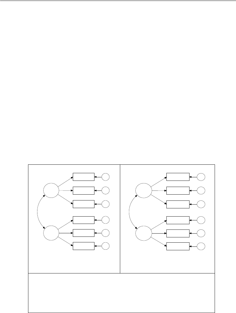
Simply specify the model graphically (left). Amos quickly performs the
computations and displays the results (right).
spatial
visperc
cubes
lozenges
wordmean
paragraph
sentence
e1
e2
e3
e4
e5
e6
verbal
1
1
1
1
1
1
1
1
Input:
spatial
visperc
cubes
.43
lozenges
.54
wordmean
.71
paragraph
.77
sentence
.68
e1
e2
e3
e4
e5
e6
verbal
.70
.65
.74
.88
.83
.84
.49
Chi-square = 7.853 (8 df)
p = .448
Output:

2
Chapter 1
Structural equation modeling (SEM) is sometimes thought of as esoteric and difficult
to learn and use. This is a complete mistake. Indeed, the growing importance of SEM
in data analysis is largely due to its ease of use. SEM opens the door for nonstatisticians
to solve estimation and hypothesis testing problems that once would have required the
services of a specialist.
IBM SPSS Amos was originally designed as a tool for teaching this powerful and
fundamentally simple method. For this reason, every effort was made to see that it is
easy to use. Amos integrates an easy-to-use graphical interface with an advanced
computing engine for SEM. The publication-quality path diagrams of Amos provide a
clear representation of models for students and fellow researchers. The numeric
methods implemented in Amos are among the most effective and reliable available.
Featured Methods
Amos provides the following methods for estimating structural equation models:
Maximum likelihood
Unweighted least squares
Generalized least squares
Browne’s asymptotically distribution-free criterion
Scale-free least squares
Bayesian estimation
When confronted with missing data, Amos performs estimation by full information
maximum likelihood instead of relying on ad-hoc methods like listwise or pairwise
deletion, or mean imputation. The program can analyze data from several populations
at once. It can also estimate means for exogenous variables and for intercepts in
regression equations.
The program makes bootstrap standard errors and confidence intervals available for
all parameter estimates, effect estimates, sample means, variances, covariances, and
correlations. It also implements percentile intervals and bias-corrected percentile
intervals (Stine, 1989), as well as Bollen and Stine’s (1992) bootstrap approach to
model testing.
Multiple models can be fitted in a single analysis. Amos examines every pair of
models in which one model can be obtained by placing restrictions on the parameters
of the other. The program reports several statistics appropriate for comparing such

3
Introduction
models. It provides a test of univariate normality for each observed variable as well as
a test of multivariate normality and attempts to detect outliers.
IBM SPSS Amos accepts a path diagram as a model specification and displays
parameter estimates graphically on a path diagram. Path diagrams used for model
specification and those that display parameter estimates are of presentation quality.
They can be printed directly or imported into other applications such as word
processors, desktop publishing programs, and general-purpose graphics programs.
About the Tutorial
The tutorial is designed to get you up and running with Amos Graphics. It covers some
of the basic functions and features and guides you through your first Amos analysis.
Once you have worked through the tutorial, you can learn about more advanced
functions using the online help, or you can continue working through the examples to
get a more extended introduction to structural modeling with IBM SPSS Amos.
About the Examples
Many people like to learn by doing. Knowing this, we have developed many examples
that quickly demonstrate practical ways to use IBM SPSS Amos. The initial examples
introduce the basic capabilities of Amos as applied to simple problems. You learn
which buttons to click, how to access the several supported data formats, and how to
maneuver through the output. Later examples tackle more advanced modeling
problems and are less concerned with program interface issues.
Examples 1 through 4 show how you can use Amos to do some conventional
analyses—analyses that could be done using a standard statistics package. These
examples show a new approach to some familiar problems while also demonstrating
all of the basic features of Amos. There are sometimes good reasons for using Amos
to do something simple, like estimating a mean or correlation or testing the hypothesis
that two means are equal. For one thing, you might want to take advantage of the ability
of Amos to handle missing data. Or maybe you want to use the bootstrapping capability
of Amos, particularly to obtain confidence intervals.
Examples 5 through 8 illustrate the basic techniques that are commonly used
nowadays in structural modeling.

4
Chapter 1
Example 9 and those that follow demonstrate advanced techniques that have so far not
been used as much as they deserve. These techniques include:
Simultaneous analysis of data from several different populations.
Estimation of means and intercepts in regression equations.
Maximum likelihood estimation in the presence of missing data.
Bootstrapping to obtain estimated standard errors and confidence intervals. Amos
makes these techniques especially easy to use, and we hope that they will become
more commonplace.
Specification searches.
Bayesian estimation.
Imputation of missing values.
Analysis of censored data.
Analysis of ordered-categorical data.
Mixture modeling.
Tip: If you have questions about a particular Amos feature, you can always refer to the
extensive online help provided by the program.
About the Documentation
IBM SPSS Amos 25 comes with extensive documentation, including online help, this
user’s guide, and advanced reference material for Visual Basic or C# and the Amos API
(Application Programming Interface) in the file
%amosprogram%\Documentation\Programming Reference.pdf.
Other Sources of Information
Although this user’s guide contains a good bit of expository material, it is not by any
means a complete guide to the correct and effective use of structural modeling. Many
excellent SEM textbooks are available.
Structural Equation Modeling: A Multidisciplinary Journal contains
methodological articles as well as applications of structural modeling. It is
published by Taylor and Francis (http://www.tandf.co.uk).

5
Introduction
Carl Ferguson and Edward Rigdon established an electronic mailing list called
Semnet to provide a forum for discussions related to structural modeling. You can
find information about subscribing to Semnet at
www.gsu.edu/~mkteer/semnet.html.
Acknowledgments
Many users of previous versions of Amos provided valuable feedback, as did many
users who tested the present version. Torsten B. Neilands wrote Examples 26 through
31 in this User’s Guide with contributions by Joseph L. Schafer. Eric Loken reviewed
Examples 32 and 33. He also provided valuable insights into mixture modeling as well
as important suggestions for future developments in Amos.
A last word of warning: While Amos Development Corporation has engaged in
extensive program testing to ensure that Amos operates correctly, all complicated
software, Amos included, is bound to contain some undetected bugs. We are
committed to correcting any program errors. If you believe you have encountered one,
please report it to technical support.
James L. Arbuckle

7
Chapter
2
Tutorial: Getting Started with
Amos Graphics
Introduction
Remember your first statistics class when you sweated through memorizing formulas
and laboriously calculating answers with pencil and paper? The professor had you do
this so that you would understand some basic statistical concepts. Later, you
discovered that a calculator or software program could do all of these calculations in
a split second.
This tutorial is a little like that early statistics class. There are many shortcuts for
drawing and labeling path diagrams in Amos Graphics that you will discover as you
work through the examples in this user’s guide or as you refer to the online help. The
intent of this tutorial is to simply get you started using Amos Graphics. It will cover
some of the basic functions and features of IBM SPSS Amos and guide you through
your first Amos analysis.
Once you have worked through the tutorial, you can learn about more advanced
functions from the online help, or you can continue to learn incrementally by working
your way through the examples.
You can find the path diagram created in this tutorial in the file
%amostutorial%\startsps.amw. That file makes use of a data file in SPSS Statistics
format. The same path diagram can also be found in %amostutorial%\Getstart.amw,
which uses data from a Microsoft Excel file.
Amos provides toolbar buttons as well as keyboard shortcuts that perform many of
the same tasks that can be performed from the menu. This user's guide emphasizes the
use of the menu. See the online help for more information about the use of toolbar
buttons and keyboard shortcuts.

8
Chapter 2
About the Data
Hamilton (1990) provided several measurements on each of 21 states. Three of the
measurements will be used in this tutorial:
Average SAT score
Per capita income expressed in $1,000 units
Median education for residents 25 years of age or older
You can find the data in the Tutorial directory within the Excel 8.0 workbook
Hamilton.xls in the worksheet named Hamilton. The data are as follows:
SAT Income Education
899 14.345 12.7
896 16.37 12.6
897 13.537 12.5
889 12.552 12.5
823 11.441 12.2
857 12.757 12.7
860 11.799 12.4
890 10.683 12.5
889 14.112 12.5
888 14.573 12.6
925 13.144 12.6
869 15.281 12.5
896 14.121 12.5
827 10.758 12.2
908 11.583 12.7
885 12.343 12.4
887 12.729 12.3
790 10.075 12.1
868 12.636 12.4
904 10.689 12.6
888 13.065 12.4
9
Tutorial: Getting Started with Amos Graphics
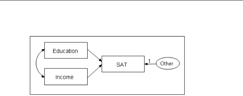
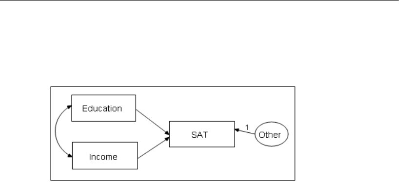
The following path diagram shows a model for these data:
This is a simple regression model where one observed variable, SAT, is predicted as a
linear combination of the other two observed variables, Education and Income. As with
nearly all empirical data, the prediction will not be perfect. The variable Other
represents variables other than Education and Income that affect SAT.
Each single-headed arrow represents a regression weight. The number 1 in the
figure specifies that Other must have a weight of 1 in the prediction of SAT. Some such
constraint must be imposed in order to make the model identified, and it is one of the
features of the model that must be communicated to Amos.
Launching Amos Graphics
You can launch Amos Graphics in any of the following ways:
Open the Windows Start menu and search for IBM SPSS Amos 25 Graphics.
Double-click any path diagram (*.amw) in Windows Explorer.
From within SPSS Statistics, choose Analyze > IBM SPSS Amos from the menus.

10
Chapter 2
Creating a New Model
EFrom the menus, choose File > New.
Your work area appears. The large area on the right is where you draw path diagrams.
The toolbar on the left provides one-click access to the most frequently used buttons.
You can use either the toolbar or menu commands for most operations.

11
Tutorial: Getting Started with Amos Graphics
Specifying the Data File
The next step is to specify the file that contains the Hamilton data. This tutorial uses a
Microsoft Excel 8.0 (*.xls) file, but Amos supports several common database formats,
including SPSS Statistics *.sav files. If you launch Amos from the Add-ons menu in
SPSS Statistics, Amos automatically uses the file that is open in SPSS Statistics.
EFrom the menus, choose File > Data Files.
EIn the Data Files dialog, click File Name.
EIn the Open dialog, enter the file name %tutorial%\hamilton.xls, and then click the
Open button.
EIn the Data Files dialog, click OK.
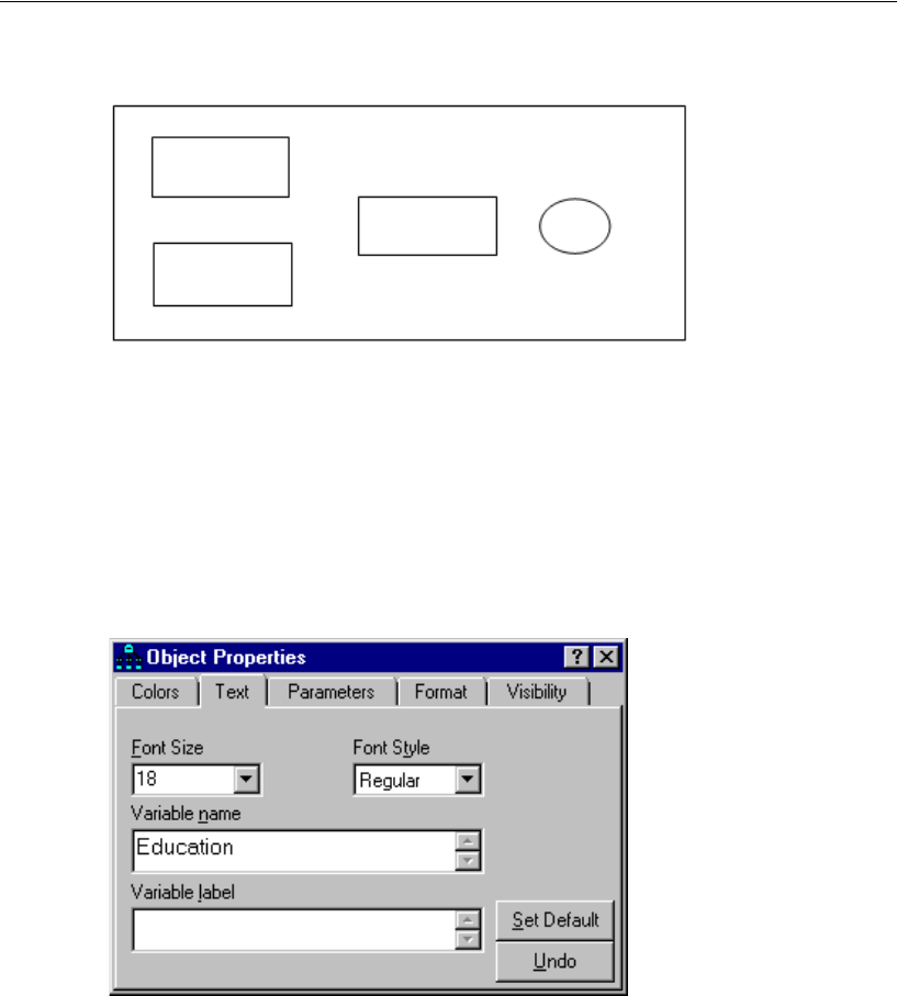
Specifying the Model and Drawing Variables
The next step is to draw the variables in your model. First, you’ll draw three rectangles
to represent the observed variables, and then you’ll draw an ellipse to represent the
unobserved variable.
EFrom the menus, choose Diagram > Draw Observed.
EIn the drawing area, move your mouse pointer to where you want the Education
rectangle to appear. Click and drag to draw the rectangle. Don’t worry about the exact
size or placement of the rectangle because you can change it later.
EUse the same method to draw two more rectangles for Income and SAT.
EFrom the menus, choose Diagram > Draw Unobserved.
EIn the drawing area, move your mouse pointer to the right of the three rectangles and
click and drag to draw the ellipse.
The model in your drawing area should now look similar to the following:
12
Chapter 2
Naming the Variables
EIn the drawing area, right-click the top left rectangle and choose Object Properties from
the pop-up menu.
EClick the Text tab.
EIn the Variable name text box, type Education.
EUse the same method to name the remaining variables. Then close the Object
Properties dialog box.
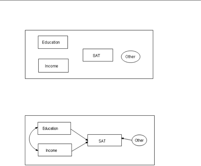
13
Tutorial: Getting Started with Amos Graphics
Your path diagram should now look like this:
Drawing Arrows
Now you will add arrows to the path diagram, using the following model as your guide:
EFrom the menus, choose Diagram > Draw Path.
EClick and drag to draw an arrow between Education and SAT.
EUse this method to add each of the remaining single-headed arrows.
EFrom the menus, choose Diagram > Draw Covariance.
EClick and drag to draw a double-headed arrow between Income and Education. Don’t
worry about the curvature of the arrow because you can adjust it later.
14
Chapter 2
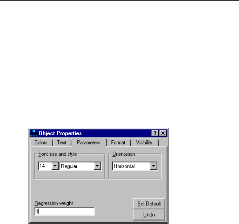
Constraining a Parameter
To identify the regression model, you must define the scale of the latent variable Other.
You can do this by fixing either the variance of Other or the path coefficient from Other
to SAT at some positive value. The following shows you how to fix the path coefficient
at unity (1).
EIn the drawing area, right-click the arrow between Other and SAT and choose Object
Properties from the pop-up menu.
EClick the Parameters tab.
EIn the Regression weight text box, type 1.
EClose the Object Properties dialog box.
15
Tutorial: Getting Started with Amos Graphics
There is now a 1 above the arrow between Other and SAT. Your path diagram is now
complete, other than any changes you may wish to make to its appearance. It should
look something like this:
Altering the Appearance of a Path Diagram
You can change the appearance of your path diagram by moving and resizing objects.
These changes are visual only; they do not affect the model specification.
To Move an Object
EFrom the menus, choose Edit > Move.
EIn the drawing area, click and drag the object to its new location.
To Reshape an Object or Double-Headed Arrow
EFrom the menus, choose Edit > Shape of Object.
EIn the drawing area, click and drag the object until you are satisfied with its size and
shape.
To Delete an Object
EFrom the menus, choose Edit > Erase.
EIn the drawing area, click the object you wish to delete.

16
Chapter 2
To Undo an Action
EFrom the menus, choose Edit > Undo.
To Redo an Action
EFrom the menus, choose Edit > Redo.
Setting Up Optional Output
Some of the output in Amos is optional. In this step, you will choose which portions of
the optional output you want Amos to display after the analysis.
EFrom the menus, choose View > Analysis Properties.
EClick the Output tab.

17
Tutorial: Getting Started with Amos Graphics
ESelect the Minimization history, Standardized estimates, and Squared multiple correlations
check boxes.
EClose the Analysis Properties dialog box.
18
Chapter 2
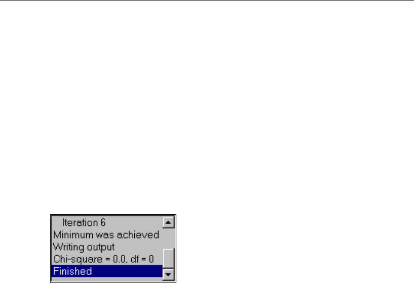
Performing the Analysis
The only thing left to do is perform the calculations for fitting the model. Note that in
order to keep the parameter estimates up to date, you must do this every time you
change the model, the data, or the options in the Analysis Properties dialog box.
EFrom the menus, click Analyze > Calculate Estimates.
EBecause you have not yet saved the file, the Save As dialog box appears. Type a name
for the file and click Save.
Amos calculates the model estimates. The panel to the left of the path diagram displays
a summary of the calculations.
Viewing Output
When Amos has completed the calculations, you have two options for viewing the
output: text and graphics.
19
Tutorial: Getting Started with Amos Graphics
To View Text Output
EFrom the menus, choose View > Text Output.
The tree diagram in the upper left pane of the Amos Output window allows you to
choose a portion of the text output for viewing.
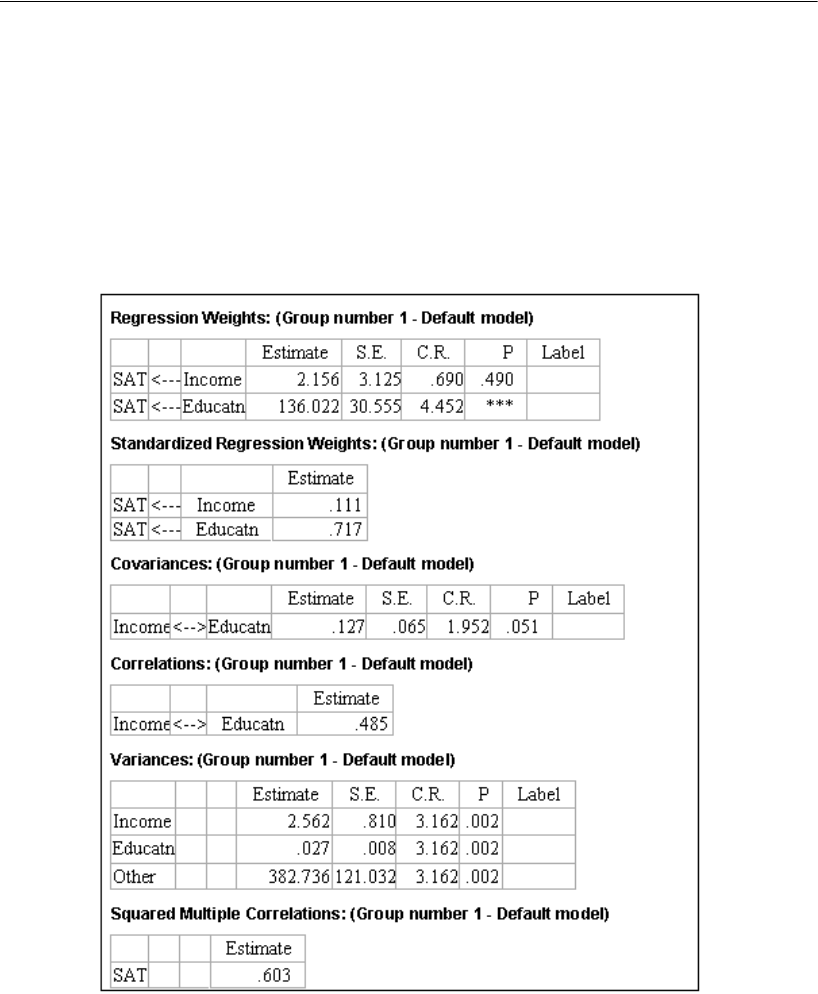
EClick Estimates to view the parameter estimates.
20
Chapter 2
To View Graphics Output
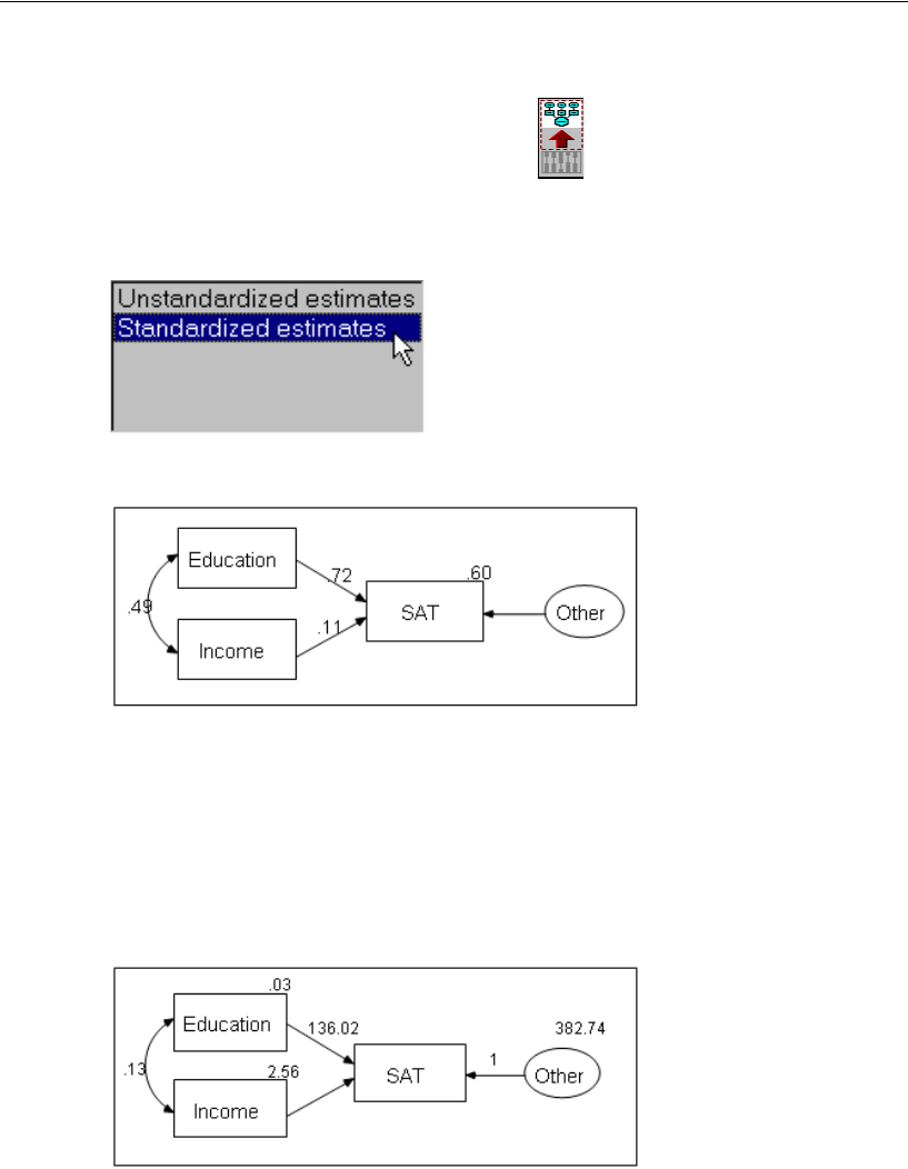
EClick the Show the output path diagram button .
EIn the Parameter Formats pane to the left of the drawing area, click Standardized
estimates.
Your path diagram now looks like this:
The value 0.49 is the correlation between Education and Income. The values 0.72 and
0.11 are standardized regression weights. The value 0.60 is the squared multiple
correlation of SAT with Education and Income.
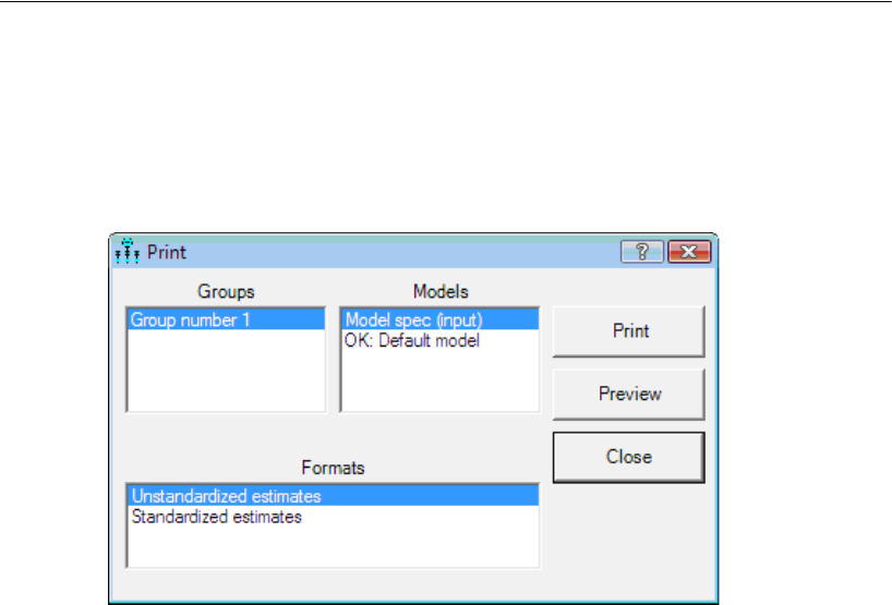
EIn the Parameter Formats pane to the left of the drawing area, click Unstandardized
estimates.
Your path diagram should now look like this:
21
Tutorial: Getting Started with Amos Graphics
Printing the Path Diagram
EFrom the menus, choose File > Print.
The Print dialog box appears.
EClick Print.
Copying the Path Diagram
Amos Graphics lets you easily export your path diagram to other applications such as
Microsoft Word.
EFrom the menus, choose Edit > Copy (to Clipboard).
ESwitch to the other application and use the Paste function to insert the path diagram.
Amos Graphics exports only the diagram; it does not export the background.
Copying Text Output
EIn the Amos Output window, select the text you want to copy.
ERight-click the selected text, and choose Copy from the pop-up menu.
ESwitch to the other application and use the Paste function to insert the text.

23
Example
1
Estimating Variances and
Covariances
Introduction
This example shows you how to estimate population variances and covariances. It also
discusses the general format of Amos input and output.
About the Data
Attig (1983) showed 40 subjects a booklet containing several pages of advertisements.
Then each subject was given three memory performance tests.
Attig repeated the study with the same 40 subjects after a training exercise intended
to improve memory performance. There were thus three performance measures
before training and three performance measures after training. In addition, she
recorded scores on a vocabulary test, as well as age, sex, and level of education.
Attig’s data files are included in the Examples folder provided by Amos.
Tes t E xp lanation
recall
The subject was asked to recall as many of the advertisements as possible.
The subject’s score on this test was the number of advertisements recalled
correctly.
cued
The subject was given some cues and asked again to recall as many of the
advertisements as possible. The subject’s score was the number of
advertisements recalled correctly.
place
The subject was given a list of the advertisements that appeared in the
booklet and was asked to recall the page location of each one. The subject’s
score on this test was the number of advertisements whose location was
recalled correctly.
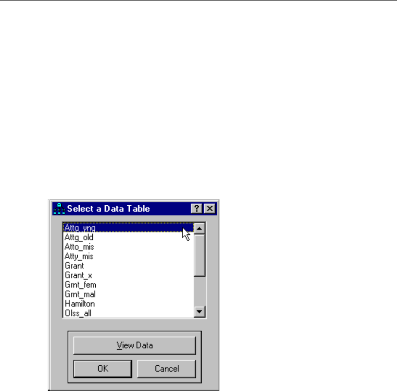
24
Example 1
Bringing In the Data
EFrom the menus, choose File > New.
EFrom the menus, choose File > Data Files.
EIn the Data Files dialog, click File Name.
EIn the Open dialog, enter the file name %examples%\UserGuide.xls, and then click the
Open button.
EIn the Select a Data Table dialog, select Attg_yng, then click View Data.
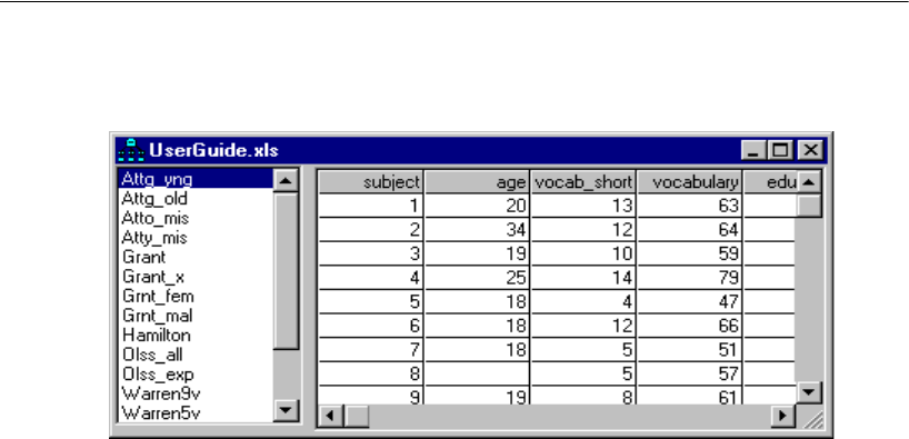
25
Estimating Variances and Covariances
The Excel worksheet for the Attg_yng data file opens.
As you scroll across the worksheet, you will see all of the test variables from the Attig
study. This example uses only the following variables: recall1 (recall pretest), recall2
(recall posttest), place1 (place recall pretest), and place2 (place recall posttest).
EAfter you review the data, close the data window.
EIn the Data Files dialog, click OK.
Analyzing the Data
In this example, the analysis consists of estimating the variances and covariances of the
recall and place variables before and after training.
Specifying the Model
EFrom the menus, choose Diagram > Draw Observed.
EIn the drawing area, move your mouse pointer to where you want the first rectangle to
appear. Click and drag to draw the rectangle.
EFrom the menus, choose Edit > Duplicate.
EClick and drag a duplicate from the first rectangle. Release the mouse button to
position the duplicate.
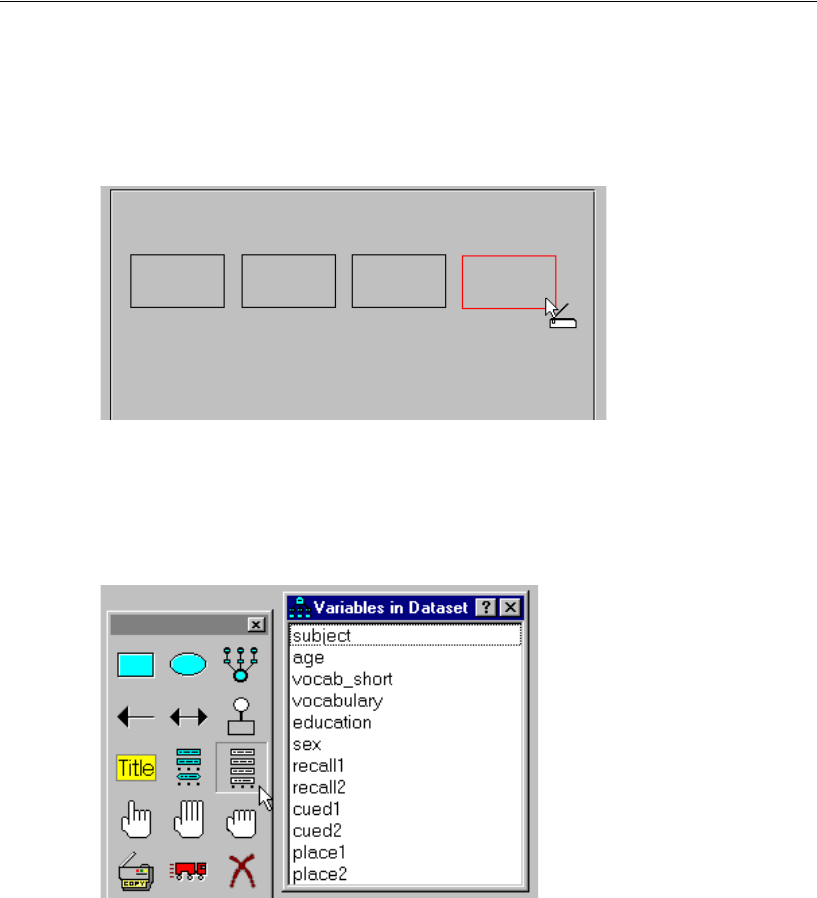
26
Example 1
ECreate two more duplicate rectangles until you have four rectangles side by side.
Tip: If you want to reposition a rectangle, choose Edit > Move from the menus and drag
the rectangle to its new position.
Naming the Variables
EFrom the menus, choose View > Variables in Dataset.
The Variables in Dataset dialog appears.
EClick and drag the variable recall1 from the list to the first rectangle in the drawing
area.
EUse the same method to name the variables recall2, place1, and place2.
EClose the Variables in Dataset dialog.
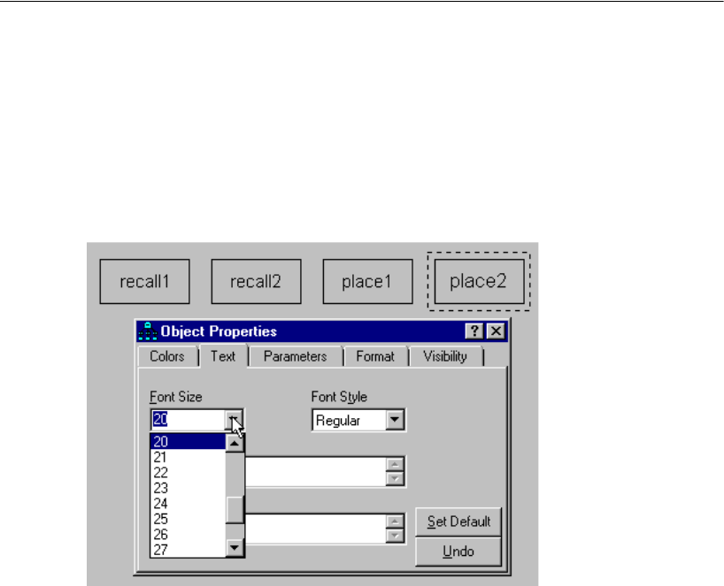
27
Estimating Variances and Covariances
Changing the Font
ERight-click a variable and choose Object Properties from the pop-up menu.
The Object Properties dialog appears.
EClick the Text tab and adjust the font attributes as desired.
Establishing Covariances
If you leave the path diagram as it is, Amos Graphics will estimate the variances of the
four variables, but it will not estimate the covariances between them. In Amos
Graphics, the rule is to assume a correlation or covariance of 0 for any two variables
that are not connected by arrows. To estimate the covariances between the observed
variables, we must first connect all pairs with double-headed arrows.
EFrom the menus, choose Diagram > Draw Covariances.
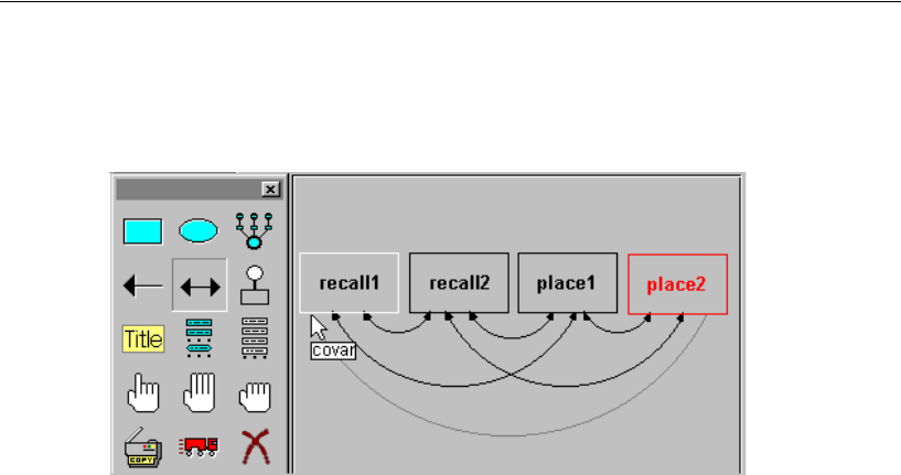
28
Example 1
EClick and drag to draw arrows that connect each variable to every other variable.
Your path diagram should have six double-headed arrows.
Performing the Analysis
EFrom the menus, choose Analyze > Calculate Estimates.
Because you have not yet saved the file, the Save As dialog appears.
EEnter a name for the file and click Save.
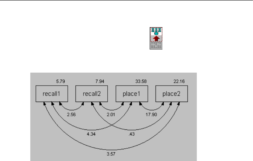
29
Estimating Variances and Covariances
Viewing Graphics Output
EClick the Show the output path diagram button .
Amos displays the output path diagram with parameter estimates.
In the output path diagram, the numbers displayed next to the boxes are estimated
variances, and the numbers displayed next to the double-headed arrows are estimated
covariances. For example, the variance of recall1 is estimated at 5.79, and that of
place1 at 33.58. The estimated covariance between these two variables is 4.34.
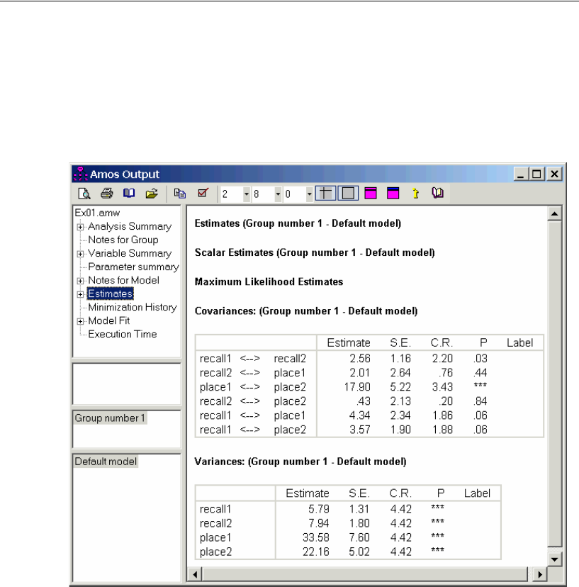
30
Example 1
Viewing Text Output
EFrom the menus, choose View > Text Output.
EIn the tree diagram in the upper left pane of the Amos Output window, click Estimates.
The first estimate displayed is of the covariance between recall1 and recall2. The
covariance is estimated to be 2.56. Right next to that estimate, in the S.E. column, is an
estimate of the standard error of the covariance, 1.16. The estimate 2.56 is an
observation on an approximately normally distributed random variable centered
around the population covariance with a standard deviation of about 1.16, that is, if the
assumptions in the section “Distribution Assumptions for Amos Models” on p. 36 are
met. For example, you can use these figures to construct a 95% confidence interval on
the population covariance by computing . Later,
you will see that you can use Amos to estimate many kinds of population parameters
besides covariances and can follow the same procedure to set a confidence interval on
any one of them.
2.56 1.96 1.160 2.56 2.27±=×±

31
Estimating Variances and Covariances
Next to the standard error, in the C.R. column, is the critical ratio obtained by
dividing the covariance estimate by its standard error . This ratio
is relevant to the null hypothesis that, in the population from which Attig’s 40 subjects
came, the covariance between recall1 and recall2 is 0. If this hypothesis is true, and
still under the assumptions in the section “Distribution Assumptions for Amos
Models” on p. 36, the critical ratio is an observation on a random variable that has an
approximate standard normal distribution. Thus, using a significance level of 0.05, any
critical ratio that exceeds 1.96 in magnitude would be called significant. In this
example, since 2.20 is greater than 1.96, you would say that the covariance between
recall1 and recall2 is significantly different from 0 at the 0.05 level.
The P column, to the right of C.R., gives an approximate two-tailed p value for
testing the null hypothesis that the parameter value is 0 in the population. The table
shows that the covariance between recall1 and recall2 is significantly different from 0
with . The calculation of P assumes that parameter estimates are normally
distributed, and it is correct only in large samples. See Appendix A for more
information.
The assertion that the parameter estimates are normally distributed is only an
approximation. Moreover, the standard errors reported in the S.E. column are only
approximations and may not be the best available. Consequently, the confidence
interval and the hypothesis test just discussed are also only approximate. This is
because the theory on which these results are based is asymptotic. Asymptotic means
that it can be made to apply with any desired degree of accuracy, but only by using a
sufficiently large sample. We will not discuss whether the approximation is
satisfactory with the present sample size because there would be no way to generalize
the conclusions to the many other kinds of analyses that you can do with Amos.
However, you may want to re-examine the null hypothesis that recall1 and recall2 are
uncorrelated, just to see what is meant by an approximate test. We previously
concluded that the covariance is significantly different from 0 because 2.20 exceeds
1.96. The p value associated with a standard normal deviate of 2.20 is 0.028 (two-
tailed), which, of course, is less than 0.05. By contrast, the conventional tstatistic (for
example, Runyon and Haber, 1980, p. 226) is 2.509 with 38 degrees of freedom
. In this example, both p values are less than 0.05, so both tests agree in
rejecting the null hypothesis at the 0.05 level. However, in other situations, the two
pvalues might lie on opposite sides of 0.05. You might or might not regard this as
especially serious—at any rate, the two tests can give different results. There should be
no doubt about which test is better. The t test is exact under the assumptions of
normality and independence of observations, no matter what the sample size. In Amos,
the test based on critical ratio depends on the same assumptions; however, with a finite
sample, the test is only approximate.
2.20 2.56 1.16⁄=()
p0.03=
p0.016=()
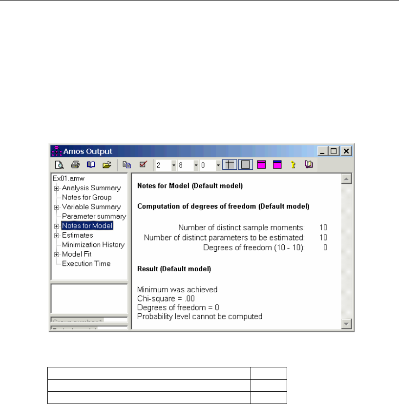
32
Example 1
Note: For many interesting applications of Amos, there is no exact test or exact
standard error or exact confidence interval available.
On the bright side, when fitting a model for which conventional estimates exist,
maximum likelihood point estimates (for example, the numbers in the Estimate
column) are generally identical to the conventional estimates.
ENow click Notes for Model in the upper left pane of the Amos Output window.
The following table plays an important role in every Amos analysis:
The Number of distinct sample moments referred to are sample means, variances, and
covariances. In most analyses, including the present one, Amos ignores means, so that
the sample moments are the sample variances of the four variables, recall1, recall2,
place1, and place2, and their sample covariances. There are four sample variances and
six sample covariances, for a total of 10 sample moments.
The Number of distinct parameters to be estimated are the corresponding
population variances and covariances. There are, of course, four population variances
and six population covariances, which makes 10 parameters to be estimated.
Number of distinct sample moments: 10
Number of distinct parameters to be estimated: 10
Degrees of freedom (10 – 10): 0

33
Estimating Variances and Covariances
The Degrees of freedom is the amount by which the number of sample moments
exceeds the number of parameters to be estimated. In this example, there is a one-to-
one correspondence between the sample moments and the parameters to be estimated,
so it is no accident that there are zero degrees of freedom.
As we will see beginning with Example 2, any nontrivial null hypothesis about the
parameters reduces the number of parameters that have to be estimated. The result will
be positive degrees of freedom. For now, there is no null hypothesis being tested.
Without a null hypothesis to test, the following table is not very interesting:
If there had been a hypothesis under test in this example, the chi-square value would have
been a measure of the extent to which the data were incompatible with the hypothesis. A
chi-square value of 0 would ordinarily indicate no departure from the null hypothesis.
But in the present example, the 0 value for degrees of freedom and the 0 chi-square value
merely reflect the fact that there was no null hypothesis in the first place.
This line indicates that Amos successfully estimated the variances and covariances.
Sometimes structural modeling programs like Amos fail to find estimates. Usually,
when Amos fails, it is because you have posed a problem that has no solution, or no
unique solution. For example, if you attempt maximum likelihood estimation with
observed variables that are linearly dependent, Amos will fail because such an analysis
cannot be done in principle. Problems that have no unique solution are discussed
elsewhere in this user’s guide under the subject of identifiability. Less commonly,
Amos can fail because an estimation problem is just too difficult. The possibility of
such failures is generic to programs for analysis of moment structures. Although the
computational method used by Amos is highly effective, no computer program that
does the kind of analysis that Amos does can promise success in every case.
Chi-square = 0.00
Degrees of freedom = 0
Probability level cannot be computed
Minimum was achieved
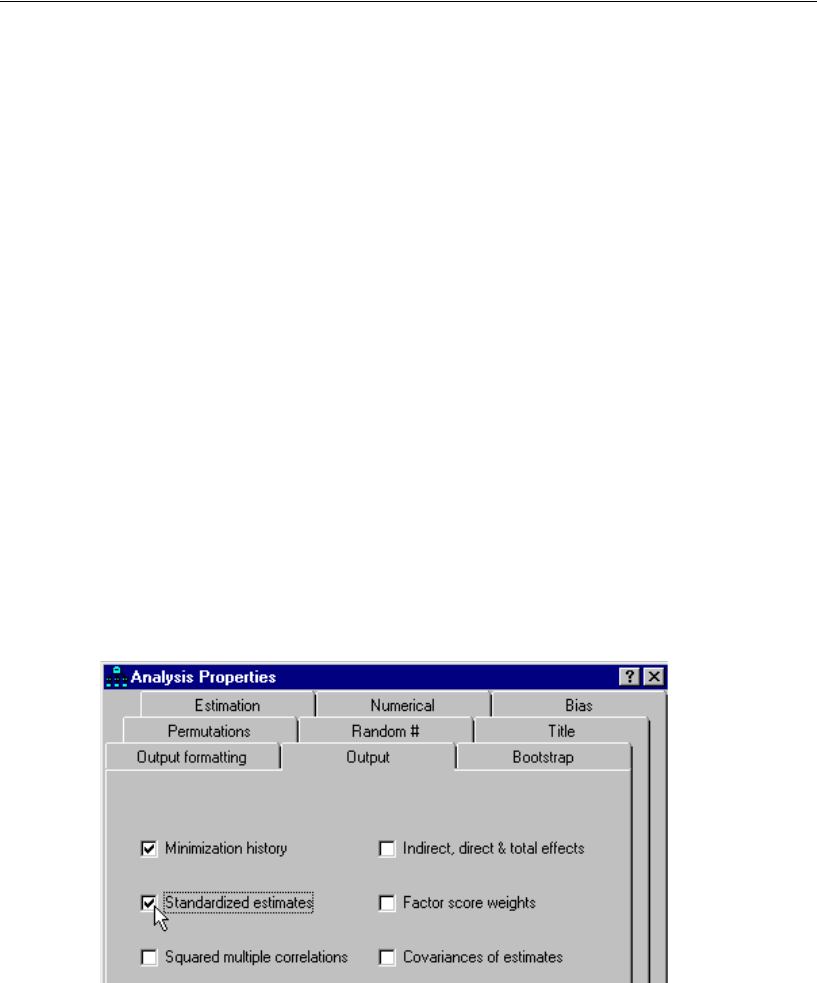
34
Example 1
Optional Output
So far, we have discussed output that Amos generates by default. You can also request
additional output.
Calculating Standardized Estimates
You may be surprised to learn that Amos displays estimates of covariances rather than
correlations. When the scale of measurement is arbitrary or of no substantive interest,
correlations have more descriptive meaning than covariances. Nevertheless, Amos and
similar programs insist on estimating covariances. Also, as will soon be seen, Amos
provides a simple method for testing hypotheses about covariances but not about
correlations. This is mainly because it is easier to write programs that way. On the other
hand, it is not hard to derive correlation estimates after the relevant variances and
covariances have been estimated. To calculate standardized estimates:
EFrom the menus, choose View > Analysis Properties.
EIn the Analysis Properties dialog, click the Output tab.
ESelect the Standardized estimates check box.
EClose the Analysis Properties dialog.
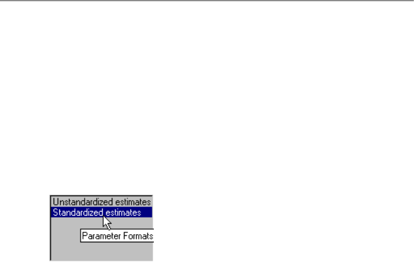
35
Estimating Variances and Covariances
Rerunning the Analysis
Because you have changed the options in the Analysis Properties dialog, you must
rerun the analysis.
EFrom the menus, choose Analyze > Calculate Estimates.
EClick the Show the output path diagram button.
EIn the Parameter Formats pane to the left of the drawing area, click Standardized
estimates.
Viewing Correlation Estimates as Text Output
EFrom the menus, choose View > Text Output.
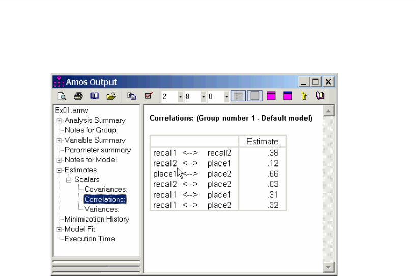
36
Example 1
EIn the tree diagram in the upper left pane of the Amos Output window, expand
Estimates, Scalars, and then click Correlations.
Distribution Assumptions for Amos Models
Hypothesis testing procedures, confidence intervals, and claims for efficiency in
maximum likelihood or generalized least-squares estimation depend on certain
assumptions. First, observations must be independent. For example, the 40 young
people in the Attig study have to be picked independently from the population of young
people. Second, the observed variables must meet some distributional requirements. If
the observed variables have a multivariate normal distribution, that will suffice.
Multivariate normality of all observed variables is a standard distribution assumption
in many structural equation modeling and factor analysis applications.
There is another, more general, situation under which maximum likelihood
estimation can be carried out. If some exogenous variables are fixed (that is, they are
either known beforehand or measured without error), their distributions may have any
shape, provided that:
For any value pattern of the fixed variables, the remaining (random) variables have
a (conditional) normal distribution.
The (conditional) variance-covariance matrix of the random variables is the same
for every pattern of the fixed variables.
The (conditional) expected values of the random variables depend linearly on the
values of the fixed variables.
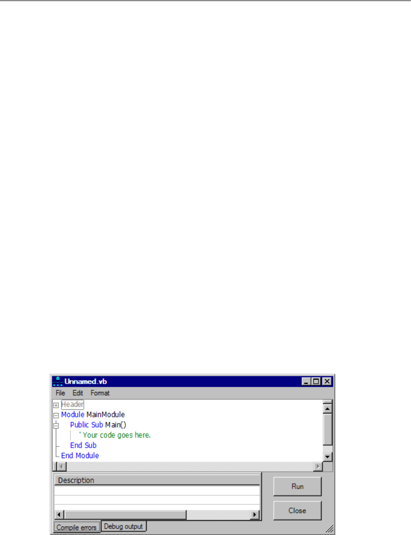
37
Estimating Variances and Covariances
A typical example of a fixed variable would be an experimental treatment, classifying
respondents into a study group and a control group, respectively. It is all right that
treatment is non-normally distributed, as long as the other exogenous variables are
normally distributed for study and control cases alike, and with the same conditional
variance-covariance matrix. Predictor variables in regression analysis (see Example 4)
are often regarded as fixed variables.
Many people are accustomed to the requirements for normality and independent
observations, since these are the usual requirements for many conventional procedures.
However, with Amos, you have to remember that meeting these requirements leads
only to asymptotic conclusions (that is, conclusions that are approximately true for
large samples).
Modeling in VB.NET
It is possible to specify and fit a model by writing a program in VB.NET or in C#. Writing
programs is an alternative to using Amos Graphics to specify a model by drawing its path
diagram. This section shows how to write a VB.NET program to perform the analysis of
Example 1. A later section explains how to do the same thing in C#.
Amos comes with its own built-in editor for VB.NET and C# programs. It is
accessible from the Windows Start menu. To begin Example 1 using the built-in editor:
EOpen the Windows Start menu and search for IBM SPSS Amos 25 Program Editor.
EIn the Program Editor window, choose File > New VB Program.
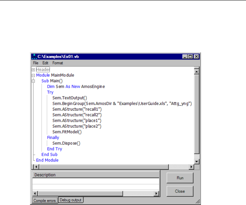
38
Example 1
EEnter the VB.NET code for specifying and fitting the model in place of the ‘Your code
goes here comment. The following figure shows the program editor after the complete
program has been entered.
Note: The %examples% directory contains all of the pre-written examples.
To open the VB.NET file for the present example:
EFrom the Program Editor menus, choose File > Open.
EIn the Open dialog, enter the file name %examples%\Ex01.vb, and then click the Open
button.

39
Estimating Variances and Covariances
The following table gives a line-by-line explanation of the program.
ETo perform the analysis, from the menus, choose File > Run.
Program Statement Explanation
Dim Sem As New AmosEngine
Declares Sem as an object of type
AmosEngine. The methods and properties of
the Sem object are used to specify and fit the
model.
Sem.TextOutput
Creates an output file containing the results of
the analysis. At the end of the analysis, the
contents of the output file are displayed in a
separate window.
Sem.BeginGroup …
Begins the model specification for a single
group (that is, a single population). This line
also specifies that the Attg_yng worksheet in the
Excel workbook UserGuide.xls contains the
input data. Sem.AmosDir() is the location of the
Amos program directory.
Sem.AStructure("recall1")
Sem.AStructure("recall2")
Sem.AStructure("place1")
Sem.AStructure("place2")
Specifies the model. The four AStructure
statements declare the variances of recall1,
recall2, place1, and place2 to be free
parameters. The other eight variables in the
Attg_yng data file are left out of this analysis. In
an Amos program (but not in Amos Graphics),
observed exogenous variables are assumed by
default to be correlated, so that Amos will
estimate the six covariances among the four
variables.
Sem.FitModel() Fits the model.
Sem.Dispose()
Releases resources used by the Sem object. It is
particularly important for your program to use
an AmosEngine object’s Dispose method before
creating another AmosEngine object. A process
is allowed only one instance of an AmosEngine
object at a time.
Try/Finally/End Try
The Try block guarantees that the Dispose
method will be called even if an error occurs
during program execution.
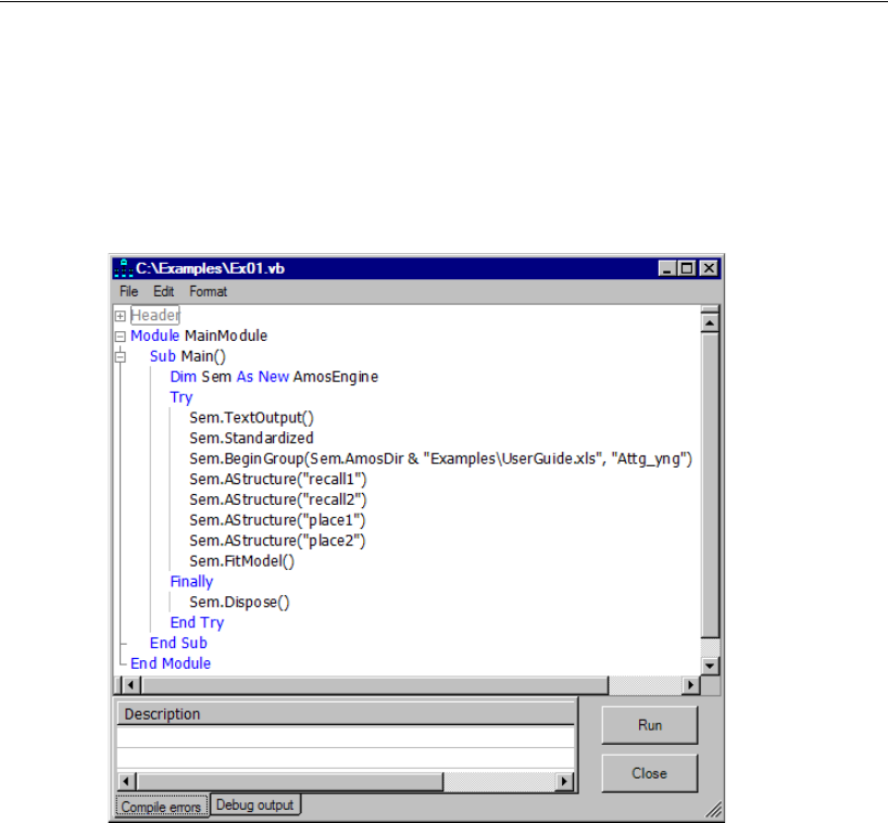
40
Example 1
Generating Additional Output
Some AmosEngine methods generate additional output. For example, the Standardized
method displays standardized estimates. The following figure shows the use of the
Standardized method:
Modeling in C#
Writing an Amos program in C# is similar to writing one in VB.NET. To start a new
C# program, in the built-in program editor of Amos:
EChoose File > New C# Program (rather than File > New VB Program).
EChoose File > Open to open Ex01.cs, which is a C# version of the VB.NET program
Ex01.vb.

41
Estimating Variances and Covariances
Other Program Development Tools
The built-in program editor in Amos is used throughout this user’s guide for writing
and executing Amos programs. However, you can use the development tool of your
choice. The Examples folder contains a VisualStudio subfolder where you can find
Visual Studio VB.NET and C# solutions for Example 1.

43
Example SWS
2
Testing Hypotheses
Introduction
This example demonstrates how you can use Amos to test simple hypotheses about
variances and covariances. It also introduces the chi-square test for goodness of fit and
elaborates on the concept of degrees of freedom.
About the Data
We will use Attig’s (1983) spatial memory data, which were described in Example 1.
We will also begin with the same path diagram as in Example 1. To demonstrate the
ability of Amos to use different data formats, this example uses a data file in SPSS
Statistics format instead of an Excel file.
Parameters Constraints
The following is the path diagram from Example 1. We can think of the variable
objects as having small boxes nearby (representing the variances) that are filled in
once Amos has estimated the parameters.
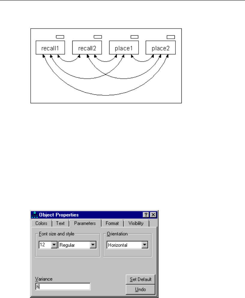
44
Example 2
You can fill these boxes yourself instead of letting Amos fill them.
Constraining Variances
Suppose you want to set the variance of recall1 to 6 and the variance of recall2 to 8.
EIn the drawing area, right-click recall1 and choose Object Properties from the pop-up
menu.
EClick the Parameters tab.
EIn the Variance text box, type 6.
EWith the Object Properties dialog still open, click recall2 and set its variance to 8.
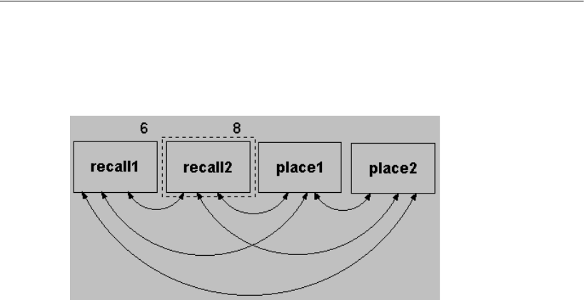
45
Testing Hypotheses
EClose the dialog.
The path diagram displays the parameter values you just specified.
This is not a very realistic example because the numbers 6 and 8 were just picked out
of the air. Meaningful parameter constraints must have some underlying rationale,
perhaps being based on theory or on previous analyses of similar data.
Specifying Equal Parameters
Sometimes you will be interested in testing whether two parameters are equal in the
population. You might, for example, think that the variances of recall1 and recall2
might be equal without having a particular value for the variances in mind. To
investigate this possibility, do the following:
EIn the drawing area, right-click recall1 and choose Object Properties from the pop-up
menu.
EClick the Parameters tab.
EIn the Variance text box, type v_recall.
EClick recall2 and label its variance as v_recall.
EUse the same method to label the place1 and place2 variances as v_place.
It doesn’t matter what label you use. The important thing is to enter the same label for
each variance you want to force to be equal. The effect of using the same label is to
require both of the variances to have the same value without specifying ahead of time
what that value is.

46
Example 2
Benefits of Specifying Equal Parameters
Before adding any further constraints on the model parameters, let’s examine why we
might want to specify that two parameters, like the variances of recall1 and recall2 or
place1 and place2, are equal. Here are two benefits:
If you specify that two parameters are equal in the population and if you are correct
in this specification, then you will get more accurate estimates, not only of the
parameters that are equal but usually of the others as well. This is the only benefit
if you happen to know that the parameters are equal.
If the equality of two parameters is a mere hypothesis, requiring their estimates to
be equal will result in a test of that hypothesis.
Constraining Covariances
Your model may also include restrictions on parameters other than variances. For
example, you may hypothesize that the covariance between recall1 and place1 is equal
to the covariance between recall2 and place2. To impose this constraint:
EIn the drawing area, right-click the double-headed arrow that connects recall1 and
place1, and choose Object Properties from the pop-up menu.
EClick the Parameters tab.
EIn the Covariance text box, type a non-numeric string such as cov_rp.
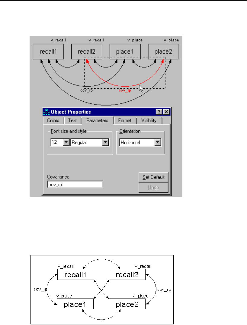
47
Testing Hypotheses
EUse the same method to set the covariance between recall2 and place2 to cov_rp.
Moving and Formatting Objects
While a horizontal layout is fine for small examples, it is not practical for analyses that
are more complex. The following is a different layout of the path diagram on which
we’ve been working:
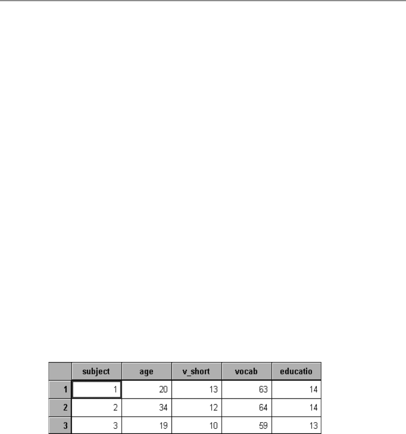
48
Example 2
You can use the following tools to rearrange your path diagram until it looks like the
one above:
To move objects, choose Edit > Move from the menus, and then drag the object to
its new location. You can also use the Move button to drag the endpoints of arrows.
To copy formatting from one object to another, choose Edit > Drag Properties from
the menus, select the properties you wish to apply, and then drag from one object
to another.
For more information about the Drag Properties feature, refer to online help.
Data Input
EFrom the menus, choose File > Data Files.
EIn the Data Files dialog, click File Name.
EBrowse to the %examples% folder.
EIn the Files of type list, select SPSS Statistics (*.sav), click Attg_yng, and then click
Open.
EIf you have SPSS Statistics installed, click the View Data button in the Data Files
dialog. An SPSS Statistics window opens and displays the data.
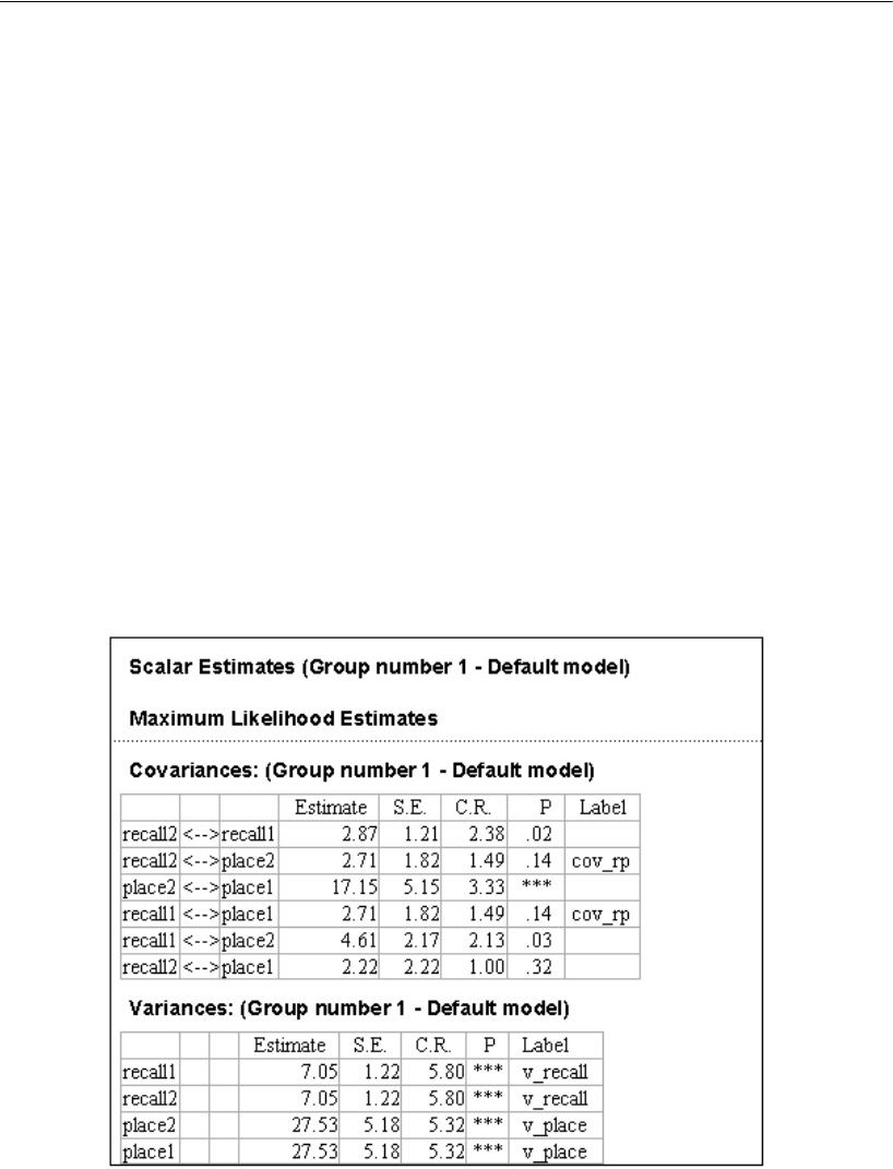
49
Testing Hypotheses
EReview the data and close the data view.
EIn the Data Files dialog, click OK.
Performing the Analysis
EFrom the menus, choose Analyze > Calculate Estimates.
EIn the Save As dialog, enter a name for the file and click Save.
Amos calculates the model estimates.
Viewing Text Output
EFrom the menus, choose View > Text Output.
ETo view the parameter estimates, click Estimates in the tree diagram in the upper left
pane of the Amos Output window.
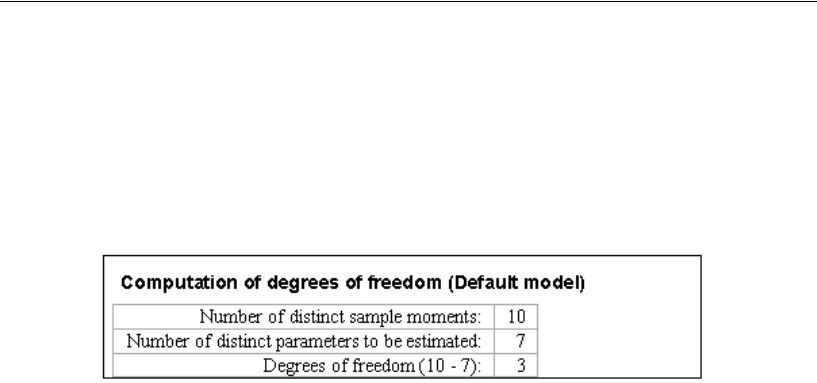
50
Example 2
You can see that the parameters that were specified to be equal do have equal estimates.
The standard errors here are generally smaller than the standard errors obtained in
Example 1. Also, because of the constraints on the parameters, there are now positive
degrees of freedom.
ENow click Notes for Model in the upper left pane of the Amos Output window.
While there are still 10 sample variances and covariances, the number of parameters to
be estimated is only seven. Here is how the number seven is arrived at: The variances
of recall1 and recall2, labeled v_recall, are constrained to be equal, and thus count as
a single parameter. The variances of place1 and place2 (labeled v_place) count as
another single parameter. A third parameter corresponds to the equal covariances
recall1 <> place1 and recall2 <> place2 (labeled cov_rp). These three parameters,
plus the four unlabeled, unrestricted covariances, add up to seven parameters that have
to be estimated.
The degrees of freedom ( ) may also be thought of as the number of
constraints placed on the original 10 variances and covariances.
Optional Output
The output we just discussed is all generated by default. You can also request additional
output:
EFrom the menus, choose View > Analysis Properties.
EClick the Output tab.
10 7 3=–
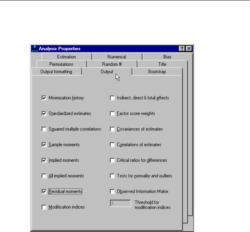
51
Testing Hypotheses
EEnsure that the following check boxes are selected: Minimization history, Standardized
estimates, Sample moments, Implied moments, and Residual moments.
EFrom the menus, choose Analyze > Calculate Estimates.
Amos recalculates the model estimates.
Covariance Matrix Estimates
ETo see the sample variances and covariances collected into a matrix, choose View > Text
Output from the menus.
EClick Sample Moments in the tree diagram in the upper left corner of the Amos Output
window.
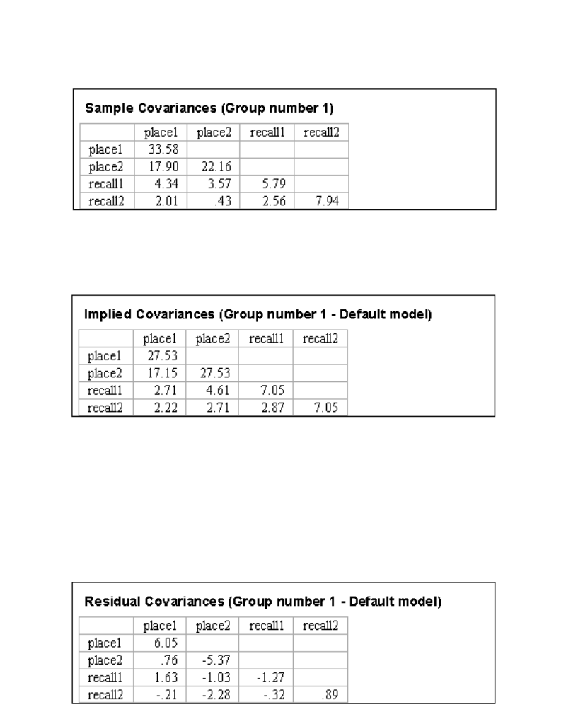
52
Example 2
The following is the sample covariance matrix:
EIn the tree diagram, expand Estimates and then click Matrices.
The following is the matrix of implied covariances:
Note the differences between the sample and implied covariance matrices. Because the
model imposes three constraints on the covariance structure, the implied variances and
covariances are different from the sample values. For example, the sample variance of
place1 is 33.58, but the implied variance is 27.53. To obtain a matrix of residual
covariances (sample covariances minus implied covariances), put a check mark next to
Residual moments on the Output tab and repeat the analysis.
The following is the matrix of residual covariances:
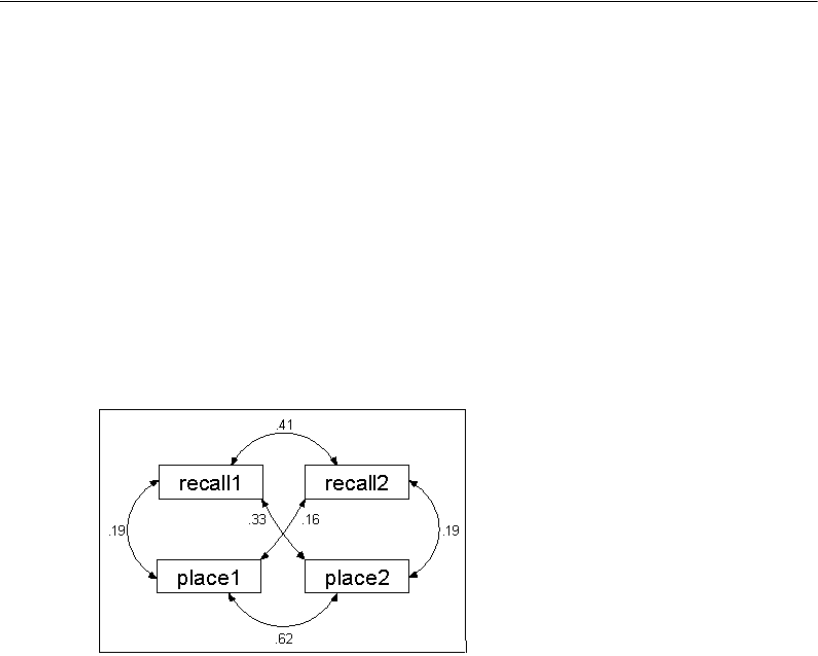
53
Testing Hypotheses
Displaying Covariance and Variance Estimates on the Path Diagram
As in Example 1, you can display the covariance and variance estimates on the path
diagram.
EClick the Show the output path diagram button.
EIn the Parameter Formats pane to the left of the drawing area, click Unstandardized
estimates. Alternatively, you can request correlation estimates in the path diagram by
clicking Standardized estimates.
The following is the path diagram showing correlations:
Labeling Output
It may be difficult to remember whether the displayed values are covariances or
correlations. To avoid this problem, you can use Amos to label the output.
EOpen the file Ex02.amw.
ERight-click the caption at the bottom of the path diagram, and choose Object Properties
from the pop-up menu.

54
Example 2
EClick the Text tab.
Notice the word \format in the bottom line of the figure caption. Words that begin with
a backward slash, like \format, are called text macros. Amos replaces text macros with
information about the currently displayed model. The text macro \format will be
replaced by the heading Model Specification, Unstandardized estimates, or
Standardized estimates, depending on which version of the path diagram is displayed.
Hypothesis Testing
The implied covariances are the best estimates of the population variances and
covariances under the null hypothesis. (The null hypothesis is that the parameters
required to have equal estimates are truly equal in the population.) As we know from
Example 1, the sample covariances are the best estimates obtained without making any
assumptions about the population values. A comparison of these two matrices is
relevant to the question of whether the null hypothesis is correct. If the null hypothesis
is correct, both the implied and sample covariances are maximum likelihood estimates
of the corresponding population values (although the implied covariances are better
estimates). Consequently, you would expect the two matrices to resemble each other.
On the other hand, if the null hypothesis is wrong, only the sample covariances are
maximum likelihood estimates, and there is no reason to expect them to resemble the
implied covariances.

55
Testing Hypotheses
The chi-square statistic is an overall measure of how much the implied covariances
differ from the sample covariances.
In general, the more the implied covariances differ from the sample covariances, the
bigger the chi-square statistic will be. If the implied covariances had been identical to
the sample covariances, as they were in Example 1, the chi-square statistic would have
been 0. You can use the chi-square statistic to test the null hypothesis that the
parameters required to have equal estimates are really equal in the population.
However, it is not simply a matter of checking to see if the chi-square statistic is 0.
Since the implied covariances and the sample covariances are merely estimates, you
can’t expect them to be identical (even if they are both estimates of the same population
covariances). Actually, you would expect them to differ enough to produce a chi-square
in the neighborhood of the degrees of freedom, even if the null hypothesis is true. In
other words, a chi-square value of 3 would not be out of the ordinary here, even with a
true null hypothesis. You can say more than that: If the null hypothesis is true, the chi-
square value (6.276) is a single observation on a random variable that has an
approximate chi-square distribution with three degrees of freedom. The probability is
about 0.099 that such an observation would be as large as 6.276. Consequently, the
evidence against the null hypothesis is not significant at the 0.05 level.
Displaying Chi-Square Statistics on the Path Diagram
You can get the chi-square statistic and its degrees of freedom to appear in a figure
caption on the path diagram using the text macros \cmin and \df. Amos replaces these
text macros with the numeric values of the chi-square statistic and its degrees of
freedom. You can use the text macro \p to display the corresponding right-tail
probability under the chi-square distribution.
EFrom the menus, choose Diagram > Figure Caption.
EClick the location on the path diagram where you want the figure caption to appear.
The Figure Caption dialog appears.
Chi-square = 6.276
Degrees of freedom = 3
Probability level = 0.099
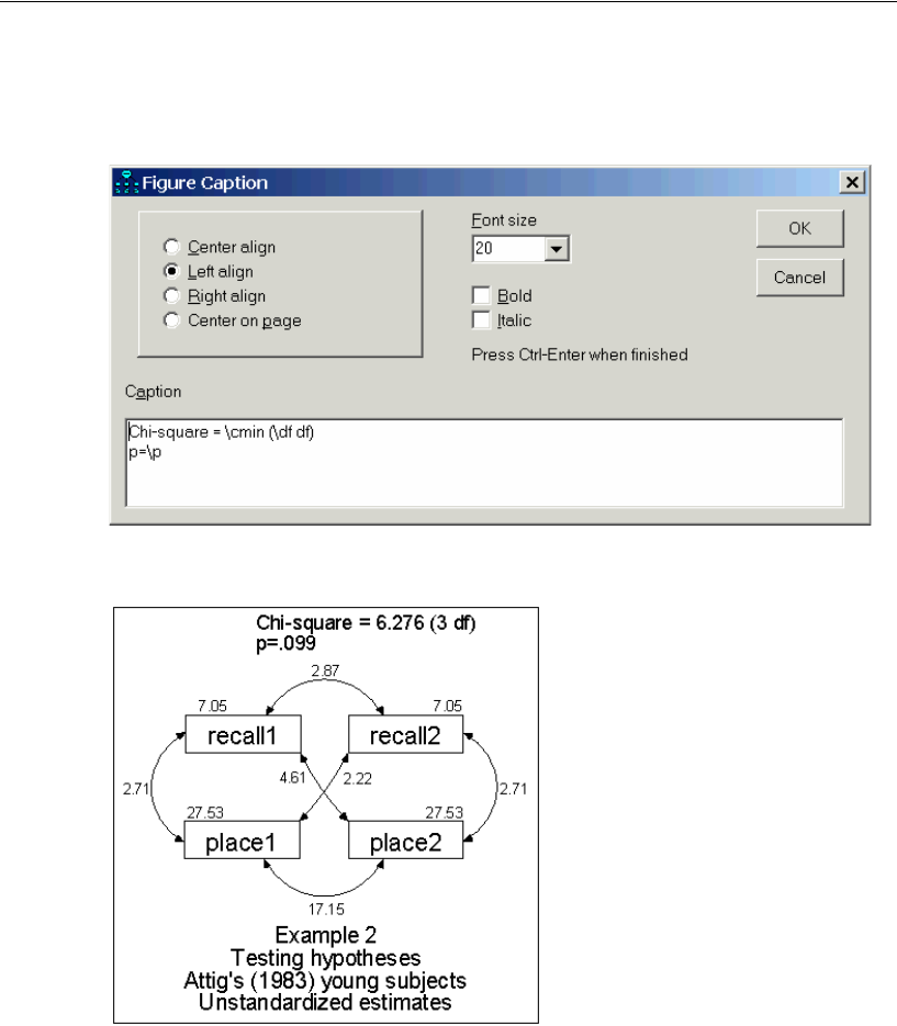
56
Example 2
EIn the Figure Caption dialog, enter a caption that includes the \cmin, \df, and \p text
macros, as follows:
When Amos displays the path diagram containing this caption, it appears as follows:


58
Example 2
This table gives a line-by-line explanation of the program:
ETo perform the analysis, from the menus, choose File > Run.
Program Statement Explanation
Dim Sem As New AmosEngine
Declares Sem as an object of type
AmosEngine. The methods and
properties of the Sem object are used to
specify and fit the model.
Sem.TextOutput
Creates an output file containing the
results of the analysis. At the end of the
analysis, the contents of the output file
are displayed in a separate window.
Sem.Standardized()
Sem.ImpliedMoments()
Sem.SampleMoments()
Sem.ResidualMoments()
Displays standardized estimates, implied
covariances, sample covariances, and
residual covariances.
Sem.BeginGroup …
Begins the model specification for a
single group (that is, a single
population). This line also specifies that
the SPSS Statistics file Attg_yng.sav
contains the input data. Sem.AmosDir()
is the location of the Amos program
directory.
Sem.AStructure("recall1 (v_recall)")
Sem.AStructure("recall2 (v_recall)")
Sem.AStructure("place1 (v_place)")
Sem.AStructure("place2 (v_place)")
Sem.AStructure("recall1 <> place1 (cov_rp)")
Sem.AStructure("recall2 <> place2 (cov_rp)")
Specifies the model. The first four
AStructure statements constrain the
variances of the observed variables
through the use of parameter names in
parentheses. Recall1 and recall2 are
required to have the same variance
because both variances are labeled
v_recall. The variances of place1 and
place2 are similarly constrained to be
equal. Each of the last two AStructure
lines represents a covariance. The two
covariances are both named cov_rp.
Consequently, those covariances are
constrained to be equal.
Sem.FitModel() Fits the model.
Sem.Dispose()
Releases resources used by the Sem
object. It is particularly important for
your program to use an AmosEngine
object’s Dispose method before creating
another AmosEngine object. A process is
allowed to have only one instance of an
AmosEngine object at a time.
Try/Finally/End Try
This Try block guarantees that the
Dispose method will be called even if an
error occurs during program execution.

59
Testing Hypotheses
Timing Is Everything
The AStructure lines must appear after BeginGroup; otherwise, Amos will not recognize
that the variables named in the AStructure lines are observed variables in the
attg_yng.sav dataset.
In general, the order of statements matters in an Amos program. In organizing an
Amos program, AmosEngine methods can be divided into three general groups1.
Group 1 — Declarative Methods
This group contains methods that tell Amos what results to compute and display.
TextOutput is a Group 1 method, as are Standardized, ImpliedMoments, SampleMoments,
and ResidualMoments. Many other Group 1 methods that are not used in this example
are documented in the Amos 25 Programming Reference Guide.
Group 2 — Data and Model Specification Methods
This group consists of data description and model specification commands.
BeginGroup and AStructure are Group 2 methods. Others are documented in the Amos
25 Programming Reference Guide.
Group 3 — Methods for Retrieving Results
These are commands to…well, retrieve results. So far, we have not used any Group 3
methods. Examples using Group 3 methods are given in the Amos 25 Programming
Reference Guide.
Tip: When you write an Amos program, it is important to pay close attention to the
order in which you call the Amos engine methods. The rule is that groups must appear
in order: Group 1, then Group 2, and finally Group 3.
For more detailed information about timing rules and a complete listing of methods and
their group membership, see the Amos 25 Programming Reference Guide.
1 There is also a fourth special group, consisting of only the Initialize Method. If the optional Initialize Method
is used, it must come before the Group 1 methods.

61
Example
3
More Hypothesis Testing
Introduction
This example demonstrates how to test the null hypothesis that two variables are
uncorrelated, reinforces the concept of degrees of freedom, and demonstrates, in a
concrete way, what is meant by an asymptotically correct test.
About the Data
For this example, we use the group of older subjects from Attig’s (1983) spatial
memory study and the two variables age and vocabulary. We will use data formatted
as a tab-delimited text file.
Bringing In the Data
EFrom the menus, choose File > New.
EFrom the menus, choose File > Data Files.
EIn the Data Files dialog, select File Name.
EBrowse to the %examples% folder.
EIn the Files of type list, select Text (*.txt), select Attg_old.txt, and then click Open.
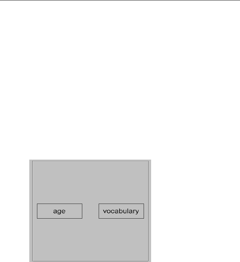
62
Example 3
EIn the Data Files dialog, click OK.
Testing a Hypothesis That Two Variables Are Uncorrelated
Among Attig’s 40 old subjects, the sample correlation between age and vocabulary is
–0.09 (not very far from 0). Is this correlation nevertheless significant? To find out, we
will test the null hypothesis that, in the population from which these 40 subjects came,
the correlation between age and vocabulary is 0. We will do this by estimating the
variance-covariance matrix under the constraint that age and vocabulary are
uncorrelated.
Specifying the Model
Begin by drawing and naming the two observed variables, age and vocabulary, in the
path diagram, using the methods you learned in Example 1.
Amos provides two ways to specify that the covariance between age and vocabulary is
0. The most obvious way is simply to not draw a double-headed arrow connecting the
two variables. The absence of a double-headed arrow connecting two exogenous
variables implies that they are uncorrelated. So, without drawing anything more, the
model specified by the simple path diagram above specifies that the covariance (and
thus the correlation) between age and vocabulary is 0.
The second method of constraining a covariance parameter is the more general
procedure introduced in Example 1 and Example 2.
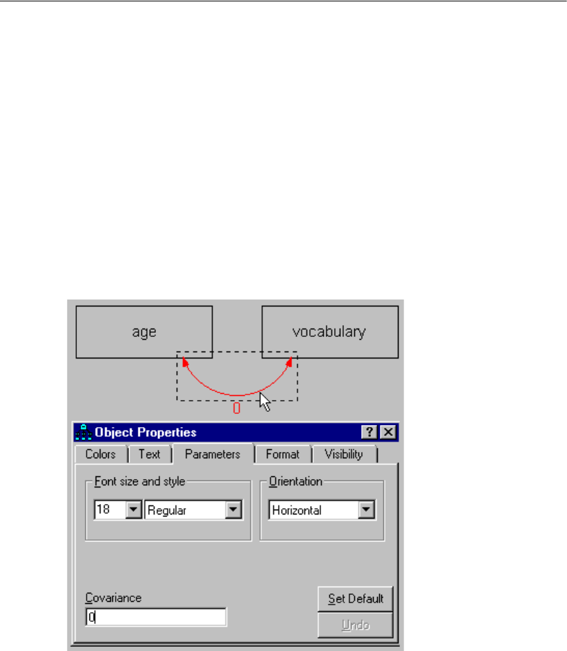
63
More Hypothesis Testing
EFrom the menus, choose Diagram > Draw Covariances.
EClick and drag to draw an arrow that connects vocabulary and age.
ERight-click the arrow and choose Object Properties from the pop-up menu.
EClick the Parameters tab.
EType 0 in the Covariance text box.
EClose the Object Properties dialog.
Your path diagram now looks like this:
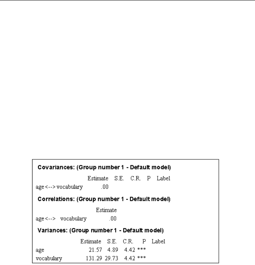
64
Example 3
EFrom the menus, choose Analyze > Calculate Estimates.
The Save As dialog appears.
EEnter a name for the file and click Save.
Amos calculates the model estimates.
Viewing Text Output
EFrom the menus, choose View > Text Output.
EIn the tree diagram in the upper left pane of the Amos Output window, click Estimates.
Although the parameter estimates are not of primary interest in this analysis, they are
as follows:
In this analysis, there is one degree of freedom, corresponding to the single constraint
that age and vocabulary be uncorrelated. The degrees of freedom can also be arrived
at by the computation shown in the following text. To display this computation:
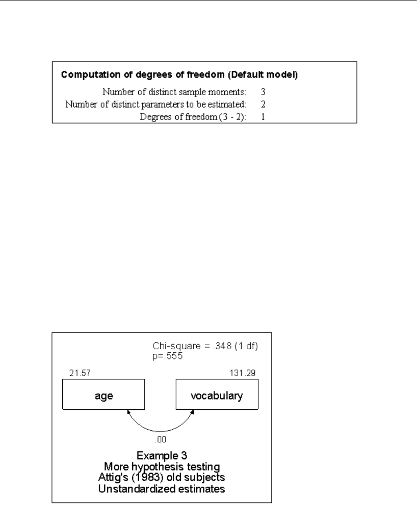
65
More Hypothesis Testing
EClick Notes for Model in the upper left pane of the Amos Output window.
The three sample moments are the variances of age and vocabulary and their
covariance. The two distinct parameters to be estimated are the two population
variances. The covariance is fixed at 0 in the model, not estimated from the sample
information.
Viewing Graphics Output
EClick the Show the output path diagram button.
EIn the Parameter Formats pane to the left of the drawing area, click Unstandardized
estimates.
The following is the path diagram output of the unstandardized estimates, along with
the test of the null hypothesis that age and vocabulary are uncorrelated:
The probability of accidentally getting a departure this large from the null hypothesis
is 0.555. The null hypothesis would not be rejected at any conventional significance
level.

66
Example 3
The usual t statistic for testing this null hypothesis is 0.59 ( ,
two-sided). The probability level associated with the t statistic is exact. The probability
level of 0.555 of the chi-square statistic is off, owing to the fact that it does not have an
exact chi-square distribution in finite samples. Even so, the probability level of 0.555
is not bad.
Here is an interesting question: If you use the probability level displayed by Amos
to test the null hypothesis at either the 0.05 or 0.01 level, then what is the actual
probability of rejecting a true null hypothesis? In the case of the present null
hypothesis, this question has an answer, although the answer depends on the sample
size. The second column in the next table shows, for several sample sizes, the real
probability of a Type I error when using Amos to test the null hypothesis of zero
correlation at the 0.05 level. The third column shows the real probability of a Type I
error if you use a significance level of 0.01. The table shows that the bigger the sample
size, the closer the true significance level is to what it is supposed to be. It’s too bad
that such a table cannot be constructed for every hypothesis that Amos can be used to
test. However, this much can be said about any such table: Moving from top to bottom,
the numbers in the 0.05 column would approach 0.05, and the numbers in the 0.01
column would approach 0.01. This is what is meant when it is said that hypothesis tests
based on maximum likelihood theory are asymptotically correct.
The following table shows the actual probability of a Type I error when using Amos
to test the hypothesis that two variables are uncorrelated:
Sample Size Nominal Significance Level
0.05 0.01
30.250 0.122
40.150 0.056
50.115 0.038
10 0.073 0.018
20 0.060 0.013
30 0.056 0.012
40 0.055 0.012
50 0.054 0.011
100 0.052 0.011
150 0.051 0.010
200 0.051 0.010
>500 0.050 0.010
df 38=
p0.56=
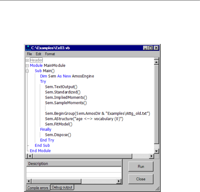
67
More Hypothesis Testing
Modeling in VB.NET
Here is a program for performing the analysis of this example:
The AStructure method constrains the covariance, fixing it at a constant 0. The program
does not refer explicitly to the variances of age and vocabulary. The default behavior
of Amos is to estimate those variances without constraints. Amos treats the variance of
every exogenous variable as a free parameter except for variances that are explicitly
constrained by the program.

69
Example
4
Conventional Linear Regression
Introduction
This example demonstrates a conventional regression analysis, predicting a single
observed variable as a linear combination of three other observed variables. It also
introduces the concept of identifiability.
About the Data
Warren, White, and Fuller (1974) studied 98 managers of farm cooperatives. We will
use the following four measurements:
A fifth measure, past training, was also reported, but we will not use it.
EIn this example, you will use the Excel worksheet Warren5v in the file UserGuide.xls,
which is located in the %examples% folder.
Tes t E xpl anation
performance A 24-item test of performance related to “planning, organization,
controlling, coordinating, and directing”
knowledge
A 26-item test of knowledge of “economic phases of
management directed toward profit-making...and product
knowledge”
value A 30-item test of “tendency to rationally evaluate means to an
economic end”
satisfaction An 11-item test of “gratification obtained...from performing the
managerial role”
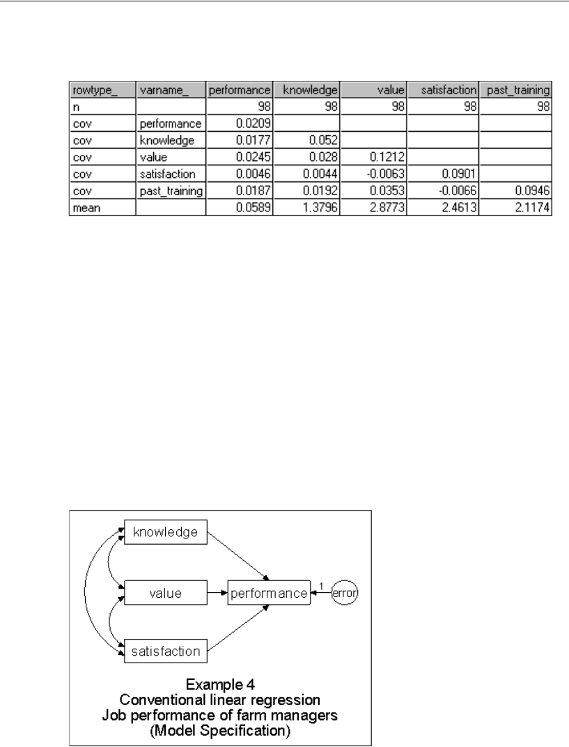
70
Example 4
Here are the sample variances and covariances:
Warren5v also contains the sample means. Raw data are not available, but they are not
needed by Amos for most analyses, as long as the sample moments (that is, means,
variances, and covariances) are provided. In fact, only sample variances and
covariances are required in this example. We will not need the sample means in
Warren5v for the time being, and Amos will ignore them.
Analysis of the Data
Suppose you want to use scores on knowledge, value, and satisfaction to predict
performance. More specifically, suppose you think that performance scores can be
approximated by a linear combination of knowledge, value, and satisfaction. The
prediction will not be perfect, however, and the model should thus include an error
variable.
Here is the initial path diagram for this relationship:

71
Conventional Linear Regression
The single-headed arrows represent linear dependencies. For example, the arrow
leading from knowledge to performance indicates that performance scores depend, in
part, on knowledge. The variable error is enclosed in a circle because it is not directly
observed. Error represents much more than random fluctuations in performance scores
due to measurement error. Error also represents a composite of age, socioeconomic
status, verbal ability, and anything else on which performance may depend but which
was not measured in this study. This variable is essential because the path diagram is
supposed to show all variables that affect performance scores. Without the circle, the
path diagram would make the implausible claim that performance is an exact linear
combination of knowledge, value, and satisfaction.
The double-headed arrows in the path diagram connect variables that may be
correlated with each other. The absence of a double-headed arrow connecting error
with any other variable indicates that error is assumed to be uncorrelated with every
other predictor variable—a fundamental assumption in linear regression. Performance
is also not connected to any other variable by a double-headed arrow, but this is for a
different reason. Since performance depends on the other variables, it goes without
saying that it might be correlated with them.
Specifying the Model
Using what you learned in the first three examples, do the following:
EStart a new path diagram.
ESpecify that the dataset to be analyzed is in the Excel worksheet Warren5v in the file
UserGuide.xls.
EDraw four rectangles and label them knowledge, value, satisfaction, and performance.
EDraw an ellipse for the error variable.
EDraw single-headed arrows that point from the exogenous, or predictor, variables
(knowledge, value, satisfaction, and error) to the endogenous, or response, variable
(performance).
Note: Endogenous variables have at least one single-headed path pointing toward them.
Exogenous variables, in contrast, send out only single-headed paths but do not receive any.
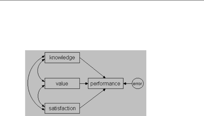
72
Example 4
EDraw three double-headed arrows that connect the observed exogenous variables
(knowledge, satisfaction, and value).
Your path diagram should look like this:
Identification
In this example, it is impossible to estimate the regression weight for the regression of
performance on error, and, at the same time, estimate the variance of error. It is like
having someone tell you, “I bought $5 worth of widgets,” and attempting to infer both
the price of each widget and the number of widgets purchased. There is just not enough
information.
You can solve this identification problem by fixing either the regression weight
applied to error in predicting performance, or the variance of the error variable itself,
at an arbitrary, nonzero value. Let’s fix the regression weight at 1. This will yield the
same estimates as conventional linear regression.
Fixing Regression Weights
ERight-click the arrow that points from error to performance and choose Object Properties
from the pop-up menu.
EClick the Parameters tab.
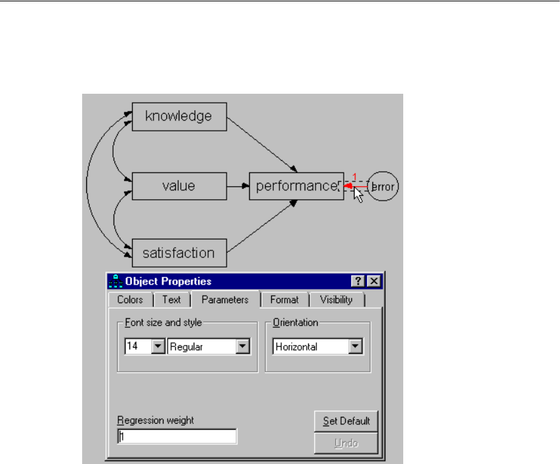
73
Conventional Linear Regression
EType 1 in the Regression weight box.
Setting a regression weight equal to 1 for every error variable can be tedious.
Fortunately, Amos Graphics provides a default solution that works well in most cases.
EClick the Add a unique variable to an existing variable button.
EClick an endogenous variable.
Amos automatically attaches an error variable to it, complete with a fixed regression
weight of 1. Clicking the endogenous variable repeatedly changes the position of the
error variable.
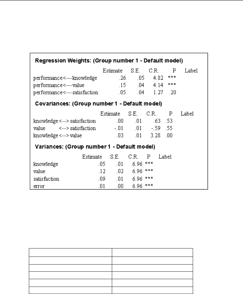
74
Example 4
Viewing the Text Output
Here are the maximum likelihood estimates:
Amos does not display the path performance <— error because its value is fixed at the
default value of 1. You may wonder how much the other estimates would be affected
if a different constant had been chosen. It turns out that only the variance estimate for
error is affected by such a change.
The following table shows the variance estimate that results from various choices for
the performance <— error regression weight.
Fixed regression weight Estimated variance of error
0.5 0.050
0.707 0.025
1.0 0.0125
1.414 0.00625
2.0 0.00313
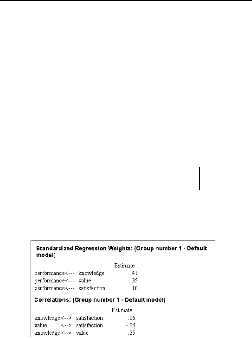
75
Conventional Linear Regression
Suppose you fixed the path coefficient at 2 instead of 1. Then the variance estimate
would be divided by a factor of 4. You can extrapolate the rule that multiplying the path
coefficient by a fixed factor goes along with dividing the error variance by the square
of the same factor. Extending this, the product of the squared regression weight and the
error variance is always a constant. This is what we mean when we say the regression
weight (together with the error variance) is unidentified. If you assign a value to one
of them, the other can be estimated, but they cannot both be estimated at the same time.
The identifiability problem just discussed arises from the fact that the variance of a
variable, and any regression weights associated with it, depends on the units in which
the variable is measured. Since error is an unobserved variable, there is no natural way
to specify a measurement unit for it. Assigning an arbitrary value to a regression weight
associated with error can be thought of as a way of indirectly choosing a unit of
measurement for error. Every unobserved variable presents this identifiability
problem, which must be resolved by imposing some constraint that determines its unit
of measurement.
Changing the scale unit of the unobserved error variable does not change the overall
model fit. In all the analyses, you get:
There are four sample variances and six sample covariances, for a total of 10 sample
moments. There are three regression paths, four model variances, and three model
covariances, for a total of 10 parameters that must be estimated. Hence, the model has
zero degrees of freedom. Such a model is often called saturated or just-identified.
The standardized coefficient estimates are as follows:
Chi-square = 0.00
Degrees of freedom = 0
Probability level cannot be computed
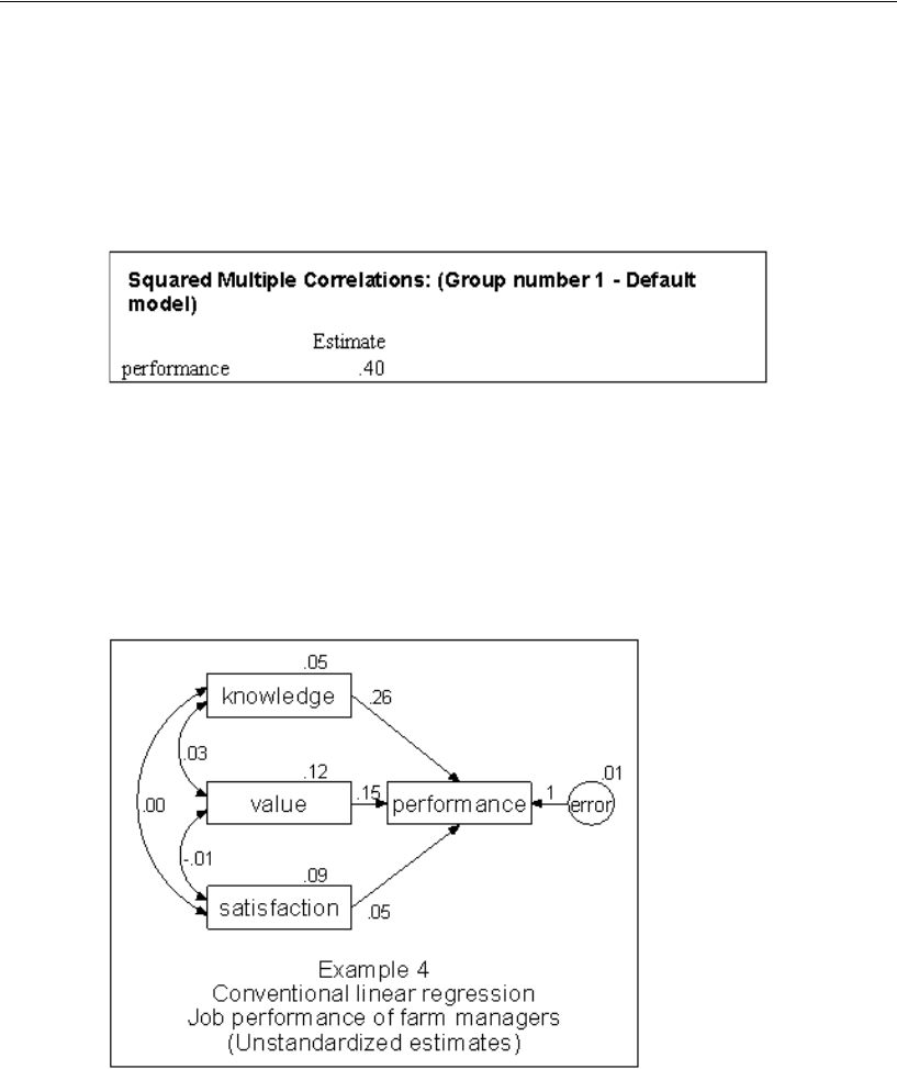
76
Example 4
The standardized regression weights and the correlations are independent of the units
in which all variables are measured; therefore, they are not affected by the choice of
identification constraints.
Squared multiple correlations are also independent of units of measurement. Amos
displays a squared multiple correlation for each endogenous variable.
Note: The squared multiple correlation of a variable is the proportion of its variance that
is accounted for by its predictors. In the present example, knowledge, value, and
satisfaction account for 40% of the variance of performance.
Viewing Graphics Output
The following path diagram output shows unstandardized values:
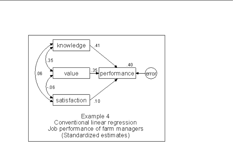
77
Conventional Linear Regression
Here is the standardized solution:
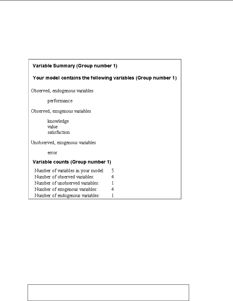
78
Example 4
Viewing Additional Text Output
EIn the tree diagram in the upper left pane of the Amos Output window, click Variable
Summary.
Endogenous variables are those that have single-headed arrows pointing to them; they
depend on other variables. Exogenous variables are those that do not have single-
headed arrows pointing to them; they do not depend on other variables.
Inspecting the preceding list will help you catch the most common (and insidious)
errors in an input file: typing errors. If you try to type performance twice but
unintentionally misspell it as preformance one of those times, both versions will
appear on the list.
ENow click Notes for Model in the upper left pane of the Amos Output window.
The following output indicates that there are no feedback loops in the path diagram:
Notes for Group (Group number 1)
The model is recursive.
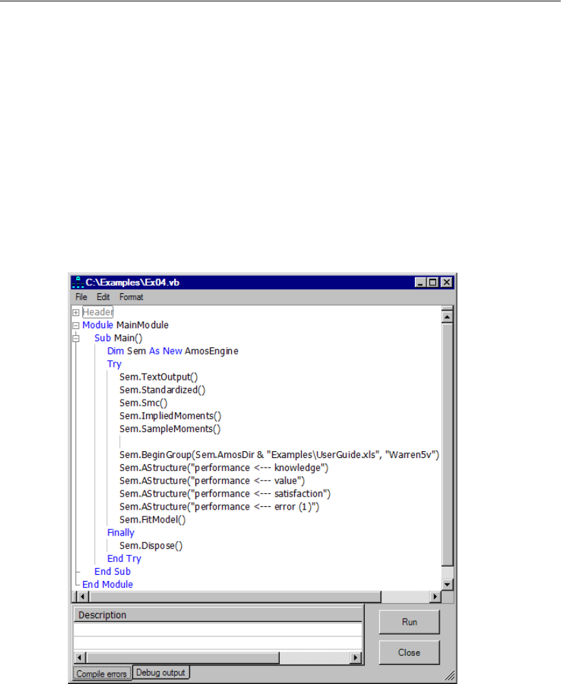
79
Conventional Linear Regression
Later you will see path diagrams where you can pick a variable and, by tracing along
the single-headed arrows, follow a path that leads back to the same variable.
Note: Path diagrams that have feedback loops are called nonrecursive. Those that do
not are called recursive.
Modeling in VB.NET
The model in this example consists of a single regression equation. Each single-headed
arrow in the path diagram represents a regression weight. Here is a program for
estimating those regression weights:
The four lines that come after Sem.BeginGroup correspond to the single-headed arrows
in the Amos Graphics path diagram. The (1) in the last AStructure line fixes the error
regression weight at a constant 1.

80
Example 4
Assumptions about Correlations among Exogenous Variables
When executing a program, Amos makes assumptions about the correlations among
exogenous variables that are not made in Amos Graphics. These assumptions simplify
the specification of many models, especially models that have parameters. The
differences between specifying a model in Amos Graphics and specifying one
programmatically are as follows:
Amos Graphics is entirely WYSIWYG (What You See Is What You Get). If you
draw a two-headed arrow (without constraints) between two exogenous variables,
Amos Graphics will estimate their covariance. If two exogenous variables are not
connected by a double-headed arrow, Amos Graphics will assume that the
variables are uncorrelated.
The default assumptions in an Amos program are:
Unique variables (unobserved, exogenous variables that affect only one other
variable) are assumed to be uncorrelated with each other and with all other
exogenous variables.
Exogenous variables other than unique variables are assumed to be correlated
among themselves.
In Amos programs, these defaults reflect standard assumptions of conventional linear
regression analysis. Thus, in this example, the program assumes that the predictors,
knowledge, value, and satisfaction, are correlated and that error is uncorrelated with
the predictors.
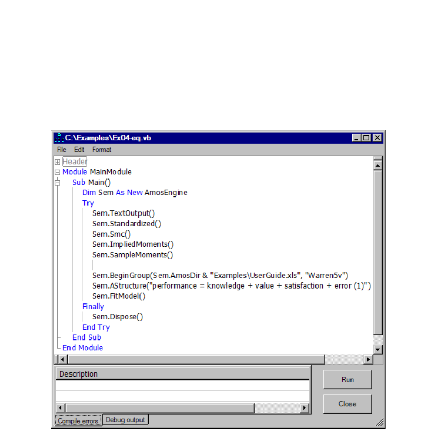
81
Conventional Linear Regression
Equation Format for the AStructure Method
The AStructure method permits model specification in equation format. For instance,
the single Sem.AStructure statement in the following program describes the same
model as the program on p. 79 but in a single line. This program is saved under the
name Ex04-eq.vb in the Examples directory.
Note that in the AStructure line above, each predictor variable (on the right side of the
equation) is associated with a regression weight to be estimated. We could make these
regression weights explicit through the use of empty parentheses as follows:
Sem.AStructure("performance = ()knowledge + ()value + ()satisfaction + error(1)")
The empty parentheses are optional. By default, Amos will automatically estimate a
regression weight for each predictor.

83
Example
5
Unobserved Variables
Introduction
This example demonstrates a regression analysis with unobserved variables.
About the Data
The variables in the previous example were surely unreliable to some degree. The fact
that the reliability of performance is unknown presents a minor problem when it
comes to interpreting the fact that the predictors account for only 39.9% of the
variance of performance. If the test were extremely unreliable, that fact in itself would
explain why the performance score could not be predicted accurately. Unreliability of
the predictors, on the other hand, presents a more serious problem because it can lead
to biased estimates of regression weights.
The present example, based on Rock, et al. (1977), will assess the reliabilities of
the four tests included in the previous analysis. It will also obtain estimates of
regression weights for perfectly reliable, hypothetical versions of the four tests. Rock,
et al. re-examined the data of Warren, White, and Fuller (1974) that were discussed
in the previous example. This time, each test was randomly split into two halves, and
each half was scored separately.

84
Example 5
Here is a list of the input variables:
For this example, we will use the data file Warren9v.sav to obtain the sample variances
and covariances of these subtests. The sample means that appear in the file will not be
used in this example. Statistics on formal education (past_training) are present in the
file, but they also will not enter into the present analysis.
Variable name Description
performance1 12-item subtest of Role Performance
performance2 12-item subtest of Role Performance
knowledge1 13-item subtest of Knowledge
knowledge2 13-item subtest of Knowledge
value1 15-item subtest of Value Orientation
value2 15-item subtest of Value Orientation
satisfaction1 5-item subtest of Role Satisfaction
satisfaction2 6-item subtest of Role Satisfaction
past_training degree of formal education
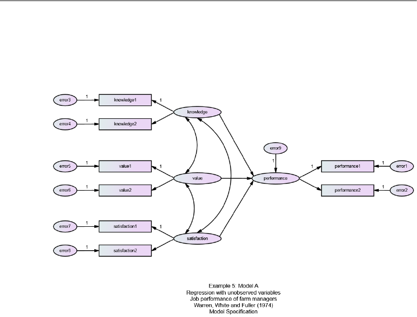
85
Unobserved Variables
Model A
The following path diagram presents a model for the eight subtests:
Four ellipses in the figure are labeled knowledge, value, satisfaction, and performance.
They represent unobserved variables that are indirectly measured by the eight split-half
tests.
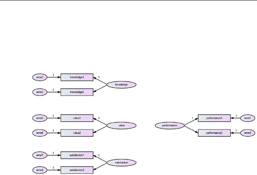
86
Example 5
Measurement Model
The portion of the model that specifies how the observed variables depend on the
unobserved, or latent, variables is sometimes called the measurement model. The
current model has four distinct measurement submodels.
Consider, for instance, the knowledge submodel: The scores of the two split-half
subtests, knowledge1 and knowledge2, are hypothesized to depend on the single
underlying, but not directly observed variable, knowledge. According to the model,
scores on the two subtests may still disagree, owing to the influence of error3 and
error4, which represent errors of measurement in the two subtests. knowledge1 and
knowledge2 are called indicators of the latent variable knowledge. The measurement
model for knowledge forms a pattern that is repeated three more times in the path
diagram shown above.
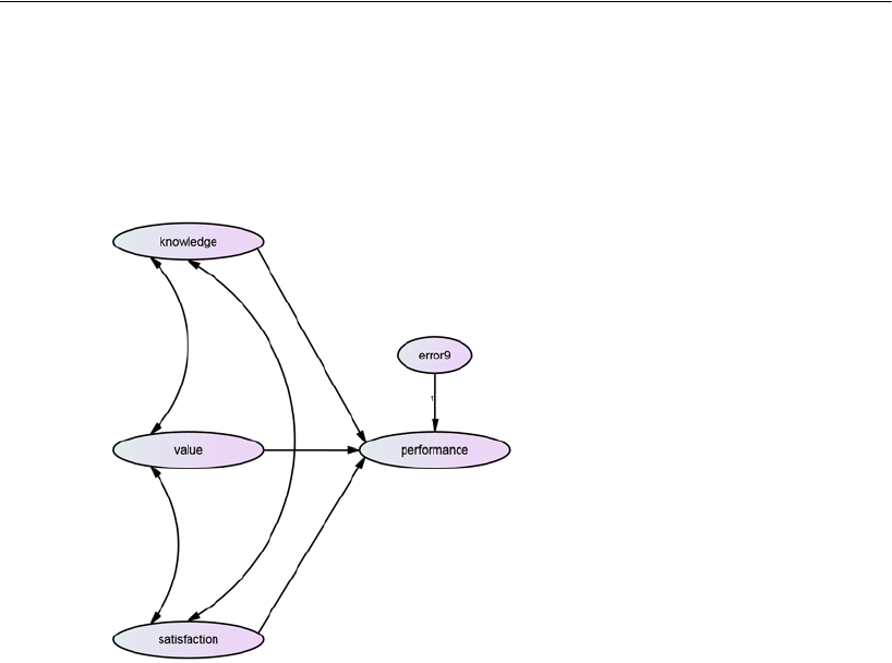
87
Unobserved Variables
Structural Model
The portion of the model that specifies how the latent variables are related to each other
is sometimes called the structural model.
The structural part of the current model is the same as the one in Example 4. It is only
in the measurement model that this example differs from the one in Example 4.
Identification
With 13 unobserved variables in this model, it is certainly not identified. It will be
necessary to fix the unit of measurement of each unobserved variable by suitable
constraints on the parameters. This can be done by repeating 13 times the trick that was
used for the single unobserved variable in Example 4: Find a single-headed arrow
leading away from each unobserved variable in the path diagram, and fix the
corresponding regression weight to an arbitrary value such as 1. If there is more than
one single-headed arrow leading away from an unobserved variable, any one of them
will do. The path diagram for “Model A” on p. 85 shows one satisfactory choice of
identifiability constraints.
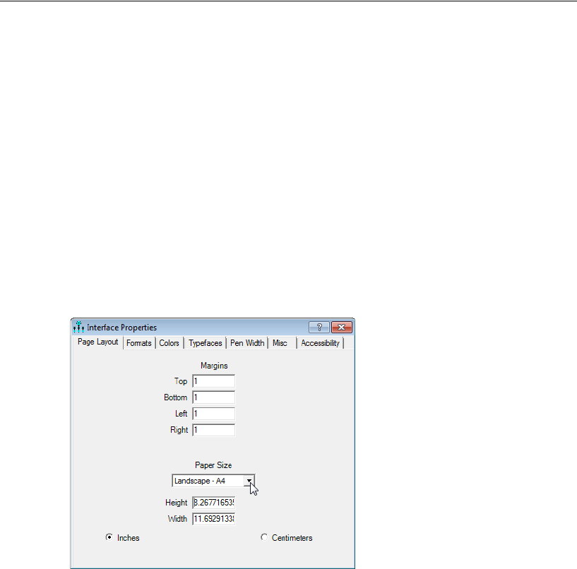
88
Example 5
Specifying the Model
Because the path diagram is wider than it is tall, you may want to change the shape of
the drawing area so that it fits the path diagram better. By default, the drawing area in
Amos is taller than it is wide so that it is suitable for printing in portrait mode.
Changing the Orientation of the Drawing Area
EFrom the menus, choose View > Interface Properties.
EIn the Interface Properties dialog, click the Page Layout tab.
ESet Paper Size to one of the “Landscape” paper sizes, such as Landscape - A4.
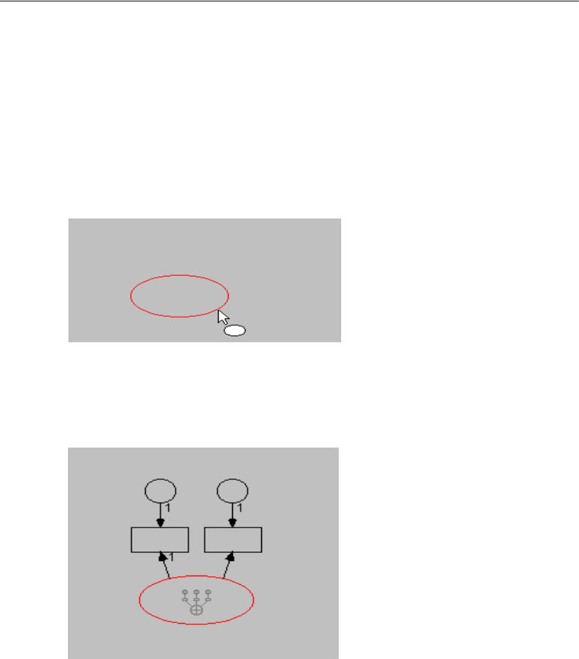
89
Unobserved Variables
Creating the Path Diagram
Now you are ready to draw the model as shown in the path diagram on page 85. There
are a number of ways to do this. One is to start by drawing the measurement model first.
Here, we draw the measurement model for one of the latent variables, knowledge, and
then use it as a pattern for the other three.
EDraw an ellipse for the unobserved variable knowledge.
EFrom the menus, choose Diagram > Draw Indicator Variable.
EClick twice inside the ellipse.
Each click creates one indicator variable for knowledge:
As you can see, with the Draw indicator variable button enabled, you can click multiple
times on an unobserved variable to create multiple indicators, complete with unique or
error variables. Amos Graphics maintains suitable spacing among the indicators and
inserts identification constraints automatically.
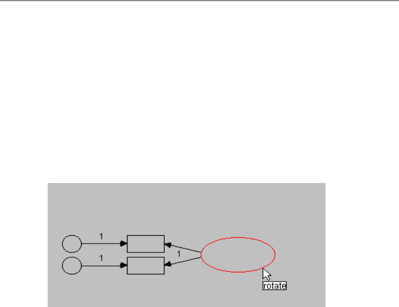
90
Example 5
Rotating Indicators
The indicators appear by default above the knowledge ellipse, but you can change their
location.
EFrom the menus, choose Edit > Rotate.
EClick the knowledge ellipse.
Each time you click the knowledge ellipse, its indicators rotate 90° clockwise. If you
click the ellipse three times, its indicators will look like this:
Duplicating Measurement Models
The next step is to create measurement models for value and satisfaction.
EFrom the menus, choose Edit > Select All.
The measurement model turns blue.
EFrom the menus, choose Edit > Duplicate.
EClick any part of the measurement model, and drag a copy to beneath the original.
ERepeat to create a third measurement model above the original.
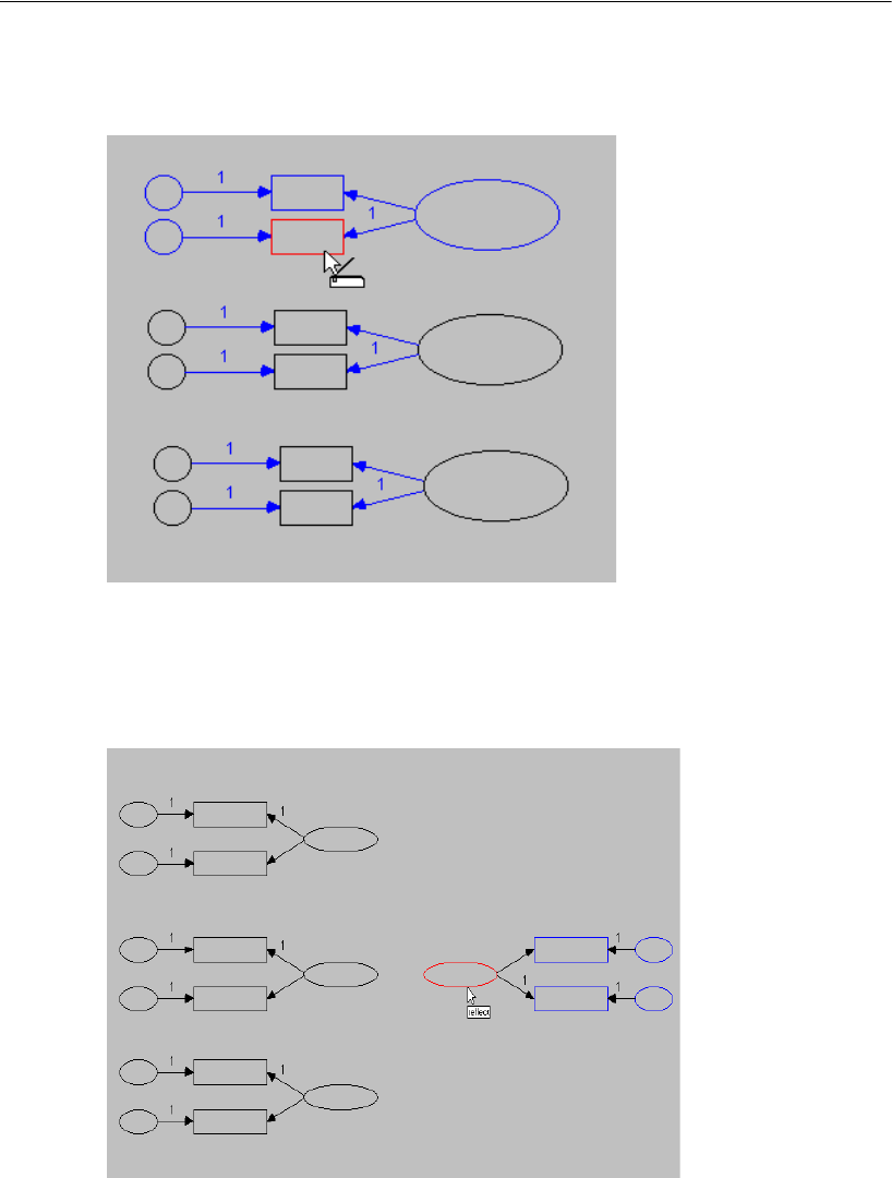
91
Unobserved Variables
Your path diagram should now look like this:
ECreate a fourth copy for performance, and position it to the right of the original.
EFrom the menus, choose Edit > Reflect.
This repositions the two indicators of performance as follows:

92
Example 5
Entering Variable Names
ERight-click each object and select Object Properties from the pop-up menu
EIn the Object Properties dialog, click the Text tab, and enter a name into the Variable
Name text box.
Alternatively, you can choose View > Variables in Dataset from the menus and then drag
variable names onto objects in the path diagram.
Completing the Structural Model
There are only a few things left to do to complete the structural model.
EDraw the three covariance paths connecting knowledge, value, and satisfaction.
EDraw a single-headed arrow from each of the latent predictors, knowledge, value, and
satisfaction, to the latent dependent variable, performance.
EAdd the unobserved variable error9 as a predictor of performance (from the menus,
choose Diagram > Draw Unique Variable).
Your path diagram should now look like the one on p. 85. The Amos Graphics input
file that contains this path diagram is Ex05-a.amw.
Results for Model A
As an exercise, you might want to confirm the following degrees of freedom
calculation:

93
Unobserved Variables
The hypothesis that Model A is correct is accepted.
The parameter estimates are affected by the identification constraints.
Chi-square = 10.335
Degrees of freedom = 14
Probability level = 0.737
Regression Weights: (Group number 1 - Default model)
Estimate S.E. C.R. P Label
p
erformance
<--- knowledge
.337 .125 2.697 .007
p
erformance
<--- satisfaction
.061 .054 1.127 .260
p
erformance
<--- value
.176 .079 2.225 .026
satisfaction2 <--- satisfaction
.792 .438 1.806 .071
satisfaction1 <--- satisfaction 1.000
value2 <--- value
.763 .185 4.128 ***
value1 <--- value 1.000
knowledge2 <--- knowledge
.683 .161 4.252 ***
knowledge1 <--- knowledge 1.000
p
erformance1
<---
p
erforman
ce 1.000
p
erformance2
<---
p
erformance
.867 .116 7.450 ***
Covariances: (Group number 1 - Default model)
Estimate S.E. C.R. P Label
value <--> knowledge
.037 .012 3.036 .002
satisfaction <--> value -
.008 .013
-
.610 .542
satisfaction <--> knowledge
.004 .009 .462 .644
Variances: (Group number 1 - Default model)
Estimate S.E. C.R. P Label
satisfaction
.090 .052 1.745 .081
value
.100 .032 3.147 .002
knowledge
.046 .015 3.138 .002
error9
.007 .003 2.577 .010
error3
.041
.011
3.611 ***
error4
.035 .007 5.167 ***
error5
.080 .025 3.249 .001
error6
.087 .018 4.891 ***
error7
.022 .049 .451 .652
error8
.045 .032 1.420 .156
error1
.007 .002 3.110 .002
error2
.007 .002 3.871 ***

94
Example 5
Standardized estimates, on the other hand, are not affected by the identification
constraints. To calculate standardized estimates:
EFrom the menus, choose View > Analysis Properties.
EIn the Analysis Properties dialog, click the Output tab.
EEnable the Standardized estimates check box.
Standardized Regression Weights: (Group number 1 - Default model)
Estimate
performance <---
knowledge
.516
performance <---
satisfaction
.130
performance <---
value
.398
satisfaction2 <---
satisfaction
.747
satisfaction1 <---
satisfaction
.896
value2 <---
value
.633
value1 <---
value
.745
knowledge2 <---
knowledge
.618
knowledge1 <---
knowledge
.728
performance1
<---
performance
.856
performance2
<---
performance
.819
Correlations: (Group number 1 - Default model)
Estimate
value <-->
knowledge
.542
satisfaction <-->
value -
.084
satisfaction <-->
knowledge
.064
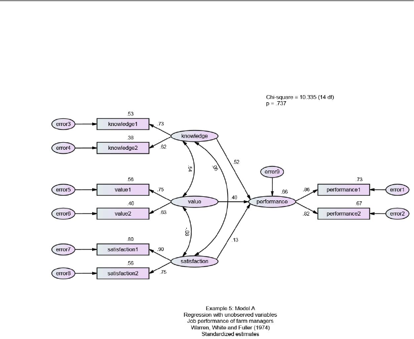
95
Unobserved Variables
Viewing the Graphics Output
The path diagram with standardized parameter estimates displayed is as follows:
The value above performance indicates that pure knowledge, value, and satisfaction
account for 66% of the variance of performance. The values displayed above the
observed variables are reliability estimates for the eight individual subtests. A formula
for the reliability of the original tests (before they were split in half) can be found in
Rock et al. (1977) or any book on mental test theory.
Model B
Assuming that Model A is correct (and there is no evidence to the contrary), consider
the additional hypothesis that knowledge1 and knowledge2 are parallel tests. Under the
parallel tests hypothesis, the regression of knowledge1 on knowledge should be the
same as the regression of knowledge2 on knowledge. Furthermore, the error variables
associated with knowledge1 and knowledge2 should have identical variances. Similar
consequences flow from the assumption that value1 and value2 are parallel tests, as
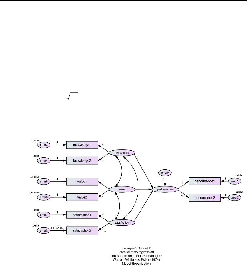
96
Example 5
well as performance1 and performance2. But it is not altogether reasonable to assume
that satisfaction1 and satisfaction2 are parallel. One of the subtests is slightly longer
than the other because the original test had an odd number of items and could not be
split exactly in half. As a result, satisfaction2 is 20% longer than satisfaction1.
Assuming that the tests differ only in length leads to the following conclusions:
The regression weight for regressing satisfaction2 on satisfaction should be 1.2
times the weight for regressing satisfaction1 on satisfaction.
Given equal variances for error7 and error8, the regression weight for error8
should be times as large as the regression weight for error7.
You do not need to redraw the path diagram from scratch in order to impose these
parameter constraints. You can take the path diagram that you created for Model A as
a starting point and then change the values of two regression weights. Here is the path
diagram after those changes:
1.2 1.095445=
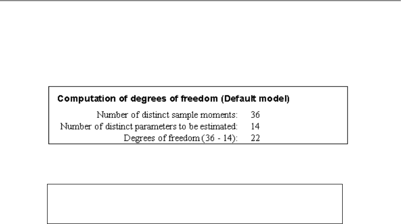
97
Unobserved Variables
Results for Model B
The additional parameter constraints of Model B result in increased degrees of freedom:
The chi-square statistic has also increased but not by much. It indicates no significant
departure of the data from Model B.
Chi-square = 26.967
Degrees of freedom = 22
Probability level = 0.212

98
Example 5
If Model B is indeed correct, the associated parameter estimates are to be preferred
over those obtained under Model A. The raw parameter estimates will not be presented
here because they are affected too much by the choice of identification constraints.
However, here are the standardized estimates and the squared multiple correlations:
Standardized Regression Weights: (Group number 1 - Default model)
Estimate
p
erformance
<--- knowledge .529
p
erformance
<--- satisfaction .114
p
erformance
<--- value .382
satisfaction2 <--- error8 .578
satisfaction2 <--- satisfaction .816
satisfaction1 <--- satisfaction .790
value2 <--- value .685
value1 <--- value .685
knowledge2 <--- knowledge .663
knowledge1 <--- knowledge .663
p
erformance1
<---
p
erformance
.835
p
erformance2
<---
p
erformance
.835
Correlations: (Group number 1 - Default model)
Estimate
satisfaction <--> value -.085
value <--> knowledge .565
satisfaction <--> knowledge .094
Squared Multiple Correlations: (Group number 1 - Default model)
Estimate
p
erformance
.671
p
erformance2
.698
p
erformance1
.698
satisfaction2
.666
satisfaction1
.625
value2
.469
value1
.469
knowledge2
.439
knowledge1
.439
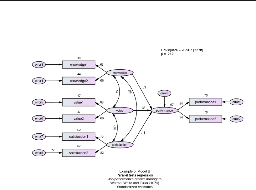
99
Unobserved Variables
Here are the standardized estimates and squared multiple correlations displayed on the
path diagram:
Testing Model B against Model A
Sometimes you may have two alternative models for the same set of data, and you
would like to know which model fits the data better. You can perform a direct
comparison whenever one of the models can be obtained by placing additional
constraints on the parameters of the other. We have such a case here. We obtained
Model B by imposing eight additional constraints on the parameters of Model A. Let
us say that Model B is the stronger of the two models, in the sense that it represents the
stronger hypothesis about the population parameters. (Model A would then be the
weaker model). The stronger model will have greater degrees of freedom. The chi-
square statistic for the stronger model will be at least as large as the chi-square statistic
for the weaker model.

100
Example 5
A test of the stronger model (Model B) against the weaker one (Model A) can be
obtained by subtracting the smaller chi-square statistic from the larger one. In this
example, the new statistic is 16.632 (that is, ). If the stronger model
(Model B) is correctly specified, this statistic will have an approximate chi-square
distribution with degrees of freedom equal to the difference between the degrees of
freedom of the competing models. In this example, the difference in degrees of
freedom is 8 (that is, ). Model B imposes all of the parameter constraints of
Model A, plus an additional 8.
In summary, if Model B is correct, the value 16.632 comes from a chi-square
distribution with eight degrees of freedom. If only the weaker model (Model A) is
correct, and not the stronger model (Model B), the new statistic will tend to be large.
Hence, the stronger model (Model B) is to be rejected in favor of the weaker model
(Model A) when the new chi-square statistic is unusually large. With eight degrees of
freedom, chi-square values greater than 15.507 are significant at the 0.05 level. Based
on this test, we reject Model B.
What about the earlier conclusion, based on the chi-square value of 26.967 with
22 degrees of freedom, that Model B is correct? The disagreement between the two
conclusions can be explained by noting that the two tests differ in their assumptions.
The test based on eight degrees of freedom assumes that Model A is correct when
testing Model B. The test based on 22 degrees of freedom makes no such assumption
about Model A. If you are quite sure that Model A is correct, you should use the test
comparing Model B against Model A (the one based here on eight degrees of freedom);
otherwise, you should use the test based on 22 degrees of freedom.
26.967 10.335–
22 14–

101
Unobserved Variables
Modeling in VB.NET
Model A
The following program fits Model A:
Because of the assumptions that Amos makes about correlations among exogenous
variables (discussed in Example 4), the program does not need to indicate that
knowledge, value, and satisfaction are allowed to be correlated. It is also not necessary
to specify that error1, error2, ... , error9 are uncorrelated among themselves and with
every other exogenous variable.
Sub Main()
Dim Sem As New AmosEngine
Try
Sem.TextOutput()
Sem.Standardized()
Sem.Smc()
Sem.BeginGroup(Sem.AmosDir & "Examples\Warren9v.wk1")
Sem.AStructure("performance1 <--- performance (1)")
Sem.AStructure("performance2 <--- performance")
Sem.AStructure("knowledge1 <--- knowledge (1)")
Sem.AStructure("knowledge2 <--- knowledge")
Sem.AStructure("value1 <--- value (1)")
Sem.AStructure("value2 <--- value")
Sem.AStructure("satisfaction1 <--- satisfaction (1)")
Sem.AStructure("satisfaction2 <--- satisfaction")
Sem.AStructure("performance1 <--- error1 (1)")
Sem.AStructure("performance2 <--- error2 (1)")
Sem.AStructure("knowledge1 <--- error3 (1)")
Sem.AStructure("knowledge2 <--- error4 (1)")
Sem.AStructure("value1 <--- error5 (1)")
Sem.AStructure("value2 <--- error6 (1)")
Sem.AStructure("satisfaction1 <--- error7 (1)")
Sem.AStructure("satisfaction2 <--- error8 (1)")
Sem.AStructure("performance <--- knowledge")
Sem.AStructure("performance <--- satisfaction")
Sem.AStructure("performance <--- value")
Sem.AStructure("performance <--- error9 (1)")
Sem.FitModel()
Finally
Sem.Dispose()
End Try
End Sub

102
Example 5
Model B
The following program fits Model B:
Sub Main()
Dim Sem As New AmosEngine
Try
Sem.TextOutput()
Sem.Standardized()
Sem.Smc()
Sem.BeginGroup(Sem.AmosDir & "Examples\Warren9v.wk1")
Sem.AStructure("performance1 <--- performance (1)")
Sem.AStructure("performance2 <--- performance (1)")
Sem.AStructure("knowledge1 <--- knowledge (1)")
Sem.AStructure("knowledge2 <--- knowledge (1)")
Sem.AStructure("value1 <--- value (1)")
Sem.AStructure("value2 <--- value (1)")
Sem.AStructure("satisfaction1 <--- satisfaction (1)")
Sem.AStructure("satisfaction2 <--- satisfaction (" & CStr(1.2) & ")")
Sem.AStructure("performance <--- knowledge")
Sem.AStructure("performance <--- value")
Sem.AStructure("performance <--- satisfaction")
Sem.AStructure("performance <--- error9 (1)")
Sem.AStructure("performance1 <--- error1 (1)")
Sem.AStructure("performance2 <--- error2 (1)")
Sem.AStructure("knowledge1 <--- error3 (1)")
Sem.AStructure("knowledge2 <--- error4 (1)")
Sem.AStructure("value1 <--- error5 (1)")
Sem.AStructure("value2 <--- error6 (1)")
Sem.AStructure("satisfaction1 <--- error7 (1)")
Sem.AStructure("satisfaction2 <--- error8 (" & CStr(1.095445) & ")")
Sem.AStructure("error1 (alpha)")
Sem.AStructure("error2 (alpha)")
Sem.AStructure("error8 (delta)")
Sem.AStructure("error7 (delta)")
Sem.AStructure("error6 (gamma)")
Sem.AStructure("error5 (gamma)")
Sem.AStructure("error4 (beta)")
Sem.AStructure("error3 (beta)")
Sem.FitModel()
Finally
Sem.Dispose()
End Try
End Sub

103
Example
6
Exploratory Analysis
Introduction
This example demonstrates structural modeling with time-related latent variables, the
use of modification indices and critical ratios in exploratory analyses, how to compare
multiple models in a single analysis, and computation of implied moments, factor
score weights, total effects, and indirect effects.
About the Data
Wheaton et al. (1977) reported a longitudinal study of 932 persons over the period
from 1966 to 1971. Jöreskog and Sörbom (1984), and others since, have used the
Wheaton data to demonstrate analysis of moment structures. Six of Wheaton's
measures will be used for this example.
Measure Explanation
anomia67 1967 score on the anomia scale
anomia71 1971 anomia score
powles67 1967 score on the powerlessness scale
powles71 1971 powerlessness score
education Years of schooling recorded in 1966
SEI Duncan's Socioeconomic Index administered in 1966
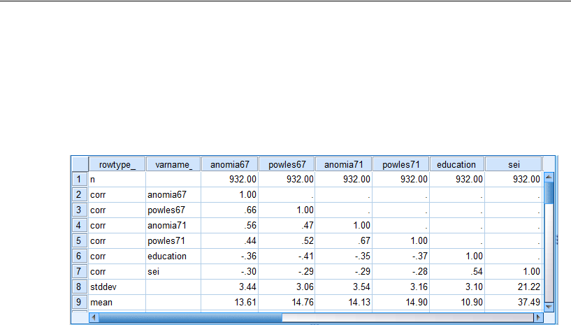
104
Example 6
Take a look at the sample means, standard deviations, and correlations for these six
measures. You will find the following table in the SPSS Statistics file, Wheaton.sav.
After reading the data, Amos converts the standard deviations and correlations into
variances and covariances, as needed for the analysis. We will not use the sample
means in the analysis.
Model A for the Wheaton Data
Jöreskog and Sörbom (1984) proposed the model shown on p. 106 for the Wheaton
data, referring to it as their Model A. The model asserts that all of the observed
variables depend on underlying, unobserved variables. For example, anomia67 and
powles67 both depend on the unobserved variable alienation67, a hypothetical variable
that Jöreskog and Sörbom referred to as alienation. The unobserved variables eps1 and
eps2 appear to play the same role as the variables error1 and error2 did in Example 5.
However, their interpretation here is different. In Example 5, error1 and error2 had a
natural interpretation as errors of measurement. In the present example, since the
anomia and powerlessness scales were not designed to measure the same thing, it
seems reasonable to believe that differences between them will be due to more than just
measurement error. So in this case, eps1 and eps2 should be thought of as representing
not only errors of measurement in anomia67 and powles67 but in every other variable
that might affect scores on the two tests besides alienation67 (the one variable that
affects them both).
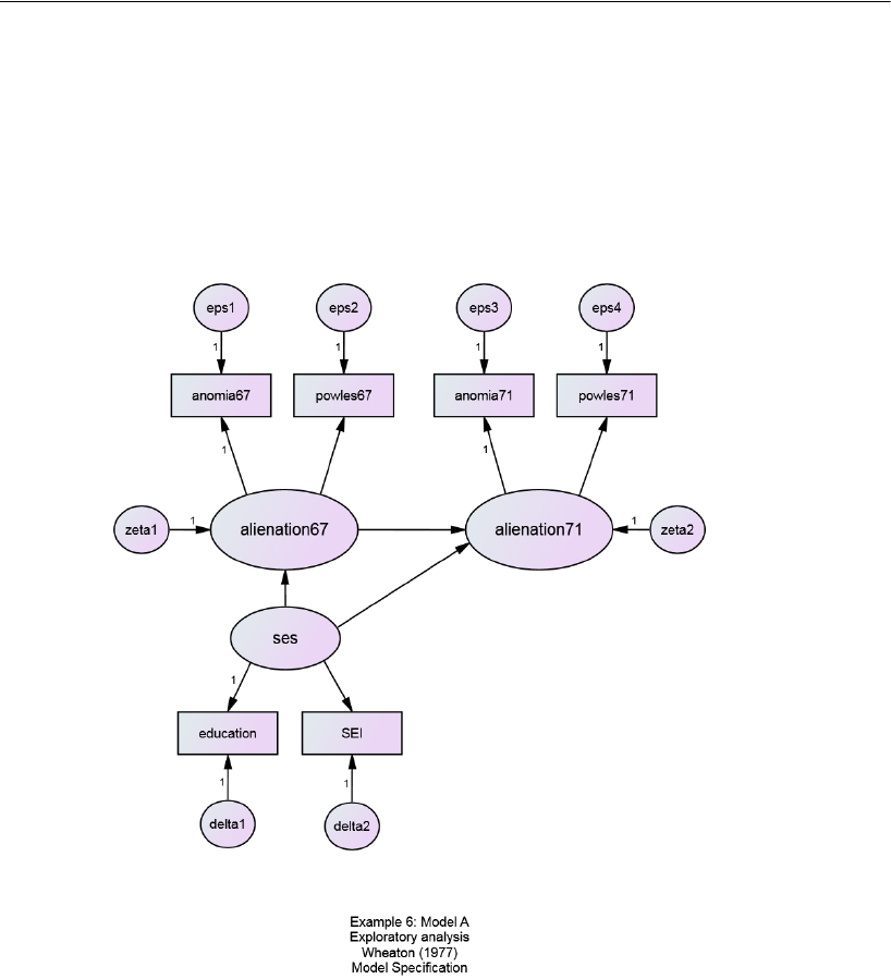
105
Exploratory Analysis
Specifying the Model
To specify Model A in Amos Graphics, draw the path diagram shown next, or open the
example file Ex06–a.amw. Notice that the eight unique variables (delta1, delta2, zeta1,
zeta2, and eps1 through eps4) are uncorrelated among themselves and with the three
latent variables: ses, alienation67, and alienation71.
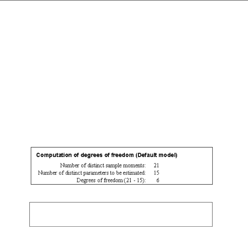
106
Example 6
Identification
Model A is identified except for the usual problem that the measurement scale of each
unobserved variable is indeterminate. The measurement scale of each unobserved
variable may be fixed arbitrarily by setting a regression weight to unity (1) for one of
the paths that points away from it. The path diagram shows 11 regression weights fixed
at unity (1), that is, one constraint for each unobserved variable. These constraints are
sufficient to make the model identified.
Results of the Analysis
The model has 15 parameters to be estimated (6 regression weights and 9 variances).
There are 21 sample moments (6 sample variances and 15 covariances). This leaves 6
degrees of freedom.
The Wheaton data depart significantly from Model A.
Dealing with Rejection
You have several options when a proposed model has to be rejected on statistical
grounds:
You can point out that statistical hypothesis testing can be a poor tool for choosing
a model. Jöreskog (1967) discussed this issue in the context of factor analysis. It is
a widely accepted view that a model can be only an approximation at best, and that,
fortunately, a model can be useful without being true. In this view, any model is
bound to be rejected on statistical grounds if it is tested with a big enough sample.
From this point of view, rejection of a model on purely statistical grounds
(particularly with a large sample) is not necessarily a condemnation.
Chi-square = 71.544
Degrees of freedom = 6
Probability level = 0.000

107
Exploratory Analysis
You can start from scratch to devise another model to substitute for the rejected one.
You can try to modify the rejected model in small ways so that it fits the data better.
It is the last tactic that will be demonstrated in this example. The most natural way of
modifying a model to make it fit better is to relax some of its assumptions. For
example, Model A assumes that eps1 and eps3 are uncorrelated. You could relax this
restriction by connecting eps1 and eps3 with a double-headed arrow. The model also
specifies that anomia67 does not depend directly on ses. You could remove this
assumption by drawing a single-headed arrow from ses to anomia67. Model A does not
happen to constrain any parameters to be equal to other parameters, but if such
constraints were present, you might consider removing them in hopes of getting a
better fit. Of course, you have to be careful when relaxing the assumptions of a model
that you do not turn an identified model into an unidentified one.
Modification Indices
You can test various modifications of a model by carrying out a separate analysis for
each potential modification, but this approach is time-consuming. Modification
indices allow you to evaluate many potential modifications in a single analysis. They
provide suggestions for model modifications that are likely to pay off in smaller chi-
square values.
Using Modification Indices
EFrom the menus, choose View > Analysis Properties.
EIn the Analysis Properties dialog, click the Output tab.
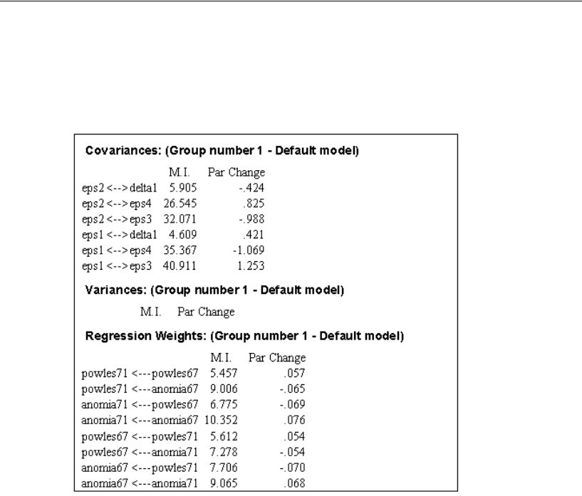
108
Example 6
EEnable the Modification Indices check box. For this example, leave the Threshold for
modification indices set at 4.
The following are the modification indices for Model A:
The column heading M.I. in this table is short for Modification Index. The modification
indices produced are those described by Jöreskog and Sörbom (1984). The first
modification index listed (5.905) is a conservative estimate of the decrease in
chi-square that will occur if eps2 and delta1 are allowed to be correlated. The new
chi-square statistic would have 5 degrees of freedom and would be no
greater than 65.639 ( ). The actual decrease of the chi-square statistic
might be much larger than 5.905. The column labeled Par Change gives approximate
estimates of how much each parameter would change if it were estimated rather than
fixed at 0. Amos estimates that the covariance between eps2 and delta1 would be
. Based on the small modification index, it does not look as though much would
be gained by allowing eps2 and delta1 to be correlated. Besides, it would be hard to
justify this particular modification on theoretical grounds even if it did produce an
acceptable fit.
61–=()
71.544 5.905–
0.424–

109
Exploratory Analysis
Changing the Modification Index Threshold
By default, Amos displays only modification indices that are greater than 4, but you
can change this threshold.
EFrom the menus, choose View > Analysis Properties.
EIn the Analysis Properties dialog, click the Output tab.
EEnter a value in the Threshold for modification indices text box. A very small threshold
will result in the display of a lot of modification indices that are too small to be of
interest.
The largest modification index in Model A is 40.911. It indicates that allowing eps1
and eps3 to be correlated will decrease the chi-square statistic by at least 40.911. This
is a modification well worth considering because it is quite plausible that these two
variables should be correlated. Eps1 represents variability in anomia67 that is not due
to variation in alienation67. Similarly, eps3 represents variability in anomia71 that is
not due to variation in alienation71. Anomia67 and anomia71 are scale scores on the
same instrument (at different times). If the anomia scale measures something other
than alienation, you would expect to find a nonzero correlation between eps1 and eps3.
In fact, you would expect the correlation to be positive, which is consistent with the
fact that the number in the Par Change column is positive.
The theoretical reasons for suspecting that eps1 and eps3 might be correlated apply
to eps2 and eps4 as well. The modification indices also suggest allowing eps2 and eps4
to be correlated. However, we will ignore this potential modification and proceed
immediately to look at the results of modifying Model A by allowing eps1 and eps3 to
be correlated. The new model is Jöreskog and Sörbom’s Model B.
Model B for the Wheaton Data
You can obtain Model B by starting with the path diagram for Model A and drawing a
double-headed arrow between eps1 and eps3. If the new double-headed arrow extends
beyond the bounds of the print area, you can use the Shape button to adjust the
curvature of the double-headed arrow. You can also use the Move button to reposition
the end points of the double-headed arrow.
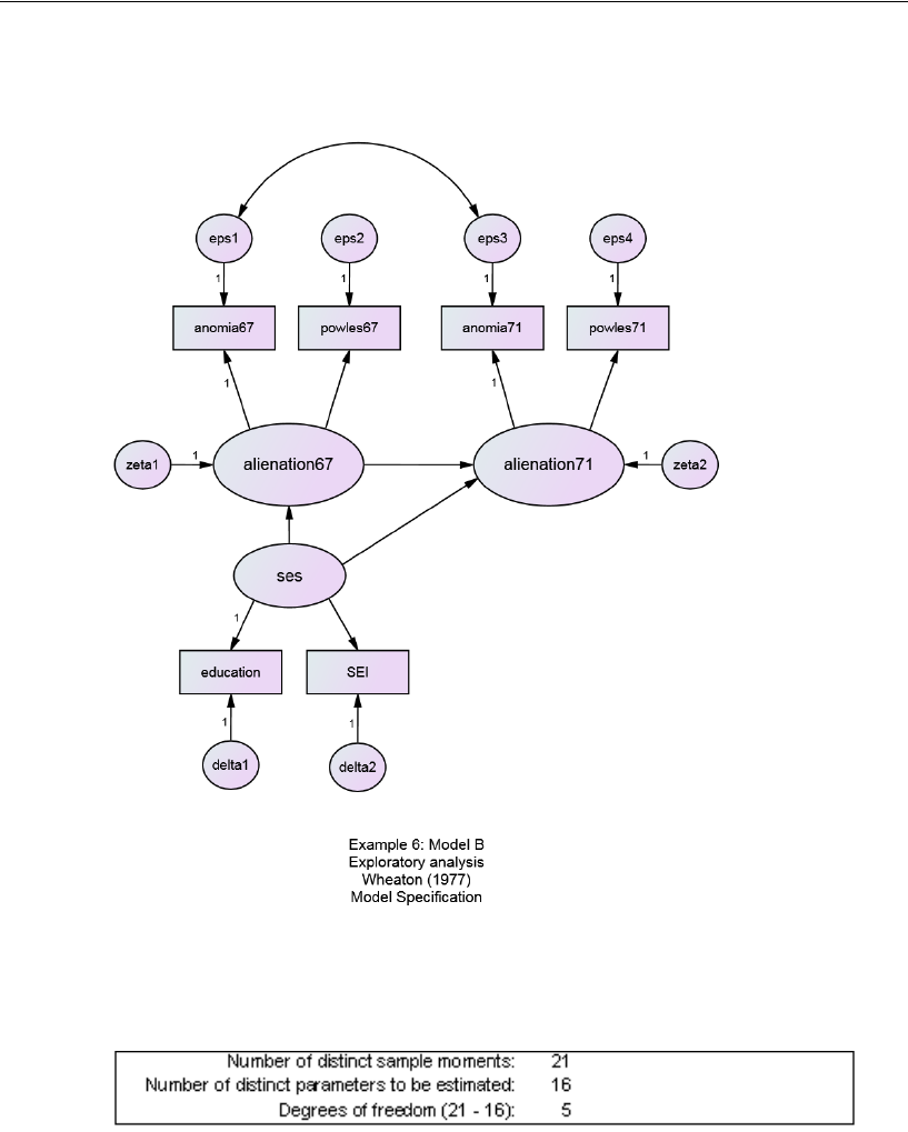
110
Example 6
The path diagram for Model B is contained in the file Ex06-b.amw.
Text Output
The added covariance between eps1 and eps3 decreases the degrees of freedom by 1.

111
Exploratory Analysis
The chi-square statistic is reduced by substantially more than the promised 40.911.
Model B cannot be rejected. Since the fit of Model B is so good, we will not pursue the
possibility, mentioned earlier, of allowing eps2 and eps4 to be correlated. (An
argument could be made that a nonzero correlation between eps2 and eps4 should be
allowed in order to achieve a symmetry that is lacking in the Model B.)
The raw parameter estimates must be interpreted cautiously since they would have
been different if different identification constraints had been imposed.
Note the large critical ratio associated with the new covariance path. The covariance
between eps1 and eps3 is clearly different from 0. This explains the poor fit of Model
A, in which that covariance was fixed at 0.
Chi-square = 6.383
Degrees of freedom = 5
Probability level = 0.271
Regression Weights: (Group number 1 - Default model)
Estimate
S.E.
C.R.
PLabel
alienation67 <--- ses -
.550 .053
-
10.294 ***
alienation71 <--- alienation67
.617 .050 12.421 ***
alienation71 <--- ses -
.212 .049
-
4.294 ***
p
owles71
<--- alienation71
.971 .049 19.650 ***
anomia71 <--- alienation71
1.000
p
owles67
<--- alienation67
1.027 .053 19.322 ***
anomia67 <--- alienation67
1.000
education <--- ses
1.000
SEI <--- ses
5.164 .421 12.255 ***
Covariances: (Group number 1 - Default model)
Estimate S.E.
C.R.
P
Label
eps1 <--> eps3
1.886 .240
7.866
***
Variances: (Group number 1 - Default model)
Estimate S.E.
C.R. P Label
ses
6.872 .657 10.458
***
zeta1
4.700 .433 10.864
***
zeta2
3.862 .343 11.257
***
eps1
5.059
.371
13.650
***
eps2
2.211 .317 6.968
***
eps3
4.806 .395 12.173
***
eps4
2.681 .329 8.137
***
delta1
2.728 .516 5.292
***
delta2
266.567 18.173 14.668
***
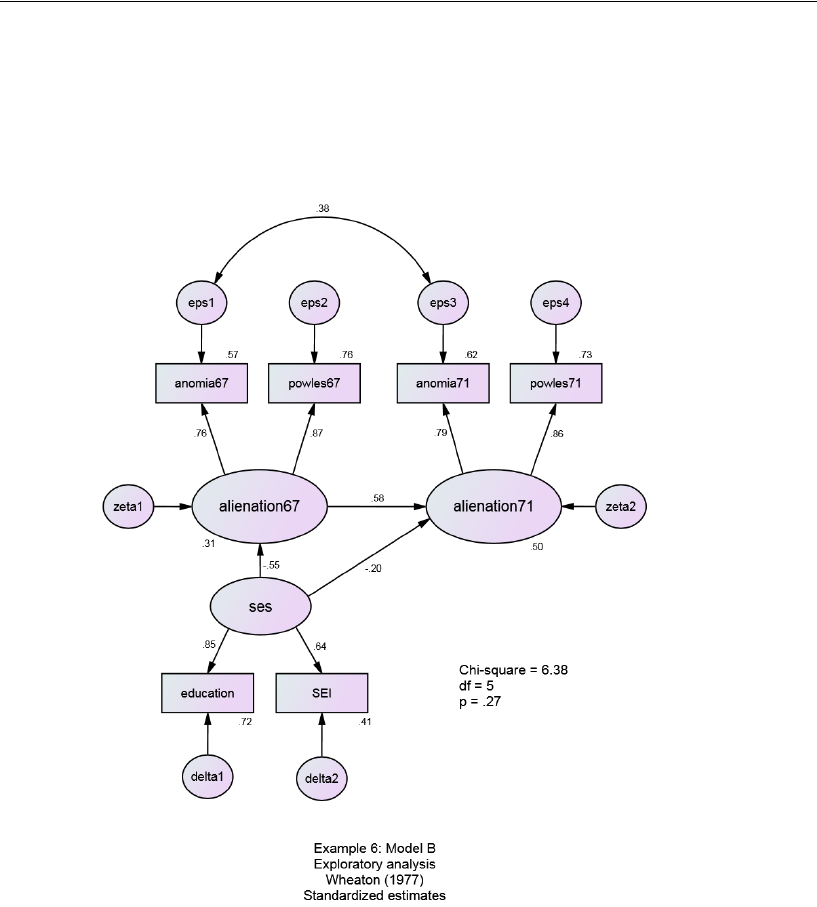
112
Example 6
Graphics Output for Model B
The following path diagram displays the standardized estimates and the squared
multiple correlations:
Because the error variables in the model represent more than just measurement error,
the squared multiple correlations cannot be interpreted as estimates of reliabilities.
Rather, each squared multiple correlation is an estimate of a lower bound on the
corresponding reliability. Take education, for example. Ses accounts for 72% of its
variance. Because of this, you would estimate its reliability to be at least 0.72.
Considering that education is measured in years of schooling, it seems likely that its
reliability is much greater.

113
Exploratory Analysis
Misuse of Modification Indices
In trying to improve upon a model, you should not be guided exclusively by
modification indices. A modification should be considered only if it makes theoretical
or common sense.
A slavish reliance on modification indices without such a limitation amounts to
sorting through a very large number of potential modifications in search of one that
provides a big improvement in fit. Such a strategy is prone, through capitalization on
chance, to producing an incorrect (and absurd) model that has an acceptable chi-square
value. This issue is discussed by MacCallum (1986) and by MacCallum, Roznowski,
and Necowitz (1992).
Improving a Model by Adding New Constraints
Modification indices suggest ways of improving a model by increasing the number of
parameters in such a way that the chi-square statistic falls faster than its degrees of
freedom. This device can be misused, but it has a legitimate place in exploratory
studies. There is also another trick that can be used to produce a model with a more
acceptable chi-square value. This technique introduces additional constraints in such a
way as to produce a relatively large increase in degrees of freedom, coupled with a
relatively small increase in the chi-square statistic. Many such modifications can be
roughly evaluated by looking at the critical ratios in the C.R. column. We have already
seen (in Example 1) how a single critical ratio can be used to test the hypothesis that a
single population parameter equals 0. However, the critical ratio also has another
interpretation. The square of the critical ratio of a parameter is, approximately, the
amount by which the chi-square statistic will increase if the analysis is repeated with
that parameter fixed at 0.
Calculating Critical Ratios
If two parameter estimates turn out to be nearly equal, you might be able to improve
the chi-square test of fit by postulating a new model where those two parameters are
specified to be exactly equal. To assist in locating pairs of parameters that do not differ
significantly from each other, Amos provides a critical ratio for every pair of
parameters.

114
Example 6
EFrom the menus, choose View > Analysis Properties.
EIn the Analysis Properties dialog, click the Output tab.
EEnable the Critical ratios for differences check box.
When Amos calculates critical ratios for parameter differences, it generates names for
any parameters that you did not name during model specification. The names are
displayed in the text output next to the parameter estimates.
Here are the parameter estimates for Model B. The parameter names generated by
Amos are in the Label column.
Regression Weights: (Group number 1 - Default model)
Estimate S.E.
C.R.
P Label
alienation67 <--- ses -
.550 .053
-
10.294 *** par_6
alienation71 <--- alienation67
.617 .050 12.421 *** par_4
alienation71 <--- ses -
.212 .049
-
4.294 *** par_5
p
owles71
<--- alienation71
.971 .049 19.650 *** par_1
anomia71 <--- alienation71
1.000
p
owles67
<--- alienation67
1.027 .053 19.322 *** par_2
anomia67 <--- alienation67
1.000
education <--- ses
1.000
SEI <--- ses
5.164 .421 12.255 *** par_3
Covariances: (Group number 1 - Default model)
Estimate
S.E. C.R.
P Label
eps1 <--> eps3
1.886 .240 7.866
*** par_7
Variances: (Group number 1 - Default model)
Estimate
S.E.
C.R. P
Label
ses
6.872
.657
10.458
***
par_8
zeta1
4.700
.433
10.864
*** par
_
9
zeta2
3.862
.343
11.257
***
par_10
eps1
5.059
.371
13.650
***
par_11
eps2
2.211
.317
6.968
***
par_12
eps3
4.806
.395
12.173
***
par_13
eps4
2.681
.329
8.137
***
par_14
delta1
2.728
.516
5.292
***
par_15
delta2 266.567 18.173
14.668
***
par_16

115
Exploratory Analysis
The parameter names are needed for interpreting the critical ratios in the following table:
Ignoring the 0’s down the main diagonal, the table of critical ratios contains 120
entries, one for each pair of parameters. Take the number 0.877 near the upper left
corner of the table. This critical ratio is the difference between the parameters labeled
Critical Ratios for Differences between Parameters (Default model)
par_1 par_2 par_3 par_4 par_5 par_6
par_1 .000
par_2 .877 .000
par_3 9.883 9.741 .000
par_4 -4.429 -5.931 -10.579 .000
par_5 -17.943 -16.634 -12.284 -18.098 .000
par_6 -22.343 -26.471 -12.661 -17.300 -5.115 .000
par_7 3.903 3.689 -6.762 5.056 8.490 10.124
par_8 8.955 8.866 1.707 9.576 10.995 11.797
par_9 8.364 7.872 -.714 9.256 11.311 12.047
par_10 7.781 8.040 -2.362 9.470 11.683 12.629
par_11 11.106 11.705 -.186 11.969 14.039 15.431
par_12 3.826 3.336 -5.599 4.998 7.698 8.253
par_13 10.425 9.659 -.621 10.306 12.713 13.575
par_14 4.697 4.906 -4.642 6.353 8.554 9.602
par_15 3.393 3.283 -7.280 4.019 5.508 5.975
par_16 14.615 14.612 14.192 14.637 14.687 14.712
Critical Ratios for Differences between Parameters (Default model)
par_7 par_8 par_9 par_10 par_11 par_12
par_7 .000
par_8 7.128 .000
par_9 5.388 -2.996 .000
par_10 4.668 -4.112 -1.624 .000
par_11 9.773 -2.402 .548 2.308 .000
par_12 .740 -6.387 -5.254 -3.507 -4.728 .000
par_13 8.318 -2.695 .169 1.554 -.507 5.042
par_14 1.798 -5.701 -3.909 -2.790 -4.735 .999
par_15 1.482 -3.787 -2.667 -1.799 -3.672 .855
par_16 14.563 14.506 14.439 14.458 14.387 14.544
Critical Ratios for Differences between Parameters (Default model)
par_13 par_14 par_15 par_16
par_13 .000
par_14 -3.322 .000
par_15 -3.199 .077 .000
par_16 14.400 14.518 14.293 .000

116
Example 6
par_1 and par_2 divided by the estimated standard error of this difference. These two
parameters are the regression weights for powles71 <– alienation71 and
powles67 <– alienation67.
Under the distribution assumptions stated on p. 36, the critical ratio statistic can be
evaluated using a table of the standard normal distribution to test whether the two
parameters are equal in the population. Since 0.877 is less in magnitude than 1.96, you
would not reject, at the 0.05 level, the hypothesis that the two regression weights are
equal in the population.
The square of the critical ratio for differences between parameters is approximately
the amount by which the chi-square statistic would increase if the two parameters were
set equal to each other. Since the square of 0.877 is 0.769, modifying Model B to
require that the two regression weights have equal estimates would yield a chi-square
value of about . The degrees of freedom for the new model
would be 6 instead of 5. This would be an improved fit ( versus
for Model B), but we can do much better than that.
Let’s look for the smallest critical ratio. The smallest critical ratio in the table is
0.077, for the parameters labeled par_14 and par_15. These two parameters are the
variances of eps4 and delta1. The square of 0.077 is about 0.006. A modification of
Model B that assumes eps4 and delta1 to have equal variances will result in a
chi-square value that exceeds 6.383 by about 0.006, but with 6 degrees of freedom
instead of 5. The associated probability level would be about 0.381. The only problem
with this modification is that there does not appear to be any justification for it; that is,
there does not appear to be any a priori reason for expecting eps4 and delta1 to have
equal variances.
We have just been discussing a misuse of the table of critical ratios for differences.
However, the table does have a legitimate use in the quick examination of a small
number of hypotheses. As an example of the proper use of the table, consider the fact
that observations on anomia67 and anomia71 were obtained by using the same
instrument on two occasions. The same goes for powles67 and powles71. It is plausible
that the tests would behave the same way on the two occasions. The critical ratios for
differences are consistent with this hypothesis. The variances of eps1 and eps3 (par_11
and par_13) differ with a critical ratio of –0.51. The variances of eps2 and eps4 (par_12
and par_14) differ with a critical ratio of 1.00. The weights for the regression of
powerlessness on alienation (par_1 and par_2) differ with a critical ratio of 0.88. None
of these differences, taken individually, is significant at any conventional significance
level. This suggests that it may be worthwhile to investigate more carefully a model in
which all three differences are constrained to be 0. We will call this new model Model C.
6.383 0.769 7.172=+
p0.307=
p0.275=
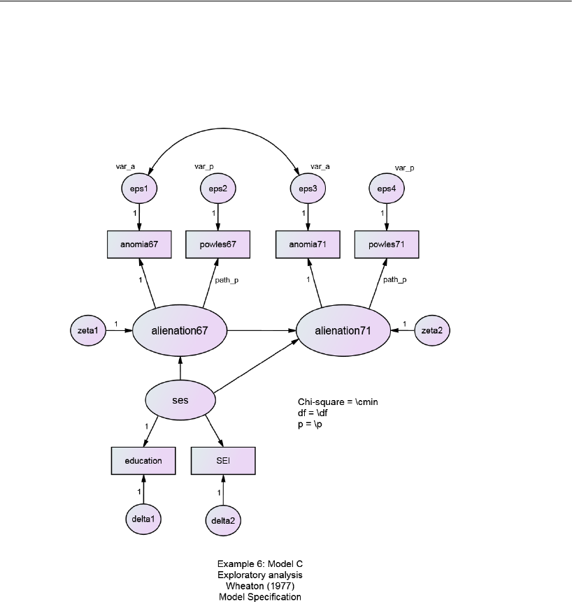
117
Exploratory Analysis
Model C for the Wheaton Data
Here is the path diagram for Model C from the file Ex06–c.amw:
The label path_p requires the regression weight for predicting powerlessness from
alienation to be the same in 1971 as it is in 1967. The label var_a is used to specify
that eps1 and eps3 have the same variance. The label var_p is used to specify that eps2
and eps4 have the same variance.
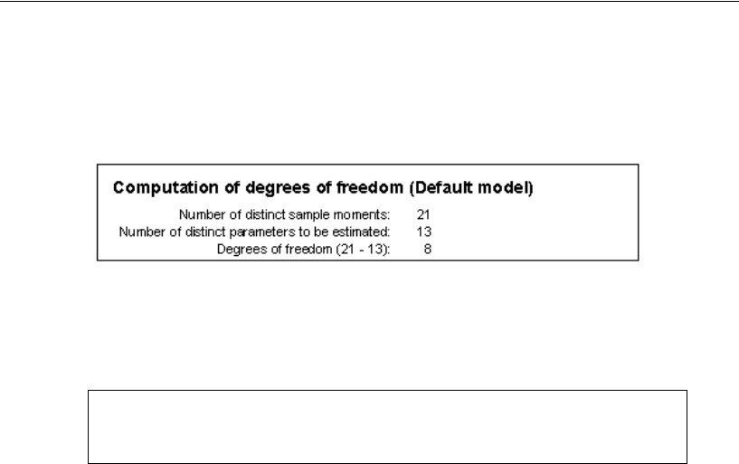
118
Example 6
Results for Model C
Model C has three more degrees of freedom than Model B:
Testing Model C
As expected, Model C has an acceptable fit, with a higher probability level than Model B:
You can test Model C against Model B by examining the difference in chi-square
values ( ) and the difference in degrees of freedom ( ).
A chi-square value of 1.118 with 3 degrees of freedom is not significant.
Chi-square = 7.501
Degrees of freedom = 8
Probability level = 0.484
7.501 6.383 1.118=–
85 3=–

119
Exploratory Analysis
Parameter Estimates for Model C
The standardized estimates for Model C are as follows:
Multiple Models in a Single Analysis
Amos allows for the fitting of multiple models in a single analysis. This allows Amos
to summarize the results for all models in a single table. It also allows Amos to perform
a chi-square test for nested model comparisons. In this example, Models A, B, and C
can be fitted in a single analysis by noting that Models A and C can each be obtained
by constraining the parameters of Model B.
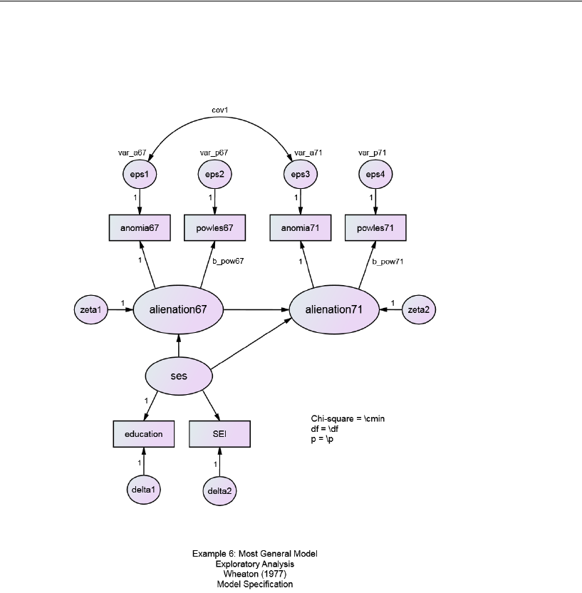
120
Example 6
In the following path diagram from the file Ex06-all.amw, parameters of Model B that
need to be constrained to yield Model A or Model C have been assigned names:
Seven parameters in this path diagram are named: var_a67, var_p67, var_a71,
var_p71, b_pow67, b_pow71, and cov1. The naming of the parameters does not
constrain any of the parameters to be equal to each other because no two parameters
were given the same name. However, having names for the variables allows
constraining them in various ways, as will now be demonstrated.
Using the parameter names just introduced, Model A can be obtained from the most
general model (Model B) by requiring cov1 = 0.
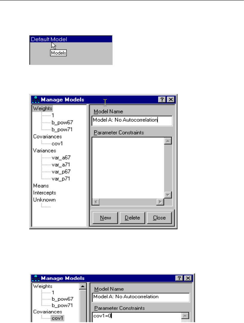
121
Exploratory Analysis
EIn the Models panel to the left of the path diagram, double-click Default Model.
The Manage Models dialog appears.
EIn the Model Name text box, type Model A: No Autocorrelation.
EDouble-click cov1 in the left panel.
Notice that cov1 appears in the Parameter Constraints box.
EType cov1 =0 in the Parameter Constraints box.
This completes the specification of Model A.
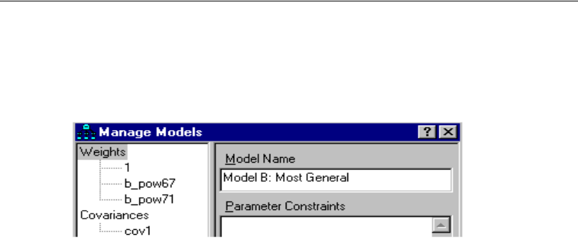
122
Example 6
EIn the Manage Models dialog, click New.
EIn the Model Name text box, type Model B: Most General.
Model B has no constraints other than those in the path diagram, so you can proceed
immediately to Model C.
EClick New.
EIn the Model Name text box, type Model C: Time-Invariance.
EIn the Parameter Constraints box, type:
b_pow67 = b_pow71
var_a67 = var_a71
var_p67 = var_p71
For the sake of completeness, a fourth model (Model D) will be introduced, combining
the single constraint of Model A with the three constraints of Model C. Model D can
be specified without retyping the constraints.
EClick New.
EIn the Model Name text box, type Model D: A and C Combined.
EIn the Parameter Constraints box, type:
Model A: No Autocorrelation
Model C: Time-Invariance
These lines tell Amos that Model D incorporates the constraints of both Model A and
Model C.
Now that we have set up the parameter constraints for all four models, the final step
is to perform the analysis and view the output.
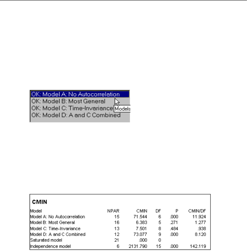
123
Exploratory Analysis
Output from Multiple Models
Viewing Graphics Output for Individual Models
When you are fitting multiple models, use the Models panel to display the diagrams
from different models. The Models panel is just to the left of the path diagram. To
display a model, click its name.
Viewing Fit Statistics for All Four Models
EFrom the menus, choose View > Text Output.
EIn the tree diagram in the upper left pane of the Amos Output window, click Model Fit.
The following is the portion of the output that shows the chi-square statistic:
The CMIN column contains the minimum discrepancy for each model. In the case of
maximum likelihood estimation (the default), the CMIN column contains the
chi-square statistic. The p column contains the corresponding upper-tail probability for
testing each model.
For nested pairs of models, Amos provides tables of model comparisons, complete
with chi-square difference tests and their associated p values.
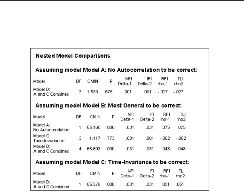
124
Example 6
EIn the tree diagram in the upper left pane of the Amos Output window, click Model
Comparison.
This table shows, for example, that Model C does not fit significantly worse than
Model B ( ). In other words, assuming that Model B is correct, you would
accept the hypothesis of time invariance.
On the other hand, the table shows that Model A fits significantly worse than Model
B ( ). In other words, assuming that Model B is correct, you would reject the
hypothesis that eps1 and eps3 are uncorrelated.
Obtaining Optional Output
The variances and covariances among the observed variables can be estimated under
the assumption that Model C is correct.
EFrom the menus, choose View > Analysis Properties.
EIn the Analysis Properties dialog, click the Output tab.
p0.773=
p0.000=

125
Exploratory Analysis
ESelect Implied moments (a check mark appears next to it).
ETo obtain the implied variances and covariances for all the variables in the model
except error variables, select All implied moments.
For Model C, selecting All implied moments gives the following output:
The implied variances and covariances for the observed variables are not the same as
the sample variances and covariances. As estimates of the corresponding population
values, the implied variances and covariances are superior to the sample variances and
covariances (assuming that Model C is correct).
If you enable both the Standardized estimates and All implied moments check boxes
in the Analysis Properties dialog, Amos will give you the implied correlation matrix
of all variables as well as the implied covariance matrix.
Implied (for all variables) Covariances (Group number 1 - Model C: Time-Invariance)
ses alienation67 alienation71
SEI
education
ses
6.858
alienation67 -
3.838 6.914
alienation71 -
3.720 4.977 7.565
SEI
35.484
-
19.858
-
19.246
449.805
education
6.858
-
3.838
-
3.720 35.484 9.600
powles71 -
3.717 4.973 7.559
-
19.231
-
3.717
anomia71 -
3.720 4.977 7.565
-
19.246
-
3.720
powles67 -
3.835 6.909 4.973
-
19.842
-
3.835
anomia67 -
3.838 6.914 4.977
-
19.858
-
3.838
powles71 anomia71 powles67 anomia67
powles71 9.989
anomia71 7.559
12.515
powles67 4.969
4.973
9.339
anomia67 4.973
6.865
6.909 11.864

126
Example 6
The matrix of implied covariances for all variables in the model can be used to carry
out a regression of the unobserved variables on the observed variables. The resulting
regression weight estimates can be obtained from Amos by enabling the Factor score
weights check box. Here are the estimated factor score weights for Model C:
The table of factor score weights has a separate row for each unobserved variable, and
a separate column for each observed variable. Suppose you wanted to estimate the ses
score of an individual. You would compute a weighted sum of the individual’s six
observed scores using the six weights in the ses row of the table.
Obtaining Tables of Indirect, Direct, and Total Effects
The coefficients associated with the single-headed arrows in a path diagram are
sometimes called direct effects. In Model C, for example, ses has a direct effect on
alienation71. In turn, alienation71 has a direct effect on powles71. Ses is then said to
have an indirect effect (through the intermediary of alienation71) on powles71.
EFrom the menus, choose View > Analysis Properties.
EIn the Analysis Properties dialog, click the Output tab.
EEnable the Indirect, direct & total effects check box.
Factor Score Weights (Group number 1 - Model C: Time-Invariance)
SEI education powles71
anomia71
p
owles67
anomia67
ses
.029 .542
-
.055
-
.016
-
.069
-.028
alienation67 -
.003
-
.061 .134
-
.027 .471
.242
alienation71 -
.003
-
.049 .491 .253 .134
-.031

127
Exploratory Analysis
For Model C, the output includes the following table of total effects:
The first row of the table indicates that alienation67 depends, directly or indirectly, on
ses only. The total effect of ses on alienation67 is –0.56. The fact that the effect is
negative means that, all other things being equal, relatively high ses scores are
associated with relatively low alienation67 scores. Looking in the fifth row of the table,
powles71 depends, directly or indirectly, on ses, alienation67, and alienation71. Low
scores on ses, high scores on alienation67, and high scores on alienation71 are
associated with high scores on powles71. See Fox (1980) for more help in interpreting
direct, indirect, and total effects.
Total Effects (Group number 1 - Model C: Time-Invariance)
ses
alienation67
alienation71
alienation67 -
.560
.000
.000
alienation71 -
.542
.607
.000
SEI
5.174
.000
.000
education
1.000
.000
.000
powles71 -
.542
.607
.999
anomia71 -
.542
.607
1.000
powles67 -
.559
.999
.000
anomia67 -
.560 1.000 .000

128
Example 6
Modeling in VB.NET
Model A
The following program fits Model A. It is saved as Ex06–a.vb.
Sub Main()
Dim Sem As New AmosEngine
Try
Sem.TextOutput()
Sem.Mods(4)
Sem.BeginGroup(Sem.AmosDir & "Examples\Wheaton.sav")
Sem.AStructure("anomia67 <--- alienation67 (1)")
Sem.AStructure("anomia67 <--- eps1 (1)")
Sem.AStructure("powles67 <--- alienation67")
Sem.AStructure("powles67 <--- eps2 (1)")
Sem.AStructure("anomia71 <--- alienation71 (1)")
Sem.AStructure("anomia71 <--- eps3 (1)")
Sem.AStructure("powles71 <--- alienation71")
Sem.AStructure("powles71 <--- eps4 (1)")
Sem.AStructure("alienation67 <--- ses")
Sem.AStructure("alienation67 <--- zeta1 (1)")
Sem.AStructure("alienation71 <--- alienation67")
Sem.AStructure("alienation71 <--- ses")
Sem.AStructure("alienation71 <--- zeta2 (1)")
Sem.AStructure("education <--- ses (1)")
Sem.AStructure("education <--- delta1 (1)")
Sem.AStructure("SEI <--- ses")
Sem.AStructure("SEI <--- delta2 (1)")
Sem.FitModel()
Finally
Sem.Dispose()
End Try
End Sub

129
Exploratory Analysis
Model B
The following program fits Model B. It is saved as Ex06–b.vb.
Sub Main()
Dim Sem As New AmosEngine
Try
Sem.TextOutput()
Sem.Standardized()
Sem.Smc()
Sem.Crdiff()
Sem.BeginGroup(Sem.AmosDir & "Examples\Wheaton.sav")
Sem.AStructure("anomia67 <--- alienation67 (1)")
Sem.AStructure("anomia67 <--- eps1 (1)")
Sem.AStructure("powles67 <--- alienation67")
Sem.AStructure("powles67 <--- eps2 (1)")
Sem.AStructure("anomia71 <--- alienation71 (1)")
Sem.AStructure("anomia71 <--- eps3 (1)")
Sem.AStructure("powles71 <--- alienation71")
Sem.AStructure("powles71 <--- eps4 (1)")
Sem.AStructure("alienation67 <--- ses")
Sem.AStructure("alienation67 <--- zeta1 (1)")
Sem.AStructure("alienation71 <--- alienation67")
Sem.AStructure("alienation71 <--- ses")
Sem.AStructure("alienation71 <--- zeta2 (1)")
Sem.AStructure("education <--- ses (1)")
Sem.AStructure("education <--- delta1 (1)")
Sem.AStructure("SEI <--- ses")
Sem.AStructure("SEI <--- delta2 (1)")
Sem.AStructure("eps1 <---> eps3") ' Autocorrelated residual
Sem.FitModel()
Finally
Sem.Dispose()
End Try
End Sub

130
Example 6
Model C
The following program fits Model C. It is saved as Ex06–c.vb.
Sub Main()
Dim Sem As New AmosEngine
Try
Sem.TextOutput()
Sem.Standardized()
Sem.Smc()
Sem.AllImpliedMoments()
Sem.FactorScoreWeights()
Sem.TotalEffects()
Sem.BeginGroup(Sem.AmosDir & "Examples\Wheaton.sav")
Sem.AStructure("anomia67 <--- alienation67 (1)")
Sem.AStructure("anomia67 <--- eps1 (1)")
Sem.AStructure("powles67 <--- alienation67 (path_p)")
Sem.AStructure("powles67 <--- eps2 (1)")
Sem.AStructure("anomia71 <--- alienation71 (1)")
Sem.AStructure("anomia71 <--- eps3 (1)")
Sem.AStructure("powles71 <--- alienation71 (path_p)")
Sem.AStructure("powles71 <--- eps4 (1)")
Sem.AStructure("alienation67 <--- ses")
Sem.AStructure("alienation67 <--- zeta1 (1)")
Sem.AStructure("alienation71 <--- alienation67")
Sem.AStructure("alienation71 <--- ses")
Sem.AStructure("alienation71 <--- zeta2 (1)")
Sem.AStructure("education <--- ses (1)")
Sem.AStructure("education <--- delta1 (1)")
Sem.AStructure("SEI <--- ses")
Sem.AStructure("SEI <--- delta2 (1)")
Sem.AStructure("eps3 <--> eps1")
Sem.AStructure("eps1 (var_a)")
Sem.AStructure("eps2 (var_p)")
Sem.AStructure("eps3 (var_a)")
Sem.AStructure("eps4 (var_p)")
Sem.FitModel()
Finally
Sem.Dispose()
End Try
End Sub

131
Exploratory Analysis
Fitting Multiple Models
To fit all three models, A, B, and C in a single analysis, start with the following
program, which assigns unique names to some parameters:
Sub Main()
Dim Sem As New AmosEngine
Try
Sem.TextOutput()
Sem.Standardized()
Sem.Smc()
Sem.AllImpliedMoments()
Sem.TotalEffects()
Sem.FactorScoreWeights()
Sem.Mods(4)
Sem.Crdiff()
Sem.BeginGroup(Sem.AmosDir & "Examples\Wheaton.sav")
Sem.AStructure("anomia67 <--- alienation67 (1)")
Sem.AStructure("anomia67 <--- eps1 (1)")
Sem.AStructure("powles67 <--- alienation67 (b_pow67)")
Sem.AStructure("powles67 <--- eps2 (1)")
Sem.AStructure("anomia71 <--- alienation71 (1)")
Sem.AStructure("anomia71 <--- eps3 (1)")
Sem.AStructure("powles71 <--- alienation71 (b_pow71)")
Sem.AStructure("powles71 <--- eps4 (1)")
Sem.AStructure("alienation67 <--- ses")
Sem.AStructure("alienation67 <--- zeta1 (1)")
Sem.AStructure("alienation71 <--- alienation67")
Sem.AStructure("alienation71 <--- ses")
Sem.AStructure("alienation71 <--- zeta2 (1)")
Sem.AStructure("education <--- ses (1)")
Sem.AStructure("education <--- delta1 (1)")
Sem.AStructure("SEI <--- ses")
Sem.AStructure("SEI <--- delta2 (1)")
Sem.AStructure("eps3 <--> eps1 (cov1)")
Sem.AStructure("eps1 (var_a67)")
Sem.AStructure("eps2 (var_p67)")
Sem.AStructure("eps3 (var_a71)")
Sem.AStructure("eps4 (var_p71)")
Sem.FitModel()
Finally
Sem.Dispose()
End Try
End Sub

Since the parameter names are unique, naming the parameters does not constrain them.
However, naming the parameters does permit imposing constraints through the use of
the Model method. Adding the following lines to the program, in place of the
Sem.FitModel line, will fit the model four times, each time with a different set of
parameter constraints:
The first line defines a version of the model called Model A: No Autocorrelation in which
the parameter called cov1 is fixed at 0.
The second line defines a version of the model called Model B: Most General in which
no additional constraints are imposed on the model parameters.
The third use of the Model method defines a version of the model called Model C:
Time-Invariance that imposes the equality constraints:
b_pow67 = b_pow71
var_a67 = var_a71
var_p67 = var_p71
The fourth use of the Model method defines a version of the model called Model D: A
and C Combined that combines the single constraint of Model A with the three
constraints of Model C.
The last model specification (Model D) shows how earlier model specifications can
be used in the definition of a new, more constrained model.
In order to fit all models at once, the FitAllModels method has to be used instead of
FitModel. The FitModel method fits a single model only. By default, it fits the first
model, which in this example is Model A. You could use FitModel(1) to fit the first
model, or FitModel(2) to fit the second model. You could also use, say, FitModel(“Model
C: Time-Invariance”) to fit Model C.
Ex06–all.vb contains a program that fits all four models.
Sem.Model("Model A: No Autocorrelation", "cov1 = 0")
Sem.Model("Model B: Most General", "")
Sem.Model("Model C: Time-Invariance", _
"b_pow67 = b_pow71;var_a67 = var_a71;var_p67 = var_p71")
Sem.Model("Model D: A and C Combined", _
"Model A: No Autocorrelation;Model C: Time-Invariance")
Sem.FitAllModels()

133
Example
7
A Nonrecursive Model
Introduction
This example demonstrates structural equation modeling with a nonrecursive model.
About the Data
Felson and Bohrnstedt (1979) studied 209 girls from sixth through eighth grade. They
made measurements on the following variables:
Variables Description
academic Perceived academic ability, a sociometric measure based on the item
Name who you think are your three smartest classmates
athletic Perceived athletic ability, a sociometric measure based on the item
Name three of your classmates who you think are best at sports
attract
Perceived attractiveness, a sociometric measure based on the item
Name the three girls in the classroom who you think are the most
good-looking (excluding yourself)
GPA Grade point average
height Deviation of height from the mean height for a subject’s grade and
sex
weight Weight, adjusted for height
rating Ratings of physical attractiveness obtained by having children from
another city rate photographs of the subjects
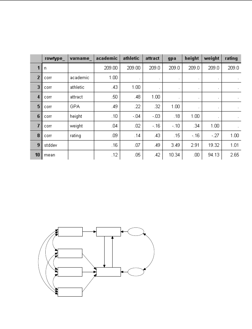
134
Example 7
Sample correlations, means, and standard deviations for these six variables are
contained in the SPSS Statistics file, Fels_fem.sav. Here is the data file as it appears in
the SPSS Statistics Data Editor:
The sample means are not used in this example.
Felson and Bohrnstedt’s Model
Felson and Bohrnstedt proposed the following model for six of their seven measured
variables:
GPA
height
rating
weight
academic
attract
error1
error2
1
1
Example 7
A nonrecursive model
Felson and Bohrnstedt (1979)
(Female subjects)
Model Specification

135
A Nonrecursive Model
Perceived academic performance is modeled as a function of GPA and perceived
attractiveness (attract). Perceived attractiveness, in turn, is modeled as a function of
perceived academic performance, height, weight, and the rating of attractiveness by
children from another city. Particularly noteworthy in this model is that perceived
academic ability depends on perceived attractiveness, and vice versa. A model with
these feedback loops is called nonrecursive (the terms recursive and nonrecursive
were defined earlier in Example 4). The current model is nonrecursive because it is
possible to trace a path from attract to academic and back. This path diagram is saved
in the file Ex07.amw.
Model Identification
We need to establish measurement units for the two unobserved variables, error1 and
error2, for identification purposes. The preceding path diagram shows two regression
weights fixed at 1. These two constraints are enough to make the model identified.
Results of the Analysis
Text Output
The model has two degrees of freedom, and there is no significant evidence that the
model is wrong.
Chi-square = 2.761
Degrees of freedom = 2
Probability level = 0.251

136
Example 7
There is, however, some evidence that the model is unnecessarily complicated, as
indicated by some exceptionally small critical ratios in the text output.
Judging by the critical ratios, you see that each of these three null hypotheses would be
accepted at conventional significance levels:
Perceived attractiveness does not depend on height (critical ratio = 0.050).
Perceived academic ability does not depend on perceived attractiveness (critical
ratio = –0.039).
The residual variables error1 and error2 are uncorrelated (critical ratio =
–0.382).
Strictly speaking, you cannot use the critical ratios to test all three hypotheses at once.
Instead, you would have to construct a model that incorporates all three constraints
simultaneously. This idea will not be pursued here.
The raw parameter estimates reported above are not affected by the identification
constraints (except for the variances of error1 and error2). They are, of course,
affected by the units in which the observed variables are measured. By contrast, the
standardized estimates are independent of all units of measurement.
Regression Weights: (Group number 1 - Default model)
Estimate
S.E. C.R. P Label
academic
<---
GPA .023
.004 6.241 ***
attract <---
height .000
.010 .050 .960
attract <---
weight -.002
.001 -1.321 .186
attract <---
rating .176
.027 6.444 ***
attract <---
academic
1.607
.349 4.599 ***
academic
<---
attract -.002
.051 -.039 .969
Covariances: (Group number 1 - Default model)
Estimate
S.E. C.R. P Label
GPA <-->
rating
.526
.246 2.139 .032
height
<-->
rating
-.468
.205 -2.279 .023
GPA <-->
weight
-6.710
4.676 -1.435 .151
GPA <-->
height
1.819
.712 2.555 .011
height
<-->
weight
19.024
4.098 4.643 ***
weight
<-->
rating
-5.243
1.395 -3.759 ***
error1
<-->
error2
-.004
.010 -.382 .702
Variances: (Group number 1 - Default model)
Estimate
S.E.
C.R. P Label
GPA
12.122
1.189
10.198 ***
height
8.428
.826
10.198 ***
weight
371.476
36.426
10.198 ***
rating
1.015
.100
10.198 ***
error1
.019
.003
5.747 ***
error2
.143
.014
9.974 ***

137
A Nonrecursive Model
Obtaining Standardized Estimates
Before you perform the analysis, do the following:
EFrom the menus, choose View > Analysis Properties.
EIn the Analysis Properties dialog, click the Output tab.
ESelect Standardized estimates (a check mark appears next to it).
EClose the dialog.
Here it can be seen that the regression weights and the correlation that we discovered
earlier to be statistically insignificant are also, speaking descriptively, small.
Obtaining Squared Multiple Correlations
The squared multiple correlations, like the standardized estimates, are independent of
units of measurement. To obtain squared multiple correlations, do the following before
you perform the analysis:
EFrom the menus, choose View > Analysis Properties.
Standardized Regression Weights: (Group number 1 -
Default model)
Estimate
academic
<---
GPA .492
attract <---
height .003
attract <---
weight -.078
attract <---
rating .363
attract <---
academic .525
academic
<---
attract -.006
Correlations: (Group number 1 - Default model)
Estimate
GPA <-->
rating .150
height
<-->
rating -.160
GPA <-->
weight -.100
GPA <-->
height .180
height
<-->
weight .340
weight
<-->
rating -.270
error1
<-->
error2 -.076
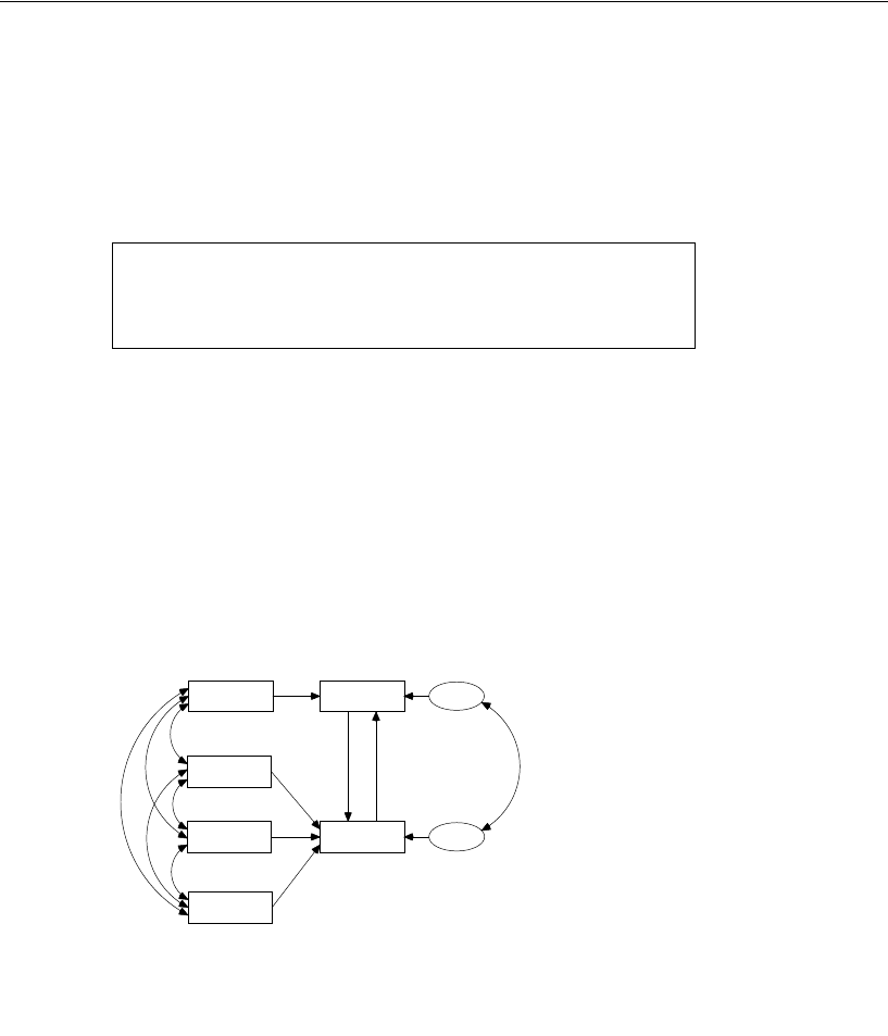
138
Example 7
EIn the Analysis Properties dialog, click the Output tab.
ESelect Squared multiple correlations (a check mark appears next to it).
EClose the dialog.
The squared multiple correlations show that the two endogenous variables in this
model are not predicted very accurately by the other variables in the model. This goes
to show that the chi-square test of fit is not a measure of accuracy of prediction.
Graphics Output
Here is the path diagram output displaying standardized estimates and squared
multiple correlations:
Squared Multiple Correlations: (Group number 1 -
Default model)
Estimate
attract
.402
academic
.236
GPA
height
rating
weight
.24
academic
.40
attract
.49
.00
-.08
.36
error1
error2
.15
-.16
-.10
.18
.34
-.27
.52 -.01 -.08
Example 7
A nonrecursive model
Felson and Bohrnstedt (1979)
(Female subjects)
Standardized estimates
Chi-square = 2.761 (2 df)
p = .251

139
A Nonrecursive Model
Stability Index
The existence of feedback loops in a nonrecursive model permits certain problems to
arise that cannot occur in recursive models. In the present model, attractiveness
depends on perceived academic ability, which in turn depends on attractiveness, which
depends on perceived academic ability, and so on. This appears to be an infinite
regress, and it is. One wonders whether this infinite sequence of linear dependencies
can actually result in well-defined relationships among attractiveness, academic
ability, and the other variables of the model. The answer is that they might, and then
again they might not. It all depends on the regression weights. For some values of the
regression weights, the infinite sequence of linear dependencies will converge to a set
of well-defined relationships. In this case, the system of linear dependencies is called
stable; otherwise, it is called unstable.
Note: You cannot tell whether a linear system is stable by looking at the path diagram.
You need to know the regression weights.
Amos cannot know what the regression weights are in the population, but it estimates
them and, from the estimates, it computes a stability index (Fox, 1980; Bentler and
Freeman, 1983).
If the stability index falls between –1 and +1, the system is stable; otherwise, it is
unstable. In the present example, the system is stable.
To view the stability index for a nonrecursive model:
EClick Notes for Group/Model in the tree diagram in the upper left pane of the Amos
Output window.
An unstable system (with a stability index equal to or greater than 1) is impossible, in
the same sense that, for example, a negative variance is impossible. If you do obtain a
stability index of 1 (or greater than 1), this implies that your model is wrong or that
your sample size is too small to provide accurate estimates of the regression weights.
If there are several loops in a path diagram, Amos computes a stability index for each
one. If any one of the stability indices equals or exceeds 1, the linear system is unstable.
Stability index for the following variables is 0.003:
attract
academic

140
Example 7
Modeling in VB.NET
The following program fits the model of this example. It is saved in the file Ex07.vb.
The final AStructure line is essential to Felson and Bohrnstedt’s model. Without it,
Amos would assume that error1 and error2 are uncorrelated.
You can specify the same model in an equation-like format as follows:
Sub Main()
Dim Sem As New AmosEngine
Try
Sem.TextOutput()
Sem.Standardized()
Sem.Smc()
Sem.BeginGroup(Sem.AmosDir & "Examples\Fels_fem.sav")
Sem.AStructure("academic <--- GPA")
Sem.AStructure("academic <--- attract")
Sem.AStructure("academic <--- error1 (1)")
Sem.AStructure("attract <--- height")
Sem.AStructure("attract <--- weight")
Sem.AStructure("attract <--- rating")
Sem.AStructure("attract <--- academic")
Sem.AStructure("attract <--- error2 (1)")
Sem.AStructure("error2 <--> error1")
Sem.FitModel()
Finally
Sem.Dispose()
End Try
End Sub
Sub Main()
Dim Sem As New AmosEngine
Try
Sem.TextOutput()
Sem.Standardized()
Sem.Smc()
Sem.BeginGroup(Sem.AmosDir & "Examples\Fels_fem.sav")
Sem.AStructure("academic = GPA + attract + error1 (1)")
Sem.AStructure("attract = height + weight + rating + " _
& "academic + error2 (1)")
Sem.AStructure("error2 <--> error1")
Sem.FitModel()
Finally
Sem.Dispose()
End Try
End Sub

141
Example
8
Factor Analysis
Introduction
This example demonstrates confirmatory common factor analysis.
About the Data
Holzinger and Swineford (1939) administered 26 psychological tests to 301 seventh-
and eighth-grade students in two Chicago schools. In the present example, we use
scores obtained by the 73 girls from a single school (the Grant-White school). Here is
a summary of the six tests used in this example:
Tes t E xpl anation
visperc Visual perception scores
cubes Test of spatial visualization
lozenges Test of spatial orientation
paragraph Paragraph comprehension score
sentence Sentence completion score
wordmean Word meaning test score
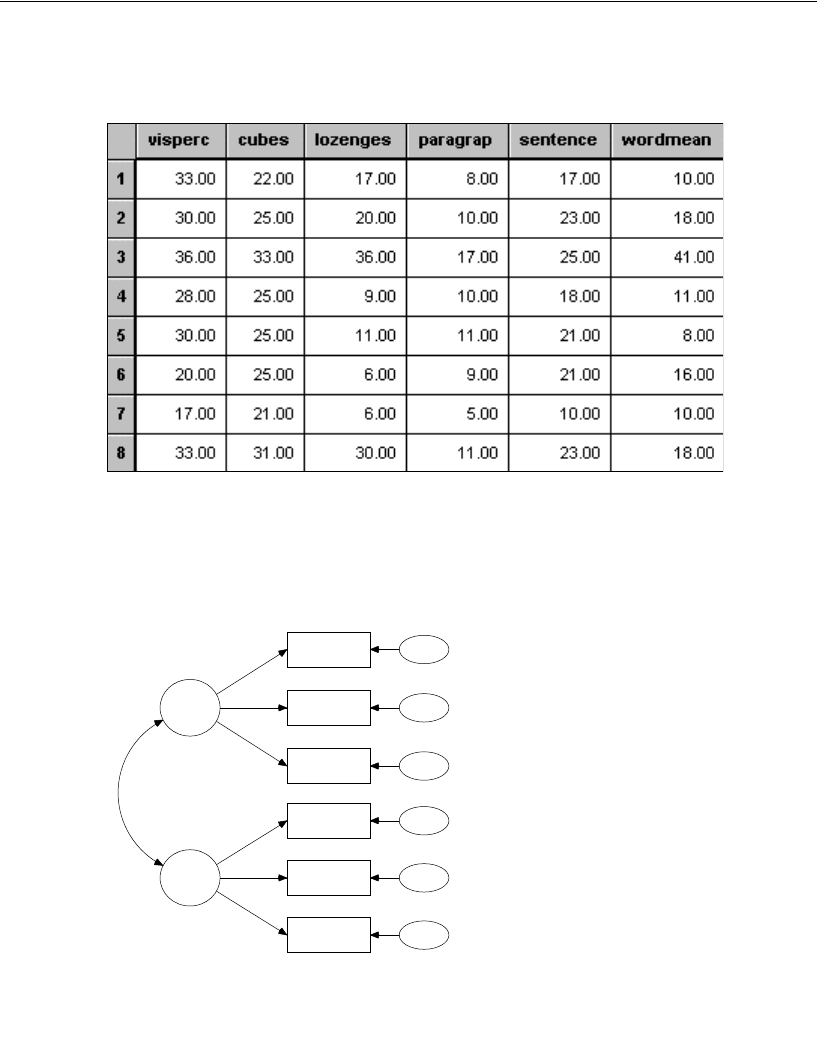
142
Example 8
The file Grnt_fem.sav contains the test scores:
A Common Factor Model
Consider the following model for the six tests:
spatial
visperc
cubes
lozenges
wordmean
paragrap
sentence
err_v
err_c
err_l
err_p
err_s
err_w
verbal
1
1
1
1
1
1
1
1
Example 8
Factor analysis: Girls' sample
Holzinger and Swineford (1939)
Model Specification

143
Factor Analysis
This model asserts that the first three tests depend on an unobserved variable called
spatial. Spatial can be interpreted as an underlying ability (spatial ability) that is not
directly observed. According to the model, performance on the first three tests depends
on this ability. In addition, performance on each of these tests may depend on
something other than spatial ability as well. In the case of visperc, for example, the
unique variable err_v is also involved. Err_v represents any and all influences on
visperc that are not shown elsewhere in the path diagram. Err_v represents error of
measurement in visperc, certainly, but also socioeconomic status, age, physical
stamina, vocabulary, and every other trait or ability that might affect scores on visperc
but that does not appear elsewhere in the model.
The model presented here is a common factor analysis model. In the lingo of
common factor analysis, the unobserved variable spatial is called a common factor,
and the three unobserved variables, err_v, err_c, and err_l, are called unique factors.
The path diagram shows another common factor, verbal, on which the last three tests
depend. The path diagram also shows three more unique factors, err_p, err_s, and
err_w. The two common factors, spatial and verbal, are allowed to be correlated. On
the other hand, the unique factors are assumed to be uncorrelated with each other and
with the common factors. The path coefficients leading from the common factors to the
observed variables are sometimes called factor loadings.
Identification
This model is identified except that, as usual, the measurement scale of each
unobserved variable is indeterminate. The measurement scale of each unobserved
variable can be established arbitrarily by setting its regression weight to a constant,
such as 1, in some regression equation. The preceding path diagram shows how to do
this. In that path diagram, eight regression weights are fixed at 1, which is one fixed
regression weight for each unobserved variable. These constraints are sufficient to
make the model identified.
The proposed model is a particularly simple common factor analysis model, in that
each observed variable depends on just one common factor. In other applications of
common factor analysis, an observed variable can depend on any number of common
factors at the same time. In the general case, it can be very difficult to decide whether
a common factor analysis model is identified or not (Davis, 1993; Jöreskog, 1969,
1979). The discussion of identifiability given in this and earlier examples made the
issue appear simpler than it actually is, giving the impression that the lack of a natural
unit of measurement for unobserved variables is the sole cause of non-identification. It

144
Example 8
is true that the lack of a unit of measurement for unobserved variables is an
ever-present cause of non-identification. Fortunately, it is one that is easy to cure, as
we have done repeatedly.
But other kinds of under-identification can occur for which there is no simple
remedy. Conditions for identifiability have to be established separately for individual
models. Jöreskog and Sörbom (1984) show how to achieve identification of many
models by imposing equality constraints on their parameters. In the case of the factor
analysis model (and many others), figuring out what must be done to make the model
identified requires a pretty deep understanding of the model. If you are unable to tell
whether a model is identified, you can try fitting the model in order to see whether
Amos reports that it is unidentified. In practice, this empirical approach works quite
well, although there are objections to it in principle (McDonald and Krane, 1979), and
it is no substitute for an a priori understanding of the identification status of a model.
Bollen (1989) discusses causes and treatments of many types of non-identification in
his excellent textbook.
Specifying the Model
Amos analyzes the model directly from the path diagram shown on p. 142. Notice that
the model can conceptually be separated into spatial and verbal branches. You can use
the structural similarity of the two branches to accelerate drawing the model.
Drawing the Model
After you have drawn the first branch:
EFrom the menus, choose Edit > Select All to highlight the entire branch.
ETo create a copy of the entire branch, from the menus, choose Edit > Duplicate and drag
one of the objects in the branch to another location in the path diagram.
Be sure to draw a double-headed arrow connecting spatial and verbal. If you leave out
the double-headed arrow, Amos will assume that the two common factors are
uncorrelated. The input file for this example is Ex08.amw.

145
Factor Analysis
Results of the Analysis
Here are the unstandardized results of the analysis. As shown at the upper right corner
of the figure, the model fits the data quite well.
As an exercise, you may wish to confirm the computation of degrees of freedom.
Computation of degrees of freedom: (Default model)
Number of distinct sample moments: 21
Number of distinct parameters to be estimated: 13
Degrees of freedom (21 – 13): 8
23.30
spatial
visperc
cubes
lozenges
wordmean
paragrap
sentence
23.87
err_v
11.60
err_c
28.28
err_l
2.83
err_p
7.97
err_s
19.93
err_w
9.68
verbal
1.00
.61
1.20
1.00
1.33
2.23
1
1
1
1
1
1
7.32
Example 8
Factor analysis: Girls' sample
Holzinger and Swineford (1939)
Unstandardized estimates
Chi-square = 7.853 (8 df)
p = .448

146
Example 8
The parameter estimates, both standardized and unstandardized, are shown next. As
you would expect, the regression weights are positive, as is the correlation between
spatial ability and verbal ability.
Obtaining Standardized Estimates
To get the standardized estimates shown above, do the following before you perform
the analysis:
EFrom the menus, choose View > Analysis Properties.
EIn the Analysis Properties dialog, click the Output tab.
Regression Weights: (Group number 1 - Default model)
Estimate
S.E. C.R. P Label
visperc <---
spatial
1.000
cubes <---
spatial
.610
.143 4.250 ***
lozenges <---
spatial
1.198
.272 4.405 ***
paragrap <---
verbal
1.000
sentence <---
verbal
1.334
.160 8.322 ***
wordmean
<---
verbal
2.234
.263 8.482 ***
Standardized Regression Weights: (Group number 1 -
Default model)
Estimate
visperc <---
spatial .703
cubes <---
spatial .654
lozenges <---
spatial .736
paragrap <---
verbal .880
sentence <---
verbal .827
wordmean
<---
verbal .841
Covariances: (Group number 1 - Default model)
Estimate
S.E. C.R. P Label
spatial
<-->
verbal
7.315
2.571 2.846 .004
Correlations: (Group number 1 - Default model)
Estimate
spatial
<-->
verbal .487
Variances: (Group number 1 - Default model)
Estimate
S.E.
C.R. P Label
spatial
23.302
8.123
2.868 .004
verbal
9.682
2.159
4.485 ***
err_v
23.873
5.986
3.988 ***
err_c
11.602
2.584
4.490 ***
err_l
28.275
7.892
3.583 ***
err_p
2.834
.868
3.263 .001
err_s
7.967
1.869
4.263 ***
err_w
19.925
4.951
4.024 ***

147
Factor Analysis
ESelect Standardized estimates (a check mark appears next to it).
EAlso select Squared multiple correlations if you want squared multiple correlation for
each endogenous variable, as shown in the next graphic.
EClose the dialog.
Viewing Standardized Estimates
EIn the Amos Graphics window, click the Show the output path diagram button.
ESelect Standardized estimates in the Parameter Formats panel at the left of the path
diagram.
Squared Multiple Correlations: (Group number 1 -
Default model)
Estimate
wordmean
.708
sentence
.684
paragrap
.774
lozenges
.542
cubes
.428
visperc
.494
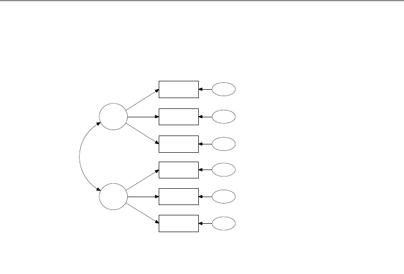
148
Example 8
Here is the path diagram with standardized estimates displayed:
The squared multiple correlations can be interpreted as follows: To take wordmean as
an example, 71% of its variance is accounted for by verbal ability. The remaining 29%
of its variance is accounted for by the unique factor err_w. If err_w represented
measurement error only, we could say that the estimated reliability of wordmean is
0.71. As it is, 0.71 is an estimate of a lower-bound on the reliability of wordmean.
The Holzinger and Swineford data have been analyzed repeatedly in textbooks and
in demonstrations of new factor analytic techniques. The six tests used in this example
are taken from a larger subset of nine tests used in a similar example by Jöreskog and
Sörbom (1984). The factor analysis model employed here is also adapted from theirs.
In view of the long history of exploration of the Holzinger and Swineford data in the
factor analysis literature, it is no accident that the present model fits very well. Even
more than usual, the results presented here require confirmation on a fresh set of data.
spatial
.49
visperc
.43
cubes
.54
lozenges
.71
wordmean
.77
paragrap
.68
sentence
err_v
err_c
err_l
err_p
err_s
err_w
verbal
.70
.65
.74
.88
.83
.84
.49
Example 8
Factor analysis: Girls' sample
Holzinger and Swineford (1939)
Standardized estimates
Chi-square = 7.853 (8 df)
p = .448

149
Factor Analysis
Modeling in VB.NET
The following program specifies the factor model for Holzinger and Swineford’s data.
It is saved in the file Ex08.vb.
You do not need to explicitly allow the factors (spatial and verbal) to be correlated. Nor
is it necessary to specify that the unique factors be uncorrelated with each other and
with the two factors. These are default assumptions in an Amos program (but not in
Amos Graphics).
Sub Main()
Dim Sem As New AmosEngine
Try
Sem.TextOutput()
Sem.Standardized()
Sem.Smc()
Sem.BeginGroup(Sem.AmosDir & "Examples\Grnt_fem.sav")
Sem.AStructure("visperc = (1) spatial + (1) err_v")
Sem.AStructure("cubes = spatial + (1) err_c")
Sem.AStructure("lozenges = spatial + (1) err_l")
Sem.AStructure("paragrap = (1) verbal + (1) err_p")
Sem.AStructure("sentence = verbal + (1) err_s")
Sem.AStructure("wordmean = verbal + (1) err_w")
Sem.FitModel()
Finally
Sem.Dispose()
End Try
End Sub

150
Example 8

151
Example
9
An Alternative to Analysis of
Covariance
Introduction
This example demonstrates a simple alternative to an analysis of covariance that does
not require perfectly reliable covariates. A better, but more complicated, alternative
will be demonstrated in Example 16.
Analysis of Covariance and Its Alternative
Analysis of covariance is a technique that is frequently used in experimental and
quasi-experimental studies to reduce the effect of pre-existing differences among
treatment groups. Even when random assignment to treatment groups has eliminated
the possibility of systematic pretreatment differences among groups, analysis of
covariance can pay off in increased precision in evaluating treatment effects.
The usefulness of analysis of covariance is compromised by the assumption that
each covariate be measured without error. The method makes other assumptions as
well, but the assumption of perfectly reliable covariates has received particular
attention (for example, Cook and Campbell, 1979). In part, this is because the effects
of violating the assumption can be so bad. Using unreliable covariates can lead to the
erroneous conclusion that a treatment has an effect when it doesn’t or that a treatment
has no effect when it really does. Unreliable covariates can even make a treatment
look like it does harm when it is actually beneficial. At the same time, unfortunately,
the assumption of perfectly reliable covariates is typically impossible to meet.

152
Example 9
The present example demonstrates an alternative to analysis of covariance in which
no variable has to be measured without error. The method to be demonstrated here has
been employed by Bentler and Woodward (1979) and others. Another approach, by
Sörbom (1978), is demonstrated in Example 16. The Sörbom method is more general.
It allows testing other assumptions of analysis of covariance and permits relaxing some
of them as well. The Sörbom approach is comparatively complicated because of its
generality. By contrast, the method demonstrated in this example makes the usual
assumptions of analysis of covariance, except for the assumption that covariates are
measured without error. The virtue of the method is its comparative simplicity.
The present example employs two treatment groups and a single covariate. It may
be generalized to any number of treatment groups and any number of covariates.
Sörbom (1978) used the data that we will be using in this example and Example 16.
The analysis closely follows Sörbom’s example.
About the Data
Olsson (1973) administered a battery of eight tests to 213 eleven-year-old students on
two occasions. We will employ two of the eight tests, Synonyms and Opposites, in this
example. Between the two administrations of the test battery, 108 of the students (the
experimental group) received training that was intended to improve performance on the
tests. The other 105 students (the control group) did not receive any special training.
As a result of taking two tests on two occasions, each of the 213 students obtained four
test scores. A fifth, dichotomous variable was created to indicate membership in the
experimental or control group. Altogether, the following variables are used in this
example:
Variable Description
pre_syn Pretest scores on the Synonyms test.
pre_opp Pretest scores on the Opposites test.
post_syn Posttest scores on the Synonyms test.
post_opp Posttest scores on the Opposites test.
treatment
A dichotomous variable taking on the value 1 for students who
received the special training, and 0 for those who did not. This
variable was created especially for the analyses in this example.
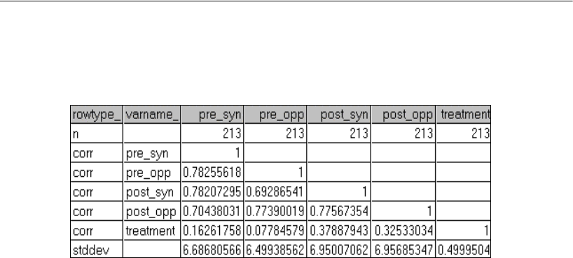
153
An Alternative to Analysis of Covariance
Correlations and standard deviations for the five measures are contained in the Microsoft
Excel workbook UserGuide.xls, in the Olss_all worksheet. Here is the dataset:
There are positive correlations between treatment and each of the posttests, which
indicates that the trained students did better on the posttests than the untrained students.
The correlations between treatment and each of the pretests are positive but relatively
small. This indicates that the control and experimental groups did about equally well
on the pretests. You would expect this, since students were randomly assigned to the
control and experimental groups.
Analysis of Covariance
To evaluate the effect of training on performance, one might consider carrying out an
analysis of covariance with one of the posttests as the criterion variable, and the two
pretests as covariates. In order for that analysis to be appropriate, both the synonyms
pretest and the opposites pretest would have to be perfectly reliable.
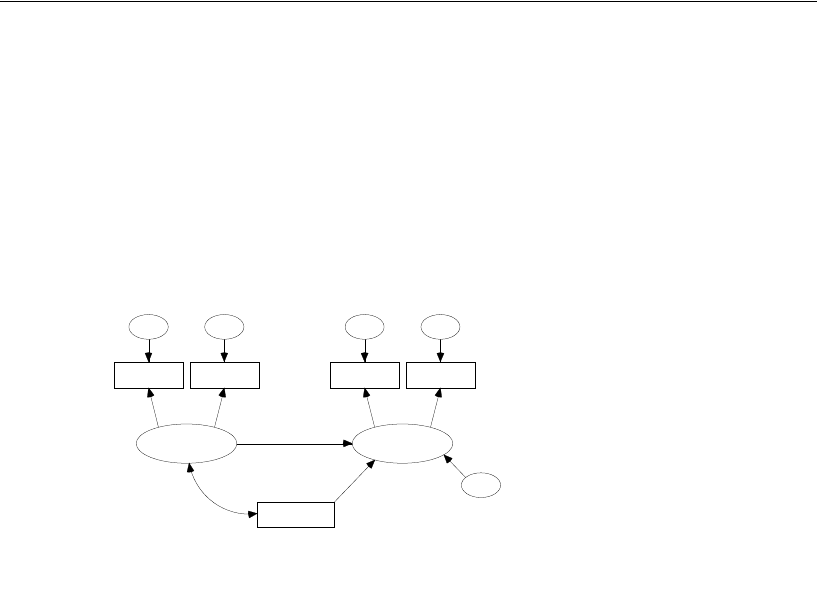
154
Example 9
Model A for the Olsson Data
Consider the model for the Olsson data shown in the next path diagram. The model
asserts that pre_syn and pre_opp are both imperfect measures of an unobserved ability
called pre_verbal that might be thought of as verbal ability at the time of the pretest.
The unique variables eps1 and eps2 represent errors of measurement in pre_syn and
pre_opp, as well as any other influences on the two tests not represented elsewhere in
the path diagram.
Similarly, the model asserts that post_syn and post_opp are imperfect measures of an
unobserved ability called post_verbal, which might be thought of as verbal ability at
the time of the posttest. Eps3 and eps4 represent errors of measurement and other
sources of variation not shown elsewhere in the path diagram.
The model shows two variables that may be useful in accounting for verbal ability
at the time of the posttest. One such predictor is verbal ability at the time of the pretest.
It would not be surprising to find that verbal ability at the time of the posttest depends
on verbal ability at the time of the pretest. Because past performance is often an
excellent predictor of future performance, the model uses the latent variable
pre_verbal as a covariate. However, our primary interest lies in the second predictor,
treatment. We are mostly interested in the regression weight associated with the arrow
pointing from treatment to post_verbal, and whether it is significantly different from
0. In other words, we will eventually want to know whether the model shown above
could be accepted as correct under the additional hypothesis that that particular
regression weight is 0. But first, we had better ask whether Model A can be accepted
as it stands.
pre_verbal
pre_syn
eps1
1
1
pre_opp
eps2
1
post_verbal
post_syn
eps3
post_opp
eps4
1
1 1
treatment
zeta
1
Example 9: Model A
Olsson (1973) test coaching study
Model Specification

155
An Alternative to Analysis of Covariance
Identification
The units of measurement of the seven unobserved variables are indeterminate. This
indeterminacy can be remedied by finding one single-headed arrow pointing away
from each unobserved variable in the above figure, and fixing the corresponding
regression weight to unity (1). The seven 1’s shown in the path diagram above indicate
a satisfactory choice of identification constraints.
Specifying Model A
To specify Model A, draw a path diagram similar to the one on p. 154. The path
diagram is saved as the file Ex09-a.amw.
Results for Model A
There is considerable empirical evidence against Model A:
This is bad news. If we had been able to accept Model A, we could have taken the next
step of repeating the analysis with the regression weight for regressing post_verbal on
treatment fixed at 0. But there is no point in doing that now. We have to start with a
model that we believe is correct in order to use it as the basis for testing a stronger no
treatment effect version of the model.
Searching for a Better Model
Perhaps there is some way of modifying Model A so that it fits the data better. Some
suggestions for suitable modifications can be obtained from modification indices.
Chi-square = 33.215
Degrees of freedom = 3
Probability level = 0.000
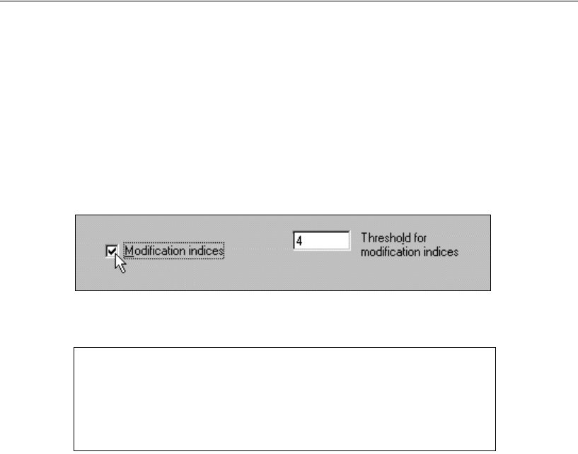
156
Example 9
Requesting Modification Indices
EFrom the menus, choose View > Analysis Properties.
EIn the Analysis Properties dialog, click the Output tab.
ESelect Modification indices and enter a suitable threshold in the field to its right. For this
example, the threshold will remain at its default value of 4.
Requesting modification indices with a threshold of 4 produces the following
additional output:
According to the first modification index in the M.I. column, the chi-square statistic
will decrease by at least 13.161 if the unique variables eps2 and eps4 are allowed to be
correlated (the actual decrease may be greater). At the same time, of course, the
number of degrees of freedom will drop by 1 because of the extra parameter that will
have to be estimated. Since 13.161 is the largest modification index, we should
consider it first and ask whether it is reasonable to think that eps2 and eps4 might be
correlated.
Eps2 represents whatever pre_opp measures other than verbal ability at the pretest.
Similarly, eps4 represents whatever post_opp measures other than verbal ability at the
posttest. It is plausible that some stable trait or ability other than verbal ability is
measured on both administrations of the Opposites test. If so, then you would expect a
positive correlation between eps2 and eps4. In fact, the expected parameter change (the
number in the Par Change column) associated with the covariance between eps2 and
eps4 is positive, which indicates that the covariance will probably have a positive
estimate if the covariance is not fixed at 0.
Modification Indices (Group number 1 - Default model)
Covariances: (Group number 1 - Default model)
M.I. Par Change
eps2
<-->
eps4
13.161
3.249
eps2
<-->
eps3
10.813
-2.822
eps1
<-->
eps4
11.968
-3.228
eps1
<-->
eps3
9.788
2.798
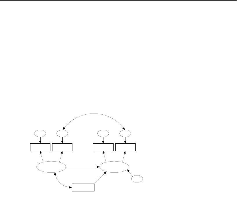
157
An Alternative to Analysis of Covariance
It might be added that the same reasoning that suggests allowing eps2 and eps4 to
be correlated applies almost as well to eps1 and eps3, whose covariance also has a
fairly large modification index. For now, however, we will add only one parameter to
Model A: the covariance between eps2 and eps4. We call this new model Model B.
Model B for the Olsson Data
Below is the path diagram for Model B. It can be obtained by taking the path diagram
for Model A and adding a double-headed arrow connecting eps2 and eps4. This path
diagram is saved in the file Ex09-b.amw.
You may find your error variables already positioned at the top of the path diagram,
with no room to draw the double-headed arrow. To fix the problem:
EFrom the menus, choose Edit > Fit to Page.
Alternatively, you can:
EDraw the double-headed arrow and, if it is out of bounds, click the Resize (page with
arrows) button. Amos will shrink your path diagram to fit within the page boundaries.
pre_verbal
pre_syn
eps1
1
1
pre_opp
eps2
1
post_verbal
post_syn
eps3
post_opp
eps4
1
1 1
treatment
zeta
1
Example 9: Model B
Olsson (1973) test coaching study
Model Specification

158
Example 9
Results for Model B
Allowing eps2 and eps4 to be correlated results in a dramatic reduction of the
chi-square statistic.
You may recall from the results of Model A that the modification index for the
covariance between eps1 and eps3 was 9.788. Clearly, freeing that covariance in
addition to the covariance between eps2 and eps4 covariance would not have produced
an additional drop in the chi-square statistic of 9.788, since this would imply a negative
chi-square statistic. Thus, a modification index represents the minimal drop in the
chi-square statistic that will occur if the corresponding constraint—and only that
constraint—is removed.
The following raw parameter estimates are difficult to interpret because they would
have been different if the identification constraints had been different:
Chi-square = 2.684
Degrees of freedom = 2
Probability level = 0.261
Regression Weights: (Group number 1 - Default model)
Estimate S.E. C.R. P Label
post_verbal
<---
pre_verbal
.889 .053 16.900 ***
post_verbal
<---
treatment 3.640 .477 7.625 ***
pre_syn <---
pre_verbal
1.000
pre_opp <---
pre_verbal
.881 .053 16.606 ***
post_syn <---
post_verbal
1.000
post_opp <---
post_verbal
.906 .053 16.948 ***
Covariances: (Group number 1 - Default model)
Estimate S.E. C.R. P Label
pre_verbal
<-->
treatment
.467 .226 2.066 .039
eps2 <-->
eps4 6.797 1.344 5.059 ***
Variances: (Group number 1 - Default model)
Estimate S.E. C.R. P Label
pre_verbal
38.491 4.501 8.552 ***
treatment
.249 .024 10.296 ***
zeta
4.824 1.331 3.625 ***
eps1
6.013 1.502 4.004 ***
eps2
12.255 1.603 7.646 ***
eps3
6.546 1.501 4.360 ***
eps4
14.685 1.812 8.102 ***
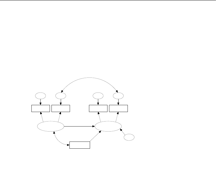
159
An Alternative to Analysis of Covariance
As expected, the covariance between eps2 and eps4 is positive. The most interesting
result that appears along with the parameter estimates is the critical ratio for the effect
of treatment on post_verbal. This critical ratio shows that treatment has a highly
significant effect on post_verbal. We will shortly obtain a better test of the significance
of this effect by modifying Model B so that this regression weight is fixed at 0. In the
meantime, here are the standardized estimates and the squared multiple correlations as
displayed by Amos Graphics:
In this example, we are primarily concerned with testing a particular hypothesis and
not so much with parameter estimation. However, even when the parameter estimates
themselves are not of primary interest, it is a good idea to look at them anyway to see
if they are reasonable. Here, for instance, you may not care exactly what the correlation
between eps2 and eps4 is, but you would expect it to be positive. Similarly, you would
be surprised to find any negative estimates for regression weights in this model. In any
model, you know that variables cannot have negative variances, so a negative variance
estimate would always be an unreasonable estimate. If estimates cannot pass a gross
sanity check, particularly with a reasonably large sample, you have to question the
correctness of the model under which they were obtained, no matter how well the
model fits the data.
pre_verbal
.86
pre_syn
eps1
.93
.71
pre_opp
eps2
.84 .88
post_verbal
.86
post_syn
eps3
.70
post_opp
eps4
.93 .84
treatment
.86
.28
zeta
Example 9: Model B
Olsson (1973) test coaching study
Standardized estimates
.15
.51

160
Example 9
Model C for the Olsson Data
Now that we have a model (Model B) that we can reasonably believe is correct, let’s
see how it fares if we add the constraint that post_verbal does not depend on treatment.
In other words, we will test a new model (call it Model C) that is just like Model B
except that Model C specifies that post_verbal has a regression weight of 0 on
treatment.
Drawing a Path Diagram for Model C
To draw the path diagram for Model C:
EStart with the path diagram for Model B.
ERight-click the arrow that points from treatment to post_verbal and choose Object
Properties from the pop-up menu.
EIn the Object Properties dialog, click the Parameters tab and type 0 in the Regression
weight text box.
The path diagram for Model C is saved in the file Ex09-c.amw.
Results for Model C
Model C has to be rejected at any conventional significance level.
If you assume that Model B is correct and that only the correctness of Model C is in
doubt, then a better test of Model C can be obtained as follows: In going from Model
B to Model C, the chi-square statistic increased by 52.712 (that is, ),
while the number of degrees of freedom increased by 1 (that is, 3 – 2). If Model C is
correct, 52.712 is an observation on a random variable that has an approximate
chi-square distribution with one degree of freedom. The probability of such a random
variable exceeding 52.712 is exceedingly small. Thus, Model C is rejected in favor of
Model B. Treatment has a significant effect on post_verbal.
Chi-square = 55.396
Degrees of freedom = 3
Probability level = 0.000
55.396 2.684–

161
An Alternative to Analysis of Covariance
Fitting All Models At Once
The example file Ex09-all.amw fits all three models (A through C) in a single analysis.
The procedure for fitting multiple models in a single analysis was demonstrated in
Example 6.
Modeling in VB.NET
Model A
This program fits Model A. It is saved in the file Ex09–a.vb.
Sub Main()
Dim Sem As New AmosEngine
Try
Sem.TextOutput()
Sem.Mods(4)
Sem.Standardized()
Sem.Smc()
Sem.BeginGroup(Sem.AmosDir & "Examples\UserGuide.xls", "Olss_all")
Sem.AStructure("pre_syn = (1) pre_verbal + (1) eps1")
Sem.AStructure("pre_opp = pre_verbal + (1) eps2")
Sem.AStructure("post_syn = (1) post_verbal + (1) eps3")
Sem.AStructure("post_opp = post_verbal + (1) eps4")
Sem.AStructure("post_verbal = pre_verbal + treatment + (1) zeta")
Sem.FitModel()
Finally
Sem.Dispose()
End Try
End Sub

162
Example 9
Model B
This program fits Model B. It is saved in the file Ex09–b.vb.
Sub Main()
Dim Sem As New AmosEngine
Try
Sem.TextOutput()
Sem.Standardized()
Sem.Smc()
Sem.BeginGroup(Sem.AmosDir & "Examples\UserGuide.xls", "Olss_all")
Sem.AStructure("pre_syn = (1) pre_verbal + (1) eps1")
Sem.AStructure("pre_opp = pre_verbal + (1) eps2")
Sem.AStructure("post_syn = (1) post_verbal + (1) eps3")
Sem.AStructure("post_opp = post_verbal + (1) eps4")
Sem.AStructure("post_verbal = pre_verbal + treatment + (1) zeta")
Sem.AStructure("eps2 <---> eps4")
Sem.FitModel()
Finally
Sem.Dispose()
End Try
End Sub

163
An Alternative to Analysis of Covariance
Model C
This program fits Model C. It is saved in the file Ex09–c.vb.
Sub Main()
Dim Sem As New AmosEngine
Try
Sem.TextOutput()
Sem.Mods(4)
Sem.Standardized()
Sem.Smc()
Sem.BeginGroup(Sem.AmosDir & "Examples\UserGuide.xls", "Olss_all")
Sem.AStructure("pre_syn = (1) pre_verbal + (1) eps1")
Sem.AStructure("pre_opp = pre_verbal + (1) eps2")
Sem.AStructure("post_syn = (1) post_verbal + (1) eps3")
Sem.AStructure("post_opp = post_verbal + (1) eps4")
Sem.AStructure("post_verbal = pre_verbal + (0) treatment + (1) zeta")
Sem.AStructure("eps2 <---> eps4")
Sem.FitModel()
Finally
Sem.Dispose()
End Try
End Sub

Fitting Multiple Models
This program (Ex09-all.vb) fits all three models (A through C).
Sub Main()
Dim Sem As New AmosEngine
Try
Sem.TextOutput()
Sem.Mods(4)
Sem.Standardized()
Sem.Smc()
Sem.BeginGroup(Sem.AmosDir & "Examples\UserGuide.xls", "Olss_all")
Sem.AStructure("pre_syn = (1) pre_verbal + (1) eps1")
Sem.AStructure("pre_opp = pre_verbal + (1) eps2")
Sem.AStructure("post_syn = (1) post_verbal + (1) eps3")
Sem.AStructure("post_opp = post_verbal + (1) eps4")
Sem.AStructure("post_verbal = pre_verbal + (effect) treatment + (1) zeta")
Sem.AStructure("eps2 <---> eps4 (cov2_4)")
Sem.Model("Model_A", "cov2_4 = 0")
Sem.Model("Model_B")
Sem.Model("Model_C", "effect = 0")
Sem.FitAllModels()
Finally
Sem.Dispose()
End Try
End Sub

165
Example
10
Simultaneous Analysis of Several
Groups
Introduction
This example demonstrates how to fit a model to two sets of data at once. Amos is
capable of modeling data from multiple groups (or samples) simultaneously. This
multigroup facility allows for many additional types of analyses, as illustrated in the
next several examples.
Analysis of Several Groups
We return once again to Attig’s (1983) memory data from young and old subjects,
which were used in Example 1 through Example 3. In this example, we will compare
results from the two groups to see how similar they are. However, we will not compare
the groups by performing separate analyses for old people and young people. Instead,
we will perform a single analysis that estimates parameters and tests hypotheses about
both groups at once. This method has two advantages over doing separate analyses for
the young and old groups. First, it provides a test for the significance of any
differences found between young and old people. Second, if there are no differences
between young and old people or if the group differences concern only a few model
parameters, the simultaneous analysis of both groups provides more accurate
parameter estimates than would be obtained from two separate single-group analyses.
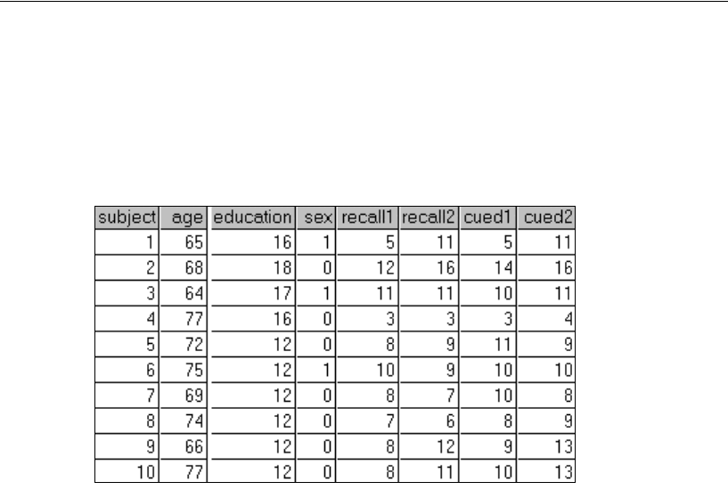
166
Example 10
About the Data
We will use Attig’s memory data from both young and old subjects. Following is a
partial listing of the old subjects’ data found in the worksheet Attg_old located in the
Microsoft Excel workbook UserGuide.xls:
The young subjects’ data are in the Attg_yng worksheet. This example uses only the
measures recall1 and cued1.
Data for multigroup analysis can be organized in a variety of ways. One option is to
separate the data into different files, with one file for each group (as we have done in
this example). A second possibility is to keep all the data in one big file and include a
group membership variable.
Model A
We will begin with a truly trivial model (Model A) for two variables: recall1 and
cued1. The model simply says that, for young subjects as well as old subjects, recall1
and cued1 are two variables that have some unspecified variances and some
unspecified covariance. The variances and the covariance are allowed to be different
for young and old people.
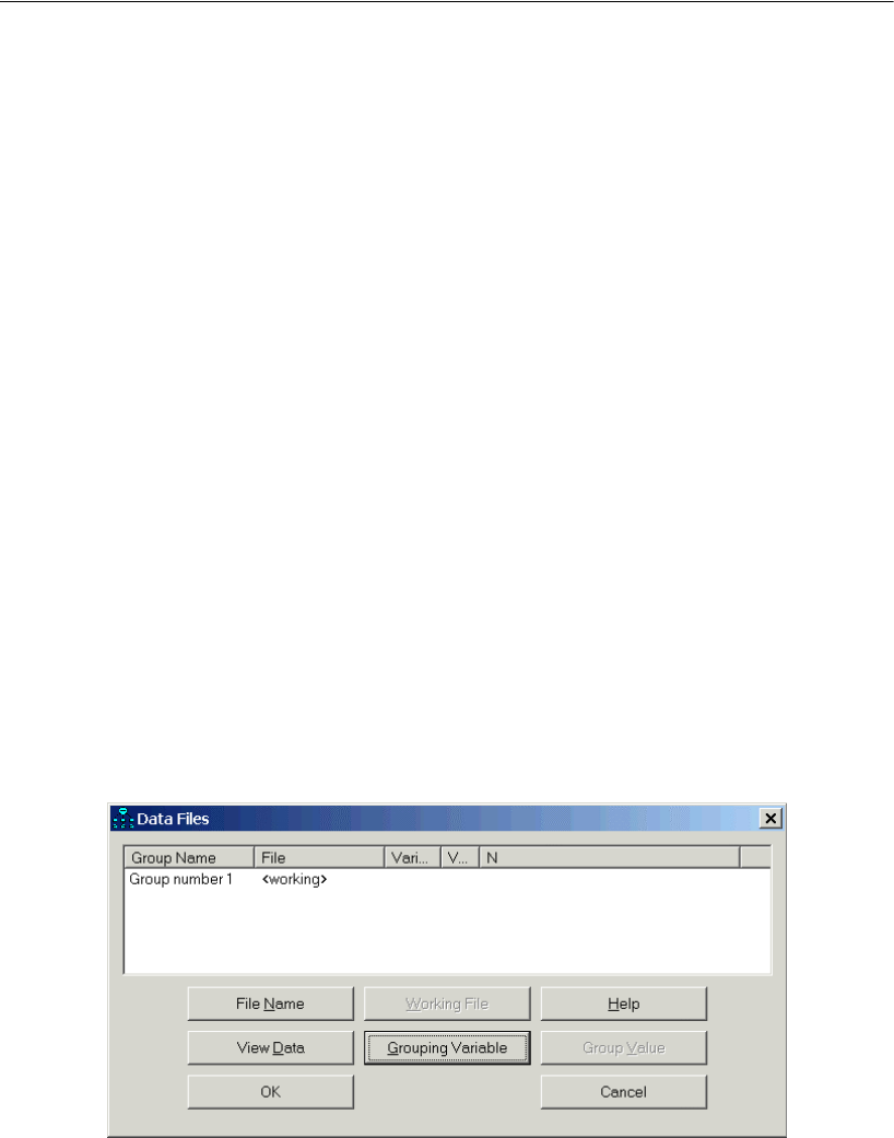
167
Simultaneous Analysis of Several Groups
Conventions for Specifying Group Differences
The main purpose of a multigroup analysis is to find out the extent to which groups
differ. Do the groups all have the same path diagram with the same parameter values?
Do the groups have the same path diagram but with different parameter values for
different groups? Does each group need a different path diagram? Amos Graphics has
the following conventions for specifying group differences in a multigroup analysis:
All groups have the same path diagram unless explicitly declared otherwise.
Unnamed parameters are permitted to have different values in different groups.
Thus, the default multigroup model under Amos Graphics uses the same path
diagram for all groups but allows different parameter values for different groups.
Parameters in different groups can be constrained to the same value by giving them
the same label. (This will be demonstrated in Model B on p. 178.)
Specifying Model A
EFrom the menus, choose File > New to start a new path diagram.
EFrom the menus, choose File > Data Files.
Notice that the Data Files dialog allows you to specify a data file for only a single group
called Group number 1. We have not yet told the program that this is a multigroup
analysis.
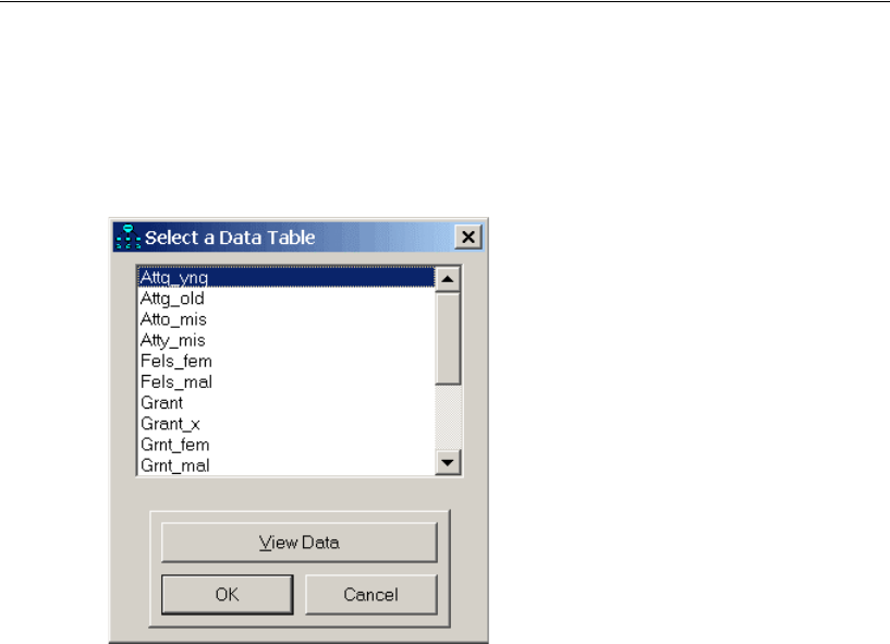
168
Example 10
EClick File Name, select the Excel workbook UserGuide.xls that is in the Amos
Examples directory, and click Open.
EIn the Select a Data Table dialog, select the Attg_yng worksheet.
EClick OK to close the Select a Data Table dialog.
EClick OK to close the Data Files dialog.
EFrom the menus, choose View > Variables in Dataset.
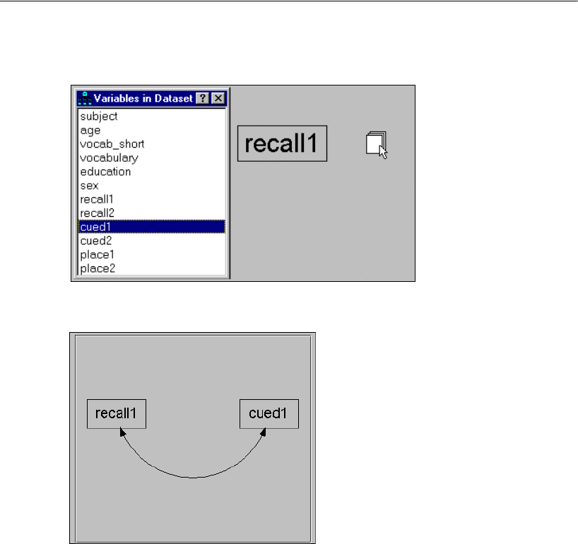
169
Simultaneous Analysis of Several Groups
EDrag observed variables recall1 and cued1 to the diagram.
EConnect recall1 and cued1 with a double-headed arrow.
ETo add a caption to the path diagram, from the menus, choose Diagram > Figure Caption
and then click the path diagram at the spot where you want the caption to appear.
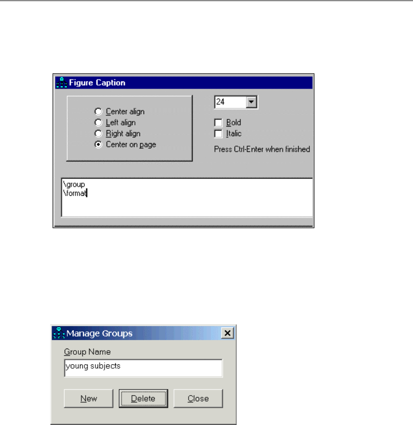
170
Example 10
EIn the Figure Caption dialog, enter a title that contains the text macros \group and
\format.
EClick OK to complete the model specification for the young group.
ETo add a second group, from the menus, choose Analyze > Manage Groups.
EIn the Manage Groups dialog, change the name in the Group Name text box from
Group number 1 to young subjects.
EClick New to create a second group.
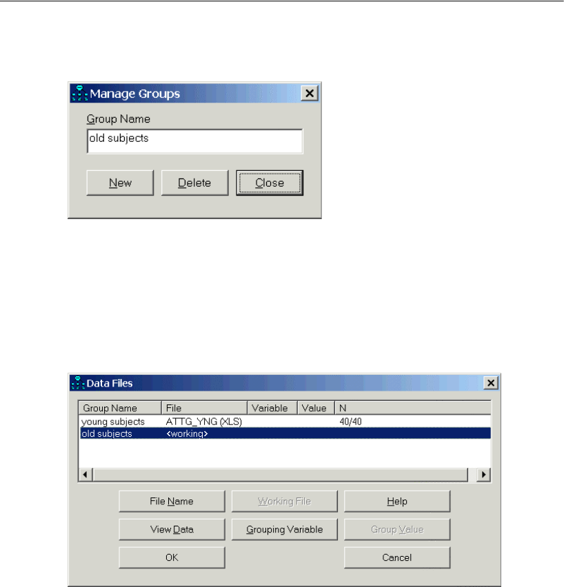
171
Simultaneous Analysis of Several Groups
EChange the name in the Group Name text box from Group number 2 to old subjects.
EClick Close.
EFrom the menus, choose File > Data Files.
The Data Files dialog shows that there are two groups labeled young subjects and old
subjects.
ETo specify the dataset for the old subjects, in the Data Files dialog, select old subjects.
EClick File Name, select the Excel workbook UserGuide.xls that is in the Amos
Examples directory, and click Open.
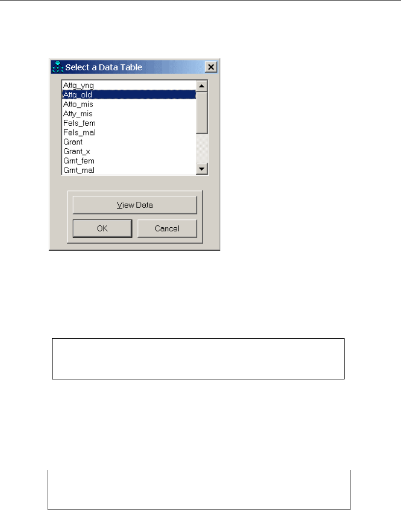
172
Example 10
EIn the Select a Data Table dialog, select the Attg_old worksheet.
EClick OK.
Text Output
Model A has zero degrees of freedom.
Amos computed the number of distinct sample moments this way: The young subjects
have two sample variances and one sample covariance, which makes three sample
moments. The old subjects also have three sample moments, making a total of six
sample moments. The parameters to be estimated are the population moments, and
there are six of them as well. Since there are zero degrees of freedom, this model is
untestable.
Chi-square = 0.000
Degrees of freedom = 0
Probability level cannot be computed
Computation of degrees of freedom (Default model)
Number of distinct sample moments: 6
Number of distinct parameters to be estimated: 6
Degrees of freedom (6 - 6): 0

173
Simultaneous Analysis of Several Groups
To view parameter estimates for the young people in the Amos Output window:
EClick Estimates in the tree diagram in the upper left pane.
EClick young subjects in the Groups panel at the left side of the window.
To view the parameter estimates for the old subjects:
EClick old subjects in the Groups panel.
Graphics Output
The following are the output path diagrams showing unstandardized estimates for the
two groups:
The panels at the left of the Amos Graphics window provide a variety of viewing
options.
Covariances: (young subjects - Default model)
Estimate S.E. C.R. P Label
recall1
<-->
cued1
3.225 .944 3.416 ***
Variances: (young subjects - Default model)
Estimate S.E. C.R. P Label
recall1
5.787 1.311 4.416 ***
cued1
4.210 .953 4.416 ***
Covariances: (old subjects - Default model)
Estimate S.E. C.R. P Label
recall1
<-->
cued1
4.887 1.252 3.902 ***
Variances: (old subjects - Default model)
Estimate S.E. C.R. P Label
recall1
5.569 1.261 4.416 ***
cued1
6.694 1.516 4.416 ***
5.79
recall1
4.21
cued1
3.22
Example 10: Model A
Simultaneous analysis of several groups
Attig (1983) young subjects
Unstandardized estimates
5.57
recall1
6.69
cued1
4.89
Example 10: Model A
Simultaneous analysis of several groups
Attig (1983) old subjects
Unstandardized estimates
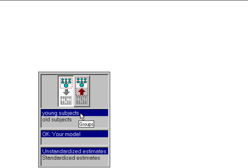
174
Example 10
Click either the View Input or View Output button to see an input or output path
diagram.
Select either young subjects or old subjects in the Groups panel.
Select either Unstandardized estimates or Standardized estimates in the Parameter
Formats panel.
Model B
It is easy to see that the parameter estimates are different for the two groups. But are
the differences significant? One way to find out is to repeat the analysis, but this time
requiring that each parameter in the young population be equal to the corresponding
parameter in the old population. The resulting model will be called Model B.
For Model B, it is necessary to name each parameter, using the same parameter
names in the old group as in the young group.
EStart by clicking young subjects in the Groups panel at the left of the path diagram.
ERight-click the recall1 rectangle in the path diagram.
EFrom the pop-up menu, choose Object Properties.
EIn the Object Properties dialog, click the Parameters tab.
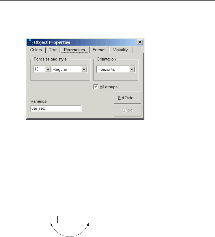
175
Simultaneous Analysis of Several Groups
EIn the Variance text box, enter a name for the variance of recall1; for example, type
var_rec.
ESelect All groups (a check mark will appear next to it).
The effect of the check mark is to assign the name var_rec to the variance of recall1 in
all groups. Without the check mark, var_rec would be the name of the variance for
recall1 for the young group only.
EWhile the Object Properties dialog is open, click cued1 and type the name var_cue for
its variance.
EClick the double-headed arrow and type the name cov_rc for the covariance. Always
make sure that you select All groups.
The path diagram for each group should now look like this:
var_rec
recall1
var_cue
cued1
cov_rc
Example 10: Model B
Homogenous covariance structures
in two groups, Attig (1983) data.
Model Specification

176
Example 10
Text Output
Because of the constraints imposed in Model B, only three distinct parameters are
estimated instead of six. As a result, the number of degrees of freedom has increased
from 0 to 3.
Model B is acceptable at any conventional significance level.
The following are the parameter estimates obtained under Model B for the young
subjects. (The parameter estimates for the old subjects are the same.)
You can see that the standard error estimates obtained under Model B are smaller (for
the young subjects, 0.780, 0.909, and 0.873) than the corresponding estimates obtained
under Model A (0.944, 1.311, and 0.953). The Model B estimates are to be preferred
over the ones from Model A as long as you believe that Model B is correct.
Chi-square = 4.588
Degrees of freedom = 3
Probability level = 0.205
Computation of degrees of freedom (Default model)
Number of distinct sample moments: 6
Number of distinct parameters to be estimated: 3
Degrees of freedom (6 - 3): 3
Covariances: (young subjects - Default model)
Estimate S.E. C.R. P Label
recall1
<-->
cued1
4.056 .780 5.202 *** cov_rc
Variances: (young subjects - Default model)
Estimate S.E. C.R. P Label
recall1
5.678
.909 6.245 *** var_rec
cued1
5.452
.873 6.245 *** var_cue
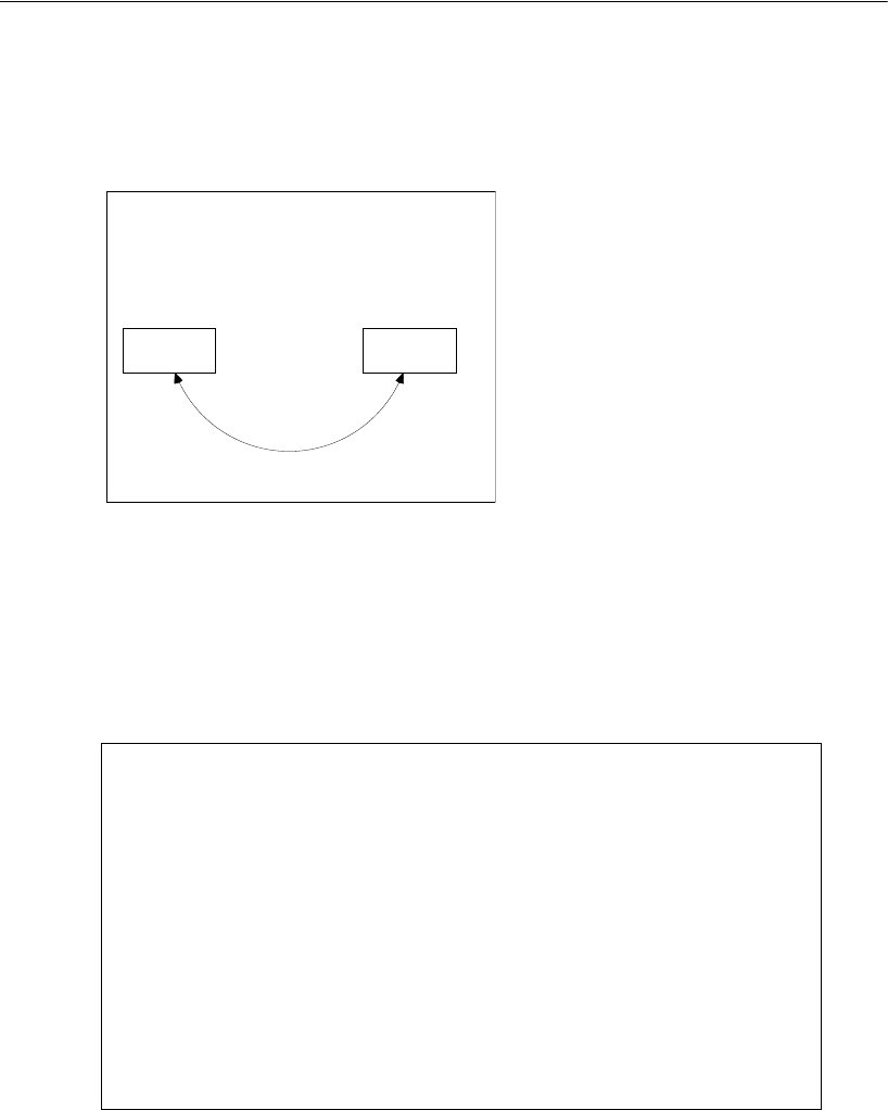
177
Simultaneous Analysis of Several Groups
Graphics Output
For Model B, the output path diagram is the same for both groups.
Modeling in VB.NET
Model A
Here is a program (Ex10-a.vb) for fitting Model A:
Sub Main()
Dim Sem As New AmosEngine
Try
Sem.TextOutput()
Sem.BeginGroup(Sem.AmosDir & "Examples\UserGuide.xls", "Attg_yng")
Sem.GroupName("young subjects")
Sem.AStructure("recall1")
Sem.AStructure("cued1")
Sem.BeginGroup(Sem.AmosDir & "Examples\UserGuide.xls", "Attg_old")
Sem.GroupName("old subjects")
Sem.AStructure("recall1")
Sem.AStructure("cued1")
Sem.FitModel()
Finally
Sem.Dispose()
End Try
End Sub
5.68
recall1
5.45
cued1
4.06
Chi-square = 4.588 (3 df)
p = .205

178
Example 10
The BeginGroup method is used twice in this two-group analysis. The first BeginGroup
line specifies the Attg_yng dataset. The three lines that follow supply a name and a
model for that group. The second BeginGroup line specifies the Attg_old dataset, and
the following three lines supply a name and a model for that group. The model for each
group simply says that recall1 and cued1 are two variables with unconstrained
variances and an unspecified covariance. The GroupName method is optional, but it is
useful in multiple-group analyses because it helps Amos to label the output in a
meaningful way.
Model B
The following program for Model B is saved in Ex10-b.vb:
The parameter names var_rec, var_cue, and cov_rc (in parentheses) are used to require
that some parameters have the same value for old people as for young people. Using
the name var_rec twice requires recall1 to have the same variance in both populations.
Similarly, using the name var_cue twice requires cued1 to have the same variance in
both populations. Using the name cov_rc twice requires that recall1 and cued1 have
the same covariance in both populations.
Sub Main()
Dim Sem As New AmosEngine
Try
Dim dataFile As String = Sem.AmosDir & "Examples\UserGuide.xls"
Sem.Standardized()
Sem.TextOutput()
Sem.BeginGroup(dataFile, "Attg_yng")
Sem.GroupName("young subjects")
Sem.AStructure("recall1 (var_rec)")
Sem.AStructure("cued1 (var_cue)")
Sem.AStructure("recall1 <> cued1 (cov_rc)")
Sem.BeginGroup(dataFile, "Attg_old")
Sem.GroupName("old subjects")
Sem.AStructure("recall1 (var_rec)")
Sem.AStructure("cued1 (var_cue)")
Sem.AStructure("recall1 <> cued1 (cov_rc)")
Sem.FitModel()
Finally
Sem.Dispose()
End Try
End Sub

179
Simultaneous Analysis of Several Groups
Multiple Model Input
Here is a program (Ex10-all.vb) for fitting both Models A and B.1
The Sem.Model statements should appear immediately after the AStructure
specifications for the last group. It does not matter which Model statement goes first.
1 In Example 6 (Ex06-all.vb), multiple model constraints were written in a single string, within which individual
constraints were separated by semicolons. In the present example, each constraint is in its own string, and the
individual strings are separated by commas. Either syntax is acceptable.
Sub Main()
Dim Sem As New AmosEngine
Try
Sem.Standardized()
Sem.TextOutput()
Sem.BeginGroup(Sem.AmosDir & "Examples\UserGuide.xls", "Attg_yng")
Sem.GroupName("young subjects")
Sem.AStructure("recall1 (yng_rec)")
Sem.AStructure("cued1 (yng_cue)")
Sem.AStructure("recall1 <> cued1 (yng_rc)")
Sem.BeginGroup(Sem.AmosDir & "Examples\UserGuide.xls", "Attg_old")
Sem.GroupName("old subjects")
Sem.AStructure("recall1 (old_rec)")
Sem.AStructure("cued1 (old_cue)")
Sem.AStructure("recall1 <> cued1 (old_rc)")
Sem.Model("Model A")
Sem.Model("Model B", "yng_rec=old_rec", "yng_cue=old_cue", _
"yng_rc=old_rc")
Sem.FitAllModels()
Finally
Sem.Dispose()
End Try
End Sub

181
Example
11
Felson and Bohrnstedt’s Girls and
Boys
Introduction
This example demonstrates how to fit a simultaneous equations model to two sets of
data at once.
Felson and Bohrnstedt’s Model
Example 7 tested Felson and Bohrnstedt’s (1979) model for perceived attractiveness
and perceived academic ability using a sample of 209 girls. Here, we take the same
model and attempt to apply it simultaneously to the Example 7 data and to data from
another sample of 207 boys. We will examine the question of whether the measured
variables are related to each other in the same way for boys as for girls.
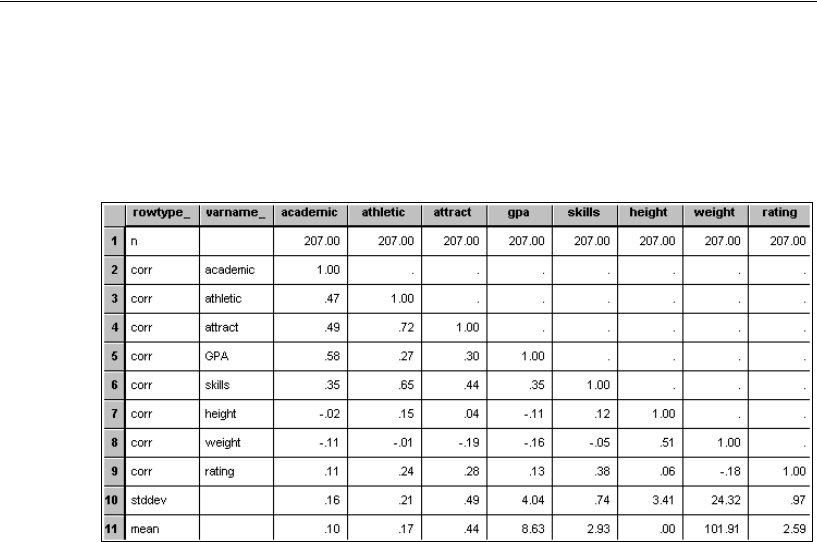
182
Example 11
About the Data
The Felson and Bohrnstedt (1979) data for girls were described in Example 7. Here is
a table of the boys’ data from the SPSS Statistics file Fels_mal.sav:
Notice that there are eight variables in the boys’ data file but only seven in the girls’
data file. The extra variable skills is not used in any model of this example, so its
presence in the data file is ignored.
Specifying Model A for Girls and Boys
Consider extending the Felson and Bohrnstedt model of perceived attractiveness and
academic ability to boys as well as girls. To do this, we will start with the girls-only
model specification from Example 7 and modify it to accommodate two groups. If you
have already drawn the path diagram for Example 7, you can use it as a starting point
for this example. No additional drawing is needed.
Parameter estimates can be displayed on a path diagram for only one group at a time
in a multigroup analysis. It is useful then to display a figure caption that tells which
group the parameter estimates represent.
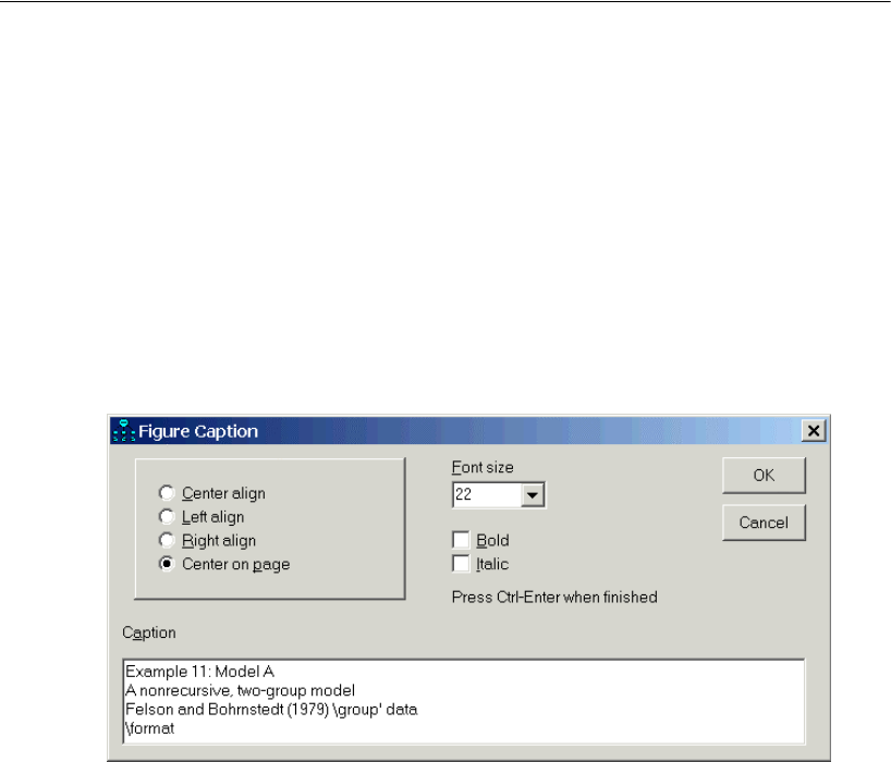
183
Felson and Bohrnstedt’s Girls and Boys
Specifying a Figure Caption
To create a figure caption that displays the group name, place the \group text macro in
the caption.
EFrom the menus, choose Diagram > Figure Caption.
EClick the path diagram at the spot where you want the caption to appear.
EIn the Figure Caption dialog, enter a title that contains the text macro \group. For
example:
In Example 7, where there was only one group, the group’s name didn’t matter.
Accepting the default name Group number 1 was good enough. Now that there are two
groups to keep track of, the groups should be given meaningful names.
EFrom the menus, choose Analyze > Manage Groups.
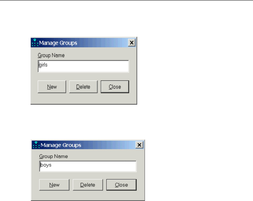
184
Example 11
EIn the Manage Groups dialog, type girls for Group Name.
EWhile the Manage Groups dialog is open, create a second group by clicking New.
EType boys in the Group Name text box.
EClick Close to close the Manage Groups dialog.
EFrom the menus, choose File > Data Files.
EIn the Data Files dialog, double-click girls and select the data file Fels_fem.sav.
EThen, double-click boys and select the data file Fels_mal.sav.
EClick OK to close the Data Files dialog.
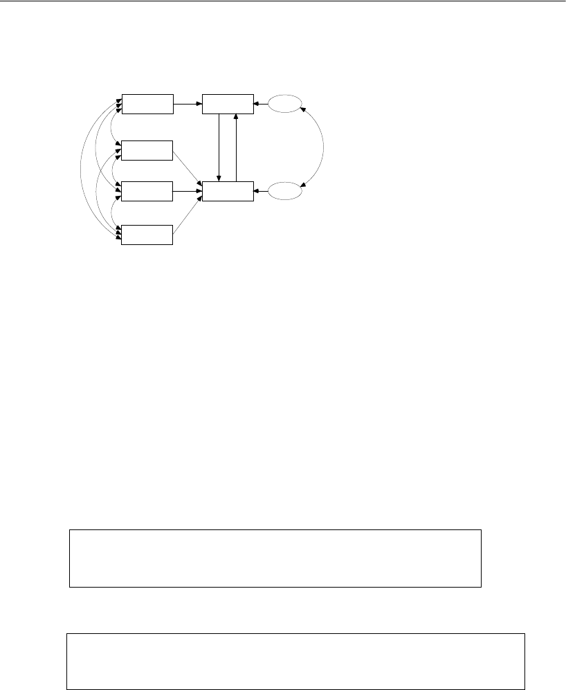
185
Felson and Bohrnstedt’s Girls and Boys
Your path diagram should look something like this for the boys’ sample:
Notice that, although girls and boys have the same path diagram, there is no
requirement that the parameters have the same values in the two groups. This means
that estimates of regression weights, covariances, and variances may be different for
boys than for girls.
Text Output for Model A
With two groups instead of one (as in Example 7), there are twice as many sample
moments and twice as many parameters to estimate. Therefore, you have twice as many
degrees of freedom as there were in Example 7.
The model fits the data from both groups quite well.
Chi-square = 3.183
Degrees of freedom = 4
Probability level = 0.528
GPA
height
rating
weight
academic
attract
error1
error2
1
1
Example 11: Model A
A nonrecursive, two-group model
Felson and Bohrnstedt (1979) boys' data
Model Specification
Computation of degrees of freedom (Default model)
Number of distinct sample moments: 42
Number of distinct parameters to be estimated: 38
Degrees of freedom (42 - 38): 4

186
Example 11
We accept the hypothesis that the Felson and Bohrnstedt model is correct for both boys
and girls. The next thing to look at is the parameter estimates. We will be interested in
how the girls’ estimates compare to the boys’ estimates. The following are the
parameter estimates for the girls:
Regression Weights: (girls - Default model)
Estimate S.E. C.R. P Label
academic
<---
GPA .023 .004 6.241 ***
attract <---
height .000 .010 .050 .960
attract <---
weight -.002 .001 -1.321 .186
attract <---
rating .176 .027 6.444 ***
attract <---
academic
1.607 .350 4.599 ***
academic
<---
attract -.002 .051 -.039 .969
Covariances: (girls - Default model)
Estimate S.E. C.R. P Label
GPA <-->
rating
.526
.246 2.139 .032
height
<-->
rating
-.468
.205 -2.279 .023
GPA <-->
weight
-6.710
4.676 -1.435 .151
GPA <-->
height
1.819
.712 2.555 .011
height
<-->
weight
19.024
4.098 4.642 ***
weight
<-->
rating
-5.243
1.395 -3.759 ***
error1
<-->
error2
-.004
.010 -.382 .702
Variances: (girls - Default model)
Estimate S.E. C.R. P Label
GPA
12.122
1.189 10.198 ***
height
8.428
.826 10.198 ***
weight
371.476
36.427 10.198 ***
rating
1.015
.100 10.198 ***
error1
.019
.003 5.747 ***
error2
.143
.014 9.974 ***

187
Felson and Bohrnstedt’s Girls and Boys
These parameter estimates are the same as in Example 7. Standard errors, critical
ratios, and p values are also the same. The following are the unstandardized estimates
for the boys:
Regression Weights: (boys - Default model)
Estimate S.E. C.R. P Label
academic
<---
GPA .021 .003 6.927 ***
attract <---
height .019 .010 1.967 .049
attract <---
weight -.003 .001 -2.484 .013
attract <---
rating .095 .030 3.150 .002
attract <---
academic
1.386 .315 4.398 ***
academic
<---
attract .063 .059 1.071 .284
Covariances: (boys - Default model)
Estimate S.E. C.R. P Label
GPA <-->
rating
.507 .274 1.850 .064
height
<-->
rating
.198 .230 .860 .390
GPA <-->
weight
-15.645 6.899 -2.268 .023
GPA <-->
height
-1.508 .961 -1.569 .117
height
<-->
weight
42.091 6.455 6.521 ***
weight
<-->
rating
-4.226 1.662 -2.543 .011
error1
<-->
error2
-.010 .011 -.898 .369
Variances: (boys - Default model)
Estimate S.E. C.R. P Label
GPA
16.243 1.600 10.149 ***
height
11.572 1.140 10.149 ***
weight
588.605 57.996 10.149 ***
rating
.936 .092 10.149 ***
error1
.015 .002 7.571 ***
error2
.164 .016 10.149 ***
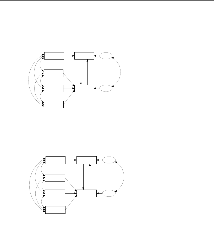
188
Example 11
Graphics Output for Model A
For girls, this is the path diagram with unstandardized estimates displayed:
The following is the path diagram with the estimates for the boys:
You can visually inspect the girls’ and boys’ estimates in Model A, looking for sex
differences. To find out if girls and boys differ significantly with respect to any single
parameter, you could examine the table of critical ratios of differences among all pairs
of free parameters.
12.12
GPA
8.43
height
1.02
rating
371.48
weight
academic
attract
.02
.00
.00
.18
.02
error1
.14
error2
1
1
.53
-.47
-6.71
1.82
19.02-5.24
1.61 .00 .00
Example 11: Model A
A nonrecursive, two-group model
Felson and Bohrnstedt (1979) girls' data
Unstandardized estimates
16.24
GPA
11.57
height
.94
rating
588.61
weight
academic
attract
.02
.02
.00
.10
.01
error1
.16
error2
1
1
.51
.20
-15.64
-1.51
42.09-4.23
1.39 .06 -.01
Example 11: Model A
A nonrecursive, two-group model
Felson and Bohrnstedt (1979) boys' data
Unstandardized estimates
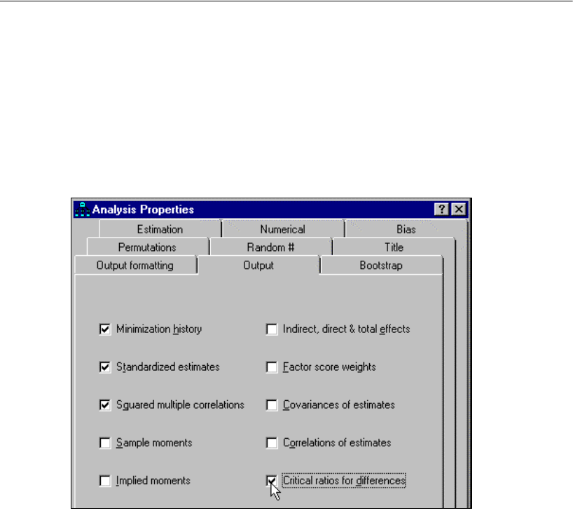
189
Felson and Bohrnstedt’s Girls and Boys
Obtaining Critical Ratios for Parameter Differences
EFrom the menus, choose View > Analysis Properties.
EIn the Analysis Properties dialog, click the Output tab.
ESelect Critical ratios for differences.
In this example, however, we will not use critical ratios for differences; instead, we will
take an alternative approach to looking for group differences.
Model B for Girls and Boys
Suppose we are mainly interested in the regression weights, and we hypothesize
(Model B) that girls and boys have the same regression weights. In this model, the
variances and covariances of the exogenous variables are still allowed to differ from
one group to another.
This model allows the distribution of variables such as height and weight to be
different for boys than for girls while requiring the linear dependencies among
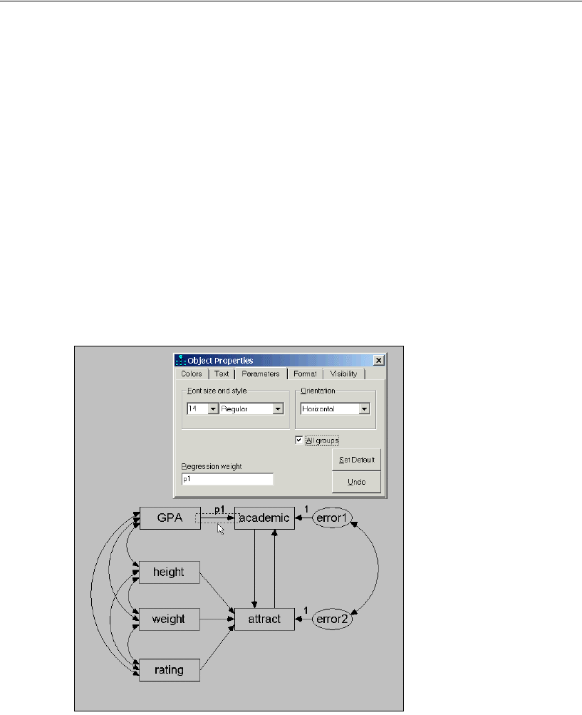
190
Example 11
variables to be group-invariant. For Model B, you need to constrain six regression
weights in each group.
EFirst, display the girls’ path diagram by clicking girls in the Groups panel at the left of
the path diagram.
ERight-click one of the single-headed arrows and choose Object Properties from the pop-
up menu.
EIn the Object Properties dialog, click the Parameters tab.
EEnter a name in the Regression weight text box.
ESelect All groups. A check mark appears next to it. The effect of the check mark is to
assign the same name to this regression weight in all groups.
EKeeping the Object Properties dialog open, click another single-headed arrow and
enter another name in the Regression weight text box.
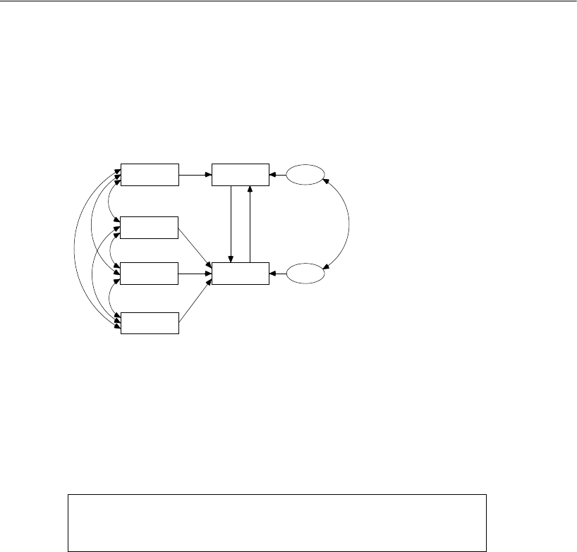
191
Felson and Bohrnstedt’s Girls and Boys
ERepeat this until you have named every regression weight. Always make sure to select
(put a check mark next to) All groups.
After you have named all of the regression weights, the path diagram for each sample
should look something like this:
Results for Model B
Text Output
Model B fits the data very well.
Chi-square = 9.493
Degrees of freedom = 10
Probability level = 0.486
GPA
height
rating
weight
academic
attract
p1
p3
p4
p5
error1
error2
1
1
p6 p2

192
Example 11
Comparing Model B against Model A gives a nonsignificant chi-square of
with degrees of freedom. Assuming that Model B
is indeed correct, the Model B estimates are preferable over the Model A estimates.
The unstandardized parameter estimates for the girls’ sample are:
9.493 3.183–6.310=
10 4 6=–
Regression Weights: (girls - Default model)
Estimate S.E. C.R. P Label
academic
<---
GPA .022 .002 9.475 *** p1
attract <---
height .008 .007 1.177 .239 p3
attract <---
weight -.003 .001 -2.453 .014 p4
attract <---
rating .145 .020 7.186 *** p5
attract <---
academic
1.448 .232 6.234 *** p6
academic
<---
attract .018 .039 .469 .639 p2
Covariances: (girls - Default model)
Estimate S.E. C.R. P Label
GPA <-->
rating
.526
.246 2.139 .032
height
<-->
rating
-.468
.205 -2.279 .023
GPA <-->
weight
-6.710
4.676 -1.435 .151
GPA <-->
height
1.819
.712 2.555 .011
height
<-->
weight
19.024
4.098 4.642 ***
weight
<-->
rating
-5.243
1.395 -3.759 ***
error1
<-->
error2
-.004
.008 -.464 .643
Variances: (girls - Default model)
Estimate S.E. C.R. P Label
GPA
12.122
1.189 10.198 ***
height
8.428
.826 10.198 ***
weight
371.476
36.427 10.198 ***
rating
1.015
.100 10.198 ***
error1
.018
.003 7.111 ***
error2
.144
.014 10.191 ***

193
Felson and Bohrnstedt’s Girls and Boys
The unstandardized parameter estimates for the boys are:
As Model B requires, the estimated regression weights for the boys are the same as
those for the girls.
Regression Weights: (boys - Default model)
Estimate S.E. C.R. P Label
academic
<---
GPA .022 .002 9.475 *** p1
attract <---
height .008 .007 1.177 .239 p3
attract <---
weight -.003 .001 -2.453 .014 p4
attract <---
rating .145 .020 7.186 *** p5
attract <---
academic
1.448 .232 6.234 *** p6
academic
<---
attract .018 .039 .469 .639 p2
Covariances: (boys - Default model)
Estimate S.E. C.R. P Label
GPA <-->
rating
.507 .274 1.850 .064
height
<-->
rating
.198 .230 .860 .390
GPA <-->
weight
-15.645 6.899 -2.268 .023
GPA <-->
height
-1.508 .961 -1.569 .117
height
<-->
weight
42.091 6.455 6.521 ***
weight
<-->
rating
-4.226 1.662 -2.543 .011
error1
<-->
error2
-.004 .008 -.466 .641
Variances: (boys - Default model)
Estimate S.E. C.R. P Label
GPA
16.243 1.600 10.149 ***
height
11.572 1.140 10.149 ***
weight
588.605 57.996 10.149 ***
rating
.936 .092 10.149 ***
error1
.016 .002 7.220 ***
error2
.167 .016 10.146 ***
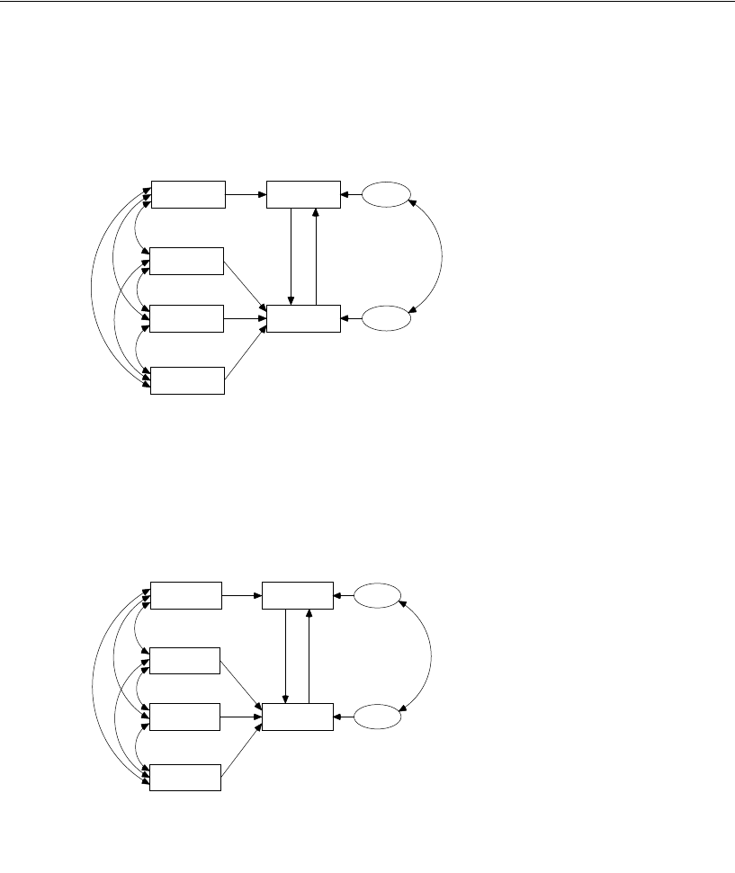
194
Example 11
Graphics Output
The output path diagram for the girls is:
And the output for the boys is:
12.12
GPA
8.43
height
1.02
rating
371.48
weight
academic
attract
.02
.01
.00
.15
.02
error1
.14
error2
1
1
.53
-.47
-6.71
1.82
19.02-5.24
1.45 .02 .00
Example 11: Model B
A nonrecursive, two-group model
Felson and Bohrnstedt (1979) girls' data
Unstandardized estimates
16.24
GPA
11.57
height
.94
rating
588.61
weight
academic
attract
.02
.01
.00
.15
.02
error1
.17
error2
1
1
.51
.20
-15.64
-1.51
42.09-4.23
1.45 .02 .00
Example 11: Model B
A nonrecursive, two-group model
Felson and Bohrnstedt (1979) boys' data
Unstandardized estimates
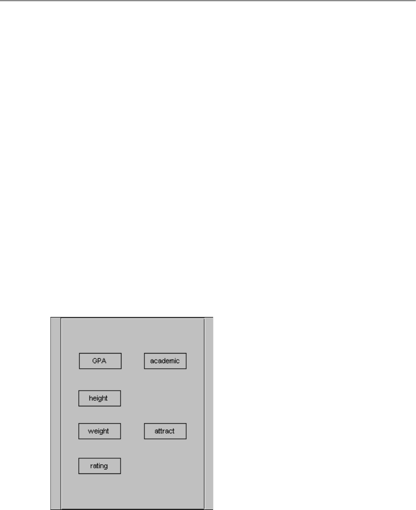
195
Felson and Bohrnstedt’s Girls and Boys
Fitting Models A and B in a Single Analysis
It is possible to fit both Model A and Model B in the same analysis. The file
Ex11-ab.amw in the Amos Examples directory shows how to do this.
Model C for Girls and Boys
You might consider adding additional constraints to Model B, such as requiring every
parameter to have the same value for boys as for girls. This would imply that the entire
variance/covariance matrix of the observed variables is the same for boys as for girls,
while also requiring that the Felson and Bohrnstedt model be correct for both groups.
Instead of following this course, we will now abandon the Felson and Bohrnstedt
model and concentrate on the hypothesis that the observed variables have the same
variance/covariance matrix for girls and boys. We will construct a model (Model C)
that embodies this hypothesis.
EStart with the path diagram for Model A or Model B and delete (Edit > Erase) every
object in the path diagram except the six observed variables. The path diagram will
then look something like this:
Each pair of rectangles needs to be connected by a double-headed arrow, for a total of
15 double-headed arrows.
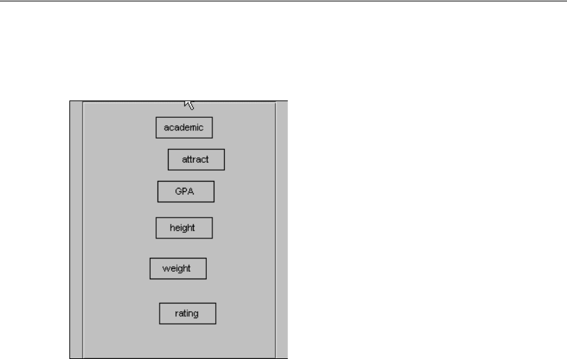
196
Example 11
ETo improve the appearance of the results, from the menus, choose Edit > Move and use
the mouse to arrange the six rectangles in a single column like this:
The Drag properties option can be used to put the rectangles in perfect vertical
alignment.
EFrom the menus, choose Edit > Drag properties.
EIn the Drag Properties dialog, select height, width, and X-coordinate. A check mark will
appear next to each one.
EUse the mouse to drag these properties from academic to attract.
This gives attract the same x coordinate as academic. In other words, it aligns them
vertically. It also makes attract the same size as academic if they are not already the
same size.
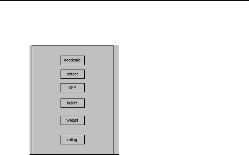
197
Felson and Bohrnstedt’s Girls and Boys
EThen drag from attract to GPA, GPA to height, and so on. Keep this up until all six
variables are lined up vertically.
ETo even out the spacing between the rectangles, from the menus, choose Edit > Select All.
EThen choose Edit > Space Vertically.
There is a special button for drawing large numbers of double-headed arrows at once.
With all six variables still selected from the previous step:
EFrom the menus, choose Tools > Macro > Draw Covariances.
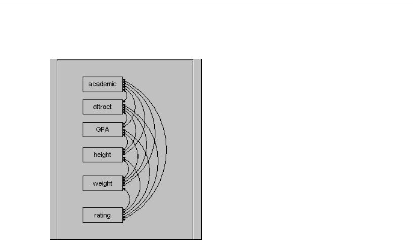
198
Example 11
Amos draws all possible covariance paths among the selected variables.
ELabel all variances and covariances with suitable names; for example, label them with
letters a through u. In the Object Properties dialog, always put a check mark next to All
groups when you name a parameter.
EFrom the menus, choose Analyze > Manage Models and create a second group for the
boys.
EChoose File > Data Files and specify the boys’ dataset (Fels_mal.sav) for this group.
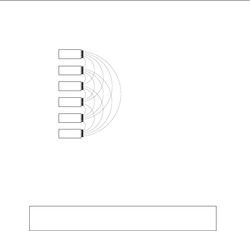
199
Felson and Bohrnstedt’s Girls and Boys
The file Ex11-c.amw contains the model specification for Model C. Here is the input
path diagram, which is the same for both groups:
Results for Model C
Model C has to be rejected at any conventional significance level.
This result means that you should not waste time proposing models that allow no
differences at all between boys and girls.
Chi-square = 48.977
Degrees of freedom = 21
Probability level = 0.001
c
GPA
d
height
f
rating
e
weight
a
academic
b
attract
Example 11: Model C
Test of variance/covariance homogeneity
Felson and Bohrnstedt (1979) girls' data
Model Specification
p
r
q
h
l
t
s
i
m
u
k
o
j
n
g

200
Example 11
Modeling in VB.NET
Model A
The following program fits Model A. It is saved as Ex11-a.vb.
Sub Main()
Dim Sem As New AmosEngine
Try
Sem.TextOutput()
Sem.BeginGroup(Sem.AmosDir & "Examples\Fels_fem.sav")
Sem.GroupName("girls")
Sem.AStructure("academic = GPA + attract + error1 (1)")
Sem.AStructure _
("attract = height + weight + rating + academic + error2 (1)")
Sem.AStructure("error2 <--> error1")
Sem.BeginGroup(Sem.AmosDir & "Examples\Fels_mal.sav")
Sem.GroupName("boys")
Sem.AStructure("academic = GPA + attract + error1 (1)")
Sem.AStructure _
("attract = height + weight + rating + academic + error2 (1)")
Sem.AStructure("error2 <--> error1")
Sem.FitModel()
Finally
Sem.Dispose()
End Try
End Sub

201
Felson and Bohrnstedt’s Girls and Boys
Model B
The following program fits Model B, in which parameter labels p1 through p6 are used
to impose equality constraints across groups. The program is saved in Ex11-b.vb.
Model C
The VB.NET program for Model C is not displayed here. It is saved in the file
Ex11-c.vb.
Sub Main()
Dim Sem As New AmosEngine
Try
Sem.TextOutput()
Sem.BeginGroup(Sem.AmosDir & "Examples\Fels_fem.sav")
Sem.GroupName("girls")
Sem.AStructure("academic = (p1) GPA + (p2) attract + (1) error1")
Sem.AStructure("attract = " & _
"(p3) height + (p4) weight + (p5) rating + (p6) academic + (1) error2")
Sem.AStructure("error2 <--> error1")
Sem.BeginGroup(Sem.AmosDir & "Examples\Fels_mal.sav")
Sem.GroupName("boys")
Sem.AStructure("academic = (p1) GPA + (p2) attract + (1) error1")
Sem.AStructure("attract = " & _
"(p3) height + (p4) weight + (p5) rating + (p6) academic + (1) error2")
Sem.AStructure("error2 <--> error1")
Sem.FitModel()
Finally
Sem.Dispose()
End Try
End Sub

202
Example 11
Fitting Multiple Models
The following program fits both Models A and B. The program is saved in the file
Ex11-ab.vb.
Sub Main()
Dim Sem As New AmosEngine
Try
Sem.TextOutput()
Sem.BeginGroup(Sem.AmosDir & "Examples\Fels_fem.sav")
Sem.GroupName("girls")
Sem.AStructure("academic = (g1) GPA + (g2) attract + (1) error1")
Sem.AStructure("attract = " & _
"(g3) height + (g4) weight + (g5) rating + (g6) academic + (1) error2")
Sem.AStructure("error2 <--> error1")
Sem.BeginGroup(Sem.AmosDir & "Examples\Fels_mal.sav")
Sem.GroupName("boys")
Sem.AStructure("academic = (b1) GPA + (b2) attract + (1) error1")
Sem.AStructure("attract = " & _
"(b3) height + (b4) weight + (b5) rating + (b6) academic + (1) error2")
Sem.AStructure("error2 <--> error1")
Sem.Model("Model_A")
Sem.Model("Model_B", _
"g1=b1", "g2=b2", "g3=b3", "g4=b4", "g5=b5", "g6=b6")
Sem.FitAllModels()
Finally
Sem.Dispose()
End Try
End Sub

203
Example
12
Simultaneous Factor Analysis for
Several Groups
Introduction
This example demonstrates how to test whether the same factor analysis model holds
for each of several populations, possibly with different parameter values for different
populations (Jöreskog, 1971).
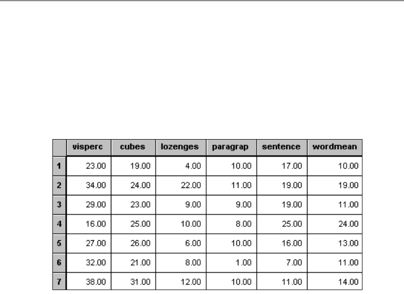
204
Example 12
About the Data
We will use the Holzinger and Swineford (1939) data described in Example 8. This
time, however, data from the 72 boys in the Grant-White sample will be analyzed along
with data from the 73 girls studied in Example 8. The girls’ data are in the file
Grnt_fem.sav and were described in Example 8. The following is a sample of the boys’
data in the file, Grnt_mal.sav:
Model A for the Holzinger and Swineford Boys and Girls
Consider the hypothesis that the common factor analysis model of Example 8 holds for
boys as well as for girls. The path diagram from Example 8 can be used as a starting
point for this two-group model. By default, Amos Graphics assumes that both groups
have the same path diagram, so the path diagram does not have to be drawn a second
time for the second group.
In Example 8, where there was only one group, the name of the group didn’t matter.
Accepting the default name Group number 1 was good enough. Now that there are two
groups to keep track of, the groups should be given meaningful names.
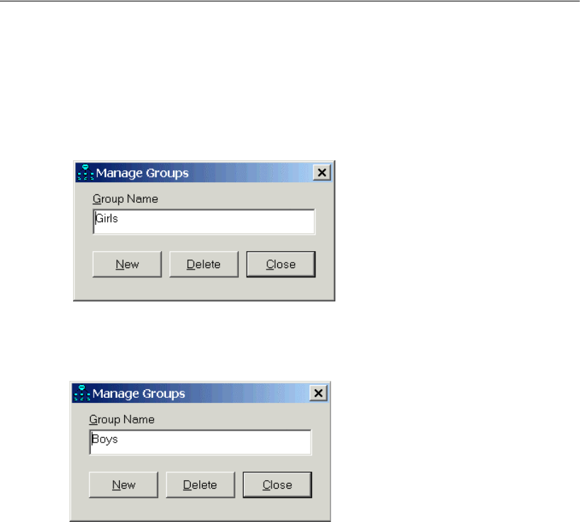
205
Simultaneous Factor Analysis for Several Groups
Naming the Groups
EFrom the menus, choose Analyze > Manage Groups.
EIn the Manage Groups dialog, type Girls for Group Name.
EWhile the Manage Groups dialog is open, create another group by clicking New.
EThen, type Boys in the Group Name text box.
EClick Close to close the Manage Groups dialog.
Specifying the Data
EFrom the menus, choose File > Data Files.
EIn the Data Files dialog, double-click Girls and specify the data file grnt_fem.sav.
EThen double-click Boys and specify the data file grnt_mal.sav.
EClick OK to close the Data Files dialog.
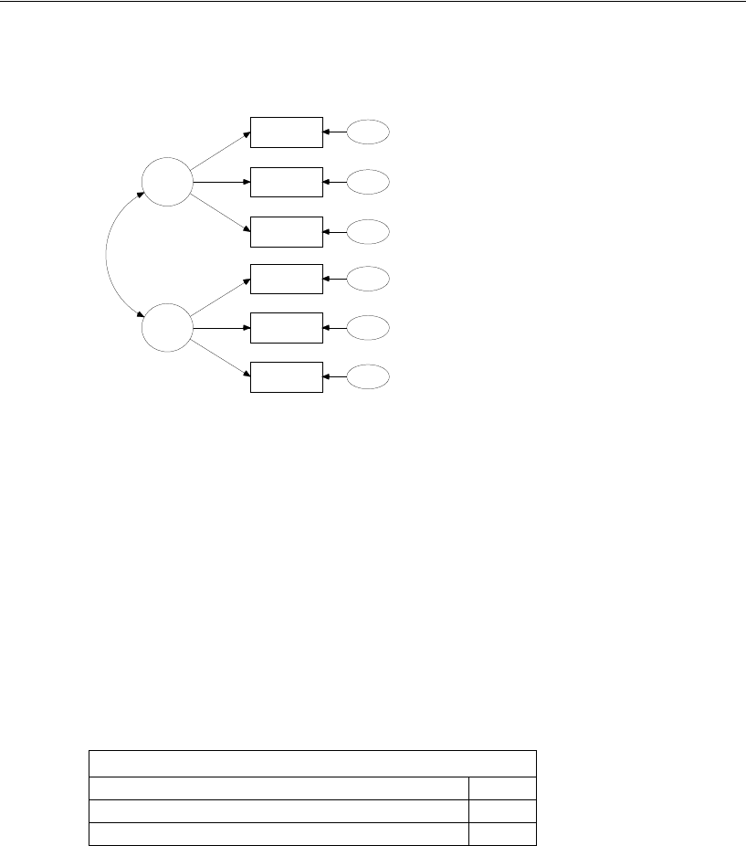
206
Example 12
Your path diagram should look something like this for the girls’ sample:
The boys’ path diagram is identical. Note, however, that the parameter estimates are
allowed to be different for the two groups.
Results for Model A
Text Output
In the calculation of degrees of freedom for this model, all of the numbers from
Example 8 are exactly doubled.
Computation of degrees of freedom: (Default model)
Number of distinct sample moments: 42
Number of distinct parameters to be estimated: 26
Degrees of freedom (42 – 26): 16
spatial
visperc
cubes
lozenges
wordmean
paragrap
sentence
err_v
err_c
err_l
err_p
err_s
err_w
verbal
1
1
1
1
1
1
1
1
Example 12: Model A
Factor analysis: Girls' sample
Holzinger and Swineford (1939)
Model Specification
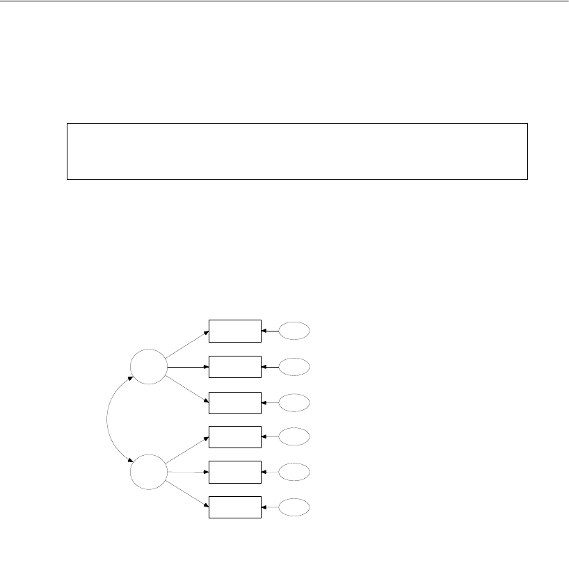
207
Simultaneous Factor Analysis for Several Groups
Model A is acceptable at any conventional significance level. If Model A had been
rejected, we would have had to make changes in the path diagram for at least one of the
two groups.
Graphics Output
Here are the (unstandardized) parameter estimates for the 73 girls. They are the same
estimates that were obtained in Example 8 where the girls alone were studied.
Chi-square = 16.480
Degrees of freedom = 16
Probability level = 0.420
23.30
spatial
visperc
cubes
lozenges
wordmean
paragrap
sentence
23.87
err_v
11.60
err_c
28.28
err_l
2.83
err_p
7.97
err_s
19.93
err_w
9.68
verbal
1.00
.61
1.20
1.00
1.33
2.23
1
1
1
1
1
1
Example 12: Model A
Factor analysis: Girls' sample
Holzinger and Swineford (1939)
Unstandardized estimates
Chi-square = 16.480 (16 df)
p = .420
7.32
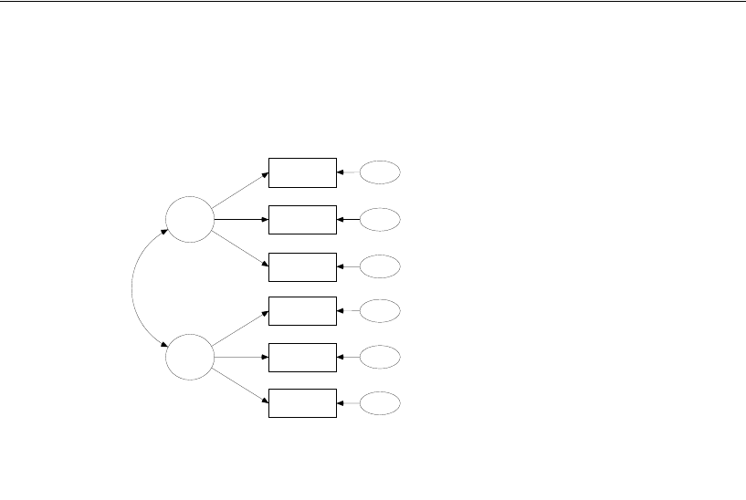
208
Example 12
The corresponding output path diagram for the 72 boys is:
Notice that the estimated regression weights vary little across groups. It seems
plausible that the two populations have the same regression weights—a hypothesis that
we will test in Model B.
Model B for the Holzinger and Swineford Boys and Girls
We now accept the hypothesis that boys and girls have the same path diagram. The next
step is to ask whether boys and girls have the same parameter values. The next model
(Model B) does not go as far as requiring that every parameter for the population of
boys be equal to the corresponding parameter for girls. It does require that the factor
pattern (that is, the regression weights) be the same for both groups. Model B still
permits different unique variances for boys and girls. The common factor variances and
covariances may also differ across groups.
ETake Model A as a starting point for Model B.
EFirst, display the girls’ path diagram by clicking Girls in the Groups panel at the left of
the path diagram.
16.06
spatial
visperc
cubes
lozenges
wordmean
paragrap
sentence
31.57
err_v
15.69
err_c
36.53
err_l
2.36
err_p
6.04
err_s
19.70
err_w
6.90
verbal
1.00
.45
1.51
1.00
1.28
2.29
1
1
1
1
1
1
6.84
Example 12: Model A
Factor analysis: Boys' sample
Holzinger and Swineford (1939)
Unstandardized estimates
Chi-square = 16.480 (16 df)
p = .420
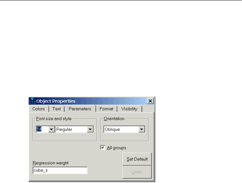
209
Simultaneous Factor Analysis for Several Groups
ERight-click the arrow that points from spatial to cubes and choose Object Properties
from the pop-up menu.
EIn the Object Properties dialog, click the Parameters tab.
EType cube_s in the Regression weight text box.
ESelect All groups. A check mark appears next to it. The effect of the check mark is to
assign the same name to this regression weight in both groups.
ELeaving the Object Properties dialog open, click each of the remaining single-headed
arrows in turn, each time typing a name in the Regression weight text box. Keep this
up until you have named every regression weight. Always make sure to select (put a
check mark next to) All groups. (Any regression weights that are already fixed at 1
should be left alone.)
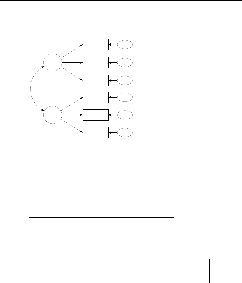
210
Example 12
The path diagram for either of the two samples should now look something like this:
Results for Model B
Text Output
Because of the additional constraints in Model B, four fewer parameters have to be
estimated from the data, increasing the number of degrees of freedom by 4.
The chi-square fit statistic is acceptable.
The chi-square difference between Models A and B, , is not
significant at any conventional level, either. Thus, Model B, which specifies a
group-invariant factor pattern, is supported by the Holzinger and Swineford data.
Computation of degrees of freedom: (Default model)
Number of distinct sample moments: 42
Number of distinct parameters to be estimated: 22
Degrees of freedom (42 – 20): 20
Chi-square = 18.292
Degrees of freedom = 20
Probability level = 0.568
spatial
visperc
cubes
lozenges
wordmean
paragrap
sentence
err_v
err_c
err_l
err_p
err_s
err_w
verbal
1
cube_s
lozn_s
1
sent_v
word_v
1
1
1
1
1
1
18.292 16.480 1.812=–
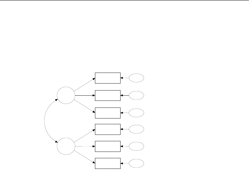
211
Simultaneous Factor Analysis for Several Groups
Graphics Output
Here are the parameter estimates for the 73 girls:
22.00
spatial
visperc
cubes
lozenges
wordmean
paragrap
sentence
25.08
err_v
12.38
err_c
25.24
err_l
2.83
err_p
8.12
err_s
19.55
err_w
9.72
verbal
1.00
.56
1.33
1.00
1.31
2.26
1
1
1
1
1
1
7.22
Example 12: Model B
Factor analysis: Girls' sample
Holzinger and Swineford (1939)
Unstandardized estimates
Chi-square = 18.292 (20 df)
p = .568
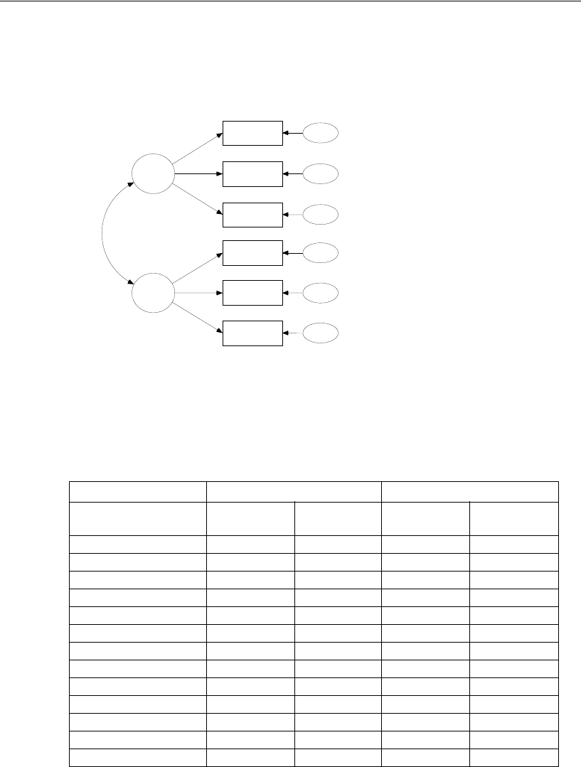
212
Example 12
Here are the parameter estimates for the 72 boys:
Not surprisingly, the Model B parameter estimates are different from the Model A
estimates. The following table shows estimates and standard errors for the two models
side by side:
Parameters Model A Model B
Girls’ sample Estimate Standard
Error Estimate Standard
Error
g: cubes <--- spatial 0.610 0.143 0.557 0.114
g: lozenges <--- spatial 1.198 0.272 1.327 0.248
g: sentence <--- verbal 1.334 0.160 1.305 0.117
g: wordmean <--- verbal 2.234 0.263 2.260 0.200
g: spatial <---> verbal 7.315 2.571 7.225 2.458
g: var(spatial) 23.302 8.124 22.001 7.078
g: var(verbal) 9.682 2.159 9.723 2.025
g: var(err_v) 23.873 5.986 25.082 5.832
g: var(err_c) 11.602 2.584 12.382 2.481
g: var(err_l) 28.275 7.892 25.244 8.040
g: var(err_p) 2.834 0.869 2.835 0.834
g: var(err_s) 7.967 1.869 8.115 1.816
g: var(err_w) 19.925 4.951 19.550 4.837
16.18
spatial
visperc
cubes
lozenges
wordmean
paragrap
sentence
31.56
err_v
15.25
err_c
40.97
err_l
2.36
err_p
5.95
err_s
19.94
err_w
6.87
verbal
1.00
.56
1.33
1.00
1.31
2.26
1
1
1
1
1
1
7.00
Example 12: Model B
Factor analysis: Boys' sample
Holzinger and Swineford (1939)
Unstandardized estimates
Chi-square = 18.292 (20 df)
p = .568

213
Simultaneous Factor Analysis for Several Groups
All but two of the estimated standard errors are smaller in Model B, including those for
the unconstrained parameters. This is a reason to use Model B for parameter estimation
rather than Model A, assuming, of course, that Model B is correct.
Boys’ sample Estimate Standard
Error Estimate Standard
Error
b: cubes <--- spatial 0.450 0.176 0.557 0.114
b: lozenges <--- spatial 1.510 0.461 1.327 0.248
b: sentence <--- verbal 1.275 0.171 1.305 0.117
b: wordmean <--- verbal 2.294 0.308 2.260 0.200
b: spatial <---> verbal 6.840 2.370 6.992 2.090
b: var(spatial) 16.058 7.516 16.183 5.886
b: var(verbal) 6.904 1.622 6.869 1.465
b: var(err_v) 31.571 6.982 31.563 6.681
b: var(err_c) 15.693 2.904 15.245 2.934
b: var(err_l) 36.526 11.532 40.974 9.689
b: var(err_p) 2.364 0.726 2.363 0.681
b: var(err_s) 6.035 1.433 5.954 1.398
b: var(err_w) 19.697 4.658 19.937 4.470

214
Example 12
Modeling in VB.NET
Model A
The following program (Ex12-a.vb) fits Model A for boys and girls:
The same model is specified for boys as for girls. However, the boys’ parameter values
can be different from the corresponding girls’ parameters.
Sub Main()
Dim Sem As New AmosEngine
Try
Sem.TextOutput()
Sem.Standardized()
Sem.Smc()
Sem.BeginGroup(Sem.AmosDir & "Examples\Grnt_fem.sav")
Sem.GroupName("Girls")
Sem.AStructure("visperc = (1) spatial + (1) err_v")
Sem.AStructure("cubes = spatial + (1) err_c")
Sem.AStructure("lozenges = spatial + (1) err_l")
Sem.AStructure("paragrap = (1) verbal + (1) err_p")
Sem.AStructure("sentence = verbal + (1) err_s")
Sem.AStructure("wordmean = verbal + (1) err_w")
Sem.BeginGroup(Sem.AmosDir & "Examples\Grnt_mal.sav")
Sem.GroupName("Boys")
Sem.AStructure("visperc = (1) spatial + (1) err_v")
Sem.AStructure("cubes = spatial + (1) err_c")
Sem.AStructure("lozenges = spatial + (1) err_l")
Sem.AStructure("paragrap = (1) verbal + (1) err_p")
Sem.AStructure("sentence = verbal + (1) err_s")
Sem.AStructure("wordmean = verbal + (1) err_w")
Sem.FitModel()
Finally
Sem.Dispose()
End Try
End Sub

215
Simultaneous Factor Analysis for Several Groups
Model B
Here is a program for fitting Model B, in which some parameters are identically named
so that they are constrained to be equal. The program is saved as Ex12-b.vb.
Sub Main()
Dim Sem As New AmosEngine
Try
Sem.TextOutput()
Sem.Standardized()
Sem.Smc()
Sem.BeginGroup(Sem.AmosDir & "Examples\Grnt_fem.sav")
Sem.GroupName("Girls")
Sem.AStructure("visperc = (1) spatial + (1) err_v")
Sem.AStructure("cubes = (cube_s) spatial + (1) err_c")
Sem.AStructure("lozenges = (lozn_s) spatial + (1) err_l")
Sem.AStructure("paragrap = (1) verbal + (1) err_p")
Sem.AStructure("sentence = (sent_v) verbal + (1) err_s")
Sem.AStructure("wordmean = (word_v) verbal + (1) err_w")
Sem.BeginGroup(Sem.AmosDir & "Examples\Grnt_mal.sav")
Sem.GroupName("Boys")
Sem.AStructure("visperc = (1) spatial + (1) err_v")
Sem.AStructure("cubes = (cube_s) spatial + (1) err_c")
Sem.AStructure("lozenges = (lozn_s) spatial + (1) err_l")
Sem.AStructure("paragrap = (1) verbal + (1) err_p")
Sem.AStructure("sentence = (sent_v) verbal + (1) err_s")
Sem.AStructure("wordmean = (word_v) verbal + (1) err_w")
Sem.FitModel()
Finally
Sem.Dispose()
End Try
End Sub

217
Example
13
Estimating and Testing Hypotheses
about Means
Introduction
This example demonstrates how to estimate means and how to test hypotheses about
means. In large samples, the method demonstrated is equivalent to multivariate
analysis of variance.
Means and Intercept Modeling
Amos and similar programs are usually used to estimate variances, covariances, and
regression weights, and to test hypotheses about those parameters. Means and
intercepts are not usually estimated, and hypotheses about means and intercepts are
not usually tested. At least in part, means and intercepts have been left out of structural
equation modeling because of the relative difficulty of specifying models that include
those parameters.
Amos, however, was designed to make means and intercept modeling easy. The
present example is the first of several showing how to estimate means and intercepts
and test hypotheses about them. In this example, the model parameters consist only
of variances, covariances, and means. Later examples introduce regression weights
and intercepts in regression equations.
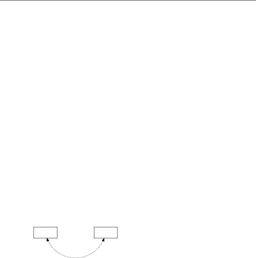
218
Example 13
About the Data
For this example, we will be using Attig’s (1983) memory data, which was described
in Example 1. We will use data from both young and old subjects. The raw data for the
two groups are contained in the Microsoft Excel workbook UserGuide.xls, in the
Attg_yng and Attg_old worksheets. In this example, we will be using only the measures
recall1 and cued1.
Model A for Young and Old Subjects
In the analysis of Model B of Example 10, we concluded that recall1 and cued1 have
the same variances and covariance for both old and young people. At least, the
evidence against that hypothesis was found to be insignificant. Model A in the present
example replicates the analysis in Example 10 of Model B with an added twist. This
time, the means of the two variables recall1 and cued1 will also be estimated.
Mean Structure Modeling in Amos Graphics
In Amos Graphics, estimating and testing hypotheses involving means is not too
different from analyzing variance and covariance structures. Take Model B of Example
10 as a starting point. Young and old subjects had the same path diagram:
The same parameter names were used in both groups, which had the effect of requiring
parameter estimates to be the same in both groups.
Means and intercepts did not appear in Example 10. To introduce means and
intercepts into the model:
EFrom the menus, choose View > Analysis Properties.
EIn the Analysis Properties dialog, click the Estimation tab.
var_rec
recall1
var_cue
cued1
cov_rc
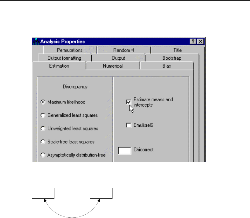
219
Estimating and Testing Hypotheses about Means
ESelect Estimate means and intercepts.
Now the path diagram looks like this (the same path diagram for each group):
The path diagram now shows a mean, variance pair of parameters for each exogenous
variable. There are no endogenous variables in this model and hence no intercepts. For
each variable in the path diagram, there is a comma followed by the name of a variance.
There is only a blank space preceding each comma because the means in the model
have not yet been named.
When you choose Calculate Estimates from the Analyze menu, Amos will estimate
two means, two variances, and a covariance for each group. The variances and the
covariance will be constrained to be equal across groups, while the means will be
unconstrained.
,var_rec
recall1
,var_cue
cued1
cov_rc

220
Example 13
The behavior of Amos Graphics changes in several ways when you select (put a check
mark next to) Estimate means and intercepts:
Mean and intercept fields appear on the Parameters tab in the Object Properties
dialog.
Constraints can be applied to means and intercepts as well as regression weights,
variances, and covariances.
From the menus, choosing Analyze > Calculate Estimates estimates means and
intercepts—subject to constraints, if any.
You have to provide sample means if you provide sample covariances as input.
When you do not put a check mark next to Estimate means and intercepts:
Only fields for variances, covariances, and regression weights are displayed on the
Parameters tab in the Object Properties dialog. Constraints can be placed only on
those parameters.
When Calculate Estimates is chosen, Amos estimates variances, covariances, and
regression weights, but not means or intercepts.
You can provide sample covariances as input without providing sample means. If
you do provide sample means, they are ignored.
If you remove the check mark next to Estimate means and intercepts after a means
model has already been fitted, the output path diagram will continue to show means
and intercepts. To display the correct output path diagram without means or
intercepts, recalculate the model estimates after removing the check mark next to
Estimate means and intercepts.
With these rules, the Estimate mean and intercepts check box makes estimating and
testing means models as easy as traditional path modeling.

221
Estimating and Testing Hypotheses about Means
Results for Model A
Text Output
The number of degrees of freedom for this model is the same as in Example 10, Model
B, but we arrive at it in a different way. This time, the number of distinct sample
moments includes the sample means as well as the sample variances and covariances.
In the young sample, there are two variances, one covariance, and two means, for a
total of five sample moments. Similarly, there are five sample moments in the old
sample. So, taking both samples together, there are 10 sample moments. As for the
parameters to be estimated, there are seven of them, namely var_rec (the variance of
recall1), var_cue (the variance of cued1), cov_rc (the covariance between recall1 and
cued1), the means of recall1 among young and old people (2), and the means of cued1
among young and old people (2).
The number of degrees of freedom thus works out to be:
The chi-square statistic here is also the same as in Model B of Example 10. The
hypothesis that old people and young people share the same variances and covariance
would be accepted at any conventional significance level.
Here are the parameter estimates for the 40 young subjects:
Chi-square = 4.588
Degrees of freedom = 3
Probability level = 0.205
Computation of degrees of freedom (Default model)
Number of distinct sample moments: 10
Number of distinct parameters to be estimated: 7
Degrees of freedom (10 - 7): 3
Means: (young subjects - Default model)
Estimate S.E. C.R. P Label
recall1
10.250 .382 26.862 ***
cued1
11.700 .374 31.292 ***
Covariances: (young subjects - Default model)
Estimate S.E. C.R. P Label
recall1
<-->
cued1
4.056 .780 5.202 *** cov_rc
Variances: (young subjects - Default model)
Estimate S.E. C.R. P Label
recall1
5.678 .909 6.245 *** var_rec
cued1
5.452 .873 6.245 *** var_cue
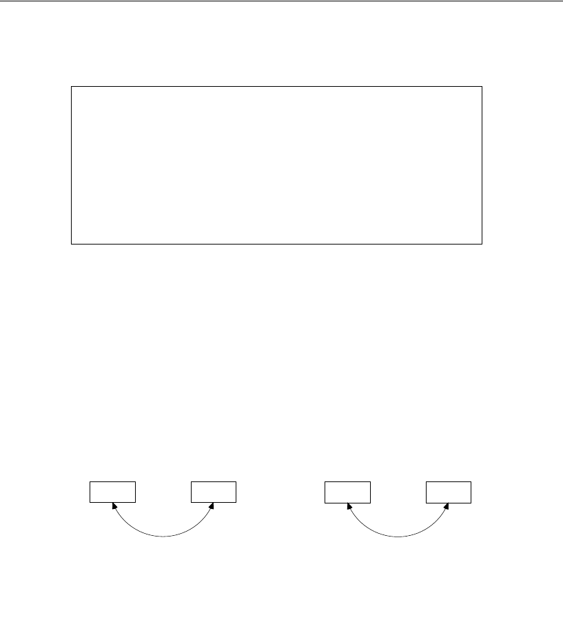
222
Example 13
Here are the estimates for the 40 old subjects:
Except for the means, these estimates are the same as those obtained in Example 10,
Model B. The estimated standard errors and critical ratios are also the same. This
demonstrates that merely estimating means, without placing any constraints on them,
has no effect on the estimates of the remaining parameters or their standard errors.
Graphics Output
The path diagram output for the two groups follows. Each variable has a mean,
variance pair displayed next to it. For instance, for young subjects, variable recall1 has
an estimated mean of 10.25 and an estimated variance of 5.68.
Means: (old subjects - Default model)
Estimate S.E. C.R. P Label
recall1
8.675
.382 22.735 ***
cued1
9.575
.374 25.609 ***
Covariances: (old subjects - Default model)
Estimate S.E. C.R. P Label
recall1
<--> cued1
4.056
.780 5.202 *** cov_rc
Variances: (old subjects - Default model)
Estimate S.E. C.R. P Label
recall1
5.678
.909 6.245 *** var_rec
cued1
5.452
.873 6.245 *** var_cue
10.25, 5.68
recall1
11.70, 5.45
cued1
4.06
Example 13: Model A
Homogenous covariance structures
Attig (1983) young subjects
Unstandardized estimates
8.68, 5.68
recall1
9.58, 5.45
cued1
4.06
Example 13: Model A
Homogenous covariance structures
Attig (1983) old subjects
Unstandardized estimates
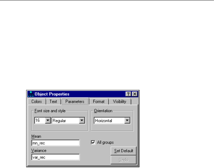
223
Estimating and Testing Hypotheses about Means
Model B for Young and Old Subjects
From now on, assume that Model A is correct, and consider the more restrictive
hypothesis that the means of recall1 and cued1 are the same for both groups.
To constrain the means for recall1 and cued1:
ERight-click recall1 and choose Object Properties from the pop-up menu.
EIn the Object Properties dialog, click the Parameters tab.
EYou can enter either a numeric value or a name in the Mean text box. For now, type the
name mn_rec.
ESelect All groups. (A check mark appears next to it. The effect of the check mark is to
assign the name mn_rec to the mean of recall1 in every group, requiring the mean of
recall1 to be the same for all groups.)
EAfter giving the name mn_rec to the mean of recall1, follow the same steps to give the
name mn_cue to the mean of cued1.
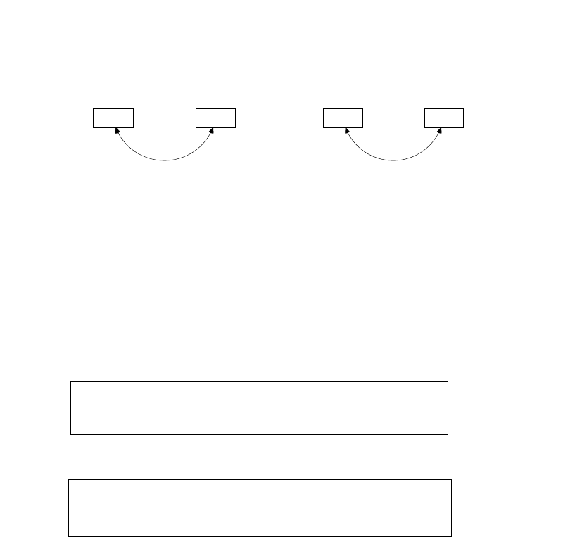
224
Example 13
The path diagrams for the two groups should now look like this:
These path diagrams are saved in the file Ex13-b.amw.
Results for Model B
With the new constraints on the means, Model B has five degrees of freedom.
Model B has to be rejected at any conventional significance level.
Chi-square = 19.267
Degrees of freedom = 5
Probability level = 0.002
mn_rec, var_rec
recall1
mn_cue, var_cue
cued1
cov_rc
Example 13: Model B
Invariant means and (co-)variances
Attig (1983) young subjects
Model Specification
mn_rec, var_rec
recall1
mn_cue, var_cue
cued1
cov_rc
Example 13: Model B
Invariant means and (co-)variances
Attig (1983) old subjects
Model Specification
Computation of degrees of freedom (Default model)
Number of distinct sample moments: 10
Number of distinct parameters to be estimated: 5
Degrees of freedom (10 - 5): 5

225
Estimating and Testing Hypotheses about Means
Comparison of Model B with Model A
If Model A is correct and Model B is wrong (which is plausible, since Model A was
accepted and Model B was rejected), then the assumption of equal means must be
wrong. A better test of the hypothesis of equal means under the assumption of equal
variances and covariances can be obtained in the following way: In comparing Model
B with Model A, the chi-square statistics differ by 14.679, with a difference of 2 in
degrees of freedom. Since Model B is obtained by placing additional constraints on
Model A, we can say that, if Model B is correct, then 14.679 is an observation on a
chi-square variable with two degrees of freedom. The probability of obtaining this
large a chi-square value is 0.001. Therefore, we reject Model B in favor of Model A,
concluding that the two groups have different means.
The comparison of Model B against Model A is as close as Amos can come to
conventional multivariate analysis of variance. In fact, the test in Amos is equivalent
to a conventional MANOVA, except that the chi-square test provided by Amos is only
asymptotically correct. By contrast, MANOVA, for this example, provides an exact
test.
Multiple Model Input
It is possible to fit both Model A and Model B in a single analysis. The file
Ex13-all.amw shows how to do this. One benefit of fitting both models in a single
analysis is that Amos will recognize that the two models are nested and will
automatically compute the difference in chi-square values as well as the p value for
testing Model B against Model A.

226
Example 13
Mean Structure Modeling in VB.NET
Model A
Here is a program (Ex13-a.vb) for fitting Model A. The program keeps the variance and
covariance restrictions that were used in Example 10, Model B, and, in addition, places
constraints on the means.
The ModelMeansAndIntercepts method is used to specify that means (of exogenous
variables) and intercepts (in predicting endogenous variables) are to be estimated as
explicit model parameters.
The Mean method is used twice in each group in order to estimate the means of
recall1 and cued1. If the Mean method had not been used in this program, recall1 and
cued1 would have had their means fixed at 0. When you use the
ModelMeansAndIntercepts method in an Amos program, Amos assumes that each
exogenous variable has a mean of 0 unless you specify otherwise. You need to use the
Model method once for each exogenous variable whose mean you want to estimate. It
is easy to forget that Amos programs behave this way when you use
ModelMeansAndIntercepts.
Sub Main()
Dim Sem As New AmosEngine
Try
Sem.TextOutput()
Sem.ModelMeansAndIntercepts()
Sem.BeginGroup(Sem.AmosDir & "Examples\UserGuide.xls", "Attg_yng")
Sem.GroupName("young_subjects")
Sem.AStructure("recall1 (var_rec)")
Sem.AStructure("cued1 (var_cue)")
Sem.AStructure("recall1 <> cued1 (cov_rc)")
Sem.Mean("recall1")
Sem.Mean("cued1")
Sem.BeginGroup(Sem.AmosDir & "Examples\UserGuide.xls", "Attg_old")
Sem.GroupName("old_subjects")
Sem.AStructure("recall1 (var_rec)")
Sem.AStructure("cued1 (var_cue)")
Sem.AStructure("recall1 <> cued1 (cov_rc)")
Sem.Mean("recall1")
Sem.Mean("cued1")
Sem.FitModel()
Finally
Sem.Dispose()
End Try
End Sub

227
Estimating and Testing Hypotheses about Means
Note: If you use the Sem.ModelMeansAndIntercepts method in an Amos program, then
the Mean method must be called once for each exogenous variable whose mean you
want to estimate. Any exogenous variable that is not explicitly estimated through use
of the Mean method is assumed to have a mean of 0.
This is different from Amos Graphics, where putting a check mark next to Estimate
means and intercepts causes the means of all exogenous variables to be treated as free
parameters except for those means that are explicitly constrained.
Model B
The following program (Ex13-b.vb) fits Model B. In addition to requiring
group-invariant variances and covariances, the program also requires the means to be
equal across groups.
Sub Main()
Dim Sem As New AmosEngine
Try
Sem.TextOutput()
Sem.ModelMeansAndIntercepts()
Sem.BeginGroup(Sem.AmosDir & "Examples\UserGuide.xls", "Attg_yng")
Sem.GroupName("young_subjects")
Sem.AStructure("recall1 (var_rec)")
Sem.AStructure("cued1 (var_cue)")
Sem.AStructure("recall1 <> cued1 (cov_rc)")
Sem.Mean("recall1", "mn_rec")
Sem.Mean("cued1", "mn_cue")
Sem.BeginGroup(Sem.AmosDir & "Examples\UserGuide.xls", "Attg_old")
Sem.GroupName("old_subjects")
Sem.AStructure("recall1 (var_rec)")
Sem.AStructure("cued1 (var_cue)")
Sem.AStructure("recall1 <> cued1 (cov_rc)")
Sem.Mean("recall1", "mn_rec")
Sem.Mean("cued1", "mn_cue")
Sem.FitModel()
Finally
Sem.Dispose()
End Try
End Sub

Fitting Multiple Models
Both models A and B can be fitted by the following program. It is saved as Ex13-all.vb.
Sub Main()
Dim Sem As New AmosEngine
Try
Sem.TextOutput()
Sem.ModelMeansAndIntercepts()
Sem.BeginGroup(Sem.AmosDir & "Examples\UserGuide.xls", "Attg_yng")
Sem.GroupName("young subjects")
Sem.AStructure("recall1 (var_rec)")
Sem.AStructure("cued1 (var_cue)")
Sem.AStructure("recall1 <> cued1 (cov_rc)")
Sem.Mean("recall1", "yng_rec")
Sem.Mean("cued1", "yng_cue")
Sem.BeginGroup(Sem.AmosDir & "Examples\UserGuide.xls", "Attg_old")
Sem.GroupName("old subjects")
Sem.AStructure("recall1 (var_rec)")
Sem.AStructure("cued1 (var_cue)")
Sem.AStructure("recall1 <> cued1 (cov_rc)")
Sem.Mean("recall1", "old_rec")
Sem.Mean("cued1", "old_cue")
Sem.Model("Model_A", "")
Sem.Model("Model_B", "yng_rec = old_rec", "yng_cue = old_cue")
Sem.FitAllModels()
Finally
Sem.Dispose()
End Try
End Sub

229
Example
14
Regression with an Explicit Intercept
Introduction
This example shows how to estimate the intercept in an ordinary regression analysis.
Assumptions Made by Amos
Ordinarily, when you specify that some variable depends linearly on some others,
Amos assumes that the linear equation expressing the dependency contains an
additive constant, or intercept, but does not estimate it. For instance, in Example 4, we
specified the variable performance to depend linearly on three other variables:
knowledge, value, and satisfaction. Amos assumed that the regression equation was
of the following form:
where , , and are regression weights, and a is the intercept. In Example 4, the
regression weights through were estimated. Amos did not estimate a in Example
4, and it did not appear in the path diagram. Nevertheless, , , and were
estimated under the assumption that a was present in the regression equation.
Similarly, knowledge, value, and satisfaction were assumed to have means, but their
means were not estimated and did not appear in the path diagram. You will usually be
satisfied with this method of handling means and intercepts in regression equations.
Sometimes, however, you will want to see an estimate of an intercept or to test a
hypothesis about an intercept. For that, you will need to take the steps demonstrated in
this example.
performance a b1knowledge b2value b3satisfaction error+×+×+×+=
b1
b2
b3
b1
b3
b1
b2
b3
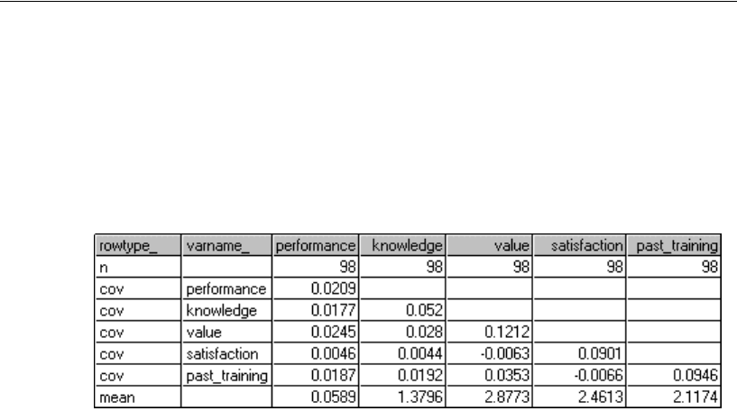
230
Example 14
About the Data
We will once again use the data of Warren, White, and Fuller (1974), first used in
Example 4. We will use the Excel worksheet Warren5v in UserGuide.xls found in the
Examples directory. Here are the sample moments (means, variances, and
covariances):
Specifying the Model
You can specify the regression model exactly as you did in Example 4. In fact, if you
have already worked through Example 4, you can use that path diagram as a starting
point for this example. Only one change is required to get Amos to estimate the means
and the intercept.
EFrom the menus, choose View > Analysis Properties.
EIn the Analysis Properties dialog, click the Estimation tab.
ESelect Estimate means and intercepts.
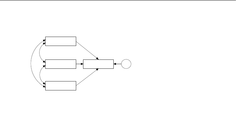
231
Regression with an Explicit Intercept
Your path diagram should then look like this:
Notice the string 0, displayed above the error variable. The 0 to the left of the comma
indicates that the mean of the error variable is fixed at 0, a standard assumption in
linear regression models. The absence of anything to the right of the comma in 0,
means that the variance of error is not fixed at a constant and does not have a name.
With a check mark next to Estimate means and intercepts, Amos will estimate a mean
for each of the predictors, and an intercept for the regression equation that predicts
performance.
Results of the Analysis
Text Output
The present analysis gives the same results as in Example 4 but with the explicit
estimation of three means and an intercept. The number of degrees of freedom is again
0, but the calculation of degrees of freedom goes a little differently. Sample means are
required for this analysis; therefore, the number of distinct sample moments includes
the sample means as well as the sample variances and covariances. There are four
sample means, four sample variances, and six sample covariances, for a total of 14
sample moments. As for the parameters to be estimated, there are three regression
weights and an intercept. Also, the three predictors have among them three means,
three variances, and three covariances. Finally, there is one error variance, for a total of
14 parameters to be estimated.
value
knowledge
performance
satisfaction
0,
error
1
Example 14
Job Performance of Farm Managers
Regression with an explicit intercept
(Model Specification)

232
Example 14
With 0 degrees of freedom, there is no hypothesis to be tested.
The estimates for regression weights, variances, and covariances are the same as in
Example 4, and so are the associated standard error estimates, critical ratios, and
pvalues.
Chi-square = 0.000
Degrees of freedom = 0
Probability level cannot be computed
Computation of degrees of freedom (Default model)
Number of distinct sample moments: 14
Number of distinct parameters to be estimated: 14
Degrees of freedom (14 - 14): 0
Regression Weights: (Group number 1 - Default model)
Estimate S.E. C.R. P Label
performance
<---
knowledge
.258 .054 4.822 ***
performance
<---
value .145 .035 4.136 ***
performance
<---
satisfaction
.049 .038 1.274 .203
Means: (Group number 1 - Default model)
Estimate
S.E. C.R. P Label
value
2.877
.035 81.818 ***
knowledge
1.380
.023 59.891 ***
satisfaction
2.461
.030 81.174 ***
Intercepts: (Group number 1 - Default model)
Estimate
S.E. C.R. P Label
performance
-.834
.140 -5.951 ***
Covariances: (Group number 1 - Default model)
Estimate S.E. C.R. P Label
knowledge
<-->
satisfaction
.004 .007 .632 .528
value <-->
satisfaction
-.006 .011 -.593 .553
knowledge
<-->
value .028 .008 3.276 .001
Variances: (Group number 1 - Default model)
Estimate
S.E. C.R. P Label
knowledge
.051
.007 6.964 ***
value
.120
.017 6.964 ***
satisfaction
.089
.013 6.964 ***
error
.012
.002 6.964 ***
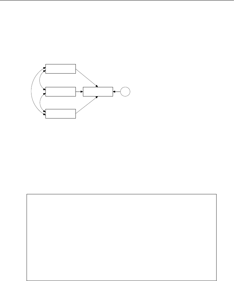
233
Regression with an Explicit Intercept
Graphics Output
Below is the path diagram that shows the unstandardized estimates for this example.
The intercept of –0.83 appears just above the endogenous variable performance.
Modeling in VB.NET
As a reminder, here is the Amos program from Example 4 (equation version):
Sub Main()
Dim Sem As New AmosEngine
Try
Sem.TextOutput()
Sem.Standardized()
Sem.Smc()
Sem.ImpliedMoments()
Sem.SampleMoments()
Sem.BeginGroup(Sem.AmosDir & "Examples\UserGuide.xls", "Warren5v")
Sem.AStructure _
("performance = knowledge + value + satisfaction + error (1)")
Sem.FitModel()
Finally
Sem.Dispose()
End Try
End Sub
2.88, .12
value
1.38, .05
knowledge
-.83
performance
2.46, .09
satisfaction
.26
.15
.05
0, .01
error
1
.00
-.01
.03
Example 14
Job Performance of Farm Managers
Regression with an explicit intercept
(Unstandardized estimates)

234
Example 14
The following program for the model of Example 14 gives all the same results, plus
mean and intercept estimates. This program is saved as Ex14.vb.
Note the Sem.ModelMeansAndIntercepts statement that causes Amos to treat means and
intercepts as explicit model parameters. Another change from Example 4 is that there
is now an additional pair of empty parentheses and a plus sign in the AStructure line.
The extra pair of empty parentheses represents the intercept in the regression equation.
The Sem.Mean statements request estimates for the means of knowledge, value, and
satisfaction. Each exogenous variable with a mean other than 0 has to appear as the
argument in a call to the Mean method. If the Mean method had not been used in this
program, Amos would have fixed the means of the exogenous variables at 0.
Sub Main()
Dim Sem As New AmosEngine
Try
Sem.TextOutput()
Sem.Standardized()
Sem.Smc()
Sem.ImpliedMoments()
Sem.SampleMoments()
Sem.ModelMeansAndIntercepts()
Sem.BeginGroup( _
Sem.AmosDir & "Examples\UserGuide.xls", "Warren5v")
Sem.AStructure( _
"performance = () + knowledge + value + satisfaction + error (1)")
Sem.Mean("knowledge")
Sem.Mean("value")
Sem.Mean("satisfaction")
Sem.FitModel()
Finally
Sem.Dispose()
End Try
End Sub

235
Regression with an Explicit Intercept
Intercept parameters can be specified by an extra pair of parentheses in a
Sem.AStructure command (as we just showed) or by using the Intercept method. In the
following program, the Intercept method is used to specify that there is an intercept in
the regression equation for predicting performance:
Sub Main()
Dim Sem As New AmosEngine
Try
Sem.TextOutput()
Sem.Standardized()
Sem.Smc()
Sem.ImpliedMoments()
Sem.SampleMoments()
Sem.ModelMeansAndIntercepts()
Sem.BeginGroup( _
Sem.AmosDir & "Examples\UserGuide.xls", "Warren5v")
Sem.AStructure("performance <--- knowledge")
Sem.AStructure("performance <--- value")
Sem.AStructure("performance <--- satisfaction")
Sem.AStructure("performance <--- error (1)")
Sem.Intercept("performance")
Sem.Mean("knowledge")
Sem.Mean("value")
Sem.Mean("satisfaction")
Sem.FitModel()
Finally
Sem.Dispose()
End Try
End Sub

237
Example
15
Factor Analysis with Structured
Means
Introduction
This example demonstrates how to estimate factor means in a common factor analysis
of data from several populations.
Factor Means
Conventionally, the common factor analysis model does not make any assumptions
about the means of any variables. In particular, the model makes no assumptions about
the means of the common factors. In fact, it is not even possible to estimate factor
means or to test hypotheses in a conventional, single-sample factor analysis.
However, Sörbom (1974) showed that it is possible to make inferences about factor
means under reasonable assumptions, as long as you are analyzing data from more
than one population. Using Sörbom’s approach, you cannot estimate the mean of
every factor for every population, but you can estimate differences in factor means
across populations. For instance, think about Example 12, where a common factor
analysis model was fitted simultaneously to a sample of girls and a sample of boys.
For each group, there were two common factors, interpreted as verbal ability and
spatial ability. The method used in Example 12 did not permit an examination of
mean verbal ability or mean spatial ability. Sörbom’s method does. Although his
method does not provide mean estimates for either girls or boys, it does give an
estimate of the mean difference between girls and boys for each factor. The method
also provides a test of significance for differences of factor means.

238
Example 15
The identification status of the factor analysis model is a difficult subject when
estimating factor means. In fact, Sörbom’s accomplishment was to show how to
constrain parameters so that the factor analysis model is identified and so that
differences in factor means can be estimated. We will follow Sörbom’s guidelines for
achieving model identification in the present example.
About the Data
We will use the Holzinger and Swineford (1939) data from Example 12. The girls’
dataset is in Grnt_fem.sav. The boys’ dataset is in Grnt_mal.sav.
Model A for Boys and Girls
Specifying the Model
We need to construct a model to test the following null hypothesis: Boys and girls have
the same average spatial ability and the same average verbal ability, where spatial and
verbal ability are common factors. In order for this hypothesis to have meaning, the
spatial and the verbal factors must be related to the observed variables in the same way
for girls as for boys. This means that the girls’ regression weights and intercepts must
be equal to the boys’ regression weights and intercepts.
Model B of Example 12 can be used as a starting point for specifying Model A of
the present example. Starting with Model B of Example 12:
EFrom the menus, choose View > Analysis Properties.
EIn the Analysis Properties dialog, click the Estimation tab.
ESelect Estimate means and intercepts (a check mark appears next to it).
The regression weights are already constrained to be equal across groups. To begin
constraining the intercepts to be equal across groups:
ERight-click one of the observed variables, such as visperc.
EChoose Object Properties from the pop-up menu.
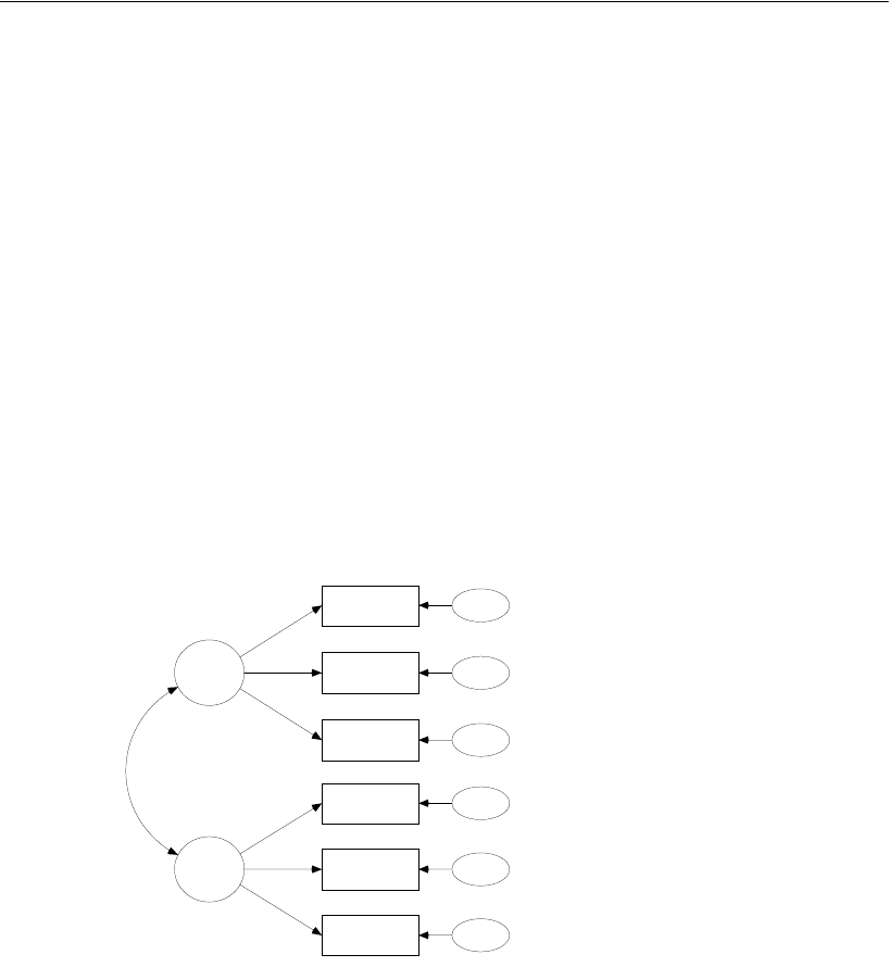
239
Factor Analysis with Structured Means
EIn the Object Properties dialog, click the Parameters tab.
EEnter a parameter name, such as int_vis, in the Intercept text box.
ESelect All groups, so that the intercept is named int_vis in both groups.
EProceed in the same way to give names to the five remaining intercepts.
As Sörbom showed, it is necessary to fix the factor means in one of the groups at a
constant. We will fix the means of the boys’ spatial and verbal factors at 0. Example
13 shows how to fix the mean of a variable to a constant value.
Note: When using the Object Properties dialog to fix the boys’ factor means at 0, be
sure that you do not put a check mark next to All groups.
After fixing the boys’ factor means at 0, follow the same procedure to assign names to
the girls’ factor means. At this point, the girls’ path diagram should look something
like this:
mn_s,
spatial
int_vis
visperc
int_cub
cubes
int_loz
lozenges
int_wrd
wordmean
int_par
paragrap
int_sen
sentence
0,
err_v
0,
err_c
0,
err_l
0,
err_p
0,
err_s
0,
err_w
mn_v,
verbal
1
cube_s
lozn_s
1
sent_v
word_v
1
1
1
1
1
1
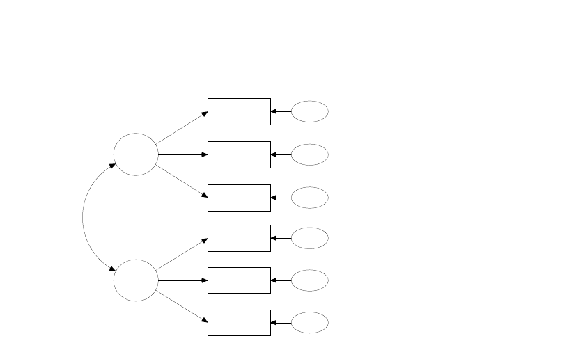
240
Example 15
The boys’ path diagram should look like this:
Understanding the Cross-Group Constraints
The cross-group constraints on intercepts and regression weights may or may not be
satisfied in the populations. One result of fitting the model will be a test of whether
these constraints hold in the populations of girls and boys. The reason for starting out
with these constraints is that (as Sörbom points out) it is necessary to impose some
constraints on the intercepts and regression weights in order to make the model
identified when estimating factor means. These are not the only constraints that would
make the model identified, but they are plausible ones.
The only difference between the boys’ and girls’ path diagrams is in the constraints
on the two factor means. For boys, the means are fixed at 0. For girls, both factor means
are estimated. The girls’ factor means are named mn_s and mn_v, but the factor means
are unconstrained because each mean has a unique name.
The boys’ factor means were fixed at 0 in order to make the model identified.
Sörbom showed that, even with all the other constraints imposed here, it is still not
possible to estimate factor means for both boys and girls simultaneously. Take verbal
ability, for example. If you fix the boys’ mean verbal ability at some constant (like 0),
you can then estimate the girls’ mean verbal ability. Alternatively, you can fix the girls’
mean verbal ability at some constant, and then estimate the boys’ mean verbal ability.
The bad news is that you cannot estimate both means at once. The good news is that
the difference between the boys’ mean and the girls’ mean will be the same, no matter
which mean you fix and no matter what value you fix for it.
0,
spatial
int_vis
visperc
int_cub
cubes
int_loz
lozenges
int_wrd
wordmean
int_par
paragrap
int_sen
sentence
0,
err_v
0,
err_c
0,
err_l
0,
err_p
0,
err_s
0,
err_w
0,
verbal
1
cube_s
lozn_s
1
sent_v
word_v
1
1
1
1
1
1
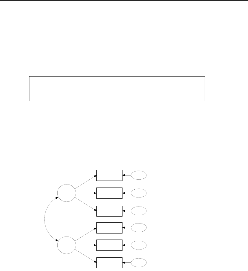
241
Factor Analysis with Structured Means
Results for Model A
Text Output
There is no reason to reject Model A at any conventional significance level.
Graphics Output
We are primarily interested in estimates of mean verbal ability and mean spatial ability,
and not so much in estimates of the other parameters. However, as always, all the
estimates should be inspected to make sure that they are reasonable. Here are the
unstandardized parameter estimates for the 73 girls:
Chi-square = 22.593
Degrees of freedom = 24
Probability level = 0.544
-1.07, 21.19
spatial
30.14
visperc
25.12
cubes
16.60
lozenges
16.22
wordmean
9.45
paragrap
18.26
sentence
0, 25.62
err_v
0, 12.55
err_c
0, 24.65
err_l
0, 2.84
err_p
0, 8.21
err_s
0, 19.88
err_w
.96, 9.95
verbal
1.00
.56
1.37
1.00
1.28
2.21
1
1
1
1
1
1
7.19
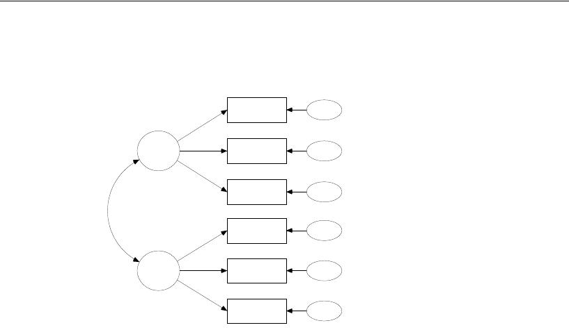
242
Example 15
Here are the boys’ estimates:
Girls have an estimated mean spatial ability of –1.07. We fixed the mean of boys’
spatial ability at 0. Thus, girls’ mean spatial ability is estimated to be 1.07 units below
boys’ mean spatial ability. This difference is not affected by the initial decision to fix
the boys’ mean at 0. If we had fixed the boys’ mean at 10.000, the girls’ mean would
have been estimated to be 8.934. If we had fixed the girls’ mean at 0, the boys’ mean
would have been estimated to be 1.07.
What unit is spatial ability expressed in? A difference of 1.07 verbal ability units
may be important or not, depending on the size of the unit. Since the regression weight
for regressing visperc on spatial ability is equal to 1, we can say that spatial ability is
expressed in the same units as scores on the visperc test. Of course, this is useful
information only if you happen to be familiar with the visperc test. There is another
approach to evaluating the mean difference of 1.07, which does not involve visperc. A
portion of the text output not reproduced here shows that spatial has an estimated
variance of 15.752 for boys, or a standard deviation of about 4.0. For girls, the variance
of spatial is estimated to be 21.188, so that its standard deviation is about 4.6. With
standard deviations this large, a difference of 1.07 would not be considered very large
for most purposes.
The statistical significance of the 1.07 unit difference between girls and boys is easy
to evaluate. Since the boys’ mean was fixed at 0, we need to ask only whether the girls’
mean differs significantly from 0.
0, 15.75
spatial
30.14
visperc
25.12
cubes
16.60
lozenges
16.22
wordmean
9.45
paragrap
18.26
sentence
0, 31.87
err_v
0, 15.31
err_c
0, 40.71
err_l
0, 2.35
err_p
0, 6.02
err_s
0, 20.33
err_w
0, 7.03
verbal
1.00
.56
1.37
1.00
1.28
2.21
1
1
1
1
1
1
6.98

243
Factor Analysis with Structured Means
Here are the girls’ factor mean estimates from the text output:
The girls’ mean spatial ability has a critical ratio of –1.209 and is not significantly
different from 0 ( ). In other words, it is not significantly different from the
boys’ mean.
Turning to verbal ability, the girls’ mean is estimated 0.96 units above the boys’
mean. Verbal ability has a standard deviation of about 2.7 among boys and about 3.15
among girls. Thus, 0.96 verbal ability units is about one-third of a standard deviation
in either group. The difference between boys and girls approaches significance at the
0.05 level ( ).
Model B for Boys and Girls
In the discussion of Model A, we used critical ratios to carry out two tests of
significance: a test for sex differences in spatial ability and a test for sex differences in
verbal ability. We will now carry out a single test of the null hypothesis that there are
no sex differences, either in spatial ability or in verbal ability. To do this, we will repeat
the previous analysis with the additional constraint that boys and girls have the same
mean on spatial ability and on verbal ability. Since the boys’ means are already fixed
at 0, requiring the girls’ means to be the same as the boys’ means amounts to setting
the girls’ means to 0 also.
The girls’ factor means have already been named mn_s and mn_v. To fix the means at 0:
EFrom the menus, choose Analyze > Manage Models.
EIn the Manage Models dialog, type Model A in the Model Name text box,
Means: (Girls - Default model)
Estimate S.E. C.R. P Label
spatial
-1.066 .881 -1.209 .226 mn_s
verbal
.956 .521 1.836 .066 mn_v
p0.226=
p0.066=
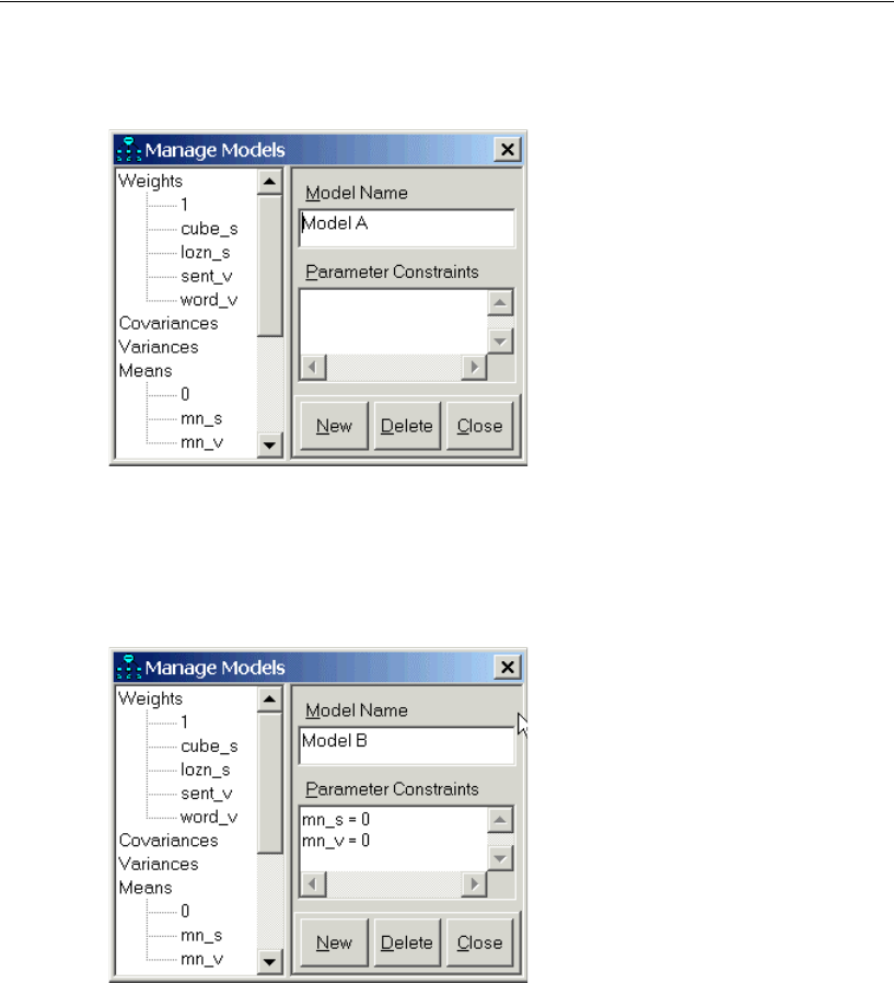
244
Example 15
ELeave the Parameter Constraints box empty.
EClick New.
EType Model B in the Model Name text box.
EType the constraints mn_s = 0 and mn_v = 0 in the Parameter Constraints text box.
EClick Close.
Now when you choose Analyze > Calculate Estimates, Amos will fit both Model A and
Model B. The file Ex15-all.amw contains this two-model setup.

245
Factor Analysis with Structured Means
Results for Model B
If we did not have Model A as a basis for comparison, we would now accept Model B,
using any conventional significance level.
Comparing Models A and B
An alternative test of Model B can be obtained by assuming that Model A is correct
and testing whether Model B fits significantly worse than Model A. A chi-square test
for this comparison is given in the text output.
EIn the Amos Output window, click Model Comparison in the tree diagram in the upper
left pane.
The table shows that Model B has two more degrees of freedom than Model A, and a
chi-square statistic that is larger by 8.030. If Model B is correct, the probability of such
a large difference in chi-square values is 0.018, providing some evidence against
Model B.
Chi-square = 30.624
Degrees of freedom = 26
Probability level = 0.243
Assuming model Model A to be correct:
Model DF CMIN P NFI
Delta-1 IFI
Delta-2 RFI
rho-1 TLI
rho2
Model B 2 8.030 .018 .024 .026 .021 .023

246
Example 15
Modeling in VB.NET
Model A
The following program fits Model A. It is saved as Ex15-a.vb.
The AStructure method is called once for each endogenous variable. The Mean method
in the girls’ group is used to specify that the means of the verbal ability and spatial
ability factors are freely estimated. The program also uses the Mean method to specify
that verbal ability and spatial ability have zero means in the boys’ group. Actually,
Amos assumes zero means by default, so the use of the Mean method for the boys is
unnecessary.
Sub Main()
Dim Sem As New AmosEngine
Try
Sem.TextOutput()
Sem.Standardized()
Sem.Smc()
Sem.ModelMeansAndIntercepts()
Sem.BeginGroup(Sem.AmosDir & "Examples\Grnt_fem.sav")
Sem.GroupName("Girls")
Sem.AStructure("visperc = (int_vis) + (1) spatial + (1) err_v")
Sem.AStructure("cubes = (int_cub) + (cube_s) spatial + (1) err_c")
Sem.AStructure("lozenges = (int_loz) + (lozn_s) spatial + (1) err_l")
Sem.AStructure("paragrap = (int_par) + (1) verbal + (1) err_p")
Sem.AStructure("sentence = (int_sen) + (sent_v) verbal + (1) err_s")
Sem.AStructure("wordmean = (int_wrd) + (word_v) verbal + (1) err_w")
Sem.Mean("spatial", "mn_s")
Sem.Mean("verbal", "mn_v")
Sem.BeginGroup(Sem.AmosDir & "Examples\Grnt_mal.sav")
Sem.GroupName("Boys")
Sem.AStructure("visperc = (int_vis) + (1) spatial + (1) err_v")
Sem.AStructure("cubes = (int_cub) + (cube_s) spatial + (1) err_c")
Sem.AStructure("lozenges = (int_loz) + (lozn_s) spatial + (1) err_l")
Sem.AStructure("paragrap = (int_par) + (1) verbal + (1) err_p")
Sem.AStructure("sentence = (int_sen) + (sent_v) verbal + (1) err_s")
Sem.AStructure("wordmean = (int_wrd) + (word_v) verbal + (1) err_w")
Sem.Mean("spatial", "0")
Sem.Mean("verbal", "0")
Sem.FitModel()
Finally
Sem.Dispose()
End Try
End Sub

247
Factor Analysis with Structured Means
Model B
The following program fits Model B. In this model, the factor means are fixed at 0 for
both boys and girls. The program is saved as Ex15-b.vb.
Sub Main()
Dim Sem As New AmosEngine
Try
Dim dataFile As String = Sem.AmosDir & "Examples\userguide.xls"
Sem.TextOutput()
Sem.Standardized()
Sem.Smc()
Sem.ModelMeansAndIntercepts()
Sem.BeginGroup(dataFile, "grnt_fem")
Sem.GroupName("Girls")
Sem.AStructure("visperc = (int_vis) + (1) spatial + (1) err_v")
Sem.AStructure("cubes = (int_cub) + (cube_s) spatial + (1) err_c")
Sem.AStructure("lozenges = (int_loz) + (lozn_s) spatial + (1) err_l")
Sem.AStructure("paragraph = (int_par) + (1) verbal + (1) err_p")
Sem.AStructure("sentence = (int_sen) + (sent_v) verbal + (1) err_s")
Sem.AStructure("wordmean = (int_wrd) + (word_v) verbal + (1) err_w")
Sem.Mean("spatial", "0")
Sem.Mean("verbal", "0")
Sem.BeginGroup(dataFile, "grnt_mal")
Sem.GroupName("Boys")
Sem.AStructure("visperc = (int_vis) + (1) spatial + (1) err_v")
Sem.AStructure("cubes = (int_cub) + (cube_s) spatial + (1) err_c")
Sem.AStructure("lozenges = (int_loz) + (lozn_s) spatial + (1) err_l")
Sem.AStructure("paragraph = (int_par) + (1) verbal + (1) err_p")
Sem.AStructure("sentence = (int_sen) + (sent_v) verbal + (1) err_s")
Sem.AStructure("wordmean = (int_wrd) + (word_v) verbal + (1) err_w")
Sem.Mean("spatial", "0")
Sem.Mean("verbal", "0")
Sem.FitModel()
Finally
Sem.Dispose()
End Try
End Sub

248
Example 15
Fitting Multiple Models
The following program (Ex15-all.vb) fits both models A and B.
Sub Main()
Dim Sem As New AmosEngine
Try
Sem.TextOutput()
Sem.Standardized()
Sem.Smc()
Sem.ModelMeansAndIntercepts()
Sem.BeginGroup(Sem.AmosDir & "Examples\Grnt_fem.sav")
Sem.GroupName("Girls")
Sem.AStructure("visperc = (int_vis) + (1) spatial + (1) err_v")
Sem.AStructure("cubes = (int_cub) + (cube_s) spatial + (1) err_c")
Sem.AStructure("lozenges = (int_loz) + (lozn_s) spatial + (1) err_l")
Sem.AStructure("paragrap = (int_par) + (1) verbal + (1) err_p")
Sem.AStructure("sentence = (int_sen) + (sent_v) verbal + (1) err_s")
Sem.AStructure("wordmean = (int_wrd) + (word_v) verbal + (1) err_w")
Sem.Mean("spatial", "mn_s")
Sem.Mean("verbal", "mn_v")
Sem.BeginGroup(Sem.AmosDir & "Examples\Grnt_mal.sav")
Sem.GroupName("Boys")
Sem.AStructure("visperc = (int_vis) + (1) spatial + (1) err_v")
Sem.AStructure("cubes = (int_cub) + (cube_s) spatial + (1) err_c")
Sem.AStructure("lozenges = (int_loz) + (lozn_s) spatial + (1) err_l")
Sem.AStructure("paragrap = (int_par) + (1) verbal + (1) err_p")
Sem.AStructure("sentence = (int_sen) + (sent_v) verbal + (1) err_s")
Sem.AStructure("wordmean = (int_wrd) + (word_v) verbal + (1) err_w")
Sem.Mean("spatial", "0")
Sem.Mean("verbal", "0")
Sem.Model("Model A") ' Sex difference in factor means.
Sem.Model("Model B", "mn_s=0", "mn_v=0") ' Equal factor means.
Sem.FitAllModels()
Finally
Sem.Dispose()
End Try
End Sub

249
Example
16
Sörbom’s Alternative to
Analysis of Covariance
Introduction
This example demonstrates latent structural equation modeling with longitudinal
observations in two or more groups, models that generalize traditional analysis of
covariance techniques by incorporating latent variables and autocorrelated residuals
(compare to Sörbom, 1978), and how assumptions employed in traditional analysis of
covariance can be tested.
Assumptions
Example 9 demonstrated an alternative to conventional analysis of covariance that
works even with unreliable covariates. Unfortunately, analysis of covariance also
depends on other assumptions besides the assumption of perfectly reliable covariates,
and the method of Example 9 also depends on those. Sörbom (1978) developed a more
general approach that allows testing many of those assumptions and relaxing some of
them.
The present example uses the same data that Sörbom used to introduce his method.
The exposition closely follows Sörbom’s.
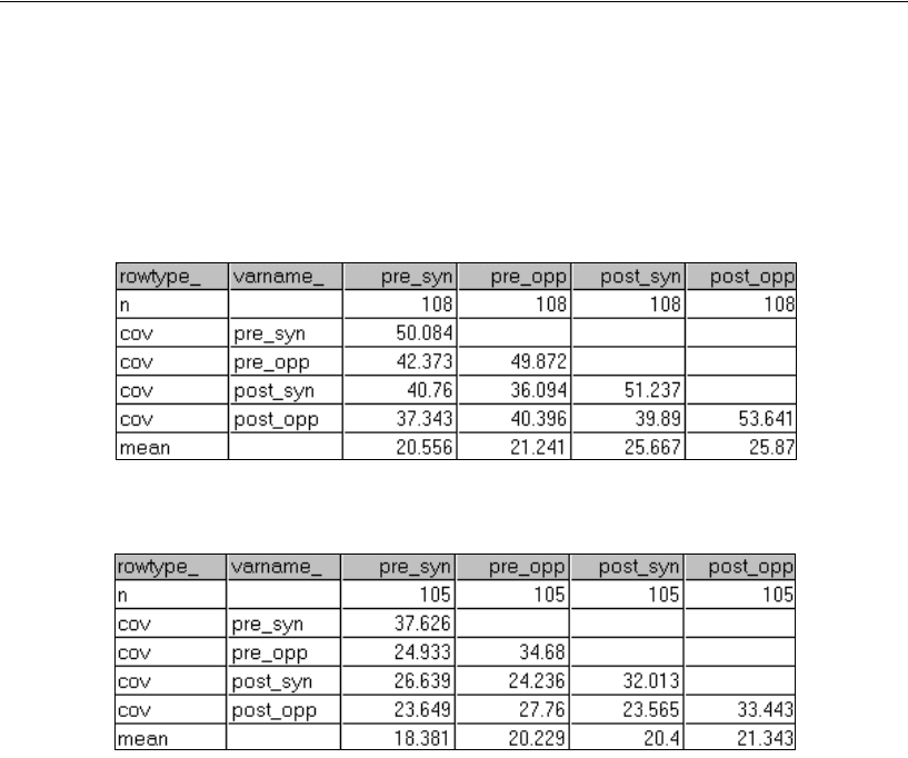
250
Example 16
About the Data
We will again use the Olsson (1973) data introduced in Example 9. The sample means,
variances, and covariances from the 108 experimental subjects are in the Microsoft
Excel worksheet Olss_exp in the workbook UserGuide.xls.
The sample means, variances, and covariances from the 105 control subjects are in the
worksheet Olss_cnt.
Both datasets contain the customary unbiased estimates of variances and covariances.
That is, the elements in the covariance matrix were obtained by dividing by ( ).
This also happens to be the default setting used by Amos for reading covariance
matrices. However, for model fitting, the default behavior is to use the maximum
likelihood estimate of the population covariance matrix (obtained by dividing by N) as
the sample covariance matrix. Amos performs the conversion from unbiased estimates
to maximum likelihood estimates automatically.
N1–
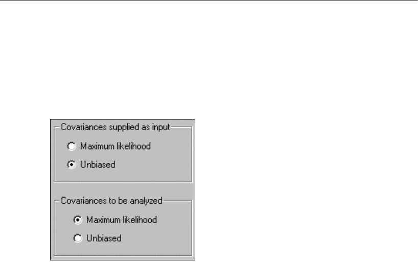
251
Sörbom’s Alternative to Analysis of Covariance
Changing the Default Behavior
EFrom the menus, choose View > Analysis Properties.
EIn the Analysis Properties dialog, click the Bias tab.
The default setting used by Amos yields results that are consistent with missing data
modeling (discussed in Example 17 and Example 18). Other SEM programs like
LISREL (Jöreskog and Sörbom, 1989) and EQS (Bentler, 1985) analyze unbiased
moments instead, resulting in slightly different results when sample sizes are small.
Selecting both Unbiased options on the Bias tab causes Amos to produce the same
estimates as LISREL or EQS. Appendix B discusses further the tradeoffs in choosing
whether to fit the maximum likelihood estimate of the covariance matrix or the
unbiased estimate.
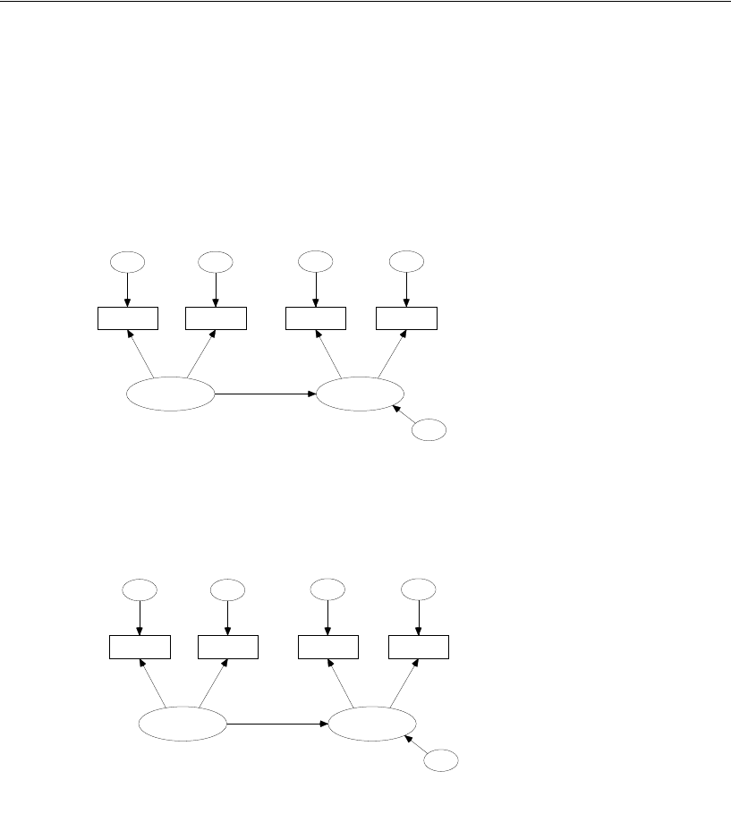
252
Example 16
Model A
Specifying the Model
Consider Sörbom’s initial model (Model A) for the Olsson data. The path diagram for
the control group is:
The following path diagram is Model A for the experimental group:
0,
pre_verbal
a_syn1
pre_syn
0,
eps1
1
1a_opp1
pre_opp
0,
eps2
opp_v1
1
0
post_verbal
a_syn2
post_syn
0,
eps3
a_opp2
post_opp
0,
eps4
1
1
opp_v2
1
0,
zeta
1
Example 16: Model A
An alternative to ANCOVA
Olsson (1973): control condition.
Model Specification
pre_diff,
pre_verbal
a_syn1
pre_syn
0,
eps1
1
1a_opp1
pre_opp
0,
eps2
opp_v1
1
effect
post_verbal
a_syn2
post_syn
0,
eps3
a_opp2
post_opp
0,
eps4
1
1
opp_v2
1
0,
zeta
1
Example 16: Model A
An alternative to ANCOVA
Olsson (1973): experimental condition.
Model Specification

253
Sörbom’s Alternative to Analysis of Covariance
Means and intercepts are an important part of this model, so be sure that you do the
following:
EFrom the menus, choose View > Analysis Properties.
EClick the Estimation tab.
ESelect Estimate means and intercepts (a check mark appears next to it).
In each group, Model A specifies that pre_syn and pre_opp are indicators of a single
latent variable called pre_verbal, and that post_syn and post_opp are indicators of
another latent variable called post_verbal. The latent variable pre_verbal is interpreted
as verbal ability at the beginning of the study, and post_verbal is interpreted as verbal
ability at the conclusion of the study. This is Sörbom’s measurement model. The
structural model specifies that post_verbal depends linearly on pre_verbal.
The labels opp_v1 and opp_v2 require the regression weights in the measurement
model to be the same for both groups. Similarly, the labels a_syn1, a_opp1, a_syn2,
and a_opp2 require the intercepts in the measurement model to be the same for both
groups. These equality constraints are assumptions that could be wrong. In fact, one
result of the upcoming analyses will be a test of these assumptions. As Sörbom points
out, some assumptions have to be made about the parameters in the measurement
model in order to make it possible to estimate and test hypotheses about parameters in
the structural model.
For the control subjects, the mean of pre_verbal and the intercept of post_verbal are
fixed at 0. This establishes the control group as the reference group for the group
comparison. You have to pick such a reference group to make the latent variable means
and intercepts identified.
For the experimental subjects, the mean and intercept parameters of the latent
factors are allowed to be nonzero. The latent variable mean labeled pre_diff represents
the difference in verbal ability prior to treatment, and the intercept labeled effect
represents the improvement of the experimental group relative to the control group.
The path diagram for this example is saved in Ex16-a.amw.
Note that Sörbom’s model imposes no cross-group constraints on the variances of
the six unobserved exogenous variables. That is, the four observed variables may have
different unique variances in the control and experimental conditions, and the
variances of pre_verbal and zeta may also be different in the two groups. We will
investigate these assumptions more closely when we get to Models X, Y, and Z.

254
Example 16
Results for Model A
Text Output
In the Amos Output window, clicking Notes for Model in the tree diagram in the upper
left pane shows that Model A cannot be accepted at any conventional significance level.
We also get the following message that provides further evidence that Model A is wrong:
Can we modify Model A so that it will fit the data while still permitting a meaningful
comparison of the experimental and control groups? It will be helpful here to repeat the
analysis and request modification indices. To obtain modification indices:
EFrom the menus, choose View > Analysis Properties.
EIn the Analysis Properties dialog, click the Output tab.
ESelect Modification indices and enter a suitable threshold in the text box to its right. For
this example, the threshold will be left at its default value of 4.
Chi-square = 34.775
Degrees of freedom = 6
Probability level = 0.000
The following variances are negative. (control - Default
model)
zeta
-2.868

255
Sörbom’s Alternative to Analysis of Covariance
Here is the modification index output from the experimental group:
In the control group, no parameter had a modification index greater than the threshold
of 4.
Model B
The largest modification index obtained with Model A suggests adding a covariance
between eps2 and eps4 in the experimental group. The modification index indicates
that the chi-square statistic will drop by at least 10.508 if eps2 and eps4 are allowed to
have a nonzero covariance. The parameter change statistic of 4.700 indicates that the
covariance estimate will be positive if it is allowed to take on any value. The suggested
modification is plausible. Eps2 represents unique variation in pre_opp, and eps4
represents unique variation in post_opp, where measurements on pre_opp and
post_opp are obtained by administering the same test, opposites, on two different
occasions. It is therefore reasonable to think that eps2 and eps4 might be positively
correlated.
The next step is to consider a revised model, called Model B, in which eps2 and eps4
are allowed to be correlated in the experimental group. To obtain Model B from Model A:
Modification Indices (experimental - Default model)
Covariances: (experimental - Default model)
M.I.
Par Change
eps2
<-->
eps4
10.508
4.700
eps2
<-->
eps3
8.980
-4.021
eps1
<-->
eps4
8.339
-3.908
eps1
<-->
eps3
7.058
3.310
Variances: (experimental - Default model)
M.I. Par Change
Regression Weights: (experimental - Default model)
M.I. Par Change
Means: (experimental - Default model)
M.I. Par Change
Intercepts: (experimental - Default model)
M.I. Par Change
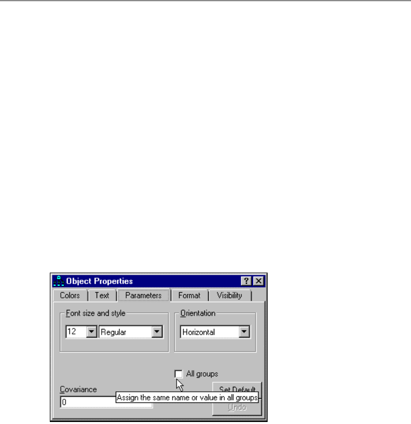
256
Example 16
EDraw a double-headed arrow connecting eps2 and eps4.
This allows eps2 and eps4 to be correlated in both groups. We do not want them to be
correlated in the control group, so the covariance must be fixed at 0 in the control
group. To accomplish this:
EClick control in the Groups panel (at the left of the path diagram) to display the path
diagram for the control group.
ERight-click the double-headed arrow and choose Object Properties from the pop-up
menu.
EIn the Object Properties dialog, click the Parameters tab.
EType 0 in the Covariance text box.
EMake sure the All groups check box is empty. With the check box empty, the constraint
on the covariance applies to only the control group.
257
Sörbom’s Alternative to Analysis of Covariance
For Model B, the path diagram for the control group is:
For the experimental group, the path diagram is:
0,
pre_verbal
a_syn1
pre_syn
0,
eps1
1
1a_opp1
pre_opp
0,
eps2
opp_v1
1
0
post_verbal
a_syn2
post_syn
0,
eps3
a_opp2
post_opp
0,
eps4
1
1
opp_v2
1
0,
zeta
1
Example 16: Model B
An alternative to ANCOVA
Olsson (1973): control condition.
Model Specification
0
pre_diff,
pre_verbal
a_syn1
pre_syn
0,
eps1
1
1a_opp1
pre_opp
0,
eps2
opp_v1
1
effect
post_verbal
a_syn2
post_syn
0,
eps3
a_opp2
post_opp
0,
eps4
1
1
opp_v2
1
0,
zeta
1
Example 16: Model B
An alternative to ANCOVA
Olsson (1973): experimental condition.
Model Specification

258
Example 16
Results for Model B
In moving from Model A to Model B, the chi-square statistic dropped by 17.712 (more
than the promised 10.508) while the number of degrees of freedom dropped by just 1.
Model B is an improvement over Model A but not enough of an improvement. Model
B still does not fit the data well. Furthermore, the variance of zeta in the control group
has a negative estimate (not shown here), just as it had for Model A. These two facts
argue strongly against Model B. There is room for hope, however, because the
modification indices suggest further modifications of Model B. The modification
indices for the control group are:
The largest modification index (4.727) suggests allowing eps2 and eps4 to be
correlated in the control group. (Eps2 and eps4 are already correlated in the
experimental group.) Making this modification leads to Model C.
Chi-square = 17.063
Degrees of freedom = 5
Probability level = 0.004
Modification Indices (control - Default model)
Covariances: (control - Default model)
M.I. Par Change
eps2
<-->
eps4
4.727
2.141
eps1
<-->
eps4
4.086
-2.384
Variances: (control - Default model)
M.I. Par Change
Regression Weights: (control - Default model)
M.I. Par Change
Means: (control - Default model)
M.I. Par Change
Intercepts: (control - Default model)
M.I. Par Change
259
Sörbom’s Alternative to Analysis of Covariance
Model C
Model C is just like Model B except that the terms eps2 and eps4 are correlated in both
the control group and the experimental group.
To specify Model C, just take Model B and remove the constraint on the covariance
between eps2 and eps4 in the control group. Here is the new path diagram for the
control group, as found in file Ex16-c.amw:
Results for Model C
Finally, we have a model that fits.
Chi-square = 2.797
Degrees of freedom = 4
Probability level = 0.592
0,
pre_verbal
a_syn1
pre_syn
0,
eps1
1
1a_opp1
pre_opp
0,
eps2
opp_v1
1
0
post_verbal
a_syn2
post_syn
0,
eps3
a_opp2
post_opp
0,
eps4
1
1
opp_v2
1
0,
zeta
1
Example 16: Model C
An alternative to ANCOVA
Olsson (1973): control condition.
Model Specification
260
Example 16
From the point of view of statistical goodness of fit, there is no reason to reject Model
C. It is also worth noting that all the variance estimates are positive. The following are
the parameter estimates for the 105 control subjects:
Next is a path diagram displaying parameter estimates for the 108 experimental
subjects:
Most of these parameter estimates are not very interesting, although you may want to
check and make sure that the estimates are reasonable. We have already noted that the
variance estimates are positive. The path coefficients in the measurement model are
positive, which is reassuring. A mixture of positive and negative regression weights in
the measurement model would have been difficult to interpret and would have cast
doubt on the model. The covariance between eps2 and eps4 is positive in both groups,
as expected.
0, 28.10
pre_verbal
18.63
pre_syn
0, 10.04
eps1
1.00
119.91
pre_opp
0, 12.12
eps2
.88
1
0
post_verbal
20.38
post_syn
0, 5.63
eps3
21.21
post_opp
0, 12.36
eps4
1.00
1
.90
1
.95
0, .54
zeta
1
Example 16: Model C
An alternative to ANCOVA
Olsson (1973): control condition.
Unstandardized estimates
6.22
1.87, 47.46
pre_verbal
18.63
pre_syn
0, 2.19
eps1
1.00
119.91
pre_opp
0, 12.39
eps2
.88
1
3.71
post_verbal
20.38
post_syn
0, 7.51
eps3
21.21
post_opp
0, 17.07
eps4
1.00
1
.90
1
.85
0, 8.86
zeta
1
Example 16: Model C
An alternative to ANCOVA
Olsson (1973): experimental condition.
Unstandardized estimates
7.34
261
Sörbom’s Alternative to Analysis of Covariance
We are primarily interested in the regression of post_verbal on pre_verbal. The
intercept, which is fixed at 0 in the control group, is estimated to be 3.71 in the
experimental group. The regression weight is estimated at 0.95 in the control group and
0.85 in the experimental group. The regression weights for the two groups are close
enough that they might even be identical in the two populations. Identical regression
weights would allow a greatly simplified evaluation of the treatment by limiting the
comparison of the two groups to a comparison of their intercepts. It is therefore
worthwhile to try a model in which the regression weights are the same for both
groups. This will be Model D.
Model D
Model D is just like Model C except that it requires the regression weight for predicting
post_verbal from pre_verbal to be the same for both groups. This constraint can be imposed
by giving the regression weight the same name, for example pre2post, in both groups. The
following is the path diagram for Model D for the experimental group:
pre_diff,
pre_verbal
a_syn1
pre_syn
0,
eps1
1
1a_opp1
pre_opp
0,
eps2
opp_v1
1
effect
post_verbal
a_syn2
post_syn
0,
eps3
a_opp2
post_opp
0,
eps4
1
1
opp_v2
1
pre2post
0,
zeta
1
Example 16: Model D
An alternative to ANCOVA
Olsson (1973): experimental condition.
Model Specification
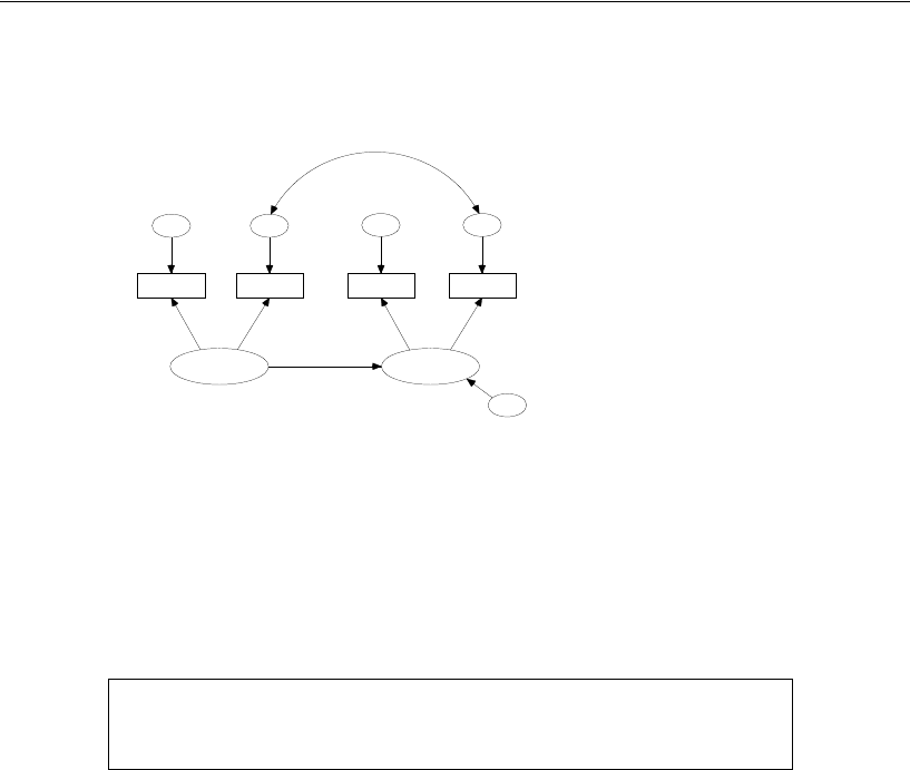
262
Example 16
Next is the path diagram for Model D for the control group:
Results for Model D
Model D would be accepted at conventional significance levels.
Testing Model D against Model C gives a chi-square value of 1.179 (= 3.976 – 2.797)
with 1 (that is, 5 – 4) degree of freedom. Again, you would accept the hypothesis of
equal regression weights (Model D).
Chi-square = 3.976
Degrees of freedom = 5
Probability level = 0.553
0,
pre_verbal
a_syn1
pre_syn
0,
eps1
1
1a_opp1
pre_opp
0,
eps2
opp_v1
1
0
post_verbal
a_syn2
post_syn
0,
eps3
a_opp2
post_opp
0,
eps4
1
1
opp_v2
1
pre2post
0,
zeta
1
Example 16: Model D
An alternative to ANCOVA
Olsson (1973): control condition.
Model Specification
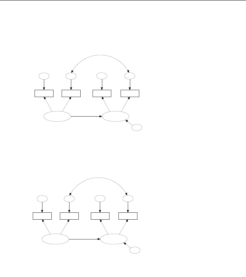
263
Sörbom’s Alternative to Analysis of Covariance
With equal regression weights, the comparison of treated and untreated subjects
now turns on the difference between their intercepts. Here are the parameter estimates
for the 105 control subjects:
The estimates for the 108 experimental subjects are:
The intercept for the experimental group is estimated as 3.63. According to the text
output (not shown here), the estimate of 3.63 has a critical ratio of 7.59. Thus, the
intercept for the experimental group is significantly different from the intercept for the
control group (which is fixed at 0).
0, 29.51
pre_verbal
18.62
pre_syn
0, 9.49
eps1
1.00
119.91
pre_opp
0, 11.92
eps2
.88
1
0
post_verbal
20.38
post_syn
0, 5.78
eps3
21.20
post_opp
0, 12.38
eps4
1.00
1
.91
1
.90
0, 1.02
zeta
1
Example 16: Model D
An alternative to ANCOVA
Olsson (1973): control condition.
Unstandardized estimates
6.33
1.88, 46.90
pre_verbal
18.62
pre_syn
0, 2.52
eps1
1.00
119.91
pre_opp
0, 12.25
eps2
.88
1
3.63
post_verbal
20.38
post_syn
0, 7.38
eps3
21.20
post_opp
0, 17.05
eps4
1.00
1
.91
1
.90
0, 8.74
zeta
1
Example 16: Model D
An alternative to ANCOVA
Olsson (1973): experimental condition.
Unstandardized estimates
7.24

264
Example 16
Model E
Another way of testing the difference in post_verbal intercepts for significance is to
repeat the Model D analysis with the additional constraint that the intercept be equal
across groups. Since the intercept for the control group is already fixed at 0, we need
add only the requirement that the intercept be 0 in the experimental group as well. This
restriction is used in Model E.
The path diagrams for Model E are just like that for Model D, except that the
intercept in the regression of post_verbal on pre_verbal is fixed at 0 in both groups.
The path diagrams are not reproduced here. They can be found in Ex16-e.amw.
Results for Model E
Model E has to be rejected.
Comparing Model E against Model D yields a chi-square value of 51.018 (= 55.094 –
3.976) with 1 (= 6 – 5) degree of freedom. Model E has to be rejected in favor of Model
D. Because the fit of Model E is significantly worse than that of Model D, the
hypothesis of equal intercepts again has to be rejected. In other words, the control and
experimental groups differ at the time of the posttest in a way that cannot be accounted
for by differences that existed at the time of the pretest.
This concludes Sörbom’s (1978) analysis of the Olsson data.
Fitting Models A Through E in a Single Analysis
The example file Ex16-a2e.amw fits all five models (A through E) in a single analysis.
The procedure for fitting multiple models in a single analysis was shown in detail in
Example 6.
Chi-square = 55.094
Degrees of freedom = 6
Probability level = 0.000

265
Sörbom’s Alternative to Analysis of Covariance
Comparison of Sörbom’s Method with the Method of Example 9
Sörbom’s alternative to analysis of covariance is more difficult to apply than the
method of Example 9. On the other hand, Sörbom’s method is superior to the method
of Example 9 because it is more general. That is, you can duplicate the method of
Example 9 by using Sörbom’s method with suitable parameter constraints.
We end this example with three additional models called X, Y, and Z. Comparisons
among these new models will allow us to duplicate the results of Example 9. However,
we will also find evidence that the method used in Example 9 was inappropriate. The
purpose of this fairly complicated exercise is to call attention to the limitations of the
approach in Example 9 and to show that some of the assumptions of that method can
be tested and relaxed in Sörbom’s approach.
Model X
First, consider a new model (Model X) that requires that the variances and covariances
of the observed variables be the same for the control and experimental conditions. The
means of the observed variables may differ between the two populations. Model X
does not specify any linear dependencies among the variables. Model X is not, by
itself, very interesting; however, Models Y and Z (coming up) are interesting, and we
will want to know how well they fit the data, compared to Model X.
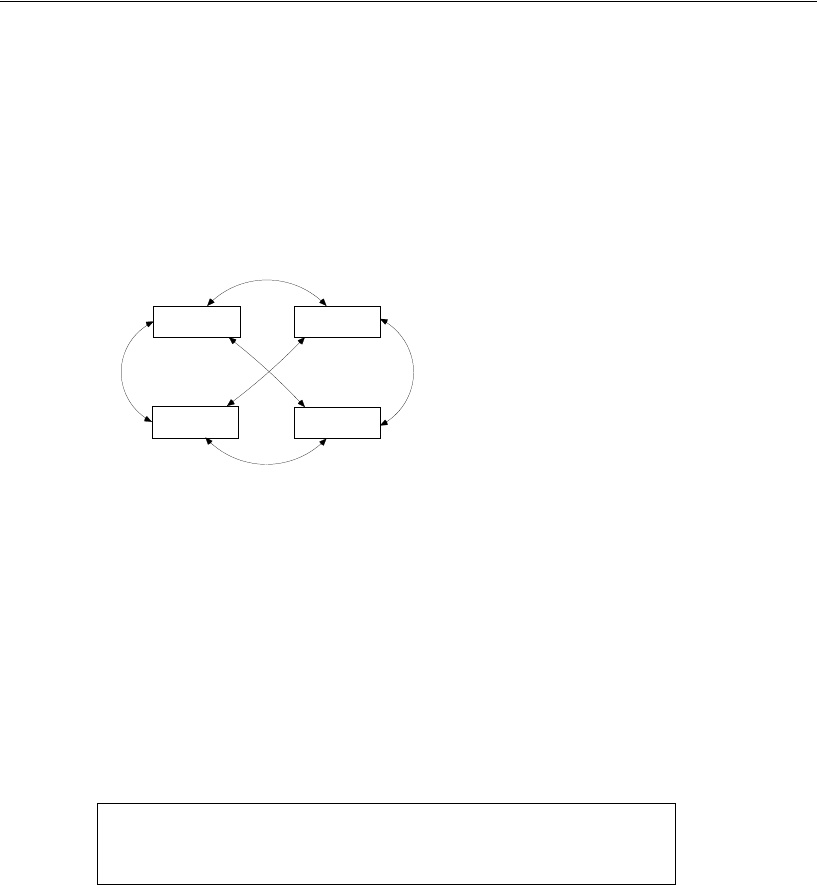
266
Example 16
Modeling in Amos Graphics
Because there are no intercepts or means to estimate, make sure that there is not a check
mark next to Estimate means and intercepts on the Estimation tab of the Analysis
Properties dialog.
The following is the path diagram for Model X for the control group:
The path diagram for the experimental group is identical. Using the same parameter
names for both groups has the effect of requiring the two groups to have the same
parameter values.
Results for Model X
Model X would be rejected at any conventional level of significance.
The analyses that follow (Models Y and Z) are actually inappropriate now that we are
satisfied that Model X is inappropriate. We will carry out the analyses as an exercise in
order to demonstrate that they yield the same results as obtained in Example 9.
Chi-square = 29.145
Degrees of freedom = 10
Probability level = 0.001
v_s1
pre_syn
v_o1
pre_opp
v_s2
post_syn
v_o2
post_opp
Example 16: Model X
Group-invariant covariance structure
Olsson (1973): control condition
Model Specification
c_s1o1
c_s2o2
c_s1s2
c_s1o2
c_s2o1
c_o1o2

267
Sörbom’s Alternative to Analysis of Covariance
Model Y
Consider a model that is just like Model D but with these additional constraints:
Verbal ability at the pretest (pre_verbal) has the same variance in the control and
experimental groups.
The variances of eps1, eps2, eps3, eps4, and zeta are the same for both groups.
The covariance between eps2 and eps4 is the same for both groups.
Apart from the correlation between eps2 and eps4, Model D required that eps1, eps2,
eps3, eps4, and zeta be uncorrelated among themselves and with every other
exogenous variable. These new constraints amount to requiring that the variances and
covariances of all exogenous variables be the same for both groups.
Altogether, the new model imposes two kinds of constraints:
All regression weights and intercepts are the same for both groups, except possibly
for the intercept used in predicting post_verbal from pre_verbal (Model D
requirements).
The variances and covariances of the exogenous variables are the same for both
groups (additional Model Y requirements).
These are the same assumptions we made in Model B of Example 9. The difference
this time is that the assumptions are made explicit and can be tested. Path diagrams for
Model Y are shown below. Means and intercepts are estimated in this model, so be sure
that you:
EFrom the menus, choose View > Analysis Properties.
EClick the Estimation tab.
ESelect Estimate means and intercepts (a check mark appears next to it).
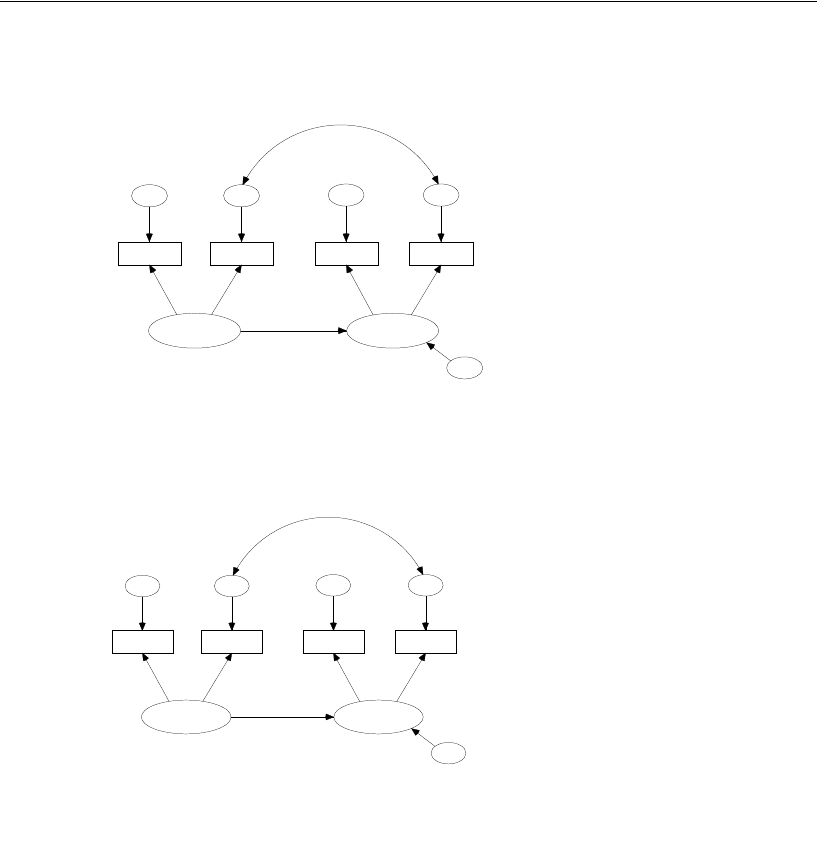
268
Example 16
Here is the path diagram for the experimental group:
Here is the path diagram for the control group:
r
e_diff, v_v1
pre_verbal
a_syn1
pre_syn
0, v_e1
eps1
1
1a_opp1
pre_opp
0, v_e2
eps2
opp_v1
1
effect
post_verbal
a_syn2
post_syn
0, v_e3
eps3
a_opp2
post_opp
0, v_e4
eps4
1
1
opp_v2
1
pre2post
0, v_z
zeta
1
Example 16: Model Y
An alternative to ANCOVA
Olsson (1973): experimental condition.
Model S
p
ecification
c_e2e4
0, v_v1
pre_verbal
a_syn1
pre_syn
0, v_e1
eps1
1
1a_opp1
pre_opp
0, v_e2
eps2
opp_v1
1
0
post_verbal
a_syn2
post_syn
0, v_e3
eps3
a_opp2
post_opp
0, v_e4
eps4
1
1
opp_v2
1
pre2post
0, v_z
zeta
1
Example 16: Model Y
An alternative to ANCOVA
Olsson (1973): control condition.
Model S
p
ecification
c_e2e4

269
Sörbom’s Alternative to Analysis of Covariance
Results for Model Y
We must reject Model Y.
This is a good reason for being dissatisfied with the analysis of Example 9, since it
depended upon Model Y (which, in Example 9, was called Model B) being correct. If
you look back at Example 9, you will see that we accepted Model B there (χ2= 2.684,
df = 2, p = 0.261). So how can we say that the same model has to be rejected here (χ2
= 31.816, df = 1, p = 0.001)? The answer is that, while the null hypothesis is the same
in both cases (Model B in Example 9 and Model Y in the present example), the
alternative hypotheses are different. In Example 9, the alternative against which Model
B is tested includes the assumption that the variances and covariances of the observed
variables are the same for both values of the treatment variable (also stated in the
assumptions on p. 36). In other words, the test of Model B carried out in Example 9
implicitly assumed homogeneity of variances and covariances for the control and
experimental populations. This is the very assumption that is made explicit in Model X
of the present example.
Model Y is a restricted version of Model X. It can be shown that the assumptions of
Model Y (equal regression weights for the two populations, and equal variances and
covariances of the exogenous variables) imply the assumptions of Model X (equal
covariances for the observed variables). Models X and Y are therefore nested models,
and it is possible to carry out a conditional test of Model Y under the assumption that
Model X is true. Of course, it will make sense to do that test only if Model X really is
true, and we have already concluded it is not. Nevertheless, let’s go through the
motions of testing Model Y against Model X. The difference in chi-square values is
2.671 (that is, 31.816 – 29.145) with 2 (= 12 – 10) degrees of freedom. These figures
are identical (within rounding error) to those of Example 9, Model B. The difference
is that in Example 9 we assumed that the test was appropriate. Now we are quite sure
(because we rejected Model X) that it is not.
Chi-square = 31.816
Degrees of freedom = 12
Probability level = 0.001
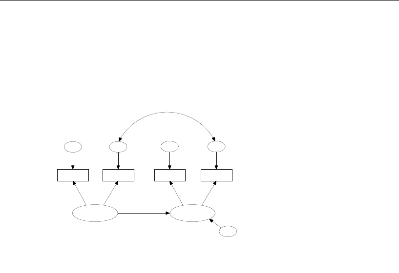
270
Example 16
If you have any doubts that the current Model Y is the same as Model B of Example
9, you should compare the parameter estimates from the two analyses. Here are the
Model Y parameter estimates for the 108 experimental subjects. See if you can match
up these estimates displayed with the unstandardized parameter estimates obtained in
Model B of Example 9.
1.88, 37.79
pre_verbal
18.53
pre_syn
0, 6.04
eps1
1.00
119.90
pre_opp
0, 12.31
eps2
.88
1
3.64
post_verbal
20.38
post_syn
0, 6.58
eps3
21.20
post_opp
0, 14.75
eps4
1.00
1
.91
1
.89
0, 4.85
zeta
1
Example 16: Model Y
An alternative to ANCOVA
Olsson (1973): experimental condition.
Unstandardized estimates
6.83
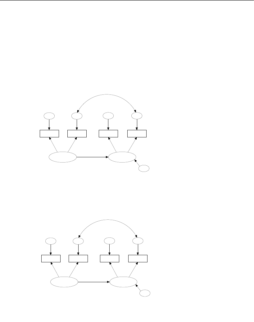
271
Sörbom’s Alternative to Analysis of Covariance
Model Z
Finally, construct a new model (Model Z) by starting with Model Y and adding the
requirement that the intercept in the equation for predicting post_verbal from
pre_verbal be the same in both populations. This model is equivalent to Model C of
Example 9. The path diagrams for Model Z are as follows:
Here is the path diagram for Model Z for the experimental group:
Here is the path diagram for the control group:
pre_diff, v_v1
pre_verbal
a_syn1
pre_syn
0, v_e1
eps1
1
1a_opp1
pre_opp
0, v_e2
eps2
opp_v1
1
0
post_verbal
a_syn2
post_syn
0, v_e3
eps3
a_opp2
post_opp
0, v_e4
eps4
1
1
opp_v2
1
pre2post
0, v_z
zeta
1
Example 16: Model Z
An alternative to ANCOVA
Olsson (1973): experimental condition.
Model Specification
c_e2e4
0, v_v1
pre_verbal
a_syn1
pre_syn
0, v_e1
eps1
1
1a_opp1
pre_opp
0, v_e2
eps2
opp_v1
1
0
post_verbal
a_syn2
post_syn
0, v_e3
eps3
a_opp2
post_opp
0, v_e4
eps4
1
1
opp_v2
1
pre2post
0, v_z
zeta
1
Example 16: Model Z
An alternative to ANCOVA
Olsson (1973): control condition.
Model Specification
c_e2e4

272
Example 16
Results for Model Z
This model has to be rejected.
Model Z also has to be rejected when compared to Model Y (χ2 = 84.280 – 31.816 =
52.464, df = 13 – 12 = 1). Within rounding error, this is the same difference in
chi-square values and degrees of freedom as in Example 9, when Model C was
compared to Model B.
Chi-square = 84.280
Degrees of freedom = 13
Probability level = 0.000

273
Sörbom’s Alternative to Analysis of Covariance
Modeling in VB.NET
Model A
The following program fits Model A. It is saved as Ex16-a.vb.
Sub Main()
Dim Sem As New AmosEngine
Try
Dim dataFile As String = Sem.AmosDir & "Examples\UserGuide.xls"
Sem.TextOutput()
Sem.Mods(4)
Sem.Standardized()
Sem.Smc()
Sem.ModelMeansAndIntercepts()
Sem.BeginGroup(dataFile, "Olss_cnt")
Sem.GroupName("control")
Sem.AStructure("pre_syn = (a_syn1) + (1) pre_verbal + (1) eps1")
Sem.AStructure( _
"pre_opp = (a_opp1) + (opp_v1) pre_verbal + (1) eps2")
Sem.AStructure("post_syn = (a_syn2) + (1) post_verbal + (1) eps3")
Sem.AStructure( _
"post_opp = (a_opp2) + (opp_v2) post_verbal + (1) eps4")
Sem.AStructure("post_verbal = (0) + () pre_verbal + (1) zeta")
Sem.BeginGroup(dataFile, "Olss_exp")
Sem.GroupName("experimental")
Sem.AStructure("pre_syn = (a_syn1) + (1) pre_verbal + (1) eps1")
Sem.AStructure( _
"pre_opp = (a_opp1) + (opp_v1) pre_verbal + (1) eps2")
Sem.AStructure("post_syn = (a_syn2) + (1) post_verbal + (1) eps3")
Sem.AStructure( _
"post_opp = (a_opp2) + (opp_v2) post_verbal + (1) eps4")
Sem.AStructure("post_verbal = (effect) + () pre_verbal + (1) zeta")
Sem.Mean("pre_verbal", "pre_diff")
Sem.FitModel()
Finally
Sem.Dispose()
End Try
End Sub

274
Example 16
Model B
To fit Model B, start with the program for Model A and add the line
Sem.AStructure("eps2 <---> eps4")
to the model specification for the experimental group. Here is the resulting program for
Model B. It is saved as Ex16-b.vb.
Sub Main()
Dim Sem As New AmosEngine
Try
Dim dataFile As String = Sem.AmosDir & "Examples\UserGuide.xls"
Sem.TextOutput()
Sem.Mods(4)
Sem.Standardized()
Sem.Smc()
Sem.ModelMeansAndIntercepts()
Sem.BeginGroup(dataFile, "Olss_cnt")
Sem.GroupName("control")
Sem.AStructure("pre_syn = (a_syn1) + (1) pre_verbal + (1) eps1")
Sem.AStructure( _
"pre_opp = (a_opp1) + (opp_v1) pre_verbal + (1) eps2")
Sem.AStructure("post_syn = (a_syn2) + (1) post_verbal + (1) eps3")
Sem.AStructure( _
"post_opp = (a_opp2) + (opp_v2) post_verbal + (1) eps4")
Sem.AStructure("post_verbal = (0) + () pre_verbal + (1) zeta")
Sem.BeginGroup(dataFile, "Olss_exp")
Sem.GroupName("experimental")
Sem.AStructure("pre_syn = (a_syn1) + (1) pre_verbal + (1) eps1")
Sem.AStructure( _
"pre_opp = (a_opp1) + (opp_v1) pre_verbal + (1) eps2")
Sem.AStructure("post_syn = (a_syn2) + (1) post_verbal + (1) eps3")
Sem.AStructure( _
"post_opp = (a_opp2) + (opp_v2) post_verbal + (1) eps4")
Sem.AStructure("post_verbal = (effect) + () pre_verbal + (1) zeta")
Sem.AStructure("eps2 <---> eps4")
Sem.Mean("pre_verbal", "pre_diff")
Sem.FitModel()
Finally
Sem.Dispose()
End Try
End Sub

275
Sörbom’s Alternative to Analysis of Covariance
Model C
The following program fits Model C. The program is saved as Ex16-c.vb.
Sub Main()
Dim Sem As New AmosEngine
Try
Dim dataFile As String = Sem.AmosDir & "Examples\UserGuide.xls"
Sem.TextOutput()
Sem.Mods(4)
Sem.Standardized()
Sem.Smc()
Sem.ModelMeansAndIntercepts()
Sem.BeginGroup(dataFile, "Olss_cnt")
Sem.GroupName("control")
Sem.AStructure("pre_syn = (a_syn1) + (1) pre_verbal + (1) eps1")
Sem.AStructure( _
"pre_opp = (a_opp1) + (opp_v1) pre_verbal + (1) eps2")
Sem.AStructure("post_syn = (a_syn2) + (1) post_verbal + (1) eps3")
Sem.AStructure( _
"post_opp = (a_opp2) + (opp_v2) post_verbal + (1) eps4")
Sem.AStructure("post_verbal = (0) + () pre_verbal + (1) zeta")
Sem.AStructure("eps2 <---> eps4")
Sem.BeginGroup(dataFile, "Olss_exp")
Sem.GroupName("experimental")
Sem.AStructure("pre_syn = (a_syn1) + (1) pre_verbal + (1) eps1")
Sem.AStructure( _
"pre_opp = (a_opp1) + (opp_v1) pre_verbal + (1) eps2")
Sem.AStructure("post_syn = (a_syn2) + (1) post_verbal + (1) eps3")
Sem.AStructure( _
"post_opp = (a_opp2) + (opp_v2) post_verbal + (1) eps4")
Sem.AStructure("post_verbal = (effect) + () pre_verbal + (1) zeta")
Sem.AStructure("eps2 <---> eps4")
Sem.Mean("pre_verbal", "pre_diff")
Sem.FitModel()
Finally
Sem.Dispose()
End Try
End Sub

276
Example 16
Model D
The following program fits Model D. The program is saved as Ex16-d.vb.
Sub Main()
Dim Sem As New AmosEngine
Try
Dim dataFile As String = Sem.AmosDir & "Examples\UserGuide.xls"
Sem.TextOutput()
Sem.Mods(4)
Sem.Standardized()
Sem.Smc()
Sem.ModelMeansAndIntercepts()
Sem.BeginGroup(dataFile, "Olss_cnt")
Sem.GroupName("control")
Sem.AStructure("pre_syn = (a_syn1) + (1) pre_verbal + (1) eps1")
Sem.AStructure( _
"pre_opp = (a_opp1) + (opp_v1) pre_verbal + (1) eps2")
Sem.AStructure("post_syn = (a_syn2) + (1) post_verbal + (1) eps3")
Sem.AStructure( _
"post_opp = (a_opp2) + (opp_v2) post_verbal + (1) eps4")
Sem.AStructure("post_verbal = (0) + (pre2post) pre_verbal + (1) zeta")
Sem.AStructure("eps2 <---> eps4")
Sem.BeginGroup(dataFile, "Olss_exp")
Sem.GroupName("experimental")
Sem.AStructure("pre_syn = (a_syn1) + (1) pre_verbal + (1) eps1")
Sem.AStructure( _
"pre_opp = (a_opp1) + (opp_v1) pre_verbal + (1) eps2")
Sem.AStructure("post_syn = (a_syn2) + (1) post_verbal + (1) eps3")
Sem.AStructure( _
"post_opp = (a_opp2) + (opp_v2) post_verbal + (1) eps4")
Sem.AStructure( _
"post_verbal = (effect) + (pre2post) pre_verbal + (1) zeta")
Sem.AStructure("eps2 <---> eps4")
Sem.Mean("pre_verbal", "pre_diff")
Sem.FitModel()
Finally
Sem.Dispose()
End Try
End Sub

277
Sörbom’s Alternative to Analysis of Covariance
Model E
The following program fits Model E. The program is saved as Ex16-e.vb.
Sub Main()
Dim Sem As New AmosEngine
Try
Dim dataFile As String = Sem.AmosDir & "Examples\UserGuide.xls"
Sem.TextOutput()
Sem.Mods(4)
Sem.Standardized()
Sem.Smc()
Sem.ModelMeansAndIntercepts()
Sem.BeginGroup(dataFile, "Olss_cnt")
Sem.GroupName("control")
Sem.AStructure("pre_syn = (a_syn1) + (1) pre_verbal + (1) eps1")
Sem.AStructure( _
"pre_opp = (a_opp1) + (opp_v1) pre_verbal + (1) eps2")
Sem.AStructure("post_syn = (a_syn2) + (1) post_verbal + (1) eps3")
Sem.AStructure( _
"post_opp = (a_opp2) + (opp_v2) post_verbal + (1) eps4")
Sem.AStructure("post_verbal = (0) + (pre2post) pre_verbal + (1) zeta")
Sem.AStructure("eps2 <---> eps4")
Sem.BeginGroup(dataFile, "Olss_exp")
Sem.GroupName("experimental")
Sem.AStructure("pre_syn = (a_syn1) + (1) pre_verbal + (1) eps1")
Sem.AStructure( _
"pre_opp = (a_opp1) + (opp_v1) pre_verbal + (1) eps2")
Sem.AStructure("post_syn = (a_syn2) + (1) post_verbal + (1) eps3")
Sem.AStructure( _
"post_opp = (a_opp2) + (opp_v2) post_verbal + (1) eps4")
Sem.AStructure("post_verbal = (0) + (pre2post) pre_verbal + (1) zeta")
Sem.AStructure("eps2 <---> eps4")
Sem.Mean("pre_verbal", "pre_diff")
Sem.FitModel()
Finally
Sem.Dispose()
End Try
End Sub

278
Example 16
Fitting Multiple Models
The following program fits all five models, A through E. The program is saved as
Ex16-a2e.vb.
Sub Main()
Dim Sem As New AmosEngine
Try
Dim dataFile As String = Sem.AmosDir & "Examples\UserGuide.xls"
Sem.TextOutput()
Sem.Mods(4)
Sem.Standardized()
Sem.Smc()
Sem.ModelMeansAndIntercepts()
Sem.BeginGroup(dataFile, "Olss_cnt")
Sem.GroupName("control")
Sem.AStructure("pre_syn = (a_syn1) + (1) pre_verbal + (1) eps1")
Sem.AStructure( _
"pre_opp = (a_opp1) + (opp_v1) pre_verbal + (1) eps2")
Sem.AStructure("post_syn = (a_syn2) + (1) post_verbal + (1) eps3")
Sem.AStructure( _
"post_opp = (a_opp2) + (opp_v2) post_verbal + (1) eps4")
Sem.AStructure("post_verbal = (0) + (c_beta) pre_verbal + (1) zeta")
Sem.AStructure("eps2 <---> eps4 (c_e2e4)")
Sem.BeginGroup(dataFile, "Olss_exp")
Sem.GroupName("experimental")
Sem.AStructure("pre_syn = (a_syn1) + (1) pre_verbal + (1) eps1")
Sem.AStructure( _
"pre_opp = (a_opp1) + (opp_v1) pre_verbal + (1) eps2")
Sem.AStructure("post_syn = (a_syn2) + (1) post_verbal + (1) eps3")
Sem.AStructure( _
"post_opp = (a_opp2) + (opp_v2) post_verbal + (1) eps4")
Sem.AStructure("post_verbal = (effect) + (e_beta) pre_verbal + (1) zeta")
Sem.AStructure("eps2 <---> eps4 (e_e2e4)")
Sem.Mean("pre_verbal", "pre_diff")
Sem.Model("Model A", "c_e2e4 = 0", "e_e2e4 = 0")
Sem.Model("Model B", "c_e2e4 = 0")
Sem.Model("Model C")
Sem.Model("Model D", "c_beta = e_beta")
Sem.Model("Model E", "c_beta = e_beta", "effect = 0")
Sem.FitAllModels()
Finally
Sem.Dispose()
End Try
End Sub

279
Sörbom’s Alternative to Analysis of Covariance
Models X, Y, and Z
VB.NET programs for Models X, Y, and Z will not be discussed here. The programs
can be found in the files Ex16-x.vb, Ex16-y.vb, and Ex16-z.vb.

281
Example
17
Missing Data
Introduction
This example demonstrates the analysis of a dataset in which some values are missing.
Incomplete Data
It often happens that data values that were anticipated in the design of a study fail to
materialize. Perhaps a subject failed to participate in part of a study. Or maybe a
person filling out a questionnaire skipped a couple of questions. You may find that
some people did not tell you their age, some did not report their income, others did
not show up on the day you measured reaction times, and so on. For one reason or
another, you often end up with a set of data that has gaps in it.
One standard method for dealing with incomplete data is to eliminate from the
analysis any observation for which some data value is missing. This is sometimes
called listwise deletion. For example, if a person fails to report his income, you would
eliminate that person from your study and proceed with a conventional analysis based
on complete data but with a reduced sample size. This method is unsatisfactory
inasmuch as it requires discarding the information contained in the responses that the
person did give because of the responses that he did not give. If missing values are
common, this method may require discarding the bulk of a sample.

282
Example 17
Another standard approach, in analyses that depend on sample moments, is to
calculate each sample moment separately, excluding an observation from the
calculation only when it is missing a value that is needed for the computation of that
particular moment. For example, in calculating the sample mean income, you would
exclude only persons whose incomes you do not know. Similarly, in computing the
sample covariance between age and income, you would exclude an observation only if
age is missing or if income is missing. This approach to missing data is sometimes
called pairwise deletion.
A third approach is data imputation, replacing the missing values with some kind
of guess, and then proceeding with a conventional analysis appropriate for complete
data. For example, you might compute the mean income of the persons who reported
their income, and then attribute that income to all persons who did not report their
income. Beale and Little (1975) discuss methods for data imputation, which are
implemented in many statistical packages.
Amos does not use any of these methods. Even in the presence of missing data, it
computes maximum likelihood estimates (Anderson, 1957). For this reason, whenever
you have missing data, you may prefer to use Amos to do a conventional analysis, such as
a simple regression analysis (as in Example 4) or to estimate means (as in Example 13).
It should be mentioned that there is one kind of missing data that Amos cannot deal
with. (Neither can any other general approach to missing data, such as the three
mentioned above.) Sometimes the very fact that a value is missing conveys
information. It could be, for example, that people with very high incomes tend (more
than others) not to answer questions about income. Failure to respond may thus convey
probabilistic information about a person’s income level, beyond the information
already given in the observed data. If this is the case, the approach to missing data that
Amos uses is inapplicable.
Amos assumes that data values that are missing are missing at random. It is not
always easy to know whether this assumption is valid or what it means in practice
(Rubin, 1976). On the other hand, if the missing at random condition is satisfied, Amos
provides estimates that are efficient and consistent. By contrast, the methods
mentioned previously do not provide efficient estimates, and provide consistent
estimates only under the stronger condition that missing data are missing completely
at random (Little and Rubin, 1989).
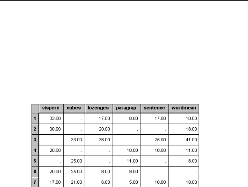
283
Missing Data
About the Data
For this example, we have modified the Holzinger and Swineford (1939) data used in
Example 8. The original dataset (in the SPSS Statistics file Grnt_fem.sav) contains the
scores of 73 girls on six tests, for a total of 438 data values. To obtain a dataset with
missing values, each of the 438 data values in Grnt_fem.sav was deleted with
probability 0.30.
The resulting dataset is in the SPSS Statistics file Grant_x.sav. Below are the first few
cases in that file. A period (.) represents a missing value.
Amos recognizes the periods in SPSS Statistics datasets and treats them as missing
data.
Amos recognizes missing data in many other data formats as well. For instance, in
an ASCII dataset, two consecutive delimiters indicate a missing value. The seven cases
shown above would look like this in ASCII format:
visperc,cubes,lozenges,paragraph,sentence,wordmean
33,,17,8,17,10
30,,20,,,18
,33,36,,25,41
28,,,10,18,11
,,25,,11,,8
20,25,6,9,,,,
17,21,6,5,10,10
Approximately 27% of the data in Grant_x.sav are missing. Complete data are
available for only seven cases.
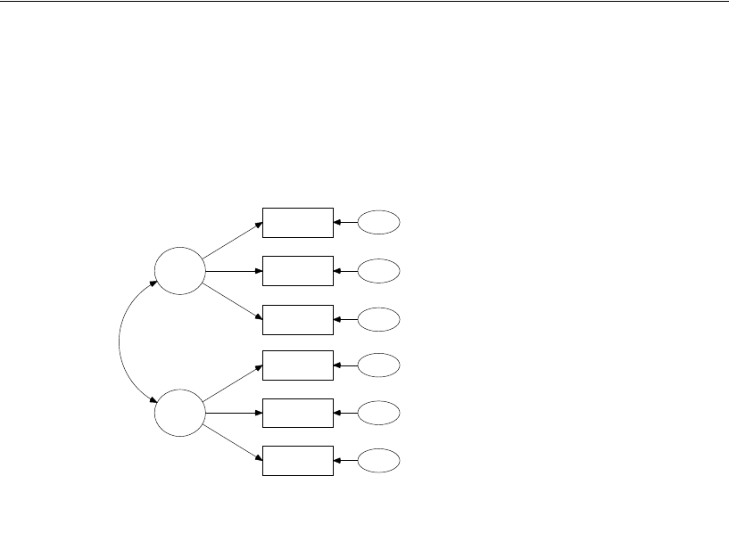
284
Example 17
Specifying the Model
We will now fit the common factor analysis model of Example 8 (shown on p. 284) to
the Holzinger and Swineford data in the file Grant_x.sav. The difference between this
analysis and the one in Example 8 is that this time 27% of the data are missing.
After specifying the data file to be Grant_x.sav and drawing the above path diagram:
EFrom the menus, choose View > Analysis Properties.
EIn the Analysis Properties dialog, click the Estimation tab.
ESelect Estimate means and intercepts (a check mark appears next to it).
This will give you an estimate of the intercept in each of the six regression equations
for predicting the measured variables. Maximum likelihood estimation with missing
values works only when you estimate means and intercepts, so you have to estimate
them even if you are not interested in the estimates.
spatial
visperc
cubes
lozenges
wordmean
paragraph
sentence
err_v
err_c
err_l
err_p
err_s
err_w
verbal
1
1
1
1
1
1
1
1
Example 17, Model A
Factor analysis with missing data
Holzinger and Swineford (1939): Girls' sample
Model Specification

285
Missing Data
Saturated and Independence Models
Computing some fit measures requires fitting the saturated and independence models in
addition to your model. This is never a problem with complete data, but fitting these
models can require extensive computation when there are missing values. The saturated
model is especially problematic. With p observed variables, the saturated model has
parameters. For example, with 10 observed variables, there are 65
parameters; with 20 variables, there are 230 parameters; with 40 variables, there are 860
parameters; and so on. It may be impractical to fit the saturated model because of the
large number of parameters. In addition, some missing data value patterns can make it
impossible in principle to fit the saturated model even if it is possible to fit your model.
With incomplete data, Amos Graphics tries to fit the saturated and independence
models in addition to your model. If Amos fails to fit the independence model, then fit
measures that depend on the fit of the independence model, such as CFI, cannot be
computed. If Amos cannot fit the saturated model, the usual chi-square statistic cannot
be computed.
Results of the Analysis
Text Output
For this example, Amos succeeds in fitting both the saturated and the independence
model. Consequently, all fit measures, including the chi-square statistic, are reported.
To see the fit measures:
EClick Model Fit in the tree diagram in the upper left corner of the Amos Output window.
The following is the portion of the output that shows the chi-square statistic for the
factor analysis model (called Default model), the saturated model, and the
independence model:
The chi-square value of 11.547 is not very different from the value of 7.853 obtained
in Example 8 with the complete dataset. In both analyses, the p values are above 0.05.
pp3+()×2⁄
CMIN
Model NPAR CMIN DF P CMIN/DF
Default model 19 11.547 8 .173 1.443
Saturated model 27 .000 0
Independence model 6 117.707 21 .000 5.605

286
Example 17
Parameter estimates, standard errors, and critical ratios have the same interpretation
as in an analysis of complete data.
Regression Weights: (Group number 1 - Default model)
Estimate S.E. C.R. P Label
visperc <---
spatial
1.000
cubes <---
spatial
.511
.153 3.347 ***
lozenges <---
spatial
1.047
.316 3.317 ***
paragrap <---
verbal
1.000
sentence <---
verbal
1.259
.194 6.505 ***
wordmean
<---
verbal
2.140
.326 6.572 ***
Intercepts: (Group number 1 - Default model)
Estimate S.E. C.R. P Label
visperc
28.885
.913 31.632 ***
cubes
24.998
.536 46.603 ***
lozenges
15.153
1.133 13.372 ***
wordmean
18.097
1.055 17.146 ***
paragrap
10.987
.468 23.495 ***
sentence
18.864
.636 29.646 ***
Covariances: (Group number 1 - Default model)
Estimate S.E. C.R. P Label
verbal
<-->
spatial
7.993
3.211 2.490 .013
Variances: (Group number 1 - Default model)
Estimate S.E. C.R. P Label
spatial
29.563
11.600 2.549 .011
verbal
10.814
2.743 3.943 ***
err_v
18.776
8.518 2.204 .028
err_c
8.034
2.669 3.011 .003
err_l
36.625
11.662 3.141 .002
err_p
2.825
1.277 2.212 .027
err_s
7.875
2.403 3.277 .001
err_w
22.677
6.883 3.295 ***

287
Missing Data
Standardized estimates and squared multiple correlations are as follows:
Standardized Regression Weights: (Group number 1 -
Default model)
Estimate
visperc <---
spatial .782
cubes <---
spatial .700
lozenges <---
spatial .685
paragrap <---
verbal .890
sentence <---
verbal .828
wordmean
<---
verbal .828
Correlations: (Group number 1 - Default model)
Estimate
verbal
<-->
spatial .447
Squared Multiple Correlations: (Group number 1 -
Default model)
Estimate
wordmean
.686
sentence
.685
paragrap
.793
lozenges
.469
cubes
.490
visperc
.612
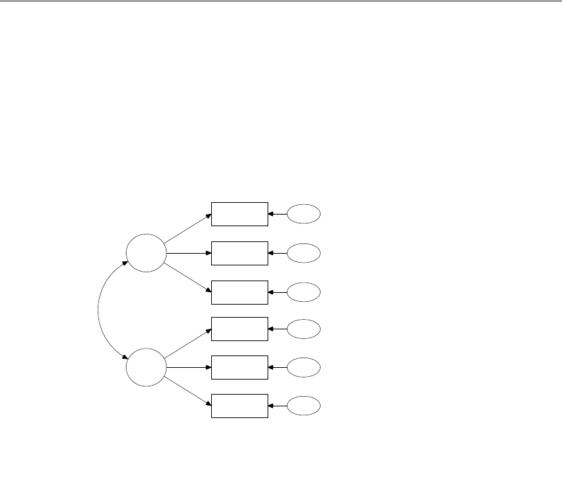
288
Example 17
Graphics Output
Here is the path diagram showing the standardized estimates and the squared multiple
correlations for the endogenous variables:
The standardized parameter estimates may be compared to those obtained from the
complete data in Example 8. The two sets of estimates are identical in the first decimal
place.
Modeling in VB.NET
When you write an Amos program to analyze incomplete data, Amos does not
automatically fit the independence and saturated models. (Amos Graphics does fit
those models automatically.) If you want your Amos program to fit the independence
and saturated models, your program has to include code to specify those models. In
particular, in order for your program to compute the usual likelihood ratio chi-square
statistic, your program must include code to fit the saturated model.
spatial
.61
visperc
.49
cubes
.47
lozenges
.69
wordmean
.79
paragraph
.69
sentence
err_v
err_c
err_l
err_p
err_s
err_w
verbal
.78
.70
.69
.89
.83
.83
.45
Example 17
Factor analysis with missing data
Holzinger and Swineford (1939): Girls' sample
Standardized estimates
Chi square = 11.547
df = 8
p = .173

289
Missing Data
This section outlines three steps necessary for computing the likelihood ratio chi-
square statistic:
Fitting the factor model
Fitting the saturated model
Computing the likelihood ratio chi-square statistic and its p value
First, the three steps are performed by three separate programs. After that, the three
steps will be combined into a single program.
Fitting the Factor Model (Model A)
The following program fits the confirmatory factor model (Model A). It is saved as
Ex17-a.vb.
Notice that the ModelMeansAndIntercepts method is used to specify that means and
intercepts are parameters of the model, and that each of the six regression equations
contains a set of empty parentheses representing an intercept. When you analyze data
with missing values, means and intercepts must appear in the model as explicit
parameters. This is different from the analysis of complete data, where means and
intercepts do not have to appear in the model unless you want to estimate them or
constrain them.
Sub Main()
Dim Sem As New AmosEngine
Try
Sem.Title("Example 17 a: Factor Model")
Sem.TextOutput()
Sem.Standardized()
Sem.Smc()
Sem.AllImpliedMoments()
Sem.ModelMeansAndIntercepts()
Sem.BeginGroup(Sem.AmosDir & "Examples\Grant_x.sav")
Sem.AStructure("visperc = ( ) + (1) spatial + (1) err_v")
Sem.AStructure("cubes = ( ) + spatial + (1) err_c")
Sem.AStructure("lozenges = ( ) + spatial + (1) err_l")
Sem.AStructure("paragrap = ( ) + (1) verbal + (1) err_p")
Sem.AStructure("sentence = ( ) + verbal + (1) err_s")
Sem.AStructure("wordmean = ( ) + verbal + (1) err_w")
Sem.FitModel()
Finally
Sem.Dispose()
End Try
End Sub

290
Example 17
The fit of Model A is summarized as follows:
The Function of log likelihood value is displayed instead of the chi-square fit statistic
that you get with complete data. In addition, at the beginning of the Summary of models
section of the text output, Amos displays the warning:
Whenever Amos prints this note, the values in the cmin column of the Summary of
models section do not contain the familiar fit chi-square statistics. To evaluate the fit
of the factor model, its Function of log likelihood value has to be compared to that of
some less constrained baseline model, such as the saturated model.
Fitting the Saturated Model (Model B)
The saturated model has as many free parameters as there are first and second order
moments. When complete data are analyzed, the saturated model always fits the
sample data perfectly (with chi-square = 0.00 and df = 0). All structural equation
models with the same six observed variables are either equivalent to the saturated
model or are constrained versions of it. A saturated model will fit the sample data at
least as well as any constrained model, and its Function of log likelihood value will be
no larger and is, typically, smaller.
Function of log likelihood = 1375.133
Number of parameters = 19
The saturated model was not fitted to the data of at least one group. For this
reason, only the 'function of log likelihood', AIC and BCC are reported. The
likelihood ratio chi-square statistic and other fit measures are not reported.

291
Missing Data
The following program fits the saturated model (Model B). The program is saved as
Ex17-b.vb.
Following the BeginGroup line, there are six uses of the Mean method, requesting
estimates of means for the six variables. When Amos estimates their means, it will
automatically estimate their variances and covariances as well, as long as the program
does not explicitly constrain the variances and covariances.
Sub Main()
Dim Saturated As New AmosEngine
Try
'Set up and estimate Saturated model:
Saturated.Title("Example 17 b: Saturated Model")
Saturated.TextOutput()
Saturated.AllImpliedMoments()
Saturated.ModelMeansAndIntercepts()
Saturated.BeginGroup(Saturated.AmosDir & "Examples\Grant_x.sav")
Saturated.Mean("visperc")
Saturated.Mean("cubes")
Saturated.Mean("lozenges")
Saturated.Mean("paragrap")
Saturated.Mean("sentence")
Saturated.Mean("wordmean")
Saturated.FitModel()
Finally
Saturated.Dispose()
End Try
End Sub

292
Example 17
The following are the unstandardized parameter estimates for the saturated Model B:
Means: (Group number 1 - Model 1)
Estimate
S.E. C.R. P Label
visperc 28.883
.910 31.756 ***
cubes 25.154
.540 46.592 ***
lozenges 14.962
1.101 13.591 ***
paragrap 10.976
.466 23.572 ***
sentence 18.802
.632 29.730 ***
wordmean
18.263
1.061 17.211 ***
Covariances: (Group number 1 - Model 1)
Estimate S.E. C.R. P Label
visperc <-->
cubes 17.484 4.614 3.789 ***
visperc <-->
lozenges 31.173 9.232 3.377 ***
cubes <-->
lozenges 17.036 5.459 3.121 .002
visperc <-->
paragrap 8.453 3.705 2.281 .023
cubes <-->
paragrap 2.739 2.179 1.257 .209
lozenges
<-->
paragrap 9.287 4.596 2.021 .043
visperc <-->
sentence 14.382 5.114 2.813 .005
cubes <-->
sentence 1.678 2.929 .573 .567
lozenges
<-->
sentence 10.544 6.050 1.743 .081
paragrap
<-->
sentence 13.470 2.945 4.574 ***
visperc <-->
wordmean
14.665 8.314 1.764 .078
cubes <-->
wordmean
3.470 4.870 .713 .476
lozenges
<-->
wordmean
29.655 10.574 2.804 .005
paragrap
<-->
wordmean
23.616 5.010 4.714 ***
sentence
<-->
wordmean
29.577 6.650 4.447 ***
Variances: (Group number 1 - Model 1)
Estimate
S.E.
C.R. P Label
visperc 49.584
9.398
5.276 ***
cubes 16.484
3.228
5.106 ***
lozenges 67.901
13.404
5.066 ***
paragrap 13.570
2.515
5.396 ***
sentence 25.007
4.629
5.402 ***
wordmean
73.974
13.221
5.595 ***

293
Missing Data
The AllImpliedMoments method in the program displays the following table of
estimates:
These estimates, even the estimated means, are different from the sample values
computed using either pairwise or listwise deletion methods. For example, 53 people
took the visual perception test (visperc). The sample mean of those 53 visperc scores
is 28.245. One might expect the Amos estimate of the mean visual perception score to
be 28.245. In fact it is 28.883.
Amos displays the following fit information for Model B:
Function of log likelihood values can be used to compare the fit of nested models. In
this case, Model A (with a fit statistic of 1375.133 and 19 parameters) is nested within
Model B (with a fit statistic of 1363.586 and 27 parameters). When a stronger model
(Model A) is being compared to a weaker model (Model B), and where the stronger
model is correct, you can say the following: The amount by which the Function of log
likelihood increases when you switch from the weaker model to the stronger model is
an observation on a chi-square random variable with degrees of freedom equal to the
difference in the number of parameters of the two models. In the present example, the
Function of log likelihood for Model A exceeds that for Model B by 11.547
(= 1375.133 – 1363.586). At the same time, Model A requires estimating only 19
parameters while Model B requires estimating 27 parameters, for a difference of 8. In
other words, if Model A is correct, 11.547 is an observation on a chi-square variable
with 8 degrees of freedom. A chi-square table can be consulted to see whether this chi-
square statistic is significant.
Function of log likelihood = 1363.586
Number of parameters = 27
Implied (for all variables) Covariances (Group number 1 - Model 1)
wordmean sentence paragrap lozenges cubes visperc
wordmean 73.974
sentence 29.577 25.007
paragrap 23.616 13.470 13.570
lozenges 29.655 10.544 9.287 67.901
cubes 3.470 1.678 2.739 17.036 16.484
visperc 14.665 14.382 8.453 31.173 17.484 49.584
Implied (for all variables) Means (Group number 1 - Model 1)
wordmean sentence paragrap lozenges cubes visperc
18.263 18.802 10.976 14.962 25.154 28.883
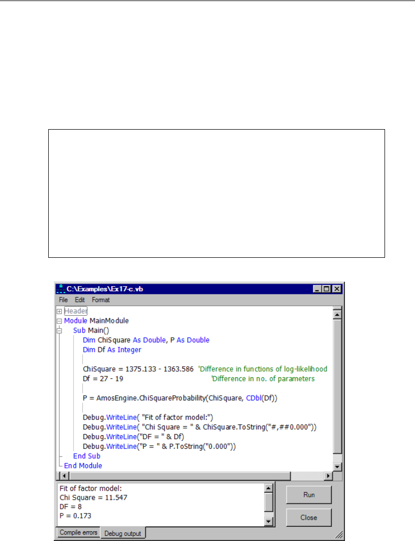
294
Example 17
Computing the Likelihood Ratio Chi-Square Statistic and P
Instead of consulting a chi-square table, you can use the ChiSquareProbability method
to find the probability that a chi-square value as large as 11.547 would have occurred
with a correct factor model. The following program shows how the
ChiSquareProbability method is used. The program is saved as Ex17-c.vb.
The program output is displayed in the Debug output panel of the program editor.
Sub Main()
Dim ChiSquare As Double, P As Double
Dim Df As Integer
ChiSquare = 1375.133 - 1363.586 'Difference in functions of log-likelihood
Df = 27 - 19 'Difference in no. of parameters
P = AmosEngine.ChiSquareProbability(ChiSquare, CDbl(Df))
Debug.WriteLine( "Fit of factor model:")
Debug.WriteLine( "Chi Square = " & ChiSquare.ToString("#,##0.000"))
Debug.WriteLine("DF = " & Df)
Debug.WriteLine("P = " & P.ToString("0.000"))
End Sub

295
Missing Data
The p value is 0.173; therefore, we accept the hypothesis that Model A is correct at the
0.05 level.
As the present example illustrates, in order to test a model with incomplete data, you
have to compare its fit to that of another, alternative model. In this example, we wanted
to test Model A, and it was necessary also to fit Model B as a standard against which
Model A could be compared. The alternative model has to meet two requirements.
First, you have to be satisfied that it is correct. Model B certainly meets this criterion,
since it places no constraints on the implied moments, and cannot be wrong. Second,
it must be more general than the model you wish to test. Any model that can be
obtained by removing some of the constraints on the parameters of the model under
test will meet this second criterion. If you have trouble thinking up an alternative
model, you can always use the saturated model, as was done here.
Performing All Steps with One Program
It is possible to write a single program that fits both models (the factor model and the
saturated model) and then calculates the chi-square statistic and its p value. The
program in Ex17-all.vb shows how this can be done.

297
Example
18
More about Missing Data
Introduction
This example demonstrates the analysis of data in which some values are missing by
design and then explores the benefits of intentionally collecting incomplete data.
Missing Data
Researchers do not ordinarily like missing data. They typically take great care to avoid
these gaps whenever possible. But sometimes it is actually better not to observe every
variable on every occasion. Matthai (1951) and Lord (1955) described designs where
certain data values are intentionally not observed.
The basic principle employed in such designs is that, when it is impossible or too
costly to obtain sufficient observations on a variable, estimates with improved
accuracy can be obtained by taking additional observations on other correlated
variables.
Such designs can be highly useful, but because of computational difficulties, they
have not previously been employed except in very simple situations. This example
describes only one of many possible designs where some data are intentionally not
collected. The method of analysis is the same as in Example 17.
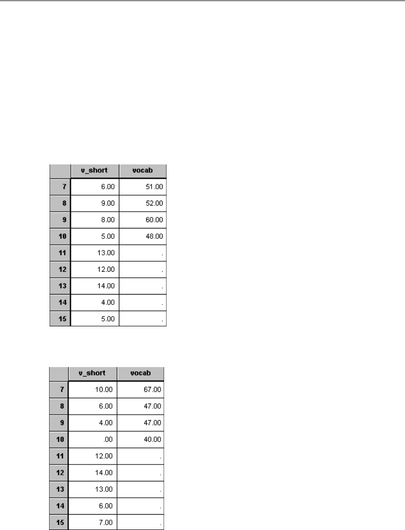
298
Example 18
About the Data
For this example, the Attig data (introduced in Example 1) was modified by
eliminating some of the data values and treating them as missing. A portion of the
modified data file for young people, Atty_mis.sav, is shown below as it appears in the
SPSS Statistics Data Editor. The file contains scores of Attig’s 40 young subjects on
the two vocabulary tests v_short and vocab. The variable vocab is the WAIS vocabulary
score. V_short is the score on a small subset of items on the WAIS vocabulary test.
Vocab scores were deleted for 30 randomly picked subjects.
A second data file, Atto_mis.sav, contains vocabulary test scores for the 40 old
subjects, again with 30 randomly picked vocab scores deleted.

299
More about Missing Data
Of course, no sensible person deletes data that have already been collected. In order for
this example to make sense, imagine this pattern of missing data arising in the
following circumstances.
Suppose that vocab is the best vocabulary test you know of. It is highly reliable and
valid, and it is the vocabulary test that you want to use. Unfortunately, it is an
expensive test to administer. Maybe it takes a long time to give the test, maybe it has
to be administered on an individual basis, or maybe it has to be scored by a highly
trained person. V_short is not as good a vocabulary test, but it is short, inexpensive,
and easy to administer to a large number of people at once. You administer the cheap
test, v_short, to 40 young and 40 old subjects. Then you randomly pick 10 people from
each group and ask them to take the expensive test, vocab.
Suppose the purpose of the research is to:
Estimate the average vocab test score in the population of young people.
Estimate the average vocab score in the population of old people.
Test the hypothesis that young people and old people have the same average vocab
score.
In this scenario, you are not interested in the average v_short score. However, as will
be demonstrated below, the v_short scores are still useful because they contain
information that can be used to estimate and test hypotheses about vocab scores.
The fact that missing values are missing by design does not affect the method of
analysis. Two models will be fitted to the data. In both models, means, variances, and
the covariance between the two vocabulary tests will be estimated for young people
and also for old people. In Model A, there will be no constraints requiring parameter
estimates to be equal across groups. In Model B, vocab will be required to have the
same mean in both groups.
Model A
To estimate means, variances, and the covariance between vocab and v_short, set up a
two-group model for the young and old groups.
EDraw a path diagram in which vocab and v_short appear as two rectangles connected
by a double-headed arrow.
EFrom the menus, choose View > Analysis Properties.

300
Example 18
EIn the Analysis Properties dialog, click the Estimation tab.
ESelect Estimate means and intercepts (a check mark appears next to it).
EWhile the Analysis Properties dialog is open, click the Output tab.
ESelect Standardized estimates and Critical ratios for differences.
Because this example focuses on group differences in the mean of vocab, it will be
useful to have names for the mean of the young group and the mean of the old group.
To give a name to the mean of vocab in the young group:
ERight-click the vocab rectangle in the path diagram for the young group.
EChoose Object Properties from the pop-up menu.
EIn the Object Properties dialog, click the Parameters tab.
EEnter a name, such as m1_yng, in the Mean text box.
EFollow the same procedure for the old group. Be sure to give the mean of the old group
a unique name, such as m1_old.
Naming the means does not constrain them as long as each name is unique. After the
means are named, the two groups should have path diagrams that look something like
this:
m1_yng,
vocab v_short
Example 18: Model A
Incompletely observed data.
Attig (1983) young subjects
Model Specification
m1_old,
vocab v_short
Example 18: Model A
Incompletely observed data.
Attig (1983) old subjects
Model Specification
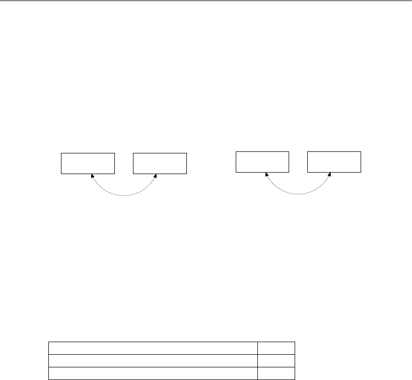
301
More about Missing Data
Results for Model A
Graphics Output
Here are the two path diagrams containing means, variances, and covariances for the
young and old subjects respectively:
Text Output
EIn the Amos Output window, click Notes for Model in the upper left pane.
The text output shows that Model A is saturated, so that the model is not testable.
Number of distinct sample moments: 10
Number of distinct parameters to be estimated: 10
Degrees of freedom (10 – 10): 0
56.89, 83.32
vocab
7.95, 15.35
v_short
32.92
Example 18: Model A
Incompletely observed data.
Attig (1983) young subjects
Unstandardized estimates
65.00, 115.06
vocab
10.03, 10.77
v_short
31.54
Example 18: Model A
Incompletely observed data.
Attig (1983) old subjects
Unstandardized estimates

302
Example 18
The parameter estimates and standard errors for young subjects are:
The parameter estimates and standard errors for old subjects are:
The estimates for the mean of vocab are 56.891 in the young population and 65.001 in
the old population. Notice that these are not the same as the sample means that would
have been obtained from the 10 young and 10 old subjects who took the vocab test. The
sample means of 58.5 and 62 are good estimates of the population means (the best that
can be had from the two samples of size 10), but the Amos estimates (56.891 and
65.001) have the advantage of using information in the v_short scores.
How much more accurate are the mean estimates that include the information in the
v_short scores? Some idea can be obtained by looking at estimated standard errors. For
the young subjects, the standard error for 56.891 shown above is about 1.765, whereas
the standard error of the sample mean, 58.5, is about 2.21. For the old subjects, the
standard error for 65.001 is about 2.167 while the standard error of the sample mean,
Means: (young subjects - Default model)
Estimate
S.E.
C.R. P Label
vocab
56.891
1.765
32.232 *** m1_yng
v_short
7.950
.627
12.673 *** par_4
Covariances: (young subjects - Default model)
Estimate
S.E. C.R. P Label
vocab
<-->
v_short
32.916
8.694 3.786 *** par_3
Correlations: (young subjects - Default model)
Estimate
vocab
<-->
v_short .920
Variances: (young subjects - Default model)
Estimate
S.E.
C.R. P Label
vocab
83.320
25.639
3.250 .001 par_7
v_short
15.347
3.476
4.416 *** par_8
Means: (old subjects - Default model)
Estimate
S.E.
C.R. P Label
vocab
65.001
2.167
29.992 *** m1_old
v_short
10.025
.526
19.073 *** par_6
Covariances: (old subjects - Default model)
Estimate
S.E. C.R. P Label
vocab
<-->
v_short
31.545
8.725 3.616 *** par_5
Correlations: (old subjects - Default model)
Estimate
vocab
<-->
v_short .896
Variances: (old subjects - Default model)
Estimate
S.E.
C.R. P Label
vocab
115.063
37.463
3.071 .002 par_9
v_short
10.774
2.440
4.416 *** par_10

303
More about Missing Data
62, is about 4.21. Although the standard errors just mentioned are only approximations,
they still provide a rough basis for comparison. In the case of the young subjects, using
the information contained in the v_short scores reduces the standard error of the
estimated vocab mean by about 21%. In the case of the old subjects, the standard error
was reduced by about 49%.
Another way to evaluate the additional information that can be attributed to the
v_short scores is by evaluating the sample size requirements. Suppose you did not use
the information in the v_short scores. How many more young examinees would have
to take the vocab test to reduce the standard error of its mean by 21%? Likewise, how
many more old examinees would have to take the vocab test to reduce the standard
error of its mean by 49%? The answer is that, because the standard error of the mean
is inversely proportional to the square root of the sample size, it would require about
1.6 times as many young subjects and about 3.8 times as many old subjects. That is, it
would require about 16 young subjects and 38 old subjects taking the vocab test,
instead of 10 young and 10 old subjects taking both tests, and 30 young and 30 old
subjects taking the short test alone. Of course, this calculation treats the estimated
standard errors as though they were exact standard errors, and so it gives only a rough
idea of how much is gained by using scores on the v_short test.
Do the young and old populations have different mean vocab scores? The estimated
mean difference is 8.110 (65.001 – 56.891). A critical ratio for testing this difference
for significance can be found in the following table:
Critical Ratios for Differences between Parameters
(Default model)
m1_yng m1_old par_3 par_4 par_5 par_6 par_7
m1_yng .000
m1_old 2.901 .000
par_3 -2.702 -3.581 .000
par_4 -36.269 -25.286 -2.864 .000
par_5 -2.847 -3.722 -.111 2.697 .000
par_6 -25.448 -30.012 -2.628 2.535 -2.462 .000
par_7 1.028 .712 2.806 2.939 1.912 2.858 .000
par_8 -10.658 -12.123 -2.934 2.095 -1.725 1.514 -2.877
par_9 1.551 1.334 2.136 2.859 2.804 2.803 .699
par_10 -15.314 -16.616 -2.452 1.121 -3.023 .300 -2.817
Critical Ratios for Differences between Parameters
(Default model)
par_8 par_9 par_10
par_8 .000
par_9 2.650 .000
par_10 -1.077 -2.884 .000
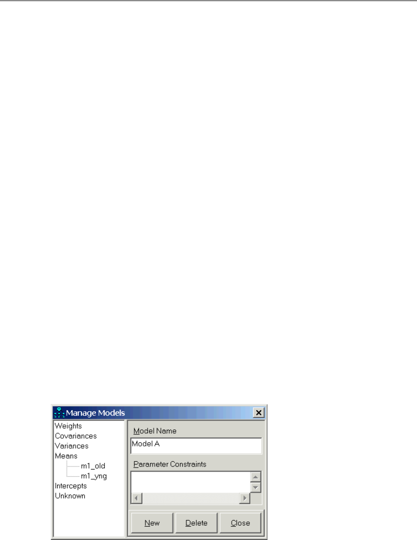
304
Example 18
The first two rows and columns, labeled m1_yng and m1_old, refer to the group means
of the vocab test. The critical ratio for the mean difference is 2.901, according to which
the means differ significantly at the 0.05 level; the older population scores higher on
the long test than the younger population.
Another test of the hypothesis of equal vocab group means can be obtained by
refitting the model with equality constraints imposed on these two means. We will do
that next.
Model B
In Model B, vocab is required to have the same mean for young people as for old
people. There are two ways to impose this constraint. One method is to change the
names of the means. In Model A, each mean has a unique name. You can change the
names and give each mean the same name. This will have the effect of requiring the
two mean estimates to be equal.
A different method of constraining the means will be used here. The name of the
means, m1_yng and m1_old, will be left alone. Amos will use its Model Manager to fit
both Model A and Model B in a single analysis. To use this approach:
EStart with Model A.
EFrom the menus, choose Analyze > Manage Models.
EIn the Manage Models dialog, type Model A in the Model Name text box.
ELeave the Parameter Constraints box empty.
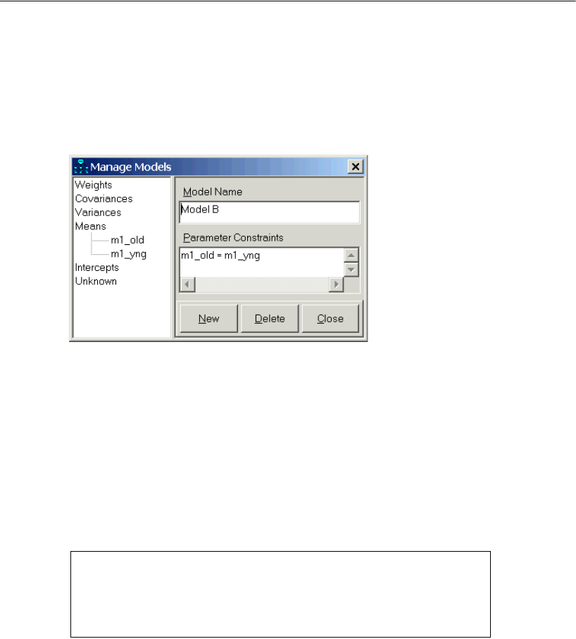
305
More about Missing Data
ETo specify Model B, click New.
EIn the Model Name text box, change Model Number 2 to Model B.
EType m1_old = m1_yng in the Parameter Constraints text box.
EClick Close.
A path diagram that fits both Model A and Model B is saved in the file Ex18-b.amw.
Output from Models A and B
ETo see fit measures for both Model A and Model B, click Model Fit in the tree diagram
in the upper left pane of the Amos Output window.
The portion of the output that contains chi-square values is shown here:
If Model B is correct (that is, the young and old populations have the same mean vocab
score), then 7.849 is an observation on a random variable that has a chi-square
distribution with one degree of freedom. The probability of getting a value as large as
7.849 by chance is small (p = 0.005), so Model B is rejected. In other words, young and
old subjects differ significantly in their mean vocab scores.]
CMIN
Model NPAR CMIN DF P CMIN/DF
Model A 10 .000 0
Model B 9 7.849 1 .005 7.849
Saturated model 10 .000 0
Independence model 4 33.096 6 .000 5.516

306
Example 18
Modeling in VB.NET
Model A
The following program fits Model A. It estimates means, variances, and covariances of
both vocabulary tests in both groups of subjects, without constraints. The program is
saved as Ex18-a.vb.
The Crdiff method displays the critical ratios for parameter differences that were
discussed earlier.
For later reference, note the value of the Function of log likelihood for Model A.
Sub Main()
Dim Sem As New AmosEngine
Try
Sem.TextOutput()
Sem.Crdiff()
Sem.ModelMeansAndIntercepts()
Sem.BeginGroup(Sem.AmosDir & "Examples\atty_mis.sav")
Sem.GroupName("young_subjects")
Sem.Mean("vocab", "m1_yng")
Sem.Mean("v_short")
Sem.BeginGroup(Sem.AmosDir & "Examples\atto_mis.sav")
Sem.GroupName("old_subjects")
Sem.Mean("vocab", "m1_old")
Sem.Mean("v_short")
Sem.FitModel()
Finally
Sem.Dispose()
End Try
End Sub
Function of log likelihood = 429.963
Number of parameters = 10

307
More about Missing Data
Model B
Here is a program for fitting Model B. In this program, the same parameter name
(mn_vocab) is used for the vocab mean of the young group as for the vocab mean of
the old group. In this way, the young group and old group are required to have the same
vocab mean. The program is saved as Ex18-b.vb.
Amos reports the fit of Model B as:
The difference in fit measures between Models B and A is 7.85 (= 437.813 – 429.963),
and the difference in the number of parameters is 1 (= 10 – 9). These are the same
figures we obtained earlier with Amos Graphics.
Sub Main()
Dim Sem As New AmosEngine
Try
Sem.TextOutput()
Sem.Crdiff()
Sem.ModelMeansAndIntercepts()
Sem.BeginGroup(Sem.AmosDir & "Examples\atty_mis.sav")
Sem.GroupName("young_subjects")
Sem.Mean("vocab", "mn_vocab")
Sem.Mean("v_short")
Sem.BeginGroup(Sem.AmosDir & "Examples\atto_mis.sav")
Sem.GroupName("old_subjects")
Sem.Mean("vocab", "mn_vocab")
Sem.Mean("v_short")
Sem.FitModel()
Finally
Sem.Dispose()
End Try
End Sub
Function of log likelihood = 437.813
Number of parameters = 9

309
Example
19
Bootstrapping
Introduction
This example demonstrates how to obtain robust standard error estimates by the
bootstrap method.
The Bootstrap Method
The bootstrap (Efron, 1982) is a versatile method for estimating the sampling
distribution of parameter estimates. In particular, the bootstrap can be used to find
approximate standard errors. As we saw in earlier examples, Amos automatically
displays approximate standard errors for the parameters it estimates. In computing
these approximations, Amos uses formulas that depend on the assumptions on p. 36.
The bootstrap is a completely different approach to the problem of estimating
standard errors. Why would you want another approach? To begin with, Amos does
not have formulas for all of the standard errors you might want, such as standard
errors for squared multiple correlations. The unavailability of formulas for standard
errors is never a problem with the bootstrap, however. The bootstrap can be used to
generate an approximate standard error for every estimate that Amos computes,
whether or not a formula for the standard error is known. Even when Amos has
formulas for standard errors, the formulas are good only under the assumptions on
p. 36. Not only that, but the formulas work only when you are using a correct model.
Approximate standard errors arrived at by the bootstrap do not suffer from these
limitations.
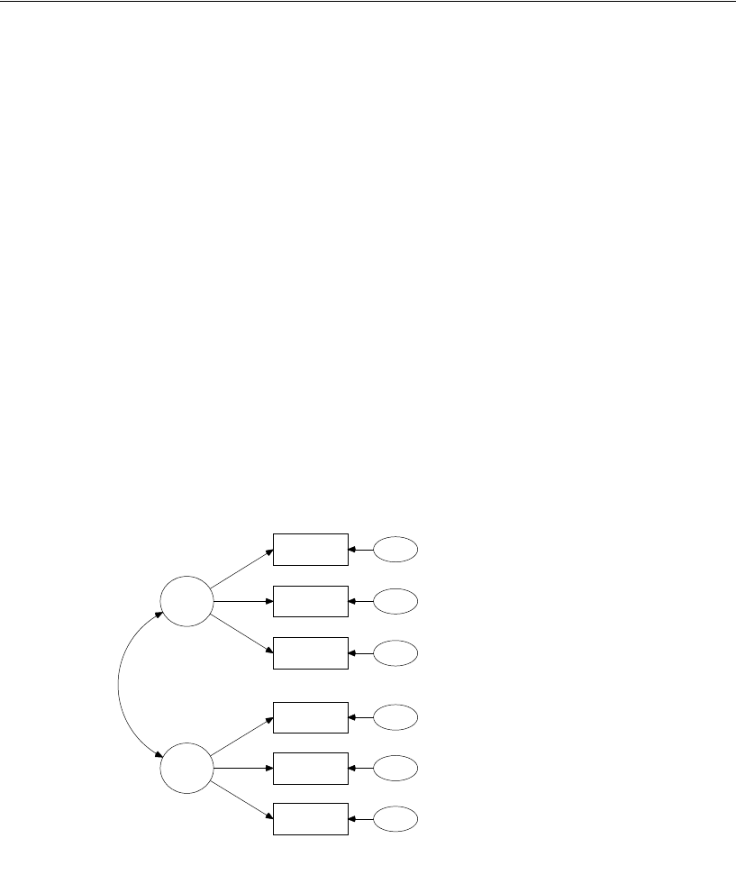
310
Example 19
The bootstrap has its own shortcomings, including the fact that it can require fairly
large samples. For readers who are new to bootstrapping, we recommend the Scientific
American article by Diaconis and Efron (1983).
The present example demonstrates the bootstrap with a factor analysis model, but,
of course, you can use the bootstrap with any model. Incidentally, don’t forget that
Amos can solve simple estimation problems like the one in Example 1. You might
choose to use Amos for such simple problems just so you can use the bootstrapping
capability of Amos.
About the Data
We will use the Holzinger and Swineford (1939) data, introduced in Example 8, for this
example. The data are contained in the file Grnt_fem.sav.
A Factor Analysis Model
The path diagram for this model (Ex19.amw) is the same as in Example 8.
spatial
visperc
cubes
lozenges
wordmean
paragraph
sentence
err_v
err_c
err_l
err_p
err_s
err_w
verbal
1
1
1
1
1
1
1
1
Example 19: Bootstrapping
Holzinger and Swineford (1939) Girls' sample
Model Specification
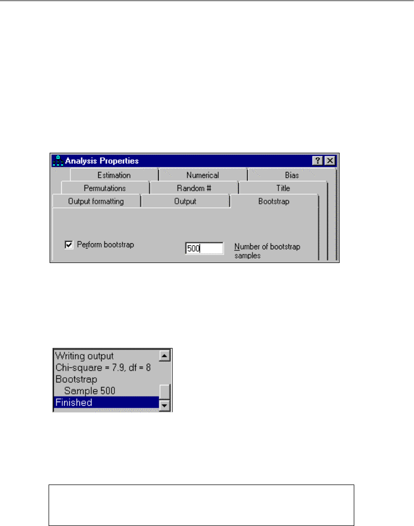
311
Bootstrapping
ETo request 500 bootstrap replications, from the menus, choose View > Analysis
Properties.
EClick the Bootstrap tab.
ESelect Perform bootstrap.
EType 500 in the Number of bootstrap samples text box.
Monitoring the Progress of the Bootstrap
You can monitor the progress of the bootstrap algorithm by watching the Computation
summary panel at the left of the path diagram.
Results of the Analysis
The model fit is, of course, the same as in Example 8.
Chi-square = 7.853
Degrees of freedom = 8
Probability level = 0.448

312
Example 19
The parameter estimates are also the same as in Example 8. However, we would now
like to look at the standard error estimates based on the maximum likelihood theory, so
that we can compare them to standard errors obtained from the bootstrap.
Here, then, are the maximum likelihood estimates of parameters and their standard
errors:

313
Bootstrapping
Regression Weights: (Group number 1 - Default
model)
Estimate S.E. C.R. P Label
visperc <---
spatial
1.000
cubes <---
spatial
.610 .143 4.250 ***
lozenges <---
spatial
1.198 .272 4.405 ***
paragrap <---
verbal
1.000
sentence <---
verbal
1.334 .160 8.322 ***
wordmean
<---
verbal
2.234 .263 8.482 ***
Standardized Regression Weights: (Group number 1 -
Default model)
Estimate
visperc <---
spatial .703
cubes <---
spatial .654
lozenges <---
spatial .736
paragrap <---
verbal .880
sentence <---
verbal .827
wordmean
<---
verbal .841
Covariances: (Group number 1 - Default model)
Estimate S.E. C.R. P Label
spatial
<-->
verbal
7.315 2.571 2.846 .004
Correlations: (Group number 1 - Default model)
Estimate
spatial
<-->
verbal .487
Variances: (Group number 1 - Default model)
Estimate S.E. C.R. P Label
spatial
23.302 8.123 2.868 .004
verbal
9.682 2.159 4.485 ***
err_v
23.873 5.986 3.988 ***
err_c
11.602 2.584 4.490 ***
err_l
28.275 7.892 3.583 ***
err_p
2.834 .868 3.263 .001
err_s
7.967 1.869 4.263 ***
err_w
19.925 4.951 4.024 ***
Squared Multiple Correlations: (Group number 1 -
Default model)
Estimate
wordmean
.708
sentence
.684
paragrap
.774
lozenges
.542
cubes
.428
visperc
.494

314
Example 19
The bootstrap output begins with a table of diagnostic information that is similar to the
following:
It is possible that one or more bootstrap samples will have a singular covariance matrix,
or that Amos will fail to find a solution for some bootstrap samples. If any such
samples occur, Amos reports their occurrence and omits them from the bootstrap
analysis. In the present example, no bootstrap sample had a singular covariance matrix,
and a solution was found for each of the 500 bootstrap samples. The bootstrap
estimates of standard errors are:
0 bootstrap samples were unused because of a singular covariance matrix.
0 bootstrap samples were unused because a solution was not found.
500 usable bootstrap samples were obtained.

315
Bootstrapping
Scalar Estimates (Group number 1 - Default model)
Regression Weights: (Group number 1 - Default
model)
Parameter SE SE-SE Mean Bias SE-Bias
visperc <---
spatial
.000 .000 1.000 .000 .000
cubes <---
spatial
.140 .004 .609 -.001 .006
lozenges <---
spatial
.373 .012 1.216 .018 .017
paragrap <---
verbal
.000 .000 1.000 .000 .000
sentence <---
verbal
.176 .006 1.345 .011 .008
wordmean
<---
verbal
.254 .008 2.246 .011 .011
Standardized Regression Weights: (Group number 1 -
Default model)
Parameter SE SE-SE Mean Bias SE-Bias
visperc <---
spatial
.123 .004 .709 .006 .005
cubes <---
spatial
.101 .003 .646 -.008 .005
lozenges <---
spatial
.121 .004 .719 -.017 .005
paragrap <---
verbal
.047 .001 .876 -.004 .002
sentence <---
verbal
.042 .001 .826 .000 .002
wordmean
<---
verbal
.050 .002 .841 -.001 .002
Covariances: (Group number 1 - Default model)
Parameter SE SE-SE Mean Bias SE-Bias
spatial
<-->
verbal
2.393
.076 7.241 -.074 .107
Correlations: (Group number 1 - Default model)
Parameter SE SE-SE Mean Bias SE-Bias
spatial
<-->
verbal
.132
.004 .495 .008 .006
Variances: (Group number 1 - Default model)
Parameter
SE SE-SE Mean Bias SE-Bias
spatial
9.086
.287 23.905 .603 .406
verbal
2.077
.066 9.518 -.164 .093
err_v
9.166
.290 22.393 -1.480 .410
err_c
3.195
.101 11.191 -.411 .143
err_l
9.940
.314 27.797 -.478 .445
err_p
.878
.028 2.772 -.062 .039
err_s
1.446
.046 7.597 -.370 .065
err_w
5.488
.174 19.123 -.803 .245
Squared Multiple Correlations: (Group number 1 -
Default model)
Parameter SE SE-SE Mean Bias SE-Bias
wordmean
.083
.003 .709 .001 .004
sentence
.069
.002 .685 .001 .003
paragrap
.081
.003 .770 -.004 .004
lozenges
.172
.005 .532 -.010 .008
cubes
.127
.004 .428 .000 .006
visperc
.182
.006 .517 .023 .008

The first column, labeled S.E., contains bootstrap estimates of standard errors.
These estimates may be compared to the approximate standard error estimates
obtained by maximum likelihood.
The second column, labeled S.E.-S.E., gives an approximate standard error for the
bootstrap standard error estimate itself.
The column labeled Mean represents the average parameter estimate computed
across bootstrap samples. This bootstrap mean is not necessarily identical to the
original estimate.
The column labeled Bias gives the difference between the original estimate and the
mean of estimates across bootstrap samples. If the mean estimate across bootstrapped
samples is higher than the original estimate, then Bias will be positive.
The last column, labeled S.E.-Bias, gives an approximate standard error for the bias
estimate.
Modeling in VB.NET
The following program (Ex19.vb) fits the model of Example 19 and performs a
bootstrap with 500 bootstrap samples. The program is the same as in Example 8, but
with an additional Bootstrap line.
The line Sem.Bootstrap(500) requests bootstrap standard errors based on 500 bootstrap
samples.
Sub Main()
Dim Sem As New AmosEngine
Try
Sem.TextOutput()
Sem.Bootstrap(500)
Sem.Standardized()
Sem.Smc()
Sem.BeginGroup(Sem.AmosDir & "Examples\Grnt_fem.sav")
Sem.AStructure("visperc = (1) spatial + (1) err_v")
Sem.AStructure("cubes = spatial + (1) err_c")
Sem.AStructure("lozenges = spatial + (1) err_l")
Sem.AStructure("paragrap = (1) verbal + (1) err_p")
Sem.AStructure("sentence = verbal + (1) err_s")
Sem.AStructure("wordmean = verbal + (1) err_w")
Sem.FitModel()
Finally
Sem.Dispose()
End Try
End Sub

317
Example
20
Bootstrapping for Model Comparison
Introduction
This example demonstrates the use of the bootstrap for model comparison.
Bootstrap Approach to Model Comparison
The problem addressed by this method is not that of evaluating an individual model
in absolute terms but of choosing among two or more competing models. Bollen and
Stine (1992), Bollen (1982), and Stine (1989) suggested the possibility of using the
bootstrap for model selection in analysis of moment structures. Linhart and Zucchini
(1986) described a general schema for bootstrapping and model selection that is
appropriate for a large class of models, including structural modeling. The Linhart and
Zucchini approach is employed here.
The bootstrap approach to model comparison can be summarized as follows:
Generate several bootstrap samples by sampling with replacement from the
original sample. In other words, the original sample serves as the population for
purposes of bootstrap sampling.
Fit every competing model to every bootstrap sample. After each analysis,
calculate the discrepancy between the implied moments obtained from the
bootstrap sample and the moments of the bootstrap population.
Calculate the average (across bootstrap samples) of the discrepancies for each
model from the previous step.
Choose the model whose average discrepancy is smallest.
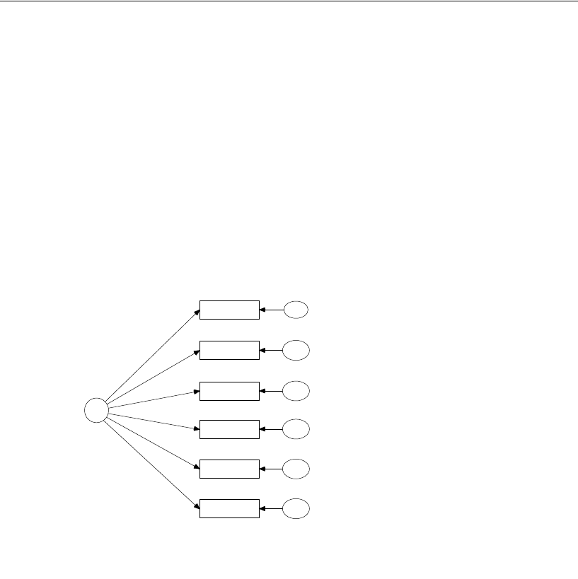
318
Example 20
About the Data
The present example uses the combined male and female data from the Grant-White
high school sample of the Holzinger and Swineford (1939) study, previously discussed
in Examples 8, 12, 15, 17, and 19. The 145 combined observations are given in the file
Grant.sav.
Five Models
Five measurement models will be fitted to the six psychological tests. Model 1 is a
factor analysis model with one factor.
F1
visperc
cubes
lozenges
wordmean
paragraph
sentence
e_v
e_c
e_l
e_p
e_s
e_w
1
1
1
1
1
1
1
Example 20: Model 1
One-factor model
Holzinger and Swineford (1939) data
Model Specification
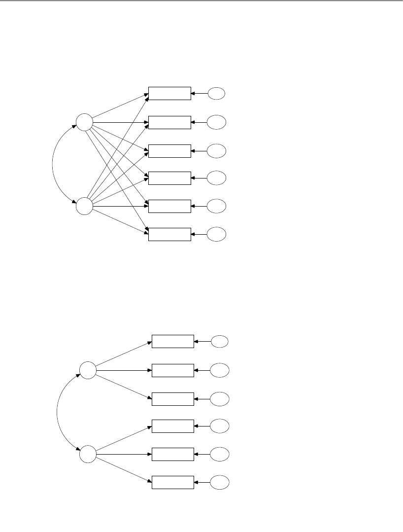
319
Bootstrapping for Model Comparison
Model 2 is an unrestricted factor analysis with two factors. Note that fixing two of the
regression weights at 0 does not constrain the model but serves only to make the model
identified (Anderson, 1984; Bollen and Jöreskog, 1985; Jöreskog, 1979).
Model 2R is a restricted factor analysis model with two factors, in which the first three
tests depend upon only one of the factors while the remaining three tests depend upon
only the other factor.
F1
visperc
cubes
lozenges
wordmean
paragraph
sentence
e_v
e_c
e_l
e_p
e_s
e_w
F2
1
1
1
1
1
1
1
1
Example 20: Model 2
Two unconstrained factors
Holzinger and Swineford (1939) data
Model Specification
0
0
F1
visperc
cubes
lozenges
wordmean
paragraph
sentence
e_v
e_c
e_l
e_p
e_s
e_w
F2
1
1
1
1
1
1
1
1
Example 20: Model 2R
Restricted two-factor model
Holzinger and Swineford (1939) data
Model Specification
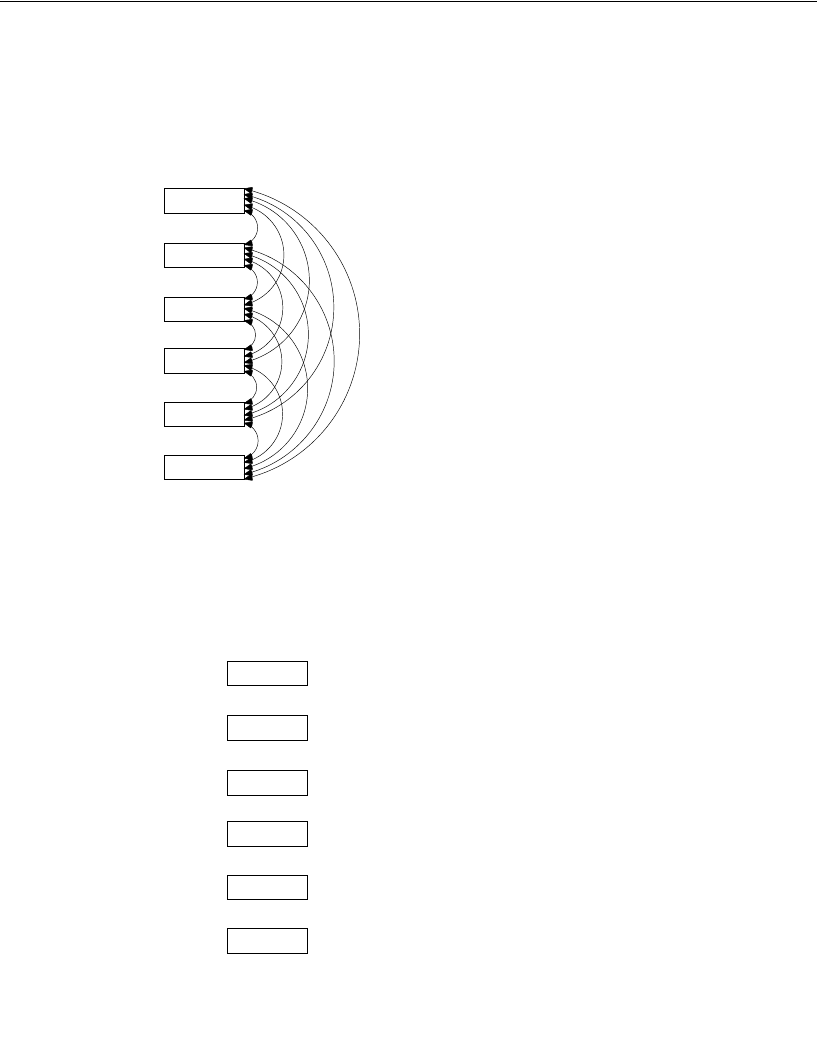
320
Example 20
The remaining two models provide customary points of reference for evaluating the fit
of the previous models. In the saturated model, the variances and covariances of the
observed variables are unconstrained.
In the independence model, the variances of the observed variables are unconstrained
and their covariances are required to be 0.
visperc
cubes
lozenges
wordmean
paragraph
sentence
Example 20: Saturated model
Variances and covariances
Holzinger and Swineford (1939) data
Model Specification
visperc
cubes
lozenges
wordmean
paragraph
sentence
Example 20: Independence model
Only variances are estimated
Holzinger and Swineford (1939) data
Model Specification
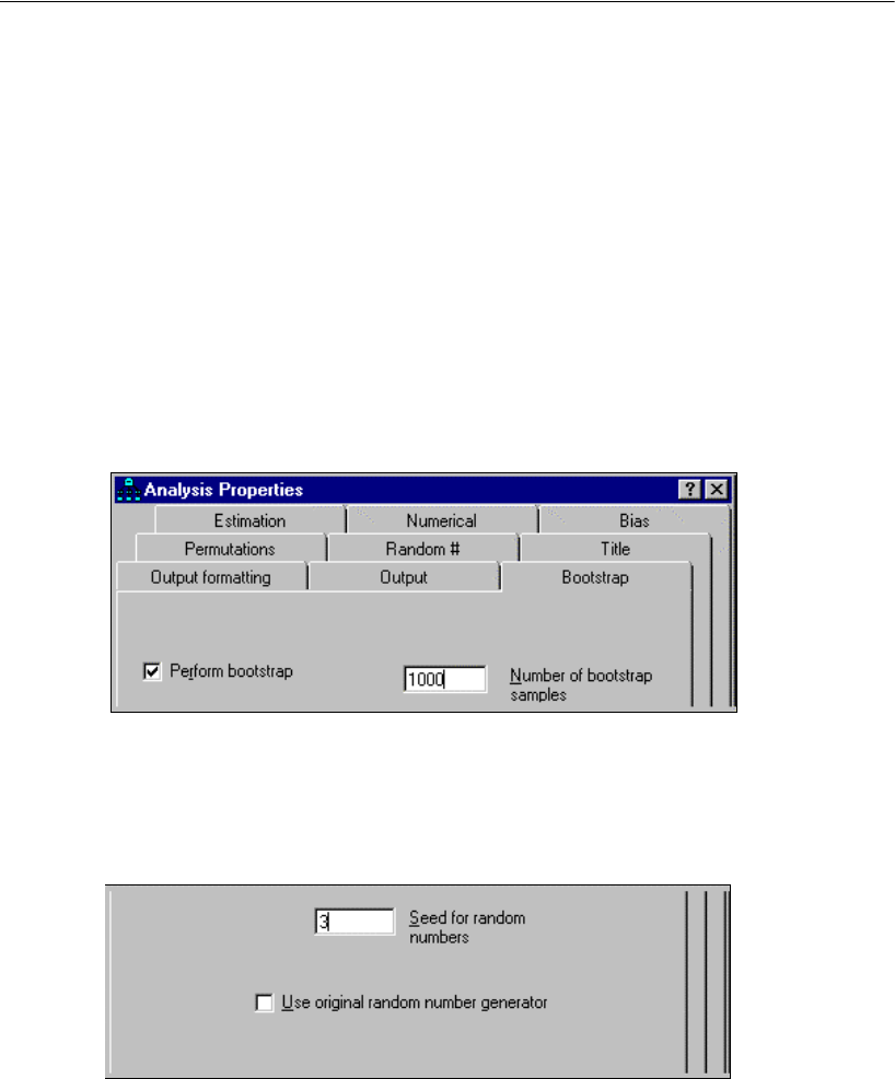
321
Bootstrapping for Model Comparison
You would not ordinarily fit the saturated and independence models separately, since
Amos automatically reports fit measures for those two models in the course of every
analysis. However, it is necessary to specify explicitly the saturated and independence
models in order to get bootstrap results for those models. Five separate bootstrap
analyses must be performed, one for each model. For each of the five analyses:
EFrom the menus, choose View > Analysis Properties.
EIn the Analysis Properties dialog, click the Bootstrap tab.
ESelect Perform bootstrap (a check mark appears next to it).
EType 1000 in the Number of bootstrap samples text box.
EClick the Random # tab and enter a value for Seed for random numbers.
It does not matter what seed you choose, but in order to draw the exact same set of
samples in each of several Amos sessions, the same seed number must be given each
time. For this example, we used a seed of 3.
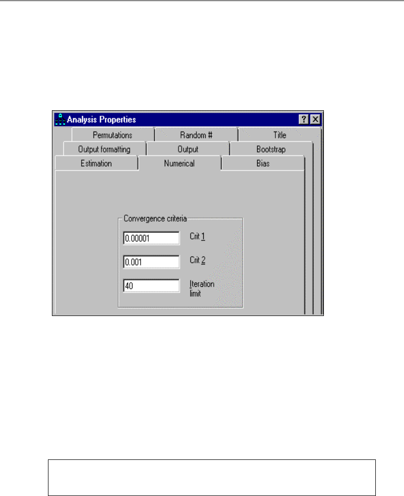
322
Example 20
Occasionally, bootstrap samples are encountered for which the minimization algorithm
does not converge. To keep overall computation times in check:
EClick the Numerical tab and limit the number of iterations to a realistic figure (such as
40) in the Iteration limit field.
Amos Graphics input files for the five models have been saved with the names
Ex20-1.amw, Ex20-2.amw, Ex20-2r.amw, Ex20-sat.amw, and Ex20-ind.amw.
Text Output
EIn viewing the text output for Model 1, click Summary of Bootstrap Iterations in the tree
diagram in the upper left pane of the Amos Output window.
The following message shows that it was not necessary to discard any bootstrap
samples. All 1,000 bootstrap samples were used.
0 bootstrap samples were unused because of a singular covariance matrix.
0 bootstrap samples were unused because a solution was not found.
1000 usable bootstrap samples were obtained.

323
Bootstrapping for Model Comparison
EClick Bootstrap Distributions in the tree diagram to see a histogram of
where a contains sample moments from the original sample of 145 Grant-White
students (that is, the moments in the bootstrap population), and contains the
implied moments obtained from fitting Model 1 to the b-th bootstrap sample. Thus,
is a measure of how much the population moments differ from the
moments estimated from the b-th bootstrap sample using Model 1.
The average of over 1,000 bootstrap samples was 64.162 with a standard
error of 0.292. Similar histograms, along with means and standard errors, are displayed
for the other four models but are not reproduced here. The average discrepancies for
the five competing models are shown in the table below, along with values of BCC,
AIC, and CAIC. The table provides fit measures for five competing models (standard
errors in parentheses).
Model Failures Mean
Discrepancy BCC AIC CAIC
1 0 64.16 (0.29) 68.17 66.94 114.66
2 19 29.14 (0.35 36.81 35.07 102.68
2R 0 26.57 (0.30) 30.97 29.64 81.34
Sat. 0 32.05 (0.37) 44.15 42.00 125.51
Indep. 0 334.32 (0.24) 333.93 333.32 357.18
(
)
(
)
()
1000,,1 ,
ˆˆ h
=−=
b
KL
C
bKL
C
bML
Caa,a,a,
α
α
α
ˆb
CML α
ˆba,()
ML discrepancy (implied vs pop) (Default model)
|--------------------
48.268 |**
52.091 |*********
55.913 |*************
59.735 |*******************
63.557 |*****************
67.379 |************
71.202 |********
N = 1000 75.024 |******
Mean = 64.162 78.846 |***
S. e. = .292 82.668 |*
86.490 |**
90.313 |**
94.135 |*
97.957 |*
101.779 |*
|--------------------
CML α
ˆba,()

324
Example 20
The Failures column in the table indicates that the likelihood function of Model 2 could
not be maximized for 19 of the 1,000 bootstrap samples, at least not with the iteration
limit of 40. Nineteen additional bootstrap samples were generated for Model 2 in order
to bring the total number of bootstrap samples to the target of 1,000. The 19 samples
where Model 2 could not be fitted successfully caused no problem with the other four
models. Consequently, 981 bootstrap samples were common to all five models.
No attempt was made to find out why Model 2 estimates could not be computed for
19 bootstrap samples. As a rule, algorithms for analysis of moment structures tend to
fail for models that fit poorly. If some way could be found to successfully fit Model 2
to these 19 samples—for example, with hand-picked start values or a superior
algorithm—it seems likely that the discrepancies would be large. According to this line
of reasoning, discarding bootstrap samples for which estimation failed would lead to a
downward bias in the mean discrepancy. Thus, you should be concerned by estimation
failures during bootstrapping, primarily when they occur for the model with the lowest
mean discrepancy.
In this example, the lowest mean discrepancy (26.57) occurs for Model 2R,
confirming the model choice based on the BCC, AIC, and CAIC criteria. The
differences among the mean discrepancies are large compared to their standard errors.
Since all models were fitted to the same bootstrap samples (except for samples where
Model 2 was not successfully fitted), you would expect to find positive correlations
across bootstrap samples between discrepancies for similar models. Unfortunately,
Amos does not report those correlations. Calculating the correlations by hand shows
that they are close to 1, so that standard errors for the differences between means in the
table are, on the whole, even smaller than the standard errors of the means.
Summary
The bootstrap can be a practical aid in model selection for analysis of moment
structures. The Linhart and Zucchini (1986) approach uses the expected discrepancy
between implied and population moments as the basis for model comparisons. The
method is conceptually simple and easy to apply. It does not employ any arbitrary
magic number such as a significance level. Of course, the theoretical appropriateness
of competing models and the reasonableness of their associated parameter estimates
are not taken into account by the bootstrap procedure and need to be given appropriate
weight at some other stage in the model evaluation process.

325
Bootstrapping for Model Comparison
Modeling in VB.NET
Visual Basic programs for this example are in the files Ex20-1.vb, Ex20-2.vb, Ex20-
2r.vb, Ex20-ind.vb, and Ex20-sat.vb.
326

327
Example
21
Bootstrapping to Compare
Estimation Methods
Introduction
This example demonstrates how bootstrapping can be used to choose among
competing estimation criteria.
Estimation Methods
The discrepancy between the population moments and the moments implied by a
model depends not only on the model but also on the estimation method. The
technique used in Example 20 to compare models can be adapted to the comparison
of estimation methods. This capability is particularly needed when choosing among
estimation methods that are known to be optimal only asymptotically, and whose
relative merits in finite samples would be expected to depend on the model, the sample
size, and the population distribution. The principal obstacle to carrying out this
program for comparing estimation methods is that it requires a prior decision about
how to measure the discrepancy between the population moments and the moments
implied by the model. There appears to be no way to make this decision without
favoring some estimation criteria over others. Of course, if every choice of population
discrepancy leads to the same conclusion, questions about which is the appropriate
population discrepancy can be considered academic. The present example presents
such a clear-cut case.
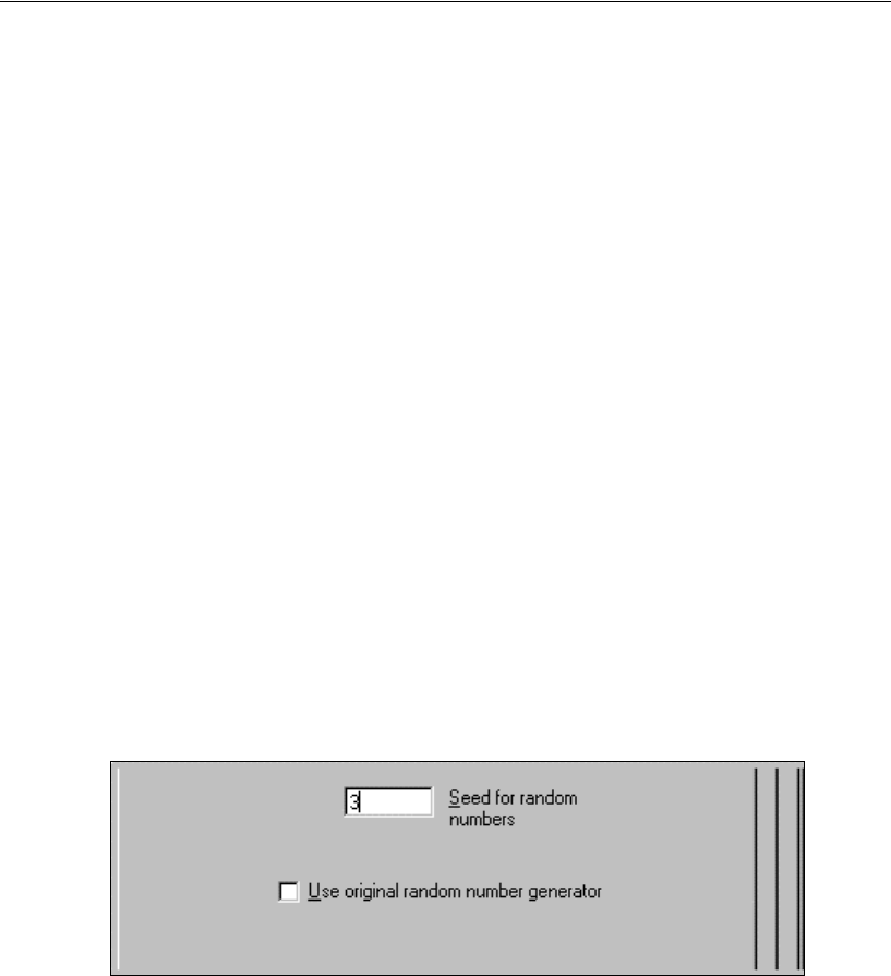
328
Example 21
About the Data
The Holzinger-Swineford (1939) data from Example 20 (in the file Grant.sav) are used
in the present example.
About the Model
The present example estimates the parameters of Model 2R from Example 20 by four
alternative methods: Asymptotically distribution-free (ADF), maximum likelihood
(ML), generalized least squares (GLS), and unweighted least squares (ULS). To
compare the four estimation methods, you need to run Amos four times.
To specify the estimation method and bootstrap parameters:
EFrom the menus, choose View > Analysis Properties.
EIn the Analysis Properties dialog, click the Random # tab.
EEnter a Seed for random numbers.
As we discussed in Example 20, it does not matter what seed value you choose, but in
order to draw the exact same set of samples in each of several Amos sessions, the same
seed number must be given each time. In this example, we use a seed of 3.
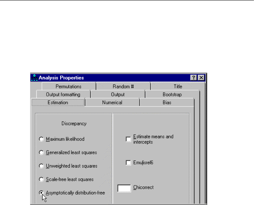
329
Bootstrapping to Compare Estimation Methods
ENext, click the Estimation tab.
ESelect the Asymptotically distribution-free discrepancy.
This discrepancy specifies that ADF estimation should be used to fit the model to each
bootstrap sample.
EFinally, click the Bootstrap tab.
ESelect Perform bootstrap and type 1000 for Number of bootstrap samples.
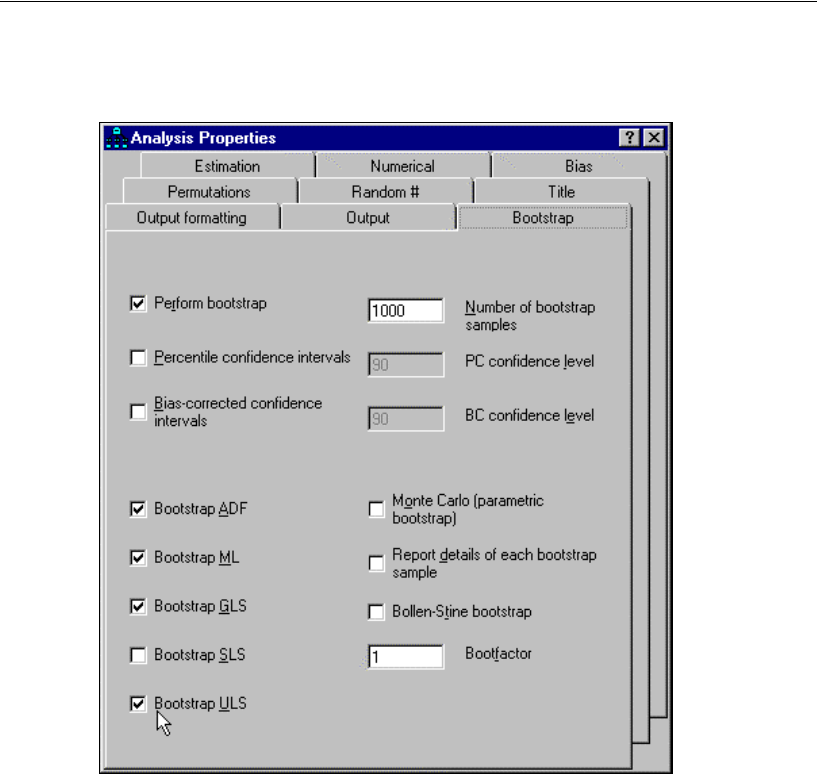
330
Example 21
ESelect Bootstrap ADF, Bootstrap ML, Bootstrap GLS, and Bootstrap ULS.
Selecting Bootstrap ADF, Bootstrap ML, Bootstrap GLS, Bootstrap SLS, and Bootstrap
ULS specifies that each of CADF, CML, CGLS, and CULS is to be used to measure the
discrepancy between the sample moments in the original sample and the implied
moments from each bootstrap sample.
To summarize, when you perform the analysis (Analyze > Calculate Estimates),
Amos will fit the model to each of 1,000 bootstrap samples using the ADF discrepancy.
For each bootstrap sample, the closeness of the implied moments to the population
moments will be measured four different ways, using CADF , CML, CGLS, and CULS.
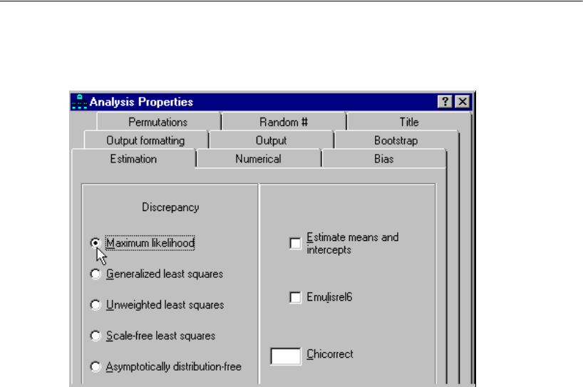
331
Bootstrapping to Compare Estimation Methods
ESelect the Maximum likelihood discrepancy to repeat the analysis.
ESelect the Generalized least squares discrepancy to repeat the analysis again.
ESelect the Unweighted least squares discrepancy to repeat the analysis one last time.
The four Amos Graphics input files for this example are Ex21-adf.amw, Ex21-ml.amw,
Ex21-gls.amw, and Ex21-uls.amw.
Text Output
In the first of the four analyses (as found in Ex21-adf.amw), estimation using ADF
produces the following histogram output. To view this histogram:

332
Example 21
EClick Bootstrap Distributions > ADF Discrepancy (implied vs pop) in the tree diagram in
the upper left pane of the Amos Output window.
This portion of the output shows the distribution of the population discrepancy
across 1,000 bootstrap samples, where contains the implied moments
obtained by minimizing , that is, the sample discrepancy. The average of
across 1,000 bootstrap samples is 20.601, with a standard error of 0.218.
The following histogram shows the distribution of . To view this histogram:
ADF discrepancy (implied vs pop) (Default model)
|--------------------
7.359 |*
10.817 |********
14.274 |****************
17.732 |********************
21.189 |*******************
24.647 |*************
28.104 |********
N = 1000 31.562 |****
Mean = 20.601 35.019 |**
S. e. = .218 38.477 |**
41.934 |*
45.392 |*
48.850 |*
52.307 |*
55.765 |*
|--------------------
CADF α
ˆba,()
α
ˆb
CADF α
ˆbab
,()
CADF α
ˆba,()
CML α
ˆba,()

333
Bootstrapping to Compare Estimation Methods
EClick Bootstrap Distributions > ML Discrepancy (implied vs pop) in the tree diagram in the
upper left pane of the Amos Output window.
The following histogram shows the distribution of . To view this histogram:
EClick Bootstrap Distributions > GLS Discrepancy (implied vs pop) in the tree diagram in
the upper left pane of the Amos Output window.
ML discrepancy (implied vs pop) (Default model)
|--------------------
11.272 |****
22.691 |********************
34.110 |********************
45.530 |***********
56.949 |*****
68.368 |***
79.787 |**
N = 1000 91.207 |*
Mean = 36.860 102.626 |*
S. e. = .571 114.045 |*
125.464 |*
136.884 |
148.303 |
159.722 |
171.142 |*
|--------------------
CGLS α
ˆba,()
GLS discrepancy (implied vs pop) (Default model)
|--------------------
7.248 |**
11.076 |*********
14.904 |***************
18.733 |********************
22.561 |**************
26.389 |***********
30.217 |*******
N = 1000 34.046 |****
Mean = 21.827 37.874 |**
S. e. = .263 41.702 |***
45.530 |*
49.359 |*
53.187 |*
57.015 |*
60.844 |*
|--------------------

334
Example 21
The following histogram shows the distribution of . To view this histogram:
EClick Bootstrap Distributions > ULS Discrepancy (implied vs pop) in the tree diagram in
the upper left pane of the Amos Output window.
Below is a table showing the mean of across 1,000 bootstrap samples with
the standard errors in parentheses. The four distributions just displayed are
summarized in the first row of the table. The remaining three rows show the results of
estimation by minimizing CML, CGLS, and CULS, respectively.
The first column, labeled CADF , shows the relative performance of the four estimation
methods according to the population discrepancy, CADF . Since 19.19 is the smallest
mean discrepancy in the CADF column, CML is the best estimation method according to
the CADF criterion. Similarly, examining the CML column of the table shows that CML
is the best estimation method according to the CML criterion.
Although the four columns of the table disagree on the exact ordering of the four
estimation methods, ML is, in all cases, the method with the lowest mean discrepancy.
The difference between ML estimation and GLS estimation is slight in some cases.
Population discrepancy for evaluation:
CADF CML CGLS CULS
Sample
discrepancy
for estimation
CADF 20.60 (0.22) 36.86 (0.57) 21.83 (0.26) 43686 (1012)
CML 19.19 (0.20) 26.57 (0.30) 18.96 (0.22) 34760 (830)
CGLS 19.45 (0.20) 31.45 (0.40) 19.03 (0.21) 37021 (830)
CULS 24.89 (0.35) 31.78 (0.43) 24.16 (0.33) 35343 (793)
CULS α
ˆba,()
ULS discrepancy (implied vs pop) (Default model)
|--------------------
5079.897 |******
30811.807 |********************
56543.716 |********
82275.625 |****
108007.534 |**
133739.443 |*
159471.352 |*
N = 1000 185203.261 |*
Mean = 43686.444 210935.170 |
S. e. = 1011.591 236667.079 |*
262398.988 |
288130.897 |
313862.806 |
339594.715 |
365326.624 |*
|--------------------
Cα
ˆba,()
Cα
ˆbab
,()
Cα
ˆbab
,()

335
Bootstrapping to Compare Estimation Methods
Unsurprisingly, ULS estimation performed badly, according to all of the population
discrepancies employed. More interesting is the poor performance of ADF estimation,
indicating that ADF estimation is unsuited to this combination of model, population,
and sample size.
Modeling in VB.NET
Visual Basic programs for this example are in the files Ex21-adf.vb, Ex21-gls.vb, Ex21-
ml.vb, and Ex21-uls.vb.

337
Example
22
Specification Search
Introduction
This example takes you through two specification searches: one is largely
confirmatory (with few optional arrows), and the other is largely exploratory (with
many optional arrows).
About the Data
This example uses the Felson and Bohrnstedt (1979) girls’ data, also used in Example 7.
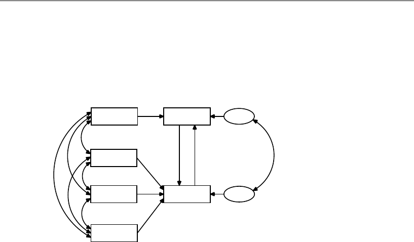
338
Example 22
About the Model
The initial model for the specification search comes from Felson and Bohrnstedt
(1979), as seen in Figure 22-1:
Figure 22-1: Felson and Bohrnstedt’s model for girls
Specification Search with Few Optional Arrows
Felson and Bohrnstedt were primarily interested in the two single-headed arrows,
academic←attract and attract←academic. The question was whether one or both, or
possibly neither, of the arrows was needed. For this reason, you will make both arrows
optional during this specification search. The double-headed arrow connecting error1
and error2 is an undesirable feature of the model because it complicates the
interpretation of the effects represented by the single-headed arrows, and so you will
also make it optional. The specification search will help to decide which of these three
optional arrows, if any, are essential to the model.
This specification search is largely confirmatory because most arrows are required
by the model, and only three are optional.
GPA
height
rating
weight
academic
attract
error1
error2
1
1
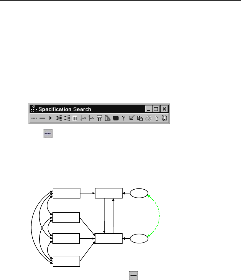
339
Specification Search
Specifying the Model
EOpen %examples%\Ex22a.amw.
The path diagram opens in the drawing area. Initially, there are no optional arrows, as
seen in Figure 22-1.
EFrom the menus, choose Analyze > Specification Search.
The Specification Search window appears. Initially, only the toolbar is visible.
EClick on the Specification Search toolbar, and then click the double-headed arrow
that connects error1 and error2. The arrow changes color to indicate that the arrow is
optional.
Tip: If you want the optional arrow to be dashed as well as colored, as seen below,
choose View →Interface Properties from the menus, click the Accessibility tab, and
select the Alternative to color check box.
ETo make the arrow required again, click on the Specification Search toolbar, and
then click the arrow. When you move the pointer away, the arrow will again display as
a required arrow.
GPA
height
rating
weight
academic
attract
error1
error2
1
1
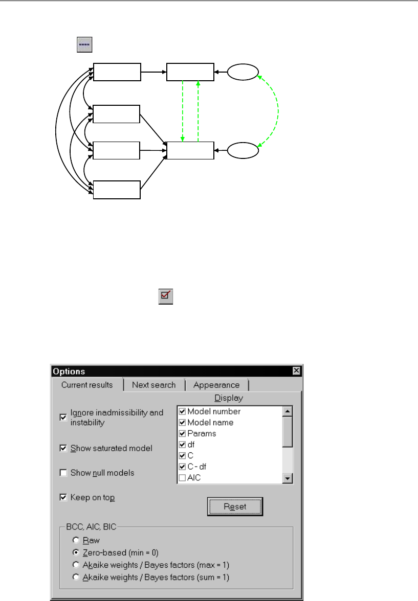
340
Example 22
EClick again, and then click the arrows in the path diagram until it looks like this:
When you perform the exploratory analysis later on, the program will treat the three
colored arrows as optional and will try to fit the model using every possible subset of
them.
Selecting Program Options
EClick the Options button on the Specification Search toolbar.
EIn the Options dialog, click the Current results tab.
EClick Reset to ensure that your options are the same as those used in this example.
GPA
height
rating
weight
academic
attract
error1
error2
1
1
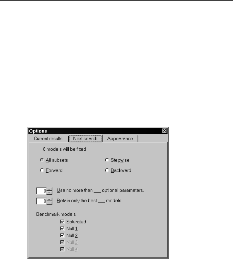
341
Specification Search
ENow click the Next search tab. The text at the top indicates that the exploratory analysis
will fit eight (that is, 23) models.
EIn the Retain only the best ___ models box, change the value from 10 to 0.
With a default value of 10, the specification search reports at most 10 one-parameter
models, at most 10 two-parameter models, and so on. If the value is set to 0, there is no
limitation on the number of models reported.
Limiting the number of models reported can speed up a specification search
significantly. However, only eight models in total will be encountered during the
specification search for this example, and specifying a nonzero value for Retain only
the best ___ models would have the undesirable side effect of inhibiting the program
from normalizing Akaike weights and Bayes factors so that they sum to 1 across all
models, as seen later.
EClose the Options dialog.
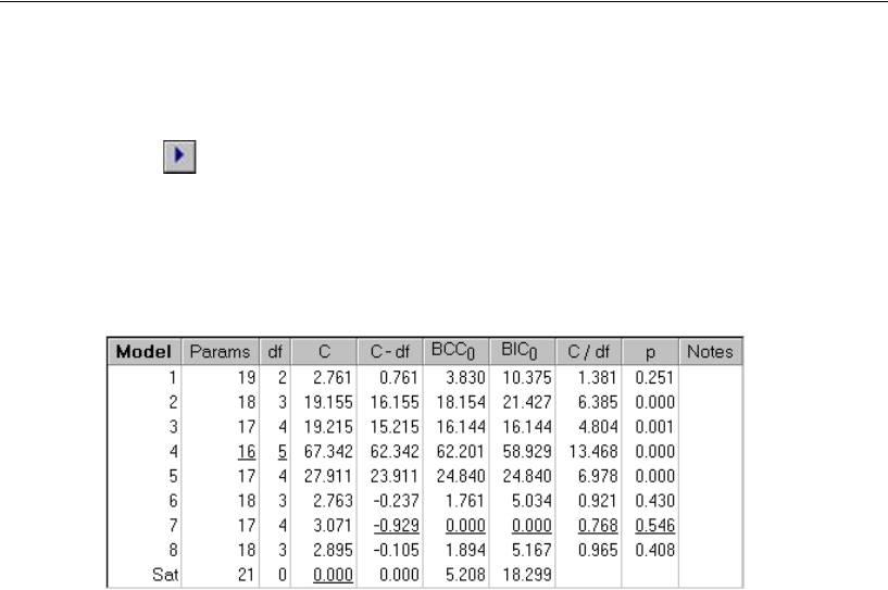
342
Example 22
Performing the Specification Search
EClick on the Specification Search toolbar.
The program fits the model eight times, using every subset of the optional arrows.
When it finishes, the Specification Search window expands to show the results.
The following table summarizes fit measures for the eight models and the saturated
model:
The Model column contains an arbitrary index number from 1 through 8 for each of the
models fitted during the specification search. Sat identifies the saturated model.
Looking at the first row, Model 1 has 19 parameters and 2 degrees of freedom. The
discrepancy function (which in this case is the likelihood ratio chi-square statistic) is
2.761. Elsewhere in Amos output, the minimum value of the discrepancy function is
referred to as CMIN. Here it is labeled C for brevity. To get an explanation of any
column of the table, right-click anywhere in the column and choose What’s This? from
the pop-up menu.
Notice that the best value in each column is underlined, except for the Model and
Notes columns.
Many familiar fit measures (CFI and RMSEA, for example) are omitted from this
table. Appendix E gives a rationale for the choice of fit measures displayed.
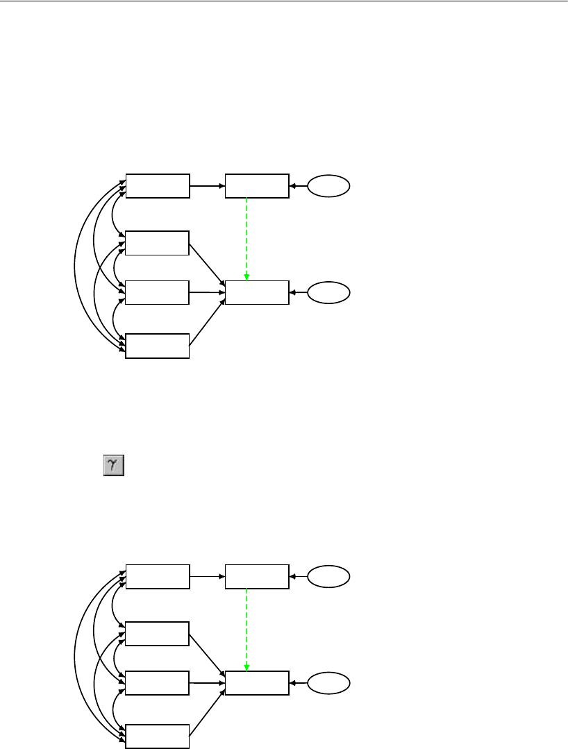
343
Specification Search
Viewing Generated Models
EYou can double-click any row in the table (other than the Sat row) to see the
corresponding path diagram in the drawing area. For example, double-click the row for
Model 7 to see its path diagram.
Figure 22-2: Path diagram for Model 7
Viewing Parameter Estimates for a Model
EClick on the Specification Search toolbar.
EIn the Specification Search window, double-click the row for Model 7.
The drawing area displays the parameter estimates for Model 7.
Figure 22-3: Parameter estimates for Model 7
GPA
height
rating
weight
academic
attract
error1
error2
1
1
12.12
GPA
8.43
height
1.02
rating
371.48
weight
academic
attract
.02
.00
.00
.18
.02
error1
.14
error2
1
1
.53
-.47
-6.71
1.82
19.02
-5.24
1.44
Chi-square = 3.071 (4 df)
p = .546
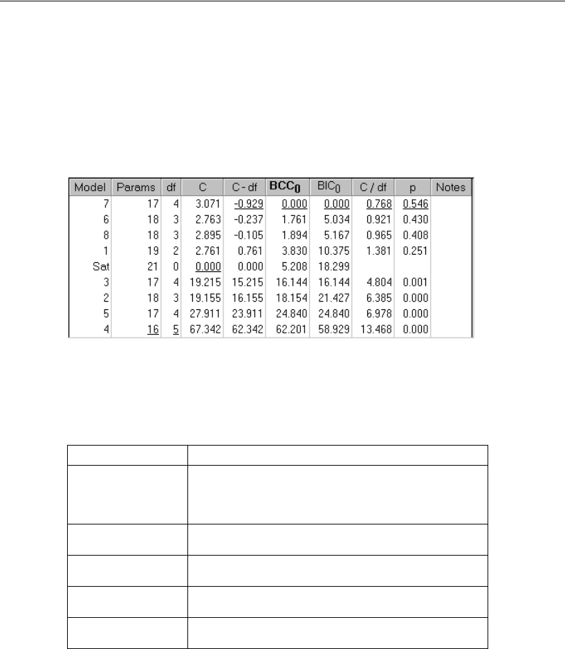
344
Example 22
Using BCC to Compare Models
EIn the Specification Search window, click the column heading BCC0.
The table sorts according to BCC so that the best model according to BCC (that is, the
model with the smallest BCC) is at the top of the list.
Based on a suggestion by Burnham and Anderson (1998), a constant has been added
to all the BCC values so that the smallest BCC value is 0. The 0 subscript on BCC0
serves as a reminder of this rescaling. AIC (not shown in the above figure) and BIC
have been similarly rescaled. As a rough guideline, Burnham and Anderson (1998,
p. 128) suggest the following interpretation of AIC0. BCC0 can be interpreted similarly.
Although Model 7 is estimated to be the best model according to Burnham and
Anderson’s guidelines, Models 6 and 8 should not be ruled out.
AIC0 or BCC0Burnham and Anderson interpretation
0 – 2
There is no credible evidence that the model should be
ruled out as being the actual K-L best model for the
population of possible samples. (See Burnham and
Anderson for the definition of K-L best.)
2 – 4 There is weak evidence that the model is not the K-L
best model.
4 – 7 There is definite evidence that the model is not the K-L
best model.
7 – 10 There is strong evidence that the model is not the K-L
best model.
>10 There is very strong evidence that the model is not the
K-L best model.
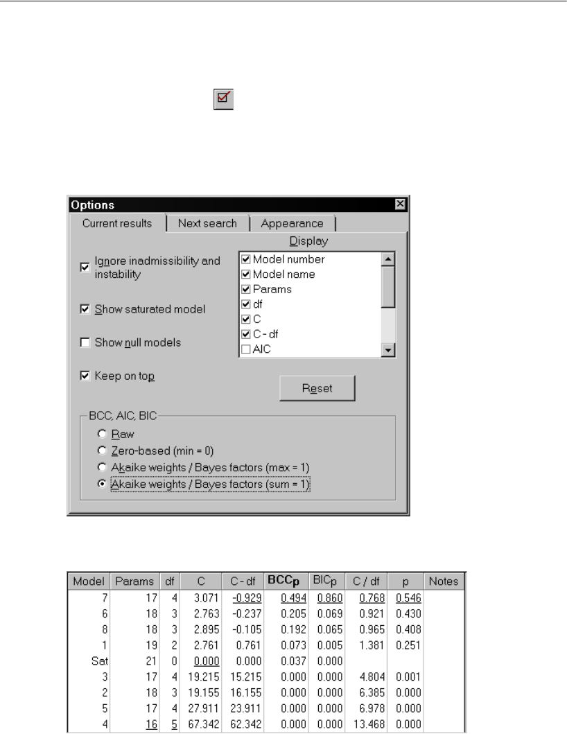
345
Specification Search
Viewing the Akaike Weights
EClick the Options button on the Specification Search toolbar.
EIn the Options dialog, click the Current results tab.
EIn the BCC, AIC, BIC group, select Akaike weights / Bayes factors (sum = 1).
In the table of fit measures, the column that was labeled BCC0 is now labeled BCCp and
contains Akaike weights. (See Appendix G.)
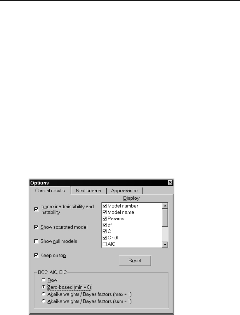
346
Example 22
The Akaike weight has been interpreted (Akaike, 1978; Bozdogan, 1987; Burnham and
Anderson, 1998) as the likelihood of the model given the data. With this interpretation,
the estimated K-L best model (Model 7) is only about 2.4 times more likely (0.494 /
0.205 = 2.41) than Model 6. Bozdogan (1987) points out that, if it is possible to assign
prior probabilities to the candidate models, the prior probabilities can be used together
with the Akaike weights (interpreted as model likelihoods) to obtain posterior
probabilities. With equal prior probabilities, the Akaike weights are themselves
posterior probabilities, so that one can say that Model 7 is the K-L best model with
probability 0.494, Model 6 is the K-L best model with probability 0.205, and so on. The
four most probable models are Models 7, 6, 8, and 1. After adding their probabilities
(0.494 + 0.205 + 0.192 + 0.073 = 0.96), one can say that there is a 96% chance that the
K-L best model is among those four. (Burnham and Anderson, 1998, pp. 127-129). The
p subscript on BCCp serves as a reminder that BCCp can be interpreted as a probability
under some circumstances.
Using BIC to Compare Models
EOn the Current results tab of the Options dialog, select Zero-based (min = 0) in the BCC,
AIC, BIC group.
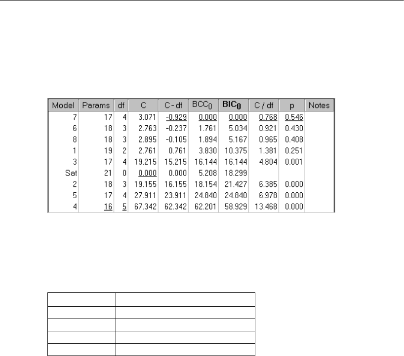
347
Specification Search
EIn the Specification Search window, click the column heading BIC0.
The table is now sorted according to BIC so that the best model according to BIC (that
is, the model with the smallest BIC) is at the top of the list.
Model 7, with the smallest BIC, is the model with the highest approximate posterior
probability (using equal prior probabilities for the models and using a particular prior
distribution for the parameters of each separate model). Raftery (1995) suggests the
following interpretation of BIC0 values in judging the evidence for Model 7 against a
competing model:
Using these guidelines, you have positive evidence against Models 6 and 8, and very
strong evidence against all of the other models as compared to Model 7.
BIC0Raftery (1995) interpretation
0 – 2 Weak
2 – 6 Positive
6 – 10 Strong
>10 Very strong
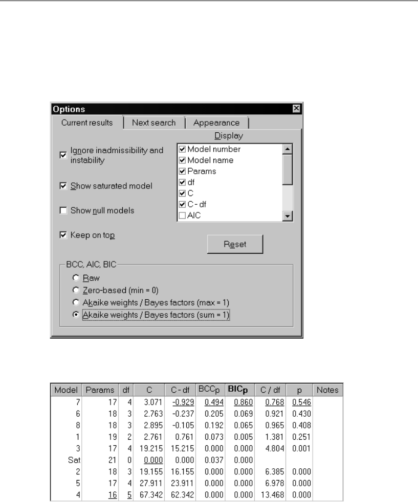
348
Example 22
Using Bayes Factors to Compare Models
EOn the Current results tab of the Options dialog, select Akaike weights / Bayes factors
(sum = 1) in the BCC, AIC, BIC group.
In the table of fit measures, the column that was labeled BIC0 is now labeled BICp and
contains Bayes factors scaled so that they sum to 1.
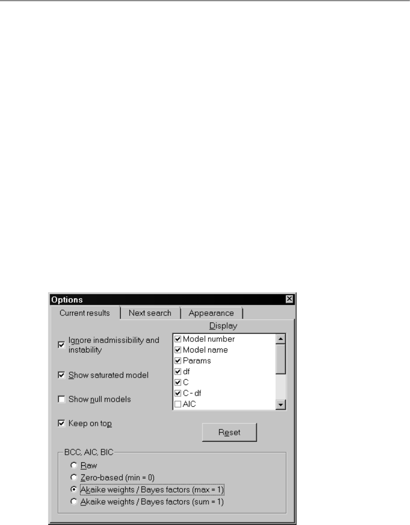
349
Specification Search
With equal prior probabilities for the models and using a particular prior distribution
of the parameters of each separate model (Raftery, 1995; Schwarz, 1978), BICp values
are approximate posterior probabilities. Model 7 is the correct model with probability
0.860. One can be 99% sure that the correct model is among Models 7, 6, and 8 (0.860
+ 0.069 + 0.065 = 0.99). The p subscript is a reminder that BICp values can be
interpreted as probabilities.
Madigan and Raftery (1994) suggest that only models in Occam’s window be used
for purposes of model averaging (a topic not discussed here). The symmetric Occam’s
window is the subset of models obtained by excluding models that are much less
probable (Madigan and Raftery suggest something like 20 times less probable) than the
most probable model. In this example, the symmetric Occam’s window contains
models 7, 6, and 8 because these are the models whose probabilities (BICp values) are
greater than .
Rescaling the Bayes Factors
EOn the Current results tab of the Options dialog, select Akaike weights / Bayes factors
(max = 1) in the BCC, AIC, BIC group.
0.860 20⁄0.043=
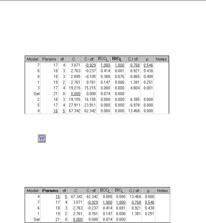
350
Example 22
In the table of fit measures, the column that was labeled BICp is now labeled BICL and
contains Bayes factors scaled so that the largest value is 1. This makes it easier to pick
out Occam’s window. It consists of models whose BICL values are greater than
; in other words, Models 7, 6, and 8. The L subscript on BICL is a
reminder that the analogous statistic BCCL can be interpreted as a likelihood.
Examining the Short List of Models
EClick on the Specification Search toolbar. This displays a short list of models.
In the figure below, the short list shows the best model for each number of parameters.
It shows the best 16-parameter model, the best 17-parameter model, and so on. Notice
that all criteria agree on the best model when the comparison is restricted to models
with a fixed number of parameters. The overall best model must be on this list, no
matter which criterion is employed.
Figure 22-4: The best model for each number of parameters
This table shows that the best 17-parameter model fits substantially better than the best
16-parameter model. Beyond 17 parameters, adding additional parameters yields
relatively small improvements in fit. In a cost-benefit analysis, stepping from 16
parameters to 17 parameters has a relatively large payoff, while going beyond 17
parameters has a relatively small payoff. This suggests adopting the best 17-parameter
model, using a heuristic point of diminishing returns argument. This approach to
120⁄0.05=
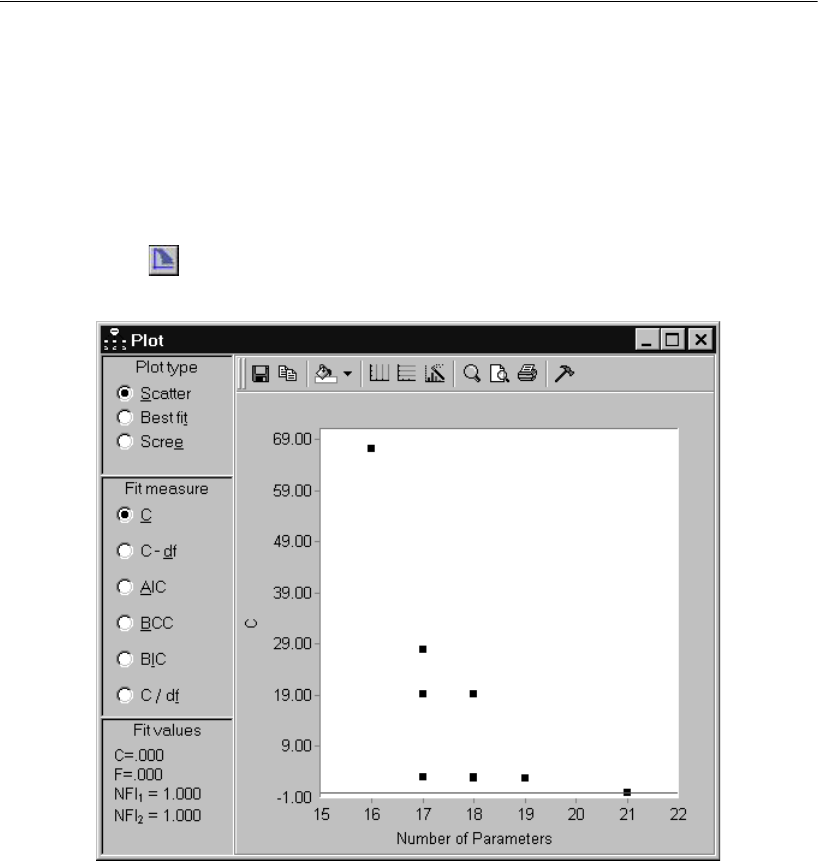
351
Specification Search
determining the number of parameters is pursued further later in this example (see
“Viewing the Best-Fit Graph for C” on p. 356 and “Viewing the Scree Plot for C” on
p. 359).
Viewing a Scatterplot of Fit and Complexity
EClick on the Specification Search toolbar. This opens the Plot window, which
displays the following graph:
The graph shows a scatterplot of fit (measured by C) versus complexity (measured by
the number of parameters) where each point represents a model. The graph portrays the
trade-off between fit and complexity that Steiger characterized as follows:
In the final analysis, it may be, in a sense, impossible to define one best
way to combine measures of complexity and measures of badness-of-fit
in a single numerical index, because the precise nature of the best
numerical trade-off between complexity and fit is, to some extent, a
matter of personal taste. The choice of a model is a classic problem in
the two-dimensional analysis of preference. (Steiger, 1990, p. 179.)
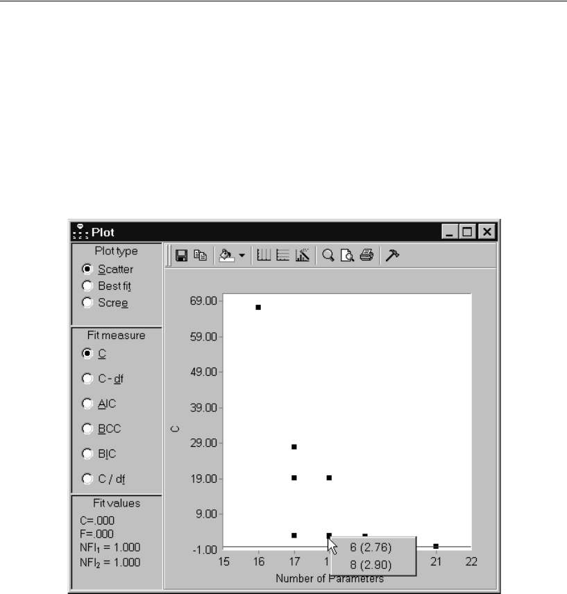
352
Example 22
EClick any of the points in the scatterplot to display a menu that indicates which models
are represented by that point and any overlapping points.
EChoose one of the models from the pop-up menu to see that model highlighted in the
table of model fit statistics and, at the same time, to see the path diagram of that model
in the drawing area.
In the following figure, the cursor points to two overlapping points that represent
Model 6 (with a discrepancy of 2.76) and Model 8 (with a discrepancy of 2.90).
The graph contains a horizontal line representing points for which C is constant.
Initially, the line is centered at 0 on the vertical axis. The Fit values panel at the lower
left shows that, for points on the horizontal line, C = 0 and also F = 0. (F is referred to
as FMIN in Amos output.) NFI1 and NFI2 are two versions of NFI that use two different
baseline models (see Appendix F).
Initially, both NFI1 and NFI2 are equal to 1 for points on the horizontal line. The
location of the horizontal line is adjustable. You can move the line by dragging it with
the mouse. As you move the line, you can see the changes in the location of the line
reflected in the fit measures in the lower left panel.
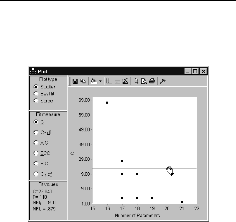
353
Specification Search
Adjusting the Line Representing Constant Fit
EMove your mouse over the adjustable line. When the pointer changes to a hand, drag
the line so that NFI1 is equal to 0.900. (Keep an eye on NFI1 in the lower left panel while
you reposition the adjustable line.)
NFI1 is the familiar form of the NFI statistic for which the baseline model requires the
observed variables to be uncorrelated without constraining their means and variances.
Points that are below the line have NFI1 > 0.900 and those above the line have
NFI1< 0.900. That is, the adjustable line separates the acceptable models from the
unacceptable ones according to a widely used convention based on a remark by Bentler
and Bonett (1980).
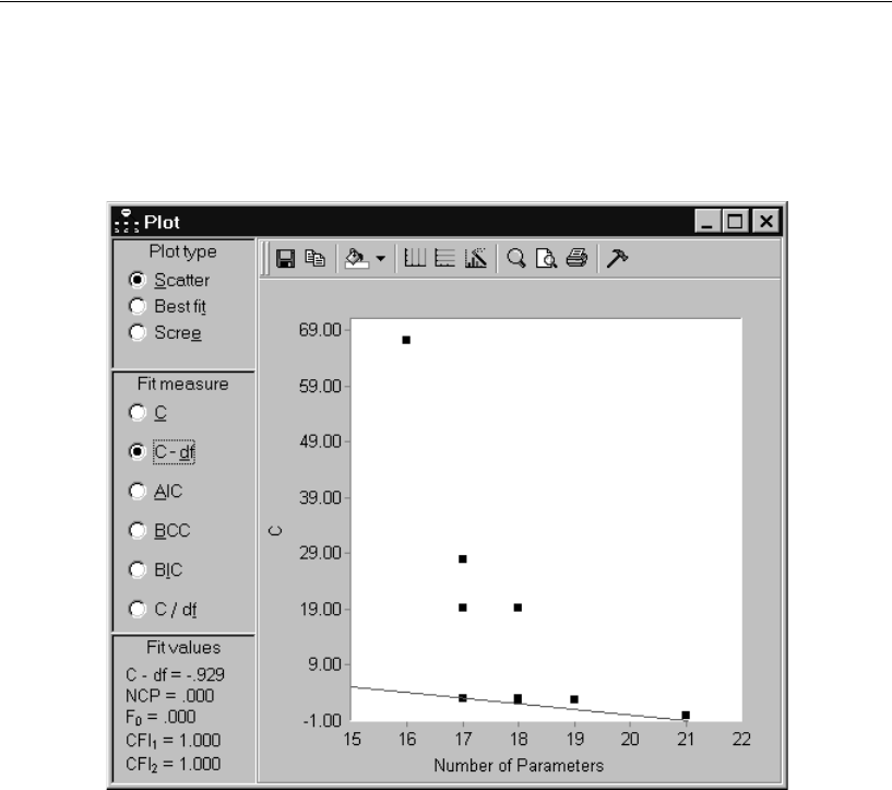
354
Example 22
Viewing the Line Representing Constant C – df
EIn the Plot window, select C – df in the Fit measure group. This displays the following:
The scatterplot remains unchanged except for the position of the adjustable line. The
adjustable line now contains points for which C – df is constant. Whereas the line was
previously horizontal, it is now tilted downward, indicating that C – df gives some
weight to complexity in assessing model adequacy. Initially, the adjustable line passes
through the point for which C – df is smallest.
EClick that point, and then choose Model 7 from the pop-up menu.
This highlights Model 7 in the table of fit measures and also displays the path diagram
for Model 7 in the drawing area.
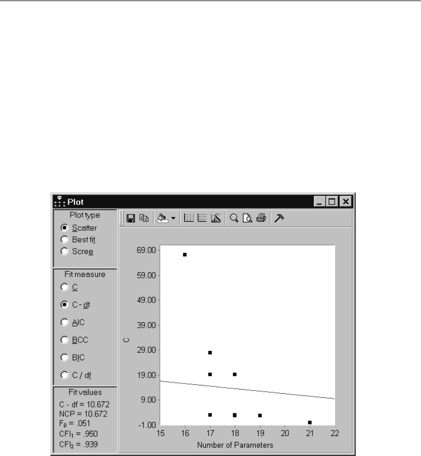
355
Specification Search
The panel in the lower left corner shows the value of some fit measures that depend
only on C – df and that are therefore, like C – df itself, constant along the adjustable
line. CFI1 and CFI2 are two versions of CFI that use two different baseline models (see
Appendix G). Initially, both CFI1 and CFI2 are equal to 1 for points on the adjustable
line. When you move the adjustable line, the fit measures in the lower left panel change
to reflect the changing position of the line.
Adjusting the Line Representing Constant C – df
EDrag the adjustable line so that CFI1 is equal to 0.950.
CFI1 is the usual CFI statistic for which the baseline model requires the observed
variables to be uncorrelated without constraining their means and variances. Points that
are below the line have CFI1 > 0.950 and those above the line have CFI1 < 0.950. That
is, the adjustable line separates the acceptable models from the unacceptable ones
according to the recommendation of Hu and Bentler (1999).
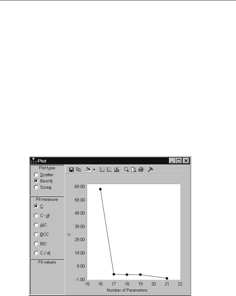
356
Example 22
Viewing Other Lines Representing Constant Fit
EClick AIC, BCC, and BIC in turn.
Notice that the slope of the adjustable line becomes increasingly negative. This reflects
the fact that the five measures (C, C – df, AIC, BCC, and BIC) give increasing weight
to model complexity. For each of these five measures, the adjustable line has constant
slope, which you can confirm by dragging the line with the mouse. By contrast, the
slope of the adjustable line for C / df is not constant (the slope of the line changes when
you drag it with the mouse) and so the slope for C / df cannot be compared to the slopes
for C, C – df, AIC, BCC, and BIC.
Viewing the Best-Fit Graph for C
EIn the Plot window, select Best fit in the Plot type group.
EIn the Fit measure group, select C.
Figure 22-5: Smallest value of C for each number of parameters
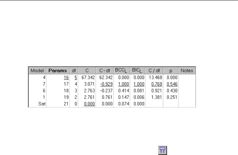
357
Specification Search
Each point in this graph represents a model for which C is less than or equal to that of
any other model that has the same number of parameters. The graph shows that the best
16-parameter model has , the best 17-parameter model has ,
and so on. While Best fit is selected, the table of fit measures shows the best model for
each number of parameters. This table appeared earlier on p. 350.
Notice that the best model for a fixed number of parameters does not depend on the
choice of fit measure. For example, Model 7 is the best 17-parameter model according
to C – df, and also according to C / df and every other fit measure. This short list of best
models is guaranteed to contain the overall best model, no matter which fit measure is
used as the criterion for model selection.
You can view the short list at any time by clicking . The best-fit graph suggests
the choice of 17 as the correct number of parameters on the heuristic grounds that it is
the point of diminishing returns. That is, increasing the number of parameters from 16
to 17 buys a comparatively large improvement in C( ), while
increasing the number of parameters beyond 17 yields relatively small improvements.
C67.342=
C3.071=
67.342 3.071–64.271=
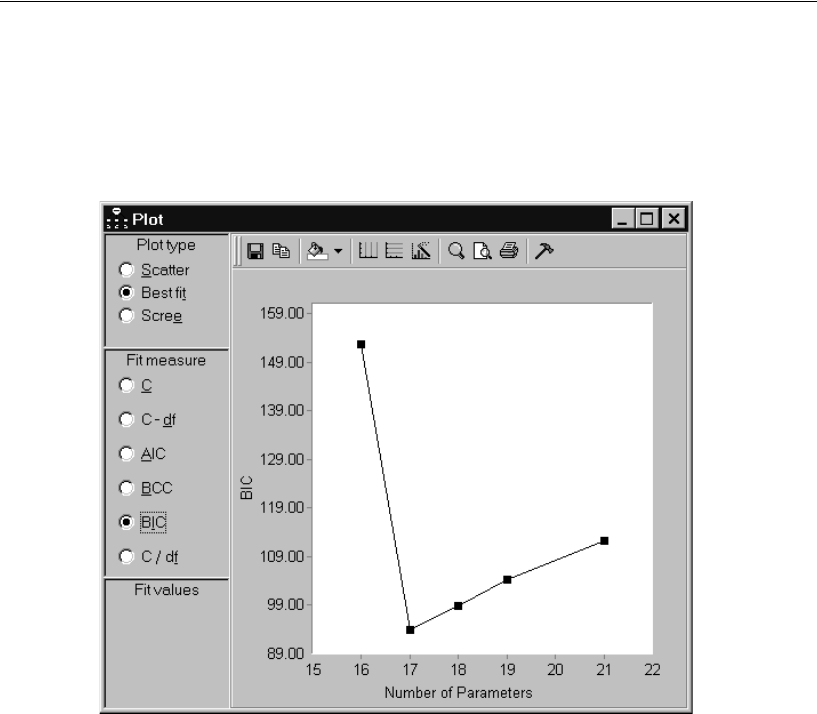
358
Example 22
Viewing the Best-Fit Graph for Other Fit Measures
EWhile Best fit is selected, try selecting the other choices in the Fit measure group:
C–df, AIC, BCC, BIC, and C / df. For example, if you click BIC, you will see this:
BIC is the measure among C, C – df, AIC, BCC, and BIC that imposes the greatest
penalty for complexity. The high penalty for complexity is reflected in the steep
positive slope of the graph as the number of parameters increases beyond 17. The graph
makes it clear that, according to BIC, the best 17-parameter model is superior to any
other candidate model.
Notice that clicking different fit measures changes the vertical axis of the best-fit
graph and changes the shape of the configuration of points.1 However, the identity of
each point is preserved. The best 16-parameter model is always Model 4, the best 17-
parameter model is always Model 7, and so on. This is because, for a fixed number of
parameters, the rank order of models is the same for every fit measure.
1 The saturated model is missing from the C / df graph because C / df is not defined for the saturated model.
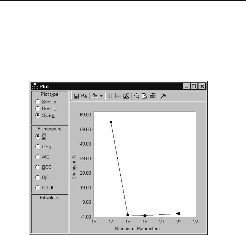
359
Specification Search
Viewing the Scree Plot for C
EIn the Plot window, select Scree in the Plot type group.
EIn the Fit measure group, select C.
The Plot window displays the following graph:
Figure 22-6: Scree plot for C
In this scree plot, the point with coordinate 17 on the horizontal axis has coordinate
64.271 on the vertical axis. This represents the fact that the best 17-parameter model
( ) fits better than the best 16-parameter model ( ), with the
difference being . Similarly, the height of the graph at 18
parameters shows the improvement in C obtained by moving from the best 17-
parameter model to the best 18-parameter model, and so on. The point located above
21 on the horizontal axis requires a separate explanation. There is no 20-parameter
model with which the best 21-parameter model can be compared. (Actually, there is
only one 21-parameter model—the saturated model.) The best 21-parameter model
C3.071=
C67.342=
67.342 3.071 64.271=–

360
Example 22
( ) is therefore compared to the best 19-parameter model ( ). The
height of the 21-parameter point is calculated as . That is, the
improvement in C obtained by moving from the 19-parameter model to the 21-
parameter model is expressed as the amount of reduction in C per parameter.
The figure on either p. 356 or p. 359 can be used to support a heuristic point of
diminishing returns argument in favor of 17 parameters. There is this difference: In the
best-fit graph (p. 356), one looks for an elbow in the graph, or a place where the slope
changes from relatively steep to relatively flat. For the present problem, this occurs at
17 parameters, which can be taken as support for the best 17-parameter model. In the
scree plot (p. 359), one also looks for an elbow, but the elbow occurs at 18 parameters
in this example. This is also taken as support for the best 17-parameter model. In a
scree plot, an elbow at k parameters provides support for the best ( ) parameter
model.
The scree plot is so named because of its similarity to the graph known as a scree
plot in principal components analysis (Cattell, 1966). In principal components
analysis, a scree plot shows the improvement in model fit that is obtained by adding
components to the model, one component at a time. The scree plot presented here for
SEM shows the improvement in model fit that is obtained by incrementing the number
of model parameters. The scree plot for SEM is not identical in all respects to the scree
plot for principal components analysis. For example, in principal components, one
obtains a sequence of nested models when introducing components one at a time. This
is not necessarily the case in the scree plot for SEM. The best 17-parameter model, say,
and the best 18-parameter model may or may not be nested. (In the present example,
they are.) Furthermore, in principal components, the scree plot is always monotone
non-increasing, which is not guaranteed in the case of the scree plot for SEM, even with
nested models. Indeed, the scree plot for the present example is not monotone.
In spite of the differences between the traditional scree plot and the scree plot
presented here, it is proposed that the new scree plot be used in the same heuristic
fashion as the traditional one. A two-stage approach to model selection is suggested.
In the first stage, the number of parameters is selected by examining either the scree
plot or the short list of models. In the second stage, the best model is chosen from
among those models that have the number of parameters determined in the first stage.
C0=
C2.761=
2.761 0–()2⁄
k1–
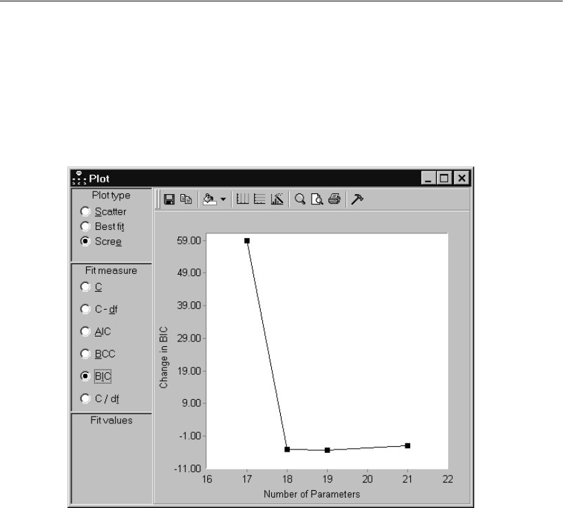
361
Specification Search
Viewing the Scree Plot for Other Fit Measures
EWith Scree selected in the Plot type group, select the other choices in the Fit measure
group: C – df, AIC, BCC, and BIC (but not C / df).
For example, if you select BIC, you will see this:
For C – df, AIC, BCC, and BIC, the units and the origin of the vertical axis are different
than for C, but the graphs are otherwise identical. This means that the final model
selected by the scree test is independent of which measure of fit is used (unless C / df
is used). This is the advantage of the scree plot over the best-fit plot demonstrated
earlier in this example (see “Viewing the Best-Fit Graph for C” on p. 356, and
“Viewing the Best-Fit Graph for Other Fit Measures” on p. 358). The best-fit plot and
the scree plot contain nearly the same information, but the shape of the best-fit plot
depends on the choice of fit measure while the shape of the scree plot does not (with
the exception of C / df).
Both the best-fit plot and the scree plot are independent of sample size in the sense
that altering the sample size without altering the sample moments has no effect other
than to rescale the vertical axis.
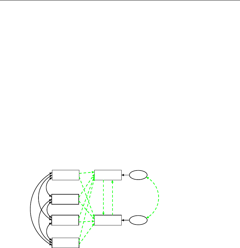
362
Example 22
Specification Search with Many Optional Arrows
The previous specification search was largely confirmatory in that there were only
three optional arrows. You can take a much more exploratory approach to constructing
a model for the Felson and Bohrnstedt data. Suppose that your only hypothesis about
the six measured variables is that
academic depends on the other five variables, and
attract depends on the other five variables.
The path diagram shown in Figure 22-7 with 11 optional arrows implements this
hypothesis. It specifies which variables are endogenous, and nothing more. Every
observed-variable model that is consistent with the hypothesis is included in the
specification search. The covariances among the observed, exogenous variables could
have been made optional, but doing so would have increased the number of optional
arrows from 11 to 17, increasing the number of candidate models from 2,048 (that is, 211)
to 131,072 (that is, 217). Allowing the covariances among the observed, exogenous
variables to be optional would have been costly, and there would seem to be little interest
in searching for models in which some pairs of those variables are uncorrelated.
Figure 22-7: Highly exploratory model for Felson and Bohrnstedt’s girls’ data
GPA
height
rating
weight
academic
attract
error1
error2
1
1
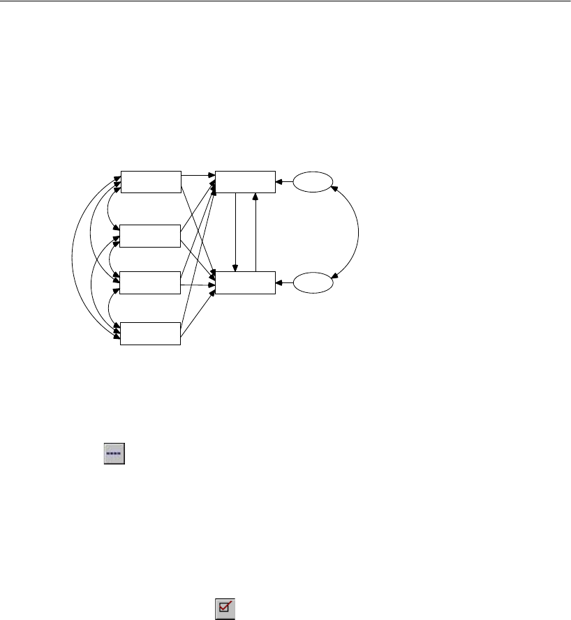
363
Specification Search
Specifying the Model
EOpen %examples%\Ex22b.amw.
Tip: If the last file you opened was in the Examples folder, you can open the file by
double-clicking it in the Files list to the left of the drawing area.
Making Some Arrows Optional
EFrom the menus, choose Analyze > Specification Search.
EClick on the Specification Search toolbar, and then click the arrows in the path
diagram until it looks like the diagram on p. 362.
Tip: You can change multiple arrows at once by clicking and dragging the mouse
pointer through them.
Setting Options to Their Defaults
EClick the Options button on the Specification Search toolbar.
EIn the Options dialog, click the Next search tab.
GPA
height
rating
weight
academic
attract
error1
error2
1
1
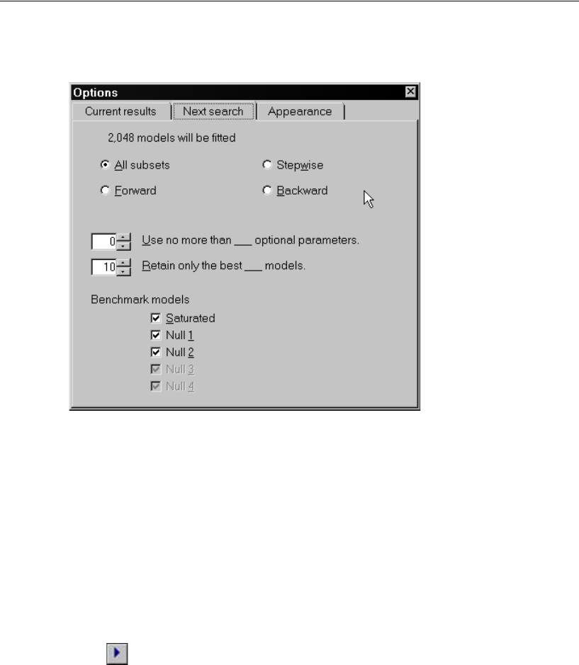
364
Example 22
EIn the Retain only the best ___ models box, change the value from 0 to 10.
This restores the default setting we altered earlier in this example. With the default
setting, the program displays only the 10 best models according to whichever criterion
you use for sorting the columns of the model list. This limitation is desirable now
because of the large number of models that will be generated for this specification
search.
EClick the Current results tab.
EIn the BCC, AIC, BIC group, select Zero-based (min = 0).
Performing the Specification Search
EClick on the Specification Search toolbar.
The search takes about 10 seconds on a 1.8 GHz Pentium 4. When it finishes, the
Specification Search window expands to show the results.
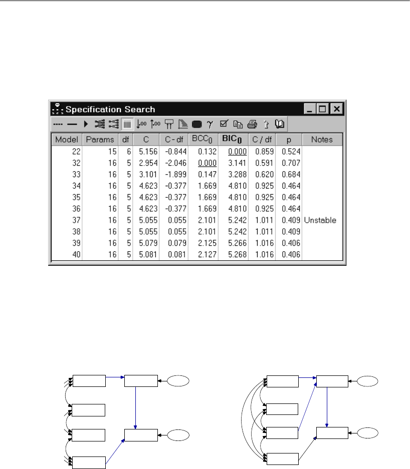
365
Specification Search
Using BIC to Compare Models
EIn the Specification Search window, click the BIC0 column heading. This sorts the table
according to BIC0.
Figure 22-8: The 10 best models according to BIC0
The sorted table shows that Model 22 is the best model according to BIC0. (Model
numbers depend in part on the order in which the objects in the path diagram were
drawn; therefore, if you draw your own path diagram, your model numbers may differ
from the model numbers here.) The second-best model according to BIC0, namely
Model 32, is the best according to BCC0. These models are shown below:
Model 22 Model 32
GPA
height
rating
weight
academic
attract
error1
error2
1
1
GPA
height
rating
weight
academic
attract
error1
error2
1
1
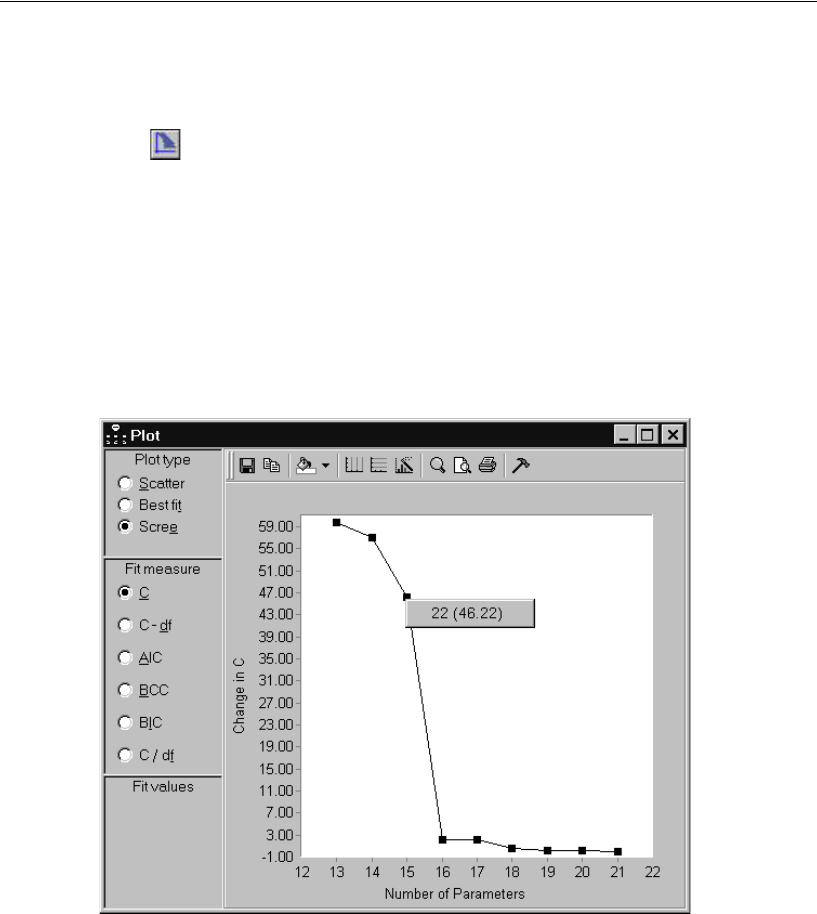
366
Example 22
Viewing the Scree Plot
EClick on the Specification Search toolbar.
EIn the Plot window, select Scree in the Plot type group.
The scree plot strongly suggests that models with 15 parameters provide an optimum
trade-off of model fit and parsimony.
EClick the point with the horizontal coordinate 15. A pop-up appears that indicates the
point represents Model 22, for which the change in chi-square is 46.22.
EClick 22 (46.22) to display Model 22 in the drawing area.
Limitations
The specification search procedure is limited to the analysis of data from a single
group.

367
Example
23
Exploratory Factor Analysis by
Specification Search
Introduction
This example demonstrates exploratory factor analysis by means of a specification
search. In this approach to exploratory factor analysis, any measured variable can
(optionally) depend on any factor. A specification search is performed to find the
subset of single-headed arrows that provides the optimum combination of simplicity
and fit. It also demonstrates a heuristic specification search that is practical for models
that are too big for an exhaustive specification search.
About the Data
This example uses the Holzinger and Swineford girls’ (1939) data from Example 8.
About the Model
The initial model is shown in Figure 23-1 on p. 368. During the specification search,
all single-headed arrows that point from factors to measured variables will be made
optional. The purpose of the specification search is to obtain guidance as to which
single-headed arrows are essential to the model; in other words, which variables
depend on which factors.
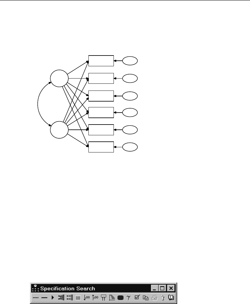
368
Example 23
The two factor variances are both fixed at 1, as are all the regression weights
associated with residual variables. Without these constraints, all the models
encountered during the specification search would be unidentified.
Figure 23-1: Exploratory factor analysis model with two factors
Specifying the Model
EOpen the file %examples%\Ex23.amw.
Initially, the path diagram appears as in Figure 23-1. There is no point in trying to fit this
model as it stands because it is not identified, even with the factor variances fixed at 1.
Opening the Specification Search Window
ETo open the Specification Search window, choose Analyze > Specification Search.
Initially, only the toolbar is visible, as seen here:
1
F1
visperc
cubes
lozenges
wordmean
paragraph
sentence
err_v
err_c
err_l
err_p
err_s
err_w
1
F2
1
1
1
1
1
1
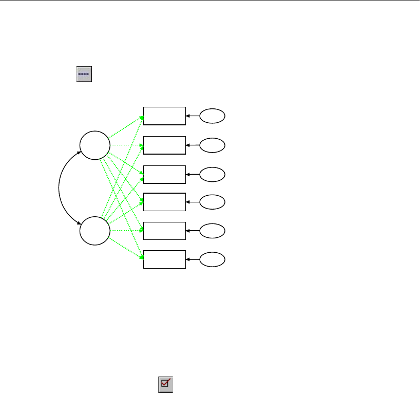
369
Exploratory Factor Analysis by Specification Search
Making All Regression Weights Optional
EClick on the Specification Search toolbar, and then click all the single-headed
arrows in the path diagram.
Figure 23-2: Two-factor model with all regression weights optional
During the specification search, the program will attempt to fit the model using every
possible subset of the optional arrows.
Setting Options to Their Defaults
EClick the Options button on the Specification Search toolbar.
EIn the Options dialog, click the Current results tab.
1
F1
visperc
cubes
lozenges
wordmean
paragraph
sentence
err_v
err_c
err_l
err_p
err_s
err_w
1
F2
1
1
1
1
1
1
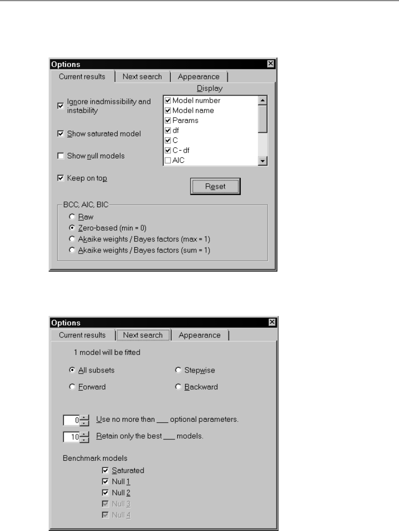
370
Example 23
EClick Reset to ensure that your options are the same as those used in this example.
ENow click the Next search tab. Notice that the default value for Retain only the best ___
models is 10.
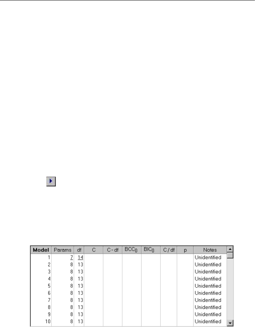
371
Exploratory Factor Analysis by Specification Search
With this setting, the program will display only the 10 best models according to
whichever criterion you use for sorting the columns of the model list. For example, if
you click the column heading C / df, the table will show the 10 models with the smallest
values of C / df, sorted according to C / df. Scatterplots will display only the 10 best
1-parameter models, the 10 best 2-parameter models, and so on. It is useful to place a
limit on the number of parameters to be displayed when there are a lot of optional
parameters.
In this example, there are 12 optional parameters so that there are
candidate models. Storing results for a large number of models can affect performance.
Limiting the display to the best 10 models for each number of parameters means that
the program has to maintain a list of only about 10 × 13 = 130 models. The program
will have to fit many more than 130 models in order to find the best 10 models for each
number of parameters, but not quite as many as 4,096. The program uses a branch-and-
bound algorithm similar to the one used in all-possible-subsets regression (Furnival
and Wilson, 1974) to avoid fitting some models unnecessarily.
Performing the Specification Search
EClick on the Specification Search toolbar.
The search takes about 12 seconds on a 1.8 GHz Pentium 4. When it finishes, the
Specification Search window expands to show the results.
Initially, the list of models is not very informative. The models are listed in the order
in which they were encountered, and the models encountered early in the search were
found to be unidentified. The method used for classifying models as unidentified is
described in Appendix D.
212 4096=
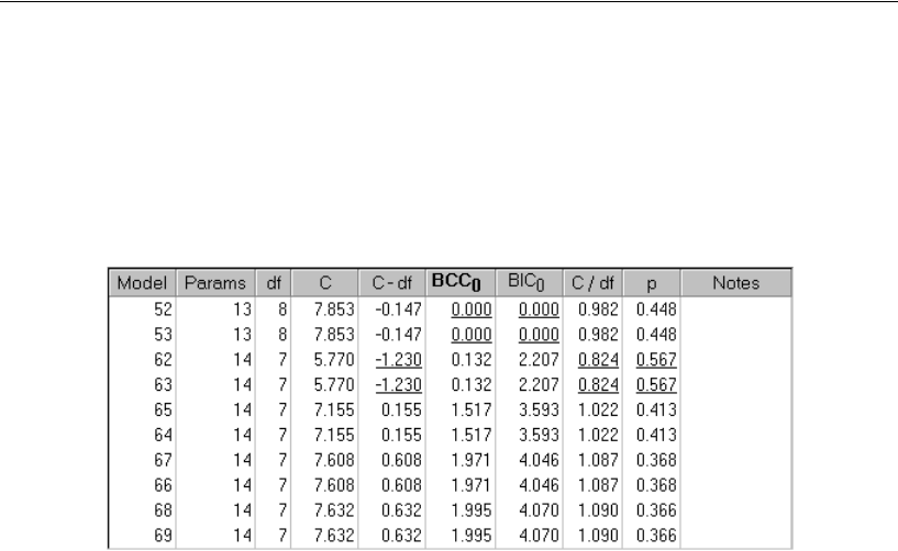
372
Example 23
Using BCC to Compare Models
EIn the Specification Search window, click the column heading BCC0.
The table sorts according to BCC so that the best model according to BCC (that is, the
model with the smallest BCC) is at the top of the list.
Figure 23-3: The 10 best models according to BCC0
The two best models according to BCC0 (Models 52 and 53) have identical fit measures
(out to three decimal places anyway). The explanation for this can be seen from the
path diagrams for the two models.
EIn the Specification Search window, double-click the row for Model 52. This displays
its path diagram in the drawing area.
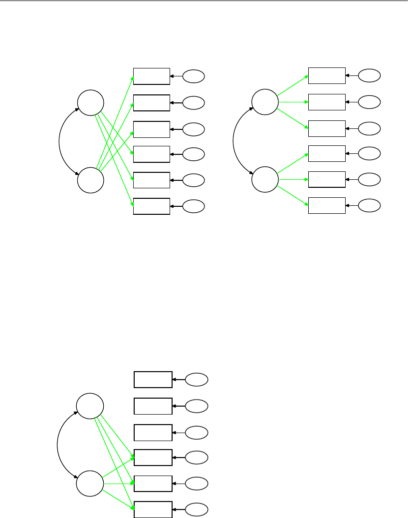
373
Exploratory Factor Analysis by Specification Search
ETo see the path diagram for Model 53, double-click its row.
Figure 23-4: Reversing F1 and F2 yields another candidate model
This is just one pair of models where reversing the roles of F1 and F2 changes one
member of the pair into the other. There are other such pairs. Models 52 and 53 are
equivalent, although they are counted separately in the list of 4,096 candidate models.
The 10 models in Figure 23-3 on p. 372 come in five pairs, but candidate models do
not always come in equivalent pairs, as Figure 23-5 illustrates. The model in that figure
does not occur among the 10 best models for six optional parameters and is not
identified for that matter, but it does illustrate how reversing F1 and F2 can fail to yield
a different member of the set of 4,096 candidate models.
Figure 23-5: Reversing F1 and F2 yields the same candidate model
Model 52 Model 53
1
F1
visperc
cubes
lozenges
wordmean
paragraph
sentence
err_v
err_c
err_l
err_p
err_s
err_w
1
F2
1
1
1
1
1
1
1
F1
visperc
cubes
lozenges
wordmean
paragraph
sentence
err_v
err_c
err_l
err_p
err_s
err_w
1
F2
1
1
1
1
1
1
1
F1
visperc
cubes
lozenges
wordmean
paragraph
sentence
err_v
err_c
err_l
err_p
err_s
err_w
1
F2
1
1
1
1
1
1
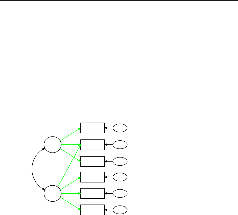
374
Example 23
The occurrence of equivalent candidate models makes it unclear how to apply
Bayesian calculations to select a model in this example. Similarly, it is unclear how to
use Akaike weights. Furthermore, Burnham and Anderson’s guidelines (see p. 344) for
the interpretation of BCC0 are based on reasoning about Akaike weights, so it is not
clear whether those guidelines apply in the present example. On the other hand, the use
of BCC0 without reference to the Burnham and Anderson guidelines seems
unexceptionable. Model 52 (or the equivalent Model 53) is the best model according
to BCC0.
Although BCC0 chooses the model employed in Example 8, which was based on a
model of Jöreskog and Sörbom (1996), it might be noted that Model 62 (or its
equivalent, Model 63) is a very close second in terms of BCC0 and is the best model
according to some other fit measures. Model 63 has the following path diagram:
Figure 23-6: Model 63
The factors, F1 and F2, seem roughly interpretable as spatial ability and verbal ability
in both Models 53 and 63. The two models differ in their explanation of scores on the
cubes test. In Model 53, cubes scores depend entirely on spatial ability. In Model 63,
cubes scores depend on both spatial ability and verbal ability. Since it is a close call in
terms of every criterion based on fit and parsimony, it may be especially appropriate
here to pay attention to interpretability as a model selection criterion. The scree test in
the following step, however, does not equivocate as to which is the best model.
1
F1
visperc
cubes
lozenges
wordmean
paragraph
sentence
err_v
err_c
err_l
err_p
err_s
err_w
1
F2
1
1
1
1
1
1
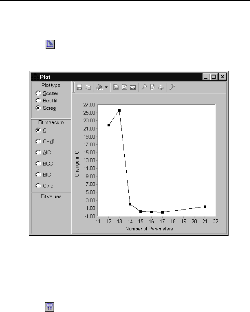
375
Exploratory Factor Analysis by Specification Search
Viewing the Scree Plot
EClick on the Specification Search toolbar.
EIn the Plot window, select Scree in the Plot type group.
The scree plot strongly suggests the use of 13 parameters because of the way the graph
drops abruptly and then levels off immediately after the 13th parameter. Click the point
with coordinate 13 on the horizontal axis. A pop-up shows that the point represents
Models 52 and 53, as shown in Figure 23-4 on p. 373.
Viewing the Short List of Models
EClick on the Specification Search toolbar. Take note of the short list of models for
future reference.

376
Example 23
Heuristic Specification Search
The number of models that must be fitted in an exhaustive specification search grows
rapidly with the number of optional arrows. There are 12 optional arrows in Figure
23-2 on p. 369 so that an exhaustive specification search requires fitting
models. (The number of models will be somewhat smaller if you specify a small
positive number for Retain only the best___models on the Next search tab of the Options
dialog.) A number of heuristic search procedures have been proposed for reducing the
number of models that have to be fitted (Salhi, 1998). None of these is guaranteed to
find the best model, but they have the advantage of being computationally feasible in
problems with more than, say, 20 optional arrows where an exhaustive specification
search is impossible.
Amos provides three heuristic search strategies in addition to the option of an
exhaustive search. The heuristic strategies do not attempt to find the overall best model
because this would require choosing a definition of best in terms of the minimum or
maximum of a specific fit measure. Instead, the heuristic strategies attempt to find the
1-parameter model with the smallest discrepancy, the 2-parameter model with the
smallest discrepancy, and so on. By adopting this approach, a search procedure can be
designed that is independent of the choice of fit measure. You can select among the
available search strategies on the Next search tab of the Options dialog. The choices are
as follows:
All subsets. An exhaustive search is performed. This is the default.
Forward. The program first fits the model with no optional arrows. Then it adds one
optional arrow at a time, always adding whichever arrow gives the largest
reduction in discrepancy.
Backward. The program first fits the model with all optional arrows in the model.
Then it removes one optional arrow at a time, always removing whichever arrow
gives the smallest increase in discrepancy.
Stepwise. The program alternates between Forward and Backward searches,
beginning with a Forward search. The program keeps track of the best 1-optional-
arrow model encountered, the best 2-optional-arrow model, and so on. After the
first Forward search, the Forward and Backward search algorithms are modified by
the following rule: The program will add an arrow or remove an arrow only if the
resulting model has a smaller discrepancy than any previously encountered model
with the same number of arrows. For example, the program will add an arrow to a
5-optional-arrow model only if the resulting 6-optional-arrow model has a smaller
discrepancy than any previously encountered 6-optional-arrow model. Forward
and Backward searches are alternated until one Forward or Backward search is
completed with no improvement.
212 4096=
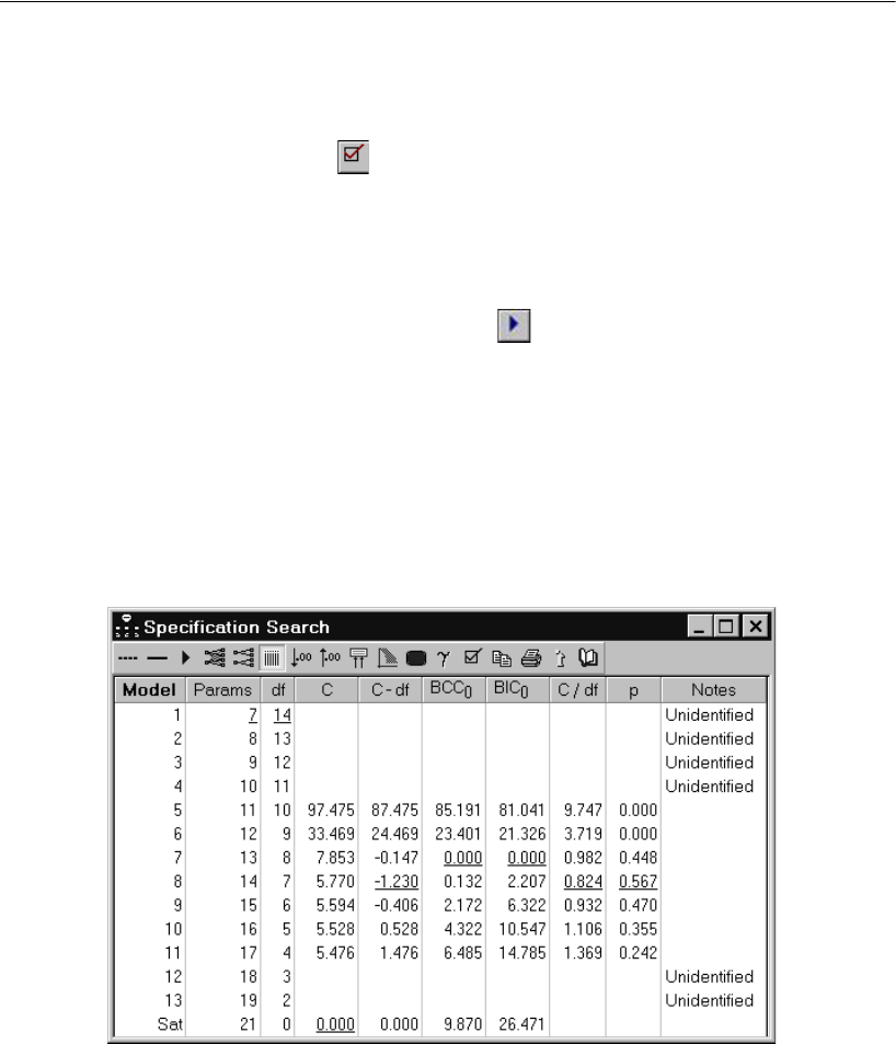
377
Exploratory Factor Analysis by Specification Search
Performing a Stepwise Search
EClick the Options button on the Specification Search toolbar.
EIn the Options dialog, click the Next search tab.
ESelect Stepwise.
EOn the Specification Search toolbar, click .
The results in Figure 23-7 suggest examining the 13-parameter model, Model 7. Its
discrepancy C is much smaller than the discrepancy for the best 12-parameter model
and not much larger than the best 14-parameter model. Model 7 is also best according
to both BCC and BIC. (Your results may differ from those in the figure because of an
element of randomness in the heuristic specification search algorithms. When adding
an arrow during a forward step or removing an arrow during a backward step, there
may not be a unique best choice. In that case, one arrow is picked at random from
among the arrows that are tied for best.)
Figure 23-7: Results of stepwise specification search
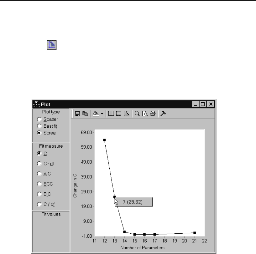
378
Example 23
Viewing the Scree Plot
EClick on the Specification Search toolbar.
EIn the Plot window, select Scree in the Plot type group.
The scree plot confirms that adding a 13th parameter provides a substantial reduction
in discrepancy and that adding additional parameters beyond the 13th provides only
slight reductions.
Figure 23-8: Scree plot after stepwise specification search
EClick the point in the scree plot with horizontal coordinate 13, as in Figure 23-8. The
pop-up that appears shows that Model 7 is the best 13-parameter model.
EClick 7 (25.62) on the pop-up. This displays the path diagram for Model 7 in the
drawing area.
Tip: You can also do this by double-clicking the row for Model 7 in the Specification
Search window.

379
Exploratory Factor Analysis by Specification Search
Limitations of Heuristic Specification Searches
A heuristic specification search can fail to find any of the best models for a given
number of parameters. In fact, the stepwise search in the present example did fail to
find any of the best 11-parameter models. As Figure 23-7 on p. 377 shows, the best
11-parameter model found by the stepwise search had a discrepancy (C) of 97.475. An
exhaustive search, however, turns up two models that have a discrepancy of 55.382. For
every other number of parameters, the stepwise search did find one of the best models.
Of course, it is only when you can perform an exhaustive search to double-check the
result of a heuristic search that you can know whether the heuristic search was
successful. In those problems where a heuristic search is the only available technique,
not only is there no guarantee that it will find one of the best models for each number
of parameters, but there is no way to know whether it has succeeded in doing so.
Even in those cases where a heuristic search finds one of the best models for a given
number of parameters, it does not (as implemented in Amos) give information about
other models that fit equally as well or nearly as well.

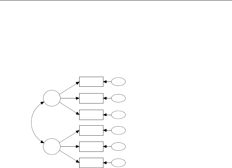
382
Example 24
Model 24a: Modeling Without Means and Intercepts
The presence of means and intercepts as explicit model parameters adds to the
complexity of a multiple-group analysis. The treatment of means and intercepts will be
postponed until Model 24b. For now, consider fitting the following factor analysis
model, with no explicit means and intercepts, to the data of girls and of boys:
Figure 24-1: Two-factor model for girls and boys
This is the same two-group factor analysis problem that was considered in Example 12.
The results obtained in Example 12 will be obtained here automatically.
Specifying the Model
EFrom the menus, choose File > Open.
EIn the Open dialog, enter the file name %examples%\Ex24a.amw, and then click the
Open button.
The path diagram is the same for boys as for girls and is shown in Figure 24-1. Some
regression weights are fixed at 1. These regression weights will remain fixed at 1
throughout the analysis to follow. The assisted multiple-group analysis adds
constraints to the model you specify but does not remove any constraints.
spatial
visperc
cubes
lozenges
wordmean
paragrap
sentence
err_v
err_c
err_l
err_p
err_s
err_w
verbal
1
1
1
1
1
1
1
1
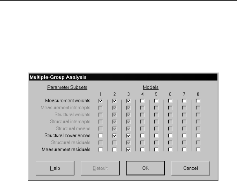
383
Multiple-Group Factor Analysis
Opening the Multiple-Group Analysis Dialog Box
EFrom the menus, choose Analyze > Multiple-Group Analysis.
EClick OK in the message box that appears. This opens the Multiple-Group Analysis
dialog.
Figure 24-2: The Multiple-Group Analysis dialog
Most of the time, you will simply click OK. This time, however, let's take a look at some
parts of the Multiple-Group Analysis dialog.
There are eight columns of check boxes. Check marks appear only in the columns
labeled 1, 2, and 3. This means that the program will generate three models, each with
a different set of cross-group constraints.
Column 1 contains a single check mark in the row labeled Measurement weights,
which is short for regression weights in the measurement part of the model. In the case
of a factor analysis model, these are the factor loadings. The following section shows
you how to view the measurement weights in the path diagram. Column 1 generates a
model in which measurement weights are constant across groups (that is, the same for
boys as for girls).
Column 2 contains check marks for Measurement weights and also Structural
covariances, which is short for variances and covariances in the structural part of the
model. In a factor analysis model, these are the factor variances and covariances. The
following section shows you how to view the structural covariances in the path
diagram. Column 2 generates a model in which measurement weights and structural
covariances are constant across groups.
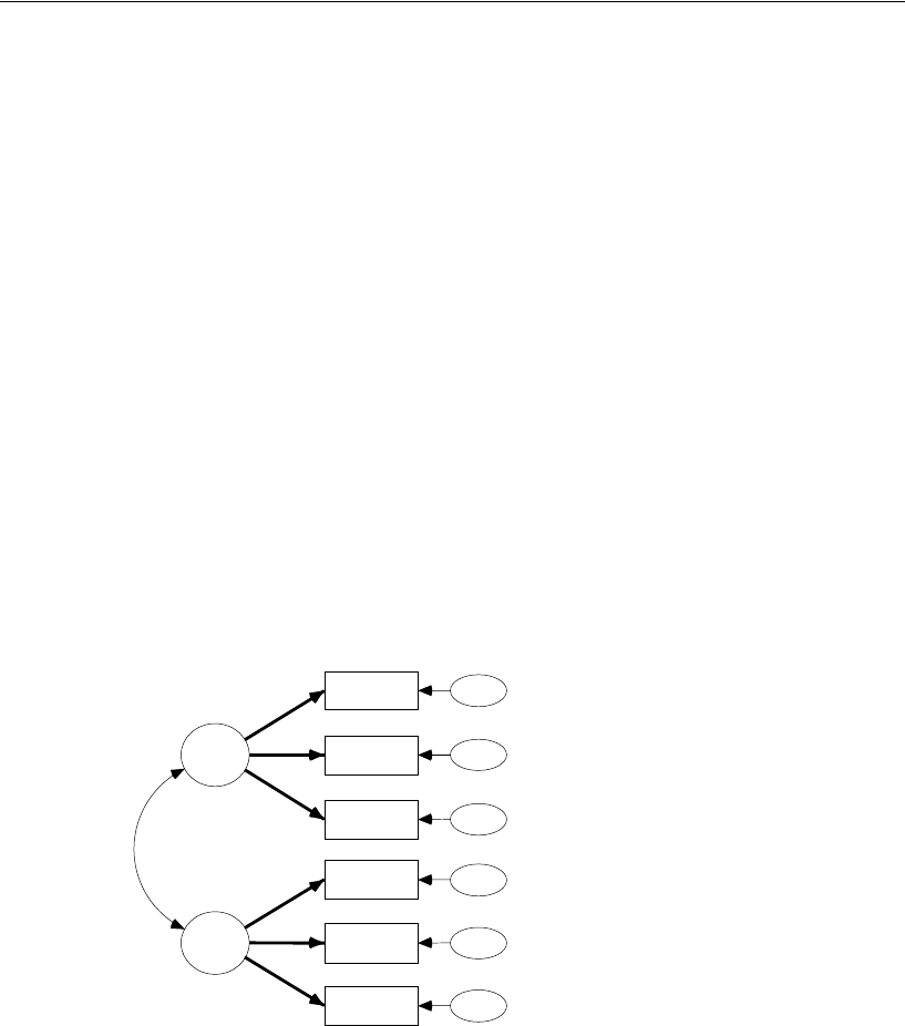
384
Example 24
Column 3 contains all the check marks in column 2 and also a check mark next to
Measurement residuals, which is short for variances and covariances of residual
(error) variables in the measurement part of the model. The following section shows
you how to view the measurement residuals in the path diagram. The three parameter
subsets that appear in a black (that is, not gray) font are mutually exclusive and
exhaustive, so that column 3 generates a model in which all parameters are constant
across groups.
In summary, columns 1 through 3 generate a hierarchy of models in which each
model contains all the constraints of its predecessor. First, the factor loadings are held
constant across groups. Then, the factor variances and covariances are held constant.
Finally, the residual (unique) variances are held constant.
Viewing the Parameter Subsets
EIn the Multiple-Group Analysis dialog, click Measurement weights.
The measurement weights are now displayed in color in the drawing area. If there is a
check mark next to Alternative to color on the Accessibility tab of the Interface Properties
dialog, the measurement weights will also display as thick lines, as shown here:
EClick Structural covariances to see the factor variances and covariances emphasized.
EClick Measurement residuals to see the error variables emphasized.
This is an easy way to visualize which parameters are affected by each cross-group
constraint.
spatial
visperc
cubes
lozenges
wordmean
paragrap
sentence
err_v
err_c
err_l
err_p
err_s
err_w
verbal
1
1
1
1
1
1
1
1
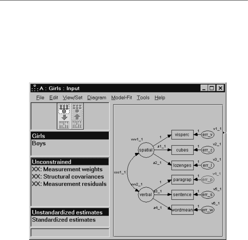
385
Multiple-Group Factor Analysis
Viewing the Generated Models
EIn the Multiple-Group Analysis dialog, click OK.
The path diagram now shows names for all parameters. In the panel at the left of the
path diagram, you can see that the program has generated three new models in addition
to an Unconstrained model in which there are no cross-group constraints at all.
Figure 24-3: Amos Graphics window after automatic constraints
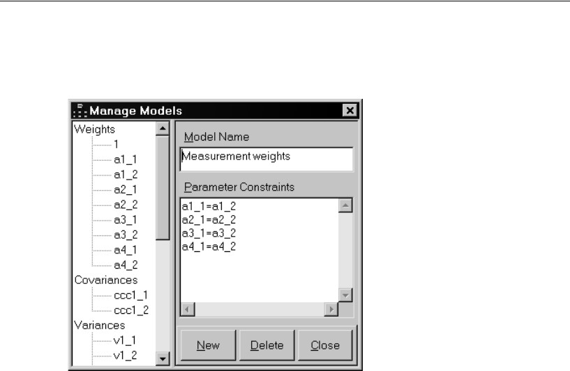
386
Example 24
EDouble-click XX: Measurement weights. This opens the Manage Models dialog, which
shows you the constraints that require the factor loadings to be constant across groups.
Fitting All the Models and Viewing the Output
EFrom the menus, choose Analyze > Calculate Estimates to fit all models.
EFrom the menus, choose View > Text Output.
EIn the navigation tree of the output viewer, click the Model Fit node to expand it, and
then click CMIN.
The CMIN table shows the likelihood ratio chi-square statistic for each fitted model.
The data do not depart significantly from any of the models. Furthermore, at each step
up the hierarchy from the Unconstrained model to the Measurement residuals model,
the increase in chi-square is never much larger than the increase in degrees of freedom.
There appears to be no significant evidence that girls’ parameter values differ from
boys’ parameter values.
387
Multiple-Group Factor Analysis
Here is the CMIN table:
EIn the navigation tree, click AIC under the Model Fit node.
AIC and BCC values indicate that the best trade-off of model fit and parsimony is
obtained by constraining all parameters to be equal across groups (the Measurement
residuals model).
Here is the AIC table:
Customizing the Analysis
There were two opportunities to override the automatically generated cross-group
constraints. In Figure 24-2 on p. 383, you could have changed the check marks in
columns 1, 2, and 3, and you could have generated additional models by placing check
marks in columns 4 through 8. Then, in Figure 24-3 on p. 385, you could have renamed
or modified any of the automatically generated models listed in the panel at the left of
the path diagram.
Model NPAR CMIN DF P CMIN/DF
Unconstrained 26 16.48 16 0.42 1.03
Measurement weights 22 18.29 20 0.57 0.91
Structural covariances 19 22.04 23 0.52 0.96
Measurement residuals 13 26.02 29 0.62 0.90
Saturated model 42 0.00 0
Independence model 12 337.55 30 0.00 11.25
Model AIC BCC BIC CAIC
Unconstrained 68.48 74.12
Measurement weights 62.29 67.07
Structural covariances 60.04 64.16
Measurement residuals 52.02 54.84
Saturated model 84.00 93.12
Independence model 361.55 364.16
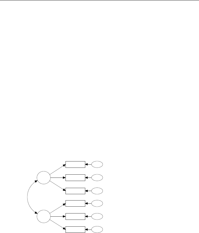
388
Example 24
Model 24b: Comparing Factor Means
Introducing explicit means and intercepts into a model raises additional questions
about which cross-group parameter constraints should be tested, and in what order.
This example shows how Amos constrains means and intercepts while fitting the factor
analysis model in Figure 24-1 on p. 382 to data from separate groups of girls and boys.
This is the same two-group factor analysis problem that was considered in Example
15. The results in Example 15 will be obtained here automatically.
Specifying the Model
EFrom the menus, choose File > Open.
EIn the Open dialog, enter the file name %examples%\Ex24b.amw, and then click the
Open button.
The path diagram is the same for boys as for girls and is shown below. Some regression
weights are fixed at 1. The means of all the unobserved variables are fixed at 0. In the
following section, you will remove the constraints on the girls’ factor means. The other
constraints (the ones that you do not remove) will remain in effect throughout the
analysis.
Figure 24-4: Two-factor model with explicit means and intercepts
0,
spatial
visperc
cubes
lozenges
wordmean
paragrap
sentence
0,
err_v
0,
err_c
0,
err_l
0,
err_p
0,
err_s
0,
err_w
0,
verbal
1
1
1
1
1
1
1
1

389
Multiple-Group Factor Analysis
Removing Constraints
Initially, the factor means are fixed at 0 for both boys and girls. It is not possible to
estimate factor means for both groups. However, Sörbom (1974) showed that, by fixing
the factor means of a single group to constant values and placing suitable constraints
on the regression weights and intercepts in a factor model, it is possible to obtain
meaningful estimates of the factor means for all of the other groups. In the present
example, this means picking one group, say boys, and fixing their factor means to a
constant, say 0, and then removing the constraints on the factor means of the remaining
group, the girls. The constraints on regression weights and intercepts required by
Sörbom’s approach will be generated automatically by Amos.
The boys’ factor means are already fixed at 0. To remove the constraints on the girls'
factor means, do the following:
EIn the drawing area of the Amos Graphics window, right-click Spatial and choose
Object Properties from the pop-up menu.
EIn the Object Properties dialog, click the Parameters tab.
ESelect the 0 in the Mean box, and press the Delete key.
EWith the Object Properties dialog still open, click Verbal in the drawing area. This
displays the properties for the verbal factor in the Object Properties dialog.
EIn the Mean box on the Parameters tab, select the 0 and press the Delete key.
EClose the Object Properties dialog.
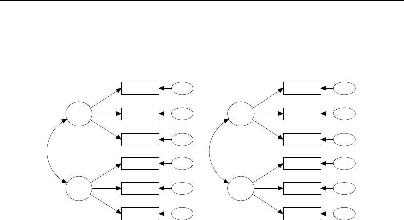
390
Example 24
Now that the constraints on the girls’ factor means have been removed, the girls’ and
boys’ path diagrams look like this:
Tip: To switch between path diagrams in the drawing area, click either Boys or Girls in
the List of Groups pane to the left.
Girls Boys
spatial
visperc
cubes
lozenges
wordmean
paragrap
sentence
0,
err_v
0,
err_c
0,
err_l
0,
err_p
0,
err_s
0,
err_w
verbal
1
1
1
1
1
1
1
1
0,
spatial
visperc
cubes
lozenges
wordmean
paragrap
sentence
0,
err_v
0,
err_c
0,
err_l
0,
err_p
0,
err_s
0,
err_w
0,
verbal
1
1
1
1
1
1
1
1
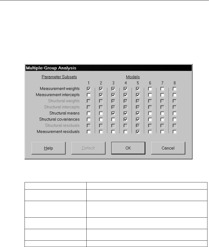
391
Multiple-Group Factor Analysis
Generating the Cross-Group Constraints
EFrom the menus, choose Analyze > Multiple-Group Analysis.
EClick OK in the message box that appears. This opens the Multiple-Group Analysis
dialog.
The default settings, as shown above, will generate the following nested hierarchy of
five models:
EClick OK.
Model Constraints
Model 1 (column 1) Measurement weights (factor loadings) are equal across
groups.
Model 2 (column 2)
All of the above, and measurement intercepts (intercepts in
the equations for predicting measured variables) are equal
across groups.
Model 3 (column 3) All of the above, and structural means (factor means) are
equal across groups.
Model 4 (column 4) All of the above, and structural covariances (factor variances
and covariances) are equal across groups.
Model 5 (column 5) All parameters are equal across groups.

392
Example 24
Fitting the Models
EFrom the menus, choose Analyze > Calculate Estimates.
The panel at the left of the path diagram shows that two models could not be fitted to
the data. The two models that could not be fitted, the Unconstrained model with no
cross-group constraints, and the Measurement weights model with factor loadings held
equal across groups, are unidentified.
Viewing the Output
EFrom the menus, choose View > Text Output.
EIn the navigation tree of the output viewer, expand the Model Fit node.
Some fit measures for the four automatically generated and identified models are
shown here, along with fit measures for the saturated and independence models.
EClick CMIN under the Model Fit node.
The CMIN table shows that none of the generated models can be rejected when tested
against the saturated model.
Model NPAR CMIN DF P CMIN/DF
Measurement intercepts 30 22.593 24 0.544 0.941
Structural means 28 30.624 26 0.243 1.178
Structural covariances 25 34.381 29 0.226 1.186
Measurement residuals 19 38.459 35 0.316 1.099
Saturated model 54 0.00 0
Independence model 24 337.553 30 0.00 11.252
393
Multiple-Group Factor Analysis
On the other hand, the change in chi-square ( ) when introducing
the equal-factor-means constraint looks large compared to the change in degrees of
freedom ( ).
EIn the navigation tree, click the Model Comparison node.
Assuming model Measurement intercepts to be correct, the following table shows that
this chi-square difference is significant:
In the preceding two tables, two chi-square statistics and their associated degrees of
freedom are especially important. The first, with , allowed
accepting the hypothesis of equal intercepts and equal regression weights in the
measurement model. It was important to establish the credibility of this hypothesis
because, without equal intercepts and equal regression weights, it would be unclear
that the factors have the same meaning for boys as for girls and so there would be no
interest in comparing their means. The other important chi-square statistic,
with , leads to rejection of the hypothesis that boys and girls have the same
factor means.
Group differences between the boys’ and girls’ factor means can be determined
from the girls’ estimates in the Measurement intercepts model.
ESelect the Measurement intercepts model in the pane at the lower left of the output
viewer.
EIn the navigation tree, click Estimates, then Scalars, and then Means.
The boys’ means were fixed at 0, so only the girls’ means were estimated, as shown in
the following table:
These estimates were discussed in Model A of Example 15, which is identical to the
present Measurement intercepts model. (Model B of Example 15 is identical to the
present Structural means model.)
Model DF CMIN P NFI
Delta-1
IFI
Delta-2
RFI
rho-1
TLI
rho2
Structural means 2 8.030 0.018 0.024 0.026 0.021 0.023
Structural covariances 5 11.787 0.038 0.035 0.038 0.022 0.024
Measurement residuals 11 15.865 0.146 0.047 0.051 0.014 0.015
Estimate S.E. C.R. P Label
spatial –1.066 0.881 –1.209 0.226 m1_1
verbal 0.956 0.521 1.836 0.066 m2_1
30.62 22.59 8.03=–
26 24 2=–
χ222.59=
df 24=
χ28.03=
df 2=

395
Example
25
Multiple-Group Analysis
Introduction
This example shows you how to automatically implement Sörbom’s alternative to
analysis of covariance.
Example 16 demonstrates the benefits of Sörbom’s approach to analysis of
covariance with latent variables. Unfortunately, as Example 16 also showed, the
Sörbom approach is difficult to apply, involving many steps. This example
automatically obtains the same results as Example 16.
About the Data
The Olsson (1973) data from Example 16 will be used here. The sample moments can
be found in the workbook UserGuide.xls. Sample moments from the experimental
group are in the worksheet Olss_exp. Sample moments from the control group are in
the worksheet Olss_cnt.

396
Example 25
About the Model
The model was described in Example 16. The Sörbom method requires that the
experimental and the control group have the same path diagram.
Figure 25-1: Sörbom model for Olsson data
Specifying the Model
EOpen %examples%\Ex25.amw.
The path diagram is the same for the control and experimental groups and is shown in
Figure 25-1. Some regression weights are fixed at 1. The means of all the residual
(error) variable means are fixed at 0. These constraints will remain in effect throughout
the analysis.
Constraining the Latent Variable Means and Intercepts
The model in Figure 25-1, Sörbom’s model for Olsson data, is unidentified and will
remain unidentified for every set of cross-group constraints that Amos automatically
generates. For every set of cross-group constraints, the mean of pre_verbal and the
intercept in the equation for predicting post_verbal will be unidentified. In order to
allow the model to be identified for at least some cross-group constraints, it is
necessary to pick one group, such as the control group, and fix the pre_verbal mean
and the post_verbal intercept to a constant, such as 0.
pre_verbal
pre_syn
0,
eps1
1
1
pre_opp
0,
eps2
1
post_verbal
post_syn
0,
eps3
post_opp
0,
eps4
1
1 1
0,
zeta
1
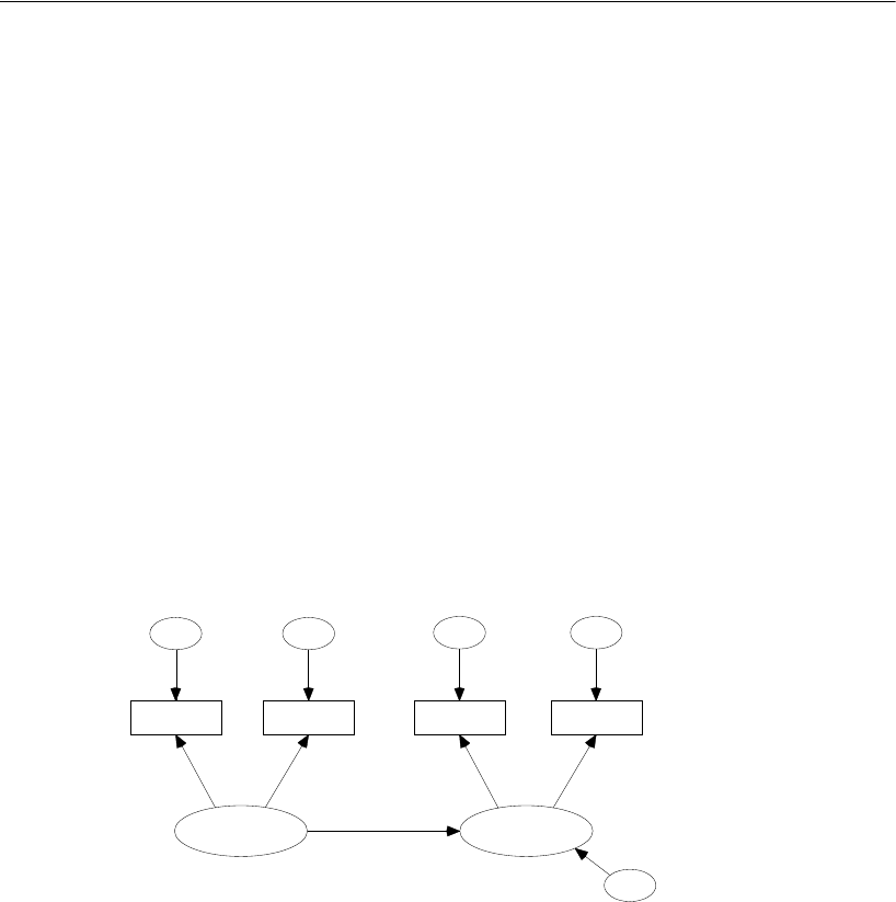
397
Multiple-Group Analysis
EIn the List of Groups pane to the left of the path diagram, ensure that Control is selected.
This indicates that the path diagram for the control group is displayed in the drawing
area.
EIn the drawing area, right-click pre_verbal and choose Object Properties from the pop-
up menu.
EIn the Object Properties dialog, click the Parameters tab.
EIn the Mean text box, type 0.
EWith the Object Properties dialog still open, click post_verbal in the drawing area.
EIn the Intercept text box of the Object Properties dialog, type 0.
EClose the Object Properties dialog.
Now, the path diagram for the control group appears as follows:
The path diagram for the experimental group continues to look like Figure 25-1.
Generating Cross-Group Constraints
EFrom the menus, choose Analyze > Multiple-Group Analysis.
EClick OK in the message box that appears.
0,
pre_verbal
pre_syn
0,
eps1
1
1
pre_opp
0,
eps2
1
0
post_verbal
post_syn
0,
eps3
post_opp
0,
eps4
1
1 1
0,
zeta
1

398
Example 25
The Multiple-Group Analysis dialog appears.
EClick OK to generate the following nested hierarchy of eight models:
Model Constraints
Model 1 (column 1) Measurement weights (factor loadings) are constant across
groups.
Model 2 (column 2)
All of the above, and measurement intercepts (intercepts in
the equations for predicting measured variables) are constant
across groups.
Model 3 (column 3) All of the above, and the structural weight (the regression
weight for predicting post_verbal) is constant across groups.
Model 4 (column 4)
All of the above, and the structural intercept (the intercept in
the equation for predicting post_verbal) is constant across
groups.
Model 5 (column 5) All of the above, and the structural mean (the mean of
pre_verbal) is constant across groups.
Model 6 (column 6) All of the above, and the structural covariance (the variance
of pre_verbal) is constant across groups.
Model 7 (column 7) All of the above, and the structural residual (the variance of
zeta) is constant across groups.
Model 8 (column 8) All parameters are constant across groups.

399
Multiple-Group Analysis
Fitting the Models
EFrom the menus, choose Analyze > Calculate Estimates.
The panel to the left of the path diagram shows that two models could not be fitted to
the data. The two models that could not be fitted, the Unconstrained model and the
Measurement weights model, are unidentified.
Viewing the Text Output
EFrom the menus, choose View > Text Output.
EIn the navigation tree of the output viewer, expand the Model Fit node, and click CMIN.
This displays some fit measures for the seven automatically generated and identified
models, along with fit measures for the saturated and independence models, as shown
in the following CMIN table:
Model NPAR CMIN DF P CMIN/DF
Measurement intercepts 22 34.775 6 0.000 5.796
Structural weights 21 36.340 7 0.000 5.191
Structural intercepts 20 84.060 8 0.000 10.507
Structural means 19 94.970 9 0.000 10.552
Structural covariances 18 99.976 10 0.000 9.998
Structural residuals 17 112.143 11 0.000 10.195
Measurement residuals 13 122.366 15 0.000 8.158
Saturated model 28 0.000 0
Independence model 16 682.638 12 0.000 56.887

400
Example 25
There are many chi-square statistics in this table, but only two of them matter. The
Sörbom procedure comes down to two basic questions. First, does the Structural
weights model fit? This model specifies that the regression weight for predicting
post_verbal from pre_verbal be constant across groups.
If the Structural weights model is accepted, one follows up by asking whether the
next model up the hierarchy, the Structural intercepts model, fits significantly worse.
On the other hand, if the Structural weights model has to be rejected, one never gets to
the question about the Structural intercepts model. Unfortunately, that is the case here.
The Structural weights model, with and , is rejected at any
conventional significance level.
Examining the Modification Indices
To see if it is possible to improve the fit of the Structural weights model:
EClose the output viewer.
EFrom the Amos Graphics menus, choose View > Analysis Properties.
EClick the Output tab and select the Modification Indices check box.
EClose the Analysis Properties dialog.
EFrom the menus, choose Analyze > Calculate Estimates to fit all models.
Only the modification indices for the Structural weights model need to be examined
because this is the only model whose fit is essential to the analysis.
EFrom the menus, choose View > Text Output, select Modification Indices in the navigation
tree of the output viewer, then select Structural weights in the lower left panel.
EExpand the Modification Indices node and select Covariances.
As you can see in the following covariance table for the control group, only one
modification index exceeds the default threshold of 4:
M.I. Par Change
eps2 <--> eps4 4.553 2.073
χ236.34=
df 7=

401
Multiple-Group Analysis
ENow click experimental in the panel on the left. As you can see in the following
covariance table for the experimental group, there are four modification indices greater
than 4:
Of these, only two modifications have an obvious theoretical justification: allowing
eps2 to correlate with eps4, and allowing eps1 to correlate with eps3. Between these
two, allowing eps2 to correlate with eps4 has the larger modification index. Thus the
modification indices from the control group and the experimental group both suggest
allowing eps2 to correlate with eps4.
Modifying the Model and Repeating the Analysis
EClose the output viewer.
EFrom the menus, choose Diagram > Draw Covariances.
EClick and drag to draw a double-headed arrow between eps2 and eps4.
EFrom the menus, choose Analyze > Multiple-Group Analysis, and click OK in the message
box that appears.
EIn the Multiple-Group Analysis dialog, click OK.
EFrom the menus, choose Analyze > Calculate Estimates to fit all models.
EFrom the menus, choose View > Text Output.
EUse the navigation tree to view the fit measures for the Structural weights model.
With the additional double-headed arrow connecting eps2 and eps4, the Structural
weights model has an adequate fit ( with ), as shown in the
following CMIN table:
M.I. Par Change
eps2 <--> eps4 9.314 4.417
eps2 <--> eps3 9.393 –4.117
eps1 <--> eps4 8.513 –3.947
eps1 <--> eps3 6.192 3.110
χ23.98=
df 5=

402
Example 25
Now that the Structural weights model fits the data, it can be asked whether the
Structural intercepts model fits significantly worse. Assuming the Structural weights
model to be correct:
The Structural intercepts model does fit significantly worse than the Structural weights
model. When the intercept in the equation for predicting post_verbal is required to be
constant across groups, the chi-square statistic increases by 51.12 while degrees of
freedom increases by only 1. That is, the intercept for the experimental group differs
significantly from the intercept for the control group. The intercept for the
experimental group is estimated to be 3.627.
Recalling that the intercept for the control group was fixed at 0, it is estimated that the
treatment increases post_verbal scores by 3.63 with pre_verbal held constant.
The results obtained in the present example are identical to the results of Example
16. The Structural weights model is the same as Model D in Example 16. The
Structural intercepts model is the same as Model E in Example 16.
Model NPAR CMIN DF P CMIN/DF
Measurement intercepts 24 2.797 4 0.59 0.699
Structural weights 23 3.976 5 0.55 0.795
Structural intercepts 22 55.094 6 0.00 9.182
Structural means 21 63.792 7 0.00 9.113
Structural covariances 20 69.494 8 0.00 8.687
Structural residuals 19 83.194 9 0.00 9.244
Measurement residuals 14 93.197 14 0.00 6.657
Saturated model 28 0.000 0
Independence model 16 682.638 12 0.00 56.887
Model DF CMIN P NFI
Delta-1
IFI
Delta-2
RFI
rho-1
TLI
rho2
Structural intercepts 1 51.118 0.000 0.075 0.075 0.147 0.150
Structural means 2 59.816 0.000 0.088 0.088 0.146 0.149
Structural covariances 3 65.518 0.000 0.096 0.097 0.139 0.141
Structural residuals 4 79.218 0.000 0.116 0.117 0.149 0.151
Measurement residuals 9 89.221 0.000 0.131 0.132 0.103 0.105
Estimate S.E. C.R. P Label
post_verbal 3.627 0.478 7.591 <0.001 j1_2
pre_syn 18.619 0.594 31.355 <0.001 i1_1
pre_opp 19.910 0.541 36.781 <0.001 i2_1
post_syn 20.383 0.535 38.066 <0.001 i3_1
post_opp 21.204 0.531 39.908 <0.001 i4_1

403
Example
26
Bayesian Estimation
Introduction
This example demonstrates Bayesian estimation using Amos.
Bayesian Estimation
In maximum likelihood estimation and hypothesis testing, the true values of the
model parameters are viewed as fixed but unknown, and the estimates of those
parameters from a given sample are viewed as random but known. An alternative kind
of statistical inference, called the Bayesian approach, views any quantity that is
unknown as a random variable and assigns it a probability distribution. From a
Bayesian standpoint, true model parameters are unknown and therefore considered to
be random, and they are assigned a joint probability distribution. This distribution is
not meant to suggest that the parameters are varying or changing in some fashion.
Rather, the distribution is intended to summarize our state of knowledge, or what is
currently known about the parameters. The distribution of the parameters before the
data are seen is called a prior distribution. Once the data are observed, the evidence
provided by the data is combined with the prior distribution by a well-known formula
called Bayes’ Theorem. The result is an updated distribution for the parameters,
called a posterior distribution, which reflects a combination of prior belief and
empirical evidence (Bolstad, 2004).

404
Example 26
Human beings tend to have difficulty visualizing and interpreting the joint posterior
distribution for the parameters of a model. Therefore, when performing a Bayesian
analysis, one needs summaries of the posterior distribution that are easy to interpret. A
good way to start is to plot the marginal posterior density for each parameter, one at a
time. Often, especially with large data samples, the marginal posterior distributions for
parameters tend to resemble normal distributions. The mean of a marginal posterior
distribution, called a posterior mean, can be reported as a parameter estimate. The
posterior standard deviation, the standard deviation of the distribution, is a useful
measure of uncertainty similar to a conventional standard error.
The analogue of a confidence interval may be computed from the percentiles of the
marginal posterior distribution; the interval that runs from the 2.5 percentile to the 97.5
percentile forms a Bayesian 95% credible interval. If the marginal posterior
distribution is approximately normal, the 95% credible interval will be approximately
equal to the posterior mean ± 1.96 posterior standard deviations. In that case, the
credible interval becomes essentially identical to an ordinary confidence interval that
assumes a normal sampling distribution for the parameter estimate. If the posterior
distribution is not normal, the interval will not be symmetric about the posterior mean.
In that case, the Bayesian version often has better properties than the conventional one.
Unlike a conventional confidence interval, the Bayesian credible interval is
interpreted as a probability statement about the parameter itself;
Prob ) literally means that you are 95% sure that the true value of
lies between a and b. Tail areas from a marginal posterior distribution can even be
used as a kind of Bayesian pvalue for hypothesis testing. If 96.5% of the area under
the marginal posterior density for lies to the right of some value a, then the Bayesian
p value for testing the null hypothesis against the alternative hypothesis
is 0.045. In that case, one would actually say, I’m 96.5% sure that the alternative
hypothesis is true.
Although the idea of Bayesian inference dates back to the late 18th century, its use
by statisticians has been rare until recently. For some, reluctance to apply Bayesian
methods stems from a philosophical distaste for viewing probability as a state of belief
and from the inherent subjectivity in choosing prior distributions. But for the most part,
Bayesian analyses have been rare because computational methods for summarizing
joint posterior distributions have been difficult or unavailable. Using a new class of
simulation techniques called Markov chain Monte Carlo (MCMC), however, it is now
possible to draw random values of parameters from high-dimensional joint posterior
distributions, even in complex problems. With MCMC, obtaining posterior summaries
becomes as simple as plotting histograms and computing sample means and
percentiles.
a
θ
b≤≤()0.95=
θ
θ
θ
a≤
θ
a>

405
Bayesian Estimation
Selecting Priors
A prior distribution quantifies the researcher’s belief concerning where the unknown
parameter may lie. Knowledge of how a variable is distributed in the population can
sometimes be used to help researchers select reasonable priors for parameters of
interest. Hox (2002) cites the example of a normed intelligence test with a mean of 100
units and a standard deviation of 15 units in the general population. If the test is given
to participants in a study who are fairly representative of the general population, then
it would be reasonable to center the prior distributions for the mean and standard
deviation of the test score at 100 and 15, respectively. Knowing that an observed
variable is bounded may help us to place bounds on the parameters. For instance, the
mean of a Likert-type survey item taking values 0, 1, …, 10 must lie between 0 and 10,
and its maximum variance is 25. Prior distributions for the mean and variance of this
item can be specified to enforce these bounds.
In many cases, one would like to specify prior distribution that introduces as little
information as possible, so that the data may be allowed to speak for themselves. A
prior distribution is said to be diffuse if it spreads its probability over a very wide range
of parameter values. By default, Amos applies a uniform distribution from
to to each parameter.
Diffuse prior distributions are often said to be non-informative, and we will use that
term as well. In a strict sense, however, no prior distribution is ever completely non-
informative, not even a uniform distribution over the entire range of allowable values,
because it would cease to be uniform if the parameter were transformed. (Suppose, for
example, that the variance of a variable is uniformly distributed from 0 to ; then the
standard deviation will not be uniformly distributed.) Every prior distribution carries
with it at least some information. As the size of a dataset grows, the evidence from the
data eventually swamps this information, and the influence of the prior distribution
diminishes. Unless your sample is unusually small or if your model and/or prior
distribution are strongly contradicted by the data, you will find that the answers from a
Bayesian analysis tend to change very little if the prior is changed. Amos makes it easy
for you to change the prior distribution for any parameter, so you can easily perform
this kind of sensitivity check.
3.4–10 38–
×
3.4 1038
×
∞
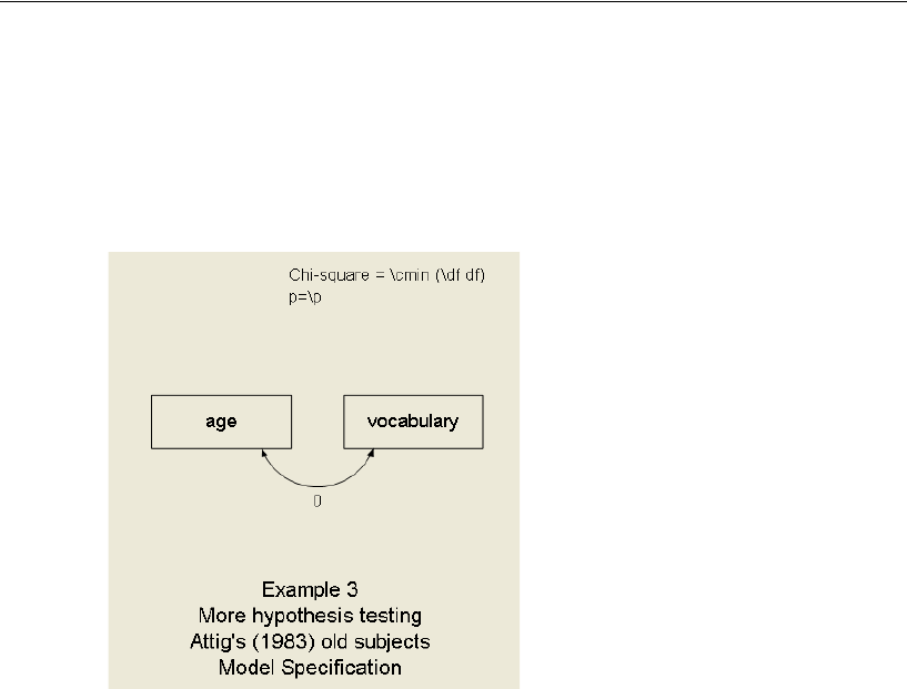
406
Example 26
Performing Bayesian Estimation Using Amos Graphics
To illustrate Bayesian estimation using Amos Graphics, we revisit Example 3, which
shows how to test the null hypothesis that the covariance between two variables is 0 by
fixing the value of the covariance between age and vocabulary to 0.
Estimating the Covariance
The first thing we need to do for the present example is to remove the zero constraint
on the covariance so that the covariance can be estimated.
EOpen %examples%\Ex03.amw.
ERight-click the double-headed arrow in the path diagram and choose Object Properties
from the pop-up menu.
EIn the Object Properties dialog, click the Parameters tab.
EDelete the 0 in the Covariance text box.
EClose the Object Properties dialog.
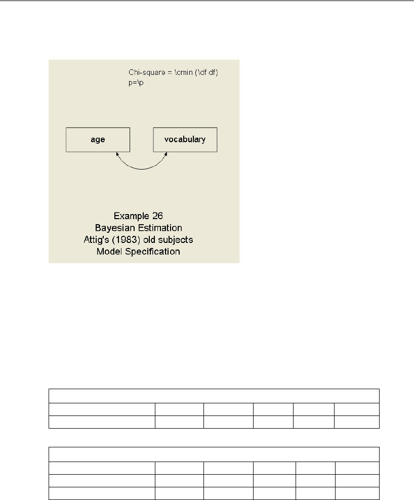
407
Bayesian Estimation
This is the resulting path diagram (you can also find it in Ex26.amw):
Results of Maximum Likelihood Analysis
Before performing a Bayesian analysis of this model, we perform a maximum
likelihood analysis for comparison purposes.
EFrom the menus, choose Analyze > Calculate Estimates to display the following
parameter estimates and standard errors:
Covariances: (Group number 1 - Default model)
Estimate S.E. C.R. P Label
age <--> vocabulary –5.014 8.560 –0.586 0.558
Variances: (Group number 1 - Default model)
Estimate S.E. C.R. P Label
age 21.574 4.886 4.416 ***
vocabulary 131.294 29.732 4.416 ***
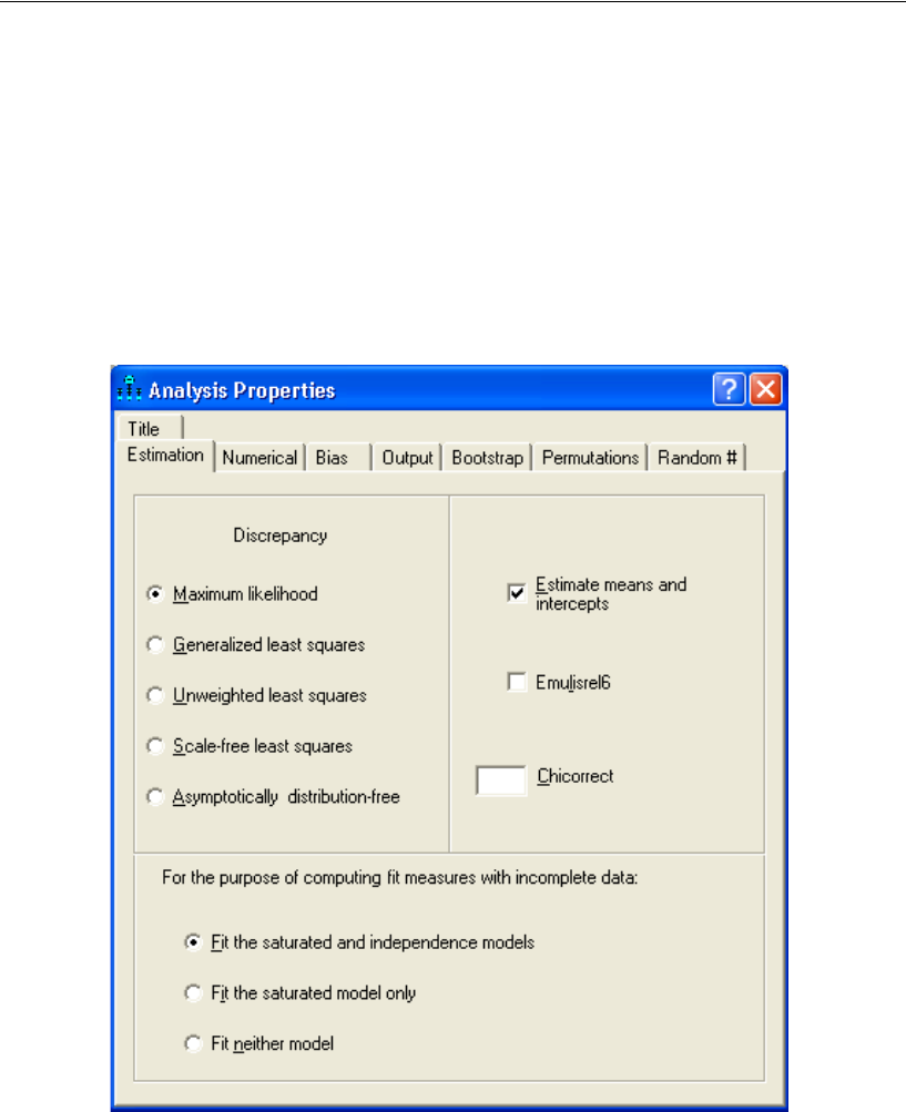
408
Example 26
Bayesian Analysis
Bayesian analysis requires estimation of explicit means and intercepts. Before
performing any Bayesian analysis in Amos, you must first tell Amos to estimate means
and intercepts.
EFrom the menus, choose View > Analysis Properties.
ESelect Estimate means and intercepts. (A check mark will appear next to it.)
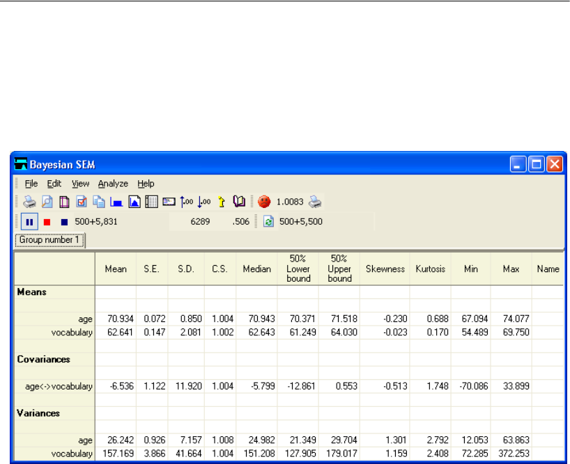
409
Bayesian Estimation
ETo perform a Bayesian analysis, from the menus, choose Analyze > Bayesian Estimation,
or press the keyboard combination Ctrl+B.
The Bayesian SEM window appears, and the MCMC algorithm immediately begins
generating samples.
The Bayesian SEM window has a toolbar near the top of the window and has a results
summary table below. Each row of the summary table describes the marginal posterior
distribution of a single model parameter. The first column, labeled Mean, contains the
posterior mean, which is the center or average of the posterior distribution. This can be
used as a Bayesian point estimate of the parameter, based on the data and the prior
distribution. With a large dataset, the posterior mean will tend to be close to the
maximum likelihood estimate. (In this case, the two are somewhat close; compare the
posterior mean of –6.536 for the age-vocabulary covariance to the maximum
likelihood estimate of –5.014 reported earlier.)

410
Example 26
Replicating Bayesian Analysis and Data Imputation Results
The multiple imputation and Bayesian estimation algorithms implemented in Amos
make extensive use of a stream of random numbers that depends on an initial random
number seed. The default behavior of Amos is to change the random number seed
every time you perform Bayesian estimation, Bayesian data imputation, or stochastic
regression data imputation. Consequently, when you try to replicate one of those
analyses, you can expect to get slightly different results because of using a different
random number seed.
If, for any reason, you need an exact replication of an earlier analysis, you can do
so by starting with the same random number seed that was used in the earlier analysis.
Examining the Current Seed
To find out what the current random number seed is or to change its value:
EFrom the menus, choose Tools > Seed Manager.
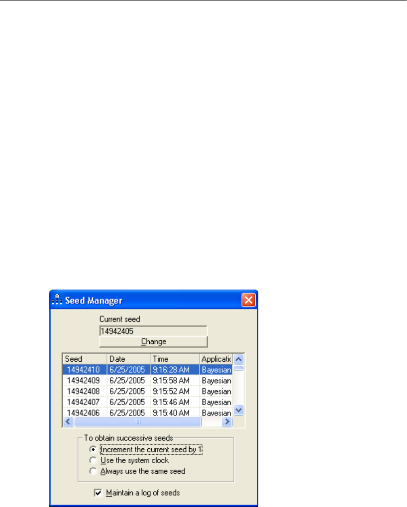
411
Bayesian Estimation
By default, Amos increments the current random number seed by one for each
invocation of a simulation method that makes use of random numbers (either Bayesian
SEM, stochastic regression data imputation, or Bayesian data imputation). Amos
maintains a log of previous seeds used, so it is possible to match the file creation dates
of previously generated analysis results or imputed datasets with the dates reported in
the Seed Manager.
Changing the Current Seed
EClick Change and enter a previously used seed before performing an analysis.
Amos will use the same stream of random numbers that it used the last time it started
out with that seed. For example, we used the Seed Manager to discover that Amos used
a seed of 14942405 when the analysis for this example was performed. To generate the
same Bayesian analysis results as we did:
EClick Change and change the current seed to 14942405.
The following figure shows the Seed Manager dialog after making the change:
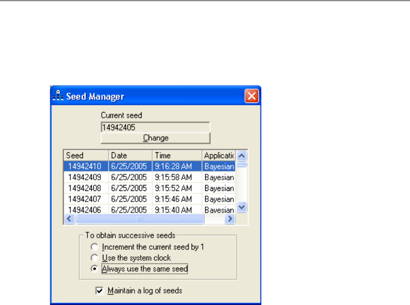
412
Example 26
A more proactive approach is to select a fixed seed value prior to running a Bayesian
or data imputation analysis. You can have Amos use the same seed value for all
analyses if you select the Always use the same seed option.
Record the value of this seed in a safe place so that you can replicate the results of your
analysis at a later date.
Tip: We use the same seed value of 14942405 for all examples in this guide so that you
can reproduce our results.
We mentioned earlier that the MCMC algorithm used by Amos draws random values
of parameters from high-dimensional joint posterior distributions via Monte Carlo
simulation of the posterior distribution of parameters. For instance, the value reported
in the Mean column is not the exact posterior mean but is an estimate obtained by
averaging across the random samples produced by the MCMC procedure. It is
important to have at least a rough idea of how much uncertainty in the posterior mean
is attributable to Monte Carlo sampling.

413
Bayesian Estimation
The second column, labeled S.E., reports an estimated standard error that suggests
how far the Monte-Carlo estimated posterior mean may lie from the true posterior
mean. As the MCMC procedure continues to generate more samples, the estimate of
the posterior mean becomes more precise, and the S.E. gradually drops. Note that this
S.E. is not an estimate of how far the posterior mean may lie from the unknown true
value of the parameter. That is, one would not use ± 2 S.E. values as the width of a
95% interval for the parameter.
The likely distance between the posterior mean and the unknown true parameter is
reported in the third column, labeled S.D., and that number is analogous to the standard
error in maximum likelihood estimation. Additional columns contain the convergence
statistic (C.S.), the median value of each parameter, the lower and upper 50%
boundaries of the distribution of each parameter, and the skewness, kurtosis, minimum
value, and maximum value of each parameter. The lower and upper 50% boundaries
are the endpoints of a 50% Bayesian credible set, which is the Bayesian analogue of a
50% confidence interval. Most of us are accustomed to using a confidence level of
95%, so we will soon show you how to change to 95%.
When you choose Analyze →Bayesian Estimation, the MCMC algorithm begins
sampling immediately, and it continues until you click the Pause Sampling button to
halt the process. In the figure on p. 409, sampling was halted after
completed samples. Amos generated and discarded 500 burn-in samples prior to
drawing the first sample that was retained for the analysis. Amos draws burn-in
samples to allow the MCMC procedure to converge to the true joint posterior
distribution. After Amos draws and discards the burn-in samples, it draws additional
samples to give us a clear picture of what this joint posterior distribution looks like. In
the example shown on p. 409, Amos has drawn 5,831 of these analysis samples, and it
is upon these analysis samples that the results in the summary table are based. Actually,
the displayed results are for 500 burn-in and 5,500 analysis samples. Because the
sampling algorithm Amos uses is very fast, updating the summary table after each
sample would lead to a rapid, incomprehensible blur of changing results in the
Bayesian SEM window. It would also slow the analysis down. To avoid both problems,
Amos refreshes the results after every 1,000 samples.
500 5831 6331=+
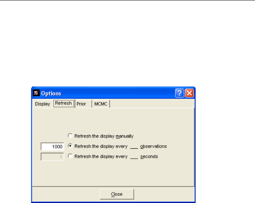
414
Example 26
Changing the Refresh Options
To change the refresh interval:
EFrom the menus, choose View > Options.
EClick the Refresh tab in the Options dialog to show the refresh options.
You can change the refresh interval to something other than the default of 1,000
observations. Alternatively, you can refresh the display at a regular time interval that
you specify.
If you select Refresh the display manually, the display will never be updated
automatically. Regardless of what you select on the Refresh tab, you can refresh the
display manually at any time by clicking the Refresh button on the Bayesian SEM
toolbar.

415
Bayesian Estimation
Assessing Convergence
Are there enough samples to yield stable estimates of the parameters? Before
addressing this question, let us briefly discuss what it means for the procedure to have
converged. Convergence of an MCMC algorithm is quite different from convergence
of a nonrandom method such as maximum likelihood. To properly understand MCMC
convergence, we need to distinguish two different types.
The first type, which we may call convergence in distribution, means that the
analysis samples are, in fact, being drawn from the actual joint posterior distribution of
the parameters. Convergence in distribution takes place in the burn-in period, during
which the algorithm gradually forgets its initial starting values. Because these samples
may not be representative of the actual posterior distribution, they are discarded. The
default burn-in period of 500 is quite conservative, much longer than needed for most
problems. Once the burn-in period is over and Amos begins to collect the analysis
samples, one may ask whether there are enough of these samples to accurately estimate
the summary statistics, such as the posterior mean.
That question pertains to the second type of convergence, which we may call
convergence of posterior summaries. Convergence of posterior summaries is
complicated by the fact that the analysis samples are not independent but are actually
an autocorrelated time series. The 1001th sample is correlated with the 1000th, which,
in turn, is correlated with the 999th, and so on. These correlations are an inherent
feature of MCMC, and because of these correlations, the summary statistics from
5,500 (or whatever number of) analysis samples have more variability than they would
if the 5,500 samples had been independent. Nevertheless, as we continue to accumulate
more and more analysis samples, the posterior summaries gradually stabilize.
Amos provides several diagnostics that help you check convergence. Notice the
value 1.0083 on the toolbar of the Bayesian SEM window on p. 409. This is an overall
convergence statistic based on a measure suggested by Gelman, Carlin, Stern, and
Rubin (2004). Each time the screen refreshes, Amos updates the C.S. for each
parameter in the summary table; the C.S. value on the toolbar is the largest of the
individual C.S. values. By default, Amos judges the procedure to have converged if the
largest of the C.S. values is less than 1.002. By this standard, the maximum C.S. of
1.0083 is not small enough. Amos displays an unhappy face when the overall C.S.
is not small enough. The C.S. compares the variability within parts of the analysis
sample to the variability across these parts. A value of 1.000 represents perfect
convergence, and larger values indicate that the posterior summaries can be made more
precise by creating more analysis samples.
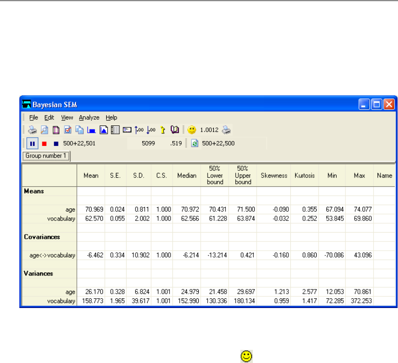
416
Example 26
Clicking the Pause Sampling button a second time instructs Amos to resume the
sampling process. You can also pause and resume sampling by choosing Pause
Sampling from the Analyze menu, or by using the keyboard combination Ctrl+E. The
next figure shows the results after resuming the sampling for a while and pausing again.
At this point, we have 22,501 analysis samples, although the display was most recently
updated at the 22,500th sample. The largest C.S. is 1.0012, which is below the 1.002
criterion that indicates acceptable convergence. Reflecting the satisfactory
convergence, Amos now displays a happy face . Gelman et al. (2004) suggest that,
for many analyses, values of 1.10 or smaller are sufficient. The default criterion of
1.002 is conservative. Judging that the MCMC chain has converged by this criterion
does not mean that the summary table will stop changing. The summary table will
continue to change as long as the MCMC algorithm keeps running. As the overall C.S.
value on the toolbar approaches 1.000, however, there is not much more precision to
be gained by taking additional samples, so we might as well stop.
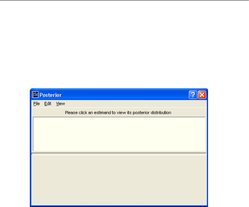
417
Bayesian Estimation
Diagnostic Plots
In addition to the C.S. value, Amos offers several plots that can help you check
convergence of the Bayesian MCMC method. To view these plots:
EFrom the menus, choose View > Posterior.
Amos displays the Posterior dialog.
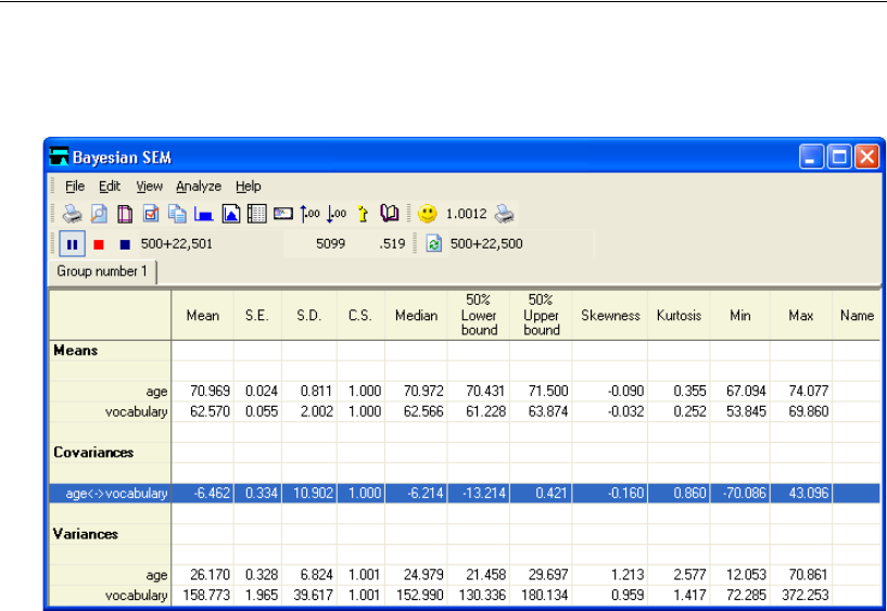
418
Example 26
ESelect the age< - >vocabulary parameter from the Bayesian SEM window.
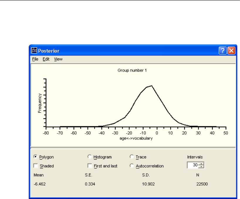
419
Bayesian Estimation
The Posterior dialog now displays a frequency polygon of the distribution of the age-
vocabulary covariance across the 22,500 samples.
One visual aid you can use to judge whether it is likely that Amos has converged to the
posterior distribution is a simultaneous display of two estimates of the distribution, one
obtained from the first third of the accumulated samples and another obtained from the
last third. To display the two estimates of the marginal posterior on the same graph:
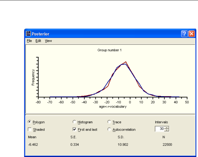
420
Example 26
ESelect First and last. (A check mark will appear next to the option.)
In this example, the distributions of the first and last thirds of the analysis samples are
almost identical, which suggests that Amos has successfully identified the important
features of the posterior distribution of the age-vocabulary covariance. Note that this
posterior distribution appears to be centered at some value near –6, which agrees with
the Mean value for this parameter. Visual inspection suggests that the standard
deviation is roughly 10, which agrees with the value of S.D.
Notice that more than half of the sampled values are to the left of 0. This provides
mild evidence that the true value of the covariance parameter is negative, but this result
is not statistically significant because the proportion to the right of 0 is still quite large.
If the proportion of sampled values to the right of 0 were very small—for example, less
than 5%—then we would be able to reject the null hypothesis that the covariance
parameter is greater than or equal to 0. In this case, however, we cannot.
Another plot that helps in assessing convergence is the trace plot. The trace plot,
sometimes called a time-series plot, shows the sampled values of a parameter over
time. This plot helps you to judge how quickly the MCMC procedure converges in
distribution—that is, how quickly it forgets its starting values.
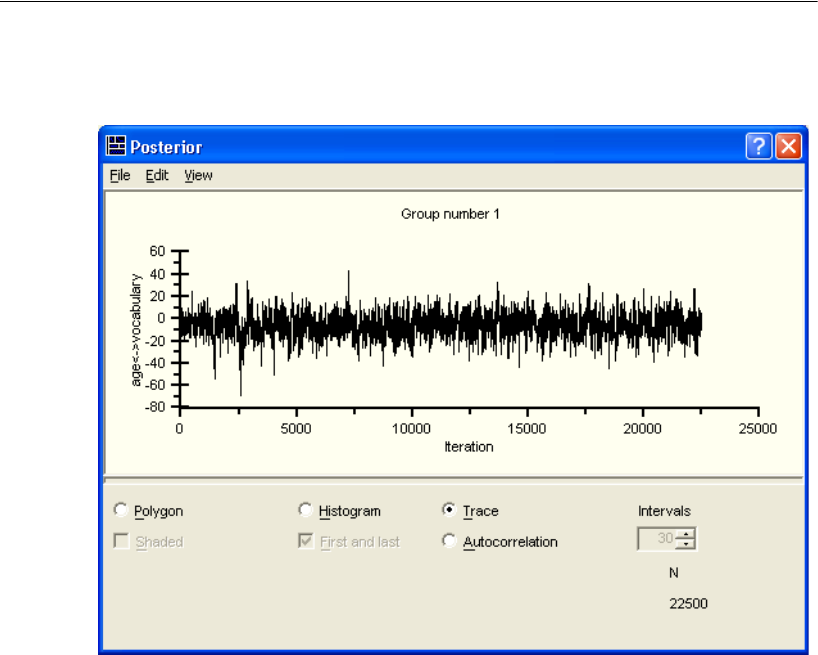
421
Bayesian Estimation
ETo view the trace plot, select Trace.
The plot shown here is quite ideal. It exhibits rapid up-and-down variation with no
long-term trends or drifts. If we were to mentally break up this plot into a few
horizontal sections, the trace within any section would not look much different from
the trace in any other section. This indicates that the convergence in distribution takes
place rapidly. Long-term trends or drifts in the plot indicate slower convergence. (Note
that long-term is relative to the horizontal scale of this plot, which depends on the
number of samples. As we take more samples, the trace plot gets squeezed together like
an accordion, and slow drifts or trends eventually begin to look like rapid up-and-down
variation.) The rapid up-and-down motion means that the sampled value at any
iteration is unrelated to the sampled value k iterations later, for values of k that are small
relative to the total number of samples.
To see how long it takes for the correlations among the samples to die down, we can
examine a third plot, called an autocorrelation plot. This plot displays the estimated
correlation between the sampled value at any iteration and the sampled value k
iterations later for k = 1, 2, 3,….
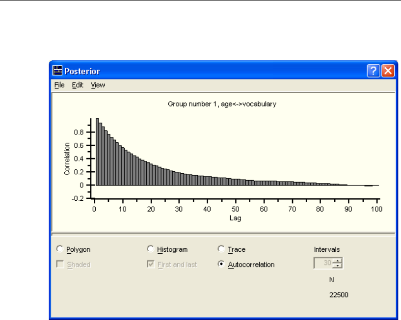
422
Example 26
ETo display this plot, select Autocorrelation.
Lag, along the horizontal axis, refers to the spacing at which the correlation is
estimated. In ordinary situations, we expect the autocorrelation coefficients to die
down and become close to 0, and remain near 0, beyond a certain lag. In the
autocorrelation plot shown above, the lag-10 correlation—the correlation between any
sampled value and the value drawn 10 iterations later—is approximately 0.50. The
lag-35 correlation lies below 0.20, and at lag 90 and beyond, the correlation is
effectively 0. This indicates that by 90 iterations, the MCMC procedure has essentially
forgotten its starting position, at least as far as this covariance parameter is concerned.
Forgetting the starting position is equivalent to convergence in distribution. If we were
to examine the autocorrelation plots for the other parameters in the model, we would
find that they also effectively die down to 0 by 90 or so iterations. This fact gives us
confidence that a burn-in period of 500 samples was more than enough to ensure that
convergence in distribution was attained, and that the analysis samples are indeed
samples from the true posterior distribution.

423
Bayesian Estimation
In certain pathological situations, the MCMC procedure may converge very slowly
or not at all. This may happen in data sets with high proportions of missing values,
when the missing values fall in a peculiar pattern, or in models with some parameters
that are poorly estimated. If this should happen, the trace plots for one or more
parameters in the model will have long-term drifts or trends that do not diminish as
more and more samples are taken. Even as the trace plot gets squeezed together like an
accordion, the drifts and trends will not go away. In that case, you will probably see
that the range of sampled values for the parameter (as indicated by the vertical scale of
the trace plot, or by the S.D. or the difference between Min and Max in the Bayesian
SEM window) is huge. The autocorrelations may remain high for large lags or may
appear to oscillate between positive and negative values for a long time. When this
happens, it suggests that the model is too complicated to be supported by the data at
hand, and we ought to consider either fitting a simpler model or introducing
information about the parameters by specifying a more informative prior distribution.
Bivariate Marginal Posterior Plots
The summary table in the Bayesian SEM window and the frequency polygon in each
Posterior dialog box describe the marginal posterior distributions of the estimands, one
at a time. The marginal posterior distributions are very important, but they do not reveal
relationships that may exist among the estimands. For example, two covariances or
regression coefficients may share significance in the sense that either one could
plausibly be 0, but both cannot. To help us visualize the relationships among pairs of
estimands, Amos provides bivariate marginal posterior plots.
ETo display the marginal posterior of two parameters, begin by displaying the posterior
distribution of one of the parameters (for example, the variance of age).
EHold down the control (Ctrl) key on the keyboard and select the second parameter in
the summary table (for example, the variance of vocabulary).
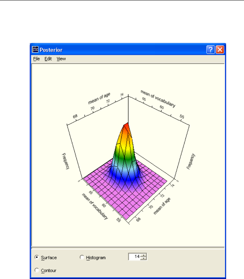
424
Example 26
Amos then displays a three-dimensional surface plot of the marginal posterior
distribution of the variances of age and vocabulary.
ESelect Histogram to display a similar plot using vertical blocks.
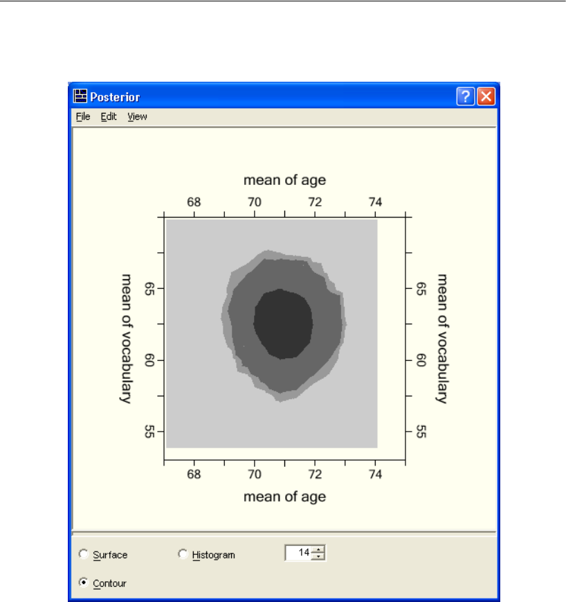
425
Bayesian Estimation
ESelect Contour to display a two-dimensional plot of the bivariate posterior density.
Ranging from dark to light, the three shades of gray represent 50%, 90%, and 95%
credible regions, respectively. A credible region is conceptually similar to a bivariate
confidence region that is familiar to most data analysts acquainted with classical
statistical inference methods.
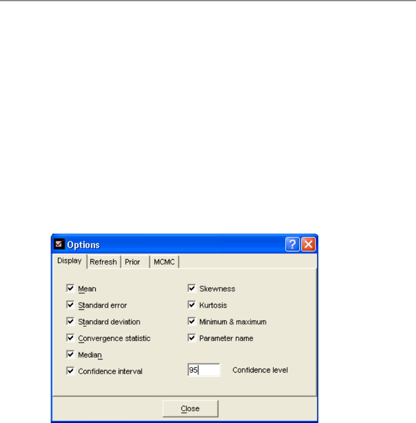
426
Example 26
Credible Intervals
Recall that the summary table in the Bayesian SEM window displays the lower and
upper endpoints of a Bayesian credible interval for each estimand. By default, Amos
presents a 50% interval, which is similar to a conventional 50% confidence interval.
Researchers often report 95% confidence intervals, so you may want to change the
boundaries to correspond to a posterior probability content of 95%.
Changing the Confidence Level
EClick the Display tab in the Options dialog box.
EType 95 as the Confidence level value.
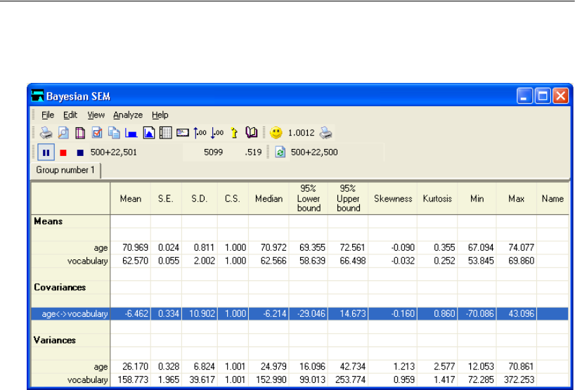
427
Bayesian Estimation
EClick the Close button. Amos now displays 95% credible intervals.
Learning More about Bayesian Estimation
Gill (2004) provides a readable overview of Bayesian estimation and its advantages in
a special issue of Political Analysis. Jackman (2000) offers a more technical treatment
of the topic, with examples, in a journal article format. The book by Gelman, Carlin,
Stern, and Rubin (2004) addresses a multitude of practical issues with numerous
examples.

429
Example
27
Bayesian Estimation Using a
Non-Diffuse Prior Distribution
Introduction
This example demonstrates using a non-diffuse prior distribution.
About the Example
Example 26 showed how to perform Bayesian estimation for a simple model with the
uniform prior distribution that Amos uses by default. In the present example, we
consider a more complex model and make use of a non-diffuse prior distribution. In
particular, the example shows how to specify a prior distribution so that we avoid
negative variance estimates and other improper estimates.
More about Bayesian Estimation
In the discussion of the previous example, we noted that Bayesian estimation depends
on information supplied by the analyst in conjunction with data. Whereas maximum
likelihood estimation maximizes the likelihood of an unknown parameter θ when
given the observed data y through the relationship L(θ|y) ∝ p(y|θ), Bayesian
estimation approximates the posterior density of y, p(θ|y) ∝ p(θ)L(θ|y), where p(θ) is
the prior distribution of θ, and p(θ|y) is the posterior density of θ given y.
Conceptually, this means that the posterior density of y given θ is the product of the
prior distribution of θ and the likelihood of the observed data (Jackman, 2000, p. 377).

430
Example 27
As the sample size increases, the likelihood function becomes more and more
tightly concentrated about the ML estimate. In that case, a diffuse prior tends to be
nearly flat or constant over the region where the likelihood is high; the shape of the
posterior distribution is largely determined by the likelihood, that is by the data
themselves.
Under a uniform prior distribution for θ, p(θ) is completely flat, and the posterior
distribution is simply a re-normalized version of the likelihood. Even under a non-
uniform prior distribution, the influence of the prior distribution diminishes as the
sample size increases. Moreover, as the sample size increases, the joint posterior
distribution for θ comes to resemble a normal distribution. For this reason, Bayesian
and classical maximum likelihood analyses yield equivalent asymptotic results
(Jackman, 2000). In smaller samples, if you can supply sensible prior information to
the Bayesian procedure, the parameter estimates from a Bayesian analysis can be more
precise. (The other side of the coin is that a bad prior can do harm by introducing bias.)
Bayesian Analysis and Improper Solutions
One familiar problem in the fitting of latent variable models is the occurrence of
improper solutions (Chen, Bollen, Paxton, Curran, and Kirby, 2001). An improper
solution occurs, for example, when a variance estimate is negative. Such a solution is
called improper because it is impossible for a variance to be less than 0. An improper
solution may indicate that the sample is too small or that the model is wrong. Bayesian
estimation cannot help with a bad model, but it can be used to avoid improper solutions
that result from the use of small samples. Martin and McDonald (1975), discussing
Bayesian estimation for exploratory factor analysis, suggested that estimates can be
improved and improper solutions can be avoided by choosing a prior distribution that
assigns zero probability to improper solutions. The present example demonstrates
Martin and McDonald’s approach to avoiding improper solutions by a suitable choice
of prior distribution.
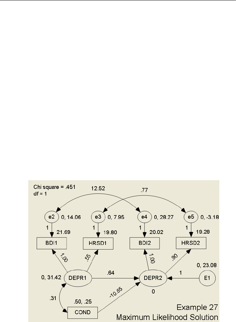
431
Bayesian Estimation Using a Non-Diffuse Prior Distribution
About the Data
Jamison and Scogin (1995) conducted an experimental study of the effectiveness of a
new treatment for depression in which participants were asked to read and complete
the homework exercises in Feeling Good: The New Mood Therapy (Burns, 1999).
Jamison and Scogin randomly assigned participants to a control condition or an
experimental condition, measured their levels of depression, treated the experimental
group, and then re-measured participants’ depression. The researchers did not rely on
a single measure of depression. Instead, they used two well-known depression scales,
the Beck Depression Inventory (Beck, 1967) and the Hamilton Rating Scale for
Depression (Hamilton, 1960). We will call them BDI and HRSD for short. The data
are in the file feelinggood.sav.
Fitting a Model by Maximum Likelihood
The following figure shows the results of using maximum likelihood estimation to fit
a model for the effect of treatment (COND) on depression at Time 2. Depression at
Time 1 is used as a covariate. At Time 1 and then again at Time 2, BDI and HRSD are
modeled as indicators of a single underlying variable, depression (DEPR).
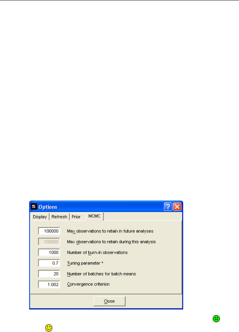
432
Example 27
The path diagram for this model is in Ex27.amw. The chi-square statistic of 0.059 with
one degree of freedom indicates a good fit, but the negative residual variance for post-
therapy HRSD makes the solution improper.
Bayesian Estimation with a Non-Informative (Diffuse) Prior
Does a Bayesian analysis with a diffuse prior distribution yield results similar to those
of the maximum likelihood solution? To find out, we will do a Bayesian analysis of the
same model. First, we will show how to increase the number of burn-in observations.
This is just to show you how to do it. Nothing suggests that the default of 500 burn-in
observations needs to be changed.
Changing the Number of Burn-In Observations
To change the number of burn-in observations to 1,000:
EFrom the menus, choose View > Options.
EIn the Options dialog, select the MCMC tab.
EChange Number of burn-in observations to 1000.
EClick Close and allow MCMC sampling to proceed until the unhappy face turns
happy .
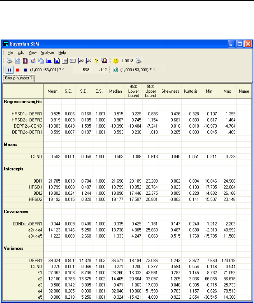
433
Bayesian Estimation Using a Non-Diffuse Prior Distribution
The summary table should look something like this:

434
Example 27
In this analysis, we allowed Amos to reach its default limit of 100,000 MCMC
samples. When Amos reaches this limit, it begins a process known as thinning.
Thinning involves retaining an equally-spaced subset of samples rather than all
samples. Amos begins the MCMC sampling process by retaining all samples until the
limit of 100,000 samples is reached. At that point, if the data analyst has not halted the
sampling process, Amos discards half of the samples by removing every alternate one,
so that the lag-1 dependence in the remaining sequence is the same as the lag-2
dependence of the original unthinned sequence. From that point, Amos continues the
sampling process, keeping one sample out of every two that are generated, until the
upper limit of 100,000 is again reached. At that point, Amos thins the sample a second
time and begins keeping one new sample out of every four...and so on.
Why does Amos perform thinning? Thinning reduces the autocorrelation between
successive samples, so a thinned sequence of 100,000 samples provides more
information than an unthinned sequence of the same length. In the current example, the
displayed results are based on 53,000 samples that were collected after 1,000 burn-in
samples, for a total of 54,000 samples. However, this is after the sequence of samples
has been thinned twice, so that four samples had to be generated for every one that was
kept. If thinning had not been performed, there would have been
burn-in samples and analysis samples.
1000,88000,=×
53 000,8424000,=×
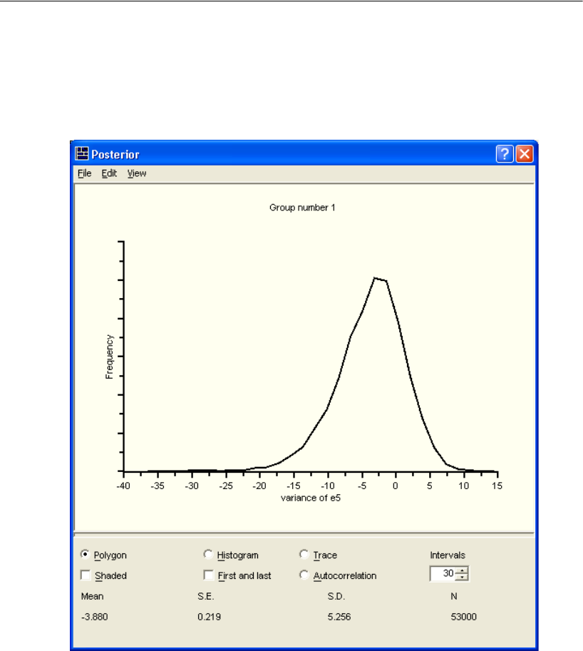
435
Bayesian Estimation Using a Non-Diffuse Prior Distribution
The results of the Bayesian analysis are very similar to the maximum likelihood
results. The posterior Mean for the residual variance of e5 is negative, just as the
maximum likelihood estimate is. The posterior distribution itself lies largely to the left
of 0.
Fortunately, there is a remedy for this problem: Assign a prior density of 0 to any
parameter vector for which the variance of e5 is negative. To change the prior
distribution of the variance of e5:
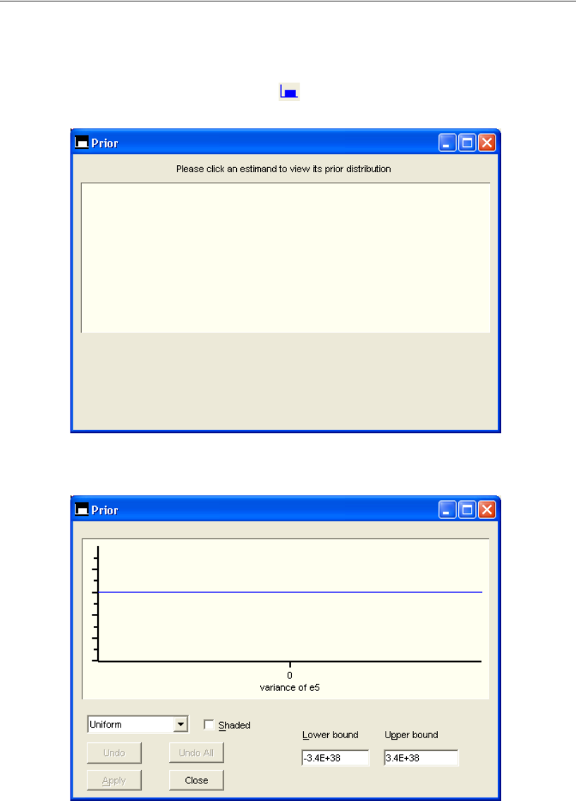
436
Example 27
EFrom the menus, choose View > Prior.
Alternatively, click the Prior button on the Bayesian SEM toolbar, or enter the
keyboard combination Ctrl+R. Amos displays the Prior dialog.
ESelect the variance of e5 in the Bayesian SEM window to display the default prior
distribution for e5.
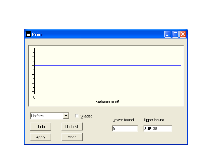
437
Bayesian Estimation Using a Non-Diffuse Prior Distribution
EReplace the default lower bound of with 0.
EClick Apply to save this change.
3.4–10 38–
×
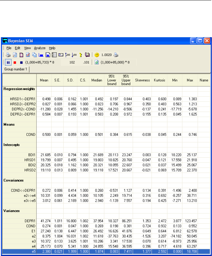
438
Example 27
Amos immediately discards the accumulated MCMC samples and begins sampling all
over again. After a while, the Bayesian SEM window should look something like this:
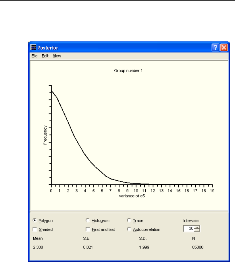
439
Bayesian Estimation Using a Non-Diffuse Prior Distribution
The posterior mean of the variance of e5 is now positive. Examining its posterior
distribution confirms that no sampled values fall below 0.
Is this solution proper? The posterior mean of each variance is positive, but a glance at
the Min column shows that some of the sampled values for the variance of e2 and the
variance of e3 are negative. To avoid negative variances for e2 and e3, we can modify
their prior distributions just as we did for e5.
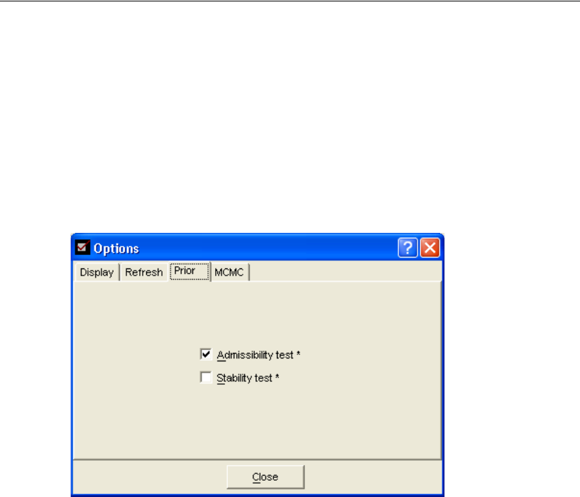
440
Example 27
It is not too difficult to impose such constraints on a parameter-by-parameter basis
in small models like this one. However, there is also a way to automatically set the
prior density to 0 for any parameter values that are improper. To use this feature:
EFrom the menus, choose View > Options.
EIn the Options dialog, click the Prior tab.
ESelect Admissibility test. (A check mark will appear next to it.)
Selecting Admissibility test sets the prior density to 0 for parameter values that result in
a model where any covariance matrix fails to be positive definite. In particular, the prior
density is set to 0 for non-positive variances.
Amos also provides a stability test option that works much like the admissibility test
option. Selecting Stability test sets the prior density to 0 for parameter values that result
in an unstable system of linear equations.
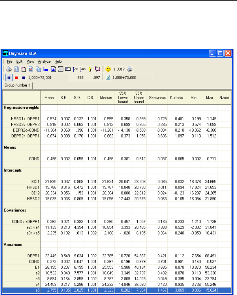
441
Bayesian Estimation Using a Non-Diffuse Prior Distribution
As soon as you select Admissibility test, the MCMC sampling starts all over,
discarding any previously accumulated samples. After a short time, the results should
look something like this:
Notice that the analysis took only 73,000 observations to meet the convergence
criterion for all estimands. Minimum values for all estimated variances are now
positive.

443
Example
28
Bayesian Estimation of Values Other
Than Model Parameters
Introduction
This example shows how to estimate other quantities besides model parameters in a
Bayesian analyses.
About the Example
Examples 26 and 27 demonstrated Bayesian analysis. In both of those examples, we
were concerned exclusively with estimating model parameters. We may also be
interested in estimating other quantities that are functions of the model parameters.
For instance, one of the most common uses of structural equation modeling is the
simultaneous estimation of direct and indirect effects. In this example, we
demonstrate how to estimate the posterior distribution of an indirect effect.
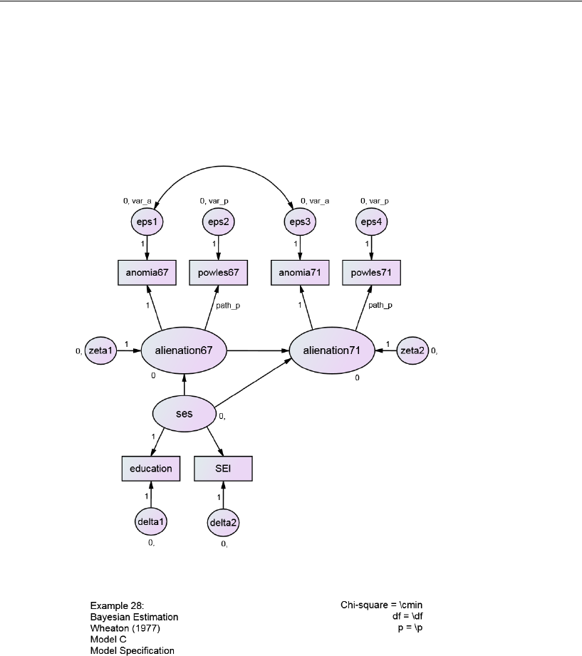
444
Example 28
The Wheaton Data Revisited
In Example 6, we profiled the Wheaton et al. (1977) alienation data and described three
alternative models for the data. Here, we re-examine Model C from Example 6. The
following path diagram is in the file Ex28.amw:
Indirect Effects
Suppose we are interested in the indirect effect of ses on alienation71 through the
mediation of alienation67. In other words, we suspect that socioeconomic status exerts
an impact on alienation in 1967, which in turn influences alienation in 1971.
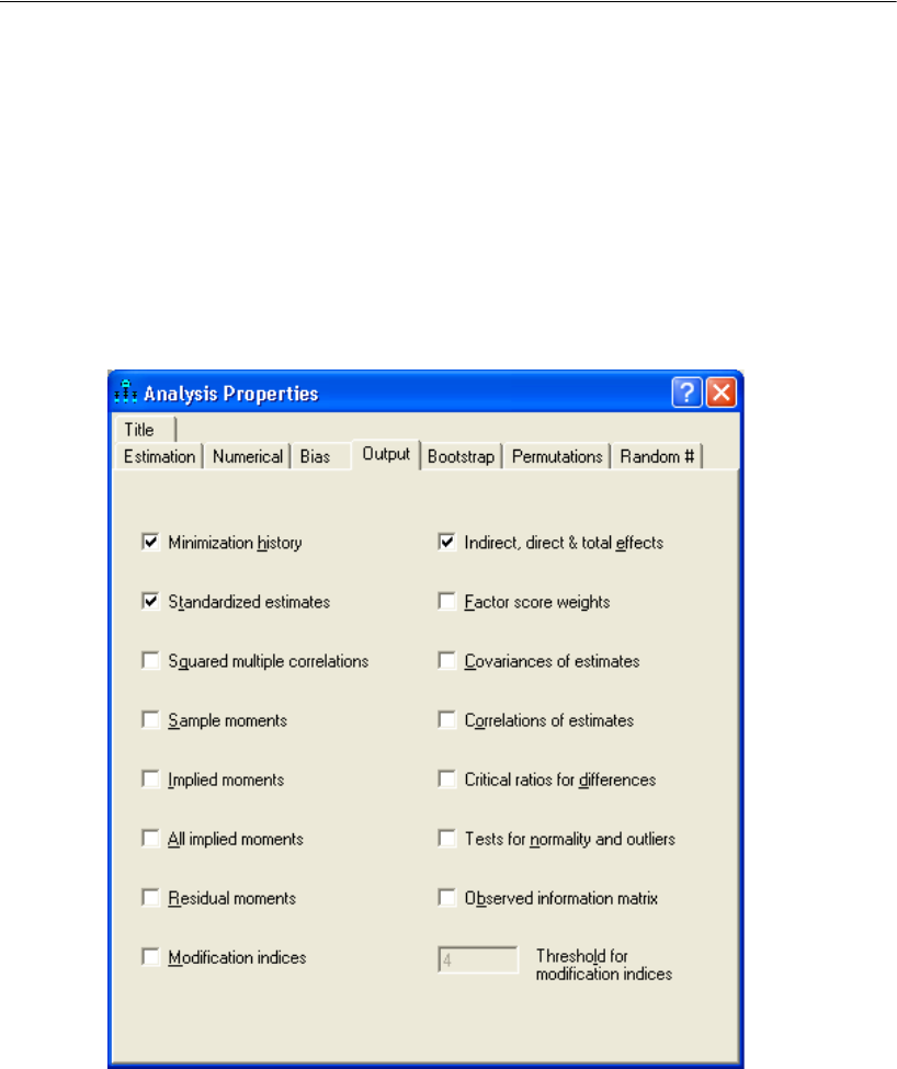
445
Bayesian Estimation of Values Other Than Model Parameters
Estimating Indirect Effects
EBefore starting the Bayesian analysis, from the menus in Amos Graphics, choose View
> Analysis Properties.
EIn the Analysis Properties dialog, click the Output tab.
ESelect Indirect, direct & total effects and Standardized estimates to estimate standardized
indirect effects. (A check mark will appear next to these options.)
EClose the Analysis Properties dialog.
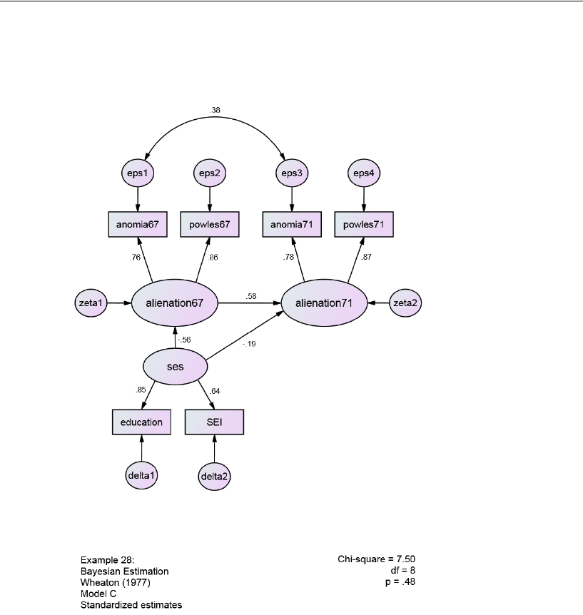
446
Example 28
EFrom the menus, choose Analyze > Calculate Estimates to obtain the maximum
likelihood chi-square test of model fit and the parameter estimates.
The results are identical to those shown in Example 6, Model C. The standardized
direct effect of ses on alienation71 is –0.19. The standardized indirect effect of ses on
alienation71 is defined as the product of two standardized direct effects: the
standardized direct effect of ses on alienation67 (–0.56) and the standardized direct
effect of alienation67 on alienation71 (0.58). The product of these two standardized
direct effects is .
You do not have to work the standardized indirect effect out by hand. To view all
the standardized indirect effects:
0.56–0.58 0.32–=×
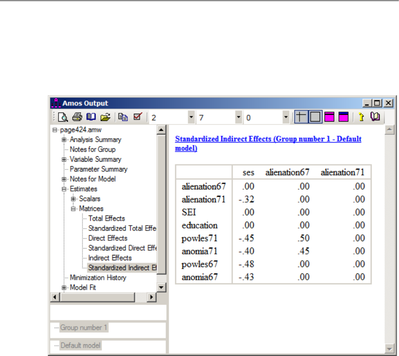
447
Bayesian Estimation of Values Other Than Model Parameters
EFrom the menus, choose View > Text Output.
EIn the upper left corner of the Amos Output window, select Estimates, then Matrices,
and then Standardized Indirect Effects.
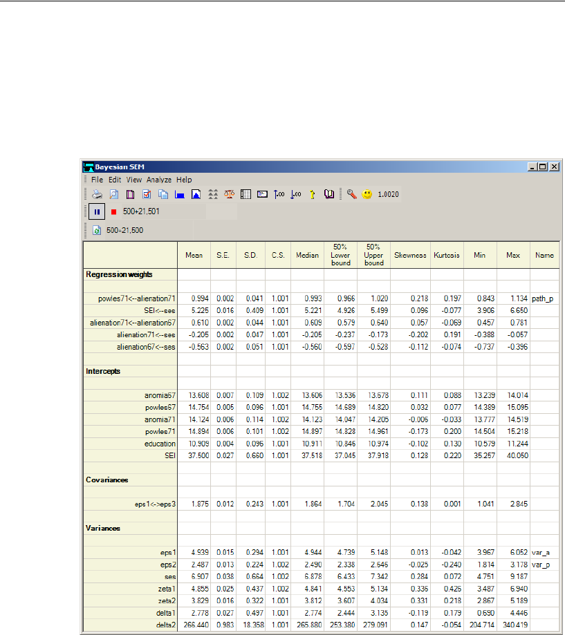
448
Example 28
Bayesian Analysis of Model C
To begin Bayesian estimation for Model C:
EFrom the menus, choose Analyze > Bayesian Estimation.
The MCMC algorithm converges quite rapidly within 22,000 MCMC samples.
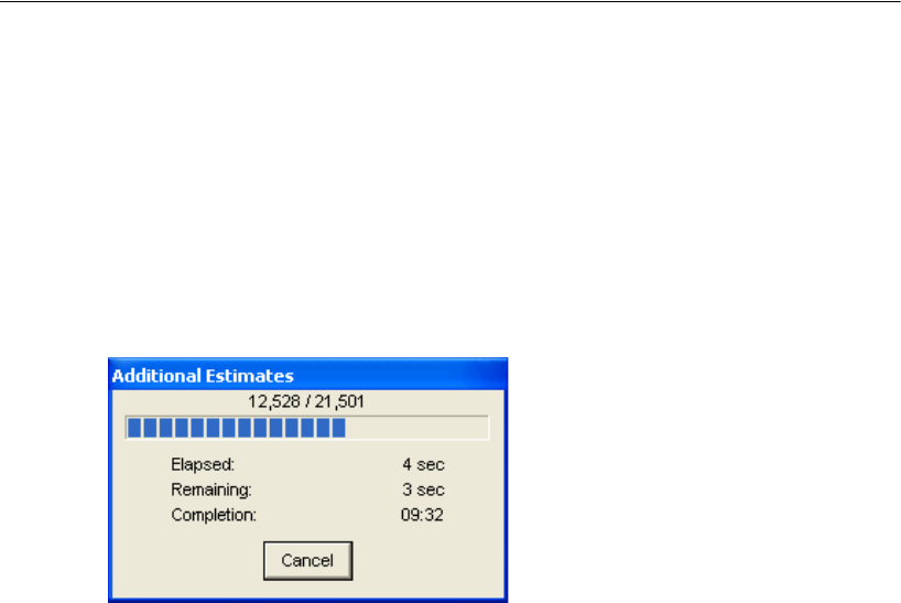
449
Bayesian Estimation of Values Other Than Model Parameters
Additional Estimands
The summary table displays results for model parameters only. To estimate the
posterior of quantities derived from the model parameters, such as indirect effects:
EFrom the menus, choose View > Additional Estimands.
Estimating the marginal posterior distribution of the additional estimands may take a
while. A status window keeps you informed of progress.
Results are displayed in the Additional Estimands window. To display the posterior
mean for each standardized indirect effect:
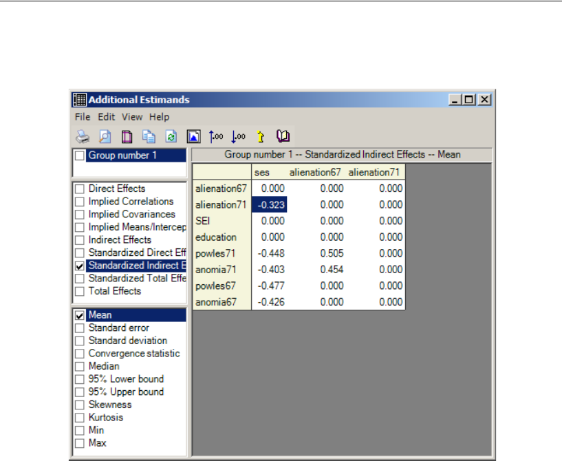
450
Example 28
ESelect Standardized Indirect Effects and Mean in the panel at the left side of the window.
ETo print the results, select the items you want to print. (A check mark will appear next
to them).
EFrom the menus, choose File > Print.
Be careful because it is possible to generate a lot of printed output. If you put a check
mark in every check box in this example, the program will print
matrices.
1811×× 88=

451
Bayesian Estimation of Values Other Than Model Parameters
ETo view the posterior means of the standardized direct effects, select Standardized
Direct Effects and Mean in the panel at the left.
The posterior means of the standardized direct and indirect effects of socioeconomic
status on alienation in 1971 are almost identical to the maximum likelihood estimates.
Inferences about Indirect Effects
There are two methods for finding a confidence interval for an indirect effect or for
testing an indirect effect for significance. Sobel (1982, 1986) gives a method that
assumes that the indirect effect is normally distributed. A growing body of statistical
simulation literature calls into question this assumption, however, and advocates the
use of the bootstrap to construct better, typically asymmetric, confidence intervals
(MacKinnon, Lockwood, and Williams, 2004; Shrout and Bolger, 2002). These studies
have found that the bias-corrected bootstrap confidence intervals available in Amos
produce reliable inferences for indirect effects.
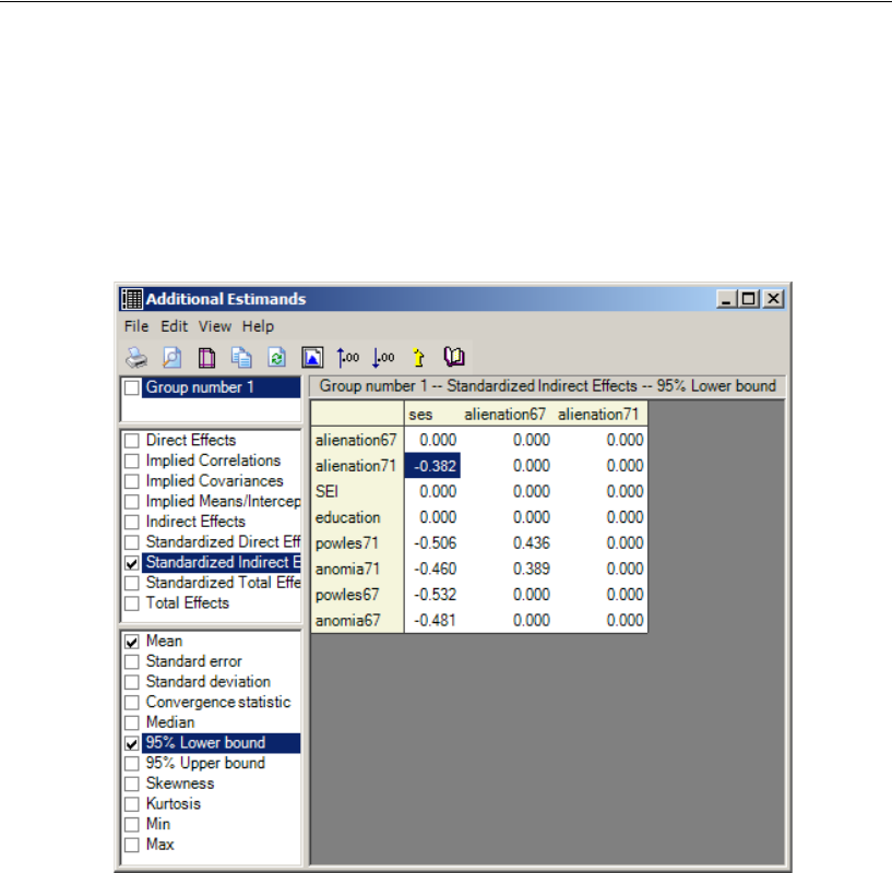
452
Example 28
As an alternative to the Sobel method and the bootstrap for finding confidence
intervals, Amos can provide (typically asymmetric) credible intervals for standardized
or unstandardized indirect effects. The next figure shows the lower boundary of a 95%
credible interval for each standardized indirect effect in the model. Notice that 95%
Lower bound is selected in the panel at the left of the Additional Estimands window.
(You can specify a value other than 95% in the Bayesian Sem Options dialog.)
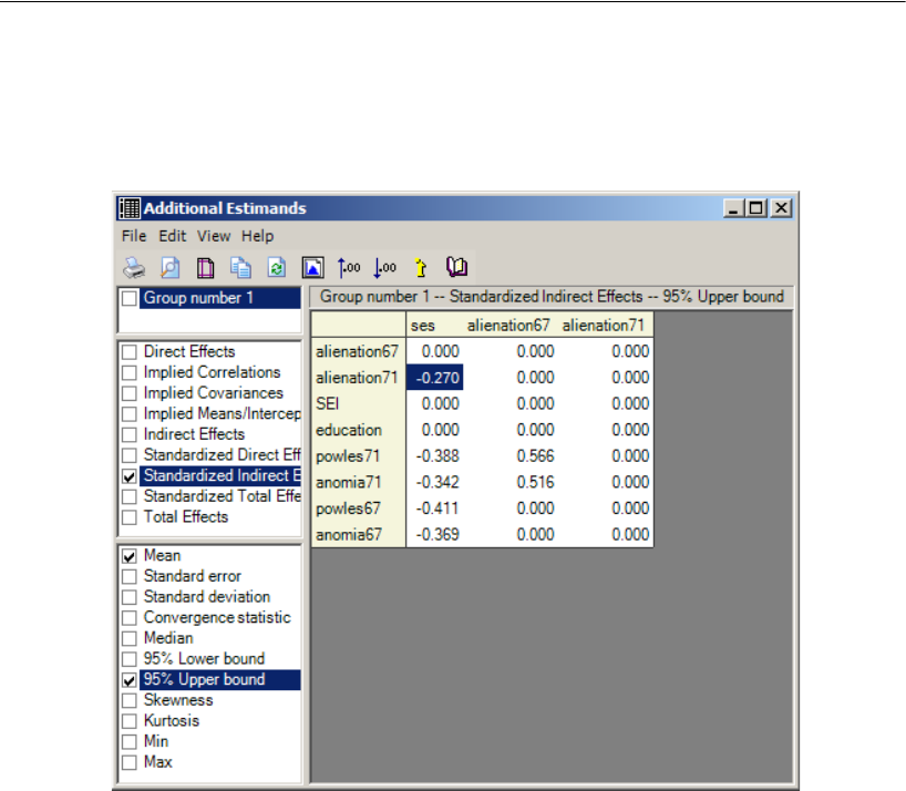
453
Bayesian Estimation of Values Other Than Model Parameters
The lower boundary of the 95% credible interval for the indirect effect of
socioeconomic status on alienation in 1971 is –0.382. The corresponding upper
boundary value is –0.270, as shown below:
We are now 95% certain that the true value of this standardized indirect effect lies
between –0.382 and –0.270. To view the posterior distribution:
EFrom the menus in the Additional Estimands window, choose View > Posterior.
454
Example 28
At first, Amos displays an empty posterior window.
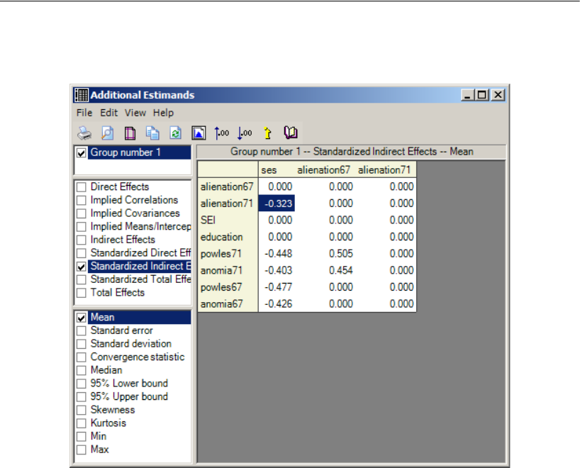
455
Bayesian Estimation of Values Other Than Model Parameters
ESelect Mean and Standardized Indirect Effects in the Additional Estimands window.
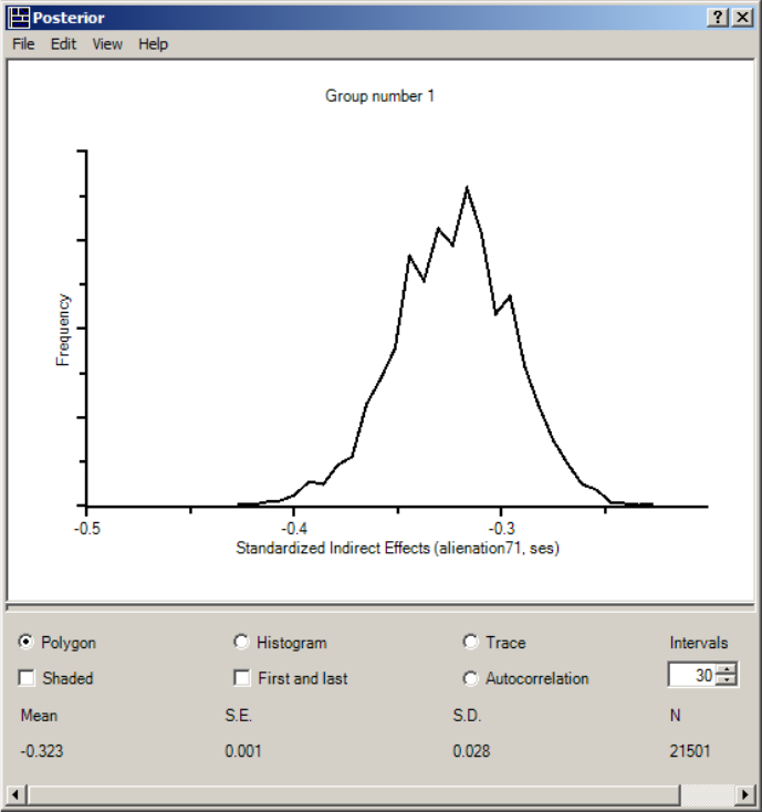
Amos then displays the posterior distribution of the indirect effect of socioeconomic
status on alienation in 1971. The distribution of the indirect effect is approximately, but
not exactly, normal.

457
Example
29
Estimating a User-Defined Quantity
in Bayesian SEM
Introduction
This example shows how to estimate a user-defined quantity: in this case, the
difference between a direct effect and an indirect effect.
About the Example
In the previous example, we showed how to use the Additional Estimands feature of
Amos Bayesian analysis to estimate an indirect effect. Suppose you wanted to carry
the analysis a step further and address a commonly asked research question: How does
an indirect effect compare to the corresponding direct effect?
The Stability of Alienation Model
You can use the Custom Estimands feature of Amos to estimate and draw inferences
about an arbitrary function of the model parameters. To illustrate the Custom
Estimands feature, let us revisit the previous example. The path diagram for the model
is shown on p. 459 and can be found in the file Ex29.amw. The model allows
socioeconomic status to exert a direct effect on alienation experienced in 1971. It also
allows an indirect effect that is mediated by alienation experienced in 1967.
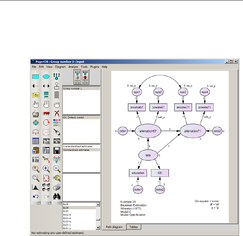
458
Example 29
The remainder of this example focuses on the direct effect, the indirect effect, and
a comparison of the two. Notice that we supplied parameter labels for the direct effect
(“c”) and the two components of the indirect effect (“a” and “b”). Although not
required, parameter labels make it easier to specify custom estimands.
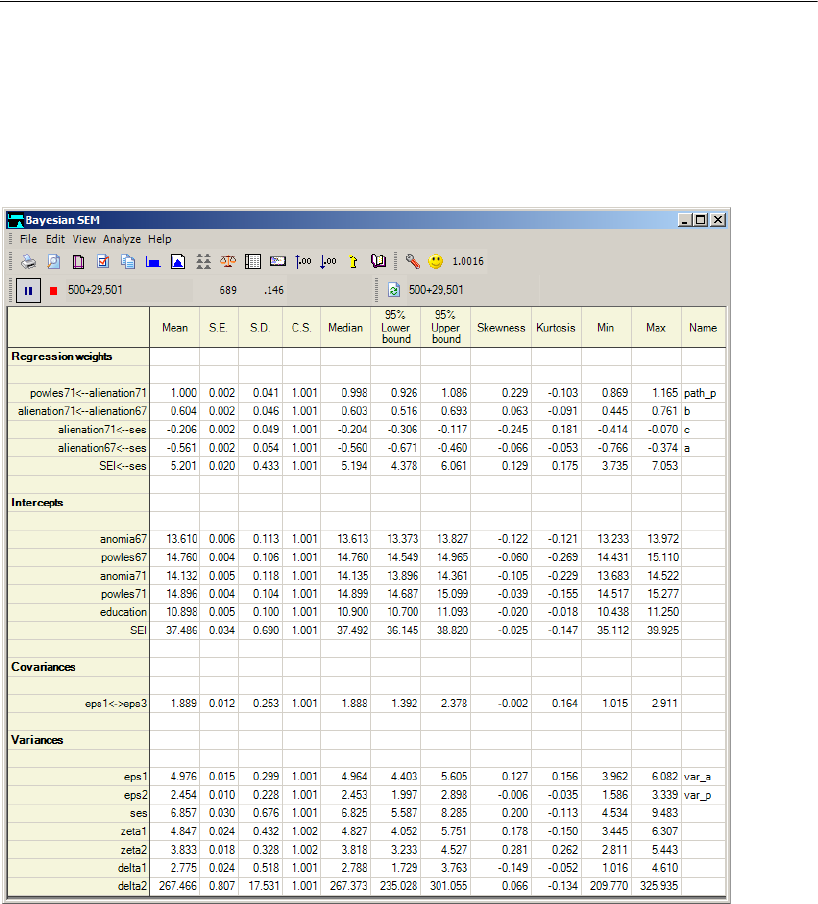
459
Estimating a User-Defined Quantity in Bayesian SEM
To begin a Bayesian analysis of this model:
EFrom the menus, choose Analyze > Bayesian Estimation.
After a while, the Bayesian SEM window should look something like this:
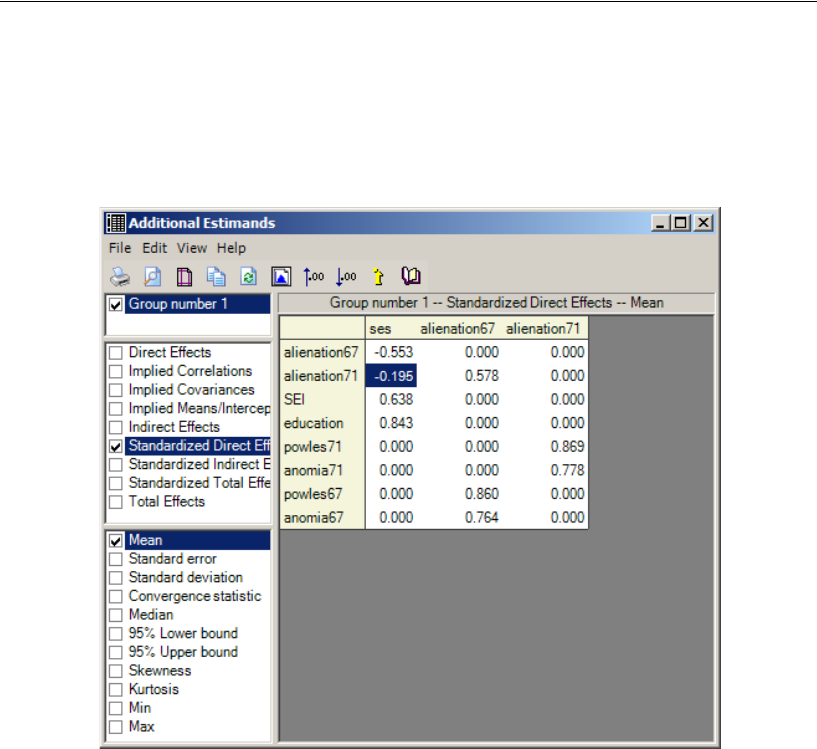
460
Example 29
EFrom the menus, choose View > Additional Estimands.
EIn the Additional Estimands window, select Standardized Direct Effects and Mean.
The posterior mean for the direct effect of ses on alienation71 is –0.195.
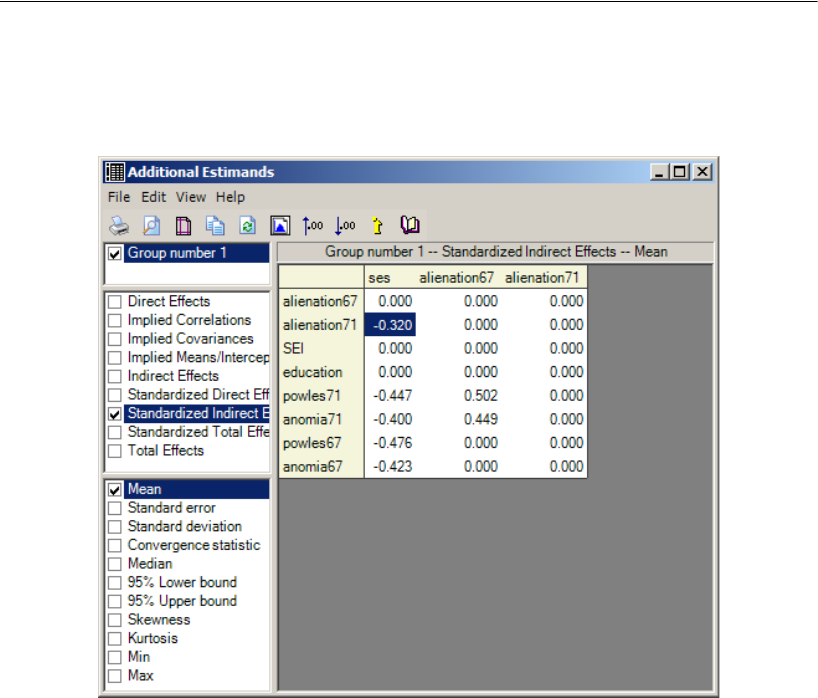
461
Estimating a User-Defined Quantity in Bayesian SEM
ESelect Standardized Indirect Effects and Mean.
The indirect effect of socioeconomic status on alienation in 1971 is –0.320.
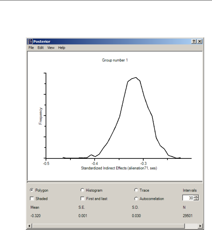
462
Example 29
The posterior distribution of the indirect effect lies entirely to the left of 0, so we are
practically certain that the indirect effect is less than 0.
You can also display the posterior distribution of the direct effect. The program does
not, however, have any built-in way to examine the posterior distribution of the
difference between the indirect effect and the direct effect (or perhaps their ratio). This
is a case of wanting to estimate and draw inferences about a quantity that the
developers of the program did not anticipate. For this, you need to extend the
capabilities of Amos by defining your own custom estimand.
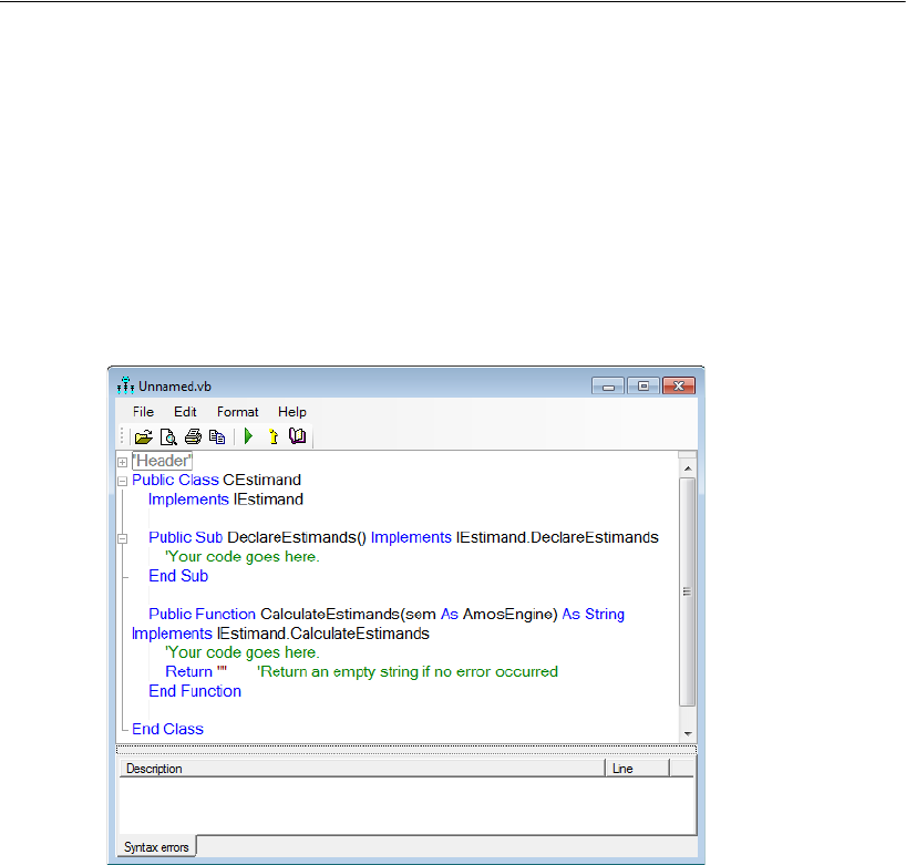
463
Estimating a User-Defined Quantity in Bayesian SEM
Numeric Custom Estimands
In this section, we show how to write a Visual Basic program for estimating the
numeric difference between a direct effect and an indirect effect. (You can use C#
instead of Visual Basic.) The final Visual Basic program is in the file Ex29.vb.
The first step in writing a program to define a custom estimand is to open the custom
estimands window.
EFrom the menus on the Bayesian SEM window, choose View > Custom estimands.
This window displays a skeleton Visual Basic program to which we will add lines to
define the new quantities that we want Amos to estimate.
Note: If you want to use C# instead of Visual Basic, from the menus, choose File > New
Estimands (C#).
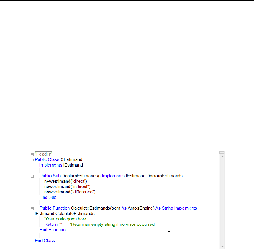
464
Example 29
The skeleton program contains a subroutine and a function. You have no control over
when the subroutine and the function are called. They are called by Amos.
Amos calls your DeclareEstimands subroutine once to find out how many new
quantities (estimands) you want to estimate and what you want to call them.
Amos calls your CalculateEstimands function repeatedly. Each time your
CalculateEstimands function is called, it has to calculate the value of your custom
estimands for a given set of parameter values.
In the subroutine DeclareEstimands, you need to replace the placeholder “Your code
goes here” with lines that specify how many new quantities you want to estimate and
what you want to call them. For this example, we want to estimate the difference
between the direct effect of ses on alienation71 and the corresponding indirect effect.
We will also write code for computing the direct effect and the indirect effect
individually. To define each estimand, we use the keyword newestimand, as shown
below:
The words “direct”, “indirect”, and “difference” are estimand labels. You can use different
labels.

465
Estimating a User-Defined Quantity in Bayesian SEM
In the function CalculateEstimands, the placeholder “Your code goes here” needs to be
replaced with lines for evaluating the estimands called “direct”, “indirect” and
“difference”. We start by writing Visual Basic code for computing the direct effect. In
the following figure, we have already typed part of a Visual Basic statement:
estimand(“direct”) .value =.
We need to finish the statement by adding additional code to the right of the equals (=)
sign, describing how to compute the direct effect. The direct effect is to be calculated
for a set of parameter values that are accessible through the AmosEngine object that is
supplied as an argument to the CalculateEstimands function. Unless you are an expert
Amos programmer, you would not know how to use the AmosEngine object; however,
there is an easy way to get the needed Visual Basic syntax by dragging and dropping.
Dragging and Dropping
EFind the direct effect in the Bayesian SEM window and click to select its row. (Its row
is highlighted in the following figure.)
EMove the mouse pointer to an edge of the selected row. Either the top edge or the
bottom edge will do.
Tip: When you get the mouse pointer on the right spot, a plus (+) symbol will appear
next to the mouse pointer.
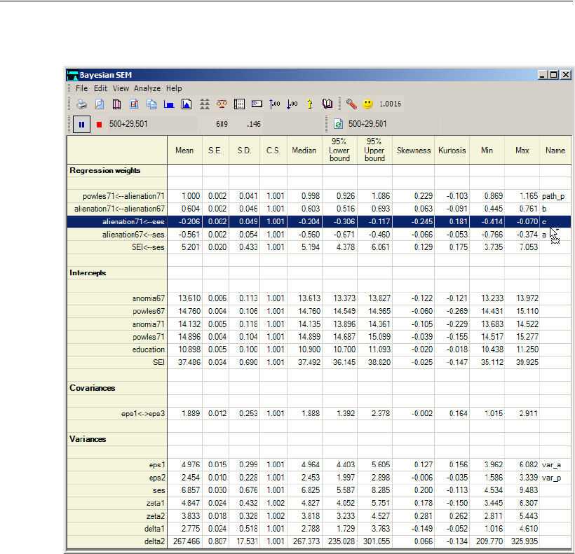
466
Example 29
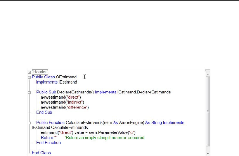
467
Estimating a User-Defined Quantity in Bayesian SEM
EHold down the left mouse button, drag the mouse pointer into the Visual Basic window
to the spot where you want the expression for the direct effect to go, and release the
mouse button.
When you complete this operation, Amos fills in the appropriate parameter expression,
as shown in the next figure:
The parameter on the right side of the equation is identified by the label (“c”) that was
used in the path diagram shown earlier.
We next turn our attention to calculating the indirect effect of socioeconomic status
on alienation in 1971. This indirect effect is defined as the product of its two direct
effects, the direct effect of socioeconomic status on alienation in 1967 (parameter a)
and the direct effect of alienation in 1967 on alienation in 1971 (parameter b).
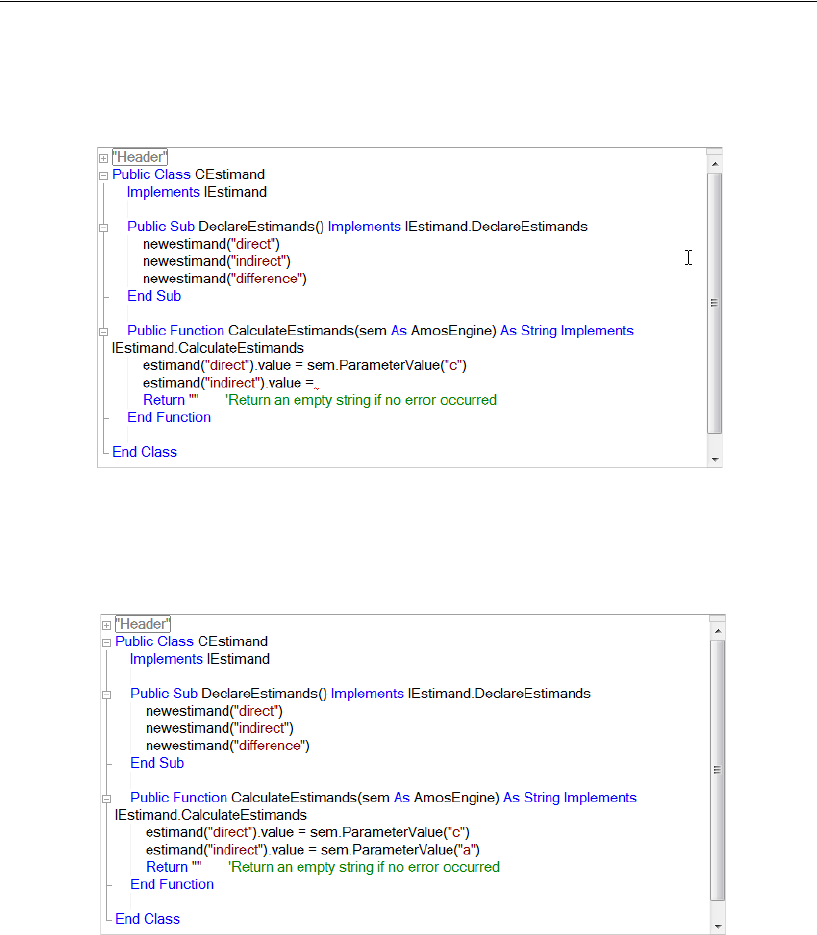
468
Example 29
EOn the left side of the Visual Basic assignment statement for computing the indirect
effect, type estimand(“indirect”) .value =.
Using the same drag-and-drop process as previously described, start dragging things
from the Bayesian SEM window to the Unnamed.vb window.
EFirst, drag the direct effect of socioeconomic status on alienation in 1967 to the right
side of the equals sign in the unfinished statement.
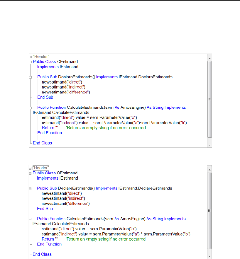
469
Estimating a User-Defined Quantity in Bayesian SEM
ENext, drag and drop the direct effect of 1967 alienation on 1971 alienation.
This second direct effect appears in the Unnamed.vb window as
sem.ParameterValue(“b”).
EFinally, use the keyboard to insert an asterisk (*) between the two parameter values.
Hint: For complicated custom estimands, you can also drag and drop from the
Additional Estimands window to the Custom Estimands window.
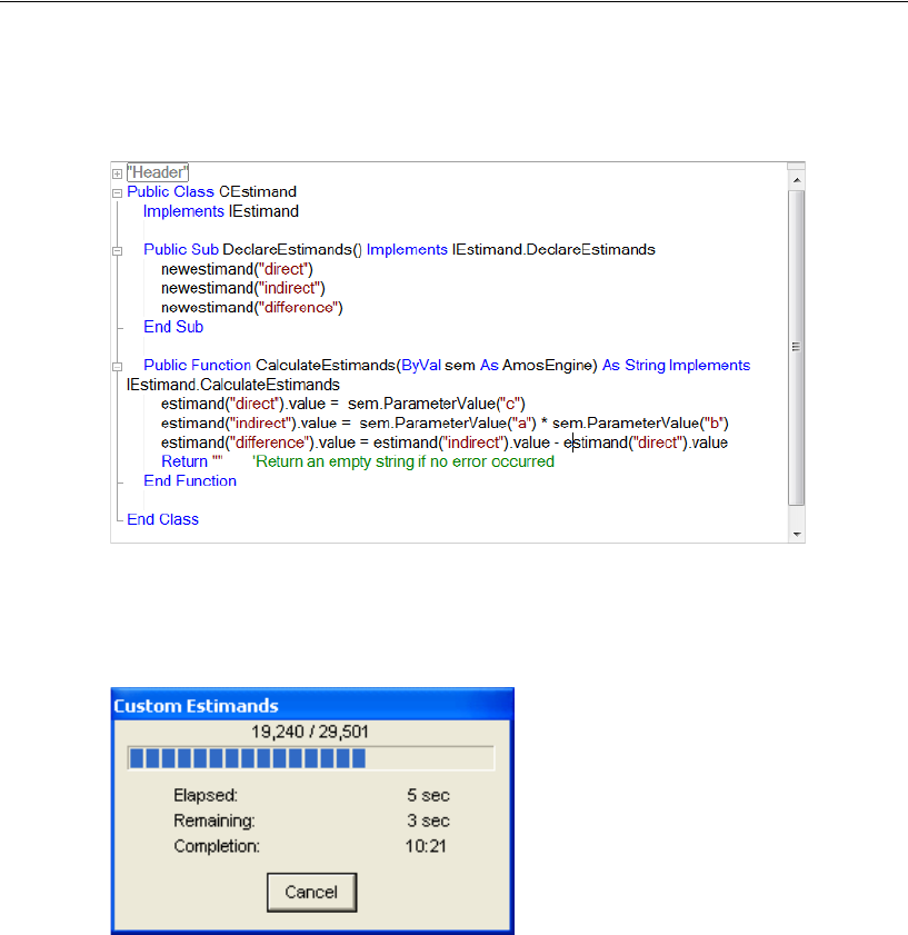
470
Example 29
To compute the difference between the direct and indirect effects, add a third line of
Visual Basic syntax, as seen in the following figure:
ETo find the posterior distribution of all three custom estimands, click File > Run (or
click the Run button on the toolbar).
The results will take a few seconds. A status window keeps you informed of progress.
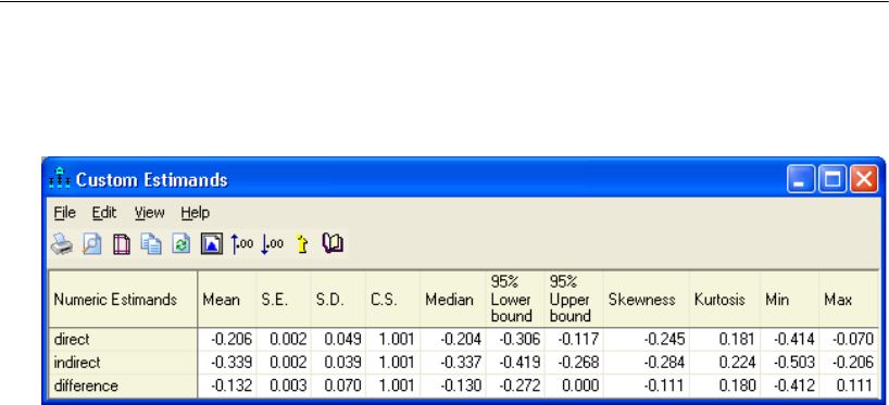
471
Estimating a User-Defined Quantity in Bayesian SEM
The marginal posterior distributions of the three custom estimands are summarized in
the following table:
The results for direct can also be found in the Bayesian SEM summary table, and the
results for indirect can be found in the Additional Estimands table. We are really
interested in difference. Its posterior mean is –0.132. Its minimum is –0.412, and its
maximum is 0.111.
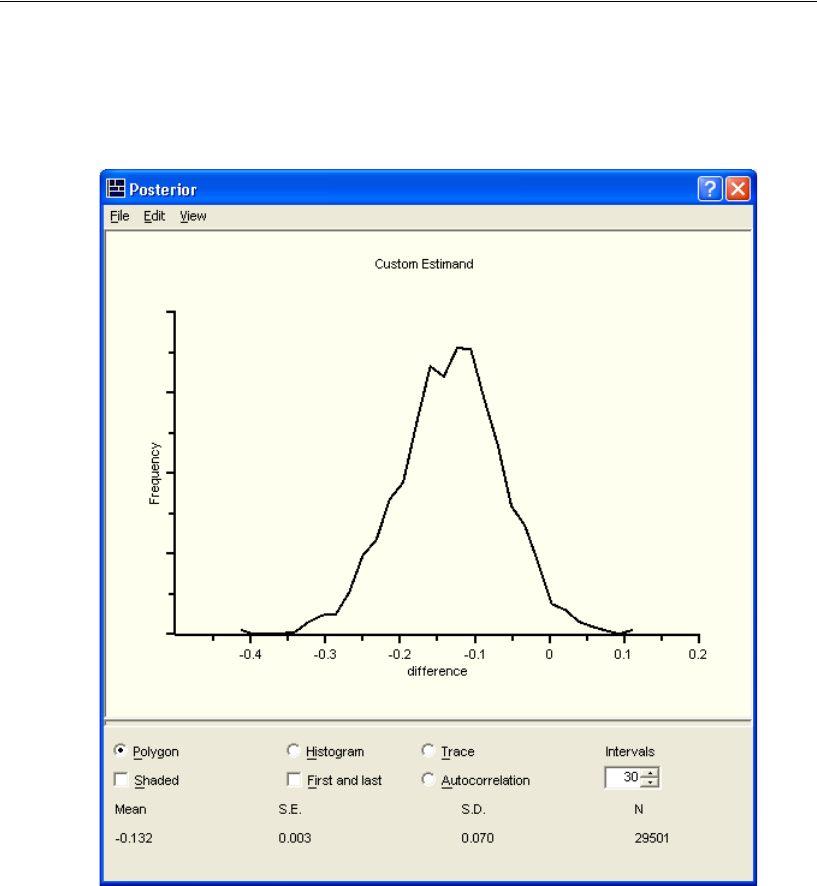
472
Example 29
ETo see its marginal posterior, from the menus, choose View > Posterior.
ESelect the difference row in the Custom Estimands table.
Most of the area lies to the left of 0, meaning that the difference is almost sure to be
negative. In other words, it is almost certain that the indirect effect is more negative
than the direct effect. Eyeballing the posterior, perhaps 95% or so of the area lies to the
left of 0, so there is about a 95% chance that the indirect effect is larger than the direct
effect. It is not necessary to rely on eyeballing the posterior, however. There is a way
to find any area under a marginal posterior or, more generally, to estimate the
probability that any proposition about the parameters is true.
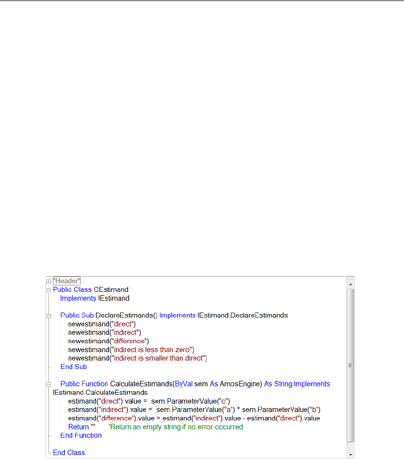
473
Estimating a User-Defined Quantity in Bayesian SEM
Dichotomous Custom Estimands
Visual inspection of the frequency polygon reveals that the majority of difference
values are negative, but it does not tell us exactly what proportion of values are
negative. That proportion is our estimate of the probability that the indirect effect
exceeds the direct effect. To estimate probabilities like these, we can use dichotomous
estimands. In Visual Basic (or C#) programs, dichotomous estimands are just like
numeric estimands except that dichotomous estimands take on only two values: true
and false. In order to estimate the probability that the indirect effect is more negative
than the direct effect, we need to define a function of the model parameters that is true
when the indirect effect is more negative than the direct effect and is false otherwise.
Defining a Dichotomous Estimand
EName each dichotomous estimand in the DeclareEstimands subroutine. For purposes of
illustration, we will declare two dichotomous estimands, calling them “indirect is less
than zero” and “indirect is smaller than direct”.
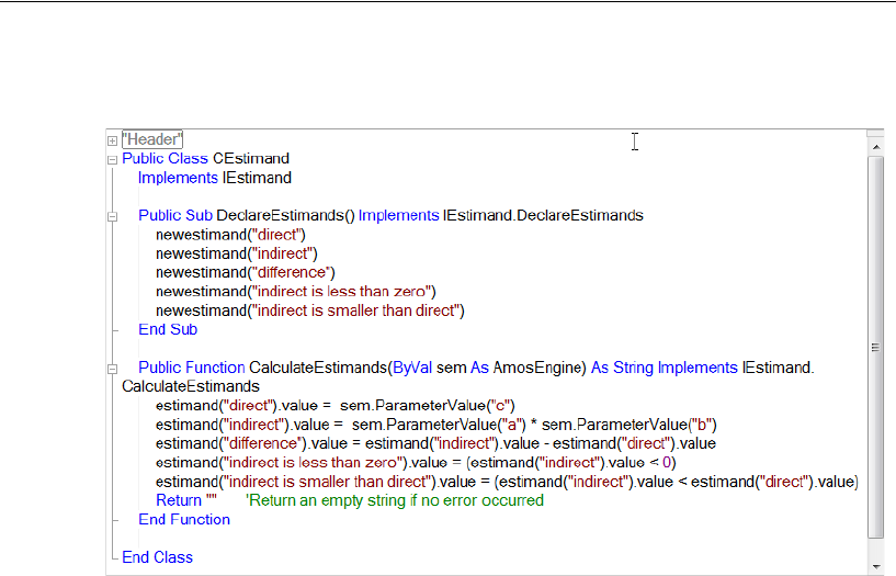
474
Example 29
EAdd lines to the CalculateEstimands function specifying how to compute them.
In this example, the first dichotomous custom estimand is true when the value of the
indirect effect is less than 0. The second dichotomous custom estimand is true when
the indirect effect is smaller than the direct effect.
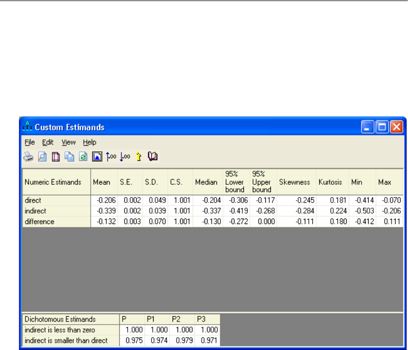
475
Estimating a User-Defined Quantity in Bayesian SEM
EClick File > Run (or click the Run button on the toolbar).
Amos evaluates the truth of each logical expression for each MCMC sample drawn.
When the analysis finishes, Amos reports the proportion of MCMC samples in which
each expression was found to be true. These proportions appear in the Dichotomous
Estimands section of the Custom Estimands summary table.
The P column shows the proportion of times that each evaluated expression was true
in the whole series of MCMC samples. In this example, the number of MCMC samples
was 29,501, so P is based on approximately 30,000 samples. The P1, P2, and P3
columns show the proportion of times each logical expression was true in the first third,
the middle third, and the final third of the MCMC samples. In this illustration, each of
these proportions is based upon approximately 10,000 MCMC samples.

476
Example 29
Based on the proportions in the Dichotomous Estimands area of the Custom
Estimands window, we can say with near certainty that the indirect effect is negative.
This is consistent with the frequency polygon on p. 462 that showed no MCMC
samples with an indirect effect value greater than or equal to 0.
Similarly, the probability is about 0.975 that the indirect effect is larger (more
negative) than the direct effect. The 0.975 is only an estimate of the probability. It is a
proportion based on 29,501 correlated observations. However it appears to be a good
estimate because the proportions from the first third (0.974), middle third (0.979) and
final third (0.971) are so close together.

477
Example
30
Data Imputation
Introduction
This example demonstrates multiple imputation in a factor analysis model.
About the Example
Example 17 showed how to fit a model using maximum likelihood when the data
contain missing values. Amos can also impute values for those that are missing. In
data imputation, each missing value is replaced by some numeric guess. Once each
missing value has been replaced by an imputed value, the resulting completed dataset
can be analyzed by data analysis methods that are designed for complete data. Amos
provides three methods of data imputation.
In regression imputation, the model is first fitted using maximum likelihood.
After that, model parameters are set equal to their maximum likelihood estimates,
and linear regression is used to predict the unobserved values for each case as a
linear combination of the observed values for that same case. Predicted values are
then plugged in for the missing values.
Stochastic regression imputation (Little and Rubin, 2002) imputes values for
each case by drawing, at random, from the conditional distribution of the missing
values given the observed values, with the unknown model parameters set equal
to their maximum likelihood estimates. Because of the random element in
stochastic regression imputation, repeating the imputation process many times
will produce a different completed dataset each time.

478
Example 30
Bayesian imputation is like stochastic regression imputation except that it takes
into account the fact that the parameter values are only estimated and not known.
Multiple Imputation
In multiple imputation (Schafer, 1997), a nondeterministic imputation method (either
stochastic regression imputation or Bayesian imputation) is used to create multiple
completed datasets. While the observed values never change, the imputed values vary
from one completed dataset to the next. Once the completed datasets have been
created, each completed dataset is analyzed alone. For example, if there are m
completed datasets, then there will be m separate sets of results, each containing
estimates of various quantities along with estimated standard errors. Because the m
completed datasets are different from each other, the m sets of results will also differ
from one to the next.
After each of the m completed datasets has been analyzed alone, the data analyst has
m sets of estimates and standard errors that must be combined into a single set of results.
Well-known formulas attributed to Rubin (1987) are available for combining the results
from multiple completed datasets. Those formulas will be used in Example 31.
Model-Based Imputation
In this example, imputation is performed using a factor analysis model. Model-based
imputation has two advantages. First, you can impute values for any latent variables in
the model. Second, if the model is correct and has positive degrees of freedom, the
implied covariance matrix and implied means will be estimated more accurately than
with a saturated model. (Imputation is based on the implied covariance matrix and
means.) However, a saturated model like the model in Example 1 can be used for
imputation when no other model is appropriate.
Performing Multiple Data Imputation Using Amos Graphics
For this example, we will perform Bayesian multiple imputation using the
confirmatory factor analysis model from Example 17. The dataset is the incomplete
Holzinger and Swineford (1939) dataset in the file grant_x.sav. The imputation of
missing values is only the first step in obtaining useful results from multiple
imputation. Eventually, all three of the following steps need to be carried out.
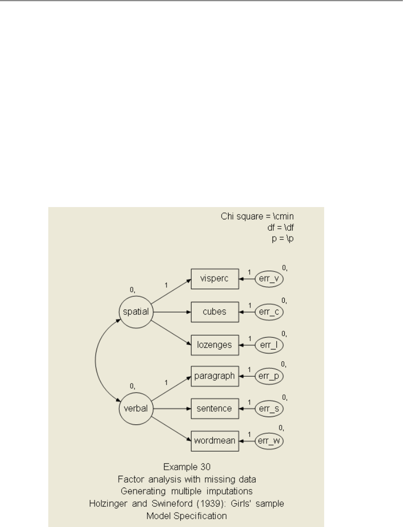
479
Data Imputation
Step 1: Use the Data Imputation feature of Amos to create m complete data files.
Step 2: Perform an analysis of each of the m completed data files separately.
Performing this analysis is up to you. You can perform the analysis in Amos but,
typically, you would use some other program. For purposes of this example and the
next, we will use SPSS Statistics to carry out a regression analysis in which one
variable (sentence) is used to predict another variable (wordmean). Specifically, we
will focus on the estimation of the regression weight and its standard error.
Step 3: Combine the results from the analyses of the m data files.
This example covers the first step. Steps 2 and 3 will be covered in Example 31.
ETo generate the completed data files, open the Amos Graphics file Ex30.amw.
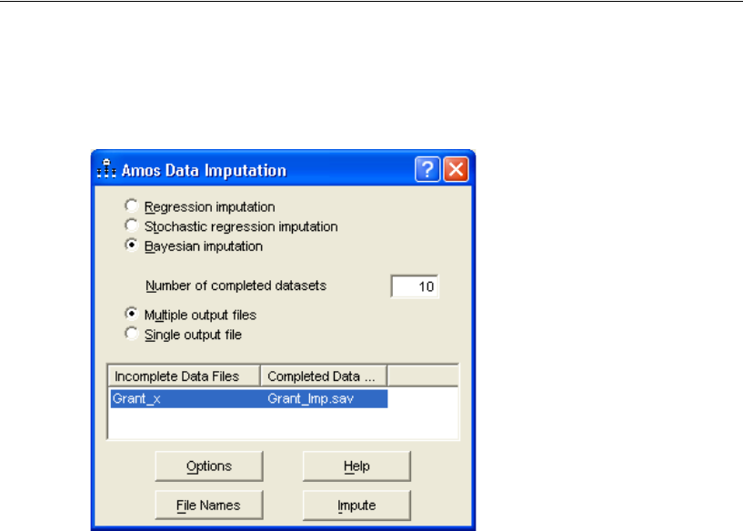
480
Example 30
EFrom the menus, choose Analyze > Data Imputation.
Amos displays the Amos Data Imputation window.
EMake sure that Bayesian imputation is selected.
ESet Number of completed datasets to 10. (This sets m = 10.)
You might suppose that a large number of completed data files are needed. It turns out
that, in most applications, very few completed data files are needed. Five to 10
completed data files are generally sufficient to obtain accurate parameter estimates and
standard errors (Rubin, 1987). There is no penalty for using more than 10 imputations
except for the clerical effort involved in Steps 2 and 3.
Amos can save the completed datasets in a single file (Single output file) with the
completed datasets stacked, or it can save each completed dataset in a separate file
(Multiple output files). In a single-group analysis, selecting Single output file yields one
output data file, whereas selecting Multiple output files yields m separate data files.
In a multiple-group analysis, when you select the Single output file option, you get a
separate output file for each analysis group; if you select the Multiple output files option,
you get m output files per group. For instance, if you had four groups and requested
five completed datasets, then selecting Single output file would give you four output
files, and selecting Multiple output files would give you 20. Since we are going to use
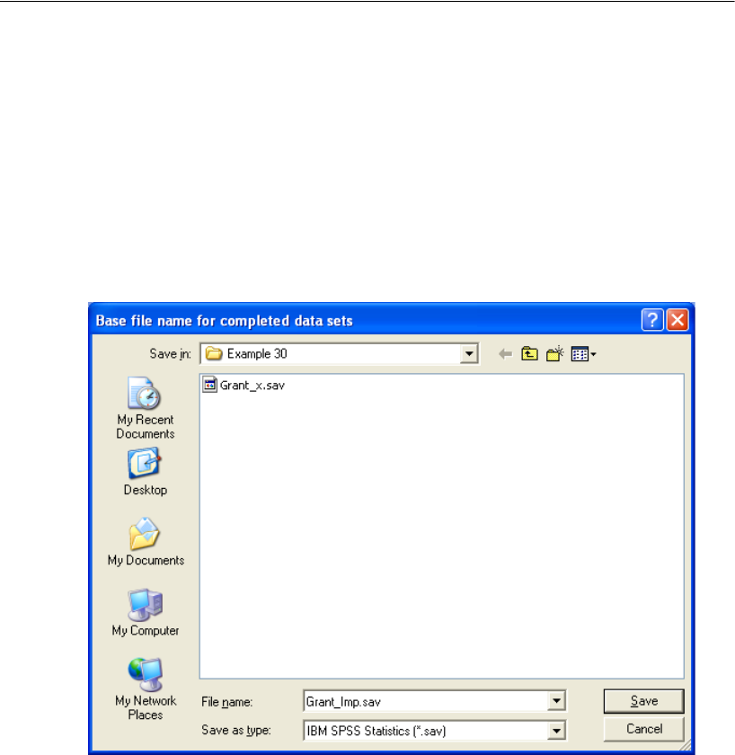
481
Data Imputation
SPSS Statistics to analyze the completed datasets, the simplest thing would be to select
Single output file. Then, the split file capability of SPSS Statistics could be used in Step
2 to analyze each completed dataset separately. However, to make it easy to replicate
this example using any regression program:
ESelect Multiple output files.
You can save imputed data in two file formats: plain text or SPSS Statistics format.
EClick File Names to display a Save As dialog.
EIn the File name text box, you can specify a prefix name for the imputed datasets. Here,
we have specified Grant_Imp.
Amos will name the imputed data files Grant_Imp1, Grant_Imp2, and so on through
Grant_Imp10.
EUse the Save as type drop-down list to select plain text (.txt) or the SPSS Statistics
format (.sav).
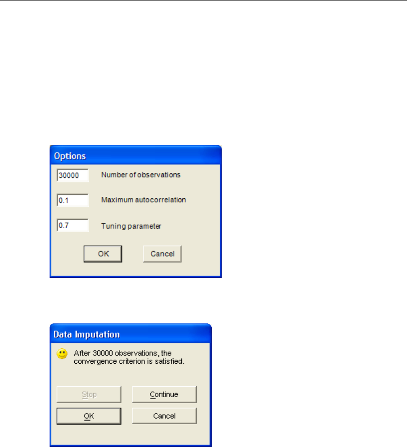
482
Example 30
EClick Save.
EClick Options in the Data Imputation window to display the available imputation
options.
The online help explains these options. To get an explanation of an option, place your
mouse pointer over the option in question and press the F1 key. The figure below shows
how the number of observations can be changed from 10,000 (the default) to 30,000.
EClose the Options dialog and click the Impute button in the Data Imputation window.
After a short time, the following message appears:
EClick OK.
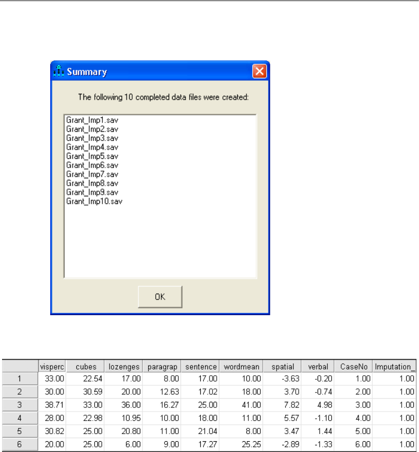
483
Data Imputation
Amos lists the names of the completed data files.
Each completed data file contains 73 complete cases. Here is a view of the first few
records of the first completed data file, Grant_Imp1.sav:
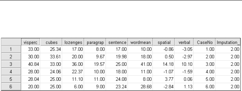
484
Example 30
Here is an identical view of the second completed data file, Grant_Imp2.sav:
The values in the first two cases for visperc were observed in the original data file and
therefore do not change across the imputed data files. By contrast, the values for these
cases for cubes were missing in the original data file, Grant_x.sav, so Amos has
imputed different values across the imputed data files for cubes for these two cases.
In addition to the original observed variables, Amos added four new variables to the
imputed data files. Spatial and verbal are imputed latent variable scores. CaseNo and
Imputation_ are the case number and completed dataset number, respectively.

485
Example
31
Analyzing Multiply Imputed Datasets
Introduction
This example demonstrates the analysis of multiply (pronounced multiplee) imputed
datasets.
Analyzing the Imputed Data Files Using SPSS Statistics
Ten completed datasets were created in Example 30. That was Step 1 in a three-step
process: Use the Data Imputation feature of Amos to impute m complete data files.
(Here, m = 10.) The next two steps are:
Step 2: Perform an analysis of each of the m completed data files separately.
Step 3: Combine the results from the analyses of the m data files.
The analysis in Step 2 can be performed using Amos, SPSS Statistics, or any other
program. Without knowing ahead of time what program will be used to analyze the
completed datasets, it is not possible to automate Steps 2 and 3.
To walk through Steps 2 and 3 for a specific problem, we will analyze the
completed datasets by using SPSS Statistics to carry out a regression analysis in
which one variable (sentence) is used to predict another variable (wordmean). We will
focus specifically on the estimation of the regression weight and its standard error.
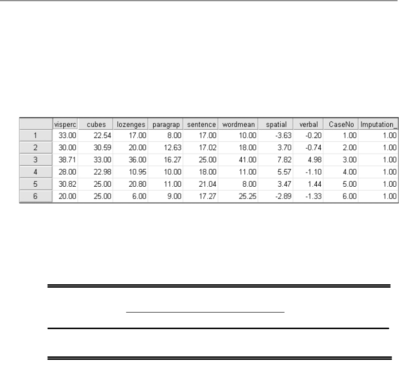
486
Example 31
Step 2: Ten Separate Analyses
For each of the 10 completed datasets from Example 30, we need to perform a
regression analysis in which sentence is used to predict wordmean. We start by opening
the first completed dataset, Grant_Imp1.sav, in SPSS Statistics.
EFrom the SPSS Statistics menus, choose Analyze > Regression > Linear and perform the
regression analysis. (We assume you do not need detailed instructions for this step.)
The results are as follows:
We are going to focus on the regression weight estimate (1.106) and its estimated
standard error (0.160). Repeating the analysis that was just performed for each of the
other nine completed datasets gives nine more estimates for the regression weight and
for its standard error. All 10 estimates and standard errors are shown in the following
table:
Coefficientsa
-2.712 3.110 -.872 .386
1.106 .160 .634 6.908 .000
(Constant)
sentence
Model
1
BStd. Error
Unstandardized Coefficients
Beta
Standardized
Coefficients
tSig.
Dependent Variable: wordmean
a.

487
Analyzing Multiply Imputed Datasets
Step 3: Combining Results of Multiply Imputed Data Files
The standard errors from an analysis of any single completed dataset are not accurate
because they do not take into account the uncertainty arising from imputing missing
data values. The estimates and standard errors must be gathered from the separate
analyses of the completed data files and combined into single summary values, one
summary value for the parameter estimate and another summary value for the standard
error of the parameter estimate. Formulas for doing this (Rubin, 1987) can be found in
many places. The formulas below were taken from Schafer (1997, p. 109). The
remainder of this section applies those formulas to the table of 10 estimates and 10
standard errors shown above. In what follows:
Let m be the number of completed datasets (m = 10 in this case).
Let be the estimate from sample t, so = 1.106, = 1.080, and so on.
Let be the estimated standard error from sample t, so = 0.160, =
0.160, and so on.
Then the multiple-imputation estimate of the regression weight is simply the mean of
the 10 estimates from the 10 completed datasets:
Imputation ML Estimate ML Standard Error
1 1.106 0.160
2 1.080 0.160
3 1.118 0.151
4 1.273 0.155
5 1.102 0.154
6 1.286 0.152
7 1.121 0.139
8 1.283 0.140
9 1.270 0.156
10 1.081 0.157
Q
ˆt()
Q
ˆ1()
Q
ˆ2()
Ut()
U1()
U2()
()
172.1
ˆ
1
1
==
=
m
t
t
Q
m
Q

488
Example 31
To obtain a standard error for the combined parameter estimate, go through the
following steps:
ECompute the average within-imputation variance.
ECompute the between-imputation variance.
ECompute the total variance.
The multiple-group standard error is then
A test of the null hypothesis that the regression weight is 0 in the population can be
based on the statistic
which, if the regression weight is 0, has a t distribution with degrees of freedom given
by
Joseph Schafer’s NORM program performs these calculations. NORM can be
downloaded from http://www.stat.psu.edu/~jls/misoftwa.html#win.
U1
m
----Ut()
t1=
m
0.0233==
B1
m1–
-------------Q
ˆt() Q–()
t1=
m
=20.0085=
TU=11
m
----+
B+0.0233=11
10
------+
0.0085+0.0326=
T0.0326 0.1807==
Q
T
------- 1.172
0.1807
---------------- 6.49==
vm1–()=1U
11
m
----+
B
-----------------------+
2
10 1–()=10.0233
11
10
------+
0.0085
-------------------------------------+
2
109=

489
Analyzing Multiply Imputed Datasets
Further Reading
Amos provides several advanced methods of handling missing data, including FIML
(described in Example 17), multiple imputation, and Bayesian estimation. To learn
more about each method, consult Schafer and Graham (2002) for an overview of the
strengths of FIML and multiple imputation. Allison has a concise, readable monograph
that covers both FIML and multiple imputation, including a number of worked
examples and an excellent discussion of how to handle non-normal and categorical
variables within the context of multiple imputation methods that assume multivariate
normality (Allison, 2002). Schafer (1997) provides an in-depth, technical treatment of
multiple imputation. Schafer and Olsen (1998) provide a readable, step-by-step guide
to performing multiple imputation.
A SEM-specific study comparing the statistical performance of FIML and multiple
imputation in structural equation models is also available (Olinsky, Chen, and Harlow,
2003). Lastly, it is worth noting that the Bayesian estimation approach discussed in
Examples 26 through 29 is similar to FIML in its handling of missing data. Ibrahim
and colleagues recently compared the performance of FIML, Bayesian estimation,
probability weighting, and multiple imputation approaches to address incomplete data
problems and concluded that these four approaches were generally similar in their
satisfactory performance for handling incomplete data problems in which the missing
data arose from a missing-at-random (MAR) process (Ibrahim, Chen, Lipsitz, and
Herring, 2005). While their review considered generalized linear models rather than
SEM, their results and conclusions should be generally applicable to a wide range of
statistical models and data analysis scenarios, including those featuring SEM.

491
Example
32
Censored Data
Introduction
This example demonstrates parameter estimation, estimation of posterior predictive
distributions, and data imputation with censored data.
About the Data
For this example, we use the censored data from 103 patients who were accepted into
the Stanford Heart Transplantation Program during the years 1967 through 1974. The
data were collected by Crowley and Hu (1977) and have been reanalyzed by
Kalbfleisch and Prentice (2002), among others. The dataset is saved in the file
transplant-a.sav.
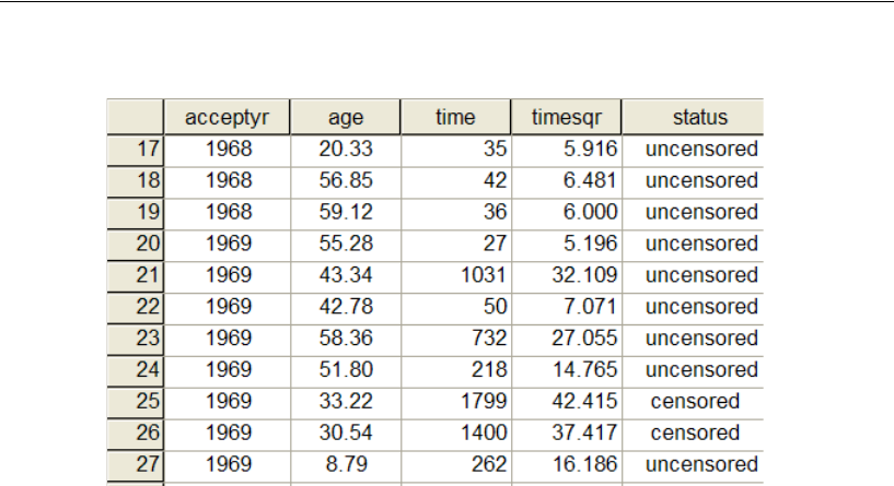
492
Example 32
Reading across the first visible row in the figure above, Patient 17 was accepted into
the program in 1968. The patient at that time was 20.33 years old. The patient died 35
days later. The next number, 5.916, is the square root of 35. Amos assumes that
censored variables are normally distributed. The square root of survival time will be
used in this example in the belief that it is probably more nearly normally distributed
than is survival time itself. Uncensored simply means that we know how long the
patient lived. In other words, the patient has already died, and that is how we are able
to tell that he lived for 35 days after being admitted into the program.
Some patients were still alive when last seen. For example, Patient 25 entered the
program in 1969 at the age of 33.22 years. The patient was last seen 1,799 days later.
The number 42.415 is the square root of 1,799. The word censored in the Status column
means that the patient was still alive 1,799 days after being accepted into the program,
and that is the last time the patient was seen. So, we can’t say that the patient survived
for 1,799 days. In fact, he survived for longer than that; we just don’t know how much
longer. There are more cases like that. Patient number 26 was last seen 1,400 days after
acceptance into the program and, at that time, was still alive, so we know that that
patient lived for at least 1,400 days.
It is not clear what is to be done with a censored value like Patient 25’s survival time
of 1,799 days. You can’t just discard the 1,799 and all the other censored values
because that amounts to discarding the patients who lived a long time. On the other
hand, you can’t keep the 1,799 and treat it as an ordinary score because you know the
patient really lived for more than 1,799 days.
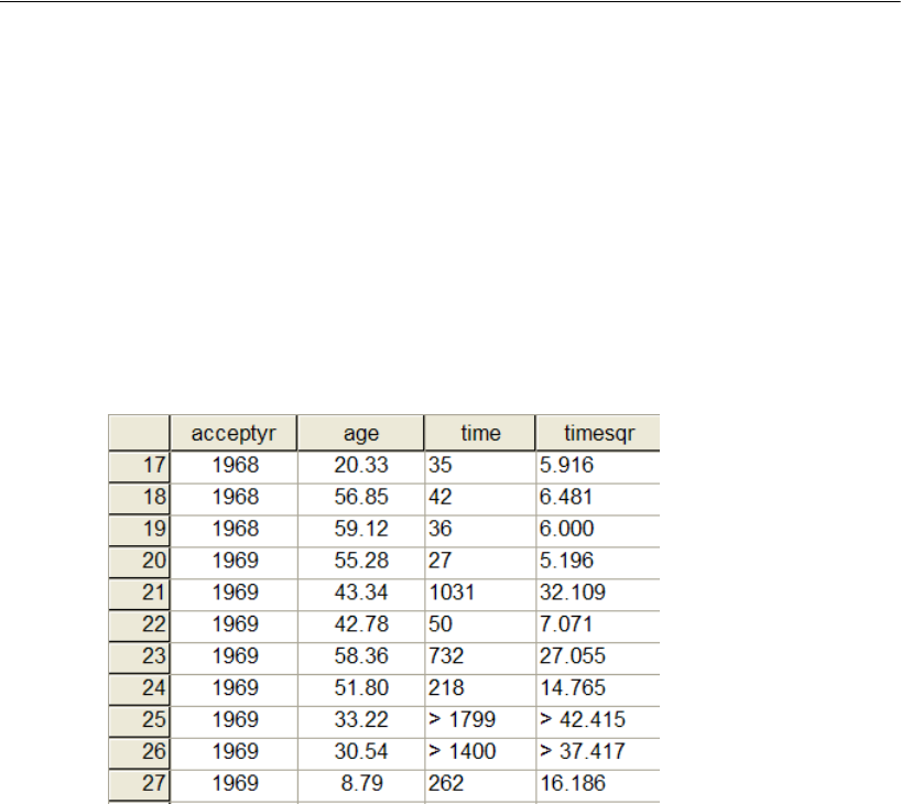
493
Censored Data
In Amos, you can use the information that Patient 25 lived for more than 1,799 days,
neither discarding the information nor pretending that the patient’s survival time is
known more precisely than it is. Of course, wherever the data provide an exact numeric
value, as in the case of Patient 24 who is known to have survived for 218 days, that
exact numeric value is used.
Recoding the Data
The data file needs to be recoded before Amos reads it. The next figure shows a portion
of the dataset after recoding. (This complete dataset is in the file transplant-b.sav.)
Every uncensored observation appears in the new data file just the way it did in the
original data file. Censored values, however, are coded differently. For example,
Patient 25’s survival time, which is known only to be greater than 1,799, is coded as
> 1799 in the new data file. (Spaces in a string like > 1799 are optional.) The square root
of survival time is known to be greater than 42.415, so the timesqr column of the data
file contains > 42.415 for Patient 25. For data file formats (like SPSS Statistics) that
make a distinction between numeric and string variables, time and timesqr need to be
coded as string variables.
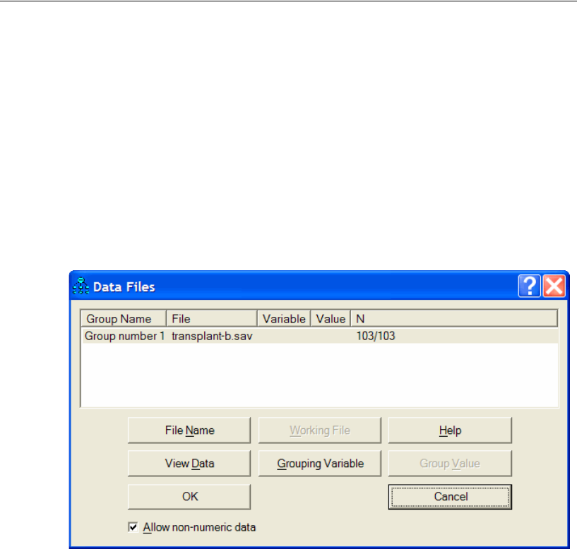
494
Example 32
Analyzing the Data
To specify the data file in Amos Graphics:
EFrom the menus, choose File > Data Files.
EThen in the Data Files dialog, click the File Name button.
ESelect the data file transplant-b.sav.
ESelect Allow non-numeric data (a check mark appears next to it).
Recoding the data as shown above and selecting Allow non-numeric data are the only
extra steps that are required for analyzing censored data. In all other respects, fitting a
model with censored data and interpreting the results is exactly the same as if the data
were purely numeric.
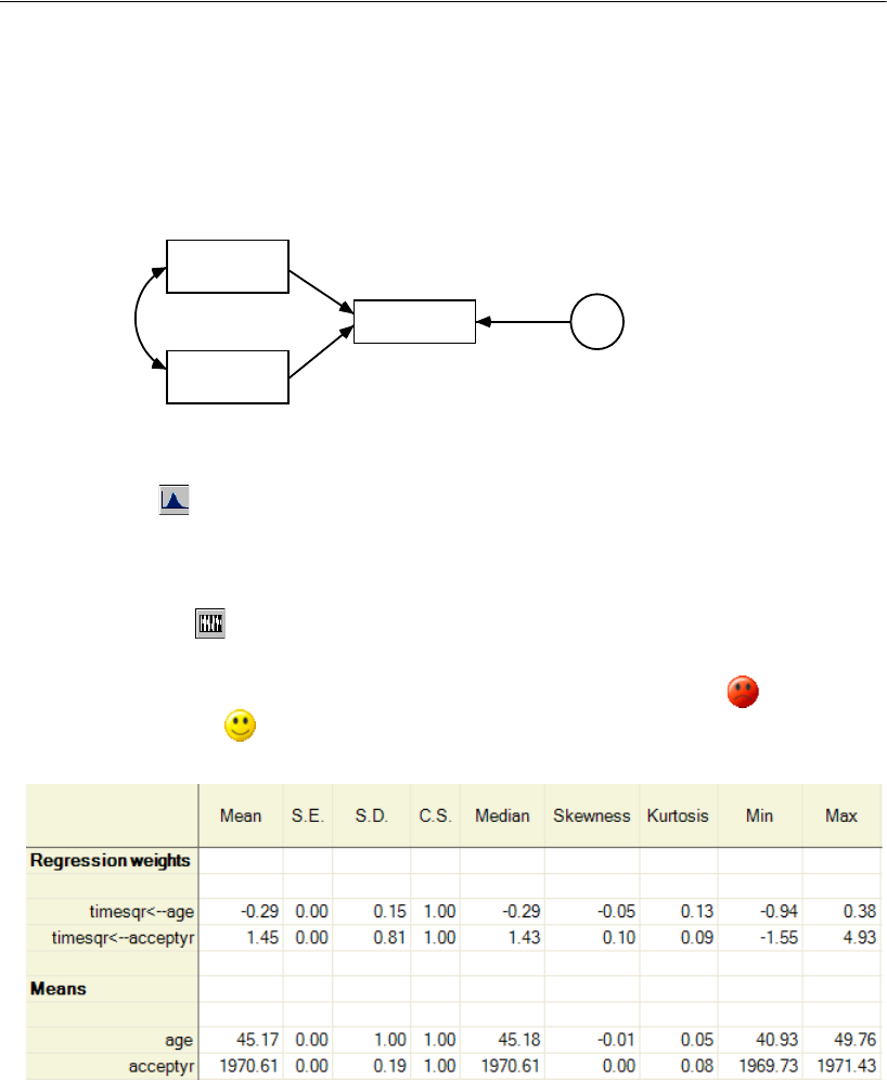
495
Censored Data
Performing a Regression Analysis
Let’s try predicting timesqr using age and year of acceptance (acceptyr) as predictors.
Begin by drawing the following path diagram:
To fit the model:
EClick on the toolbar.
or
EFrom the menus, choose Analyze > Bayesian Estimation.
Note: The button is disabled because, with non-numeric data, you can perform only
Bayesian estimation.
After the Bayesian SEM window opens, wait until the unhappy face changes into
a happy face . The table of estimates in the Bayesian SEM window should look
something like this:
timesqr
age
0,
e
1
acceptyr

496
Example 32
(Only a portion of the table is shown in the figure.) The Mean column contains point
estimates for the parameters. The regression weight for using acceptyr to predict
timesqr is 1.45, so that each time the calendar advances by one year, you predict an
increase of 1.45 in the square root of survival time. This suggests that the transplant
program may have been improving over the period covered by the study. The
regression weight for using age to predict timesqr is –0.29, so for every year older a
patient is when admitted into the transplant program, you expect a decrease of 0.29 in
the square root of survival time. The regression weight estimate of –0.29 is actually the
mean of the posterior distribution of the regression weight.
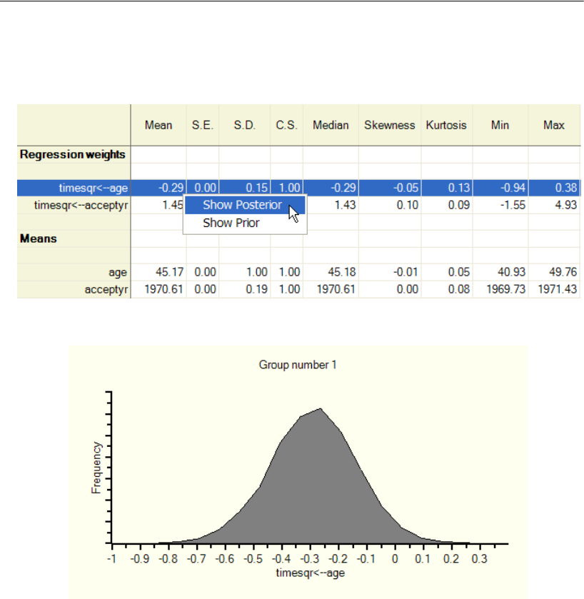
497
Censored Data
ETo see the entire posterior distribution, right-click the row that contains the –0.29
estimate and choose Show Posterior from the pop-up menu.
The Posterior dialog opens, displaying the posterior distribution of the regression
weight.
The posterior distribution of the regression weight is indeed centered around –0.29.
The distribution lies almost entirely between –0.75 and 0.25, so it is practically
guaranteed that the regression weight lies in that range. Most of the distribution lies
between –0.5 and 0, so we are pretty sure that the regression weight lies between –0.5
and 0.
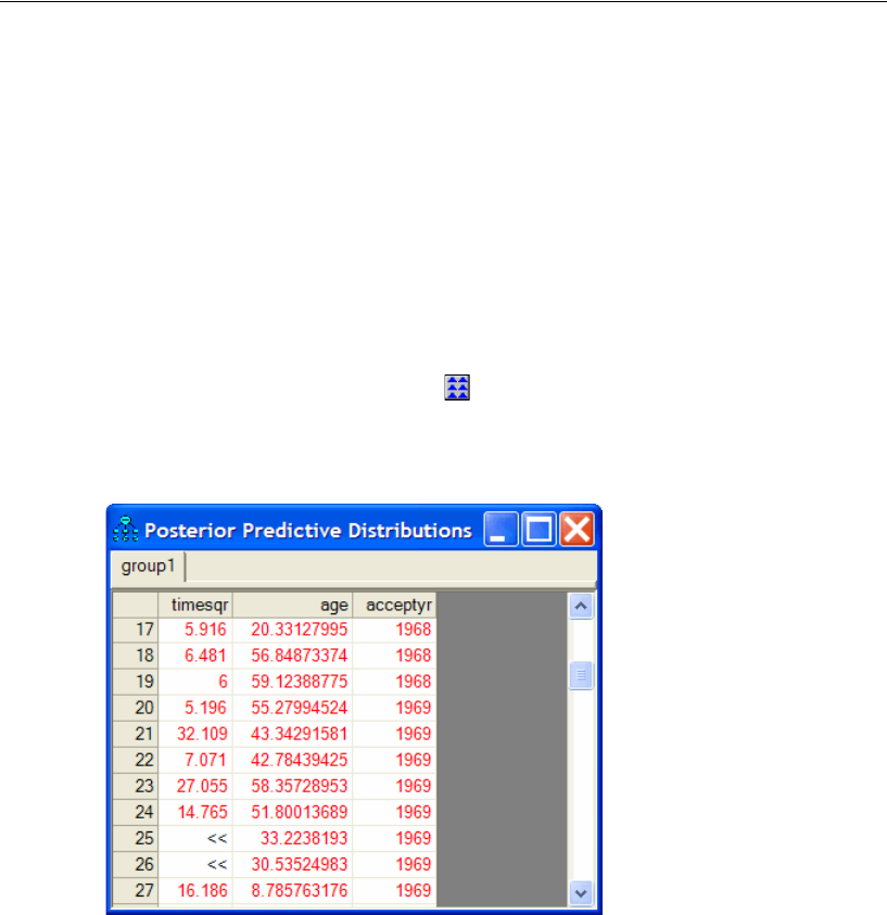
498
Example 32
Posterior Predictive Distributions
Recall that the dataset contains some censored values like Patient 25’s survival time.
All we really know about Patient 25’s survival time is that it is longer than 1,799 days
or, equivalently, that the square root of survival time exceeds 42.415. Even though we
do not know the amount by which this patient’s timesqr exceeds 42.415, we can ask for
its posterior distribution. Taking into account the fact that timesqr exceeds 42.415,
assuming that the model is correct, and taking the patient’s age and acceptyr into
account, what can be said about Patient 25’s survival time? To find out:
EClick the Posterior Predictive button .
or
EFrom the menus, choose View > Posterior Predictive.
The Posterior Predictive Distributions window shows a table with a row for every
person and a column for every observed variable in the model. Looking in the 25th row,
we see Patient 25’s age and acceptyr scores. For Patient 25’s timesqr, all we see is the
symbol <<, which indicates that the data provide an inequality constraint on the timesqr
score and not an actual numeric value.
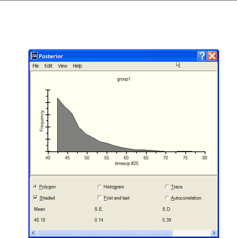
499
Censored Data
To see the posterior distribution of Patient 25’s timesqr:
EClick <<. The posterior distribution appears in the Posterior window.
The posterior distribution for Patient 25’s timesqr lies entirely to the right of 42.415.
Of course, we knew from the data alone that timesqr exceeds 42.415, but now we also
know that there is practically no chance that Patient 25’s timesqr exceeds 70. For that
matter, there is only a slim chance that timesqr exceeds even 55.
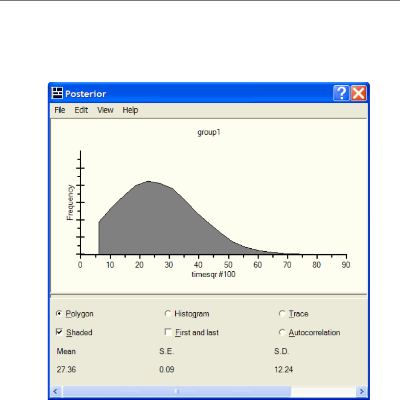
500
Example 32
To see a posterior predictive distribution that looks very different from Patient 25’s:
EClick the << symbol in the 100th row of the Posterior Predictive Distributions table.
Patient 100 was still alive when last observed on the 38th day after acceptance into the
program, so that his timesqr is known to exceed 6.164. The posterior distribution of
that patient’s timesqr shows that it is practically guaranteed to be between 6.164 and
70, and almost certain to be between, 6.164 and 50. The mean is 27.36, providing a
point estimate of timesqr if one is needed. Squaring 27.36 gives 748, an estimate of
Patient 100’s survival time in days.

501
Censored Data
Imputation
You can use this model to impute values for the censored values.
EClose the Bayesian SEM window if it is open.
EFrom the Amos Graphics menu, choose Analyze > Data Imputation.
Notice that Regression imputation and Stochastic regression imputation are disabled.
When you have non-numeric data such as censored data, Bayesian imputation is the only
choice.
We will accept the options shown in the preceding figure, creating 10 completed
datasets and saving all 10 in a single SPSS Statistics data file called transplant-
b_C.sav. To start the imputation:
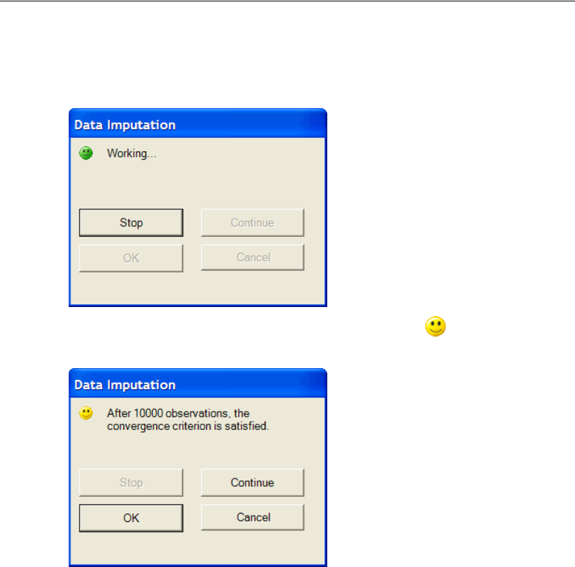
502
Example 32
EClick the Impute button.
The Bayesian SEM window opens along with the Data Imputation dialog.
EWait until the Data Imputation dialog displays a happy face to indicate that each
of the 10 completed datasets is effectively uncorrelated with the others.
Note: After you see a happy face but before you click OK, you may optionally choose to
right-click a parameter in the Bayesian SEM window and choose Show Posterior from
the pop-up menu. This will allow you to examine the Trace and Autocorrelation plots.
EClick OK in the Data Imputation dialog.
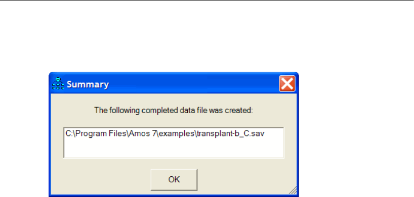
503
Censored Data
The Summary window shows a list of the completed data files that were created. In this
case, only one completed data file was created.
EDouble-click the file name to display the contents of the single completed data file,
which contains 10 completed datasets.
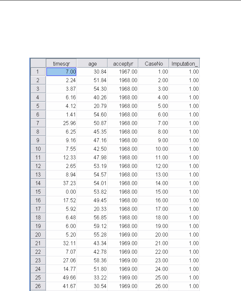
504
Example 32
The file contains 1,030 cases because each of the 10 completed datasets contains 103
cases. The first 103 rows of the new data file contain the first completed dataset. The
Imputation_ variable is equal to 1 for each row in the first completed dataset, and the
CaseNo variable runs from 1 through 103.

505
Censored Data
The first row of the completed data file contains a timesqr value of 7. Because that was
not a censored value, 7 is not an imputed value. It is just an ordinary numeric value that
was present in the original data file. On the other hand, Patient 25’s timesqr was
censored, so that patient has an imputed timesqr (in this case, 49.66.) The value of
49.66 is a value drawn randomly from the posterior predictive distribution in the figure
on p. 499.
Normally, the next step would be to use the 10 completed datasets in transplant-
b_C.sav as input to some other program that cannot accept censored data. You would
use that other program to perform 10 separate analyses, using each one of the 10
completed datasets in turn. Then you would do further computations to combine the
results of those 10 separate analyses into a single set of results, as was done in Example
31. Those steps will not be carried out here.
General Inequality Constraints on Data Values
This example employed only inequality constraints like >1799. Here are some other
examples of string values that can be used in a data file to place inequality constraints
on the value of an underlying numeric variable:
The string value < 5 means that the underlying numeric value is less than 5.
The string value 4<<5 means that the underlying numeric value is between 4 and 5.

507
Example
33
Ordered-Categorical Data
Introduction
This example shows how to fit a factor analysis model to ordered-categorical data. It
also shows how to find the posterior predictive distribution for the numeric variable
that underlies a categorical response and how to impute a numeric value for a
categorical response.
About the Data
This example uses data on attitudes toward environment issues obtained from a
questionnaire administered to 1,017 respondents in the Netherlands. The data come
from the European Values Study Group (see the bibliography for a citation). The data
file environment-nl-string.sav contains responses to six questionnaire items with
categorical responses strongly disagree (SD), disagree (D), agree (A), and strongly
agree (SA).
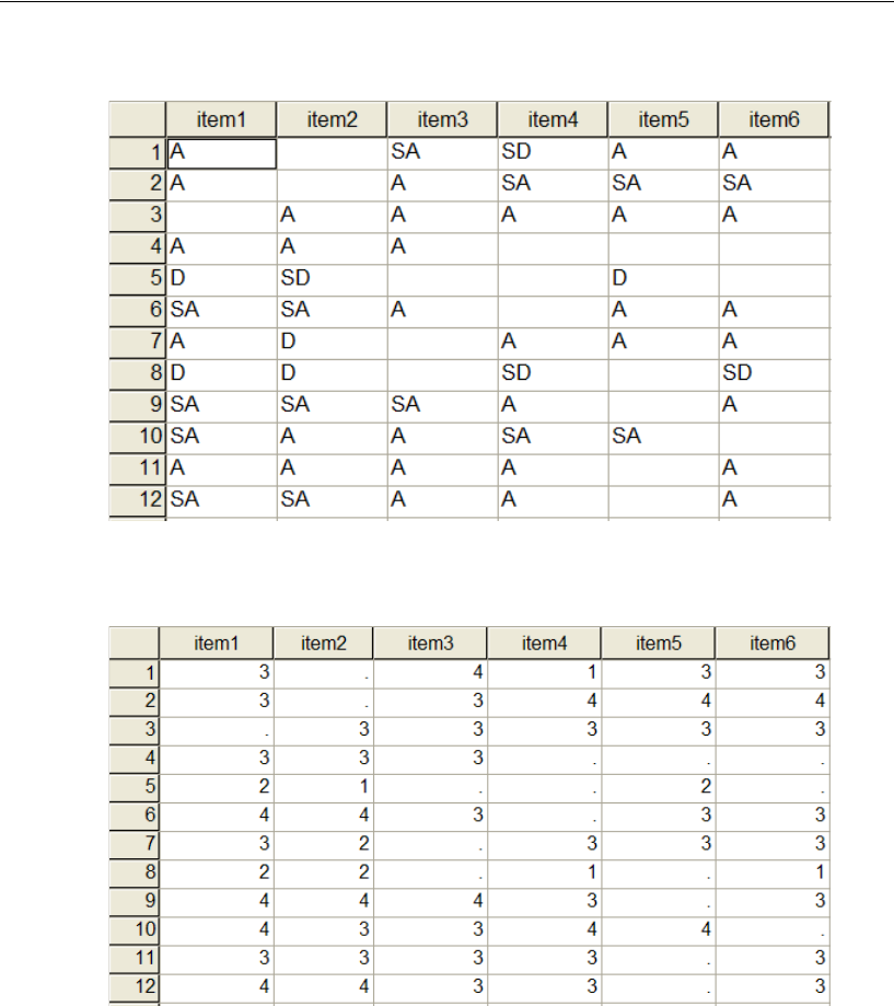
508
Example 33
One way to analyze these data is to assign numbers to the four categorical responses;
for example, using the assignment 1 = SD, 2 = D, 3 = A, 4 = SA. If you assign numbers
to categories in that way, you get the dataset in environment-nl-numeric.sav.
In an Amos analysis, it is not necessary to assign numbers to categories in the way just
shown. It is possible to use only the ordinal properties of the four categorical responses.
If you want to use only the ordinal properties of the data, you can use either dataset,
environment-nl-string.sav or environment-nl-numeric.sav.
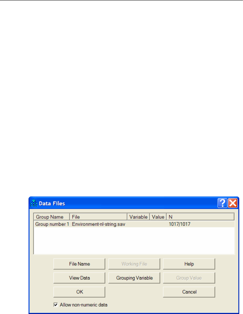
509
Ordered-Categorical Data
It may be slightly easier to use environment-nl-numeric.sav because Amos will
assume by default that the numbered categories go in the order 1, 2, 3, 4, with 1 being
the lowest category. That happens to be the correct order. With environment-nl-
string.sav, by contrast, Amos will assume by default that the categories are arranged
alphabetically in the order A, D, SA, SD, with A being the lowest category. That is the
wrong order, so the default ordering of the categories by Amos has to be overridden.
The data file environment-nl-string.sav will be used for this example because then
it will be clear that only the ordinal properties of the data are employed, and also you
can see how to specify the correct ordering of the categories.
Specifying the Data File
EFrom the Amos Graphics menus, choose File > Data Files.
EIn the Data Files window, click the File Name button.
ESelect the data file environment-nl-string.sav.
ESelect Allow non-numeric data (a check mark appears next to it).
EClick OK.
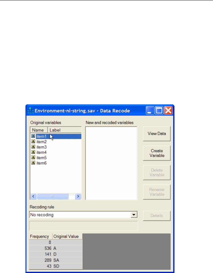
510
Example 33
Recoding the Data within Amos
The ordinal properties of the data cannot be inferred from the data file alone. To give
Amos the additional information it needs so that it can interpret the data values SD, D,
A, and SA:
EFrom the Amos Graphics menus, choose Tools > Data Recode.
ESelect item1 in the list of variables in the upper-left corner of the Data Recode window.
This displays a frequency distribution of the responses to item1 at the bottom of the
window.
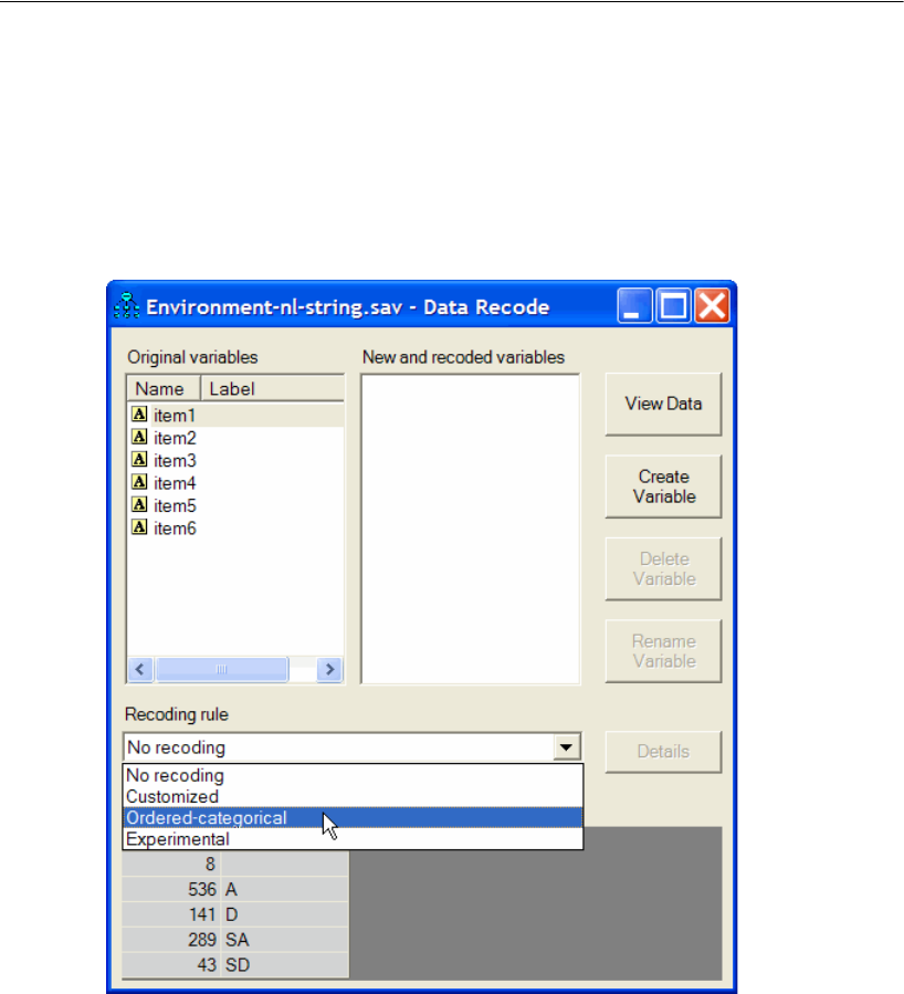
511
Ordered-Categorical Data
In the box labeled Recoding rule, the notation No recoding means that Amos will read
the responses to item1 as is. In other words, it will read either SD, D, A, SA, or an empty
string. We can’t leave things that way because Amos doesn’t know what to do with SD,
D, and so on.
EClick No recoding and select Ordered-categorical from the drop-down list.
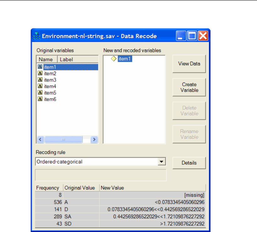
512
Example 33
The frequency table at the bottom of the window now has a New Value column that
shows how the item1 values in the data file will be recoded before Amos reads the data.
The first row of the frequency table shows that empty strings in the original data file
will be treated as missing values. The second row shows that the A response will be
translated into the string <0.0783345405060296. Amos will interpret this to mean that
there is a continuous numeric variable that underlies responses to item1, and that a
person who gives the A response has a score that is less than 0.0783345405060296 on
that underlying variable. Similarly, the third row shows that the D response will be
translated into the string 0.0783345405060296<<0.442569286522029 and interpreted
by Amos to mean that the score on the underlying numeric variable is between
0.0783345405060296 and 0.442569286522029. The numbers, 0.0783345405060296,
0.442569286522029, and so on, are derived from the frequencies in the Frequency
column, based on the assumption that scores on the underlying numeric variable are
normally distributed with a mean of 0 and a standard deviation of 1.
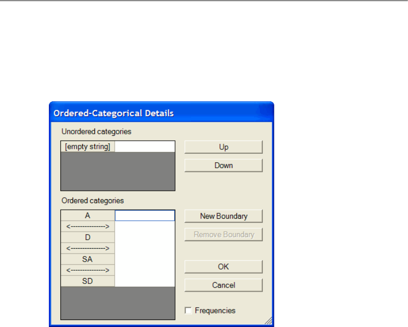
513
Ordered-Categorical Data
The ordering of the categories in the Original Value column needs to be changed. To
change the ordering:
EClick the Details button. The Ordered-Categorical Details dialog opens.
The Ordered categories list box shows four response categories arranged in the order
A, D, SA, SD, and separated from each other by dashed lines, <---->. The dashed
lines represent three boundaries that divide the real numbers into four intervals, with
the four intervals being associated with the four categorical responses. The assumption
is made that a person who scores below the lowest boundary on some unobserved
numeric variable gives the A response. A person who scores between the lowest
boundary and the middle boundary gives the D response. A person who scores between
the middle boundary and the highest boundary gives the SA response. Finally, a person
who scores above the highest boundary gives the SD response.
The program is correct about there being four categories (intervals) and three
boundaries, but it has the ordering of the categories wrong. The program arbitrarily
alphabetized the categories. We need to keep the four categories and the three
boundaries but rearrange them. We want SD to fall in the lowest interval (below the
lowest boundary), and so on.
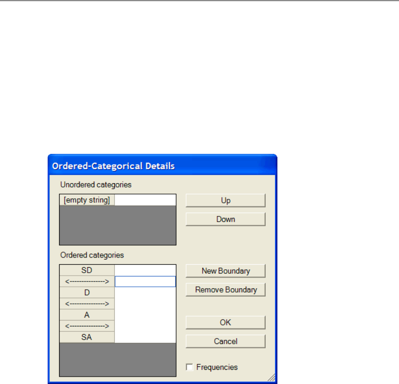
514
Example 33
You can rearrange the categories and the boundaries. To do this:
EDrag and drop with the mouse.
or
ESelect a category or boundary with the mouse and then click the Up or Down button.
After putting the categories and boundaries in the correct order, the Ordered-
Categorical Details dialog looks like this:
The Unordered categories list box contains a list of values that Amos will treat as
missing. At the moment, the list contains one entry, [empty string], so that Amos will
treat an empty string as a missing value. If a response coded as an empty string was
actually a response that could be meaningfully compared to SD, D, A, and SA, then you
would select [empty string] in the Unordered categories list box and click the Down
button to move [empty string] into the Ordered categories list box.
Similarly, if a response in the Ordered categories list box, for example SD, was not
comparable to the other responses, you would select it with the mouse and click the Up
button to move it into the Unordered categories list box. Then SD would be treated as
a missing value.
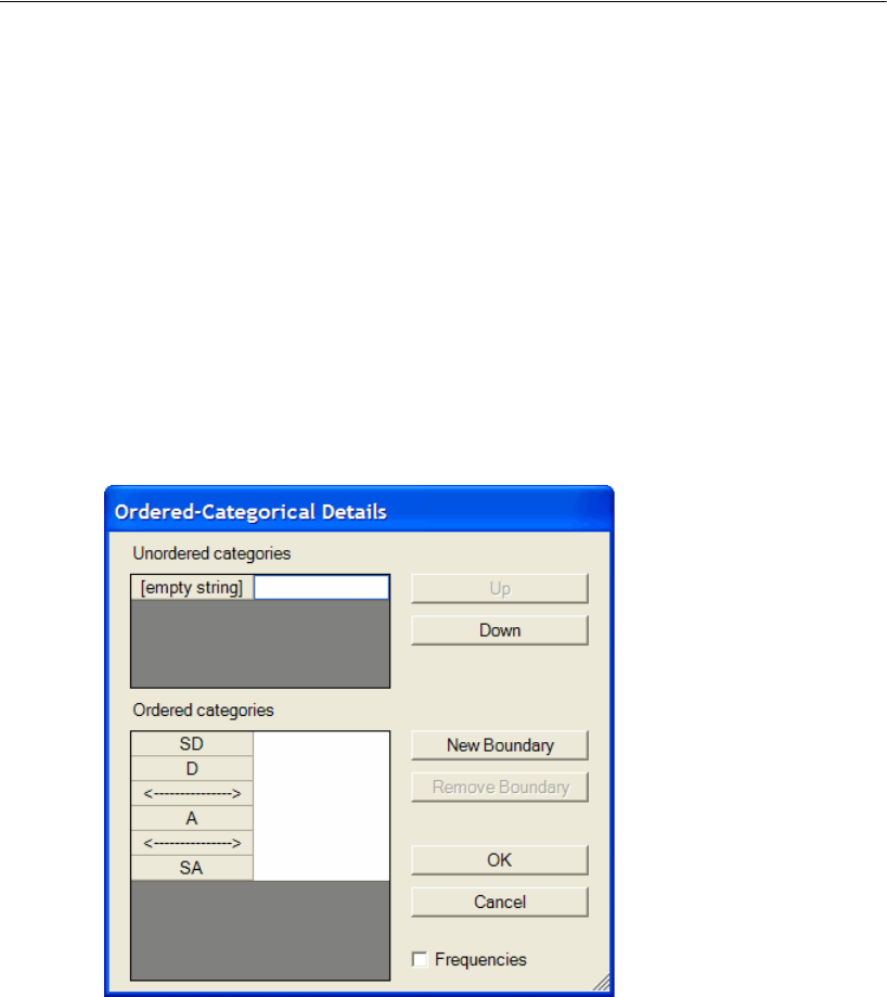
515
Ordered-Categorical Data
Note: You can’t drag and drop between the Ordered categories list box and the
Unordered categories list box. You have to use the Up and Down buttons to move a
category from one box to the other.
We could stop here and close the Ordered-Categorical Details dialog because we have
the right number of boundaries and categories and we have the categories going in the
right order. However, we will make a further change based on a suggestion by Croon
(2002), who also worked with this dataset and concluded that the SD category occurred
so seldom that it should be combined with the D category. To merge those two
categories into a single category:
ESelect the boundary between the two categories you want to merge.
EClick the Remove Boundary button. The Ordered categories list now looks like this:
Now the SD response and the D response are indistinguishable. Either response means
that the person who gave the response has a score that lies in the lowest interval on the
underlying numeric variable.
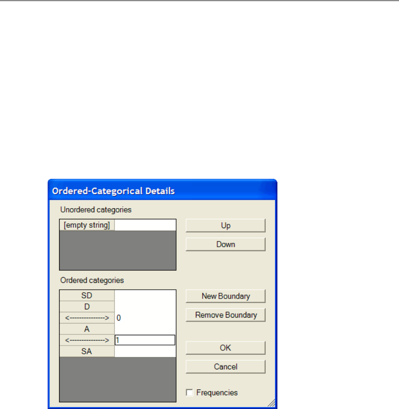
516
Example 33
There remains the question of the values of the two boundaries that separate the
three intervals. If you do not specify values for the boundaries, Amos will estimate the
boundaries by assuming that scores on the underlying numeric variable are normally
distributed with a mean of 0 and a standard deviation of 1. Alternatively, you can
assign a value to a boundary instead of letting Amos estimate it. To assign a value:
ESelect the boundary with the mouse.
EType a numeric value in the text box.
The following figure shows the result of assigning values 0 and 1 to the two boundaries.
Although it may not be obvious, it is permissible to assign 0 and 1, or any pair of
numbers, to the two boundaries, as long as the higher boundary is assigned a larger
value than the lower one. No matter how many boundaries there are (as long as there
are at least two), assigning values to two of the boundaries amounts to choosing a zero
point and a unit of measurement for the underlying numeric variable. The scaling of
the underlying numeric variable is discussed further in the Help file under the topic
“Choosing boundaries when there are three categories.”
EClick OK to close the Ordered-Categorical Details dialog.
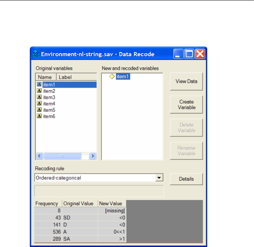
517
Ordered-Categorical Data
The changes that were just made to the categories and the interval boundaries are now
reflected in the frequency table at the bottom of the Data Recode window.
The frequency table shows how the values that appear in the data file will be recoded
before Amos reads them. Reading the frequency table from top to bottom:
An empty string will be treated as a missing value.
The strings SD and D will be recoded as <0, meaning that the underlying numeric
score is less than 0.
A will be recoded as 0<<1, meaning that the underlying numeric score is between
0 and 1.
SA will be recoded as >1, meaning that the underlying numeric score is greater
than 1.
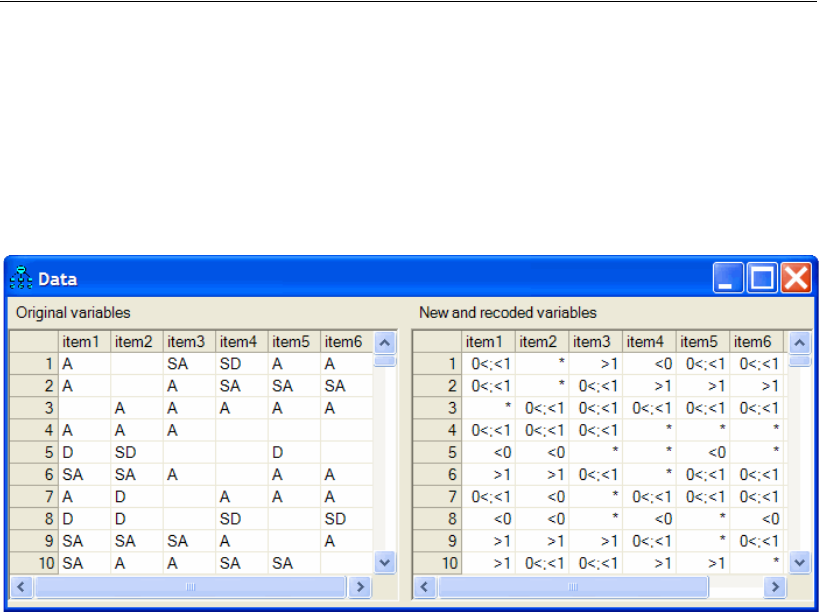
518
Example 33
That takes care of item1. What was just done for item1 has to be repeated for each of
the five remaining observed variables. After specifying the recoding for all six
observed variables, you can view the original dataset along with the recoded variables.
To do this:
EClick the View Data button.
The table on the left shows the contents of the original data file before recoding. The
table on the right shows the recoded variables after recoding. When Amos performs an
analysis, it reads the recoded values, not the original values.
Note: You can create a raw data file in which the data recoding has already been
performed. In other words, you can create a raw data file that contains the inequalities
on the right-hand side of the figure above. In that case, you wouldn’t need to use the
Data Recode window in Amos. Indeed, that approach was used in Chapter 32.
EFinally, close the Data Recode window before specifying the model.

519
Ordered-Categorical Data
Specifying the Model
After you have specified the rules for data recoding as shown above, the analysis
proceeds just like any Bayesian analysis. For this example, a factor analysis model will
be fitted to the six questionnaire items in the environment dataset. The first three items
were designed to be measures of willingness to spend money to take care of the
environment. The other three items were designed to be measures of awareness of
environmental issues. This design of the questionnaire is reflected in the following
factor analysis model, which is saved in the file Ex33-a.amw.
The path diagram is drawn exactly as it would be drawn for numeric data. This is one
of the good things about having at least three categories for each ordered-categorical
variable: You can specify a model in the way that you are used to, just as though all the
variables were numeric, and the model will work for any combination of numeric and
ordered-categorical variables. If variables are dichotomous, you will need to impose
additional parameter constraints in order to make the model identified. This issue is
discussed further in the online help under the topic “Parameter identification with
dichotomous variables.”
0, 1
WILLING
item1
item2
item3
item6
item4
item5
0,
e1
0,
e2
0,
e3
0,
e4
0,
e5
0,
e6
0, 1
AWARE
1
1
1
1
1
1
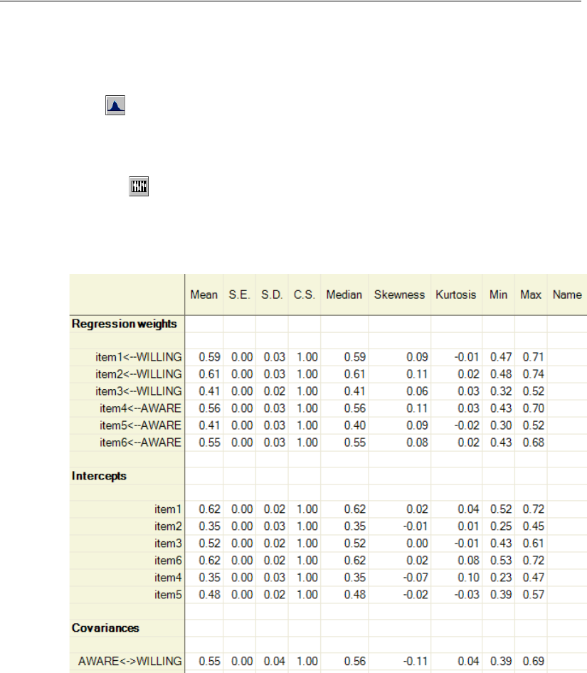
520
Example 33
Fitting the Model
EClick on the toolbar.
or
EFrom the menus, choose Analyze > Bayesian Estimation.
Note: The button is disabled because, with non-numeric data, you can perform only
Bayesian estimation.
After the Bayesian SEM window opens, wait until the unhappy face changes into a
happy face. The Bayesian SEM window should then look something like this:
(The figure above shows some, but not all, of the parameter estimates.) The Mean
column provides a point estimate for each parameter. For example, the regression
weight for using WILLING to predict item1 is estimated to be 0.59. The skewness
(0.09) and kurtosis (–0.01) of the posterior distribution are close to 0, which is
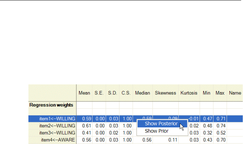
521
Ordered-Categorical Data
compatible with the posterior distribution being nearly normal. The standard deviation
(S.D.) is 0.03, so there is about a 67% chance that the regression weight is within 0.03
of 0.59. Doubling the standard deviation gives 0.06, so there is about a 95% chance that
the regression weight is within 0.06 of 0.59.
To view the posterior distribution of the regression weight:
ERight-click its row and choose Show Posterior from the pop-up menu.
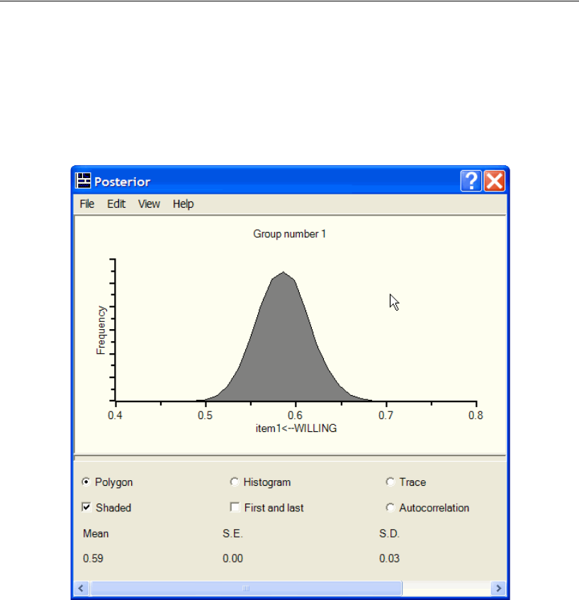
522
Example 33
The Posterior window displays the posterior distribution. The appearance of the
distribution confirms what was concluded above from the mean, standard deviation,
skewness, and kurtosis of the distribution. The shape of the distribution is nearly
normal, and it looks like roughly 95% of the area lies between 0.53 and 0.65 (that is,
within 0.06 of 0.59).
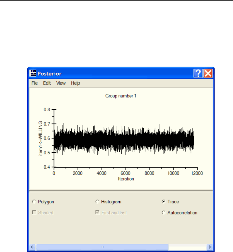
523
Ordered-Categorical Data
MCMC Diagnostics
If you know how to interpret the diagnostic output from MCMC algorithms (for
example, see Gelman, et al, 2004), you might want to view the Trace plot and the
Autocorrelation plot.
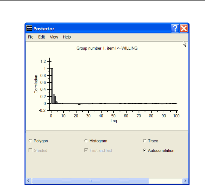
524
Example 33
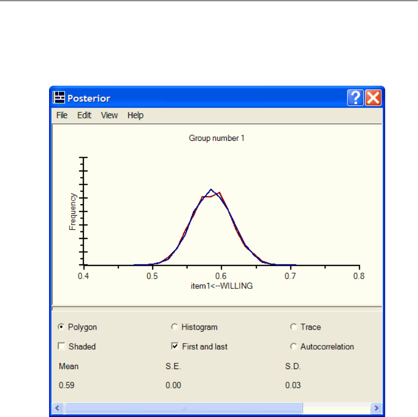
525
Ordered-Categorical Data
The First and last plot provides another diagnostic. It shows two estimates of the
posterior distribution (two superimposed plots), one estimate from the first third of the
MCMC sample and another estimate from the last third of the MCMC sample.

526
Example 33
Posterior Predictive Distributions
When you think of estimation, you normally think of estimating model parameters or
some function of the model parameters such as a standardized regression weight or an
indirect effect. However, there are other unknown quantities in the present analysis.
Each entry in the data table on p. 508 represents a numeric value that is either unknown
or partially known. For example, Person 1 did not respond to item2, so we can only
guess at (estimate) that person’s score on the underlying numeric variable. On the other
hand, it seems like we ought to be able to make a fairly educated guess about the
underlying numeric value, considering that we know how the person responded to the
other items, and that we can also make use of the assumption that the model is correct.
We are in an even better position to guess at Person 1’s score on the numeric
variable that underlies item1 because Person 1 gave a response to item1. This person’s
response places his or her score in the middle interval, between the two boundaries.
Since the two boundaries were arbitrarily fixed at 0 and 1, we know that the score is
somewhere between 0 and 1, but it seems like we should be able to say more than that
by using the person’s responses on the other variables along with the assumption that
the model is correct.
In Bayesian estimation, all unknown quantities are treated in the same way. Just as
unknown parameter values are estimated by giving their posterior distribution, so are
unknown data values. A posterior distribution for an unknown data value is called a
posterior predictive distribution, but it is interpreted just like any posterior
distribution. To view posterior predictive distributions for unknown data values:
EClick the Posterior Predictive button .
or
EFrom the menus, choose View > Posterior Predictive.
The Posterior Predictive Distributions window appears.
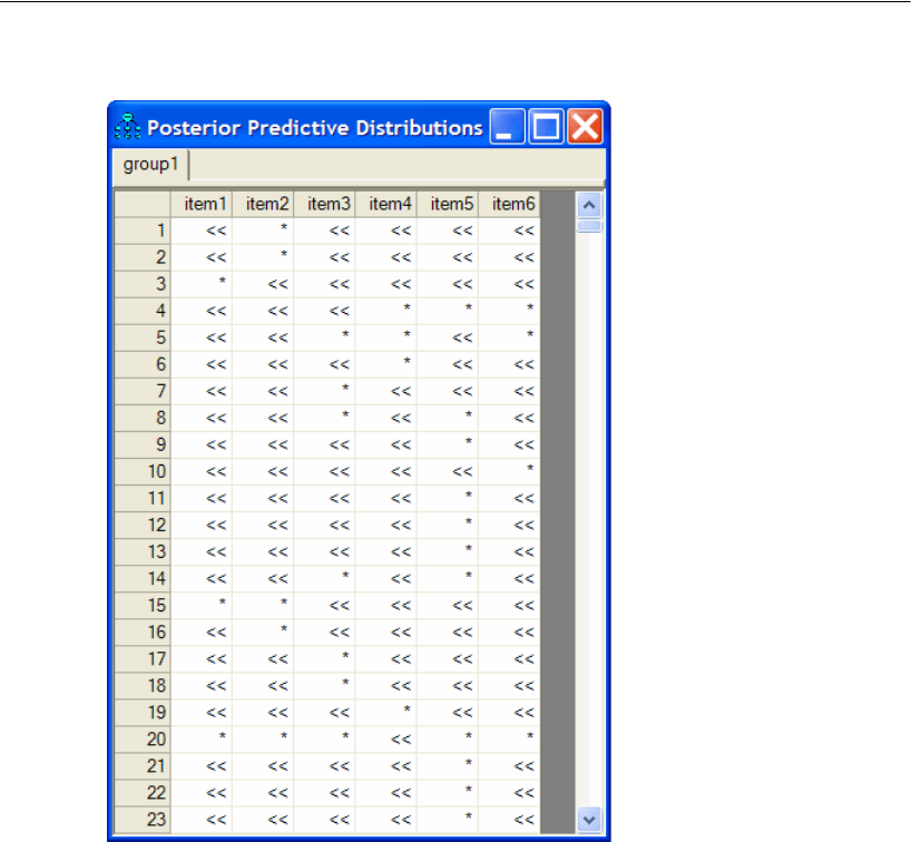
527
Ordered-Categorical Data
The Posterior Predictive Distributions window contains a table with a row for every
person and a column for every observed variable in the model. An asterisk (*) indicates
a missing value, while << indicates a response that places inequality constraints on the
underlying numeric variable. To display the posterior distribution for an item:
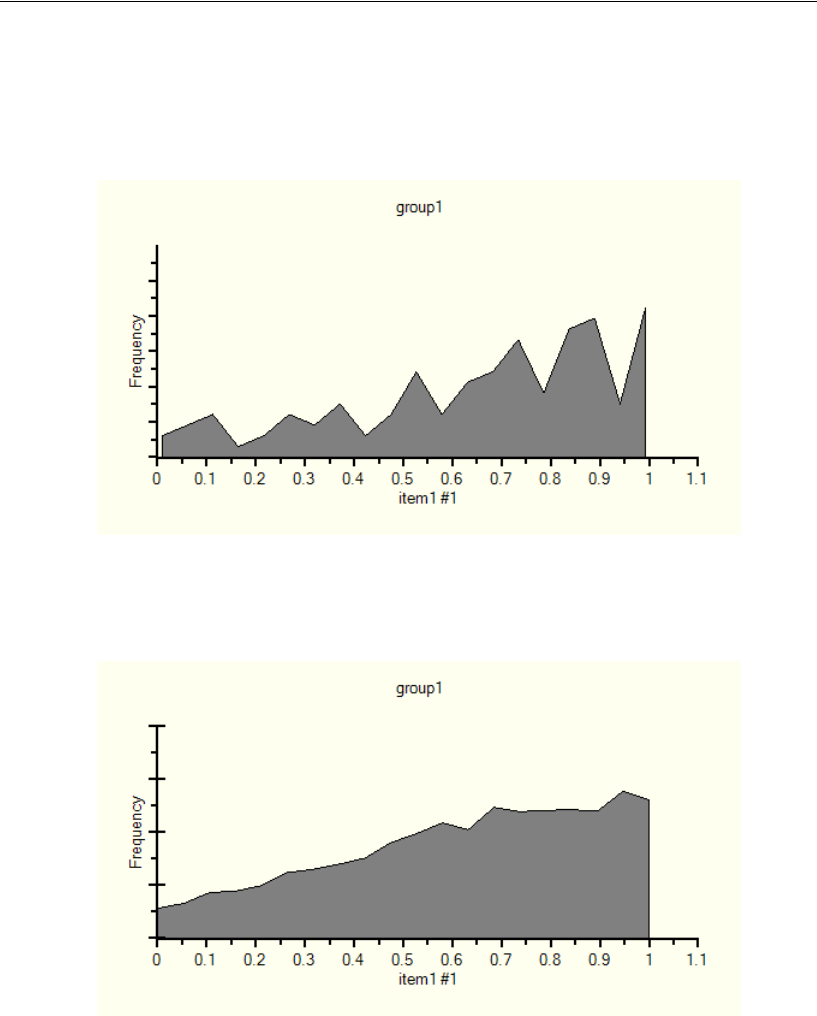
528
Example 33
EClick on the table entry in the upper-left corner (Person 1’s response to item1).
The Posterior window opens, displaying the posterior distribution of Person 1’s
underlying numeric score. At first, the posterior distribution looks jagged and random.
That is because the program is building up an estimate of the posterior distribution as
MCMC sampling proceeds. The longer you wait, the better the estimate of the posterior
distribution will be. After a while, the estimate of the posterior distribution stabilizes
and looks something like this:
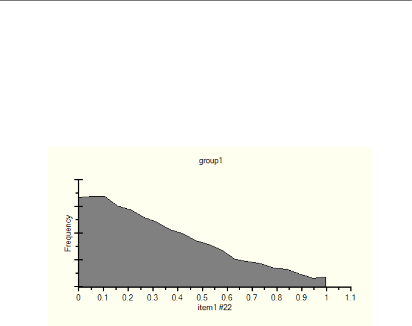
529
Ordered-Categorical Data
The posterior distribution shows that Person 1’s score on the numeric variable that
underlies his or her response to item1 is between 0 and 1 (which we knew already), and
that the score is more likely to be close to 1 than close to 0.
ENext, click the table entry in the first column of the 22nd row to estimate Person 22’s
score on the numeric variable that underlies his or her response to item1.
After you wait a while to get a good estimate of the posterior distribution, you see this:
Both Person 1 and Person 22 gave the agree response to item1, so both people have
scores between 0 and 1 on the underlying numeric variable; however, their posterior
distributions are very different
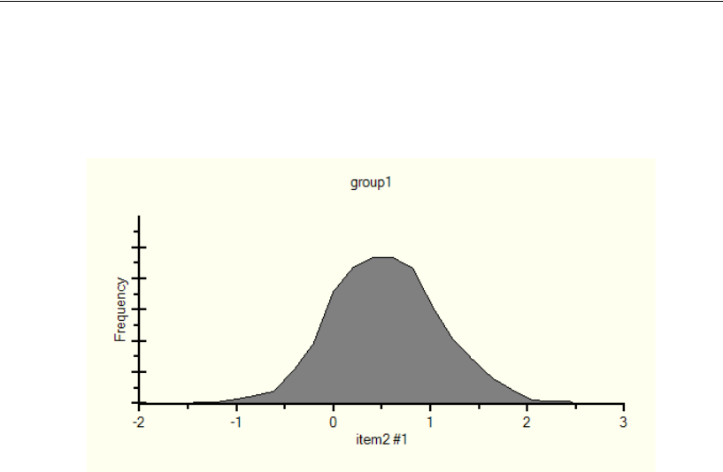
530
Example 33
For another example of a posterior predictive distribution, select a missing value
like Person 1’s response to item2. After allowing MCMC sampling to proceed long
enough to get a good estimate of the posterior distribution, it looks like this:
The mean of the posterior distribution (0.52) can be taken as an estimate of Person 1’s
score on the underlying variable if a point estimate is required. Looking at the plot of
the posterior distribution, we can be nearly 100% sure that the score is between –1 and
2. The score is probably between 0 and 1 because most of the area under the posterior
distribution lies between 0 and 1.
Posterior Predictive Distributions for Latent Variables
Suppose you want to estimate Person 1’s score on the WILLING factor. Amos can
estimate posterior predictive distributions for unknown scores only for observed
variables. It cannot estimate a posterior predictive distribution of a score on a latent
variable. However, there is a trick that you can use to estimate the posterior predictive
distribution of a score on WILLING. You can change WILLING to an observed
variable, treating it not as a latent variable but as an observed variable that has a missing
value for every case. That requires two changes – a change to the path diagram and a
change to the data.
In the path diagram, the WILLING ellipse has to be changed into a rectangle. To
accomplish this:
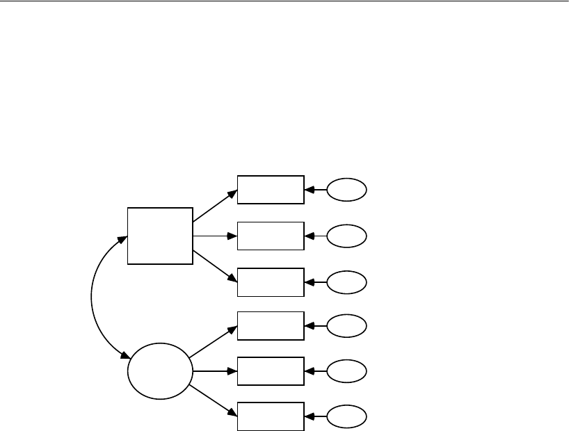
531
Ordered-Categorical Data
ERight-click the WILLING ellipse and choose Toggle Observed/Unobserved from the pop-
up menu.
EClick the WILLING ellipse.
The WILLING ellipse changes to a rectangle so that the path diagram looks like this:
That takes care of the path diagram. It is also necessary to make a change to the data
because if WILLING is an observed variable, then there has to be a WILLING column
in the data file. You can directly modify the data file. Since this is a data file in SPSS
Statistics format, you would use SPSS Statistics to add a WILLING variable to the data
file, making sure that all the scores on WILLING are missing.
To avoid changing the original data file:
ERight-click the WILLING variable in the path diagram
EChoose Data Recode from the pop-up menu to open the Data Recode window.
0, 1
WILLING
item1
item2
item3
item6
item4
item5
0,
e1
0,
e2
0,
e3
0,
e4
0,
e5
0,
e6
0, 1
AWARE
1
1
1
1
1
1
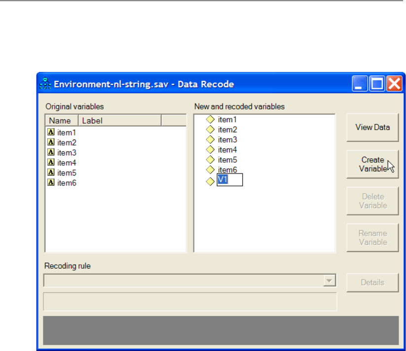
532
Example 33
EIn the Data Recode window, click Create Variable. A new variable with the default
name V1, appears in the New and recoded variables list box.
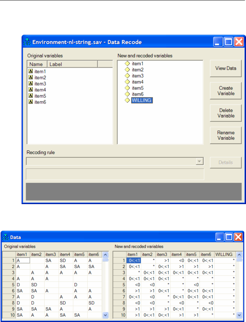
533
Ordered-Categorical Data
EChange V1 to WILLING. (If necessary, click the Rename Variable button.)
EYou can optionally view the recoded dataset that includes the new WILLING variable
by clicking the View Data button.
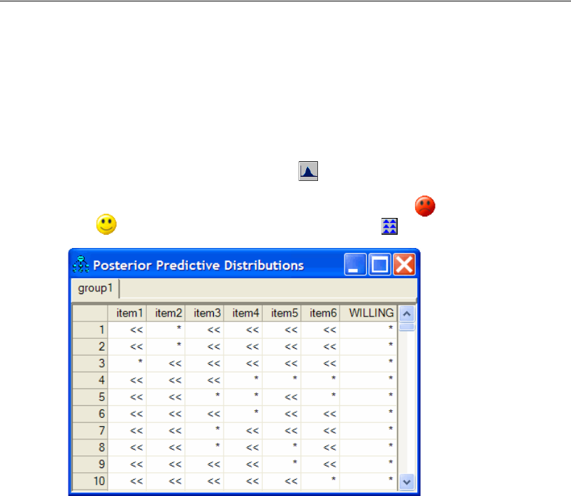
534
Example 33
The table on the left shows the original dataset. The table on the right shows the
recoded dataset as read by Amos. It includes item1 through item6 after recoding, and
also the new WILLING variable.
EClose the Data Recode window.
EStart the Bayesian analysis by clicking on the Amos Graphics toolbar.
EIn the Bayesian SEM window, wait until the unhappy face changes into a happy
face and then click the Posterior Predictive button .
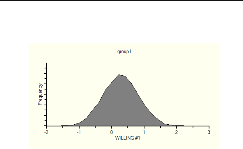
535
Ordered-Categorical Data
EClick the entry in the upper-right corner of the table to display the posterior distribution
of Person 1’s score on the WILLING factor.
Imputation
Data imputation works the same way for ordered-categorical data as it does for
numeric data. With ordered-categorical data, you can impute numeric values for
missing values, for scores on latent variables, and for scores on the unobserved numeric
variables that underlie observed ordered-categorical measurements.
You need a model in order to perform imputation. You could use the factor analysis
model that was used earlier. There are several advantages and one disadvantage to
using the factor analysis model for imputation. One advantage is that, if the model is
correct, you can impute values for the factors. That is, you can create a new data set in
which WILLING and AWARE are observed variables. The other advantage is that, if
the factor analysis model is correct, it can be expected to give more accurate
imputations for item1 through item6 than would be obtained from a less restrictive
model. The disadvantage of using the factor analysis model is that it may be wrong. To
be on the safe side, the present example will use the model that has the biggest chance
of being correct, the saturated model shown in the following figure. (See the file
Ex33-c.amw.)
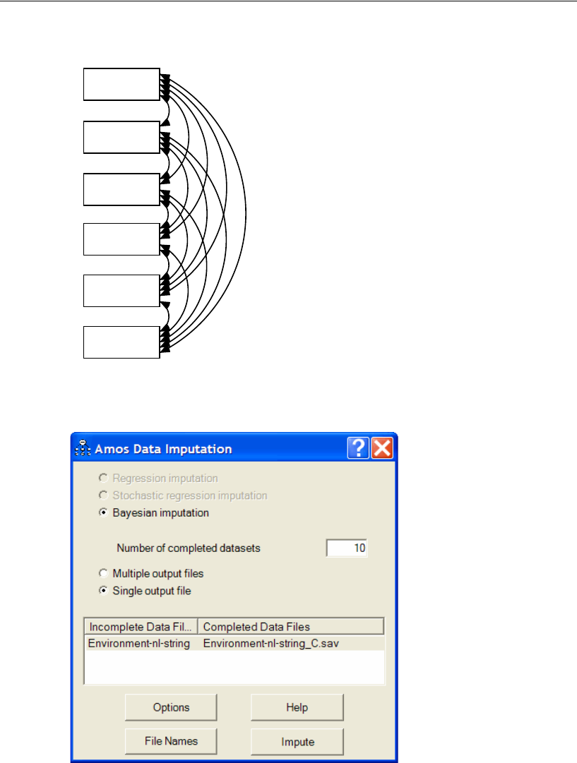
536
Example 33
After drawing the path diagram for the saturated model, you can begin the imputation.
EFrom the Amos Graphics menu, choose Analyze > Data Imputation.
item1
item2
item3
item6
item4
item5
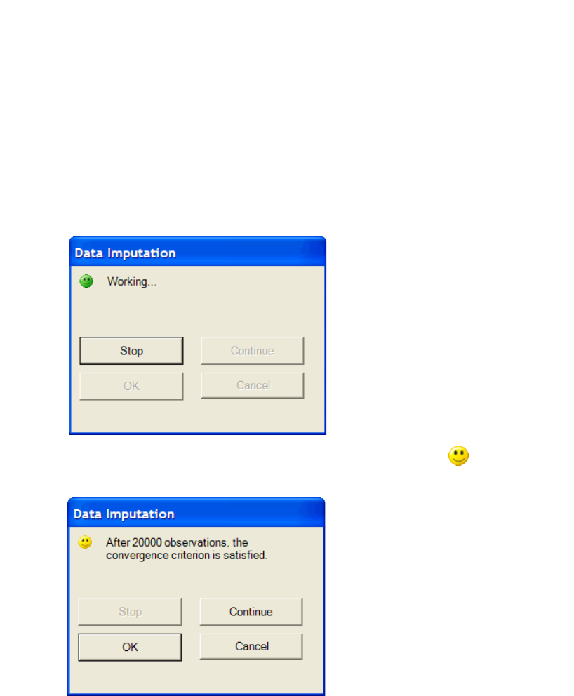
537
Ordered-Categorical Data
In the Amos Data Imputation window, notice that Regression imputation and Stochastic
regression imputation are disabled. When you have non-numeric data, Bayesian
imputation is the only choice.
We will accept the options shown in the preceding figure, creating 10 completed
datasets and saving all 10 in a single SPSS Statistics data file called environment-nl-
string_C.sav. To start the imputation:
EClick the Impute button.
The Bayesian SEM window opens along with the Data Imputation dialog box.
EWait until the Data Imputation dialog box displays a happy face to indicate that
each of the 10 completed data sets is effectively uncorrelated with the others.
Note: After you see a happy face but before you click OK, you may optionally right-
click a parameter in the Bayesian SEM window and choose Show Posterior from the
pop-up menu. This will allow you to examine the Trace and Autocorrelation plots.
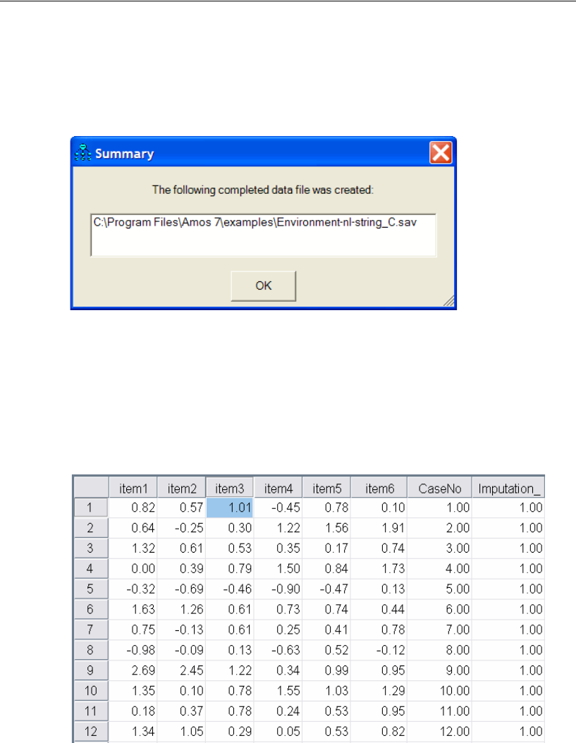
538
Example 33
EClick OK in the Data Imputation dialog box.
The Summary window shows a list of the completed data files that were created. In this
case, only one completed data file was created.
EDouble-click the file name in the Summary window to display the contents of the
single completed data file, which contains 10 completed data sets.
The file contains 10,170 cases because each of the 10 completed datasets contains
1,017 cases. The first 1,017 rows of the new data file contain the first completed
dataset. The Imputation_ variable is equal to 1 for each row in the first completed
dataset, and the CaseNo variable runs from 1 through 1,017 before starting over
again at 1.

539
Ordered-Categorical Data
Normally, the next step would be to use the 10 completed datasets in environment-nl-
string_C.sav as input to some other program that requires numeric (not ordered-
categorical) data. You would use that other program to perform 10 separate analyses
using each one of the 10 completed data sets in turn. Then, you would do further
computations to combine the results of those 10 separate analyses into a single set of
results, as was done in Example 31. Those steps will not be carried out here.

540
Example 33

541
Example
34
Mixture Modeling with Training Data
Introduction
Mixture modeling is appropriate when you have a model that is incorrect for an entire
population, but where the population can be divided into subgroups in such a way that
the model is correct in each subgroup.
Mixture modeling is discussed in the context of structural equation modeling by
Arminger, Stein, and Wittenberg (1999), Hoshino (2001), Lee (2007, Chapter 11),
Loken (2004), Vermunt and Magidson (2005), and Zhu and Lee (2001), among
others.
The present example demonstrates mixture modeling for the situation in which
some cases have already been assigned to groups while other cases have not. It is up
to Amos to learn from the cases that are already classified and to classify the others.
We begin mixture modeling with an example in which some cases have already
been classified because setting up such an analysis is almost identical to setting up an
ordinary multiple-group analysis such as in Examples 10, 11, and 12.
It is possible to perform mixture modeling when no cases have been classified in
advance so that the program must classify every case. Example 35 demonstrates this
type of analysis.
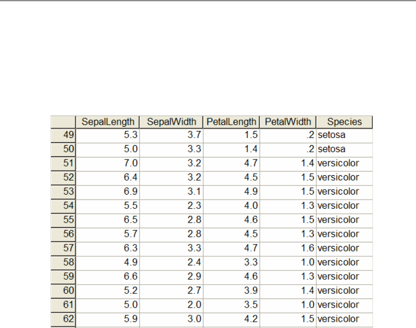
542
Example 34
About the Data
The data for this example were collected by Anderson (1935) and used by Fisher
(1936) to demonstrate discriminant analysis. The original data are in the file iris.sav,
of which a portion is shown here:
The dataset contains four measurements on flowers from 150 different plants. The first
50 flowers were irises of the species setosa. The next 50 were irises of the species
versicolor. The last 50 were of the species virginica.
543
Mixture Modeling with Training Data
A scatterplot of two of the numeric measurements, PetalLength and PetalWidth,
suggests that those two measurements alone will be useful in classifying the flowers
according to species.
The setosa flowers are all by themselves in the lower left corner of the scatterplot. It
should therefore be easy for Amos to use PetalLength and PetalWidth to distinguish
the setosa flowers from the others. On the other hand, there is some overlap of
versicolor and virginica, so we should expect that sometimes it will be hard to tell
whether a flower is versicolor or virginica purely on the basis of PetalLength and
PetalWidth.
setosa
versicolor
virginica
Species
0.5 1.0 1.5 2.0 2.5
PetalWidth
2.0
4.0
6.0
PetalLength
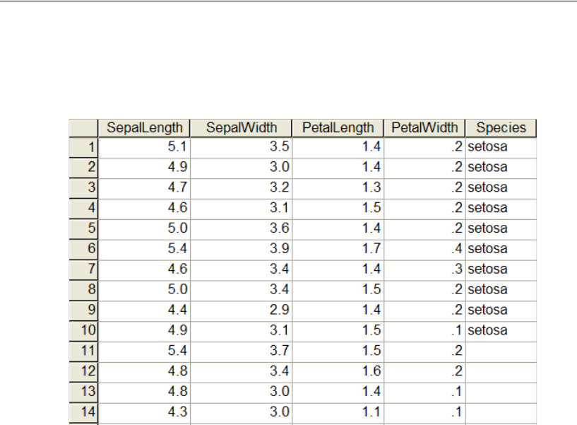
544
Example 34
This example will not use the iris.sav dataset, which gives the species of every
flower. Instead, the example will use the iris3.sav dataset, which gives the species for
only a few flowers. The following figure shows a portion of the iris3.sav dataset.
Species information is available for 10 of the setosa flowers, 10 of the versicolor
flowers, and 10 of the virginica flowers. Species is unknown for the remaining 120
flowers. When Amos analyzes these data, it will have 10 examples of each kind of
flower to assist in classifying the rest of the flowers.
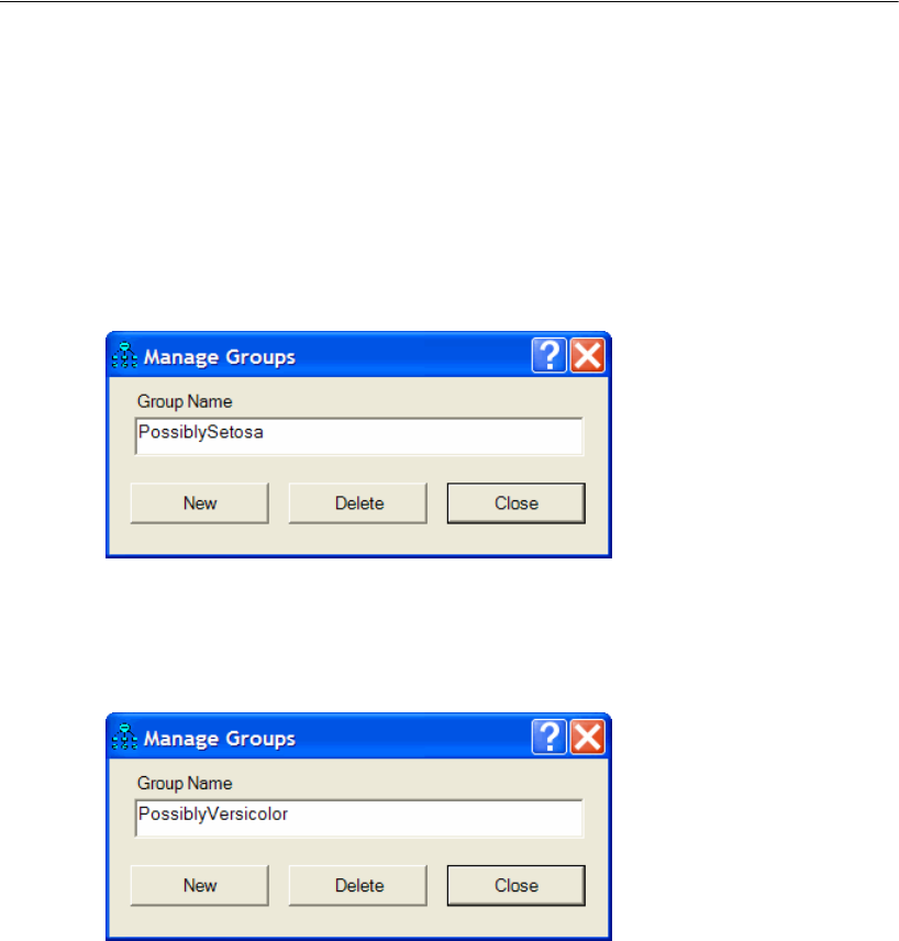
545
Mixture Modeling with Training Data
Performing the Analysis
EFrom the menus, choose File > New to start a new path diagram.
EFrom the menus, choose Analyze > Manage Groups.
EIn the Manage Groups dialog, change the name in the Group Name text box from
Group number 1 to PossiblySetosa.
EClick New to create a second group.
EChange the name in the Group Name text box from Group number 2 to
PossiblyVersicolor.
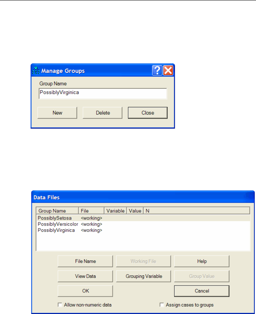
546
Example 34
EClick New to create a third group.
EChange the name in the Group Name text box from Group number 3 to
PossiblyVirginica.
EClick Close.
Specifying the Data File
EFrom the menus, choose File > Data Files.
EClick PossiblySetosa to select that row.
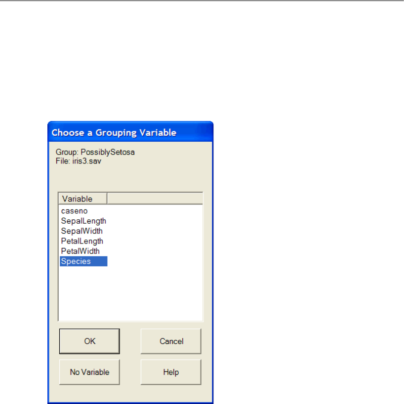
547
Mixture Modeling with Training Data
EClick File Name, select the iris3.sav file that is in the Amos Examples directory, and
click Open.
EClick Grouping Variable and double-click Species in the Choose a Grouping Variable
dialog. This tells the program that the Species variable will be used for classifying
flowers.
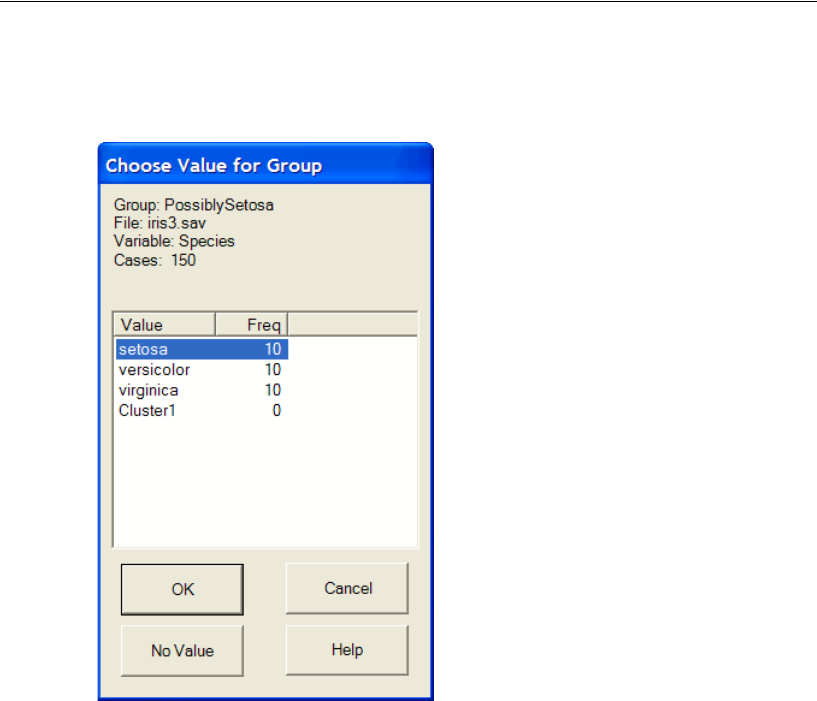
548
Example 34
EIn the Data Files dialog, click Group Value and then double-click setosa in the Choose
Value for Group dialog.
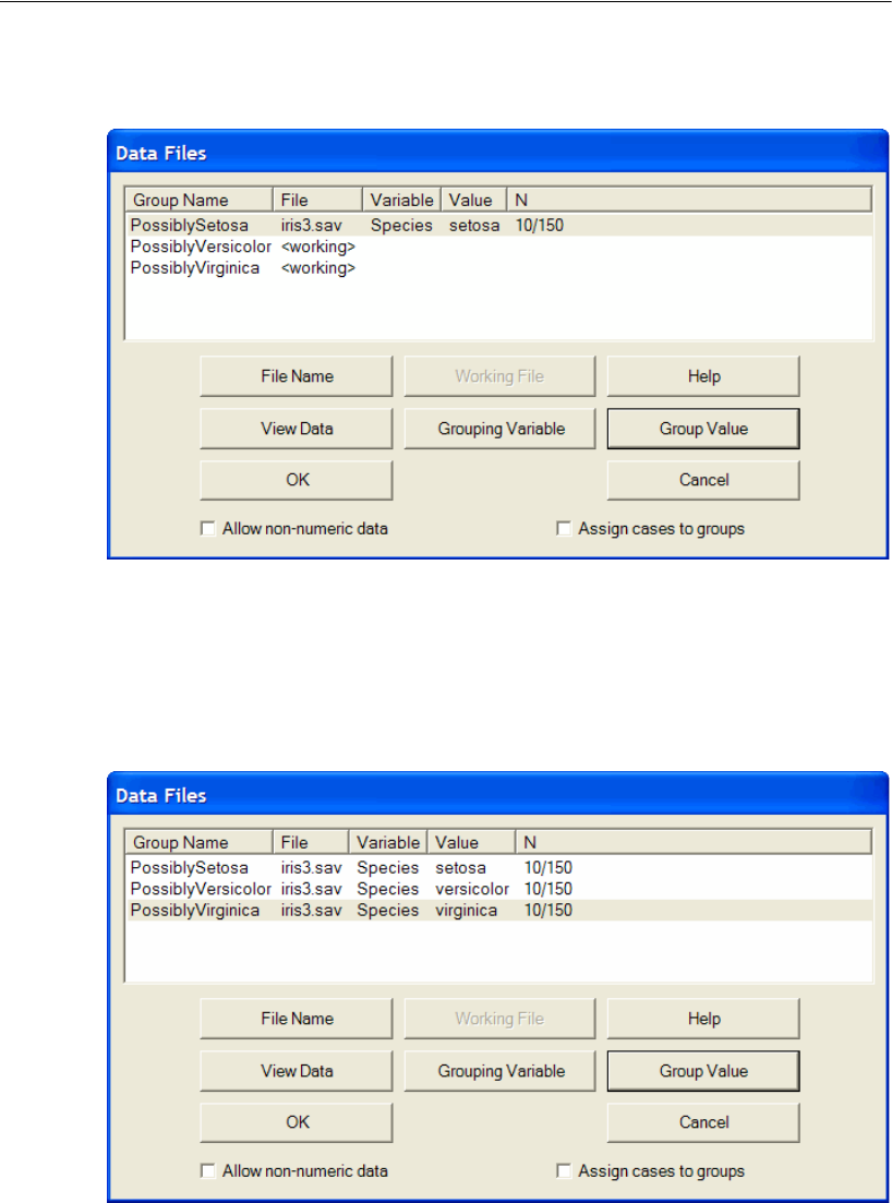
549
Mixture Modeling with Training Data
The Data Files dialog should now look like this:
ERepeat the preceding steps for the PossiblyVersicolor group, but this time double-click
versicolor in the Choose Value for Group dialog.
ERepeat the preceding steps once more for the PossiblyVirginica group, but this time
double-click virginica in the Choose Value for Group dialog. The Data Files dialog will
end up looking like this:
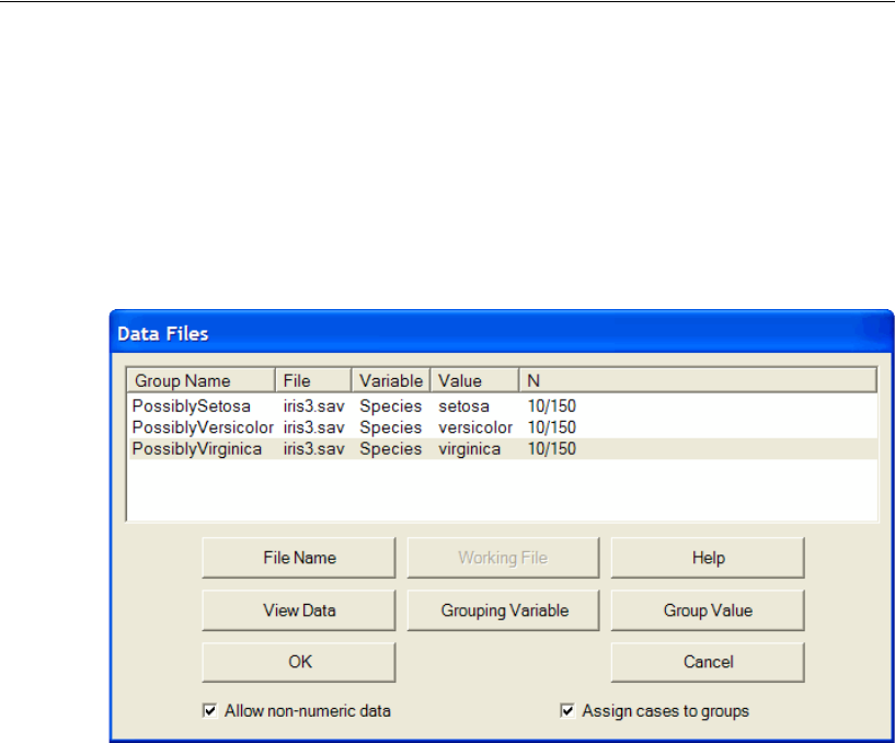
550
Example 34
So far, the analysis has been set up exactly like an ordinary three-group analysis in
which the species of every flower is known. The next step is unique to mixture
modeling.
ESelect Assign cases to groups (a check mark will appear next to it). The check mark tells
Amos to assign a case to a group whenever the dataset does not specify which group
that case belongs to.
EClick OK to close the Data Files dialog.
Specifying the Model
We will use a saturated model for the variables PetalLength and PetalWidth. The
scatterplot that was shown earlier suggests that these two variables will allow the
program to do a good job of classifying the flowers according to species.
Note that you are not limited to saturated models when doing mixture modeling.
You can use a factor analysis model or a regression model or any other kind of model.
See Example 36 for a demonstration of mixture modeling with a regression model.
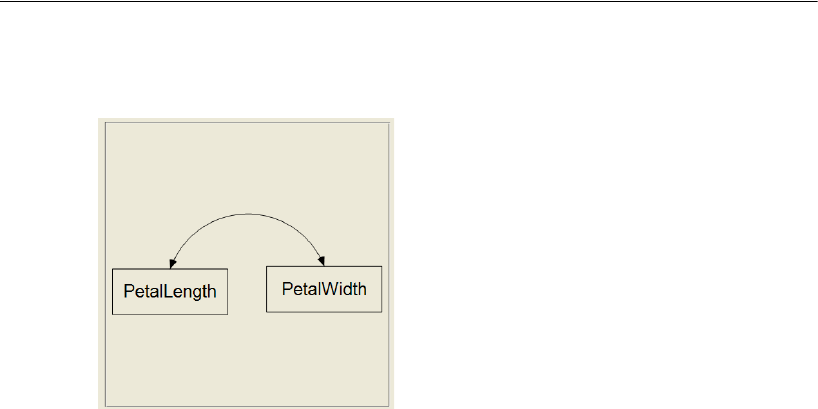
551
Mixture Modeling with Training Data
EDraw the following path diagram. (This path diagram is saved as Ex34-a.amw.)
EFrom the menus, choose View > Analysis Properties.
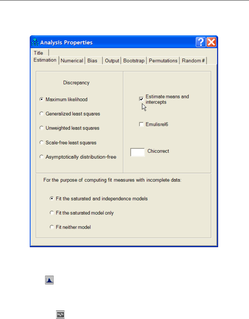
552
Example 34
ESelect Estimate means and intercepts (a check mark will appear next to it).
Fitting the Model
EClick on the toolbar.
or
EFrom the menus, choose Analyze > Bayesian Estimation.
Note: The button is disabled because, in mixture modeling, you can perform only
Bayesian estimation.
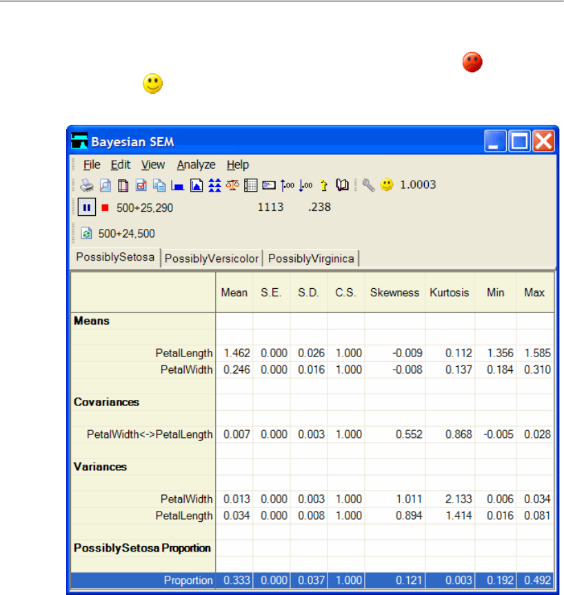
553
Mixture Modeling with Training Data
After the Bayesian SEM window opens, wait until the unhappy face changes into
a happy face . The table of estimates in the Bayesian SEM window should look
something like this:
The Bayesian SEM window displays all of the parameter estimates that you would get
in an ordinary three-group analysis. The table displays the results for one group at a
time. You can switch from one group to another by clicking the tabs at the top of the
table. In this example, the model parameters include only means, variances, and
covariances. In a more complicated model, there would also be estimates of regression
weights and intercepts.
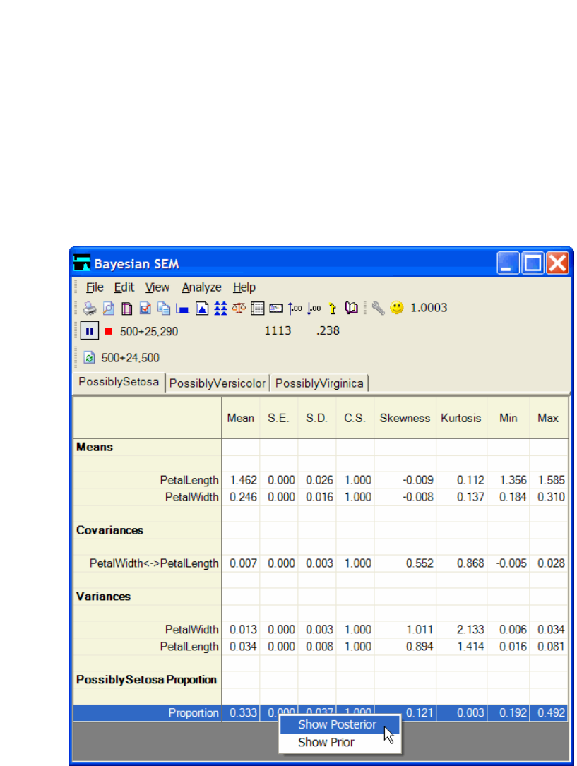
554
Example 34
In a mixture modeling analysis, you also get an estimate of the proportion of the
population that lies in each group. The preceding figure shows that the proportion of
setosa flowers in the population is estimated to be 0.333. (It should be pointed out that
it was by design that the sample contained equal numbers of setosa, versicolor, and
virginica flowers. It is therefore not meaningful in this example to draw inferences
about population proportions from the sample. Nevertheless, we will treat species here
as a random variable in order to demonstrate how such inferences can be made.)
To view the posterior distribution of a population proportion, right-click the row that
contains the proportion and choose Show Posterior from the pop-up menu.
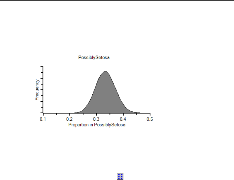
555
Mixture Modeling with Training Data
The Posterior window shows that the proportion of flowers that belong to the setosa
species is almost certainly between 0.25 and 0.45. It looks like there is about a 50–50
chance that the proportion is somewhere between 0.3 and 0.35.
Classifying Individual Cases
To obtain probabilities of group membership for each individual flower:
EClick the Posterior Predictive button .
or
EFrom the menus, choose View > Posterior Predictive.
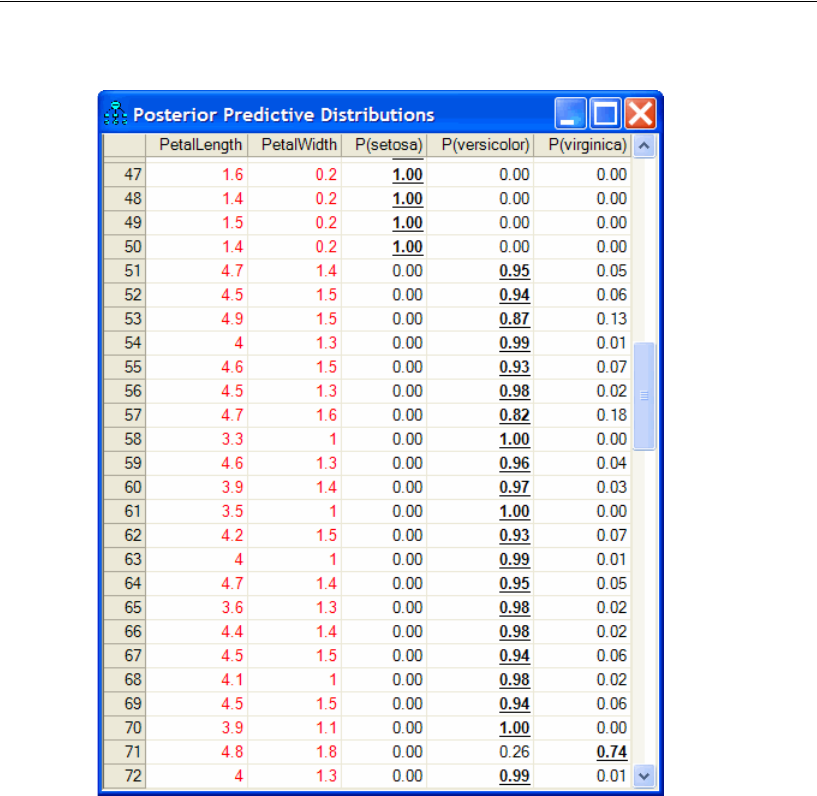
556
Example 34
For each flower, the Posterior Predictive Distributions window shows the probability
that that flower is setosa, versicolor, or virginica.
For the first 50 flowers (the ones that actually are setosa), the probability of
membership in the setosa group is nearly 1. We expected that result because the setosa
flowers were clearly separated from flowers of other species in the scatterplot shown
earlier.
Most of the versicolor flowers (starting with case number 51) were also correctly
classified. For example, flower number 51 has posterior probability 0.95 of being
versicolor. However, classification errors do occur. Case number 71, for example, is
misclassified. It is a versicolor flower, but it is estimated to have a 0.74 probability of
being virginica.
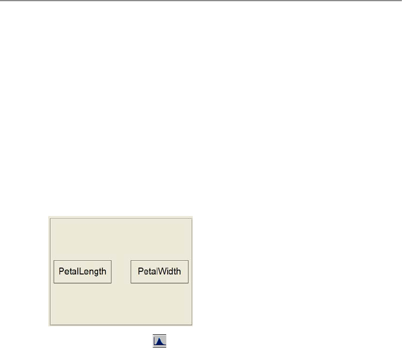
557
Mixture Modeling with Training Data
Latent Structure Analysis
It was mentioned earlier that you are not limited to saturated models when doing
mixture modeling. You can use a factor analysis model, a regression model, or any
model at all. You may want to become familiar with an important variation of the
saturated model. Latent structure analysis (Lazarsfeld and Henry, 1968) is a variation
of mixture modeling in which the measured variables are required to be independent
within each group. When the measured variables are multivariate normal, they are
required to be uncorrelated.
ETo require that the measured variables be uncorrelated, delete the double-headed arrow
in the path diagram of the saturated model. (This path diagram is saved as Ex34-
b.amw.)
EClick the Bayesian button to perform the latent structure analysis. The results of the
latent structure analysis will not be presented here.

559
Example
35
Mixture Modeling without
Training Data
Introduction
Mixture modeling is appropriate when you have a model that is incorrect for an entire
population, but where the population can be divided into subgroups in such a way that
the model is correct in each subgroup.
When Amos performs mixture modeling, it allows you to assign some cases to
groups before the analysis starts. Example 34 shows how to do that. In the present
example, all cases are unclassified at the start of the mixture modeling analysis.
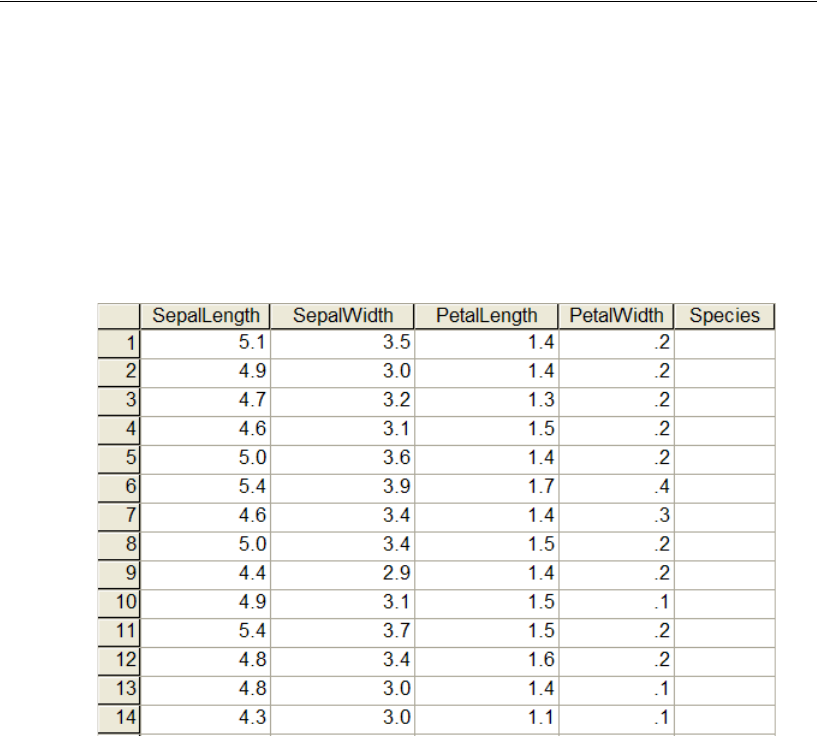
560
Example 35
About the Data
This example uses the Anderson (1935) iris data that was used in Example 34. This
time, however, we will not use the iris3.sav dataset, which contains species information
for 30 of the 150 flowers. Instead, we will use the iris2.sav dataset, which contains no
species information at all. That is the difference between Example 34 and the present
example: In Example 34, some cases were pre-classified; in the present example, no
cases are pre-classified. The following figure shows a portion of the iris2.sav dataset.
Notice that the dataset contains a Species column, even though that column is empty.
It is important that the Species column be present even if it contains no values. This is
because Amos allows for the possibility that you might already know the species of
some cases (as in Example 34). The variable that is used for classifying cases does not
actually have to be named Species. Any variable name will do. The variable does,
however, have to be a string (non-numeric) variable.
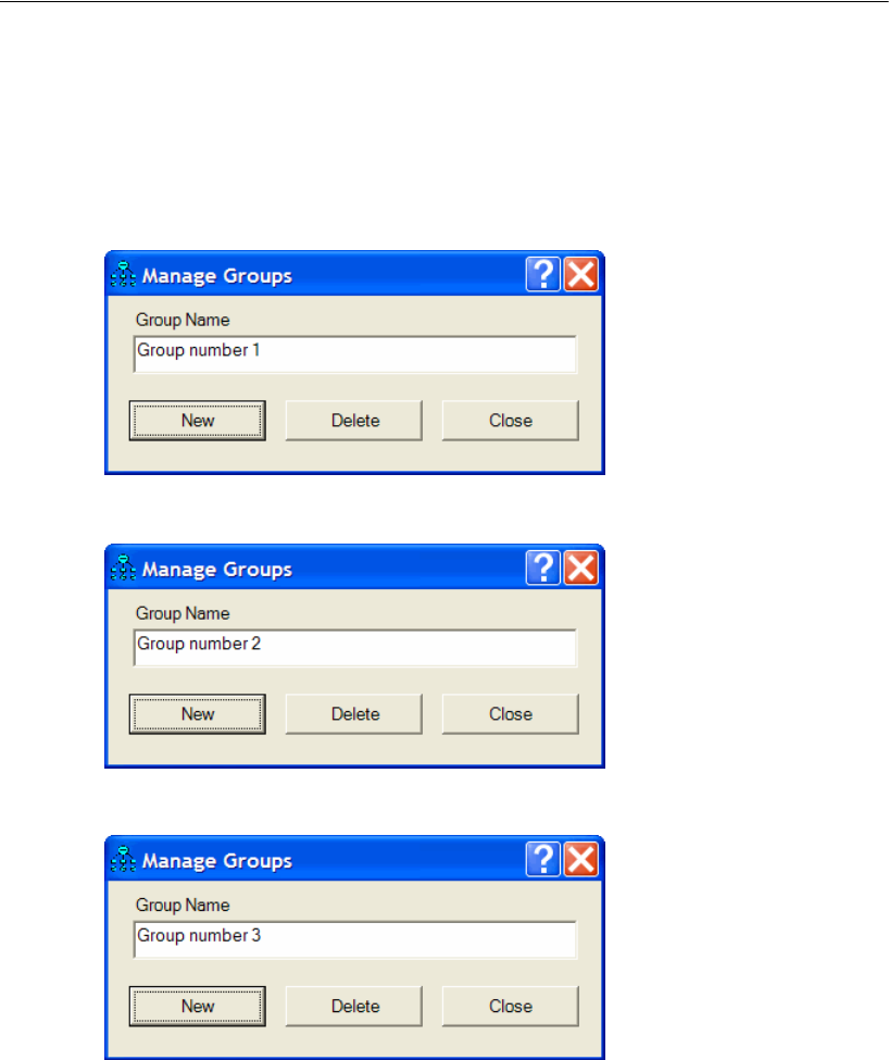
561
Mixture Modeling without Training Data
Performing the Analysis
EFrom the menus, choose File > New to start a new path diagram.
EFrom the menus, choose Analyze > Manage Groups.
EClick New to create a second group.
EClick New once more to create a third group.
EClick Close.
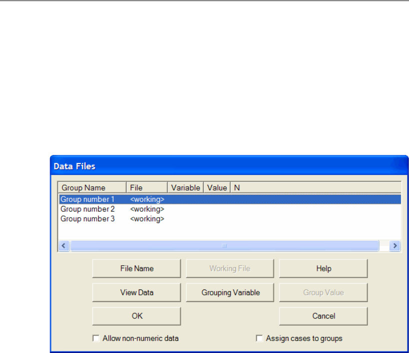
562
Example 35
This example fits a three-group mixture model. When you aren’t sure how many
groups there are, you can run the program multiple times. Run the program once to fit
a two-group model, then again to fit a three-group model, and so on.
Specifying the Data File
EFrom the menus, choose File > Data Files.
EClick Group number 1 to select the first row.
EClick File Name, select the iris2.sav file that is in the Amos Examples directory, and
click Open.
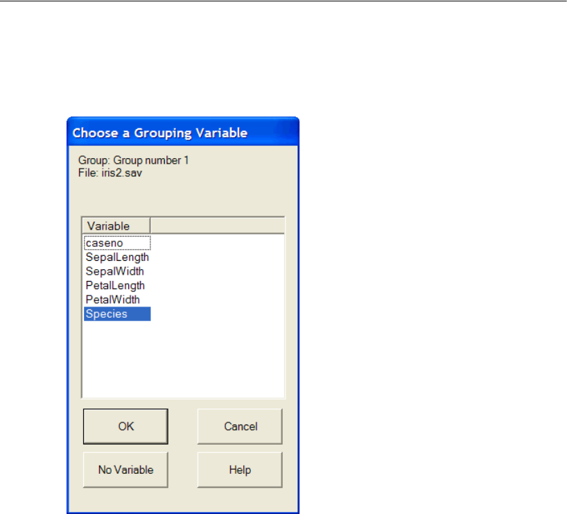
563
Mixture Modeling without Training Data
EClick Grouping Variable and double-click Species in the Choose a Grouping Variable
dialog. This tells the program that the Species variable will be used to distinguish one
group from another.
ERepeat the preceding steps for Group number 2, specifying the same data file (iris2.sav)
and the same grouping variable (Species).
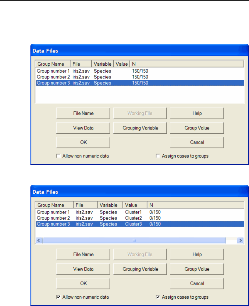
564
Example 35
ERepeat the preceding steps once more for Group number 3, specifying the same data file
(iris2.sav) and the same grouping variable (Species).
ESelect Assign cases to groups (a check mark will appear next to it).
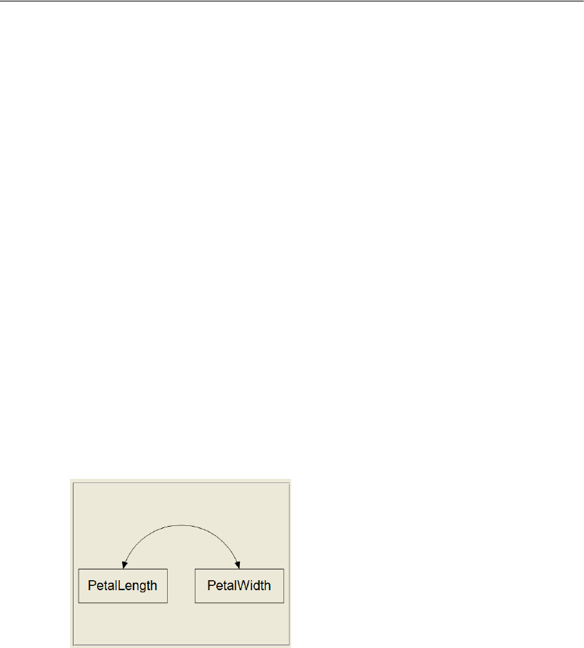
565
Mixture Modeling without Training Data
So far, this has been just like any ordinary multiple-group analysis except for the check
mark next to Assign cases to groups. That check mark turns this into a mixture
modeling analysis. The check mark tells Amos to assign a flower to a group if the
grouping variable in the data file does not already assign it to a group. Notice that it
was not necessary to click Group Value to specify a value for the grouping variable. The
data file contains no values for the grouping variable (Species), so the program
automatically constructed the following Species values for the three groups: Cluster1,
Cluster2, and Cluster3.
EClick OK to close the Data Files dialog.
Specifying the Model
We will use a saturated model for the variables PetalLength and PetalWidth. The
scatterplot in Example 34 suggests that these two variables will allow the program to
do a good job of classifying the flowers according to species.
Note that you are not limited to saturated models when doing mixture modeling.
You can use a factor analysis model, a regression model, or any other kind of model.
Example 36 demonstrates mixture modeling with a regression model.
EDraw the following path diagram:
EFrom the menus, choose View > Analysis Properties.
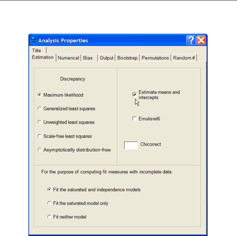
566
Example 35
ESelect Estimate means and intercepts (a check mark will appear next to it).
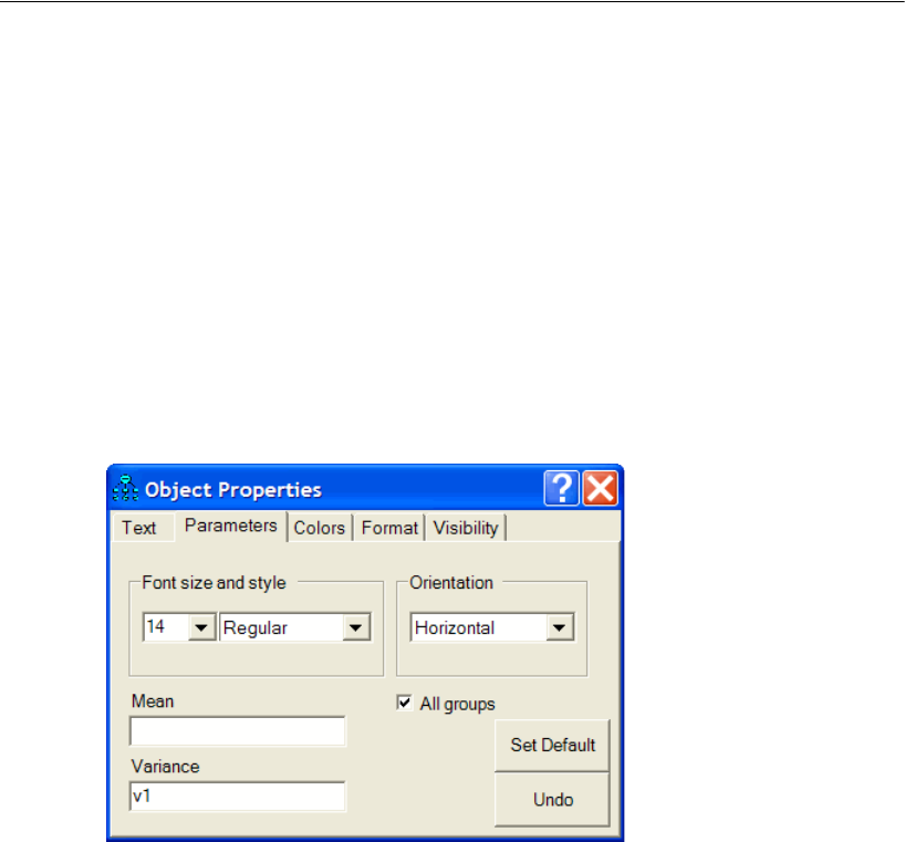
567
Mixture Modeling without Training Data
Constraining the Parameters
In this example, variances and covariances will be required to be invariant across
groups. This is the assumption of homogeneity of variances and covariances that is
often made in discriminant analysis and some kinds of clustering. In principle, the
assumption of homogeneity of variances and covariances is not necessary in mixture
modeling. The reason we will make the assumption here is that, for this example, the
algorithm in Amos fails without that assumption. (It should be noted that the scatterplot
in Example 34 suggests that the assumption is violated.)
ERight-click PetalLength in the path diagram, choose Object Properties from the pop-up
menu, and enter the parameter name, v1, in the Variance text box.
While the Object Properties dialog is still open, click Peta lWidth in the path diagram.
EWhile the Object Properties dialog is still open, click PetalWidth in the path diagram.
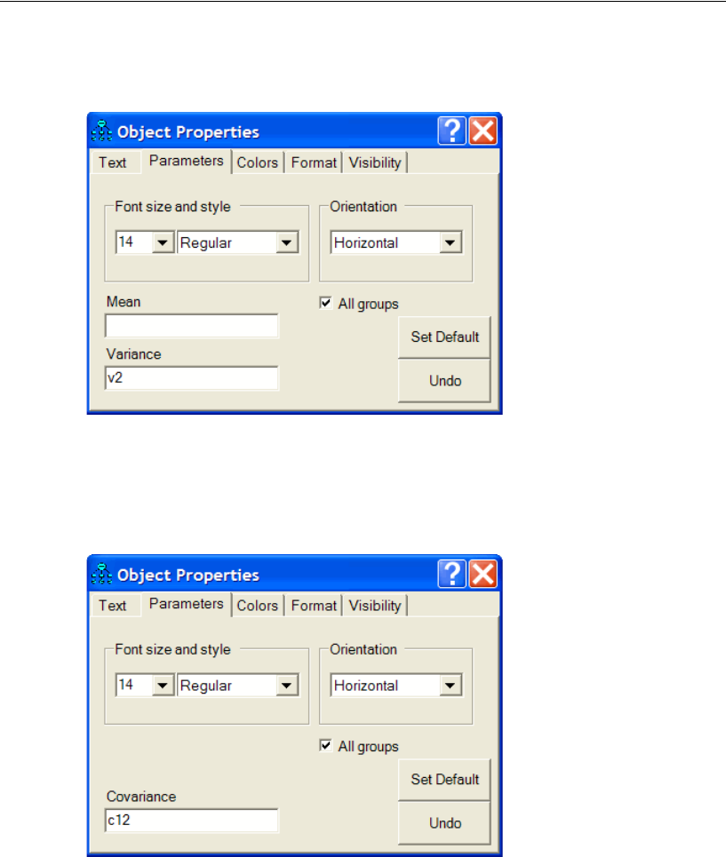
568
Example 35
EIn the Object Properties dialog, enter the parameter name, v2, in the Variance text box.
EWhile the Object Properties dialog is still open, click the double-headed arrow that
represents the covariance between PetalLength and PetalWidth.
EIn the Object Properties dialog, enter the parameter name, c12, in the Covariance text
box.
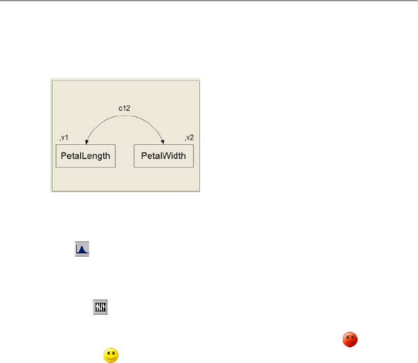
569
Mixture Modeling without Training Data
The path diagram should now look like the following figure. (This path diagram is
saved as Ex35-a.amw.)
Fitting the Model
EClick on the toolbar.
or
EFrom the menus, choose Analyze > Bayesian Estimation.
Note: The button is disabled because, in mixture modeling, you can perform only
Bayesian estimation.
After the Bayesian SEM window opens, wait until the unhappy face changes into
a happy face . The table of estimates in the Bayesian SEM window should then look
something like this:
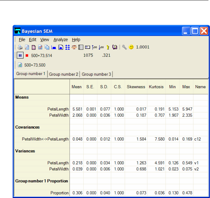
570
Example 35
The Bayesian SEM window displays all of the parameter estimates that you would get
in an ordinary three-group analysis. The table displays the estimates for one group at a
time. You can switch from one group to another by clicking the tabs at the top of the
table. In this example, the model parameters include only means, variances, and
covariances. In a more complicated model, there would also be estimates of regression
weights and intercepts.
In a mixture modeling analysis, you also get an estimate of the proportion of the
population that lies in each group. In the preceding figure, the proportion of setosa
flowers in the population is estimated to be 0.306.
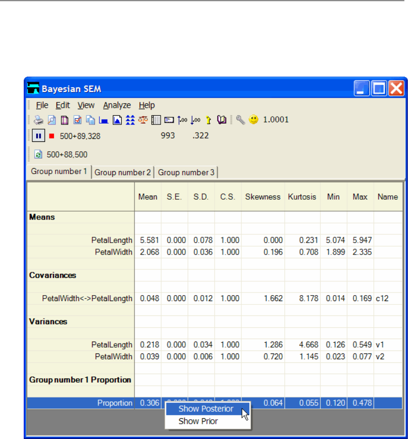
571
Mixture Modeling without Training Data
ETo view the posterior distribution of a population proportion, right-click the row that
contains the proportion and choose Show Posterior from the pop-up menu.
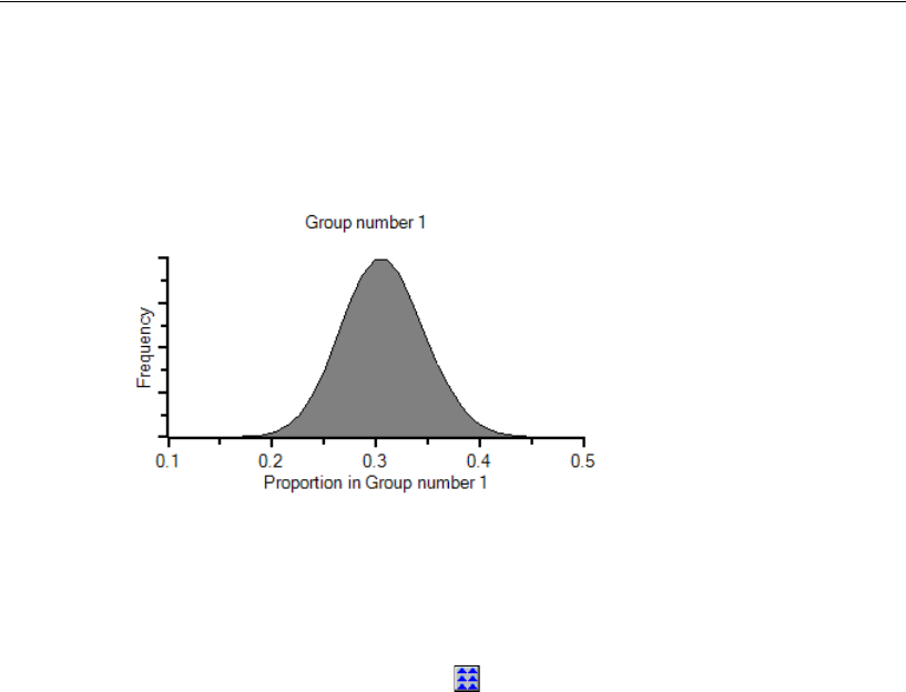
572
Example 35
The graph of the posterior distribution in the Posterior window shows that the
proportion of flowers that belong in Group number 1 is certainly between 0.15 and
0.45. There is a very high probability that the proportion is between 0.25 and 0.35.
Classifying Individual Cases
To obtain probabilities of group membership for each individual flower:
EClick the Posterior Predictive button .
or
EFrom the menus, choose View > Posterior Predictive.
For each flower, the Posterior Predictive Distributions window shows the probability
that the value of the Species variable is Cluster1, Cluster2, or Cluster3.
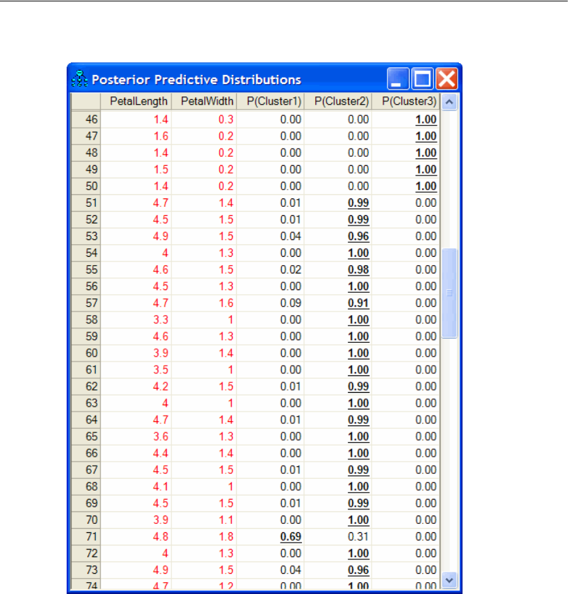
573
Mixture Modeling without Training Data
The first 50 cases, which we know to be examples of setosa, are placed in Group
number 3 with a probability of 1, so Group number 3 clearly contains setosa flowers.
Cases 51 through 100 fall mainly into Group number 2, so Group number 2 clearly
contains versicolor flowers. Similarly, although the preceding figure does not show it,
cases 101 through 150 are assigned mainly to Group number 1, so Group number 1
clearly contains virginica flowers.
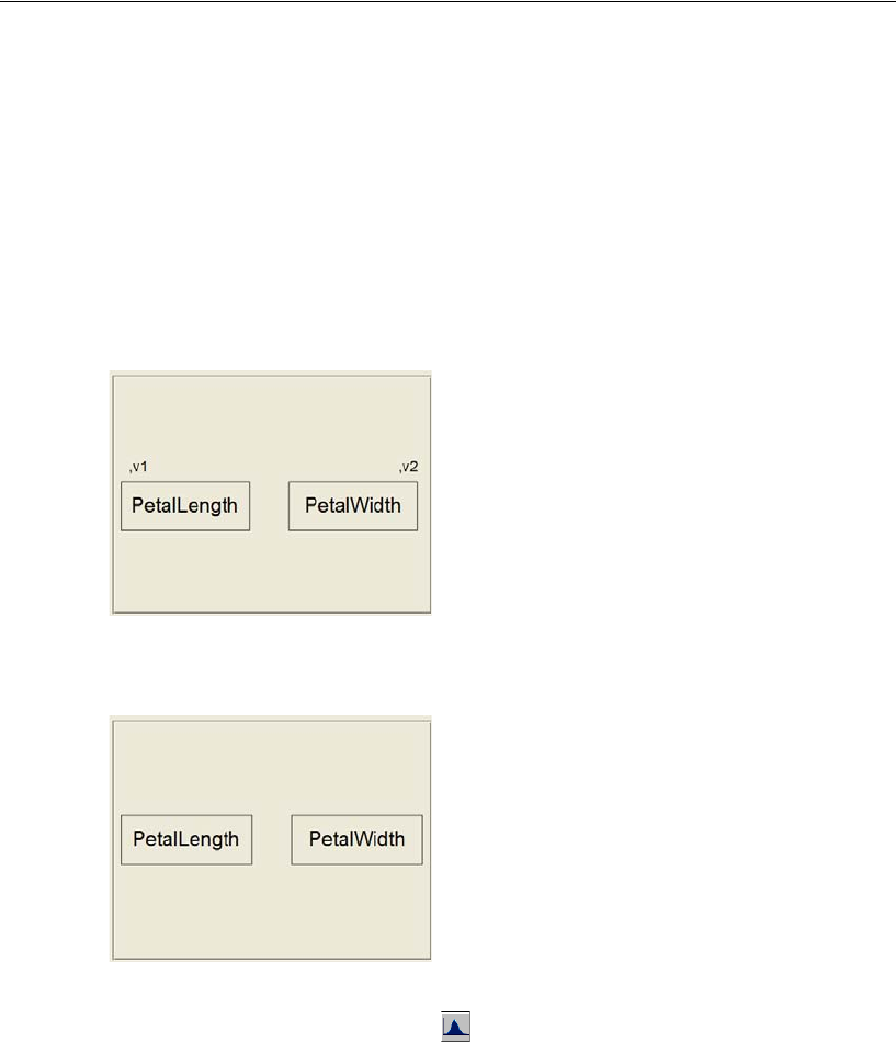
574
Example 35
Latent Structure Analysis
There is a variation of mixture modeling called latent structure analysis in which
observed variables are required to be independent within each group.
ETo require that PetalLength and PetalWidth be uncorrelated and therefore (because
they are multivariate normally distributed) independent, remove the double-headed
arrow that connects them in the path diagram. The resulting path diagram is shown
here. (This path diagram is saved as the file, Ex35-b.amw.)
EOptionally, remove the constraints on the variances by deleting the parameter names,
v1 and v2. (The resulting path diagram is saved as Ex35-c.amw.)
EAfter deleting the double-headed arrow and possibly removing the constraints on the
variances, click the Bayesian button to perform the latent structure analysis. The
results of the latent structure analysis will not be reported here.
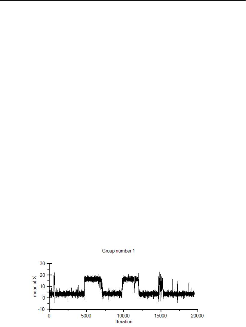
575
Mixture Modeling without Training Data
Label Switching
If you attempt to replicate the analysis in this example, it is possible that you will get
the results that are reported here but with the group names permuted. The results
reported here for Group number 1 might correspond to the results you get for Group
number 2 or Group number 3. This is sometimes called label switching (Chung,
Loken, and Schafer, 2004). Label switching is not really a problem unless it occurs
during the course of a single analysis. Unfortunately, label switching can in fact occur
in the middle of an analysis. When label switching occurs, it is usually revealed by
trace plots for individual parameters. To display a trace plot during Bayesian
estimation:
ERight-click a parameter in the Bayesian SEM window and choose Show Posterior from
the pop-up menu.
EIn the Posterior window, select Trace.
Label switching did not occur in the analysis of the present example. The following
figure, from another analysis, shows a trace plot that is typical of label switching. This
trace plot came from an analysis of data with two clusters of cases. In one cluster, the
mean of a variable called X was about 4. In the other cluster, the mean of the X variable
was about 17. The trace plot shows that, in the group called Group number 1, the
sampled values of the mean of X stayed close to 4 most of the time until about the
5,000-th iteration of the MCMC algorithm. At about the 5,000-th iteration, sampled
values started fluctuating around 17. This abrupt shift in the trace plot is evidence that
the group labels (Group number 1 and Group number 2) were switched at about the
5,000-th iteration. The trace plot shows that this label switching occurred several times
during the first 20,000 iterations of the MCMC algorithm.
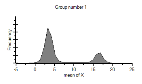
Label switching can be revealed by a multi-model posterior distribution for one or
more parameters. The preceding trace plot corresponds to the following posterior
distribution estimate.
The preceding graph shows that the mean of a parameter’s posterior distribution may
not be a meaningful estimate in a mixture modeling analysis when label switching
occurs. Some methods for preventing label switching have been proposed (Celeux,
Hurn, and Robert, 2000; Frühwirth-Schnatter, 2004; Jasra, Holmes, and Stephens,
2005; Stephens, 2000). Chung, Loken, and Schafer (2004) suggest that pre-assigning
even one or two cases to groups can be effective in eliminating label switching. Amos
allows pre-assigning cases to groups, as shown in Example 34. Amos 25 does not
implement any other method for preventing label switching.

577
Example
36
Mixture Regression Modeling
Introduction
Mixture regression modeling (Ding, 2006) is appropriate when you have a regression
model that is incorrect for an entire population, but where the population can be
divided into subgroups in such a way that the regression model is correct in each
subgroup.
About the Data
Two artificial datasets will be used to explain mixture regression.
First Dataset
The following dataset is in the file DosageAndPerformance1.sav. Dosage is the
intensity of some treatment. Performance is just some performance measure. Group
is a string (non-numeric) variable whose role in mixture regression analysis will be
explained later.
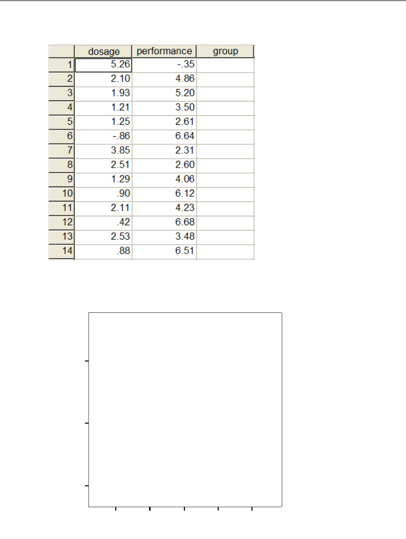
578
Example 36
A scatterplot of dosage and performance shows two distinct groups of people in the
sample. In one group, performance improves as dosage goes up. In the other group,
performance gets worse as dosage goes up.
-2.00 0.00 2.00 4.00 6.00
dosage
0.00
10.00
20.00
performance
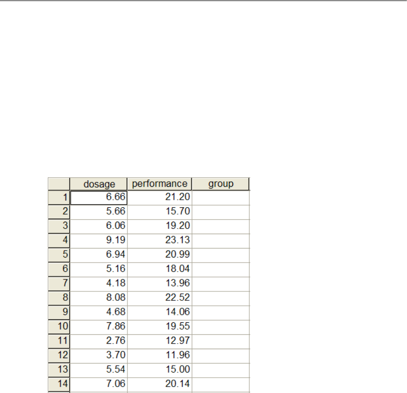
579
Mixture Regression Modeling
It would be a mistake to try to fit a single regression line to the whole sample. On the
other hand, two straight lines, one for each group, would fit the data well. This is a job
for mixture regression modeling. A mixture regression analysis would attempt to
divide the sample up into groups and to fit a separate regression line to each group.
Second Dataset
The following dataset, in the file DosageAndPerformance2.sav, also contains data on
the variables dosage, performance, and group.
Again, a scatterplot of the data shows evidence of two groups, with each group
requiring its own regression line. In either group by itself, an increase of one unit in
dosage is associated with an increase of about two units in performance, so that the
slope of the regression line is about 2 within each group. On the other hand, the two
groups have different intercepts. At any particular dosage level, performance is 5
points or so higher in one group than in the other. A mixture regression analysis of this
dataset would attempt to divide the sample up into groups and to fit a separate
regression line to each group.
580
Example 36
The Group Variable in the Dataset
Both of the datasets just described include a string (non-numeric) variable called group
that contains no data. In a mixture regression analysis, Amos will use the group
variable to classify individual cases. (The fact that the variable is called group is not
important. Any variable name will do; however, it does have to be a string variable.)
If some cases have already been assigned to groups before the analysis starts, you
can put the group names in the group column of the dataset. For example, if you know
ahead of time (before the mixture regression analysis starts) that the sample contains
high performers and low performers and you know that the first two people in the
sample are high performers and that the next three people are low performers, then you
can enter that information in the group column of the data table in the following way:
0.00 5.00 10.00
dosage
5.00
10.00
15.00
20.00
25.00
performance
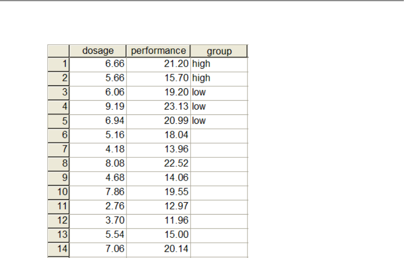
581
Mixture Regression Modeling
The program will then use the five cases that have been pre-classified to assist in
classifying the remaining cases. Pre-assigning selected individual cases to groups is
mentioned here only as a possibility. In the present example, no cases will be pre-
assigned to groups.
Performing the Analysis
Only the DosageAndPerformance2.sav dataset will be analyzed in this example.
EFrom the menus, choose File > New to start a new path diagram.
EFrom the menus, choose Analyze > Manage Groups.
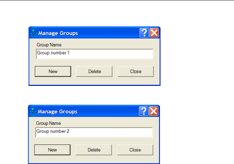
582
Example 36
EClick New to create a second group.
EClick Close.
This example fits a two-group mixture regression model. When you aren’t sure how
many groups there are, you can run the program multiple times. Run the program once
to fit a two-group model, then again to fit a three-group model, and so on.
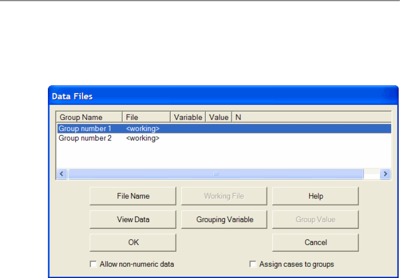
583
Mixture Regression Modeling
Specifying the Data File
EFrom the menus, choose File > Data Files.
EClick Group number 1 to select that row.
EClick File Name, select the DosageAndPerformance2.sav file that is in the Amos
Examples directory, and click Open.
EClick Grouping Variable and double-click group in the Choose a Grouping Variable
dialog. This tells the program that the variable called group will be used to distinguish
one group from another.
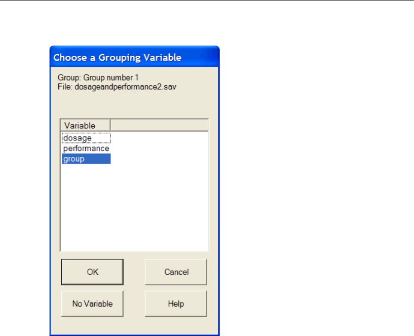
584
Example 36
ERepeat the preceding steps for Group number 2, specifying the same data file
(DosageAndPerformance2.sav) and the same grouping variable (group).
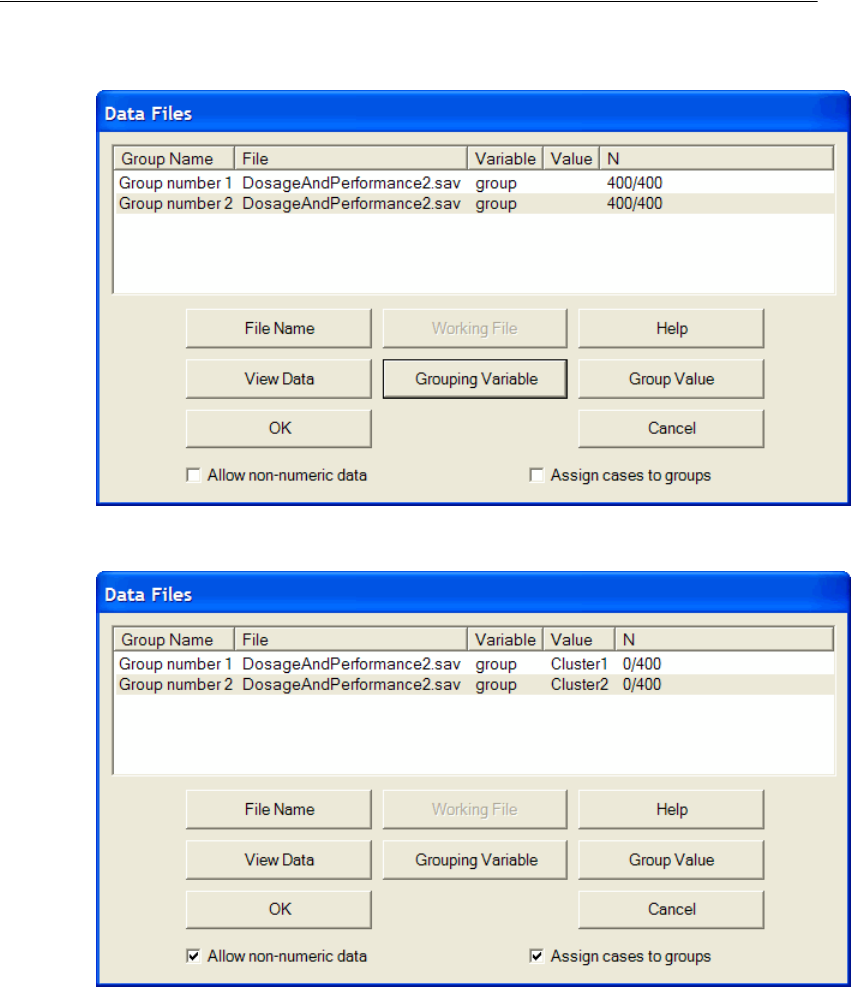
585
Mixture Regression Modeling
ESelect Assign cases to groups (a check mark will appear next to it).
So far, this has been just like any ordinary multiple-group analysis except for the check
mark next to Assign cases to groups. That check mark turns this into a mixture
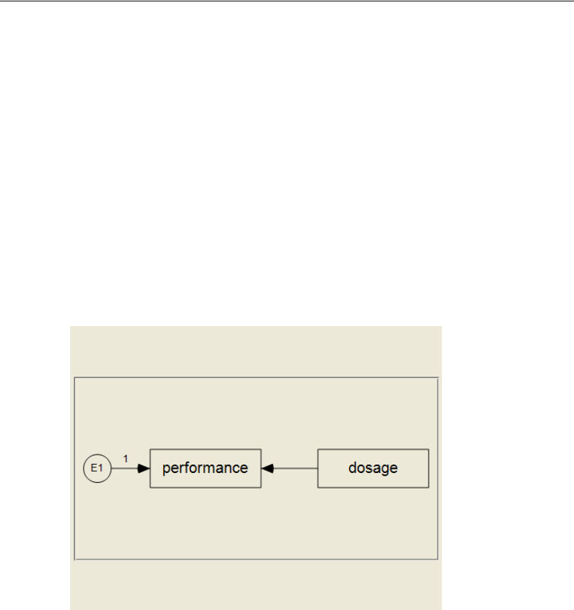
586
Example 36
modeling analysis. The check mark tells Amos to assign a case to a group if the
grouping variable in the data file does not already assign it to a group. Notice that it
was not necessary to click Group Value to specify a value for the grouping variable. The
data file contains no values for the grouping variable (group), so the program
automatically constructed values for the group variable: Cluster1 for cases in Group
number 1, and Cluster2 for cases in Group number 2.
EClick OK to close the Data Files dialog.
Specifying the Model
EDraw a path diagram for the regression model, as follows. (This path diagram is saved
as Ex36-a.amw.)
EFrom the menus, choose View > Analysis Properties.
ESelect Estimate means and intercepts (a check mark will appear next to it).
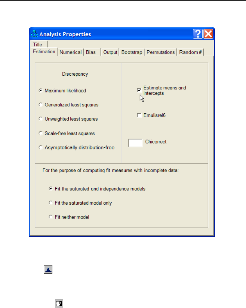
587
Mixture Regression Modeling
Fitting the Model
EClick on the toolbar.
or
EFrom the menus, choose Analyze > Bayesian Estimation.
Note: The button is disabled because, in mixture modeling, you can perform only
Bayesian estimation.
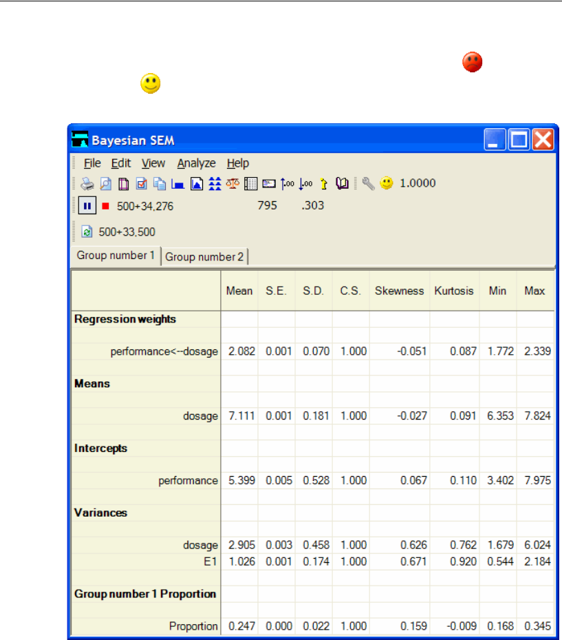
588
Example 36
After the Bayesian SEM window opens, wait until the unhappy face changes into
a happy face . The table of estimates in the Bayesian SEM window should then look
something like this:
The Bayesian SEM window contains all of the parameter estimates that you would get
in an ordinary multiple-group regression analysis. There is a separate table of estimates
for each group. You can switch from group to group by clicking the tabs just above the
table of estimates.
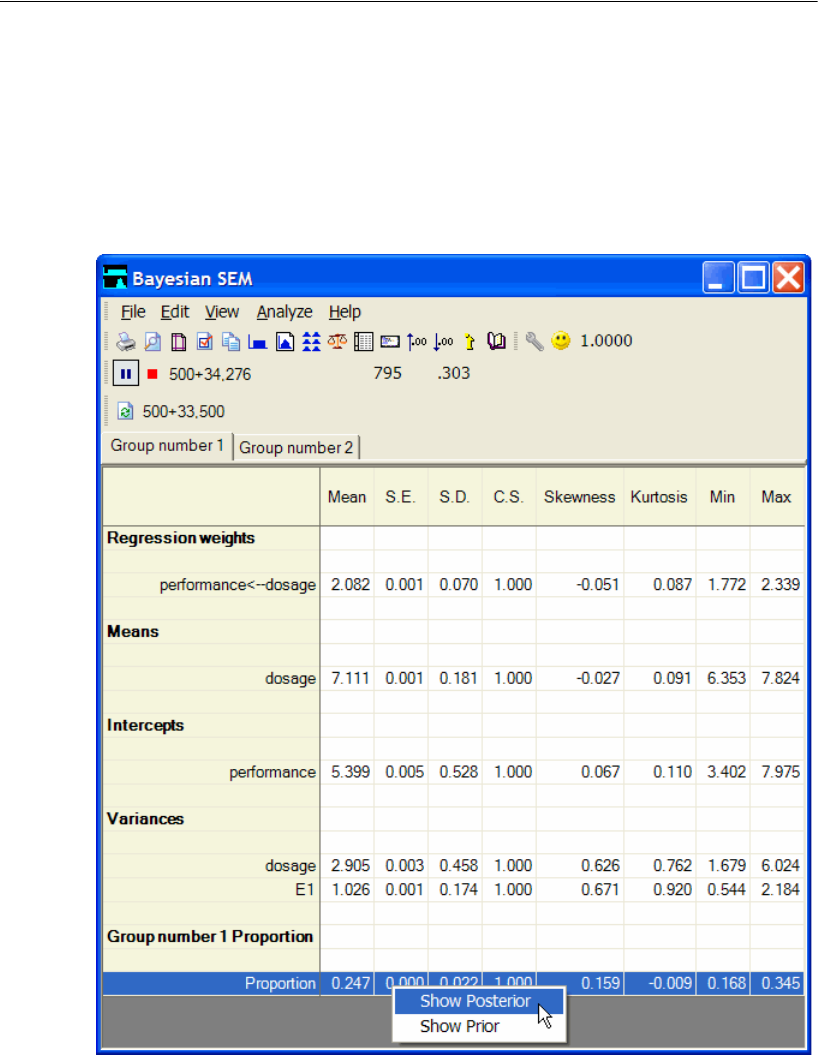
589
Mixture Regression Modeling
The bottom row of the table contains an estimate of the proportion of the population
that lies in an individual group. The preceding figure, which displays estimates for
Group number 1, shows that the proportion of the population in Group number 1 is
estimated to be 0.247. To see the estimated posterior distribution of that population
proportion, right-click the proportion’s row in the table and choose Show Posterior
from the pop-up menu.
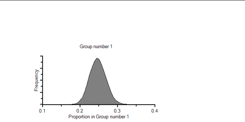
590
Example 36
The graph in the Posterior window shows that the proportion of the population in
Group number 1 is practically guaranteed to be somewhere between 0.15 and 0.35.
Let’s compare the regression weight and the intercept in Group number 1 with the
corresponding estimates in Group number 2. In Group number 1, the regression weight
estimate is 2.082 and the intercept estimate is 5.399. In Group number 2, the regression
weight estimate (1.999) is about the same as in Group number 1 while the intercept
estimate (9.955) is substantially higher than in Group number 1.
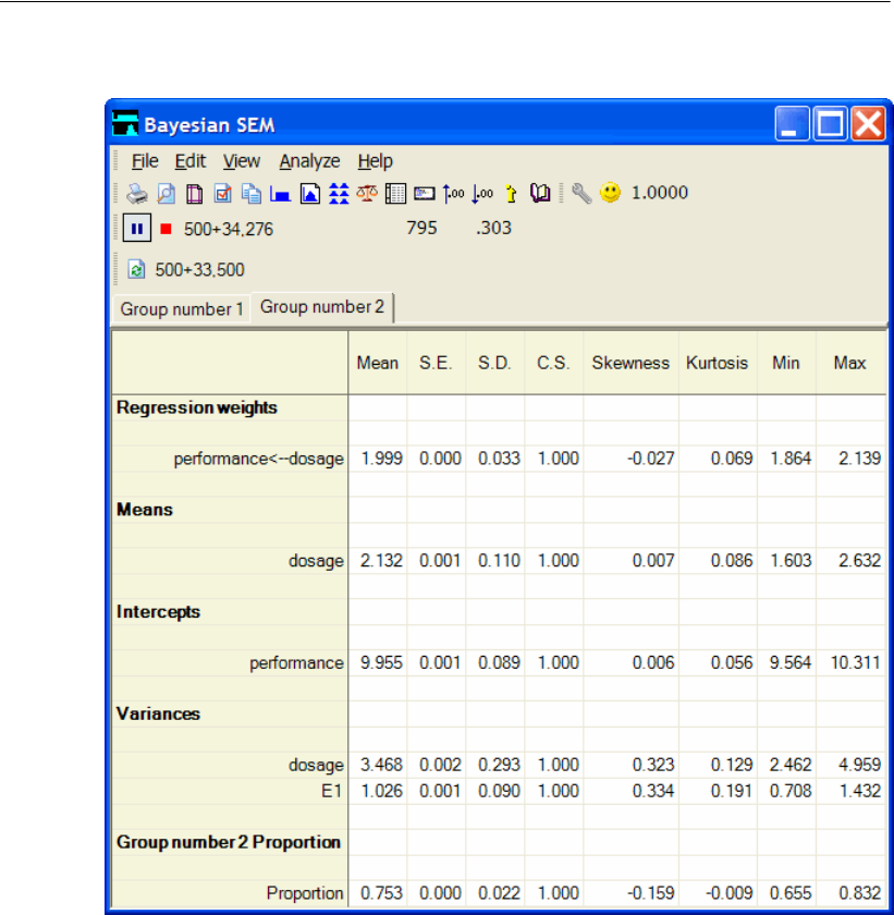
591
Mixture Regression Modeling
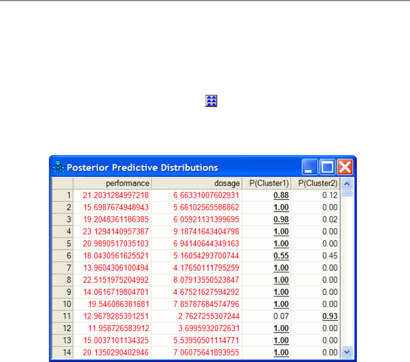
592
Example 36
Classifying Individual Cases
To obtain probabilities of group membership for each individual case:
EClick the Posterior Predictive button .
or
EFrom the menus, choose View > Posterior Predictive.
For each case, the Posterior Predictive Distributions window shows the probability that
the group variable takes on the value Cluster1 or Cluster2. Case 1 is estimated to have
a 0.88 probability of being in Group number 1 and a 0.12 probability of being in Group
number 2. Recall that the first group has an intercept of about 5.399 while the second
group has an intercept of about 9.955, so Group number 1 is the low performing group.
Therefore, there is an 88 percent chance that the first person in the sample is in the low
performing group and a 12 percent chance that that person is in the high performing
group.
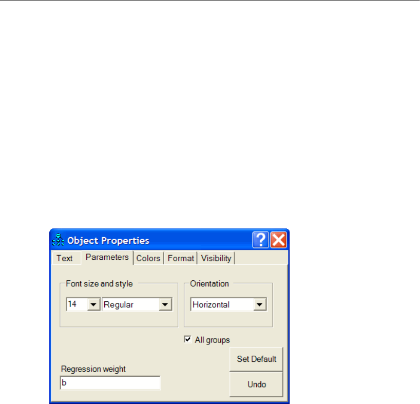
593
Mixture Regression Modeling
Improving Parameter Estimates
You can improve the parameter estimates (and also improve Amos’s ability to form
clusters) by reducing the number of parameters that need to be estimated. As we have
seen, the slope of the regression line is about the same for the two groups. Also, the
variability about each regression line appears to be about the same for the two groups.
It is possible to incorporate into the mixture modeling analysis the hypothesis that the
slopes and the error variances are the same for the two groups, thereby reducing the
number of distinct parameters to be estimated. To do this:
EOn the path diagram, right-click the single-headed arrow that connects dosage and
performance, choose Object Properties from the pop-up menu, and enter the parameter
name, b, in the Regression weight text box.
EWhile the Object Properties dialog is still open, click E1 in the path diagram.
EIn the Object Properties dialog, enter the parameter name, v, in the Variance text box.
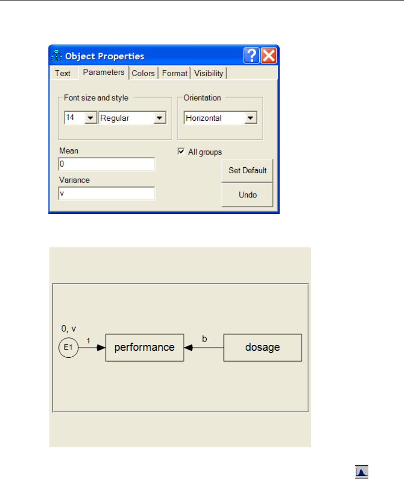
594
Example 36
The path diagram should now look like the following figure. (This path diagram is
saved as Ex36-b.amw.)
After constraining the slope and error variance to be the same for the two groups, you
can repeat the mixture modeling analysis by clicking the Bayesian button . The
results of that analysis will not be presented here.
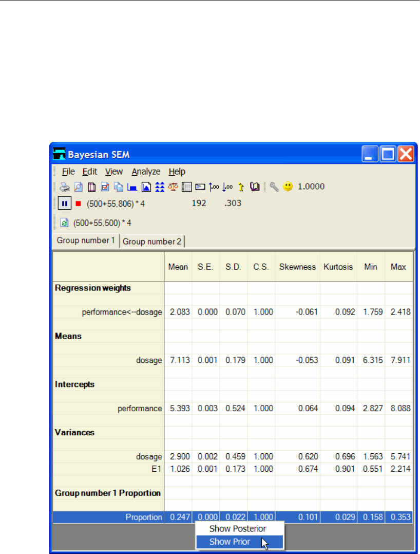
595
Mixture Regression Modeling
Prior Distribution of Group Proportions
For the prior distribution of group proportions, Amos uses a Dirichlet distribution with
parameters that you can specify. By default, the Dirichlet parameters are 4, 4, ….
ETo specify the Dirichlet parameters, right-click on a group proportion’s estimate in the
Bayesian SEM window and choose Show Prior from the pop-up menu.

596
Example 36
Label Switching
It is possible that the results reported here for Group number 1 will match the results
that you get for Group number 2, and that the results reported here for Group number
2 will match those that you get for Group number 1. In other words, your results may
match the results reported here, but with the group names reversed. This is sometimes
called label switching (Chung, Loken, and Schafer, 2004). Label switching is
discussed further at the end of Example 35.

597
Example
37
Using Amos Graphics without
Drawing a Path Diagram
Introduction
People usually specify models in Amos Graphics by drawing path diagrams; however,
Amos Graphics also provides a non-graphical method for model specification. If you
don't want to draw a path diagram, you can specify a model by entering text in the
form of a Visual Basic or C# program. In such a program, each object in a path
diagram (for example, each rectangle, ellipse, single-headed arrow, double-headed
arrow, and figure caption) corresponds to a single program statement. Usually, a
program statement is one line of text.
Here are some reasons why you might choose to specify a model by entering text
rather than by drawing a path diagram.
Your model is so big that drawing its path diagram would be difficult.
You prefer using a keyboard to using a mouse, or prefer working with text to
working with graphics.
You need to generate a lot of similar models that differ only in some detail such
as the number of variables or the variable names. If you need to generate such
models frequently, it can be efficient to automate the chore by creating a super
program whose text output is a tailor-made Visual Basic or C# program that
specifies the particular model that you want Amos to fit.
The present example shows how to specify a model in Amos Graphics by entering text
rather than by drawing a path diagram.
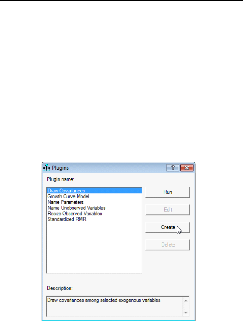
598
Example 37
About the Data
The Holzinger and Swineford (1939) dataset from Example 8 is used for this example.
A Common Factor Model
The factor analysis model from Example 8 is used for this example. Whereas the model
was specified in Example 8 by drawing its path diagram, the same model will be
specified in the current example by writing a Visual Basic program.
Creating a Plugin to Specify the Model
EFrom the menus, choose Plugins > Plugins.
EIn the Plugins dialog, click Create.
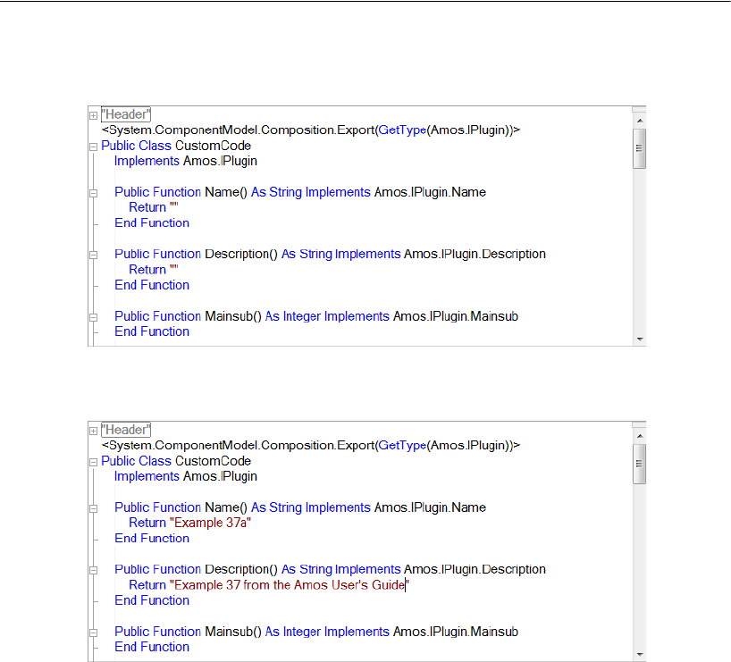
599
Using Amos Graphics without Drawing a Path Diagram
The Program Editor window opens.
EIn the Program Editor window, change the Name and Description functions so that they
return meaningful strings.
You may find it helpful at this point to refer to the first path diagram in Example 8. We
are going to add one line to the Mainsub function for each rectangle, ellipse and arrow
in the path diagram.
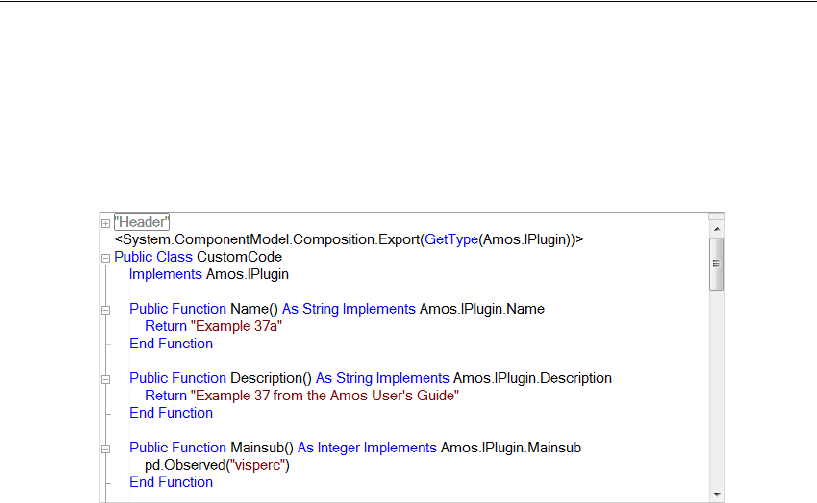
600
Example 37
EIn the Program Editor, enter the line
pd.Observed("visperc")
as the first line in the Mainsub function.
If you save the plugin now, you can use it later on to draw a rectangle representing a
variable called visperc. The rectangle will be drawn with arbitrary height and width at
a random location in the path diagram. You can specify its height, width and location.
For example,
pd.Observed("visperc", 400, 300, 200, 100)
draws a rectangle for a variable called visperc. The rectangle will be centered 400
logical pixels from the left edge of the path diagram, 300 logical pixels from the top
edge. It will be 200 logical pixels wide and 100 logical pixels high. (A logical pixel is
1/96 of an inch.) The online help gives other variations of the Observed method.
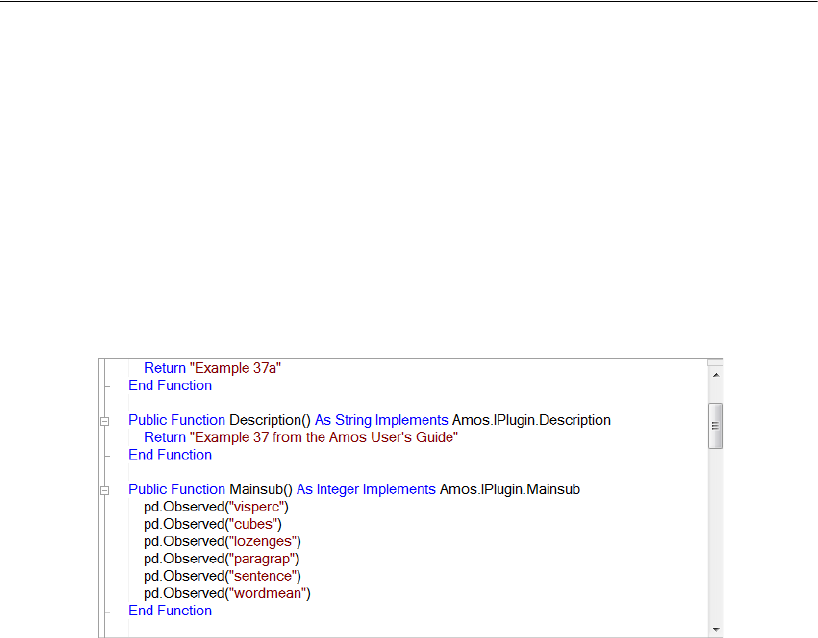
601
Using Amos Graphics without Drawing a Path Diagram
In this example, we will not specify the height, width or location of any path diagram
objects.
EEnter the following additional lines in the Mainsub function so that the plugin will
draw five more rectangles for the five remaining observed variables:
pd.Observed("cubes")
pd.Observed("lozenges")
pd.Observed("paragrap")
pd.Observed("sentence")
pd.Observed("wordmean")
EEnter the following lines so that the plugin will draw eight ellipses for the eight
unobserved variables:
pd.Unobserved("err_v")
pd.Unobserved("err_c")
pd.Unobserved("err_l")
pd.Unobserved("err_p")
pd.Unobserved("err_s")
pd.Unobserved("err_w")
pd.Unobserved("spatial")
pd.Unobserved("verbal")

602
Example 37
EEnter the following lines so that the plugin will draw the 12 single-headed arrows:
pd.Path("visperc", "spatial", 1)
pd.Path("cubes", "spatial")
pd.Path("lozenges", "spatial")
pd.Path("paragrap", "verbal", 1)
pd.Path("sentence", "verbal")
pd.Path("wordmean", "verbal")
pd.Path("visperc", "err_v", 1)
pd.Path("cubes", "err_c", 1)
pd.Path("lozenges", "err_l", 1)
pd.Path("paragrap", "err_p", 1)
pd.Path("sentence", "err_s", 1)
pd.Path("wordmean", "err_w", 1)
Notice that in some of the lines above, the Path method has a third argument that is set
equal to 1. This is how you fix a regression weight to a constant value of 1. See the
online help for other variations of the Path method.
EEnter the following line so that the plugin will draw the double-headed arrow:
pd.Cov("spatial", "verbal")
EEnter the following line to reposition the objects in the path diagram so as to improve
its appearance:
pd.Reposition()
As mentioned above, the simple forms of the Observed, Unobserved and Caption
methods that are used in this example place objects at random positions in the path
diagram. The Reposition method attempts to make the path diagram look better by
rearranging objects. The Reposition method does not produce path diagrams of
presentation quality. Far from it, in fact. On the other hand, Reposition usually
improves a path diagram’s appearance substantially. In order to get objects in the path
diagram sized and positioned exactly the way you want, you can use one of the
following approaches.

603
Using Amos Graphics without Drawing a Path Diagram
ESpecify a height, width and location each time you use the Observed, Unobserved and
Caption methods of the pd class. (See the online help for the Observed, Unobserved
and Caption methods.)
or
EIn your plugin, use the Reposition method to improve the positioning of objects. After
running the plugin, use the drawing tools in the Amos Graphics toolbox to interactively
move and resize the objects in the path diagram.
Controlling Undo Capability
EEnter the following line as the first line in the Mainsub function:
pd.UndoToHere
EEnter the following line as the last line in the Mainsub function:
pd.UndoResume
The UndoToHere method and the UndoResume method work together to ensure that
the effect of running the plugin can be undone by one click of the Undo button.
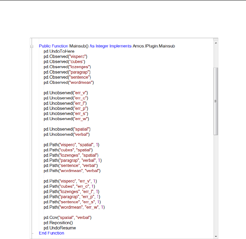
604
Example 37
The Mainsub function now looks like this in the Program Editor:
This completes the plugin for specifying the factor analysis model from Example 8.
Amos comes with a pre-written copy of the plugin in a file called Ex37a-plugin.vb.
Language-specific versions of this file are saved in the folders
%amosplugins%\Japanese and %amosplugins%\English. You can use one of the pre-
written language-specific plugins by copying it to the %amosplugins% folder.
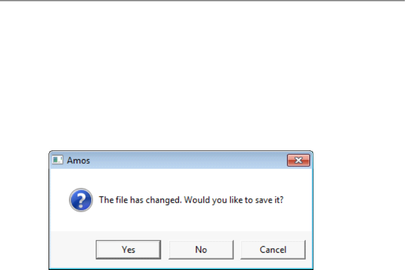
605
Using Amos Graphics without Drawing a Path Diagram
Compiling and Saving the Plugin
EClick the Check Syntax button on the toolbar in the Program Editor window. Any
compilation errors will be displayed on the Syntax errors tab of the Program Editor
window.
EAfter you fix any compilation errors, click Close in the Program Editor window. You
will be asked if you want to save the file:
EClick Yes. The Save As dialog will be displayed.
EIn the Save As dialog, type a filename for your plugin and click Save. Your plugin must
be saved in the Save As dialog’s default folder location. If you have inadvertently
changed the folder in the Save As dialog, you can change it back to the default by
entering %amosplugins% as the folder name.
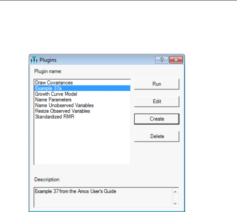
606
Example 37
After you have saved your plugin, its name, Example 37a, appears on the list of plugins
in the Plugins window. (Recall that Example 37a is the string returned by the plugin’s
Name function.)
EClose the Plugins window.
Using the Plugin
EFrom the menus, choose File > New to start with an empty path diagram.
If you are asked whether you want to save your work, choose either Yes or No:
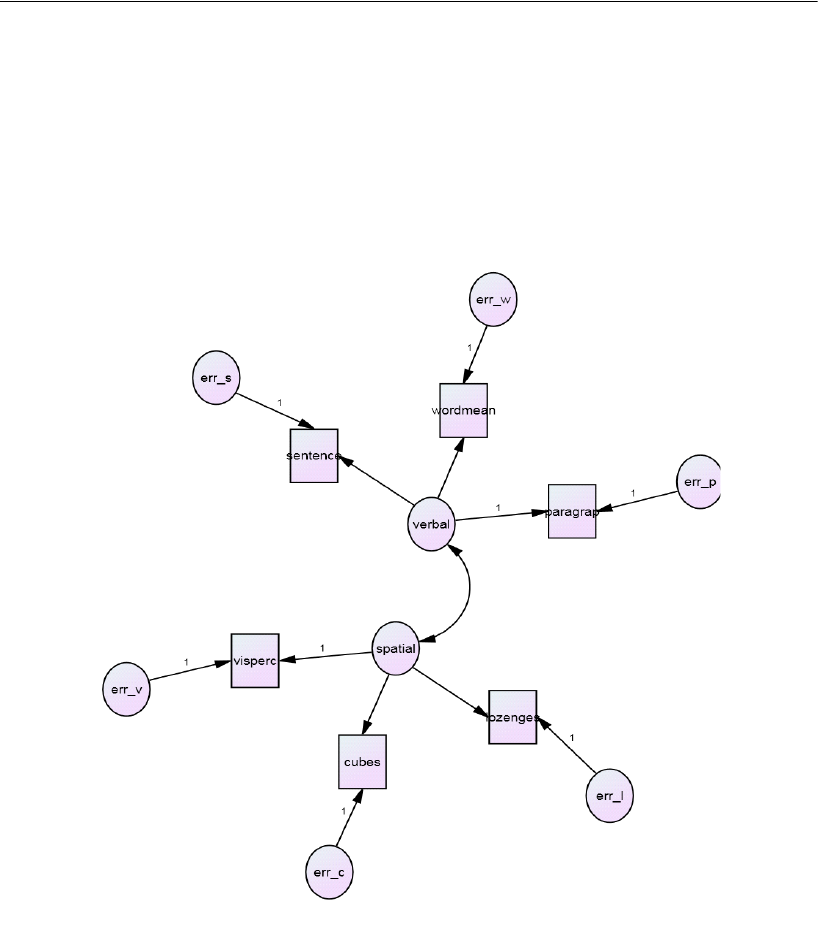
607
Using Amos Graphics without Drawing a Path Diagram
EFrom the menus, choose Plugins > Example 37a. The plugin generates the model’s path
diagram, which is then displayed in the path diagram window. The following path
diagram was generated during the preparation of this example. (You will almost
certainly get a different path diagram because a random number generator plays a role
in positioning the elements in the path diagram.)

608
Example 37
Other Aspects of the Analysis in Addition to Model
Specification
In Example 8, the data file Grnt_fem.sav was specified interactively (by choosing
File > Data Files on the menus). You can do the same thing here as well. As an
alternative, you can specify the Grnt_fem.sav data file within the plugin by adding the
following lines to the Mainsub function:
pd.SetDataFile(1, MiscAmosTypes.cDatabaseFormat.mmSPSS, _
Environment.GetEnvironmentVariable("examples") & "\grnt_fem.sav", "", "",
"")
Similarly, in Example 8, standardized estimates were requested interactively (by
choosing View > Analysis Properties on the menus). As an alternative to requesting
standardized estimates interactively, you can request them within a plugin by adding
the following line to the Mainsub function:
pd.GetCheckBox("AnalysisPropertiesForm", "StandardizedCheck").Checked = True
Generally, any aspect of an analysis that can be specified interactively can be specified
within a plugin by using the methods and properties of the pd class.
Defining Program Variables that Correspond to Model Variables
There are five pd methods that create an object in a path diagram: Observed,
Unobserved, Path, Cov and Caption. Each of these methods returns a reference to the
object that it creates. For example, the Observed method creates an observed variable
in the path diagram and also returns a reference to that observed variable. Instead of
writing the lines
pd.Observed("wordmean")
pd.Unobserved("verbal")
to create an observed variable called wordmean and an unobserved variable called
verbal, you can write the following lines (in Visual Basic):
Dim wordmean As PDElement = pd.Observed("wordmean")
Dim verbal As PDElement = pd.Unobserved("verbal")

609
Using Amos Graphics without Drawing a Path Diagram
Then you can use the program variable wordmean to refer to the model variable called
wordmean, and use the program variable verbal to refer to the model variable called
verbal. If you want to draw a single-headed arrow from the verbal variable to the
wordmean variable, you can write either
pd.Path(wordmean, verbal)
or
pd.Path(“wordmean”, "verbal")
The advantage of the unquoted version over the quoted version is that, with the
unquoted version, typing errors are likely to be detected when you click the Check
Syntax button. With the quoted version, typing errors cannot be detected until you use
the plugin, if they are detected at all.
The file Ex37b-plugin.vb contains a plugin that has the same functionality as Ex37a-
plugin.vb. The difference is that Ex37b-plugin.vb uses Visual Basic variables to refer
to model variables. Language-specific versions of Ex37b-plugin.vb are saved in the
folders %amosplugins%\Japanese and %amosplugins%\English. You can use one of
the pre-written language-specific plugins by copying it to the %amosplugins% folder.

611
Example
38
Simple User-Defined Estimands I
Introduction
This example shows how to estimate user-defined functions of model parameters
along with bootstrap standard errors, confidence intervals, and significance tests. In
this example, a single user-defined function is estimated—an indirect effect.
The example demonstrates a simplified approach to the estimation of user-defined
functions of parameters. The simplified version is limited to estimands that can be
defined by a single expression. A more general version (not demonstrated here) of
Amos's user-defined estimand capability allows the estimands to be defined by a
program of arbitrary length and complexity. The more general version is documented
in the online help under the topic “CValue Class Reference” and is demonstrated in
videos at http://amosdevelopment.com/features/user-defined/user-defined-
general/index.html.
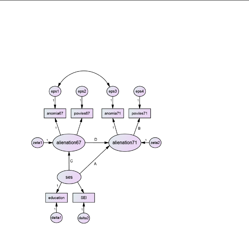
612
Example 38
The Wheaton Data Revisited
Example 6 described three alternative models for the Wheaton et al. (1977) data. Here,
we re-examine Model B from Example 6. The following path diagram, which is in the
file Ex38.amw, shows Model B from Example 6, with some parameter names added.
Estimating an Indirect Effect
Five of the regression weights in this model have been named A, B, C, D, and E, in
order to make it easy to discuss the indirect effect of ses on powles71. There are two
such indirect effects: the product AB and the product CDB. You can estimate the sum
of the two indirect effects, AB + CDB, by clicking View > Analysis Properties > Output
and putting a check mark next to Indirect, direct & total effects. This capability is built
into Amos and does not require you to specify a user-defined estimand. Suppose,
however, that you want to estimate both of the individual indirect effects, AB and CDB,
as well as their sum. All three can be estimated as user-defined estimands in the
following way.
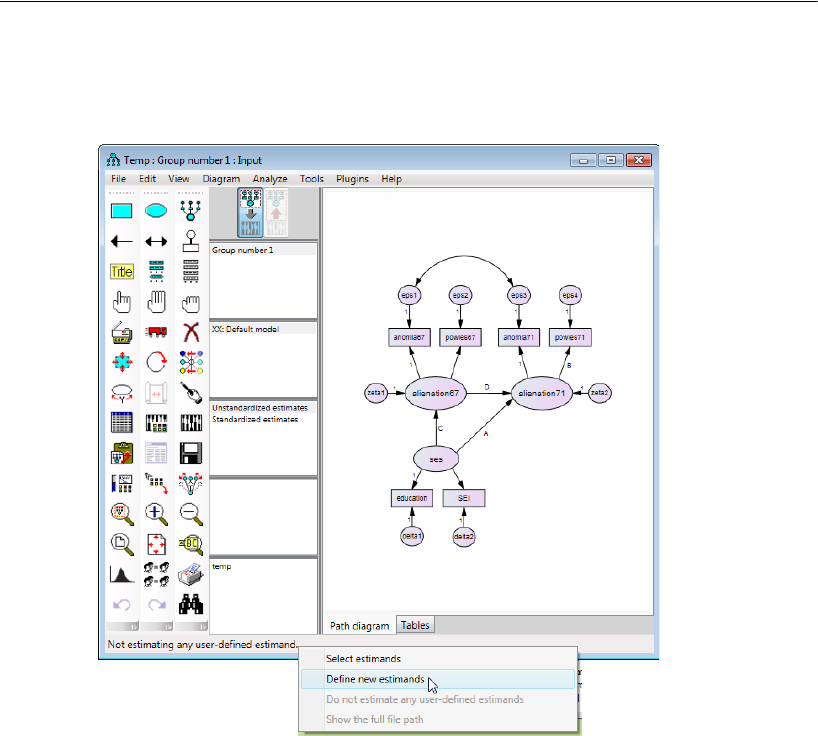
613
Simple User-Defined Estimands I
EClick Not estimating any user-defined estimand on the status bar in the lower-left corner
of the Amos Graphics window. Then click Define new estimands from the pop-up menu.
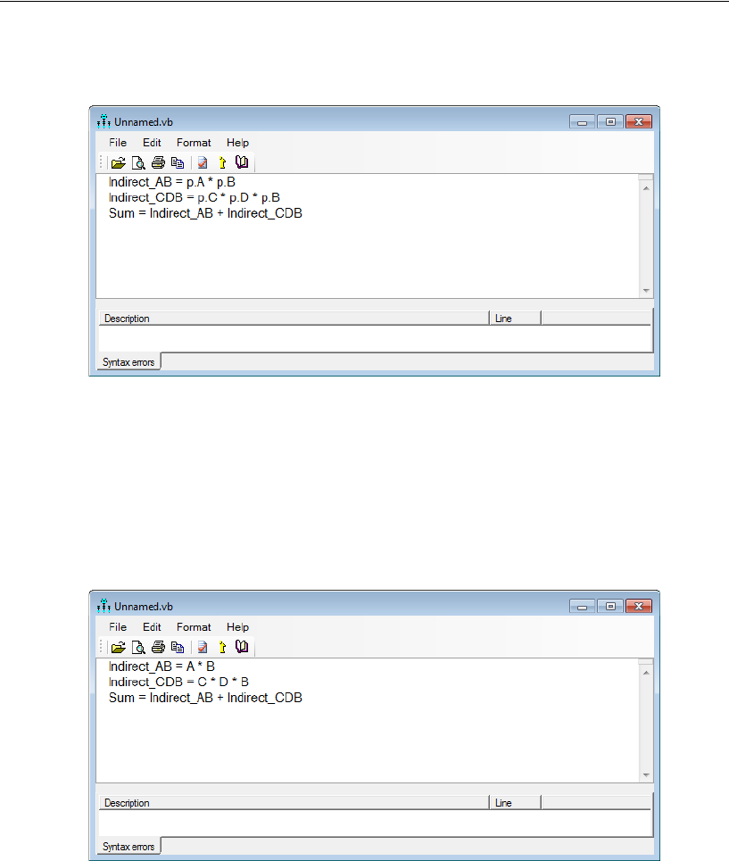
614
Example 38
EIn the new window that opens, enter three lines to define three custom estimands:
The names of the three custom estimands are Indirect_AB, Indirect_CDB and Sum.
You can make up other names instead. Names for estimands must be made up of letters
of the alphabet, numbers, and the underscore character. The first character must be
alphabetic. Uppercase and lowercase are not distinguished, so that if you call an
estimand Abc you cannot call another estimand abc.
The two-character sequence "p." is used as a prefix for parameter names. For example,
"p.A" means "the parameter named A." The "p." prefixes can usually be omitted with
some improvement in readability as shown here:
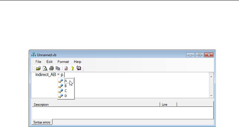
615
Simple User-Defined Estimands I
One benefit of using the "p." prefix is that typing "p." displays a list of parameter names
that you can choose from. In the following screenshot, double-clicking A in the
parameter list has the same effect as typing "A" on the keyboard,
There is one situation where you must use the "p.": If you have a parameter named A
and also a variable named A, then typing a plain “A” will be ambiguous. You will in
that case have to type "p.A" for the parameter called A, or "v.A" for the variable called A,
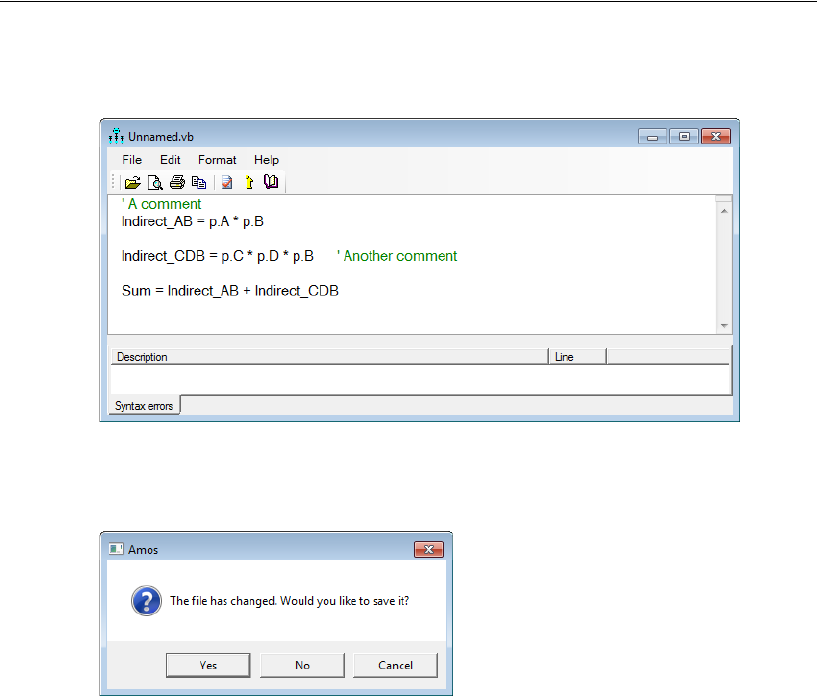
616
Example 38
EOptionally, add lines and comments, as shown here:
EClick the Close button.
E Click Yes in the following dialog.
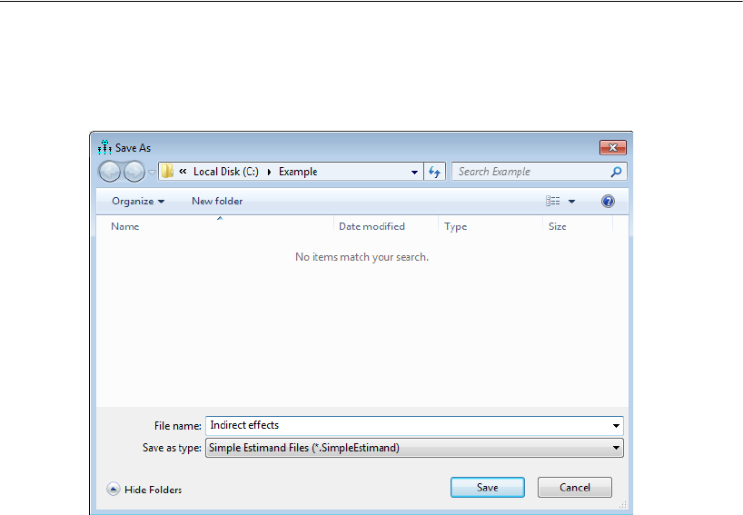
617
Simple User-Defined Estimands I
EIn the Save As dialog, type indirect effects in the File name box. Then click the Save
button.
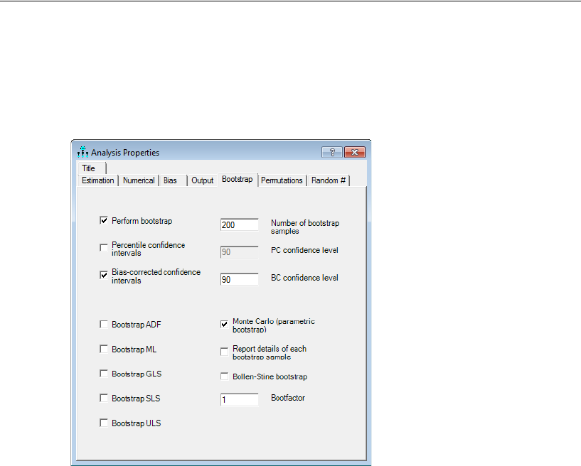
618
Example 38
EClick View > Analysis Properties > Bootstrap, and put check marks next to Perform
bootstrap and Bias-corrected confidence intervals. Also, since the data file contains
sample moments and not raw data, put a check mark next to Monte Carlo (parameteric
bootstrap).
EClick Analyze > Calculate Estimates.
EClick View > Text Output.
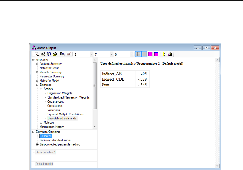
619
Simple User-Defined Estimands I
EIn the Amos Output window, double-click Estimates, then double-click Scalars, then
click User-defined estimands.
The estimand called Indirect_AB is estimated to be –0.205. This is the product of the
regression weight A (–0.212) and the regression weight B (0.971).
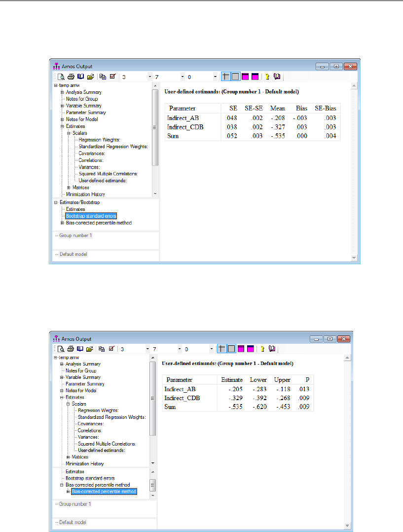
620
Example 38
EClick Bootstrap standard errors.
Indirect_AB is approximately normally distributed with a standard error of about
0.048.
EClick Bootstrap Confidence.
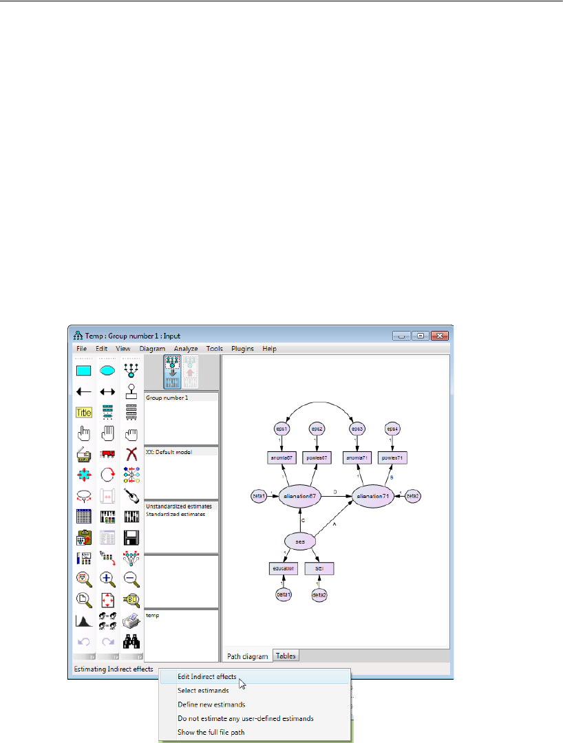
621
Simple User-Defined Estimands I
The population value of the Indirect_AB is between –0.283 and –0.118 with 90%
confidence. The estimate of –0.205 has a p value of 0.013. It is significantly different
from zero at the 0.05 level but not at the 0.01 level.
Estimating the Indirect Effect without Naming Parameters
If you plan on estimating a function of some parameters, it helps to name those
parameters, as was done above. However, you don't have to name the parameters. The
following steps show how to estimate the same indirect effect that we just estimated
but without making use of parameter names.
EClick Estimating Simple indirect effect on the status bar in the lower-left corner of the
Amos Graphics window. Then click Edit Simple indirect effects on the menu that pops
up.
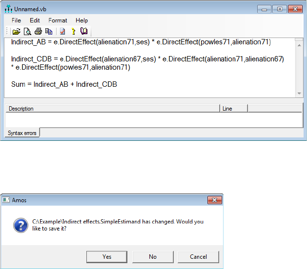
Wherever a parameter is referred to by name, substitute a description of the parameter
as follows.
EChange "p.A" to "e.DirectEffect(alienation71,ses)"
EChange "p.B" to "e.DirectEffect(powles71,alienation71)"
EChange "p.C" to "e.DirectEffect(alienation67,ses)"
EChange "p.D" to "e.DirectEffect(alienation71,alienation67)"
After these substitutions, the specification for the custom estimands looks like this:
E Close the window.
EClick Yes in the dialog that appears.
EClick Analyze > Calculate Estimates.
EClick View > Text Output. (The text output is the same as before.)
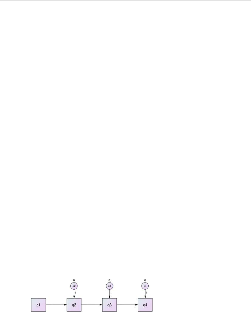
623
Example
39
Simple User-Defined Estimands II
Introduction
This example shows how to estimate the difference between two standardized
regression weights, along with a bootstrap standard error, a confidence interval, and a
significance test for the difference.
About the Data
Four quizzes were administered to a class of 39 students. The quizzes were
approximately equally spaced throughout the semester. The file QuizComplete.txt
contains the scores of the 22 students who took all four quizzes.
A Markov Model
The file Ex39.amw contains the following Markov model for scores on the four
quizzes.
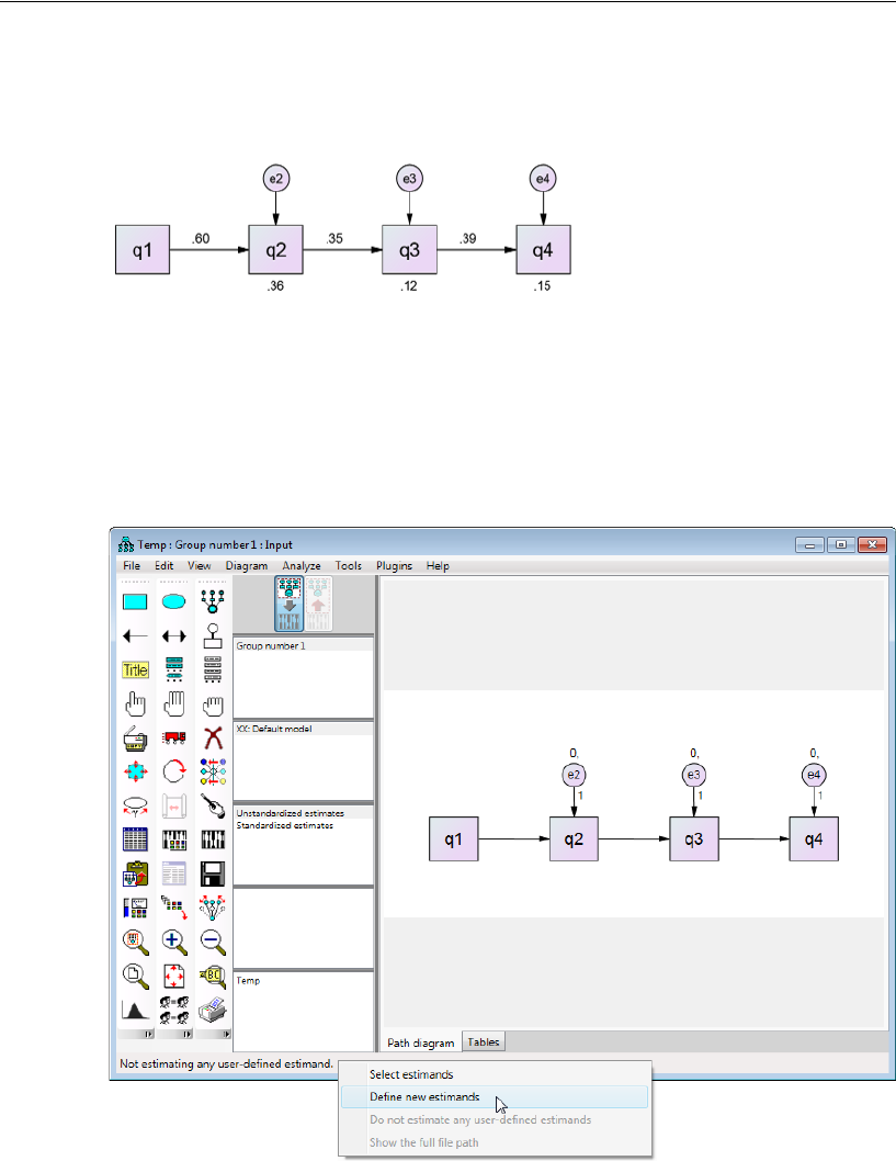
624
Example 39
The following path diagram shows the standardized regression weights estimated for
this model.
Let's compare two standardized regression weights, say the weight for using q2 to
predict q3, and the weight for using q3 to predict q4. The difference between the two
estimates is about . Let's also get a standard error for that
difference, along with a confidence interval and significance test for the difference.
EClick Not estimating any user-defined estimand on the status bar in the lower-left corner of
the Amos Graphics window. Then click Define new estimands on the menu that pops up.
0.39 0.35–0.04=
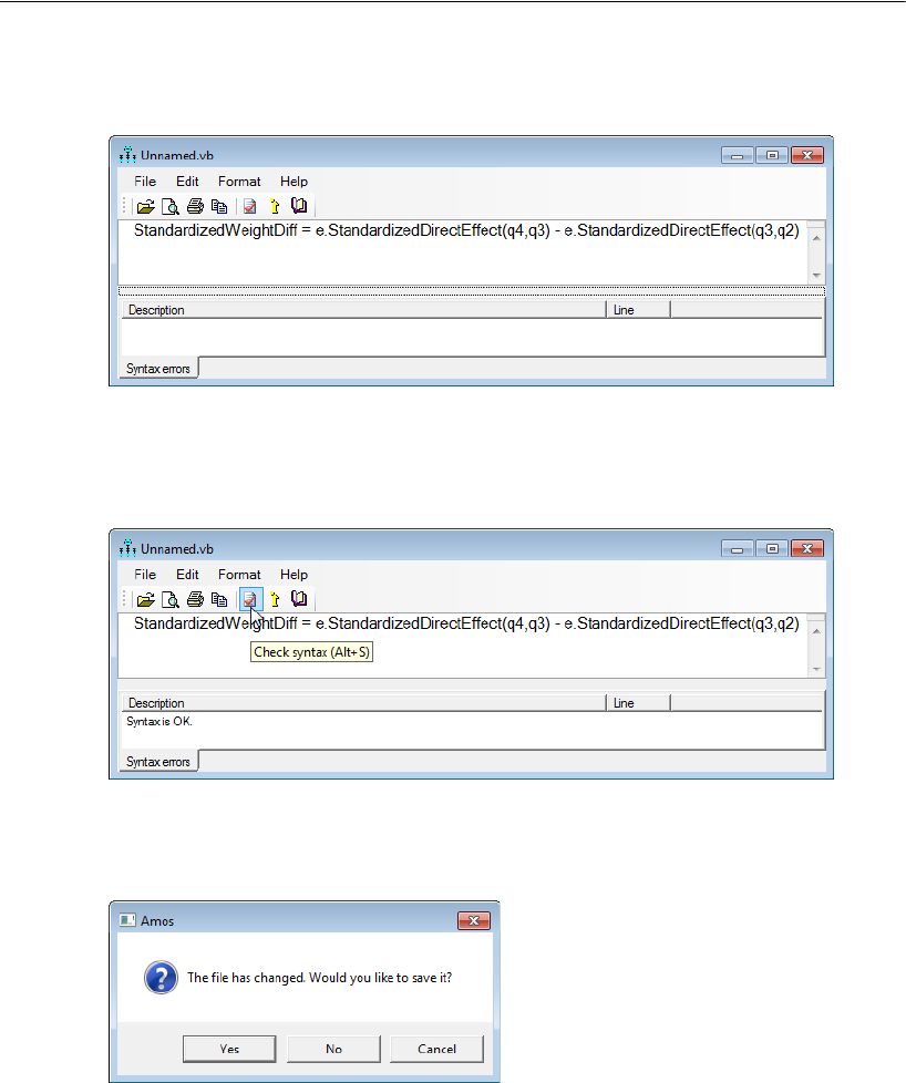
625
Simple User-Defined Estimands II
E In the window that opens, enter one line to specify the new estimand, as follows:
You can choose a name other than StandardizedWeightDiff if you wish.
EClick the Check Syntax button on the toolbar. If you have made no typing mistakes, the
message “Syntax is OK” will be displayed in the Description box.
EClose the window.
E Click Yes in the following dialog.
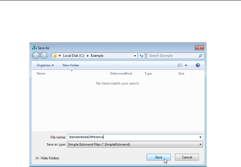
626
Example 39
EIn the Save As dialog, type StandardizedDifference in the File name box. Then click
the Save button.
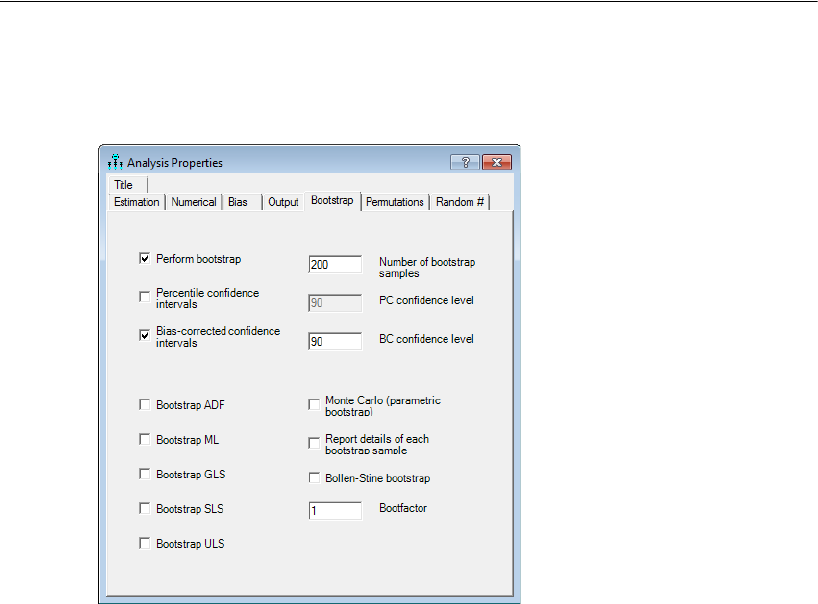
627
Simple User-Defined Estimands II
EClick View > Analysis Properties > Bootstrap, and put check marks next to Perform
bootstrap and Bias-corrected confidence intervals.
EClick Analyze > Calculate Estimates.
EClick View > Text Output.
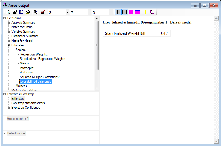
EIn the Amos Output window, double-click Estimates, then double-click Scalars, then
click User-defined estimands.
The estimand called StandardizedWeightDiff is estimated to be 0.047.
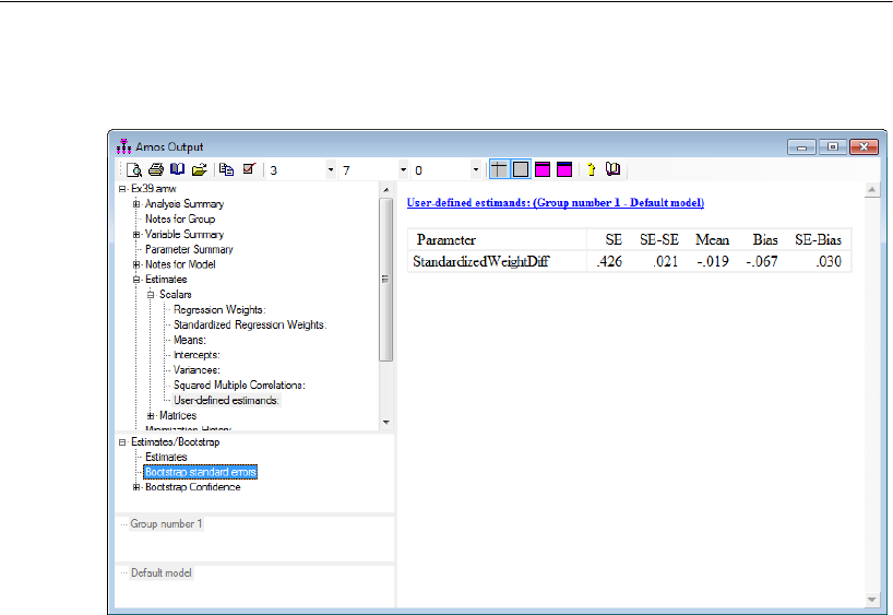
629
Simple User-Defined Estimands II
EClick Bootstrap standard errors.
The difference is approximately normally distributed with a standard error of about
0.426.
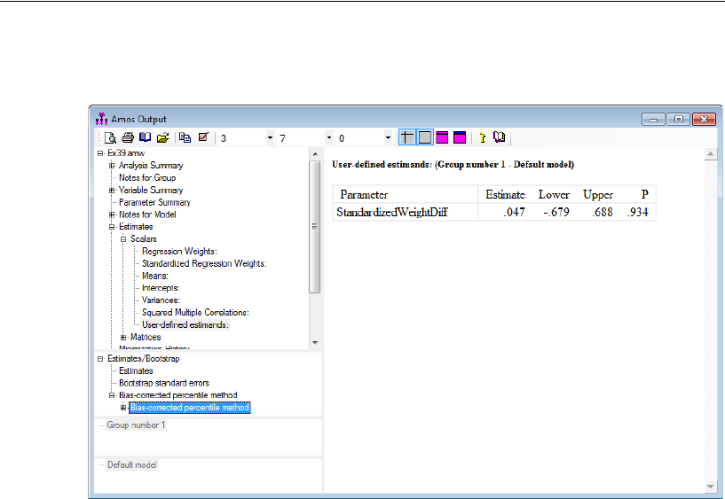
630
Example 39
EClick Bootstrap Confidence.
The population value of the difference is between –0.679 and 0.688 with 90%
confidence. The estimate of 0.047 is not significantly different from zero at any
conventional significance level (p = 0.934).

631
Appendix
A
Notation
q = the number of parameters
= the vector of parameters (of order q)
G = the number of groups
= the number of observations in group g
= the total number of observations in all groups combined
= the number of observed variables in group g
= the number of sample moments in group g. When means and intercepts are
explicit model parameters, the relevant sample moments are means,
variances, and covariances, so that . Otherwise,
only sample variances and covariances are counted so that
.
= the number of sample moments in all groups combined
= the number of degrees of freedom for testing the model
= the r-th observation on the i-th variable in group g
= the r-th observation in group g
= the sample covariance matrix for group g
γ
Ng()
NN
g()
g1=
G
=
pg()
p*g
()
p*g
() pg()pg() 3+()2⁄=
p*g
() pg()pg() 1+()2⁄=
pp
*g
()
g1=
G
=
dpq–=
xir
g
()
xrg
()
Sg()

632
Appendix A
= the covariance matrix for group g, according to the model
= the mean vector for group g, according to the model
= the population covariance matrix for group g
= the population mean vector for group g
= the distinct elements of arranged in a single column
vector
r = the non-negative integer specified by the ChiCorrect method. By default r = G.
When the Emulisrel6 method is used, r = G and cannot be changed by using
ChiCorrect.
n = N – r
= the vector of order p containing the sample moments for all groups; that is,
contains the elements of and also (if means and intercepts are
explicit model parameters) .
= the vector of order p containing the population moments for all groups; that is,
contains the elements of and also (if means and intercepts
are explicit model parameters) . The ordering of the elements of
must match the ordering of the elements of .
= the vector of order p containing the population moments for all groups
according to the model; that is, contains the elements of
and also (if means and intercepts are explicit model
parameters) . The ordering of the elements of must
match the ordering of the elements of .
= the function (of Ö) that is minimized in fitting the model to the sample
= the value of Ö that minimizes
Σg()γ()
μg()γ()
Σ0g()
μ
0g()
sg() vec Sg()
()=
p*g
()
Sg()
σg()γ() vec Σg()γ()
()=
a
a
S1() …SG()
,,
x1() …xG()
,,
a0
a0
Σ1()
0…Σ
G()
0
,,
μ
1()
0…
μ
G()
0
,,
aγ()
a
aγ()
aγ()
Σ1()γ()…Σ
G()
γ(),,
μ
1()γ()…
μ
G()
γ(),,
aγ()
a
Faγ()a,()
γ
ˆ
Faγ()a,()
Σ
ˆg() Σg()γ
ˆ
()=
μ
ˆg() μg()γ
ˆ
()=
a
ˆaγ
ˆ
()=

633
Appendix
B
Discrepancy Functions
Amos minimizes discrepancy functions (Browne, 1982, 1984) of the form:
(D1)
Different discrepancy functions are obtained by changing the way f is defined. If
means and intercepts are unconstrained and do not appear as explicit model
parameters, and will be omitted and f will be written .
The discrepancy functions and are obtained by taking f to be:
Except for an additive constant that depends only on the sample size, is –2 times
the Kullback-Leibler information quantity (Kullback and Leibler, 1951). Strictly
speaking, and do not qualify as discrepancy functions according to
Browne’s definition because .
For maximum likelihood estimation (ML), , and are obtained by taking f to be:
()
[]
() () () () ()
()
[]
()
a
S,x;,
a,, 1
α
μ
α
FrN
N
fN
rNC
G
g
ggggg
−=
Σ
−=
=
xg()
μ
g()
fΣg() Sg()
;()
CKL
FKL
() () () ()
()
() () ()
()
() ()
()
() () ()
()
gggggggggggg
KL
f
μμμ
−Σ
′
−+Σ+Σ=Σ −− xxSS,x;, 11
trlog
fKL
CKL
FKL
FKL aa,()0≠
CML
FML

634
Appendix B
(D2)
For generalized least squares estimation (GLS), , and are obtained by
taking f to be:
(D3)
For asymptotically distribution-free estimation (ADF), , and are obtained
by taking f to be:
(D4)
where the elements of are given by Browne (1984, Equations 3.1–3.4):
() () () ()
()
() () () ()
()
() () () ()
()
() () ()
()
() () () ()
()
() () ()
()
.logtrlog gggggggggg
gggg
KL
gggg
KL
gggg
ML
p
fff
μμ
μμ
−Σ
′
−+−−Σ+Σ=
−Σ=Σ
−− xxSS
S,x;S,xS,x;,S,x;,
11
CGLS
FGLS
() ()
()
() () ()
()
[]
2
2
1tr ggggg
GLS
fΣ−=Σ −SSS; 1
CADF
FADF
() ()
()
() ()
[]
() () ()
[]
=
−
′
−=Σ −
G
g
ggggggg
ADF
f
1
)()(; 1γσγσ sUsS
Ug()
=
=
g
N
r
g
ir
g
g
ix
N
x
1
)()( 1
()()
)()(
1
)()()( 1g
j
g
jr
N
r
g
i
g
ir
g
g
ij xxxx
N
wg
−−=
=
()()()()
)()()()()()(
1
)()()( ,
1g
l
g
lr
g
k
g
kr
g
j
g
jr
N
r
g
i
g
ir
g
gklij xxxxxxxx
N
wg
−−−−=
=

635
Discrepancy Functions
For scale-free least squares estimation (SLS), , and are obtained by taking
f to be:
(D5)
where .
For unweighted least squares estimation (ULS), , and are obtained by
taking f to be:
(D6)
The Emulisrel6 method in Amos can be used to replace (D1) with:
(D1a)
F is then calculated as .
When G = 1 and r = 1, (D1) and (D1a) are equivalent, giving:
For maximum likelihood, asymptotically distribution-free, and generalized least
squares estimation, both (D1) and (D1a) have a chi-square distribution for correctly
specified models under appropriate distributional assumptions. Asymptotically, (D1)
and (D1a) are equivalent; however, both formulas can exhibit some inconsistencies in
finite samples.
()
[
]
)()()( ,, g
kl
g
ij
gklijklij
gwww −=U
CSLS
FSLS
() ()
()
() () ()
()
[]
2
2
1tr ggggg
SLS
fΣ−=Σ −SDS; 1
Dg() diag Sg()
()=
CULS
FULS
() ()
()
() ()
[]
2
2
1tr gggg
ULS
fΣ−=Σ SS;
()
()
()
=
−=
G
g
gg FNC
1
1
FCNG–()⁄=
()
()
()
FNFNC )1(1 11 −=−=

636
Appendix B
Suppose you have two independent samples and a model for each. Furthermore,
suppose that you analyze the two samples simultaneously, but that, in doing so, you
impose no constraints requiring any parameter in one model to equal any parameter in
the other model. Then, if you minimize (D1a), the parameter estimates obtained from
the simultaneous analysis of both groups will be the same as from separate analyses of
each group alone.
Furthermore, the discrepancy function (D1a) obtained from the simultaneous
analysis will be the sum of the discrepancy functions from the two separate analyses.
Formula (D1) does not have this property when r is nonzero. Using formula (D1) to do
a simultaneous analysis of the two groups will give the same parameter estimates as
two separate analyses, but the discrepancy function from the simultaneous analysis
will not be the sum of the individual discrepancy functions.
On the other hand, suppose you have a single sample to which you have fitted some
model using Amos. Now suppose that you arbitrarily split the sample into two groups
of unequal size and perform a simultaneous analysis of both groups, employing the
original model for both groups and constraining each parameter in the first group to be
equal to the corresponding parameter in the second group. If you have minimized (D1)
in both analyses, you will get the same results in both. However, if you use (D1a) in
both analyses, the two analyses will produce different estimates and a different
minimum value for F.
All of the inconsistencies just pointed out can be avoided by using (D1) with the
choice r= 0, so that (D1) becomes:
() ()
FNFNC G
g
gg ==
=1

637
Appendix
C
Measures of Fit
Model evaluation is one of the most unsettled and difficult issues connected with
structural modeling. Bollen and Long (1993), MacCallum (1990), Mulaik, et al.
(1989), and Steiger (1990) present a variety of viewpoints and recommendations on
this topic. Dozens of statistics, besides the value of the discrepancy function at its
minimum, have been proposed as measures of the merit of a model. Amos calculates
most of them.
Fit measures are reported for each model specified by the user and for two
additional models called the saturated model and the independence model.
In the saturated model, no constraints are placed on the population moments. The
saturated model is the most general model possible. It is a vacuous model in the
sense that it is guaranteed to fit any set of data perfectly. Any Amos model is a
constrained version of the saturated model.
The independence model goes to the opposite extreme. In the independence
model, the observed variables are assumed to be uncorrelated with each other.
When means are being estimated or constrained, the means of all observed variables
are fixed at 0. The independence model is so severely and implausibly constrained
that you would expect it to provide a poor fit to any interesting set of data.
It frequently happens that each one of the models that you have specified can be so
constrained as to be equivalent to the independence model. If this is the case, the
saturated model and the independence model can be viewed as two extremes between
which your proposed models lie.
For every estimation method except maximum likelihood, Amos also reports fit
measures for a zero model, in which every parameter is fixed at 0.

638
Appendix C
Measures of Parsimony
Models with relatively few parameters (and relatively many degrees of freedom) are
sometimes said to be high in parsimony, or simplicity. Models with many parameters
(and few degrees of freedom) are said to be complex, or lacking in parsimony. This use
of the terms simplicity and complexity does not always conform to everyday usage. For
example, the saturated model would be called complex, while a model with an
elaborate pattern of linear dependencies but with highly constrained parameter values
would be called simple.
While one can inquire into the grounds for preferring simple, parsimonious models
(such as Mulaik, et al., 1989), there does not appear to be any disagreement that
parsimonious models are preferable to complex ones. When it comes to parameters, all
other things being equal, less is more. At the same time, well-fitting models are
preferable to poorly fitting ones. Many fit measures represent an attempt to balance
these two conflicting objectives—simplicity and goodness of fit.
In the final analysis, it may be, in a sense, impossible to define one best way to
combine measures of complexity and measures of badness-of-fit in a single
numerical index, because the precise nature of the best numerical trade-off
between complexity and fit is, to some extent, a matter of personal taste. The
choice of a model is a classic problem in the two-dimensional analysis of
preference. (Steiger, 1990, p. 179)
NPAR
NPAR is the number of distinct parameters (q) being estimated. For example, two
regression weights that are required to be equal to each other count as one parameter,
not two.
Note: Use the \npar text macro to display the number of parameters in the output path
diagram.
DF
DF is the number of degrees of freedom for testing the model
qpd
−==
df

639
Measures of Fit
where p is the number of sample moments and q is the number of distinct parameters.
Rigdon (1994a) gives a detailed explanation of the calculation and interpretation of
degrees of freedom.
Note: Use the \df text macro to display the degrees of freedom in the output path
diagram.
PRATIO
The parsimony ratio (James, Mulaik, and Brett, 1982; Mulaik, et al., 1989) expresses
the number of constraints in the model being evaluated as a fraction of the number of
constraints in the independence model
where d is the degrees of freedom of the model being evaluated and is the degrees
of freedom of the independence model. The parsimony ratio is used in the calculation
of PNFI and PCFI (see “Parsimony Adjusted Measures” on p. 652).
Note: Use the \pratio text macro to display the parsimony ratio in the output path
diagram.
Minimum Sample Discrepancy Function
The following fit measures are based on the minimum value of the discrepancy.
CMIN
CMIN is the minimum value, , of the discrepancy, C (see Appendix B).
Note: Use the \cmin text macro to display the minimum value of the discrepancy
function C in the output path diagram.
P
P is the probability of getting as large a discrepancy as occurred with the present
sample (under appropriate distributional assumptions and assuming a correctly
i
d
d
=PRATIO
di
C
ˆ
C
ˆ

640
Appendix C
specified model). That is, P is a “p value” for testing the hypothesis that the model fits
perfectly in the population.
One approach to model selection employs statistical hypothesis testing to eliminate
from consideration those models that are inconsistent with the available data.
Hypothesis testing is a widely accepted procedure, and there is a lot of experience in
its use. However, its unsuitability as a device for model selection was pointed out early
in the development of analysis of moment structures (Jöreskog, 1969). It is generally
acknowledged that most models are useful approximations that do not fit perfectly in
the population. In other words, the null hypothesis of perfect fit is not credible to begin
with and will, in the end, be accepted only if the sample is not allowed to get too big.
If you encounter resistance to the foregoing view of the role of hypothesis testing in
model fitting, the following quotations may come in handy. The first two predate the
development of structural modeling and refer to other model fitting problems.
The power of the test to detect an underlying disagreement between theory and
data is controlled largely by the size of the sample. With a small sample an
alternative hypothesis which departs violently from the null hypothesis may still
have a small probability of yielding a significant value of . In a very large
sample, small and unimportant departures from the null hypothesis are almost
certain to be detected. (Cochran, 1952)
If the sample is small, then the test will show that the data are ‘not
significantly different from’ quite a wide range of very different theories, while
if the sample is large, the test will show that the data are significantly
different from those expected on a given theory even though the difference may
be so very slight as to be negligible or unimportant on other criteria. (Gulliksen
and Tukey, 1958, pp. 95–96)
Such a hypothesis [of perfect fit] may be quite unrealistic in most empirical work
with test data. If a sufficiently large sample were obtained this statistic would,
no doubt, indicate that any such non-trivial hypothesis is statistically untenable.
(Jöreskog, 1969, p. 200)
...in very large samples virtually all models that one might consider would have
to be rejected as statistically untenable.... In effect, a nonsignificant chi-square
value is desired, and one attempts to infer the validity of the hypothesis of no
difference between model and data. Such logic is well-known in various
statistical guises as attempting to prove the null hypothesis. This procedure
cannot generally be justified, since the chi-square variate v can be made small by
simply reducing sample size. (Bentler and Bonett, 1980, p. 591)
χ2
χ2
χ2
χ2

641
Measures of Fit
Our opinion...is that this null hypothesis [of perfect fit] is implausible and that it
does not help much to know whether or not the statistical test has been able to
detect that it is false. (Browne and Mels, 1992, p. 78).
See also “PCLOSE” on p. 645.
Note: Use the \p text macro for displaying this p value in the output path diagram.
CMIN/DF
CMIN/DF is the minimum discrepancy, , (see Appendix B) divided by its degrees
of freedom.
Several writers have suggested the use of this ratio as a measure of fit. For every
estimation criterion except for ULS and SLS, the ratio should be close to 1 for correct
models. The trouble is that it isn’t clear how far from 1 you should let the ratio get
before concluding that a model is unsatisfactory.
Rules of Thumb
...Wheaton et al. (1977) suggest that the researcher also compute a relative chi-
square ( ).... They suggest a ratio of approximately five or less ‘as
beginning to be reasonable.’ In our experience, however, to degrees of
freedom ratios in the range of 2 to 1 or 3 to 1 are indicative of an acceptable fit
between the hypothetical model and the sample data. (Carmines and McIver,
1981, p. 80)
...different researchers have recommended using ratios as low as 2 or as high as
5 to indicate a reasonable fit. (Marsh and Hocevar, 1985).
...it seems clear that a ratio > 2.00 represents an inadequate fit. (Byrne,
1989, p. 55).
Note: Use the \cmindf text macro to display the value of CMIN/DF in the output path
diagram.
C
ˆ
d
C
ˆ
χ2df⁄
χ2
χ2df⁄

642
Appendix C
FMIN
FMIN is the minimum value, , of the discrepancy, F (see Appendix B).
Note: Use the \fmin text macro to display the minimum value of the discrepancy
function F in the output path diagram.
Measures Based On the Population Discrepancy
Steiger and Lind (1980) introduced the use of the population discrepancy function as
a measure of model adequacy. The population discrepancy function, , is the value
of the discrepancy function obtained by fitting a model to the population moments
rather than to sample moments. That is,
in contrast to
Steiger, Shapiro, and Browne (1985) showed that, under certain conditions,
has a noncentral chi-square distribution with d degrees of freedom and noncentrality
parameter . The Steiger-Lind approach to model evaluation centers
around the estimation of and related quantities.
This section of the User’s Guide relies mainly on Steiger and Lind (1980) and
Steiger, Shapiro, and Browne (1985). The notation is primarily that of Browne and
Mels (1992).
NCP
is an estimate of the noncentrality parameter,
.
The columns labeled LO 90 and HI 90 contain the lower limit ( ) and upper limit
( ) of a 90% confidence interval, on δ. is obtained by solving
F
ˆ
F
ˆ
F0
F0min Fαγ()α
0
,()[]
γ
=
F
ˆmin Fαγ()a,()[]
γ
=
C
ˆnF
ˆ
=
δ
CnF==
F0
NCP max C
ˆd–0,()=
δ
C0nF0
==
δ
L
δ
U
δ
L
(
)
95.,
ˆ=Φ dC
δ

643
Measures of Fit
for , and is obtained by solving
for , where is the distribution function of the noncentral chi-squared
distribution with noncentrality parameter and d degrees of freedom.
Note: Use the \ncp text macro to display the value of the noncentrality parameter
estimate in the path diagram, \ncplo to display the lower 90% confidence limit, and
\ncphi for the upper 90% confidence limit.
F0
is an estimate of .
The columns labeled LO 90 and HI 90 contain the lower limit and upper limit of a 90%
confidence interval for .
Note: Use the \f0 text macro to display the value of in the output path diagram, \f0lo
to display its lower 90% confidence estimate, and \f0hi to display the upper 90%
confidence estimate.
RMSEA
incorporates no penalty for model complexity and will tend to favor models with
many parameters. In comparing two nested models, will never favor the simpler
model. Steiger and Lind (1980) suggested compensating for the effect of model
complexity by dividing by the number of degrees of freedom for testing the model.
Taking the square root of the resulting ratio gives the population root mean square
δ
δ
U
(
)
05.,|
ˆ=Φ dC
δ
δ
Φx
δ
d,()
δ
F0 F
ˆ0max C
ˆd–
n
-------------0,
NCP
n
-----------== =
δ
n
---F0
=
F0
n
L
δ
= 90 LO
n
U
δ
= 90 HI
F
ˆ0
F0
F0
F0
644
Appendix C
error of approximation, called RMS by Steiger and Lind, and RMSEA by Browne and
Cudeck (1993).
The columns labeled LO 90 and HI 90 contain the lower limit and upper limit of a 90%
confidence interval on the population value of RMSEA. The limits are given by
Rule of Thumb
Practical experience has made us feel that a value of the RMSEA of about 0.05 or
less would indicate a close fit of the model in relation to the degrees of freedom.
This figure is based on subjective judgment. It cannot be regarded as infallible or
correct, but it is more reasonable than the requirement of exact fit with the
RMSEA = 0.0. We are also of the opinion that a value of about 0.08 or less for the
RMSEA would indicate a reasonable error of approximation and would not want
to employ a model with a RMSEA greater than 0.1. (Browne and Cudeck, 1993)
Note: Use the \rmsea text macro to display the estimated root mean square error of
approximation in the output path diagram, \rmsealo for its lower 90% confidence
estimate, and \rmseahi for its upper 90% confidence estimate.
d
F0
RMSEA population =
d
F0
ˆ
RMSEA estimated =
d
n
L
δ
= 90 LO
d
n
U
δ
= 90 HI

645
Measures of Fit
PCLOSE
is a p value for testing the null hypothesis that the
population RMSEA is no greater than 0.05.
By contrast, the p value in the P column (see “P” on p. 639) is for testing the hypothesis
that the population RMSEA is 0.
Based on their experience with RMSEA, Browne and Cudeck (1993) suggest that a
RMSEA of 0.05 or less indicates a close fit. Employing this definition of close fit,
PCLOSE gives a test of close fit while P gives a test of exact fit.
Note: Use the \pclose text macro to display the p value for close fit of the population
RMSEA in the output path diagram.
Information-Theoretic Measures
Amos reports several statistics of the form or , where k is some positive
constant. Each of these statistics creates a composite measure of badness of fit
( or ) and complexity (q) by forming a weighted sum of the two. Simple models
that fit well receive low scores according to such a criterion. Complicated, poorly
fitting models get high scores. The constant k determines the relative penalties to be
attached to badness of fit and to complexity.
The statistics described in this section are intended for model comparisons and not
for the evaluation of an isolated model.
All of these statistics were developed for use with maximum likelihood estimation.
Amos reports them for GLS and ADF estimation as well, although it is not clear that
their use is appropriate there.
AIC
The Akaike information criterion (Akaike, 1973, 1987) is given by
PCLOSE 1 ΦC
ˆ.052nd d,()–=
05.RMSEA :
0
≤
H
0RMSEA :
0=H
C
ˆkq+
F
ˆkq+
C
ˆ
F
ˆ
qC 2
ˆ
AIC +=

646
Appendix C
See also “ECVI” on p. 647.
Note: Use the \aic text macro to display the value of the Akaike information criterion
in the output path diagram.
BCC
The Browne-Cudeck (1989) criterion is given by
where if the
Emulisrel6 command has been used, or if it
has not.
BCC imposes a slightly greater penalty for model complexity than does AIC. BCC
is the only measure in this section that was developed specifically for analysis of
moment structures. Browne and Cudeck provided some empirical evidence suggesting
that BCC may be superior to more generally applicable measures. Arbuckle (in
preparation) gives an alternative justification for BCC and derives the above formula
for multiple groups.
See also “MECVI” on p. 648.
Note: Use the \bcc text macro to display the value of the Browne-Cudeck criterion in
the output path diagram.
BIC
The Bayes information criterion (Schwarz, 1978; Raftery, 1993) is given by the
formula
In comparison to the AIC, BCC, and CAIC, the BIC assigns a greater penalty to model
complexity and, therefore, has a greater tendency to pick parsimonious models. The
BIC is reported only for the case of a single group where means and intercepts are not
explicit model parameters.
()
() ()
()
() ()
() ()
()
=
=
+
−−
+
+= G
g
gg
G
ggg
gg
g
pp
pN
pp
b
qC
1
1
3
2
3
2
ˆ
BCC
bg() Ng() 1–=
bg() nNg()
N
---------=
BIC C
ˆqN
1()
()ln+=

647
Measures of Fit
Note: Use the \bic text macro to display the value of the Bayes information criterion in
the output path diagram.
CAIC
Bozdogan’s (1987) CAIC (consistent AIC) is given by the formula
CAIC assigns a greater penalty to model complexity than either AIC or BCC but not as
great a penalty as does BIC. CAIC is reported only for the case of a single group where
means and intercepts are not explicit model parameters.
Note: Use the \caic text macro to display the value of the consistent AIC statistic in the
output path diagram.
ECVI
Except for a constant scale factor, ECVI is the same as AIC.
The columns labeled LO 90 and HI 90 give the lower limit and upper limit of a 90%
confidence interval on the population ECVI:
See also “AIC” on p. 645.
Note: Use the \ecvi text macro to display the value of the expected cross-validation
index in the output path diagram, \ecvilo to display its lower 90% confidence estimate,
and \ecvihi for its upper 90% confidence estimate.
()
(
)
1ln
ˆ
CAIC 1++= NqC
()
n
q
F
n
2
ˆ
AIC
1
ECVI +==
n
qd
L2
90 LO
++
=
δ
n
qd
U2
90 HI
++
=
δ

648
Appendix C
MECVI
Except for a scale factor, MECVI is identical to BCC.
where if the Emulisrel6 command has been used, or if it
has not.
See also “BCC” on p. 646.
Note: Use the \mecvi text macro to display the modified ECVI statistic in the output
path diagram.
Comparisons to a Baseline Model
Several fit measures encourage you to reflect on the fact that, no matter how badly your
model fits, things could always be worse.
Bentler and Bonett (1980) and Tucker and Lewis (1973) suggested fitting the
independence model or some other very badly fitting baseline model as an exercise to
see how large the discrepancy function becomes. The object of the exercise is to put
the fit of your own model(s) into some perspective. If none of your models fit very
well, it may cheer you up to see a really bad model. For example, as the following
output shows, Model A from Example 6 has a rather large discrepancy ( )
in relation to its degrees of freedom. On the other hand, 71.544 does not look so bad
compared to 2131.790 (the discrepancy for the independence model).
()
()
() ()
()
() ()
() ()
()
=
=
+
−−
+
+== G
g
gg
G
ggg
gg
g
pp
pN
pp
a
qF
n
1
1
3
2
3
2
ˆ
1BCCMECVI
ag() Ng() 1–
NG–
------------------=
ag() Ng()
N
---------=
C
ˆ71.544=

649
Measures of Fit
This things-could-be-much-worse philosophy of model evaluation is incorporated into
a number of fit measures. All of the measures tend to range between 0 and 1, with
values close to 1 indicating a good fit. Only NFI (described below) is guaranteed to be
between 0 and 1, with 1 indicating a perfect fit. (CFI is also guaranteed to be between
0 and 1, but this is because values bigger than 1 are reported as 1, while values less than
0 are reported as 0.)
The independence model is only one example of a model that can be chosen as the
baseline model, although it is the one most often used and the one that Amos uses.
Sobel and Bohrnstedt (1985) contend that the choice of the independence model as a
baseline model is often inappropriate. They suggest alternatives, as did Bentler and
Bonett (1980), and give some examples to demonstrate the sensitivity of NFI to the
choice of baseline model.
NFI
The Bentler-Bonett (1980) normed fit index (NFI), or Δ1 in the notation of Bollen
(1989b) can be written
where is the minimum discrepancy of the model being evaluated and
is the minimum discrepancy of the baseline model.
In Example 6, the independence model can be obtained by adding constraints to any
of the other models. Any model can be obtained by constraining the saturated model.
So Model A, for instance, with , is unambiguously in between the
perfectly fitting saturated model ( ) and the independence model
().
Model NPAR CMIN DF PCMIN/DF
Model A: No Autocorrelation 15 71.544 60.000 11.924
Model B: Most General 16 6.383 5 0.271 1.277
Model C: Time-Invariance 13 7.501 8 0.484 0.938
Model D: A and C Combined 12 73.077 90.000 8.120
Saturated model 21 0.000 0
Independence model 62131.790 15 0.000 142.119
b
bF
F
C
Cˆ
ˆ
1
ˆ
ˆ
1NFI 1−=−=Δ=
C
ˆnF
ˆ
=
Cb
ˆnFb
ˆ
=
χ271.544=
χ20=
χ22131.790=

650
Appendix C
Looked at in this way, the fit of Model A is a lot closer to the fit of the saturated model
than it is to the fit of the independence model. In fact, you might say that Model A has
a discrepancy that is 96.6% of the way between the (terribly fitting) independence
model and the (perfectly fitting) saturated model.
Rule of Thumb
Since the scale of the fit indices is not necessarily easy to interpret (e.g., the indices
are not squared multiple correlations), experience will be required to establish
values of the indices that are associated with various degrees of meaningfulness
of results. In our experience, models with overall fit indices of less than 0.9 can
usually be improved substantially. These indices, and the general hierarchical
comparisons described previously, are best understood by examples. (Bentler and
Bonett, 1980, p. 600, referring to both the NFI and the TLI)
Note: Use the \nfi text macro to display the normed fit index value in the output path
diagram.
RFI
Bollen’s (1986) relative fit index (RFI) is given by
Model NPAR CMIN DF PCMIN/DF
Model A: No Autocorrelation 15 71.544 60.000 11.924
Model B: Most General 16 6.383 50.271 1.277
Model C: Time-Invariance 13 7.501 80.484 0.938
Model D: A and C Combined 12 73.077 90.000 8.120
Saturated model 21 0.000 0
Independence model 62131.790 15 0.000 142.119
966.
790.2131
54.71
1
790.2131
54.71790.2131 =−=
−
=NFI
bb
bb dF
dF
dC
dC ˆ
ˆ
1
ˆ
ˆ
1RFI 1−=−==
ρ

651
Measures of Fit
where and d are the discrepancy and the degrees of freedom for the model being
evaluated, and and are the discrepancy and the degrees of freedom for the
baseline model.
The RFI is obtained from the NFI by substituting F / d for F. RFI values close to 1
indicate a very good fit.
Note: Use the \rfi text macro to display the relative fit index value in the output path
diagram.
IFI
Bollen’s (1989b) incremental fit index (IFI) is given by:
where and d are the discrepancy and the degrees of freedom for the model being
evaluated, and and are the discrepancy and the degrees of freedom for the
baseline model. IFI values close to 1 indicate a very good fit.
Note: Use the \ifi text macro to display the incremental fit index value in the output path
diagram.
TLI
The Tucker-Lewis coefficient (ρ2 in the notation of Bollen, 1989b) was discussed by
Bentler and Bonett (1980) in the context of analysis of moment structures and is also
known as the Bentler-Bonett non-normed fit index (NNFI).
The typical range for TLI lies between 0 and 1, but it is not limited to that range. TLI
values close to 1 indicate a very good fit.
Note: Use the \tli text macro to display the value of the Tucker-Lewis index in the output
path diagram.
C
ˆ
C
ˆb
db
dC
CC
b
b
−
−
=Δ= ˆ
ˆˆ
IFI 2
C
ˆ
C
ˆb
db
1
TLI ˆ
ˆ
ˆ
2−
−
==
b
b
b
b
d
C
d
C
d
C
ρ

652
Appendix C
CFI
The comparative fit index (CFI; Bentler, 1990) is given by
where , d, and NCP are the discrepancy, the degrees of freedom, and the
noncentrality parameter estimate for the model being evaluated, and , , and
are the discrepancy, the degrees of freedom, and the noncentrality parameter
estimate for the baseline model.
The CFI is identical to McDonald and Marsh’s (1990) relative noncentrality index
(RNI)
except that the CFI is truncated to fall in the range from 0 to 1. CFI values close to 1
indicate a very good fit.
Note: Use the \cfi text macro to display the value of the comparative fit index in the
output path diagram.
Parsimony Adjusted Measures
James, et al. (1982) suggested multiplying the NFI by a parsimony index so as to take
into account the number of degrees of freedom for testing both the model being
evaluated and the baseline model. Mulaik, et al. (1989) suggested applying the same
adjustment to the GFI. Amos also applies a parsimony adjustment to the CFI.
See also “PGFI” on p. 655.
()
()
b
bb dC
dC
NCP
NCP
1
0,
ˆ
max
0,
ˆ
max
1CFI −=
−
−
−=
C
ˆ
C
ˆb
db
NCPb
bb dC
dC
−
−
−= ˆ
ˆ
1RNI

653
Measures of Fit
PNFI
The PNFI is the result of applying James, et al.’s (1982) parsimony adjustment to the
NFI
where d is the degrees of freedom for the model being evaluated, and is the degrees
of freedom for the baseline model.
Note: Use the \pnfi text macro to display the value of the parsimonious normed fit index
in the output path diagram.
PCFI
The PCFI is the result of applying James, et al.’s (1982) parsimony adjustment to the
CFI:
where d is the degrees of freedom for the model being evaluated, and is the degrees
of freedom for the baseline model.
Note: Use the \pcfi text macro to display the value of the parsimonious comparative fit
index in the output path diagram.
GFI and Related Measures
The GFI and related fit measures are described here.
GFI
The GFI (goodness-of-fit index) was devised by Jöreskog and Sörbom (1984) for ML
and ULS estimation, and generalized to other estimation criteria by Tanaka and Huba
(1985).
()( )
b
d
d
NFIPRATIONFIPNFI ==
db
()( )
b
d
d
CFI=PRATIOCFIPCFI =
db

654
Appendix C
The GFI is given by
where is the minimum value of the discrepancy function defined in Appendix B and
is obtained by evaluating F with , g = 1, 2,...,G. An exception has to be
made for maximum likelihood estimation, since (D2) in Appendix B is not defined for
. For the purpose of computing GFI in the case of maximum likelihood
estimation, in Appendix B is calculated as
with , where is the maximum likelihood estimate of . GFI is
always less than or equal to 1. GFI = 1 indicates a perfect fit.
Note: Use the \gfi text macro to display the value of the goodness-of-fit index in the
output path diagram.
AGFI
The AGFI (adjusted goodness-of-fit index) takes into account the degrees of freedom
available for testing the model. It is given by
where
The AGFI is bounded above by 1, which indicates a perfect fit. It is not, however,
bounded below by 0, as the GFI is.
Note: Use the \agfi text macro to display the value of the adjusted GFI in the output path
diagram.
b
F
F
ˆ
ˆ
1GFI −=
F
ˆ
Fb
ˆ
Σg() 0=
Σg() 0=
fΣg() Sg()
;()
() ()
()
() () ()
()
2
2
1tr
Σ−=Σ −ggggg
fSKS; 1
Kg() Σg()γ
ˆML
()=
γ
ˆML
γ
()
d
db
GFI11AGFI −−=
()
=
=
G
g
g
bpd
1
*

655
Measures of Fit
PGFI
The PGFI (parsimony goodness-of-fit index), suggested by Mulaik, et al. (1989), is a
modification of the GFI that takes into account the degrees of freedom available for
testing the model
where d is the degrees of freedom for the model being evaluated, and
is the degrees of freedom for the baseline zero model.
Note: Use the \pgfi text macro to display the value of the parsimonious GFI in the
output path diagram.
Miscellaneous Measures
Miscellaneous fit measures are described here.
HI 90
Amos reports a 90% confidence interval for the population value of several statistics.
The upper and lower boundaries are given in columns labeled HI 90 and LO 90.
HOELTER
Hoelter’s (1983) critical N is the largest sample size for which one would accept the
hypothesis that a model is correct. Hoelter does not specify a significance level to be
used in determining the critical N, although he uses 0.05 in his examples. Amos reports
a critical N for significance levels of 0.05 and 0.01.
b
d
d
GFIPGFI =
()
=
=
G
g
g
bpd
1
*
656
Appendix C
Here are the critical N’s displayed by Amos for each of the models in Example 6:
Model A, for instance, would have been accepted at the 0.05 level if the sample
moments had been exactly as they were found to be in the Wheaton study but with a
sample size of 164. With a sample size of 165, Model A would have been rejected.
Hoelter argues that a critical N of 200 or better indicates a satisfactory fit. In an analysis
of multiple groups, he suggests a threshold of 200 times the number of groups.
Presumably this threshold is to be used in conjunction with a significance level of 0.05.
This standard eliminates Model A and the independence model in Example 6. Model B
is satisfactory according to the Hoelter criterion. I am not myself convinced by
Hoelter’s arguments in favor of the 200 standard. Unfortunately, the use of critical N
as a practical aid to model selection requires some such standard. Bollen and Liang
(1988) report some studies of the critical N statistic.
Note: Use the \hfive text macro to display Hoelter’s critical N in the output path diagram
for , or the \hone text macro for .
LO 90
Amos reports a 90% confidence interval for the population value of several statistics.
The upper and lower boundaries are given in columns labeled HI 90 and LO 90.
RMR
The RMR (root mean square residual) is the square root of the average squared amount
by which the sample variances and covariances differ from their estimates obtained
under the assumption that your model is correct.
Model HOELTER
0.05
HOELTER
0.01
Model A: No Autocorrelation 164 219
Model B: Most General 1615 2201
Model C: Time-Invariance 1925 2494
Model D: A and C Combined 216 277
Independence model 11 14
α0.05=
α0.01=
()
()
===
≤
=
−=
G
g
g
G
g
p
i
ij
j
g
ij
g
ij ps
g
1111
)()( *
ˆ
RMR
σ

657
Measures of Fit
The smaller the RMR is, the better. An RMR of 0 indicates a perfect fit.
The following output from Example 6 shows that, according to the RMR, Model A
is the best among the models considered except for the saturated model:
Note: Use the \rmr text macro to display the value of the root mean square residual in
the output path diagram.
Selected List of Fit Measures
If you want to focus on a few fit measures, you might consider the implicit
recommendation of Browne and Mels (1992), who elect to report only the following fit
measures:
“CMIN” on p. 639
“P” on p. 639
“FMIN” on p. 642
“F0” on p. 643, with 90% confidence interval
“PCLOSE” on p. 645
“RMSEA” on p. 643, with 90% confidence interval
“ECVI” on p. 647, with 90% confidence interval (See also “AIC” on p. 645)
For the case of maximum likelihood estimation, Browne and Cudeck (1989, 1993)
suggest substituting MECVI (p. 648) for ECVI.
Model RMR GFI AGFI PGFI
Model A: No Autocorrelation 0.284 0.975 0.913 0.279
Model B: Most General 0.757 0.998 0.990 0.238
Model C: Time-Invariance 0.749 0.997 0.993 0.380
Model D: A and C Combined 0.263 0.975 0.941 0.418
Saturated model 0.000 1.000
Independence model 12.342 0.494 0.292 0.353

659
Appendix
D
Numeric Diagnosis of
Non-Identifiability
In order to decide whether a parameter is identified or an entire model is identified,
Amos examines the rank of the matrix of approximate second derivatives and of some
related matrices. The method used is similar to that of McDonald and Krane (1977).
There are objections to this approach in principle (Bentler and Weeks, 1980;
McDonald, 1982). There are also practical problems in determining the rank of a
matrix in borderline cases. Because of these difficulties, you should judge the
identifiability of a model on a priori grounds if you can. With complex models, this
may be impossible, so you will have to rely on the numeric determination of Amos.
Fortunately, Amos is pretty good at assessing identifiability in practice.

661
Appendix
E
Using Fit Measures to Rank Models
In general, it is hard to pick a fit measure because there are so many from which to
choose. The choice gets easier when the purpose of the fit measure is to compare
models to each other rather than to judge the merit of models by an absolute standard.
For example, it turns out that it does not matter whether you use RMSEA, RFI, or TLI
when rank ordering a collection of models. Each of those three measures depends on
and d only through , and each depends monotonically on . Thus, each
measure gives the same rank ordering of models. For this reason, the specification
search procedure reports only RMSEA.
The following fit measures depend on and d only through , and they depend
monotonically on . The specification search procedure reports only CFI as
representative of them all.
C
ˆ
C
ˆd⁄
C
ˆd⁄
RMSEA C
ˆd–
nd
-------------1
n
---C
ˆ
d
----1–
==
RFI
ρ
11C
ˆd⁄
C
ˆbdb
⁄
---------------–==
TLI
ρ
2
C
ˆb
db
------C
ˆ
d
----–
C
ˆb
db
------1–
----------------==
C
ˆ
C
ˆd–
C
ˆd–

662
Appendix E
(not reported by Amos)
The following fit measures depend monotonically on and not at all on d. The
specification search procedure reports only as representative of them all.
Each of the following fit measures is a weighted sum of and d and can produce a
distinct rank order of models. The specification search procedure reports each of them
except for CAIC.
NCP max C
ˆd–0,()=
F0 F
ˆ0max C
ˆd–
n
-------------0,
==
CFI 1 max C
ˆd–0,()
max Cb
ˆdb
–C
ˆ
,d–0,()
------------------------------------------------------–=
RNI 1 C
ˆd–
Cb
ˆdb
–
-----------------–=
C
ˆ
C
ˆ
CMIN C
ˆ
=
FMIN C
ˆ
n
----=
NFI 1 C
ˆ
C
ˆb
------–=
C
ˆ
BCC
AIC
BIC
CAIC

663
Using Fit Measures to Rank Models
Each of the following fit measures is capable of providing a unique rank order of
models. The rank order depends on the choice of baseline model as well. The
specification search procedure does not report these measures.
The following fit measures are the only ones reported by Amos that are not functions
of and d in the case of maximum likelihood estimation. The specification search
procedure does not report these measures.
IFI Δ2
=
PNFI
PCFI
C
ˆ
GFI
AGFI
PGFI

665
Appendix
F
Baseline Models for Descriptive Fit
Measures
Seven measures of fit (NFI, RFI, IFI, TLI, CFI, PNFI, and PCFI) require a null or
baseline bad model against which other models can be compared. The specification
search procedure offers a choice of four null, or baseline, models:
Null 1: The observed variables are required to be uncorrelated. Their means and
variances are unconstrained. This is the baseline Independence model in an ordinary
Amos analysis when you do not perform a specification search.
Null 2: The correlations among the observed variables are required to be equal. The
means and variances of the observed variables are unconstrained.
Null 3: The observed variables are required to be uncorrelated and to have means of 0.
Their variances are unconstrained. This is the baseline Independence model used by
Amos 4.0.1 and earlier for models where means and intercepts are explicit model
parameters.
Null 4: The correlations among the observed variables are required to be equal. The
variances of the observed variables are unconstrained. Their means are required to be 0.
Each null model gives rise to a different value for NFI, RFI, IFI, TLI, CFI, PNFI, and
PCFI. Models Null 3 and Null 4 are fitted during a specification search only when
means and intercepts are explicitly estimated in the models you specify. The Null 3
and Null 4 models may be appropriate when evaluating models in which means and
intercepts are constrained. There is little reason to fit the Null 3 and Null 4 models in
the common situation where means and intercepts are not constrained but are
estimated for the sole purpose of allowing maximum likelihood estimation with
missing data.
To specify which baseline models you want to be fitted during specification searches:

666
Appendix F
EFrom the menus, choose Analyze > Specification Search.
EClick the Options button on the Specification Search toolbar.
EIn the Options dialog, click the Next search tab.
The four null models and the saturated model are listed in the Benchmark models
group.

667
Appendix
G
Rescaling of AIC, BCC, and BIC
The fit measures, AIC, BCC, and BIC, are defined in Appendix C. Each measure is of
the form , where k takes on the same value for all models. Small values are
good, reflecting a combination of good fit to the data (small ) and parsimony
(small q). The measures are used for comparing models to each other and not for
judging the merit of a single model.
The specification search procedure in Amos provides three ways of rescaling these
measures, which were illustrated in Examples 22 and 23. This appendix provides
formulas for the rescaled fit measures.
In what follows, let , , and be the fit values for model i.
Zero-Based Rescaling
Because AIC, BCC, and BIC are used only for comparing models to each other, with
smaller values being better than larger values, there is no harm in adding a constant,
as in:
C
ˆkq+
C
ˆ
AIC i()
BCC i()
BIC i()
AIC 0i() AIC i() min
iAIC i()
[]–=
BCC 0i() BCC i() min
iBCC i()
[]–=
BIC 0i() BIC i() min
iBIC i()
[]–=

668
Appendix G
The rescaled values are either 0 or positive. For example, the best model according to
AIC has , while inferior models have positive values that reflect how
much worse they are than the best model.
ETo display , , and after a specification search, click on the
Specification Search toolbar.
EOn the Current results tab of the Options dialog, click Zero-based (min = 0).
Akaike Weights and Bayes Factors (Sum = 1)
ETo obtain the following rescaling, select Akaike weights and Bayes factors (sum = 1) on
the Current results tab of the Options dialog.
Each of these rescaled measures sums to 1 across models. The rescaling is performed
only after an exhaustive specification search. If a heuristic search is carried out or if a
positive value is specified for Retain only the best ___ models, then the summation in
the denominator cannot be calculated, and rescaling is not performed. The are
called Akaike weights by Burnham and Anderson (1998). has the same
interpretation as . Within the Bayesian framework and under suitable
assumptions with equal prior probabilities for the models, the are approximate
posterior probabilities (Raftery, 1993, 1995).
AIC00=
AIC0
AIC0
BCC0
BIC0
AICpi
() eAIC i() 2⁄–
eAIC m()2⁄–
-----------------------------=
BCCpi
() eBCC i() 2⁄–
eBCC m()2⁄–
------------------------------=
BICpi
() eBIC i() 2⁄–
eBIC m()2⁄–
-----------------------------=
AICpi
()
BCCpi
()
AICpi
()
BICpi
()

669
Rescaling of AIC, BCC, and BIC
Akaike Weights and Bayes Factors (Max = 1)
ETo obtain the following rescaling, select Akaike weights and Bayes factors (max = 1) on
the Current results tab of the Options dialog.
For example, the best model according to AIC has , while inferior models
have between 0 and 1. See Burnham and Anderson (1998) for further discussion
of , and Raftery (1993, 1995) and Madigan and Raftery (1994) for further
discussion of .
AICLi
() eAIC i() 2⁄–
max
meAIC m()2⁄–
[]
---------------------------------------=
BCCLi
() eBCC i() 2⁄–
max
meBCC m()2⁄–
[]
----------------------------------------=
BICLi
() eBIC i() 2⁄–
max
meBIC m()2⁄–
[]
---------------------------------------=
AICL1=
AICL
AICL
BICL

671
Notices
This information was developed for products and services offered in the U.S.A.
IBM may not offer the products, services, or features discussed in this document in other
countries. Consult your local IBM representative for information on the products and
services currently available in your area. Any reference to an IBM product, program, or
service is not intended to state or imply that only that IBM product, program, or service may
be used. Any functionally equivalent product, program, or service that does not infringe any
IBM intellectual property right may be used instead. However, it is the user's responsibility
to evaluate and verify the operation of any non-IBM product, program, or service.
IBM may have patents or pending patent applications covering subject matter described in
this document. The furnishing of this document does not grant you any license to these
patents. You can send license inquiries, in writing, to:
IBM Director of Licensing
IBM Corporation
North Castle Drive
Armonk, NY 10504-1785
U.S.A.
For license inquiries regarding double-byte character set (DBCS) information, contact the
IBM Intellectual Property Department in your country or send inquiries, in writing, to:
Intellectual Property Licensing
Legal and Intellectual Property Law
IBM Japan Ltd.
1623-14, Shimotsuruma, Yamato-shi
Kanagawa 242-8502 Japan

672
Notices
The following paragraph does not apply to the United Kingdom or any other country
where such provisions are inconsistent with local law: INTERNATIONAL BUSINESS
MACHINES CORPORATION PROVIDES THIS PUBLICATION "AS IS" WITHOUT
WARRANTY OF ANY KIND, EITHER EXPRESS OR IMPLIED, INCLUDING, BUT
NOT LIMITED TO, THE IMPLIED WARRANTIES OF NON-INFRINGEMENT,
MERCHANTABILITY OR FITNESS FOR A PARTICULAR PURPOSE. Some states do
not allow disclaimer of express or implied warranties in certain transactions, therefore, this
statement may not apply to you.
This information could include technical inaccuracies or typographical errors. Changes are
periodically made to the information herein; these changes will be incorporated in new
editions of the publication. IBM may make improvements and/or changes in the product(s)
and/or the program(s) described in this publication at any time without notice.
Any references in this information to non-IBM Web sites are provided for convenience only
and do not in any manner serve as an endorsement of those Web sites. The materials at those
Web sites are not part of the materials for this IBM product and use of those Web sites is at
your own risk.
IBM may use or distribute any of the information you supply in any way it believes
appropriate without incurring any obligation to you.
Licensees of this program who wish to have information about it for the purpose of enabling:
(i) the exchange of information between independently created programs and other programs
(including this one) and (ii) the mutual use of the information which has been exchanged,
should contact:
IBM Software Group
Attention: Licensing
71 S Wacker Dr, 6th Floor
Chicago, IL 60606
U.S.A.
Such information may be available, subject to appropriate terms and conditions, including in
some cases, payment of a fee.
The licensed program described in this document and all licensed material available for it are
provided by IBM under terms of the IBM Customer Agreement, IBM International Program
License Agreement or any equivalent agreement between us.

673
Notices
Information concerning non-IBM products was obtained from the suppliers of those
products, their published announcements or other publicly available sources. IBM has not
tested those products and cannot confirm the accuracy of performance, compatibility or any
other claims related to non-IBM products. Questions on the capabilities of non-IBM
products should be addressed to the suppliers of those products.
All statements regarding IBM's future direction or intent are subject to change or withdrawal
without notice, and represent goals and objectives only.
This information contains examples of data and reports used in daily business operations. To
illustrate them as completely as possible, the examples include the names of individuals,
companies, brands, and products. All of these names are fictitious and any similarity to the
names and addresses used by an actual business enterprise is entirely coincidental.
If you are viewing this information softcopy, the photographs and color illustrations may not
appear.
Trademarks
IBM, the IBM logo, and ibm.com, and SPSS are trademarks or registered trademarks of
International Business Machines Corp., registered in many jurisdictions worldwide. Other
product and service names might be trademarks of IBM or other companies. A current list of
IBM trademarks is available on the Web at http://www.ibm.com/legal/copytrade.shtml.
AMOS is a trademark of Amos Development Corporation.
Microsoft, Windows, Windows NT, and the Windows logo are trademarks of Microsoft
Corporation in the United States, other countries, or both.

675
Bibliography
Akaike, H. 1973. Information theory and an extension of the maximum likelihood principle. In:
Proceedings of the 2nd International Symposium on Information Theory, B. N. Petrov and F.
Csaki, eds. Budapest: Akademiai Kiado. 267–281.
______. 1978. A Bayesian analysis of the minimum AIC procedure. Annals of the Institute of
Statistical Mathematics, 30: 9–14.
______. 1987. Factor analysis and AIC. Psychometrika, 52: 317–332.
Allison, P. D. 2002. Missing data. Thousand Oaks, CA: Sage Publications.
Anderson, E. 1935. The irises of the Gaspe Peninsula. Bulletin of the American Iris Society, 59:
2–5.
Anderson, T. W. 1957. Maximum likelihood estimates for a multivariate normal distribution
when some observations are missing. Journal of the American Statistical Association, 52:
200–203.
______. 1984. An introduction to multivariate statistical analysis. New York: John Wiley and
Sons.
Arbuckle, J. L. Unpublished, 1991. Bootstrapping and model selection for analysis of moment
structures.
______. 1994a. Advantages of model-based analysis of missing data over pairwise deletion.
Presented at the RMD Conference on Causal Modeling, West Lafayette, IN.
______. 1994b. A permutation test for analysis of covariance structures. Presented at the annual
meeting of the Psychometric Society, University of Illinois, Champaign, IL.
______. 1996. Full information estimation in the presence of incomplete data. In: Advanced
structural equation modeling, G. A. Marcoulides and R. E. Schumacker, eds. Mahwah, New
Jersey: Lawrence Erlbaum Associates.
Arminger, G., P. Stein, and J. Wittenberg. 1999. Mixtures of conditional mean- and covariance-
structure models. Psychometrika, 64:4, 475–494.

676
Bibliography
Attig, M. S. 1983. The processing of spatial information by adults. Presented at the annual meeting
of The Gerontological Society, San Francisco.
Beale, E. M. L., and R. J. A. Little. 1975. Missing values in multivariate analysis. Journal of the
Royal Statistical Society Series B, 37: 129–145.
Beck, A. T. 1967. Depression: causes and treatment. Philadelphia, PA: University of
Pennsylvania Press.
Bentler, P. M. 1980. Multivariate analysis with latent variables: Causal modeling. Annual Review
of Psychology, 31: 419–456.
______. 1985. Theory and Implementation of EQS: A Structural Equations Program. Los
Angeles, CA: BMDP Statistical Software.
______. 1989. EQS structural equations program manual. Los Angeles, CA: BMDP Statistical
Software.
______. 1990. Comparative fit indexes in structural models. Psychological Bulletin, 107:
238–246.
Bentler, P. M., and D. G. Bonett. 1980. Significance tests and goodness of fit in the analysis of
covariance structures. Psychological Bulletin, 88: 588–606.
Bentler, P. M., and C. Chou. 1987. Practical issues in structural modeling. Sociological Methods
and Research, 16: 78–117.
Bentler, P. M., and E. H. Freeman. 1983. Tests for stability in linear structural equation systems.
Psychometrika, 48: 143–145.
Bentler, P. M., and D. G. Weeks. 1980. Linear structural equations with latent variables.
Psychometrika, 45: 289–308.
Bentler, P. M., and J. A. Woodward. 1979. Nonexperimental evaluation research: Contributions
of causal modeling. In: Improving Evaluations, L. Datta and R. Perloff, eds. Beverly Hills: Sage
Publications.
Bollen, K. A. 1986. Sample size and Bentler and Bonett’s non-normed fit index. Psychometrika,
51: 375–377.
______. 1987. Outliers and improper solutions: A confirmatory factor analysis example.
Sociological Methods and Research, 15: 375–384.
______. 1989a. Structural equations with latent variables. New York: John Wiley and Sons.
______. 1989b. A new incremental fit index for general structural equation models. Sociological
Methods and Research, 17: 303–316.
Bollen, K. A., and K. G. Jöreskog. 1985. Uniqueness does not imply identification: A note on
confirmatory factor analysis. Sociological Methods and Research, 14: 155–163.
Bollen, K. A., and J. Liang. 1988. Some properties of Hoelter’s CN. Sociological Methods and
Research, 16: 492–503.

677
Bibliography
Bollen, K. A., and J. S. Long, eds. 1993. Testing structural equation models. Newbury Park, CA:
Sage Publications.
Bollen, K. A., and R. A. Stine. 1992. Bootstrapping goodness-of-fit measures in structural
equation models. Sociological Methods and Research, 21: 205–229.
Bolstad, W. M. 2004. Introduction to Bayesian Statistics. Hoboken, NJ: John Wiley and Sons.
Boomsma, A. 1987. The robustness of maximum likelihood estimation in structural equation
models. In: Structural Modeling by Example: Applications in Educational, Sociological, and
Behavioral Research, P. Cuttance and R. Ecob, eds. Cambridge University Press, 160–188.
Botha, J. D., A. Shapiro, and J. H. Steiger. 1988. Uniform indices-of-fit for factor analysis models.
Multivariate Behavioral Research, 23: 443–450.
Bozdogan, H. 1987. Model selection and Akaike’s information criterion (AIC): The general theory
and its analytical extensions. Psychometrika, 52: 345–370.
Brown, C. H. 1983. Asymptotic comparison of missing data procedures for estimating factor
loadings. Psychometrika, 48:2, 269–291.
Brown, R. L. 1994. Efficacy of the indirect approach for estimating structural equation models
with missing data: A comparison of five methods. Structural Equation Modeling: A
Multidisciplinary Journal, 1: 287–316.
Browne, M. W. 1982. Covariance structures. In: Topics in applied multivariate analysis, D. M.
Hawkins, ed. Cambridge: Cambridge University Press, 72–141.
______. 1984. Asymptotically distribution-free methods for the analysis of covariance structures.
British Journal of Mathematical and Statistical Psychology, 37: 62–83.
Browne, M. W., and R. Cudeck. 1989. Single sample cross-validation indices for covariance
structures. Multivariate Behavioral Research, 24: 445–455.
______. 1993. Alternative ways of assessing model fit. In: Testing structural equation models, K.
A. Bollen and J. S. Long, eds. Newbury Park, CA: Sage Publications, 136–162.
Browne, M. W., and G. Mels. 1992. RAMONA user’s guide. The Ohio State University,
Columbus, OH.
Burnham, K. P., and D. R. Anderson. 1998. Model selection and inference: A practical
information-theoretic approach. New York: Springer-Verlag.
Burnham, K. P., and D. R. Anderson. 2002. Model selection and multimodel inference: A practical
information-theoretic approach. 2nd ed. New York: Springer-Verlag.
Burns, D. D. 1999. Feeling good: the new mood therapy. New York: Avon Books.
Byrne, B. M. 1989. A primer of LISREL: Basic applications and programming for confirmatory
factor analytic models. New York: Springer-Verlag.
______. 2001. Structural equation modeling with Amos: Basic concepts, applications, and
programming. Mahwah, New Jersey: Erlbaum.

678
Bibliography
Carmines, E. G., and J. P. McIver. 1981. Analyzing models with unobserved variables. In: Social
measurement: Current issues, G. W. Bohrnstedt and E. F. Borgatta, eds. Beverly Hills: Sage
Publications.
Cattell, R. B. 1966. The scree test for the number of factors. Multivariate Behavioral Research,
1: 245–276.
Celeux, G., M. Hurn, and C. P. Robert. 2000. Computational and inferential difficulties with
mixture posterior distributions. Journal of the American Statistical Association, 95:451,
957–970.
Chen, F., K. A. Bollen, P. Paxton, P. J. Curran, and J. B. Kirby. 2001. Improper solutions in
structural equation models: Causes, consequences, and strategies. Sociological Methods and
Research, 29:4, 468–508.
Chung, H., E. Loken, and J. L. Schafer. 2004. Difficulties in drawing inferences with finite-
mixture models: A simple example with a simple solution. American Statistician, 58:2,
152–158.
Cliff, N. 1973. Scaling. Annual Review of Psychology, 24: 473–506.
______. 1983. Some cautions concerning the application of causal modeling methods.
Multivariate Behavioral Research, 18: 115–126.
Cochran, W. G. 1952. The χ2 test of goodness of fit. Annals of Mathematical Statistics, 23:
315–345.
Cook, T. D., and D. T. Campbell. 1979. Quasi-experimentation: Design and analysis issues for
field settings. Chicago: Rand McNally.
Croon, M. 2002. Ordering the classes. In: Applied Latent Class Analysis: 137–162, J. A.
Hagenaars and A. L. McCutcheon, eds. Cambridge, UK: Cambridge University Press.
Crowley, J., and M. Hu. 1977. Covariance analysis of heart transplant data. Journal of the
American Statistical Association, 72: 27–36.
Cudeck, R., and M. W. Browne. 1983. Cross-validation of covariance structures. Multivariate
Behavioral Research, 18: 147–167.
Davis, W. R. 1993. The FC1 rule of identification for confirmatory factor analysis: A general
sufficient condition. Sociological Methods and Research, 21: 403–437.
Diaconis, P., and B. Efron. 1983. Computer-intensive methods in statistics. Scientific American,
248:5, 116–130.
Ding, C. 2006. Using regression mixture analysis in educational research. Practical Assessment
Research and Evaluation, 11:11. Available online:
http://pareonline.net/getvn.asp?v=11&n=11.
Dolker, M., S. Halperin, and D. R. Divgi. 1982. Problems with bootstrapping Pearson correlations
in very small samples. Psychometrika, 47: 529–530.

679
Bibliography
Draper, N. R., and H. Smith. 1981. Applied regression analysis. 2nd ed. New York: John Wiley
and Sons.
Edgington, E. S. 1987. Randomization Tests. 2nd ed. New York: Marcel Dekker.
Efron, B. 1979. Bootstrap methods: Another look at the jackknife. Annals of Statistics, 7: 1–26.
______. 1982. The jackknife, the bootstrap, and other resampling plans. (SIAM Monograph #38)
Philadelphia: Society for Industrial and Applied Mathematics.
______. 1987. Better bootstrap confidence intervals. Journal of the American Statistical
Association, 82: 171–185.
Efron, B., and G. Gong. 1983. A leisurely look at the bootstrap, the jackknife, and cross-validation.
American Statistician, 37: 36–48.
Efron, B., and D. V. Hinkley. 1978. Assessing the accuracy of the maximum likelihood estimator:
Observed versus expected Fisher information. Biometrika, 65: 457–87.
Efron, B., and R. J. Tibshirani. 1993. An introduction to the bootstrap. New York: Chapman and
Hall.
European Values Study Group and World Values Survey Association. European and world values
surveys four-wave integrated data file, 1981–2004. Vol. 20060423. 2006.
Felson, R.B., and G. W. Bohrnstedt 1979. “Are the good beautiful or the beautiful good?” The
relationship between children’s perceptions of ability and perceptions of physical
attractiveness. Social Psychology Quarterly, 42: 386–392.
Fisher, R. A. 1936. The use of multiple measurements in taxonomic problems. Annals of Eugenics,
7: 179–188.
Fox, J. 1980. Effect analysis in structural equation models. Sociological Methods and Research,
9: 3–28.
Fraley, C., and A. E. Raftery. 2002. Model-based clustering, discriminant analysis, and density
estimation. Journal of the American Statistical Association, 97:458, 611–631.
Frühwirth-Schnatter, S. 2004. Estimating marginal likelihoods for mixture and Markov switching
models using bridge sampling techniques. The Econometrics Journal, 7: 143–167.
Furnival, G. M., and R. W. Wilson. 1974. Regression by leaps and bounds. Technometrics, 16:
499–511.
Gelman, A., J. B. Carlin, H. S. Stern, and D. B. Rubin. 2004. Bayesian Data Analysis. 2nd ed. Boca
Raton: Chapman and Hall/CRC.
Gill, J. 2004. Introduction to the special issue. Political Analysis, 12:4, 323–337.
Graham, J. W., S. M. Hofer, S. I. Donaldson, D. P. MacKinnon, and J. L. Schafer. 1997. Analysis
with missing data in prevention research. In: The science of prevention: Methodological
advances from alcohol and substance abuse research, K. Bryant, M. Windle, and S. West, eds.
Washington, DC: American Psychological Association.

680
Bibliography
Graham, J. W., S. M. Hofer, and D. P. MacKinnon. 1996. Maximizing the usefulness of data
obtained with planned missing value patterns: An application of maximum likelihood
procedures. Multivariate Behavorial Research, 31: 197–218.
Gulliksen, H., and J. W. Tukey. 1958. Reliability for the law of comparative judgment.
Psychometrika, 23: 95–110.
Hamilton, L. C. 1990. Statistics with Stata. Pacific Grove, CA: Brooks/Cole.
Hamilton, M. 1960. A rating scale for depression. Journal of Neurology, Neurosurgery, and
Psychiatry, 23: 56–62.
Hayduk, L. A. 1987. Structural equation modeling with LISREL. Baltimore: Johns Hopkins
University Press.
Hoelter, J. W. 1983. The analysis of covariance structures: Goodness-of-fit indices. Sociological
Methods and Research, 11: 325–344.
Hoeting, J. A., D. Madigan, A. E. Raftery, and C. T. Volinsky. 1999. Bayesian model averaging:
a tutorial. Statistical Science, 14: 382–417.
Holzinger, K. J., and F. A. Swineford. 1939. A study in factor analysis: The stability of a bi-factor
solution. Supplementary Educational Monographs, No. 48. Chicago: University of Chicago,
Dept. of Education.
Hoshino, T. 2001. Bayesian inference for finite mixtures in confirmatory factor analysis.
Behaviormetrika, 28:1, 37–63.
Hu, L., and P. M. Bentler. 1999. Cutoff criteria for fit indices in covariance structure analysis:
conventional criteria versus new alternatives. Structural Equation Modeling, 6: 1–55.
Hubert, L. J., and R. G. Golledge. 1981. A heuristic method for the comparison of related
structures. Journal of Mathematical Psychology, 23: 214–226.
Huitema, B. E. 1980. The analysis of covariance and alternatives. New York: John Wiley and
Sons.
Ibrahim, J. G., M-H Chen, S. R. Lipsitz, and A. H. Herring. 2005. Missing data methods for
generalized linear models: A review. Journal of the American Statistical Association, 100:469,
332–346.
Jackman, S. 2000. Estimation and inference via Bayesian simulation: An introduction to Markov
chain Monte Carlo. American Journal of Political Science, 44:2, 375–404.
James, L. R., S. A. Mulaik, and J. M. Brett. 1982. Causal analysis: Assumptions, models, and data.
Beverly Hills: Sage Publications.
Jamison, C., and F. Scogin. 1995. The outcome of cognitive bibliotherapy with depressed adults.
Journal of Consulting and Clinical Psychology, 63: 644–650.
Jasra, A., C. C. Holmes, and D. A. Stephens. 2005. Markov chain Monte Carlo methods and the
label switching problem in Bayesian mixture modeling. Statistical Science, 20:1, 50–67.

681
Bibliography
Jöreskog, K. G. 1967. Some contributions to maximum likelihood factor analysis. Psychometrika,
32: 443–482.
______. 1969. A general approach to confirmatory maximum likelihood factor analysis.
Psychometrika, 34: 183–202.
______. 1971. Simultaneous factor analysis in several populations. Psychometrika, 36: 409–426.
______. 1979. A general approach to confirmatory maximum likelihood factor analysis with
addendum. In: Advances in factor analysis and structural equation models, K. G. Jöreskog and
D. Sörbom, eds. Cambridge, MA: Abt Books, 21–43.
Jöreskog, K. G., and D. Sörbom. 1984. LISREL-VI user’s guide. 3rd ed. Mooresville, IN:
Scientific Software.
______. 1989. LISREL-7 user’s reference guide. Mooresville, IN: Scientific Software.
______. 1996. LISREL-8 user’s reference guide. Chicago: Scientific Software.
Judd, C. M., and M. A. Milburn. 1980. The structure of attitude systems in the general public:
Comparisons of a structural equation model. American Sociological Review, 45: 627–643.
Kalbfleisch, J. D., and R. L. Prentice. 2002. The statistical analysis of failure time data. Hoboken,
NJ: John Wiley and Sons.
Kaplan, D. 1989. Model modification in covariance structure analysis: Application of the expected
parameter change statistic. Multivariate Behavioral Research, 24: 285–305.
Kendall, M. G., and A. Stuart. 1973. The advanced theory of statistics. Vol. 2, 3rd ed. New York:
Hafner.
Kline, R. B. 2011. Principles and practice of structural equation modeling. 3rd ed. New York: The
Guilford Press.
Kullback, S., and R. A. Leibler. 1951. On information and sufficiency. Annals of Mathematical
Statistics, 22: 79–86.
Lazarsfeld, P. F., and N. W. Henry. 1968. Latent structure analysis. Boston: Houghton Mifflin.
Lee, S., and S. Hershberger. 1990. A simple rule for generating equivalent models in covariance
structure modeling. Multivariate Behavioral Research, 25: 313–334.
Lee, S. Y. 2007. Structural equation modeling: A Bayesian approach. Chichester, UK: John Wiley
and Sons.
Lee, S. Y., and X. Y. Song. 2004. Evaluation of the Bayesian and maximum likelihood approaches
in analyzing structural equation models with small sample sizes. Multivariate Behavioral
Research, 39:4, 653–686.
Lee, S. Y., and X. Y. Song. 2003. Bayesian analysis of structural equation models with
dichotomous variables. Statistics in Medicine, 22: 3073–3088.
Linhart, H., and W. Zucchini. 1986. Model selection. New York: John Wiley and Sons.

682
Bibliography
Little, R. J. A., and D. B. Rubin. 1987. Statistical analysis with missing data. New York: John
Wiley and Sons.
______. 1989. The analysis of social science data with missing values. Sociological Methods and
Research, 18: 292–326.
______. 2002. Statistical analysis with missing data. New York: John Wiley and Sons.
Little, R. J. A., and N. Schenker. 1995. Missing data. In: Handbook of statistical modeling for the
social and behavioral sciences, G. Arminger, C. C. Clogg, and M. E. Sobel, eds. New York:
Plenum.
Loehlin, J. C. 1992. Latent variable models: An introduction to factor, path, and structural
analysis. 2nd ed. Mahwah, New Jersey: Lawrence Erlbaum Associates.
Loken, E. 2004. Using latent class analysis to model temperament types. Multivariate Behavioral
Research, 39:4, 625–652.
Lord, F. M. 1955. Estimation of parameters from incomplete data. Journal of the American
Statistical Association, 50: 870–876.
Lubke, G. H., and B. Muthén. 2005. Investigating population heterogeneity with factor mixture
models. Psychological Methods, 10:1, 21–39.
MacCallum, R. C. 1986. Specification searches in covariance structure modeling. Psychological
Bulletin, 100: 107–120.
______. 1990. The need for alternative measures of fit in covariance structure modeling.
Multivariate Behavioral Research, 25: 157–162.
MacCallum, R. C., M. Roznowski, and L. B. Necowitz. 1992. Model modifications in covariance
structure analysis: The problem of capitalization on chance. Psychological Bulletin, 111:
490–504.
MacCallum, R. C., D. T. Wegener, B. N. Uchino, and L. R. Fabrigar. 1993. The problem of
equivalent models in applications of covariance structure analysis. Psychological Bulletin, 114:
185–199.
MacKay, D. J. C. 2003. Information theory, inference and learning algorithms. Cambridge, UK:
Cambridge University Press.
MacKinnon, D. P., C. M. Lockwood, and J. Williams. 2004. Confidence limits for the indirect
effect: distribution of the product and resampling methods. Multivariate Behavioral Research,
39:1, 99–128.
Madigan, D., and A. E. Raftery. 1994. Model selection and accounting for model uncertainty in
graphical models using Occam’s window. Journal of the American Statistical Association, 89:
1535–1546.
Manly, B. F. J. 1991. Randomization and Monte Carlo Methods in Biology. London: Chapman and
Hall.

683
Bibliography
Mantel, N. 1967. The detection of disease clustering and a generalized regression approach.
Cancer Research, 27: 209–220.
Mantel, N., and R. S. Valand. 1970. A technique of nonparametric multivariate analysis.
Biometrics, 26: 47–558.
Mardia, K. V. 1970. Measures of multivariate skewness and kurtosis with applications.
Biometrika, 57: 519–530.
______. 1974. Applications of some measures of multivariate skewness and kurtosis in testing
normality and robustness studies. Sankhya, Series B, 36: 115–128.
Marsh, H. W., and D. Hocevar. 1985. Application of confirmatory factor analysis to the study of
self-concept: First- and higher-order factor models and their invariance across groups.
Psychological Bulletin, 97: 562–582.
Martin, J. K., and R. P. McDonald. 1975. Bayesian estimation in unrestricted factor analysis: A
treatment for Heywood cases. Psychometrika, 40: 505–517.
Matsumoto, M., and T. Nishimura. 1998. Mersenne twister: A 623-dimensionally equidistributed
uniform pseudo-random number generator. ACM Transactions on Modeling and Computer
Simulation, 8: 3–30.
Matthai, A. 1951. Estimation of parameters from incomplete data with application to design of
sample surveys. Sankhya, 11: 145–152.
McArdle, J. J., and M. S. Aber. 1990. Patterns of change within latent variable structural equation
models. In: Statistical methods in longitudinal research, Volume I: Principles and structuring
change, A. von Eye, ed. New York: Academic Press, 151–224.
McDonald, R. P. 1978. A simple comprehensive model for the analysis of covariance structures.
British Journal of Mathematical and Statistical Psychology, 31: 59–72.
______. 1982. A note on the investigation of local and global identifiability. Psychometrika, 47:
101–103.
______. 1989. An index of goodness-of-fit based on noncentrality. Journal of Classification, 6:
97–103.
McDonald, R. P., and W. R. Krane. 1977. A note on local identifiability and degrees of freedom
in the asymptotic likelihood ratio test. British Journal of Mathematical and Statistical
Psychology, 30: 198–203.
______. 1979. A Monte-Carlo study of local identifiability and degrees of freedom in the
asymptotic likelihood ratio test. British Journal of Mathematical and Statistical Psychology,
32: 121–132.
McDonald, R. P., and H. W. Marsh. 1990. Choosing a multivariate model: Noncentrality and
goodness of fit. Psychological Bulletin, 107: 247–255.

684
Bibliography
Mulaik, S. A. 1990. An analysis of the conditions under which the estimation of parameters
inflates goodness of fit indices as measures of model validity. Paper presented at the Annual
Meeting, Psychometric Society, Princeton, New Jersey, June 28–30, 1990.
Mulaik, S. A., L. R. James, J. Van Alstine, N. Bennett, S. Lind, and C. D. Stilwell. 1989.
Evaluation of goodness-of-fit indices for structural equation models. Psychological Bulletin,
105: 430–445.
Muthén, B., D. Kaplan, and M. Hollis. 1987. On structural equation modeling with data that are
not missing completely at random. Psychometrika, 52: 431–462
Olinsky, A., S. Chen, and L. Harlow. 2003. The comparitive efficacy of imputation methods for
missing data in structural equation modeling. European Journal of Operational Research, 151:
53–79.
Olsson, S. 1973. An experimental study of the effects of training on test scores and factor structure.
Uppsala, Sweden: University of Uppsala, Department of Education.
Raftery, A. E. 1993. Bayesian model selection in structural equation models. In: Testing structural
equation models, K. A. Bollen and J. S. Long, eds. Newbury Park, CA: Sage Publications,
163–180.
______. 1995. Bayesian model selection in social research. In: Sociological Methodology, P. V.
Marsden, ed. San Francisco: Jossey-Bass, 111–163.
Rigdon, E. E. 1994a. Calculating degrees of freedom for a structural equation model. Structural
Equation Modeling, 1: 274–278.
______. 1994b. Demonstrating the effects of unmodeled random measurement error. Structural
Equation Modeling, 1: 375–380.
Rock, D. A., C. E. Werts, R. L. Linn, and K. G. Jöreskog. 1977. A maximum likelihood solution
to the errors in variables and errors in equations model. Journal of Multivariate Behavioral
Research, 12: 187–197.
Rubin, D. B. 1976. Inference and missing data. Biometrika, 63: 581–592.
______. 1987. Multiple imputation for nonresponse in surveys. New York: John Wiley and Sons.
Runyon, R. P., and A. Haber. 1980. Fundamentals of behavioral statistics, 4th ed. Reading, Mass.:
Addison-Wesley.
Salhi, S. 1998. Heuristic search methods. In: Modern methods for business research, G. A.
Marcoulides, ed. Mahwah, NJ: Erlbaum, 147–175.
Saris, W. E., A. Satorra, and D. Sörbom. 1987. The detection and correction of specification errors
in structural equation models. In: Sociological methodology, C. C. Clogg, ed. San Francisco:
Jossey-Bass.
Schafer, J. L. 1997. Analysis of incomplete multivariate data. London, UK: Chapman and Hall.
Schafer, J. L., and J. W. Graham. 2002. Missing data: Our view of the state of the art.
Psychological Methods, 7:2, 147–177.

685
Bibliography
Schafer, J. L., and M. K. Olsen. 1998. Multiple imputation for multivariate missing-data problems:
A data analyst's perspective. Multivariate Behavioral Research, 33:4, 545–571.
Schwarz, G. 1978. Estimating the dimension of a model. The Annals of Statistics, 6: 461–464.
Scheines, R., H. Hoijtink, and A. Boomsma. 1999. Bayesian estimation and testing of structural
equation models. Psychometrika, 64: 37–52.
Shrout, P. E., and N. Bolger. 2002. Mediation in experimental and nonexperimental studies: New
procedures and recommendations. Psychological Methods, 7:4, 422–445.
Sobel, M. E. 1982. Asymptotic confidence intervals for indirect effects in structural equation
models. In: Sociological methodology, S. Leinhart, ed. San Francisco: Jossey-Bass, 290–312.
______. 1986. Some new results on indirect effects and their standard errors in covariance
structure models. In: Sociological methodology, S. Leinhart, ed. San Francisco: Jossey-Bass,
159–186.
Sobel, M. E., and G. W. Bohrnstedt. 1985. Use of null models in evaluating the fit of covariance
structure models. In: Sociological methodology, N. B. Tuma, ed. San Francisco: Jossey-Bass,
152-178.
Sörbom, D. 1974. A general method for studying differences in factor means and factor structure
between groups. British Journal of Mathematical and Statistical Psychology, 27: 229–239.
______. 1978. An alternative to the methodology for analysis of covariance. Psychometrika, 43:
381–396.
Spirtes, P., R. Scheines, and C. Glymour. 1990. Simulation studies of the reliability of computer-
aided model specification using the TETRAD II, EQS, and LISREL programs. Sociological
Methods and Research, 19: 3–66.
Steiger, J. H. 1989. EzPATH: Causal modeling. Evanston, IL: Systat.
______. 1990. Structural model evaluation and modification: An interval estimation approach.
Multivariate Behavioral Research, 25: 173–180.
Steiger, J. H., and J. C. Lind. 1980, May 30. Statistically-based tests for the number of common
factors. Paper presented at the Annual Spring Meeting of the Psychometric Society, Iowa City.
Steiger, J. H., A. Shapiro, and M. W. Browne. 1985. On the multivariate asymptotic distribution
of sequential chi-square statistics. Psychometrika, 50: 253–263.
Stelzl, I. 1986. Changing a causal hypothesis without changing the fit: Some rules for generating
equivalent path models. Multivariate Behavioral Research, 21: 309–331.
Stephens, M. 2000. Dealing with label switching in mixture models. Journal of the Royal
Statistical Society, Series B, 62:4, 795–809.
Stine, R. A. 1989. An introduction to bootstrap methods: Examples and ideas. Sociological
Methods and Research, 18: 243–291.
Swain, A. J. 1975. Analysis of parametric structures for variance matrices. Unpublished Ph.D.
thesis, University of Adelaide.

686
Bibliography
Tanaka, J. S., and G. J. Huba. 1985. A fit index for covariance structure models under arbitrary
GLS estimation. British Journal of Mathematical and Statistical Psychology, 38: 197–201.
______. 1989. A general coefficient of determination for covariance structure models under
arbitrary GLS estimation. British Journal of Mathematical and Statistical Psychology, 42:
233–239.
Tucker, L. R., and C. Lewis. 1973. A reliability coefficient for maximum likelihood factor
analysis. Psychometrika, 38: 1–10.
Verleye, G. 1996. Missing at random data problems in attitude measurements using maximum
likelihood structural equation modeling. Unpublished dissertation. Frije Universiteit Brussels,
Department of Psychology.
Vermunt, J. K., and J. Magidson. 2005. Structural equation models: Mixture models. In:
Encyclopedia of statistics in behavioral scientce, B. Everitt and D. Howell, eds. Chichester,
UK: John Wiley and Sons, 1922–1927.
Warren, R. D., J. K. White, and W. A. Fuller. 1974. An errors-in-variables analysis of managerial
role performance. Journal of the American Statistical Association, 69: 886–893.
Wheaton, B. 1987. Assessment of fit in overidentified models with latent variables. Sociological
Methods and Research, 16: 118–154.
Wheaton, B., B. Muthén, D. F. Alwin, and G. F. Summers. 1977. Assessing reliability and stability
in panel models. In: Sociological methodology, D. R. Heise, ed. San Francisco: Jossey-Bass,
84–136.
Wichman, B. A., and I. D. Hill. 1982. An efficient and portable pseudo-random number generator.
Algorithm AS 183. Applied Statistics, 31: 188–190.
Winer, B. J. 1971. Statistical principles in experimental design. New York: McGraw-Hill.
Wothke, W. 1993. Nonpositive definite matrices in structural modeling. In: Testing structural
equation models, K. A. Bollen and J. S. Long, eds. Newbury Park, CA: Sage Publications,
256–293.
______. 1999 Longitudinal and multi-group modeling with missing data. In: Modeling
longitudinal and multiple group data: Practical issues, applied approaches and specific
examples, T. D. Little, K. U. Schnabel, and J. Baumert, eds. Mahwah, New Jersey: Lawrence
Erlbaum Associates.
Zhu, H. T., and S. Y. Lee. 2001. A Bayesian analysis of finite mixtures in the LISREL model.
Psychometrika, 66:1, 133–152.

687
Index
additive constant (intercept), 229
ADF, asymptotically distribution-free, 634
admissibility test in Bayesian estimation, 440
AGFI, adjusted goodness-of-fit index, 654
AIC
Akaike information criterion, 323, 645
Burnham and Anderson’s guidelines for, 344
Akaike weights, 668, 669
interpreting, 346
viewing, 345
alternative to analysis of covariance, 151, 249
Amos Graphics, launching, 9
AmosEngine methods, 59
analysis of covariance, 153
alternative to, 151, 249
comparison of methods, 265
Anderson iris data, 542, 560
assumptions by Amos
about analysis of covariance, 249
about correlations among exogenous variables,
80
about distribution, 36
about missing data, 282
about parameters in the measurement model, 253
about regression, 229
asymptotic, 31
autocorrelation plot, 421, 524
backwards heuristic specification search, 376
baseline model, 665
comparisons to, 648
specifying, 665
Bayes factors, 668, 669
rescaling of, 349
Bayes’ Theorem, 403
Bayesian estimation, 403
of additional estimands, 449
Bayesian imputation, 478
BCC
Browne-Cudeck criterion, 323, 646
Burnham and Anderson’s guidelines for, 344
comparing models using, 344
best-fit graph
for C, 356
for fit measures, 358
point of diminishing returns, 357
BIC
Bayes information criterion, 646
comparing models using, 365
bootstrap, 309–316
ADF, 330
approach to model comparison, 317–324
compare estimation methods, 327–335
failures, 323
GLS, 330
ML, 330
monitoring progress, 311
number of samples, 311, 321
samples, 317
shortcomings, 310
table of diagnostic information, 314
ULS, 330
boundaries. See category boundaries
burn-in samples, 413
CAIC, consistent AIC, 647
calculate
critical ratios, 113
standardized estimates, 34
Caption
pd method for drawing path diagrams, 603

688
Index
category boundaries, 513
censored data, 491
CFI, comparative fit index, 652
change
default behavior, 251
defaults, 251
fonts, 27
orientation of drawing area, 88
chi-square probability method, 294
chi-square statistic, 55
display in figure caption, 55
classification errors, 556
CMIN
minimum discrepancy function C, 123, 639
table, 386
CMIN/DF, minimum discrepancy function divided
by degrees of freedom, 641
combining results of multiply imputed data files, 487
common factor analysis model, 143
common factor model, 142
common factors, 143
comparing models
using Bayes factors, 348
using BCC, 344
using BIC, 346, 365
complex model, 638
conditional test, 269
conditions for identifiability, 144
confidence limits, 655, 656
consistent AIC (CAIC), 323
constrain
covariances, 46
means and intercepts, 396
parameters, 14
variances, 44
constraints
add to improve model, 113
conventional linear regression, 69
conventions for specifying group differences, 167
convergence
in Bayesian estimation, 415
in distribution, 415
of posterior summaries, 415
copy
path diagram, 21
text output, 21
correlation estimates as text output, 35
correlations among exogenous variables, 80
Cov
pd method for drawing path diagrams, 602
covariances
draw, 197
label, 198
structural, 383
unbiased estimates, 250
create
a second group, 198
path diagram, 89
credible interval, 404
credible regions, 425
critical ratio, 31
calculate, 113
cross-group constraints, 240
generating, 397
parameters affected by, 384
setting manually, 387
custom estimands, 457
data and model specification methods, 59
data files, 11
data imputation, 282, 477, 501, 535
data input, 48
data recoding, 493, 510, 531
declarative methods, 59
defaults, changing, 251
degrees of freedom, 33
descriptive fit measures, 665
DF, degrees of freedom, 638
diagnostics
MCMC, 523
direct effect, 126
discrepancy functions, 633
distribution assumptions for Amos models, 36
drag properties option, 196

689
Index
draw covariances, 197
drawing area
add covariance paths, 92
add unobserved variable, 92
change orientation of, 88
viewing measurement weights, 384
duplicate measurement model, 90
ECVI, expected cross-validation index, 647
endogenous variables, 71, 78
EQS (SEM program), 251
equality constraints, 144
equation format for AStructure method, 81
establishing covariances, 27
estimands, 611
estimate means and intercepts option
when not selected, 220
when selected, 220
estimating
indirect effects, 445
means, 217
variances and covariances, 23
European Values Study Group, 507
exhaustive specification search, 376
exogenous variables, 39, 71, 78, 80
exploratory analysis, 103
exploratory factor analysis, 362, 367
F0, population discrepancy function, 643
factor analysis, 141
exploratory, 367
model, 237
with structured means, 237
factor loadings, 143, 383
factor means
comparing, 388
removing constraints, 389
factor score weights, 126
Fisher iris data, 542, 560
fit measures, 637, 657, 661
fitting all models, 386
in a single analysis, 195
fixed variables, 36
FMIN, minimum value of discrepancy F, 642
forward heuristic specification search, 376
free parameters, 39
generated models, 385
generating cross-group constraints, 397
GetCheckBox
pd method, 608
GFI, goodness-of-fit index, 653
GLS, generalized least squares, 634
graph
best-fit, 356
scatterplot of fit and complexity, 351
scree plot, 359
GroupName method, 178
heuristic specification search, 367, 376
backwards, 376
forward, 376
limitations of, 379
stepwise, 376, 377
HOELTER, critical N, 655
homogeneity of variances and covariances, 567
hypothesis testing, 54
identifiability, 69, 143, 659
conditions for, 144
identification constraints, 155
IFI, incremental fit index, 651
improper solutions, 430
imputation
Bayesian, 478
data, 477, 501, 535
model-based, 478
multiple, 478
regression, 477
stochastic regression, 477

690
Index
independence model, 285, 288, 320, 637
indirect effects, 126
estimating, 445
finding a confidence interval for, 451
viewing standardized, 447
inequality constraints on data, 498, 505
information-theoretic measures of fit, 645
iris data, 542, 560
journals about structural equation modeling, 4
just-identified model, 75
label
output, 53
variances and covariances, 198
label switching, 575, 596
latent structure analysis, 557, 574
latent variable
posterior predictive distribution, 530
linear dependencies, 71
LISREL (SEM program), 251
listwise deletion, 281
Mainsub function, 599
MCMC diagnostics, 523
means and intercept
modeling, 217
means and intercepts
constraining, 388, 396
measurement error, 71
measurement model, 86, 318
measurement residuals, 384
measurement weights, 383
viewing in the drawing area, 384
measures of fit, 637
MECVI, modified expected cross-validation index,
648
methods for retrieving results, 59
minimum discrepancy function C, 123
missing data, 281–307
misuse of modification indices, 113
mixture modeling, 541
ML, maximum likelihood estimation, 633
model
common factor, 142
common factor analysis, 143
complex, 638
draw, 144
drawing arrows in, 13
drawing variables in, 11
factor analysis, 237
generated, 385
identification, 69, 72, 87, 106, 135, 143, 155, 238
improve by adding new constraints, 113
independence, 285, 288, 320, 637
just-identified, 75
measurement, 86, 318
modification, 107
naming variables in, 12
nested, 269
new, 10
nonrecursive, 79, 133, 135
recursive, 79
regression, 9
rejection of, 106
saturated, 75, 285, 288, 320, 637
simple, 638
simultaneous equations, 181
specification, 39
specify, 11
stable, 139
structural, 87
test one against another, 99
unstable, 139
without means and intercepts, 382
zero, 637
model specification, non-graphical, 597
model-based imputation, 478
models
individual, view graphics for, 123
multiple in a single analysis, 119
multiple, view statistics for, 123
modification indices, 107, 113, 400
misuse of, 113
request, 156

691
Index
move objects, 15
multiple imputation, 478
multiple models in a single analysis, 119
multiple-group analysis, 395
multiple-group factor analysis, 381
multiply imputed data file, combining results, 487
multiply imputed datasets, 485
multivariate analysis of variance, 225
naming
groups, 205
variables, 26
NCP, noncentrality parameter, 642
negative variances, 159
nested models, 269
new group, 58, 79, 178
NFI, normed fit index, 649
NNFI, non-normed fit index, 651
non-diffuse prior distribution, 429
non-graphical model specification, 597
non-identifiability, 659
nonrecursive model, 79, 133, 135
normal distribution, 36
NPAR, number of parameters, 638
null model, 665
numeric custom estimands, 463
Observed
pd method for drawing path diagrams, 600
obtain
critical rations for parameter differences, 189
squared multiple correlations, 137
standardized estimates, 137, 146
Occam’s window, symmetric, 349
optional output, 16, 34, 50, 124
ordered-categorical data, 507
P, probability, 639
pairwise deletion, 282
parameter constraints, 43
parameter estimation
structure specification, 81
parameters
affected by cross-group constraints, 384
equal, benefits of specifying, 46
specifying equal, 45
parsimony, 638
parsimony index, 652
Path
pd method for drawing path diagrams, 602
path diagram, 3
alter the appearance, 15
attach data file, 24, 48
constrain parameters, 14
copy, 21
create, 89
delete an object, 15
display chi-square statistics, 55
draw arrows, 13
duplicate measurement model, 90
format objects, 47
move objects, 15, 47
new, 24
print, 21
redo an action, 16
reshape an object, 15
rotate indicators, 90
specify group name in caption, 183
undo an action, 16
PCFI, parsimonious comparative fit index, 653
PCLOSE, for close fit of the population RMSEA,
645
pd methods
Caption, 603
Cov, 602
GetCheckBox, 608
Observed, 600
Path, 602
Reposition, 602
SetDataFile, 608
UndoResume, 603
UndoToHere, 603
Unobserved, 601
PGFI, parsimony goodness-of-fit index, 655
Plot window
display best-fit graphs, 358
scree plot, 359
PNFI, parsimonious normed fit index, 653

692
Index
point of diminishing returns, 350, 357, 360
population discrepancy
measure of model adequacy, 642
posterior
distribution, 403
mean, 404
standard deviation, 404
posterior predictive distribution, 498, 526, 555, 572,
592
for a latent variable, 530
PRATIO, parsimony ratio, 639
predictive distribution. See posterior predictive dis-
tribution
predictor variables, 37
prior distribution, 403, 405, 429
of group proportions, 595
probability, 31
random number seed, 410
random variables, 36
recoding data, 493, 510, 531
recursive model, 79
regression imputation, 477
regression model, 9, 14, 495
regression weights
fix, 72
making optional, 369
unidentified, 75
Reposition
pd method for drawing path diagrams, 602
request modification indices, 156
rescaled measures, 667
reshape an object, 15
RFI, relative fit index, 650
RMR, root mean square residual, 656
RMSEA, root mean square error of approximation,
643
RNI, relative noncentrality index, 652
rotate indicators, 90
saturated model, 75, 285, 288, 320, 637
scatterplot
adjusting line of constant fit, 353
adjusting line representing C - df, 355
line representing C - df, 354
line representing constant fit, 353
of fit and complexity, 351
other lines representing constant fit, 356
scree plot, 360
for C, 359
seed, random number, 410
Semnet, 5
SetDataFile
pd method, 608
simple model, 638
simultaneous analysis of several groups, 165
simultaneous equations model, 181
simultaneous factor analysis, 203
SLS, scale-free least squares, 635
space vertically, 197
specification search, 337–366
Akaike weights, 345
CAIC, 662
CFI, 661
comparing models using Bayes factor, 348
comparing models using BCC, 344
comparing models using BIC, 346
confirmatory, 338
exploratory factor analysis, 362, 367
generated models, 343
heuristic, 367, 376
increasing speed of, 341
limiting models retained, 341
number of parameters to use, 350
optional arrows, 363
parameter estimates, 343
performing, 342
point of diminishing returns, 350
program options, 340
required arrows, 339
resetting defaults, 340, 363
RMSEA, 661
viewing fit measures, 342
with few optional arrows, 338

693
Index
specify
benefits of equal parameters, 46
equal paramaters, 45
group name in figure caption, 183
specifying group differences
conventions, 167
squared multiple correlation, 148
stability index, 139
stability test in Bayesian estimation, 440
stable model, 139
standardized estimates, 34, 136
obtain, 146
view, 147
statistical hypothesis testing, 106
stochastic regression imputation, 477
structural covariances, 383
structural equation modeling, 2
journals, 4
methods for estimating, 2
structural model, 87
structure specification, 59, 81
parameter estimation, 81
survival time, 492
symettric Occam’s window, 349
test for uncorreletated variables, 62
testing hypotheses about means, 217
text file with results, 58
text macros, 54, 638–657
text output
copy, 21
thinning, 434
thresholds. See category boundaries
time-series plot, 420
TLI, Tucker-Lewis index, 651
total effect, 127
trace plot, 420, 523, 575
training data, 541
ULS, unweighted least squares, 635
unbiased estimates of variance and covariances, 250
uncorrelated variables, 62
UndoResume
pd method, 603
UndoToHere
pd method, 603
unidentified regression weights, 75
unique factor, 143
unique variables, 80
Unobserved
pd method for drawing path diagrams, 601
unobserved variables, 83
unstable model, 139
using BCC to compare models, 372
variables
endogenous, 71, 78
entering names, 92
exogenous, 71, 78, 80
unique, 80
unobserved, 83
variances
label, 198
unbiased estimates, 250
view
generated models, 385
graphics output, 20, 29
parameter subsets, 384
standardized estimates, 147
standardized indirect effects, 447
text output, 19, 30
zero model, 637
zero-based rescaling, 667
