IBM SPSS Statistics 24 Core System User's Guide IBM_SPSS_Statistics_Core_System_User_Guide User
User Manual: IBM_SPSS_Statistics_Core_System_User_Guide user guide pdf - FTP File Search (14/20)
Open the PDF directly: View PDF ![]() .
.
Page Count: 310 [warning: Documents this large are best viewed by clicking the View PDF Link!]
- Contents
- Chapter 1. Overview
- Chapter 2. Getting Help
- Chapter 3. Data files
- Opening data files
- File information
- Saving data files
- To save modified data files
- To save data files in code page character encoding
- Saving data files in external formats
- Saving data files in Excel format
- Saving data files in SAS format
- Saving data files in Stata format
- Saving Subsets of Variables
- Encrypting data files
- Exporting to a Database
- Exporting to Data Collection
- Exporting to Cognos TM1
- Comparing datasets
- Protecting original data
- Virtual Active File
- Chapter 4. Distributed Analysis Mode
- Chapter 5. Data Editor
- Data View
- Variable View
- To display or define variable attributes
- Variable names
- Variable measurement level
- Variable type
- Variable labels
- Value labels
- Inserting line breaks in labels
- Missing values
- Roles
- Column width
- Variable alignment
- Applying variable definition attributes to multiple variables
- Custom Variable Attributes
- Customizing Variable View
- Spell checking
- Entering data
- Editing data
- Finding cases, variables, or imputations
- Finding and replacing data and attribute values
- Obtaining Descriptive Statistics for Selected Variables
- Case selection status in the Data Editor
- Data Editor display options
- Data Editor printing
- Chapter 6. Working with Multiple Data Sources
- Chapter 7. Data preparation
- Chapter 8. Data Transformations
- Data Transformations
- Computing Variables
- Functions
- Missing Values in Functions
- Random Number Generators
- Count Occurrences of Values within Cases
- Shift Values
- Recoding Values
- Recode into Same Variables
- Recode into Different Variables
- Automatic Recode
- Rank Cases
- Date and Time Wizard
- Time Series Data Transformations
- Chapter 9. File handling and file transformations
- File handling and file transformations
- Sort cases
- Sort variables
- Transpose
- Merging Data Files
- Aggregate Data
- Split file
- Select cases
- Weight cases
- Restructuring Data
- To Restructure Data
- Restructure Data Wizard: Select Type
- Restructure Data Wizard (Variables to Cases): Number of Variable Groups
- Restructure Data Wizard (Variables to Cases): Select Variables
- Restructure Data Wizard (Variables to Cases): Create Index Variables
- Restructure Data Wizard (Variables to Cases): Create One Index Variable
- Restructure Data Wizard (Variables to Cases): Create Multiple Index Variables
- Restructure Data Wizard (Variables to Cases): Options
- Restructure Data Wizard (Cases to Variables): Select Variables
- Restructure Data Wizard (Cases to Variables): Sort Data
- Restructure Data Wizard (Cases to Variables): Options
- Restructure Data Wizard: Finish
- Chapter 10. Working with output
- Working with output
- Viewer
- Copying output into other applications
- Interactive output
- Export output
- Viewer printing
- Saving output
- Chapter 11. Pivot tables
- Pivot tables
- Manipulating a pivot table
- Activating a pivot table
- Pivoting a table
- Changing display order of elements within a dimension
- Moving rows and columns within a dimension element
- Transposing rows and columns
- Grouping rows or columns
- Ungrouping rows or columns
- Rotating row or column labels
- Sorting rows
- Inserting rows and columns
- Controlling display of variable and value labels
- Changing the output language
- Navigating large tables
- Undoing changes
- Working with layers
- Showing and hiding items
- TableLooks
- Table properties
- Cell properties
- Footnotes and captions
- Data cell widths
- Changing column width
- Displaying hidden borders in a pivot table
- Selecting rows, columns and cells in a pivot table
- Printing pivot tables
- Creating a chart from a pivot table
- Legacy tables
- Chapter 12. Models
- Chapter 13. Automated Output Modification
- Chapter 14. Working with Command Syntax
- Chapter 15. Overview of the chart facility
- Chapter 16. Scoring data with predictive models
- Chapter 17. Utilities
- Chapter 18. Options
- Chapter 19. Customizing Menus and Toolbars
- Chapter 20. Extensions
- Extension Hub
- Installing local extension bundles
- Creating and managing custom dialogs
- Custom Dialog Builder layout
- Building a custom dialog
- Dialog Properties
- Specifying the Menu Location for a Custom Dialog
- Laying out controls on the canvas
- Building the Syntax Template
- Previewing a custom dialog
- Control types
- Source List
- Target List
- Field Chooser
- Filtering Variable Lists
- Dataset Selector
- Check Box
- Combo Box
- List Box
- Text control
- Number Control
- Date control
- Secured Text
- Static Text Control
- Color Picker
- Table Control
- Item Group
- Radio Group
- Check Box Group
- File Browser
- Tab
- Sub-dialog button
- Specifying an Enabling Rule for a Control
- Extension Properties
- Managing custom dialogs
- Custom Dialogs for Extension Commands
- Creating Localized Versions of Custom Dialogs
- Creating and editing extension bundles
- Chapter 21. Production jobs
- Chapter 22. Output Management System
- Chapter 23. Scripting Facility
- Chapter 24. TABLES and IGRAPH Command Syntax Converter
- Chapter 25. Encrypting data files, output documents, and syntax files
- Notices
- Index

IBM SPSS Statistics 24 Core System
User's Guide
IBM

Note
Before using this information and the product it supports, read the information in “Notices” on page 289.
Product Information
This edition applies to version 24, release 0, modification 0 of IBM SPSS Statistics and to all subsequent releases and
modifications until otherwise indicated in new editions.

Contents
Chapter 1. Overview ......... 1
Windows ............... 1
Designated window versus active window ... 1
Variable names and variable labels in dialog box lists 2
Data type, measurement level, and variable list icons 2
Statistics Coach ............. 2
Finding out more ............. 3
Chapter 2. Getting Help ........ 5
Chapter 3. Data files ......... 7
Opening data files ............ 7
To open data files............ 7
Data file types ............. 7
Reading Excel Files ........... 8
Reading Older Excel Files and Other Spreadsheets 9
Reading dBASE files........... 9
Reading Stata files ........... 9
Reading CSV Files ........... 10
Text Wizard ............. 10
Reading Database Files ......... 14
Reading Cognos BI data ......... 20
Reading Cognos TM1 data ........ 22
Reading Data Collection Data ....... 23
File information ............. 25
Saving data files ............. 25
To save modified data files ........ 25
To save data files in code page character
encoding .............. 25
Saving data files in external formats ..... 26
Saving data files in Excel format ...... 29
Saving data files in SAS format....... 29
Saving data files in Stata format ...... 30
Saving Subsets of Variables ........ 31
Encrypting data files .......... 31
Exporting to a Database ......... 32
Exporting to Data Collection........ 38
Exporting to Cognos TM1 ........ 38
Comparing datasets ........... 40
Compare Datasets: Compare tab ...... 40
Compare Datasets: Attributes tab ...... 41
Comparing datasets: Output tab ...... 41
Protecting original data .......... 42
Virtual Active File ............ 42
Creating a Data Cache.......... 43
Chapter 4. Distributed Analysis Mode 45
Server Login .............. 45
Adding and Editing Server Login Settings ... 45
To Select, Switch, or Add Servers ...... 46
Searching for Available Servers ....... 47
Opening Data Files from a Remote Server .... 47
File Access in Local and Distributed Analysis Mode 47
Availability of Procedures in Distributed Analysis
Mode ................ 48
Absolute versus Relative Path Specifications ... 48
Chapter 5. Data Editor ........ 51
Data View ............... 51
Variable View.............. 51
To display or define variable attributes .... 52
Variable names ............ 52
Variable measurement level ........ 53
Variable type ............. 53
Variable labels ............ 55
Value labels ............. 55
Inserting line breaks in labels ....... 55
Missing values ............ 55
Roles ............... 56
Column width ............ 56
Variable alignment ........... 56
Applying variable definition attributes to
multiple variables ........... 56
Custom Variable Attributes ........ 57
Customizing Variable View ........ 59
Spell checking ............ 60
Entering data .............. 60
To enter numeric data .......... 60
To enter non-numeric data ........ 61
To use value labels for data entry ...... 61
Data value restrictions in the data editor ... 61
Editing data .............. 61
Replacing or modifying data values ..... 61
Cutting, copying, and pasting data values ... 61
Inserting new cases........... 62
Inserting new variables ......... 62
To change data type .......... 63
Finding cases, variables, or imputations ..... 63
Finding and replacing data and attribute values .. 64
Obtaining Descriptive Statistics for Selected
Variables ............... 64
Case selection status in the Data Editor ..... 65
Data Editor display options ......... 65
Data Editor printing ........... 65
To print Data Editor contents ....... 66
Chapter 6. Working with Multiple Data
Sources .............. 67
Basic Handling of Multiple Data Sources .... 67
Working with Multiple Datasets in Command
Syntax ................ 67
Copying and Pasting Information between Datasets 67
Renaming Datasets ............ 68
Suppressing Multiple Datasets ........ 68
Chapter 7. Data preparation...... 69
Variable properties ............ 69
Defining Variable Properties ......... 69
To Define Variable Properties ....... 70
iii
Defining Value Labels and Other Variable
Properties .............. 70
Assigning the Measurement Level ...... 71
Custom Variable Attributes ........ 72
Copying Variable Properties ........ 72
Setting measurement level for variables with
unknown measurement level ........ 72
Multiple Response Sets .......... 73
Defining Multiple Response Sets ...... 73
Copy Data Properties ........... 75
Copying Data Properties ......... 75
Identifying Duplicate Cases ......... 78
Visual Binning ............. 79
To Bin Variables ............ 79
Binning Variables ........... 80
Automatically Generating Binned Categories .. 81
Copying Binned Categories ........ 82
User-Missing Values in Visual Binning .... 83
Chapter 8. Data Transformations ... 85
Data Transformations ........... 85
Computing Variables ........... 85
Compute Variable: If Cases ........ 85
Compute Variable: Type and Label ..... 86
Functions ............... 86
Missing Values in Functions ......... 86
Random Number Generators ........ 87
Count Occurrences of Values within Cases .... 87
Count Values within Cases: Values to Count .. 87
Count Occurrences: If Cases ........ 87
Shift Values .............. 88
Recoding Values ............. 88
Recode into Same Variables ......... 88
Recode into Same Variables: Old and New Values 89
Recode into Different Variables ........ 90
Recode into Different Variables: Old and New
Values ............... 90
Automatic Recode ............ 91
Rank Cases .............. 92
Rank Cases: Types ........... 93
Rank Cases: Ties............ 93
Date and Time Wizard........... 94
Dates and Times in IBM SPSS Statistics .... 94
Create a Date/Time Variable from a String ... 95
Create a Date/Time Variable from a Set of
Variables .............. 95
Add or Subtract Values from Date/Time
Variables .............. 96
Extract Part of a Date/Time Variable ..... 98
Time Series Data Transformations ....... 98
Define Dates ............. 98
Create Time Series ........... 99
Replace Missing Values ......... 101
Chapter 9. File handling and file
transformations .......... 103
File handling and file transformations ..... 103
Sort cases............... 103
Sort variables ............. 104
Transpose .............. 105
Merging Data Files ........... 105
Add Cases ............. 105
Add Variables ............ 106
Aggregate Data............. 108
Aggregate Data: Aggregate Function .... 109
Aggregate Data: Variable Name and Label... 109
Split file ............... 109
Select cases .............. 110
Select cases: If ............ 111
Select cases: Random sample ....... 111
Select cases: Range........... 111
Weight cases.............. 111
Restructuring Data ........... 112
To Restructure Data .......... 112
Restructure Data Wizard: Select Type .... 112
Restructure Data Wizard (Variables to Cases):
Number of Variable Groups ....... 115
Restructure Data Wizard (Variables to Cases):
Select Variables ............ 115
Restructure Data Wizard (Variables to Cases):
Create Index Variables ......... 116
Restructure Data Wizard (Variables to Cases):
Create One Index Variable ........ 117
Restructure Data Wizard (Variables to Cases):
Create Multiple Index Variables ...... 118
Restructure Data Wizard (Variables to Cases):
Options .............. 118
Restructure Data Wizard (Cases to Variables):
Select Variables ............ 119
Restructure Data Wizard (Cases to Variables):
Sort Data .............. 119
Restructure Data Wizard (Cases to Variables):
Options .............. 119
Restructure Data Wizard: Finish ...... 120
Chapter 10. Working with output ... 123
Working with output ........... 123
Viewer ............... 123
Showing and hiding results ....... 123
Moving, deleting, and copying output .... 123
Changing initial alignment ........ 124
Changing alignment of output items .... 124
Viewer outline ............ 124
Adding items to the Viewer ....... 125
Finding and replacing information in the Viewer 126
Closing output items .......... 127
Copying output into other applications..... 127
Interactive output ............ 128
Export output ............. 128
HTML options ............ 129
Web report options .......... 130
Word/RTF options .......... 131
Excel options ............ 131
PowerPoint options .......... 132
PDF options ............. 132
Text options ............. 133
Graphics only options ......... 134
Graphics format options......... 134
Viewer printing ............ 135
To print output and charts ........ 135
Print Preview ............ 135
iv IBM SPSS Statistics 24 Core System User's Guide
Page Attributes: Headers and Footers .... 135
Page Attributes: Options......... 136
Saving output ............. 136
To save a Viewer document ....... 137
Chapter 11. Pivot tables ....... 139
Pivot tables .............. 139
Manipulating a pivot table ......... 139
Activating a pivot table ......... 139
Pivoting a table............ 139
Changing display order of elements within a
dimension ............. 139
Moving rows and columns within a dimension
element .............. 139
Transposing rows and columns ...... 140
Grouping rows or columns ........ 140
Ungrouping rows or columns ....... 140
Rotating row or column labels....... 140
Sorting rows............. 140
Inserting rows and columns ....... 141
Controlling display of variable and value labels 141
Changing the output language ...... 141
Navigating large tables ......... 142
Undoing changes ........... 142
Working with layers ........... 142
Creating and displaying layers ...... 142
Go to layer category .......... 143
Showing and hiding items ......... 143
Hiding rows and columns in a table..... 143
Showing hidden rows and columns in a table 143
Hiding and showing dimension labels .... 143
Hiding and showing table titles ...... 143
TableLooks .............. 143
To apply a TableLook.......... 144
To edit or create a TableLook ....... 144
Table properties ............ 144
To change pivot table properties ...... 144
Table properties: general......... 144
Table properties: notes ......... 145
Table properties: cell formats ....... 146
Table properties: borders ........ 146
Table properties: printing ........ 146
Cell properties ............. 147
Font and background.......... 147
Format value ............ 147
Alignment and margins ......... 147
Footnotes and captions .......... 147
Adding footnotes and captions ...... 147
To hide or show a caption ........ 148
To hide or show a footnote in a table .... 148
Footnote marker ........... 148
Renumbering footnotes ......... 149
Editing footnotes in legacy tables...... 149
Data cell widths ............ 149
Changing column width.......... 150
Displaying hidden borders in a pivot table ... 150
Selecting rows, columns and cells in a pivot table 150
Printing pivot tables ........... 150
Controlling table breaks for wide and long
tables ............... 150
Creating a chart from a pivot table ...... 151
Legacy tables ............. 151
Chapter 12. Models ......... 153
Interacting with a model ......... 153
Working with the Model Viewer ...... 153
Printing a model ............ 154
Exporting a model............ 155
Saving fields used in the model to a new dataset 155
Saving predictors to a new dataset based on
importance .............. 155
Ensemble Viewer ............ 155
Models for Ensembles ......... 155
Split Model Viewer ........... 157
Chapter 13. Automated Output
Modification ............ 159
Style Output: Select ........... 159
Style Output ............. 160
Style Output: Labels and Text ....... 162
Style Output: Indexing ......... 162
Style Output: TableLooks ........ 163
Style Output: Size ........... 163
Table Style .............. 163
Table Style: Condition ......... 164
Table Style: Format .......... 164
Chapter 14. Working with Command
Syntax .............. 167
Syntax Rules ............. 167
Pasting Syntax from Dialog Boxes ...... 168
To Paste Syntax from Dialog Boxes ..... 168
Copying Syntax from the Output Log ..... 168
To Copy Syntax from the Output Log .... 169
Using the Syntax Editor .......... 169
Syntax Editor Window ......... 169
Terminology............. 170
Auto-Completion ........... 171
Color Coding ............ 171
Breakpoints ............. 172
Bookmarks ............. 173
Commenting or Uncommenting Text .... 174
Formatting Syntax........... 174
Running Command Syntax ........ 175
Character Set Encoding in Syntax Files .... 176
Multiple Execute Commands ....... 176
Character Set Encoding in Syntax Files ..... 177
Multiple Execute Commands ........ 177
Encrypting syntax files .......... 178
Chapter 15. Overview of the chart
facility .............. 181
Building and editing a chart ........ 181
Building Charts ........... 181
Editing Charts ............ 182
Chart definition options .......... 183
Adding and Editing Titles and Footnotes ... 183
Setting General Options ......... 184
Contents v
Chapter 16. Scoring data with
predictive models ......... 185
Scoring Wizard ............. 185
Matching model fields to dataset fields .... 186
Selecting scoring functions ........ 187
Scoring the active dataset ........ 188
Merging model and transformation XML files .. 188
Chapter 17. Utilities......... 191
Utilities ............... 191
Variable information ........... 191
Data file comments ........... 191
Variable sets .............. 192
Defining variable sets .......... 192
Using variable sets to show and hide variables .. 192
Reordering target variable lists ....... 193
Chapter 18. Options ........ 195
Options ............... 195
General options ............ 195
Viewer Options............. 196
Data Options ............. 197
Changing the default variable view ..... 199
Language options ............ 199
Currency options ............ 200
To create custom currency formats ..... 200
Output options ............. 200
Chart options ............. 201
Data Element Colors .......... 201
Data Element Lines .......... 201
Data Element Markers ......... 202
Data Element Fills ........... 202
Pivot table options ........... 203
File locations options ........... 204
Script options ............. 205
Syntax editor options........... 205
Multiple imputations options ........ 206
Chapter 19. Customizing Menus and
Toolbars ............. 209
Customizing Menus and Toolbars ...... 209
Menu Editor.............. 209
Customizing Toolbars .......... 209
Show Toolbars ............. 209
To Customize Toolbars .......... 209
Toolbar Properties ........... 210
Edit Toolbar ............. 210
Create New Tool ........... 210
Chapter 20. Extensions ....... 211
Extension Hub ............. 211
Explore tab ............. 212
Installed tab ............. 212
Settings .............. 213
Extension Details ........... 213
Installing local extension bundles....... 214
Installation locations for extensions ..... 214
Required R packages .......... 215
Batch installation of extension bundles .... 216
Creating and managing custom dialogs..... 216
Custom Dialog Builder layout ....... 217
Building a custom dialog ........ 217
Dialog Properties ........... 218
Specifying the Menu Location for a Custom
Dialog............... 219
Laying out controls on the canvas ..... 220
Building the Syntax Template ....... 220
Previewing a custom dialog ....... 222
Control types ............ 222
Extension Properties .......... 243
Managing custom dialogs ........ 246
Custom Dialogs for Extension Commands... 250
Creating Localized Versions of Custom Dialogs 251
Creating and editing extension bundles..... 252
Chapter 21. Production jobs ..... 255
Syntax files .............. 256
Output ............... 256
HTML options ............ 257
PowerPoint options .......... 257
PDF options ............. 257
Text options ............. 258
Production jobs with OUTPUT commands .. 258
Runtime values............. 258
Run options .............. 259
Server login .............. 259
Adding and Editing Server Login Settings... 259
User prompts ............. 260
Background job status .......... 260
Running production jobs from a command line .. 260
Converting Production Facility files ...... 261
Chapter 22. Output Management
System .............. 263
Output object types ........... 264
Command identifiers and table subtypes .... 265
Labels ................ 266
OMS options ............. 266
Logging ............... 268
Excluding output display from the viewer.... 269
Routing output to IBM SPSS Statistics data files 269
Data files created from multiple tables .... 269
Controlling column elements to control
variables in the data file ......... 270
Variable names in OMS-generated data files .. 270
OXML table structure .......... 270
OMS identifiers ............ 273
Copying OMS identifiers from the viewer
outline .............. 273
Chapter 23. Scripting Facility .... 275
Autoscripts .............. 276
Creating Autoscripts .......... 276
Associating Existing Scripts with Viewer Objects 277
Scripting with the Python Programming Language 277
Running Python Scripts and Python programs 278
Script Editor for the Python Programming
Language.............. 279
Scripting in Basic ............ 279
vi IBM SPSS Statistics 24 Core System User's Guide
Compatibility with Versions Prior to 16.0 ... 279
The scriptContext Object ........ 281
Startup Scripts ............. 282
Chapter 24. TABLES and IGRAPH
Command Syntax Converter ..... 285
Chapter 25. Encrypting data files,
output documents, and syntax files.. 287
Notices .............. 289
Trademarks .............. 291
Index ............... 293
Contents vii
viii IBM SPSS Statistics 24 Core System User's Guide

Chapter 1. Overview
Windows
There are a number of different types of windows in IBM®SPSS®Statistics:
Data Editor. The Data Editor displays the contents of the data file. You can create new data files or
modify existing data files with the Data Editor. If you have more than one data file open, there is a
separate Data Editor window for each data file.
Viewer. All statistical results, tables, and charts are displayed in the Viewer. You can edit the output and
save it for later use. A Viewer window opens automatically the first time you run a procedure that
generates output.
Pivot Table Editor. Output that is displayed in pivot tables can be modified in many ways with the Pivot
Table Editor. You can edit text, swap data in rows and columns, add color, create multidimensional tables,
and selectively hide and show results.
Chart Editor. You can modify high-resolution charts and plots in chart windows. You can change the
colors, select different type fonts or sizes, switch the horizontal and vertical axes, rotate 3-D scatterplots,
and even change the chart type.
Text Output Editor. Text output that is not displayed in pivot tables can be modified with the Text
Output Editor. You can edit the output and change font characteristics (type, style, color, size).
Syntax Editor. You can paste your dialog box choices into a syntax window, where your selections appear
in the form of command syntax. You can then edit the command syntax to use special features that are
not available through dialog boxes. You can save these commands in a file for use in subsequent sessions.
Designated window versus active window
If you have more than one open Viewer window, output is routed to the designated Viewer window. If
you have more than one open Syntax Editor window, command syntax is pasted into the designated
Syntax Editor window. The designated windows are indicated by a plus sign in the icon in the title bar.
You can change the designated windows at any time.
The designated window should not be confused with the active window, which is the currently selected
window. If you have overlapping windows, the active window appears in the foreground. If you open a
window, that window automatically becomes the active window and the designated window.
Changing the designated window
1. Make the window that you want to designate the active window (click anywhere in the window).
2. Click the Designate Window button on the toolbar (the plus sign icon).
or
3. From the menus choose:
Utilities > Designate Window
Note: For Data Editor windows, the active Data Editor window determines the dataset that is used in
subsequent calculations or analyses. There is no "designated" Data Editor window. See the topic “Basic
Handling of Multiple Data Sources” on page 67 for more information.
© Copyright IBM Corporation 1989, 2016 1
Variable names and variable labels in dialog box lists
You can display either variable names or variable labels in dialog box lists, and you can control the sort
order of variables in source variable lists. To control the default display attributes of variables in source
lists, choose Options on the Edit menu. See the topic “General options” on page 195 for more
information.
You can also change the variable list display attributes within dialogs. The method for changing the
display attributes depends on the dialog:
vIf the dialog provides sorting and display controls above the source variable list, use those controls to
change the display attributes.
vIf the dialog does not contain sorting controls above the source variable list, right-click any variable in
the source list and select the display attributes from the pop-up menu.
You can display either variable names or variable labels (names are displayed for any variables without
defined labels), and you can sort the source list by file order, alphabetical order, or measurement level. (In
dialogs with sorting controls above the source variable list, the default selection of None sorts the list in
file order.)
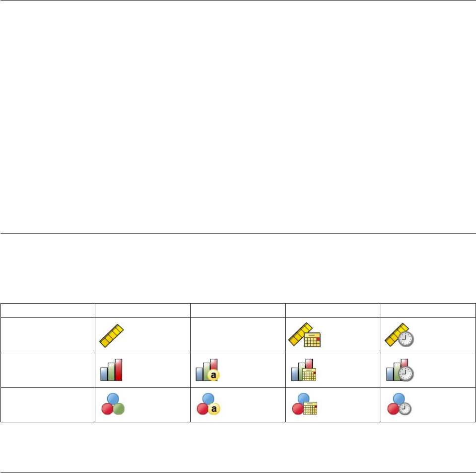
Data type, measurement level, and variable list icons
The icons that are displayed next to variables in dialog box lists provide information about the variable
type and measurement level.
Table 1. Measurement level icons
Numeric String Date Time
Scale (Continuous) n/a
Ordinal
Nominal
vFor more information on measurement level, see “Variable measurement level” on page 53.
vFor more information on numeric, string, date, and time data types, see “Variable type” on page 53.
Statistics Coach
If you are unfamiliar with IBM SPSS Statistics or with the available statistical procedures, the Statistics
Coach can help you get started by prompting you with simple questions, nontechnical language, and
visual examples that help you select the basic statistical and charting features that are best suited for your
data.
To use the Statistics Coach, from the menus in any IBM SPSS Statistics window choose:
Help > Statistics Coach
The Statistics Coach covers only a selected subset of procedures. It is designed to provide general
assistance for many of the basic, commonly used statistical techniques.
2IBM SPSS Statistics 24 Core System User's Guide

Finding out more
For a comprehensive overview of the basics, see the online tutorial. From any IBM SPSS Statistics menu
choose:
Help > Tutorial
Chapter 1. Overview 3
4IBM SPSS Statistics 24 Core System User's Guide

Chapter 2. Getting Help
The Help system contains a number of different sections.
Help Information on the user interface. There is a separate section for each optional module.
Reference
Reference information for the command language, GPL, VizML, and schemas. The reference
material for the command language is also available in PDF form: Help>Command Syntax
Reference.
Tutorial
Step-by-step instructions on how to use many of the basic features.
Case Studies
Hands-on examples of how to create various types of statistical analyses and how to interpret the
results.
Statistics Coach
Guides you through the process of finding the procedure that you want to use.
Integration Plug-ins
Separate sections for each programming plug-in, including Python, R, Java, and .Net
Context-sensitive help
In many places in the user interface, you can get context-sensitive help.
vHelp buttons in dialog boxes take you directly to the help topic for that dialog.
vRight-click on terms in an activated pivot table in the Viewer and choose What's This? from the
pop-up menu to display definitions of the terms.
vIn a command syntax window, position the cursor anywhere within a syntax block for a command and
press F1 on the keyboard. The help for that command is displayed
Other resources
Answers to many common problems can be found at http://www.ibm.com/support .
If you're a student using a student, academic or grad pack version of any IBM SPSS software product,
please see our special online Solutions for Education pages for students. If you're a student using a
university-supplied copy of the IBM SPSS software, please contact the IBM SPSS product coordinator at
your university.
The IBM SPSS Predictive Analytics community has resources for all levels of users and application
developers. Download utilities, graphics examples, new statistical modules, and articles. Visit the IBM
SPSS Predictive Analytics community at https://developer.ibm.com/predictiveanalytics/.
Documentation in PDF format is available at http://www.ibm.com/support/
docview.wss?uid=swg27047033.
Documentation of statistical algorithms is available at http://www.ibm.com/support/
docview.wss?uid=swg27047033.
© Copyright IBM Corporation 1989, 2016 5
6IBM SPSS Statistics 24 Core System User's Guide

Chapter 3. Data files
Data files come in a wide variety of formats, and this software is designed to handle many of them,
including:
vExcel spreadsheets
vDatabase tables from many database sources, including Oracle, SQLServer, DB2, and others
vTab-delimited, CSV, and other types of simple text files
vSAS data files
vStata data files
Opening data files
In addition to files saved in IBM SPSS Statistics format, you can open Excel, SAS, Stata, tab-delimited,
and other files without converting the files to an intermediate format or entering data definition
information.
vOpening a data file makes it the active dataset. If you already have one or more open data files, they
remain open and available for subsequent use in the session. Clicking anywhere in the Data Editor
window for an open data file will make it the active dataset. See the topic Chapter 6, “Working with
Multiple Data Sources,” on page 67 for more information.
vIn distributed analysis mode using a remote server to process commands and run procedures, the
available data files, folders, and drives are dependent on what is available on or from the remote
server. The current server name is indicated at the top of the dialog box. You will not have access to
data files on your local computer unless you specify the drive as a shared device and the folders
containing your data files as shared folders. See the topic Chapter 4, “Distributed Analysis Mode,” on
page 45 for more information.
To open data files
1. From the menus choose:
File > Open > Data...
2. In the Open Data dialog box, select the file that you want to open.
3. Click Open.
Optionally, you can:
vAutomatically set the width of each string variable to the longest observed value for that variable
using Minimize string widths based on observed values. This is particularly useful when reading
code page data files in Unicode mode. See the topic “General options” on page 195 for more
information.
vRead variable names from the first row of spreadsheet files.
vSpecify a range of cells to read from spreadsheet files.
vSpecify a worksheet within an Excel file to read (Excel 95 or later).
For information on reading data from databases, see “Reading Database Files” on page 14. For
information on reading data from text data files, see “Text Wizard” on page 10. For information on
reading IBM Cognos®data, see “Reading Cognos BI data” on page 20.
Data file types
SPSS Statistics. Opens data files that are saved in IBM SPSS Statistics format and also the DOS product
SPSS/PC+.
© Copyright IBM Corporation 1989, 2016 7
SPSS Statistics Compressed. Opens data files that are saved in IBM SPSS Statistics compressed format.
SPSS/PC+. Opens SPSS/PC+ data files. This option is available only on Windows operating systems.
Portable. Opens data files that are saved in portable format. Saving a file in portable format takes
considerably longer than saving the file in IBM SPSS Statistics format.
Excel. Opens Excel files.
Lotus 1-2-3. Opens data files that are saved in 1-2-3 format for release 3.0, 2.0, or 1A of Lotus.
SYLK. Opens data files that are saved in SYLK (symbolic link) format, a format that is used by some
spreadsheet applications.
dBASE. Opens dBASE-format files for either dBASE IV, dBASE III or III PLUS, or dBASE II. Each case is
a record. Variable and value labels and missing-value specifications are lost when you save a file in this
format.
SAS. SAS versions 6–9 and SAS transport files.
Stata. Stata versions 4–13.
Reading Excel Files
This topic applies to Excel 95 and later files. To read Excel 4 or earlier versions, see the topic “Reading
Older Excel Files and Other Spreadsheets” on page 9.
Worksheet
Excel files can contain multiple worksheets. By default, the Data Editor reads the first worksheet.
To read a different worksheet, select the worksheet from the list.
Range You can also read a range of cells. Use the same method for specifying cell ranges as you would
in Excel. For example: A1:D10.
Read variable names from first row of data
You can read variable names from the first row of the file or the first row of the defined range.
Values that don't conform to variable naming rules are converted to valid variable names, and the
original names are used as variable labels.
Percentage of values that determine data type
The data type for each variable is determined by the percentage of values that conform to the
same format.
vThe value must be greater than 50.
vThe denominator used to determine the percentage is the number of non-blank values for each
variable.
vIf no consistent format is used by the specified percentage of values, the variable is assigned
the string data type.
vFor variables that are assigned a numeric format (including date and time formats) based on
the percentage value, values that do not conform to that format are assigned the
system-missing value.
Ignore hidden rows and columns
Hidden rows and columns in the Excel file are not included. This option is available only for
Excel 2007 and later files (XLSX, XLSM).
Remove leading spaces from string values
Any blank spaces at the beginning of string values are removed.
8IBM SPSS Statistics 24 Core System User's Guide
Remove trailing spaces from string values
Blank spaces at the end of the string values are removed. This setting affects the calculation of the
defined width of string variables.
Reading Older Excel Files and Other Spreadsheets
This topic applies to reading Excel 4 or earlier files, Lotus 1-2-3 files and SYLK format spreadsheet files.
For information on reading Excel 95 or later files, see the topic “Reading Excel Files” on page 8.
Read variable names. For spreadsheets, you can read variable names from the first row of the file or the
first row of the defined range. The values are converted as necessary to create valid variable names,
including converting spaces to underscores.
Range. For spreadsheet data files, you can also read a range of cells. Use the same method for specifying
cell ranges as you would with the spreadsheet application.
How Spreadsheets are Read
vThe data type and width for each variable are determined by the column width and data type of the
first data cell in the column. Values of other types are converted to the system-missing value. If the
first data cell in the column is blank, the global default data type for the spreadsheet (usually numeric)
is used.
vFor numeric variables, blank cells are converted to the system-missing value, indicated by a period. For
string variables, a blank is a valid string value, and blank cells are treated as valid string values.
vIf you do not read variable names from the spreadsheet, the column letters (A, B, C, ...) are used for
variable names for Excel and Lotus files. For SYLK files and Excel files saved in R1C1 display format,
the software uses the column number preceded by the letter Cfor variable names (C1, C2, C3, ...).
Reading dBASE files
Database files are logically very similar to IBM SPSS Statistics data files. The following general rules
apply to dBASE files:
vField names are converted to valid variable names.
vColons used in dBASE field names are translated to underscores.
vRecords marked for deletion but not actually purged are included. The software creates a new string
variable, D_R, which contains an asterisk for cases marked for deletion.
Reading Stata files
The following general rules apply to Stata data files:
vVariable names. Stata variable names are converted to IBM SPSS Statistics variable names in
case-sensitive form. Stata variable names that are identical except for case are converted to valid
variable names by appending an underscore and a sequential letter (_A, _B, _C, ..., _Z, _AA, _AB, ...,
and so forth).
vVariable labels. Stata variable labels are converted to IBM SPSS Statistics variable labels.
vValue labels. Stata value labels are converted to IBM SPSS Statistics value labels, except for Stata
value labels assigned to "extended" missing values. Value labels longer than 120 bytes are truncated.
vString variables. Stata strl variables are converted to string variables. Values longer than 32K bytes are
truncated. Stata strl values that contain blobs (binary large objects) are converted to blank strings.
vMissing values. Stata "extended" missing values are converted to system-missing values.
vDate conversion. Stata date format values are converted to IBM SPSS Statistics DATE format (d-m-y)
values. Stata "time-series" date format values (weeks, months, quarters, and so on) are converted to
simple numeric (F) format, preserving the original, internal integer value, which is the number of
weeks, months, quarters, and so on, since the start of 1960.
Chapter 3. Data files 9
Reading CSV Files
To read CSV files, from the menus choose: File > Import Data > CSV
The Read CSV File dialog reads CSV format text data files that use a comma, a semicolon, or a tab as the
delimiter between values.
If the text file uses a different delimiter, contains text at the beginning of the file that is not variable
names or data values, or has other special considerations, use the Text Wizard to read the files.
First line contains variable names
The first non-blank line in the file contains label text that is used as variable names. Values that
are invalid as variable names are automatically converted to valid variable names.
Remove leading spaces from string values
Any blank spaces at the beginning of string values are removed.
Remove trailing spaces from string values
Blank spaces at the end of the string values are removed. This setting affects the calculation of the
defined width of string variables.
Delimiter between values
The delimiter can be a comma, a semicolon, or a tab. If the delimiter is any other character or a
blank space, use the Text Wizard to read the file.
Decimal symbol
The symbol that is used to indicate decimals in the text data file. The symbol can be a period or a
comma.
Text Qualifier
Character that is used to enclose values that contain the delimiter character. The qualifier appears
at the start and the end of the value. The qualifier can be double quotation mark, single quotation
mark, or none.
Percentage of values that determine data type
The data type for each variable is determined by the percentage of values that conform to the
same format.
vThe value must be greater than 50.
vIf no consistent format is used by the specified percentage of values, the variable is assigned
the string data type.
vFor variables that are assigned a numeric format (including date and time formats) based on
the percentage value, values that do not conform to that format are assigned the
system-missing value.
Cache data locally
A data cache is a complete copy of the data file that is stored in temporary disk space. Caching
the data file can improve performance.
Text Wizard
The Text Wizard can read text data files formatted in a variety of ways:
vTab-delimited files
vSpace-delimited files
vComma-delimited files
vFixed-field format files
For delimited files, you can also specify other characters as delimiters between values, and you can
specify multiple delimiters.
10 IBM SPSS Statistics 24 Core System User's Guide
To Read Text Data Files
1. From the menus choose:
File > Import Data > Text Data...
2. Select the text file in the Open Data dialog box.
3. If necessary, select the encoding of the file.
4. Follow the steps in the Text Wizard to define how to read the data file.
Encoding
The encoding of a file affects the way character data are read. Unicode data files typically contain a byte
order mark that identifies the character encoding. Some applications create Unicode files without a byte
order mark, and code page data files do not contain any encoding identifier.
vUnicode (UTF-8). Reads the file as Unicode UTF-8.
vUnicode (UTF-16). Reads the file as Unicode UTF-16 in the endianness of the operating system.
vUnicode (UTF-16BE). Reads the file as Unicode UTF-16, big endian.
vUnicode (UTF-16LE). Reads the file as Unicode UTF-16, little endian.
vLocal Encoding. Reads the file in current locale code page character encoding.
If a file contains a Unicode byte order mark, it is read in that Unicode encoding, regardless of the
encoding you select. If a file does not contain a Unicode byte order mark, by default the encoding is
assumed to be the current locale code page character encoding, unless you select one of the Unicode
encodings.
To change the current locale for data files in a different code page character encoding, select Edit>Options
from the menus, and change the locale on the Language tab.
Text Wizard: Step 1
The text file is displayed in a preview window. You can apply a predefined format (previously saved
from the Text Wizard) or follow the steps in the Text Wizard to specify how the data should be read.
Text Wizard: Step 2
This step provides information about variables. A variable is similar to a field in a database. For example,
each item in a questionnaire is a variable.
How are your variables arranged?
The arrangement of variables defines the method that is used to differentiate one variable from
the next.
Delimited
Spaces, commas, tabs, or other characters are used to separate variables. The variables are
recorded in the same order for each case but not necessarily in the same column
locations.
Fixed width
Each variable is recorded in the same column location on the same record (line) for each
case in the data file. No delimiter is required between variables. The column location
determines which variable is being read.
Note: The Text Wizard cannot read fixed-width Unicode text files. You can use the DATA
LIST command to read fixed-width Unicode files.
Are variable names included at the top of your file?
The values on the specified line number are used to create variable names. Values that don't
conform to variable naming rules are converted to valid variable names.
What is the decimal symbol?
The character that indicates decimal values can be either a period or a comma.
Chapter 3. Data files 11
Text Wizard: Step 3 (Delimited Files)
This step provides information about cases. A case is similar to a record in a database. For example, each
respondent to a questionnaire is a case.
The first case of data begins on which line number? Indicates the first line of the data file that contains
data values. If the top line(s) of the data file contain descriptive labels or other text that does not
represent data values, this will not be line 1.
How are your cases represented? Controls how the Text Wizard determines where each case ends and
the next one begins.
vEach line represents a case. Each line contains only one case. It is fairly common for each case to be
contained on a single line (row), even though this can be a very long line for data files with a large
number of variables. If not all lines contain the same number of data values, the number of variables
for each case is determined by the line with the greatest number of data values. Cases with fewer data
values are assigned missing values for the additional variables.
vA specific number of variables represents a case. The specified number of variables for each case
tells the Text Wizard where to stop reading one case and start reading the next. Multiple cases can be
contained on the same line, and cases can start in the middle of one line and be continued on the next
line. The Text Wizard determines the end of each case based on the number of values read, regardless
of the number of lines. Each case must contain data values (or missing values indicated by delimiters)
for all variables, or the data file will be read incorrectly.
How many cases do you want to import? You can import all cases in the data file, the first ncases (nis a
number you specify), or a random sample of a specified percentage. Since the random sampling routine
makes an independent pseudo-random decision for each case, the percentage of cases selected can only
approximate the specified percentage. The more cases there are in the data file, the closer the percentage
of cases selected is to the specified percentage.
Text Wizard: Step 3 (Fixed-Width Files)
This step provides information about cases. A case is similar to a record in a database. For example, each
respondent to questionnaire is a case.
The first case of data begins on which line number? Indicates the first line of the data file that contains
data values. If the top line(s) of the data file contain descriptive labels or other text that does not
represent data values, this will not be line 1.
How many lines represent a case? Controls how the Text Wizard determines where each case ends and
the next one begins. Each variable is defined by its line number within the case and its column location.
You need to specify the number of lines for each case to read the data correctly.
How many cases do you want to import? You can import all cases in the data file, the first ncases (nis a
number you specify), or a random sample of a specified percentage. Since the random sampling routine
makes an independent pseudo-random decision for each case, the percentage of cases selected can only
approximate the specified percentage. The more cases there are in the data file, the closer the percentage
of cases selected is to the specified percentage.
Text Wizard: Step 4 (Delimited Files)
This step specifies delimiters and text qualifiers that are used in the text data file. You can also specify
the treatment of leading and trailing spaces in string values.
Which delimiters appear between variables?
The characters or symbols that separate data values. You can select any combination of spaces,
commas, semicolons, tabs, or other characters. Multiple, consecutive delimiters without
intervening data values are treated as missing values.
12 IBM SPSS Statistics 24 Core System User's Guide
What is the text qualifier?
Characters that are used to enclose values that contain delimiter characters. The text qualifier
appears at both the beginning and the end of the value, enclosing the entire value.
Leading and Trailing Spaces
Controls the treatment of leading and trailing blank spaces in string values.
Remove leading spaces from string values
Any blank spaces at the beginning of string values are removed.
Remove trailing spaces from string values
Blank spaces at the end of a value are ignored when the defined width of string variables
is calculated. If Space is selected as a delimiter, multiple consecutive blank spaces are not
treated as multiple delimiters.
Text Wizard: Step 4 (Fixed-Width Files)
This step displays the Text Wizard's best guess on how to read the data file and allows you to modify
how the Text Wizard will read variables from the data file. Vertical lines in the preview window indicate
where the Text Wizard currently thinks each variable begins in the file.
Insert, move, and delete variable break lines as necessary to separate variables. If multiple lines are used
for each case, the data will be displayed as one line for each case, with subsequent lines appended to the
end of the line.
Notes:
For computer-generated data files that produce a continuous stream of data values with no intervening
spaces or other distinguishing characteristics, it may be difficult to determine where each variable begins.
Such data files usually rely on a data definition file or some other written description that specifies the
line and column location for each variable.
Text Wizard: Step 5
This step controls the variable name and the data format that is used to read each variable. You can also
specify variables to exclude.
Variable name
You can overwrite the default variable names with your own variable names. If you read variable
names from the data file, names that do not conform to variable naming rules are automatically
modified. Select a variable in the preview window and then enter a variable name.
Data format
Select a variable in the preview window and then select a format from the list.
vAutomatic determines the data format based on an evaluation of all the data values.
vTo exclude a variable, select Do Not Import.
Percentage of values that determine Automatic data format
For automatic format, the data format for each variable is determined by the percentage of values
that conform to the same format.
vThe value must be greater than 50.
vThe denominator used to determine the percentage is the number of non-blank values for each
variable.
vIf no consistent format is used by the specified percentage of values, the variable is assigned
the string data type.
vFor variables that are assigned a numeric format (including date and time formats) based on
the percentage value, values that do not conform to that format are assigned the
system-missing value.
Chapter 3. Data files 13
Text Wizard Formatting Options: Formatting options for reading variables with the Text Wizard
include:
Automatic. The format is determined based on an evaluation of all the data values.
Do not import. Omit the selected variable(s) from the imported data file.
Numeric. Valid values include numbers, a leading plus or minus sign, and a decimal indicator.
String. Valid values include virtually any keyboard characters and embedded blanks. For delimited files,
you can specify the number of characters in the value, up to a maximum of 32,767. By default, the Text
Wizard sets the number of characters to the longest string value encountered for the selected variable(s)
in the first 250 rows of the file. For fixed-width files, the number of characters in string values is defined
by the placement of variable break lines in step 4.
Date/Time. Valid values include dates of the general format dd-mm-yyyy, mm/dd/yyyy, dd.mm.yyyy,
yyyy/mm/dd, hh:mm:ss, and a variety of other date and time formats. Months can be represented in digits,
Roman numerals, or three-letter abbreviations, or they can be fully spelled out. Select a date format from
the list.
Dollar. Valid values are numbers with an optional leading dollar sign and optional commas as thousands
separators.
Comma. Valid values include numbers that use a period as a decimal indicator and commas as thousands
separators.
Dot. Valid values include numbers that use a comma as a decimal indicator and periods as thousands
separators.
Note: Values that contain invalid characters for the selected format will be treated as missing. Values that
contain any of the specified delimiters will be treated as multiple values.
Text Wizard: Step 6
This is the final step of the Text Wizard. You can save your specifications in a file for use when importing
similar text data files. You can also paste the syntax generated by the Text Wizard into a syntax window.
You can then customize and/or save the syntax for use in other sessions or in production jobs.
Cache data locally. A data cache is a complete copy of the data file, stored in temporary disk space.
Caching the data file can improve performance.
Reading Database Files
You can read data from any database format for which you have a database driver. In local analysis
mode, the necessary drivers must be installed on your local computer. In distributed analysis mode
(available with IBM SPSS Statistics Server), the drivers must be installed on the remote server. See the
topic Chapter 4, “Distributed Analysis Mode,” on page 45 for more information.
Note: If you are running the Windows 64-bit version of IBM SPSS Statistics, you cannot read Excel,
Access, or dBASE database sources, even though they may appear on the list of available database
sources. The 32-bit ODBC drivers for these products are not compatible.
To Read Database Files
1. From the menus choose:
File > Import Data > Database > New Query...
2. Select the data source.
14 IBM SPSS Statistics 24 Core System User's Guide
3. If necessary (depending on the data source), select the database file and/or enter a login name,
password, and other information.
4. Select the table(s) and fields. For OLE DB data sources (available only on Windows operating
systems), you can only select one table.
5. Specify any relationships between your tables.
6. Optionally:
vSpecify any selection criteria for your data.
vAdd a prompt for user input to create a parameter query.
vSave your constructed query before running it.
Connection Pooling
If you access the same database source multiple times in the same session or job, you can improve
performance with connection pooling.
1. In the last step of the wizard, paste the command syntax into a syntax window.
2. At the end of the quoted CONNECT string, add Pooling=true.
To Edit Saved Database Queries
1. From the menus choose:
File > Import Data > Database > Edit Query...
2. Select the query file (*.spq) that you want to edit.
3. Follow the instructions for creating a new query.
To Read Database Files with Saved Queries
1. From the menus choose:
File > Import Data > Database > Run Query...
2. Select the query file (*.spq) that you want to run.
3. If necessary (depending on the database file), enter a login name and password.
4. If the query has an embedded prompt, enter other information if necessary (for example, the quarter
for which you want to retrieve sales figures).
Selecting a Data Source
Use the first screen of the Database Wizard to select the type of data source to read.
ODBC Data Sources
If you do not have any ODBC data sources configured, or if you want to add a new data source, click
Add ODBC Data Source.
vOn Linux operating systems, this button is not available. ODBC data sources are specified in odbc.ini,
and the ODBCINI environment variables must be set to the location of that file. For more information,
see the documentation for your database drivers.
vIn distributed analysis mode (available with IBM SPSS Statistics Server), this button is not available.
To add data sources in distributed analysis mode, see your system administrator.
An ODBC data source consists of two essential pieces of information: the driver that will be used to
access the data and the location of the database you want to access. To specify data sources, you must
have the appropriate drivers installed. Drivers for a variety of database formats are included with the
installation media.
To access OLE DB data sources (available only on Microsoft Windows operating systems), you must have
the following items installed:
Chapter 3. Data files 15
v.NET framework. To obtain the most recent version of the .NET framework, go to http://
www.microsoft.com/net.
vData Collection Survey Reporter Developer Kit.
The following limitations apply to OLE DB data sources:
vTable joins are not available for OLE DB data sources. You can read only one table at a time.
vYou can add OLE DB data sources only in local analysis mode. To add OLE DB data sources in
distributed analysis mode on a Windows server, consult your system administrator.
vIn distributed analysis mode (available with IBM SPSS Statistics Server), OLE DB data sources are
available only on Windows servers, and both .NET and Data Collection Survey Reporter Developer Kit
must be installed on the server.
To add an OLE DB data source:
1. Click Add OLE DB Data Source.
2. In Data Link Properties, click the Provider tab and select the OLE DB provider.
3. Click Next or click the Connection tab.
4. Select the database by entering the directory location and database name or by clicking the button to
browse to a database. (A user name and password may also be required.)
5. Click OK after entering all necessary information. (You can make sure the specified database is
available by clicking the Test Connection button.)
6. Enter a name for the database connection information. (This name will be displayed in the list of
available OLE DB data sources.)
7. Click OK.
This takes you back to the first screen of the Database Wizard, where you can select the saved name from
the list of OLE DB data sources and continue to the next step of the wizard.
Deleting OLE DB Data Sources
To delete data source names from the list of OLE DB data sources, delete the UDL file with the name of
the data source in:
[drive]:\Documents and Settings\[user login]\Local Settings\Application Data\SPSS\UDL
Selecting Data Fields
The Select Data step controls which tables and fields are read. Database fields (columns) are read as
variables.
If a table has any field(s) selected, all of its fields will be visible in the following Database Wizard
windows, but only fields that are selected in this step will be imported as variables. This enables you to
create table joins and to specify criteria by using fields that you are not importing.
Displaying field names. To list the fields in a table, click the plus sign (+) to the left of a table name. To
hide the fields, click the minus sign (–) to the left of a table name.
To add a field. Double-click any field in the Available Tables list, or drag it to the Retrieve Fields In This
Order list. Fields can be reordered by dragging and dropping them within the fields list.
To remove a field. Double-click any field in the Retrieve Fields In This Order list, or drag it to the
Available Tables list.
Sort field names. If this check box is selected, the Database Wizard will display your available fields in
alphabetical order.
16 IBM SPSS Statistics 24 Core System User's Guide
By default, the list of available tables displays only standard database tables. You can control the type of
items that are displayed in the list:
vTables. Standard database tables.
vViews. Views are virtual or dynamic "tables" defined by queries. These can include joins of multiple
tables and/or fields derived from calculations based on the values of other fields.
vSynonyms. A synonym is an alias for a table or view, typically defined in a query.
vSystem tables. System tables define database properties. In some cases, standard database tables may
be classified as system tables and will only be displayed if you select this option. Access to real system
tables is often restricted to database administrators.
Note: For OLE DB data sources (available only on Windows operating systems), you can select fields only
from a single table. Multiple table joins are not supported for OLE DB data sources.
Creating a Relationship between Tables
The Specify Relationships step allows you to define the relationships between the tables for ODBC data
sources. If fields from more than one table are selected, you must define at least one join.
Establishing relationships. To create a relationship, drag a field from any table onto the field to which
you want to join it. The Database Wizard will draw a join line between the two fields, indicating their
relationship. These fields must be of the same data type.
Auto Join Tables. Attempts to automatically join tables based on primary/foreign keys or matching field
names and data type.
Join Type. If outer joins are supported by your driver, you can specify inner joins, left outer joins, or
right outer joins.
vInner joins. An inner join includes only rows where the related fields are equal. In this example, all
rows with matching ID values in the two tables will be included.
vOuter joins. In addition to one-to-one matching with inner joins, you can also use outer joins to merge
tables with a one-to-many matching scheme. For example, you could match a table in which there are
only a few records representing data values and associated descriptive labels with values in a table
containing hundreds or thousands of records representing survey respondents. A left outer join
includes all records from the table on the left and, from the table on the right, includes only those
records in which the related fields are equal. In a right outer join, the join imports all records from the
table on the right and, from the table on the left, imports only those records in which the related fields
are equal.
Computing New Fields
If you are in distributed mode, connected to a remote server (available with IBM SPSS Statistics Server),
you can compute new fields before you read the data into IBM SPSS Statistics.
You can also compute new fields after you read the data into IBM SPSS Statistics, but computing new
fields in the database can save time for large data sources.
New Field Name. The name must comply with IBM SPSS Statistics variable name rules.
Expression. Enter the expression to compute the new field. You can drag existing field names from the
Fields list and functions from the Functions list.
Limiting Retrieved Cases
The Limit Retrieved Cases step allows you to specify the criteria to select subsets of cases (rows).
Limiting cases generally consists of filling the criteria grid with criteria. Criteria consist of two
expressions and some relation between them. The expressions return a value of true, false, or missing for
each case.
Chapter 3. Data files 17
vIf the result is true, the case is selected.
vIf the result is false or missing, the case is not selected.
vMost criteria use one or more of the six relational operators (<, >, <=, >=, =, and <>).
vExpressions can include field names, constants, arithmetic operators, numeric and other functions, and
logical variables. You can use fields that you do not plan to import as variables.
To build your criteria, you need at least two expressions and a relation to connect the expressions.
1. To build an expression, choose one of the following methods:
vIn an Expression cell, type field names, constants, arithmetic operators, numeric and other
functions, or logical variables.
vDouble-click the field in the Fields list.
vDrag the field from the Fields list to an Expression cell.
vChoose a field from the drop-down menu in any active Expression cell.
2. To choose the relational operator (such as = or >), put your cursor in the Relation cell and either type
the operator or choose it from the drop-down menu.
If the SQL contains WHERE clauses with expressions for case selection, dates and times in expressions
need to be specified in a special manner (including the curly braces shown in the examples):
vDate literals should be specified using the general form {d ’yyyy-mm-dd’}.
vTime literals should be specified using the general form {t ’hh:mm:ss’}.
vDate/time literals (timestamps) should be specified using the general form {ts ’yyyy-mm-dd
hh:mm:ss’}.
vThe entire date and/or time value must be enclosed in single quotes. Years must be expressed in
four-digit form, and dates and times must contain two digits for each portion of the value. For
example January 1, 2005, 1:05 AM would be expressed as:
{ts ’2005-01-01 01:05:00’}
Functions. A selection of built-in arithmetic, logical, string, date, and time SQL functions is provided.
You can drag a function from the list into the expression, or you can enter any valid SQL function.
See your database documentation for valid SQL functions.
Use Random Sampling. This option selects a random sample of cases from the data source. For large
data sources, you may want to limit the number of cases to a small, representative sample, which can
significantly reduce the time that it takes to run procedures. Native random sampling, if available for
the data source, is faster than IBM SPSS Statistics random sampling, because IBM SPSS Statistics
random sampling must still read the entire data source to extract a random sample.
vApproximately. Generates a random sample of approximately the specified percentage of cases.
Since this routine makes an independent pseudorandom decision for each case, the percentage of
cases selected can only approximate the specified percentage. The more cases there are in the data
file, the closer the percentage of cases selected is to the specified percentage.
vExactly. Selects a random sample of the specified number of cases from the specified total number
of cases. If the total number of cases specified exceeds the total number of cases in the data file, the
sample will contain proportionally fewer cases than the requested number.
Note: If you use random sampling, aggregation (available in distributed mode with IBM SPSS
Statistics Server) is not available.
Prompt For Value. You can embed a prompt in your query to create a parameter query. When users
run the query, they will be asked to enter information (based on what is specified here). You might
want to do this if you need to see different views of the same data. For example, you may want to
run the same query to see sales figures for different fiscal quarters.
3. Place your cursor in any Expression cell, and click Prompt For Value to create a prompt.
18 IBM SPSS Statistics 24 Core System User's Guide
Creating a Parameter Query
Use the Prompt for Value step to create a dialog box that solicits information from users each time
someone runs your query. This feature is useful if you want to query the same data source by using
different criteria.
To build a prompt, enter a prompt string and a default value. The prompt string is displayed each time a
user runs your query. The string should specify the kind of information to enter. If the user is not
selecting from a list, the string should give hints about how the input should be formatted. An example is
as follows: Enter a Quarter (Q1, Q2, Q3, ...).
Allow user to select value from list. If this check box is selected, you can limit the user to the values that
you place here. Ensure that your values are separated by returns.
Data type. Choose the data type here (Number, String, or Date).
Date and time values must be entered in special manner:
vDate values must use the general form yyyy-mm-dd.
vTime values must use the general form: hh:mm:ss.
vDate/time values (timestamps) must use the general form yyyy-mm-dd hh:mm:ss.
Aggregating Data
If you are in distributed mode, connected to a remote server (available with IBM SPSS Statistics Server),
you can aggregate the data before reading it into IBM SPSS Statistics.
You can also aggregate data after reading it into IBM SPSS Statistics, but preaggregating may save time
for large data sources.
1. To create aggregated data, select one or more break variables that define how cases are grouped.
2. Select one or more aggregated variables.
3. Select an aggregate function for each aggregate variable.
4. Optionally, create a variable that contains the number of cases in each break group.
Note: If you use IBM SPSS Statistics random sampling, aggregation is not available.
Defining Variables
Variable names and labels. The complete database field (column) name is used as the variable label.
Unless you modify the variable name, the Database Wizard assigns variable names to each column from
the database in one of two ways:
vIf the name of the database field forms a valid, unique variable name, the name is used as the variable
name.
vIf the name of the database field does not form a valid, unique variable name, a new, unique name is
automatically generated.
Click any cell to edit the variable name.
Converting strings to numeric values. Select the Recode to Numeric box for a string variable if you
want to automatically convert it to a numeric variable. String values are converted to consecutive integer
values based on alphabetical order of the original values. The original values are retained as value labels
for the new variables.
Width for variable-width string fields. This option controls the width of variable-width string values. By
default, the width is 255 bytes, and only the first 255 bytes (typically 255 characters in single-byte
languages) will be read. The width can be up to 32,767 bytes. Although you probably don't want to
truncate string values, you also don't want to specify an unnecessarily large value, which will cause
processing to be inefficient.
Chapter 3. Data files 19
Minimize string widths based on observed values. Automatically set the width of each string variable
to the longest observed value.
Sorting Cases
If you are in distributed mode, connected to a remote server (available with IBM SPSS Statistics Server),
you can sort the data before reading it into IBM SPSS Statistics.
You can also sort data after reading it into IBM SPSS Statistics, but presorting may save time for large
data sources.
Results
The Results step displays the SQL Select statement for your query.
vYou can edit the SQL Select statement before you run the query, but if you click the Back button to
make changes in previous steps, the changes to the Select statement will be lost.
vTo save the query for future use, use the Save query to file section.
vTo paste complete GET DATA syntax into a syntax window, select Paste it into the syntax editor for
further modification. Copying and pasting the Select statement from the Results window will not
paste the necessary command syntax.
Note: The pasted syntax contains a blank space before the closing quote on each line of SQL that is
generated by the wizard. These blanks are not superfluous. When the command is processed, all lines of
the SQL statement are merged together in a very literal fashion. Without the space, there would be no
space between the last character on one line and first character on the next line.
Reading Cognos BI data
If you have access to a IBM Cognos Business Intelligence server, you can read IBM Cognos Business
Intelligence data packages and list reports into IBM SPSS Statistics.
To read IBM Cognos Business Intelligence data:
1. From the menus choose:
File > Import Data > Cognos Business Intelligence
2. Specify the URL for the IBM Cognos Business Intelligence server connection.
3. Specify the location of the data package or report.
4. Select the data fields or report that you want to read.
Optionally, you can:
vSelect filters for data packages.
vImport aggregated data instead of raw data.
vSpecify parameter values.
Mode. Specifies the type of information you want to read: Data or Report. The only type of report that
can be read is a list report.
Connection. The URL of the Cognos Business Intelligence server. Click the Edit button to define the
details of a new Cognos connection from which to import data or reports. See the topic “Cognos
connections” on page 21 for more information.
Location. The location of the package or report that you want to read. Click the Edit button to display a
list of available sources from which to import content. See the topic “Cognos location” on page 21 for
more information.
Content. For data, displays the available data packages and filters. For reports, display the available
reports.
20 IBM SPSS Statistics 24 Core System User's Guide
Fields to import. For data packages, select the fields you want to include and move them to this list.
Report to import. For reports, select the list report you want to import. The report must be a list report.
Filters to apply. For data packages, select the filters you want to apply and move them to this list.
Parameters. If this button is enabled, the selected object has parameters defined. You can use parameters
to make adjustments (for example, perform a parameterized calculation) before importing the data. If
parameters are defined but no default is provided, the button displays a warning triangle.
Aggregate data before performing import. For data packages, if aggregation is defined in the package,
you can import the aggregated data instead of the raw data.
Cognos connections
The Cognos Connections dialog specifies the IBM Cognos Business Intelligence server URL and any
required additional credentials.
Cognos server URL. The URL of the IBM Cognos Business Intelligence server. This is the value of the
"external dispatcher URI" environment property of IBM Cognos Configuration on the server. Contact your
system administrator for more information
Mode. Select Set Credentials if you need to log in with a specific namespace, username and password
(for example, as an administrator). Select Use Anonymous connection to log in with no user credentials,
in which case you do not fill in the other fields. Select Stored Credentials to use the login information
from a stored credential. To use a stored credential, you must be connected to the IBM SPSS
Collaboration and Deployment Services Repository that contains the credential. After you are connected
to the repository, click Browse to see the list of available credentials.
Namespace ID. The security authentication provider used to log on to the server. The authentication
provider is used to define and maintain users, groups, and roles, and to control the authentication
process.
User name. Enter the user name with which to log on to the server.
Password. Enter the password associated with the specified user name.
Save as Default. Saves these settings as your default, to avoid having to re-enter them each time.
Cognos location
The Specify Location dialog box enables you to select a package from which to import data, or a package
or folder from which to import reports. It displays the public folders that are available to you. If you
select Data in the main dialog, the list will display folders containing data packages. If you select Report
in the main dialog, the list will display folders containing list reports. Select the location you want by
navigating through the folder structure.
Specifying parameters for data or reports
If parameters have been defined, either for a data object or a report, you can specify values for these
parameters before importing the data or report. An example of parameters for a report would be start
and end dates for the report contents.
Name. The parameter name as it is specified in the IBM Cognos Business Intelligence database.
Type. A description of the parameter.
Value. The value to assign to the parameter. To enter or edit a value, double-click its cell in the table.
Values are not validated here; any invalid values are detected at run time.
Chapter 3. Data files 21
Automatically remove invalid parameters from table. This option is selected by default and will remove
any invalid parameters found within the data object or report.
Changing variable names
For IBM Cognos Business Intelligence data packages, package field names are automatically converted to
valid variable names. You can use the Fields tab of the Read Cognos Data dialog to override the default
names. Names must be unique and must conform to variable naming rules. See the topic “Variable
names” on page 52 for more information.
Reading Cognos TM1 data
If you have access to an IBM Cognos TM1®database, you can import TM1 data from a specified view
into IBM SPSS Statistics. The multidimensional OLAP cube data from TM1 is flattened when read into
SPSS Statistics.
Important: To enable the exchange of data between SPSS Statistics and TM1, you must copy the
following three processes from SPSS Statistics to the TM1 server: ExportToSPSS.pro, ImportFromSPSS.pro,
and SPSSCreateNewMeasures.pro. To add these processes to the TM1 server, you must copy them to the
data directory of the TM1 server and restart the TM1 server. These files are available from the
common/scripts/TM1 directory under the SPSS Statistics installation directory.
Restriction:
vThe TM1 view from which you import must include one or more elements from a measure dimension.
vThe data to be imported from TM1 must be in UTF-8 format.
All of the data in the specified TM1 view are imported. It is therefore best to limit the view to the data
that are required for the analysis. Any necessary filtering of the data is best done in TM1, for example
with the TM1 Subset Editor.
To read TM1 data:
1. From the menus, choose:
File > Import Data > Cognos TM1
2. Connect to the TM1 Performance Management system.
3. Log in to the TM1 server.
4. Select a TM1 cube and select the view that you want to import.
Optionally, you can override the default names of the SPSS Statistics variables that are created from the
names of the TM1 dimensions and measures.
PM System
The URL of the Performance Management system that contains the TM1 server to which you
want to connect. The Performance Management system is defined as a single URL for all TM1
servers. From this URL, all TM1 servers that are installed and running on your environment can
be discovered and accessed. Enter the URL and click Connect.
TM1 Server
When the connection to the Performance Management system is established, select the server that
contains the data you want to import and click Login. If you did not previously connect to this
server, you are prompted to log in.
Username and password
Select this option to log in with a specific username and password. If the server uses
authentication mode 5 (IBM Cognos security), then select the namespace that identifies
the security authentication provider from the available list.
Stored credential
Select this option to use the login information from a stored credential. To use a stored
22 IBM SPSS Statistics 24 Core System User's Guide
credential, you must be connected to the IBM SPSS Collaboration and Deployment
Services Repository that contains the credential. After you are connected to the repository,
click Browse to see the list of available credentials.
Select a TM1 cube view to import
Lists the names of the cubes within the TM1 server from which you can import data.
Double-click a cube to display a list of the views that you can import. Select a view and click the
right arrow to move it into the View to import field.
Column dimension(s)
Lists the names of the column dimensions in the selected view.
Row dimension(s)
Lists the names of the row dimensions in the selected view.
Context dimension(s)
Lists the names of the context dimensions in the selected view.
Note:
vWhen the data are imported, a separate SPSS Statistics variable is created for each regular dimension
and for each element in the measure dimension.
vEmpty cells and cells with a value of zero in TM1 are converted to the system-missing value.
vCells with string values that cannot be converted to a numeric value are converted to the
system-missing value.
Changing variable names
By default, valid IBM SPSS Statistics variable names are automatically generated from the dimension
names and names of elements in the measure dimension from the selected IBM Cognos TM1 cube view.
You can use the Fields tab of the Import from TM1 dialog to override the default names. Names must be
unique and must conform to variable naming rules.
Reading Data Collection Data
On Microsoft Windows operating systems, you can read data from Data Collection products. (Note: This
feature is only available with IBM SPSS Statistics installed on Microsoft Windows operating systems.)
To read Data Collection data sources, you must have the following items installed:
v.NET framework. To obtain the most recent version of the .NET framework, go to http://
www.microsoft.com/net.
vData Collection Survey Reporter Developer Kit.
You can read Data Collection data sources only in local analysis mode. This feature is not available in
distributed analysis mode using IBM SPSS Statistics Server.
To read data from a Data Collection data source:
1. In any open IBM SPSS Statistics window, from the menus choose:
File > Import Data > Data Collection
2. On the Connection tab of Data Link Properties, specify the metadata file, the case data type, and the
case data file.
3. Click OK.
4. In the Data Collection Data Import dialog box, select the variables that you want to include and select
any case selection criteria.
5. Click OK to read the data.
Chapter 3. Data files 23
Data Link Properties Connection tab
To read a Data Collection data source, you need to specify:
Metadata Location. The metadata document file (.mdd) that contains questionnaire definition information.
Case Data Type. The format of the case data file. Available formats include:
vQuancept Data File (DRS). Case data in a Quancept .drs, .drz, or .dru file.
vQuanvert Database. Case data in a Quanvert database.
vData Collection Database (MS SQL Server). Case data in a relational database in SQL Server.
vData Collection XML Data File. Case data in an XML file.
Case Data Location. The file that contains the case data. The format of this file must be consistent with
the selected case data type.
Note: The extent to which other settings on the Connection tab or any settings on the other Data Link
Properties tabs may or may not affect reading Data Collection data into IBM SPSS Statistics is not known,
so we recommend that you do not change any of them.
Select Variables tab
You can select a subset of variables to read. By default, all standard variables in the data source are
displayed and selected.
vShow System variables. Displays any "system" variables, including variables that indicate interview
status (in progress, completed, finish date, and so on). You can then select any system variables that you
want to include. By default, all system variables are excluded.
vShow Codes variables. Displays any variables that represent codes that are used for open-ended
"Other" responses for categorical variables. You can then select any Codes variables that you want to
include. By default, all Codes variables are excluded.
vShow SourceFile variables. Displays any variables that contain filenames of images of scanned
responses. You can then select any SourceFile variables that you want to include. By default, all
SourceFile variables are excluded.
Case Selection Tab
For Data Collection data sources that contain system variables, you can select cases based on a number of
system variable criteria. You do not need to include the corresponding system variables in the list of
variables to read, but the necessary system variables must exist in the source data to apply the selection
criteria. If the necessary system variables do not exist in the source data, the corresponding selection
criteria are ignored.
Data collection status. You can select respondent data, test data, or both. You can also select cases based
on any combination of the following interview status parameters:
vCompleted successfully
vActive/in progress
vTimed out
vStopped by script
vStopped by respondent
vInterview system shutdown
vSignal (terminated by a signal statement in the script)
Data collection finish date. You can select cases based on the data collection finish date.
vStart Date. Cases for which data collection finished on or after the specified date are included.
vEnd Date. Cases for which data collection finished before the specified date are included. This does not
include cases for which data collection finished on the end date.
24 IBM SPSS Statistics 24 Core System User's Guide

vIf you specify both a start date and end date, this defines a range of finish dates from the start date to
(but not including) the end date.
File information
A data file contains much more than raw data. It also contains any variable definition information,
including:
vVariable names
vVariable formats
vDescriptive variable and value labels
This information is stored in the dictionary portion of the data file. The Data Editor provides one way to
view the variable definition information. You can also display complete dictionary information for the
active dataset or any other data file.
To Display Data File Information
1. From the menus in the Data Editor window choose:
File > Display Data File Information
2. For the currently open data file, choose Working File.
3. For other data files, choose External File, and then select the data file.
The data file information is displayed in the Viewer.
Saving data files
In addition to saving data files in IBM SPSS Statistics format, you can save data in a wide variety of
external formats, including:
vExcel and other spreadsheet formats
vTab-delimited and CSV text files
vSAS
vStata
vDatabase tables
To save modified data files
1. Make the Data Editor the active window (click anywhere in the window to make it active).
2. From the menus choose:
File > Save
The modified data file is saved, overwriting the previous version of the file.
To save data files in code page character encoding
Unicode data files cannot be read by IBM SPSS Statistics versions prior to version 16.0. In Unicode mode,
to save a data file in code page character encoding:
1. Make the Data Editor the active window (click anywhere in the window to make it active).
2. From the menus choose:
File > Save As
3. From the Save as type drop-down list in the Save Data dialog, select SPSS Statistics Local Encoding.
4. Enter a name for the new data file.
Chapter 3. Data files 25
The modified data file is saved in the current locale code page character encoding. This action has no
effect on the active dataset. The encoding of the active dataset is not changed. Saving a file in code page
character encoding is similar to saving a file in an external format, such as tab-delimited text or Excel.
Saving data files in external formats
1. Make the Data Editor the active window (click anywhere in the window to make it active).
2. From the menus choose:
File > Save As...
3. Select a file type from the drop-down list.
4. Enter a file name for the new data file.
Options
Depending on the file type, additional options are available.
Encoding
Available for SAS files and text data formats: tab-delimited, comma-delimited, and fixed ASCII
text.
Write variable names to file
Available for Excel, tab-delimited, comma-delimited, 1-2-3, and SYLK. For Excel 97 and later
versions, you can write either variable names or labels. For variables without defined variable
labels, the variable name is used.
Sheet name
For Excel 2007 and later versions, you can specify a sheet name. You can also append a sheet to
an existing file.
Save value labels to a .sas file
SAS 6 and later versions.
For information on exporting data to database tables, see “Exporting to a Database” on page 32.
Saving data: Data file types
You can save data in the following formats:
SPSS Statistics (*.sav). IBM SPSS Statistics format.
vData files saved in IBM SPSS Statistics format cannot be read by versions of the software prior to
version 7.5. Data files saved in Unicode encoding cannot be read by releases of IBM SPSS Statistics
prior to version 16.0
vWhen using data files with variable names longer than eight bytes in version 10.x or 11.x, unique,
eight-byte versions of variable names are used—but the original variable names are preserved for use
in release 12.0 or later. In releases prior to 10.0, the original long variable names are lost if you save the
data file.
vWhen using data files with string variables longer than 255 bytes in versions prior to release 13.0, those
string variables are broken up into multiple 255-byte string variables.
SPSS Statistics Compressed (*.zsav). Compressed IBM SPSS Statistics format.
vZSAV files have the same features as SAV files, but they take up less disk space.
vZSAV files may take more or less time to open and save, depending on the file size and system
configuration. Extra time is needed to de-compress and compress ZSAV files. However, because ZSAV
files are smaller on disk, they reduce the time needed to read and write from disk. As the file size gets
larger, this time savings surpasses the extra time needed to de-compress and compress the files.
vOnly IBM SPSS Statistics version 21 or higher can open ZSAV files.
26 IBM SPSS Statistics 24 Core System User's Guide
vThe option to save the data file with your local code page encoding is not available for ZSAV files.
These files are always saved in UTF-8 encoding.
SPSS Statistics Local Encoding (*.sav). In Unicode mode, this option saves the data file in the current
locale code page character encoding. This option is not available in code page mode.
SPSS 7.0 (*.sav). Version 7.0 format. Data files saved in version 7.0 format can be read by version 7.0 and
earlier versions but do not include defined multiple response sets or Data Entry for Windows
information.
SPSS/PC+ (*.sys). SPSS/PC+ format. If the data file contains more than 500 variables, only the first 500
will be saved. For variables with more than one defined user-missing value, additional user-missing
values will be recoded into the first defined user-missing value. This format is available only on
Windows operating systems.
Portable (*.por). Portable format that can be read by other versions of IBM SPSS Statistics and versions
on other operating systems. Variable names are limited to eight bytes and are automatically converted to
unique eight-byte names if necessary. In most cases, saving data in portable format is no longer necessary,
since IBM SPSS Statistics data files should be platform/operating system independent. You cannot save
data files in portable file in Unicode mode. See the topic “General options” on page 195 for more
information.
Tab-delimited (*.dat). Text files with values separated by tabs. (Note: Tab characters embedded in string
values are preserved as tab characters in the tab-delimited file. No distinction is made between tab
characters embedded in values and tab characters that separate values.) You can save files in Unicode
encoding or local code page encoding.
Comma-delimited (*.csv). Text files with values separated by commas or semicolons. If the current IBM
SPSS Statistics decimal indicator is a period, values are separated by commas. If the current decimal
indicator is a comma, values are separated by semicolons. You can save files in Unicode encoding or local
code page encoding.
Fixed ASCII (*.dat). Text file in fixed format, using the default write formats for all variables. There are
no tabs or spaces between variable fields. You can save files in Unicode encoding or local code page
encoding.
Excel 2007 (*.xlsx). Microsoft Excel 2007 XLSX-format workbook. The maximum number of variables is
16,000; any additional variables beyond the first 16,000 are dropped. If the dataset contains more than one
million cases, multiple sheets are created in the workbook.
Excel 97 through 2003 (*.xls). Microsoft Excel 97 workbook. The maximum number of variables is 256;
any additional variables beyond the first 256 are dropped. If the dataset contains more than 65,356 cases,
multiple sheets are created in the workbook.
Excel 2.1 (*.xls). Microsoft Excel 2.1 spreadsheet file. The maximum number of variables is 256, and the
maximum number of rows is 16,384.
1-2-3 Release 3.0 (*.wk3). Lotus 1-2-3 spreadsheet file, release 3.0. The maximum number of variables that
you can save is 256.
1-2-3 Release 2.0 (*.wk1). Lotus 1-2-3 spreadsheet file, release 2.0. The maximum number of variables that
you can save is 256.
1-2-3 Release 1.0 (*.wks). Lotus 1-2-3 spreadsheet file, release 1A. The maximum number of variables that
you can save is 256.
Chapter 3. Data files 27
SYLK (*.slk). Symbolic link format for Microsoft Excel and Multiplan spreadsheet files. The maximum
number of variables that you can save is 256.
dBASE IV (*.dbf). dBASE IV format.
dBASE III (*.dbf). dBASE III format.
dBASE II (*.dbf). dBASE II format.
SAS v9+ Windows (*.sas7bdat). SAS versions 9 for Windows. You can save files in Unicode (UTF-8) or
local code page encoding.
SAS v9+ UNIX (*.sas7bdat). SAS versions 9 for UNIX. You can save files in Unicode (UTF-8) or local
code page encoding.
SAS v7-8 Windows short extension (*.sd7). SAS versions 7–8 for Windows short filename format.
SAS v7-8 Windows long extension (*.sas7bdat). SAS versions 7–8 for Windows long filename format.
SAS v7-8 for UNIX (*.sas7bdat). SAS v8 for UNIX.
SAS v6 for Windows (*.sd2). SAS v6 file format for Windows/OS2.
SAS v6 for UNIX (*.ssd01). SAS v6 file format for UNIX (Sun, HP, IBM).
SAS v6 for Alpha/OSF (*.ssd04). SAS v6 file format for Alpha/OSF (DEC UNIX).
SAS Transport (*.xpt). SAS transport file.
Stata Version 13 Intercooled (*.dta).
Stata Version 13 SE (*.dta).
Stata Version 12 Intercooled (*.dta).
Stata Version 12 SE (*.dta).
Stata Version 11 Intercooled (*.dta).
Stata Version 11 SE (*.dta).
Stata Version 10 Intercooled (*.dta).
Stata Version 10 SE (*.dta).
Stata Version 9 Intercooled (*.dta).
Stata Version 9 SE (*.dta).
Stata Version 8 Intercooled (*.dta).
Stata Version 8 SE (*.dta).
Stata Version 7 Intercooled (*.dta).
Stata Version 7 SE (*.dta).
28 IBM SPSS Statistics 24 Core System User's Guide
Stata Version 6 (*.dta).
Stata Versions 4–5 (*.dta).
Note: SAS data file names can be up to 32 characters in length. Blank spaces and non-alphanumeric
characters other than the underscore ("_") are not allowed and names have to start with a letter or an
underscore, numbers can follow.
Saving data files in Excel format
You can save your data in one of three Microsoft Excel file formats. Excel 2.1, Excel 97, and Excel 2007.
vExcel 2.1 and Excel 97 are limited to 256 columns; so only the first 256 variables are included.
vExcel 2007 is limited to 16,000 columns; so only the first 16,000 variables are included.
vExcel 2.1 is limited to 16,384 rows; so only the first 16,384 cases are included.
vExcel 97 and Excel 2007 also have limits on the number of rows per sheet, but workbooks can have
multiple sheets, and multiple sheets are created if the single-sheet maximum is exceeded.
Options
vFor all versions of Excel, you can include variable names as the first row of the Excel file.
vFor Excel 97 and later versions, you can write either variable names or labels. For variables without
defined variable labels, the variable name is used.
vFor Excel 2007 and later versions, you can specify a sheet name. You can also append a sheet to an
existing file.
Variable types
The following table shows the variable type matching between the original data in IBM SPSS Statistics
and the exported data in Excel.
Table 2. How Excel data formats map to IBM SPSS Statistics variable types and formats
IBM SPSS Statistics Variable Type Excel Data Format
Numeric 0.00; #,##0.00; ...
Comma 0.00; #,##0.00; ...
Dollar $#,##0_); ...
Date d-mmm-yyyy
Time hh:mm:ss
String General
Saving data files in SAS format
Special handling is given to various aspects of your data when saved as a SAS file. These cases include:
vCertain characters that are allowed in IBM SPSS Statistics variable names are not valid in SAS, such as
@, #, and $. These illegal characters are replaced with an underscore when the data are exported.
vIBM SPSS Statistics variable names that contain multibyte characters (for example, Japanese or Chinese
characters) are converted to variables names of the general form Vnnn, where nnn is an integer value.
vIBM SPSS Statistics variable labels containing more than 40 characters are truncated when exported to
a SAS v6 file.
vWhere they exist, IBM SPSS Statistics variable labels are mapped to the SAS variable labels. If no
variable label exists in the IBM SPSS Statistics data, the variable name is mapped to the SAS variable
label.
Chapter 3. Data files 29
vSAS allows only one value for system-missing, whereas IBM SPSS Statistics allows numerous
user-missing values in addition to system-missing. As a result, all user-missing values in IBM SPSS
Statistics are mapped to a single system-missing value in the SAS file.
vSAS 6-8 data files are saved in the current IBM SPSS Statistics locale encoding, regardless of current
mode (Unicode or code page). In Unicode mode, SAS 9 files are saved in UTF-8 format. In code page
mode, SAS 9 files are saved in the current locale encoding.
vA maximum of 32,767 variables can be saved to SAS 6-8.
vSAS data file names can be up to 32 characters in length. Blank spaces and non-alphanumeric
characters other than the underscore ("_") are not allowed and names have to start with a letter or an
underscore, numbers can follow.
Save value labels
You have the option of saving the values and value labels associated with your data file to a SAS syntax
file. This syntax file contains proc format and proc datasets commands that can be run in SAS to create
a SAS format catalog file.
This feature is not supported for the SAS transport file.
Variable types
The following table shows the variable type matching between the original data in IBM SPSS Statistics
and the exported data in SAS.
Table 3. How SAS variable types and formats map to IBM SPSS Statistics types and formats
IBM SPSS Statistics Variable Type SAS Variable Type SAS Data Format
Numeric Numeric 12
Comma Numeric 12
Dot Numeric 12
Scientific Notation Numeric 12
Date Numeric (Date) for example, MMDDYY10, ...
Date (Time) Numeric Time18
Dollar Numeric 12
Custom Currency Numeric 12
String Character $8
Saving data files in Stata format
vData can be written in Stata 5–13 format and in both Intercooled and SE format (version 7 or later).
vData files that are saved in Stata 5 format can be read by Stata 4.
vThe first 80 bytes of variable labels are saved as Stata variable labels.
vFor Stata releases 4-8, the first 80 bytes of value labels for numeric variables are saved as Stata value
labels. For Stata release 9 or later, the complete value labels for numeric variables are saved. Value
labels are dropped for string variables, non-integer numeric values, and numeric values greater than an
absolute value of 2,147,483,647.
vFor versions 7 and later, the first 32 bytes of variable names in case-sensitive form are saved as Stata
variable names. For earlier versions, the first eight bytes of variable names are saved as Stata variable
names. Any characters other than letters, numbers, and underscores are converted to underscores.
vIBM SPSS Statistics variable names that contain multi-byte characters (for example, Japanese or Chinese
characters) are converted to generic single-byte variable names.
30 IBM SPSS Statistics 24 Core System User's Guide
vFor versions 5–6 and Intercooled versions 7 and later, the first 80 bytes of string values are saved. For
Stata SE 7–12, the first 244 bytes of string values are saved. For Stata SE 13 or later, complete string
values are saved, regardless of length.
vFor versions 5–6 and Intercooled versions 7 and later, only the first 2,047 variables are saved. For Stata
SE 7 or later, only the first 32,767 variables are saved.
Table 4. How Stata variable type and format map to IBM SPSS Statistics type and format
IBM SPSS Statistics Variable Type Stata Variable Type Stata Data Format
Numeric Numeric g
Comma Numeric g
Dot Numeric g
Scientific Notation Numeric g
Date*, Datetime Numeric D_m_Y
Time, DTime Numeric g (number of seconds)
Wkday Numeric g (1–7)
Month Numeric g (1–12)
Dollar Numeric g
Custom Currency Numeric g
String String s
*Date, Adate, Edate, SDate, Jdate, Qyr, Moyr, Wkyr
Saving Subsets of Variables
The Save Data As Variables dialog box allows you to select the variables that you want saved in the new
data file. By default, all variables will be saved. Deselect the variables that you don't want to save, or
click Drop All and then select the variables that you want to save.
Visible Only. Selects only variables in variable sets currently in use. See the topic “Using variable sets to
show and hide variables” on page 192 for more information.
To Save a Subset of Variables
1. Make the Data Editor the active window (click anywhere in the window to make it active).
2. From the menus choose:
File > Save As...
3. Click Variables.
4. Select the variables that you want to save.
Encrypting data files
For IBM SPSS Statistics data files, you can protect confidential information stored in a data file by
encrypting the file with a password. Once encrypted, the file can only be opened by providing the
password.
1. Make the Data Editor the active window (click anywhere in the window to make it active).
2. From the menus choose:
File > Save As...
3. Select Encrypt file with password in the Save Data As dialog box.
4. Click Save.
Chapter 3. Data files 31
5. In the Encrypt File dialog box, provide a password and re-enter it in the Confirm password text box.
Passwords are limited to 10 characters and are case-sensitive.
Warning: Passwords cannot be recovered if they are lost. If the password is lost the file cannot be opened.
Creating strong passwords
vUse eight or more characters.
vInclude numbers, symbols and even punctuation in your password.
vAvoid sequences of numbers or characters, such as "123" and "abc", and avoid repetition, such as
"111aaa".
vDo not create passwords that use personal information such as birthdays or nicknames.
vPeriodically change the password.
Note: Storing encrypted files to an IBM SPSS Collaboration and Deployment Services Repository is not
supported.
Modifying encrypted files
vIf you open an encrypted file, make modifications to it and choose File > Save, the modified file will be
saved with the same password.
vYou can change the password on an encrypted file by opening the file, repeating the steps for
encrypting it, and specifying a different password in the Encrypt File dialog box.
vYou can save an unencrypted version of an encrypted file by opening the file, choosing File > Save As
and deselecting Encrypt file with password in the Save Data As dialog box.
Note: Encrypted data files and output documents cannot be opened in versions of IBM SPSS Statistics
prior to version 21. Encrypted syntax files cannot be opened in versions prior to version 22.
Exporting to a Database
You can use the Export to Database Wizard to:
vReplace values in existing database table fields (columns) or add new fields to a table.
vAppend new records (rows) to a database table.
vCompletely replace a database table or create a new table.
To export data to a database:
1. From the menus in the Data Editor window for the dataset that contains the data you want to export,
choose:
File > Export > Database
2. Select the database source.
3. Follow the instructions in the export wizard to export the data.
Creating Database Fields from IBM SPSS Statistics Variables
When creating new fields (adding fields to an existing database table, creating a new table, replacing a
table), you can specify field names, data type, and width (where applicable).
Field name. The default field names are the same as the IBM SPSS Statistics variable names. You can
change the field names to any names allowed by the database format. For example, many databases
allow characters in field names that aren't allowed in variable names, including spaces. Therefore, a
variable name like CallWaiting could be changed to the field name Call Waiting.
Type. The export wizard makes initial data type assignments based on the standard ODBC data types or
data types allowed by the selected database format that most closely matches the defined IBM SPSS
32 IBM SPSS Statistics 24 Core System User's Guide
Statistics data format--but databases can make type distinctions that have no direct equivalent in IBM
SPSS Statistics, and vice versa. For example, most numeric values in IBM SPSS Statistics are stored as
double-precision floating-point values, whereas database numeric data types include float (double),
integer, real, and so on. In addition, many databases don't have equivalents to IBM SPSS Statistics time
formats. You can change the data type to any type available in the drop-down list.
As a general rule, the basic data type (string or numeric) for the variable should match the basic data
type of the database field. If there is a data type mismatch that cannot be resolved by the database, an
error results and no data are exported to the database. For example, if you export a string variable to a
database field with a numeric data type, an error will result if any values of the string variable contain
non-numeric characters.
Width. You can change the defined width for string (char, varchar) field types. Numeric field widths are
defined by the data type.
By default, IBM SPSS Statistics variable formats are mapped to database field types based on the
following general scheme. Actual database field types may vary, depending on the database.
Table 5. Format conversion for databases
IBM SPSS Statistics Variable Format Database Field Type
Numeric Float or Double
Comma Float or Double
Dot Float or Double
Scientific Notation Float or Double
Date Date or Datetime or Timestamp
Datetime Datetime or Timestamp
Time, DTime Float or Double (number of seconds)
Wkday Integer (1–7)
Month Integer (1–12)
Dollar Float or Double
Custom Currency Float or Double
String Char or Varchar
User-Missing Values
There are two options for the treatment of user-missing values when data from variables are exported to
database fields:
vExport as valid values. User-missing values are treated as regular, valid, nonmissing values.
vExport numeric user-missing as nulls and export string user-missing values as blank spaces.
Numeric user-missing values are treated the same as system-missing values. String user-missing values
are converted to blank spaces (strings cannot be system-missing).
Selecting a Data Source
In the first panel of the Export to Database Wizard, you select the data source to which you want to
export data.
You can export data to any database source for which you have the appropriate ODBC driver. (Note:
Exporting data to OLE DB data sources is not supported.)
If you do not have any ODBC data sources configured, or if you want to add a new data source, click
Add ODBC Data Source.
Chapter 3. Data files 33
vOn Linux operating systems, this button is not available. ODBC data sources are specified in odbc.ini,
and the ODBCINI environment variables must be set to the location of that file. For more information,
see the documentation for your database drivers.
vIn distributed analysis mode (available with IBM SPSS Statistics Server), this button is not available.
To add data sources in distributed analysis mode, see your system administrator.
An ODBC data source consists of two essential pieces of information: the driver that will be used to
access the data and the location of the database you want to access. To specify data sources, you must
have the appropriate drivers installed. Drivers for a variety of database formats are included with the
installation media.
Some data sources may require a login ID and password before you can proceed to the next step.
Choosing How to Export the Data
After you select the data source, you indicate the manner in which you want to export the data.
The following choices are available for exporting data to a database:
vReplace values in existing fields. Replaces values of selected fields in an existing table with values
from the selected variables in the active dataset. See the topic “Replacing Values in Existing Fields” on
page 35 for more information.
vAdd new fields to an existing table. Creates new fields in an existing table that contain the values of
selected variables in the active dataset. See the topic “Adding New Fields” on page 35 for more
information. This option is not available for Excel files.
vAppend new records to an existing table. Adds new records (rows) to an existing table containing the
values from cases in the active dataset. See the topic “Appending New Records (Cases)” on page 36 for
more information.
vDrop an existing table and create a new table of the same name. Deletes the specified table and
creates a new table of the same name that contains selected variables from the active dataset. All
information from the original table, including definitions of field properties (for example, primary keys,
data types) is lost. See the topic “Creating a New Table or Replacing a Table” on page 36 for more
information.
vCreate a new table. Creates a new table in the database containing data from selected variables in the
active dataset. The name can be any value that is allowed as a table name by the data source. The
name cannot duplicate the name of an existing table or view in the database. See the topic “Creating a
New Table or Replacing a Table” on page 36 for more information.
Selecting a Table
When modifying or replacing a table in the database, you need to select the table to modify or replace.
This panel in the Export to Database Wizard displays a list of tables and views in the selected database.
By default, the list displays only standard database tables. You can control the type of items that are
displayed in the list:
vTables. Standard database tables.
vViews. Views are virtual or dynamic "tables" defined by queries. These can include joins of multiple
tables and/or fields derived from calculations based on the values of other fields. You can append
records or replace values of existing fields in views, but the fields that you can modify may be
restricted, depending on how the view is structured. For example, you cannot modify a derived field,
add fields to a view, or replace a view.
vSynonyms. A synonym is an alias for a table or view, typically defined in a query.
vSystem tables. System tables define database properties. In some cases, standard database tables may
be classified as system tables and will be displayed only if you select this option. Access to real system
tables is often restricted to database administrators.
34 IBM SPSS Statistics 24 Core System User's Guide
Selecting Cases to Export
Case selection in the Export to Database Wizard is limited either to all cases or to cases selected using a
previously defined filter condition. If no case filtering is in effect, this panel will not appear, and all cases
in the active dataset will be exported.
For information on defining a filter condition for case selection, see “Select cases” on page 110.
Matching Cases to Records
When adding fields (columns) to an existing table or replacing the values of existing fields, you need to
make sure that each case (row) in the active dataset is correctly matched to the corresponding record in
the database.
vIn the database, the field or set of fields that uniquely identifies each record is often designated as the
primary key.
vYou need to identify which variable(s) correspond to the primary key field(s) or other fields that
uniquely identify each record.
vThe fields don't have to be the primary key in the database, but the field value or combination of field
values must be unique for each case.
To match variables with fields in the database that uniquely identify each record:
1. Drag and drop the variable(s) onto the corresponding database fields.
or
2. Select a variable from the list of variables, select the corresponding field in the database table, and
click Connect.
To delete a connection line:
3. Select the connection line and press the Delete key.
Note: The variable names and database field names may not be identical (since database field names may
contain characters not allowed in IBM SPSS Statistics variable names), but if the active dataset was
created from the database table you are modifying, either the variable names or the variable labels will
usually be at least similar to the database field names.
Replacing Values in Existing Fields
To replace values of existing fields in a database:
1. In the Choose how to export the data panel of the Export to Database Wizard, select Replace values
in existing fields.
2. In the Select a table or view panel, select the database table.
3. In the Match cases to records panel, match the variables that uniquely identify each case to the
corresponding database field names.
4. For each field for which you want to replace values, drag and drop the variable that contains the new
values into the Source of values column, next to the corresponding database field name.
vAs a general rule, the basic data type (string or numeric) for the variable should match the basic data
type of the database field. If there is a data type mismatch that cannot be resolved by the database, an
error results and no data is exported to the database. For example, if you export a string variable to a
database field with a numeric data type (for example, double, real, integer), an error will result if any
values of the string variable contain non-numeric characters. The letter ain the icon next to a variable
denotes a string variable.
vYou cannot modify the field name, type, or width. The original database field attributes are preserved;
only the values are replaced.
Adding New Fields
To add new fields to an existing database table:
Chapter 3. Data files 35
1. In the Choose how to export the data panel of the Export to Database Wizard, select Add new fields
to an existing table.
2. In the Select a table or view panel, select the database table.
3. In the Match cases to records panel, match the variables that uniquely identify each case to the
corresponding database field names.
4. Drag and drop the variables that you want to add as new fields to the Source of values column.
For information on field names and data types, see the section on creating database fields from IBM SPSS
Statistics variables in “Exporting to a Database” on page 32.
Value Labels. If a variable has defined variable labels, export value label text instead of values. For
values that do not have a defined value label, the data value is exported as a text string. This option is
not available for date format variables or variables that do not have any defined value labels.
Show existing fields. Select this option to display a list of existing fields. You cannot use this panel in the
Export to Database Wizard to replace existing fields, but it may be helpful to know what fields are
already present in the table. If you want to replace the values of existing fields, see “Replacing Values in
Existing Fields” on page 35.
Appending New Records (Cases)
To append new records (cases) to a database table:
1. In the Choose how to export the data panel of the Export to Database Wizard, select Append new
records to an existing table.
2. In the Select a table or view panel, select the database table.
3. Match variables in the active dataset to table fields by dragging and dropping variables to the Source
of values column.
The Export to Database Wizard will automatically select all variables that match existing fields, based on
information about the original database table stored in the active dataset (if available) and/or variable
names that are the same as field names. This initial automatic matching is intended only as a guide and
does not prevent you from changing the way in which variables are matched with database fields.
When adding new records to an existing table, the following basic rules/limitations apply:
vAll cases (or all selected cases) in the active dataset are added to the table. If any of these cases
duplicate existing records in the database, an error may result if a duplicate key value is encountered.
For information on exporting only selected cases, see “Selecting Cases to Export” on page 35.
vYou can use the values of new variables created in the session as the values for existing fields, but you
cannot add new fields or change the names of existing fields. To add new fields to a database table, see
“Adding New Fields” on page 35.
vAny excluded database fields or fields not matched to a variable will have no values for the added
records in the database table. (If the Source of values cell is empty, there is no variable matched to the
field.)
Creating a New Table or Replacing a Table
To create a new database table or replace an existing database table:
1. In the Choose how to export the data panel of the export wizard, select Drop an existing table and
create a new table of the same name or select Create a new table and enter a name for the new
table. If the table name contains any characters other than letters, numbers, or an underscore, the
name must be enclosed in double quotes.
2. If you are replacing an existing table, in the Select a table or view panel, select the database table.
3. Drag and drop variables into the Variables to save column.
4. Optionally, you can designate variables/fields that define the primary key, change field names, and
change the data type.
36 IBM SPSS Statistics 24 Core System User's Guide
Primary key. To designate variables as the primary key in the database table, select the box in the column
identified with the key icon.
vAll values of the primary key must be unique or an error will result.
vIf you select a single variable as the primary key, every record (case) must have a unique value for that
variable.
vIf you select multiple variables as the primary key, this defines a composite primary key, and the
combination of values for the selected variables must be unique for each case.
For information on field names and data types, see the section on creating database fields from IBM SPSS
Statistics variables in “Exporting to a Database” on page 32.
Value Labels. If a variable has defined variable labels, export value label text instead of values. For
values that do not have a defined value label, the data value is exported as a text string. This option is
not available for date format variables or variables that do not have any defined value labels.
Completing the Database Export Wizard
The last step of the Export to Database Wizard provides a summary of the export specifications.
Summary
vDataset. The IBM SPSS Statistics session name for the dataset that is used to export data. This
information is primarily useful if you have multiple open data sources. A data source opened with
command syntax has a dataset name only if one is explicitly assigned.
vTable. The name of the table to be modified or created.
vCases to Export. Either all cases are exported or cases that are selected by a previously defined filter
condition are exported.
vAction. Indicates how the database is modified (for example, create a new table, add fields or records
to an existing table).
vUser-Missing Values. User-missing values can be exported as valid values or treated the same as
system-missing for numeric variables and converted to blank spaces for string variables. This setting is
controlled in the panel in which you select the variables to export.
Bulk Loading
Bulk load. Submits data to the database in batches instead of one record at a time. This action can make
the operation much faster, particularly for large data files.
vBatch size. Specifies the number records to submit in each batch.
vBatch commit. Commits records to the database in the specified batch size.
vODBC binding. Uses the ODBC binding method to commit records in the specified batch size. This
option is only available if the database supports ODBC binding. This option is not available on Mac
OS.
–Row-wise binding. Row-wise binding typically improves speed compared to the use of
parameterized inserts that insert data on a record-by-record basis.
–Column-wise binding. Column-wise binding improves performance by binding each database
column to an array of nvalues.
What would you like to do?
vExport the data. Exports the data to the database.
vPaste the syntax. Pastes the command syntax for exporting the data to a syntax window. You can
modify and save the pasted command syntax.
Chapter 3. Data files 37
Exporting to Data Collection
The Export to Data Collection dialog box creates IBM SPSS Statistics data files and Data Collection
metadata files that you can use to read the data into Data Collection applications. This is particularly
useful when "roundtripping" data between IBM SPSS Statistics and Data Collection applications.
Note: There may be instances where the data cannot be re-loaded to the Data Collection database in the
correct format due to the complexity in the structure.
To export data for use in Data Collection applications:
1. From the menus in the Data Editor window that contains the data you want to export, choose:
File > Export > Data Collection
2. Click Data File to specify the name and location of the IBM SPSS Statistics data file.
3. Click Metadata File to specify the name and location of the Data Collection metadata file.
For new variables and datasets not created from Data Collection data sources, IBM SPSS Statistics
variable attributes are mapped to Data Collection metadata attributes.
If the active dataset was created from a Data Collection data source:
vThe new metadata file is created by merging the original metadata attributes with metadata attributes
for any new variables, plus any changes to original variables that might affect their metadata attributes
(for example, addition of, or changes to, value labels).
vFor original variables read from the Data Collection data source, any metadata attributes not
recognized by IBM SPSS Statistics are preserved in their original state. For example, IBM SPSS Statistics
converts grid variables to regular IBM SPSS Statistics variables, but the metadata that defines these
grid variables is preserved when you save the new metadata file.
vIf any Data Collection variables were automatically renamed to conform to IBM SPSS Statistics variable
naming rules, the metadata file maps the converted names back to the original Data Collection variable
names.
The presence or absence of value labels can affect the metadata attributes of variables and consequently
the way those variables are read by Data Collection applications. If value labels have been defined for
any nonmissing values of a variable, they should be defined for all nonmissing values of that variable;
otherwise, the unlabeled values will be dropped when the data file is read by Data Collection.
This feature is only available with IBM SPSS Statistics installed on Microsoft Windows operating systems,
and is only available in local analysis mode. This feature is not available in distributed analysis mode
using IBM SPSS Statistics Server.
To write Data Collection metadata files, you must have the following items installed:
v.NET framework. To obtain the most recent version of the .NET framework, go to http://
www.microsoft.com/net.
vData Collection Survey Reporter Developer Kit.
Exporting to Cognos TM1
If you have access to an IBM Cognos TM1 database, you can export data from IBM SPSS Statistics to
TM1. This feature is particularly useful when you import data from TM1, transform or score the data in
SPSS Statistics, and then want to export the results back to TM1.
Important: To enable the exchange of data between SPSS Statistics and TM1, you must copy the
following three processes from SPSS Statistics to the TM1 server: ExportToSPSS.pro, ImportFromSPSS.pro,
and SPSSCreateNewMeasures.pro. To add these processes to the TM1 server, you must copy them to the
data directory of the TM1 server and restart the TM1 server. These files are available from the
common/scripts/TM1 directory under the SPSS Statistics installation directory.
38 IBM SPSS Statistics 24 Core System User's Guide
To export data to TM1:
1. From the menus, choose:
File > Export > Cognos TM1
2. Connect to the TM1 Performance Management system.
3. Log in to the TM1 server.
4. Select the TM1 cube where you want to export the data.
5. Specify the mappings from the fields in the active dataset to the dimensions and measures in the TM1
cube.
PM System
The URL of the Performance Management system that contains the TM1 server to which you
want to connect. The Performance Management system is defined as a single URL for all TM1
servers. From this URL, all TM1 servers that are installed and running on your environment can
be discovered and accessed. Enter the URL and click Connect.
TM1 Server
When the connection to the Performance Management system is established, select the server that
contains the cube to which you want to export the data and click Login. If you did not
previously connect to this server, you are prompted to enter your user name and password. If the
server uses authentication mode 5 (IBM Cognos security), then select the namespace that
identifies the security authentication provider from the available list.
Select a TM1 cube to export
Lists the names of the cubes within the TM1 server into which you can export data. Select a cube
and click the right arrow to move it into the Export to cube field.
Note:
vSystem-missing and user-missing values of fields that are mapped to elements in the measure
dimension of the TM1 cube are ignored on export. The associated cells in the TM1 cube are unchanged.
vFields with a value of zero, that are mapped to elements in the measure dimension, are exported as a
valid value.
Mapping fields to TM1 dimensions
Use the Mapping tab in the Export to TM1 dialog box to map SPSS Statistics fields to the associated IBM
Cognos TM1 dimensions and measures. You can map to existing elements in the measure dimension or
you can create new elements in the measure dimension of the TM1 cube.
vFor each regular dimension in the specified TM1 cube, you must either map a field in the active
dataset to the dimension or specify a slice for the dimension. A slice specifies a single leaf element of a
dimension so that all exported cases are associated with the specified leaf element.
vFor a field that is mapped to a regular dimension, cases with field values that do not match a leaf
element in the specified dimension are not exported. In that regard, you can export only to leaf
elements.
vOnly string fields in the active dataset can be mapped to regular dimensions. Only numeric fields in
the active dataset can be mapped to elements in the measure dimension of the cube.
vValues that are exported to an existing element in the measure dimension overwrite the associated cells
in the TM1 cube.
To map an SPSS Statistics field to a regular TM1 dimension or to an existing element in the measure
dimension:
1. Select the SPSS Statistics field from the Fields list.
2. Select the associated TM1 dimension or measure from the TM1 Dimensions list.
3. Click Map.
To map an SPSS Statistics field to a new element in the measure dimension:
Chapter 3. Data files 39

1. Select the SPSS Statistics field from the Fields list.
2. Select the item for the measure dimension from the TM1 Dimensions list.
3. Click Create New, enter the name of the measure element in the TM1 Measure Name dialog and click
OK.
To specify a slice for a regular dimension:
1. Select the dimension from the TM1 Dimensions list.
2. Click Slice on.
3. In the Select Leaf Member dialog, select the element that specifies the slice and then click OK. You
can search for a specific element by entering a search string in the Find text box and clicking Find
Next. A match is found if any part of an element matches the search string.
vSpaces included in the search string are included in the search.
vSearches are not case-sensitive.
vThe asterisk (*) is treated as any other character and does not indicate a wildcard search.
You can remove a mapping definition by selecting the mapped item from the TM1 Dimensions list and
clicking Unmap. You can delete the specification of a new measure by selecting the measure from the
TM1 Dimensions list and clicking Delete.
Comparing datasets
Compare Datasets compares the active dataset to another dataset in the current session or an external file
in IBM SPSS Statistics format.
To compare datasets
1. Open a data file and make sure it is the active dataset. (You can make a dataset the active dataset by
clicking on the Data Editor window for that dataset.)
2. From the menus choose:
Data > Compare Datasets
3. Select the open dataset or IBM SPSS Statistics data file that you want to compare to the active dataset.
4. Select one or more fields (variables) that you want to compare.
Optionally, you can:
vMatch cases (records) based on one or more case ID values.
vCompare data dictionary properties (field and value labels, user-missing values, measurement level,
etc).
vCreate a flag field in the active dataset that identifies mismatched cases.
vCreate new datasets that contain only matched cases or only mismatched cases.
Compare Datasets: Compare tab
The Matched fields list displays a list of fields that have the same name and same basic type (string or
numeric) in both datasets.
1. Select one or more fields (variables) to compare. The comparison of the two datasets is based on the
selected fields only.
2. To see a list of fields that either do no have matching names or are not the same basic type in both
datasets, click Unmatched fields. Unmatched fields are excluded from the comparison of the two
datasets.
3. Optionally, select one or more case (record) ID fields that identify each case.
vIf you specify multiple case ID fields, each unique combination of values identifies a case.
40 IBM SPSS Statistics 24 Core System User's Guide
vBoth files must be sorted in ascending order of the case ID fields. If the datasets are not already sorted,
select (check) Sort Cases to sort both datasets in case ID order.
vIf you do not include any case ID fields, cases are compared in file order. That is, the first case (record)
in the active dataset is compared to the first case in the other dataset, and so on.
Compare Datasets: Unmatched Fields
The Unmatched Fields dialog displays a list of fields (variables) that are considered unmatched in the
two datasets. An unmatched field is a field that either is missing from one of the datasets or is not the
same basic type (string or numeric) in both files. Unmatched fields are excluded from the comparison of
the two datasets.
Compare Datasets: Attributes tab
By default, only data values are compared, and field attributes (data dictionary properties) such as value
labels, user-missing values, and measurement level, are not compared. To compare field attributes:
1. In the Compare Datasets dialog, click the Attributes tab.
2. Click Compare the Data Dictionaries.
3. Select the attributes you want to compare.
vWidth. For numeric fields, the maximum number of characters displayed (digits plus formatting
characters, such as currency symbols, grouping symbols, and decimal indicator). For string fields, the
maximum number of bytes allowed.
vLabel. Descriptive field label.
vValue Label. Descriptive value labels.
vMissing. Defined user-missing values.
vColumns. Column width in Data view of the Data Editor.
vAlign. Alignment in Data view of the Data Editor.
vMeasure. Measurement level.
vRole. Field role.
vAttributes. User-defined custom field attributes.
Comparing datasets: Output tab
By default, Compare Datasets creates a new field in the active dataset that identifies mismatches and
produces a table that provides details for the first 100 mismatches. You can use the Output tab to change
the output options.
Flag mismatches in a new field. A new field that identifies mismatches is created in the active dataset.
vThe value of the new field is 1 if there are differences and 0 if all the values are the same. If there are
cases (records) in the active dataset that are not present in the other dataset, the value is -1.
vThe default name of the new field is CasesCompare. You can specify a different field name. The name
must conform to field (variable) naming rules. See the topic “Variable names” on page 52 for more
information.
Copy matched cases to a new dataset. Creates a new dataset that contains only cases (records) from the
active dataset that have matching values in the other dataset. The dataset name must conform to field
(variable) naming rules. If the dataset already exists, it will be overwritten.
Copy mismatched cases to a new dataset. Creates a new dataset that contains only cases from the active
dataset that have different values in the other dataset. The dataset name must conform to field (variable)
naming rules. If the dataset already exists, it will be overwritten.
Limit the case-by-case table. For cases (records) in the active dataset that also exist in the other dataset
and also have the same basic type (numeric or string) in both datasets, the case-by-case table provides
Chapter 3. Data files 41

details on the mismatched values for each case. By default, the table is limited to the first 100
mismatches. You can specify a different value or deselect (clear) this item to include all mismatches.
Protecting original data
To prevent the accidental modification or deletion of your original data, you can mark the file as
read-only.
1. From the Data Editor menus choose:
File > Mark File Read Only
If you make subsequent modifications to the data and then try to save the data file, you can save the
data only with a different filename, so the original data are not affected.
You can change the file permissions back to read-write by choosing Mark File Read Write from the File
menu.
Virtual Active File
The virtual active file enables you to work with large data files without requiring equally large (or larger)
amounts of temporary disk space. For most analysis and charting procedures, the original data source is
reread each time you run a different procedure. Procedures that modify the data require a certain amount
of temporary disk space to keep track of the changes, and some actions always require enough disk space
for at least one entire copy of the data file.
Actions that don't require any temporary disk space include:
vReading IBM SPSS Statistics data files
vMerging two or more IBM SPSS Statistics data files
vReading database tables with the Database Wizard
vMerging IBM SPSS Statistics data files with database tables
vRunning procedures that read data (for example, Frequencies, Crosstabs, Explore)
Actions that create one or more columns of data in temporary disk space include:
vComputing new variables
vRecoding existing variables
vRunning procedures that create or modify variables (for example, saving predicted values in Linear
Regression)
Actions that create an entire copy of the data file in temporary disk space include:
vReading Excel files
vRunning procedures that sort data (for example, Sort Cases, Split File)
vReading data with GET TRANSLATE or DATA LIST commands
vUsing the Cache Data facility or the CACHE command
vLaunching other applications from IBM SPSS Statistics that read the data file (for example, AnswerTree,
DecisionTime)
Note: The GET DATA command provides functionality comparable to DATA LIST without creating an entire
copy of the data file in temporary disk space. The SPLIT FILE command in command syntax does not
sort the data file and therefore does not create a copy of the data file. This command, however, requires
sorted data for proper operation, and the dialog box interface for this procedure will automatically sort
the data file, resulting in a complete copy of the data file. (Command syntax is not available with the
Student Version.)
42 IBM SPSS Statistics 24 Core System User's Guide
Actions that create an entire copy of the data file by default:
vReading databases with the Database Wizard
vReading text files with the Text Wizard
The Text Wizard provides an optional setting to automatically cache the data. By default, this option is
selected. You can turn it off by deselecting Cache data locally. For the Database Wizard, you can paste
the generated command syntax and delete the CACHE command.
Creating a Data Cache
Although the virtual active file can vastly reduce the amount of temporary disk space required, the
absence of a temporary copy of the "active" file means that the original data source has to be reread for
each procedure. For large data files read from an external source, creating a temporary copy of the data
may improve performance. For example, for data tables read from a database source, the SQL query that
reads the information from the database must be reexecuted for any command or procedure that needs to
read the data. Since virtually all statistical analysis procedures and charting procedures need to read the
data, the SQL query is reexecuted for each procedure you run, which can result in a significant increase
in processing time if you run a large number of procedures.
If you have sufficient disk space on the computer performing the analysis (either your local computer or
a remote server), you can eliminate multiple SQL queries and improve processing time by creating a data
cache of the active file. The data cache is a temporary copy of the complete data.
Note: By default, the Database Wizard automatically creates a data cache, but if you use the GET DATA
command in command syntax to read a database, a data cache is not automatically created. (Command
syntax is not available with the Student Version.)
To Create a Data Cache
1. From the menus choose:
File > Cache Data...
2. Click OK or Cache Now.
OK creates a data cache the next time the program reads the data (for example, the next time you run a
statistical procedure), which is usually what you want because it doesn't require an extra data pass.
Cache Now creates a data cache immediately, which shouldn't be necessary under most circumstances.
Cache Now is useful primarily for two reasons:
vA data source is "locked" and can't be updated by anyone until you end your session, open a different
data source, or cache the data.
vFor large data sources, scrolling through the contents of the Data View tab in the Data Editor will be
much faster if you cache the data.
To Cache Data Automatically
You can use the SET command to automatically create a data cache after a specified number of changes in
the active data file. By default, the active data file is automatically cached after 20 changes in the active
data file.
1. From the menus choose:
File > New > Syntax
2. In the syntax window, type SET CACHE n (where nrepresents the number of changes in the active data
file before the data file is cached).
3. From the menus in the syntax window choose:
Run > All
Note: The cache setting is not persistent across sessions. Each time you start a new session, the value is
reset to the default of 20.
Chapter 3. Data files 43
44 IBM SPSS Statistics 24 Core System User's Guide

Chapter 4. Distributed Analysis Mode
Distributed analysis mode allows you to use a computer other than your local (or desktop) computer for
memory-intensive work. Because remote servers that are used for distributed analysis are typically more
powerful and faster than your local computer, distributed analysis mode can significantly reduce
computer processing time. Distributed analysis with a remote server can be useful if your work involves:
vLarge data files, particularly data read from database sources.
vMemory-intensive tasks. Any task that takes a long time in local analysis mode may be a good
candidate for distributed analysis.
Distributed analysis affects only data-related tasks, such as reading data, transforming data, computing
new variables, and calculating statistics. Distributed analysis has no effect on tasks related to editing
output, such as manipulating pivot tables or modifying charts.
Note: Distributed analysis is available only if you have both a local version and access to a licensed server
version of the software that is installed on a remote server.
Server Login
The Server Login dialog box allows you to select the computer that processes commands and runs
procedures. You can select your local computer or a remote server.
You can add, modify, or delete remote servers in the list. Remote servers usually require a user ID and
password, and a domain name may also be necessary. If you are licensed to use the Statistics Adapter
and your site is running IBM SPSS Collaboration and Deployment Services you may be able to connect to
a remote server using single sign-on. Single sign-on allows users to connect to a remote server without
explicitly providing a user ID and password. The necessary authentication is performed with the user's
existing credentials on the current machine--obtained, for example, from Windows Active Directory.
Contact your system administrator for information about available servers, a user ID and password,
domain names, and other connection information, including whether single sign-on is supported at your
site.
You can select a default server and save the user ID, domain name, and password that are associated
with any server. You are automatically connected to the default server when you start a new session.
Important: You can connect to a server that is not at the same release level as the client. The server can be
one or two releases newer or older compared to the client. However, it is not recommended to maintain
this configuration for an extended time. If the server is newer than the client, the server may create
output that cannot be read by the client. If the client is newer than the server, syntax submitted by the
client may not be recognized by the server. Therefore, you should talk to your administrator about
connecting to a server that is at the same release level as the client.
If you are licensed to use the Statistics Adapter and your site is running IBM SPSS Collaboration and
Deployment Services 3.5 or later, you can click Search... to view a list of servers that are available on
your network. If you are not logged on to a IBM SPSS Collaboration and Deployment Services
Repository, you will be prompted to enter connection information before you can view the list of servers.
Adding and Editing Server Login Settings
Use the Server Login Settings dialog box to add or edit connection information for remote servers for use
in distributed analysis mode.
© Copyright IBM Corporation 1989, 2016 45
Contact your system administrator for a list of available servers, port numbers for the servers, and
additional connection information. Do not use the Secure Socket Layer unless instructed to do so by your
administrator.
Server Name. A server "name" can be an alphanumeric name that is assigned to a computer (for
example, NetworkServer) or a unique IP address that is assigned to a computer (for example,
202.123.456.78).
Port Number. The port number is the port that the server software uses for communications.
Description. You can enter an optional description to display in the servers list.
Connect with Secure Socket Layer. Secure Socket Layer (SSL) encrypts requests for distributed analysis
when they are sent to the remote server. Before you use SSL, check with your administrator. For this
option to be enabled, SSL must be configured on your desktop computer and the server.
To Select, Switch, or Add Servers
1. From the menus choose:
File > Switch Server...
To select a default server:
2. In the server list, select the box next to the server that you want to use.
3. If the server is configured for single sign-on then simply ensure that Set Credentials is unchecked.
Otherwise, select Set Credentials and enter the user ID, domain name, and password that were
provided by your administrator.
Note: You are automatically connected to the default server when you start a new session.
To switch to another server:
4. Select the server from the list.
5. If the server is configured for single sign-on then simply ensure that Set Credentials is unchecked.
Otherwise, select Set Credentials and enter the user ID, domain name, and password (if necessary).
Note: When you switch servers during a session, all open windows are closed. You will be prompted
to save changes before the windows are closed.
To add a server:
6. Get the server connection information from your administrator.
7. Click Add to open the Server Login Settings dialog box.
8. Enter the connection information and optional settings, and then click OK.
To edit a server:
9. Get the revised connection information from your administrator.
10. Click Edit to open the Server Login Settings dialog box.
11. Enter the changes and click OK.
To search for available servers:
Note: The ability to search for available servers is available only if you are licensed to use the
Statistics Adapter and your site is running IBM SPSS Collaboration and Deployment Services 3.5 or
later.
12. Click Search... to open the Search for Servers dialog box. If you are not logged on to a IBM SPSS
Collaboration and Deployment Services Repository, you will be prompted for connection
information.
13. Select one or more available servers and click OK. The servers will now appear in the Server Login
dialog box.
14. To connect to one of the servers, follow the instructions "To switch to another server."
46 IBM SPSS Statistics 24 Core System User's Guide

Searching for Available Servers
Use the Search for Servers dialog box to select one or more servers that are available on your network.
This dialog box appears when you click Search... on the Server Login dialog box.
Select one or more servers and click OK to add them to the Server Login dialog box. Although you can
manually add servers in the Server Login dialog box, searching for available servers lets you connect to
servers without requiring that you know the correct server name and port number. This information is
automatically provided. However, you still need the correct logon information, such as user name,
domain, and password.
Opening Data Files from a Remote Server
In distributed analysis mode, the Open Remote File dialog box replaces the standard Open File dialog
box.
vThe contents of the list of available files, folders, and drives depends on what is available on or from
the remote server. The current server name is indicated at the top of the dialog box.
vIn distributed analysis mode, you will not have access to files on your local computer unless you
specify the drive as a shared device or specify the folders containing your data files as shared folders.
Consult the documentation for your operating system for information on how to "share" folders on
your local computer with the server network.
vIf the server is running a different operating system (for example, you are running Windows and the
server is running UNIX), you probably won't have access to local data files in distributed analysis
mode even if they are in shared folders.
File Access in Local and Distributed Analysis Mode
The view of data folders (directories) and drives for both your local computer and the network is based
on the computer that you are currently using to process commands and run procedures—which is not
necessarily the computer in front of you.
Local analysis mode. When you use your local computer as your "server," the view of data files, folders,
and drives in the file access dialog box (for opening data files) is similar to what you see in other
applications or in Windows Explorer. You can see all of the data files and folders on your computer and
any files and folders on mounted network drives.
Distributed analysis mode. When you use another computer as a "remote server" to run commands and
procedures, the view of data files, folders, and drives represents the view from the remote server
computer. Although you may see familiar folder names (such as Program Files) and drives (such as C),
these items are not the folders and drives on your computer; they are the folders and drives on the
remote server.
In distributed analysis mode, you will not have access to data files on your local computer unless you
specify the drive as a shared device or specify the folders containing your data files as shared folders. If
the server is running a different operating system (for example, you are running Windows and the server
is running UNIX), you probably won't have access to local data files in distributed analysis mode even if
they are in shared folders.
Distributed analysis mode is not the same as accessing data files that reside on another computer on your
network. You can access data files on other network devices in local analysis mode or in distributed
analysis mode. In local mode, you access other devices from your local computer. In distributed mode,
you access other network devices from the remote server.
Chapter 4. Distributed Analysis Mode 47

If you're not sure if you're using local analysis mode or distributed analysis mode, look at the title bar in
the dialog box for accessing data files. If the title of the dialog box contains the word Remote (as in Open
Remote File), or if the text Remote Server: [server name] appears at the top of the dialog box, you're
using distributed analysis mode.
Note: This situation affects only dialog boxes for accessing data files (for example, Open Data, Save Data,
Open Database, and Apply Data Dictionary). For all other file types (for example, Viewer files, syntax
files, and script files), the local view is always used.
Availability of Procedures in Distributed Analysis Mode
In distributed analysis mode, procedures are available for use only if they are installed on both your local
version and the version on the remote server.
If you have optional components installed locally that are not available on the remote server and you
switch from your local computer to a remote server, the affected procedures will be removed from the
menus and the corresponding command syntax will result in errors. Switching back to local mode will
restore all affected procedures.
Absolute versus Relative Path Specifications
In distributed analysis mode, relative path specifications for data files and command syntax files are
relative to the current server, not relative to your local computer. A relative path specification such as
/mydocs/mydata.sav does not point to a directory and file on your local drive; it points to a directory and
file on the remote server's hard drive.
Windows UNC Path Specifications
If you are using a Windows server version, you can use universal naming convention (UNC)
specifications when accessing data and syntax files with command syntax. The general form of a UNC
specification is:
\\servername\sharename\path\filename
vServername is the name of the computer that contains the data file.
vSharename is the folder (directory) on that computer that is designated as a shared folder.
vPath is any additional folder (subdirectory) path below the shared folder.
vFilename is the name of the data file.
An example is as follows:
GET FILE=’\\hqdev001\public\july\sales.sav’.
If the computer does not have a name assigned to it, you can use its IP address, as in:
GET FILE=’\\204.125.125.53\public\july\sales.sav’.
Even with UNC path specifications, you can access data and syntax files only from devices and folders
that are designated as shared. When you use distributed analysis mode, this situation includes data and
syntax files on your local computer.
UNIX Absolute Path Specifications
48 IBM SPSS Statistics 24 Core System User's Guide
For UNIX server versions, there is no equivalent to the UNC path, and all directory paths must be
absolute paths that start at the root of the server; relative paths are not allowed. For example, if the data
file is located in /bin/data and the current directory is also /bin/data, GET FILE=’sales.sav’is not valid;
you must specify the entire path, as in:
GET FILE=’/bin/sales.sav’.
INSERT FILE=’/bin/salesjob.sps’.
Chapter 4. Distributed Analysis Mode 49
50 IBM SPSS Statistics 24 Core System User's Guide

Chapter 5. Data Editor
The Data Editor provides a convenient, spreadsheet-like method for creating and editing data files. The
Data Editor window opens automatically when you start a session.
The Data Editor provides two views of your data:
vData View. This view displays the actual data values or defined value labels.
vVariable View. This view displays variable definition information, including defined variable and
value labels, data type (for example, string, date, or numeric), measurement level (nominal, ordinal, or
scale), and user-defined missing values.
In both views, you can add, change, and delete information that is contained in the data file.
Data View
Many of the features of Data View are similar to the features that are found in spreadsheet applications.
There are, however, several important distinctions:
vRows are cases. Each row represents a case or an observation. For example, each individual respondent
to a questionnaire is a case.
vColumns are variables. Each column represents a variable or characteristic that is being measured. For
example, each item on a questionnaire is a variable.
vCells contain values. Each cell contains a single value of a variable for a case. The cell is where the case
and the variable intersect. Cells contain only data values. Unlike spreadsheet programs, cells in the
Data Editor cannot contain formulas.
vThe data file is rectangular. The dimensions of the data file are determined by the number of cases and
variables. You can enter data in any cell. If you enter data in a cell outside the boundaries of the
defined data file, the data rectangle is extended to include any rows and/or columns between that cell
and the file boundaries. There are no "empty" cells within the boundaries of the data file. For numeric
variables, blank cells are converted to the system-missing value. For string variables, a blank is
considered a valid value.
Variable View
Variable View contains descriptions of the attributes of each variable in the data file. In Variable View:
vRows are variables.
vColumns are variable attributes.
You can add or delete variables and modify attributes of variables, including the following attributes:
vVariable name
vData type
vNumber of digits or characters
vNumber of decimal places
vDescriptive variable and value labels
vUser-defined missing values
vColumn width
vMeasurement level
All of these attributes are saved when you save the data file.
51
In addition to defining variable properties in Variable View, there are two other methods for defining
variable properties:
vThe Copy Data Properties Wizard provides the ability to use an external IBM SPSS Statistics data file
or another dataset that is available in the current session as a template for defining file and variable
properties in the active dataset. You can also use variables in the active dataset as templates for other
variables in the active dataset. Copy Data Properties is available on the Data menu in the Data Editor
window.
vDefine Variable Properties (also available on the Data menu in the Data Editor window) scans your
data and lists all unique data values for any selected variables, identifies unlabeled values, and
provides an auto-label feature. This method is particularly useful for categorical variables that use
numeric codes to represent categories--for example, 0 = Male, 1 = Female.
To display or define variable attributes
1. Make the Data Editor the active window.
2. Double-click a variable name at the top of the column in Data View, or click the Variable View tab.
3. To define new variables, enter a variable name in any blank row.
4. Select the attribute(s) that you want to define or modify.
Variable names
The following rules apply to variable names:
vEach variable name must be unique; duplication is not allowed.
vVariable names can be up to 64 bytes long, and the first character must be a letter or one of the
characters @, #, or $. Subsequent characters can be any combination of letters, numbers,
nonpunctuation characters, and a period (.). In code page mode, sixty-four bytes typically means 64
characters in single-byte languages (for example, English, French, German, Spanish, Italian, Hebrew,
Russian, Greek, Arabic, and Thai) and 32 characters in double-byte languages (for example, Japanese,
Chinese, and Korean). Many string characters that only take one byte in code page mode take two or
more bytes in Unicode mode. For example, é is one byte in code page format but is two bytes in
Unicode format; so résumé is six bytes in a code page file and eight bytes in Unicode mode.
Note: Letters include any nonpunctuation characters used in writing ordinary words in the languages
supported in the platform's character set.
vVariable names cannot contain spaces.
vA # character in the first position of a variable name defines a scratch variable. You can only create
scratch variables with command syntax. You cannot specify a # as the first character of a variable in
dialog boxes that create new variables.
vA $ sign in the first position indicates that the variable is a system variable. The $ sign is not allowed
as the initial character of a user-defined variable.
vThe period, the underscore, and the characters $, #, and @ can be used within variable names. For
example, A._$@#1 is a valid variable name.
vVariable names ending with a period should be avoided, since the period may be interpreted as a
command terminator. You can only create variables that end with a period in command syntax. You
cannot create variables that end with a period in dialog boxes that create new variables.
vVariable names ending in underscores should be avoided, since such names may conflict with names of
variables automatically created by commands and procedures.
vReserved keywords cannot be used as variable names. Reserved keywords are ALL, AND, BY, EQ, GE,
GT, LE, LT, NE, NOT, OR, TO, and WITH.
vVariable names can be defined with any mixture of uppercase and lowercase characters, and case is
preserved for display purposes.
vWhen long variable names need to wrap onto multiple lines in output, lines are broken at underscores,
periods, and points where content changes from lower case to upper case.
52 IBM SPSS Statistics 24 Core System User's Guide

Variable measurement level
You can specify the level of measurement as scale (numeric data on an interval or ratio scale), ordinal, or
nominal. Nominal and ordinal data can be either string (alphanumeric) or numeric.
vNominal. A variable can be treated as nominal when its values represent categories with no intrinsic
ranking (for example, the department of the company in which an employee works). Examples of
nominal variables include region, postal code, and religious affiliation.
vOrdinal. A variable can be treated as ordinal when its values represent categories with some intrinsic
ranking (for example, levels of service satisfaction from highly dissatisfied to highly satisfied).
Examples of ordinal variables include attitude scores representing degree of satisfaction or confidence
and preference rating scores.
vScale. A variable can be treated as scale (continuous) when its values represent ordered categories with
a meaningful metric, so that distance comparisons between values are appropriate. Examples of scale
variables include age in years and income in thousands of dollars.
Note: For ordinal string variables, the alphabetic order of string values is assumed to reflect the true order
of the categories. For example, for a string variable with the values of low, medium, high, the order of the
categories is interpreted as high, low, medium, which is not the correct order. In general, it is more reliable
to use numeric codes to represent ordinal data.
For new numeric variables created with transformations, data from external sources, and IBM SPSS
Statistics data files created prior to version 8, default measurement level is determined by the conditions
in the following table. Conditions are evaluated in the order listed in the table . The measurement level
for the first condition that matches the data is applied.
Table 6. Rules for determining measurement level
Condition Measurement Level
All values of a variable are missing Nominal
Format is dollar or custom-currency Continuous
Format is date or time (excluding Month and Wkday) Continuous
Variable contains at least one non-integer value Continuous
Variable contains at least one negative value Continuous
Variable contains no valid values less than 10,000 Continuous
Variable has Nor more valid, unique values* Continuous
Variable has no valid values less than 10 Continuous
Variable has less than Nvalid, unique values* Nominal
* Nis a user-specified cut-off value. The default is 24.
vYou can change the cutoff value in the Options dialog box. See the topic “Data Options” on page 197
for more information.
vThe Define Variable Properties dialog box, available from the Data menu, can help you assign the
correct measurement level. See the topic “Assigning the Measurement Level” on page 71 for more
information.
Variable type
Variable Type specifies the data type for each variable. By default, all new variables are assumed to be
numeric. You can use Variable Type to change the data type. The contents of the Variable Type dialog box
depend on the selected data type. For some data types, there are text boxes for width and number of
decimals; for other data types, you can simply select a format from a scrollable list of examples.
The available data types are as follows:
Chapter 5. Data Editor 53
Numeric. A variable whose values are numbers. Values are displayed in standard numeric format. The
Data Editor accepts numeric values in standard format or in scientific notation.
Comma. A numeric variable whose values are displayed with commas delimiting every three places and
displayed with the period as a decimal delimiter. The Data Editor accepts numeric values for comma
variables with or without commas or in scientific notation. Values cannot contain commas to the right of
the decimal indicator.
Dot. A numeric variable whose values are displayed with periods delimiting every three places and with
the comma as a decimal delimiter. The Data Editor accepts numeric values for dot variables with or
without periods or in scientific notation. Values cannot contain periods to the right of the decimal
indicator.
Scientific notation. A numeric variable whose values are displayed with an embedded E and a signed
power-of-10 exponent. The Data Editor accepts numeric values for such variables with or without an
exponent. The exponent can be preceded by E or D with an optional sign or by the sign alone--for
example, 123, 1.23E2, 1.23D2, 1.23E+2, and 1.23+2.
Date. A numeric variable whose values are displayed in one of several calendar-date or clock-time
formats. Select a format from the list. You can enter dates with slashes, hyphens, periods, commas, or
blank spaces as delimiters. The century range for two-digit year values is determined by your Options
settings (from the Edit menu, choose Options, and then click the Data tab).
Dollar. A numeric variable displayed with a leading dollar sign ($), commas delimiting every three
places, and a period as the decimal delimiter. You can enter data values with or without the leading
dollar sign.
Custom currency. A numeric variable whose values are displayed in one of the custom currency formats
that you have defined on the Currency tab of the Options dialog box. Defined custom currency characters
cannot be used in data entry but are displayed in the Data Editor.
String. A variable whose values are not numeric and therefore are not used in calculations. The values
can contain any characters up to the defined length. Uppercase and lowercase letters are considered
distinct. This type is also known as an alphanumeric variable.
Restricted numeric. A variable whose values are restricted to non-negative integers. Values are displayed
with leading zeros padded to the maximum width of the variable. Values can be entered in scientific
notation.
To define variable type
1. Click the button in the Type cell for the variable that you want to define.
2. Select the data type in the Variable Type dialog box.
3. Click OK.
Input versus display formats
Depending on the format, the display of values in Data View may differ from the actual value as entered
and stored internally. Following are some general guidelines:
vFor numeric, comma, and dot formats, you can enter values with any number of decimal positions (up
to 16), and the entire value is stored internally. The Data View displays only the defined number of
decimal places and rounds values with more decimals. However, the complete value is used in all
computations.
vFor string variables, all values are right-padded to the maximum width. For a string variable with a
maximum width of three, a value of No is stored internally as ’No ’and is not equivalent to ’No’.
vFor date formats, you can use slashes, dashes, spaces, commas, or periods as delimiters between day,
month, and year values, and you can enter numbers, three-letter abbreviations, or complete names for
54 IBM SPSS Statistics 24 Core System User's Guide
month values. Dates of the general format dd-mmm-yy are displayed with dashes as delimiters and
three-letter abbreviations for the month. Dates of the general format dd/mm/yy and mm/dd/yy are
displayed with slashes for delimiters and numbers for the month. Internally, dates are stored as the
number of seconds from October 14, 1582. The century range for dates with two-digit years is
determined by your Options settings (from the Edit menu, choose Options, and then click the Data
tab).
vFor time formats, you can use colons, periods, or spaces as delimiters between hours, minutes, and
seconds. Times are displayed with colons as delimiters. Internally, times are stored as a number of
seconds that represents a time interval. For example, 10:00:00 is stored internally as 36000, which is 60
(seconds per minute) x 60 (minutes per hour) x 10 (hours).
Variable labels
You can assign descriptive variable labels up to 256 characters (128 characters in double-byte languages).
Variable labels can contain spaces and reserved characters that are not allowed in variable names.
To specify variable labels
1. Make the Data Editor the active window.
2. Double-click a variable name at the top of the column in Data View, or click the Variable View tab.
3. In the Label cell for the variable, enter the descriptive variable label.
Value labels
You can assign descriptive value labels for each value of a variable. This process is particularly useful if
your data file uses numeric codes to represent non-numeric categories (for example, codes of 1 and 2 for
male and female).
To specify value labels
1. Click the button in the Values cell for the variable that you want to define.
2. For each value, enter the value and a label.
3. Click Add to enter the value label.
4. Click OK.
Inserting line breaks in labels
Variable labels and value labels automatically wrap to multiple lines in pivot tables and charts if the cell
or area isn't wide enough to display the entire label on one line, and you can edit results to insert manual
line breaks if you want the label to wrap at a different point. You can also create variable labels and
value labels that will always wrap at specified points and be displayed on multiple lines.
1. For variable labels, select the Label cell for the variable in Variable View in the Data Editor.
2. For value labels, select the Values cell for the variable in Variable View in the Data Editor, click the
button in the cell, and select the label that you want to modify in the Value Labels dialog box.
3. At the place in the label where you want the label to wrap, type \n.
The \n is not displayed in pivot tables or charts; it is interpreted as a line break character.
Missing values
Missing Values defines specified data values as user-missing. For example, you might want to
distinguish between data that are missing because a respondent refused to answer and data that are
missing because the question didn't apply to that respondent. Data values that are specified as
user-missing are flagged for special treatment and are excluded from most calculations.
Chapter 5. Data Editor 55
To define missing values
1. Click the button in the Missing cell for the variable that you want to define.
2. Enter the values or range of values that represent missing data.
Roles
Some dialogs support predefined roles that can be used to pre-select variables for analysis. When you
open one of these dialogs, variables that meet the role requirements will be automatically displayed in
the destination list(s). Available roles are:
Input. The variable will be used as an input (e.g., predictor, independent variable).
Target. The variable will be used as an output or target (e.g., dependent variable).
Both. The variable will be used as both input and output.
None. The variable has no role assignment.
Partition. The variable will be used to partition the data into separate samples for training, testing, and
validation.
Split. Included for round-trip compatibility with IBM SPSS Modeler. Variables with this role are not used
as split-file variables in IBM SPSS Statistics.
vBy default, all variables are assigned the Input role. This includes data from external file formats and
data files from versions of IBM SPSS Statistics prior to version 18.
vRole assignment only affects dialogs that support role assignment. It has no effect on command syntax.
To assign roles
1. Select the role from the list in the Role cell for the variable.
Column width
You can specify a number of characters for the column width. Column widths can also be changed in
Data View by clicking and dragging the column borders.
vColumn width for proportional fonts is based on average character width. Depending on the characters
used in the value, more or fewer characters may be displayed in the specified width.
vColumn width affect only the display of values in the Data Editor. Changing the column width does
not change the defined width of a variable.
Variable alignment
Alignment controls the display of data values and/or value labels in Data View. The default alignment is
right for numeric variables and left for string variables. This setting affects only the display in Data View.
Applying variable definition attributes to multiple variables
After you have defined variable definition attributes for a variable, you can copy one or more attributes
and apply them to one or more variables.
Basic copy and paste operations are used to apply variable definition attributes. You can:
vCopy a single attribute (for example, value labels) and paste it to the same attribute cell(s) for one or
more variables.
vCopy all attributes from one variable and paste them to one or more other variables.
vCreate multiple new variables with all the attributes of a copied variable.
56 IBM SPSS Statistics 24 Core System User's Guide
Applying variable definition attributes to other variables
To Apply Individual Attributes from a Defined Variable
1. In Variable View, select the attribute cell that you want to apply to other variables.
2. From the menus choose:
Edit > Copy
3. Select the attribute cell(s) to which you want to apply the attribute. (You can select multiple target
variables.)
4. From the menus choose:
Edit > Paste
If you paste the attribute to blank rows, new variables are created with default attributes for all attributes
except the selected attribute.
To apply all attributes from a defined variable
1. In Variable View, select the row number for the variable with the attributes that you want to use. (The
entire row is highlighted.)
2. From the menus choose:
Edit > Copy
3. Select the row number(s) for the variable(s) to which you want to apply the attributes. (You can select
multiple target variables.)
4. From the menus choose:
Edit > Paste
Generating multiple new variables with the same attributes
1. In Variable View, click the row number for the variable that has the attributes that you want to use for
the new variable. (The entire row is highlighted.)
2. From the menus choose:
Edit > Copy
3. Click the empty row number beneath the last defined variable in the data file.
4. From the menus choose:
Edit > Paste Variables...
5. In the Paste Variables dialog box, enter the number of variables that you want to create.
6. Enter a prefix and starting number for the new variables.
7. Click OK.
The new variable names will consist of the specified prefix plus a sequential number starting with the
specified number.
Custom Variable Attributes
In addition to the standard variable attributes (for example, value labels, missing values, measurement
level), you can create your own custom variable attributes. Like standard variable attributes, these custom
attributes are saved with IBM SPSS Statistics data files. Therefore, you could create a variable attribute
that identifies the type of response for survey questions (for example, single selection, multiple selection,
fill-in-the-blank) or the formulas used for computed variables.
Creating Custom Variable Attributes
To create new custom attributes:
1. In Variable View, from the menus choose:
Data > New Custom Attribute...
Chapter 5. Data Editor 57
2. Drag and drop the variables to which you want to assign the new attribute to the Selected Variables
list.
3. Enter a name for the attribute. Attribute names must follow the same rules as variable names. See the
topic “Variable names” on page 52 for more information.
4. Enter an optional value for the attribute. If you select multiple variables, the value is assigned to all
selected variables. You can leave this blank and then enter values for each variable in Variable View.
Display attribute in the Data Editor. Displays the attribute in Variable View of the Data Editor. For
information on controlling the display of custom attributes, see “Displaying and Editing Custom Variable
Attributes” below.
Display Defined List of Attributes. Displays a list of custom attributes already defined for the dataset.
Attribute names that begin with a dollar sign ($) are reserved attributes that cannot be modified.
Displaying and Editing Custom Variable Attributes
Custom variable attributes can be displayed and edited in the Data Editor in Variable View.
vCustom variable attribute names are enclosed in square brackets.
vAttribute names that begin with a dollar sign are reserved and cannot be modified.
vA blank cell indicates that the attribute does not exist for that variable; the text Empty displayed in a
cell indicates that the attribute exists for that variable but no value has been assigned to the attribute
for that variable. Once you enter text in the cell, the attribute exists for that variable with the value you
enter.
vThe text Array... displayed in a cell indicates that this is an attribute array--an attribute that contains
multiple values. Click the button in the cell to display the list of values.
To Display and Edit Custom Variable Attributes
1. In Variable View, from the menus choose:
View > Customize Variable View...
2. Select (check) the custom variable attributes you want to display. (The custom variable attributes are
the ones enclosed in square brackets.)
Once the attributes are displayed in Variable View, you can edit them directly in the Data Editor.
Variable Attribute Arrays: The text Array... (displayed in a cell for a custom variable attribute in
Variable View or in the Custom Variable Properties dialog box in Define Variable Properties) indicates
that this is an attribute array, an attribute that contains multiple values. For example, you could have an
attribute array that identifies all of the source variables used to compute a derived variable. Click the
button in the cell to display and edit the list of values.
Customizing Variable View
You can use Customize Variable View to control which attributes are displayed in Variable View (for
example, name, type, label) and the order in which they are displayed.
vAny custom variable attributes associated with the dataset are enclosed in square brackets. See the
topic “Creating Custom Variable Attributes” on page 57 for more information.
vCustomized display settings are saved with IBM SPSS Statistics data files.
vYou can also control the default display and order of attributes in Variable View. See the topic
“Changing the default variable view” on page 199 for more information.
To customize Variable View
1. In Variable View, from the menus choose:
View > Customize Variable View...
2. Select (check) the variable attributes you want to display.
58 IBM SPSS Statistics 24 Core System User's Guide
3. Use the up and down arrow buttons to change the display order of the attributes.
Restore Defaults. Apply the default display and order settings.
Spell checking
variable and value labels
To check the spelling of variable labels and value labels:
1. Select the Variable View tab in the Data Editor window.
2. Right-click the Labels or Values column and from the pop-up menu choose:
Spelling
or
3. In Variable View, from the menus choose:
Utilities > Spelling
or
4. In the Value Labels dialog box, click Spelling. (This limits the spell checking to the value labels for a
particular variable.)
Spell checking is limited to variable labels and value labels in Variable View of the Data Editor.
String data values
To check the spelling of string data values:
1. Select the Data View tab of the Data Editor.
2. Optionally, select one or more variables (columns) to check. To select a variable, click the variable
name at the top of the column.
3. From the menus choose:
Utilities > Spelling
vIf there are no selected variables in Data View, all string variables will be checked.
vIf there are no string variables in the dataset or the none of the selected variables is a string variable,
the Spelling option on the Utilities menu is disabled.
Customizing Variable View
You can use Customize Variable View to control which attributes are displayed in Variable View (for
example, name, type, label) and the order in which they are displayed.
vAny custom variable attributes associated with the dataset are enclosed in square brackets. See the
topic “Creating Custom Variable Attributes” on page 57 for more information.
vCustomized display settings are saved with IBM SPSS Statistics data files.
vYou can also control the default display and order of attributes in Variable View. See the topic
“Changing the default variable view” on page 199 for more information.
To customize Variable View
1. In Variable View, from the menus choose:
View > Customize Variable View...
2. Select (check) the variable attributes you want to display.
3. Use the up and down arrow buttons to change the display order of the attributes.
Restore Defaults. Apply the default display and order settings.
Chapter 5. Data Editor 59

Spell checking
variable and value labels
To check the spelling of variable labels and value labels:
1. Select the Variable View tab in the Data Editor window.
2. Right-click the Labels or Values column and from the pop-up menu choose:
Spelling
or
3. In Variable View, from the menus choose:
Utilities > Spelling
or
4. In the Value Labels dialog box, click Spelling. (This limits the spell checking to the value labels for a
particular variable.)
Spell checking is limited to variable labels and value labels in Variable View of the Data Editor.
String data values
To check the spelling of string data values:
1. Select the Data View tab of the Data Editor.
2. Optionally, select one or more variables (columns) to check. To select a variable, click the variable
name at the top of the column.
3. From the menus choose:
Utilities > Spelling
vIf there are no selected variables in Data View, all string variables will be checked.
vIf there are no string variables in the dataset or the none of the selected variables is a string variable,
the Spelling option on the Utilities menu is disabled.
Entering data
In Data View, you can enter data directly in the Data Editor. You can enter data in any order. You can
enter data by case or by variable, for selected areas or for individual cells.
vThe active cell is highlighted.
vThe variable name and row number of the active cell are displayed in the top left corner of the Data
Editor.
vWhen you select a cell and enter a data value, the value is displayed in the cell editor at the top of the
Data Editor.
vData values are not recorded until you press Enter or select another cell.
vTo enter anything other than simple numeric data, you must define the variable type first.
If you enter a value in an empty column, the Data Editor automatically creates a new variable and
assigns a variable name.
To enter numeric data
1. Select a cell in Data View.
2. Enter the data value. (The value is displayed in the cell editor at the top of the Data Editor.)
3. To record the value, press Enter or select another cell.
60 IBM SPSS Statistics 24 Core System User's Guide

To enter non-numeric data
1. Double-click a variable name at the top of the column in Data View or click the Variable View tab.
2. Click the button in the Type cell for the variable.
3. Select the data type in the Variable Type dialog box.
4. Click OK.
5. Double-click the row number or click the Data View tab.
6. Enter the data in the column for the newly defined variable.
To use value labels for data entry
1. If value labels aren't currently displayed in Data View, from the menus choose:
View > Value Labels
2. Click the cell in which you want to enter the value.
3. Choose a value label from the drop-down list.
The value is entered, and the value label is displayed in the cell.
Note: This process works only if you have defined value labels for the variable.
Data value restrictions in the data editor
The defined variable type and width determine the type of value that can be entered in the cell in Data
View.
vIf you type a character that is not allowed by the defined variable type, the character is not entered.
vFor string variables, characters beyond the defined width are not allowed.
vFor numeric variables, integer values that exceed the defined width can be entered, but the Data Editor
displays either scientific notation or a portion of the value followed by an ellipsis (...) to indicate that
the value is wider than the defined width. To display the value in the cell, change the defined width of
the variable.
Note: Changing the column width does not affect the variable width.
Editing data
With the Data Editor, you can modify data values in Data View in many ways. You can:
vChange data values
vCut, copy, and paste data values
vAdd and delete cases
vAdd and delete variables
vChange the order of variables
Replacing or modifying data values
To Delete the Old Value and Enter a New Value
1. In Data View, double-click the cell. (The cell value is displayed in the cell editor.)
2. Edit the value directly in the cell or in the cell editor.
3. Press Enter or select another cell to record the new value.
Cutting, copying, and pasting data values
You can cut, copy, and paste individual cell values or groups of values in the Data Editor. You can:
vMove or copy a single cell value to another cell
vMove or copy a single cell value to a group of cells
Chapter 5. Data Editor 61
vMove or copy the values for a single case (row) to multiple cases
vMove or copy the values for a single variable (column) to multiple variables
vMove or copy a group of cell values to another group of cells
Data conversion for pasted values in the data editor
If the defined variable types of the source and target cells are not the same, the Data Editor attempts to
convert the value. If no conversion is possible, the system-missing value is inserted in the target cell.
Converting numeric or date into string. Numeric (for example, numeric, dollar, dot, or comma) and date
formats are converted to strings if they are pasted into a string variable cell. The string value is the
numeric value as displayed in the cell. For example, for a dollar format variable, the displayed dollar
sign becomes part of the string value. Values that exceed the defined string variable width are truncated.
Converting string into numeric or date. String values that contain acceptable characters for the numeric
or date format of the target cell are converted to the equivalent numeric or date value. For example, a
string value of 25/12/91 is converted to a valid date if the format type of the target cell is one of the
day-month-year formats, but the value is converted to system-missing if the format type of the target cell
is one of the month-day-year formats.
Converting date into numeric. Date and time values are converted to a number of seconds if the target
cell is one of the numeric formats (for example, numeric, dollar, dot, or comma). Because dates are stored
internally as the number of seconds since October 14, 1582, converting dates to numeric values can yield
some extremely large numbers. For example, the date 10/29/91 is converted to a numeric value of
12,908,073,600.
Converting numeric into date or time. Numeric values are converted to dates or times if the value
represents a number of seconds that can produce a valid date or time. For dates, numeric values that are
less than 86,400 are converted to the system-missing value.
Inserting new cases
Entering data in a cell in a blank row automatically creates a new case. The Data Editor inserts the
system-missing value for all other variables for that case. If there are any blank rows between the new
case and the existing cases, the blank rows become new cases with the system-missing value for all
variables. You can also insert new cases between existing cases.
To insert new cases between existing cases
1. In Data View, select any cell in the case (row) below the position where you want to insert the new
case.
2. From the menus choose:
Edit > Insert Cases
A new row is inserted for the case, and all variables receive the system-missing value.
Inserting new variables
Entering data in an empty column in Data View or in an empty row in Variable View automatically
creates a new variable with a default variable name (the prefix var and a sequential number) and a
default data format type (numeric). The Data Editor inserts the system-missing value for all cases for the
new variable. If there are any empty columns in Data View or empty rows in Variable View between the
new variable and the existing variables, these rows or columns also become new variables with the
system-missing value for all cases. You can also insert new variables between existing variables.
To insert new variables between existing variables
1. Select any cell in the variable to the right of (Data View) or below (Variable View) the position where
you want to insert the new variable.
62 IBM SPSS Statistics 24 Core System User's Guide

2. From the menus choose:
Edit > Insert Variable
A new variable is inserted with the system-missing value for all cases.
To move variables
1. To select the variable, click the variable name in Data View or the row number for the variable in
Variable View.
2. Drag and drop the variable to the new location.
3. If you want to place the variable between two existing variables: In Data View, drop the variable on
the variable column to the right of where you want to place the variable, or in Variable View, drop the
variable on the variable row below where you want to place the variable.
To change data type
You can change the data type for a variable at any time by using the Variable Type dialog box in Variable
View. The Data Editor will attempt to convert existing values to the new type. If no conversion is
possible, the system-missing value is assigned. The conversion rules are the same as the rules for pasting
data values to a variable with a different format type. If the change in data format may result in the loss
of missing-value specifications or value labels, the Data Editor displays an alert box and asks whether
you want to proceed with the change or cancel it.
Finding cases, variables, or imputations
The Go To dialog box finds the specified case (row) number or variable name in the Data Editor.
Cases
1. For cases, from the menus choose:
Edit > Go to Case...
2. Enter an integer value that represents the current row number in Data View.
Note: The current row number for a particular case can change due to sorting and other actions.
Variables
1. For variables, from the menus choose:
Edit > Go to Variable...
2. Enter the variable name or select the variable from the drop-down list.
Imputations
1. From the menus choose:
Edit > Go to Imputation...
2. Select the imputation (or Original data) from the drop-down list.
Alternatively, you can select the imputation from the drop-down list in the edit bar in Data View of the
Data Editor.
Relative case position is preserved when selecting imputations. For example, if there are 1000 cases in the
original dataset, case 1034, the 34th case in the first imputation, displays at the top of the grid. If you
select imputation 2in the dropdown, case 2034, the 34th case in imputation 2, would display at the top of
the grid. If you select Original data in the dropdown, case 34 would display at the top of the grid.
Column position is also preserved when navigating between imputations, so that it is easy to compare
values between imputations.
Chapter 5. Data Editor 63

Finding and replacing data and attribute values
To find and/or replace data values in Data View or attribute values in Variable View:
1. Click a cell in the column you want to search. (Finding and replacing values is restricted to a single
column.)
2. From the menus choose:
Edit > Find
or
Edit > Replace
Data View
vYou cannot search up in Data View. The search direction is always down.
vFor dates and times, the formatted values as displayed in Data View are searched. For example, a date
displayed as 10/28/2007 will not be found by a search for a date of 10-28-2007.
vFor other numeric variables, Contains, Begins with, and Ends with search formatted values. For
example, with the Begins with option, a search value of $123 for a Dollar format variable will find
both $123.00 and $123.40 but not $1,234. With the Entire cell option, the search value can be formatted
or unformatted (simple F numeric format), but only exact numeric values (to the precision displayed in
the Data Editor) are matched.
vThe numeric system-missing value is represented by a single period (.) To find system-missing values,
enter a single period as the search value and select Entire cell.
vIf value labels are displayed for the selected variable column, the label text is searched, not the
underlying data value, and you cannot replace the label text.
Variable View
vFind is only available for the Name, Label, Values, Missing, and custom variable attribute columns.
vReplace is only available for the Label, Values, and custom attribute columns.
vIn the Values (value labels) column, the search string can match either the data value or a value label.
Note: Replacing the data value will delete any previous value label associated with that value.
Obtaining Descriptive Statistics for Selected Variables
To obtain descriptive statistics for selected variables:
1. Right-click the selected variables in either Data View or Variable View.
2. From the pop-up menu select Descriptive Statistics.
By default, frequency tables (tables of counts) are displayed for all variables with 24 or fewer unique
values. Summary statistics are determined by variable measurement level and data type (numeric or
string):
vString. No summary statistics are calculated for string variables.
vNumeric, nominal or unknown measurement level. Range, minimum, maximum, mode.
vNumeric, ordinal measurement level. Range, minimum, maximum, mode, mean, median.
vNumeric, continuous (scale) measurement level. Range, minimum, maximum, mode, mean, median,
standard deviation.
You can also obtain bar charts for nominal and ordinal variables, histograms for continuous (scale)
variables, and change the cut-off value that determines when to display frequency tables. See the topic
“Output options” on page 200 for more information.
64 IBM SPSS Statistics 24 Core System User's Guide
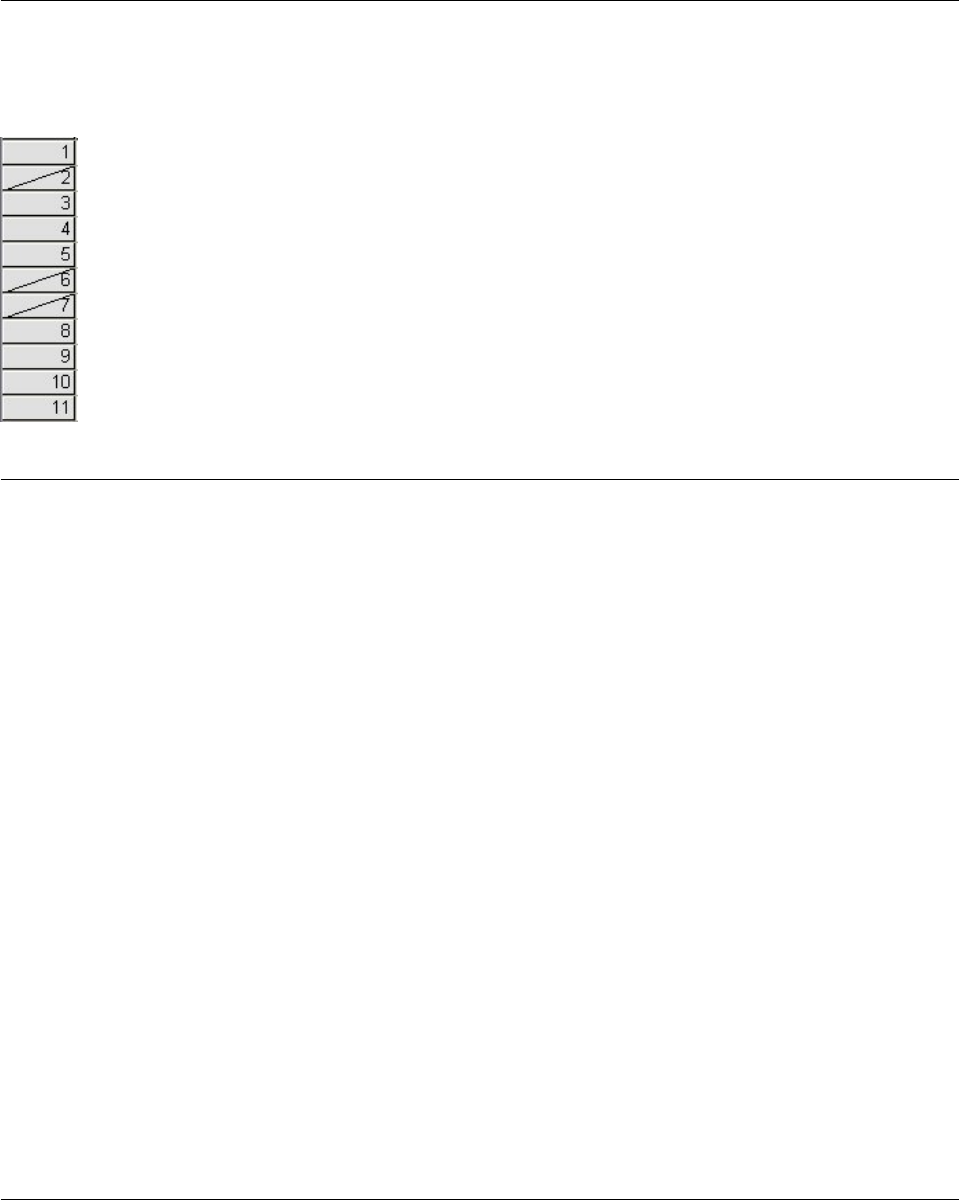
Case selection status in the Data Editor
If you have selected a subset of cases but have not discarded unselected cases, unselected cases are
marked in the Data Editor with a diagonal line (slash) through the row number.
Data Editor display options
The View menu provides several display options for the Data Editor:
Fonts. This option controls the font characteristics of the data display.
Grid Lines. This option toggles the display of grid lines.
Value Labels. This option toggles between the display of actual data values and user-defined descriptive
value labels. This option is available only in Data View.
Using Multiple Views
In Data View, you can create multiple views (panes) by using the splitters that are located below the
horizontal scroll bar and to the right of the vertical scroll bar.
You can also use the Window menu to insert and remove pane splitters. To insert splitters:
1. In Data View, from the menus choose:
Window > Split
Splitters are inserted above and to the left of the selected cell.
vIf the top left cell is selected, splitters are inserted to divide the current view approximately in half,
both horizontally and vertically.
vIf any cell other than the top cell in the first column is selected, a horizontal pane splitter is inserted
above the selected cell.
vIf any cell other than the first cell in the top row is selected, a vertical pane splitter is inserted to the
left of the selected cell.
Data Editor printing
A data file is printed as it appears on the screen.
Figure 1. Filtered cases in the Data Editor
Chapter 5. Data Editor 65
vThe information in the currently displayed view is printed. In Data View, the data are printed. In
Variable View, data definition information is printed.
vGrid lines are printed if they are currently displayed in the selected view.
vValue labels are printed in Data View if they are currently displayed. Otherwise, the actual data values
are printed.
Use the View menu in the Data Editor window to display or hide grid lines and toggle between the
display of data values and value labels.
To print Data Editor contents
1. Make the Data Editor the active window.
2. Click the tab for the view that you want to print.
3. From the menus choose:
File > Print...
66 IBM SPSS Statistics 24 Core System User's Guide

Chapter 6. Working with Multiple Data Sources
Starting with version 14.0, multiple data sources can be open at the same time, making it easier to:
vSwitch back and forth between data sources.
vCompare the contents of different data sources.
vCopy and paste data between data sources.
vCreate multiple subsets of cases and/or variables for analysis.
vMerge multiple data sources from various data formats (for example, spreadsheet, database, text data)
without saving each data source first.
Basic Handling of Multiple Data Sources
By default, each data source that you open is displayed in a new Data Editor window. (See “General
options” on page 195 for information on changing the default behavior to only display one dataset at a
time, in a single Data Editor window.)
vAny previously open data sources remain open and available for further use.
vWhen you first open a data source, it automatically becomes the active dataset.
vYou can change the active dataset simply by clicking anywhere in the Data Editor window of the data
source that you want to use or by selecting the Data Editor window for that data source from the
Window menu.
vOnly the variables in the active dataset are available for analysis.
vYou cannot change the active dataset when any dialog box that accesses the data is open (including all
dialog boxes that display variable lists).
vAt least one Data Editor window must be open during a session. When you close the last open Data
Editor window, IBM SPSS Statistics automatically shuts down, prompting you to save changes first.
Working with Multiple Datasets in Command Syntax
If you use command syntax to open data sources (for example, GET FILE, GET DATA), you need to use the
DATASET NAME command to name each dataset explicitly in order to have more than one data source open
at the same time.
When working with command syntax, the active dataset name is displayed on the toolbar of the syntax
window. All of the following actions can change the active dataset:
vUse the DATASET ACTIVATE command.
vClick anywhere in the Data Editor window of a dataset.
vSelect a dataset name from the Active drop-down list on the toolbar in the syntax window.
Copying and Pasting Information between Datasets
You can copy both data and variable definition attributes from one dataset to another dataset in basically
the same way that you copy and paste information within a single data file.
vCopying and pasting selected data cells in Data View pastes only the data values, with no variable
definition attributes.
vCopying and pasting an entire variable in Data View by selecting the variable name at the top of the
column pastes all of the data and all of the variable definition attributes for that variable.
vCopying and pasting variable definition attributes or entire variables in Variable View pastes the
selected attributes (or the entire variable definition) but does not paste any data values.
67

Renaming Datasets
When you open a data source through the menus and dialog boxes, each data source is automatically
assigned a dataset name of DataSetn, where nis a sequential integer value, and when you open a data
source using command syntax, no dataset name is assigned unless you explicitly specify one with
DATASET NAME . To provide more descriptive dataset names:
1. From the menus in the Data Editor window for the dataset whose name you want to change choose:
File > Rename Dataset...
2. Enter a new dataset name that conforms to variable naming rules. See the topic “Variable names” on
page 52 for more information.
Suppressing Multiple Datasets
If you prefer to have only one dataset available at a time and want to suppress the multiple dataset
feature:
1. From the menus choose:
Edit > Options...
2. Click the General tab.
Select (check) Open only one dataset at a time.
See the topic “General options” on page 195 for more information.
68 IBM SPSS Statistics 24 Core System User's Guide

Chapter 7. Data preparation
Once you've opened a data file or entered data in the Data Editor, you can start creating reports, charts,
and analyses without any additional preliminary work. However, there are some additional data
preparation features that you may find useful, including the ability to:
vAssign variable properties that describe the data and determine how certain values should be treated.
vIdentify cases that may contain duplicate information and exclude those cases from analyses or delete
them from the data file.
vCreate new variables with a few distinct categories that represent ranges of values from variables with
a large number of possible values.
Variable properties
Data entered in the Data Editor in Data View or read from an external file format (such as an Excel
spreadsheet or a text data file) lack certain variable properties that you may find very useful, including:
vDefinition of descriptive value labels for numeric codes (for example, 0 = Male and 1 = Female).
vIdentification of missing values codes (for example, 99 = Not applicable).
vAssignment of measurement level (nominal, ordinal, or scale).
All of these variable properties (and others) can be assigned in Variable View in the Data Editor. There
are also several utilities that can assist you in this process:
vDefine Variable Properties can help you define descriptive value labels and missing values. This is
particularly useful for categorical data with numeric codes used for category values. See the topic
“Defining Variable Properties” for more information.
vSet Measurement Level for Unknown identifies variables (fields) that do not have a defined
measurement level and provides the ability to set the measurement level for those variables. This is
important for procedures in which measurement level can affect the results or determines which
features are available. See the topic “Setting measurement level for variables with unknown
measurement level” on page 72 for more information.
vCopy Data Properties provides the ability to use an existing IBM SPSS Statistics data file as a template
for file and variable properties in the current data file. This is particularly useful if you frequently use
external-format data files that contain similar content (such as monthly reports in Excel format). See the
topic “Copying Data Properties” on page 75 for more information.
Defining Variable Properties
Define Variable Properties is designed to assist you in the process of assigning attributes to variables,
including creating descriptive value labels for categorical (nominal, ordinal) variables. Define Variable
Properties:
vScans the actual data values and lists all unique data values for each selected variable.
vIdentifies unlabeled values and provides an "auto-label" feature.
vProvides the ability to copy defined value labels and other attributes from another variable to the
selected variable or from the selected variable to multiple additional variables.
Note: To use Define Variable Properties without first scanning cases, enter 0 for the number of cases to
scan.
© Copyright IBM Corporation 1989, 2016 69
To Define Variable Properties
1. From the menus choose:
Data > Define Variable Properties...
2. Select the numeric or string variables for which you want to create value labels or define or change
other variable properties, such as missing values or descriptive variable labels.
3. Specify the number of cases to scan to generate the list of unique values. This is particularly useful
for data files with a large number of cases for which a scan of the complete data file might take a
significant amount of time.
4. Specify an upper limit for the number of unique values to display. This is primarily useful to
prevent listing hundreds, thousands, or even millions of values for scale (continuous interval, ratio)
variables.
5. Click Continue to open the main Define Variable Properties dialog box.
6. Select a variable for which you want to create value labels or define or change other variable
properties.
7. Enter the label text for any unlabeled values that are displayed in the Value Label grid.
8. If there are values for which you want to create value labels but those values are not displayed, you
can enter values in the Value column below the last scanned value.
9. Repeat this process for each listed variable for which you want to create value labels.
10. Click OK to apply the value labels and other variable properties.
Defining Value Labels and Other Variable Properties
The Define Variable Properties main dialog box provides the following information for the scanned
variables:
Scanned Variable List. For each scanned variable, a check mark in the Unlabeled (U.) column indicates
that the variable contains values without assigned value labels.
To sort the variable list to display all variables with unlabeled values at the top of the list:
1. Click the Unlabeled column heading under Scanned Variable List.
You can also sort by variable name or measurement level by clicking the corresponding column heading
under Scanned Variable List.
Value Label Grid
vLabel. Displays any value labels that have already been defined. You can add or change labels in this
column.
vValue. Unique values for each selected variable. This list of unique values is based on the number of
scanned cases. For example, if you scanned only the first 100 cases in the data file, then the list reflects
only the unique values present in those cases. If the data file has already been sorted by the variable
for which you want to assign value labels, the list may display far fewer unique values than are
actually present in the data.
vCount. The number of times each value occurs in the scanned cases.
vMissing. Values defined as representing missing data. You can change the missing values designation
of the category by clicking the check box. A check indicates that the category is defined as a
user-missing category. If a variable already has a range of values defined as user-missing (for example,
90-99), you cannot add or delete missing values categories for that variable with Define Variable
Properties. You can use Variable View in the Data Editor to modify the missing values categories for
variables with missing values ranges. See the topic “Missing values” on page 55 for more information.
vChanged. Indicates that you have added or changed a value label.
70 IBM SPSS Statistics 24 Core System User's Guide
Note: If you specified 0 for the number of cases to scan in the initial dialog box, the Value Label grid will
initially be blank, except for any preexisting value labels and/or defined missing values categories for the
selected variable. In addition, the Suggest button for the measurement level will be disabled.
Measurement Level. Value labels are primarily useful for categorical (nominal and ordinal) variables, and
some procedures treat categorical and scale variables differently; so it is sometimes important to assign
the correct measurement level. However, by default, all new numeric variables are assigned the scale
measurement level. Thus, many variables that are in fact categorical may initially be displayed as scale.
If you are unsure of what measurement level to assign to a variable, click Suggest.
Role. Some dialogs support the ability to pre-select variables for analysis based on defined roles. See the
topic “Roles” on page 56 for more information.
Copy Properties. You can copy value labels and other variable properties from another variable to the
currently selected variable or from the currently selected variable to one or more other variables.
Unlabeled Values. To create labels for unlabeled values automatically, click Automatic Labels.
Variable Label and Display Format
You can change the descriptive variable label and the display format.
vYou cannot change the variable's fundamental type (string or numeric).
vFor string variables, you can change only the variable label, not the display format.
vFor numeric variables, you can change the numeric type (such as numeric, date, dollar, or custom
currency), width (maximum number of digits, including any decimal and/or grouping indicators), and
number of decimal positions.
vFor numeric date format, you can select a specific date format (such as dd-mm-yyyy, mm/dd/yy, and
yyyyddd)
vFor numeric custom format, you can select one of five custom currency formats (CCA through CCE).
See the topic “Currency options” on page 200 for more information.
vAn asterisk is displayed in the Value column if the specified width is less than the width of the
scanned values or the displayed values for preexisting defined value labels or missing values
categories.
vA period (.) is displayed if the scanned values or the displayed values for preexisting defined value
labels or missing values categories are invalid for the selected display format type. For example, an
internal numeric value of less than 86,400 is invalid for a date format variable.
Assigning the Measurement Level
When you click Suggest for the measurement level in the Define Variable Properties main dialog box, the
current variable is evaluated based on the scanned cases and defined value labels, and a measurement
level is suggested in the Suggest Measurement Level dialog box that opens. The Explanation area
provides a brief description of the criteria used to provide the suggested measurement level.
Note: Values defined as representing missing values are not included in the evaluation for measurement
level. For example, the explanation for the suggested measurement level may indicate that the suggestion
is in part based on the fact that the variable contains no negative values, whereas it may in fact contain
negative values--but those values are already defined as missing values.
1. Click Continue to accept the suggested level of measurement or Cancel to leave the measurement
level unchanged.
Chapter 7. Data preparation 71

Custom Variable Attributes
The Attributes button in Define Variable Properties opens the Custom Variable Attributes dialog box. In
addition to the standard variable attributes, such as value labels, missing values, and measurement level,
you can create your own custom variable attributes. Like standard variable attributes, these custom
attributes are saved with IBM SPSS Statistics data files.
Name. Attribute names must follow the same rules as variable names. See the topic “Variable names” on
page 52 for more information.
Value. The value assigned to the attribute for the selected variable.
vAttribute names that begin with a dollar sign are reserved and cannot be modified. You can view the
contents of a reserved attribute by clicking the button in the desired cell.
vThe text Array..., displayed in a Value cell, indicates that this is an attribute array, an attribute that
contains multiple values. Click the button in the cell to display the list of values.
Copying Variable Properties
The Apply Labels and Level dialog box is displayed when you click From Another Variable or To Other
Variables in the Define Variable Properties main dialog box. It displays all of the scanned variables that
match the current variable's type (numeric or string). For string variables, the defined width must also
match.
1. Select a single variable from which to copy value labels and other variable properties (except variable
label).
or
2. Select one or more variables to which to copy value labels and other variable properties.
3. Click Copy to copy the value labels and the measurement level.
vExisting value labels and missing value categories for target variable(s) are not replaced.
vValue labels and missing value categories for values not already defined for the target variable(s) are
added to the set of value labels and missing value categories for the target variable(s).
vThe measurement level for the target variable is always replaced.
vThe role for the target variable is always replaced.
vIf either the source or target variable has a defined range of missing values, missing values definitions
are not copied.
Setting measurement level for variables with unknown measurement
level
For some procedures, measurement level can affect the results or determine which features are available,
and you cannot access the dialogs for these procedures until all variables have a defined measurement
level. The Set Measurement Level for Unknown dialog allows you to define measurement level for any
variables with an unknown measurement level without performing a data pass (which may be
time-consuming for large data files).
Under certain conditions, the measurement level for some or all numeric variables (fields) in a file may
be unknown. These conditions include:
vNumeric variables from Excel 95 or later files, text data files, or data base sources prior to the first data
pass.
vNew numeric variables created with transformation commands prior to the first data pass after
creation of those variables.
72 IBM SPSS Statistics 24 Core System User's Guide

These conditions apply primarily to reading data or creating new variables via command syntax. Dialogs
for reading data and creating new transformed variables automatically perform a data pass that sets the
measurement level, based on the default measurement level rules.
To set the measurement level for variables with an unknown measurement level
1. In the alert dialog that appears for the procedure, click Assign Manually.
or
2. From the menus, choose:
Data > Set Measurement Level for Unknown
3. Move variables (fields) from the source list to the appropriate measurement level destination list.
vNominal. A variable can be treated as nominal when its values represent categories with no intrinsic
ranking (for example, the department of the company in which an employee works). Examples of
nominal variables include region, postal code, and religious affiliation.
vOrdinal. A variable can be treated as ordinal when its values represent categories with some intrinsic
ranking (for example, levels of service satisfaction from highly dissatisfied to highly satisfied).
Examples of ordinal variables include attitude scores representing degree of satisfaction or confidence
and preference rating scores.
vContinuous. A variable can be treated as scale (continuous) when its values represent ordered categories
with a meaningful metric, so that distance comparisons between values are appropriate. Examples of
scale variables include age in years and income in thousands of dollars.
Multiple Response Sets
Custom Tables and the Chart Builder support a special kind of "variable" called a multiple response set.
Multiple response sets aren't really "variables" in the normal sense. You can't see them in the Data Editor,
and other procedures don't recognize them. Multiple response sets use multiple variables to record
responses to questions where the respondent can give more than one answer. Multiple response sets are
treated like categorical variables, and most of the things you can do with categorical variables, you can
also do with multiple response sets.
Multiple response sets are constructed from multiple variables in the data file. A multiple response set is
a special construct within a data file. You can define and save multiple response sets in IBM SPSS
Statistics data files, but you cannot import or export multiple response sets from/to other file formats.
You can copy multiple response sets from other IBM SPSS Statistics data files using Copy Data Properties,
which is accessed from the Data menu in the Data Editor window.
Defining Multiple Response Sets
To define multiple response sets:
1. From the menus, choose:
Data > Define Multiple Response Sets...
2. Select two or more variables. If your variables are coded as dichotomies, indicate which value you
want to have counted.
3. Enter a unique name for each multiple response set. The name can be up to 63 bytes long. A dollar
sign is automatically added to the beginning of the set name.
4. Enter a descriptive label for the set. (This is optional.)
5. Click Add to add the multiple response set to the list of defined sets.
Dichotomies
Chapter 7. Data preparation 73
A multiple dichotomy set typically consists of multiple dichotomous variables: variables with only two
possible values of a yes/no, present/absent, checked/not checked nature. Although the variables may not
be strictly dichotomous, all of the variables in the set are coded the same way, and the Counted Value
represents the positive/present/checked condition.
For example, a survey asks the question, "Which of the following sources do you rely on for news?" and
provides five possible responses. The respondent can indicate multiple choices by checking a box next to
each choice. The five responses become five variables in the data file, coded 0 for No (not checked) and 1
for Yes (checked). In the multiple dichotomy set, the Counted Value is 1.
The sample data file survey_sample.sav already has three defined multiple response sets. $mltnews is a
multiple dichotomy set.
1. Select (click) $mltnews in the Mult. Response Sets list.
This displays the variables and settings used to define this multiple response set.
vThe Variables in Set list displays the five variables used to construct the multiple response set.
vThe Variable Coding group indicates that the variables are dichotomous.
vThe Counted Value is 1.
2. Select (click) one of the variables in the Variables in Set list.
3. Right-click the variable and select Variable Information from the pop-up pop-up menu.
4. In the Variable Information window, click the arrow on the Value Labels drop-down list to display the
entire list of defined value labels.
The value labels indicate that the variable is a dichotomy with values of 0 and 1, representing No and Yes,
respectively. All five variables in the list are coded the same way, and the value of 1 (the code for Yes) is
the counted value for the multiple dichotomy set.
Categories
A multiple category set consists of multiple variables, all coded the same way, often with many possible
response categories. For example, a survey item states, "Name up to three nationalities that best describe
your ethnic heritage." There may be hundreds of possible responses, but for coding purposes the list is
limited to the 40 most common nationalities, with everything else relegated to an "other" category. In the
data file, the three choices become three variables, each with 41 categories (40 coded nationalities and one
"other" category).
In the sample data file, $ethmult and $mltcars are multiple category sets.
Category Label Source
For multiple dichotomies, you can control how sets are labeled.
vVariable labels. Uses the defined variable labels (or variable names for variables without defined
variable labels) as the set category labels. For example, if all of the variables in the set have the same
value label (or no defined value labels) for the counted value (for example, Yes), then you should use
the variable labels as the set category labels.
vLabels of counted values. Uses the defined value labels of the counted values as set category labels.
Select this option only if all variables have a defined value label for the counted value and the value
label for the counted value is different for each variable.
vUse variable label as set label. If you select Label of counted values, you can also use the variable
label for the first variable in the set with a defined variable label as the set label. If none of the
variables in the set have defined variable labels, the name of the first variable in the set is used as the
set label.
74 IBM SPSS Statistics 24 Core System User's Guide

Copy Data Properties
Copying Data Properties
The Copy Data Properties Wizard provides the ability to use an external IBM SPSS Statistics data file as a
template for defining file and variable properties in the active dataset. You can also use variables in the
active dataset as templates for other variables in the active dataset. You can:
vCopy selected file properties from an external data file or open dataset to the active dataset. File
properties include documents, file labels, multiple response sets, variable sets, and weighting.
vCopy selected variable properties from an external data file or open dataset to matching variables in
the active dataset. Variable properties include value labels, missing values, level of measurement,
variable labels, print and write formats, alignment, and column width (in the Data Editor).
vCopy selected variable properties from one variable in either an external data file, open dataset, or the
active dataset to many variables in the active dataset.
vCreate new variables in the active dataset based on selected variables in an external data file or open
dataset.
When copying data properties, the following general rules apply:
vIf you use an external data file as the source data file, it must be a data file in IBM SPSS Statistics
format.
vIf you use the active dataset as the source data file, it must contain at least one variable. You cannot
use a completely blank active dataset as the source data file.
vUndefined (empty) properties in the source dataset do not overwrite defined properties in the active
dataset.
vVariable properties are copied from the source variable only to target variables of a matching
type--string (alphanumeric) or numeric (including numeric, date, and currency).
Note: Copy Data Properties replaces Apply Data Dictionary, formerly available on the File menu.
To Copy Data Properties
1. From the menus in the Data Editor window choose:
Data > Copy Data Properties...
2. Select the data file with the file and/or variable properties that you want to copy. This can be a
currently open dataset, an external IBM SPSS Statistics data file, or the active dataset.
3. Follow the step-by-step instructions in the Copy Data Properties Wizard.
Selecting Source and Target Variables
In this step, you can specify the source variables containing the variable properties that you want to copy
and the target variables that will receive those variable properties.
Apply properties from selected source dataset variables to matching active dataset variables. Variable
properties are copied from one or more selected source variables to matching variables in the active
dataset. Variables "match" if both the variable name and type (string or numeric) are the same. For string
variables, the defined length must also be the same. By default, only matching variables are displayed in
the two variable lists.
vCreate matching variables in the active dataset if they do not already exist. This updates the source
list to display all variables in the source data file. If you select source variables that do not exist in the
active dataset (based on variable name), new variables will be created in the active dataset with the
variable names and properties from the source data file.
If the active dataset contains no variables (a blank, new dataset), all variables in the source data file are
displayed and new variables based on the selected source variables are automatically created in the active
dataset.
Chapter 7. Data preparation 75
Apply properties from a single source variable to selected active dataset variables of the same type.
Variable properties from a single selected variable in the source list can be applied to one or more
selected variables in the active dataset list. Only variables of the same type (numeric or string) as the
selected variable in the source list are displayed in the active dataset list. For string variables, only strings
of the same defined length as the source variable are displayed. This option is not available if the active
dataset contains no variables.
Note: You cannot create new variables in the active dataset with this option.
Apply dataset properties only--no variable selection. Only file properties (for example, documents, file
label, weight) will be applied to the active dataset. No variable properties will be applied. This option is
not available if the active dataset is also the source data file.
Choosing Variable Properties to Copy
You can copy selected variable properties from the source variables to the target variables. Undefined
(empty) properties in the source variables do not overwrite defined properties in the target variables.
Value Labels. Value labels are descriptive labels associated with data values. Value labels are often used
when numeric data values are used to represent non-numeric categories (for example, codes of 1 and 2
for Male and Female). You can replace or merge value labels in the target variables.
vReplace deletes any defined value labels for the target variable and replaces them with the defined
value labels from the source variable.
vMerge merges the defined value labels from the source variable with any existing defined value label
for the target variable. If the same value has a defined value label in both the source and target
variables, the value label in the target variable is unchanged.
Custom Attributes. User-defined custom variable attributes. See the topic “Custom Variable Attributes”
on page 57 for more information.
vReplace deletes any custom attributes for the target variable and replaces them with the defined
attributes from the source variable.
vMerge merges the defined attributes from the source variable with any existing defined attributes for
the target variable.
Missing Values. Missing values are values identified as representing missing data (for example, 98 for Do
not know and 99 for Not applicable). Typically, these values also have defined value labels that describe
what the missing value codes stand for. Any existing defined missing values for the target variable are
deleted and replaced with the defined missing values from the source variable.
Variable Label. Descriptive variable labels can contain spaces and reserved characters not allowed in
variable names. If you're copying variable properties from a single source variable to multiple target
variables, you might want to think twice before selecting this option.
Measurement Level. The measurement level can be nominal, ordinal, or scale.
Role. Some dialogs support the ability to pre-select variables for analysis based on defined roles. See the
topic “Roles” on page 56 for more information.
Formats. For numeric variables, this controls numeric type (such as numeric, date, or currency), width
(total number of displayed characters, including leading and trailing characters and decimal indicator),
and number of decimal places displayed. This option is ignored for string variables.
Alignment. This affects only alignment (left, right, center) in Data View in the Data Editor.
Data Editor Column Width. This affects only column width in Data View in the Data Editor.
76 IBM SPSS Statistics 24 Core System User's Guide
Copying Dataset (File) Properties
You can apply selected, global dataset properties from the source data file to the active dataset. (This is
not available if the active dataset is the source data file.)
Multiple Response Sets. Applies multiple response set definitions from the source data file to the active
dataset.
vMultiple response sets that contain no variables in the active dataset are ignored unless those variables
will be created based on specifications in step 2 (Selecting Source and Target Variables) in the Copy
Data Properties Wizard.
vReplace deletes all multiple response sets in the active dataset and replaces them with the multiple
response sets from the source data file.
vMerge adds multiple response sets from the source data file to the collection of multiple response sets
in the active dataset. If a set with the same name exists in both files, the existing set in the active
dataset is unchanged.
Variable Sets. Variable sets are used to control the list of variables that are displayed in dialog boxes.
Variable sets are defined by selecting Define Variable Sets from the Utilities menu.
vSets in the source data file that contain variables that do not exist in the active dataset are ignored
unless those variables will be created based on specifications in step 2 (Selecting Source and Target
Variables) in the Copy Data Properties Wizard.
vReplace deletes any existing variable sets in the active dataset, replacing them with variable sets from
the source data file.
vMerge adds variable sets from the source data file to the collection of variable sets in the active
dataset. If a set with the same name exists in both files, the existing set in the active dataset is
unchanged.
Documents. Notes appended to the data file via the DOCUMENT command.
vReplace deletes any existing documents in the active dataset, replacing them with the documents from
the source data file.
vMerge combines documents from the source and active dataset. Unique documents in the source file
that do not exist in the active dataset are added to the active dataset. All documents are then sorted by
date.
Custom Attributes. Custom data file attributes, typically created with the DATAFILE ATTRIBUTE command
in command syntax.
vReplace deletes any existing custom data file attributes in the active dataset, replacing them with the
data file attributes from the source data file.
vMerge combines data file attributes from the source and active dataset. Unique attribute names in the
source file that do not exist in the active dataset are added to the active dataset. If the same attribute
name exists in both data files, the named attribute in the active dataset is unchanged.
Weight Specification. Weights cases by the current weight variable in the source data file if there is a
matching variable in the active dataset. This overrides any weighting currently in effect in the active
dataset.
File Label. Descriptive label applied to a data file with the FILE LABEL command.
Results
The last step in the Copy Data Properties Wizard provides information on the number of variables for
which variable properties will be copied from the source data file, the number of new variables that will
be created, and the number of dataset (file) properties that will be copied.
Chapter 7. Data preparation 77

You can also choose to paste the generated command syntax into a syntax window and save the syntax
for later use.
Identifying Duplicate Cases
"Duplicate" cases may occur in your data for many reasons, including:
vData entry errors in which the same case is accidentally entered more than once.
vMultiple cases share a common primary ID value but have different secondary ID values, such as
family members who all live in the same house.
vMultiple cases represent the same case but with different values for variables other than those that
identify the case, such as multiple purchases made by the same person or company for different
products or at different times.
Identify Duplicate Cases allows you to define duplicate almost any way that you want and provides some
control over the automatic determination of primary versus duplicate cases.
To Identify and Flag Duplicate Cases
1. From the menus choose:
Data > Identify Duplicate Cases...
2. Select one or more variables that identify matching cases.
3. Select one or more of the options in the Variables to Create group.
Optionally, you can:
4. Select one or more variables to sort cases within groups defined by the selected matching cases
variables. The sort order defined by these variables determines the "first" and "last" case in each
group. Otherwise, the original file order is used.
5. Automatically filter duplicate cases so that they won't be included in reports, charts, or calculations of
statistics.
Define matching cases by. Cases are considered duplicates if their values match for all selected variables.
If you want to identify only cases that are a 100% match in all respects, select all of the variables.
Sort within matching groups by. Cases are automatically sorted by the variables that define matching
cases. You can select additional sorting variables that will determine the sequential order of cases in each
matching group.
vFor each sort variable, you can sort in ascending or descending order.
vIf you select multiple sort variables, cases are sorted by each variable within categories of the
preceding variable in the list. For example, if you select date as the first sorting variable and amount as
the second sorting variable, cases will be sorted by amount within each date.
vUse the up and down arrow buttons to the right of the list to change the sort order of the variables.
vThe sort order determines the "first" and "last" case within each matching group, which determines the
value of the optional primary indicator variable. For example, if you want to filter out all but the most
recent case in each matching group, you could sort cases within the group in ascending order of a date
variable, which would make the most recent date the last date in the group.
Indicator of primary cases. Creates a variable with a value of 1 for all unique cases and the case
identified as the primary case in each group of matching cases and a value of 0 for the nonprimary
duplicates in each group.
vThe primary case can be either the last or first case in each matching group, as determined by the sort
order within the matching group. If you don't specify any sort variables, the original file order
determines the order of cases within each group.
vYou can use the indicator variable as a filter variable to exclude non-primary duplicates from reports
and analyses without deleting those cases from the data file.
78 IBM SPSS Statistics 24 Core System User's Guide

Sequential count of matching cases in each group. Creates a variable with a sequential value from 1 to n
for cases in each matching group. The sequence is based on the current order of cases in each group,
which is either the original file order or the order determined by any specified sort variables.
Move matching cases to the top. Sorts the data file so that all groups of matching cases are at the top of
the data file, making it easy to visually inspect the matching cases in the Data Editor.
Display frequencies for created variables. Frequency tables containing counts for each value of the
created variables. For example, for the primary indicator variable, the table would show the number of
cases with a value 0 for that variable, which indicates the number of duplicates, and the number of cases
with a value of 1 for that variable, which indicates the number of unique and primary cases.
Missing values
For numeric variables, the system-missing value is treated like any other value—cases with the
system-missing value for an identifier variable are treated as having matching values for that variable.
For string variables, cases with no value for an identifier variable are treated as having matching values
for that variable.
Filtered cases
Filter conditions are ignored. Filtered cases are included in the evaluation of duplicate cases. If you want
to exclude cases, define selection rules with Data > Select Cases and select Delete unselected cases.
Visual Binning
Visual Binning is designed to assist you in the process of creating new variables based on grouping
contiguous values of existing variables into a limited number of distinct categories. You can use Visual
Binning to:
vCreate categorical variables from continuous scale variables. For example, you could use a scale income
variable to create a new categorical variable that contains income ranges.
vCollapse a large number of ordinal categories into a smaller set of categories. For example, you could
collapse a rating scale of nine down to three categories representing low, medium, and high.
In the first step, you:
1. Select the numeric scale and/or ordinal variables for which you want to create new categorical
(binned) variables.
Optionally, you can limit the number of cases to scan. For data files with a large number of cases,
limiting the number of cases scanned can save time, but you should avoid this if possible because it will
affect the distribution of values used in subsequent calculations in Visual Binning.
Note: String variables and nominal numeric variables are not displayed in the source variable list. Visual
Binning requires numeric variables, measured on either a scale or ordinal level, since it assumes that the
data values represent some logical order that can be used to group values in a meaningful fashion. You
can change the defined measurement level of a variable in Variable View in the Data Editor. See the topic
“Variable measurement level” on page 53 for more information.
To Bin Variables
1. From the menus in the Data Editor window choose:
Transform > Visual Binning...
2. Select the numeric scale and/or ordinal variables for which you want to create new categorical
(binned) variables.
3. Select a variable in the Scanned Variable List.
Chapter 7. Data preparation 79
4. Enter a name for the new binned variable. Variable names must be unique and must follow variable
naming rules. See the topic “Variable names” on page 52 for more information.
5. Define the binning criteria for the new variable. See the topic “Binning Variables” for more
information.
6. Click OK.
Binning Variables
The Visual Binning main dialog box provides the following information for the scanned variables:
Scanned Variable List. Displays the variables you selected in the initial dialog box. You can sort the list
by measurement level (scale or ordinal) or by variable label or name by clicking on the column headings.
Cases Scanned. Indicates the number of cases scanned. All scanned cases without user-missing or
system-missing values for the selected variable are used to generate the distribution of values used in
calculations in Visual Binning, including the histogram displayed in the main dialog box and cutpoints
based on percentiles or standard deviation units.
Missing Values. Indicates the number of scanned cases with user-missing or system-missing values.
Missing values are not included in any of the binned categories. See the topic “User-Missing Values in
Visual Binning” on page 83 for more information.
Current Variable. The name and variable label (if any) for the currently selected variable that will be
used as the basis for the new, binned variable.
Binned Variable. Name and optional variable label for the new, binned variable.
vName. You must enter a name for the new variable. Variable names must be unique and must follow
variable naming rules. See the topic “Variable names” on page 52 for more information.
vLabel. You can enter a descriptive variable label up to 255 characters long. The default variable label is
the variable label (if any) or variable name of the source variable with (Binned) appended to the end of
the label.
Minimum and Maximum. Minimum and maximum values for the currently selected variable, based on
the scanned cases and not including values defined as user-missing.
Nonmissing Values. The histogram displays the distribution of nonmissing values for the currently
selected variable, based on the scanned cases.
vAfter you define bins for the new variable, vertical lines on the histogram are displayed to indicate the
cutpoints that define bins.
vYou can click and drag the cutpoint lines to different locations on the histogram, changing the bin
ranges.
vYou can remove bins by dragging cutpoint lines off the histogram.
Note: The histogram (displaying nonmissing values), the minimum, and the maximum are based on the
scanned values. If you do not include all cases in the scan, the true distribution may not be accurately
reflected, particularly if the data file has been sorted by the selected variable. If you scan zero cases, no
information about the distribution of values is available.
Grid. Displays the values that define the upper endpoints of each bin and optional value labels for each
bin.
vValue. The values that define the upper endpoints of each bin. You can enter values or use Make
Cutpoints to automatically create bins based on selected criteria. By default, a cutpoint with a value of
HIGH is automatically included. This bin will contain any nonmissing values above the other
80 IBM SPSS Statistics 24 Core System User's Guide
cutpoints. The bin defined by the lowest cutpoint will include all nonmissing values lower than or
equal to that value (or simply lower than that value, depending on how you define upper endpoints).
vLabel. Optional, descriptive labels for the values of the new, binned variable. Since the values of the
new variable will simply be sequential integers from 1 to n, labels that describe what the values
represent can be very useful. You can enter labels or use Make Labels to automatically create value
labels.
To Delete a Bin from the Grid
1. Right-click either the Value or Label cell for the bin.
2. From the pop-up menu, select Delete Row.
Note: If you delete the HIGH bin, any cases with values higher than the last specified cutpoint value will
be assigned the system-missing value for the new variable.
To Delete All Labels or Delete All Defined Bins
1. Right-click anywhere in the grid.
2. From the pop-up menu select either Delete All Labels or Delete All Cutpoints.
Upper Endpoints. Controls treatment of upper endpoint values entered in the Value column of the grid.
vIncluded (<=). Cases with the value specified in the Value cell are included in the binned category. For
example, if you specify values of 25, 50, and 75, cases with a value of exactly 25 will go in the first bin,
since this will include all cases with values less than or equal to 25.
vExcluded (<). Cases with the value specified in the Value cell are not included in the binned category.
Instead, they are included in the next bin. For example, if you specify values of 25, 50, and 75, cases
with a value of exactly 25 will go in the second bin rather than the first, since the first bin will contain
only cases with values less than 25.
Make Cutpoints. Generates binned categories automatically for equal width intervals, intervals with the
same number of cases, or intervals based on standard deviations. This is not available if you scanned
zero cases. See the topic “Automatically Generating Binned Categories” for more information.
Make Labels. Generates descriptive labels for the sequential integer values of the new, binned variable,
based on the values in the grid and the specified treatment of upper endpoints (included or excluded).
Reverse scale. By default, values of the new, binned variable are ascending sequential integers from 1 to
n. Reversing the scale makes the values descending sequential integers from nto 1.
Copy Bins. You can copy the binning specifications from another variable to the currently selected
variable or from the selected variable to multiple other variables. See the topic “Copying Binned
Categories” on page 82 for more information.
Automatically Generating Binned Categories
The Make Cutpoints dialog box allows you to auto-generate binned categories based on selected criteria.
To Use the Make Cutpoints Dialog Box
1. Select (click) a variable in the Scanned Variable List.
2. Click Make Cutpoints.
3. Select the criteria for generating cutpoints that will define the binned categories.
4. Click Apply.
Note: The Make Cutpoints dialog box is not available if you scanned zero cases.
Chapter 7. Data preparation 81
Equal Width Intervals. Generates binned categories of equal width (for example, 1–10, 11–20, and 21–30)
based on any two of the following three criteria:
vFirst Cutpoint Location. The value that defines the upper end of the lowest binned category (for
example, a value of 10 indicates a range that includes all values up to 10).
vNumber of Cutpoints. The number of binned categories is the number of cutpoints plus one. For
example, 9 cutpoints generate 10 binned categories.
vWidth. The width of each interval. For example, a value of 10 would bin age in years into 10-year
intervals.
Equal Percentiles Based on Scanned Cases. Generates binned categories with an equal number of cases
in each bin (using the aempirical algorithm for percentiles), based on either of the following criteria:
vNumber of Cutpoints. The number of binned categories is the number of cutpoints plus one. For
example, three cutpoints generate four percentile bins (quartiles), each containing 25% of the cases.
vWidth (%). Width of each interval, expressed as a percentage of the total number of cases. For
example, a value of 33.3 would produce three binned categories (two cutpoints), each containing 33.3%
of the cases.
If the source variable contains a relatively small number of distinct values or a large number of cases
with the same value, you may get fewer bins than requested. If there are multiple identical values at a
cutpoint, they will all go into the same interval; so the actual percentages may not always be exactly
equal.
Cutpoints at Mean and Selected Standard Deviations Based on Scanned Cases. Generates binned
categories based on the values of the mean and standard deviation of the distribution of the variable.
vIf you don't select any of the standard deviation intervals, two binned categories will be created, with
the mean as the cutpoint dividing the bins.
vYou can select any combination of standard deviation intervals based on one, two, and/or three
standard deviations. For example, selecting all three would result in eight binned categories--six bins in
one standard deviation intervals and two bins for cases more than three standard deviations above and
below the mean.
In a normal distribution, 68% of the cases fall within one standard deviation of the mean; 95%, within
two standard deviations; and 99%, within three standard deviations. Creating binned categories based on
standard deviations may result in some defined bins outside of the actual data range and even outside of
the range of possible data values (for example, a negative salary range).
Note: Calculations of percentiles and standard deviations are based on the scanned cases. If you limit the
number of cases scanned, the resulting bins may not contain the proportion of cases that you wanted in
those bins, particularly if the data file is sorted by the source variable. For example, if you limit the scan
to the first 100 cases of a data file with 1000 cases and the data file is sorted in ascending order of age of
respondent, instead of four percentile age bins each containing 25% of the cases, you may find that the
first three bins each contain only about 3.3% of the cases, and the last bin contains 90% of the cases.
Copying Binned Categories
When creating binned categories for one or more variables, you can copy the binning specifications from
another variable to the currently selected variable or from the selected variable to multiple other
variables.
To Copy Binning Specifications
1. Define binned categories for at least one variable--but do not click OK or Paste.
2. Select (click) a variable in the Scanned Variable List for which you have defined binned categories.
3. Click To Other Variables.
4. Select the variables for which you want to create new variables with the same binned categories.
82 IBM SPSS Statistics 24 Core System User's Guide
5. Click Copy.
or
6. Select (click) a variable in the Scanned Variable List to which you want to copy defined binned
categories.
7. Click From Another Variable.
8. Select the variable with the defined binned categories that you want to copy.
9. Click Copy.
If you have specified value labels for the variable from which you are copying the binning specifications,
those are also copied.
Note: Once you click OK in the Visual Binning main dialog box to create new binned variables (or close
the dialog box in any other way), you cannot use Visual Binning to copy those binned categories to other
variables.
User-Missing Values in Visual Binning
Values defined as user-missing (values identified as codes for missing data) for the source variable are
not included in the binned categories for the new variable. User-missing values for the source variables
are copied as user-missing values for the new variable, and any defined value labels for missing value
codes are also copied.
If a missing value code conflicts with one of the binned category values for the new variable, the missing
value code for the new variable is recoded to a nonconflicting value by adding 100 to the highest binned
category value. For example, if a value of 1 is defined as user-missing for the source variable and the
new variable will have six binned categories, any cases with a value of 1 for the source variable will have
a value of 106 for the new variable, and 106 will be defined as user-missing. If the user-missing value for
the source variable had a defined value label, that label will be retained as the value label for the recoded
value of the new variable.
Note: If the source variable has a defined range of user-missing values of the form LO-n, where nis a
positive number, the corresponding user-missing values for the new variable will be negative numbers.
Chapter 7. Data preparation 83
84 IBM SPSS Statistics 24 Core System User's Guide

Chapter 8. Data Transformations
Data Transformations
In an ideal situation, your raw data are perfectly suitable for the type of analysis you want to perform,
and any relationships between variables are either conveniently linear or neatly orthogonal.
Unfortunately, this is rarely the case. Preliminary analysis may reveal inconvenient coding schemes or
coding errors, or data transformations may be required in order to expose the true relationship between
variables.
You can perform data transformations ranging from simple tasks, such as collapsing categories for
analysis, to more advanced tasks, such as creating new variables based on complex equations and
conditional statements.
Computing Variables
Use the Compute dialog box to compute values for a variable based on numeric transformations of other
variables.
vYou can compute values for numeric or string (alphanumeric) variables.
vYou can create new variables or replace the values of existing variables. For new variables, you can
also specify the variable type and label.
vYou can compute values selectively for subsets of data based on logical conditions.
vYou can use a large variety of built-in functions, including arithmetic functions, statistical functions,
distribution functions, and string functions.
To Compute Variables
1. From the menus choose:
Transform > Compute Variable...
2. Type the name of a single target variable. It can be an existing variable or a new variable to be added
to the active dataset.
3. To build an expression, either paste components into the Expression field or type directly in the
Expression field.
vYou can paste functions or commonly used system variables by selecting a group from the Function
group list and double-clicking the function or variable in the Functions and Special Variables list (or
select the function or variable and click the arrow adjacent to the Function group list). Fill in any
parameters indicated by question marks (only applies to functions). The function group labeled All
provides a listing of all available functions and system variables. A brief description of the currently
selected function or variable is displayed in a reserved area in the dialog box.
vString constants must be enclosed in quotation marks or apostrophes.
vIf values contain decimals, a period (.) must be used as the decimal indicator.
vFor new string variables, you must also select Type & Label to specify the data type.
Compute Variable: If Cases
The If Cases dialog box allows you to apply data transformations to selected subsets of cases, using
conditional expressions. A conditional expression returns a value of true, false, or missing for each case.
vIf the result of a conditional expression is true, the case is included in the selected subset.
vIf the result of a conditional expression is false or missing, the case is not included in the selected
subset.
© Copyright IBM Corporation 1989, 2016 85

vMost conditional expressions use one or more of the six relational operators (<, >, <=, >=, =, and ~=)
on the calculator pad.
vConditional expressions can include variable names, constants, arithmetic operators, numeric (and
other) functions, logical variables, and relational operators.
Compute Variable: Type and Label
By default, new computed variables are numeric. To compute a new string variable, you must specify the
data type and width.
Label. Optional, descriptive variable label up to 255 bytes long. You can enter a label or use the first 110
characters of the compute expression as the label.
Type. Computed variables can be numeric or string (alphanumeric). String variables cannot be used in
calculations.
Functions
Many types of functions are supported, including:
vArithmetic functions
vStatistical functions
vString functions
vDate and time functions
vDistribution functions
vRandom variable functions
vMissing value functions
vScoring functions
For more information and a detailed description of each function, type functions on the Index tab of the
Help system.
Missing Values in Functions
Functions and simple arithmetic expressions treat missing values in different ways. In the expression:
(var1+var2+var3)/3
the result is missing if a case has a missing value for any of the three variables.
In the expression:
MEAN(var1, var2, var3)
the result is missing only if the case has missing values for all three variables.
For statistical functions, you can specify the minimum number of arguments that must have nonmissing
values. To do so, type a period and the minimum number after the function name, as in:
MEAN.2(var1, var2, var3)
86 IBM SPSS Statistics 24 Core System User's Guide

Random Number Generators
The Random Number Generators dialog box allows you to select the random number generator and set
the starting sequence value so you can reproduce a sequence of random numbers.
Active Generator. Two different random number generators are available:
vVersion 12 Compatible. The random number generator used in version 12 and previous releases. If you
need to reproduce randomized results generated in previous releases based on a specified seed value,
use this random number generator.
vMersenne Twister. A newer random number generator that is more reliable for simulation purposes. If
reproducing randomized results from version 12 or earlier is not an issue, use this random number
generator.
Active Generator Initialization. The random number seed changes each time a random number is
generated for use in transformations (such as random distribution functions), random sampling, or case
weighting. To replicate a sequence of random numbers, set the initialization starting point value prior to
each analysis that uses the random numbers. The value must be a positive integer.
Some procedures, such as Linear Models, have internal random number generators.
To select the random number generator and/or set the initialization value:
1. From the menus choose:
Transform > Random Number Generators
Count Occurrences of Values within Cases
This dialog box creates a variable that counts the occurrences of the same value(s) in a list of variables for
each case. For example, a survey might contain a list of magazines with yes/no check boxes to indicate
which magazines each respondent reads. You could count the number of yes responses for each
respondent to create a new variable that contains the total number of magazines read.
To Count Occurrences of Values within Cases
1. From the menus choose:
Transform > Count Values within Cases...
2. Enter a target variable name.
3. Select two or more variables of the same type (numeric or string).
4. Click Define Values and specify which value or values should be counted.
Optionally, you can define a subset of cases for which to count occurrences of values.
Count Values within Cases: Values to Count
The value of the target variable (on the main dialog box) is incremented by 1 each time one of the
selected variables matches a specification in the Values to Count list here. If a case matches several
specifications for any variable, the target variable is incremented several times for that variable.
Value specifications can include individual values, missing or system-missing values, and ranges. Ranges
include their endpoints and any user-missing values that fall within the range.
Count Occurrences: If Cases
The If Cases dialog box allows you to count occurrences of values for a selected subset of cases, using
conditional expressions. A conditional expression returns a value of true, false, or missing for each case.
Chapter 8. Data Transformations 87

Shift Values
Shift Values creates new variables that contain the values of existing variables from preceding or
subsequent cases.
Name. Name for the new variable. This must be a name that does not already exist in the active dataset.
Get value from earlier case (lag). Get the value from a previous case in the active dataset. For example,
with the default number of cases value of 1, each case for the new variable has the value of the original
variable from the case that immediately precedes it.
Get value from following case (lead). Get the value from a subsequent case in the active dataset. For
example, with the default number of cases value of 1, each case for the new variable has the value of the
original variable from the next case.
Number of cases to shift. Get the value from the nth preceding or subsequent case, where nis the value
specified. The value must be a non-negative integer.
vIf split file processing is on, the scope of the shift is limited to each split group. A shift value cannot be
obtained from a case in a preceding or subsequent split group.
vFilter status is ignored.
vThe value of the result variable is set to system-missing for the first or last ncases in the dataset or
split group, where nis the value specified for Number of cases to shift. For example, using the Lag
method with a value of 1 would set the result variable to system-missing for the first case in the
dataset (or first case in each split group).
vUser-missing values are preserved.
vDictionary information from the original variable, including defined value labels and user-missing
value assignments, is applied to the new variable. (Note: Custom variable attributes are not included.)
vA variable label is automatically generated for the new variable that describes the shift operation that
created the variable.
To Create a New Variable with Shifted Values
1. From the menus, choose:
Transform > Shift Values
2. Select the variable to use as the source of values for the new variable.
3. Enter a name for the new variable.
4. Select the shift method (lag or lead) and the number of cases to shift.
5. Click Change.
6. Repeat for each new variable you want to create.
Recoding Values
You can modify data values by recoding them. This is particularly useful for collapsing or combining
categories. You can recode the values within existing variables, or you can create new variables based on
the recoded values of existing variables.
Recode into Same Variables
The Recode into Same Variables dialog box allows you to reassign the values of existing variables or
collapse ranges of existing values into new values. For example, you could collapse salaries into salary
range categories.
88 IBM SPSS Statistics 24 Core System User's Guide
You can recode numeric and string variables. If you select multiple variables, they must all be the same
type. You cannot recode numeric and string variables together.
To Recode Values of a Variable
1. From the menus choose:
Transform > Recode into Same Variables...
2. Select the variables you want to recode. If you select multiple variables, they must be the same type
(numeric or string).
3. Click Old and New Values and specify how to recode values.
Optionally, you can define a subset of cases to recode. The If Cases dialog box for doing this is the same
as the one described for Count Occurrences.
Recode into Same Variables: Old and New Values
You can define values to recode in this dialog box. All value specifications must be the same data type
(numeric or string) as the variables selected in the main dialog box.
Old Value. The value(s) to be recoded. You can recode single values, ranges of values, and missing
values. System-missing values and ranges cannot be selected for string variables because neither concept
applies to string variables. Ranges include their endpoints and any user-missing values that fall within
the range.
vValue. Individual old value to be recoded into a new value. The value must be the same data type
(numeric or string) as the variable(s) being recoded.
vSystem-missing. Values assigned by the program when values in your data are undefined according to
the format type you have specified, when a numeric field is blank, or when a value resulting from a
transformation command is undefined. Numeric system-missing values are displayed as periods. String
variables cannot have system-missing values, since any character is legal in a string variable.
vSystem- or user-missing. Observations with values that either have been defined as user-missing values
or are unknown and have been assigned the system-missing value, which is indicated with a period (.).
vRange. Inclusive range of values. Not available for string variables. Any user-missing values within the
range are included.
vAll other values. Any remaining values not included in one of the specifications on the Old-New list.
This appears as ELSE on the Old-New list.
New Value. The single value into which each old value or range of values is recoded. You can enter a
value or assign the system-missing value.
vValue. Value into which one or more old values will be recoded. The value must be the same data type
(numeric or string) as the old value.
vSystem-missing. Recodes specified old values into the system-missing value. The system-missing value
is not used in calculations, and cases with the system-missing value are excluded from many
procedures. Not available for string variables.
Old–>New. The list of specifications that will be used to recode the variable(s). You can add, change, and
remove specifications from the list. The list is automatically sorted, based on the old value specification,
using the following order: single values, missing values, ranges, and all other values. If you change a
recode specification on the list, the procedure automatically re-sorts the list, if necessary, to maintain this
order.
Chapter 8. Data Transformations 89

Recode into Different Variables
The Recode into Different Variables dialog box allows you to reassign the values of existing variables or
collapse ranges of existing values into new values for a new variable. For example, you could collapse
salaries into a new variable containing salary-range categories.
vYou can recode numeric and string variables.
vYou can recode numeric variables into string variables and vice versa.
vIf you select multiple variables, they must all be the same type. You cannot recode numeric and string
variables together.
To Recode Values of a Variable into a New Variable
1. From the menus choose:
Transform > Recode into Different Variables...
2. Select the variables you want to recode. If you select multiple variables, they must be the same type
(numeric or string).
3. Enter an output (new) variable name for each new variable and click Change.
4. Click Old and New Values and specify how to recode values.
Optionally, you can define a subset of cases to recode. The If Cases dialog box for doing this is the same
as the one described for Count Occurrences.
Recode into Different Variables: Old and New Values
You can define values to recode in this dialog box.
Old Value. The value(s) to be recoded. You can recode single values, ranges of values, and missing
values. System-missing values and ranges cannot be selected for string variables because neither concept
applies to string variables. Old values must be the same data type (numeric or string) as the original
variable. Ranges include their endpoints and any user-missing values that fall within the range.
vValue. Individual old value to be recoded into a new value. The value must be the same data type
(numeric or string) as the variable(s) being recoded.
vSystem-missing. Values assigned by the program when values in your data are undefined according to
the format type you have specified, when a numeric field is blank, or when a value resulting from a
transformation command is undefined. Numeric system-missing values are displayed as periods. String
variables cannot have system-missing values, since any character is legal in a string variable.
vSystem- or user-missing. Observations with values that either have been defined as user-missing values
or are unknown and have been assigned the system-missing value, which is indicated with a period (.).
vRange. Inclusive range of values. Not available for string variables. Any user-missing values within the
range are included.
vAll other values. Any remaining values not included in one of the specifications on the Old-New list.
This appears as ELSE on the Old-New list.
New Value. The single value into which each old value or range of values is recoded. New values can be
numeric or string.
vValue. Value into which one or more old values will be recoded. The value must be the same data type
(numeric or string) as the old value.
vSystem-missing. Recodes specified old values into the system-missing value. The system-missing value
is not used in calculations, and cases with the system-missing value are excluded from many
procedures. Not available for string variables.
vCopy old values. Retains the old value. If some values don't require recoding, use this to include the old
values. Any old values that are not specified are not included in the new variable, and cases with those
values will be assigned the system-missing value for the new variable.
90 IBM SPSS Statistics 24 Core System User's Guide

Output variables are strings. Defines the new, recoded variable as a string (alphanumeric) variable. The old
variable can be numeric or string.
Convert numeric strings to numbers. Converts string values containing numbers to numeric values. Strings
containing anything other than numbers and an optional sign (+ or -) are assigned the system-missing
value.
Old–>New. The list of specifications that will be used to recode the variable(s). You can add, change, and
remove specifications from the list. The list is automatically sorted, based on the old value specification,
using the following order: single values, missing values, ranges, and all other values. If you change a
recode specification on the list, the procedure automatically re-sorts the list, if necessary, to maintain this
order.
Automatic Recode
The Automatic Recode dialog box allows you to convert string and numeric values into consecutive
integers. When category codes are not sequential, the resulting empty cells reduce performance and
increase memory requirements for many procedures. Additionally, some procedures cannot use string
variables, and some require consecutive integer values for factor levels.
vThe new variable(s) created by Automatic Recode retain any defined variable and value labels from the
old variable. For any values without a defined value label, the original value is used as the label for
the recoded value. A table displays the old and new values and value labels.
vString values are recoded in alphabetical order, with uppercase letters preceding their lowercase
counterparts.
vMissing values are recoded into missing values higher than any nonmissing values, with their order
preserved. For example, if the original variable has 10 nonmissing values, the lowest missing value
would be recoded to 11, and the value 11 would be a missing value for the new variable.
Use the same recoding scheme for all variables. This option allows you to apply a single autorecoding
scheme to all the selected variables, yielding a consistent coding scheme for all the new variables.
If you select this option, the following rules and limitations apply:
vAll variables must be of the same type (numeric or string).
vAll observed values for all selected variables are used to create a sorted order of values to recode into
sequential integers.
vUser-missing values for the new variables are based on the first variable in the list with defined
user-missing values. All other values from other original variables, except for system-missing, are
treated as valid.
Treat blank string values as user-missing. For string variables, blank or null values are not treated as
system-missing. This option will autorecode blank strings into a user-missing value higher than the highest
nonmissing value.
Templates
You can save the autorecoding scheme in a template file and then apply it to other variables and other
data files.
For example, you may have a large number of alphanumeric product codes that you autorecode into
integers every month, but some months new product codes are added that change the original
autorecoding scheme. If you save the original scheme in a template and then apply it to the new data
that contain the new set of codes, any new codes encountered in the data are autorecoded into values
higher than the last value in the template, preserving the original autorecode scheme of the original
product codes.
Chapter 8. Data Transformations 91

Save template as. Saves the autorecode scheme for the selected variables in an external template file.
vThe template contains information that maps the original nonmissing values to the recoded values.
vOnly information for nonmissing values is saved in the template. User-missing value information is not
retained.
vIf you have selected multiple variables for recoding but you have not selected to use the same
autorecoding scheme for all variables or you are not applying an existing template as part of the
autorecoding, the template will be based on the first variable in the list.
vIf you have selected multiple variables for recoding and you have also selected Use the same recoding
scheme for all variables and/or you have selected Apply template, then the template will contain the
combined autorecoding scheme for all variables.
Apply template from. Applies a previously saved autorecode template to variables selected for recoding,
appending any additional values found in the variables to the end of the scheme and preserving the
relationship between the original and autorecoded values stored in the saved scheme.
vAll variables selected for recoding must be the same type (numeric or string), and that type must
match the type defined in the template.
vTemplates do not contain any information on user-missing values. User-missing values for the target
variables are based on the first variable in the original variable list with defined user-missing values.
All other values from other original variables, except for system-missing, are treated as valid.
vValue mappings from the template are applied first. All remaining values are recoded into values
higher than the last value in the template, with user-missing values (based on the first variable in the
list with defined user-missing values) recoded into values higher than the last valid value.
vIf you have selected multiple variables for autorecoding, the template is applied first, followed by a
common, combined autorecoding for all additional values found in the selected variables, resulting in a
single, common autorecoding scheme for all selected variables.
To Recode String or Numeric Values into Consecutive Integers
1. From the menus choose:
Transform > Automatic Recode...
2. Select one or more variables to recode.
3. For each selected variable, enter a name for the new variable and click New Name.
Rank Cases
The Rank Cases dialog box allows you to create new variables containing ranks, normal and Savage
scores, and percentile values for numeric variables.
New variable names and descriptive variable labels are automatically generated, based on the original
variable name and the selected measure(s). A summary table lists the original variables, the new
variables, and the variable labels. (Note: The automatically generated new variable names are limited to a
maximum length of 8 bytes.)
Optionally, you can:
vRank cases in ascending or descending order.
vOrganize rankings into subgroups by selecting one or more grouping variables for the By list. Ranks
are computed within each group. Groups are defined by the combination of values of the grouping
variables. For example, if you select gender and minority as grouping variables, ranks are computed for
each combination of gender and minority.
To Rank Cases
1. From the menus choose:
Transform > Rank Cases...
92 IBM SPSS Statistics 24 Core System User's Guide
2. Select one or more variables to rank. You can rank only numeric variables.
Optionally, you can rank cases in ascending or descending order and organize ranks into subgroups.
Rank Cases: Types
You can select multiple ranking methods. A separate ranking variable is created for each method.
Ranking methods include simple ranks, Savage scores, fractional ranks, and percentiles. You can also
create rankings based on proportion estimates and normal scores.
Rank. Simple rank. The value of the new variable equals its rank.
Savage score. The new variable contains Savage scores based on an exponential distribution.
Fractional rank. The value of the new variable equals rank divided by the sum of the weights of the
nonmissing cases.
Fractional rank as percent. Each rank is divided by the number of cases with valid values and multiplied
by 100.
Sum of case weights. The value of the new variable equals the sum of case weights. The new variable is a
constant for all cases in the same group.
Ntiles. Ranks are based on percentile groups, with each group containing approximately the same number
of cases. For example, 4 Ntiles would assign a rank of 1 to cases below the 25th percentile, 2 to cases
between the 25th and 50th percentile, 3 to cases between the 50th and 75th percentile, and 4 to cases
above the 75th percentile.
Proportion estimates. Estimates of the cumulative proportion of the distribution corresponding to a
particular rank.
Normal scores. The z scores corresponding to the estimated cumulative proportion.
Proportion Estimation Formula. For proportion estimates and normal scores, you can select the
proportion estimation formula: Blom, Tukey, Rankit, or Van der Waerden.
vBlom. Creates new ranking variable based on proportion estimates that uses the formula (r-3/8) /
(w+1/4), where w is the sum of the case weights and r is the rank.
vTukey. Uses the formula (r-1/3) / (w+1/3), where r is the rank and w is the sum of the case weights.
vRankit. Uses the formula (r-1/2) / w, where w is the number of observations and r is the rank, ranging
from 1 to w.
vVan der Waerden. Van der Waerden's transformation, defined by the formula r/(w+1), where w is the
sum of the case weights and r is the rank, ranging from 1 to w.
Rank Cases: Ties
This dialog box controls the method for assigning rankings to cases with the same value on the original
variable.
The following table shows how the different methods assign ranks to tied values:
Table 7. Ranking methods and results
Value Mean Low High Sequential
10 1 1 1 1
15 3 2 4 2
15 3 2 4 2
Chapter 8. Data Transformations 93

Table 7. Ranking methods and results (continued)
Value Mean Low High Sequential
15 3 2 4 2
16 5 5 5 3
20 6 6 6 4
Date and Time Wizard
The Date and Time Wizard simplifies a number of common tasks associated with date and time variables.
To Use the Date and Time Wizard
1. From the menus choose:
Transform > Date and Time Wizard...
2. Select the task you want to accomplish and follow the steps to define the task.
vLearn how dates and times are represented. This choice leads to a screen that provides a brief
overview of date/time variables in IBM SPSS Statistics. By clicking on the Help button, it also provides
a link to more detailed information.
vCreate a date/time variable from a string containing a date or time. Use this option to create a
date/time variable from a string variable. For example, you have a string variable representing dates in
the form mm/dd/yyyy and want to create a date/time variable from this.
vCreate a date/time variable from variables holding parts of dates or times. This choice allows you to
construct a date/time variable from a set of existing variables. For example, you have a variable that
represents the month (as an integer), a second that represents the day of the month, and a third that
represents the year. You can combine these three variables into a single date/time variable.
vCalculate with dates and times. Use this option to add or subtract values from date/time variables.
For example, you can calculate the duration of a process by subtracting a variable representing the
start time of the process from another variable representing the end time of the process.
vExtract a part of a date or time variable. This option allows you to extract part of a date/time
variable, such as the day of the month from a date/time variable, which has the form mm/dd/yyyy.
vAssign periodicity to a dataset. This choice takes you to the Define Dates dialog box, used to create
date/time variables that consist of a set of sequential dates. This feature is typically used to associate
dates with time series data.
Note: Tasks are disabled when the dataset lacks the types of variables required to accomplish the task. For
instance, if the dataset contains no string variables, then the task to create a date/time variable from a
string does not apply and is disabled.
Dates and Times in IBM SPSS Statistics
Variables that represent dates and times in IBM SPSS Statistics have a variable type of numeric, with
display formats that correspond to the specific date/time formats. These variables are generally referred
to as date/time variables. Date/time variables that actually represent dates are distinguished from those
that represent a time duration that is independent of any date, such as 20 hours, 10 minutes, and 15
seconds. The latter are referred to as duration variables and the former as date or date/time variables.
For a complete list of display formats, see "Date and Time" in the "Universals" section of the Command
Syntax Reference.
Date and date/time variables. Date variables have a format representing a date, such as mm/dd/yyyy.
Date/time variables have a format representing a date and time, such as dd-mmm-yyyy hh:mm:ss.
Internally, date and date/time variables are stored as the number of seconds from October 14, 1582. Date
and date/time variables are sometimes referred to as date-format variables.
94 IBM SPSS Statistics 24 Core System User's Guide
vBoth two- and four-digit year specifications are recognized. By default, two-digit years represent a
range beginning 69 years prior to the current date and ending 30 years after the current date. This
range is determined by your Options settings and is configurable (from the Edit menu, choose Options
and click the Data tab).
vDashes, periods, commas, slashes, or blanks can be used as delimiters in day-month-year formats.
vMonths can be represented in digits, Roman numerals, or three-character abbreviations, and they can
be fully spelled out. Three-letter abbreviations and fully spelled-out month names must be in English;
month names in other languages are not recognized.
Duration variables. Duration variables have a format representing a time duration, such as hh:mm. They
are stored internally as seconds without reference to a particular date.
vIn time specifications (applies to date/time and duration variables), colons can be used as delimiters
between hours, minutes, and seconds. Hours and minutes are required, but seconds are optional. A
period is required to separate seconds from fractional seconds. Hours can be of unlimited magnitude,
but the maximum value for minutes is 59 and for seconds is 59.999....
Current date and time. The system variable $TIME holds the current date and time. It represents the
number of seconds from October 14, 1582, to the date and time when the transformation command that
uses it is executed.
Create a Date/Time Variable from a String
To create a date/time variable from a string variable:
1. Select Create a date/time variable from a string containing a date or time on the introduction screen
of the Date and Time Wizard.
Select String Variable to Convert to Date/Time Variable
1. Select the string variable to convert in the Variables list. Note that the list displays only string
variables.
2. Select the pattern from the Patterns list that matches how dates are represented by the string variable.
The Sample Values list displays actual values of the selected variable in the data file. Values of the
string variable that do not fit the selected pattern result in a value of system-missing for the new
variable.
Specify Result of Converting String Variable to Date/Time Variable
1. Enter a name for the Result Variable. This cannot be the name of an existing variable.
Optionally, you can:
vSelect a date/time format for the new variable from the Output Format list.
vAssign a descriptive variable label to the new variable.
Create a Date/Time Variable from a Set of Variables
To merge a set of existing variables into a single date/time variable:
1. Select Create a date/time variable from variables holding parts of dates or times on the introduction
screen of the Date and Time Wizard.
Select Variables to Merge into Single Date/Time Variable
1. Select the variables that represent the different parts of the date/time.
vSome combinations of selections are not allowed. For instance, creating a date/time variable from Year
and Day of Month is invalid because once Year is chosen, a full date is required.
vYou cannot use an existing date/time variable as one of the parts of the final date/time variable you’re
creating. Variables that make up the parts of the new date/time variable must be integers. The
Chapter 8. Data Transformations 95
exception is the allowed use of an existing date/time variable as the Seconds part of the new variable.
Since fractional seconds are allowed, the variable used for Seconds is not required to be an integer.
vValues, for any part of the new variable, that are not within the allowed range result in a value of
system-missing for the new variable. For instance, if you inadvertently use a variable representing day
of month for Month, any cases with day of month values in the range 14–31 will be assigned the
system-missing value for the new variable since the valid range for months in IBM SPSS Statistics is
1–13.
Specify Date/Time Variable Created by Merging Variables
1. Enter a name for the Result Variable. This cannot be the name of an existing variable.
2. Select a date/time format from the Output Format list.
Optionally, you can:
vAssign a descriptive variable label to the new variable.
Add or Subtract Values from Date/Time Variables
To add or subtract values from date/time variables:
1. Select Calculate with dates and times on the introduction screen of the Date and Time Wizard.
Select Type of Calculation to Perform with Date/Time Variables
vAdd or subtract a duration from a date. Use this option to add to or subtract from a date-format
variable. You can add or subtract durations that are fixed values, such as 10 days, or the values from a
numeric variable, such as a variable that represents years.
vCalculate the number of time units between two dates. Use this option to obtain the difference
between two dates as measured in a chosen unit. For example, you can obtain the number of years or
the number of days separating two dates.
vSubtract two durations. Use this option to obtain the difference between two variables that have
formats of durations, such as hh:mm or hh:mm:ss.
Note: Tasks are disabled when the dataset lacks the types of variables required to accomplish the task. For
instance, if the dataset lacks two variables with formats of durations, then the task to subtract two
durations does not apply and is disabled.
Add or Subtract a Duration from a Date
To add or subtract a duration from a date-format variable:
1. Select Add or subtract a duration from a date on the screen of the Date and Time Wizard labeled Do
Calculations on Dates.
Select Date/Time Variable and Duration to Add or Subtract:
1. Select a date (or time) variable.
2. Select a duration variable or enter a value for Duration Constant. Variables used for durations cannot
be date or date/time variables. They can be duration variables or simple numeric variables.
3. Select the unit that the duration represents from the drop-down list. Select Duration if using a
variable and the variable is in the form of a duration, such as hh:mm or hh:mm:ss.
Specify Result of Adding or Subtracting a Duration from a Date/Time Variable:
1. Enter a name for Result Variable. This cannot be the name of an existing variable.
Optionally, you can:
vAssign a descriptive variable label to the new variable.
Subtract Date-Format Variables
To subtract two date-format variables:
96 IBM SPSS Statistics 24 Core System User's Guide
1. Select Calculate the number of time units between two dates on the screen of the Date and Time
Wizard labeled Do Calculations on Dates.
Select Date-Format Variables to Subtract:
1. Select the variables to subtract.
2. Select the unit for the result from the drop-down list.
3. Select how the result should be calculated (Result Treatment).
Result Treatment
The following options are available for how the result is calculated:
vTruncate to integer. Any fractional portion of the result is ignored. For example, subtracting
10/28/2006 from 10/21/2007 returns a result of 0 for years and 11 for months.
vRound to integer. The result is rounded to the closest integer. For example, subtracting 10/28/2006
from 10/21/2007 returns a result of 1 for years and 12 for months.
vRetain fractional part. The complete value is retained; no rounding or truncation is applied. For
example, subtracting 10/28/2006 from 10/21/2007 returns a result of 0.98 for years and 11.76 for
months.
For rounding and fractional retention, the result for years is based on average number of days in a year
(365.25), and the result for months is based on the average number of days in a month (30.4375). For
example, subtracting 2/1/2007 from 3/1/2007 (m/d/y format) returns a fractional result of 0.92 months,
whereas subtracting 3/1/2007 from 2/1/2007 returns a fractional difference of 1.02 months. This also
affects values calculated on time spans that include leap years. For example, subtracting 2/1/2008 from
3/1/2008 returns a fractional difference of 0.95 months, compared to 0.92 for the same time span in a
non-leap year.
Table 8. Date difference for years
Date 1 Date 2 Truncate Round Fraction
10/21/2006 10/28/2007 1 1 1.02
10/28/2006 10/21/2007 0 1 .98
2/1/2007 3/1/2007 0 0 .08
2/1/2008 3/1/2008 0 0 .08
3/1/2007 4/1/2007 0 0 .08
4/1/2007 5/1/2007 0 0 .08
Table 9. Date difference for months
Date 1 Date 2 Truncate Round Fraction
10/21/2006 10/28/2007 12 12 12.22
10/28/2006 10/21/2007 11 12 11.76
2/1/2007 3/1/2007 1 1 .92
2/1/2008 3/1/2008 1 1 .95
3/1/2007 4/1/2007 1 1 1.02
4/1/2007 5/1/2007 1 1 .99
Specify Result of Subtracting Two Date-Format Variables:
1. Enter a name for Result Variable. This cannot be the name of an existing variable.
Optionally, you can:
Chapter 8. Data Transformations 97

vAssign a descriptive variable label to the new variable.
Subtract Duration Variables
To subtract two duration variables:
1. Select Subtract two durations on the screen of the Date and Time Wizard labeled Do Calculations on
Dates.
Select Duration Variables to Subtract:
1. Select the variables to subtract.
Specify Result of Subtracting Two Duration Variables:
1. Enter a name for Result Variable. This cannot be the name of an existing variable.
2. Select a duration format from the Output Format list.
Optionally, you can:
vAssign a descriptive variable label to the new variable.
Extract Part of a Date/Time Variable
To extract a component--such as the year--from a date/time variable:
1. Select Extract a part of a date or time variable on the introduction screen of the Date and Time
Wizard.
Select Component to Extract from Date/Time Variable
1. Select the variable containing the date or time part to extract.
2. Select the part of the variable to extract, from the drop-down list. You can extract information from
dates that is not explicitly part of the display date, such as day of the week.
Specify Result of Extracting Component from Date/Time Variable
1. Enter a name for Result Variable. This cannot be the name of an existing variable.
2. If you're extracting the date or time part of a date/time variable, then you must select a format from
the Output Format list. In cases where the output format is not required, the Output Format list will
be disabled.
Optionally, you can:
vAssign a descriptive variable label to the new variable.
Time Series Data Transformations
Several data transformations that are useful in time series analysis are provided:
vGenerate date variables to establish periodicity and to distinguish between historical, validation, and
forecasting periods.
vCreate new time series variables as functions of existing time series variables.
vReplace system- and user-missing values with estimates based on one of several methods.
A time series is obtained by measuring a variable (or set of variables) regularly over a period of time.
Time series data transformations assume a data file structure in which each case (row) represents a set of
observations at a different time, and the length of time between cases is uniform.
Define Dates
The Define Dates dialog box allows you to generate date variables that can be used to establish the
periodicity of a time series and to label output from time series analysis.
98 IBM SPSS Statistics 24 Core System User's Guide
Cases Are. Defines the time interval used to generate dates.
vNot dated removes any previously defined date variables. Any variables with the following names are
deleted: year_, quarter_, month_, week_, day_, hour_, minute_, second_, and date_.
vCustom indicates the presence of custom date variables created with command syntax (for example, a
four-day workweek). This item merely reflects the current state of the active dataset. Selecting it from
the list has no effect.
First Case Is. Defines the starting date value, which is assigned to the first case. Sequential values, based
on the time interval, are assigned to subsequent cases.
Periodicity at higher level. Indicates the repetitive cyclical variation, such as the number of months in a
year or the number of days in a week. The value displayed indicates the maximum value you can enter.
For hours, minutes, and seconds the maximum is the displayed value minus one.
A new numeric variable is created for each component that is used to define the date. The new variable
names end with an underscore. A descriptive string variable, date_, is also created from the components.
For example, if you selected Weeks, days, hours, four new variables are created: week_, day_, hour_, and
date_.
If date variables have already been defined, they are replaced when you define new date variables that
will have the same names as the existing date variables.
To Define Dates for Time Series Data
1. From the menus choose:
Data > Define Dates...
2. Select a time interval from the Cases Are list.
3. Enter the value(s) that define the starting date for First Case Is, which determines the date assigned to
the first case.
Date Variables versus Date Format Variables
Date variables created with Define Dates should not be confused with date format variables defined in
the Variable View of the Data Editor. Date variables are used to establish periodicity for time series data.
Date format variables represent dates and/or times displayed in various date/time formats. Date
variables are simple integers representing the number of days, weeks, hours, and so on, from a
user-specified starting point. Internally, most date format variables are stored as the number of seconds
from October 14, 1582.
Create Time Series
The Create Time Series dialog box allows you to create new variables based on functions of existing
numeric time series variables. These transformed values are useful in many time series analysis
procedures.
Default new variable names are the first six characters of the existing variable used to create it, followed
by an underscore and a sequential number. For example, for the variable price, the new variable name
would be price_1. The new variables retain any defined value labels from the original variables.
Available functions for creating time series variables include differences, moving averages, running
medians, lag, and lead functions.
To Create New Time Series Variables
1. From the menus choose:
Transform > Create Time Series...
2. Select the time series function that you want to use to transform the original variable(s).
Chapter 8. Data Transformations 99
3. Select the variable(s) from which you want to create new time series variables. Only numeric variables
can be used.
Optionally, you can:
vEnter variable names to override the default new variable names.
vChange the function for a selected variable.
Time Series Transformation Functions
Difference. Nonseasonal difference between successive values in the series. The order is the number of
previous values used to calculate the difference. Because one observation is lost for each order of
difference, system-missing values appear at the beginning of the series. For example, if the difference
order is 2, the first two cases will have the system-missing value for the new variable.
Seasonal difference. Difference between series values a constant span apart. The span is based on the
currently defined periodicity. To compute seasonal differences, you must have defined date variables
(Data menu, Define Dates) that include a periodic component (such as months of the year). The order is
the number of seasonal periods used to compute the difference. The number of cases with the
system-missing value at the beginning of the series is equal to the periodicity multiplied by the order. For
example, if the current periodicity is 12 and the order is 2, the first 24 cases will have the system-missing
value for the new variable.
Centered moving average. Average of a span of series values surrounding and including the current
value. The span is the number of series values used to compute the average. If the span is even, the
moving average is computed by averaging each pair of uncentered means. The number of cases with the
system-missing value at the beginning and at the end of the series for a span of nis equal to n/2 for
even span values and (n–1)/2 for odd span values. For example, if the span is 5, the number of cases
with the system-missing value at the beginning and at the end of the series is 2.
Prior moving average. Average of the span of series values preceding the current value. The span is the
number of preceding series values used to compute the average. The number of cases with the
system-missing value at the beginning of the series is equal to the span value.
Running medians. Median of a span of series values surrounding and including the current value. The
span is the number of series values used to compute the median. If the span is even, the median is
computed by averaging each pair of uncentered medians. The number of cases with the system-missing
value at the beginning and at the end of the series for a span of nis equal to n/2 for even span values
and (n–1)/2 for odd span values. For example, if the span is 5, the number of cases with the
system-missing value at the beginning and at the end of the series is 2.
Cumulative sum. Cumulative sum of series values up to and including the current value.
Lag. Value of a previous case, based on the specified lag order. The order is the number of cases prior to
the current case from which the value is obtained. The number of cases with the system-missing value at
the beginning of the series is equal to the order value.
Lead. Value of a subsequent case, based on the specified lead order. The order is the number of cases
after the current case from which the value is obtained. The number of cases with the system-missing
value at the end of the series is equal to the order value.
Smoothing. New series values based on a compound data smoother. The smoother starts with a running
median of 4, which is centered by a running median of 2. It then resmoothes these values by applying a
running median of 5, a running median of 3, and hanning (running weighted averages). Residuals are
computed by subtracting the smoothed series from the original series. This whole process is then
repeated on the computed residuals. Finally, the smoothed residuals are computed by subtracting the
smoothed values obtained the first time through the process. This is sometimes referred to as T4253H
smoothing.
100 IBM SPSS Statistics 24 Core System User's Guide
Replace Missing Values
Missing observations can be problematic in analysis, and some time series measures cannot be computed
if there are missing values in the series. Sometimes the value for a particular observation is simply not
known. In addition, missing data can result from any of the following:
vEach degree of differencing reduces the length of a series by 1.
vEach degree of seasonal differencing reduces the length of a series by one season.
vIf you create new series that contain forecasts beyond the end of the existing series (by clicking a Save
button and making suitable choices), the original series and the generated residual series will have
missing data for the new observations.
vSome transformations (for example, the log transformation) produce missing data for certain values of
the original series.
Missing data at the beginning or end of a series pose no particular problem; they simply shorten the
useful length of the series. Gaps in the middle of a series (embedded missing data) can be a much more
serious problem. The extent of the problem depends on the analytical procedure you are using.
The Replace Missing Values dialog box allows you to create new time series variables from existing ones,
replacing missing values with estimates computed with one of several methods. Default new variable
names are the first six characters of the existing variable used to create it, followed by an underscore and
a sequential number. For example, for the variable price, the new variable name would be price_1. The
new variables retain any defined value labels from the original variables.
To Replace Missing Values for Time Series Variables
1. From the menus choose:
Transform > Replace Missing Values...
2. Select the estimation method you want to use to replace missing values.
3. Select the variable(s) for which you want to replace missing values.
Optionally, you can:
vEnter variable names to override the default new variable names.
vChange the estimation method for a selected variable.
Estimation Methods for Replacing Missing Values
Series mean. Replaces missing values with the mean for the entire series.
Mean of nearby points. Replaces missing values with the mean of valid surrounding values. The span of
nearby points is the number of valid values above and below the missing value used to compute the
mean.
Median of nearby points. Replaces missing values with the median of valid surrounding values. The
span of nearby points is the number of valid values above and below the missing value used to compute
the median.
Linear interpolation. Replaces missing values using a linear interpolation. The last valid value before the
missing value and the first valid value after the missing value are used for the interpolation. If the first or
last case in the series has a missing value, the missing value is not replaced.
Linear trend at point. Replaces missing values with the linear trend for that point. The existing series is
regressed on an index variable scaled 1 to n. Missing values are replaced with their predicted values.
Chapter 8. Data Transformations 101
102 IBM SPSS Statistics 24 Core System User's Guide

Chapter 9. File handling and file transformations
File handling and file transformations
Data files are not always organized in the ideal form for your specific needs. You may want to combine
data files, sort the data in a different order, select a subset of cases, or change the unit of analysis by
grouping cases together. A wide range of file transformation capabilities is available, including the ability
to:
Sort data. You can sort cases based on the value of one or more variables.
Transpose cases and variables. The IBM SPSS Statistics data file format reads rows as cases and columns
as variables. For data files in which this order is reversed, you can switch the rows and columns and read
the data in the correct format.
Merge files. You can merge two or more data files. You can combine files with the same variables but
different cases or the same cases but different variables.
Select subsets of cases. You can restrict your analysis to a subset of cases or perform simultaneous
analyses on different subsets.
Aggregate data. You can change the unit of analysis by aggregating cases based on the value of one or
more grouping variables.
Weight data. You can weight cases for analysis based on the value of a weight variable.
Restructure data. You can restructure data to create a single case (record) from multiple cases or create
multiple cases from a single case.
Sort cases
This dialog box sorts cases (rows) of the active dataset based on the values of one or more sorting
variables. You can sort cases in ascending or descending order.
vIf you select multiple sort variables, cases are sorted by each variable within categories of the
preceding variable on the Sort list. For example, if you select gender as the first sorting variable and
minority as the second sorting variable, cases will be sorted by minority classification within each
gender category.
vThe sort sequence is based on the locale-defined order (and is not necessarily the same as the
numerical order of the character codes). The default locale is the operating system locale. You can
control the locale with the Language setting on the General tab of the Options dialog box (Edit menu).
To Sort Cases
1. From the menus choose:
Data > Sort Cases...
2. Select one or more sorting variables.
Optionally, you can do the following:
Index the saved file. Indexing table lookup files can improve performance when merging data files
with STAR JOIN.
Save the sorted file. You can save the sorted file, with the option of saving it as encrypted.
Encryption allows you to protect confidential information stored in the file. Once encrypted, the file
can only be opened by providing the password assigned to the file.
© Copyright IBM Corporation 1989, 2016 103

To save the sorted file with encryption:
3. Select Save file with sorted data and click File.
4. Select Encrypt file with password in the Save Sorted Data As dialog box.
5. Click Save.
6. In the Encrypt File dialog box, provide a password and re-enter it in the Confirm password text box.
Passwords are limited to 10 characters and are case-sensitive.
Warning: Passwords cannot be recovered if they are lost. If the password is lost the file cannot be opened.
Creating strong passwords
vUse eight or more characters.
vInclude numbers, symbols and even punctuation in your password.
vAvoid sequences of numbers or characters, such as "123" and "abc", and avoid repetition, such as
"111aaa".
vDo not create passwords that use personal information such as birthdays or nicknames.
vPeriodically change the password.
Note: Storing encrypted files to an IBM SPSS Collaboration and Deployment Services Repository is not
supported.
Note: Encrypted data files and output documents cannot be opened in versions of IBM SPSS Statistics
prior to version 21. Encrypted syntax files cannot be opened in versions prior to version 22.
Sort variables
You can sort the variables in the active dataset based on the values of any of the variable attributes (e.g.,
variable name, data type, measurement level), including custom variable attributes.
vValues can be sorted in ascending or descending order.
vYou can save the original (pre-sorted) variable order in a custom variable attribute.
vSorting by values of custom variable attributes is limited to custom variable attributes that are
currently visible in Variable View.
For more information on custom variable attributes, see “Custom Variable Attributes” on page 57.
To Sort Variables
In Variable View of the Data Editor:
1. Right-click the attribute column heading and from the pop-up menu choose Sort Ascending or Sort
Descending.
or
2. From the menus in Variable View or Data View, choose:
Data > Sort Variables
3. Select the attribute you want to use to sort variables.
4. Select the sort order (ascending or descending).
vThe list of variable attributes matches the attribute column names displayed in Variable View of the
Data Editor.
vYou can save the original (pre-sorted) variable order in a custom variable attribute. For each variable,
the value of the attribute is an integer value indicating its position prior to sorting; so by sorting
variables based on the value of that custom attribute you can restore the original variable order.
104 IBM SPSS Statistics 24 Core System User's Guide

Transpose
Transpose creates a new data file in which the rows and columns in the original data file are transposed
so that cases (rows) become variables and variables (columns) become cases. Transpose automatically
creates new variable names and displays a list of the new variable names.
vA new string variable that contains the original variable name, case_lbl, is automatically created.
vIf the active dataset contains an ID or name variable with unique values, you can use it as the name
variable, and its values will be used as variable names in the transposed data file. If it is a numeric
variable, the variable names start with the letter V, followed by the numeric value.
vUser-missing values are converted to the system-missing value in the transposed data file. To retain
any of these values, change the definition of missing values in the Variable View in the Data Editor.
To Transpose Variables and Cases
1. From the menus choose:
Data > Transpose...
2. Select one or more variables to transpose into cases.
Merging Data Files
You can merge data from two files in two different ways. You can:
vMerge the active dataset with another open dataset or IBM SPSS Statistics data file containing the same
variables but different cases.
vMerge the active dataset with another open dataset or IBM SPSS Statistics data file containing the same
cases but different variables.
To Merge Files
1. From the menus choose:
Data > Merge Files
2. Select Add Cases or Add Variables.
Add Cases
Add Cases merges the active dataset with a second dataset or external IBM SPSS Statistics data file that
contains the same variables (columns) but different cases (rows). For example, you might record the same
information for customers in two different sales regions and maintain the data for each region in separate
files. The second dataset can be an external IBM SPSS Statistics data file or a dataset available in the
current session.
Unpaired Variables. Variables to be excluded from the new, merged data file. Variables from the active
dataset are identified with an asterisk (*). Variables from the other dataset are identified with a plus sign
(+). By default, this list contains:
vVariables from either data file that do not match a variable name in the other file. You can create pairs
from unpaired variables and include them in the new, merged file.
vVariables defined as numeric data in one file and string data in the other file. Numeric variables cannot
be merged with string variables.
vString variables of unequal width. The defined width of a string variable must be the same in both
data files.
Variables in New Active Dataset. Variables to be included in the new, merged data file. By default, all of
the variables that match both the name and the data type (numeric or string) are included on the list.
vYou can remove variables from the list if you do not want them to be included in the merged file.
Chapter 9. File handling and file transformations 105
vAny unpaired variables included in the merged file will contain missing data for cases from the file
that does not contain that variable.
Indicate case source as variable. Indicates the source data file for each case. This variable has a value of 0 for
cases from the active dataset and a value of 1 for cases from the external data file.
1. Open at least one of the data files that you want to merge. If you have multiple datasets open, make
one of the datasets that you want to merge the active dataset. The cases from this file will appear first
in the new, merged data file.
2. From the menus choose:
Data > Merge Files > Add Cases...
3. Select the dataset or external IBM SPSS Statistics data file to merge with the active dataset.
4. Remove any variables that you do not want from the Variables in New Active Dataset list.
5. Add any variable pairs from the Unpaired Variables list that represent the same information recorded
under different variable names in the two files. For example, date of birth might have the variable
name brthdate in one file and datebrth in the other file.
To Select a Pair of Unpaired Variables
1. Click one of the variables on the Unpaired Variables list.
2. Ctrl-click the other variable on the list. (Press the Ctrl key and click the left mouse button at the same
time.)
3. Click Pair to move the variable pair to the Variables in New Active Dataset list. (The variable name
from the active dataset is used as the variable name in the merged file.)
Add Cases: Rename
You can rename variables from either the active dataset or the other dataset before moving them from the
unpaired list to the list of variables to be included in the merged data file. Renaming variables enables
you to:
vUse the variable name from the other dataset rather than the name from the active dataset for variable
pairs.
vInclude two variables with the same name but of unmatched types or different string widths. For
example, to include both the numeric variable sex from the active dataset and the string variable sex
from the other dataset, one of them must be renamed first.
Add Cases: Dictionary Information
Any existing dictionary information (variable and value labels, user-missing values, display formats) in
the active dataset is applied to the merged data file.
vIf any dictionary information for a variable is undefined in the active dataset, dictionary information
from the other dataset is used.
vIf the active dataset contains any defined value labels or user-missing values for a variable, any
additional value labels or user-missing values for that variable in the other dataset are ignored.
Merging More Than Two Data Sources
Using command syntax, you can merge up to 50 datasets and/or data files. For more information, see the
ADD FILES command in the Command Syntax Reference (available from the Help menu).
Add Variables
Add Variables merges the active dataset with another open dataset or external IBM SPSS Statistics data
file that contains the same cases (rows) but different variables (columns). For example, you might want to
merge a data file that contains pre-test results with one that contains post-test results.
vIf you are not matching cases based on the values of key variables, file order determines how cases are
matched.
106 IBM SPSS Statistics 24 Core System User's Guide
vIf one or more key variables are used to match cases and you indicate that the files are already sorted,
the two datasets must be sorted by ascending order of the key variable(s).
vVariable names in the second data file that duplicate variable names in the active dataset are excluded
by default because Add Variables assumes that these variables contain duplicate information.
Indicate case source as variable. Indicates the source data file for each case. This variable has a value of 0 for
cases from the active dataset and a value of 1 for cases from the external data file.
Excluded Variables. Variables to be excluded from the new, merged data file. By default, this list contains
any variable names from the other dataset that duplicate variable names in the active dataset. Variables
from the active dataset are identified with an asterisk (*). Variables from the other dataset are identified
with a plus sign (+). If you want to include an excluded variable with a duplicate name in the merged
file, you can rename it and add it to the list of variables to be included.
New Active Dataset. Variables to be included in the new, merged dataset. By default, all unique variable
names in both datasets are included on the list.
Key Variables. You can use key variables to correctly match cases in the two files. For example, there
may be an ID variable that identifies each case.
vIf one of the files is a table lookup file, you must use key variables to match cases in the two files. Key
values must be unique in table lookup files. If there are multiple keys, the combination of key values
must be unique.
vThe key variables must have the same names in both datasets. Use Rename to change the key variable
names if they are not the same.
Non-active or active dataset is keyed table. A keyed table, or table lookup file, is a file in which data
for each "case" can be applied to multiple cases in the other data file. For example, if one file contains
information on individual family members (such as sex, age, education) and the other file contains
overall family information (such as total income, family size, location), you can use the file of family data
as a table lookup file and apply the common family data to each individual family member in the
merged data file.
1. Open at least one of the data files that you want to merge. If you have multiple datasets open, make
one of the datasets that you want to merge the active dataset.
2. From the menus choose:
Data > Merge Files > Add Variables...
3. Select the dataset or external IBM SPSS Statistics data file to merge with the active dataset.
To Select Key Variables
1. Select the variables from the external file variables (+) on the Excluded Variables list.
2. Select Match cases on key variables in sorted files.
3. Add the variables to the Key Variables list.
The key variables must exist in both the active dataset and the other dataset.
Add Variables: Rename
You can rename variables from either the active dataset or the other data file before moving them to the
list of variables to be included in the merged data file. This is primarily useful if you want to include two
variables with the same name that contain different information in the two files or if a key variable has
different names in the two files.
Merging More Than Two Data Sources
Using command syntax, you can merge more than two data files.
Chapter 9. File handling and file transformations 107

vUse MATCH FILES to merge multiple files that don't contain key variables or multiple files already sorted
on key variable values.
vUse STAR JOIN to merge multiple files where there is one case data file and multiple table lookup files.
Files do not need to be sorted in order of key variable values, and each table lookup file can use a
different key variable.
Aggregate Data
Aggregate Data aggregates groups of cases in the active dataset into single cases and creates a new,
aggregated file or creates new variables in the active dataset that contain aggregated data. Cases are
aggregated based on the value of zero or more break (grouping) variables. If no break variables are
specified, then the entire dataset is a single break group.
vIf you create a new, aggregated data file, the new data file contains one case for each group defined
by the break variables. For example, if there is one break variable with two values, the new data file
will contain only two cases. If no break variable is specified, the new data file will contain one case.
vIf you add aggregate variables to the active dataset, the data file itself is not aggregated. Each case
with the same value(s) of the break variable(s) receives the same values for the new aggregate
variables. For example, if gender is the only break variable, all males would receive the same value for
a new aggregate variable that represents average age. If no break variable is specified, all cases would
receive the same value for a new aggregate variable that represents average age.
Break Variable(s). Cases are grouped together based on the values of the break variables. Each unique
combination of break variable values defines a group. When creating a new, aggregated data file, all
break variables are saved in the new file with their existing names and dictionary information. The break
variable, if specified, can be either numeric or string.
Aggregated Variables. Source variables are used with aggregate functions to create new aggregate
variables. The aggregate variable name is followed by an optional variable label, the name of the
aggregate function, and the source variable name in parentheses.
You can override the default aggregate variable names with new variable names, provide descriptive
variable labels, and change the functions used to compute the aggregated data values. You can also create
a variable that contains the number of cases in each break group.
To Aggregate a Data File
1. From the menus choose:
Data > Aggregate...
2. Optionally select break variables that define how cases are grouped to create aggregated data. If no
break variables are specified, then the entire dataset is a single break group.
3. Select one or more aggregate variables.
4. Select an aggregate function for each aggregate variable.
Saving Aggregated Results
You can add aggregate variables to the active dataset or create a new, aggregated data file.
vAdd aggregated variables to active dataset. New variables based on aggregate functions are added to the
active dataset. The data file itself is not aggregated. Each case with the same value(s) of the break
variable(s) receives the same values for the new aggregate variables.
vCreate a new dataset containing only the aggregated variables. Saves aggregated data to a new dataset in
the current session. The dataset includes the break variables that define the aggregated cases and all
aggregate variables defined by aggregate functions. The active dataset is unaffected.
108 IBM SPSS Statistics 24 Core System User's Guide

vWrite a new data file containing only the aggregated variables. Saves aggregated data to an external data
file. The file includes the break variables that define the aggregated cases and all aggregate variables
defined by aggregate functions. The active dataset is unaffected.
Sorting Options for Large Data Files
For very large data files, it may be more efficient to aggregate presorted data.
File is already sorted on break variable(s). If the data have already been sorted by values of the break
variables, this option enables the procedure to run more quickly and use less memory. Use this option
with caution.
vData must by sorted by values of the break variables in the same order as the break variables specified
for the Aggregate Data procedure.
vIf you are adding variables to the active dataset, select this option only if the data are sorted by
ascending values of the break variables.
Sort file before aggregating. In very rare instances with large data files, you may find it necessary to sort the
data file by values of the break variables prior to aggregating. This option is not recommended unless
you encounter memory or performance problems.
Aggregate Data: Aggregate Function
This dialog box specifies the function to use to calculate aggregated data values for selected variables on
the Aggregate Variables list in the Aggregate Data dialog box. Aggregate functions include:
vSummary functions for numeric variables, including mean, median, standard deviation, and sum
vNumber of cases, including unweighted, weighted, nonmissing, and missing
vPercentage, fraction or count of values above or below a specified value
vPercentage, fraction, or count of values inside or outside of a specified range
Aggregate Data: Variable Name and Label
Aggregate Data assigns default variable names for the aggregated variables in the new data file. This
dialog box enables you to change the variable name for the selected variable on the Aggregate Variables
list and provide a descriptive variable label. See the topic “Variable names” on page 52 for more
information.
Split file
Split File splits the data file into separate groups for analysis based on the values of one or more
grouping variables. If you select multiple grouping variables, cases are grouped by each variable within
categories of the preceding variable on the Groups Based On list. For example, if you select gender as the
first grouping variable and minority as the second grouping variable, cases will be grouped by minority
classification within each gender category.
vYou can specify up to eight grouping variables.
vEach eight bytes of a long string variable (string variables longer than eight bytes) counts as a variable
toward the limit of eight grouping variables.
vCases should be sorted by values of the grouping variables and in the same order that variables are
listed in the Groups Based On list. If the data file isn't already sorted, select Sort the file by grouping
variables.
Compare groups. Split-file groups are presented together for comparison purposes. For pivot tables, a
single pivot table is created and each split-file variable can be moved between table dimensions. For
charts, a separate chart is created for each split-file group and the charts are displayed together in the
Viewer.
Chapter 9. File handling and file transformations 109

Organize output by groups. All results from each procedure are displayed separately for each split-file
group.
To Split a Data File for Analysis
1. From the menus choose:
Data > Split File...
2. Select Compare groups or Organize output by groups.
3. Select one or more grouping variables.
Select cases
Select Cases provides several methods for selecting a subgroup of cases based on criteria that include
variables and complex expressions. You can also select a random sample of cases. The criteria used to
define a subgroup can include:
vVariable values and ranges
vDate and time ranges
vCase (row) numbers
vArithmetic expressions
vLogical expressions
vFunctions
All cases. Turns case filtering off and uses all cases.
If condition is satisfied. Use a conditional expression to select cases. If the result of the conditional
expression is true, the case is selected. If the result is false or missing, the case is not selected.
Random sample of cases. Selects a random sample based on an approximate percentage or an exact number
of cases.
Based on time or case range. Selects cases based on a range of case numbers or a range of dates/times.
Use filter variable. Use the selected numeric variable from the data file as the filter variable. Cases with
any value other than 0 or missing for the filter variable are selected.
Output
This section controls the treatment of unselected cases. You can choose one of the following alternatives
for the treatment of unselected cases:
vFilter out unselected cases. Unselected cases are not included in the analysis but remain in the
dataset. You can use the unselected cases later in the session if you turn filtering off. If you select a
random sample or if you select cases based on a conditional expression, this generates a variable
named filter_$ with a value of 1 for selected cases and a value of 0 for unselected cases.
vCopy selected cases to a new dataset. Selected cases are copied to a new dataset, leaving the original
dataset unaffected. Unselected cases are not included in the new dataset and are left in their original
state in the original dataset.
vDelete unselected cases. Unselected cases are deleted from the dataset. Deleted cases can be recovered
only by exiting from the file without saving any changes and then reopening the file. The deletion of
cases is permanent if you save the changes to the data file.
Note: If you delete unselected cases and save the file, the cases cannot be recovered.
To Select a Subset of Cases
110 IBM SPSS Statistics 24 Core System User's Guide

1. From the menus choose:
Data > Select Cases...
2. Select one of the methods for selecting cases.
3. Specify the criteria for selecting cases.
Select cases: If
This dialog box allows you to select subsets of cases using conditional expressions. A conditional
expression returns a value of true, false, or missing for each case.
vIf the result of a conditional expression is true, the case is included in the selected subset.
vIf the result of a conditional expression is false or missing, the case is not included in the selected
subset.
vMost conditional expressions use one or more of the six relational operators (<, >, <=, >=, =, and ~=)
on the calculator pad.
vConditional expressions can include variable names, constants, arithmetic operators, numeric (and
other) functions, logical variables, and relational operators.
Select cases: Random sample
This dialog box allows you to select a random sample based on an approximate percentage or an exact
number of cases. Sampling is performed without replacement; so, the same case cannot be selected more
than once.
Approximately. Generates a random sample of approximately the specified percentage of cases. Since this
routine makes an independent pseudo-random decision for each case, the percentage of cases selected can
only approximate the specified percentage. The more cases there are in the data file, the closer the
percentage of cases selected is to the specified percentage.
Exactly. A user-specified number of cases. You must also specify the number of cases from which to
generate the sample. This second number should be less than or equal to the total number of cases in the
data file. If the number exceeds the total number of cases in the data file, the sample will contain
proportionally fewer cases than the requested number.
Select cases: Range
This dialog box selects cases based on a range of case numbers or a range of dates or times.
vCase ranges are based on row number as displayed in the Data Editor.
vDate and time ranges are available only for time series data with defined date variables (Data menu,
Define Dates).
Note: If unselected cases are filtered (rather than deleted), subsequently sorting the dataset will turn off
filtering applied by this dialog.
Weight cases
Weight Cases gives cases different weights (by simulated replication) for statistical analysis.
vThe values of the weighting variable should indicate the number of observations represented by single
cases in your data file.
vCases with zero, negative, or missing values for the weighting variable are excluded from analysis.
vFractional values are valid and some procedures, such as Frequencies, Crosstabs, and Custom Tables,
will use fractional weight values. However, most procedures treat the weighting variable as a
replication weight and will simply round fractional weights to the nearest integer. Some procedures
ignore the weighting variable completely, and this limitation is noted in the procedure-specific
documentation.
Chapter 9. File handling and file transformations 111

Once you apply a weight variable, it remains in effect until you select another weight variable or turn off
weighting. If you save a weighted data file, weighting information is saved with the data file. You can
turn off weighting at any time, even after the file has been saved in weighted form.
Weights in Crosstabs. The Crosstabs procedure has several options for handling case weights.
Weights in scatterplots and histograms. Scatterplots and histograms have an option for turning case
weights on and off, but this does not affect cases with a zero, negative, or missing value for the weight
variable. These cases remain excluded from the chart even if you turn weighting off from within the
chart.
To Weight Cases
1. From the menus choose:
Data > Weight Cases...
2. Select Weight cases by.
3. Select a frequency variable.
The values of the frequency variable are used as case weights. For example, a case with a value of 3 for
the frequency variable will represent three cases in the weighted data file.
Restructuring Data
Use the Restructure Data Wizard to restructure your data for the procedure that you want to use. The
wizard replaces the current file with a new, restructured file. The wizard can:
vRestructure selected variables into cases
vRestructure selected cases into variables
vTranspose all data
To Restructure Data
1. From the menus choose:
Data > Restructure...
2. Select the type of restructuring that you want to do.
3. Select the data to restructure.
Optionally, you can:
vCreate identification variables, which allow you to trace a value in the new file back to a value in the
original file
vSort the data prior to restructuring
vDefine options for the new file
vPaste the command syntax into a syntax window
Restructure Data Wizard: Select Type
Use the Restructure Data Wizard to restructure your data. In the first dialog box, select the type of
restructuring that you want to do.
vRestructure selected variables into cases. Choose this when you have groups of related columns in
your data and you want them to appear in groups of rows in the new data file. If you choose this, the
wizard will display the steps for Variables to Cases.
vRestructure selected cases into variables. Choose this when you have groups of related rows in your
data and you want them to appear in groups of columns in the new data file. If you choose this, the
wizard will display the steps for Cases to Variables.
112 IBM SPSS Statistics 24 Core System User's Guide
vTranspose all data. Choose this when you want to transpose your data. All rows will become columns
and all columns will become rows in the new data. This choice closes the Restructure Data Wizard and
opens the Transpose Data dialog box.
Deciding How to Restructure the Data
A variable contains information that you want to analyze--for example, a measurement or a score. A case
is an observation--for example, an individual. In a simple data structure, each variable is a single column
in your data and each case is a single row. So, for example, if you were measuring test scores for all
students in a class, all score values would appear in only one column, and there would be a row for each
student.
When you analyze data, you are often analyzing how a variable varies according to some condition. The
condition can be a specific experimental treatment, a demographic, a point in time, or something else. In
data analysis, conditions of interest are often referred to as factors. When you analyze factors, you have a
complex data structure. You may have information about a variable in more than one column in your data
(for example, a column for each level of a factor), or you may have information about a case in more
than one row (for example, a row for each level of a factor). The Restructure Data Wizard helps you to
restructure files with a complex data structure.
The structure of the current file and the structure that you want in the new file determine the choices that
you make in the wizard.
How are the data arranged in the current file? The current data may be arranged so that factors are
recorded in a separate variable (in groups of cases) or with the variable (in groups of variables).
vGroups of cases. Does the current file have variables and conditions recorded in separate columns?
For example:
Table 10. Data with variables and conditions in separate columns
var factor
8 1
9 1
3 2
1 2
In this example, the first two rows are a case group because they are related. They contain data for the
same factor level. In IBM SPSS Statistics data analysis, the factor is often referred to as a grouping
variable when the data are structured this way.
vGroups of columns. Does the current file have variables and conditions recorded in the same column?
For example:
Table 11. Data with variables and conditions in same column
var_1 var_2
8 3
9 1
In this example, the two columns are a variable group because they are related. They contain data for the
same variable--var_1 for factor level 1 and var_2 for factor level 2. In IBM SPSS Statistics data analysis, the
factor is often referred to as a repeated measure when the data are structured this way.
How should the data be arranged in the new file? This is usually determined by the procedure that you
want to use to analyze your data.
Chapter 9. File handling and file transformations 113
vProcedures that require groups of cases. Your data must be structured in case groups to do analyses
that require a grouping variable. Examples are univariate, multivariate, and variance components with
General Linear Model, Mixed Models, and OLAP Cubes and independent samples with T Test or
Nonparametric Tests. If your current data structure is variable groups and you want to do these
analyses, select Restructure selected variables into cases.
vProcedures that require groups of variables. Your data must be structured in variable groups to
analyze repeated measures. Examples are repeated measures with General Linear Model, time-dependent
covariate analysis with Cox Regression Analysis, paired samples with T Test, or related samples with
Nonparametric Tests. If your current data structure is case groups and you want to do these analyses,
select Restructure selected cases into variables.
Example of Variables to Cases
In this example, test scores are recorded in separate columns for each factor, Aand B.
Table 12. Test scores recorded in separate columns for each factor
score_a score_b
1014 864
684 636
810 638
You want to do an independent-samples ttest. You have a column group consisting of score_a and score_b,
but you don't have the grouping variable that the procedure requires. Select Restructure selected
variables into cases in the Restructure Data Wizard, restructure one variable group into a new variable
named score, and create an index named group. The new data file is shown in the following figure.
Table 13. New, restructured data for variables to cases
group score
SCORE_A 1014
SCORE_B 864
SCORE_A 684
SCORE_B 636
SCORE_A 810
SCORE_B 638
When you run the independent-samples ttest, you can now use group as the grouping variable.
Example of Cases to Variables
In this example, test scores are recorded twice for each subject—before and after a treatment.
Table 14. Current data for cases to variables
id scor time
1 1014 bef
1 864 aft
2 684 bef
2 636 aft
114 IBM SPSS Statistics 24 Core System User's Guide

You want to do a paired-samples ttest. Your data structure is case groups, but you don't have the
repeated measures for the paired variables that the procedure requires. Select Restructure selected cases
into variables in the Restructure Data Wizard, use id to identify the row groups in the current data, and
use time to create the variable group in the new file.
Table 15. New, restructured data for cases to variables
id aft bef
1 864 1014
2 636 684
When you run the paired-samples ttest, you can now use bef and aft as the variable pair.
Restructure Data Wizard (Variables to Cases): Number of Variable
Groups
Note: The wizard presents this step if you choose to restructure variable groups into rows.
In this step, decide how many variable groups in the current file that you want to restructure in the new
file.
How many variable groups are in the current file? Think about how many variable groups exist in the
current data. A group of related columns, called a variable group, records repeated measures of the same
variable in separate columns. For example, if you have three columns in the current data--w1, w2, and
w3--that record width, you have one variable group. If you have an additional three columns--h1, h2, and
h3--that record height, you have two variable groups.
How many variable groups should be in the new file? Consider how many variable groups you want to
have represented in the new data file. You do not have to restructure all variable groups into the new file.
vOne. The wizard will create a single restructured variable in the new file from one variable group in
the current file.
vMore than one. The wizard will create multiple restructured variables in the new file. The number
that you specify affects the next step, in which the wizard automatically creates the specified number
of new variables.
Restructure Data Wizard (Variables to Cases): Select Variables
Note: The wizard presents this step if you choose to restructure variable groups into rows.
In this step, provide information about how the variables in the current file should be used in the new
file. You can also create a variable that identifies the rows in the new file.
How should the new rows be identified? You can create a variable in the new data file that identifies
the row in the current data file that was used to create a group of new rows. The identifier can be a
sequential case number or it can be the values of the variable. Use the controls in Case Group
Identification to define the identification variable in the new file. Click a cell to change the default
variable name and provide a descriptive variable label for the identification variable.
What should be restructured in the new file? In the previous step, you told the wizard how many
variable groups you want to restructure. The wizard created one new variable for each group. The values
for the variable group will appear in that variable in the new file. Use the controls in Variable to be
Transposed to define the restructured variable in the new file.
To Specify One Restructured Variable
Chapter 9. File handling and file transformations 115

1. Put the variables that make up the variable group that you want to transform into the Variable to be
Transposed list. All of the variables in the group must be of the same type (numeric or string).
You can include the same variable more than once in the variable group (variables are copied rather than
moved from the source variable list); its values are repeated in the new file.
To Specify Multiple Restructured Variables
1. Select the first target variable that you want to define from the Target Variable drop-down list.
2. Put the variables that make up the variable group that you want to transform into the Variable to be
Transposed list. All of the variables in the group must be of the same type (numeric or string). You
can include the same variable more than once in the variable group. (A variable is copied rather than
moved from the source variable list, and its values are repeated in the new file.)
3. Select the next target variable that you want to define, and repeat the variable selection process for all
available target variables.
vAlthough you can include the same variable more than once in the same target variable group, you
cannot include the same variable in more than one target variable group.
vEach target variable group list must contain the same number of variables. (Variables that are listed
more than once are included in the count.)
vThe number of target variable groups is determined by the number of variable groups that you
specified in the previous step. You can change the default variable names here, but you must return to
the previous step to change the number of variable groups to restructure.
vYou must define variable groups (by selecting variables in the source list) for all available target
variables before you can proceed to the next step.
What should be copied into the new file? Variables that aren't restructured can be copied into the new
file. Their values will be propagated in the new rows. Move variables that you want to copy into the new
file into the Fixed Variable(s) list.
Restructure Data Wizard (Variables to Cases): Create Index Variables
Note: The wizard presents this step if you choose to restructure variable groups into rows.
In this step, decide whether to create index variables. An index is a new variable that sequentially
identifies a row group based on the original variable from which the new row was created.
How many index variables should be in the new file? Index variables can be used as grouping variables
in procedures. In most cases, a single index variable is sufficient; however, if the variable groups in your
current file reflect multiple factor levels, multiple indices may be appropriate.
vOne. The wizard will create a single index variable.
vMore than one. The wizard will create multiple indices and enter the number of indices that you want
to create. The number that you specify affects the next step, in which the wizard automatically creates
the specified number of indices.
vNone. Select this if you do not want to create index variables in the new file.
Example of One Index for Variables to Cases
In the current data, there is one variable group, width, and one factor, time. Width was measured three
times and recorded in w1, w2, and w3.
Table 16. Current data for one index
subject w1 w2 w3
1 6.7 4.3 5.7
2 7.1 5.9 5.6
116 IBM SPSS Statistics 24 Core System User's Guide
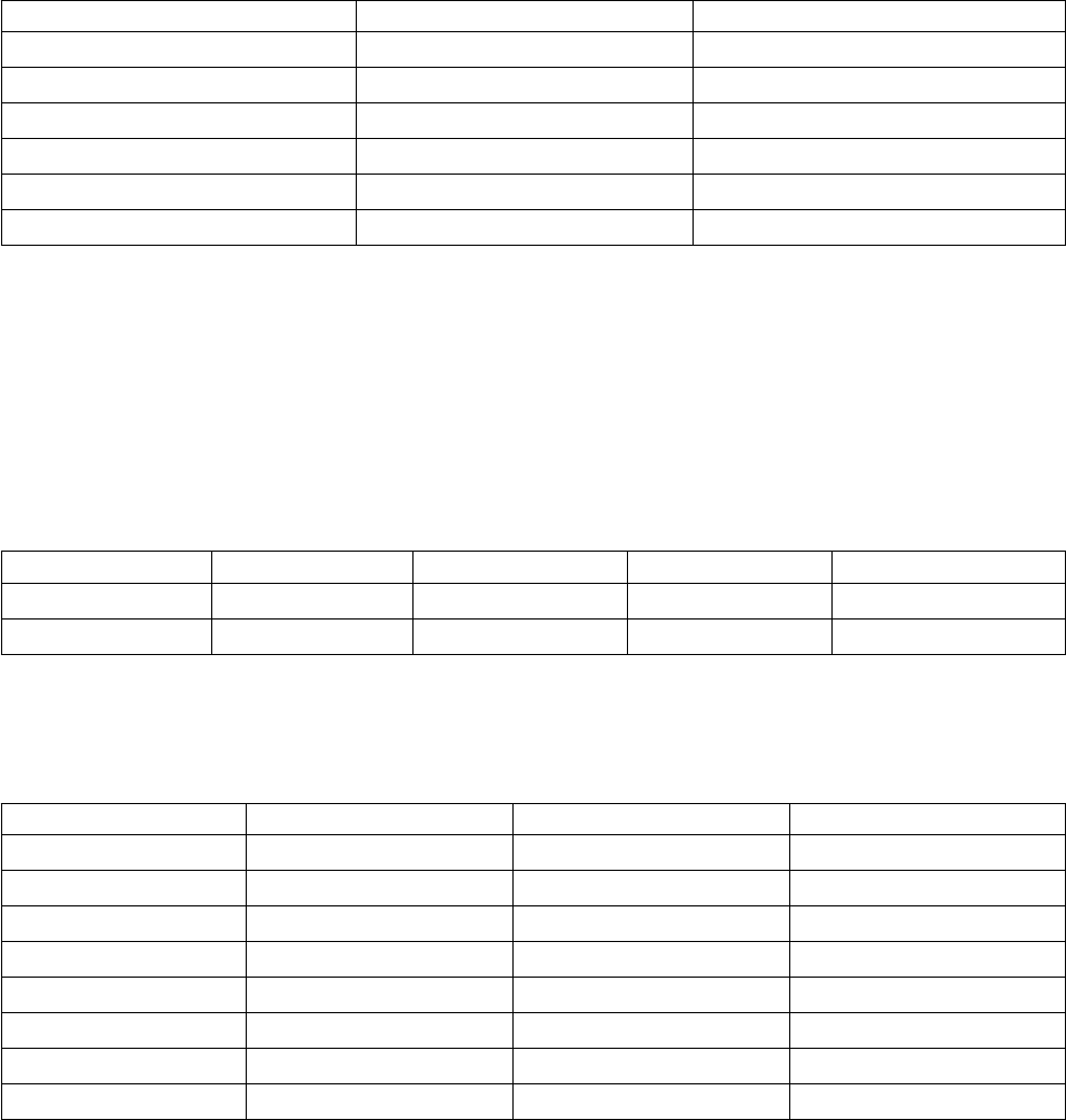
We'll restructure the variable group into a single variable, width, and create a single numeric index. The
new data are shown in the following table.
Table 17. New, restructured data with one index
subject index width
1 1 6.7
1 2 4.3
1 3 5.7
2 1 7.1
2 2 5.9
2 3 5.6
Index starts with 1 and increments for each variable in the group. It restarts each time a new row is
encountered in the original file. We can now use index in procedures that require a grouping variable.
Example of Two Indices for Variables to Cases
When a variable group records more than one factor, you can create more than one index; however, the
current data must be arranged so that the levels of the first factor are a primary index within which the
levels of subsequent factors cycle. In the current data, there is one variable group, width, and two factors,
Aand B. The data are arranged so that levels of factor Bcycle within levels of factor A.
Table 18. Current data for two indices
subject w_a1b1 w_a1b2 w_a2b1 w_a2b2
1 5.5 6.4 5.8 5.9
2 7.4 7.1 5.6 6.7
We'll restructure the variable group into a single variable, width, and create two indices. The new data are
shown in the following table.
Table 19. New, restructured data with two indices
subject index_a index_b width
1 1 1 5.5
1 1 2 6.4
1 2 1 5.8
1 2 2 5.9
2 1 1 7.4
2 1 2 7.1
2 2 1 5.6
2 2 2 6.7
Restructure Data Wizard (Variables to Cases): Create One Index
Variable
Note: The wizard presents this step if you choose to restructure variable groups into rows and create one
index variable.
Chapter 9. File handling and file transformations 117
In this step, decide what values you want for the index variable. The values can be sequential numbers
or the names of the variables in an original variable group. You can also specify a name and a label for
the new index variable.
See the topic “Example of One Index for Variables to Cases” on page 116 for more information.
vSequential numbers. The wizard will automatically assign sequential numbers as index values.
vVariable names. The wizard will use the names of the selected variable group as index values. Choose
a variable group from the list.
vNames and labels. Click a cell to change the default variable name and provide a descriptive variable
label for the index variable.
Restructure Data Wizard (Variables to Cases): Create Multiple Index
Variables
Note: The wizard presents this step if you choose to restructure variable groups into rows and create
multiple index variables.
In this step, specify the number of levels for each index variable. You can also specify a name and a label
for the new index variable.
See the topic “Example of Two Indices for Variables to Cases” on page 117 for more information.
How many levels are recorded in the current file? Consider how many factor levels are recorded in the
current data. A level defines a group of cases that experienced identical conditions. If there are multiple
factors, the current data must be arranged so that the levels of the first factor are a primary index within
which the levels of subsequent factors cycle.
How many levels should be in the new file? Enter the number of levels for each index. The values for
multiple index variables are always sequential numbers. The values start at 1 and increment for each
level. The first index increments the slowest, and the last index increments the fastest.
Total combined levels. You cannot create more levels than exist in the current data. Because the
restructured data will contain one row for each combination of treatments, the wizard checks the number
of levels that you create. It will compare the product of the levels that you create to the number of
variables in your variable groups. They must match.
Names and labels. Click a cell to change the default variable name and provide a descriptive variable
label for the index variables.
Restructure Data Wizard (Variables to Cases): Options
Note: The wizard presents this step if you choose to restructure variable groups into rows.
In this step, specify options for the new, restructured file.
Drop unselected variables? In the Select Variables step (step 3), you selected variable groups to be
restructured, variables to be copied, and an identification variable from the current data. The data from
the selected variables will appear in the new file. If there are other variables in the current data, you can
choose to discard or keep them.
Keep missing data? The wizard checks each potential new row for null values. A null value is a
system-missing or blank value. You can choose to keep or discard rows that contain only null values.
Create a count variable? The wizard can create a count variable in the new file. It contains the number
of new rows generated by a row in the current data. A count variable may be useful if you choose to
discard null values from the new file because that makes it possible to generate a different number of
118 IBM SPSS Statistics 24 Core System User's Guide
new rows for a given row in the current data. Click a cell to change the default variable name and
provide a descriptive variable label for the count variable.
Restructure Data Wizard (Cases to Variables): Select Variables
Note: The wizard presents this step if you choose to restructure case groups into columns.
In this step, provide information about how the variables in the current file should be used in the new
file.
What identifies case groups in the current data? A case group is a group of rows that are related
because they measure the same observational unit--for example, an individual or an institution. The
wizard needs to know which variables in the current file identify the case groups so that it can
consolidate each group into a single row in the new file. Move variables that identify case groups in the
current file into the Identifier Variable(s) list. Variables that are used to split the current data file are
automatically used to identify case groups. Each time a new combination of identification values is
encountered, the wizard will create a new row, so cases in the current file should be sorted by values of
the identification variables in the same order that variables are listed in the Identifier Variable(s) list. If
the current data file isn't already sorted, you can sort it in the next step.
How should the new variable groups be created in the new file? In the original data, a variable appears
in a single column. In the new data file, that variable will appear in multiple new columns. Index
variables are variables in the current data that the wizard should use to create the new columns. The
restructured data will contain one new variable for each unique value in these columns. Move the
variables that should be used to form the new variable groups to the Index Variable(s) list. When the
wizard presents options, you can also choose to order the new columns by index.
What happens to the other columns? The wizard automatically decides what to do with the variables
that remain in the Current File list. It checks each variable to see if the data values vary within a case
group. If they do, the wizard restructures the values into a variable group in the new file. If they don't,
the wizard copies the values into the new file. When determining if a variable varies within a group,
user-missing values are treated like valid values, but system-missing values are not. If the group contains
one valid or use-missing value plus the system-missing value, then it is treated as a variable that does
not vary within the group, and the wizard copies the values into the new file.
Restructure Data Wizard (Cases to Variables): Sort Data
Note: The wizard presents this step if you choose to restructure case groups into columns.
In this step, decide whether to sort the current file before restructuring it. Each time the wizard
encounters a new combination of identification values, a new row is created, so it is important that the
data are sorted by the variables that identify case groups.
How are the rows ordered in the current file? Consider how the current data are sorted and which
variables you are using to identify case groups (specified in the previous step).
vYes. The wizard will automatically sort the current data by the identification variables in the same
order that variables are listed in the Identifier Variable(s) list in the previous step. Choose this when
the data aren't sorted by the identification variables or when you aren't sure. This choice requires a
separate pass of the data, but it guarantees that the rows are correctly ordered for restructuring.
vNo. The wizard will not sort the current data. Choose this when you are sure that the current data are
sorted by the variables that identify case groups.
Restructure Data Wizard (Cases to Variables): Options
Note: The wizard presents this step if you choose to restructure case groups into columns.
In this step, specify options for the new, restructured file.
Chapter 9. File handling and file transformations 119
How should the new variable groups be ordered in the new file?
vBy variable. The wizard groups the new variables created from an original variable together.
vBy index. The wizard groups the variables according to the values of the index variables.
Example. The variables to be restructured are wand h, and the index is month:
w, h, month
Grouping by variable results in:
w.jan, w.feb, h.jan
Grouping by index results in:
w.jan, h.jan, w.feb
Create a count variable? The wizard can create a count variable in the new file. It contains the number of
rows in the current data that were used to create a row in the new data file.
Create indicator variables? The wizard can use the index variables to create indicator variables in the
new data file. It creates one new variable for each unique value of the index variable. The indicator
variables signal the presence or absence of a value for a case. An indicator variable has the value of 1 if
the case has a value; otherwise, it is 0.
Example. The index variable is product. It records the products that a customer purchased. The original
data are:
Table 20. All products in a single variable (column)
customer product
1 chick
1 eggs
2 eggs
3 chick
Creating an indicator variable results in one new variable for each unique value of product. The
restructured data are:
Table 21. Separate indicator variables for each product type
customer indchick indeggs
1 1 1
2 0 1
3 1 0
In this example, the restructured data could be used to get frequency counts of the products that
customers buy.
Restructure Data Wizard: Finish
This is the final step of the Restructure Data Wizard. Decide what to do with your specifications.
vRestructure now. The wizard will create the new, restructured file. Choose this if you want to replace
the current file immediately.
120 IBM SPSS Statistics 24 Core System User's Guide
Note: If original data are weighted, the new data will be weighted unless the variable that is used as the
weight is restructured or dropped from the new file.
vPaste syntax. The wizard will paste the syntax it generates into a syntax window. Choose this when
you are not ready to replace the current file, when you want to modify the syntax, or when you want
to save it for future use.
Chapter 9. File handling and file transformations 121
122 IBM SPSS Statistics 24 Core System User's Guide

Chapter 10. Working with output
Working with output
When you run a procedure, the results are displayed in a window called the Viewer. In this window, you
can easily navigate to the output that you want to see. You can also manipulate the output and create a
document that contains precisely the output that you want.
Viewer
Results are displayed in the Viewer. You can use the Viewer to:
vBrowse results
vShow or hide selected tables and charts
vChange the display order of results by moving selected items
vMove items between the Viewer and other applications
The Viewer is divided into two panes:
vThe left pane contains an outline view of the contents.
vThe right pane contains statistical tables, charts, and text output.
You can click an item in the outline to go directly to the corresponding table or chart. You can click and
drag the right border of the outline pane to change the width of the outline pane.
Showing and hiding results
In the Viewer, you can selectively show and hide individual tables or results from an entire procedure.
This process is useful when you want to shorten the amount of visible output in the contents pane.
To hide tables and charts
1. Double-click the item's book icon in the outline pane of the Viewer.
or
2. Click the item to select it.
3. From the menus choose:
View > Hide
or
4. Click the closed book (Hide) icon on the Outlining toolbar.
The open book (Show) icon becomes the active icon, indicating that the item is now hidden.
To hide procedure results
1. Click the box to the left of the procedure name in the outline pane.
This hides all results from the procedure and collapses the outline view.
Moving, deleting, and copying output
You can rearrange the results by copying, moving, or deleting an item or a group of items.
To move output in the Viewer
1. Select the items in the outline or contents pane.
2. Drag and drop the selected items into a different location.
123
To delete output in the Viewer
1. Select the items in the outline or contents pane.
2. Press the Delete key.
or
3. From the menus choose:
Edit > Delete
Changing initial alignment
By default, all results are initially left-aligned. To change the initial alignment of new output items:
1. From the menus choose:
Edit > Options
2. Click the Viewer tab.
3. In the Initial Output State group, select the item type (for example, pivot table, chart, text output).
4. Select the alignment option you want.
Changing alignment of output items
1. In the outline or contents pane, select the items that you want to align.
2. From the menus choose:
Format > Align Left
or
Format > Center
or
Format > Align Right
Viewer outline
The outline pane provides a table of contents of the Viewer document. You can use the outline pane to
navigate through your results and control the display. Most actions in the outline pane have a
corresponding effect on the contents pane.
vSelecting an item in the outline pane displays the corresponding item in the contents pane.
vMoving an item in the outline pane moves the corresponding item in the contents pane.
vCollapsing the outline view hides the results from all items in the collapsed levels.
Controlling the outline display. To control the outline display, you can:
vExpand and collapse the outline view
vChange the outline level for selected items
vChange the size of items in the outline display
vChange the font that is used in the outline display
To collapse and expand the outline view
1. Click the box to the left of the outline item that you want to collapse or expand.
or
2. Click the item in the outline.
3. From the menus choose:
View > Collapse
or
View > Expand
124 IBM SPSS Statistics 24 Core System User's Guide
To change the outline level
1. Click the item in the outline pane.
2. Click the left arrow on the Outlining toolbar to promote the item (move the item to the left).
or
Click the right arrow on the Outlining toolbar to demote the item (move the item to the right).
or
3. From the menus choose:
Edit > Outline > Promote
or
Edit > Outline > Demote
Changing the outline level is particularly useful after you move items in the outline level. Moving items
can change the outline level of the items, and you can use the left- and right-arrow buttons on the
Outlining toolbar to restore the original outline level.
To change the size of outline items
1. From the menus choose:
View > Outline Size
2. Select the outline size (Small, Medium, or Large).
To change the font in the outline
1. From the menus choose:
View > Outline Font...
2. Select a font.
Adding items to the Viewer
In the Viewer, you can add items such as titles, new text, charts, or material from other applications.
To add a title or text
Text items that are not connected to a table or chart can be added to the Viewer.
1. Click the table, chart, or other object that will precede the title or text.
2. From the menus choose:
Insert > New Title
or
Insert > New Text
3. Double-click the new object.
4. Enter the text.
To add a text file
1. In the outline pane or contents pane of the Viewer, click the table, chart, or other object that will
precede the text.
2. From the menus choose:
Insert > Text File...
3. Select a text file.
To edit the text, double-click it.
Chapter 10. Working with output 125
Pasting Objects into the Viewer
Objects from other applications can be pasted into the Viewer. You can use either Paste After or Paste
Special. Either type of pasting puts the new object after the currently selected object in the Viewer. Use
Paste Special when you want to choose the format of the pasted object.
Finding and replacing information in the Viewer
1. To find or replace information in the Viewer, from the menus choose:
Edit > Find
or
Edit > Replace
You can use Find and Replace to:
vSearch the entire document or just the selected items.
vSearch down or up from the current location.
vSearch both panes or restrict the search to the contents or outline pane.
vSearch for hidden items. These include any items hidden in the contents pane (for example, Notes
tables, which are hidden by default) and hidden rows and columns in pivot tables.
vRestrict the search criteria to case-sensitive matches.
vRestrict the search criteria in pivot tables to matches of the entire cell contents.
vRestrict the search criteria in pivot tables to footnote markers only. This option is not available if the
selection in the Viewer includes anything other than pivot tables.
Hidden Items and Pivot Table Layers
vLayers beneath the currently visible layer of a multidimensional pivot table are not considered hidden
and will be included in the search area even when hidden items are not included in the search.
vHidden items include hidden items in the contents pane (items with closed book icons in the outline
pane or included within collapsed blocks of the outline pane) and rows and columns in pivot tables
either hidden by default (for example, empty rows and columns are hidden by default) or manually
hidden by editing the table and selectively hiding specific rows or columns. Hidden items are only
included in the search if you explicitly select Include hidden items.
vIn both cases, the hidden or nonvisible element that contains the search text or value is displayed when
it is found, but the item is returned to its original state afterward.
Finding a range of values in pivot tables
To find values that fall within a specified range of values in pivot tables:
1. Activate a pivot table or select one or more pivot tables in the Viewer. Make sure that only pivot
tables are selected. If any other objects are selected, the Range option is not available.
2. From the menus choose:
Edit > Find
3. Click the Range tab.
4. Select the type of range: Between, Greater than or equal to, or Less than or equal to.
5. Select the value or values that define the range.
vIf either value contains non-numeric characters, both values are treated as strings.
vIf both values are numbers, only numeric values are searched.
vYou cannot use the Range tab to replace values.
This feature is not available for legacy tables. See the topic “Legacy tables” on page 151 for more
information.
126 IBM SPSS Statistics 24 Core System User's Guide

Closing output items
You can close all currently open output items that were opened from a particular Viewer window.
1. Select the Viewer window that you want.
2. From the menus, choose:
Window > Close output items
Copying output into other applications
Output objects can be copied and pasted into other applications, such as a word-processing program or a
spreadsheet. You can paste output in a variety of formats. Depending on the target application and the
selected output object(s), some or all of the following formats may be available:
Metafile. WMF and EMF metafile format. These formats are available only on Windows operating
systems.
RTF (rich text format). Multiple selected objects, text output, and pivot tables can be copied and pasted
in RTF format. For pivot tables, in most applications this means that the tables are pasted as tables that
can then be edited in the other application. Pivot tables that are too wide for the document width will
either be wrapped, scaled down to fit the document width, or left unchanged, depending on the pivot
table options settings. See the topic “Pivot table options” on page 203 for more information.
Note: Microsoft Word may not display extremely wide tables properly.
Image. JPG and PNG image formats.
BIFF. Pivot tables and text output can be pasted into a spreadsheet in BIFF format. Numbers in pivot
tables retain numeric precision. This format is available only on Windows operating systems.
Text. Pivot tables and text output can be copied and pasted as text. This process can be useful for
applications such as e-mail, where the application can accept or transmit only text.
If the target application supports multiple available formats, it may have a Paste Special menu item that
allows you to select the format, or it may automatically display a list of available formats.
Copying and Pasting Multiple Output Objects
The following limitations apply when pasting multiple output objects into other applications:
vRTF format. In most applications, pivot tables are pasted as tables that can be edited in that
application. Charts, trees, and model views are pasted as images.
vMetafile and image formats. All the selected output objects are pasted as a single object in the other
application.
vBIFF format. Charts, trees, and model views are excluded.
You can also use “Export output” on page 128 to export multiple output objects to other
applications/formats.
Copy Special
When copying and pasting large amounts of output, particularly very large pivot tables, you can improve
the speed of the operation by using Edit > Copy Special to limit the number of formats copied to the
clipboard.
You can also save the selected formats as the default set of formats to copy to the clipboard. This setting
persists across sessions.
Chapter 10. Working with output 127

Interactive output
Interactive output objects contain multiple, related output objects. The selection in one object can change
what is displayed or highlighted in the other object. For example, selecting a row in a table might
highlight an area in a map or display a chart for a different category.
Interactive output objects do not support editing features, such as changing text, colors, fonts, or table
borders. The individual objects can be copied from the interactive object to the Viewer. Tables copied
from interactive output can be edited in the pivot table editor.
Copying objects from interactive output
File>Copy to Viewer copies individual output objects to the Viewer window.
vThe available options depend on the contents of the interactive output.
vChart and Map create chart objects.
vTable creates a pivot table that can be edited in the pivot table editor.
vSnapshot creates an image of the current view.
vModel creates a copy of the current interactive output object.
Edit>Copy Object copies individual output objects to the clipboard.
vPasting the copied object into the Viewer is equivalent to File>Copy to Viewer.
vPasting the object into another application pastes the object as an image.
Zoom and Pan
For maps, you can use View>Zoom to zoom the view of the map. Within a zoomed map view, you can
use View>Pan to move the view.
Print settings
File>Print Settings controls how interactive objects are printed.
vPrint visible view only. Prints only the view that is currently displayed. This option is the default
setting.
vPrint all views. Prints all views contained in the interactive output.
vThe selected option also determines the default action for exporting the output object.
Export output
Export Output saves Viewer output in HTML, text, Word/RTF, Excel, PowerPoint (requires PowerPoint
97 or later), and PDF formats. Charts can also be exported in a number of different graphics formats.
Note: Export to PowerPoint is available only on Windows operating systems and is not available in the
Student Version.
To export output
1. Make the Viewer the active window (click anywhere in the window).
2. From the menus choose:
File > Export...
3. Enter a file name (or prefix for charts) and select an export format.
Objects to Export. You can export all objects in the Viewer, all visible objects, or only selected objects.
128 IBM SPSS Statistics 24 Core System User's Guide
Document Type. The available options are:
vWord/RTF. Pivot tables are exported as Word tables with all formatting attributes intact (for example,
cell borders, font styles, and background colors). Text output is exported as formatted RTF. Charts, tree
diagrams, and model views are included in PNG format. Note that Microsoft Word might not display
extremely wide tables properly.
vExcel. Pivot table rows, columns, and cells are exported as Excel rows, columns, and cells, with all
formatting attributes intact (for example, cell borders, font styles, and background colors). Text output
is exported with all font attributes intact. Each line in the text output is a row in the Excel file, with the
entire contents of the line in a single cell. Charts, tree diagrams, and model views are included in PNG
format. Output can be exported as Excel 97-2004 or Excel 2007 and higher.
vHTML. Pivot tables are exported as HTML tables. Text output is exported as preformatted HTML.
Charts, tree diagrams, and model views are embedded in the document in the selected graphic format.
A browser compatible with HTML 5 is required for viewing output that is exported in HTML format.
vWeb Report. A web report is an interactive document that is compatible with most browsers. Many of
the interactive features of pivot tables available in the Viewer are also available in web reports. You can
also export a web report as an IBM Cognos Active Report.
vPortable Document Format. All output is exported as it appears in Print Preview, with all formatting
attributes intact.
vPowerPoint file. Pivot tables are exported as Word tables and are embedded on separate slides in the
PowerPoint file, with one slide for each pivot table. All formatting attributes of the pivot table are
retained (for example, cell borders, font styles, and background colors). Charts, tree diagrams, and
model views are exported in TIFF format. Text output is not included.
Export to PowerPoint is available only on Windows operating systems.
vText. Text output formats include plain text, UTF-8, and UTF-16. Pivot tables can be exported in
tab-separated or space-separated format. All text output is exported in space-separated format. For
charts, tree diagrams, and model views, a line is inserted in the text file for each graphic, indicating the
image file name.
vNone (Graphics Only). Available export formats include: EPS, JPEG, TIFF, PNG, and BMP. On
Windows operating systems, EMF (enhanced metafile) format is also available.
Open the containing folder. Opens the folder that contains the files that are created by the export.
Output Management System. You can also automatically export all output or user-specified types of
output as Word, Excel, PDF, HTML, text, or IBM SPSS Statistics format data files. See Chapter 22, “Output
Management System,” on page 263 for more information.
HTML options
HTML export requires a browser that is compatible with HTML 5. The following options are available for
exporting output in HTML format:
Layers in pivot tables. By default, inclusion or exclusion of pivot table layers is controlled by the table
properties for each pivot table. You can override this setting and include all layers or exclude all but the
currently visible layer. See the topic “Table properties: printing” on page 146 for more information.
Export layered tables as interactive. Layered tables are displayed as they appear in the Viewer, and you
can interactively change the displayed layer in the browser. If this option is not selected, each table layer
is displayed as a separate table.
Tables as HTML. This controls style information included for exported pivot tables.
vExport with styles and fixed column width. All pivot table style information (font styles, background
colors, etc.) and column widths are preserved.
vExport without styles. Pivot tables are converted to default HTML tables. No style attributes are
preserved. Column width is determined automatically.
Chapter 10. Working with output 129
Include footnotes and captions. Controls the inclusion or exclusion of all pivot table footnotes and
captions.
Views of Models. By default, inclusion or exclusion of model views is controlled by the model properties
for each model. You can override this setting and include all views or exclude all but the currently visible
view. See the topic “Model properties” on page 154 for more information. (Note: all model views,
including tables, are exported as graphics.)
Note: For HTML, you can also control the image file format for exported charts. See the topic “Graphics
format options” on page 134 for more information.
To set HTML export options
1. Select HTML as the export format.
2. Click Change Options.
Web report options
A web report is an interactive document that is compatible with most browsers. Many of the interactive
features of pivot tables available in the Viewer are also available in web reports.
Report Title. The title that is displayed in the header of the report. By default, the file name is used. You
can specify a custom title to use instead of the file name.
Format. There are two options for report format:
vSPSS Web Report (HTML 5). This format requires a browser that is compatible with HTML 5.
vCognos Active Report (mht). This format requires a browser that supports MHT format files or the
Cognos Active Report application.
Exclude Objects. You can exclude selected object types from the report:
vText. Text objects that are not logs. This option includes text objects that contain information about the
active dataset.
vLogs. Text objects that contain a listing of the command syntax that was run. Log items also include
warnings and error messages that are encountered by commands that do not produce any Viewer
output.
vNotes Tables. Output from statistical and charting procedures includes a Notes table. This table
contains information about the dataset that was used, missing values, and the command syntax that
was used to run the procedure.
vWarnings and Error Messages. Warnings and error messages from statistical and charting procedures.
Restyle the tables and charts to match the Web Report. This option applies the standard web report
style to all tables and charts. This setting overrides any fonts, colors, or other styles in the output as
displayed in the Viewer. You cannot modify the standard web report style.
Web Server Connection. You can include the URL location of one or more application servers that are
running the IBM SPSS Statistics Web Report Application Server. The web application server provides
features to pivot tables, edit charts, and save modified web reports.
vSelect Use for each application server that you want to include in the web report.
vIf a web report contains a URL specification, the web report connects to that application server to
provide the additional editing features.
vIf you specify multiple URLs, the web report attempts to connect to each server in the order in which
they are specified.
The IBM SPSS Statistics Web Report Application Server can be downloaded from http://www.ibm.com/
developerworks/spssdevcentral.
130 IBM SPSS Statistics 24 Core System User's Guide
Word/RTF options
The following options are available for exporting output in Word format:
Layers in pivot tables. By default, inclusion or exclusion of pivot table layers is controlled by the table
properties for each pivot table. You can override this setting and include all layers or exclude all but the
currently visible layer. See the topic “Table properties: printing” on page 146 for more information.
Wide Pivot Tables. Controls the treatment of tables that are too wide for the defined document width. By
default, the table is wrapped to fit. The table is divided into sections, and row labels are repeated for
each section of the table. Alternatively, you can shrink wide tables or make no changes to wide tables and
allow them to extend beyond the defined document width.
Preserve break points. If you have defined break points, these settings will be preserved in the Word
tables.
Include footnotes and captions. Controls the inclusion or exclusion of all pivot table footnotes and
captions.
Views of Models. By default, inclusion or exclusion of model views is controlled by the model properties
for each model. You can override this setting and include all views or exclude all but the currently visible
view. See the topic “Model properties” on page 154 for more information. (Note: all model views,
including tables, are exported as graphics.)
Page Setup for Export. This opens a dialog where you can define the page size and margins for the
exported document. The document width used to determine wrapping and shrinking behavior is the
page width minus the left and right margins.
To set Word export options
1. Select Word/RTF as the export format.
2. Click Change Options.
Excel options
The following options are available for exporting output in Excel format:
Create a worksheet or workbook or modify an existing worksheet. By default, a new workbook is
created. If a file with the specified name already exists, it will be overwritten. If you select the option to
create a worksheet, if a worksheet with the specified name already exists in the specified file, it will be
overwritten. If you select the option to modify an existing worksheet, you must also specify the
worksheet name. (This is optional for creating a worksheet.) Worksheet names cannot exceed 31
characters and cannot contain forward or back slashes, square brackets, question marks, or asterisks.
When exporting to Excel 97-2004, if you modify an existing worksheet, charts, model views, and tree
diagrams are not included in the exported output.
Location in worksheet. Controls the location within the worksheet for the exported output. By default,
exported output will be added after the last column that has any content, starting in the first row,
without modifying any existing contents. This is a good choice for adding new columns to an existing
worksheet. Adding exported output after the last row is a good choice for adding new rows to an
existing worksheet. Adding exported output starting at a specific cell location will overwrite any existing
content in the area where the exported output is added.
Layers in pivot tables. By default, inclusion or exclusion of pivot table layers is controlled by the table
properties for each pivot table. You can override this setting and include all layers or exclude all but the
currently visible layer. See the topic “Table properties: printing” on page 146 for more information.
Chapter 10. Working with output 131
Include footnotes and captions. Controls the inclusion or exclusion of all pivot table footnotes and
captions.
Views of Models. By default, inclusion or exclusion of model views is controlled by the model properties
for each model. You can override this setting and include all views or exclude all but the currently visible
view. See the topic “Model properties” on page 154 for more information. (Note: all model views,
including tables, are exported as graphics.)
To set Excel export options
1. Select Excel as the export format.
2. Click Change Options.
PowerPoint options
The following options are available for PowerPoint:
Layers in pivot tables. By default, inclusion or exclusion of pivot table layers is controlled by the table
properties for each pivot table. You can override this setting and include all layers or exclude all but the
currently visible layer. See the topic “Table properties: printing” on page 146 for more information.
Wide Pivot Tables. Controls the treatment of tables that are too wide for the defined document width. By
default, the table is wrapped to fit. The table is divided into sections, and row labels are repeated for
each section of the table. Alternatively, you can shrink wide tables or make no changes to wide tables and
allow them to extend beyond the defined document width.
Include footnotes and captions. Controls the inclusion or exclusion of all pivot table footnotes and
captions.
Use Viewer outline entries as slide titles. Includes a title on each slide that is created by the export.
Each slide contains a single item that is exported from the Viewer. The title is formed from the outline
entry for the item in the outline pane of the Viewer.
Views of Models. By default, inclusion or exclusion of model views is controlled by the model properties
for each model. You can override this setting and include all views or exclude all but the currently visible
view. See the topic “Model properties” on page 154 for more information. (Note: all model views,
including tables, are exported as graphics.)
Page Setup for Export. This opens a dialog where you can define the page size and margins for the
exported document. The document width used to determine wrapping and shrinking behavior is the
page width minus the left and right margins.
To set PowerPoint export options
1. Select PowerPoint as the export format.
2. Click Change Options.
Note: Export to PowerPoint is available only on Windows operating systems.
PDF options
The following options are available for PDF:
Embed bookmarks. This option includes bookmarks in the PDF document that correspond to the Viewer
outline entries. Like the Viewer outline pane, bookmarks can make it much easier to navigate documents
with a large number of output objects.
132 IBM SPSS Statistics 24 Core System User's Guide
Embed fonts. Embedding fonts ensures that the PDF document will look the same on all computers.
Otherwise, if some fonts used in the document are not available on the computer being used to view (or
print) the PDF document, font substitution may yield suboptimal results.
Layers in pivot tables. By default, inclusion or exclusion of pivot table layers is controlled by the table
properties for each pivot table. You can override this setting and include all layers or exclude all but the
currently visible layer. See the topic “Table properties: printing” on page 146 for more information.
Views of Models. By default, inclusion or exclusion of model views is controlled by the model properties
for each model. You can override this setting and include all views or exclude all but the currently visible
view. See the topic “Model properties” on page 154 for more information. (Note: all model views,
including tables, are exported as graphics.)
To set PDF export options
1. Select Portable Document Format as the export format.
2. Click Change Options.
Other Settings That Affect PDF Output
Page Setup/Page Attributes. Page size, orientation, margins, content and display of page headers and
footers, and printed chart size in PDF documents are controlled by page setup and page attribute options.
Table Properties/TableLooks. Scaling of wide and/or long tables and printing of table layers are
controlled by table properties for each table. These properties can also be saved in TableLooks.
Default/Current Printer. The resolution (DPI) of the PDF document is the current resolution setting for
the default or currently selected printer (which can be changed using Page Setup). The maximum
resolution is 1200 DPI. If the printer setting is higher, the PDF document resolution will be 1200 DPI.
Note: High-resolution documents may yield poor results when printed on lower-resolution printers.
Text options
The following options are available for text export:
Pivot Table Format. Pivot tables can be exported in tab-separated or space-separated format. For
space-separated format, you can also control:
vColumn Width. Autofit does not wrap any column contents, and each column is as wide as the widest
label or value in that column. Custom sets a maximum column width that is applied to all columns in
the table, and values that exceed that width wrap onto the next line in that column.
vRow/Column Border Character. Controls the characters used to create row and column borders. To
suppress display of row and column borders, enter blank spaces for the values.
Layers in pivot tables. By default, inclusion or exclusion of pivot table layers is controlled by the table
properties for each pivot table. You can override this setting and include all layers or exclude all but the
currently visible layer. See the topic “Table properties: printing” on page 146 for more information.
Include footnotes and captions. Controls the inclusion or exclusion of all pivot table footnotes and
captions.
Views of Models. By default, inclusion or exclusion of model views is controlled by the model properties
for each model. You can override this setting and include all views or exclude all but the currently visible
view. See the topic “Model properties” on page 154 for more information. (Note: all model views,
including tables, are exported as graphics.)
Chapter 10. Working with output 133
To set text export options
1. Select Text as the export format.
2. Click Change Options.
Graphics only options
The following options are available for exporting graphics only:
Views of Models. By default, inclusion or exclusion of model views is controlled by the model properties
for each model. You can override this setting and include all views or exclude all but the currently visible
view. See the topic “Model properties” on page 154 for more information. (Note: all model views,
including tables, are exported as graphics.)
Graphics format options
For HTML and text documents and for exporting charts only, you can select the graphic format, and for
each graphic format you can control various optional settings.
To select the graphic format and options for exported charts:
1. Select HTML, Text, or None (Graphics only) as the document type.
2. Select the graphic file format from the drop-down list.
3. Click Change Options to change the options for the selected graphic file format.
JPEG Chart Export Options
vImage size. Percentage of original chart size, up to 200 percent.
vConvert to grayscale. Converts colors to shades of gray.
BMP chart export options
vImage size. Percentage of original chart size, up to 200 percent.
vCompress image to reduce file size. A lossless compression technique that creates smaller files without
affecting image quality.
PNG chart export options
Image size. Percentage of original chart size, up to 200 percent.
Color Depth. Determines the number of colors in the exported chart. A chart that is saved under any
depth will have a minimum of the number of colors that are actually used and a maximum of the
number of colors that are allowed by the depth. For example, if the chart contains three colors--red,
white, and black--and you save it as 16 colors, the chart will remain as three colors.
vIf the number of colors in the chart exceeds the number of colors for that depth, the colors will be
dithered to replicate the colors in the chart.
vCurrent screen depth is the number of colors currently displayed on your computer monitor.
EMF and TIFF chart export options
Image size. Percentage of original chart size, up to 200 percent.
Note: EMF (enhanced metafile) format is available only on Windows operating systems.
EPS chart export options
Image size. You can specify the size as a percentage of the original image size (up to 200 percent), or you
can specify an image width in pixels (with height determined by the width value and the aspect ratio).
The exported image is always proportional to the original.
134 IBM SPSS Statistics 24 Core System User's Guide

Include TIFF preview image. Saves a preview with the EPS image in TIFF format for display in
applications that cannot display EPS images on screen.
Fonts. Controls the treatment of fonts in EPS images.
vUse font references. If the fonts that are used in the chart are available on the output device, the fonts
are used. Otherwise, the output device uses alternate fonts.
vReplace fonts with curves. Turns fonts into PostScript curve data. The text itself is no longer editable
as text in applications that can edit EPS graphics. This option is useful if the fonts that are used in the
chart are not available on the output device.
Viewer printing
There are two options for printing the contents of the Viewer window:
All visible output. Prints only items that are currently displayed in the contents pane. Hidden items
(items with a closed book icon in the outline pane or hidden in collapsed outline layers) are not printed.
Selection. Prints only items that are currently selected in the outline and/or contents panes.
To print output and charts
1. Make the Viewer the active window (click anywhere in the window).
2. From the menus choose:
File > Print...
3. Select the print settings that you want.
4. Click OK to print.
Print Preview
Print Preview shows you what will print on each page for Viewer documents. It is a good idea to check
Print Preview before actually printing a Viewer document, because Print Preview shows you items that
may not be visible by looking at the contents pane of the Viewer, including:
vPage breaks
vHidden layers of pivot tables
vBreaks in wide tables
vHeaders and footers that are printed on each page
If any output is currently selected in the Viewer, the preview displays only the selected output. To view a
preview for all output, make sure nothing is selected in the Viewer.
Page Attributes: Headers and Footers
Headers and footers are the information that is printed at the top and bottom of each page. You can enter
any text that you want to use as headers and footers. You can also use the toolbar in the middle of the
dialog box to insert:
vDate and time
vPage numbers
vViewer filename
vOutline heading labels
vPage titles and subtitles
vMake Default uses the settings specified here as the default settings for new Viewer documents. (Note:
this makes the current settings on both the Header/Footer tab and the Options tab the default
settings.)
Chapter 10. Working with output 135

vOutline heading labels indicate the first-, second-, third-, and/or fourth-level outline heading for the
first item on each page.
vPage titles and subtitles print the current page titles and subtitles. These can be created with New Page
Title on the Viewer Insert menu or with the TITLE and SUBTITLE commands. If you have not specified
any page titles or subtitles, this setting is ignored.
Note: Font characteristics for new page titles and subtitles are controlled on the Viewer tab of the
Options dialog box (accessed by choosing Options on the Edit menu). Font characteristics for existing
page titles and subtitles can be changed by editing the titles in the Viewer.
To see how your headers and footers will look on the printed page, choose Print Preview from the File
menu.
To insert page headers and footers
1. Make the Viewer the active window (click anywhere in the window).
2. From the menus, choose:
File > Page Attributes...
3. Click the Header/Footer tab.
4. Enter the header and/or footer that you want to appear on each page.
Page Attributes: Options
This dialog box controls the printed chart size, the space between printed output items, and page
numbering.
vPrinted Chart Size. Controls the size of the printed chart relative to the defined page size. The chart's
aspect ratio (width-to-height ratio) is not affected by the printed chart size. The overall printed size of
a chart is limited by both its height and width. When the outer borders of a chart reach the left and
right borders of the page, the chart size cannot increase further to fill more page height.
vSpace between items. Controls the space between printed items. Each pivot table, chart, and text object
is a separate item. This setting does not affect the display of items in the Viewer.
vNumber pages starting with. Numbers pages sequentially, starting with the specified number.
vMake Default. This option uses the settings that are specified here as the default settings for new
Viewer documents. (Note that this option makes the current Header/Footer settings and Options
settings the default.)
To change printed chart size, page numbering, and space between printed Items
1. Make the Viewer the active window (click anywhere in the window).
2. From the menus choose:
File > Page Attributes...
3. Click the Options tab.
4. Change the settings and click OK.
Saving output
The contents of the Viewer can be saved to several formats:
vViewer files (*.spv). The format that is used to display files in the Viewer window.
vSPSS Web Report (*.htm). A web report is an interactive document that is compatible with most
browsers. Many of the interactive features of pivot tables available in the Viewer are also available in
web reports. This format requires a browser that is compatible with HTML 5.
vCognos Active Report (*.mht). This format requires a browser that supports MHT format files or the
Cognos Active Report application.
136 IBM SPSS Statistics 24 Core System User's Guide
To control options for saving web reports or save results in other formats (for example, text, Word, Excel),
use Export on the File menu.
To save a Viewer document
1. From the Viewer window menus choose:
File > Save
2. Enter the name of the document, and then click Save.
Optionally, you can do the following:
Lock files to prevent editing in IBM SPSS Smartreader
If a Viewer document is locked, you can manipulate pivot tables (swap rows and columns,
change the displayed layer, etc.) but you cannot edit any output or save any changes to the
Viewer document in IBM SPSS Smartreader (a separate product for working with Viewer
documents). This setting has no effect on Viewer documents opened in IBM SPSS Statistics or
IBM SPSS Modeler.
Encrypt files with a password
You can protect confidential information stored in a Viewer document by encrypting the
document with a password. Once encrypted, the document can only be opened by providing
the password. IBM SPSS Smartreader users will also be required to provide the password in
order to open the file.
To encrypt a Viewer document:
a. Select Encrypt file with password in the Save Output As dialog box.
b. Click Save.
c. In the Encrypt File dialog box, provide a password and re-enter it in the Confirm
password text box. Passwords are limited to 10 characters and are case-sensitive.
Warning: Passwords cannot be recovered if they are lost. If the password is lost the file cannot
be opened.
Creating strong passwords
vUse eight or more characters.
vInclude numbers, symbols and even punctuation in your password.
vAvoid sequences of numbers or characters, such as "123" and "abc", and avoid repetition,
such as "111aaa".
vDo not create passwords that use personal information such as birthdays or nicknames.
vPeriodically change the password.
Note: Storing encrypted files to an IBM SPSS Collaboration and Deployment Services
Repository is not supported.
Modifying encrypted files
vIf you open an encrypted file, make modifications to it and choose File > Save, the
modified file will be saved with the same password.
vYou can change the password on an encrypted file by opening the file, repeating the steps
for encrypting it, and specifying a different password in the Encrypt File dialog box.
vYou can save an unencrypted version of an encrypted file by opening the file, choosing File
> Save As and deselecting Encrypt file with password in the Save Output As dialog box.
Note: Encrypted data files and output documents cannot be opened in versions of IBM SPSS
Statistics prior to version 21. Encrypted syntax files cannot be opened in versions prior to
version 22.
Store required model information with the output document
This option applies only when there are model viewer items in the output document that
Chapter 10. Working with output 137
require auxiliary information to enable some of the interactive features. Click More Info to
display a list of these model viewer items and the interactive features that require auxiliary
information. Storing this information with the output document might substantially increase
the document size. If you choose not to store this information, you can still open these output
items but the specified interactive features will not be available.
138 IBM SPSS Statistics 24 Core System User's Guide

Chapter 11. Pivot tables
Pivot tables
Many results are presented in tables that can be pivoted interactively. That is, you can rearrange the rows,
columns, and layers.
Note: If you require tables that are compatible with IBM SPSS Statistics releases prior to 20, then it is
recommended to render them as legacy tables. See the topic “Legacy tables” on page 151 for more
information.
Manipulating a pivot table
Options for manipulating a pivot table include:
vTransposing rows and columns
vMoving rows and columns
vCreating multidimensional layers
vGrouping and ungrouping rows and columns
vShowing and hiding rows, columns, and other information
vRotating row and column labels
vFinding definitions of terms
Activating a pivot table
Before you can manipulate or modify a pivot table, you need to activate the table. To activate a table:
1. Double-click the table.
or
2. Right-click the table and from the pop-up menu choose Edit Content.
3. From the sub-menu choose either In Viewer or In Separate Window.
Pivoting a table
1. Activate the pivot table.
2. From the menus choose:
Pivot > Pivoting Trays
A table has three dimensions: rows, columns, and layers. A dimension can contain multiple elements (or
none at all). You can change the organization of the table by moving elements between or within
dimensions. To move an element, just drag and drop it where you want it.
Changing display order of elements within a dimension
To change the display order of elements within a table dimension (row, column, or layer):
1. If pivoting trays are not already on, from the Pivot Table menu choose:
Pivot > Pivoting Trays
2. Drag and drop the elements within the dimension in the pivoting tray.
Moving rows and columns within a dimension element
1. In the table itself (not the pivoting trays), click the label for the row or column you want to move.
2. Drag the label to the new position.
139
Transposing rows and columns
If you just want to flip the rows and columns, there's a simple alternative to using the pivoting trays:
1. From the menus choose:
Pivot > Transpose Rows and Columns
This has the same effect as dragging all of the row elements into the column dimension and dragging all
of the column elements into the row dimension.
Grouping rows or columns
1. Select the labels for the rows or columns that you want to group together (click and drag or
Shift+click to select multiple labels).
2. From the menus choose:
Edit > Group
A group label is automatically inserted. Double-click the group label to edit the label text.
Note: To add rows or columns to an existing group, you must first ungroup the items that are currently in
the group. Then you can create a new group that includes the additional items.
Ungrouping rows or columns
1. Click anywhere in the group label for the rows or columns that you want to ungroup.
2. From the menus choose:
Edit > Ungroup
Ungrouping automatically deletes the group label.
Rotating row or column labels
You can rotate labels between horizontal and vertical display for the innermost column labels and the
outermost row labels in a table.
1. From the menus choose:
Format > Rotate Inner Column Labels
or
Format > Rotate Outer Row Labels
Only the innermost column labels and the outermost row labels can be rotated.
Sorting rows
To sort the rows of a pivot table:
1. Activate the table.
2. Select any cell in the column you want to use to sort on. To sort just a selected group of rows, select
two or more contiguous cells in the column you want to use to sort on.
3. From the menus, choose:
Edit > Sort rows
4. Select Ascending or Descending from the submenu.
vIf the row dimension contains groups, sorting affects only the group that contains the selection.
vYou cannot sort across group boundaries.
vYou cannot sort tables with more than one item in the row dimension.
Note: This feature is not available in legacy tables.
140 IBM SPSS Statistics 24 Core System User's Guide
Related information:
“Legacy tables” on page 151
Inserting rows and columns
To insert a row or column in a pivot table:
1. Activate the table.
2. Select any cell in the table.
3. From the menus, choose:
Insert Before
or
Insert After
From the submenu, choose:
Row
or
Column
vA plus sign (+) is inserted in each cell of the new row or column to prevent the new row or column
from being automatically hidden because it is empty.
vIn a table with nested or layered dimensions, a column or row is inserted at every corresponding
dimension level.
Note: This feature is not available in legacy tables.
Related information:
“Legacy tables” on page 151
Controlling display of variable and value labels
If variables contain descriptive variable or value labels, you can control the display of variable names and
labels and data values and value labels in pivot tables.
1. Activate the pivot table.
2. From the menus, choose:
View > Variable labels
or
View > Value labels
3. Select one of the follow options from the submenu:
vName or Value. Only variable names (or values) are displayed. Descriptive labels are not displayed.
vLabel. Only descriptive labels are displayed. Variable names (or values) are not displayed.
vBoth. Both names (or values) and descriptive labels are displayed.
Note: This feature is not available for legacy tables.
To control the default label display for pivot tables and other output objects, use Edit>Options>Output.
Related information:
“Legacy tables” on page 151
“Output options” on page 200
Changing the output language
To change the output language in a pivot table:
1. Activate the table
Chapter 11. Pivot tables 141

2. From the menus, choose:
View > Language
3. Select one of the available languages.
Changing the language affects only text that is generated by the application, such as table titles, row and
column labels, and footnote text. Variable names and descriptive variable and value labels are not
affected.
Note: This feature is not available for legacy tables.
To control the default language for pivot tables and other output objects, use Edit>Options>Language.
Related information:
“Legacy tables” on page 151
“Language options” on page 199
Navigating large tables
To use the navigation window to navigate large tables:
1. Activate the table.
2. From the menus choose:
View > Navigation
Undoing changes
You can undo the most recent change or all changes to an activated pivot table. Both actions apply only
to changes made since the most recent activation of the table.
To undo the most recent change:
1. From the menus, choose:
Edit > Undo
To undo all changes:
2. From the menus, choose:
Edit > Restore
Note: Edit > Restore is not available for legacy tables.
Working with layers
You can display a separate two-dimensional table for each category or combination of categories. The
table can be thought of as stacked in layers, with only the top layer visible.
Creating and displaying layers
To create layers:
1. Activate the pivot table.
2. If pivoting trays are not already on, from the Pivot Table menu, choose:
Pivot > Pivoting Trays
3. Drag an element from the row or column dimension into the layer dimension.
Moving elements to the layer dimension creates a multidimensional table, but only a single
two-dimensional "slice" is displayed. The visible table is the table for the top layer. For example, if a
yes/no categorical variable is in the layer dimension, then the multidimensional table has two layers: one
for the "yes" category and one for the "no" category.
142 IBM SPSS Statistics 24 Core System User's Guide

Changing the displayed layer
1. Choose a category from the drop-down list of layers (in the pivot table itself, not the pivoting tray).
Go to layer category
Go to Layer Category allows you to change layers in a pivot table. This dialog box is particularly useful
when there are many layers or the selected layer has many categories.
Showing and hiding items
Many types of cells can be hidden, including:
vDimension labels
vCategories, including the label cell and data cells in a row or column
vCategory labels (without hiding the data cells)
vFootnotes, titles, and captions
Hiding rows and columns in a table
Showing hidden rows and columns in a table
1. From the menus choose:
View > Show All Categories
This displays all hidden rows and columns in the table. (If Hide empty rows and columns is selected in
Table Properties for this table, a completely empty row or column remains hidden.)
Hiding and showing dimension labels
1. Select the dimension label or any category label within the dimension.
2. From the View menu or the pop-up menu choose Hide Dimension Label or Show Dimension Label.
Hiding and showing table titles
To hide a title:
1. Activate the pivot table.
2. Select the title.
3. From the View menu choose Hide.
To show hidden titles:
4. From the View menu choose Show All.
TableLooks
A TableLook is a set of properties that define the appearance of a table. You can select a previously
defined TableLook or create your own TableLook.
vBefore or after a TableLook is applied, you can change cell formats for individual cells or groups of
cells by using cell properties. The edited cell formats remain intact, even when you apply a new
TableLook.
vOptionally, you can reset all cells to the cell formats that are defined by the current TableLook. This
option resets any cells that were edited. If As Displayed is selected in the TableLook Files list, any
edited cells are reset to the current table properties.
vOnly table properties that are defined in the Table Properties dialog are saved in TableLooks.
TableLooks do not include individual cell modifications.
Chapter 11. Pivot tables 143

Note: TableLooks created in earlier versions of IBM SPSS Statistics cannot be used in version 16.0 or later.
To apply a TableLook
1. Activate a pivot table.
2. From the menus, choose:
Format > TableLooks...
3. Select a TableLook from the list of files. To select a file from another directory, click Browse.
4. Click OK to apply the TableLook to the selected pivot table.
To edit or create a TableLook
1. In the TableLooks dialog box, select a TableLook from the list of files.
2. Click Edit Look.
3. Adjust the table properties for the attributes that you want, and then click OK.
4. Click Save Look to save the edited TableLook, or click Save As to save it as a new TableLook.
vEditing a TableLook affects only the selected pivot table. An edited TableLook is not applied to any
other tables that use that TableLook unless you select those tables and reapply the TableLook.
vOnly table properties that are defined in the Table Properties dialog are saved in TableLooks.
TableLooks do not include individual cell modifications.
Related information:
Detailed examples
Table properties
Table Properties allows you to set general properties of a table, set cell styles for various parts of a table,
and save a set of those properties as a TableLook. You can:
vControl general properties, such as hiding empty rows or columns and adjusting printing properties.
vControl the format and position of footnote markers.
vDetermine specific formats for cells in the data area, for row and column labels, and for other areas of
the table.
vControl the width and color of the lines that form the borders of each area of the table.
To change pivot table properties
1. Activate the pivot table.
2. From the menus choose:
Format > Table Properties...
3. Select a tab (General, Footnotes, Cell Formats, Borders, or Printing).
4. Select the options that you want.
5. Click OK or Apply.
The new properties are applied to the selected pivot table. To apply new table properties to a TableLook
instead of just the selected table, edit the TableLook (Format menu, TableLooks).
Table properties: general
Several properties apply to the table as a whole. You can:
vShow or hide empty rows and columns. (An empty row or column has nothing in any of the data
cells.)
144 IBM SPSS Statistics 24 Core System User's Guide
vControl the default number of rows to display in long tables. To display all the rows in a table,
regardless of how long it is, clear Display table by rows. Note: This feature applies only to legacy
tables.
vControl the placement of row labels, which can be in the upper left corner or nested.
vControl maximum and minimum column width (expressed in points).
To change general table properties:
1. Click the General tab.
2. Select the options that you want.
3. Click OK or Apply.
Set rows to display
Note: This feature only applies to legacy tables.
By default, tables with many rows are displayed in sections of 100 rows. To control the number of rows
displayed in a table:
1. Select Display table by rows.
2. Click Set Rows to Display.
or
3. From the View menu of an activated pivot table, choose Display table by rows and Set Rows to
Display.
Rows to display. Controls the maximum number of rows to display at one time. Navigation controls
allow you move to different sections of the table. The minimum value is 10. The default is 100.
Widow/orphan tolerance. Controls the maximum number of rows of the inner most row dimension of
the table to split across displayed views of the table. For example, if there are six categories in each group
of the inner most row dimension, specifying a value of six would prevent any group from splitting across
displayed views. This setting can cause the total number of rows in a displayed view to exceed the
specified maximum number of rows to display.
Table properties: notes
The Notes tab of the Table Properties dialog controls footnote formatting and table comment text.
Footnotes. The properties of footnote markers include style and position in relation to text.
vThe style of footnote markers is either numbers (1, 2, 3, ...) or letters (a, b, c, ...).
vThe footnote markers can be attached to text as superscripts or subscripts.
Comment Text. You can add comment text to each table.
vComment text is displayed in a tooltip when you hover over a table in the Viewer.
vScreen readers read the comment text when the table has focus.
vThe tooltip in the Viewer displays only the first 200 characters of the comment, but screen readers read
the entire text.
vWhen you export output to HTML or a web report, the comment text is used as alt text.
You can automatically add comments to all tables when they are created (Edit menu>Options>Pivot
Tables).
Chapter 11. Pivot tables 145
Table properties: cell formats
For formatting, a table is divided into areas: title, layers, corner labels, row labels, column labels, data,
caption, and footnotes. For each area of a table, you can modify the associated cell formats. Cell formats
include text characteristics (such as font, size, color, and style), horizontal and vertical alignment,
background colors, and inner cell margins.
Cell formats are applied to areas (categories of information). They are not characteristics of individual
cells. This distinction is an important consideration when pivoting a table.
For example,
vIf you specify a bold font as a cell format of column labels, the column labels will appear bold no
matter what information is currently displayed in the column dimension. If you move an item from the
column dimension to another dimension, it does not retain the bold characteristic of the column labels.
vIf you make column labels bold simply by highlighting the cells in an activated pivot table and clicking
the Bold button on the toolbar, the contents of those cells will remain bold no matter what dimension
you move them to, and the column labels will not retain the bold characteristic for other items moved
into the column dimension.
To change cell formats:
1. Select the Cell Formats tab.
2. Select an Area from the drop-down list or click an area of the sample.
3. Select characteristics for the area. Your selections are reflected in the sample.
4. Click OK or Apply.
Alternating row colors
To apply a different background and/or text color to alternate rows in the Data area of the table:
1. Select Data from the Area drop-down list.
2. Select (check) Alternate row color in the Background Color group.
3. Select the colors to use for the alternate row background and text.
Alternate row colors affect only the Data area of the table. They do not affect row or column label areas.
Table properties: borders
For each border location in a table, you can select a line style and a color. If you select None as the style,
there will be no line at the selected location.
To change table borders:
1. Click the Borders tab.
2. Select a border location, either by clicking its name in the list or by clicking a line in the Sample area.
3. Select a line style or select None.
4. Select a color.
5. Click OK or Apply.
Table properties: printing
You can control the following properties for printed pivot tables:
vPrint all layers or only the top layer of the table, and print each layer on a separate page.
vShrink a table horizontally or vertically to fit the page for printing.
146 IBM SPSS Statistics 24 Core System User's Guide

vControl widow/orphan lines by controlling the minimum number of rows and columns that will be
contained in any printed section of a table if the table is too wide and/or too long for the defined page
size.
Note: If a table is too long to fit on the current page because there is other output above it, but it will
fit within the defined page length, the table is automatically printed on a new page, regardless of the
widow/orphan setting.
vInclude continuation text for tables that don't fit on a single page. You can display continuation text at
the bottom of each page and at the top of each page. If neither option is selected, the continuation text
will not be displayed.
To control pivot table printing properties:
1. Click the Printing tab.
2. Select the printing options that you want.
3. Click OK or Apply.
Cell properties
Cell properties are applied to a selected cell. You can change the font, value format, alignment, margins,
and colors. Cell properties override table properties; therefore, if you change table properties, you do not
change any individually applied cell properties.
To change cell properties:
1. Activate a table and select the cell(s) in the table.
2. From the Format menu or the pop-up menu choose Cell Properties.
Font and background
The Font and Background tab controls the font style and color and background color for the selected cells
in the table.
Format value
The Format Value tab controls value formats for the selected cells. You can select formats for numbers,
dates, time, or currencies, and you can adjust the number of decimal digits that are displayed.
Note: The list of Currency formats contains Dollar format (numbers with a leading dollar sign) and five
custom currency formats. By default, all custom currency formats are set to the default number format,
which contains no currency or other custom symbols. Use Edit>Options>Currency to define custom
currency formats.
Alignment and margins
The Alignment and Margins tab controls horizontal and vertical alignment of values and top, bottom, left,
and right margins for the selected cells. Mixed horizontal alignment aligns the content of each cell
according to its type. For example, dates are right-aligned and text values are left-aligned.
Footnotes and captions
You can add footnotes and captions to a table. You can also hide footnotes or captions, change footnote
markers, and renumber footnotes.
Adding footnotes and captions
To add a caption to a table:
1. From the Insert menu choose Caption.
Chapter 11. Pivot tables 147
A footnote can be attached to any item in a table. To add a footnote:
1. Click a title, cell, or caption within an activated pivot table.
2. From the Insert menu choose Footnote.
3. Insert the footnote text in the provided area.
To hide or show a caption
To hide a caption:
1. Select the caption.
2. From the View menu choose Hide.
To show hidden captions:
1. From the View menu choose Show All.
To hide or show a footnote in a table
To hide a footnote:
1. Right-click the cell that contains the footnote reference and select Hide Footnotes from the pop-up
menu
or
2. Select the footnote in the footnote area of the table and select Hide from the pop-up menu.
Note: For legacy tables, select the footnote area of the table, select Edit Footnote from the pop-up
menu, and then deselect (clear) the Visible property for any footnotes you want to hide.
If a cell contains multiple footnotes, use the latter method to selectively hide footnotes.
To hide all footnotes in the table:
1. Select all of the footnotes in the footnote area of the table (use click and drag or Shift+click to select
the footnotes) and select Hide from the View menu.
Note: For legacy tables, select the footnote area of the table and select Hide from the View menu.
To show hidden footnotes:
1. Select Show All Footnotes from the View menu.
Footnote marker
Footnote Marker changes the characters that can be used to mark a footnote. By default, standard
footnote markers are sequential letters or numbers, depending on the table properties settings. You can
also assign a special marker. Special markers are not affected when you renumber footnotes or switch
between numbers and letters for standard markers. The display of numbers or letters for standard
markers and the subscript or superscript position of footnote markers are controlled by the Footnotes tab
of the Table Properties dialog.
Note: For changing footnote markers in legacy tables, see “Editing footnotes in legacy tables” on page
149.
To change footnote markers:
1. Select a footnote.
2. From the Format menu, choose Footnote Marker.
Special markers are limited to 2 characters. Footnotes with special markers precede footnotes with
sequential letters or numbers in the footnote area of the table; so changing to a special marker can
reorder the footnote list.
148 IBM SPSS Statistics 24 Core System User's Guide

Renumbering footnotes
When you have pivoted a table by switching rows, columns, and layers, the footnotes may be out of
order. To renumber the footnotes:
1. From the Format menu choose Renumber Footnotes.
Editing footnotes in legacy tables
For legacy tables, you can use the Edit Footnotes dialog to enter and modify footnote text and font
settings, change footnote markers, and selectively hide or delete footnotes.
When you insert a new footnote in a legacy table, the Edit Footnotes dialog automatically opens. To use
the Edit Footnotes dialog to edit existing footnotes (without creating a new footnote):
1. Double-click the footnote area of the table or from the menus choose: Format > Edit Footnote.
Marker. By default, standard footnote markers are sequential letters or numbers, depending on the table
properties settings. To assign a special marker, simply enter the new marker value in the Marker column.
Special markers are not affected when you renumber footnotes or switch between numbers and letters for
standard markers. The display of numbers or letters for standard markers and the subscript or
superscript position of footnote markers are controlled by the Footnotes tab of the Table Properties dialog.
See the topic “Table properties: notes” on page 145 for more information.
To change a special marker back to a standard marker, right-click on the marker in the Edit Footnotes
dialog, select Footnote Marker from the pop-up menu, and select Standard marker in the Footnote
Marker dialog box.
Footnote. The content of the footnote. The display reflects the current font and background settings. The
font settings can be changed for individual footnotes using the Format subdialog. See the topic “Footnote
font and color settings” for more information. A single background color is applied to all footnotes and
can be changed in the Font and Background tab of the Cell Properties dialog. See the topic “Font and
background” on page 147 for more information.
Visible. All footnotes are visible by default. Deselect (clear) the Visible checkbox to hide a footnote.
Footnote font and color settings
For legacy tables, you can use the Format dialog to change the font family, style, size and color for one or
more selected footnotes:
1. In the Edit Footnotes dialog, select (click) one or more footnotes in the Footnotes grid.
2. Click the Format button.
The selected font family, style, size, and colors are applied to all the selected footnotes.
Background color, alignment, and margins can be set in the Cell Properties dialog and apply to all
footnotes. You cannot change these settings for individual footnotes. See the topic “Font and background”
on page 147 for more information.
Data cell widths
Set Data Cell Width is used to set all data cells to the same width.
To set the width for all data cells:
1. From the menus choose:
Format > Set Data Cell Widths...
2. Enter a value for the cell width.
Chapter 11. Pivot tables 149

Changing column width
1. Click and drag the column border.
Displaying hidden borders in a pivot table
For tables without many visible borders, you can display the hidden borders. This can simplify tasks like
changing column widths.
1. From the View menu choose Gridlines.
Selecting rows, columns and cells in a pivot table
You can select an entire row or column or a specified set of data and label cells.
To select multiple cells:
Select > Data and Label Cells
Printing pivot tables
Several factors can affect the way that printed pivot tables look, and these factors can be controlled by
changing pivot table attributes.
vFor multidimensional pivot tables (tables with layers), you can either print all layers or print only the
top (visible) layer. See the topic “Table properties: printing” on page 146 for more information.
vFor long or wide pivot tables, you can automatically resize the table to fit the page or control the
location of table breaks and page breaks. See the topic “Table properties: printing” on page 146 for
more information.
vFor tables that are too wide or too long for a single page, you can control the location of table breaks
between pages.
Use Print Preview on the File menu to see how printed pivot tables will look.
Controlling table breaks for wide and long tables
Pivot tables that are either too wide or too long to print within the defined page size are automatically
split and printed in multiple sections. You can:
vControl the row and column locations where large tables are split.
vSpecify rows and columns that should be kept together when tables are split.
vRescale large tables to fit the defined page size.
To specify row and column breaks for printed pivot tables:
1. Activate the pivot table.
2. Click any cell in the column to the left of where you want to insert the break, or click any cell in the
row before the row where you want to insert the break.
Note: For legacy tables, you must click a column label or row label cell.
3. From the menus, choose:
Format > Breakpoints > Vertical Breakpoint
or
Format > Breakpoints > Horizontal Breakpoint
Note: For legacy tables, choose Format > Break Here for both vertical and horizontal breakpoints.
To specify rows or columns to keep together:
150 IBM SPSS Statistics 24 Core System User's Guide

1. Select the labels of the rows or columns that you want to keep together. Click and drag or Shift+click
to select multiple row or column labels.
2. From the menus, choose:
Format > Breakpoints > Keep Together
Note: For legacy tables, choose Format > Keep Together.
To view breakpoints and keep together groups:
1. From the menus, choose:
Format > Breakpoints > Display Breakpoints
Breakpoints are shown as vertical or horizontal lines. Keep together groups appear as grayed out
rectangular regions that are enclosed by a darker border.
Note: Displaying breakpoints and keep together groups is not supported for legacy tables.
To clear breakpoints and keep together groups
To clear a breakpoint:
1. Click any cell in the column to the left of a vertical breakpoint, or click any cell in the row above a
horizontal breakpoint.
Note: For legacy tables, you must click a column label or row label cell.
2. From the menus, choose:
Format > Breakpoints > Clear Breakpoint or Group
Note: For legacy tables, choose Format > Remove Break Here.
To clear a keep together group:
3. Select the column or row labels that specify the group.
4. From the menus, choose:
Format > Breakpoints > Clear Breakpoint or Group
Note: For legacy tables, choose Format > Remove Keep Together.
All breakpoints and keep together groups are automatically cleared when you pivot or reorder any row
or column. This behavior does not apply to legacy tables.
Creating a chart from a pivot table
1. Double-click the pivot table to activate it.
2. Select the rows, columns, or cells you want to display in the chart.
3. Right-click anywhere in the selected area.
4. Choose Create Graph from the pop-up menu and select a chart type.
Legacy tables
You can choose to render tables as legacy tables (referred to as full-featured tables in release 19) which
are then fully compatible with IBM SPSS Statistics releases prior to 20. Legacy tables may render slowly
and are only recommended if compatibility with releases prior to 20 is required. For information on how
to create legacy tables, see “Pivot table options” on page 203.
Chapter 11. Pivot tables 151
152 IBM SPSS Statistics 24 Core System User's Guide

Chapter 12. Models
Some results are presented as models, which appear in the output Viewer as a special type of
visualization. The visualization displayed in the output Viewer is not the only view of the model that is
available. A single model contains many different views. You can activate the model in the Model Viewer
and interact with the model directly to display the available model views. You can also choose to print
and export all the views in the model.
Interacting with a model
To interact with a model, you first activate it:
1. Double-click the model.
or
2. Right-click the model and from the pop-up menu choose Edit Content.
3. From the submenu choose In Separate Window.
Activating the model displays the model in the Model Viewer. See the topic “Working with the Model
Viewer” for more information.
Working with the Model Viewer
The Model Viewer is an interactive tool for displaying the available model views and editing the look of
the model views. (For information about displaying the Model Viewer, see “Interacting with a model”.)
There are two different styles of Model Viewer:
vSplit into main/auxiliary views. In this style the main view appears in the left part of the Model
Viewer. The main view displays some general visualization (for example, a network graph) for the
model. The main view itself may have more than one model view. The drop-down list below the main
view allows you to choose from the available main views.
The auxiliary view appears in the right part of the Model Viewer. The auxiliary view typically displays
a more detailed visualization (including tables) of the model compared to the general visualization in
the main view. Like the main view, the auxiliary view may have more than one model view. The
drop-down list below the auxiliary view allows you to choose from the available main views. The
auxiliary can also display specific visualizations for elements that are selected in the main view. For
example, depending on the type of model, you may be able to select a variable node in the main view
to display a table for that variable in the auxiliary view.
vOne view at a time, with thumbnails. In this style there is only one view visible, and other views are
accessed via thumbnails on the left of the Model Viewer. Each view displays some visualization for the
model.
The specific visualizations that are displayed depend on the procedure that created the model. For
information about working with specific models, refer to the documentation for the procedure that
created the model.
Model view tables
Tables displayed in the Model Viewer are not pivot tables. You cannot manipulate these tables as you can
manipulate pivot tables.
Setting model properties
© Copyright IBM Corporation 1989, 2016 153

Within the Model Viewer, you can set specific properties for the model. See the topic “Model properties”
for more information.
Copying model views
You can also copy individual model views within the Model Viewer. See the topic “Copying model
views” for more information.
Model properties
Depending on your Model Viewer, choose:
File > Properties
or
File > Print View
Each model has associated properties that let you specify which views are printed from the output
Viewer. By default, only the view that is visible in the output Viewer is printed. This is always a main
view, and only one main view. You can also specify that all available model views are printed. These
include all the main views and all the auxiliary views (except for auxiliary views based on selection in
the main view; these are not printed). Note that you can also print individual model views within the
Model Viewer itself. See the topic “Printing a model” for more information.
Copying model views
From the Edit menu within the Model Viewer, you can copy the currently displayed main view or the
currently display auxiliary view. Only one model view is copied. You can paste the model view into the
output Viewer, where the individual model view is subsequently rendered as a visualization that can be
edited in the Graphboard Editor. Pasting into the output Viewer allows you to display multiple model
views simultaneously. You can also paste into other applications, where the view may appear as an image
or a table depending on the target application.
Printing a model
Printing from the Model Viewer
You can print a single model view within the Model Viewer itself.
1. Activate the model in the Model Viewer. See the topic “Interacting with a model” on page 153 for
more information.
2. From the menus choose View > Edit Mode, if available.
3. On the General toolbar palette in the main or auxiliary view (depending on which one you want to
print), click the print icon. (If this palette is not displayed, choose Palettes>General from the View
menu.)
Note: If your Model Viewer does not support a print icon, then choose File > Print.
Printing from the output Viewer
When you print from the output Viewer, the number of views that are printed for a specific model
depend on the model's properties. The model can be set to print only the displayed view or all of the
available model views. See the topic “Model properties” for more information.
154 IBM SPSS Statistics 24 Core System User's Guide

Exporting a model
By default, when you export models from the output Viewer, inclusion or exclusion of model views is
controlled by the model properties for each model. For more information about model properties, see
“Model properties” on page 154. On export, you can override this setting and include all model views or
only the currently visible model view. In the Export Output dialog box, click Change Options... in the
Document group. For more information about exporting and this dialog box, see “Export output” on
page 128. Note that all model views, including tables, are exported as graphics. Also note that auxiliary
views based on selections in the main view are never exported.
Saving fields used in the model to a new dataset
You can save fields used in the model to a new dataset.
1. Activate the model in the Model Viewer. See the topic “Interacting with a model” on page 153 for
more information.
2. From the menus choose:
Generate > Field Selection (Model input and target)
Dataset name. Specify a valid dataset name. Datasets are available for subsequent use in the same session
but are not saved as files unless explicitly saved prior to the end of the session. Dataset names must
conform to variable naming rules. See the topic “Variable names” on page 52 for more information.
Saving predictors to a new dataset based on importance
You can save predictors to a new dataset based on the information in the predictor importance chart.
1. Activate the model in the Model Viewer. See the topic “Interacting with a model” on page 153 for
more information.
2. From the menus choose:
Generate > Field Selection (Predictor Importance)
Top number of variables. Includes or excludes the most important predictors up to the specified
number.
Importance greater than. Includes or excludes all predictors with relative importance greater than the
specified value.
3. After you click OK, the New Dataset dialog appears.
Dataset name. Specify a valid dataset name. Datasets are available for subsequent use in the same session
but are not saved as files unless explicitly saved prior to the end of the session. Dataset names must
conform to variable naming rules. See the topic “Variable names” on page 52 for more information.
Ensemble Viewer
Models for Ensembles
The model for an ensemble provides information about the component models in the ensemble and the
performance of the ensemble as a whole.
The main (view-independent) toolbar allows you to choose whether to use the ensemble or a reference
model for scoring. If the ensemble is used for scoring you can also select the combining rule. These
changes do not require model re-execution; however, these choices are saved to the model for scoring
and/or downstream model evaluation. They also affect PMML exported from the ensemble viewer.
Chapter 12. Models 155
Combining Rule. When scoring an ensemble, this is the rule used to combine the predicted values from
the base models to compute the ensemble score value.
vEnsemble predicted values for categorical targets can be combined using voting, highest probability, or
highest mean probability. Voting selects the category that has the highest probability most often across
the base models. Highest probability selects the category that achieves the single highest probability
across all base models. Highest mean probability selects the category with the highest value when the
category probabilities are averaged across base models.
vEnsemble predicted values for continuous targets can be combined using the mean or median of the
predicted values from the base models.
The default is taken from the specifications made during model building. Changing the combining rule
recomputes the model accuracy and updates all views of model accuracy. The Predictor Importance chart
also updates. This control is disabled if the reference model is selected for scoring.
Show All Combining rules. When selected , results for all available combining rules are shown in the
model quality chart. The Component Model Accuracy chart is also updated to show reference lines for
each voting method.
Model Summary
The Model Summary view is a snapshot, at-a-glance summary of the ensemble quality and diversity.
Quality. The chart displays the accuracy of the final model, compared to a reference model and a naive
model. Accuracy is presented in larger is better format; the "best" model will have the highest accuracy.
For a categorical target, accuracy is simply the percentage of records for which the predicted value
matches the observed value. For a continuous target, accuracy is 1 minus the ratio of the mean absolute
error in prediction (the average of the absolute values of the predicted values minus the observed values)
to the range of predicted values (the maximum predicted value minus the minimum predicted value).
For bagging ensembles, the reference model is a standard model built on the whole training partition. For
boosted ensembles, the reference model is the first component model.
The naive model represents the accuracy if no model were built, and assigns all records to the modal
category. The naive model is not computed for continuous targets.
Diversity. The chart displays the "diversity of opinion" among the component models used to build the
ensemble, presented in larger is more diverse format. It is a measure of how much predictions vary
across the base models. Diversity is not available for boosted ensemble models, nor is it shown for
continuous targets.
Predictor Importance
Typically, you will want to focus your modeling efforts on the predictor fields that matter most and
consider dropping or ignoring those that matter least. The predictor importance chart helps you do this
by indicating the relative importance of each predictor in estimating the model. Since the values are
relative, the sum of the values for all predictors on the display is 1.0. Predictor importance does not relate
to model accuracy. It just relates to the importance of each predictor in making a prediction, not whether
or not the prediction is accurate.
Predictor importance is not available for all ensemble models. The predictor set may vary across
component models, but importance can be computed for predictors used in at least one component
model.
Predictor Frequency
The predictor set can vary across component models due to the choice of modeling method or predictor
selection. The Predictor Frequency plot is a dot plot that shows the distribution of predictors across
component models in the ensemble. Each dot represents one or more component models containing the
predictor. Predictors are plotted on the y-axis, and are sorted in descending order of frequency; thus the
156 IBM SPSS Statistics 24 Core System User's Guide

topmost predictor is the one that is used in the greatest number of component models and the
bottommost one is the one that was used in the fewest. The top 10 predictors are shown.
Predictors that appear most frequently are typically the most important. This plot is not useful for
methods in which the predictor set cannot vary across component models.
Component Model Accuracy
The chart is a dot plot of predictive accuracy for component models. Each dot represents one or more
component models with the level of accuracy plotted on the y-axis. Hover over any dot to obtain
information on the corresponding individual component model.
Reference lines. The plot displays color coded lines for the ensemble as well as the reference model and
naïve models. A checkmark appears next to the line corresponding to the model that will be used for
scoring.
Interactivity. The chart updates if you change the combining rule.
Boosted ensembles. A line chart is displayed for boosted ensembles.
Component Model Details
The table displays information on component models, listed by row. By default, component models are
sorted in ascending model number order. You can sort the rows in ascending or descending order by the
values of any column.
Model. A number representing the sequential order in which the component model was created.
Accuracy. Overall accuracy formatted as a percentage.
Method. The modeling method.
Predictors. The number of predictors used in the component model.
Model Size. Model size depends on the modeling method: for trees, it is the number of nodes in the tree;
for linear models, it is the number of coefficients; for neural networks, it is the number of synapses.
Records. The weighted number of input records in the training sample.
Automatic Data Preparation
This view shows information about which fields were excluded and how transformed fields were derived
in the automatic data preparation (ADP) step. For each field that was transformed or excluded, the table
lists the field name, its role in the analysis, and the action taken by the ADP step. Fields are sorted by
ascending alphabetical order of field names.
The action Trim outliers, if shown, indicates that values of continuous predictors that lie beyond a cutoff
value (3 standard deviations from the mean) have been set to the cutoff value.
Split Model Viewer
The Split Model Viewer lists the models for each split, and provides summaries about the split models.
Split. The column heading shows the field(s) used to create splits, and the cells are the split values.
Double-click any split to open a Model Viewer for the model built for that split.
Accuracy. Overall accuracy formatted as a percentage.
Chapter 12. Models 157
Model Size. Model size depends on the modeling method: for trees, it is the number of nodes in the tree;
for linear models, it is the number of coefficients; for neural networks, it is the number of synapses.
Records. The weighted number of input records in the training sample.
158 IBM SPSS Statistics 24 Core System User's Guide

Chapter 13. Automated Output Modification
Automated output modification applies formatting and other changes to the contents of the active Viewer
window. Changes that can be applied include:
vAll or selected viewer objects
vSelected types of output objects (for example, charts, logs, pivot tables)
vPivot table content based on conditional expressions
vOutline (navigation) pane content
The types of changes you can make include:
vDelete objects
vIndex objects (add a sequential numbering scheme)
vChange the visible property of objects
vChange the outline label text
vTranspose rows and columns in pivot tables
vChange the selected layer of pivot tables
vChange the formatting of selected areas or specific cells in a pivot table based on conditional
expressions (for example, make all significance values less than 0.05 bold)
To specify automated output modification:
1. From the menus, choose:Utilities > Style Output
2. Select one or more objects in the Viewer.
3. Select the options you want in the Select dialog. (You can also select objects before you open the
dialog.)
4. Select the output changes you want in the Style Output dialog.
Style Output: Select
The Style Output: Select dialog specifies basic selection criteria for changes that you specify on the Style
Output dialog.
You can also select objects in the Viewer after opening the Style Output: Select dialog.
Selected only. Changes are applied only to the selected objects that meet the specified criteria.
vSelect as last command. If selected, changes are only applied to the output from the last procedure. If
not selected, changes are applied to the specific instance of the procedure. For example, if there are
three instances of the Frequencies procedure and you select the second instance, changes are applied
only to that instance. If you paste the syntax based on your selections, this option selects the second
instance of that procedure. If output from multiple procedures is selected, this option applies only to
the procedure for which the output is the last block of output in the Viewer.
vSelect as a group. If selected, all of the objects in the selection are treated as a single group on the
main Style Output dialog. If not selected, the selected objects are treated as individual selections, and
you can set the properties for each object individually.
All objects of this type. Changes are applied to all objects of the selected type that meet the specified
criteria. This option is only available if there is a single object type selected in the Viewer. Object types
include tables, warnings, logs, charts, tree diagrams, text, models, and outline headers.
© Copyright IBM Corporation 1989, 2016 159

All objects of this sub-type. Changes are applied to all tables of the same subtype as the selected tables
that meet the specified criteria. This option is only available if there is a single table subtype selected in
the Viewer. For example, the selection can include two separate Frequencies tables, but not a Frequencies
table and a Descriptives table.
Objects with a similar name. Changes are applied to all objects with a similar name that meet the
specified criteria.
vCriteria. The options are Contains, Exactly, Starts with, and Ends with.
vValue. The name as it is displayed in the outline pane of the Viewer.
vUpdate. Selects all the objects in the Viewer that meet the specified criteria for the specified value.
Style Output
The Style Output dialog specifies the changes you want to make to the selected output objects in the
Viewer.
Create a Backup of the Output. Changes made by the automated output modification process cannot be
undone. To preserve the original Viewer document, create a backup copy.
Selections and Properties
The list of objects or groups of objects that you can modify is determined by the objects you select in the
Viewer and the selections you make in the Style Output: Select dialog.
Selection. The name of the selected procedure or group of object types. When there is an integer in
parentheses after the selection text, changes are applied only to that instance of that procedure in the
sequence of objects in the Viewer. For example, "Frequencies(2)" applies change only to the second
instance of the Frequencies procedure in the Viewer output.
Type. The type of object. For example, log, title, table, chart. For individual table types, the table subtype
is also displayed.
Delete. Specifies whether the selection should be deleted.
Visible. Specifies whether the selection should be visible or hidden. The default option is "As Is," which
means that current visibility property of the selection is preserved.
Properties. A summary of changes to apply to the selection.
Add. Adds a row to the list and opens the Style Output: Select dialog. You can select other objects in the
Viewer and specify the selection conditions.
Duplicate. Duplicates the selected row.
Move Up and Move Down. Moves the selected row up or down in the list. The order can be important
since changes specified in subsequent rows can overwrite changes that are specified in previous rows.
Create a report of the property changes. Displays a table that summarizes the changes in the Viewer.
Object Properties
You specify the changes that you want to make to each selection from the Selections and Properties
section in the Object Properties section. The available properties are determined by the selected row in
the Selections and Properties section.
160 IBM SPSS Statistics 24 Core System User's Guide
Command. The name of the procedure if the selection refers to a single procedure. The selection can
include multiple instances of the same procedure.
Type. The type of object.
Subtype. If the selection refers to a single table type, the table subtype name is displayed.
Outline Label. The label in the outline pane that is associated with the selection. You can replace the
label text or add information to the label. For more information, see the topic Style Output: Labels and
Text.
Indexing Format. Adds a sequential number, letter, or roman numeral to the objects in the selection. For
more information, see the topic Style Output: Indexing.
Table Title. The title of table or tables. You can replace the title or add information to the title. For more
information, see the topic Style Output: Labels and Text.
TableLook. The TableLook used for tables. For more information, see the topic Style Output: TableLooks.
Transpose. Transposes rows and columns in tables.
Top Layer. For tables with layers, the category that is displayed for each layer.
Conditional styling. Conditional style changes for tables. For more information, see the topic Table Style.
Sort. Sorts table contents by the values of the selected column label. The available column labels are
displayed in a dropdown list. This option is only available if the selection contains a single table subtype.
Sort Direction. Specifies the sort direction for tables.
Comment Text. You can add comment text to each table.
vComment text is displayed in a tooltip when you hover over a table in the Viewer.
vScreen readers read the comment text when the table has focus.
vThe tooltip in the Viewer displays only the first 200 characters of the comment, but screen readers read
the entire text.
vWhen you export output to HTML or a web report, the comment text is used as alt text.
Contents. The text of logs, titles, and text objects. You can replace the text or add information to the text.
For more information, see the topic Style Output: Labels and Text.
Font. The font for logs, titles, and text objects.
Font Size. The font size for logs, titles, and text objects.
Text Color. Text color for logs, titles, and text objects.
Chart Template. The chart template that is used for charts, except charts that are created with the
Graphboard Template Chooser.
Graphboard Stylesheet. The style sheet used for charts that are created with the Graphboard Template
Chooser.
Size. The size of charts and tree diagrams.
Chapter 13. Automated Output Modification 161
Special Variables in Comment Text
You can include special variables to insert date, time, and other values in the Comment Text field.
)DATE
Current date in the form dd-mmm-yyyy.
)ADATE
Current date in the form mm/dd/yyyy.
)SDATE
Current date in the form yyyy/mm/dd.
)EDATE
Current date in the form dd.mm.yyyy.
)TIME Current 12-hour clock time in the form hh:mm:ss.
)ETIME
Current 24-hour clock time in the form hh:mm:ss.
)INDEX
The defined index value. For more information, see the topic Style Output: Indexing.
)TITLE
The text of the outline label for the table.
)PROCEDURE
The name of the procedure that created the table.
)DATASET
The name of the dataset used to create the table.
\n Inserts a line break.
Style Output: Labels and Text
The Style Output: Labels and Text dialog replaces or adds text to outline labels, text objects, and table
titles. It also specifies the inclusion and placement of index values for outline labels, text objects, and
table titles.
Add text to the label or text object.. You can add the text before or after the existing text or replace the
existing text.
Add indexing. Adds a sequential letter, number, or roman numeral. You can place the index before or
after the text. You can also specify one or more characters that are used as a separator between the text
and the index. For information about index formatting, see the topic Style Output: Indexing.
Style Output: Indexing
The Style Output: Indexing dialog specifies the index format and the starting value.
Type: The sequential index values can be numbers, lower or uppercase letters, lower or uppercase roman
numerals.
Starting value. The starting value can be any value that is valid for the type that is selected.
To display index values in the output, you must select Add indexing in the Style Output: Labels and Text
dialog for the selected object type.
vFor outline labels, select Outline label in the Properties column in the Style Output dialog.
vFor table titles, select Table Title in the Properties column in the Style Output dialog.
vFor text objects, select Contents in the Properties column in the Style Output dialog.
162 IBM SPSS Statistics 24 Core System User's Guide

Style Output: TableLooks
A TableLook is a set of properties that define the appearance of a table. You can select a previously
defined TableLook or create your own TableLook.
vBefore or after a TableLook is applied, you can change cell formats for individual cells or groups of
cells by using cell properties. The edited cell formats remain intact, even when you apply a new
TableLook.
vOptionally, you can reset all cells to the cell formats that are defined by the current TableLook. This
option resets any cells that were edited. If As Displayed is selected in the TableLook Files list, any
edited cells are reset to the current table properties.
vOnly table properties that are defined in the Table Properties dialog are saved in TableLooks.
TableLooks do not include individual cell modifications.
Style Output: Size
The Style Output: Size dialog controls the size of charts and tree diagrams. You can specify the height
and width in centimeters, inches, or points.
Table Style
The Table Style dialog specifies conditions for automatically changing properties of pivot tables based on
specific conditions. For example, you can make all significance values less than 0.05 bold and red. The
Table Style dialog can be accessed from the Style Output dialog or from the dialogs for specific statistical
procedures.
vThe Table Style dialog can be accessed from the Style Output dialog or from the dialogs for specific
statistical procedures.
vThe statistical procedure dialogs that support the Table Style dialog are Bivariate Correlations,
Crosstabs, Custom Tables, Descriptives, Frequencies, Logistic Regression, Linear Regression, and
Means.
Table. The table or tables to which the conditions apply. When you access this dialog from the Style
Output dialog, the only choice is "All applicable tables." When you access this dialog from a statistical
procedure dialog, you can select the table type from a list of procedure-specific tables.
Value. The row or column label value that defines the area of the table to search for values that meet the
conditions. You can select a value from the list or enter a value. The values in the list are not affected by
the output language and apply to numerous variations of the value. The values available in the list
depend on the table type.
vCount. Rows or columns with any of these labels or the equivalent in the current output language:
"Frequency", "Count", "N".
vMean. Rows or columns with the label "Mean" or the equivalent in the current output language.
vMedian Rows or columns with the label "Median" or the equivalent in the current output language.
vPercent. Rows or columns with the label "Percent" or the equivalent in the current output language.
vResidual. Rows or columns with any of these labels or the equivalent in the current output language:
"Resid", "Residual", "Std. Residual".
vCorrelation. Rows or columns with any of these labels or the equivalent in the current output
language: "Adjusted R Square", "Correlation Coefficient", "Correlations", "Pearson Correlation", "R
Square".
vSignificance. Rows or columns with any of these labels or the equivalents in the current output
language: "Approx Sig.", "Asymp. Sig (2-sided)", "Exact Sig.", "Exact Sig. (1-sided)", "Exact Sig.
(2-sided)", "Sig.", "Sig. (1-tailed)", "Sig. (2-tailed)"
vAll data cells. All data cells are included.
Chapter 13. Automated Output Modification 163
Dimension. Specifies whether to search rows, columns, or both for a label with the specified value.
Condition. Specifies the condition to find. For more information, see the topic Table Style: Condition.
Formatting. Specifies the formatting to apply to the table cells or areas that meet the condition. For more
information, see the topic Table Style: Format.
Add. Adds a row to the list.
Duplicate. Duplicates the selected row.
Move Up and Move Down. Moves the selected row up or down in the list. The order can be important
since changes specified in subsequent rows can overwrite changes that are specified in previous rows.
Create a report of the conditional styling. Displays a table that summarizes the changes in the Viewer.
This option is available when the Table Style dialog is accessed from a statistical procedure dialog. The
Style Output dialog has a separate option to create a report.
Table Style: Condition
The Table Style: Condition dialog specifies the conditions under which the changes are applied. There are
two options.
vTo all values of this type. The only condition is the value specified in the Value column in the Table
Style dialog. This option is the default.
vBased on the following conditions. Within the table area specified by the Value and Dimension
columns in the Table Style dialog, find values that meet the specified conditions.
Values. The list contains comparison expressions, such as Exactly, Less than, Greater Than, and
Between.
vAbsolute value is available for comparison expressions that only require one value. For example, you
could find correlations with an absolute value greater than 0.5.
vTop and Bottom are the highest and lowest nvalues in the specified table area. The value for Number
must be an integer.
vSystem-missing. Finds system-missing values in the specified table area.
Table Style: Format
The Table Style: Format dialog specifies changes to apply, based on the conditions specified in the Table
Style: Conditions dialog.
Use TableLook defaults. If no previous format changes have been made, either manually or by
automated output modification, this is equivalent to making no format changes. If previous changes have
been made, this removes those changes and restores the affected areas of the table to their default format.
Apply new formatting. Applies the specified format changes. Format changes include font style and
color, background color, format for numeric values (including dates and times), and number of decimals
displayed.
Apply to. Specifies the area of the table to which to apply the changes.
vCells only. Applies changes only to table cells that meet the condition.
vEntire column. Applies changes to the entire column that contains a cell that meet the condition. This
option includes the column label.
vEntire row. Applies changes to the entire row that contains a cell that meets the condition. This option
includes the row label.
164 IBM SPSS Statistics 24 Core System User's Guide
Replace value. Replaces values with the specified new value. For Cells only, this option replaces
individual cell values that meet the condition. For Entire row and Entire column, this option replaces all
values in the row or column.
Chapter 13. Automated Output Modification 165
166 IBM SPSS Statistics 24 Core System User's Guide

Chapter 14. Working with Command Syntax
The powerful command language allows you to save and automate many common tasks. It also provides
some functionality not found in the menus and dialog boxes.
Most commands are accessible from the menus and dialog boxes. However, some commands and options
are available only by using the command language. The command language also allows you to save your
jobs in a syntax file so that you can repeat your analysis at a later date or run it in an automated job with
the a production job.
A syntax file is simply a text file that contains commands. While it is possible to open a syntax window
and type in commands, it is often easier if you let the software help you build your syntax file using one
of the following methods:
vPasting command syntax from dialog boxes
vCopying syntax from the output log
vCopying syntax from the journal file
Detailed command syntax reference information is available in two forms: integrated into the overall
Help system and as a separate PDF file, called the Command Syntax Reference, also available from the Help
menu. Context-sensitive Help for the current command in a syntax window is available by pressing the
F1 key.
Syntax Rules
When you run commands from a command syntax window during a session, you are running commands
in interactive mode.
The following rules apply to command specifications in interactive mode:
vEach command must start on a new line. Commands can begin in any column of a command line and
continue for as many lines as needed. The exception is the END DATA command, which must begin in
the first column of the first line after the end of data.
vEach command should end with a period as a command terminator. It is best to omit the terminator on
BEGIN DATA, however, so that inline data are treated as one continuous specification.
vThe command terminator must be the last nonblank character in a command.
vIn the absence of a period as the command terminator, a blank line is interpreted as a command
terminator.
Note: For compatibility with other modes of command execution (including command files run with
INSERT or INCLUDE commands in an interactive session), each line of command syntax should not exceed
256 characters.
vMost subcommands are separated by slashes (/). The slash before the first subcommand on a
command is usually optional.
vVariable names must be spelled out fully.
vText included within apostrophes or quotation marks must be contained on a single line.
vA period (.) must be used to indicate decimals, regardless of your regional or locale settings.
vVariable names ending in a period can cause errors in commands created by the dialog boxes. You
cannot create such variable names in the dialog boxes, and you should generally avoid them.
Command syntax is case insensitive, and three- or four-letter abbreviations can be used for many
command specifications. You can use as many lines as you want to specify a single command. You can
© Copyright IBM Corporation 1989, 2016 167

add space or break lines at almost any point where a single blank is allowed, such as around slashes,
parentheses, arithmetic operators, or between variable names. For example,
FREQUENCIES
VARIABLES=JOBCAT GENDER
/PERCENTILES=25 50 75
/BARCHART.
and
freq var=jobcat gender /percent=25 50 75 /bar.
are both acceptable alternatives that generate the same results.
INCLUDE Files
For command files run via the INCLUDE command, batch mode syntax rules apply.
The following rules apply to command specifications in batch mode:
vAll commands in the command file must begin in column 1. You can use plus (+) or minus (–) signs in
the first column if you want to indent the command specification to make the command file more
readable.
vIf multiple lines are used for a command, column 1 of each continuation line must be blank.
vCommand terminators are optional.
vA line cannot exceed 256 characters; any additional characters are truncated.
Unless you have existing command files that already use the INCLUDE command, you should probably use
the INSERT command instead, since it can accommodate command files that conform to either set of rules.
If you generate command syntax by pasting dialog box choices into a syntax window, the format of the
commands is suitable for any mode of operation. See the Command Syntax Reference (available in PDF
format from the Help menu) for more information.
Pasting Syntax from Dialog Boxes
The easiest way to build a command syntax file is to make selections in dialog boxes and paste the
syntax for the selections into a syntax window. By pasting the syntax at each step of a lengthy analysis,
you can build a job file that allows you to repeat the analysis at a later date or run an automated job
with the Production Facility.
In the syntax window, you can run the pasted syntax, edit it, and save it in a syntax file.
To Paste Syntax from Dialog Boxes
1. Open the dialog box and make the selections that you want.
2. Click Paste.
The command syntax is pasted to the designated syntax window. If you do not have an open syntax
window, a new syntax window opens automatically, and the syntax is pasted there. By default, the syntax
is pasted after the last command. You can choose to have syntax pasted at the position of the cursor or to
overwrite selected syntax. The setting is specified from the Syntax Editor tab in the Options dialog box.
Copying Syntax from the Output Log
You can build a syntax file by copying command syntax from the log that appears in the Viewer. To use
this method, you must select Display commands in the log in the Viewer settings (Edit menu, Options,
Viewer tab) before running the analysis. Each command will then appear in the Viewer along with the
output from the analysis.
168 IBM SPSS Statistics 24 Core System User's Guide

In the syntax window, you can run the pasted syntax, edit it, and save it in a syntax file.
To Copy Syntax from the Output Log
1. Before running the analysis, from the menus choose:
Edit > Options...
2. On the Viewer tab, select Display commands in the log.
As you run analyses, the commands for your dialog box selections are recorded in the log.
3. Open a previously saved syntax file or create a new one. To create a new syntax file, from the menus
choose:
File > New > Syntax
4. In the Viewer, double-click a log item to activate it.
5. Select the text that you want to copy.
6. From the Viewer menus choose:
Edit > Copy
7. In a syntax window, from the menus choose:
Edit > Paste
Using the Syntax Editor
The Syntax Editor provides an environment specifically designed for creating, editing, and running
command syntax. The Syntax Editor features:
vAuto-Completion. As you type, you can select commands, subcommands, keywords, and keyword
values from a context-sensitive list. You can choose to be prompted automatically with the list or
display the list on demand.
vColor Coding. Recognized elements of command syntax (commands, subcommands, keywords, and
keyword values) are color coded so, at a glance, you can spot unrecognized terms. Also, a number of
common syntactical errors--such as unmatched quotes--are color coded for quick identification.
vBreakpoints. You can stop execution of command syntax at specified points, allowing you to inspect
the data or output before proceeding.
vBookmarks. You can set bookmarks that allow you to quickly navigate large command syntax files.
vAuto-Indentation. You can automatically format your syntax with an indentation style similar to
syntax pasted from a dialog box.
vStep Through. You can step through command syntax one command at a time, advancing to the next
command with a single click.
Note: When working with right to left languages, it is recommended to check the Optimize for right to
left languages box on the Syntax Editor tab in the Options dialog box.
Syntax Editor Window
The Syntax Editor window is divided into four areas:
vThe editor pane is the main part of the Syntax Editor window and is where you enter and edit
command syntax.
vThe gutter is adjacent to the editor pane and displays information such as line numbers and breakpoint
positions.
vThe navigation pane is to the left of the gutter and editor pane and displays a list of all commands in
the Syntax Editor window and provides single click navigation to any command.
vThe error pane is below the editor pane and displays runtime errors.
Gutter Contents
Chapter 14. Working with Command Syntax 169
Line numbers, breakpoints, bookmarks, command spans, and a progress indicator are displayed in the
gutter to the left of the editor pane in the syntax window.
vLine numbers do not account for any external files referenced in INSERT and INCLUDE commands. You
can show or hide line numbers by choosing View > Show Line Numbers from the menus.
vBreakpoints stop execution at specified points and are represented as a red circle adjacent to the
command on which the breakpoint is set.
vBookmarks mark specific lines in a command syntax file and are represented as a square enclosing the
number (1-9) assigned to the bookmark. Hovering over the icon for a bookmark displays the number
of the bookmark and the name, if any, assigned to the bookmark.
vCommand spans are icons that provide visual indicators of the start and end of a command. You can
show or hide command spans by choosing View > Show Command Spans from the menus.
vThe progress of a given syntax run is indicated with a downward pointing arrow in the gutter,
stretching from the first command run to the last command run. This is most useful when running
command syntax containing breakpoints and when stepping through command syntax. See the topic
“Running Command Syntax” on page 175 for more information.
Navigation Pane
The navigation pane contains a list of all recognized commands in the syntax window, displayed in the
order in which they occur in the window. Clicking on a command in the navigation pane positions the
cursor at the start of the command.
vYou can use the Up and Down arrow keys to move through the list of commands or click a command
to navigate to it. A double click will select the command.
vCommand names for commands containing certain types of syntactical errors--such as unmatched
quotes--are colored red and in bold text by default. See the topic “Color Coding” on page 171 for more
information.
vThe first word of each line of unrecognized text is shown in gray.
vYou can show or hide the navigation pane by choosing View > Show Navigation Pane from the menus.
Error Pane
The error pane displays runtime errors from the most previous run.
vThe information for each error contains the starting line number of the command containing the error.
vYou can use the Up and Down arrow keys to move through the list of errors.
vClicking on an entry in the list will position the cursor on the first line of the command that generated
the error.
vYou can show or hide the error pane by choosing View > Show Error Pane from the menus.
Using Multiple Views
You can split the editor pane into two panes arranged with one above the other.
1. From the menus choose:
Window > Split
Actions in the navigation and error panes--such as clicking on an error--act on the pane where the cursor
is positioned.
You can remove the splitter by double-clicking it or choosing Window > Remove Split.
Terminology
Commands. The basic unit of syntax is the command. Each command begins with the command name,
which consists of one, two, or three words--for example, DESCRIPTIVES, SORT CASES, or ADD VALUE LABELS.
170 IBM SPSS Statistics 24 Core System User's Guide
Subcommands. Most commands contain subcommands. Subcommands provide for additional
specifications and begin with a forward slash followed by the name of the subcommand.
Keywords. Keywords are fixed terms that are typically used within a subcommand to specify options
available for the subcommand.
Keyword Values. Keywords can have values such as a fixed term that specifies an option or a numeric
value.
Example
CODEBOOK gender jobcat salary
/VARINFO VALUELABELS MISSING
/OPTIONS VARORDER=MEASURE.
vThe name of the command is CODEBOOK.
vVARINFO and OPTIONS are subcommands.
vVALUELABELS, MISSING, and VARORDER are keywords.
vMEASURE is a keyword value associated with VARORDER.
Auto-Completion
The Syntax Editor provides assistance in the form of auto-completion of commands, subcommands,
keywords, and keyword values. By default, you are prompted with a context-sensitive list of available
terms as you type. Pressing Enter or Tab will insert the currently highlighted item in the list at the
position of the cursor. You can display the list on demand by pressing Ctrl+Spacebar and you can close
the list by pressing the Esc key.
The Auto Complete menu item on the Tools menu toggles the automatic display of the auto-complete list
on or off. You can also enable or disable automatic display of the list from the Syntax Editor tab in the
Options dialog box. Toggling the Auto Complete menu item overrides the setting on the Options dialog
but does not persist across sessions.
Note: The auto-completion list will close if a space is entered. For commands consisting of multiple
words--such as ADD FILES--select the command before entering any spaces.
Color Coding
The Syntax Editor color codes recognized elements of command syntax, such as commands and
subcommands, as well as various syntactical errors like unmatched quotes or parentheses. Unrecognized
text is not color coded.
Commands. By default, recognized commands are colored blue and in bold text. If, however, there is a
recognized syntactical error within the command--such as a missing parenthesis--the command name is
colored red and in bold text by default.
Note: Abbreviations of command names--such as FREQ for FREQUENCIES--are not colored, but such
abbreviations are valid.
Subcommands. Recognized subcommands are colored green by default. If, however, the subcommand is
missing a required equals sign or an invalid equals sign follows it, the subcommand name is colored red
by default.
Keywords. Recognized keywords are colored maroon by default. If, however, the keyword is missing a
required equals sign or an invalid equals sign follows it, the keyword is colored red by default.
Keyword values. Recognized keyword values are colored orange by default. User-specified values of
keywords such as integers, real numbers, and quoted strings are not color coded.
Chapter 14. Working with Command Syntax 171
Comments. Text within a comment is colored gray by default.
Quotes. Quotes and text within quotes are colored black by default.
Syntactical Errors. Text associated with the following syntactical errors is colored red by default.
vUnmatched Parentheses, Brackets, and Quotes. Unmatched parentheses and brackets within
comments and quoted strings are not detected. Unmatched single or double quotes within quoted
strings are syntactically valid.
Certain commands contain blocks of text that are not command syntax--such as BEGIN DATA-END DATA,
BEGIN GPL-END GPL, and BEGIN PROGRAM-END PROGRAM. Unmatched values are not detected within such
blocks.
vLong lines. Long lines are lines containing more than 251 characters.
vEnd statements. Several commands require either an END statement prior to the command terminator
(for example, BEGIN DATA-END DATA) or require a matching END command at some point later in the
command stream (for example, LOOP-END LOOP). In both cases, the command will be colored red, by
default, until the required END statement is added.
Note: You can navigate to the next or previous syntactical error by choosing Next Error or Previous error
from the Validation Errors submenu of the Tools menu.
From the Syntax Editor tab in the Options dialog box, you can change default colors and text styles and
you can turn color coding off or on. You can also turn color coding of commands, subcommands,
keywords, and keyword values off or on by choosing Tools > Color Coding from the menus. You can
turn color coding of syntactical errors off or on by choosing Tools > Validation. Choices made on the
Tools menu override settings in the Options dialog box but do not persist across sessions.
Note: Color coding of command syntax within macros is not supported.
Breakpoints
Breakpoints allow you to stop execution of command syntax at specified points within the syntax
window and continue execution when ready.
vBreakpoints are set at the level of a command and stop execution prior to running the command.
vBreakpoints cannot occur within LOOP-END LOOP, DO IF-END IF, DO REPEAT-END REPEAT, INPUT
PROGRAM-END INPUT PROGRAM, and MATRIX-END MATRIX blocks. They can, however, be set at the beginning
of such blocks and will stop execution prior to running the block.
vBreakpoints cannot be set on lines containing non-IBM SPSS Statistics command syntax, such as occur
within BEGIN PROGRAM-END PROGRAM, BEGIN DATA-END DATA, and BEGIN GPL-END GPL blocks.
vBreakpoints are not saved with the command syntax file and are not included in copied text.
vBy default, breakpoints are honored during execution. You can toggle whether breakpoints are honored
or not from Tools > Honor Breakpoints.
To Insert a Breakpoint
1. Click anywhere in the gutter to the left of the command text.
or
2. Position the cursor within the command.
3. From the menus choose:
Tools > Toggle Breakpoint
The breakpoint is represented as a red circle in the gutter to the left of the command text and on the
same line as the command name.
Clearing Breakpoints
172 IBM SPSS Statistics 24 Core System User's Guide
To clear a single breakpoint:
1. Click the icon representing the breakpoint in the gutter to the left of the command text.
or
2. Position the cursor within the command.
3. From the menus choose:
Tools > Toggle Breakpoint
To clear all breakpoints:
4. From the menus choose:
Tools > Clear All Breakpoints
See “Running Command Syntax” on page 175 for information about the run-time behavior in the
presence of breakpoints.
Bookmarks
Bookmarks allow you to quickly navigate to specified positions in a command syntax file. You can have
up to 9 bookmarks in a given file. Bookmarks are saved with the file, but are not included when copying
text.
To Insert a Bookmark
1. Position the cursor on the line where you want to insert the bookmark.
2. From the menus choose:
Tools > Toggle Bookmark
The new bookmark is assigned the next available number, from 1 to 9. It is represented as a square
enclosing the assigned number and displayed in the gutter to the left of the command text.
Clearing Bookmarks
To clear a single bookmark:
1. Position the cursor on the line containing the bookmark.
2. From the menus choose:
Tools > Toggle Bookmark
To clear all bookmarks:
1. From the menus choose:
Tools > Clear All Bookmarks
Renaming a Bookmark
You can associate a name with a bookmark. This is in addition to the number (1-9) assigned to the
bookmark when it was created.
1. From the menus choose:
Tools > Rename Bookmark
2. Enter a name for the bookmark and click OK.
The specified name replaces any existing name for the bookmark.
Navigating with Bookmarks
To navigate to the next or previous bookmark:
Chapter 14. Working with Command Syntax 173
1. From the menus choose:
Tools > Next Bookmark
or
Tools > Previous Bookmark
To navigate to a specific bookmark:
1. From the menus choose:
Tools > Go To Bookmark
2. Select the bookmark.
Commenting or Uncommenting Text
You can comment out entire commands as well as text that is not recognized as command syntax and
you can uncomment text that has previously been commented out.
To comment out text
1. Select the text. Note that a command will be commented out if any part of it is selected.
2. From the menus choose:
Tools > Toggle Comment Selection
You can comment out a single command by positioning the cursor anywhere within the command and
choosing Tools > Toggle Comment Selection.
To uncomment text
1. Select the text to uncomment. Note that a command will be uncommented if any part of it is selected.
2. From the menus choose:
Tools > Toggle Comment Selection
You can uncomment a single command by positioning the cursor anywhere within the command and
choosing Tools > Toggle Comment Selection. Note that this feature will not remove comments within a
command (text set off by /* and */) or comments created with the COMMENT keyword.
Formatting Syntax
You can indent or outdent selected lines of syntax and you can automatically indent selections so that the
syntax is formatted in a manner similar to syntax pasted from a dialog box.
vThe default indent is four spaces and applies to indenting selected lines of syntax as well as to
automatic indentation. You can change the indent size from the Syntax Editor tab in the Options dialog
box.
vNote that using the Tab key in the Syntax Editor does not insert a tab character. It inserts a space.
To indent text
1. Select the text or position the cursor on a single line that you want to indent.
2. From the menus choose:
Tools > Indent Syntax > Indent
You can also indent a selection or line by pressing the Tab key.
To outdent text
1. Select the text or position the cursor on a single line that you want to outdent.
2. From the menus choose:
Tools > Indent Syntax > Outdent
174 IBM SPSS Statistics 24 Core System User's Guide
To automatically indent text
1. Select the text.
2. From the menus choose:
Tools > Indent Syntax > Auto Indent
When you automatically indent text, any existing indentation is removed and replaced with the
automatically generated indents. Note that automatically indenting code within a BEGIN PROGRAM block
may break the code if it depends on specific indentation to function, such as Python code containing
loops and conditional blocks.
Syntax formatted with the auto-indent feature may not run in batch mode. For example, auto-indenting
an INPUT PROGRAM-END INPUT PROGRAM, LOOP-END LOOP, DO IF-END IF or DO REPEAT-END REPEAT block will
cause the syntax to fail in batch mode because commands in the block will be indented and will not start
in column 1 as required for batch mode. You can, however, use the -i switch in batch mode to force the
Batch Facility to use interactive syntax rules. See the topic “Syntax Rules” on page 167 for more
information.
Running Command Syntax
1. Highlight the commands that you want to run in the syntax window.
2. Click the Run button (the right-pointing triangle) on the Syntax Editor toolbar. It runs the selected
commands or the command where the cursor is located if there is no selection.
or
3. Choose one of the items from the Run menu.
vAll. Runs all commands in the syntax window, honoring any breakpoints.
vSelection. Runs the currently selected commands, honoring any breakpoints. This includes any
partially highlighted commands. If there is no selection, the command where the cursor is positioned is
run.
vTo End. Runs all commands starting from the first command in the current selection to the last
command in the syntax window, honoring any breakpoints. If nothing is selected, the run starts from
the command where the cursor is positioned.
vStep Through. Runs the command syntax one command at a time starting from the first command in
the syntax window (Step Through From Start) or from the command where the cursor is positioned
(Step Through From Current). If there is selected text, the run starts from the first command in the
selection. After a given command has run, the cursor advances to the next command and you continue
the step through sequence by choosing Continue.
LOOP-END LOOP, DO IF-END IF, DO REPEAT-END REPEAT, INPUT PROGRAM-END INPUT PROGRAM, and
MATRIX-END MATRIX blocks are treated as single commands when using Step Through. You can not step
into one of these blocks.
vContinue. Continues a run stopped by a breakpoint or Step Through.
Progress Indicator
The progress of a given syntax run is indicated with a downward pointing arrow in the gutter, spanning
the last set of commands run. For instance, you choose to run all commands in a syntax window that
contains breakpoints. At the first breakpoint, the arrow will span the region from the first command in
the window to the command prior to the one containing the breakpoint. At the second breakpoint, the
arrow will stretch from the command containing the first breakpoint to the command prior to the one
containing the second breakpoint.
Run-time Behavior with Breakpoints
Chapter 14. Working with Command Syntax 175
vWhen running command syntax containing breakpoints, execution stops at each breakpoint.
Specifically, the block of command syntax from a given breakpoint (or beginning of the run) to the next
breakpoint (or end of the run) is submitted for execution exactly as if you had selected that syntax and
chosen Run > Selection.
vYou can work with multiple syntax windows, each with its own set of breakpoints, but there is only
one queue for executing command syntax. Once a block of command syntax has been submitted--such
as the block of command syntax up to the first breakpoint--no other block of command syntax will be
executed until the previous block has completed, regardless of whether the blocks are in the same or
different syntax windows.
vWith execution stopped at a breakpoint, you can run command syntax in other syntax windows, and
inspect Data Editor or Viewer windows. However, modifying the contents of the syntax window
containing the breakpoint or changing the cursor position in that window will cancel the run.
Character Set Encoding in Syntax Files
The character set encoding of a syntax file can be either Unicode or code page encoding. A Unicode file
can contain characters from many different character sets. Code page files are restricted to characters
supported in a specific language or locale. For example, a code page file in a western European encoding
cannot contain Japanese or Chinese characters.
Reading syntax files
To read syntax files correctly, the syntax editor needs to know the character encoding of the file.
vFiles with a Unicode UTF-8 byte order mark are read as Unicode UTF-8 encoding, regardless of any
encoding selection you make. This byte order mark is at the beginning of the file, but it is not
displayed.
vBy default, files without any encoding information are read as Unicode UTF-8 in Unicode mode or the
current locale character encoding in code page mode. To override the default behavior, select Unicode
(UTF-8) or Local Encoding.
vAs Declared is enabled if the syntax file contains a code page encoding identifier at the top of the file.
Starting with release 23, a comment is automatically inserted in syntax files that are saved in code page
encoding. For example, the first line in the file could be:
* Encoding: en_US.windows-1252.
If you select As Declared, that encoding is used to read the file.
Saving syntax files
By default, syntax files are saved as Unicode UTF-8 in Unicode mode or the current locale character
encoding in code page mode. To override the default behavior, select Unicode (UTF-8) or Local Encoding
in the Save Syntax As dialog.
vIf you save a new syntax file or save the file in a different encoding, a comment is inserted at the top
of the file that identifies the encoding. If an encoding comment is already present, it is replaced.
vIf you save a syntax file and then save it again without closing it, it is saved in the same encoding.
Multiple Execute Commands
Syntax pasted from dialog boxes or copied from the log or the journal may contain EXECUTE commands.
When you run commands from a syntax window, EXECUTE commands are generally unnecessary and may
slow performance, particularly with larger data files, because each EXECUTE command reads the entire
data file. For more information, see the EXECUTE command in the Command Syntax Reference (available
from the Help menu in any IBM SPSS Statistics window).
Lag Functions
176 IBM SPSS Statistics 24 Core System User's Guide

One notable exception is transformation commands that contain lag functions. In a series of
transformation commands without any intervening EXECUTE commands or other commands that read the
data, lag functions are calculated after all other transformations, regardless of command order. For
example,
COMPUTE lagvar=LAG(var1).
COMPUTE var1=var1*2.
and
COMPUTE lagvar=LAG(var1).
EXECUTE.
COMPUTE var1=var1*2.
yield very different results for the value of lagvar, since the former uses the transformed value of var1
while the latter uses the original value.
Character Set Encoding in Syntax Files
The character set encoding of a syntax file can be either Unicode or code page encoding. A Unicode file
can contain characters from many different character sets. Code page files are restricted to characters
supported in a specific language or locale. For example, a code page file in a western European encoding
cannot contain Japanese or Chinese characters.
Reading syntax files
To read syntax files correctly, the syntax editor needs to know the character encoding of the file.
vFiles with a Unicode UTF-8 byte order mark are read as Unicode UTF-8 encoding, regardless of any
encoding selection you make. This byte order mark is at the beginning of the file, but it is not
displayed.
vBy default, files without any encoding information are read as Unicode UTF-8 in Unicode mode or the
current locale character encoding in code page mode. To override the default behavior, select Unicode
(UTF-8) or Local Encoding.
vAs Declared is enabled if the syntax file contains a code page encoding identifier at the top of the file.
Starting with release 23, a comment is automatically inserted in syntax files that are saved in code page
encoding. For example, the first line in the file could be:
* Encoding: en_US.windows-1252.
If you select As Declared, that encoding is used to read the file.
Saving syntax files
By default, syntax files are saved as Unicode UTF-8 in Unicode mode or the current locale character
encoding in code page mode. To override the default behavior, select Unicode (UTF-8) or Local Encoding
in the Save Syntax As dialog.
vIf you save a new syntax file or save the file in a different encoding, a comment is inserted at the top
of the file that identifies the encoding. If an encoding comment is already present, it is replaced.
vIf you save a syntax file and then save it again without closing it, it is saved in the same encoding.
Multiple Execute Commands
Syntax pasted from dialog boxes or copied from the log or the journal may contain EXECUTE commands.
When you run commands from a syntax window, EXECUTE commands are generally unnecessary and may
slow performance, particularly with larger data files, because each EXECUTE command reads the entire
data file. For more information, see the EXECUTE command in the Command Syntax Reference (available
from the Help menu in any IBM SPSS Statistics window).
Chapter 14. Working with Command Syntax 177

Lag Functions
One notable exception is transformation commands that contain lag functions. In a series of
transformation commands without any intervening EXECUTE commands or other commands that read the
data, lag functions are calculated after all other transformations, regardless of command order. For
example,
COMPUTE lagvar=LAG(var1).
COMPUTE var1=var1*2.
and
COMPUTE lagvar=LAG(var1).
EXECUTE.
COMPUTE var1=var1*2.
yield very different results for the value of lagvar, since the former uses the transformed value of var1
while the latter uses the original value.
Encrypting syntax files
You can protect your syntax files by encrypting them with a password. Encrypted files can be opened
only by providing the password.
Note: Encrypted syntax files cannot be used in production jobs or with the IBM SPSS Statistics Batch
Facility (available with IBM SPSS Statistics Server).
To save the contents of the syntax editor as an encrypted syntax file:
1. Make the Syntax Editor the active window (click anywhere in the window to make it active).
2. From the menus, choose:
File > Save As...
3. Select Encrypted Syntax from the Save as type drop-down list.
4. Click Save.
5. In the Encrypt File dialog box, provide a password and reenter it in the Confirm password text box.
Passwords are limited to 10 characters and are case-sensitive.
Warning: Passwords cannot be recovered if they are lost. If the password is lost the file cannot be opened.
Creating strong passwords
vUse eight or more characters.
vInclude numbers, symbols and even punctuation in your password.
vAvoid sequences of numbers or characters, such as "123" and "abc", and avoid repetition, such as
"111aaa".
vDo not create passwords that use personal information such as birthdays or nicknames.
vPeriodically change the password.
Note: Storing encrypted files to an IBM SPSS Collaboration and Deployment Services Repository is not
supported.
Modifying encrypted files
vIf you open an encrypted file, modify the file and choose File > Save, the modified file is saved with
the same password.
vYou can change the password on an encrypted file by opening the file, repeating the steps for
encrypting it, and specifying a different password in the Encrypt File dialog box.
178 IBM SPSS Statistics 24 Core System User's Guide
vYou can save an unencrypted version of an encrypted file by opening the file, choosing File > Save As
and selecting Syntax from the Save as type drop-down list.
Note: Encrypted syntax files cannot be opened in versions of IBM SPSS Statistics prior to version 22.
Chapter 14. Working with Command Syntax 179
180 IBM SPSS Statistics 24 Core System User's Guide

Chapter 15. Overview of the chart facility
High-resolution charts and plots are created by the procedures on the Graphs menu and by many of the
procedures on the Analyze menu. This chapter provides an overview of the chart facility.
Building and editing a chart
Before you can create a chart, you need to have your data in the Data Editor. You can enter the data
directly into the Data Editor; open a previously saved data file; or read a spreadsheet, tab-delimited data
file, or database file. The Tutorial selection on the Help menu has online examples of creating and
modifying a chart, and the online Help system provides information about creating and modifying all
chart types.
Building Charts
The Chart Builder allows you to build charts from predefined gallery charts or from the individual parts
(for example, axes and bars). You build a chart by dragging and dropping the gallery charts or basic
elements onto the canvas, which is the large area to the right of the Variables list in the Chart Builder
dialog box.
As you are building the chart, the canvas displays a preview of the chart. Although the preview uses
defined variable labels and measurement levels, it does not display your actual data. Instead, it uses
randomly generated data to provide a rough sketch of how the chart will look.
Using the gallery is the preferred method for new users. For information about using the gallery, see
“Building a Chart from the Gallery.”
How to Start the Chart Builder
1. From the menus choose:
Graphs > Chart Builder
Building a Chart from the Gallery
The easiest method for building charts is to use the gallery. Following are general steps for building a
chart from the gallery.
1. Click the Gallery tab if it is not already displayed.
2. In the Choose From list, select a category of charts. Each category offers several types.
3. Drag the picture of the chart you want onto the canvas. You can also double-click the picture. If the
canvas already displays a chart, the gallery chart replaces the axis set and graphic elements on the
chart.
a. Drag variables from the Variables list and drop them into the axis drop zones and, if available, the
grouping drop zone. If an axis drop zone already displays a statistic and you want to use that
statistic, you do not have to drag a variable into the drop zone. You need to add a variable to a
zone only when the text in the zone is blue. If the text is black, the zone already contains a
variable or statistic.
Note: The measurement level of your variables is important. The Chart Builder sets defaults based
on the measurement level while you are building the chart. Furthermore, the resulting chart may
also look different for different measurement levels. You can temporarily change a variable's
measurement level by right-clicking the variable and choosing an option.
b. If you need to change statistics or modify attributes of the axes or legends (such as the scale
range), click Element Properties.
181
c. In the Edit Properties Of list, select the item you want to change. (For information about the
specific properties, click Help.)
d. After making any changes, click Apply.
e. If you need to add more variables to the chart (for example, for clustering or paneling), click the
Groups/Point ID tab in the Chart Builder dialog box and select one or more options. Then drag
categorical variables to the new drop zones that appear on the canvas.
4. If you want to transpose the chart (for example, to make the bars horizontal), click the Basic Elements
tab and then click Transpose.
5. Click OK to create the chart. The chart is displayed in the Viewer.
Editing Charts
The Chart Editor provides a powerful, easy-to-use environment where you can customize your charts and
explore your data. The Chart Editor features:
vSimple, intuitive user interface. You can quickly select and edit parts of the chart using menus and
toolbars. You can also enter text directly on a chart.
vWide range of formatting and statistical options. You can choose from a full range of styles and
statistical options.
vPowerful exploratory tools. You can explore your data in various ways, such as by labeling,
reordering, and rotating it. You can change chart types and the roles of variables in the chart. You can
also add distribution curves and fit, interpolation, and reference lines.
vFlexible templates for consistent look and behavior. You can create customized templates and use
them to easily create charts with the look and options that you want. For example, if you always want
a specific orientation for axis labels, you can specify the orientation in a template and apply the
template to other charts.
How to View the Chart Editor
1. Double-click a chart in the Viewer.
Chart Editor Fundamentals
The Chart Editor provides various methods for manipulating charts.
Menus
Many actions that you can perform in the Chart Editor are done with the menus, especially when you are
adding an item to the chart. For example, you use the menus to add a fit line to a scatterplot. After
adding an item to the chart, you often use the Properties dialog box to specify options for the added
item.
Properties Dialog Box
Options for the chart and its chart elements can be found in the Properties dialog box.
To view the Properties dialog box, you can:
1. Double-click a chart element.
or
2. Select a chart element, and then from the menus choose:
Edit > Properties
Additionally, the Properties dialog box automatically appears when you add an item to the chart.
The Properties dialog box has tabs that allow you to set the options and make other changes to a chart.
The tabs that you see in the Properties dialog box are based on your current selection.
182 IBM SPSS Statistics 24 Core System User's Guide

Some tabs include a preview to give you an idea of how the changes will affect the selection when you
apply them. However, the chart itself does not reflect your changes until you click Apply. You can make
changes on more than one tab before you click Apply. If you have to change the selection to modify a
different element on the chart, click Apply before changing the selection. If you do not click Apply before
changing the selection, clicking Apply at a later point will apply changes only to the element or elements
currently selected.
Depending on your selection, only certain settings will be available. The help for the individual tabs
specifies what you need to select to view the tabs. If multiple elements are selected, you can change only
those settings that are common to all the elements.
Toolbars
The toolbars provide a shortcut for some of the functionality in the Properties dialog box. For example,
instead of using the Text tab in the Properties dialog box, you can use the Edit toolbar to change the font
and style of the text.
Saving the Changes
Chart modifications are saved when you close the Chart Editor. The modified chart is subsequently
displayed in the Viewer.
Chart definition options
When you are defining a chart in the Chart Builder, you can add titles and change options for the chart
creation.
Adding and Editing Titles and Footnotes
You can add titles and footnotes to the chart to help a viewer interpret it. The Chart Builder also
automatically displays error bar information in the footnotes.
How to Add Titles and Footnotes
1. Click the Titles/Footnotes tab.
2. Select one or more titles and footnotes. The canvas displays some text to indicate that these were
added to the chart.
3. Use the Element Properties dialog box to edit the title/footnote text.
How to Remove a Title or Footnote
1. Click the Titles/Footnotes tab.
2. Deselect the title or footnote that you want to remove.
How to Edit the Title or Footnote Text
When you add titles and footnotes, you cannot edit their associated text directly on the chart. As with
other items in the Chart Builder, you edit them using the Element Properties dialog box.
1. Click Element Properties if the Element Properties dialog box is not displayed.
2. In the Edit Properties Of list, select a title, subtitle, or footnote (for example, Title 1).
3. In the content box, type the text associated with the title, subtitle, or footnote.
4. Click Apply.
Chapter 15. Overview of the chart facility 183
Setting General Options
The Chart Builder offers general options for the chart. These are options that apply to the overall chart,
rather than a specific item on the chart. General options include missing value handling, templates, chart
size, and panel wrapping.
1. Click Options.
2. Modify the general options. Details about these follow.
3. Click Apply.
User-Missing Values
Break Variables. If there are missing values for the variables used to define categories or subgroups,
select Include so that the category or categories of user-missing values (values identified as missing by
the user) are included in the chart. These "missing" categories also act as break variables in calculating
the statistic. The "missing" category or categories are displayed on the category axis or in the legend,
adding, for example, an extra bar or a slice to a pie chart. If there are no missing values, the "missing"
categories are not displayed.
If you select this option and want to suppress display after the chart is drawn, open the chart in the
Chart Editor and choose Properties from the Edit menu. Use the Categories tab to move the categories
that you want to suppress to the Excluded list. Note, however, that the statistics are not recalculated if
you hide the "missing" categories. Therefore, something like a percent statistic will still take the "missing"
categories into account.
Note: This control does not affect system-missing values. These are always excluded from the chart.
Summary Statistics and Case Values. You can choose one of the following alternatives for exclusion of
cases having missing values:
vExclude listwise to obtain a consistent base for the chart. If any of the variables in the chart has a
missing value for a given case, the whole case is excluded from the chart.
vExclude variable-by-variable to maximize the use of the data. If a selected variable has any missing
values, the cases having those missing values are excluded when the variable is analyzed.
Templates
A chart template allows you to apply the attributes of one chart to another. When you open a chart in the
Chart Editor, you can save it as a template. You can then apply that template by specifying it at creation
or later by applying it in the Chart Editor.
Default Template. This is the template specified by the Options. You can access these by choosing
Options from the Edit menu in the Data Editor and then clicking the Charts tab. The default template is
applied first, which means that the other templates can override it.
Template Files. Click Add to specify one or more templates with the standard file selection dialog box.
These are applied in the order in which they appear. Therefore, templates at the end of the list can
override templates at the beginning of the list.
Chart Size and Panels
Chart Size. Specify a percentage greater than 100 to enlarge the chart or less than 100 to shrink it. The
percentage is relative to the default chart size.
Panels. When there are many panel columns, select Wrap Panels to allow panels to wrap across rows
rather than being forced to fit in a specific row. Unless this option is selected, the panels are shrunk to
force them to fit in a row.
184 IBM SPSS Statistics 24 Core System User's Guide

Chapter 16. Scoring data with predictive models
The process of applying a predictive model to a set of data is referred to as scoring the data. IBM SPSS
Statistics has procedures for building predictive models such as regression, clustering, tree, and neural
network models. Once a model has been built, the model specifications can be saved in a file that
contains all of the information necessary to reconstruct the model. You can then use that model file to
generate predictive scores in other datasets. Note: Some procedures produce a model XML file, and some
procedures produce a compressed file archive (.zip file).
Example. The direct marketing division of a company uses results from a test mailing to assign
propensity scores to the rest of their contact database, using various demographic characteristics to
identify contacts most likely to respond and make a purchase.
Scoring is treated as a transformation of the data. The model is expressed internally as a set of numeric
transformations to be applied to a given set of fields (variables)--the predictors specified in the model--in
order to obtain a predicted result. In this sense, the process of scoring data with a given model is
inherently the same as applying any function, such as a square root function, to a set of data.
The scoring process consists of two basic steps:
1. Build the model and save the model file. You build the model using a dataset for which the outcome
of interest (often referred to as the target) is known. For example, if you want to build a model that
will predict who is likely to respond to a direct mail campaign, you need to start with a dataset that
already contains information on who responded and who did not respond. For example, this might be
the results of a test mailing to a small group of customers or information on responses to a similar
campaign in the past.
Note: For some model types there is no target outcome of interest. Clustering models, for example, do
not have a target, and some nearest neighbor models do not have a target.
2. Apply that model to a different dataset (for which the outcome of interest is not known) to obtain
predicted outcomes.
Scoring Wizard
You can use the Scoring Wizard to apply a model created with one dataset to another dataset and
generate scores, such as the predicted value and/or predicted probability of an outcome of interest.
To score a dataset with a predictive model
1. Open the dataset that you want to score.
2. Open the Scoring Wizard. From the menus choose:
Utilities > Scoring Wizard.
3. Select a model XML file or compressed file archive (.zip fle). Use the Browse button to navigate to a
different location to select a model file.
4. Match fields in the active dataset to fields used in the model. See the topic “Matching model fields to
dataset fields” on page 186 for more information.
5. Select the scoring functions you want to use. See the topic “Selecting scoring functions” on page 187
for more information.
Select a Scoring Model. The model file can be an XML file or a compressed file archive (.zip file) that
contains model PMML. The list only displays files with a .zip or .xml extension; the file extensions are
not displayed in the list. You can use any model file created by IBM SPSS Statistics. You can also use
© Copyright IBM Corporation 1989, 2016 185
some model files created by other applications, such as IBM SPSS Modeler, but some model files created
by other applications cannot be read by IBM SPSS Statistics, including any models that have multiple
target fields (variables).
Model Details. This area displays basic information about the selected model, such as model type, target
(if any), and predictors used to build the model. Since the model file has to be read to obtain this
information, there may be a delay before this information is displayed for the selected model. If the XML
file or .zip file is not recognized as a model that IBM SPSS Statistics can read, a message indicating that
the file cannot be read is displayed.
Matching model fields to dataset fields
In order to score the active dataset, the dataset must contain fields (variables) that correspond to all the
predictors in the model. If the model also contains split fields, then the dataset must also contain fields
that correspond to all the split fields in the model.
vBy default, any fields in the active dataset that have the same name and type as fields in the model are
automatically matched.
vUse the drop-down list to match dataset fields to model fields. The data type for each field must be the
same in both the model and the dataset in order to match fields.
vYou cannot continue with the wizard or score the active dataset unless all predictors (and split fields if
present) in the model are matched with fields in the active dataset.
Dataset Fields. The drop-down list contains the names of all the fields in the active dataset. Fields that
do not match the data type of the corresponding model field cannot be selected.
Model Fields. The fields used in the model.
Role. The displayed role can be one of the following:
vPredictor. The field is used as a predictor in the model. That is, values of the predictors are used to
"predict" values of the target outcome of interest.
vSplit. The values of the split fields are used to define subgroups, which are each scored separately.
There is a separate subgroup for each unique combination of split field values. (Note: splits are only
available for some models.)
vRecord ID. Record (case) identifier.
Measure. Measurement level for the field as defined in the model. For models in which measurement
level can affect the scores, the measurement level as defined in the model is used, not the measurement
level as defined in the active dataset. For more information on measurement level, see “Variable
measurement level” on page 53.
Type. Data type as defined in the model. The data type in the active dataset must match the data type in
the model. Data type can be one of the following:
vString. Fields with a data type of string in the active dataset match the data type of string in the
model.
vNumeric. Numeric fields with display formats other than date or time formats in the active dataset
match the numeric data type in the model. This includes F (numeric), Dollar, Dot, Comma, E (scientific
notation), and custom currency formats. Fields with Wkday (day of week) and Month (month of year)
formats are also considered numeric, not dates. For some model types, date and time fields in the
active dataset are also considered a match for the numeric data type in the model.
vDate. Numeric fields with display formats that include the date but not the time in the active dataset
match the date type in the model. This includes Date (dd-mm-yyyy), Adate (mm/dd/yyyy), Edate
(dd.mm.yyyy), Sdate (yyyy/mm/dd), and Jdate (dddyyyy).
vTime. Numeric fields with display formats that include the time but not the date in the active dataset
match the time data type in the model. This includes Time (hh:mm:ss) and Dtime (dd hh:mm:ss)
186 IBM SPSS Statistics 24 Core System User's Guide
vTimestamp. Numeric fields with a display format that includes both the date and the time in the active
dataset match the timestamp data type in the model. This corresponds to the Datetime format
(dd-mm-yyyy hh:mm:ss) in the active dataset.
Note: In addition to field name and type, you should make sure that the actual data values in the dataset
being scored are recorded in the same fashion as the data values in the dataset used to build the model.
For example, if the model was built with an Incomefield that has income divided into four categories, and
IncomeCategory in the active dataset has income divided into six categories or four different categories,
those fields don't really match each other and the resulting scores will not be reliable.
Missing Values
This group of options controls the treatment of missing values, encountered during the scoring process,
for the predictor variables defined in the model. A missing value in the context of scoring refers to one of
the following:
vA predictor contains no value. For numeric fields (variables), this means the system-missing value. For
string fields, this means a null string.
vThe value has been defined as user-missing, in the model, for the given predictor. Values defined as
user-missing in the active dataset, but not in the model, are not treated as missing values in the scoring
process.
vThe predictor is categorical and the value is not one of the categories defined in the model.
Use Value Substitution. Attempt to use value substitution when scoring cases with missing values. The
method for determining a value to substitute for a missing value depends on the type of predictive
model.
vLinear Regression and Discriminant models. For independent variables in linear regression and
discriminant models, if mean value substitution for missing values was specified when building and
saving the model, then this mean value is used in place of the missing value in the scoring
computation, and scoring proceeds. If the mean value is not available, then the system-missing value is
returned.
vDecision Tree models. For the CHAID and Exhaustive CHAID models, the biggest child node is
selected for a missing split variable. The biggest child node is the one with the largest population
among the child nodes using learning sample cases. For C&RT and QUEST models, surrogate split
variables (if any) are used first. (Surrogate splits are splits that attempt to match the original split as
closely as possible using alternate predictors.) If no surrogate splits are specified or all surrogate split
variables are missing, the biggest child node is used.
vLogistic Regression models. For covariates in logistic regression models, if a mean value of the
predictor was included as part of the saved model, then this mean value is used in place of the
missing value in the scoring computation, and scoring proceeds. If the predictor is categorical (for
example, a factor in a logistic regression model), or if the mean value is not available, then the
system-missing value is returned.
Use System-Missing. Return the system-missing value when scoring a case with a missing value.
Selecting scoring functions
The scoring functions are the types of "scores" available for the selected model. For example, predicted
value of the target, probability of the predicted value, or probability of a selected target value.
Scoring function. The scoring functions available are dependent on the model. One or more of the
following will be available in the list:
vPredicted value. The predicted value of the target outcome of interest. This is available for all models,
except those that do not have a target.
Chapter 16. Scoring data with predictive models 187

vProbability of predicted value. The probability of the predicted value being the correct value,
expressed as a proportion. This is available for most models with a categorical target.
vProbability of selected value. The probability of the selected value being the correct value, expressed
as a proportion. Select a value from the drop-down list in the Value column. The available values are
defined by the model. This is available for most models with a categorical target.
vConfidence. A probability measure associated with the predicted value of a categorical target. For
Binary Logistic Regression, Multinomial Logistic Regression, and Naive Bayes models, the result is
identical to the probability of the predicted value. For Tree and Ruleset models, the confidence can be
interpreted as an adjusted probability of the predicted category and is always less than the probability
of the predicted value. For these models, the confidence value is more reliable than the probability of
the predicted value.
vNode number. The predicted terminal node number for Tree models.
vStandard error.The standard error of the predicted value. Available for Linear Regression models,
General Linear models, and Generalized Linear models with a scale target. This is available only if the
covariance matrix is saved in the model file.
vCumulative Hazard. The estimated cumulative hazard function. The value indicates the probability of
observing the event at or before the specified time, given the values of the predictors.
vNearest neighbor. The ID of the nearest neighbor. The ID is the value of the case labels variable, if
supplied, and otherwise the case number. Applies only to nearest neighbor models.
vKth nearest neighbor. The ID of the kth nearest neighbor. Enter an integer for the value of kin the
Value column. The ID is the value of the case labels variable, if supplied, and otherwise the case
number. Applies only to nearest neighbor models.
vDistance to nearest neighbor. The distance to the nearest neighbor. Depending on the model, either
Euclidean or City Block distance will be used. Applies only to nearest neighbor models.
vDistance to kth nearest neigbor. The distance to the kth nearest neighbor. Enter an integer for the
value of kin the Value column. Depending on the model, either Euclidean or City Block distance will
be used. Applies only to nearest neighbor models.
Field Name. Each selected scoring function saves a new field (variable) in the active dataset. You can use
the default names or enter new names. If fields with those names already exist in the active dataset, they
will be replaced. For information on field naming rules, see “Variable names” on page 52.
Value. See the descriptions of the scoring functions for descriptions of functions that use a Value setting.
Scoring the active dataset
On the final step of the wizard, you can score the active dataset or paste the generated command syntax
to a syntax window. You can then modify and/or save the generated command syntax.
Merging model and transformation XML files
Some predictive models are built with data that have been modified or transformed in various ways. In
order to apply those models to other datasets in a meaningful way, the same transformations must also
be performed on the dataset being scored, or the transformations must also be reflected in the model file.
Including transformations in the model file is a two-step process:
1. Save the transformations in a transformation XML file. This can only be done using TMS BEGIN and
TMS END in command syntax.
2. Combine the model file (XML file or .zip file) and the transformation XML file in a new, merged
model XML file.
To combine a model file and a transformation XML file in a new, merged model file:
3. From the menus choose:
Utilities > Merge Model XML
4. Select the model XML file.
188 IBM SPSS Statistics 24 Core System User's Guide
5. Select the transformation XML file.
6. Enter a path and name for the new merged model XML file, or use Browse to select the location and
name.
Note: You cannot merge model .zip files for models that contain splits (separate model information for
each split group) or ensemble models with transformation XML files.
Chapter 16. Scoring data with predictive models 189
190 IBM SPSS Statistics 24 Core System User's Guide
Chapter 17. Utilities
Utilities
This chapter describes the functions found on the Utilities menu and the ability to reorder target variable
lists.
vFor information on the Scoring Wizard, see Chapter 16, “Scoring data with predictive models,” on page
185.
vFor information on merging model and transformation XML files, see “Merging model and
transformation XML files” on page 188.
Variable information
The Variables dialog box displays variable definition information for the currently selected variable,
including:
vVariable label
vData format
vUser-missing values
vValue labels
vMeasurement level
Visible. The Visible column in the variable list indicates if the variable is currently visible in the Data
Editor and in dialog box variable lists.
Go To. Goes to the selected variable in the Data Editor window.
Paste. Pastes the selected variables into the designated syntax window at the cursor location.
To modify variable definitions, use the Variable view in the Data Editor.
There are two ways to open the Variables dialog box.
vFrom the menus, choose Utilities > Variables....
vRight-click a variable name in the Data Editor and select Variable Information... from the context
menu.
Data file comments
You can include descriptive comments with a data file. For IBM SPSS Statistics data files, these comments
are saved with the data file.
To add, modify, delete, or display data file comments
1. From the menus choose:
Utilities > Data File Comments...
2. To display the comments in the Viewer, select Display comments in output.
Comments can be any length but are limited to 80 bytes (typically 80 characters in single-byte languages)
per line; lines will automatically wrap at 80 characters. Comments are displayed in the same font as text
output to accurately reflect how they will appear when displayed in the Viewer.
© Copyright IBM Corporation 1989, 2016 191

A date stamp (the current date in parentheses) is automatically appended to the end of the list of
comments whenever you add or modify comments. This may lead to some ambiguity concerning the
dates associated with comments if you modify an existing comment or insert a new comment between
existing comments.
Variable sets
You can restrict the variables that are displayed in the Data Editor and in dialog box variable lists by
defining and using variable sets. This is particularly useful for data files with a large number of variables.
Small variable sets make it easier to find and select the variables for your analysis.
Defining variable sets
Define Variable Sets creates subsets of variables to display in the Data Editor and in dialog box variable
lists. Defined variable sets are saved with IBM SPSS Statistics data files.
Set Name. Set names can be up to 64 bytes. Any characters, including blanks, can be used.
Variables in Set. Any combination of numeric and string variables can be included in a set. The order of
variables in the set has no effect on the display order of the variables in the Data Editor or in dialog box
variable lists. A variable can belong to multiple sets.
To define variable sets
1. From the menus choose:
Utilities > Define Variable Sets...
2. Select the variables that you want to include in the set.
3. Enter a name for the set (up to 64 bytes).
4. Click Add Set.
Using variable sets to show and hide variables
Use Variable Sets restricts the variables displayed in the Data Editor and in dialog box variable lists to the
variables in the selected (checked) sets.
vThe set of variables displayed in the Data Editor and in dialog box variable lists is the union of all
selected sets.
vA variable can be included in multiple selected sets.
vThe order of variables in the selected sets and the order of selected sets have no effect on the display
order of variables in the Data Editor or in dialog box variable lists.
vAlthough the defined variable sets are saved with IBM SPSS Statistics data files, the list of currently
selected sets is reset to the default, built-in sets each time you open the data file.
The list of available variable sets includes any variable sets defined for the active dataset, plus two
built-in sets:
vALLVARIABLES. This set contains all variables in the data file, including new variables created
during a session.
vNEWVARIABLES. This set contains only new variables created during the session.
Note: Even if you save the data file after creating new variables, the new variables are still included in
the NEWVARIABLES set until you close and reopen the data file.
At least one variable set must be selected. If ALLVARIABLES is selected, any other selected sets will not
have any visible effect, since this set contains all variables.
1. From the menus choose:
192 IBM SPSS Statistics 24 Core System User's Guide

Utilities > Use Variable Sets...
2. Select the defined variable sets that contain the variables that you want to appear in the Data Editor
and in dialog box variable lists.
To display all variables
1. From the menus choose:
Utilities > Show All Variables
Reordering target variable lists
Variables appear on dialog box target lists in the order in which they are selected from the source list. If
you want to change the order of variables on a target list—but you don't want to deselect all of the
variables and reselect them in the new order—you can move variables up and down on the target list
using the Ctrl key (Macintosh: Command key) with the up and down arrow keys. You can move multiple
variables simultaneously if they are contiguous (grouped together). You cannot move noncontiguous
groups of variables.
Chapter 17. Utilities 193
194 IBM SPSS Statistics 24 Core System User's Guide

Chapter 18. Options
Options
Options control a wide variety of settings:
vSession journal, which keeps a record of all commands run in every session
vDisplay order for variables in dialog box source lists
vItems that are displayed and hidden in new output results
vTableLook for new pivot tables
vCustom currency formats
Options control various settings.
To change options settings
1. From the menus, choose:
Edit > Options...
2. Click the tabs for the settings that you want to change.
3. Change the settings.
4. Click OK or Apply.
General options
Variable Lists
These settings control the display of variables in dialog box lists. You can display variable names or
variable labels. Names or labels can be displayed in alphabetical or file order or grouped by
measurement level. Display order affects only source variable lists. Target variable lists always reflect the
order in which variables were selected.
Roles
Some dialogs support the ability to pre-select variables for analysis based on defined roles. See the topic
“Roles” on page 56 for more information.
vUse predefined roles. By default, pre-select variables based on defined roles.
vUse custom assignments. By default, do not use roles to pre-select variables.
You can also switch between predefined roles and custom assignment within the dialogs that support this
functionality. The setting here controls only the initial default behavior in effect for each dataset.
Maximum Number of Threads
The number of threads that multithreaded procedures use when calculating results. The Automatic
setting is based on the number of available processing cores. Specify a lower value if you want to make
more processing resources available to other applications while multithreaded procedures are running.
This option is disabled in distributed analysis mode.
© Copyright IBM Corporation 1989, 2016 195

Windows
Look and feel. Controls the basic appearance of windows and dialog boxes. If you notice any display
issues after changing the look and feel, try shutting down and restarting the application.
Open syntax window at startup. Syntax windows are text file windows used to enter, edit, and run
commands. If you frequently work with command syntax, select this option to automatically open a
syntax window at the beginning of each session. This is useful primarily for experienced users who
prefer to work with command syntax instead of dialog boxes.
Open only one dataset at a time. Closes the currently open data source each time you open a different
data source using the menus and dialog boxes. By default, every time you use the menus and dialog
boxes to open a new data source, that data source opens in a new Data Editor window, and any other
data sources open in other Data Editor windows remain open and available during the session until
explicitly closed.
When you select this option, it takes effect immediately but does not close any datasets that were open at
the time the setting was changed. This setting has no effect on data sources opened using command
syntax, which relies on DATASET commands to control multiple datasets. See the topic Chapter 6, “Working
with Multiple Data Sources,” on page 67 for more information.
Output
No scientific notation for small numbers in tables. Suppresses the display of scientific notation for small
decimal values in output. Very small decimal values will be displayed as 0 (or 0.000). This setting only
affects output with the "general" format, which is determined by the application. This setting does not
affect the display of significance levels or other statistics with a standard range of values. The format of
many numeric values in pivot tables is based on the format of the variable associated with the numeric
value.
Apply locale's digit grouping format to numeric values. Applies the current locale’s digit grouping
format to numeric values in pivot tables and charts as well as in the Data Editor. For example, in a
French locale with this setting enabled the value 34419,57 will be displayed as 34 419,57.
The grouping format does not apply to trees, Model Viewer items, numeric values with the DOT or COMMA
format, or numeric values with a DOLLAR or custom currency format. It does, however, apply to the
display of the days value for numeric values with a DTIME format--for example, to the value of ddd in the
format ddd hh:mm.
Display a leading zero for decimal values. Displays leading zeros for numeric values that consist only of
a decimal part. For example, when leading zeros are displayed, the value .123 is displayed as 0.123. This
setting does not apply to numeric values that have a currency or percent format. Except for fixed ASCII
files (*.dat), leading zeros are not included when the data are saved to an external file.
Measurement System. The measurement system used (points, inches, or centimeters) for specifying
attributes such as pivot table cell margins, cell widths, and space between tables for printing.
Notification. Controls the manner in which the program notifies you that it has finished running a
procedure and that the results are available in the Viewer.
Viewer Options
Viewer output display options affect only new output that is produced after you change the settings.
Output that is already displayed in the Viewer is not affected by changes in these settings.
196 IBM SPSS Statistics 24 Core System User's Guide

Initial Output State. Controls which items are automatically displayed or hidden each time that you run
a procedure and how items are initially aligned. You can control the display of the following items: log,
warnings, notes, titles, pivot tables, charts, tree diagrams, and text output. You can also turn the display
of commands in the log on or off. You can copy command syntax from the log and save it in a syntax
file.
Note: All output items are displayed left-aligned in the Viewer. Only the alignment of printed output is
affected by the justification settings. Centered and right-aligned items are identified by a small symbol.
Title. Controls the font style, size, and color for new output titles.
Page Title. Controls the font style, size, and color for new page titles and page titles that are generated
by TITLE and SUBTITLE command syntax or created by New Page Title on the Insert menu.
Text Output Font that is used for text output. Text output is designed for use with a monospaced
(fixed-pitch) font. If you select a proportional font, tabular output does not align properly.
Default Page Setup. Controls the default options for orientation and margins for printing.
Data Options
Transformation and Merge Options. Each time the program executes a command, it reads the data file.
Some data transformations (such as Compute and Recode) and file transformations (such as Add
Variables and Add Cases) do not require a separate pass of the data, and execution of these commands
can be delayed until the program reads the data to execute another command, such as a statistical or
charting procedure.
vFor large data files, where reading the data can take some time, you may want to select Calculate
values before used to delay execution and save processing time. When this option is selected, the
results of transformations you make using dialog boxes such as Compute Variable will not appear
immediately in the Data Editor; new variables created by transformations will be displayed without
any data values; and data values in the Data Editor cannot be changed while there are pending
transformations. Any command that reads the data, such as a statistical or charting procedure, will
execute the pending transformations and update the data displayed in the Data Editor. Alternatively,
you can use Run Pending Transforms on the Transform menu.
vWith the default setting of Calculate values immediately, when you paste command syntax from
dialogs, an EXECUTE command is pasted after each transformation command. See the topic “Multiple
Execute Commands” on page 176 for more information.
Display Format for New Numeric Variables. Controls the default display width and number of decimal
places for new numeric variables. There is no default display format for new string variables. If a value is
too large for the specified display format, first decimal places are rounded and then values are converted
to scientific notation. Display formats do not affect internal data values. For example, the value 123456.78
may be rounded to 123457 for display, but the original unrounded value is used in any calculations.
Set Century Range for 2-Digit Years. Defines the range of years for date-format variables entered and/or
displayed with a two-digit year (for example, 10/28/86, 29-OCT-87). The automatic range setting is based
on the current year, beginning 69 years prior to and ending 30 years after the current year (adding the
current year makes a total range of 100 years). For a custom range, the ending year is automatically
determined based on the value that you enter for the beginning year.
Random Number Generator. Two different random number generators are available:
vVersion 12 Compatible. The random number generator used in version 12 and previous releases. If you
need to reproduce randomized results generated in previous releases based on a specified seed value,
use this random number generator.
Chapter 18. Options 197

vMersenne Twister. A newer random number generator that is more reliable for simulation purposes. If
reproducing randomized results from version 12 or earlier is not an issue, use this random number
generator.
Assigning Measurement Level. For data read from external file formats, older IBM SPSS Statistics data
files (prior to release 8.0) and new fields created in a session, measurement level for numeric fields is
determined by a set of rules, including the number of unique values. You can specify the minimum
number of data values for a numeric variable used to classify the variable as continuous (scale) or
nominal. Variables with fewer than the specified number of unique values are classified as nominal.
There are numerous other conditions that are evaluated prior to applying the minimum number of data
values rule when determining to apply the continuous (scale) or nominal measurement level. Conditions
are evaluated in the order listed in the table below. The measurement level for the first condition that
matches the data is applied.
Table 22. Rules for determining default measurement level
Condition Measurement Level
Format is dollar or custom-currency Continuous
Format is date or time (excluding Month and Wkday) Continuous
All values of a variable are missing Nominal
Variable contains at least one non-integer value Continuous
Variable contains at least one negative value Continuous
Variable contains no valid values less than 10,000 Continuous
Variable has Nor more valid, unique values* Continuous
Variable has no valid values less than 10 Continuous
Variable has less than Nvalid, unique values* Nominal
* Nis the user-specified cut-off value. The default is 24.
Rounding and Truncation of Numeric Values. For the RND and TRUNC functions, this setting controls the
default threshold for rounding up values that are very close to a rounding boundary. The setting is
specified as a number of bits and is set to 6 at install time, which should be sufficient for most
applications. Setting the number of bits to 0 produces the same results as in release 10. Setting the
number of bits to 10 produces the same results as in releases 11 and 12.
vFor the RND function, this setting specifies the number of least-significant bits by which the value to be
rounded may fall short of the threshold for rounding up but still be rounded up. For example, when
rounding a value between 1.0 and 2.0 to the nearest integer this setting specifies how much the value
can fall short of 1.5 (the threshold for rounding up to 2.0) and still be rounded up to 2.0.
vFor the TRUNC function, this setting specifies the number of least-significant bits by which the value to
be truncated may fall short of the nearest rounding boundary and be rounded up before truncating.
For example, when truncating a value between 1.0 and 2.0 to the nearest integer this setting specifies
how much the value can fall short of 2.0 and be rounded up to 2.0.
Customize Variable View. Controls the default display and order of attributes in Variable View. See the
topic “Changing the default variable view” on page 199 for more information.
Change Dictionary. Controls the language version of the dictionary used for checking the spelling of
items in Variable View. See the topic “Spell checking” on page 59 for more information.
198 IBM SPSS Statistics 24 Core System User's Guide

Changing the default variable view
You can use Customize Variable View to control which attributes are displayed by default in Variable
View (for example, name, type, label) and the order in which they are displayed.
Click Customize Variable View.
1. Select (check) the variable attributes you want to display.
2. Use the up and down arrow buttons to change the display order of the attributes.
Language options
Language
Output language. Controls the language that is used in the output. Does not apply to simple text output.
The list of available languages depends on the currently installed language files. (Note: This setting does
not affect the user interface language.) Depending on the language, you might also need to use Unicode
character encoding for characters to render properly.
Note: Custom scripts that rely on language-specific text strings in the output might not run correctly
when you change the output language. For more information, see the topic “Script options” on page 205.
User Interface. This setting controls the language that is used in menus, dialogs, and other user interface
features. (Note: This setting does not affect the output language.)
Character Encoding and Locale
This controls the default behavior for determining the encoding for reading and writing data files and
syntax files. You can change these settings only when there are no open data sources, and the settings
remain in effect for subsequent sessions until explicitly changed.
Unicode (universal character set). Use Unicode encoding (UTF-8) for reading and writing files. This
mode is referred to as Unicode mode.
Locale's writing system. Use the current locale selection to determine the encoding for reading and
writing files. This mode is referred to as code page mode.
Locale. You can select a locale from the list or enter any valid locale value. OS writing system sets the
locale to the writing system of the operating system. The application gets this information from the
operating system each time you start the application. The locale setting is primarily relevant in code page
mode, but it can also affect how some characters are rendered in Unicode mode.
There are a number of important implications for Unicode mode and Unicode files:
vIBM SPSS Statistics data files and syntax files that are saved in Unicode encoding should not be used
in releases of IBM SPSS Statistics before 16.0. For syntax files, you can specify the encoding when you
save the file. For data files, you should open the data file in code page mode and then resave it if you
want to read the file with earlier versions.
vWhen code page data files are read in Unicode mode, the defined width of all string variables is
tripled. To automatically set the width of each string variable to the longest observed value for that
variable, select Minimize string widths based on observed values in the Open Data dialog box.
Bidirectional Text
If you use a combination of right-to-left (for example, Arabic or Hebrew) languages and left-to-right
languages (for example, English), select the direction for text flow. Individual words will still flow in the
Chapter 18. Options 199

correct direction, based on the language. This option controls only the text flow for complete blocks of
text (for example, all the text that is entered in an edit field).
vAutomatic. Text flow is determined by characters that are used in each word. This option is the
default.
vRight-to-left. Text flows right to left.
vLeft-to-right. Text flows left to right.
Currency options
You can create up to five custom currency display formats that can include special prefix and suffix
characters and special treatment for negative values.
The five custom currency format names are CCA, CCB, CCC, CCD, and CCE. You cannot change the
format names or add new ones. To modify a custom currency format, select the format name from the
source list and make the changes that you want.
Prefixes, suffixes, and decimal indicators defined for custom currency formats are for display purposes
only. You cannot enter values in the Data Editor using custom currency characters.
To create custom currency formats
1. Click the Currency tab.
2. Select one of the currency formats from the list (CCA, CCB, CCC, CCD, and CCE).
3. Enter the prefix, suffix, and decimal indicator values.
4. Click OK or Apply.
Output options
Output options control the default setting for a number of output options.
Outline labeling. Controls display of variable names, variable labels, data values, and value labels in the
outline pane of the Viewer.
Pivot table labeling. Controls display of variable names, variable labels, data values, and value labels in
pivot tables.
Descriptive variable and value labels (Variable view in the Data Editor, Label and Values columns) often
make it easier to interpret your results. However, long labels can be awkward in some tables. Changing
labeling options here only affects the default display for new output.
One click descriptives. Controls options for descriptive statistics generated for selected variables in the
Data Editor. See the topic “Obtaining Descriptive Statistics for Selected Variables” on page 64 for more
information.
vSuppress tables with many categories. For variables with more than the specified number of unique
values, frequency tables will not be displayed.
vInclude a chart in the output. For nominal and ordinal variables and variables with an unknown
measurement level, a bar chart is displayed. For continuous (scale) variables, a histogram is displayed.
Output display. Controls which type of output is generated for procedures that can generate either
Model Viewer output or pivot table and chart output. For version 24, this setting only applies to the
Generalized Linear Mixed Models and Nonparametric Tests procedures.
200 IBM SPSS Statistics 24 Core System User's Guide

Screen Reader Accessibility. Controls how pivot table row and column labels are read by screen readers.
You can read full row and column labels for each data cell or read only the labels that change as you
move between data cells in the table.
Chart options
Chart Template. New charts can use either the settings selected here or the settings from a chart template
file. Click Browse to select a chart template file. To create a chart template file, create a chart with the
attributes that you want and save it as a template (choose Save Chart Template from the File menu).
Chart Aspect Ratio. The width-to-height ratio of the outer frame of new charts. You can specify a
width-to-height ratio from 0.1 to 10.0. Values less than 1 make charts that are taller than they are wide.
Values greater than 1 make charts that are wider than they are tall. A value of 1 produces a square chart.
Once a chart is created, its aspect ratio cannot be changed.
Current Settings. Available settings include:
vFont. Font used for all text in new charts.
vStyle Cycle Preference. The initial assignment of colors and patterns for new charts. Cycle through
colors only uses only colors to differentiate chart elements and does not use patterns. Cycle through
patterns only uses only line styles, marker symbols, or fill patterns to differentiate chart elements and
does not use color.
vFrame. Controls the display of inner and outer frames on new charts.
vGrid Lines. Controls the display of scale and category axis grid lines on new charts.
Style Cycles. Customizes the colors, line styles, marker symbols, and fill patterns for new charts. You can
change the order of the colors and patterns that are used when a new chart is created.
Data Element Colors
Specify the order in which colors should be used for the data elements (such as bars and markers) in
your new chart. Colors are used whenever you select a choice that includes color in the Style Cycle
Preference group in the main Chart Options dialog box.
For example, if you create a clustered bar chart with two groups and you select Cycle through colors,
then patterns in the main Chart Options dialog box, the first two colors in the Grouped Charts list are
used as the bar colors on the new chart.
To Change the Order in Which Colors Are Used
1. Select Simple Charts and then select a color that is used for charts without categories.
2. Select Grouped Charts to change the color cycle for charts with categories. To change a category's
color, select a category and then select a color for that category from the palette.
Optionally, you can:
vInsert a new category above the selected category.
vMove a selected category.
vRemove a selected category.
vReset the sequence to the default sequence.
vEdit a color by selecting its well and then clicking Edit.
Data Element Lines
Specify the order in which styles should be used for the line data elements in your new chart. Line styles
are used whenever your chart includes line data elements and you select a choice that includes patterns in
the Style Cycle Preference group in the main Chart Options dialog box.
Chapter 18. Options 201
For example, if you create a line chart with two groups and you select Cycle through patterns only in
the main Chart Options dialog box, the first two styles in the Grouped Charts list are used as the line
patterns on the new chart.
To Change the Order in Which Line Styles Are Used
1. Select Simple Charts and then select a line style that is used for line charts without categories.
2. Select Grouped Charts to change the pattern cycle for line charts with categories. To change a
category's line style, select a category and then select a line style for that category from the palette.
Optionally, you can:
vInsert a new category above the selected category.
vMove a selected category.
vRemove a selected category.
vReset the sequence to the default sequence.
Data Element Markers
Specify the order in which symbols should be used for the marker data elements in your new chart.
Marker styles are used whenever your chart includes marker data elements and you select a choice that
includes patterns in the Style Cycle Preference group in the main Chart Options dialog box.
For example, if you create a scatterplot chart with two groups and you select Cycle through patterns
only in the main Chart Options dialog box, the first two symbols in the Grouped Charts list are used as
the markers on the new chart.
To Change the Order in Which Marker Styles Are Used
1. Select Simple Charts and then select a marker symbol that is used for charts without categories.
2. Select Grouped Charts to change the pattern cycle for charts with categories. To change a category's
marker symbol, select a category and then select a symbol for that category from the palette.
Optionally, you can:
vInsert a new category above the selected category.
vMove a selected category.
vRemove a selected category.
vReset the sequence to the default sequence.
Data Element Fills
Specify the order in which fill styles should be used for the bar and area data elements in your new
chart. Fill styles are used whenever your chart includes bar or area data elements, and you select a choice
that includes patterns in the Style Cycle Preference group in the main Chart Options dialog box.
For example, if you create a clustered bar chart with two groups and you select Cycle through patterns
only in the main Chart Options dialog box, the first two styles in the Grouped Charts list are used as the
bar fill patterns on the new chart.
To Change the Order in Which Fill Styles Are Used
1. Select Simple Charts and then select a fill pattern that is used for charts without categories.
2. Select Grouped Charts to change the pattern cycle for charts with categories. To change a category's
fill pattern, select a category and then select a fill pattern for that category from the palette.
Optionally, you can:
vInsert a new category above the selected category.
202 IBM SPSS Statistics 24 Core System User's Guide

vMove a selected category.
vRemove a selected category.
vReset the sequence to the default sequence.
Pivot table options
Pivot Table options set various options for the display of pivot tables.
TableLook
Select a TableLook from the list of files and click OK or Apply. You can use one of the TableLooks
provided with IBM SPSS Statistics, or you can create your own in the Pivot Table Editor (choose
TableLooks from the Format menu).
vBrowse. Allows you to select a TableLook from another directory.
vSet TableLook Directory. Allows you to change the default TableLook directory. Use Browse to
navigate to the directory you want to use, select a TableLook in that directory, and then select Set
TableLook Directory.
Note: TableLooks created in earlier versions of IBM SPSS Statistics cannot be used in version 16.0 or later.
Column Widths
These options control the automatic adjustment of column widths in pivot tables.
vAdjust for labels only. Adjusts column width to the width of the column label. This produces more
compact tables, but data values wider than the label may be truncated.
vAdjust for labels and data for all tables. Adjusts column width to whichever is larger: the column
label or the largest data value. This produces wider tables, but it ensures that all values will be
displayed.
Table Comments
You can automatically include comments for each table.
vComment text is displayed in a tooltip when you hover over a table in the Viewer.
vScreen readers read the comment text when the table has focus.
vThe tooltip in the Viewer displays only the first 200 characters of the comment, but screen readers read
the entire text.
vWhen you export output to HTML or a web report, the comment text is used as alt text.
Title. Include the table title in the comment.
Procedure. Include the name of the procedure that created the table.
Date. Includes the date the table was created.
Dataset. Includes the name of the dataset that was used to create the table.
Default Editing Mode
This option controls activation of pivot tables in the Viewer window or in a separate window. By default,
double-clicking a pivot table activates all but very large tables in the Viewer window. You can choose to
activate pivot tables in a separate window or select a size setting that will open smaller pivot tables in
the Viewer window and larger pivot tables in a separate window.
Chapter 18. Options 203

Copying wide tables to the clipboard in rich text format
When pivot tables are pasted in Word/RTF format, tables that are too wide for the document width will
either be wrapped, scaled down to fit the document width, or left unchanged.
File locations options
Options on the File Locations tab control the default location that the application will use for opening
and saving files at the start of each session, the location of the journal file, the location of the temporary
folder, the number of files that appear in the recently used file list, and the installation of Python 2.7 that
is used by the IBM SPSS Statistics - Integration Plug-in for Python.
Startup Folders for Open and Save Dialog Boxes
vSpecified folder. The specified folder is used as the default location at the start of each session. You
can specify different default locations for data and other (non-data) files.
vLast folder used. The last folder used to either open or save files in the previous session is used as the
default at the start of the next session. This applies to both data and other (non-data) files.
These settings apply only to dialog boxes for opening and saving files—and the "last folder used" is
determined by the last dialog box used to open or save a file. Files opened or saved via command syntax
have no effect on—and are not affected by—these settings. These settings are only available in local
analysis mode. In distributed analysis mode connected to a remote server (requires IBM SPSS Statistics
Server), you cannot control the startup folder locations.
Session Journal
You can use the session journal to automatically record commands run in a session. This includes
commands entered and run in syntax windows and commands generated by dialog box choices. You can
edit the journal file and use the commands again in other sessions. You can turn journaling off and on,
append or overwrite the journal file, and select the journal filename and location. You can copy command
syntax from the journal file and save it in a syntax file.
Temporary Folder
This specifies the location of temporary files created during a session. In distributed mode (available with
the server version), this does not affect the location of temporary data files. In distributed mode, the
location of temporary data files is controlled by the environment variable SPSSTMPDIR, which can be set
only on the computer running the server version of the software. If you need to change the location of
the temporary directory, contact your system administrator.
Recently Used File List
This controls the number of recently used files that appear on the File menu.
Python 2.7 and Python 3 Locations
These settings specify the installations of Python 2.7 and 3.4 that are used by the IBM SPSS Statistics -
Integration Plug-in for Python when you are running Python from SPSS Statistics. By default, the
distributions of Python 2.7 and 3.4 that are installed with SPSS Statistics (as part of IBM SPSS Statistics -
Essentials for Python) are used. They are in the Python (contains Python 2.7) and Python3 directories
under the directory where SPSS Statistics is installed. To use a different installation of Python 2.7 or
Python 3.4 on your computer, specify the path to the root directory of that installation of Python. The
setting takes effect in the current session unless Python was already started by running a Python
program, a Python script, or an extension command that is implemented in Python. In that case, the
setting will be in effect in the next session. This setting is only available in local analysis mode. In
204 IBM SPSS Statistics 24 Core System User's Guide

distributed analysis mode (requires IBM SPSS Statistics Server), the Python location on the remote server
is set from the IBM SPSS Statistics Administration Console. Contact your system administrator for
assistance.
Script options
Use the Scripts tab to specify the default script language and any autoscripts you want to use. You can
use scripts to automate many functions, including customizing pivot tables.
Note: Legacy Sax Basic users must manually convert any custom autoscripts. The autoscripts installed
with pre-16.0 versions are available as a set of separate script files located in the Samples subdirectory of
the directory where IBM SPSS Statistics is installed. By default, no output items are associated with
autoscripts. You must manually associate all autoscripts with the output items, as described below. For
information on converting legacy autoscripts, see “Compatibility with Versions Prior to 16.0” on page 279.
Default script language. The default script language determines the script editor that is launched when
new scripts are created. It also specifies the default language whose executable will be used to run
autoscripts. The available scripting languages depend on your platform. For Windows, the available
scripting languages are Basic, which is installed with the Core system, and the Python programming
language. For all other platforms, scripting is available with the Python programming language. For the
Python programming language, you can choose Python 2 or Python 3 as the default script language.
To use scripting with the Python programming language, you need IBM SPSS Statistics - Essentials for
Python, which is installed by default with your IBM SPSS Statistics product.
Enable Autoscripting. This check box allows you to enable or disable autoscripting. By default,
autoscripting is enabled.
Base Autoscript. An optional script that is applied to all new Viewer objects before any other autoscripts
are applied. Specify the script file to be used as the base autoscript as well as the language whose
executable will be used to run the script.
To Apply Autoscripts to Output Items
1. In the Command Identifiers grid, select a command that generates output items to which autoscripts
will be applied.
The Objects column, in the Objects and Scripts grid, displays a list of the objects associated with the
selected command. The Script column displays any existing script for the selected command.
2. Specify a script for any of the items shown in the Objects column. click the corresponding Script cell.
Enter the path to the script or click the ellipsis (...) button to browse for the script.
3. Specify the language whose executable will be used to run the script. Note: The selected language is
not affected by changing the default script language.
4. Click Apply or OK.
To remove autoscript associations
1. In the Objects and Scripts grid, click the cell in the Script column corresponding to the script to
dissociate.
2. Delete the path to the script and then click any other cell in the Objects and Scripts grid.
3. Click Apply or OK.
Syntax editor options
Syntax Color Coding
Chapter 18. Options 205

You can turn color coding of commands, subcommands, keywords, keyword values, and comments off or
on and you can specify the font style and color for each.
Error Color Coding
You can turn color coding of certain syntactical errors off or on and you can specify the font style and
color used. Both the command name and the text (within the command) containing the error are color
coded, and you can choose different styles for each. See the topic “Color Coding” on page 171 for more
information.
Auto-Complete Settings
You can turn automatic display of the auto-complete control off or on. The auto-complete control can
always be displayed by pressing Ctrl+Spacebar. See the topic “Auto-Completion” on page 171 for more
information.
Indent size
Specifies the number of spaces in an indent. The setting applies to indenting selected lines of syntax as
well as to automatic indentation.
Gutter
These options specify the default behavior for showing or hiding line numbers and command spans
within the Syntax Editor's gutter--the region to the left of the text pane that is reserved for line numbers,
bookmarks, breakpoints, and command spans. Command spans are icons that provide visual indicators of
the start and end of a command.
Panes
Display the navigation pane. This specifies the default for showing or hiding the navigation pane. The
navigation pane contains a list of all recognized commands in the syntax window, displayed in the order
in which they occur. Clicking on a command in the navigation pane positions the cursor at the start of
the command.
Automatically open Error Tracking pane when errors are found. This specifies the default for showing
or hiding the error tracking pane when run-time errors are found.
Optimize for right to left languages. Check this box for the best user experience when working with
right to left languages.
Paste syntax from dialogs. Specifies the position at which syntax is inserted into the designated syntax
window when pasting syntax from a dialog. After last command inserts pasted syntax after the last
command. At cursor or selection inserts pasted syntax at the position of the cursor; or, if a block of
syntax is selected, then the selection will be replaced by the pasted syntax.
Multiple imputations options
The Multiple Imputations tab controls two kinds of preferences related to Multiple Imputations:
Appearance of Imputed Data. By default, cells containing imputed data will have a different background
color than cells containing nonimputed data. The distinctive appearance of the imputed data should
make it easy for you to scroll through a dataset and locate those cells. You can change the default cell
background color, the font, and make the imputed data display in bold type.
206 IBM SPSS Statistics 24 Core System User's Guide
Analysis Output. This group controls the type of Viewer output produced whenever a multiply imputed
dataset is analyzed. By default, output will be produced for the original (pre-imputation) dataset and for
each of the imputed datasets. In addition, for those procedures that support pooling of imputed data,
final pooled results will be generated. When univariate pooling is performed, pooling diagnostics will
also display. However, you can suppress any output you do not want to see.
To Set Multiple Imputation Options
From the menus, choose:
Edit > Options
Click the Multiple Imputation tab.
Chapter 18. Options 207
208 IBM SPSS Statistics 24 Core System User's Guide
Chapter 19. Customizing Menus and Toolbars
Customizing Menus and Toolbars
Menu Editor
You can use the Menu Editor to customize your menus. With the Menu Editor you can:
vAdd menu items that run customized scripts.
vAdd menu items that run command syntax files.
vAdd menu items that launch other applications and automatically send data to other applications.
You can send data to other applications in the following formats: IBM SPSS Statistics, Excel, Lotus 1-2-3,
tab-delimited, and dBASE IV.
To Add Items to Menus
1. From the menus choose:
View > Menu Editor...
2. In the Menu Editor dialog box, double-click the menu (or click the plus sign icon) to which you want
to add a new item.
3. Select the menu item above which you want the new item to appear.
4. Click Insert Item to insert a new menu item.
5. Enter the text for the new item. On Windows operating systems, an ampersand (&) before a letter
specifies that letter should be used as the underlined mnemonic key.
6. Select the file type for the new item (script file, command syntax file, or external application).
7. Click Browse to select a file to attach to the menu item.
You can also add entirely new menus and separators between menu items. Optionally, you can
automatically send the contents of the Data Editor to another application when you select that application
on the menu.
Customizing Toolbars
You can customize toolbars and create new toolbars. Toolbars can contain any of the available tools,
including tools for all menu actions. They can also contain custom tools that launch other applications,
run command syntax files, or run script files.
Show Toolbars
Use Show Toolbars to show or hide toolbars, customize toolbars, and create new toolbars. Toolbars can
contain any of the available tools, including tools for all menu actions. They can also contain custom tools
that launch other applications, run command syntax files, or run script files.
To Customize Toolbars
1. From the menus choose:
View > Toolbars > Customize
2. Select the toolbar you want to customize and click Edit, or click New to create a new toolbar.
3. For new toolbars, enter a name for the toolbar, select the windows in which you want the toolbar to
appear, and click Edit.
© Copyright IBM Corporation 1989, 2016 209
4. Select an item in the Categories list to display available tools in that category.
5. Drag and drop the tools you want onto the toolbar displayed in the dialog box.
6. To remove a tool from the toolbar, drag it anywhere off the toolbar displayed in the dialog box.
To create a custom tool to open a file, to run a command syntax file, or to run a script:
7. Click New Tool in the Edit Toolbar dialog box.
8. Enter a descriptive label for the tool.
9. Select the action you want for the tool (open a file, run a command syntax file, or run a script).
10. Click Browse to select a file or application to associate with the tool.
New tools are displayed in the User-Defined category, which also contains user-defined menu items.
Toolbar Properties
Use Toolbar Properties to select the window types in which you want the selected toolbar to appear. This
dialog box is also used for creating names for new toolbars.
To Set Toolbar Properties
1. From the menus choose:
View > Toolbars > Customize
2. For existing toolbars, click Edit, and then click Properties in the Edit Toolbar dialog box.
3. For new toolbars, click New Tool.
4. Select the window types in which you want the toolbar to appear. For new toolbars, also enter a
toolbar name.
Edit Toolbar
Use the Edit Toolbar dialog box to customize existing toolbars and create new toolbars. Toolbars can
contain any of the available tools, including tools for all menu actions. They can also contain custom tools
that launch other applications, run command syntax files, or run script files.
To Change Toolbar Images
1. Select the tool for which you want to change the image on the toolbar display.
2. Click Change Image.
3. Select the image file that you want to use for the tool. The following image formats are supported:
BMP, PNG, GIF, JPG.
vImages should be square. Images that are not square are clipped to a square area.
vImages are automatically scaled to fit. For optimal display, use 16x16 pixel images for small toolbar
images or 32x32 pixel images for large toolbar images.
Create New Tool
Use the Create New Tool dialog box to create custom tools to launch other applications, run command
syntax files, and run script files.
210 IBM SPSS Statistics 24 Core System User's Guide

Chapter 20. Extensions
Extensions are custom components that extend the capabilities of IBM SPSS Statistics. Extensions are
packaged in extension bundles (.spe files) and are installed to IBM SPSS Statistics. Extensions can be
created by any user and shared with other users by sharing the associated extension bundle.
The following utilities are provided for working with extensions:
vThe “Extension Hub,” which is accessed from Extensions > Extension Hub, is an interface for
searching for, downloading, and installing extensions from the IBM SPSS Predictive Analytics collection
on GitHub. From the Extension Hub dialog, you can also view details of the extensions that are
installed on your computer, get updates for installed extensions, and remove extensions.
vYou can install an extension bundle that is stored on your local computer from Extensions > Install
Local Extension Bundle.
vYou can use the Custom Dialog Builder for Extensions to create an extension that includes a user
interface, which is referred to as a custom dialog. Custom dialogs generate SPSS Statistics command
syntax that carries out the tasks that are associated with the extension. You design the generated syntax
as part of designing the custom dialog.
vYou can use the Create Extension Bundle and Edit Extension Bundle dialogs for cases where you can't
use the Custom Dialog Builder for Extensions. For more information, see the topic “Creating and
editing extension bundles” on page 252.
Extension Hub
From the Extension Hub dialog, you can do the following tasks:
vExplore extensions that are available from the IBM SPSS Predictive Analytics collection on GitHub. You
can select extensions to install now or you can download selected extensions and install them later.
vGet updated versions of extensions that are already installed on your computer.
vView details about the extensions that are already installed on your computer.
vRemove extensions that are installed on your computer.
To download or remove extensions:
1. From the menus, choose: Extensions > Extension Hub
2. Select the extensions that you want to download or remove and click OK. All selections that are made
on the Explore and Installed tabs are processed when you click OK.
By default, the extensions that are selected for download are downloaded and installed on your
computer. From the Settings tab, you can choose to download the selected extensions to a specified
location without installing them. You can then install them later by choosing Extensions > Install Local
Extension Bundle. For Windows and Mac, you can install an extension by double-clicking the extension
bundle file.
Important:
vExtensions are always installed, or downloaded, to your local computer. If you work in distributed
analysis mode, then see the topic “Installing local extension bundles” on page 214 for further details.
vFor Windows 7 and later, installing an updated version of an existing extension bundle might require
running IBM SPSS Statistics with administrator privileges. You can start IBM SPSS Statistics with
administrator privileges by right-clicking the icon for IBM SPSS Statistics and choosing Run as
administrator. In particular, if you receive an error message that states that one or more extension
bundles could not be installed, then try running with administrator privileges.
© Copyright IBM Corporation 1989, 2016 211
Note: The license that you agree to when you install an extension can be viewed at any later time by
clicking More info... for the extension on the Installed tab.
Explore tab
The Explore tab displays all of the extensions that are available from the IBM SPSS Predictive Analytics
collection on GitHub (https:/ibmpredictiveanalytics.github.io/). From the Explore tab, you can select new
extensions to download and install, and you can select updates for extensions that are already installed
on your computer. The Explore tab requires an internet connection.
vFor each extension, the number of the latest version and the associated date of that version are
displayed. A brief summary of the extension is also provided. For extensions that are already installed
on your computer, the installed version number is also displayed.
vYou can view detailed information about an extension by clicking More info. When an update is
available, More info displays information about the update.
vYou can view the prerequisites for running an extension, such as whether the IBM SPSS Statistics -
Integration Plug-in for R is required, by clicking Prerequisites. When an update is available,
Prerequisites displays information about the update.
Refine by
You can refine the set of extensions that are displayed. You can refine by general categories of extensions,
the language in which the extension is implemented, the type of organization that provided the
extension, or the state of the extension. For each group, such as Category, you can select multiple items
by which to refine the displayed list of extensions. You can also refine by search terms. Searches are not
case-sensitive, and the asterisk (*) is treated as any other character and does not indicate a wildcard
search.
vTo refine the displayed list of extensions, click Apply. Pressing the enter key when the cursor is in the
Search box has the same effect as clicking Apply.
vTo reset the list to display all available extensions, delete any text in the Search box, deselect all items,
and click Apply.
Installed tab
The Installed tab displays all of the extensions that are installed on your computer. From the Installed
tab, you can select updates for installed extensions that are available from the IBM SPSS Predictive
Analytics collection on GitHub and you can remove extensions. To get updates for installed extensions,
you must have an internet connection.
vFor each extension, the installed version number is displayed. When an internet connection is available,
the number of the latest version and the associated date of that version are displayed. A brief summary
of the extension is also provided.
vYou can view detailed information about an extension by clicking More info. When an update is
available, More info displays information about the update.
vYou can view the prerequisites for running an extension, such as whether the IBM SPSS Statistics -
Integration Plug-in for R is required, by clicking Prerequisites. When an update is available,
Prerequisites displays information about the update.
Refine by
You can refine the set of extensions that are displayed. You can refine by general categories of extensions,
the language in which the extension is implemented, the type of organization that provided the
extension, or the state of the extension. For each group, such as Category, you can select multiple items
by which to refine the displayed list of extensions. You can also refine by search terms. Searches are not
case-sensitive, and the asterisk (*) is treated as any other character and does not indicate a wildcard
search.
212 IBM SPSS Statistics 24 Core System User's Guide
vTo refine the displayed list of extensions, click Apply. Pressing the enter key when the cursor is in the
Search box has the same effect as clicking Apply.
vTo reset the list to display all available extensions, delete any text in the Search box, deselect all items,
and click Apply.
Private extensions
Private extensions are extensions that are installed on your computer but are not available from the IBM
SPSS Predictive Analytics collection on GitHub. The features for refining the set of displayed extensions
and for viewing the prerequisites to run an extension are not available for private extensions.
Note: When using the Extension Hub without an internet connection, some of the features of the
Installed tab might not be available.
Settings
The Settings tab specifies whether extensions that are selected for download are downloaded and then
installed or downloaded but not installed. This setting applies to new extensions and updates to existing
extensions. You might choose to download extensions without installing them if you are downloading
extensions to distribute to other users within your organization. You might also choose to download, but
not install, extensions if you don't have the prerequisites for running the extensions but plan to get the
prerequisites.
If you choose to download extensions without installing them, you can install them later by choosing
Extensions > Install Local Extension Bundle. For Windows and Mac, you can install an extension by
double-clicking the extension bundle file.
Extension Details
The Extension Details dialog box displays the information that was provided by the author of the
extension. In addition to required information, such as Summary, and Version, the author might have
included URLs to locations of relevance, such as the author's home page. If the extension was
downloaded from the Extension Hub, then it includes a license that can be viewed by clicking View
license.
Components. The Components group lists the custom dialogs, if any, and the names of any extension
commands that are included in the extension. Extension commands can be run from the syntax editor in
the same manner as built-in IBM SPSS Statistics commands. Help for an extension command might be
available by positioning the cursor within the command (in a syntax window) and pressing the F1 key.
Help might also be available by running CommandName /HELP in the syntax editor.
Note: Installing an extension that contains a custom dialog might require a restart of IBM SPSS Statistics
to see the entry for the dialog in the Components table.
Dependencies. The Dependencies group lists add-ons that are required to run the components included
in the extension.
vIntegration Plug-Ins for Python and R. The components for an extension may require the Integration
Plug-in for Python, or the Integration Plug-in for R, or both. The Integration Plug-in for Java™is
installed with the Core system and does not require separate installation.
vR packages. Lists any R packages that are required by the extension. During installation of the
extension, the installer attempts to download and install the necessary packages on your machine. If
this process fails, you will be alerted and you will then need to manually install the packages. See the
topic “Required R packages” on page 215 for more information.
vPython modules. Lists any Python modules that are required by the extension. Any such modules may
be available from the IBM SPSS Predictive Analytics community at https://developer.ibm.com/
Chapter 20. Extensions 213

predictiveanalytics/. Copy the modules to a location specified for extension commands as shown in the
output from the SHOW EXTPATHS command. Alternatively, you can copy the modules to a location on the
Python search path, such as the Python site-packages directory.
vExtensions. Lists the names of any extensions that are required by the current extension. Any such
extensions might be available for download from the Extension Hub.
Installing local extension bundles
To install an extension bundle that is stored on your local computer:
1. From the menus choose:
Extensions > Install Local Extension Bundle...
2. Select the extension bundle. Extension bundles have a file type of spe.
You can also install extension bundles with a command line utility that allows you to install multiple
bundles at once. See the topic “Batch installation of extension bundles” on page 216 for more information.
Installing extension bundles in distributed mode
If you work in distributed mode, then you must install the extension bundle on the associated IBM SPSS
Statistics Server, using the command line utility. If the extension bundle contains a custom dialog, then
you must also install the extension bundle on your local machine (from the menus, as described
previously). If you don't know whether the extension bundle contains a custom dialog, then it is best to
install the extension bundle on your local machine and on the IBM SPSS Statistics Server machine. For
information on using the command line utility, see “Batch installation of extension bundles” on page 216.
Important: For users of Windows 7 and later versions of Windows, installing an updated version of an
existing extension bundle might require running IBM SPSS Statistics with administrator privileges. You
can start IBM SPSS Statistics with administrator privileges by right-clicking the icon for IBM SPSS
Statistics and choosing Run as administrator. In particular, if you receive an error message that states
that one or more extension bundles could not be installed, then try running with administrator privileges.
Installation locations for extensions
By default, extensions are installed to a general user-writable location for your operating system. To view
the location, run the SHOW EXTPATHS syntax command. The output displays a list of locations, under the
heading "Locations for extension commands," for installing extensions. Extensions are installed to the first
writable location in the list.
You can override the default location by defining a path with the SPSS_EXTENSIONS_PATH environment
variable. For multiple locations, separate each with a semicolon on Windows and a colon on Linux and
Mac. The specified location must exist on the target computer. After you set SPSS_EXTENSIONS_PATH, you
must restart IBM SPSS Statistics for the changes to take effect.
Custom dialogs, contained in extension bundles, are installed to the first writable location in the list
under the heading "Locations for custom dialogs" in the output from the SHOW EXTPATHS syntax command.
You can override the default location by defining a path with the SPSS_CDIALOGS_PATH environment
variable, with the same specifications as for the SPSS_EXTENSIONS_PATH environment variable.
Note: For an extension that is implemented in Python 3, you can specify alternative installation locations
with the SPSSEX_EXTENSIONS_PATH and SPSSEX_CDIALOGS_PATH environment variables. The
SPSSEX_EXTENSIONS_PATH and SPSSEX_CDIALOGS_PATH variables have the same specifications as
SPSS_EXTENSIONS_PATH and SPSS_CDIALOGS_PATH and take precedence over them and over the default
installation location for extensions. The SPSSEX_EXTENSIONS_PATH and SPSSEX_CDIALOGS_PATH environment
variables apply only in the case that Python 3 is specified as the Python Version for the extension. You
214 IBM SPSS Statistics 24 Core System User's Guide
can view the Python Version from the Extension Details dialog, which is accessed by clicking More info
for the associated extension in the Extension Hub dialog.
To create an environment variable on Windows, from the Control Panel:
Windows 7
1. Select User Accounts.
2. Select Change my environment variables.
3. Click New, enter the name of the environment variable (for instance, SPSS_EXTENSIONS_PATH) in the
Variable name field and enter the path or paths in the Variable value field.
Windows 8 or Later
1. Select System.
2. Select the Advanced tab and click Environment Variables. The Advanced tab is accessed from
Advanced system settings.
3. In the User variables section, click New, enter the name of the environment variable (for instance,
SPSS_EXTENSIONS_PATH) in the Variable name field and enter the path or paths in the Variable value
field.
Important: For users of Windows 7 and later versions of Windows, installing an updated version of an
existing extension bundle might require running IBM SPSS Statistics with administrator privileges. You
can start IBM SPSS Statistics with administrator privileges by right-clicking the icon for IBM SPSS
Statistics and choosing Run as administrator. In particular, if you receive an error message that states
that one or more extension bundles could not be installed, then try running with administrator privileges.
Required R packages
The extension installer attempts to download and install any R packages that are required by the
extension and not found on your computer. If you do not have internet access, you will need to obtain
the necessary packages from someone who does. If installation of the packages fails, you will be alerted
with the list of required packages. You can also view the list from the Extension Details dialog box, once
the extension is installed. See the topic “Extension Details” on page 213 for more information. Packages
can be downloaded from and then installed from within R. For details, see the R Installation and
Administration guide, distributed with R.
Note: For UNIX (including Linux) users, packages are downloaded in source form and then compiled.
This requires that you have the appropriate tools installed on your machine. See the R Installation and
Administration guide for details. In particular, Debian users should install the r-base-dev package from
apt-get install r-base-dev.
Permissions
By default, required R packages are installed to the library folder under the location where R is installed
(for example, C:\Program Files\R\R-3.2.2\library on Windows). If you do not have write permission to
this location or would like to store R packages--installed for extensions--elsewhere, you can specify one or
more alternate locations by defining the SPSS_RPACKAGES_PATH environment variable. When present, the
paths specified in SPSS_RPACKAGES_PATH are added to the R library search path and take precedence over
the default location. R packages will be installed to the first writable location. For multiple locations,
separate each with a semicolon on Windows and a colon on Linux and Mac. The specified locations must
exist on the target machine. After setting SPSS_RPACKAGES_PATH, you will need to restart IBM SPSS
Statistics for the changes to take effect. For information on how to set an environment variable on
Windows, see “Installation locations for extensions” on page 214.
Chapter 20. Extensions 215

Batch installation of extension bundles
You can install multiple extension bundles at once using the batch utility installextbundles.bat
(installextbundles.sh for Mac and UNIX systems) located in the IBM SPSS Statistics installation
directory. For Windows and Mac, the utility is located at the root of the installation directory. For Linux
and IBM SPSS Statistics Server for UNIX, the utility is located in the bin subdirectory of the installation
directory. The utility is designed to run from a command prompt and must be run from its installed
location. The form of the command line is:
installextbundles [–statssrv] [–download no|yes ] –source <folder> | <filename>...
-statssrv. Specifies that you are running the utility on a IBM SPSS Statistics Server. You should also install
the same extension bundles on client machines that connect to the server.
-download no|yes. Specifies whether the utility has permission to access the internet in order to
download any R packages required by the specified extension bundles. The default is no. If you keep the
default or do not have internet access then you will need to manually install any required R packages.
See the topic “Required R packages” on page 215 for more information.
–source <folder> | <filename>... Specifies the extension bundles to install. You can specify the path to a
folder containing extension bundles or you can specify a list of filenames of extension bundles. If you
specify a folder, all extension bundles (files of type .spe) found in the folder will be installed. Separate
multiple filenames with one or more spaces. Enclose paths with double-quotes if they contain spaces.
Note: When running installextbundles.sh on IBM SPSS Statistics Server for UNIX, the Bash shell must
be present on the server machine.
Creating and managing custom dialogs
The Custom Dialog Builder creates custom dialogs for generating command syntax.
Using the Custom Dialog Builder you can:
vCreate your own version of a dialog for a built-in IBM SPSS Statistics procedure. For example, you can
create a dialog for the Frequencies procedure that only allows the user to select the set of variables and
then generates command syntax with pre-set options that standardize the output.
vCreate a user interface that generates command syntax for an extension command. Extension
commands are user-defined IBM SPSS Statistics commands that are implemented in the Python
programming language, R or Java. See the topic “Custom Dialogs for Extension Commands” on page
250 for more information.
vOpen a file containing the specification for a custom dialog--perhaps created by another user--and add
the dialog to your installation of IBM SPSS Statistics, optionally making your own modifications.
vSave the specification for a custom dialog so that other users can add it to their installations of IBM
SPSS Statistics.
The Custom Dialog Builder supports two modes of operation:
Custom Dialog Builder for Extensions
This mode creates and modifies custom dialogs within new or existing extensions. When you
open the Custom Dialog Builder in this mode, a new extension that contains an empty custom
dialog is created. When you save or install custom dialogs in this mode, they are saved or
installed as part of an extension.
Dialogs that you create in this mode are referred to as enhanced custom dialogs. Enhanced custom
dialogs have many new features that were not available in releases of IBM SPSS Statistics before
release 24. In that regard, enhanced dialogs are incompatible with pre-24 releases.
To open the Custom Dialog Builder in this mode, from the menus choose:
216 IBM SPSS Statistics 24 Core System User's Guide
Extensions > Custom Dialog Builder for Extensions
Custom Dialog Builder - Compatibility mode
This mode creates and modifies custom dialogs that are compatible with all releases of IBM SPSS
Statistics and are referred to as compatible custom dialogs. Compatible custom dialogs do not have
the added features that are available with enhanced dialogs.
vThe controls and control properties that are supported in compatibility mode are the same
controls and properties that are supported in the Custom Dialog Builder in pre-24 releases.
vWhen you save a dialog in compatibility mode, it is saved as a compatible custom dialog
package (.spd) file, which you can then add to an extension.
vYou can convert a dialog that is open in compatibility mode to an enhanced dialog that is then
part of a new extension.
To open the Custom Dialog Builder in compatibility mode, from the menus choose:
Extensions > Utilities > Custom Dialog Builder (Compatibility mode)...
Custom Dialog Builder layout
Canvas
The canvas is the area of the Custom Dialog Builder where you design the layout of your dialog.
Properties Pane
The properties pane is the area of the Custom Dialog Builder where you specify properties of the controls
that make up the dialog as well as properties of the dialog itself, such as the menu location.
Tools Palette
The tools palette provides the set of controls that can be included in a custom dialog. You can show or
hide the Tools Palette by choosing Tools Palette from the View menu.
Syntax Template
The Syntax Template specifies the command syntax that is generated by the custom dialog. You can move
the Syntax Template pane to a separate window by clicking Move to New Window. To move a separate
Syntax Template window back into the Custom Dialog Builder, click Restore to Main Window.
Building a custom dialog
The basic steps involved in building a custom dialog are:
Note: If you are working in compatibility mode, then some special considerations apply as noted in what
follows.
1. Specify the properties of the dialog itself, such as the title that appears when the dialog is launched
and the location of the new menu item for the dialog within the IBM SPSS Statistics menus. See the
topic “Dialog Properties” on page 218 for more information.
2. Specify the controls, such as source and target variable lists, that make up the dialog and any
sub-dialogs. See the topic “Control types” on page 222 for more information.
3. Create the syntax template that specifies the command syntax to be generated by the dialog. See the
topic “Building the Syntax Template” on page 220 for more information.
4. Specify properties of the extension that contains your dialog. See the topic “Extension Properties” on
page 243 for more information.
Note: This step does not apply in Compatibility mode.
Chapter 20. Extensions 217
5. Install the extension that contains the dialog to IBM SPSS Statistics and/or save the extension to an
extension bundle (.spe) file. See the topic “Managing custom dialogs” on page 246 for more
information.
Note: In Compatibility mode, you install the dialog to IBM SPSS Statistics and/or save the
specification for the dialog to a compatible custom dialog package (.spd) file. See the topic “Managing
custom dialogs in compatibility mode” on page 248 for more information.
You can preview your dialog as you're building it. See the topic “Previewing a custom dialog” on page
222 for more information.
Dialog Properties
To view and set Dialog Properties:
1. Click on the canvas in an area outside of any controls. With no controls on the canvas, Dialog
Properties are always visible.
Dialog Name. The Dialog Name property is required and specifies a unique name to associate with the
dialog. To minimize the possibility of name conflicts, you may want to prefix the dialog name with an
identifier for your organization, such as a URL.
Menu Location. Click the ellipsis (...) button to open the Menu Location dialog box, which allows you to
specify the name and location of the menu item for the custom dialog.
Title. The Title property specifies the text to be displayed in the title bar of the dialog box.
Help File. The Help File property is optional and specifies the path to a help file for the dialog. This is
the file that will be launched when the user clicks the Help button on the dialog. Help files must be in
HTML format. A copy of the specified help file is included with the specifications for the dialog when the
dialog is installed or saved. The Help button on the run-time dialog is hidden if there is no associated
help file.
vLocalized versions of the help file that exist in the same directory as the help file are automatically
added to the dialog when you add the help file. Localized versions of the help file are named <Help
File>_<language identifier>.htm. For more information, see the topic “Creating Localized Versions of
Custom Dialogs” on page 251.
vSupporting files, such as image files and style sheets, can be added to the dialog by first saving the
dialog. You then manually add the supporting files to the dialog file (.cfe or .spd). For information
about accessing and manually modifying custom dialog files, see the section that is titled "To localize
dialog strings" in the topic “Creating Localized Versions of Custom Dialogs” on page 251.
Web Deployment Properties. Allows you to associate a properties file with this dialog for use in building
thin client applications that are deployed over the web.
Modeless. Specifies whether the dialog is modal or modeless. When a dialog is modal, it must be closed
before the user can interact with the main application windows (Data, Output, and Syntax) or with other
open dialogs. Modeless dialogs do not have that constraint. The default is modeless.
Data Source. Specifies the source of the fields that are displayed in Source List, Target List, and Field
Chooser controls. By default, the active dataset is the data source. You can specify a Dataset Selector
control as the data source. At run time, the dataset that is selected in the control is the data source. Click
the ellipsis (...) button to open the dialog box and specify the data source.
Required Add-Ons. Specifies one or more add-ons--such as the Integration Plug-in for Python or the
Integration Plug-in for R--that are required in order to run the command syntax generated by the dialog.
218 IBM SPSS Statistics 24 Core System User's Guide
For example, if the dialog generates command syntax for an extension command implemented in R, then
check the box for the Integration Plug-in for R. Users will be warned about required add-ons that are
missing when they try to install or run the dialog.
Note: The Required Add-Ons property applies only in Compatibility mode. When you are working with
the Custom Dialog Builder for Extensions, any required add-ons are specified as part of the extension
properties.
Specifying the Data Source for a Dialog
The Data Source dialog box specifies the source of the fields that are displayed in Source List, Target List,
and Field Chooser controls. By default, the active dataset is the data source. You can specify a Dataset
Selector control as the data source. At run time, the dataset that is selected in the control is the data
source.
Specifying the Menu Location for a Custom Dialog
The Menu Location dialog box is used to specify the name and location of the menu item for a custom
dialog. Menu items for custom dialogs do not appear in the Menu Editor within IBM SPSS Statistics. If
you are working in compatibility mode, then see the Compatibility Mode section for instructions.
1. Double-click the menu (or click the plus sign icon) to which you want to add the item for the new
dialog. By default, the dialog is installed to all window types (Data Editor, Syntax, and Viewer) and
the menus that are common to all window types are displayed. You can choose to install the dialog to
a particular window type, and display the menus for that window type, by selecting the window type
from the Install to list.
2. Select the menu item above which you want the item for the new dialog to appear and click Add.
After the item is added, you can use Move Up and Move Down to reposition it. You can also move
the item under a new submenu by clicking Move Under New Menu. When the dialog is installed, the
submenu is added to the IBM SPSS Statistics menu system if it is not already present.
3. Enter the name of the menu item. Names within a particular menu or submenu must be unique.
Compatibility Mode
1. Double-click the menu (or click the plus sign icon) to which you want to add the item for the new
dialog.
If you want to create custom menus or submenus, use the Menu Editor. For more information, see the
topic “Menu Editor” on page 209, and also see the associated note in the Note section.
2. Select the menu item above which you want the item for the new dialog to appear. After the item is
added, you can use the Move Up and Move Down buttons to reposition it.
3. Enter a title for the menu item. Titles within a particular menu or submenu must be unique.
4. Click Add.
Options
vAdd a separator above or below the new menu item.
vSpecify the path to an image that appears next to the menu item for the custom dialog. The supported
image types are gif and png. The image cannot be larger than 16 x 16 pixels.
Note:
vThe Menu Location dialog box displays menus for all add-on modules. Be sure to add the menu item
for your custom dialog to a menu that is available to you or other users of your dialog.
vIf you add your dialog to a menu that was created from the Menu Editor (View>Menu Editor), then
users of your dialog must manually create the same menu from their Menu Editor. Otherwise, the
dialog is added to their Extensions menu.
Chapter 20. Extensions 219
Laying out controls on the canvas
You add controls to a custom dialog by dragging them from the tools palette onto the canvas. The canvas
is divided into four functional columns in which you can place controls. The following considerations
apply:
vThe first (leftmost) column is primarily intended for a Source List control. Source List controls must in
fact be in the first column.
vTarget List controls must be in the second column.
vSub-dialog buttons must be in the rightmost column (for example, the third column if only three
columns are used) and no other controls can be in the same column as Sub-dialog buttons. In that
regard, the fourth column can contain only Sub-dialog buttons.
Note: In compatibility mode, only three columns are available for laying out controls.
Although not shown on the canvas, each custom dialog contains OK, Paste, Cancel, and Help buttons
positioned across the bottom of the dialog. The presence and locations of these buttons is automatic,
however, the Help button is hidden if there is no help file associated with the dialog (as specified by the
Help File property in Dialog Properties).
You can change the vertical order of the controls within a column by dragging them up or down, but the
exact position of the controls is determined automatically for you. At run-time, controls resize in
appropriate ways when the dialog itself is resized. Controls such as source and target lists automatically
expand to fill the available space below them.
Building the Syntax Template
The syntax template specifies the command syntax that will be generated by the custom dialog. A single
custom dialog can generate command syntax for any number of built-in IBM SPSS Statistics commands
or extension commands.
The syntax template can consist of static text that is always generated and control identifiers that are
replaced at run time with the values of the associated custom dialog controls. For example, command
names and subcommand specifications that don't depend on user input would be static text. The set of
variables that is specified in a target list, however, would be represented with the control identifier for
the target list control.
To Build the Syntax Template
1. For static command syntax that does not depend on user-specified values, enter the syntax as you
would in the Syntax Editor. The Syntax Template supports the auto-completion and color coding
features of the Syntax Editor. See the topic “Using the Syntax Editor” on page 169 for more
information.
2. Add control identifiers of the form %%Identifier%% at the locations where you want to insert
command syntax that is generated by controls, where Identifier is the value of the Identifier
property for the control.
vYou can insert a control identifier by selecting a row in the table of identifiers, right-clicking and
selecting Add to syntax template. You can also insert a control identifier by right-clicking a control
on the canvas and selecting Add to syntax template.
vYou can also select from a list of available control identifiers by pressing Ctrl+Spacebar. The list
contains the control identifiers followed by the items available with the syntax auto-completion
feature.
If you manually enter identifiers, retain any spaces, since all spaces in identifiers are significant.
At run time, and for all controls other than check boxes and check box groups, each identifier is
replaced with the current value of the Syntax property of the associated control. For check boxes and
check box groups, the identifier is replaced by the current value of the Checked Syntax or Unchecked
220 IBM SPSS Statistics 24 Core System User's Guide
Syntax property of the associated control, depending on the current state of the control--checked or
unchecked. See the topic “Control types” on page 222 for more information.
Note: The syntax that is generated at run-time automatically includes a command terminator (period) as
the very last character if one is not present.
Example: Including Run-time Values in the Syntax Template
Consider a simplified version of the Frequencies dialog that contains only a source list control and a
target list control, and generates command syntax of the following form:
FREQUENCIES VARIABLES=var1 var2...
/FORMAT = NOTABLE
/BARCHART.
The syntax template to generate this syntax might look like:
FREQUENCIES VARIABLES=%%target_list%%
/FORMAT = NOTABLE
/BARCHART.
v%%target_list%% is the value of the Identifier property for the target list control. At run time it will be
replaced by the current value of the Syntax property of the control.
vDefining the Syntax property of the target list control to be %%ThisValue%% specifies that at run time,
the current value of the property will be the value of the control, which is the set of variables in the
target list.
Example: Including Command Syntax from Container Controls
Building on the previous example, consider adding a Statistics sub-dialog that contains a single group of
check boxes that allow a user to specify mean, standard deviation, minimum, and maximum. Assume
that the check boxes are contained in an item group control.
An example of the generated command syntax would be:
FREQUENCIES VARIABLES=var1 var2...
/FORMAT = NOTABLE
/STATISTICS MEAN STDDEV
/BARCHART.
The syntax template to generate this syntax might look like:
FREQUENCIES VARIABLES=%%target_list%%
/FORMAT = NOTABLE
%%stats_group%%
/BARCHART.
v%%target_list%% is the value of the Identifier property for the target list control and %%stats_group%% is
the value of the Identifier property for the item group control.
The following definitions illustrate one way to specify the Syntax properties of the item group and the
check boxes that are contained within it to generate the correct result. The Syntax property of the target
list would be set to %%ThisValue%%, as described in the previous example.
Syntax property of item group: /STATISTICS %%ThisValue%%
Checked Syntax property of mean check box: MEAN
Checked Syntax property of stddev check box: STDDEV
Checked Syntax property of min check box: MINIMUM
Checked Syntax property of max check box: MAXIMUM
Chapter 20. Extensions 221
At run time, %%stats_group%% will be replaced by the current value of the Syntax property for the item
group control. Specifically, %%ThisValue%% will be replaced by a blank-separated list of the values of the
Checked or Unchecked Syntax property of each check box, depending on its state--checked or unchecked.
Since we only specified values for the Checked Syntax property, only checked boxes will contribute to
%%ThisValue%%. For example, if the user checks the mean and standard deviation boxes, the run time
value of the Syntax property for the item group will be /STATISTICS MEAN STDDEV.
If no boxes are checked, then the Syntax property for the item group control will be empty, and the
generated command syntax will not contain any reference to %%stats_group%%. This might or might not
be desirable. For example, even with no boxes checked you might still want to generate the STATISTICS
subcommand. This can be accomplished by referencing the identifiers for the check boxes directly in the
syntax template, as in:
FREQUENCIES VARIABLES=%%target_list%%
/FORMAT = NOTABLE
/STATISTICS %%stats_mean%% %%stats_stddev%% %%stats_min%% %%stats_max%%
/BARCHART.
Previewing a custom dialog
You can preview the dialog that is currently open in the Custom Dialog Builder. The dialog appears and
functions as it would when run from the menus within IBM SPSS Statistics.
vSource variable lists are populated with dummy variables that can be moved to target lists.
vThe Paste button pastes command syntax into the designated syntax window.
vThe OK button closes the preview.
vIf a help file is specified, the Help button is enabled and will open the specified file. If no help file is
specified, the help button is disabled when previewing, and hidden when the actual dialog is run.
To preview a custom dialog:
1. From the menus in the Custom Dialog Builder choose:
File > Preview Dialog
Control types
The tools palette provides the controls that can be added to a custom dialog.
vSource List: A list of source variables from the active dataset. See the topic “Source List” on page 223
for more information.
vTarget List: A target for variables transferred from the source list. See the topic “Target List” on page
223 for more information.
vField Chooser: A list of all the fields from the active dataset. See the topic “Field Chooser” on page 224
for more information.
vDataset Selector: A list of the datasets that are currently open. See the topic “Dataset Selector” on page
226 for more information.
vCheck Box: A single check box. See the topic “Check Box” on page 226 for more information.
vCombo Box: A combo box for creating drop-down lists. See the topic “Combo Box” on page 227 for
more information.
vList Box: A list box for creating single selection or multiple selection lists. See the topic “Combo Box”
on page 227 for more information.
vText control: A text box that accepts arbitrary text as input. See the topic “Text control” on page 230 for
more information.
vNumber control: A text box that is restricted to numeric values as input. See the topic “Number
Control” on page 231 for more information.
vDate control: A spinner control for specifying date/time values, which include dates, times, and
datetimes. See the topic “Date control” on page 232 for more information.
222 IBM SPSS Statistics 24 Core System User's Guide
vSecured Text: A text box that masks user entry with asterisks. See the topic “Secured Text” on page 233
for more information.
vStatic Text control: A control for displaying static text. See the topic “Static Text Control” on page 235
for more information.
vColor Picker: A control for specifying a color and generating the associated RGB value. See the topic
“Color Picker” on page 235 for more information.
vTable control: A table with a fixed number of columns and a variable number of rows that are added
at run time. See the topic “Table Control” on page 235 for more information.
vItem Group: A container for grouping a set of controls, such as a set of check boxes. See the topic
“Item Group” on page 238 for more information.
vRadio Group: A group of radio buttons. See the topic “Radio Group” on page 238 for more
information.
vCheck Box Group: A container for a set of controls that are enabled or disabled as a group, by a single
check box. See the topic “Check Box Group” on page 239 for more information.
vFile Browser: A control for browsing the file system to open or save a file. See the topic “File Browser”
on page 240 for more information.
vTab: A single tab. See the topic “Tab” on page 241 for more information.
vSub-dialog Button: A button for launching a sub-dialog. See the topic “Sub-dialog button” on page 242
for more information.
Source List
The Source Variable List control displays the list of variables from the active dataset that are available to
the end user of the dialog. You can display all variables from the active dataset (the default) or you can
filter the list based on type and measurement level--for instance, numeric variables that have a
measurement level of scale. Use of a Source List control implies the use of one or more Target List
controls. The Source List control has the following properties:
Identifier. The unique identifier for the control.
Title. An optional title that appears with the control. For multi-line titles or long titles, click the ellipsis
(...) button and enter your title in the Title Property dialog.
ToolTip. Optional ToolTip text that appears when the user hovers over the control. The specified text
only appears when hovering over the title area of the control. Hovering over one of the listed variables
will display the variable name and label.
Mnemonic Key. An optional character in the title to use as a keyboard shortcut to the control. The
character appears underlined in the title. The shortcut is activated by pressing Alt+[mnemonic key]. The
Mnemonic Key property is not supported on Mac.
Variable Transfers. Specifies whether variables transferred from the source list to a target list remain in
the source list (Copy Variables), or are removed from the source list (Move Variables).
Variable Filter. Allows you to filter the set of variables displayed in the control. You can filter on variable
type and measurement level, and you can specify that multiple response sets are included in the variable
list. Click the ellipsis (...) button to open the Filter dialog. You can also open the Filter dialog by
double-clicking the Source List control on the canvas. See the topic “Filtering Variable Lists” on page 226
for more information.
Note: The Source List control cannot be added to a sub-dialog.
Target List
The Target List control provides a target for variables that are transferred from the source list. Use of the
Target List control assumes the presence of a Source List control. You can specify that only a single
Chapter 20. Extensions 223
variable can be transferred to the control or that multiple variables can be transferred to it, and you can
constrain which types of variables can be transferred to the control--for instance, only numeric variables
with a measurement level of nominal or ordinal. The Target List control has the following properties:
Identifier. The unique identifier for the control. This is the identifier to use when referencing the control
in the syntax template.
Title. An optional title that appears with the control. For multi-line titles or long titles, click the ellipsis
(...) button and enter your title in the Title Property dialog.
ToolTip. Optional ToolTip text that appears when the user hovers over the control. The specified text
only appears when hovering over the title area of the control. Hovering over one of the listed variables
will display the variable name and label.
Target list type. Specifies whether multiple variables or only a single variable can be transferred to the
control.
Mnemonic Key. An optional character in the title to use as a keyboard shortcut to the control. The
character appears underlined in the title. The shortcut is activated by pressing Alt+[mnemonic key]. The
Mnemonic Key property is not supported on Mac.
Separator Type. Specifies the delimiter between the selected fields in the generated syntax. The allowed
separators are a blank, a comma, and a plus sign (+). You can also enter an arbitrary single character to
be used as the separator.
Minimum Fields. The minimum number of fields that must be specified for the control, if any.
Maximum Fields. The maximum number of fields that can be specified for the control, if any.
Required for execution. Specifies whether a value is required in this control in order for execution to
proceed. If True is specified, the OK and Paste buttons will be disabled until a value is specified for this
control. If False is specified, the absence of a value in this control has no effect on the state of the OK
and Paste buttons. The default is True.
Variable Filter. Allows you to constrain the types of variables that can be transferred to the control. You
can constrain by variable type and measurement level, and you can specify whether multiple response
sets can be transferred to the control. Click the ellipsis (...) button to open the Filter dialog. You can also
open the Filter dialog by double-clicking the Target List control on the canvas. See the topic “Filtering
Variable Lists” on page 226 for more information.
Syntax. Specifies command syntax that is generated by this control at run time and can be inserted in the
syntax template.
vYou can specify any valid command syntax. For multi-line syntax or long syntax, click the ellipsis (...)
button and enter your syntax in the Syntax Property dialog.
vThe value %%ThisValue%% specifies the run time value of the control, which is the list of variables
transferred to the control. This is the default.
Enabling Rule. Specifies a rule that determines when the current control is enabled. Click the ellipsis (...)
button to open the dialog box and specify the rule. The Enabling Rule property is visible only when other
controls that can be used to specify an enabling rule exist on the canvas.
Note: The Target List control cannot be added to a sub-dialog.
Field Chooser
The Field Chooser control displays the list of fields that are available to the end user of the dialog. You
can filter the list based on type and measurement level--for instance, numeric fields that have a
224 IBM SPSS Statistics 24 Core System User's Guide
measurement level of scale. You can also specify any other Field Chooser or Target List control as the
source of fields for the current Field Chooser. The Field Chooser control has the following properties:
Identifier. The unique identifier for the control.
Title. An optional title that appears with the control. For multi-line titles or long titles, click the ellipsis
(...) button and enter your title in the Title Property dialog.
Title Position. Specifies the position of the title relative to the control. Values are Top and Left where Top
is the default. This property only applies when the chooser type is set to select a single field.
ToolTip. Optional ToolTip text that appears when the user hovers over the control. The specified text
only appears when hovering over the title area of the control. Hovering over one of the listed fields
displays the field name and label.
Mnemonic Key. An optional character in the title to use as a keyboard shortcut to the control. The
character appears underlined in the title. The shortcut is activated by pressing Alt+[mnemonic key].
Chooser Type. Specifies whether the Field Chooser in the custom dialog can be used to select a single
field or multiple fields from the field list.
Separator Type. Specifies the delimiter between the selected fields in the generated syntax. The allowed
separators are a blank, a comma, and a plus sign (+). You can also enter an arbitrary single character to
be used as the separator.
Minimum Fields. The minimum number of fields that must be specified for the control, if any.
Maximum Fields. The maximum number of fields that can be specified for the control, if any.
Required for Execution. Specifies whether a value is required in this control in order for execution to
proceed. If True is specified, the OK and Paste buttons will be disabled until a value is specified for this
control. If False is specified, the absence of a value in this control has no effect on the state of the OK
and Paste buttons.
Variable Filter. Allows you to filter the set of fields that are displayed in the control. You can filter on
field type and measurement level, and you can specify that multiple response sets are included in the
field list. Click the ellipsis (...) button to open the Filter dialog. You can also open the Filter dialog by
double-clicking the Field Chooser control on the canvas. See the topic “Filtering Variable Lists” on page
226 for more information.
Field Source. Specifies that another Field Chooser or Target List control is the source of fields for the
current Field Chooser. When the Field Source property is not set, the source of fields is the current data
source as determined by the Data Source property of the dialog. Click the ellipsis (...) button to open the
dialog box and specify the field source.
Syntax. Specifies the command syntax that is generated and run by this control at run-time and can be
inserted in the syntax template.
vYou can specify any valid command syntax. For multi-line syntax or long syntax, click the ellipsis (...)
button and enter your syntax in the Syntax Property dialog.
vThe value %%ThisValue%% specifies the run-time value of the control, which is the list of fields. This is
the default.
Enabling Rule. Specifies a rule that determines when the current control is enabled. Click the ellipsis (...)
button to open the dialog box and specify the rule. The Enabling Rule property is visible only when other
controls that can be used to specify an enabling rule exist on the canvas.
Chapter 20. Extensions 225
Note: The Field Chooser control is not available in compatibility mode.
Specifying the Field Source for a Field Chooser: The Field Source dialog box specifies the source of the
fields that are displayed in the Field Chooser, and overrides the setting of the Data Source property for
the dialog. The source can be any other Field Chooser or Target List control. You can choose to display
the fields that are in the selected control or the fields, from the current data source, that are not in the
selected control. The data source is determined by the Data Source property of the dialog.
Filtering Variable Lists
The Filter dialog box, associated with source list, target list, and field chooser controls, allows you to filter
the types of variables from the active dataset that can appear in the lists. You can also specify whether
multiple response sets associated with the active dataset are included. Numeric variables include all
numeric formats except date and time formats.
Dataset Selector
The Dataset Selector control displays a list of the datasets that are currently open. You can use the
Dataset Selector control to capture the name of a selected dataset. You can also use it with the Data
Source property of the dialog to set the data source that is used by Source List and Field Chooser
controls.
Identifier. The unique identifier for the control. This is the identifier to use when referencing the control
in the syntax template.
Title. An optional title that appears with the control. For multi-line titles or long titles, click the ellipsis
(...) button and enter your title in the Title Property dialog.
ToolTip. Optional ToolTip text that appears when the user hovers over the control.
Mnemonic Key. An optional character in the title to use as a keyboard shortcut to the control. The
character appears underlined in the title. The shortcut is activated by pressing Alt+[mnemonic key]. The
Mnemonic Key property is not supported on Mac.
Required for execution. Specifies whether a value is required in this control in order for execution to
proceed. If True is specified, the OK and Paste buttons will be disabled until a value is specified for this
control. If False is specified, the absence of a value in this control has no effect on the state of the OK
and Paste buttons. The default is False.
Syntax. Specifies the command syntax that is generated by this control at run time and can be inserted in
the syntax template.
vYou can specify any valid command syntax. For multi-line syntax or long syntax, click the ellipsis (...)
button and enter your syntax in the Syntax Property dialog.
vThe value %%ThisValue%% specifies the run time value of the control, which is the name of the selected
dataset. This is the default.
Enabling Rule. Specifies a rule that determines when the current control is enabled. Click the ellipsis (...)
button to open the dialog box and specify the rule. The Enabling Rule property is visible only when other
controls that can be used to specify an enabling rule exist on the canvas.
Note: Dataset Selector control is not available in compatibility mode.
Check Box
The Check Box control is a simple check box that can generate different command syntax for the checked
versus the unchecked state. The Check Box control has the following properties:
Identifier. The unique identifier for the control. This is the identifier to use when referencing the control
in the syntax template.
226 IBM SPSS Statistics 24 Core System User's Guide
Title. An optional title that appears with the control. For multi-line titles or long titles, click the ellipsis
(...) button and enter your title in the Title Property dialog.
ToolTip. Optional ToolTip text that appears when the user hovers over the control.
Mnemonic Key. An optional character in the title to use as a keyboard shortcut to the control. The
character appears underlined in the title. The shortcut is activated by pressing Alt+[mnemonic key]. The
Mnemonic Key property is not supported on Mac.
Default Value. The default state of the check box--checked or unchecked.
Checked/Unchecked Syntax. Specifies the command syntax that is generated when the control is checked
and when it is unchecked. To include the command syntax in the syntax template, use the value of the
Identifier property. The generated syntax, whether from the Checked Syntax or Unchecked Syntax
property, will be inserted at the specified position(s) of the identifier. For example, if the identifier is
checkbox1, then at run time, instances of %%checkbox1%% in the syntax template will be replaced by the
value of the Checked Syntax property when the box is checked and the Unchecked Syntax property when
the box is unchecked.
vYou can specify any valid command syntax. For multi-line syntax or long syntax, click the ellipsis (...)
button and enter your syntax in the Syntax Property dialog.
Enabling Rule. Specifies a rule that determines when the current control is enabled. Click the ellipsis (...)
button to open the dialog box and specify the rule. The Enabling Rule property is visible only when other
controls that can be used to specify an enabling rule exist on the canvas.
Combo Box
The Combo Box control allows you to create a drop-down list that can generate command syntax specific
to the selected list item. It is limited to single selection. The Combo Box control has the following
properties:
Identifier. The unique identifier for the control. This is the identifier to use when referencing the control
in the syntax template.
Title. An optional title that appears with the control. For multi-line titles or long titles, click the ellipsis
(...) button and enter your title in the Title Property dialog.
Title Position. Specifies the position of the title relative to the control. Values are Top and Left where Top
is the default.
ToolTip. Optional ToolTip text that appears when the user hovers over the control.
List Items. Click the ellipsis (...) button to open the List Item Properties dialog box, which allows you to
specify the list items of the control. You can also open the List Item Properties dialog by double-clicking
the Combo Box control on the canvas.
Mnemonic Key. An optional character in the title to use as a keyboard shortcut to the control. The
character appears underlined in the title. The shortcut is activated by pressing Alt+[mnemonic key].The
Mnemonic Key property is not supported on Mac.
Editable. Specifies whether the Combo Box control is editable. When the control is editable, a custom
value can be entered at run time.
Syntax. Specifies the command syntax that is generated by this control at run time and can be inserted in
the syntax template.
vThe value %%ThisValue%% specifies the run time value of the control and is the default. If the list items
are manually defined, the run time value is the value of the Syntax property for the selected list item.
Chapter 20. Extensions 227
If the list items are based on a target list control, the run time value is the value of the selected list
item. For multiple selection list box controls, the run time value is a blank-separated list of the selected
items. See the topic “Specifying list items for combo boxes and list boxes” for more information.
vYou can specify any valid command syntax. For multi-line syntax or long syntax, click the ellipsis (...)
button and enter your syntax in the Syntax Property dialog.
Quote Handling. Specifies handling of quotation marks in the run time value of %%ThisValue%% when the
Syntax property contains %%ThisValue%% as part of a quoted string. In this context, a quoted string is a
string that is enclosed in single quotation marks or double quotation marks. Quote handling applies only
to quotation marks that are the same type as the quotation marks that enclose %%ThisValue%%. The
following types of quote handling are available.
Syntax
Quotation marks in the run time value of %%ThisValue%% that match the enclosing
quotation marks are doubled. For example, if the Syntax property is '%%ThisValue%%'
and the run time value of the combo box is Combo box’s value, then the generated syntax
is ’Combo box’’s value’.
Python
Quotation marks in the run time value of %%ThisValue%% that match the enclosing
quotation marks are escaped with the backslash character (\). For example, if the Syntax
property is '%%ThisValue%%' and the run time value of the combo box is Combo box’s
value, then the generated syntax is ’Combo box\’s value’. Note that quote handling is
not done when %%ThisValue%% is enclosed in triple quotation marks.
RQuotation marks in the run time value of %%ThisValue%% that match the enclosing
quotation marks are escaped with the backslash character (\). For example, if the Syntax
property is '%%ThisValue%%' and the run time value of the combo box is Combo box’s
value, then the generated syntax is ’Combo box\’s value’.
None Quotation marks in the run time value of %%ThisValue%% that match the enclosing
quotation marks are retained with no modification.
Enabling Rule. Specifies a rule that determines when the current control is enabled. Click the ellipsis (...)
button to open the dialog box and specify the rule. The Enabling Rule property is visible only when other
controls that can be used to specify an enabling rule exist on the canvas.
Specifying list items for combo boxes and list boxes: The List Item Properties dialog box allows you to
specify the list items of a combo box or list box control.
Manually defined values. Allows you to explicitly specify each of the list items.
vIdentifier. A unique identifier for the list item.
vName. The name that appears in the list for this item. The name is a required field.
vDefault. For a combo box, specifies whether the list item is the default item displayed in the combo
box. For a list box, specifies whether the list item is selected by default.
vSyntax. Specifies the command syntax that is generated when the list item is selected.
vYou can specify any valid command syntax. For multi-line syntax or long syntax, click the ellipsis (...)
button and enter your syntax in the Syntax Property dialog.
Note: You can add a new list item in the blank line at the bottom of the existing list. Entering any of the
properties other than the identifier will generate a unique identifier, which you can keep or modify. You
can delete a list item by clicking on the Identifier cell for the item and pressing delete.
Values based on the contents of a target list or field chooser control. Specifies that the list items are
dynamically populated with values associated with the variables in a selected target list or field chooser
228 IBM SPSS Statistics 24 Core System User's Guide
control. Select an existing target list or field chooser control as the source of the list items, or enter the
value of the Identifier property for a target list or field chooser control into the text area of the Target List
or Field Chooser combo box. The latter approach allows you to enter the Identifier for a target list or field
chooser control that you plan to add later.
vVariable Names. Populate the list items with the names of the variables in the specified target list or
field chooser control.
vValue Labels. Populate the list items with the union of the value labels associated with the variables in
the specified target list control. You can choose whether the command syntax generated by the
associated combo box or list box control contains the selected value label or its associated value. The
Value Labels option is not available for field choosers.
vCustom Attribute. Populate the list items with the union of the attribute values associated with
variables in the target list control that contain the specified custom attribute. The Custom Attribute
option is not available for field choosers.
vSyntax. Displays the Syntax property of the associated combo box or list box control, allowing you to
make changes to the property. See the topic “Combo Box” on page 227 for more information.
List Box
The List Box control allows you to display a list of items that support single or multiple selection and
generate command syntax specific to the selected item(s). The List Box control has the following
properties:
Identifier. The unique identifier for the control. This is the identifier to use when referencing the control
in the syntax template.
Title. An optional title that appears with the control. For multi-line titles or long titles, click the ellipsis
(...) button and enter your title in the Title Property dialog.
ToolTip. Optional ToolTip text that appears when the user hovers over the control.
List Items. Click the ellipsis (...) button to open the List Item Properties dialog box, which allows you to
specify the list items of the control. You can also open the List Item Properties dialog by double-clicking
the List Box control on the canvas.
Mnemonic Key. An optional character in the title to use as a keyboard shortcut to the control. The
character appears underlined in the title. The shortcut is activated by pressing Alt+[mnemonic key].The
Mnemonic Key property is not supported on Mac.
List Box Type. Specifies whether the list box supports single selection only or multiple selection. You can
also specify that items are displayed as a list of check boxes.
Separator Type. Specifies the delimiter between the selected list items in the generated syntax. The
allowed separators are a blank, a comma, and a plus sign (+). You can also enter an arbitrary single
character to be used as the separator.
Minimum Selected. The minimum number of items that must be selected in the control, if any.
Maximum Selected. The maximum number of items that can be selected in the control, if any.
Syntax. Specifies the command syntax that is generated by this control at run time and can be inserted in
the syntax template.
vThe value %%ThisValue%% specifies the run time value of the control and is the default. If the list items
are manually defined, the run time value is the value of the Syntax property for the selected list item.
If the list items are based on a target list control, the run time value is the value of the selected list
item. For multiple selection list box controls, the run time value is a list of the selected items, delimited
Chapter 20. Extensions 229
by the specified Separator Type (default is blank separated). See the topic “Specifying list items for
combo boxes and list boxes” on page 228 for more information.
vYou can specify any valid command syntax. For multi-line syntax or long syntax, click the ellipsis (...)
button and enter your syntax in the Syntax Property dialog.
Quote Handling. Specifies handling of quotation marks in the run time value of %%ThisValue%% when the
Syntax property contains %%ThisValue%% as part of a quoted string. In this context, a quoted string is a
string that is enclosed in single quotation marks or double quotation marks. Quote handling applies only
to quotation marks that are the same type as the quotation marks that enclose %%ThisValue%%. The
following types of quote handling are available.
Syntax
Quotation marks in the run time value of %%ThisValue%% that match the enclosing
quotation marks are doubled. For example, if the Syntax property is '%%ThisValue%%'
and the selected list item is List item’s value, then the generated syntax is ’List
item’’s value’.
Python
Quotation marks in the run time value of %%ThisValue%% that match the enclosing
quotation marks are escaped with the backslash character (\). For example, if the Syntax
property is '%%ThisValue%%' and the selected list item is List item’s value, then the
generated syntax is ’List item\’s value’. Note that quote handling is not done when
%%ThisValue%% is enclosed in triple quotation marks.
RQuotation marks in the run time value of %%ThisValue%% that match the enclosing
quotation marks are escaped with the backslash character (\). For example, if the Syntax
property is '%%ThisValue%%' and the selected list item is List item’s value, then the
generated syntax is ’List item\’s value’.
None Quotation marks in the run time value of %%ThisValue%% that match the enclosing
quotation marks are retained with no modification.
Enabling Rule. Specifies a rule that determines when the current control is enabled. Click the ellipsis (...)
button to open the dialog box and specify the rule. The Enabling Rule property is visible only when other
controls that can be used to specify an enabling rule exist on the canvas.
Text control
The Text control is a simple text box that can accept arbitrary input, and has the following properties:
Identifier. The unique identifier for the control. This is the identifier to use when referencing the control
in the syntax template.
Title. An optional title that appears with the control. For multi-line titles or long titles, click the ellipsis
(...) button and enter your title in the Title Property dialog.
Title Position. Specifies the position of the title relative to the control. Values are Top and Left where Top
is the default.
ToolTip. Optional ToolTip text that appears when the user hovers over the control.
Mnemonic Key. An optional character in the title to use as a keyboard shortcut to the control. The
character appears underlined in the title. The shortcut is activated by pressing Alt+[mnemonic key]. The
Mnemonic Key property is not supported on Mac.
Text Content. Specifies the allowed contents. The value Any specifies that the contents are arbitrary. The
value Variable Name specifies that the text box must contain a string that adheres to rules for IBM SPSS
230 IBM SPSS Statistics 24 Core System User's Guide
Statistics variable names. See the topic “Variable names” on page 52 for more information. The value
New dataset name specifies that the text box must contain a valid IBM SPSS Statistics dataset name and
cannot be the name of a currently open dataset.
Default Value. The default contents of the text box.
Width. Specifies the width of the text area of the control in characters. The allowed values are positive
integers. An empty value means that the width is automatically determined.
Required for execution. Specifies whether a value is required in this control in order for execution to
proceed. If True is specified, the OK and Paste buttons will be disabled until a value is specified for this
control. If False is specified, the absence of a value in this control has no effect on the state of the OK
and Paste buttons. The default is False.
Syntax. Specifies the command syntax that is generated by this control at run time and can be inserted in
the syntax template.
vYou can specify any valid command syntax. For multi-line syntax or long syntax, click the ellipsis (...)
button and enter your syntax in the Syntax Property dialog.
vThe value %%ThisValue%% specifies the run time value of the control, which is the content of the text
box. This is the default.
vIf the Syntax property includes %%ThisValue%% and the run time value of the text box is empty, then the
text box control does not generate any command syntax.
Quote Handling. Specifies handling of quotation marks in the run time value of %%ThisValue%% when the
Syntax property contains %%ThisValue%% as part of a quoted string. In this context, a quoted string is a
string that is enclosed in single quotation marks or double quotation marks. Quote handling applies only
to quotation marks that are the same type as the quotation marks that enclose %%ThisValue%%. The
following types of quote handling are available.
Syntax
Quotation marks in the run time value of %%ThisValue%% that match the enclosing
quotation marks are doubled. For example, if the Syntax property is’%%ThisValue%%’and
the run time value of the text control is Text box’s value, then the generated syntax is
’Text box’’s value’.
Python
Quotation marks in the run time value of %%ThisValue%% that match the enclosing
quotation marks are escaped with the backslash character (\). For example, if the Syntax
property is ’%%ThisValue%%’and the run time value of the text control is Text box’s
value, then the generated syntax is ’Text box\’s value’. Quote handling is not done
when %%ThisValue%% is enclosed in triple quotation marks.
RQuotation marks in the run time value of %%ThisValue%% that match the enclosing
quotation marks are escaped with the backslash character (\). For example, if the Syntax
property is ’%%ThisValue%%’and the run time value of the text control is Text box’s
value, then the generated syntax is ’Text box\’s value’.
None Quotation marks in the run time value of %%ThisValue%% that match the enclosing
quotation marks are retained with no modification.
Enabling Rule. Specifies a rule that determines when the current control is enabled. Click the ellipsis (...)
button to open the dialog box and specify the rule. The Enabling Rule property is visible only when other
controls that can be used to specify an enabling rule exist on the canvas.
Number Control
The Number control is a text box for entering a numeric value, and has the following properties:
Chapter 20. Extensions 231
Identifier. The unique identifier for the control. This is the identifier to use when referencing the control
in the syntax template.
Title. An optional title that appears with the control. For multi-line titles or long titles, click the ellipsis
(...) button and enter your title in the Title Property dialog.
Title Position. Specifies the position of the title relative to the control. Values are Top and Left where Top
is the default.
ToolTip. Optional ToolTip text that appears when the user hovers over the control.
Mnemonic Key. An optional character in the title to use as a keyboard shortcut to the control. The
character appears underlined in the title. The shortcut is activated by pressing Alt+[mnemonic key]. The
Mnemonic Key property is not supported on Mac.
Numeric Type. Specifies any limitations on what can be entered. A value of Real specifies that there are
no restrictions on the entered value, other than it be numeric. A value of Integer specifies that the value
must be an integer.
Spin Input. Specifies whether the control is displayed as a spinner. The default is False.
Increment. The increment when the control is displayed as a spinner.
Default Value. The default value, if any.
Minimum Value. The minimum allowed value, if any.
Maximum Value. The maximum allowed value, if any.
Width. Specifies the width of the text area of the control in characters. The allowed values are positive
integers. An empty value means that the width is automatically determined.
Required for execution. Specifies whether a value is required in this control in order for execution to
proceed. If True is specified, the OK and Paste buttons will be disabled until a value is specified for this
control. If False is specified, the absence of a value in this control has no effect on the state of the OK
and Paste buttons. The default is False.
Syntax. Specifies the command syntax that is generated by this control at run time and can be inserted in
the syntax template.
vYou can specify any valid command syntax. For multi-line syntax or long syntax, click the ellipsis (...)
button and enter your syntax in the Syntax Property dialog.
vThe value %%ThisValue%% specifies the run time value of the control, which is the numeric value. This is
the default.
vIf the Syntax property includes %%ThisValue%% and the run time value of the number control is empty,
then the number control does not generate any command syntax.
Enabling Rule. Specifies a rule that determines when the current control is enabled. Click the ellipsis (...)
button to open the dialog box and specify the rule. The Enabling Rule property is visible only when other
controls that can be used to specify an enabling rule exist on the canvas.
Date control
The Date control is a spinner control for specifying date/time values, which include dates, times, and
datetimes. The Date control has the following properties:
232 IBM SPSS Statistics 24 Core System User's Guide
Identifier. The unique identifier for the control. This is the identifier to use when referencing the control
in the syntax template.
Title. An optional title that appears with the control. For multi-line titles or long titles, click the ellipsis
(...) button and enter your title in the Title Property dialog.
Title Position. Specifies the position of the title relative to the control. Values are Top and Left where Top
is the default.
ToolTip. Optional ToolTip text that appears when the user hovers over the control.
Mnemonic Key. An optional character in the title to use as a keyboard shortcut to the control. The
character appears underlined in the title. The shortcut is activated by pressing Alt+[mnemonic key]. The
Mnemonic Key property is not supported on Mac.
Type. Specifies whether the control is for dates, times, or datetime values.
Date The control specifies a calendar date of the form yyyy-mm-dd. The default run time value
is specified by the Default Value property.
Time The control specifies the time of day in the form hh:mm:ss. The default run time value is
the current time of day.
Datetime
The control specifies a date and time of the form yyyy-mm-dd hh:mm:ss. The default run
time value is the current date and time of day.
Default Value. The default run time value of the control when the type is Date. You can specify to
display the current date or a particular date.
Syntax. Specifies the command syntax that is generated by this control at run time and can be inserted in
the syntax template.
vYou can specify any valid command syntax. For multi-line syntax or long syntax, click the ellipsis (...)
button and enter your syntax in the Syntax Property dialog.
vThe value %%ThisValue%% specifies the run time value of the control. This is the default.
Enabling Rule. Specifies a rule that determines when the current control is enabled. Click the ellipsis (...)
button to open the dialog box and specify the rule. The Enabling Rule property is visible only when other
controls that can be used to specify an enabling rule exist on the canvas.
Note: The Date control is not available in compatibility mode.
Secured Text
The Secured Text control is a text box that masks user entry with asterisks.
Identifier. The unique identifier for the control. This is the identifier to use when referencing the control
in the syntax template.
Title. An optional title that appears with the control. For multi-line titles or long titles, click the ellipsis
(...) button and enter your title in the Title Property dialog.
Title Position. Specifies the position of the title relative to the control. Values are Top and Left where Top
is the default.
ToolTip. Optional ToolTip text that appears when the user hovers over the control.
Chapter 20. Extensions 233
Mnemonic Key. An optional character in the title to use as a keyboard shortcut to the control. The
character appears underlined in the title. The shortcut is activated by pressing Alt+[mnemonic key]. The
Mnemonic Key property is not supported on Mac.
Encrypt passed value. Specifies whether the value in the generated command syntax is encrypted. True
specifies that the value is encrypted. The default is False, which specifies that the value is not encrypted.
Encrypted values can be decrypted only by IBM SPSS Statistics commands that can process encrypted
passwords, such as the GET and SAVE commands.
Width. Specifies the width of the text area of the control in characters. The allowed values are positive
integers. An empty value means that the width is automatically determined.
Required for execution. Specifies whether a value is required in this control in order for execution to
proceed. If True is specified, the OK and Paste buttons will be disabled until a value is specified for this
control. If False is specified, the absence of a value in this control has no effect on the state of the OK
and Paste buttons. The default is False.
Syntax. Specifies the command syntax that is generated by this control at run time and can be inserted in
the syntax template.
vYou can specify any valid command syntax. For multi-line syntax or long syntax, click the ellipsis (...)
button and enter your syntax in the Syntax Property dialog.
vThe value %%ThisValue%% specifies the run time value of the control, which is the content of the text
box. This is the default.
vIf the Syntax property includes %%ThisValue%% and the run time value of the secured text control is
empty, then the secured text control does not generate any command syntax.
Quote Handling. Specifies handling of quotation marks in the run time value of %%ThisValue%% when the
Syntax property contains %%ThisValue%% as part of a quoted string. In this context, a quoted string is a
string that is enclosed in single quotation marks or double quotation marks. Quote handling applies only
to quotation marks that are the same type as the quotation marks that enclose %%ThisValue%% and only
when Encrypt passed value=False. The following types of quote handling are available.
Syntax
Quotation marks in the run time value of %%ThisValue%% that match the enclosing
quotation marks are doubled. For example, if the Syntax property is ’%%ThisValue%%’and
the run time value of the control is Secured Text’s value, then the generated syntax is
’Secured Text’’s value’.
Python
Quotation marks in the run time value of %%ThisValue%% that match the enclosing
quotation marks are escaped with the backslash character (\). For example, if the Syntax
property is ’%%ThisValue%%’and the run time value of the control is Secured Text’s
value, then the generated syntax is ’Secured Text\’s value’. Quote handling is not done
when %%ThisValue%% is enclosed in triple quotation marks.
RQuotation marks in the run time value of %%ThisValue%% that match the enclosing
quotation marks are escaped with the backslash character (\). For example, if the Syntax
property is ’%%ThisValue%%’and the run time value of the control is Secured Text’s
value, then the generated syntax is ’Secured Text\’s value’.
None Quotation marks in the run time value of %%ThisValue%% that match the enclosing
quotation marks are retained with no modification.
Enabling Rule. Specifies a rule that determines when the current control is enabled. Click the ellipsis (...)
button to open the dialog box and specify the rule. The Enabling Rule property is visible only when other
controls that can be used to specify an enabling rule exist on the canvas.
234 IBM SPSS Statistics 24 Core System User's Guide
Note: The Secured Text control is not available in compatibility mode.
Static Text Control
The Static Text control allows you to add a block of text to your dialog, and has the following properties:
Identifier. The unique identifier for the control.
Title. The content of the text block. For multiple lines or long lines of text, click the ellipsis (...) button
and enter your text in the Title Property dialog.
Enabling Rule. Specifies a rule that determines when the current control is enabled. Click the ellipsis (...)
button to open the dialog box and specify the rule. The Enabling Rule property is visible only when other
controls that can be used to specify an enabling rule exist on the canvas.
Color Picker
The Color Picker control is a user interface for specifying a color and generating the associated RGB
value. The Color Picker control has the following properties:
Identifier. The unique identifier for the control. This is the identifier to use when referencing the control
in the syntax template.
Title. An optional title that appears with the control. For multi-line titles or long titles, click the ellipsis
(...) button and enter your title in the Title Property dialog.
Title Position. Specifies the position of the title relative to the control. Values are Top and Left where Top
is the default.
ToolTip. Optional ToolTip text that appears when the user hovers over the control.
Mnemonic Key. An optional character in the title to use as a keyboard shortcut to the control. The
character appears underlined in the title. The shortcut is activated by pressing Alt+[mnemonic key]. The
Mnemonic Key property is not supported on Mac.
Syntax. Specifies the command syntax that is generated by this control at run time and can be inserted in
the syntax template.
vYou can specify any valid command syntax. For multi-line syntax or long syntax, click the ellipsis (...)
button and enter your syntax in the Syntax Property dialog.
vThe value %%ThisValue%% specifies the run time value of the control, which is the RGB value of the
selected color. The RGB value is represented as a blank separated list of integers in the following order:
R value, G value, B value.
Enabling Rule. Specifies a rule that determines when the current control is enabled. Click the ellipsis (...)
button to open the dialog box and specify the rule. The Enabling Rule property is visible only when other
controls that can be used to specify an enabling rule exist on the canvas.
Note: The Color Picker control is not available in compatibility mode.
Table Control
The Table control creates a table with a fixed number of columns and a variable number of rows that are
added at run time. The Table control has the following properties:
Identifier. The unique identifier for the control. This is the identifier to use when referencing the control
in the syntax template.
Title. An optional title that appears with the control. For multi-line titles or long titles, click the ellipsis
(...) button and enter your title in the Title Property dialog.
Chapter 20. Extensions 235
ToolTip. Optional ToolTip text that appears when the user hovers over the control.
Mnemonic Key. An optional character in the title to use as a keyboard shortcut to the control. The
character appears underlined in the title. The shortcut is activated by pressing Alt+[mnemonic key].The
Mnemonic Key property is not supported on Mac.
Reorder Buttons. Specifies whether move up and move down buttons are added to the table. These
buttons are used at run time to reorder the rows of the table.
Table Columns. Click the ellipsis (...) button to open the Table Columns dialog box, where you specify
the columns of the table.
Minimum Rows. The minimum number of rows that must be in the table.
Maximum Rows. The maximum number of rows that can be in the table.
Required for Execution. Specifies whether a value is required in this control in order for execution to
proceed. If True is specified, the OK and Paste buttons will be disabled until a value is specified for this
control. If False is specified, the absence of a value in this control has no effect on the state of the OK
and Paste buttons.
Syntax. Specifies the command syntax that is generated by this control at run time and can be inserted in
the syntax template.
vThe value %%ThisValue%% specifies the run time value of the control and is the default. The run time
value is a blank-separated list of the syntax that is generated by each column in the table, starting with
the leftmost column. If the Syntax property includes %%ThisValue%% and none of the columns generate
syntax, then the table as a whole does not generate any syntax.
vYou can specify any valid command syntax. For multi-line syntax or long syntax, click the ellipsis (...)
button and enter your syntax in the Syntax Property dialog.
Enabling Rule. Specifies a rule that determines when the current control is enabled. Click the ellipsis (...)
button to open the dialog box and specify the rule. The Enabling Rule property is visible only when other
controls that can be used to specify an enabling rule exist on the canvas.
Note: The Table control is not available in compatibility mode.
Specifying columns for table controls: The Table Columns dialog box specifies the properties of the
columns of the Table control.
Identifier. A unique identifier for the column.
Column Name. The name of the column as it appears in the table.
Contents. Specifies the type of data for the column. The value Real specifies that there are no restrictions
on the entered value, other than it is numeric. The value Integer specifies that the value must be an
integer. The value Any specifies that there are no restrictions on the entered value. The value Variable
Name specifies that the value must meet the requirements for a valid variable name in IBM SPSS
Statistics.
Default Value. The default value for this column, if any, when new rows are added to the table at run
time.
Separator Type. Specifies the delimiter between the values of the column, in the generated syntax. The
allowed separators are a blank, a comma, and a plus sign (+). You can also enter an arbitrary single
character to be used as the separator.
236 IBM SPSS Statistics 24 Core System User's Guide
Quoted. Specifies whether each value in the column is enclosed in double quotation marks in the
generated syntax.
Quote Handling. Specifies handling of quotation marks in cell entries for the column when the Quoted
property is true. Quote handling applies only to double quotation marks in cell values. The following
types of quote handling are available.
Syntax
Double quotation marks in cell values are doubled. For example, if the cell value is This
"quoted" value then the generated syntax is "This ""quoted"" value".
Python
Double quotation marks in cell values are escaped with the backslash character (\). For
example, if the cell value is This "quoted" value then the generated syntax is "This
\"quoted\" value".
RDouble quotation marks in cell values are escaped with the backslash character (\). For
example, if the cell value is This "quoted" value then the generated syntax is "This
\"quoted\" value".
None Double quotation marks in cell values are retained with no modification.
Width(chars). Specifies the width of the column in characters. The allowed values are positive integers.
Syntax. Specifies the command syntax that is generated by this column at run time. The generated syntax
for the table as a whole is a blank-separated list of the syntax that is generated by each column in the
table, starting with the leftmost column.
vYou can specify any valid command syntax. For multi-line syntax or long syntax, click the ellipsis (...)
button and enter your syntax in the Syntax Property dialog.
vThe value %%ThisValue%% specifies the run time value of the column, which is a list of the values in the
column, delimited by the specified separator.
vIf the Syntax property for the column includes %%ThisValue%% and the run time value of the column is
empty, then the column does not generate any syntax.
Note: You can add a row for a new Table column in the blank line at the bottom of the existing list in the
Table Columns dialog. Entering any of the properties other than the identifier generates a unique
identifier, which you can keep or modify. You can delete a Table column by clicking the identifier cell for
the Table column and pressing delete.
Link to Control
You can link a Table control to a Field Chooser control. When a Table control is linked to a Field Chooser,
there is a row in the table for each field in the Field Chooser. Rows are added to the table by adding
fields to the Field Chooser. Rows are deleted from the table by removing fields from the Field Chooser. A
linked Table control can be used, for example, to specify properties of fields that are selected in a Field
Chooser.
To enable linking, the table must have a column with Variable Name for the Contents property and there
must be at least one Field Chooser control on the canvas.
To link a Table control to a Field Chooser, specify the Field Chooser from the list of Available controls in
the Link to Control group on the Table Columns dialog box. Then, select the table column, referred to as
the Linked column, that defines the link. When the table is rendered, the linked column displays the
current fields in the Field Chooser. You can link only to multi-field Field Choosers.
Chapter 20. Extensions 237
Item Group
The Item Group control is a container for other controls, allowing you to group and control the syntax
generated from multiple controls. For example, you have a set of check boxes that specify optional
settings for a subcommand, but only want to generate the syntax for the subcommand if at least one box
is checked. This is accomplished by using an Item Group control as a container for the check box
controls. The following types of controls can be contained in an Item Group: field chooser, dataset
selector, check box, combo box, list box, text control, number control, date control, secured text, static text,
color picker, table control, radio group, and file browser. The Item Group control has the following
properties:
Identifier. The unique identifier for the control. This is the identifier to use when referencing the control
in the syntax template.
Title. An optional title for the group. For multi-line titles or long titles, click the ellipsis (...) button and
enter your title in the Title Property dialog.
Required for execution. True specifies that the OK and Paste buttons will be disabled until at least one
control in the group has a value. The default is False.
For example, the group consists of a set of check boxes. If Required for execution is set to True and all of
the boxes are unchecked, then OK and Paste will be disabled.
Syntax. Specifies the command syntax that is generated by this control at run time and can be inserted in
the syntax template.
vYou can specify any valid command syntax. For multi-line syntax or long syntax, click the ellipsis (...)
button and enter your syntax in the Syntax Property dialog.
vYou can include identifiers for any controls contained in the item group. At run time the identifiers are
replaced with the syntax generated by the controls.
vThe value %%ThisValue%% generates a blank-separated list of the syntax generated by each control in the
item group, in the order in which they appear in the group (top to bottom). This is the default. If the
Syntax property includes %%ThisValue%% and no syntax is generated by any of the controls in the item
group, then the item group as a whole does not generate any command syntax.
Enabling Rule. Specifies a rule that determines when the current control is enabled. Click the ellipsis (...)
button to open the dialog box and specify the rule. The Enabling Rule property is visible only when other
controls that can be used to specify an enabling rule exist on the canvas.
Radio Group
The Radio Group control is a container for a set of radio buttons, each of which can contain a set of
nested controls. The Radio Group control has the following properties:
Identifier. The unique identifier for the control. This is the identifier to use when referencing the control
in the syntax template.
Title. An optional title for the group. For multi-line titles or long titles, click the ellipsis (...) button and
enter your title in the Title Property dialog.
ToolTip. Optional ToolTip text that appears when the user hovers over the control.
Radio Buttons. Click the ellipsis (...) button to open the Radio Group Properties dialog box, which allows
you to specify the properties of the radio buttons as well as to add or remove buttons from the group.
The ability to nest controls under a given radio button is a property of the radio button and is set in the
Radio Group Properties dialog box. Note that you can also open the Radio Group Properties dialog by
double-clicking the Radio Group control on the canvas.
238 IBM SPSS Statistics 24 Core System User's Guide
Syntax. Specifies the command syntax that is generated by this control at run time and can be inserted in
the syntax template.
vYou can specify any valid command syntax. For multi-line syntax or long syntax, click the ellipsis (...)
button and enter your syntax in the Syntax Property dialog.
vThe value %%ThisValue%% specifies the run time value of the radio button group, which is the value of
the Syntax property for the selected radio button. This is the default. If the Syntax property includes
%%ThisValue%% and no syntax is generated by the selected radio button, then the radio button group
does not generate any command syntax.
Enabling Rule. Specifies a rule that determines when the current control is enabled. Click the ellipsis (...)
button to open the dialog box and specify the rule. The Enabling Rule property is visible only when other
controls that can be used to specify an enabling rule exist on the canvas.
Defining radio buttons: The Radio Button Group Properties dialog box allows you to specify a group of
radio buttons.
Identifier. A unique identifier for the radio button.
Column Name. The name that appears next to the radio button. The name is a required field.
ToolTip. Optional ToolTip text that appears when the user hovers over the control.
Mnemonic Key. An optional character in the name to use as a mnemonic. The specified character must
exist in the name.
Nested Group. Specifies whether other controls can be nested under this radio button. The default is
false. When the nested group property is set to true, a rectangular drop zone is displayed, nested and
indented, under the associated radio button. The following controls can be nested under a radio button:
field chooser, dataset selector, check box, combo box, list box, text control, number control, date control,
secured text, static text, color picker, table control, and file browser.
Default. Specifies whether the radio button is the default selection.
Enabling Rule. Specifies a rule that determines when the current control is enabled. Click the ellipsis (...)
button to open the dialog box and specify the rule. The Enabling Rule property is visible only when other
controls that can be used to specify an enabling rule exist on the canvas.
Syntax. Specifies the command syntax that is generated when the radio button is selected.
vYou can specify any valid command syntax. For multi-line syntax or long syntax, click the ellipsis (...)
button and enter your syntax in the Syntax Property dialog.
vFor radio buttons containing nested controls, the value %%ThisValue%% generates a blank-separated list
of the syntax generated by each nested control, in the order in which they appear under the radio
button (top to bottom).
You can add a new radio button in the blank line at the bottom of the existing list. Entering any of the
properties other than the identifier will generate a unique identifier, which you can keep or modify. You
can delete a radio button by clicking on the Identifier cell for the button and pressing delete.
Check Box Group
The Check Box Group control is a container for a set of controls that are enabled or disabled as a group,
by a single check box. The following types of controls can be contained in a Check Box Group: field
chooser, dataset selector, check box, combo box, list box, text control, number control, date control,
secured text, static text, color picker, table control, radio group, and file browser. The Check Box Group
control has the following properties:
Chapter 20. Extensions 239
Identifier. The unique identifier for the control. This is the identifier to use when referencing the control
in the syntax template.
Title. An optional title for the group. For multi-line titles or long titles, click the ellipsis (...) button and
enter your title in the Title Property dialog.
Checkbox Title. An optional label that is displayed with the controlling check box. Supports \n to specify
line breaks.
ToolTip. Optional ToolTip text that appears when the user hovers over the control.
Mnemonic Key. An optional character in the title to use as a keyboard shortcut to the control. The
character appears underlined in the title. The shortcut is activated by pressing Alt+[mnemonic key]. The
Mnemonic Key property is not supported on Mac.
Default Value. The default state of the controlling check box--checked or unchecked.
Checked/Unchecked Syntax.Specifies the command syntax that is generated when the control is checked
and when it is unchecked. To include the command syntax in the syntax template, use the value of the
Identifier property. The generated syntax, whether from the Checked Syntax or Unchecked Syntax
property, will be inserted at the specified position(s) of the identifier. For example, if the identifier is
checkboxgroup1, then at run time, instances of %%checkboxgroup1%% in the syntax template will be replaced
by the value of the Checked Syntax property when the box is checked and the Unchecked Syntax
property when the box is unchecked.
vYou can specify any valid command syntax. For multi-line syntax or long syntax, click the ellipsis (...)
button and enter your syntax in the Syntax Property dialog.
vYou can include identifiers for any controls contained in the check box group. At run time the
identifiers are replaced with the syntax generated by the controls.
vThe value %%ThisValue%% can be used in either the Checked Syntax or Unchecked Syntax property. It
generates a blank-separated list of the syntax generated by each control in the check box group, in the
order in which they appear in the group (top to bottom).
vBy default, the Checked Syntax property has a value of %%ThisValue%% and the Unchecked Syntax
property is blank.
Enabling Rule. Specifies a rule that determines when the current control is enabled. Click the ellipsis (...)
button to open the dialog box and specify the rule. The Enabling Rule property is visible only when other
controls that can be used to specify an enabling rule exist on the canvas.
File Browser
The File Browser control consists of a text box for a file path and a browse button that opens a standard
IBM SPSS Statistics dialog to open or save a file. The File Browser control has the following properties:
Identifier. The unique identifier for the control. This is the identifier to use when referencing the control
in the syntax template.
Title. An optional title that appears with the control. For multi-line titles or long titles, click the ellipsis
(...) button and enter your title in the Title Property dialog.
Title Position. Specifies the position of the title relative to the control. Values are Top and Left where Top
is the default.
ToolTip. Optional ToolTip text that appears when the user hovers over the control.
240 IBM SPSS Statistics 24 Core System User's Guide
Mnemonic Key. An optional character in the title to use as a keyboard shortcut to the control. The
character appears underlined in the title. The shortcut is activated by pressing Alt+[mnemonic key]. The
Mnemonic Key property is not supported on Mac.
File System Operation. Specifies whether the dialog launched by the browse button is appropriate for
opening files or for saving files. A value of Open indicates that the browse dialog validates the existence
of the specified file. A value of Save indicates that the browse dialog does not validate the existence of
the specified file.
Browser Type. Specifies whether the browse dialog is used to select a file (Locate File) or to select a
folder (Locate Folder).
File Filter. Click the ellipsis (...) button to open the File Filter dialog box, which allows you to specify the
available file types for the open or save dialog. By default, all file types are allowed. Note that you can
also open the File Filter dialog by double-clicking the File Browser control on the canvas.
File System Type. In distributed analysis mode, this specifies whether the open or save dialog browses
the file system on which IBM SPSS Statistics Server is running or the file system of your local computer.
Select Server to browse the file system of the server or Client to browse the file system of your local
computer. The property has no effect in local analysis mode.
Required for execution. Specifies whether a value is required in this control in order for execution to
proceed. If True is specified, the OK and Paste buttons will be disabled until a value is specified for this
control. If False is specified, the absence of a value in this control has no effect on the state of the OK
and Paste buttons. The default is False.
Default. The default value of the control.
Syntax. Specifies the command syntax that is generated by this control at run time and can be inserted in
the syntax template.
vYou can specify any valid command syntax. For multi-line syntax or long syntax, click the ellipsis (...)
button and enter your syntax in the Syntax Property dialog.
vThe value %%ThisValue%% specifies the run time value of the text box, which is the file path, specified
manually or populated by the browse dialog. This is the default.
vIf the Syntax property includes %%ThisValue%% and the run time value of the text box is empty, then the
file browser control does not generate any command syntax.
Enabling Rule. Specifies a rule that determines when the current control is enabled. Click the ellipsis (...)
button to open the dialog box and specify the rule. The Enabling Rule property is visible only when other
controls that can be used to specify an enabling rule exist on the canvas.
File type filter: The File Filter dialog box allows you to specify the file types displayed in the Files of
type and Save as type drop-down lists for open and save dialogs accessed from a File System Browser
control. By default, all file types are allowed.
To specify file types not explicitly listed in the dialog box:
1. Select Other.
2. Enter a name for the file type.
3. Enter a file type using the form *.suffix--for example, *.xls. You can specify multiple file types,
each separated by a semicolon.
Tab
The Tab control adds a tab to the dialog. Any of the other controls can be added to the new tab. The Tab
control has the following properties:
Chapter 20. Extensions 241
Identifier. The unique identifier for the control.
Title. The title of the tab.
Position. Specifies the position of the tab on the dialog, relative to the other tabs on the dialog.
Enabling Rule. Specifies a rule that determines when the current control is enabled. Click the ellipsis (...)
button to open the dialog box and specify the rule. The Enabling Rule property is visible only when other
controls that can be used to specify an enabling rule exist on the canvas.
Note: The Tab control is not available in compatibility mode.
Sub-dialog button
The Sub-dialog Button control specifies a button for launching a sub-dialog and provides access to the
Dialog Builder for the sub-dialog. The Sub-dialog Button has the following properties:
Identifier. The unique identifier for the control.
Title. The text that is displayed in the button.
ToolTip. Optional ToolTip text that appears when the user hovers over the control.
Sub-dialog. Click the ellipsis (...) button to open the Custom Dialog Builder for the sub-dialog. You can
also open the builder by double-clicking on the Sub-dialog button.
Mnemonic Key. An optional character in the title to use as a keyboard shortcut to the control. The
character appears underlined in the title. The shortcut is activated by pressing Alt+[mnemonic key]. The
Mnemonic Key property is not supported on Mac.
Enabling Rule. Specifies a rule that determines when the current control is enabled. Click the ellipsis (...)
button to open the dialog box and specify the rule. The Enabling Rule property is visible only when other
controls that can be used to specify an enabling rule exist on the canvas.
Note: The Sub-dialog Button control cannot be added to a sub-dialog.
Dialog properties for a sub-dialog: To view and set properties for a sub-dialog:
1. Open the sub-dialog by double-clicking on the button for the sub-dialog in the main dialog, or
single-click the sub-dialog button and click the ellipsis (...) button for the Sub-dialog property.
2. In the sub-dialog, click on the canvas in an area outside of any controls. With no controls on the
canvas, the properties for a sub-dialog are always visible.
Sub-dialog Name. The unique identifier for the sub-dialog. The Sub-dialog Name property is required.
Note: If you specify the Sub-dialog Name as an identifier in the Syntax Template--as in %%My Sub-dialog
Name%%--it will be replaced at run-time with a blank-separated list of the syntax generated by each control
in the sub-dialog, in the order in which they appear (top to bottom and left to right).
Title. Specifies the text to be displayed in the title bar of the sub-dialog box. The Title property is
optional but recommended.
Help File. Specifies the path to an optional help file for the sub-dialog. This is the file that will be
launched when the user clicks the Help button on the sub-dialog, and may be the same help file
specified for the main dialog. Help files must be in HTML format. See the description of the Help File
property for Dialog Properties for more information.
242 IBM SPSS Statistics 24 Core System User's Guide
Specifying an Enabling Rule for a Control
You can specify a rule that determines when a control is enabled. For example, you can specify that a
radio group is enabled when a target list is populated. The available options for specifying the enabling
rule depend on the type of control that defines the rule.
Target List or Field Chooser
You can specify that the current control is enabled when a Target List or Field Chooser is
populated with at least one field (Non-empty). You can alternately specify that the current control
is enabled when a Target List or Field Chooser is not populated (Empty).
Check Box or Check Box Group
You can specify that the current control is enabled when a Check Box or Check Box Group is
checked. You can alternately specify that the current control is enabled when a Check Box or
Check Box Group is not checked.
Combo Box or Single-Select List Box
You can specify that the current control is enabled when a particular value is selected in a Combo
Box or Single-Select List Box. You can alternately specify that the current control is enabled when
a particular value is not selected in a Combo Box or Single-Select List Box.
Multi-Select List Box
You can specify that the current control is enabled when a particular value is among the selected
values in a Multi-Select List Box. You can alternately specify that the current control is enabled
when a particular value is not among the selected values in a Multi-Select List Box.
Radio Group
You can specify that the current control is enabled when a particular radio button is selected. You
can alternately specify that the current control is enabled when a particular radio button is not
selected.
Controls for which an enabling rule can be specified have an associated Enabling Rule property.
Note:
vEnabling rules apply whether the control that defines the rule is enabled or not. For example, consider
a rule that specifies that a radio group is enabled when a target list is populated. The radio group is
then enabled whenever the target list is populated, regardless of whether the target list is enabled.
vWhen a Tab control is disabled, all controls on the tab are disabled regardless of whether any of those
controls have an enabling rule that is satisfied.
vWhen a Check Box Group is disabled, all controls in the group are disabled regardless of whether the
controlling check box is checked.
Extension Properties
The Extension Properties dialog specifies information about the current extension within the Custom
Dialog Builder for Extensions, such as the name of the extension and the files in the extension.
Note: The Extension Properties dialog does not apply in Compatibility mode.
vAll custom dialogs that are created in the Custom Dialog Builder for Extensions are part of an
extension.
vFields on the Required tab of the Extension Properties dialog must be specified before you can install
an extension and the custom dialogs that are contained in it.
To specify the properties for an extension, from the menus in the Custom Dialog Builder for Extensions
choose:
Extension > Properties
Chapter 20. Extensions 243
Required properties of extensions
Name A unique name to associate with the extension. It can consist of up to three words and is not case
sensitive. Characters are restricted to seven-bit ASCII. To minimize the possibility of name
conflicts, you may want to use a multi-word name, where the first word is an identifier for your
organization, such as a URL.
Summary
A short description of the extension that is intended to be displayed as a single line.
Version
A version identifier of the form x.x.x, where each component of the identifier must be an integer,
as in 1.0.0. Zeros are implied if not provided. For example, a version identifier of 3.1 implies
3.1.0. The version identifier is independent of the IBM SPSS Statistics version.
Minimum SPSS Statistics Version
The minimum version of SPSS Statistics required to run the extension.
Files The Files list displays the files that are currently included in the extension. Click Add to add files
to the extension. You can also remove files from the extension and you can extract files to a
specified folder.
vEnhanced custom dialogs have a filetype of .cfe and compatible custom dialogs have a
filetype of .spd. An extension can contain multiple .cfe files but it can contain only one .spd
file.
vAn extension must at least include a custom dialog specification (.cfe or .spd) file, or an XML
specification file for an extension command. If an XML specification file is included, then the
extension must include at least one Python, R, or Java code file--specifically, a file of type .py,
.pyc, .pyo, .R, .class, or .jar.
vTranslation files for components of the extension are added from the Localization settings on
the Optional tab.
vYou can add a readme file to the extension. Specify the filename as ReadMe.txt. Users can
access the readme file from the dialog that displays the details for the extension. You can
include localized versions of the readme file, specified as ReadMe_<language identifier>.txt,
as in ReadMe_fr.txt for a French version.
Optional properties of extensions
General properties
Description
A more detailed description of the extension than that provided for the Summary field. For
example, you might list the major features available with the extension.
Date An optional date for the current version of the extension. No formatting is provided.
Author
The author of the extension. You might want to include an email address.
Links A set of URLs to associate with the extension; for example, the author's home page. The format of
this field is arbitrary so be sure to delimit multiple URLs with spaces, commas, or some other
reasonable delimiter.
Keywords
A set of keywords with which to associate the extension.
Platform
Information about any restrictions that apply to using the extension on particular operating
system platforms.
244 IBM SPSS Statistics 24 Core System User's Guide
Dependencies
Maximum SPSS Statistics Version
The maximum version of IBM SPSS Statistics on which the extension can be run.
Integration Plug-in for Python required
Specifies whether the Integration Plug-in for Python is required.
vIf the Python implementation code is specified to run in Python 3, then select Python 3 for the
Python Version.
vIf the extension requires Python modules that are not explicitly included in the extension, then
enter the names in the Required Python Modules control. Any such modules should be
contributed to the IBM SPSS Predictive Analytics community (https://developer.ibm.com/
predictiveanalytics/). To add the first module, click anywhere in the Required Python Modules
control to highlight the entry field. Pressing Enter, with the cursor in a given row, will create a
new row. You delete a row by selecting it and pressing Delete.
The user of the extension is responsible for downloading any required Python modules and
copying them to a location that is specified for extension commands, as shown in the output
from the SHOW EXTPATHS command. Alternatively, the modules can be copied to a location on
the Python search path, such as the Python site-packages directory.
Integration Plug-in for R required
Specifies whether the Integration Plug-in for R is required.
If the extension requires any R packages from the CRAN package repository, then enter the
names of those packages in the Required R Packages control. Names are case sensitive. To add
the first package, click anywhere in the Required R Packages control to highlight the entry field.
Pressing Enter, with the cursor in a given row, will create a new row. You delete a row by
selecting it and pressing Delete. When the extension is installed, IBM SPSS Statistics will check if
the required R packages are installed and attempt to download and install any that are missing.
Required Extensions
Enter the names of any extensions that are required by the current extension. To add the first
extension, click anywhere in the Required Extensions control to highlight the entry field. Pressing
Enter, with the cursor in a particular row, creates a new row. You delete a row by selecting it and
pressing Delete. The user of the extensions is responsible for installing any required extensions.
Note: There is no option for specifying the Integration Plug-in for Java because it is always installed with
IBM SPSS Statistics.
Localization
Custom Dialogs
You can add translated versions of the properties file (specifies all strings that appear in the
dialog) for a custom dialog within the extension. To add translations for a particular dialog, select
the dialog, click Add Translations, and select the folder that contains the translated versions. All
translated files for a particular dialog must be in the same folder. For instructions on creating the
translation files, see the topic “Creating Localized Versions of Custom Dialogs” on page 251.
Translation Catalogues Folder
You can include a folder containing translation catalogues. This allows you to provide localized
messages and localized output from Python or R programs that implement an extension
command included in the extension. You can also provide localized versions of the Summary and
Description fields for the extension that are displayed when end users view the extension details
from the Extension Hub. The set of all localized files for an extension must be in a folder named
lang. Browse to the lang folder that contains the localized files and select that folder.
For information on localizing output from Python and R programs, see the topics on the
Integration Plug-in for Python and the Integration Plug-in for R, in the Help system.
Chapter 20. Extensions 245
To provide localized versions of the Summary and Description fields, create a file named
<extension name>_<language-identifier>.properties for each language for which a translation
is being provided. At run time, if the .properties file for the current user interface language
cannot be found, the values of the Summary and Description fields that are specified on the
Required and Optional tabs are used.
v<extension name> is the value of the Name field for the extension, with any spaces replaced by
underscore characters.
v<language-identifier> is the identifier for a particular language. Identifiers for the languages
that are supported by IBM SPSS Statistics are shown in what follows.
For example, the French translations for an extension named MYORG MYSTAT are stored in the file
MYORG_MYSTAT_fr.properties.
The .properties file must contain the following two lines, which specify the localized text for the
two fields:
Summary=<localized text for Summary field>
Description=<localized text for Description field>
vThe keywords Summary and Description must be in English and the localized text must be on
the same line as the keyword, and with no line breaks.
vThe file must be in ISO 8859-1 encoding. Characters that cannot be directly represented in this
encoding must be written with Unicode escapes ("\u").
The lang folder that contains the localized files must have a subfolder named
<language-identifier> that contains the localized .properties file for a particular language. For
example, the French .properties file must be in the lang/fr folder.
Language Identifiers
de. German
en. English
es. Spanish
fr. French
it. Italian
ja. Japanese
ko. Korean
pl. Polish
pt_BR. Brazilian Portuguese
ru. Russian
zh_CN. Simplified Chinese
zh_TW. Traditional Chinese
Managing custom dialogs
The Custom Dialog Builder for Extensions allows you to manage custom dialogs, within extensions that
are created by you or by other users. Custom dialogs must be installed before they can be used.
246 IBM SPSS Statistics 24 Core System User's Guide
Note: If you are working in compatibility mode, then see the topic “Managing custom dialogs in
compatibility mode” on page 248.
Opening an extension that contains custom dialogs
You can open an extension bundle file (.spe) that contains the specifications for one or more custom
dialogs or you can open an installed extension. You can modify any of the enhanced dialogs in the
extension and save or install the extension. Installing the extension installs the dialogs that are contained
in the extension. Saving the extension saves changes that were made to any of the dialogs in the
extension.
To open an extension bundle file, from the menus in the Custom Dialog Builder for Extensions choose:
File > Open
To open an installed extension, from the menus in the Custom Dialog Builder for Extensions choose:
File > Open Installed
Note: If you are opening an installed extension to modify it, choosing File > Install reinstalls it, replacing
the existing version.
Saving to an extension bundle file
Saving the extension that is open in the Custom Dialog Builder for Extensions also saves the custom
dialogs that are contained in the extension. Extensions are saved to an extension bundle file (.spe).
From the menus in the Custom Dialog Builder for Extensions, choose:
File > Save
Installing an extension
Installing the extension that is open in the Custom Dialog Builder for Extensions also installs the custom
dialogs that are contained in the extension. Installing an existing extension replaces the existing version,
which includes replacing all custom dialogs in the extension that were already installed.
To install the currently open extension, from the menus in the Custom Dialog Builder for Extensions
choose:
File > Install
By default, extensions are installed to a general user-writable location for your operating system. For
more information, see the topic “Installation locations for extensions” on page 214.
Uninstalling an extension
From the menus in the Custom Dialog Builder for Extensions, choose:
File > Uninstall
Uninstalling an extension uninstalls all custom dialogs that are contained in the extension. You can also
uninstall extensions from the Extension Hub.
Chapter 20. Extensions 247
Converting a compatible custom dialog to an enhanced custom dialog
If the currently open extension contains a compatible custom dialog (.spd) file, you can convert the
compatible dialog to an enhanced dialog. The original compatible version of the custom dialog is retained
in the extension.
From the menus in the Custom Dialog Builder for Extensions, choose:
Extension > Convert Compatible Dialog
Adding a custom dialog to an extension
You can add a new enhanced custom dialog to an extension.
From the menus in the Custom Dialog Builder for Extensions, choose:
Extension > New Dialog
Switching between multiple custom dialogs in an extension
If the current extension contains multiple custom dialogs, you can switch between them.
From the menus in the Custom Dialog Builder for Extensions, choose:
Extension > Edit Dialog and select the custom dialog that you want to work with.
Note: You cannot edit compatible custom dialog (.spd) files in the Custom Dialog Builder for Extensions.
To modify a compatible custom dialog, you must use the Custom Dialog Builder in Compatibility mode.
If you do not have a separate copy of the compatible custom dialog, you can extract it using the
Extension Properties dialog, which is accessed from Extension>Properties within the Custom Dialog
Builder for Extensions.
Creating a new extension
When you create a new extension in the Custom Dialog Builder for Extensions, a new empty custom
dialog is added to the extension.
To create a new extension, from the menus in the Custom Dialog Builder for Extensions choose:
File > New
Managing custom dialogs in compatibility mode
In compatibility mode, you create and modify custom dialogs that are compatible with all releases of IBM
SPSS Statistics and are referred to as compatible custom dialogs.
To open the Custom Dialog Builder in compatibility mode, from the menus choose:
Extensions > Utilities > Custom Dialog Builder (Compatibility mode)...
Opening a compatible custom dialog
You can open a compatible custom dialog package (.spd) file containing the specifications for a
compatible custom dialog or you can open an installed compatible custom dialog.
To open a compatible custom dialog package file, from the menus in the Custom Dialog Builder choose:
248 IBM SPSS Statistics 24 Core System User's Guide
File > Open
To open an installed compatible custom dialog, from the menus in the Custom Dialog Builder choose:
File > Open Installed
Note: If you open an installed dialog and modify it, choosing File > Install reinstalls it, replacing the
existing version.
Saving to a compatible custom dialog package file
You can save the specifications for a compatible custom dialog to an external file. Specifications are saved
to a compatible custom dialog package (.spd) file.
From the menus in the Custom Dialog Builder, choose:
File > Save
Converting a compatible custom dialog to an enhanced custom dialog
You can convert a dialog that is open in compatibility mode to an enhanced dialog to take advantage of
the features that are available for enhanced dialogs. The enhanced version of the dialog is then part of a
new extension.
From the menus in the Custom Dialog Builder, choose:
File > Convert to enhanced
Note: The conversion to an enhanced dialog cannot be undone.
Installing a compatible custom dialog
You can install the dialog that is open in the Custom Dialog Builder or you can install a dialog from a
compatible custom dialog package (.spd) file. Reinstalling an existing dialog replaces the existing version.
To install the currently open dialog, from the menus in the Custom Dialog Builder choose:
File > Install
To install from a compatible custom dialog package file, from the IBM SPSS Statistics menus choose:
Extensions > Utilities > Install Custom Dialog (Compatibility mode)...
For Windows 7 and later, and Mac, dialogs are installed to a general user-writable location. To view the
current installation locations for custom dialogs, run the following command syntax: SHOW EXTPATHS.
For Linux, and by default, installing a dialog requires write permission to the IBM SPSS Statistics
installation directory.
If you do not have write permissions to the required location or would like to store installed dialogs
elsewhere, you can specify one or more alternate locations by defining the SPSS_CDIALOGS_PATH
environment variable. When present, the paths specified in SPSS_CDIALOGS_PATH take precedence over
the default location. Custom dialogs will be installed to the first writable location. Note that Mac users
may also utilize the SPSS_CDIALOGS_PATH environment variable. For multiple locations, separate each
Chapter 20. Extensions 249
with a semicolon on Windows and a colon on Linux and Mac. The specified locations must exist on the
target machine. After setting SPSS_CDIALOGS_PATH, you must restart IBM SPSS Statistics for the
changes to take effect.
To create the SPSS_CDIALOGS_PATH environment variable on Windows, from the Control Panel:
Windows 7
1. Select User Accounts.
2. Select Change my environment variables.
3. Click New, enter SPSS_CDIALOGS_PATH in the Variable name field and the path(s) in the Variable
value field.
Windows 8 and Later
1. Select System.
2. Select the Advanced tab, which is accessed from Advanced system settings, and click Environment
Variables.
3. In the User variables section, click New, enter SPSS_CDIALOGS_PATH in the Variable name field and
the path(s) in the Variable value field.
Sharing a compatible custom dialog as an extension
You can create an extension that includes a compatible custom dialog so that you can share the dialog
with other users. See the topic “Creating and editing extension bundles” on page 252 for more
information.
Uninstalling a compatible custom dialog
From the menus in the Custom Dialog Builder, choose:
File > Uninstall
Creating a new compatible custom dialog
To create a new compatible custom dialog, from the menus in the Custom Dialog Builder choose:
File > New
Custom Dialogs for Extension Commands
Extension commands are user-defined IBM SPSS Statistics commands that are implemented in the Python
programming language, R or Java. Once deployed to an instance of IBM SPSS Statistics, an extension
command is run in the same manner as any built-in IBM SPSS Statistics command. You can use the
Custom Dialog Builder to create a dialog for an extension command by specifying the dialog's syntax
template so that it generates the command syntax for the extension command.
When you build your custom dialog in the Custom Dialog Builder for Extensions, you add the files for
the extension command (the XML file that specifies the syntax of the extension command and the
implementation files that are written in Python, R, or Java) to the extension that contains your dialog. In
the Custom Dialog Builder for Extensions, you add files to an extension from the Extension Properties
dialog, which is accessed from Extension > Properties. You can then install the extension or save it to an
extension bundle (.spe) file so that you can share it with other users.
If you are working in Compatibility mode, you first save the custom dialog to a compatible custom
dialog package (.spd) file. You then create a new extension bundle and add the .spd file and the files for
the extension command (the XML file that specifies the syntax of the extension command and the
250 IBM SPSS Statistics 24 Core System User's Guide
implementation files that are written in Python, R, or Java) to the extension bundle. You can then install
the extension bundle or share it with other users. See the topic “Creating and editing extension bundles”
on page 252 for more information.
Creating Localized Versions of Custom Dialogs
You can create localized versions of custom dialogs for any of the languages supported by IBM SPSS
Statistics. You can localize any string that appears in a custom dialog and you can localize the optional
help file.
To localize dialog strings
You must create a copy of the properties file associated with the custom dialog for each language that
you plan to deploy. The properties file contains all of the localizable strings associated with the dialog.
Extract the custom dialog file (.cfe) from the extension by selecting the file in the Extension Properties
dialog (within the Custom Dialog Builder for Extensions) and clicking Extract. Then, extract the contents
of the .cfe file. A .cfe file is simply a .zip file. The extracted contents of a .cfe file includes a properties
file for each supported language, where the name of the file for a particular language is given by <Dialog
Name>_<language identifier>.properties (see language identifiers in the table that follows).
Note: If you are working in Compatibility mode, then save the custom dialog to an external .spd file and
extract the contents of the .spd file. An .spd file is simply a .zip file. Make a copy of the <Dialog
Name>.properties file for each language that you plan to deploy and rename it to <Dialog
Name>_<language identifier>.properties. Use the language identifiers in the table that follows. For
example, if the dialog name is mydialog and you want to create a Japanese version of the dialog, then the
localized properties file must be named mydialog_ja.properties.
1. Open each properties file, that you plan to translate, with a text editor that supports UTF-8, such as
Notepad on Windows, or the TextEdit application on Mac. Modify the values associated with any
properties that need to be localized, but do not modify the names of the properties. Properties
associated with a specific control are prefixed with the identifier for the control. For example, the
ToolTip property for a control with the identifier options_button is options_button_tooltip_LABEL. Title
properties are simply named <identifier>_LABEL, as in options_button_LABEL.
2. Add the localized versions of the properties files back to the custom dialog file (.cfe) from the
Localization settings on the Optional tab of the Extension Properties dialog. For more information, see
the topic “Optional properties of extensions” on page 244. If you are working with an .spd file, then
the localized properties files must be manually added back to the .spd file.
When the dialog is launched, IBM SPSS Statistics searches for a properties file whose language identifier
matches the current language, as specified by the Language drop-down on the General tab in the Options
dialog box. If no such properties file is found, the default file <Dialog Name>.properties is used.
To localize the help file
1. Make a copy of the help file associated with the custom dialog and localize the text for the language
you want.
2. Rename the copy to <Help File>_<language identifier>.htm, using the language identifiers in the
table below. For example, if the help file is myhelp.htm and you want to create a German version of
the file, then the localized help file should be named myhelp_de.htm.
Store all localized versions of the help file in the same directory as the non-localized version. When you
add the non-localized help file from the Help File property of Dialog Properties, the localized versions
are automatically added to the dialog.
If there are supplementary files such as image files that also need to be localized, then you must
manually modify the appropriate paths in the main help file to point to the localized versions.
Chapter 20. Extensions 251

Supplementary files, including localized versions, must be manually added to the custom dialog (.cfe or
.spd) file. See the previous section titled "To localize dialog strings" for information about accessing and
manually modifying custom dialog files.
When the dialog is launched, IBM SPSS Statistics searches for a help file whose language identifier
matches the current language, as specified by the Language drop-down on the General tab in the Options
dialog box. If no such help file is found, the help file specified for the dialog (the file specified in the
Help File property of Dialog Properties) is used.
Language Identifiers
de. German
en. English
es. Spanish
fr. French
it. Italian
ja. Japanese
ko. Korean
pl. Polish
pt_BR. Brazilian Portuguese
ru. Russian
zh_CN. Simplified Chinese
zh_TW. Traditional Chinese
Note: Text in custom dialogs and associated help files is not limited to the languages supported by IBM
SPSS Statistics. You are free to write the dialog and help text in any language without creating
language-specific properties and help files. All users of your dialog will then see the text in that
language.
Creating and editing extension bundles
You can create or edit any extension bundle from the Create Extension Bundle or Edit Extension Bundle
dialog.
vIf you are creating or editing an extension bundle that contains an enhanced custom dialog, then you
might prefer to use the Custom Dialog Builder for Extensions. With the Custom Dialog Builder for
Extensions, you can create or modify an enhanced custom dialog at the same time as you create or edit
the extension that contains the dialog. And you can edit installed extensions from within the Custom
Dialog Builder for Extensions.
vIf your extension bundle does not contain an enhanced custom dialog, then you must use the Create
Extension Bundle or Edit Extension Bundle dialog to create or edit the extension bundle. For example,
if you are creating an extension that includes a compatible custom dialog package (.spd) file and no
enhanced dialogs, or an extension that consists only of an extension command, then you must use the
Create Extension Bundle dialog.
252 IBM SPSS Statistics 24 Core System User's Guide
Creating an extension bundle
1. From the menus, choose:
Extensions > Utilities > Create Extension Bundle...
2. Enter values for all fields on the Required tab.
3. Enter values for any fields on the Optional tab that are needed for your extension.
4. Specify a target file for the extension bundle.
5. Click Save to save the extension bundle to the specified location. This action closes the Create
Extension Bundle dialog box.
Editing an extension bundle
1. From the menus, choose:
Extensions > Utilities > Edit Extension Bundles...
2. Open the extension bundle.
3. Modify values for any fields on the Required tab.
4. Modify values for any fields on the Optional tab.
5. Specify a target file for the extension bundle.
6. Click Save to save the extension bundle to the specified location. This action closes the Edit Extension
Bundle dialog box.
For detailed information about fields on the Required tab and Optional tab, see the topics “Required
properties of extensions” on page 244 and “Optional properties of extensions” on page 244.
Chapter 20. Extensions 253
254 IBM SPSS Statistics 24 Core System User's Guide

Chapter 21. Production jobs
Production jobs run IBM SPSS Statistics in an automated fashion. The program runs unattended and ends
after the last command runs. You can also schedule the production job to run automatically at scheduled
times. Production jobs are useful if you often run the same set of time-consuming analyses, such as
weekly reports.
You can run production jobs in two different ways:
Interactively. The program runs unattended in a separate session on either your local computer or a
remote server. Your local computer must remain on (and connected to the remote server, if applicable)
until the job is complete.
In the background on a server. The program runs in a separate session on a remote server. Your local
computer does not have to remain on and does not have to remain connected to the remote server. You
can disconnect and retrieve the results later.
Note: Running a production job on a remote server requires access to a server that is running IBM SPSS
Statistics Server.
Creating and running production jobs
To create and run a production job:
1. From the menus, choose:
Utilities > Production Job
2. Click New to create a new production job.
or
3. Select a production job to run or modify from the list. Click Browse to change the directory location
for the files that appears in the list.
Note: Production Facility job files (.spp) created in releases before release 16.0 do not run in release
16.0 or later. A conversion utility is available to convert Windows and Macintosh Production Facility
job files to production jobs (.spj). For more information, see the topic “Converting Production Facility
files” on page 261.
4. Specify one or more command syntax files to include in the job. Click the plus sign (+) icon to select
command syntax files.
5. Select the output file name, location, and format.
6. Click Run to run the production job interactively or in the background on a server.
Default encoding
By default, IBM SPSS Statistics runs in Unicode mode. You can run production jobs in Unicode mode or
the current locale encoding. The encoding affects how data and syntax files are read. For more
information, see the topic “General options” on page 195.
vUnicode (UTF-8). The production job runs in Unicode mode. By default, text data files and command
syntax files are read as Unicode UTF-8. You can specify a code page encoding for text data files with
the ENCODING subcommand on the GET DATA command. You can specify a code page encoding for
syntax files with the ENCODING subcommand on the INCLUDE or INSERT command.
–Local encoding for syntax files. If a syntax file does not contain a UTF-8 byte order mark, read
syntax files as the current locale encoding. This setting overrides any ENCODING specification on
INCLUDE or INSERT. It also ignores any code page identifier in the file.
© Copyright IBM Corporation 1989, 2016 255

vLocal encoding. The production job runs in the current locale encoding. Unless a different encoding is
explicitly specified on a command that reads text data (for example, GET DATA), text data files are read
in the current locale encoding. Syntax file with a Unicode UTF-8 byte order mark are read as Unicode
UTF-8. All other syntax files are read in the current locale encoding.
Syntax files
Production jobs use command syntax files to tell IBM SPSS Statistics what to do. A command syntax file
is a simple text file containing command syntax. You can use the syntax editor or any text editor to create
the file. You can also generate command syntax by pasting dialog box selections into a syntax window.
See the topic Chapter 14, “Working with Command Syntax,” on page 167 for more information.
If you include multiple command syntax files, the files are concatenated together in the order they appear
in the list and run as a single job.
Syntax format. Controls the form of the syntax rules used for the job.
vInteractive. Each command must end with a period. Periods can appear anywhere within the
command, and commands can continue on multiple lines, but a period as the last nonblank character
on a line is interpreted as the end of the command. Continuation lines and new commands can start
anywhere on a new line. These are the "interactive" rules in effect when you select and run commands
in a syntax window.
vBatch. Each command must start at the beginning of a new line (no blank spaces before the start of
the command), and continuation lines must be indented at least one space. If you want to indent new
commands, you can use a plus sign, dash, or period as the first character at the start of the line and
then indent the actual command. The period at the end of the command is optional. This setting is
compatible with the syntax rules for command files included with the INCLUDE command.
Note: Do not use the Batch option if your syntax files contain GGRAPH command syntax that includes GPL
statements. GPL statements will only run under interactive rules.
Error Processing. Controls the treatment of error conditions in the job.
vContinue processing after errors. Errors in the job do not automatically stop command processing.
The commands in the production job files are treated as part of the normal command stream, and
command processing continues in the normal fashion.
vStop processing immediately. Command processing stops when the first error in a production job file
is encountered. This is compatible with the behavior of command files included with the INCLUDE
command.
Output
These options control the name, location, and format of the production job results. The following format
options are available:
vViewer file (.spv). Results are saved in IBM SPSS Statistics Viewer format in the specified file location.
You can store to disk or to an IBM SPSS Collaboration and Deployment Services Repository. Storing to
an IBM SPSS Collaboration and Deployment Services Repository requires the Statistics Adapter.
vWeb Reports (.spw). Results are stored to an IBM SPSS Collaboration and Deployment Services
Repository. This requires the Statistics Adapter.
vWord/RTF. Pivot tables are exported as Word tables with all formatting attributes intact (for example,
cell borders, font styles, and background colors). Text output is exported as formatted RTF. Charts, tree
diagrams, and model views are included in PNG format. Note that Microsoft Word might not display
extremely wide tables properly.
vExcel. Pivot table rows, columns, and cells are exported as Excel rows, columns, and cells, with all
formatting attributes intact (for example, cell borders, font styles, and background colors). Text output
is exported with all font attributes intact. Each line in the text output is a row in the Excel file, with the
256 IBM SPSS Statistics 24 Core System User's Guide
entire contents of the line in a single cell. Charts, tree diagrams, and model views are included in PNG
format. Output can be exported as Excel 97-2004 or Excel 2007 and higher.
vHTML. Pivot tables are exported as HTML tables. Text output is exported as preformatted HTML.
Charts, tree diagrams, and model views are embedded in the document in the selected graphic format.
A browser compatible with HTML 5 is required for viewing output that is exported in HTML format.
vWeb Report. A web report is an interactive document that is compatible with most browsers. Many of
the interactive features of pivot tables available in the Viewer are also available in web reports. You can
also export a web report as an IBM Cognos Active Report.
vPortable Document Format. All output is exported as it appears in Print Preview, with all formatting
attributes intact.
vPowerPoint file. Pivot tables are exported as Word tables and are embedded on separate slides in the
PowerPoint file, with one slide for each pivot table. All formatting attributes of the pivot table are
retained (for example, cell borders, font styles, and background colors). Charts, tree diagrams, and
model views are exported in TIFF format. Text output is not included.
Export to PowerPoint is available only on Windows operating systems.
vText. Text output formats include plain text, UTF-8, and UTF-16. Pivot tables can be exported in
tab-separated or space-separated format. All text output is exported in space-separated format. For
charts, tree diagrams, and model views, a line is inserted in the text file for each graphic, indicating the
image file name.
Print Viewer file on completion. Sends the final Viewer output file to the printer on completion of the
production job. This option is not available when running a production job in the background on a
remote server.
HTML options
Table Options. No table options are available for HTML format. All pivot tables are converted to HTML
tables.
Image Options. The available image types are: EPS, JPEG, TIFF, PNG, and BMP. On Windows operating
systems, EMF (enhanced metafile) format is also available. You can also scale the image size from 1% to
200%.
PowerPoint options
Table Options. You can use the Viewer outline entries as slide titles. Each slide contains a single output
item. The title is formed from the outline entry for the item in the outline pane of the Viewer.
Image Options. You can scale the image size from 1% to 200%. (All images are exported to PowerPoint in
TIFF format.)
Note: PowerPoint format is only available on Windows operating systems and requires PowerPoint 97 or
later.
PDF options
Embed bookmarks. This option includes bookmarks in the PDF document that correspond to the Viewer
outline entries. Like the Viewer outline pane, bookmarks can make it much easier to navigate documents
with a large number of output objects.
Embed fonts. Embedding fonts ensures that the PDF document will look the same on all computers.
Otherwise, if some fonts used in the document are not available on the computer being used to view (or
print) the PDF document, font substitution may yield suboptimal results.
Chapter 21. Production jobs 257

Text options
Table Options. Pivot tables can be exported in tab-separated or space-separated format. For
space-separated format, you can also control:
vColumn Width. Autofit does not wrap any column contents, and each column is as wide as the widest
label or value in that column. Custom sets a maximum column width that is applied to all columns in
the table, and values that exceed that width wrap onto the next line in that column.
vRow/Column Border Character. Controls the characters used to create row and column borders. To
suppress display of row and column borders, enter blank spaces for the values.
Image Options. The available image types are: EPS, JPEG, TIFF, PNG, and BMP. On Windows operating
systems, EMF (enhanced metafile) format is also available. You can also scale the image size from 1% to
200%.
Production jobs with OUTPUT commands
Production jobs honor OUTPUT commands, such as OUTPUT SAVE, OUTPUT ACTIVATE, and OUTPUT NEW. OUTPUT
SAVE commands executed during the course of a production job will write the contents of the specified
output documents to the specified locations. This is in addition to the output file created by the
production job. When using OUTPUT NEW to create a new output document, it is recommended that you
explicitly save it with the OUTPUT SAVE command.
A production job output file consists of the contents of the active output document as of the end of the
job. For jobs containing OUTPUT commands, the output file may not contain all output created in the
session. For example, suppose the production job consists of a number of procedures followed by an
OUTPUT NEW command, followed by more procedures but no more OUTPUT commands. The OUTPUT NEW
command defines a new active output document. At the end of the production job, it will contain output
from only the procedures executed after the OUTPUT NEW command.
Runtime values
Runtime values defined in a production job file and used in a command syntax file simplify tasks such as
running the same analysis for different data files or running the same set of commands for different sets
of variables. For example, you could define the runtime value @datafile to prompt you for a data file
name each time you run a production job that uses the string @datafile in place of a file name in the
command syntax file.
vRuntime value substitution uses the macro facility (DEFINE-!ENDDEFINE) to create string substitution
values.
vRuntime values in command syntax files are ignored if they are enclosed in quotation marks. If the
runtime value needs to be quoted, select Quote Value. If the runtime value is only part of a quoted
string, you can include the runtime value in a macro with the !UNQUOTE and !EVAL parameters.
Symbol. The string in the command syntax file that triggers the production job to prompt the user for a
value. The symbol name must begin with an @ sign and must conform to variable naming rules. See the
topic “Variable names” on page 52 for more information.
Default Value. The value that the production job supplies by default if you don't enter a different value.
This value is displayed when the production job prompts you for information. You can replace or modify
the value at runtime. If you don't provide a default value, don't use the silent keyword when running
the production job with command line switches, unless you also use the -symbol switch to specify
runtime values. See the topic “Running production jobs from a command line” on page 260 for more
information.
User Prompt. The descriptive label that is displayed when the production job prompts you to enter
information. For example, you could use the phrase "What data file do you want to use?" to identify a
field that requires a data filename.
258 IBM SPSS Statistics 24 Core System User's Guide

Quote Value. Encloses the default value or the value entered by the user in quotes. For example, file
specifications should be enclosed in quotes.
Command syntax file with user prompt symbols
GET FILE @datafile. /*check the Quote value option to quote file specifications.
FREQUENCIES VARIABLES=@varlist. /*do not check the Quote value option
Using a macro to replace part of a string value
If the entire replacement string is enclosed in quotes, you can use the Quote Value option. If the
replacement string is only part of a quoted string, you can include the runtime value in a macro, using
the !UNQUOTE and !EVAL functions.
DEFINE !LabelSub()
VARIABLE LABELS Var1
!QUOTE(!concat(!UNQUOTE(’First part of label - ’), !UNQUOTE(!EVAL(@replace)), !UNQUOTE(’- rest of label’))).
!ENDDEFINE.
!LabelSub.
Run options
You can run production jobs in two different ways:
Interactively. The program runs unattended in a separate session on either your local computer or a
remote server. Your local computer must remain on (and connected to the remote server, if applicable)
until the job is complete.
In the background on a server. The program runs in a separate session on a remote server. Your local
computer does not have to remain on and does not have to remain connected to the remote server. You
can disconnect and retrieve the results later.
Note: Running a production job on a remote server requires access to a server that is running IBM SPSS
Statistics Server.
Statistics server. If you select to run the production job in the background on a remote server, you must
specify the server on which it will run. Click Select Server to specify the server. This applies only to jobs
run in the background on a remote server, not jobs run interactively on a remote server.
Server login
Use the Server login dialog to add and modify remote servers and to select the server to use to run the
current production job. Remote servers usually require a user ID and password, and a domain name may
also be necessary. Contact your system administrator for information about available servers, a user ID
and password, domain names, and other connection information.
If your site is running IBM SPSS Collaboration and Deployment Services 3.5 or later, you can click
Search... to view a list of servers that are available on your network. If you are not logged on to a IBM
SPSS Collaboration and Deployment Services Repository, you will be prompted to enter connection
information before you can view the list of servers.
Adding and Editing Server Login Settings
Use the Server Login Settings dialog box to add or edit connection information for remote servers for use
in distributed analysis mode.
Contact your system administrator for a list of available servers, port numbers for the servers, and
additional connection information. Do not use the Secure Socket Layer unless instructed to do so by your
administrator.
Chapter 21. Production jobs 259

Server Name. A server "name" can be an alphanumeric name that is assigned to a computer (for
example, NetworkServer) or a unique IP address that is assigned to a computer (for example,
202.123.456.78).
Port Number. The port number is the port that the server software uses for communications.
Description. You can enter an optional description to display in the servers list.
Connect with Secure Socket Layer. Secure Socket Layer (SSL) encrypts requests for distributed analysis
when they are sent to the remote server. Before you use SSL, check with your administrator. For this
option to be enabled, SSL must be configured on your desktop computer and the server.
User prompts
A production job prompts you for values whenever you run a production job that contains defined
runtime symbols. You can replace or modify the default values that are displayed. Those values are then
substituted for the runtime symbols in all command syntax files associated with the production job.
Background job status
The background job status tab displays the status of production jobs that have been submitted to run in
the background on a remote server.
Server name. Displays the name of the currently selected remote server. Only jobs submitted to that
server are displayed in the list. To display jobs submitted to a different server, click Select Server.
Job status information. Includes production job name, current job status, and start and end time.
Refresh. Updates the job status information.
Get job output. Retrieves the output from the selected production job. The output for each job resides on
the server the job was run on; so you must switch to the status for that server to select the job and
retrieve the output. This button is disabled if the job status is Running.
Cancel job. Cancels the selected production job. This button is only enabled if the job status is Running.
Remove job. Removes the selected production job. This removes the job from the list and removes the
associated files from the remote server. This button is disabled if the job status is Running.
Note: Background job status does not reflect the status of any jobs run interactively on a remote server.
Running production jobs from a command line
Command line switches enable you to schedule production jobs to run automatically at certain times,
using scheduling utilities available on your operating system. The basic form of the command line
argument is:
stats filename.spj -production
Depending on how you invoke the production job, you may need to include directory paths for the stats
executable file (located in the directory in which the application is installed) and/or the production job
file.
You can run production jobs from a command line with the following switches:
-production [prompt|silent]. Start the application in production mode. The prompt and silent keywords
specify whether to display the dialog box that prompts for runtime values if they are specified in the job.
260 IBM SPSS Statistics 24 Core System User's Guide

The prompt keyword is the default and shows the dialog box. The silent keyword suppresses the dialog
box. If you use the silent keyword, you can define the runtime symbols with the -symbol switch.
Otherwise, the default value is used. The -switchserver and -singleseat switches are ignored when
using the -production switch.
-symbol <values>. List of symbol-value pairs used in the production job. Each symbol name starts with
@. Values that contain spaces should be enclosed in quotes. Rules for including quotes or apostrophes in
string literals may vary across operating systems, but enclosing a string that includes single quotes or
apostrophes in double quotes usually works (for example, “’a quoted value’”). The symbols must be
defined in the production job using the Runtime Values tab. See the topic “Runtime values” on page 258
for more information.
-background. Run the production job in the background on a remote server. Your local computer does
not have to remain on and does not have to remain connected to the remote server. You can disconnect
and retrieve the results later. You must also include the -production switch and specify the server using
the -server switch.
To run production jobs on a remote server, you also need to specify the server login information:
-server <inet:hostname:port> or -server <ssl:hostname:port>. The name or IP address and port number
of the server. Windows only.
-user <name>. A valid user name. If a domain name is required, precede the user name with the domain
name and a backslash (\). Windows only.
-password <password>. The user's password.
Example
stats \production_jobs\prodjob1.spj -production silent -symbol @datafile /data/July_data.sav
vThis example assumes that you are running the command line from the installation directory, so no
path is required for the stats executable file.
vThis example also assumes that the production job specifies that the value for @datafile should be
quoted (Quote Value checkbox on the Runtime Values tab), so no quotes are necessary when specifying
the data file on the command line. Otherwise, you would need to specify something like
"’/data/July_data.sav’"to include quotes with the data file specification, since file specifications
should be quoted in command syntax.
vThe directory path for the location of the production job uses the Windows back slash convention. On
Macintosh and Linux, use forward slashes. The forward slashes in the quoted data file specification
will work on all operating systems since this quoted string is inserted into the command syntax file
and forward slashes are acceptable in commands that include file specifications (for example, GET FILE,
GET DATA, SAVE) on all operating systems.
vThe silent keyword suppresses any user prompts in the production job, and the -symbol switch
inserts the quoted data file name and location wherever the runtime symbol @datafile appears in the
command syntax files included in the production job.
Converting Production Facility files
Production Facility job files (.spp) created in releases prior to 16.0 will not run in release 16.0 or later. For
Windows and Macintosh Production Facility job files created in earlier releases, you can use prodconvert,
located in the installation directory, to convert those files to new production job files (.spj). Run
prodconvert from a command window using the following specifications:
[installpath]\prodconvert [filepath]\filename.spp
where [installpath] is the location of the folder in which IBM SPSS Statistics is installed and [filepath] is the
folder t the original production job file is located. A new file with the same name but with the extension
Chapter 21. Production jobs 261
.spj is created in the same folder as the original file. (Note: If the path contains spaces, enclose each path
and file specification in double quotes. On Macintosh operating systems, use forward slashes instead of
back slashes.)
Limitations
vWMF and EMF chart formats are not supported. PNG format is used in place of these formats.
vThe export options Output Document (No Charts), Charts Only, and Nothing are not supported. All
output objects supported by the selected format are included.
vRemote server settings are ignored. To specify remote server settings for distributed analysis, you need
to run the production job from a command line, using command line switches to specify the server
settings. See the topic “Running production jobs from a command line” on page 260 for more
information.
vPublish to Web settings are ignored.
262 IBM SPSS Statistics 24 Core System User's Guide

Chapter 22. Output Management System
The Output Management System (OMS) provides the ability to automatically write selected categories of
output to different output files in different formats. Formats include: Word, Excel, PDF, IBM SPSS
Statistics data file format (.sav), Viewer file format (.spv), web report format (.spw), XML, HTML, and
text. See the topic “OMS options” on page 266 for more information.
To use the Output Management System Control Panel
1. From the menus choose:
Utilities > OMS Control Panel...
You can use the control panel to start and stop the routing of output to various destinations.
vEach OMS request remains active until explicitly ended or until the end of the session.
vA destination file that is specified on an OMS request is unavailable to other procedures and other
applications until the OMS request is ended.
vWhile an OMS request is active, the specified destination files are stored in memory (RAM), so active
OMS requests that write a large amount of output to external files may consume a large amount of
memory.
vMultiple OMS requests are independent of each other. The same output can be routed to different
locations in different formats, based on the specifications in different OMS requests.
vThe order of the output objects in any particular destination is the order in which they were created,
which is determined by the order and operation of the procedures that generate the output.
Limitations
vFor Output XML format, the specification for the Headings output type has no effect. If any output
from a procedure is included, the procedure title output is included.
vIf the OMS specification results in nothing other than Headings objects or a Notes tables being
included for a procedure, then nothing is included for that procedure.
Adding new OMS requests
1. Select the output types (tables, charts, etc.) that you want to include. See the topic “Output object
types” on page 264 for more information.
2. Select the commands to include. If you want to include all output, select all items in the list. See the
topic “Command identifiers and table subtypes” on page 265 for more information.
3. For commands that produce pivot table output, select the specific table types to include.
The list displays only the tables that are available in the selected commands; any table type that is
available in one or more of the selected commands is displayed in the list. If no commands are
selected, all table types are displayed. See the topic “Command identifiers and table subtypes” on
page 265 for more information.
4. To select tables based on text labels instead of subtypes, click Labels. See the topic “Labels” on page
266 for more information.
5. Click Options to specify the output format (for example, IBM SPSS Statistics data file, XML, or
HTML). By default, Output XML format is used. See the topic “OMS options” on page 266 for more
information.
6. Specify an output destination:
vFile. All selected output is routed to a single file.
263

vBased on object names. Output is routed to multiple destination files based on object names. A
separate file is created for each output object, with a filename based on either table subtype names
or table labels. Enter the destination folder name.
vNew dataset. For IBM SPSS Statistics data file format output, you can route the output to a
dataset. The dataset is available for subsequent use in the same session but is not saved unless you
explicitly save it as a file prior to the end of the session. This option is available only for IBM SPSS
Statistics data file format output. Dataset names must conform to variable-naming rules. See the
topic “Variable names” on page 52 for more information.
7. Optionally:
vExclude the selected output from the Viewer. If you select Exclude from Viewer, the output types in
the OMS request will not be displayed in the Viewer window. If multiple active OMS requests include
the same output types, the display of those output types in the Viewer is determined by the most
recent OMS request that contains those output types. See the topic “Excluding output display from the
viewer” on page 269 for more information.
vAssign an ID string to the request. All requests are automatically assigned an ID value, and you can
override the system default ID string with a descriptive ID, which can be useful if you have multiple
active requests that you want to identify easily. ID values that you assign cannot start with a dollar
sign ($).
Tips for selecting multiple items in a list
The following tips are for selecting multiple items in a list:
vPress Ctrl+A to select all items in a list.
vUse Shift+click to select multiple contiguous items.
vUse Ctrl+click to select multiple noncontiguous items.
To end and delete OMS requests
Active and new OMS requests are displayed in the Requests list, with the most recent request at the top.
You can change the widths of the information columns by clicking and dragging the borders, and you
can scroll the list horizontally to see more information about a particular request.
An asterisk (*) after the word Active in the Status column indicates an OMS request that was created
with command syntax that includes features that are not available in the Control Panel.
To end a specific, active OMS request:
1. In the Requests list, click any cell in the row for the request.
2. Click End.
To end all active OMS requests:
1. Click End All.
To delete a new request (a request that has been added but is not yet active):
1. In the Requests list, click any cell in the row for the request.
2. Click Delete.
Note: Active OMS requests are not ended until you click OK.
Output object types
There are different types of output objects:
264 IBM SPSS Statistics 24 Core System User's Guide

Charts. This includes charts created with the Chart Builder, charting procedures, and charts created by
statistical procedures (for example, a bar chart created by the Frequencies procedure).
Headings. Text objects that are labeled Title in the outline pane of the Viewer.
Logs. Log text objects. Log objects contain certain types of error and warning messages. Depending on
your Options settings (Edit menu, Options, Viewer tab), log objects may also contain the command
syntax that is executed during the session. Log objects are labeled Log in the outline pane of the Viewer.
Models. Output objects displayed in the Model Viewer. A single model object can contain multiple views
of the model, including both tables and charts.
Tables. Output objects that are pivot tables in the Viewer (includes Notes tables). Tables are the only
output objects that can be routed to IBM SPSS Statistics data file (.sav) format.
Texts. Text objects that aren't logs or headings (includes objects labeled Text Output in the outline pane of
the Viewer).
Trees. Tree model diagrams that are produced by the Decision Tree option.
Warnings. Warning objects contain certain types of error and warning messages.
Command identifiers and table subtypes
Command identifiers
Command identifiers are available for all statistical and charting procedures and any other commands
that produce blocks of output with their own identifiable heading in the outline pane of the Viewer.
These identifiers are usually (but not always) the same or similar to the procedure names on the menus
and dialog box titles, which are usually (but not always) similar to the underlying command names. For
example, the command identifier for the Frequencies procedure is "Frequencies," and the underlying
command name is also the same.
There are, however, some cases where the procedure name and the command identifier and/or the
command name are not all that similar. For example, all of the procedures on the Nonparametric Tests
submenu (from the Analyze menu) use the same underlying command, and the command identifier is
the same as the underlying command name: Npar Tests.
Table subtypes
Table subtypes are the different types of pivot tables that can be produced. Some subtypes are produced
by only one command; other subtypes can be produced by multiple commands (although the tables may
not look similar). Although table subtype names are generally descriptive, there can be many names to
choose from (particularly if you have selected a large number of commands); also, two subtypes may
have very similar names.
To find command identifiers and table subtypes
When in doubt, you can find command identifiers and table subtype names in the Viewer window:
1. Run the procedure to generate some output in the Viewer.
2. Right-click the item in the outline pane of the Viewer.
3. Choose Copy OMS Command Identifier or Copy OMS Table Subtype.
4. Paste the copied command identifier or table subtype name into any text editor (such as a Syntax
Editor window).
Chapter 22. Output Management System 265

Labels
As an alternative to table subtype names, you can select tables based on the text that is displayed in the
outline pane of the Viewer. You can also select other object types based on their labels. Labels are useful
for differentiating between multiple tables of the same type in which the outline text reflects some
attribute of the particular output object, such as the variable names or labels. There are, however, a
number of factors that can affect the label text:
vIf split-file processing is on, split-file group identification may be appended to the label.
vLabels that include information about variables or values are affected by your current output label
options settings (Edit menu, Options, Output Labels tab).
vLabels are affected by the current output language setting (Edit menu, Options, General tab).
To specify labels to use to identify output objects
1. In the Output Management System Control Panel, select one or more output types and then select one
or more commands.
2. Click Labels.
3. Enter the label exactly as it appears in the outline pane of the Viewer window. (You can also
right-click the item in the outline, choose Copy OMS Label, and paste the copied label into the Label
text field.)
4. Click Add.
5. Repeat the process for each label that you want to include.
6. Click Continue.
Wildcards
You can use an asterisk (*) as the last character of the label string as a wildcard character. All labels that
begin with the specified string (except for the asterisk) will be selected. This process works only when the
asterisk is the last character, because asterisks can appear as valid characters inside a label.
OMS options
You can use the OMS Options dialog box to:
vSpecify the output format.
vSpecify the image format (for HTML and Output XML output formats).
vSpecify what table dimension elements should go into the row dimension.
vInclude a variable that identifies the sequential table number that is the source for each case (for IBM
SPSS Statistics data file format).
To specify OMS options
1. Click Options in the Output Management System Control Panel.
Format
Excel. Excel 97-2004 and Excel 2007 and higher formats. Pivot table rows, columns, and cells are exported
as Excel rows, columns, and cells, with all formatting attributes intact -- for example, cell borders, font
styles, and background colors. Text output is exported with all font attributes intact. Each line in the text
output is a row in the Excel file, with the entire contents of the line contained in a single cell. Charts, tree
diagrams, and model views are included in PNG format.
HTML. Output objects that would be pivot tables in the Viewer are converted to HTML tables. Text
output objects are tagged <PRE> in the HTML. Charts, tree diagrams, and model views are embedded in
the document in the selected format.
266 IBM SPSS Statistics 24 Core System User's Guide
Output XML. XML that conforms to the spss-output schema.
PDF. Output is exported as it would appear in Print Preview, with all formatting attributes intact. The
PDF file includes bookmarks that correspond to the entries in the Viewer outline pane.
IBM SPSS Statistics Data File. This format is a binary file format. All output object types other than
tables are excluded. Each column of a table becomes a variable in the data file. To use a data file that is
created with OMS in the same session, you must end the active OMS request before you can open the
data file.See the topic “Routing output to IBM SPSS Statistics data files” on page 269 for more
information.
Text. Space-separated text. Output is written as text, with tabular output aligned with spaces for
fixed-pitch fonts. Charts, tree diagrams, and model views are excluded.
Tabbed Text. Tab-delimited text. For output that is displayed as pivot tables in the Viewer, tabs delimit
table column elements. Text block lines are written as is; no attempt is made to divide them with tabs at
useful places. Charts, tree diagrams, and model views are excluded.
Viewer File. This is the same format used when you save the contents of a Viewer window.
Web Report File. This output file format is designed for use with Predictive Enterprise Services. It is
essentially the same as the IBM SPSS Statistics Viewer format except that tree diagrams are saved as static
images.
Word/RTF. Pivot tables are exported as Word tables with all formatting attributes intact--for example, cell
borders, font styles, and background colors. Text output is exported as formatted RTF. Charts, tree
diagrams, and model views are included in PNG format.
Graphics Images
For HTML and Output XML formats, you can include charts, tree diagrams, and model views as image
files. A separate image file is created for each chart and/or tree.
vFor HTML document format, standard <IMG SRC=’filename’>tags are included in the HTML document
for each image file.
vFor Output XML document format, the XML file contains a chart element with an ImageFile attribute
of the general form <chart imageFile="filepath/filename"/> for each image file.
vImage files are saved in a separate subdirectory (folder). The subdirectory name is the name of the
destination file, without any extension and with _files appended to the end. For example, if the
destination file is julydata.htm, the images subdirectory will be named julydata_files.
Format. The available image formats are PNG, JPG, and BMP.
Size. You can scale the image size from 10% to 200%.
Include Imagemaps. For HTML document format, this option creates image map ToolTips that display
information for some chart elements, such as the value of the selected point on a line chart or bar on a
bar chart.
Table Pivots
For pivot table output, you can specify the dimension element(s) that should appear in the columns. All
other dimension elements appear in the rows. For IBM SPSS Statistics data file format, table columns
become variables, and rows become cases.
Chapter 22. Output Management System 267

vIf you specify multiple dimension elements for the columns, they are nested in the columns in the
order in which they are listed. For IBM SPSS Statistics data file format, variable names are constructed
by nested column elements. See the topic “Variable names in OMS-generated data files” on page 270
for more information.
vIf a table doesn't contain any of the listed dimension elements, all dimension elements for that table
will appear in the rows.
vTable pivots that are specified here have no effect on tables that are displayed in the Viewer.
Each dimension of a table--row, column, layer--may contain zero or more elements. For example, a simple
two-dimensional crosstabulation contains a single row dimension element and a single column dimension
element, each of which contains one of the variables that are used in the table. You can use either
positional arguments or dimension element "names" to specify the dimension elements that you want to
put into the column dimension.
All dimensions in rows. Creates a single row for each table. For IBM SPSS Statistics format data files,
this means each table is a single case, and all the table elements are variables.
List of positions. The general form of a positional argument is a letter indicating the default position of
the element--C for column, R for row, or L for layer--followed by a positive integer indicating the default
position within that dimension. For example, R1 would indicate the outermost row dimension element.
vTo specify multiple elements from multiple dimensions, separate each dimension with a space—for
example, R1 C2.
vThe dimension letter followed by ALL indicates all elements in that dimension in their default order.
For example, CALL is the same as the default behavior (using all column elements in their default
order to create columns).
vCALL RALL LALL (or RALL CALL LALL, and so on) will put all dimension elements into the
columns. For IBM SPSS Statistics data file format, this creates one row/case per table in the data file.
List of dimension names. As an alternative to positional arguments, you can use dimension element
"names," which are the text labels that appear in the table. For example, a simple two-dimensional
crosstabulation contains a single row dimension element and a single column dimension element, each
with labels based on the variables in those dimensions, plus a single layer dimension element labeled
Statistics (if English is the output language).
vDimension element names may vary, based on the output language and/or settings that affect the
display of variable names and/or labels in tables.
vEach dimension element name must be enclosed in single or double quotation marks. To specify
multiple dimension element names, include a space between each quoted name.
The labels that are associated with the dimension elements may not always be obvious.
To see all dimension elements and their labels for a pivot table
1. Activate (double-click) the table in the Viewer.
2. From the menus choose:
View > Show All
or
3. If the pivoting trays aren't displayed, from the menus choose:
Pivot > Pivoting Trays
The element labels are dispalyed in the pivoting trays.
Logging
You can record OMS activity in a log in XML or text format.
268 IBM SPSS Statistics 24 Core System User's Guide

vThe log tracks all new OMS requests for the session but does not include OMS requests that were
already active before you requested a log.
vThe current log file ends if you specify a new log file or if you deselect (clear) Log OMS activity.
How to specify OMS logging
To specify OMS logging:
1. Click Logging in the Output Management System Control Panel.
Excluding output display from the viewer
The Exclude from Viewer check box affects all output that is selected in the OMS request by suppressing
the display of that output in the Viewer window. This process is often useful for production jobs that
generate a lot of output and when you don't need the results in the form of a Viewer document (.spv
file). You can also use this functionality to suppress the display of particular output objects that you
simply never want to see, without routing any other output to some external file and format.
To suppress the display of certain output objects without routing other output to an external file:
1. Create an OMS request that identifies the unwanted output.
2. Select Exclude from Viewer.
3. For the output destination, select File--but leave the File field blank.
4. Click Add.
The selected output will be excluded from the Viewer while all other output will be displayed in the
Viewer in the normal fashion.
Note: This setting has no effect on OMS output saved to external formats or files, including the Viewer
SPV and SPW formats. It also has no effect on output saved to SPV format in a batch job executed with
the Batch Facility (available with IBM SPSS Statistics Server).
Routing output to IBM SPSS Statistics data files
A data file in IBM SPSS Statistics format consists of variables in the columns and cases in the rows, which
is essentially the format in which pivot tables are converted to data files:
vColumns in the table are variables in the data file. Valid variable names are constructed from the
column labels.
vRow labels in the table become variables with generic variable names (Var1, Var2, Var3, and so on) in
the data file. The values of these variables are the row labels in the table.
vThree table-identifier variables are automatically included in the data file: Command_, Subtype_, and
Label_. All three are string variables. The first two variables correspond to the command and subtype
identifiers. See the topic “Command identifiers and table subtypes” on page 265 for more information.
Label_ contains the table title text.
vRows in the table become cases in the data file.
Data files created from multiple tables
When multiple tables are routed to the same data file, each table is added to the data file in a fashion
that is similar to merging data files by adding cases from one data file to another data file (Data menu,
Merge Files, Add Cases).
vEach subsequent table will always add cases to the data file.
vIf column labels in the tables differ, each table may also add variables to the data file, with missing
values for cases from other tables that don't have an identically labeled column.
Chapter 22. Output Management System 269

vIf any tables do not have the same number of row elements as the other tables, no data file will be
created. The number of rows doesn't have to be the same; the number of row elements that become
variables in the data file must be the same. For example, a two-variable crosstabulation and a
three-variable crosstabulation contain different numbers of row elements, because the “layer” variable
is actually nested within the row variable in the default three-variable crosstabulation display.
Controlling column elements to control variables in the data file
In the Options dialog box of the Output Management System Control Panel, you can specify which
dimension elements should be in the columns and therefore will be used to create variables in the
generated data file. This process is equivalent to pivoting the table in the Viewer.
For example, the Frequencies procedure produces a descriptive statistics table with statistics in the rows,
while the Descriptives procedure produces a descriptive statistics table with statistics in the columns. To
include both table types in the same data file in a meaningful fashion, you need to change the column
dimension for one of the table types.
Because both table types use the element name "Statistics" for the statistics dimension, we can put the
statistics from the Frequencies statistics table in the columns simply by specifying "Statistics" (in
quotation marks) in the list of dimension names in the OMS Options dialog box.
Some of the variables will have missing values, because the table structures still aren't exactly the same
with statistics in the columns.
Variable names in OMS-generated data files
OMS constructs valid, unique variable names from column labels:
vRow and layer elements are assigned generic variable names—the prefix Var followed by a sequential
number.
vCharacters that aren't allowed in variable names (spaces, parentheses, etc.) are removed. For example,
“This (Column) Label” would become a variable named ThisColumnLabel.
vIf the label begins with a character that is allowed in variable names but not allowed as the first
character (for example, a number), “@” is inserted as a prefix. For example, “2nd” would become a
variable named @2nd.
vColumn labels that would result in duplicate variable names are resolved by appending an underscore
and a sequential letter. For example, the second instance of "Count" would become a variable named
Count_A.
vUnderscores or periods at the end of labels are removed from the resulting variable names. The
underscores at the end of the automatically generated variables Command_, Subtype_, and Label_ are not
removed.
vIf more than one element is in the column dimension, variable names are constructed by combining
category labels with underscores between category labels. Group labels are not included. For example,
if VarB is nested under VarA in the columns, you would get variables like CatA1_CatB1, not
VarA_CatA1_VarB_CatB1.
OXML table structure
Output XML (OXML) is XML that conforms to the spss-output schema. For a detailed description of the
schema, see the Output Schema section of the Help system.
vOMS command and subtype identifiers are used as values of the command and subType attributes in
OXML. An example is as follows:
<command text="Frequencies" command="Frequencies"...>
<pivotTable text="Gender" label="Gender" subType="Frequencies"...>
vOMS command and subType attribute values are not affected by output language or display settings for
variable names/labels or values/value labels.
270 IBM SPSS Statistics 24 Core System User's Guide
vXML is case sensitive. A subType attribute value of "frequencies" is not the same as a subType attribute
value of "Frequencies."
vAll information that is displayed in a table is contained in attribute values in OXML. At the individual
cell level, OXML consists of “empty” elements that contain attributes but no “content” other than the
content that is contained in attribute values.
vTable structure in OXML is represented row by row; elements that represent columns are nested within
the rows, and individual cells are nested within the column elements:
<pivotTable...>
<dimension axis=’row’...>
<dimension axis=’column’...>
<category...>
<cell text='...’number=’...’decimals=’...’/>
</category>
<category...>
<cell text=’...’number=’...’decimals=’...’/>
</category>
</dimension>
</dimension>
...
</pivotTable>
The preceding example is a simplified representation of the structure that shows the descendant/ancestor
relationships of these elements. However, the example does not necessarily show the parent/child
relationships, because there are typically intervening nested element levels.
The following example shows a simple frequency table and the complete output XML representation of
that table.
Table 23. Simple frequency table
Gender Frequency Percent Valid Percent Cumulative
Percent
Valid Female 216 45.6 45.6 45.6
Male 258 54.4 54.4 100.0
Total 474 100.0 100.0
Chapter 22. Output Management System 271
As you may notice, a simple, small table produces a substantial amount of XML. That's partly because
the XML contains some information that is not readily apparent in the original table, some information
that might not even be available in the original table, and a certain amount of redundancy.
vThe table contents as they are (or would be) displayed in a pivot table in the Viewer are contained in
text attributes. An example is as follows:
<command text="Frequencies" command="Frequencies"...>
<?xml version="1.0" encoding="UTF-8" ?>
<outputTreeoutputTree xmlns="http://xml.spss.com/spss/oms"
xmlns:xsi="http://www.w3.org/2001/XMLSchema-instance"
xsi:schemaLocation="http://xml.spss.com/spss/oms
http://xml.spss.com/spss/oms/spss-output-1.0.xsd">
<command text="Frequencies" command="Frequencies"
displayTableValues="label" displayOutlineValues="label"
displayTableVariables="label" displayOutlineVariables="label">
<pivotTable text="Gender" label="Gender" subType="Frequencies"
varName="gender" variable="true">
<dimension axis="row" text="Gender" label="Gender"
varName="gender" variable="true">
<group text="Valid">
<group hide="true" text="Dummy">
<category text="Female" label="Female" string="f"
varName="gender">
<dimension axis="column" text="Statistics">
<category text="Frequency">
<cell text="216" number="216"/>
</category>
<category text="Percent">
<cell text="45.6" number="45.569620253165" decimals="1"/>
</category>
<category text="Valid Percent">
<cell text="45.6" number="45.569620253165" decimals="1"/>
</category>
<category text="Cumulative Percent">
<cell text="45.6" number="45.569620253165" decimals="1"/>
</category>
</dimension>
</category>
<category text="Male" label="Male" string="m" varName="gender">
<dimension axis="column" text="Statistics">
<category text="Frequency">
<cell text="258" number="258"/>
</category>
<category text="Percent">
<cell text="54.4" number="54.430379746835" decimals="1"/>
</category>
<category text="Valid Percent">
<cell text="54.4" number="54.430379746835" decimals="1"/>
</category>
<category text="Cumulative Percent">
<cell text="100.0" number="100" decimals="1"/>
</category>
</dimension>
</category>
</group>
<category text="Total">
<dimension axis="column" text="Statistics">
<category text="Frequency">
<cell text="474" number="474"/>
</category>
<category text="Percent">
<cell text="100.0" number="100" decimals="1"/>
</category>
<category text="Valid Percent">
<cell text="100.0" number="100" decimals="1"/>
</category>
</dimension>
</category>
</group>
</dimension>
</pivotTable>
</command>
</outputTree>
Figure 2. Output XML for the simple frequency table
272 IBM SPSS Statistics 24 Core System User's Guide

vText attributes can be affected by both output language and settings that affect the display of variable
names/labels and values/value labels. In this example, the text attribute value will differ, depending
on the output language, whereas the command attribute value remains the same, regardless of output
language.
vWherever variables or values of variables are used in row or column labels, the XML will contain a
text attribute and one or more additional attribute values. An example is as follows:
<dimension axis="row" text="Gender" label="Gender" varName="gender">
...<category text="Female" label="Female" string="f" varName="gender">
vFor a numeric variable, there would be a number attribute instead of a string attribute. The label
attribute is present only if the variable or values have defined labels.
vThe <cell> elements that contain cell values for numbers will contain the text attribute and one or
more additional attribute values. An example is as follows:
<cell text="45.6" number="45.569620253165" decimals="1"/>
The number attribute is the actual, unrounded numeric value, and the decimals attribute indicates the
number of decimal positions that are displayed in the table.
vBecause columns are nested within rows, the category element that identifies each column is repeated
for each row. For example, because the statistics are displayed in the columns, the element <category
text="Frequency"> appears three times in the XML: once for the male row, once for the female row,
and once for the total row.
OMS identifiers
The OMS Identifiers dialog box is designed to assist you in writing OMS command syntax. You can use
this dialog box to paste selected command and subtype identifiers into a command syntax window.
To use the oms identifiers dialog box
1. From the menus choose:
Utilities > OMS Identifiers...
2. Select one or more command or subtype identifiers. (Use Ctrl+click to select multiple identifiers in
each list.)
3. Click Paste Commands and/or Paste Subtypes.
vThe list of available subtypes is based on the currently selected command(s). If multiple commands are
selected, the list of available subtypes is the union of all subtypes that are available for any of the
selected commands. If no commands are selected, all subtypes are listed.
vThe identifiers are pasted into the designated command syntax window at the current cursor location.
If there are no open command syntax windows, a new syntax window is automatically opened.
vEach command and/or subtype identifier is enclosed in quotation marks when pasted, because OMS
command syntax requires these quotation marks.
vIdentifier lists for the COMMANDS and SUBTYPES keywords must be enclosed in brackets, as in:
/IF COMMANDS=[’Crosstabs’ ’Descriptives’]
SUBTYPES=[’Crosstabulation’ ’Descriptive Statistics’]
Copying OMS identifiers from the viewer outline
You can copy and paste OMS command and subtype identifiers from the Viewer outline pane.
1. In the outline pane, right-click the outline entry for the item.
2. Choose Copy OMS Command Identifier or Copy OMS Table Subtype.
This method differs from the OMS Identifiers dialog box method in one respect: The copied identifier is
not automatically pasted into a command syntax window. The identifier is simply copied to the
clipboard, and you can then paste it anywhere you want. Because command and subtype identifier
Chapter 22. Output Management System 273
values are identical to the corresponding command and subtype attribute values in Output XML format
(OXML), you might find this copy/paste method useful if you write XSLT transformations.
Copying OMS labels
Instead of identifiers, you can copy labels for use with the LABELS keyword. Labels can be used to
differentiate between multiple graphs or multiple tables of the same type in which the outline text reflects
some attribute of the particular output object, such as the variable names or labels. There are, however, a
number of factors that can affect the label text:
vIf split-file processing is on, split-file group identification may be appended to the label.
vLabels that include information about variables or values are affected by the settings for the display of
variable names/labels and values/value labels in the outline pane (Edit menu, Options, Output Labels
tab).
vLabels are affected by the current output language setting (Edit menu, Options, General tab).
To copy OMS labels
1. In the outline pane, right-click the outline entry for the item.
2. Choose Copy OMS Label.
As with command and subtype identifiers, the labels must be in quotation marks, and the entire list must
be enclosed in square brackets, as in:
/IF LABELS=[’Employment Category’ ’Education Level’]
274 IBM SPSS Statistics 24 Core System User's Guide

Chapter 23. Scripting Facility
The scripting facility allows you to automate tasks, including:
vOpening and saving data files.
vExporting charts as graphic files in a variety of formats.
vCustomizing output in the Viewer.
The available scripting languages depend on your platform. For Windows, the available scripting
languages are Basic, which is installed with the Core system, and the Python programming language. For
all other platforms, scripting is available with the Python programming language.
To use scripting with the Python programming language, you need IBM SPSS Statistics - Essentials for
Python, which is installed by default with your IBM SPSS Statistics product.
Default Script Language
The default script language determines the script editor that is launched when new scripts are created. It
also specifies the default language whose executable will be used to run autoscripts. On Windows, the
default script language is Basic. You can change the default language from the Scripts tab in the Options
dialog. See the topic “Script options” on page 205 for more information.
Sample Scripts
A number of scripts are included with the software, in the Samples subdirectory of the directory where
IBM SPSS Statistics is installed. You can use these scripts as they are or you can customize them to your
needs.
To Create a New Script
1. From the menus choose:
File > New > Script
The editor associated with the default script language opens.
To Run a Script
1. From the menus choose:
Utilities > Run Script...
2. Select the script you want.
3. Click Run.
Python scripts can be run in a number of ways, other than from Utilities>Run Script. See the topic
“Scripting with the Python Programming Language” on page 277 for more information.
To Edit a Script
1. From the menus choose:
File > Open > Script...
2. Select the script you want.
3. Click Open.
The script is opened in the editor associated with the language in which the script is written.
275

Autoscripts
Autoscripts are scripts that run automatically when triggered by the creation of specific pieces of output
from selected procedures. For example, you can use an autoscript to automatically remove the upper
diagonal and highlight correlation coefficients below a certain significance whenever a Correlations table
is produced by the Bivariate Correlations procedure.
Autoscripts can be specific to a given procedure and output type or apply to specific output types from
different procedures. For example, you might have an autoscript that formats the ANOVA tables
produced by One-Way ANOVA as well as ANOVA tables produced by other statistical procedures. On
the other hand, Frequencies produces both a frequency table and a table of statistics, and you might
choose to have a different autoscript for each.
Each output type for a given procedure can only be associated with a single autoscript. You can, however,
create a base autoscript that is applied to all new Viewer items prior to the application of any autoscripts
for specific output types. See the topic “Script options” on page 205 for more information.
The Scripts tab in the Options dialog box (accessed from the Edit menu) displays the autoscripts that
have been configured on your system and allows you to set up new autoscripts or modify the settings for
existing ones. Optionally, you can create and configure autoscripts for output items directly from the
Viewer.
Events that Trigger Autoscripts
The following events can trigger autoscripts:
vCreation of a pivot table
vCreation of a Notes object
vCreation of a Warnings object
You can also use a script to trigger an autoscript indirectly. For example, you could write a script that
invokes the Correlations procedure, which in turn triggers an autoscript registered to the resulting
Correlations table.
Creating Autoscripts
You can create an autoscript by starting with the output object that you want to serve as the trigger--for
instance, a frequency table.
1. In the Viewer, select the object that will trigger the autoscript.
2. From the menus choose:
Utilities > Create/Edit AutoScript...
If the selected object does not have an associated autoscript, an Open dialog prompts you for the
location and name of a new script.
3. Browse to the location where the new script will be stored, enter a file name and click Open. The
editor for the default script language opens. You can change the default script language from the
Scripts tab on the Options dialog. See the topic “Script options” on page 205 for more information.
4. Type the code.
For help with converting custom Sax Basic autoscripts used in pre-16.0 versions, see “Compatibility with
Versions Prior to 16.0” on page 279.
Note: By default, the executable associated with the default script language will be used to run the
autoscript. You can change the executable from the Scripts tab in the Options dialog.
276 IBM SPSS Statistics 24 Core System User's Guide

If the selected object is already associated with an autoscript, the script is opened in the script editor
associated with the language in which the script is written.
Associating Existing Scripts with Viewer Objects
You can use existing scripts as autoscripts by associating them with a selected object in the Viewer--for
instance, a frequency table.
1. In the Viewer, select an object to associate with an autoscript (multiple Viewer objects can trigger the
same autoscript, but each object can only be associated with a single autoscript).
2. From the menus choose:
Utilities > Associate AutoScript...
If the selected object does not have an associated autoscript, the Select Autoscript dialog opens.
3. Browse for the script you want and select it.
4. Click Apply.
If the selected object is already associated with an autoscript, you are prompted to verify that you want
to change the association. Clicking OK opens the Select Autoscript dialog.
Optionally, you can configure an existing script as an autoscript from the Scripts tab in the Options
dialog box. The autoscript can be applied to a selected set of output types or specified as the base
autoscript that is applied to all new Viewer items. See the topic “Script options” on page 205 for more
information.
Scripting with the Python Programming Language
IBM SPSS Statistics provides two separate interfaces for programming with the Python language on
Windows, Linux, Mac OS, and for IBM SPSS Statistics Server. Use of these interfaces requires the IBM
SPSS Statistics - Integration Plug-in for Python, which is installed by default with your IBM SPSS
Statistics product. For help getting started with the Python programming language, see the Python
tutorial, available at http://docs.python.org/tut/tut.html.
Python Scripts
Python scripts make use of the interface exposed by the Python SpssClient module. They operate on
user interface and output objects and can also run command syntax. For instance, you would use a
Python script to customize a pivot table.
vPython scripts are run from Utilities>Run Script, from the Python editor launched from IBM SPSS
Statistics (accessed from File>Open>Script), or from an external Python process, such as a Python IDE
or the Python interpreter.
vPython scripts can be run as autoscripts.
vPython scripts run on the machine where the IBM SPSS Statistics client is running.
Complete documentation of the IBM SPSS Statistics classes and methods available for Python scripts can
be found in the Scripting Guide for IBM SPSS Statistics, available under Integration Plug-in for Python in
the Help system.
Python Programs
Python programs make use of the interface exposed by the Python spss module. They operate on the
IBM SPSS Statistics processor and are used to control the flow of a command syntax job, read from and
write to the active dataset, create new datasets, and create custom procedures that generate their own
pivot table output.
vPython programs are run from command syntax within BEGIN PROGRAM-END PROGRAM blocks, or from an
external Python process, such as a Python IDE or the Python interpreter.
Chapter 23. Scripting Facility 277
vPython programs cannot be run as autoscripts.
vIn distributed analysis mode (available with IBM SPSS Statistics Server), Python programs execute on
the computer where IBM SPSS Statistics Server is running.
More information about Python programs, including complete documentation of the IBM SPSS Statistics
functions and classes available for them, can be found in the documentation for the Python Integration
Package for IBM SPSS Statistics, available under Integration Plug-in for Python in the Help system.
Running Python Scripts and Python programs
Both Python scripts and Python programs can be run from within IBM SPSS Statistics or from an external
Python process, such as a Python IDE or the Python interpreter.
Python Scripts
Python Script Run from IBM SPSS Statistics. You can run a Python script from Utilities>Run Script or
from the Python script editor which is launched when opening a Python file (.py) from File>Open>Script.
Scripts run from the Python editor that is launched from IBM SPSS Statistics operate on the IBM SPSS
Statistics client that launched the editor. This allows you to debug your Python code from a Python
editor.
Python Script Run from an External Python Process. You can run a Python script from any external
Python process, such as a Python IDE that is not launched from IBM SPSS Statistics, or the Python
interpreter. The script will attempt to connect to an existing IBM SPSS Statistics client. If more than one
client is found, a connection is made to the most recently launched one. If an existing client is not found,
the Python script starts up a new instance of the IBM SPSS Statistics client. By default, the Data Editor
and Viewer are invisible for the new client. You can choose to make them visible or work in invisible
mode with datasets and output documents.
Python Programs
Python Program Run from Command Syntax. You can run a Python program by embedding Python
code within a BEGIN PROGRAM-END PROGRAM block in command syntax. The command syntax can be run
from the IBM SPSS Statistics client or from the IBM SPSS Statistics Batch Facility--a separate executable
provided with IBM SPSS Statistics Server.
Python Program Run from an External Python Process. You can run a Python program from any
external Python process, such as a Python IDE or the Python interpreter. In this mode, the Python
program starts up a new instance of the IBM SPSS Statistics processor without an associated instance of
the IBM SPSS Statistics client. You can use this mode to debug your Python programs using the Python
IDE of your choice.
Invoking Python Scripts from Python Programs and Vice Versa
Python Script Run from Python Program. You can run a Python script from a Python program by
importing the Python module containing the script and calling the function in the module that
implements the script. You can also call Python script methods directly from within a Python program.
These features are not available when running a Python program from an external Python process or
when running a Python program from the IBM SPSS Statistics Batch Facility (available with IBM SPSS
Statistics Server).
Python Autoscript Triggered from Python Program. A Python script specified as an autoscript will be
triggered when a Python program executes the procedure containing the output item associated with the
autoscript. For example, you associate an autoscript with the Descriptive Statistics table generated by the
Descriptives procedure. You then run a Python program that executes the Descriptives procedure. The
Python autoscript will be executed.
278 IBM SPSS Statistics 24 Core System User's Guide

Python Program Run from Python Script. Python scripts can run command syntax, which means they
can run command syntax containing Python programs.
Limitations and Warnings
vRunning a Python program from the Python editor launched by IBM SPSS Statistics will start up a new
instance of the IBM SPSS Statistics processor and will not interact with the instance of IBM SPSS
Statistics that launched the editor.
vPython programs are not intended to be run from Utilities>Run Script.
vPython programs cannot be run as autoscripts.
vThe interfaces exposed by the spss module cannot be used in a Python script.
Script Editor for the Python Programming Language
For the Python programming language, the default editor is IDLE, which is provided with Python. IDLE
provides an integrated development environment (IDE) with a limited set of features. Many IDE's are
available for the Python programming language. For instance, on Windows you might choose to use the
freely available PythonWin IDE.
To change the script editor for the Python programming language:
1. Open the file clientscriptingcfg.ini, located in the directory where IBM SPSS Statistics is installed. Note:
clientscriptingcfg.ini must be edited with a UTF-16 aware editor, such as SciTE on Windows or the
TextEdit application on Mac.
2. Under the section that is labeled [Python2] or [Python3], change the value of EDITOR_PATH to point to
the file that starts the editor. The specifications for Python 2 and Python 3 are independent.
3. In that same section, change the value of EDITOR_ARGS to handle any arguments that need to be passed
to the editor. If no arguments are required, remove any existing values.
Scripting in Basic
Scripting in Basic is available on Windows only and is installed with the Core system. Extensive online
help for scripting in Basic is available from the IBM SPSS Statistics Basic Script Editor. The editor can be
accessed from File>New>Script when the default script language (set from the Scripts tab on the Options
dialog) is set to Basic (the system default on Windows). It is also accessed from File>Open>Script, by
choosing Basic (wwd;sbs) in the Files of type list.
Note: For Windows 7 and higher, accessing the online help for Basic scripting requires the Windows Help
program (WinHlp32.exe), which may not be present on your system. If you cannot view the online help,
then contact Microsoft for instructions on how to obtain the Windows Help program (WinHlp32.exe).
Compatibility with Versions Prior to 16.0
Obsolete Methods and Properties
A number of automation methods and properties are obsolete for version 16.0 and above. In terms of
general features, this includes all objects associated with interactive graphs, the Draft Document object,
and methods and properties associated with maps. For additional information, see "Release Notes for
Version 16.0" in the help system provided with the IBM SPSS Statistics Basic Script Editor. The IBM SPSS
Statistics-specific help is accessed from Help>IBM SPSS Statistics Objects Help, in the script editor.
Global Procedures
Prior to version 16.0, the scripting facility included a global procedures file. For version 16.0 and above
the scripting facility does not use a global procedures file, although the pre-16.0 version of Global.sbs
(renamed Global.wwd) is installed for backwards compatibility.
Chapter 23. Scripting Facility 279
To migrate a pre-16.0 version of a script that called functions in the global procedures file, add the
statement ’#Uses "<install dir>\Samples\Global.wwd" to the declarations section of the script, where
<install dir> is the directory where IBM SPSS Statistics is installed. ’#Uses is a special comment
recognized by the Basic script processor. If you're not sure if a script uses the global procedures file, you
should add the ’#Uses statement. You can also use ’$Include: instead of ’#Uses.
Legacy Autoscripts
Prior to version 16.0, the scripting facility included a single autoscript file containing all autoscripts. For
version 16.0 and above there is no single autoscript file. Each autoscript is now stored in a separate file
and can be applied to one or more output items, in contrast to pre-16.0 versions where each autoscript
was specific to a particular output item.
Some of the autoscripts installed with pre-16.0 versions are available as a set of separate script files
located in the Samples subdirectory of the directory where IBM SPSS Statistics is installed. They are
identified by a filename ending in Autoscript, with a file type of wwd. By default, they are not associated
with any output items. The association is done from the Scripts tab of the Options dialog. See the topic
“Script options” on page 205 for more information.
Any custom autoscripts used in pre-16.0 versions must be manually converted and associated with one or
more output items, from the Scripts tab of the Options dialog. The conversion process involves the
following steps:
1. Extract the subroutine specifying the autoscript from the legacy Autoscript.sbs file and save it as a new
file with an extension of wwd or sbs. The name of the file is arbitrary.
2. Change the name of the subroutine to Main and remove the parameter specification, keeping track of
which parameters are required by the script, such as a pivot table that triggers the autoscript.
3. Use the scriptContext object (always available) to get the values required by the autoscript, such as
the output item that triggered the autoscript.
4. From the Scripts tab of the Options dialog, associate the script file with the output object.
To illustrate the converted code, consider the autoscript Descriptives_Table_DescriptiveStatistics_Create from
the legacy Autoscript.sbs file.
Sub Descriptives_Table_DescriptiveStatistics_Create _
(objPivotTable As Object,objOutputDoc As Object,lngIndex As Long)
’Autoscript
’Trigger Event: DescriptiveStatistics Table Creation after running
’Descriptives procedure.
’Purpose: Swaps the Rows and Columns in the currently active pivot table.
’Assumptions: Selected Pivot Table is already activated.
’Effects: Swaps the Rows and Columns in the output
’Inputs: Pivot Table, OutputDoc, Item Index
Dim objPivotManager As ISpssPivotMgr
Set objPivotManager=objPivotTable.PivotManager
objPivotManager.TransposeRowsWithColumns
End Sub
Following is the converted script:
Sub Main
’Purpose: Swaps the Rows and Columns in the currently active pivot table.
’Effects: Swaps the Rows and Columns in the output
Dim objOutputItem As ISpssItem
Dim objPivotTable as PivotTable
Set objOutputItem = scriptContext.GetOutputItem()
Set objPivotTable = objOutputItem.ActivateTable
Dim objPivotManager As ISpssPivotMgr
280 IBM SPSS Statistics 24 Core System User's Guide
Set objPivotManager = objPivotTable.PivotManager
objPivotManager.TransposeRowsWithColumns
objOutputItem.Deactivate
End Sub
vNotice that nothing in the converted script indicates which object the script is to be applied to. The
association between an output item and an autoscript is set from the Scripts tab of the Options dialog
and maintained across sessions.
vscriptContext.GetOutputItem gets the output item (an ISpssItem object) that triggered the autoscript.
vThe object returned by scriptContext.GetOutputItem is not activated. If your script requires an
activated object, you'll need to activate it, as done in this example with the ActivateTable method.
When you're finished with any table manipulations, call the Deactivate method.
For version 16.0, there is no distinction between scripts that are run as autoscripts and scripts that aren't
run as autoscripts. Any script, appropriately coded, can be used in either context. See the topic “The
scriptContext Object” for more information.
Note: To trigger a script from the application creation event, see “Startup Scripts” on page 282.
Script Editor
For version 16.0 and above the script editor for Basic no longer supports the following pre-16.0 features:
vThe Script, Analyze, Graph, Utilities, and Add-Ons menus.
vThe ability to paste command syntax into a script window.
The IBM SPSS Statistics Basic Script Editor is a standalone application that is launched from within IBM
SPSS Statistics via File>New>Script, File>Open>Script, or Utilities>Create/Edit AutoScript (from a Viewer
window). It allows you to run scripts against the instance of IBM SPSS Statistics from which it was
launched. Once opened, the editor will remain open after exiting IBM SPSS Statistics, but scripts that use
IBM SPSS Statistics objects will no longer run.
File Types
For version 16.0 and above, the scripting facility will continue to support running and editing scripts
with a file type of sbs. By default, new Basic scripts created with the IBM SPSS Statistics Basic Script
Editor have a file type of wwd.
Using External COM Clients
For version 16.0 and above, the program identifier for instantiating IBM SPSS Statistics from an external
COM client is SPSS.Application16. Application objects should be declared as spsswinLib.Application16.
For example:
Dim objSpssApp As spsswinLib.Application16
Set objSpssApp=CreateObject("SPSS.Application16")
To connect to a running instance of the IBM SPSS Statistics client from an external COM client, use:
Dim objSpssApp As spsswinLib.Application16
Set objSpssApp=GetObject("","SPSS.Application16")
If more than one client is running, GetObject will connect to the most recently launched one.
Note: For post-16.0 versions, the identifier is still Application16.
The scriptContext Object
Detecting When a Script is Run as an Autoscript
Chapter 23. Scripting Facility 281

Using the scriptContext object, you can detect when a script is being run as an autoscript. This allows
you to code a script so that it functions in either context (autoscript or not). This trivial script illustrates
the approach.
Sub Main
If scriptContext Is Nothing Then
MsgBox "I’m not an autoscript"
Else
MsgBox "I’m an autoscript"
End If
End Sub
vWhen a script is not run as an autoscript, the scriptContext object will have a value of Nothing.
vGiven the If-Else logic in this example, you would include your autoscript-specific code in the Else
clause. Any code that is not to be run in the context of an autoscript would be included in the If
clause. Of course you can also include code that is to be run in either context.
Getting Values Required by Autoscripts
The scriptContext object provides access to values required by an autoscript, such as the output item
that triggered the current autoscript.
vThe scriptContext.GetOutputItem method returns the output item (an ISpssItem object) that triggered
the current autoscript.
vThe scriptContext.GetOutputDoc method returns the output document (an ISpssOutputDoc object)
associated with the current autoscript.
vThe scriptContext.GetOutputItemIndex method returns the index, in the associated output document,
of the output item that triggered the current autoscript.
Note: The object returned by scriptContext.GetOutputItem is not activated. If your script requires an
activated object, you'll need to activate it--for instance, with the ActivateTable method. When you're
finished with any manipulations, call the Deactivate method.
Startup Scripts
You can create a script that runs at the start of each session and a separate script that runs each time you
switch servers. For Windows you can have versions of these scripts in both Python and Basic. For all
other platforms the scripts can only be in Python.
vThe startup script must be named StartClient_.py for Python or StartClient_.wwd for Basic.
vThe script that runs when switching servers must be named StartServer_.py for Python or
StartServer_.wwd for Basic.
vThe scripts must be located in the scripts directory of the installation directory--located at the root of
the installation directory for Windows and Linux, and under the Contents directory in the application
bundle for Mac. Note that regardless of whether you are working in distributed mode, all scripts
(including the StartServer_ scripts) must reside on the client machine.
vOn Windows, if the scripts directory contains both a Python and a Basic version of StartClient_ or
StartServer_ then both versions are executed. The order of execution is the Python version followed by
the Basic version.
vIf your system is configured to start up in distributed mode, then at the start of each session any
StartClient_ scripts are run followed by any StartServer_ scripts. Note: The StartServer_ scripts also run
each time you switch servers, but the StartClient_ scripts only run at the start of a session.
Example
This is an example of a StartServer_ script that maps a drive letter to a shared network resource specified
by a UNC identifier. This allows users working in distributed mode to access data files on the network
resource from the Open Remote File dialog box.
282 IBM SPSS Statistics 24 Core System User's Guide
#StartServer_.py
import SpssClient
SpssClient.StartClient()
SpssClient.RunSyntax(r""" HOST COMMAND=[’net use y: \\myserver\data’]. """)
SpssClient.StopClient()
The SpssClient.RunSyntax method is used to run a HOST command that calls the Windows net use
command to perform the mapping. When the StartServer_ script runs, IBM SPSS Statistics is in distributed
mode so the HOST command runs on the IBM SPSS Statistics Server machine.
Chapter 23. Scripting Facility 283
284 IBM SPSS Statistics 24 Core System User's Guide

Chapter 24. TABLES and IGRAPH Command Syntax Converter
If you have command syntax files that contain TABLES syntax that you want to convert to CTABLES syntax
and/or IGRAPH syntax that you want to convert to GGRAPH syntax, a simple utility program is provided to
help you get started with the conversion process. There are, however, significant functionality differences
between TABLES and CTABLES and between IGRAPH and GGRAPH. It is likely that you will find that the utility
program cannot convert some of your TABLES and IGRAPH syntax jobs or may generate CTABLES and
GGRAPH syntax that produces tables and graphs that do not closely resemble the originals produced by the
TABLES and IGRAPH commands. For most tables, you can edit the converted syntax to produce a table
closely resembling the original.
The utility program is designed to:
vCreate a new syntax file from an existing syntax file. The original syntax file is not altered.
vConvert only TABLES and IGRAPH commands in the syntax file. Other commands in the file are not
altered.
vRetain the original TABLES and IGRAPH syntax in commented form.
vIdentify the beginning and end of each conversion block with comments.
vIdentify TABLES and IGRAPH syntax commands that could not be converted.
vConvert command syntax files that follow either interactive or production mode syntax rules.
This utility cannot convert commands that contain errors. The following other limitations also apply.
TABLES Limitations
The utility program may convert TABLES commands incorrectly under some circumstances, including
TABLES commands that contain:
vParenthesized variable names with the initial letters "sta" or "lab" in the TABLES subcommand if the
variable is parenthesized by itself—for example, var1 by (statvar) by (labvar). These will be
interpreted as the (STATISTICS) and (LABELS) keywords.
vSORT subcommands that use the abbreviations Aor Dto indicate ascending or descending sort order.
These will be interpreted as variable names.
The utility program cannot convert TABLES commands that contain:
vSyntax errors.
vOBSERVATION subcommands that refer to a range of variables using the TO keyword (for example, var01
TO var05).
vString literals broken into segments separated by plus signs (for example, TITLE "My" + "Title").
vMacro calls that, in the absence of macro expansion, would be invalid TABLES syntax. Since the
converter does not expand the macro calls, it treats them as if they were simply part of the standard
TABLES syntax.
The utility program will not convert TABLES commands contained in macros. All macros are unaffected by
the conversion process.
IGRAPH Limitations
IGRAPH changed significantly in release 16. Because of these changes, some subcommands and keywords
in IGRAPH syntax created before that release may not be honored. See the IGRAPH section in the Command
Syntax Reference for the complete revision history.
© Copyright IBM Corporation 1989, 2016 285
The conversion utility program may generate additional syntax that it stores in the INLINETEMPLATE
keyword within the GGRAPH syntax. This keyword is created only by the conversion program. Its syntax is
not intended to be user-editable.
Using the Conversion Utility Program
The conversion utility program, SyntaxConverter.exe, can be found in the installation directory. It is
designed to run from a command prompt. The general form of the command is:
syntaxconverter.exe [path]/inputfilename.sps [path]/outputfilename.sps
You must run this command from the installation directory.
If any directory names contain spaces, enclose the entire path and filename in quotation marks, as in:
syntaxconverter.exe /myfiles/oldfile.sps "/new files/newfile.sps"
Interactive versus Production Mode Command Syntax Rules
The conversion utility program can convert command files that use interactive or production mode
syntax rules.
Interactive. The interactive syntax rules are:
vEach command begins on a new line.
vEach command ends with a period (.).
Production mode. The Production Facility and commands in files accessed via the INCLUDE command in a
different command file use production mode syntax rules:
vEach command must begin in the first column of a new line.
vContinuation lines must be indented at least one space.
vThe period at the end of the command is optional.
If your command files use production mode syntax rules and don't contain periods at the end of each
command, you need to include the command line switch -b (or /b) when you run SyntaxConverter.exe, as
in:
syntaxconverter.exe -b /myfiles/oldfile.sps /myfiles/newfile.sps
SyntaxConverter Script (Windows Only)
On Windows, you can also run the syntax converter with the script SyntaxConverter.wwd, located in the
Samples directory of the installation directory.
1. From the menus choose:
Utilities > Run Script...
2. Navigate to the Samples directory and select SyntaxConverter.wwd.
This will open a simple dialog box where you can specify the names and locations of the old and new
command syntax files.
286 IBM SPSS Statistics 24 Core System User's Guide

Chapter 25. Encrypting data files, output documents, and
syntax files
You can protect confidential information stored in a data file, an output document, or a syntax file by
encrypting the file with a password. Once encrypted, the file can only be opened by providing the
password. The option to encrypt a file is provided on the Save As dialogs for data files, output
documents, and syntax files. You can also encrypt a data file when sorting it and saving the sorted file.
vPasswords cannot be recovered if they are lost. If the password is lost the file cannot be opened.
vPasswords are limited to 10 characters and are case-sensitive.
Creating strong passwords
vUse eight or more characters.
vInclude numbers, symbols and even punctuation in your password.
vAvoid sequences of numbers or characters, such as "123" and "abc", and avoid repetition, such as
"111aaa".
vDo not create passwords that use personal information such as birthdays or nicknames.
vPeriodically change the password.
Modifying encrypted files
vIf you open an encrypted file, make modifications to it and choose File > Save, the modified file will be
saved with the same password.
vYou can change the password on an encrypted file by opening the file, repeating the steps for
encrypting it, and specifying a different password in the Encrypt File dialog box.
vYou can save an unencrypted version of an encrypted data file or output document by opening the file,
choosing File > Save As and deselecting Encrypt file with password in the associated Save As dialog
box. For an encrypted syntax file, select Syntax from the Save as type drop-down list to save an
unencrypted version of the file.
Note: Encrypted data files and output documents cannot be opened in versions of IBM SPSS Statistics
prior to version 21. Encrypted syntax files cannot be opened in versions prior to version 22.
© Copyright IBM Corporation 1989, 2016 287
288 IBM SPSS Statistics 24 Core System User's Guide

Notices
This information was developed for products and services offered in the US. This material might be
available from IBM in other languages. However, you may be required to own a copy of the product or
product version in that language in order to access it.
IBM may not offer the products, services, or features discussed in this document in other countries.
Consult your local IBM representative for information on the products and services currently available in
your area. Any reference to an IBM product, program, or service is not intended to state or imply that
only that IBM product, program, or service may be used. Any functionally equivalent product, program,
or service that does not infringe any IBM intellectual property right may be used instead. However, it is
the user's responsibility to evaluate and verify the operation of any non-IBM product, program, or
service.
IBM may have patents or pending patent applications covering subject matter described in this
document. The furnishing of this document does not grant you any license to these patents. You can send
license inquiries, in writing, to:
IBM Director of Licensing
IBM Corporation
North Castle Drive, MD-NC119
Armonk, NY 10504-1785
US
For license inquiries regarding double-byte (DBCS) information, contact the IBM Intellectual Property
Department in your country or send inquiries, in writing, to:
Intellectual Property Licensing
Legal and Intellectual Property Law
IBM Japan Ltd.
19-21, Nihonbashi-Hakozakicho, Chuo-ku
Tokyo 103-8510, Japan
INTERNATIONAL BUSINESS MACHINES CORPORATION PROVIDES THIS PUBLICATION "AS IS"
WITHOUT WARRANTY OF ANY KIND, EITHER EXPRESS OR IMPLIED, INCLUDING, BUT NOT
LIMITED TO, THE IMPLIED WARRANTIES OF NON-INFRINGEMENT, MERCHANTABILITY OR
FITNESS FOR A PARTICULAR PURPOSE. Some jurisdictions do not allow disclaimer of express or
implied warranties in certain transactions, therefore, this statement may not apply to you.
This information could include technical inaccuracies or typographical errors. Changes are periodically
made to the information herein; these changes will be incorporated in new editions of the publication.
IBM may make improvements and/or changes in the product(s) and/or the program(s) described in this
publication at any time without notice.
Any references in this information to non-IBM websites are provided for convenience only and do not in
any manner serve as an endorsement of those websites. The materials at those websites are not part of
the materials for this IBM product and use of those websites is at your own risk.
IBM may use or distribute any of the information you provide in any way it believes appropriate without
incurring any obligation to you.
289
Licensees of this program who wish to have information about it for the purpose of enabling: (i) the
exchange of information between independently created programs and other programs (including this
one) and (ii) the mutual use of the information which has been exchanged, should contact:
IBM Director of Licensing
IBM Corporation
North Castle Drive, MD-NC119
Armonk, NY 10504-1785
US
Such information may be available, subject to appropriate terms and conditions, including in some cases,
payment of a fee.
The licensed program described in this document and all licensed material available for it are provided
by IBM under terms of the IBM Customer Agreement, IBM International Program License Agreement or
any equivalent agreement between us.
The performance data and client examples cited are presented for illustrative purposes only. Actual
performance results may vary depending on specific configurations and operating conditions.
Information concerning non-IBM products was obtained from the suppliers of those products, their
published announcements or other publicly available sources. IBM has not tested those products and
cannot confirm the accuracy of performance, compatibility or any other claims related to
non-IBMproducts. Questions on the capabilities of non-IBM products should be addressed to the
suppliers of those products.
Statements regarding IBM's future direction or intent are subject to change or withdrawal without notice,
and represent goals and objectives only.
This information contains examples of data and reports used in daily business operations. To illustrate
them as completely as possible, the examples include the names of individuals, companies, brands, and
products. All of these names are fictitious and any similarity to actual people or business enterprises is
entirely coincidental.
COPYRIGHT LICENSE:
This information contains sample application programs in source language, which illustrate programming
techniques on various operating platforms. You may copy, modify, and distribute these sample programs
in any form without payment to IBM, for the purposes of developing, using, marketing or distributing
application programs conforming to the application programming interface for the operating platform for
which the sample programs are written. These examples have not been thoroughly tested under all
conditions. IBM, therefore, cannot guarantee or imply reliability, serviceability, or function of these
programs. The sample programs are provided "AS IS", without warranty of any kind. IBM shall not be
liable for any damages arising out of your use of the sample programs.
Each copy or any portion of these sample programs or any derivative work, must include a copyright
notice as follows:
© your company name) (year). Portions of this code are derived from IBM Corp. Sample Programs.
© Copyright IBM Corp. _enter the year or years_. All rights reserved.
290 IBM SPSS Statistics 24 Core System User's Guide

Trademarks
IBM, the IBM logo, and ibm.com are trademarks or registered trademarks of International Business
Machines Corp., registered in many jurisdictions worldwide. Other product and service names might be
trademarks of IBM or other companies. A current list of IBM trademarks is available on the web at
"Copyright and trademark information" at www.ibm.com/legal/copytrade.shtml.
Adobe, the Adobe logo, PostScript, and the PostScript logo are either registered trademarks or trademarks
of Adobe Systems Incorporated in the United States, and/or other countries.
Intel, Intel logo, Intel Inside, Intel Inside logo, Intel Centrino, Intel Centrino logo, Celeron, Intel Xeon,
Intel SpeedStep, Itanium, and Pentium are trademarks or registered trademarks of Intel Corporation or its
subsidiaries in the United States and other countries.
Linux is a registered trademark of Linus Torvalds in the United States, other countries, or both.
Microsoft, Windows, Windows NT, and the Windows logo are trademarks of Microsoft Corporation in the
United States, other countries, or both.
UNIX is a registered trademark of The Open Group in the United States and other countries.
Java and all Java-based trademarks and logos are trademarks or registered trademarks of Oracle and/or
its affiliates.
Notices 291
292 IBM SPSS Statistics 24 Core System User's Guide

Index
A
Access (Microsoft) 15
active file 42, 43
caching 43
creating a temporary active file 43
virtual active file 42
active window 1
adding group labels 140
aggregating data 108
aggregate functions 109
variable names and labels 109
algorithms 5
alignment 56, 124, 196
in Data Editor 56
output 124, 196
alternating row colors
pivot tables 146
aspect ratio 201
attributes
custom variable attributes 57
automated output modification 159, 160,
162, 163, 164
automated production 255
automatic output modification 159
autoscripts 205, 276
associating with viewer objects 277
Basic 281
creating 276
trigger events 276
B
background color 147
banding 79
bi-directional text 199
binning 79
Blom estimates 93
BMP files 128, 134
exporting charts 128, 134
bookmarks
syntax editor 173
borders 146, 150
displaying hidden borders 150
break variables
in Aggregate Data 108
breakpoints
syntax editor 172
C
caching 43
active file 43
captions 147, 148
cases 62, 112
finding duplicates 78
finding in Data Editor 63
inserting new cases 62
restructuring into variables 112
selecting subsets 110, 111
sorting 103
cases (continued)
weighting 111
categorical data 71
converting interval data to discrete
categories 79
cell properties 147
cells in pivot tables 143, 146, 149
formats 146
hiding 143
selecting 150
showing 143
widths 149
centered moving average function 100
centering output 124, 196
character encoding 199
Chart Builder
gallery 181
Chart Editor
properties 182
chart options 201
charts 123, 128, 151, 201
aspect ratio 201
creating from pivot tables 151
exporting 128
hiding 123
missing values 184
overview 181
size 184
templates 184, 201
wrapping panels 184
Cognos
exporting to Cognos TM1 38
reading Cognos Business Intelligence
data 20
reading Cognos TM1 data 22
Cognos active report 130
collapsing categories 79
color coding
syntax editor 171
colors in pivot tables 146
borders 146
column width 56, 144, 150, 203
controlling default width 203
controlling maximum width 144
controlling width for wrapped
text 144
in Data Editor 56
pivot tables 150
columns 150
changing width in pivot tables 150
selecting in pivot tables 150
COMMA format 53, 54
comma-delimited files 10
command identifiers 265
command language 167
command line switches 260
Production jobs 260
command syntax 167, 175, 209, 210, 255
accessing Command Syntax
Reference 5
adding to menus 209
command syntax (continued)
journal file 176, 177
output log 168
pasting 168
Production jobs rules 255
running 175
running with toolbar buttons 210
syntax rules 167
command syntax editor 169
auto-completion 171
bookmarks 169, 173
breakpoints 169, 172, 175
color coding 171
command spans 169
commenting or uncommenting
text 174
formatting syntax 174
indenting syntax 174
line numbers 169
multiple views/panes 169
options 205
command syntax files 176, 177
comparing datasets 40
compatible custom dialog 216
computing variables 85
computing new string variables 86
conditional transformations 85
continuation text 146
for pivot tables 146
controlling number of rows to
display 144
copy special 127
copying and pasting output into other
applications 127
counting occurrences 87
Crosstabs
fractional weights 111
CSV format
reading data 10
saving data 26
CTABLES
converting TABLES command syntax
to CTABLES 285
cumulative sum function 100
currency formats 200
custom attributes 57
custom currency formats 53, 200
Custom Dialog Builder 216
check box 226
check box group 239
color picker 235
combo box 227
combo box list items 228
compatible custom dialog package
(spd) files 248
converting to enhanced dialogs 248
custom dialogs for extension
commands 250
data source 219
dataset selector 226
date control 232
293
Custom Dialog Builder (continued)
dialog properties 218
enabling rules 243
extension bundle files 246
field chooser 224
field source 226
file browser 240
file type filter 241
filtering variable lists 226
help file 218
installing compatible custom
dialogs 248
installing extensions containing
dialogs 246
item group control 238
layout rules 220
list box 229
list box list items 228
localizing dialogs and help files 251
menu location 219
modifying compatible custom
dialogs 248
modifying dialogs in installed
extensions 246
number control 231
opening compatible custom dialog
package files 248
opening extensions containing
dialogs 246
preview 222
radio group 238
radio group buttons 239
saving compatible custom
dialogs 248
saving extensions containing
dialogs 246
secured text 233
source list 223
static text control 235
sub-dialog button 242
sub-dialog properties 242
syntax template 220
tab 241
table control 235
table control columns 236
target list 223
text control 230
Custom Dialog Builder for
Extensions 216
custom tables
converting TABLES command syntax
to CTABLES 285
custom variable attributes 57
D
data dictionary
applying from another file 75
Data Editor 51, 52, 56, 60, 61, 62, 63, 65,
209
alignment 56
changing data type 63
column width 56
data value restrictions 61
Data View 51
defining variables 52
descriptive statistics 64
Data Editor (continued)
descriptive statistics options 200
display options 65
editing data 61, 62
entering data 60
entering non-numeric data 61
entering numeric data 60
filtered cases 65
inserting new cases 62
inserting new variables 62
moving variables 63
multiple open data files 67, 195
multiple views/panes 65
printing 65
roles 56
sending data to other
applications 209
Variable View 51
data entry 60
data files 7, 10, 25, 26, 31, 43, 47, 112
adding comments 191
dictionary information 25
encrypting 31
file information 25
flipping 105
IBM SPSS Data Collection 23
improving performance for large
files 43
multiple open data files 67, 195
opening 7
protecting 42
Quancept 23
Quanvert 23
remote servers 47
restructuring 112
saving 25, 26
saving output as IBM SPSS Statistics
data files 263
saving subsets of variables 31
text 10
transposing 105
DATA LIST 42
versus GET DATA command 42
data transformations 197
computing variables 85
conditional transformations 85
delaying execution 197
functions 86
ranking cases 92
recoding values 88, 89, 90, 91
string variables 86
time series 98, 99
data types 53, 54, 63, 200
changing 63
custom currency 53, 200
defining 53
display formats 54
input formats 54
Data View 51
databases 14, 15, 16, 17, 19, 20
adding new fields to a table 35
appending records (cases) to a
table 36
conditional expressions 17
converting strings to numeric
variables 19
creating a new table 36
databases (continued)
creating relationships 17
defining variables 19
Microsoft Access 15
parameter queries 17, 19
Prompt for Value 19
random sampling 17
reading 14, 15, 16
replacing a table 36
replacing values in existing fields 35
saving 32
saving queries 20
selecting a data source 15
selecting data fields 16
specifying criteria 17
SQL syntax 20
table joins 17
updating 32
verifying results 20
Where clause 17
datasets
comparing 40
renaming 68
date format variables 53, 54, 197
add or subtract from date/time
variables 94
create date/time variable from set of
variables 94
create date/time variable from
string 94
extract part of date/time variable 94
date formats
two-digit years 197
date variables
defining for time series data 98
dBASE files 7, 9, 26
reading 7, 9
saving 26
default file locations 204
defining variables 52, 53, 55, 56, 57, 69
applying a data dictionary 75
copying and pasting attributes 56, 57
data types 53
missing values 55
templates 56, 57
value labels 55, 69
variable labels 55
deleting multiple EXECUTES in syntax
files 176, 177
deleting output 124
descriptive statistics
Data Editor 64
designated window 1
dialog boxes 192, 195
defining variable sets 192
displaying variable labels 2, 195
displaying variable names 2, 195
reordering target lists 193
using variable sets 192
variable display order 195
variable icons 2
dictionary 25
difference function 100
disk space 42, 43
temporary 42, 43
display formats 54
display order 139
294 IBM SPSS Statistics 24 Core System User's Guide
distributed mode 45, 47, 48, 259
available procedures 48
data file access 47
relative paths 48
DOLLAR format 53, 54
DOT format 53, 54
duplicate cases (records)
finding and filtering 78
E
editing data 61, 62
enhanced custom dialog 216
ensemble viewer 155
automatic data preparation 157
component model accuracy 157
component model details 157
model summary 156
predictor frequency 156
predictor importance 156
entering data 60, 61
non-numeric 61
numeric 60
using value labels 61
environment variables 204
SPSSTMPDIR 204
EPS files 128, 134
exporting charts 128, 134
Excel files 7, 26, 209
adding menu item to send data to
Excel 209
opening 7
reading 8
saving 26
saving value labels instead of
values 26
Excel format
exporting output 128, 131, 266
excluding output from Viewer with
OMS 269
EXECUTE (command)
pasted from dialog boxes 176, 177
export data 26
exporting
models 155
exporting charts 128, 134, 255
automated production 255
exporting data 209
adding menu items to export
data 209
exporting output 128, 132, 133
Excel format 128, 131, 266
HTML 129
HTML format 128
OMS 263
PDF format 128, 132, 266
PowerPoint format 128
text format 266
web report 130
Word format 128, 131, 266
extension bundles
batch installation 216
creating extension bundles 252
installing extension bundles 214
installing on Statistics Server 216
extension commands
custom dialogs 250
extensions 211
extension details 213
finding and installing new
extensions 212
installing updates to extensions 212
removing extensions 212
viewing installed extensions 212
F
fast pivot tables 203
file information 25
file locations
controlling default file locations 204
file transformations 112
aggregating data 108
merging data files 105, 106
restructuring data 112
sorting cases 103
split-file processing 109
transposing variables and cases 105
weighting cases 111
files 125
adding a text file to the Viewer 125
opening 7
filtered cases 65
in Data Editor 65
find and replace
Viewer documents 126
fixed format 10
fonts 65, 125, 147
in Data Editor 65
in the outline pane 125
footers 135
footnotes 145, 147, 148, 149
charts 183
markers 145
renumbering 149
freefield format 10
functions 86
missing value treatment 86
G
GET DATA 42
versus DATA LIST command 42
versus GET CAPTURE command 42
GGRAPH
converting IGRAPH to
GGRAPH 285
grid lines 150
pivot tables 150
group labels 140
grouping rows or columns 140
grouping variables 112
creating 112
H
headers 135
Help windows 5
hiding 123, 143, 209
captions 148
dimension labels 143
footnotes 148
procedure results 123
hiding (continued)
rows and columns 143
titles 143
toolbars 209
hiding (excluding) output from the
Viewer with OMS 269
hiding variables
Data Editor 192
dialog lists 192
HTML 128, 129
exporting output 128, 129
I
IBM SPSS Data Collection data 23
saving 38
IBM SPSS Statistics data file format
routing output to a data file 266, 269
icons
in dialog boxes 2
IGRAPH
converting IGRAPH to
GGRAPH 285
import data 7, 14
imputations
finding in Data Editor 63
inner join 17
input formats 54
inserting group labels 140
interactive output 128
J
journal file 204
JPEG files 128, 134
exporting charts 128, 134
justification 124, 196
output 124, 196
K
keyed table 106
L
labels 140
deleting 140
inserting group labels 140
vs. subtype names in OMS 266
LAG (function) 100
lag function 88
language
changing output language 141
language settings 199
layers 135, 142, 143, 144, 146
creating 142
displaying 142, 143
in pivot tables 142
printing 135, 144, 146
lead function 88, 100
legacy tables 151
level of measurement 53, 71
defining 53
line breaks
variable and value labels 55
Index 295
local encoding 176, 177
logging in to a server 45
Lotus 1-2-3 files 7, 26, 209
adding menu item to send data to
Lotus 209
opening 7
saving 26
M
measurement level 53, 71
default measurement level 197
defining 53
icons in dialog boxes 2
unknown measurement level 72
measurement system 195
memory 195
menus 209
customizing 209
merging data files
dictionary information 106
files with different cases 105
files with different variables 106
renaming variables 106
metafiles 128
exporting charts 128
Microsoft Access 15
missing values 55, 184
charts 184
defining 55
in functions 86
replacing in time series data 101
scoring models 186
string variables 55
model viewer
split models 157
Model Viewer 153
models 153
activating 153
copying 154
exporting 155
interacting 153
merging model and transformation
files 188
Model Viewer 153
models supported for export and
scoring 185
printing 154
properties 154
scoring 185
moving rows and columns 139
multiple open data files 67, 195
suppressing 68
multiple response sets
defining 73
multiple categories 73
multiple dichotomies 73
multiple views/panes
Data Editor 65
syntax editor 169
N
nominal 53
measurement level 53, 71
normal scores
in Rank Cases 93
numeric format 53, 54
O
OMS 263, 273
command identifiers 265
controlling table pivots 266, 270
Excel format 266
excluding output from the
Viewer 269
IBM SPSS Statistics data file
format 266, 269
output object types 264
PDF format 266
SAV file format 266, 269
table subtypes 265
text format 266
using XSLT with OXML 273
variable names in SAV files 270
Word format 266
XML 266, 270
online Help 5
Statistics Coach 2
opening files 7, 9, 10, 14, 15
controlling default file locations 204
data files 7
dBASE files 7, 9
Excel files 7
Lotus 1-2-3 files 7
spreadsheet files 7
Stata files 9
SYSTAT files 7
tab-delimited files 7
text data files 10
options 195, 196, 197, 200, 201, 203, 204,
205
charts 201
currency 200
data 197
descriptive statistics in Data
Editor 200
general 195
language 199
output labels 200
pivot table look 203
scripts 205
syntax editor 205
temporary directory 204
two-digit years 197
Variable View 199
Viewer 196
ordinal 53
measurement level 53, 71
outer join 17
outline 124, 125
changing levels 125
collapsing 124
expanding 124
in Viewer 124
output 123, 124, 127, 128, 136, 196
alignment 124, 196
centering 124, 196
changing output language 141
closing output items 127
copying 123
output (continued)
deleting 123, 124
encrypting 136
exporting 128
hiding 123
interactive 128
modifying 159, 160, 162, 163, 164
moving 123
pasting into other applications 127
saving 136
showing 123
Viewer 123
Output Management System (OMS) 263,
273
output object types
in OMS 264
OXML 273
P
page numbering 136
page setup 135, 136
chart size 136
headers and footers 135
pane splitter
Data Editor 65
syntax editor 169
pasting output into other
applications 127
PDF
exporting output 128, 132
PDF format
exporting output 266
performance 43
caching data 43
pivot tables 123, 127, 128, 135, 139, 140,
142, 143, 144, 145, 146, 149, 150, 151, 203
alignment 147
alternating row colors 146
background color 147
borders 146
captions 147, 148
cell formats 146
cell properties 147
cell widths 149
changing display order 139
changing the look 143
continuation text 146
controlling number of rows to
display 145
controlling table breaks 150
creating charts from tables 151
default column width
adjustment 203
default look for new tables 203
deleting group labels 140
displaying hidden borders 150
editing 139
exporting as HTML 128
fast pivot tables 203
fonts 147
footnote properties 145
footnotes 147, 148, 149
general properties 144
grid lines 150
grouping rows or columns 140
hiding 123
296 IBM SPSS Statistics 24 Core System User's Guide
pivot tables (continued)
inserting group labels 140
inserting rows and columns 141
language 141
layers 142
legacy tables 151
manipulating 139
margins 147
moving rows and columns 139
pasting as tables 127
pasting into other applications 127
pivoting 139
printing large tables 150
printing layers 135
properties 144
render tables faster 203
rotating labels 140
scaling to fit page 144, 146
selecting rows and columns 150
showing and hiding cells 143
sorting rows 140
transposing rows and columns 140
undoing changes 142
ungrouping rows or columns 140
using icons 139
value labels 141
variable labels 141
pivoting
controlling with OMS for exported
output 270
PNG files 128, 134
exporting charts 128, 134
port numbers 45, 259
portable files
variable names 26
post-processing output 159, 160, 162,
163, 164
PostScript files (encapsulated) 128, 134
exporting charts 128, 134
PowerPoint 132
exporting output as PowerPoint 132
PowerPoint format
exporting output 128
printing 65, 135, 136, 144, 146, 150
chart size 136
charts 135
controlling table breaks 150
data 65
headers and footers 135
layers 135, 144, 146
models 154
page numbers 136
pivot tables 135
print preview 135
scaling tables 144, 146
space between output items 136
text output 135
prior moving average function 100
Production Facility 195
converting files to production
jobs 261
using command syntax from journal
file 195
Production jobs 255, 260
command line switches 260
converting Production Facility
files 261
Production jobs (continued)
exporting charts 255
output files 255
running multiple production
jobs 260
scheduling production jobs 260
syntax rules 255
programming with command
language 167
properties 144
pivot tables 144
tables 144
proportion estimates
in Rank Cases 93
Python
scripts 277
Q
Quancept 23
Quanvert 23
R
random number seed 87
random sample 17
databases 17
random number seed 87
selecting 111
ranking cases 92
fractional ranks 93
percentiles 93
Savage scores 93
tied values 93
Rankit estimates 93
recoding values 79, 88, 89, 90, 91
remote servers 45, 47, 48, 259
adding 45, 259
available procedures 48
data file access 47
editing 45, 259
logging in 45
relative paths 48
removing group labels 140
renaming datasets 68
reordering rows and columns 139
replacing missing values
linear interpolation 101
linear trend 101
mean of nearby points 101
median of nearby points 101
series mean 101
restricted numeric format 53
restructuring data 112, 114, 115, 116, 117,
118, 119, 120
and weighted data 120
creating a single index variable for
variables to cases 117
creating index variables for variables
to cases 116
creating multiple index variables for
variables to cases 118
example of cases to variables 114
example of one index for variables to
cases 116
restructuring data (continued)
example of two indices for variables
to cases 117
example of variables to cases 114
options for cases to variables 119
options for variables to cases 118
overview 112
selecting data for cases to
variables 119
selecting data for variables to
cases 115
sorting data for cases to
variables 119
types of restructuring 112
variable groups for variables to
cases 115
roles
Data Editor 56
rotating labels 140
rows 150
selecting in pivot tables 150
running median function 100
S
sampling
random sample 111
SAS files
opening 7
reading 7
saving 26
SAV file format
routing output to IBM SPSS Statistics
data file 266
routing output to IBM SPSS Statistics
data files 269
Savage scores 93
saving charts 128, 134
BMP files 128, 134
EMF files 128
EPS files 128, 134
JPEG files 128, 134
metafiles 128
PICT files 128
PNG files 134
PostScript files 134
TIFF files 134
saving files 25, 26
controlling default file locations 204
data files 26
database file queries 20
IBM SPSS Statistics data files 25
saving output 128, 132, 133
Excel format 128, 131
HTML 128, 129
HTML format 128
PDF format 128, 132
PowerPoint format 128, 132
text format 128, 133
web report 130
Word format 128, 131
scale 53
measurement level 53, 71
scale variables
binning to create categorical
variables 79
Index 297
scaling
pivot tables 144, 146
scientific notation 53, 195
suppressing in output 195
scoring 185
matching dataset fields to model
fields 186
merging model and transformation
XML files 188
missing values 186
models supported for export and
scoring 185
scoring functions 187
scripts 209, 210, 275
adding to menus 209
autoscripts 276
Basic 279
creating 275
default language 205, 275
editing 275
languages 275
Python 277
running 275
running with toolbar buttons 210
startup scripts 282
search and replace
Viewer documents 126
seasonal difference function 100
select cases 110
selecting cases 110
based on selection criteria 111
date range 111
random sample 111
range of cases 111
time range 111
selection methods 150
selecting rows and columns in pivot
tables 150
servers 45, 259
adding 45, 259
editing 45, 259
logging in 45
names 45, 259
port numbers 45, 259
session journal 204
Shift Values 88
showing 123, 143, 209
captions 148
dimension labels 143
footnotes 148
results 123
rows or columns 143
titles 143
toolbars 209
sizes 125
in outline 125
smoothing function 100
sorting
pivot table rows 140
variables 104
sorting cases 103
sorting variables 104
space-delimited data 10
speed 43
caching data 43
spelling 59, 60
dictionary 197
split-file processing 109
split-model viewer 157
splitting tables 150
controlling table breaks 150
spp files
converting to spj files 261
spreadsheet files 7
reading 9
SPSSTMPDIR environment variable 204
Stata files 9
opening 7, 9
reading 7
saving 26
Statistics Coach 2
string format 53
string variables 55, 61
breaking up long strings in earlier
releases 26
computing new string variables 86
entering data 61
missing values 55
recoding into consecutive integers 91
style output 160
subsets of cases
random sample 111
selecting 110, 111
subtitles
charts 183
subtypes 265
vs. labels 266
syntax 167, 175, 210, 255
accessing Command Syntax
Reference 5
journal file 176, 177
output log 168
pasting 168
Production jobs rules 255
running 175
running command syntax with toolbar
buttons 210
syntax rules 167
Unicode command syntax files 176,
177
syntax converter 285
syntax editor 169
auto-completion 171
bookmarks 169, 173
breakpoints 169, 172, 175
color coding 171
command spans 169
commenting or uncommenting
text 174
formatting syntax 174
indenting syntax 174
line numbers 169
multiple views/panes 169
options 205
syntax files
encrypting 178
SYSTAT files 7
opening 7
T
T4253H smoothing 100
tab-delimited files 7, 10, 26
opening 7
tab-delimited files (continued)
saving 26
table breaks 150
table chart 151
table subtypes 265
vs. labels 266
TableLooks 143, 144
applying 144
creating 144
tables 150
alignment 147
background color 147
cell properties 147
controlling table breaks 150
converting TABLES command syntax
to CTABLES 285
fonts 147
margins 147
TABLES
converting TABLES command syntax
to CTABLES 285
target lists 193
templates 56, 57, 184, 201
charts 184
in charts 201
using an external data file as a
template 75
variable definition 56, 57
temporary active file 43
temporary directory 204
setting location in local mode 204
SPSSTMPDIR environment
variable 204
temporary disk space 42, 43
text 10, 125, 128, 133
adding a text file to the Viewer 125
adding to Viewer 125
data files 10
exporting output as text 128, 133,
266
TIFF files 134
exporting charts 128, 134
time series data
creating new time series variables 99
data transformations 98
defining date variables 98
replacing missing values 101
transformation functions 100
titles 125
adding to Viewer 125
charts 183
TM1
exporting to Cognos TM1 38
reading Cognos TM1 data 22
toolbars 209, 210
creating 209, 210
creating new tools 210
customizing 209, 210
displaying in different windows 210
showing and hiding 209
transposing rows and columns 140
transposing variables and cases 105
trigger events 276
autoscripts 276
Tukey estimates 93
298 IBM SPSS Statistics 24 Core System User's Guide
U
Unicode 7, 25, 199
Unicode command syntax files 176, 177
unknown measurement level 72
user-missing values 55
V
value labels 55, 61, 65, 69, 141, 200
applying to multiple variables 72
copying 72
in Data Editor 65
in merged data files 106
in outline pane 200
in pivot tables 200
inserting line breaks 55
saving in Excel files 26
using for data entry 61
Van der Waerden estimates 93
variable attributes 56, 57
copying and pasting 56, 57
custom 57
variable information 191
variable labels 55, 141, 195, 200
in dialog boxes 2, 195
in merged data files 106
in outline pane 200
in pivot tables 200
inserting line breaks 55
variable lists 193
reordering target lists 193
variable names 52, 195
generated by OMS 270
in dialog boxes 2, 195
mixed case variable names 52
portable files 26
rules 52
truncating long variable names in
earlier releases 26
wrapping long variable names in
output 52
variable pairs 112
creating 112
variable sets 192
defining 192
using 192
Variable View 51
customizing 58, 59, 199
variables 52, 62, 63, 112, 191, 192, 195
defining 52
defining variable sets 192
definition information 191
display order in dialog boxes 195
finding in Data Editor 63
inserting new variables 62
moving 63
recoding 88, 89, 90, 91
renaming for merged data files 106
restructuring into cases 112
sorting 104
vertical label text 140
Viewer 123, 124, 125, 136, 196, 200
changing outline font 125
changing outline levels 125
changing outline sizes 125
collapsing outline 124
Viewer (continued)
deleting output 124
display options 196
displaying data values 200
displaying value labels 200
displaying variable labels 200
displaying variable names 200
excluding output types with
OMS 269
expanding outline 124
find and replace information 126
hiding results 123
moving output 123
outline 124
outline pane 123
results pane 123
saving document 136
search and replace information 126
space between output items 136
virtual active file 42
Visual Bander 79
W
web report 130
exporting output 130
weighted data 120
and restructured data files 120
weighting cases 111
fractional weights in Crosstabs 111
wide tables
pasting into Microsoft Word 127
window splitter
Data Editor 65
syntax editor 169
windows 1
active window 1
designated window 1
Word format
exporting output 128, 131, 266
wide tables 128
wrapping 144
controlling column width for wrapped
text 144
variable and value labels 55
X
XML
OXML output from OMS 273
routing output to XML 266
saving output as XML 263
table structure in OXML 270
XSLT
using with OXML 273
Y
years 197
two-digit values 197
Z
z scores
in Rank Cases 93
Index 299
300 IBM SPSS Statistics 24 Core System User's Guide
IBM®
Printed in USA
