IP4M.manual

User Manual:

Open the PDF directly: View PDF .
Page Count: 75

Integrated Platform for Metabolomics Data

Mining (IP4M, V1.8)

User Manual

Feb 25 2019

Contents

1. Introduction ................................................................................................................................. 1

1.1 Aim and main features ........................................................................................................ 1

1.2 Running environments ........................................................................................................ 2

2. Usage rules ................................................................................................................................... 3

2.1 Interface structure and workflow ........................................................................................ 3

2.2 Inputs and outputs: .............................................................................................................. 7

3. Functional modules ..................................................................................................................... 8

3.1 Raw data Preprocessing ...................................................................................................... 8

3.1.1 LC-MS preprocessing .............................................................................................. 8

3.1.2 GC-MS preprocessing ............................................................................................ 10

3.2 Annotation by Public and Custom Libraries ..................................................................... 14

3.2.1 GC-MS peak annotation ......................................................................................... 14

3.2.2 LC-MS peak annotation ......................................................................................... 15

3.3 Peak Table Operations ....................................................................................................... 18

3.3.1 Pretreatment ........................................................................................................... 18

3.3.3 Other operations ..................................................................................................... 21

3.3.4 Transformation ....................................................................................................... 23

3.3.5 Merge tables ........................................................................................................... 24

3.4 Statistical Analysis ............................................................................................................ 26

3.4.1 Univariate statistical analysis ................................................................................. 26

3.4.2 Multivariate statistical analysis .............................................................................. 29

3.5 Pathway Analysis .............................................................................................................. 43

Tool: Compounds ID mapping ........................................................................................ 43

Tool: Pathway analysis on compounds ID mapping results ............................................ 44

Tool: Enrichment analysis on compounds ID mapping results ....................................... 45

3.6 Workflows ......................................................................................................................... 47

3.6.1 GC-MS data preprocessing workflow: from raw data to peak table ...................... 47

3.6.2 LC-MS data preprocessing workflow: from raw data to peak table ....................... 48

3.6.3 Statistical analysis based on peak table .................................................................. 49

3.6.4 Pathway and enrichment analysis .......................................................................... 51

3.7 Other Tools ........................................................................................................................ 53

3.7.1 Merge LECO CSV files ......................................................................................... 53

3.7.2 GLM on two groups ............................................................................................... 53

3.7.3 ROC analysis .......................................................................................................... 54

3.7.4 Hierarchical cluster analysis .................................................................................. 55

3.7.5 Plot tree .................................................................................................................. 57

3.7.6 Plot heatmap with tree ............................................................................................ 58

3.7.7 Sub-cluster expression analysis .............................................................................. 58

3.7.8 Correlation and distance analysis ........................................................................... 61

3.7.9 Plotting tools .......................................................................................................... 66

3.7.10 Sample size and power analysis ........................................................................... 69

IP4M V1.0

1. Introduction

1.1 Aim and main features

Metabolomics depends more and more on bioinformatics tools, along with its rapid evolution

and broad application. Currently, a number of free or commercial, desktop or web based, separate

or comprehensive tools have been developed but there is still an unmet demand for a green and

user-friendly desktop platform to cover all the steps of computational metabolomics. Here, an

all-in-one platform for mass spectrometry-based untargeted metabolomics data mining (IP4M)

was developed to provide an alternative tool for beginners and advanced users.

The main features of IP4M include the following: 1) IP4M developed using Java, Perl, and R

is a freely available, green, and instrument-independent tool. 2) IP4M covers all the representative

steps and functions of computational metabolomics, including peak identification and annotation,

raw data and peak table preprocessing, univariate and multivariate difference analysis, correlation

analysis, cluster and sub-cluster analysis, linear regression analysis, ROC analysis, pathway

analysis, venn analysis, and sample size and power analysis. The integrated functions and

packages are selected from numerous popular and representative ones. 3) IP4M is suitable for

beginners and advanced users, as it provides workflows for a quick and reproducible analysis and

offers sufficient basic/advanced parameters for a more refined analysis.

Compared with other multi-function platforms, the strengths of IP4M are the GC-MS peak

identification, many simple but useful tools, and rich knowledgebase. However, it is limited in

integration with other omics data. IP4M can be further extended to an online platform and NMR

data preprocessing module is could be incorporated. Nevertheless, it is still an attractive

alternative to existing platforms.

IP4M V1.0

1.2 Running environments

Software: Windows 7 and above

Hardware: CPU > 3.0 GHz; Memory > 8 Gb

Programming language: Java, Perl, and R

Administrator privileges are required.

This is a green desktop software. No registration is required.

IP4M V1.0

2. Usage rules

2.1 Interface structure and workflow

The software interface includes four parts: tools window, main window, task window and file

window.

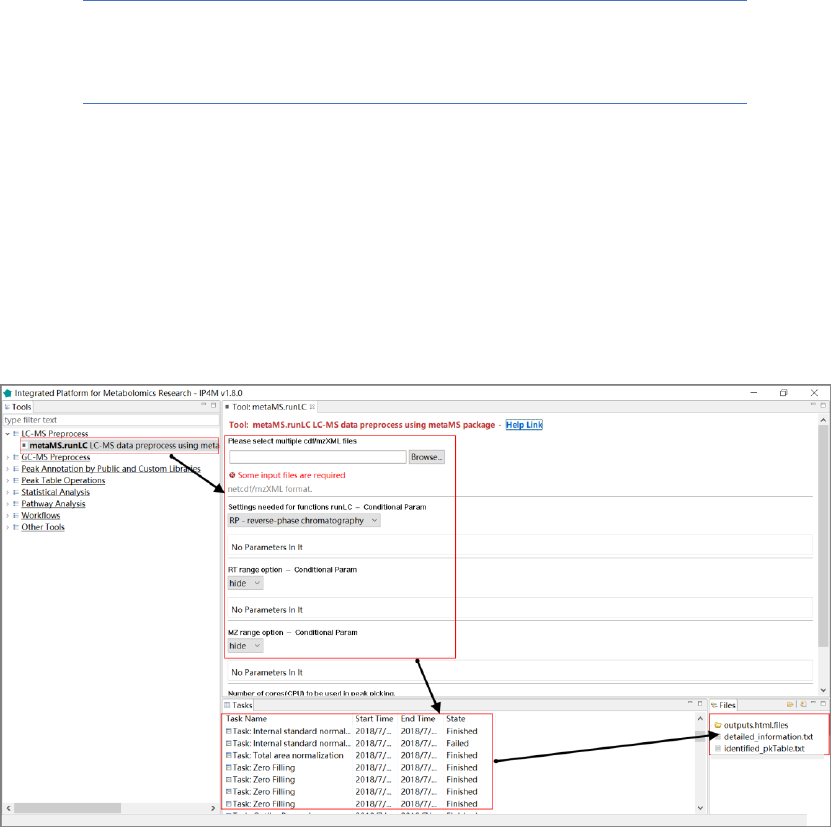
Workflow (Fig. 1): select a tool in tools window–> Set parameters and execute in main

window –> View running status in task window –> View results in main and file window.

Fig.1 Workflow of usage

Specific steps:

1) In the tools window, double-click the tool you want to use and the parameters setting panel

will pop up automatically (fig. 2).

IP4M V1.0

Fig.2 Select a tool

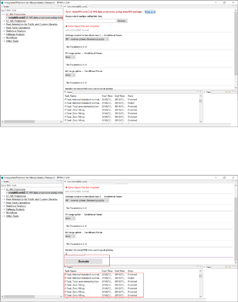
2) Use the default parameters or edit them as you want. Click the “Execute” button to run and

the corresponding task information will appear in the task window (fig. 3).

Fig.3 Execute the task

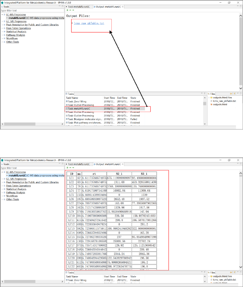
3) When the task is finished, double-click the task to view the list of result files in main window

and file window. Click the files to view the specific results (Fig. 4-5).

IP4M V1.0

Fig.4 View the results 1

Fig.5 View the results 2

IP4M V1.0

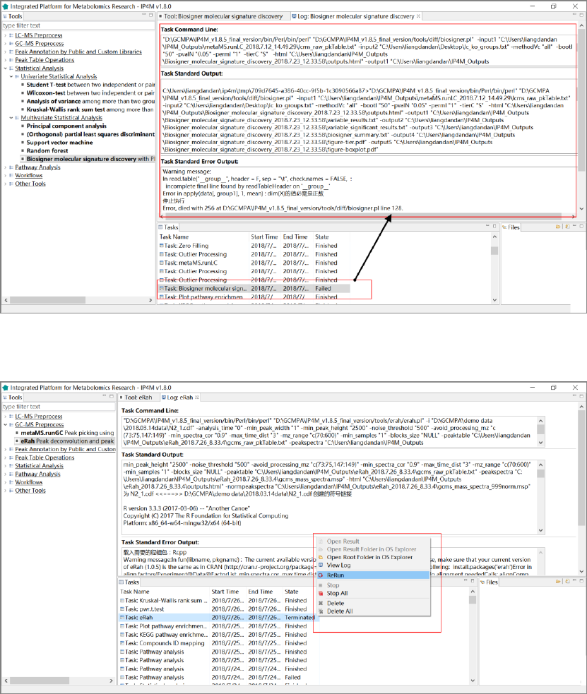
4) If the task has failed, you can double-click the task item to view the log information (fig. 6).

5) Right-click on the task item and select „Rerun‟ to edit the inputs and/or parameters as the error

messages and then re-run the task (fig. 7).

Fig.6 View the log information

Fig.7 Rerun the task

IP4M V1.0

2.2 Inputs and outputs:

Raw data of mzXML and NetCDF formats and other files (peak table, sample information,

compound list etc.) of tab-delimited text format are supported inputs. The free software

ProteoWizard (http://proteowizard.sourceforge.net/) is recommended for converting raw data files

from various instrument vendors to mzXML format. All the intermediate and final results are

exported as .txt files (data) or .pdf (figures) files.

IP4M V1.0

3. Functional modules

3.1 Raw data Preprocessing

3.1.1 LC-MS preprocessing

Tool: metaMS.runLC LC-MS data preprocessing using metaMS

package

This tool is a wrapper for the function 'runLC()' in the R 'metaMS' package. It is designed to

process a series of LC-MS data files and to produce a peak table with mz, rt, and intensities of

peaks in all samples. The popular package xcms is used to perform the peak picking, grouping and

retention correction, and peak filling operations.

Parameter：

1. RP - reverse-phase chromatography: This particular setting is fine-tuned for the analysis of

LC-MS runs.

2. NP - normal-phase chromatography: This particular setting is fine-tuned for the analysis of

LC-MS runs.

3. RT range: RT range to process in minutes, for example, 5,25.

4. MZ range option: MZ range retained for the analysis, for example, 50,500.

5. matchedFilter: Method to use for peak detection. This function identifies peaks in the

chromatographic time domain. The intensity values are binned by cutting the LC/MS data

into slices (bins) of a mass unit (binSize m/z) wide. Within each bin, the maximal intensity is

selected. The peak detection is then performed in each bin by extending it based on the steps

parameter to generate slices comprising bins current _bin - steps +1 to current _bin + steps -

1. Each of these slices is then filtered with matched filtration using a second-derivative

Gaussian as the model peak shape. After filtration peaks are detected using a signal-to-ration

cut-off.

6. step size: The peak detection algorithm creates extracted base peak chromatograms (EIBPC)

on a fixed step size.

7. FWHM: Full width at half maximum of matched filtration gaussian model peak. Can only be

used to calculate the actual sigma.

8. max: Maximum number of peak per extracted ion chromatogram.

9. snthresh: Signal to noise ratio cutoff.

IP4M V1.0

10. min. class. Fraction: Minimum fraction of sample necessary in at least one of the sample

groups for it to be a valid group.

11. min. class. Size: Minimum number of sample necessary in at least one of the sample groups

for it to be a valid group.

12. mzwid: Width of overlapping m/z slices to use for creating peak density chromatograms and

grouping peaks across samples.

13. bws: The two bandwidths used for grouping before and after retention time alignment.

14. missing ratio: Ratio of missing samples to allow in retention time correction groups.

15. extra ratio: Ratio of extra peaks to allow in retention time correction groups.

16. centWave: Method to use for peak detection. The centWave algorithm performs peak density

and wavelet-based chromatographic peak detection. It is most suitable for high-resolution

LC/{TOF,OrbiTrap,FTICR}-MS data in centroid mode. In the first phase the method

identifies regions of interest (ROIs) representing mass traces that are characterized as regions

with less than ppm m/z deviation in consecutive scans in the LC/MS map. These ROIs are

then subsequently analyzed using continuous wavelet transform (CWT) to locate

chromatographic peaks on different scales. The first analysis step is skipped, if regions of

interest are passed via the param parameter.

17. ppm: Numeric defining the maximal tolerated m/z deviation in consecutive scans in parts per

million (ppm) for the initial ROI definition

18. peakwidth: numeric with the expected approximate peak width in chromatographic space.

Given as a range (min, max) in seconds.

19. prefilter: numeric: c (k, I) specifying the prefilter step for the first analysis step (ROI

detection). Mass traces are only retained if they contain at least k peaks with intensity >= I.

Reference:

[1] R. Wehrens, G. Weingart and F. Mattivi, metaMS: An open-source pipeline for GC-MS-based

untargeted metabolomics J. Chrom. B (2014), v966, 109-116.

[2] Colin A. Smith, Elizabeth J. Want, Grace O‟Maille, Ruben Abagyan and Gary Siuzdak.

"XCMS: Processing Mass Spectrometry Data for Metabolite Profiling Using Nonlinear Peak

Alignment, Matching, and Identification" Anal. Chem. 2006, 78:779-787.

[3] Ralf Tautenhahn, Christoph B\"ottcher, and Steffen Neumann "Highly sensitive feature

detection for high resolution LC/MS" BMC Bioinformatics 2008, 9:504

IP4M V1.0

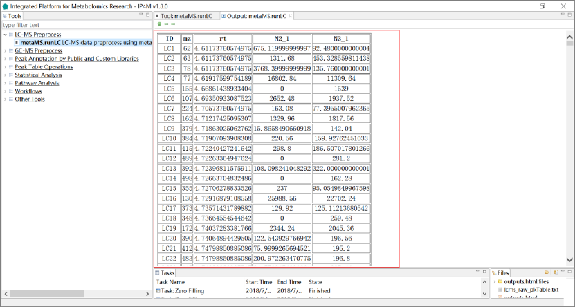
Results and visualization:

Fig. 1 the outputted Peak table with two samples of metaMS.runLC tool

3.1.2 GC-MS preprocessing

Tool: metaMS.runGC peak picking using metaMS package

This tool is a wrapper for the function 'runGC()' in the R 'metaMS' package which is designed

to process a series of GC-MS data files and to produce a peak table. It performs a

pseudospectrum-based analysis, where the basic entity is a collection of (mz, I) pairs at specific

retention times. The standard workflow of metaMS for GC-MS data is the following:

1. peak picking;

2. definition of pseudospectra;

3. identification and elimination of artefacts;

4. annotation by comparison to a database of standards;

5. definition of unknowns;

6. output.

Parameter:

1. RT range: part of the chromatograms that is to be analyzed. If given, it should be a vector of

two numbers indicating minimal and maximal retention time (in minutes). For example 5, 25.

2. FWHM: numeric specifying the full width at half maximum of matched filtration gaussian

model peak. Can only be used to calculate the actual sigma.

3. RT_ Diff: the allowed RT shift in minutes between different samples.

IP4M V1.0

4. Min_ Features: the minimum number of ion in a mass spectrum.

5. similarity_ threshold: the minimum similarity allowed between mass spectra considered as

the same compound.

6. min. class. fract: the fraction of samples in which a pseudospectrum is present before it is

regarded as an unknown.

7. min. class. size: the absolute number of samples in which a pseudospectrum is present before

it is regarded as an unknown.

Reference:

[1] R. Wehrens, G. Weingart and F. Mattivi, metaMS: An open-source pipeline for GC-MS-based

untargeted metabolomics J. Chrom. B (2014), v966, 109-116.

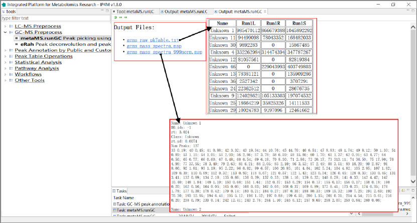
Results and visualization:

Fig.2 The outputted total results files, peak table, and normalized mass spectra information of

metaMS.runGC.

IP4M V1.0

Tool: eRah Peak deconvolution and peak picking using eRah package

This tool is a wrapper of the R 'eRah' package for GC-MS data processing. 'eRah' is an R

package that allows for an innovative deconvolution of GC-MS chromatograms using multivariate

techniques based on blind source separation (BSS). It automatically detects and deconvolves the

spectra of the compounds appearing in GC-MS chromatograms. Then, compounds are aligned by

spectral similarity and retention time distance. It computes the Euclidean distance between

retention time distance and spectral similarity for all compounds in the chromatograms, resulting

in compounds appearing across the maximum number of samples and with the least retention time

and spectral distance. After that, a missing compound recovery step can be applied to recover

those compounds that are missing in some samples. Missing compounds appear as a result of an

incorrect deconvolution or alignment - due to a low compound concentration in a sample - , or

because it is not present in the sample. This forces the final data table with compound names and

compounds area, to not have any missing (zero) values. Please see the references for detailed

descriptions.

Parameter：

1. RT window: The chromatographic retention time window to process. If 0 all the

chromatogram is processed.

2. Minimum peak width: This is a critical parameter that conditions the efficiency of eRah.

Typically, it should be the half of the mean compound width.

3. noise. threshold: Data above this threshold will be considered as noise

4. avoid.processing.mz: The masses that do not want to be considered for processing. Typically,

in GCMS those masses are 73,74,75,147,148 and 149, since they are ubiquitous mass

fragments typically generated from compounds carrying a trimethylsilyl moiety.

5. Minimum spectral correlation value: From 0 (no similar) to 1 (very similar). This value sets

how similar two or more compounds have to be considered for alignment between them.

6. Maximum retention time distance: This value (in seconds) sets how far two or more

compounds can be considered for alignment between them.

7. Minimum. sample: The minimum number of samples in which a compound has to appear to

be considered for searching into the rest of the samples where this compound is missing.

8. blocks. size: For experiments containing more than 100 (Windows) or 1000 (Mac or Linux)

samples (numbers depending on the computer resources and sample type). In those cases,

alignment can be conducted by block segmentation. For an experiment of e.g. 1000 samples,

the block.size can be set to 100, so the alignment will perform as multiple (ten) 100-samples

experiments, to later align them into a single experiment.

This parameter is designed to solve the typical problem that appears when aligning under the

IP4M V1.0

Windows operating system: "Error: cannot allocate vector of size XX Gb". Such a problem

will not appear with Mac or Linux, but several hours of computation are expected when

aligning a large number of samples. Using block segmentation provides a greatly improved

run-time performance.

Reference:

[1] X. Domingo-Almenara, et al., eRah: a computational tool integrating spectral deconvolution

and alignment with quantification and identification of metabolites in GC{MS-based

metabolomics. Analytical Chemistry. 88 (2016) 9821{9829. DOI:

10.1021/acs.analchem.6v02927

[2] X. Domingo-Almenara, et al., Compound identification in gas chromatography/mass

spectrometry-based metabolomics by blind source separation. Journal of Chromatography A

1409 (2015) 226{233. DOI: 10.1016/j.chroma.2015.07.044

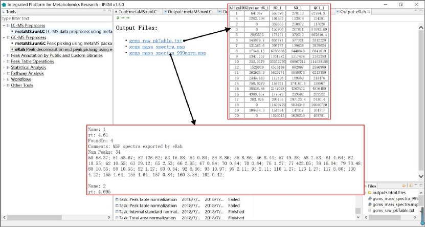
Results visualization:

Fig.3 The outputted results files, peak table, and normalized mass spectra of eRah package.

IP4M V1.0

3.2 Annotation by Public and Custom Libraries

3.2.1 GC-MS peak annotation

Tool: GC-MS peak annotation on msp database files

This tool intends to annotate compounds from the GC-MS peak table by matching mass

spectra and/or retention times of public/custom library and detected peaks. If you want to use the

custom library for annotation, a standard MSP format file is required.

Parameter:

1. normalized dot product: Matching factor function for mass spectrum. The function applies

weights to an input to get weighted outputs.

2. normalized Euclidean distance: Matching factor function for mass spectrum.

3. mass spectrum similarity cutoff: 0-1, more similar larger matching factor.

4. RT window: The retention time difference that can be allowed.

5. NSEN: An integrated library derived from NIST/EPA/NIH. It is the default public library.

6. GMD_ALK: A public database from the Golm Metabolome Database (GMD). ALK - based

on 9 n-alkanes (C10–C36).

7. GMD_FAME: A public database from the Golm Metabolome Database (GMD). FAME -

based on 13 fatty acid methyl esters (C8 ME–C30 ME).

8. GMD_MSIR: The 'Q_MSRI_ID' GC-Quadrupole-MS MSRI Database of Golm Metabolome

library.

9. MoNA-HMDB: It is derived from MassBank of North America, with 4620

spectra(http://mona.fiehnlab.ucdavis.edu/downloads).

10. MoNA-MetaboBASE: It is derived from MassBank of North America, with 1254 spectra

(http://mona.fiehnlab.ucdavis.edu/downloads).

11. MoNA-ReSpect: It is derived from MassBank of North America, with 6290

spectra(http://mona.fiehnlab.ucdavis.edu/downloads).

Note:

There is no retention time field in the public library and only mass spectrum information is

used for annotation. For a custom library, this tool supports the joint annotation by mass spectrum

and retention time. Users can provide an in-house library file in MSP format containing the field

'rt'. This is an optional field. A compound can be repeated in the database with the same 'Name '

IP4M V1.0

but a different mass spectrum. In this case, the best hit will be outputted.

Reference:

[1] Schauer N, Steinhauser D, Strelkov S, Schomburg D, Allison G, Moritz T, Lundgren K,

Roessner-Tunali U, Forbes MG, Willmitzer L, Fernie AR, Kopka J: GC-MS libraries for the

rapid identification of metabolites in complex biological samples. FEBS Lett 2005,

579(6):1332–1337. 10.1016/j.febslet.2005.01.029

[2] Kopka, J., Schauer, N., Krueger, S., Birkemeyer, C., Usadel, B., Bergmuller, E., Dormann, P.,

Weckwerth, W., Gibon, Y., Stitt, M., Willmitzer, L., Fernie, A.R. and Steinhauser, D. (2005)

GMD@CSB.DB: the Golm Metabolome Database, Bioinformatics, 21, 1635-1638.

Results and visualization:

Fig.4 The outputted total files, identified peak table, and compounds detailed information of

GC-MS peak table annotation.

3.2.2 LC-MS peak annotation

Tool: LC-MS peak annotation on xls database files

This tool is used to annotate compounds from the LC-MS peak table by comparing m/z and

RT with the public/custom library. The best top five hits will be shown in the results. If you want

to use the custom library for annotation, a two-column Tab-delimited text file is required with the

first column as compound name and the second column as precise MZ.

IP4M V1.0

Parameter:

1. mz cutoff: A hit that difference of mz must be <=mz_cutoff.

2. RT window: The acceptable retention time difference.

3. ppm: Parts per million. numeric the relative error for matching peaks that is a window of user

specified error (or the default 10) in ppm for each fragment mass.

(|M- M0|÷m)×106 (ppm). „M‟ is the measured value of the ion mass; „M0‟ is the theoretical

value of the ion mass; „m‟, an integer, is the mass of the ion.

For example, the molecular ion measured value of a compound is 364.2504, the theoretical

value is 364.2509, and the mass measurement accuracy is:

|364.2504-364.2509|÷364×106=1.4ppm

4. adducts type: There are several possible adducts and the recommended type that most

commonly occurs is “M+H” or “M-H”.

Note:

1. There is no retention time field in the public library and only mass spectrum information is

used for annotation. For a custom library, this tool supports the joint annotation by precise

MZ and retention time. Users can provide an in-house two-column Tab-delimited text file

with the first column as compound name and the second column as precise MZ.

2. The tool will identify all possible matching compounds based on all adduct types selected,

sort them according to the matching score, and output them all as 'detailed_information.txt'.

Also, the compound with the smallest MZ and RT deviation will be outputted as the final

identified compound in 'identified_pkTable.txt' file.

Results and visualization:

IP4M V1.0

Fig.5 The outputted results files, identified peak table, and detailed information of compounds of

LC-MS peak annotation.

IP4M V1.0

3.3 Peak Table Operations

3.3.1 Pretreatment

Tool: Outlier processing on peak table

The tool takes a peak table file as input and processes the outliers using the capping method.

Default boundary is [0, Q3+1.5*IQR]. If the value > (Q3+1.5*IQR), it is identified as an outlier

and replaced by the maximum value within the normal range.

Parameter:

1. Q3: The third quartile (Q3), also known as the "larger quartile", equals to the value ranked at

75% of all values in ascending order.

2. IQR: InterQuartile Range, equals to |Q3 minus Q1|.

Tool: Zero filling on peak table

This tool takes a peak table file as input and fills the missing values (zero , null value or „NA‟,

or negative values) with 1) the a*min value, where 'a' is a user-defined coefficient; 2) 'min' which

is the minimum non-negative value in the peak table; 3) user-specified value; 4) values computed

by 'KNN'; and 5) values computed by 'qirlc'. The „qirlc‟ algorithm is especially suitable for

left-censored data.

Reference:

If you use 'KNN' method, references:

[1] Hastie, T., Tibshirani, R., Sherlock, G., Eisen, M., Brown, P. and Botstein, D., Imputing

Missing Data for Gene Expression Arrays, Stanford University Statistics Department

Technical report (1999).

[2] Olga Troyanskaya, Michael Cantor, Gavin Sherlock, Pat Brown, Trevor Hastie, Robert

Tibshirani, David Botstein and Russ B. Altman, Missing value estimation methods for DNA

microarrays BIOINFORMATICS Vol. 17 no. 6, 2001 Pages 520-525

If you use 'qirlc' method, references:

[3] QRILC: a quantile regression approach for the imputation of left-censored missing data in

quantitative proteomics, Cosmin Lazar et al.

[4] Wei R, Wang J, Su M, et al. Missing Value Imputation Approach for Mass Spectrometry-based

IP4M V1.0

Metabolomics Data: [J]. Scientific Reports, 2018, 8(1).

[5] Wei R, Wang J, Jia E, et al. GSimp: A Gibbs sampler based left-censored missing value

imputation approach for metabolomics studies: [J]. Plos Computational Biology, 2018,

14(1):e1005973.

3.3.2 Normalization

Tool: Total area normalization on peak table

This tool takes a peak table file as input and performs total intensity normalization within

samples. The formula is (x/sum of total intensity within the corresponding sample) *1000.

Tool: Internal standard normalization

This tool takes a peak table file as input and performs internal standard (IS) normalization

within samples. The normalization formula is (x/internal standard) *10000.

Parameters:

Set the standard compound: for example Chlorophenylalanine

Note:

1. The IS compound must exist in the inputted peak table.

2. Experimental preparation: The internal standard must be prepared in advance and added

quantitatively to each sample.

Tool: Peak table normalization based on QC (pooled samples)

This tool takes a peak table file as input and performs normalization based on quality control

samples (QCs).

QCs are pooled samples. They contain the same compounds as the subject samples and are

supposed to reflect the average metabolite concentrations within a study. QCs are pretreated

according to the same protocols as the subject samples and are evenly injected throughout the

analyses. The performances of the pretreatment and the analytical platform can be assessed using

the QCs. The normalization formula is (x metabolite/QC metabolite) *10000.

Input files:

IP4M V1.0

1. Peak table file in Tab-delimited text format, with the first column as the compound identifier

and others as samples.

For example:

Table.1 Peak table with QC

AlignID

STDmix_GC_01

STDmix_GC_02

QC1

STDmix_GC_03

QC2

Unknown 1

1486892478

561322777

3448620272

561322777

Nitrogen dioxide

5492977592

684434115

3265669981

Ethanol, 2-fluoro-

2265686433

4182838129

4365291513

4182838129

3-Pentanone, 2,2,4,4-

tetramethyl-

13390154

12612932

21155307

21155322

Hydrazine

14588107

8510918

7224351

7224380

2. Sample-to-QC design file, a Tab-delimited text file with two columns, "sample" and "QC".

For example:

Table.2 Sample-to-QC group file

STDmix_GC_01

QC1

STDmix_GC_02

QC1

STDmix_GC_03

QC2

Output files:

'QC_norm_pkTable.txt', normalized peak table.

For example:

Table.3 Normalized peak table based on QC

AlignID

STDmix_GC_01

STDmix_GC_02

QC1

STDmix_GC_03

QC2

4311.558

1627.673

10000

61437.38

10000

Nitrogen dioxide

16820.37

2095.846

10000

Ethanol, 2-fluoro-

5190.229

9582.036

10000

10436.2

10000

3-Pentanone, 2,2,4,4-tetramethyl-

6329.454

5962.065

10000

9999.993

10000

Hydrazine

20192.97

11780.88

10000

9999.96

10000

IP4M V1.0

3.3.3 Other operations

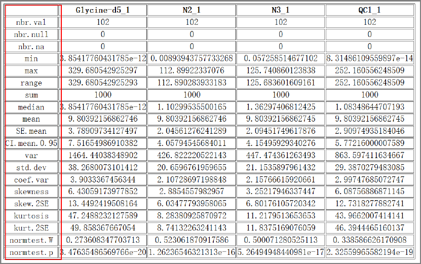
Tool: Basic statistics summary

This tool takes a peak table file as input and outputs the basic statistics, including 'nbr.val',

'nbr.null', 'nbr.na', 'min', 'max', 'range', 'sum', 'median', 'mean', 'SE.mean', 'CI.mean.0.95' ,'var',

'std.dev', 'coef.var', 'skewness', 'skew.2SE', 'kurtosis', 'kurt.2SE', 'normtest.W', and 'normtest.p'. .

Results and visualization:

Fig.6 The basic statistics summary of four samples

Tool: retrieve rows from peak table

The tool takes a peak table file and a one-column compounds list file as inputs and outputs a

sub-peak table file which rows correspond to the compounds list.

Input files:

1. Peak table file in Tab-delimited text format, with the first column as the compound identifier

and others as samples.

For example:

Table.4 Peak table

IP4M V1.0

HU_011

HU_014

HU_015

HU_017

HU_018

HU_019

(2-methoxyethoxy)propanoic

acid isomer

3.019766

3.814339

3.519691

2.562183

3.781922

4.161074

(gamma)Glu-Leu/Ile

3.888479

4.277149

4.195649

4.32376

4.629329

4.412266

1-Methyluric acid

3.869006

3.837704

4.102254

4.53852

4.178829

4.516805

1-Methylxanthine

3.717259

3.776851

4.291665

4.432216

4.11736

4.562052

1,3-Dimethyluric acid

3.535461

3.932581

3.955376

4.228491

4.005545

4.320582

2. A one-column compound list file in text format.

For example:

Table.5 Compound list file

1-methyluric acid

1-Methylxanthine

1,3-Dimethyluric acid

1,7-Dimethyluric acid

Output files:

A sub-peak table file in Tab-delimited text format, with the retrieved information according

to the compounds list.

For example:

Table.6 Sub-peak table

HU_011

HU_014

HU_015

HU_017

HU_018

HU_019

1-Methyluric acid

3.869006

3.837704

4.102254

4.53852

4.178829

4.516805

1-Methylxanthine

3.717259

3.776851

4.291665

4.432216

4.11736

4.562052

1,3-Dimethyluric acid

3.535461

3.932581

3.955376

4.228491

4.005545

4.320582

1,7-Dimethyluric acid

3.325199

4.025125

3.972904

4.109927

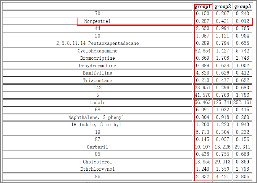
Tool: Row average by groups

This tool takes a peak table file and a samples-to-group design file as inputs, and outputs the

averaged intensity of every compound in every group.

Results and visualization:

IP4M V1.0

Fig.7 The outputted averaged intensity of every compound in 3 groups.

3.3.4 Transformation

Tool: Log2 transformation

This tool takes a peak table file as input and performs log transformation (base 2) or median

centered log2 transformation on the peaks.

Note:

The transformation formula is: log2 (value+1)

The median center is performed on the row (compound data).

Tool: Z-score transformation

This tool takes a peak table file as input and performs z-score transformation on the peaks.

This method standardizes the data by mean and standard deviation of the original data. It is

applicable to the cases where the maximum and minimum values are unknown, or there is outlier

data beyond the range of values. Formula is new data = (original data - mean)/standard deviation.

IP4M V1.0

Tool: Transpose

This tool takes a matrix data as input and performs transpose operation.

3.3.5 Merge tables

Tool: Merge tables by compound name

This tool takes multiple peak tables as input and merges them together. The outputted peak

table will have more samples and compounds. If a compound exists in some but not all tables, it

will be filled as NA in missing position in the final merged table. If same sample names exist in

different tables, their common compounds will be averaged and outputted in the final table.

Input files:

Multiple peak table files in Tab-delimited text format, with the first column as the compound

identifier and the others as samples.

For example:

Peak table 1:

Table.7 The inputted table1

AlignID

STDmix_GC_01

STDmix_GC_02

1486892478

451322711

Nitrogen dioxide

5492977400

684433223

Ethanol, 2-fluoro-

2265686433

4182838129

Peak table2:

Table.8 The inputted table2

AlignID

STDmix_GC_02

STDmix_GC_03

3448620100

Nitrogen dioxide

3265968000

3265668000

Norgestrel

789.33

5315.224

Output files:

'merged_matrix.txt', merged peak table file in Tab-delimited text format.

Table.9 The merged table

AlignID

STDmix_GC_01

STDmix_GC_02

STDmix_GC_03

1486892478

451322711

3448620272

IP4M V1.0

Nitrogen dioxide

5492977592

1975200611.5

3265669981

Ethanol, 2-fluoro-

2265686433

4182838129

Norgestrel

789.33

5315.224

IP4M V1.0

3.4 Statistical Analysis

3.4.1 Univariate statistical analysis

Tool: Student t test between two independent or paired groups

This tool performs the Student t-test and multiple comparison correction on the peaks of the

inputted table. Group information is given by a group design file (Tab-delimited text file). The

number of groups should be 2. For paired t-test, pairs are defined according to the order in each of

the two groups and the number of samples must be equal in the two groups.

Note:

Groups number must be 2 in the sample group file.

Group names of characters or string are preferred. Numbers are also supported but not

recommended.

Input files:

Group design file. For paired t-test, pairs are according to the order in each of the two groups.

For example:

Table.10 The group file for paired t-test, with 3 pairs (_p1, _p2, and _p3) in different color blocks

HU_01_p1

HU_02_p1

HU_03_p2

HU_04_p3

HU_05_p2

HU_06_p3

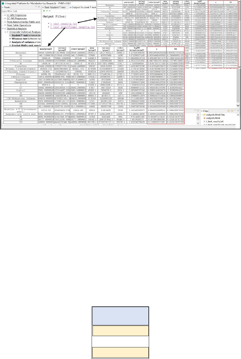
Output files:

1. 't_test_results.txt', t-test results with p value, log2FC, and q value.

2. 't_test_significant_results.txt', significant t-test results.

Note:

Groups number must be 2 in the sample group file.

Group names of characters or string are preferred. Numbers are also supported but not

IP4M V1.0

recommended.

Results and visualization:

Fig.8 The outputted files with the full results and significant results of t-test method.

Tool: Wilcoxon-signed-rank-test between two paired groups

This tool performs the Wilcoxon-test and multiple comparison corrections to find the

significant peaks on the peak table data. Group information is given by a group design file

(Tab-delimited text file). The number of groups should be 2. For a paired test, pairs are according

to the order in each of the two groups. For example, A-group-first-sample and

B-group-first-sample are a pair. For a paired test, the number of samples must be equal in the two

groups. For a paired-test, a Wilcoxon rank sum test (equivalent to the Mann-Whitney test) is

carried out, otherwise, a Wilcoxon signed rank test is performed.

Input files:

Group design file. For a paired t-test, pairs are according to the order in each two groups.

For example:

Table.11 The group file for paired test, with 3 pairs in different color blocks

HU_01_p1

HU_02_p1

HU_03_p2

HU_04_p3

HU_05_p2

IP4M V1.0

HU_06_p3

Output files:

1. 'wilcox_test_results.txt', Wilcoxon-test results with p value, log2FC, and q value.

2. 'wilcox _test_significant_results.txt', significant Wilcoxon-test results.

Note:

Group number must be 2 in the sample group file.

Group names of characters or string are preferred. Numbers are also supported but not

recommended.

Results and visualization:

Fig.10 The results of Wilcoxon-signed-rank-test between two paired groups

Tool: Analysis of variance among more than two groups

This tool fits an analysis of variance model to find the significant peaks on the inputted peak

table. Group information is given by a group design file (Tab-delimited text file).

Note:

Group names of characters or string are preferred. Numbers are also supported but not

recommended.

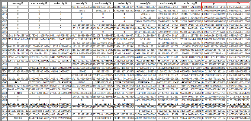
Results and visualization:

IP4M V1.0

Fig.11 The result of analysis of variance among 3 groups

Tool: Kruskal-Wallis rank test among more than two groups

This tool performs a Kruskal-Wallis rank sum test and multiple comparison corrections to

find the significant peaks on the inputted peak table. Group information is given by a group design

file (Tab-delimited text file).

Note:

Group names of characters or string are preferred. Numbers are also supported but not

recommended.

3.4.2 Multivariate statistical analysis

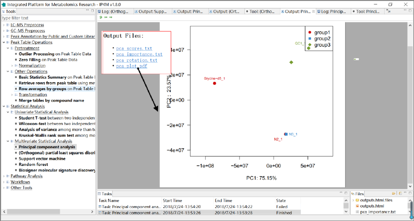
Tool: Principal component analysis

This tool performs a principal components analysis on the inputted peak table data. If the

group design file (a Tab-delimited text file) is provided, samples in the same group will be plotted

as the same color.

Input files:

1. Peak table file in Tab-delimited text format, with the first column as compound identifier, the

others as samples.

For example:

IP4M V1.0

Table.12 The inputted peak table file

HU_01

(2-methoxyethoxy)propanic

acid isomer

3.0197

3.8143

3.5196

2.5621

3.7819

4.1610

(gamma)Glu-Leu/Ile

3.8884

4.2771

4.1956

4.3237

4.6293

4.4122

1-Methyluric acid

3.8690

3.8377

4.1022

4.5385

4.1788

4.5168

1-Methylxanthine

3.7172

3.7768

4.2916

4.4322

4.1173

4.5620

1,3-Dimethyluric acid

3.5354

3.9325

3.9553

4.2284

4.0055

4.3205

1,7-Dimethyluric acid

3.3251

4.0251

3.9729

4.1099

4.0240

4.3268

2-acetamido-4-methylphenyl

acetate

4.2047

5.1818

3.8856

4.2379

1.8529

4.0806

2-Aminoadipic acid

4.0802

4.3592

4.2491

4.2314

4.3236

4.2444

2.(Optional), Group design file in Tab-delimited text file.

For example:

Table.13 The inputted group design file

HU_011

HU 014

HU_015

HU_017

HU_018

HU_019

Output files:

1. 'pca_scores.txt', PCs (scores) matrix.

2. 'pca_importance.txt', importance of PCs.

3. 'pca_rotation.txt', the matrix of variable loadings (i.e., a matrix whose columns contain the

eigenvectors).

4. 'pca_plot.pdf', PCA plot using PCs score values, the default is PC1 and PC2.

Results and visualization:

IP4M V1.0

Fig.12 The resulting files and the PCA scores plot

Tool: (Orthogonal) partial least squares discriminant analysis

This tool performs the OPLS-DA algorithm to rank peaks on the inputted table by variable

importance in projection (VIP). Group information is given by a group design file (Tab-delimited

text file). OPLS-DA is only available for binary classification and the number of groups should be

The orthogonal Partial Least-Squares (OPLS) algorithm was introduced by J. Trygg and

Wold (2002) in order to model separately the variations of the predictors correlated and orthogonal

to the response. It has a similar predictive capacity compared to PLS and improves the

interpretation of the predictive components and of the systematic variation (Pinto, Trygg, and

Gottfries 2012). In particular, OPLS modeling of single responses only requires one predictive

component. Diagnostics such as the Q2Y metrics and permutation testing are of high importance

to avoid overfitting and assess the statistical significance of the model. The VIP, which reflects

both the loading weights for each component and the variability of the response explained by this

component (Pinto, Trygg, and Gottfries 2012; Mehmood et al. 2012), can be used for feature

ranking and selection (J. Trygg and Wold 2002; Pinto, Trygg, and Gottfries 2012).

Input files:

1. Peak table file in Tab-delimited text format, with the first column as the compound identifier

and others as samples.

For example:

Table.13 The inputted peak table file

IP4M V1.0

HU_01

(2-methoxyethoxy)propanoic

acid isomer

3.0197

3.8143

3.5196

2.5621

3.7819

4.1610

(gamma)Glu-Leu/Ile

3.8884

4.2771

4.1956

4.3237

4.6293

4.4122

1-Methyluric acid

3.8690

3.8377

4.1022

4.5385

4.1788

4.5168

1-Methylxanthine

3.7172

3.7768

4.2916

4.4322

4.1173

4.5620

1,3-Dimethyluric acid

3.5354

3.9325

3.9553

4.2284

4.0055

4.3205

1,7-Dimethyluric acid

3.3251

4.0251

3.9729

4.1099

4.0240

4.3268

2-acetamido-4-methylphenyl

acetate

4.2047

5.1818

3.8856

4.2379

1.8529

4.0806

2-Aminoadipic acid

4.0802

4.3592

4.2491

4.2314

4.3236

4.2444

2. Group design file in Tab-delimited text file with two columns (samplename groupname).

For example:

Table.14 The inputted group design file

HU_011

HU 014

HU_015

HU_017

HU_018

HU_019

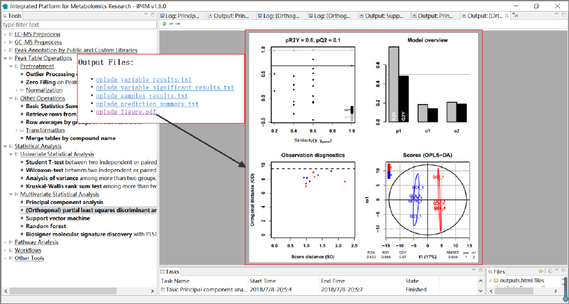
Output files:

1. 'oplsda_variable_results.txt', feature ranked results that are sorted by VIP.

2. 'oplsda_variable_significant_results.txt', significant feature results.

3. 'oplsda_samples_results.txt', OPLS-DA model sample prediction results using inputted

data.

4. 'oplsda_prediction_summary.txt', prediction summary.

5. 'oplsda_figure.pdf', OPLS-DA plot.

Parameter:

IP4M V1.0

1. VIP-value: A numerical variable indicating the Variable Importance in Projection.

2. orthogonal components: The number of orthogonal components (for OPLS only); when

set to 0 [default], PLS will be performed; otherwise OPLS will be performed; when set

to NA, OPLS is performed and the number of orthogonal components is automatically

computed by using the cross-validation (with a maximum of 9 orthogonal components).

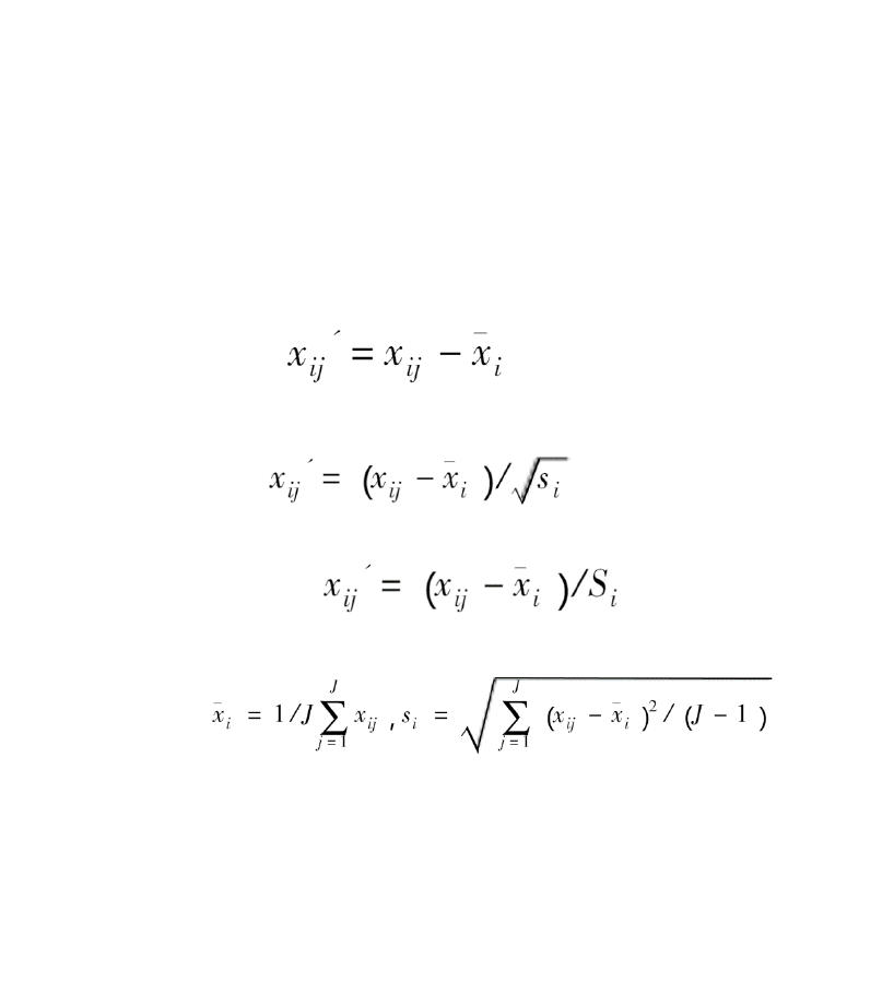
3. scaling methods: Either no centering nor scaling (‟none‟), mean-centering only (‟center‟),

mean-centering and Pareto scaling (‟Pareto‟), or mean-centering and unit variance

scaling (‟standard‟) [default].

Mean-centering:

Pareto scaling:

unit variance scaling:

Comments:

4. crossvalI: Number of cross-validation segments (default is 7); The number of samples

(rows of ‟x‟) must be at least >= crossvalI

5. permutation: Number of random permutations of response labels to estimate R2Y and

Q2Y significance by permutation testing [default is 20 for single response models

(without train/test partition), and 0 otherwise]

6. graphical parameters: This tool provides ten graphic parameters for ten different graphic

types. They are displayed in 'oplsda_figure.pdf' file.

Note：

Group number must be 2 in the sample group file.

Group names of characters or string are preferred. Numbers are also supported but not

recommended.

Reference:

[1] Thevenot, E.A., Roux, A., Xu, Y., Ezan, E., Junot, C. 2015. Analysis of the human adult

urinary metabolome variations with age, body mass index and gender by implementing a

comprehensive workflow for univariate and OPLS statistical analyses. Journal of Proteome

IP4M V1.0

Research. 14: 3322-3335.

[2] Trygg J, Wold S. Orthogonal projections to latent structures (O-PLS) [J]. Journal of

Chemometrics 2002,16:119 –128.

[3] Rui C P, Trygg J, Gottfries J. Advantages of orthogonal inspection in chemometrics[J]. Journal

of Chemometrics, 2012, 26(6):231–235.

[4] Mehmood, T., KH. Liland, L. Snipen, and S. Saebo. 2012. “A Review of Variable Selection

Methods in Partial Least Squares Regression.” Chemometrics and Intelligent Laboratory

Systems 118 (0): 62–69.

[5] Galindo-Prieto B., Eriksson L. and Trygg J. (2014). Variable influence on projection (VIP) for

orthogonal projections to latent structures (OPLS). Journal of Chemometrics 28, 623-632.

Results and visualization:

Fig.13 The resulting files and the summary plot of OPLS-DA

Tool: Support vector machine

This tool performs support vector machines to rank peaks in the inputted table by SVM-RFE.

Group information is given by a group design file (Tab-delimited text file).

The SVM-RFE algorithm proposed by Guyon returns a ranking of the features of a

classification problem by training an SVM with a linear kernel and removing the feature with the

smallest ranking criterion. This criterion is the w value of the decision hyperplane given by the

SVM. For more detailed information, please review the original paper.

Input files:

IP4M V1.0

1. Peak table file in Tab-delimited text format, with the first column as the compound identifier

and the others as samples.

For example:

Table.15 The inputted peak table file

HU_01

(2-methoxyethoxy)propanoic

acid isomer

3.0197

3.8143

3.5196

2.5621

3.7819

4.1610

(gamma)Glu-Leu/Ile

3.8884

4.2771

4.1956

4.3237

4.6293

4.4122

1-Methyluric acid

3.8690

3.8377

4.1022

4.5385

4.1788

4.5168

1-Methylxanthine

3.7172

3.7768

4.2916

4.4322

4.1173

4.5620

1,3-Dimethyluric acid

3.5354

3.9325

3.9553

4.2284

4.0055

4.3205

1,7-Dimethyluric acid

3.3251

4.0251

3.9729

4.1099

4.0240

4.3268

2-acetamido-4-methylphenyl

acetate

4.2047

5.1818

3.8856

4.2379

1.8529

4.0806

2-Aminoadipic acid

4.0802

4.3592

4.2491

4.2314

4.3236

4.2444

2. Group design file in Tab-delimited text file with two columns (samplename groupname).

For example:

Table.16 The inputted group design file

HU_011

HU 014

HU_015

HU_017

HU_018

HU_019

Output files:

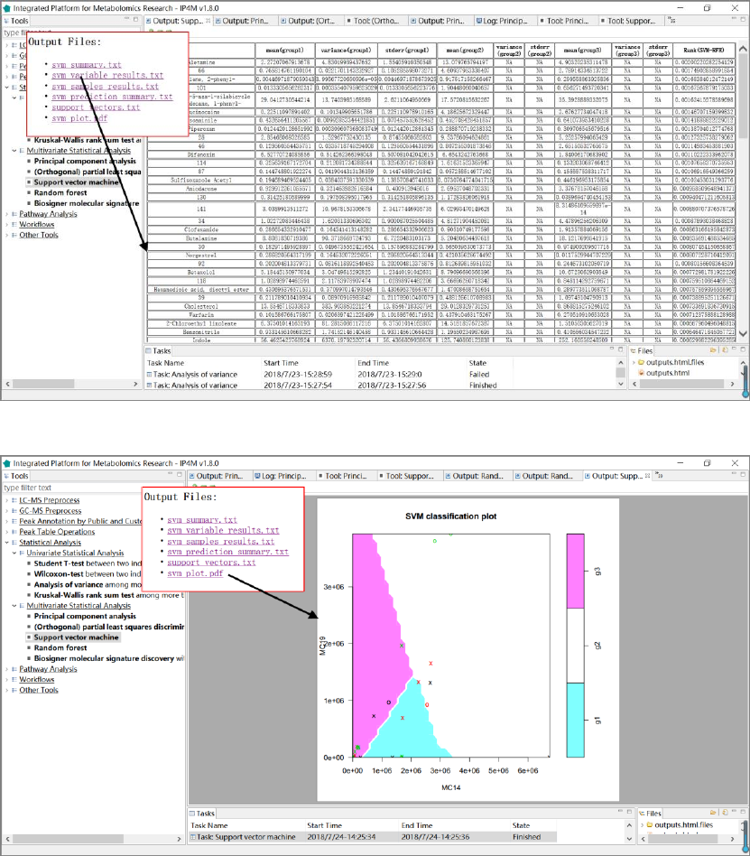
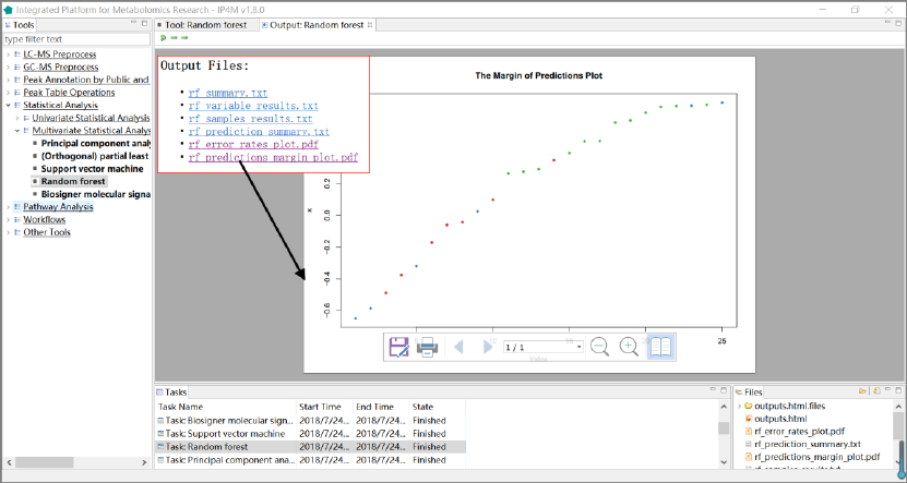
1. 'svm_summary.txt', summary information about SVM.

2. 'svm_variable_results.txt', feature ranked results that are sorted by SVM-RFE.

3. ' svm_samples_results.txt', SVM model sample prediction results using inputted data.

4. 'svm_prediction_summary.txt', prediction summary.

5. 'support_vectors.txt', support vectors in the model.

IP4M V1.0

6. 'svm_plot.pdf', SVM plot.

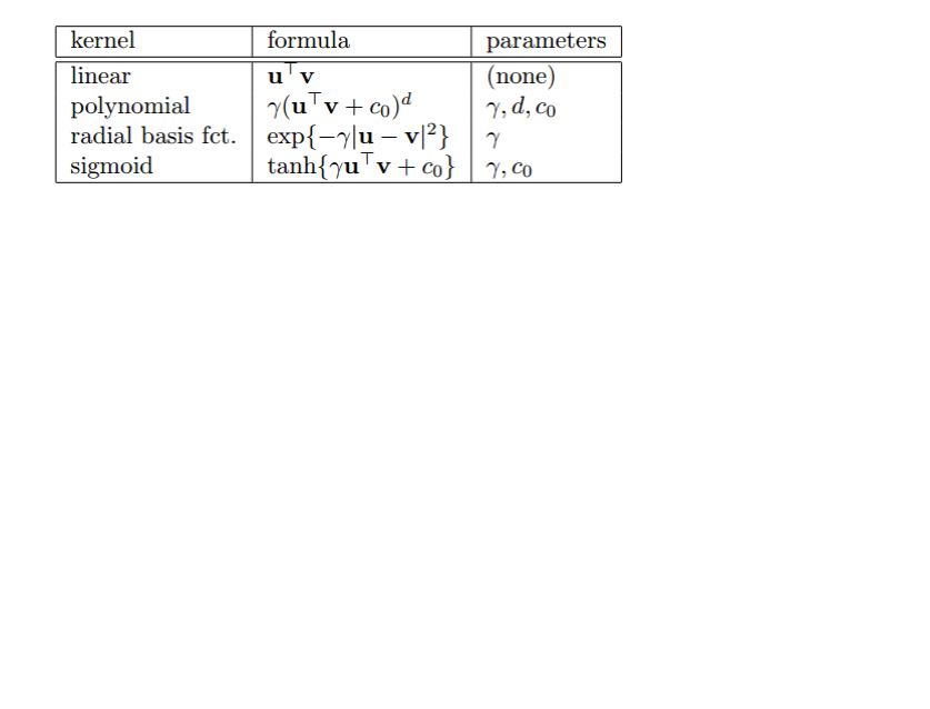
Parameter:

kernel function: The kernel function reflects the similarity between the inputted data. The

correct choice of kernel parameters is crucial for obtaining good results, which practically

means that an extensive search must be conducted on the parameter space before results can

be trusted.

1. Linear kernel: Simple and safe, try it first. The model is interpretative. It indicates which

features or data points in the model are important. But it is not available if the data is not

linearly separable.

2. Polynomial kernel: Less restrictive than linear applications, it can solve non-linear separable

data. But it is more complicated with three parameters.

3. Radial basis function (RBF): Usually defined as a monotonic function of the Euclidean

distance between any points in space to a certain center. It maps primitive features to infinite

dimensions. It is able to achieve nonlinear mapping and also has less numerical difficulties.

4. Sigmoid: Squashes numbers to the range [0, 1]. Historically popular since they have a nice

interpretation as a saturating “firing rate” of a neuron. But there are some fatal disadvantages.

For instance, saturated neurons “kill” the gradients, sigmoid outputs are not zero-centered,

and exp () is a bit computationally expensive.

Note:

Group names of characters or string are preferred. Numbers are also supported but not

recommended.

Reference:

[1] Marchiori E, Sebag M. Bayesian Learning with Local Support Vector Machines for Cancer

Classification with Gene Expression Data[M]// Applications of Evolutionary Computing.

Springer Berlin Heidelberg, 2005:74-83.[2] Gene Selection for Cancer Classification using

Support Vector Machines (2002) Isabelle Guyon, Jason Weston, Stephen Barnhill, Vladimir

Vapnik.

Results and visualization:

IP4M V1.0

Fig.14 The resulting files and the variable ranks of SVM (3 groups)

Fig.15 The resulting files and the classification plot of SVM (3 groups)

Tool: Random forest

This tool implements Breiman's random forest algorithm (R randomforest package) for

classification and peak ranking based on the inputted table. The peaks are ranked by the mean

decrease in Gini index. Group information is given by a group design file (Tab-delimited text file).

Input files:

1. Peak table file in Tab-delimited text format, with the first column as the compound identifier

IP4M V1.0

and the others as samples.

For example:

Table.17 The inputted peak table file

HU_01

(2-methoxyethoxy)propanoic

acid isomer

3.0197

3.8143

3.5196

2.5621

3.7819

4.1610

(gamma)Glu-Leu/Ile

3.8884

4.2771

4.1956

4.3237

4.6293

4.4122

1-Methyluric acid

3.8690

3.8377

4.1022

4.5385

4.1788

4.5168

1-Methylxanthine

3.7172

3.7768

4.2916

4.4322

4.1173

4.5620

1,3-Dimethyluric acid

3.5354

3.9325

3.9553

4.2284

4.0055

4.3205

1,7-Dimethyluric acid

3.3251

4.0251

3.9729

4.1099

4.0240

4.3268

2-acetamido-4-methylphenyl

acetate

4.2047

5.1818

3.8856

4.2379

1.8529

4.0806

2-Aminoadipic acid

4.0802

4.3592

4.2491

4.2314

4.3236

4.2444

2. Group design file in Tab-delimited text format with two columns (samplename

groupname).

For example:

Table.18 The inputted group design file

HU_011

HU 014

HU_015

HU_017

HU_018

HU_019

Output files:

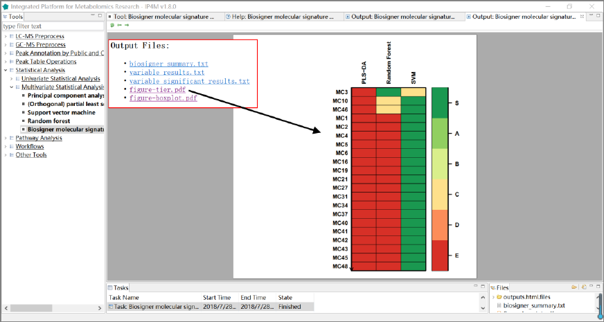
1. 'rf_summary.txt ', summary information about random forest model.

2. 'rf_variable_results.txt ', feature rank results that sorted by mean decrease in Gini index.

3. 'rf_prediction_summary.txt ', random forest model sample prediction results using inputted

data.

4. 'rf_prediction_summary.txt', prediction summary.

5. 'rf_error_rates_plot.pdf ', error rates plot in the model.

IP4M V1.0

6. 'rf_predictions_margin_plot.pdf ', predictions_margin plot.

Parameter:

1. number of trees: It specifies the number of decision trees included in the random forest. The

default is 500.

2. mtry: Mtry specifies the number of variables used in the node for the binary tree. The default

is the quadratic root of the data set variable (classification model) or one- third (predictive

model). Generally, it is necessary to carry out artificial selection step by step to determine the

optimal m value.

3. replacement: Specify the way to randomly sample Bootstrap. The default is resampling.

4. nodesize: The minimum number of decision tree nodes. By default, the discriminant model is

1 and the regression model is 5.

5. maxnodes: The maximum number of decision tree nodes

Results and visualization:

Fig.16 The resulting files and the margin of prediction plot of RF

IP4M V1.0

Fig.17 The resulting files and error rate plot of RF

Tool: Biosigner molecular signature discovery with PLSDA, RF, and

SVM

This tool is the wrapper of the R package 'biosigner' and aims to find the significant peaks in

the inputted table. Three binary classifiers have been jointly used in biosigner, namely Partial

Least Square Discriminant Analysis (PLS-DA), Random Forest (RF) and Support Vector

Machines (SVM), to achieve high levels of prediction accuracy. Group information is given by a

group design file (Tab-delimited text file).

Input files:

1. Peak table file in Tab-delimited text format, with the first column as the compound identifier

and the others as samples.

For example:

Table.19 The inputted peak table file

HU_01

(2-methoxyethoxy)propanoic

acid isomer

3.0197

3.8143

3.5196

2.5621

3.7819

4.1610

(gamma)Glu-Leu/Ile

3.8884

4.2771

4.1956

4.3237

4.6293

4.4122

1-Methyluric acid

3.8690

3.8377

4.1022

4.5385

4.1788

4.5168

IP4M V1.0

1-Methylxanthine

3.7172

3.7768

4.2916

4.4322

4.1173

4.5620

1,3-Dimethyluric acid

3.5354

3.9325

3.9553

4.2284

4.0055

4.3205

1,7-Dimethyluric acid

3.3251

4.0251

3.9729

4.1099

4.0240

4.3268

2-acetamido-4-methylphenyl

acetate

4.2047

5.1818

3.8856

4.2379

1.8529

4.0806

2-Aminoadipic acid

4.0802

4.3592

4.2491

4.2314

4.3236

4.2444

2. Group design file in Tab-delimited text format with two columns (samplename

groupname).

For example:

Table.20 The inputted group design file

HU_011

HU 014

HU_015

HU_017

HU_018

HU_019

Output files:

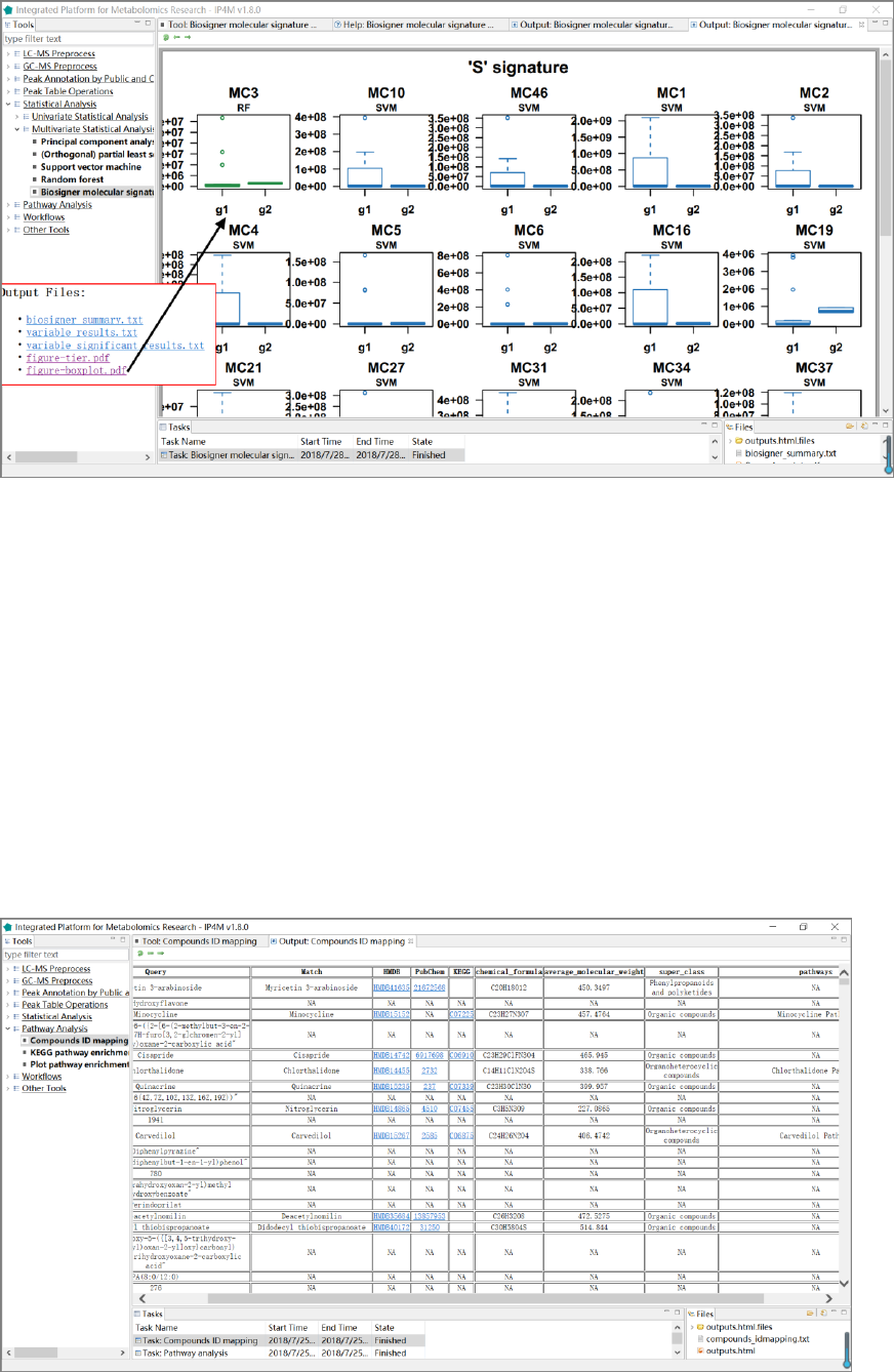
1. 'biosigner_summary.txt', summary information about biosigner algorithm.

2. 'biosigner_variable_results.txt', ranked feature results by biosigner algorithm.

3. 'biosigner_variable_significant_results.txt', significant feature results.

4. ' biosigner_figure-tier.pdf ', displays classifier tiers from selected features.

5. ' biosigner_figure-boxplot.pdf ', individual boxplots from selected features.

Parameter:

1. bootstraps for resampling: The number of bootstraps is set to 5 to speed up computations

when generating this vignette; we however recommend to keep the default 50 value for

analyzing (otherwise signatures may be less stable).

2. pvalN: To speed up the selection, only variables which significantly improve the model up to

two times this threshold (to take into account potential fluctuations) are computed.

3. Selection tiers: Tiers from S, A, up to E by decreasing relevance. The (S) tier corresponds to

the final signature, i.e. features which passed through all the backward selection steps. In

contrast, features from the other tiers were discarded during the last (A) or previous (B to E)

selection rounds. Note that tierMaxC = „A‟ argument in the print and plot methods can be

used to view the features from the larger S+A signatures (especially when no S features have

IP4M V1.0

been found, or when the performance of the S model is much lower than the S+A model).

Note:

1. Group number must be 2 in the sample group file.

2. Group names of characters or string are preferred. Numbers are also supported but not

recommended.

3. The algorithm returns the tier of each feature for the selected classifier (s): tier S corresponds

to the final signature, i.e., features which have been found significant in all the selection steps;

features with tier A have been found significant in all but the last selection, and so on for tier

B to D. Tier E regroup all previous round of selection.

Reference:

[1] Rinaudo P, Boudah S, Junot C, et al. biosigner: A New Method for the Discovery of Significant

Molecular Signatures from Omics Data[J]. Frontiers in Molecular Biosciences, 2016, 3.

Results and visualization:

Fig.18 The resulting files and the potential biomarker (signatures) plot of biosigner

IP4M V1.0

Fig.19 The resulting files and the boxplot of „S‟ signatures by biosigner.

3.5 Pathway Analysis

Tool: Compounds ID mapping

The tool takes a one-column compound list file as input and performs libraries (HMDB,

PubChem, KEGG, etc.) IDs and basic information searching. This is a wrapper of the popular R

package metaboAnalystR (https://github.com/xialab/MetaboAnalystR).

Results and visualization:

Fig.20 The resulting file of compound IDs annotation.

IP4M V1.0

Tool: Pathway analysis on compounds ID mapping results

KEGG (Kyoto Encyclopedia of Genes and Genomes) is a database resource that integrates

genomic, chemical and systemic functional information. Gene catalogs from completely

sequenced genomes are linked to higher-level systemic functions of the cell, the organism, and the

ecosystem. This tool is a wrapper of the „metabolic pathway analysis‟ modules of the popular

MetaboAnalyst platform.

The tool takes a compounds annotation file as input and performs pathway analysis based on

information from KEGG.

Parameter:

1. pathway library: 21 different species libraries have been provided, including Human, Mouse,

Rat, Cow, Chicken, Zebrafish, Arabidopsis thaliana, Rice, Drosophila, Malaria, Budding

yeast, E.coli., etc., with a total of 1600 pathways.

2. representation analysis algorithm:

hypergeometric test: In statistics, the hypergeometric test uses the hypergeometric

distribution to calculate the statistical significance of having drawn a specific {\displaystyle k}

k successes (out of {\displaystyle n} n total draws) from the aforementioned population. The

test is often used to identify which subpopulations are over- or under-represented in a sample.

Fisher's exact test: It is a statistical significance test used in the analysis of contingency tables.

The test is useful for categorical data that result from classifying objects in two different

ways; it is used to examine the significance of the association (contingency) between the two

kinds of classification.

3. Specify pathway topology analysis algorithm:

The module provides two popular topological measures found on the left-panel to provide

users greater insight into their networks.

Out-degree centrality: It refers to the number of links a node has to other nodes.

Relative betweenness centrality: It represents the degree of centrality a node has in a network

by measuring the number of shortest paths that pass through that node.

Nodes with high scores in both measures are more likely to be important hubs.

Reference:

[1] Xia J, Wishart D S. Web-based inference of biological patterns, functions and pathways from

metabolomic data using MetaboAnalyst[J]. Nature Protocols, 2011, 6(6):743-760.

[2] Chong, J., et al. (2018) MetaboAnalyst 4.0: towards more transparent and integrative

metabolomics analysis. Nucleic acids research, 46, W486-w494.

http://www.metaboanalyst.ca.

IP4M V1.0

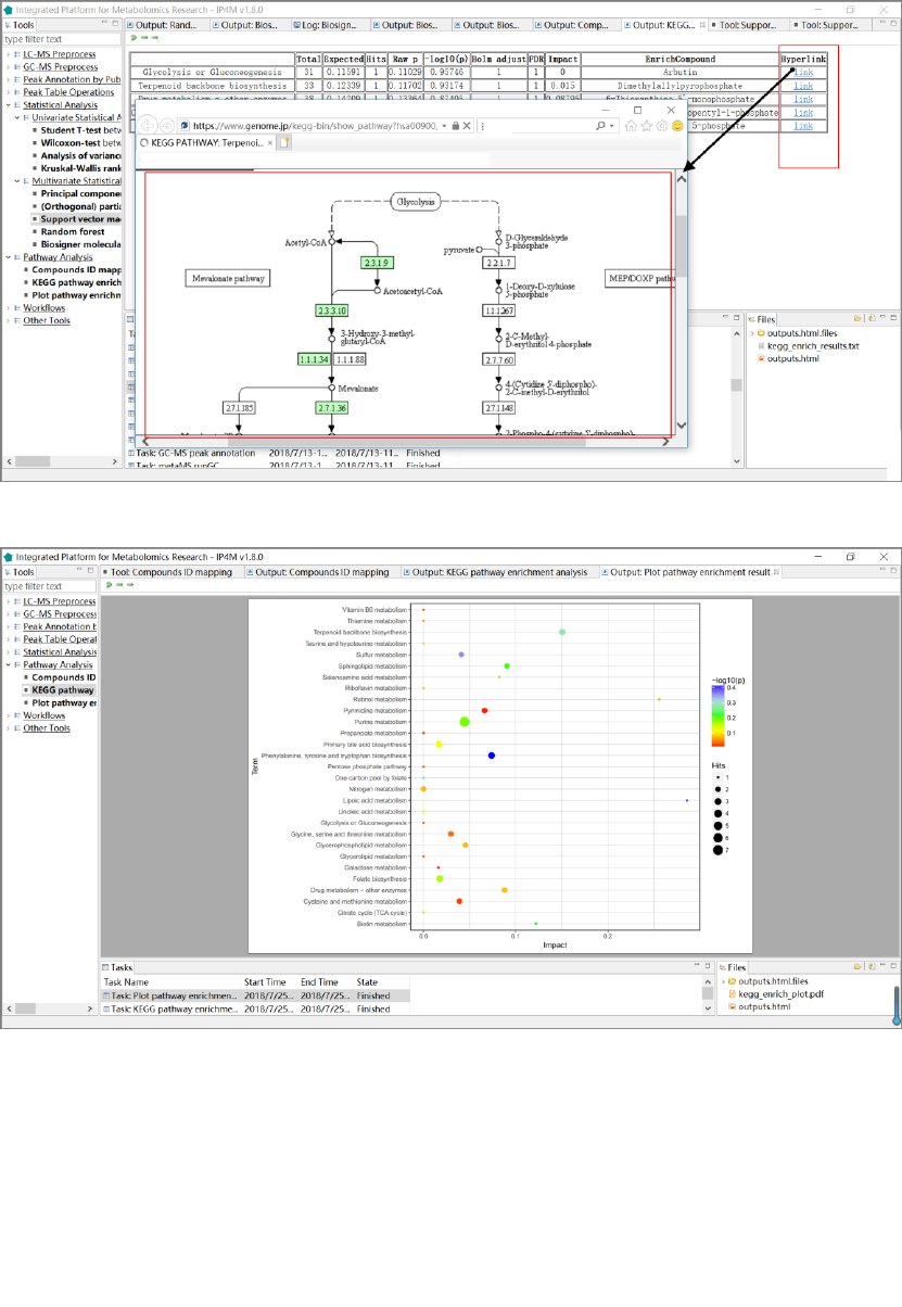
Results and visualization:

Fig.21 The results of pathway analysis with detailed information and hyperlink of the pathways.

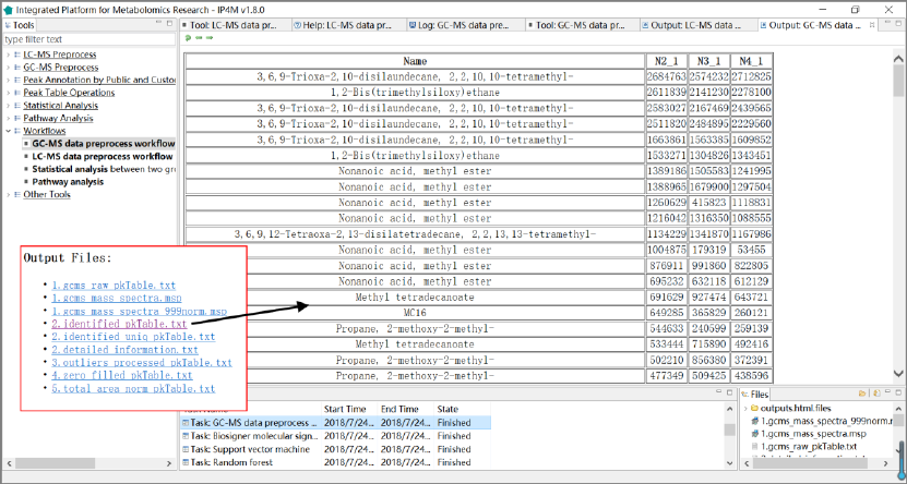
Fig.22 The pathway analysis plot of the first 30 compounds

Tool: Enrichment analysis on compounds ID mapping

results

The tool takes a one-column compound list file and performs metabolite set enrichment

analysis for human and mammalian species. The analysis is based on eight metabolite set libraries

containing ~7000 groups of biologically meaningful metabolite sets collected primarily from

human studies. This tool is a wrapper of the „enrichment analysis‟ modules of the popular

IP4M V1.0

MetaboAnalyst platform.

Parameter:

metabolite set library: Eight different metabolite set libraries have been provided, containing

~6300 groups of biologically meaningful metabolite sets collected primarily from human

studies. Pathway-associated metabolite set library contains 99 metabolite sets based on

normal metabolic pathways. Diseased-associated metabolite set library contains 344

metabolite sets reported in human blood. Disease-associated metabolite set library contains

384 metabolite sets reported in human urine. Disease-associated metabolite set (CSF) library

contains 166 metabolite sets reported in human cerebral spinal fluid (CSF). SNP-associated

metabolite set library contains 4598 metabolite sets based on their associations with detected

single nucleotide polymorphisms (SNPs) loci. Predicted metabolite set library contains 912

metabolic sets that are predicted to be changed in the case of dysfunctional enzymes using

genome-scale network model of human metabolism. Location-based metabolite set library

contains 73 metabolite sets based on organ, tissue and subcellular localizations.

Drug-pathway-associated metabolite set library contains 461 metabolite sets based on drug

pathway.

Reference:

[1] Xia J, Wishart D S. Web-based inference of biological patterns, functions and pathways from

metabolomic data using MetaboAnalyst[J]. Nature Protocols, 2011, 6(6):743-760.

[2] Chong, J., et al. (2018) MetaboAnalyst 4.0: towards more transparent and integrative

metabolomics analysis. Nucleic acids research, 46, W486-w494.

http://www.metaboanalyst.ca.

IP4M V1.0

3.6 Workflows

3.6.1 GC-MS data preprocessing workflow: from raw data to

peak table

This workflow takes multiple GC-MS raw data files in netCDF or mzXML format as inputs

and outputs a peak table. It performs GC-MS data preprocessing and peak table operation,

including mainly peak detection, spectrum aligning, metabolites annotation and peak table

pretreatment.

Input files:

Multiple GC-MS raw data files in netCDF or mzXML format.

Output files:

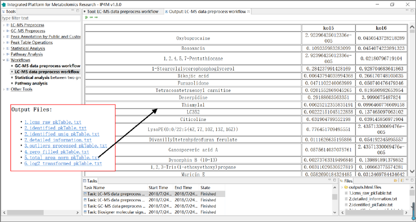
'gcms_raw_pkTable.txt', raw peak table is generated with one line per "compound" and one

column per sample.

'gcms_mass_spectra.msp', Corresponding pseudospectrum(compound) mass spectrum

information in MSP format, the identifier is same in peak table file.

'gcms_mass_spectra_999norm.msp', intensities normalized mass spectrum information in

MSP format, intensities sum=999.

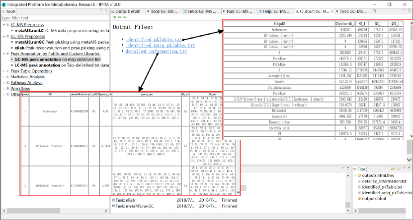
'identified_pkTable.txt', identified peak table file in Tab-delimited text format.

'identified_uniq_pkTable.txt', identified unique peak table file in Tab-delimited text format.

When row names are duplication, the row with the maximum intensity will be retained.

'detailed_information.txt', detailed information about query and database relationship in

library searching.

'zero_filled_pkTable.txt', zero filled peak table file in Tab-delimited text format.

'total_area_norm_pkTable.txt', total area normalized peak table file in Tab-delimited text

format.

'log2_transformed_pkTable.txt', log2 transformed peak table file in Tab-delimited text format.

Results and visualization:

IP4M V1.0

Fig.23 The outputted files and the identified peak table of GC-MS data processing workflow

3.6.2 LC-MS data preprocessing workflow: from raw data to

peak table

This workflow takes multiple LC-MS raw data files in netCDF or mzXML format as inputs

and outputs peak table. It performs LC-MS data preprocessing and peak table operation, including

peak detection, spectrum aligning, metabolites annotation and peak table pretreatment.

Input files:

Multiple GC-MS raw data files in netCDF or mzXML format.

Output files:

'lcms_raw_pkTable.txt', a peak table is generated with one line per "compound" and one

column per sample.

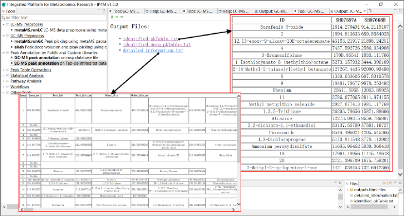
'identified_pkTable.txt', identified peak table file in Tab-delimited text format.

'identified_uniq_pkTable.txt', identified unique peak table file in Tab-delimited text format.

When row names are duplication, the row with the maximum intensity will be retained.

'detailed_information.txt', detailed information about query and database relationship in

library searching.

'zero_filled_pkTable.txt', zero filled peak table file in Tab-delimited text format.

'total_area_norm_pkTable.txt', total area normalized peak table file in Tab-delimited text

format.

'log2_transformed_pkTable.txt', log2 transformed peak table file in Tab-delimited text format.

IP4M V1.0

Results and visualization:

Fig.24 The outputted files and the total area normalized peak table of LC-MS data

processing workflow

3.6.3 Statistical analysis based on peak table

This workflow takes a peak table file and a group design file as inputs. It performs all

univariate and multivariate statistical analysis as user selected (between two groups).

Input files:

1. Peak table file in Tab-delimited text format, with the first column as the compound identifier

and the others as samples.

2. Group design file in Tab-delimited text format with two columns (samplename

groupname).

Output files:

'pkTable_summary.txt', basic statistics summary information on columns (sample data).

't_test_results.txt', t-test results with p value, log2FC, and q value.

't_test_significant_results.txt', significant t-test results.

'wilcox_test_results.txt', Wilcoxon-test results with p value, log2FC, and q value.

'wilcox _test_significant_results.txt', significant Wilcoxon-test results.

'aov_results.txt', analysis of variance model results with p-value and q value.

'aov_significant_results.txt', significant analysis of variance model results.

IP4M V1.0

'kw_test_results.txt ', Kruskal-Wallis rank sum test results with p-value and q value.

'kw_test_significant_results.txt ', significant Kruskal-Wallis rank sum test results.

'pca_scores.txt', PCs (scores) matrix.

'pca_importance.txt', the importance of PCs.

'pca_rotation.txt', the matrix of variable loadings (i.e., a matrix whose columns contain the

eigenvectors).

'pca_plot.pdf', PCA plot using PCs score values, the default is PC1 and PC2.

'oplsda_variable_results.txt', feature ranked results that are sorted by VIP.

'oplsda_variable_significant_results.txt', significant feature results.

'oplsda_samples_results.txt', OPLS-DA model sample prediction results using inputted data.

'oplsda_prediction_summary.txt', prediction summary.

'oplsda_figure.pdf', OPLS-DA Plot.

'svm_summary.txt', summary information about SVM.

'svm_variable_results.txt', feature ranked results that are sorted by SVM-RFE.

' svm_samples_results.txt', SVM model sample prediction results using inputted data.

'svm_prediction_summary.txt', prediction summary of SVM.

'support_vectors.txt', support vectors in the model of SVM.

'svm_plot.pdf', SVM plot.

'rf_summary.txt ', summary information about random forest model.

'rf_variable_results.txt ', feature ranked results that are sorted by mean decrease in Gini index

using RF.

'rf_samples_results.txt ', random forest model sample prediction results using inputted data.

'rf_prediction_summary.txt', prediction summary of RF.

'rf_error_rates_plot.pdf ', error rates plot in the RF model.

'rf_predictions_margin_plot.pdf ', predictions _margin plot of RF.

'biosigner_summary.txt', summary information about biosigner algorithm.

'biosigner_variable_results.txt', feature ranked results by biosigner algorithm.

'biosigner_variable_significant_results.txt', significant feature results by biosigner algorithm.

' biosigner_figure-tier.pdf ', displaying classifier tiers from selected features by biosigner

algorithm.

' biosigner_figure-boxplot.pdf ', individual boxplots from selected features by biosigner

algorithm.

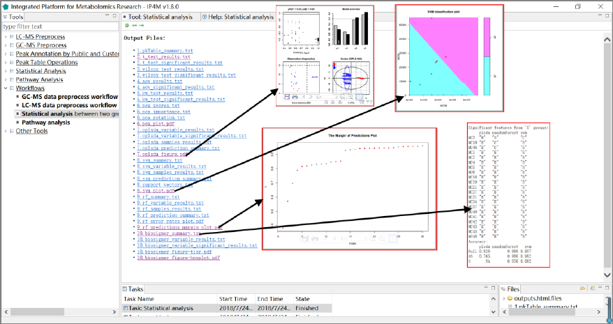
Results and visualization:

IP4M V1.0

Fig.25 The outputted files and demos (opls-da plot, SVM plot, the margin of prediction plot by

RF, and the biosigner summary) of statistical analysis workflow

3.6.4 Pathway and enrichment analysis

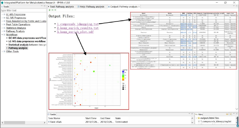
The tool takes a one-column compound list file as input and performs pathway analysis and

enrichment analysis, including compounds ID mapping, KEGG pathway, and enrichment analysis.

KEGG pathway libraries with ~1600 pathways are the knowledgebase for this tool which covers

21 species (human, mouse, rat, cow, chicken, zebrafish, arabidopsis thaliana, drosophila, malaria,

etc.). The enrichment analysis performs metabolite set enrichment analysis for human and

mammalian species. The analysis is based on 8 libraries containing ~6300 groups of biologically

meaningful metabolite sets collected primarily from human studies.

Input files:

A one-column compound list file in text format.

Output files:

'compounds_idmapping.txt ', compounds annotation result.

' pathway_results.txt ', KEGG pathway enrichment analysis result.

'pathway_results_plot.txt ', KEGG pathway enrichment result visualization diagram.

' enrichment_results.txt ', enrichment analysis result.

' enrichment_plot.pdf', enrichment result visualization diagram.

IP4M V1.0

Results and visualization:

Fig.26 The outputted files and visualization of pathway and enrichment analysis workflow

IP4M V1.0

3.7 Other Tools

3.7.1 Merge LECO CSV files

Tool: Merge LECO CSV files on peak table

The tool takes multiple .CSV files as inputs (outputted from the Chromatof software of

LECO., USA, reference mode) and merges them to generate a combined peak table file, according

to „R.T.‟, „Quant mass‟, and „Area‟. The .CSV files from BT, 4D, and HRT GC-TOF/MS

instruments (LECO, USA) are supported.

Parameter:

Merge method:

Same mass and RT difference within the cutoff: if same quant mass and rt difference within

the cutoff are met, the corresponding compounds of multiple samples is considered as the same

one. The “area” values of the same compound will be merged and the name of the compound

outputted is the one with the highest frequency of occurrence. For same frequency names, the one

with the maximum average strength is taken. If more than one variable (in the same sample) meet

the criteria, the largest “area” will be taken.

Same mass and one by one according to RT order: all the inputted files will be sorted by

“Quant mass” and “R.T.”, and then merged directly one by one. This option is simple but

effective.

Note:

This tool is strict to file format. Make sure these columns exist: the retention time column

with the name starts with „R.T.‟, the peak area column named „Area‟, the quant mass column

named „Quant Masses‟, and the compound name column named „Name‟. Other columns are also

permitted but will not be involved in process. The row number of all the inputted files should be

the same.

3.7.2 GLM on two groups

Tool: GLM on two groups

This tool is the wrapper of the R „glm‟ function and aims at peak ranking by coefficients of

linear regression. Group information is given by a group design file (Tab-delimited text file). The

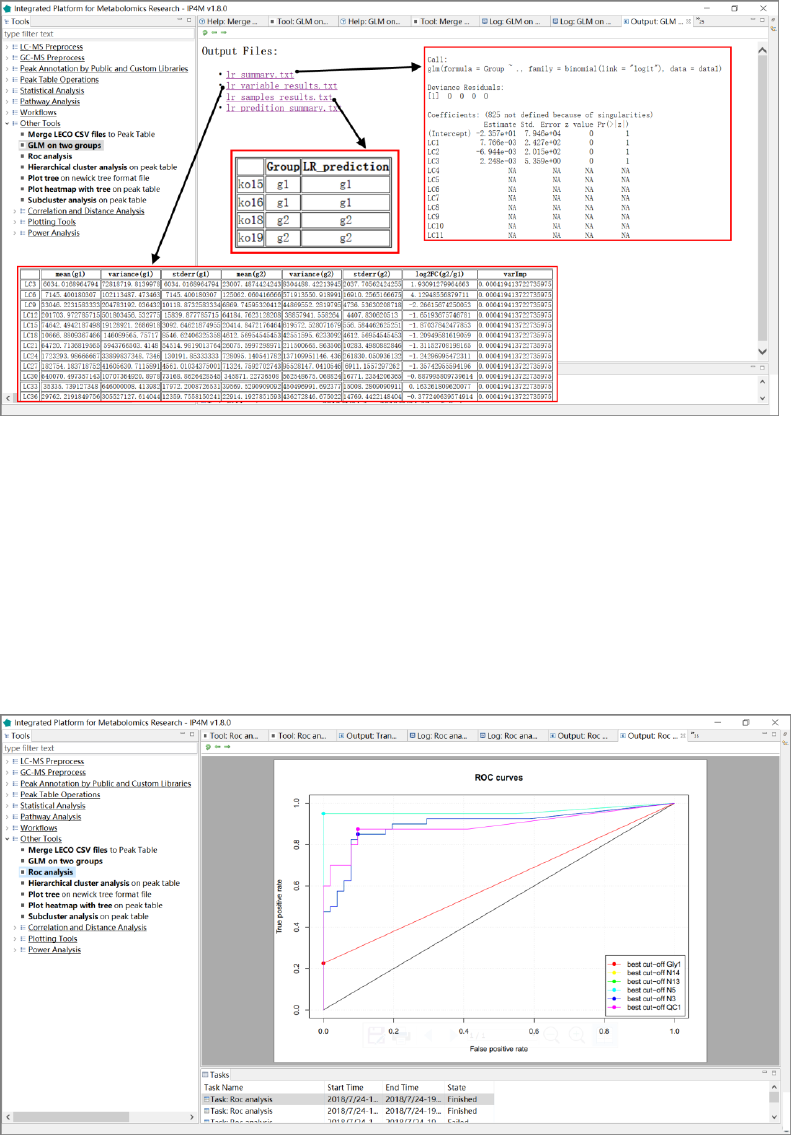
IP4M V1.0

tool is only available for binary classification and the number of groups should be 2.

Results and visualization:

Fig.28 The outputted files and corresponding information of GLM analysis

3.7.3 ROC analysis

Tool: ROC analysis

This tool takes a peak table file as input and computes ROC curves for every peak.

Fig.29 ROC curves of six peaks

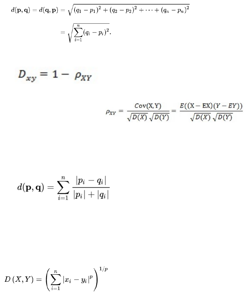
IP4M V1.0

3.7.4 Hierarchical cluster analysis

Tool: Hierarchical cluster analysis on peak table

This tool takes a peak table file as input and performs hierarchical cluster analysis on it.

Parameter:

Distance calculate method:

1. Euclidean:

The Euclidean distance between points p and q is the length of the line segment connecting

them.

2. Correlation distance:

Correlation coefficient:

3. Canberra distance：sum (|p_i - q_i| / |p_i + q_i|). Terms with zero numerator and

denominator are omitted from the sum and treated as if the values were missing. This is

intended for non-negative values (e.g., counts): take the absolute value of the denominator.

4. Binary distance: The vectors are regarded as binary bits, so non-zero elements are „on‟ and

zero elements are „off‟. The distance is the proportion of bits in which the only one is on

amongst those in which at least one is on.

5. Minkowski distance: The p norm, the pth root of the sum of the pth powers of the differences

between the components.

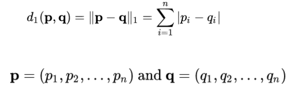
IP4M V1.0

6. Manhattan: Absolute distance between the two vectors.

where (p, q) are vectors.

7. maximum distance：Maximum distance between two components of x and y (supremum

norm).

Cluster methods:

1. ward: Ward's minimum variance method aims at finding compact, spherical clusters.

2. complete: The complete linkage method finds similar clusters.

3. single: The single linkage method (which is closely related to the minimal spanning tree)

adopts a „friends of friends‟ clustering strategy.

The other methods can be regarded as aiming for clusters with characteristics somewhere

between the single and complete link methods.

4. centroid: Method "centroid" is typically meant to be used with squared Euclidean distances.

5. average: The average distance method measures the average distance between each pair of

observations

6. mcquitty: It finds the similar cluster.

7. median: Median distance method.

Results and visualization:

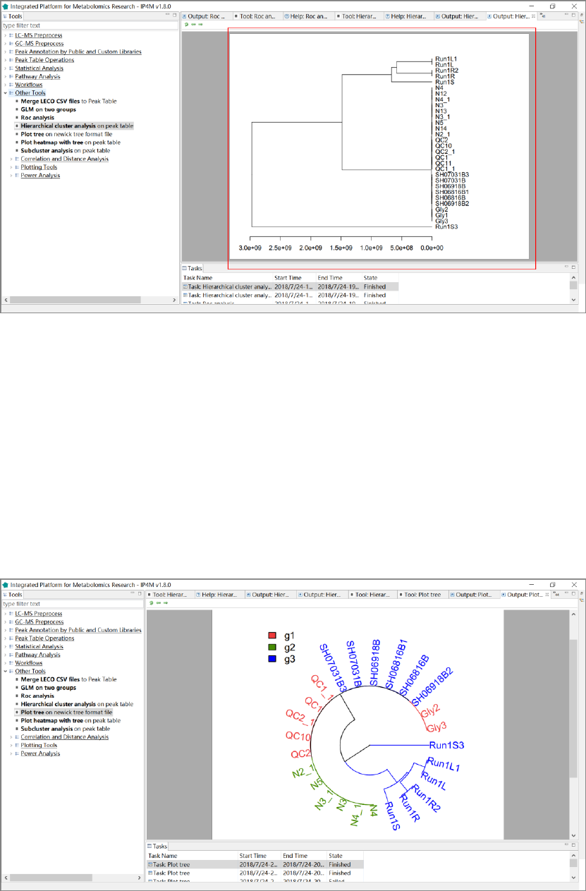
IP4M V1.0

Fig.30 The hierarchical cluster tree plot.

3.7.5 Plot tree

Tool: Plot tree on Newick tree format file

This tool takes a standard Newick format tree file as input and plots hierarchical tree by

phylogram, fan, or cladogram mode.

Fig.31 The hierarchical tree plot by fan mode.

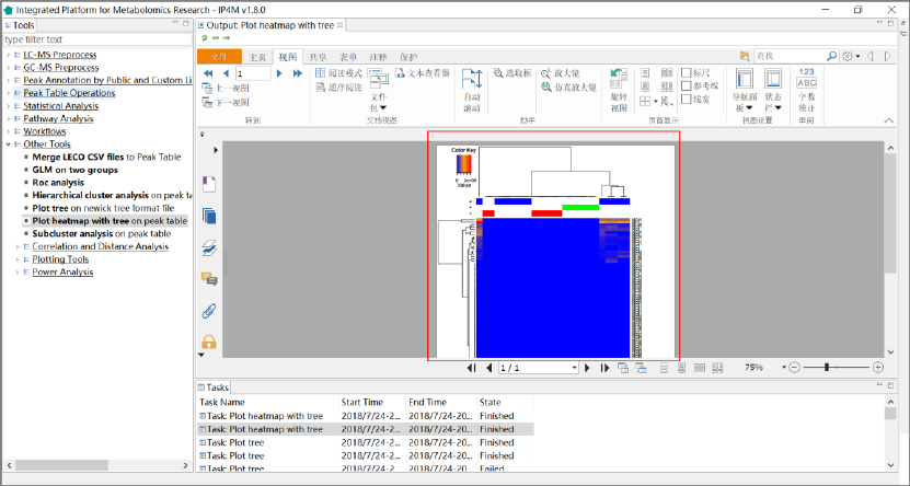
IP4M V1.0

3.7.6 Plot heatmap with tree

Tool: Plot heatmap with tree on peak table

This tool takes a peak table file as input and plots heatmap with clusters on it.

Results and visualization:

Fig.32 The heatmap with tree in pdf edit box.

3.7.7 Sub-cluster expression analysis

Tool: Sub-cluster expression analysis on peak table

This tool takes a peak table file as input and performs cluster analysis on it. The metabolites

are classified into several groups (clusters) according to their distance or variation similarity.

Parameter:

Distance calculate method:

1. Euclidean:

The Euclidean distance between points p and q is the length of the line segment connecting

them.

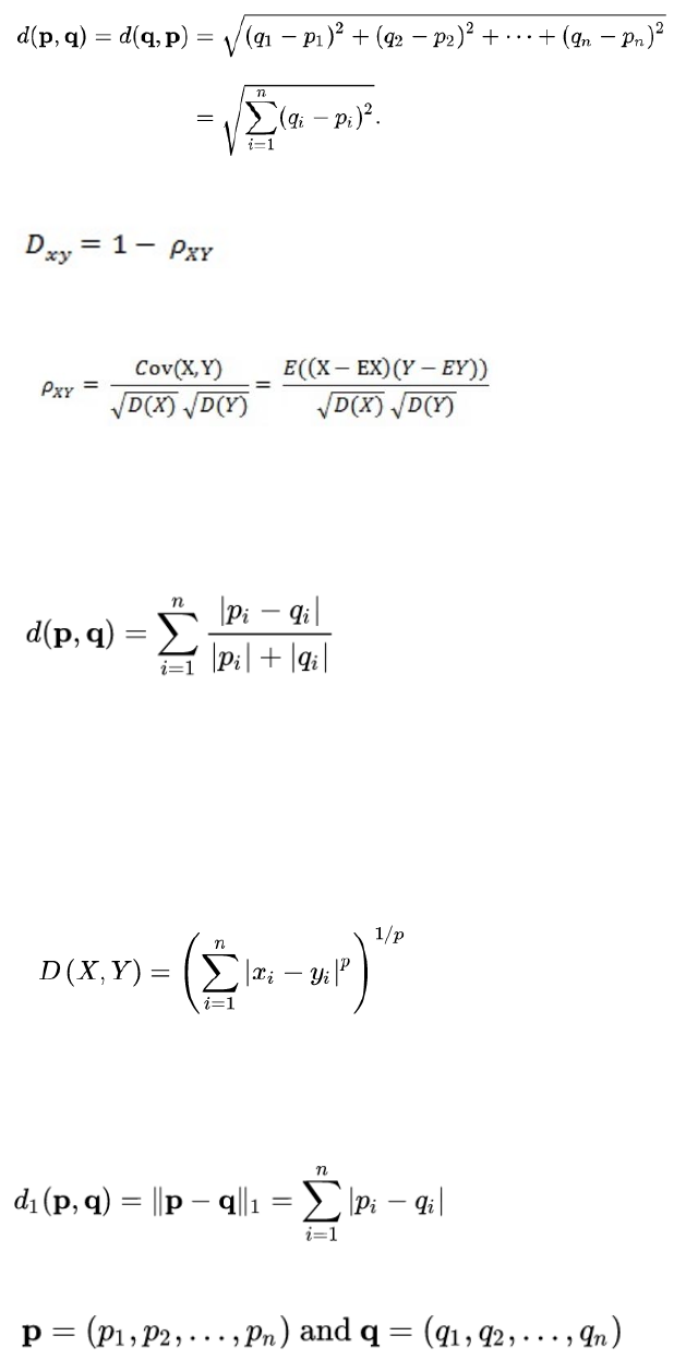
IP4M V1.0

2. Correlation distance:

Correlation coefficient:

3. Canberra distance: sum (|p_i - q_i| / |p_i + q_i|). Terms with zero numerator and

denominator are omitted from the sum and treated as if the values were missing. This is

intended for non-negative values (e.g., counts): take the absolute value of the denominator.

4. Binary distance: The vectors are regarded as binary bits, so non-zero elements are „on‟ and

zero elements are „off‟. The distance is the proportion of bits in which the only one is on

amongst those in which at least one is on.

5. Minkowski distance: The p norm, the pth root of the sum of the pth powers of the differences

between the components.

6. Manhattan: Absolute distance between the two vectors.

where (p, q) are vectors.

7. maximum distance：Maximum distance between two components of x and y (supreme norm).

Cluster methods:

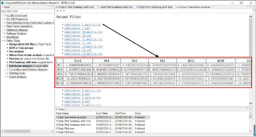
IP4M V1.0

1. ward: Ward's minimum variance method aims at finding compact, spherical clusters.

2. complete: The complete linkage method finds similar clusters.

3. single: The single linkage method (which is closely related to the minimal spanning tree)

adopts a „friends of friends‟ clustering strategy.

The other methods can be regarded as aiming for clusters with characteristics somewhere

between the single and complete link methods.

4. centroid: Method "centroid" is typically meant to be used with squared Euclidean distances.

5. average: The average distance method measures the average distance between each pair of

observations

6. mcquitty: It finds the similar cluster.

7. median: Median distance method.

Results and visualization:

Fig.33 Th outputted files and one matrix of sub-cluster analysis.

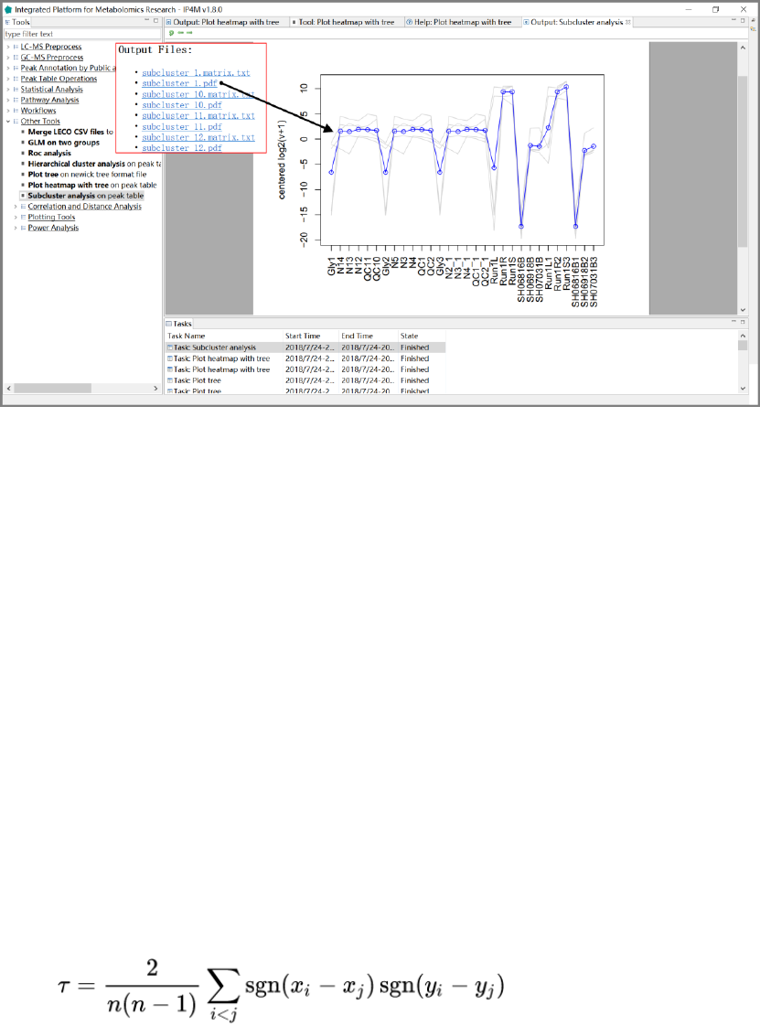
IP4M V1.0

Fig.34 The line chart of sub-cluster1.

3.7.8 Correlation and distance analysis

Tool: Create sample correlation matrix and make heatmap plot

This tool takes a peak table file as input and performs correlation analysis on it.

Parameter:

Correlation methods:

1. Kendall rank correlation:

The Kendall rank correlation coefficient, commonly referred to as Kendall's tau coefficient

(after the Greek letter τ), is a statistic used to measure the ordinal association between two

measured quantities. A tau test is a non-parametric hypothesis test for statistical dependence

based on the tau coefficient.

2. Pearson correlation:

the Pearson correlation coefficient, also referred to as Pearson's r is a measure of the linear

correlation between two variables X and Y. It has a value between +1 and −1, where 1 is a

total positive linear correlation, 0 is no linear correlation, and −1 is a total negative linear

correlation.

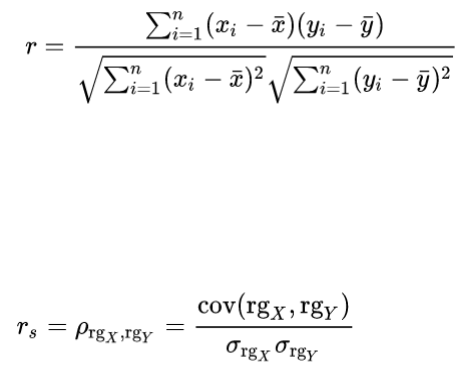
IP4M V1.0

3. Spearman correlation:

Spearman's rank correlation coefficient or Spearman's rho is a nonparametric measure of rank

correlation. It assesses how well the relationship between two variables can be described

using a monotonic function.

Cluster methods:

1. ward: Ward's minimum variance method aims at finding compact, spherical clusters.

2. complete: The complete linkage method finds similar clusters.

3. single: The single linkage method (which is closely related to the minimal spanning tree)

adopts a „friends of friends‟ clustering strategy.

The other methods can be regarded as aiming for clusters with characteristics somewhere

between the single and complete link methods.

4. centroid: Method "centroid" is typically meant to be used with squared Euclidean distances.

5. average: The average distance method measures the average distance between each pair of

observations

6. mcquitty: It finds the similar cluster.

7. median: Median distance method.

Results and visualization:

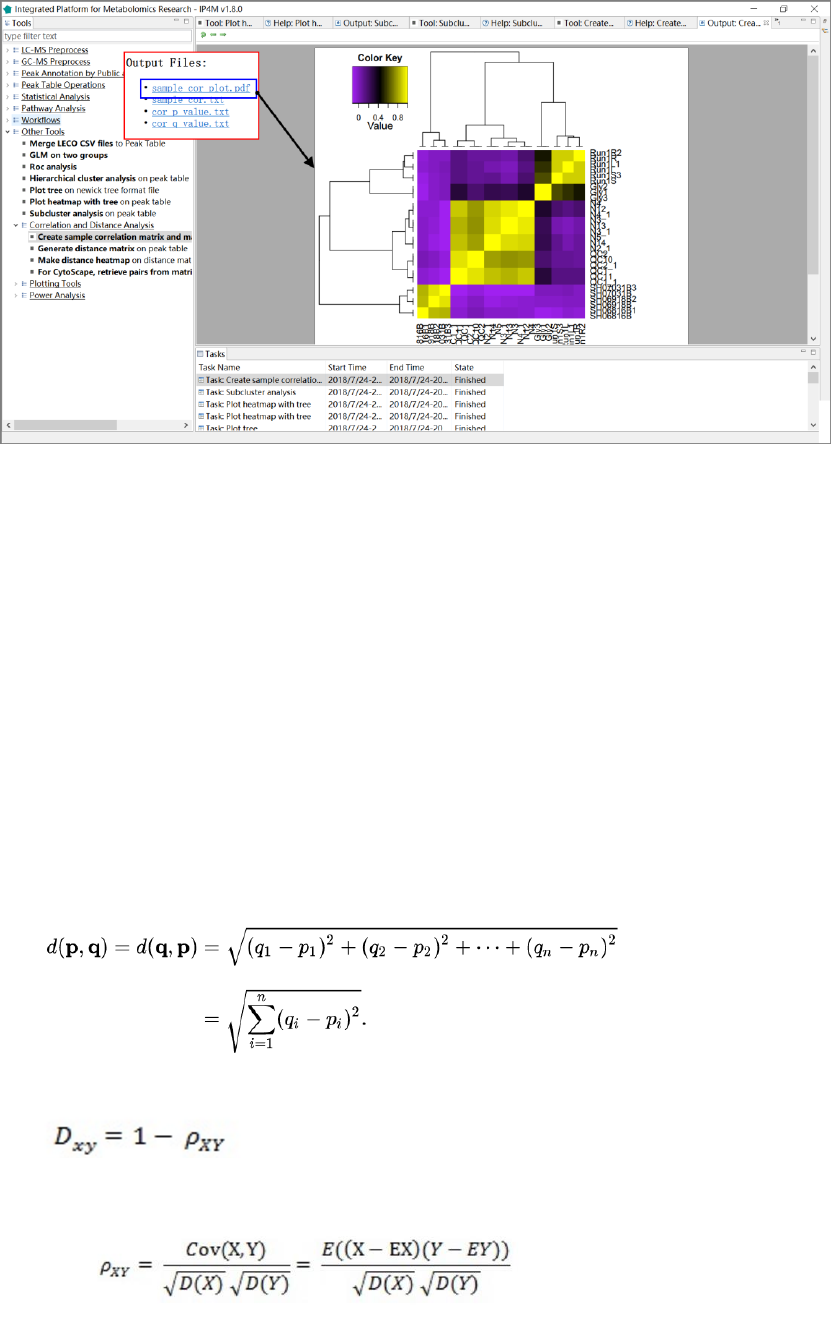
IP4M V1.0

Fig.35 The heatmap of correlation analysis

Tool: Generate distance matrix on peak table

This tool takes a peak table file as input and generates the distance matrix.

Parameter:

Distance calculate method:

1. Euclidean:

The Euclidean distance between points p and q is the length of the line segment connecting

them.

2. Correlation distance:

Correlation coefficient:

3. Canberra distance: sum (|p_i - q_i| / |p_i + q_i|). Terms with zero numerator and

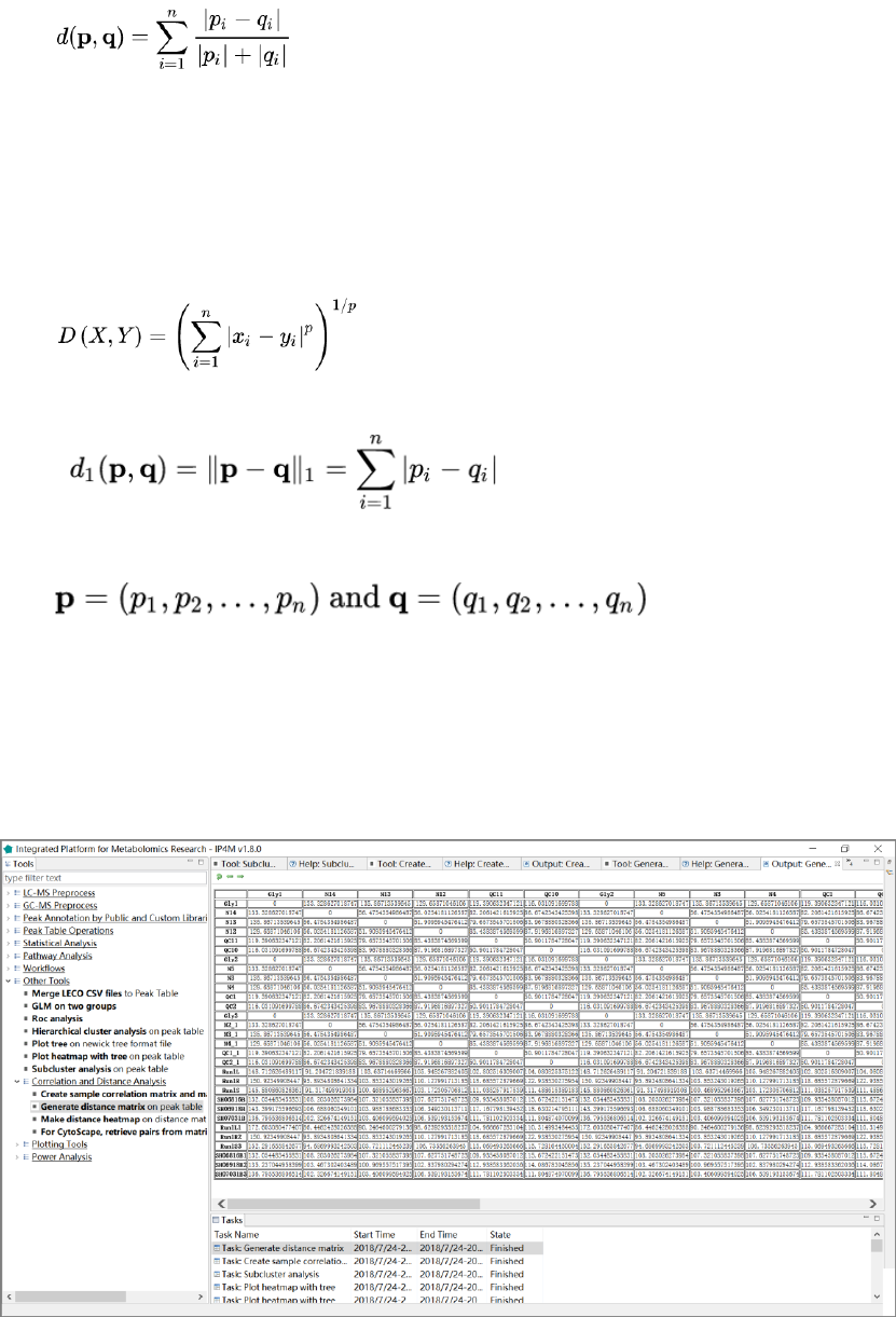
IP4M V1.0

denominator are omitted from the sum and treated as if the values were missing. This is

intended for non-negative values (e.g., counts): take the absolute value of the denominator.

4. Binary distance: The vectors are regarded as binary bits, so non-zero elements are „on‟ and

zero elements are „off‟. The distance is the proportion of bits in which the only one is on

amongst those in which at least one is on.

5. Minkowski distance: The p norm, the pth root of the sum of the pth powers of the differences

between the components.

6. Manhattan: Absolute distance between the two vectors.

where (p, q) are vectors.

7. maximum distance：Maximum distance between two components of x and y (supremum

norm).

Results and visualization:

Fig.36 The distance matrix.

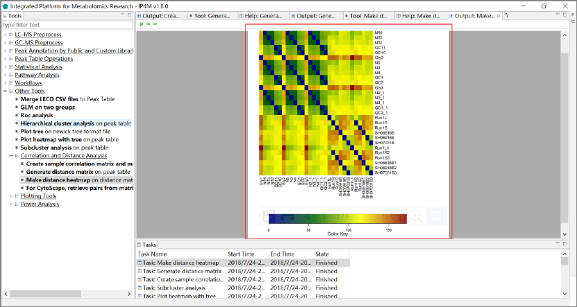
IP4M V1.0

Tool: Make distance heatmap on distance matrix

This tool takes a distance matrix as input and makes a heat map plot based on it.

Results and visualization:

Fig.37 The distance heatmap

Tool: For Cytoscape: retrieve pairs from matrix according to specific

criterion

This tool retrieves pairs from matrix according to a specific criterion. The result can be

imported directly into Cytoscape for network construction.

Results and visualization:

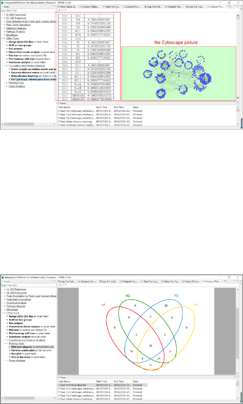
IP4M V1.0

Fig.38 The retrieved pairs for Cytoscape, and the outputted network of Cytoscape.

3.7.9 Plotting tools

Tool: Plot Venn diagram on metabolites lists

With this tool, you can calculate the intersection(s) of the list of elements. It will generate a

Venn plot and textual output indicating which elements are exist in each intersection or are unique

to a certain list/group.

Results and visualization:

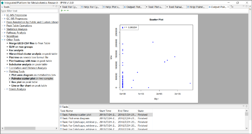
IP4M V1.0

Fig.39 The Venn plot of four groups.

Tool: Pairwise scatter plot on two samples

This tool is used for plotting pairwise scatter figures in batch mode. All the scatter plots will

be saved in one pdf file.

Results and visualization:

Fig.40 The pairwise scatter plot on two samples.

Tool: Box plot on peak table

This tool is used for plotting box figures in batch mode. All the box plots will be saved in one

pdf file.

Results and visualization:

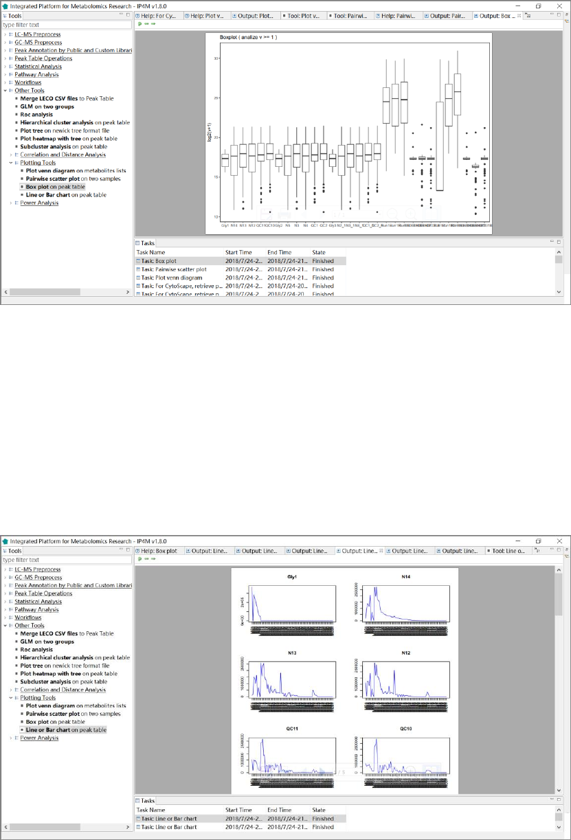
IP4M V1.0

Fig.41 The box plot of samples (one box per sample)

Tool: Line chart on peak table

This tool is used for plotting line or bar charts in batch mode. All the plots will be saved in

one pdf file.

Results and visualization:

Fig.42 The line charts of samples.

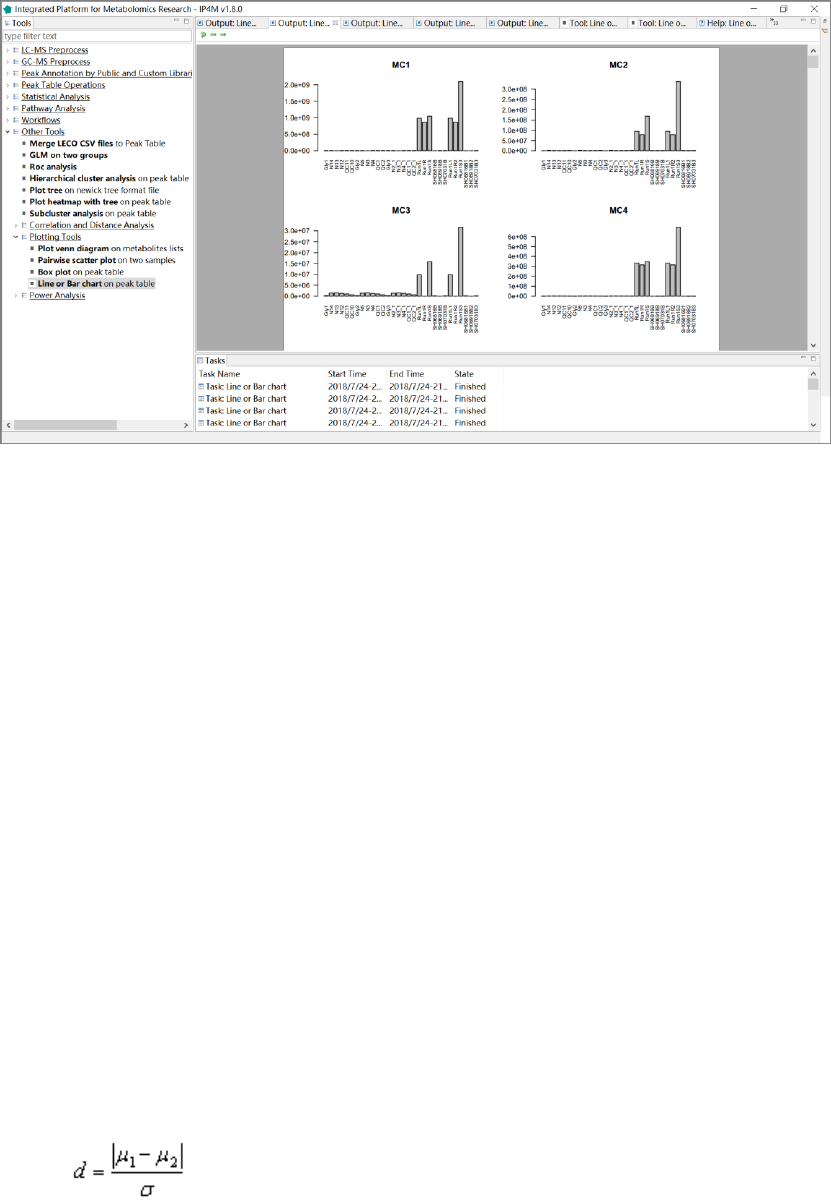
IP4M V1.0

Fig.43 The bar charts of samples.

3.7.10 Sample size and power analysis

Sample size and power analysis is helpful to estimate a reasonable sample size before

experiments or to evaluate the power of analysis results after experiments.

1) Tool: Pwr.t.test power calculation for t-test (one, two, and paired

samples)

For t-tests, the following functions are used:

pwr.t.test(n = , d = , sig.level = , power = , type = c("two.sample", "one.sample", "paired"))

where n is the sample size, d is the effect size, and type indicates a two-sample t-test, one-sample

t-test or paired t-test. If you have unequal sample sizes, use

pwr.t2n.test(n1 =, n2=, d =, sig.level =, power = )

where n1 and n2 are the sample sizes.

For t-tests, the effect size is assessed as

μ1: mean of group1

μ2: mean of group1

σ2: common error variance

Cohen suggests that d values of 0.2, 0.5, and 0.8 represent small, medium, and large effect sizes

respectively.

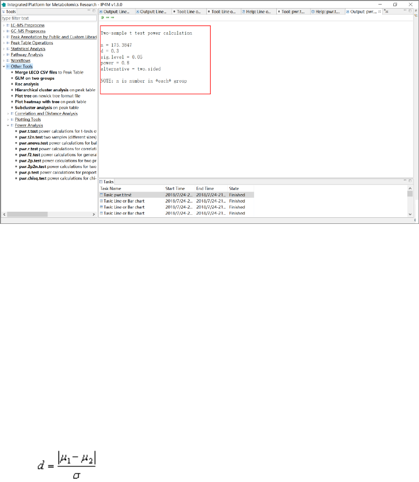
IP4M V1.0

You can specify alternative="two.sided", "less", or "greater" to indicate a two-tailed, or one-tailed

test. A two-tailed test is the default.

Results and visualization:

Fig.44 The results of power analysis when two samples t- test is used.

2) Tool: Pwr.t2n.test power calculation for t-test (different sizes)

For t-tests, the following functions are used:

pwr.t.test(n = , d = , sig.level = , power = , type = c("two.sample", "one.sample", "paired"))

where n is the sample size, d is the effect size, and type indicates a two-sample t-test, one-sample

t-test or paired t-test. If you have unequal sample sizes, use

pwr.t2n.test(n1 = , n2= , d = , sig.level =, power = )

where n1 and n2 are the sample sizes.

For t-tests, the effect size is assessed as

μ1: mean of group1

μ2: mean of group1

σ2: common error variance

IP4M V1.0

3) Tool: Pwr.anova.test power calculation for balanced one way

ANOVA

For a one-way analysis of variance, the following functions are used:pwr.anova.test(k = , n = , f

= , sig.level = , power = )

where k is the number of groups and n is the common sample size in each group.

For a one-way ANOVA, effect size is measured by f where

pi=ni / N

ni=number of observations in group i

N=total number of observations

μi= mean of group i

μ=grand mean

σ2= error variance within groups

Cohen suggests that f values of 0.1, 0.25, and 0.4 represent small, medium, and large

effect sizes respectively.

4) Tool: Pwr.r.test power calculation for correlation test

For correlation coefficients, the following functions are used:

pwr.r.test(n = , r = , sig.level = , power = )

where n is the sample size and r is the correlation. We use the population correlation coefficient as

the effect size measure. Cohen suggests that r values of 0.1, 0.3, and 0.5 represent small, medium,

and large effect sizes respectively.

5) Tool: Pwr.f2.test power calculation for general linear model

For linear models (e.g., multiple regression), the following functions are used:

pwr.f2.test(u =, v = , f2 = , sig.level = , power = )

where u and v are the numerator and denominator degrees of freedom. We use f2 as the effect size

measure.

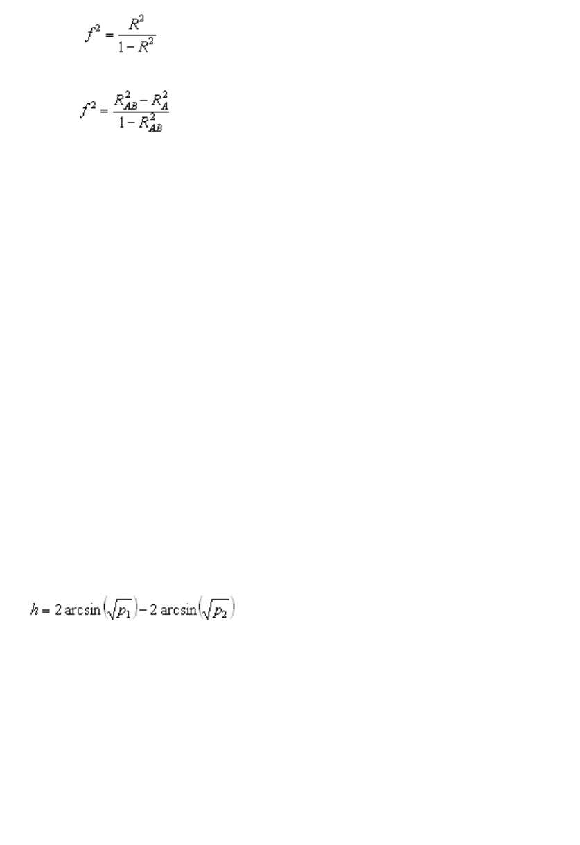
IP4M V1.0

R2 = population squared multiple correlation

R2A = variance accounted for in the population by variable set A

R2AB = variance accounted for in the population by variable set A and B together

The first formula is appropriate when we are evaluating the impact of a set of predictors on an

outcome. The second formula is appropriate when we are evaluating the impact of one set of

predictors above and beyond the second set of predictors (or covariates). Cohen suggests f2 values

of 0.02, 0.15, and 0.35 represent small, medium, and large effect sizes.

6) Tool: Pwr.2p.test power calculation for two proportions (equal n)

When comparing two proportions, the following functions are used:

pwr.2p.test(h = , n = , sig.level =, power = )

where h is the effect size and n is the common sample size in each group.

Cohen suggests that h values of 0.2, 0.5, and 0.8 represent small, medium, and large effect sizes

respectively.

7) Pwr.2p2n.test power calculation for two proportions (unequal n)

When comparing two proportions, the following functions are used:

pwr.2p.test(h = , n = , sig.level =, power = )

For unequal n's

pwr.2p2n.test(h = , n1 = , n2 = , sig.level = , power = )

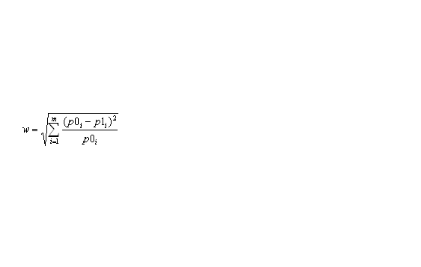
IP4M V1.0

8) Pwr.p.test power calculation for proportions (one sample)

To test a single proportion, the following functions are used:

pwr.p.test (h = , n = , sig.level = power = )

For both two sample and one sample proportion tests, you can specify alternative="two. sided",

"less", or "greater" to indicate a two-tailed, or one-tailed test. A two-tailed test is the default.

9) Pwr.chisq.test power calculation for the chi-square test

For chi-square tests, the following functions are used:pwr.chisq.test(w =, N = , df = , sig.level =,

power = )

where w is the effect size, N is the total sample size, and df is the degrees of freedom. The effect

size w is defined as

p0i = cell probability in an ith cell under H0

p1i = cell probability in an ith cell under H1

Cohen suggests that w values of 0.1, 0.3, and 0.5 represent small, medium, and large effect sizes

respectively.

IP4M.manual

Navigation menu

Versions of this User Manual:

Views

Navigation