ISA User Guide
User Manual:
Open the PDF directly: View PDF ![]() .
.
Page Count: 46
Contents
1 Introduction 3
1.1 The Complex AM–FM Component . . . . . . . . . . . . . . . . . . . . . . . 4
1.2 The Complex AM–FM Model . . . . . . . . . . . . . . . . . . . . . . . . . . 5
1.3 Instantaneous Spectral Analysis . . . . . . . . . . . . . . . . . . . . . . . . . 6
1.3.1 Denition of the Instantaneous Spectrum . . . . . . . . . . . . . . . 7
1.3.2 Visualization of the Instantaneous Spectrum . . . . . . . . . . . . . . 8
1.4 LatentSignalAnalysis .............................. 9
2 Modulation/Demodulation Algorithms 10
2.1 amfmmod.m.................................... 11
2.2 amfmdemod.m .................................. 13
3 Decomposition Algorithms 15
4 Visualization 16
4.1 Argand.m ..................................... 17
4.2 ISA2dPlot.m ................................... 18
4.3 ISA3dPlot.m ................................... 19
4.4 ISA3dPlotPrint.m................................. 21
4.5 STFT2dPlot.m .................................. 23
5 Other Algorithms 24
5.1 derivApprox.m .................................. 25
5.2 intApprox.m.................................... 26
6 Demo Scripts 27
6.1 DEMO_1_SimpleHarmicComponent.m . . . . . . . . . . . . . . . . . . . . . 28
6.2 DEMO_2_SimpleAMComponent.m . . . . . . . . . . . . . . . . . . . . . . . 30
6.3 DEMO_3_SimpleFMComponent.m . . . . . . . . . . . . . . . . . . . . . . . 32
6.4 DEMO_4_AMFMComponent.m......................... 34
6.5 DEMO_5_MultiComponentSignal.m . . . . . . . . . . . . . . . . . . . . . . 36
6.6 FIGURE_ISA2018_SinusoidalAM.m ...................... 38
6.7 FIGURE_ISA2018_SinusoidalFM.m....................... 39
6.8 FIGURE_ISA2018_GaussianAMchirpFMchirp.m . . . . . . . . . . . . . . . 40
6.9 DEMO_intApprox.m............................... 41
6.10 DEMO_derivApprox.m.............................. 43
7 Bibliography 45
1
Preface
ISA Toolbox is a software library for Matlab implementing algorithms related to AM–FM
modeling and the Instantaneous Spectrum. The most important research paper related to
the theoretical foundation for the Instantaneous Spectral Analysis (ISA) is [1]. The ISA
Toolbox has been has been developed for research purposes, and while the reuse of this code
can be seen as good practice, copying other peoples computer code without citing it correctly
may be a plagiarism violation. If you use this code in your research please cite the following
work:
@article{ISA2018_Sandoval,
title = {The Instantaneous Spectrum: A General Framework for
Time-Frequency Analysis},
author = {S.~Sandoval and P.~L.~De~Leon},
journal = {{IEEE Trans.~Signal Process.}},
volume = {66},
year = {2018},
month = {Nov},
pages = {5679-5693}
}
2

Chapter 1
Introduction
Table of Principle Symbols
Symbol Description
ttime instants
Sthe component set, S≜{C0,C1,· · · ,CK−1}
Ckcanonical triplet for the kth AM–FM component, Ck≜(ak(t), ωk(t), ϕk)
ψk(t)the kth AM–FM component, ψk(t)≜ak(t)ej[∫t
−∞ ωk(τ)dτ+ϕk]
sk(t)real part of the kth component, sk(t) = Re{ψk(t)}
σk(t)imaginary part of the kth component, σk(t) = Im{ψk(t)}
ak(t)instantaneous amplitude (IA) of the kth component, ak(t) = ±abs{ψk(t)}
θk(t)phase, or instantaneous angle of the kth component, θk(t) = arg{ψk(t)}
ωk(t)instantaneous frequency (IF) of the kth component, ωk(t) = d
dtθk(t)
mk(t)frequency modulation (FM) message of the kth component, mk(t) = ωk(t)−ϖk
Mk(t)phase modulation (PM) message of the kth component, Mk(t) = t
−∞ mk(τ)dτ
ϕkphase reference of the kth component, 0
−∞ mk(t)dt=Mk(0) = 0 =⇒ϕk=θk(0)
ϖkfrequency reference of the kth component, ϖk=ωk(0) −mk(0)
S(t, ω)the instantaneous spectrum (IS)
z(t)the complex signal, z(t) = K−1
k=0 ψk(t)
x(t)real part of the complex signal, x(t) = Re{z(t)}
y(t)imaginary part of the complex signal, y(t) = Im{z(t)}
ρ(t)instantaneous amplitude (IA) of the signal, ρ(t) = ±|z(t)|
Θ(t)phase, or instantaneous angle of the signal, Θ(t) = arg{z(t)}
Ω(t)instantaneous frequency (IF) of the signal, Ω(t) = d
dtΘ(t)
τa dummy time variable for integration
τa time-shift variable
Z(jω)the Fourier spectrum, Z(jω) = ∞
−∞ x(t)e−jωt dt
3
1.1 The Complex AM–FM Component
In the most general sense, a complex AM–FM component is any complex-valued signal that
can be expressed as
ψt;C≜a(t)expjt
−∞
ω(τ)dτ+ϕ (1.1)
where C≜(a(t), ω(t), ϕ)is a canonical triplet. This denition is useful because it guarantees
dierentiability of the phase function, ensuring both a well-dened IA and IF.
s(t)
σ(t)
ψ(t)
θ(t)
a(t)
Re−Re
−Im
Im
(a)
x(t)
y(t)
z(t)
Θ(t)
ρ(t)
Re−Re
−Im
Im
(b)
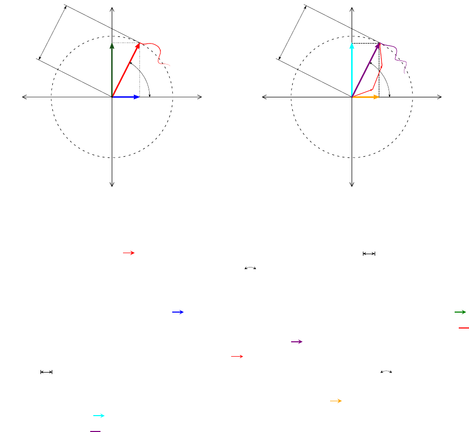
Figure 1.1.1: (a) Argand diagram of an AM–FM component in (1.1) at some time instant.
Each component, ψ(t)( ) is interpreted as a vector: the IA a(t)( ) is interpreted as
the component vector’s length, the phase θ(t)( ) is interpreted as a component vectors’s
angular position. Although not shown, the IF ω(t)is interpreted as a component vector’s
angular velocity and phase reference ϕis interpreted the angular position at t= 0. The
real part of the component s(t)( ) and the imaginary part of the component σ(t)( )
are interpreted as orthogonal projections of ψ(t). We have included an example path ( )
taken by ψ(t). (b) Argand diagram of the signal z(t)( ) in (1.2) at some time instant,
composed of a superposition of components ( ). The signal is interpreted as a vector: the
IA ρ(t)( ) is interpreted as the signal vector’s length, the phase Θ(t)( ) is interpreted
as a signal vector’s angular position, and although not shown the IF Ω(t)is interpreted as a
signal vector’s angular velocity. The real part of the signal x(t)( ) and the imaginary part
of the signal y(t)( ) are interpreted as orthogonal projections of z(t). We have included
an example path ( ) taken by z(t).
4

1.2 The Complex AM–FM Model
We meticulously parameterize the complex AM–FM model for a complex signal z(t)as a
superposition of K(possibly innite) complex AM–FM components
zt;S≜
K−1
k=0
ψkt;Ck(1.2a)
=ρ(t)ej[∫t
−∞ Ω(τ)dτ+Φ](1.2b)
=ρ(t)ejΘ(t)(1.2c)
=x(t) + jy(t)(1.2d)
where S≜{C0,C1,· · · ,CK−1}is the component set; Ck≜(ak(t), ωk(t), ϕk)is the canonical
triplet for the kth component; and for the signal z(t),ρ(t)is the IA, Θ(t)is the phase
function, Ω(t) = d
dtΘ(t)is the IF, Φis the phase reference, x(t)is the real part, and y(t)is
the imaginary part. The kth complex AM–FM component in (1.2a) is dened as
ψkt;Ck≜ak(t)ej[∫t
−∞ ωk(τ)dτ+ϕk](1.3a)
=ak(t)ejθk(t)(1.3b)
=sk(t) + jσk(t)(1.3c)
where for the kth AM–FM component ψk(t),ak(t)is the IA, θk(t)is the phase function,
ωk(t) = d
dtθk(t)(1.4)
is the IF, ϕkis the phase reference, sk(t)is the real part, and σk(t)is the imaginary part.
Rewriting ωk(t) = ϖk+mk(t), the phase θk(t)may be expressed in terms of frequency
reference ϖkand FM message mk(t)as θk(t) = ϖkt+t
−∞ mk(τ)dτ+ϕkor in terms of the
phase modulation message Mk(t)as θk(t) = ϖkt+Mk(t)+ϕk. The geometric interpretations
of the AM–FM component in (1.1) and the AM–FM model in (1.2) are illustrated with
the Argand diagrams in Fig. 1.1.1. The AM–FM component can be visually interpreted
as a single rotating vector in the complex plane with time-varying length and time-varying
angular velocity. The time evolution of the AM–FM model may be interpreted directly in
terms of mechanics—where the sometimes misunderstood concept of IF may be conveniently
interpreted as angular velocity.
We assume that the phase and frequency references are selected at t= 0, i.e. 0
−∞ ωk(t)dt=
0which implies 0
−∞ mk(t)dt=Mk(0) = 0,ϕk=θk(0), and ϖk=ωk(0)−mk(0). We dene a
monocomponent signal as any signal expressed with K= 1 and thus with a single canonical
triplet. A multicomponent signal can then be dened as any signal expressed with K > 1
and thus with a set of canonical triplets.
5
1.3 Instantaneous Spectral Analysis
We use the term instantaneous spectral analysis (ISA) to refer to a very general framework
for TFA consisting of three parts: 1) a parameter set, 2) an instantaneous spectrum, and
3) a signal model. Specically, in the ISA framework: 1) a signal is represented by a set
of canonical triplets S={C0,C1,· · · ,CK−1}, 2) each component set has a single-valued
mapping to an IS S7→ S(t, ω), and 3) each IS has a single-valued mapping to a signal
S(t, ω)7→ z(t).
For the signal model we use the complex AM–FM model as parameterized in Section
1.2. Thus using terminology by Flandrin, the complex AM–FM signal model is a formal
model because the structure of the analyzed signal is incorporated in the parameterization
and is also a formal decomposition because the construction process is a linear superposition
of time-frequency atoms [2]. In fact, we consider the AM–FM component parameterized by
Cin (1.1) as the most general form of a time-frequency atom.
The IS is both moving and joint because it consists of a local description in both time
and frequency and evolutionary because the coecients are explicitly time-dependent [2].
The IS is also “causal” in the sense of Page and Gupta [3, 4], i.e. the value at time t0does
not require the signal for t>t0. Although the IS may be considered a “distribution” in the
sense that it describes the energy allocation in time and frequency, it is not a formal TFD [5]
because it is not obtained via an integral transform.
At its heart, the TFA problem is that of signal representation. ISA provides a mathe-
matical framework which is similar to a coordinate system. When using IS framework the
TFA problem may be stated as follows. For a given signal z(t)or x(t)nd Ssubject to
SEqn. (1.5)
7−→ S(t, ω)Eqn. (1.6)
7−→ z(t)Eqn. (1.7)
7−→ x(t).
The problem is not, in general, uniquely solvable because the problem is under-constrained—
providing few general mathematical constraints and allowing for innite degrees of freedom.
This under-determinedness manifests as an innite number of ways to decompose a signal
into a sum of parts, each leading to a dierent IS.
6

1.3.1 Denition of the Instantaneous Spectrum
We dene the IS in the time-frequency coordinates for a signal expressed with set of canonical
triplets S={C0,C1,· · · ,CK−1}as
S(t, ω;S)≜2π
K−1
k=0 ∞
−∞
ψkτ;Ck2
δt−τ, ω −ωk(τ)dτ
= 2π
K−1
k=0
ψkt;Ckδω−ωk(t)(1.5)
where δ(·)and 2
δ(·,·)are 1-D and 2-D Dirac deltas and we have used the well-known sifting
property ∞
−∞ f(τ)δ(t−τ)dτ=f(t)and 2
δ(t, ω) = δ(t)δ(ω)[6].
The IS, S(t, ω;S)maps to signal z(t;S)with
1
2π∞
−∞
S(t, ω;S)dω=z(t;S).(1.6)
One consideration with the IS is that in general, it is not unique for a particular signal
under analysis. That is, in general, there are an innite number of dierent sets of canoni-
cal triplets S={C0,C1,· · · ,CK−1}and subsequently an innite number of instantaneous
spectra that can be associated with a given complex signal. Despite this non-uniqueness,
this framework is advantageous because the inherent ambiguities allow for exibility in the
model. Furthermore, with the proper constraints placed on the model, a unique IS will arise.
7
1.3.2 Visualization of the Instantaneous Spectrum
For purposes of interpretation and visualization, we extend (1.5) by dening a 3-D IS in the
time-frequency-real coordinates as
S(t, ω, s;S) = 2π
K−1
k=0
ψkt;Ck2
δω−ωk(t), s −sk(t)
where sk(t)is the real part of the kth component, as shown in (1.3c), and it is understood
that the sifting property has been used to rewrite the 3-D Dirac delta as a 2-D Dirac delta
similar to (1.5). We consider the time-frequency-real space as the most intuitive space for
interpretation. Integrating out the real dimension, it can be shown that
∞
−∞
S(t, ω, s;S)ds=S(t, ω;S).
We can visualize S(t, ω, s)by plotting ωk(t)vs. sk(t)vs. tas a line in a 3-D space
and coloring the line with respect to |ak(t)|for each component. Thus, the simultaneous
visualization of multiple parameters for each component in the time-frequency-real space is
possible. Further, orthographic projections of S(t, ω, s)yield common plots: the time-real
plane (the real component waveforms), the time-frequency plane (the IS), and the frequency-
real plane (analogous to the Fourier magnitude spectrum). We consider the 3-D visualization
as a type of phase space plot as illustrated in Fig. 1.3.1.
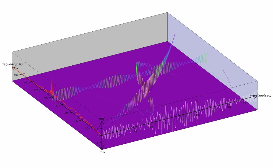
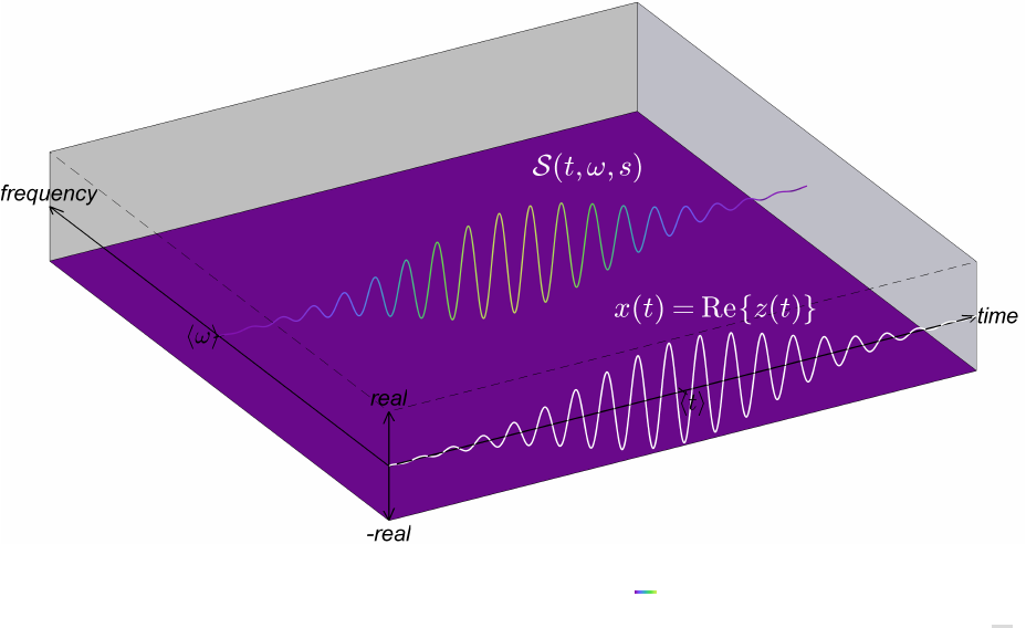
Figure 1.3.1: The 3-D instantaneous spectrum S(t, ω, s)( ) for a signal consisting of a single
Gabor atom z(t) = a0e−π(t−⟨t⟩)2/(2σ2
t)ej⟨ω⟩(t−⟨t⟩)with real part shown along the time axis ( ).
8
1.4 Latent Signal Analysis
The complex-valued nature of the proposed model leads to a new, possibly radical view of
signals. This view is that all signals are in fact complex-valued and that in reality, only the
real part x(t), is observed (or measured) and the imaginary part y(t), is latent, i.e. the act
of observation corresponds to
z(t)7→ x(t)according to x(t) = Re{z(t)}.(1.7)
We term this view Latent Signal Analysis (LSA). The problem considered in LSA is to
determine a complex signal extension, i.e. to determine the (total) latent signal z(t) =
x(t) + jy(t)when the imaginary part y(t)is hidden, given an observation x(t).
Traditionally, there are two choices for y(t)that are made in the literature. If one chooses
y(t) = 0, then conjugate symmetry is imposed in frequency, i.e. Z(jω) = Z∗(−jω). If one
chooses y(t) = H{x(t)}, then single-sidedness is imposed in frequency, Z(jω) = 0 for ω < 0,
which may also be considered a symmetry in frequency, as we will show. We note that both
of these choices may articially impose symmetry.
In the context of this work, determining the IA/IF of a signal becomes that of determining
y(t)and hence z(t)from the observation (or measurement) of x(t), in the most general way
possible without imposing unnecessary constraints. In the frequency domain, this problem
can alternatively be stated as that of determining the latent spectrum,Z(jω) = X(jω) +
jY(jω)from X(jω)where both X(jω)and Y(jω)are complex-valued.
9

Chapter 2
Modulation/Demodulation
Algorithms
The functions in this chapter, are used to create complex AM–FM signal components
(modulate) and extract component parameters from complex AM–FM signal components
(demodulate).
Contents
2.1 amfmmod.m ................................ 11
2.2 amfmdemod.m............................... 13
10

2.1 amfmmod.m
Call Syntax: [psi, s, sigma, , t, theta] = amfmmod(a, m, fc, fs, phi, method)
Description: This function synthesizes an AM-FM component based on a specied in-
stantaneous amplitude, FM message, frequency reference, sampling frequency, and phase
reference. Additionally, there is an optional parameter to specify the method for integration
approximation.
Algorithm 1 Synthesis of a complex AM–FM component from parameters.
1: procedure [ψ0(t), s0(t), σ0(t),ω0(t)
2π, t, θ0(t)] = amfmmod( a0(t),m0(t)
2π,ϖ0
2π, fs, ϕ0)
2: t∈(0, T )
3: M0(t) = t
0m0(τ)dτ
4: ω0(t) = 2π[ϖ0+M0(t)]
5: θ0(t) = ϖ0+M0(t) + ϕ0
6: ψ0(t) = a0(t)exp[jθ0(t)]
7: s0(t) = Re{ψ0(t)}
8: σ0(t) = Im{ψ0(t)}
9: end procedure
Input Arguments:
Name: a=
⊥
a0(t)
⊥
Type: vector (real)
Description: instantaneous amplitude
Name: m=1
2π
⊥
m0(t)
⊥
Type: vector (real)
Description: FM message in Hertz
Name: fc =ϖ0
2π
Type: scalar
Description: initial frequency in Hertz
Name: fs =fs
Type: scalar
Description: sampling frequency in Hertz
Name: phi =ϕ0
Type: scalar
Description: phase reference in radians
11

Name: method
Type: string
Description: numerical integration method: ’left’ or ’right’ or ’center’ or ’trapz’[default]
or ’simps’
Output Arguments:
Name: psi =
⊥
ψ0(t)
⊥
Type: vector (complex)
Description: AM-FM component
Name: s=
⊥
s0(t)
⊥
Type: vector
Description: real part of the AM-FM signal
Name: sigma =
⊥
σ0(t)
⊥
Type: vector
Description: imaginary part of the AM-FM signal
Name: =1
2π
⊥
ω0(t)
⊥
Type: vector
Description: instantaneous frequency of the AM-FM signal
Name: t=
0
1
fs
.
.
.
⊥
Type: vector
Description: time instants
References:
Notes:
Function Dependencies:
amfmmod intApprox
12

2.2 amfmdemod.m
Call Syntax: [A,IF,S,SIGMA,THETA] = amfmdemod(PSI,varargin)
Description: This function demodulates a complex AM-FM component.
Algorithm 2 Demodulation of a complex AM–FM component.
1: procedure [ak(t), ωk(t), sk(t), σk(t), θk(t)] = amfmdemod( ψk(t))
2: for k∈ {0,1,· · · , K −1}do
3: θk(t) = unwrap∠ψk(t)
4: ωk(t) = d
dtθk(t)
5: ak(t) = |ψk(t)|
6: sk(t) = Re{ψk(t)}
7: σk(t) = Im{ψk(t)}
8: end for
9: end procedure
Input Arguments:
Name: PSI =
⊥⊥⊥
ψ0(t)ψ1(t)· · · ψK−1(t)
⊥ ⊥ ⊥
Type: complex matrix (or vector)
Description: the kth column is the kth component ψk(t)
Optional Input Arguments:
Name: demodPhaseDeriv
Type: string
Default: ’center9’
Description: numerical dierentiation methodmethod: ’forward’ or ’backward’ or ’cen-
ter3’ or ’center5’ or ’center7’ or ’center9’ [default] or ’center11’ or ’center13’ or ’cen-
ter15’
Name: fs
Type: scalar
Default: 1
Description: sampling freq
13
Output Arguments:
Name: A=
⊥⊥⊥
a0(t)a1(t)· · · aK−1(t)
⊥ ⊥ ⊥
Type: real matrix (or vector)
Description: the kth column is the IA of ψk(t)
Name: IF =1
2π
⊥⊥⊥
ω0(t)ω1(t)· · · ωK−1(t)
⊥ ⊥ ⊥
Type: real matrix (or vector)
Description: the kth column is the IF of ψk(t)in Hertz
Name: S=
⊥⊥⊥
s0(t)s1(t)· · · sK−1(t)
⊥ ⊥ ⊥
Type: real matrix (or vector)
Description: the kth column is the real part of ψk(t)
Name: SIGMA =
⊥⊥⊥
σ0(t)σ1(t)· · · σK−1(t)
⊥ ⊥ ⊥
Type: real matrix (or vector)
Description: the kth column is the imaginary part of ψk(t)
Name: THETA =
⊥⊥⊥
θ0(t)θ1(t)· · · θK−1(t)
⊥ ⊥ ⊥
Type: real matrix (or vector)
Description: the kth column is the instantaneous angle of ψk(t)
References:
Notes:
Function Dependencies:
amfmdemod
derivApprox
parse_pv_pairs
14
Chapter 3
Decomposition Algorithms
This Chapter is in Development
15

Chapter 4
Visualization
The functions in this chapter are used to visualize and interpret the instantaneous
spectrum. Additionally, some functions are provided to help facilitate the comparison to
other time-frequency methods.
Contents
4.1 Argand.m.................................. 17
4.2 ISA2dPlot.m................................ 18
4.3 ISA3dPlot.m................................ 19
4.4 ISA3dPlotPrint.m............................. 21
4.5 STFT2dPlot.m............................... 23
16

4.1 Argand.m
Call Syntax: h = Argand(t,psi)
Description: This function plots an AM-FM component as a rotating vector.
Input Arguments:
Name: t
Type: vector (real)
Description: time instants
Name: psi =
⊥
ψ0(t)
⊥
Type: vector (complex)
Description: AM-FM component
Output Arguments:
Name: h
Type: handle
Description: gure handle
References:
Notes:
Function Dependencies:
17
4.2 ISA2dPlot.m
Call Syntax: h = ISA2dPlot(t, S, IF, A, fs, fMax)
Description: This function plots a 2D instantenous spectrum
Name: t
Type: vector (real)
Description: time instants
Name: S=
⊥⊥⊥
s0(t)s1(t)· · · sK−1(t)
⊥ ⊥ ⊥
Type: real matrix (or vector)
Description: the kth column is the real part of ψk(t)
Name: IF =1
2π
⊥⊥⊥
ω0(t)ω1(t)· · · ωK−1(t)
⊥ ⊥ ⊥
Type: real matrix (or vector)
Description: the kth column is the IF of ψk(t)in Hertz
Name: A=
⊥⊥⊥
a0(t)a1(t)· · · aK−1(t)
⊥ ⊥ ⊥
Type: real matrix (or vector)
Description: the kth column is the IA of ψk(t)
Name: fs
Type: scalar
Description: sampling frequency
Name: fMax or [fMax, fMin] (optional)
Type: scalar or [scalar,scalar]
Description: maximum plotting frequency and optionally the minimum plotting fre-
quency
Output Arguments:
Name: h
Type: handle
Description: gure handle
References:
Notes:
Function Dependencies:
ISA2dPlot ISplot
pmkmp
colorLine
18

4.3 ISA3dPlot.m
Call Syntax: h = ISA3dPlot(t, PSI, IF, A, fs, fMax, STFTparams)
Description: This function plots a 3D instantaneous spectrum.
Name: t
Type: vector (real)
Description: time instants
Name: PSI =
⊥⊥⊥
ψ0(t)ψ1(t)· · · ψK−1(t)
⊥ ⊥ ⊥
Type: complex matrix (or vector)
Description: the kth column is the kth component ψk(t)
Name: IF =1
2π
⊥⊥⊥
ω0(t)ω1(t)· · · ωK−1(t)
⊥ ⊥ ⊥
Type: real matrix (or vector)
Description: the kth column is the IF of ψk(t)in Hertz
Name: A=
⊥⊥⊥
a0(t)a1(t)· · · aK−1(t)
⊥ ⊥ ⊥
Type: real matrix (or vector)
Description: the kth column is the IA of ψk(t)
Name: fs
Type: scalar
Description: sampling frequency
Name: fMax or [fMax, fMin] (optional)
Type: scalar or [scalar,scalar]
Description: maximum plotting frequency and optionally the minimum plotting fre-
quency
Name: STFTparams (optional)
Type: vector (1x2)
Description: STFT parameters: [N_FFT, frame_advance]
Output Arguments:
Name: h
Type: handle
Description: gure handle
19
References:
Notes:
Function Dependencies:
ISA3dPlot
oaxes
patchline
pmkmp
rgb
ISstft
PlayFromPlot
ToggleVis
changeview
colorLine
dispAMPPlot
dispFSPlot
dispISPlot
dispRealPlot
freerotate
draw
enable
freeze
methods
oaxes
schema
toggle
schema
frame
ISplot
calcticks
20

4.4 ISA3dPlotPrint.m
Call Syntax: h = ISA3dPlotPrint(t, PSI, IF, A, fs, fMax, STFTparams)
Description: This function plots a 3D instantaneous spectrum without the GUI buttons.
Name: t
Type: vector (real)
Description: time instants
Name: PSI =
⊥⊥⊥
ψ0(t)ψ1(t)· · · ψK−1(t)
⊥ ⊥ ⊥
Type: complex matrix (or vector)
Description: the kth column is the kth component ψk(t)
Name: IF =1
2π
⊥⊥⊥
ω0(t)ω1(t)· · · ωK−1(t)
⊥ ⊥ ⊥
Type: real matrix (or vector)
Description: the kth column is the IF of ψk(t)in Hertz
Name: A=
⊥⊥⊥
a0(t)a1(t)· · · aK−1(t)
⊥ ⊥ ⊥
Type: real matrix (or vector)
Description: the kth column is the IA of ψk(t)
Name: fs
Type: scalar
Description: sampling frequency
Name: fMax or [fMax, fMin] (optional)
Type: scalar or [scalar,scalar]
Description: maximum plotting frequency and optionally the minimum plotting fre-
quency
Name: STFTparams (optional)
Type: vector (1x2)
Description: STFT parameters: [N_FFT, frame_advance]
Output Arguments:
Name: h
Type: handle
Description: gure handle
21

References:
Notes:
Function Dependencies:
ISA3dPlot
oaxes
patchline
pmkmp
rgb
ISstft
PlayFromPlot
ToggleVis
changeview
colorLine
dispAMPPlot
dispFSPlot
dispISPlot
dispRealPlot
freerotate
draw
enable
freeze
methods
oaxes
schema
toggle
schema
frame
ISplot
calcticks
22
4.5 STFT2dPlot.m
Call Syntax: h = STFT2dPlot(z, fs, fMax, STFTparams)
Description: This function plots the short-time Fourier transform magnitude using a Ham-
ming window.
Input Arguments:
Name: z
Type: vector
Description: complex signal
Name: fs
Type: scalar
Description: sampling frequency
Name: fMax or [fMax, fMin] (optional)
Type: scalar or [scalar,scalar]
Description: maximum plotting frequency and optionally the minimum plotting fre-
quency
Name: STFTparams
Type: vector (1x2)
Description: STFT parameters: [N_FFT,frame_advance]
Output Arguments:
Name: h
Type: handle
Description: gure handle
References:
Notes:
Function Dependencies:
STFT2dPlot
ISstft
dispFSPlot
frame
pmkmp
23


5.1 derivApprox.m
Call Syntax: Y = derivApprox(X,fs,method)
Description: This function estimates the approximate computation of a derivative using
various numerical techniques.
Input Arguments:
Name: X=
⊥⊥⊥
x0(t)x1(t)· · · xK−1(t)
⊥ ⊥ ⊥
Type: matrix (or vector)
Description: the kth column is the kth signal
Name: fs (optional)
Type: scalar
Description: sampling frequency [default = 1]
Name: method (optional)
Type: string
Description: numerical dierentiation method
‘forward’ - forward dierence
‘backward’ - backward dierence
‘center3’ - 3-pt stencil central dierence
‘center5’ - 5-pt stencil central dierence
‘center7’ - 7-pt stencil central dierence
‘center9’ - 9-pt stencil central dierence
‘center11’ - 11-pt stencil central dierence
‘center13’ - 13-pt stencil central dierence
‘center15’ - 15-pt stencil central dierence [default]
Output Arguments:
Name: Y=
⊥⊥⊥
d
dtx0(t)d
dtx1(t)· · · d
dtxK−1(t)
⊥ ⊥ ⊥
Type: matrix (or vector)
Description: the kth column is the integral estimate of the kth signal
References:
[1] http://www.holoborodko.com/pavel/numerical-methods/numerical-derivative/
central-differences/
[2] http://web.media.mit.edu/~crtaylor/calculator.html
Notes: See DEMO_derivApprox.m
Function Dependencies: None
25

5.2 intApprox.m
Call Syntax: Y = intApprox(X, fs, method)
Description: This function evaluates an approximate computation of an integral using
various numerical techniques.
Input Arguments:
Name: X=
⊥⊥⊥
x0(t)x1(t)· · · xK−1(t)
⊥ ⊥ ⊥
Type: matrix (or vector)
Description: the kth column is the kth signal
Name: fs (optional)
Type: scalar
Description: sampling frequency [default = 1]
Name: method (optional)
Type: string
Description: numerical integration method
‘left’ - use the left rectangle rule
‘right’ - use the right rectangle rule
’center’ - use the midpoint rule
‘trapz’ - use the trapezoidal rule [default]
‘simps’ - use Simpson’s rule
Output Arguments:
Name: Y=
⊥⊥⊥
t
0x0(τ)dτt
0x1(τ)dτ· · · t
0xK−1(τ)dτ
⊥ ⊥ ⊥
Type: matrix (or vector)
Description: the kth column is the cumulative integral estimate of the kth signal up
to time t
References:
Notes: See DEMO_intApprox.m
Function Dependencies: None
26

Chapter 6
Demo Scripts
Contents
6.1 DEMO_1_SimpleHarmicComponent.m . . . . . . . . . . . . . . . . 28
6.2 DEMO_2_SimpleAMComponent.m . . . . . . . . . . . . . . . . . . 30
6.3 DEMO_3_SimpleFMComponent.m . . . . . . . . . . . . . . . . . . 32
6.4 DEMO_4_AMFMComponent.m . . . . . . . . . . . . . . . . . . . . 34
6.5 DEMO_5_MultiComponentSignal.m . . . . . . . . . . . . . . . . . . 36
6.6 FIGURE_ISA2018_SinusoidalAM.m . . . . . . . . . . . . . . . . . . 38
6.7 FIGURE_ISA2018_SinusoidalFM.m . . . . . . . . . . . . . . . . . . 39
6.8 FIGURE_ISA2018_GaussianAMchirpFMchirp.m . . . . . . . . . . 40
6.9 DEMO_intApprox.m ........................... 41
6.10 DEMO_derivApprox.m.......................... 43
27
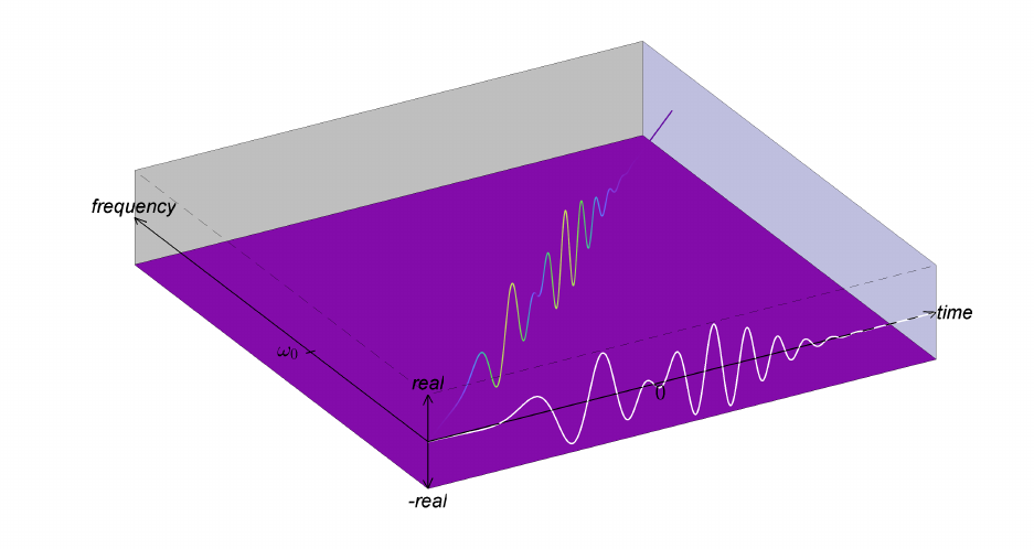
6.1 DEMO_1_SimpleHarmicComponent.m
Description: This script demonstrates the functionality of ‘amfmmod.m’, ‘Argand.m’,
‘ISA2dPlot.m’, and ‘ISA3dPlot.m’ by synthesizing a simple harmonic component and gen-
erating several visualizations.
A simple harmonic component has both constant IA and constant IF.
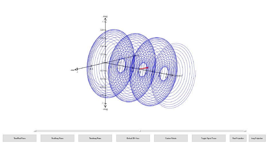
Figure 6.1.1: The interactive gure generated by running ‘Argand.m’ for a simple harmonic
component.
28
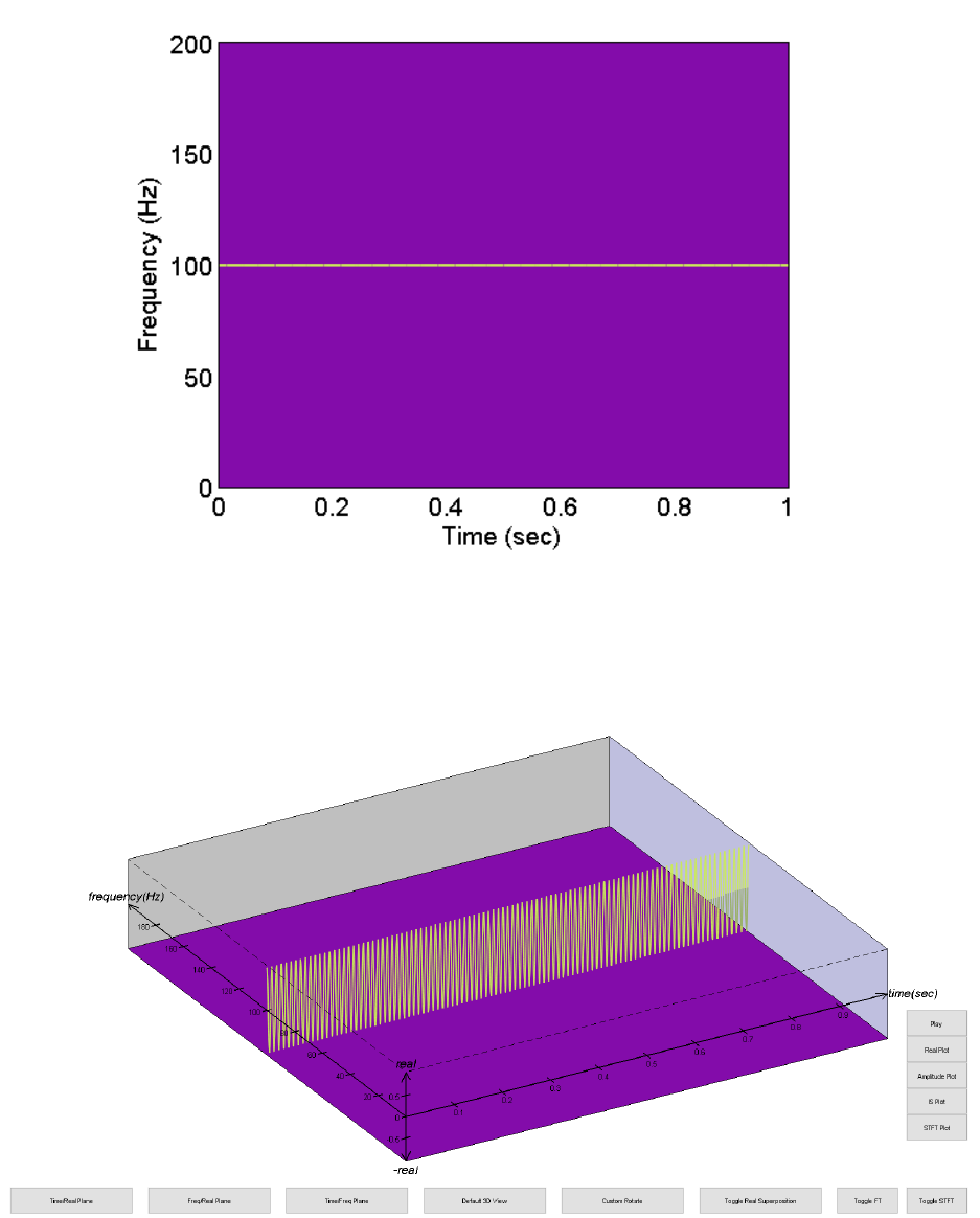
Figure 6.1.2: The IS plot generated by running ‘ISA2dPlot.m’ for a simple harmonic com-
ponent.
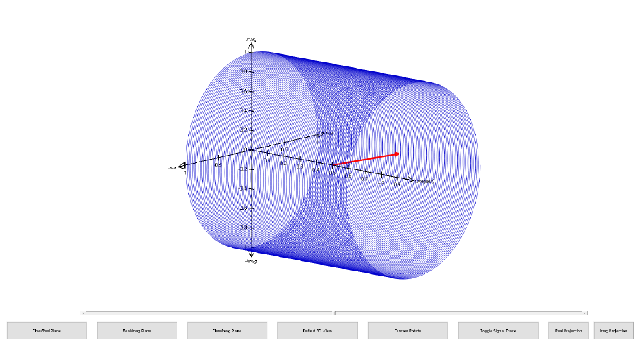
Figure 6.1.3: The interactive 3D gure generated by running ‘ISA3dPlot.m’ for a simple
harmonic component.
29
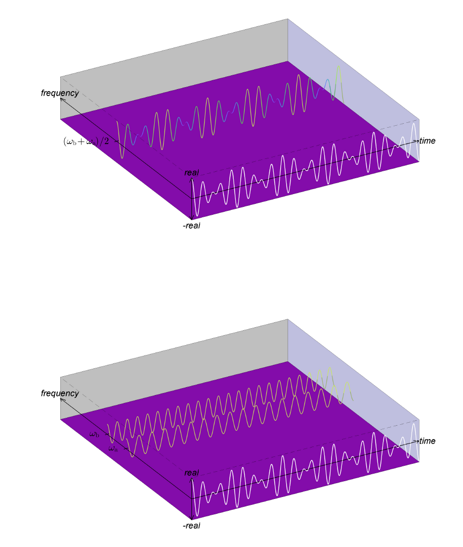
6.2 DEMO_2_SimpleAMComponent.m
Description: This script demonstrates the functionality of ‘amfmmod.m’, ‘Argand.m’,
‘ISA2dPlot.m’, and ‘ISA3dPlot.m’ by synthesizing a simple AM component and generat-
ing several visualizations.
A simple AM component has constant IF but time-varying IA. Lines 40-43 in the demo le
allow the user to switch between three predened IA functions. The default is sinusoidal
AM.
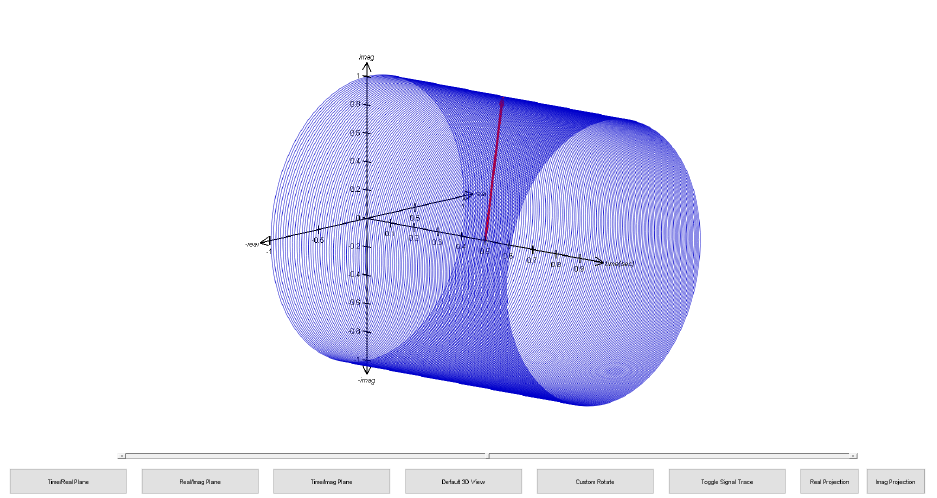
Figure 6.2.1: The interactive gure generated by running ‘Argand.m’ for a simple AM com-
ponent with sinusoidal AM.
30
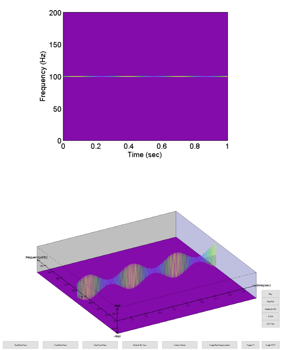
Figure 6.2.2: The IS plot generated by running ‘ISA2dPlot.m’ for a simple AM component
with sinusoidal AM.
Figure 6.2.3: The interactive 3D gure generated by running ‘ISA3dPlot.m’ for a AM har-
monic component with sinusoidal AM.
31
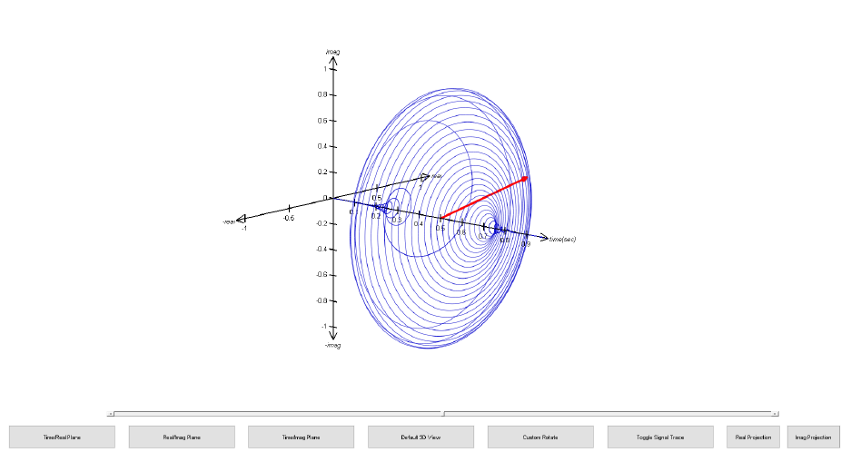
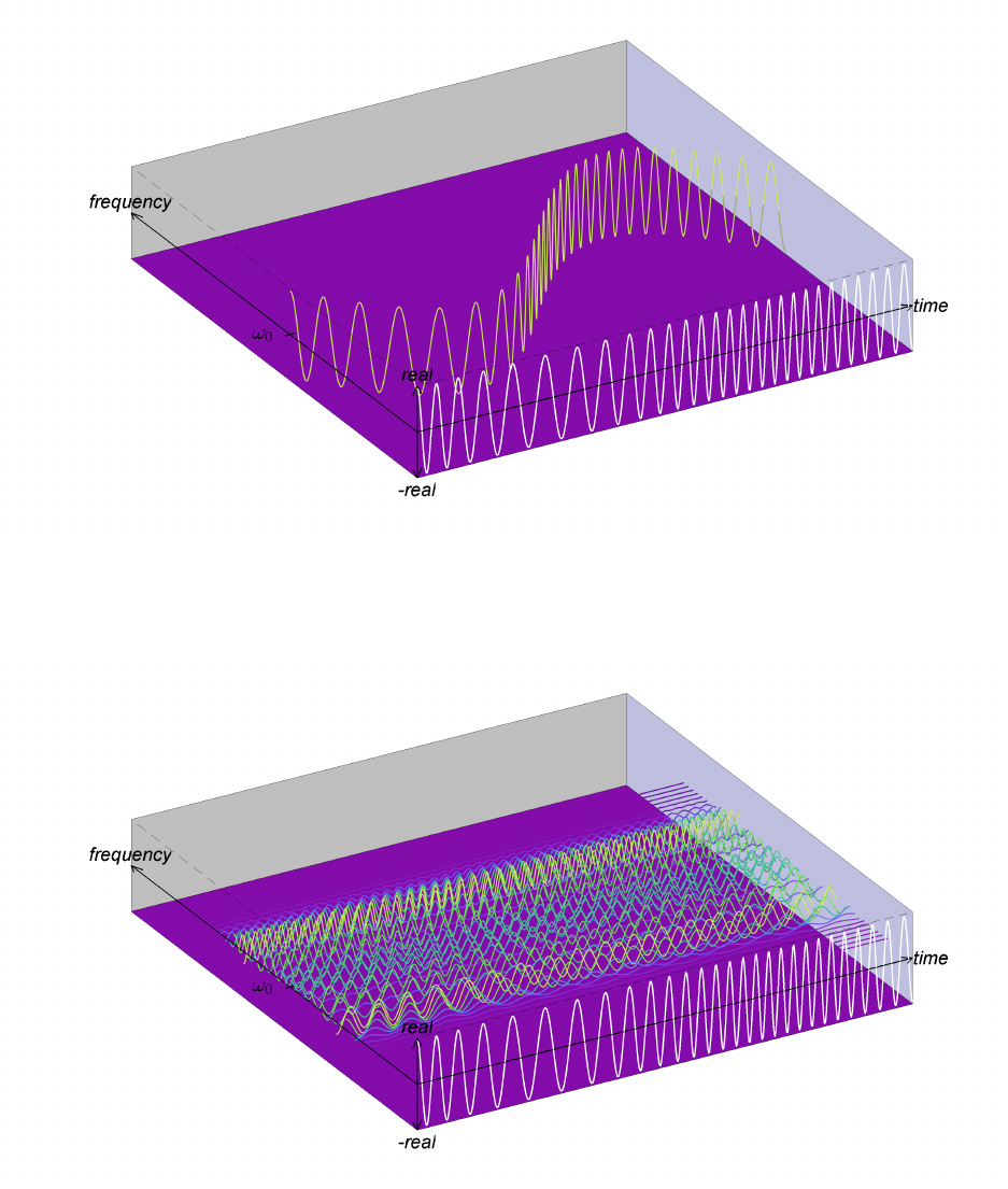
6.3 DEMO_3_SimpleFMComponent.m
Description: This script demonstrates the functionality of ‘amfmmod.m’, ‘Argand.m’,
‘ISA2dPlot.m’, and ‘ISA3dPlot.m’ by synthesizing a simple FM component and generat-
ing several visualizations.
A simple FM component has constant IA but time-varying IF. Lines 39-41 in the demo le
allow the user to switch between three predened IF functions. The default is an FM chirp.
Figure 6.3.1: The interactive gure generated by running ‘Argand.m’ for a simple FM com-
ponent chirp.
32
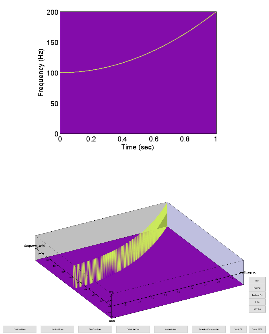
Figure 6.3.2: The IS plot generated by running ‘ISA2dPlot.m’ for a simple FM component
chirp.
Figure 6.3.3: The interactive 3D gure generated by running ‘ISA3dPlot.m’ for a simple FM
component chirp.
33
6.4 DEMO_4_AMFMComponent.m
Description: This script demonstrates the functionality of ‘amfmmod.m’, ‘Argand.m’,
‘ISA2dPlot.m’, and ‘ISA3dPlot.m’ by synthesizing an AM–FM component and generating
several visualizations.
An AM–FM component has both a time-varying IA and IF.
Figure 6.4.1: The interactive gure generated by running ‘Argand.m’ for an AM–FM com-
ponent.
34
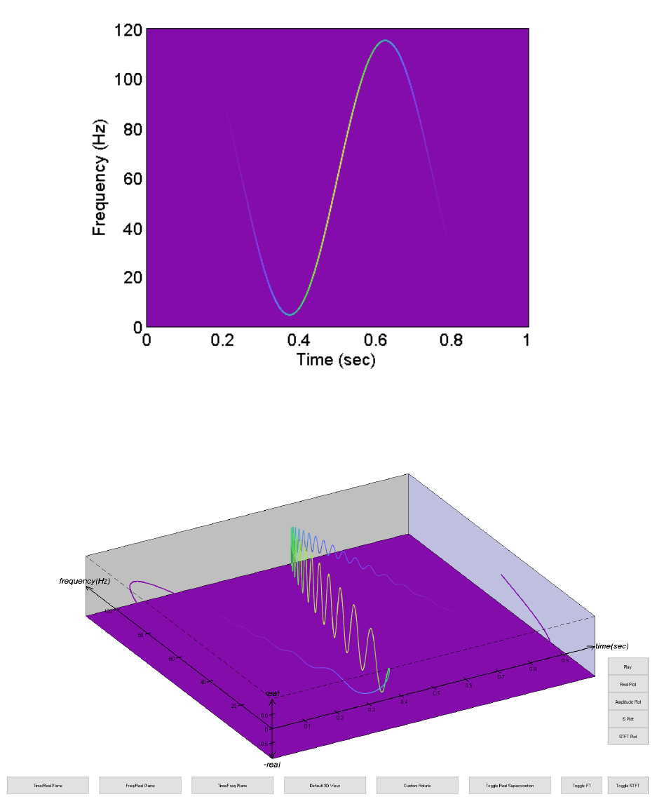
Figure 6.4.2: The IS plot generated by running ‘ISA2dPlot.m’ for an AM–FM component.
Figure 6.4.3: The interactive 3D gure generated by running ‘ISA3dPlot.m’ for an AM–FM
component.
35
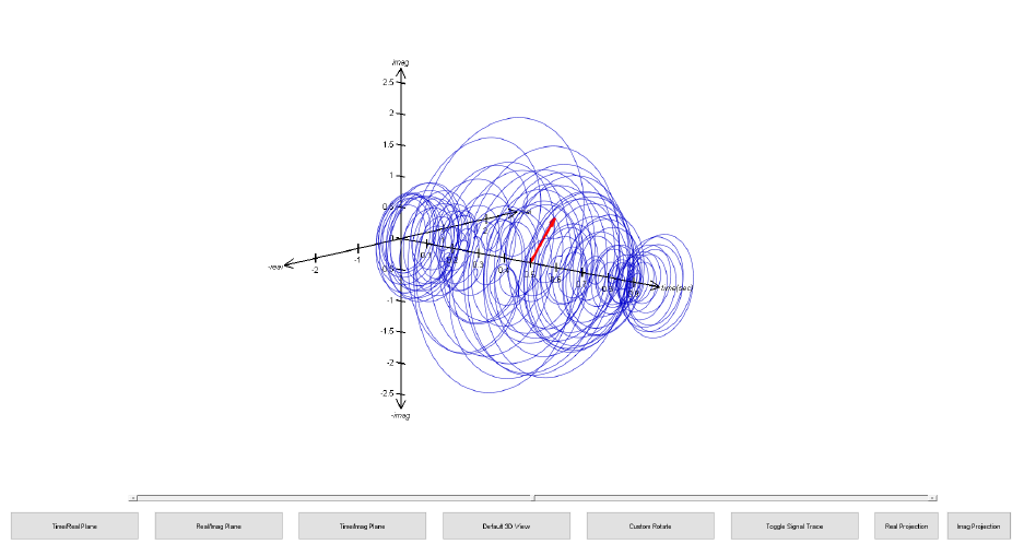
6.5 DEMO_5_MultiComponentSignal.m
Description: This script demonstrates the functionality of ‘amfmmod.m’, ‘Argand.m’,
‘ISA2dPlot.m’, and ‘ISA3dPlot.m’ by synthesizing a multi-component AM–FM signal and
generating several visualizations.
A multi-component signal consists of multiple AM–FM components.
Figure 6.5.1: The interactive gure generated by running ‘Argand.m’ for a multi-component
AM–FM signal.
36
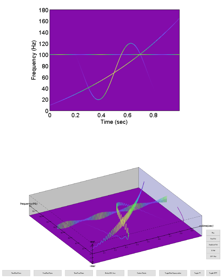
Figure 6.5.2: The IS plot generated by running ‘ISA2dPlot.m’ for a multi-component AM–
FM signal.
Figure 6.5.3: The interactive 3D gure generated by running ‘ISA3dPlot.m’ for a multi-
component AM–FM signal.
37
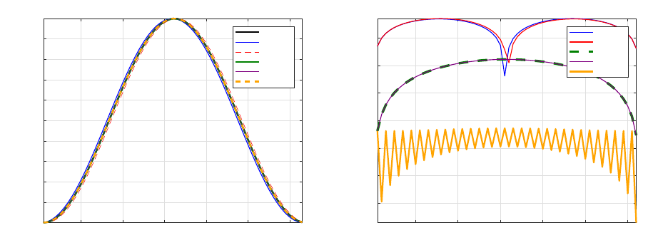
6.9 DEMO_intApprox.m
Description: This script demonstrates the ‘intApprox.m’, which estimates the integral of
a signal using one of several methods.
A time-domain comparison of the integration approximation methods is given in Figure 6.9.1.
Figure 6.9.1(a) shows the various integration approximations for one period of a sinusoid.
The corresponding error at each instant, given in dB, in shown in Figure 6.9.1(b).
10 20 30 40 50 60
time (sample)
0
0.2
0.4
0.6
0.8
1
1.2
1.4
1.6
1.8 Ideal
forward
backward
center
trap
simp
(a)
123456
time (s)
-160
-140
-120
-100
-80
-60
-40
Error (dB)
forward
backward
center
trap
simp
(b)
Figure 6.9.1: Comparison of the various integral approximations methods for one period
of a of a sinusoid. As the order of the approximation increases, the approximation error
decreases.
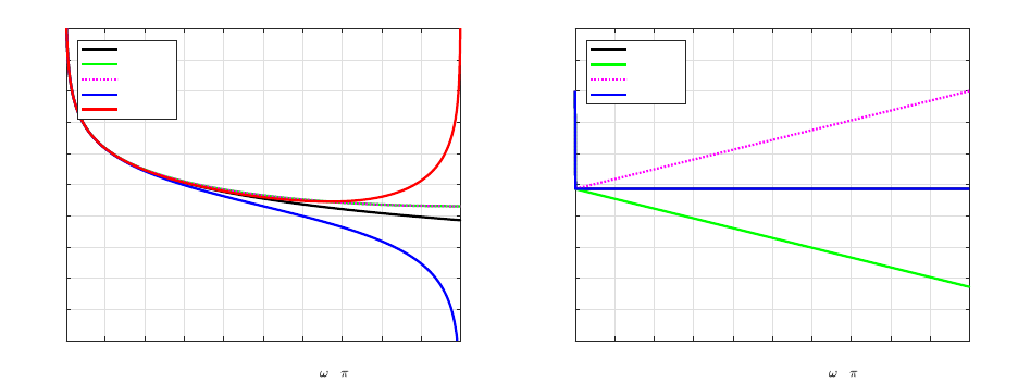
A frequency-domain comparison of the magnitude responses of the approximations is given in
Figure 6.9.2. Figure 6.9.2(a) shows the magnitude response of the ideal integrator alongside
the various approximation methods. Based on the magnitude response, the forward and
backward method is the one closest to the ideal signal. However, the phase response shown
in Figure 6.9.2(b) needs to be considered as well. Here it is apparent that the forward and
backward dierences introduce phase distortions while the center and trap dierences do not
41
0.05 0.1 0.15 0.2 0.25 0.3 0.35 0.4 0.45 0.5
Normalized Frequency ( /2 )
-100
-80
-60
-40
-20
0
20
40
60
80
100
Magnitude Response (dB)
Ideal
forward
backward
center/trap
simp
(a)
0 0.05 0.1 0.15 0.2 0.25 0.3 0.35 0.4 0.45 0.5
Normalized Frequency ( /2 )
-4
-3.5
-3
-2.5
-2
-1.5
-1
-0.5
0
0.5
1
Phase Response
Ideal
forward
backward
center/trap
(b)
Figure 6.9.2: (a) Magnitude response and (b) phase response of the ideal integrator along
side the various integral approximation methods. As the methods of integration changes,
the frequency response approaches the ideal integrator
42
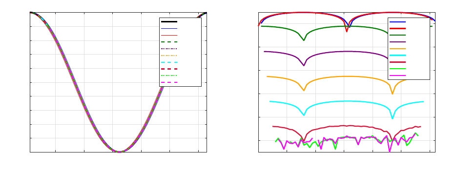
6.10 DEMO_derivApprox.m
Description: This script demonstrates the functionality of ‘derivApprox.m’, which esti-
mates the derivative of a signal using one of several methods.
A time-domain comparison of the derivative approximation methods is given in Figure 6.10.1.
Figure 6.10.1(a) shows the various derivative approximations for one period of a sinusoid.
The corresponding error at each instant, given in dB, in shown in Figure 6.10.1(b). It appears
that the 13-point and 15-point central dierences are limited by the numerical precision of
the computer.
10 20 30 40 50 60
time (sample)
-0.8
-0.6
-0.4
-0.2
0
0.2
0.4
0.6
0.8
1
Ideal
forward
backward
3-point
5-point
7-point
9-point
11-point
13-point
15-point
(a)
0123456
time (s)
-300
-250
-200
-150
-100
-50
Error (dB)
forward
backward
3-point
5-point
7-point
9-point
11-point
13-point
15-point
(b)
Figure 6.10.1: Comparison of the various derivative approximations methods for one period
of a of a sinusoid. As the order of the approximation increases, the error decreases and
performance increases.
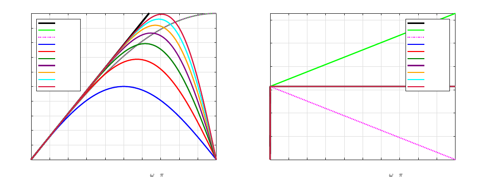
A frequency-domain comparison of the magnitude responses of the approximations is given
in Figure 6.10.2. Figure 6.10.2(a) shows the magnitude response of the ideal dierentiator
alongside the various approximation methods. Based on the magnitude response, the per-
formance of the central dierences improves as the order of the approximation is increased.
From the magnitude response plot, it may appear that the forward and backward dierences
outperform the central dierences at certain frequency ranges, however, consider the phase
responses show in Figure 6.10.2(b). Here it is apparent that the forward and backward
dierences introduce phase distortions while the central dierences do not.
43
0 0.05 0.1 0.15 0.2 0.25 0.3 0.35 0.4 0.45 0.5
Normalized Frequency ( /2 )
0
0.2
0.4
0.6
0.8
1
1.2
1.4
1.6
1.8
2
Magnitude Response
Ideal
forward
backward
3-point
5-point
7-point
9-point
11-point
13-point
15-point
(a)
0 0.05 0.1 0.15 0.2 0.25 0.3 0.35 0.4 0.45 0.5
Normalized Frequency ( /2 )
0
0.5
1
1.5
2
2.5
3
Phase Response
Ideal
forward
backward
3-point
5-point
7-point
9-point
11-point
13-point
15-point
(b)
Figure 6.10.2: (a) Magnitude response and (b) phase response of the ideal dierentiator for
various derivative approximation methods. As the order of the approximation increases, the
frequency response approaches the ideal dierentiator.
44
Chapter 7
Bibliography
[1] S. Sandoval and P. L. D. Leon, “The instantaneous spectrum: A general framework for
time-frequency analysis,” IEEE Trans. Signal Process., vol. 66, pp. 5679–5693, Nov 2018.
[2] P. Flandrin, Time-Frequency/Time-Scale Analysis. Academic press, 1998, vol. 10.
[3] C. Page, “Instantaneous power spectra,” J. Appl. Phys., vol. 23, no. 1, pp. 103–106, 1952.
[4] M. S. Gupta, “Denition of instantaneous frequency and frequency measurability,”
Am. J. of Phys., vol. 43, no. 12, pp. 1087–1088, 1975.
[5] L. Cohen, “Time-frequency distributions–a review,” Proc. IEEE, vol. 77, no. 7, pp. 941–
981, 1989.
[6] R. Bracewell, The Fourier Transform and Its Applications. McGraw-Hill, 1980.
45
