Instructions

User Manual:

Open the PDF directly: View PDF .
Page Count: 9

CSC421 Winter 2019 Programming Assignment 3

Programming Assignment 3: Attention-Based Neural Machine Trans-

lation

Deadline: March 22, 2019 at 11:59pm

Based on an assignment by Paul Vicol

Submission: You must submit two ﬁles through MarkUs1: a PDF ﬁle containing your writeup,

titled a3-writeup.pdf, and your code ﬁle nmt.ipynb. Your writeup must be typeset.

The programming assignments are individual work. See the Course Information handout2for de-

tailed policies.

You should attempt all questions for this assignment. Most of them can be answered at least par-

tially even if you were unable to ﬁnish earlier questions. If you were unable to run the experiments,

please discuss what outcomes you might hypothetically expect from the experiments. If you think

your computational results are incorrect, please say so; that may help you get partial credit.

Introduction

In this assignment, you will train a few attention-based neural machine translation models to

translate words from English to Pig-Latin. Along the way, you’ll gain experience with several

important concepts in NMT, including gated recurrent neural networks and attention.

Pig Latin

Pig Latin is a simple transformation of English based on the following rules (applied on a per-word

basis):

1. If the ﬁrst letter of a word is a consonant, then the letter is moved to the end of the word,

and the letters “ay” are added to the end: team →eamtay.

2. If the ﬁrst letter is a vowel, then the word is left unchanged and the letters “way” are added

to the end: impress →impressway.

3. In addition, some consonant pairs, such as “sh”, are treated as a block and are moved to the

end of the string together: shopping →oppingshay.

To translate a whole sentence from English to Pig-Latin, we simply apply these rules to each word

independently:

i went shopping →iway entway oppingshay

We would like a neural machine translation model to learn the rules of Pig-Latin implicitly,

from (English, Pig-Latin) word pairs. Since the translation to Pig Latin involves moving characters

around in a string, we will use character-level recurrent neural networks for our model.

Because English and Pig-Latin are so similar in structure, the translation task is almost a copy

task; the model must remember each character in the input, and recall the characters in a speciﬁc

1https://markus.teach.cs.toronto.edu/csc421-2019-01

2http://cs.toronto.edu/~rgrosse/courses/csc421_2019/syllabus.pdf

CSC421 Winter 2019 Programming Assignment 3

order to produce the output. This makes it an ideal task for understanding the capacity of NMT

models.

Setting Up

We recommend that you use Colab(https://colab.research.google.com/) for the assignment,

as all the assignment notebooks have been tested on Colab. Otherwise, if you are working on your

own environment, you will need to install Python 2, PyTorch (https://pytorch.org), iPython

Notebooks, SciPy, NumPy and scikit-learn. Check out the websites of the course and relevant

packages for more details.

From the assignment zip ﬁle, you will ﬁnd one python notebook ﬁle: nmt.ipynb. To setup

the Colab environment, you will need to upload the two notebook ﬁles using the upload tab at

https://colab.research.google.com/.

Data

The data for this task consists of pairs of words {(s(i), t(i))}N

i=1 where the source s(i)is an English

word, and the target t(i)is its translation in Pig-Latin. The dataset is composed of unique words

from the book “Sense and Sensibility,” by Jane Austen. The vocabulary consists of 29 tokens:

the 26 standard alphabet letters (all lowercase), the dash symbol -, and two special tokens <SOS>

and <EOS> that denote the start and end of a sequence, respectively. 3The dataset contains 6387

unique (English, Pig-Latin) pairs in total; the ﬁrst few examples are:

{ (the, ethay), (family, amilyfay), (of, ofway), ... }

In order to simplify the processing of mini-batches of words, the word pairs are grouped based

on the lengths of the source and target. Thus, in each mini-batch the source words are all the same

length, and the target words are all the same length. This simpliﬁes the code, as we don’t have to

worry about batches of variable-length sequences.

Part 1: Encoder-Decoder Models and Teacher-Forcing [2 mark]

Translation is a sequence-to-sequence problem: in our case, both the input and output are sequences

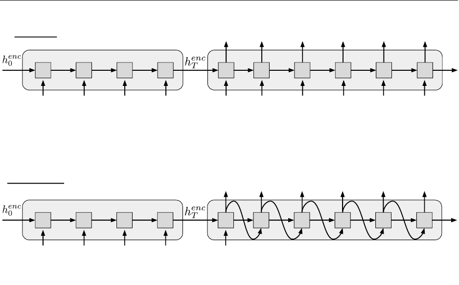
of characters. A common architecture used for seq-to-seq problems is the encoder-decoder model [2],

composed of two RNNs, as follows:

The encoder RNN compresses the input sequence into a ﬁxed-length vector, represented by

the ﬁnal hidden state hT. The decoder RNN conditions on this vector to produce the translation,

character by character.

Input characters are passed through an embedding layer before they are fed into the encoder

RNN; in our model, we learn a 29 ×10 embedding matrix, where each of the 29 characters in the

vocabulary is assigned a 10-dimensional embedding. At each time step, the decoder RNN outputs a

vector of unnormalized log probabilities given by a linear transformation of the decoder hidden state.

When these probabilities are normalized, they deﬁne a distribution over the vocabulary, indicating

the most probable characters for that time step. The model is trained via a cross-entropy loss

between the decoder distribution and ground-truth at each time step.

3Note that for the English-to-Pig-Latin task, the input and output sequences share the same vocabulary; this is

not always the case for other translation tasks (i.e., between languages that use diﬀerent alphabets).

CSC421 Winter 2019 Programming Assignment 3

c a t <EOS> <SOS> a t c a y

a t c a y <EOS>

Encoder Decoder

Training

Figure 1: Training the NMT encoder-decoder architecture.

c a t <EOS> <SOS>

a t c a y <EOS>

Encoder Decoder

Generation

Figure 2: Generating text with the NMT encoder-decoder architecture.

The decoder produces a distribution over the output vocabulary conditioned on the previous

hidden state and the output token in the previous timestep. A common practice used to train

NMT models is to feed in the ground-truth token from the previous time step to condition the

decoder output in the current step. This training procedure is known as “teacher-forcing” shown in

Figure 1. At test time, we don’t have access to the ground-truth output sequence, so the decoder

must condition its output on the token it generated in the previous time step, as shown in Figure 2.

Conceptual Questions

1. How do you think the architecture in Figure 1will perform on long sequences, and why?

Consider the amount of information the decoder gets to see about the input sequence.

2. What are some techniques / modiﬁcations we can use to improve the performance of this

architecture on long sequences? List at least two.

3. What problem may arise when training with teacher forcing? Consider the diﬀerences that

arise when we switch from training to testing.

4. Can you think of any way to address this issue? Read the abstract and introduction of the

paper “Scheduled sampling for sequence prediction with recurrent neural networks” [1], and

answer this question in your own words.

Part 3: Gated Recurrent Unit (GRU) [2 marks]

Throughout the rest of the assignment, you will implement some attention-based neural machine

translation models, and ﬁnally train the model and examine the results.

CSC421 Winter 2019 Programming Assignment 3

Open the notebook nmt.ipynb on Colab and answer the following questions.

1. The forward pass of a Gated Recurrent Unit is deﬁned by the following equations:

rt=σ(Wirxt+Whrht−1+br) (1)

zt=σ(Wizxt+Whzht−1+bz) (2)

gt= tanh(Winxt+rt(Whnht−1+bg)) (3)

ht= (1 −z)gt+zht−1,(4)

where is the element-wise multiplication. Although PyTorch has a GRU built in (nn.GRUCell),

we’ll implement our own GRU cell from scratch, to better understand how it works. The note-

book has been divided into diﬀerent sections. Find the GRU cell section of the notebook.

Complete the __init__ and forward methods of the MyGRUCell class, to implement the

above equations. A template has been provided for the forward method.

2. Train the GRU RNN in the “Training - RNN decoder” section. (Make sure you run all the

previous cells to load the training and utility functions.)

By default, the script runs for 100 epochs. At the end of each epoch, the script prints training

and validation losses, and the Pig-Latin translation of a ﬁxed sentence, “the air conditioning

is working”, so that you can see how the model improves qualitatively over time. The script

also saves several items to the directory h20-bs64-rnn:

•The best encoder and decoder model paramters, based on the validation loss.

•A plot of the training and validation losses.

How do the results look, qualitatively? Does the model do better for certain types of words

than others?

3. Use this model to translate words in the next notebook cell using translate_sentence

function. Try a few of your own words by changing the variable TEST_SENTENCE. Which

failure modes can you identify?

Part 4: Implementing Attention [4 marks]

Attention allows a model to look back over the input sequence, and focus on relevant input tokens

when producing the corresponding output tokens. For our simple task, attention can help the

model remember tokens from the input, e.g., focusing on the input letter cto produce the output

letter c.

The hidden states produced by the encoder while reading the input sequence, henc

1, . . . , henc

Tcan

be viewed as annotations of the input; each encoder hidden state henc

icaptures information about

the ith input token, along with some contextual information. At each time step, an attention-based

decoder computes a weighting over the annotations, where the weight given to each one indicates

its relevance in determining the current output token.

In particular, at time step t, the decoder computes an attention weight α(t)

ifor each of the

encoder hidden states henc

i. The attention weights are deﬁned such that 0 ≤α(t)

i≤1 and Piα(t)

1. α(t)

iis a function of an encoder hidden state and the previous decoder hidden state, f(hdec

t−1, henc

i),

where iranges over the length of the input sequence.

CSC421 Winter 2019 Programming Assignment 3

There are a few engineering choices for the possible function f. In this assignment, we will

implement two diﬀerent attention models: 1) the additive attention using a two-layer MLP and 2)

the scaled dot product attention, which measures the similarity between the two hidden states.

To unify the interface across diﬀerent attention modules, we consider attention as a function

whose inputs are triple (queries, keys, values), denoted as (Q, K, V ).

1. In the additive attention, we will learn the function f, parameterized as a two-layer fully-

connected network with a ReLU activation. This network produces unnormalized weights

˜α(t)

ithat are used to compute the ﬁnal context vector:

˜α(t)

i=f(Qt, Ki) = W2(max(0, W1[Qt;Ki] + b1)) + b2,

α(t)

i= softmax(˜α(t))i,

ct=

i=1

α(t)

iVi.

Here, the notation [Qt;Ki] denotes the concatenation of vectors Qtand Ki. To obtain the

attention weights in between 0 and 1, we apply the softmax function over the unnormalized

attention. Once we have the attention weights, a context vector ctis computed as a linear

combination of the encoder hidden states, with coeﬃcients given by the weights.

Implement the additive attention mechanism. Fill in the forward methods of the

AdditiveAttention class. Use the self.softmax function in the forward pass of the AdditiveAttention

class to normalize the weights.

...

Decoder Hidden States Encoder Hidden States

batch_size

seq_len

hidden_sizehidden_size

batch_size

seq_len

Attention Weights

Figure 3: Dimensions of the inputs, Decoder Hidden States (query), Encoder Hidden States

(keys/values) and the attention weights (α(t)).

For the forward pass, you are given a batch of query of the current time step, which has di-

mension batch_size x hidden_size, and a batch of keys and values for each time step of the

input sequence, both have dimension batch_size x seq_len x hidden_size. The goal is to

obtain the context vector. We ﬁrst compute the function f(Qt, K) for each query in the batch

and all corresponding keys Ki, where iranges over seq_len diﬀerent values. You must do this

in a vectorized fashion. Since f(Qt, Ki) is a scalar, the resulting tensor of attention weights

should have dimension batch_size x seq_len x 1. Some of the important tensor dimen-

sions in the AdditiveAttention module are visualized in Figure 3. The AdditiveAttention

CSC421 Winter 2019 Programming Assignment 3

module should return both the context vector batch_size x 1 x hidden_size and the at-

tention weights batch_size x seq_len x 1.

Depending on your implementation, you will need one or more of these functions (click to

jump to the PyTorch documentation):

•squeeze

•unsqueeze

•expand as

•cat

•view

•bmm

We have provided a template for the forward method of the AdditiveAttention class. You

are free to use the template, or code it from scratch, as long as the output is correct.

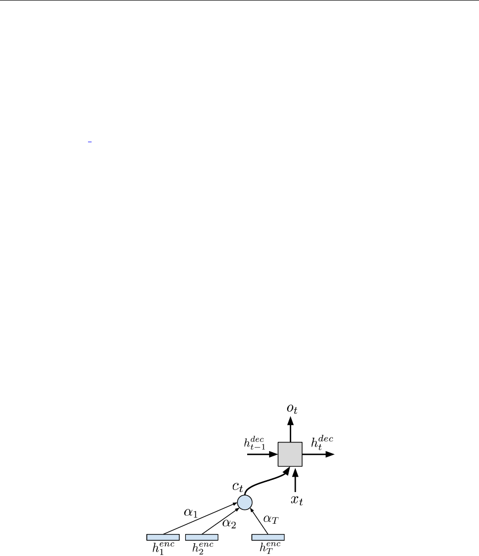
2. We will now apply the AdditiveAttention module to the RNN decoder. You are given

a batch of decoder hidden states as the query, hdec

t−1, for time t−1, which has dimension

batch_size x hidden_size, and a batch of encoder hidden states as the keys and values,

henc = [henc

1, . . . , henc

i, . . . ] (annotations), for each timestep in the input sequence, which has

dimension batch_size x seq_len x hidden_size.

Qt←hdec

t−1, K ←henc, V ←henc

We will use these as the inputs to the self.attention to obtain the context. The output

context vector is concatenated with the input vector and passed into the decoder GRU cell

at each time step, as shown in Figure 4.

...

enc

α1αT

Figure 4: Computing a context vector with attention.

Fill in the forward method of the RNNAttentionDecoder class, to implement the interface

shown in Figure 4. You will need to:

(a) Compute the context vector and the attention weights using self.attention

(b) Concatenate the context vector with the current decoder input.

CSC421 Winter 2019 Programming Assignment 3

3. Train the Attention RNN in the “Training - RNN attention decoder” section. How do the

results compare to RNN decoder without attention for certain type of words? Can you identity

any failure mode? How does the training speed compare? Why?

4. In lecture, we learnt about Scaled Dot-product Attention used in the transformer models. The

function fis a dot product between the linearly transformed query and keys using weight

matrices Wqand Wk:

˜α(t)

i=f(Qt, Ki) = (WqQt)T(WkKi)

√d,

α(t)

i= softmax(˜α(t))i,

ct=

i=1

α(t)

iWvVi,

where, dis the dimension of the query and the Wvdenotes weight matrix project the value

to produce the ﬁnal context vectors.

Implement the scaled dot-product attention mechanism. Fill in the __init__ and

forward methods of the ScaledDotAttention class. Use the PyTorch torch.bmm to compute

the dot product between the batched queries and the batched keys in the forward pass of

the ScaledDotAttention class for the unnormalized attention weights. Your forward pass

needs to work with both 2D query tensor (batch_size x (1) x hidden_size)and 3D

query tensor (batch_size x k x hidden_size).

Because we use the same interface between diﬀerent attention modules, we can reuse the

previous RNN attention decoder with the scaled dot-product attention.

Train the Attention RNN using scaled dot-product attention in the “Training - RNN scaled

dot-product attention decoder” section. How do the results and training speed compare to

the additive attention? Why is there such diﬀerent?

Part 5: Attention is All You Need [2 mark]

1. What are the advantages and disadvantages of using additive attention vs scaled dot-product

attention? List one advantage and one disadvantage for each method.

2. Fill in the forward method in the CausalScaledDotAttention. It will be mostly the same

as the ScaledDotAttention class. The additional computation is to mask out the attention

to the future time steps. You will need to add self.neg_inf to some of the entries in the

unnormalized attention weights. You may ﬁnd torch.tril handy for this part.

3. We will now use ScaledDotAttention as the building blocks for a simpliﬁed transformer[3]

decoder. You are given a batch of decoder input embeddings, xdec across all time steps,

which has dimension batch_size x decoder_seq_len x hidden_size. and a batch of en-

coder hidden states, henc = [henc

1, . . . , henc

i, . . . ] (annotations), for each time step in the input

sequence, which has dimension batch_size x encoder_seq_len x hidden_size.

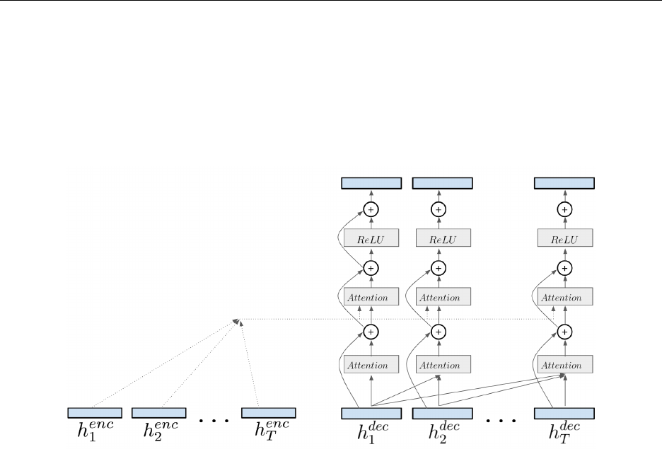
The transformer solves the translation problem using layers of attention modules. In each

layer, we ﬁrst apply the CausalScaledDotAttention self-attention to the decoder inputs

CSC421 Winter 2019 Programming Assignment 3

followed by ScaledDotAttention attention module to the encoder annotations, similar to

the attention decoder from the previous question. The output of the attention layers are fed

into an hidden layer using ReLU activation. The ﬁnal output of the last transformer layer are

passed to the self.out to compute the word prediction. To improve the optimization, we add

residual connections between the attention layers and ReLU layers. The simple transformer

architecture is shown in Figure 5

Figure 5: Computing the output of a transformer layer.

Fill in the forward method of the TransformerDecoder class, to implement the interface

shown in Figure 5.

Train the transformer in the “Training - Transformer decoder” section. How do the translation

results compare to the previous decoders? How does the training speed compare?

4. Modify the transformer decoder __init__ to use non-causal attention for both self attention

and encoder attention. What do you observe when training this modiﬁed transformer? How

do the results compare with the causal model? Why?

5. In the lecture, we mentioned the transformer encoder will be able to learn the ordering of its

inputs without the explicit positional encoding. Why does our simple transformer decoder

work without the positional encoding?

Part 6: Attention Visualizations [2 marks]

One of the beneﬁts of using attention is that it allows us to gain insight into the inner workings

of the model. By visualizing the attention weights generated for the input tokens in each decoder

step, we can see where the model focuses while producing each output token. In this part of the

assignment, you will visualize the attention learned by your model, and try to ﬁnd interesting

success and failure modes that illustrate its behaviour.

The Attention visualization section loads the model you trained from the previous section

and uses it to translate a given set of words: it prints the translations and display heatmaps to

show how attention is used at each step. endcenter

CSC421 Winter 2019 Programming Assignment 3

1. Visualize diﬀerent attention models using your own word by modifying TEST_WORD_ATTN.

Since the model operates at the character-level, the input doesn’t even have to be a real word

in the dictionary. You can be creative! You should examine the generated attention maps.

Try to ﬁnd failure cases, and hypothesize about why they occur. Some interesting classes of

words you may want to try are:

•Words that begin with a single consonant (e.g., cake).

•Words that begin with two or more consonants (e.g., drink).

•Words that have unusual/rare letter combinations (e.g., aardvark).

•Compound words consisting of two words separated by a dash (e.g., well-mannered).

These are the hardest class of words present in the training data, because they are

long, and because the rules of Pig-Latin dictate that each part of the word (e.g., well

and mannered) must be translated separately, and stuck back together with a dash:

ellway-annerdmay.

•Made-up words or toy examples to show a particular behaviour.

Include attention maps for both success and failure cases in your writeup, along

with your hypothesis about why the models succeeds or fails.

What you need to submit

•One code ﬁle: nmt.ipynb.

•A PDF document titled a3-writeup.pdf containing your answers to the conceptual questions,

and the attention visualizations, with explanations.

References

[1] Samy Bengio, Oriol Vinyals, Navdeep Jaitly, and Noam Shazeer. Scheduled sampling for se-

quence prediction with recurrent neural networks. In Advances in Neural Information Processing

Systems, pages 1171–1179, 2015.

[2] Ilya Sutskever, Oriol Vinyals, and Quoc V Le. Sequence to sequence learning with neural

networks. In Advances in neural information processing systems, pages 3104–3112, 2014.

[3] Ashish Vaswani, Noam Shazeer, Niki Parmar, Jakob Uszkoreit, Llion Jones, Aidan N Gomez,

Lukasz Kaiser, and Illia Polosukhin. Attention is all you need. In Advances in Neural Informa-

tion Processing Systems, pages 5998–6008, 2017.

Instructions

Navigation menu

Versions of this User Manual:

Views

Navigation