Instructions For Using Simple Dyno 6.5
User Manual:
Open the PDF directly: View PDF ![]() .
.
Page Count: 40
SimpleDyno Manual v3.0, Nov 2013
Page 1 of 40
Instructions for Using SimpleDyno
Welcome to SimpleDyno, a free application to support DIY dyno projects. This document describes the
features of SimpleDyno software and how to use it to measure the performance of motors or vehicles.
Note: This document does not cover dyno construction or data acquisition hardware in great detail.
Note: Many of the images presented are screen captures from version 6.3 and not the current version.
Problems, questions, or comments? Please feel free to post them at the SimpleDyno forum:
z7.invisionfree.com/SimpleDyno.
Downloading and Installing the Software
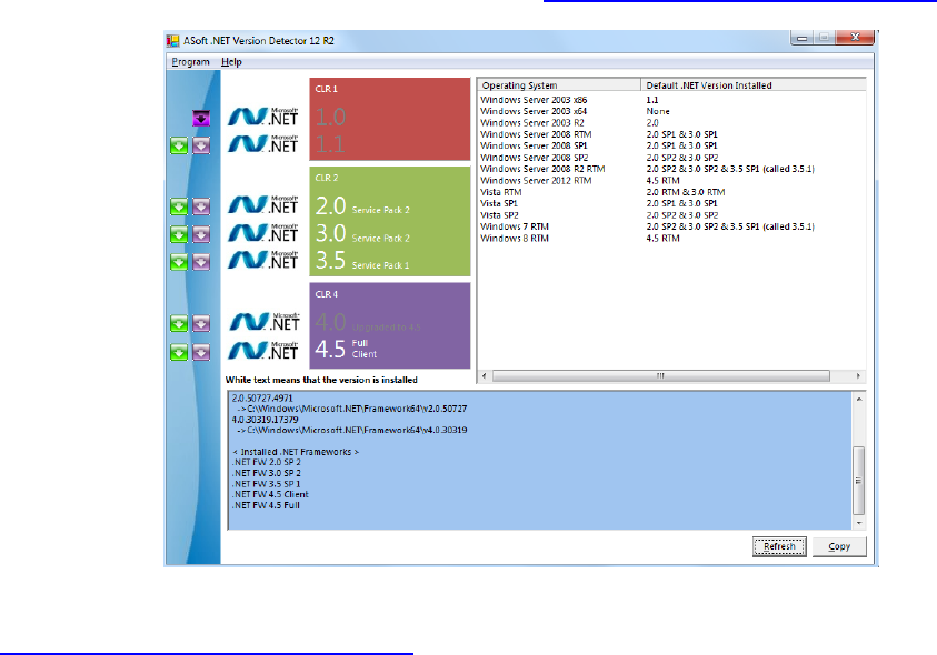
The current Microsoft .NET framework version must be installed for SimpleDyno to run correctly.
Asoft’s .Net Version Detector is an excellent freeware application to check installed.NET framework
versions and update the framework if necessary. Visit http://www.asoft.be/prod_netver.html.
The SimpleDyno application is downloaded as a compressed .zip file from the SimpleDyno website at
https://sites.google.com/site/simpledyno. The latest versions and updates are on the Software page.
The zipped file contains the SimpleDyno.exe application and associated documentation. It also contains
and Arduino Sketch to support using an Arduino Uno microcontroller to expand data acquisition
capabilities (optional).
Download the zipped SimpleDyno release package file and extract the contents to any location.
SimpleDyno Manual v3.0, Nov 2013
Page 2 of 40
First Startup
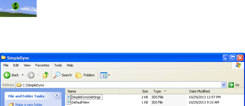
Double click the Simpledyno.exe icon to start the software. The first time SimpleDyno runs it will create
a folder on the C:\ drive called SimpleDyno. This folder contains a settings file (SimpleDynoSettings.sds)
and the basic graphical interface definition (DefaultView.sdi).
The settings file stores all the information required by the software to run such as dyno parameters, last
used graphical interface, calibration curves for Arduino inputs, etc.
The DefaultView interface file stores information on the basic graphical interface (RPM gauge, actual
and maximum RPM labels, and an RPM versus Time plot). This interface is created when SimpleDyno is
first run. The computer’s screen settings and resolution are used to ensure that the interface fits on the
screen. The graphical interface in from version 6.3 onwards is flexible to allow the creation of multiple
interfaces using the building blocks provided (gauges, labels, etc.).
Previously run versions of SimpleDyno will have created the C:\SimpleDyno folder already. There is no
guarantee of backward compatibility between version 6.5 (and higher) and the 5.5 version therefore
existing dyno parameters may need to be re-entered. Note that once version 6.5 is run, it may not be
possible to run the older versions without removing the SimpleDyno folder and allowing SimpleDyno to
recreate the folder from scratch.
SimpleDyno Manual v3.0, Nov 2013
Page 3 of 40
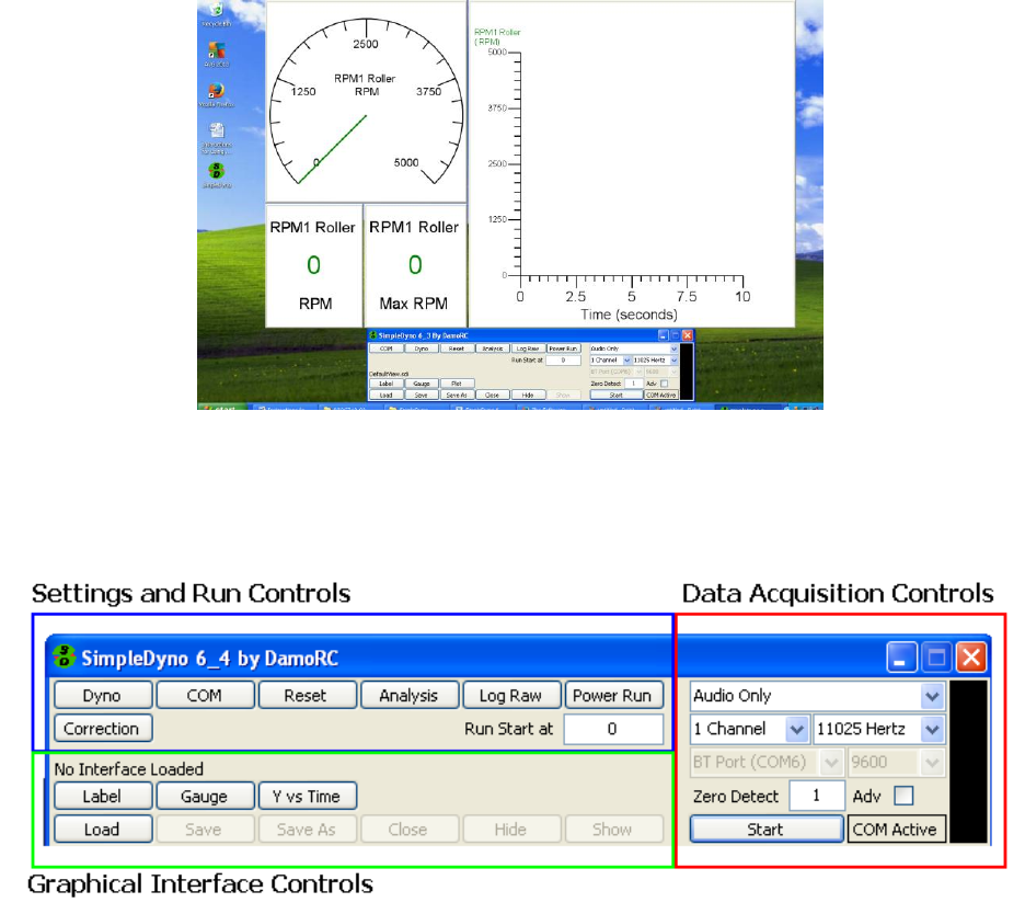
Once the initial setting and interface files are created, the primary application screen and
DefaultView.sdi interface will display.
Primary Application Screen
The following screen capture serves as a reference for the brief descriptions that follow.
Settings and Run Controls
Dyno opens the Dyno Setup window where the parameters that define the physical characteristics of
the dyno are entered.
COM opens the COM Port Calibration window where the parameters required to calibrate inputs
received from an Arduino (or other microcontroller) are entered. Note: Use of the COM port to acquire
data is optional. A microcontroller is not needed to use SimpleDyno 6.3.
Reset All resets actual and maximum data values to 0, minimum data values to 999,999.
SimpleDyno Manual v3.0, Nov 2013
Page 4 of 40
Analysis loads and displays Power Run data to the Data Analysis screen. Various combinations of Power
Run data can be visualized and multiple Power Runs can be overlaid.
Log Raw starts the process of logging data to disk. Logged data is saved as a space delimited .sdr file.
These data can be imported into data analysis applications such as Microsoft Excel. The dataset cannot
be further analyzed by SimpleDyno. Click on Log Raw and provide a filename for the data. The button
will turn red. When SimpleDyno detects the first RPM in the dataset the button will turn green
indicating that data is being collected in memory. If the maximum number of datapoints (50,000) is
exceeded, the button will turn red again. When data collection is complete click on Log Raw again.
SimpleDyno will write the collected data to the filename provided.
Power Run starts the workflow for gathering and processing RPM1 data to establish a Power Curve
Run Start at is the RPM at which Power Run data collection will start. Typically this is zero but some
applications require the dyno to idle at a low RPM prior to initiating a run. Set this value to just above
idling RPM. When RPM1 exceeds this value data collection will begin. Data collection will stop when
RPM1 has dropped to this value.
Correction opens the dyno corrections dialog where Coast Down and atmospheric corrections can be
selected and applied to the torque and power results. Note: Atmospheric corrections are not yet
implemented.
Graphical Interface Controls
Label creates a new SimpleDyno interface component which displays data as text.
Gauge creates a new interface component that displays data in a gauge format
Y vs Time creates a new interface component that displays data as a Y versus time graph.
Load loads a previously saved interface. The loaded interface name is displayed. If no interface is loaded
“No Interface Loaded” will be displayed.
Save saves the current interface, overwriting the previous interface.
Save As saves the current interface as a new file.
Close closes the current interface, removing all components.
Hide hides the current interface without closing it.
Show shows an interface that has been hidden.
Data Acquisition Controls
Data Acquisition Mode. Select a data acquisition mode. Options are Audio Only to use the mic-in jack
for RPM data acquisition; Audio + COM sensing to use the mic-in jack for RPM data and an attached
SimpleDyno Manual v3.0, Nov 2013
Page 5 of 40
microcontroller to collect additional data such as Voltage, Current, etc; and COM Only to collect both
RPM and additional data from an attached microcontroller.
Audio Settings
Number of channels. Select how many channels of RPM data to acquire. This applies to Audio data
collection only. Select 2 Channels if to process second RPM data set (RPM2).
Sample rate. Select the sample rate for Audio data collection. Options are 11025, 22050, and 44100 Hz.
Higher sampling rates typically produce more accurate and precise RPM data, provided the computer
performance is sufficient.
COM Port Settings
Port Selection. Select the virtual COM port to which a microcontroller is attached. Ports are listed by
name and number. Note: Do not attempt to start data acquisition using a COM option unless the
required microcontroller is available and can be selected.
Baud Rate. Select the Baud rate for communications with an attached microcontroller. A list of
commonly used Baud rates is provided. Note: Ensure the selected Baud rate matches that programmed
on the microcontroller.
Zero Detect and Adv settings
Zero Detect sets the time SimpleDyno will wait before deciding that the roller or flywheel has stopped. If
this value is set to 1 second and the dyno is configured to produce one signal for each RPM, any value
less than 60 RPM (or 1 revolution per second) will be considered stopped and RPM will reset to zero.
Note: The Zero Detect applies to both RPM1 and RPM2 data acquired either by Audio (mic-in) or by
COM port. The setting is accurate for Audio RPM data. It is less accurate for the COM port data as it
relies upon the data transfer rate between the computer and microcontroller. :Note: When using Log
Raw, the Zero Detect setting determines how often data is collected if the RPM1 value times out to zero.
For example, if Zero Detect is set for 1 second and RPM1 is zero, other data (RPM2, voltage, current etc)
will be collected once every second. .
Adv. Check this box to use Advanced audio stream processing which utilizes a more sophisticated
algorithm to time incoming pulses. This increases RPM1 precision significantly. Advanced analysis adds
some processing overhead but is more efficient than using higher sampling rates. Adv is recommended
for computers that can only support the 11025 Hz sampling rate.
Start and Monitoring
Start will initiate data acquisition based on Audio and/or COM port settings.
The Signal panel displays raw audio data and is used to set signal thresholds for pulse detection. Traces
in this panel are color coded. The red trace is the raw audio data for RPM1, the primary RPM measure.
This is typically the left channel of a stereo input. The green line is the threshold the red trace must
SimpleDyno Manual v3.0, Nov 2013
Page 6 of 40
exceed to be considered part of a pulse. The yellow trace is the raw audio data for RPM2. This is typically
the right channel of a stereo input. The blue line is the threshold the yellow trace must exceed to be
considered part of a pulse. When the mouse enters the signal panel it expands to fill the entire
application window allowing more signal detail to be seen. Left click to set RPM1 threshold (green line).
Right click to set RPM2 threshold (blue line).
COM Active indicator flashes to indicate active communication with a microcontroller.
Using SimpleDyno
Dyno Setup
SimpleDyno was written to support DIY inertia dyno projects by providing a simple way to monitor the
RPM of a dyno roller or flywheel. To calculate torque and power produced, the software needs the
Moment of Inertia (MOI) of the rotating parts. Using basic parameters such as roller diameter, roller
mass etc., SimpleDyno will calculate the dyno MOI. MOI information produced by SimpleDyno can help
in dyno design appropriate for specific vehicles and applications. Open the Dyno Setup window by
clicking the Dyno button.
Note: The Dyno Setup window is designed for roller chassis dynos. However, all relevant information for
a motor flywheel dyno can be entered here.
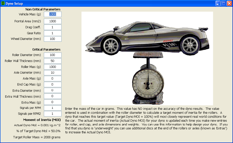
The Dyno Setup window has two data entry areas (Non Critical and Critical Parameters), an MOI display
area (Moment of Inertia), a graphics area, and a descriptive text area. As each field is entered the
SimpleDyno Manual v3.0, Nov 2013
Page 7 of 40
graphics image and descriptive text will change and refer specifically to the associated parameter. The
graphics and descriptive text are sufficiently detailed to guide correct parameter entry, therefore this
document will not explain each parameter in detail. Note: SimpleDyno was initially developed for radio
controlled scale vehicles and therefore all length and mass entries are in millimeter and gram units.
Non Critical Parameters are those that will not impact the primary results produced when running
SimpleDyno, that is, they do not impact the accuracy of RPM detection and they do not impact the MOI.
This means that they will have no effect on RPM1 Roller, Roller Torque and Power results. It is, however,
useful provide accurate values in these fields. For example, the frontal area and drag coefficient values
are used to calculate the drag a vehicle experiences at speed. A vehicle on a chassis dyno will reach
speeds that exceed actual speeds on the ground. SimpleDyno calculates the drag corrected speed for a
vehicle during power runs to provide a realistic value for top speed. Another example is the
combination of wheel diameter and gear ratio settings. SimpleDyno calculates RPM1 Motor and Motor
Torque for a chassis dyno by using the ratio of wheel diameter to roller diameter and the gear ratio.
Accurate entry of these parameters ensures accurate RPM1 Motor and Motor Torque results.
Critical Parameters must be entered correctly and accurately for SimpleDyno to produce accurate
results for RPM, torque, and power.
Note: For motor dynos complete the entries for Roller Diameter and Roller Mass. Also complete entries
for Axle Diameter and Axle Mass depending on the dyno design. If the flywheel is attached directly to
the motor set the Wheel Diameter value to the same value as Roller Diameter and set the Gear Ratio to
1. There is currently no option to display accurate Speed values if SimpleDyno is used to run a motor
dyno.
Moment of Inertia (MOI)
As critical and non critical parameters are updated, SimpleDyno will display three results at the bottom
left hand side of the window, Actual Dyno MOI, % of Target Dyno MOI, and Target Roller Mass. The
Actual Dyno MOI is provided in kg.m2 or g.m2 for “light” dynos. The % Target Dyno MOI provides an
indication of how close the dyno is to representing real world conditions for the vehicle information
provided, specifically the mass of the vehicle. If % Target Dyno MOI is 100% the dyno will provide a real
world load to the vehicle when accelerated from zero RPM. If % Target Dyno MOI is less than 100%, the
dyno is “light” for the vehicle. The dyno will spool up to max RPM in a shorter period of time, and the
vehicle powertrain will not experience an appropriate load. The dyno may reach maximum RPM too
quickly, preventing SimpleDyno from collecting sufficient data to accurately calculate torque and power.
Conversely, if % Target Dyno MOI is greater than 100%, the vehicle’s powertrain will be placed under
greater stress than it would encounter on the ground, essentially simulating increased vehicle weight.
SimpleDyno also calculates the Target Roller Mass to get to 100% Target Dyno MOI. This calculation
takes into consideration all parameters entered for the dyno (diameter, wall thickness, etc.)
By providing you with these MOI data, the Dyno Setup screen can be used to design and build the
optimal dyno for a specific vehicle.
SimpleDyno Manual v3.0, Nov 2013
Page 8 of 40
Note: The % Target Dyno MOI and Target Roller Mass calculation holds true for a vehicle accelerating
from rest. As the vehicle speed increases, the load on the vehicle becomes less than it would on the
ground due to the missing drag component.
Note: The % Target Dyno MOI and Target Roller Mass values are not applicable to motor dynos using a
flywheel. These values can be calculated for a motor flywheel. For help designing a flywheel for a
motor dyno application please post the question to the SimpleDyno Forum.
Audio RPM Detection
The original SimpleDyno application introduced the concept of monitoring RPM by processing
audio/electronic signal data input through the mic-in jack. This is the simplest and easiest way to
monitor RPM using SimpleDyno. The original hardware consisted of a magnet attached to the dyno
roller and a coil attached to the dyno frame. The coil is positioned so that the magnet passes it as the
roller rotates. The coil is attached to the appropriate wires on a head set which has one of the head
phones removed. The headset is plugged into the mic-in jack on a laptop computer. SimpleDyno opens
an audio recording stream which monitors the signal coming into the mic-in jack. Each time the magnet
passes the coil a pulse is detected by the software. By measuring the time between pulses, SimpleDyno
can calculate the RPM of the roller.
A detailed description of the hardware possibilities for Audio RPM detection is beyond the scope of this
document, which focuses on operating the software. Any combination of hardware that can generate a
pulse when the dyno rotates will work. This section of the document will assume that the materials for
the simplest type of sensor are available; a magnet on the dyno roller and a set of stereo headphones.
“Seeing” SimpleDyno Process Audio Data and measuring RPM
(1) Plug the stereo headphones into the mic-in jack and start the SimpleDyno application.
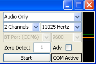
(2) Using the drop-down lists on the right hand side of the application screen select the following
a. “Audio Only”
b. “2 Channels”
c. “11025 Hz”
(3) Click on the start button. A red and yellow trace and green and blue threshold lines should be
visible in the Audio signal monitoring panel.
SimpleDyno Manual v3.0, Nov 2013
Page 9 of 40
(4) Move the mouse over the Audio signal monitoring panel. It should expand to fill the application
window. If the mouse is moved off the expanded panel, it will contract to its original size.
Keeping the mouse over the panel will keep it expanded.
(5) To pin the panel so that it stays expanded move the mouse to the very right hand edge of the
panel until the mouse cursor changes to a Hand shape and left click the panel. To unpin the
panel, repeat this step. Note: There is significantly increased processing overhead when the
panel is expanded. Audio processing speed is improved with the panel at its default size.
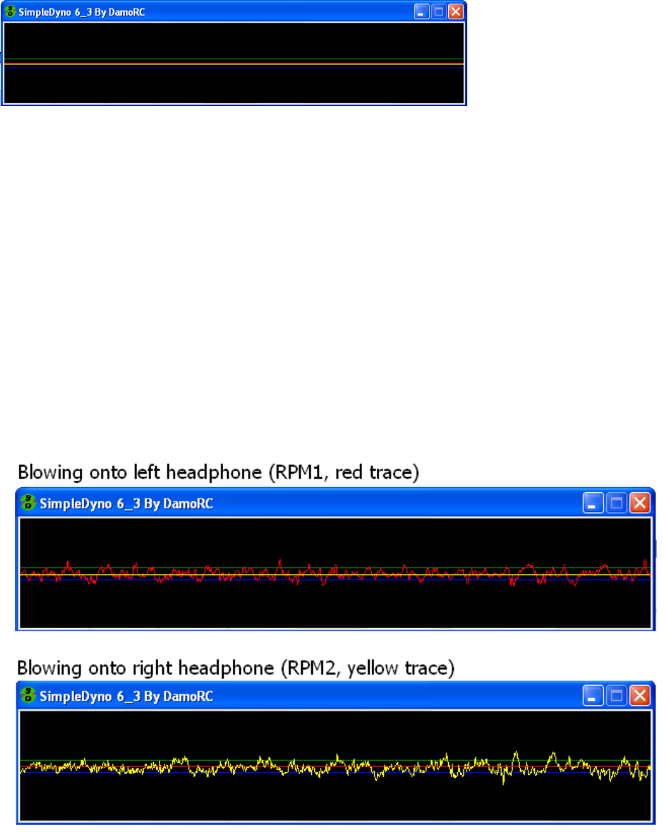
(6) Tap, blow, whistle, or speak into each of the headphones separately. Headphones behave like
small microphones and therefore the red and yellow traces react to the sound. If the traces
don’t react try increasing the audio recording level for the mic-in jack. With different Windows
operating systems and different types of audio hardware, details as to how to increase the audio
recording level are not described here. Typically, right clicking on the speaker icon that is shown
at the bottom right hand side of the desktop will open utilities for adjusting this level. If the
audio recording level is set to max and an audio signal is still not visible confirm that the
operating system has set the default audio recording device to the mic-in or external
microphone as SimpleDyno opens the recording stream on the default recording device. Note:
If both RPM1 and RPM2 (red and yellow traces respectively) respond together regardless of
which headphone is stimulated it is likely that the mic-in line is a mono only line. This means
that a separate RPM2 signal cannot be monitored.
SimpleDyno Manual v3.0, Nov 2013
Page 10 of 40
(7) Confirm which headphone stimulates the RPM1 (red trace) and RPM2 (yellow trace) and label
these headphones as RPM1 and RPM2. The remainder of this section will focus on RPM1 as it is
the primary RPM data channel from which torque and power values are calculated.
(8) Using the RPM1 headphone, try to measure the RPM of the dyno. It is assumed that a roller or
flywheel dyno is available with a magnet attached. Select “1 Channel” from the appropriate
drop down list and click Start. SimpleDyno will stop the current audio recording session and re-
start using the newly selected options. Expand and pin the signal monitoring panel to see the
raw audio signal.
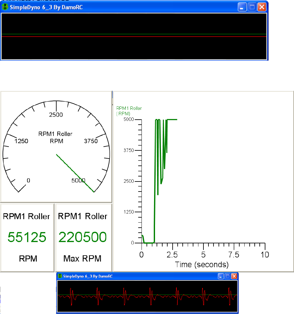
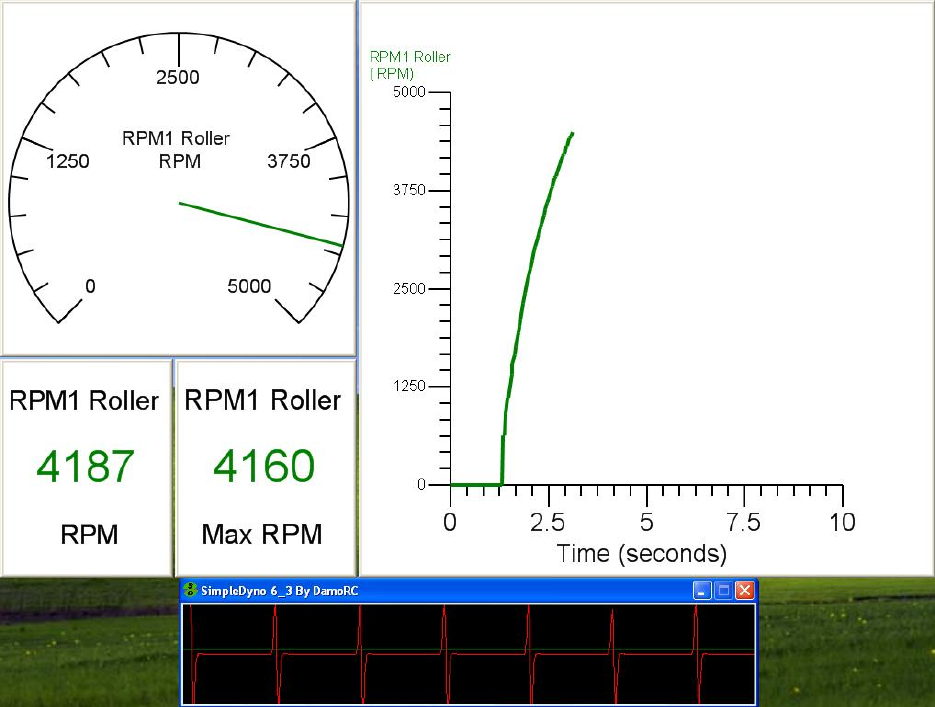
(9) Mount the RPM1 headphone close to the dyno so that as the dyno turns, the magnet passes by
the speaker side of the headphone. Run the dyno and watch the signal panel and RPM1 Roller
gauge and graph. A first attempt may look like the following:
SimpleDyno Manual v3.0, Nov 2013
Page 11 of 40
The graph of RPM1 Roller versus time shows the RPM fluctuating wildly, with a maximum RPM1
of 220,500 RPM being recorded! Although a train of pulses is observable in the signal panel,
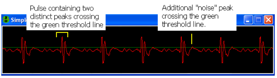
there is considerable noise in the RPM1 (red) signal trace. Examining the trace closely reveals
that each pulse contains two distinct peaks. There is also a third peak between the pulses that
crosses over the green threshold line.
Each time the RPM1 signal crosses the green threshold line, SimpleDyno measures the time
since the last crossover occurred (in the same direction) and uses the time to calculate RPM.
There is a short time between the two peaks within the pulse leading to a high RPM result.
Then there is a gap to the next pulse leading to a lower RPM result. This fluctuating RPM1 value
due to noisy raw audio data is a common problem. It should be noted that the audio signal
quality and RPM fluctuation presented in this example not suitable for generating high quality
data. The main reason for such a poor quality signal in this case is the headphone’s ability to act
like a microphone. In addition to the magnetic pulse the headphone is picking up the noise of
the motor, the dyno, and any other local sound.
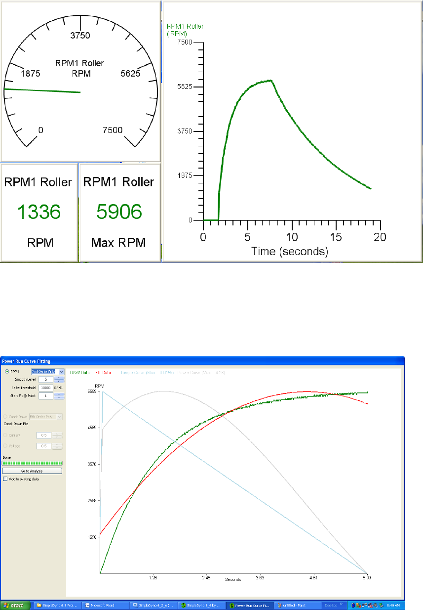
(10) Completely cover the speaker side of the headphone with electrical tape. This makes the
headphone mostly “deaf”. By reducing significantly its ability to detect and transmit audible
noise, the signal quality will be improved. A more effective method is to remove the speaker
cover and fill the space with epoxy. The following screen capture was taken almost immediately
after the previous one, the only difference being that the headphone was wrapped in electrical
tape. The signal quality is improved leading to smooth RPM results.
SimpleDyno Manual v3.0, Nov 2013
Page 12 of 40
(11) Even with a “deafened” headphone, there may be some low level noise in the signal that causes
fluctuations in the RPM results. If these cannot be removed through hardware adjustments, set
the green threshold line to a position where it continues to pick up your main peak but ignores
the noise peak. Left click the signal panel to set the green threshold line. The same procedure
applies to RPM2 noise. Right click the signal panel to set the blue, RPM2, threshold line. Note:
Threshold lines can be set anywhere on the signal panel, above or below the center of the panel.
Magnet/headphone combinations will produce both peak and a trough for each pass of the
magnet. If the noise is a small peak, set the threshold to below the center line so that
SimpleDyno uses the trough for RPM detection (and vice-versa). Generally speaking, it is best to
keep the threshold line as close to the center of the signal panel as possible because the peak
height decreases with lower RPM due to the slower linear speed at which the magnet passes the
headphone. You can increase your peak height by positioning the magnet further away from the
center of rotation of the roller or flywheel. Typically, the magnet should be placed as far away
from the center of rotation as possible to produce the largest signal. Also, the audio recording
level can be reduced such that the noise peak is eliminated but the pulse peak is retained.
Ultimately, producing a high quality signal requires balancing the audio recording level with the
threshold level which will take some experimentation. Note that the signal threshold level is less
SimpleDyno Manual v3.0, Nov 2013
Page 13 of 40
important is your are using a sensor that produces a constant voltage pulse, regardless of RPM,
such as an IR sensor.
(12) Note: The most important component in the magnet/headphone sensor system is the magnet.
The smaller and stronger the magnet, the higher quality the signal. It is easier to improve signal
with a better magnet than removing the headphone and replacing it with a coil.
The Power Run.
A Power Run is a wide open throttle (WOT) run from zero to maximum RPM in as short a time as the
vehicle or motor can accomplish. This maximum acceleration run is how an inertia dyno measures peak
power, the point at which the product of torque and RPM is highest. SimpleDyno can display these
results live. However, even with the cleanest of audio signals and a perfectly balanced dyno, there will
be some slight fluctuation in the RPM measured by SimpleDyno and this fluctuation is magnified
significantly in the calculations for torque and power. To overcome this problem, the Power Run
function collects the data during the run and subjects it to a curve fitting operation which smoothes out
these slight fluctuations, producing smoothed torque and power curves. To execute a power run:
(1) Ensure that sensor hardware is connected and that high quality RPM1 Roller data is being
produced.
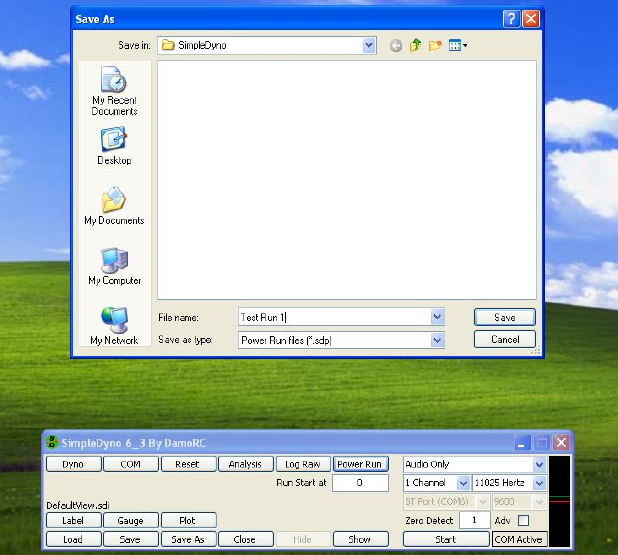
(2) Click the Power Run button.
(3) Provide a filename for the run which will be saved as a space delimited text file with an .sdp
extension. Note: The Power Run button will turn red once a filename has been provided. It will
turn green when the minimum number of points (10) has been collected. If the maximum
number of points (50,000) is exceeded it will turn red again..
SimpleDyno Manual v3.0, Nov 2013
Page 14 of 40
(4) Wide open throttle the vehicle or motor until to maximum RPM. Then allow the dyno to coast to
a stop (or use a brake if the dyno is fitted with one).
(5) When the dyno is stopped the curve fitting process will start. SimpleDyno will open the Curve
Fitting window. The first time SimpleDyno is run the default curve fit model selected will be the
2rd Order Poly (polynomial) model. Note: Depending on the processing speed of your computer,
the size of the data set, and how well it fits the selected model the amount of time taken to
complete the curve fit can vary from a few seconds up to a minute. A progress bar indicates that
the software is processing the data.
SimpleDyno Manual v3.0, Nov 2013
Page 15 of 40
(6) The goal in the Power Run Curve Fitting window is to find a curve fit that closely models the
data. The green trace is raw RPM data. The red trace is the curve fit model produced by
SimpleDyno. Additional traces are provided to show what the torque (pale blue) and power
(pale gray) curves will look like in the final analysis and the maximum torque and power results
for the current fit are presented at the top of the window in N.m and Watts respectively. Note:
the addition of the torque and power traces is to allow examination of the shape of these curves
and not to maximize torque or power results. These traces are particularly useful when using
the MA smooth fitting model. In the previous figure, the 2rd Order Poly model does not fit the
data well, that is, the green (raw data) and red (fitted data) do not overlay well. This example
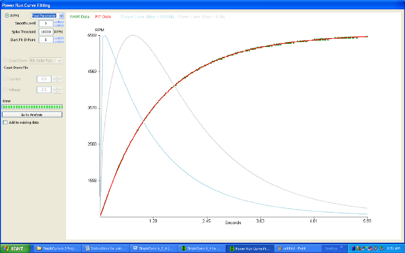
run is a small brushed electric motor dyno and therefore the Four Parameter model fits the data
well. Select various models from the drop down list until the optimal curve fit is found. Note:
Once the optimal model is found, the same model should apply to subsequent Power Runs.
There is typically no need to test all of the models for each run. The same raw data is presented
in the next figure using the Four Parameter fit model. The raw and fit curves are almost
perfectly overlaid making this a good fit.
(7) Occasionally, a curve fit that should work well with the data set, does not produce a satisfactory
fit. This can be due to problems with the first few data points in the raw data set. The software
can be directed to refit the data skipping the initial data points by changing the Start Fit @ Point
field.
(8) If the raw data set suffered from a spike during the run, SimpleDyno will remove the spike based
in the value entered for Spike Threshold. Any data point that differs from its neighboring data
points by this amount will be considered a spike and be removed from the curve fit. Note: Care
should be taken in setting this value. Setting the value too low has the potential to remove key
data points from the beginning of the run. Note: The spike threshold value is also applied to
spike removal from the Coast Down data set.
SimpleDyno Manual v3.0, Nov 2013
Page 16 of 40
(9) Using the MA Smooth Fitting Option. Some engine and dyno setups will produce data that is
not easily constrained to a mathematical model. Typically larger internal combustion engines
fall into this category. Rather than use a poorly fitting mathematical model, SimpleDyno offers a
smoothing option. The option currently available (Version 6.4) is a moving average smoothing
process. The following example data is courtesy of Makr (a.k.a. Mark) and was generated on a
motor flywheel dyno by a motorbike engine developing approximately 100 HP.
SimpleDyno Manual v3.0, Nov 2013
Page 17 of 40
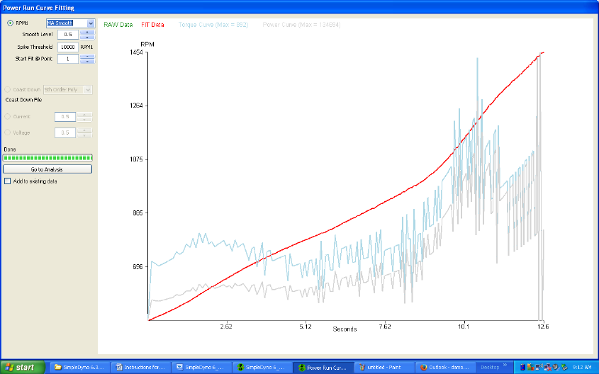
(10) In the figure above the data was smoothed using the lowest smoothing level of 0.5. This will
typically produce power and torque curves that are almost identical to using the raw data and
therefore will be extremely noisy and unusable. Note that the red fit trace perfectly overlays
the green raw data trace so that it is difficult to see the raw data. Increasing the smoothing level
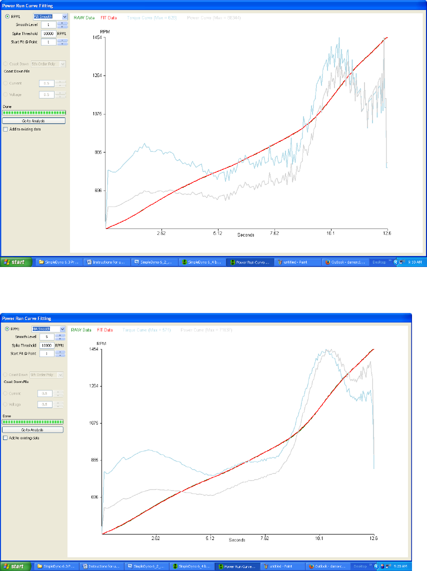
to 1.0 produces the following result.
Although the power and torque curves are still noisy, the bigger picture of torque and power
development is somewhat clearer. Note that the raw and fit data traces are still perfectly
overlayed. Increasing the smoothing level to 5.0 produces the following result.
SimpleDyno Manual v3.0, Nov 2013
Page 18 of 40
Now the data look reasonable for use. There are some minor deviations between the raw and
fit data but overall the fit is good and the power and torque curves are appropriately smoothed.
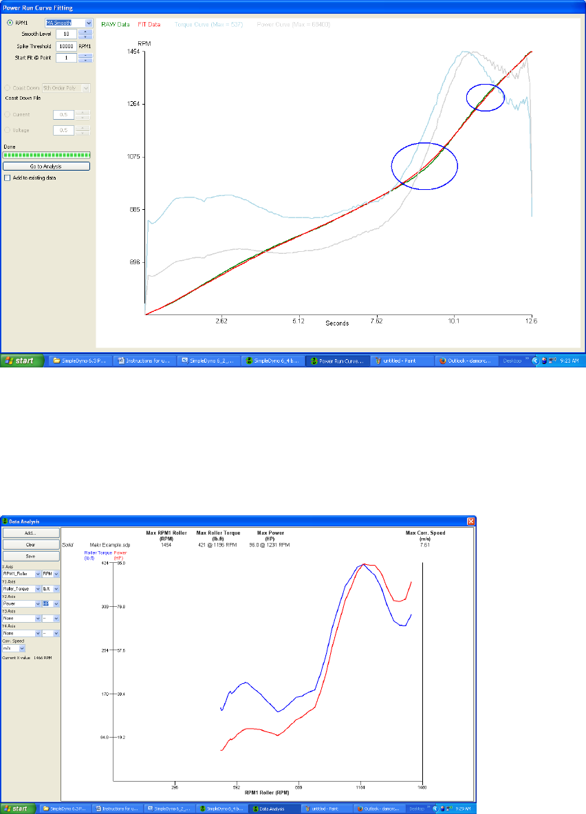
If the data processed further using a smoothing level of 10.0 the following results are observed.
Although the power and torque curves still look good, there are gaps appearing between the
raw and fit data sets as indicated by the blue ovals. This indicates that the smoothing level is too
high and should be scaled back. Using the MA Smooth fit model is a balance between smoothest
possible power and torque curves with little or no deviation between the raw and fit data,
particularly around areas of interest such as peak power or torque. Returning the smoothing
level to 5.0 and examining the data in the Analysis screen shows that this smoothing level is
appropriate for these data.
SimpleDyno Manual v3.0, Nov 2013
Page 19 of 40
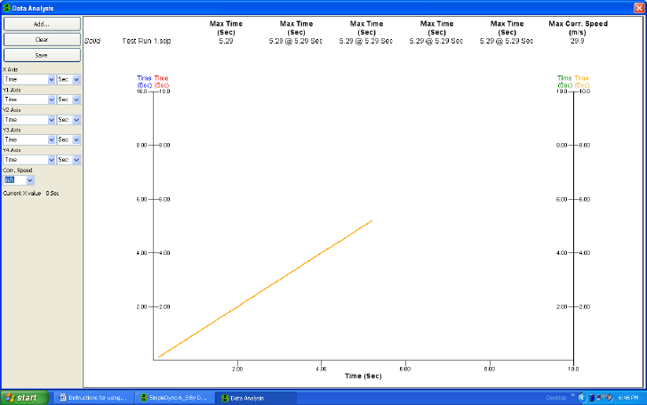
(11) Once the optimal model is found, click the Go to Analysis button. The first time the Data Analysis
window loads, all of the axes will be set to “Time”.
(12) Typically, power runs are plotted against RPM. Select the following options from the described
drop down lists.
a. X Axis : RPM1 Roller (also select RPM units)
b. Y1 Axis: Roller Torque
c. Y2 Axis: Power
d. Y3 Axis: Speed (also select MPH units)
e. Y4 Axis: None
f. Corr. Speed: MPH
SimpleDyno Manual v3.0, Nov 2013
Page 20 of 40
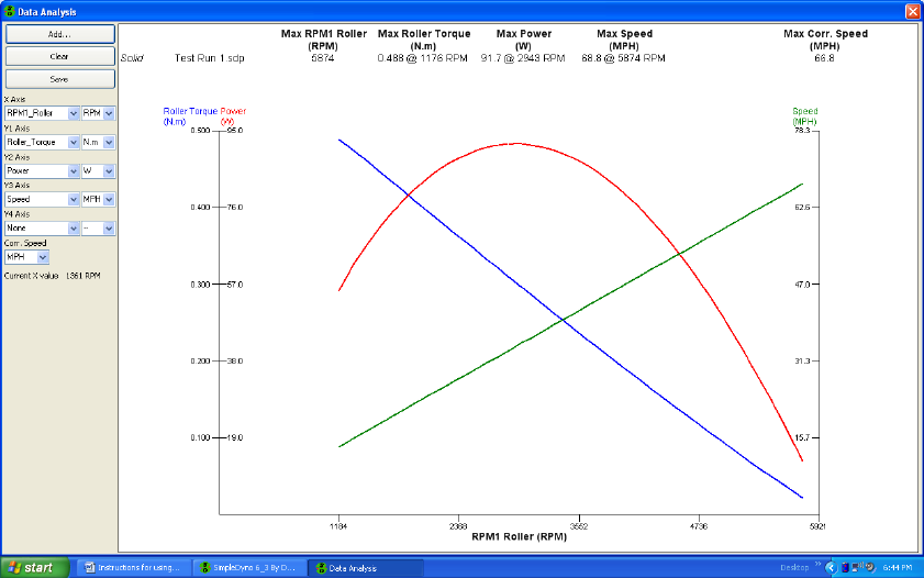
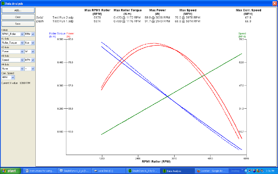
(13) The Data Analysis window displays the data so that torque and power curves are clear.
Maximum results are shown at the top of the screen. To see data for a specific part of the run
click on the graph at that point. To see maximum results again, click on the graph outside of the
area contained by the axes. Note: The presented Corr. Speed results are the maximum speed
the vehicle would have reached if power losses due to drag were considered.
(14) To cancel a Power Run after providing a file name, click the Power Run button again. If
SimpleDyno has already moved onto the curve fitting screen, click on the Stop Fitting button to
stop the curve fitting process.
(15) Use the Spike Threshold setting in the Power Run Curve Fitting screen to filter out occasional
spikes. Note: The Spike threshold should only be used if one or two large spikes appear in the
Power Run raw data.
(16) The fit can sometimes benefit from skipping the first few points of raw data. This is achieved
using the “Start Fit at Point” field. This is typically not needed.
(17) If Voltage and Current data was recorded during the power run these data can be selected for
smoothing. Modify the smoothing level required using the up/down arrows.
Dyno Corrections
SimpleDyno 6.4 introduces a Coast Down correction feature for adjusting torque and power results
based on dyno or drivetrain losses.. The coast down RPM data of the dyno are subjected to a curve
fitting algorithm and the Coast Down Torque and Power results are generated. These results are then
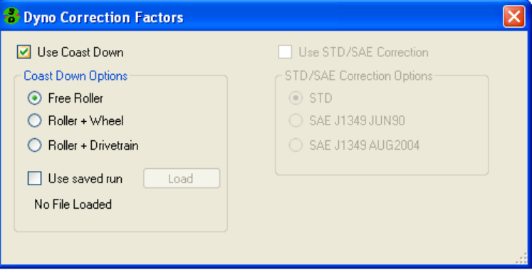
used to modify (typically increase) the Power Run torque and power results. To setup this feature, click
the Correction button on the primary application screen. To use coast down correction, first check the
Use Coast Down checkbox. Then select the type of coast down configuration you are going to use.
There are three options available, Free Roller, Roller + Wheel, and Roller + Drivetrain. The type of
SimpleDyno Manual v3.0, Nov 2013
Page 21 of 40
configuration you choose controls how the coast down corrections are applied.
Free Roller is appropriate for those dyno configurations where all motor and drivetrain components can
be physically disengaged from the roller or flywheel once maximum RPM is reached. An example is an
RC chassis dyno where the vehicle can be physically lifted off the rollers when the Power Run maximum
RPM is reached. The coast down torque and power data represent the parasitic losses of the roller or
flywheel only. These losses are added back to the roller torque and power results and, subsequently,
used to adjust wheel and motor torque and power. Therefore Corrected Roller, Corrected Wheel and
Corrected Motor results for Torque and Power are all adjusted.
Roller + Wheel is appropriate for those dyno configurations where the motor and drivetrain can be
disengaged from the vehicle wheels at maximum RPM so that the losses now represent those created by
wheel contact with the roller and the rollers own losses. An example of this configuration would be a
bike dyno where the wheel has a freewheel capability. The losses are added back to the wheel torque
and power results and subsequently used to adjust motor torque and power. Therefore Corrected
Wheel and Corrected Motor results for Torque and Power are adjusted. Corrected Roller results are
not adjusted.
Roller + Drivetrain is appropriate for those dyno configurations where the motor can be disengaged
from the drivetrain, wheel and roller at maximum RPM so that the losses represent those of the entire
system except for the motor. An example of this type of configuration is any vehicle chassis dyno where
the motor can be disengaged with a conventional clutch. The losses are added back to the motor torque
and power results only. Therefore, Corrected Motor results are adjusted. Corrected Roller and
Corrected Wheel results are not adjusted.
Note: The Free Roller coast down feature is the most justifiable loss correction configuration that can
be used. Although the Roller + Wheel and Roller + Drivetrain loss adjustments are available, the user
should think carefully about the impact of these corrections on true Torque and Power results.
SimpleDyno Manual v3.0, Nov 2013
Page 22 of 40
Once the “Use Coast Down” feature is selected and the type of run down model is chosen, this
correction applies to all Power Runs performed in a session. If SimpleDyno is closed and re-started, the
Correction information must be re-entered for the new session.
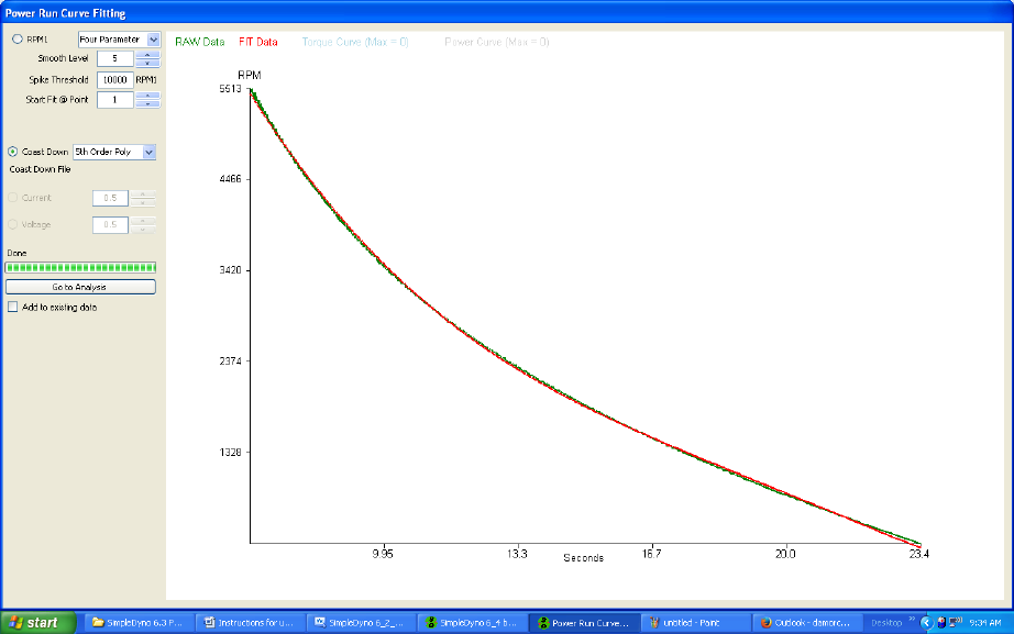
The Coast Down data must be processed using curve fitting or smoothing algorithms in the same way
that the Power Run acceleration data is handled. If Use Coast Down is selected, an additional curve
fitting operation will be performed by the software on the deceleration phase of the run. Using the
electric motor data previously presented and having selected the Free Roller option, the curve fitting
screen will look as follows.
SimpleDyno Manual v3.0, Nov 2013
Page 23 of 40
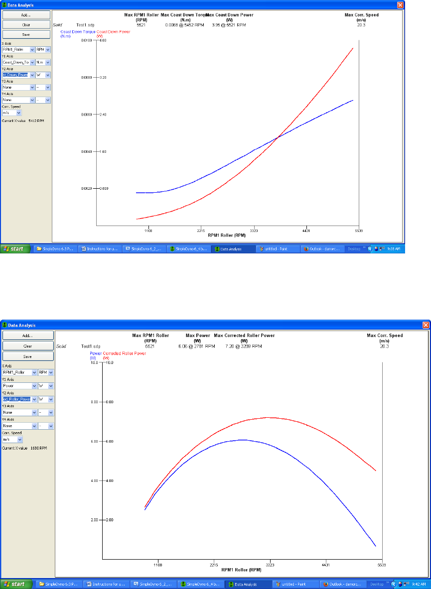
The Coast Down was fitted using the 5th Order Poly fit in this example. Moving to the Analysis screen
and selecting Coast Down Torque and Coast Down Power for display looks as follows.
These are
torque and power losses over the RPM range. These losses are used to correct torque and power results
for the roller, wheel, and motor as described earlier (depending on the Coast Down option selected).
For example, these are the results from this run when the Power and Corrected Roller Power are plotted
in the Analysis screen.
SimpleDyno Manual v3.0, Nov 2013
Page 24 of 40
Using a Saved Run for Correction
You can use the coast down data from a previous run to adjust all Power Runs in a single session. For
example, if you have already created a Free Roller run down data set for your dyno, you can apply this
data set to all subsequent power runs if needed. To use a previously saved Power Run for correction,
simply check the “Use saved run” checkbox and click on Load to load the previously saved coast down
data. Note: If the file selected was not processed for coast down data it cannot be used. Also, the way
in which the coast down data was used in the saved file will be applied. For example, if the loaded file
was processed using the Free Roller option for coast down correction, the coast down losses contained
in the file can only be applied as Free Roller corrections.
Data Analysis
The Data Analysis window is used to examine Power Run files. It can be also used to overlay multiple
files to compare different runs. The Data Analysis window appears automatically as part of the Power
Run workflow. It can also be opened by clicking the Analysis button on the primary application screen.
Currently a maximum of five files can be overlaid. Use Add… to add files, Clear to remove all files and
Save to save and image of the overlaid results. SimpleDyno distinguishes individual runs graphically by
using solid, dashed and dotted lines. Note: All available SimpleDyno parameters are available for
plotting in the Data Analysis window. However, if a parameter is selected for which no data was
collected during the run (for example, Voltage data during Power Run that used Audio Only as the data
acquisition mode), it will be displayed as a flat line of zero values. Note: SimpleDyno 6.3 offers
backwards compatibility with version 5.5 power run files.
SimpleDyno Manual v3.0, Nov 2013
Page 25 of 40
The Graphical Interface
SimpleDyno 6.3 introduces a new graphical interface for viewing live data. The interface approach is
more flexible than the old fixed window layout and allows viewing of as many or as few parameters as
needed in a number of different formats. Each interface component can be moved and resized and color
and font options are available.
A SimpleDyno interface is built using interface components. In version 6.3 the available components are
Label, Gauge and Y vs Time. When first run, SimpleDyno creates a DefaultView interface comprising of
two vertical Labels, a 270 degree Gauge and a Y vs Time with RPM1 Roller selected as the only Y Axis.
The buttons Load, Save, Save As, and Close apply to all of the components as a group and their functions
do not require detailed explanation. Hide and Show also apply to the components as a group. All
components created by SimpleDyno are coded to be on top of everything else on the desktop.
Switching from SimpleDyno to another application will cause the primary application screen to move to
the background but the interface components will not. They will insist on being visible at all times. Use
the Hide and Show buttons to control the visibility of the interface.
All of the interface components share a number of common characteristics which are as follows:
(1) To move a component, click the component anywhere inside its frame and drag the component
to the new position.
(2) To resize a component, click and drag its frame as with any Windows form. Note: When moving
or resizing a component, a snap-to-grid type function is used to help keep sizes uniform and
layout aligned.
(3) To remove a component from the interface, double click the component anywhere inside its
frame. Note: Components cannot be hidden individually. Double clicking a component
permanently removes it from the interface being displayed. However this change is not written
to file unless the interface is saved using Save or Save As.
(4) To assign a value or to configure a component, right click anywhere inside the component and
the component menu will be displayed.
The Label component will be used to demonstrate how to use the new graphical interface.
The Label
The Label component displays the selected parameter value as text.
(1) Start SimpleDyno. The DefaultView interface will load. Click the Close button to close the
interface.
SimpleDyno Manual v3.0, Nov 2013
Page 26 of 40
(2) Click the Label button to create a new Label.
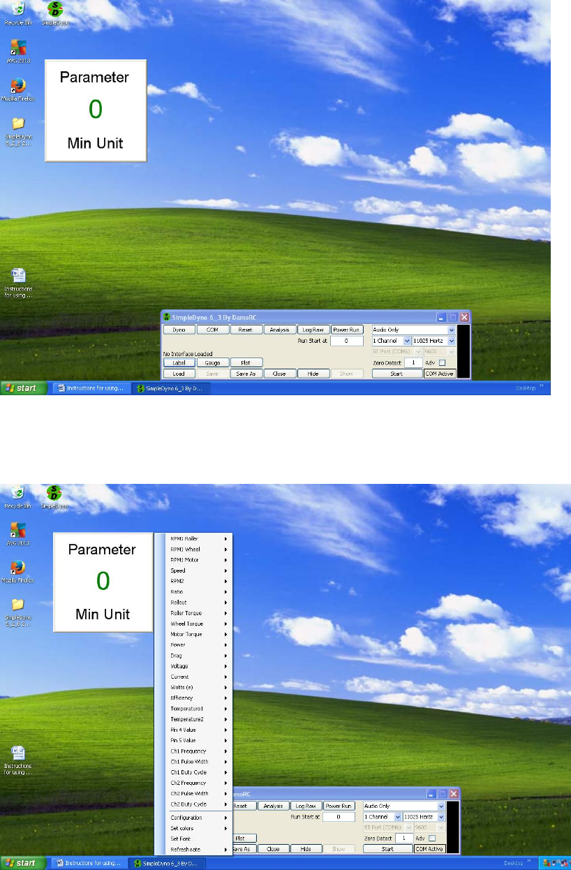
(3) Right click inside the Label frame to open the component menu. The component menu is
divided into two sections. The upper section lists all of the parameters that SimpleDyno makes
available for display. The lower section lists component specific options and formatting
functions.
SimpleDyno Manual v3.0, Nov 2013
Page 27 of 40
(4) Note: If data acquisition has not been started, the component menu will list all possible
parameters available for display. Once data acquisition is started, the component menu will
limit the available parameters to those appropriate for the data acquisition setup. For example,
using 1 Channel, Audio only data acquisition will produce the following truncated component
menu.
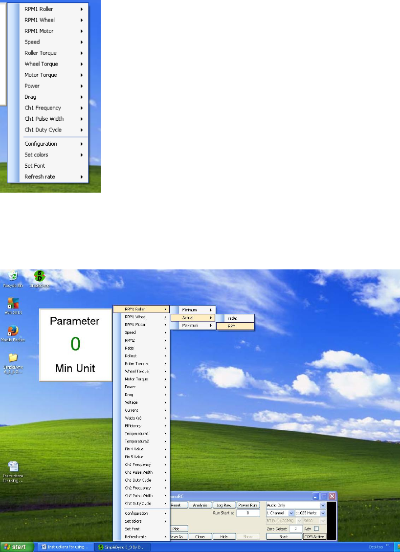
(5) Configure the Label to display the current RPM1 Roller data in units of RPM. As RPM1 Roller is
selected, a sub menu item for Minimum, Actual, or Maximum will appear. As Actual is selected
(for the live value) another sub menu item listing the units rads/s and RPM will appear. Select
the RPM option. Note: All of the component menu items operate in this fashion, that is, follow a
path of sub menu items to its final destination to complete the operation.
SimpleDyno Manual v3.0, Nov 2013
Page 28 of 40
(6) The label is now connected to a data parameter. Once the data parameter is selected, the
component is active and will be monitoring and displaying the appropriate data.
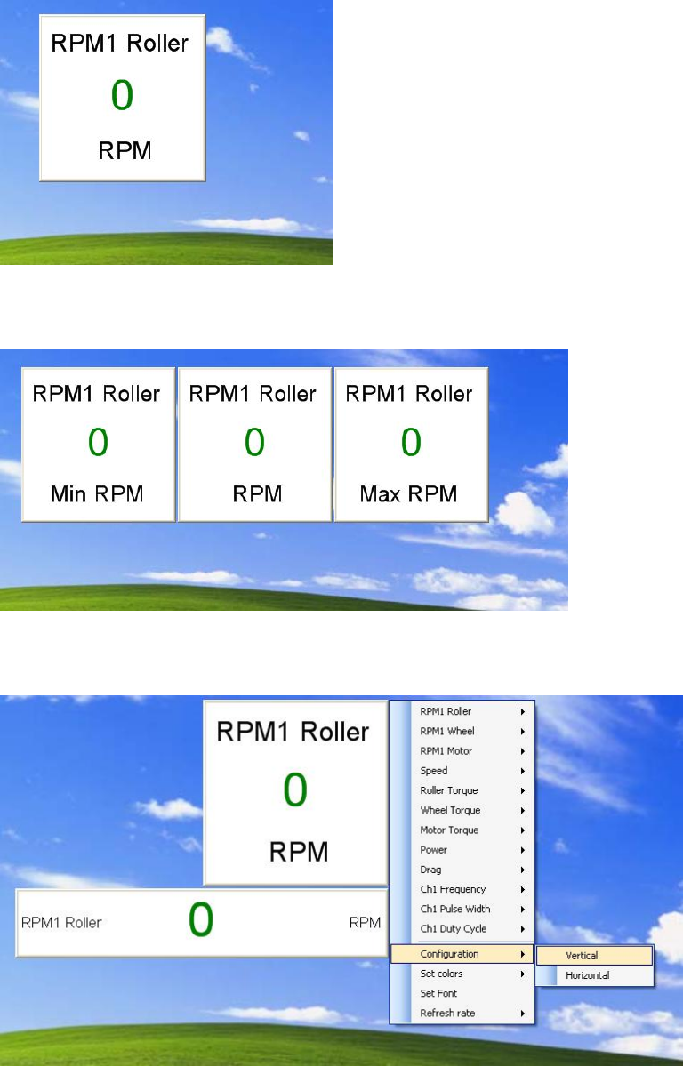
(7) Note: For Actual (live) data, only the unit name is displayed. For Minimum and Maximum data,
the unit is prefixed with Min and Max respectively. Here are three labels for Minimum, Actual
and Maximum RPM1 Roller data.
(8) Configuration. Each component has its own specific configuration. In the case of the Label
component these are Vertical and Horizontal, which adjust how the parameter name and units
are displayed relative to the data value.
SimpleDyno Manual v3.0, Nov 2013
Page 29 of 40
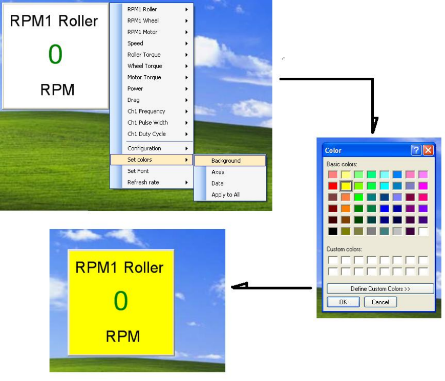
(9) Set Colors. Each component has a Set Colors option which is common to all components. This
allows the selection of colors for various parts of the component. The available options are
Background, Axes, Data, and Apply to All. When Background, Axes, or Data are selected
SimpleDyno opens a color selection dialog for color selection. When Apply to All is selected, the
colors for that component are applied to all other visible components. For the Label control,
setting the Axes color sets the color used to write the parameter name and units.
SimpleDyno Manual v3.0, Nov 2013
Page 30 of 40
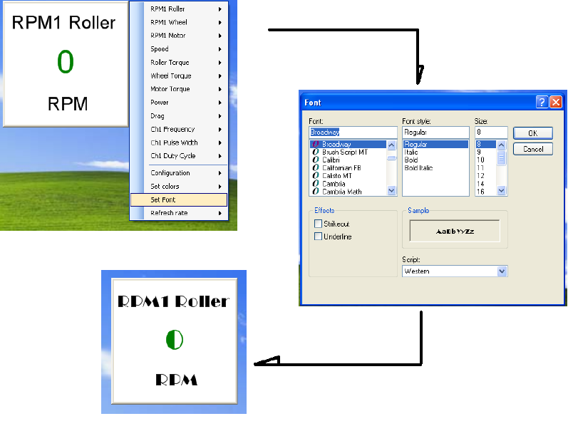
(10) Set Font. Each component has a Set Font option which will open a Font dialog. The font
selection applies to all of the text displayed in the component. Note: Although all available fonts
are presented for selection, some fonts do not meet certain software requirements to allow
SimpleDyno to use them. If these are selected, SimpleDyno will revert to the previously used
font. Note: The font selection process ignores any selections for bold, italic, etc. It also ignores
any font size selections made as these are calculated by SimpleDyno to ensure all text fits
appropriately on the component.
(11) Refresh Rate. Each component has a setting for Refresh Rate which sets the component’s
internal timer controlling the interval between each call to SimpleDyno for new data. The
default time is 1000 miliseconds (ms) which is 1 second. This is appropriate for a Label
component as the data in the component need to be read. For graphical representation of data
such as the Gauge and Y vs Time components, a higher Refresh Rate may be appropriate for
smooth operation. Note: Higher refresh rates requires the computer to work harder to update
the components. Using more components with higher refresh rates can impact SimpleDyno’s
performance, most notably in processing high sample rate Audio data.
SimpleDyno Manual v3.0, Nov 2013
Page 31 of 40
The Gauge
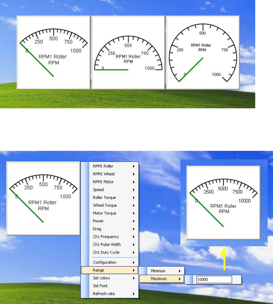
The Gauge component provides a gauge representation of data. The previously described functionality
of the Label component applies also to the Gauge component. The configurations available in 6.3 and
6.4 versions for the Gauge component are 90, 180 and 270 degree dials, all upward pointing. Version 6.5
introduces a totally configurable gauge allowing the gauge arc width (degrees) and point direction
(degrees) to be set. Version 6.5 also allows the sweep direction of the gauge to be clockwise or
anticlockwise.
The Gauge component also has a Range option which is used to set the Minimum and Maximum display
values for the Gauge. Follow the sub menu items under Range to the text box and enter the value for
Minimum or Maximum. You MUST press Enter after inputting the new value to apply it to the
component.
SimpleDyno Manual v3.0, Nov 2013
Page 32 of 40
The Y vs Time Component
The Y vs Time component graphs selected parameter(s) on the Y axes against Time (seconds) on the X-
Axis. All of the previously described functionality is available with the Y vs Time component. The
configuration options for the Y vs Time component are Lines and Points where data will be displayed as
joined lines or separated points respectively. Each axis also has Minimum and Maximum Range options
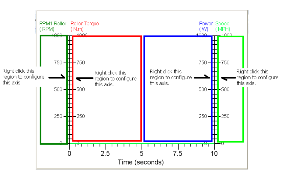
The default Y vs Time component displays a single Y parameter versus Time. Up to four different
parameters can be dilsplayed on the one Y vs Time component. Additional parameters can be added to
the plot by right clicking the component. Use the following as a reference to add, remove, or configure
additional axes/parameters. Minimum and Maximum Range values for the X Axis can be set from any
visible component menu.
SimpleDyno Manual v3.0, Nov 2013
Page 33 of 40
Using a Microcontroller with SimpleDyno
A microcontroller can be used with SimpleDyno to add data acquisition functionality. This functionality
was developed with the Arduino Uno platform but any microcontroller that can perform serial
communication through a virtual COM port can be used. The Arduino was chosen for development due
to its ease of use both from a hardware and firmware / software standpoint. If a different
microcontroller is to be used, see the end of the section for the communication requirements. The rest
of this section will refer generally to the Uno platform.
Preparing the Arduino Uno for use with SimpleDyno
For any microcontroller to be used with SimpleDyno, it must be programmed. A description of how to
program the Arduino Uno is beyond the scope of this document. However, there is an enormous
amount of information available for using this platform. The first place to visit is the Arduino website at
www.arduino.cc. The software required to program your Uno can be downloaded from this site. This
software creates programs known as Sketch files which are uploaded to the microcontroller. The Sketch
file required to program an Arduino to work with SimpleDyno is included in the SimpleDyno zipped file
(SD6_3 Sketch.ino). Follow the instructions at the Arduino website for compiling and uploading this
Sketch file to the microcontroller.
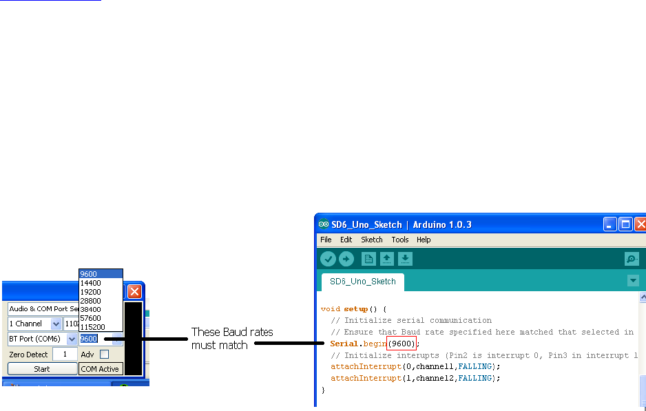
There is only one line of code in the Sketch that requires attention, the Baud rate at which the
microcontroller communicates with the computer. The default setting is 9600 Baud, both in the Sketch
file and in SimpleDyno. To use a higher data transfer rate by selecting this rate from the appropriate
drop down menu in SimpleDyno, the same rate must be defined in the Sketch file. Then re-compile the
Sketch and upload it to the Arduino before SimpleDynois started.
Once the SD6_3 Sketch file is uploaded to the Arduino it is ready to gather data and transfer data to
SimpleDyno.
SimpleDyno offers two options for using a microcontroller to acquire data. Audio & COM Port Sensing
allows the use of the mic-in line to gather RPM1 and RPM2 data while also reading additional sensor
data from the microcontroller. In COM Port Only mode, the microcontroller will read the RPM1 and
RPM2 values as well as reading the additional sensor data. For this discussion we will only describe use
of the Audio and COM Port Sensing because , from a SimpleDyno software perspective, handling of
SimpleDyno Manual v3.0, Nov 2013
Page 34 of 40
RPM1 and RPM2 data from the microcontroller is identical to handling RPM1 and RPM2 data from the
Audio stream (without having to deal with an audio signal).
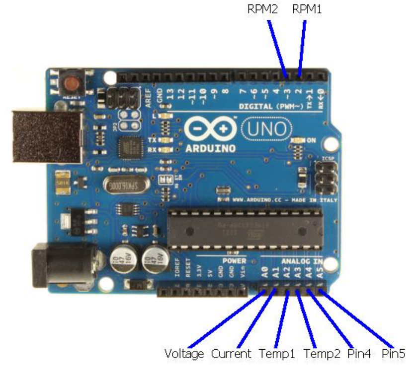
SimpleDyno will process 6 analog data streams supplied to it from the microcontroller. These are
Voltage, Current, Temperature 1, Temperature 2, Pin 4 Value, and Pin 5 Value. These data are collected
from the Arduino Analog In pins A0 – A5 respectively.
The design and use of individual sensors / circuits is beyond the scope of this document. However, to
demonstrate how the COM Port communications and calibrations are used, the Voltage for a 2S Lipo
battery with a measured voltage of 8.29V is discussed.
Note: CHECK the maximum voltage inputs that the microcontroller can handle before attempting to
connect any sensors otherwise damage to the pin or entire microcontroller may occur. In the case of
the Arduino Uno, 5V is the maximum voltage to apply to the Analog In pins. If a battery other than a 2S
Lipo is chosen for this exercise, the voltage delivered to Pins A0 and A1 must not exceed 5V.
SimpleDyno Manual v3.0, Nov 2013
Page 35 of 40
Calibrating COM Port Data
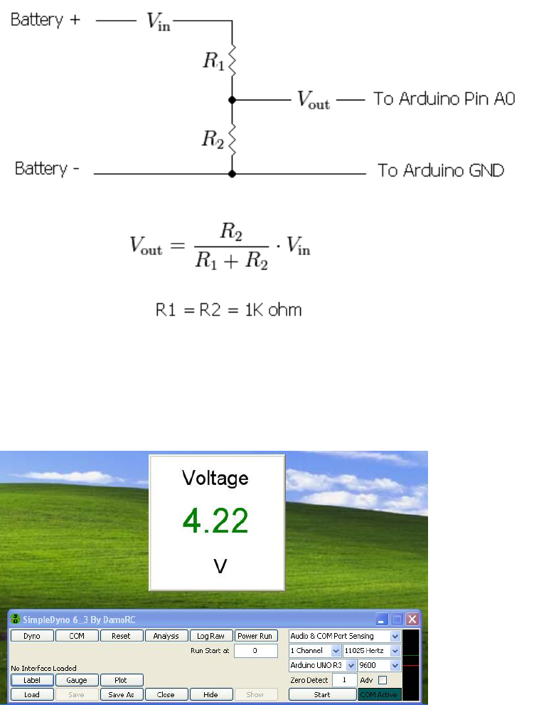
To allow SimpleDyno measure the voltage of a battery which is greater than the allowed Pin A0 voltage
of 5V a voltage divider must be used. Construct the voltage divider using two resistors in series. Connect
the battery across the resistors and connect the junction between the resistors to the A0 pin. Connect
the battery ground or negative terminal to the GND pin on the Arduino. The voltage at pin A0 will be
approximately half of the battery voltage depending on the tolerances of the resistors used in the
voltage divider.
Start SimpleDyno. Select Audio & COM Port Sensing as the data acquisition mode and click the Start
button. The COM Active label will flash indicating that communication with the Arduino is working.
Close any open graphical interface and create a new Label component. Select Voltage as the parameter
to monitor.
SimpleDyno Manual v3.0, Nov 2013
Page 36 of 40
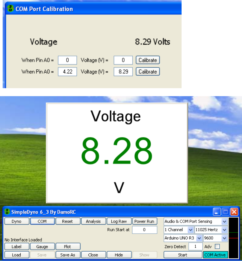
SimpleDyno is reporting a battery voltage of 4.22 volts. Technically this is correct as this is the voltage
being applied to Pin A0. However the actual voltage of our battery is 8.29V. For SimpleDyno to report
the battery voltage accurately, a calibration curve for the Voltage parameter being measured at Pin A0 is
required.
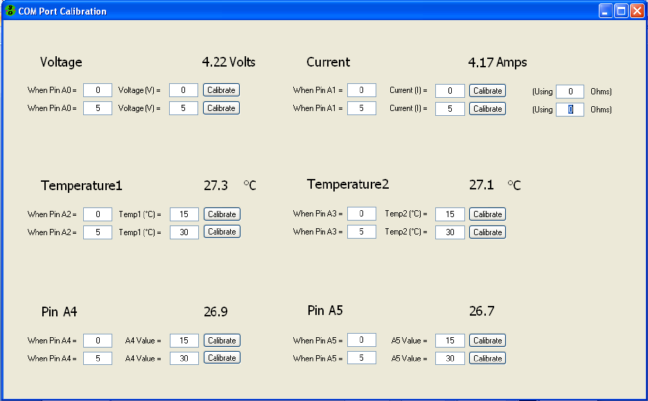
To provide SimpleDyno with the necessary values for calibration, click on the COM button to open the
COM Port Calibration window.
The COM Port Calibration window is where calibration values for each of the analog voltage data
streams being transmitted to SimpleDyno from the Arduino are entered. SimpleDyno uses linear
calibration for all analog inputs on Pins A0 to A5. Two points are needed to define a line, typically a low
point and a high point. Each parameter (Voltage, Current, etc.) requires two sets of entries. These
entries are presented as statements to help clarify the calibration process. For example, for the Voltage
parameter calibration entries for two statements are required. The first is “When the voltage at Pin A0
is 0, the actual voltage of the battery is 0V”. The second statement, using the values measured earlier is
“When the voltage at Pin A0 is 4.22, the actual voltage of the battery is 8.29V”. When these values are
entered SimpleDyno creates a calibration curve displays the correct voltage on the COM Port Calibration
window and also, if this window is closed, on the Label created earlier.
SimpleDyno Manual v3.0, Nov 2013
Page 37 of 40
Note: Because the voltage calibration curve originally stated that “When Pin A0 equals 5, Voltage = 5V”,
this essentially made Pin A0 a voltmeter so the original value of 4.22V could be used for calibration.
SimpleDyno also provides a means to complete the calibration entries without needing to measure the
voltage at the relevant Pin. Because the Arduino is constantly measuring the voltages at the Analog Pins
and transmitting the data to SimpleDyno there are slight fluctuations in the Pin measurements making it
difficult to decide what value to enter for “When Pin Ax . This is made easier by using the Calibrate
buttons associated with each statement. In this example the actual battery voltage is 8.29V. Enter this
into the second part of the statement “Voltage (V) = “. Then click the Calibrate button. SimpleDyno will
record the actual voltage at Pin A0 for one second and then place the average of all the values recorded
into the “When Pin A0 = “ field.
Calibration of the other parameters (Current, Temp1 and Temp2) is performed in the same way.
SimpleDyno Manual v3.0, Nov 2013
Page 38 of 40
Additional Notes on Current Calibration
SimpleDyno offers an additional functionality for calibrating current measurements. When using a
current sensor with specified measurement ratings (for example 10 Amps produces a 3 V output) then
simply enter the specified values into the calibration. However, if the current sensor needs to be
calibrated experimentally by applying a voltage across a resistance, the Using X Ohms functionality on
the COM Port Calibration window can be used. First, connect and calibrate the Voltage of the power
source to be applied across the resistive load. Then enter the accurate resistance of the test load into
the Using … Ohms field. Connect the output of the current sensor to Pin A1 (Current). Connect the
battery across the resistive load and click Calibrate. SimpleDyno will monitor the signal at Pin A1 for 1
second. It also monitors the battery voltage (Pin A0) at the same time. Once the calibration fields have
updated, SimpleDyno uses Ohms law to calculate the actual current measured by the sensor. This
feature was introduced because typically, connecting a battery across a resistive load for this calibration
causes the voltage across the battery to decrease. Measuring the voltage accurately during the current
sensor calibration will produce more accurate calibration values.
Microcontroller Transmission String for use with SimpleDyno
To use a microcontroller other than an Arduino for use with SimpleDyno it must be capable of serial
communications with the computer over a COM port. For each transaction where the microcontroller
sends data to the COM port (which will be received by SimpleDyno) the message string should contain
eleven (11) comma separated values which are:
(1) Session time (length of time controller has been running) in microseconds
(2) The recorded session time for an interrupt triggered at the RPM 1 pin
(3) The recorded time between the current and the last interrupt triggered at the RPM1 pin
(4) The recorded session time for an interrupt triggered at the RPM 2 pin
(5) The recorded time between the current and the last interrupt triggered at the RPM2 pin
(6) 10 bit result for Analog pin measuring Voltage
(7) 10 bit result for Analog pin measuring Current
(8) 10 bit result for Analog pin measuring Temperature1
(9) 10 bit result for Analog pin measuring Temperature2
(10) 10 bit result for Analog pin measuring a fifth analog pin (equivalent to Pin A4)
(11) 10 bit result for Analog pin measuring a sixth analog pin (equivalent to Pin A5)
It is not necessary to measure all the parameters to create the 11 pieces of information and it is not
necessary to use analog inputs for the parameters (6) to (11). However, the string sent to SimpleDyno
must contain 11 pieces of data and if values are transmitted for parameters (6) to (11) they will be
scaled for 5V at 10 bit resolution by SimpleDyno.
SimpleDyno Manual v3.0, Nov 2013
Page 39 of 40
Final Notes on using Arduino
Using the Arduino for additional data acquisition has been a significant enhancement to SimpleDyno’s
capabilities. The advantages are obvious. The main disadvantages are that the electronics are more
complicated. For example, the electronics required to accurately measure RPM1 and RPM2 (not
covered here) are considerably more complicated than the simple Audio approach with headphones and
magnet. That is why a hybrid option is offered via the Audio & COM Port Sensing mode. This is the
simplest hardware setup to use with a microcontroller. However, the clock resolution of the Arduino is
better than the highest sample rate option of 44,100 Hz for Audio signal processing and therefore more
accurate RPM1 and RPM2 measurements are possible using the Arduino.
SimpleDyno Manual v3.0, Nov 2013
Page 40 of 40
Document History
(1) Version 1.0 – First version of instructions distributed with 6.3
(2) Version 2.0 – Updated instructions for distribution with 6.4 including
a. Description of newly added corrections button with details on the coast down function
b. Update of curve fitting section to describe MA Smooth function and new feature
whereby the torque and power curves are overlaid on the fit to aid in selecting a curve
fit model or smoothing window.
(3) Version 3.0 – Updated instructions for version 6.5 including
a. Description of the new gauge formatting options
