Instructions For Preparing Input Files Gsflow

User Manual:

Open the PDF directly: View PDF .
Page Count: 178 [warning: Documents this large are best viewed by clicking the View PDF Link!]

GSFlow Training Class Material: Instructions for GSFLOW Model Input Preparation

Contents

Overview ................................................................................................................................................................................ 1

Purpose and Scope ........................................................................................................................................................... 1

Software Requirements ..................................................................................................................................................... 1

Hardware Requirements ................................................................................................................................................... 2

Download Example Problem Data Sets ........................................................................................................................... 2

Making PRMS Data File ........................................................................................................................................................ 3

Create a PRMS Data File (for time series climate and stream flow data) ...................................................................... 3

Creating a PRMS Data File with the USGS Downsizer ............................................................................................... 3

Set the time period for the data pull .......................................................................................................................... 4

Set the PRMS Data File name and format ............................................................................................................... 5

Selecting the stations for the PRMS Data File ......................................................................................................... 6

Set the Units for the PRMS Data File ..................................................................................................................... 10

Look at the Flags for Quality Control Checks ......................................................................................................... 11

Run the Downsizer ................................................................................................................................................... 11

Creating a PRMS Data File with a text editor ............................................................................................................. 14

Computation of Lapse Rates/Monthly Means using Excel ............................................................................................ 14

Making GSFLOW maps ...................................................................................................................................................... 18

Before Starting ................................................................................................................................................................. 18

Arcmap with Archydro and XTool Pro installed ......................................................................................................... 18

Set the "Environments" for the ArcMap Project.......................................................................................................... 22

Check the Digital Elevation Model (DEM) raster map................................................................................................ 24

GSFlow Training Class Material: Instructions for GSFLOW Model Input Preparation

Check the streamgage map ........................................................................................................................................ 25

Data Bin raster maps ................................................................................................................................................... 25

DEM Reconditioning ........................................................................................................................................................ 26

Fill the DEM .................................................................................................................................................................. 26

Determine Flow Direction ............................................................................................................................................ 27

Determine Flow Accumulation .................................................................................................................................... 29

Delineation of Spatial Modeling Features for GSFLOW ................................................................................................ 31

Natural Watershed Boundary ...................................................................................................................................... 31

Generation of the Stream Segment map .................................................................................................................... 33

Generation of the MODFLOW Grid Cell map ............................................................................................................. 41

Generation of "Clipped" Model Domain and Active Cells Maps ................................................................................ 47

Generation of PRMS HRU map .................................................................................................................................. 51

Generation of GSFLOW Gravity Reservoir (GVR) map ............................................................................................ 62

Adding modeling attributes to the GSFLOW maps ............................................................................................................ 66

HRU map ......................................................................................................................................................................... 66

cov_type ....................................................................................................................................................................... 67

covden_sum ................................................................................................................................................................. 68

covden_win .................................................................................................................................................................. 71

soil_moist_max ............................................................................................................................................................ 73

soil_rchr_max ............................................................................................................................................................... 77

soil_type ....................................................................................................................................................................... 80

snow_intcp ................................................................................................................................................................... 80

wrain_intcp ................................................................................................................................................................... 83

srain_intcp .................................................................................................................................................................... 83

GSFlow Training Class Material: Instructions for GSFLOW Model Input Preparation

iii

hru_lat........................................................................................................................................................................... 83

hru_elev ........................................................................................................................................................................ 84

hru_slope...................................................................................................................................................................... 87

hru_aspect ................................................................................................................................................................... 88

tmax_adj ....................................................................................................................................................................... 89

tmin_adj ........................................................................................................................................................................ 91

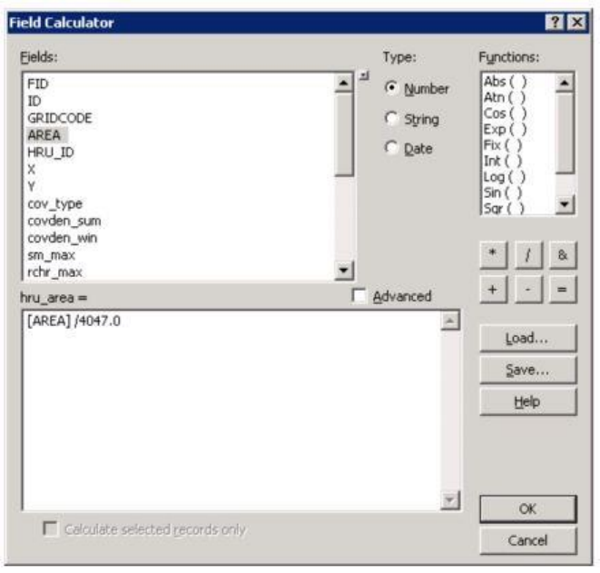
hru_area ....................................................................................................................................................................... 91

jh_coef_hru .................................................................................................................................................................. 92

rad_trncf ....................................................................................................................................................................... 94

MODFLOW Grid Cell map (shapefile mfcells) ............................................................................................................... 94

Fill in the cell altitude attribute (ALT) .......................................................................................................................... 95

Identify the active cells (ACTIVE) ............................................................................................................................... 99

Fill in the cell precipitation attribute (PRECIP) ......................................................................................................... 102

Fill in the cell IRUNBND attribute .............................................................................................................................. 104

GVR map ....................................................................................................................................................................... 112

Making the PRMS Parameter File .................................................................................................................................... 118

Dimension sizes ............................................................................................................................................................. 118

Spatial parameters ........................................................................................................................................................ 119

HRU parameters ........................................................................................................................................................ 119

Parameters that come from the Gravity Reservoir (gis\shapes\gvrs.dbf) map and go into the nhrucell dimension

.................................................................................................................................................................................... 122

Cascade parameters ..................................................................................................................................................... 123

Non-spatial parameters ................................................................................................................................................. 125

Making the MODFLOW Files ............................................................................................................................................ 128

GSFlow Training Class Material: Instructions for GSFLOW Model Input Preparation

Create the MODFLOW Grid Cell map (ModelMuse method) ...................................................................................... 128

Select MODFLOW packages ........................................................................................................................................ 128

Set MODFLOW Output Control................................................................................................................................. 132

Set MODFLOW Units and Other Options ..................................................................................................................... 133

Importing Shapefiles in ModelMuse.............................................................................................................................. 136

Create Point Objects for Cells with Springs ............................................................................................................. 144

Add Additional Springs not Mapped on Topo Map .................................................................................................. 145

Create UZF gages for Added Springs ...................................................................................................................... 146

Set Stream Segment Information ................................................................................................................................. 147

Specify Segment Information .................................................................................................................................... 150

Set Gage to last Reach in Outflow Segment ............................................................................................................ 152

Set Hydraulic Conductivity for Aquifers ........................................................................................................................ 153

Set Layer Top and Bottom Altitudes ............................................................................................................................. 158

Check Layer Altitudes ................................................................................................................................................ 161

Set Wet_Dry Data ...................................................................................................................................................... 162

Set Active Cells .............................................................................................................................................................. 165

Set All other Cell Property Data .................................................................................................................................... 167

Layer 1 ....................................................................................................................................................................... 167

Set IUZFBND for UZF ............................................................................................................................................... 170

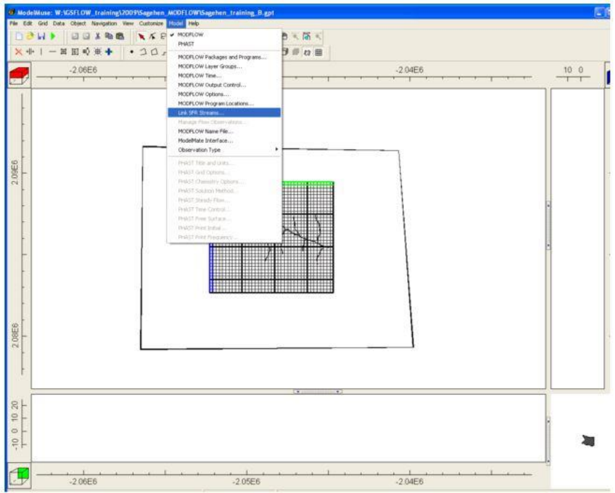
Link Outflow Segments.............................................................................................................................................. 172

GSFlow Training Class Material: Instructions for GSFLOW Model Input Preparation

................... 173

GSFlow Training Class Material: Instructions for GSFLOW Model Input Preparation

GSFlow Training Class Material: Instructions for GSFLOW

Model Input Preparation

Overview

Purpose and Scope

This report describes the input preparation process for GSFLOW, version 1.1, specifically, the

creation of the PRMS Data File, the GSFLOW maps, the PRMS Parameter File, and the MODFLOW

Input Files.

These instructions are not the only way to prepare input for GSFLOW, but are intended to serve

as a procedural guide. Clearly, any single step from the outline below, could involve (and may require)

much more effort, study, and expertise from a GSFLOW modeler or modeling team. Anyone

considering a GSFLOW modeling project is encouraged to work through this outline and complete the

example problem to gain insight into what will be required to develop a full application.

The USGS has corporate policies about the hardware and software tools which are made

available to its employees and cooperators. These instructions reflect these policies and are not intended

to endorse any particular trade, product, or firm. These instructions can (and have been) successfully

carried out with many alternative hardware and software configureations.

Software Requirements

The following software packages are required to prepare input for GSFLOW:

GSFlow Training Class Material: Instructions for GSFLOW Model Input Preparation

 USGS Downsizer (available only on USGS computers)

 ESRI ArcMap and Workstation (version 9.3), including a license for the Spatial Analyst extension

 CRWR ArcHydro extension to ArcMap

 XTools Pro extension to ArcMap

 Microsoft Excel

 USGS PRMS Paramtool

 USGS ModelMuse

Hardware Requirements

The following represents a minimum hardware configuration to prepare input for GSFLOW:

 PC with Windows XP Operating System

 2.0 GHz PC (or higher) Processor

 1 GB (or higher) RAM

 100 GB (or higher) Hard Disk

 SVGA, 1024x768 resolution, 16 bit color (or better) Monitor

 32 MB RAM (or higher), 24 bit true color Graphics Card

Download Example Problem Data Sets

The data for the following example is available here

(ftp://brrftp.cr.usgs.gov/pub/mows/data/gsflowTrainingMaterial.zip).

GSFlow Training Class Material: Instructions for GSFLOW Model Input Preparation

These steps should be completed in order, as later steps may require maps or data produced in

earlier steps.

Making PRMS Data File

Create a PRMS Data File (for time series climate and stream flow data)

Creating a PRMS Data File with the USGS Downsizer

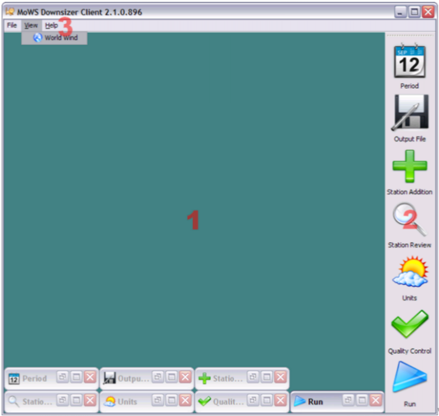
Start the Downsizer by navigating to the download directory and double click on client.bat.

The Downsizer client window is the parent container from which all Downsizer functionality is

accessible. This window contains (1) the desktop area, (2) the tool bar, and (3) the menu bar. These

parts are described below.

GSFlow Training Class Material: Instructions for GSFLOW Model Input Preparation

Use the icons on the toolbar on the right side to go through the steps in order:

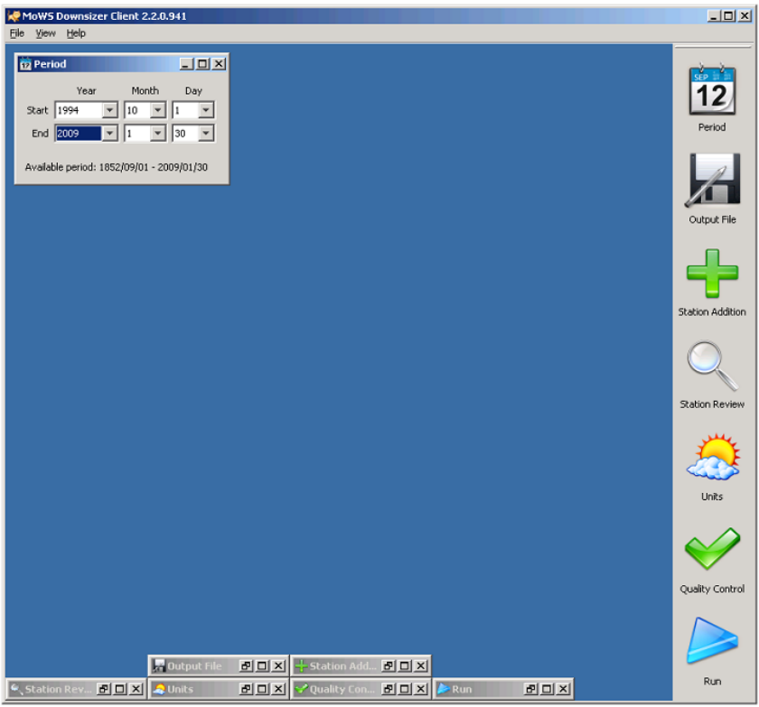
Set the time period for the data pull

Click on the Period icon in the toolbar. Set the start period to 1994-10-1. Set the end period to

2009-01-30

GSFlow Training Class Material: Instructions for GSFLOW Model Input Preparation

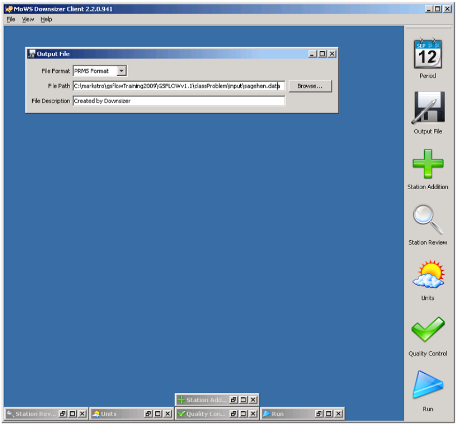
Set the PRMS Data File name and format

Click on the Output File icon in the toolbar. Set the File Format to PRMS Format. Set the File

Path by browsing to the classProblem\input folder. Name the file sagehen.data

GSFlow Training Class Material: Instructions for GSFLOW Model Input Preparation

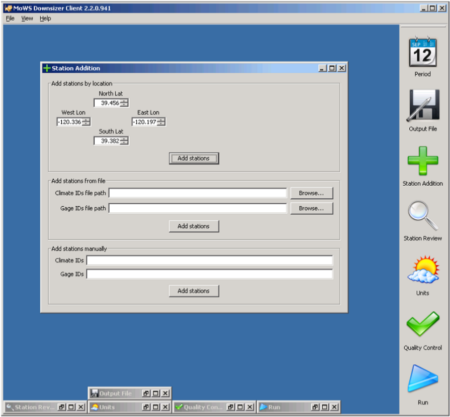
Selecting the stations for the PRMS Data File

Click on the Station Addition icon in the toolbar. Set the North Lat to 39.456; West Lon to -

120.336; East Lon to -120.197; and South Lat to 39.382

GSFlow Training Class Material: Instructions for GSFLOW Model Input Preparation

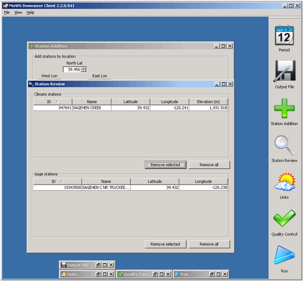
Click the Add stations button to bring up the Station Review window.

GSFlow Training Class Material: Instructions for GSFLOW Model Input Preparation

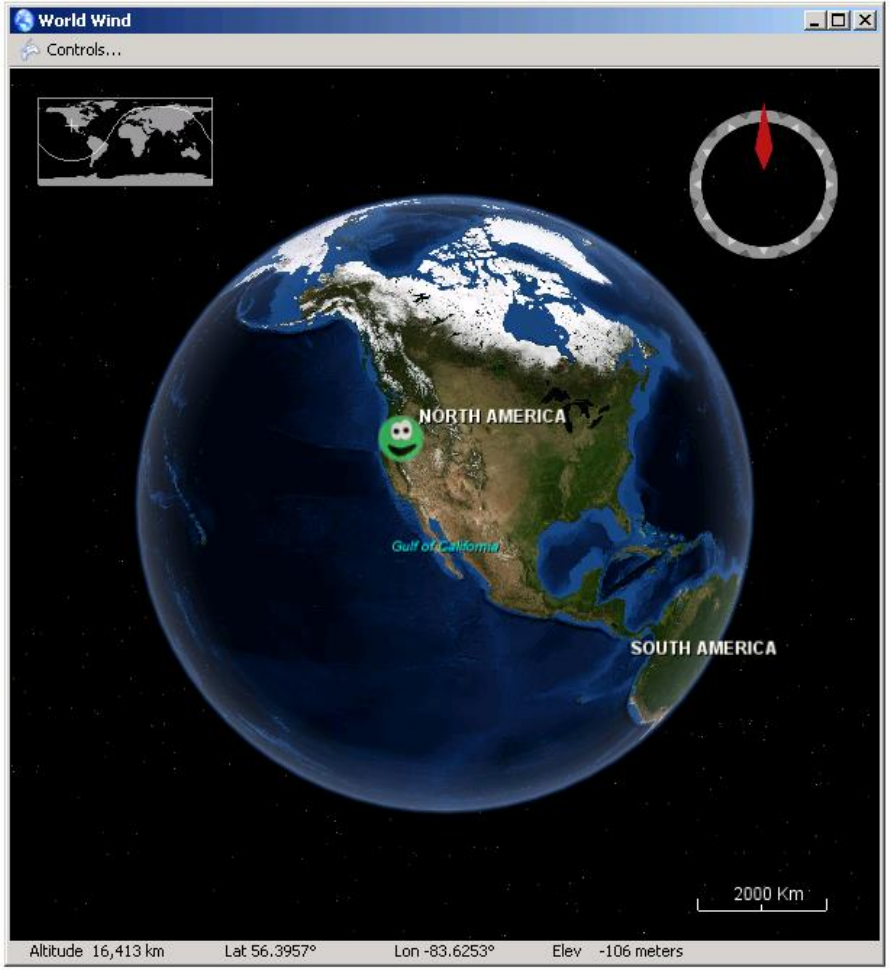
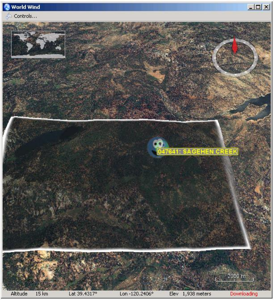
Also notice that the locations of the stations are shown in the World Wind window.

GSFlow Training Class Material: Instructions for GSFLOW Model Input Preparation

Zoom in, with the mouse wheel, to better see the selection.

GSFlow Training Class Material: Instructions for GSFLOW Model Input Preparation

The World Wind window can be used to set the extent of the lat/lon selection box in the Station

Addition window. It can also be used to select/deselect individual station in the tables in the Station

Review window.

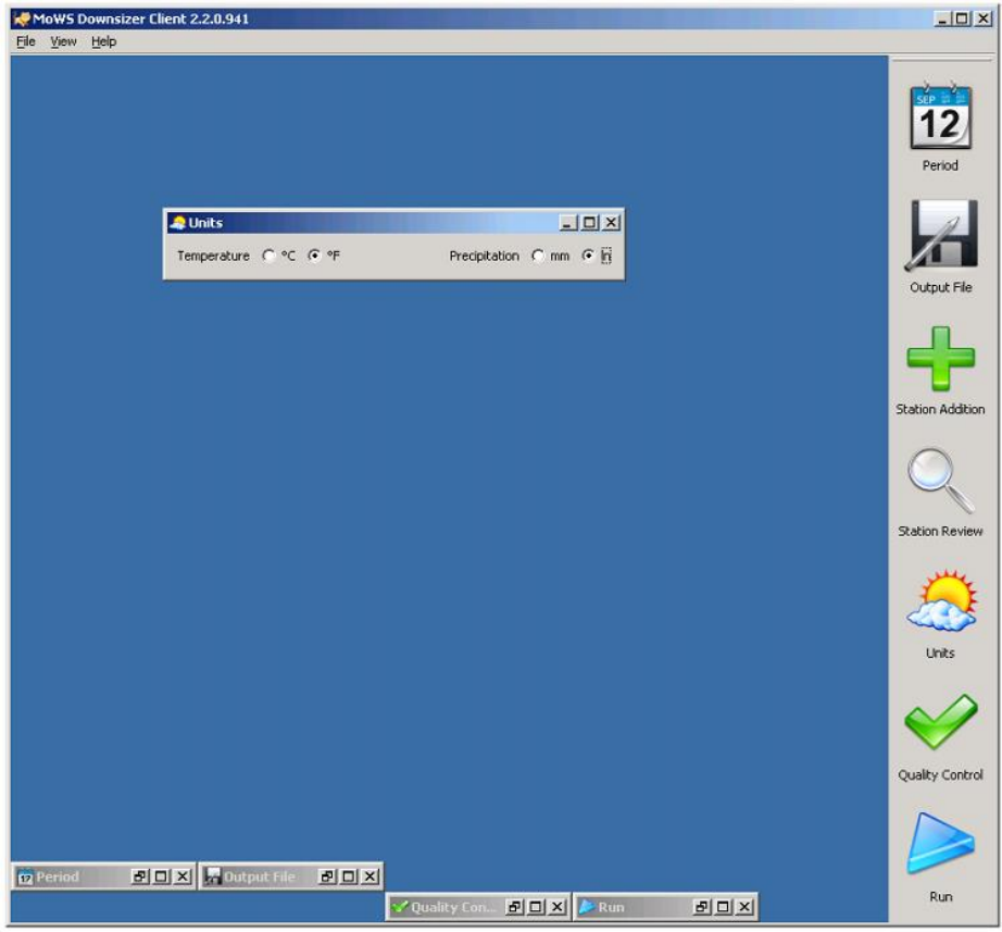
Set the Units for the PRMS Data File

Click on the Units icon in the toolbar. Set the Temperature to F and Precipitation to in (inches).

GSFlow Training Class Material: Instructions for GSFLOW Model Input Preparation

Look at the Flags for Quality Control Checks

Click on the Quality Control icon in the toolbar. This is where different flags can be set to look

for "bad data." This tool will set bad data values to the missing data value

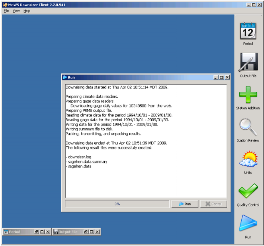
Run the Downsizer

Click on the Run icon in the toolbar. Click on the Run button.

GSFlow Training Class Material: Instructions for GSFLOW Model Input Preparation

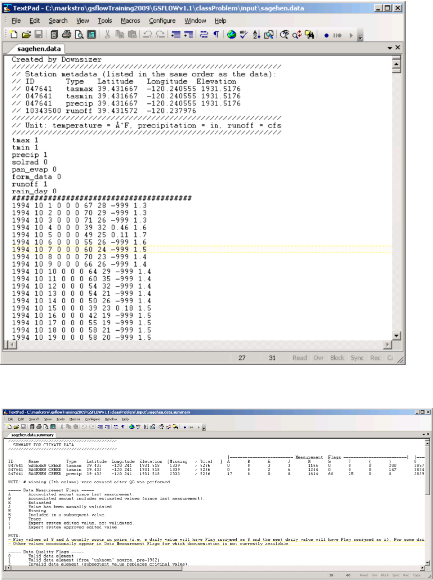
Look at the sagehen.data file that was made by the Downsizer.

GSFlow Training Class Material: Instructions for GSFLOW Model Input Preparation

Look at the sagehen.data.summary file that was made by the Downsizer.

GSFlow Training Class Material: Instructions for GSFLOW Model Input Preparation

Creating a PRMS Data File with a text editor

Create the PRMS Data File according to the description on pages 139 - 142 of GSFLOW -

Coupled Ground-Water and Surface-Water Flow Model Based on the Integration of the Precipitation-

Runoff Modeling System (PRMS) and the Modular Ground-Water Flow Model (MODFLOW-2005)

(http://pubs.er.usgs.gov/publication/tm6D1).

People have successfully created this file on Linux based systems using the cut, paste, and awk

utilities. Also, people have successfully created this file on PC based systems using text editors and/or

spreadsheet programs.

Computation of Lapse Rates/Monthly Means using Excel

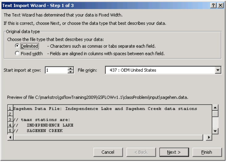
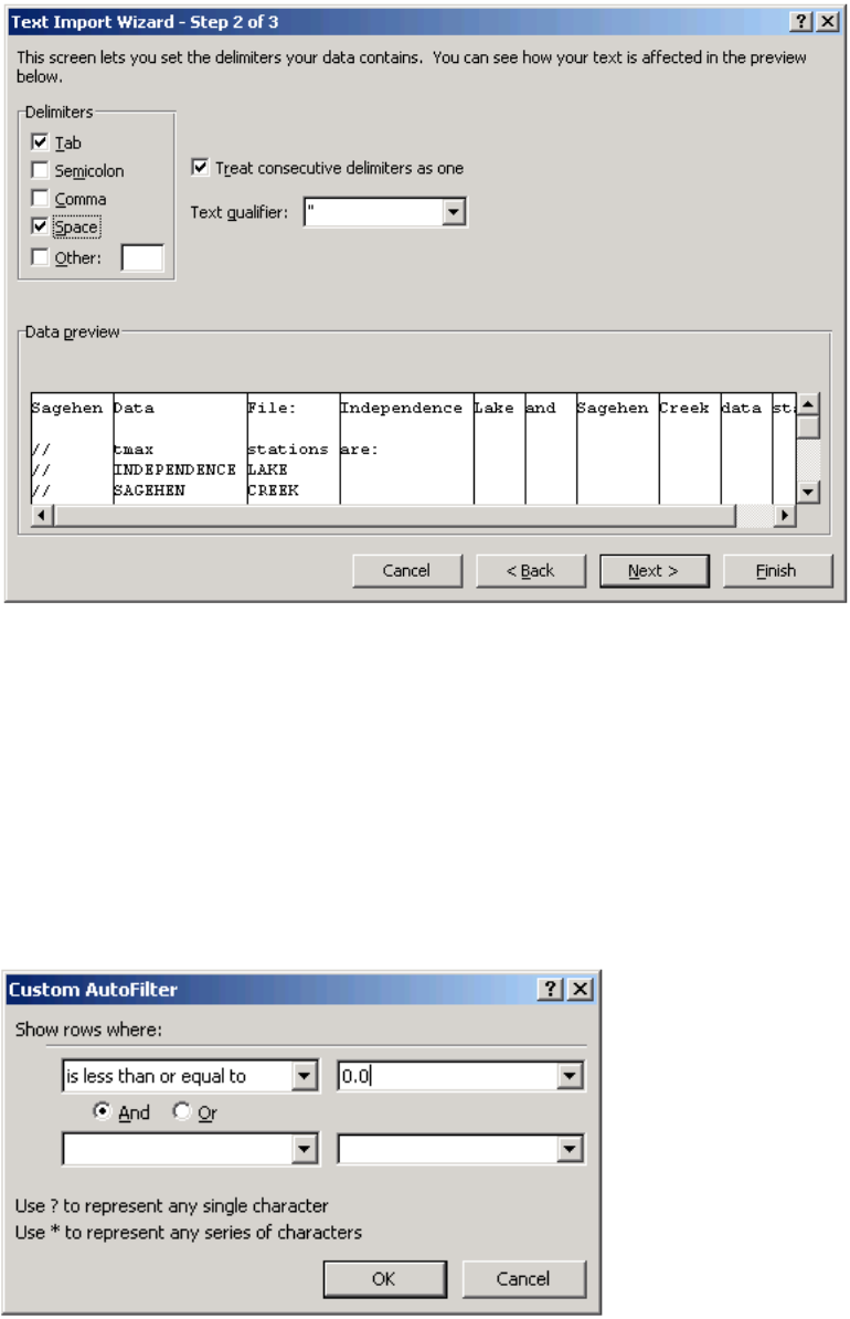
Start MS Excel. Select Data->From Text and browse to the PRMS Data File (sagehen.data).

Choose "Delimited" in Step 1 of the Text Import Wizard.

Check on "Space" in Step 2 of the Text Import Wizard.

GSFlow Training Class Material: Instructions for GSFLOW Model Input Preparation

Click on Finish in Step 3 of the Text Import Wizard.

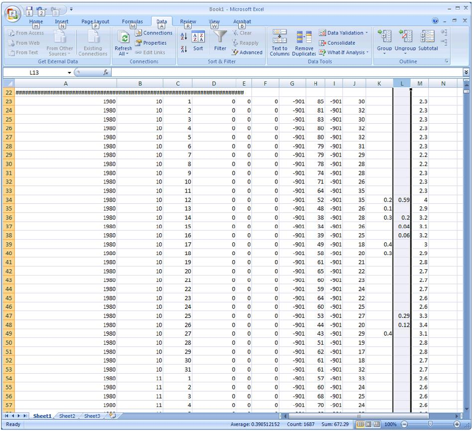
Column K is the precipitation values for Independence Lake SNOTEL and column L is the

precipitation values for Sagehen Creek COOP. Click on the column K label heading and then click on

Data-> Filter. Choose Number Filter->Less Than or Equal To for column K. Enter 0.0 into the box next

to is less than or equal to.

GSFlow Training Class Material: Instructions for GSFLOW Model Input Preparation

Right click on column K header and select Clear Contents. This blanks out all cells which are

less than or equal to zero. Repeat this process for column L too.

Mean precipitation amount can be computed from these two columns for days with precipitation.

For example, to compute mean monthly precipitation for January, filter column B to show the values for

month 1 only. The average value for a station will be the average precipitation (on days with

precipitation) for the selected month. These averages can vary greatly depending on which years are

included in the analysis, so be sure and choose years that are representative of the simulation time

period.

GSFlow Training Class Material: Instructions for GSFLOW Model Input Preparation

The results of this for both stations, for all months have already been computed and are located

in the Excel worksheet sagehenLapseRates.xls.

GSFlow Training Class Material: Instructions for GSFLOW Model Input Preparation

Making GSFLOW maps

Before Starting

GOAL: Make sure that the GIS software and the basic spatial data sets are ready to go.

Arcmap with Archydro and XTool Pro installed

General notes about ArcMap:

 If tools/windows give an unexpected error, shorten the path names

 If tools/windows give an unexpected error, exit and restart ArcMap.

 In general, anything produced by ArcMap should be moved, copied, deleted, etc. with ArcCatalog.

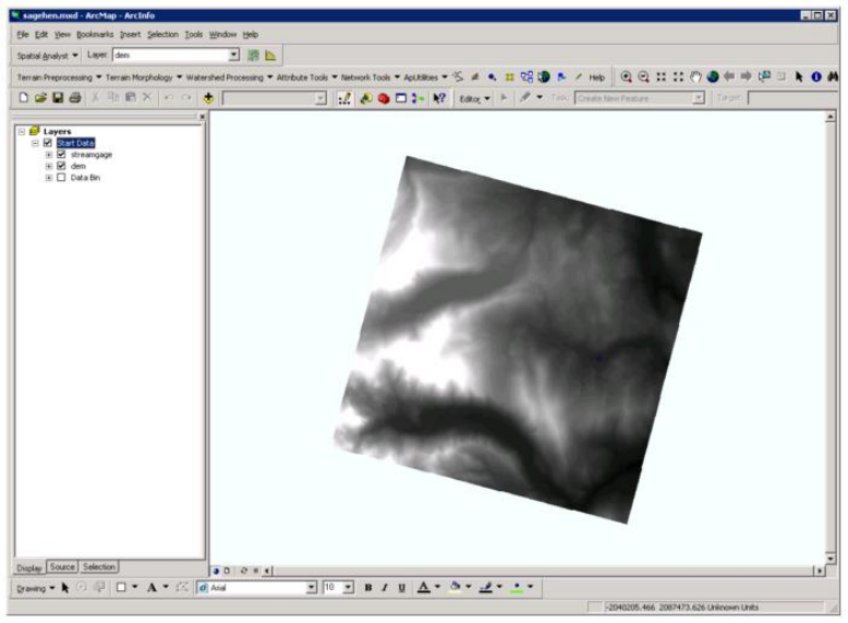
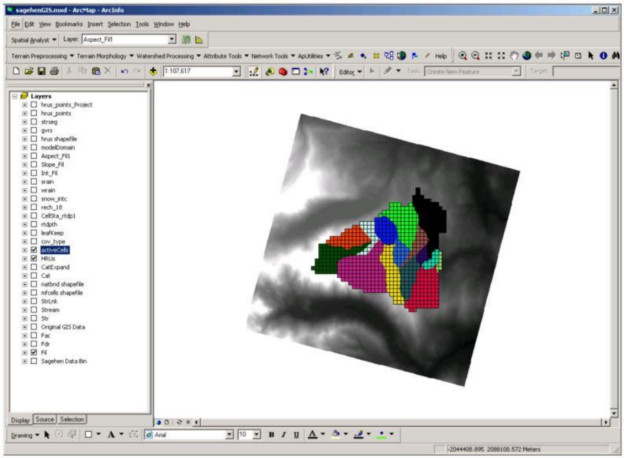
Start the ArcMap application by double clicking on the gis\sagehenGIS.mxd. This will start the

Sagehen GIS project with the necessary starting data preloaded. Check to make sure that the ArcHydro

extension is installed (requires admin rights) and ArcHydro toolbox is added to the ArcToolbox (does

not requires admin rights).

http://www.crwr.utexas.edu/giswr/hydro/ArcHOSS/index.cfm

http://support.esri.com/index.cfm?fa=downloads.dataModels.filteredGateway&dmid=15

GSFlow Training Class Material: Instructions for GSFLOW Model Input Preparation

If the ArcHydro toolbar is not visible Click: View->Toolbars->Arc Hydro Tools 9

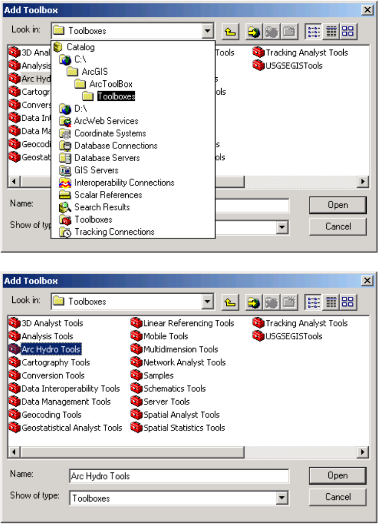
If ArcHydro toolbox is not present in the ArcToolbox, add the Archydro Tool box, right click on the

ArcToolbox root node and choose Add Toolbox.

GSFlow Training Class Material: Instructions for GSFLOW Model Input Preparation

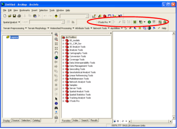
Check to make sure that the XTools Pro extension is installed (requires admin rights) and XToolsPro

toolbox is added to the ArcToolbox (does not requires admin rights). The USGS has an enterprise

license for this extension. If you are a USGS employee, have your system administrator install and

configure XToolsPro for you.

GSFlow Training Class Material: Instructions for GSFLOW Model Input Preparation

Confirm that the XTools Pro extension is turned on. Tool->Extensions->XTools Pro

If the XTools Pro toolbar is not visible Click: View->Toolbars-> XTools Pro

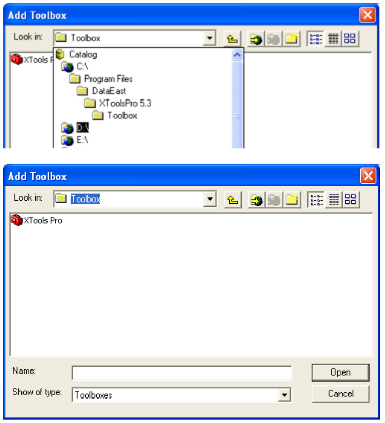
If XTools Pro toolbox is not present in the ArcToolbox, add the XTools Pro Toolbox, right click on the

ArcToolbox root node and choose Add Toolbox.

GSFlow Training Class Material: Instructions for GSFLOW Model Input Preparation

This example problem uses an ESRI "Personal Geodatabase." There are many reasons for this, but ease

of set up, distribution, and use are primary ones. Also, it is possible to query the spatial data directly

with the Microsoft Access application.

Set the "Environments" for the ArcMap Project

Here's ESRI's webpage describing environment settings:

http://webhelp.esri.com/arcgisdesktop/9.2/index.cfm?TopicName=An_overview_of_geoprocessing_env

ironments

GSFlow Training Class Material: Instructions for GSFLOW Model Input Preparation

If the Environment is set for the ArcMap project, it will retain those settings during any

geoprocessing within the project, i.e. Toolbox, toolbars (such as Spatial Analyst), ModelBuilder, etc. If

the Environment is set only with the Toolbox, the settings will be retained during any geoprocessing

within the toolbox. Also, environments can be set for individual tools as well. For this example, make

sure that the environments are set for the entire project.

Within the environments, it is possible to set the current and scratch workspace (workspaces for

inputs and outputs), the extent, and output coordinate system. More importantly, the cell size (especially

for MODFLOW models) and the snap raster can be set. The snap raster setting is what lines everything

up, so subsequent maps don't have slivers. Usually, it is a good idea to set the snap raster to the original

DEM:

http://webhelp.esri.com/arcgisdesktop/9.3/index.cfm?TopicName=How_Snap_Raster_works

However, the MODFLOW cells the DEM are rarely the same size. So, the cell size can be fixed as a

ratio of the original DEM or the cell size can be set to the desired model cell size and interpolation will

be used to adjust the cells to that specified size as it is being snapped to the raster.

Now, on how to physically set the environments. To set the environments within the ArcMap project,

Tools>Options>Geoprocessing>Environments. Once in the Environment Settings dialog box, the Snap

Raster can be set under General Settings.

GSFlow Training Class Material: Instructions for GSFLOW Model Input Preparation

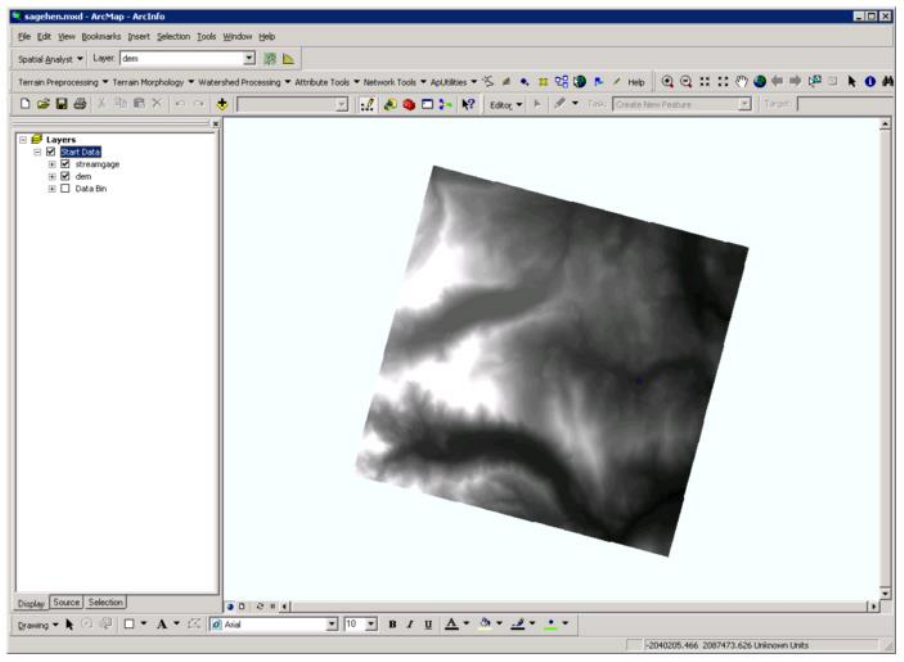
Check the Digital Elevation Model (DEM) raster map

GSFlow Training Class Material: Instructions for GSFLOW Model Input Preparation

A DEM which covers the model domain is required. The DEM for the Sagehen example

problem is located in Start Data->dem. DEMs for other basins can be obtained from the USGS

"Seamless" server (http://ned.usgs.gov/downloads.asp).

Check the streamgage map

In this exercise, a point corresponding to a streamgage location will be used to help define

the model domain. Load this point with is located in Start Data->streamgage.

Data Bin raster maps

The Data Bin folder contains raster maps of information that will be needed to estimate spatially

distributed parameters for GSFLOW. This includes: (1) available water holding capacity of the soil

(awc1k), (2) clay content of the soil (clayav1k), (3) vegetation density (density1k), (4) land use/land

cover (lulc1k), (5) soil depth to bed rock (rockdep1k), and (6) sand content of the soil (sandave1k).

GSFlow Training Class Material: Instructions for GSFLOW Model Input Preparation

DEM Reconditioning

GOAL: Process the DEM so it is ready for GSFLOW modeling.

Fill the DEM

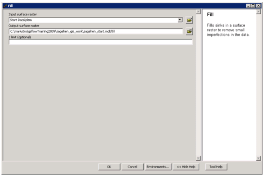
Sinks may exist in the DEM. These must be filled using Fill (Spatial Analyst) tool. Access all

tools using the ArcMap Search window. Use Raw dem as the input. Browse to the raster\ folder and

name the new raster map fil. Click OK.

GSFlow Training Class Material: Instructions for GSFLOW Model Input Preparation

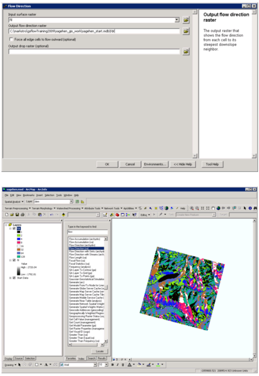
Determine Flow Direction

For each raster cell in fil the flow direction is calculated. These must be done using the Flow

Direction (Spatial Analyst) tool. Name the map fdr.

GSFlow Training Class Material: Instructions for GSFLOW Model Input Preparation

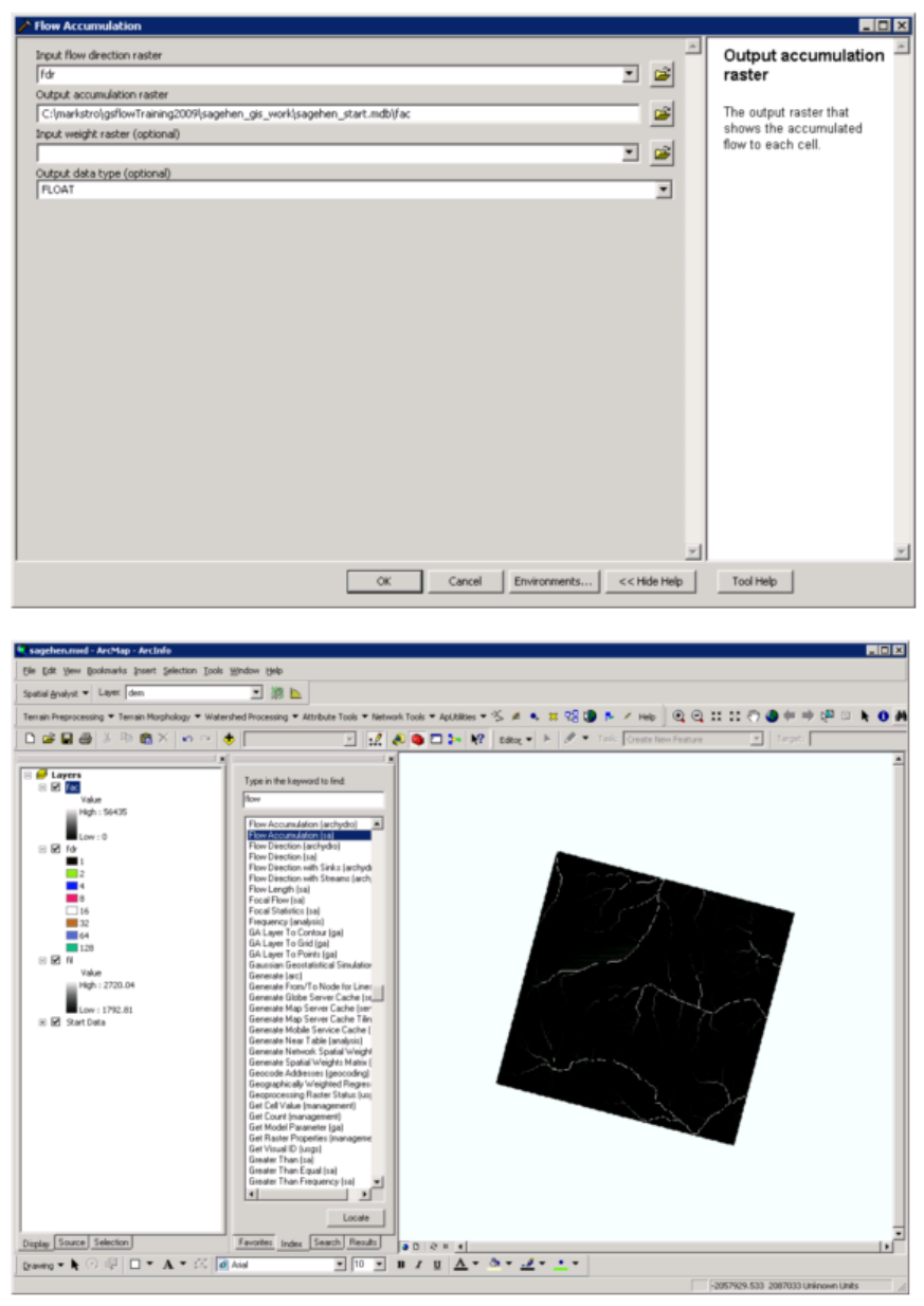
Determine Flow Accumulation

For each raster cell in fdr, the flow accumulation is calculated. This is done using the Flow

Accumulation (Spatial Analyst) tool. Name the map fac.

GSFlow Training Class Material: Instructions for GSFLOW Model Input Preparation

After all of these map have been created, save the Sagehen ArcMap project by clicking File->Save.

GSFlow Training Class Material: Instructions for GSFLOW Model Input Preparation

Delineation of Spatial Modeling Features for GSFLOW

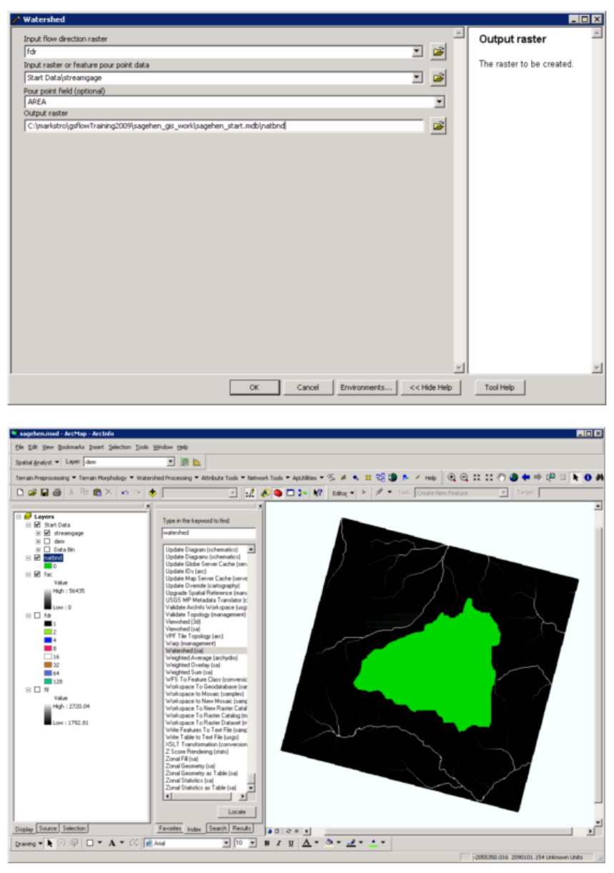
Natural Watershed Boundary

Use the Watershed (sa) tool to determine the natural watershed boundary. Use the fdr and

streamgage maps as input.

GSFlow Training Class Material: Instructions for GSFLOW Model Input Preparation

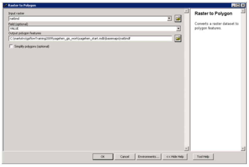
Name the output natbnd. Use the Raster to Polygon (conversion) tool to make a feature map. Name the

output natbndf. Make sure the Simplify polygons box is unchecked.

After this map has been created, save the Sagehen ArcMap project by clicking File->Save.

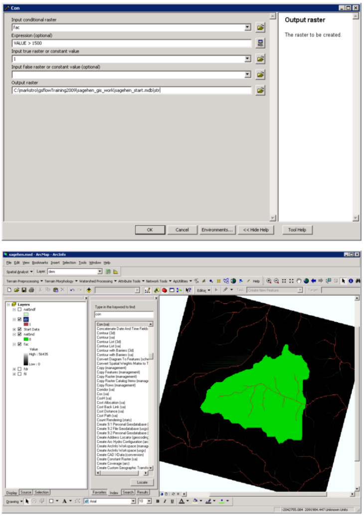
Generation of the Stream Segment map

Find the location of the streams using the flow accumulation (fac) surface. Use the Con (sa) tool

to create a new raster map that has a value of 1 in every cell that has a flow accumulation over 1500

cells, and NO DATA in all other cells. Name the output raster str.

GSFlow Training Class Material: Instructions for GSFLOW Model Input Preparation

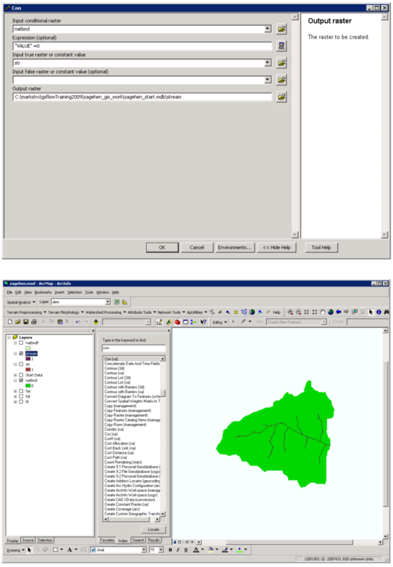
Use the Con (sa) tool to get rid of streams outside of Natural Boundary. Use the settings as shown

below. This makes the raster map Stream.

GSFlow Training Class Material: Instructions for GSFLOW Model Input Preparation

Use the Stream Link (sa) tool to break the stream raster map into stream segments. This makes the

raster map StrLnk.

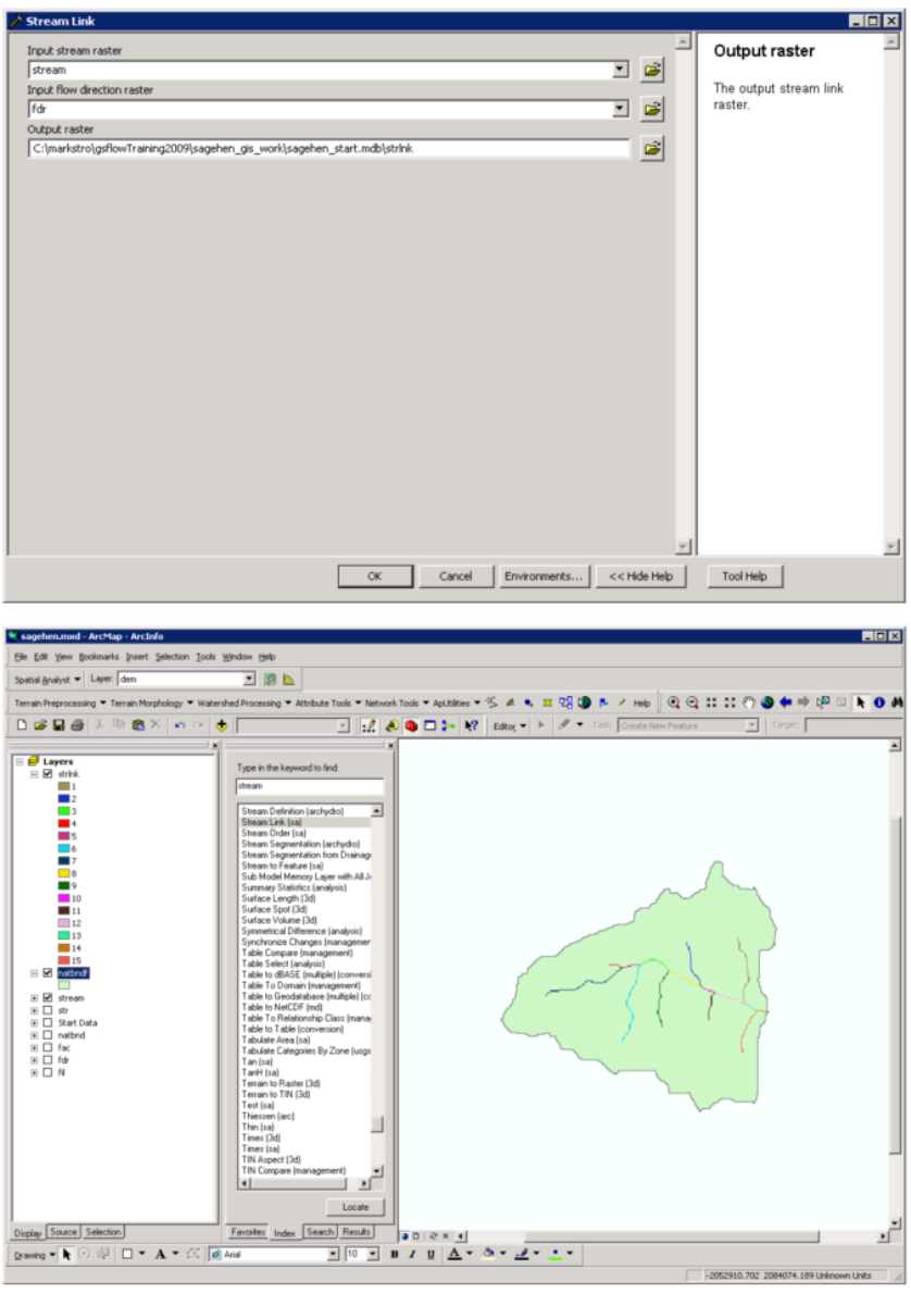
GSFlow Training Class Material: Instructions for GSFLOW Model Input Preparation

Use the ArcMap tool Stream to Feature (sa) tool to make features and add connectivity and flow

direction. Click off the check box to Simplify polygons. Name the output strseg.

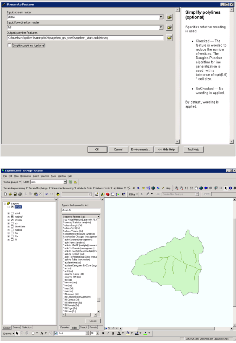
GSFlow Training Class Material: Instructions for GSFLOW Model Input Preparation

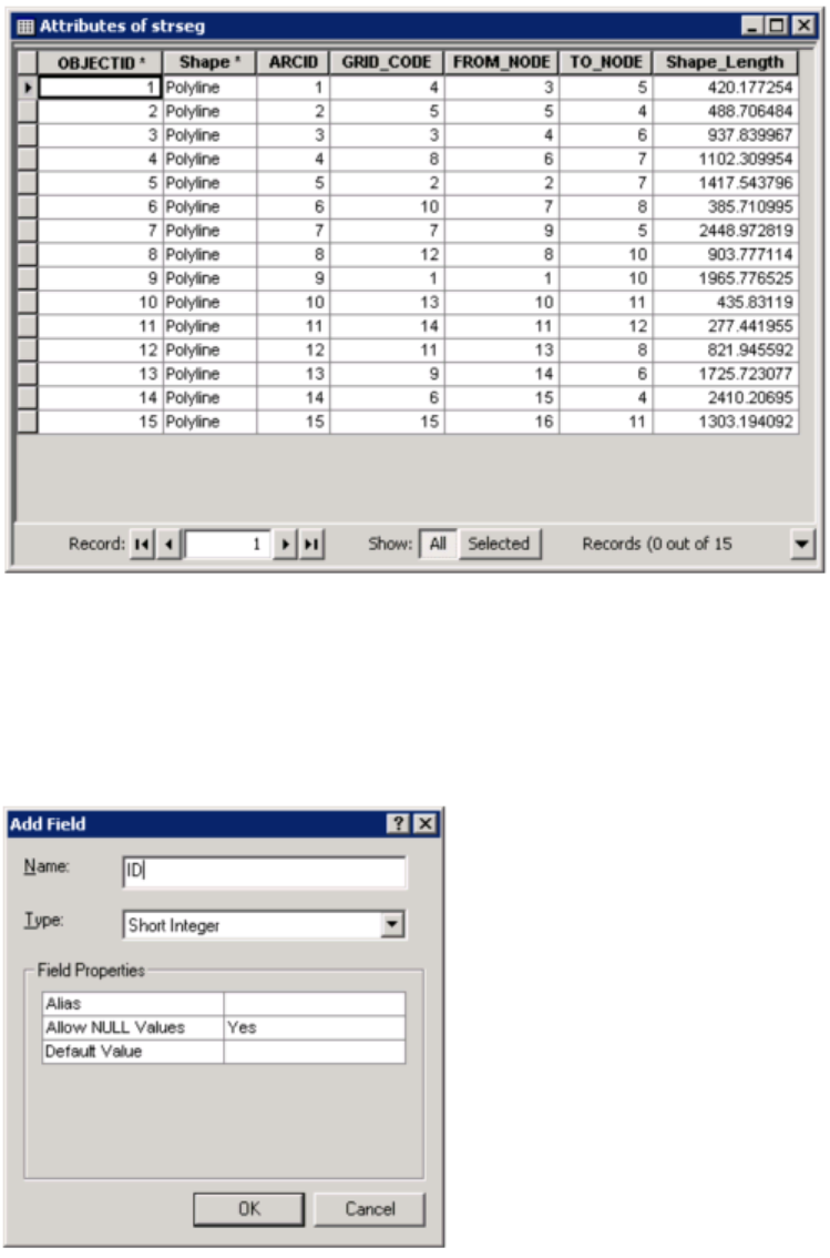
Right click on strseg in the ArcMap tree and select Open Attribute Table.

GSFlow Training Class Material: Instructions for GSFLOW Model Input Preparation

The values in the GRID_CODE column will be used as the stream segment IDs. Click on the Down

Arrow (in the lower-right corner of the Attributes window) and select Add Field from the pop-up

window. Add the new attribute ID as shown below.

Copy the values from GRID_CODE to ID using the Field Calculator.

GSFlow Training Class Material: Instructions for GSFLOW Model Input Preparation

After this map has been created, save the Sagehen ArcMap project by clicking File->Save.

Strseg is the stream segment feature set.

GSFlow Training Class Material: Instructions for GSFLOW Model Input Preparation

Generation of the MODFLOW Grid Cell map

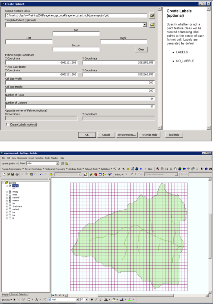
Use the Create Fishnet (management) tool to create the MODFLOW Grid. The fishnet origin,

number of rows, and number of columns have been computed so that the MODFLOW Grid will totally

cover the natbndf natural watershed boundary. Use the following settings for the example problem:

 Set the Output Feature Class to mfgrid

 Set the Fishnet Origin Coordinate to X = -2052121.286 and Y = 2082652.955

 Set the Y-Axis Coordinate to X = -2052121.286 and Y = 2082662.955

 Set the Cell Size Width = 200

 Set the Cell Size Height = 200

 Set the Number of Rows = 34

 Set the Number of Columns = 37

 Uncheck the Create Labels box

Click OK.

GSFlow Training Class Material: Instructions for GSFLOW Model Input Preparation

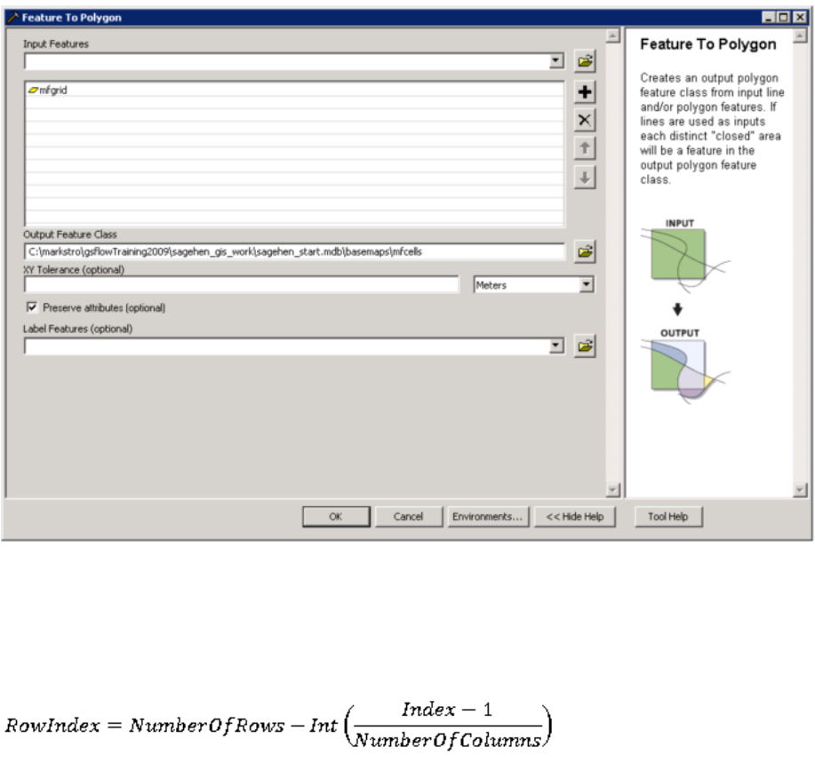
Use the Feature to Polygon (management) tool to create the MODFLOW Grid Cells. Set Input Features

to mfgrid. Set Output Feature Class to mfcells. Click OK.

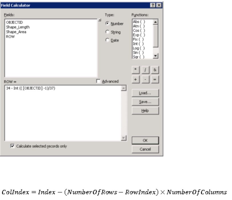
Add the attribute ROW to the table in the Attributes of mfcells window. The row index can be

calculated according to:

This is what it looks like in the Field Calculator.

GSFlow Training Class Material: Instructions for GSFLOW Model Input Preparation

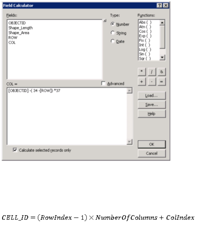
Add the attribute COL to the table in the Attributes of mfcells window. The row index can be calculated according to:

This is what it looks like in the Field Calculator.

GSFlow Training Class Material: Instructions for GSFLOW Model Input Preparation

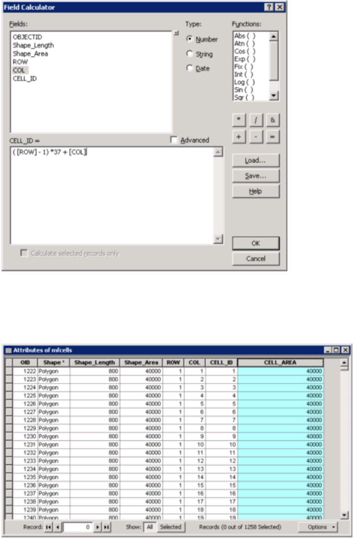
Add the attribute CELL_ID to the table in the Attributes of mfcells window. The cell index can be

calculated according to:

This is what it looks like in the Field Calculator.

GSFlow Training Class Material: Instructions for GSFLOW Model Input Preparation

Add the attribute CELL_AREA to the table in the Attributes of mfcells window. Copy the values from

the Shape_Area attribute using the Field Calculator:

After this map has been created, save the Sagehen ArcMap project by clicking File->Save.

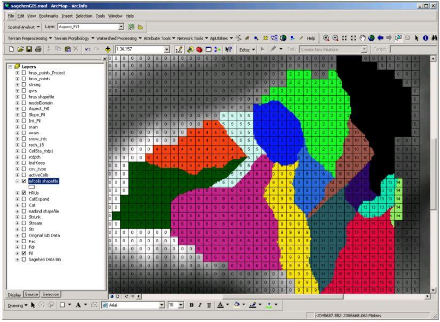
The feature set mfcells is the vector version of the MODFLOW grid cell map.

GSFlow Training Class Material: Instructions for GSFLOW Model Input Preparation

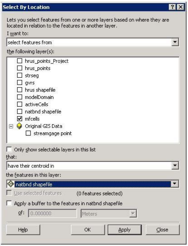
Generation of "Clipped" Model Domain and Active Cells Maps

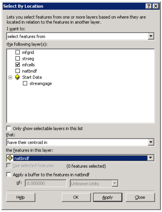
Choose Selection-> Select By Location from the top level ArcMap menu bar. Choose the

options specified below:

GSFlow Training Class Material: Instructions for GSFLOW Model Input Preparation

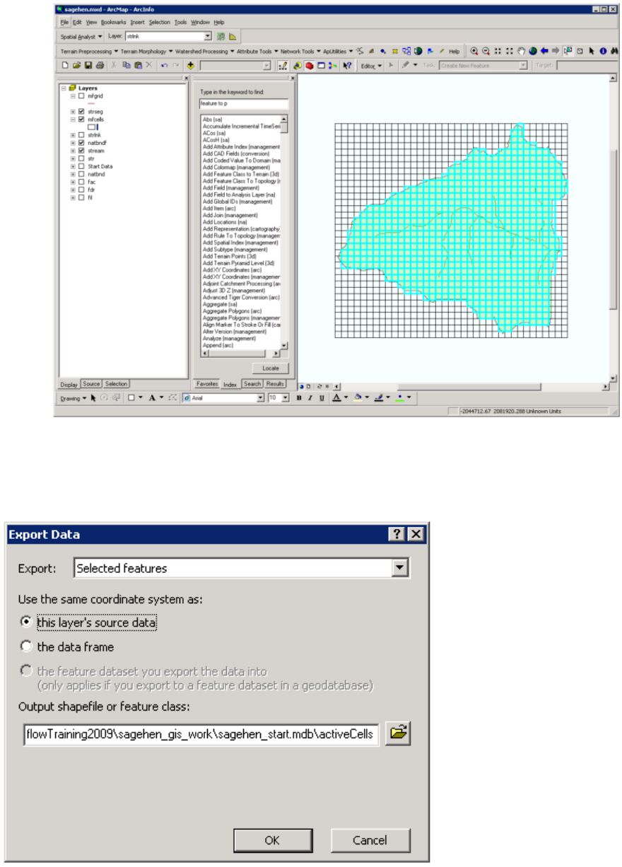
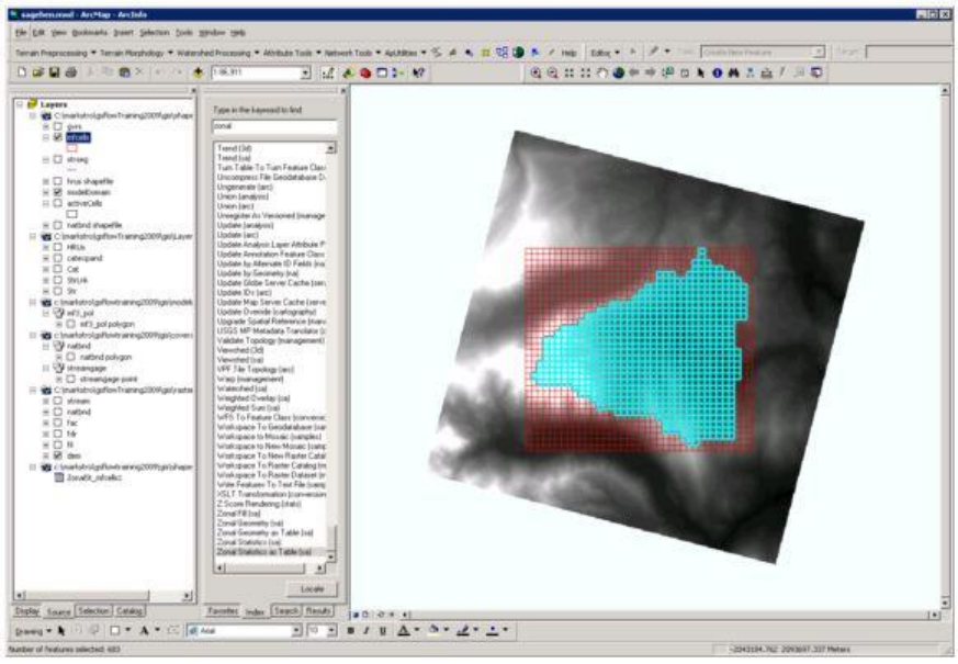
Right click on the mfcells map in the tree. Choose Data->Export Data to make a new feature class of the

active cells. Name this activeCells.

GSFlow Training Class Material: Instructions for GSFLOW Model Input Preparation

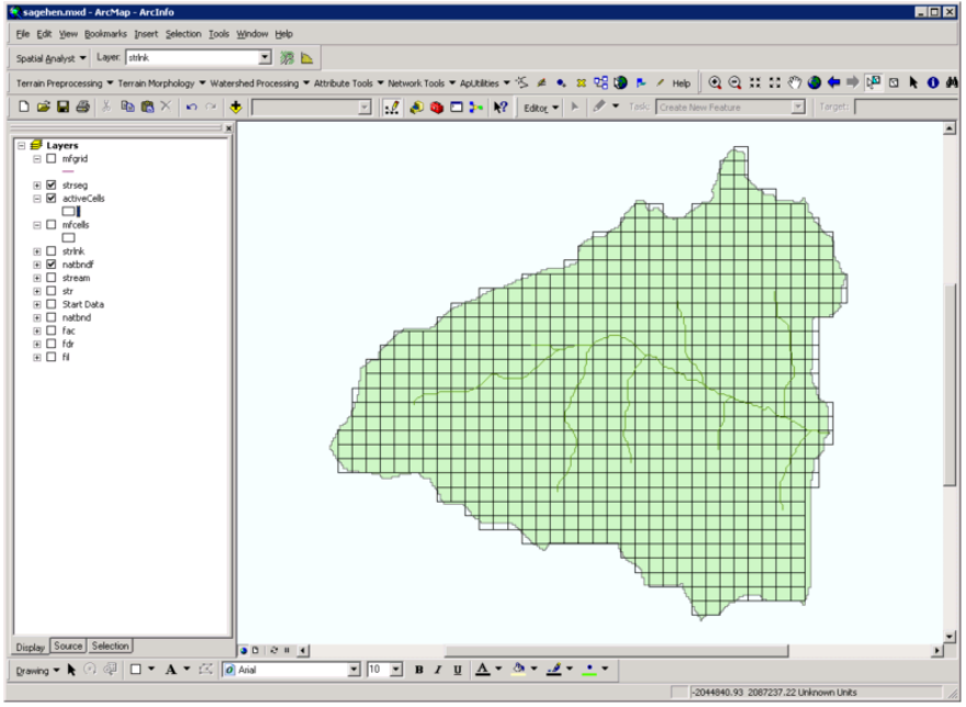
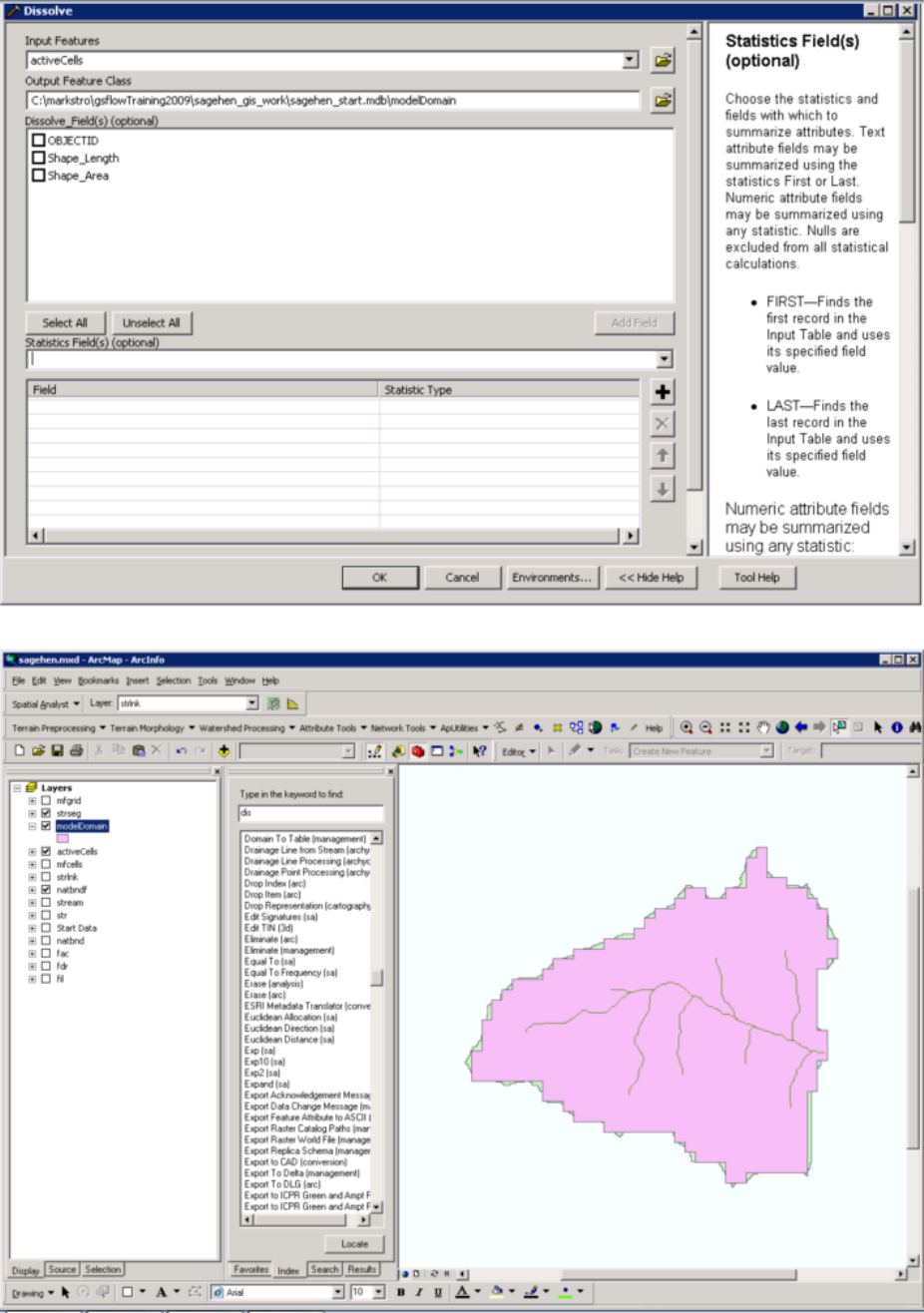
Next, dissolve all of the active cells into one big feature to get the map of the "Clipped" Model Domain.

Use the Dissolve(management) tool to do this. Name the output feature class modelDomain.

GSFlow Training Class Material: Instructions for GSFLOW Model Input Preparation

After this map has been created, save the Sagehen ArcMap project by clicking File->Save.

The feature class modelDomain is the vector version of the model domain map. This map defines

that areal extent of the Sagehen example problem. The feature class activeCells is the vector

version of the cells which are active in the MODFLOW model.

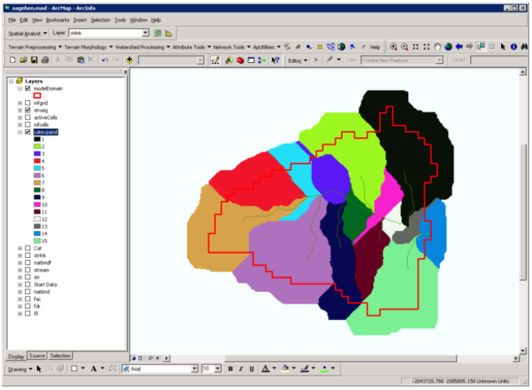
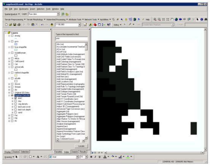
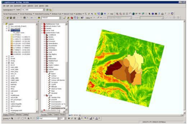
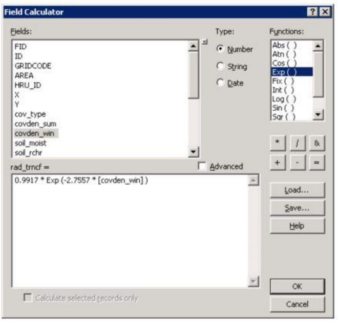
Generation of PRMS HRU map

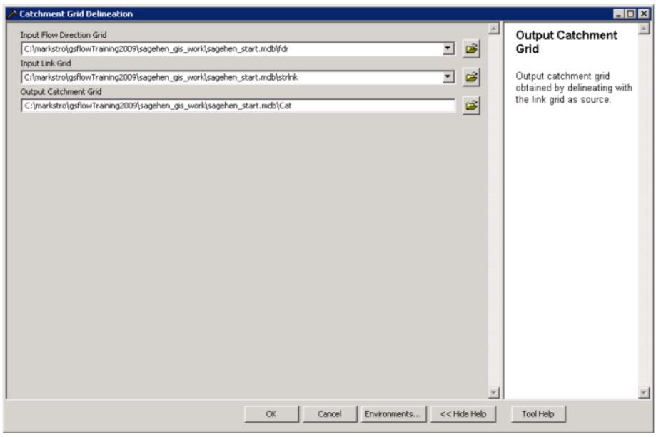
Make sure that the Spatial Analyst extension is turned on: Tools->Extensions. Check Spatial

Analyst. Use the Catchment Grid Delineation (archydro) tool. Specify the flow direction (fdr) and the

stream link (strlnk) grids as input. Name the output grid Cat. Click OK.

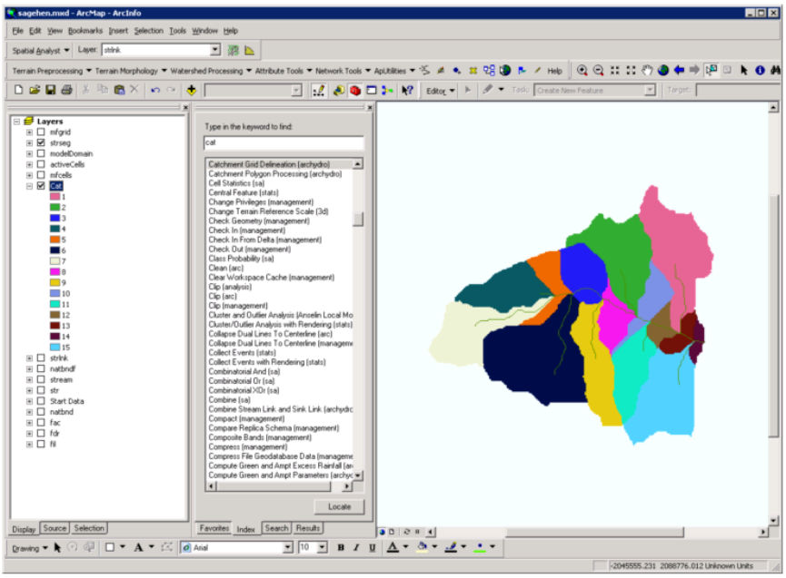
Here is the resulting Cat grid.

GSFlow Training Class Material: Instructions for GSFLOW Model Input Preparation

These are the natural HRUs. Note that the HRU Grid code matches the corresponding stream segment

that was used to define it. This is because the Catchment Grid Delineation (archydro) tool generates

HRUs based on only the contributing area to each stream segment.

Move the modelDomain feature class to the top of the ArcMap tree stack and make it "hollow". In some

areas, the HRUs need to be clipped, while in others, the HRUs need to be extended to the model domain

edge.

GSFlow Training Class Material: Instructions for GSFLOW Model Input Preparation

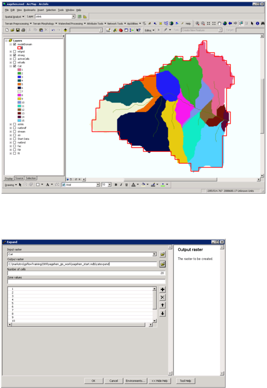
Use the Expand (sa) tool to fill in the HRUs that don't quite go to the edge. Set the Number of cells to

20 and fill in the Zone values with all 15 categories (HRU IDs). Name this grid CatExpand.

GSFlow Training Class Material: Instructions for GSFLOW Model Input Preparation

Here is the resulting catexpand grid.

Now there are no holes between the HRUs and the modelDomain.

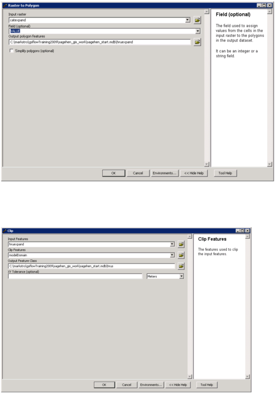
Use the Raster to Polygon(conversion) tool to make a feature set from catexpand. Set output polygon

feature to hruexpand and uncheck Simplify polygons.

GSFlow Training Class Material: Instructions for GSFLOW Model Input Preparation

Use the Clip (anylsis) tool to make the output feature class hrus. Set the Input Features to hruexpand and

the Clip Features to modelDomain.

GSFlow Training Class Material: Instructions for GSFLOW Model Input Preparation

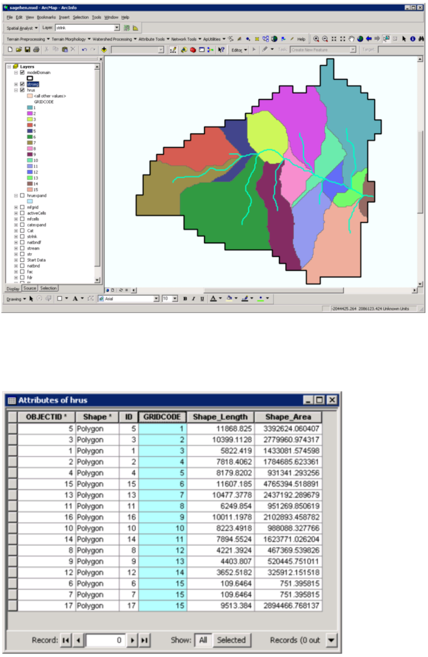
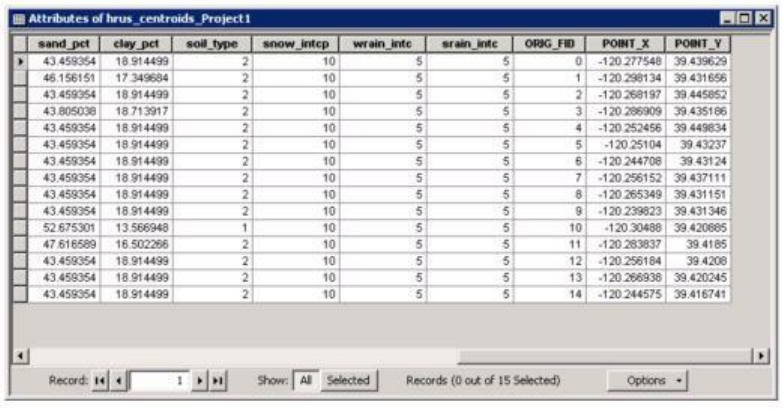
Open the Attributes of hrus window and Sort Ascending on the GRIDCODE attribute. This attribute

will be used as the HRU ID.

GSFlow Training Class Material: Instructions for GSFLOW Model Input Preparation

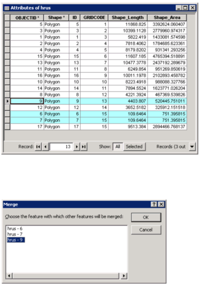
There are 17 features, but there are only 15 HRUs. This means that some HRUs are split. Notice that

there are 3 features assigned to the GRIDCODE attribute values of 15 and that two of these features

have a very small comparative area (751 square meters compared to 2,894,467 square meters). Find

these small features by selecting them from the Attributes of hrus table.

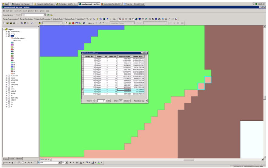
Select the hrus feature class in the ArcMap tree and then choose the XTools Pro -> Start Editing

Selected Layer menu option. Select the features with OBJECTID values of 9, 6, and 7.

GSFlow Training Class Material: Instructions for GSFLOW Model Input Preparation

Choose the Editor->Merge menu option. Choose hrus 9 in the Merge window. This will dissolve the

two small features into the big adjacent one. Click OK.

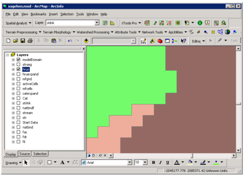
Choose the Editor->Stop Editing to save the edits. The hrus map should look like this:

GSFlow Training Class Material: Instructions for GSFLOW Model Input Preparation

Click on Editor->Stop Editing when finished.

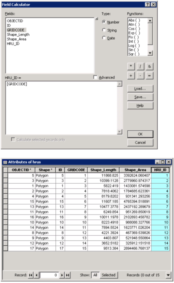
Add the attribute HRU_ID to the hrus feature class in the Attributes of hrus window. Copy the values

from the GRIDCODE attribute to the new HRU_ID attribute.

GSFlow Training Class Material: Instructions for GSFLOW Model Input Preparation

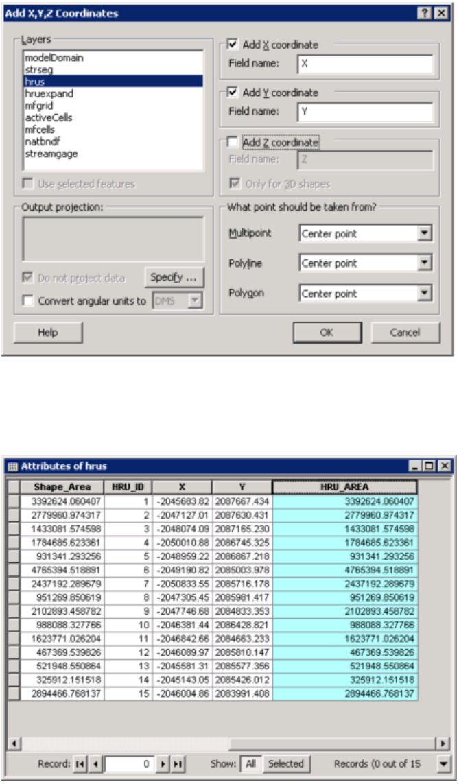
Calculate X and Y coordinates for each HRU using XTools Pro Toolbar-> Table Operations ->Add

X,Y,Z Coordinates. Select hrus Layers, uncheck Add Z coordinate, and modify X and Y field if desired.

GSFlow Training Class Material: Instructions for GSFLOW Model Input Preparation

Add the attribute HRU_AREA to the table in the Attributes of hrus window. Copy the values from the

Shape_Area attribute using the Field Calculator:

After this map has been created, save the Sagehen ArcMap project by clicking File->Save.

The feature class hrus is the HRU map.

GSFlow Training Class Material: Instructions for GSFLOW Model Input Preparation

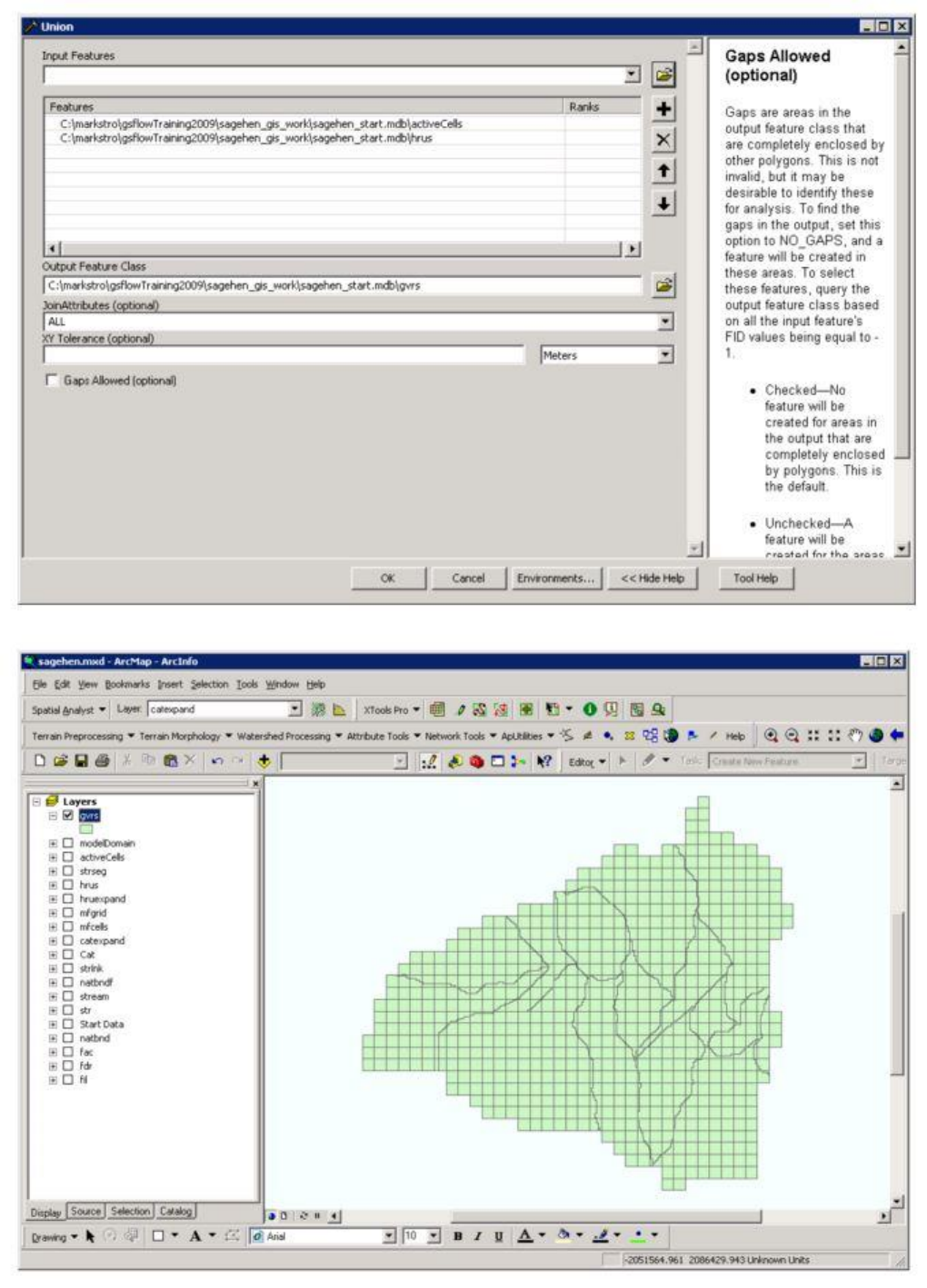
Generation of GSFLOW Gravity Reservoir (GVR) map

Use the Union (analysis) tool to cut the feature class activeCells with the feature class hrus.

Click off the Gaps Allowed check box. Name this feature class gvrs. Click OK.

GSFlow Training Class Material: Instructions for GSFLOW Model Input Preparation

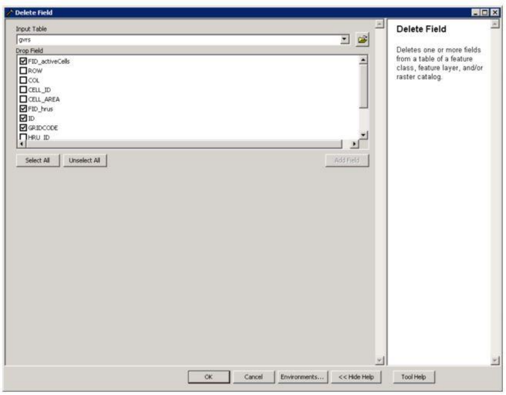
Use the Delete Field (management) tool. Set input table to grvs and select fields to delete. Delete the

attributes FID_hrus, ID; GRIDCODE; and FID_activeCells. Click OK.

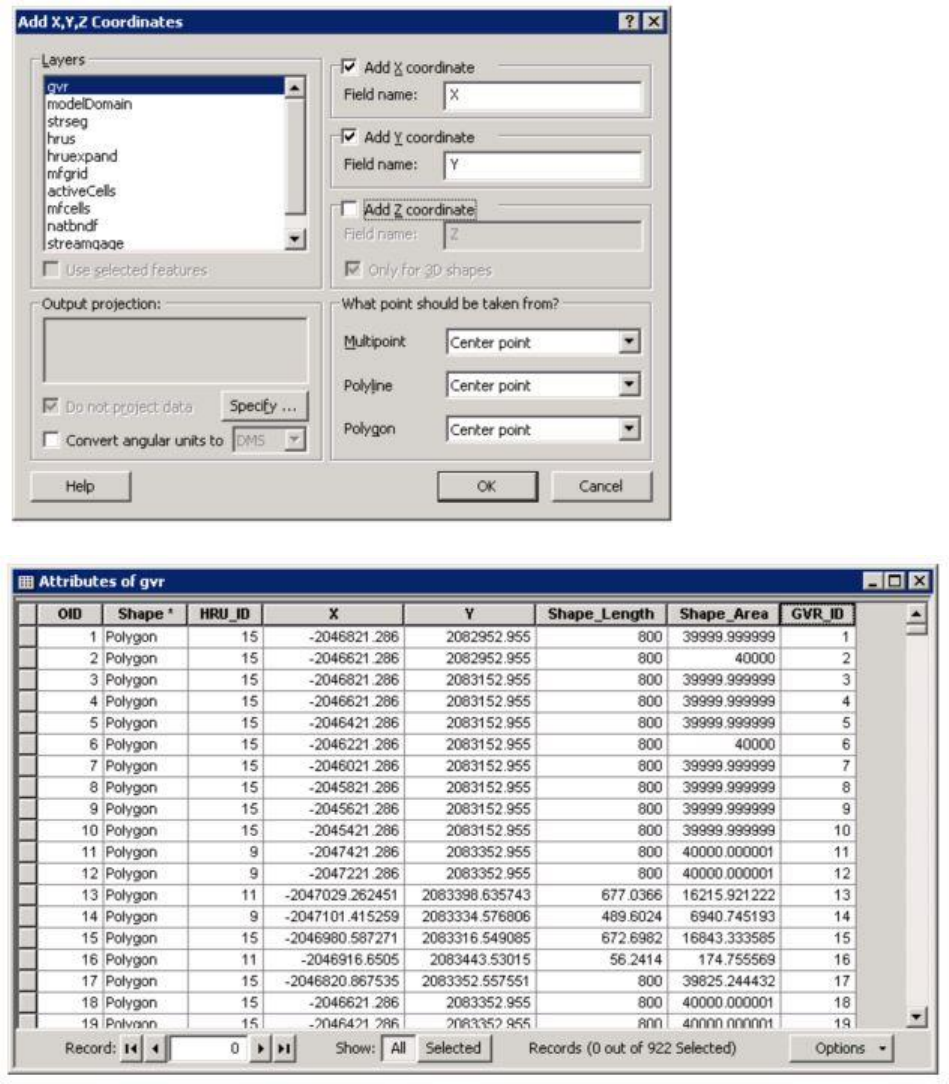
Add attribute GRV_ID to the gvrs feature class. Use the Field Calculator to copy the values from the

OBJECTID attribute to the new GRV_ID attribute.

Calculate X and Y coordinates for each gvrs using XTools Pro Toolbar-> Table Operations ->Add

X,Y,Z Coordinates. Select gvrs Layer, uncheck Add Z coordinate, and modify X and Y field if desired.

Note make sure to overwrite existing values, as they are remnants and don't represent the correct values.

GSFlow Training Class Material: Instructions for GSFLOW Model Input Preparation

After the feature class gvrs has been created, save the Sagehen ArcMap project by clicking File->Save.

The feature class gvrs is the gravity reservoir map.

GSFlow Training Class Material: Instructions for GSFLOW Model Input Preparation

Adding modeling attributes to the GSFLOW maps

HRU map

PRMS HRU Parameters (these sections come from unpublished document by Gregg Lamorey).

Several of the PRMS parameters are determined using a DEM and other GIS coverages

including coverages of vegetation and soil data. The GIS coverages used in parameterization are

available for the US on a 1 km grid. The required coverages are: vegetation type (lulc), vegetation

density (density), available water-holding capacity (awc), soil depth (rockdep), sand content (sandave)

and clay contents (clayav). These coverages should be projected into the same projection, same extent

and same cell resolution as the local DEM used to delineate the basin. The "Environments" setting

should be set to the extent and cell size used in the DEM for all coverages generated.

Note: the clipping steps have already been done for the Sagehen example problem and are

located in Sagehen Data Bin in the ArcMap tree. All ArcMap analysis tools can be accessed using the

ArcMap Search window.

This shows LULC clipped to the extent of the DEM.

GSFlow Training Class Material: Instructions for GSFLOW Model Input Preparation

Remap tables used to reclassify coverages are also used in the parameterization. The necessary

tables are in the folder gis\startData\SagehenDataBin\remap. The cov-den-winter2.rmp, prms-

intcp_snow.rmp, prms-intcp_srain.rmp, and prms-intcp_wrain.rmp remap tables are in percent or

hundredths of an inch and need to be divided by 100 to obtain the correct values while the temp_adj.rmp

remap table is in tenths of degrees and needs to be divided by 10 to obtain the correct values (this was

done because of problems reclassing an integer to a real number in ArcMap).

cov_type

The coverage type (0 for bare, 1 for grass, 2 for shrub, 3 for deciduous trees, and 4 for

coniferous tress) is determined from the vegetation type coverage. This can be calculated in ArcMap by

first using "Spatial Analyst Tools > Reclass > Reclass by ASCII file" with the vegetation species

coverage "lulc" as the input raster, "cov-type_new.rmp" as the "Input ASCII remap file", and

"cov_type" as the "Output raster."

GSFlow Training Class Material: Instructions for GSFLOW Model Input Preparation

The values for each HRU can be determined using the Zonal Statistics (Spatial Analyst) tool in

ArcMap with the HRU shapefile specified as the "Input raster or feature zone data", the HRU id field as

the "Zone field", and "cov_type" specified as the "Input value raster". The output from the zonal

statistics is a .dbf file that can be opened in a spreadsheet.

*****Do not modify the .dbf file in excel it will corrupt the data *****

Make a new field "cov_type" in the HRUs shapefile. Join the table made above and bring up the

attribute table. Copy the values from the joined "MAJORITY" field into the cov_type field. Unjoin the

table from the HRUs shapefile.

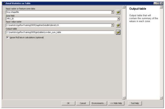
covden_sum

The vegetation coverage density in the summer is the mean value of the vegetation density. This

can be calculated Zonal Statistics (Spatial Analyst) tool with the HRU shapefile specified as the "Input

raster or feature zone data", the HRU id field as the "Zone field", and "SagehenDataBin\density1k"

specified as the "Value raster."

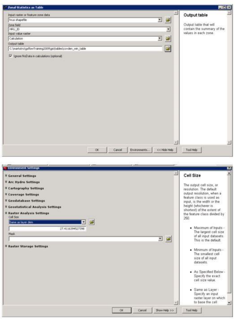
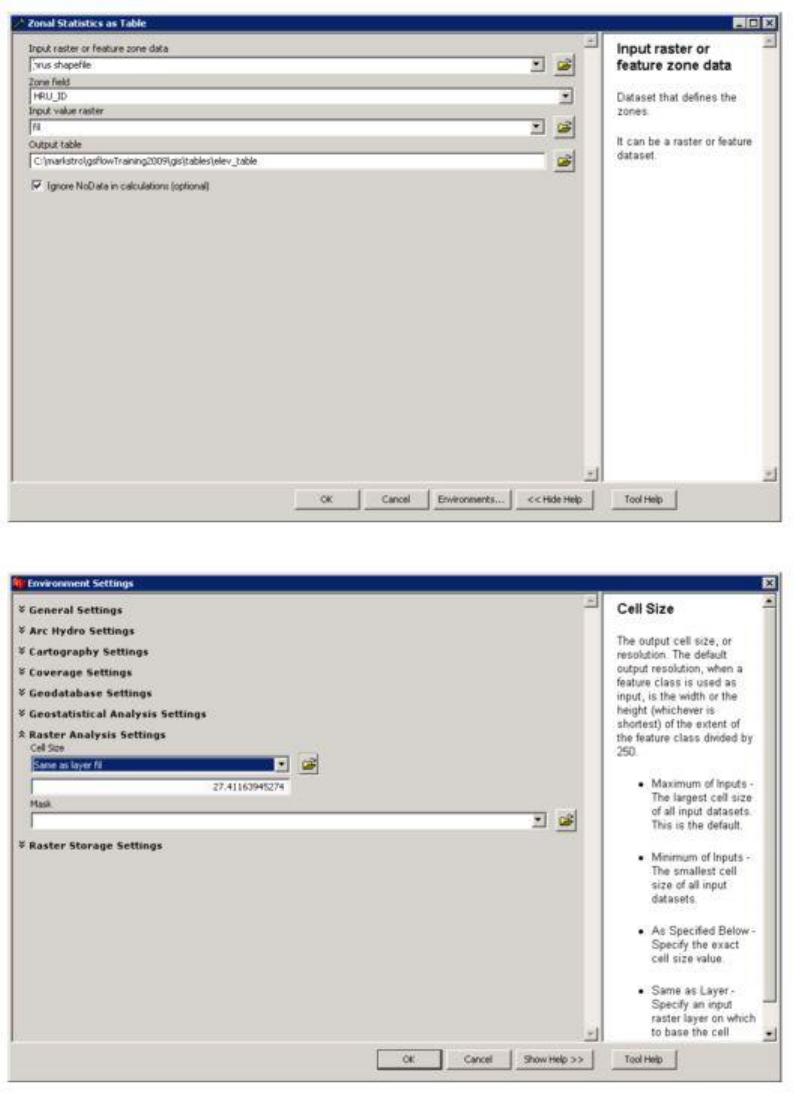
Use the Zonal Statistics as Table tool:

GSFlow Training Class Material: Instructions for GSFLOW Model Input Preparation

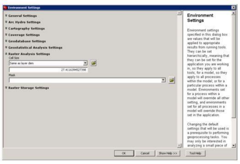
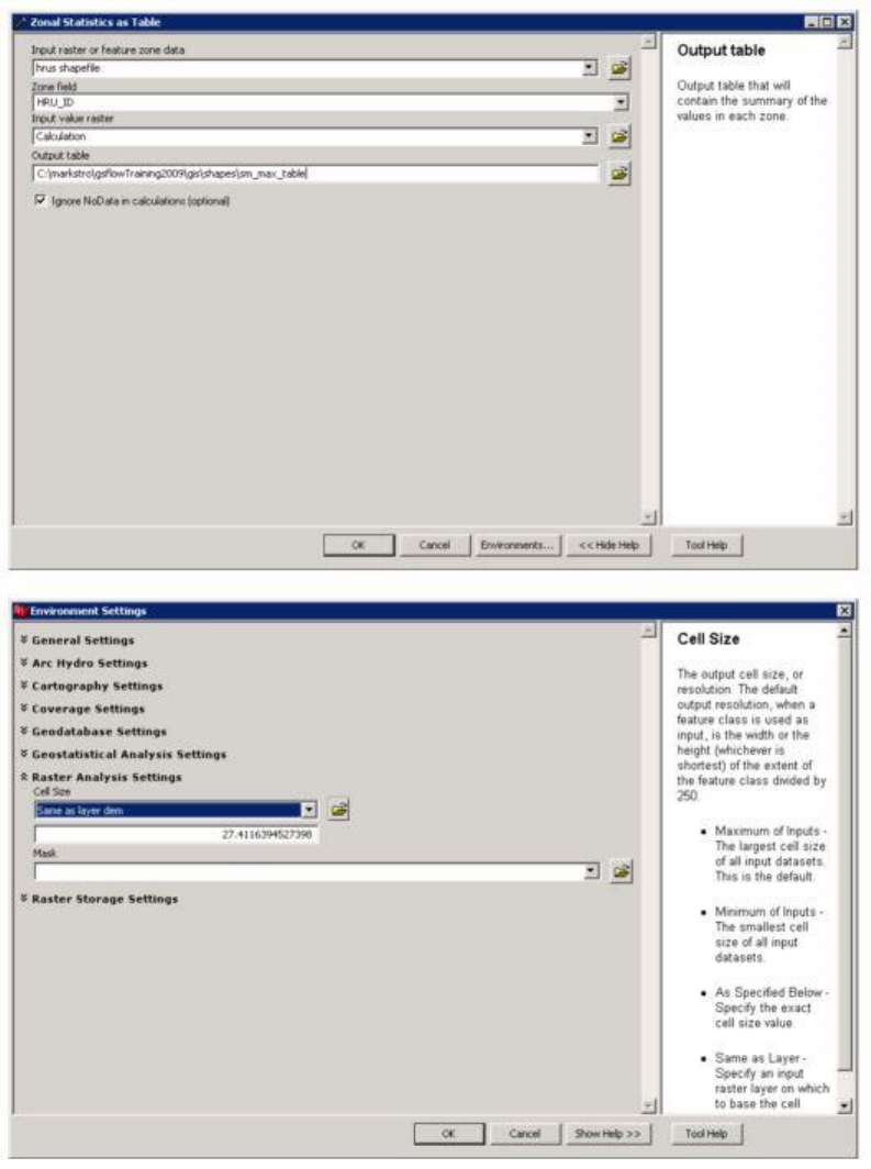
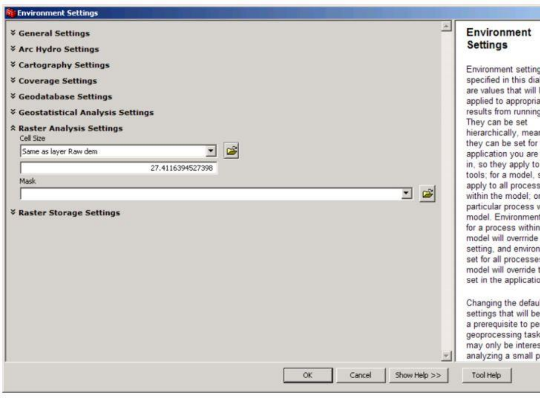
Be sure to set Environments->Raster Analysis Settings -> Cell Size to Same as layer dem. This sets the

cell size in the analysis to 27.4… This is important because this tool converts the HRU shapefile to a

raster to do the analysis. If the Input value raster is too coarse (in this case it is 1 km2) the HRUs will

not be able to be represented and the zonal statistics will be messed up. If the generated zonal statistics

table does not have a valid row for each HRU, this is what happened.

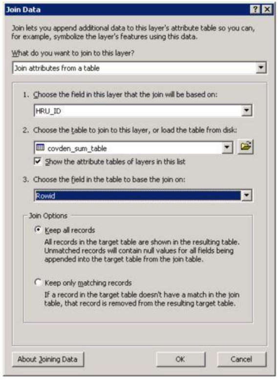
Choose the MEAN value from the joined table and using the Field Calculator, divide by 100 (to

make decimal fraction out of percent) and copy it into a new field called covden_sum (type double), as

for parameter cov_type.

GSFlow Training Class Material: Instructions for GSFLOW Model Input Preparation

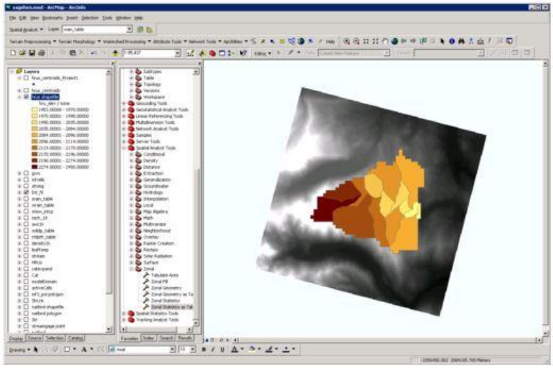
To see the HRUs colored by the parameter values (do this for every parameter), bring up the properties

for the HRUs shapefile and set the Symbology to something similar to what is shown:

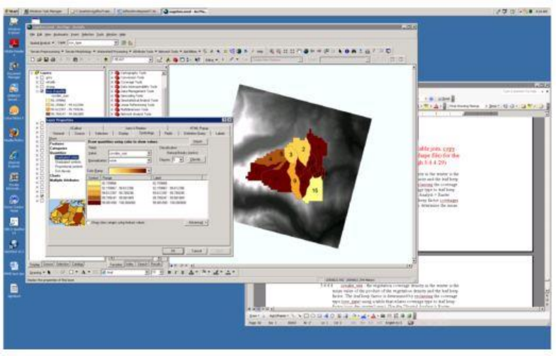
GSFlow Training Class Material: Instructions for GSFLOW Model Input Preparation

Repeat the above steps (reclass, zonal statictics, table join, copy out the parameter values into

fields in the HRU shape file) for the rest of the PRMS parameters (steps 4.13 through 4.1.18)

covden_win

The vegetation coverage density in the winter is the mean value of the product of the vegetation

density and the leaf keep factor. The leaf keep factor is determined by reclassing the coverage type

(cov_type) using a table that relates coverage type to leaf keep factor (cov-den-winter2.rmp).

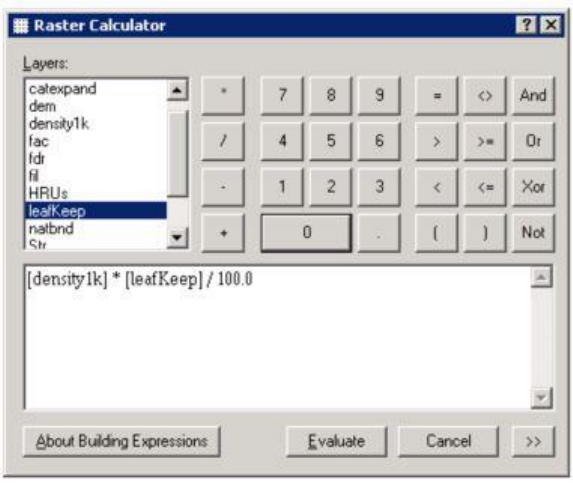
Use the Raster Calculator (Spatial Analyst) tool to multiply the vegetation

(SagehenDatabin\density1k) and leaf keep factor coverages (divide by 100.0 to keep it as a percentage).

GSFlow Training Class Material: Instructions for GSFLOW Model Input Preparation

Then use the Zonal Statistics as Table (Spatial Analyst) tool to determine the mean value for each HRU.

GSFlow Training Class Material: Instructions for GSFLOW Model Input Preparation

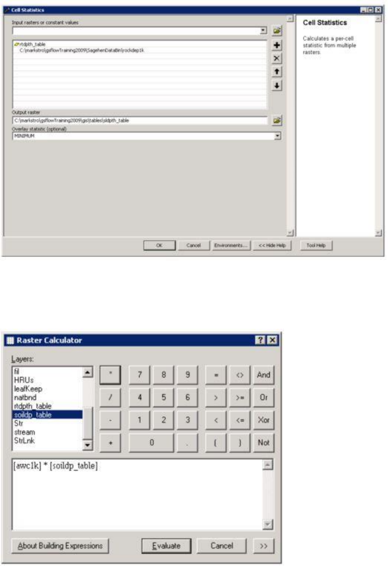
soil_moist_max

The soil moisture maximum is the product of the Available Water Content (awc) and the rooting

depth.

GSFlow Training Class Material: Instructions for GSFLOW Model Input Preparation

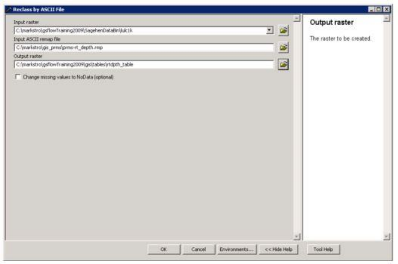
The rooting depth is calculated as the minimum of the root depth and the soil depth. The root

depth is determined by reclassing from vegetation species (SagehenDataBin\lulc1k) to root depth using

the Reclass by ASCII file (Spatial Analyst) tool with the remap table, prms_rt_depth.rmp.

The minimum of root depth and bed rock depth (SagehenDataBin\rockdep1k) coverages can be

generated using the Cell Statistics (Spatial Analyst) tool and specifying the two coverages as the input

rasters and setting the "Overlay statistic" to "Minimum".

GSFlow Training Class Material: Instructions for GSFLOW Model Input Preparation

The product of the awc and minimum depth rasters can be determined with the Raster Calculator

(Spatial Analyst) tool.

A zonal mean of this raster for each HRU can be calculated using the Zonal Statistics as Table (Spatial

Analyst) tool.

GSFlow Training Class Material: Instructions for GSFLOW Model Input Preparation

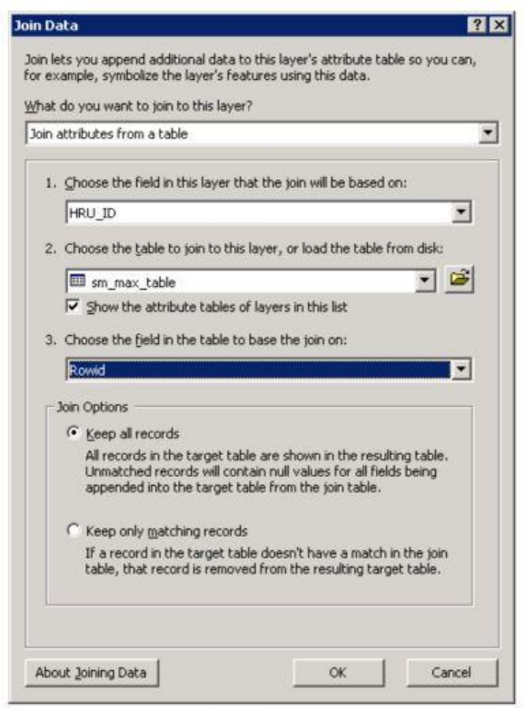
Copy the zonal MEAN value to sm_max (PRMS parameter soil_moist_max) in HRUs shapefile.

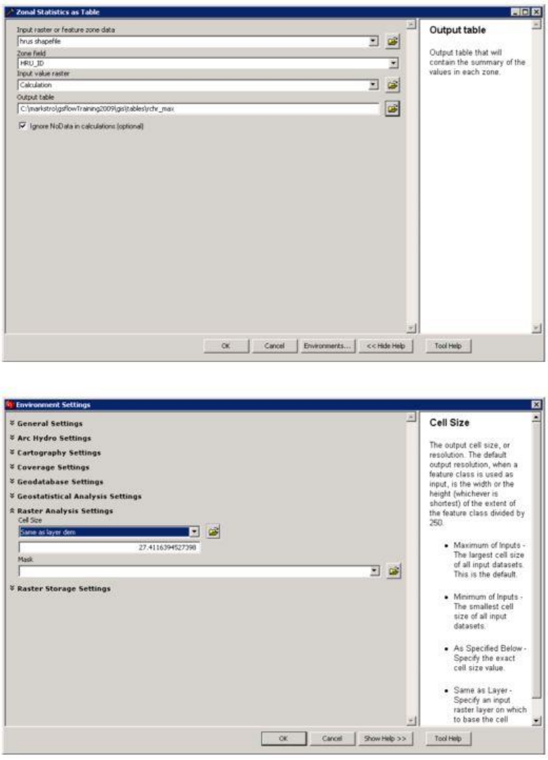
soil_rchr_max

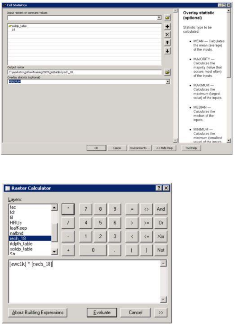
The soil recharge zone maximum value is the minimum of the rooting depth and 18 inches

multiplied by AWC. First, the minimum of the rooting depth (determined under soil_moist_max) and 18

inches is calculated usingthe Cell Statistics (Spatial Analyst) tool.

GSFlow Training Class Material: Instructions for GSFLOW Model Input Preparation

Next, the resulting coverage is multiplied by awc using "Spatial Analyst > Raster Calculator".

A zonal mean of this raster for each HRU can be calculated using Zonal Statistics as Table (Spatial

Analyst) tool

GSFlow Training Class Material: Instructions for GSFLOW Model Input Preparation

Copy the zonal MEAN value to rchr_max (PRMS parameter soil_rchr_max) in HRUs shapefile.

GSFlow Training Class Material: Instructions for GSFLOW Model Input Preparation

soil_type

The soil type (1 for sand, 2 for loam, and 3 for clay) is determined by first calculating the zonal

means of the sandave and clayav coverages for each HRU using the Zonal Statistics as Table (Spatial

Analyst) tool.

If sandav is greater than 50% then the type is 1, if clayav is greater than 40% then the type is 3,

otherwise the type is 2. This calculation can be implemented by hand by sorting the means and setting

the corresponding cells.

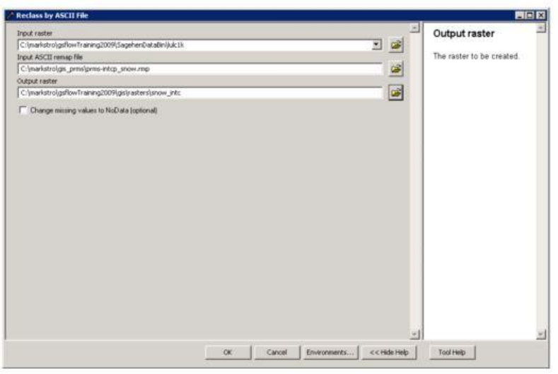
snow_intcp

The snow interception storage capacity is determined by reclassing from vegetation species

(lulc) to snow interception storage capacity using the Reclass by ASCII File (Spatial Analyst) tool with

the remap table prms-intcp_snow.rmp.

GSFlow Training Class Material: Instructions for GSFLOW Model Input Preparation

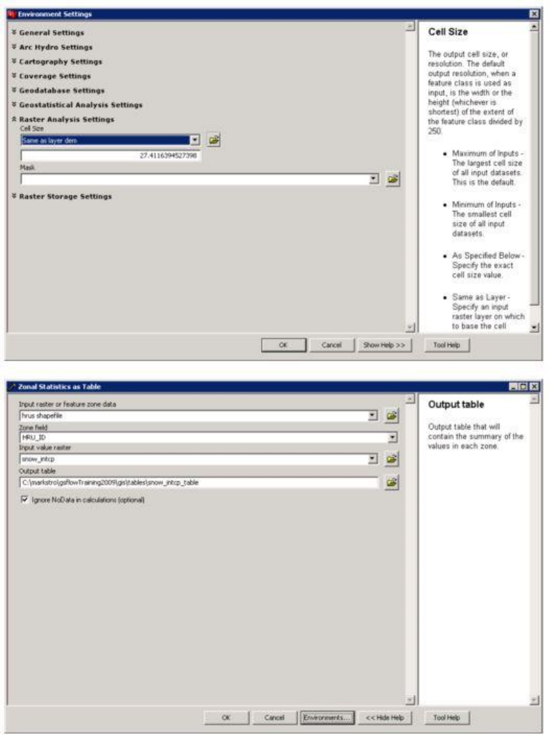
A zonal mean of this raster for each HRU can be calculated using the Zonal Statistics as Table (Spatial

Analyst) tool.

GSFlow Training Class Material: Instructions for GSFLOW Model Input Preparation

Divide these values by 100.0 when copying the zonal mean field into the snow_intcp field.

GSFlow Training Class Material: Instructions for GSFLOW Model Input Preparation

wrain_intcp

The winter rain interception storage capacity is determined by reclassing from vegetation species

(lulc) to winter rain interception storage capacity using the Reclass by ASCII File (Spatial Analyst) tool

with the remap table prms-intcp_wrain.rmp. A zonal mean of this raster for each HRU can be calculated

using the Zonal Statistics as Table (Spatial Analyst) tool. Divide these values by 100.0 when copying

the zonal mean field into the wrain_intcp field.

srain_intcp

The summer rain interception storage capacity is determined by reclassing from vegetation

species (lulc) to summer rain interception storage capacity using the Reclass by ASCII File (Spatial

Analyst) tool with the remap table prms-intcp_srain.rmp. A zonal mean of this raster for each HRU can

be calculated using the Zonal Statistics as Table (Spatial Analyst) tool. Divide these values by 100.0

when copying the zonal mean field into the srain_intcp field.

hru_lat

The latitude of the centroids of the HRU's can be determined by first converting the polygon

coverage of the HRU's to centroids using the Feature to Point (Data Managment) tool. The centroid

coverage can be projected to latitude and longitude using the Project (Data Management) tool and

specifying the output coordinate system (by clicking on the button next to "Output Coordinate System"

and selecting the "Select" button on the resulting "Spatial Reference Properties" dialog box) to be

"Geographic > North America > North American Datum 1983.prj". The new coordinates can be added

to the coverage attribute table using the Add XY Coordinates (Data Management) tool.

GSFlow Training Class Material: Instructions for GSFLOW Model Input Preparation

hru_elev

The hru elevation is determined as the zonal median elevation instead of mean elevation because

the median is less sensitive to outliers such as a few very high elevation points. To calculate the median

elevation, the DEM used to delineate the basin (Fil) must first be converted to an integer coverage using

the Int (Spatial Analyst) tool. The zonal median for each HRU can be calculated from this coverage

using the Zonal Statistics as Table (Spatial Analyst) tool.

GSFlow Training Class Material: Instructions for GSFLOW Model Input Preparation

hru_slope

The hru slope can be calculated from Fil using the Slope (Spatial Analyst) tool and select the

output measurement as "percent_rise". The zonal mean for each HRU can be calculated from this

coverage using the Zonal Statistics as Table (Spatial Analyst) tool. Divide these values by 100.0 when

copying the zonal mean field into the hru_slope field.

GSFlow Training Class Material: Instructions for GSFLOW Model Input Preparation

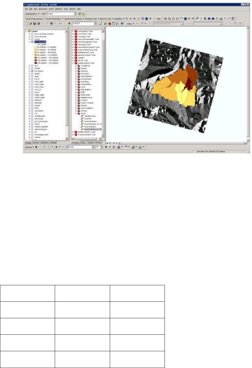
hru_aspect

The hru aspect can be calculated from Fil using the Aspect (Spatial Analyst) tool. To calculate

the median aspect, the Aspect map just created must first be converted to an integer coverage using the

Int (Spatial Analyst) tool. The zonal median for each HRU can be calculated from this coverage using

the Zonal Statistics as Table (Spatial Analyst) tool.

GSFlow Training Class Material: Instructions for GSFLOW Model Input Preparation

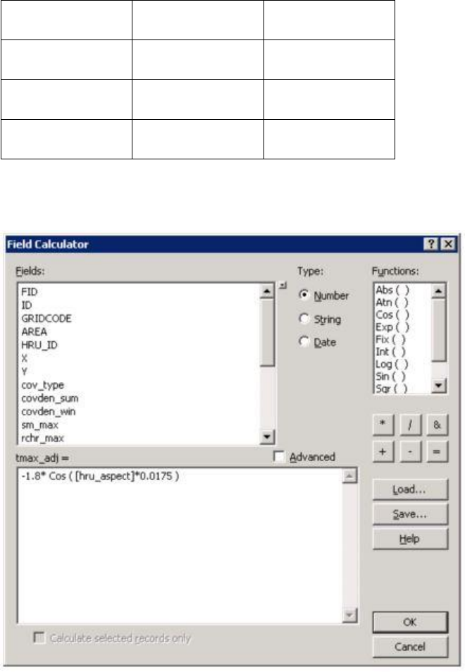
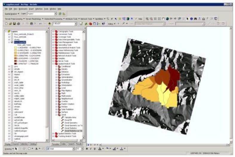
tmax_adj

tmax_adj is an adjustment made to the hru maximum temperature based on the aspect of the hru.

This parameter is estimated with the equation:

tmax_adj = -1.8 cos(hru_aspect * 0.0175)

Use the Field Calculator to fill in the tmax_adj field. The multiplier 0.0175 converts degrees to radians.

In addition to the tmax_adj method calculated above a more simple method can be employed.

Degree

Direction

tmax_adj

337.5-22.5

North

-1.7

22.5-67.5

Northeast

-1.0

67.5-112.5

East

0.0

112.5-157.5

Southeast

1.0

GSFlow Training Class Material: Instructions for GSFLOW Model Input Preparation

157.5-202.5

South

1.7

202.5-247.5

Southwest

1.0

2478.5-292.5

West

0.0

292.5-337.5

Northwest

-1.0

This is the method employed in the original GSFLOW Sagehen example problem.

GSFlow Training Class Material: Instructions for GSFLOW Model Input Preparation

tmin_adj

tmin_adj is an adjustment made to the hru minimum temperature based on the aspect of the hru.

The values are the same as calculated for tmax_adj.

hru_area

The area of the hru's is already a field in the hru polygon shapefile. The area listed in this field is

the number of cells in each hru. This must be converted to acres by first converting to map units (square

meters if in UTM) then converting to acres (1 acre = 4047 m2).

GSFlow Training Class Material: Instructions for GSFLOW Model Input Preparation

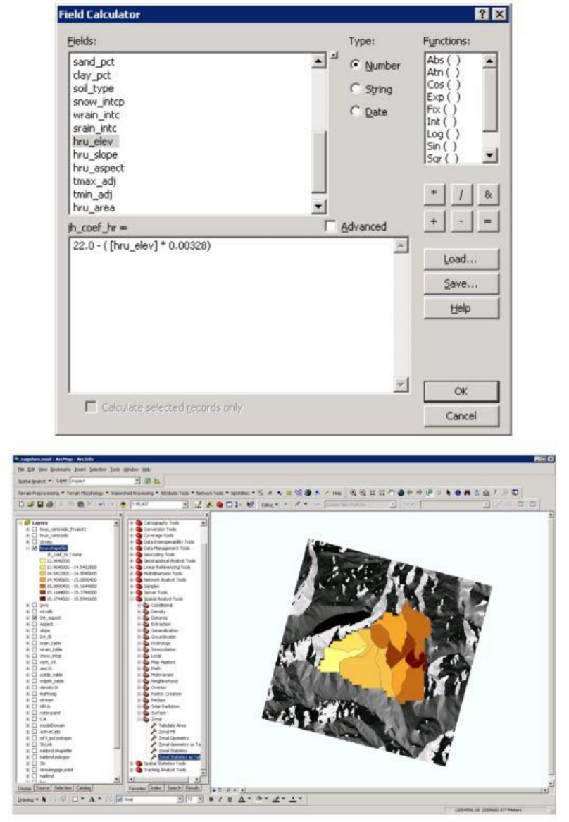
jh_coef_hru

This air temperature coefficient used in Jensen-Haise potential evapotranspiration computations

can be calculated for each HRU using the following equation: jh_coef_hru = 27.5-0.25*(high_sat -

low_sat)-(hru_elev/1000) where high sat is the saturation vapor pressure, in millibars, for the mean

maximum air temperature for the warmest month of the year and low_sat is the saturation vapor

pressure, in millibars, for the mean minimum air temperature for the warmest month of the year. The

saturation vapor pressure can be calculated using sat function = 6.1078exp^[(17.269(x)/(x + 237.3)

where x is the temperature. .Assume the minimum temperature is 10 C and maximum temperature is 25

C so that low_sat is 10.02 and high_sat is 31.67. This parameter can be calculated with a spreadsheet

since it is only a function of hru_elev. So, if hru_elevation is in meters, the equation is: jh_coef_hru =

22.0 - (hru_elev * 0.00328)

GSFlow Training Class Material: Instructions for GSFLOW Model Input Preparation

rad_trncf

The transmission coefficient for short-wave radiation through the winter vegetation canopy can

be calculated as

rad_trncf = 0.9917 * exp(-2.7557 * covden_win).

This parameter can be calculated with the Field Calculator since it is only a function of covden_win.

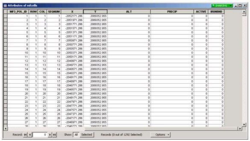
MODFLOW Grid Cell map (shapefile mfcells)

Add fields X (double) and Y (double) use Calculate Geometry to fill them in. Add fields ALT

(integer), PRECIP (double), ACTIVE (integer), IRUNBND (integer).

GSFlow Training Class Material: Instructions for GSFLOW Model Input Preparation

Fill in the cell altitude attribute (ALT)

The fiield ALT is the cell top altitude and is determined as the zonal median altitude. To

calculate the median altitiude, use the integer version of the DEM (Int_Fil) that was created to

determine the parameter hru_elev. The zonal median for each cell can be calculated from this coverage

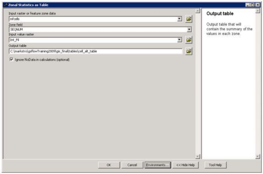
using "Spatial Analyst > Zonal Statistics".

GSFlow Training Class Material: Instructions for GSFLOW Model Input Preparation

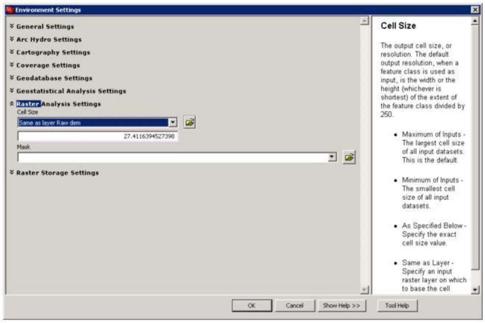
Click on the Environments button to set the Raster Analysis Settings Cell Size

GSFlow Training Class Material: Instructions for GSFLOW Model Input Preparation

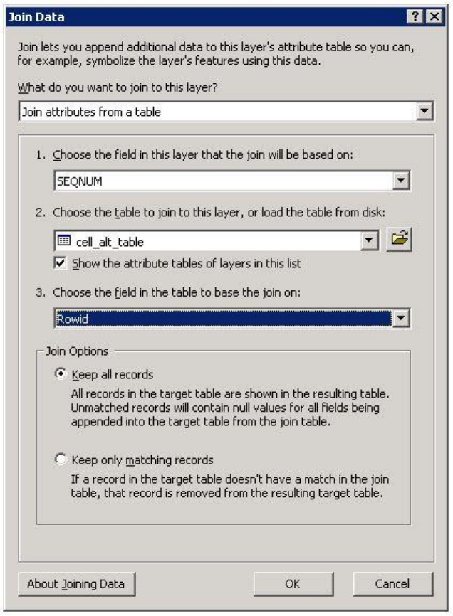
Join the table in the mfcells shapefile to the cell_alt_table attribute table.

GSFlow Training Class Material: Instructions for GSFLOW Model Input Preparation

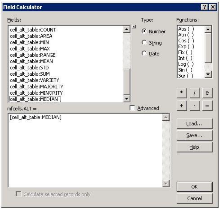
Assign the MEDIAN into the ALT field with the Field Calculator:

GSFlow Training Class Material: Instructions for GSFLOW Model Input Preparation

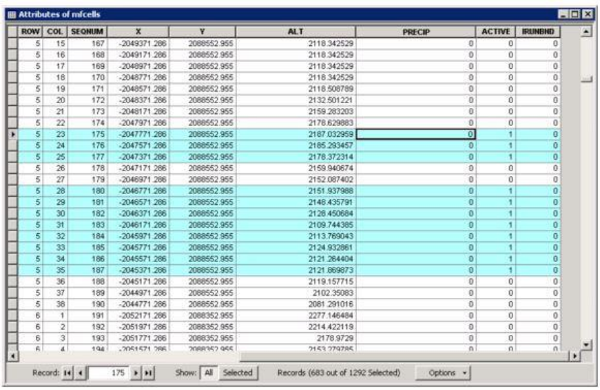
Identify the active cells (ACTIVE)

The field ACTIVE defines the active and inactive MODFLOW cells. 1= active cell; 0 = inactive

cell. Use the Selection->Select By Location tool to select the active cells in the mfcells shapefile with

the modelDomain shapefile.

GSFlow Training Class Material: Instructions for GSFLOW Model Input Preparation

100

The selection looks like this.

GSFlow Training Class Material: Instructions for GSFLOW Model Input Preparation

101

Bring up the Attributes of mfcells table. Make sure that all of the values in the ACTIVE field are set to

0. Click on the Show: Selected button at the bottom of the window. Use the Field Calculator to set the

selected (ACTIVE) cells to 1.

GSFlow Training Class Material: Instructions for GSFLOW Model Input Preparation

102

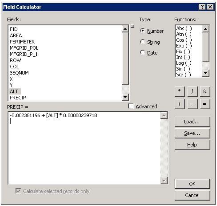
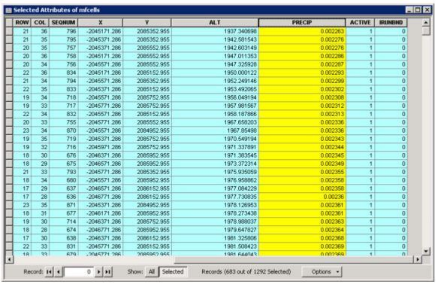
Fill in the cell precipitation attribute (PRECIP)

The field PRECIP is used for steady state recharge; only active cells have values; inactive cells

are blank Load sagehen.data Data File into excel and compute the long term (period of record) means.

This is described in Section 2.2 "Computation of Lapse Rates/Monthly Means using Excel" of this

document. Using this information, a relationship can be developed to estimate long term PRECIP

(recharge) for calibrating a steady state MODFLOW model. This is based on the lapse rates for the

Sagehen Creek COOP station and the cell altitude:

PRECIP = 0.002249 + (ALT-1931.518)* 0.00000239718

PRECIP = 0. 002249 0.00463019 + ALT * 0.00000239718

PRECIP = -0.002381196+ ALT * 0.00000239718

Select only the ACTIVE cells again. Use the Field Calculator to input the above equation for PRECIP.

GSFlow Training Class Material: Instructions for GSFLOW Model Input Preparation

103

Results look like this in the table.

GSFlow Training Class Material: Instructions for GSFLOW Model Input Preparation

104

Fill in the cell IRUNBND attribute

Bring up the HRUs raster (not shapefile) and the activeCell shapefile. The activeCell shapefile

was made in step 3.3.4.

GSFlow Training Class Material: Instructions for GSFLOW Model Input Preparation

105

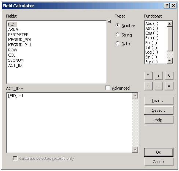
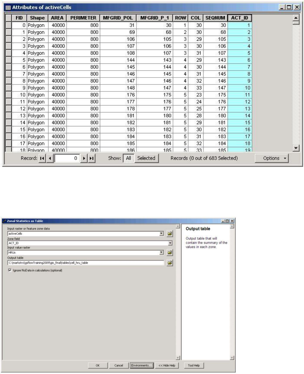
Open up the Attributes of activeCell table and add the field ACT_ID (short integer). Use the Field

Calculator to set the values in ACT_ID to FID + 1.

GSFlow Training Class Material: Instructions for GSFLOW Model Input Preparation

106

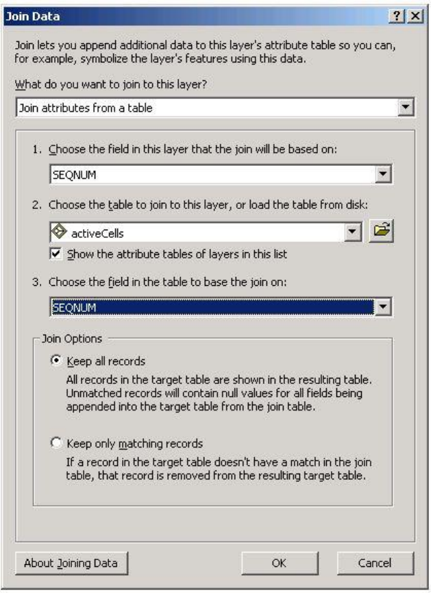
The field ACT_ID will be used in a double-table join using the field SEQNUM.

GSFlow Training Class Material: Instructions for GSFLOW Model Input Preparation

107

Now, use the Zonal Statistics as Table(sa) tool using the activeCells shapefile as input. The Zone field is

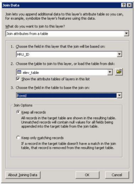
ACT_ID. The Input value raster is HRUs. Name this table tables\cell_hru_table.

GSFlow Training Class Material: Instructions for GSFLOW Model Input Preparation

108

Set the Raster Analysis Cell Size to the Raw DEM.

Do a double-join to get the HRU ID information into the mfcells shapefile.

First, join the table in the mfcells shapefile to the table in the activeCells shapefile using the field

SEQNUM.

GSFlow Training Class Material: Instructions for GSFLOW Model Input Preparation

109

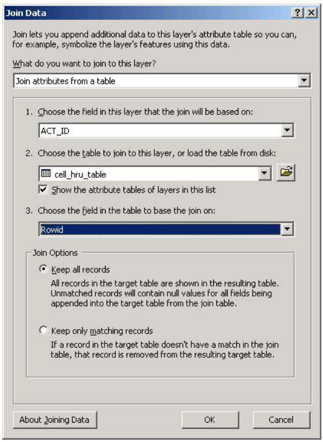
Now, join the table in the mfcells shapefile (field ACT_ID) to the table cell_hru_table (using field

Rowid).

GSFlow Training Class Material: Instructions for GSFLOW Model Input Preparation

110

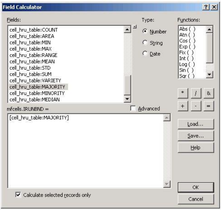
Use the Field Calculator to copy the values from cell_hru_table:Majority into the field

IRUNBND.

GSFlow Training Class Material: Instructions for GSFLOW Model Input Preparation

111

Remove the joins on the mfcells shapefile. Use IRUNBND to label the cells in mfcells. It should look

like this.

GSFlow Training Class Material: Instructions for GSFLOW Model Input Preparation

112

After this map has been created, save the Sagehen ArcMap project by clicking File->Save.

The shapefile gis\shapes\mfcells is the vector version of the MODFLOW cell map. The attributes

that were added to this shapefile can be used in ModelMuse.

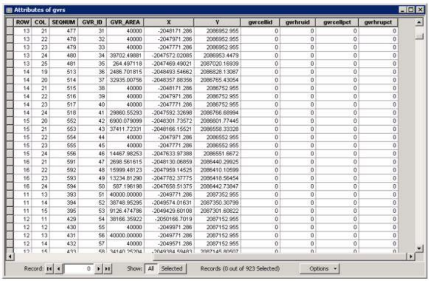
GVR map

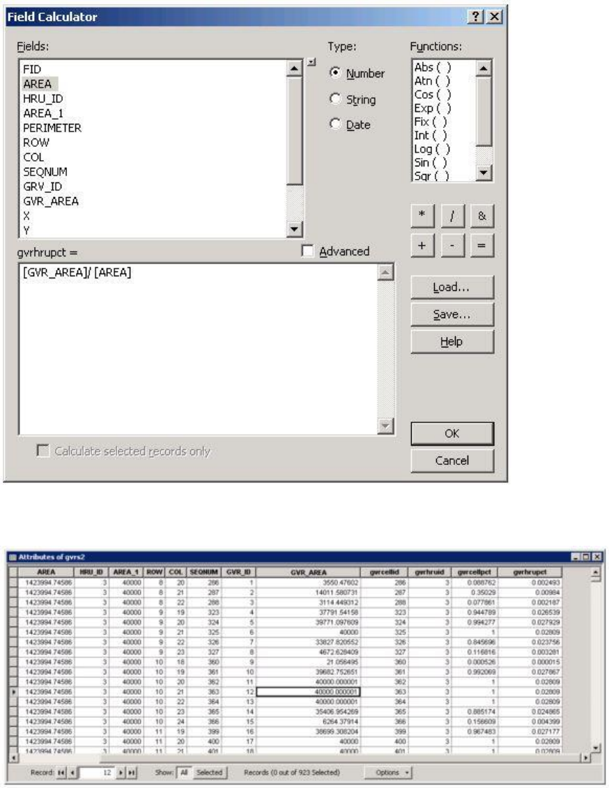
Add four fields to the gvrs shapefile attribute table: gvrhruid (short integer), gvrcellid (short

integer), gvrcellpct (double), gvrhrupct (double).

GSFlow Training Class Material: Instructions for GSFLOW Model Input Preparation

113

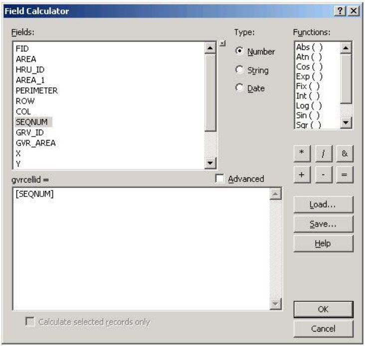
Gvrcellid is the MODFLOW cell id (SEQNUM) which corresponds to the GVR. Set gvrcellid =

SEQNUM using the Field Calculator.

GSFlow Training Class Material: Instructions for GSFLOW Model Input Preparation

114

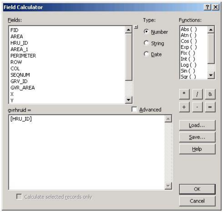
Gvrhruid is the PRMS HRU id (HRU_ID) which corresponds to the GVR. Set gvrhruid = HRU_ID

using the Field Calculator.

GSFlow Training Class Material: Instructions for GSFLOW Model Input Preparation

115

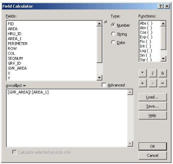
Gvrcellpct is the decimal fraction that the GVR area covers the MODFLOW cell area. Set gvrcellpct =

GVR_AREA / AREA_1 using the Field Calculator. AREA_1 is the area of the MODFLOW cell

(40,000 meters2)

GSFlow Training Class Material: Instructions for GSFLOW Model Input Preparation

116

Gvrhrupct is the decimal fraction that the GVR area covers the PRMS HRU area. Set gvrhrupct =

GVR_AREA / AREA using the Field Calculator. AREA is the area of the HRU.

GSFlow Training Class Material: Instructions for GSFLOW Model Input Preparation

117

The gvrs shapefile attribute table should look like this when finished.

After this information has been created, save the Sagehen ArcMap project by clicking File->Save.

GSFlow Training Class Material: Instructions for GSFLOW Model Input Preparation

118

Making the PRMS Parameter File

Dimension sizes

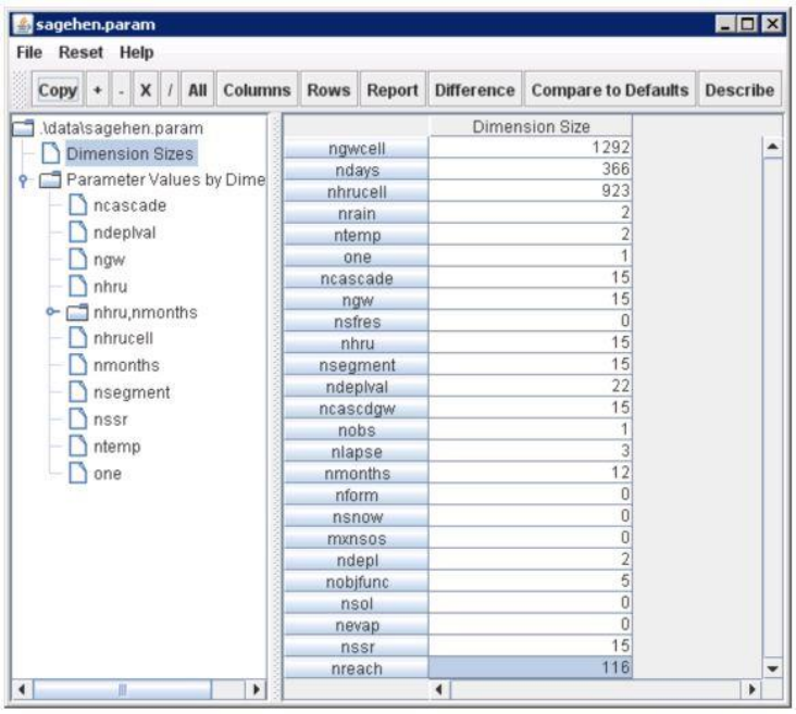
Start the paramtool by double-clicking on classProblem\paramtool.bat

Set the Dimension Sizes as follows. For this problem, always click on Default when asked about Resize

Dimension:

This step is setting the dimension sizes (array sizes) in the PRMS modules. To find out what these

dimensions are, left-click in a table cell (select it) and then click on the Describe button in the tool bar.

Click on the menu item File->Save when finished. Remember that all edit made in the paramtool tables

must be saved to the Parameter File for the edits to take effect when the model runs.

GSFlow Training Class Material: Instructions for GSFLOW Model Input Preparation

119

Spatial parameters

Transfer the spatial attributes developed in section 4 to the PRMS Parameter File.

HRU parameters

Start the paramtool by double-clicking on classProblem\paramtool.bat. Click on Parameter

Values by Dimension->nhru in the paramtool tree.

Open the gis\shapes\hrus.dbf in excel. This file contains all of the attribute values that were derived for

the gis\shapes\hrus shapefile.

GSFlow Training Class Material: Instructions for GSFLOW Model Input Preparation

120

REALLY IMPORTANT: Sort the excel worksheet in ascending order on the HRU_ID column

(not the ID column). This will insure that that spatial attributes will be pasted into the PRMS

Parameter File in the correct order.

It is also REALLY IMPORTANT that these .dbf files are not save from excel after the content is

sorted.

GSFlow Training Class Material: Instructions for GSFLOW Model Input Preparation

121

Copy the attributes values, column by column, out of excel and into the appropriate column in the

paramtool using cut and paste (ctrl-c and ctrl-v). There are 18 HRU parameters to transfer over:

1. cov_type

2. covden_sum (divide by 100 if needed - needs to be decimal fraction, not percent)

3. covden_win (divide by 100 if needed - needs to be decimal fraction, not percent)

4. hru_area (use the values in acres, not m2)

5. hru_aspect

6. hru_elev

7. hru_slope

8. jh_coef_hru

9. rad_trncf

10. snow_intcp (divide by 100 - needs to be decimal fraction, not percent)

11. soil_moist_max

12. soil_rech_max

13. soil_type

14. srain_intcp (divide by 100 if needed)

15. tmax_adj

16. tmin_adj

17. wrain_intcp (divide by 100 if needed)

Open the gis\shapes\hru_centoid_project.dbf in excel.

GSFlow Training Class Material: Instructions for GSFLOW Model Input Preparation

122

18. hru_lat - this in the Y coordinate of the HRU in geographical coordinates (Don't forget to sort

them by HRU_ID)

Parameters that come from the Gravity Reservoir (gis\shapes\gvrs.dbf) map and go into the nhrucell

dimension

Use excel to open the gis\shapes\gvrs.dbf file. Sort the columns on GVR_ID. In the paramtool,

click on Parameter Values by Dimension->nhrucell.

1. Find the column gvrcellid in excel. Copy and paste the values into the gvr_cell_id column in the

paramtool table.

2. Find the column gvrcellpct in excel. Copy and paste the values into the gvr_cell_pct column in

the paramtool table.

3. Find the column gvrhruid in excel. Copy and paste the values into the gvr_hru_id column in the

paramtool table.

4. Find the column gvrhrupct in excel. Copy and paste the values into the gvr_hru_pct column in

the paramtool table.

GSFlow Training Class Material: Instructions for GSFLOW Model Input Preparation

123

To find out what these parameters are, left-click in a table cell (select it) and then click on the Describe

button in the tool bar.

Click on the menu item File->Save when finished. Remember that all edit made in the paramtool tables

must be saved to the Parameter File for the edits to take effect when the model runs.

Cascade parameters

Normally the cascade parameters (click on Parameter Values by Dimension->ncascade in

paramtool) would come from GIS (or other analysis). At this time, the current methods for doing this

GIS analysis are beyond a reasonable exercise for this class. Because of the way that the HRU and

stream segment IDs were were assigned, it will be quite easy to do this by hand.

Set all the values (15 of them) in the hru_down_id column to the value 0. Because of the way that the

HRUs were delineated, all of them drain (cascade) into stream segments (not HRUs).

GSFlow Training Class Material: Instructions for GSFLOW Model Input Preparation

124

Set all of the values in the hru_pct_up column to the value 1. This is because there is only one cascade

coming from each HRU and all of the area from the HRU contributes to each the cascade.

Set the values in the hru_strmseg_down_id column to be the cascade number: 1 for row 1, 2 for row 2, 3

for row 3, etc. all the way to 15. This is because there is only one destination for each cascade, and it is

the stream segment with the ID corresponding to the cascade ID.

Copy the values from the hru_strmseg_down_id column to the hru_up_id column. In the example

problem, each cascade connects the corresponding HRU to the corresponding stream segment.

GSFlow Training Class Material: Instructions for GSFLOW Model Input Preparation

125

Remember that this only works out this way because of the simple way that HRUs and stream

segments were developed for this problem.

Repeat the instructions above for the ground water cascade parameters (click on Parameter Values by

Dimension->ncascadgw in paramtool). These parameters describe how PRMS routes groundwater from

HRU to HRU to streams. Usually these should be set to the same as the surface cascades. If your PRMS

model has swales or lakes, you will need to set these different. In the class problem, used the same

routing scheme as the surface parameters (ncascade).

Click on the menu item File->Save when finished. Remember that all edit made in the paramtool tables

must be saved to the Parameter File for the edits to take effect when the model runs.

Non-spatial parameters

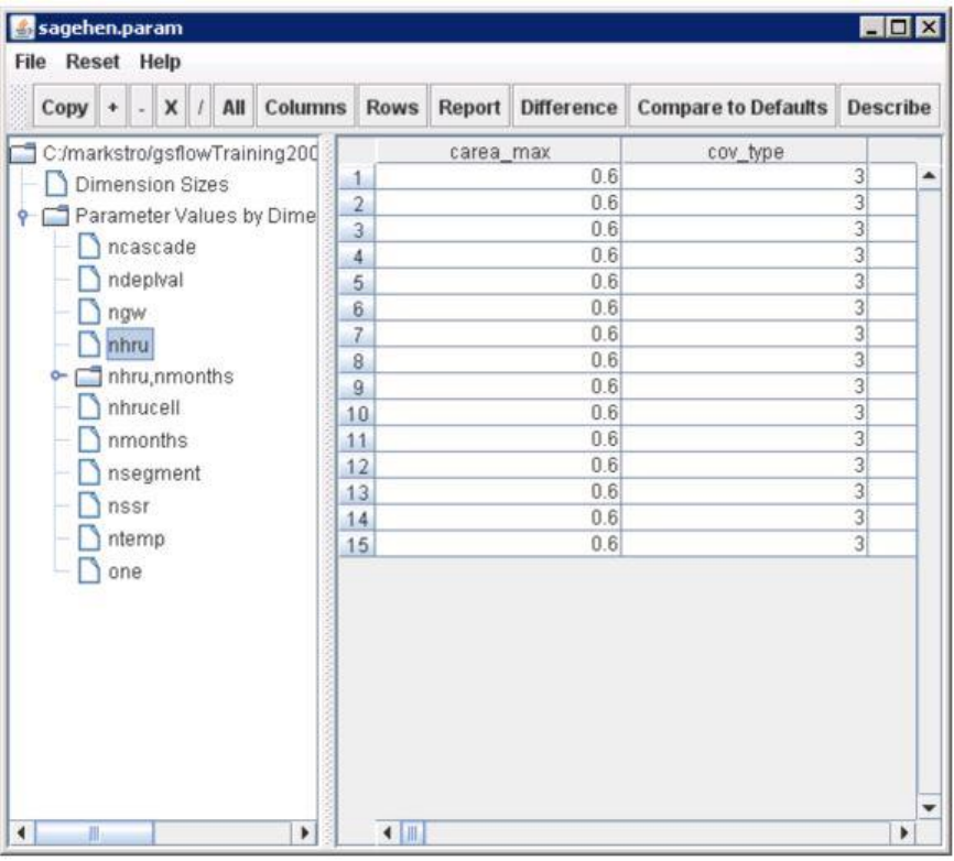
By nhru (click on Parameter Values by Dimension->nhru in paramtool):

1. hru_psta set all of these to "1". This means that the "base" precipitation station is the first one

(Independence Lake SNOTEL) specified in the Data File.

2. hru_plaps set all of these to "2". This means that the "lapse" precipitation station is the second

one (Sagehen COOP) specified in the Data File.

3. hru_tsta set all of these to "1". This means that the "base" temperature station is the first one

(Independence Lake SNOTEL) specified in the Data File.

4. hru_tlaps set all of these to "2". This means that the "lapse" temperature station is the second one

(Sagehen COOP) specified in the Data File.

By nrain (click on Parameter Values by Dimension->nrain in paramtool):

GSFlow Training Class Material: Instructions for GSFLOW Model Input Preparation

126

psta_elev Independence Lake SNOTEL (index = 1) is at 2576 meters. Sagehen COOP (index = 2) is at

1932 meters. Make sure that these units match the units used for parameter hru_elev. The units are

meters in the example problem.

By ntemp (click on Parameter Values by Dimension->ntemp in paramtool):

tsta_elev Independence Lake SNOTEL (index = 1) is at 2576 meters. Sagehen COOP (index = 2) is at

1932 meters. Make sure that these units match the units used for parameter hru_elev. The units are

meters in the example problem.

By nrain,nmonths (click on Parameter Values by Dimension->nrain,nmonth in paramtool):

pmn_mo These are the mean monthly precipitation on days with precipitation (storm size) for

Independence Lake SNOTEL (index = 1) and Sagehen COOP (index = 2).

These values (calculated according to Step 2.2) are in the excel file sagehenLapseRates.xls. Copy and

paste them into the pmn_mo table using the paramtool.

GSFlow Training Class Material: Instructions for GSFLOW Model Input Preparation

127

Click on the menu item File->Save when finished. Remember that all edit made in the paramtool

tables must be saved to the Parameter File for the edits to take effect when the model runs.

GSFlow Training Class Material: Instructions for GSFLOW Model Input Preparation

128

Making the MODFLOW Files

Create the MODFLOW Grid Cell map (ModelMuse method)

1. Open ModelMuse

2. Choose New Modflow Model

3. Set data for MODFLOW Grid:

X origin = -2052271.286

Y origin = 2089452.995

This origin is determined from ARC, and is the upper left corner of the model domain in ModelMuse.

Select MODFLOW packages

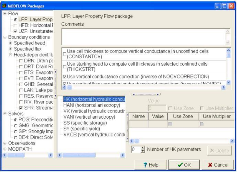
1. Choose "Model|Modflow packages and programs"

2. Select "LPF: Layer Property Flow"

GSFlow Training Class Material: Instructions for GSFLOW Model Input Preparation

129

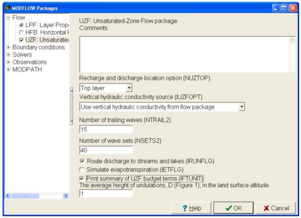
3. Select "UZF: Unsaturated-Zone Flow"

4. Choose "Use vertical hydraulic conductivity from flow package"

5. Change "NSETS2" to 40

6. Remove check from "Simulate evapotranspiration"

7. Add check to "Print summary UZF budget terms"

GSFlow Training Class Material: Instructions for GSFLOW Model Input Preparation

130

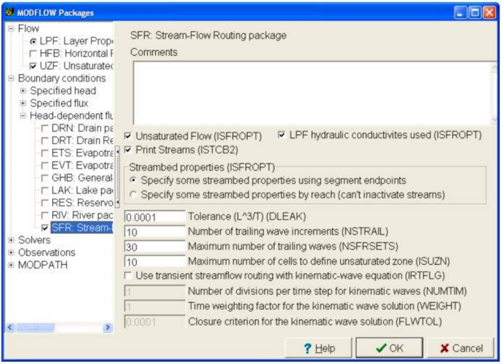
8. Select "Boundary conditions|Head-dependent flux|SFR: Streamflow-Routing"

9. Include "Unsaturated Flow" beneath streams

10. Add check to "Print Streams"

GSFlow Training Class Material: Instructions for GSFLOW Model Input Preparation

131

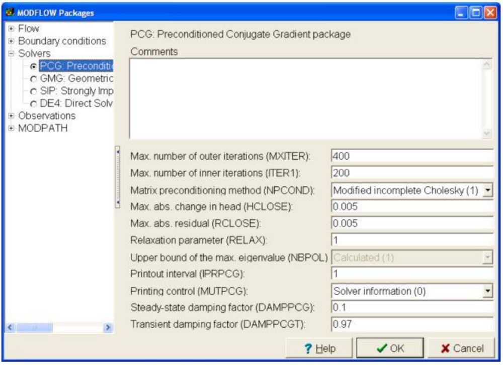
11. Select "PCG: Preconditioned Conjugate Gradient" and type values as shown below.

GSFlow Training Class Material: Instructions for GSFLOW Model Input Preparation

132

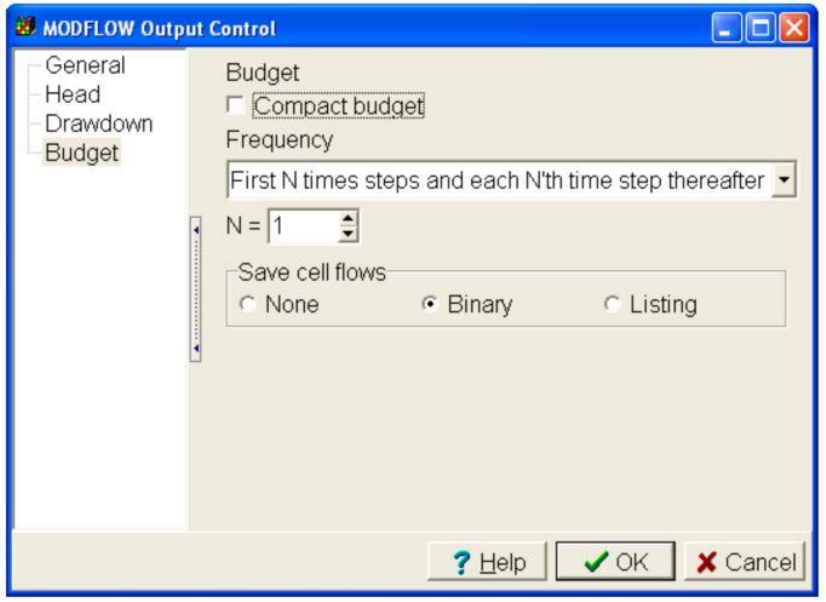
Set MODFLOW Output Control

1. Select "Model|Modflow Output Control"

2. Unselect "Compact Budget"

GSFlow Training Class Material: Instructions for GSFLOW Model Input Preparation

133

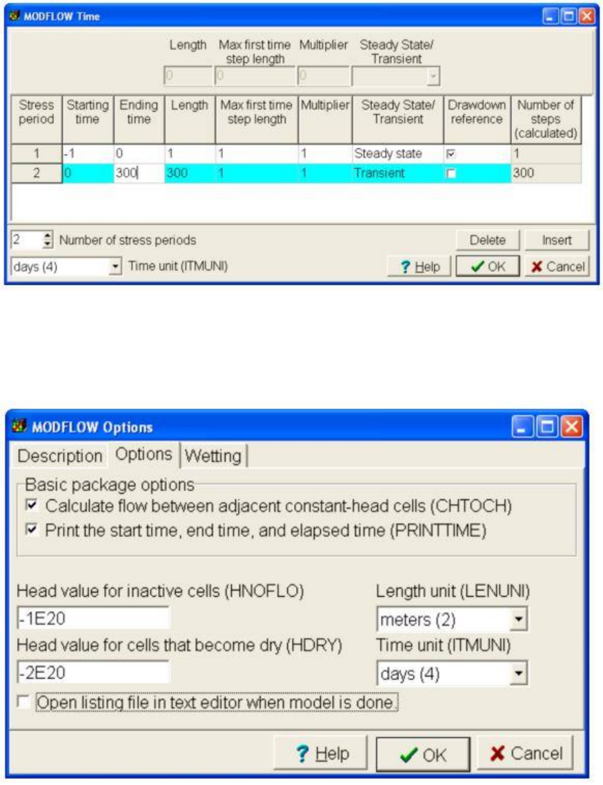
Set MODFLOW Units and Other Options

1. Select "Model|Modflow Time"

2. Set # of stress periods = 2

3. Choose "days (4)" for "ITMUNI"

4. First stress period -1 to 0

5. Second stress period 0 to 300

GSFlow Training Class Material: Instructions for GSFLOW Model Input Preparation

134

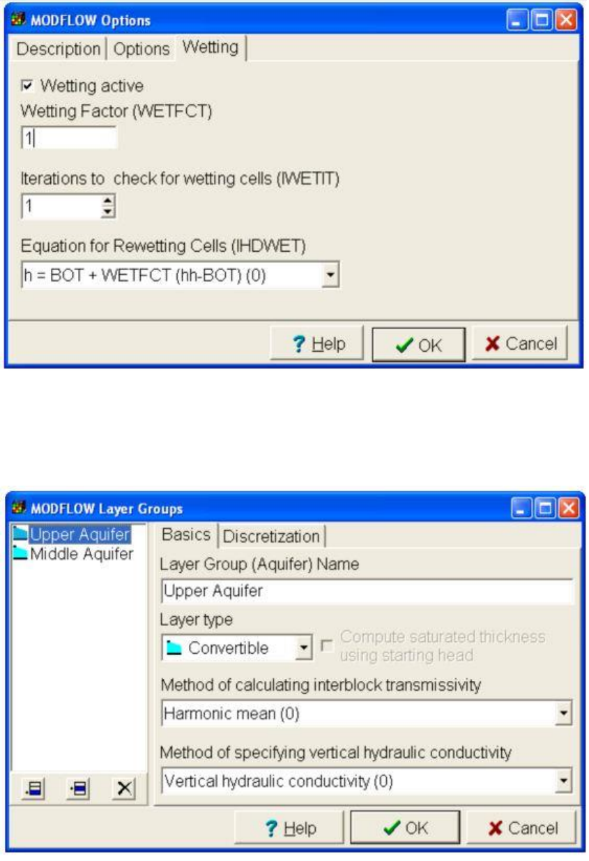
6. Select "Model|Modflow Options"

7. Set "LENUNI" = "meters (2)"

8. Continue with: "Model|Modflow Options"

9. Add check mark to "Wetting Active"

GSFlow Training Class Material: Instructions for GSFLOW Model Input Preparation

135

10. Select "Model|Modflow Layer Groups"

11. Make LAYTYP convertible

GSFlow Training Class Material: Instructions for GSFLOW Model Input Preparation

136

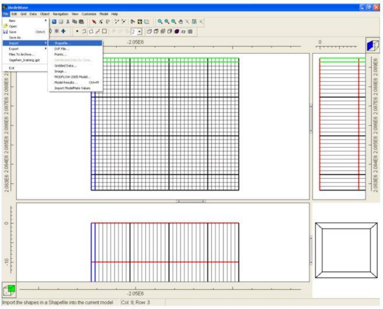
Importing Shapefiles in ModelMuse

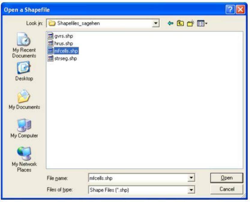
1. Select: "File|Import|Shapefiles"

2. Import "mfcells.shp"

GSFlow Training Class Material: Instructions for GSFLOW Model Input Preparation

137

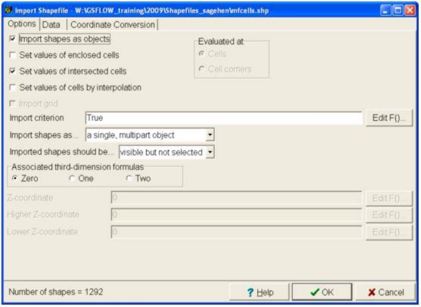
3. Choose "Options" Tab

4. Select "import shapes as Objects"

5. Choose "Set Values to Intersected Cells"

GSFlow Training Class Material: Instructions for GSFLOW Model Input Preparation

138

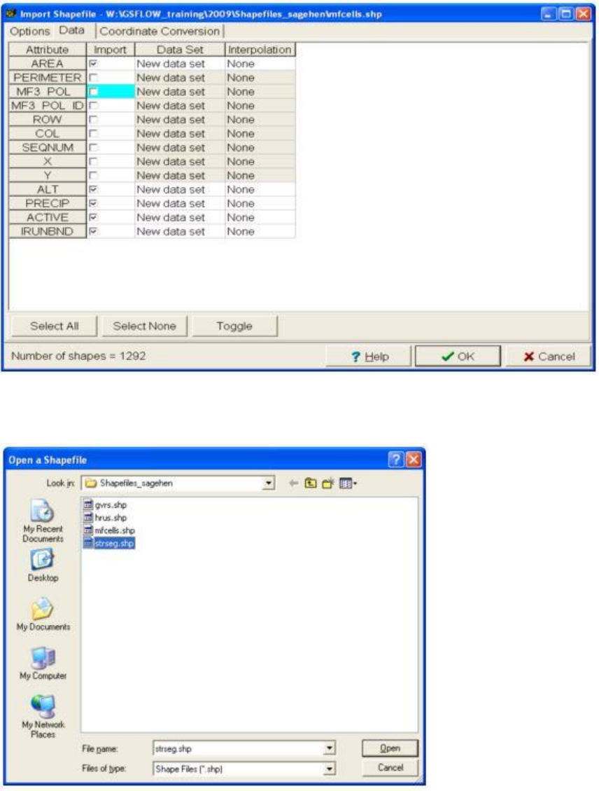
6. Select "Data" Tab

7. Add check to "ALT", "PRECIP", "ACTIVE", and "IRUNBND"

GSFlow Training Class Material: Instructions for GSFLOW Model Input Preparation

139

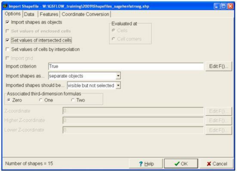
8. Import "strseg.shp"

9. Select "Import Shapes as Separate Objects"

10. Select "set values of intersected cells"

GSFlow Training Class Material: Instructions for GSFLOW Model Input Preparation

140

11. Select "Data" Tab

12. Add check mark to "ID"

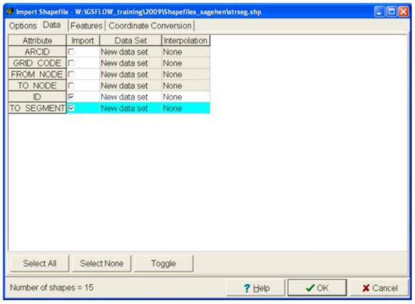
GSFlow Training Class Material: Instructions for GSFLOW Model Input Preparation

141

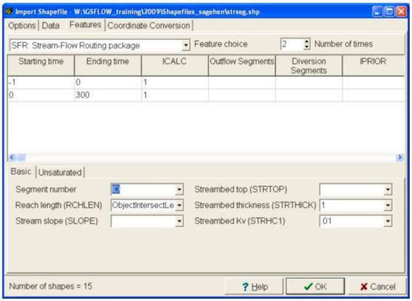
13. "Features" tab: Define segment #s time data and ICALC (scroll to right)

GSFlow Training Class Material: Instructions for GSFLOW Model Input Preparation

142

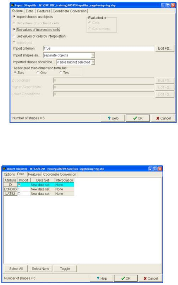
14. Import "spring.shp"

15. Check "Import Shapes as Objects"

16. Check "Set values to intersected cells"

GSFlow Training Class Material: Instructions for GSFLOW Model Input Preparation

143

17. Choose "Data" tab

18. Check "ID", which will become "ID2" because ID is already a data set.

GSFlow Training Class Material: Instructions for GSFLOW Model Input Preparation

144

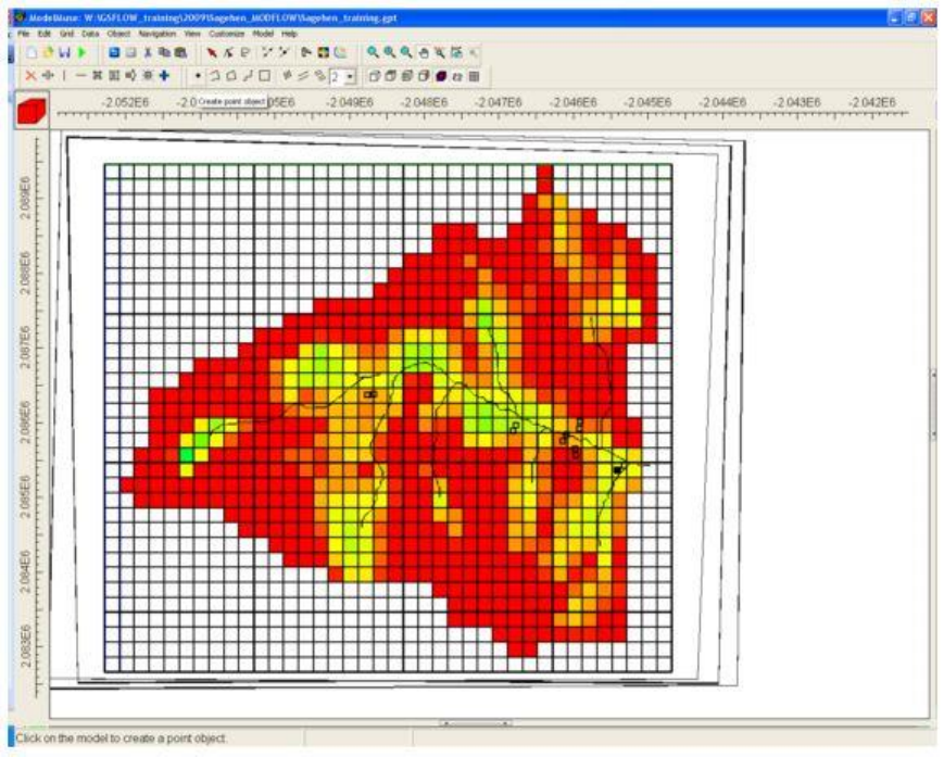
Create Point Objects for Cells with Springs

19. Select "Object|Select Object by Name"

20. Choose "Select none"

21. Select all spring objects

22. Select "Create Point Object"

23. Select each cell with a Springs in it.

24. Add check to UZF gages (Print volumes and rates)

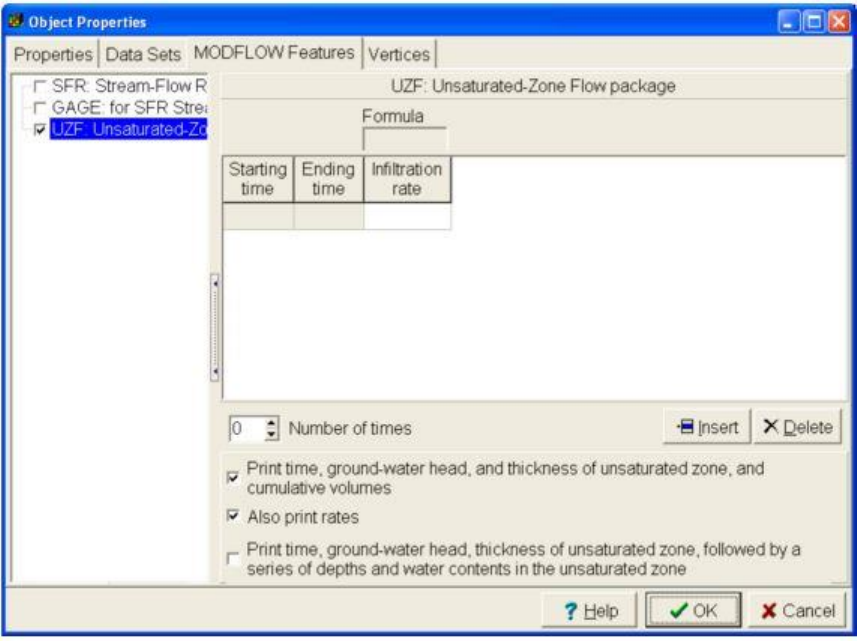
GSFlow Training Class Material: Instructions for GSFLOW Model Input Preparation

145

Add Additional Springs not Mapped on Topo Map

25. Select "Create Point Object"

26. Select anywhere on map

27. Select "Vertices" tab, and enter in UTM coordinates shown below.

X, Y coordinates:

28. -2051196.10562, 2085539.7193 (Spring7)

29. -2049368.54429, 2086950.2532 (Spring8)

30. -2046167.2455, 2083356.4582 (Spring9)

31. -2047553.2484, 2084533.9473 (Spring10)

GSFlow Training Class Material: Instructions for GSFLOW Model Input Preparation

146

Don't select "OK" yet. Goto "MODFLOW Features" tab

Create UZF gages for Added Springs

1. Select "MODFLOW Features" Tab

2. Select "UZF: Unsaturated Zone"

3. Add check to UZF gages (Print volumes and rates)

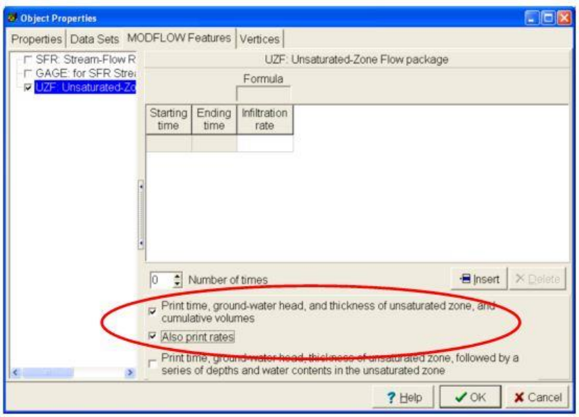
GSFlow Training Class Material: Instructions for GSFLOW Model Input Preparation

147

Set Stream Segment Information

1. Choose "Object|Select Objects by Name"

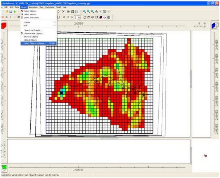
GSFlow Training Class Material: Instructions for GSFLOW Model Input Preparation

148

2. Click on "Select None"

3. Add check mark to all "strseg_" objects

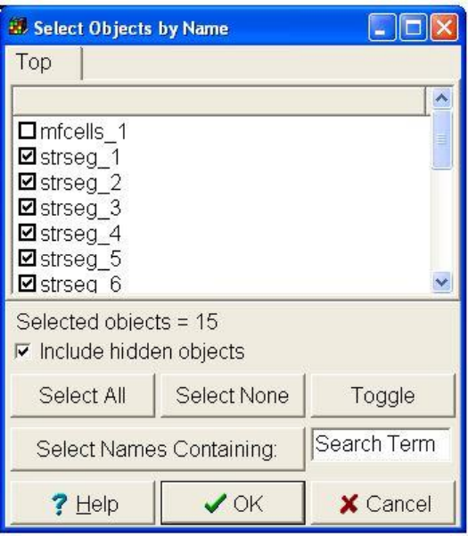
GSFlow Training Class Material: Instructions for GSFLOW Model Input Preparation

149

4. Choose arrow selection tool

5. Double click on highlighted segments

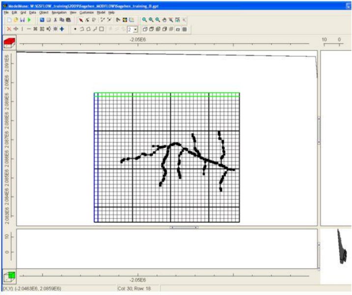
GSFlow Training Class Material: Instructions for GSFLOW Model Input Preparation

150

Specify Segment Information

6. Select "MODFLOW Features" tab

7. Select "SFR: Streamflow Routing" Select on F() under "Streambed elevation"

8. Select "Segment" sub tab

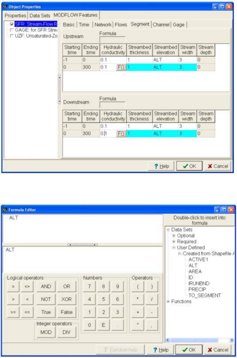
GSFlow Training Class Material: Instructions for GSFLOW Model Input Preparation

151

9. Set streambed Elevation with User defined "ALT" data set

10. Continue with: "Modflow Features" tab.

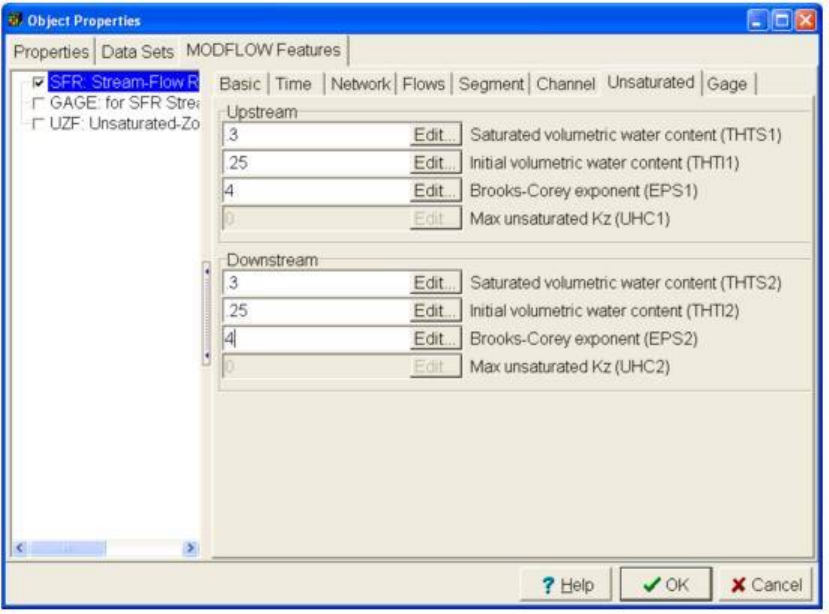
GSFlow Training Class Material: Instructions for GSFLOW Model Input Preparation

152

11. Select: "Unsaturated" sub tab and input values for unsaturated zone beneath streams

12. Select "OK"

Set Gage to last Reach in Outflow Segment

13. Use Selection arrow double click on last outflow segment

14. Choose "MODFLOW Features" tab

15. Click on "SFR: Streamflow Routing"

16. Select "Gage" sub tab

17. Add check mark for "Standard default" output

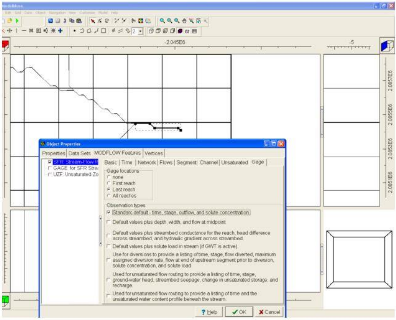
GSFlow Training Class Material: Instructions for GSFLOW Model Input Preparation

153

Set Hydraulic Conductivity for Aquifers

1. Select "Create Polygon Object"

2. Create Polygon containing all of model grid

3. Double click new polygon

4. Name object "K_layer1"

Notice range for which object applies. This will be important for multi-layer models

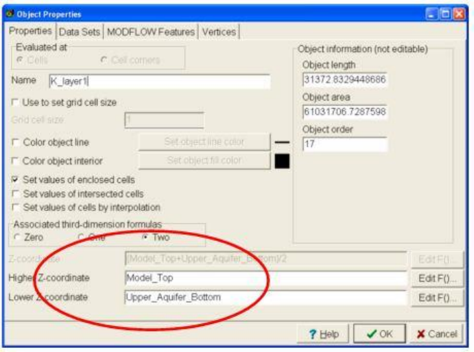
GSFlow Training Class Material: Instructions for GSFLOW Model Input Preparation

154

5. Select "Data Sets" tab

6. Choose "Required|Hydrology"

7. Add check to variable "Kx" and specify value of "0.06"

8. Add checks to "Ky" and "Kz" and set Kz= Kx / 2

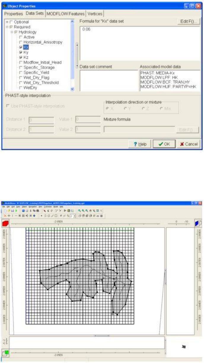
GSFlow Training Class Material: Instructions for GSFLOW Model Input Preparation

155

9. Select "Create Polygon Object"

10. Create 2-3 cell buffer around streams

11. Select "Select Objects" arrow

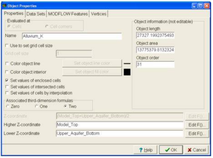
GSFlow Training Class Material: Instructions for GSFLOW Model Input Preparation

156

12. Double click new polygon object

13. Name object "Alluvium_K"

14. Select "Data Sets" tab

15. Click on "Required|Hydrology|Kx" and add check mark.

16. Type "0.25" in "Formula for "Kx" data set

17. Add check mark to "Ky" and "Kz" and set Kz= Kx / 5

GSFlow Training Class Material: Instructions for GSFLOW Model Input Preparation

157

18. Use "Color grid" to verify Kx

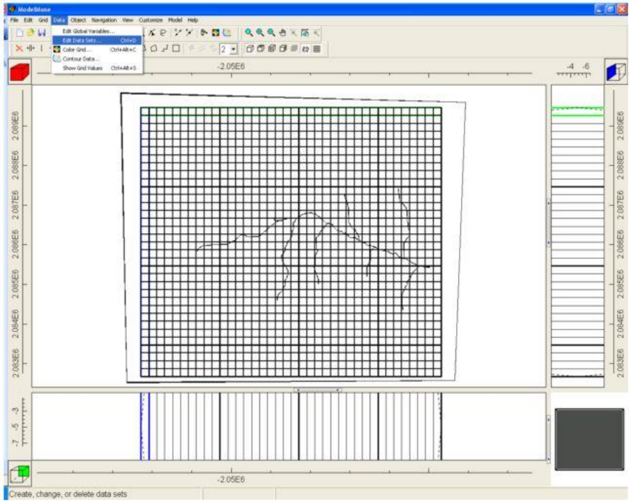
GSFlow Training Class Material: Instructions for GSFLOW Model Input Preparation

158

Set Layer Top and Bottom Altitudes

1. Choose "Create Polygon Object"

2. Put polygon around model grid

3. Double click selected polygon

The associated third-dimension formulas should be set to "zero"

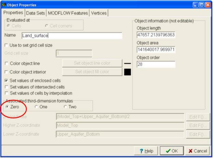
GSFlow Training Class Material: Instructions for GSFLOW Model Input Preparation

159

4. Select "Data Sets" tab

5. Select "Required|Layer Definition"

6. Select "Model_Top" and click on "Edit formula"

7. Choose "User Defined| Created from Shapefile" and double click "ALT"

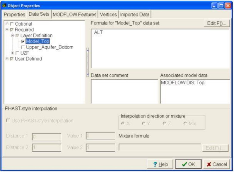
GSFlow Training Class Material: Instructions for GSFLOW Model Input Preparation

160

8. Repeat for "Upper_aquifer_bottom" Set to ALT-120

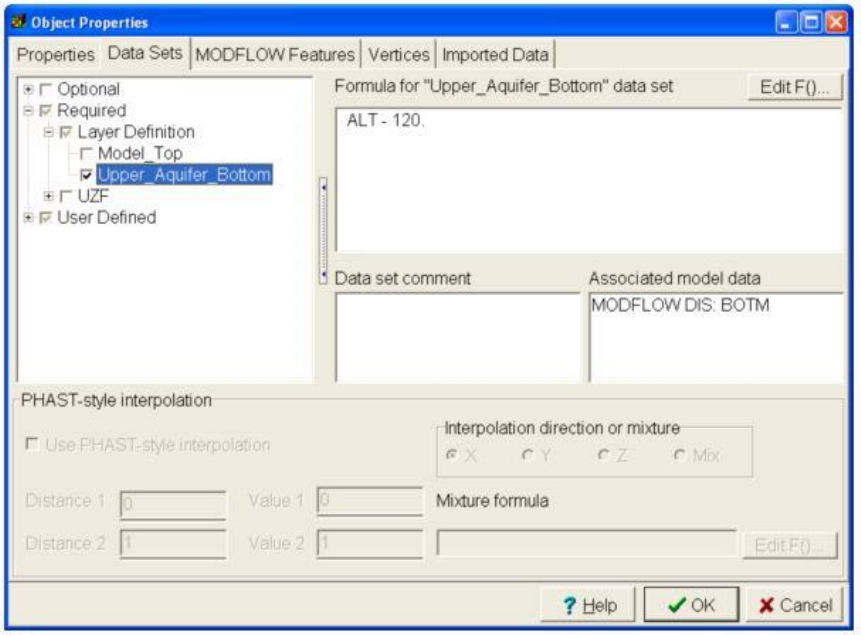
GSFlow Training Class Material: Instructions for GSFLOW Model Input Preparation

161

Check Layer Altitudes

9. Select "Color Grid"

10. Choose "Data Sets|Requied|Layer definition|Model Top"

11. Select "Apply"

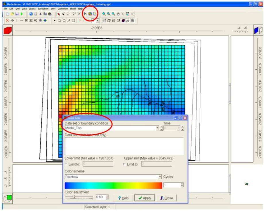
GSFlow Training Class Material: Instructions for GSFLOW Model Input Preparation

162

Set Wet_Dry Data

12. Choose "Create Polygon Object"

13. Put polygon around model grid

14. Double click selected polygon

15. Set associated third-dimension formulas to "Two"

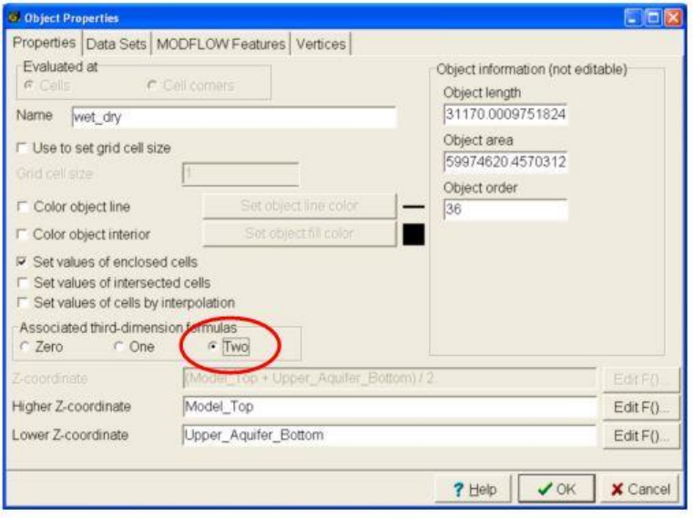
GSFlow Training Class Material: Instructions for GSFLOW Model Input Preparation

163

16. Choose "Data sets" tab

17. Choose "Required|Hydrology|Wet_Dry_Flag"

18. Click on "Edit formula"

19. Type if((ACTIVE1>0),1,0)

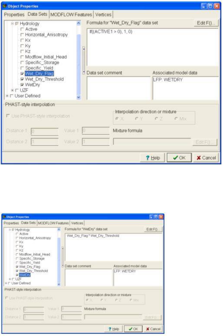
GSFlow Training Class Material: Instructions for GSFLOW Model Input Preparation

164

20. Set Wet_Dry_Threshold=0.01

21. Set Wet_Dry =Wet_Dry_Flag*Wet_Dry_Threshold

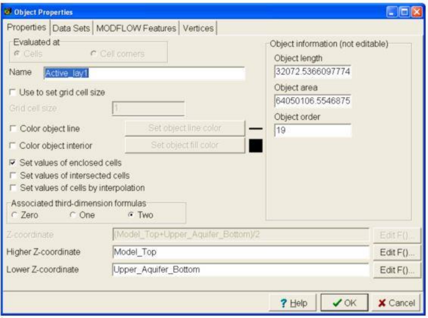
GSFlow Training Class Material: Instructions for GSFLOW Model Input Preparation

165

Set Active Cells

1. Select "Create polygon object" tool

2. Put polygon around model grid

3. Double click on selected object

4. In "Properties tab" Name object "Active_lay1"

5. Select "Data Sets" tab

6. Choose (with check mark) "Required|Hyrology|Active"

7. Select Edit F()

8. Choose "User Defined| Created from Shapefile" and double click on "ACTIVE1"

9. Type ">0" so formula reads "ACTIVE1>0"

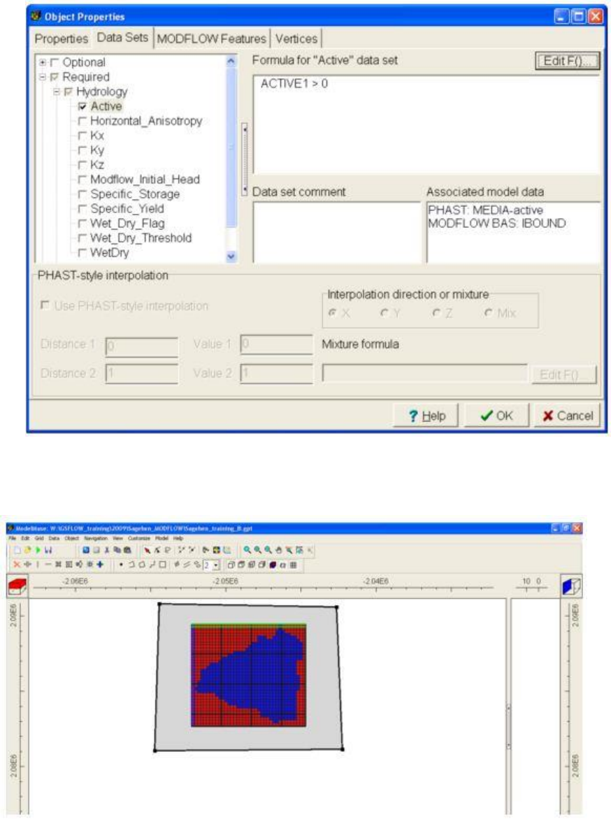
GSFlow Training Class Material: Instructions for GSFLOW Model Input Preparation

166

Use "Color Grid" again to check that IBOUND was set correctly

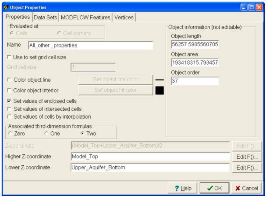
GSFlow Training Class Material: Instructions for GSFLOW Model Input Preparation

167

Set All other Cell Property Data

Layer 1

1. Select "Data Sets" tab

2. Select "Create Polygon Object"

3. Put polygon around model grid

4. Double click polygon

5. Name object "All_other_properties"

6. Select "Data Sets" tab

7. Choose "Required|Hydrology|MODFLOW_Initial_Head"

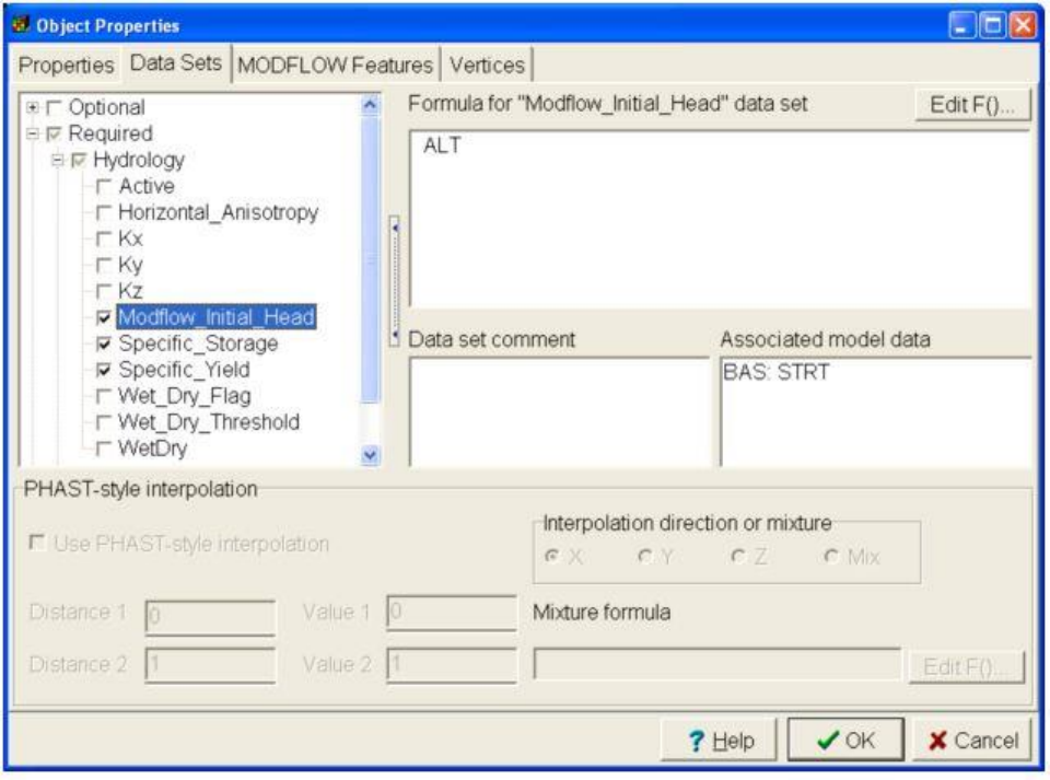
GSFlow Training Class Material: Instructions for GSFLOW Model Input Preparation

168

8. Type: "ALT"

9. Add check to "Specific_Storage" and use default values

10. Add check to "Specific_Yield" and use default value

11. Add check to "UZF" and select "Discharge_Routing"

12. Type "IRUNBND"

Don't choose OK YET!

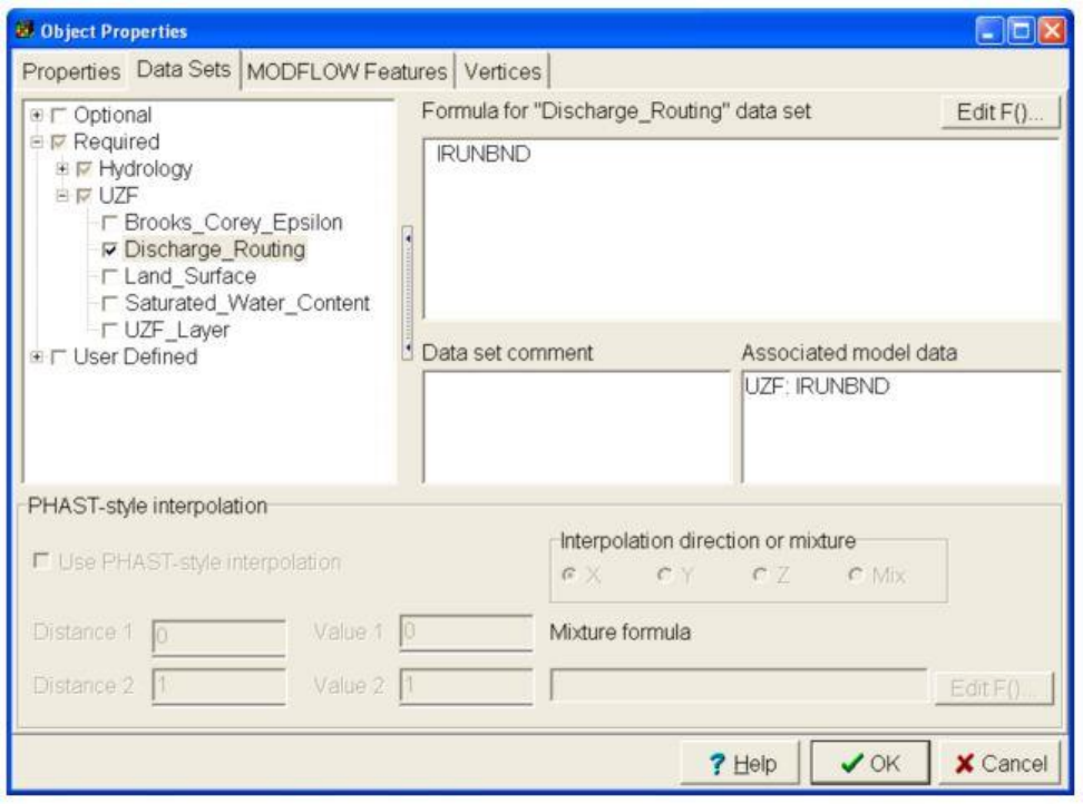
GSFlow Training Class Material: Instructions for GSFLOW Model Input Preparation

169

13. Choose "MODFLOW Features"

14. Add check to "UZF: Unsaturated-Zone Flow"

15. Increase "Number of times" to 2

16. Set "Infiltration rate" to "PRECIP*0.55" for both times

Don't choose OK YET!

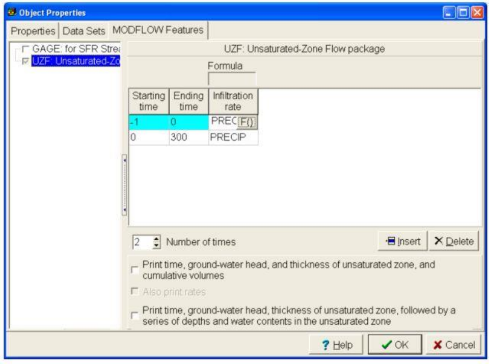
GSFlow Training Class Material: Instructions for GSFLOW Model Input Preparation

170

Set IUZFBND for UZF

17. Select "Data Sets" tab

18. Choose "Required|UZF|UZF_Layer"

19. Type in "ACTIVE1" in to "Formula for UZF_Layer" data set

20. Choose "OK"

Note: The other option would be to set "UZF_Layer" to imported data set "ALT" and ModelMuse will

determine which layer for each column is the land surface cell.

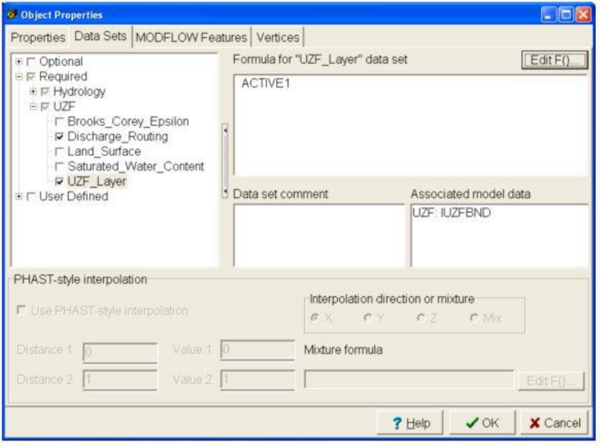
GSFlow Training Class Material: Instructions for GSFLOW Model Input Preparation

171

Use Color Grid to check that IRUNBND was set correctly

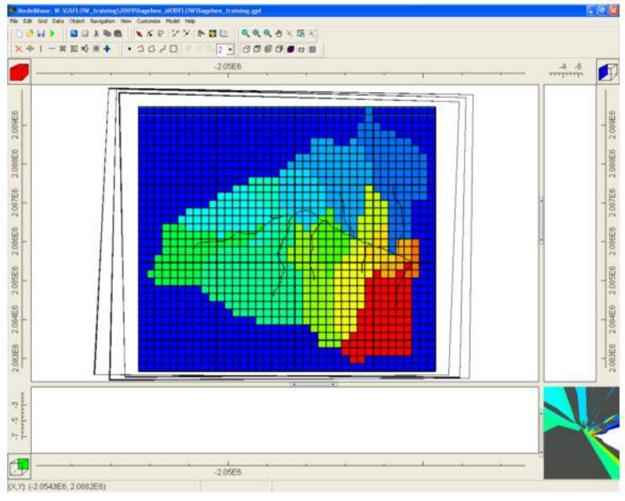
GSFlow Training Class Material: Instructions for GSFLOW Model Input Preparation

172

Link Outflow Segments

1. This determines the outflow segment for each segment.

2. Choose "All streams"

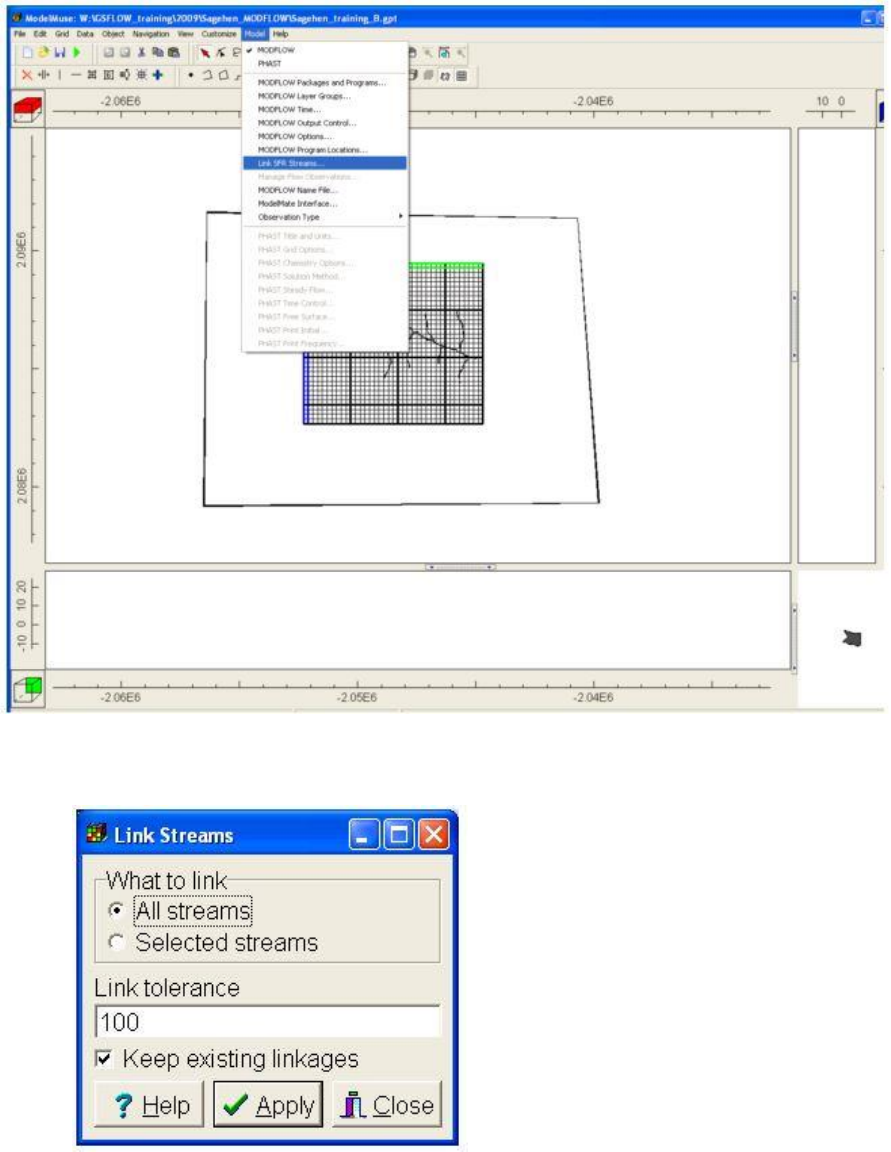
GSFlow Training Class Material: Instructions for GSFLOW Model Input Preparation

173

Instructions For Preparing Input Files Gsflow

Navigation menu

Versions of this User Manual:

Views

Navigation