Instructor's Solution Manual To Speech And Language Processing 2ed. (2009, Pearson)
User Manual:
Open the PDF directly: View PDF ![]() .
.
Page Count: 1

Instructor’s Solution Manual
Speech and Language Processing
An Introduction to Natural Language Processing, Computational
Linguistics, and Speech Recognition
Second Edition
Steven Bethard
University of Colorado at Boulder
Daniel Jurafsky
Stanford University
James H. Martin
University of Colorado at Boulder
Instructor’s Solutions Manual to accompany Speech and Language Processing: An Introduction to Natural
Language Processing, Computational Linguistics, and Speech Recognition, Second Edition, by Steven Bethard
for Daniel Jurafsky and James H. Martin. ISBN 0136072658.
c
2009 Pearson Education, Inc., Upper Saddle River, NJ. All rights reserved.
This publication is protected by Copyright and written permission should be obtained from the publisher prior to
any prohibited reproduction, storage in a retrieval system, or transmission in any form or by any means, electronic,
mechanical, photocopying, recording, or likewise. For information regarding permission(s), write to:
Rights and Permissions Department, Pearson Education, Inc., Upper Saddle River, NJ 07458.
Contents
Preface . . . . . . .. . . . . .. . . . . .. . . . . . . . . . . . . . . . . . . . . . . . . . . . . . . . . . . . . . . . . . ii
I Words 1
2 Regular Expressions and Automata .. . . . . . . . . . . . . . . . . . . . . . . . . . . . . . 1
3 Words and Transducers . . . . . . . .. . . . . .. . . . . .. . . . . . .. . . . . .. . . . . .. . . 6
4 N-Grams . . . . . . . . . . . . . . . . . . . . . . . . . . . . . . . . . . . . . . . . . . . . . . . . . . . . . . . . 13
5 Part-of-Speech Tagging . . . . . . . . . . . . . . . . . . . . . . . . . . . . . . . . . . . . . . . . . . 20
6 Hidden Markov and Maximum Entropy Models. . . . . . .. . . . . .. . . . . . 27
II Speech 31
7 Phonetics . . . . . . . . . . . . . . . . . . . . . . . . . . . . . . . . . . . . .. . . . . .. . . . . . .. . . . . . 32
8 Speech Synthesis .. . . . . . .. . . . . .. . . . . .. . . . . . .. . . . . .. . . . . . .. . . . . . . . . 34
9 Automatic Speech Recognition. . . . . . . . . . . . . . . . . . . . . . . . . . . . . . . . . . . . 38
10 Speech Recognition: Advanced Topics . . . . . . . . . . . . . . . . . . . . . . . . . . . . 41
11 Computational Phonology .. . . . . . . . . . . . . . . . . . . . . .. . . . . .. . . . . . .. . . . 42
III Syntax 43
12 Formal Grammars of English. . . . . . . . . . . . . . . .. . . . . . .. . . . . .. . . . . .. . 44
13 Syntactic Parsing . . . . . . . . . . . . . . . . . . . . . . . . . . . . . . .. . . . . .. . . . . . .. . . . 51
14 Statistical Parsing. . . . . . . . . . . . . . . . . . . . . . . . . . . . . . . . . . . . . . . . . . . . . . . . 57
15 Features and Unification . . . . . . . . . . . . . . . . . . . . . . . . . . . . . . . . . . . . . . . . . 62
16 Language and Complexity. .. . . . . . .. . . . . .. . . . . . .. . . . . . . . . . . . . . . . . . 67
IV Semantics and Pragmatics 69
17 The Representation of Meaning. . . . . . . . . . . . . . . . . . . . . . . . . . . . . . . . . . . 69
18 Computational Semantics . . . . . . . . . . . . . . . . . . . . . . . . . . . . . . . . . . . . . . . . 72
19 Lexical Semantics . . . . . . . . . . . . . . . . . . . . . . . . . . . . . . . . . . . . . . . . . . . . . . . . 78
20 Computational Lexical Semantics. . . . . . . . . . . . . . . . . . . . . . . . . . . . . . . . . 82
21 Computational Discourse. . . . . . . . . . . . . . . . . . . . . . . . . . . . . . . . . . . . . . . . . 88
V Applications 93
22 Information Extraction. . .. . . . . .. . . . . . . . . . . . . . . . . . . . . . . . . . . . . . . . . . 94
23 Question Answering and Summarization. . . . . . . . . . . . . . . . . . . . . . . . . . 100
24 Dialogue and Conversational Agents . . . . . . .. . . . . . .. . . . . .. . . . . .. . . . 102
25 Machine Translation . . . . . . . . . . . . . . . . . . . . . . . . . . . . . . . . . . . . . . . . . . . . . 106
i
Preface
This Instructor’s Solution Manual provides solutions for the end-of-chapter exer-
cises in Speech and Language Processing: An Introduction to Natural Language Pro-
cessing, Computational Linguistics, and Speech Recognition (Second Edition). For
the more interactive exercises, or where a complete solution would be infeasible (e.g.,
would require too much code), a sketch of the solution or discussion of the issues
involved is provided instead. In general, the solutions in this manual aim to provide
enough information about each problem to allow an instructor to meaningfully evaluate
student responses.
Note that many of the exercises in this book could be solved in a number of different
ways, though we often provide only a single answer. We have aimed for what we
believe to be the most typical answer, but instructors should be open to alternative
solutions for most of the more complex exercises. The goal is to get students thinking
about the issues involved in the various speech and language processing tasks, so most
solutions that demonstrate such an understanding have achieved the main purpose of
their exercises.
On a more technical note, throughout this manual, when code is provided as the
solution to an exercise, the code is written in the Python programming language. This
is done both for consistency, and ease of comprehension - in many cases, the Python
code reads much like the algorithmic pseudocode used in other parts of the book. For
more information about the Python programming language, please visit:
http://www.python.org/
The code in this manual was written and tested using Python 2.5. It will likely work on
newer versions of Python, but some constructs used in the manual may not be valid on
older versions of Python.
Acknowledgments
Kevin Bretonnel Cohen deserves particular thanks for providing the solutions to
the biomedical information extraction problems in Chapter 22, and they are greatly
improved with his insights into the field. Thanks also to the many researchers upon
whose work and careful documentation some of the solutions in this book are based,
including Alan Black, Susan Brennan, Eric Brill, Michael Collins, Jason Eisner, Jerry
Hobbs, Kevin Knight, Peter Norvig, Martha Palmer, Bo Pang, Ted Pedersen, Martin
Porter, Stuart Shieber, and many others.
ii
Chapter 2
Regular Expressions and Automata
2.1 Write regular expressions for the following languages. You may use either
Perl/Python notation or the minimal “algebraic” notation of Section 2.3, but
make sure to say which one you are using. By “word”, we mean an alphabetic
string separated from other words by whitespace, any relevant punctuation, line
breaks, and so forth.
1. the set of all alphabetic strings;
[a-zA-Z]+
2. the set of all lower case alphabetic strings ending in a b;
[a-z]*b
3. the set of all strings with two consecutive repeated words (e.g., “Humbert
Humbert” and “the the” but not “the bug” or “the big bug”);
([a-zA-Z]+)\s+\1
4. the set of all strings from the alphabet a, b such that each ais immediately
preceded by and immediately followed by a b;
(b+(ab+)+)?
5. all strings that start at the beginning of the line with an integer and that end
at the end of the line with a word;
ˆ\d+\b.*\b[a-zA-Z]+$
6. all strings that have both the word grotto and the word raven in them (but
not, e.g., words like grottos that merely contain the word grotto);
\bgrotto\b.*\braven\b|\braven\b.*\bgrotto\b
7. write a pattern that places the first word of an English sentence in a register.
Deal with punctuation.
ˆ[ˆa-zA-Z]*([a-zA-Z]+)
2.2 Implement an ELIZA-like program, using substitutions such as those described
on page 26. You may choose a different domain than a Rogerian psychologist,
if you wish, although keep in mind that you would need a domain in which your
program can legitimately engage in a lot of simple repetition.
The following implementation can reproduce the dialog on page 26.
A more complete solution would include additional patterns.
import re, string
patterns = [
(r"\b(i’m|i am)\b", "YOU ARE"),
(r"\b(i|me)\b", "YOU"),
(r"\b(my)\b", "YOUR"),
(r"\b(well,?) ", ""),
(r".*YOU ARE (depressed|sad) .*",
r"I AM SORRY TO HEAR YOU ARE \1"),
(r".*YOU ARE (depressed|sad) .*",
r"WHY DO YOU THINK YOU ARE \1"),
1
2 Chapter 2. Regular Expressions and Automata
(r".*all .*", "IN WHAT WAY"),
(r".*always .*", "CAN YOU THINK OF A SPECIFIC EXAMPLE"),
(r"[%s]" % re.escape(string.punctuation), ""),
]
while True:
comment = raw_input()
response = comment.lower()
for pat, sub in patterns:
response = re.sub(pat, sub, response)
print response.upper()
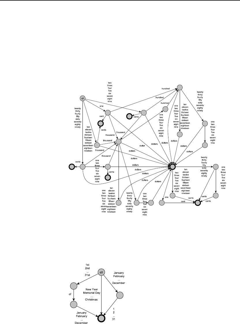
2.3 Complete the FSA for English money expressions in Fig. 2.15 as suggested in the
text following the figure. You should handle amounts up to $100,000, and make
sure that “cent” and “dollar” have the proper plural endings when appropriate.
2.4 Design an FSA that recognizes simple date expressions like March 15,the 22nd
of November,Christmas. You should try to include all such “absolute” dates
(e.g., not “deictic” ones relative to the current day, like the day before yesterday).
Each edge of the graph should have a word or a set of words on it. You should
use some sort of shorthand for classes of words to avoid drawing too many arcs
(e.g., furniture →desk, chair, table).
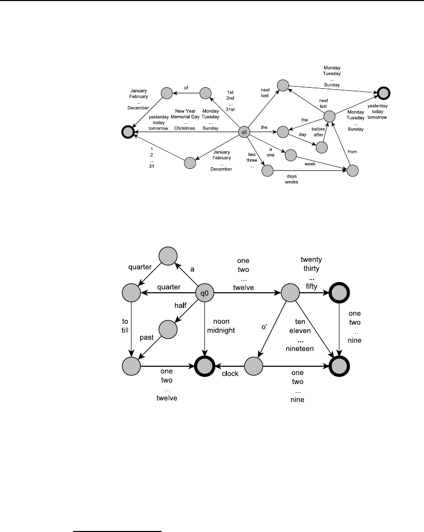
3
2.5 Now extend your date FSA to handle deictic expressions like yesterday,tomor-
row,a week from tomorrow,the day before yesterday,Sunday,next Monday,
three weeks from Saturday.
2.6 Write an FSA for time-of-day expressions like eleven o’clock,twelve-thirty,mid-
night, or a quarter to ten, and others.
2.7 (Thanks to Pauline Welby; this problem probably requires the ability to knit.)
Write a regular expression (or draw an FSA) that matches all knitting patterns
for scarves with the following specification: 32 stitches wide, K1P1 ribbing on
both ends, stockinette stitch body, exactly two raised stripes. All knitting patterns
must include a cast-on row (to put the correct number of stitches on the needle)
and a bind-off row (to end the pattern and prevent unraveling). Here’s a sample
pattern for one possible scarf matching the above description:1
1Knit and purl are two different types of stitches. The notation Knmeans do nknit stitches. Similarly for
purl stitches. Ribbing has a striped texture—most sweaters have ribbing at the sleeves, bottom, and neck.
Stockinette stitch is a series of knit and purl rows that produces a plain pattern—socks or stockings are knit
with this basic pattern, hence the name.
4 Chapter 2. Regular Expressions and Automata
1. Cast on 32 stitches. cast on; puts stitches on needle
2. K1 P1 across row (i.e., do (K1 P1) 16 times). K1P1 ribbing
3. Repeat instruction 2 seven more times. adds length
4. K32, P32. stockinette stitch
5. Repeat instruction 4 an additional 13 times. adds length
6. P32, P32. raised stripe stitch
7. K32, P32. stockinette stitch
8. Repeat instruction 7 an additional 251 times. adds length
9. P32, P32. raised stripe stitch
10. K32, P32. stockinette stitch
11. Repeat instruction 10 an additional 13 times. adds length
12. K1 P1 across row. K1P1 ribbing
13. Repeat instruction 12 an additional 7 times. adds length
14. Bind off 32 stitches. binds off row: ends pattern
In the expression below, Cstands for cast on,Kstands for knit,P
stands for purl and Bstands for bind off:
C{32}
((KP){16})+
(K{32}P{32})+
P{32}P{32}
(K{32}P{32})+
P{32}P{32}
(K{32}P{32})+
((KP){16})+
B{32}
2.8 Write a regular expression for the language accepted by the NFSA in Fig. 2.26.
q3
q0q1q2
a b a
b
a
Figure 2.1 A mystery language.
(aba?)+
2.9 Currently the function D-RECOGNIZE in Fig. 2.12 solves only a subpart of the
important problem of finding a string in some text. Extend the algorithm to solve
the following two deficiencies: (1) D-RECOGNIZE currently assumes that it is
already pointing at the string to be checked, and (2) D-RECOGNIZE fails if the
string it is pointing to includes as a proper substring a legal string for the FSA.
That is, D-RECOGNIZE fails if there is an extra character at the end of the string.
To address these problems, we will have to try to match our FSA at
each point in the tape, and we will have to accept (the current sub-
string) any time we reach an accept state. The former requires an

5
additional outer loop, and the latter requires a slightly different struc-
ture for our case statements:
function D-RECOGNIZE(tape,machine)returns accept or reject
current-state ←Initial state of machine
for index from 0to LENGTH(tape)do
current-state ←Initial state of machine
while index <LENGTH(tape)and
transition-table[current-state,tape[index]] is not empty do
current-state ←transition-table[current-state,tape[index]]
index ←index + 1
if current-state is an accept state then
return accept
index ←index + 1
return reject
2.10 Give an algorithm for negating a deterministic FSA. The negation of an FSA
accepts exactly the set of strings that the original FSA rejects (over the same
alphabet) and rejects all the strings that the original FSA accepts.
First, make sure that all states in the FSA have outward transitions for
all characters in the alphabet. If any transitions are missing, introduce
a new non-accepting state (the fail state), and add all the missing
transitions, pointing them to the new non-accepting state.
Finally, make all non-accepting states into accepting states, and
vice-versa.
2.11 Why doesn’t your previous algorithm work with NFSAs? Now extend your al-
gorithm to negate an NFSA.
The problem arises from the different definition of accept and reject
in NFSA. We accept if there is “some” path, and only reject if all
paths fail. So a tape leading to a single reject path does neccessarily
get rejected, and so in the negated machine does not necessarily get
accepted.
For example, we might have an -transition from the accept state
to a non-accepting state. Using the negation algorithm above, we
swap accepting and non-accepting states. But we can still accept
strings from the original NFSA by simply following the transitions as
before to the original accept state. Though it is now a non-accepting
state, we can simply follow the -transition and stop. Since the -
transition consumes no characters, we have reached an accepting state
with the same string as we would have using the original NFSA.
To solve this problem, we first convert the NFSA to a DFSA, and
then apply the algorithm as before.
Chapter 3
Words and Transducers
3.1 Give examples of each of the noun and verb classes in Fig. 3.6, and find some
exceptions to the rules.
Examples:
•nouni: fossil
•verbj: pass
•verbk: conserve
•nounl: wonder
Exceptions:
•nouni:apology accepts -ize but apologization sounds odd
•verbj:detect accepts -ive but it becomes a noun, not an adjective
•verbk:cause accepts -ative but causitiveness sounds odd
•nounl:arm accepts -ful but it becomes a noun, not an adjective
3.2 Extend the transducer in Fig. 3.17 to deal with sh and ch.
One possible solution:
6
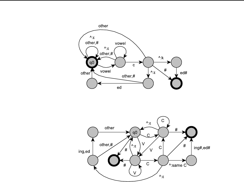
7
3.3 Write a transducer(s) for the K insertion spelling rule in English.
One possible solution:
3.4 Write a transducer(s) for the consonant doubling spelling rule in English.
One possible solution, where V stands for vowel, and C stands for
consonant:
3.5 The Soundex algorithm (Knuth, 1973; Odell and Russell, 1922) is a method
commonly used in libraries and older census records for representing people’s
names. It has the advantage that versions of the names that are slightly misspelled
or otherwise modified (common, e.g., in hand-written census records) will still
have the same representation as correctly spelled names. (e.g., Jurafsky, Jarofsky,
Jarovsky, and Jarovski all map to J612).
1. Keep the first letter of the name, and drop all occurrences of non-initial a,
e, h, i, o, u, w, y.
2. Replace the remaining letters with the following numbers:
b, f, p, v →1
c, g, j, k, q, s, x, z →2
d, t →3
l→4
m, n →5
r→6
3. Replace any sequences of identical numbers, only if they derive from two or
more letters that were adjacent in the original name, with a single number
(e.g., 666 →6).
4. Convert to the form Letter Digit Digit Digit by dropping digits
past the third (if necessary) or padding with trailing zeros (if necessary).
The exercise: write an FST to implement the Soundex algorithm.
8 Chapter 3. Words and Transducers
One possible solution, using the following abbreviations:
V = a, e, h, i, o, u, w, y
C1 = b, f, p, v
C2 = c, g, j, k, q, s, x, z
C3 = d, t
C4 = l
C5 = m, n
C6 = r
3.6 Read Porter (1980) or see Martin Porter’s official homepage on the Porter stem-
mer. Implement one of the steps of the Porter Stemmer as a transducer.
Porter stemmer step 1a looks like:
SSES →SS
IES →I
SS →SS
S→
One possible transducer for this step:

9
3.7 Write the algorithm for parsing a finite-state transducer, using the pseudocode
introduced in Chapter 2. You should do this by modifying the algorithm ND-
RECOGNIZE in Fig. 2.19 in Chapter 2.
FSTs consider pairs of strings and output accept or reject. So the
major changes to the ND-RECOGNIZE algorithm all revolve around
moving from looking at a single tape to looking at a pair of tapes.
Probably the most important change is in GENERATE-NEW-STATES,
where we now must try all combinations of advancing a character or
staying put (for an ) on either the source string or the target string.
function ND-RECOGNIZE(s-tape,t-tape,machine)returns accept/reject
agenda ← {(Machine start state, s-tape start, t-tape start)}
while agenda is not empty do
current-state ←NEXT(agenda)
if ACCEPT-STATE?(current-state)then
return accept
agenda ←agenda ∪GENERATE-NEW-STATES(current-state)
return reject
function GENERATE-NEW-STATES(current-state)returns search states
node ←the node the current-state is on
s-index ←the point on s-tape the current-state is on
t-index ←the point on t-tape the current-state is on
return
(transition[node,:], s-index,t-index)∪
(transition[node,s-tape[s-index]:], s-index + 1, t-index)∪
(transition[node,:t-tape[t-index]], s-index,t-index + 1) ∪
(transition[node,s-tape[s-index]:t-tape[t-index]],s-index+1,t-index+1)
function ACCEPT-STATE?(search-state)returns true/false
node ←the node the current-state is on
s-index ←the point on s-tape the current-state is on
t-index ←the point on t-tape the current-state is on
return s-index is at the end of the tape and
t-index is at the end of the tape and
node is an accept state of the machine
3.8 Write a program that takes a word and, using an on-line dictionary, computes
possible anagrams of the word, each of which is a legal word.
def permutations(string):
if len(string) < 2:
yield string
else:
first, rest = string[:1], string[1:]
indices = range(len(string))
for sub_string in permutations(rest):
for i in indices:
yield sub_string[:i] + first + sub_string[i:]
def anagrams(string):
for string in permutations(string):
if is_word(string): # query online dictionary
yield string

10 Chapter 3. Words and Transducers
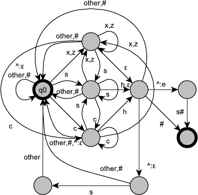
3.9 In Fig. 3.17, why is there a z, s, x arc from q5to q1?
State q1represents the point at which we have seen at least one z,
sor x. If the z, s, x arc from q5to q1were not present, it would
be possible to transition on an z, s or xback to the initial state, q0.
This would allow invalid strings like sˆssˆs# by following the path
q0→q1→q2→q5→q0→q1→q0.
3.10 Computing minimum edit distances by hand, figure out whether drive is closer
to brief or to divers and what the edit distance is. You may use any version of
distance that you like.
Using 1-insertion, 1-deletion, 2-substitution costs, there is a distance
of 4 between drive and brief:
e565434
v454345
i343234
r232345
d123456
#012345
# b r i e f
Using 1-insertion, 1-deletion, 2-substitution costs, there is a distance
of 3 between drive and divers:
e 5 4 3 2 1 2 3
v4321234
i 3 2 1 2 3 4 5
r 2 1 2 3 4 3 4
d1012345
#0123456
# d i v e r s
Thus, drive is closer to divers than to brief.
3.11 Now implement a minimum edit distance algorithm and use your hand-computed
results to check your code.
def min_edit_distance(target, source):
n = len(target)
m = len(source)
cols = range(1, n + 1)
rows = range(1, m + 1)
# initialize the distance matrix
distance = {(0, 0): 0}
for i in cols:
mod = ins_cost(target[i - 1])
distance[i, 0] = distance[i - 1, 0] + mod
for j in rows:
mod = del_cost(source[j - 1])
distance[0, j] = distance[0, j - 1] + mod
# sort like (0, 0) (0, 1) (1, 0) (0, 2) (1, 1) (2, 0) ...
# this guarantees the matrix is filled in the right order
indices = [(i, j) for i in cols for j in rows]
indices.sort(key=sum)

11
# helper function for calculating distances
def get_dist(row, col, func, t_char, s_char):
chars = t_char, s_char
args = [char for char in chars if char != ’*’]
return distance[row, col] + func(*args)
# for each pair of indices, choose insertion, substitution
# or deletion, whichever gives the shortest distance
for i, j in indices:
t_char = target[i - 1]
s_char = source[j - 1]
distance[i, j] = min(
get_dist(i -1, j, ins_cost, t_char, ’*’),
get_dist(i - 1, j - 1, sub_cost, t_char, s_char),
get_dist(i, j - 1, del_cost, ’*’, s_char))
# return distance from the last row and column
return distance[n, m]
3.12 Augment the minimum edit distance algorithm to output an alignment; you will
need to store pointers and add a stage to compute the backtrace.
def min_edit(target, source):
n = len(target)
m = len(source)
cols = range(1, n + 1)
rows = range(1, m + 1)
# initialize the distance and pointer matrices
distance = {(0, 0): 0}
pointers = {(0, 0): (None, None, None, None)}
for i in cols:
t_char = target[i - 1]
distance[i, 0] = distance[i - 1, 0] + ins_cost(t_char)
pointers[i, 0] = (i - 1, 0, t_char, ’*’)
for j in rows:
s_char = source[j - 1]
distance[0, j] = distance[0, j - 1] + del_cost(s_char)
pointers[0, j] = (0, j - 1, ’*’, s_char)
# sort like (0, 0) (0, 1) (1, 0) (0, 2) (1, 1) (2, 0) ...
# this guarantees the matrix is filled in the right order
indices = [(i, j) for i in cols for j in rows]
indices.sort(key=sum)
# helper function for creating distance/pointer pairs
def get_pair(row, col, func, t_char, s_char):
chars = t_char, s_char
args = [char for char in chars if char != ’*’]
dist = distance[row, col] + func(*args)
pointer = row, col, t_char, s_char
return dist, pointer
# for each pair of indices, choose insertion, substitution
# or deletion, whichever gives the shortest distance
for i, j in indices:
t_char = target[i - 1]
s_char = source[j - 1]
pairs = [
get_pair(i -1, j, ins_cost, t_char, ’*’),
get_pair(i - 1, j - 1, sub_cost, t_char, s_char),
get_pair(i, j - 1, del_cost, ’*’, s_char),
]
dist, pointer = min(pairs, key=operator.itemgetter(0))
distance[i, j] = dist
pointers[i, j] = pointer
# follow pointers backwards through the path selected

12 Chapter 3. Words and Transducers
t_chars = []
s_chars = []
row, col = n, m
while True:
row, col, t_char, s_char = pointers[row, col]
if row is col is None:
break
t_chars.append(t_char)
s_chars.append(s_char)
# return distance, and two character strings
target_string = ’’.join(reversed(t_chars))
source_string = ’’.join(reversed(s_chars))
return distance[n, m], target_string, source_string

Chapter 4
N-Grams
4.1 Write out the equation for trigram probability estimation (modifying Eq. 4.14).
P(wn|wn−1, wn−2) = C(wn−2wn−1wn)
C(wn−2wn−1)
4.2 Write a program to compute unsmoothed unigrams and bigrams.
from __future__ import division
from collections import defaultdict as ddict
import itertools
import math
import random
class NGrams(object):
def __init__(self, max_n, words=None):
self._max_n = max_n
self._n_range = range(1, max_n + 1)
self._counts = ddict(lambda: 0)
# if words were supplied, update the counts
if words is not None:
self.update(words)
def update(self, words):
# increment the total word count, storing this under
# the empty tuple - storing it this way simplifies
# the _probability() method
self._counts[()] += len(words)
# count ngrams of all the given lengths
for i, word in enumerate(words):
for n in self._n_range:
if i + n <= len(words):
ngram_range = xrange(i, i + n)
ngram = [words[j] for j in ngram_range]
self._counts[tuple(ngram)] += 1
def probability(self, words):
if len(words) <= self._max_n:
return self._probability(words)
else:
prob = 1
for i in xrange(len(words) - self._max_n + 1):
ngram = words[i:i + self._max_n]
prob *= self._probability(ngram)
return prob
def _probability(self, ngram):
# get count of ngram and its prefix
ngram = tuple(ngram)
ngram_count = self._counts[ngram]
prefix_count = self._counts[ngram[:-1]]
# divide counts (or return 0.0 if not seen)
if ngram_count and prefix_count:
return ngram_count / prefix_count
else:
return 0.0
13

14 Chapter 4. N-Grams
4.3 Run your N-gram program on two different small corpora of your choice (you
might use email text or newsgroups). Now compare the statistics of the two
corpora. What are the differences in the most common unigrams between the
two? How about interesting differences in bigrams?
A good approach to this problem would be to sort the N-grams for
each corpus by their probabilities, and then examine the first 100-
200 for each corpus. Both lists should contain the common function
words, e.g., the,of,to, etc near the top. The content words are proba-
bly where the more interesting differences are – it should be possible
to see some topic differences between the corpora from these.
4.4 Add an option to your program to generate random sentences.
class NGrams(object):
...
def generate(self, n_words):
# select unigrams
ngrams = iter(self._counts)
unigrams = [x for x in ngrams if len(x) == 1]
# keep trying to generate sentences until successful
while True:
try:
return self._generate(n_words, unigrams)
except RuntimeError:
pass
def _generate(self, n_words, unigrams):
# add the requested number of words to the list
words = []
for i in itertools.repeat(self._max_n):
# the prefix of the next ngram
if i == 1:
prefix = ()
else:
prefix = tuple(words[-i + 1:])
# select a probability cut point, and then try
# adding each unigram to the prefix until enough
# probability has been seen to pass the cut point
threshold = random.random()
total = 0.0
for unigram in unigrams:
total += self._probability(prefix + unigram)
if total >= threshold:
words.extend(unigram)
break
# return the sentence if enough words were found
if len(words) == n_words:
return words
# exit if it was impossible to find a plausible
# ngram given the current partial sentence
if total == 0.0:
raise RuntimeError(’impossible sequence’)

15
4.5 Add an option to your program to do Good-Turing discounting.
class GoodTuringNGrams(NGrams):
def __init__(self, max_n, words=None):
self._default_probs = {}
self._smoothed_counts = ddict(lambda: 0)
super(GoodTuringNGrams, self).__init__(max_n, words)
def update(self, words):
super(GoodTuringNGrams, self).update(words)
# calculate number of ngrams with each count
vocab_counts = ddict(lambda: 0)
count_counts = ddict(lambda: ddict(lambda: 0))
for ngram in self._counts:
vocab_counts[len(ngram)] += 1
count_counts[len(ngram)][self._counts[ngram]] += 1
# determine counts for zeros
defaults = self._default_probs
defaults[0] = 0.0
for n in self._n_range:
# missing probability mass is the number of ngrams
# seen once divided by the number of ngrams seen
seen_count = vocab_counts[n]
missing_mass = count_counts[n][1] / seen_count
# for unigrams, there is no way to guess the number
# of unseen items, so the extra probability mass is
# arbitrarily distributed across as many new items
# as there were old items
if n == 1:
defaults[n] = missing_mass / seen_count
# for other ngrams, the extra probability mass
# is distributed across the remainder of the
# V ** N ngrams possible given V unigrams
else:
possible_ngrams = vocab_counts[1] ** n
unseen_count = possible_ngrams - seen_count
defaults[n] = missing_mass / unseen_count
# apply the count smoothing for all existing ngrams
self._smoothed_counts[()] = self._counts[()]
for ngram in self._counts:
if len(ngram) == 0:
continue
count = self._counts[ngram]
one_more = count_counts[len(ngram)][count + 1]
same = count_counts[len(ngram)][count]
smoothed_count = (count + 1) *one_more / same
self._smoothed_counts[ngram] = smoothed_count
def _probability(self, ngram):
# if ngram was never seen, return default probability
ngram = tuple(ngram)
ngram_count = self._counts[ngram]
if ngram_count == 0:
return self._default_probs[len(ngram)]
# divide smoothed counts (or return 0.0 if not seen)
else:
ngram_count = self._smoothed_counts[ngram]
prefix_count = self._smoothed_counts[ngram[:-1]]
if ngram_count and prefix_count:
return ngram_count / prefix_count
else:
return 0.0

16 Chapter 4. N-Grams
4.6 Add an option to your program to implement Katz backoff.
class KatzBackoffNGrams(GoodTuringNGrams):
def _discounted_probability(self, ngram):
return super(KatzBackoffNGrams, self)._probability(ngram)
def _alpha(self, ngram):
get_prob = self._discounted_probability
longer_grams = [x for x in self._counts if x[:-1] == ngram]
longer_prob = sum(get_prob(x) for x in longer_grams)
suffix_prob = sum(get_prob(x[1:]) for x in longer_grams)
return (1 - longer_prob) / (1 - suffix_prob)
def _probability(self, ngram):
ngram = tuple(ngram)
if ngram in self._counts:
return self._discounted_probability(ngram)
else:
alpha = self._alpha(ngram[:-1])
prob = self._probability(ngram[1:])
return alpha *prob
4.7 Add an option to your program to compute the perplexity of a test set.
class NGrams(object):
...
def perplexity(self, words):
prob = self.probability(words)
return math.pow(prob, -1 / len(words))
4.8 (Adapted from Michael Collins). Prove Eq. 4.27 given Eq. 4.26 and any neces-
sary assumptions. That is, show that given a probability distribution defined by
the GT formula in Eq. 4.26 for the Nitems seen in training, the probability of the
next (i.e., N+ 1st) item being unseen in training can be estimated by Eq. 4.27.
You may make any necessary assumptions for the proof, including assuming that
all Ncare non-zero.
The missing mass is just the sum of the probabilities of all the ngrams
that were not yet seen:
missing mass = Px:count(x)=0 P(x)
=Px:count(x)=0
c∗(x)
N
Now using Eq. 4.26:
missing mass = Px:count(x)=0
(0+1) N0+1
N0
N
=Px:count(x)=0
N1
N·N0
=N1
N·N0Px:count(x)=0 1
But the sum of all ngrams with a count of zero is just N0, so:
missing mass = N1
N·N0·N0
=N1
N

17
4.9 (Advanced) Suppose someone took all the words in a sentence and reordered
them randomly. Write a program that takes as input such a bag of words and
Bag of words
produces as output a guess at the original order. You will need to use an N-gram
grammar produced by your N-gram program (on some corpus), and you will
need to use the Viterbi algorithm introduced in the next chapter. This task is
sometimes called bag generation.
Bag generation
This problem is quite difficult. Generating the string with the maxi-
mum N-gram probability from a bag of words is NP-complete (see,
e.g., Knight (1999a)), so solutions to this problem shouldn’t try to
generate the maximum probability string. A good approach is prob-
ably to use one of the beam-search versions of Viterbi or best-first
search algorithms introduced for machine translation in Section 25.8,
collapsing the probabilities of candidates that use the same words in
the bag.
Another approach is to modify Viterbi to keep track of the set of
words used so far at each state in the trellis. This approach is closer
to Viterbi as discussed in the next chapter, but throws away many
less probable partial bags at each stage, so it doesn’t search the entire
space and can’t promise to produce the optimal word order.
import collections
ddict = collections.defaultdict
def guess_order(ngrams, word_bag):
# convert list of words into word counts
word_counts = ddict(lambda: 0)
for word in word_bag:
word_counts[word] += 1
# helper for creating new word counts minus one word
def removed(word_counts, word):
word_counts = word_counts.copy()
assert word_counts[word] > 0
word_counts[word] -= 1
return word_counts
# initialize the matrices for probabilities, backpointers
# and words remaining to be used
probs = ddict(lambda: ddict(lambda: 0))
pointers = ddict(lambda: {})
remaining = ddict(lambda: {})
for word in word_counts:
probs[0][word] = 1.0
pointers[0][word] = None
remaining[0][word] = removed(word_counts, word)
# for each word in the sentence-to-be, determine the best
# previous word by checking bigram probabilities
for i in xrange(1, len(word_bag)):
for word in word_counts:
# helper for calculating probability of going to
# this word from the previous, giving impossible
# values to words that have been used already
def get_prob(other_word):
if not remaining[i - 1][other_word][word]:
return -1
prob = ngrams.probability((other_word, word))
return probs[i - 1][other_word] *prob

18 Chapter 4. N-Grams
# select the best word and update the matrices
best_word = max(word_counts, key=get_prob)
probs[i][word] = get_prob(best_word)
pointers[i][word] = best_word
best_remaining = remaining[i - 1][best_word]
remaining[i][word] = removed(best_remaining, word)
# get the best final state
def get_final_prob(word):
return probs[i][word]
curr_word = max(word_counts, key=get_final_prob)
# follow the pointers to get the best state sequence
word_list = []
for i in xrange(i, -1, -1):
word_list.append(curr_word)
curr_word = pointers[i][curr_word]
word_list.reverse()
return word_list
4.10 The field of authorship attribution is concerned with discovering the author of
Authorship
attribution a particular text. Authorship attribution is important in many fields, including
history, literature, and forensic linguistics. For example, Mosteller and Wallace
(1964) applied authorship identification techniques to discover who wrote The
Federalist papers. The Federalist papers were written in 1787–1788 by Alexan-
der Hamilton, John Jay, and James Madison to persuade New York to ratify
the United States Constitution. They were published anonymously, and as a re-
sult, although some of the 85 essays were clearly attributable to one author or
another, the authorship of 12 were in dispute between Hamilton and Madison.
Foster (1989) applied authorship identification techniques to suggest that W.S.’s
Funeral Elegy for William Peter might have been written by William Shake-
speare (he turned out to be wrong on this one) and that the anonymous author of
Primary Colors, the roman `a clef about the Clinton campaign for the American
presidency, was journalist Joe Klein (Foster, 1996).
A standard technique for authorship attribution, first used by Mosteller and
Wallace, is a Bayesian approach. For example, they trained a probabilistic model
of the writing of Hamilton and another model on the writings of Madison, then
computed the maximum-likelihood author for each of the disputed essays. Many
complex factors go into these models, including vocabulary use, word length,
syllable structure, rhyme, grammar; see Holmes (1994) for a summary. This
approach can also be used for identifying which genre a text comes from.
One factor in many models is the use of rare words. As a simple approx-
imation to this one factor, apply the Bayesian method to the attribution of any
particular text. You will need three things: a text to test and two potential au-
thors or genres, with a large computer-readable text sample of each. One of
them should be the correct author. Train a unigram language model on each
of the candidate authors. You are going to use only the singleton unigrams in
each language model. You will compute P(T|A1), the probability of the text
given author or genre A1, by (1) taking the language model from A1, (2) multi-
plying together the probabilities of all the unigrams that occur only once in the
“unknown” text, and (3) taking the geometric mean of these (i.e., the nth root,

19
where nis the number of probabilities you multiplied). Do the same for A2.
Choose whichever is higher. Did it produce the correct candidate?
This approach can perform well by finding odd vocabulary choices
(singleton unigrams) that are unique to one author or the other. Ex-
ploring author pairs with varying degrees of similarity should give a
good idea of the power (and limitations) of this approach.
Chapter 5
Part-of-Speech Tagging
5.1 Find one tagging error in each of the following sentences that are tagged with
the Penn Treebank tagset:
1. I/PRP need/VBP a/DT flight/NN from/IN Atlanta/NN
Atlanta/NNP
2. Does/VBZ this/DT flight/NN serve/VB dinner/NNS
dinner/NN
3. I/PRP have/VB a/DT friend/NN living/VBG in/IN Denver/NNP
have/VBP
4. Can/VBP you/PRP list/VB the/DT nonstop/JJ afternoon/NN flights/NNS
Can/MD
5.2 Use the Penn Treebank tagset to tag each word in the following sentences from
Damon Runyon’s short stories. You may ignore punctuation. Some of these are
quite difficult; do your best.
1. It is a nice night.
It/PRP is/VBZ a/DT nice/JJ night/NN ./.
2. This crap game is over a garage in Fifty-second Street...
This/DT crap/NN game/NN is/VBZ over/IN a/DT garage/NN
in/IN Fifty-second/NNP Street/NNP...
3. . .. Nobody ever takes the newspapers she sells . ..
... Nobody/NN ever/RB takes/VBZ the/DT newspapers/NNS
she/PRP sells/VBZ.. .
4. He is a tall, skinny guy with a long, sad, mean-looking kisser, and a mourn-
ful voice.
He/PRP is/VBZ a/DT tall/JJ ,/, skinny/JJ guy/NN with/IN a/DT
long/JJ ,/, sad/JJ ,/, mean-looking/JJ kisser/NN ,/, and/CC a/DT
mournful/JJ voice/NN ./.
5. . .. I am sitting in Mindy’s restaurant putting on the gefillte fish, which is a
dish I am very fond of, . . .
... I/PRP am/VBP sitting/VBG in/IN Mindy/NNP ’s/POS restau-
rant/NN putting/VBG on/RP the/DT gefillte/NN fish/NN ,/,
which/WDT is/VBZ a/DT dish/NN I/PRP am/VBP very/RB
fond/JJ of/RP ,/, . . .
6. When a guy and a doll get to taking peeks back and forth at each other, why
there you are indeed.
When/WRB a/DT guy/NN and/CC a/DT doll/NN get/VBP to/TO
taking/VBG peeks/NNS back/RB and/CC forth/RB at/IN
each/DT other/JJ ,/, why/WRB there/EX you/PRP are/VBP in-
deed/RB ./.
20

21
5.3 Now compare your tags from the previous exercise with one or two friend’s
answers. On which words did you disagree the most? Why?
It should be nearly impossible for two people to come up with exactly
the same tags for all words in all the above sentences. Some of the
more difficult phrases are probably nobody,gefillte fish,each other
and there you are.
5.4 Now tag the sentences in Exercise 5.2; use the more detailed Brown tagset in
Fig. 5.7.
1. It/PPS is/BEZ a/AT nice/JJ night/NN ./.
2. This/DT crap/NN game/NN is/BEZ over/IN a/AT garage/NN
in/IN Fifty-second/NP Street/NP
3. .. . Nobody/NN ever/RB takes/VBZ the/AT newspapers/NNS
she/PPS sells/VBZ
4. He/PPS is/BEZ a/AT tall/JJ ,/, skinny/JJ guy/NN with/IN a/AT
long/JJ ,/, sad/JJ ,/, mean-looking/JJ kisser/NN ,/, and/CC a/AT
mournful/JJ voice/NN ./.
5. .. . I/PPSS am/BEM sitting/VBG in/IN Mindy’s/NP$
restaurant/NN putting/VBG on/RP the/AT gefillte/NN fish/NN
,/, which/WDT is/BEZ a/AT dish/NN I/PPSS am/BEM very/RB
fond/JJ of/RP ,/, . . .
6. When/WRB a/AT guy/NN and/CC a/AT doll/NN get/VB to/TO
taking/VBG peeks/NNS back/RB and/CC forth/RB at/IN
each/DT other/JJ ,/, why/WRB there/EX you/PPSS are/BER in-
deed/RB ./.
5.5 Implement the TBL algorithm in Fig. 5.21. Create a small number of templates
and train the tagger on any POS-tagged training set you can find.
See Exercise 5.6 for the definition of MostLikelyTagModel,
which is used as a basis for the TBL implementation below. Note
that this implementation only includes rules looking for a single tag
in the surrounding tags, and not rules looking for multiple tags.
from __future__ import division
class Transform(object):
def __init__(self, old_tag, new_tag, key_tag, start, end):
self._old_tag = old_tag
self._new_tag = new_tag
self._key_tag = key_tag
self._start = start
self._end = end
def apply(self, tags):
# for each tag that matches the old_tag
for i, tag in enumerate(tags):
if tag == self._old_tag:
# if the key tag is in the window, change to new_tag
start = max(0, i + self._start)
end = max(0, i + self._end)
if self._key_tag in tags[start:end]:
tags[i] = self._new_tag

22 Chapter 5. Part-of-Speech Tagging
class TBLModel(MostLikelyTagModel):
def train(self, tagged_sentences):
super(TBLModel, self).train(train_data)
self._transforms = []
# collect the most likely tags
tags = []
correct_tags = []
for train_words, train_tags in tagged_sentences:
model_tags = super(TBLModel, self).predict(train_words)
tags.extend(model_tags)
correct_tags.extend(train_tags)
# generate all possible transforms that:
# change an old_tag at index i to a new_tag
# if key_tag is in tags[i + start: i + end]
transforms = []
windows = [(-3,0), (-2,0), (-1,0), (0,1), (0,2), (0,3)]
tag_set = set(correct_tags)
for old_tag in tag_set:
for new_tag in tag_set:
for key_tag in tag_set:
for start, end in windows:
transforms.append(Transform(
old_tag, new_tag, key_tag, start, end))
# helper for scoring predicted tags against the correct ones
def get_error(tags, correct_tags):
incorrect = 0
for tag, correct_tag in zip(tags, correct_tags):
incorrect += tag != correct_tag
return incorrect / len(tags)
# helper for getting the error of a transform
def transform_error(transform):
tags_copy = list(tags)
transform.apply(tags_copy)
return get_error(tags_copy, correct_tags)
# look for transforms that reduce the current error
old_error = get_error(tags, correct_tags)
while True:
# select the transform that has the lowest error, and
# stop searching if the overall error was not reduced
best_transform = min(transforms, key=transform_error)
best_error = transform_error(best_transform)
if best_error >= old_error:
break
# add the transform, and apply it to the tags
old_error = best_error
self._transforms.append(best_transform)
best_transform.apply(tags)
def predict(self, sentence):
# get most likely tags, and then apply transforms
tags = super(TBLModel, self).predict(sentence)
for transform in self._transforms:
transform.apply(tags)
return tags

23
5.6 Implement the “most likely tag” baseline. Find a POS-tagged training set, and
use it to compute for each word the tag that maximizes p(t|w). You will need to
implement a simple tokenizer to deal with sentence boundaries. Start by assum-
ing that all unknown words are NN and compute your error rate on known and
unknown words.
(Implementing a tokenizer was omitted below - sentences are as-
sumed to already be parsed into words and part-of-speech tags.)
from __future__ import division
from collections import defaultdict as ddict
class MostLikelyTagModel(object):
def __init__(self):
super(MostLikelyTagModel, self).__init__()
self._word_tags = {}
def train(self, tagged_sentences):
# count number of times a word is given each tag
word_tag_counts = ddict(lambda: ddict(lambda: 0))
for words, tags in tagged_sentences:
for word, tag in zip(words, tags):
word_tag_counts[word][tag] += 1
# select the tag used most often for the word
for word in word_tag_counts:
tag_counts = word_tag_counts[word]
tag = max(tag_counts, key=tag_counts.get)
self._word_tags[word] = tag
def predict(self, sentence):
# predict the most common tag, or NN if never seen
get_tag = self._word_tags.get
return [get_tag(word, ’NN’) for word in sentence]
def get_error(self, tagged_sentences):
# get word error rate
word_tuples = self._get_word_tuples(tagged_sentences)
return self._get_error(word_tuples)
def get_known_unknown_error(self, tagged_sentences):
# split predictions into known and unknown words
known = []
unknown = []
for tup in self._get_word_tuples(tagged_sentences):
word, _, _ = tup
dest = known if word in self._word_tags else unknown
dest.append(tup)
# calculate and return known and unknown error rates
return self._get_error(known), self._get_error(unknown)
def _get_word_tuples(self, tagged_sentences):
# convert a list of sentences into word-tag tuples
word_tuples = []
for words, tags in tagged_sentences:
model_tags = self.predict(words)
word_tuples.extend(zip(words, tags, model_tags))
return word_tuples
def _get_error(self, word_tuples):
# calculate total and incorrect labels
incorrect = 0
for word, expected_tag, actual_tag in word_tuples:
if expected_tag != actual_tag:
incorrect += 1
return incorrect / len(word_tuples)

24 Chapter 5. Part-of-Speech Tagging
Now write at least five rules to do a better job of tagging unknown words, and
show the difference in error rates.
class RulesModel(MostLikelyTagModel):
def predict(self, sentence):
tags = super(RulesModel, self).predict(sentence)
for i, word in enumerate(sentence):
if word not in self._word_tags:
# capitalized words are proper nouns
# about 20% improvement on unknown words
if word.istitle():
tags[i] = ’NNP’
# words ending in -s are plural nouns
# about 10% improvement on unknown words
elif word.endswith(’s’):
tags[i] = ’NNS’
# words with an initial digit are numbers
# about 7% improvement on unkown words
elif word[0].isdigit():
tags[i] = ’CD’
# words with hyphens are adjectives
# about 3% improvement on unknown words
elif ’-’ in word:
tags[i] = ’JJ’
# words ending with -ing are gerunds
# about 2% improvement on unknown words
elif word.endswith(’ing’):
tags[i] = ’VBG’
return tags
5.7 Recall that the Church (1988) tagger is not an HMM tagger since it incorporates
the probability of the tag given the word:
P(tag|word)∗P(tag|previous ntags)(5.1)
rather than using the likelihood of the word given the tag, as an HMM tagger
does:
P(word|tag)∗P(tag|previous ntags)(5.2)
Interestingly, this use of a kind of “reverse likelihood” has proven to be useful
in the modern log-linear approach to machine translation (see page 903). As a
gedanken-experiment, construct a sentence, a set of tag transition probabilities,
and a set of lexical tag probabilities that demonstrate a way in which the HMM
tagger can produce a better answer than the Church tagger, and create another
example in which the Church tagger is better.
The Church (1988) and HMM taggers will perform differently when,
given two tags, tag1and tag2,:
P(tag1|word)> P (tag2|word)
but,
P(word|tag1)< P (word|tag2)

25
This happens, for example, with words like manufacturing which was
associated with the following probabilities in a sample of text from
the Wall Street Journal:
P(VBG|manufacturing) = 0.231
P(NN|manufacturing) = 0.769
P(manufacturing|VBG) = 0.004
P(manufacturing|NN) = 0.001
Thus, if we are looking at the words and we see manufacturing, we
expect this word to receive the tag NN, not the tag VBG. But if we
are looking at the tags, we expect manufacturing to be produced more
often from a VBG state than from an NN state.
Given a word like this, we can construct situations where either
the Church (1988) tagger or the HMM tagger produces the wrong
result by building a simple transition table where all transitions are
equally likely, e.g.:
P(NN|<s>) = P(VBG|<s>) = 0.5
Then the HMM model will select the VBG label:
P(manufacturing|NN)∗P(NN|<s>) = 0.001 ∗0.5 = 0.0005
P(manufacturing|VBG)∗P(VBG|<s>) = 0.004 ∗0.5 = 0.002
while the Church (1988) tagger will select the NN label:
P(NN|manufacturing)∗P(NN|<s>) = 0.769 ∗0.5 = 0.3845
P(VBG|manufacturing)∗P(VBG|<s>) = 0.231 ∗0.5 = 0.1155
If we have a phrase like Manufacturing plants are useful, then the
Church (1988) tagger has the better answer, while if we have a phrase
like Manufacturing plants that are brightly colored is popular, then
the HMM tagger has the better answer.
5.8 Build a bigram HMM tagger. You will need a part-of-speech-tagged corpus.
First split the corpus into a training set and test set. From the labeled training set,
train the transition and observation probabilities of the HMM tagger directly on
the hand-tagged data. Then implement the Viterbi algorithm from this chapter
and Chapter 6 so that you can decode (label) an arbitrary test sentence. Now run
your algorithm on the test set. Report its error rate and compare its performance
to the most frequent tag baseline.
Note that it’s extremely important that the probabilities obtained from
the corpus are smoothed, particularly the probability of emitting a
word from a particular tag. If they aren’t smoothed, then any word
never seen in the training data will have an emission probability of
zero for all states, and an entire column of the Viterbi search will
have probability zero.
With even a simple smoothing model though, the HMM tagger
should outperform the most frequent tag baseline. See the Chapter 6
exercises for HMM code.

26 Chapter 5. Part-of-Speech Tagging
5.9 Do an error analysis of your tagger. Build a confusion matrix and investigate the
most frequent errors. Propose some features for improving the performance of
your tagger on these errors.
Some common confusions are nouns vs. adjectives, common nouns
vs. proper nouns, past tense verbs vs. past participle verbs, etc. A va-
riety of features could be proposed to address such problems, though
one obvious one is including capitalization information to help iden-
tify proper nouns.
5.10 Compute a bigram grammar on a large corpus and re-estimate the spelling cor-
rection probabilities shown in Fig. 5.25 given the correct sequence .. . was called
a “stellar and versatile acress whose combination of sass and glamour has de-
fined her. . .”’. Does a bigram grammar prefer the correct word actress?
Scoring corrections using the bigram probability:
P(corrected-word|previous-word)
instead of the unigram probability
P(corrected-word)
should make actress more probable, since versatile actress is much
more likely to occur in a corpus than versatile acres.
5.11 Read Norvig (2007) and implement one of the extensions he suggests to his
Python noisy channel spellchecker.
Some of the suggested extensions are:
•Improve the language model by using an N-gram model instead
of a unigram one.
•Improve the error model so that it knows something about char-
acter substitutions. For example, changing adres to address or
thay to they should be penalized less than changing adres to acres
or thay to that. This will likely require allowing two character ed-
its to sometimes be less expensive than one character edits. Also,
setting such weights manually is likely to be difficult, so this will
probably require training on a corpus of spelling mistakes.
•Allow unseen verbs to be created from seen verbs by adding -ed,
unseen nouns to be created from seen nouns by adding -s, etc.
•Allow words with edit distance greater than two, but without al-
lowing all possible sequences with edit distance three. For ex-
ample, allow vowel replacements or similar consonant replace-
ments, but no other types of edits.
Chapter 6
Hidden Markov and
Maximum Entropy Models
6.1 Implement the Forward algorithm and run it with the HMM in Fig. 6.3 to com-
pute the probability of the observation sequences 331122313 and 331123312.
Which is more likely?
An HMM that calculates probabilities with the forward algorithm:
from collections import defaultdict as ddict
class HMM(object):
INITIAL = ’*Initial*’
FINAL = ’*Final*’
def __init__(self):
self._states = []
self._transitions = ddict(lambda: ddict(lambda: 0.0))
self._emissions = ddict(lambda: ddict(lambda: 0.0))
def add(self, state, transition_dict={}, emission_dict={}):
self._states.append(state)
# build state transition matrix
for target_state, prob in transition_dict.items():
self._transitions[state][target_state] = prob
# build observation emission matrix
for observation, prob in emission_dict.items():
self._emissions[state][observation] = prob
def probability(self, observations):
# get probability from the last entry in the trellis
probs = self._forward(observations)
return probs[len(observations)][self.FINAL]
def _forward(self, observations):
# initialize the trellis
probs = ddict(lambda: ddict(lambda: 0.0))
probs[-1][self.INITIAL] = 1.0
# update the trellis for each observation
i = -1
for i, observation in enumerate(observations):
for state in self._states:
# sum the probabilities of transitioning to
# the current state and emitting the current
# observation from any of the previous states
probs[i][state] = sum(
probs[i - 1][prev_state] *
self._transitions[prev_state][state] *
self._emissions[state][observation]
for prev_state in self._states)
# sum the probabilities for all states in the last
# column (the last observation) of the trellis
probs[len(observations)][self.FINAL] = sum(
probs[i][state] for state in self._states)
return probs
27

28 Chapter 6. Hidden Markov and Maximum Entropy Models
Building the HMM in Fig. 6.3, we see that the sequence 331123312
is more likely than the sequence 331122313:
>>> hmm = HMM()
>>> hmm.add(HMM.INITIAL, dict(H=0.8, C=0.2))
>>> hmm.add(’H’, dict(H=0.7, C=0.3), {1:.2, 2:.4, 3:.4})
>>> hmm.add(’C’, dict(H=0.4, C=0.6), {1:.5, 2:.4, 3:.1})
>>> hmm.probability([3, 3, 1, 1, 2, 3, 3, 1, 2])
3.9516275425280015e-005
>>> hmm.probability([3, 3, 1, 1, 2, 2, 3, 1, 3])
3.575714750873601e-005
6.2 Implement the Viterbi algorithm and run it with the HMM in Fig. 6.3 to compute
the most likely weather sequences for each of the two observation sequences
above, 331122313 and 331123312.
Here, we add a method for using the Viterbi algorithm to predict the
most likely sequence of states given a sequence of observations. The
code closely mirrors that of the forward algorithm, but looks for the
maximum probability instead of the sum, and keeps a table of back-
pointers to recover the best state sequence.
class HMM(object):
...
def predict(self, observations):
# initialize the probabilities and backpointers
probs = ddict(lambda: ddict(lambda: 0.0))
probs[-1][self.INITIAL] = 1.0
pointers = ddict(lambda: {})
# update the probabilities for each observation
i = -1
for i, observation in enumerate(observations):
for state in self._states:
# calculate probabilities of taking a transition
# from a previous state to this one and emitting
# the current observation
path_probs = {}
for prev_state in self._states:
path_probs[prev_state] = (
probs[i - 1][prev_state] *
self._transitions[prev_state][state] *
self._emissions[state][observation])
# select previous state with the highest probability
best_state = max(path_probs, key=path_probs.get)
probs[i][state] = path_probs[best_state]
pointers[i][state] = best_state
# get the best final state
curr_state = max(probs[i], key=probs[i].get)
# follow the pointers to get the best state sequence
states = []
for i in xrange(i, -1, -1):
states.append(curr_state)
curr_state = pointers[i][curr_state]
states.reverse()
return states
Using the HMM from Fig. 6.3 as in 1, we can see that 331122313 and
331123312 both correspond to the sequence HHCCHHHHH:
>>> ’’.join(hmm.predict([3, 3, 1, 1, 2, 2, 3, 1, 3]))
’HHCCHHHHH’
>>> ’’.join(hmm.predict([3, 3, 1, 1, 2, 3, 3, 1, 2]))
’HHCCHHHHH’

29
6.3 Extend the HMM tagger you built in Exercise 5.8 by adding the ability to make
use of some unlabeled data in addition to your labeled training corpus. First ac-
quire a large unlabeled (i.e., no part-of-speech tags) corpus. Next, implement
the forward-backward training algorithm. Now start with the HMM parameters
you trained on the training corpus in Exercise 5.8; call this model M0. Run the
forward-backward algorithm with these HMM parameters to label the unsuper-
vised corpus. Now you have a new model M1. Test the performance of M1on
some held-out labeled data.
Here, we add a method for training the HMM using the forward-
backward algorithm. We simplify the problem a bit by using a fixed
number of iterations instead of trying to determine convergence.
class HMM(object):
...
def train(self, observations, iterations=100):
# only update non-initial, non-final states
states_to_update = list(self._states)
for state in [self.INITIAL, self.FINAL]:
if state in states_to_update:
states_to_update.remove(state)
# iteratively update states
for _ in range(iterations):
# run the forward and backward algorithms and get the
# probability of the observations sequence
forward_probs = self._forward(observations)
backward_probs = self._backward(observations)
obs_prob = forward_probs[len(observations)][self.FINAL]
# calculate probabilities of being at a given state and
# emitting observation i
emission_probs = ddict(lambda: {})
for i, observation in enumerate(observations):
for state in states_to_update:
emission_probs[i][state] = (
forward_probs[i][state] *
backward_probs[i][state] /
obs_prob)
# calculate probabilities of taking the transition
# between a pair of states for observations i and i + 1
transition_probs = ddict(lambda: ddict(lambda: {}))
transition_indices = range(len(observations) - 1)
for i in transition_indices:
next_obs = observations[i + 1]
for state1 in states_to_update:
for state2 in states_to_update:
transition_probs[i][state1][state2] = (
forward_probs[i][state1] *
self._transitions[state1][state2] *
self._emissions[state2][next_obs] *
backward_probs[i + 1][state2] /
obs_prob)
# update transition probabilities by summing the
# probabilities of each state-state transition
for state1 in states_to_update:
total = 0
for state2 in states_to_update:
count = self._transitions[state1][state2] = sum(
transition_probs[i][state1][state2]
for i in transition_indices)
total += count

30 Chapter 6. Hidden Markov and Maximum Entropy Models
# normalize counts into probabilities
if total:
for state2 in states_to_update:
self._transitions[state1][state2] /= total
# find which observations occurred at which indices
observation_indices = ddict(lambda: [])
for i, observation in enumerate(observations):
observation_indices[observation].append(i)
# update emission probabilities by summing the
# probabilities for each state-observation pair
for state in states_to_update:
total = 0
for obs, indices in observation_indices.items():
count = self._emissions[state][obs] = sum(
emission_probs[i][state] for i in indices)
total += count
# normalize counts into probabilities
if total:
for obs in observation_indices:
self._emissions[state][obs] /= total
def _backward(self, observations):
# initialize the trellis
probs = ddict(lambda: ddict(lambda: 0.0))
# all states have equal probability of the final state
for state in self._states:
probs[len(observations) - 1][state] = 1.0
# update the trellis for each observation
for i in xrange(len(observations) - 2, -1, -1):
for state in self._states:
# sum the probabilities of transitioning to
# the current state and emitting the current
# observation from any of the previous states
probs[i][state] = sum(
probs[i + 1][next_state] *
self._transitions[state][next_state] *
self._emissions[next_state][observations[i + 1]]
for next_state in self._states)
# sum the probabilities of transitioning from the start
# state to any of the paths in the trellis
probs[0][self.INITIAL] = sum(
probs[0][state] *
self._transitions[self.INITIAL][state] *
self._emissions[state][observations[0]]
for state in self._states)
return probs
Given reasonable data and a good set of initial transition and emis-
sion probabilities, running the forward-backward training algorithm
should generally improve the performance of the original model.

31
6.4 As a generalization of the previous homework, implement Jason Eisner’s HMM
tagging homework available from his webpage. His homework includes a cor-
pus of weather and ice-cream observations, a corpus of English part-of-speech
tags, and a very hand spreadsheet with exact numbers for the forward-backward
algorithm that you can compare against.
Jason Eisner’s handout for this homework is quite detailed, and care-
fully walks through the implementation of Viterbi, a smoothed bigram
model, and the forward-backward algorithm. The handout also gives
expected results at a number of points during the process so that you
can check that your code is producing the correct numbers.
6.5 Train a MaxEnt classifier to decide if a movie review is a positive review (the
critic liked the movie) or a negative review. Your task is to take the text of a
movie review as input, and produce as output either 1 (positive) or 0 (negative).
You don’t need to implement the classifier itself, you can find various MaxEnt
classifiers on the Web. You’ll need training and test sets of documents from
a labeled corpus (which you can get by scraping any web-based movie review
site), and a set of useful features. For features, the simplest thing is just to create
a binary feature for the 2500 most frequent words in your training set, indicating
if the word was present in the document or not.
Determining the polarity of a movie review is a kind of sentiment analysis
Sentiment analysis
task. For pointers to the rapidly growing body of work on extraction of sen-
timent, opinions, and subjectivity see the collected papers in Qu et al. (2005),
and individual papers like Wiebe (2000), Pang et al. (2002), Turney (2002), Tur-
ney and Littman (2003), Wiebe and Mihalcea (2006), Thomas et al. (2006) and
Wilson et al. (2006).
There are basically three steps to this exercise:
1. Collect movie reviews from the web. This will require either
using one of the standard corpora, e.g.,
www.cs.cornell.edu/People/pabo/movie-review-data/
or finding an appropriate site, doing a simple web crawl of their
pages, and parsing enough of the HTML to extract the ratings
and some text for each page.
2. Extract all words from the collection, count them, and select the
top 2500. For each movie review, generate a classification in-
stance with a label of 0 (negative review) or 1 (positive review)
and with one binary feature for each of the 2500 words.
3. Train a MaxEnt classifier on the training portion of the classifi-
cation instances, and test it on the testing portion.
Additional exploration of the problem might involve doing some error
analysis of the classifier, and including some features that go beyond
a simple bag-of-words.

Chapter 7
Phonetics
7.1 Find the mistakes in the ARPAbet transcriptions of the following words:
Word Original Corrected
a. “three” [dh r i] [th r iy]
b. “sing” [s ih n g] [s ih ng]
c. “eyes” [ay s] [ay z]
d. “study” [s t uh d i] [s t ah d iy]
e. “though” [th ow] [dh ow]
f. “planning” [pl aa n ih ng] [p l ae n ih ng]
g. “slight” [s l iy t] [s l ay t]
7.2 Translate the pronunciations of the following color words from the IPA into the
ARPAbet (and make a note if you think you pronounce them differently than
this!):
IPA ARPAbet
a. [rEd] [r eh d]
b. [blu] [b l uw]
c. [grin] [g r iy n]
d. ["jEloU] [y eh l ow]
e. [blæk] [b l ae k]
f. [waIt] [w ay t]
g. ["OrIndZ] [ao r ix n jh]
h. ["pÇpl
"][p er p el]
i. [pjus] [p y uw s]
j. [toUp] [t ow p]
7.3 Ira Gershwin’s lyric for Let’s Call the Whole Thing Off talks about two pronun-
ciations (each) of the words “tomato”, “potato”, and “either”. Transcribe into the
ARPAbet both pronunciations of each of these three words.
“tomato” [t ax m ey dx ow] [t ax m aa dx ow]
(or alternatively) [t ax m ey t ow] [t ax m aa t ow]
“potato” [p ax t ey dx ow] [p ax t aa dx ow]
(or alternatively) [p ax t ey t ow] [p ax t aa t ow]
“either” [iy dh axr] [ay dh axr]
7.4 Transcribe the following words in the ARPAbet:
1. dark [d aa r k]
2. suit [s uw t]
3. greasy [g r iy s iy]
4. wash [w aa sh]
5. water [w aa dx axr]
32

33
7.5 Take a wavefile of your choice. Some examples are on the textbook website.
Download the Praat software, and use it to transcribe the wavefiles at the word
level and into ARPAbet phones, using Praat to help you play pieces of each
wavefile and to look at the wavefile and the spectrogram.
From the textbook website:
2001 B 0049a.wav
yeah but there’s really no written rule
iy ae b uh d eh r sh r ih l iy n ow r ih t n r uw l
2005 A 0046.wav
I truly wish that if something like
ay t r uw l iy w ih sh dh ih t ih f s ah m th ih ng l ay k
that were to happen then my children
dh ae w er dx ax h ae p n dh ax m ay ch ih l d r n
would do something like
w ax d uw s ah m th ih ng l ay
radionews.wav
police also say Levy’s blood alcohol
p ax l ih s aa l s ax s ey l iy v iy z b l ah d ae l k ax h aa
level was twice the legal limit
l eh v l w ax z t w ay s dh ax l iy g l l ih m ih t
7.6 Record yourself saying five of the English vowels: [aa], [eh], [ae], [iy], [uw].
Find F1 and F2 for each of your vowels.
These vowels typicaly have formants something like:
Vowel F1 F2
[aa]700 1150
[eh]550 1750
[ae]700 1650
[iy]300 2300
[uw]300 850
Individual variation is quite large, and seeing even a difference of 100
Hz or more is not unreasonable. However, the ordering of formants
should be relatively stable, e.g., F1 for [aa] and [ae] should be higher
than that of [eh] which should be higher than that of [iy] and [uw].
Chapter 8
Speech Synthesis
8.1 Implement the text normalization routine that deals with MONEY, that is, map-
ping strings of dollar amounts like
$
45,
$
320, and
$
4100 to words (either writing
code directly or designing an FST). If there are multiple ways to pronounce a
number you may pick your favorite way.
def expand_money(money_string):
# strip off the dollar sign and commas
number = int(re.sub(r’[,$]’, ’’, money_string))
# generate a number followed by ’dollars’
words = expand_number(number)
words.append(’dollars’)
return words
def expand_number(number):
words = []
# break off chunks for trillions, millions, ... hundreds
for divisor, word in _chunk_pairs:
chunk, number = divmod(number, divisor)
if chunk:
words.extend(expand_number(chunk))
words.append(word)
# use a table for single digits and irregulars
if number and number in _numbers:
words.append(_numbers[number])
# otherwise, split into tens and ones
elif number:
tens, ones = divmod(number, 10)
words.append(_numbers[tens *10])
words.append(_numbers[ones])
# return the words, or ’zero’ if no words were found
return words or [_numbers[0]]
_chunk_pairs = [
(1000000000000, ’trillion’), (1000000000, ’billion’),
(1000000, ’million’), (1000, ’thousand’), (100, ’hundred’)]
_numbers = {
0: ’zero’, 1: ’one’, 2: ’two’, 3: ’three’, 4: ’four’,
5: ’five’, 6: ’six’, 7: ’seven’, 8: ’eight’, 9: ’nine’,
10: ’ten’, 11: ’eleven’, 12: ’twelve’, 13: ’thirteen’,
14: ’fourteen’, 15: ’fifteen’, 16: ’sixteen’,
17: ’seventeen’, 18: ’eighteen’, 19: ’nineteen’,
20: ’twenty’, 30: ’thirty’, 40: ’forty’, 50: ’fifty’,
60: ’sixty’, 70: ’seventy’, 80: ’eighty’, 90: ’ninety’}
34

35
8.2 Implement the text normalization routine that deals with NTEL, that is, seven-
digit phone numbers like 555-1212,555-1300, and so on. Use a combination of
the paired and trailing unit methods of pronunciation for the last four digits.
(Again, either write code or design an FST).
def expand_telephone(number_string):
# clean the string, then convert all but the last four digits
number_string = re.sub(r’[-()\s]’, ’’, number_string)
words = [_phone_digits[int(d)] for d in number_string[:-4]]
last4 = number_string[-4:]
# convert zeros individually and all else pairwise
if last4 == ’0000’:
words.extend([_phone_digits[0]] *4)
else:
words.extend(expand_pairwise(last4))
return words
def expand_pairwise(four_digits):
# convert thousands as a single number
words = []
if four_digits[-3:-1] == ’00’:
words.extend(expand_number(int(four_digits)))
# otherwise, convert the digits in pairs
# (using ’hundred’ for a final 00)
else:
pair1 = int(four_digits[:-2])
pair2 = int(four_digits[-2:])
words.extend(expand_number(pair1))
word = expand_number(pair2) if pair2 else [’hundred’]
words.extend(word)
return words
_phone_digits = {
0: ’oh’, 1: ’one’, 2: ’two’, 3: ’three’, 4: ’four’,
5: ’five’, 6: ’six’, 7: ’seven’, 8: ’eight’, 9: ’nine’}
8.3 Implement the text normalization routine that deals with type NDATE in Fig. 8.4.
def expand_date(date_string):
# split date into days, months and years
date_parts = re.split(r’[/-]’, date_string)
date_parts = [int(part) for part in date_parts]
date_parts.extend([None] *(3 - len(date_parts)))
day, month, year = date_parts
# swap day and month if necessary (NOTE: this may miss
# some swaps when both month and day are less than 12)
if month > 12 >= day:
day, month = month, day
# add digits to year if necessary
if year is not None and year < 100:
this_year = datetime.datetime.today().year
year += this_year / 100 *100
# years too far in the future are probably
# in the past, e.g., 89 probably means 1989
if year > this_year + 10:
year -= 100
# expand months, day and year
words = [_months[month - 1]]
words.extend(to_ordinal(expand_number(day)))
if year is not None:
words.extend(expand_pairwise(str(year)))
return words

36 Chapter 8. Speech Synthesis
def to_ordinal(number_words):
# convert the last word to an ordinal
last_word = number_words[-1]
# use a table for irregulars
if last_word in _ordinals:
ordinal = _ordinals[last_word]
# otherwise, add ’th’ (changing ’y’ to ’i’ if necessary)
elif last_word.endswith(’y’):
ordinal = last_word[:-1] + ’ieth’
else:
ordinal = last_word + ’th’
# add the ordinal back to the rest of the words
return number_words[:-1] + [ordinal]
_ordinals = dict(
one=’first’, two=’second’, three=’third’,
five=’fifth’, eight=’eighth’, nine=’ninth’, twelve=’twelfth’)
_months = [
’january’, ’february’, ’march’, ’april’,
’may’, ’june’, ’july’, ’august’,
’september’, ’october’, ’november’, ’december’]
8.4 Implement the text normalization routine that deals with type NTIME in Fig. 8.4.
def expand_time(time_string):
# split time into hours and minutes
time_parts = re.split(r’[.:]’, time_string)
hours, minutes = [int(part) for part in time_parts]
# if minutes == 00, add "o’clock"
words = expand_number(hours)
if not minutes:
words.append("o’clock")
# otherwise, expand the minutes as well, adding the
# ’oh’ for ’01’ through ’09’
else:
if minutes < 10:
words.append(’oh’)
words.extend(expand_number(minutes))
return words
8.5 (Suggested by Alan Black.) Download the free Festival speech synthesizer. Aug-
ment the lexicon to correctly pronounce the names of everyone in your class.
Lexicon entries for Festival look something like:
("photography" n (
((f @) 0)
((t o g) 1)
((r @ f) 0)
((ii) 0)))
This says that when the word photography is encountered and it is a
noun, it is pronounced as [f@ ’tAg r@f i].
The most important sections of the Festival documentation are
probably the “Lexicons” chapter, which explains the lexicon entry
format, and the “US phoneset” and “UK phoneset” sections at the
end of the documentation, which explain the transcription symbols.

37
8.6 Download the Festival synthesizer. Using your own voice, record and train a
diphone synthesizer.
If the recording is done in a language for which Festival already has
a phoneset and lexicon, e.g., English, then this exercise requires only
three major steps:
•Speaking and recording a long list of diphones
•Automatically aligning and labeling the diphone segments
•Testing the model and hand-correcting the diphone labelings
The Festival documentation walks through each of these steps in de-
tail, and shows the Festival commands that must be run at each stage.
8.7 Build a phrase boundary predictor. You can use any classifier you like, and you
should implement some of the features described on page 263.
Good baselines to compare the models against:
•Boundaries after all punctuation
•Boundaries before function words preceded by content words
To get the best picture of model performance, models should be eval-
uated using precision and recall rather than simple accuracy.
Chapter 9
Automatic Speech Recognition
9.1 Analyze each of the errors in the incorrectly recognized transcription of “um the
phone is I left the. . .” on page 328. For each one, give your best guess as to
whether you think it is caused by a problem in signal processing, pronunciation
modeling, lexicon size, language model, or pruning in the decoding search.
There are many possible explanations for each of the errors of the
system. This exercise is just intended to get students thinking about
the different components of an ASR system, and how they interact.
The following are a few possible explanations for the system errors.
i UM →i GOT IT TO
Assigning a cause to this error was unintentionally tricky because
the alignment program dropped all word fragments in its output. So
the input probably looked more like G- T- UM, or something similar.
Given such input, both the lexicon and language model would proba-
bly try to turn these partial words into full words, producing GOT IT
TO instead of UM.
PHONE IS →FULLEST
LEFT THE →LOVE TO
PHONE →FORM
UPSTAIRS →OF STORES
For all of these errors, the two phrases are similar phonetically, e.g.,
[l eh f th ax] and [l ah f t ax]. On the one hand, this could suggest
that the acoustic model correctly identified them as being similar, and
the problem was in the language model, e.g., having seen “i love to”
more than “i left the” during training. On the other hand, this could
suggest that the problem is that the acoustic model didn’t sufficiently
distinguish between the two phrases phonetically.
Particularly in the case of the language model, the compounding
of other errors could also be at fault. For example, given that the
model has already made the error, GOT IT TO, the phrase TO the
FULLEST is probably much more likely in the language model than
TO the PHONE IS.
38

39
9.2 In practice, as we mentioned earlier in Chapter 4, speech recognizers do all their
probability computation by using the log probability (logprob) rather than ac-
tual probabilities. This helps avoid underflow for very small probabilities, but
also makes the Viterbi algorithm very efficient since all probability multiplica-
tions can be implemented by adding logprobs. Rewrite the pseudocode for the
Viterbi algorithm in Fig. 9.26 on page 321 to make use of logprobs instead of
probabilities.
function VITERBI(observations of len T,state-graph of len N)returns best-path
;; initialize the probability and backpointer matrices
create a path log-probability matrix viterbi[N+2,T]
for each state sfrom 1to Ndo
viterbi[s,1] ←log(a0,s) + log(bs(o1))
backpointer[s,1] ←0
;; fill in the matrices from left to right
for each time step tfrom 2to Tdo
for each state sfrom 1to Ndo
viterbi[s,t]←N
max
s0=1
viterbi[s0, t −1] + log(as0,s) + log(bs(ot))
backpointer[s,t]←N
argmax
s0=1
viterbi[s0, t −1] + log(as0,s)
;; select the best final state
viterbi[qF,T]←N
max
s=1 viterbi[s, T ] + log(as,qF)
backpointer[qF,T]←N
argmax
s=1
viterbi[s, T ] + log(as,qF)
return ...
9.3 Now modify the Viterbi algorithm in Fig. 9.26 to implement the beam search
described on page 323. Hint: You will probably need to add in code to check
whether a given state is at the end of a word or not.
function VITERBI(observations of len T,state-graph of len N,θ)returns best-path
...
;; fill in the matrices from left to right
for each time step tfrom 2to Tdo
for each state sfrom 1to Ndo
viterbi[s,t]←N
max
s0=1
viterbi[s0, t −1] + log(as0,s) + log(bs(ot))
backpointer[s,t]←N
argmax
s0=1
viterbi[s0, t −1] + log(as0,s)
;; prune any word-final states that are outside of the beam
best-prob ←N
max
s=1 viterbi[s, t]
for each state swhere sis at the end of a word do
if viterbi[s, t] + θ < best-prob then
Prune viterbi[s, t]
;; select the best final state . . .

40 Chapter 9. Automatic Speech Recognition
9.4 Finally, modify the Viterbi algorithm in Fig. 9.26 with more detailed pseudocode
implementing the array of backtrace pointers.
function VITERBI(observations of len T,state-graph of len N,θ)returns best-path
...
create an array best-path[T]
s←backpointer[qF,T]
for each time step tfrom Tto 1do
best-path[t] ←s
s←backpointer[s,t]
return best-path
9.5 Using the tutorials available as part of a publicly available recognizer like HTK
or Sonic, build a digit recognizer.
This exercise consists of the following steps:
1. Record each digit several times
2. Label the recordings with silence and digit segments
3. Convert the waveforms to acoustical vectors
4. Train the recognizer on the vectors and their labels
5. Record some new digits and test the model
Manually creating the dataset is likely to be the most time consuming
part of this exercise. Most publicly available recognizers include tools
for doing the other steps automatically.
9.6 Take the digit recognizer above and dump the phone likelihoods for a sentence.
Show that your implementation of the Viterbi algorithm can successfully decode
these likelihoods.
The goal of this exercise is to convert the pseudocode developed in
Exercises 9.2, 9.3 and 9.4, and apply it to an actual problem. Using
logprobs, in particular, will be crucial for this task since the many
small probabilities would quickly run into numeric underflow issues.
Chapter 10
Speech Recognition:
Advanced Topics
10.1 Implement the Stack decoding algorithm of Fig. 10.7 on page 342. Pick a simple
h∗function like an estimate of the number of words remaining in the sentence.
To simplify this assignment a bit, skip the fast matching part. Those
interested in trying the fast-match technique should see Gopalakrish-
nan and Bahl (1996).
10.2 Modify the forward algorithm of Fig. 9.23 on page 319 to use the tree-structured
lexicon of Fig. 10.10 on page 345.
Sor more information on the implementation of tree-structured lexi-
cons, see Chapter 13 of Huang et al. (2001).
41
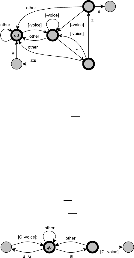
Chapter 11
Computational Phonology
11.1 Build an automaton for rule (11.3).
The symbol “[-voice]” means a voiced sound (potentially producing
anything) and the symbol “other” means any sound not used on other
arcs leaving the same state (also potentially producing anything).
11.2 Some Canadian dialects of English exhibit Canadian raising:/aI/ is raised to
Canadian raising
[2I] and /aU/ to [2U] in stressed position before a voiceless consonant (Brom-
berger and Halle, 1989). A simplified rule dealing only with /aI/ can be stated
as:
/aI/ →[2I] /C
−voice (11.1)
In some Canadian dialects this rule interacts with the flapping rule, causing dif-
ferent pronunciations for the words rider ([raIRÄ]) and writer ([r2IRÄ]). Write a
two-level rule and an automaton for the raising and flapping rules that correctly
models this distinction, making simplifying assumptions as needed.
When applying the Canadian raising rule, we must look for voiceless
consonants at the lexical level, not the surface level. Otherwise, the
rule would not apply to writer which has the lexical form /raItÄ/ but
the surface form [raIRÄ]. Thus, our two-level rules should look like:
´aI:´2I ⇔C
−voice :
t:dx ⇔´
VV
The automaton for the raising rule then looks like:
42
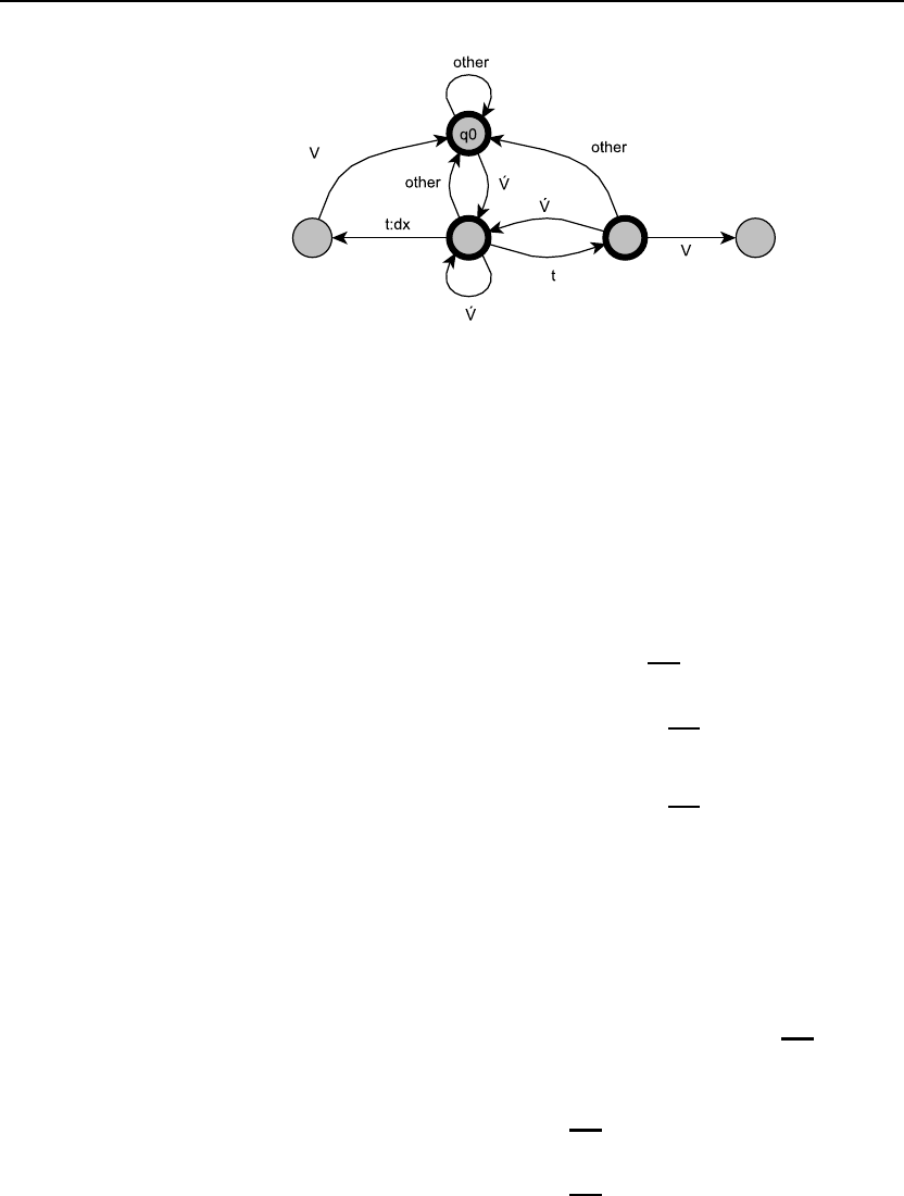
43
And the automaton for the flapping rule looks like:
11.3 Write the lexical entry for the pronunciation of the English past tense (preterite)
suffix -d, and the two-level rules that express the difference in its pronunciation
depending on the previous context. Don’t worry about the spelling rules. Make
sure you correctly handle the pronunciation of the past tenses of the words add,
pat,bake, and bag.
The suffix -d is pronounced as [Id] when following an alveolar stop
like [t] or [d] (e.g., added,patted), as [t] when following voiceless
sounds (e.g., baked), and as [d] when following voiced sounds (e.g.,
bagged).
To allow the rules to run in parallel, we can give them mutually
exclusive conditions, and look for these only at the lexical level:
d:Id ⇔[+alveolar-stop]: ˆ#
d:t⇔−alveolar-stop
−voice :ˆ#
d⇔−alveolar-stop
+voice :ˆ#
11.4 Write two-level rules for the Yawelmani Yokuts Harmony, Shortening, and Low-
ering phenomena from page 365. Make sure your rules can run in parallel.
The key here is to make sure that the Harmony rule only looks at the
lexical context, so that changes to the surface forms from the Short-
ening and Lowering rules do not affect it.
[+αhigh]:+βback
+γround ⇔
+αhigh
+βback
+γround
:C∗ˆC∗
+high
+long :[−high]⇔
[+long]:[−long]⇔C
Chapter 12
Formal Grammars of English
12.1 Draw tree structures for the following ATIS phrases:
The trees below use, as much as possible, the rules from the chapter.
Other tree structures are also possible.
1. Dallas NP
ProperNoun
Dallas
2. from Denver
PP
NP
ProperNoun
Denver
Prep
from
3. after five p.m.
PP
NP
Nom
Noun
p.m.
Card
five
Prep
after
4. arriving in Washington
GerundVP
PP
NP
ProperNoun
Washington
Prep
in
GerundV
arriving
5. early flights
NP
Nom
Noun
flights
AP
Adj
early
44
45
6. all redeye flights
NP
Nom
Noun
flights
Nom
Noun
redeye
Quant
all
7. on Thursday
PP
NP
ProperNoun
Thursday
Prep
on
8. a one-way fare
NP
Nom
Noun
fare
AP
Adj
one-way
Det
a
9. any delays in Denver
NP
Nom
PP
NP
ProperNoun
Denver
Prep
in
Nom
Noun
delays
Quant
any
46 Chapter 12. Formal Grammars of English
12.2 Draw tree structures for the following ATIS sentences:
The trees below use, as much as possible, the rules from the chapter.
Other tree structures are also possible.
1. Does American airlines have a flight between five a.m. and six a.m.?
S
VP
NP
Nom
PP
NP
NP
Nom
Noun
a.m.
Card
six
andNP
Nom
Noun
a.m.
Card
five
Prep
between
Nom
Noun
flight
Det
a
Verb
have
NP
ProperNoun
American airlines
Aux
Does
2. I would like to fly on American airlines.
S
VP
VP
VP
PP
NP
ProperNoun
American airlines
Prep
on
Verb
fly
Inf
to
Verb
like
Verb
would
NP
Pro
I
3. Please repeat that.
S
VP
NP
Pro
that
Verb
repeat
Adv
Please
47
4. Does American 487 have a first-class section?
S
VP
NP
Nom
Noun
section
AP
Adj
first-class
Det
a
Verb
have
NP
ProperNoun
American 487
Aux
Does
5. I need to fly between Philadelphia and Atlanta.
S
VP
VP
PP
NP
NP
ProperNoun
Atlanta
andNP
ProperNoun
Philadelphia
Prep
between
Verb
fly
Inf
to
Verb
need
NP
Pro
I
6. What is the fare from Atlanta to Denver?
S
VP
NP
Nom
PP
NP
ProperNoun
Denver
Prep
to
Nom
PP
NP
ProperNoun
Atlanta
Prep
from
Nom
Noun
fare
Det
the
Verb
is
NP
Pro
what
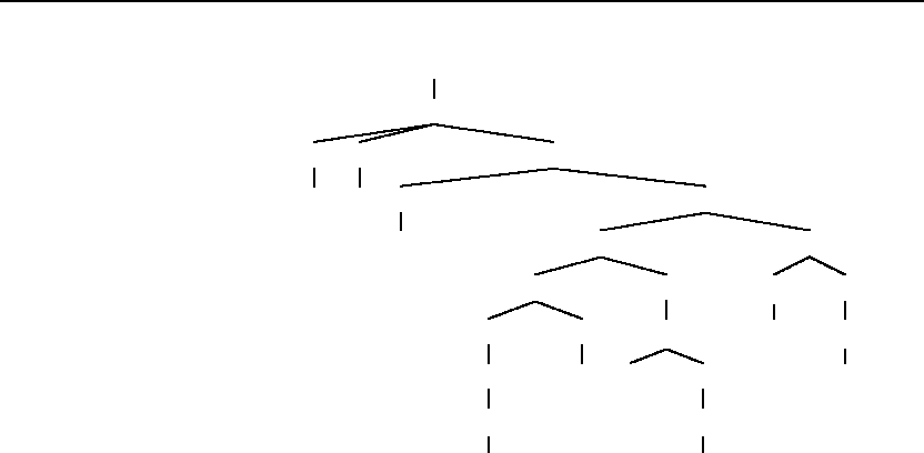
48 Chapter 12. Formal Grammars of English
7. Is there an American airlines flight from Philadelphia to Dallas?
S
VP
NP
Nom
PP
NP
ProperNoun
Dallas
Prep
to
Nom
PP
Prep
NP
ProperNoun
Philadelphia
from
Nom
Noun
flight
Nom
NP
ProperNoun
American airlines
Det
an
Ex
there
Verb
Is
12.3 Augment the grammar rules on page 399 to handle pronouns. Deal properly with
person and case.
S→3sgAux 3sgNomNP VP
S→Non3sgAux Non3sgNomNP VP
3sgAux →does |has |can |...
Non3sgAux →do |have |can |...
3sgNomNP →3sgNomPronoun
3sgNomNP →Det SgNominal
3sgNomPronoun →he |she |it
Non3sgNomNP →Non3sgNomPronoun
Non3sgNomNP →Det PlNominal
Non3sgNomPronoun →I|you |we |they
VP →Verb (AccNP) (PP)
AccNP →AccPronoun
AccNP →Det Nominal
AccPronoun →me |us |you |him |her |it |them
12.4 Modify the noun phrase grammar of Sections 12.3.3–12.3.4 to correctly model
mass nouns and their agreement properties
3sgNP →SgCountNP |MassNP
SgCountNP →SgCountDet SgCountNominal
SgCountDet →a|one |the |any |...
SgCountNominal →flight |pilot |...
MassNP →(MassDet) MassNominal
MassDet →some |the |any |...
MassNominal →snow |breakfast |...

49
12.5 How many types of NPs would the rule on page 396 expand to if we didn’t allow
parentheses in our grammar formalism?
Since there is a binary decision of whether or not to include each of
the five options (Det,Card,Ord,Quant and AP), we would need
25= 32
rules to express the grammar without a way of denoting optionality.
12.6 Assume a grammar that has many VP rules for different subcategorizations,
as expressed in Section 12.3.5, and differently subcategorized verb rules like
Verb-with-NP-complement. How would the rule for postnominal relative clauses
(12.5) need to be modified if we wanted to deal properly with examples like the
earliest flight that you have? Recall that in such examples the pronoun that is
the object of the verb get. Your rules should allow this noun phrase but should
correctly rule out the ungrammatical S *I get.
RelClause →(who |that) VP
RelClause →(who |that) NoObjS
NoObjS →NP NoObjVP
NoObjVP →(Aux) Verb-with-NP-Comp (PP)
NoObjVP →(Aux) Verb-with-S-Comp (NoObjS)
NoObjVP →(Aux) Verb-with-Inf-VP-Comp ((NP) to NoObjVP)
12.7 Does your solution to the previous problem correctly model the NP the earliest
flight that I can get? How about the earliest flight that I think my mother wants
me to book for her? Hint: this phenomenon is called long-distance dependency.
Yes, the optional Aux elements allow for auxiliaries like can, and the
recursive uses of NoObjS and NoObjVP in the last two rules allow for
the long-distance dependencies.
12.8 Write rules expressing the verbal subcategory of English auxiliaries; for exam-
ple, you might have a rule verb-with-bare-stem-VP-complement →can.
For the sake of conciseness, we list only one form per verb, but for
example, am,are,was follow the same pattern as is.
verb-with-bare-stem-VP-complement →do |can |could |may |
might |must |shall |
should |will |would
verb-with-gerund-VP-complement →is
verb-with-perfect-VP-complement →has |is
verb-with-infinitive-VP-complement →ought

50 Chapter 12. Formal Grammars of English
12.9 NPs like Fortune’s office or my uncle’s marks are called possessive or genitive
Possessive
Genitive noun phrases. We can be model possessive noun phrases by treating the sub-NP
like Fortune’s or my uncle’s as a determiner of the following head noun. Write
grammar rules for English possessives. You may treat ’s as if it were a separate
word (i.e., as if there were always a space before ’s).
NP →(Det) Nominal
NP →ProperNoun
Det →NP ’s
Det →my |a|the |...
12.10 Page 393 discussed the need for a Wh-NP constituent. The simplest Wh-NP is
one of the Wh-pronouns (who, whom, whose, which). The Wh-words what and
which can be determiners: which four will you have?,what credit do you have
with the Duke? Write rules for the different types of Wh-NPs.
Wh-NP →Wh-Pro
Wh-NP →Wh-Det Nominal
Wh-Pro →who |whom |whose |which
Wh-Det →what |which
12.11 Write an algorithm for converting an arbitrary context-free grammar into Chom-
sky normal form.
function CHOMSKY-NORMAL-FORM(grammar)returns grammar
; remove epsilon rules
while grammar has a rule A→where Ais not the start state do
Remove the rule A→
for each rule B→β0. . . βiAβj...βNdo
Replace the rule with B→β0. . . βiβj...βN
; remove single symbol nonterminal rules
while grammar has a rule A→Bwhere Bis a nonterminal do
Remove the rule A→B
for each rule B→β0. . . βNdo
Add the rule A→β0. . . βN
if Bis not the start symbol do
if no rule C→γ Bδ exists do
Remove all rules B→C
; move terminals to their own rules
for each rule A→β0β1. . . βNin grammar where N > 1do
for each βiwhere βiis a terminal do
Create a new symbol B
Add a rule B→βito grammar
Replace βiin the original rule with B
; ensure there are only two nonterminals per rule
while grammar has a rule A→β0. . . βN−2βN−1βNwhere N > 2do
Create a new symbol B
Add a rule B→βN−1βN
Replace the original rule with A→β0. . . βN−2B
return grammar
Chapter 13
Syntactic Parsing
13.1 Implement the algorithm to convert arbitrary context-free grammars to CNF.
def chomsky_normal_form(grammar):
grammar = set(grammar)
nonterminals = set(rule.head for rule in grammar)
# remove single symbol nonterminal rules
for rule, symbol in _unary_rules(grammar, nonterminals):
grammar.discard(rule)
for rule2 in _rules_headed_by(grammar, symbol):
grammar.add(Rule(rule.head, tuple(rule2.symbols)))
if all(symbol not in rule.symbols for rule in grammar):
for rule2 in _rules_headed_by(grammar, symbol):
grammar.discard(rule2)
# move terminals to their own rules
for rule in list(grammar):
if len(rule.symbols) >= 2:
for i, symbol in enumerate(rule.symbols):
if all(rule.head != symbol for rule in grammar):
rule = _new_symbol(grammar, rule, i, i + 1)
# ensure there are only two nonterminals per rule
for rule in _multi_symbol_rules(grammar):
_new_symbol(grammar, rule, 0, 2)
# return the grammar in CNF
return grammar
# find A -> B rules, allowing concurrent modifications
def _unary_rules(grammar, nonterminals):
while True:
g = ((rule, rule.symbols[0])
for rule in grammar
if len(rule.symbols) == 1
if rule.symbols[0] in nonterminals)
yield g.next()
# find all rules headed by the given symbol
def _rules_headed_by(grammar, symbol):
return [rule for rule in grammar if rule.head == symbol]
# create a new symbol which derives the given span of symbols
def _new_symbol(grammar, rule, start, stop):
symbols = rule.symbols
new_head = ’_’.join(symbols[start:stop]).upper()
new_symbols = symbols[:start] + (new_head,) + symbols[stop:]
new_rule = Rule(rule.head, new_symbols)
grammar.discard(rule)
grammar.add(new_rule)
grammar.add(Rule(new_head, symbols[start:stop]))
return new_rule
# find A -> BCD... rules, allowing concurrent modifications
def _multi_symbol_rules(grammar):
while True:
g = (rule for rule in grammar if len(rule.symbols) >= 3)
yield g.next()
51

52 Chapter 13. Syntactic Parsing
Apply your program to the L1grammar.
# representation of a rule A -> B...C
class Rule(object):
def __init__(self, head, symbols):
self.head = head
self.symbols = symbols
self._key = head, symbols
def __eq__(self, other):
return self._key == other._key
def __hash__(self):
return hash(self._key)
# build a grammar from a string of lines like "X -> YZ | b"
def get_grammar(string):
grammar = set()
for line in string.splitlines():
head, symbols_str = line.split(’ -> ’)
for symbols_str in symbols_str.split(’ | ’):
symbols = tuple(symbols_str.split())
grammar.add(Rule(head, symbols))
return grammar
grammar = get_grammar(’’’\
S -> NP VP | Aux NP VP | VP
NP -> Pronoun | Proper-Noun | Det Nominal
Nominal -> Noun | Nominal Noun | Nominal PP
VP -> Verb | Verb NP | Verb NP PP | Verb PP | VP PP
PP -> Preposition NP
Det -> that | this | a
Noun -> book | flight | meal | money
Verb -> book | include | prefer
Pronoun -> I | she | me
Proper-Noun -> Houston | TWA
Aux -> does
Preposition -> from | to | on | near | through’’’)
grammar_cnf = chomsky_normal_form(grammar)
assert grammar_cnf == get_grammar(’’’\
S -> NP VP | AUX_NP VP | Verb NP | VERB_NP PP | Verb PP | VP PP
S -> book | include | prefer
AUX_NP -> Aux NP
NP -> Det Nominal
NP -> TWA | Houston | I | she | me
Nominal -> Nominal Noun | Nominal PP
Nominal -> book | flight | meal | money
VP -> Verb NP | VERB_NP PP | Verb PP | VP PP
VP -> book | include | prefer
VERB_NP -> Verb NP
PP -> Preposition NP
Det -> this | that | a
Noun -> book | flight | meal | money
Verb -> book | include | prefer
Aux -> does
Preposition -> from | to | on | near | through’’’)
13.2 Implement the CKY algorithm and test it with your converted L1grammar.
import collections
def cky_table(grammar, words):
table = collections.defaultdict(set)
for col, word in enumerate(words):
col += 1
# find all rules for the current word
for rule in grammar:
if rule.symbols == (word,):
table[col - 1, col].add(rule.head)

53
# for each span of words ending at the current word,
# find all splits that could have formed that span
for row in xrange(col - 2, -1, -1):
for mid in xrange(row + 1, col):
# if the two constituents identified by this
# split can be combined, add the combination
# to the table
for rule in grammar:
if len(rule.symbols) == 2:
sym1, sym2 = rule.symbols
if sym1 in table[row, mid]:
if sym2 in table[mid, col]:
table[row, col].add(rule.head)
return table
words = ’book a flight through Houston’.split()
table = cky_table(grammar_cnf, words)
assert table[0, 1] == set(’S VP Verb Nominal Noun’.split())
assert table[0, 2] == set()
assert table[0, 3] == set(’S VP VERB_NP’.split())
assert table[0, 4] == set()
assert table[0, 5] == set(’S VP VERB_NP’.split())
assert table[1, 2] == set(’Det’.split())
assert table[1, 3] == set(’NP’.split())
assert table[1, 4] == set()
assert table[1, 5] == set(’NP’.split())
assert table[2, 3] == set(’Nominal Noun’.split())
assert table[2, 4] == set()
assert table[2, 5] == set(’Nominal’.split())
assert table[3, 4] == set(’Preposition’.split())
assert table[3, 5] == set(’PP’.split())
assert table[4, 5] == set(’NP’.split())
13.3 Rewrite the CKY algorithm given in Fig. 13.10 on page 440 so that it can accept
grammars that contain unit productions.
Solving this problem requires that each time we add a symbol to a
cell in the table, we also add all symbols to that cell which could have
produced the original symbol through a sequence of unary rules. So,
for example, if we add Cto table[i,j], and we have the rules A→B
and B→C, then we must also add Aand Bto table[i,j].
13.4 Augment the Earley algorithm of Fig. 13.13 to enable parse trees to be retrieved
from the chart by modifying the pseudocode for COMPLETER as described on
page 448.
Basically, we add a list of backpointers to each of our states. When
the dot in a rule is advanced, the state that allowed that advance is
appended to the list of backpointers.
procedure COMPLETER(Sx=(B→γ•, [j,k], Sn. . . Sm))
for each (A→α•B β, [i,j], Sp. . . Sq)in chart[j]do
ENQUEUE((A→α B •β, [i,k], Sp. . . SqSx), chart[k])

54 Chapter 13. Syntactic Parsing
13.5 Implement the Earley algorithm as augmented in the previous exercise. Check it
on a test sentence by using the L1grammar.
def earley_parse(grammar, words):
nonterminals = set(rule.head for rule in grammar)
# never allow states already seen to be added to the chart
chart = collections.defaultdict(list)
seen = collections.defaultdict(set)
def add(i, rule, dot, start, end, pointers=()):
state = State(rule, dot, start, end, pointers)
if state not in seen[i]:
chart[i].append(state)
seen[i].add(state)
# iteratively build the chart
add(0, Rule(’START’, (’S’,)), 0, 0, 0)
for i in xrange(len(words) + 1):
for state in chart[i]:
complete = state.is_complete()
next_symbol = state.next_symbol()
# Scanner - the state is expecting a word, so if the
# expected word is next in the input, advance the
# rule past the word
if not complete and next_symbol not in nonterminals:
if state.end < len(words):
if next_symbol == words[state.end]:
add(state.end + 1, state.rule,
state.dot + 1, state.start,
state.end + 1, state.pointers)
# Predictor - the state is expecting a constituent C,
# so add new states for all expansions of C, starting
# at the end of the current state
elif not complete and next_symbol in nonterminals:
for rule in grammar:
if rule.head == next_symbol:
add(state.end, rule, 0,
state.end, state.end)
# Completer - the state is complete, advance any
# states that were expecting a state like this (both
# the symbol and the location)
else:
for other in chart[state.start]:
if other.next_symbol() == state.rule.head:
if other.end == state.start:
add(state.end, other.rule,
other.dot + 1,
other.start, state.end,
other.pointers + (state,))
# helper for creating tree strings from states
def to_tree(state):
children = [to_tree(child) for child in state.pointers]
if not children:
children = state.rule.symbols
return ’(%s %s)’ % (state.rule.head, ’ ’.join(children))
# generate all trees from the START rules
for state in chart[i]:
if state.rule.head == ’START’ and state.is_complete():
top, = state.pointers
yield to_tree(top)

55
# state class encapsulating rule position, word span and
# pointers for retrieving full parse
class State(object):
def __init__(self, rule, dot, start, end, pointers=()):
self.rule = rule
self.dot = dot
self.start = start
self.end = end
self.pointers = pointers
self._key = rule, dot, start, end, pointers
def __hash__(self):
return hash(self._key)
def __eq__(self, other):
return self._key == other._key
def is_complete(self):
return self.dot == len(self.rule.symbols)
def next_symbol(self):
if self.is_complete():
return None
else:
return self.rule.symbols[self.dot]
grammar = get_grammar(’’’\
S -> NP VP | Aux NP VP | VP
NP -> Pronoun | Proper-Noun | Det Nominal
Nominal -> Noun | Nominal Noun | Nominal PP
VP -> Verb | Verb NP | Verb NP PP | Verb PP | VP PP
PP -> Preposition NP
Det -> that | this | a
Noun -> book | flight | meal | money
Verb -> book | include | prefer
Pronoun -> I | she | me
Proper-Noun -> Houston | TWA
Aux -> does
Preposition -> from | to | on | near | through’’’)
words = ’book through Houston’.split()
assert set(earley_parse(grammar, words)) == set([
’(S (VP (Verb book) ’
’(PP (Preposition through) (NP (Proper-Noun Houston)))))’,
’(S (VP (VP (Verb book)) ’
’(PP (Preposition through) (NP (Proper-Noun Houston)))))’])
13.6 Alter the Earley algorithm so that it makes better use of bottom-up information
to reduce the number of useless predictions.
One way to achieve this would be to determine for each nonterminal,
all possible terminals that could appear in the first position of a string
derived from that rule. For example, in the L1grammar,
FIRST(P P ) ={from, to, on, near, through}
FIRST(V P ) ={book, include, prefer}
The predictor would only insert new states for nonterminals whose
FIRST set included the current word in the string.
13.7 Attempt to recast the CKY and Earley algorithms in the chart-parsing paradigm.
In the chart-parsing version of CKY, we would first INITIALIZE by
looking up words in the grammar and adding their rules to the agenda.
This is basically the equivalent of filling in the table cells along the
diagonal. We then alternate between MAKE-PREDICTIONS, which
generates parent rules from rules in the table, and the FUNDAMENTAL

56 Chapter 13. Syntactic Parsing
rule, which takes pairs of these rules and completes them. The agenda
would make sure we consider rules in the same order as the traditional
CKY algorithm.
In the chart-parsing version of Earley, we again INITIALIZE by
adding all the part of speech rules, basically the equivalent of SCAN-
NER. Then MAKE-PREDICTIONS does what PREDICTOR used to do,
and the FUNDAMENTAL rule does what COMPLETER used to do. The
agenda would basically be a sequence of queues, one for each word,
and where we process all edges for each word in the order they were
produced.
13.8 Discuss the relative advantages and disadvantages of partial versus full parsing.
Partial parsing is generally much faster than full parsing, but pro-
vides less syntactic detail. Thus, for a task where only a few pieces
of surface level syntax are necessary, e.g., named entity recognition,
partial parsing can provide similar results to a full parse in substan-
tially reduced times. However, for a task where a great amount of
syntactic detail is needed, e.g., construction of logical forms, even
cascaded partial parsers will not produce as complete information as
a full parser.
13.9 Implement a more extensive finite-state grammar for noun groups by using the
examples given in Section 13.5 and test it on some NPs. Use an on-line dictio-
nary with parts-of-speech if available; if not, build a more restricted system by
hand.
Below, we use NN to stand for NN or NNS or NNP.
NP →(DT) (CD) JJ∗(VBG) NN∗NN
NP →(DT) (CD) NN∗NN CC NN∗NN
These rules cover NPs like the following found in the Penn Treebank:
one Cray Computer share
an Italian state-owned holding company
the Cray-3 research and development expenses
13.10 Discuss how to augment a parser to deal with input that may be incorrect, for
example, containing spelling errors or mistakes arising from automatic speech
recognition.
One approach might be to take the partial syntactic structures that the
parser was able to identify and join them together to form full parses.
These full parses would necessarily introduce new rules, so this ap-
proach would likely require searching through the space of possible
new rules to find a minimal set that produces a full parse.
Another approach, and perhaps the more common one, would be
to use one of the probabilistic approaches discussed in Chapter 14.
Chapter 14
Statistical Parsing
14.1 Implement the CKY algorithm.
import collections
def prob_cky(grammar, words):
ddict = collections.defaultdict
probs = ddict(lambda: ddict(lambda: 0.0))
backs = ddict(lambda: {})
# helpers for getting rules that produce the given symbols
# and for getting heads of rules with probability > 0
def get_rules(*symbols):
for rule in grammar:
if rule.symbols == symbols:
yield rule
def probs_positive(row, col):
for head in probs[row, col]:
if probs[row, col][head] > 0.0:
yield head
# for each word in the input, update the table cells in the
# corresponding column, from bottom to top
for col, word in enumerate(words):
col += 1
# find rules that could have produced the word directly
for rule in get_rules(word):
probs[col - 1, col][rule.head] = rule.prob
backs[col - 1, col][rule.head] = None, None, None
# create a new span when two existing spans meet at their
# endpoints and a rule producing those two symbols exists
for row in xrange(col - 2, -1, -1):
for mid in xrange(row + 1, col):
for head1 in probs_positive(row, mid):
for head2 in probs_positive(mid, col):
for rule in get_rules(head1, head2):
# combine rule and span probabilities
prob = rule.prob
prob *= probs[row, mid][head1]
prob *= probs[mid, col][head2]
# keep higher probability rules
if prob > probs[row, col][rule.head]:
probs[row, col][rule.head] = prob
back = mid, head1, head2
backs[row, col][rule.head] = back
# helper for converting the backpointers to a tree
def get_tree(row, col, symbol):
mid, head1, head2 = backs[row, col][symbol]
if mid is head1 is head2 is None:
return ’(%s %s)’ % (symbol, words[row])
else:
tree1 = get_tree(row, mid, head1)
tree2 = get_tree(mid, col, head2)
return ’(%s %s %s)’ % (symbol, tree1, tree2)
# return tree and expected probability
return get_tree(0, len(words), ’S’), probs[0, len(words)][’S’]
57

58 Chapter 14. Statistical Parsing
14.2 Modify the algorithm for conversion to CNF from Chapter 13 to correctly han-
dle rule probabilities. Make sure that the resulting CNF assigns the same total
probability to each parse tree.
The three basic CNF transformation rules, and their corresponding
probability calculations (shown in brackets following each rule):
•Replace A→B[p1]rules with A→β0. . . βN[p1∗p2]rules
for each B→β0...βN[p2]rule.
•Replace A→β0. . . βibβjβN[p1]rules (where bis a terminal)
with A→β0...βiBβjβN[p1]and B→b[1.0] rules (where B
is a new symbol).
•Replace A→β0...βN−2βN−1βN[p1]rules (where N > 2)
with A→β0...βN−2B[p1]and B→βN−1βN[1.0] rules
(where Bis a new symbol).
14.3 Recall that Exercise 13.3 asked you to update the CKY algorithm to handle unit
productions directly rather than converting them to CNF. Extend this change to
probabilistic CKY.
def prob_cky(grammar, words):
ddict = collections.defaultdict
probs = ddict(lambda: ddict(lambda: 0.0))
backs = ddict(lambda: {})
# helpers for getting rules that produce the given symbols
# and for getting heads of rules with probability > 0
def get_rules(*symbols):
for rule in grammar:
if rule.symbols == symbols:
yield rule
def probs_positive(row, col):
for head in probs[row, col]:
if probs[row, col][head] > 0.0:
yield head
# helper for adding heads to table cells that could have
# been generated using a chain of unary rules
def add_unaries(row, col):
# iterate over a queue with the heads from the table cell
seen = set()
heads_todo = set(probs_positive(row, col))
while heads_todo:
head = heads_todo.pop()
# add to the queue rules that could have generated
# this symbol, that were not previously seen
for rule in get_rules(head):
if rule not in seen:
seen.add(rule)
heads_todo.add(rule.head)
# combine A -> B and B -> C rules and add the
# new A -> C rule to the table
prob = rule.prob *probs[row, col][head]
if prob > probs[row, col][rule.head]:
probs[row, col][rule.head] = prob
back = None, head, None
backs[row, col][rule.head] = back
# for each word in the input, update the table cells in the
# corresponding column, from bottom to top

59
for col, word in enumerate(words):
col += 1
# find rules that could have produced the word directly
for rule in get_rules(word):
probs[col - 1, col][rule.head] = rule.prob
backs[col - 1, col][rule.head] = None, None, None
# propagate any unary rules
add_unaries(col - 1, col)
# create a new span when two existing spans meet at their
# endpoints and a rule producing those two symbols exists
for row in xrange(col - 2, -1, -1):
for mid in xrange(row + 1, col):
for head1 in probs_positive(row, mid):
for head2 in probs_positive(mid, col):
for rule in get_rules(head1, head2):
# combine rule and span probabilities
prob = rule.prob
prob *= probs[row, mid][head1]
prob *= probs[mid, col][head2]
# keep higher probability rules
if prob > probs[row, col][rule.head]:
probs[row, col][rule.head] = prob
back = mid, head1, head2
backs[row, col][rule.head] = back
# propagate any unary rules
add_unaries(row, col)
# helper for converting the backpointers to a tree
def get_tree(row, col, symbol):
mid, head1, head2 = backs[row, col][symbol]
if mid is head1 is head2 is None:
return ’(%s %s)’ % (symbol, words[row])
elif mid is head2 is None:
tree = get_tree(row, col, head1)
return ’(%s %s)’ % (symbol, tree)
else:
tree1 = get_tree(row, mid, head1)
tree2 = get_tree(mid, col, head2)
return ’(%s %s %s)’ % (symbol, tree1, tree2)
# return tree and expected probability
return get_tree(0, len(words), ’S’), probs[0, len(words)][’S’]
60 Chapter 14. Statistical Parsing
14.4 Fill out the rest of the probabilistic CKY chart in Fig. 14.4.
Det: .4
[0,1]
NP: .0024
[0,2] [0,3] [0,4]
S: 2.304e-8
[0,5]
N: .02
[1,2] [1,3] [1,4] [1,5]
V: .05
[2,3] [2,4]
VP: 1.2e-5
[2,5]
Det: .4
[3,4]
NP: .0012
[3,5]
N: .01
[4,5]
14.7 Implement the PARSEVAL metrics described in Section 14.7. Next, either use a
treebank or create your own hand-checked parsed testset. Now use your CFG (or
other) parser and grammar, parse the test set and compute labeled recall, labeled
precision, and cross-brackets.
The code below implements the PARSEVAL metrics.
from __future__ import division
def parseval(expected_trees, predicted_trees):
correct = 0
expected = 0
predicted = 0
crossed = 0
# count numbers of correct, expected and predicted
# constituents, as well as number of crossing brackets
tree_pairs = zip(expected_trees, predicted_trees)
for expected_tree, predicted_tree in tree_pairs:
# convert trees to spans
expected_spans = get_spans(expected_tree)
predicted_spans = get_spans(predicted_tree)
expected += len(expected_spans)
predicted += len(predicted_spans)
# look for matching spans and crossing brackets
for predicted_span in predicted_spans:
had_match = had_crossing = False
for expected_span in expected_spans:
# look for matching spans
if predicted_span == expected_span:
had_match = True
# look for crossing brackets
_, s1, e1 = predicted_span
_, s2, e2 = expected_span
if s1 < s2 < e1 < e2 or s2 < s1 < e2 < e1:
had_crossing = True
# update correct and crossing bracket counts
correct += had_match
crossed += had_crossing

61
# calculate precision, recall, F-measure and crossing brackets
precision = correct / predicted
recall = correct / expected
f = 2 *precision *recall / (precision + recall)
crossing_brackets = crossed / predicted
return precision, recall, f, crossing_brackets
def get_spans(tree, offset=0):
start = offset
# spans of terminals are length 1
if not tree:
offset += 1
# spans of nonterminals are determined from their children
spans = []
for child in tree:
spans.extend(get_spans(child, offset))
offset = spans[-1][-1]
# add the span for this subtree and return the span list
spans.append((tree.tag, start, offset))
return spans
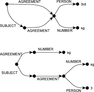
Chapter 15
Features and Unification
15.1 Draw the DAGs corresponding to the AVMs given in Examples 15.1–15.2.
Example 15.1
Example 15.2
15.2 Consider the following examples from the Berkeley Restaurant Project (BERP),
focusing on their use of pronouns.
I want to spend lots of money.
Tell me about Chez Panisse.
I’d like to take her to dinner.
She doesn’t like Italian.
Assuming that these pronouns all belong to the category Pro, write lexical and
grammatical entries with unification constraints that block the following exam-
ples.
*Me want to spend lots of money.
*Tell I about Chez Panisse.
*I would like to take she to dinner.
*Her doesn’t like Italian.
S→(NP) (Aux)VP
hNP CASEi= nominative
VP →V NP ...
hNP CASEi= accusative
NP →Pro
hPro CASEi=hNP CASEi
62

63
15.3 Draw a picture of the subsumption semilattice corresponding to the feature struc-
tures in Examples 15.3 to 15.7. Be sure to include the most general feature struc-
ture [].
An arrow from node Ato node Bindicates that BvA.
15.4 Consider the following examples.
The sheep are baaaaing.
The sheep is baaaaing.
Create appropriate lexical entries for the words the,sheep, and baaaaing. Show
that your entries permit the correct assignment of a value to the NUMBER feature
for the subjects of these examples, as well as their various parts.
Since the text introduced agreement features for determiners, nouns,
auxiliaries and verbs, the desired outcome is:
•For The sheep is baaaaing, all words have NUMBER =sg
•For The sheep are baaaaing, all words have NUMBER =pl
For the,sheep and baaing, we leave the agreements unspecified. Then
for is and are we specify singular and plural agreements, respectively:
Aux →is
hAux AGREEMENT NUMBERi= sg
Aux →are
hAux AGREEMENT NUMBERi= pl
We also need to introduce a new grammar rule:
VP →Aux Verb
hAux AGREEMENTi=hVerb AGREEMENTi
hVP AGREEMENTi=hVerb AGREEMENTi
Then unification should take care of the rest:
•The VP →Aux Verb rule from above requires VP,Aux and Verb
to have the same AGREEMENT
•The NP →Det Nominal rule from the chapter requires NP,Det
and Nominal to have the same AGREEMENT
•The S→NP VP rule gives from the chapter requires S,NP and
VP to have the same AGREEMENT
Thus, for our sentences, the Aux,Verb,Det and Noun all must have
the same agreement. So when the verb is is, all NUMBER features will
be sg, and when the verb is are, all NUMBER features will be pl.

64 Chapter 15. Features and Unification
15.5 Create feature structures expressing the different SUBCAT frames for while and
during shown on page 506.
ORTH while
CAT Prep
HEAD SUBCAT h[CAT S]i
ORTH during
CAT Prep
HEAD SUBCAT h[CAT NP]i
15.6 Alter the pseudocode shown in Figure 15.11 so that it performs the more radical
kind of unification-based parsing described on page 519.
function EARLEY-PARSE(words,grammar)returns chart
for (X0→α,dagX0)in grammar do
if dagX0(hX0CAT i) = Sthen
ADDTOCHART((γ→ • X0,[0,0],dagγ), chart[0])
for ifrom 0to LENGTH(words)do
for each state in chart[i]do
if INCOMPLETE?(state)
if NEXT-CAT(state) is a part of speech do
SCANNER(state)
else
PREDICTOR(state)
else
COMPLETER(state)
procedure PREDICTOR((X0→α•X1β,[i, j],dagX0))
for each (X2→γ,dagX2)in grammar do
if new-dag ←UNIFY-STATES(dagX1,dagX2,X0)6=Fails then
ADDTOCHART((X2→ • γ,[j, j],new-dag), chart[j])
procedure SCANNER((X0→α•X1β,[i, j],dagX0))
if dagX1(hX1CAT i)∈PARTS-OF-SPEECH(words[j])then
ADDTOCHART((X1→words[j]•,[j, j+1],dagX1), chart[j+1])
procedure COMPLETER((X0→γ•,[j, k],dagX0))
for each (X1→α•X2β,[i, j],dagX1)in chart[j]do
if new-dag ←UNIFY-STATES(dagX0,dagX1,X1)6=Fails then
ADDTOCHART((X1→α X0•β,[i, k],new-dag), chart[k])

65
15.7 Consider the following problematic grammar suggested by Shieber (1985).
S→T
hTFi= a
T1→T2A
hT1Fi=hT2F Fi
S→A
A→a
Show the first Sstate entered into the chart by using your modified PREDICTOR
from the previous exercise, then describe any problematic behavior displayed by
PREDICTOR on subsequent iterations. Discuss the cause of the problem and how
it might be remedied.
The first two rules in the grammar look like:
X0←X1
X0CAT S
X1CAT T
Fa
X0→X1X2
X0CAT T
F1
X1CAT T
FF:1
X2CAT A
So the first state put on the chart is:
γ→ •X0,[0,0],
X0CAT S
X1CAT T
Fa
This state is incomplete, so we go to the PREDICTOR and unify this
state with the second rule, adding the new state:
X0→ •X1X2,[0,0],
X0CAT T
F1a
X1CAT T
FF1
X2CAT A
But the PREDICTOR then then unifies this again with the second rule,
adding the new state:
X0→ •X1X2,[0,0],
X0CAT T
F1a
X1CAT T
FFF1
X2CAT A
We’re now stuck in a loop where we create a new state, unify it with
rule two, and produce a new state that will unify with rule two again.
To solve this problem, we need to restrict our view to only part of
the dag instead of the whole thing. Then instead of the PREDICTOR
unifying whole dags, it would just unify the sub-dags containing the
category information.
66 Chapter 15. Features and Unification
15.8 Using the list approach to representing a verb’s subcategorization frame, show
how a grammar could handle any number of verb subcategorization frames with
only the following two VP rules. More specifically, show the constraints that
would have to be added to these rules to make this work.
VP →Verb
VP →VP X
The solution to this problem involves thinking about a recursive walk down
a verb’s subcategorization frame. This is a hard problem; you might consult
Shieber (1986) if you get stuck.
Under these rules, each element of a verb’s subcategorization frame is
attached to its own VP. So each time we use the VP →VP X rule, the
newly introduced VP should contain one more category expected by
the verb. We can do this recursively, by defining the subcategorization
of the child VP in terms of its parent.
This approach requires decomposing the subcategorization lists,
so we introduce the syntax hXi+Yto mean that Xis the first item in
a list and Yis the remaining items.
VP CAT VP
HEAD 1
Verb CAT Verb
HEAD 1
VP CAT VP
HEAD SUBCAT 1
VP "CAT VP
HEAD hSUBCAT D2E+1i#
XCAT 2
15.9 Page 524 showed how to use typed feature structures to represent constituency.
Use that notation to represent rules 15.11, 15.12, and 15.13 shown on page 501.
CAT VP
HEAD 1
DTRS CAT Verb
HEAD 1,CAT NP
CAT NP
HEAD 1
DTRS CAT Det
HEAD AGREE 2,CAT Nominal
HEAD 1AGREE 2
CAT Nominal
HEAD 1
DTRS CAT Noun
HEAD 1
Chapter 16
Language and Complexity
16.1 Is the language anb2ancontext free?
Yes. It can be generated with the following context free grammar:
S→aSa
S→bb
Technically, to confirm that the language is context free, we must also
show that it is not a regular language. See Exercise 16.3 for details.
16.2 Use the pumping lemma to show this language is not regular:
L=xnyn−1likes tuna fish, x ∈A, y ∈B
The pumping lemma states that if this language is regular, then there
exist strings a,band csuch that b6=and abnc∈Lfor n≥0. Given
our language, there are four possible assignments of a,band c:
•bis all xs:
a=xq
b=xr
c=xsytlikes tuna fish
By the pumping lemma, both xqxrxsytand xq(xr)2xsytmust
be in the language. Since strings in our language look like
xnyn−1, we must have q+r+s=t−1 = q+ 2r+s. But then
r= 0 and y=, failing the y6=requirement of the pumping
lemma.
•bis all ys:
a=xqyr
b=ys
c=ytlikes tuna fish
By the pumping lemma, both xqyrysytand xqyr(ys)2ytmust be
in the language. Since strings in our language look like xnyn−1,
we must have r+s+t−1 = q=r+ 2s+t−1. But then r= 0
and y=, failing the y6=requirement of the pumping lemma.
•bis both xs and ys:
a=xq
b=xrys
c=ytlikes tuna fish
By the pumping lemma, xq(xrys)2yt=xqxrysxrysytmust be
in the language. But this string allows xs to follow ys, which is
not possible in our language.
67
•bcontains likes tuna fish. By the pumping lemma, we should be
able to generate bnfor any positive n, but our language is limited
to a single likes tuna fish, so bcannot contain likes tuna fish.
Thus, since no string in our language can be divided into a,band c
appropriately for the pumping lemma, our language is not regular.
16.3 Partee et al. (1990) showed that the language xxR, x ∈a, b∗is not regular,
by intersecting it with the regular language aa∗bbaa∗. The resulting language
is anb2an. Use the pumping lemma to show that this language is not regular,
completing the proof that xxR, x ∈ {a, b}∗ is not regular.
By the pumping lemma, there should exist strings x,yand zsuch that
y6=and xynz∈anb2anfor n≥0. Given our language, there are
three possible assignments of x,yand z:
•yis all as and before the first b:
x=aq
y=ar
z=asb2at
By the pumping lemma, both aqarasb2atand aq(ar)2asb2at
must be in the language. Since strings in our language look like
anb2an, we must have q+r+s=t=q+ 2r+s. But then
r= 0 and y=, failing the y6=requirement of the pumping
lemma.
•yis all as and is after the last b:
x=aqb2ar
y=as
z=at
By the pumping lemma, both aqb2arasatand aqb2ar(as)2at
must be in the language. Since strings in our language look like
anb2an, we must have r+s+t=q=r+ 2s+t. But then
r= 0 and y=, failing the y6=requirement of the pumping
lemma.
•ycontains any bs. By the pumping lemma, we should be able to
generate ynfor any positive n, but our language is limited to a
maximum of 2 bs, so ycannot contain bs.
So the language is not a regular language, and since it can be ex-
pressed with a context free grammar, it is a context free language.
16.4 Build a context-free grammar for the language
L={xxR|x∈ {a, b}∗}
Given that xRmeans xreversed, the following grammar produces L:
S→aSa
S→bSb
S→
Chapter 17
The Representation of Meaning
17.1 Peruse your daily newspaper for three examples of ambiguous sentences or head-
lines. Describe the various sources of the ambiguities.
The following ambiguous headlines are from BBC news articles:
US offensive in Euphrates region Either offensive is an adjective,
in which case the US has acted inappropriately near the Eu-
phrates, or offensive is a noun, in which case the US is deploying
troops there.
Baby doctor cleared of misconduct Either Baby indicates the age
of doctor, in which case a very young doctor was cleared of mis-
conduct, or Baby indicates the type of doctor, in which case a
doctor who takes care of infants was cleared.
PM vows to stand by Afghanistan Either stand by is used literally,
in which case the prime minister will be physically present some-
where near the country of Afghanistan, or stand by is used figura-
tively, in which case the prime minister will support the decisions
made by the governing body of Afghanistan.
17.2 Consider a domain in which the word coffee can refer to the following concepts
in a knowledge-based system: a caffeinated or decaffeinated beverage, ground
coffee used to make either kind of beverage, and the beans themselves. Give
arguments as to which of the following uses of coffee are ambiguous and which
are vague.
1. I’ve had my coffee for today.
This use is vague - it is clear that the beverage is what the speaker
had, but it is not clear whether the beverage was caffeinated or
decaffeinated.
2. Buy some coffee on your way home.
This use is ambiguous - this could be a request to buy beans,
ground coffee, or beverages.
3. Please grind some more coffee.
This use is vague - it is clear that coffee beans are what is to be
ground, but it is not clear whether the beans should be caffeinated
or decaffeinated.
69

70 Chapter 17. The Representation of Meaning
17.3 The following rule, which we gave as a translation for Example 17.26, is not a
reasonable definition of what it means to be a vegetarian restaurant.
∀xV egetarianRestaurant(x)⇒Serves(x, V egetarianF ood)
Give a FOL rule that better defines vegetarian restaurants in terms of what they
serve.
∀xV egetarianRestaurant(x)⇒
Serves(x, V egetarianF ood)∧
(∀yServes(x, y)⇒Is(y, V egetarianF ood))
17.4 Give FOL translations for the following sentences:
1. Vegetarians do not eat meat.
∀xV egetarian(x)⇒ ¬Eats(x, Meat)
2. Not all vegetarians eat eggs.
∃xV egetarian(x)∧ ¬Eats(x, Eggs)
17.5 Give a set of facts and inferences necessary to prove the following assertions:
1. McDonald’s is not a vegetarian restaurant.
2. Some vegetarians can eat at McDonald’s.
Don’t just place these facts in your knowledge base. Show that they can be
inferred from some more general facts about vegetarians and McDonald’s.
The initial knowledge base:
∀xServes(x, Meat)⇒ ¬V egetarianRestaurant(x)
∀xServes(x, V egetables)⇒ ∃yV egetarian(y)∧CanEatAt(x, y)
Serves(M cDonalds, M eat)
Serves(M cDonalds, V egetables)
Inferring that McDonald’s is not a vegetarian restaurant:
Serves(M cDonalds, M eat)
∀xServes(x, Meat)⇒ ¬V egetarianRestaurant(x)
¬V egetarianRestaurant(M cDonalds)
Inferring that some vegetarians can eat at McDonald’s:
Serves(M cDonalds, V egetables)
∀xServes(x, V egetables)⇒ ∃yV egetarian(y)∧CanEatAt(x, y)
∃yV egetarian(y)∧CanEatAt(M cDonalds, y)

71
17.6 For the following sentences, give FOL translations that capture the temporal re-
lationships between the events.
1. When Mary’s flight departed, I ate lunch.
∃d, e, f, id, ie, nd, ne
F light(f)∧P assenger(f, M ary)∧
Departing(d)∧Departer(d, f )∧
Eating(e)∧Eater(e, Speaker)∧M eal(e, Lunch)∧
IntervalOf (d, id)∧IntervalOf (e, ie)∧
EndP oint(id, nd)∧StartP oint(ie, ne)∧P recedes(nd, ne)
2. When Mary’s flight departed, I had eaten lunch.
∃d, e, f, id, ie, nd, ne
F light(f)∧P assenger(f, M ary)∧
Departing(d)∧Departer(d, f )∧
Eating(e)∧Eater(e, Speaker)∧M eal(e, Lunch)∧
IntervalOf (d, id)∧IntervalOf (e, ie)∧
StartP oint(id, nd)∧EndP oint(ie, ne)∧P recedes(ne, nd)
17.7 On page 560, we gave the representation Near(Centro, Bacaro)as a transla-
tion for the sentence Centro is near Bacaro. In a truth-conditional semantics, this
formula is either true or false given some model. Critique this truth-conditional
approach with respect to the meaning of words like near.
Words like near require a particular frame of reference to be inter-
preted correctly. For example, if the distance between Centro and
Bacaro was around 5 miles, it might be appropriate to consider them
near each other if traveling by car, but not if traveling by foot. Thus
using predicates like N ear(x, y)where for a given two places the
predicate must be either true or false, is only practical if there is only
a single frame of reference that the system must understand.
Chapter 18
Computational Semantics
18.1 Develop a set of grammar rules and semantic attachments to handle predicate
adjectives such as the following:
1. Flight 308 from New York is expensive.
2. Murphy’s restaurant is cheap.
To produce representations like Cheap(MurphysRestaurant)we can
use the following rules:
VP →Verb Adj {Verb.sem(Adj.sem)}
Verb →is {λP.λx.P (x)}
Adj →expensive {Expensive}
Adj →cheap {Cheap}
Applying these rules to the latter sentence looks like:
λx.x(MurphysRestaurant)(λP.λx.P (x)(Cheap))
=λx.x(MurphysRestaurant)(λx.Cheap(x))
=Cheap(M urphysRestaurant)
18.2 Develop a set of grammar rules and semantic attachments to handle so-called
control verbs as in the following:
1. Franco decided to leave.
2. Nicolas told Franco to go to Frasca.
The first of these is an example of subject control—Franco plays the role of the
agent for both decide and leave. The second is an example of object control—
there Franco is the person being told and the agent of the going event. The
challenge in creating attachments for these rules is to properly incorporate the
semantic representation of a single noun phrase into two roles.
One approach to this problem is to give predicates like decide and
tell two extra parameters - one for the other event they take as an
argument, and one which is that event’s predication. In this way, the
control predicates can pass all the necessary information on to their
72

73
controlled predicates. The following rules take that approach:
S→NP VP {NP.sem(VP.sem)}
VP →Verb to VP {Verb.sem(VP.sem)}
VP →Verb NP to VP {NP.sem(Verb.sem)(VP.sem)}
VP →Verb to NP {NP.sem(Verb.sem)}
Verb →leave {λx.λe.Leaving(e)∧Leaver(e, x)}
Verb →go {λw.λxλe.Going(e)∧Goer(e, x)∧Destination(e, w)}
Verb →decided {λP λx.λdλe.P (x)(e)
∧Deciding(d)∧Decider(d, x)∧Decision(d, e)}
Verb →told {λw.λP λx.λdλe.P (w)(e)∧Telling(d)
∧Hearer(d, w)∧Speaker(d, x)∧Message(d, e)}
Note that we had to use λfor events instead of ∃as before. This was
necessary to make sure that both the controlling and controlled verbs
referred to the same events. As a result, when the semantic analysis
of a sentence is complete, we should read any remaining λas ∃.
Here is the derivation of the VP go to Frasca using these rules:
NP.sem(Verb.sem)
λx.x(Frasca)(λw.λxλe.Going(e)∧Goer(e, x)∧Destination(e, w))
λw.λxλe.Going(e)∧Goer(e, x)∧Destination(e, w)(Frasca)
λxλe.Going(e)∧Goer(e, x)∧Destination(e, F rasca)
And here is the derivation of the VP told Franco to go to Frasca:
NP.sem(Verb.sem)(VP.sem)
λx.x(Franco)(Verb.sem)(VP.sem)
Verb.sem(Franco)(VP.sem)
λw.λP λx.λdλe.P (w)(e)∧Telling(d)∧Hearer(d, w)
∧Speaker(d, x)∧Message(d, e)(Franco)(VP.sem)
λP λx.λdλe.P (Franco)(e)∧Telling(d)∧Hearer(d, Franco)
∧Speaker(d, x)∧Message(d, e)(VP.sem)
λP λx.λdλe.P (Franco)(e)∧Telling(d)∧Hearer(d, Franco)∧Speaker(d, x)
∧Message(d, e)(λxλe.Going(e)∧Goer(e, x)∧Destination(e, F rasca))
λx.λdλe.Going(e)∧Goer(e, Franco)∧Destination(e, F rasca)∧Telling(d)
∧Hearer(d, Franco)∧Speaker(d, x)∧Message(d, e)

74 Chapter 18. Computational Semantics
18.3 None of the attachments given in this chapter provide temporal information.
Augment a small number of the most basic rules to add temporal information
along the lines sketched in Chapter 17. Use your rules to create meaning repre-
sentations for the following examples:
1. Flight 299 departed at 9 o’clock.
2. Flight 208 will arrive at 3 o’clock.
3. Flight 1405 will arrive late.
We first define some new temporal predicates for convenience:
∀d, eBefore(d, e)→ ∃i, jEnd(d, i)∧Start(e, j)∧Precedes(i, j)
∀d, eAt(d, e)→ ∃i, jStart(d, i)∧Start(e, i)∧End(d, j)∧End(e, j)
And now the rules for creating temporal representations:
S→NP VP {λe.NP.sem(VP.sem(e))}
VP →Aux VP {Aux.sem(VP.sem)}
VP →Verb PP {PP.sem(Verb.sem)}
VP →Verb Adv {Adv.sem(Verb.sem)}
PP →Prep NP {NP.sem(Prep.sem)}
Verb →Verb Suffix {Suffix.sem(VP.sem)}
Verb →depart {λe.λx.Departing(e)∧Departer(e, x)}
Verb →arrive {λe.λx.Arriving(e)∧Arriver(e, x)}
Aux →will {λP.λe.Before(Now, e)∧P(e)}
Suffix →-ed {λP.λe.Before(e, Now)∧P(e)}
Prep →at {λx.λP.λe.At(e, x)∧P(e)}
Adv →late {λP.λe.Before(ExpectedInterval(e), e)∧P(e)}
To see these rules in action, let’s derive the representation for the
second sentence. We’ll start with the PP at 3 o’clock:
NP.sem(Prep.sem)
λx.x(3:00)(Prep.sem)
λx.x(3:00)(λx.λP.λe.At(e, x)∧P(e))
λP.λe.At(e, 3:00)∧P(e)
Now the VP arrive at 3 o’clock:
PP.sem(Verb.sem)
PP.sem(λe.λx.Arriving(e)∧Arriver(e, x))
λP.λe.At(e, 3:00)∧P(e)(λe.λx.Arriving(e)∧Arriver(e, x))
λe.At(e, 3:00)∧λx.Arriving(e)∧Arriver(e, x)
λe.λx.At(e, 3:00)∧Arriving(e)∧Arriver(e, x)

75
Now the VP will arrive at 3 o’clock:
Aux.sem(VP.sem)
Aux.sem(λe.λx.At(e, 3:00)∧Arriving(e)∧Arriver(e, x))
λP.λe.Before(Now, e)∧P(e)(λe.λx.At(e, 3:00)∧Arriving(e)∧Arriver(e, x))
λe.Before(Now, e)∧λx.At(e, 3:00)∧Arriving(e)∧Arriver(e, x)
λe.λx.Before(Now, e)∧At(e, 3:00)∧Arriving(e)∧Arriver(e, x)
And finally the whole sentence:
λe.NP.sem(VP.sem(e))
λe.NP.sem(λe.λx.Before(Now, e)∧At(e, 3:00)∧Arriving(e)∧Arriver(e, x)(e))
λe.NP.sem(λx.Before(Now, e)∧At(e, 3:00)∧Arriving(e)∧Arriver(e, x))
λe.λx.x(F208)(λx.Before(Now, e)∧At(e, 3:00)∧Arriving(e)∧Arriver(e, x))
λe.(λx.Before(Now, e)∧At(e, 3:00)∧Arriving(e)∧Arriver(e, x))(F208)
λe.Before(Now, e)∧At(e, 3:00)∧Arriving(e)∧Arriver(e, F208)
18.4 As noted in Chapter 17, the present tense in English can be used to refer to
either the present or the future. However, it can also be used to express habitual
behavior, as in the following:
1. Flight 208 leaves at 3 o’clock.
This could be a simple statement about today’s Flight 208, or alternatively it
might state that this flight leaves at 3 o’clock every day. Create a FOL mean-
ing representation along with appropriate semantic attachments for this habitual
sense.
Assuming a suitably defined During predicate, one possible solution
is to have the present tense introduce a universal quantifier over days:
Verb →Verb PRES {λe.∀dDay(d)⇒Verb.sem(e)∧During(e, d)}
This says roughly that the event occurs (at least once) every day. Of
course, this solution is not very general, as other uses of habituals
may require longer or shorter spans than a day.
18.5 Implement an Earley-style semantic analyzer based on the discussion on page
604.
It may simplify the implementation to use a language that explicitly
supports λand λ-reduction, e.g. lisp, scheme, python, etc. Then
the semantic attachments can just be normal λ-functions, and passed
around and applied as usual.
The key to making such a type-driven approach work is the ability
to reason not only about the types of the semantic attachments, but
also about the types of the values that result from the λ-reductions
(the types of the return values).

76 Chapter 18. Computational Semantics
18.6 It has been claimed that it is not necessary to explicitly list the semantic attach-
ment for most grammar rules. Instead, the semantic attachment for a rule should
be inferable from the semantic types of the rule’s constituents. For example, if a
rule has two constituents, where one is a single-argument λ-expression and the
other is a constant, then the semantic attachment must apply the λ-expression
to the constant. Given the attachments presented in this chapter, does this type-
driven semantics seem like a reasonable idea? Explain your answer.
Using this approach would be difficult given that even noun phrases
are treated as λ-expressions in this chapter. Consider the simple sen-
tence Maharani closed. The representations from the chapter look
like:
λx.x(Maharani)
λx.Closed(x)
Now, when we see the NP VP constituent, there is no obvious way to
guess whether we apply the verb function to the noun (wrong) or the
noun function to the verb (right) because both Maharani and Closed
have the same type: a single-argument λ-expression.
18.8 Using a phrasal search on your favorite Web search engine, collect a small corpus
of the tip of the iceberg examples. Be certain that you search for an appropriate
range of examples (i.e., don’t just search for “the tip of the iceberg”). Analyze
these examples and come up with a set of grammar rules that correctly accounts
for them.
Some examples from the web:
•the tip of an iceberg of {cool designs,tremendous proportions}
•the tip of {fraud,xenophobic,very large.. .}iceberg
•the tip of {a,the,my,.. . }iceberg
•the {visible,... }tip of the iceberg
One set of rules that could account for these examples:
NP →TipNP of IcebergNP {TipNP.sem(IcebergNP.sem)}
TipNP →Det TipNominal {Det.sem(TipNominal.sem)}
TipNominal →AdjP TipNominal {AdjP.sem(TipNominal.sem)}
TipNominal →tip {λx.Beginning(x)}
IcebergNP →Det IcebergNominal {Det.sem(IcebergNominal.sem)}
IcebergNominal →AdjP IcebergNominal {AdjP.sem(IcebergNominal.sem)}
IcebergNominal →NP IcebergNominal {NP.sem(IcebergNominal.sem)}
IcebergNominal →IcebergNominal PP {PP.sem(IcebergNominal.sem)}
IcebergNominal →iceberg {LargeThing}

77
18.9 Collect a similar corpus of examples for the idiom miss the boat. Analyze these
examples and come up with a set of grammar rules that correctly accounts for
them.
Some examples from the web:
•miss {the,your,.. .}boat
•miss the boat {again,in China,on aged care reform,.. .}
One set of rules that could account for these examples:
VP →MissTheBoatVP {MissTheBoatVP.sem}
MissTheBoatVP →MissTheBoatVP PP {PP.sem(MissTheBoatNP.sem)}
MissTheBoatVP →miss BoatNominal {λx.∃eMissing(e)∧
Misser(e, x)∧
ThingMissed(e, BoatNominal.sem)}
BoatNominal →Det boat {Det.sem(ImportantOpportunity)}
Chapter 19
Lexical Semantics
19.1 From a dictionary of your choice, collect three definitions of ordinary non-
technical English words that you feel are flawed in some way. Explain the nature
of the flaw and how it might be remedied.
There are a variety of reasonable responses to this question, but the
most obvious ones include some form of circularity, i.e., the definition
of a word uses the word itself, or refers to a word (which refers to a
word . . .) which refers to the original word.
19.2 Give a detailed account of similarities and differences among the following set
of lexemes: imitation,synthetic,artificial,fake, and simulated.
Some possible similarities and differences between these words:
•fake,imitation and simulated all imply that the object was inten-
tionally created to look or function like another object
•synthetic and artificial imply that the object was not created by
natural means, but do not necessarily imply that it was created to
mimic another object
19.3 Examine the entries for these lexemes in WordNet (or some dictionary of your
choice). How well does it reflect your analysis?
WordNet puts fake,imitation and simulated into in the same synset,
indicating that they all share a sense with roughly the same meaning.
WordNet indicates that artificial is SIMILAR-TO both synthetic and
fake/imitation/simulated, yet does not list synthetic as SIMILAR-TO
fake/imitation/simulated.
19.4 The WordNet entry for the noun bat lists six distinct senses. Cluster these senses
by using the definitions of homonymy and polysemy given in this chapter. For
any senses that are polysemous, give an argument as to how the senses are re-
lated.
One possible grouping of senses:
Animal bats
•bat#1: nocturnal mouselike mammal. ..
Bats in sports
•bat#5: a club used for hitting a ball in various games. ..
•bat#3: a small racket... for playing squash (A type of bat#5)
•bat#4: the club used in playing cricket (A type of bat#5)
•bat#2: (baseball) a turn trying to get a hit (A use of bat#5)
78

79
19.5 Assign the various verb arguments in the following WSJ examples to their ap-
propriate thematic roles, using the set of roles shown in Fig. 19.6.
1. The intense heat buckled the highway about three feet.
2. He melted her reserve with a husky-voiced paean to her eyes.
3. But Mingo, a major Union Pacific shipping center in the 1890s, has melted
away to little more than the grain elevator now.
Part of the goal of this exercise is to understand why there is still no
universally agreed-upon set of thematic roles: for any given set, there
are always still constituents that don’t quite match.
Given the thematic roles of Fig. 19.6, one reasonable assignment
of thematic roles is:
1. [FORCE The intense heat] buckled [THEME the highway]
[RESULT about three feet].
2. [AGENT He] melted [THEME her reserve] [INSTRUMENT with a
husky-voiced paean to her eyes].
3. But [EXPERIENCER Mingo, a major Union Pacific shipping center
in the 1890s,] has melted away [RESULT to little more than the
grain elevator] now.
19.6 Using WordNet, describe appropriate selectional restrictions on the verbs drink,
kiss, and write.
drink
AGENT living thing#1: a living (or once living) entity
THEME beverage#1: any liquid suitable for drinking
kiss
AGENT animal#1: a living organism. .. [having] voluntary movement
THEME physical object#1: a tangible and visible entity. ..
write
AGENT writer#2: a person who is able to write...
THEME writing#2: the work of a writer. ..
19.7 Collect a small corpus of examples of the verbs drink,kiss, and write, and ana-
lyze how well your selectional restrictions worked.
Some phrases from the web that break the selectional restrictions:
drink caffeine In WordNet, caffeine is a compound, not a beverage.
sun kissed In WordNet, sun is a star, not an animal.
yahoo.com wrote In WordNet, Yahoo is software, not a writer.

80 Chapter 19. Lexical Semantics
19.8 Consider the following examples from McCawley (1968):
My neighbor is a father of three.
?My buxom neighbor is a father of three.
What does the ill-formedness of the second example imply about how con-
stituents satisfy or violate selectional restrictions?
Selectional restrictions must apply not to individual lexical items but
to the entire constituent. In other words, we must semantically inter-
pret the entire phrase before we attempt to apply selectional restric-
tions to it.
19.9 Find some articles about business, sports, or politics from your daily newspaper.
Identify as many uses of conventional metaphors as you can in these articles.
How many of the words used to express these metaphors have entries in either
WordNet or your favorite dictionary that directly reflect the metaphor.
A good set of metaphors are available from the Berkeley Conceptual
Metaphor site (http://cogsci.berkeley.edu/lakoff/). For
example:
Competition Is A Race e.g., The arms race, corresponding to Word-
Net’s race#1.
Ideas Are Food e.g., half-baked idea, corresponding to WordNet’s
half-baked#1.
Note that both WordNet metaphorical senses were marked #1, mean-
ing that they were the first and most common uses of the words – even
more common than the literal uses.
19.10 Consider the following example:
The stock exchange wouldn’t talk publicly, but a spokesman said a news
conference is set for today to introduce a new technology product.
Assuming that stock exchanges are not the kinds of things that can literally talk,
give a sensible account for this phrase in terms of a metaphor or metonymy.
The people that “wouldn’t talk publicly” here are the people in charge
of the company that runs the stock exchange. Thus, this appears to be
a multilayered metonomy:
HeadsOfOrganization ↔Organization ↔ProcessRunByOrganization
19.11 Choose an English verb that occurs in both FrameNet and PropBank. Compare
the FrameNet and PropBank representations of the arguments of the verb.
SemLink (http://verbs.colorado.edu/semlink/) provides a
browser for viewing predicates aligned across FrameNet, PropBank
and other sources. This can be used to quickly examine the different
role sets, e.g., for the predicate sell:

81
PropBank FrameNet
Arg0:Seller Seller
Arg1:Thing Sold Goods
Arg2:Buyer Buyer
Arg3:Price Paid Money / Rate [non-core roles]
Arg4:Benefactive Purpose / Reason [non-core roles]
Note that core roles Arg3 and Arg4 in PropBank correspond to sev-
eral different non-core roles in FrameNet. In particular, PropBank
introduces an Arg4:Benefactive role, even though it already has an
ARGM-PRP which more closely corresponds to the Purpose role in
FrameNet.
Chapter 20
Computational Lexical Semantics
20.1 Collect a small corpus of example sentences of varying lengths from any news-
paper or magazine. Using WordNet or any standard dictionary, determine how
many senses there are for each of the open-class words in each sentence. How
many distinct combinations of senses are there for each sentence? How does this
number seem to vary with sentence length?
An example from Wikipedia, with the number of WordNet senses for
each open-class word indicated by (N):
At 05:20:59 GMT(1) this morning(4), the Echostar(0) XI(2)
satellite(3) was successfully(1) launched(6) into a geosyn-
chronous(1) transfer(6) orbit(5) atop a Zenit-3SL(0) car-
rier(11) rocket(5).
For this sentence, there are
1∗4∗2∗3∗1∗6∗1∗6∗5∗11 ∗5 = 237600
possible combinations of senses. Since the number of distinct com-
binations is just the product of the number of senses for each word,
in general we expect that the longer the sentence is, the greater the
number of possible sense combinations.
20.2 Using WordNet or a standard reference dictionary, tag each open-class word
in your corpus with its correct tag. Was choosing the correct sense always a
straightforward task? Report on any difficulties you encountered.
WordNet senses are fine-grained and often difficult to assign with
confidence, but here is a reasonable assignment of specific senses to
the sentence from Exercise 20.1:
At 05:20:59 GMT#1 this morning#1, the Echostar XI#1
satellite#1 was successfully#1 launched#2 into a geosyn-
chronous#1 transfer#1 orbit#1 atop a Zenit-3SL carrier#2
rocket#1.
An example difficulty: is the appropriate meaning of XI in this sce-
nario “the cardinal number that is the sum of ten and one” or is it “the
14th letter of the Greek alphabet”? The sense assignment above as-
sumes the former, but the latter could be a reasonable choice as well.
20.3 Using the same corpus, isolate the words taking part in all the verb-subject and
verb-object relations. How often does it appear to be the case that the words
taking part in these relations could be disambiguated with only information about
the words in the relation?
Many words cannot be disambiguated using just verb-subject and
verb-object relations. For example, consider the sentence from Ex-
ercise 20.1. The subject-verb relation between satellite and launched
82

83
is useful to distinguish between “begin with vigor” (launch#4) and
“propel with force” (launch#2), since satellites generally don’t expe-
rience vigor. However, this relation is not so useful for distinguish-
ing between “propel with force” (launch#2) and “launch on a maiden
voyage” (launch#3), as a satellite could undergo either of these.
20.4 Between the words eat and find, which would you expect to be more effective in
selectional restriction-based sense disambiguation? Why?
Generally, we expect words with stricter selectional restrictions to be
more useful because they allow fewer senses in their arguments. For
example, if we saw eat a dish, we could rule out the sense dish#1 “a
container for holding or serving food”, which we could not rule out if
we saw find a dish.
20.5 Using your favorite dictionary, simulate the original Lesk word overlap disam-
biguation algorithm described on page 647 on the phrase Time flies like an arrow.
Assume that the words are to be disambiguated one at a time, from left to right,
and that the results from earlier decisions are used later in the process.
A subset of the WordNet senses:
time#n#5 (the continuum of experience in which events pass
from the future through the present to the past)
time#v#1 (measure the time or duration of an event or action or
the person who performs an action in a certain period
of time) “he clocked the runners”
flies#n#1 (two-winged insects characterized by active flight)
flies#v#8 (pass away rapidly) “Time flies like an arrow”; “Time
fleeing beneath him”
like#v#4 (feel about or towards; consider, evaluate, or regard)
“How did you like the President’s speech last night?”
like#a#1 (resembling or similar; having the same or some of the
same characteristics; often used in combination) “suits
of like design”; “a limited circle of like minds”; “mem-
bers of the cat family have like dispositions”; “as like
as two peas in a pod”; “doglike devotion”; “a dream-
like quality”
arrow#n#1 (a mark to indicate a direction or relation)
arrow#n#2 (a projectile with a straight thin shaft and an arrowhead
on one end and stabilizing vanes on the other; intended
to be shot from a bow)
Disambiguating time:
•time#n#5 shares pass with flies#v#8
•time#v#1 shares time with flies#v#8
There is a tie, so we should select the most frequent sense. But Word-
Net does not compare sense frequencies between nouns and verbs, so
we cannot select a sense for time.

84 Chapter 20. Computational Lexical Semantics
Disambiguating flies:
•flies#n#1 shares two with like#a#1
•flies#v#8 shares pass with time#n#5, time with time#v#1 and like
with like#v#4 and like#a#1
So we select flies#v#8.
Disambiguating like:
•like#v#4 shares like with flies#v#8
•like#a#1 shares like with flies#v#8 (and two with flies#n#1, but
we have already decided on flies#v#8)
There is a tie, so we should select the most frequent sense. But Word-
Net does not compare sense frequencies between verbs and adjec-
tives, so we cannot select a sense for like.
Disambiguating arrow:
•arrow#n#1 shares nothing with any other signatures
•arrow#n#2 shares nothing with any other signatures
Since there is a tie, we select the most frequent sense, arrow#n#1.
In the end, we were only able to assign senses to flies and arrow,
with the latter simply assigned the most frequent sense. Performance
would probably have been even worse had we included all the other
possible senses of each of these words in WordNet - there simply was
not enough overlap in the sense glosses and definitions to determine
appropriate senses.
20.6 Build an implementation of your solution to the previous exercise. Using Word-
Net, implement the original Lesk word overlap disambiguation algorithm de-
scribed on page 647 on the phrase Time flies like an arrow.
import wordnet
punct_matcher = re.compile(’[%s]+’ % re.escape(string.punctuation))
stop_words = set(line.strip() for line in open(’stop_words.txt’))
def get_senses(stems):
# collect synsets for each stem
default_synsets = []
synset_lists = []
synset_sigs = {}
for stem in stems:
# don’t look for senses for stopwords
if stem in stop_words:
synset_lists.append([])
default_synsets.append(None)
# get synsets from WordNet, calculate signatures and
# save them, and set default synset to the first one
else:
synsets = wordnet.synsets(stem)
synset_lists.append(synsets)
default_synsets.append(synsets[0])
for synset in synsets:
# the signature is set of all words in the

85
# definitions and examples, skipping stopwords
signature = set()
text_lists = synset.definitions, synset.examples
for text_list in text_lists:
for text in text_list:
text = punct_matcher.sub(’’, text)
signature.update(text.lower().split())
synset_sigs[synset] = signature - stop_words
# fill in the senses incrementally
for i, synset_list in enumerate(synset_lists):
# combine the signatures of all other synsets currently
# still being considered for the words
other_sig = set()
for other_list in synset_lists[:i] + synset_lists[i + 1:]:
for synset in other_list:
other_sig.update(synset_sigs[synset])
# for each synset of the word, count the overlapping
# words between its signature and the combined signature
overlap_counts = {}
for synset in synset_list:
overlaps = synset_sigs[synset] & other_sig
overlap_counts[synset] = len(overlaps)
# select the synset with the greatest overlap, or if no
# synsets had any overlap, use the most frequent sense
if synset_list:
max_synset = max(synset_list, key=overlap_counts.get)
if overlap_counts[max_synset] == 0:
max_synset = default_synsets[i]
synset_lists[i] = [max_synset]
# return the selected synsets (or None for stopwords)
return [synset_list[0] if synset_list else None
for synset_list in synset_lists]
20.7 Implement and experiment with a decision-list sense disambiguation system. As
a model, use the kinds of features shown in Fig. 20.2 on page 643. Use one of the
publicly available decision-list packages like WEKA (or see Russell and Norvig
(2002) for more details on implementing decision-list learning yourself). To
facilitate evaluation of your system, you should obtain one of the freely available
sense-tagged corpora.
Data for a variety of different WSD tasks are available from the Sen-
sEval and SemEval competitions:
http://www.senseval.org/
http://nlp.cs.swarthmore.edu/semeval/
A good solution to this problem will involve not only training a model
on the data, but also inspecting the model, figuring out some of the
errors it’s making, and then introducing features accordingly. These
kinds of decision list models are unlikely to produce state-of-the-art
performance, but constructing them should at least build some in-
tuitions about what kinds of features are important for word sense
disambiguation.

86 Chapter 20. Computational Lexical Semantics
20.8 Evaluate two or three of the similarity methods from the publicly available Word-
net Similarity package (Pedersen et al., 2004). You might do this by hand-
labeling some word pairs with similarity scores and seeing how well the algo-
rithms approximate your hand labels.
In general, comparing the absolute values of the various similarity
metrics is probably not as useful as comparing the relative orderings.
For example, both the Resnik and Jiang & Conrath measures identify
nickel as being more related to fund than it is to scale, while the Path
Length measure identifies these pairs as being equally related:
nickel-fund nickel-scale
Path Length 0.1429 0.1429
Resnik 6.6478 6.4379
Jiang & Conrath 0.1516 0.1211
20.9 Implement a distributional word similarity algorithm that can take different mea-
sures of association and different measures of vector similarity. Now evalu-
ate two measures of association and two measures of vector similarity from
Fig. 20.13 on page 666. Again, you might do this by hand-labeling some word
pairs with similarity scores and seeing how well the algorithms approximate
these labels.
from __future__ import division
import collections
import math
ddict = collections.defaultdict
# a generic model for calculating word similarity, parameterized
# by two functions: one for producing a vector from a word, and
# one for comparing two vectors
class WordSimilarityModel(object):
def __init__(self, get_vector, get_similarity):
self._get_vector = get_vector
self._get_similarity = get_similarity
def __call__(self, word1, word2):
vector1 = self._get_vector(word1)
vector2 = self._get_vector(word2)
return self._get_similarity(vector1, vector2)
# a generic model for creating feature vectors for words, based
# on a list of words and the relations they were observed with
class WordVectorModel(object):
def __init__(self, word_relation_lists):
self._word_rel_counts = ddict(lambda: ddict(lambda: 0))
self._word_rel_count = 0
self._word_counts = ddict(lambda: 0)
self._rel_counts = ddict(lambda: 0)
# calculate counts of words and relations
for word, relations in word_relation_lists:
for relation in relations:
self._word_rel_counts[word][relation] += 1
self._word_rel_count += 1
self._word_counts[word] += 1
self._rel_counts[relation] += 1
# pick a canonical order for the vectors
self._rels = sorted(self._rel_counts)
# probability of the word appearing with the relation
def get_probability(self, word, rel):

87
word_rel_count = self._word_rel_counts[word][rel]
word_count = self._word_counts[word]
return word_rel_count / word_count
# pointwise mutual information between word and relation events
def get_mutual_information(self, word, rel):
word_given_rel_prob = self.get_probability(word, rel)
rel_prob = self._rel_counts[rel] / self._word_rel_count
try:
return math.log(word_given_rel_prob / rel_prob, 2)
except OverflowError:
return 0
# vector of relation probabilities
def get_probability_vector(self, word):
return self._get_vector(self.get_probability, word)
# vector of word-relation pointwise mutual informations
def get_mutual_information_vector(self, word):
func = self.get_mutual_information
return self._get_vector(func, word)
# helper for creating vectors
def _get_vector(self, func, word):
return [func(word, rel) for rel in self._rels]
# calculate Jaccard similarity
def get_jaccard_similarity(vector1, vector2):
top = sum(min(x1, x2) for x1, x2 in zip(vector1, vector2))
bottom = sum(max(x1, x2) for x1, x2 in zip(vector1, vector2))
return top / bottom
# calculate Dice similarity
def get_dice_similarity(vector1, vector2):
top = 2 *sum(min(x1, x2) for x1, x2 in zip(vector1, vector2))
bottom = sum(x1 + x2 for x1, x2 in zip(vector1, vector2))
return top / bottom
Scores may then be generated like this:
>>> words = ...
>>> vector_model = WordVectorModel(get_window_relations(5, words))
>>> get_sim = WordSimilarityModel(vector_model.get_probability_vector,
... get_jaccard_similarity)
>>> get_sim(’red’, ’green’)
0.046843607909485496
The following similarities, based on Wall Street Journal data, suggest
that red is more related to green than it is to angry:
sim(red, green) assocprob assocPMI
simJaccard 0.047 0.017
simDice 0.089 0.034
sim(red, angry) assocprob assocPMI
simJaccard 0.033 0.011
simDice 0.063 0.021

Chapter 21
Computational Discourse
21.1 Early work in syntactic theory attempted to characterize rules for pronominaliza-
tion through purely syntactic means. One such early rule interprets a pronoun by
deleting it from the syntactic structure of the sentence that contains it and replac-
ing it with the syntactic representation of the antecedent noun phrase. Explain
why the following sentences (called “Bach-Peters” sentences) are problematic
for such an analysis:
(21.92) The man who deserves it gets the prize he wants.
(21.93) The pilot who shot at it hit the MIG that chased him.
What other types of reference discussed on pages 698–701 are problematic for
this type of analysis?
For both of these sentences, the referring expression for one pronoun
is contained in the referring expression for the other pronoun. As a
result, replacing expressions with their antecedents leads to infinite
recursion, e.g.:
•[The man who deserves [it]i]j
•[The man who deserves [the prize [he]jwants]]j
•[The man who deserves [the prize [the man who deserves [the
prize [he]jwants]]jwants]]j
•etc.
Another major problem with simply replacing replacing referring ex-
pressions with their antecedents is that names and both indefinite and
definite noun phrases frequently have no antecedent in the text. For
example, the man in the sentences above has no antecedent, and there-
fore the syntactic substitution approach would be unable to assign it
a meaning.
21.2 Draw syntactic trees for Example 21.66 on page 707 and apply Hobbs’s tree-
search algorithm to it, showing each step in the search.
S1
VP
PP
at the used car dealership
NP1.2
a beautiful 1961 Ford Falcon
saw
NP1.1
John
88

89
S2
VP
PP
NP2.3
Bob
to
NP2.2
it
showed
NP2.1
He
S3
VP
NP3.2
it
bought
NP3.1
He
Determining the referent of NP2.1(He):
1. Start at NP2.1(He)
2. Go up to S2and traverse all unseen left branches
3. Determine that there are no unseen left branches along the path
4. Move to S1and traverse it left to right
5. Propose and accept NP1.1(John)
Determining the referent of NP2.2(it):
1. Start at NP2.2(it)
2. Go up to S2and traverse all unseen left branches
3. Determine that NP2.1(He) does not have an NP or S node be-
tween itself and S2
4. Move to S1and traverse it left to right
5. Propose NP1.1(John), but reject it since gender does not match
6. Propose and accept NP1.2(a beautiful 1961 Ford Falcon)
Determining the referent of NP3.1(He):
1. Start at NP3.1(He)
2. Go up to S3and traverse all unseen left branches
3. Determine that there are no unseen left branches along the path
4. Move to S2and traverse it left to right
5. Propose and accept NP2.1(He)
Thus, the Hobbs algorithm suggests that for these sentences:
He =He =John
it =a beautiful 1961 Ford Falcon
21.3 Hobbs (1977) cites the following examples from his corpus as being problematic
for his tree-search algorithm:
(21.94) The positions of pillars in one hall were marked by river boulders and a shaped
convex cushion of bronze that had served as their footings.
(21.95) They were at once assigned an important place among the scanty remains
which record the physical developments of the human race from the time of its
first appearance in Asia.

90 Chapter 21. Computational Discourse
(21.96) Sites at which the coarse grey pottery of the Shang period has been discovered
do not extend far beyond the southernmost reach of the Yellow River, or
westward beyond its junction with the Wei.
(21.97) The thin, hard, black-burnished pottery, made in shapes of angular profile,
which archaeologists consider as the clearest hallmark of the Lung Shan
culture, developed in the east. The site from which it takes its name is in
Shantung. It is traced to the north-east as far as Liao-ning province.
(21.98) He had the duty of performing the national sacrifices to heaven and earth: his
role as source of honours and material rewards for services rendered by feudal
lords and ministers is commemorated in thousands of inscriptions made by the
recipients on bronze vessels which were eventually deposited in their graves.
In each case, identify the correct referent of the underlined pronoun and the one
that the algorithm will identify incorrectly. Discuss any factors that come into
play in determining the correct referent in each case, and the types of information
that might be necessary to account for them.
The full Hobbs algorithm requires a person/number check for each
NP proposed, and rejects ones that don’t match. However, the nine
step process presented in Section 21.6 doesn’t include this check, so
skipping the person/number check is permissable for this exercise.
The person/number check changes only one answer, as pointed out in
the response for (21.95).
21.94 The algorithm proposes river boulders and . .. bronze,river boul-
ders,the positions and then pillars (the correct response). Ex-
cluding the first two probably requires more knowledge of con-
joined noun phrases. Excluding positions probably requires rec-
ognizing that positions don’t have footings.
21.95 The algorithm proposes the physical developments and then the
human race (the correct response). Excluding the physical devel-
opments could be done using a number check, recognizing that
the singular its should not refer to the plural developments.
21.96 The algorithm proposes the southernmost reach and then the Yel-
low river (the correct response). Selecting the Yellow river prob-
ably requires some recognition of the tendency for parallel struc-
tures in conjoined phrases.
21.97 For the first it, the algorithm proposes the site,Shantung,pottery,
the east,angular profile,the clearest hallmark, and finally the
Lung Shan culture (the correct response). Everything but Shan-
tung could probably be excluded by recognizing that taking its
name requires something with a proper name. Shantung could
probably be excluded by recognizing that something can’t take
its name from itself.
For the second it, the algorithm proposes the site,Shantung
and then it (the correct response). Excluding the first two proba-
bly involves recognizing that cultures are traced, while sites and
Shantungs are not.

91
21.98 The algorithm proposes bronze vessels,thousands and then re-
cipients (the correct response). Excluding the first two probably
involves recognizing that bronze vessels and thousands typically
do not own graves.
21.4 Implement the Hobbs algorithm. Test it on a sample of the Penn TreeBank. You
will need to modify the algorithm to deal with differences between the Hobbs
and TreeBank grammars.
This is a challenging tree-walking problem. Some areas where extra
care is needed:
•In the Treebank, S can be expressed as S, SBAR, SINV, etc.
•In the Treebank, there is no Nominal node, only NP nodes.
•All node searches need to be breadth first, not depth first.
•Left branches are searched left to right, even though when walk-
ing up the tree they are encountered from right to left.
The algorithm itself just proposes NP nodes, with the expectation that
some nodes will be ruled out by gender, number, etc. To actually eval-
uate the algorithm on the TreeBank, some heuristics will be necessary
to rule out obviously wrong candidates.
21.5 Consider the following passage, from Brennan et al. (1987):
(21.99) Brennan drives an Alfa Romeo.
She drives too fast.
Friedman races her on weekends.
She goes to Laguna Seca.
Identify the referent that the BFP algorithm finds for the pronoun in the final
sentence. Do you agree with this choice, or do you find the example ambiguous?
Discuss why introducing a new noun phrase in subject position with a pronom-
inalized reference in object position might lead to an ambiguity for a subject
pronoun in the next sentence. What preferences are competing here?
For the sentence Brennan drives an Alfa Romeo (U1), there are no
pronouns, so we simply have:
Cf(U1):{Brennan, Alfa Romeo}
Cp(U1): Brennan
Cb(U1): undefined
The sentence She drives too fast (U2) has the pronoun She, so we
have the two choices below. Since Continue is preferred to Retain,
we choose the first where She =Brennan:
Cf(U2):{Brennan}
Cp(U2): Brennan
Cb(U2): Brennan
Continue: Cb(U2) = Cp(U2)and Cb(U1)is undefined
Cf(U2):{Alfa Romeo}
Cp(U2): Alfa Romeo
Cb(U2): Brennan
Retain: Cb(U2)6=Cp(U2)and Cb(U1)is undefined

92 Chapter 21. Computational Discourse
The sentence Friedman races her on weekends (U3) has the pronoun
her, but since Cf(U2) = {Brennan}, we must have her =Brennan:
Cf(U3):{Friedman, Brennan}
Cp(U3): Friedman
Cb(U3): Brennan
Retain: Cb(U3)6=Cp(U3)and Cb(U3) = Cb(U2)
The sentence She goes to Laguna Seca. (U4) has the pronoun She,
so we have the two choices below. Since Continue is preferred to
Smooth-Shift, we choose the first where She =Brennan:
Cf(U4):{Brennan, Laguna Seca}
Cp(U4): Brennan
Cb(U4): Brennan
Continue: Cb(U4) = Cp(U4)and Cb(U4) = Cb(U3)
Cf(U4):{Friedman, Laguna Seca}
Cp(U4): Friedman
Cb(U4): Friedman
Smooth-Shift: Cb(U4) = Cp(U4)and Cb(U4)6=Cb(U3)
However, for many speakers, the final She can refer to Friedman. In
situations like this, there seems to be some competition between the
subject bias (i.e., the grammatical role hierarchy, which prefers to
refer back to the subject, Friedman), and Centering’s Continue bias
(which prefers to keep refering to the same person, Brennan).
21.6 Consider passages (21.100a-b), adapted from Winograd (1972).
(21.100) The city council denied the demonstrators a permit because
a. they feared violence.
b. they advocated violence.
What are the correct interpretations for the pronouns in each case? Sketch an
analysis of each in the interpretation as abduction framework, in which these
reference assignments are made as a by-product of establishing the Explanation
relation.
The correct interpretations are:
a. they =city council
b. they =demonstrators
In order to reason about the reference assignments, we first estab-
lish some basic rules corresponding to coherence relations and world
knowledge about permit denials:
(A) ∀e, f explanation(e, f)⇒coherence-rel(e, f)
(B) ∀e, f cause(f, e)⇒explanation(e, f)
(C) ∀f, a, e, d, w, x, y, z
fear(f, w, y)∧advocate(a, x, y)∧enables(e, z, x, y)
⇒deny(d, w, x, z)∧(cause(f, d)∨cause(a, d))
Concluding that they =city council then looks like:

93
(1) deny(d, Council,Demonstrators,Permit)Given
(2) fear(f, they,Violence)Given
(3) coherence-rel(d, f)Assumed
(4) explanation(d, f)Abduction: A, 3
(5) cause(f, d)Abduction: B, 4
(6) fear(f, Council, y)Abduction: C, 1, 5
(7) fear(f, they =Council, y =Violence)Substitution: 2, 6
The derivation for they =demonstrators works in a similar manner.
21.7 Select an editorial column from your favorite newspaper, and determine the
discourse structure for a 10–20 sentence portion. What problems did you en-
counter? Were you helped by superficial cues the speaker included (e.g., dis-
course connectives) in any places?
Assigning discourse structure is difficult and no two solutions to this
problem are likely to be the same, even if they started with the same
text. Discourse connectives typically appear infrequently, and they
are often vague as to which relation they express.
One approach that might make assigning the relations easier is to
follow the Penn Discourse TreeBank (Miltsakaki et al., 2004) guide-
lines and use discourse connectives themselves as the relation labels
instead of abstract relations like Elaboration or Background. For ex-
ample, a because relation would be assigned to the two sentences
below since because reads well when inserted between them:
Some have raised their cash positions to record levels.
[Because]High cash positions help buffer a fund when the
market falls.
Chapter 22
Information Extraction
22.1 Develop a set of regular expressions to recognize the character shape features
described in Fig. 22.7.
import re
pattern_labels = {
r’ˆ[a-z]+$’: ’Lower’,
r’ˆ[A-Z][a-z]+$’: ’Capitalized’,
r’ˆ[A-Z]+$’: ’All caps’,
r’ˆ[A-z]*[a-z]+[A-Z]+[a-z]+[A-z]*’: ’Mixed caps’,
r’ˆ[A-z]*[A-Z]+[a-z]+[A-Z]+[A-z]*’: ’Mixed caps’,
r’ˆ[A-Z]\.$’: ’Caps char with period’,
r’ˆ.*\d$’: ’Ends in digit’,
r’ˆ.*-.*$’: ’Contains hyphen’
}
def shape(word):
for pattern, label in pattern_labels.items():
if re.match(pattern, word):
return label
22.2 Using a statistical sequence modeling toolkit of your choosing, develop and eval-
uate an NER system.
Good solutions to this problem should implement at least the first five
features in Fig. 22.6, and include some sort of window of features for
each word classified. For evaluating systems, data for Spanish and
Dutch from the CoNLL 2002 competitions are freely available here:
http://www.cnts.ua.ac.be/conll2002/ner/
Of course, a variety of other named entity data sets could also be used.
22.3 The IOB labeling scheme given in this chapter isn’t the only possible one. For
example, an Etag might be added to mark the end of entities, or the Btag can
be reserved only for those situations where an ambiguity exists between adjacent
entities. Propose a new set of IOB tags for use with your NER system. Exper-
iment with it and compare its performance with the scheme presented in this
chapter.
Some schemes that have been compared in the literature:
IOB1Btags are only used between adjacent chunks
IOB2Btags are used at the starts of all chunks
IOE1Etags are only used between adjacent chunks
IOE2Etags are used at the ends of all chunks
IOBES both starts and ends are marked, and single word
chunks get the tag S
Tjong Kim Sang and Veenstra (1999) found that IOB1 performed best,
while Kudo and Matsumoto (2001) found that IOB2 performed best.
In both cases however, the performance differences were quite small.
94

95
22.4 Names of works of art (books, movies, video games, etc.) are quite different
from the kinds of named entities we’ve discussed in this chapter. Collect a list of
names of works of art from a particular category from a Web-based source (e.g.,
gutenberg.org, amazon.com, imdb.com, etc.). Analyze your list and give exam-
ples of ways that the names in it are likely to be problematic for the techniques
described in this chapter.
Titles of works of art look much more like regular language than the
people, organizations, etc. discussed earlier. For example:
•The Color Purple
•To Kill a Mockingbird
•The Grapes of Wrath
•Of Mice and Men
•The Call of the Wild
In particular, titles include many more determiners and prepositional
phrases, and often consist of common nouns instead of proper nouns.
22.5 Develop an NER system specific to the category of names that you collected in
the last exercise. Evaluate your system on a collection of text likely to contain
instances of these named entities.
Good solutions to this problem will likely need to introduce some
new features that better characterize how these names appear in texts.
It may also be necessary to increase the classifier window size since
names of works of art are likely to be longer than names of people,
locations, etc.
22.6 Acronym expansion, the process of associating a phrase with an acronym, can
be accomplished by a simple form of relational analysis. Develop a system
based on the relation analysis approaches described in this chapter to popu-
late a database of acronym expansions. If you focus on English Three Letter
Acronyms (TLAs) you can evaluate your system’s performance by comparing it
to Wikipedia’s TLA page.
A baseline approach to finding acronyms is to look for patterns like:
Xxxxx Yyy Zzzzzz (XYZ)
These kinds of patterns can be matched with regular expressions like:
([A-Z]).*([A-Z])\w*\(\1[A-Z]*\2\)
The expression above would match phrases like:
•Alternative Minimum Tax (AMT)
•International Foundation for Art Research (IFAR)
•LONDON INTERBANK OFFERED RATES (LIBOR)
However it would miss phrases like:
•diethylstilbestrol (DES)
•“world dollar base” (WDB)
•Bell Mueller Cannon Inc. (BMC)

96 Chapter 22. Information Extraction
A more thorough solution to this problem would involve taking seed
acronyms like the ones found above, and using them in a bootstrap-
ping approach to find additional acronym patterns.
Note that if Wikipedia’s TLA page is used for evaluation, it will
be necessary make sure that the TLA page is never used during the
bootstrapping process, or the evaluation will be invalid.
22.7 A useful functionality in newer email and calendar applications is the ability to
associate temporal expressions connected with events in email (doctor’s appoint-
ments, meeting planning, party invitations, etc.) with specific calendar entries.
Collect a corpus of email containing temporal expressions related to event plan-
ning. How do these expressions compare to the kinds of expressions commonly
found in news text that we’ve been discussing in this chapter?
Some example temporal expressions from event planning emails:
•Sunday
•June 23
•Fri, Jul 25th - 8pm
•coming Wednesday at 6:30 pm
Generally, the expressions look quite similar to the expressions found
in news text, though informal expressions like coming Wednesday
are more frequent. In this sense, temporal expression recognition is
a more constrained task than named entity recognition because the
forms do not change as dramatically across different genres of text.
22.8 Develop and evaluate a recognition system capable of recognizing temporal ex-
pressions of the kind appearing in your email corpus.
A good baseline to compare the system against is the TempEx tagger,
a rule based system created by MITRE for newswire data:
http://timex2.mitre.org/taggers/timex2_taggers.html
Performing better than TempEx will likely require a machine learn-
ing approach and/or identifying some types of temporal expressions
common in email data that are missed by TempEx.
22.9 Design a system capable of normalizing these expressions to the degree required
to insert them into a standard calendaring application.
The bulk of the work for this solution is in creating rules that map
natural language words into numeric temporal representations. Even
for fully qualified absolute times, this is a complex task as there are
many ways of expressing the same time, e.g.
•January 25th, 2007 at 2:00pm
•at 14:00 on Jan 25 2007
•2007-01-25 14:00:00
For times that are not fully specified, some temporal arithmetic will
be necessary, though in most cases, it should be possible to assume
that events will be scheduled later than their email’s date.

97
22.10 Acquire the CMU seminar announcement corpus and develop a template-filling
system by using any of the techniques mentioned in Section 22.4. Analyze how
well your system performs as compared with state-of-the-art results on this cor-
pus.
A good summary of state of the art results is available in (Peshkin and
Pfefer, 2003). The features used by the best models are pretty much
the same as the features presented in Fig. 22.6, so one reasonable
approach to this problem is simply to retrain the system developed in
Exercise 22.2 using the new label set.
22.11 Given your corpus, develop an approach to annotating the relevant slots in your
corpus so that it can serve as a training corpus. Your approach should involve
some hand-annotation but should not be based solely on it.
The goal of this problem was to investigate the construction of a cor-
pus useful for template-filling tasks. The intent was that students
would come up with an idea for a template, find documents likely
to instantiate that template, and then annotate each document for the
slot-fillers of that template.
One approach to reduce the amount of hand-annotation would be
to build a simple rule based template-filling system first, run that on
the data, and then hand correct all of the outputs. For this approach to
work, a system with a relatively high precision (probably at the cost
of recall) is usually necessary.
22.12 Retrain your system and analyze how well it functions on your new domain.
The intent of this problem was for students to retrain their template-
filling models created in Exercise 22.10 on the new data created in
Exercise 22.11.
Since only a small amount of data is likely to be produced in Ex-
ercise 22.11, performance on this data is likely to be much lower than
performance on the CMU seminar announcement corpus unless the
new template selected was particularly easy. If there are any slots
in common with the CMU seminar announcement corpus, it may be
possible to gain some performance by combining the two data sets
and training on both.
22.13 Species identification is a critical issue for biomedical information extraction
applications such as document routing and classification. But it is especially
crucial for realistic versions of the gene normalization problem.
Build a species identification system that works on the document level, using the
machine learning or rule-based method of your choice. Use the BioCreative gene
normalization data (biocreative.sourceforge.net) as gold-standard
data.
The goal of species identification is, given a passage of biomedical
text about an organism, to identify the species of the organism being
described. The best beginning to a successful solution to this problem
is to start with a document set in which documents are likely to have

98 Chapter 22. Information Extraction
only a single species mentioned. This is often not the case – one study
found that over 70% of documents in the set mentioned more than one
species. This is more of a problem with full-text journal articles than
it is with abstracts. The BioCreative data is a good starting point
because it is all abstracts and it tends to have single-species abstracts.
It is also artificially easy in that the number of species mentioned
is only four (if you combine the BioCreative I and BioCreative II
collections) – realistic text collections may mention tens of species.
For the BioCreative data sets, rule-based and machine-learning-
based systems should both work well; a simple Bayesian classifier is
likely to suffice, as would a simple rule-based method that counted
mentions of species names and assigned the most-mentioned species
to the document.
Note that document-level classification is an unrealistically easy
task, although it is a good one for students who would benefit from
building a simple classifier with a BOW feature set. The real task is
to do classification at the level of the individual entity mention within
the document. mouse or yeast.
22.14 Build, or borrow, a named entity recognition system that targets mentions of
genes and gene products in texts. As development data, use the BioCreative
gene mention corpus (biocreative.sourceforge.net).
There are a number of publicly available systems. The ABNER sys-
tem (http://pages.cs.wisc.edu/˜bsettles/abner/), is one
the most nicely engineered and probably the easiest to use at this time.
To build an NER system, the easiest approach to take with the BioCre-
ative corpus is to treat it as a POS tagging problem with a GENE tag,
since that is how the data is represented – all tokens are POS-tagged,
except for tokens which are part of gene names – they are tagged
GENE. Most imaginable machine-learning-based methods have been
tried; see the proceedings of either of the two BioCreative meetings
for lots of suggestions on feature sets. Note that dictionary-based
methods tend to perform quite poorly.
22.15 Build a gene normalization system that maps the output of your gene mention
recognition system to the appropriate database entry. Use the BioCreative gene
normalization data as your development and test data. Be sure you don’t give
your system access to the species identification in the metadata.
While gene normalization can be thought of as a word sense disam-
biguation (WSD) task, it differs from traditional WSD tasks in that
there are often many different realizations of each gene, e.g., soma-
totropin and growth hormone both refer to the same biomolecule.
Thus, unlike traditional WSD tasks, where the possible senses to be
assigned can simply be looked up in a dictionary, in gene normaliza-
tion, a large part of the task is finding which entries in the dictionary
might be relevant.

99
Gene normalization is mostly an unsolved problem, and a student
who does well on it is likely to have a publishable paper on their
hands. For one very recent system that has tackled this problem on
the BioCreative data, see Wang and Matthews (2008). Their work
got the best results from a hybrid system that did an initial pass with
a machine-learning-based system and then used a rule-based system
for post-processing.
Chapter 23
Question Answering
and Summarization
23.1 Pose the following queries to your favorite Web search engine.
Who did the Vice President kill?
Who killed the former Treasury Secretary?
Do an error-analysis on the returned snippets and pages. What are the sources of
the errors? How might these errors be addressed by a more intelligent question-
answering system?
In recent results from Google, the best hit for Who did the Vice Pres-
ident kill is the second one, which contains a paragraph about Vice
President Aaron Burr shooting the former Secretary of the Treasury
Alexander Hamilton. This is a reasonable response, but it misses the
fact that the Vice President probably refers to the current one. Giving
a better answer would likely require a better understanding of deter-
miners like the.
The best hits for Who killed the former Treasury Secretary are
probably the third and fourth, which refer to an internet conspiracy
theory that Treasury Secretary Henry Paulson was shot and killed by
assassins of Putin. This is bad because at the time of the query, Henry
Paulson was the current Treasury Secretary (and still alive!) not the
former Treasury Secretary. Giving a better answer would likely re-
quire a better understanding of temporal terms like former (and per-
haps a better recognition of dubious conspiracy theories).
For both questions, many of the remaining hits seem to be miscel-
laneous combinations of the words in the query, e.g., some Treasury
Secretary and someone else being killed, but no particular relation be-
tween the two. Getting better responses here would require acknowl-
edging the predicate-argument structure of the question and trying to
better match that in the response, probably using one of the semantic
role labeling techniques introduced in Chapter 20.
23.2 Do some error analysis on Web-based question answering. Choose 10 questions
and type them all into two different search engines. Analyze the errors. For
example, what kinds of questions could neither system answer? Which kinds of
questions did one work better on? Was there a type of question that could be
answered just from the snippets?
The goal of this problem is to get a sense of the limitations of search
engines, as well as the differences between different search engine
implementations. Since most search engines are based in slight vari-
ants of the same vector space models, while the individual hits are
100

101
likely to be different, the basic kinds of errors are likely to be simi-
lar. For example, the problems with predicate-argument structure we
saw in the preceding exercise are likely to be problems for all cur-
rent search engines, though the exact hits returned are likely to be
different.
23.3 Read Brill et al. (2002). Implement a simple version of the AskMSR system.
The basic approach of the AskMSR system is to convert questions
into declarative phrases, use phrasal searches to find those phrases on
the web, and then search for n-grams that occur near the phrases in
the hits returned. An implementation of AskMSR would probably
include the following steps:
1. Rewrite the query in a declarative form, e.g., When was the paper
clip invented? is rewritten as The paper clip was invented.
2. Using a phrasal search engine, find hits containing the rewritten
query phrase.
3. Using only the summaries returned by the search engine, extract
unigrams, bigrams and trigrams around the matched phrase.
4. Find the unigrams, bigrams and trigrams that appeared in the
largest number of summaries.
5. Analyze the query’s expected answer type and filter n-grams that
would be inappropriate.
6. Assemble the longest possible answer by starting with the best
scoring n-gram and tiling other n-grams onto it, e.g., combining
ABCand B C D into A B C D.
The full version of AskMSR includes a little more detail (e.g., pro-
ducing several query rewrites with different scores), but the above
steps capture the core ideas of the approach.
23.4 Apply the system you developed for the last question to a small, closed, set of
Web pages of interest. For example, you could use the set of pages that describe
the undergraduate degree and course requirements at a university. How does the
restriction to a small collection affect the performance of the system?
Systems like the AskMSR system rely on the massive redundancy of
corpora like the web
•to be able to find full phrasal matches, since only with a large
number of documents can we expect the exact query phrase to
occur, and
•to be able to score and tile the n-grams, since we need a large
number of responses to calculate meaningful n-gram frequen-
cies.
As a result, using a system like the AskMSR system on a small corpus
is likely to see a substantial drop in performance.
Chapter 24
Dialogue and ConversationalAgents
24.1 List the dialogue act misinterpretations in the Who’s on First routine at the be-
ginning of the chapter.
C: I want you to tell me the names of the fellows on the St Louis
team.
A: I’m telling you. Who’s on first, What’s on second, I Don’t Know
is on third.
Intended: STATEMENT
Understood: QUESTION
C: You know the fellows’ names?
A: Yes.
C: Well, then, who’s playing first?
Intended: QUESTION
Understood: CHECK
A: Yes.
C: I mean the fellow’s name on first.
A: Who.
Intended: STATEMENT
Understood: QUESTION
C: The guy on first base.
A: Who is on first.
Intended: STATEMENT
Understood: QUESTION
C: Well what are you askin’ me for?
A: I’m not asking you – I’m telling you. Who is on first.
24.2 Write a finite-state automaton for a dialogue manager for checking your bank
balance and withdrawing money at an automated teller machine.
One possible solution:
102

103
24.3 Dispreferred responses (e.g., turning down a request) are usually signaled by
surface cues such as significant silence. Try to notice the next time you or some-
one else utters a dispreferred response, and write down the utterance. What are
some other cues in the response that a system might use to detect a dispreferred
response? Consider non-verbal cues like eye gaze and body gestures.
The question is ambiguous, but the intent was to ask for both verbal
and non-verbal cues. Verbal cues include pauses, fillers like well, dis-
fluencies or self-repair, apologies or qualifications, etc. Non-verbal
cues include a lowered gaze, changes in facial expression like frown-
ing (or even smiling), gestures like a raised hand, etc.
24.4 When asked a question to which they aren’t sure they know the answer, peo-
ple display their lack of confidence by cues that resemble other dispreferred re-
sponses. Try to notice some unsure answers to questions. What are some of the
cues? If you have trouble doing this, read Smith and Clark (1993) and listen
specifically for the cues they mention.
Some cues for unsure answers identified by Smith and Clark (1993):
•Long pauses
•Rising intonation
•Hedges like I guess or I think
•Fillers like uh,um, tongue clicks, whistling or sighing
24.5 Build a VoiceXML dialogue system for giving the current time around the world.
The system should ask the user for a city and a time format (24 hour, etc) and
should return the current time, properly dealing with time zones.
Initial VoiceXML prompts for the user might look like:
<?xml version="1.0" ?>
<vxml version="2.0">
<form>
<field name="city">
<prompt>
What city would you like the time for?
</prompt>
<grammar type="application/x-nuance-gsl">
[denver (san francisco) ...]
</grammar>
</field>
<field name="format">
<prompt>
Twelve hour or twenty four hour clock?
</prompt>
<grammar type="application/x-nuance-gsl">
[[twelve (twenty four)] ?hour]
</grammar>
</field>
</form>
<block>
<submit next="http://example.com/get-time"/>
</block>
</vxml>
This script would submit the fields city and format to the server
at http://example.com/get-time. The server would need
to look up the the current time for the city, and return VoiceXML like
the following, with City and Time filled in with appropriate values:

104 Chapter 24. Dialogue and Conversational Agents
<?xml version="1.0" ?>
<vxml version="2.0">
<block>
<prompt>
The time in [City] is [Time]
</prompt>
</block>
</vxml>
24.6 Implement a small air-travel help system based on text input. Your system should
get constraints from users about a particular flight that they want to take, ex-
pressed in natural language, and display possible flights on a screen. Make sim-
plifying assumptions. You may build in a simple flight database or you may use
a flight information system on the Web as your backend.
This is a challenging problem that requires at least:
•A parser component that extracts slots like ORIGIN and DESTI-
NATION from natural language text.
•A dialog management component that prompts the user for addi-
tional information when necessary.
•A database component that translates the requested slots into ap-
propriate database queries.
•A generation component that presents the flights retrieved from
the database to the user.
One of the key goals of this exercise is to help develop a better under-
standing of how each of these components interact with each other,
and what the most important points of integration are.
24.7 Augment your previous system to work with speech input through VoiceXML.
(Or alternatively, describe the user interface changes you would have to make for
it to work via speech over the phone.) What were the major differences?
Some of the biggest changes for a phone-based interface would be in
the generation component. When visualizing flight information on a
screen, tables can be used to display a lot of information simultane-
ously. Over the phone, the same information must be given, but listing
everything would overwhelm most users. Thus, the output generation
will need better integration with the dialog management to allow the
user to verbally browse the flights by date, time of day, airport, etc.
Of course, other areas of the system will also need adaptation,
e.g., errors in speech recognition make the information extraction
more difficult, as a result requiring greater interaction with the user to
verify words when uncertain.
24.8 Design a simple dialogue system for checking your email over the telephone.
Implement in VoiceXML.
This exercise shares many of the challenges of Exercise 24.6, though
the grammar the parser must understand may be somewhat simpler,
and much of the generation will simply be reading text. Good solu-
tions to this problem will allow actions like checking for new mes-
sages, reading a message aloud, advancing to the next message, etc.

105
24.9 Test your email-reading system on some potential users. Choose some of the
metrics described in Section 24.4.2 and evaluate your system.
Most of the evaluation metrics require that the users attempt some
sort of task. Good tasks to evaluate the email-reading system include
reading the most recent email, scanning for an email with a particular
title, etc. To get a good feel for how effective each of the types of
metrics are, it would be best to use at least one metric each from the
task completion metrics, the efficiency cost metrics and the quality
cost metrics.
Chapter 25
Machine Translation
25.1 Select at random a paragraph of Chapter 12 that describes a fact about English
syntax. a) Describe and illustrate how your favorite foreign language differs in
this respect. b) Explain how an MT system could deal with this difference.
For example, the rule:
NP →(Det)(Card)(Ord)(Quant)(AP)Nominal
is wrong since in Spanish adjectives usually follow nouns, e.g.:
la manzana roja
THE APPLE RED
Det Noun Adj
Particularly when the word is a simple adjective (and not a long ad-
jectival phrase), an MT system could address this difference with a
simple reordering strategy that put adjectives after nouns.
25.2 Choose a foreign language novel in a language you know. Copy down the short-
est sentence on the first page. Now look up the rendition of that sentence in an
English translation of the novel. a) For both original and translation, draw parse
trees. b) For both original and translation, draw dependency structures. c) Draw
a case structure representation of the meaning that the original and translation
share. d) What does this exercise suggest to you regarding intermediate repre-
sentations for MT?
From Don Quixote (from gutenberg.org):
a) Syntactic trees
S
VP
NP
his wits
lost
NP
the poor gentleman
PP
NP
conceits of this sort
Over
S
VP
NP
el juicio
NP
el pobre caballero
perd´ıa
PP
NP
estas razones
Con
106
107
b) Dependency trees
lost
wits
his
gentleman
poor
the
over
conceits
of this sort
perd´ıa
juicio
el
caballero
pobre
el
con
razones
estas
c) Case structures
lost
THEME
his wits
EXPERIENCER
the poor gentleman
REASON
over conceits of this sort
perd´ıa
THEME
el juicio
EXPERIENCER
el pobre caballero
REASON
Con estas razones
d) Translating between dependency trees or case role representations
looks relatively straightforward, while translating between syntactic
parses would require some additional work since the subject noun
phrase is before the verb in English but after the verb in Spanish.
Of course, this same problem would arise for the dependency tree
or case role representations when converting the words in the tree to
their final ordered output.
25.3 Version 1 (for native English speakers): Consider the following sentence:
These lies are like their father that begets them; gross as a mountain, open,
palpable. Henry IV, Part 1, act 2, scene 2
Translate this sentence into some dialect of modern vernacular English, such as
the style of a New York Times editorial, an Economist opinion piece, or your
favorite television talk-show host.
Version 2 (for native speakers of other languages): Translate the following sen-
tence into your native language.
One night my friend Tom, who had just moved into a new apartment, saw
a cockroach scurrying about in the kitchen.
For either version, now:
a) Describe how you did the translation: What steps did you perform? In what
order did you do them? Which steps took the most time?
One possible approach would be to perform a multi-staged trans-
lation. First, do a simple word-by-word translation. (Note that in
the process, we lose the pun on gross, which could mean both fat
and obvious.)
These lies are like the man who gave birth to them: obvious
as a mountain, open, blatant.

108 Chapter 25. Machine Translation
Next remove the somewhat stilted metaphor:
These lies are like the man speaking them: obvious as a
mountain, open, blatant.
Then condense some redundancies:
These lies are like the man speaking them: blatant and obvi-
ous.
Finally, reorder phrases to use the more common as X as con-
struction:
These lies are as blatant and obvious as the man speaking
them.
The major time sink of this approach is not in any given step,
but in deciding which steps to apply and in what order, that is, in
planning the translation strategy.
b) Could you write a program that would translate by the same methods that
you did? Why or why not?
Some of these steps would be quite difficult to do automatically.
For example, automatically detecting metaphors is an unsolved
problem, and having to translate them into non-metaphoric speech
would make the problem even more difficult.
c) What aspects were hardest for you? Would they be hard for an MT system?
One of the difficulties was in recognizing that the as X as con-
struction was a more natural way of expressing the sentence. This
would likely be difficult for an MT system was well, since this
construction is not all that frequent, and the translation requires
some substatial phrase movements.
d) What aspects would be hardest for an MT system? Are they hard for people
too?
Removing the metaphor would be extremely hard for an MT sys-
tem to do unless the gave birth/speaking metaphor is for some
reason very common in the training corpus.
e) Which models are best for describing various aspects of your process (di-
rect, transfer, interlingua, or statistical)?
The approach given here is a combination of a couple different
models: the word-by-word translation was like a direct model,
while the phrase reorderings were more like a transfer model.
f) Now compare your translation with those produced by friends or class-
mates. What is different? Why were the translations different?
Translations by others are likely to be fairly different, particularly
if the others aimed for a different genre to translate to. Investigat-
ing the differences should give some idea of where in the process
alternate decisions could have been made, and how such decisions
would have influenced the final result.

109
25.4 Type a sentence into any MT system and see what it outputs. a) List the problems
with the translation. b) Rank these problems in order of severity. c) For the two
most severe problems, suggest the probable root cause.
Using Google Translate in 2008:
Input Mary did not slap the green witch.
Output Mar´ıa no bofetada la bruja verde.
Expected Mar´ıa no d´ıo una bofetada a la bruja verde.
There are three words missing in the Spanish translation: d´
ıo,una
and a. Probably the most significant one is d´
ıo - in Spanish, you must
give a slap, you cannot use slap as a verb. Note that without d´
ıo,
there is no verb in the sentence, so this is a pretty serious error. The
other major error is the missing a, which indicates that the slap is
being given to the witch. This error is related to the missing d´
ıo as
well - una bofetada should be the only object of d´
ıo, but since d´
ıo
was missing, there was no way to guess that. In both cases, the most
likely root cause is the fact that none of the missing words align to
any of the English words.
25.5 Build a very simple, direct MT system for translating from some language you
know at least somewhat into English (or into a language in which you are rel-
atively fluent), as follows. a) First, find some good test sentences in the source
language. Reserve half of these as a development test set, and half as an unseen
test set. Next, acquire a bilingual dictionary for these two languages (for many
languages, limited dictionaries can be found on the Web that will be sufficient
for this exercise). Your program should translate each word by looking up its
translation in your dictionary. You may need to implement some stemming or
simple morphological analysis. b) Next, examine your output, and do a prelim-
inary error analysis on the development test set. What are the major sources of
error? c) Write some general rules for correcting the translation mistakes. You
will probably want to run a part-of-speech tagger on the English output, if you
have one. d) Then see how well your system runs on the test set.
There are likely to be two major sources of errors in these simple
dictionary based MT systems: selecting the wrong words, and failing
to change the word order. Correcting the word selection problems
will likely require WSD-like methods, e.g., looking for keywords in
the surrounding context. Correcting the word order problems will
likely require reordering rules that move words or phrases around,
e.g., moving adjectives after the nouns instead of before them.
110 Chapter 25. Machine Translation
25.6 Continue the calculations for the EM example on page 887, performing the sec-
ond and third round of E-steps and M-steps.
E-step 2a Recompute P(a, f|e)by multiplying tprobabilities:
green house
casa verde
P(a, f|e)
=t(casa,green)×
t(verde,house)
=1
2×1
4=1
8
green house
casa verde
P(a, f|e)
=t(verde,green)×
t(casa,house)
=1
2×1
2=1
4
the house
la casa
P(a, f|e)
=t(la,the)×
t(casa,house)
=1
2×1
2=1
4
the house
la casa
P(a, f|e)
=t(casa,the)×
t(la,house)
=1
2×1
4=1
8
E-step 2b Normalize P(a, f|e)to get P(a|e, f ):
green house
casa verde
P(a|f, e)
=1/8
3/8=1
3
green house
casa verde
P(a|f, e)
=1/4
3/8=2
3
the house
la casa
P(a|f, e)
=1/4
3/8=2
3
the house
la casa
P(a|f, e)
=1/8
3/8=1
3
E-step 2c Compute expected counts by weighting each count by P(a|e, f ):
tcnt(casa|green)=1
3tcnt(verde|green)=2
3tcnt(la|green)=0total(green) = 1
tcnt(casa|house)=2
3+2
3tcnt(verde|house)=1
3tcnt(la|house)=1
3total(house) = 2
tcnt(casa|the)=1
3tcnt(verde|the)=0tcnt(la|the)=2
3total(the) = 1
M-step 2 Compute MLE probability parameters by normalizing the tcounts:
t(casa|green)=1/3
1=1
3t(verde|green)=2/3
1=2
3t(la|green)=0
1=0
t(casa|house)=4/3
2=2
3t(verde|house)=1/3
2=1
6t(la|house)=1/3
2=1
6
t(casa|the)=1/3
1=1
3t(verde|the)=0
1=0t(la|the)=2/3
1=2
3
E-step 3a Recompute P(a, f|e)by multiplying tprobabilities:
green house
casa verde
P(a, f|e)
=t(casa,green)×
t(verde,house)
=1
3×1
6=1
18
green house
casa verde
P(a, f|e)
=t(verde,green)×
t(casa,house)
=2
3×2
3=4
9
the house
la casa
P(a, f|e)
=t(la,the)×
t(casa,house)
=2
3×2
3=4
9
the house
la casa
P(a, f|e)
=t(casa,the)×
t(la,house)
=1
3×1
6=1
18
E-step 3b Normalize P(a, f|e)to get P(a|e, f ):
green house
casa verde
P(a|f, e)
=1/18
1/2=1
9
green house
casa verde
P(a|f, e)
=4/9
1/2=8
9
the house
la casa
P(a|f, e)
=4/9
1/2=8
9
the house
la casa
P(a|f, e)
=1/18
1/2=1
9
111
E-step 3c Compute expected counts by weighting each count by P(a|e, f ):
tcnt(casa|green)=1
9tcnt(verde|green)=8
9tcnt(la|green)=0total(green) = 1
tcnt(casa|house)=8
9+8
9tcnt(verde|house)=1
9tcnt(la|house)=1
9total(house) = 2
tcnt(casa|the)=1
9tcnt(verde|the)=0tcnt(la|the)=8
9total(the) = 1
M-step 3 Compute MLE probability parameters by normalizing the tcounts:
t(casa|green)=1/9
1=1
9t(verde|green)=8/9
1=8
9t(la|green)=0
1=0
t(casa|house)=16/9
2=8
9t(verde|house)=1/9
2=1
18 t(la|house)=1/9
2=1
18
t(casa|the)=1/9
1=1
9t(verde|the)=0
1=0t(la|the)=8/9
1=8
9
25.7 (Derived from Knight (1999b)) How many possible Model 3 alignments are there
between a 20-word English sentence and a 20-word Spanish sentence, allowing
for NULL and fertilities?
Just like in Model 1, every Spanish word is aligned NULL or a single
English word. Since the word fertilities φiare constrained to be a non-
negative numbers, and we have 20 Spanish words to generate from
our English words, we have 0≤φi≤20. And since we can generate
zero or one spurious Spanish words for each of our 20 English words,
we have 0≤φ0≤20.
So just as with Model 1, we calculate the total possible alignments
by choosing for each of our 20 Spanish words one of the 20 English
words or NULL. Thus the total possible alignments is:
2120 = 278,218,429,446,951,548,637,196,401
Note however, that if we could guarantee that our φivalues were
smaller than 20, we could have a smaller total number of possible
alignments.

112 Chapter 25. Machine Translation
Brennan, S. E., Friedman, M. W., and Pollard, C. (1987). A
centering approach to pronouns. In ACL-87, Stanford, CA,
pp. 155–162.
Brill, E., Dumais, S. T., and Banko, M. (2002). An analysis of
the AskMSR question-answering system. In EMNLP 2002,
pp. 257–264.
Bromberger, S. and Halle, M. (1989). Why phonology is dif-
ferent. Linguistic Inquiry,20, 51–70.
Church, K. W. (1988). A stochastic parts program and noun
phrase parser for unrestricted text. In ANLP 1988, pp. 136–
143.
Foster, D. W. (1989). Elegy by W.S.: A Study in Attribution.
Associated University Presses, Cranbury, NJ.
Foster, D. W. (1996). Primary culprit. New York,29(8), 50–57.
Gopalakrishnan, P. S. and Bahl, L. R. (1996). Fast match
techniques. In Lee, C.-H., Soong, F. K., and Paliwal, K. K.
(Eds.), Automatic Speech and Speaker Recognition, pp. 413–
428. Kluwer.
Hobbs, J. R. (1977). 38 examples of elusive antecedents from
published texts. Tech. rep. 77–2, Department of Computer
Science, City University of New York.
Holmes, D. I. (1994). Authorship attribution. Computers and
the Humanities,28, 87–106.
Huang, X., Acero, A., and Hon, H.-W. (2001). Spoken Lan-
guage Processing: A Guide to Theory, Algorithm, and System
Development. Prentice Hall.
Knight, K. (1999a). Decoding complexity in word-replacement
translation models. Computational Linguistics,25(4), 607–
615.
Knight, K. (1999b). A statistical MT tutorial workbook.
Manuscript prepared for the 1999 JHU Summer Workshop.
Knuth, D. E. (1973). Sorting and Searching: The Art of Com-
puter Programming Volume 3. Addison-Wesley.
Kudo, T. and Matsumoto, Y. (2001). Chunking with support
vector machines. In NAACL 2001.
McCawley, J. D. (1968). The role of semantics in a grammar. In
Bach, E. W. and Harms, R. T. (Eds.), Universals in Linguistic
Theory, pp. 124–169. Holt, Rinehart & Winston.
Miltsakaki, E., Prasad, R., Joshi, A. K., and Webber, B. L.
(2004). Annotating discourse connectives and their argu-
ments. In Proceedings of the NAACL/HLT Workshop: Fron-
tiers in Corpus Annotation.
Mosteller, F. and Wallace, D. L. (1964). Inference and Dis-
puted Authorship: The Federalist. Springer-Verlag. A second
edition appeared in 1984 as Applied Bayesian and Classical
Inference.
Norvig, P. (2007). How to write a spelling corrector. http:
//www.norvig.com/spell-correct.html.
Odell, M. K. and Russell, R. C. (1918/1922). U.S. Patents
1261167 (1918), 1435663 (1922). Cited in Knuth (1973).
Pang, B., Lee, L., and Vaithyanathan, S. (2002). Thumbs up?
Sentiment classification using machine learning techniques.
In EMNLP 2002, pp. 79–86.
Partee, B. H., ter Meulen, A., and Wall, R. E. (1990). Mathe-
matical Methods in Linguistics. Kluwer.
Pedersen, T., Patwardhan, S., and Michelizzi, J. (2004). Word-
Net::Similarity – Measuring the relatedness of concepts. In
HLT-NAACL-04.
Peshkin, L. and Pfefer, A. (2003). Bayesian information extrac-
tion network. In IJCAI-03.
Porter, M. F. (1980). An algorithm for suffix stripping. Pro-
gram,14(3), 130–127.
Qu, Y., Shanahan, J., and Wiebe, J. (Eds.). (2005). Com-
puting Attitude and Affect in Text: Theory and Applications.
Springer.
Russell, S. and Norvig, P. (2002). Artificial Intelligence: A
Modern Approach (2nd Ed.). Prentice Hall.
Shieber, S. M. (1985). Using restriction to extend parsing al-
gorithms for complex-feature-based formalisms. In ACL-85,
Chicago, pp. 145–152.
Shieber, S. M. (1986). An Introduction to Unification-Based
Approaches to Grammar. Center for the Study of Language
and Information, Stanford University, Stanford, CA.
Smith, V. L. and Clark, H. H. (1993). On the course of answer-
ing questions. Journal of Memory and Language,32, 25–38.
Thomas, M., Pang, B., and Lee, L. (2006). Get out the vote:
Determining support or opposition from Congressional floor-
debate transcripts. In EMNLP 2006, pp. 327–335.
Tjong Kim Sang, E. F. and Veenstra, J. (1999). Representing
text chunks. In EACL-99, pp. 173–179.
Turney, P. and Littman, M. (2003). Measuring praise and crit-
icism: Inference of semantic orientation from association.
ACM Transactions on Information Systems (TOIS),21, 315–
346.
Turney, P. (2002). Thumbs up or thumbs down? semantic ori-
entation applied to unsupervised classification of reviews. In
ACL-02.
Wang, X. and Matthews, M. (2008). Species disambiguation for
biomedical term identification. In Proceedings of the Work-
shop on Current Trends in Biomedical Natural Language Pro-
cessing, Columbus, Ohio, pp. 71–79. Association for Compu-
tational Linguistics.
Wiebe, J. (2000). Learning subjective adjectives from corpora.
In AAAI-00, Austin, TX, pp. 735–740.
Wiebe, J. and Mihalcea, R. (2006). Word sense and subjectivity.
In COLING/ACL 2006, Sydney, Australia.
Wilson, T., Wiebe, J., and Hwa, R. (2006). Recognizing strong
and weak opinion clauses. Computational Intelligence,22(2),
73–99.
Winograd, T. (1972). Understanding Natural Language. Aca-
demic Press.
