Instructors Solution Manual Introduction
Instructors_Solution_Manual_Introduction
User Manual:
Open the PDF directly: View PDF ![]() .
.
Page Count: 297 [warning: Documents this large are best viewed by clicking the View PDF Link!]
Instructor’s Solution Manual
Introduction to Electrodynamics
Fourth Edition
David J. Griffiths
2014
2
Contents
1 Vector Analysis 4
2 Electrostatics 26
3 Potential 53
4 Electric Fields in Matter 92
5 Magnetostatics 110
6 Magnetic Fields in Matter 133
7 Electrodynamics 145
8 Conservation Laws 168
9 Electromagnetic Waves 185
10 Potentials and Fields 210
11 Radiation 231
12 Electrodynamics and Relativity 262
c
2012 Pearson Education, Inc., Upper Saddle River, NJ. All rights reserved. This material is
protected under all copyright laws as they currently exist. No portion of this material may be
reproduced, in any form or by any means, without permission in writing from the publisher.
3
Preface
Although I wrote these solutions, much of the typesetting was done by Jonah Gollub, Christopher Lee, and
James Terwilliger (any mistakes are, of course, entirely their fault). Chris also did many of the figures, and I
would like to thank him particularly for all his help. If you find errors, please let me know (griffith@reed.edu).
David Griffiths
c
2012 Pearson Education, Inc., Upper Saddle River, NJ. All rights reserved. This material is
protected under all copyright laws as they currently exist. No portion of this material may be
reproduced, in any form or by any means, without permission in writing from the publisher.

4CHAPTER 1. VECTOR ANALYSIS
Chapter 1
Vector Analysis
Problem 1.1
CHAPTER 1. VECTOR ANALYSIS 3
Chapter 1
Vector Analysis
Problem 1.1
✲
✒
✯
✣
A
B
C
B+C
! "# $
|B|cos θ1!"# $
|C|cos θ2
}
|B|sin θ1
}
|C|sin θ2
θ1
θ2
θ3
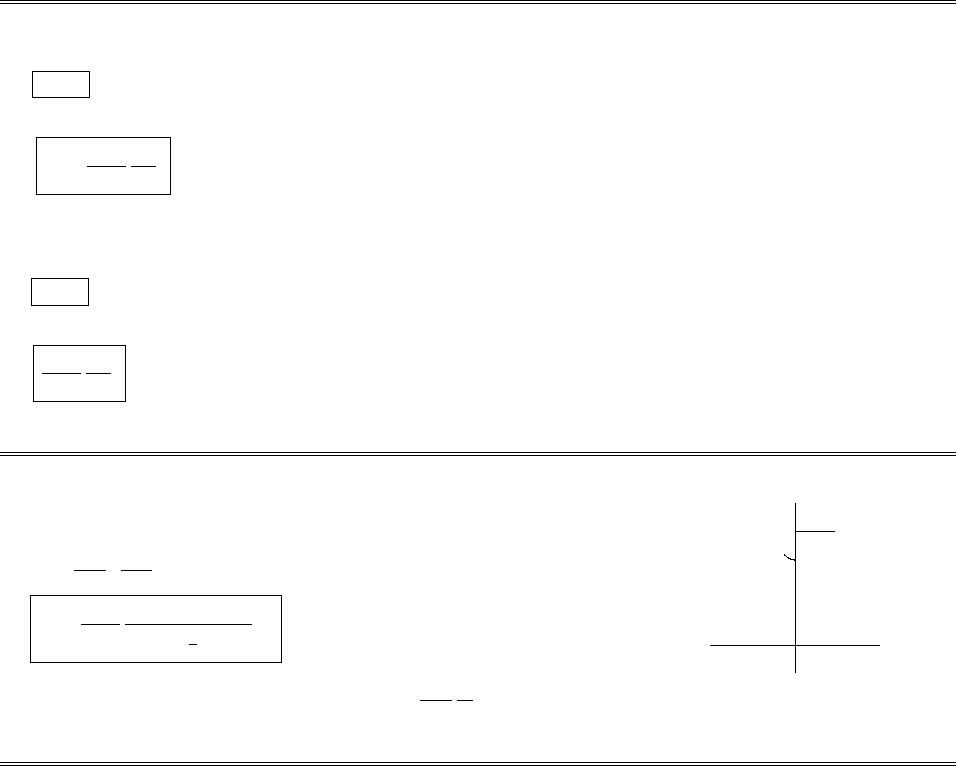
(a) From the diagram, |B+C|cos θ3=|B|cos θ1+|C|cos θ2.
|A||B+C|cos θ3=|A||B|cos θ1+|A||C|cos θ2.
So: A·(B+C) = A·B+A·C. (Dot product is distributive)
Similarly: |B+C|sin θ3=|B|sin θ1+|C|sin θ2. Mulitply by |A|ˆn.
|A||B+C|sin θ3ˆn =|A||B|sin θ1ˆn +|A||C|sin θ2ˆn.
If ˆn is the unit vector pointing out of the page, it follows that
A×(B+C) = (A×B) + (A×C). (Cross product is distributive)
(b) For the general case, see G. E. Hay’s Vector and Tensor Analysis, Chapter 1, Section 7 (dot product) and
Section 8 (cross product)
Problem 1.2
✲A=B
✻
C
❂
B×C❄A×(B×C)
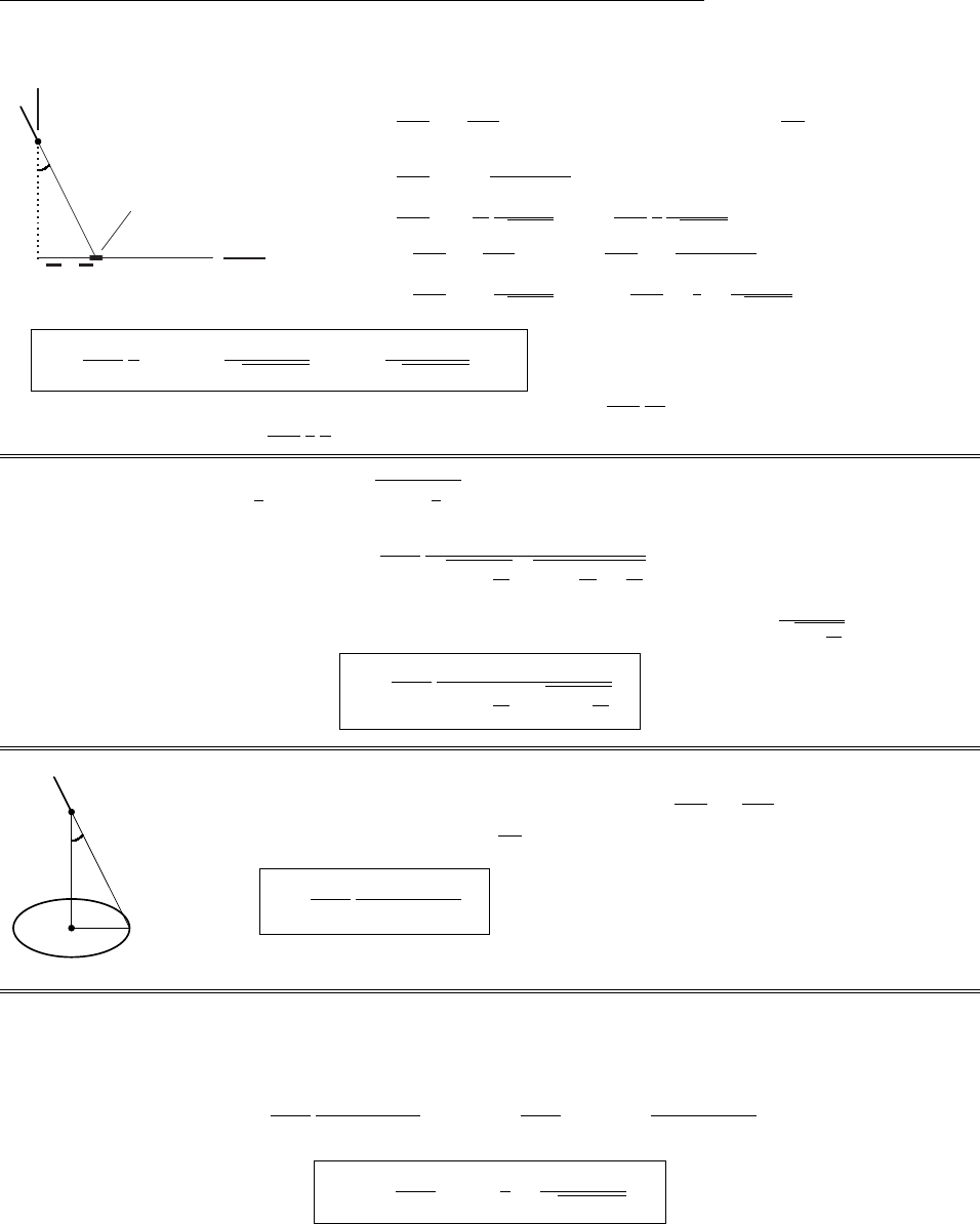
The triple cross-product is not in general associative. For example,
suppose A=Band Cis perpendicular to A, as in the diagram.
Then (B×C) points out-of-the-page, and A×(B×C) points down,
and has magnitude ABC. But (A×B) = 0, so (A×B)×C= 0 ̸=
A×(B×C).
Problem 1.3
✲y
✻
z
✰
x
✣B
❲
A
θ
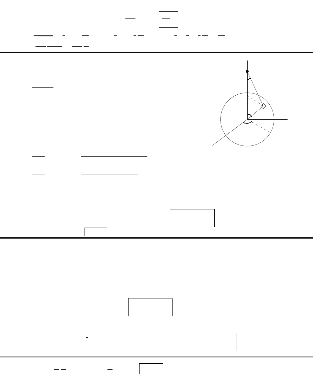
A= +1 ˆx + 1 ˆy −1ˆz;A=√3; B= 1 ˆx + 1 ˆy + 1 ˆz;
A·B= +1 + 1 −1 = 1 = AB cos θ=√3√3 cos θ⇒cos θ.
θ= cos−1%1
3&≈70.5288◦
Problem 1.4
The cross-product of any two vectors in the plane will give a vector perpendicular to the plane. For example,
we might pick the base (A) and the left side (B):
c
⃝2005 Pearson Education, Inc., Upper Saddle River, NJ. All rights reserved. This material is
protected under all copyright laws as they currently exist. No portion of this material may be
reproduced, in any form or by any means, without permission in writing from the publisher.
(a) From the diagram, |B+C|cos ✓3=|B|cos ✓1+|C|cos ✓2. Multiply by |A|.
|A||B+C|cos ✓3=|A||B|cos ✓1+|A||C|cos ✓2.
So: A·(B+C)=A·B+A·C. (Dot product is distributive)
Similarly: |B+C|sin ✓3=|B|sin ✓1+|C|sin ✓2. Mulitply by |A|ˆn .
|A||B+C|sin ✓3ˆn =|A||B|sin ✓1ˆn +|A||C|sin ✓2ˆn .
If ˆn is the unit vector pointing out of the page, it follows that
A⇥(B+C)=(A⇥B)+(A⇥C). (Cross product is distributive)
(b) For the general case, see G. E. Hay’s Vector and Tensor Analysis, Chapter 1, Section 7 (dot product) and
Section 8 (cross product)
Problem 1.2
CHAPTER 1. VECTOR ANALYSIS 3
Chapter 1
Vector Analysis
Problem 1.1
✲
✒
✯
✣
A
B
C
B+C
! "# $
|B|cos θ1! "# $
|C|cos θ2
}
|B|sin θ1
}
|C|sin θ2
θ1
θ2
θ3
(a) From the diagram, |B+C|cos θ3=|B|cos θ1+|C|cos θ2. Multiply by |A|.
|A||B+C|cos θ3=|A||B|cos θ1+|A||C|cos θ2.
So: A·(B+C) = A·B+A·C. (Dot product is distributive)
Similarly: |B+C|sin θ3=|B|sin θ1+|C|sin θ2. Mulitply by |A|ˆn.
|A||B+C|sin θ3ˆn =|A||B|sin θ1ˆn +|A||C|sin θ2ˆn.
If ˆn is the unit vector pointing out of the page, it follows that
A×(B+C) = (A×B) + (A×C). (Cross product is distributive)
(b) For the general case, see G. E. Hay’s Vector and Tensor Analysis, Chapter 1, Section 7 (dot product) and
Section 8 (cross product)
Problem 1.2
✲A=B
✻
C
❂
B×C❄A×(B×C)
The triple cross-product is not in general associative. For example,
suppose A=Band Cis perpendicular to A, as in the diagram.
Then (B×C) points out-of-the-page, and A×(B×C) points down,
and has magnitude ABC. But (A×B) = 0, so (A×B)×C= 0 ̸=
A×(B×C).
Problem 1.3
✲y
✻
z
✰
x
✣B
❲
A
θ
A= +1 ˆx + 1 ˆy −1ˆz;A=√3; B= 1 ˆx + 1 ˆy + 1 ˆz;B=√3.
A·B= +1 + 1 −1 = 1 = AB cos θ=√3√3 cos θ⇒cos θ=1
3.
θ= cos−1%1
3&≈70.5288◦
Problem 1.4
The cross-product of any two vectors in the plane will give a vector perpendicular to the plane. For example,
we might pick the base (A) and the left side (B):
A=−1ˆx + 2 ˆy + 0 ˆz;B=−1ˆx + 0 ˆy + 3 ˆz.
c
⃝2005 Pearson Education, Inc., Upper Saddle River, NJ. All rights reserved. This material is
protected under all copyright laws as they currently exist. No portion of this material may be
reproduced, in any form or by any means, without permission in writing from the publisher.
The triple cross-product is not in general associative. For example,
suppose A=Band Cis perpendicular to A, as in the diagram.
Then (B⇥C) points out-of-the-page, and A⇥(B⇥C) points down,
and has magnitude ABC. But (A⇥B)=0, so (A⇥B)⇥C=06=
A⇥(B⇥C).
Problem 1.3
CHAPTER 1. VECTOR ANALYSIS 3
Chapter 1
Vector Analysis
Problem 1.1
✲
✒
✯
✣
A
B
C
B+C
! "# $
|B|cos θ1!"# $
|C|cos θ2
}
|B|sin θ1
}
|C|sin θ2
θ1
θ2
θ3
(a) From the diagram, |B+C|cos θ3=|B|cos θ1+|C|cos θ2.
|A||B+C|cos θ3=|A||B|cos θ1+|A||C|cos θ2.
So: A·(B+C) = A·B+A·C. (Dot product is distributive)
Similarly: |B+C|sin θ3=|B|sin θ1+|C|sin θ2. Mulitply by |A|ˆn.
|A||B+C|sin θ3ˆn =|A||B|sin θ1ˆn +|A||C|sin θ2ˆn.
If ˆn is the unit vector pointing out of the page, it follows that
A×(B+C) = (A×B) + (A×C). (Cross product is distributive)
(b) For the general case, see G. E. Hay’s Vector and Tensor Analysis, Chapter 1, Section 7 (dot product) and
Section 8 (cross product)
Problem 1.2
✲A=B
✻
C
❂
B×C❄A×(B×C)
The triple cross-product is not in general associative. For example,
suppose A=Band Cis perpendicular to A, as in the diagram.
Then (B×C) points out-of-the-page, and A×(B×C) points down,
and has magnitude ABC. But (A×B) = 0, so (A×B)×C= 0 ̸=
A×(B×C).
Problem 1.3
✲y
✻
z
✰
x
✣B
❲
A
θ
A= +1 ˆx + 1 ˆy −1ˆz;A=√3; B= 1 ˆx + 1 ˆy + 1 ˆz;
A·B= +1 + 1 −1 = 1 = AB cos θ=√3√3 cos θ⇒cos θ.
θ= cos−1%1
3&≈70.5288◦
Problem 1.4
The cross-product of any two vectors in the plane will give a vector perpendicular to the plane. For example,
we might pick the base (A) and the left side (B):
c
⃝2005 Pearson Education, Inc., Upper Saddle River, NJ. All rights reserved. This material is
protected under all copyright laws as they currently exist. No portion of this material may be
reproduced, in any form or by any means, without permission in writing from the publisher.
A=+1ˆx +1ˆy 1ˆz ;A=p3; B=1ˆx +1ˆy +1ˆz ;B=p3.
A·B= +1 + 1 1=1=AB cos ✓=p3p3 cos ✓)cos ✓=1
3.
✓= cos11
3⇡70.5288
Problem 1.4
The cross-product of any two vectors in the plane will give a vector perpendicular to the plane. For example,
we might pick the base (A) and the left side (B):
A=1ˆx +2ˆy +0ˆz ;B=1ˆx +0ˆy +3ˆz .
c
2012 Pearson Education, Inc., Upper Saddle River, NJ. All rights reserved. This material is
protected under all copyright laws as they currently exist. No portion of this material may be
reproduced, in any form or by any means, without permission in writing from the publisher.

CHAPTER 1. VECTOR ANALYSIS 5
A⇥B=
ˆx ˆy ˆz
120
103
=6ˆx +3ˆy +2ˆz .
This has the right direction, but the wrong magnitude. To make a unit vector out of it, simply divide by its
length:
|A⇥B|=p36 + 9 + 4 = 7. ˆn =A⇥B
|A⇥B|=6
7ˆx +3
7ˆy +2
7ˆz .
Problem 1.5
A⇥(B⇥C)=
ˆx ˆy ˆz
AxAyAz
(ByCzBzCy)(BzCxBxCz)(BxCyByCx)
=ˆx [Ay(BxCyByCx)Az(BzCxBxCz)] + ˆy () + ˆz ()
(I’ll just check the x-component; the others go the same way)
=ˆx (AyBxCyAyByCxAzBzCx+AzBxCz)+ˆy () + ˆz ().
B(A·C)C(A·B)=[Bx(AxCx+AyCy+AzCz)Cx(AxBx+AyBy+AzBz)] ˆx + () ˆy + () ˆz
=ˆx (AyBxCy+AzBxCzAyByCxAzBzCx)+ˆy () + ˆz (). They agree.
Problem 1.6
A⇥(B⇥C)+B⇥(C⇥A)+C⇥(A⇥B)=B(A·C)C(A·B)+C(A·B)A(C·B)+A(B·C)B(C·A)=0.
So: A⇥(B⇥C)(A⇥B)⇥C=B⇥(C⇥A)=A(B·C)C(A·B).
If this is zero, then either Ais parallel to C(including the case in which they point in opposite directions, or
one is zero), or else B·C=B·A= 0, in which case Bis perpendicular to Aand C(including the case B=0.)
Conclusion: A⇥(B⇥C)=(A⇥B)⇥C() either Ais parallel to C, or Bis perpendicular to Aand C.
Problem 1.7
r
= (4 ˆx +6ˆy +8ˆz )(2 ˆx +8ˆy +7ˆz )= 2ˆx 2ˆy +ˆz
r
=p4+4+1= 3
ˆ
r
=
r
r
=2
3ˆx 2
3ˆy +1
3ˆz
Problem 1.8
(a) ¯
Ay¯
By+¯
Az¯
Bz= (cos Ay+ sin Az)(cos By+ sin Bz)+(sin Ay+ cos Az)(sin By+ cos Bz)
= cos2AyBy+sincos (AyBz+AzBy) + sin2AzBz+sin
2AyBysin cos (AyBz+AzBy)+
cos2AzBz
= (cos2+ sin2)AyBy+ (sin2+ cos2)AzBz=AyBy+AzBz.X
(b) (Ax)2+(Ay)2+(Az)2=⌃3
i=1AiAi=⌃3
i=1 ⌃3
j=1Rij Aj⌃3
k=1RikAk=⌃j,k (⌃iRij Rik)AjAk.
This equals A2
x+A2
y+A2
zprovided ⌃3
i=1Rij Rik =1if j =k
0if j 6=k
Moreover, if Ris to preserve lengths for all vectors A, then this condition is not only sufficient but also
necessary. For suppose A= (1,0,0). Then ⌃j,k (⌃iRij Rik )AjAk=⌃iRi1Ri1, and this must equal 1 (since we
want A2
x+A2
y+A2
z= 1). Likewise, ⌃3
i=1Ri2Ri2=⌃3
i=1Ri3Ri3= 1. To check the case j6=k, choose A=(1,1,0).
Then we want 2 = ⌃j,k (⌃iRij Rik)AjAk=⌃iRi1Ri1+⌃iRi2Ri2+⌃iRi1Ri2+⌃iRi2Ri1. But we already
know that the first two sums are both 1; the third and fourth are equal, so ⌃iRi1Ri2=⌃iRi2Ri1= 0, and so
on for other unequal combinations of j,k.XIn matrix notation: ˜
RR = 1, where ˜
Ris the transpose of R.
c
2012 Pearson Education, Inc., Upper Saddle River, NJ. All rights reserved. This material is
protected under all copyright laws as they currently exist. No portion of this material may be
reproduced, in any form or by any means, without permission in writing from the publisher.

6CHAPTER 1. VECTOR ANALYSIS
Problem 1.9
CHAPTER 1. VECTOR ANALYSIS 5
✲x
✻
y
✠
z
❃
✿
Looking down the axis:
✻
y
&
x
✰
z
✻
z′
&y′
✰
x′
❄
■
✒
c
⃝2005 Pearson Education, Inc., Upper Saddle River, NJ. All rights reserved. This material is
protected under all copyright laws as they currently exist. No portion of this material may be
reproduced, in any form or by any means, without permission in writing from the publisher.
Looking down the axis:
CHAPTER 1. VECTOR ANALYSIS 5
✲x
✻
y
✠
z
❃
✿
Looking down the axis:
✻
y
&
x
✰
z
✻
z′
&y′
✰
x′
❄
■
✒
c
⃝2005 Pearson Education, Inc., Upper Saddle River, NJ. All rights reserved. This material is
protected under all copyright laws as they currently exist. No portion of this material may be
reproduced, in any form or by any means, without permission in writing from the publisher.
A 120rotation carries the zaxis into the y(= z) axis, yinto x(= y), and xinto z(= x). So Ax=Az,
Ay=Ax,Az=Ay.
R=
001
100
010
Problem 1.10
(a) No change. (Ax=Ax,Ay=Ay,Az=Az)
(b) A! A, in the sense (Ax=Ax,Ay=Ay,Az=Az)
(c) (A⇥B)! (A)⇥(B)=(A⇥B). That is, if C=A⇥B,C! C.No minus sign, in contrast to
behavior of an “ordinary” vector, as given by (b). If Aand Bare pseudovectors, then (A⇥B)! (A)⇥(B)=
(A⇥B). So the cross-product of two pseudovectors is again a pseudovector. In the cross-product of a vector
and a pseudovector, one changes sign, the other doesn’t, and therefore the cross-product is itself a vector.
Angular momentum (L=r⇥p) and torque (N=r⇥F) are pseudovectors.
(d) A·(B⇥C)! (A)·((B)⇥(C)) = A·(B⇥C). So, if a=A·(B⇥C), then a! a; a pseudoscalar
changes sign under inversion of coordinates.
Problem 1.11
(a)rf=2xˆx +3y2ˆy +4z3ˆz
(b)rf=2xy3z4ˆx +3x2y2z4ˆy +4x2y3z3ˆz
(c)rf=exsin yln zˆx +excos yln zˆy +exsin y(1/z)ˆz
Problem 1.12
(a) rh= 10[(2y6x18) ˆx + (2x8y+ 28) ˆy ]. rh= 0 at summit, so
2y6x18 = 0
2x8y+ 28 = 0 =)6x24y+ 84 = 0 2y18 24y+ 84 = 0.
22y=66=)y=3=)2x24 + 28 = 0 =)x=2.
Top is 3 miles north, 2 miles west, of South Hadley.
(b) Putting in x=2, y= 3:
h= 10(12 12 36 + 36 + 84 + 12) = 720 ft.
(c) Putting in x=1,y=1: rh= 10[(2 618) ˆx + (2 8 + 28) ˆy ] = 10(22 ˆx + 22 ˆy ) = 220(ˆx +ˆy ).
|rh|= 220p2⇡311 ft/mile; direction: northwest.
c
2012 Pearson Education, Inc., Upper Saddle River, NJ. All rights reserved. This material is
protected under all copyright laws as they currently exist. No portion of this material may be
reproduced, in any form or by any means, without permission in writing from the publisher.

CHAPTER 1. VECTOR ANALYSIS 7
Problem 1.13
r
=(xx0)ˆx +(yy0)ˆy +(zz0)ˆz ;
r
=(xx0)2+(yy0)2+(zz0)2.
(a) r(
r
2)= @
@x[(xx0)2+(yy0)2+(zz0)2]ˆx +@
@y() ˆy +@
@z() ˆz = 2(xx0)ˆx +2(yy0)ˆy +2(zz0)ˆz =2
r
.
(b) r(1
r
)= @
@x[(xx0)2+(yy0)2+(zz0)2]1
2ˆx +@
@y()1
2ˆy +@
@z()1
2ˆz
=1
2()3
22(xx0)ˆx 1
2()3
22(yy0)ˆy 1
2()3
22(zz0)ˆz
=()3
2[(xx0)ˆx +(yy0)ˆy +(zz0)ˆz ]=(1/
r
3)
r
=(1/
r
2)ˆ
r
.
(c) @
@x(
r
n)=n
r
n1@
r
@x=n
r
n1(1
2
1
r
2
r
x)=n
r
n1ˆ
r
x,so r(
r
n)=n
r
n1ˆ
r
Problem 1.14
y=+ycos +zsin ; multiply by sin :ysin =+ysin cos +zsin2.
z=ysin +zcos ; multiply by cos :zcos =ysin cos +zcos2.
Add: ysin +zcos =z(sin2+ cos2)=z. Likewise, ycos zsin =y.
So @y
@y= cos ;@y
@z=sin ;@z
@y= sin ;@z
@z= cos . Therefore
(rf)y=@f
@y=@f
@y
@y
@y+@f
@z
@z
@y= + cos (rf)y+ sin (rf)z
(rf)z=@f
@z=@f
@y
@y
@z+@f
@z
@z
@z=sin (rf)y+ cos (rf)zSo rftransforms as a vector. qed
Problem 1.15
(a)r·va=@
@x(x2)+ @
@y(3xz2)+ @
@z(2xz)=2x+02x=0.
(b)r·vb=@
@x(xy)+ @
@y(2yz)+ @
@z(3xz)=y+2z+3x.
(c)r·vc=@
@x(y2)+ @
@y(2xy +z2)+ @
@z(2yz) = 0 + (2x) + (2y) = 2(x+y)
Problem 1.16
r·v=@
@x(x
r3)+ @
@y(y
r3)+ @
@z(z
r3)= @
@xx(x2+y2+z2)3
2
+@
@yy(x2+y2+z2)3
2+@
@zz(x2+y2+z2)3
2
= ()3
2+x(3/2)()5
22x+ ()3
2+y(3/2)()5
22y+ ()3
2
+z(3/2)()5
22z=3r33r5(x2+y2+z2)=3r33r3=0.
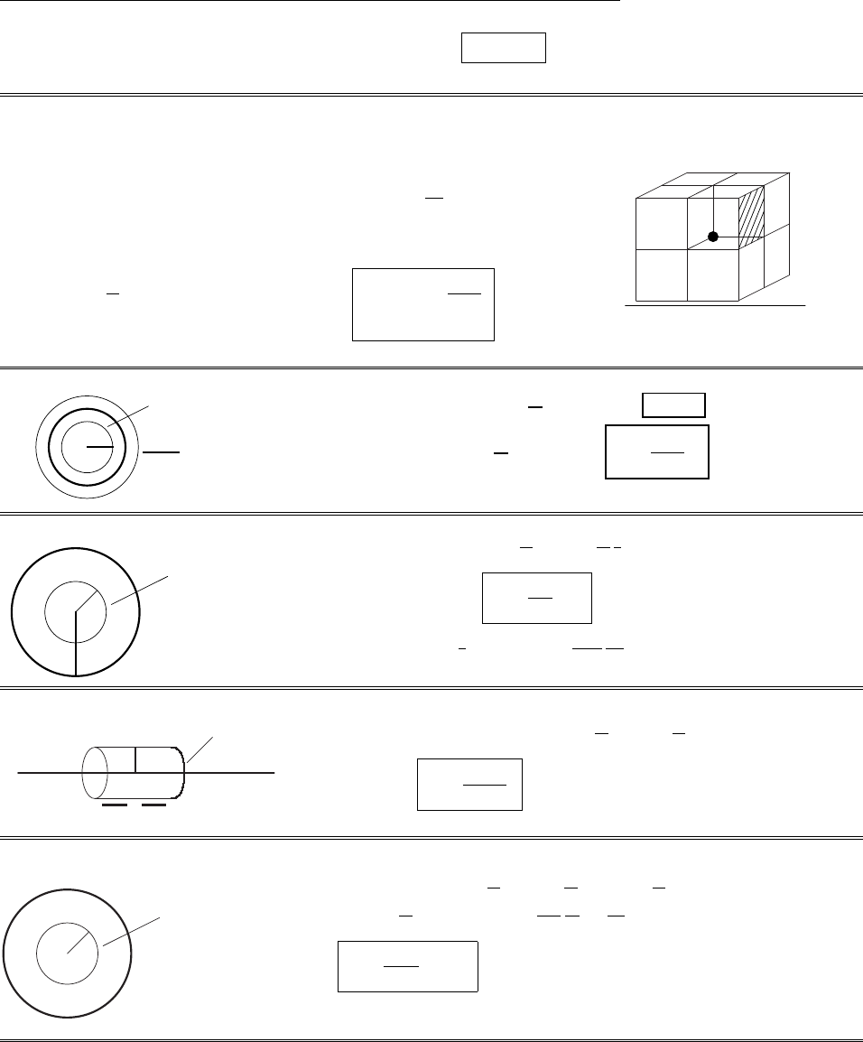
This conclusion is surprising, because, from the diagram, this vector field is obviously diverging away from the
origin. How, then, can r·v= 0? The answer is that r·v= 0 everywhere except at the origin, but at the
origin our calculation is no good, since r= 0, and the expression for vblows up. In fact, r·vis infinite at
that one point, and zero elsewhere, as we shall see in Sect. 1.5.
Problem 1.17
vy= cos vy+ sin vz;vz=sin vy+ cos vz.
@vy
@y=@vy
@ycos +@vz
@ysin =@vy
@y
@y
@y+@vy
@z
@z
@ycos +@vz
@y
@y
@y+@vz
@z
@z
@ysin .Use result in Prob. 1.14:
=@vy
@ycos +@vy
@zsin cos +@vz
@ycos +@vz
@zsin sin .
@vz
@z=@vy
@zsin +@vz
@zcos =@vy
@y
@y
@z+@vy
@z
@z
@zsin +@vz
@y
@y
@z+@vz
@z
@z
@zcos
=@vy
@ysin +@vy
@zcos sin +@vz
@ysin +@vz
@zcos cos . So
c
2012 Pearson Education, Inc., Upper Saddle River, NJ. All rights reserved. This material is
protected under all copyright laws as they currently exist. No portion of this material may be
reproduced, in any form or by any means, without permission in writing from the publisher.

8CHAPTER 1. VECTOR ANALYSIS
@vy
@y+@vz
@z=@vy
@ycos2+@vy
@zsin cos +@vz
@ysin cos +@vz
@zsin2+@vy
@ysin2@vy
@zsin cos
@vz
@ysin cos +@vz
@zcos2
=@vy
@ycos2+ sin2+@vz
@zsin2+ cos2=@vy
@y+@vz
@z.X
Problem 1.18
(a) r⇥va=
ˆx ˆy ˆz
@
@x
@
@y
@
@z
x23xz22xz =ˆx (0 6xz)+ˆy (0 + 2z)+ˆz (3z20) = 6xz ˆx +2zˆy +3z2ˆz .
(b) r⇥vb=
ˆx ˆy ˆz
@
@x
@
@y
@
@z
xy 2yz 3xz =ˆx (0 2y)+ˆy (0 3z)+ˆz (0 x)= 2yˆx 3zˆy xˆz .
(c) r⇥vc=
ˆx ˆy ˆz
@
@x
@
@y
@
@z
y2(2xy +z2)2yz =ˆx (2z2z)+ˆy (0 0) + ˆz (2y2y)= 0.
Problem 1.19
Ax
y
z
v
v
v
v
B
As we go from point Ato point B(9 o’clock to 10 o’clock), x
increases, yincreases, vxincreases, and vydecreases, so @vx/@y>
0, while @vy/@y<0. On the circle, vz= 0, and there is no
dependence on z, so Eq. 1.41 says
r⇥v=ˆz @vy
@x@vx
@y
points in the negative zdirection (into the page), as the right
hand rule would suggest. (Pick any other nearby points on the
circle and you will come to the same conclusion.) [I’m sorry, but I
cannot remember who suggested this cute illustration.]
Problem 1.20
v=yˆx +xˆy ; or v=yz ˆx +xz ˆy +xy ˆz ; or v= (3x2zz3)ˆx +3ˆy +(x33xz2)ˆz ;
or v= (sin x)(cosh y)ˆx (cos x)(sinh y)ˆy ;etc.
Problem 1.21
(i) r(fg)= @(fg)
@xˆx +@(fg)
@yˆy +@(fg)
@zˆz =f@g
@x+g@f
@xˆx +f@g
@y+g@f
@yˆy +f@g
@z+g@f
@zˆz
=f@g
@xˆx +@g
@yˆy +@g
@zˆz +g@f
@xˆx +@f
@yˆy +@f
@zˆz =f(rg)+g(rf). qed
(iv) r·(A⇥B)= @
@x(AyBzAzBy)+ @
@y(AzBxAxBz)+ @
@z(AxByAyBx)
=Ay@Bz
@x+Bz@Ay
@xAz@By
@xBy@Az
@x+Az@Bx
@y+Bx@Az
@yAx@Bz
@yBz@Ax
@y
+Ax@By
@z+By@Ax
@zAy@Bx
@zBx@Ay
@z
=Bx@Az
@y@Ay
@z+By@Ax
@z@Az
@x+Bz@Ay
@x@Ax
@yAx@Bz
@y@By
@z
Ay@Bx
@z@Bz
@xAz@By
@x@Bx
@y=B·(r⇥A)A·(r⇥B). qed
(v) r⇥(fA)=@(fAz)
@y@(fAy)
@zˆx +@(fAx)
@z@(fAz)
@xˆy +@(fAy)
@x@(fAx)
@yˆz
c
2012 Pearson Education, Inc., Upper Saddle River, NJ. All rights reserved. This material is
protected under all copyright laws as they currently exist. No portion of this material may be
reproduced, in any form or by any means, without permission in writing from the publisher.

CHAPTER 1. VECTOR ANALYSIS 9
=f@Az
@y+Az@f
@yf@Ay
@zAy@f
@zˆx +f@Ax
@z+Ax@f
@zf@Az
@xAz@f
@xˆy
+f@Ay
@x+Ay@f
@xf@Ax
@yAx@f
@yˆz
=f@Az
@y@Ay
@zˆx +@Ax
@z@Az
@xˆy +@Ay
@x@Ax
@yˆz
Ay@f
@zAz@f
@yˆx +Az@f
@xAx@f
@zˆy +Ax@f
@yAy@f
@xˆz
=f(r⇥A)A⇥(rf). qed
Problem 1.22
(a) (A·r)B=Ax@Bx
@x+Ay@Bx
@y+Az@Bx
@zˆx +Ax@By
@x+Ay@By
@y+Az@By
@zˆy
+Ax@Bz
@x+Ay@Bz
@y+Az@Bz
@zˆz .
(b) ˆr =r
r=xˆx +yˆy +zˆz
px2+y2+z2. Let’s just do the xcomponent.
[(ˆr ·r)ˆr ]x=1
px@
@x+y@
@y+z@
@zx
px2+y2+z2
=1
rx1
p+x(1
2)1
(p)32x+yx 1
2
1
(p)32y+zx1
2
1
(p)32z
=1
rx
r1
r3x3+xy2+xz2=1
rx
rx
r3x2+y2+z2=1
rx
rx
r= 0.
Same goes for the other components. Hence: (ˆr ·r)ˆr =0.
(c) (va·r)vb=x2@
@x+3xz2@
@y2xz @
@z(xy ˆx +2yz ˆy +3xz ˆz )
=x2(yˆx +0ˆy +3zˆz )+3xz2(xˆx +2zˆy +0ˆz )2xz (0 ˆx +2yˆy +3xˆz )
=x2y+3x2z2ˆx +6xz34xyzˆy +3x2z6x2zˆz
=x2y+3z2ˆx +2xz 3z22yˆy 3x2zˆz
Problem 1.23
(ii) [r(A·B)]x=@
@x(AxBx+AyBy+AzBz)=@Ax
@xBx+Ax@Bx
@x+@Ay
@xBy+Ay@By
@x+@Az
@xBz+Az@Bz
@x
[A⇥(r⇥B)]x=Ay(r⇥B)zAz(r⇥B)y=Ay@By
@x@Bx
@yAz@Bx
@z@Bz
@x
[B⇥(r⇥A)]x=By@Ay
@x@Ax
@yBz@Ax
@z@Az
@x
[(A·r)B]x=Ax@
@x+Ay@
@y+Az@
@zBx=Ax@Bx
@x+Ay@Bx
@y+Az@Bx
@z
[(B·r)A]x=Bx@Ax
@x+By@Ax
@y+Bz@Ax
@z
So [A⇥(r⇥B)+B⇥(r⇥A)+(A·r)B+(B·r)A]x
=Ay@By
@xAy@Bx
@yAz@Bx
@z+Az@Bz
@x+By@Ay
@xBy@Ax
@yBz@Ax
@z+Bz@Az
@x
+Ax@Bx
@x+Ay@Bx
@y+Az@Bx
@z+Bx@Ax
@x+By@Ax
@y+Bz@Ax
@z
=Bx@Ax
@x+Ax@Bx
@x+By@Ay
@x@Ax
@y
/+@Ax
@y
/+Ay@By
@x@Bx
@y
/+@Bx
@y
/
+Bz@Ax
@z
/+@Az
@x+@Ax
@z
/+Az@Bx
@z
/+@Bz
@x+@Bx
@z
/
=[r(A·B)]x(same for yand z)
(vi) [r⇥(A⇥B)]x=@
@y(A⇥B)z@
@z(A⇥B)y=@
@y(AxByAyBx)@
@z(AzBxAxBz)
=@Ax
@yBy+Ax@By
@y@Ay
@yBxAy@Bx
@y@Az
@zBxAz@Bx
@z+@Ax
@zBz+Ax@Bz
@z
[(B·r)A(A·r)B+A(r·B)B(r·A)]x
=Bx@Ax
@x+By@Ax
@y+Bz@Ax
@zAx@Bx
@xAy@Bx
@yAz@Bx
@z+Ax@Bx
@x+@By
@y+@Bz
@zBx@Ax
@x+@Ay
@y+@Az
@z
c
2012 Pearson Education, Inc., Upper Saddle River, NJ. All rights reserved. This material is
protected under all copyright laws as they currently exist. No portion of this material may be
reproduced, in any form or by any means, without permission in writing from the publisher.
10 CHAPTER 1. VECTOR ANALYSIS
=By@Ax
@y+Ax@Bx
@x
/+@Bx
@x
/+@By
@y+@Bz
@z+Bx@Ax
@x
/@Ax
@x
/@Ay
@y@Az
@z
+Ay@Bx
@y+Az@Bx
@z+Bz@Ax
@z
=[r⇥(A⇥B)]x(same for yand z)
Problem 1.24
r(f/g)= @
@x(f/g)ˆx +@
@y(f/g)ˆy +@
@z(f/g)ˆz
=g@f
@xf@g
@x
g2ˆx +g@f
@yf@g
@y
g2ˆy +g@f
@zf@g
@z
g2ˆz
=1
g2g@f
@xˆx +@f
@yˆy +@f
@zˆz f@g
@xˆx +@g
@yˆy +@g
@zˆz =grffrg
g2.qed
r·(A/g)= @
@x(Ax/g)+ @
@y(Ay/g)+ @
@z(Az/g)
=g@Ax
@xAx@g
@x
g2+g@Ay
@yAy@g
@y
g2+g@Az
@zAz@g
@x
g2
=1
g2g@Ax
@x+@Ay
@y+@Az
@zAx@g
@x+Ay@g
@y+Az@g
@z=gr·AA·rg
g2.qed
[r⇥(A/g)]x=@
@y(Az/g)@
@z(Ay/g)
=g@Az
@yAz@g
@y
g2g@Ay
@zAy@g
@z
g2
=1
g2g@Az
@y@Ay
@zAz@g
@yAy@g
@z
=g(r⇥A)x+(A⇥rg)x
g2(same for yand z).qed
Problem 1.25
(a) A⇥B=
ˆx ˆy ˆz
x2y3z
3y2x0=ˆx (6xz)+ˆy (9zy)+ˆz (2x26y2)
r·(A⇥B)= @
@x(6xz)+ @
@y(9zy)+ @
@z(2x26y2)=6z+9z+ 0 = 15z
r⇥A=ˆx @
@y(3z)@
@z(2y)+ˆy @
@z(x)@
@x(3z)+ˆz @
@x(2y)@
@y(x)= 0; B·(r⇥A)=0
r⇥B=ˆx @
@y(0) @
@z(2x)+ˆy @
@z(3y)@
@x(0)+ˆz @
@x(2x)@
@y(3y)=5ˆz ;A·(r⇥B)=15z
r·(A⇥B)?
=B·(r⇥A)A·(r⇥B)=0(15z) = 15z. X
(b) A·B=3xy 4xy =xy ;r(A·B)=r(xy)=ˆx @
@x(xy)+ˆy @
@y(xy)=yˆx xˆy
A⇥(r⇥B)=
ˆx ˆy ˆz
x2y3z
005=ˆx (10y)+ˆy (5x); B⇥(r⇥A)=0
(A·r)B=x@
@x+2y@
@y+3z@
@z(3yˆx 2xˆy )=ˆx (6y)+ˆy (2x)
(B·r)A=3y@
@x2x@
@y(xˆx +2yˆy +3zˆz )=ˆx (3y)+ˆy (4x)
A⇥(r⇥B)+B⇥(r⇥A)+(A·r)B+(B·r)A
=10yˆx +5xˆy +6yˆx 2xˆy +3yˆx 4xˆy =yˆx xˆy =r·(A·B).X
(c) r⇥(A⇥B)=ˆx @
@y(2x26y2)@
@z(9zy)+ˆy @
@z(6xz)@
@x(2x26y2)+ˆz @
@x(9zy)@
@y(6xz)
=ˆx (12y9y)+ˆy (6x+4x)+ˆz (0) = 21yˆx + 10xˆy
r·A=@
@x(x)+ @
@y(2y)+ @
@z(3z) = 1 + 2 + 3 = 6; r·B=@
@x(3y)+ @
@y(2x)=0
c
2012 Pearson Education, Inc., Upper Saddle River, NJ. All rights reserved. This material is
protected under all copyright laws as they currently exist. No portion of this material may be
reproduced, in any form or by any means, without permission in writing from the publisher.

CHAPTER 1. VECTOR ANALYSIS 11
(B·r)A(A·r)B+A(r·B)B(r·A)=3yˆx 4xˆy 6yˆx +2xˆy 18yˆx + 12xˆy =21yˆx + 10xˆy
=r⇥(A⇥B).X
Problem 1.26
(a) @2Ta
@x2= 2; @2Ta
@y2=@2Ta
@z2=0 ) r2Ta=2.
(b) @2Tb
@x2=@2Tb
@y2=@2Tb
@z2=Tb) r2Tb=3Tb=3 sin xsin ysin z.
(c) @2Tc
@x2= 25Tc;@2Tc
@y2=16Tc;@2Tc
@z2=9Tc) r2Tc=0.
(d) @2vx
@x2=2;@2vx
@y2=@2vx
@z2=0 )r
2vx=2
@2vy
@x2=@2vy
@y2=0;@2vy
@z2=6x)r
2vy=6x
@2vz
@x2=@2vz
@y2=@2vz
@z2=0 )r
2vz=0
r2v=2ˆx +6xˆy .
Problem 1.27
r·(r⇥v)= @
@x@vz
@y@vy
@z+@
@y@vx
@z@vz
@x+@
@z@vy
@x@vx
@y
=@2vz
@x@y@2vz
@y@x+@2vx
@y@z@2vx
@z@y+@2vy
@z@x@2vy
@x@z= 0, by equality of cross-derivatives.
From Prob. 1.18: r⇥va=6xz ˆx +2zˆy +3z2ˆz )r·(r⇥va)= @
@x(6xz)+ @
@y(2z)+ @
@z(3z2)=6z+6z=0.
Problem 1.28
r⇥(rt)=
ˆx ˆy ˆz
@
@x
@
@y
@
@z
@t
@x
@t
@y
@t
@z
=ˆx @2t
@y@z@2t
@z@y+ˆy @2t
@z@x@2t
@x@z+ˆz @2t
@x@y@2t
@y@x
= 0, by equality of cross-derivatives.
In Prob. 1.11(b), rf=2xy3z4ˆx +3x2y2z4ˆy +4x2y3z3ˆz ,so
r⇥(rf)=
ˆx ˆy ˆz
@
@x
@
@y
@
@z
2xy3z43x2y2z44x2y3z3
=ˆx (3 ·4x2y2z34·3x2y2z3)+ˆy (4 ·2xy3z32·4xy3z3)+ˆz (2 ·3xy2z43·2xy2z4)=0.X
Problem 1.29
(a) (0,0,0) ! (1,0,0).x:0!1,y =z= 0; dl=dx ˆx ;v·dl=x2dx;v·dl=1
0x2dx =(x3/3)|1
0=1/3.
(1,0,0) ! (1,1,0).x=1,y :0!1,z = 0; dl=dy ˆy ;v·dl=2yz dy = 0; v·dl=0.
(1,1,0) ! (1,1,1).x=y=1,z :0!1; dl=dz ˆz ;v·dl=y2dz =dz;v·dl=1
0dz =z|1
0=1.
Total: v·dl=(1/3) + 0 + 1 = 4/3.
(b) (0,0,0) ! (0,0,1).x=y=0,z :0!1; dl=dz ˆz ;v·dl=y2dz = 0; v·dl=0.
(0,0,1) ! (0,1,1).x=0,y :0!1,z = 1; dl=dy ˆy ;v·dl=2yz dy =2y dy;v·dl=1
02y dy =y2|1
0=1.
(0,1,1) ! (1,1,1).x:0!1,y =z= 1; dl=dx ˆx ;v·dl=x2dx;v·dl=1
0x2dx =(x3/3)|1
0=1/3.
Total: v·dl=0+1+(1/3) = 4/3.
(c) x=y=z:0!1; dx =dy =dz;v·dl=x2dx +2yz dy +y2dz =x2dx +2x2dx +x2dx =4x2dx;
v·dl=1
04x2dx = (4x3/3)|1
0= 4/3.
(d) v·dl=(4/3) (4/3) = 0.
c
2012 Pearson Education, Inc., Upper Saddle River, NJ. All rights reserved. This material is
protected under all copyright laws as they currently exist. No portion of this material may be
reproduced, in any form or by any means, without permission in writing from the publisher.
12 CHAPTER 1. VECTOR ANALYSIS
Problem 1.30
x, y :0!1,z = 0; da=dx dy ˆz ;v·da=y(z23) dx dy =3y dx dy;v·da=32
0dx 2
0y dy =
3(x|2
0)(y2
2|2
0)=3(2)(2) = 12. In Ex. 1.7 we got 20, for the same boundary line (the square in the
xy-plane), so the answer is no: the surface integral does not depend only on the boundary line. The total flux
for the cube is 20 + 12 = 32.
Problem 1.31
Td⌧=z2dx dy dz. You can do the integrals in any order—here it is simplest to save zfor last:
z2dxdydz.
The sloping surface is x+y+z= 1, so the xintegral is (1yz)
0dx =1yz. For a given z,yranges from 0 to
1z, so the yintegral is (1z)
0(1 yz)dy = [(1 z)y(y2/2)]|(1z)
0= (1 z)2[(1 z)2/2] = (1 z)2/2=
(1/2) z+(z2/2).Finally, the zintegral is 1
0z2(1
2z+z2
2)dz =1
0(z2
2z3+z4
2)dz =(
z3
6z4
4+z5
10 )|1
0=
1
61
4+1
10 = 1/60.
Problem 1.32
T(b) = 1 + 4 + 2 = 7; T(a)=0.)T(b)T(a)=7.
rT=(2x+4y)ˆx + (4x+2z3)ˆy + (6yz2)ˆz ;rT·dl=(2x+4y)dx + (4x+2z3)dy + (6yz2)dz
(a) Segment 1: x:0!1,y=z=dy =dz =0.rT·dl=1
0(2x)dx =x21
0=1.
Segment 2: y:0!1,x=1,z=0, dx =dz =0.rT·dl=1
0(4) dy =4y|1
0=4.
Segment 3: z:0!1,x=y=1, dx =dy =0.rT·dl=1
0(6z2)dz =2z31
0=2.
b
arT·dl=7.X
(b) Segment 1: z:0!1,x=y=dx =dy =0.rT·dl=1
0(0) dz =0.
Segment 2: y:0!1,x=0,z=1, dx =dz =0.rT·dl=1
0(2) dy =2y|1
0=2.
Segment 3: x:0!1,y=z=1, dy =dz =0.rT·dl=1
0(2x+ 4) dx
=(x2+4x)1
0=1+4=5.
b
arT·dl=7.X
(c) x:0!1,y=x, z =x2, dy =dx, dz =2xdx.
rT·dl=(2x+4x)dx + (4x+2x6)dx + (6xx4)2xdx= (10x+ 14x6)dx.
b
arT·dl=1
0(10x+ 14x6)dx =(5x2+2x7)1
0=5+2=7.X
Problem 1.33
r·v=y+2z+3x
(r·v)d⌧=(y+2z+3x)dx dy dz =2
0(y+2z+3x)dxdy dz
,!(y+2z)x+3
2x22
0= 2(y+2z)+6
=2
0(2y+4z+ 6)dydz
,!y2+ (4z+ 6)y2
0= 4 + 2(4z+ 6) = 8z+ 16
=2
0(8z+ 16)dz =(4z2+ 16z)2
0= 16 + 32 = 48.
Numbering the surfaces as in Fig. 1.29:
c
2012 Pearson Education, Inc., Upper Saddle River, NJ. All rights reserved. This material is
protected under all copyright laws as they currently exist. No portion of this material may be
reproduced, in any form or by any means, without permission in writing from the publisher.
CHAPTER 1. VECTOR ANALYSIS 13
(i) da=dy dz ˆx ,x =2.v·da=2y dy dz. v·da=2y dy dz =2y22
0=8.
(ii) da=dy dz ˆx ,x =0.v·da=0.v·da=0.
(iii) da=dx dz ˆy ,y =2.v·da=4z dx dz. v·da=4z dx dz = 16.
(iv) da=dx dz ˆy ,y =0.v·da=0.v·da=0.
(v) da=dx dy ˆz ,z =2.v·da=6x dx dy. v·da=24.
(vi) da=dx dy ˆz ,z =0.v·da=0.v·da=0.
)v·da= 8 + 16 + 24 = 48 X
Problem 1.34
r⇥v=ˆx (0 2y)+ˆy (0 3z)+ˆz (0 x)=2yˆx 3zˆy xˆz .
da=dy dz ˆx , if we agree that the path integral shall run counterclockwise. So
(r⇥v)·da=2y dy dz.
(r⇥v)·da=2z
0(2y)dydz
,!y22z
0=(2 z)2
=2
0(4 4z+z2)dz =4z2z2+z3
3
2
0
=88+8
3=8
3-
6
z
y
@@@@@
@
y=2z
Meanwhile, v·dl=(xy)dx + (2yz)dy + (3zx)dz. There are three segments.
-
6
z
y
@@@@@
@
-
(1)
@
@I (2)
?
(3)
(1) x=z=0; dx =dz =0.y:0!2.v·dl=0.
(2) x= 0; z=2y;dx =0, dz =dy, y :2!0.v·dl=2yz dy.
v·dl=0
22y(2 y)dy =2
0(4y2y2)dy =2y22
3y32
0=82
3·8=8
3.
(3) x=y= 0; dx =dy = 0; z:2!0.v·dl=0.v·dl=0.So v·dl=8
3.X
Problem 1.35
By Corollary 1, (r⇥v)·dashould equal 4
3.r⇥v=(4z22x)ˆx +2zˆz .
(i) da=dy dz ˆx ,x= 1; y, z :0!1.(r⇥v)·da=(4z22)dy dz;(r⇥v)·da=1
0(4z22)dz
=(
4
3z32z)1
0=4
32=2
3.
(ii) da=dx dy ˆz ,z= 0; x, y :0!1.(r⇥v)·da=0; (r⇥v)·da=0.
(iii) da=dx dz ˆy ,y= 1; x, z :0!1.(r⇥v)·da=0; (r⇥v)·da=0.
(iv) da=dx dz ˆy ,y= 0; x, z :0!1.(r⇥v)·da=0; (r⇥v)·da=0.
(v) da=dx dy ˆz ,z= 1; x, y :0!1.(r⇥v)·da=2dx dy;(r⇥v)·da=2.
)(r⇥v)·da=2
3+2= 4
3.X
c
2012 Pearson Education, Inc., Upper Saddle River, NJ. All rights reserved. This material is
protected under all copyright laws as they currently exist. No portion of this material may be
reproduced, in any form or by any means, without permission in writing from the publisher.

14 CHAPTER 1. VECTOR ANALYSIS
Problem 1.36
(a) Use the product rule r⇥(fA)=f(r⇥A)A⇥(rf):
S
f(r⇥A)·da=Sr⇥(fA)·da+S
[A⇥(rf)] ·da=P
fA·dl+S
[A⇥(rf)] ·da.qed
(I used Stokes’ theorem in the last step.)
(b) Use the product rule r·(A⇥B)=B·(r⇥A)A·(r⇥B):
V
B·(r⇥A)d⌧=Vr·(A⇥B)d⌧+V
A·(r⇥B)d⌧=S
(A⇥B)·da+V
A·(r⇥B)d⌧.qed
(I used the divergence theorem in the last step.)
Problem 1.37 r=x2+y2+z2;✓= cos1z
px2+y2+z2;= tan1y
x.
Problem 1.38
There are many ways to do this one—probably the most illuminating way is to work it out by trigonometry
from Fig. 1.36. The most systematic approach is to study the expression:
r=xˆx +yˆy +zˆz =rsin ✓cos ˆx +rsin ✓sin ˆy +rcos ✓ˆz .
If I only vary rslightly, then dr=@
@r(r)dr is a short vector pointing in the direction of increase in r. To make
it a unit vector, I must divide by its length. Thus:
ˆr =
@r
@r
@r
@r;ˆ
✓=
@r
@✓
@r
@✓ ;ˆ
=
@r
@
@r
@.
@r
@r= sin ✓cos ˆx + sin ✓sin ˆy + cos ✓ˆz ;@r
@r2= sin2✓cos2+ sin2✓sin2+ cos2✓=1.
@r
@✓ =rcos ✓cos ˆx +rcos ✓sin ˆy rsin ✓ˆz ;@r
@✓ 2=r2cos2✓cos2+r2cos2✓sin2+r2sin2✓=r2.
@r
@ =rsin ✓sin ˆx +rsin ✓cos ˆy ;@r
@2=r2sin2✓sin2+r2sin2✓cos2=r2sin2✓.
)
ˆr = sin ✓cos ˆx + sin ✓sin ˆy + cos ✓ˆz .
ˆ
✓= cos ✓cos ˆx + cos ✓sin ˆy sin ✓ˆz .
ˆ
=sin ˆx + cos ˆy .
Check: ˆr ·ˆr = sin2✓(cos2+ sin2) + cos2✓= sin2✓+ cos2✓=1,X
ˆ
✓·ˆ
=cos ✓sin cos + cos ✓sin cos =0,Xetc.
sin ✓ˆr = sin2✓cos ˆx + sin2✓sin ˆy + sin ✓cos ✓ˆz .
cos ✓ˆ
✓= cos2✓cos ˆx + cos2✓sin ˆy sin ✓cos ✓ˆz .
Add these:
(1) sin ✓ˆr + cos ✓ˆ
✓= + cos ˆx + sin ˆy ;
(2) ˆ
=sin ˆx + cos ˆy .
Multiply (1) by cos , (2) by sin , and subtract:
ˆx = sin ✓cos ˆr + cos ✓cos ˆ
✓sin ˆ
.
c
2012 Pearson Education, Inc., Upper Saddle River, NJ. All rights reserved. This material is
protected under all copyright laws as they currently exist. No portion of this material may be
reproduced, in any form or by any means, without permission in writing from the publisher.
CHAPTER 1. VECTOR ANALYSIS 15
Multiply (1) by sin , (2) by cos , and add:
ˆy = sin ✓sin ˆr + cos ✓sin ˆ
✓+ cos ˆ
.
cos ✓ˆr = sin ✓cos ✓cos ˆx + sin ✓cos ✓sin ˆy + cos2✓ˆz .
sin ✓ˆ
✓= sin ✓cos ✓cos ˆx + sin ✓cos ✓sin ˆy sin2✓ˆz .
Subtract these:
ˆz = cos ✓ˆr sin ✓ˆ
✓.
Problem 1.39
(a) r·v1=1
r2
@
@r(r2r2)= 1
r24r3=4r
(r·v1)d⌧=(4r)(r2sin ✓dr d✓d) = (4) R
0r3dr ⇡
0sin ✓d✓2⇡
0d= (4) R4
4(2)(2⇡)=4⇡R4
v1·da=(r2ˆr )·(r2sin ✓d✓dˆr )=r4⇡
0sin ✓d✓2⇡
0d=4⇡R4X(Note: at surface of sphere r=R.)
(b) r·v2=1
r2
@
@rr21
r2=0 )(r·v2)d⌧=0
v2·da=1
r2ˆr (r2sin ✓d✓dˆr )=sin ✓d✓d= 4⇡.
They don’t agree! The point is that this divergence is zero except at the origin, where it blows up, so our
calculation of (r·v2) is incorrect. The right answer is 4⇡.
Problem 1.40
r·v=1
r2
@
@r(r2rcos ✓)+ 1
rsin ✓
@
@✓ (sin ✓rsin ✓)+ 1
rsin ✓
@
@(rsin ✓cos )
=1
r23r2cos ✓+1
rsin ✓r2 sin ✓cos ✓+1
rsin ✓rsin ✓(sin )
= 3 cos ✓+ 2 cos ✓sin = 5 cos ✓sin
(r·v)d⌧=(5 cos ✓sin )r2sin ✓dr d✓d=R
0r2dr ✓
2
02⇡
0(5 cos ✓sin )dd✓sin ✓
,!2⇡(5 cos ✓)
=R3
3(10⇡)⇡
2
0sin ✓cos ✓d✓
,!sin2✓
2
⇡
2
0=1
2
=5⇡
3R3.
Two surfaces—one the hemisphere: da=R2sin ✓d✓dˆr ;r=R;:0!2⇡,✓:0!⇡
2.
v·da=(rcos ✓)R2sin ✓d✓d=R3⇡
2
0sin ✓cos ✓d✓2⇡
0d=R31
2(2⇡)=⇡R3.
other the flat bottom: da=(dr)(rsin ✓d)(+ˆ
✓)=r dr dˆ
✓(here ✓=⇡
2). r:0!R, :0!2⇡.
v·da=(rsin ✓)(r dr d)=R
0r2dr 2⇡
0d=2⇡R3
3.
Total: v·da=⇡R3+2
3⇡R3=5
3⇡R3.X
Problem 1.41 rt= (cos ✓+ sin ✓cos )ˆr +(sin ✓+ cos ✓cos )ˆ
✓+1
sin ✓
/(sin ✓
/sin )ˆ
r2t=r·(rt)
=1
r2
@
@rr2(cos ✓+ sin ✓cos )+1
rsin ✓
@
@✓ (sin ✓(sin ✓+ cos ✓cos )) + 1
rsin ✓
@
@(sin )
=1
r22r(cos ✓+ sin ✓cos )+ 1
rsin ✓(2 sin ✓cos ✓+ cos2✓cos sin2✓cos )1
rsin ✓cos
=1
rsin ✓[2 sin ✓cos ✓+ 2 sin2✓cos 2 sin ✓cos ✓+ cos2✓cos sin2✓cos cos ]
=1
rsin ✓(sin2✓+ cos2✓) cos cos =0.
c
2012 Pearson Education, Inc., Upper Saddle River, NJ. All rights reserved. This material is
protected under all copyright laws as they currently exist. No portion of this material may be
reproduced, in any form or by any means, without permission in writing from the publisher.

16 CHAPTER 1. VECTOR ANALYSIS
) r2t=0
Check: rcos ✓=z, r sin ✓cos =x)in Cartesian coordinates t=x+z. Obviously Laplacian is zero.
Gradient Theorem: b
art·dl=t(b)t(a)
Segment 1: ✓=⇡
2,=0,r:0!2.dl=dr ˆr ;rt·dl= (cos ✓+ sin ✓cos )dr = (0 + 1)dr =dr.
rt·dl=2
0dr =2.
Segment 2: ✓=⇡
2,r=2,:0!⇡
2.dl=rsin ✓dˆ
=2dˆ
.
rt·dl=(sin )(2 d)=2 sin d.rt·dl=⇡
2
02 sin d= 2 cos |⇡
2
0=2.
Segment 3: r=2,=⇡
2;✓:⇡
2!0.
dl=rd✓ˆ
✓=2d✓ˆ
✓;rt·dl=(sin ✓+ cos ✓cos )(2 d✓)=2 sin ✓d✓.
rt·dl=0
⇡
22 sin ✓d✓= 2 cos ✓|0
⇡
2=2.
Total: b
art·dl=22+2= 2 . Meanwhile, t(b)t(a) = [2(1 + 0)] [0( )] = 2.X
Problem 1.42 From Fig. 1.42, ˆs = cos ˆx + sin ˆy ;ˆ
=sin ˆx + cos ˆy ;ˆz =ˆz
Multiply first by cos , second by sin , and subtract:
ˆs cos ˆ
sin = cos2ˆx + cos sin ˆy + sin2ˆx sin cos ˆy =ˆx (sin2+ cos2)=ˆx .
So ˆx = cos ˆs sin ˆ
.
Multiply first by sin , second by cos , and add:
ˆs sin +ˆ
cos = sin cos ˆx + sin2ˆy sin cos ˆx + cos2ˆy =ˆy (sin2+ cos2)=ˆy .
So ˆy = sin ˆs + cos ˆ
.ˆz =ˆz .
Problem 1.43
(a) r·v=1
s
@
@sss(2 + sin2)+1
s
@
@(ssin cos )+ @
@z(3z)
=1
s2s(2 + sin2)+1
ss(cos2sin2)+3
= 4 + 2 sin2+ cos2sin2+3
= 4 + sin2+ cos2+3= 8.
(b) (r·v)d⌧=(8)sdsddz =82
0sds⇡
2
0d5
0dz = 8(2) ⇡
2(5) = 40⇡.
Meanwhile, the surface integral has five parts:
top: z=5,da=sdsdˆz ;v·da=3zsdsd=15sdsd.v·da= 15 2
0sds⇡
2
0d= 15⇡.
bottom: z=0,da=sdsdˆz ;v·da=3zsdsd=0.v·da=0.
back: =⇡
2,da=ds dz ˆ
;v·da=ssin cos ds dz =0.v·da=0.
left: =0,da=ds dz ˆ
;v·da=ssin cos ds dz =0.v·da=0.
front: s=2,da=sddz ˆs ;v·da=s(2 + sin2)sddz = 4(2 + sin2)ddz.
v·da=4⇡
2
0(2 + sin2)d5
0dz = (4)(⇡+⇡
4)(5) = 25⇡.
So v·da= 15⇡+ 25⇡= 40⇡.X
(c) r⇥v=1
s
@
@(3z)@
@z(ssin cos )ˆs +@
@zs(2 + sin2)@
@s(3z)ˆ
+1
s@
@s(s2sin cos )@
@ s(2 + sin2)ˆz
=1
s(2ssin cos s2 sin cos )ˆz =0.
c
2012 Pearson Education, Inc., Upper Saddle River, NJ. All rights reserved. This material is
protected under all copyright laws as they currently exist. No portion of this material may be
reproduced, in any form or by any means, without permission in writing from the publisher.

CHAPTER 1. VECTOR ANALYSIS 17
Problem 1.44
(a) 3(32)2(3) 1 = 27 61= 20.
(b) cos ⇡= -1.
(c) zero.
(d) ln(2 + 3) = ln 1 = zero.
Problem 1.45
(a) 2
2(2x+ 3)1
3(x)dx =1
3(0 + 3) = 1.
(b) By Eq. 1.94, (1 x)=(x1), so 1 + 3 + 2 = 6.
(c) 1
19x21
3(x+1
3)dx =91
321
3=1
3.
(d) 1 (if a>b), 0 (if a<b).
Problem 1.46
(a) 1
1 f(x)xd
dx (x)dx =xf(x)(x)|1
1 1
1
d
dx (xf(x)) (x)dx.
The first term is zero, since (x) = 0 at ±1;d
dx (xf(x)) = xdf
dx +dx
dx f=xdf
dx +f.
So the integral is 1
1 xdf
dx +f(x)dx =0f(0) = f(0) = 1
1 f(x)(x)dx.
So, xd
dx (x)=(x).qed
(b) 1
1 f(x)d✓
dx dx =f(x)✓(x)|1
1 1
1
df
dx ✓(x)dx =f(1)1
0
df
dx dx =f(1)(f(1)f(0))
=f(0) = 1
1 f(x)(x)dx. So d✓
dx =(x).qed
Problem 1.47
(a) ⇢(r)=q3(rr0).Check: ⇢(r)d⌧=q3(rr0)d⌧=q. X
(b) ⇢(r)=q3(ra)q3(r).
(c) Evidently ⇢(r)=A(rR).To determine the constant A, we require
Q=⇢d⌧=A(rR)4⇡r2dr =A4⇡R2.So A=Q
4⇡R2.⇢(r)= Q
4⇡R2(rR).
Problem 1.48
(a) a2+a·a+a2= 3a2.
(b) (rb)21
533(r)d⌧=1
125 b2=1
125 (42+3
2)= 1
5.
(c) c2= 25 + 9 + 4 = 38 >36 = 62,socis outside V, so the integral is zero.
(d) (e(2 ˆx +2ˆy +2ˆz ))2=(1ˆx +0ˆy +(1) ˆz )2=1+1=2<(1.5)2=2.25, so eis inside V,
and hence the integral is e·(de) = (3,2,1)·(2,0,2) = 6+0+2= -4.
Problem 1.49
First method: use Eq. 1.99 to write J=er4⇡3
(r)d⌧=4⇡e0= 4⇡.
Second method: integrating by parts (use Eq. 1.59).
c
2012 Pearson Education, Inc., Upper Saddle River, NJ. All rights reserved. This material is
protected under all copyright laws as they currently exist. No portion of this material may be
reproduced, in any form or by any means, without permission in writing from the publisher.

18 CHAPTER 1. VECTOR ANALYSIS
J=
V
ˆr
r2·r(er)d⌧+
S
erˆr
r2·da.But rer=@
@rerˆr =erˆr .
=1
r2er4⇡r2dr +erˆr
r2·r2sin ✓d✓dˆr =4⇡
R
0
erdr +eRsin ✓d✓d
=4⇡erR
0+4⇡eR=4⇡eR+e0+4⇡eR=4⇡.XHere R=1,so eR=0.
Problem 1.50 (a) r·F1=@
@x(0) + @
@y(0) + @
@zx2= 0 ; r·F2=@x
@x+@y
@y+@z
@z=1+1+1= 3
r⇥F1=
ˆx ˆy ˆz
@
@x
@
@y
@
@z
00x2=ˆy @
@xx2=2xˆy ;r⇥F2=
ˆx ˆy ˆz
@
@x
@
@y
@
@z
xyz
=0
F2is a gradient; F1is a curl U2=1
2x3+y2+z2would do (F2=rU2).
For A1, we want @Ay
@z@Az
@y=@Ax
@z@Az
@x= 0; @Ay
@x@Ax
@y=x2.A
y=x3
3,A
x=Az= 0 would do it.
A1=1
3x2ˆy (F1=r⇥A1).(But these are not unique.)
(b) r·F3=@
@x(yz)+ @
@y(xz)+ @
@z(xy) = 0; r⇥F3=
ˆx ˆy ˆz
@
@x
@
@y
@
@z
yz xz xy =ˆx (xx)+ˆy (yy)+ˆz (zz)=0.
So F3can be written as the gradient of a scalar (F3=rU3) and as the curl of a vector (F3=r⇥A3). In
fact, U3=xyz does the job. For the vector potential, we have
@Az
@y@Ay
@z=yz, which suggests Az=1
4y2z+f(x, z); Ay=1
4yz2+g(x, y)
@Ax
@z@Az
@x=xz, suggesting Ax=1
4z2x+h(x, y); Az=1
4zx2+j(y, z)
@Ay
@x@Ax
@y=xy, so Ay=1
4x2y+k(y, z); Ax=1
4xy2+l(x, z)
Putting this all together: A3=1
4xz2y2ˆx +yx2z2ˆy +zy2x2ˆz (again, not unique).
Problem 1.51
(d) )(a): r⇥F=r⇥(rU)=0(Eq. 1.44 – curl of gradient is always zero).
(a) )(c): F·dl=(r⇥F)·da= 0 (Eq. 1.57–Stokes’ theorem).
(c) )(b): b
aIF·dlb
aIIF·dl=b
aIF·dl+a
bIIF·dl=F·dl=0,so
b
aI
F·dl=b
aII
F·dl.
(b) )(c): same as (c) )(b), only in reverse; (c) )(a): same as (a))(c).
Problem 1.52
(d) )(a): r·F=r·(r⇥W) = 0 (Eq 1.46—divergence of curl is always zero).
(a) )(c): F·da=(r·F)d⌧= 0 (Eq. 1.56—divergence theorem).
c
2012 Pearson Education, Inc., Upper Saddle River, NJ. All rights reserved. This material is
protected under all copyright laws as they currently exist. No portion of this material may be
reproduced, in any form or by any means, without permission in writing from the publisher.

CHAPTER 1. VECTOR ANALYSIS 19
(c) )(b): IF·daII F·da=F·da= 0, so
I
F·da=II
F·da.
(Note: sign change because for F·da,dais outward, whereas for surface II it is inward.)
(b) )(c): same as (c) )(b), in reverse; (c))(a): same as (a))(c) .
Problem 1.53
In Prob. 1.15 we found that r·va= 0; in Prob. 1.18 we found that r⇥vc=0. So
vccan be written as the gradient of a scalar; vacan be written as the curl of a vector.
(a) To find t:
(1) @t
@x=y2)t=y2x+f(y, z)
(2) @t
@y=2xy +z2
(3) @t
@z=2yz
From (1) & (3) we get @f
@z=2yz )f=yz2+g(y))t=y2x+yz2+g(y), so @t
@y=2xy +z2+@g
@y=
2xy +z2(from (2)) )@g
@y= 0. We may as well pick g= 0; then t=xy2+yz2.
(b) To find W:@Wz
@y@Wy
@z=x2;@Wx
@z@Wz
@x=3z2x;@Wy
@x@Wx
@y=2xz.
Pick Wx= 0; then
@Wz
@x=3xz2)Wz=3
2x2z2+f(y, z)
@Wy
@x=2xz )Wy=x2z+g(y, z).
@Wz
@y@Wy
@z=@f
@y+x2@g
@z=x2)@f
@y@g
@z= 0. May as well pick f=g= 0.
W=x2zˆy 3
2x2z2ˆz .
Check: r⇥W=
ˆx ˆy ˆz
@
@x
@
@y
@
@z
0x2z3
2x2z2=ˆx x2+ˆy 3xz2+ˆz (2xz).X
You can add any gradient (rt) to Wwithout changing its curl, so this answer is far from unique. Some
other solutions:
W=xz3ˆx x2zˆy ;
W=2xyz +xz3ˆx +x2yˆz ;
W=xyz ˆx 1
2x2zˆy +1
2x2y3z2ˆz .
c
2012 Pearson Education, Inc., Upper Saddle River, NJ. All rights reserved. This material is
protected under all copyright laws as they currently exist. No portion of this material may be
reproduced, in any form or by any means, without permission in writing from the publisher.

20 CHAPTER 1. VECTOR ANALYSIS
Problem 1.54
r·v=1
r2
@
@rr2r2cos ✓+1
rsin ✓
@
@✓ sin ✓r2cos +1
rsin ✓
@
@ r2cos ✓sin
=1
r24r3cos ✓+1
rsin ✓cos ✓r2cos +1
rsin ✓r2cos ✓cos
=rcos ✓
sin ✓[4 sin ✓+ cos cos ]=4rcos ✓.
(r·v)d⌧=(4rcos ✓)r2sin ✓dr d✓d=4
R
0
r3dr
⇡/2
0
cos ✓sin ✓d✓
⇡/2
0
d
=R41
2⇡
2=⇡R4
4.
Surface consists of four parts:
(1) Curved: da=R2sin ✓d✓dˆr ;r=R. v·da=R2cos ✓R2sin ✓d✓d.
v·da=R4
⇡/2
0
cos ✓sin ✓d✓
⇡/2
0
d=R41
2⇡
2=⇡R4
4.
(2) Left: da=r dr d✓ˆ
;=0.v·da=r2cos ✓sin (r dr d✓)=0.v·da=0.
(3) Back: da=r dr d✓ˆ
;=⇡/2.v·da=r2cos ✓sin (r dr d✓)=r3cos ✓dr d✓.
v·da=
R
0
r3dr
⇡/2
0
cos ✓d✓=1
4R4(+1) = 1
4R4.
(4) Bottom: da=rsin ✓dr dˆ
✓;✓=⇡/2.v·da=r2cos (r dr d).
v·da=
R
0
r3dr
⇡/2
0
cos d=1
4R4.
Total: v·da=⇡R4/4+01
4R4+1
4R4=⇡R4
4.X
Problem 1.55
r⇥v=
ˆx ˆy ˆz
@
@x
@
@y
@
@z
ay bx 0=ˆz (ba).So (r⇥v)·da=(ba)⇡R2.
v·dl=(ay ˆx +bx ˆy )·(dx ˆx +dy ˆy +dz ˆz )=ay dx +bx dy;x2+y2=R2)2xdx+2y dy = 0,
so dy =(x/y)dx. So v·dl=ay dx +bx(x/y)dx =1
yay2bx2dx.
c
2012 Pearson Education, Inc., Upper Saddle River, NJ. All rights reserved. This material is
protected under all copyright laws as they currently exist. No portion of this material may be
reproduced, in any form or by any means, without permission in writing from the publisher.

CHAPTER 1. VECTOR ANALYSIS 21
For the “upper” semicircle, y=pR2x2,sov·dl=a(R2x2)bx2
pR2x2dx.
v·dl=
R
R
aR2(a+b)x2
pR2x2dx =aR2sin1x
R(a+b)x
2R2x2+R2
2sin1x
R
R
+R
=1
2R2(ab) sin1(x/R)
R
+R
=1
2R2(ab)sin1(1) sin1(+1)=1
2R2(ab)⇡
2⇡
2
=1
2⇡R2(ba).
And the same for the lower semicircle (ychanges sign, but the limits on the integral are reversed) so
v·dl=⇡R2(ba). X
Problem 1.56
(1) x=z=0; dx =dz = 0; y:0!1.v·dl=(yz2)dy = 0; v·dl=0.
(2) x= 0; z=22y;dz =2dy;y:1!0.v·dl=(yz2)dy +(3y+z)dz =y(22y)2dy (3y+22y)2 dy;
v·dl=2
0
1
(2y34y2+y2) dy =2y4
24y3
3+y2
22y
0
1
=14
3.
(3) x=y= 0; dx =dy = 0; z:2!0.v·dl=(3y+z)dz =z dz;
v·dl=
0
2
z dz =z2
2
0
2=2.
Total: v·dl=0+14
32= 8
3.
Meanwhile, Stokes’ thereom says v·dl=(r⇥v)·da. Here da=dy dz ˆx , so all we need is
(r⇥v)x=@
@y(3y+z)@
@z(yz2)=32yz. Therefore
(r⇥v)·da=(3 2yz)dy dz =1
022y
0
(3 2yz)dzdy
=1
03(2 2y)2y1
2(2 2y)2dy =1
0
(4y3+8y210y+ 6) dy
=y4+8
3y35y2+6y
1
0=1+8
35+6= 8
3.X
Problem 1.57
Start at the origin.
(1) ✓=⇡
2,=0; r:0!1.v·dl=rcos2✓(dr)=0.v·dl=0.
(2) r=1,✓=⇡
2;:0!⇡/2.v·dl= (3r)(rsin ✓d)=3d.v·dl=3
⇡/2
0
d=3⇡
2.
c
2012 Pearson Education, Inc., Upper Saddle River, NJ. All rights reserved. This material is
protected under all copyright laws as they currently exist. No portion of this material may be
reproduced, in any form or by any means, without permission in writing from the publisher.

22 CHAPTER 1. VECTOR ANALYSIS
(3) =⇡
2;rsin ✓=y=1,so r=1
sin ✓, dr =1
sin2✓cos ✓d✓,✓:⇡
2!✓0⌘tan1(1/2).
v·dl=rcos2✓(dr)(rcos ✓sin ✓)(rd✓)= cos2✓
sin ✓cos ✓
sin2✓d✓cos ✓sin ✓
sin2✓d✓
=cos3✓
sin3✓+cos ✓
sin ✓d✓=cos ✓
sin ✓cos2✓+ sin2✓
sin2✓d✓=cos ✓
sin3✓d✓.
Therefore v·dl=
✓0
⇡/2
cos ✓
sin3✓d✓=1
2 sin2✓
✓0
⇡/2
=1
2·(1/5) 1
2·(1) =5
21
2=2.
(4) ✓=✓0,=⇡
2;r:p5!0.v·dl=rcos2✓(dr)=4
5r dr.
v·dl=4
5
0
p5
r dr =4
5
r2
2
0
p5
=4
5·5
2=2.
Total:
v·dl=0+3⇡
2+22= 3⇡
2.
Stokes’ theorem says this should equal (r⇥v)·da
r⇥v=1
rsin ✓@
@✓(sin ✓3r)@
@(rsin ✓cos ✓)ˆr +1
r1
sin ✓
@
@ rcos2✓@
@r(r3r)ˆ
✓
+1
r@
@r(rr cos ✓sin ✓)@
@✓ rcos2✓ˆ
=1
rsin ✓[3rcos ✓]ˆr +1
r[6r]ˆ
✓+1
r[2rcos ✓sin ✓+2rcos ✓sin ✓]ˆ
= 3 cot ✓ˆr 6ˆ
✓.
(1) Back face: da=r dr d✓ˆ
;(r⇥v)·da=0.(r⇥v)·da=0.
(2) Bottom: da=rsin ✓dr dˆ
✓;(r⇥v)·da=6rsin ✓dr d.✓=⇡
2,so(r⇥v)·da=6r dr d
(r⇥v)·da=
1
0
6r dr
⇡/2
0
d=6·1
2·⇡
2=3⇡
2.X
Problem 1.58
v·dl=y dz.
(1) Left side: z=ax;dz =dx;y= 0. Therefore v·dl=0.
(2) Bottom: dz = 0. Therefore v·dl=0.
c
2012 Pearson Education, Inc., Upper Saddle River, NJ. All rights reserved. This material is
protected under all copyright laws as they currently exist. No portion of this material may be
reproduced, in any form or by any means, without permission in writing from the publisher.

CHAPTER 1. VECTOR ANALYSIS 23
(3) Back: z=a1
2y;dz =1/2dy;y:2a!0.v·dl=
0
2a
y1
2dy=1
2
y2
2
0
2a=4a2
4=a2.
Meanwhile, r⇥v=ˆx ,so(r⇥v)·dais the projection of this surface on the xy plane = 1
2·a·2a=a2.X
Problem 1.59
r·v=1
r2
@
@rr2r2sin ✓+1
rsin ✓
@
@✓ sin ✓4r2cos ✓+1
rsin ✓
@
@ r2tan ✓
=1
r24r3sin ✓+1
rsin ✓4r2cos2✓sin2✓=4r
sin ✓sin2✓+ cos2✓sin2✓
=4rcos2✓
sin ✓.
(r·v)d⌧=4rcos2✓
sin ✓r2sin ✓dr d✓d=
R
0
4r3dr
⇡/6
0
cos2✓d✓
2⇡
0
d=R4(2⇡)✓
2+sin 2✓
4
⇡/6
0
=2⇡R4⇡
12 +sin 60
4=⇡R4
6⇡+3p3
2=⇡R4
12 2⇡+3
p3.
Surface coinsists of two parts:
(1) The ice cream: r=R;:0!2⇡;✓:0!⇡/6; da=R2sin ✓d✓dˆr ;v·da=R2sin ✓R2sin ✓d✓d=
R4sin2✓d✓d.
v·da=R4
⇡/6
0
sin2✓d✓
2⇡
0
d=R4(2⇡)1
2✓1
4sin 2✓⇡/6
0
=2⇡R4⇡
12 1
4sin 60=⇡R4
6⇡3p3
2
(2) The cone: ✓=⇡
6;:0!2⇡;r:0!R;da=rsin ✓ddr ˆ
✓=p3
2r dr dˆ
✓;v·da=p3r3dr d
v·da=p3
R
0
r3dr
2⇡
0
d=p3·R4
4·2⇡=p3
2⇡R4.
Therefore v·da=⇡R4
2⇡
3p3
2+p3=⇡R4
12 2⇡+3
p3.X.
Problem 1.60
(a) Corollary 2 says (rT)·dl=0.Stokes’ theorem says (rT)·dl=[r⇥(rT)]·da.So [r⇥(rT)]·da=0,
and since this is true for any surface, the integrand must vanish: r⇥(rT)=0,confirming Eq. 1.44.
(b) Corollary 2 says (r⇥v)·da=0.Divergence theorem says (r⇥v)·da=r·(r⇥v)d⌧.So r·(r⇥v)d⌧
=0,and since this is true for any volume, the integrand must vanish: r(r⇥v)=0,confirming Eq. 1.46.
Problem 1.61
(a) Divergence theorem: v·da=(r·v)d⌧.Let v=cT, where cis a constant vector. Using product
rule #5 in front cover: r·v=r·(cT)=T(r·c)+c·(rT).But cis constant so r·c= 0. Therefore we have:
c·(rT)d⌧=Tc·da.Since cis constant, take it outside the integrals: c·rTd⌧=c·Tda.But c
c
2012 Pearson Education, Inc., Upper Saddle River, NJ. All rights reserved. This material is
protected under all copyright laws as they currently exist. No portion of this material may be
reproduced, in any form or by any means, without permission in writing from the publisher.

24 CHAPTER 1. VECTOR ANALYSIS
is any constant vector—in particular, it could be be ˆx , or ˆy , or ˆz —so each component of the integral on left
equals corresponding component on the right, and hence
rTd⌧=Tda.qed
(b) Let v!(v⇥c) in divergence theorem. Then r·(v⇥c)d⌧=(v⇥c)·da.Product rule #6 )
r·(v⇥c)=c·(r⇥v)v·(r⇥c)=c·(r⇥v).(Note: r⇥c=0, since cis constant.) Meanwhile vector
indentity (1) says da·(v⇥c)=c·(da⇥v)=c·(v⇥da).Thus c·(r⇥v)d⌧=c·(v⇥da).Take c
outside, and again let cbe ˆx ,ˆy ,ˆz then:
(r⇥v)d⌧=v⇥da.qed
(c) Let v=TrUin divergence theorem: r·(TrU)d⌧=TrU·da.Product rule #(5) )r·(TrU)=
Tr·(rU)+(rU)·(rT)=Tr2U+(rU)·(rT). Therefore
Tr2U+(rU)·(rT)d⌧=(TrU)·da.qed
(d) Rewrite (c) with T$U:Ur2T+(rT)·(rU)d⌧=(UrT)·da. Subtract this from (c), noting
that the (rU)·(rT) terms cancel:
Tr2UUr2Td⌧=(TrUUrT)·da.qed
(e) Stokes’ theorem: (r⇥v)·da=v·dl. Let v=cT. By Product Rule #(7): r⇥(cT)=T(r⇥c)
c⇥(rT)=c⇥(rT) (since cis constant). Therefore, (c⇥(rT)) ·da=Tc·dl. Use vector indentity
#1 to rewrite the first term (c⇥(rT)) ·da=c·(rT⇥da). So c·(rT⇥da)=c·Tdl. Pull coutside,
and let c!ˆx ,ˆy ,and ˆz to prove: rT⇥da=Tdl.qed
Problem 1.62
(a) da=R2sin ✓d✓dˆr .Let the surface be the northern hemisphere. The ˆx and ˆy components clearly integrate
to zero, and the ˆz component of ˆr is cos ✓,so
a=R2sin ✓cos ✓d✓dˆz =2⇡R2ˆz ⇡/2
0
sin ✓cos ✓d✓=2⇡R2ˆz sin2✓
2
⇡/2
0=⇡R2ˆz .
(b) Let T= 1 in Prob. 1.61(a). Then rT= 0, so da=0.qed
(c) This follows from (b). For suppose a16=a2; then if you put them together to make a closed surface,
da=a1a26=0.
(d) For one such triangle, da=1
2(r⇥dl) (since r⇥dlis the area of the parallelogram, and the direction is
perpendicular to the surface), so for the entire conical surface, a=1
2r⇥dl.
(e) Let T=c·r, and use product rule #4: rT=r(c·r)=c⇥(r⇥r)+(c·r)r.But r⇥r= 0, and
(c·r)r=(cx@
@x+cy@
@y+cz@
@z)(xˆx +yˆy +zˆz )=cxˆx +cyˆy +czˆz =c.So Prob. 1.61(e) says
Tdl=(c·r)dl=(rT)⇥da=c⇥da=c⇥da=c⇥a=a⇥c.qed
c
2012 Pearson Education, Inc., Upper Saddle River, NJ. All rights reserved. This material is
protected under all copyright laws as they currently exist. No portion of this material may be
reproduced, in any form or by any means, without permission in writing from the publisher.

CHAPTER 1. VECTOR ANALYSIS 25
Problem 1.63
(1)
r·v=1
r2
@
@rr2·1
r=1
r2
@
@r(r)= 1
r2.
For a sphere of radius R:
v·da=1
Rˆr ·R2sin ✓d✓dˆr =Rsin ✓d✓d=4⇡R.
(r·v)d⌧=1
r2r2sin ✓dr d✓d=R
0
drsin ✓d✓d=4⇡R.
So divergence
theorem checks.
Evidently there is no delta function at the origin.
r⇥(rnˆr )= 1
r2
@
@rr2rn=1
r2
@
@rrn+2=1
r2(n+ 2)rn+1 = (n+ 2)rn1
(except for n=2, for which we already know (Eq. 1.99) that the divergence is 4⇡3
(r)).
(2) Geometrically, it should be zero. Likewise, the curl in the spherical coordinates obviously gives zero.
To be certain there is no lurking delta function here, we integrate over a sphere of radius R, using
Prob. 1.61(b): If r⇥(rnˆr )=0, then (r⇥v)d⌧=0?
=v⇥da.Butv=rnˆr and da=
R2sin ✓d✓dˆr are both in the ˆr directions, so v⇥da=0.X
Problem 1.64
(a) Since the argument is not a function of angle, Eq. 1.73 says
D=1
4⇡
1
r2
d
dr r21
22r
(r2+✏2)3/2=1
4⇡r2
d
dr r3
(r2+✏2)3/2
=1
4⇡r23r2
(r2+✏2)3/23
2
r32r
(r2+✏2)5/3=1
4⇡r2
3r2
(r2+✏2)5/2r2+✏2r2=3✏2
4⇡(r2+✏2)5/2.X
(b) Setting r!0:
D(0,✏)= 3✏2
4⇡✏5=3
4⇡✏3,
which goes to infinity as ✏!0. X
(c) From (a) it is clear that D(r, 0) = 0 for r6= 0. X
(d) D(r, ✏)4⇡r2dr =3✏21
0
r2
(r2+✏2)5/2dr =3✏21
3✏2=1.X
(I looked up the integral.) Note that (b), (c), and (d) are the defining conditions for 3(r).
c
2012 Pearson Education, Inc., Upper Saddle River, NJ. All rights reserved. This material is
protected under all copyright laws as they currently exist. No portion of this material may be
reproduced, in any form or by any means, without permission in writing from the publisher.
26 CHAPTER 2. ELECTROSTATICS
Chapter 2
Electrostatics
Problem 2.1
(a) Zero.
(b) F=1
4⇡✏0
qQ
r2,where ris the distance from center to each numeral. Fpoints toward the missing q.
Explanation: by superposition, this is equivalent to (a), with an extra qat 6 o’clock—since the force of all
twelve is zero, the net force is that of qonly.
(c) Zero.
(d) 1
4⇡✏0
qQ
r2,pointing toward the missing q. Same reason as (b). Note, however, that if you explained (b) as
a cancellation in pairs of opposite charges (1 o’clock against 7 o’clock; 2 against 8, etc.), with one unpaired q
doing the job, then you’ll need a di↵erent explanation for (d).
Problem 2.2
This time the “vertical” components cancel, leaving
E=1
4⇡✏02q
r
2sin ✓ˆx , or
r
E=1
4⇡✏0
qd
z2+d
223/2ˆx .-x
z
s
qs
q
A
A
A
A
A
A
✓
-E
A
AU
From far away, (zd), the field goes like E⇡1
4⇡✏0
qd
z3ˆz , which, as we shall see, is the field of a dipole. (If we
set d!0, we get E=0, as is appropriate; to the extent that this configuration looks like a single point charge
from far away, the net charge is zero, so E!0.)
c
2012 Pearson Education, Inc., Upper Saddle River, NJ. All rights reserved. This material is
protected under all copyright laws as they currently exist. No portion of this material may be
reproduced, in any form or by any means, without permission in writing from the publisher.
CHAPTER 2. ELECTROSTATICS 27
Problem 2.3
r
1
Problem 2.3
✲
x
✻
z
z
L
!"# $
x
✴
dq =λdx
θ
❑Ez=1
4πϵ0%L
0
λdx
η2cos θ; (η2=z2+x2; cos θ=z
η)
=1
4πϵ0λz%L
0
1
(z2+x2)3/2dx
=1
4πϵ0λz&1
z2
x
√z2+x2'(((
L
0=1
4πϵ0
λ
z
L
√z2+L2.
Ex=−1
4πϵ0%L
0
λdx
η2sin θ=−1
4πϵ0λ%x dx
(x2+z2)3/2
=−1
4πϵ0λ&−1
√x2+z2'(((
L
0=−1
4πϵ0λ&1
z−1
√z2+L2'.
E=1
4πϵ0
λ
z)*−1 + z
√z2+L2+ˆx +*L
√z2+L2+ˆz,.
For z≫Lyou expect it to look like a point charge q=λL:E→1
4πϵ0
λL
z2ˆz. It checks, for with z≫Lthe ˆx
term →0, and the ˆz term →1
4πϵ0
λ
z
L
zˆz.
Problem 2.4
From Ex. 2.1, with L→a
2and z→-z2+.a
2/2(distance from center of edge to P), field of one edge is:
E1=1
4πϵ0
λa
-z2+a2
4-z2+a2
4+a2
4
.
There are 4 sides, and we want vertical components only, so multiply by 4 cos θ= 4 z
qz2+a2
4
:
E=1
4πϵ0
4λaz
.z2+a2
4/-z2+a2
2
ˆz.
Problem 2.5
r
z
θ
❑
“Horizontal” components cancel, leaving: E=1
4πϵ00%λdl
η2cos θ1ˆz.
Here, η2=r2+z2, cos θ=z
η(both constants), while %dl = 2πr. So
E=1
4πϵ0
λ(2πr)z
(r2+z2)3/2ˆz.
c
⃝2005 Pearson Education, Inc., Upper Saddle River, NJ. All rights reserved. This material is
protected under all copyright laws as they currently exist. No portion of this material may be
reproduced, in any form or by any means, without permission in writing from the publisher.
Ez=1
4⇡✏0L
0
dx
r
2cos ✓;(
r
2=z2+x2; cos ✓=z
r
)
=1
4⇡✏0zL
0
1
(z2+x2)3/2dx
=1
4⇡✏0z1
z2
x
pz2+x2
L
0=1
4⇡✏0
z
L
pz2+L2.
Ex=1
4⇡✏0L
0
dx
r
2sin ✓=1
4⇡✏0x dx
(x2+z2)3/2
=1
4⇡✏01
px2+z2
L
0=1
4⇡✏01
z1
pz2+L2.
E=1
4⇡✏0
z1+ z
pz2+L2ˆx +L
pz2+L2ˆz .
For zLyou expect it to look like a point charge q=L:E!1
4⇡✏0
L
z2ˆz . It checks, for with zLthe ˆx
term !0, and the ˆz term !1
4⇡✏0
z
L
zˆz .
Problem 2.4
From Ex. 2.2, with L!a
2and z!z2+a
22(distance from center of edge to P), field of one edge is:
E1=1
4⇡✏0
a
z2+a2
4z2+a2
4+a2
4
.
There are 4 sides, and we want vertical components only, so multiply by 4 cos ✓=4 z
qz2+a2
4
:
E=1
4⇡✏0
4az
z2+a2
4z2+a2
2
ˆz .
Problem 2.5
1
Problem 2.3
✲
x
✻
z
zL
! "# $
x✴
dq =λdx
ηθ
❑Ez=1
4πϵ0%L
0
λdx
η2cos θ; (η2=z2+x2; cos θ=z
η)
=1
4πϵ0λz%L
0
1
(z2+x2)3/2dx
=1
4πϵ0λz&1
z2
x
√z2+x2'(((
L
0=1
4πϵ0
λ
z
L
√z2+L2.
Ex=−1
4πϵ0%L
0
λdx
η2sin θ=−1
4πϵ0λ%x dx
(x2+z2)3/2
=−1
4πϵ0λ&−1
√x2+z2'(((
L
0=−1
4πϵ0λ&1
z−1
√z2+L2'.
E=1
4πϵ0
λ
z)*−1 + z
√z2+L2+ˆx +*L
√z2+L2+ˆz,.
For z≫Lyou expect it to look like a point charge q=λL:E→1
4πϵ0
λL
z2ˆz. It checks, for with z≫Lthe ˆx
term →0, and the ˆz term →1
4πϵ0
λ
z
L
zˆz.
Problem 2.4
From Ex. 2.1, with L→a
2and z→-z2+.a
2/2(distance from center of edge to P), field of one edge is:
E1=1
4πϵ0
λa
-z2+a2
4-z2+a2
4+a2
4
.
There are 4 sides, and we want vertical components only, so multiply by 4 cos θ= 4 z
qz2+a2
4
:
E=1
4πϵ0
4λaz
.z2+a2
4/-z2+a2
2
ˆz.
Problem 2.5
r
z
θ
❑
“Horizontal” components cancel, leaving: E=1
4πϵ00%λdl
η2cos θ1ˆz.
Here, η2=r2+z2, cos θ=z
η(both constants), while %dl = 2πr. So
E=1
4πϵ0
λ(2πr)z
(r2+z2)3/2ˆz.
c
⃝2005 Pearson Education, Inc., Upper Saddle River, NJ. All rights reserved. This material is
protected under all copyright laws as they currently exist. No portion of this material may be
reproduced, in any form or by any means, without permission in writing from the publisher.
“Horizontal” components cancel, leaving: E=1
4⇡✏0dl
r
2cos ✓ˆz .
Here,
r
2=r2+z2, cos ✓=z
r
(both constants), while dl =2⇡r. So
r
E=1
4⇡✏0
(2⇡r)z
(r2+z2)3/2ˆz .
Problem 2.6
Break it into rings of radius r, and thickness dr, and use Prob. 2.5 to express the field of each ring. Total
charge of a ring is ·2⇡r·dr =·2⇡r,so=dr is the “line charge” of each ring.
Ering =1
4⇡✏0
(dr)2⇡rz
(r2+z2)3/2;Edisk =1
4⇡✏0
2⇡zR
0
r
(r2+z2)3/2dr.
Edisk =1
4⇡✏0
2⇡z1
z1
pR2+z2ˆz .
c
2012 Pearson Education, Inc., Upper Saddle River, NJ. All rights reserved. This material is
protected under all copyright laws as they currently exist. No portion of this material may be
reproduced, in any form or by any means, without permission in writing from the publisher.
28 CHAPTER 2. ELECTROSTATICS
For Rzthe second term !0, so Eplane =1
4⇡✏02⇡ˆz =
2✏0
ˆz .
For zR,1
pR2+z2=1
z1+R2
z21/2⇡1
z11
2
R2
z2, so [ ] ⇡1
z1
z+1
2
R2
z3=R2
2z3,
and E=1
4⇡✏0
2⇡R2
2z2=1
4⇡✏0
Q
z2, where Q=⇡R2.X
Problem 2.7
Eis clearly in the zdirection. From the diagram,
dq =da =R2sin ✓d✓d,
r
2=R2+z22Rz cos ✓,
cos =zRcos ✓
r
.
r
So
1
Contents
❂
x
✲y
✻
z
φ
R
z
θ
ψ
Ez=1
4πϵ0!σR2sin θdθdφ(z−Rcos θ)
(R2+z2−2Rz cos θ)3/2."dφ= 2π.
=1
4πϵ0
(2πR2σ)!π
0
(z−Rcos θ) sin θ
(R2+z2−2Rz cos θ)3/2dθ.Let u= cos θ;du =−sin θdθ;#θ= 0 ⇒u= +1
θ=π⇒u=−1$.
=1
4πϵ0
(2πR2σ)!1
−1
z−Ru
(R2+z2−2Rzu)3/2du. Integral can be done by partial fractions—or look it up.
=1
4πϵ0
(2πR2σ)%1
z2
zu −R
√R2+z2−2Rzu &1
−1
=1
4πϵ0
2πR2σ
z2#(z−R)
|z−R|−(−z−R)
|z+R|$.
For z > R (outside the sphere), Ez=1
4πϵ0
4πR2σ
z2=1
4πϵ0
q
z2, so E=1
4πϵ0
q
z2ˆz.
For z < R (inside), Ez= 0, so E= 0.
Problem 2.8
According to Prob. 2.7, all shells interior to the point (i.e. at smaller r) contribute as though their charge
were concentrated at the center, while all exterior shells contribute nothing. Therefore:
E(r) = 1
4πϵ0
Qint
r2ˆr,
where Qint is the total charge interior to the point. Outside the sphere, all the charge is interior, so
E=1
4πϵ0
Q
r2ˆr.
Inside the sphere, only that fraction of the total which is interior to the point counts:
c
⃝2005 Pearson Education, Inc., Upper Saddle River, NJ. All rights reserved. This material is
protected under all copyright laws as they currently exist. No portion of this material may be
reproduced, in any form or by any means, without permission in writing from the publisher.
Ez=1
4⇡✏0R2sin ✓d✓d(zRcos ✓)
(R2+z22Rz cos ✓)3/2.d=2⇡.
=1
4⇡✏0
(2⇡R2)⇡
0
(zRcos ✓) sin ✓
(R2+z22Rz cos ✓)3/2d✓.Let u= cos ✓;du =sin ✓d✓;✓=0)u=+1
✓=⇡)u=1.
=1
4⇡✏0
(2⇡R2)1
1
zRu
(R2+z22Rzu)3/2du. Integral can be done by partial fractions—or look it up.
=1
4⇡✏0
(2⇡R2)1
z2
zu R
pR2+z22Rzu1
1
=1
4⇡✏0
2⇡R2
z2(zR)
|zR|(zR)
|z+R|.
For z>R(outside the sphere), Ez=1
4⇡✏0
4⇡R2
z2=1
4⇡✏0
q
z2,so E=1
4⇡✏0
q
z2ˆz .
For z<R(inside), Ez= 0, so E=0.
Problem 2.8
According to Prob. 2.7, all shells interior to the point (i.e. at smaller r) contribute as though their charge
were concentrated at the center, while all exterior shells contribute nothing. Therefore:
E(r)= 1
4⇡✏0
Qint
r2ˆr ,
where Qint is the total charge interior to the point. Outside the sphere, all the charge is interior, so
E=1
4⇡✏0
Q
r2ˆr .
Inside the sphere, only that fraction of the total which is interior to the point counts:
Qint =
4
3⇡r3
4
3⇡R3Q=r3
R3Q, so E=1
4⇡✏0
r3
R3Q1
r2ˆr =1
4⇡✏0
Q
R3r.
Problem 2.9
(a) ⇢=✏0r·E=✏01
r2
@
@rr2·kr3=✏01
r2k(5r4)= 5✏0kr2.
c
2012 Pearson Education, Inc., Upper Saddle River, NJ. All rights reserved. This material is
protected under all copyright laws as they currently exist. No portion of this material may be
reproduced, in any form or by any means, without permission in writing from the publisher.
CHAPTER 2. ELECTROSTATICS 29
(b) By Gauss’s law: Qenc =✏0E·da=✏0(kR3)(4⇡R2)= 4⇡✏0kR5.
By direct integration: Qenc =⇢d⌧=R
0(5✏0kr2)(4⇡r2dr) = 20⇡✏0kR
0r4dr =4⇡✏0kR5.X
Problem 2.10
Think of this cube as one of 8 surrounding the charge. Each of the 24 squares which make up the surface
of this larger cube gets the same flux as every other one, so:
2
Qint =
4
3πr3
4
3πR3Q=r3
R3Q, so E=1
4πϵ0
r3
R3Q1
r2ˆr =1
4πϵ0
Q
R3r.
Problem 2.9
(a) ρ=ϵ0∇·E=ϵ01
r2
∂
∂r!r2·kr3"=ϵ01
r2k(5r4) = 5ϵ0kr2.
(b) By Gauss’s law: Qenc =ϵ0#E·da=ϵ0(kR3)(4πR2) = 4πϵ0kR5.
By direct integration: Qenc =$ρdτ=$R
0(5ϵ0kr2)(4πr2dr) = 20πϵ0k$R
0r4dr = 4πϵ0kR5.!
Problem 2.10
Think of this cube as one of 8 surrounding the charge. Each of the 24 squares which make up the surface
of this larger cube gets the same flux as every other one, so:
%
one
face
E·da=1
24 %
whole
large
cube
E·da.
The latter is 1
ϵ0q, by Gauss’s law. Therefore %
one
face
E·da=q
24ϵ0
.
Problem 2.11
✲
r
✙Gaussian surface: Inside:#E·da=E(4πr2) = 1
ϵ0Qenc = 0 ⇒E= 0.
✲Gaussian surface: Outside:E(4πr2) = 1
ϵ0(σ4πR2)⇒E=σR2
ϵ0r2ˆr.}(As in Prob. 2.7.)
Problem 2.12
✒
r
❄
R
✙
Gaussian surface #E·da=E·4πr2=1
ϵ0Qenc =1
ϵ0
4
3πr3ρ.So
E=1
3ϵ0
ρrˆr.
Since Qtot =4
3πR2ρ,E=1
4πϵ0
Q
R3ˆr (as in Prob. 2.8).
Problem 2.13
✻
s
&'( )
l
✠
Gaussian surface #E·da=E·2πs·l=1
ϵ0Qenc =1
ϵ0λl. So
E=λ
2πϵ0sˆs (same as Ex. 2.1).
Problem 2.14
c
⃝2005 Pearson Education, Inc., Upper Saddle River, NJ. All rights reserved. This material is
protected under all copyright laws as they currently exist. No portion of this material may be
reproduced, in any form or by any means, without permission in writing from the publisher.
one
face
E·da=1
24
whole
large
cube
E·da.
The latter is 1
✏0q, by Gauss’s law. Therefore
one
face
E·da=q
24✏0
.
Problem 2.11
2
Qint =
4
3πr3
4
3πR3Q=r3
R3Q, so E=1
4πϵ0
r3
R3Q1
r2ˆr =1
4πϵ0
Q
R3r.
Problem 2.9
(a) ρ=ϵ0∇·E=ϵ01
r2
∂
∂r!r2·kr3"=ϵ01
r2k(5r4) = 5ϵ0kr2.
(b) By Gauss’s law: Qenc =ϵ0#E·da=ϵ0(kR3)(4πR2) = 4πϵ0kR5.
By direct integration: Qenc =$ρdτ=$R
0(5ϵ0kr2)(4πr2dr) = 20πϵ0k$R
0r4dr = 4πϵ0kR5.!
Problem 2.10
Think of this cube as one of 8 surrounding the charge. Each of the 24 squares which make up the surface
of this larger cube gets the same flux as every other one, so:
%
one
face
E·da=1
24 %
whole
large
cube
E·da.
The latter is 1
ϵ0q, by Gauss’s law. Therefore %
one
face
E·da=q
24ϵ0
.
Problem 2.11
✲
r
✙Gaussian surface: Inside:#E·da=E(4πr2) = 1
ϵ0Qenc = 0 ⇒E= 0.
✲Gaussian surface: Outside:E(4πr2) = 1
ϵ0(σ4πR2)⇒E=σR2
ϵ0r2ˆr.}(As in Prob. 2.7.)
Problem 2.12
✒
r
❄
R
✙
Gaussian surface #E·da=E·4πr2=1
ϵ0Qenc =1
ϵ0
4
3πr3ρ.So
E=1
3ϵ0
ρrˆr.
Since Qtot =4
3πR2ρ,E=1
4πϵ0
Q
R3ˆr (as in Prob. 2.8).
Problem 2.13
✻
s
&'( )
l
✠
Gaussian surface #E·da=E·2πs·l=1
ϵ0Qenc =1
ϵ0λl. So
E=λ
2πϵ0sˆs (same as Ex. 2.1).
Problem 2.14
c
⃝2005 Pearson Education, Inc., Upper Saddle River, NJ. All rights reserved. This material is
protected under all copyright laws as they currently exist. No portion of this material may be
reproduced, in any form or by any means, without permission in writing from the publisher.
Problem 2.12
2
Qint =
4
3πr3
4
3πR3Q=r3
R3Q, so E=1
4πϵ0
r3
R3Q1
r2ˆr =1
4πϵ0
Q
R3r.
Problem 2.9
(a) ρ=ϵ0∇·E=ϵ01
r2
∂
∂r!r2·kr3"=ϵ01
r2k(5r4) = 5ϵ0kr2.
(b) By Gauss’s law: Qenc =ϵ0#E·da=ϵ0(kR3)(4πR2) = 4πϵ0kR5.
By direct integration: Qenc =$ρdτ=$R
0(5ϵ0kr2)(4πr2dr) = 20πϵ0k$R
0r4dr = 4πϵ0kR5.!
Problem 2.10
Think of this cube as one of 8 surrounding the charge. Each of the 24 squares which make up the surface
of this larger cube gets the same flux as every other one, so:
%
one
face
E·da=1
24 %
whole
large
cube
E·da.
The latter is 1
ϵ0q, by Gauss’s law. Therefore %
one
face
E·da=q
24ϵ0
.
Problem 2.11
✲
r
✙Gaussian surface: Inside:#E·da=E(4πr2) = 1
ϵ0Qenc = 0 ⇒E= 0.
✲Gaussian surface: Outside:E(4πr2) = 1
ϵ0(σ4πR2)⇒E=σR2
ϵ0r2ˆr.}(As in Prob. 2.7.)
Problem 2.12
✒
r
❄
R
✙
Gaussian surface #E·da=E·4πr2=1
ϵ0Qenc =1
ϵ0
4
3πr3ρ.So
E=1
3ϵ0
ρrˆr.
Since Qtot =4
3πR2ρ,E=1
4πϵ0
Q
R3ˆr (as in Prob. 2.8).
Problem 2.13
✻
s
&'( )
l
✠
Gaussian surface #E·da=E·2πs·l=1
ϵ0Qenc =1
ϵ0λl. So
E=λ
2πϵ0sˆs (same as Ex. 2.1).
Problem 2.14
c
⃝2005 Pearson Education, Inc., Upper Saddle River, NJ. All rights reserved. This material is
protected under all copyright laws as they currently exist. No portion of this material may be
reproduced, in any form or by any means, without permission in writing from the publisher.
E·da=E·4⇡r2=1
✏0Qenc =1
✏0
4
3⇡r3⇢.So
E=1
3✏0
⇢rˆr .
Since Qtot =4
3⇡R3⇢,E=1
4⇡✏0
Q
R3ˆr (as in Prob. 2.8).
Problem 2.13
1
Contents
Problem 2.13
✻
s
!"# $
l
✠
Gaussian surface %E·da=E·2πs·l=1
ϵ0Qenc =1
ϵ0λl. So
E=λ
2πϵ0sˆs (same as Ex. 2.1).
Problem 2.14
✒
r✙
Gaussian surface
Problem 2.15
(i) Qenc = 0, so E= 0.
(ii) %E·da=E(4πr2) = 1
ϵ0Qenc =1
ϵ0&ρdτ=1
ϵ0&k
¯r2¯r2sin θd¯r dθdφ
=4πk
ϵ0&r
ad¯r=4πk
ϵ0(r−a)∴E=k
ϵ0'r−a
r2(ˆr.
(iii) E(4πr2) = 4πk
ϵ0&b
ad¯r=4πk
ϵ0(b−a),so
E=k
ϵ0'b−a
r2(ˆr.
✲
r
✻
|E|
a b
Problem 2.16
c
⃝2005 Pearson Education, Inc., Upper Saddle River, NJ. All rights reserved. This material is
protected under all copyright laws as they currently exist. No portion of this material may be
reproduced, in any form or by any means, without permission in writing from the publisher.
E·da=E·2⇡s·l=1
✏0Qenc =1
✏0l. So
E=
2⇡✏0sˆs (same as Eq. 2.9).
Problem 2.14
1
Contents
Problem 2.13
✻
s
!"# $
l
✠
Gaussian surface %E·da=E·2πs·l=1
ϵ0Qenc =1
ϵ0λl. So
E=λ
2πϵ0sˆs (same as Ex. 2.1).
Problem 2.14
✒
r✙
Gaussian surface
Problem 2.15
(i) Qenc = 0, so E= 0.
(ii) %E·da=E(4πr2) = 1
ϵ0Qenc =1
ϵ0&ρdτ=1
ϵ0&k
¯r2¯r2sin θd¯r dθdφ
=4πk
ϵ0&r
ad¯r=4πk
ϵ0(r−a)∴E=k
ϵ0'r−a
r2(ˆr.
(iii) E(4πr2) = 4πk
ϵ0&b
ad¯r=4πk
ϵ0(b−a),so
E=k
ϵ0'b−a
r2(ˆr.
✲
r
✻
|E|
a b
Problem 2.16
c
⃝2005 Pearson Education, Inc., Upper Saddle River, NJ. All rights reserved. This material is
protected under all copyright laws as they currently exist. No portion of this material may be
reproduced, in any form or by any means, without permission in writing from the publisher.
E·da=E·4⇡r2=1
✏0Qenc =1
✏0⇢d⌧=1
✏0(k¯r)(¯r2sin ✓d¯rd✓d)
=1
✏0k4⇡r
0¯r3d¯r=4⇡k
✏0
r4
4=⇡k
✏0r4.
)E=1
4⇡✏0
⇡kr2ˆr .
c
2012 Pearson Education, Inc., Upper Saddle River, NJ. All rights reserved. This material is
protected under all copyright laws as they currently exist. No portion of this material may be
reproduced, in any form or by any means, without permission in writing from the publisher.
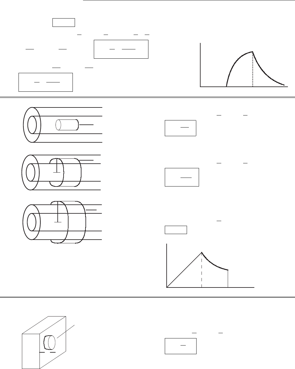
30 CHAPTER 2. ELECTROSTATICS
Problem 2.15
(i) Qenc = 0, so E=0.
(ii) E·da=E(4⇡r2)= 1
✏0Qenc =1
✏0⇢d⌧=1
✏0k
¯r2¯r2sin ✓d¯rd✓d
=4⇡k
✏0r
ad¯r=4⇡k
✏0(ra))E=k
✏0ra
r2ˆr .
(iii) E(4⇡r2)=4⇡k
✏0b
ad¯r=4⇡k
✏0(ba),so
E=k
✏0ba
r2ˆr .
1
Contents
Problem 2.13
✻
s
!"# $
l
✠
Gaussian surface %E·da=E·2πs·l=1
ϵ0Qenc =1
ϵ0λl. So
E=λ
2πϵ0sˆs (same as Ex. 2.1).
Problem 2.14
✒
r✙
Gaussian surface
Problem 2.15
(i) Qenc = 0, so E= 0.
(ii) %E·da=E(4πr2) = 1
ϵ0Qenc =1
ϵ0&ρdτ=1
ϵ0&k
¯r2¯r2sin θd¯r dθdφ
=4πk
ϵ0&r
ad¯r=4πk
ϵ0(r−a)∴E=k
ϵ0'r−a
r2(ˆr.
(iii) E(4πr2) = 4πk
ϵ0&b
ad¯r=4πk
ϵ0(b−a),so
E=k
ϵ0'b−a
r2(ˆr.
✲
r
✻
|E|
a b
Problem 2.16
c
⃝2005 Pearson Education, Inc., Upper Saddle River, NJ. All rights reserved. This material is
protected under all copyright laws as they currently exist. No portion of this material may be
reproduced, in any form or by any means, without permission in writing from the publisher.
Problem 2.16
(i)
1
Contents
Problem 2.13
Problem 2.16
(i)
l
✛Gaussian surface !E·da=E·2πs·l=1
ϵ0Qenc =1
ϵ0ρπs2l;
E=ρs
2ϵ0
ˆs.
(ii)
l
✛Gaussian surface
✻
s!E·da=E·2πs·l=1
ϵ0Qenc =1
ϵ0ρπa2l;
E=ρa2
2ϵ0sˆs.
(iii)
l
✛Gaussian surface
✻
s
!E·da=E·2πs·l=1
ϵ0Qenc = 0;
E= 0.
✲
s
✻
|E|
a b
c
⃝2005 Pearson Education, Inc., Upper Saddle River, NJ. All rights reserved. This material is
protected under all copyright laws as they currently exist. No portion of this material may be
reproduced, in any form or by any means, without permission in writing from the publisher.
E·da=E·2⇡s·l=1
✏0Qenc =1
✏0⇢⇡s2l;
E=⇢s
2✏0
ˆs .
(ii)
1
Contents
Problem 2.13
Problem 2.16
(i)
l
✛Gaussian surface !E·da=E·2πs·l=1
ϵ0Qenc =1
ϵ0ρπs2l;
E=ρs
2ϵ0
ˆs.
(ii)
l
✛Gaussian surface
✻
s!E·da=E·2πs·l=1
ϵ0Qenc =1
ϵ0ρπa2l;
E=ρa2
2ϵ0sˆs.
(iii)
l
✛Gaussian surface
✻
s
!E·da=E·2πs·l=1
ϵ0Qenc = 0;
E= 0.
✲
s
✻
|E|
a b
c
⃝2005 Pearson Education, Inc., Upper Saddle River, NJ. All rights reserved. This material is
protected under all copyright laws as they currently exist. No portion of this material may be
reproduced, in any form or by any means, without permission in writing from the publisher.
E·da=E·2⇡s·l=1
✏0Qenc =1
✏0⇢⇡a2l;
E=⇢a2
2✏0sˆs .
(iii)
1
Contents
Problem 2.13
Problem 2.16
(i)
l
✛Gaussian surface !E·da=E·2πs·l=1
ϵ0Qenc =1
ϵ0ρπs2l;
E=ρs
2ϵ0
ˆs.
(ii)
l
✛Gaussian surface
✻
s!E·da=E·2πs·l=1
ϵ0Qenc =1
ϵ0ρπa2l;
E=ρa2
2ϵ0sˆs.
(iii)
l
✛Gaussian surface
✻
s
!E·da=E·2πs·l=1
ϵ0Qenc = 0;
E= 0.
✲
s
✻
|E|
a b
c
⃝2005 Pearson Education, Inc., Upper Saddle River, NJ. All rights reserved. This material is
protected under all copyright laws as they currently exist. No portion of this material may be
reproduced, in any form or by any means, without permission in writing from the publisher.
E·da=E·2⇡s·l=1
✏0Qenc = 0;
E=0.
1
Contents
Problem 2.13
Problem 2.16
(i)
l
✛Gaussian surface !E·da=E·2πs·l=1
ϵ0Qenc =1
ϵ0ρπs2l;
E=ρs
2ϵ0
ˆs.
(ii)
l
✛Gaussian surface
✻
s!E·da=E·2πs·l=1
ϵ0Qenc =1
ϵ0ρπa2l;
E=ρa2
2ϵ0sˆs.
(iii)
l
✛Gaussian surface
✻
s
!E·da=E·2πs·l=1
ϵ0Qenc = 0;
E= 0.
✲
s
✻
|E|
a b
c
⃝2005 Pearson Education, Inc., Upper Saddle River, NJ. All rights reserved. This material is
protected under all copyright laws as they currently exist. No portion of this material may be
reproduced, in any form or by any means, without permission in writing from the publisher.
Problem 2.17 On the xz plane E= 0 by symmetry. Set up a Gaussian “pillbox” with one face in this plane
and the other at y.
1
Contents
Problem 2.17
On the x z plane E= 0 by symmetry. Set up a Gaussian “pillbox” with one face in this plane and the
other at y.
y
✲ ✛
❂
Gaussian pillbox
Qenc =1
ϵ0Adρ⇒E=ρ
ϵ0
dˆy (for y > d).
✲
✻
E
y
−d
d
ρd
ϵ0
Problem 2.18
From Prob. 2.12, the field inside the positive sphere is E+=ρ
3ϵ0r+, where r+is the vector from the positive
center to the point in question. Likewise, the field of the negative sphere is −ρ
3ϵ0r−. So the total field is
E=ρ
3ϵ0
(r+−r−)
But (see diagram) r+−r−=d. So E=ρ
3ϵ0
d.
✕✯
✛
+
−
r+
r−
d
c
⃝2005 Pearson Education, Inc., Upper Saddle River, NJ. All rights reserved. This material is
protected under all copyright laws as they currently exist. No portion of this material may be
reproduced, in any form or by any means, without permission in writing from the publisher.
E·da=E·A=1
✏0Qenc =1
✏0Ay⇢;
E=⇢
✏0
yˆy (for |y|<d).
c
2012 Pearson Education, Inc., Upper Saddle River, NJ. All rights reserved. This material is
protected under all copyright laws as they currently exist. No portion of this material may be
reproduced, in any form or by any means, without permission in writing from the publisher.
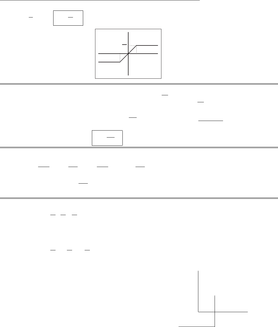
CHAPTER 2. ELECTROSTATICS 31
Qenc =1
✏0Ad⇢)E=⇢
✏0
dˆy (for y>d).
2
Problem 2.17
On the x z plane E= 0 by symmetry. Set up a Gaussian “pillbox” with one face in this plane and the
other at y.
y
✲ ✛
❂
Gaussian pillbox !E·da=E·A=1
ϵ0Qenc =1
ϵ0Ayρ;
E=ρ
ϵ0
yˆy (for |y|< d).
Qenc =1
ϵ0Adρ⇒E=ρ
ϵ0
dˆy (for y > d).
✲
✻
E
y
−d
d
ρd
ϵ0
Problem 2.18
From Prob. 2.12, the field inside the positive sphere is E+=ρ
3ϵ0r+, where r+is the vector from the positive
center to the point in question. Likewise, the field of the negative sphere is −ρ
3ϵ0r−. So the total field is
E=ρ
3ϵ0
(r+−r−)
But (see diagram) r+−r−=d. So E=ρ
3ϵ0
d.
✕✯
✛
+
−
r+
r−
d
Problem 2.19
∇×E=1
4πϵ0
∇×"ˆηˆη
ˆη
η2ρdτ=1
4πϵ0"#∇×$ˆηˆη
ˆη
η2%&ρdτ(since ρdepends on r′, not r)
= 0 (since ∇×$ˆηˆη
ˆη
η2%= 0, from Prob. 1.62).
Problem 2.20
(1) ∇×E1=k'
'
'
'
'
'
ˆx ˆy ˆz
∂
∂x
∂
∂y
∂
∂z
xy 2yz 3zx
'
'
'
'
'
'
=k[ˆx(0 −2y) + ˆy(0 −3z) + ˆz(0 −x)] ̸= 0,
so E1is an impossible electrostatic field.
(2) ∇×E2=k'
'
'
'
'
'
ˆx ˆy ˆz
∂
∂x
∂
∂y
∂
∂z
y22xy +z22yz
'
'
'
'
'
'
=k[ˆx(2z−2z) + ˆy(0 −0) + ˆz(2y−2y)] = 0,
so E2is a possible electrostatic field.
c
⃝2005 Pearson Education, Inc., Upper Saddle River, NJ. All rights reserved. This material is
protected under all copyright laws as they currently exist. No portion of this material may be
reproduced, in any form or by any means, without permission in writing from the publisher.
Problem 2.18
From Prob. 2.12, the field inside the positive sphere is E+=⇢
3✏0r+,wherer+is the vector from the positive
center to the point in question. Likewise, the field of the negative sphere is ⇢
3✏0r. So the total field is
E=⇢
3✏0
(r+r)
But (see diagram) r+r=d. So E=⇢
3✏0
d.r
r
*
+
r+
r
d
Problem 2.19
r⇥E=1
4⇡✏0r⇥ˆ
r
r
2⇢d⌧=1
4⇡✏0r⇥ˆ
r
r
2⇢d⌧(since ⇢depends on r0, not r)
=0(since r⇥ˆ
r
r
2=0, from Prob. 1.63).
Problem 2.20
(1) r⇥E1=k
ˆx ˆy ˆz
@
@x
@
@y
@
@z
xy 2yz 3zx=k[ˆx (0 2y)+ˆy (0 3z)+ˆz (0 x)] 6=0,
so E1is an impossible electrostatic field.
(2) r⇥E2=k
ˆx ˆy ˆz
@
@x
@
@y
@
@z
y22xy +z22yz=k[ˆx (2z2z)+ˆy (0 0) + ˆz (2y2y)] = 0,
so E2is a possible electrostatic field.
Let’s go by the indicated path:
⇢
⇢
⇢
⇢
⇢=
x
-y
6
z
⇢
⇢
⇢
⇢=
I
-
II
6
III
r(x0,y
0,z
0)
E·dl=(y2dx + (2xy +z2)dy +2yz dz)k
Step I: y=z=0;dy =dz =0.E·dl=ky2dx =0.
Step II: x=x0,y:0!y0,z=0.dx=dz =0.
E·dl=k(2xy +z2)dy =2kx0y dy.
II E·dl=2kx0y0
0y dy =kx0y2
0.
Step III :x=x0,y=y0,z:0!z0;dx =dy =0.
E·dl=2kyz dz =2ky0z dz.
c
2012 Pearson Education, Inc., Upper Saddle River, NJ. All rights reserved. This material is
protected under all copyright laws as they currently exist. No portion of this material may be
reproduced, in any form or by any means, without permission in writing from the publisher.

32 CHAPTER 2. ELECTROSTATICS
III E·dl=2y0kz0
0z dz =ky0z2
0.
V(x0,y
0,z
0)=
(x0,y0,z0)
0
E·dl=k(x0y2
0+y0z2
0), or V(x, y, z)=k(xy2+yz2).
Check:rV=k[@
@x(xy2+yz2)ˆx +@
@y(xy2+yz2)ˆy +@
@z(xy2+yz2)ˆz ]=k[y2ˆx +(2xy+z2)ˆy +2yz ˆz ]=E.X
Problem 2.21
V(r)=r
1E·dl.
Outside the sphere (r>R): E=1
4⇡✏0
q
r2ˆr .
Inside the sphere (r<R): E=1
4⇡✏0
q
R3rˆr .
So for r>R:V(r)=r
11
4⇡✏0
q
¯r2d¯r=1
4⇡✏0q1
¯r
r
1=q
4⇡✏0
1
r,
and for r<R:V(r)=R
11
4⇡✏0
q
¯r2d¯rr
R1
4⇡✏0
q
R3¯rd¯r=q
4⇡✏01
R1
R3r2R2
2
=q
4⇡✏0
1
2R3r2
R2.
When r>R,rV=q
4⇡✏0
@
@r1
rˆr =q
4⇡✏0
1
r2ˆr ,soE=rV=q
4⇡✏0
1
r2ˆr .X
When r<R,rV=q
4⇡✏0
1
2R
@
@r3r2
R2ˆr =q
4⇡✏0
1
2R2r
R2ˆr =q
4⇡✏0
r
R3ˆr ;soE=rV=1
4⇡✏0
q
R3rˆr .X
0.5 1 1.5 2 2.5 3
0.2
0.4
0.6
0.8
1
1.2
1.4
1.6
r
V(r)
(In the figure, ris in units of R, and V(r) is in units of q/4⇡✏0R.)
Problem 2.22
E=1
4⇡✏0
2
sˆs (Prob. 2.13). In this case we cannot set the reference point at 1, since the charge itself
extends to 1. Let’s set it at s=a. Then
V(s)=s
a1
4⇡✏0
2
¯sd¯s=1
4⇡✏0
2ln s
a.
(In this form it is clear why a=1would be no good—likewise the other “natural” point, a= 0.)
rV=1
4⇡✏02@
@sln s
aˆs =1
4⇡✏021
sˆs =E.X
Problem 2.23
V(0) = 0
1E·dl=b
1k
✏0
(ba)
r2dr a
bk
✏0
(ra)
r2dr 0
a(0)dr =k
✏0
(ba)
bk
✏0ln a
b+a1
a1
b
=k
✏01a
bln a
b1+a
b=k
✏0
ln b
a.
Problem 2.24
Using Eq. 2.22 and the fields from Prob. 2.16:
V(b)V(0) = b
0E·dl=a
0E·dlb
aE·dl=⇢
2✏0a
0sds⇢a2
2✏0b
a
1
sds
c
2012 Pearson Education, Inc., Upper Saddle River, NJ. All rights reserved. This material is
protected under all copyright laws as they currently exist. No portion of this material may be
reproduced, in any form or by any means, without permission in writing from the publisher.

CHAPTER 2. ELECTROSTATICS 33
=⇢
2✏0s2
2
a
0+⇢a2
2✏0ln s|b
a=⇢a2
4✏01 + 2 ln b
a.
Problem 2.25
(a) V=1
4⇡✏0
2q
z2+d
22.
(b) V=1
4⇡✏0L
L
dx
pz2+x2=
4⇡✏0ln(x+pz2+x2)L
L
=
4⇡✏0
ln L+pz2+L2
L+pz2+L2=
2⇡✏0
ln L+pz2+L2
z.
r
1
Contents
Problem 2.25
(a) V=1
4πϵ0
2q
!z2+"d
2#2.
(b) V=1
4πϵ0$L
−L
λdx
√z2+x2=λ
4πϵ0ln(x+√z2+x2)%%
L
−L
=λ
4πϵ0
ln &L+√z2+L2
−L+√z2+L2'=λ
2πϵ0ln (L+√z2+L2
z).
x
z
(c) V=1
4πϵ0$R
0
σ2πr dr
√r2+z2=1
4πϵ02πσ (√r2+z2)%%
R
0=σ
2ϵ0(*R2+z2−z).
In each case, by symmetry ∂V
∂y=∂V
∂x= 0.∴E=−
∂V
∂zˆz.
(a) E=−1
4πϵ02q"−1
2#2z
“z2+(d
2)2”3/2ˆz =1
4πϵ0
2qz
"z2+"d
2#2#3/2ˆz (agrees with Prob. 2.2a).
(b) E=−
λ
4πϵ0+1
(L+√z2+L2)
1
2
1
√z2+L22z−1
(−L+√z2+L2)
1
2
1
√z2+L22z,ˆz
=−
λ
4πϵ0
z
√z2+L2+−L+√z2+L2−L−√z2+L2
(z2+L2)−L2,ˆz =2Lλ
4πϵ0
1
z√z2+L2ˆz (agrees with Ex. 2.1).
(c) E=−
σ
2ϵ0+1
2
1
√R2+z22z−1,ˆz =σ
2ϵ0-1−
z
√R2+z2.ˆz (agrees with Prob. 2.6).
If the right-hand charge in (a) is −q, then V= 0 , which, naively, suggests E=−∇V= 0, in contradiction
with the answer to Prob. 2.2b. The point is that we only know Von the zaxis, and from this we cannot
hope to compute Ex=−
∂V
∂xor Ey=−
∂V
∂y. That was OK in part (a), because we knew from symmetry that
Ex=Ey= 0. But now Epoints in the xdirection, so knowing Von the zaxis is insufficient to determine E.
c
⃝2005 Pearson Education, Inc., Upper Saddle River, NJ. All rights reserved. This material is
protected under all copyright laws as they currently exist. No portion of this material may be
reproduced, in any form or by any means, without permission in writing from the publisher.
(c) V=1
4⇡✏0R
0
2⇡rdr
pr2+z2=1
4⇡✏0
2⇡ (r2+z2)
R
0=
2✏0R2+z2z.
In each case, by symmetry @V
@y=@V
@x=0.)E=@V
@zˆz .
(a) E=1
4⇡✏0
2q1
22z
z2+d
223/2ˆz =1
4⇡✏0
2qz
z2+d
223/2ˆz (agrees with Ex. 2.1).
(b) E=
4⇡✏01
(L+pz2+L2)
1
2
1
pz2+L22z1
(L+pz2+L2)
1
2
1
pz2+L22zˆz
=
4⇡✏0
z
pz2+L2L+pz2+L2Lpz2+L2
(z2+L2)L2ˆz =2L
4⇡✏0
1
zpz2+L2ˆz (agrees with Ex. 2.2).
(c) E=
2✏01
2
1
pR2+z22z1ˆz =
2✏01z
pR2+z2ˆz (agrees with Prob. 2.6).
If the right-hand charge in (a) is q, then V=0 , which, naively, suggests E=rV=0, in contradiction
with the answer to Prob. 2.2. The point is that we only know Von the zaxis, and from this we cannot hope
to compute Ex=@V
@xor Ey=@V
@y. That was OK in part (a), because we knew from symmetry that
Ex=Ey= 0. But now Epoints in the xdirection, so knowing Von the zaxis is insufficient to determine E.
Problem 2.26
2
✲
✻
a
bh
h
c
⃝2005 Pearson Education, Inc., Upper Saddle River, NJ. All rights reserved. This material is
protected under all copyright laws as they currently exist. No portion of this material may be
reproduced, in any form or by any means, without permission in writing from the publisher.
r
¯
r
V(a)= 1
4⇡✏0p2h
02⇡r
r
d
r
=2⇡
4⇡✏0
1
p2(p2h)= h
2✏0
(where r=
r
/p2)
c
2012 Pearson Education, Inc., Upper Saddle River, NJ. All rights reserved. This material is
protected under all copyright laws as they currently exist. No portion of this material may be
reproduced, in any form or by any means, without permission in writing from the publisher.

34 CHAPTER 2. ELECTROSTATICS
V(b)= 1
4⇡✏0p2h
02⇡r
¯
r
d
r
(where ¯
r
=h2+
r
2p2h
r
)
=2⇡
4⇡✏0
1
p2p2h
0
r
h2+
r
2p2h
r
d
r
=
2p2✏0h2+
r
2p2h
r
+h
p2ln(2h2+
r
2p2h
r
+2
r
p2h)
p2h
0
=
2p2✏0h+h
p2ln(2h+2
p2hp2h)hh
p2ln(2hp2h)
=
2p2✏0
h
p2ln(2h+p2h)ln(2hp2h)=h
4✏0
ln 2+p2
2p2=h
4✏0
ln (2 + p2)2
2
=h
2✏0
ln(1 + p2).)V(a)V(b)= h
2✏01ln(1 + p2).
Problem 2.27
3
Problem 2.27
! "# $
z−L
2
#$! "
x
!"# $
L
dx
✲ ✛
Cut the cylinder into slabs, as shown in the figure, and
use result of Prob. 2.25c, with z→xand σ→ρdx:
V=ρ
2ϵ0
z+L/2
%
z−L/2&√R2+x2−x'dx
=ρ
2ϵ0
1
2(x√R2+x2+R2ln(x+√R2+x2)−x2)**z+L/2
z−L/2
=ρ
4ϵ08
<
:
(z+L
2)qR2+(z+L
2)2−(z−L
2)qR2+(z−L
2)2+R2ln2
4
z+L
2+rR2+(z+L
2)2
z−
L
2+rR2+(z−
L
2)23
5−2zL9
=
;
.
(Note: −&z+L
2'2+&z−L
2'2=−z2−zL −L2
4+z2−zL +L2
4=−2zL.)
E=−∇V=−ˆz ∂V
∂z=−
ˆzρ
4ϵ0+,R2+-z+L
2.2
+&z+L
2'2
/R2+&z+L
2'2−,R2+-z−L
2.2
−&z−L
2'2
/R2+&z−L
2'2
+R201 + z+L
2
qR2+(z+L
2)2
z+L
2+/R2+&z+L
2'2−
1 + z−L
2
qR2+(z−L
2)2
z−L
2+/R2+&z−L
2'2
#$! "
1
/R2+&z+L
2'2−1
/R2+&z−L
2'2
1−2L2
E=−
ˆzρ
4ϵ0⎧
⎨
⎩
2,R2+-z+L
2.2
−2,R2+-z−L
2.2
−2L⎫
⎬
⎭
=ρ
2ϵ0⎡
⎣L−,R2+-z+L
2.2
+,R2+-z−L
2.2⎤
⎦ˆz.
Problem 2.28
Orient axes so Pis on zaxis.
❂
x
✲y
✻
z
φ
r
P
zθ
V=1
4πϵ0%ρ
ηdτ.=Here ρis constant, dτ=r2sin θdr dθdφ,
η=√z2+r2−2rz cos θ.
V=ρ
4πϵ0%r2sin θdr dθdφ
√z2+r2−2rz cos θ;%2π
0dφ= 2π.
%π
0
sin θ
√z2+r2−2rz cos θdθ=1
rz &√r2+z2−2rz cos θ'**π
0=1
rz &√r2+z2+ 2rz −√r2+z2−2rz'
=1
rz (r+z−|r−z|) = =2/z , if r < z,
2/r , if r > z. >
c
⃝2005 Pearson Education, Inc., Upper Saddle River, NJ. All rights reserved. This material is
protected under all copyright laws as they currently exist. No portion of this material may be
reproduced, in any form or by any means, without permission in writing from the publisher.
Cut the cylinder into slabs, as shown in the figure, and
use result of Prob. 2.25c, with z!xand !⇢dx:
V=⇢
2✏0
z+L/2
zL/2pR2+x2xdx
=⇢
2✏0
1
2xpR2+x2+R2ln(x+pR2+x2)x2z+L/2
zL/2
=⇢
4✏08
<
:
(z+L
2)qR2+(z+L
2)2(zL
2)qR2+(zL
2)2+R2ln2
4
z+L
2+rR2+(z+L
2)2
zL
2+rR2+(zL
2)23
52zL9
=
;
.
(Note: z+L
22+zL
22=z2zL L2
4+z2zL +L2
4=2zL.)
E=rV=ˆz @V
@z=ˆz ⇢
4✏0R2+z+L
22
+z+L
22
R2+z+L
22R2+zL
22
zL
22
R2+zL
22
+R21+ z+L
2
qR2+(z+L
2)2
z+L
2+R2+z+L
22
1+ zL
2
qR2+(zL
2)2
zL
2+R2+zL
22
1
R2+z+L
221
R2+zL
22
2L
E=ˆz ⇢
4✏0
2R2+z+L
22
2R2+zL
22
2L
c
2012 Pearson Education, Inc., Upper Saddle River, NJ. All rights reserved. This material is
protected under all copyright laws as they currently exist. No portion of this material may be
reproduced, in any form or by any means, without permission in writing from the publisher.

CHAPTER 2. ELECTROSTATICS 35
=⇢
2✏0
LR2+z+L
22
+R2+zL
22
ˆz .
Problem 2.28
Orient axes so Pis on zaxis.
1
Hello
❂
x
✲y
✻
z
φ
r
P
zθ
c
⃝2005 Pearson Education, Inc., Upper Saddle River, NJ. All rights reserved. This material is
protected under all copyright laws as they currently exist. No portion of this material may be
reproduced, in any form or by any means, without permission inwritingfromthepublisher.
V=1
4⇡✏0⇢
r
d⌧.Here ⇢is constant, d⌧=r2sin ✓dr d✓d,
r
r
=pz2+r22rz cos ✓.
V=⇢
4⇡✏0r2sin ✓dr d✓d
pz2+r22rz cos ✓;2⇡
0d=2⇡.
⇡
0
sin ✓
pz2+r22rz cos ✓d✓=1
rz pr2+z22rz cos ✓⇡
0=1
rz pr2+z2+2rz pr2+z22rz
=1
rz (r+z|rz|)=2/z , if r<z,
2/r , if r>z.
)V=⇢
4⇡✏0·2⇡·2z
0
1
zr2dr +
R
z
1
rr2dr=⇢
✏01
z
z3
3+R2z2
2=⇢
2✏0R2z2
3.
But ⇢=q
4
3⇡R3,soV(z)= 1
2✏0
3q
4⇡R3R2z2
3=q
8⇡✏0R3z2
R2;V(r)= q
8⇡✏0R3r2
R2.X
Problem 2.29
r2V=1
4⇡✏0r2⇢
r
d⌧=1
4⇡✏0⇢(r0)r21
r
d⌧(since ⇢is a function of r0, not r)
=1
4⇡✏0⇢(r0)[4⇡3(rr0)] d⌧=1
✏0⇢(r).X
Problem 2.30.
(a) Ex. 2.5: Eabove =
2✏0ˆn ;Ebelow =
2✏0ˆn (ˆn always pointing up); Eabove Ebelow =
✏0ˆn .X
Ex. 2.6: At each surface, E= 0 one side and E=
✏0other side, so E=
✏0.X
Prob. 2.11: Eout =R2
✏0r2ˆr =
✏0ˆr ;Ein =0;soE=
✏0ˆr .X
(b) Outside:E·da=E(2⇡s)l=1
✏0Qenc =
✏0(2⇡R)l)E=
✏0
R
sˆs =
✏0ˆs (at surface).
Inside:Qenc = 0, so E= 0. )E=
✏0ˆs .X
1
Contents
Problem 2.30.
(a) Ex. 2.4: Eabove =σ
2ϵ0
ˆn;Ebelow =−σ
2ϵ0
ˆn (ˆn always pointing up); Eabove −Ebelow =σ
ϵ0
ˆn.!
Ex. 2.5: At each surface, E= 0 one side and E=σ
ϵ0other side, so ∆E=σ
ϵ0.!
Prob. 2.11: Eout =σR2
ϵ0r2ˆr =σ
ϵ0
ˆr ;Ein = 0 ; so ∆E=σ
ϵ0
ˆr.!
(b) Outside:!E·da=E(2πs)l=1
ϵ0Qenc =1
ϵ0(2πR)l⇒E=σ
ϵ0
R
sˆs =σ
ϵ0
ˆs (at surface).
Inside:Qenc = 0, so E= 0. ∴∆E=σ
ϵ0
ˆs.!
✻
s✻
R
"#$%
l
(c) Vout =R2σ
ϵ0r=Rσ
ϵ0(at surface); Vin =Rσ
ϵ0; so Vout =Vin.!
∂Vout
∂r=−R2σ
ϵ0r2=−σ
ϵ0(at surface); ∂Vin
∂r= 0 ; so ∂Vout
∂r−∂Vin
∂r=−σ
ϵ0.!
Problem 2.31
(a) V=1
4πϵ0&qi
rij =1
4πϵ0'−q
a+q
√2a+−q
a(=q
4πϵ0a)−2 + 1
√2*.
∴W4=qV =q2
4πϵ0a+−2 + 1
√2,.
(2)
+
(3)
−
(4)
+
(1)
−
(b) W1= 0, W2=1
4πϵ0)−q2
a*;W3=1
4πϵ0)q2
√2a−q2
a*;W4= (see (a)).
Wtot =1
4πϵ0
q2
a'−1 + 1
√2−1−2 + 1
√2(=1
4πϵ0
2q2
a+−2 + 1
√2,.
c
⃝2005 Pearson Education, Inc., Upper Saddle River, NJ. All rights reserved. This material is
protected under all copyright laws as they currently exist. No portion of this material may be
reproduced, in any form or by any means, without permission in writing from the publisher.
(c) Vout =R2
✏0r=R
✏0(at surface); Vin =R
✏0; so Vout =Vin.X
@Vout
@r=R2
✏0r2=
✏0(at surface); @Vin
@r= 0 ; so @Vout
@r@Vin
@r=
✏0.X
c
2012 Pearson Education, Inc., Upper Saddle River, NJ. All rights reserved. This material is
protected under all copyright laws as they currently exist. No portion of this material may be
reproduced, in any form or by any means, without permission in writing from the publisher.

36 CHAPTER 2. ELECTROSTATICS
Problem 2.31
(a) V=1
4⇡✏0qi
rij =1
4⇡✏0q
a+q
p2a+q
a=q
4⇡✏0a2+ 1
p2.
)W4=qV =q2
4⇡✏0a2+ 1
p2.
r
(2)
+r(3)
r(4)
+
r
(1)
(b) W1= 0, W2=1
4⇡✏0q2
a;W3=1
4⇡✏0q2
p2aq2
a;W4= (see (a)).
Wtot =1
4⇡✏0
q2
a1+ 1
p212+ 1
p2=1
4⇡✏0
2q2
a2+ 1
p2.
Problem 2.32
Conservation of energy (kinetic plus potential):
1
2mAv2
A+1
2mBv2
B+1
4⇡✏0
qAqB
r=E.
At release vA=vB=0,r=a,so
E=1
4⇡✏0
qAqB
a.
When they are very far apart (r!1) the potential energy is zero, so
1
2mAv2
A+1
2mBv2
B=1
4⇡✏0
qAqB
a.
Meanwhile, conservation of momentum says mAvA=mBvB, or vB=(mA/mB)vA. So
1
2mAv2
A+1
2mBmA
mB2
v2
A=1
2mA
mB(mA+mB)v2
A=1
4⇡✏0
qAqB
a.
vA=1
2⇡✏0
qAqB
(mA+mB)amA
mB;vB=1
2⇡✏0
qAqB
(mA+mB)amB
mA.
Problem 2.33
From Eq. 2.42, the energy of one charge is
W=1
2qV =1
2(2) 1
n=1
1
4⇡✏0
(1)nq2
na =q2
4⇡✏0a
1
1
(1)n
n.
(The factor of 2 out front counts the charges to the left as well as to the right of q.) The sum is ln 2 (you
can get it from the Taylor expansion of ln(1 + x):
ln(1 + x)=x1
2x2+1
3x31
4x4+···
with x= 1. Evidently ↵=ln2.
c
2012 Pearson Education, Inc., Upper Saddle River, NJ. All rights reserved. This material is
protected under all copyright laws as they currently exist. No portion of this material may be
reproduced, in any form or by any means, without permission in writing from the publisher.

CHAPTER 2. ELECTROSTATICS 37
Problem 2.34
(a) W=1
2⇢Vd⌧. From Prob. 2.21 (or Prob. 2.28): V=⇢
2✏0R2r2
3=1
4⇡✏0
q
2R3r2
R2
W=1
2⇢1
4⇡✏0
q
2RR
03r2
R24⇡r2dr =q⇢
4✏0R3r3
31
R2
r5
5
R
0
=q⇢
4✏0RR3R3
5
=q⇢
5✏0
R2=qR2
5✏0
q
4
3⇡R3=1
4⇡✏03
5
q2
R.
(b) W=✏0
2E2d⌧.Outside (r>R)E=1
4⇡✏0
q
r2ˆr ;Inside (r<R)E=1
4⇡✏0
q
R3rˆr .
)W=✏0
2
1
(4⇡✏0)2q21
R
1
r4(r24⇡dr)+R
0r
R32(4⇡r2dr)
=1
4⇡✏0
q2
21
r
1
R
+1
R6r5
5
R
0=1
4⇡✏0
q2
21
R+1
5R=1
4⇡✏0
3
5
q2
R.X
(c) W=✏0
2SVE·da+VE2d⌧, where Vis large enough to enclose all the charge, but otherwise
arbitrary. Let’s use a sphere of radius a>R. Here V=1
4⇡✏0
q
r.
W=✏0
2
r=a1
4⇡✏0
q
r 1
4⇡✏0
q
r2r2sin ✓d✓d+R
0
E2d⌧+a
R1
4⇡✏0
q
r22
(4⇡r2dr)
=✏0
2q2
(4⇡✏0)2
1
a4⇡+q2
(4⇡✏0)2
4⇡
5R+1
(4⇡✏0)24⇡q21
r
a
R
=1
4⇡✏0
q2
21
a+1
5R1
a+1
R=1
4⇡✏0
3
5
q2
R.X
As a!1, the contribution from the surface integral 1
4⇡✏0
q2
2agoes to zero, while the volume integral
1
4⇡✏0
q2
2a(6a
5R1)picks up the slack.
Problem 2.35
2
Problem 2.32
(a) W=1
2!ρV dτ. From Prob. 2.21 (or Prob. 2.28): V=ρ
2ϵ0"R2−r2
3#=1
4πϵ0
q
2R"3−r2
R2#
W=1
2ρ1
4πϵ0
q
2R$R
0%3−
r2
R2&4πr2dr =qρ
4ϵ0R'3r3
3−1
R2
r5
5())))
R
0
=qρ
4ϵ0R%R3−
R3
5&
=qρ
5ϵ0
R2=qR2
5ϵ0
q
4
3πR3=1
4πϵ0%3
5
q2
R&.
(b) W=ϵ0
2!E2dτ.Outside (r > R)E=1
4πϵ0
q
r2ˆr ;Inside (r < R)E=1
4πϵ0
q
R3rˆr.
∴W=ϵ0
2
1
(4πϵ0)2q2*$∞
R
1
r4(r24πdr) + $R
0"r
R3#2
(4πr2dr)+
=1
4πϵ0
q2
2*%−1
r&))))
∞
R
+1
R6%r5
5&))))
R
0+=1
4πϵ0
q2
2%1
R+1
5R&=1
4πϵ0
3
5
q2
R."
(c) W=ϵ0
2,-SVE·da+!VE2dτ., where Vis large enough to enclose all the charge, but otherwise
arbitrary. Let’s use a sphere of radius a > R. Here V=1
4πϵ0
q
r.
W=ϵ0
2*$
r=a%1
4πϵ0
q
r&% 1
4πϵ0
q
r2&r2sin θdθdφ+$R
0
E2dτ+$a
R%1
4πϵ0
q
r2&2
(4πr2dr)+
=ϵ0
2/q2
(4πϵ0)2
1
a4π+q2
(4πϵ0)2
4π
5R+1
(4πϵ0)24πq2%−1
r&))))
a
R0
=1
4πϵ0
q2
2/1
a+1
5R−1
a+1
R0=1
4πϵ0
3
5
q2
R."
As a→ ∞, the contribution from the surface integral "1
4πϵ0
q2
2a#goes to zero, while the volume integral
"1
4πϵ0
q2
2a(6a
5R−1)#picks up the slack.
Problem 2.33
¯q
✯
r
✮
d¯q
c
⃝2005 Pearson Education, Inc., Upper Saddle River, NJ. All rights reserved. This material is
protected under all copyright laws as they currently exist. No portion of this material may be
reproduced, in any form or by any means, without permission in writing from the publisher.
dW =d¯qV =d¯q1
4⇡✏0¯q
r,(¯q= charge on sphere of radius r).
¯q=4
3⇡r3⇢=qr3
R3(q= total charge on sphere).
d¯q=4⇡r2dr ⇢=4⇡r2
4
3⇡R3q dr =3q
R3r2dr.
dW =1
4⇡✏0qr3
R31
r3q
R3r2dr=1
4⇡✏0
3q2
R6r4dr
W=1
4⇡✏0
3q2
R6R
0
r4dr =1
4⇡✏0
3q2
R6
R5
5=1
4⇡✏03
5
q2
R.X
c
2012 Pearson Education, Inc., Upper Saddle River, NJ. All rights reserved. This material is
protected under all copyright laws as they currently exist. No portion of this material may be
reproduced, in any form or by any means, without permission in writing from the publisher.

38 CHAPTER 2. ELECTROSTATICS
Problem 2.36
(a) W=✏0
2E2d⌧.E=1
4⇡✏0
q
r2(a<r<b),zero elsewhere.
W=✏0
2q
4⇡✏02b
a1
r224⇡r2dr =q2
8⇡✏0b
a
1
r2=q2
8⇡✏01
a1
b.
(b) W1=1
8⇡✏0
q2
a,W
2=1
8⇡✏0
q2
b,E1=1
4⇡✏0
q
r2ˆr (r>a),E2=1
4⇡✏0q
r2ˆr (r>b).So
E1·E2=1
4⇡✏02q2
r4,(r>b),and hence E1·E2d⌧=1
4⇡✏02q21
b
1
r44⇡r2dr =q2
4⇡✏0b.
Wtot =W1+W2+✏0E1·E2d⌧=1
8⇡✏0q21
a+1
b2
b=q2
8⇡✏01
a1
b.X
Problem 2.37
r
a
x
y
z
b
q
q2
q1
r
E1=1
4⇡✏0
q1
r2ˆr ;E2=1
4⇡✏0
q2
r
2ˆ
r
;Wi=✏0
q1q2
(4⇡✏0)21
r2
r
2cos r2sin ✓dr d✓d,
where (from the figure)
r
=r2+a22ra cos ✓,cos =(racos ✓)
r
.
Therefore
Wi=q1q2
(4⇡)2✏0
2⇡(racos ✓)
r
3sin ✓dr d✓.
It’s simplest to do the rintegral first, changing variables to
r
:
2
r
d
r
=(2r2acos ✓)dr )(racos ✓)dr =
r
d
r
.
As r:0!1,
r
:a!1,so
Wi=q1q2
8⇡✏0⇡
01
a
1
r
2d
r
sin ✓d✓.
The
r
integral is 1/a,so
Wi=q1q2
8⇡✏0a⇡
0
sin ✓d✓=q1q2
4⇡✏0a.
Of course, this is precisely the interaction energy of two point charges.
Problem 2.38
(a) R=q
4⇡R2;a=q
4⇡a2;b=q
4⇡b2.
c
2012 Pearson Education, Inc., Upper Saddle River, NJ. All rights reserved. This material is
protected under all copyright laws as they currently exist. No portion of this material may be
reproduced, in any form or by any means, without permission in writing from the publisher.

CHAPTER 2. ELECTROSTATICS 39
(b) V(0) = 0
1E·dl=b
11
4⇡✏0
q
r2dr a
b(0)dr R
a1
4⇡✏0
q
r2dr 0
R(0)dr =1
4⇡✏0q
b+q
Rq
a.
(c) b!0 (the charge “drains o↵”); V(0) = a
1(0)dr R
a1
4⇡✏0
q
r2dr 0
R(0)dr =1
4⇡✏0q
Rq
a.
Problem 2.39
(a) a=qa
4⇡a2;b=qb
4⇡b2;R=qa+qb
4⇡R2.
(b) Eout =1
4⇡✏0
qa+qb
r2ˆr ,where r= vector from center of large sphere.
(c) Ea=1
4⇡✏0
qa
r2
a
ˆr a,Eb=1
4⇡✏0
qb
r2
b
ˆr b,where ra(rb) is the vector from center of cavity a(b).
(d) Zero.
(e) Rchanges (but not aor b); Eoutside changes (but not Eaor Eb); force on qaand qbstill zero.
Problem 2.40
(a) No. For example, if it is very close to the wall, it will induce charge of the opposite sign on the wall,
and it will be attracted.
(b) No. Typically it will be attractive, but see footnote 12 for an extraordinary counterexample.
Problem 2.41
Between the plates, E= 0; outside the plates E=/✏0=Q/✏0A. So
P=✏0
2E2=✏0
2
Q2
✏2
0A2=Q2
2✏0A2.
Problem 2.42
Inside, E=0; outside, E=1
4⇡✏0
Q
r2ˆr ; so
3
Problem 2.34
(a) W=ϵ0
2!E2dτ.E=1
4πϵ0
q
r2(a < r < b),zero elsewhere.
W=ϵ0
2"q
4πϵ0#2!b
a$1
r2%24πr2dr =q2
8πϵ0!b
a
1
r2=q2
8πϵ0&1
a
−1
b'.
(b) W1=1
8πϵ0
q2
a, W2=1
8πϵ0
q2
b,E1=1
4πϵ0
q
r2ˆr (r > a),E2=1
4πϵ0
−q
r2ˆr (r > b).So
E1·E2="1
4πϵ0#2−q2
r4,(r > b),and hence !E1·E2dτ=−"1
4πϵ0#2
q2!∞
b
1
r44πr2dr =−q2
4πϵ0b.
Wtot =W1+W2+ϵ0!E1·E2dτ=1
8πϵ0q2$1
a+1
b−2
b%=q2
8πϵ0$1
a−1
b%.!
Problem 2.35
(a) σR=q
4πR2;σa=−q
4πa2;σb=q
4πb2.
(b) V(0) = −!0
∞E·dl=−!b
∞$1
4πϵ0
q
r2%dr −!a
b(0)dr −!R
a$1
4πϵ0
q
r2%dr −!0
R(0)dr =1
4πϵ0"q
b+q
R
−q
a#.
(c) σb→0 (the charge “drains off”); V(0) = −!a
∞(0)dr −!R
a$1
4πϵ0
q
r2%dr −!0
R(0)dr =1
4πϵ0"q
R
−q
a#.
Problem 2.36
(a) σa=−qa
4πa2;σb=−qb
4πb2;σR=qa+qb
4πR2.
(b) Eout =1
4πϵ0
qa+qb
r2ˆr,where r= vector from center of large sphere.
(c) Ea=1
4πϵ0
qa
r2
a
ˆra,Eb=1
4πϵ0
qb
r2
b
ˆrb,where ra(rb) is the vector from center of cavity a(b).
(d) Zero.
(e) σRchanges (but not σaor σb); Eoutside changes (but not Eaor Eb); force on qaand qbstill zero.
Problem 2.37
Between the plates, E= 0; outside the plates E=σ/ϵ0=Q/ϵ0A. So
P=ϵ0
2E2=ϵ0
2
Q2
ϵ2
0A2=Q2
2ϵ0A2.
Problem 2.38
Inside, E= 0; outside, E=1
4πϵ0
Q
r2ˆr; so
✻
z
✒
E
θ
Eave =1
2
1
4πϵ0
Q
R2ˆr;fz=σ(Eave)z;σ=Q
4πR2.
Fz=!fzda =!$ Q
4πR2%1
2$1
4πϵ0
Q
R2%cos θR2sin θdθdφ
=1
2ϵ0$Q
4πR%22π!π/2
0sin θcos θdθ=1
πϵ0$Q
4R%2$1
2sin2θ%(
(
π/2
0=1
2πϵ0$Q
4R%2=Q2
32πR2ϵ0
.
c
⃝2005 Pearson Education, Inc., Upper Saddle River, NJ. All rights reserved. This material is
protected under all copyright laws as they currently exist. No portion of this material may be
reproduced, in any form or by any means, without permission in writing from the publisher.
Eave =1
2
1
4⇡✏0
Q
R2ˆr ;fz=(Eave)z;=Q
4⇡R2.
Fz=fzda =Q
4⇡R21
21
4⇡✏0
Q
R2cos ✓R2sin ✓d✓d
=1
2✏0Q
4⇡R22⇡⇡/2
0sin ✓cos ✓d✓=1
⇡✏0Q
4R21
2sin2✓⇡/2
0=1
2⇡✏0Q
4R2=Q2
32⇡R2✏0
.
Problem 2.43
Say the charge on the inner cylinder is Q, for a length L. The field is given by Gauss’s law:
E·da=E·2⇡s·L=1
✏0Qenc =1
✏0Q)E=Q
2⇡✏0L
1
sˆs . Potential di↵erence between the cylinders is
V(b)V(a)=b
a
E·dl=Q
2⇡✏0Lb
a
1
sds =Q
2⇡✏0Lln b
a.
As set up here, ais at the higher potential, so V=V(a)V(b)= Q
2⇡✏0Lln b
a.
c
2012 Pearson Education, Inc., Upper Saddle River, NJ. All rights reserved. This material is
protected under all copyright laws as they currently exist. No portion of this material may be
reproduced, in any form or by any means, without permission in writing from the publisher.

40 CHAPTER 2. ELECTROSTATICS
C=Q
V=2⇡✏0L
ln(b
a), so capacitance per unit length is 2⇡✏0
ln b
a.
Problem 2.44
(a) W= (force)⇥(distance) = (pressure)⇥(area)⇥(distance) = ✏0
2E2A✏.
(b) W= (energy per unit volume)⇥(decrease in volume) = ✏0E2
2(A✏). Same as (a), confirming that the
energy lost is equal to the work done.
Problem 2.45
4
Problem 2.39
Say the charge on the inner cylinder is Q, for a length L. The field is given by Gauss’s law:
!E·da=E·2πs·L=1
ϵ0Qenc =1
ϵ0Q⇒E=Q
2πϵ0L
1
sˆs. Potential difference between the cylinders is
V(b)−V(a) = −"b
a
E·dl=−Q
2πϵ0L"b
a
1
sds =−Q
2πϵ0Lln #b
a$.
As set up here, ais at the higher potential, so V=V(a)−V(b) = Q
2πϵ0Lln %b
a&.
C=Q
V=2πϵ0L
ln(b
a), so capacitance per unit length is 2πϵ0
ln %b
a&.
Problem 2.40
(a) W= (force)×(distance) = (pressure)×(area)×(distance) = ϵ0
2E2Aϵ.
(b) W= (energy per unit volume)×(decrease in volume) = 'ϵ0E2
2((Aϵ). Same as (a), confirming that the
energy lost is equal to the work done.
Problem 2.41
✲ ✛ da
2
✛ ✲
a
✛ ✲
a+da
✲ ✛ da
2
From Prob. 2.4, the field at height zabove the center of a square loop (side a) is
E=1
4πϵ0
4λaz
%z2+a2
4&)z2+a2
2
ˆz.
Here λ→σda
2(see figure), and we integrate over afrom 0 to ¯a:
E=1
4πϵ0
2σz"¯a
0
a da
%z2+a2
4&)z2+a2
2
. Let u=a2
4, so a da = 2 du.
=1
4πϵ0
4σz"¯a2/4
0
du
(u+z2)√2u+z2=σz
πϵ0*2
ztan−1+√2u+z2
z,-¯a2/4
0
=2σ
πϵ0.tan−1+)¯a2
2+z2
z,−tan−1(1)/;
E=2σ
πϵ0*tan−101 + a2
2z2−
π
4-ˆz.
a→ ∞ (infinite plane): E=2σ
πϵ01tan−1(∞)−π
42=2σ
πϵ0%π
2−π
4&=σ
2ϵ0.!
z≫a(point charge): Let f(x) = tan−1√1 + x−π
4, and expand as a Taylor series:
f(x) = f(0) + xf ′(0) + 1
2x2f′′(0) + · · ·
c
⃝2005 Pearson Education, Inc., Upper Saddle River, NJ. All rights reserved. This material is
protected under all copyright laws as they currently exist. No portion of this material may be
reproduced, in any form or by any means, without permission in writing from the publisher.
From Prob. 2.4, the field at height zabove the center of a square loop (side a) is
E=1
4⇡✏0
4az
z2+a2
4z2+a2
2
ˆz .
Here !da
2(see figure), and we integrate over afrom 0 to ¯a:
E=1
4⇡✏0
2z¯a
0
ada
z2+a2
4z2+a2
2
. Let u=a2
4, so ada=2du.
=1
4⇡✏0
4z¯a2/4
0
du
(u+z2)p2u+z2=z
⇡✏02
ztan1p2u+z2
z¯a2/4
0
=2
⇡✏0tan1¯a2
2+z2
ztan1(1);
E=2
⇡✏0tan11+ a2
2z2⇡
4ˆz =
⇡✏0
tan1a2
4zz2+(a2/2) ˆz .
a!1(infinite plane): E=2
⇡✏0tan1(1)⇡
4=2
⇡✏0⇡
2⇡
4=
2✏0.X
za(point charge): Let f(x) = tan1p1+x⇡
4, and expand as a Taylor series:
f(x)=f(0) + xf0(0) + 1
2x2f00(0) + ···
Here f(0) = tan1(1) ⇡
4=⇡
4⇡
4= 0; f0(x)= 1
1+(1+x)
1
2
1
p1+x=1
2(2+x)p1+x,sof0(0) = 1
4,so
f(x)=1
4x+()x2+()x3+···
Thus (since a2
2z2=x⌧1), E⇡2
⇡✏01
4
a2
2z2=1
4⇡✏0
a2
z2=1
4⇡✏0
q
z2.X
c
2012 Pearson Education, Inc., Upper Saddle River, NJ. All rights reserved. This material is
protected under all copyright laws as they currently exist. No portion of this material may be
reproduced, in any form or by any means, without permission in writing from the publisher.

CHAPTER 2. ELECTROSTATICS 41
Problem 2.46
⇢=✏0r·E=✏01
r2
@
@rr23k
r+1
rsin ✓
@
@✓ sin ✓2ksin ✓cos ✓sin
r+1
rsin ✓
@
@ ksin ✓cos
r
=✏01
r23k+1
rsin ✓
2ksin (2 sin ✓cos2✓sin3✓)
r+1
rsin ✓
(ksin ✓sin )
r
=k✏0
r23 + 2 sin (2 cos2✓sin2✓)sin =k✏0
r23+sin(4 cos2✓2 + 2 cos2✓1)
=3k✏0
r21+sin(2 cos2✓1)=3k✏0
r2(1 + sin cos 2✓).
Problem 2.47
From Prob. 2.12, the field inside a uniformly charged sphere is: E=1
4⇡✏0
Q
R3r. So the force per unit volume
is f=⇢E=Q
4
3⇡R3 Q
4⇡✏0R3r=3
✏0Q
4⇡R32r, and the force in the zdirection on d⌧is:
dFz=fzd⌧=3
✏0Q
4⇡R32
rcos ✓(r2sin ✓dr d✓d).
The total force on the “northern” hemisphere is:
Fz=fzd⌧=3
✏0Q
4⇡R32R
0
r3dr ⇡/2
0
cos ✓sin ✓d✓2⇡
0
d
=3
✏0Q
4⇡R32R4
4sin2✓
2
⇡/2
0(2⇡)= 3Q2
64⇡✏0R2.
Problem 2.48
5
Here f(0) = tan−1(1) −π
4=π
4−π
4= 0; f′(x) = 1
1+(1+x)
1
2
1
√1+x=1
2(2+x)√1+x, so f′(0) = 1
4, so
f(x) = 1
4x+ ( )x2+ ( )x3+···
Thus (since a2
2z2=x≪1), E≈2σ
πϵ0!1
4
a2
2z2"=1
4πϵ0
σa2
z2=1
4πϵ0
q
z2.!
Problem 2.42
ρ=ϵ0∇·E=ϵ0#1
r2
∂
∂r$r2A
r%+1
rsin θ
∂
∂φ $Bsin θcos φ
r%&
=ϵ0'1
r2A+1
rsin θ
Bsin θ
r(−sin φ)(=ϵ0
r2(A−Bsin φ).
Problem 2.43
From Prob. 2.12, the field inside a uniformly charged sphere is: E=1
4πϵ0
Q
R3r. So the force per unit volume
is f=ρE=)Q
4
3πR3*) Q
4πϵ0R3*r=3
ϵ0)Q
4πR3*2r, and the force in the zdirection on dτis:
dFz=fzdτ=3
ϵ0$Q
4πR3%2
rcos θ(r2sin θdr dθdφ).
The total force on the “northern” hemisphere is:
Fz=+fzdτ=3
ϵ0$Q
4πR3%2+R
0
r3dr +π/2
0
cos θsin θdθ+2π
0
dφ
=3
ϵ0$Q
4πR3%2$R4
4%,sin2θ
2----
π/2
0.(2π) = 3Q2
64πϵ0R2.
Problem 2.44
R
Rθ
Vcenter =1
4πϵ0+σ
ηda =1
4πϵ0
σ
R+da =1
4πϵ0
σ
R(2πR2) = σR
2ϵ0
Vpole =1
4πϵ0+σ
ηda , with /da = 2πR2sin θdθ,
η2=R2+R2−2R2cos θ= 2R2(1 −cos θ).
=1
4πϵ0
σ(2πR2)
R√2+π/2
0
sin θdθ
√1−cos θ=σR
2√2ϵ0
(2√1−cos θ)---
π/2
0
=σR
√2ϵ0
(1 −0) = σR
√2ϵ0
.∴Vpole −Vcenter =σR
2ϵ0
(√2−1).
Problem 2.45
First let’s determine the electric field inside and outside the sphere, using Gauss’s law:
ϵ00E·da=ϵ04πr2E=Qenc =+ρdτ=+(k¯r)¯r2sin θd¯r dθdφ= 4πk+r
0
¯r3d¯r=/πkr4(r < R),
πkR4(r > R).
c
⃝2005 Pearson Education, Inc., Upper Saddle River, NJ. All rights reserved. This material is
protected under all copyright laws as they currently exist. No portion of this material may be
reproduced, in any form or by any means, without permission in writing from the publisher.
Vcenter =1
4⇡✏0
r
da =1
4⇡✏0
Rda =1
4⇡✏0
R(2⇡R2)=R
2✏0
r
Vpole =1
4⇡✏0
r
da , with da =2⇡R2sin ✓d✓,
r
2=R2+R22R2cos ✓=2R2(1 cos ✓).
=1
4⇡✏0
(2⇡R2)
Rp2⇡/2
0
sin ✓d✓
p1cos ✓=R
2p2✏0
(2p1cos ✓)
⇡/2
0
=R
p2✏0
(1 0) = R
p2✏0
.)Vpole Vcenter =R
2✏0
(p21).
Problem 2.49
First let’s determine the electric field inside and outside the sphere, using Gauss’s law:
✏0E·da=✏04⇡r2E=Qenc =⇢d⌧=(k¯r)¯r2sin ✓d¯rd✓d=4⇡kr
0
¯r3d¯r=⇡kr4(r<R),
⇡kR4(r>R).
So E=k
4✏0r2ˆr (r<R); E=kR4
4✏0r2ˆr (r>R).
c
2012 Pearson Education, Inc., Upper Saddle River, NJ. All rights reserved. This material is
protected under all copyright laws as they currently exist. No portion of this material may be
reproduced, in any form or by any means, without permission in writing from the publisher.
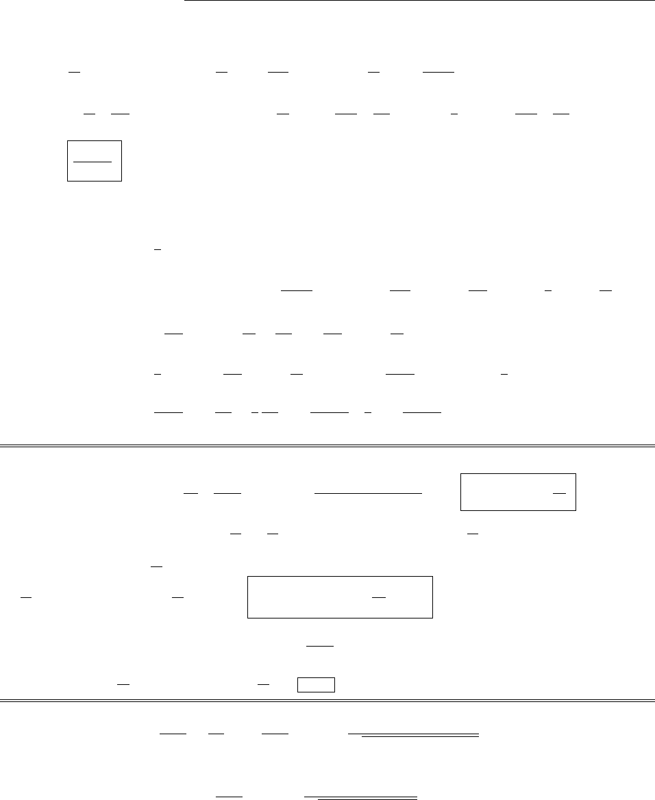
42 CHAPTER 2. ELECTROSTATICS
Method I :
W=✏0
2E2d⌧(Eq.2.45) = ✏0
2R
0kr2
4✏02
4⇡r2dr +✏0
21
RkR4
4✏0r22
4⇡r2dr
=4⇡✏0
2k
4✏02R
0
r6dr +R81
R
1
r2dr=⇡k2
8✏0R7
7+R81
r
1
R=⇡k2
8✏0R7
7+R7
=⇡k2R7
7✏0
.
Method II :
W=1
2⇢Vd⌧(Eq.2.43).
For r<R,V(r)=r
1
E·dl=R
1kR4
4✏0r2dr r
Rkr2
4✏0dr =k
4✏0R41
r
R
1
+r3
3
r
R
=k
4✏0R3+r3
3R3
3=k
3✏0R3r3
4.
)W=1
2R
0
(kr)k
3✏0R3r3
44⇡r2dr =2⇡k2
3✏0R
0R3r31
4r6dr
=2⇡k2
3✏0R3R4
41
4
R7
7=⇡k2R7
2·3✏06
7=⇡k2R7
7✏0
.X
Problem 2.50
E=rV=A@
@rer
rˆr =Ar()erer
r2ˆr =Aer(1 + r)ˆr
r2.
⇢=✏0r·E=✏0Aer(1 + r)r·ˆr
r2+ˆr
r2·rer(1 + r).Butr·ˆr
r2=4⇡3(r) (Eq. 1.99), and
er(1 + r)3(r)=3(r) (Eq. 1.88). Meanwhile,
rer(1 + r)=ˆr @
@rer(1 + r)=ˆr er(1 + r)+er=ˆr (2rer).
So ˆr
r2·rer(1 + r)=2
rer, and ⇢=✏0A4⇡3(r)2
rer.
Q=⇢d⌧=✏0A4⇡3(r)d⌧2er
r4⇡r2dr=✏0A4⇡24⇡1
0
rerdr.
But 1
0rerdr =1
2, so Q=4⇡✏0A12
2= zero.
Problem 2.51
V=1
4⇡✏0
r
da =
4⇡✏0R
02⇡
0
1
R2+s22Rs cos sdsd.
Let u⌘s/R. Then
V=2R
4⇡✏01
0⇡
0
u
1+u22ucos ddu.
c
2012 Pearson Education, Inc., Upper Saddle River, NJ. All rights reserved. This material is
protected under all copyright laws as they currently exist. No portion of this material may be
reproduced, in any form or by any means, without permission in writing from the publisher.

CHAPTER 2. ELECTROSTATICS 43
The (double) integral is a pure number; Mathematica says it is 2. So
V=R
⇡✏0
.
Problem 2.52
(a) Potential of +is V+=
2⇡✏0ln s+
a, where s+is distance from +(Prob. 2.22).
Potential of is V=+
2⇡✏0ln s
a, where sis distance from .
)Total V=
2⇡✏0
ln s
s+.
Now s+=(ya)2+z2, and s=(y+a)2+z2,so
V(x, y, z)=
2⇡✏0ln p(y+a)2+z2
p(ya)2+z2=
4⇡✏0
ln (y+a)2+z2
(ya)2+z2.
7
∴Total V=λ
2πϵ0
ln !s−
s+".
Now s+=#(y−a)2+z2, and s−=#(y+a)2+z2, so
V(x, y, z) = λ
2πϵ0ln !√(y+a)2+z2
√(y−a)2+z2"=λ
4πϵ0
ln $(y+a)2+z2
(y−a)2+z2%.
✲y
✻
z
−λ λ
(x, y, z)
a a
s−
s+
(b) Equipotentials are given by (y+a)2+z2
(y−a)2+z2=e(4πϵ0V0/λ)=k= constant. That is:
y2+ 2ay +a2+z2=k(y2−2ay +a2+z2)⇒y2(k−1) + z2(k−1) + a2(k−1) −2ay(k+ 1) = 0, or
y2+z2+a2−2ay &k+1
k−1'= 0. The equation for a circle, with center at (y0,0) and radius R, is
(y−y0)2+z2=R2, or y2+z2+ (y2
0−R2)−2yy0= 0.
Evidently the equipotentials are circles, with y0=a&k+1
k−1'and
a2=y2
0−R2⇒R2=y2
0−a2=a2&k+1
k−1'2
−a2=a2(k2+2k+1−k2+2k−1)
(k−1)2=a24k
(k−1)2, or
R=2a√k
|k−1|; or, in terms of V0:
y0=ae4πϵ0V0/λ+ 1
e4πϵ0V0/λ−1=ae2πϵ0V0/λ+e−2πϵ0V0/λ
e2πϵ0V0/λ−e−2πϵ0V0/λ=acoth !2πϵ0V0
λ".
R= 2ae2πϵ0V0/λ
e4πϵ0V0/λ−1=a2
(e2πϵ0V0/λ−e−2πϵ0V0/λ)=a
sinh (2πϵ0V0
λ)=acsch !2πϵ0V0
λ".
✲y
✻
z
λ−λy0
✒
R
Problem 2.48
(a) ∇2V=−ρ
ϵ0(Eq. 2.24), so d2V
dx2=−1
ϵ0
ρ.
(b) qV =1
2mv2→v=*2qV
m.
(c) dq =Aρdx ;dq
dt =aρdx
dt =Aρv=I(constant). (Note:ρ, hence also I, is negative.)
c
⃝2005 Pearson Education, Inc., Upper Saddle River, NJ. All rights reserved. This material is
protected under all copyright laws as they currently exist. No portion of this material may be
reproduced, in any form or by any means, without permission in writing from the publisher.
(b) Equipotentials are given by (y+a)2+z2
(ya)2+z2=e(4⇡✏0V0/)=k= constant. That is:
y2+2ay +a2+z2=k(y22ay +a2+z2))y2(k1) + z2(k1) + a2(k1) 2ay(k+ 1) = 0, or
y2+z2+a22ay k+1
k1= 0. The equation for a circle, with center at (y0,0) and radius R, is
(yy0)2+z2=R2, or y2+z2+(y2
0R2)2yy0= 0.
Evidently the equipotentials are circles, with y0=ak+1
k1and
a2=y2
0R2)R2=y2
0a2=a2k+1
k12a2=a2(k2+2k+1k2+2k1)
(k1)2=a24k
(k1)2, or
R=2apk
|k1|; or, in terms of V0:
y0=ae4⇡✏0V0/+1
e4⇡✏0V0/1=ae2⇡✏0V0/+e2⇡✏0V0/
e2⇡✏0V0/e2⇡✏0V0/=acoth 2⇡✏0V0
.
R=2ae2⇡✏0V0/
e4⇡✏0V0/1=a2
(e2⇡✏0V0/e2⇡✏0V0/)=a
sinh 2⇡✏0V0
=acsch 2⇡✏0V0
.
7
∴Total V=λ
2πϵ0
ln !s−
s+".
Now s+=#(y−a)2+z2, and s−=#(y+a)2+z2, so
V(x, y, z) = λ
2πϵ0ln !√(y+a)2+z2
√(y−a)2+z2"=λ
4πϵ0
ln $(y+a)2+z2
(y−a)2+z2%.
✲y
✻
z
−λ λ
(x, y, z)
a a
s−
s+
(b) Equipotentials are given by (y+a)2+z2
(y−a)2+z2=e(4πϵ0V0/λ)=k= constant. That is:
y2+ 2ay +a2+z2=k(y2−2ay +a2+z2)⇒y2(k−1) + z2(k−1) + a2(k−1) −2ay(k+ 1) = 0, or
y2+z2+a2−2ay &k+1
k−1'= 0. The equation for a circle, with center at (y0,0) and radius R, is
(y−y0)2+z2=R2, or y2+z2+ (y2
0−R2)−2yy0= 0.
Evidently the equipotentials are circles, with y0=a&k+1
k−1'and
a2=y2
0−R2⇒R2=y2
0−a2=a2&k+1
k−1'2
−a2=a2(k2+2k+1−k2+2k−1)
(k−1)2=a24k
(k−1)2, or
R=2a√k
|k−1|; or, in terms of V0:
y0=ae4πϵ0V0/λ+ 1
e4πϵ0V0/λ−1=ae2πϵ0V0/λ+e−2πϵ0V0/λ
e2πϵ0V0/λ−e−2πϵ0V0/λ=acoth !2πϵ0V0
λ".
R= 2ae2πϵ0V0/λ
e4πϵ0V0/λ−1=a2
(e2πϵ0V0/λ−e−2πϵ0V0/λ)=a
sinh (2πϵ0V0
λ)=acsch !2πϵ0V0
λ".
✲y
✻
z
λ−λy0
✒
R
Problem 2.48
(a) ∇2V=−ρ
ϵ0(Eq. 2.24), so d2V
dx2=−1
ϵ0
ρ.
(b) qV =1
2mv2→v=*2qV
m.
(c) dq =Aρdx ;dq
dt =aρdx
dt =Aρv=I(constant). (Note:ρ, hence also I, is negative.)
c
⃝2005 Pearson Education, Inc., Upper Saddle River, NJ. All rights reserved. This material is
protected under all copyright laws as they currently exist. No portion of this material may be
reproduced, in any form or by any means, without permission in writing from the publisher.
c
2012 Pearson Education, Inc., Upper Saddle River, NJ. All rights reserved. This material is
protected under all copyright laws as they currently exist. No portion of this material may be
reproduced, in any form or by any means, without permission in writing from the publisher.
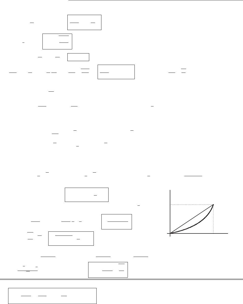
44 CHAPTER 2. ELECTROSTATICS
Problem 2.53
(a) r2V=⇢
✏0(Eq. 2.24), so d2V
dx2=1
✏0
⇢.
(b) qV =1
2mv2!v=2qV
m.
(c) dq =A⇢dx ;dq
dt =a⇢dx
dt =A⇢v=I(constant). (Note:⇢, hence also I, is negative.)
(d) d2V
dx2=1
✏0⇢=1
✏0
I
Av =I
✏0Am
2qV )d2V
dx2=V1/2, where =I
✏0Am
2q.
(Note: Iis negative,sois positive; qis positive.)
(e) Multiply by V0=dV
dx :
V0dV 0
dx =V1/2dV
dx )V0dV 0=V1/2dV )1
2V02=2V1/2+ constant.
But V(0) = V0(0) = 0 (cathode is at potential zero, and field at cathode is zero), so the constant is zero, and
V02=4V1/2)dV
dx =2
V1/4)V1/4dV =2
dx;
V1/4dV =2
dx )4
3V3/4=2
x+ constant.
But V(0) = 0, so this constant is also zero.
V3/4=3
2x, so V(x)=3
24/3
x4/3,or V(x)=9
42/3
x4/3=81I2m
32✏2
0A2q1/3
x4/3.
Interms of V0(instead of I): V(x)=V0x
d4/3(see graph).
Without space-charge, Vwould increase linearly: V(x)=V0x
d.
⇢=✏0
d2V
dx2=✏0V0
1
d4/3
4
3·1
3x2/3=4✏0V0
9(d2x)2/3.
v=2q
mpV=2qV0/m x
d2/3.
8
(d) d2V
dx2=−1
ϵ0ρ=−1
ϵ0
I
Av =−I
ϵ0A!m
2qV ⇒d2V
dx2=βV−1/2, where β=−I
ϵ0A!m
2q.
(Note: Iis negative, so βis positive; qis positive.)
(e) Multiply by V′=dV
dx :
V′dV ′
dx =βV−1/2dV
dx ⇒"V′dV ′=β"V−1/2dV ⇒1
2V′2= 2βV1/2+ constant.
But V(0) = V′(0) = 0 (cathode is at potential zero, and field at cathode is zero), so the constant is zero, and
V′2= 4βV1/2⇒dV
dx = 2#βV1/4⇒V−1/4dV = 2#βdx;
"V−1/4dV = 2#β"dx ⇒4
3V3/4= 2#βx+ constant.
But V(0) = 0, so this constant is also zero.
V3/4=3
2#βx, so V(x) = $3
2#β%4/3
x4/3,or V(x) = $9
4β%2/3
x4/3=$81I2m
32ϵ2
0A2q%1/3
x4/3.
Interms of V0(instead of I): V(x) = V0&x
d'4/3
(see graph).
Without space-charge, Vwould increase linearly: V(x) = V0(x
d).
ρ=−ϵ0
d2V
dx2=−ϵ0V0
1
d4/3
4
3
·
1
3x−2/3=−4ϵ0V0
9(d2x)2/3.
v=*2q
m√V=#2qV0/m &x
d'2/3
.✲x
✻
V
V0
d
without
with
(f) V(d) = V0=&81I2m
32ϵ2
0A2q'1/3
d4/3⇒V3
0=81md4
32ϵ2
0A2qI2;I2=32ϵ2
0A2q
81md4V3
0;
I=4√2ϵ0A√q
9√m d2V3/2
0=KV 3/2
0, where K=4ϵ0A
9d2*2q
m.
Problem 2.49
(a) E=1
4πϵ0"ρˆηˆη
ˆη
η2&1 + η
λ'e−η/λdτ.
(b) Yes. The field of a point charge at the origin is radial and symmetric, so ∇×E= 0, and hence this is also
true (by superposition) for any collection of charges.
(c) V=−"r
∞
E·dl=−1
4πϵ0
q"r
∞
1
r2&1 + r
λ'e−r/λdr
=1
4πϵ0
q"∞
r
1
r2&1 + r
λ'e−r/λdr =q
4πϵ0+"∞
r
1
r2e−r/λdr +1
λ"∞
r
1
re−r/λdr,.
c
⃝2005 Pearson Education, Inc., Upper Saddle River, NJ. All rights reserved. This material is
protected under all copyright laws as they currently exist. No portion of this material may be
reproduced, in any form or by any means, without permission in writing from the publisher.
(f) V(d)=V0=81I2m
32✏2
0A2q1/3d4/3)V3
0=81md4
32✏2
0A2qI2;I2=32✏2
0A2q
81md4V3
0;
I=4p2✏0Apq
9pmd
2V3/2
0=KV 3/2
0, where K=4✏0A
9d22q
m.
Problem 2.54
(a) E=1
4⇡✏0⇢ˆ
r
r
21+
r
e
r
/d⌧.
c
2012 Pearson Education, Inc., Upper Saddle River, NJ. All rights reserved. This material is
protected under all copyright laws as they currently exist. No portion of this material may be
reproduced, in any form or by any means, without permission in writing from the publisher.
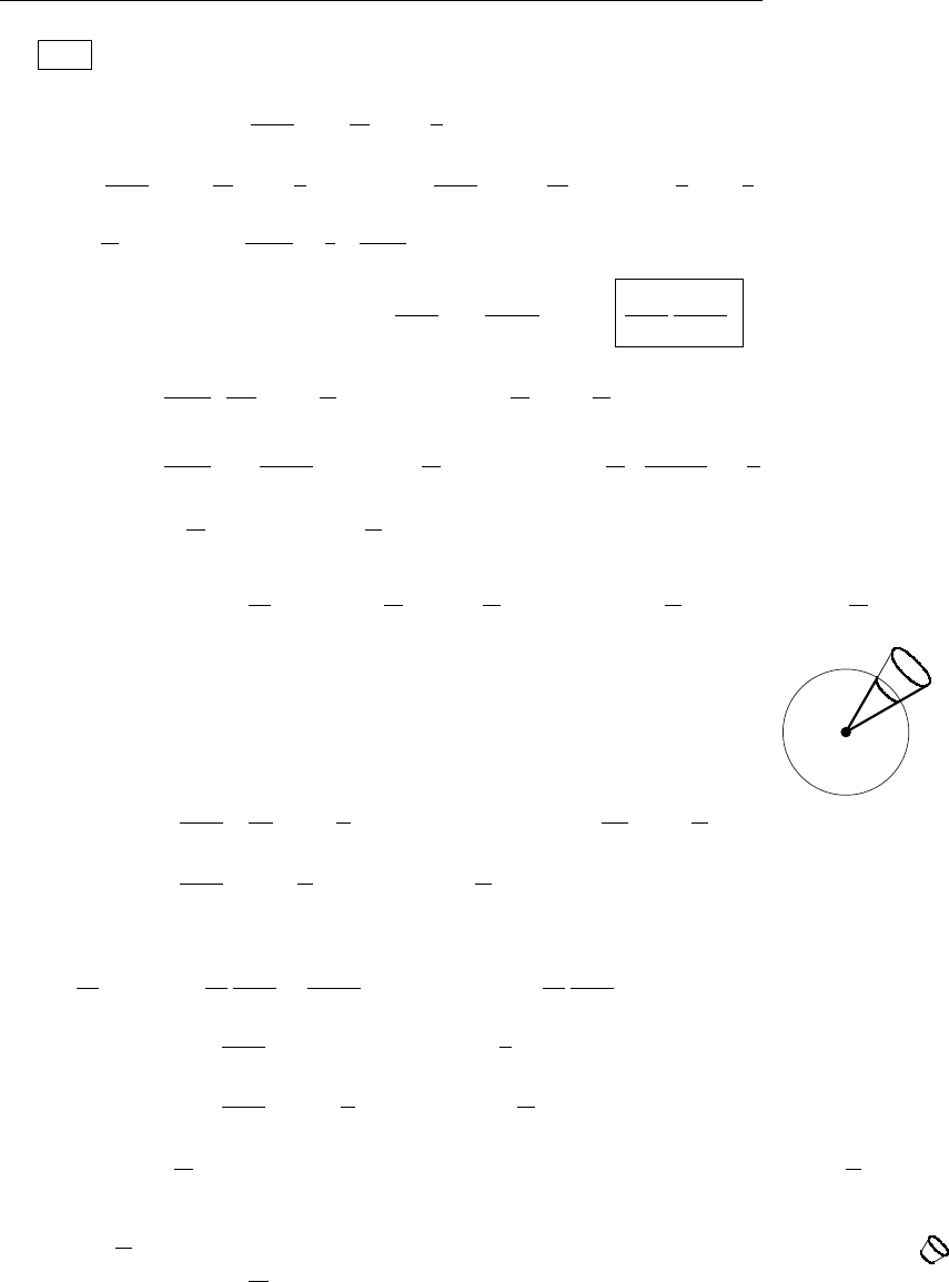
CHAPTER 2. ELECTROSTATICS 45
(b) Yes. The field of a point charge at the origin is radial and symmetric, so r⇥E=0, and hence this is
also true (by superposition) for any collection of charges.
(c) V=r
1
E·dl=1
4⇡✏0
qr
1
1
r21+ r
er/dr
=1
4⇡✏0
q1
r
1
r21+ r
er/dr =q
4⇡✏01
r
1
r2er/dr +1
1
r
1
rer/dr.
Now 1
r2er/dr =er/
r1
er/
rdr exactly right to kill the last term. Therefore
V(r)= q
4⇡✏0er/
r
1
r=q
4⇡✏0
er/
r.
(d) S
E·da=1
4⇡✏0
q1
R2
1+R
eR/4⇡R2
=q
✏01+R
eR/.
V
Vd⌧=q
4⇡✏0
R
0
er/
rr24⇡dr =q
✏0R
0
rer/dr =q
✏0er/
(1/)2r
1R
0
=2q
✏0eR/1+R
+1
.
)S
E·da+1
2V
Vd⌧=q
✏01+R
eR/1+R
eR/+1
=q
✏0
.qed
(e) Does the result in (d) hold for a nonspherical surface? Suppose we
make a “dent” in the sphere—pushing a patch (area R2sin ✓d✓d)
from radius Rout to radius S(area S2sin ✓d✓d).
9
Now !1
r2e−r/λdr =−e−r/λ
r−1
λ!e−r/λ
rdr ←− exactly right to kill the last term. Therefore
V(r) = q
4πϵ0"−e−r/λ
r####
∞
r$=q
4πϵ0
e−r/λ
r.
(d) %S
E·da=1
4πϵ0
!q1
R2
!&1 + R
λ'e−R/λ4π!R2
!=q
ϵ0&1 + R
λ'e−R/λ.
(V
V dτ=q
4πϵ0
!(R
0
e−r/λ
rr24π!dr =q
ϵ0(R
0
re−r/λdr =q
ϵ0)e−r/λ
(1/λ)2*−r
λ−1+,R
0
=λ2q
ϵ0-−e−R/λ&1 + R
λ'+ 1..
∴%S
E·da+1
λ2(V
V dτ=q
ϵ0-&1 + R
λ'e−R/λ−&1 + R
λ'e−R/λ+ 1.=q
ϵ0
.qed
(e) Does the result in (d) hold for a nonspherical surface? Suppose we
make a “dent” in the sphere—pushing a patch (area R2sin θdθdφ)
from radius Rout to radius S(area S2sin θdθdφ). q
RS
∆%E·da=q
4πϵ0-1
S2&1 + S
λ'e−S/λ(S2sin θdθdφ)−1
R2&1 + R
λ'e−R/λ(R2sin θdθdφ).
=q
4πϵ0)&1 + S
λ'e−S/λ−&1 + R
λ'e−R/λ,sin θdθdφ.
∆1
λ2(V dτ=1
λ2
q
4πϵ0(e−r/λ
rr2sin θdr dθdφ=1
λ2
q
4πϵ0
sin θdθdφ(S
R
re−r/λdr
=−q
4πϵ0
sin θdθdφ*e−r/λ*1 + r
λ++###
S
R
=−q
4πϵ0)&1 + S
λ'e−S/λ−&1 + R
λ'e−R/λ,sin θdθdφ.
So the change in 1
λ2!V dτexactly compensates for the change in /E·da, and we get 1
ϵ0qfor the total using
the dented sphere, just as we did with the perfect sphere. Any closed surface can be built up by successive
distortions of the sphere, so the result holds for all shapes. By superposition, if there are many charges inside,
the total is 1
ϵ0Qenc. Charges outside do not contribute (in the argument above we found that for this
volume /E·da+1
λ2!V dτ= 0—and, again, the sum is not changed by distortions of the surface, as long as q
remains outside. So the new “Gauss’s Law” holds for any charge configuration.
(f) In differential form, “Gauss’s law” reads: ∇·E+1
λ2V=1
ϵ0
ρ,or, putting it all in terms of E:
∇·E−1
λ2(E·dl=1
ϵ0
ρ.Since E=−∇V, this also yields “Poisson’s equation”: −∇2V+1
λ2V=1
ϵ0
ρ.
c
⃝2005 Pearson Education, Inc., Upper Saddle River, NJ. All rights reserved. This material is
protected under all copyright laws as they currently exist. No portion of this material may be
reproduced, in any form or by any means, without permission in writing from the publisher.
E·da=q
4⇡✏01
S21+S
eS/(S2sin ✓d✓d)1
R21+R
eR/(R2sin ✓d✓d)
=q
4⇡✏01+ S
eS/1+R
eR/sin ✓d✓d.
1
2Vd⌧=1
2
q
4⇡✏0er/
rr2sin ✓dr d✓d=1
2
q
4⇡✏0
sin ✓d✓dS
R
rer/dr
=q
4⇡✏0
sin ✓d✓der/1+ r
S
R
=q
4⇡✏01+ S
eS/1+R
eR/sin ✓d✓d.
So the change in 1
2Vd⌧exactly compensates for the change in E·da, and we get 1
✏0qfor the total using
the dented sphere, just as we did with the perfect sphere. Any closed surface can be built up by successive
distortions of the sphere, so the result holds for all shapes. By superposition, if there are many charges inside,
the total is 1
✏0Qenc. Charges outside do not contribute (in the argument above we found that
9
Now !1
r2e−r/λdr =−e−r/λ
r−1
λ!e−r/λ
rdr ←− exactly right to kill the last term. Therefore
V(r) = q
4πϵ0"−e−r/λ
r####
∞
r$=q
4πϵ0
e−r/λ
r.
(d) %S
E·da=1
4πϵ0
!q1
R2
!&1 + R
λ'e−R/λ4π!R2
!=q
ϵ0&1 + R
λ'e−R/λ.
(V
V dτ=q
4πϵ0
!(R
0
e−r/λ
rr24π!dr =q
ϵ0(R
0
re−r/λdr =q
ϵ0)e−r/λ
(1/λ)2*−r
λ−1+,R
0
=λ2q
ϵ0-−e−R/λ&1 + R
λ'+ 1..
∴%S
E·da+1
λ2(V
V dτ=q
ϵ0-&1 + R
λ'e−R/λ−&1 + R
λ'e−R/λ+ 1.=q
ϵ0
.qed
(e) Does the result in (d) hold for a nonspherical surface? Suppose we
make a “dent” in the sphere—pushing a patch (area R2sin θdθdφ)
from radius Rout to radius S(area S2sin θdθdφ). q
RS
∆%E·da=q
4πϵ0-1
S2&1 + S
λ'e−S/λ(S2sin θdθdφ)−1
R2&1 + R
λ'e−R/λ(R2sin θdθdφ).
=q
4πϵ0)&1 + S
λ'e−S/λ−&1 + R
λ'e−R/λ,sin θdθdφ.
∆1
λ2(V dτ=1
λ2
q
4πϵ0(e−r/λ
rr2sin θdr dθdφ=1
λ2
q
4πϵ0
sin θdθdφ(S
R
re−r/λdr
=−q
4πϵ0
sin θdθdφ*e−r/λ*1 + r
λ++###
S
R
=−q
4πϵ0)&1 + S
λ'e−S/λ−&1 + R
λ'e−R/λ,sin θdθdφ.
So the change in 1
λ2!V dτexactly compensates for the change in /E·da, and we get 1
ϵ0qfor the total using
the dented sphere, just as we did with the perfect sphere. Any closed surface can be built up by successive
distortions of the sphere, so the result holds for all shapes. By superposition, if there are many charges inside,
the total is 1
ϵ0Qenc. Charges outside do not contribute (in the argument above we found that for this
volume /E·da+1
λ2!V dτ= 0—and, again, the sum is not changed by distortions of the surface, as long as q
remains outside. So the new “Gauss’s Law” holds for any charge configuration.
(f) In differential form, “Gauss’s law” reads: ∇·E+1
λ2V=1
ϵ0
ρ,or, putting it all in terms of E:
∇·E−1
λ2(E·dl=1
ϵ0
ρ.Since E=−∇V, this also yields “Poisson’s equation”: −∇2V+1
λ2V=1
ϵ0
ρ.
c
⃝2005 Pearson Education, Inc., Upper Saddle River, NJ. All rights reserved. This material is
protected under all copyright laws as they currently exist. No portion of this material may be
reproduced, in any form or by any means, without permission in writing from the publisher.
for this volume E·da+1
2Vd⌧= 0—and, again, the sum is not changed by distortions of the surface, as
long as qremains outside). So the new “Gauss’s Law” holds for any charge configuration.
c
2012 Pearson Education, Inc., Upper Saddle River, NJ. All rights reserved. This material is
protected under all copyright laws as they currently exist. No portion of this material may be
reproduced, in any form or by any means, without permission in writing from the publisher.
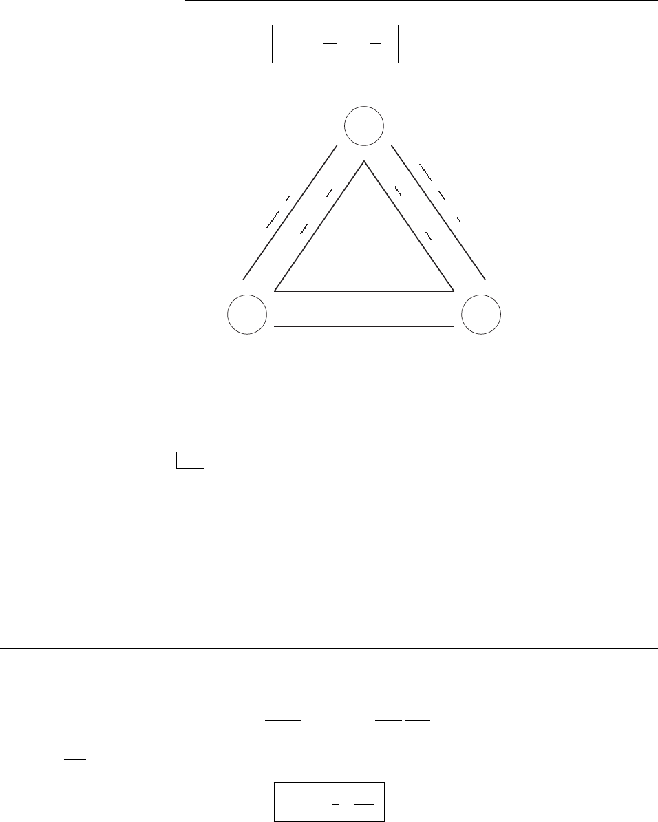
46 CHAPTER 2. ELECTROSTATICS
(f) In di↵erential form, “Gauss’s law” reads: r·E+1
2V=1
✏0
⇢,or, putting it all in terms of E:
r·E1
2E·dl=1
✏0
⇢.Since E=rV, this also yields “Poisson’s equation”: r2V+1
2V=1
✏0
⇢.
2
∆1
λ2!V dτ=1
λ2
q
4πϵ0!e−r/λ
rr2sin θdr dθdφ=1
λ2
q
4πϵ0
sin θdθdφ!S
R
re−r/λdr
=−q
4πϵ0
sin θdθdφ"e−r/λ"1 + r
λ##$
$
$
S
R
=−q
4πϵ0%&1 + S
λ'e−S/λ−&1 + R
λ'e−R/λ(sin θdθdφ.
So the change in 1
λ2)V dτexactly compensates for the change in *E·da, and we get 1
ϵ0qfor the total using
the dented sphere, just as we did with the perfect sphere. Any closed surface can be built up by successive
distortions of the sphere, so the result holds for all shapes. By superposition, if there are many charges inside,
the total is 1
ϵ0Qenc. Charges outside do not contribute (in the argument above we found that for this
volume *E·da+1
λ2)V dτ= 0—and, again, the sum is not changed by distortions of the surface, as long as q
remains outside. So the new “Gauss’s Law” holds for any charge configuration.
(f) In differential form, “Gauss’s law” reads: ∇·E+1
λ2V=1
ϵ0
ρ,or, putting it all in terms of E:
∇·E−1
λ2!E·dl=1
ϵ0
ρ.Since E=−∇V, this also yields “Poisson’s equation”: −∇2V+1
λ2V=1
ϵ0
ρ.
VE
ρ
✣
✢✲
✛
❪
❫
E=−∇V
V=−RE·dl
(∇2−1
λ2)V=−ρ
ϵ0
V=1
4πϵ0Rρe−/λdτ
∇·E−1
λ2RE·dl=ρ
ϵ0;∇×E=0
E=1
4πϵ0Rρ
2(1+λ)e−/λdτ
Problem 2.50
ρ=ϵ0∇·E=ϵ0
∂
∂x(ax) = ϵ0a(constant everywhere).
The same charge density would be compatible (as far as Gauss’s law is concerned) with E=ayˆy, for
instance, or E= (a
3)r, etc. The point is that Gauss’s law (and ∇×E= 0) by themselves do not determine
the field—like any differential equations, they must be supplemented by appropriate boundary conditions.
Ordinarily, these are so “obvious” that we impose them almost subconsciously (“Emust go to zero far from
the source charges”)—or we appeal to symmetry to resolve the ambiguity (“the field must be the same—in
magnitude—on both sides of an infinite plane of surface charge”). But in this case there are no natural
boundary conditions, and no persuasive symmetry conditions, to fix the answer. The question “What is the
electric field produced by a uniform charge density filling all of space?” is simply ill-posed: it does not give
c
⃝2005 Pearson Education, Inc., Upper Saddle River, NJ. All rights reserved. This material is
protected under all copyright laws as they currently exist. No portion of this material may be
reproduced, in any form or by any means, without permission in writing from the publisher.
r
r
r
r
r
ˆ
r
(g) Refer to ”Gauss’s law” in di↵erential form (f). Since Eis zero, inside a conductor (otherwise charge would
move, and in such a direction as to cancel the field), Vis constant (inside), and hence ⇢is uniform, throughout
the volume. Any “extra” charge must reside on the surface. (The fraction at the surface depends on , and
on the shape of the conductor.)
Problem 2.55
⇢=✏0r·E=✏0@
@x(ax)= ✏0a(constant everywhere).
The same charge density would be compatible (as far as Gauss’s law is concerned) with E=ayˆy , for
instance, or E=(
a
3)r, etc. The point is that Gauss’s law (and r⇥E=0) by themselves do not determine
the field—like any di↵erential equations, they must be supplemented by appropriate boundary conditions.
Ordinarily, these are so “obvious” that we impose them almost subconsciously (“Emust go to zero far from
the source charges”)—or we appeal to symmetry to resolve the ambiguity (“the field must be the same—in
magnitude—on both sides of an infinite plane of surface charge”). But in this case there are no natural
boundary conditions, and no persuasive symmetry conditions, to fix the answer. The question “What is the
electric field produced by a uniform charge density filling all of space?” is simply ill-posed: it does not give
us sufficient information to determine the answer. (Incidentally, it won’t help to appeal to Coulomb’s law
E=1
4⇡✏0⇢ˆ
r
r
2d⌧—the integral is hopelessly indefinite, in this case.)
Problem 2.56
Compare Newton’s law of universal gravitation to Coulomb’s law:
F=Gm1m2
r2ˆr ;F=1
4⇡✏0
q1q2
r2ˆr .
Evidently 1
4⇡✏0!Gand q!m. The gravitational energy of a sphere (translating Prob. 2.34) is therefore
Wgrav =3
5GM2
R.
c
2012 Pearson Education, Inc., Upper Saddle River, NJ. All rights reserved. This material is
protected under all copyright laws as they currently exist. No portion of this material may be
reproduced, in any form or by any means, without permission in writing from the publisher.
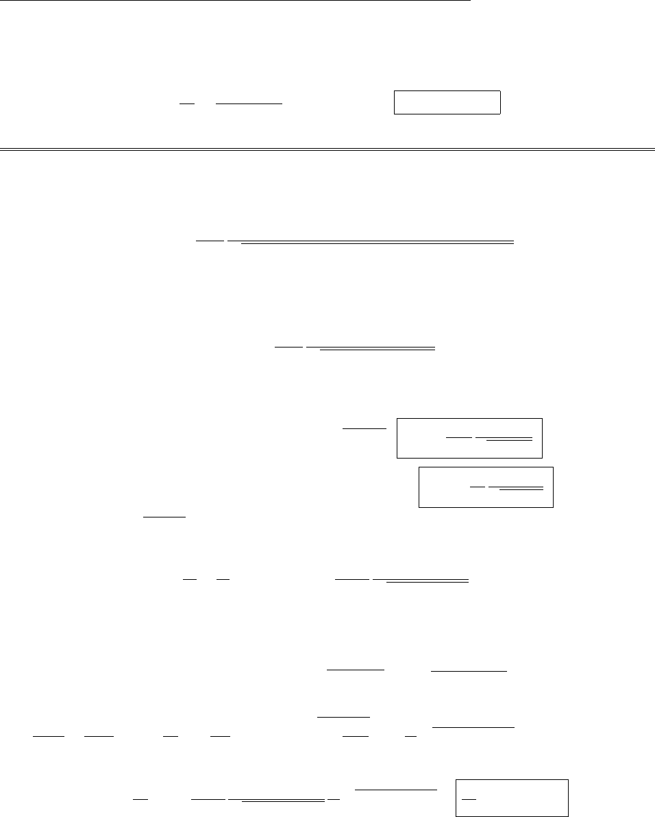
CHAPTER 2. ELECTROSTATICS 47
Now, G=6.67 ⇥1011 Nm
2/kg2, and for the sun M=1.99 ⇥1030 kg, R=6.96 ⇥108m, so the sun’s
gravitational energy is W=2.28 ⇥1041 J. At the current rate this energy would be dissipated in a time
t=W
P=2.28 ⇥1041
3.86 ⇥1026 =5.90 ⇥1014 s= 1.87 ⇥107years.
Problem 2.57
First eliminate z, using the formula for the ellipsoid:
(x, y)= Q
4⇡ab
1
c2(x2/a4)+c2(y2/b4)+1(x2/a2)(y2/b2).
Now (for parts (a) and (b)) set c!0, “squashing” the ellipsoid down to an ellipse in the xy plane:
(x, y)= Q
2⇡ab
1
1(x/a)2(y/b)2.
(I multiplied by 2 to count both surfaces.)
(a) For the circular disk, set a=b=Rand let r⌘x2+y2.(r)= Q
2⇡R
1
pR2r2.
(b) For the ribbon, let Q/2b⌘⇤, and then take the limit b!1:(x)= ⇤
2⇡
1
pa2x2.
(c) Let b=c,r⌘y2+z2, making an ellipsoid of revolution:
x2
a2+r2
c2=1,with =Q
4⇡ac2
1
x2/a4+r2/c4.
The charge on a ring of width dx is
dq =2⇡r ds, where ds =dx2+dr2=dx1+(dr/dx)2.
Now 2xdx
a2+2r dr
c2=0)dr
dx =c2x
a2r,sods =dx1+c4x2
a4r2=dxc2
rx2/a4+r2/c4. Thus
(x)= dq
dx =2⇡rQ
4⇡ac2
1
x2/a4+r2/c4
c2
rx2/a4+r2/c4=Q
2a.(Constant!)
c
2012 Pearson Education, Inc., Upper Saddle River, NJ. All rights reserved. This material is
protected under all copyright laws as they currently exist. No portion of this material may be
reproduced, in any form or by any means, without permission in writing from the publisher.

48 CHAPTER 2. ELECTROSTATICS
Problem 2.58
b
x
y
rq
(0,-a)
( , )
a
_
2
a
_
2
( ,- )
a
_
2
a
_
2
÷3
÷3
(a) One such point is on the xaxis (see diagram) at x=r. Here the field is
Ex=q
4⇡✏01
(a+r)22cos ✓
b2=0,or 2 cos ✓
b2=1
(a+r)2.
Now,
cos ✓=(a/2) r
b;b2=a
2r2+p3
2a2
=(a2ar +r2).
Therefore
2[(a/2) r]
(a2ar +r2)3/2=1
(a+r)2.To simplify,let r
a⌘u:
(1 2u)
(1 u+u2)3/2=1
(1 + u)2,or (1 2u)2(1 + u)4=(1u+u2)3.
c
2012 Pearson Education, Inc., Upper Saddle River, NJ. All rights reserved. This material is
protected under all copyright laws as they currently exist. No portion of this material may be
reproduced, in any form or by any means, without permission in writing from the publisher.

CHAPTER 2. ELECTROSTATICS 49
Multiplying out each side:
16u24u3+9u4+ 12u5+4u6=13u+6u27u3+6u43u5+u6,
or
3u12u2+3u3+3u4+ 15u5+3u6=0.
u= 0 is a solution (of course—the center of the triangle); factoring out 3uwe are left with a quintic equation:
14u+u2+u3+5u4+u5=0.
According to Mathematica, this has two complex roots, and one negative root. The two remaining solutions are
u=0.284718 and u=0.626691. The latter is outside the triangle, and clearly spurious. So r=0.284718 a.
(The other two places where E=0are at the symmetrically located points, of course.)
b
x
y
r
q
+_
q
+_
b
( )
a
_
÷2
a
_
÷2
,
(b) For the square:
Ex=q
4⇡✏02cos ✓+
b2
+2cos ✓
b2
=0 )cos ✓+
b2
+
=cos ✓
b2
,
where
cos ✓±=(a/p2) ±r
b±
;b2
±=a
p22
+a
p2±r2
=a2±p2ar +r2.
Thus
(a/p2) + r
(a2+p2ar +r2)3/2=(a/p2) r
(a2p2ar +r2)3/2.
To simplify, let w⌘p2r/a; then
1+w
(2 + 2w+w2)3/2=1w
(2 2w+w2)3/2,or (1 + w)2(2 2w+w2)3= (1 w)2(2 + 2w+w2)3.
Multiplying out the left side:
88w4w2+ 16w310w42w5+7w64w7+w8= (same thing with w!w).
c
2012 Pearson Education, Inc., Upper Saddle River, NJ. All rights reserved. This material is
protected under all copyright laws as they currently exist. No portion of this material may be
reproduced, in any form or by any means, without permission in writing from the publisher.

50 CHAPTER 2. ELECTROSTATICS
The even powers cancel, leaving
8w16w3+2w5+4w7=0,or 4 8v+v2+2v3=0,
where v⌘w2. According to Mathematica, this cubic equation has one negative root, one root that is spurious
(the point lies outside the square), and v=0.598279, which yields
r=v
2a= 0.546936 a .
b
x
y
r
q
c
f
a
(a cos(p/5), a sin(p/5))
(-a cos(2p/5), a sin(2p/5))
For the pentagon:
Ex=q
4⇡✏01
(a+r)2+2cos ✓
b22cos
c2=0,
where
cos ✓=acos(2⇡/5) + r
b,cos =acos(⇡/5) r
c;
b2=[acos(2⇡/5) + r]2+[asin(2⇡/5)]2=a2+r2+2ar cos(2⇡/5),
c2=[acos(⇡/5) r]2+[asin(⇡/5)]2=a2+r22ar cos(⇡/5).
1
(a+r)2+2 r+acos(2⇡/5)
[a2+r2+2ar cos(2⇡/5)]3/2+2 racos(⇡/5)
[a2+r22ar cos(⇡/5)]3/2=0.
Mathematica gives the solution r=0.688917 a.
For an n-sided regular polygon there are evidently nsuch points, lying on the radial spokes that bisect
the sides; their distance from the center appears to grow monotonically with n:r(3) = 0.285, r(4) = 0.547,
r(5) = 0.689, . . . . As n!1they fill out a circle that (in the limit) coincides with the ring of charge itself.
Problem 2.59 The theorem is false. For example, suppose the conductor is a neutral sphere and the external
field is due to a nearby positive point charge q. A negative charge will be induced on the near side of the sphere
(and a positive charge on the far side), so the force will be attractive (toward q). If we now reverse the sign of
q, the induced charges will also reverse, but the force will still be attractive.
If the external field is uniform, then the net force on the induced charges is zero, and the total force on the
conductor is QEe, which does switch signs if Eeis reversed. So the “theorem” is valid in this very special case.
c
2012 Pearson Education, Inc., Upper Saddle River, NJ. All rights reserved. This material is
protected under all copyright laws as they currently exist. No portion of this material may be
reproduced, in any form or by any means, without permission in writing from the publisher.

CHAPTER 2. ELECTROSTATICS 51
Problem 2.60 The initial configuration consists of a point charge qat the center, qinduced on the inner
surface, and +qon the outer surface. What is the energy of this configuration? Imagine assembling it piece-by-
piece. First bring in qand place it at the origin—this takes no work. Now bring in qand spread it over the
surface at a—using the method in Prob. 2.35, this takes work q2/(8⇡✏0a). Finally, bring in +qand spread it
over the surface at b—this costs q2/(8⇡✏0b). Thus the energy of the initial configuration is
Wi=q2
8⇡✏01
a1
b.
The final configuration is a neutral shell and a distant point charge—the energy is zero. Thus the work
necessary to go from the initial to the final state is
W=WfWi=q2
8⇡✏01
a1
b.
Problem 2.61
r
j
Rx
y
(2pj/n)
R
Suppose the npoint charges are evenly spaced around the circle, with the jth particle at angle j(2⇡/n).
According to Eq. 2.42, the energy of the configuration is
Wn=n1
2qV,
where Vis the potential due to the (n1) other charges, at charge # n(on the xaxis).
V=1
4⇡✏0
q
n1
j=1
1
r
j
,
r
j=2Rsin j⇡
n
(see the figure). So
Wn=q2
4⇡✏0R
n
4
n1
j=1
1
sin(j⇡/n)=q2
4⇡✏0R⌦n.
c
2012 Pearson Education, Inc., Upper Saddle River, NJ. All rights reserved. This material is
protected under all copyright laws as they currently exist. No portion of this material may be
reproduced, in any form or by any means, without permission in writing from the publisher.

52 CHAPTER 2. ELECTROSTATICS
Mathematica says
⌦10 =10
4
9
j=1
1
sin(j⇡/10) = 38.6245
⌦11 =11
4
10
j=1
1
sin(j⇡/11) = 48.5757
⌦12 =12
4
11
j=1
1
sin(j⇡/12) = 59.8074
If (n1) charges are on the circle (energy ⌦n1q2/4⇡✏0R), and the nth is at the center, the total energy is
Wn=[⌦n1+(n1)] q2
4⇡✏0R.
For
n=11: ⌦10 + 10 = 38.6245 + 10 = 48.6245 >⌦11
n=12: ⌦11 + 11 = 48.5757 + 11 = 59.5757 <⌦12
Thus a lower energy is achieved for 11 charges if they are all at the rim, but for 12 it is better to put one at
the center.
c
2012 Pearson Education, Inc., Upper Saddle River, NJ. All rights reserved. This material is
protected under all copyright laws as they currently exist. No portion of this material may be
reproduced, in any form or by any means, without permission in writing from the publisher.

CHAPTER 3. POTENTIAL 53
Chapter 3
Potential
Problem 3.1
The argument is exactly the same as in Sect. 3.1.4, except that since z<R,pz2+R22zR =(Rz),
instead of (zR). Hence Vave =q
4⇡✏0
1
2zR [(z+R)(Rz)] = 1
4⇡✏0
q
R. If there is more than one charge
inside the sphere, the average potential due to interior charges is 1
4⇡✏0
Qenc
R,and the average due to exterior
charges is Vcenter,soVave =Vcenter +Qenc
4⇡✏0R.X
Problem 3.2
A stable equilibrium is a point of local minimum in the potential energy. Here the potential energy is qV .
But we know that Laplace’s equation allows no local minima for V. What looks like a minimum, in the figure,
must in fact be a saddle point, and the box “leaks” through the center of each face.
Problem 3.3
Laplace’s equation in spherical coordinates, for Vdependent only on r, reads:
r2V=1
r2
d
dr r2dV
dr =0)r2dV
dr =c(constant) )dV
dr =c
r2)V=c
r+k.
Example: potential of a uniformly charged sphere.
In cylindrical coordinates: r2V=1
s
d
ds sdV
ds =0)sdV
ds =c)dV
ds =c
s)V=cln s+k.
Example: potential of a long wire.
Problem 3.4
Refer to Fig. 3.3, letting ↵be the angle between
r
and the zaxis. Obviously, Eave points in the ˆz
direction, so
Eave =1
4⇡R2Eda =ˆz 1
4⇡R2
q
4⇡✏01
r
2cos ↵da.
By the law of cosines,
R2=z2+
r
22
r
zcos ↵)cos ↵=z2+
r
2R2
2
r
z,
r
2=R2+z22Rz cos ✓)cos ↵
r
2=z2+
r
2R2
2z
r
3=zRcos ✓
(R2+z22Rz cos ✓)3/2.
c
2012 Pearson Education, Inc., Upper Saddle River, NJ. All rights reserved. This material is
protected under all copyright laws as they currently exist. No portion of this material may be
reproduced, in any form or by any means, without permission in writing from the publisher.

54 CHAPTER 3. POTENTIAL
Eave =ˆz q
16⇡2R2✏0zRcos ✓
(R2+z22Rz cos ✓)3/2R2sin ✓d✓d
=qˆz
8⇡✏0⇡
0
zRcos ✓
(R2+z22Rz cos ✓)3/2sin ✓d✓=qˆz
8⇡✏01
1
zRu
(R2+z22Rzu)3/2du
(where u⌘cos ✓). The integral is
I=1
RpR2+z22Rzu
1
11
2Rz2R2+z22Rzu +R2+z2
pR2+z22Rzu
1
1
=1
R1
|zR|1
z+R1
2Rz2|zR|(z+R)+(R2+z2)1
|zR|1
z+R.
(a) If z>R,
I=1
R1
zR1
z+R1
2Rz2(zR)(z+R)+(R2+z2)1
zR1
z+R
=1
R2R
z2R21
2Rz22R+(R2+z2)2R
z2R2=2
z2.
So
Eave =1
4⇡✏0
q
z2ˆz ,
the same as the field at the center. By superposition the same holds for any collection of charges outside the
sphere.
(b) If z<R,
I=1
R1
Rz1
z+R1
2Rz2(Rz)(z+R)+(R2+z2)1
Rz1
z+R
=1
R2z
R2z21
2Rz22z+(R2+z2)2z
R2z2=0.
So
Eave =0.
By superposition the same holds for any collection of charges inside the sphere.
Problem 3.5
Same as proof of second uniqueness theorem, up to the equation SV3E3·da=V(E3)2d⌧. But on
each surface, either V3= 0 (if Vis specified on the surface), or else E3?= 0 (if @V
@n=E?is specified). So
V(E3)2= 0, and hence E2=E1. qed
Problem 3.6
Putting U=T=V3into Green’s identity:
VV3r2V3+rV3·rV3d⌧=S
V3rV3·da.But r2V3=r2V1r2V2=⇢
✏0
+⇢
✏0
= 0, and rV3=E3.
So V
E2
3d⌧=S
V3E3·da, and the rest is the same as before.
Problem 3.7
Place image charges +2qat z=dand qat z=3d. Total force on +qis
F=q
4⇡✏02q
(2d)2+2q
(4d)2+q
(6d)2ˆz =q2
4⇡✏0d21
2+1
81
36ˆz =1
4⇡✏029q2
72d2ˆz .
c
2012 Pearson Education, Inc., Upper Saddle River, NJ. All rights reserved. This material is
protected under all copyright laws as they currently exist. No portion of this material may be
reproduced, in any form or by any means, without permission in writing from the publisher.

CHAPTER 3. POTENTIAL 55
Problem 3.8
(a) From Fig. 3.13:
r
=pr2+a22ra cos ✓;
r
0=pr2+b22rb cos ✓.Therefore:
q0
r
0=R
a
q
pr2+b22rb cos ✓(Eq.3.15),while b=R2
a(Eq.3.16).
=q
a
Rr2+R4
a22rR2
acos ✓
=q
ar
R2+R22ra cos ✓
.
Therefore:
V(r, ✓)= 1
4⇡✏0q
r
+q0
r
0=q
4⇡✏01
pr2+a22ra cos ✓1
R2+(ra/R)22ra cos ✓.
Clearly, when r=R,V!0.
(b) =✏0@V
@n(Eq. 2.49). In this case, @V
@n=@V
@rat the point r=R. Therefore,
(✓)=✏0q
4⇡✏01
2(r2+a22ra cos ✓)3/2(2r2acos ✓)
+1
2R2+(ra/R)22ra cos ✓3/2a2
R22r2acos ✓r=R
=q
4⇡(R2+a22Ra cos ✓)3/2(Racos ✓)+R2+a22Ra cos ✓3/2a2
Racos ✓
=q
4⇡(R2+a22Ra cos ✓)3/2Racos ✓a2
R+acos ✓
=q
4⇡R(R2a2)(R2+a22Ra cos ✓)3/2.
qinduced =da =q
4⇡R(R2a2)(R2+a22Ra cos ✓)3/2R2sin ✓d✓d
=q
4⇡R(R2a2)2⇡R21
Ra(R2+a22Ra cos ✓)1/2
⇡
0
=q
2a(a2R2)1
pR2+a2+2Ra 1
pR2+a22Ra.
But a>R(else qwould be inside),so R2+a22Ra =aR.
=q
2a(a2R2)1
(a+R)1
(aR)=q
2a[(aR)(a+R)] = q
2a(2R)
=qR
a=q0.
(c) The force on q, due to the sphere, is the same as the force of the image charge q0, to wit:
F=1
4⇡✏0
qq0
(ab)2=1
4⇡✏0R
aq21
(aR2/a)2=1
4⇡✏0
q2Ra
(a2R2)2.
c
2012 Pearson Education, Inc., Upper Saddle River, NJ. All rights reserved. This material is
protected under all copyright laws as they currently exist. No portion of this material may be
reproduced, in any form or by any means, without permission in writing from the publisher.

56 CHAPTER 3. POTENTIAL
To bring qin from infinity to a, then, we do work
W=q2R
4⇡✏0
a
1
a
(a2R2)2da =q2R
4⇡✏01
2
1
(a2R2)
a
1
=1
4⇡✏0
q2R
2(a2R2).
Problem 3.9
4CHAPTER 3. SPECIAL TECHNIQUES
(c) The force on q, due to the sphere, is the same as the force of the image charge q′, to wit:
F=1
4πϵ0
qq′
(a−b)2=1
4πϵ0!−
R
aq2"1
(a−R2/a)2=−
1
4πϵ0
q2Ra
(a2−R2)2.
To bring qin from infinity to a, then, we do work
W=q2R
4πϵ0
a
#
∞
a
(a2−R2)2da =q2R
4πϵ0$−
1
2
1
(a2−R2)%&&&&
a
∞
=−
1
4πϵ0
q2R
2(a2−R2).
Problem 3.8
q′′ q′q
'() *
a
a−b
)*' (
Place a second image charge, q′′, at the center of the sphere;
this will not alter the fact that the sphere is an equipotential,
but merely increase that potential from zero to V0=1
4πϵ0
q′′
R;
q′′ = 4πϵ0V0Rat center of sphere.
For a neutral sphere, q′+q′′ = 0.
F=1
4πϵ0
q!q′′
a2+q′
(a−b)2"=qq′
4πϵ0!−
1
a2+1
(a−b)2"
=qq′
4πϵ0
b(2a−b)
a2(a−b)2=q(−Rq/a)
4πϵ0
(R2/a)(2a−R2/a)
a2(a−R2/a)2
=−
q2
4πϵ0!R
a"3(2a2−R2)
(a2−R2)2.
(Drop the minus sign, because the problem asks for the force of attraction.)
Problem 3.9
✲x
✻
z
✣y
λ
✲y
✻
z
+
−
d
d
(y, z)s+
s−
(a) Image problem: λabove, −λbelow. Potential was found in Prob. 2.47:
V(y, z) = 2λ
4πϵ0
ln(s−/s+) = λ
4πϵ0
ln(s2
−/s2
+)
=λ
4πϵ0
ln +y2+ (z+d)2
y2+ (z−d)2,
(b) σ=−ϵ0
∂V
∂n. Here ∂V
∂n=∂V
∂z, evaluated at z= 0.
σ(y) = −ϵ0
λ
4πϵ0+1
y2+ (z+d)22(z+d)−
1
y2+ (z−d)22(z−d),&&&&z=0
=−
2λ
4π+d
y2+d2
−
−d
y2+d2,=−
λd
π(y2+d2).
Check: Total charge induced on a strip of width lparallel to the yaxis:
qind =−
lλd
π
∞
#
−∞
1
y2+d2dy =−
lλd
π$1
dtan−1-y
d.%&&&&
∞
−∞
=−
lλd
π/π
2
−-−
π
2.0
=−λl. Therefore λind =−λ,as it should be.
c
⃝2005 Pearson Education, Inc., Upper Saddle River, NJ. All rights reserved. This material is
protected under all copyright laws as they currently exist. No portion of this material may be
reproduced, in any form or by any means, without permission in writing from the publisher.
Place a second image charge, q00, at the center of the sphere;
this will not alter the fact that the sphere is an equipotential,
but merely increase that potential from zero to V0=1
4⇡✏0
q00
R;
q00 =4⇡✏0V0Rat center of sphere.
For a neutral sphere, q0+q00 = 0.
F=1
4⇡✏0
qq00
a2+q0
(ab)2=qq0
4⇡✏01
a2+1
(ab)2
=qq0
4⇡✏0
b(2ab)
a2(ab)2=q(Rq/a)
4⇡✏0
(R2/a)(2aR2/a)
a2(aR2/a)2
=q2
4⇡✏0R
a3(2a2R2)
(a2R2)2.
(Drop the minus sign, because the problem asks for the force of attraction.)
Problem 3.10
(a) Image problem: above, below. Potential was found in Prob. 2.52:
2CHAPTER 3. SPECIAL TECHNIQUES
Chapter 1
Special Techniques
Problem 3.9
✲x
✻
z
✣y
λ
c
⃝2005 Pearson Education, Inc., Upper Saddle River, NJ. All rights reserved. This material is
protected under all copyright laws as they currently exist. No portion of this material may be
reproduced, in any form or by any means, without permission in writing from the publisher.
4CHAPTER 3. SPECIAL TECHNIQUES
(c) The force on q, due to the sphere, is the same as the force of the image charge q′, to wit:
F=1
4πϵ0
qq′
(a−b)2=1
4πϵ0!−
R
aq2"1
(a−R2/a)2=−
1
4πϵ0
q2Ra
(a2−R2)2.
To bring qin from infinity to a, then, we do work
W=q2R
4πϵ0
a
#
∞
a
(a2−R2)2da =q2R
4πϵ0$−
1
2
1
(a2−R2)%&&&&
a
∞
=−
1
4πϵ0
q2R
2(a2−R2).
Problem 3.8
q′′ q′q
'() *
a
a−b
)*' (
Place a second image charge, q′′, at the center of the sphere;
this will not alter the fact that the sphere is an equipotential,
but merely increase that potential from zero to V0=1
4πϵ0
q′′
R;
q′′ = 4πϵ0V0Rat center of sphere.
For a neutral sphere, q′+q′′ = 0.
F=1
4πϵ0
q!q′′
a2+q′
(a−b)2"=qq′
4πϵ0!−
1
a2+1
(a−b)2"
=qq′
4πϵ0
b(2a−b)
a2(a−b)2=q(−Rq/a)
4πϵ0
(R2/a)(2a−R2/a)
a2(a−R2/a)2
=−
q2
4πϵ0!R
a"3(2a2−R2)
(a2−R2)2.
(Drop the minus sign, because the problem asks for the force of attraction.)
Problem 3.9
✲x
✻
z
✣y
λ
✲y
✻
z
+
−
d
d
(y, z)s+
s−
(a) Image problem: λabove, −λbelow. Potential was found in Prob. 2.47:
V(y, z) = 2λ
4πϵ0
ln(s−/s+) = λ
4πϵ0
ln(s2
−/s2
+)
=λ
4πϵ0
ln +y2+ (z+d)2
y2+ (z−d)2,
(b) σ=−ϵ0
∂V
∂n. Here ∂V
∂n=∂V
∂z, evaluated at z= 0.
σ(y) = −ϵ0
λ
4πϵ0+1
y2+ (z+d)22(z+d)−
1
y2+ (z−d)22(z−d),&&&&z=0
=−
2λ
4π+d
y2+d2
−
−d
y2+d2,=−
λd
π(y2+d2).
Check: Total charge induced on a strip of width lparallel to the yaxis:
qind =−
lλd
π
∞
#
−∞
1
y2+d2dy =−
lλd
π$1
dtan−1-y
d.%&&&&
∞
−∞
=−
lλd
π/π
2
−-−
π
2.0
=−λl. Therefore λind =−λ,as it should be.
c
⃝2005 Pearson Education, Inc., Upper Saddle River, NJ. All rights reserved. This material is
protected under all copyright laws as they currently exist. No portion of this material may be
reproduced, in any form or by any means, without permission in writing from the publisher.
V(y, z)= 2
4⇡✏0
ln(s/s+)=
4⇡✏0
ln(s2
/s2
+)
=
4⇡✏0
ln y2+(z+d)2
y2+(zd)2
(b) =✏0
@V
@n. Here @V
@n=@V
@z, evaluated at z= 0.
(y)=✏0
4⇡✏01
y2+(z+d)22(z+d)1
y2+(zd)22(zd)z=0
=2
4⇡d
y2+d2d
y2+d2=d
⇡(y2+d2).
Check: Total charge induced on a strip of width lparallel to the yaxis:
qind =ld
⇡
1
1
1
y2+d2dy =ld
⇡1
dtan1y
d
1
1
=ld
⇡⇡
2⇡
2
=l. Therefore ind =,as it should be.
c
2012 Pearson Education, Inc., Upper Saddle River, NJ. All rights reserved. This material is
protected under all copyright laws as they currently exist. No portion of this material may be
reproduced, in any form or by any means, without permission in writing from the publisher.

CHAPTER 3. POTENTIAL 57
Problem 3.11
The image configuration is as shown.
V(x, y)= q
4⇡✏01
(xa)2+(yb)2+z2+1
(x+a)2+(y+b)2+z2
1
(x+a)2+(yb)2+z21
(xa)2+(y+b)2+z2.
CHAPTER 3. SPECIAL TECHNIQUES 5
Problem 3.10
The image configuration is as shown.
V(x, y) = q
4πϵ0!1
"(x−a)2+ (y−b)2+z2+1
"(x+a)2+ (y+b)2+z2
−1
"(x+a)2+ (y−b)2+z2−1
"(x−a)2+ (y+b)2+z2#.
✲x
✻
y
q−q
q−q
For this to work, θmust be and integer divisor of 180◦. Thus 180◦, 90◦, 60◦, 45◦, etc., are OK, but no
others. It works for 45◦, say, with the charges as shown.
(Note the strategy: to make the xaxis an equipotential (V= 0),
you place the image charge (1) in the reflection point. To make the
45◦line an equipotential, you place charge (2) at the image point.
But that screws up the xaxis, so you must now insert image (3) to
balance (2). Moreover, to make the 45◦line V= 0 you also need (4),
to balance (1). But now, to restore the xaxis to V= 0 you need (5)
to balance (4), and so on.
✲x
45◦line
+
−(1)
−
(2)
+
(4)
−
+
−
(5)
+
(3)
why it works for θ= 45◦
✲x
■
135◦line
+
(0)
−
(1)
−(2)
+(3)
⇐
No good
why it doesn’t work for θ= 135◦
The reason this doesn’t work for arbitrary angles is that you are even-
tually forced to place an image charge within the original region of
interest, and that’s not allowed—all images must go outside the re-
gion, or you’re no longer dealing with the same problem at all.)
Problem 3.11
From Prob. 2.47 (with y0→d): V=λ
4πϵ0
ln $(x+a)2+y2
(x−a)2+y2%,where a2=y02−R2⇒a=√d2−R2,
and
&acoth(2πϵ0V0/λ) = d
acsch(2πϵ0V0/λ) = R'⇒(dividing) d
R= cosh (2πϵ0V0
λ),or λ=2πϵ0V0
cosh−1(d/R).
Problem 3.12
V(x, y) =
∞
*
n=1
Cne−nπx/a sin(nπy/a) (Eq.3.30),where Cn=2
a
a
+
0
V0(y) sin(nπy/a)dy (Eq.3.34).
In this case V0(y) = &+V0,for 0 < y < a/2
−V0,for a/2< y < a '.Therefore,
Cn=2
aV0⎧
⎪
⎨
⎪
⎩
a/2
+
0
sin(nπy/a)dy −
a
+
a/2
sin(nπy/a)dy⎫
⎪
⎬
⎪
⎭
=2V0
a!−cos(nπy/a)
(nπ/a)3333
a/2
0
+cos(nπy/a)
(nπ/a)3333
a
a/2#
=2V0
nπ4−cos 5nπ
26+ cos(0) + cos(nπ)−cos 5nπ
267=2V0
nπ41 + (−1)n−2 cos 5nπ
267.
c
⃝2005 Pearson Education, Inc., Upper Saddle River, NJ. All rights reserved. This material is
protected under all copyright laws as they currently exist. No portion of this material may be
reproduced, in any form or by any means, without permission in writing from the publisher.
F=q2
4⇡✏01
(2a)2ˆx 1
(2b)2ˆy +1
(2pa2+b2)2[cos ✓ˆx + sin ✓ˆy ],
where cos ✓=a/pa2+b2,sin ✓=b/pa2+b2.
F=q2
16⇡✏0 a
(a2+b2)3/21
a2ˆx +b
(a2+b2)3/21
b2ˆy .
W=1
2
1
4⇡✏0q2
(2a)+q2
(2b)+q2
(2pa2+b2)=q2
16⇡✏01
pa2+b21
a1
b.
For this to work, ✓must be an integer divisor of 180. Thus 180, 90, 60, 45, etc., are OK, but no
others. It works for 45, say, with the charges as shown.
(Note the strategy: to make the xaxis an equipotential (V= 0),
you place the image charge (1) in the reflection point. To make the
45line an equipotential, you place charge (2) at the image point.
But that screws up the xaxis, so you must now insert image (3) to
balance (2). Moreover, to make the 45line V= 0 you also need (4),
to balance (1). But now, to restore the xaxis to V= 0 you need (5)
to balance (4), and so on.
CHAPTER 3. SPECIAL TECHNIQUES 5
Problem 3.10
The image configuration is as shown.
V(x, y) = q
4πϵ0!1
"(x−a)2+ (y−b)2+z2+1
"(x+a)2+ (y+b)2+z2
−1
"(x+a)2+ (y−b)2+z2−1
"(x−a)2+ (y+b)2+z2#.
✲x
✻
y
q−q
q−q
For this to work, θmust be and integer divisor of 180◦. Thus 180◦, 90◦, 60◦, 45◦, etc., are OK, but no
others. It works for 45◦, say, with the charges as shown.
(Note the strategy: to make the xaxis an equipotential (V= 0),
you place the image charge (1) in the reflection point. To make the
45◦line an equipotential, you place charge (2) at the image point.
But that screws up the xaxis, so you must now insert image (3) to
balance (2). Moreover, to make the 45◦line V= 0 you also need (4),
to balance (1). But now, to restore the xaxis to V= 0 you need (5)
to balance (4), and so on.
✲x
45◦line
+
−(1)
−
(2)
+
(4)
−
+
−
(5)
+
(3)
why it works for θ= 45◦
✲x
■
135◦line
+
(0)
−
(1)
−(2)
+(3)
⇐
No good
why it doesn’t work for θ= 135◦
The reason this doesn’t work for arbitrary angles is that you are even-
tually forced to place an image charge within the original region of
interest, and that’s not allowed—all images must go outside the re-
gion, or you’re no longer dealing with the same problem at all.)
Problem 3.11
From Prob. 2.47 (with y0→d): V=λ
4πϵ0
ln $(x+a)2+y2
(x−a)2+y2%,where a2=y02−R2⇒a=√d2−R2,
and
&acoth(2πϵ0V0/λ) = d
acsch(2πϵ0V0/λ) = R'⇒(dividing) d
R= cosh (2πϵ0V0
λ),or λ=2πϵ0V0
cosh−1(d/R).
Problem 3.12
V(x, y) =
∞
*
n=1
Cne−nπx/a sin(nπy/a) (Eq.3.30),where Cn=2
a
a
+
0
V0(y) sin(nπy/a)dy (Eq.3.34).
In this case V0(y) = &+V0,for 0 < y < a/2
−V0,for a/2< y < a '.Therefore,
Cn=2
aV0⎧
⎪
⎨
⎪
⎩
a/2
+
0
sin(nπy/a)dy −
a
+
a/2
sin(nπy/a)dy⎫
⎪
⎬
⎪
⎭
=2V0
a!−cos(nπy/a)
(nπ/a)3333
a/2
0
+cos(nπy/a)
(nπ/a)3333
a
a/2#
=2V0
nπ4−cos 5nπ
26+ cos(0) + cos(nπ)−cos 5nπ
267=2V0
nπ41 + (−1)n−2 cos 5nπ
267.
c
⃝2005 Pearson Education, Inc., Upper Saddle River, NJ. All rights reserved. This material is
protected under all copyright laws as they currently exist. No portion of this material may be
reproduced, in any form or by any means, without permission in writing from the publisher.
The reason this doesn’t work for arbitrary angles is that you are even-
tually forced to place an image charge within the original region of
interest, and that’s not allowed—all images must go outside the re-
gion, or you’re no longer dealing with the same problem at all.)
Problem 3.12
From Prob. 2.52 (with y0!d): V=
4⇡✏0
ln (x+a)2+y2
(xa)2+y2, where a2=y02R2)a=pd2R2,
and acoth(2⇡✏0V0/)=d
acsch(2⇡✏0V0/)=R)(dividing) d
R= cosh 2⇡✏0V0
,or =2⇡✏0V0
cosh1(d/R).
Problem 3.13
V(x, y)= 1
n=1
Cnen⇡x/a sin(n⇡y/a) (Eq.3.30),where Cn=2
a
a
0
V0(y) sin(n⇡y/a)dy (Eq.3.34).
c
2012 Pearson Education, Inc., Upper Saddle River, NJ. All rights reserved. This material is
protected under all copyright laws as they currently exist. No portion of this material may be
reproduced, in any form or by any means, without permission in writing from the publisher.
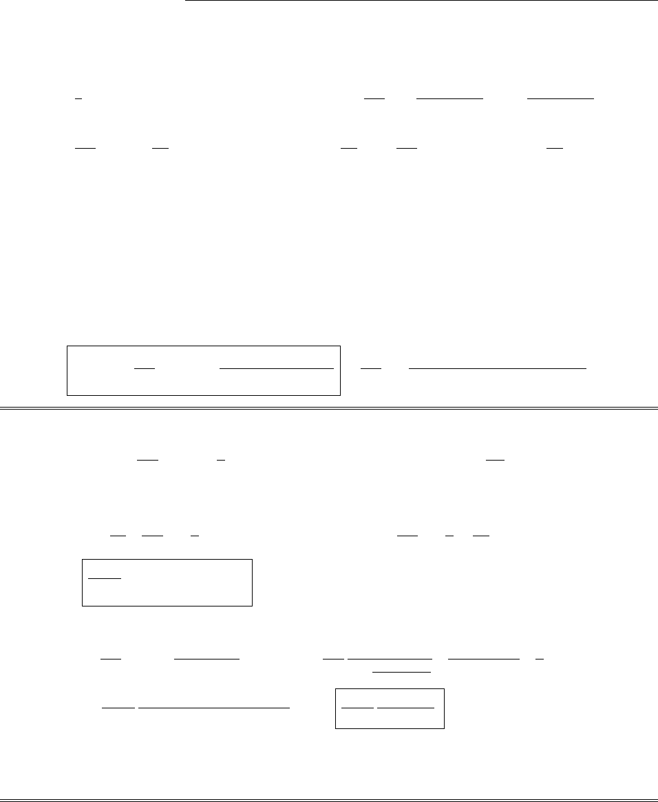
58 CHAPTER 3. POTENTIAL
In this case V0(y)=+V0,for 0 <y<a/2
V0,for a/2<y<a.Therefore,
Cn=2
aV0
a/2
0
sin(n⇡y/a)dy
a
a/2
sin(n⇡y/a)dy
=2V0
acos(n⇡y/a)
(n⇡/a)
a/2
0
+cos(n⇡y/a)
(n⇡/a)
a
a/2
=2V0
n⇡cos n⇡
2+ cos(0) + cos(n⇡)cos n⇡
2=2V0
n⇡1+(1)n2 cos n⇡
2.
The term in curly brackets is:
n=1 :112 cos(⇡/2) = 0,
n=2 :1+12 cos(⇡)=4,
n=3 :112 cos(3⇡/2) = 0,
n=4 :1+12 cos(2⇡)=0,
etc.(Zero if nis odd or divisible by 4,otherwise 4.)
Therefore
Cn=8V0/n⇡,n=2,6,10,14,etc.(in general,4j+2,for j=0,1,2, ...),
0,otherwise.
So
V(x, y)=8V0
⇡
n=2,6,10,...
en⇡x/a sin(n⇡y/a)
n=8V0
⇡
1
j=0
e(4j+2)⇡x/a sin[(4j+ 2)⇡y/a]
(4j+ 2) .
Problem 3.14
V(x, y)=4V0
⇡
n=1,3,5,...
1
nen⇡x/a sin(n⇡y/a) (Eq.3.36); =✏0
@V
@n(Eq.2.49).
So
(y)=✏0
@
@x4V0
⇡1
nen⇡x/a sin(n⇡y/a)x=0
=✏0
4V0
⇡1
n(n⇡
a)en⇡x/a sin(n⇡y/a)x=0
=4✏0V0
a
n=1,3,5,...
sin(n⇡y/a).
Or, using the closed form 3.37:
V(x, y)=2V0
⇡tan1sin(⇡y/a)
sinh(⇡x/a))=✏0
2V0
⇡
1
1+ sin2(⇡y/a)
sinh2(⇡x/a)sin(⇡y/a)
sinh2(⇡x/a)⇡
acosh(⇡x/a)x=0
=2✏0V0
a
sin(⇡y/a) cosh(⇡x/a)
sin2(⇡y/a) + sinh2(⇡x/a)x=0
=2✏0V0
a
1
sin(⇡y/a).
[Comment: Technically, the series solution for is defective, since term-by-term di↵erentiation has produced
a (naively) non-convergent sum. More sophisticated definitions of convergence permit one to work with series
of this form, but it is better to sum the series first and then di↵erentiate (the second method.)]
c
2012 Pearson Education, Inc., Upper Saddle River, NJ. All rights reserved. This material is
protected under all copyright laws as they currently exist. No portion of this material may be
reproduced, in any form or by any means, without permission in writing from the publisher.
CHAPTER 3. POTENTIAL 59
Summation of series Eq. 3.36
V(x, y)=4V0
⇡I, where I⌘
n=1,3,5,...
1
nen⇡x/a sin(n⇡y/a).
Now sin w=Imeiw,so
I=Im1
nen⇡x/aein⇡y/a =Im1
nZn,
where Z⌘e⇡(xiy)/a.Now
1,3,5,...
1
nZn=1
j=0
1
(2j+ 1)Z(2j+1) =Z
0
1
j=0
u2j
du
=
Z
0
1
1u2du =1
2ln 1+Z
1Z=1
2ln Rei✓=1
2(ln R+i✓),
where Rei✓=1+Z
1Z. Therefore
I=Im1
2(ln R+i✓)=1
2✓.But 1+Z
1Z=1+e⇡(xiy)/a
1e⇡(xiy)/a =1+e⇡(xiy)/a1e⇡(x+iy)/a
1e⇡(xiy)/a1e⇡(x+iy)/a
=1+e⇡x/a ei⇡y/a ei⇡y/ae2⇡x/a
1e⇡(xiy)/a2=1+2ie⇡x/a sin(⇡y/a)e2⇡x/a
1e⇡(xiy)/a2,
so
tan ✓=2e⇡x/a sin(⇡y/a)
1e2⇡x/a =2 sin(⇡y/a)
e⇡x/a e⇡x/a =sin(⇡y/a)
sinh(⇡x/a).
Therefore
I=1
2tan1sin(⇡y/a)
sinh(⇡x/a),and V(x, y)=2V0
⇡tan1sin(⇡y/a)
sinh(⇡x/a).
Problem 3.15
CHAPTER 3. SPECIAL TECHNIQUES 7
where Reiθ=1+Z
1−Z. Therefore
I=Im!1
2(ln R+iθ)"=1
2θ.But 1 + Z
1−Z=1 + e−π(x−iy)/a
1−e−π(x−iy)/a =#1 + e−π(x−iy)/a$#1−e−π(x+iy)/a$
#1−e−π(x−iy)/a$#1−e−π(x+iy)/a$
=1 + e−πx/a #eiπy/a −e−iπy/a$−e−2πx/a
%
%1−e−π(x−iy)/a%
%
2=1 + 2ie−πx/a sin(πy/a)−e−2πx/a
%
%1−e−π(x−iy)/a%
%
2,
so
tan θ=2e−πx/a sin(πy/a)
1−e−2πx/a =2 sin(πy/a)
eπx/a −e−πx/a =sin(πy/a)
sinh(πx/a).
Therefore
I=1
2tan−1&sin(πy/a)
sinh(πx/a)',and V(x, y) = 2V0
πtan−1&sin(πy/a)
sinh(πx/a)'.
Problem 3.14
✲x
✻
y
✙
z
a
b
V= 0
V0(y)
(a) ∂2V
∂x2+∂2V
∂y2= 0, with boundary conditions
⎧
⎪
⎪
⎨
⎪
⎪
⎩
(i) V(x, 0) = 0,
(ii) V(x, a) = 0,
(iii) V(0, y) = 0,
(iv) V(b, y) = V0(y).
⎫
⎪
⎪
⎬
⎪
⎪
⎭
As in Ex. 3.4, separation of variables yields
V(x, y) = #Aekx +Be−kx$(Csin ky +Dcos ky).
Here (i)⇒D= 0,(iii)⇒B=−A, (ii)⇒ka is an integer multiple of π:
V(x, y) = AC /enπx/a −e−nπx/a0sin(nπy/a) = (2AC) sinh(nπx/a) sin(nπy/a).
But (2AC) is a constant, and the most general linear combination of separable solutions consistent with (i),
(ii), (iii) is
V(x, y) =
∞
1
n=1
Cnsinh(nπx/a) sin(nπy/a).
It remains to determine the coefficients Cnso as to fit boundary condition (iv):
1Cnsinh(nπb/a) sin(nπy/a) = V0(y).Fourier’s trick ⇒Cnsinh(nπb/a) = 2
a
a
2
0
V0(y) sin(nπy/a)dy.
Therefore
Cn=2
asinh(nπb/a)
a
2
0
V0(y) sin(nπy/a)dy.
c
⃝2005 Pearson Education, Inc., Upper Saddle River, NJ. All rights reserved. This material is
protected under all copyright laws as they currently exist. No portion of this material may be
reproduced, in any form or by any means, without permission in writing from the publisher.
(a) @2V
@x2+@2V
@y2= 0, with boundary conditions
(i) V(x, 0) = 0,
(ii) V(x, a)=0,
(iii) V(0,y)=0,
(iv) V(b, y)=V0(y).
As in Ex. 3.4, separation of variables yields
V(x, y)=Aekx +Bekx(Csin ky +Dcos ky).
Here (i))D=0,(iii))B=A, (ii))ka is an integer multiple of ⇡:
V(x, y)=AC en⇡x/a en⇡x/asin(n⇡y/a) = (2AC) sinh(n⇡x/a) sin(n⇡y/a).
c
2012 Pearson Education, Inc., Upper Saddle River, NJ. All rights reserved. This material is
protected under all copyright laws as they currently exist. No portion of this material may be
reproduced, in any form or by any means, without permission in writing from the publisher.
60 CHAPTER 3. POTENTIAL
But (2AC) is a constant, and the most general linear combination of separable solutions consistent with (i),
(ii), (iii) is
V(x, y)= 1
n=1
Cnsinh(n⇡x/a) sin(n⇡y/a).
It remains to determine the coefficients Cnso as to fit boundary condition (iv):
Cnsinh(n⇡b/a) sin(n⇡y/a)=V0(y).Fourier’s trick )Cnsinh(n⇡b/a)= 2
a
a
0
V0(y) sin(n⇡y/a)dy.
Therefore
Cn=2
asinh(n⇡b/a)
a
0
V0(y) sin(n⇡y/a)dy.
(b) Cn=2
asinh(n⇡b/a)V0
a
0
sin(n⇡y/a)dy =2V0
asinh(n⇡b/a)⇥0,if nis even,
2a
n⇡,if nis odd.
V(x, y)=4V0
⇡
n=1,3,5,...
sinh(n⇡x/a) sin(n⇡y/a)
nsinh(n⇡b/a).
Problem 3.16
Same format as Ex. 3.5, only the boundary conditions are:
(i) V=0 when x=0,
(ii) V=0 when x=a,
(iii) V=0 when y=0,
(iv) V=0 when y=a,
(v) V=0 when z=0,
(vi) V=V0when z=a.
This time we want sinusoidal fuctions in xand y, exponential in z:
X(x)=Asin(kx)+Bcos(kx),Y(y)=Csin(ly)+Dcos(ly),Z(z)=Eepk2+l2z+Gepk2+l2z.
(i))B= 0; (ii))k=n⇡/a; (iii))D= 0; (iv))l=m⇡/a; (v))E+G=0.Therefore
Z(z)=2Esinh(⇡n2+m2z/a).
Putting this all together, and combining the constants, we have:
V(x, y, z)= 1
n=1
1
m=1
Cn,m sin(n⇡x/a) sin(m⇡y/a) sinh(⇡n2+m2z/a).
It remains to evaluate the constants Cn,m, by imposing boundary condition (vi):
V0=Cn,m sinh(⇡n2+m2)sin(n⇡x/a) sin(m⇡y/a).
c
2012 Pearson Education, Inc., Upper Saddle River, NJ. All rights reserved. This material is
protected under all copyright laws as they currently exist. No portion of this material may be
reproduced, in any form or by any means, without permission in writing from the publisher.
CHAPTER 3. POTENTIAL 61
According to Eqs. 3.50 and 3.51:
Cn,m sinh ⇡n2+m2=2
a2
V0
a
0
a
0
sin(n⇡x/a) sin(m⇡y/a)dx dy =0,if nor mis even,
16V0
⇡2nm,if both are odd.
Therefore
V(x, y, z)=16V0
⇡2
n=1,3,5,...
m=1,3,5,...
1
nm sin(n⇡x/a) sin(m⇡y/a)sinh ⇡pn2+m2z/a
sinh ⇡pn2+m2.
Consider the superposition of six such cubes, one with V0on each of the six faces. The result is a cube
with V0on its entire surface, so the potential at the center is V0. Evidently the potential at the center of the
original cube (with V0on just one face) is one sixth of this: V0/6.To check it, put in x=y=z=a/2:
V(a/2, a/2, a/2) = 16V0
⇡2
n=1,3,5,...
m=1,3,5,...
1
nm sin(n⇡/2) sin(m⇡/2)sinh ⇡pn2+m2/2
sinh ⇡pn2+m2.
Let n⌘2i+ 1, m⌘2j+ 1, and note that sinh(2u) = 2 sinh(u) cosh(u). The double sum is then
S=1
2
1
i=0
1
j=0
(1)i+j
(2i+ 1)(2j+ 1)sech ⇡(2i+ 1)2+ (2j+ 1)2/2.
Setting the upper limits at i=3,j= 3 (or above) Mathematica returns S=0.102808, which (to 6 digits) is
equal to ⇡2/96, confirming (at least, numerically) that V(a/2, a/2, a/2) = V0/6.
Problem 3.17
P3(x)= 1
8·6
d3
dx3x213=1
48
d2
dx23x2122x=1
8
d2
dx2xx212
=1
8
d
dx x212+2xx212x=1
8
d
dx x21x21+4x2
=1
8
d
dx x215x21=1
82x5x21+x2110x
=1
45x3x+5x35x=1
410x36x=5
2x33
2x.
We need to show that P3(cos ✓) satisfies
1
sin ✓
d
d✓sin ✓dP
d✓=l(l+ 1)P, with l=3,
where P3(cos ✓)=1
2cos ✓5 cos2✓3.
dP3
d✓=1
2sin ✓5 cos2✓3+ cos ✓(10 cos ✓(sin ✓)=1
2sin ✓5 cos2✓3 + 10 cos2✓
=3
2sin ✓5 cos2✓1.
c
2012 Pearson Education, Inc., Upper Saddle River, NJ. All rights reserved. This material is
protected under all copyright laws as they currently exist. No portion of this material may be
reproduced, in any form or by any means, without permission in writing from the publisher.
62 CHAPTER 3. POTENTIAL
@
@✓ sin ✓dP3
d✓=3
2
d
d✓sin2✓5 cos2✓1=3
22 sin ✓cos ✓5 cos2✓1+ sin2✓(10 cos ✓sin ✓)
=3 sin ✓cos ✓5 cos2✓15 sin2✓.
1
sin ✓
d
d✓sin ✓dP
d✓=3 cos ✓5 cos2151cos2✓=3 cos ✓10 cos2✓6
=3·4·1
2cos ✓5 cos2✓3=l(l+ 1)P3.qed
1
1
P1(x)P3(x)dx =
1
1
(x)1
25x33xdx =1
2x5x31
1=1
2(1 1+11) = 0.X
Problem 3.18
(a) Inside: V(r, ✓)= 1
l=0
AlrlPl(cos ✓) (Eq.3.66) where
Al=(2l+ 1)
2Rl
⇡
0
V0(✓)Pl(cos ✓) sin ✓d✓(Eq.3.69).
In this case V0(✓)=V0comes outside the integral, so
Al=(2l+ 1)V0
2Rl
⇡
0
Pl(cos ✓) sin ✓d✓.
But P0(cos ✓) = 1, so the integral can be written
⇡
0
P0(cos ✓)Pl(cos ✓) sin ✓d✓=0,if l6=0
2,if l=0(Eq.3.68).
Therefore
Al=0,if l6=0
V0,if l=0.
Plugging this into the general form:
V(r, ✓)=A0r0P0(cos ✓)= V0.
The potential is constant throughout the sphere.
Outside:V(r, ✓)= 1
l=0
Bl
rl+1 Pl(cos ✓) (Eq. 3.72), where
Bl=(2l+ 1)
2Rl+1
⇡
0
V0(✓)Pl(cos ✓) sin ✓d✓(Eq.3.73).
=(2l+ 1)
2Rl+1V0
⇡
0
Pl(cos ✓) sin ✓d✓=0,if l6=0
RV0,if l=0.
c
2012 Pearson Education, Inc., Upper Saddle River, NJ. All rights reserved. This material is
protected under all copyright laws as they currently exist. No portion of this material may be
reproduced, in any form or by any means, without permission in writing from the publisher.
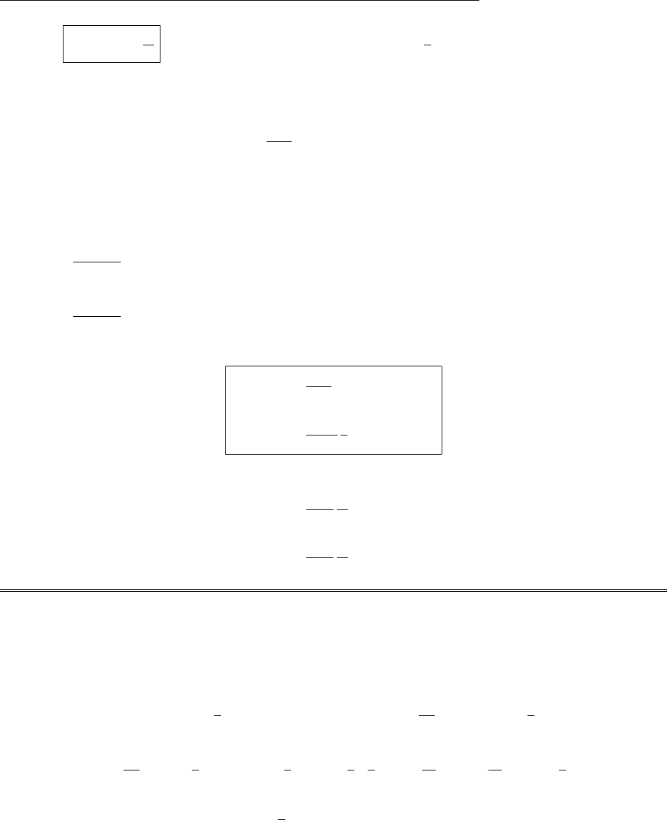
CHAPTER 3. POTENTIAL 63
Therefore V(r, ✓)=V0
R
r(i.e. equals V0at r=R, then falls o↵like 1
r).
(b)
V(r, ✓)=
1
l=0
AlrlPl(cos ✓),for rR(Eq.3.78)
1
l=0
Bl
rl+1 Pl(cos ✓),for rR(Eq.3.79)
,
where
Bl=R2l+1Al(Eq.3.81)
and
Al=1
2✏0Rl1
⇡
0
0(✓)Pl(cos ✓) sin ✓d✓(Eq.3.84)
=1
2✏0Rl10
⇡
0
Pl(cos ✓) sin ✓d✓=0,if l6=0
R0/✏0,if l=0.
Therefore
V(r, ✓)=
R0
✏0
,for rR
R20
✏0
1
r,for rR
.
Note: in terms of the total charge Q=4⇡R20,
V(r, ✓)=
1
4⇡✏0
Q
R,for rR
1
4⇡✏0
Q
r,for rR
.
Problem 3.19
V0(✓)=kcos(3✓)=k4 cos3✓3 cos ✓=k[↵P3(cos ✓)+P1(cos ✓)] .
(I know that any 3rd order polynomial can be expressed as a linear combination of the first four Legendre
polynomials; in this case, since the polynomial is odd, I only need P1and P3.)
4 cos3✓3 cos ✓=↵1
25 cos3✓3 cos ✓+cos ✓=5↵
2cos3✓+3
2↵cos ✓,
so
4=5↵
2)↵=8
5;3=3
2↵=3
2·8
5=12
5)=12
53=3
5.
Therefore
V0(✓)=k
5[8P3(cos ✓)3P1(cos ✓)] .
c
2012 Pearson Education, Inc., Upper Saddle River, NJ. All rights reserved. This material is
protected under all copyright laws as they currently exist. No portion of this material may be
reproduced, in any form or by any means, without permission in writing from the publisher.

64 CHAPTER 3. POTENTIAL
Now
V(r, ✓)=
1
l=0
AlrlPl(cos ✓),for rR(Eq.3.66)
1
l=0
Bl
rl+1 Pl(cos ✓),for rR(Eq.3.72)
,
where
Al=(2l+ 1)
2Rl
⇡
0
V0(✓)Pl(cos ✓) sin ✓d✓(Eq.3.69)
=(2l+ 1)
2Rl
k
5
8
⇡
0
P3(cos ✓)Pl(cos ✓) sin ✓d✓3
⇡
0
P1(cos ✓)Pl(cos ✓) sin ✓d✓
=k
5
(2l+ 1)
2Rl82
(2l+ 1) l332
(2l+ 1) l1=k
5
1
Rl[8 l33l1]
=8k/5R3,if l=3
3k/5R, if l=1(zero otherwise).
Therefore
V(r, ✓)=3k
5RrP1(cos ✓)+ 8k
5R3r3P3(cos ✓)= k
58r
R3P3(cos ✓)3r
RP1(cos ✓),
or
k
58r
R31
25 cos3✓3 cos ✓3r
Rcos ✓)V(r, ✓)=k
5
r
Rcos ✓4r
R25 cos2✓33
(for rR). Meanwhile, Bl=AlR2l+1 (Eq. 3.81—this follows from the continuity of Vat R). Therefore
Bl=8kR4/5,if l=3
3kR2/5,if l=1(zero otherwise).
So
V(r, ✓)=3kR2
5
1
r2P1(cos ✓)+8kR4
5
1
r4P3(cos ✓)= k
58R
r4
P3(cos ✓)3R
r2
P1(cos ✓),
or
V(r, ✓)=k
5R
r2
cos ✓4R
r25 cos2✓33
c
2012 Pearson Education, Inc., Upper Saddle River, NJ. All rights reserved. This material is
protected under all copyright laws as they currently exist. No portion of this material may be
reproduced, in any form or by any means, without permission in writing from the publisher.

CHAPTER 3. POTENTIAL 65
(for rR). Finally, using Eq. 3.83:
(✓)=✏0
1
l=0
(2l+ 1)AlRl1Pl(cos ✓)=✏03A1P1+7A3R2P3
=✏033k
5RP1+78k
5R3R2P3=✏0k
5R[9P1(cos ✓) + 56P3(cos ✓)]
=✏0k
5R9 cos ✓+56
25 cos3✓3 cos ✓=✏0k
5Rcos ✓[9 + 28 ·5 cos2✓28 ·3]
=✏0k
5Rcos ✓140 cos2✓93.
Problem 3.20
Use Eq. 3.83: (✓)=✏0
1
l=0
(2l+1)AlRl1Pl(cos ✓).But Eq. 3.69 says: Al=2l+1
2Rl
⇡
0
V0(✓)Pl(cos ✓) sin ✓d✓.
Putting them together:
(✓)= ✏0
2R
1
l=0
(2l+ 1)2ClPl(cos ✓),with Cl=
⇡
0
V0(✓)Pl(cos ✓) sin ✓d✓.qed
Problem 3.21
Set V= 0 on the equatorial plane, far from the sphere. Then the potential is the same as Ex. 3.8 plus the
potential of a uniformly charged spherical shell:
V(r, ✓)=E0rR3
r2cos ✓+1
4⇡✏0
Q
r.
Problem 3.22
(a) V(r, ✓)= 1
l=0
Bl
rl+1 Pl(cos ✓)(r>R),so V(r, 0) = 1
l=0
Bl
rl+1 Pl(1) = 1
l=0
Bl
rl+1 =
2✏0r2+R2r.
Since r>Rin this region, r2+R2=r1+(R/r)2=r1+ 1
2(R/r)21
8(R/r)4+...
, so
1
l=0
Bl
rl+1 =
2✏0
r1+1
2
R2
r21
8
R4
r4+...1=
2✏0R2
2rR4
8r3+...
.
Comparing like powers of r, I see that B0=R2
4✏0
,B
1=0,B
2=R4
16✏0
,.... Therefore
V(r, ✓)=R2
4✏01
rR2
4r3P2(cos ✓)+...
,
=R2
4✏0r11
8R
r23 cos2✓1+...
,
(for r>R).
c
2012 Pearson Education, Inc., Upper Saddle River, NJ. All rights reserved. This material is
protected under all copyright laws as they currently exist. No portion of this material may be
reproduced, in any form or by any means, without permission in writing from the publisher.

66 CHAPTER 3. POTENTIAL
(b) V(r, ✓)= 1
l=0
AlrlPl(cos ✓)(r<R). In the northern hemispere, 0 ✓⇡/2,
V(r, 0) = 1
l=0
Alrl=
2✏0r2+R2r.
Since r<Rin this region, r2+R2=R1+(r/R)2=R1+ 1
2(r/R)21
8(r/R)4+...
.Therefore
1
l=0
Alrl=
2✏0R+1
2
r2
R1
8
r4
R3+...r.
Comparing like powers: A0=
2✏0
R, A1=
2✏0
,A
2=
4✏0R,..., so
V(r, ✓)=
2✏0RrP1(cos ✓)+ 1
2Rr2P2(cos ✓)+...
,
=R
2✏01r
Rcos ✓+1
4r
R23 cos2✓1+...
,
(for r<R, northern hemisphere).
In the southern hemisphere we’ll have to go for ✓=⇡, using Pl(1) = (1)l.
V(r, ⇡)= 1
l=0
(1)lAlrl=
2✏0r2+R2r.
(I put an overbar on Alto distinguish it from the northern Al). The only di↵erence is the sign of A1:
A1= +(/2✏0), A0=A0, A2=A2. So:
V(r, ✓)=
2✏0R+rP1(cos ✓)+ 1
2Rr2P2(cos ✓)+...
,
=R
2✏01+r
Rcos ✓+1
4r
R23 cos2✓1+...
,
(for r<R, southern hemisphere).
Problem 3.23
V(r, ✓)=
1
l=0
AlrlPl(cos ✓),(rR) (Eq.3.78),
1
l=0
Bl
rl+1 Pl(cos ✓),(rR) (Eq.3.79),
c
2012 Pearson Education, Inc., Upper Saddle River, NJ. All rights reserved. This material is
protected under all copyright laws as they currently exist. No portion of this material may be
reproduced, in any form or by any means, without permission in writing from the publisher.

CHAPTER 3. POTENTIAL 67
where Bl=AlR2l+1 (Eq. 3.81) and
Al=1
2✏0Rl1
⇡
0
0(✓)Pl(cos ✓) sin ✓d✓(Eq.3.84)
=1
2✏0Rl10
⇡/2
0
Pl(cos ✓) sin ✓d✓
⇡
⇡/2
Pl(cos ✓) sin ✓d✓
(let x= cos ✓)
=0
2✏0Rl1
1
0
Pl(x)dx
0
1
Pl(x)dx
.
Now Pl(x)=(1)lPl(x), since Pl(x) is even, for even l, and odd, for odd l. Therefore
0
1
Pl(x)dx =
0
1
Pl(x)d(x)=(1)l
1
0
Pl(x)dx,
and hence
Al=0
2✏0Rl11(1)l1
0
Pl(x)dx =
0,if lis even
0
✏0Rl1
1
0
Pl(x)dx, if lis odd
.
So A0=A2=A4=A6= 0, and all we need are A1,A3, and A5.
1
0
P1(x)dx =
1
0
xdx=x2
2
1
0
=1
2.
1
0
P3(x)dx =1
2
1
05x33xdx =1
25x4
43x2
2
1
0
=1
25
43
2=1
8.
1
0
P5(x)dx =1
8
1
063x570x3+ 15xdx =1
863x6
670x4
4+ 15x2
2
1
0
=1
821
235
2+15
2=1
16(36 35) = 1
16.
Therefore
A1=0
✏01
2;A3=0
✏0R21
8;A5=0
✏0R41
16; etc.
and
B1=0
✏0
R31
2;B3=0
✏0
R51
8;B5=0
✏0
R71
16; etc.
c
2012 Pearson Education, Inc., Upper Saddle River, NJ. All rights reserved. This material is
protected under all copyright laws as they currently exist. No portion of this material may be
reproduced, in any form or by any means, without permission in writing from the publisher.

68 CHAPTER 3. POTENTIAL
Thus
V(r, ✓)=
0r
2✏0P1(cos ✓)1
4r
R2P3(cos ✓)+1
8r
R4P5(cos ✓)+...,(rR),
0R3
2✏0r2P1(cos ✓)1
4R
r2
P3(cos ✓)+1
8R
r4
P5(cos ✓)+...,(rR).
Problem 3.24
1
s
@
@ss@V
@s+1
s2
@2V
@2=0.
Look for solutions of the form V(s, )=S(s)():
1
sd
ds sdS
ds +1
s2Sd2
d2=0.
Multiply by s2and divide by V=S:
s
S
d
ds sdS
ds +1
d2
d2=0.
Since the first term involves sonly, and the second only, each is a constant:
s
S
d
ds sdS
ds =C1,1
d2
d2=C2,with C1+C2=0.
Now C2must be negative (else we get exponentials for , which do not return to their original value—as
geometrically they must— when is increased by 2⇡).
C2=k2.Then d2
d2=k2)=Acos k+Bsin k.
Moreover, since (+2⇡)=(), kmust be an integer: k=0,1,2,3,... (negative integers are just repeats,
but k= 0 must be included, since =A(a constant) is OK).
sd
ds sdS
ds =k2Scan be solved by S=sn, provided nis chosen right:
sd
ds snsn1=ns d
ds (sn)=n2ssn1=n2sn=k2S)n=±k.
Evidently the general solution is S(s)=Csk+Dsk,unless k= 0, in which case we have only one solution
to a second-order equation—namely, S= constant. So we must treat k= 0 separately. One solution is a
constant—but what’s the other? Go back to the diferential equation for S, and put in k= 0:
sd
ds sdS
ds =0)sdS
ds = constant = C)dS
ds =C
s)dS =Cds
s)S=Cln s+D(another constant).
So the second solution in this case is ln s. [How about ? That too reduces to a single solution, =A, in the
case k= 0. What’s the second solution here? Well, putting k= 0 into the equation:
d2
d2=0)d
d= constant = B)=B+A.
c
2012 Pearson Education, Inc., Upper Saddle River, NJ. All rights reserved. This material is
protected under all copyright laws as they currently exist. No portion of this material may be
reproduced, in any form or by any means, without permission in writing from the publisher.

CHAPTER 3. POTENTIAL 69
But a term of the form Bis unacceptable, since it does not return to its initial value when is augmented
by 2⇡.] Conclusion: The general solution with cylindrical symmetry is
V(s, )=a0+b0ln s+1
k=1 sk(akcos k+bksin k)+sk(ckcos k+dksin k).
Yes: the potential of a line charge goes like ln s, which is included.
Problem 3.25
Picking V= 0 on the yz plane, with E0in the xdirection, we have (Eq. 3.74):
(i) V=0,when s=R,
(ii) V!E0x=E0scos ,for sR.
1
Contents
1 Special Techniques 2
Problem 3.24
Picking V= 0 on the yz plane, with E0in the xdirection,
!(i) V= 0,when s=R,
(ii) V→ −E0x=−E0scos φ,for s≫R. "✲x
✻
y
✢
z
φ
s
−
−
−
−
−
+
+
+
+
+
=⇒E0
Evidently a0=b0=bk=dk= 0, and ak=ck= 0 except for k= 1:
V(s, φ) = #a1s+c1
s$cos φ.
(i)⇒c1=−a1R2; (ii)→a1=−E0. Therefore
V(s, φ) = %−E0s+E0R2
s&cos φ,or V(s, φ) = −E0s'%R
s&2
−1(cos φ.
σ=−ϵ0
∂V
∂s))))s=R
=−ϵ0E0%−R2
s2−1&cos φ))))s=R
=2ϵ0E0cos φ.
Problem 3.25
Inside: V(s, φ) = a0+
∞
*
k=1
sk(akcos kφ+bksin kφ).(In this region ln sand s−kare no good—they blow
up at s= 0.)
Outside: V(s, φ) = a0+
∞
*
k=1
1
sk(ckcos kφ+dksin kφ). (Here ln sand skare no good at s→ ∞).
σ=−ϵ0%∂Vout
∂s−∂Vin
∂s&))))s=R
(Eq.2.36).
Thus
asin 5φ=−ϵ0
∞
*
k=1 !−k
Rk+1 (ckcos kφ+dksin kφ)−kRk−1(akcos kφ+bksin kφ)".
c
⃝2005 Pearson Education, Inc., Upper Saddle River, NJ. All rights reserved. This material is
protected under all copyright laws as they currently exist. No portion of this material may be
reproduced, in any form or by any means, without permission in writing from the publisher.
Evidently a0=b0=bk=dk= 0, and ak=ck= 0 except for k= 1:
V(s, )=a1s+c1
scos .
(i))c1=a1R2; (ii)!a1=E0. Therefore
V(s, )=E0s+E0R2
scos ,or V(s, )=E0sR
s2
1cos .
=✏0
@V
@ss=R
=✏0E0R2
s21cos s=R
= 2✏0E0cos .
Problem 3.26
Inside: V(s, )=a0+1
k=1
sk(akcos k+bksin k).(In this region ln sand skare no good—they blow
up at s= 0.)
Outside: V(s, )=a0+1
k=1
1
sk(ckcos k+dksin k). (Here ln sand skare no good at s!1).
=✏0@Vout
@s@Vin
@ss=R
(Eq.2.36).
Thus
asin 5=✏0
1
k=1 k
Rk+1 (ckcos k+dksin k)kRk1(akcos k+bksin k).
Evidently ak=ck= 0; bk=dk= 0 except k= 5; a=5✏01
R6d5+R4b5. Also, Vis continuous at s=R:
a0+R5b5sin 5=a0+1
R5d5sin 5.Soa0=a0(might as well choose both zero); R5b5=R5d5, or d5=R10b5.
c
2012 Pearson Education, Inc., Upper Saddle River, NJ. All rights reserved. This material is
protected under all copyright laws as they currently exist. No portion of this material may be
reproduced, in any form or by any means, without permission in writing from the publisher.

70 CHAPTER 3. POTENTIAL
Combining these results: a=5✏0R4b5+R4b5= 10✏0R4b5;b5=a
10✏0R4;d5=aR6
10✏0
. Therefore
V(s, )=asin 5
10✏0s5/R4,for s<R,
R6/s5,for s>R.
Problem 3.27 Since ris on the zaxis, the angle ↵is just the polar angle ✓(I’ll drop the primes, for simplicity).
Monopole term: ⇢d⌧=kR 1
r2(R2r) sin ✓r2sin ✓dr d✓d.
But the rintegral is
R
0
(R2r)dr =Rr r2R
0=R2R2=0.
So the monopole term is zero.
Dipole term: rcos ✓⇢ d⌧=kR (rcos ✓)1
r2(R2r) sin ✓r2sin ✓dr d✓d.
But the ✓integral is ⇡
0
sin2✓cos ✓d✓=sin3✓
3
⇡
0
=1
3(0 0) = 0.
So the dipole contribution is likewise zero.
Quadrupole term:
r23
2cos2✓1
2⇢d⌧=1
2kR r23 cos2✓11
r2(R2r) sin ✓r2sin ✓dr d✓d.
rintegral: R
0
r2(R2r)dr =r3
3Rr4
2
R
0
=R4
3R4
2=R4
6.
✓integral: ⇡
03 cos2✓1
3(1sin2✓)1=23 sin2✓
sin2✓d✓=2
⇡
0
sin2✓d✓3
⇡
0
sin4✓d✓
=2
⇡
233⇡
8=⇡19
8=⇡
8.
integral:
2⇡
0
d=2⇡.
The whole integral is:
1
2kR R4
6⇡
8(2⇡)=k⇡2R5
48 .
c
2012 Pearson Education, Inc., Upper Saddle River, NJ. All rights reserved. This material is
protected under all copyright laws as they currently exist. No portion of this material may be
reproduced, in any form or by any means, without permission in writing from the publisher.

CHAPTER 3. POTENTIAL 71
For point Pon the zaxis (r!zin Eq. 3.95) the approximate potential is
V(z)⇠
=1
4⇡✏0
k⇡2R5
48z3.(Quadrupole.)
Problem 3.28
r
x
y
f'
R
z
r'
For a line charge, ⇢(r0)d⌧0!(r0)dl0, which in this case becomes Rd0.
r=rsin ✓cos ˆx +rsin ✓sin ˆy +rcos ✓ˆz ,
r0=Rcos 0+Rsin 0,so
r·r0=rR sin ✓cos cos 0+rR sin ✓sin sin 0=rR cos ↵,
cos ↵= sin ✓(cos cos 0+ sin sin 0).
n=0: ⇢(r0)d⌧0!R2⇡
0
d0=2⇡R;V0=1
4⇡✏0
2⇡R
r=
2✏0
R
r.
n=1:
r0cos ↵⇢(r0)d⌧0!Rcos ↵Rd0=R2sin ✓2⇡
0
(cos cos 0+ sin sin 0)d0=0;V1= 0.
n=2:
(r0)2P2(cos ↵)⇢(r0)d⌧0!R23
2cos2↵1
2Rd0=R3
23 sin2✓(cos cos 0+ sin sin 0)21d0
=R3
23 sin2✓cos22⇡
0
cos20d0+ sin22⇡
0
sin20d0+ 2 sin cos 2⇡
0
sin 0cos 0d02⇡
0
d0
=R3
23 sin2✓⇡cos2+⇡sin2+0
2⇡=⇡R3
23 sin2✓2=⇡R33
2cos2✓1
2.
So
V2=
8✏0
R3
r33 cos2✓1=
4✏0
R3
r3P2(cos ✓).
c
2012 Pearson Education, Inc., Upper Saddle River, NJ. All rights reserved. This material is
protected under all copyright laws as they currently exist. No portion of this material may be
reproduced, in any form or by any means, without permission in writing from the publisher.

72 CHAPTER 3. POTENTIAL
Problem 3.29
p=(3qa qa)ˆz +(2qa 2q(a)) ˆy =2qaˆz . Therefore
V⇠
=1
4⇡✏0
p·ˆr
r2,
and p·ˆr =2qaˆz ·ˆr =2qa cos ✓,so
V⇠
=1
4⇡✏0
2qa cos ✓
r2.(Dipole.)
Problem 3.30
(a) By symmetry, pis clearly in the zdirection: p=pˆz ;p=z⇢d⌧)zda.
p=(Rcos ✓)(kcos ✓)R2sin ✓d✓d=2⇡R3k
⇡
0
cos2✓sin ✓d✓=2⇡R3kcos3✓
3
⇡
0
=2
3⇡R3k[1 (1)] = 4⇡R3k
3;p=4⇡R3k
3ˆz .
(b)
V⇠
=1
4⇡✏0
4⇡R3k
3
cos ✓
r2=kR3
3✏0
cos ✓
r2.(Dipole.)
This is also the exact potential. Conclusion: all multiple moments of this distribution (except the dipole) are
exactly zero.
Problem 3.31
Using Eq. 3.94 with r0=d/2 and ↵=✓(Fig. 3.26):
1
r
+
=1
r
1
n=0 d
2rn
Pn(cos ✓);
for
r
, we let ✓!180+✓, so cos ✓!cos ✓:
1
r
=1
r
1
n=0 d
2rn
Pn(cos ✓).
But Pn(x)=(1)nPn(x), so
V=1
4⇡✏0
q1
r
+1
r
=1
4⇡✏0
q1
r
1
n=0 d
2rn
[Pn(cos ✓)Pn(cos ✓)] = 2q
4⇡✏0r
n=1,3,5,... d
2rn
Pn(cos ✓).
Therefore
Vdip =2q
4⇡✏0
1
r
d
2rP1(cos ✓)=qd cos ✓
4⇡✏0r2,while Vquad =0.
Voct =2q
4⇡✏0rd
2r3
P3(cos ✓)= 2q
4⇡✏0
d3
8r4
1
25 cos3✓3 cos ✓=qd3
4⇡✏0
1
8r45 cos3✓3 cos ✓.
c
2012 Pearson Education, Inc., Upper Saddle River, NJ. All rights reserved. This material is
protected under all copyright laws as they currently exist. No portion of this material may be
reproduced, in any form or by any means, without permission in writing from the publisher.

CHAPTER 3. POTENTIAL 73
Problem 3.32
(a) (i) Q= 2q, (ii) p= 3qaˆz ,(iii) V⇠
=1
4⇡✏0Q
r+p·ˆr
r2=1
4⇡✏02q
r+3qa cos ✓
r2.
(b) (i) Q= 2q, (ii) p=qaˆz ,(iii) V⇠
=1
4⇡✏02q
r+qa cos ✓
r2.
(c) (i) Q= 2q, (ii) p= 3qa ˆy ,(iii) V⇠
=1
4⇡✏02q
r+3qa sin ✓sin
r2(from Eq. 1.64, ˆy ·ˆr = sin ✓sin ).
Problem 3.33
(a) This point is at r=a,✓=⇡
2,= 0, so E=p
4⇡✏0a3ˆ
✓=p
4⇡✏0a3(ˆz ); F=qE=pq
4⇡✏0a3ˆz .
(b) Here r=a, ✓= 0, so E=p
4⇡✏0a3(2ˆr )= 2p
4⇡✏0a3ˆz .F=2pq
4⇡✏0a3ˆz .
(c) W=q[V(0,0,a)V(a, 0,0)] = qp
4⇡✏0a2cos(0) cos ⇡
2=pq
4⇡✏0a2.
Problem 3.34
Q=q, so Vmono =1
4⇡✏0
q
r;p=qaˆz , so Vdip =1
4⇡✏0
qa cos ✓
r2. Therefore
V(r, ✓)⇠
=q
4⇡✏01
r+acos ✓
r2.E(r, ✓)⇠
=q
4⇡✏01
r2ˆr +a
r32 cos ✓ˆr + sin ✓ˆ
✓.
Problem 3.35 The total charge is zero, so the dominant term is the dipole. We need the dipole moment
of this configuration. It obviously points in the zdirection, and for the southern hemisphere (✓:⇡
2!⇡)⇢
switches sign but so does z, so
p=z⇢d⌧=2⇢0⇡/2
✓=0
rcos ✓r2sin ✓dr d✓d=2⇢0(2⇡)R
0
r3dr ⇡/2
0
cos ✓sin ✓d✓
=4⇡⇢0
R4
4
sin2✓
2
⇡/2
0
=⇡⇢0R4
2.
Therefore (Eq. 3.103)
E⇡⇡⇢0R4
8⇡✏0r32 cos ✓ˆr + sin ✓ˆ
✓.
Problem 3.36
p=(p·ˆr )ˆr +(p·ˆ
✓)ˆ
✓=pcos ✓ˆr psin ✓ˆ
✓(Fig. 3.36). So 3(p·ˆr )ˆr p=3pcos ✓ˆr pcos ✓ˆr +psin ✓ˆ
✓=
2pcos ✓ˆr +psin ✓ˆ
✓.So Eq. 3.104 ⌘Eq. 3.103. X
Problem 3.37
Vave(R)= 1
4⇡R2V(r)da, where the integral is over the surface of a sphere of radius R. Now da =
c
2012 Pearson Education, Inc., Upper Saddle River, NJ. All rights reserved. This material is
protected under all copyright laws as they currently exist. No portion of this material may be
reproduced, in any form or by any means, without permission in writing from the publisher.

74 CHAPTER 3. POTENTIAL
R2sin ✓d✓d, so Vave(R)= 1
4⇡V(R, ✓,) sin ✓d✓d.
dVave
dR =1
4⇡@V
@Rsin ✓d✓d=1
4⇡(rV·ˆr ) sin ✓d✓d=1
4⇡R2(rV)·(R2sin ✓d✓dˆr )
=1
4⇡R2(rV)·da=1
4⇡R2(r2V)d⌧=0.
(The final integral, from the divergence theorem, is over the volume of the sphere, where by assumption the
Laplacian of Vis zero.) So Vave is independent of R—the same for all spheres, regardless of their radius—and
hence (taking the limit as R!0), Vave(R)=V(0). qed
Problem 3.38 At a point (x, y) on the plane the field of qis
Eq=1
4⇡✏0
q
r
3ˆ
r
,and
r
=xˆx +yˆy dˆz ,
so its zcomponent is q
4⇡✏0
d
(x2+y2+d2)3/2. Meanwhile, the field of (just below the surface) is
2✏0
,
(Eq. 2.17). (Of course, this is for a uniform surface charge, but as long as we are infinitesimally far away is
e↵ectively uniform.) The total field inside the conductor is zero, so
q
4⇡✏0
d
(x2+y2+d2)3/2
2✏0
=0 )(x, y)=qd
2⇡(x2+y2+d2)3/2.X
Problem 3.39
5
This integral can also be integrated directly. Let x=u2;dx = 2u du.
0
!
d
√x
√d−xdx = 2
0
!
√d
u2
√d−u2du = 2 "−u
2#d−u2+d
2sin−1$u
√d%&''''
0
√d
=−dsin−1(1) = −dπ
2.
Therefore
t=(d
2A
πd
2=)π2d2
4
d
2q216πϵ0m=)2π3d3ϵ0m
q2.
Problem 3.35
✛
x+ + + + + +− − − − − −
q
F=1
4πϵ0
q2*1
[2(a−x)]2+1
[2a+ 2(a−x)]2+1
[4a+ 2(a−x)]2+...
−1
(2x)2−1
(2a+ 2x)2−1
(4a+ 2x)2−...&
=1
4πϵ0
q2
4"+ 1
(a−x)2+1
(2a−x)2+1
(3a−x)2+. . .,−+1
x2+1
(a+x)2+1
(2a+x)2+...,&.
When a→ ∞ (i.e. a≫x) only the 1
x2term survives: F=−1
4πϵ0
q2
(2x)2!(same as for only one plane—
Eq. 3.12). When x=a/2,
F=1
4πϵ0
q2
4"+ 1
(a/2)2+1
(3a/2)2+1
(5a/2)2+. . .,−+1
(a/2)2+1
(3a/2)2+1
(5a/2)2+. . .,&= 0.!
Problem 3.36
Following Prob. 2.47, we place image line charges −λat y=band +λat y=−b(here yis the horizontal
axis, zvertical).
✲y
✻
z
☛
R
−λ λ
+λ
−b
−λ
b
- ./ 0
a−b
2- ./ 0
a−b
2
- ./ 0
y0
-./ 0
a
P
s1
s2s3s4
c
⃝2005 Pearson Education, Inc., Upper Saddle River, NJ. All rights reserved. This material is
protected under all copyright laws as they currently exist. No portion of this material may be
reproduced, in any form or by any means, without permission in writing from the publisher.
The image configuration is shown in the figure; the positive image charge forces cancel in pairs. The net
force of the negative image charges is:
F=1
4⇡✏0
q21
[2(ax)]2+1
[2a+ 2(ax)]2+1
[4a+ 2(ax)]2+...
1
(2x)21
(2a+2x)21
(4a+2x)2...
=1
4⇡✏0
q2
4 1
(ax)2+1
(2ax)2+1
(3ax)2+...
1
x2+1
(a+x)2+1
(2a+x)2+...
.
When a!1(i.e. ax) only the 1
x2term survives: F=1
4⇡✏0
q2
(2x)2X(same as for only one plane—
Eq. 3.12). When x=a/2,
F=1
4⇡✏0
q2
4 1
(a/2)2+1
(3a/2)2+1
(5a/2)2+...
1
(a/2)2+1
(3a/2)2+1
(5a/2)2+...
=0.X
Problem 3.40
Following Prob. 2.52, we place image line charges at y=band +at y=b(here yis the horizontal
axis, zvertical).
c
2012 Pearson Education, Inc., Upper Saddle River, NJ. All rights reserved. This material is
protected under all copyright laws as they currently exist. No portion of this material may be
reproduced, in any form or by any means, without permission in writing from the publisher.

CHAPTER 3. POTENTIAL 75
5
This integral can also be integrated directly. Let x=u2;dx = 2u du.
0
!
d
√x
√d−xdx = 2
0
!
√d
u2
√d−u2du = 2 "−u
2#d−u2+d
2sin−1$u
√d%&''''
0
√d
=−dsin−1(1) = −dπ
2.
Therefore
t=(d
2A
πd
2=)π2d2
4
d
2q216πϵ0m=)2π3d3ϵ0m
q2.
Problem 3.35
✛
x+ + + + + +− − − − − −
q
F=1
4πϵ0
q2*1
[2(a−x)]2+1
[2a+ 2(a−x)]2+1
[4a+ 2(a−x)]2+...
−1
(2x)2−1
(2a+ 2x)2−1
(4a+ 2x)2−...&
=1
4πϵ0
q2
4"+ 1
(a−x)2+1
(2a−x)2+1
(3a−x)2+. . .,−+1
x2+1
(a+x)2+1
(2a+x)2+...,&.
When a→ ∞ (i.e. a≫x) only the 1
x2term survives: F=−1
4πϵ0
q2
(2x)2!(same as for only one plane—
Eq. 3.12). When x=a/2,
F=1
4πϵ0
q2
4"+ 1
(a/2)2+1
(3a/2)2+1
(5a/2)2+. . .,−+1
(a/2)2+1
(3a/2)2+1
(5a/2)2+. . .,&= 0.!
Problem 3.36
Following Prob. 2.47, we place image line charges −λat y=band +λat y=−b(here yis the horizontal
axis, zvertical).
✲y
✻
z
☛
R
−λ λ
+λ
−b
−λ
b
- ./ 0
a−b
2- ./ 0
a−b
2
- ./ 0
y0
-./ 0
a
P
s1
s2s3s4
c
⃝2005 Pearson Education, Inc., Upper Saddle River, NJ. All rights reserved. This material is
protected under all copyright laws as they currently exist. No portion of this material may be
reproduced, in any form or by any means, without permission in writing from the publisher.
In the solution to Prob. 2.52 substitute:
a!ab
2,y
0!a+b
2so ab
22
=a+b
22
R2)b=R2
a.
V=
4⇡✏0ln s2
3
s2
4+ ln s2
1
s2
2=
4⇡✏0
ln s2
1s2
3
s2
4s2
2
=
4⇡✏0
ln [(y+a)2+z2][(yb)2+z2]
[(ya)2+z2][(y+b)2+z2],or,using y=scos ,z=ssin ,
=
4⇡✏0
ln (s2+a2+2as cos )[(as/R)2+R22as cos ]
(a2+a22as cos )[(as/R)2+R2+2as cos ].
Problem 3.41 Same as Problem 3.9, only this time we want q0+q00 =q,soq00 =qq0:
F=q
4⇡✏0q00
a2+q0
(ab)2=q2
4⇡✏0a2+qq0
4⇡✏01
a2+1
(ab)2.
The second term is identical to Problem 3.9, and I’ll just quote the answer from there:
F=q2
4⇡✏0a3aR3(2a2R2)
(a2R2)2.
(a) F=0)a(a2R2)2=R3(2a2R2),or (letting x⌘a/R), x(x21)22x2+ 1 = 0. We want a real
root greater than 1; Mathematica delivers x=(1+p5)/2=1.61803, so a=1.61803R= 5.66311 ˚
A.
(b) Let a0=x0Rbe the minimum value of a. The work necessary is
W=a0
1
F da =q2
4⇡✏01
a0
1
a3aR3(2a2R2)
(a2R2)2da =q2
4⇡✏0R1
x01
x2(2x21)
x3(x21)2dx
=q2
4⇡✏0R1+2x02x3
0
2x2
0(1 x2
0).
Putting in x0=(1+p5)/2, Mathematica says the term in square brackets is 1/2 (this is not an accident; see
footnote 6 on page 127), so W=q2
8⇡✏0R.Numerically,
W=(1.60 ⇥1019)2
8⇡(8.85 ⇥1012)(5.66 ⇥1010)J=2.03 ⇥1019 J= 1.27 eV.
c
2012 Pearson Education, Inc., Upper Saddle River, NJ. All rights reserved. This material is
protected under all copyright laws as they currently exist. No portion of this material may be
reproduced, in any form or by any means, without permission in writing from the publisher.
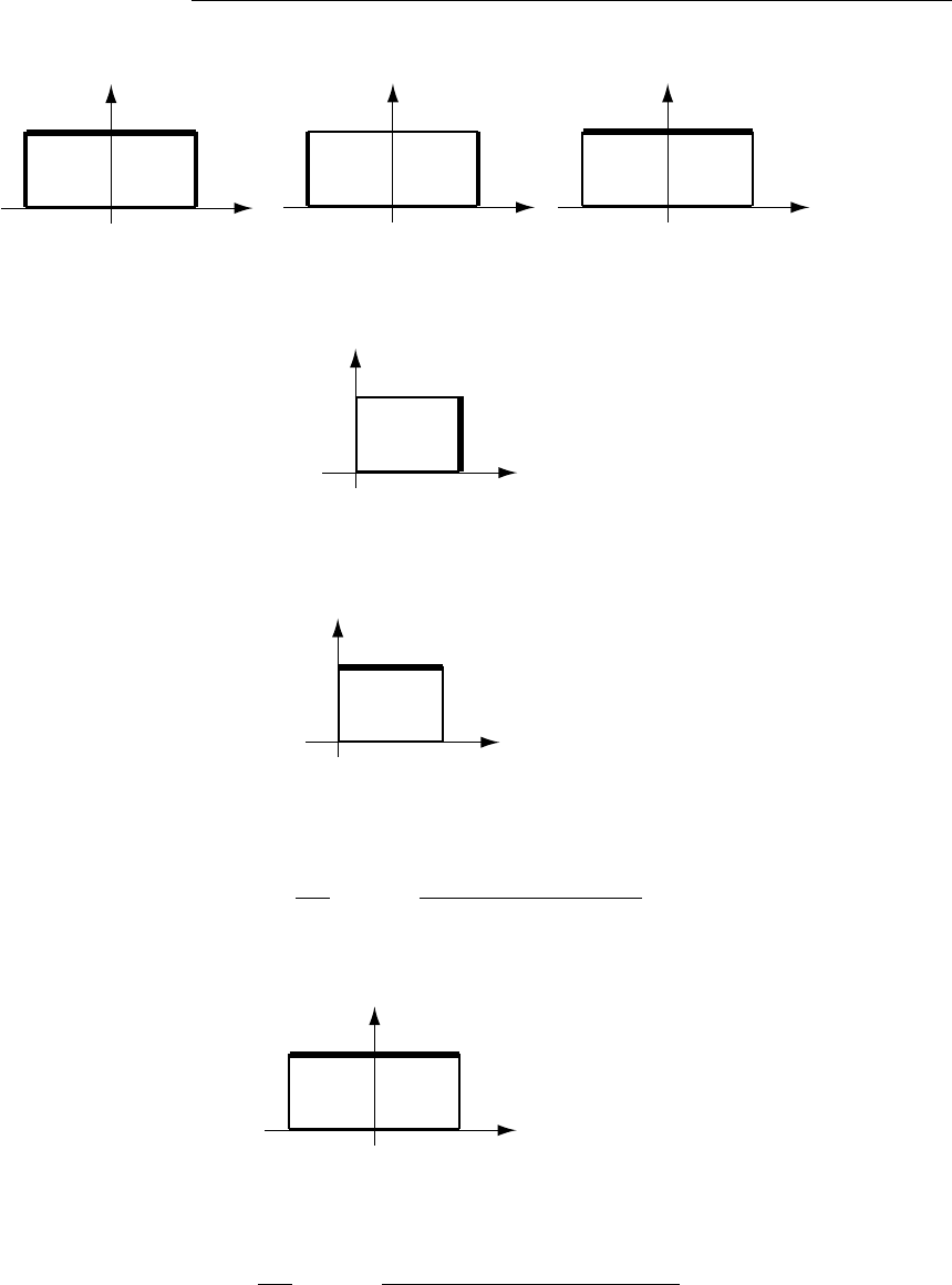
76 CHAPTER 3. POTENTIAL
Problem 3.42
x
y
a
-b b0
V
1
V
0V
0
x
y
a
-b b0
V
0V
0
0
x
y
a
-b b0
V
1
00
= +
The first configuration on the right is precisely Example 3.4, but unfortunately the second configuration is not
the same as Problem 3.15:
x
y
a
b0
V
0
0
0
We could reconstruct Problem 3.15 with the modified boundaries, but let’s see if we can’t twist it around by
an astute change of variables. Suppose we let x!y,y!u,a!c,b!a, and V0!V1:
u
y
a
c0
V
1
0
0
This is closer; making the changes in the solution to Problem 3.15 we have (for this configuration)
V(u, y)=4V1
⇡
n=1,3,5...
sinh(n⇡y/c) sin(n⇡u/c)
nsinh(n⇡a/c).
Now let c!2band u!x+b, and the configuration is just what we want:
x
y
a
-b b0
V
1
00
The potential for this configuration is
V(x, y)=4V1
⇡
n=1,3,5...
sinh(n⇡y/2b) sin(n⇡(x+b)/2b)
nsinh(n⇡a/2b).
c
2012 Pearson Education, Inc., Upper Saddle River, NJ. All rights reserved. This material is
protected under all copyright laws as they currently exist. No portion of this material may be
reproduced, in any form or by any means, without permission in writing from the publisher.

CHAPTER 3. POTENTIAL 77
(If you like, write sin(n⇡(x+b)/2b) as (1)(n1)/2cos(n⇡x/2b).) Combining this with Eq. 3.42,
V(x, y)= 4
⇡
n=1,3,5...
1
nV0
cosh(n⇡x/a) sin(n⇡y/a)
cosh(n⇡b/a)+V1
sinh(n⇡y/2b) sin(n⇡(x+b)/2b)
sinh(n⇡a/2b).
Here’s a plot of this function, for the case a=b=1,V
0=1/2,V
1=1:
-1.0
-0.5
0.0
0.5
1.0
0.0
0.5
1.0
0.0
0.5
1.0
Problem 3.43
Since the configuration is azimuthally symmetric, V(r, ✓)=Alrl+Bl
rl+1 Pl(cos ✓).
(a) r>b:Al= 0 for all l, since V!0 at 1. Therefore V(r, ✓)=Bl
rl+1 Pl(cos ✓).
a<r<b:V(r, ✓)=Clrl+Dl
rl+1 Pl(cos ✓).r<a:V(r, ✓)=V0.
We need to determine Bl,C
l,D
l,and V0. To do this, invoke boundary conditions as follows: (i) Vis
continuous at a, (ii) Vis continuous at b, (iii) 4@V
@r=1
✏0
(✓) at b.
(ii) )Bl
bl+1 Pl(cos ✓)=Clbl+Dl
bl+1 Pl(cos ✓); Bl
bl+1 =Clbl+Dl
bl+1 )Bl=b2l+1Cl+Dl.(1)
(i) )Clal+Dl
al+1 Pl(cos ✓)=V0;
Clal+Dl
al+1 =0,if l6=0,
C0a0+D0
a1=V0,if l=0;
Dl=a2l+1Cl,l6=0,
D0=aV0aC0.(2)
Putting (2) into (1) gives Bl=b2l+1Cla2l+1Cl,l6=0,B
0=bC0+aV0aC0.Therefore
Bl=b2l+1 a2l+1Cl,l6=0,
B0=(ba)C0+aV0.(10)
(iii) )Bl[(l+ 1)] 1
bl+2 Pl(cos ✓)Cllbl1+Dl(l+ 1)
bl+2 Pl(cos ✓)=k
✏0
P1(cos ✓). So
(l+ 1)
bl+2 BlCllbl1+Dl(l+ 1)
bl+2 =0,if l6= 1;
or
(l+ 1)BllClb2l+1 +(l+ 1)Dl= 0; (l+ 1)(BlDl)=lb2l+1Cl.
c
2012 Pearson Education, Inc., Upper Saddle River, NJ. All rights reserved. This material is
protected under all copyright laws as they currently exist. No portion of this material may be
reproduced, in any form or by any means, without permission in writing from the publisher.
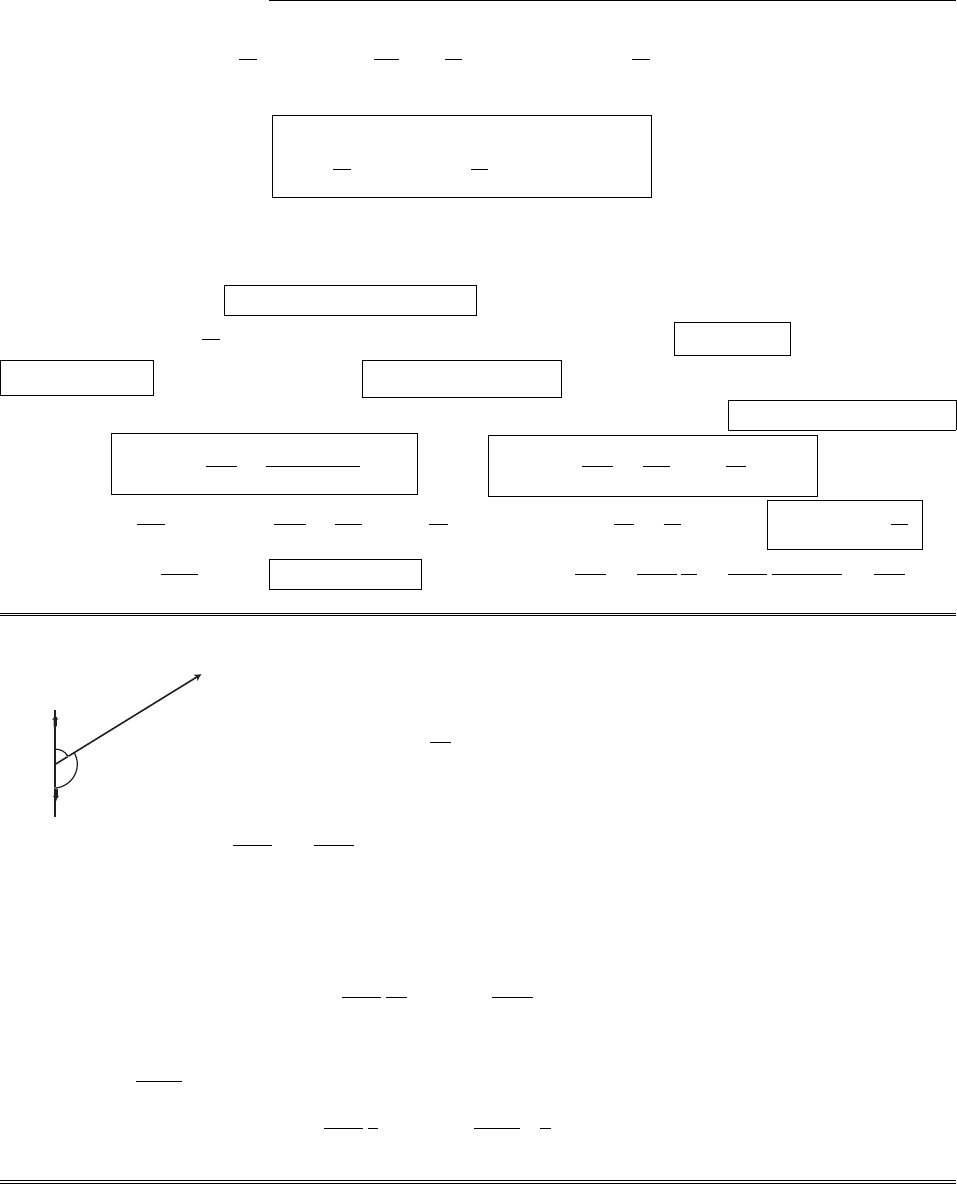
78 CHAPTER 3. POTENTIAL
B1(+2) 1
b2+C1+D12
b2=k
✏0
,for l= 1; C1+2
b3(B1D1)=k.
Therefore
(l+ 1)(BlDl)+lb2l+1Cl=0,for l6=1,
C1+2
b3(B1D1)= k
✏0
.(3)
Plug (2) and (10) into (3):
For l6= 0 or 1:
(l+1) b2l+1 a2l+1Cl+a2l+1Cl+lb2l+1Cl= 0; (l+1)b2l+1Cl+lb2l+1Cl= 0; (2l+1)Cl=0)Cl=0.
Therefore (10) and (2) )Bl=Cl=Dl= 0 for l>1.
For l= 1: C1+2
b3b3a3C1+a3C1=k;C1+2C1=k)C1=k/3✏0;D1=a3C1)
D1=a3k/3✏0;B1=b3a3C1)B1=b3a3k/3✏0.
For l= 0: B0D0=0)B0=D0)(ba)C0+aV0=aV0aC0,so bC0=0)C0= 0; D0=aV0=B0.
Conclusion: V(r, ✓)=aV0
r+b3a3k
3r2✏0
cos ✓, r b. V (r, ✓)=aV0
r+k
3✏0ra3
r2cos ✓, a rb.
(b)i(✓)=✏0
@V
@ra
=✏0aV0
a2+k
3✏01+2a3
a3cos ✓=✏0V0
a+k
✏0
cos ✓=kcos ✓+V0
✏0
a.
(c)qi=ida =V0✏0
a4⇡a2= 4⇡a✏0V0=Qtot.At large r:V⇡aV0
r
?
=1
4⇡✏0
Q
r=1
4⇡✏0
4⇡a✏0V0
r=aV0
r.X
Problem 3.44
r
r'
dr'
q'=q
q'=p-q
Use multipole expansion (Eq. 3.95): ⇢d⌧0!dr0;
=Q
2a; the r0integral breaks into two pieces:
V(r)= 1
4⇡✏0
1
n=0
1
rn+1
a
0
(r0)nPn(cos ✓0)dr0+
a
0
(r0)nPn(cos ✓0)dr0
.
In the first integral ✓0=✓(see diagram); in the second integral ✓0=⇡✓, so cos ✓0=cos ✓. But Pn(z)=
(1)nPn(z), so the integrals cancel when nis odd, and add when nis even.
V(r)=2 1
4⇡✏0
Q
2a
1
n=0,2,4,...
1
rn+1 Pn(cos ✓)
a
0
xndx.
The integral is an+1
n+1,so
V=Q
4⇡✏0
1
r
n=0,2,4,... 1
n+1a
rnPn(cos ✓).
c
2012 Pearson Education, Inc., Upper Saddle River, NJ. All rights reserved. This material is
protected under all copyright laws as they currently exist. No portion of this material may be
reproduced, in any form or by any means, without permission in writing from the publisher.

CHAPTER 3. POTENTIAL 79
Problem 3.45
Use separation of variables in cylindrical coordinates (Prob. 3.24):
V(s, )=a0+b0ln s+1
k=1 sk(akcos k+bksin k)+sk(ckcos k+dksin k).
s<R:V(s, )=1
k=1 sk(akcos k+bksin k) (ln sand skblow up at s= 0);
s>R:V(s, )=1
k=1 sk(ckcos k+dksin k) (ln sand skblow up as s!1).
(We may as well pick constants so V!0 as s!1, and hence a0= 0.) Continuity at s=R)
Rk(akcos k+bksin k)=Rk(ckcos k+dksin k), so ck=R2kak,d
k=R2kbk. Eq. 2.36 says:
@V
@sR+@V
@sR
=1
✏0
. Therefore
k
Rk+1 (ckcos k+dksin k)kRk1(akcos k+bksin k)=1
✏0
,
or: 2kRk1(akcos k+bksin k)=0/✏0(0 <<⇡)
0/✏0(⇡<<2⇡).
Fourier’s trick: multiply by (cos l)dand integrate from 0 to 2⇡, using
2⇡
0
sin kcos ld= 0;
2⇡
0
cos kcos ld=0,k6=l
⇡,k=l.
Then
2lRl1⇡al=0
✏0
⇡
0
cos ld
2⇡
⇡
cos ld
=0
✏0sin l
l
⇡
0sin l
l
2⇡
⇡= 0; al=0.
Multiply by (sin l)dand integrate, using
2⇡
0
sin ksin ld=0,k6=l
⇡,k=l:
2lRl1⇡bl=0
✏0
⇡
0
sin ld
2⇡
⇡
sin ld
=0
✏0cos l
l
⇡
0
+cos l
l
2⇡
⇡=0
l✏0
(2 2 cos l⇡)
=0,if lis even
40/l✏0,if lis odd )bl=0,if lis even
20/⇡✏0l2Rl1,if lis odd .
Conclusion:
V(s, )=20R
⇡✏0
k=1,3,5,...
1
k2sin k(s/R)k(s<R)
(R/s)k(s>R).
Problem 3.46
Use Eq. 3.95, in the form V(r)= 1
4⇡✏0
1
n=0
Pn(cos ✓)
rn+1 In;In=
a
a
zn(z)dz.
c
2012 Pearson Education, Inc., Upper Saddle River, NJ. All rights reserved. This material is
protected under all copyright laws as they currently exist. No portion of this material may be
reproduced, in any form or by any means, without permission in writing from the publisher.

80 CHAPTER 3. POTENTIAL
(a) I0=k
a
a
cos ⇡z
2adz =k2a
⇡sin ⇡z
2a
a
a
=2ak
⇡sin ⇡
2sin ⇡
2=4ak
⇡. Therefore:
1
Contents
Problem 3.40
✲z
✻
λ(z)
−a a
✲z
✻
λ(z)
−a a
✲z
✻
λ(z)
−a a
c
⃝2005 Pearson Education, Inc., Upper Saddle River, NJ. All rights reserved. This material is
protected under all copyright laws as they currently exist. No portion of this material may be
reproduced, in any form or by any means, without permission in writing from the publisher.
V(r, ✓)⇠
=1
4⇡✏04ak
⇡1
r.(Monopole.)
(b) I0=0.
I1=k
a
a
zsin(⇡z/a)dz =ka
⇡2sin ⇡z
aaz
⇡cos ⇡z
a
a
a
=ka
⇡2[sin(⇡)sin(⇡)] a2
⇡cos(⇡)a2
⇡cos(⇡)=k2a2
⇡;
1
Contents
Problem 3.40
✲z
✻
λ(z)
−a a
✲z
✻
λ(z)
−a a
✲z
✻
λ(z)
−a a
c
⃝2005 Pearson Education, Inc., Upper Saddle River, NJ. All rights reserved. This material is
protected under all copyright laws as they currently exist. No portion of this material may be
reproduced, in any form or by any means, without permission in writing from the publisher.
V(r, ✓)⇠
=1
4⇡✏02a2k
⇡1
r2cos ✓.(Dipole.)
(c) I0=I1=0.
I2=k
a
a
z2cos ⇡z
adz =k2zcos(⇡z/a)
(⇡/a)2+(⇡z/a)22
(⇡/a)3sin ⇡z
a
a
a
=2ka
⇡2[acos(⇡)+acos(⇡)] = 4a3k
⇡2.
1
Contents
Problem 3.40
✲z
✻
λ(z)
−a a
✲z
✻
λ(z)
−a a
✲z
✻
λ(z)
−a a
c
⃝2005 Pearson Education, Inc., Upper Saddle River, NJ. All rights reserved. This material is
protected under all copyright laws as they currently exist. No portion of this material may be
reproduced, in any form or by any means, without permission in writing from the publisher.
V(r, ✓)⇠
=1
4⇡✏04a3k
⇡21
2r33 cos2✓1.(Quadrupole.)
Problem 3.47
(a) The average field due to a point charge qat ris
Eave =1
4
3⇡R3Ed⌧,where E=1
4⇡✏0
q
r
2ˆ
r
,
so Eave =1
4
3⇡R31
4⇡✏0qˆ
r
r
2d⌧.
r
2
Problem 3.41
q
r
✮
dτ
c
⃝2005 Pearson Education, Inc., Upper Saddle River, NJ. All rights reserved. This material is
protected under all copyright laws as they currently exist. No portion of this material may be
reproduced, in any form or by any means, without permission in writing from the publisher.
(Here ris the source point, d⌧is the field point, so
r
goes from rto d⌧.) The field at rdue to uniform
charge ⇢over the sphere is E⇢=1
4⇡✏0⇢ˆ
r
r
2d⌧.This time d⌧is the source point and ris the field
point, so
r
goes from d⌧to r, and hence carries the opposite sign. So with ⇢=q/ 4
3⇡R3, the two
expressions agree: Eave =E⇢.
(b) From Prob. 2.12:
E⇢=1
3✏0
⇢r=q
4⇡✏0
r
R3=p
4⇡✏0R3.
c
2012 Pearson Education, Inc., Upper Saddle River, NJ. All rights reserved. This material is
protected under all copyright laws as they currently exist. No portion of this material may be
reproduced, in any form or by any means, without permission in writing from the publisher.

CHAPTER 3. POTENTIAL 81
(c) If there are many charges inside the sphere, Eave is the sum of the individual averages, and ptot is the
sum of the individual dipole moments. So Eave =p
4⇡✏0R3.qed
(d) The same argument, only with qplaced at routside the sphere, gives
Eave =E⇢=1
4⇡✏04
3⇡R3⇢
r2ˆr (field at rdue to uniformly charged sphere) = 1
4⇡✏0
q
r2ˆr .
But this is precisely the field produced by q(at r) at the center of the sphere. So the average field (over
the sphere) due to a point charge outside the sphere is the same as the field that same charge produces
at the center. And by superposition, this holds for any collection of exterior charges.
Problem 3.48
(a)
Edip =p
4⇡✏0r3(2 cos ✓ˆr + sin ✓ˆ
✓)
=p
4⇡✏0r3[2 cos ✓(sin ✓cos ˆx + sin ✓sin ˆy + cos ✓ˆz )
+ sin ✓(cos ✓cos ˆx + cos ✓sin ˆy sin ✓ˆz )]
=p
4⇡✏0r3
3 sin ✓cos ✓cos ˆx + 3 sin ✓cos ✓sin ˆy +2 cos2✓sin2✓
=3 cos2✓1
ˆz
.
Eave =1
4
3⇡R3Edip d⌧
=1
4
3⇡R3p
4⇡✏01
r33 sin ✓cos ✓(cos ˆx + sin ˆy )+3 cos2✓1ˆz r2sin ✓dr d✓d.
But
2⇡
0
cos d=
2⇡
0
sin d= 0, so the ˆx and ˆy terms drop out, and
2⇡
0
d=2⇡,so
Eave =1
4
3⇡R3p
4⇡✏02⇡
R
0
1
rdr
⇡
03 cos2✓1sin ✓d✓
(cos3✓+cos ✓)|⇡
0=11+11=0
.
Evidently Eave =0,which contradicts the result of Prob. 3.47. [Note, however, that the rintegral, R
0
1
rdr,
blows up, since ln r!1as r!0. If, as suggested, we truncate the rintegral at r=✏, then it is finite, and
the ✓integral gives Eave =0.]
(b) We want Ewithin the ✏-sphere to be a delta function: E=A3(r), with Aselected so that the average
field is consistent with the general theorem in Prob. 3.47:
Eave =1
4
3⇡R3A3(r)d⌧=A
4
3⇡R3=p
4⇡✏0R3)A=p
3✏0
,and hence E=p
3✏0
3(r).
c
2012 Pearson Education, Inc., Upper Saddle River, NJ. All rights reserved. This material is
protected under all copyright laws as they currently exist. No portion of this material may be
reproduced, in any form or by any means, without permission in writing from the publisher.

82 CHAPTER 3. POTENTIAL
Problem 3.49 We need to show that the field inside the sphere approaches a delta-function with the right
coefficient (Eq. 3.106) in the limit as R!0. From Eq. 3.86, the potential inside is
V=k
3✏0
rcos ✓=k
3✏0
z, so E=rV=k
3✏0
ˆz .
From Prob. 3.30, the dipole moment of this configuration is p= (4⇡R3k/3) ˆz , so kˆz =3p/(4⇡R3), and hence
the field inside is
E=1
4⇡✏0R3p.
Clearly E!1as R!0 (if pis held constant); its volume integral is
Ed⌧=1
4⇡✏0R3p4
3⇡R3=1
3✏0
p,
which matches the delta-function term in Eq. 3.106. X
Problem 3.50
(a) I=(rV1)·(rV2)d⌧.Butr·(V1rV2)=(rV1)·(rV2)+V1(r2V2), so
I=r·(V1rV2)d⌧V1(r2V2)=S
V1(rV2)·da+1
✏0V1⇢2d⌧.
But the surface integral is over a huge sphere “at infinity”, where V1and V2!0. So I=1
✏0V1⇢2d⌧. By
the same argument, with 1 and 2 reversed, I=1
✏0V2⇢1d⌧. So V1⇢2d⌧=V2⇢1d⌧. qed
(b)
Situation (1):Qa=a⇢1d⌧=Q;Qb=b⇢1d⌧= 0; V1b⌘Vab.
Situation (2):Qa=a⇢2d⌧= 0; Qb=b⇢2d⌧=Q;V2a⌘Vba.
V1⇢2d⌧=V1aa⇢2d⌧+V1bb⇢2d⌧=VabQ.
V2⇢1d⌧=V2aa⇢1d⌧+V2bb⇢1d⌧=VbaQ.
Green’s reciprocity theorem says QVab =QVba,so Vab =Vba.qed
Problem 3.51
2
Problem 3.41
q
r
✮
dτ
✲
0x
V=0 V=0
d
q
x
c
⃝2005 Pearson Education, Inc., Upper Saddle River, NJ. All rights reserved. This material is
protected under all copyright laws as they currently exist. No portion of this material may be
reproduced, in any form or by any means, without permission in writing from the publisher.
(a) Situation (1): actual. Situation (2): right plate at V0, left plate at V= 0, no charge at x.
V1⇢2d⌧=Vl1Ql2+Vx1Qx2+Vr1Qr2.
But Vl1=Vr1= 0 and Qx2= 0, so V1⇢2d⌧= 0.
V2⇢1d⌧=Vl2Ql1+Vx2Qx1+Vr2Qr1.
But Vl2=0Qx1=q, Vr2=V0,Q
r1=Q2, and Vx2=V0(x/d). So 0 = V0(x/d)q+V0Q2, and hence
Q2=qx/d.
c
2012 Pearson Education, Inc., Upper Saddle River, NJ. All rights reserved. This material is
protected under all copyright laws as they currently exist. No portion of this material may be
reproduced, in any form or by any means, without permission in writing from the publisher.

CHAPTER 3. POTENTIAL 83
Situation (1): actual. Situation (2): left plate at V0, right plate at V= 0, no charge at x.
V1⇢2d⌧=0=V2⇢1d⌧=Vl2Ql1+Vx2Qx1+Vr2Qr1=V0Q1+qVx2+0.
But Vx2=V01x
d,so
Q1=q(1 x/d).
(b) Situation (1): actual. Situation (2): inner sphere at V0, outer sphere at zero, no charge at r.
V1⇢2d⌧=Va1Qa2+Vr1Qr2+Vb1Qb2.
But Va1=Vb1=0,Q
r2= 0. So V1⇢2d⌧= 0.
V2⇢1d⌧=Va2Qa1+Vr2Qr1+Vb2Qb1=QaV0+qVr2+0.
But Vr2is the potential at rin configuration 2: V(r)=A+B/r, with V(a)=V0)A+B/a =V0, or
aA +B=aV0, and V(b)=0)A+B/b = 0, or bA +B= 0. Subtract: (ba)A=aV0)A=
aV0/(ba); B1
a1
b=V0=B(ba)
ab )B=abV0/(ba). So V(r)= aV0
(ba)b
r1. Therefore
QaV0+qaV0
(ba)b
r1= 0; Qa=qa
(ba)b
r1.
Now let Situation (2) be: inner sphere at zero, outer at V0, no charge at r.
V1⇢2d⌧=0=V2⇢1d⌧=Va2Qa1+Vr2Qr1+Vb2Qb1=0+qVr2+QbV0.
This time V(r)=A+B
rwith V(a)=0)A+B/a =0; V(b)=V0)A+B/b =V0, so
V(r)= bV0
(ba)1a
r. Therefore qbV0
(ba)1a
r+QbV0= 0; Qb=qb
(ba)1a
r.
Problem 3.52
(a)
3
i,j=1
ˆr iˆr jQij =1
2
3
3
i=1
ˆr ir0
i
3
j=1
ˆr jr0
j(r0)2
i,j
ˆr iˆr jij
⇢d⌧0
But
3
i=1
ˆr ir0
i=ˆr ·r0=r0cos ↵=
3
j=1
ˆr jr0
j;
i,j
ˆr iˆr jij =ˆr jˆr j=ˆr ·ˆr = 1. So
Vquad =1
4⇡✏0
1
r31
23r02cos2↵r02⇢d⌧0= the third term in Eq. 3.96. X
(b) Because x2=y2=(a/2)2for all four charges, Qxx =Qyy =1
23(a/2)2(p2a/2)2(qqq+q)=0.
Because z= 0 for all four charges, Qzz =1
2[(p2a/2)2](qqq+q) = 0 and Qxz =Qyz =Qzx =Qzy =0.
This leaves only
Qxy =Qyx =3
2a
2a
2q+a
2a
2(q)+a
2a
2(q)+a
2a
2q=3
2a2q.
c
2012 Pearson Education, Inc., Upper Saddle River, NJ. All rights reserved. This material is
protected under all copyright laws as they currently exist. No portion of this material may be
reproduced, in any form or by any means, without permission in writing from the publisher.

84 CHAPTER 3. POTENTIAL
(c)
2Qij =3(ridi)(rjdj)(rd)2ij ⇢d⌧(I0ll drop the primes,for simplicity.)
=3rirjr2ij ⇢d⌧3dirj⇢d⌧3djri⇢d⌧+3didj⇢d⌧+2d·r⇢d⌧
ij
d2ij ⇢d⌧=Qij 3(dipj+djpi)+3didjQ+2ij d·pd2ij Q.
So if p= 0 and Q= 0 then Qij =Qij .qed
(d) Eq. 3.95 with n= 3:
Voct =1
4⇡✏0
1
r4(r0)3P3(cos ↵)⇢d⌧0;P3(cos ✓)=1
25 cos3✓3 cos ✓.
Voct =1
4⇡✏0
1
r4
i,j,k
ˆr iˆr jˆr kQijk.
Define the “octopole moment” as
Qijk ⌘1
25r0
ir0
jr0
k(r0)2(r0
ijk +r0
jik +r0
kij )⇢(r0)d⌧0.
Problem 3.53
V=1
4⇡✏0q1
r
11
r
2+q01
r
31
r
4
r
1=r2+a22ra cos ✓,
r
2=r2+a2+2ra cos ✓,
r
3=r2+b22rb cos ✓,
r
1=r2+b2+2rb cos ✓.
3
Problem 3.46
−q+q
r
−q′
+q′
✯
❃
✒✼▼
24
r3
1
θ
!"# $
a
! "# $
a
!"#$
b
!"# $
b
c
⃝2005 Pearson Education, Inc., Upper Saddle River, NJ. All rights reserved. This material is
protected under all copyright laws as they currently exist. No portion of this material may be
reproduced, in any form or by any means, without permission in writing from the publisher.
r
r
r
r
Expanding as in Ex. 3.10: 1
r
11
r
2⇠
=2r
a2cos ✓(we want ar, not ra, this time).
1
r
31
r
4⇠
=2b
r2cos ✓(here we want b⌧r, because b=R2/a, Eq.3.16)
=2
a
R2
r2cos ✓.
But q0=R
aq(Eq. 3.15), so
V(r, ✓)⇠
=1
4⇡✏0q2r
a2cos ✓R
aq2
a
R2
r2cos ✓=1
4⇡✏02q
a2rR3
r2cos ✓.
c
2012 Pearson Education, Inc., Upper Saddle River, NJ. All rights reserved. This material is
protected under all copyright laws as they currently exist. No portion of this material may be
reproduced, in any form or by any means, without permission in writing from the publisher.

CHAPTER 3. POTENTIAL 85
Set E0=1
4⇡✏0
2q
a2(field in the vicinity of the sphere produced by ±q):
V(r, ✓)=E0rR3
r2cos ✓(agrees with Eq.3.76).
Problem 3.54
The boundary conditions are
(i) V= 0 when y=0,
(ii) V=V0when y=a,
(iii) V= 0 when x=b,
(iv) V= 0 when x=b.
Go back to Eq. 3.26 and examine the case k= 0: d2X/dx2=d2Y/dy2= 0, so X(x)=Ax+B, Y (y)=Cy+D.
But this configuration is symmetric in x, so A= 0, and hence the k= 0 solution is V(x, y)=Cy +D. Pick
D= 0, C=V0/a, and subtract o↵this part:
V(x, y)=V0
y
a+¯
V(x, y).
The remainder (¯
V(x, y)) satisfies boundary conditions similar to Ex. 3.4:
(i) ¯
V= 0 when y=0,
(ii) ¯
V= 0 when y=a,
(iii) ¯
V=V0(y/a) when x=b,
(iv) ¯
V=V0(y/a) when x=b.
(The point of peeling o↵V0(y/a) was to recover (ii), on which the constraint k=n⇡/a depends.)
The solution (following Ex. 3.4) is
¯
V(x, y)= 1
n=1
Cncosh(n⇡x/a) sin(n⇡y/a),
and it remains to fit condition (iii):
¯
V(b, y)=Cncosh(n⇡b/a) sin(n⇡y/a)=V0(y/a).
Invoke Fourier’s trick:
Cncosh(n⇡b/a)a
0
sin(n⇡y/a) sin(n0⇡y/a)dy =V0
aa
0
ysin(n0⇡y/a)dy,
a
2Cncosh(n⇡b/a)=V0
aa
0
ysin(n⇡y/a)dy.
Cn=2V0
a2cosh(n⇡b/a)a
n⇡2sin(n⇡y/a)ay
n⇡cos(n⇡y/a)
a
0
=2V0
a2cosh(n⇡b/a)a2
n⇡cos(n⇡)=2V0
n⇡
(1)n
cosh(n⇡b/a).
c
2012 Pearson Education, Inc., Upper Saddle River, NJ. All rights reserved. This material is
protected under all copyright laws as they currently exist. No portion of this material may be
reproduced, in any form or by any means, without permission in writing from the publisher.

86 CHAPTER 3. POTENTIAL
V(x, y)= V0y
a+2
⇡
1
n=1
(1)n
n
cosh(n⇡x/a)
cosh(n⇡b/a)sin(n⇡y/a).
Alternatively, start with the separable solution
V(x, y)=(Csin kx +Dcos kx)Aeky +Beky.
Note that the configuration is symmetric in x,soC= 0, and V(x, 0) = 0 )B=A, so (combining the
constants)
V(x, y)=Acos kx sinh ky.
But V(b, y) = 0, so cos kb = 0, which means that kb =±⇡/2,±3⇡/2,..., or k=(2n1)⇡/2b⌘↵n, with
n=1,2,3,... (negative kdoes not yield a di↵erent solution—the sign can be absorbed into A). The general
linear combination is
V(x, y)= 1
n=1
Ancos ↵nxsinh ↵ny,
and it remains to fit the final boundary condition:
V(x, a)=V0=1
n=1
Ancos ↵nxsinh ↵na.
Use Fourier’s trick, multiplying by cos ↵n0xand integrating:
V0b
b
cos ↵n0xdx=1
n=1
Ansinh ↵nab
b
cos ↵n0xcos ↵nxdx,
V0
2 sin ↵n0b
↵n0
=1
n=1
Ansinh ↵na(bn0n)=bAn0sinh ↵n0a.
So An=2V0
b
sin ↵nb
↵nsinh ↵na.But sin ↵nb= sin 2n1
2⇡=(1)n,so
V(x, y)= 2V0
b
1
n=1
(1)nsinh ↵ny
↵nsinh ↵nacos ↵nx.
Problem 3.55
(a) Using Prob. 3.15b (with b=a):
V(x, y)=4V0
⇡
nodd
sinh(n⇡x/a) sin(n⇡y/a)
nsinh(n⇡).
c
2012 Pearson Education, Inc., Upper Saddle River, NJ. All rights reserved. This material is
protected under all copyright laws as they currently exist. No portion of this material may be
reproduced, in any form or by any means, without permission in writing from the publisher.

CHAPTER 3. POTENTIAL 87
(y)=✏0
@V
@xx=0 =✏0
4V0
⇡
nodd n⇡
acosh(n⇡x/a) sin(n⇡y/a)
nsinh(n⇡)x=0
=4✏0V0
a
nodd
sin(n⇡y/a)
sinh(n⇡).
=a
0
(y)dy =4✏0V0
a
nodd
1
sinh(n⇡)a
0
sin(n⇡y/a)dy.
But a
0
sin(n⇡y/a)dy =a
n⇡cos(n⇡y/a)a
0=a
n⇡[1 cos(n⇡)] = 2a
n⇡(since nis odd).
=8✏0V0
⇡
nodd
1
nsinh(n⇡)=✏0V0
⇡ln 2.
[Summing the series numerically (using Mathematica) gives 0.0866434, which agrees precisely with ln 2/8.
The series can be summed analytically, by manipulation of elliptic integrals—see “Integrals and Series, Vol. I:
Elementary Functions,” by A. P. Prudnikov, Yu. A. Brychkov, and O. I. Marichev (Gordon and Breach, New
York, 1986), p. 721. I thank Ram Valluri for calling this to my attention.]
Using Prob. 3.54 (with b=a/2):
V(x, y)=V0y
a+2
⇡
n
(1)ncosh(n⇡x/a) sin(n⇡y/a)
ncosh(n⇡/2) .
(x)=✏0
@V
@yy=0 =✏0V01
a+2
⇡
nn⇡
a(1)ncosh(n⇡x/a) cos(n⇡y/a)
ncosh(n⇡/2) y=0
=✏0V01
a+2
a
n
(1)ncosh(n⇡x/a)
cosh(n⇡/2) =✏0V0
a1+2
n
(1)ncosh(n⇡x/a)
cosh(n⇡/2) .
=a/2
a/2
(x)dx =✏0V0
aa+2
n
(1)n
cosh(n⇡/2) a/2
a/2
cosh(n⇡x/a)dx.
But a/2
a/2
cosh(n⇡x/a)dx =a
n⇡sinh(n⇡x/a)
a/2
a/2
=2a
n⇡sinh(n⇡/2).
=✏0V0
aa+4a
⇡
n
(1)ntanh(n⇡/2)
n=✏0V01+ 4
⇡
n
(1)ntanh(n⇡/2)
n
=✏0V0
⇡ln 2.
[The numerical value is -0.612111, which agrees with the expected value (ln 2 ⇡)/4.]
(b) From Prob. 3.24:
V(s, )=a0+b0ln s+1
k=1 aksk+bk
1
sk[ckcos(k)+dksin(k)].
In the interior (s<R)b0and bkmust be zero (ln sand 1/s blow up at the origin). Symmetry )dk=0.So
V(s, )=a0+1
k=1
akskcos(k).
c
2012 Pearson Education, Inc., Upper Saddle River, NJ. All rights reserved. This material is
protected under all copyright laws as they currently exist. No portion of this material may be
reproduced, in any form or by any means, without permission in writing from the publisher.

88 CHAPTER 3. POTENTIAL
4
Problem 3.48
✲x
✻
y
V0
Problem 3.49
✻
z
❄
mg
❦
l
T
φ
θ
c
⃝2005 Pearson Education, Inc., Upper Saddle River, NJ. All rights reserved. This material is
protected under all copyright laws as they currently exist. No portion of this material may be
reproduced, in any form or by any means, without permission in writing from the publisher.
At the surface:
V(R, )=
k=0
akRkcos(k)=V0,if ⇡/4<<⇡/4,
0,otherwise.
Fourier’s trick: multiply by cos(k0) and integrate from ⇡to ⇡:
1
k=0
akRk⇡
⇡
cos(k) cos(k0)d=V0⇡/4
⇡/4
cos(k0)d=
V0sin(k0)/k0
⇡/4
⇡/4=(V0/k0) sin(k0⇡/4),if k06=0,
V0⇡/2,if k0=0.
But
⇡
⇡
cos(k) cos(k0)d=
0,if k6=k0
2⇡,if k=k0=0,
⇡,if k=k06=0.
So 2⇡a0=V0⇡/2)a0=V0/4; ⇡akRk=(2V0/k) sin(k⇡/4) )ak=(2V0/⇡kRk) sin(k⇡/4) (k6= 0); hence
V(s, )=V01
4+2
⇡
1
k=1
sin(k⇡/4)
ks
Rkcos(k).
Using Eq. 2.49, and noting that in this case ˆn =ˆs :
()=✏0
@V
@ss=R=✏0V0
2
⇡
1
k=1
sin(k⇡/4)
kRkksk1cos(k)s=R=2✏0V0
⇡R
1
k=1
sin(k⇡/4) cos(k).
We want the net (line) charge on the segment opposite to V0(⇡<<3⇡/4 and 3⇡/4<<⇡):
=()Rd=2R⇡
3⇡/4
()d=4✏0V0
⇡
1
k=1
sin(k⇡/4) ⇡
3⇡/4
cos(k)d
=4✏0V0
⇡
1
k=1
sin(k⇡/4) sin(k)
k
⇡
3⇡/4=4✏0V0
⇡
1
k=1
sin(k⇡/4) sin(3k⇡/4)
k.
ksin(k⇡/4) sin(3k⇡/4) product
11/p21/p2 1/2
2 1 -1 -1
31/p21/p2 1/2
40 0 0
5-1/p2 -1/p2 1/2
6 -1 1 -1
7-1/p2 -1/p2 1/2
80 0 0
c
2012 Pearson Education, Inc., Upper Saddle River, NJ. All rights reserved. This material is
protected under all copyright laws as they currently exist. No portion of this material may be
reproduced, in any form or by any means, without permission in writing from the publisher.

CHAPTER 3. POTENTIAL 89
=4✏0V0
⇡1
2
1,3,5...
1
k
2,6,10,...
1
k=4✏0V0
⇡1
2
1,3,5...
1
k1
2
1,3,5,...
1
k=0.
Ouch! What went wrong? The problem is that the series (1/k) is divergent, so the “subtraction” 11
is suspect. One way to avoid this is to go back to V(s, ), calculate ✏0(@V/@s) at s6=R, and save the limit
s!Runtil the end:
(,s)⌘✏0
@V
@s=2✏0V0
⇡
1
k=1
sin(k⇡/4)
k
ksk1
Rkcos(k)
=2✏0V0
⇡R
1
k=1
xk1sin(k⇡/4) cos(k) (where x⌘s/R !1 at the end).
(x)⌘(,s)Rd=4✏0V0
⇡
1
k=1
1
kxk1sin(k⇡/4) sin(3k⇡/4)
=4✏0V0
⇡1
2xx+x3
3+x5
5+···1
xx2
2+x6
6+x10
10 +···
=2✏0V0
⇡xx+x3
3+x5
5+···x2+x6
3+x10
5+···.
But (see math tables) : ln 1+x
1x=2x+x3
3+x5
5+···.
=2✏0V0
⇡x1
2ln 1+x
1x1
2ln 1+x2
1x2=✏0V0
⇡xln 1+x
1x1+x2
1x2
=✏0V0
⇡xln (1 + x)2
1+x2;= lim
x!1(x)= ✏0V0
⇡ln 2.
Problem 3.56
F=qE=qp
4⇡✏0r3(2 cos ✓ˆr + sin ✓ˆ
✓).
4
Problem 3.48
✲x
✻
y
V0
Problem 3.49
✻
z
❄
mg
❦
l
T
φ
θ
c
⃝2005 Pearson Education, Inc., Upper Saddle River, NJ. All rights reserved. This material is
protected under all copyright laws as they currently exist. No portion of this material may be
reproduced, in any form or by any means, without permission in writing from the publisher.
Now consider the pendulum: F=mg ˆz Tˆr , where Tmg cos =mv2/l and (by conservation of
energy) mgl cos = (1/2)mv2)v2=2gl cos (assuming it started from rest at = 90, as stipulated). But
cos =cos ✓,soT=mg(cos ✓)+(m/l)(2gl cos ✓)=3mg cos ✓,and hence
F=mg(cos ✓ˆr sin ✓ˆ
✓)+3mg cos ✓ˆr =mg(2 cos ✓ˆr + sin ✓ˆ
✓).
This total force is such as to keep the pendulum on a circular arc, and it is identical to the force on qin the
field of a dipole, with mg $qp/4⇡✏0l3. Evidently qalso executes semicircular motion, as though it were on a
tether of fixed length l.
Problem 3.57 Symmetry suggests that the plane of the orbit is perpendicular to the zaxis, and since we need
a centripetal force, pointing in toward the axis, the orbit must lie at the bottom of the field loops (Fig. 3.37a),
where the zcomponent of the field is zero. Referring to Eq. 3.104,
c
2012 Pearson Education, Inc., Upper Saddle River, NJ. All rights reserved. This material is
protected under all copyright laws as they currently exist. No portion of this material may be
reproduced, in any form or by any means, without permission in writing from the publisher.

90 CHAPTER 3. POTENTIAL
E·ˆz =0)3(p·ˆr )(ˆr ·ˆz )p·ˆz =0,or 3 cos2✓1=0.So cos2✓=1/3,cos ✓=1/p3,sin ✓=2/3, z/s =
tan ✓)z=p2s. The field at the orbit is (Eq. 3.103)
E=p
4⇡✏0r321
p3ˆr +2
3ˆ
✓
=p
4⇡✏0r32
3p2(sin ✓cos ˆx + sin ✓sin ˆy + cos ✓ˆz ) + (cos ✓cos ˆx + cos ✓sin ˆy sin ✓ˆz )
=p
4⇡✏0r32
3p2 sin ✓+ cos ✓cos ˆx +p2 sin ✓+ cos ✓sin ˆy +p2 cos ✓sin ✓ˆz
=p
4⇡✏0r32
3p22
31
p3(cos ˆx + sin ˆy )+p21
p32
3ˆz
=p
4⇡✏0r32
3p3 (cos ˆx + sin ˆy )=p
4⇡✏0r3p2ˆs =p
3p3⇡✏0s3ˆs .
(I used s=rsin ✓=r2/3, in the last step.)
The centripetal force is
F=qE =qp
3p3⇡✏0s3=mv2
s)v2=qp
3p3⇡✏0ms2)v=1
sqp
3p3⇡✏0m.
The angular momentum is
L=smv =qpm
3p3⇡✏0
,
the same for all orbits, regardless of their radius (!), and the energy is
W=1
2mv2+qV =1
2
qp
3p3⇡✏0s2+q
4⇡✏0
pcos ✓
r2=qp
6p3⇡✏0s2qp
4⇡✏0p3(3/2)s2= 0.
Problem 3.58
Potential of q:Vq(r)= 1
4⇡✏0
q
r
, where
r
2=a2+r22ar cos ✓.
Equation 3.94, with r0!aand ↵!✓:1
r
=1
r
1
n=0 a
rnPn(cos ✓).So
Vq(r, ✓)= q
4⇡✏0
1
r
1
n=0 a
rnPn(cos ✓).
Meanwhile, the potential of is (Eq. 3.79) V(r, ✓)= 1
l=0
Bl
rl+1 Pl(cos ✓).
Comparing the two (Vq=V) we see that Bl=(q/4⇡✏0)al, and hence (Eq. 3.81) Al=(q/4⇡✏0)al/R2l+1.Then
(Eq. 3.83)
(✓)= q
4⇡R2
1
l=0
(2l+ 1) a
RlPl(cos ✓)= q
4⇡R221
l=0
la
RlPl(cos ✓)+ 1
l=0 a
RlPl(cos ✓).
c
2012 Pearson Education, Inc., Upper Saddle River, NJ. All rights reserved. This material is
protected under all copyright laws as they currently exist. No portion of this material may be
reproduced, in any form or by any means, without permission in writing from the publisher.

CHAPTER 3. POTENTIAL 91
Now (second line above, with r!R)
1
pa2+R22aR cos ✓=1
R
1
l=0 a
RlPl(cos ✓).
Di↵erentiating with respect to a:
d
da 1
pa2+R22aR cos ✓=(aRcos ✓)
(a2+R22aR cos ✓)3/2=1
aR
1
l=0
la
RlPl(cos ✓).
Thus
(✓)= q
4⇡R22aR (aRcos ✓)
(a2+R22aR cos ✓)3/2+R
(a2+R22aR cos ✓)1/2
=q
4⇡R2a(aRcos ✓)+(a2+R22aR cos ✓)
(a2+R22aR cos ✓)3/2=q
4⇡R
(R2a2)
(a2+R22aR cos ✓)3/2.
c
2012 Pearson Education, Inc., Upper Saddle River, NJ. All rights reserved. This material is
protected under all copyright laws as they currently exist. No portion of this material may be
reproduced, in any form or by any means, without permission in writing from the publisher.
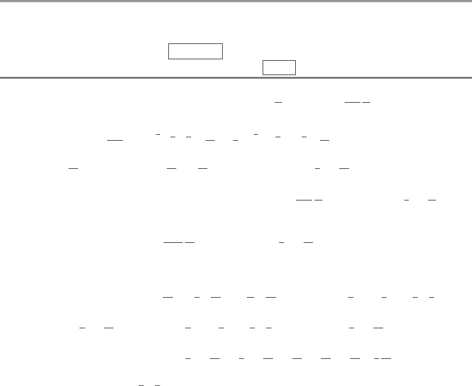
92 CHAPTER 4. ELECTRIC FIELDS IN MATTER
Chapter 4
Electric Fields in Matter
Problem 4.1
E=V/x = 500/103=5⇥105. Table 4.1: ↵/4⇡✏0=0.66⇥1030, so ↵=4⇡(8.85⇥1012)(0.66⇥1030)=
7.34 ⇥1041.p=↵E=ed )d=↵E/e =(7.34 ⇥1041)(5 ⇥105)/(1.6⇥1019)=2.29 ⇥1016 m.
d/R =(2.29 ⇥1016)/(0.5⇥1010)= 4.6⇥106.To ionize, say d=R.ThenR=↵E/e =↵V /ex )V=
Rex/↵=(0.5⇥1010)(1.6⇥1019)(103)/(7.34 ⇥1041)= 108V.
Problem 4.2
First find the field, at radius r, using Gauss’ law: E·da=1
✏0Qenc, or E=1
4⇡✏0
1
r2Qenc.
Qenc =r
0
⇢d⌧=4⇡q
⇡a3r
0
e2r/a r2dr =4q
a3a
2e2r/a r2+ar +a2
2
r
0
=2q
a2e2r/a r2+ar +a2
2a2
2=q1e2r/a 1+2r
a+2r2
a2.
[Note: Qenc(r!1)=q.] So the field of the electron cloud is Ee=1
4⇡✏0
q
r21e2r/a 1+2r
a+2r2
a2. The
proton will be shifted from r= 0 to the point dwhere Ee=E(the external field):
E=1
4⇡✏0
q
d21e2d/a 1+2d
a+2d2
a2.
Expanding in powers of (d/a):
e2d/a =12d
a+1
22d
a2
1
3! 2d
a3
+···=12d
a+2d
a2
4
3d
a3
+···
1e2d/a 1+2d
a+2d2
a2=112d
a+2d
a2
4
3d
a3
+···1+2d
a+2d2
a2
=1/1/2d
a
/2d2
a2
/+2d
a
/+4d2
a2
/+4d3
a3
/2d2
a2
/4d3
a3
/+4
3
d3
a3+···
=4
3d
a3
+ higher order terms.
c
2012 Pearson Education, Inc., Upper Saddle River, NJ. All rights reserved. This material is
protected under all copyright laws as they currently exist. No portion of this material may be
reproduced, in any form or by any means, without permission in writing from the publisher.

CHAPTER 4. ELECTRIC FIELDS IN MATTER 93
E=1
4⇡✏0
q
d24
3
d3
a3=1
4⇡✏0
4
3a3(qd)= 1
3⇡✏0a3p. ↵=3⇡✏0a3.
[Not so di↵erent from the uniform sphere model of Ex. 4.1 (see Eq. 4.2). Note that this result predicts
1
4⇡✏0↵=3
4a3=3
40.5⇥10103=0.09 ⇥1030 m3, compared with an experimental value (Table 4.1) of
0.66 ⇥1030 m3. Ironically the “classical” formula (Eq. 4.2) is slightly closer to the empirical value.]
Problem 4.3
⇢(r)=Ar. Electric field (by Gauss’s Law): E·da=E4⇡r2=1
✏0Qenc =1
✏0r
0Ar 4⇡r2dr, or E=
1
4⇡r2
4⇡A
✏0
r4
4=Ar2
4✏0
. This “internal” field balances the external field Ewhen nucleus is “o↵-center” an amount
d:ad2/4✏0=E)d=4✏0E/A. So the induced dipole moment is p=ed =2e✏0/ApE. Evidently
pis proportional to E1/2.
For Eq. 4.1 to hold in the weak-field limit, E must be proportional to r, for small r, which means that ⇢
must go to a constant (not zero) at the origin: ⇢(0) 6=0 (nor infinite).
Problem 4.4
1
Contents
Problem 4.4
q
r
Problem 4.6
✸
−
+
θ
p
❦
−
+
θ
pi
z
z
c
⃝2005 Pearson Education, Inc., Upper Saddle River, NJ. All rights reserved. This material is
protected under all copyright laws as they currently exist. No portion of this material may be
reproduced, in any form or by any means, without permission in writing from the publisher.
Field of q:1
4⇡✏0
q
r2ˆr .Induced dipole moment of atom: p=↵E=
↵q
4⇡✏0r2ˆr .
Field of this dipole, at location of q(✓=⇡, in Eq. 3.103): E=1
4⇡✏0
1
r32↵q
4⇡✏0r2(to the right).
Force on qdue to this field: F=2↵q
4⇡✏021
r5(attractive).
Problem 4.5
Field of p1at p2(✓=⇡/2 in Eq. 3.103): E1=p1
4⇡✏0r3ˆ
✓(points down).
Torque on p2:N2=p2⇥E1=p2E1sin 90=p2E1=p1p2
4⇡✏0r3(points into the page).
Field of p2at p1(✓=⇡in Eq. 3.103): E2=p2
4⇡✏0r3(2ˆr ) (points to the right).
Torque on p1:N1=p1⇥E2=2p1p2
4⇡✏0r3(points into the page).
Problem 4.6
(a) (b)
1
Contents
Problem 4.4
q
r
Problem 4.6
✸
−
+
θ
p
❦
−
+
θ
pi
z
z
c
⃝2005 Pearson Education, Inc., Upper Saddle River, NJ. All rights reserved. This material is
protected under all copyright laws as they currently exist. No portion of this material may be
reproduced, in any form or by any means, without permission in writing from the publisher.
1
Hello
θ2z
pi
p
θ
✻
✲
c
⃝2005 Pearson Education, Inc., Upper Saddle River, NJ. All rights reserved. This material is
protected under all copyright laws as they currently exist. No portion of this material may be
reproduced, in any form or by any means, without permission inwritingfromthepublisher.
Use image dipole as shown in Fig. (a).
Redraw, placing piat the origin, Fig. (b).
Ei=p
4⇡✏0(2z)3(2 cos ✓ˆr + sin ✓ˆ
✓); p=pcos ✓ˆr +psin ✓ˆ
✓.
N=p⇥Ei=p2
4⇡✏0(2z)3(cos ✓ˆr + sin ✓ˆ
✓)⇥(2 cos ✓ˆr + sin ✓ˆ
✓)
=p2
4⇡✏0(2z)3cos ✓sin ✓ˆ
+ 2 sin ✓cos ✓(ˆ
)
=p2sin ✓cos ✓
4⇡✏0(2z)3(ˆ
) (out of the page).
c
2012 Pearson Education, Inc., Upper Saddle River, NJ. All rights reserved. This material is
protected under all copyright laws as they currently exist. No portion of this material may be
reproduced, in any form or by any means, without permission in writing from the publisher.

94 CHAPTER 4. ELECTRIC FIELDS IN MATTER
But sin ✓cos ✓= (1/2) sin 2✓,so N=p2sin 2✓
4⇡✏0(16z3)(out of the page).
For 0 <✓<⇡/2, Ntends to rotate pcounterclockwise; for ⇡/2<✓<⇡,Nrotates pclockwise. Thus the
stable orientation is perpendicular to the surface—either "or #.
Problem 4.7
If the potential is zero at infinity, the energy of a point charge Qis (Eq. 2.39) W=QV (r). For a physical
dipole, with qat rand +qat r+d,
U=qV (r+d)qV (r)=q[V(r+d)V(r)] = qr+d
r
E·dl.
For an ideal dipole the integral reduces to E·d, and
U=qE·d=p·E,
since p=qd.If you do not (or cannot) use infinity as the reference point, the result still holds, as long as
you bring the two charges in from the same point,r0(or two points at the same potential). In that case
W=Q[V(r)V(r0)], and
U=q[V(r+d)V(r0)] q[V(r)V(r0)] = q[V(r+d)V(r)],
as before.
Problem 4.8
U=p1·E2, but E2=1
4⇡✏0
1
r3[3 (p2·ˆr )ˆr p2]. So U=1
4⇡✏0
1
r3[p1·p23(p1·ˆr )(p2·ˆr )]. qed
Problem 4.9
(a) F=(p·r)E(Eq. 4.5); E=1
4⇡✏0
q
r2ˆr =q
4⇡✏0
xˆx +yˆy +zˆz
(x2+y2+z2)3/2.
Fx=px
@
@x+py
@
@y+pz
@
@zq
4⇡✏0
x
(x2+y2+z2)3/2
=q
4⇡✏0px1
(x2+y2+z2)3/23
2x2x
(x2+y2+z2)5/2+py3
2x2y
(x2+y2+z2)5/2
+pz3
2x2z
(x2+y2+z2)5/2=q
4⇡✏0px
r33x
r5(pxx+pyy+pzz)=q
4⇡✏0p
r33r(p·r)
r5x
.
F=1
4⇡✏0
q
r3[p3(p·ˆr )ˆr ].
(b) E=1
4⇡✏0
1
r3{3[p·(ˆr )] (ˆr )p}=1
4⇡✏0
1
r3[3(p·ˆr )ˆr p].(This is from Eq. 3.104; the minus signs
are because rpoints toward p, in this problem.)
F=qE=1
4⇡✏0
q
r3[3(p·ˆr )ˆr p].
[Note that the forces are equal and opposite, as you would expect from Newton’s third law.]
c
2012 Pearson Education, Inc., Upper Saddle River, NJ. All rights reserved. This material is
protected under all copyright laws as they currently exist. No portion of this material may be
reproduced, in any form or by any means, without permission in writing from the publisher.

CHAPTER 4. ELECTRIC FIELDS IN MATTER 95
Problem 4.10
(a) b=P·ˆn =kR;⇢b=r·P=1
r2
@
@r(r2kr)=1
r23kr2=3k.
(b) For r<R,E=1
3✏0⇢rˆr (Prob. 2.12), so E=(k/✏0)r.
For r>R, same as if all charge at center; but Qtot =(kR)(4⇡R2)+(3k)( 4
3⇡R3) = 0, so E=0.
Problem 4.11
⇢b= 0; b=P·ˆn =±P(plus sign at one end—the one Ppoints toward; minus sign at the other—the one
Ppoints away from).
(i) La. Then the ends look like point charges, and the whole thing is like a physical dipole, of length Land
charge P⇡a2. See Fig. (a).
(ii) L⌧a. Then it’s like a circular parallel-plate capacitor. Field is nearly uniform inside; nonuniform “fringing
field” at the edges. See Fig. (b).
(iii) L⇡a. See Fig. (c).
2
θz
pi
p
θ
✻
✲
Problem 4.7
✲
x
✻
y
p
p
θ
✲✒
✻
E
Problem 4.11
✛
✛
✛
✛
✛
✛✲
P
(a) Like a dipole
−+
✛
✛
✛
✛
✛
✛
✛
✛
✛
✛
✛
✛
✛✻
❄
✻
❄
✲
P
(b) Like a parallel-plate capacitor
−+
✛
✛
✛
✛
✛
✛
✛
✛
✛
✲
P
(c)
c
⃝2005 Pearson Education, Inc., Upper Saddle River, NJ. All rights reserved. This material is
protected under all copyright laws as they currently exist. No portion of this material may be
reproduced, in any form or by any means, without permission in writing from the publisher.
Problem 4.12
V=1
4⇡✏0P·ˆ
r
r
2d⌧=P·1
4⇡✏0ˆ
r
r
2d⌧. But the term in curly brackets is precisely the field of a uniformly
charged sphere, divided by ⇢. The integral was done explicitly in Probs. 2.7 and 2.8:
1
4⇡✏0ˆ
r
r
2d⌧=1
⇢
1
4⇡✏0
(4/3)⇡R3⇢
r2ˆr ,(r>R),
1
4⇡✏0
(4/3)⇡R3⇢
R3r,(r<R).
So V(r, ✓)=
R3
3✏0r2P·ˆr =R3Pcos ✓
3✏0r2,(r>R),
1
3✏0
P·r=Prcos ✓
3✏0
,(r<R).
Problem 4.13
Think of it as two cylinders of opposite uniform charge density ±⇢.Inside, the field at a distance sfrom
the axis of a uniformly charge cylinder is given by Gauss’s law: E2⇡s`=1
✏0⇢⇡s2`)E=(⇢/2✏0)s. For
two such cylinders, one plus and one minus, the net field (inside) is E=E++E=(⇢/2✏0)(s+s). But
s+s=d, so E=⇢d/(2✏0), where dis the vector from the negative axis to positive axis. In this case
the total dipole moment of a chunk of length `is P⇡a2`=⇢⇡a2`d. So ⇢d=P, and E=P/(2✏0),for
s<a.
c
2012 Pearson Education, Inc., Upper Saddle River, NJ. All rights reserved. This material is
protected under all copyright laws as they currently exist. No portion of this material may be
reproduced, in any form or by any means, without permission in writing from the publisher.

96 CHAPTER 4. ELECTRIC FIELDS IN MATTER
Outside, Gauss’s law gives E2⇡s`=1
✏0⇢⇡a2`)E=⇢a2
2✏0
ˆs
s, for one cylinder. For the combination, E=
E++E=⇢a2
2✏0ˆs +
s+ˆs
s, where
s±=s⌥d
2;
s±
s2
±
=s⌥d
2s2+d2
4⌥s·d1
⇠
=1
s2s⌥d
21⌥s·d
s21⇠
=1
s2s⌥d
21±s·d
s2
=1
s2s±s(s·d)
s2⌥d
2(keeping only 1st order terms in d).
ˆs +
s+ˆs
s=1
s2s+s(s·d)
s2d
2ss(s·d)
s2+s
2=1
s22s(s·d)
s2d.
E(s)= a2
2✏0
1
s2[2(P·ˆs )ˆs P],for s > a.
Problem 4.14
Total charge on the dielectric is Qtot =Sbda +V⇢bd⌧=SP·daVr·Pd⌧. But the divergence
theorem says SP·da=Vr·Pd⌧,soQenc = 0. qed
Problem 4.15
(a) ⇢b=r·P=1
r2
@
@rr2k
r=k
r2;b=P·ˆn =+P·ˆr =k/b (at r=b),
P·ˆr =k/a (at r=a).
Gauss’s law )E=1
4⇡✏0
Qenc
r2ˆr . For r<a,Qenc = 0, so E=0. For r>b,Qenc = 0 (Prob. 4.14), so E=0.
For a<r<b,Qenc =k
a4⇡a2+r
ak
r24⇡r2dr =4⇡ka 4⇡k(ra)=4⇡kr;so E=(k/✏0r)ˆr .
(b) D·da=Qfenc =0)D=0everywhere. D=✏0E+P=0)E=(1/✏0)P,so
E=0(for r<aand r>b); E=(k/✏0r)ˆr (for a<r<b).
Problem 4.16
(a) Same as E0minus the field at the center of a sphere with uniform polarization P. The latter (Eq. 4.14)
is P/3✏0. So E=E0+1
3✏0
P.D=✏0E=✏0E0+1
3P=D0P+1
3P,so D=D02
3P.
(b) Same as E0minus the field of ±charges at the two ends of the “needle”—but these are small, and far
away, so E=E0.D=✏0E=✏0E0=D0P,so D=D0P.
(c) Same as E0minus the field of a parallel-plate capacitor with upper plate at =P. The latter is
(1/✏0)P,so E=E0+1
✏0P.D=✏0E=✏0E0+P,so D=D0.
c
2012 Pearson Education, Inc., Upper Saddle River, NJ. All rights reserved. This material is
protected under all copyright laws as they currently exist. No portion of this material may be
reproduced, in any form or by any means, without permission in writing from the publisher.

CHAPTER 4. ELECTRIC FIELDS IN MATTER 97
Problem 4.17
1
Hello
✻✻✻✻✻✻✻
P
(uniform)
❄ ❄ ❄❄❄ ❄❄ ❄❄
E
(field of two circular plates)
✻
❄✻❄❄
✻
❄✻❄
✻
❄✻
D
(same as Eoutside, but lines
continuous, since ∇·D=0)
c
⃝2005 Pearson Education, Inc., Upper Saddle River, NJ. All rights reserved. This material is
protected under all copyright laws as they currently exist. No portion of this material may be
reproduced, in any form or by any means, without permission inwritingfromthepublisher.
For more detailed figures see the solution to Problem 6.14, reading Pfor M,Efor H, and Dfor B.
Problem 4.18
(a) Apply D·da=Qfenc to the gaussian surface shown. DA =A)D=.(Note: D=0inside the
metal plate.) This is true in both slabs; Dpoints down.
6
Problem 4.18
❖+σ
−σ
+σ/3
−σ/3
+σ/2
−σ/2
+σ
2⃝
1⃝
Problem 4.22
✛
y
✻
x
✙
z
φ
✻
E0
c
⃝2005 Pearson Education, Inc., Upper Saddle River, NJ. All rights reserved. This material is
protected under all copyright laws as they currently exist. No portion of this material may be
reproduced, in any form or by any means, without permission in writing from the publisher.
(b) D=✏E)E=/✏1in slab 1, E=/✏2in slab 2. But ✏=✏0✏r, so ✏1=2✏0;✏2=3
2✏0.E1=/2✏0,
E2=2/3✏0.
(c) P=✏0eE,soP=✏0ed/(✏0✏r)=(e/✏r);e=✏r1)P=(1✏1
r).P1=/2, P2=/3.
(d) V=E1a+E2a=(a/6✏0)(3 + 4) = 7a/6✏0.
(e) ⇢b= 0; b=+P1at bottom of slab (1) = /2,
b=P1at top of slab (1) = /2;
b=+P2at bottom of slab (2) = /3,
b=P2at top of slab (2) = /3.
(f) In slab 1: total surface charge above:(/2) = /2,
total surface charge below:(/2) (/3) + (/3) =/2,=)E1=
2✏0
.X
In slab 2: total surface charge above:(/2) + (/2) (/3) = 2/3,
total surface charge below:(/3) =2/3,=)E2=2
3✏0
.X
6
Problem 4.18
❖+σ
−σ
+σ/3
−σ/3
+σ/2
−σ/2
+σ
2⃝
1⃝
Problem 4.22
✛
y
✻
x
✙
z
φ
✻
E0
c
⃝2005 Pearson Education, Inc., Upper Saddle River, NJ. All rights reserved. This material is
protected under all copyright laws as they currently exist. No portion of this material may be
reproduced, in any form or by any means, without permission in writing from the publisher.
Problem 4.19
With no dielectric, C0=A✏0/d (Eq. 2.54).
In configuration (a), with +on upper plate, on lower, D=between the plates.
E=/✏0(in air) and E=/✏(in dielectric). So V=
✏0
d
2+
✏
d
2=Qd
2✏0A1+✏0
✏.
c
2012 Pearson Education, Inc., Upper Saddle River, NJ. All rights reserved. This material is
protected under all copyright laws as they currently exist. No portion of this material may be
reproduced, in any form or by any means, without permission in writing from the publisher.

98 CHAPTER 4. ELECTRIC FIELDS IN MATTER
Ca=Q
V=✏0A
d2
1+1/✏r=)Ca
C0
=2✏r
1+✏r
.
In configuration (b), with potential di↵erence V:E=V/d,so=✏0E=✏0V/d (in air).
P=✏0eE=✏0eV/d (in dielectric), so b=✏0eV/d (at top surface of dielectric).
tot =✏0V/d =f+b=f✏0eV/d,sof=✏0V(1 + e)/d =✏0✏rV/d (on top plate above dielectric).
=)Cb=Q
V=1
VA
2+f
A
2=A
2V✏0
V
d+✏0
V
d✏r=A✏0
d1+✏r
2.Cb
C0
=1+✏r
2.
[Which is greater? Cb
C0Ca
C0=1+✏r
22✏r
1+✏r=(1+✏r)24✏r
2(1+✏r)=1+2✏r+4✏2
r4✏r
2(1+✏r)=(1✏r)2
2(1+✏r)>0. So Cb>C
a.]
If the xaxis points down:
E D P
(a) air 2✏r
(✏r+1)
V
dˆx 2✏r
(✏r+1)
✏0V
dˆx 0
(a) dielectric 2
(✏r+1)
V
dˆx 2✏r
(✏r+1)
✏0V
dˆx 2(✏r1)
(✏r+1)
✏0V
dˆx
(b) air V
dˆx ✏0V
dˆx 0
(b) dielectric V
dˆx ✏r✏0V
dˆx (✏r1)✏0V
dˆx
b(top surface) f(top plate)
(a) 2(✏r1)
(✏r+1)
✏0V
d
2✏r
(✏r+1)
✏0V
d
(b) (✏r1)✏0V
d✏r✏0V
d(left); ✏0V
d(right)
Problem 4.20
D·da=Qfenc )D4⇡r2=⇢4
3⇡r3)D=1
3⇢r)E=(⇢r/3✏)ˆr , for r<R;D4⇡r2=⇢4
3⇡R3)D=
⇢R3/3r2)E=(⇢R3/3✏0r2)ˆr , for r>R.
V=0
1
E·dl=⇢R3
3✏0
1
r
R
1⇢
3✏0
R
rdr =⇢R2
3✏0
+⇢
3✏
R2
2=⇢R2
3✏01+ 1
2✏r.
Problem 4.21
Let Qbe the charge on a length `of the inner conductor.
D·da=D2⇡s`=Q)D=Q
2⇡s`;E=Q
2⇡✏0s`(a<s<b),E=Q
2⇡✏s`(b<r<c).
V=a
c
E·dl=b
aQ
2⇡✏0`ds
s+c
bQ
2⇡✏`ds
s=Q
2⇡✏0`ln b
a+✏0
✏ln c
b.
C
`=Q
V`=2⇡✏0
ln(b/a) + (1/✏r) ln(c/b).
c
2012 Pearson Education, Inc., Upper Saddle River, NJ. All rights reserved. This material is
protected under all copyright laws as they currently exist. No portion of this material may be
reproduced, in any form or by any means, without permission in writing from the publisher.

CHAPTER 4. ELECTRIC FIELDS IN MATTER 99
Problem 4.22
Same method as Ex. 4.7: solve Laplace’s equation for Vin(s, )(s<a) and Vout(s, )(s>a), subject to
the boundary conditions
(i) Vin =Vout at s=a,
(ii) ✏@Vin
@s=✏0@Vout
@sat s=a,
(iii) Vout !E0scos for sa.
6
Problem 4.18
❖+σ
−σ
+σ/3
−σ/3
+σ/2
−σ/2
+σ
2⃝
1⃝
Problem 4.22
✛
y
✻
x
✙
z
φ
✻
E0
c
⃝2005 Pearson Education, Inc., Upper Saddle River, NJ. All rights reserved. This material is
protected under all copyright laws as they currently exist. No portion of this material may be
reproduced, in any form or by any means, without permission in writing from the publisher.
From Prob. 3.24 (invoking boundary condition (iii)):
Vin(s, )= 1
k=1
sk(akcos k+bksin k),V
out(s, )=E0scos +1
k=1
sk(ckcos k+dksin k).
(I eliminated the constant terms by setting V= 0 on the yz plane.) Condition (i) says
ak(akcos k+bksin k)=E0acos +ak(ckcos k+dksin k),
while (ii) says
✏rkak1(akcos k+bksin k)=E0cos kak1(ckcos k+dksin k).
Evidently bk=dk= 0 for all k,ak=ck= 0 unless k= 1, whereas for k= 1,
aa1=E0a+a1c1,✏ra1=E0a2c1.
Solving for a1,
a1=E0
(1 + e/2),so Vin(s, )=E0
(1 + e/2)scos =E0
(1 + e/2)x,
and hence Ein(s, )=@Vin
@xˆx =E0
(1 + e/2).As in the spherical case (Ex. 4.7), the field inside is uniform.
Problem 4.23
P0=✏0eE0;E1=1
3✏0
P0=e
3E0;P1=✏0eE1=✏02
e
3E0;E2=1
3✏0
P1=2
e
9E0;.... Evidently
En=e
3nE0,so
E=E0+E1+E2+···=1
n=0 e
3nE0.
The geometric series can be summed explicitly:
1
n=0
xn=1
1x,so E=1
(1 + e/3) E0,
which agrees with Eq. 4.49. [Curiously, this method formally requires that e<3 (else the infinite series
diverges), yet the result is subject to no such restriction, since we can also get it by the method of Ex. 4.7.]
c
2012 Pearson Education, Inc., Upper Saddle River, NJ. All rights reserved. This material is
protected under all copyright laws as they currently exist. No portion of this material may be
reproduced, in any form or by any means, without permission in writing from the publisher.

100 CHAPTER 4. ELECTRIC FIELDS IN MATTER
Problem 4.24
Potentials:
Vout(r, ✓)=E0rcos ✓+Bl
rl+1 Pl(cos ✓),(r>b);
Vmed(r, ✓)=Alrl+¯
Bl
rl+1 Pl(cos ✓),(a<r<b);
Vin(r, ✓)=0,(r<a).
Boundary Conditions:
(i) Vout =Vmed,(r=b);
(ii) ✏@Vmed
@r=✏0@Vout
@r,(r=b);
(iii) Vmed =0,(r=a).
(i) )E0bcos ✓+Bl
bl+1 Pl(cos ✓)=Albl+¯
Bl
bl+1 Pl(cos ✓);
(ii) )✏rlAlbl1(l+ 1) ¯
Bl
bl+2 Pl(cos ✓)=E0cos ✓(l+ 1) Bl
bl+2 Pl(cos ✓);
(iii) )Alal+¯
Bl
al+1 =0 )¯
Bl=a2l+1Al.
For l6=1:
(i) Bl
bl+1 =Albla2l+1Al
bl+1 )Bl=Alb2l+1 a2l+1;
(ii) ✏rlAlbl1+(l+ 1)a2l+1Al
bl+2 =(l+ 1) Bl
bl+2 )Bl=✏rAl l
l+1b2l+1 +a2l+1)Al=Bl=0.
For l=1:
(i) E0b+B1
b2=A1ba3A1
b2)B1E0b3=A1b3a3;
(ii) ✏rA1+2a3A1
b3=E02B1
b3)2B1E0b3=✏rA1b3+2a3.
So 3E0b3=A12b3a3+✏rb3+2a3;A1=3E0
2[1 (a/b)3]+✏r[1 + 2(a/b)3].
Vmed(r, ✓)= 3E0
2[1 (a/b)3]+✏r[1 + 2(a/b)3]ra3
r2cos ✓,
E(r, ✓)=rVmed =3E0
2[1 (a/b)3]+✏r[1 + 2(a/b)3]1+2a3
r3cos ✓ˆr 1a3
r3sin ✓ˆ
✓.
Problem 4.25
There are four charges involved: (i) q, (ii) polarization charge surrounding q, (iii) surface charge (b) on
the top surface of the lower dielectric, (iv) surface charge (0
b) on the lower surface of the upper dielectric.
c
2012 Pearson Education, Inc., Upper Saddle River, NJ. All rights reserved. This material is
protected under all copyright laws as they currently exist. No portion of this material may be
reproduced, in any form or by any means, without permission in writing from the publisher.

CHAPTER 4. ELECTRIC FIELDS IN MATTER 101
In view of Eq. 4.39, the bound charge (ii) is qp=q(0
e/(1 + 0
e), so the total (point) charge at (0,0,d) is
qt=q+qp=q/(1 + 0
e)=q/✏0
r. As in Ex. 4.8,
(a) b=✏0e1
4⇡✏0
qd/✏0
r
(r2+d2)3
2b
2✏00
b
2✏0(here b=P·ˆn =+Pz=✏0eEz);
(b) 0
b=✏00
e1
4⇡✏0
qd/✏0
r
(r2+d2)3
2b
2✏00
b
2✏0(here b=Pz=✏00
eEz).
Solve for b,0
b: first divide by eand 0
e(respectively) and subtract:
0
b
0
eb
e
=1
2⇡
qd/✏0
r
(r2+d2)3
2)0
b=0
eb
e
+1
2⇡
qd/✏0
r
(r2+d2)3
2.
Plug this into (a) and solve for b, using ✏0
r=1+0
e:
b=1
4⇡
qd/✏0
r
(r2+d2)3
2
e(1 + 0
e)b
2(e+0
e),so b=1
4⇡
qd
(r2+d2)3
2
e
[1 + (e+0
e)/2];
0
b=0
e1
4⇡
qd
(r2+d2)3
2
1
[1 + (e+0
e)/2] +1
2⇡
qd/✏0
r
(r2+d2)3
2,so 0
b=1
4⇡
qd
(r2+d2)3
2
✏r0
e/✏0
r
[1 + (e+0
e)/2].
The total bound surface charge is t=b+0
b=1
4⇡
qd
(r2+d2)3
2
(0
ee)
✏0
r[1+(e+0
e)/2] (which vanishes, as it should, when
0
e=e). The total bound charge is (compare Eq. 4.51):
qt=(0
ee)q
2✏0
r[1 + (e+0
e)/2] =✏0
r✏r
✏0
r+✏rq
✏0
r
,and hence
V(r)= 1
4⇡✏0q/✏0
r
x2+y2+(zd)2+qt
x2+y2+(z+d)2(for z>0).
Meanwhile, since q
✏0
r
+qt=q
✏0
r1+✏0
r✏r
✏0
r+✏r=2q
✏0
r+✏r
,V(r)= 1
4⇡✏0
[2q/(✏0
r+✏r)]
x2+y2+(zd)2(for z<0).
Problem 4.26
From Ex. 4.5:
D=0,(r<a)
Q
4⇡r2ˆr ,(r>a),E=
0,(r<a)
Q
4⇡✏r2ˆr ,(a<r<b)
Q
4⇡✏0r2ˆr ,(r>b)
.
W=1
2D·Ed⌧=1
2
Q2
(4⇡)24⇡1
✏b
a
1
r2
1
r2r2dr +1
✏01
b
1
r2dr=Q2
8⇡1
✏1
r
b
a
+1
✏01
r
1
b
=Q2
8⇡✏01
(1 + e)1
a1
b+1
b=Q2
8⇡✏0(1 + e)1
a+e
b.
c
2012 Pearson Education, Inc., Upper Saddle River, NJ. All rights reserved. This material is
protected under all copyright laws as they currently exist. No portion of this material may be
reproduced, in any form or by any means, without permission in writing from the publisher.

102 CHAPTER 4. ELECTRIC FIELDS IN MATTER
Problem 4.27
Using Eq. 4.55: W=✏0
2E2d⌧. From Ex. 4.2 and Eq. 3.103,
E=
1
3✏0
Pˆz ,(r<R)
R3P
3✏0r3(2 cos ✓ˆr + sin ✓ˆ
✓),(r>R)
,so
Wr<R =✏0
2P
3✏024
3⇡R3=2⇡
27
P2R3
✏0
.
Wr>R =✏0
2R3P
3✏021
r64 cos2✓+ sin2✓r2sin ✓dr d✓d
=(R3P)2
18✏0
2⇡⇡
0
(1 + 3 cos2✓) sin ✓d✓1
R
1
r4dr =⇡(R3P)2
9✏0
(cos ✓cos3✓)⇡
01
3r3
1
R
=⇡(R3P)2
9✏04
3R3=4⇡R3P2
27✏0
.
Wtot =2⇡R3P2
9✏0
.
This is the correct electrostatic energy of the configuration, but it is not the “total work necessary to assemble
the system,” because it leaves out the mechanical energy involved in polarizing the molecules.
Using Eq. 4.58: W=1
2D·Ed⌧. For r>R,D=✏0E, so this contribution is the same as before.
For r<R,D=✏0E+P=1
3P+P=2
3P=2✏0E,so1
2D·E=2✏0
2E2, and this contribution is
now (2) 2⇡
27
P2R3
✏0=4⇡
27
R3P2
✏0, exactly cancelling the exterior term. Conclusion: Wtot =0.This is not
surprising, since the derivation in Sect. 4.4.3 calculates the work done on the free charge, and in this problem
there is no free charge in sight. Since this is a nonlinear dielectric, however, the result cannot be interpreted as
the “work necessary to assemble the configuration”—the latter would depend entirely on how you assemble it.
Problem 4.28
First find the capacitance, as a function of h:
Air part: E=2
4⇡✏0s=)V=2
4⇡✏0ln(b/a),
Oil part: D=20
4⇡s=)E=20
4⇡✏s=)V=20
4⇡✏ ln(b/a),
=)
✏0
=0
✏;0=✏
✏0
=✏r.
Q=0h+(`h)=✏rhh+` =[(✏r1)h+`]=(eh+`), where `is the total height.
C=Q
V=(eh+`)
2ln(b/a)4⇡✏0=2⇡✏0
(eh+`)
ln(b/a).
The net upward force is given by Eq. 4.64: F=1
2V2dC
dh =1
2V22⇡✏0e
ln(b/a).
The gravitational force down is F=mg =⇢⇡(b2a2)gh. h=✏0eV2
⇢(b2a2)gln(b/a).
c
2012 Pearson Education, Inc., Upper Saddle River, NJ. All rights reserved. This material is
protected under all copyright laws as they currently exist. No portion of this material may be
reproduced, in any form or by any means, without permission in writing from the publisher.

CHAPTER 4. ELECTRIC FIELDS IN MATTER 103
Problem 4.29
(a) Eq. 4.5 )F2=(p2·r)E1=p2
@
@y(E1);
Eq. 3.103 )E1=p1
4⇡✏0r3ˆ
✓=p1
4⇡✏0y3ˆz . Therefore
F2=p1p2
4⇡✏0d
dy 1
y3ˆz =3p1p2
4⇡✏0y4ˆz ,or F2=3p1p2
4⇡✏0r4ˆz (upward).
7
Problem 4.29 ✻
✲
✰y
z
x
p1p2
E1
✻❄
✲
✻
✲
✰
y
z
xp1
p2
✛
✻
Problem 4.30
✌✌✌✌✌
E
−
+
◆
F
✍
F
c
⃝2005 Pearson Education, Inc., Upper Saddle River, NJ. All rights reserved. This material is
protected under all copyright laws as they currently exist. No portion of this material may be
reproduced, in any form or by any means, without permission in writing from the publisher.
To calculate F1, put p2at the origin, pointing in the zdirection; then p1
is at rˆz , and it points in the ˆy direction. So F1=(p1·r)E2=
p1
@E2
@yx=y=0,z=r
; we need E2as a function of x,y, and z.
From Eq. 3.104: E2=1
4⇡✏0
1
r33(p2·r)r
r2p2,wherer=xˆx +yˆy +zˆz ,p2=p2ˆz , and hence p2·r=p2z.
E2=p2
4⇡✏03z(xˆx +yˆy +zˆz )(x2+y2+z2)ˆz
(x2+y2+z2)5/2=p2
4⇡✏03xz ˆx +3yz ˆy (x2+y22z2)ˆz
(x2+y2+z2)5/2
@E2
@y=p2
4⇡✏05
2
2y
r7[3xz ˆx +3yz ˆy (x2+y22z2)ˆz ]+ 1
r5(3zˆy 2yˆz );
@E2
@y(0,0)
=p2
4⇡✏0
3z
r5ˆy ;F1=p1p2
4⇡✏0
3r
r5ˆy =3p1p2
4⇡✏0r4ˆy .
But ˆy in these coordinates corresponds to ˆz in the original system, so these results are consistent with
Newton’s third law: F1=F2.
(b) From the remark following Eq. 4.5, N2=(p2⇥E1)+(r⇥F2). The first term was calculated in
Prob. 4.5; the second we get from (a), using r=rˆy :
p2⇥E1=p1p2
4⇡✏0r3(ˆx ); r⇥F2=(rˆy )⇥3p1p2
4⇡✏0r4ˆz =3p1p2
4⇡✏0r3ˆx ; so N2=2p1p2
4⇡✏0r3ˆx .
This is equal and opposite to the torque on p1due to p2, with respect to the center of p1(see Prob. 4.5).
Problem 4.30
Net force is to the right (see diagram). Note that the field lines must bulge to the right, as shown, because
Eis perpendicular to the surface of each conductor.
7
Problem 4.29 ✻
✲
✰y
z
x
p1p2
E1
✻❄
✲
✻
✲
✰
y
z
xp1
p2
✛
✻
Problem 4.30
✌✌✌✌✌
E
−
+
◆
F
✍
F
c
⃝2005 Pearson Education, Inc., Upper Saddle River, NJ. All rights reserved. This material is
protected under all copyright laws as they currently exist. No portion of this material may be
reproduced, in any form or by any means, without permission in writing from the publisher.
c
2012 Pearson Education, Inc., Upper Saddle River, NJ. All rights reserved. This material is
protected under all copyright laws as they currently exist. No portion of this material may be
reproduced, in any form or by any means, without permission in writing from the publisher.

104 CHAPTER 4. ELECTRIC FIELDS IN MATTER
Problem 4.31 In cylindrical coordinates (in the z= 0 plane), p=pˆ
,p·r=p1
s
@
@, and E=1
4⇡✏0
Q
s2ˆs ,so
F=(p·r)E=p
s
@
@1
4⇡✏0
Q
s2ˆs =pQ
4⇡✏0s3
@ˆs
@ =pQ
4⇡✏0s3ˆ
=Q
4⇡✏0R3p.X
Qualitatively, the forces on the negative and positive ends, though equal in magnitude, point in slightly di↵erent
directions, and they combine to make a net force in the “forward” direction:
p
x
y
R
f
_
F
F
+
To keep the dipole going in a circle, there must be a centripetal force exerted by the track (we may as well
take it to act at the center of the dipole, and it is irrelevant to the problem), and to keep it aiming in the
tangential direction there must be a torque (which we could model by radial forces of equal magnitude acting at
the two ends). Indeed, if the dipole has the orientation indicated in the figure, and is moving in the ˆ
direction,
the torque exerted by Qis clockwise, whereas the rotation is counterclockwise, so these constraint forces must
actually be larger than the forces exerted by Q, and the net force will be in the “backward” direction—tending
to slow the dipole down. [If the motion is in the ˆ
direction, then the electrical forces will dominate, and the
net force will be in the direction of p, but this again will tend to slow it down.]
Problem 4.32
(a) According to Eqs. 4.1 and 4.5, F=↵(E·r)E.From the product rule,
rE2=r(E·E)=2E⇥(r⇥E) + 2(E·r)E.
But in electrostatics r⇥E=0,so (E·r)E=1
2r(E2), and hence
F=1
2↵r(E2).X
[It is tempting to start with Eq. 4.6, and write F=rU=r(p·E)=↵r(E·E)=↵r(E2).The
error occurs in the third step: pshould not have been di↵erentiated, but after it is replaced by ↵Ewe are
di↵erentiating both E’s.]
(b) Suppose E2has a local maximum at point P. Then there is a sphere (of radius R) about Psuch that
E2(P0)<E
2(P), and hence |E(P0)|<|E(P)|, for all points on the surface. But if there is no charge inside the
c
2012 Pearson Education, Inc., Upper Saddle River, NJ. All rights reserved. This material is
protected under all copyright laws as they currently exist. No portion of this material may be
reproduced, in any form or by any means, without permission in writing from the publisher.

CHAPTER 4. ELECTRIC FIELDS IN MATTER 105
sphere, then Problem 3.4a says the average field over the spherical surface is equal to the value at the center:
1
4⇡R2Eda =E(P),
or, choosing the zaxis to lie along E(P),
1
4⇡R2Ezda =E(P).
But if E2has a maximum at P, then
Ezda |E|da < |E(P)|da =4⇡R2E(P),
and it follows that E(P)<E(P), a contradiction. Therefore, E2cannot have a maximum in a charge-free
region. [It can have a minimum, however; at the midpoint between two equal charges the field is zero, and this
is obviously a minimum.]
Problem 4.33
P=kr=k(xˆx +yˆy +zˆz )=)⇢b=r·P=k(1 + 1 + 1) = 3k.
Total volume bound charge: Qvol =3ka3.
b=P·ˆn . At top surface, ˆn =ˆz ,z=a/2; so b=ka/2. Clearly, b=ka/2 on all six surfaces.
Total surface bound charge: Qsurf = 6(ka/2)a2=3ka3.Total bound charge is zero. X
Problem 4.34
Say the high voltage is connected to the bottom plate, so the electric field points in the xdirection, while
the free charge density (f) is positive on the lower plate and negative on the upper plate. (If you connect
the battery the other way, all the signs will switch.) The susceptibility is e=x
d, and the permittivity is
✏=✏01+x
d.Between the plates
D=fˆx ,E=1
✏D=f
✏0(1 + x/d)ˆx ;V=0
d
E·dl=f
✏0d
0
1
(1 + x/d)dx =f
✏0
dln 1+x
d
d
0=fd
✏0
ln 2.
So
f=✏0V
dln 2,E=V
dln 2
1
(1 + x/d)ˆx ,P=✏0eE=✏0V
d2ln 2
x
(1 + x/d)ˆx .
The bound charges are therefore
⇢b=r ·P=✏0V
d2ln 2 1
(1 + x/d)x/d
(1 + x/d)2=✏0V
d2ln 2
1
(1 + x/d)2;b=P·ˆn =
0 (x= 0),
✏0V
2dln 2 (x=d).
The total bound charge is
Qb=⇢bd⌧+bda =✏0V
d2ln 2 d
0
1
(1 + x/d)2A dx +✏0V
2dln 2A=✏0VA
dln 2 1
dd
(1 + x/d)
d
0
+1
2
=✏0VA
dln 2 1
21+1
2=0,X
c
2012 Pearson Education, Inc., Upper Saddle River, NJ. All rights reserved. This material is
protected under all copyright laws as they currently exist. No portion of this material may be
reproduced, in any form or by any means, without permission in writing from the publisher.

106 CHAPTER 4. ELECTRIC FIELDS IN MATTER
where Ais the area of the plates.
Problem 4.35
D·da=Qfenc )D=q
4⇡r2ˆr ;E=1
✏D=q
4⇡✏0(1 + e)
ˆr
r2;P=✏0eE=qe
4⇡(1 + e)
ˆr
r2.
⇢b=r·P=qe
4⇡(1 + e)r·ˆr
r2=qe
1+e
3(r) (Eq. 1.99); b=P·ˆr =qe
4⇡(1 + e)R2;
Qsurf =b(4⇡R2)= qe
1+e
.The compensating negative charge is at the center:
⇢bd⌧=qe
1+e3(r)d⌧=qe
1+e
.
Problem 4.36
Ekis continuous (Eq. 4.29); D?is continuous (Eq. 4.26, with f= 0). So Ex1=Ex2,Dy1=Dy2)
✏1Ey1=✏2Ey2, and hence
tan ✓2
tan ✓1
=Ex2/Ey2
Ex1/Ey1
=Ey1
Ey2
=✏2
✏1
.qed
If 1 is air and 2 is dielectric, tan ✓2/tan ✓1=✏2/✏0>1, and the field lines bend away from the normal. This is
the opposite of light rays, so a convex “lens” would defocus the field lines.
Problem 4.37
In view of Eq. 4.39, the net dipole moment at the center is p0=pe
1+ep=1
1+ep=1
✏rp. We want the
potential produced by p0(at the center) and b(at R). Use separation of variables:
Outside: V(r, ✓)= 1
l=0
Bl
rl+1 Pl(cos ✓) (Eq.3.72)
Inside: V(r, ✓)= 1
4⇡✏0
pcos ✓
✏rr2+1
l=0
AlrlPl(cos ✓) (Eqs.3.66,3.102)
.
Vcontinuous at R)
Bl
Rl+1 =AlRl,or Bl=R2l+1Al(l6= 1)
B1
R2=1
4⇡✏0
p
✏rR2+A1R, or B1=p
4⇡✏0✏r+A1R3
.
@V
@rR+@V
@rR
=(l+ 1) Bl
Rl+2 Pl(cos ✓)+ 1
4⇡✏0
2pcos ✓
✏rR3lAlRl1Pl(cos ✓)=1
✏0
b
=1
✏0
P·ˆr =1
✏0
(✏0eE·ˆr )=e
@V
@rR
=e1
4⇡✏0
2pcos ✓
✏rR3+lAlRl1Pl(cos ✓).
(l+ 1) Bl
Rl+2 lAlRl1=elAlRl1(l6= 1); or (2l+ 1)AlRl1=elAlRl1)Al=0(`6= 1).
For l=1: 2B1
R3+1
4⇡✏0
2p
✏rR3A1=e1
4⇡✏0
2p
✏rR3+A1B1+p
4⇡✏0✏rA1R3
2=1
4⇡✏0
ep
✏r
+e
A1R3
2;
c
2012 Pearson Education, Inc., Upper Saddle River, NJ. All rights reserved. This material is
protected under all copyright laws as they currently exist. No portion of this material may be
reproduced, in any form or by any means, without permission in writing from the publisher.

CHAPTER 4. ELECTRIC FIELDS IN MATTER 107
p
4⇡✏0✏rA1R3+p
4⇡✏0✏rA1R3
2=1
4⇡✏0
ep
✏r
+e
A1R3
2)A1R3
2(3 + e)= 1
4⇡✏0
ep
✏r
.
)A1=1
4⇡✏0
2ep
R3✏r(3 + e)=1
4⇡✏0
2(✏r1)p
R3✏r(✏r+ 2);B1=p
4⇡✏0✏r1+ 2(✏r1)
(✏r+ 2) =p
4⇡✏0✏r
3✏r
✏r+2.
V(r, ✓)=pcos ✓
4⇡✏0r2 3
✏r+2(rR).
Meanwhile, for rR,V(r, ✓)= 1
4⇡✏0
pcos ✓
✏rr2+1
4⇡✏0
pr cos ✓
R3
2(✏r1)
✏r(✏r+ 2)
=pcos ✓
4⇡✏0r2✏r1+2✏r1
✏r+2r3
R3(rR).
Problem 4.38
Given two solutions, V1(and E1=rV1,D1=✏E1) and V2(E2=rV2,D2=✏E2), define V3⌘V2V1
(E3=E2E1,D3=D2D1).
Vr·(V3D3)d⌧=SV3D3·da= 0, (V3= 0 on S), so (rV3)·D3d⌧+V3(r·D3)d⌧= 0.
But r·D3=r·D2r·D1=⇢f⇢f= 0, and rV3=rV2rV1=E2+E1=E3,soE3·D3d⌧= 0.
But D3=D2D1=✏E2✏E1=✏E3,so✏(E3)2d⌧= 0. But ✏>0, so E3= 0, so V2V1= constant. But
at surface, V2=V1,soV2=V1everywhere. qed
Problem 4.39
(a) Proposed potential: V(r)=V0
R
r.If so, then E=rV=V0
R
r2ˆr ,in which case P=✏0eV0
R
r2ˆr ,
in the region z<0. (P= 0 for z>0, of course.) Then b=✏0eV0
R
R2(ˆr ·ˆn )= ✏0eV0
R.(Note: ˆn points out
of dielectric )ˆn =ˆr .) This bis on the surface at r=R. The flat surface z= 0 carries no bound charge,
since ˆn =ˆz ?ˆr . Nor is there any volume bound charge (Eq. 4.39). If Vis to have the required spherical
symmetry, the net charge must be uniform:
tot4⇡R2=Qtot =4⇡✏0RV0(since V0=Qtot/4⇡✏0R), so tot =✏0V0/R. Therefore
f=(✏0V0/R),on northern hemisphere
(✏0V0/R)(1 + e),on southern hemisphere .
(b) By construction, tot =b+f=✏0V0/R is uniform (on the northern hemisphere b=0,f=✏0V0/R;
on the southern hemisphere b=✏0eV0/R,sof=✏V0/R). The potential of a uniformly charged sphere is
V0=Qtot
4⇡✏0r=tot(4⇡R2)
4⇡✏0r=✏0V0
R
R2
✏0r=V0
R
r.X
(c) Since everything is consistent, and the boundary conditions (V=V0at r=R,V!0 at 1) are met,
Prob. 4.38 guarantees that this is the solution.
(d) Figure (b) works the same way, but Fig. (a) does not: on the flat surface, Pis not perpendicular to ˆn ,
so we’d get bound charge on this surface, spoiling the symmetry.
c
2012 Pearson Education, Inc., Upper Saddle River, NJ. All rights reserved. This material is
protected under all copyright laws as they currently exist. No portion of this material may be
reproduced, in any form or by any means, without permission in writing from the publisher.
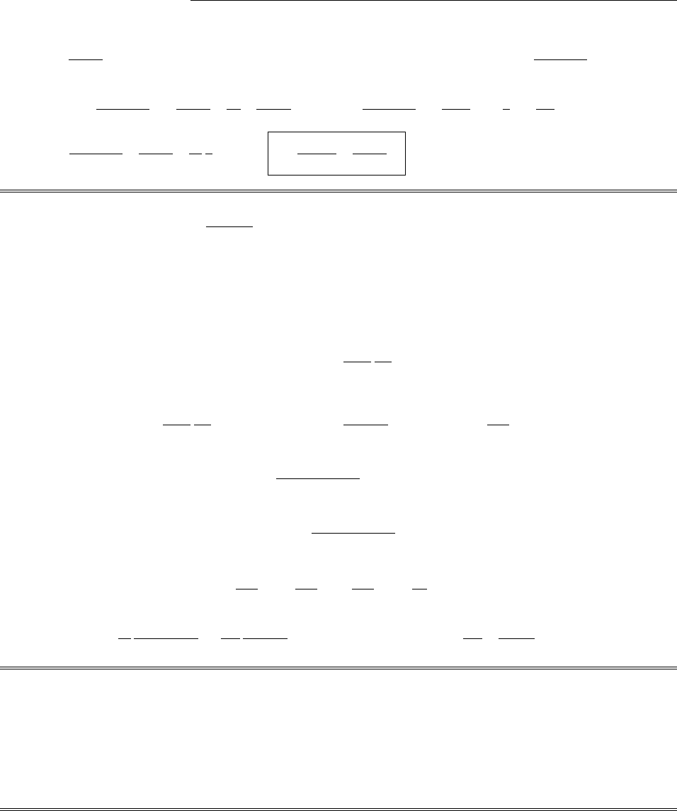
108 CHAPTER 4. ELECTRIC FIELDS IN MATTER
Problem 4.40
Eext =
2⇡✏0sˆs . Since the sphere is tiny, this is essentially constant, and hence P=✏0e
1+e/3Eext (Ex. 4.7).
F=✏0e
1+e/3
2⇡✏0sd
ds
2⇡✏0sˆs d⌧=✏0e
1+e/3
2⇡✏021
s1
s2ˆs d⌧
=e
1+e/32
4⇡2✏01
s3
4
3⇡R3ˆs =e
3+e2R3
⇡✏0s3ˆs .
Problem 4.41
The density of atoms is N=1
(4/3)⇡R3. The macroscopic field Eis Eself +Eelse, where Eself is the average
field over the sphere due to the atom itself.
p=↵Eelse )P=N↵Eelse.
[Actually, it is the field at the center, not the average over the sphere, that belongs here, but the two are in
fact equal, as we found in Prob. 3.47d.] Now
Eself =1
4⇡✏0
p
R3
(Eq. 3.105), so
E=1
4⇡✏0
↵
R3Eelse +Eelse =1↵
4⇡✏0R3Eelse =1N↵
3✏0Eelse.
So
P=N↵
(1 N↵/3✏0)E=✏0eE,
and hence
e=N↵/✏0
(1 N↵/3✏0).
Solving for ↵:
eN↵
3✏0
e=N↵
✏0)N↵
✏01+e
3=e,
or
↵=✏0
N
e
(1 + e/3) =3✏0
N
e
(3 + e
.But e=✏r1,so ↵=3✏0
N✏r1
✏r+2.qed
Problem 4.42
For an ideal gas, N= Avagadro’s number/22.4 liters = (6.02 ⇥1023)/(22.4⇥103)=2.7⇥1025.N↵/✏0=
(2.7⇥1025)(4⇡✏0⇥1030)/✏0=3.4⇥104, where is the number listed in Table 4.1.
H: =0.667,N↵/✏0= (3.4⇥104)(0.67) = 2.3⇥104,e=2.5⇥104
He: =0.205,N↵/✏0= (3.4⇥104)(0.21) = 7.1⇥105,e=6.5⇥105
Ne: =0.396,N↵/✏0= (3.4⇥104)(0.40) = 1.4⇥104,e=1.3⇥104
Ar: =1.64,N↵/✏0= (3.4⇥104)(1.64) = 5.6⇥104,e=5.2⇥104
agreement is quite good.
c
2012 Pearson Education, Inc., Upper Saddle River, NJ. All rights reserved. This material is
protected under all copyright laws as they currently exist. No portion of this material may be
reproduced, in any form or by any means, without permission in writing from the publisher.
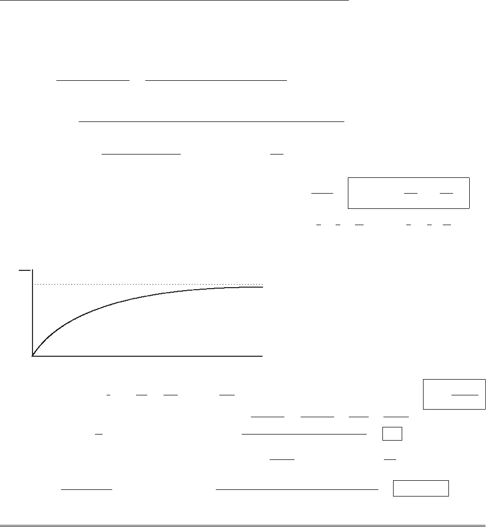
CHAPTER 4. ELECTRIC FIELDS IN MATTER 109
Problem 4.43
(a) Doing the (trivial) integral, and changing the remaining integration variable from ✓to u(du =pE sin ✓d✓),
hui=pE
pE ueu/kT du
pE
pE eu/kT du =(kT )2eu/kT [(u/kT )1]|pE
pE
kTeu/kT pE
pE
=kT epE/kT epE/kT +(pE/kT )epE/kT +(pE/kT )epE/kT
epE/kT epE/kT
=kT pE epE/kT +epE/kT
epE/kT epE/kT =kT pE coth pE
kT .
P=Nhpi;p=hpcos ✓iˆ
E=hp·Ei(ˆ
E/E)=hui(ˆ
E/E); P=Nphui
pE =Npcoth pE
kT kT
pE .
Let y⌘P/Np, x ⌘pE/kT .Theny= coth x1/x. As x!0, y=1
x+x
3x3
45 +···1
x=x
3x3
45 +···!
0, so the graph starts at the origin, with an initial slope of 1/3. As x!1,y!coth(1) = 1, so the graph
goes asymptotically to y= 1 (see Figure).
8
Problem 4.40
✻
✲
P
N p
1
pE/kT
c
⃝2005 Pearson Education, Inc., Upper Saddle River, NJ. All rights reserved. This material is
protected under all copyright laws as they currently exist. No portion of this material may be
reproduced, in any form or by any means, without permission in writing from the publisher.
(b) For small x,y⇡1
3x, so P
Np ⇡pE
3kT , or P⇡Np2
3kT E=✏0eE)Pis proportional to E, and e=Np2
3✏0kT .
For water at 20= 293 K, p=6.1⇥1030 C m; N=molecules
volume =molecules
mole ⇥moles
gram ⇥grams
volume .
N=6.0⇥1023⇥1
18 ⇥106=0.33 ⇥1029;e=(0.33⇥1029 )(6.1⇥1030)2
(3)(8.85⇥1012)(1.38⇥1023 )(293) = 12.Table 4.2 gives an
experimental value of 79, so it’s pretty far o↵.
For water vapor at 100= 373 K, treated as an ideal gas, volume
mole = (22.4⇥103)⇥373
293 =2.85 ⇥102m3.
N=6.0⇥1023
2.85 ⇥102=2.11 ⇥1025;e=(2.11 ⇥1025)(6.1⇥1030)2
(3)(8.85 ⇥1012)(1.38 ⇥1023)(373) = 5.7⇥103.
Table 4.2 gives 5.9⇥103, so this time the agreement is quite good.
c
2012 Pearson Education, Inc., Upper Saddle River, NJ. All rights reserved. This material is
protected under all copyright laws as they currently exist. No portion of this material may be
reproduced, in any form or by any means, without permission in writing from the publisher.
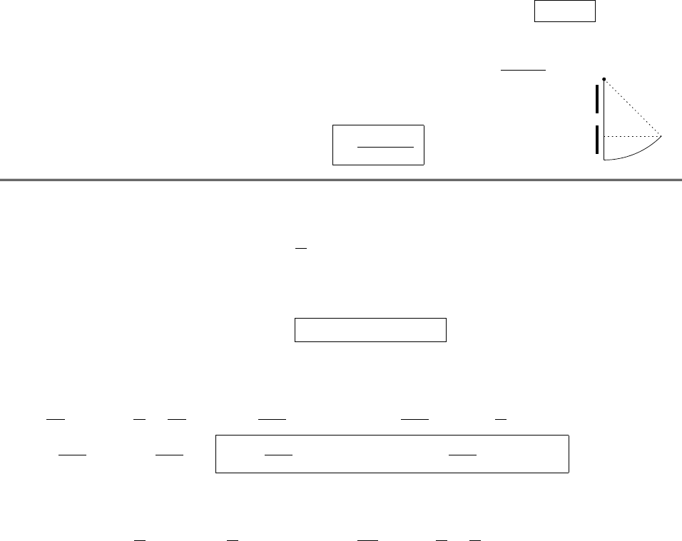
110 CHAPTER 5. MAGNETOSTATICS
Chapter 5
Magnetostatics
Problem 5.1
Since v⇥Bpoints upward, and that is also the direction of the force, qmust be positive. To find R, in
terms of aand d, use the pythagorean theorem:
(Rd)2+a2=R2)R22Rd +d2+a2=R2)R=a2+d2
2d.
2CHAPTER 5. MAGNETOSTATICS
Chapter 1
Magnetostatics
Problem 5.1
! "# $
}
R
d
R
a
Problem 5.2
✲y
✻
z
β◆
(b)
✲y
✻
z
β
−β
✸
(c)
c
⃝2005 Pearson Education, Inc., Upper Saddle River, NJ. All rights reserved. This material is
protected under all copyright laws as they currently exist. No portion of this material may be
reproduced, in any form or by any means, without permission in writing from the publisher.
The cyclotron formula then gives
p=qBR =qB (a2+d2)
2d.
Problem 5.2
The general solution is (Eq. 5.6):
y(t)=C1cos(!t)+C2sin(!t)+ E
Bt+C3;z(t)=C2cos(!t)C1sin(!t)+C4.
(a) y(0) = z(0) = 0; ˙y(0) = E/B;˙z(0) = 0. Use these to determine C1,C2,C3, and C4.
y(0) = 0 )C1+C3= 0; ˙y(0) = !C2+E/B =E/B )C2= 0; z(0) = 0 )C2+C4=0)C4= 0;
˙z(0) = 0 )C1= 0, and hence also C3=0.So y(t)=Et/B;z(t)=0.Does this make sense? The magnetic
force is q(v⇥B)=q(E/B)Bˆz =qE, which exactly cancels the electric force; since there is no net force,
the particle moves in a straight line at constant speed. X
(b) Assuming it starts from the origin, so C3=C1,C4=C2, we have ˙z(0) = 0 )C1=0)C3= 0;
˙y(0) = E
2B)C2!+E
B=E
2B)C2=E
2!B=C4;y(t)=E
2!Bsin(!t)+ E
Bt;
z(t)=E
2!Bcos(!t)+ E
2!B,or y(t)= E
2!B[2!tsin(!t)] ; z(t)= E
2!B[1 cos(!t)] .Let ⌘E/2!B.
Then y(t)=[2!tsin(!t)] ; z(t)=[1 cos(!t)] ; (y2!t)=sin(!t),(z)=cos(!t))
(y2!t)2+(z)2=2. This is a circle of radius whose center moves to the right at constant speed:
y0=2!t;z0=.
(c) ˙z(0) = ˙y(0) = E
B)C1!=E
B)C1=C3=E
!B;C2!+E
B=E
B)C2=C4=0.
c
2012 Pearson Education, Inc., Upper Saddle River, NJ. All rights reserved. This material is
protected under all copyright laws as they currently exist. No portion of this material may be
reproduced, in any form or by any means, without permission in writing from the publisher.
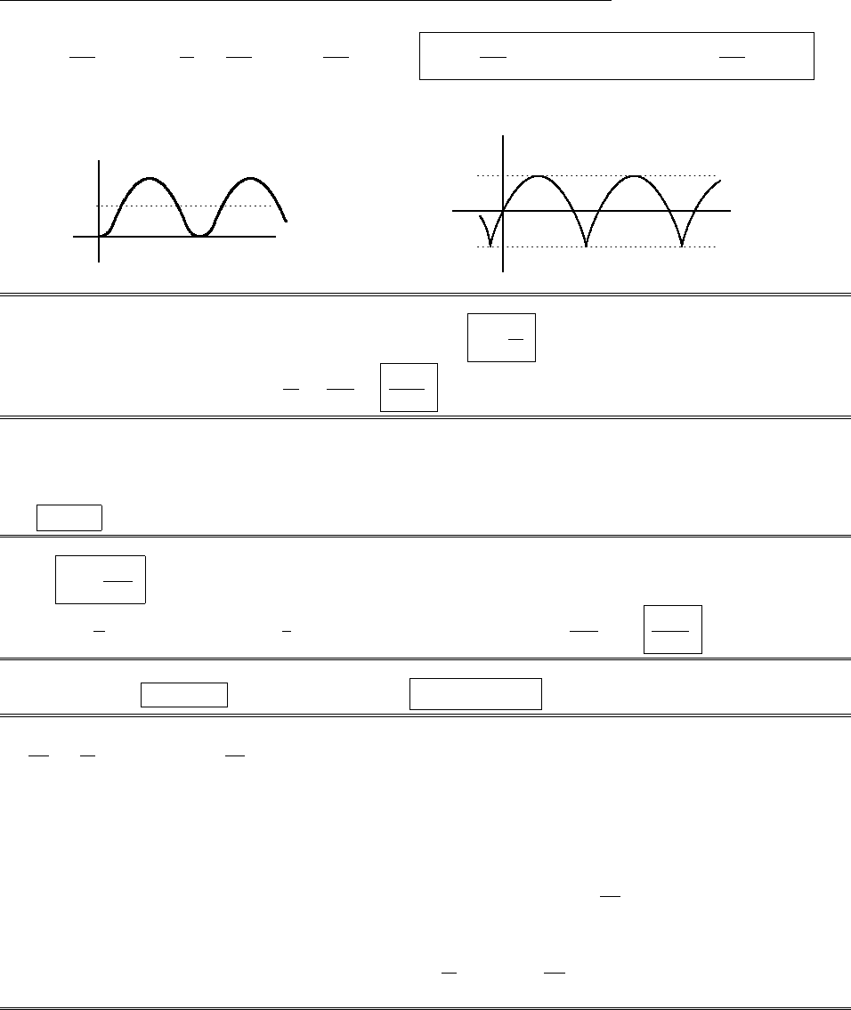
CHAPTER 5. MAGNETOSTATICS 111
y(t)=E
!Bcos(!t)+ E
Bt+E
!B;z(t)= E
!Bsin(!t). y(t)= E
!B[1 + !tcos(!t)] ; z(t)= E
!Bsin(!t).
Let ⌘E/!B; then [y(1 + !t)] = cos(!t),z=sin(!t); [y(1 + !t)]2+z2=2. This is a circle
of radius whose center is at y0=(1 + !t),z
0=0.
2CHAPTER 5. MAGNETOSTATICS
Chapter 1
Magnetostatics
Problem 5.1
! "# $
}
R
d
R
a
Problem 5.2
✲y
✻
z
β◆
(b)
✲y
✻
z
β
−β
✸
(c)
c
⃝2005 Pearson Education, Inc., Upper Saddle River, NJ. All rights reserved. This material is
protected under all copyright laws as they currently exist. No portion of this material may be
reproduced, in any form or by any means, without permission in writing from the publisher.
Problem 5.3
(a) From Eq. 5.2, F=q[E+(v⇥B)] = 0 )E=vB )v=E
B.
(b) From Eq. 5.3, mv =qBR )q
m=v
BR =E
B2R.
Problem 5.4
Suppose Iflows counterclockwise (if not, change the sign of the answer). The force on the left side (toward
the left) cancels the force on the right side (toward the right); the force on the top is IaB =Iak(a/2) =
Ika2/2, (pointing upward), and the force on the bottom is IaB =Ika2/2 (also upward). So the net force is
F=Ika2ˆz .
Problem 5.5
(a) K=I
2⇡a,because the length-perpendicular-to-flow is the circumference.
(b) J=↵
s)I=Jda=↵1
ssdsd=2⇡↵ ds =2⇡↵a)↵=I
2⇡a;J=I
2⇡as.
Problem 5.6
(a) v=!r,so K=!r. (b) v=!rsin ✓ˆ
)J=⇢!rsin ✓ˆ
,where ⇢⌘Q/(4/3)⇡R3.
Problem 5.7
dp
dt =d
dt V
⇢rd⌧=@⇢
@trd⌧=(r·J)rd⌧(by the continuity equation). Now product rule #5
says r·(xJ)=x(r·J)+J·(rx). But rx=ˆx ,sor·(xJ)=x(r·J)+Jx.Thus V(r·J)xd⌧=
Vr·(xJ)d⌧V
Jxd⌧. The first term is SxJ·da(by the divergence theorem), and since Jis entirely
inside V, it is zero on the surface S. Therefore V(r·J)xd⌧=VJxd⌧, or, combining this with the yand
zcomponents, V(r·J)rd⌧=VJd⌧.Or, referring back to the first line, dp
dt =Jd⌧.qed
Here’s a quicker method, if the distribution consists of a collection of point charges. Use Eqs. 5.30 and
3.100: Jd⌧=qivi=d
dt qiri=dp
dt .
c
2012 Pearson Education, Inc., Upper Saddle River, NJ. All rights reserved. This material is
protected under all copyright laws as they currently exist. No portion of this material may be
reproduced, in any form or by any means, without permission in writing from the publisher.

112 CHAPTER 5. MAGNETOSTATICS
Problem 5.8
(a) Use Eq. 5.37, with z=R, ✓2=✓1= 45,and four sides: B=p2µ0I
⇡R.
(b) z=R, ✓2=✓1=⇡
n, and nsides: B=nµ0I
2⇡Rsin(⇡/n).
(c) For small ✓,sin✓⇡✓. So as n!1,B !nµ0I
2⇡R⇡
n=µ0I
2R(same as Eq. 5.41, with z= 0).
Problem 5.9
(a) The straight segments produce no field at P. The two quarter-circles give B=µ0I
81
a1
b(out).
(b) The two half-lines are the same as one infinite line: µ0I
2⇡R; the half-circle contributes µ0I
4R.
So B=µ0I
4R1+ 2
⇡(into the page).
Problem 5.10
(a) The forces on the two sides cancel. At the bottom, B=µ0I
2⇡s)F=µ0I
2⇡sIa =µ0I2a
2⇡s(up). At the
top, B=µ0I
2⇡(s+a))F=µ0I2a
2⇡(s+a)(down). The net force is µ0I2a2
2⇡s(s+a)(up).
(b) The force on the bottom is the same as before, µ0I2a/2⇡s(up). On the left side, B=µ0I
2⇡yˆz ;
dF=I(dl⇥B)=I(dx ˆx +dy ˆy +dz ˆz )⇥µ0I
2⇡yˆz =µ0I2
2⇡y(dx ˆy +dy ˆx ).But the xcomponent cancels the
corresponding term from the right side, and Fy=µ0I2
2⇡(s/p3+a/2)
s/p3
1
ydx. Here y=p3x, so
Fy=µ0I2
2p3⇡ln s/p3+a/2
s/p3=µ0I2
2p3⇡ln 1+p3a
2s.The force on the right side is the same, so the net
force on the triangle is µ0I2
2⇡a
s2
p3ln 1+p3a
2s.
CHAPTER 5. MAGNETOSTATICS 3
Problem 5.10
✲x
✻
y
✰
z
s
√3
! "# $
s
60◦
a
a
Problem 5.11
✲z
η
θ
❄
a
! "# $
z
}
dz
c
⃝2005 Pearson Education, Inc., Upper Saddle River, NJ. All rights reserved. This material is
protected under all copyright laws as they currently exist. No portion of this material may be
reproduced, in any form or by any means, without permission in writing from the publisher.
c
2012 Pearson Education, Inc., Upper Saddle River, NJ. All rights reserved. This material is
protected under all copyright laws as they currently exist. No portion of this material may be
reproduced, in any form or by any means, without permission in writing from the publisher.

CHAPTER 5. MAGNETOSTATICS 113
Problem 5.11
CHAPTER 5. MAGNETOSTATICS 3
Problem 5.10
✲x
✻
y
✰
z
s
√3
! "# $
s
60◦
a
a
Problem 5.11
✲z
θ
❄
a
! "# $
z
}
dz
c
⃝2005 Pearson Education, Inc., Upper Saddle River, NJ. All rights reserved. This material is
protected under all copyright laws as they currently exist. No portion of this material may be
reproduced, in any form or by any means, without permission in writing from the publisher.
r
Use Eq. 5.41 for a ring of width dz, with I!nI dz:
B=µ0nI
2a2
(a2+z2)3/2dz. But z=acot ✓,
so dz =a
sin2✓d✓, and 1
(a2+z2)3/2=sin3✓
a3.
So
B=µ0nI
2a2sin3✓
a3sin2✓(ad✓)=µ0nI
2sin ✓d✓=µ0nI
2cos ✓✓2
✓1=µ0nI
2(cos ✓2cos ✓1).
For an infinite solenoid, ✓2= 0, ✓1=⇡, so (cos ✓2cos ✓1)=1(1) = 2,and B=µ0nI. X
Problem 5.12
z
R
q
Rsinq
Rcosq
Field (at center of sphere) due to the ring at ✓(see figure) is (Eq. 5.41):
dB =µ0dI
2
(Rsin ✓)2
[(Rsin ✓)2+(Rcos ✓)2]3/2=µ0
2Rsin2✓dI.
dI =KRd✓,K=v, =Q
4⇡R2,v=!Rsin ✓,
so
dI =Q
4⇡R2!Rsin ✓Rd✓=Q!
4⇡sin ✓d✓.
B=µ0
2R
Q!
4⇡⇡
0
sin3✓d✓=µ0Q!
8⇡R4
3.B=µ0Q!
6⇡Rˆz .
Problem 5.13
Magnetic attraction per unit length (Eqs. 5.40 and 5.13): fm=µ0
2⇡
2v2
d.
Electric field of one wire (Eq. 2.9): E=1
2⇡✏0
s. Electric repulsion per unit length on the other wire:
fe=1
2⇡✏0
2
d.They balance when µ0v2=1
✏0
, or v=1
p✏0µ0
.Putting in the numbers,
c
2012 Pearson Education, Inc., Upper Saddle River, NJ. All rights reserved. This material is
protected under all copyright laws as they currently exist. No portion of this material may be
reproduced, in any form or by any means, without permission in writing from the publisher.

114 CHAPTER 5. MAGNETOSTATICS
v=1
(8.85 ⇥1012)(4⇡⇥107)= 3.00 ⇥108m/s. This is precisely the speed of light(!), so in fact you could
never get the wires going fast enough; the electric force always dominates.
Problem 5.14
(a) B·dl=B2⇡s=µ0Ienc )B=0,for s<a;
µ0I
2⇡sˆ
,for s > a.
(b) J=ks;I=a
0
Jda =a
0
ks(2⇡s)ds =2⇡ka3
3)k=3I
2⇡a3.I
enc =s
0
Jda =s
0
k¯s(2⇡¯s)d¯s=
2⇡ks3
3=Is3
a3, for s<a;Ienc =I, for s>a. So B=
µ0Is2
2⇡a3ˆ
,for s<a;
µ0I
2⇡sˆ
,for s > a.
Problem 5.15
By the right-hand-rule, the field points in the ˆy direction for z>0, and in the +ˆy direction for z<0.
At z=0,B = 0. Use the amperian loop shown:
B·dl=Bl =µ0Ienc =µ0lzJ )B=µ0Jz ˆy (a<z<a). If z > a, Ienc =µ0laJ,
so B=µ0Jaˆy ,for z>+a;
+µ0Jaˆy ,for z>a.
4CHAPTER 5. MAGNETOSTATICS
Problem 5.14
✲y
✻
z
✲
✛
! "# $
l
{z
✠amperian loop
Problem 5.17
✲y
✰
x
✻
z
loop 1
loop 2
✿
I
✿
I
ηη
η1
ηη
η2
❥
✣
r
c
⃝2005 Pearson Education, Inc., Upper Saddle River, NJ. All rights reserved. This material is
protected under all copyright laws as they currently exist. No portion of this material may be
reproduced, in any form or by any means, without permission in writing from the publisher.
Problem 5.16
The field inside a solenoid is µ0nI, and outside it is zero. The outer solenoid’s field points to the right (ˆz ),
whereas the inner one points to the left (ˆz ). So: (i) B=µ0I(n2n1)ˆz ,(ii) B=µ0In2ˆz ,(iii) B=0.
Problem 5.17
From Ex. 5.8, the top plate produces a field µ0K/2 (aiming out of the page, for points above it, and into
the page, for points below). The bottom plate produces a field µ0K/2 (aiming into the page, for points above
it, and out of the page, for points below). Above and below both plates the two fields cancel; between the plates
they add up to µ0K, pointing in.
(a) B=µ0v(in) betweem the plates, B=0 elsewhere.
(b) The Lorentz force law says F=(K⇥B)da, so the force per unit area is f=K⇥B. Here K=v,
to the right, and B(the field of the lower plate) is µ0v/2, into the page. So fm=µ02v2/2 (up).
(c) The electric field of the lower plate is /2✏0; the electric force per unit area on the upper plate is
fe=2/2✏0(down). They balance if µ0v2=1/✏0, or v=1/p✏0µ0=c(the speed of light), as in Prob. 5.13.
Problem 5.18
We might as well orient the axes so the field point rlies on the yaxis: r=(0,y,0). Consider a source point
at (x0,y
0,z0) on loop #1:
r
=x0ˆx +(yy0)ˆy z0ˆz ;dl0=dx0ˆx +dy0ˆy ;
c
2012 Pearson Education, Inc., Upper Saddle River, NJ. All rights reserved. This material is
protected under all copyright laws as they currently exist. No portion of this material may be
reproduced, in any form or by any means, without permission in writing from the publisher.

CHAPTER 5. MAGNETOSTATICS 115
dl0⇥
r
=
ˆx ˆy ˆz
dx0dy00
x0(yy0)z0=(z0dy0)ˆx +(z0dx0)ˆy + [(yy0)dx0+x0dy0]ˆz .
dB1=µ0I
4⇡
dl0⇥
r
r
3=µ0I
4⇡
(z0dy0)ˆx +(z0dx0)ˆy + [(yy0)dx0+x0dy0]ˆz
[(x0)2+(yy0)2+(z0)2]3/2.
Now consider the symmetrically placed source element on
loop #2, at (x0,y
0,z0). Since z0changes sign, while every-
thing else is the same, the ˆx and ˆy components from dB1and
dB2cancel, leaving only a ˆz component. qed
With this, Amp´ere’s law yields immediately:
B=µ0nI ˆz ,inside the solenoid;
0,outside
(the same as for a circular solenoid—Ex. 5.9).
For the toroid, N/2⇡s=n(the number of turns per unit
length), so Eq. 5.60 yields B=µ0nI inside, and zero outside,
consistent with the solenoid. [Note: N/2⇡s=napplies only
if the toroid is large in circumference, so that sis essentially
constant over the cross-section.]
4CHAPTER 5. MAGNETOSTATICS
Problem 5.14
✲y
✻
z
✲
✛
! "# $
l
{z
✠amperian loop
Problem 5.17
✲y
✰
x
✻
z
loop 1
loop 2
✿
I
✿
I
❥
✣
r
c
⃝2005 Pearson Education, Inc., Upper Saddle River, NJ. All rights reserved. This material is
protected under all copyright laws as they currently exist. No portion of this material may be
reproduced, in any form or by any means, without permission in writing from the publisher.
r
1
r
2
Problem 5.19
It doesn’t matter. According to Theorem 2, in Sect. 1.6.2, J·dais independent of surface, for any given
boundary line, provided that Jis divergenceless, which it is, for steady currents (Eq. 5.33).
Problem 5.20
(a) ⇢=charge
volume =charge
atom ·atoms
mole ·moles
gram ·grams
volume =(e)(N)1
M(d), where
e= charge of electron = 1.6⇥1019 C,
N= Avogadro0s number = 6.0⇥1023 mole,
M= atomic mass of copper = 64 gm/mole,
d= density of copper = 9.0 gm/cm3.
⇢=(1.6⇥1019)(6.0⇥1023)9.0
64 = 1.4⇥104C/cm3.
(b) J=I
⇡s2=⇢v)v=I
⇡s2⇢=1
⇡(2.5⇥103)(1.4⇥104)= 9.1⇥103cm/s, or about 33 cm/hr. This
is astonishingly small—literally slower than a snail’s pace.
(c) From Eq. 5.40, fm=µ0
2⇡I1I2
d=(4⇡⇥107)
2⇡= 2 ⇥107N/cm.
(d) E=1
2⇡✏0
d;fe=1
2⇡✏012
d=1
v2
1
2⇡✏0I1I2
d=c2
v2µ0
2⇡I1I2
d=c2
v2fm,where
c⌘1/p✏0µ0=3.00 ⇥108m/s. Here fe
fm
=c2
v2=3.0⇥1010
9.1⇥1032
= 1.1⇥1025.
fe=(1.1⇥1025)(2 ⇥107)= 2⇥1018 N/cm.
c
2012 Pearson Education, Inc., Upper Saddle River, NJ. All rights reserved. This material is
protected under all copyright laws as they currently exist. No portion of this material may be
reproduced, in any form or by any means, without permission in writing from the publisher.

116 CHAPTER 5. MAGNETOSTATICS
Problem 5.21
Amp´ere’s law says r⇥B=µ0J. Together with the continuity equation (5.29) this gives r·(r⇥B)=
µ0r·J=µ0@⇢/@t, which is inconsistent with div(curl)=0 unless ⇢is constant (magnetostatics). The other
Maxwell equations are OK: r⇥E=0)r·(r⇥E)=0(X), and as for the two divergence equations, there
is no relevant vanishing second derivative (the other one is curl(grad), which doesn’t involve the divergence).
Problem 5.22
At this stage I’d expect no changes in Gauss’s law or Amp´ere’s law. The divergence of Bwould take the
form r·B=↵0⇢m,where ⇢mis the density of magnetic charge, and ↵0is some constant (analogous to ✏0
and µ0). The curl of Ebecomes r⇥E=0Jm,where Jmis the magnetic current density (representing the
flow of magnetic charge), and 0is another constant. Presumably magnetic charge is conserved, so ⇢mand Jm
satisfy a continuity equation: r·Jm=@⇢m/@t.
As for the Lorentz force law, one might guess something of the form qm[B+(v⇥E)] (where qmis the
magnetic charge). But this is dimensionally impossible, since Ehas the same units as vB. Evidently we
need to divide (v⇥E) by something with the dimensions of velocity-squared. The natural candidate is
c2=1/✏0µ0:F=qe[E+(v⇥B)] + qmB1
c2(v⇥E).In this form the magnetic analog to Coulomb’s
law reads F=↵0
4⇡
qm1qm2
r2ˆr , so to determine ↵0we would first introduce (arbitrarily) a unit of magnetic charge,
then measure the force between unit charges at a given separation. [For further details, and an explanation of
the minus sign in the force law, see Prob. 7.38.]
Problem 5.23
A=µ0
4⇡Iˆz
r
dz =µ0I
4⇡ˆz z2
z1
dz
pz2+s2
=µ0I
4⇡ˆz ln z+z2+s2
z2
z1
=µ0I
4⇡ln z2+(z2)2+s2
z1+(z1)2+s2ˆz
CHAPTER 5. MAGNETOSTATICS 5
Problem 5.22
✲z
s
}
z1
}
dl=dz
!"# $
z2
Problem 5.26
✲y
✻
z
✠
x
✠ ✠ ✠ ✠ ✠ ✠ K
Problem 5.36
Problem 5.37
Problem 5.44
c
⃝2005 Pearson Education, Inc., Upper Saddle River, NJ. All rights reserved. This material is
protected under all copyright laws as they currently exist. No portion of this material may be
reproduced, in any form or by any means, without permission in writing from the publisher.
r
B=r⇥A=@A
@sˆ
=µ0I
4⇡1
z2+(z2)2+s2
s
(z2)2+s21
z1+(z1)2+s2
s
(z1)2+s2ˆ
=µ0Is
4⇡z2(z2)2+s2
(z2)2[(z2)2+s2]
1
(z2)2+s2z1(z1)2+s2
z2
1[(z1)2+s2]
1
(z1)2+s2ˆ
=µ0Is
4⇡1
s2z2
(z2)2+s21z1
(z1)2+s2+1
ˆ
=µ0I
4⇡sz2
(z2)2+s2z1
(z1)2+s2ˆ
,
or,since sin ✓1=z1
(z1)2+s2and sin ✓2=z2
(z2)2+s2,
=µ0I
4⇡s(sin ✓2sin ✓1)ˆ
(as in Eq.5.37).
Problem 5.24
A=k)B=r⇥A=1
s
@
@s(sk)ˆz =k
sˆz ;J=1
µ0
(r⇥B)= 1
µ0@
@sk
s ˆ
=k
µ0s2ˆ
.
c
2012 Pearson Education, Inc., Upper Saddle River, NJ. All rights reserved. This material is
protected under all copyright laws as they currently exist. No portion of this material may be
reproduced, in any form or by any means, without permission in writing from the publisher.

CHAPTER 5. MAGNETOSTATICS 117
Problem 5.25
r·A=1
2r·(r⇥B)=1
2[B·(r⇥r)r·(r⇥B)] = 0, since r⇥B=0(Bis uniform) and
r⇥r=0(Prob. 1.63). r⇥A=1
2r⇥(r⇥B)=1
2[(B·r)r(r·r)B+r(r·B)B(r·r)]. But
(r·r)B=0and r·B= 0 (since Bis uniform), and r·r=@x
@x+@y
@y+@z
@z= 1 + 1 + 1 = 3. Finally,
(B·r)r=Bx
@
@x+By
@
@y+Bz
@
@z(xˆx +yˆy +zˆz )=Bxˆx +Byˆy +Bzˆz =B.Sor⇥A=1
2(B3B)=B.
qed
Problem 5.26
(a) Ais parallel (or antiparallel) to I, and is a function only of s(the distance from the wire). In cylindrical
coordinates, then, A=A(s)ˆz ,soB=r⇥A=@A
@sˆ
=µ0I
2⇡sˆ
(the field of an infinite wire). Therefore
@A
@s=µ0I
2⇡s, and A(r)=µ0I
2⇡ln(s/a)ˆz (the constant ais arbitrary; you could use 1, but then the units
look fishy). r·A=@Az
@z=0.Xr⇥A=@Az
@sˆ
=µ0I
2⇡sˆ
=B.X
(b) Here Amp´ere’s law gives B·dl=B2⇡s=µ0Ienc =µ0J⇡s2=µ0
I
⇡R2⇡s2=µ0Is2
R2.
B=µ0
2⇡
Is
R2ˆ
.@A
@s=µ0I
2⇡
s
R2)A=µ0I
4⇡R2(s2b2)ˆz . Here bis again arbitrary, except that since A
must be continuous at R,µ0I
2⇡ln(R/a)=µ0I
4⇡R2(R2b2), which means that we must pick aand bsuch that
2 ln(R/b)=1(b/R)2. I’ll use a=b=R. Then A=
µ0I
4⇡R2(s2R2)ˆz ,for sR;
µ0I
2⇡ln(s/R)ˆz ,for sR.
Problem 5.27
K=Kˆx )B=±µ0K
2ˆy (plus for z<0, minus for z>0).
Ais parallel (or antiparallel) to K, and depends only on z,soA=A(z)ˆx .
B=r⇥A=
ˆx ˆy ˆz
@/@x@/@y@/@z
A(z)0 0
=@A
@zˆy =±µ0K
2ˆy .
A=µ0K
2|z|ˆx will do the job—or this plus any constant.
CHAPTER 5. MAGNETOSTATICS 5
Problem 5.22
✲z
sη
}
z1
}
dl=dz
!"# $
z
Problem 5.26
✲y
✻
z
✠
x
✠ ✠ ✠ ✠ ✠ ✠ K
Problem 5.36
Problem 5.37
Problem 5.44
c
⃝2005 Pearson Education, Inc., Upper Saddle River, NJ. All rights reserved. This material is
protected under all copyright laws as they currently exist. No portion of this material may be
reproduced, in any form or by any means, without permission in writing from the publisher.
Problem 5.28
(a) r·A=µ0
4⇡r·J
r
d⌧0;r·J
r
=1
r
(r·J)+J·r1
r
. But the first term is zero, because J(r0)
is a function of the source coordinates, not the field coordinates. And since
r
=rr0,r1
r
=r01
r
.
So r·J
r
=J·r01
r
.Butr0·J
r
=1
r
(r0·J)+J·r01
r
, and r0·J= 0 in magnetostatics
(Eq. 5.33). So r·J
r
=r0·J
r
, and hence, by the divergence theorem, r·A=µ0
4⇡r0·J
r
d⌧0=
c
2012 Pearson Education, Inc., Upper Saddle River, NJ. All rights reserved. This material is
protected under all copyright laws as they currently exist. No portion of this material may be
reproduced, in any form or by any means, without permission in writing from the publisher.

118 CHAPTER 5. MAGNETOSTATICS
µ0
4⇡J
r
·da0, where the integral is now over the surface surrounding all the currents. But J=0on this
surface, so r·A=0.X
(b) r⇥A=µ0
4⇡r⇥J
r
d⌧0=µ0
4⇡1
r
(r⇥J)J⇥r1
r
d⌧0.Butr⇥J=0(since Jis
not a function of r), and r1
r
=ˆ
r
r
2(Eq. 1.101), so r⇥A=µ0
4⇡J⇥ˆ
r
r
2d⌧0=B.X
(c) r2A=µ0
4⇡r2J
r
d⌧0. But r2J
r
=Jr21
r
(once again, Jis a constant, as far as
di↵erentiation with respect to ris concerned), and r21
r
=4⇡3(
r
) (Eq. 1.102). So
r2A=µ0
4⇡J(r0)4⇡3(
r
)d⌧0=µ0J(r).X
Problem 5.29
µ0I=B·dl=b
arU·dl=[U(b)U(a)] (by the gradient theorem), so U(b)6=U(a).qed
For an infinite straight wire, B=µ0I
2⇡sˆ
. U =µ0I
2⇡would do the job, in the sense that
rU=µ0I
2⇡r()=µ0I
2⇡
1
s
@
@ ˆ
=B. But when advances by 2⇡, this function does not return to its initial
value; it works (say) for 0 <2⇡, but at 2⇡it “jumps” back to zero.
Problem 5.30
Use Eq. 5.69, with R!¯rand !⇢d¯r:
A=µ0!⇢
3
sin ✓
r2ˆ
r
0
¯r4d¯r+µ0!⇢
3rsin ✓ˆ
R
r
¯rd¯r
=µ0!⇢
3sin ✓1
r2r5
5+r
2R2r2ˆ
=µ0!⇢
2rsin ✓R2
3r2
5ˆ
.
B=r⇥A=µ0!⇢
21
rsin ✓
@
@✓ sin ✓rsin ✓R2
3r2
5ˆr 1
r
@
@rr2sin ✓R2
3r2
5ˆ
✓
=µ0!⇢ R2
3r2
5cos ✓ˆr R2
32r2
5sin ✓ˆ
✓.
Problem 5.31
(a)
@Wz
@x=Fy)Wz(x, y, z)=x
0Fy(x0,y,z)dx0+C1(y, z).
@Wy
@x=Fz)Wy(x, y, z)=+x
0Fz(x0,y,z)dx0+C2(y, z).
These satisfy (ii) and (iii), for any C1and C2; it remains to choose these functions so as to satisfy (i):
x
0
@Fy(x0,y,z)
@ydx0+@C1
@yx
0
@Fz(x0,y,z)
@zdx0@C2
@z=Fx(x, y, z). But @Fx
@x+@Fy
@y+@Fz
@z= 0, so
x
0
@Fx(x0,y,z)
@x0dx0+@C1
@y@C2
@z=Fx(x, y, z). Now x
0
@Fx(x0,y,z)
@x0dx0=Fx(x, y, z)Fx(0,y,z), so
c
2012 Pearson Education, Inc., Upper Saddle River, NJ. All rights reserved. This material is
protected under all copyright laws as they currently exist. No portion of this material may be
reproduced, in any form or by any means, without permission in writing from the publisher.

CHAPTER 5. MAGNETOSTATICS 119
@C1
@y@C2
@z=Fx(0,y,z). We may as well pick C2=0,C
1(y, z)=y
0
Fx(0,y
0,z)dy0, and we’re done, with
Wx= 0; Wy=x
0
Fz(x0,y,z)dx0;Wz=y
0
Fx(0,y
0,z)dy0x
0
Fy(x0,y,z)dx0.
(b) r⇥W=@Wz
@y@Wy
@zˆx +@Wx
@z@Wz
@xˆy +@Wy
@x@Wx
@yˆz
=Fx(0,y,z)x
0
@Fy(x0,y,z)
@ydx0x
0
@Fz(x0,y,z)
@zdx0ˆx + [0 + Fy(x, y, z)] ˆy +[Fz(x, y, z)0] ˆz .
But r·F= 0, so the ˆx term is Fx(0,y,z)+x
0
@Fx(x0,y,z)
@x0dx0=Fx(0,y,z)+Fx(x, y, z)Fx(0,y,z),
so r⇥W=F.X
r·W=@Wx
@x+@Wy
@y+@Wz
@z=0+x
0
@Fz(x0,y,z)
@ydx0+y
0
@Fx(0,y
0,z)
@zdy0x
0
@Fy(x0,y,z)
@zdx06=0,
in general.
(c) Wy=x
0
x0dx0=x2
2;Wz=y
0
y0dy0x
0
z dx0=y2
2zx.
W=x2
2ˆy +y2
2zxˆz .r⇥W=
ˆx ˆy ˆz
@/@x@/@y@/@z
0x2/2(y2/2zx)=yˆx +zˆy +xˆz =F.X
Problem 5.32
(a) At the surface of the solenoid, Babove =0,Bbelow =µ0nI ˆz =µ0Kˆz ;ˆn =ˆs ;soK⇥ˆn =Kˆz .
Evidently Eq. 5.76 holds. X
(b) In Eq. 5.69, both expressiions reduce to (µ0R2!/3) sin ✓ˆ
at the surface, so Eq. 5.77 is satisfied.
@A
@rR+
=µ0R4!
32 sin ✓
r3ˆ
R
=2µ0R!
3sin ✓ˆ
;@A
@rR
=µ0R!
3sin ✓ˆ
. So the left side of
Eq. 5.78 is µ0R! sin ✓ˆ
. Meanwhile K=v=(!!!⇥r)=!Rsin ✓ˆ
, so the right side of Eq. 5.78 is
µ0!Rsin ✓ˆ
, and the equation is satisfied.
Problem 5.33
Because Aabove =Abelow at every point on the surface, it follows that @A
@xand @A
@yare the same above
and below; any discontinuity is confined to the normal derivative.
Babove Bbelow =@Ayabove
@z+@Aybelow
@zˆx +@Axabove
@z@Axbelow
@zˆy . But Eq. 5.76 says this equals
µ0K(ˆy ). So @Ayabove
@z=@Aybelow
@z,and @Axabove
@z@Axbelow
@z=µ0K. Thus the normal derivative of the com-
ponent of Aparallel to Ksu↵ers a discontinuity µ0K, or, more compactly: @Aabove
@n@Abelow
@n=µ0K.
Problem 5.34
(Same idea as Prob. 3.36.) Write m=(m·ˆr )ˆr +(m·ˆ
✓)ˆ
✓=mcos ✓ˆr msin ✓ˆ
✓(Fig. 5.54). Then
3(m·ˆr )ˆr m=3mcos ✓ˆr mcos ✓ˆr +msin ✓ˆ
✓=2mcos ✓ˆr +msin ✓ˆ
✓, and Eq. 5.89 ,Eq. 5.88. qed
Problem 5.35
(a) m=Ia=I⇡R2ˆz .
(b) B⇡µ0
4⇡
I⇡R2
r32 cos ✓ˆr + sin ✓ˆ
✓.
c
2012 Pearson Education, Inc., Upper Saddle River, NJ. All rights reserved. This material is
protected under all copyright laws as they currently exist. No portion of this material may be
reproduced, in any form or by any means, without permission in writing from the publisher.

120 CHAPTER 5. MAGNETOSTATICS
(c) On the zaxis, ✓= 0, r=z,ˆr =ˆz (for z>0), so B⇡µ0IR2
2z3ˆz (for z<0, ✓=⇡,ˆr =ˆz , so the field
is the same, with |z|3in place of z3). The exact answer (Eq. 5.41) reduces (for zR) to B⇡µ0IR2/2|z|3,
so they agree.
Problem 5.36
The field of one side is given by Eq. 5.37, with s!
z2+(w/2)2and sin ✓2=sin ✓1=(w/2)
z2+w2/2;
B=µ0I
4⇡
w
z2+(w2/4)z2+(w2/2) . To pick o↵the vertical
component, multiply by sin =(w/2)
z2+(w/2)2; for all four
sides, multiply by 4: B=µ0I
2⇡
w2
(z2+w2/4)z2+w2/2ˆz .
For zw,B⇡µ0Iw2
2⇡z3ˆz . The field of a dipole m=Iw2,
for points on the zaxis (Eq. 5.88, with r!z,ˆr !ˆz ,✓=0)isB=µ0
2⇡
m
z3ˆz .X
Problem 5.37
(a) For a ring, m=I⇡r2. Here I!v dr =!rdr,som=R
0⇡r2!rdr =⇡!R4/4.
(b) The total charge on the shaded ring is dq =
(2⇡Rsin ✓)Rd✓. The time for one revolution is dt =2⇡/!.
So the current in the ring is I=dq
dt =!R2sin ✓d✓. The
area of the ring is ⇡(Rsin ✓)2, so the magnetic moment of the
ring is dm =(!R2sin ✓d✓)⇡R2sin2✓, and the total dipole
moment of the shell is
m=!⇡R4⇡
0sin3✓d✓=(4/3)!⇡R4, or m=4⇡
3!R4ˆz .
The dipole term in the multipole expansion for Ais therefore Adip =µ0
4⇡
4⇡
3!R4sin ✓
r2ˆ
=µ0!R4
3
sin ✓
r2ˆ
,
which is also the exact potential (Eq. 5.69); evidently a spinning sphere produces a perfect dipole field, with
no higher multipole contributions.
Problem 5.38
(a) Idl!Jd⌧,so A=µ0
4⇡
1
n=0
1
rn+1 (r0)nPn(cos ✓)Jd⌧.
(b) Amon =µ0
4⇡rJd⌧=µ0
4⇡r
dp
dt (Prob. 5.7), where pis the total electric dipole moment. In mag-
netostatics,pis constant, so dp/dt =0, and hence Amon =0. qed
(c) m=Ia=1
2I(r⇥dl)!m=1
2(r⇥J)d⌧.qed
Problem 5.39
(a) Yes. (Magnetic forces do no work.)
c
2012 Pearson Education, Inc., Upper Saddle River, NJ. All rights reserved. This material is
protected under all copyright laws as they currently exist. No portion of this material may be
reproduced, in any form or by any means, without permission in writing from the publisher.

CHAPTER 5. MAGNETOSTATICS 121
(b) B=µ0
2⇡sˆ
;v=˙sˆs +s˙
ˆ
+˙zˆz ;(v⇥B)=
ˆs ˆ
ˆz
˙ss
˙
˙z
0µ0
2⇡s0=µ0
2⇡s(˙zˆs +˙sˆz ).
F=q(v⇥B)= qµ0
2⇡s(˙zˆr +˙sˆz ).
(c) a=(¨ss˙
2)ˆs +(s¨
+2˙s˙
)ˆ
+¨zˆz (see, for example J. R. Taylor, Classical Mechanics, Eq. 1.47).
F=ma)(¨ss˙
2)ˆs +(s¨
+2˙s˙
)ˆ
+¨zˆz =↵
s(˙zˆs +˙sˆz ),
where ↵⌘qµ0
2⇡m. Thus
¨ss˙
2=↵˙z
s, s ¨
+2˙s˙
=0,¨z=↵˙s
s.
(d) If ˙zis constant, then ¨z= 0, and it follows from the third equation that ˙s= 0, and hence sis constant.
Then the first equation says ˙
2=↵(˙z/s2), so ˙
=±1
sp↵˙zis also constant (the second equation holds
automatically). The charge moves in a helix around the wire.
Problem 5.40
The mobile charges do pull in toward the axis, but the resulting concentration of (negative) charge sets up
an electric field that repels away further accumulation. Equilibrium is reached when the electric repulsion on a
mobile charge qbalances the magnetic attraction: F=q[E+(v⇥B)] = 0)E=(v⇥B). Say the current
is in the zdirection: J=⇢vˆz (where ⇢and vare both negative).
B·dl=B2⇡s=µ0J⇡s2)B=µ0⇢vs
2ˆ
;
E·da=E2⇡sl =1
✏0
(⇢++⇢)⇡s2l)E=1
2✏0
(⇢++⇢)sˆs .
1
2✏0
(⇢++⇢)sˆs =(vˆz )⇥µ0⇢vs
2ˆ
=µ0
2⇢v2sˆs )⇢++⇢=⇢(✏0µ0v2)=⇢v2
c2.
Evidently ⇢+=⇢1v2
c2=⇢
2, or ⇢=2⇢+.In this naive model the mobile negative charges fill a
smaller inner cylinder, leaving a shell of positive (stationary) charge at the outside. But since v⌧c, the e↵ect
is extremely small.
Problem 5.41
(a) If positive charges flow to the right, they are deflected down, and the bottom plate acquires a positive
charge.
(b) qvB =qE )E=vB )V=Et =vBt, with the bottom at higher potential.
(c) If negative charges flow to the left, they are also deflected down, and the bottom plate acquires a negative
charge. The potential di↵erence is still the same, but this time the top plate is at the higher potential.
Problem 5.42
From Eq. 5.17, F=I(dl⇥B). But Bis constant, in this case, so it comes outside the integral: F=
Idl⇥B, and dl=w, the vector displacement from the point at which the wire first enters the field to
the point where it leaves. Since wand Bare perpendicular, F=IBw, and Fis perpendicular to w.
c
2012 Pearson Education, Inc., Upper Saddle River, NJ. All rights reserved. This material is
protected under all copyright laws as they currently exist. No portion of this material may be
reproduced, in any form or by any means, without permission in writing from the publisher.

122 CHAPTER 5. MAGNETOSTATICS
Problem 5.43
The angular momentum acquired by the particle as it moves out from the center to the edge is
L=dL
dt dt =Ndt =(r⇥F)dt =r⇥q(v⇥B)dt =qr⇥(dl⇥B)=q(r·B)dlB(r·dl).
But ris perpendicular to B, so r·B= 0, and r·dl=r·dr=1
2d(r·r)=1
2d(r2)=r dr = (1/2⇡)(2⇡rdr).
So L=q
2⇡R
0
B2⇡rdr =q
2⇡Bda. It follows that L=q
2⇡,where =Bda is the total flux.
In particular, if = 0, then L= 0, and the charge emerges with zero angular momentum, which means it is
going along a radial line. qed
Problem 5.44
From Eq. 5.24, F=(K⇥Bave)da. Here K=v,v=!Rsin ✓ˆ
,da =R2sin ✓d✓d, and
Bave =1
2(Bin +Bout). From Eq. 5.70,
Bin =2
3µ0R!ˆz =2
3µ0R!(cos ✓ˆr sin ✓ˆ
✓).From Eq.5.69,
Bout =r⇥A=r⇥µ0R4!
3
sin ✓
r2ˆ
=µ0R4!
31
rsin ✓
@
@✓ sin2✓
r2ˆr 1
r
@
@rsin ✓
rˆ
✓
=µ0R4!
3r3(2 cos ✓ˆr + sin ✓ˆ
✓)=µ0R!
3(2 cos ✓ˆr + sin ✓ˆ
✓) (since r=R).
Bave =µ0R!
6(4 cos ✓ˆr sin ✓ˆ
✓).
K⇥Bave =(!Rsin ✓)µ0R!
6ˆ
⇥(4 cos ✓ˆr sin ✓ˆ
✓)=µ0
6(!R)2(4 cos ✓ˆ
✓+ sin ✓ˆr ) sin ✓.
Picking out the zcomponent of ˆ
✓(namely, sin ✓) and of ˆr (namely, cos ✓), we have
(K⇥Bave)z=µ0
2(!R)2sin2✓cos ✓,so
Fz=µ0
2(!R)2R2sin3✓cos ✓d✓d=µ0
2(!R2)22⇡sin4✓
4
⇡/2
0
,or F=µ0⇡
4(!R2)2ˆz .
Problem 5.45
(a) F=ma=qe(v⇥B)= µ0
4⇡
qeqm
r2(v⇥ˆr ); a=µ0
4⇡
qeqm
mr3(v⇥r).
(b) Because a?v,a·v= 0. But a·v=1
2
d
dt(v·v)= 1
2
d
dt(v2)=vdv
dt . So dv
dt =0.qed
(c) dQ
dt =m(v⇥v)+m(r⇥a)µ0qeqm
4⇡
d
dt r
r=0+µ0qeqm
4⇡r3[r⇥(v⇥r]µ0qeqm
4⇡v
rr
r2
dr
dt
=µ0qeqm
4⇡1
r3[r2v(r·v)r]v
r+r
r2
d
dt(pr·r)=µ0qeqm
4⇡v
r(ˆr ·v)
rˆr v
r+ˆr
2r
2(r·v)
r=0.X
(d) (i) Q·ˆ
=Q(ˆz ·ˆ
)=m(r⇥v)·ˆ
µ0qeqm
4⇡(ˆr ·ˆ
). But ˆz ·ˆ
=ˆr ·ˆ
= 0, so (r⇥v)·ˆ
= 0. But
c
2012 Pearson Education, Inc., Upper Saddle River, NJ. All rights reserved. This material is
protected under all copyright laws as they currently exist. No portion of this material may be
reproduced, in any form or by any means, without permission in writing from the publisher.

CHAPTER 5. MAGNETOSTATICS 123
r=rˆr , and v=dl
dt =˙rˆr +r˙
✓ˆ
✓+rsin ✓˙
ˆ
(where dots denote di↵erentiation with respect to time), so
r⇥v=
ˆr ˆ
✓ˆ
r00
˙rr
˙
✓rsin ✓˙
=(r2sin ✓˙
)ˆ
✓+(r2˙
✓)ˆ
.
Therefore (r⇥v)·ˆ
=r2˙
✓= 0, so ✓is constant. qed
(ii) Q·ˆr =Q(ˆz ·ˆr )=m(r⇥v)·ˆr µ0qeqm
4⇡(ˆr ·ˆr ). But ˆz ·ˆr = cos ✓, and (r⇥v)?r)(r⇥v)·ˆr = 0, so
Qcos ✓=µ0qeqm
4⇡, or Q=µ0qeqm
4⇡cos ✓. And since ✓is constant, so too is Q.qed
(iii) Q·ˆ
✓=Q(ˆz ·ˆ
✓)=m(r⇥v)·ˆ
✓µ0qeqm
4⇡(ˆr ·ˆ
✓). But ˆz ·ˆ
✓=sin ✓,ˆr ·ˆ
✓= 0, and (r⇥v)·ˆ
✓=r2sin ✓˙
(from (i)), so Qsin ✓=mr2sin ✓˙
)˙
=Q
mr2=k
r2, with k⌘Q
m=µ0qeqm
4⇡mcos ✓.
(e) v2=˙r2+r2˙
✓2+r2sin2✓˙
2, but ˙
✓= 0 and ˙
=k
r2,so ˙r2=v2r2sin2✓k2
r4=v2k2sin2✓
r2.
dr
d2
=˙r2
˙
2=v2(ksin ✓/r)2
(k2/r4)=r2vr
k2sin2✓;dr
d=rvr
k2sin2✓.
(f) dr
r(vr/k)2sin2✓
=d)0=1
sin ✓sec1vr
ksin ✓; sec[(0) sin ✓]= vr
ksin ✓,or
r()= A
cos[(0) sin ✓],where A⌘µ0qeqmtan ✓
4⇡mv .
Problem 5.46
Put the field point on the xaxis, so r=(s, 0,0). Then B=
µ0
4⇡(K⇥ˆ
r
)
r
2da;da =Rddz;K=Kˆ
=K(sin ˆx +
cos ˆy );
r
=(sRcos )ˆx Rsin ˆy zˆz .
K⇥
r
=K
ˆx ˆy ˆz
sin cos 0
(sRcos )(Rsin )(z)=
K[(zcos )ˆx +(zsin )ˆy +(Rscos )ˆz ];
r
2=z2+R2+s22Rs cos .Thexand ycomponents
integrate to zero (zintegrand is odd, as in Prob. 5.18).
Bz=µ0
4⇡KR(Rscos )
(z2+R2+s22Rs cos )3/2ddz =µ0KR
4⇡2⇡
0
(Rscos )1
1
dz
(z2+d2)3/2d,
where d2⌘R2+s22Rs cos .Now 1
1
dz
(z2+d2)3/2=2z
d2pz2+d21
0=2
d2.
=µ0KR
2⇡2⇡
0
(Rscos )
(R2+s22Rs cos )d;(Rscos )= 1
2R(R2s2)+(R2+s22Rs cos ).
=µ0K
4⇡(R2s2)2⇡
0
d
(R2+s22Rs cos )+2⇡
0
d.
c
2012 Pearson Education, Inc., Upper Saddle River, NJ. All rights reserved. This material is
protected under all copyright laws as they currently exist. No portion of this material may be
reproduced, in any form or by any means, without permission in writing from the publisher.
124 CHAPTER 5. MAGNETOSTATICS
2⇡
0
d
a+bcos =2
⇡
0
d
a+bcos =4
pa2b2tan1pa2b2tan(/2)
a+b
⇡
0
=4
pa2b2tan1pa2b2tan(⇡/2)
a+b=4
pa2b2⇡
2=2⇡
pa2b2.Here a=R2+s2,
b=2Rs, so a2b2=R4+2R2s2+s44R2s2=R42R2s2+s4=(R2s2)2;a2b2=|R2d2|.
Bz=µ0K
4⇡(R2s2)
|R2s2|2⇡+2⇡=µ0K
2R2s2
|R2s2|+1
.
Inside the solenoid, s<R, so Bz=µ0K
2(1+1) = µ0K.Outside the solenoid, s>R, so Bz=µ0K
2(1+1) = 0.
Here K=nI,so B=µ0nI ˆz (inside),and 0(outside) (as we found more easily using Amp´ere’s law, in Ex. 5.9).
Problem 5.47
(a) From Eq. 5.41, B=µ0IR2
21
[R2+(d/2+z)2]3/2+1
[R2+(d/2z)2]3/2.
@B
@z=µ0IR2
2(3/2)2(d/2+z)
[R2+(d/2+z)2]5/2+(3/2)2(d/2z)(1)
[R2+(d/2z)2]5/2
=3µ0IR2
2(d/2+z)
[R2+(d/2+z)2]5/2+(d/2z)
[R2+(d/2z)2]5/2.
@B
@zz=0
=3µ0IR2
2d/2
[R2+(d/2)2]5/2+d/2
[R2+(d/2)2]5/2=0.X
(b) Di↵erentiating again:
@2B
@z2=3µ0IR2
21
[R2+(d/2+z)2]5/2+(d/2+z)(5/2)2(d/2+z)
[R2+(d/2+z)2]7/2
+1
[R2+(d/2z)2]5/2+(d/2z)(5/2)2(d/2z)(1)
[R2+(d/2z)2]7/2.
@2B
@z2z=0
=3µ0IR2
22
[R2+(d/2)2]5/2+2(5/2)2(d/2)22
[R2+(d/2)2]7/2=3µ0IR2
[R2+(d/2)2]7/2R2d2
4+5d2
4
=3µ0IR2
[R2+(d/2)2]7/2d2R2.Zero if d=R, in which case
B(0) = µ0IR2
21
[R2+(R/2)2]3/2+1
[R2+(R/2)2]3/2=µ0IR21
(5R2/4)3/2=8µ0I
53/2R.
Problem 5.48
The total charge on the shaded ring is dq =(2⇡r)dr. The
time for one revolution is dt =2⇡/!. So the current in the
ring is I=dq
dt =!rdr. From Eq. 5.41, the magnetic field of
c
2012 Pearson Education, Inc., Upper Saddle River, NJ. All rights reserved. This material is
protected under all copyright laws as they currently exist. No portion of this material may be
reproduced, in any form or by any means, without permission in writing from the publisher.
CHAPTER 5. MAGNETOSTATICS 125
this ring (for points on the axis) is dB=µ0
2!rr2
(r2+z2)3/2dr ˆz , and the total field of the disk is
B=µ0!
2R
0
r3dr
(r2+z2)3/2ˆz .Let u⌘r2,so du =2r dr. Then
=µ0!
4R2
0
udu
(u+z2)3/2=µ0!
42u+2z2
pu+z2
R2
0
=µ0!
2(R2+2z2)
pR2+z22zˆz .
When zR, the term in square brackets is
[]= 2z2(1 + R2/2z2)
z[1 + (R/z)2]1/22z⇡2z1+ R2
2z211
2
R2
z2+3
8
R4
z41
⇡2z1R2
2z2+3
8
R4
z4+R2
2z2R4
4z41=2z1
8
R4
z4=R4
4z4,
so
B⇡µ0!
2
R4
4z4ˆz =µ0!R4
8z3ˆz .
Meanwhile, from Eq. 5.88, the dipole field is
Bdip =µ0m
4⇡r32 cos ✓ˆr + sin ✓ˆ
✓,
and for points on the +zaxis ✓=0,r=z,ˆr =ˆz , so Bdip =µ0m
2⇡z3ˆz .In this case (Problem 5.37a) m=⇡!R4/4,
so Bdip =µ0!R4
8z3ˆz , in agreement with the approximation. X
Problem 5.49
B=µ0I
4⇡dl0⇥
r
r
3;
r
=Rcos ˆx +(yRsin )ˆy +zˆz . (For simplicity I’ll drop the prime on
.)
r
2=R2cos2+y22Ry sin +R2sin2+z2=R2+y2+z22Ry sin . The source coordinates
(x0,y
0,z0) satisfy x0=Rcos )dx0=Rsin d;y0=Rsin )dy0=Rcos d;z0=0)dz0= 0. So
dl0=Rsin dˆx +Rcos dˆy .
dl0⇥
r
=
ˆx ˆy ˆz
Rsin dRcos d0
Rcos (yRsin )z=(Rz cos d)ˆx +(Rz sin d)ˆy +(Ry sin d+R2d)ˆz .
Bx=µ0IRz
4⇡2⇡
0
cos d
(R2+y2+z22Ry sin )3/2=µ0IRz
4⇡
1
Ry
1
R2+y2+z22Ry sin
2⇡
0
=0,
since sin = 0 at both limits. The yand zcomponents are elliptic integrals, and cannot be expressed in terms
of elementary functions.
Bx= 0; By=µ0IRz
4⇡2⇡
0
sin d
(R2+y2+z22Ry sin )3/2;Bz=µ0IR
4⇡2⇡
0
(Rysin )d
(R2+y2+z22Ry sin )3/2.
c
2012 Pearson Education, Inc., Upper Saddle River, NJ. All rights reserved. This material is
protected under all copyright laws as they currently exist. No portion of this material may be
reproduced, in any form or by any means, without permission in writing from the publisher.

126 CHAPTER 5. MAGNETOSTATICS
Problem 5.50
From the Biot-Savart law, the field of loop #1 is B=µ0I1
4⇡1
dl1⇥ˆ
r
r
2; the force on loop #2 is
F=I22
dl2⇥B=µ0
4⇡I1I212
dl2⇥(dl1⇥ˆ
r
)
r
2.Now dl2⇥(dl1⇥ˆ
r
)=dl1(dl2·ˆ
r
)ˆ
r
(dl1·dl2),so
F=µ0
4⇡I1I2 ˆ
r
r
2(dl1·dl2)dl1(dl2·ˆ
r
)
r
2
The first term is what we want. It remains to show that the second term is zero:
r
=(x2x1)ˆx +(y2y1)ˆy +(z2z1)ˆz ,sor2(1/
r
)= @
@x2(x2x1)2+(y2y1)2+(z2z1)21/2ˆx
+@
@y2(x2x1)2+(y2y1)2+(z2z1)21/2ˆy +@
@z2(x2x1)2+(y2y1)2+(z2z1)21/2ˆz
=(x2x1)
r
3ˆx (y2y1)
r
3ˆy (z2z1)
r
3ˆz =
r
r
3=ˆ
r
r
2. So ˆ
r
r
2·dl2=r21
r
·dl2= 0 (by
Corollary 2 in Sect. 1.3.3). qed
Problem 5.51
(a) B=µ0I
4⇡dl⇥ˆ
r
r
2=µ0I
4⇡dl⇥ˆr
r2,dl⇥ˆr =dl sin ˆz ,dl sin =rd✓(see diagram in the book),
so B=µ0I
4⇡d✓
r.X
(b) For a circular loop, r=Ris constant; B=µ0I
4⇡
1
Rd✓=µ0I
2R, which agrees with Eq. 5.41 (z= 0).
(c)
-0.5
0.5
1.0
1.5
-0.4
-0.2
0.2
0.4
0.6
0.8
B=µ0I
4⇡a2⇡
0
p✓d✓=µ0I
4⇡a2
3✓3/2
2⇡
0
=µ0Ip2⇡
3a.
(d) B=µ0I
4⇡p2⇡
0
(1 + ecos ✓)d✓=µ0I
4⇡p(2⇡)= µ0I
2p.X
Problem 5.52
(a)
B=µ0
4⇡J⇥ˆ
r
r
2d⌧)A=1
4⇡B⇥ˆ
r
r
2d⌧.
(b) Poisson’s equation (Eq. 2.24) says r2V=1
✏0
⇢. For dielectrics (with no free charge), ⇢b=r·P
(Eq. 4.12), and the resulting potential is V(r)= 1
4⇡✏0P(r0)·ˆ
r
r
2d⌧0. In general,⇢=✏0r·E(Gauss’s law),
c
2012 Pearson Education, Inc., Upper Saddle River, NJ. All rights reserved. This material is
protected under all copyright laws as they currently exist. No portion of this material may be
reproduced, in any form or by any means, without permission in writing from the publisher.
CHAPTER 5. MAGNETOSTATICS 127
so the analogy is P!✏0E, and hence V(r)=1
4⇡E(r0)·ˆ
r
r
2d⌧0.qed
[There are many other ways to obtain this result. For example, using Eq. 1.100:
r·ˆ
r
r
2=r0·ˆ
r
r
2=4⇡3(
r
)=4⇡3(rr0),
V(r)=V(r0)3(rr0)d⌧0=1
4⇡V(r0)r0·ˆ
r
r
2d⌧0=1
4⇡ˆ
r
r
2·r0V(r0)d⌧01
4⇡V(r0)ˆ
r
r
2·da0
(Eq. 1.59). But r0V(r0)=E(r0), and the surface integral !0 at 1, so V(r)=1
4⇡E(r0)·ˆ
r
r
2d⌧0, as
before. You can also check the result, by computing its gradient—but it’s not easy.]
Problem 5.53
(a) For uniform B,r
0(B⇥dl)=B⇥r
0dl=B⇥r6=A=1
2(B⇥r).
(b) B=µ0I
2⇡sˆ
,soB⇥dl=µ0I
2⇡aˆs µ0I
2⇡bˆs w=µ0Iw
2⇡1
a1
bˆs 6=0.
(c) A=r⇥B1
0d=1
2(r⇥B).
(d) B=µ0I
2⇡sˆ
;B(r)= µ0I
2⇡sˆ
;A=µ0I
2⇡s(r⇥ˆ
)1
0
1
d=µ0I
2⇡s(r⇥ˆ
). But rhere is the
vector from the origin—in cylindrical coordinates r=sˆs +zˆz .SoA=µ0I
2⇡ss(ˆs ⇥ˆ
)+z(ˆz ⇥ˆ
), and
(ˆs ⇥ˆ
)=ˆz ,(ˆz ⇥ˆ
)=ˆs . So A=µ0I
2⇡s(zˆs sˆz .
The examples in (c) and (d) happen to be divergenceless, but this is not in general the case. For (letting
L⌘1
0B(r)d, for short) r·A=r·(r⇥L)=[L·(r⇥r)r·(r⇥L)] = r·(r⇥L), and
r⇥L=1
0[r⇥B(r)] d=1
02[r⇥B(r)] d=µ01
02J(r)d,sor·A=µ0r·1
02J(r)d, and
it vanishes in regions where J=0(which is why the examples in (c) and (d) were divergenceless). To construct
an explicit counterexample, we need the field at a point where J6=0—say, inside a wire with uniform current.
Here Amp´ere’s law gives B2⇡s=µ0Ienc =µ0J⇡s2)B=µ0J
2sˆ
,so
A=r⇥1
0
µ0J
2sˆ
d=µ0J
6s(r⇥ˆ
)=µ0Js
6(zˆs sˆz ).
r·A=µ0J
61
s
@
@s(s2z)+ @
@z(s2)=µ0J
61
s2sz=µ0Jz
36=0.
Conclusion: (ii) does not automatically yield r·A=0.
Problem 5.54
(a) Exploit the analogy with the electrical case:
E=1
4⇡✏0
1
r3[3(p·ˆr )ˆr p] (Eq.3.104) = rV, with V=1
4⇡✏0
p·ˆr
r2(Eq.3.102).
B=µ0
4⇡
1
r3[3(m·ˆr )ˆr m] (Eq.5.89) = rU, (Eq.5.67).
c
2012 Pearson Education, Inc., Upper Saddle River, NJ. All rights reserved. This material is
protected under all copyright laws as they currently exist. No portion of this material may be
reproduced, in any form or by any means, without permission in writing from the publisher.

128 CHAPTER 5. MAGNETOSTATICS
Evidently the prescription is p/✏0!µ0m:U(r)= µ0
4⇡
m·ˆr
r2.
(b) Comparing Eqs. 5.69 and 5.87, the dipole moment of the shell is m=(4⇡/3)!R4ˆz (which we also got
in Prob. 5.37). Using the result of (a), then, U(r)= µ0!R4
3
cos ✓
r2for r>R.
Inside the shell, the field is uniform (Eq. 5.70): B=2
3µ0!Rˆz , so U(r)=2
3µ0!Rz + constant. We may
as well pick the constant to be zero, so U(r)=2
3µ0!Rr cos ✓for r<R.
[Notice that U(r) is not continuous at the surface (r=R): Uin(R)=2
3µ0!R2cos ✓6=Uout(R)=
1
3µ0!R2cos ✓. As I warned you on p. 245: if you insist on using magnetic scalar potentials, keep away from
places where there is current!]
(c)
B=µ0!Q
4⇡R13r2
5R2cos ✓ˆr 16r2
5R2sin ✓ˆ
✓=rU=@U
@rˆr 1
r
@U
@✓ ˆ
✓1
rsin ✓
@U
@ ˆ
.
@U
@ =0)U(r, ✓,)=U(r, ✓).
1
r
@U
@✓ =µ0!Q
4⇡R16r2
5R2sin ✓)U(r, ✓)=µ0!Q
4⇡R16r2
5R2rcos ✓+f(r).
@U
@r=µ0!Q
4⇡R13r2
5R2cos ✓)U(r, ✓)=µ0!Q
4⇡Rrr3
5R2cos ✓+g(✓).
Equating the two expressions:
µ0!Q
4⇡R16r2
5R2rcos ✓+f(r)=µ0!Q
4⇡R1r2
5R2rcos ✓+g(✓),
or µ0!Q
4⇡R3r3cos ✓+f(r)=g(✓).
But there is no way to write r3cos ✓as the sum of a function of ✓and a function of r, so we’re stuck. The
reason is that you can’t have a scalar magnetic potential in a region where the current is nonzero.
Problem 5.55
(a) r·B=0,r⇥B=µ0J, and r·A=0,r⇥A=B)A=µ0
4⇡J
r
d⌧0,so
r·A=0,r⇥A=B, and r·W= 0 (we’ll choose it so), r⇥W=A)W=1
4⇡B
r
d⌧0.
(b) Wwill be proportional to Band to two factors of r(since di↵erentiating twice must recover B), so I’ll
try something of the form W=↵r(r·B)+r2B, and see if I can pick the constants ↵and in such a way
that r·W= 0 and r⇥W=A.
r·W=↵[(r·B)(r·r)+r·r(r·B)] + r2(r·B)+B·r(r2).rr=@x
@x+@y
@y+@z
@z= 1 + 1 + 1 = 3;
r(r·B)=r⇥(r⇥B)+B⇥(r⇥r)+(r·r)B+(B·r)r; but Bis constant, so all derivatives of Bvanish,
and r⇥r= 0 (Prob. 1.63), so
r(r·B)=(B·r)r=Bx
@
@x+By
@
@y+Bz
@
@z(xˆx +yˆy +zˆz )=Bxˆx +Byˆy +Bzˆz =B;
r(r2)=ˆx @
@x+ˆy @
@y+ˆz @
@z(x2+y2+z2)=2xˆx +2yˆy +2zˆz =2r. So
c
2012 Pearson Education, Inc., Upper Saddle River, NJ. All rights reserved. This material is
protected under all copyright laws as they currently exist. No portion of this material may be
reproduced, in any form or by any means, without permission in writing from the publisher.

CHAPTER 5. MAGNETOSTATICS 129
r·W=↵[3(r·B)+(r·B)] + [0 + 2(r·B)] = 2(r·B)(2↵+), which is zero if 2↵+= 0.
r⇥W=↵[(r·B)(r⇥r)r⇥r(r·B)] + r2(r⇥B)B⇥r(r2)=↵[0 (r⇥B)] + [0 2(B⇥r)]
=(r⇥B)(↵2)=1
2(r⇥B) (Prob. 5.25). So we want ↵2=1/2. Evidently ↵2(2↵)=5↵=1/2,
or ↵=1/10; =2↵=1/5. Conclusion: W=1
10 r(r·B)2r2B.(But this is certainly not unique.)
(c) r⇥W=A)(r⇥W)·da=A·da.OrW·dl=
A·da. Integrate around the amperian loop shown, taking
Wto point parallel to the axis, and choosing W= 0 on the
axis:
Wl =s
0µ0nI
2l¯sd¯s=µ0nI
2
s2l
2(using Eq. 5.72 for A).
W=µ0nIs2
4ˆz (s<R).
For s>R,Wl =µ0nIR2l
4+s
Rµ0nI
2R2
¯sld¯s=µ0nIR2l
4+µ0nIR2l
2ln(s/R);
W=µ0nIR2
4[1 + 2 ln(s/R)] ˆz (s>R).
Problem 5.56
Apply the divergence theorem to the function [U⇥(r⇥V)], noting (from the product rule) that
r·[U⇥(r⇥V)] = (r⇥V)·(r⇥U)U·[r⇥(r⇥V)]:
r·[U⇥(r⇥V)] d⌧={(r⇥V)·(r⇥U)U·[r⇥(r⇥V)]}d⌧=[U⇥(r⇥V)] ·da.
As always, suppose we have two solutions, B1(and A1) and B2(and A2). Define B3⌘B2B1(and
A3⌘A2A1), so that r⇥A3=B3and r⇥B3=r⇥B1r⇥B2=µ0Jµ0J=0.SetU=V=A3
in the above identity:
{(r⇥A3)·(r⇥A3)A3·[r⇥(r⇥A3)]}d⌧={(B3)·(B3)A3·[r⇥B3]}d⌧=(B3)2d⌧
=[A3⇥(r⇥A3)] ·da=(A3⇥B3)·da.But either Ais specified (in which case A3=0), or else Bis
specified (in which case B3=0), at the surface. In either case (A3⇥B3)·da= 0. So (B3)2d⌧= 0, and
hence B1=B2. qed
Problem 5.57
From Eq. 5.88, Btot =B0ˆz µ0m0
4⇡r3(2 cos ✓ˆr +sin✓ˆ
✓). There-
fore B·ˆr =B0(ˆz ·ˆr )µ0m0
4⇡r32 cos ✓=B0µ0m0
2⇡r3cos ✓.
This is zero, for all ✓, when r=R, given by B0=µ0m0
2⇡R3, or
R=µ0m0
2⇡B01/3
.Evidently no field lines cross this sphere.
c
2012 Pearson Education, Inc., Upper Saddle River, NJ. All rights reserved. This material is
protected under all copyright laws as they currently exist. No portion of this material may be
reproduced, in any form or by any means, without permission in writing from the publisher.

130 CHAPTER 5. MAGNETOSTATICS
Problem 5.58
(a) I=Q
(2⇡/!)=Q!
2⇡;a=⇡R2;m=Q!
2⇡⇡R2ˆz =Q
2!R2ˆz .L=RM v =M!R2;L=M!R2ˆz .
m
L=Q
2
!R2
M!R2=Q
2M.m=Q
2ML,and the gyromagnetic ratio is g=Q
2M.
(b) Because gis independent of R, the same ratio applies to all “donuts”, and hence to the entire sphere
(or any other figure of revolution): g=Q
2M.
(c) m=e
2m
~
2=e~
4m=(1.60 ⇥1019)(1.05 ⇥1034)
4(9.11 ⇥1031)= 4.61 ⇥1024 Am
2.
Problem 5.59
(a) Bave =1
(3/4)⇡R3Bd⌧=3
4⇡R3(r⇥A)d⌧=
3
4⇡R3A⇥da=3
4⇡R3
µ0
4⇡J
r
d⌧0⇥da=
3µ0
(4⇡)2R3J⇥1
r
dad⌧0. Note that Jdepends on
the source point r0, not on the field point r. To do the surface
integral, choose the (x, y, z) coordinates so that r0lies on the
zaxis (see diagram). Then
r
=R2+(z0)22Rz0cos ✓,
while da=R2sin ✓d✓dˆr . By symmetry, the xand ycom-
ponents must integrate to zero; since the zcomponent of ˆr is
cos ✓, we have
1
r
da=ˆz cos ✓
R2+(z0)22Rz0cos ✓R2sin ✓d✓d=2⇡R2ˆz ⇡
0
cos ✓sin ✓
R2+(z0)22Rz0cos ✓d✓.
Let u⌘cos ✓,so du =sin ✓d✓.
=2⇡R2ˆz 1
1
u
R2+(z0)22Rz0udu
=2⇡R2ˆz 22(R2+(z0)2)+2Rz0u
3(2Rz0)2R2+(z0)22Rz0u
1
1
=2⇡R2ˆz
3(Rz0)2R2+(z0)2+Rz0R2+(z0)22Rz0R2+(z0)2Rz0R2+(z0)2+2Rz0
=2⇡
3(z0)2ˆz R2+(z0)2+Rz0|Rz0|R2+(z0)2Rz0(R+z0)
=
4⇡
3z0ˆz =4⇡
3r0,(r0<R);
4⇡R3
3(z0)2ˆz =4⇡
3
R3
(r0)3r0,(r0>R).
c
2012 Pearson Education, Inc., Upper Saddle River, NJ. All rights reserved. This material is
protected under all copyright laws as they currently exist. No portion of this material may be
reproduced, in any form or by any means, without permission in writing from the publisher.

CHAPTER 5. MAGNETOSTATICS 131
For now we want r0<R,soBave =3µ0
(4⇡)2R3
4⇡
3(J⇥r0)d⌧0=µ0
4⇡R3(J⇥r0)d⌧0. Now m=1
2(r⇥J)d⌧
(Eq. 5.90), so Bave =µ0
4⇡
2m
R3. qed
(b) This time r0>R,soBave =3µ0
(4⇡)2R3
4⇡
3R3J⇥r0
(r0)3d⌧0=µ0
4⇡J⇥ˆ
r
r
2d⌧0, where
r
now
goes from the source point to the center (
r
=r0). Thus Bave =Bcen.qed
Problem 5.60
(a) Problem 5.53 gives the dipole moment of a shell: m=4⇡
3!R4ˆz . Let R!r, !⇢dr, and integrate:
m=4⇡
3!⇢ˆz R
0
r4dr =4⇡
3!⇢R5
5ˆz .But ⇢=Q
(4/3)⇡R3,so m=1
5Q!R2ˆz .
(b) Bave =µ0
4⇡
2m
R3=µ0
4⇡
2Q!
5Rˆz .
(c) A⇠
=µ0
4⇡
msin ✓
r2ˆ
=µ0
4⇡
Q!R2
5
sin ✓
r2ˆ
.
(d) Use Eq. 5.69, with R!¯r, !⇢d¯r, and integrate:
A=µ0!⇢
3
sin ✓
r2ˆ
R
0
¯r4d¯r=µ0!
3
3Q
4⇡R3
sin ✓
r2
R5
5ˆ
=µ0
4⇡
Q!R2
5
sin ✓
r2ˆ
.
This is identical to (c); evidently the field is pure dipole, for points outside the sphere.
(e) According to Prob. 5.30, the field is B=µ0!Q
4⇡R13r2
5R2cos ✓ˆr 16r2
5R2sin ✓ˆ
✓. The average
obviously points in the zdirection, so take the zcomponent of ˆr (cos ✓) and ˆ
✓(sin ✓):
Bave =µ0!Q
4⇡R
1
(4/3)⇡R313r2
5R2cos2✓+16r2
5R2sin2✓r2sin ✓dr d✓d
=3µ0!Q
(4⇡R2)22⇡⇡
0r3
33
5
R5
5R2cos2✓+R3
36
5
R5
5R2sin2✓sin ✓d✓
=3µ0!Q
8⇡R4R3⇡
016
75 cos2✓+7
75 sin2✓sin ✓d✓=3µ0!Q
8⇡R
1
75 ⇡
07 + 9 cos2✓sin ✓d✓
=µ0!Q
200⇡R7 cos ✓3 cos3✓
⇡
0=µ0!Q
200⇡R(20) = µ0!Q
10⇡R(same as (b)).X
Problem 5.61
The issue (and the integral) is identical to the one in Prob. 3.48. The resolution (as before) is to regard
Eq. 5.89 as correct outside an infinitesimal sphere centered at the dipole. Inside this sphere the field is a
delta-function, A3(r), with Aselected so as to make the average field consistent with Prob. 5.59:
Bave =1
(4/3)⇡R3A3(r)d⌧=3
4⇡R3A=µ0
4⇡
2m
R3)A=2µ0m
3.The added term is 2µ0
3m3(r).
c
2012 Pearson Education, Inc., Upper Saddle River, NJ. All rights reserved. This material is
protected under all copyright laws as they currently exist. No portion of this material may be
reproduced, in any form or by any means, without permission in writing from the publisher.

132 CHAPTER 5. MAGNETOSTATICS
Problem 5.62
For a dipole at the origin and a field point in the xz plane (= 0), we have
B=µ0
4⇡
m
r3(2 cos ✓ˆr + sin ✓ˆ
✓)= µ0
4⇡
m
r3[2 cos ✓(sin ✓ˆx + cos ✓ˆz ) + sin ✓(cos ✓ˆx sin ✓ˆz )]
=µ0
4⇡
m
r3[3 sin ✓cos ✓ˆx + (2 cos2✓sin2✓)ˆz ].
Here we have a stack of such dipoles, running from z=
L/2 to z=+L/2. Put the field point at son the
xaxis. The ˆx components cancel (because of symmetri-
cally placed dipoles above and below z= 0), leaving B=
µ0
4⇡2Mˆz L/2
0
(3 cos2✓1)
r3dz,whereMis the dipole mo-
ment per unit length: m=I⇡R2=(vh)⇡R2=!R⇡R2h)
M=m
h=⇡!R3. Now sin ✓=s
r,so 1
r3=sin3✓
s3;z=
scot ✓)dz =s
sin2✓d✓. Therefore
B=µ0
2⇡(⇡!R3)ˆz ✓m
⇡/2
(3 cos2✓1)sin3✓
s3
s
sin2✓d✓=µ0!R3
2s2ˆz ✓m
⇡/2
(3 cos2✓1) sin ✓d✓
=µ0!R3
2s2ˆz cos3✓+ cos ✓
✓m
⇡/2=µ0!R3
2s2cos ✓m1cos2✓mˆz =µ0!R3
2s2cos ✓msin2✓mˆz .
But sin ✓m=s
s2+(L/2)2,and cos ✓m=(L/2)
s2+(L/2)2,so B=µ0!R3L
4[s2+(L/2)2]3/2ˆz .
c
2012 Pearson Education, Inc., Upper Saddle River, NJ. All rights reserved. This material is
protected under all copyright laws as they currently exist. No portion of this material may be
reproduced, in any form or by any means, without permission in writing from the publisher.

CHAPTER 6. MAGNETIC FIELDS IN MATTER 133
Chapter 6
Magnetic Fields in Matter
Problem 6.1
N=m2⇥B1;B1=µ0
4⇡
1
r3[3(m1·ˆr )ˆr m1]; ˆr =ˆy ;m1=m1ˆz ;m2=m2ˆy .B1=µ0
4⇡
m1
r3ˆz .
N=µ0
4⇡
m1m2
r3(ˆy ⇥ˆz )=µ0
4⇡
m1m2
r3ˆx . Here m1=⇡a2I,m2=b2I. So N=µ0
4
(abI)2
r3ˆx .Final orientation :
downward (ˆz ).
Problem 6.2
dF=Idl⇥B;dN=r⇥dF=Ir⇥(dl⇥B). Now (Prob. 1.6): r⇥(dl⇥B)+dl⇥(B⇥r)+B⇥(r⇥dl)=0.
But d[r⇥(r⇥B)] = dr⇥(r⇥B)+r⇥(dr⇥B) (since Bis constant), and dr=dl, so dl⇥(B⇥r)=r⇥(dl⇥B)
d[r⇥(r⇥B)]. Hence 2r⇥(dl⇥B)=d[r⇥(r⇥B)] B⇥(r⇥dl). dN=1
2I{d[r⇥(r⇥B)] B⇥(r⇥dl)}.
)N=1
2Id[r⇥(r⇥B)] B⇥(r⇥dl). But the first term is zero (d(···)=0), and the second integral is
2a(Eq. 1.107). So N=I(B⇥a)=m⇥B.qed
Problem 6.3
(a)
1
Problem 6.3
✻
m1
✻
ˆz
R✲ˆy
✸B
✕
ˆr
r
φ
θ
❥
I
Problem 6.5
✲
y
✻
z
❂
x
❂
m
!J=J0ˆz
c
⃝2005 Pearson Education, Inc., Upper Saddle River, NJ. All rights reserved. This material is
protected under all copyright laws as they currently exist. No portion of this material may be
reproduced, in any form or by any means, without permission inwritingfromthepublisher.
According to Eq. 6.2, F=2⇡IRB cos ✓. But B=
µ0
4⇡
[3(m1·ˆr )ˆr m1]
r3, and Bcos ✓=B·ˆy ,soBcos ✓=
µ0
4⇡
1
r3[3(m1·ˆr )(ˆr ·ˆy )(m1·ˆy )]. But m1·ˆy = 0 and
ˆr ·ˆy = sin , while m1·ˆr =m1cos ✓.)Bcos ✓=
µ0
4⇡
1
r33m1sin cos .
F=2⇡IRµ0
4⇡
1
r33m1sin cos . Now sin =R
r,cos =pr2R2/r, so F=3
µ0
2m1IR2pr2R2
r5.
But IR2⇡=m2, so F=3µ0
2⇡m1m2pr2R2
r5, while for a dipole, R⌧r,so F=3µ0
2⇡
m1m2
r4.
(b) F=r(m2·B)=(m2·r)B=m2d
dz µ0
4⇡
1
z3(3(m1·ˆz )ˆz m1
2m1
)=µ0
2⇡m1m2ˆz d
dz 1
z3
31
z4
,
or, since z=r:F=3µ0
2⇡
m1m2
r4ˆz .
c
2012 Pearson Education, Inc., Upper Saddle River, NJ. All rights reserved. This material is
protected under all copyright laws as they currently exist. No portion of this material may be
reproduced, in any form or by any means, without permission in writing from the publisher.

134 CHAPTER 6. MAGNETIC FIELDS IN MATTER
Problem 6.4
dF=I{(dy ˆy )⇥B(0,y,0) + (dz ˆz )⇥B(0,✏,z)(dy ˆy )⇥B(0,y,✏)(dz ˆz )⇥B(0,0,z)}
=I(dy ˆy )⇥[B(0,y,✏)B(0,y,0)]
⇡✏@B
@z
+(dz ˆz )⇥[B(0,✏,z)B(0,0,z)]
⇡✏@B
@y
)I✏2ˆz ⇥@B
@yˆy ⇥@B
@z.Note that dy @B
@z0,y,0⇡✏@B
@z0,0,0and dz @B
@y0,0,z ⇡✏@B
@y0,0,0.
F=m
ˆx ˆy ˆz
001
@Bx
@y
@By
@y
@Bz
@y
ˆx ˆy ˆz
010
@Bx
@z
@By
@z
@Bz
@z
=mˆy @Bx
@yˆx @By
@yˆx @Bz
@z+ˆz @Bx
@z
=mˆx @Bx
@x+ˆy @Bx
@y+ˆz @Bx
@z
using r·B= 0 to write @By
@y+@Bz
@z=@Bx
@x.
But m·B=mBx(since m=mˆx , here), so r(m·B)=mr(Bx)=m@Bx
@xˆx +@Bx
@yˆy +@Bx
@zˆz .
Therefore F=r(m·B). qed
Problem 6.5
1
Problem 6.3
✻
m1
✻
ˆz
R✲ˆy
✸B
✕
ˆr
r
φ
θ
❥
I
Problem 6.5
✲
y
✻
z
❂
x
❂
m
!J=J0ˆz
c
⃝2005 Pearson Education, Inc., Upper Saddle River, NJ. All rights reserved. This material is
protected under all copyright laws as they currently exist. No portion of this material may be
reproduced, in any form or by any means, without permission inwritingfromthepublisher.
(a) B=µ0J0xˆy (Prob. 5.15).
m·B= 0, so Eq. 6.3 says F=0.
(b) m·B=m0µ0J0x, so F=m0µ0J0ˆx .
(c) Use product rule #4: r(p·E)
=p⇥(r⇥E)+E⇥(r⇥p)+(p·r)E+(E·r)p.
But pdoes not depend on (x, y, z), so the second
and fourth terms vanish, and r⇥E= 0, so the
first term is zero. Hence r(p·E)=(p·r)E.qed
This argument does not apply to the magnetic analog,
since r⇥B6= 0. In fact, r(m·B)=(m·r)B+µ0(m⇥J).
(m·r)Ba=m0@
@x(B)=m0µ0J0ˆy ,(m·r)Bb=m0@
@y(µ0J0xˆy ) = 0.
Problem 6.6
Aluminum, copper, copper chloride, and sodium all have an odd number of electrons, so we expect them to
be paramagnetic. The rest (having an even number) should be diamagnetic.
Problem 6.7
1
Problem 6.7
✻
M✲ˆn
c
⃝2005 Pearson Education, Inc., Upper Saddle River, NJ. All rights reserved. This material is
protected under all copyright laws as they currently exist. No portion of this material may be
reproduced, in any form or by any means, without permission inwritingfromthepublisher.
Jb=r⇥M=0;Kb=M⇥ˆn =Mˆ
.
The field is that of a surface current Kb=Mˆ
,
but that’s just a solenoid, so the field
outside is zero, and inside B=µ0Kb=µ0M. Moreover, it points upward (in the drawing), so B=µ0M.
c
2012 Pearson Education, Inc., Upper Saddle River, NJ. All rights reserved. This material is
protected under all copyright laws as they currently exist. No portion of this material may be
reproduced, in any form or by any means, without permission in writing from the publisher.

CHAPTER 6. MAGNETIC FIELDS IN MATTER 135
Problem 6.8
r⇥M=Jb=1
s
@
@s(sks
2)ˆz =1
s(3ks2)ˆz =3ksˆz ,Kb=M⇥ˆn =ks2(ˆ
⇥ˆs )=kR2ˆz .
So the bound current flows up the cylinder, and returns down the surface. [Incidentally, the total current should
be zero. . . is it? Yes, for Jbda =R
0(3ks)(2⇡sds)=2⇡kR3, while Kbdl =(kR2)(2⇡R)=2⇡kR3.] Since
these currents have cylindrical symmetry, we can get the field by Amp`ere’s law:
B·2⇡s=µ0Ienc =µ0s
0
Jbda =2⇡kµ0s3)B=µ0ks2ˆ
=µ0M.
Outside the cylinder Ienc = 0, so B=0.
Problem 6.9
1
Problem 6.9
B
✿
③
▼
✌✎
✎ ✎ ✎ ✎ ✎ ✎K
✲
M
Kb=M׈n =Mˆ
φ.
(Essentially a long solenoid)
c
⃝2005 Pearson Education, Inc., Upper Saddle River, NJ. All rights reserved. This material is
protected under all copyright laws as they currently exist. No portion of this material may be
reproduced, in any form or by any means, without permission inwritingfromthepublisher.
2
Problem 6.7
✻
M✲ˆn
Problem 6.9
B
✿
③
▼
✌✎
✎ ✎ ✎ ✎ ✎ ✎K
✲
M
Kb=M׈n =Mˆ
φ.
(Essentially a long solenoid)
!
KB
✶
'
✻
❄
✻
❄
(Essentially a physical dipole)
c
⃝2005 Pearson Education, Inc., Upper Saddle River, NJ. All rights reserved. This material is
protected under all copyright laws as they currently exist. No portion of this material may be
reproduced, in any form or by any means, without permission inwritingfromthepublisher.
3
B
✶
"
❖
✎
✛
✛
✎ ✎
K
✲
M(Intermediate case)
Problem 6.12
.
}
l
✲
R
✻
z
❃
Kb
■Jb
c
⃝2005 Pearson Education, Inc., Upper Saddle River, NJ. All rights reserved. This material is
protected under all copyright laws as they currently exist. No portion of this material may be
reproduced, in any form or by any means, without permission inwritingfromthepublisher.
[The external fields are the same as in the electrical
case; the internal fields (inside the bar) are completely
di↵erent—in fact, opposite in direction.]
Problem 6.10
Kb=M, so the field inside a complete ring would be µ0M. The field of a square loop, at the center, is
given by Prob. 5.8: Bsq =p2µ0I/⇡R. Here I=Mw, and R=a/2, so
Bsq =p2µ0Mw
⇡(a/2) =2p2µ0Mw
⇡a; net field in gap : B=µ0M12p2w
⇡a.
c
2012 Pearson Education, Inc., Upper Saddle River, NJ. All rights reserved. This material is
protected under all copyright laws as they currently exist. No portion of this material may be
reproduced, in any form or by any means, without permission in writing from the publisher.

136 CHAPTER 6. MAGNETIC FIELDS IN MATTER
Problem 6.11
As in Sec. 4.2.3, we want the average of B=Bout +Bin,whereBout is due to molecules outside a small
sphere around point P, and Bin is due to molecules inside the sphere. The average of Bout is same as field at
center (Prob. 5.59b), and for this it is OK to use Eq. 6.10, since the center is “far” from all the molecules in
question:
Aout =µ0
4⇡
outside
M⇥ˆ
r
r
2d⌧
The average of Bin is µ0
4⇡2m
R3—Eq. 5.93—where m=4
3⇡R3M. Thus the average Bin is 2µ0M/3. But what is
left out of the integral Aout is the contribution of a uniformly magnetized sphere, to wit: 2µ0M/3 (Eq. 6.16),
and this is precisely what Bin puts back in. So we’ll get the correct macroscopic field using Eq. 6.10. qed
Problem 6.12
1
Problem 6.12
.
}
l
✲
R
✻
z
❃
Kb
■Jb
c
⃝2005 Pearson Education, Inc., Upper Saddle River, NJ. All rights reserved. This material is
protected under all copyright laws as they currently exist. No portion of this material may be
reproduced, in any form or by any means, without permission inwritingfromthepublisher.
(a) M=ksˆz ;Jb=r⇥M=kˆ
;Kb=M⇥ˆn =kR ˆ
.
Bis in the zdirection (this is essentially a superposition of solenoids). So
B= 0 outside.Use the amperian loop shown (shaded)—inner side at radius s:
B·dl=Bl =µ0Ienc =µ0Jbda +Kbl=µ0[kl(Rs)+kRl]=µ0kls.
)B=µ0ksˆz inside.
(b) By symmetry, Hpoints in the zdirection. That same amperian loop gives H·dl=Hl =µ0Ifenc = 0, since
there is no free current here. So H=0, and hence B=µ0M.Outside M= 0, so B= 0; inside M=ksˆz ,
so B=µ0ksˆz .
Problem 6.13
(a) The field of a magnetized sphere is 2
3µ0M(Eq. 6.16), so B=B02
3µ0M,with the sphere removed.
In the cavity, H=1
µ0B,soH=1
µ0B02
3µ0M=H0+M2
3M)H=H0+1
3M.
(b)
1
Problem 6.13
▼
Kb
c
⃝2005 Pearson Education, Inc., Upper Saddle River, NJ. All rights reserved. This material is
protected under all copyright laws as they currently exist. No portion of this material may be
reproduced, in any form or by any means, without permission inwritingfromthepublisher.
The field inside a long solenoid is µ0K. Here K=M, so the field of the bound current on
the inside surface of the cavity is µ0M, pointing down. Therefore
B=B0µ0M;
H=1
µ0
(B0µ0M)= 1
µ0
B0M)H=H0.
(c)
1
Problem 6.13
✰
✸Kb
c
⃝2005 Pearson Education, Inc., Upper Saddle River, NJ. All rights reserved. This material is
protected under all copyright laws as they currently exist. No portion of this material may be
reproduced, in any form or by any means, without permission inwritingfromthepublisher.
This time the bound currents are small, and far away from the center, so B=B0,
while H=1
µ0B0=H0+M)H=H0+M.
[Comment: In the wafer, Bis the field in the medium; in the needle, His the Hin the medium; in the
sphere (intermediate case) both Band Hare modified.]
c
2012 Pearson Education, Inc., Upper Saddle River, NJ. All rights reserved. This material is
protected under all copyright laws as they currently exist. No portion of this material may be
reproduced, in any form or by any means, without permission in writing from the publisher.

CHAPTER 6. MAGNETIC FIELDS IN MATTER 137
Problem 6.14
M:
1
Problem 6.14
✲
✲
✲
c
⃝2005 Pearson Education, Inc., Upper Saddle River, NJ. All rights reserved. This material is
protected under all copyright laws as they currently exist. No portion of this material may be
reproduced, in any form or by any means, without permission inwritingfromthepublisher.
;Bis the same as the field of a short solenoid; H=1
µ0BM.
1
✲
✲
✲
✲
✲
✲
✲
✲
✲
✲
✲
✲
✲
✲
✲
✲
✲
✲
✲
✲
✛
✛
✛
✛
✛
✛
❄✻
✻❄
◆✍
✍◆
❯✕
✕❯
❥✯
✯❥
+✶
✶+
✲ ✲
B
c
⃝2005 Pearson Education, Inc., Upper Saddle River, NJ. All rights reserved. This material is
protected under all copyright laws as they currently exist. No portion of this material may be
reproduced, in any form or by any means, without permission inwritingfromthepublisher.
1
Problem 6.14
✛
✛
✛
✛
✛
✛
✛
✛
❄✻
✻❄
◆✍
✍◆
❯✕
✕❯
❥✯
✯❥
*✶
✶*
✲ ✲
H
c
⃝2005 Pearson Education, Inc., Upper Saddle River, NJ. All rights reserved. This material is
protected under all copyright laws as they currently exist. No portion of this material may be
reproduced, in any form or by any means, without permission in writing from the publisher.
Problem 6.15
“Potentials”:
Win(r, ✓)=
AlrlPl(cos ✓),(r<R);
Wout(r, ✓)=Bl
rl+1 Pl(cos ✓),(r>R).
Boundary Conditions:
(i) Win(R, ✓)=Wout(R, ✓),
(ii) @Wout
@rR+@Win
@rR=M?=Mˆz ·ˆr =Mcos ✓.
(The continuity of Wfollows from the gradient theorem: W(b)W(a)=b
arW·dl=b
aH·dl;
if the two points are infinitesimally separated, this last integral !0.)
(i) )AlRl=Bl
Rl+1 )Bl=R2l+1Al,
(ii) )(l+ 1) Bl
Rl+2 Pl(cos ✓)+lAlRl2Pl(cos ✓)=Mcos ✓.
Combining these:
(2l+ 1)Rl1AlPl(cos ✓)=Mcos ✓,so Al=0(l6= 1),and 3A1=M)A1=M
3.
Thus Win(r, ✓)= M
3rcos ✓=M
3z, and hence Hin =rWin =M
3ˆz =1
3M,so
B=µ0(H+M)=µ01
3M+M=2
3µ0M.X
c
2012 Pearson Education, Inc., Upper Saddle River, NJ. All rights reserved. This material is
protected under all copyright laws as they currently exist. No portion of this material may be
reproduced, in any form or by any means, without permission in writing from the publisher.

138 CHAPTER 6. MAGNETIC FIELDS IN MATTER
Problem 6.16
H·dl=Ifenc =I,soH=I
2⇡sˆ
.B=µ0(1 + m)H=µ0(1 + m)I
2⇡sˆ
.M=mH=mI
2⇡sˆ
.
Jb=r⇥M=1
s
@
@ssmI
2⇡sˆz = 0.Kb=M⇥ˆn =mI
2⇡aˆz ,at s=a;
mI
2⇡bˆz ,at s=b.
Total enclosed current, for an amperian loop between the cylinders:
I+mI
2⇡a2⇡a=(1+m)I, so B·dl=µ0Ienc =µ0(1 + m)I)B=µ0(1 + m)I
2⇡sˆ
.X
Problem 6.17
From Eq. 6.20: H·dl=H(2⇡s)=Ifenc =I(s2/a2),(s<a);
I(s>a).
H=Is
2⇡a2,(s<a)
I
2⇡s,(s>a),so B=µH =µ0(1+m)Is
2⇡a2,(s<a);
µ0I
2⇡s,(s>a).
Jb=mJf(Eq. 6.33), and Jf=I
⇡a2,so Jb=mI
⇡a2(same direction as I).
Kb=M⇥ˆn =mH⇥ˆn )Kb=mI
2⇡a(opposite direction to I).
Ib=Jb(⇡a2)+Kb(2⇡a)=mImI= 0 (as it should be, of course).
Problem 6.18
By the method of Prob. 6.15:
For large r, we want B(r, ✓)!B0=B0ˆz ,soH=1
µ0B!1
µ0B0ˆz , and hence W!1
µ0B0z=
1
µ0B0rcos ✓.
“Potentials”:
Win(r, ✓)=
AlrlPl(cos ✓),(r<R);
Wout(r, ✓)=1
µ0B0rcos ✓+Bl
rl+1 Pl(cos ✓),(r>R).
Boundary Conditions:
(i) Win(R, ✓)=Wout(R, ✓),
(ii) µ0@Wout
@rR+µ@Win
@rR=0.
(The latter follows from Eq. 6.26.)
(ii) )µ01
µ0
B0cos ✓+(l+ 1) Bl
Rl+2 Pl(cos ✓)+µlAlRl1Pl(cos ✓)=0.
For l6= 1, (i) )Bl=R2l+1Al,so[µ0(l+ 1) + µl]AlRl1= 0, and hence Al= 0.
For l= 1, (i) )A1R=1
µ0B0R+B1/R2, and (ii) )B0+2µ0B1/R3+µA1= 0, so A1=3B0/(2µ0+µ).
Win(r, ✓)=3B0
(2µ0+µ)rcos ✓=3B0z
(2µ0+µ).Hin =rWin =3B0
(2µ0+µ)ˆz =3B0
(2µ0+µ).
B=µH=3µB0
(2µ0+µ)=1+m
1+m/3B0.
c
2012 Pearson Education, Inc., Upper Saddle River, NJ. All rights reserved. This material is
protected under all copyright laws as they currently exist. No portion of this material may be
reproduced, in any form or by any means, without permission in writing from the publisher.

CHAPTER 6. MAGNETIC FIELDS IN MATTER 139
By the method of Prob. 4.23:
Step 1 :B0magnetizes the sphere: M0=mH0=m
µ0(1+m)B0. This magnetization sets up a field within
the sphere given by Eq. 6.16:
B1=2
3µ0M0=2
3
m
1+m
B0=2
3B0(where ⌘m
1+m).
Step 2 :B1magnetizes the sphere an additional amount M1=
µ0B1. This sets up an additional field in
the sphere:
B2=2
3µ0M1=2
3B1=2
32
B0,etc.
The total field is:
B=B0+B1+B2+···=B0+ (2/3)B0+ (2/3)2B0+···=1 + (2/3) + (2/3)2+···B0=B0
(1 2/3).
1
12/3=3
32m/(1 + m)=3+3m
3+3m2m
=3(1 + m)
3+m
,so B=1+m
1+m/3B0.
Problem 6.19
m=e2r2
4meB;M=m
V=e2r2
4meVB, where Vis the volume per electron. M=mH(Eq. 6.29)
=m
µ0(1+m)B(Eq. 6.30). So m=e2r2
4meVµ0.[Note:m⌧1, so I won’t worry about the (1 + m)
term; for the same reason we need not distinguish Bfrom Belse, as we did in deriving the Clausius-Mossotti
equation in Prob. 4.41.] Let’s say V=4
3⇡r3. Then m=µ0
4⇡3e2
4mer. I’ll use 1 ˚
A= 1010 m for r.
Then m=(107)3(1.6⇥1019)2
4(9.1⇥1031)(1010 )=2⇥105,which is not bad—Table 6.1 says m=1⇥105.
However, I used only one electron per atom (copper has 29) and a very crude value for r. Since the orbital
radius is smaller for the inner electrons, they count for less (m⇠r2). I have also neglected competing
paramagnetic e↵ects. But never mind. . . this is in the right ball park.
Problem 6.20
Place the object in a region of zero magnetic field, and heat it above the Curie point—or simply drop it on
a hard surface. If it’s delicate (a watch, say), place it between the poles of an electromagnet, and magnetize it
back and forth many times; each time you reverse the direction, reduce the field slightly.
Problem 6.21
(a) The magnetic force on the dipole is given by Eq. 6.3; to move the dipole in from infinity we must exert an
opposite force, so the work done is
U=r
1
F·dl=r
1r(m·B)·dl=m·B(r)+m·B(1)
(I used the gradient theorem, Eq. 1.55). As long as the magnetic field goes to zero at infinity, then, U=m·B.
If the magnetic field does not go to zero at infinity, one must stipulate that the dipole starts out oriented
perpendicular to the field.
(b) Identical to Prob. 4.8, but starting with Eq. 5.89 instead of 3.104.
(c) U=µ0
4⇡
1
r3[3 cos ✓1cos ✓2cos(✓2✓1)]m1m2. Or, using cos(✓2✓1) = cos ✓1cos ✓2+ sin ✓1sin ✓2,
U=µ0
4⇡
m1m2
r3(sin ✓1sin ✓22 cos ✓1cos ✓2).
c
2012 Pearson Education, Inc., Upper Saddle River, NJ. All rights reserved. This material is
protected under all copyright laws as they currently exist. No portion of this material may be
reproduced, in any form or by any means, without permission in writing from the publisher.
140 CHAPTER 6. MAGNETIC FIELDS IN MATTER
Stable position occurs at minimum energy: @U
@✓1=@U
@✓2=0
@U
@✓1=µ0m1m2
4⇡r3(cos ✓1sin ✓2+ 2 sin ✓1cos ✓2)=0)2 sin ✓1cos ✓2=cos ✓1sin ✓2;
@U
@✓2=µ0m1m2
4⇡r3(sin ✓1cos ✓2+ 2 cos ✓1sin ✓2)=0)2 sin ✓1cos ✓2=4 cos ✓1sin ✓2.
Thus sin ✓1cos ✓2= sin ✓2cos ✓1=0.
Either sin ✓1= sin ✓2=0: 1
! ! or 2
!
or cos ✓1= cos ✓2=0: ""
3
or "#
4
Which of these is the stable minimum? Certainly not 2or 3—for these m2is not parallel to B1, whereas we
know m2will line up along B1. It remains to compare 1(with ✓1=✓2= 0) and 4(with ✓1=⇡/2, ✓2=⇡/2):
U1=µ0m1m2
4⇡r3(2); U2=µ0m1m2
4⇡r3(1). U1is the lower energy, hence the more stable configuration.
Conclusion: They line up parallel, along the line joining them: ! !
(d) They’d line up the same way: ! ! ! ! ! !
Problem 6.22
F=Idl⇥B=Idl⇥B0+Idl⇥[(r·r0)B0]Idl⇥[(r0·r0)B0]=Idl⇥[(r·r0)B0]
(because dl=0). Now
(dl⇥B0)i=
j,k
✏ijkdlj(B0)k,and (r·r0)=
l
rl(r0)l,so
Fi=I
j,k,l
✏ijk rldlj[(r0)l(B0)k]Lemma 1 : rldlj=
m
✏ljmam(proof below).
=I
j,k,l,m
✏ijk✏ljmam(r0)l(B0)k
Lemma 2 :
j
✏ijk✏ljm =ilkm imkl (proof below).
=I
k,l,m
(ilkm imkl)am(r0)l(B0)k=I
k
[ak(r0)i(B0)kai(r0)k(B0)k]
=I[(r0)i(a·B0)ai(r0·B0)] .
But r0·B0= 0 (Eq. 5.50), and m=Ia(Eq. 5.86), so F=r0(m·B0) (the subscript just reminds us to take
the derivatives at the point where mis located). qed
Proof of Lemma 1:
Eq. 1.108 says (c·r)dl=a⇥c=c⇥a. The jth component is pcprpdlj=p,m ✏jpmcpam. Pick
cp=pl (i.e. 1 for the lth component, zero for the others). Then rldlj=m✏jlmam=m✏ljmam.qed
Proof of Lemma 2:
✏ijk✏ljm = 0 unless ijk and ljm are both permutations of 123. In particular, imust either be lor m, and k
must be the other, so
j
✏ijk✏ljm =Ailkm +Bimkl.
c
2012 Pearson Education, Inc., Upper Saddle River, NJ. All rights reserved. This material is
protected under all copyright laws as they currently exist. No portion of this material may be
reproduced, in any form or by any means, without permission in writing from the publisher.
CHAPTER 6. MAGNETIC FIELDS IN MATTER 141
To determine the constant A, pick i=l= 1, k=m= 3; the only contribution comes from j= 2:
✏123✏123 =1=A1133 +B1331 =A)A=1.
To determine B, pick i=m= 1, k=l= 3:
✏123✏321 =1=A1331 +B1133 =B)B=1.
So
j
✏ijk✏ljm =ilkm imkl.qed
Problem 6.23
(a) B1=µ0
4⇡
2m
z3ˆz (Eq. 5.88, with ✓= 0). So m2·B1=µ0
2⇡
m2
z3.F=r(m·B) (Eq. 6.3) )F=@
@zµ0
2⇡
m2
z3ˆz =
3µ0m2
2⇡z4ˆz . This is the magnetic force upward (on the upper magnet); it balances the gravitational force downward
(mdgˆz ):
3µ0m2
2⇡z4mdg=0)z=3µ0m2
2⇡mdg1/4
.
(b) The middle magnet is repelled upward by lower magnet and downward by upper magnet:
3µ0m2
2⇡x43µ0m2
2⇡y4mdg=0.
The top magnet is repelled upward by middle magnet, and attracted downward by lower magnet:
3µ0m2
2⇡y43µ0m2
2⇡(x+y)4mdg=0.
Subtracting: 3µ0m2
2⇡1
x41
y41
y4+1
(x+y)4mdg+mdg= 0, or 1
x42
y4+1
(x+y)4= 0, so: 2 = 1
(x/y)4+1
(x/y+1)4.
Let ↵⌘x/y; then 2 = 1
↵4+1
(↵+1)4. Mathematica gives the numerical solution ↵=x/y =0.850115 ...
Problem 6.24
(a) Forces on the upper charge:
Fq=1
4⇡✏0
q2
z2ˆz ,Fm=r(m·B)=rm2µ0m
4⇡z3=µ0m2
2⇡3
z4ˆz .
At equilibrium,
1
4⇡✏0
q2
z2=3µ0m2
2⇡z4)z2=6µ0✏0m2
q2)z=p6m
qc,
where 1/p✏0µ0=c, the speed of light.
(b) For electrons, q=1.6⇥1019 C (actually, it’s the magnitude of the charge we want in the expression
above), and m=9.22 ⇥1024 Am
2(the Bohr magneton—see Problem 5.58), so
z=p69.22 ⇥1024
(1.6⇥1019)(3 ⇥108)= 4.72 ⇥1013 m.
c
2012 Pearson Education, Inc., Upper Saddle River, NJ. All rights reserved. This material is
protected under all copyright laws as they currently exist. No portion of this material may be
reproduced, in any form or by any means, without permission in writing from the publisher.

142 CHAPTER 6. MAGNETIC FIELDS IN MATTER
(For comparison, the Bohr radius is 0.5⇥1010 m, so the equilibrium separation is about 1% of the size of a
hydrogen atom.)
(c) Good question! Certainly the answer is no. Presumably this is an unstable equilibrium, so unless you
could find a way to maintain the orientation of the dipoles, and keep them on the zaxis, the structure would
fall apart.
Problem 6.25
(a) The electric field inside a uniformly polarized sphere, E=1
3✏0P(Eq. 4.14) translates to H=1
3µ0(µ0M)=
1
3M.But B=µ0(H+M). So the magnetic field inside a uniformly magnetized sphere is B=µ0(1
3M+M)=
2
3µ0M(same as Eq. 6.16).
(b) The electric field inside a sphere of linear dielectric in an otherwise uniform electric field is E=1
1+e/3E0
(Eq. 4.49). Now etranslates to m, for then Eq. 4.30 (P=✏0eE) goes to µ0M=µ0mH, or M=mH
(Eq. 6.29). So Eq. 4.49 )H=1
1+m/3H0.ButB=µ0(1 + m)H, and B0=µ0H0(Eqs. 6.31 and 6.32),
so the magnetic field inside a sphere of linear magnetic material in an otherwise uniform magnetic field is
B
µ0(1 + m)=1
(1 + m/3)
B0
µ0
, or B=1+m
1+m/3B0(as in Prob. 6.18).
(c) The average electric field over a sphere, due to charges within, is Eave =1
4⇡✏0
p
R3. Let’s pretend the charges
are all due to the frozen-in polarization of some medium (whatever ⇢might be, we can solve r·P=⇢to find
the appropriate P). In this case there are no free charges, and p=Pd⌧, so Eave =1
4⇡✏0
1
R3Pd⌧, which
translates to
Have =1
4⇡µ0
1
R3µ0Md⌧=1
4⇡R3m.
But B=µ0(H+M), so Bave =µ0
4⇡
m
R3+µ0Mave, and Mave =m
4
3⇡R3, so Bave =µ0
4⇡
2m
R3,in agreement
with Eq. 5.93. (We must assume for this argument that all the currents are bound, but again it doesn’t really
matter, since we can model any current configuration by an appropriate frozen-in magnetization. See G. H.
Goedecke, Am. J. Phys. 66, 1010 (1998).)
Problem 6.26
Eq.2.15 : E=⇢1
4⇡✏0V
ˆ
r
r
2d⌧0(for uniform charge density);
Eq.4.9: V=P·1
4⇡✏0V
ˆ
r
r
2d⌧0(for uniform polarization);
Eq.6.11 : A=µ0✏0M⇥1
4⇡✏0V
ˆ
r
r
2d⌧0(for uniform magnetization).
For a uniformly charged sphere (radius R):
Ein =⇢1
3✏0r(Prob.2.12),
Eout =⇢1
3✏0
R3
r2ˆr (Ex.2.3).
So the scalar potential of a uniformly polarized sphere is: Vin =1
3✏0(P·r),
Vout =1
3✏0
R3
r2(P·ˆr ),
and the vector potential of a uniformly magnetized sphere is: Ain =µ0
3(M⇥r),
Aout =µ0
3
R3
r2(M⇥ˆr ),
(confirming the results of Ex. 4.2 and of Exs. 6.1 and 5.11).
c
2012 Pearson Education, Inc., Upper Saddle River, NJ. All rights reserved. This material is
protected under all copyright laws as they currently exist. No portion of this material may be
reproduced, in any form or by any means, without permission in writing from the publisher.
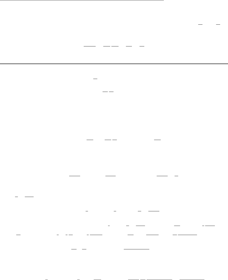
CHAPTER 6. MAGNETIC FIELDS IN MATTER 143
Problem 6.27
At the interface, the perpendicular component of Bis continuous (Eq. 6.26), and the parallel component of
His continuous (Eq. 6.25 with Kf= 0). So B?
1=B?
2,Hk
1=Hk
2. But B=µH(Eq. 6.31), so 1
µ1Bk
1=1
µ2Bk
2.
Now tan ✓1=Bk
1/B?
1, and tan ✓2=Bk
2/B?
2, so
tan ✓2
tan ✓1
=Bk
2
B?
2
B?
1
Bk
1
=Bk
2
Bk
1
=µ2
µ1
(the same form, though for di↵erent reasons, as Eq. 4.68).
Problem 6.28
In view of Eq. 6.33, there is a bound dipole at the center: mb=mm. So the net dipole moment at the
center is mcenter =m+mb= (1 + m)m=µ
µ0m. This produces a field given by Eq. 5.89:
Bcenter
dipole =µ
4⇡
1
r3[3(m·ˆr )ˆr m].
This accounts for the first term in the field. The remainder must be due to the bound surface current (Kb) at
r=R(since there can be no volume bound current, according to Eq. 6.33). Let us make an educated guess
(based either on the answer provided or on the analogous electrical Prob. 4.37) that the field due to the surface
bound current is (for interior points) of the form Bsurface
current =Am(i.e. a constant, proportional to m). In that
case the magnetization will be:
M=mH=m
µB=m
4⇡
1
r3[3(m·ˆr )ˆr m]+ m
µAm.
This will produce bound currents Jb=r⇥M=0, as it should, for 0 <r<R(no need to calculate this
curl—the second term is constant, and the first is essentially the field of a dipole, which we know is curl-less,
except at r= 0), and
Kb=M(R)⇥ˆr =m
4⇡R3(m⇥ˆr )+mA
µ(m⇥ˆr )=mm1
4⇡R3+A
µsin ✓ˆ
.
But this is exactly the surface current produced by a spinning sphere: K=v=!Rsin ✓ˆ
, with (!R)$
mmA
µ1
4⇡R3. So the field it produces (for points inside) is (Eq. 5.70):
Bsurface
current =2
3µ0(!!
!R)=2
3µ0mmA
µ1
4⇡R3.
Everything is consistent, therefore, provided A=2
3µ0mA
µ1
4⇡R3, or A12µ0
3µm=2
3
µ0m
4⇡R3. But
m=µ
µ01, so A12
3+2
3
µ0
µ=2
3
(µµ0)
4⇡R3, or A1+2µ0
µ=2
(µ0µ)
4⇡R3;A=µ
4⇡
2(µ0µ)
R3(2µ0+µ), and hence
B=µ
4⇡1
r3[3(m·ˆr )ˆr m]+ 2(µ0µ)m
R3(2µ0+µ).qed
The exterior field is that of the central dipole plus that of the surface current, which, according to Prob. 5.37,
is also a perfect dipole field, of dipole moment
msurface
current =4
3⇡R3(!!
!R)=4
3⇡R33
2µ0
Bsurface
current=2⇡R3
µ0
µ
4⇡
2(µ0µ)m
R3(2µ0+µ)=µ(µ0µ)m
µ0(2µ0+µ).
c
2012 Pearson Education, Inc., Upper Saddle River, NJ. All rights reserved. This material is
protected under all copyright laws as they currently exist. No portion of this material may be
reproduced, in any form or by any means, without permission in writing from the publisher.

144 CHAPTER 6. MAGNETIC FIELDS IN MATTER
So the total dipole moment is:
mtot =µ
µ0
m+µ
µ0
m(µ0µ)
(2µ0+µ)=3µm
(2µ0+µ),
and hence the field (for r>R) is
B=µ0
4⇡3µ
2µ0+µ1
r3[3(m·ˆr )ˆr m].
Problem 6.29
The problem is that the field inside a cavity is not the same as the field in the material itself.
(a) Amp´ere type. The field deep inside the magnet is that of a long solenoid, B0⇡µ0M. From Prob. 6.13:
Sphere : B=B02
3µ0M=1
3µ0M;
Needle : B=B0µ0M= 0;
Wafer : B=µ0M.
(b) Gilbert type. This is analogous to the electric case. The field at the center is approximately that midway
between two distant point charges, B0⇡0. From Prob. 4.16 (with E!B,1/✏0!µ0,P!M):
Sphere : B=B0+µ0
3M=1
3µ0M;
Needle : B=B0= 0;
Wafer : B=B0+µ0M=µ0M.
In the cavities, then, the fields are the same for the two models, and this will be no test at all. Yes. Fund it
with $1 M from the Office of Alternative Medicine.
c
2012 Pearson Education, Inc., Upper Saddle River, NJ. All rights reserved. This material is
protected under all copyright laws as they currently exist. No portion of this material may be
reproduced, in any form or by any means, without permission in writing from the publisher.

CHAPTER 7. ELETRODYNAMICS 145
Chapter 7
Electrodynamics
Problem 7.1
(a) Let Qbe the charge on the inner shell. Then E=1
4⇡✏0
Q
r2ˆr in the space between them, and (VaVb)=
a
bE·dr=1
4⇡✏0Qa
b
1
r2dr =Q
4⇡✏01
a1
b.
I=J·da=E·da=Q
✏0
=
✏0
4⇡✏0(VaVb)
(1/a 1/b)= 4⇡ (VaVb)
(1/a 1/b).
(b) R=VaVb
I=1
4⇡ 1
a1
b.
(c) For large b(ba), the second term is negligible, and R=1/4⇡a. Essentially all of the resistance is in
the region right around the inner sphere. Successive shells, as you go out, contribute less and less, because the
cross-sectional area (4⇡r2) gets larger and larger. For the two submerged spheres, R=2
4⇡a=1
2⇡a(one Ras
the current leaves the first, one Ras it converges on the second). Therefore I=V /R = 2⇡aV.
Problem 7.2
(a) V=Q/C =IR. Because positive Imeans the charge on the capacitor is decreasing,
dQ
dt =I=1
RC Q, so Q(t)=Q0et/RC .ButQ0=Q(0) = CV0,so Q(t)=CV0et/RC .
Hence I(t)=dQ
dt =CV0
1
RC et/RC =V0
Ret/RC .
(b) W=1
2CV 2
0.The energy delivered to the resistor is 1
0
P dt =1
0
I2R dt =V2
0
R1
0
e2t/RC dt =
V2
0
RRC
2e2t/RC
1
0
=1
2CV 2
0.X
(c) V0=Q/C +IR. This time positive Imeans Qis increasing:dQ
dt =I=1
RC (CV0Q))dQ
QCV0
=
1
RC dt )ln(QCV0)=1
RC t+ constant )Q(t)=CV0+ket/RC . But Q(0) = 0 )k=CV0, so
Q(t)=CV01et/RC . I(t)= dQ
dt =CV01
RC et/RC =V0
Ret/RC .
c
2012 Pearson Education, Inc., Upper Saddle River, NJ. All rights reserved. This material is
protected under all copyright laws as they currently exist. No portion of this material may be
reproduced, in any form or by any means, without permission in writing from the publisher.

146 CHAPTER 7. ELETRODYNAMICS
(d) Energy from battery: 1
0
V0I dt =V2
0
R1
0
et/RC dt =V2
0
RRCet/RC 1
0=V2
0
RRC =CV 2
0.
Since I(t) is the same as in (a), the energy delivered to the resistor is again 1
2CV 2
0.The final energy in
the capacitor is also 1
2CV 2
0,so half the energy from the battery goes to the capacitor, and the other half
to the resistor.
Problem 7.3
(a) I=J·da, where the integral is taken over a surface enclosing the positively charged conductor. But
J=E, and Gauss’s law says E·da=1
✏0Q,soI=E·da=
✏0Q. But Q=CV , and V=IR,so
I=
✏0CIR, or R=✏0
C.qed
(b) Q=CV =CIR )dQ
dt =I=1
RC Q)Q(t)=Q0et/RC , or, since V=Q/C,V(t)=V0et/RC . The
time constant is ⌧=RC =✏0/.
Problem 7.4
I=J(s)2⇡sL )J(s)=I/2⇡sL. E =J/=I/2⇡sL=I/2⇡kL.
V=a
b
E·dl=I
2⇡kL(ab).So R=ba
2⇡kL.
Problem 7.5
I=E
r+R;P=I2R=E2R
(r+R)2;dP
dR =E21
(r+R)22R
(r+R)3=0)r+R=2R)R=r.
Problem 7.6
E=E·dl = zero for all electrostatic fields. It looks as though E=E·dl =(/✏0)h, as would indeed
be the case if the field were really just /✏0inside and zero outside. But in fact there is always a “fringing
field” at the edges (Fig. 4.31), and this is evidently just right to kill o↵the contribution from the left end of
the loop. The current is zero.
Problem 7.7
(a) E=d
dt =Bldx
dt =Blv;E=IR )I=Blv
R.(Never mind the minus sign—it just tells you the
direction of flow: (v⇥B) is upward, in the bar, so downward through the resistor.)
(b) F=IlB =B2l2v
R,to the left.
(c) F=ma =mdv
dt =B2l2
Rv)dv
dt =B2l2
Rm v)v=v0eB2l2
mR t.
(d) The energy goes into heat in the resistor. The power delivered to resistor is I2R,so
dW
dt =I2R=B2l2v2
R2R=B2l2
Rv2
0e2↵t,where ↵⌘B2l2
mR ;dW
dt =↵mv2
0e2↵t.
The total energy delivered to the resistor is W=↵mv2
01
0
e2↵tdt =↵mv2
0
e2↵t
2↵
1
0
=↵mv2
0
1
2↵=1
2mv2
0.X
c
2012 Pearson Education, Inc., Upper Saddle River, NJ. All rights reserved. This material is
protected under all copyright laws as they currently exist. No portion of this material may be
reproduced, in any form or by any means, without permission in writing from the publisher.

CHAPTER 7. ELETRODYNAMICS 147
Problem 7.8
(a) The field of long wire is B=µ0I
2⇡sˆ
,so=B·da=µ0I
2⇡
s+a
s
1
s(ads)= µ0Ia
2⇡ln s+a
s.
(b) E=d
dt =µ0Ia
2⇡
d
dt ln s+a
s, and ds
dt =v, so µ0Ia
2⇡1
s+a
ds
dt 1
s
ds
dt =µ0Ia2v
2⇡s(s+a).
The field points out of the page, so the force on a charge in the nearby side of the square is to the right.In
the far side it’s also to the right, but here the field is weaker, so the current flows counterclockwise.
(c) This time the flux is constant, so E=0.
Problem 7.9
Since r·B= 0, Theorem 2(c) (Sect. 1.6.2) guarantees that B·dais the same for all surfaces with a given
boundary line.
Problem 7.10
1
Contents
Problem 7.10
❘
✲
✲
✲
θ
B
a
(view from above)
Φ=B·a=Ba2cos θ
c
⃝2005 Pearson Education, Inc., Upper Saddle River, NJ. All rights reserved. This material is
protected under all copyright laws as they currently exist. No portion of this material may be
reproduced, in any form or by any means, without permission inwritingfromthepublisher.
=B·a=Ba2cos ✓
Here ✓=!t,so
E=d
dt =Ba2(sin !t)!;
E=B!a2sin !t.
Problem 7.11
E=Blv =IR )I=Bl
Rv)upward magnetic force = IlB =B2l2
Rv. This opposes the gravitational force
downward:
mg B2l2
Rv=mdv
dt ;dv
dt =g↵v, where ↵⌘B2l2
mR .g↵vt=0)vt=g
↵=mgR
B2l2.
dv
g↵v=dt )1
↵ln(g↵v)=t+ const. )g↵v=Ae↵t; at t=0,v=0,so A=g.
↵v=g(1 e↵t); v=g
↵(1 e↵t)= vt(1 e↵t).
At 90% of terminal velocity, v/vt=0.9=1e↵t)e↵t=10.9=0.1; ln(0.1) = ↵t; ln 10 = ↵t;
t=1
↵ln 10, or t90% =vt
gln 10.
Now the numbers: m=4⌘Al, where ⌘is the mass density of aluminum, Ais the cross-sectional area, and
lis the length of a side. R=4l/A, where is the conductivity of aluminum. So
vt=4⌘Alg4l
AB2l2=16⌘g
B2=16g⌘⇢
B2,and
⇢=2.8⇥108⌦m
g=9.8m/s2
⌘=2.7⇥103kg/m3
B=1T
.
So vt=(16)(9.8)(2.7⇥103)(2.8⇥108)
1= 1.2 cm/s; t90% =1.2⇥102
9.8ln(10) = 2.8 ms.
If the loop were cut, it would fall freely, with acceleration g.
c
2012 Pearson Education, Inc., Upper Saddle River, NJ. All rights reserved. This material is
protected under all copyright laws as they currently exist. No portion of this material may be
reproduced, in any form or by any means, without permission in writing from the publisher.

148 CHAPTER 7. ELETRODYNAMICS
Problem 7.12
=⇡a
22B=⇡a2
4B0cos(!t); E=d
dt =⇡a2
4B0!sin(!t).I(t)= E
R=⇡a2!
4RB0sin(!t).
Problem 7.13
=B dx dy =kt2a
0
dx a
0
y3dy =1
4kt2a5.E=d
dt =1
2kta5.
Problem 7.14
2
Problem 7.14
②
Iind
✿
Iind
✲
ring
✲
pipe
✲
falling
magnet
✻
✗ ❖
B
✻❑ ✕
B
✿
✿
✿
I
c
⃝2005 Pearson Education, Inc., Upper Saddle River, NJ. All rights reserved. This material is
protected under all copyright laws as they currently exist. No portion of this material may be
reproduced, in any form or by any means, without permission in writing from the publisher.
Suppose the current (I) in the magnet flows counterclockwise (viewed from
above), as shown, so its field, near the ends, points upward. A ring of
pipe below the magnet experiences an increasing upward flux, as the magnet
approaches, and hence (by Lenz’s law) a current (Iind) will be induced in it
such as to produce a downward flux. Thus Iind must flow clockwise, which is
opposite to the current in the magnet. Since opposite currents repel, the force
on the magnet is upward. Meanwhile, a ring above the magnet experiences
adecreasing (upward) flux, so its induced current is parallel to I, and it
attracts the magnet upward. And the flux through rings next to the magnet
is constant, so no current is induced in them. Conclusion: the delay is due
to forces exerted on the magnet by induced eddy currents in the pipe.
Problem 7.15
In the quasistatic approximation, B=µ0nI ˆz ,(s<a);
0,(s>a).
Inside: for an “amperian loop” of radius s<a,
=B⇡s2=µ0nI⇡s2;E·dl=E2⇡s=d
dt =µ0n⇡s2dI
dt ;E=µ0ns
2
dI
dt ˆ
.
Outside: for an “amperian loop” of radius s>a:
=B⇡a2=µ0nI⇡a2;E2⇡s=µ0n⇡a2dI
dt ;E=µ0na2
2s
dI
dt ˆ
.
Problem 7.16
(a) The magnetic field (in the quasistatic approximation) is “circumferential”. This is analogous to the current
in a solenoid, and hence the field is longitudinal.
(b) Use the “amperian loop” shown.
Outside, B=0,sohereE=0(like Boutside a solenoid).
So E·dl =El =d
dt =d
dt B·da=d
dt a
s
µ0I
2⇡s0l ds0
)E=µ0
2⇡
dI
dt ln a
s.ButdI
dt =I0!sin !t,
so E=µ0I0!
2⇡sin(!t)lna
sˆz .
3
Problem 7.16
✲✲
Iz
✻
a✻
❄
✛ ✲
l
✻
s
c
⃝2005 Pearson Education, Inc., Upper Saddle River, NJ. All rights reserved. This material is
protected under all copyright laws as they currently exist. No portion of this material may be
reproduced, in any form or by any means, without permission in writing from the publisher.
c
2012 Pearson Education, Inc., Upper Saddle River, NJ. All rights reserved. This material is
protected under all copyright laws as they currently exist. No portion of this material may be
reproduced, in any form or by any means, without permission in writing from the publisher.

CHAPTER 7. ELETRODYNAMICS 149
Problem 7.17
(a) The field inside the solenoid is B=µ0nI. So =⇡a2µ0nI )E=⇡a2µ0n(dI/dt).
In magnitude, then, E=⇡a2µ0nk. Now E=IrR,so Iresistor =⇡a2µ0nk
R.
Bis to the right and increasing, so the field of the loop is to the left, so the current is counterclockwise, or
to the right, through the resistor.
(b) =2⇡a2µ0nI;I=dQ
dt =E
R=1
R
d
dt )Q=1
R, in magnitude. So Q=2⇡a2µ0nI
R.
Problem 7.18
=B·da;B=µ0I
2⇡sˆ
;=µ0Ia
2⇡s+a
s
ds0
s0=µ0Ia
2⇡ln s+a
s;
E=IloopR=dQ
dt R=d
dt =µ0a
2⇡ln(1 + a/s)dI
dt .
dQ =µ0a
2⇡Rln(1 + a/s)dI )Q=Iµ0a
2⇡Rln(1 + a/s).
The field of the wire, at the square loop, is out of the page, and decreasing, so the field of the induced
current must point out of page, within the loop, and hence the induced current flows counterclockwise.
Problem 7.19
In the quasistatic approximation, B=µ0NI
2⇡sˆ
,(inside toroid);
0,(outside toroid)
(Eq. 5.60). The flux around the toroid is therefore
=µ0NI
2⇡a+w
a
1
sh ds =µ0NIh
2⇡ln 1+w
a⇡µ0Nhw
2⇡aI. d
dt =µ0Nhw
2⇡a
dI
dt =µ0Nhwk
2⇡a.
The electric field is the same as the magnetic field of a circular current (Eq. 5.41):
B=µ0I
2
a2
(a2+z2)3/2ˆz ,
with (Eq. 7.19)
I!1
µ0
d
dt =Nhwk
2⇡a.So E=µ0
2Nhwk
2⇡aa2
(a2+z2)3/2ˆz =µ0
4⇡
Nhwka
(a2+z2)3/2ˆz .
Problem 7.20
@B/@tis nonzero along the left and right edges of the shaded rectangle:
c
2012 Pearson Education, Inc., Upper Saddle River, NJ. All rights reserved. This material is
protected under all copyright laws as they currently exist. No portion of this material may be
reproduced, in any form or by any means, without permission in writing from the publisher.

150 CHAPTER 7. ELETRODYNAMICS
E
The (inward) flux through the strip on the left is increasing; the (inward) flux through the strip on the right
is decreasing. This is analogous to two current sheets under Amp`ere’s law, with B!Eand µ0Ienc !d/dt
(Eq. 7.19). The one on the left is like a current flowing out (taking account of the minus sign), so its field is
counterclockwise and the one on the right is like a current flowing in, so its field is clockwise.
Problem 7.21
The answer is indeterminate, until some boundary conditions are supplied. We know that r⇥E=
(dB0/dt)ˆz (and r·E= 0), but this is insufficient information to determine E. Ordinarily we would invoke
some symmetry of the configuration, or require that the field go to zero at infinity, to resolve the ambiguity,
but neither is available in this case. E=1
2
dB0
dt (yˆx xˆy ) would do the job, in which case the force would be
zero, but we could add any constant vector to this, and make the force anything we like.
Problem 7.22
(a) From Eq. 5.41, the field (on the axis) is B=µ0I
2
b2
(b2+z2)3/2ˆz , so the flux through the little loop (area ⇡a2)
is =µ0⇡Ia2b2
2(b2+z2)3/2.
(b) The field (Eq. 5.88) is B=µ0
4⇡
m
r3(2 cos ✓ˆr + sin ✓ˆ
✓), where m=I⇡a2. Integrating over the spherical “cap”
(bounded by the big loop and centered at the little loop):
=B·da=µ0
4⇡
I⇡a2
r3(2 cos ✓)(r2sin ✓d✓d)=µ0Ia2
2r2⇡¯
✓
0
cos ✓sin ✓d✓
where r=pb2+z2and sin ¯
✓=b/r. Evidently =µ0I⇡a2
r
sin2✓
2
¯
✓
0=µ0⇡Ia2b2
2(b2+z2)3/2,the same as in (a)!!
(c) Dividing o↵I(1=M12I2,2=M21I1): M12 =M21 =µ0⇡a2b2
2(b2+z2)3/2.
Problem 7.23
E=d
dt =MdI
dt =Mk.
c
2012 Pearson Education, Inc., Upper Saddle River, NJ. All rights reserved. This material is
protected under all copyright laws as they currently exist. No portion of this material may be
reproduced, in any form or by any means, without permission in writing from the publisher.

CHAPTER 7. ELETRODYNAMICS 151
4
Problem 7.21
E=−
dΦ
dt =−MdI
dt =−Mk.
✻
❄
❄
✻
✻
❄
a
a
a
❖
I
c
⃝2005 Pearson Education, Inc., Upper Saddle River, NJ. All rights reserved. This material is
protected under all copyright laws as they currently exist. No portion of this material may be
reproduced, in any form or by any means, without permission in writing from the publisher.
It’s hard to calculate Musing a current in the little loop, so, exploiting the equality of the mutual inductances,
I’ll find the flux through the little loop when a current Iflows in the big loop: =MI. The field of one long
wire is B=µ0I
2⇡s)1=µ0I
2⇡2a
a
1
sads=µ0Ia
2⇡ln 2, so the total flux is
=21=µ0Ialn 2
⇡)M=µ0aln 2
⇡)E=µ0ka ln 2
⇡,in magnitude.
Direction: The net flux (through the big loop), due to Iin the little loop, is into the page. (Why? Field
lines point in, for the inside of the little loop, and out everywhere outside the little loop. The big loop encloses
all of the former, and only part of the latter, so net flux is inward.) This flux is increasing, so the induced
current in the big loop is such that its field points out of the page: it flows counterclockwise.
Problem 7.24
B=µ0nI )1=µ0nI⇡R2(flux through a single turn). In a length lthere are nl such turns, so the
total flux is =µ0n2⇡R2Il. The self-inductance is given by =LI, so the self-inductance per unit length is
L=µ0n2⇡R2.
Problem 7.25
The field of one wire is B1=µ0
2⇡
I
s,so =2·µ0I
2⇡·l
d✏
✏
ds
s=µ0Il
⇡ln d✏
✏. The ✏in the numerator is
negligible (compared to d), but in the denominator we cannot let ✏!0, else the flux is infinite.
L=µ0l
⇡ln(d/✏).Evidently the size of the wire itself is critical in determining L.
Problem 7.26
(a) In the quasistatic approximation B=µ0
2⇡sˆ
.So 1=µ0I
2⇡b
a
1
sh ds =µ0Ih
2⇡ln(b/a).
This is the flux through one turn; the total flux is Ntimes 1:=µ0Nh
2⇡ln(b/a)I0cos(!t).So
E=d
dt =µ0Nh
2⇡ln(b/a)I0!sin(!t)=(4⇡⇥107)(103)(102)
2⇡ln(2)(0.5)(2⇡60) sin(!t)
=2.61 ⇥104sin(!t) (in volts), where !=2⇡60 = 377/s. Ir=E
R=2.61 ⇥104
500 sin(!t)
= 5.22 ⇥107sin(!t) (amperes).
(b) Eb=LdIr
dt ; where (Eq. 7.28) L=µ0N2h
2⇡ln(b/a)=(4⇡⇥107)(106)(102)
2⇡ln(2) = 1.39 ⇥103(henries).
Therefore Eb=(1.39 ⇥103)(5.22 ⇥107!) cos(!t)= 2.74 ⇥107cos(!t) (volts).
Ratio of amplitudes: 2.74 ⇥107
2.61 ⇥104= 1.05 ⇥103=µ0N2h!
2⇡Rln(b/a).
Problem 7.27
With Ipositive clockwise, E=LdI
dt =Q/C, where Qis the charge on the capacitor; I=dQ
dt , so
d2Q
dt2=1
LC Q=!2Q, where !=1
pLC . The general solution is Q(t)=Acos !t+Bsin !t.Att= 0,
c
2012 Pearson Education, Inc., Upper Saddle River, NJ. All rights reserved. This material is
protected under all copyright laws as they currently exist. No portion of this material may be
reproduced, in any form or by any means, without permission in writing from the publisher.

152 CHAPTER 7. ELETRODYNAMICS
Q=CV ,soA=CV ;I(t)=dQ
dt =A!sin !t+B!sin !t.Att= 0, I= 0, so B= 0, and
I(t)=CV !sin !t=VC
Lsin t
pLC .
If you put in a resistor, the oscillation is “damped”. This time LdI
dt =Q
C+IR, so Ld2Q
dt2+RdQ
dt +1
CQ=0.
For an analysis of this case, see Purcell’s Electricity and Magnetism (Ch. 8) or any book on oscillations and
waves.
Problem 7.28
(a) W=1
2LI2.L=µ0n2⇡R2l(Prob. 7.24) W=1
2µ0n2⇡R2lI2.
(b) W=1
2(A·I)dl. A=(µ0nI/2)Rˆ
, at the surface (Eq. 5.72 or 5.73). So W1=1
2
µ0nI
2RI ·2⇡R, for one
turn. There are nl such turns in length l, so W=1
2µ0n2⇡R2lI2.X
(c) W=1
2µ0B2d⌧.B=µ0nI, inside, and zero outside; d⌧=⇡R2l,soW=1
2µ0µ2
0n2I2⇡R2l=
1
2µ0n2⇡R2lI2.X
(d) W=1
2µ0B2d⌧(A⇥B)·da. This time B2d⌧=µ2
0n2I2⇡(R2a2)l. Meanwhile,
A⇥B=0outside (at s=b). Inside, A=µ0nI
2aˆ
(at s=a), while B=µ0nI ˆz .
A⇥B=1
2µ2
0n2I2a(ˆ
⇥ˆz
ˆs
)
5
Problem 7.26
☛
points inward (“out” of the volume)
c
⃝2005 Pearson Education, Inc., Upper Saddle River, NJ. All rights reserved. This material is
protected under all copyright laws as they currently exist. No portion of this material may be
reproduced, in any form or by any means, without permission inwritingfromthepublisher.
(A⇥B)·da=(1
2µ2
0n2I2aˆs )·[addz(ˆs )] = 1
2µ2
0n2I2a22⇡l.
W=1
2µ0µ2
0n2I2⇡(R2a2)l+µ2
0n2I2⇡a2l=1
2µ0n2I2R2⇡l. X
1
Contents
Problem 7.26
✲ˆz
ˆ
φ
❖
✕ˆs
✲ˆz
❄
✻
h
✕
☛
w
✛ ✲
l
→I
✛
I
→
B
c
⃝2005 Pearson Education, Inc., Upper Saddle River, NJ. All rights reserved. This material is
protected under all copyright laws as they currently exist. No portion of this material may be
reproduced, in any form or by any means, without permission inwritingfromthepublisher.
Problem 7.29
B=µ0nI
2⇡s;W=1
2µ0B2d⌧=1
2µ0
µ2
0n2I2
4⇡21
s2hs dds =µ0n2I2
8⇡2h2⇡ln b
a=1
4⇡µ0n2I2hln(b/a).
L=µ0
2⇡n2hln (b/a) (same as Eq. 7.28).
Problem 7.30
B·dl=B(2⇡s)=µ0Ienc =µ0I(s2/R2))B=µ0Is
2⇡R2.
W=1
2µ0B2d⌧=1
2µ0
µ2
0I2
4⇡2R4R
0
s2(2⇡s)l ds =µ0I2l
4⇡R4s4
4
R
0=µ0l
16⇡I2=1
2LI2.
So L=µ0
8⇡l, and L=L/l =µ0/8⇡,independent of R!
Problem 7.31
(a) Initial current: I0=E0/R.SoLdI
dt =IR )dI
dt =R
LI)I=I0eRt/L, or I(t)= E0
ReRt/L.
(b) P=I2R=(E0/R)2e2Rt/LR=E2
0
Re2Rt/L =dW
dt .
W=E2
0
R1
0
e2Rt/L dt =E2
0
RL
2Re2Rt/L
1
0
=E2
0
R(0 + L/2R)= 1
2L(E0/R)2.
(c) W0=1
2LI2
0=1
2L(E0/R)2.X
Problem 7.32
(a) B1=µ0
4⇡
1
r3I1[3(a1·ˆ
r
)ˆ
r
a1], since m1=I1a1. The flux through loop 2 is then
2=B1·a2=µ0
4⇡
1
r
3I1[3(a1·ˆ
r
)(a2·ˆ
r
)a1·a2]=MI1. M =µ0
4⇡
r
3[3(a1·ˆ
r
)(a2·ˆ
r
)a1·a2].
c
2012 Pearson Education, Inc., Upper Saddle River, NJ. All rights reserved. This material is
protected under all copyright laws as they currently exist. No portion of this material may be
reproduced, in any form or by any means, without permission in writing from the publisher.

CHAPTER 7. ELETRODYNAMICS 153
(b) E1=MdI2
dt ,dW
dt 1=E1I1=MI1dI2
dt . (This is the work done per unit time against the mutual emf in
loop 1—hence the minus sign.) So (since I1is constant) W1=MI1I2, where I2is the final current in loop 2:
W=µ0
4⇡
r
3[3(m1·ˆ
r
)(m2·ˆ
r
)m1·m2].
Notice that this is opposite in sign to Eq. 6.35. In Prob. 6.21 we assumed that the magnitudes of the dipole
moments were fixed, and we did not worry about the energy necessary to sustain the currents themselves—only
the energy required to move them into position and rotate them into their final orientations. But in this
problem we are including it all, and it is a curious fact that this merely changes the sign of the answer. For
commentary on this subtle issue see R. H. Young, Am. J. Phys. 66, 1043 (1998), and the references cited
there.
Problem 7.33
(a) The (solenoid) magnetic field is
B=µ0Kˆz =µ0!Rˆz (s<R),
0(s>R).
From Example 7.7, the electric field is
E=
s
2
dB
dt ˆ
=sR
2µ0˙!ˆ
(s<R),
R2
2s
dB
dt ˆ
=R3
2sµ0˙!ˆ
(s>R).
At the surface (s=R)E=1
2µ0R2˙!ˆ
,so the torque on a length `of the cylinder is
N=R(2⇡R`)1
2µ0R2˙!ˆz =⇡µ02R4˙!`ˆz ,
and the work done per unit length is W
`=⇡µ02R4d!
dt d.
But d=!dt, and the integral becomes
!f
0
!d!=1
2!2
f;)W
`=µ0⇡
2!fR22.
(This is the work done by the field; the work you must do does not include the minus sign.)
(b) Because B=µ0Kˆz =µ0!fRˆz is uniform inside the solenoid (and zero outside), W=1
2µ0
B2⇡R2`.
W
`=1
2µ0
(µ0!fR)2⇡R2=µ0⇡
2!fR22.
Problem 7.34
The displacement current density (Sect. 7.3.2) is Jd=✏0@E
@t=I
A=I
⇡a2ˆz . Drawing an “amperian loop” at
radius s,
B·dl =B·2⇡s=µ0Idenc =µ0
I
⇡a2·⇡s2=µ0Is2
a2)B=µ0Is2
2⇡sa2;B=µ0Is
2⇡a2ˆ
.
c
2012 Pearson Education, Inc., Upper Saddle River, NJ. All rights reserved. This material is
protected under all copyright laws as they currently exist. No portion of this material may be
reproduced, in any form or by any means, without permission in writing from the publisher.
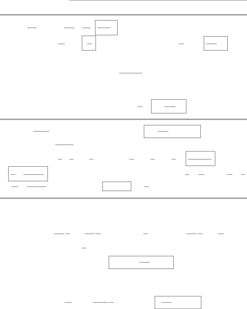
154 CHAPTER 7. ELETRODYNAMICS
Problem 7.35
(a) E=(t)
✏0
ˆz ;(t)=Q(t)
⇡a2=It
⇡a2;It
⇡✏0a2ˆz .
(b) Idenc =Jd⇡s2=✏0
dE
dt ⇡s2=Is2
a2.B·dl=µ0Idenc )B2⇡s=µ0Is2
a2)B=µ0I
2⇡a2sˆ
.
(c) A surface current flows radially outward over the left plate; let I(s) be the total current crossing a circle
of radius s. The charge density (at time t) is
(t)=[II(s)]t
⇡s2.
Since we are told this is independent of s, it must be that II(s)=s2, for some constant . But I(a) = 0,
so a2=I, or =I/a2. Therefore I(s)=I(1 s2/a2).
B2⇡s=µ0Ienc =µ0[II(s)] = µ0Is2
a2)B=µ0I
2⇡a2sˆ
.X
Problem 7.36
(a) Jd=✏0
µ0I0!2
2⇡cos(!t)ln(a/s)ˆz .ButI0cos(!t)=I. So Jd=µ0✏0
2⇡!2Iln(a/s)ˆz .
(b) Id=Jd·da=µ0✏0!2I
2⇡a
0
ln(a/s)(2⇡sds)=µ0✏0!2Ia
0
(sln asln s)ds
=µ0✏0!2I(ln a)s2
2s2
2ln s+s2
4
a
0=µ0✏0!2Ia2
2ln a
a2
2ln a
+a2
4=µ0✏0!2Ia2
4.
(c) Id
I=µ0✏0!2a2
4.Since µ0✏0=1/c2,Id/I =(!a/2c)2. If a= 103m, and Id
I=1
100 , so that !a
2c=1
10 ,
!=2c
10a=3⇥108m/s
5⇥103m, or !=0.6⇥1011/s= 6⇥1010 /s; ⌫=!
2⇡⇡1010 Hz, or 104megahertz. (This is the
microwave region, way above radio frequencies.)
Problem 7.37
Physically, this is the field of a point charge qat the origin, out to an expanding spherical shell of radius vt;
outside this shell the field is zero. Evidently the shell carries the opposite charge, q.Mathematically, using
product rule #5 and Eq. 1.99:
r·E=✓(vt r)r·1
4⇡✏0
q
r2ˆr +1
4⇡✏0
q
r2ˆr ·r[✓(vt r)] = q
✏0
3(r)✓(vt r)+ 1
4⇡✏0
q
r2(ˆr ·ˆr )@
@r✓(vt r).
But 3(r)✓(vt r)=3(r)✓(t), and @
@r✓(vt r)=(vt r) (Prob. 1.46), so
⇢=✏0r·E=q3(r)✓(t)q
4⇡r2(vt r).
(For t<0 the field and the charge density are zero everywhere.)
Clearly r·B= 0, and r⇥E=0(since Ehas only an rcomponent, and it is independent of ✓and ).
There remains only the Amp´ere/Maxwell law, r⇥B=0=µ0J+µ0✏0@E/@t. Evidently
J=✏0
@E
@t=✏0q
4⇡✏0r2
@
@t[✓(vt r)]ˆr =q
4⇡r2v(vt r)ˆr .
c
2012 Pearson Education, Inc., Upper Saddle River, NJ. All rights reserved. This material is
protected under all copyright laws as they currently exist. No portion of this material may be
reproduced, in any form or by any means, without permission in writing from the publisher.

CHAPTER 7. ELETRODYNAMICS 155
(The stationary charge at the origin does not contribute to J, of course; for the expanding shell we have J=⇢v,
as expected—Eq. 5.26.)
Problem 7.38
From r·B=µ0⇢mit follows that the field of a point monopole is B=µ0
4⇡
qm
r
2ˆ
r
. The force law has the
form F/qmB1
c2v⇥E(see Prob. 5.22—the c2is needed on dimensional grounds). The proportionality
constant must be 1 to reproduce “Coulomb’s law” for point charges at rest. So F=qmB1
c2v⇥E.
Problem 7.39
Integrate the “generalized Faraday law” (Eq. 7.44iii), r⇥E=µ0Jm@B
@t, over the surface of the loop:
(r⇥E)·da=E·dl=E=µ0Jm·dad
dt B·da=µ0Imenc d
dt .
But E=LdI
dt ,so dI
dt =µ0
LImenc +1
L
d
dt ,or I=µ0
LQm+1
L,where Qmis the total magnetic charge
passing through the surface, and is the change in flux through the surface. If we use the flat surface, then
Qm=qmand = 0 (when the monopole is far away, = 0; the flux builds up to µ0qm/2 just before
it passes through the loop; then it abruptly drops to µ0qm/2, and rises back up to zero as the monopole
disappears into the distance). If we use a huge balloon-shaped surface, so that qmremains inside it on the far
side, then Qm= 0, but rises monotonically from 0 to µ0qm. In either case,
I=µ0qm
L.
[The analysis is slightly di↵erent for a superconducting loop, but the conclusion is the same.]
Problem 7.40
E=V
d)Jc=E=1
⇢E=V
⇢d.J
d=@D
@t=@
@t(✏E)=✏@
@tV0cos(2⇡⌫t)
d=✏V0
d[2⇡⌫ sin(2⇡⌫t)].
The ratio of the amplitudes is therefore:
Jc
Jd
=V0
⇢d
d
2⇡⌫✏V0
=1
2⇡⌫✏⇢ =2⇡(4 ⇥108)(81)(8.85 ⇥1012)(0.23)1= 2.41.
Problem 7.41
Begin with a di↵erent problem: two parallel
wires carrying charges +and as shown.
9
Problem 7.39
✲y
✻
z
✰
x
bb
+λ
−λ
c
⃝2005 Pearson Education, Inc., Upper Saddle River, NJ. All rights reserved. This material is
protected under all copyright laws as they currently exist. No portion of this material may be
reproduced, in any form or by any means, without permission inwritingfromthepublisher.
Field of one wire: E=
2⇡✏0sˆs ; potential: V=
2⇡✏0ln(s/a).
Potential of combination: V=
2⇡✏0ln(s/s+),
or V(y, z)=
4⇡✏0ln (y+b)2+z2
(yb)2+z2.
Find the locus of points of fixed V(i.e. equipotential surfaces):
e4⇡✏0V/⌘µ=(y+b)2+z2
(yb)2+z2=)µ(y22yb +b2+z2)=y2+2yb +b2+z2;
y2(µ1) + b2(µ1) + z2(µ1) 2yb(µ+ 1) = 0 =)y2+z2+b22yb=0 ⌘µ+1
µ1;
(yb)2+z2+b2b22=0=)(yb2)+z2=b2(21).
c
2012 Pearson Education, Inc., Upper Saddle River, NJ. All rights reserved. This material is
protected under all copyright laws as they currently exist. No portion of this material may be
reproduced, in any form or by any means, without permission in writing from the publisher.
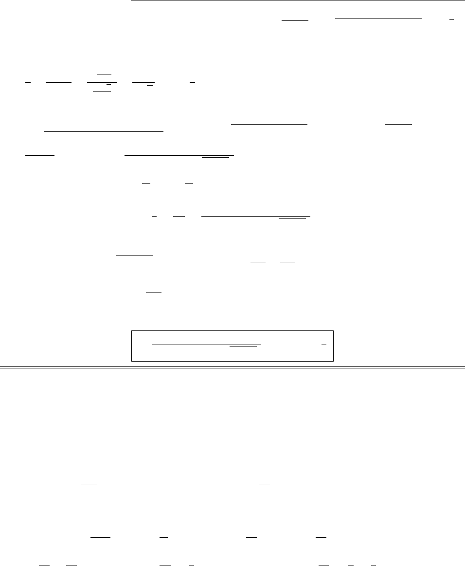
156 CHAPTER 7. ELETRODYNAMICS
This is a circle, with center at y0=b=bµ+1
µ1and radius = b21=b(µ2+2µ+1)(µ22µ+1)
(µ1)2=2bpµ
µ1.
This suggests an image solution to the problem at hand. We want y0=d, radius = a, and V=V0. These
determine the parameters b,µ, and of the image solution:
d
a=y0
radius =bµ+1
µ1
2bpµ
µ1
=µ+1
2pµ.Call d
a⌘↵.
4↵2µ=(µ+ 1)2=µ2+2µ+1=)µ2+ (2 4↵2)µ+ 1 = 0;
µ=4↵22±4(1 2↵2)24
2=2↵21±14↵2+4↵41=2↵21±2↵↵21;
4⇡✏0V0
=lnµ=)=4⇡✏0V0
ln 2↵21±2↵p↵21.That’s the line charge in the image problem.
I=J·da=E·da=1
✏0
Qenc =
✏0
l.
The current per unit length is i=I
l=
✏0
=4⇡V0
ln 2↵21±2↵p↵21. Which sign do we want? Suppose
the cylinders are far apart, da, so that ↵1.
()=2↵21±2↵211/↵2=2↵21±2↵211
2↵21
8↵4+···
=2↵2(1 ±1) (1 ±1) ⌥1
4↵2±···=4↵221/2↵2+···⇡4↵2(+ sign),
1/4↵2(sign).
The current must surely decrease with increasing ↵, so evidently the + sign is correct:
i=4⇡V0
ln 2↵21+2↵p↵21,where ↵=d
a.
Problem 7.42
From Prob. 3.24,
Vin(s, )=
1
k=1
skbksin(k),(s<a);
Vout(s, )= 1
k=1
skdksin(k),(s>a).
(We don’t need the cosine terms, because Vis clearly an odd function of .) At s=a, Vin =Vout =V0/2⇡.
Let’s start with Vin, and use Fourier’s trick to determine bk:
1
k=1
akbksin(k)=V0
2⇡)1
k=1
akbk⇡
⇡
sin(k) sin(k0)d=V0
2⇡⇡
⇡
sin(k0)d.But
⇡
⇡
sin(k) sin(k0)d=⇡kk0,and
⇡
⇡
sin(k0)d=1
(k0)2sin(k0)
k0cos(k0)
⇡
⇡
=2⇡
k0cos(k0)=2⇡
k0(1)k0.So
⇡akbk=V0
2⇡2⇡
k(1)k,or bk=V0
⇡k1
ak
,and hence Vin(s, )=V0
⇡
1
k=1
1
ks
aksin(k).
c
2012 Pearson Education, Inc., Upper Saddle River, NJ. All rights reserved. This material is
protected under all copyright laws as they currently exist. No portion of this material may be
reproduced, in any form or by any means, without permission in writing from the publisher.
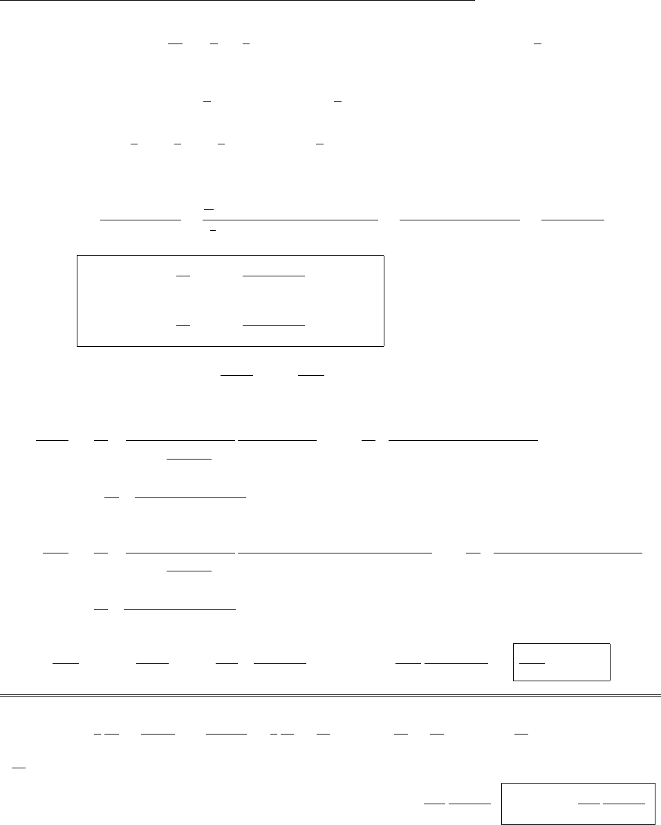
CHAPTER 7. ELETRODYNAMICS 157
Similarly, Vout(s, )=V0
⇡
1
k=1
1
ka
sksin(k). Both sums are of the form S⌘1
k=1
1
k(x)ksin(k) (with
x=s/a for r<aand x=a/s for r>a). This series can be summed explicitly, using Euler’s formula
(ei✓= cos ✓+isin ✓): S= Im 1
k=1
1
k(x)keik= Im 1
k=1
1
kxeik.
But ln(1 + w)=w1
2w2+1
3w31
4w4···=1
k=1
1
k(w)k,so S=Im ln 1+xei.
Now ln Rei✓= ln R+i✓,so S=✓, where
tan ✓=Im 1+xei
Re (1 + xei)=
1
2i1+xei1+xei
1
2[(1 + xei)+(1+xei)] =xeiei
i[2 + x(ei+ei)] =xsin
1+xcos .
Conclusion:
Vin(s, )=
V0
⇡tan1ssin
a+scos ,(s<a);
Vout(s, )= V0
⇡tan1asin
s+acos ,(s>a).
(b) From Eq. 2.36, ()=✏0@Vout
@ss=a@Vin
@ss=a.
@Vout
@s=V0
⇡
1
1+asin
s+acos 2(asin )
(s+acos )2
=V0
⇡asin
(s+acos )2+(asin )2
=V0
⇡asin
s2+2as cos +a2;
@Vin
@s=V0
⇡
1
1+ssin
a+scos 2[(a+scos ) sin ssin cos ]
(a+scos )2
=V0
⇡asin
(a+scos )2+(ssin )2
=V0
⇡asin
s2+2as cos +a2.
@Vin
@ss=a
=@Vout
@ss=a
=V0
2⇡asin
1 + cos ,so ()=✏0V0
⇡a
sin
(1 + cos )=✏0V0
⇡atan(/2).
Problem 7.43
(a) r2V=1
s
@
@ss@(zf)
@s+@2(zf)
@z2=z
s
d
ds sdf
ds=0)d
ds sdf
ds=0)sdf
ds =A(a constant) )
Ads
s=df )f=Aln(s/s0)(s0another constant).But (ii) )f(b) = 0, so ln(b/s0) = 0, so s0=b, and
V(s, z)=Az ln(s/b). But (i) )Az ln(a/b)=(I⇢z)/(⇡a2), so A=I⇢
⇡a2
1
ln(a/b);V(s, z)=I⇢z
⇡a2
ln(s/b)
ln(a/b).
c
2012 Pearson Education, Inc., Upper Saddle River, NJ. All rights reserved. This material is
protected under all copyright laws as they currently exist. No portion of this material may be
reproduced, in any form or by any means, without permission in writing from the publisher.

158 CHAPTER 7. ELETRODYNAMICS
(b) E=rV=@V
@sˆs @V
@zˆz =I⇢z
⇡a2
1
sln(a/b)ˆs +I⇢
⇡a2
ln(s/b)
ln(a/b)ˆz =I⇢
⇡a2ln(a/b)z
sˆs + ln s
bˆz .
(c) (z)=✏0Es(a+)Es(a)=✏0I⇢
⇡a2ln(a/b)z
a0=✏0I⇢z
⇡a3ln(a/b).
Problem 7.44
(a) Faraday’s law says r⇥E=@B
@t,soE=0)@B
@t=0)B(r) is independent of t.
(b) Faraday’s law in integral form (Eq. 7.19) says E·dl=d/dt. In the wire itself E=0,sothrough
the loop is constant.
(c) Amp`ere-Maxwell)r⇥B=µ0J+µ0✏0@E
@t, so E=0,B=0)J=0, and hence any current must be
at the surface.
(d) From Eq. 5.70, a rotating shell produces a uniform magnetic field (inside): B=2
3µ0!aˆz . So to cancel
such a field, we need !a=3
2
B0
µ0
. Now K=v=!asin ✓ˆ
,so K=3B0
2µ0
sin ✓ˆ
.
Problem 7.45
(a) To make the field parallel to the plane, we need image monopoles of the same sign (compare Figs. 2.13
and 2.14), so the image dipole points down (-z).
(b) From Prob. 6.3 (with r!2z):
F=3µ0
2⇡
m2
(2z)4.3µ0
2⇡
m2
(2h)4=Mg )h=1
23µ0m2
2⇡Mg 1/4
.
(c) Using Eq. 5.89, and referring to the figure:
11
Problem 7.43
✻
h
❄
h
✲
r❯
r1
✕
r2
✲ˆr
❯
ˆr 2
✕
ˆr 1
✻
m
❄
−m
θ
θ
c
⃝2005 Pearson Education, Inc., Upper Saddle River, NJ. All rights reserved. This material is
protected under all copyright laws as they currently exist. No portion of this material may be
reproduced, in any form or by any means, without permission inwritingfromthepublisher.
B=µ0
4⇡
1
(r1)3{[3(mˆz ·ˆr 1)ˆr 1mˆz ] + [3(mˆz ·ˆr 2)ˆr 2+mˆz ]}
=3µ0m
4⇡(r1)3[(ˆz ·ˆr 1)ˆr 1(ˆz ·ˆr 2)ˆr 2].But ˆz ·ˆr 1=ˆz ·ˆr 2= cos ✓.
=3µ0m
4⇡(r1)3cos ✓(ˆr 1+ˆr 2).But ˆr 1+ˆr 2=2sin✓ˆr .
=3µ0m
2⇡(r1)3sin ✓cos ✓ˆr .But sin ✓=r
r1
,cos ✓=h
r1
,and r1=r2+h2.
=3µ0mh
2⇡
r
(r2+h2)5/2ˆr .
Now B=µ0(K⇥ˆz ))ˆz ⇥B=µ0ˆz ⇥(K⇥ˆz )=µ0[Kˆz (K·ˆz )] = µ0K. (I used the BAC-CAB rule,
and noted that K·ˆz = 0, because the surface current is in the xy plane.)
K=1
µ0
(ˆz ⇥B)=3mh
2⇡
r
(r2+h2)5/2(ˆz ⇥ˆr )=3mh
2⇡
r
(r2+h2)5/2ˆ
.qed
c
2012 Pearson Education, Inc., Upper Saddle River, NJ. All rights reserved. This material is
protected under all copyright laws as they currently exist. No portion of this material may be
reproduced, in any form or by any means, without permission in writing from the publisher.
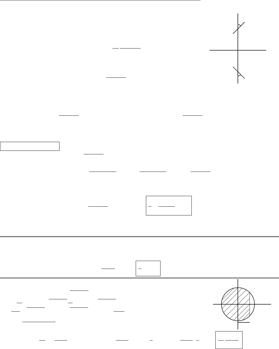
CHAPTER 7. ELETRODYNAMICS 159
Problem 7.46
Say the angle between the dipole (m1) and the zaxis is ✓(see diagram).
12
Problem 7.44
✲x
✻
z
✒
−
+
m1
θ
❘
−
+
m2
θ
h
c
⃝2005 Pearson Education, Inc., Upper Saddle River, NJ. All rights reserved. This material is
protected under all copyright laws as they currently exist. No portion of this material may be
reproduced, in any form or by any means, without permission inwritingfromthepublisher.
The field of the image dipole (m2) is
B(z)= µ0
4⇡
1
(h+z)3[3(m2·ˆz )ˆz m2]
for points on the zaxis (Eq. 5.89). The torque on m1is (Eq. 6.1)
N=m1⇥B=µ0
4⇡(2h)3[3(m2·ˆz )(m1⇥ˆz )(m1⇥m2)] .
But m1=m(sin ✓ˆx + cos ✓ˆz ),m2=m(sin ✓ˆx cos ✓ˆz ),so m2·ˆz =mcos ✓,m1⇥ˆz =msin ✓ˆy ,and
m1⇥m2=2m2sin ✓cos ✓ˆy .
N=µ0
4⇡(2h)33m2sin ✓cos ✓ˆy 2m2sin ✓cos ✓ˆy )=µ0m2
4⇡(2h)3sin ✓cos ✓ˆy .
Evidently the torque is zero for ✓= 0, ⇡/2, or ⇡. But 0 and ⇡are clearly unstable, since the nearby
ends of the dipoles (minus, in the figure) dominate, and they repel. The stable configuration is ✓=⇡/2:
parallel to the surface (contrast Prob. 4.6).
In this orientation, B(z)=µ0m
4⇡(h+z)3ˆx , and the force on m1is (Eq. 6.3):
F=rµ0m2
4⇡(h+z)3z=h
=3µ0m2
4⇡(h+z)4ˆz z=h
=3µ0m2
4⇡(2h)4ˆz .
At equilibrium this force upward balances the weight Mg:
3µ0m2
4⇡(2h)4=Mg )h=1
23µ0m2
4⇡Mg 1/4
.
Incidentally, this is (1/2)1/4=0.84 times the height it would adopt in the orientation perpendicular to the
plane (Prob. 7.45b).
Problem 7.47
f=v⇥B;v=!asin ✓ˆ
;f=!aB0sin ✓(ˆ
⇥ˆz ). E=f·dl, and dl =ad✓ˆ
✓.
So E=!a2B0⇡/2
0sin ✓(ˆ
⇥ˆz )·ˆ
✓d✓. But ˆ
✓·(ˆ
⇥ˆz )=ˆz ·(ˆ
✓⇥ˆ
)=ˆz ·ˆr = cos ✓.
E=!a2B0⇡/2
0
sin ✓cos ✓d✓=!a2B0sin2✓
2⇡/2
0=1
2!a2B0(same as the rotating disk in Ex. 7.4).
Problem 7.48
1
Contents
✲x
✻
z
✲✛
y
}
l/2
c
⃝2005 Pearson Education, Inc., Upper Saddle River, NJ. All rights reserved. This material is
protected under all copyright laws as they currently exist. No portion of this material may be
reproduced, in any form or by any means, without permission inwritingfromthepublisher.
F=IBl;=2By
apa2x2dx (a= radius of circle).
E=d
dt =2Ba2y2dy
dt =2Bva2y2=IR.
I=2Bv
Ra2y2;l/2=a2y2. So F=4B2v
R(a2y2)=mg.
vcircle =mgR
4B2(a2y2);
tcircle =a
+ady
v=4B2
mgR a
a
(a2y2)dy =4B2
mgR (a2y1
3y3)
a
a
=4B2
mgR (4
3a3)= 16
3
B2a3
mgR .
c
2012 Pearson Education, Inc., Upper Saddle River, NJ. All rights reserved. This material is
protected under all copyright laws as they currently exist. No portion of this material may be
reproduced, in any form or by any means, without permission in writing from the publisher.

160 CHAPTER 7. ELETRODYNAMICS
Problem 7.49
(a) From Prob. 5.52a,
A(r,t)= 1
4⇡B(r0,t)⇥ˆ
r
r
2d⌧0,so E=@A
@t.
[Check: r⇥E=@
@t(r⇥A)=@B
@t, and we recover Faraday’s law.]
(b) The Coulomb field is zero inside and 1
4⇡✏0
Q
r2ˆr =1
4⇡✏0
4⇡R2
r2ˆr =R2
✏0r2ˆr outside. The Faraday field is
@A
@t, where Ais given (in the quasistatic approximation) by Eq. 5.69, with !a function of time. Letting
˙!⌘d!/dt,
E(r, ✓,,t)=
µ0R˙!
3rsin ✓ˆ
(r<R),
R2
✏0r2ˆr µ0R4˙!
3
sin ✓
r2ˆ
(r>R).
Problem 7.50
qBR =mv (Eq. 5.3). If Ris to stay fixed, then qRdB
dt =mdv
dt =ma =F=qE, or E=RdB
dt . But
E·dl =d
dt ,so E2⇡R=d
dt ,so 1
2⇡R
d
dt =RdB
dt ,or B=1
21
⇡R2+ constant. If at time t=0
the field is o↵, then the constant is zero, and B(R)=1
21
⇡R2(in magnitude). Evidently the field at R
must be half the average field over the cross-section of the orbit. qed
Problem 7.51
In the quasistatic approximation the magnetic field of the wire is B=(µ0I/2⇡s)ˆ
, or, in Cartesian
coordinates,
B=µ0I
2⇡s(sin ˆx + cos ˆy )= µ0I
2⇡sy
sˆx +x
sˆy =µ0I
2⇡
(yˆx +xˆy )
x2+y2,
where xand yare measured from the wire. To convert to the stationary coordinates in the diagram, y!yvt:
B=µ0I
2⇡
[(yvt)ˆx +xˆy ]
x2+(yvt)2.
Faraday’s law says
r⇥E=@B
@t=µ0I
2⇡vˆx
x2+(yvt)2[(yvt)ˆx +xˆy ]
[x2+(yvt)2]2(2v)(yvt).
At t= 0, then,
r⇥E=µ0Iv
2⇡ˆx
x2+y2+2[y2ˆx +xy ˆy ]
[x2+y2]2=µ0Iv
2⇡(x2y2)ˆx +2xy ˆy ]
[x2+y2]2=µ0Iv
2⇡s2cos ˆs + sin ˆ
.
Our problem is to find a vector function of sand (it obviously doesn’t depend on z) whose divergence is
zero, whose curl is as given above, that goes to zero at large s:
E(s, )=Es(s, )ˆs +E(s, )ˆ
+Ez(s, )ˆz ,
c
2012 Pearson Education, Inc., Upper Saddle River, NJ. All rights reserved. This material is
protected under all copyright laws as they currently exist. No portion of this material may be
reproduced, in any form or by any means, without permission in writing from the publisher.
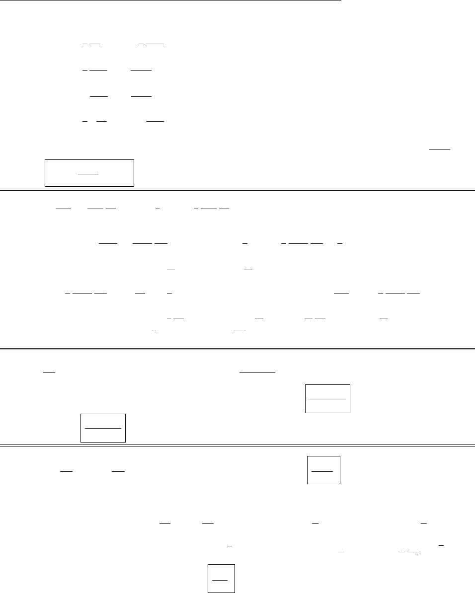
CHAPTER 7. ELETRODYNAMICS 161
with
r·E=1
s
@
@s(sEs)+1
s
@E
@ =0,
(r⇥E)s=1
s
@Ez
@ =µ0Iv
2⇡s2cos
(r⇥E)=@Ez
@s=µ0Iv
2⇡s2sin ,
(r⇥E)z=1
s@
@s(sE)@Es
@ =0.
The first and last of these are satisfied if Es=E= 0, the middle two are satisfied by Ez=µ0Iv
2⇡ssin .
Evidently E=µ0Iv
2⇡ssin ˆz .The electric and magnetic fields ride along with the wire.
Problem 7.52
Initially, mv2
r=1
4⇡✏0
qQ
r2)T=1
2mv2=1
2
1
4⇡✏0
qQ
r. After the magnetic field is on, the electron circles in a
new orbit, of radius r1and velocity v1:
mv2
1
r1
=1
4⇡✏0
qQ
r2
1
+qv1B)T1=1
2mv2
1=1
2
1
4⇡✏0
qQ
r1
+1
2qv1r1B.
But r1=r+dr,so(r1)1=r11+ dr
r1⇠
=r11dr
r, while v1=v+dv,B=dB. To first order, then,
T1=1
2
1
4⇡✏0
qQ
r1dr
r+1
2q(vr)dB, and hence dT =T1T=qvr
2dB 1
2
1
4⇡✏0
qQ
r2dr.
Now, the induced electric field is E=r
2
dB
dt (Ex. 7.7), so mdv
dt =qE =qr
2
dB
dt , or m dv =qr
2dB. The increase in
kinetic energy is therefore dT =d(1
2mv2)=mv dv =qvr
2dB. Comparing the two expressions, I conclude that
dr = 0. qed
Problem 7.53
E=d
dt =↵. So the current in R1and R2is I=↵
R1+R2
; by Lenz’s law, it flows counterclockwise. Now
the voltage across R1(which voltmeter #1 measures) is V1=IR1=↵R1
R1+R2
(Vbis the higher potential),
and V2=IR2=↵R2
R1+R2
(Vbis lower).
Problem 7.54
(a) E=d
dt =⇡r2dB
dt =↵⇡r2=IR )(in magnitude) I=⇡↵r2
R.If Bis out of the page, Lenz’s
law says the current is clockwise.
(b) Inside the shaded region, for a circle of radius s, apply Faraday’s law:
E·dl=E2⇡s=⇡s2↵)E=↵s
2ˆ
=↵s
2(sin ˆx + cos ˆy )=↵
2(ssin ˆx scos ˆy )=↵
2(yˆx xˆy ).
Along the line from Pto Q,dl =dx ˆx , and y=r/p2, so V=E·dl=↵
2y dx =↵
2
r
p2(rp2).Thus
Pis at the higher voltage, and the meter reads ↵r2
2.
c
2012 Pearson Education, Inc., Upper Saddle River, NJ. All rights reserved. This material is
protected under all copyright laws as they currently exist. No portion of this material may be
reproduced, in any form or by any means, without permission in writing from the publisher.
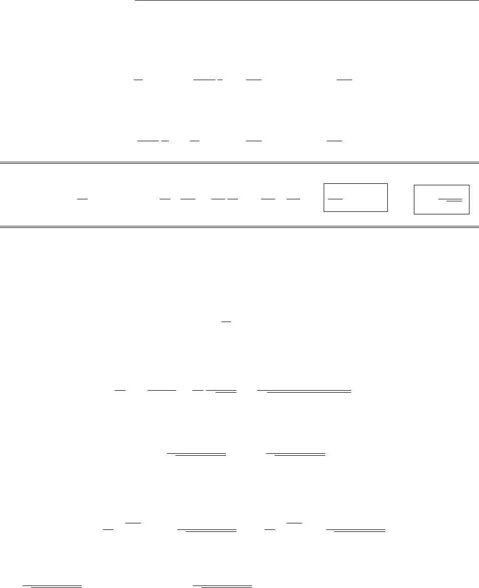
162 CHAPTER 7. ELETRODYNAMICS
That’s the simplest way to do it. But you might instead regard the 3/4-circle+chord as a circuit, and use
Kirchho↵’s rule (the total emf around a closed loop is zero): V+IR1↵A1= 0, where R1=3/4Ris the
resistance of the curved portion, and A1= (3/4)⇡r2+r2/2=(r2/4)(3⇡+ 2) is the area (3/4 of the circle, plus
the triangle). Then
V=↵r2
4(3⇡+ 2) ⇡r2↵
R
3
4R=↵r2
4(3⇡+23⇡)=↵r2
2.X
Or we could do the same thing, using the small loop at the top: V+IR2↵A2= 0, where R2=(1/4)R
and A2= (1/4)⇡r2r2/2=(r2/4)(⇡2).
V=⇡↵r2
R
R
4↵r2
4(⇡2) = ↵r2
4(⇡⇡+ 2) = ↵r2
2.X
Problem 7.55
E=vBh =LdI
dt ;F=IhB =mdv
dt ;d2v
dt2=hB
m
dI
dt =hB
mhB
Lv, d2v
dt2=!2v, with !=hB
pmL.
Problem 7.56
A point on the upper loop: r2=(acos 2,asin 2,z); a point on the lower loop: r1=(bcos 1,bsin 1,0).
r
2=(r2r1)2=(acos 2bcos 1)2+(asin 2bsin 1)2+z2
=a2cos222ab cos 2cos 1+b2cos21+a2sin222ab sin 1sin 2+b2sin21+z2
=a2+b2+z22ab(cos 2cos 1+ sin 2sin 1)=a2+b2+z22ab cos(21)
=(a2+b2+z2)12cos(21)=ab
12cos(21).
dl1=bd1ˆ
1=bd1[sin 1ˆx + cos 1ˆy ]; dl2=ad2ˆ
2=ad2[sin 2ˆx + cos 2ˆy ], so
dl1·dl2=ab d1d2[sin 1sin 2+ cos 1cos 2]=ab cos(21)d1d2.
M=µ0
4⇡ dl1·dl2
r
=µ0
4⇡
ab
ab/ cos(21)
12cos(21)d2d1.
Both integrals run from 0 to 2⇡. Do the 2integral first, letting u⌘21:
2⇡1
1
cos u
p12cos udu =
2⇡
0
cos u
p12cos udu
(since the integral runs over a complete cycle of cos u, we may as well change the limits to 0 !2⇡). Then the
1integral is just 2⇡, and
M=µ0
4⇡ab2⇡2⇡
0
cos u
p12cos udu =µ0
2ab2⇡
0
cos u
p12cos udu.
(a) If ais small, then ⌧1, so (using the binomial theorem)
1
p12cos u⇠
=1+cos u, and 2⇡
0
cos u
p12cos udu ⇠
=2⇡
0
cos udu+2⇡
0
cos2udu=0+⇡,
c
2012 Pearson Education, Inc., Upper Saddle River, NJ. All rights reserved. This material is
protected under all copyright laws as they currently exist. No portion of this material may be
reproduced, in any form or by any means, without permission in writing from the publisher.
CHAPTER 7. ELETRODYNAMICS 163
and hence M=(µ0⇡/2)ab3. Moreover, ⇠
=ab/(b2+z2), so M⇠
=µ0⇡a2b2
2(b2+z2)3/2(same as in Prob. 7.22).
(b) More generally,
(1 + ✏)1/2=11
2✏+3
8✏25
16✏3+···=)1
p12cos u=1+cos u+3
22cos2u+5
23cos3u+···,
so
M=µ0
2ab2⇡
0
cos udu+2⇡
0
cos2udu+3
222⇡
0
cos3udu+5
232⇡
0
cos4udu+···
=µ0
2ab0+(⇡)+3
22(0) + 5
23(3
4⇡)+···=µ0⇡
2ab31+15
82+()4+···.qed
Problem 7.57
Let be the flux of Bthrough a single loop of either coil, so that 1=N1and 2=N2.Then
E1=N1
d
dt ,E2=N2
d
dt ,so E2
E1
=N2
N1
.qed
Problem 7.58
(a) Suppose current I1flows in coil 1, and I2in coil 2. Then (if is the flux through one turn):
1=I1L1+MI2=N1;2=I2L2+MI1=N2,or =I1
L1
N1
+I2
M
N1
=I2
L2
N2
+I1
M
N2
.
In case I1= 0, we have M
N1=L2
N2; if I2=0,wehave L1
N1=M
N2. Dividing: M
L1=L2
M, or L1L2=M2. qed
(b) E1=d1
dt =L1dI1
dt +MdI2
dt =V1cos(!t); E2=d2
dt =L2dI2
dt +MdI1
dt =I2R.qed
(c) Multiply the first equation by L2:L1L2dI1
dt +L2dI2
dt M=L2V1cos !t. Plug in L2dI2
dt =I2RMdI1
dt .
M2dI1
dt MRI2M2dI1
dt =L2V1cos !t)I2(t)=L2V1
MR cos !t. L1dI1
dt +ML2V1
MR !sin !t=V1cos !t.
dI1
dt =V1
L1cos !tL2
R!sin !t)I1(t)= V1
L11
!sin !t+L2
Rcos !t.
(d) Vout
Vin
=I2R
V1cos !t=L2V1
MR cos !tR
V1cos !t=L2
M=N2
N1
. The ratio of the amplitudes is N2
N1
. qed
(e) Pin =VinI1=(V1cos !t)V1
L11
!sin !t+L2
Rcos !t=(V1)2
L11
!sin !tcos !t+L2
Rcos2!t.
Pout =VoutI2=(I2)2R=(L2V1)2
M2Rcos2!t. Average of cos2!tis 1/2; average of sin !tcos !tis zero.
So hPini=1
2(V1)2L2
L1R;hPouti=1
2(V1)2(L2)2
M2R=1
2(V1)2(L2)2
L1L2R;hPini=hPouti=(V1)2L2
2L1R.
c
2012 Pearson Education, Inc., Upper Saddle River, NJ. All rights reserved. This material is
protected under all copyright laws as they currently exist. No portion of this material may be
reproduced, in any form or by any means, without permission in writing from the publisher.
164 CHAPTER 7. ELETRODYNAMICS
Problem 7.59
(a) The charge flowing into dz in time dt is
dq =I(z)dt I(z+dz)dt =dI
dt dz dt =(t+dt)dz (t)dz =d
dt dt dz )d
dt =dI
dz .X
Since the left side is a function only of t, and the right side is a function only of z, they must both be constant;
call it k:d
dt =k)(t)=kt +C1;dI
dz =k)I(z)=kz +C2.
If (0) = 0 and I(0) = 0 the constants C1and C2must both be zero: (t)=kt, I(z)=kz. X
(b) In the quasistatic approximation, E=
2⇡✏0sˆs =kt
2⇡✏0sˆs ;B=µ0I
2⇡sˆ
=µ0kz
2⇡sˆ
.
r·E=1
s
@
@sskt
2⇡✏0s=0 X
r·B=1
s
@
@ µ0kz
2⇡s=0 X
r⇥E=@E
@zˆ
1
s
@E
@ ˆz =0=@B
@tX
r⇥B=@B
@zˆ
+1
s
@(sB)
@sˆz =µ0k
2⇡sˆz =µ0✏0
@E
@tX
For a gaussian cylinder of radius sabout the zaxis, at height zand with width dz:
E·da=kt
2⇡✏0s(2⇡s)dz =kt
✏0
dz =dz
✏0
=Qenc
✏0
.XB·da=0.X
For a circular amperian loop of radius sabout the zaxis, at height z:
E·dl=0=d
dt B·da,XB·dl=µ0kz
2⇡s(2⇡s)=µ0I=µ0Ienc +µ0✏0
d
dt E·da.X
(Note that B·daand E·daare zero through this loop.)
Problem 7.60
(a) The continuity equation says @⇢
@t=r·J. Here the right side is independent of t, so we can integrate:
⇢(t)=(r·J)t+ constant. The “constant” may be a function of r—it’s only constant with respect to t. So,
putting in the rdependence explicitly, and noting that r·J=˙⇢(r,0), ⇢(r,t)= ˙⇢(r,0)t+⇢(r,0). qed
(b) Suppose E=1
4⇡✏0⇢ˆ
r
r
2d⌧and B=µ0
4⇡J⇥ˆ
r
r
2d⌧. We want to show that r·B= 0, r⇥B=
µ0J+µ0✏0@E
@t;r·E=1
✏0⇢, and r⇥E=@B
@t, provided that Jis independent of t.
We know from Ch. 2 that Coulomb’s law E=1
4⇡✏0⇢ˆ
r
r
2d⌧satisfies r·E=1
✏0⇢and r⇥E=0. Since
Bis constant (in time), the r·Eand r⇥Eequations are satisfied. From Chapter 5 (specifically, Eqs. 5.47-
5.50) we know that the Biot-Savart law satisfies r·B= 0. It remains only to check r⇥B. The argument in
Sect. 5.3.2 carries through until the equation following Eq. 5.54, where I invoked r0·J= 0. In its place we
now put r0·J=˙⇢:
r⇥B=µ0Jµ0
4⇡(J·r)ˆ
r
r
2
(J·r0)ˆ
r
r
2
d⌧(Eqs. 5.51-5.53)
(Eq. 5.54)
c
2012 Pearson Education, Inc., Upper Saddle River, NJ. All rights reserved. This material is
protected under all copyright laws as they currently exist. No portion of this material may be
reproduced, in any form or by any means, without permission in writing from the publisher.
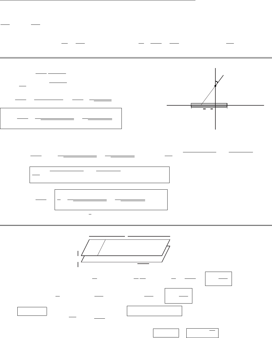
CHAPTER 7. ELETRODYNAMICS 165
Integration by parts yields two terms, one of which becomes a surface integral, and goes to zero. The other is
r
r
3r0·J=ˆ
r
r
2(˙⇢). So:
r⇥B=µ0Jµ0
4⇡ˆ
r
r
2(˙⇢)d⌧=µ0J+µ0✏0
@
@t1
4⇡✏0⇢ˆ
r
r
3d⌧=µ0J+µ0✏0
@E
@t.qed
Problem 7.61
14
Problem 7.56
vt −ϵvt
!"# $
−z
✲z
✻
y
✼
θdE
s
c
⃝2005 Pearson Education, Inc., Upper Saddle River, NJ. All rights reserved. This material is
protected under all copyright laws as they currently exist. No portion of this material may be
reproduced, in any form or by any means, without permission inwritingfromthepublisher.
(a) dEz=1
4⇡✏0
()dz
r
2sin ✓
sin ✓=z
r
;
r
=pz2+s2
Ez=
4⇡✏0z dz
(z2+s2)3/2=
4⇡✏01
pz2+s2
vt
vt✏
Ez=
4⇡✏01
(vt ✏)2+s21
(vt)2+s2.
r
(b)
E=
4⇡✏0a
01
(vt ✏)2+s21
(vt)2+s22⇡sds=
2✏0(vt ✏)2+s2(vt)2+s2
a
0
=
2✏0(vt ✏)2+a2(vt)2+a2(✏vt)+(vt).
(c) Id=✏0
dE
dt =
2v(vt ✏)
(vt ✏)2+a2v(vt)
(vt)2+a2+2v.
As ✏!0, vt < ✏also !0, so Id!
2(2v)=v=I. With an infinitesimal gap we attribute the magnetic field
to displacement current, instead of real current, but we get the same answer. qed
Problem 7.62
1
Contents
Problem 7.26
✲ˆz
ˆ
φ
❖
✕ˆs
✲ˆz
❄
✻
h
✕
☛
w
✛ ✲
l
→I
✛
I
→
B
c
⃝2005 Pearson Education, Inc., Upper Saddle River, NJ. All rights reserved. This material is
protected under all copyright laws as they currently exist. No portion of this material may be
reproduced, in any form or by any means, without permission inwritingfromthepublisher.
(a) Parallel-plate capacitor: E=1
✏0
;V=Eh =1
✏0
Q
wlh)C=Q
V=✏0wl
h)C=✏0w
h.
(b) B=µ0K=µ0
I
w;=Bhl =µ0I
whl =LI )L=µ0h
wl)L=µ0h
w.
(c) CL =µ0✏0=(4⇡⇥107)(8.85 ⇥1012)= 1.112 ⇥1017 s2/m2.
(Propagation speed 1/pLC =1/pµ0✏0=2.999 ⇥108m/s=c.)
(d) D=,E=D/✏=/✏,so just replace ✏0by ✏;
H=K, B =µH =µK, so just replace µ0by µ.LC =✏µ;v=1/p✏µ.
c
2012 Pearson Education, Inc., Upper Saddle River, NJ. All rights reserved. This material is
protected under all copyright laws as they currently exist. No portion of this material may be
reproduced, in any form or by any means, without permission in writing from the publisher.
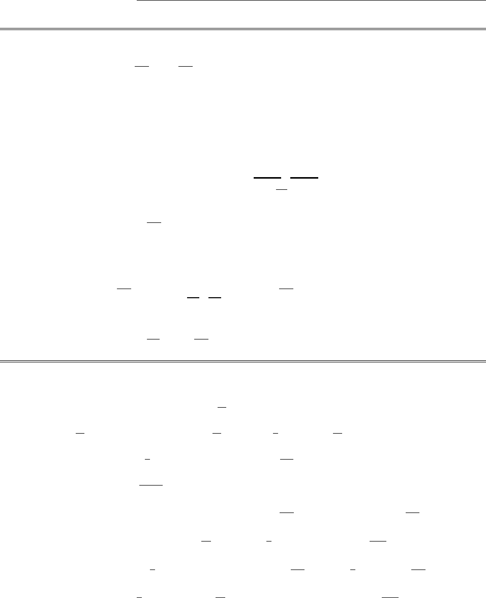
166 CHAPTER 7. ELETRODYNAMICS
Problem 7.63
(a) J=(E+v⇥B); Jfinite, =1)E+(v⇥B)=0. Take the curl: r⇥E+r⇥(v⇥B)=0. But
Faraday’s law says r⇥E=@B
@t.So @B
@t=r⇥(v⇥B). qed
(b) r·B=0)B·da= 0 for any closed surface. Apply this at time (t+dt) to the surface consisting of
S,S0, and R:S0
B(t+dt)·da+R
B(t+dt)·daS
B(t+dt)·da=0
(the sign change in the third term comes from switching outward dato inward da).
d=S0
B(t+dt)·daS
B(t)·da=SB(t+dt)B(t)
@B
@tdt ·daR
B(t+dt)·da
(for infinitesimal dt)
d=S
@B
@t·dadt R
B(t+dt)·(dl⇥v)dt(Figure 7.13).
Since the second term is already first order in dt, we can replace B(t+dt)byB(t) (the distinction would be
second order):
d=dt S
@B
@t·dadt C
B·(dl⇥v)
(v⇥B)·dl
=dt S@B
@t·daSr⇥(v⇥B)·da.
d
dt =S@B
@tr⇥(v⇥B)·da=0.qed
Problem 7.64
(a)
r·E0=(r·E) cos ↵+c(r·B) sin ↵=1
✏0
⇢ecos ↵+cµ0⇢msin ↵
=1
✏0
(⇢ecos ↵+cµ0✏0⇢msin ↵)= 1
✏0
(⇢ecos ↵+1
c⇢msin ↵)= 1
✏0
⇢0
e.X
r·B0=(r·B) cos ↵1
c(r·E) sin ↵=µ0⇢mcos ↵1
c✏0
⇢esin ↵
=µ0(⇢mcos ↵1
cµ0✏0
⇢esin ↵)=µ0(⇢mcos ↵c⇢esin ↵)=µ0⇢0
m.X
r⇥E0=(r⇥E) cos ↵+c(r⇥B) sin ↵=µ0Jm@B
@tcos ↵+cµ0Je+µ0✏0
@E
@tsin ↵
=µ0(Jmcos ↵cJesin ↵)@
@tBcos ↵1
cEsin ↵=µ0J0
m@B0
@t.X
r⇥B0=(r⇥B) cos ↵1
c(r⇥E) sin ↵=µ0Je+µ0✏0
@E
@tcos ↵1
cµ0Jm@B
@tsin ↵
=µ0(Jecos ↵+1
cJmsin ↵)+µ0✏0
@
@t(Ecos ↵+cBsin ↵)=µ0J0
e+µ0✏0
@E0
@t.X
c
2012 Pearson Education, Inc., Upper Saddle River, NJ. All rights reserved. This material is
protected under all copyright laws as they currently exist. No portion of this material may be
reproduced, in any form or by any means, without permission in writing from the publisher.
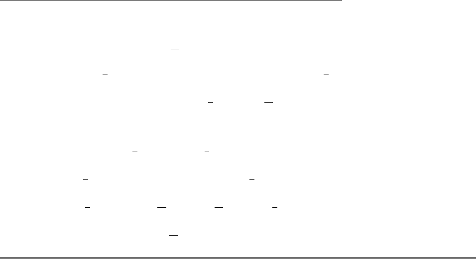
CHAPTER 7. ELETRODYNAMICS 167
(b)
F0=q0
e(E0+v⇥B0)+q0
m(B01
c2v⇥E0)
=qecos ↵+1
cqmsin ↵(Ecos ↵+cBsin ↵)+v⇥Bcos ↵1
cEsin ↵
+(qmcos ↵cqesin ↵)Bcos ↵1
cEsin ↵1
c2v⇥(Ecos ↵+cBsin ↵)
=qeEcos2↵+cBsin ↵cos ↵cBsin ↵cos ↵+Esin2↵
+v⇥Bcos2↵1
cEsin ↵cos ↵+1
cEsin ↵cos ↵+Bsin2↵
+qm1
cEsin ↵cos ↵+Bsin2↵+Bcos2↵1
cEsin ↵cos ↵
+v⇥1
cBsin ↵cos ↵1
c2Esin2↵1
c2Ecos2↵1
cBsin ↵cos ↵
=qe(E+v⇥B)+qmB1
c2v⇥E=F.qed
c
2012 Pearson Education, Inc., Upper Saddle River, NJ. All rights reserved. This material is
protected under all copyright laws as they currently exist. No portion of this material may be
reproduced, in any form or by any means, without permission in writing from the publisher.
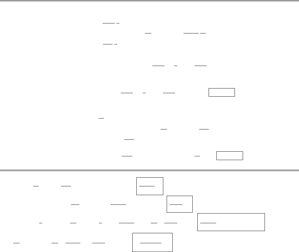
168 CHAPTER 8. CONSERVATION LAWS
Chapter 8
Conservation Laws
Problem 8.1
Example 7.13.
E=
2⇡✏0
1
sˆs
B=µ0I
2⇡
1
sˆ
S=1
µ0
(E⇥B)= I
4⇡2✏0
1
s2ˆz ;
P=S·da=
b
a
S2⇡sds=I
2⇡✏0
b
a
1
sds =I
2⇡✏0
ln(b/a).
But V=
b
a
E·dl=
2⇡✏0
b
a
1
sds =
2⇡✏0
ln(b/a),so P=IV.
Problem 7.62.
E=
✏0
ˆz
B=µ0Kˆx =µ0I
wˆx
S=1
µ0
(E⇥B)= I
✏0wˆy ;
P=S·da=Swh =Ih
✏0
,but V=E·dl=
✏0
h, so P=IV.
Problem 8.2
(a) E=
✏0
ˆz ;=Q
⇡a2;Q(t)=It )E(t)= It
⇡✏0a2ˆz .
B2⇡s=µ0✏0
@E
@t⇡s2=µ0✏0
I⇡s2
⇡✏0a2)B(s, t)= µ0Is
2⇡a2ˆ
.
(b) uem =1
2✏0E2+1
µ0
B2=1
2✏0It
⇡✏0a22
+1
µ0µ0Is
2⇡a22=µ0I2
2⇡2a4(ct)2+(s/2)2.
S=1
µ0
(E⇥B)= 1
µ0It
⇡✏0a2µ0Is
2⇡a2(ˆs )= I2t
2⇡2✏0a4sˆs .
c
2012 Pearson Education, Inc., Upper Saddle River, NJ. All rights reserved. This material is
protected under all copyright laws as they currently exist. No portion of this material may be
reproduced, in any form or by any means, without permission in writing from the publisher.
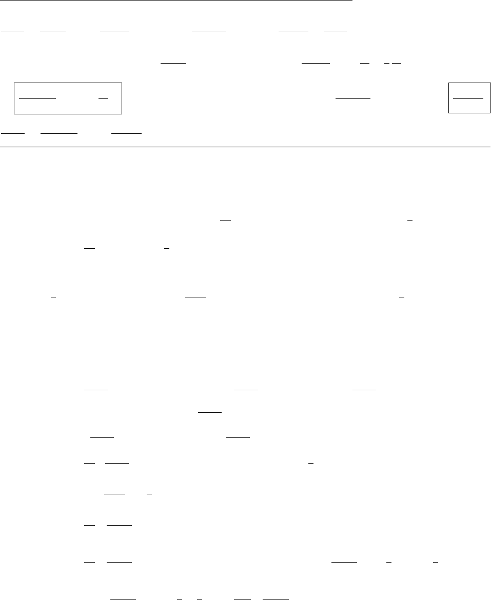
CHAPTER 8. CONSERVATION LAWS 169
@uem
@t=µ0I2
2⇡2a42c2t=I2t
⇡2✏0a4;r·S=I2t
2⇡2✏0a4r·(sˆs )= I2t
⇡2✏0a4=@uem
@t.X
(c) Uem =uemw2⇡sds=2⇡wµ0I2
2⇡2a4b
0
[(ct)2+(s/2)2]sds=µ0wI2
⇡a4(ct)2s2
2+1
4
s4
4
b
0
=µ0wI2b2
2⇡a4(ct)2+b2
8.Over a surface at radius b:Pin =S·da=I2t
2⇡2✏0a4[bˆs ·(2⇡bw ˆs )] = I2wtb2
⇡✏0a4.
dUem
dt =µ0wI2b2
2⇡a42c2t=I2wtb2
⇡✏0a4=Pin.X(Set b=afor total.)
Problem 8.3
The force is clearly in the zdirection, so we need
($
T·da)z=Tzx dax+Tzy day+Tzz daz=1
µ0BzBxdax+BzByday+BzBzdaz1
2B2daz
=1
µ0Bz(B·da)1
2B2daz.
Now B=2
3µ0R!ˆz (inside) and B=µ0m
4⇡r3(2 cos ✓ˆr + sin ✓ˆ
✓) (outside), where m=4
3⇡R3(!R). (From
Eq. 5.70, Prob. 5.37, and Eq. 5.88.) We want a surface that encloses the entire upper hemisphere—say a
hemispherical cap just outside r=Rplus the equatorial circular disk.
Hemisphere:
Bz=µ0m
4⇡R32 cos ✓(ˆr )z+ sin ✓(ˆ
✓)z=µ0m
4⇡R32 cos2✓sin2✓=µ0m
4⇡R33 cos2✓1.
da=R2sin ✓d✓dˆr ;B·da=µ0m
4⇡R3(2 cos ✓)R2sin ✓d✓d;daz=R2sin ✓d✓dcos ✓;
B2=µ0m
4⇡R324 cos2✓+ sin2✓=µ0m
4⇡R323 cos2✓+1
.
($
T·da)z=1
µ0µ0m
4⇡R323 cos2✓12 cos ✓R2sin ✓d✓d1
23 cos2✓+1
R2sin ✓cos ✓d✓d
=µ0!R
321
2R2sin ✓cos ✓d✓d12 cos2✓43 cos2✓1
=µ0
2!R2
329 cos2✓5sin ✓cos ✓d✓d.
(Fhemi)z=µ0
2!R2
32
2⇡
⇡/2
09 cos3✓5 cos ✓sin ✓d✓=µ0⇡!R2
329
4cos4✓+5
2cos2✓
⇡/2
0
=µ0⇡!R2
320+9
45
2=µ0⇡
4wR2
32
.
c
2012 Pearson Education, Inc., Upper Saddle River, NJ. All rights reserved. This material is
protected under all copyright laws as they currently exist. No portion of this material may be
reproduced, in any form or by any means, without permission in writing from the publisher.

170 CHAPTER 8. CONSERVATION LAWS
Disk:
Bz=2
3µ0R!;da=r dr dˆ
=r dr dˆz ;
B·da=2
3µ0R!rdrd;B2=2
3µ0R!2
;daz=r dr d.
($
T·da)z=1
µ02
3µ0R!2r dr d+1
2r dr d=1
2µ02
3µ0R!2
r dr d.
(Fdisk)z=2µ0!R
32
2⇡
R
0
r dr =2⇡µ0!R2
32
.
Total:
F=⇡µ0!R2
322+1
4ˆz =⇡µ0!R2
22
ˆz (agrees with Prob.5.44).
Alternatively, we could use a surface consisting of the entire equatorial plane, closing it with a hemispherical
surface “at infinity,” where (since the field is zero out there) the contribution is zero. We have already done
the integral over the disk; it remains to do rest of the integral over the plane, from Rto 1. On the plane,
✓= 0, and (for r>R)B=µ0m
4⇡r3ˆ
✓=µ0m
4⇡r3ˆz ,so
($
T·da)z=1
µ0Bz(Bzdaz)1
2B2
zdaz)=1
2µ0
B2
zdaz=1
2µ0µ0m
4⇡r32(r dr d).
The contribution from the rest of the plane is therefore
(Frest)z=1
2µ0µ0m
4⇡22⇡1
R
1
r5dr =µ0
16⇡4
3⇡R4!21
4r4
1
R
=µ0⇡R4!
321
4R4
=µ0⇡
4!R2
32
.
This is the same as (Fhemi)z, so—when added to (Fdisk)z—it will yield the same total force as before.
Problem 8.4
(a)
($
T·da)z=Tzx dax+Tzy day+Tzz daz.
But for the xy plane dax=day= 0, and daz=
r dr d(I’ll calculate the force on the upper charge).
r
($
T·da)z=✏0EzEz1
2E2(r dr d).
Now E=1
4⇡✏0
2q
r
2cos ✓ˆr , and cos ✓=r
r
,soEz=
0,E
2=q
2⇡✏02r2
(r2+a2)3. Therefore
1
Hello
✲y
✻
z
❂
x
a
a
r
✇
✼θ
c
⃝2005 Pearson Education, Inc., Upper Saddle River, NJ. All rights reserved. This material is
protected under all copyright laws as they currently exist. No portion of this material may be
reproduced, in any form or by any means, without permission in writing from the publisher.
Fz=1
2✏0q
2⇡✏02
2⇡
1
0
r3dr
(r2+a2)3=q2
4⇡✏0
1
2
1
0
udu
(u+a2)3(letting u⌘r2)
=q2
4⇡✏0
1
21
(u+a2)+a2
2(u+a2)3
1
0
=q2
4⇡✏0
1
20+ 1
a2a2
2a4=q2
4⇡✏0
1
(2a)2.X
c
2012 Pearson Education, Inc., Upper Saddle River, NJ. All rights reserved. This material is
protected under all copyright laws as they currently exist. No portion of this material may be
reproduced, in any form or by any means, without permission in writing from the publisher.

CHAPTER 8. CONSERVATION LAWS 171
(b) In this case E=1
4⇡✏0
2q
r
2sin ✓ˆz , and sin ✓=a
r
, so
E2=E2
z=qa
2⇡✏021
(r2+a2)3,and hence ($
T·da)z=✏0
2qa
2⇡✏02r dr d
(r2+a2)3.Therefore
Fz=✏0
2qa
2⇡✏02
2⇡
1
0
r dr
(r2+a2)3=q2a2
4⇡✏01
4
1
(r2+a2)21
0
=q2a2
4⇡✏00+ 1
4a4=q2
4⇡✏0
1
(2a)2.X
Problem 8.5
(a) E=
✏0
ˆz ,B=µ0vˆx ,g=✏0(E⇥B)=µ02vˆy ,p=(dA)g=dAµ02vˆy .
(b) (i) There is a magnetic force, due to the (average) magnetic field at the upper plate:
F=q(u⇥B)=A[(uˆz )⇥(1
2µ0vˆx )] = 1
2µ02Avu ˆy ,
I1=Fdt =1
2µ02Av ˆy udt=1
2dµ02Av ˆy .
[The velocity of the patch (of area A) is actually v+u=vˆy uˆz , but the ycomponent produces a magnetic
force in the zdirection (a repulsion of the plates) which reduces their (electrical) attraction but does not deliver
(horizontal) momentum to the plates.]
(ii) Meanwhile, in the space immediately above the upper plate the magnetic field drops abruptly to
zero (as the plate moves past), inducing an electric field by Faraday’s law. The magnetic field in the vicinity
of the top plate (at d(t)=d0ut) can be written, using Problem 1.46(b),
B(z,t)=µ0v✓(dz)ˆx ,)@B
@t=µ0vu (dz)ˆx .
In the analogy at the beginning of Section 7.2.2, the Faraday-induced electric field is just like the magnetostatic
field of a surface current K=vu ˆx .Referring to Eq. 5.58, then,
Eind =1
2µ0vu ˆy ,for z<d,
+1
2µ0vu ˆy ,for z>d.
This induced electric field exerts a force on area Aof the bottom plate, F=(A)(1
2µ0vu ˆy ), and delivers
an impulse
I2=1
2µ02Av ˆy udt=1
2µ02Avd ˆy .
(I dropped the subscript on d0, reverting to the original notation: dis the initial separation of the plates.)
The total impulse is thus I=I1+I2=dAµ02vˆy ,matching the momentum initially stored in the fields,
from part (a). [I thank Michael Ligare for untangling this surprisingly subtle problem. Incidentally, there is
also “hidden momentum” in the original configuration. It is not relevant here; it is (relativistic) mechanical
momentum (see Example 12.13), and is delivered to the plates as they come together, so it does not a↵ect the
overall conservation of momentum.]
Problem 8.6
(a) gem =✏0(E⇥B)=✏0EB ˆy ;pem =✏0EBAd ˆy .
(b) II
I=1
0
Fdt =1
0
I(l⇥B)dt =1
0
IBd(ˆz ⇥ˆx )dt =(Bd ˆy )1
0dQ
dt dt
c
2012 Pearson Education, Inc., Upper Saddle River, NJ. All rights reserved. This material is
protected under all copyright laws as they currently exist. No portion of this material may be
reproduced, in any form or by any means, without permission in writing from the publisher.

172 CHAPTER 8. CONSERVATION LAWS
=(Bdˆy )[Q(1)Q(0)] = BQd ˆy .But the original field was E=/✏0=Q/✏0A, so Q=✏0EA, and hence
III=✏0EBAd ˆy .
Problem 8.7
(a) Ex=Ey=0,E
z=/✏0.Therefore
Txy =Txz =Tyz =···= 0; Txx =Tyy =✏0
2E2=2
2✏0
;Tzz =✏0E2
z1
2E2=✏0
2E2=2
2✏0
.
$
T=2
2✏0
10 0
010
00+1
.
(b) F=$
T·da(S=0, since B=0); integrate over the xy plane: da=dx dy ˆz (negative because
outward with respect to a surface enclosing the upper plate). Therefore
Fz=Tzz daz=2
2✏0
A, and the force per unit area is f=F
A=2
2✏0
ˆz .
(c) Tzz =2/2✏0is the momentum in the zdirection crossing a surface perpendicular to z, per unit
area, per unit time.
(d) The recoil force is the momentum delivered per unit time, so the force per unit area on the top plate is
f=2
2✏0
ˆz (same as (b)).
Problem 8.8
B=µ0nI ˆz (for s<R; outside the solenoid B= 0). The force on a segment ds of spoke is
dF=I0dl⇥B=I0µ0nI ds(ˆs ⇥ˆz )=I0µ0nI ds ˆ
.
The torque on the spoke is
N=r⇥dF=I0µ0nI
R
a
sds(ˆs ⇥ˆ
)=I0µ0nI 1
2R2a2(ˆz ).
Therefore the angular momentum of the cylinders is L=Ndt =1
2µ0nI(R2a2)ˆz I0dt. But I0dt =Q,
so
L=1
2µ0nIQ(R2a2)ˆz (in agreement with Eq.8.34).
Problem 8.9
(a) Between the shells, E=Q
4⇡✏0
1
r2ˆr ,g=✏0(E⇥B)= QB0
4⇡r2(ˆr ⇥ˆz ).
L=(r⇥g)d⌧=QB0
4⇡1
r2[r⇥(ˆr ⇥ˆz )]r2sin ✓dr d✓d=QB0
4⇡r[ˆr ⇥(ˆr ⇥ˆz )] sin ✓dr d✓d.
c
2012 Pearson Education, Inc., Upper Saddle River, NJ. All rights reserved. This material is
protected under all copyright laws as they currently exist. No portion of this material may be
reproduced, in any form or by any means, without permission in writing from the publisher.

CHAPTER 8. CONSERVATION LAWS 173
Now ˆr ⇥(ˆr ⇥ˆz )=ˆr (ˆr ·ˆz )ˆz (ˆr ·ˆr )=ˆr cos ✓=ˆz , but Lhas to be along the zdirection, so we pick o↵the z
component of ˆr :[ˆr ⇥(ˆr ⇥ˆz )]z= cos2✓1=sin2✓.
Lz=QB0
4⇡rsin3✓dr d✓d=QB0
4⇡2⇡⇡
0
sin3✓d✓b
a
r dr =QB0
24
3b2a2
2=1
3QB0(b2a2).
L=1
3QB0(b2a2)ˆz .
(b) The changing magnetic field induces an electric field (Example 7.7). Assuming symmetry about the z
axis, E=s
2
dB
dt ˆ
.The force on a patch of area da is dF=Eda, and the torque on this patch is dN=s⇥dF.
The net torque on the sphere at radius ais (using s=asin ✓ˆs and da =a2sin ✓d✓d):
Na=Q
4⇡a21
2
dB
dt ˆz s2da =Qa2
8⇡
dB
dt ˆz 2⇡sin3✓d✓=Qa2
3
dB
dt ˆz .
Similarly, Nb=Qb2
3
dB
dt ˆz ,so the total torque is N=Q
3
dB
dt (b2a2)ˆz ,and the angular momentum delivered
to the spheres is
L=Ndt =Q
3(b2a2)ˆz 0
B0
dB
dt dt =Q
3(b2a2)B0ˆz .X
Problem 8.10
(a)
E=
0,(r<R)
1
4⇡✏0
Q
r2ˆr ,(r>R)
;B=
2
3µ0Mˆz ,(r<R)
µ0
4⇡
m
r32 cos ✓ˆr + sin ✓ˆ
✓,(r>R)
(Ex.6.1)
(where m=4
3⇡R3M); g=✏0(E⇥B)= µ0
(4⇡)2
Qm
r5(ˆr ⇥ˆ
✓) sin ✓, and (ˆr ⇥ˆ
✓)= ˆ
,so
`=r⇥g=µ0
(4⇡)2
mQ
r4sin ✓(ˆr ⇥ˆ
).
But (ˆr ⇥ˆ
)=ˆ
✓, and only the zcomponent will survive integration, so (since (ˆ
✓)z=sin ✓):
L=µ0mQ
(4⇡)2ˆz sin2✓
r4r2sin ✓dr d✓d.
2⇡
0
d=2⇡;
⇡
0
sin3✓d✓=4
3;
1
R
1
r2dr =1
r
1
R
=1
R.
L=µ0mQ
(4⇡)2ˆz (2⇡)4
31
R=2
9µ0MQR2ˆz .
c
2012 Pearson Education, Inc., Upper Saddle River, NJ. All rights reserved. This material is
protected under all copyright laws as they currently exist. No portion of this material may be
reproduced, in any form or by any means, without permission in writing from the publisher.

174 CHAPTER 8. CONSERVATION LAWS
1
✲x
✻
z
❂
y
a
a
r
✇
✼
+q
−q
θ
✻
z
R
θ
✲x
✻
z
qe
qm
d
✸
r
✶
r′
θ
c
⃝2005 Pearson Education, Inc., Upper Saddle River, NJ. All rights reserved. This material is
protected under all copyright laws as they currently exist. No portion of this material may be
reproduced, in any form or by any means, without permission inwritingfromthepublisher.
(b) Apply Faraday’s law to the ring shown:
E·dl=E(2⇡rsin ✓)=d
dt =⇡(rsin ✓)22
3µ0
dM
dt
)E=µ0
3
dM
dt (rsin ✓)ˆ
.
The force on a patch of surface (da) is dF=Eda =µ0
3
dM
dt (rsin ✓)da ˆ
=Q
4⇡R2.
The torque on the patch is dN=r⇥dF=µ0
3
dM
dt r2sin ✓da (ˆr ⇥ˆ
). But (ˆr ⇥ˆ
)=ˆ
✓, and we want
only the zcomponent (ˆ
✓z=sin ✓):
N=µ0
3
dM
dt ˆz r2sin2✓r2sin ✓d✓d.
Here r=R;
⇡
0
sin3✓d✓=4
3;
2⇡
0
d=2⇡, so N=µ0
3
dM
dt ˆz R44
3(2⇡)= 2µ0
9QR2dM
dt ˆz .
L=Ndt =2µ0
9QR2ˆz
0
M
dM =2µ0
9MQR2ˆz (same as (a)).
(c) Let the charge on the sphere at time tbe q(t); the charge density is =q(t)
4⇡R2. The charge below
(“south of”) the ring in the figure is
qs=2⇡R2⇡
0
sin ✓0d✓0=q
2(cos ✓0)|⇡
✓=q
2(1 + cos ✓).
So the total current crossing the ring (flowing “north”) is I(t)=1
2
dq
dt (1 + cos ✓), and hence
K(t)= I
2⇡Rsin ✓(ˆ
✓)= 1
4⇡R
dq
dt
(1 + cos ✓)
sin ✓ˆ
✓. The force on a patch of area da is dF=(K⇥B)da.
Bave =2
3µ0Mˆz +µ0
4⇡
4
3⇡R3M
R3(2 cos ✓ˆr + sin ✓ˆ
✓)1
2=µ0M
6[2 ˆz + 2 cos ✓ˆr + sin ✓ˆ
✓];
K⇥B=1
4⇡R
dq
dt
µ0M
6
(1 + cos ✓)
sin ✓[2(ˆ
✓⇥ˆz ) + 2 cos ✓(ˆ
✓⇥ˆr )
ˆ
].
dN=Rˆr ⇥dF=µ0M
24⇡dq
dt (1 + cos ✓)
sin ✓2[ ˆr ⇥(ˆ
✓⇥ˆz )
ˆ
✓(ˆr ·ˆz )ˆz (ˆr ·ˆ
✓)
cos ✓(ˆr ⇥ˆ
)
ˆ
✓
]R2sin ✓d✓d
=µ0M
12⇡dq
dt (1 + cos ✓)R2[cos ✓ˆ
✓+ cos ✓ˆ
✓]d✓d=µ0MR2
6⇡dq
dt (1 + cos ✓) cos ✓d✓dˆ
✓.
c
2012 Pearson Education, Inc., Upper Saddle River, NJ. All rights reserved. This material is
protected under all copyright laws as they currently exist. No portion of this material may be
reproduced, in any form or by any means, without permission in writing from the publisher.
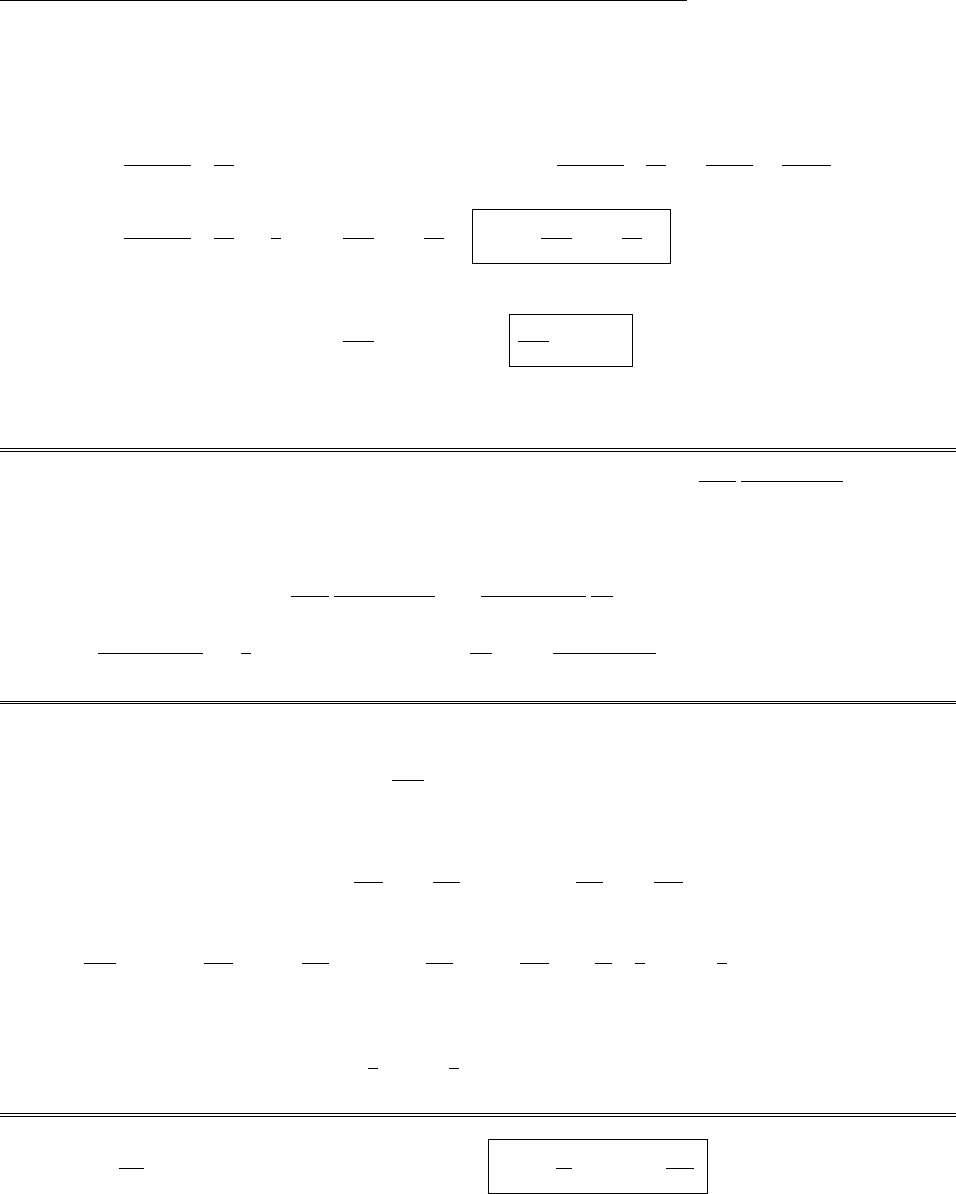
CHAPTER 8. CONSERVATION LAWS 175
The xand ycomponents integrate to zero; (ˆ
✓)z=sin ✓, so (using
2⇡
0
d=2⇡):
Nz=µ0MR2
6⇡dq
dt (2⇡)
⇡
0
(1 + cos ✓) cos ✓sin ✓d✓=µ0MR2
3dq
dt sin2✓
2cos3✓
3
⇡
0
=µ0MR2
3dq
dt 2
3=2µ0
9MR2dq
dt .N=2µ0
9MR2dq
dt ˆz .
Therefore
L=Ndt =2µ0
9MR2ˆz
0
Q
dq =2µ0
9MR2Qˆz (same as (a)).
(I used the average field at the discontinuity—which is the correct thing to do—but in this case you’d get the
same answer using either the inside field or the outside field.)
Problem 8.11 The magnetic field of the upper loop is given by Eq. 5.41: B=µ0Ib
2
b2
(b2+z2)3/2ˆz .(I put the
origin at the center of the upper loop, with the zaxis pointing up, so z=hat the location of the lower loop.)
Treat the lower loop as a magnetic dipole, with moment m=Ia⇡a2ˆz . The force on mis given by Eq. 6.3:
F=r(m·B)=rIa⇡a2µ0Ib
2
b2
(b2+z2)3/2=µ0⇡a2b2IaIb
2
@
@zb2+z23/2ˆz
=µ0⇡a2b2IaIb
23
2b2+z25/2(2z)ˆz =3⇡
2µ0IaIb
a2b2h
(b2+h2)5/2ˆz .X
Problem 8.12 Following the method of Section 7.2.4 (leading up to Eq. 7.30), the power delivered to the two
loops is
dW
dt =EaIaEbIb
(where these are the changing values as the currents are turned on, not the final values). Now
Ea=La
dIa
dt MdIb
dt ,Eb=Lb
dIb
dt MdIa
dt ,
so
dW
dt =LaIa
dIa
dt +MIa
dIb
dt +LbIb
dIb
dt +MIb
dIa
dt =d
dt 1
2LaI2
a+1
2LbI2
b+MIaIb.
The total work done, then, to increase the currents from zero to their final values, is
W=1
2LaI2
a+1
2LbI2
b+MIaIb.qed
Problem 8.13
(a) E=d
dt ;=⇡a2B;B=µ0nIs;E=IrR. So Ir=1
Rµ0⇡a2ndIs
dt .
c
2012 Pearson Education, Inc., Upper Saddle River, NJ. All rights reserved. This material is
protected under all copyright laws as they currently exist. No portion of this material may be
reproduced, in any form or by any means, without permission in writing from the publisher.
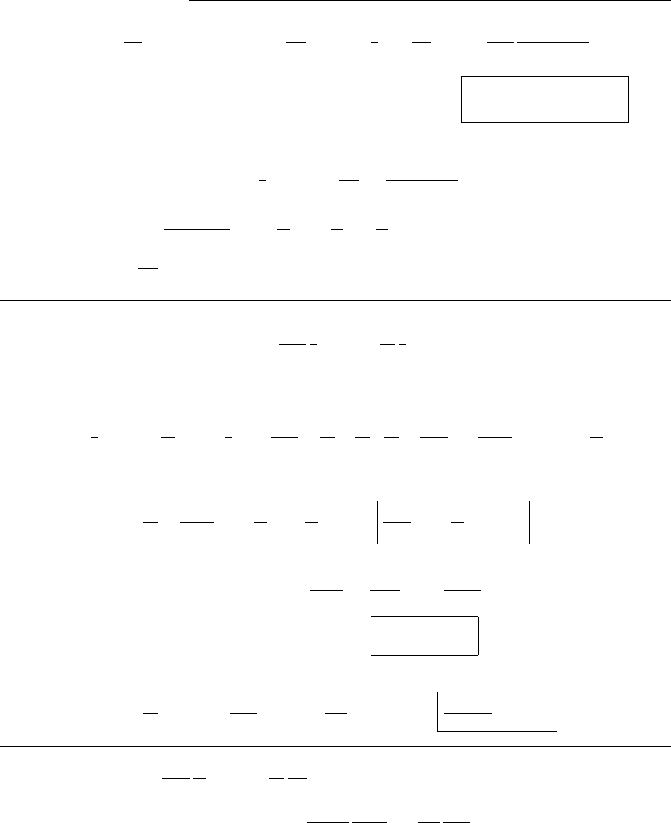
176 CHAPTER 8. CONSERVATION LAWS
(b) E·dl=d
dt )E(2⇡a)=µ0⇡a2ndIs
dt )E=1
2µ0andIs
dt ˆ
.B=µ0Ir
2
b2
(b2+z2)3/2ˆz (Eq. 5.41).
S=1
µ0
(E⇥B)= 1
µ0µ0an
2
dIs
dt µ0Ir
2
b2
(b2+z2)3/2(ˆ
⇥ˆz )= 1
4µ0Ir
dIs
dt
ab2n
(b2+z2)3/2ˆs .
Power:
P=S·da=
1
1
(S)(2⇡a)dz =1
2⇡µ0a2b2nIr
dIs
dt
1
1
1
(b2+z2)3/2dz
The integral is z
b2pz2+b21
1 =1
b21
b2=2
b2.
=⇡µ0a2ndIs
dt Ir=(RIr)Ir=Ir2R. qed
Problem 8.14 The fields are zero for s<aand s>b; between the cylinders,
E=1
2⇡✏0
sˆs ,B=µ0
2⇡
I
sˆ
,
where I=v.
(a) From Eq. 8.5:
u=1
2✏0E2+1
µ0
B2=1
2✏01
2⇡✏022
s2+1
µ0µ0
2⇡22v2
s2=2
8⇡2✏0
(1 + ✏0µ0v2)1
s2.
Writing ✏0µ0=1/c2, and integrating over the volume between the cylinders:
W
`=2
8⇡2✏01+v2
c2b
a
1
s22⇡sds=2
4⇡✏01+ v2
c2ln(b/a).
(b) From Eq. 8.29:
g=✏0(E⇥B)=✏0
2⇡✏0sµ0v
2⇡sˆz =µ02v
4⇡2s2ˆz .
p
`=µ02v
4⇡2ˆz b
a
1
s22⇡sds=µ02v
2⇡ln(b/a)ˆz .
(c) From Eq. 8.10:
S=1
µ0
(E⇥B)= 1
✏0µ0
g=c2g.dW
dt =S·da=µ02c2v
2⇡ln(b/a)ˆz .
Problem 8.15
(a) The fields are E=1
4⇡✏0
q
r2ˆr ,B=µ0
2⇡
NI
sˆ
(for points inside the toroid—see Eq. 5.60).
g=✏0(E⇥B)=✏0
q
4⇡✏0a2
µ0NI
2⇡aˆz =µ0
8⇡2
qNI
a3ˆz .
c
2012 Pearson Education, Inc., Upper Saddle River, NJ. All rights reserved. This material is
protected under all copyright laws as they currently exist. No portion of this material may be
reproduced, in any form or by any means, without permission in writing from the publisher.

CHAPTER 8. CONSERVATION LAWS 177
(Note that inside the toroid r⇡aˆs and s⇡a.)
p=µ0
8⇡2
qNI
a3ˆz (2⇡awh)= µ0
4⇡
qNIwh
a2ˆz .
(b) The changing magnetic field induces an electric field, as given by Problem 7.19 (with z= 0):
E=µ0
4⇡a2NhwdI
dt ˆz .The impulse delivered to qis therefore
I=Fdt =qEdt =qµ0
4⇡a2Nhwˆz dI
dt dt =µ0q
4⇡a2NhwI ˆz .X
Problem 8.16
According to Eqs. 3.104, 4.14, 5.89, and 6.16, the fields are
E=
1
3✏0
P,(r<R),
1
4⇡✏0
1
r3[3(p·ˆr )ˆr p],(r>R),
B=
2
3µ0M,(r<R),
µ0
4⇡
m
r3[3(m·ˆr )ˆr m],(r>R),
where p= (4/3)⇡R3P,and m= (4/3)⇡R3M. Now p=✏0(E⇥B)d⌧, and there are two contributions, one
from inside the sphere and one from outside.
Inside:
pin =✏01
3✏0
P⇥2
3µ0Md⌧=2
9µ0(P⇥M)d⌧=2
9µ0(P⇥M)4
3⇡R3=8
27µ0⇡R3(M⇥P).
Outside:
pout =✏0
1
4⇡✏0
µ0
4⇡1
r6{[3(p·ˆr )ˆr p]⇥[3(m·ˆr )ˆr m]}d⌧.
Now ˆr ⇥(p⇥m)=p(ˆr ·m)m(ˆr ·p), so ˆr ⇥[ˆr ⇥(p⇥m)] = (ˆr ·m)(ˆr ⇥p)(ˆr ·p)(ˆr ⇥m), whereas using the BAC-
CAB rule directly gives ˆr ⇥[ˆr ⇥(p⇥m)] = ˆr [ˆr ·(p⇥m)](p⇥m)(ˆr ·ˆr ). So {[3(p·ˆr )ˆr p]⇥[3(m·ˆr )ˆr m]}=
3(p·ˆr )(ˆr ⇥m)+3(m·ˆr )(ˆr ⇥p)+(p⇥m)=3{ˆr [ˆr ·(p⇥m)] (p⇥m)}+(p⇥m)=2(p⇥m)+3ˆr [ˆr ·(p⇥m)].
pout =µ0
16⇡21
r6{2(p⇥m)+3ˆr [ˆr ·(p⇥m)]}r2sin ✓dr d✓d.
To evaluate the integral, set the zaxis along (p⇥m); then ˆr ·(p⇥m)=|p⇥m|cos ✓. Meanwhile, ˆr =
sin ✓cos ˆx +sin✓sin ˆy +cos ✓ˆz . But sin and cos integrate to zero, so the ˆx and ˆy terms drop out, leaving
pout =µ0
16⇡21
0
1
r4dr2(p⇥m)sin ✓d✓d+3|p⇥m|ˆz cos2✓sin ✓d✓d
=µ0
16⇡21
3r3
1
R2(p⇥m)4⇡+ 3(p⇥m)4⇡
3=µ0
12⇡R3(p⇥m)
=µ0
12⇡R34
3⇡R3P⇥4
3⇡R3M=4µ0
27 R3(M⇥P).
ptot =8
27 +4
27µ0R3(M⇥P)= 4
9µ0R3(M⇥P).
c
2012 Pearson Education, Inc., Upper Saddle River, NJ. All rights reserved. This material is
protected under all copyright laws as they currently exist. No portion of this material may be
reproduced, in any form or by any means, without permission in writing from the publisher.

178 CHAPTER 8. CONSERVATION LAWS
Problem 8.17
(a) From Eq. 5.70 and Prob. 5.37,
r<R:E=0,B=2
3µ0R!ˆz ,with =e
4⇡R2;
r>R:E=1
4⇡✏0
e
r2ˆr ,B=µ0
4⇡
m
r3(2 cos ✓ˆr + sin ✓ˆ
✓),with m=4
3⇡!R4.
The energy stored in the electric field is (Ex. 2.9):
WE=1
8⇡✏0
e2
R.
The energy density of the internal magnetic field is:
uB=1
2µ0
B2=1
2µ02
3µ0R!e
4⇡R22
=µ0!2e2
72⇡2R2,so WBin =µ0!2e2
72⇡2R2
4
3⇡R3=µ0e2!2R
54⇡.
The energy density in the external magnetic field is:
uB=1
2µ0
µ2
0
16⇡2
m2
r64 cos2✓+ sin2✓=e2!2R4µ0
18(16⇡2)
1
r63 cos2✓+1
,so
WBout =µ0e2!2R4
(18)(16)⇡2
1
R
1
r6r2dr
⇡
03 cos2✓+1
sin ✓d✓
2⇡
0
d=µ0e2!2R4
(18)(16)⇡21
3R3(4)(2⇡)=µ0e2!2R
108⇡.
WB=WBin +Wbout =µ0e2!2R
108⇡(2 + 1) = µ0e2!2R
36⇡;W=WE+WB=1
8⇡✏0
e2
R+µ0e2!2R
36⇡.
(b) Same as Prob. 8.10(a), with Q!eand m!1
3e!R2:L=µ0e2!R
18⇡ˆz .
(c) µ0e2
18⇡!R=~
2)!R=9⇡~
µ0e2=(9)(⇡)(1.05 ⇥1034)
(4⇡⇥107)(1.60 ⇥1019)2= 9.23 ⇥1010 m/s.
1
8⇡✏0
e2
R1+2
9!R
c2=mc2;1+2
9!R
c2=1+2
99.23 ⇥1010
3⇥1082
=2.10 ⇥104;
R=(2.10 ⇥104)(1.6⇥1019)2
8⇡(8.85 ⇥1012)(9.11 ⇥1031)(3 ⇥108)2= 2.95 ⇥1011 m; !=9.23 ⇥1010
2.95 ⇥1011 = 3.13 ⇥1021 rad/s.
Since !R, the speed of a point on the equator, is 300 times the speed of light, this “classical” model is clearly
unrealistic.
Problem 8.18
Maxwell’s equations with magnetic charge (Eq. 7.44):
(i) r·E=1
✏0
⇢e,(iii) r⇥E=µ0Jm@B
@t,
(ii) r·B=µ0⇢m,(iv) r⇥B=µ0Je+µ0✏0
@E
@t.
c
2012 Pearson Education, Inc., Upper Saddle River, NJ. All rights reserved. This material is
protected under all copyright laws as they currently exist. No portion of this material may be
reproduced, in any form or by any means, without permission in writing from the publisher.

CHAPTER 8. CONSERVATION LAWS 179
The Lorentz force law becomes (Eq. 8.44)
F=qe(E+v⇥B)+qmB1
c2v⇥E.
Following the argument in Section 8.1.2:
F·dl=qe(E+v⇥B)+qmB1
c2v⇥E·vdt =(qeE+qmB)·vdt,
dW
dt =(E·Je+B·Jm)d⌧
(which generalizes Eq. 8.6). Use (iii) and (iv) to eliminate Jeand Jm:
(E·Je+B·Jm)= 1
µ0
E·(r⇥B)✏0E·@E
@t1
µ0
B·(r⇥E)1
µ0
B·@B
@t,
but r·(E⇥B)=B·(r⇥E)E·(r⇥B), so
(E·Je+B·Jm)=1
µ0r·(E⇥B)1
2
@
@t✏0E2+1
µ0
B2
(generalizing Eq. 8.8). Thus
dW
dt =d
dt 1
2✏0E2+1
µ0
B2d⌧1
µ0(E⇥B)·da,
which is identical to Eq. 8.9. Evidently Poynting’s theorem is unchanged(!), and
u=1
2✏0E2+1
µ0
B2,S=1
µ0
(E⇥B),
the same as before.
To construct the stress tensor we begin with the generalization of Eq. 8.13:
F=(E+v⇥B)⇢e+B1
c2v⇥E⇢md⌧.
The force per unit volume (Eq. 8.14) becomes
f=(⇢eE+Je⇥B)+⇢mB1
c2Jm⇥E
=✏0(r·E)E+1
µ0r⇥B✏0
@E
@t⇥B+1
µ0
(r·B)Bµ0✏01
µ0r⇥E1
µ0
@B
@t⇥E
=✏0[(r·E)EE⇥(r⇥E)] + 1
µ0
[(r·B)BB⇥(r⇥B)] ✏0
@
@t(E⇥B)
=✏0(r·E)E1
2r(E2)+(E·r)E+1
µ0(r·B)B1
2r(B2)+(B·r)B✏0
@
@t(E⇥B).
c
2012 Pearson Education, Inc., Upper Saddle River, NJ. All rights reserved. This material is
protected under all copyright laws as they currently exist. No portion of this material may be
reproduced, in any form or by any means, without permission in writing from the publisher.
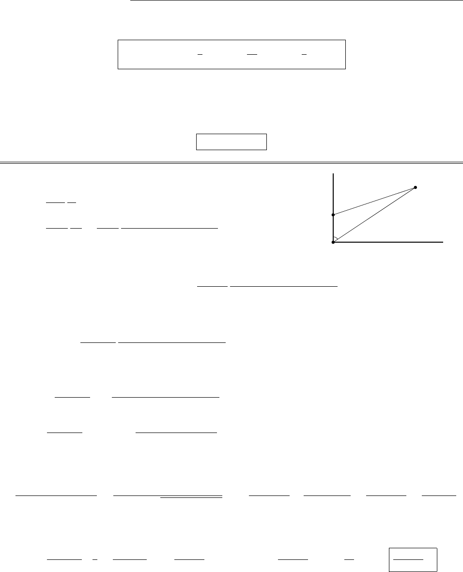
180 CHAPTER 8. CONSERVATION LAWS
This is identical to Eq. 8.16, so the stress tensor is the same as before:
Tij ⌘✏0EiEj1
2ij E2+1
µ0BiBj1
2ij B2.
Likewise, Eq. 8.20 is still valid. In fact, this argument is more straightforward when you include magnetic
charge, since you don’t need artificially to insert the (r·B)Bterm (after Eq. 8.15).
The electromagnetic momentum density (Eq. 8.29) also stays the same, since the argument in Section 8.2.3
is formulated entirely in terms of the fields:
g=✏0(E⇥B).
Problem 8.19
E=qe
4⇡✏0
r
r3;
B=µ0qm
4⇡
r0
r03=µ0qm
4⇡
(rdˆz )
(r2+d22rd cos ✓)3/2.
1
✲x
✻
z
❂
y
a
a
r
✇
✼
+q
−q
θ
✻
z
R
θ
✲x
✻
z
qe
qm
d
✸
r
✶
r′
θ
c
⃝2005 Pearson Education, Inc., Upper Saddle River, NJ. All rights reserved. This material is
protected under all copyright laws as they currently exist. No portion of this material may be
reproduced, in any form or by any means, without permission inwritingfromthepublisher.
Momentum density (Eq. 8.32):
g=✏0(E⇥B)=µ0qeqm
(4⇡)2
(d)(r⇥ˆz )
r3(r2+d22rd cos ✓)3/2.
Angular momentum density (Eq. 8.33):
`=(r⇥g)=µ0qeqmd
(4⇡)2
r⇥(r⇥ˆz )
r3(r2+d22rd cos ✓)3/2.But r⇥(r⇥ˆz )=r(r·ˆz )r2ˆz =r2cos ✓ˆr r2ˆz .
The xand ycomponents will integrate to zero; using (ˆr )z= cos ✓, we have:
L=µ0qeqmd
(4⇡)2ˆz r2(cos2✓1)
r3(r2+d22rd cos ✓)3/2r2sin ✓dr d✓d.Let u⌘cos ✓:
=µ0qeqmd
(4⇡)2ˆz (2⇡)
1
1
1
0
r1u2
(r2+d22rdu)3/2du dr.
Do the rintegral first:
1
0
r dr
(r2+d22rdu)3/2=(ru d)
d(1 u2)pr2+d22rdu
1
0
=u
d(1 u2)+d
d(1 u2)d=u+1
d(1 u2)=1
d(1 u).
Then
L=µ0qeqmd
8⇡ˆz 1
d
1
1
(1 u2)
(1 u)du =µ0qeqm
8⇡ˆz
1
1
(1 + u)du =µ0qeqm
8⇡ˆz u+u2
2
1
1
=µ0qeqm
4⇡ˆz .
c
2012 Pearson Education, Inc., Upper Saddle River, NJ. All rights reserved. This material is
protected under all copyright laws as they currently exist. No portion of this material may be
reproduced, in any form or by any means, without permission in writing from the publisher.
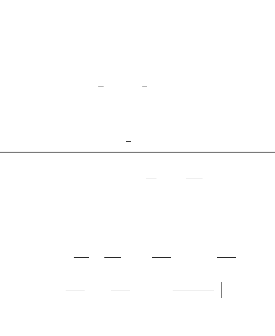
CHAPTER 8. CONSERVATION LAWS 181
Problem 8.20
p=✏0V
(E⇥B)d⌧=✏0V
(rV)⇥Bd⌧=✏0V
[r⇥(VB)Vr⇥B]d⌧
=✏0S
VB⇥da+✏0µ0V
VJd⌧=1
c2V
VJd⌧.
(I used Problem 1.61(b) in the penultimate step. Here Vis all of space, and Sis its surface at infinity, where
B=0, so the surface integral vanishes.) Using V(r)⇡V(0)+(rV)·r=V(0)E(0)·r,
p=1
c2V(0)Jd⌧1
c2[E(0)·r]Jd⌧.
For a current loop, Jd⌧!Idl =Idl=0,and (Eq. 1.108):
[E(0)·r]Jd⌧![E(0)·r]Idl =I[E(0)·r]dl=Ia⇥E(0)=m⇥E.
So
p=1
c2(m⇥E).X
Problem 8.21
(a) The rotating shell at radius bproduces a solenoidal magnetic field:
B=µ0Kˆz ,where K=b!bb, and b=Q
2⇡bl .So B=µ0!bQ
2⇡lˆz (a<s<b).
(Note that if angular velocity is defined with respect to the zaxis, then !bis a negative number.) The shell at
aalso produces a magnetic field (µ0!aQ/2⇡l)ˆz , in the region s<a, so the total field inside the inner shell is
B=µ0Q
2⇡l(!a!b)ˆz ,(s<a).
Meanwhile, the electric field is
E=1
2⇡✏0
sˆs =Q
2⇡✏0ls ˆs ,(a<s<b).
g=✏0(E⇥B)=✏0Q
2⇡✏0lsµ0!bQ
2⇡l(ˆs ⇥ˆz )= µ0!bQ2
4⇡2l2sˆ
;`=r⇥g=µ0!bQ2
4⇡2l2s(r⇥ˆ
).
Now r⇥ˆ
=(sˆs +zˆz )⇥ˆ
=sˆz zˆs , and the ˆs term integrates to zero, so
L=µ0!bQ2
4⇡2l2ˆz d⌧=µ0!bQ2
4⇡2l2⇡(b2a2)lˆz =µ0!bQ2(b2a2)
4⇡lˆz .
(b) The extra electric field induced by the changing magnetic field due to the rotating shells is given by
E2⇡s=d
dt )E=1
2⇡s
d
dt ˆ
, and in the region a<s<b
=µ0Q
2⇡l(!a!b)⇡a2µ0Q!b
2⇡l⇡s2a2=µ0Q
2l!aa2!bs2;E(s)=1
2⇡s
µ0Q
2la2d!a
dt s2d!b
dt ˆ
.
c
2012 Pearson Education, Inc., Upper Saddle River, NJ. All rights reserved. This material is
protected under all copyright laws as they currently exist. No portion of this material may be
reproduced, in any form or by any means, without permission in writing from the publisher.

182 CHAPTER 8. CONSERVATION LAWS
In particular,
E(a)=µ0Qa
4⇡ld!a
dt d!b
dt ˆ
,and E(b)=µ0Q
4⇡lb a2d!a
dt b2d!b
dt ˆ
.
The torque on a shell is N=r⇥qE=qsE ˆz ,so
Na=Qa µ0Qa
4⇡ld!a
dt d!b
dt ˆz ;La=1
0
Nadt =µ0Q2a2
4⇡l(!a!b)ˆz .
Nb=Qb µ0Q
4⇡lba2d!a
dt b2d!b
dt ˆz ;Lb=1
0
Nbdt =µ0Q2
4⇡la2!ab2!bˆz .
Ltot =La+Lb=µ0Q2
4⇡la2!ab2!ba2!a+a2!bˆz =µ0Q2!b
4⇡l(b2a2)ˆz .
Thus the reduction in the final mechanical angular momentum (b) is equal to the residual angular momentum
in the fields (a). X
Problem 8.22
B=µ0nI ˆz ,(s<R); E=q
4⇡✏0
r
r
3, where
r
=(xa, y, z).
g=✏0(E⇥B)=✏0(µ0nI)q
4⇡✏01
r
3(
r
⇥ˆz )= µ0qnI
4⇡
r
3[yˆx (xa)ˆy ].
Linear Momentum.
p=gd⌧=µ0qnI
4⇡yˆx (xa)ˆy
[(xa)2+y2+z2]3/2dx dy dz. The ˆx term is odd in y; it integrates to zero.
=µ0qnI
4⇡ˆy (xa)
[(xa)2+y2+z2]3/2dx dy dz. Do the zintegral first :
z
[(xa)2+y2](xa)2+y2+z2
1
1
=2
[(xa)2+y2].
=µ0qnI
2⇡ˆy (xa)
[(xa)2+y2]dx dy. Switch to polar coordinates :
x=scos ,y=ssin , dx dy )sdsd; [(xa)2+y2]=s2+a22sa cos .
=µ0qnI
2⇡ˆy (scos a)
(s2+a22sa cos )sdsd
Now 2⇡
0
cos d
(A+Bcos )=2⇡
B1A
pA2B2;2⇡
0
d
(A+Bcos )=2⇡
pA2B2.
Here A2B2=(s2+a2)24s2a2=s4+2s2a2+a44s2a2=(s2a2)2;A2B2=a2s2.
=µ0qnI
2aˆy 1a2+s2
a2s2+2a2
(a2s2)sds=µ0qnI
aˆy R
0
sds=µ0qnIR2
2aˆy .
c
2012 Pearson Education, Inc., Upper Saddle River, NJ. All rights reserved. This material is
protected under all copyright laws as they currently exist. No portion of this material may be
reproduced, in any form or by any means, without permission in writing from the publisher.
CHAPTER 8. CONSERVATION LAWS 183
Angular Momentum.
`=r⇥g=µ0qnI
4⇡
r
3r⇥[yˆx (xa)ˆy ]= µ0qnI
4⇡
r
3z(xa)ˆx +zy ˆy [x(xa)+y2]ˆz .
The ˆx and ˆy terms are odd in z, and integrate to zero,so
L=µ0qnI
4⇡ˆz x2+y2xa
[(xa)2+y2+z2]3/2dx dy dz. The zintegral is the same as before.
=µ0qnI
2⇡ˆz x2+y2xa
[(xa)2+y2]dx dy =µ0qnI
2⇡ˆz sacos
(s2+a22sa cos )s2ds d
=µ0qnI ˆz s2
a2s2+1a2+s2
a2s2sds=µ0qnI ˆz R
0
s2s2
a2s2sds= zero.
Problem 8.23
(a) If we’re only interested in the work done on free charges and currents, Eq. 8.6 becomes
dW
dt =V
(E·Jf)d⌧. But Jf=r⇥H@D
@t(Eq. 7.56), so E·Jf=E·(r⇥H)E·@D
@t. From product
rule #6, r·(E⇥H)=H·(r⇥E)E·(r⇥H), while r⇥E=@B
@t,so
E·(r⇥H)=H·@B
@tr·(E⇥H).Therefore E·Jf=H·@B
@tE·@D
@tr·(E⇥H), and hence
dW
dt =VE·@D
@t+H·@B
@td⌧S
(E⇥H)·da.
This is Poynting’s theorem for the fields in matter. Evidently the Poynting vector, representing the power per
unit area transported by the fields, is S=E⇥H, and the rate of change of the electromagnetic energy density
is @uem
@t=E·@D
@t+H·@B
@t.
For linear media, D=✏Eand H=1
µB, with ✏and µconstant (in time); then
@uem
@t=✏E·@E
@t+1
µB·@B
@t=1
2✏@
@t(E·E)+ 1
2µ
@
@t(B·B)=1
2
@
@t(E·D+B·H),
so uem =1
2(E·D+B·H).qed
(b) If we’re only interested in the force on free charges and currents, Eq. 8.13 becomes f=⇢fE+Jf⇥B.
But ⇢f=r·D, and Jf=r⇥H@D
@t,sof=E(r·D)+(r⇥H)⇥B@D
@t⇥B. Now
@
@t(D⇥B)=@D
@t⇥B+D⇥@B
@t, and @B
@t=r⇥E, so @D
@t⇥B=@
@t(D⇥B)+D⇥(r⇥E), and
hence f=E(r·D)D⇥(r⇥E)B⇥(r⇥H)@
@t(D⇥B). As before, we can with impunity add the
term H(r·B), so
f={[E(r·D)D⇥(r⇥E)] + [H(r·B)B⇥(r⇥H)]}@
@t(D⇥B).
The term in curly brackets can be written as the divergence of a stress tensor (as in Eq. 8.19), and the last
term is (minus) the rate of change of the momentum density, g=D⇥B.
c
2012 Pearson Education, Inc., Upper Saddle River, NJ. All rights reserved. This material is
protected under all copyright laws as they currently exist. No portion of this material may be
reproduced, in any form or by any means, without permission in writing from the publisher.

184 CHAPTER 8. CONSERVATION LAWS
Problem 8.24
(a) Initially, the disk will rise like a helicopter. The force on one charge (velocity v=!Rˆ
+vzˆz ) is
Fi=q(v⇥B)=qk
ˆs ˆ
ˆz
0!Rv
z
R02z=qk 2!Rz ˆs Rvzˆ
+!R2ˆz .
The net force on all the charges is
F=
n
i=1
Fi=nqkR2!ˆz =Md2z
dt2ˆz ;d2z
dt2=nqkR2
M!.[1]
The net torque on the disk is
N=
n
i=1
(ri⇥Fi)=n(Rˆs )⇥(qkRvzˆ
)=nqkR2vzˆz =Id!
dt ˆz
where Iis the moment of inertia of the disk. So
d!
dt =nqkR2
Idz
dt .[2]
Di↵erentiate [2], and combine with [1]:
d2z
dt2=I
nqkR2d2!
dt2=nqkR2
M!)d2!
dt2=↵!,where ↵⌘nqkR2
pMI .
The solution (with initial angular velocity !0and initial angular acceleration 0) is
!(t)=!0cos ↵t.
Meanwhile,
dz
dt =I
nqkR2d!
dt =I
nqkR2!0↵sin ↵t=!0I
Msin ↵t.
z(t)=!0I
Mt
0
sin ↵tdt=!0
↵I
M(1 cos ↵t).
[The problem is a little cleaner if you make the disk massless, and assign a mass mto each of the charges.
Then M!nm and I!nmR2,so↵=qkR/m and z(t)!(!0R/↵)(1 cos ↵t).]
(b) The disk rises and falls harmonically, as its rotation slows down and speeds up. The total energy is
E=1
2Mv2
z+1
2I!2=1
2M!2
0
I
Msin2↵t+1
2I!2
0cos2↵t=1
2I!2
0(sin2↵t+ cos2↵t)=1
2I!2
0,
which is constant (and equal to the initial energy). [Of course, if you didn’t notice that the rotation rate is
changing, you might think the magnetic force is doing work, as the disk oscillates up and down.]
c
2012 Pearson Education, Inc., Upper Saddle River, NJ. All rights reserved. This material is
protected under all copyright laws as they currently exist. No portion of this material may be
reproduced, in any form or by any means, without permission in writing from the publisher.

CHAPTER 9. ELECTROMAGNETIC WAVES 185
Chapter 9
Electromagnetic Waves
Problem 9.1
@f1
@z=2Ab(zvt)eb(zvt)2;@2f1
@z2=2Ab eb(zvt)22b(zvt)2eb(zvt)2;
@f1
@t=2Abv(zvt)eb(zvt)2;@2f1
@t2=2Abv veb(zvt)2+2bv(zvt)2eb(zvt)2=v2@2f1
@z2.X
@f2
@z=Ab cos[b(zvt)]; @2f2
@z2=Ab2sin[b(zvt)];
@f2
@t=Abv cos[b(zvt)]; @2f2
@t2=Ab2v2sin[b(zvt)] = v2@2f2
@z2.X
@f3
@z=2Ab(zvt)
[b(zvt)2+ 1]2;@2f3
@z2=2Ab
[b(zvt)2+ 1]2+8Ab2(zvt)2
[b(zvt)2+ 1]3;
@f3
@t=2Abv(zvt)
[b(zvt)2+ 1]2;@2f3
@t2=2Abv2
[b(zvt)2+ 1]2+8Ab2v2(zvt)2
[b(zvt)2+ 1]3=v2@2f3
@z2.X
@f4
@z=2Ab2zeb(bz2+vt);@2f4
@z2=2Ab2eb(bz2+vt)2b2z2eb(bz2+vt);
@f4
@t=Abveb(bz2+vt);@2f4
@t2=Ab2v2eb(bz2+vt)6=v2@2f4
@z2.
@f5
@z=Ab cos(bz) cos(bvt)3;@2f5
@z2=Ab2sin(bz) cos(bvt)3;@f5
@t=3Ab3v3t2sin(bz) sin(bvt)3;
@2f5
@t2=6Ab3v3tsin(bz) sin(bvt)39Ab6v6t4sin(bz) cos(bvt)36=v2@2f5
@z2.
Problem 9.2
@f
@z=Ak cos(kz) cos(kvt); @2f
@z2=Ak2sin(kz) cos(kvt);
@f
@t=Akv sin(kz) sin(kvt); @2f
@t2=Ak2v2sin(kz) cos(kvt)=v2@2f
@z2.X
Use the trig identity sin ↵cos =1
2[sin(↵+) + sin(↵)] to write
f=A
2{sin[k(z+vt)] + sin[k(zvt)]},
c
2012 Pearson Education, Inc., Upper Saddle River, NJ. All rights reserved. This material is
protected under all copyright laws as they currently exist. No portion of this material may be
reproduced, in any form or by any means, without permission in writing from the publisher.

186 CHAPTER 9. ELECTROMAGNETIC WAVES
which is of the form 9.6, with g=(A/2) sin[k(zvt)] and h=(A/2) sin[k(z+vt)].
Problem 9.3
(A3)2=A3ei3A3ei3=A1ei1+A2ei2A1ei1+A2ei2
=(A1)2+(A2)2+A1A2ei1ei2+ei1ei2=(A1)2+(A2)2+A1A22 cos(12);
A3=(A1)2+(A2)2+2A1A2cos(12).
A3ei3=A3(cos 3+isin 3)=A1(cos 1+isin 1)+A2(cos 2+isin 2)
=(A1cos 1+A2cos 2)+i(A1sin 1+A2sin 2).tan 3=A3sin 3
A3cos 3
=A1sin 1+A2sin 2
A1cos 1+A2cos 2
;
3= tan1A1sin 1+A2sin 2
A1cos 1+A2cos 2.
Problem 9.4
The wave equation (Eq. 9.2) says @2f
@z2=1
v2
@2f
@t2. Look for solutions of the form f(z,t)=Z(z)T(t). Plug
this in: Td2Z
dz2=1
v2Zd2T
dt2. Divide by ZT :1
Z
d2Z
dz2=1
v2T
d2T
dt2. The left side depends only on z, and the
right side only on t, so both must be constant. Call the constant k2.
d2Z
dz2=k2Z)Z(z)=Aeikz +Beikz,
d2T
dt2=(kv)2T)T(t)=Ceikvt +Deikvt.
(Note that kmust be real,elseZand Tblow up; with no loss of generality we can assume kis positive.)
f(z,t)=Aeikz +BeikzCeikvt +Deikvt=A1ei(kz+kvt)+A2ei(kzkvt)+A3ei(kz+kvt)+A4ei(kzkvt).
The general linear combination of separable solutions is therefore
f(z,t)=1
0A1(k)ei(kz+!t)+A2(k)ei(kz!t)+A3(k)ei(kz+!t)+A4(k)ei(kz!t)dk,
where !⌘kv. But we can combine the third term with the first, by allowing kto run negative (!=|k|v
remains positive); likewise the second and the fourth:
f(z,t)=1
1 A1(k)ei(kz+!t)+A2(k)ei(kz!t)dk.
Because (in the end) we shall only want the the real part of f, it suffices to keep only one of these terms (since
kgoes negative, both terms include waves traveling in both directions); the second is traditional (though either
would do). Specifically,
Re(f)=1
1
[Re(A1) cos(kz +!t)Im(A1) sin(kz +!t) + Re(A2) cos(kz !t)Im(A2) sin(kz !t)] dk.
The first term, cos(kz +!t) = cos(kz !t), combines with the third, cos(kz !t), since the negative kis
picked up in the other half of the range of integration, and the second, sin(kz+!t)=sin(kz!t), combines
with the fourth for the same reason. So the general solution, for our purposes, can be written in the form
˜
f(z,t)=1
1
˜
A(k)ei(kz!t)dk qed (the tilde0s remind us that we want the real part).
c
2012 Pearson Education, Inc., Upper Saddle River, NJ. All rights reserved. This material is
protected under all copyright laws as they currently exist. No portion of this material may be
reproduced, in any form or by any means, without permission in writing from the publisher.

CHAPTER 9. ELECTROMAGNETIC WAVES 187
Problem 9.5
Equation 9.26 )gI(v1t)+hR(v1t)=gT(v2t). Now @gI
@z=1
v1
@gI
@t;@hR
@z=1
v1
@hR
@t;@gT
@z=1
v2
@gT
@t.
Equation 9.27 )1
v1
@gI(v1t)
@t+1
v1
@hR(v1t)
@t=1
v2
@gT(v2t)
@t)gI(v1t)hR(v1t)=v1
v2
gT(v2t)+
(where is a constant).
Adding these equations, we get 2gI(v1t)=1+v1
v2gT(v2t)+, or gT(v2t)=2v2
v1+v2gI(v1t)+0
(where 0⌘v2
v1+v2
). Now gI(z, t), gT(z,t), and hR(z,t) are each functions of a single variable u(in the
first case u=zv1t, in the second u=zv2t, and in the third u=z+v1t). Thus
gT(u)=2v2
v1+v2gI(v1u/v2)+0.
Multiplying the first equation by v1/v2and subtracting, 1v1
v2gI(v1t)1+v1
v2hR(v1t)=)
hR(v1t)=v2v1
v1+v2gI(v1t)v2
v1+v2, or hR(u)=v2v1
v1+v2gI(u)+0.
[The notation is tricky, so here’s an example: for a sinusoidal wave,
gI=AIcos(k1z!t)=AIcos[k1(zv1t)] )gI(u)=AIcos(k1u).
gT=ATcos(k2z!t)=ATcos[k2(zv2t)] )gT(u)=ATcos(k2u).
hR=ARcos(k1z!t)=ARcos[k1(z+v1t)] )hR(u)=ARcos(k1u).
Here 0= 0, and the boundary conditions say AT
AI
=2v2
v1+v2
,AR
AI
=v2v1
v1+v2
(same as Eq. 9.32), and v1
v2k1=k2
(consistent with Eq. 9.24).]
Problem 9.6
(a) Tsin ✓+Tsin ✓=ma )T@f
@z0+@f
@z0=m@2f
@t20
.
(b) ˜
AI+˜
AR=˜
AT;T[ik2˜
ATik1(˜
AI˜
AR)] = m(!2˜
AT),or k1(˜
AI˜
AR)=k2im!2
T˜
AT.
Multiply first equation by k1and add: 2k1˜
AI=k1+k2im!2
T˜
AT,or ˜
AT=2k1
k1+k2im!2/T ˜
AI.
˜
AR=˜
AT˜
AI=2k1(k1+k2im!2/T )
k1+k2im!2/T ˜
AI=k1k2+im!2/T
k1+k2im!2/T ˜
AI.
If the second string is massless, so v2=T/µ2=1, then k2/k1= 0, and we have ˜
AT=2
1i˜
AI,
˜
AR=1+i
1i˜
AI, where ⌘m!2
k1T=m(k1v1)2
k1T=mk1
T
T
µ1
, or =mk1
µ1
.Now 1+i
1i=Aei,with
A2=1+i
1i1i
1+i=1)A=1,and ei=(1 + i)2
(1 i)(1 + i)=1+2i2
1+2)
tan =2
12.Thus AReiR=eiAIeiI)AR=AI,R=I+ tan12
12.
Similarly, 2
1i=Aei)A2=2
1i 2
1+i=4
1+2)A=2
1+2.
c
2012 Pearson Education, Inc., Upper Saddle River, NJ. All rights reserved. This material is
protected under all copyright laws as they currently exist. No portion of this material may be
reproduced, in any form or by any means, without permission in writing from the publisher.

188 CHAPTER 9. ELECTROMAGNETIC WAVES
Aei=2(1 + i)
(1 i)(1 + i)=2(1 + i)
(1 + 2))tan =.So ATeiT=2
1+2eiAIeiI;
AT=2
1+2AI;T=I+ tan1.
Problem 9.7
(a) F=T@2f
@z2z@f
@tz=µz@2f
@t2, or T@2f
@z2=µ@2f
@t2+@f
@t.
(b) Let ˜
f(z,t)= ˜
F(z)ei!t; then Te
i!td2˜
F
dz2=µ(!2)˜
Fe
i!t+(i!)˜
Fe
i!t)
Td2˜
F
dz2=!(µ!+i)˜
F, d2˜
F
dz2=˜
k2˜
F, where ˜
k2⌘!
T(µ!+i).Solution : ˜
F(z)= ˜
Aei˜
kz +˜
Bei˜
kz.
Resolve ˜
kinto its real and imaginary parts: ˜
k=k+i)˜
k2=k22+2ik=!
T(µ!+i).
2k=!
T)=!
2kT ;k22=k2!
2T21
k2=µ!2
T; or k4k2(µ!2/T )(!/2T)2=0)
k2=1
2(µ!2/T )±(µ!2/T )2+ 4(!/2T)2=µ!2
2T1±1+(/µ!)2. But kis real, so k2is positive, so
we need the plus sign: k=!µ
2T1+1+(/µ!)2.=!
2kT =
p2Tµ 1+1+(/µ!)21/2.
Plugging this in, ˜
F=Aei(k+i)z+Bei(k+i)z=Aezeikz +Bezeikz . But the Bterm gives an expo-
nentially increasing function, which we don’t want (I assume the waves are propagating in the +zdirection),
so B= 0, and the solution is ˜
f(z,t)= ˜
Aezei(kz!t).(The actual displacement of the string is the real part
of this, of course.)
(c) The wave is attenuated by the factor ez, which becomes 1/e when
z=1
=p2Tµ
1+1+(/µ!)2; this is the characteristic penetration depth.
(d) This is the same as before, except that k2!k+i. From Eq. 9.29, ˜
AR=k1ki
k1+k+i˜
AI;
AR
AI2
=k1ki
k1+k+ik1k+i
k1+ki=(k1k)2+2
(k1+k)2+2. AR=(k1k)2+2
(k1+k)2+2AI
(where k1=!/v1=!µ1/T , while kand are defined in part b). Meanwhile
k1ki
k1+k+i=(k1ki)(k1+k+i)
(k1+k)2+2=(k1)2k222ik1
(k1+k)2+2)R= tan12k1
(k1)2k22.
Problem 9.8
(a) fv(z,t)=Acos(kz !t)ˆx ;fh(z,t)=Acos(kz !t+ 90)ˆy =
Asin(kz!t)ˆy .Since f2
v+f2
h=A2, the vector sum f=fv+fhlies
on a circle of radius A. At time t=0,f=Acos(kz)ˆx Asin(kz)ˆy .
At time t=⇡/2!,f=Acos(kz 90)ˆx Asin(kz 90)ˆy =
Asin(kz)ˆx +Acos(kz)ˆy . Evidently it circles counterclockwise .
To make a wave circling the other way, use h=90.
c
2012 Pearson Education, Inc., Upper Saddle River, NJ. All rights reserved. This material is
protected under all copyright laws as they currently exist. No portion of this material may be
reproduced, in any form or by any means, without permission in writing from the publisher.

CHAPTER 9. ELECTROMAGNETIC WAVES 189
(b)
(c) Shake it around in a circle, instead of up and down.
Problem 9.9
(a) k=!
cˆx ;ˆn =ˆz .k·r=!
cˆx ·(xˆx +yˆy +zˆz )=!
cx;k⇥ˆn =ˆx ⇥ˆz =ˆy .
E(x, t)=E0cos !
cx+!tˆz ;B(x, t)=E0
ccos !
cx+!tˆy .
(b) k=!
cˆx +ˆy +ˆz
p3;ˆn =ˆx ˆz
p2.(Since ˆn is parallel to the xz plane, it must have the form ↵ˆx +ˆz ;
since ˆn ·k=0,=↵; and since it is a unit vector, ↵=1/p2.)
k·r=!
p3c(ˆx +ˆy +ˆz )·(xˆx +yˆy +zˆz )= !
p3c(x+y+z); ˆ
k⇥ˆn =1
p6
ˆx ˆy ˆz
11 1
101=1
p6(ˆx +2ˆy ˆz ).
E(x, y, z, t)=E0cos !
p3c(x+y+z)!tˆx ˆz
p2;
B(x, y, z, t)=E0
ccos !
p3c(x+y+z)!tˆx +2ˆy ˆz
p6.
c
2012 Pearson Education, Inc., Upper Saddle River, NJ. All rights reserved. This material is
protected under all copyright laws as they currently exist. No portion of this material may be
reproduced, in any form or by any means, without permission in writing from the publisher.

190 CHAPTER 9. ELECTROMAGNETIC WAVES
Problem 9.10
P=I
c=1.3⇥103
3.0⇥108= 4.3⇥106N/m2. For a perfect reflector the pressure is twice as great:
8.6⇥106N/m2. Atmospheric pressure is 1.03 ⇥105N/m2, so the pressure of light on a reflector is
(8.6⇥106)/(1.03 ⇥105)= 8.3⇥1011 atmospheres.
Problem 9.11 The fields are E(z,t)=E0cos(kz !t)ˆx ,B(z, t)= 1
cE0cos(kz !t)ˆy , with !=ck.
(a) The electric force is Fe=qE=qE0cos(kz !t)ˆx =ma=mdv
dt , so
v=qE0
mˆx cos(kz !t)dt =qE0
m!sin(kz !t)ˆx +C.
But vave =C=0,so v=qE0
m!sin(kz !t)ˆx .
(b) The magnetic force is
Fm=q(v⇥B)=qqE0
m!E0
csin(kz !t) cos(kz !t)(ˆx ⇥ˆy )= q2E2
0
m!csin(kz !t) cos(kz !t)ˆz .
(c) The (time) average force is (Fm)ave =q2E2
0
m!cˆz T
0
sin(kz !t) cos(kz !t)dt, where T=2⇡/!is the
period. The integral is 1
2!sin2(kz !t)
T
0=1
2!sin2(kz 2⇡)sin2(kz)= 0, so (Fm)ave =0.
(d) Adding in the damping term,
F=qEmv=qE0cos(kz !t)ˆx mv=mdv
dt )dv
dt +v=qE0
mcos(kz !t)ˆx .
The steady state solution has the form v=Acos(kz !t+✓)ˆx ,dv
dt =A!sin(kz !t+✓)ˆx .Putting this
in, and using the trig identity cos u= cos ✓cos(u+✓) + sin ✓sin(u+✓),
A!sin(kz !t+✓)+Acos(kz !t+✓)=qE0
m[cos ✓cos(kz !t+✓) + sin ✓sin(kz !t+✓)] .
Equating like terms:
A!=qE0
msin ✓,A=qE0
mcos ✓)tan ✓=!
,A
2(!2+2)=qE0
m2
)A=qE0
m!2+2.
So
v=qE0
m!2+2cos(kz !t+✓)ˆx ,✓⌘tan1(!/); Fm=q2E2
0
mc!2+2cos(kz !t+✓) cos(kz !t)ˆz .
To calculate the time average, write cos(kz !t+✓) = cos ✓cos(kz !t)sin ✓sin(kz !t). We already
know that the average of cos(kz !t) sin(kz !t) is zero, so
(Fm)ave =q2E2
0
mc!2+2ˆz cos ✓T
0
cos2(kz !t)dt.
c
2012 Pearson Education, Inc., Upper Saddle River, NJ. All rights reserved. This material is
protected under all copyright laws as they currently exist. No portion of this material may be
reproduced, in any form or by any means, without permission in writing from the publisher.
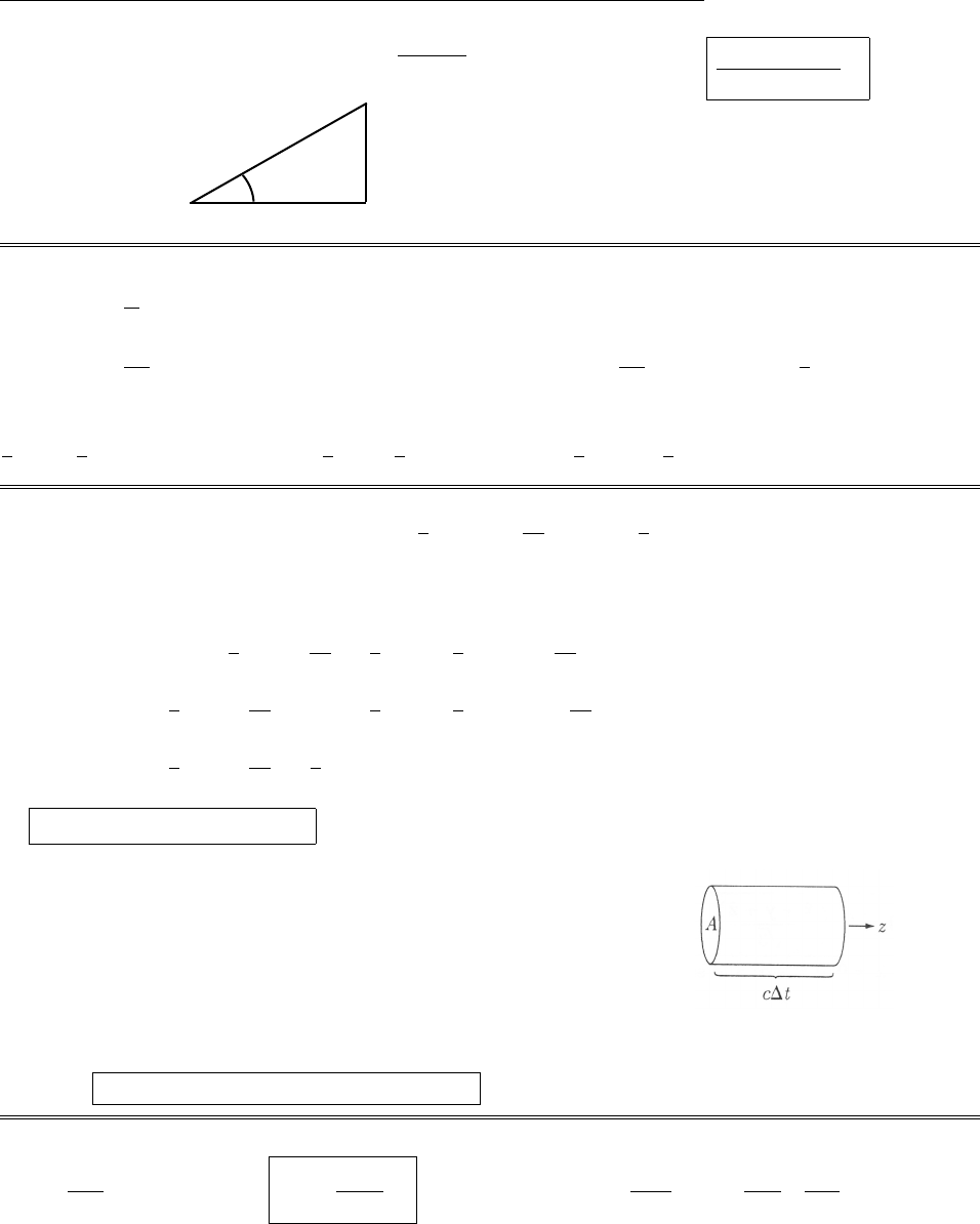
CHAPTER 9. ELECTROMAGNETIC WAVES 191
The integral is T/2=⇡/!, and cos ✓=/!2+2(see figure), so (Fm)ave =⇡q2E2
0
m!c(!2+2)ˆz .
w
q
g
Problem 9.12
hfgi=1
TT
0
acos(k·r!t+a)bcos(k·r!t+b)dt
=ab
2TT
0
[cos(2k·r2!t+a+b)+cos(ab)] dt =ab
2Tcos(ab)T=1
2ab cos(ab).
Meanwhile, in the complex notation: ˜
f=˜aeik·r!t),˜g=˜
beik·r!t),where ˜a=aeia,˜
b=beib. So
1
2˜
f˜g⇤=1
2˜aei(k·r!t)˜
b⇤ei(k·r!t)=1
2˜a˜
b⇤=1
2abei(ab),Re 1
2˜
f˜g⇤=1
2ab cos(ab)=hfgi.qed
Problem 9.13
Tij =✏0EiEj1
2ij E2+1
µ0BiBj1
2ij B2.
With the fields in Eq. 9.48, Ehas only an xcomponent, and Bonly a ycomponent. So all the “o↵-diagonal”
(i6=j) terms are zero. As for the “diagonal” elements:
Txx =✏0ExEx1
2E2+1
µ01
2B2=1
2✏0E21
µ0
B2=0.
Tyy =✏01
2E2+1
µ0ByBy1
2B2=1
2✏0E2+1
µ0
B2=0.
Tzz =✏01
2E2+1
µ01
2B2=u.
So Tzz =✏0E2
0cos2(kz !t+) (all other elements zero).
The momentum of these fields is in the zdirection, and it is
being transported in the zdirection, so yes, it does make sense
that Tzz should be the only nonzero element in Tij . According
to Sect. 8.2.3, $
T·dais the rate at which momentum crosses
an area da. Here we have no momentum crossing areas ori-
ented in the xor ydirection; the momentum per unit time
per unit area flowing across a surface oriented in the zdirec-
tion is Tzz =u=gc(Eq. 9.59), so p=gcAt, and hence
p/t=gcA = momentum per unit time crossing area A.
Evidently momentum flux density = energy density. X
Problem 9.14
R=E0R
E0I2
(Eq.9.86) )R=1
1+2
(Eq.9.82),where ⌘µ1v1
µ2v2
.T=✏2v2
✏1v1E0T
E0I2
(Eq.9.87)
c
2012 Pearson Education, Inc., Upper Saddle River, NJ. All rights reserved. This material is
protected under all copyright laws as they currently exist. No portion of this material may be
reproduced, in any form or by any means, without permission in writing from the publisher.
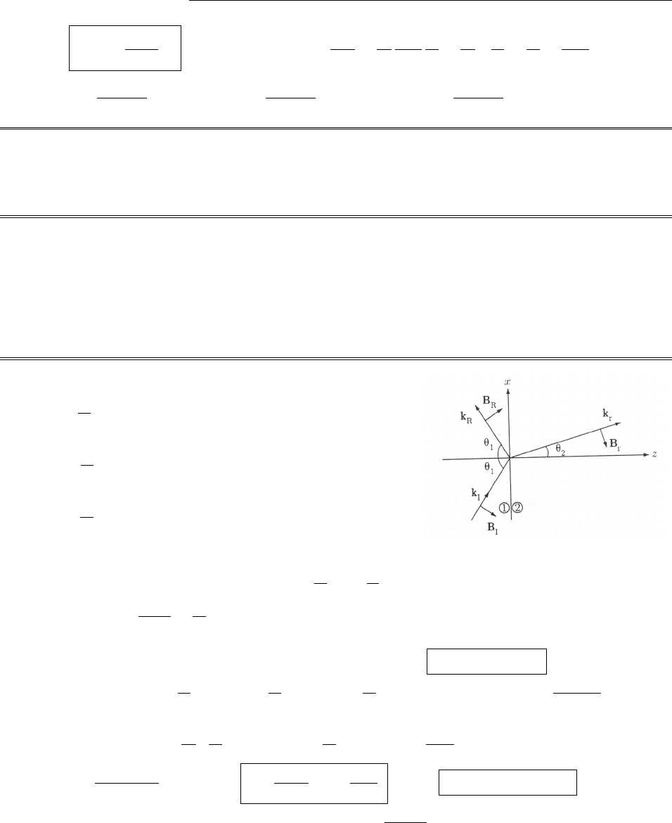
192 CHAPTER 9. ELECTROMAGNETIC WAVES
)T=2
1+2
(Eq.9.82).[Note that ✏2v2
✏1v1
=µ1
µ2
✏2µ2
✏1µ1
v2
v1
=µ1
µ2v1
v22v2
v1
=µ1v1
µ2v2
=.]
T+R=1
(1 + )24+ (1 )2=1
(1 + )2(4+12+2)= 1
(1 + )2(1 + 2+2)=1.X
Problem 9.15
Equation 9.78 is replaced by ˜
E0Iˆx +˜
E0Rˆn R=˜
E0Tˆn T, and Eq. 9.80 becomes ˜
E0Iˆy ˜
E0R(ˆz ⇥ˆn R)=
˜
E0T(ˆz ⇥ˆn T). The ycomponent of the first equation is ˜
E0Rsin ✓R=˜
E0Tsin ✓T; the xcomponent of the
second is ˜
E0Rsin ✓R=˜
E0Tsin ✓T. Comparing these two, we conclude that sin ✓R= sin ✓T= 0, and hence
✓R=✓T= 0. qed
Problem 9.16
Aeiax +Beibx =Ceicx for all x, so (using x= 0), A+B=C.
Di↵erentiate: iaAeiax +ibBeibx =icCeicx, so (using x= 0), aA +bB =cC.
Di↵erentiate again: a2Aeiax b2Beibx =c2Ceicx, so (using x= 0), a2A+b2B=c2C.
a2A+b2B=c(cC)=c(aA +bB); (A+B)(a2A+b2B)=(A+B)c(aA +bB)=cC(aA +bB);
a2A2+b2AB +a2AB +b2B2=(aA +bB)2=a2A2+2abAB +b2B2,or (a2+b22ab)AB = 0, or
(ab)2AB = 0. But Aand Bare nonzero, so a=b. Therefore (A+B)eiax =Ceicx.
a(A+B)=cC, or aC =cC, so (since C6= 0) a=c.Conclusion: a=b=c. qed
Problem 9.17
˜
EI=˜
E0Iei(kI·r!t)ˆy ,
˜
BI=1
v1
˜
E0Iei(kI·r!t)(cos ✓1ˆx + sin ✓1ˆz );
˜
ER=˜
E0Rei(kR·r!t)ˆy ,
˜
BR=1
v1
˜
E0Rei(kR·r!t)(cos ✓1ˆx + sin ✓1ˆz );
˜
ET=˜
E0Tei(kT·r!t)ˆy ,
˜
BT=1
v2
˜
E0Tei(kT·r!t)(cos ✓2ˆx + sin ✓2ˆz );
Boundary conditions:
(i) ✏1E?
1=✏2E?
2,(iii) Ek
1=Ek
2,
(ii) B?
1=B?
2,(iv) 1
µ1Bk
1=1
µ2Bk
2.
Law of refraction: sin ✓2
sin ✓1
=v2
v1
. [Note: kI·r!t=kR·r!t=kT·r!t, at z= 0, so we can drop all
exponential factors in applying the boundary conditions.]
Boundary condition (i): 0 = 0 (trivial). Boundary condition (iii): ˜
E0I+˜
E0R=˜
E0T.
Boundary condition (ii): 1
v1
˜
E0Isin ✓1+1
v1
˜
E0Rsin ✓1=1
v2
˜
E0Tsin ✓2)˜
E0I+˜
E0R=v1sin ✓2
v2sin ✓1˜
E0T.
But the term in parentheses is 1, by the law of refraction, so this is the same as (iii).
Boundary condition (iv): 1
µ11
v1
˜
E0I(cos ✓1)+ 1
v1
˜
E0Rcos ✓1=1
µ2v2
˜
E0T(cos ✓2))
˜
E0I˜
E0R=µ1v1cos ✓2
µ2v2cos ✓1˜
E0T. Let ↵⌘cos ✓2
cos ✓1
;⌘µ1v1
µ2v2
.Then ˜
E0I˜
E0R=↵ ˜
E0T.
Solving for ˜
E0Rand ˜
E0T:2
˜
E0I=(1+↵)˜
E0T)˜
E0T=2
1+↵ ˜
E0I;
c
2012 Pearson Education, Inc., Upper Saddle River, NJ. All rights reserved. This material is
protected under all copyright laws as they currently exist. No portion of this material may be
reproduced, in any form or by any means, without permission in writing from the publisher.
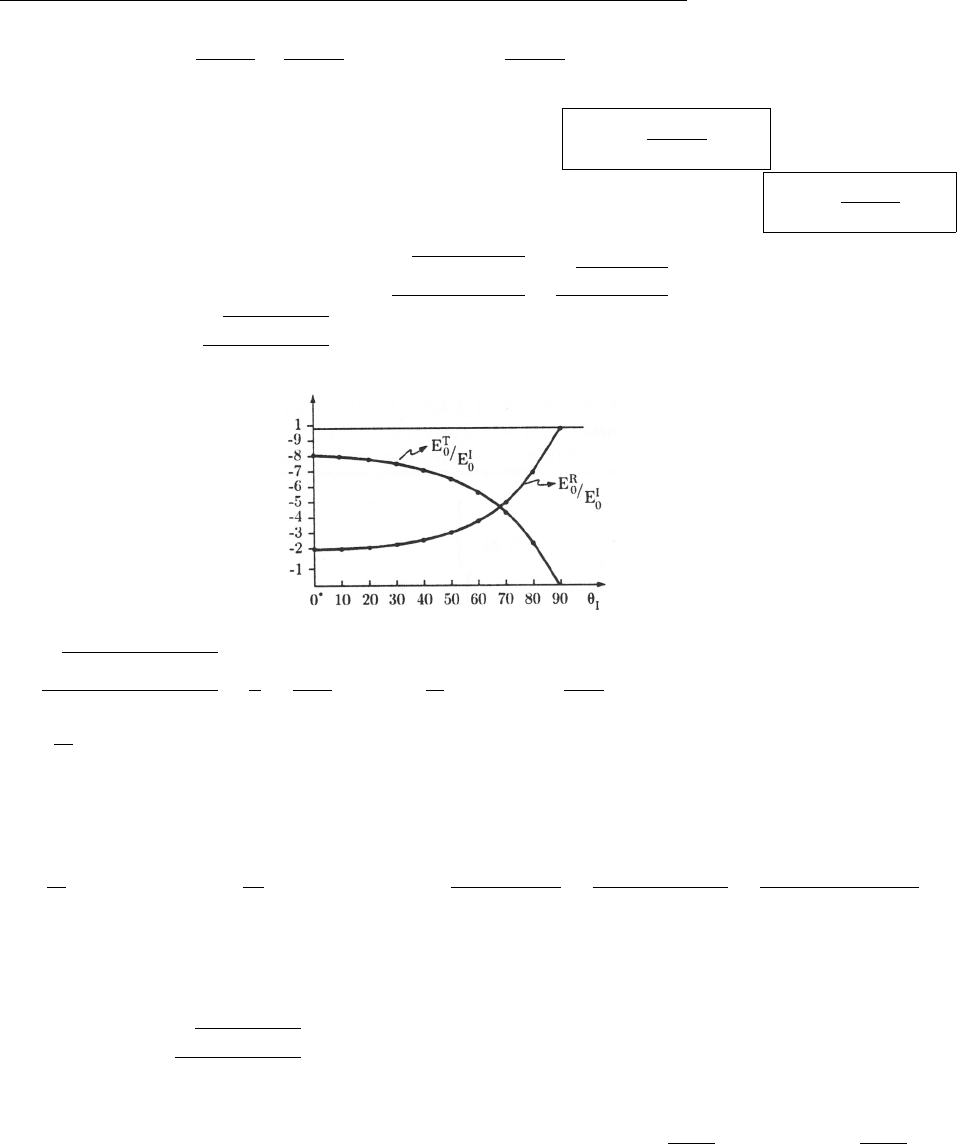
CHAPTER 9. ELECTROMAGNETIC WAVES 193
˜
E0R=˜
E0T˜
E0I=2
1+↵ 1+↵
1+↵ ˜
E0I)˜
E0R=1↵
1+↵ ˜
E0I.
Since ↵and are positive, it follows that 2/(1 + ↵) is positive, and hence the transmitted wave is in phase
with the incident wave, and the (real) amplitudes are related by E0T=2
1+↵ E0I.The reflected wave is
in phase if ↵ <1 and 180out of phase if ↵ >1; the (real) amplitudes are related by E0R=
1↵
1+↵ E0I.
These are the Fresnel equations for polarization perpendicular to the plane of incidence.
To construct the graphs, note that ↵ =1sin2✓/2
cos ✓=2sin2✓
cos ✓, where ✓is the angle of incidence,
so, for =1.5, ↵ =2.25 sin2✓
cos ✓.[In the figure, the minus signs on the vertical axis should be decimal
points.]
Is there a Brewster’s angle? Well, E0R= 0 would mean that ↵ = 1, and hence that
↵=1(v2/v1)2sin2✓
cos ✓=1
=µ2v2
µ1v1
,or 1 v2
v12
sin2✓=µ2v2
µ1v12
cos2✓,so
1=v2
v12sin2✓+(µ2/µ1)2cos2✓. Since µ1⇡µ2, this means 1 ⇡(v2/v1)2, which is only true for optically
indistinguishable media, in which case there is of course no reflection—but that would be true at any angle,
not just at a special “Brewster’s angle”. [If µ2were substantially di↵erent from µ1, and the relative velocities
were just right, it would be possible to get a Brewster’s angle for this case, at
v1
v22
=1cos2✓+µ2
µ12
cos2✓)cos2✓=(v1/v2)21
(µ2/µ1)21=(µ2✏2/µ1✏1)1
(µ2/µ1)21=(✏2/✏1)(µ1/µ2)
(µ2/µ1)(µ1/µ2).
But the media would be very peculiar.]
By the same token, Ris either always 0, or always ⇡, for a given interface—it does not switch over as you
change ✓, the way it does for polarization in the plane of incidence. In particular, if =3/2, then ↵ >1, for
↵ =2.25 sin2✓
cos ✓>1 if 2.25 sin2✓>cos2✓,or 2.25 >sin2✓+ cos2✓=1.X
In general, for >1,↵ >1, and hence R=⇡. For <1,↵ <1,and R= 0.
At normal incidence, ↵= 1, so Fresnel’s equations reduce to E0T=2
1+E0I;E0R=
1
1+E0I,
consistent with Eq. 9.82.
c
2012 Pearson Education, Inc., Upper Saddle River, NJ. All rights reserved. This material is
protected under all copyright laws as they currently exist. No portion of this material may be
reproduced, in any form or by any means, without permission in writing from the publisher.
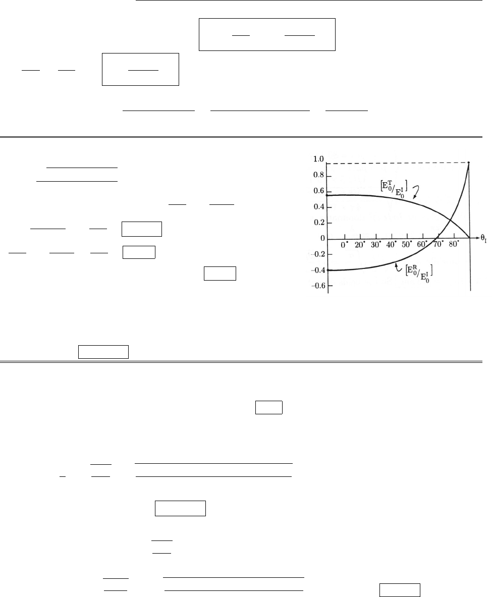
194 CHAPTER 9. ELECTROMAGNETIC WAVES
Reflection and Transmission coefficients: R=E0R
E0I2
=1↵
1+↵ 2
.Referring to Eq. 9.116,
T=✏2v2
✏1v1
↵E0T
E0I2
=↵ 2
1+↵ 2
.
R+T=(1 ↵)2+4↵
(1 + ↵)2=12↵ +↵22+4↵
(1 + ↵)2=(1 + ↵)2
(1 + ↵)2=1.X
Problem 9.18
Equation 9.106 )=2.42; Eq. 9.110 )
↵=1(sin ✓/2.42)2
cos ✓.
(a) ✓=0)↵= 1. Eq. 9.109 )E0R
E0I=↵
↵+
=12.42
1+2.42 =1.42
3.42 =0.415;
E0T
E0I=2
↵+=2
3.42 = 0.585.
(b) Equation 9.112 )✓B= tan1(2.42) = 67.5.
(c) E0R=E0T)↵=2)↵=+2=4.42;
(4.42)2cos2✓=1sin2✓/(2.42)2;
(4.42)2(1 sin2✓) = (4.42)2(4.42)2sin2✓
=10.171 sin2✓; 19.51 = (19.50.17) sin2✓;
18.5 = 19.3 sin2✓; sin2✓= 18.5/19.3=0.959;
sin ✓=0.979; ✓= 78.3.
Problem 9.19
(a) Equation 9.120 )⌧=✏/. Now ✏=✏0✏r(Eq. 4.34), ✏r⇠
=n2(Eq. 9.70), and for glass the index
of refraction is typically around 1.5, so ✏⇡(1.5)2⇥8.85 ⇥1012 =2⇥1011 C2/N m2, while =1/⇢⇡
1012 (⌦m)1(Table 7.1). Then ⌧= (2⇥1011)/1012 = 20 s. (But the resistivity of glass varies enormously
from one type to another, so this answer could be o↵by a factor of 100 in either direction.)
(b) For silver, ⇢=1.59 ⇥108(Table 7.1), and ✏⇡✏0,so!✏ =2⇡⇥1010 ⇥8.85 ⇥1012 =0.56.
Since =1/⇢=6.25 ⇥107!✏, the skin depth (Eq. 9.128) is
d=1
⇠
=2
!µ=2
2⇡⇥1010 ⇥6.25 ⇥107⇥4⇡⇥107=6.4⇥107m=6.4⇥104mm.
I’d plate silver to a depth of about 0.001 mm; there’s no point in making it any thicker, since the fields don’t
penetrate much beyond this anyway.
(c) For copper, Table 7.1 gives =1/(1.68 ⇥108)=6⇥107,!✏0= (2⇡⇥106)⇥(8.85⇥1012)=6⇥105.
Since !✏, Eq. 9.126 )k⇡!µ
2, so (Eq. 9.129)
=2⇡2
!µ0
=2⇡2
2⇡⇥106⇥6⇥107⇥4⇡⇥107=4⇥104m= 0.4 mm.
c
2012 Pearson Education, Inc., Upper Saddle River, NJ. All rights reserved. This material is
protected under all copyright laws as they currently exist. No portion of this material may be
reproduced, in any form or by any means, without permission in writing from the publisher.
CHAPTER 9. ELECTROMAGNETIC WAVES 195
From Eq. 9.129, the propagation speed is v=!
k=!
2⇡=⌫ =(4⇥104)⇥106= 400 m/s. In vacuum,
=c
⌫=3⇥108
106= 300 m; v=c= 3 ⇥108m/s. (But really, in a good conductor the skin depth is so small,
compared to the wavelength, that the notions of “wavelength” and “propagation speed” lose their meaning.)
Problem 9.20
(a) Use the binomial expansion for the square root in Eq. 9.126:
⇠
=!✏µ
21+1
2
✏! 211/2
=!✏µ
2
1
p2
✏! =
2µ
✏.
So (Eq. 9.128) d=1
⇠
=2
✏
µ. qed
For pure water,
✏=✏r✏0= 80.1✏0(Table 4.2),
µ=µ0(1 + m)=µ0(1 9.0⇥106)⇠
=µ0(Table 6.1),
=1/(2.5⇥105) (Table 7.1).
So d= (2)(2.5⇥105)(80.1)(8.85 ⇥1012)
4⇡⇥107= 1.19 ⇥104m.
(b) In this case (/✏!)2dominates, so (Eq. 9.126) k⇠
=, and hence (Eqs. 9.128 and 9.129)
=2⇡
k⇠
=2⇡
=2⇡d, or d=
2⇡. qed
Meanwhile ⇠
=!✏µ
2
✏! =!µ
2=(1015)(4⇡⇥107)(107)
2=8⇥107;d=1
=1
8⇥107=
1.3⇥108= 13 nm. So the fields do not penetrate far into a metal—which is what accounts for their opacity.
(c) Since k⇠
=, as we found in (b), Eq. 9.134 says = tan1(1) = 45. qed
Meanwhile, Eq. 9.137 says B0
E0⇠
=✏µ
✏! =µ
!.For a typical metal, then, B0
E0
=(107)(4⇡⇥107)
1015 =
107s/m.(In vacuum, the ratio is 1/c =1/(3 ⇥108)=3⇥109s/m, so the magnetic field is comparatively
about 100 times larger in a metal.)
Problem 9.21
(a) u=1
2✏E2+1
µB2=1
2e2z✏E2
0cos2(kz !t+E)+ 1
µB2
0cos2(kz !t+E+). Averaging
over a full cycle, using hcos2i=1
2and Eq. 9.137:
hui=1
2e2z✏
2E2
0+1
2µB2
0=1
4e2z✏E2
0+1
µE2
0✏µ1+
✏! 2=1
4e2z✏E2
01+1+
✏! 2.
But Eq. 9.126 )1+1+
✏! 2=2
✏µ
k2
!2, so hui=1
4e2z✏E2
0
2
✏µ
k2
!2=k2
2µ!2E2
0e2z.So the ratio of the
magnetic contribution to the electric contribution is
humagi
hueleci=B2
0/µ
E2
0✏=1
µ✏µ✏1+
✏! 2=1+
✏! 2>1.qed
c
2012 Pearson Education, Inc., Upper Saddle River, NJ. All rights reserved. This material is
protected under all copyright laws as they currently exist. No portion of this material may be
reproduced, in any form or by any means, without permission in writing from the publisher.
196 CHAPTER 9. ELECTROMAGNETIC WAVES
(b) S=1
µ(E⇥B)= 1
µE0B0e2zcos(kz!t+E) cos(kz!t+E+)ˆz ;hSi=1
2µE0B0e2zcos ˆz . [The
average of the product of the cosines is (1/2⇡)2⇡
0cos ✓cos(✓+)d✓= (1/2) cos .] So I=1
2µE0B0e2zcos =
1
2µE2
0e2zK
!cos , while, from Eqs. 9.133 and 9.134, Kcos =k,so I=k
2µ!E2
0e2z.qed
Problem 9.22
According to Eq. 9.147, R=
˜
E0R
˜
E0I
2
=
1˜
1+ ˜
2
=1˜
1+ ˜
1˜
⇤
1+ ˜
⇤,where ˜
=µ1v1
µ2!˜
k2
=µ1v1
µ2!(k2+i2) (Eqs. 9.125 and 9.146). Since silver is a good conductor (✏!), Eq. 9.126 reduces to
2⇠
=k2⇠
=!✏2µ2
2
✏2!=!µ2
2,so ˜
=µ1v1
µ2!!µ2
2(1 + i)=µ1v1
2µ2!(1 + i).
Let ⌘µ1v1
2µ2!=µ0c
2µ0!=cµ0
2!=(3⇥108)(6 ⇥107)(4⇡⇥107)
(2)(4 ⇥1015)= 29.Then
R=1i
1++i1+i
1+i=(1 )2+2
(1 + )2+2= 0.93. Evidently 93% of the light is reflected.
Problem 9.23
(a) We are told that v=↵p, where ↵is a constant. But =2⇡/k and v=!/k,so
!=↵k2⇡/k =↵p2⇡k. From Eq. 9.150, vg=d!
dk =↵p2⇡1
2pk=1
2↵2⇡
k=1
2↵p=1
2v, or v=2vg.
(b) i(px Et)
~=i(kx !t))k=p
~,!=E
~=p2
2m~=~k2
2m.Therefore v=!
k=E
p=p
2m=~k
2m;
vg=d!
dk =2~k
2m=~k
m=p
m.So v=1
2vg.Since p=mvc(where vcis the classical speed of the particle), it
follows that vg(not v) corresponds to the classical veloctity.
Problem 9.24
E=1
4⇡✏0
qd
a3)F=qE =1
4⇡✏0
q2
a3x=kspringx=m!2
0x(Eq. 9.151). So !0=q2
4⇡✏0ma3.
⌫0=!0
2⇡=1
2⇡(1.6⇥1019)2
4⇡(8.85 ⇥1012)(9.11 ⇥1031)(0.5⇥1010)3= 7.16 ⇥1015 Hz. This is ultraviolet.
From Eqs. 9.173 and 9.174,
A=nq2
2m✏0
f
!2
0
,N= # of molecules per unit volume = Avogadro0s#
22.4 liters =6.02⇥1023
22.4⇥103=2.69 ⇥1025,
f= # of electrons per molecule = 2 (for H2).
=(2.69 ⇥1025)(1.6⇥1019)2
(9.11 ⇥1031)(8.85 ⇥1012)(4.5⇥1016)2= 4.2⇥105(which is about 1/3 the actual value);
B=2⇡c
!02
=2⇡⇥3⇥108
4.5⇥1016 2
= 1.8⇥1015 m2(which is about 1/4 the actual value).
So even this extremely crude model is in the right ball park.
c
2012 Pearson Education, Inc., Upper Saddle River, NJ. All rights reserved. This material is
protected under all copyright laws as they currently exist. No portion of this material may be
reproduced, in any form or by any means, without permission in writing from the publisher.
CHAPTER 9. ELECTROMAGNETIC WAVES 197
Problem 9.25
Equation 9.170 )n=1+ Nq2
2m✏0
(!2
0!2)
[(!2
0!2)2+2!2]. Let the denominator ⌘D. Then
dn
d!=Nq2
2m✏02!
D(!2
0!2)
D22(!2
0!2)(2!)+22!=0)2!D=(!2
0!2)2(!2
0!2)22!;
(!2
0!2)2+2!2= 2(!2
0!2)22(!2
0!2),or (!2
0!2)2=2(!2+!2
0!2)=2!2
0)(!2
0!2)=±!0;
!2=!2
0⌥!0,!=!01⌥/!0⇠
=!0(1 ⌥/2!0)=!0⌥/2. So !2=!0+/2,!1=!0/2, and the
width of the anomalous region is !=!2!1=.
From Eq. 9.171, ↵=Nq2!2
m✏0c
(!2
0!2)2+2!2, so at the maximum (!=!0), ↵max =Nq2
m✏0c.
At !1and !2,!2=!2
0⌥!0,so↵=Nq2!2
m✏0c
2!2
0+2!2=↵max !2
!2+!2
0.But
!2
!2+!2
0
=!2
0⌥!0
2!2
0⌥!0=1
2
(1 ⌥/!0)
(1 ⌥/2!0)⇠
=1
21⌥
!01±
2!0⇠
=1
21⌥
2!0⇠
=1
2.
So ↵⇠
=1
2↵max at !1and !2. qed
Problem 9.26
Equation 9.170 for a single resonance:
ck
!=1+Nq2
2m✏0(!2
0!2)
(!2
0!2)2+2!2)ck =!1+ a!2
0(!2
0!2)
(!2
0!2)2+2!2where a⌘Nq2
2m✏0!2
0
.
From Eq. 9.150, the group velocity is vg=d!/dk, so
c
vg
=cdk
d!
=1+ a!2
0(!2
0!2)
(!2
0!2)2+2!2+!a!2
0
[(!2
0!2)2+2!2](2!)(!2
0!2)[2(!2
0!2)(2!)+2(2!)]
[(!2
0!2)2+2!2]2
=1+a!2
0
(!2
0!2)[(!2
0!2)2+2!2]2!2[(!2
0!2)2+2!2]+4!2(!2
0!2)222!2(!2
0!2)
[(!2
0!2)2+2!2]2
=1+a!2
0
(!2
0!2)3+2!2(!2
0!2)22!2(!2
0!2)22!4
[(!2
0!2)2+2!2]2
=1+a!2
0(!2
0+!2)(!2
0!2)22!2
[(!2
0!2)2+2!2]2.
vg=c1+a!2
0(!2
0+!2)(!2
0!2)22!2
[(!2
0!2)2+2!2]21
.
(a) For = 0 and a=0.003:
vg
c=1+a!2
0
(!2
0+!2)
(!2
0!2)21
)y=1+0.003 1+x
(1 x)21
.
c
2012 Pearson Education, Inc., Upper Saddle River, NJ. All rights reserved. This material is
protected under all copyright laws as they currently exist. No portion of this material may be
reproduced, in any form or by any means, without permission in writing from the publisher.
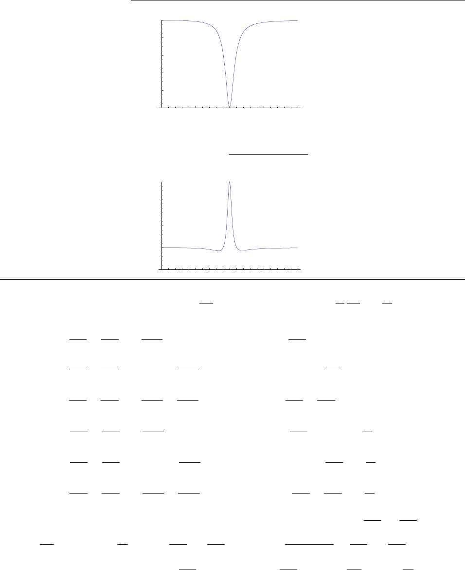
198 CHAPTER 9. ELECTROMAGNETIC WAVES
0.0
0.5
1.0
1.5
2.0
0.2
0.4
0.6
0.8
1.0
(b) For = (0.1)!0and a=0.003:
y=1+0.003(1 + x)(1 x)20.01x
[(1 x)2+0.01x]21
.
0.0
0.5
1.0
1.5
2.0
1.0
1.5
2.0
2.5
Problem 9.27
(a) From Eqs. 9.176 and 9.177, r⇥˜
E=@˜
B
@t=i!˜
B0ei(kz!t);r⇥˜
B=1
c2
@˜
E
@t=i!
c2˜
E0ei(kz!t).
In the terminology of Eq. 9.178:
(r⇥˜
E)x=@˜
Ez
@y@˜
Ey
@z=@˜
E0z
@yik ˜
E0yei(kz!t). So (ii) @Ez
@yikEy=i!Bx.
(r⇥˜
E)y=@˜
Ex
@z@˜
Ez
@x=ik ˜
E0x@˜
E0z
@xei(kz!t). So (iii) ikEx@Ez
@x=i!By.
(r⇥˜
E)z=@˜
Ey
@x@˜
Ex
@y=@˜
E0y
@x@˜
E0x
@yei(kz!t). So (i) @Ey
@x@Ex
@y=i!Bz.
(r⇥˜
B)x=@˜
Bz
@y@˜
By
@z=@˜
B0z
@yik ˜
B0yei(kz!t). So (v) @Bz
@yikBy=i!
c2Ex.
(r⇥˜
B)y=@˜
Bx
@z@˜
Bz
@x=ik ˜
B0x@˜
B0z
@xei(kz!t). So (vi) ikBx@Bz
@x=i!
c2Ey.
(r⇥˜
B)z=@˜
By
@x@˜
Bx
@y=@˜
B0y
@x@˜
B0x
@yei(kz!t). So (iv) @By
@x@Bx
@y=i!
c2Ez.
This confirms Eq. 9.179. Now multiply (iii) by k, (v) by !, and subtract: ik2Exk@Ez
@x!@Bz
@y+i!kBy=
ik!By+i!2
c2Ex)ik2!2
c2Ex=k@Ez
@x+!@Bz
@y,or (i) Ex=i
(!/c)2k2k@Ez
@x+!@Bz
@y.
Multiply (ii) by k, (vi) by !, and add: k@Ez
@yik2Ey+i!kBx!@Bz
@x=i!kBxi!2
c2Ey)i!2
c2k2Ey=
c
2012 Pearson Education, Inc., Upper Saddle River, NJ. All rights reserved. This material is
protected under all copyright laws as they currently exist. No portion of this material may be
reproduced, in any form or by any means, without permission in writing from the publisher.
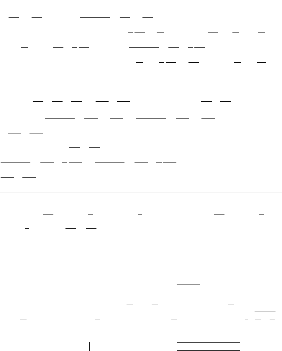
CHAPTER 9. ELECTROMAGNETIC WAVES 199
k@Ez
@y+!@Bz
@x,or (ii) Ey=i
(!/c)2k2k@Ez
@y!@Bz
@x.
Multiply (ii) by !/c2, (vi) by k, and add: !
c2
@Ez
@yi!k
c2Ey+ik2Bxk@Bz
@x=i!2
c2Bxi!k
c2Ey)
ik2!2
c2Bx=k@Bz
@x!
c2
@Ez
@y,or (iii) Bx=i
(!/c)2k2k@Bz
@x!
c2
@Ez
@y.
Multiply (iii) by !/c2, (v) by k, and subtract: i!k
c2Ex!
c2
@Ez
@xk@Bz
@y+ik2By=i!2
c2By+i!k
c2Ex)
ik2!2
c2By=!
c2
@Ez
@x+k@Bz
@y,or (iv) By=i
(!/c)2k2k@Bz
@y+!
c2
@Ez
@x.
This completes the confirmation of Eq. 9.180.
(b) r·˜
E=@˜
Ex
@x+@˜
Ey
@y+@˜
Ez
@z=@˜
E0x
@x+@˜
E0y
@y+ik ˜
E0zei(kz!t)=0)@Ex
@x+@Ey
@y+ikEz= 0.
Using Eq. 9.180, i
(!/c)2k2k@2Ez
@x2+!@2Bz
@x@y+i
(!/c)2k2k@2Ez
@2y!@2Bz
@x@y+ikEz=0,
or @2Ez
@x2+@2Ez
@2y+(!/c)2k2Ez=0.
Likewise, r·˜
B=0)@Bx
@x+@By
@y+ikBz=0)
i
(!/c)2k2k@2Bz
@x2!
c2
@2Ez
@x@y+i
(!/c)2k2k@2Bz
@y2+!
c2
@Ez
@x@y+ikBz=0)
@2Bz
@x2+@2Bz
@2y+(!/c)2k2Bz= 0.
This confirms Eqs. 9.181. [You can also do it by putting Eq. 9.180 into Eq. 9.179 (i) and (iv).]
Problem 9.28
Here Ez= 0 (TE) and !/c =k(n=m= 0), so Eq. 9.179(ii) )Ey=cBx, Eq. 9.179(iii) )Ex=cBy,
Eq. 9.179(v) )@Bz
@y=ikBy!
c2Ex=ikBy!
cBy= 0, Eq. 9.179(vi) )@Bz
@x=ikBx+!
c2Ey=
ikBx!
cBx= 0. So @Bz
@x=@Bz
@y= 0, and since Bzis a function only of xand y, this says Bzis in fact
aconstant (as Eq. 9.186 also suggests). Now Faraday’s law (in integral form) says E·dl=@B
@t·da,
and Eq. 9.176 )@B
@t=i!B,soE·dl=i!B·da. Applied to a cross-section of the waveguide this gives
E·dl=i!ei(kz!t)Bzda =i!Bzei(kz!t)(ab) (since Bzis constant, it comes outside the integral). But
if the boundary is just inside the metal, where E= 0, it follows that Bz=0.So this would be a TEM mode,
which we already know cannot exist for this guide.
Problem 9.29
Here a=2.28 cm and b=1.01 cm, so ⌫10 =1
2⇡!10 =c
2a=0.66 ⇥1010 Hz; ⌫20 =2c
2a=1.32 ⇥1010 Hz;
⌫30 =3c
2a=1.97 ⇥1010 Hz; ⌫01 =c
2b=1.49 ⇥1010 Hz; ⌫02 =2c
2b=2.97 ⇥1010 Hz; ⌫11 =c
21
a2+1
b2=
1.62 ⇥1010 Hz. Evidently just four modes occur: 10, 20, 01, and 11.
To get only one mode you must drive the waveguide at a frequency between ⌫10 and ⌫20:
0.66 ⇥1010 <⌫<1.32 ⇥1010 Hz. =c
⌫,so 10 =2a;20 =a. 2.28 cm <<4.56 cm.
c
2012 Pearson Education, Inc., Upper Saddle River, NJ. All rights reserved. This material is
protected under all copyright laws as they currently exist. No portion of this material may be
reproduced, in any form or by any means, without permission in writing from the publisher.
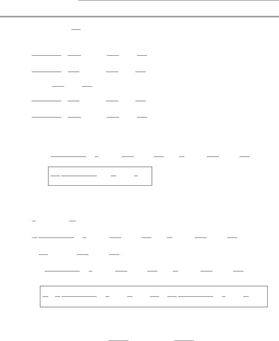
200 CHAPTER 9. ELECTROMAGNETIC WAVES
Problem 9.30
From Prob. 9.11, hSi=1
2µ0
Re( ˜
E⇥˜
B⇤). Here (Eq. 9.176) ˜
E=˜
E0ei(kz!t),˜
B⇤=˜
B⇤
0ei(kz!t), and, for
the TEmn mode (Eqs. 9.180 and 9.186)
B⇤
x=ik
(!/c)2k2m⇡
aB0sin m⇡x
acos n⇡y
b;
B⇤
y=ik
(!/c)2k2n⇡
bB0cos m⇡x
asin n⇡y
b;
B⇤
z=B0cos m⇡x
acos n⇡y
b;
Ex=i!
(!/c)2k2n⇡
bB0cos m⇡x
asin n⇡y
b;
Ey=i!
(!/c)2k2m⇡
aB0sin m⇡x
acos n⇡y
b;
Ez=0.
So
hSi=!k⇡2B2
0
[(!/c)2k2]2n
b2cos2m⇡x
asin2n⇡y
b+m
a2sin2m⇡x
acos2n⇡y
bˆz .
hSi·da=1
8µ0
!k⇡2B2
0
[(!/c)2k2]2ab m
a2+n
b2.[In the last step I used
a
0sin2(m⇡x/a)dx =a
0cos2(m⇡x/a)dx =a/2; b
0sin2(n⇡y/b)dy =b
0cos2(n⇡y/b)dy =b/2.]
Similarly,
hui=1
4✏0˜
E·˜
E⇤+1
µ0
˜
B·˜
B⇤
=✏0
4
!2⇡2B2
0
[(!/c)2k2]2n
b2cos2m⇡x
asin2n⇡y
b+m
a2sin2m⇡x
acos2n⇡y
b
+1
4µ0B2
0cos2m⇡x
acos2n⇡y
b
+k2⇡2B2
0
[(!/c)2k2]2n
b2cos2m⇡x
asin2n⇡y
b+m
a2sin2m⇡x
acos2n⇡y
b.
huida =ab
4✏0
4
!2⇡2B2
0
[(!/c)2k2]2n
b2+m
a2+B2
0
4µ0
+1
4µ0
k2⇡2B2
0
[(!/c)2k2]2n
b2+m
a2.
These results can be simplified, using Eq. 9.190 to write (!/c)2k2=(!mn/c)2,✏0µ0=1/c2to eliminate ✏0,
and Eq. 9.188 to write (m/a)2+(n/b)2=(!mn/⇡c)2:
hSi·da=!kabc2
8µ0!2
mn
B2
0;huida =!2ab
8µ0!2
mn
B2
0.
c
2012 Pearson Education, Inc., Upper Saddle River, NJ. All rights reserved. This material is
protected under all copyright laws as they currently exist. No portion of this material may be
reproduced, in any form or by any means, without permission in writing from the publisher.
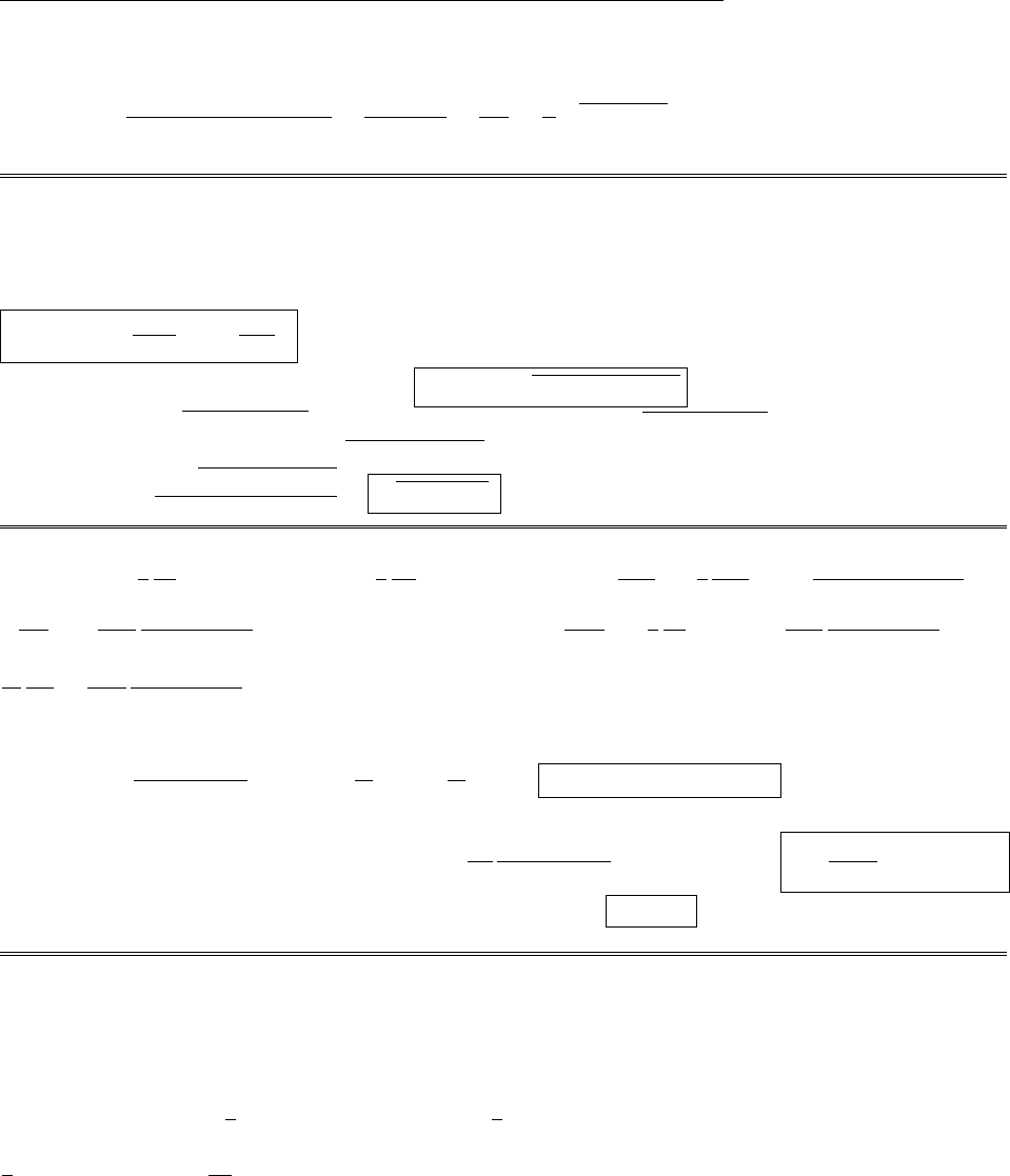
CHAPTER 9. ELECTROMAGNETIC WAVES 201
Evidently
energy per unit time
energy per unit length =hSi·da
huida =kc2
!=c
!!2!2
mn =vg(Eq.9.192).qed
Problem 9.31
Following Sect. 9.5.2, the problem is to solve Eq. 9.181 with Ez6=0,B
z= 0, subject to the boundary
conditions 9.175. Let Ez(x, y)=X(x)Y(y); as before, we obtain X(x)=Asin(kxx)+Bcos(kxx). But the
boundary condition requires Ez= 0 (and hence X= 0) when x= 0 and x=a, so B= 0 and kx=m⇡/a.
But this time m=1,2,3,..., but not zero, since m= 0 would kill Xentirely. The same goes for Y(y). Thus
Ez=E0sin m⇡x
asin n⇡y
bwith n, m =1,2,3,....
The rest is the same as for TE waves: !mn =c⇡(m/a)2+(n/b)2is the cuto↵frequency, the wave
velocity is v=c/1(!mn/!)2, and the group velocity is vg=c1(!mn/!)2. The lowest TM mode is
11, with cuto↵frequency !11 =c⇡(1/a)2+ (1/b)2. So the ratio of the lowest TM frequency to the lowest
TE frequency is c⇡(1/a)2+ (1/b)2
(c⇡/a)=1+(a/b)2.
Problem 9.32
(a) r·E=1
s
@
@s(sEs)=0X;r·B=1
s
@
@(B)=0X;r⇥E=@Es
@zˆ
1
s
@Es
@ ˆz =E0ksin(kz !t)
sˆ
?
=
@B
@t=E0!
c
sin(kz !t)
sˆ
X(since k=!/c); r⇥B=@B
@zˆs +1
s
@
@s(sB)ˆz =E0k
c
sin(kz !t)
sˆs ?
=
1
c2
@E
@t=E0!
c2
sin(kz !t)
sˆs X.Boundary conditions: Ek=Ez=0X;B?=Bs=0X.
(b) To determine , use Gauss’s law for a cylinder of radius sand length dz:
E·da=E0
cos(kz !t)
s(2⇡s)dz =1
✏0
Qenc =1
✏0
dz )=2⇡✏0E0cos(kz !t).
To determine I, use Amp´ere’s law for a circle of radius s(note that the displacement current through this
loop is zero, since Eis in the ˆs direction): B·dl=E0
c
cos(kz !t)
s(2⇡s)=µ0Ienc )I=2⇡E0
µ0ccos(kz !t).
The charge and current on the outer conductor are precisely the opposite of these, since E=B=0inside
the metal, and hence the total enclosed charge and current must be zero.
Problem 9.33
˜
f(z,0) = 1
1
˜
A(k)eikz dk )˜
f(z,0)⇤=1
1
˜
A(k)⇤eikz dk. Let l⌘k; then ˜
f(z,0)⇤=
1
1
˜
A(l)⇤eilz(dl)=1
1
˜
A(l)⇤eilz dl =1
1
˜
A(k)⇤eikz dk (renaming the dummy variable l!k).
f(z,0) = Re ˜
f(z,0)=1
2˜
f(z,0) + ˜
f(z,0)⇤=1
1
1
2˜
A(k)+ ˜
A(k)⇤eikz dk. Therefore
1
2˜
A(k)+ ˜
A(k)⇤=1
2⇡1
1
f(z,0)eikz dz.
Meanwhile, ˙
˜
f(z,t)=1
1
˜
A(k)(i!)ei(kz!t)dk )˙
˜
f(z,0) = 1
1
[i!˜
A(k)]eikz dk.
c
2012 Pearson Education, Inc., Upper Saddle River, NJ. All rights reserved. This material is
protected under all copyright laws as they currently exist. No portion of this material may be
reproduced, in any form or by any means, without permission in writing from the publisher.

202 CHAPTER 9. ELECTROMAGNETIC WAVES
(Note that !=|k|v, here, so it does not come outside the integral.)
˙
˜
f(z,0)⇤=1
1
[i!˜
A(k)⇤]eikz dk =1
1
[i|k|v˜
A(k)⇤]eikz dk =1
1
[i|l|v˜
A(l)⇤]eilz(dl)
=1
1
[i|k|v˜
A(k)⇤]eikz dk =1
1
[i!˜
A(k)⇤]eikz dk.
˙
f(z,0) = Re ˙
˜
f(z,0)=1
2˙
˜
f(z,0) + ˙
˜
f(z,0)⇤=1
1
1
2[i!˜
A(k)+i!˜
A(k)⇤]eikz dk.
i!
2˜
A(k)˜
A(k)⇤=1
2⇡1
1
˙
f(z,0)eikz dz, or 1
2˜
A(k)˜
A(k)⇤=1
2⇡1
1 i
!˙
f(z,0)eikz dz.
Adding these two results, we get ˜
A(k)= 1
2⇡1
1 f(z,0) + i
!˙
f(z,0)eikz dz. qed
Problem 9.34
(a) Since (E⇥B) points in the direction of propagation, B=E0
c[cos(kz !t)+cos(kz +!t)] ˆy .
(b) From Eq. 7.63, K⇥(ˆz )= 1
µ0
B=E0
µ0c[2 cos(!t)] ˆy ,K=2E0
µ0ccos(!t)ˆx .
(c) The force per unit area is f=K⇥Bave =2E2
0
µ0c2[cos(!t)ˆx ]⇥[cos(!t)ˆy ]= 2✏0E2
0cos2(!t)ˆz .The time
average of cos2(!t) is 1/2, so
fave =✏0E2
0.
This is twice the pressure in Eq. 9.64, but that was for a perfect absorber, whereas this is a perfect reflector.
Problem 9.35
(a) (i) Gauss’s law: r·E=1
rsin ✓
@E
@ =0.X
(ii) Faraday’s law:
@B
@t=r⇥E=1
rsin ✓
@
@✓(sin ✓E)ˆr 1
r
@
@r(rE)ˆ
✓
=1
rsin ✓
@
@✓ E0
sin2✓
rcos u1
kr sin uˆr 1
r
@
@rE0sin ✓cos u1
kr sin uˆ
✓.
But @
@rcos u=ksin u;@
@rsin u=kcos u.
=1
rsin ✓
E0
r2 sin ✓cos ✓cos u1
kr sin uˆr 1
rE0sin ✓ksin u+1
kr2sin u1
rcos uˆ
✓.
Integrating with respect to t, and noting that cos udt=1
!sin uand sin udt=1
!cos u, we obtain
B=2E0cos ✓
!r2sin u+1
kr cos uˆr +E0sin ✓
!rkcos u+1
kr2cos u+1
rsin uˆ
✓.
c
2012 Pearson Education, Inc., Upper Saddle River, NJ. All rights reserved. This material is
protected under all copyright laws as they currently exist. No portion of this material may be
reproduced, in any form or by any means, without permission in writing from the publisher.

CHAPTER 9. ELECTROMAGNETIC WAVES 203
(iii) Divergence of B:
r·B=1
r2
@
@rr2Br+1
rsin ✓
@
@✓(sin ✓B✓)
=1
r2
@
@r2E0cos ✓
!sin u+1
kr cos u+1
rsin ✓
@
@✓ E0sin2✓
!rkcos u+1
kr2cos u+1
rsin u
=1
r2
2E0cos ✓
!kcos u1
kr2cos u1
rsin u
+1
rsin ✓
2E0sin ✓cos ✓
!rkcos u+1
kr2cos u+1
rsin u
=2E0cos ✓
!r2kcos u1
kr2cos u1
rsin ukcos u+1
kr2cos u+1
rsin u=0.X
(iv) Amp´ere/Maxwell:
r⇥B=1
r@
@r(rB✓)@Br
@✓ ˆ
=1
r@
@rE0sin ✓
!kcos u+1
kr2cos u+1
rsin u@
@✓ 2E0cos ✓
!r2sin u+1
kr cos uˆ
=E0sin ✓
!rk2sin u2
kr3cos u1
r2sin u1
r2sin u+k
rcos u+2
r2sin u+2
kr3cos uˆ
=k
!
E0sin ✓
rksin u+1
rcos uˆ
=1
c
E0sin ✓
rksin u+1
rcos uˆ
.
1
c2
@E
@t=1
c2
E0sin ✓
r!sin u+!
kr cos uˆ
=1
c2
!
k
E0sin ✓
rksin u+1
rcos uˆ
=1
c
E0sin ✓
rksin u+1
rcos uˆ
=r⇥B.X
(b) Poynting Vector:
S=1
µ0
(E⇥B)=E0sin ✓
µ0rcos u1
kr sin u2E0cos ✓
!r2sin u+1
kr cos uˆ
✓
+E0sin ✓
!rkcos u+1
kr2cos u+1
rsin u(ˆr )
=E2
0sin ✓
µ0!r22 cos ✓
rsin ucos u+1
kr(cos2usin2u)1
k2r2sin ucos uˆ
✓
sin ✓kcos2u+1
kr2cos2u+1
rsin ucos u+1
rsin ucos u1
k2r3sin ucos u1
kr2sin2uˆr
=
E2
0sin ✓
µ0!r22 cos ✓
r11
k2r2sin ucos u+1
kr(cos2usin2u)ˆ
✓
+ sin ✓2
r+1
k2r3sin ucos u+kcos2u+1
kr2(sin2ucos2u)ˆr .
c
2012 Pearson Education, Inc., Upper Saddle River, NJ. All rights reserved. This material is
protected under all copyright laws as they currently exist. No portion of this material may be
reproduced, in any form or by any means, without permission in writing from the publisher.
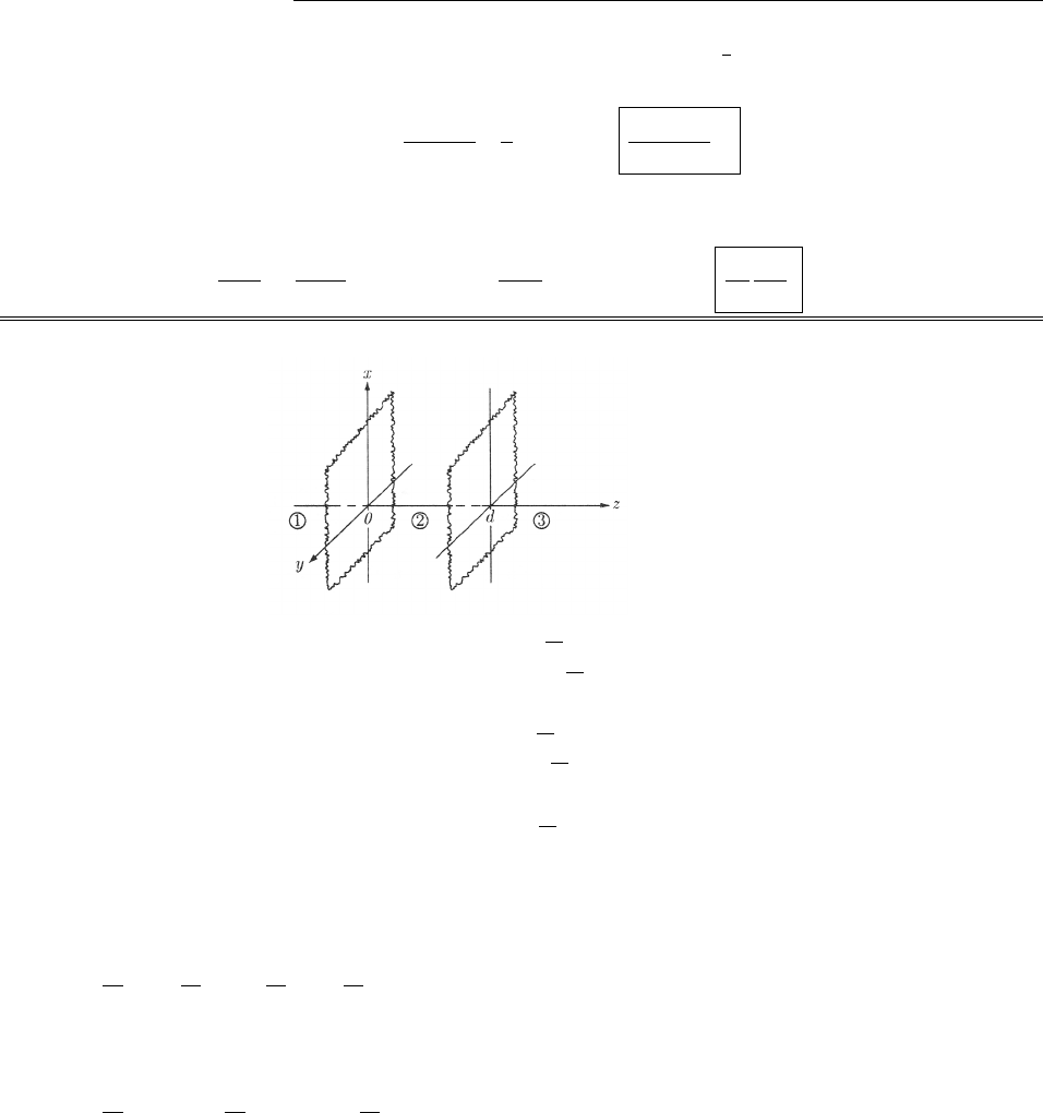
204 CHAPTER 9. ELECTROMAGNETIC WAVES
Averaging over a full cycle, using hsin ucos ui=0,hsin2ui=hcos2ui=1
2, we get the intensity:
I=hSi=E2
0sin ✓
µ0!r2k
2sin ✓ˆr =E2
0sin2✓
2µ0cr2ˆr .
It points in the ˆr direction, and falls o↵as 1/r2, as we would expect for a spherical wave.
(c) P=I·da=E2
0
2µ0csin2✓
r2r2sin ✓d✓d=E2
0
2µ0c2⇡⇡
0
sin3✓d✓=4⇡
3
E2
0
µ0c.
Problem 9.36
z<0: ˜
EI(z,t)= ˜
EIei(k1z!t)ˆx ,˜
BI(z,t)= 1
v1
˜
EIei(k1z!t)ˆy
˜
ER(z,t)= ˜
ERei(k1z!t)ˆx ,˜
BR(z,t)=1
v1
˜
ERei(k1z!t)ˆy .
0<z<d:˜
Er(z,t)= ˜
Erei(k2z!t)ˆx ,˜
Br(z,t)= 1
v2
˜
Erei(k2z!t)ˆy
˜
El(z,t)= ˜
Elei(k2z!t)ˆx ,˜
Bl(z,t)=1
v2
˜
Elei(k2z!t)ˆy .
z>d:˜
ET(z,t)= ˜
ETei(k3z!t)ˆx ,˜
BT(z,t)= 1
v3
˜
ETei(k3z!t)ˆy .
Boundary conditions: Ek
1=Ek
2,Bk
1=Bk
2, at each boundary (assuming µ1=µ2=µ3=µ0):
z=0:
˜
EI+˜
ER=˜
Er+˜
El;
1
v1
˜
EI1
v1
˜
ER=1
v2
˜
Er1
v2
˜
El)˜
EI˜
ER=(˜
Er˜
El),where ⌘v1/v2.
z=d:
˜
Ereik2d+˜
Eleik2d=˜
ETeik3d;
1
v2
˜
Ereik2d1
v2
˜
Eleik2d=1
v3
˜
ETeik3d)˜
Ereik2d˜
Eleik2d=↵˜
ETeik3d,where ↵⌘v2/v3.
We have here four equations; the problem is to eliminate ˜
ER,˜
Er, and ˜
El, to obtain a single equation for
˜
ETin terms of ˜
EI.
Add the first two to eliminate ˜
ER:2
˜
EI= (1 + )˜
Er+ (1 )˜
El;
Add the last two to eliminate ˜
El:2
˜
Ereik2d=(1+↵)˜
ETeik3d;
Subtract the last two to eliminate ˜
Er:2
˜
Eleik2d=(1↵)˜
ETeik3d.
c
2012 Pearson Education, Inc., Upper Saddle River, NJ. All rights reserved. This material is
protected under all copyright laws as they currently exist. No portion of this material may be
reproduced, in any form or by any means, without permission in writing from the publisher.

CHAPTER 9. ELECTROMAGNETIC WAVES 205
Plug the last two of these into the first:
2˜
EI= (1 + )1
2eik2d(1 + ↵)˜
ETeik3d+ (1 )1
2eik2d(1 ↵)˜
ETeik3d
4˜
EI=(1 + ↵)(1 + )eik2d+ (1 ↵)(1 )eik2d˜
ETeik3d
=(1 + ↵)eik2d+eik2d+(↵+)eik2deik2d˜
ETeik3d
= 2 [(1 + ↵) cos(k2d)i(↵+) sin(k2d)] ˜
ETeik3d.
Now the transmission coefficient is T=v3✏3E2
T0
v1✏1E2
I0
=v3
v1µ0✏3
µ0✏1|˜
ET|2
|˜
EI|2=v1
v3
|˜
ET|2
|˜
EI|2=↵ |˜
ET|2
|˜
EI|2,so
T1=1
↵ |˜
EI|2
|˜
ET|2=1
↵
1
2[(1 + ↵) cos(k2d)i(↵+) sin(k2d)] eik3d
2
=1
4↵ (1 + ↵)2cos2(k2d)+(↵+)2sin2(k2d).But cos2(k2d)=1sin2(k2d).
=1
4↵ (1 + ↵)2+(↵2+2↵ +212↵ ↵22) sin2(k2d)
=1
4↵ (1 + ↵)2(1 ↵2)(1 2) sin2(k2d).
But n1=c
v1
,n
2=c
v2
,n
3=c
v3
,so ↵=n3
n2
,=n2
n1
.
=1
4n1n3(n1+n3)2+(n2
1n2
2)(n2
3n2
2)
n2
2
sin2(k2d).
Problem 9.37
T=1)sin kd =0)kd =0,⇡,2⇡....Theminimum (nonzero) thickness is d=⇡/k.Butk=!/v =
2⇡⌫/v =2⇡⌫n/c, and n=✏µ/✏0µ0(Eq. 9.69), where (presumably) µ⇡µ0. So n=✏/✏0=p✏r, and hence
d=⇡c
2⇡⌫p✏r
=c
2⌫p✏r
=3⇥108
2(10 ⇥109)p2.5=9.49 ⇥103m, or 9.5 mm.
Problem 9.38
From Eq. 9.199,
T1=1
4(4/3)(1) [(4/3) + 1]2+[(16/9) (9/4)][1 (9/4)]
(9/4) sin2(3!d/2c)
=3
16 49
9+(17/36)(5/4)
(9/4) sin2(3!d/2c)=49
48 +85
(48)(36) sin2(3!d/2c).
T=48
49 + (85/36) sin2(3!d/2c).
Since sin2(3!d/2c) ranges from 0 to 1, Tmin =48
49 + (85/36) = 0.935; Tmax =48
49 = 0.980. Not much
variation, and the transmission is good (over 90%) for all frequencies. Since Eq. 9.199 is unchanged when you
switch 1 and 3, the transmission is the same either direction, and the fish sees you just as well as you see it.
c
2012 Pearson Education, Inc., Upper Saddle River, NJ. All rights reserved. This material is
protected under all copyright laws as they currently exist. No portion of this material may be
reproduced, in any form or by any means, without permission in writing from the publisher.

206 CHAPTER 9. ELECTROMAGNETIC WAVES
Problem 9.39
(a) Equation 9.91 )˜
ET(r,t)= ˜
E0Tei(kT·r!t);kT·r=kT(sin ✓Tˆx + cos ✓Tˆz )·(xˆx +yˆy +zˆz )=
kT(xsin ✓T+zcos ✓T)=xkTsin ✓T+izkTsin2✓T1=kx +iz, where
k⌘kTsin ✓T=!n2
cn1
n2
sin ✓I=!n1
csin ✓I,
⌘kTsin2✓T1=!n2
c(n1/n2)2sin2✓I1=!
cn2
1sin2✓In2
2.So
˜
ET(r,t)= ˜
E0Tezei(kx!t).qed
(b) R=
˜
E0R
˜
E0I
2
=
↵
↵+
2
. Here is real (Eq. 9.106) and ↵is purely imaginary (Eq. 9.108); write ↵=ia,
with areal: R=ia
ia +ia
ia +=a2+2
a2+2= 1.
(c) From Prob. 9.17, E0R=
1↵
1+↵ E0I,so R=
1↵
1+↵
2
=
1ia
1+ia
2
=(1 ia)(1 + ia)
(1 + ia)(1 ia)= 1.
(d) From the solution to Prob. 9.17, the transmitted wave is
˜
E(r,t)= ˜
E0Tei(kT·r!t)ˆy ,˜
B(r,t)= 1
v2
˜
E0Tei(kT·r!t)(cos ✓Tˆx + sin ✓Tˆz ).
Using the results in (a): kT·r=kx +iz, sin ✓T=ck
!n2
,cos ✓T=ic
!n2
:
˜
E(r,t)= ˜
E0Tezei(kx!t)ˆy ,˜
B(r,t)= 1
v2
˜
E0Tezei(kx!t)ic
!n2
ˆx +ck
!n2
ˆz .
We may as well choose the phase constant so that ˜
E0Tis real. Then
E(r,t)=E0ezcos(kx !t)ˆy ;
B(r,t)= 1
v2
E0ezc
!n2
Re {[cos(kx !t)+isin(kx !t)] [iˆx +kˆz ]}
=1
!E0ez[sin(kx !t)ˆx +kcos(kx !t)ˆz ].qed
(I used v2=c/n2to simplfy B.)
c
2012 Pearson Education, Inc., Upper Saddle River, NJ. All rights reserved. This material is
protected under all copyright laws as they currently exist. No portion of this material may be
reproduced, in any form or by any means, without permission in writing from the publisher.
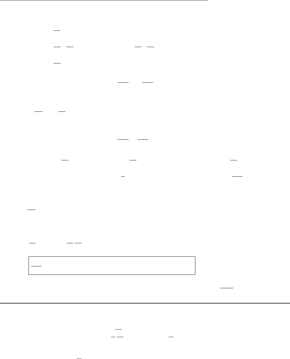
CHAPTER 9. ELECTROMAGNETIC WAVES 207
(e) (i) r·E=@
@yE0ezcos(kx !t)=0.X
(ii) r·B=@
@xE0
!ezsin(kx !t)+@
@zE0
!ezkcos(kx !t)
=E0
!ezkcos(kx !t)ezkcos(kx !t)=0.X
(iii) r⇥E=
ˆx ˆy ˆz
@/@x@/@y@/@z
0Ey0=@Ey
@zˆx +@Ey
@xˆz
=E0ezcos(kx !t)ˆx E0ezksin(kx !t)ˆz .
@B
@t=E0
!ez[! cos(kx !t)ˆx +k!sin(kx !t)ˆz ]
=E0ezcos(kx !t)ˆx kE0ezsin(kx !t)ˆz =r⇥E.X
(iv) r⇥B=
ˆx ˆy ˆz
@/@x@/@y@/@z
Bx0Bz=@Bx
@z@Bz
@xˆy
=E0
!2ezsin(kx !t)+E0
!ezk2sin(kx !t)ˆy =(k22)E0
!ezsin(kx !t)ˆy .
Eq.9.202 )k22=!
c2n2
1sin2✓I(n1sin ✓I)2+(n2)2=n2!
c2=!2✏2µ2.
=✏2µ2!E0ezsin(kx !t)ˆy .
µ2✏2
@E
@t=µ2✏2E0ez!sin(kx !t)ˆy =r⇥BX.
(f)
S=1
µ2
(E⇥B)= 1
µ2
E2
0
!e2z
ˆx ˆy ˆz
0 cos(kx !t)0
sin(kx !t)0kcos(kx !t)
=E2
0
µ2!e2zkcos2(kx !t)ˆx sin(kx !t) cos(kx !t)ˆz .
Averaging over a complete cycle, using hcos2i=1/2 and hsin cosi= 0, hSi=E2
0k
2µ2!e2zˆx . On average,
then, no energy is transmitted in the zdirection, only in the xdirection (parallel to the interface). qed
Problem 9.40
Look for solutions of the form E=E0(x, y, z)ei!t,B=B0(x, y, z)ei!t, subject to the boundary condi-
tions Ek=0,B
?= 0 at all surfaces. Maxwell’s equations, in the form of Eq. 9.177, give
r·E=0 )r·E0= 0; r⇥E=@B
@t)r⇥E0=i!B0;
r·B=0)r·B0= 0; r⇥B=1
c2
@E
@t)r⇥B0=i!
c2E0.
From now on I’ll leave o↵the subscript (0). The problem is to solve the (time independent) equations
r·E= 0; r⇥E=i!B;
r·B= 0; r⇥B=i!
c2E.
c
2012 Pearson Education, Inc., Upper Saddle River, NJ. All rights reserved. This material is
protected under all copyright laws as they currently exist. No portion of this material may be
reproduced, in any form or by any means, without permission in writing from the publisher.

208 CHAPTER 9. ELECTROMAGNETIC WAVES
From r⇥E=i!Bit follows that I can get Bonce I know E, so I’ll concentrate on the latter for the moment.
r⇥(r⇥E)=r(r·E)r
2E=r2E=r⇥(i!B)=i!i!
c2E=!2
c2E. So
r2Ex=!
c2Ex;r2Ey=!
c2Ey;r2Ez=!
c2Ez. Solve each of these by separation of variables:
Ex(x, y, z)=X(x)Y(y)Z(z))YZd2X
dx2+ZX d2Y
dy2+XY d2Z
dz2=!
c2XY Z, or 1
X
d2X
dx2+1
Y
d2Y
dy2+1
Z
d2Z
dz2=
(!/c)2. Each term must be a constant, so d2X
dx2=k2
xX, d2Y
dy2=k2
yY, d2Z
dz2=k2
zZ, with
k2
x+k2
y+k2
z=(!/c)2. The solution is
Ex(x, y, z)=[Asin(kxx)+Bcos(kxx)][Csin(kyy)+Dcos(kyy)][Esin(kzz)+Fcos(kzz)].
But Ek= 0 at the boundaries )Ex= 0 at y= 0 and z= 0, so D=F= 0, and Ex= 0 at y=band z=d, so
ky=n⇡/b and kz=l⇡/d, where nand lare integers. A similar argument applies to Eyand Ez.Conclusion:
Ex(x, y, z)=[Asin(kxx)+Bcos(kxx)] sin(kyy) sin(kzz),
Ey(x, y, z) = sin(kxx)[Csin(kyy)+Dcos(kyy)] sin(kzz),
Ez(x, y, z) = sin(kxx) sin(kyy)[Esin(kzz)+Fcos(kzz)],
where kx=m⇡/a. (Actually, there is no reason at this stage to assume that kx,ky, and kzare the same for
all three components, and I should really affix a second subscript (xfor Ex,yfor Ey, and zfor Ez), but in a
moment we shall see that in fact they do have to be the same, so to avoid cumbersome notation I’ll assume
they are from the start.)
Now r·E=0)kx[Acos(kxx)Bsin(kxx)] sin(kyy) sin(kzz)+kysin(kxx)[Ccos(kyy)Dsin(kyy)] sin(kzz)+
kzsin(kxx) sin(kyy)[Ecos(kzz)Fsin(kzz)] = 0.In particular, putting in x= 0, kxAsin(kyy) sin(kzz) = 0,
and hence A= 0. Likewise y=0)C= 0 and z=0)E= 0. (Moreover, if the k’s were not equal for di↵erent
components, then by Fourier analysis this equation could not be satisfied (for all x,y, and z) unless the other
three constants were also zero, and we’d be left with no field at all.) It follows that (Bkx+Dky+Fk
z)=0
(in order that r·E= 0), and we are left with
E=Bcos(kxx) sin(kyy) sin(kzz)ˆx +Dsin(kxx) cos(kyy) sin(kzz)ˆy +Fsin(kxx) sin(kyy) cos(kzz)ˆz ,
with kx=(m⇡/a),k
y=(n⇡/b),k
z=(l⇡/d)(l, m, n all integers),and Bkx+Dky+Fk
z=0.
The corresponding magnetic field is given by B=(i/!)r⇥E:
Bx=i
!@Ez
@y@Ey
@z=i
![Fk
ysin(kxx) cos(kyy) cos(kzz)Dkzsin(kxx) cos(kyy) cos(kzz)] ,
By=i
!@Ex
@z@Ez
@x=i
![Bkzcos(kxx) sin(kyy) cos(kzz)Fk
xcos(kxx) sin(kyy) cos(kzz)] ,
Bz=i
!@Ey
@x@Ex
@y=i
![Dkxcos(kxx) cos(kyy) sin(kzz)Bkycos(kxx) cos(kyy) sin(kzz)] .
Or:
B=i
!(Fk
yDkz) sin(kxx) cos(kyy) cos(kzz)ˆx i
!(BkzFk
x) cos(kxx) sin(kyy) cos(kzz)ˆy
i
!(DkxBky) cos(kxx) cos(kyy) sin(kzz)ˆz .
c
2012 Pearson Education, Inc., Upper Saddle River, NJ. All rights reserved. This material is
protected under all copyright laws as they currently exist. No portion of this material may be
reproduced, in any form or by any means, without permission in writing from the publisher.
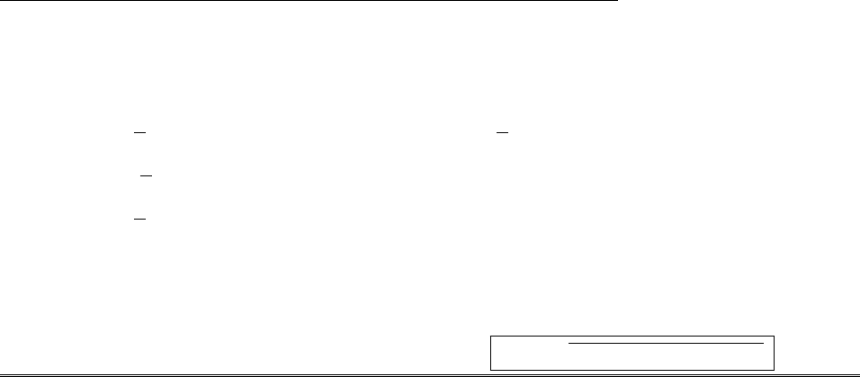
CHAPTER 9. ELECTROMAGNETIC WAVES 209
These automatically satisfy the boundary condition B?=0(Bx= 0 at x= 0 and x=a,By= 0 at y= 0 and
y=b, and Bz= 0 at z= 0 and z=d).
As a check, let’s see if r·B=0:
r·B=i
!(Fk
yDkz)kxcos(kxx) cos(kyy) cos(kzz)i
!(BkzFk
x)kycos(kxx) cos(kyy) cos(kzz)
i
!(DkxBky)kzcos(kxx) cos(kyy) cos(kzz)
=i
!(Fk
xkyDkxkz+BkzkyFk
xky+DkxkzBkykz) cos(kxx) cos(kyy) cos(kzz)=0.X
The boxed equations satisfy all of Maxwell’s equations, and they meet the boundary conditions. For TE
modes, we pick Ez= 0, so F= 0 (and hence Bkx+Dky= 0, leaving only the overall amplitude undetermined,
for given l,m, and n); for TM modes we want Bz= 0 (so DkxBky= 0, again leaving only one amplitude
undetermined, since Bkx+Dky+Fk
z= 0). In either case (TElmn or TMlmn), the frequency is given by
!2=c2(k2
x+k2
y+k2
z)=c2(m⇡/a)2+(n⇡/b)2+(l⇡/d)2, or !=c⇡(m/a)2+(n/b)2+(l/d)2.
c
2012 Pearson Education, Inc., Upper Saddle River, NJ. All rights reserved. This material is
protected under all copyright laws as they currently exist. No portion of this material may be
reproduced, in any form or by any means, without permission in writing from the publisher.
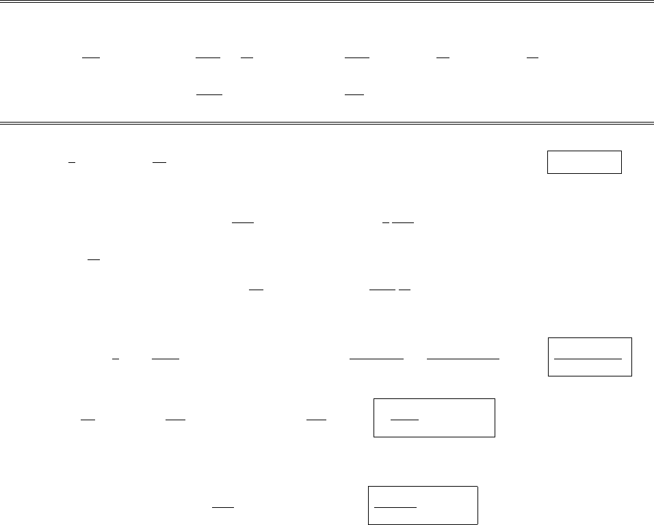
210 CHAPTER 10. POTENTIALS AND FIELDS
Chapter 10
Potentials and Fields
Problem 10.1
22V+@L
@t=r2Vµ0✏0
@2V
@t2+@
@t(r·A)+µ0✏0
@2V
@t2=r2V+@
@t(r·A)=1
✏0
⇢.X
22ArL=r2Aµ0✏0
@2A
@t2rr·A+µ0✏0
@V
@t=µ0J.X
Problem 10.2
(a) W=1
2✏0E2+1
µ0
B2d⌧.At t1=d/c, x d=ct1,so E=0,B=0,and hence W(t1)=0.
At T2=(d+h)/c,ct2=d+h:
E=µ0k
2(d+hx)ˆz ,B=1
c
µ0k
2(d+hx)ˆy ,
so B2=1
c2E2, and ✏0E2+1
µ0
B2=✏0E2+1
µ0✏0
1
c2E2=2✏0E2.
Therefore
W(t2)=1
2(2✏0)µ2
0k2
4
(d+h)
d
(d+hx)2dx (lw)= ✏0µ2
0k2lw
4(d+hx)3
3d+h
d
=✏0µ2
0k2lwh3
12 .
(b) S(x)= 1
µ0
(E⇥B)= 1
µ0cE2[ˆz ⇥(±ˆy )] = ±1
µ0cE2ˆx =±µ0k2
4c(ct |x|)2ˆx
(plus sign for x>0, as here). For |x|> ct, S= 0.
So the energy per unit time entering the box in this time interval is
dW
dt =P=S(d)·da=µ0k2lw
4c(ct d)2.
Note that no energy flows out the top, since S(d+h) = 0.
c
2012 Pearson Education, Inc., Upper Saddle River, NJ. All rights reserved. This material is
protected under all copyright laws as they currently exist. No portion of this material may be
reproduced, in any form or by any means, without permission in writing from the publisher.
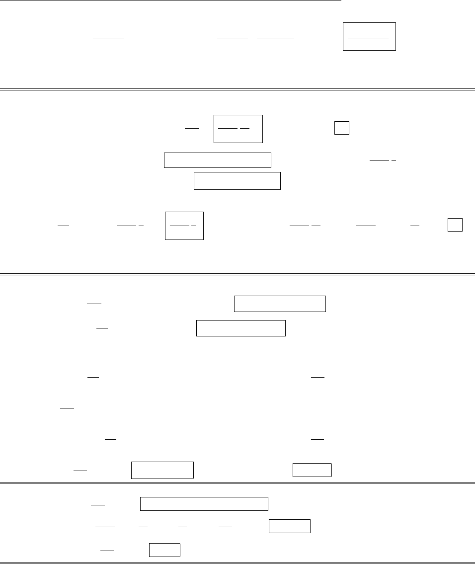
CHAPTER 10. POTENTIALS AND FIELDS 211
(c) W=
t2
t1
P dt =µ0k2lw
4c
(d+h)/c
d/c
(ct d)2dt =µ0k2lw
4c(ct d)3
3c(d+h)/c
d/c
=µ0k2lwh3
12c2.
Since 1/c2=µ0✏0, this agrees with the answer to (a).
Problem 10.3
(a)
E=rV@A
@t=1
4⇡✏0
q
r2ˆr .B=r⇥A=0.
This is a funny set of potentials for a stationary point charge qat the origin. (V=1
4⇡✏0
q
r,A=0would, of
course, be the customary choice.) Evidently ⇢=q3(r); J=0.
(b)
V0=V@
@t=01
4⇡✏0
q
r=1
4⇡✏0
q
r;A0=A+r=1
4⇡✏0
qt
r2ˆr +1
4⇡✏0
qt1
r2ˆr =0.
This gauge function transforms the “funny” potentials into the “ordinary” potentials of a stationary point
charge.
Problem 10.4
E=rV@A
@t=A0cos(kx !t)ˆy (!)= A0!cos(kx !t)ˆy ,
B=r⇥A=ˆz @
@x[A0sin(kx !t)] = A0kcos(kx !t)ˆz .
Hence r·E=0X,r·B=0X.
r⇥E=ˆz @
@x[A0!cos(kx !t)] = A0!ksin(kx !t)ˆz ,@B
@t=A0!ksin(kx !t)ˆz ,
so r⇥E=@B
@tX.
r⇥B=ˆy @
@x[A0kcos(kx !t)] = A0k2sin(kx !t)ˆy ,@E
@t=A0!2sin(kx !t)ˆy .
So r⇥B=µ0✏0
@E
@tprovided k2=µ0✏0!2,or, since c2=1/µ0✏0,!=ck.
Problem 10.5
Ex. 10.1: r·A= 0; @V
@t=0.Both Coulomb and Lorentz.
Prob. 10.3: r·A=qt
4⇡✏0r·ˆr
r2=qt
✏0
3(r); @V
@t=0. Neither.
Prob. 10.4: r·A= 0; @V
@t=0.Both.
c
2012 Pearson Education, Inc., Upper Saddle River, NJ. All rights reserved. This material is
protected under all copyright laws as they currently exist. No portion of this material may be
reproduced, in any form or by any means, without permission in writing from the publisher.
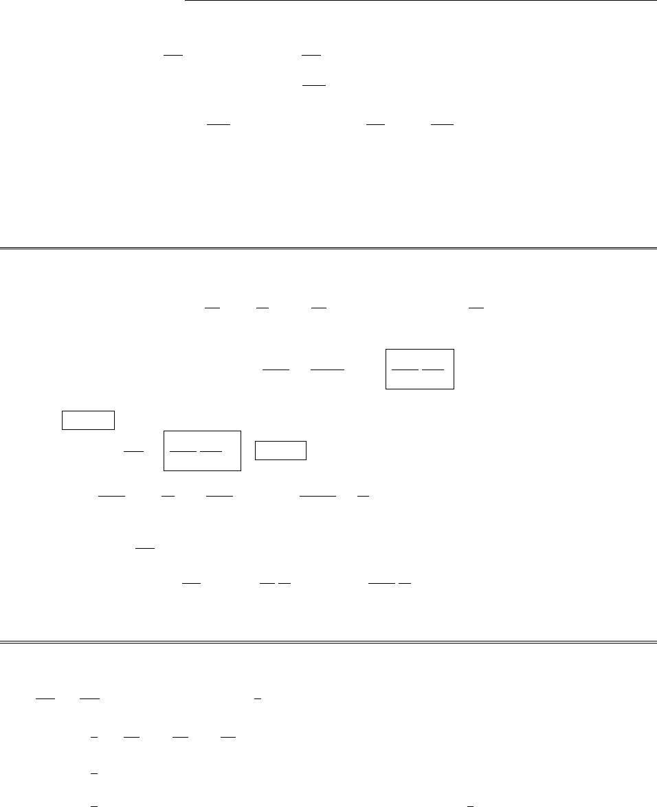
212 CHAPTER 10. POTENTIALS AND FIELDS
Problem 10.6
Suppose r·A6=µ0✏0
@V
@t. (Let r·A+µ0✏0
@V
@t=—some known function.) We want to pick such
that A0and V0(Eq. 10.7) do obey r·A0=µ0✏0
@V0
@t.
r·A0+µ0✏0
@V0
@t=r·A+r2+µ0✏0
@V
@tµ0✏0
@2
@t2=+22.
This will be zero provided we pick for the solution to 22=, which by hypothesis (and in fact) we know
how to solve.
We could always find a gauge in which V0= 0, simply by picking =t
0Vdt
0.Wecannot in general pick
A=0—this would make B=0. [Finding such a gauge function would amount to expressing Aas r, and
we know that vector functions cannot in general be written as gradients—only if they happen to have curl
zero, which A(ordinarily) does not.]
Problem 10.7
(a) Using Eq. 1.99,
r·J=˙q
4⇡r·ˆr
r2=˙q
4⇡4⇡3(r)=˙q3(r)=@⇢
@t.X
(b) From Eq. 10.10,
V(r,t)= q
4⇡✏03(r0)
r
d⌧0=1
4⇡✏0
q(t)
r.
By symmetry, B=0(what direction could it point?), so r⇥A=0,r·A= 0, and A!0at infinity.
Evidently A=0.
(c) E=rV@A
@t=1
4⇡✏0
q(t)
r2ˆr .B=0. Checking Maxwell’s equations:
r·E=q
4⇡✏0r·ˆr
r2=q
4⇡✏0
4⇡3(r)=q3(r)
✏0
=⇢
✏0
.X
r·B=0.X
r⇥E=0=@B
@t.X
r⇥B=0;µ0J+µ0✏0
@E
@t=µ01
4⇡
˙q
r2ˆr +µ0✏0˙q
4⇡✏0
1
r2ˆr =0.X
[Note that the displacement current exactly cancels the conduction current. Physically, this configuration is a
point charge at the origin that is changing with time as current flows in symmetrically (from infinity).]
Problem 10.8
Noting the Ais independent of tand Bis independent of r, use Eq. 10.19:
dA
dt =@A
@t+(v·r)A=(v·r)1
2(r⇥B)
=1
2vx
@
@x+vy
@
@y+vz
@
@z[(yBzzBy)ˆx +(zBxxBz)ˆy +(xByyBx)ˆz ]
=1
2[vx(Bzˆy +Byˆz )+vy(Bzˆx Bxˆz )+vz(Byˆx +Bxˆy )]
=1
2[(vyBzvzBy)ˆx +(vzBxvxBz)ˆy +(vxByvyBx)ˆz ]=1
2(v⇥B).X
c
2012 Pearson Education, Inc., Upper Saddle River, NJ. All rights reserved. This material is
protected under all copyright laws as they currently exist. No portion of this material may be
reproduced, in any form or by any means, without permission in writing from the publisher.
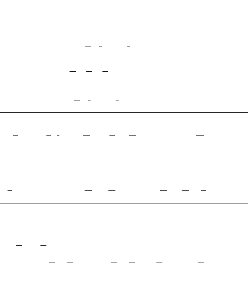
CHAPTER 10. POTENTIALS AND FIELDS 213
Equation 10.20 says
d
dt(p+qA)= dp
dt q
2(v⇥B)=qr(v·A)=q
2r[v·(r⇥B)],
or dp
dt =q
2(v⇥B)q
2r[r·(B⇥v)].
Now, for a vector cthat is independent of position,
r(r·c)=ˆx @
@x+ˆy @
@y+ˆz @
@z(xcx+ycy+zcz)=cxˆx +cyˆy +czˆz )=c.
In this case c=(B⇥v)=(v⇥B), so
dp
dt =q
2(v⇥B)+ q
2(v⇥B)=q(v⇥B).X
Problem 10.9
d
dt(T+qV )= d
dt 1
2mv2+qdV
dt =mv·dv
dt +q@V
@t+(v·r)V=v·F+q@V
@t+(v·r)V.
But Eq. 10.17 says
v·F=qv·rV@A
@t+v⇥(r⇥A)=qv·rV+v·@A
@t,
so
d
dt(T+qV )=q(v·r)V+v·@A
@t+q@V
@t+(v·r)V=q@V
@tv·@A
@t=@
@t[q(Vv·A)] .
Problem 10.10
From the product rule:
r·J
r
=1
r
(r·J)+J·r1
r
,r0·J
r
=1
r
(r0·J)+J·r01
r
.
But r1
r
=r01
r
, since
r
=rr0. So
r·J
r
=1
r
(r·J)J·r01
r
=1
r
(r·J)+ 1
r
(r0·J)r0·J
r
.
But
r·J=@Jx
@x+@Jy
@y+@Jz
@z=@Jx
@tr
@tr
@x+@Jy
@tr
@tr
@y+@Jz
@tr
@tr
@z,
and @tr
@x=1
c
@
r
@x,@tr
@y=1
c
@
r
@y,@tr
@z=1
c
@
r
@z,
c
2012 Pearson Education, Inc., Upper Saddle River, NJ. All rights reserved. This material is
protected under all copyright laws as they currently exist. No portion of this material may be
reproduced, in any form or by any means, without permission in writing from the publisher.
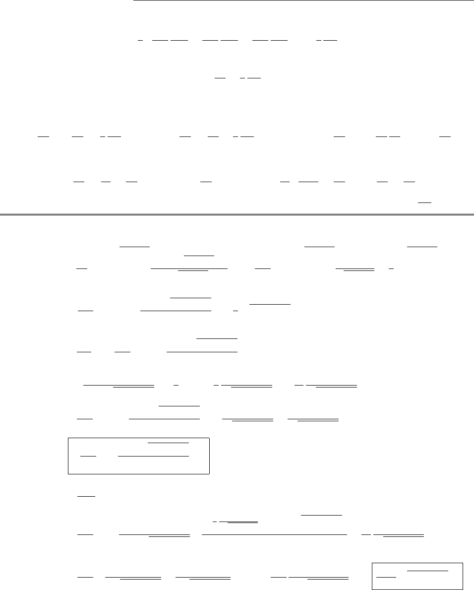
214 CHAPTER 10. POTENTIALS AND FIELDS
so
r·J=1
c@Jx
@tr
@
r
@x+@Jy
@tr
@
r
@y+@Jz
@tr
@
r
@z=1
c
@J
@tr·(r
r
).
Similarly,
r0·J=@⇢
@t1
c
@J
@tr·(r0
r
).
[The first term arises when we di↵erentiate with respect to the explicit r0, and use the continuity equation.]
thus
r·J
r
=1
r
1
c
@J
@tr·(r0
r
)+1
r
@⇢
@t1
c
@J
@tr·(r0
r
)r·J
r
=1
r
@⇢
@tr0·J
r
(the other two terms cancel, since r
r
=r0
r
). Therefore:
r·A=µ0
4⇡@
@t⇢
r
d⌧r0·J
r
d⌧=µ0✏0
@
@t1
4⇡✏0⇢
r
d⌧µ0
4⇡J
r
·da.
The last term is over the suface at “infinity”, where J= 0, so it’s zero. Therefore r·A=µ0✏0
@V
@t.X
Problem 10.11
(a) As in Ex. 10.2, for t < s/c, A=0; for t > s/c,
A(s, t)=µ0
4⇡ˆz 2
p(ct)2s2
0
k(tps2+z2/c)
ps2+z2dz =µ0k
2⇡ˆz
t
p(ct)2s2
0
dz
ps2+z21
c
p(ct)2s2
0
dz
=µ0k
2⇡ˆz tln ct +(ct)2s2
s1
c(ct)2s2.Accordingly,
E(s, t)=@A
@t=µ0k
2⇡ˆz ln ct +(ct)2s2
s+
ts
ct +(ct)2s21
sc+1
2
2c2t
(ct)2s21
2c
2c2t
(ct)2s2
=µ0k
2⇡ˆz ln ct +(ct)2s2
s+ct
(ct)2s2ct
(ct)2s2
=µ0k
2⇡ln ct +(ct)2s2
sˆz (or zero, for t < s/c).
B(s, t)=@Az
@sˆ
=µ0k
2⇡
ts
ct +(ct)2s2s1
2
(2s)
p(ct)2s2ct (ct)2s2
s21
2c
(2s)
(ct)2s2
ˆ
=µ0k
2⇡ct2
s(ct)2s2+s
c(ct)2s2ˆ
=µ0k
2⇡
(c2t2+s2)
sc(ct)2s2
ˆ
=µ0k
2⇡sc(ct)2s2ˆ
.
c
2012 Pearson Education, Inc., Upper Saddle River, NJ. All rights reserved. This material is
protected under all copyright laws as they currently exist. No portion of this material may be
reproduced, in any form or by any means, without permission in writing from the publisher.
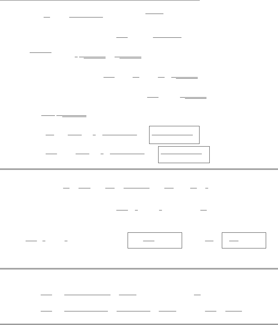
CHAPTER 10. POTENTIALS AND FIELDS 215
(b) A(s, t)= µ0
4⇡ˆz 1
1
q0(t
r
/c)
r
dz. But
r
=ps2+z2, so the integrand is even in z:
A(s, t)=µ0q0
4⇡ˆz 21
0
(t
r
/c)
r
dz.
Now z=
r
2s2)dz =1
2
2
r
d
r
p
r
2s2=
r
d
r
p
r
2s2, and z=0)
r
=s, z =1)
r
=1. So:
A(s, t)=µ0q0
2⇡ˆz 1
s
1
r
t
r
c
r
d
r
p
r
2s2.
Now (t
r
/c)=c(
r
ct) (Ex. 1.15); therefore A=µ0q0
2⇡ˆz c1
s
(
r
ct)
p
r
2s2d
r
, so
A(s, t)=µ0q0c
2⇡
1
(ct)2s2ˆz (or zero, if ct < s);
E(s, t)=@A
@t=µ0q0c
2⇡1
22c2t
[(ct)2s2]3/2ˆz =µ0q0c3t
2⇡[(ct)2s2]3/2ˆz (or zero, for t < s/c);
B(s, t)=@Az
@tˆ
=µ0q0c
2⇡1
22s
[(ct)2s2]3/2ˆ
=µ0q0cs
2⇡[(ct)2s2]3/2ˆ
(or zero, for t < s/c).
Problem 10.12
A=µ0
4⇡I(tr)
r
dl =µ0k
4⇡(t
r
/c)
r
dl=µ0k
4⇡tdl
r
1
cdl.
But for the complete loop, dl= 0, so A=µ0kt
4⇡1
a1
dl+1
b2
dl+2ˆx b
a
dx
x. Here 1dl=2aˆx (inner
circle), 2dl=2bˆx (outer circle), so
A=µ0kt
4⇡1
a(2a)+1
b(2b) + 2 ln(b/a)ˆx )A=µ0kt
2⇡ln(b/a)ˆx ,E=@A
@t=µ0k
2⇡ln(b/a)ˆx .
The changing magnetic field induces the electric field. Since we only know Aat one point (the center), we
can’t compute r⇥Ato get B.
Problem 10.13
In this case ˙⇢(r,t)= ˙⇢(r,0) and ˙
J(r,t) = 0, so Eq. 10.36 )
E(r,t)= 1
4⇡✏0⇢(r0,0) + ˙⇢(r0,0)tr
r
2+˙⇢(r0,0)
c
r
ˆ
r
d⌧0,but tr=t
r
c(Eq.10.18),so
=1
4⇡✏0⇢(r0,0) + ˙⇢(r0,0)t
r
2˙⇢(r0,0)(
r
/c)
r
2+˙⇢(r0,0)
c
r
ˆ
r
d⌧0=1
4⇡✏0⇢(r0,t)
r
2ˆ
r
d⌧0.qed
c
2012 Pearson Education, Inc., Upper Saddle River, NJ. All rights reserved. This material is
protected under all copyright laws as they currently exist. No portion of this material may be
reproduced, in any form or by any means, without permission in writing from the publisher.

216 CHAPTER 10. POTENTIALS AND FIELDS
Problem 10.14
In this approximation we’re dropping the higher derivatives of J,so ˙
J(tr)= ˙
J(t), and Eq. 10.38 )
B(r,t)= µ0
4⇡1
r
2J(r0,t)+(trt)˙
J(r0,t)+
r
c˙
J(r0,t)⇥ˆ
r
d⌧0,but trt=
r
c(Eq.10.25),so
=µ0
4⇡J(r0,t)⇥ˆ
r
r
2d⌧0.qed
Problem 10.15
At time tthe charge is at r(t)=a[cos(!t)ˆx + sin(!t)ˆy ], so v(t)=!a[sin(!t)ˆx + cos(!t)ˆy ]. Therefore
r
=zˆz a[cos(!tr)ˆx + sin(!tr)ˆy ], and hence
r
2=z2+a2(of course), and
r
=pz2+a2.
ˆ
r
·v=1
r
(
r
·v)= 1
r
!a2[sin(!tr) cos(!tr) + sin(!tr) cos(!tr)]=0,so 1ˆ
r
·v
c=1.
Therefore
V(z,t)= 1
4⇡✏0
q
pz2+a2;A(z,t)= q!a
4⇡✏0c2pz2+a2[sin(!tr)ˆx + cos(!tr)ˆy ),where tr=tpz2+a2
c.
Problem 10.16
Term under square root in (Eq. 10.49) is:
I=c4t22c2t(r·v)+(r·v)2+c2r2c4t2v2r2+v2c2t2
=(r·v)2+(c2v2)r2+c2(vt)22c2(r·vt).put in vt=rR2.
=(r·v)2+(c2v2)r2+c2(r2+R22r·R)2c2(r2r·R)=(r·v)2r2v2+c2R2.
but
(r·v)2r2v2= ((R+vt)·v)2(R+vt)2v2
=(R·v)2+v4t2+ 2(R·v)v2tR2v22(R·v)tv2v2t2v2
=(R·v)2R2v2=R2v2cos2✓R2v2=R2v21cos2✓
=R2v2sin2✓.
Therefore
I=R2v2sin2✓+c2R2=c2R21v2
c2sin2✓.
Hence
V(r,t)= 1
4⇡✏0
q
R1v2
c2sin2✓
.qed
Problem 10.17
Once seen, from a given point x, the particle will forever remain in view—to disappear it would have to
travel faster than light.
c
2012 Pearson Education, Inc., Upper Saddle River, NJ. All rights reserved. This material is
protected under all copyright laws as they currently exist. No portion of this material may be
reproduced, in any form or by any means, without permission in writing from the publisher.

CHAPTER 10. POTENTIALS AND FIELDS 217
Problem 10.18
First calculate tr:tr=t|rw(tr)|/c )
c(trt)=xb2+c2t2
r)c(trt)+x=b2+c2t2
r;
c2t2
r2c2trt+c2t2+2xctr2xct +x2=b2+c2t2
r;
2ctr(xct)+(x22xct +c2t2)=b2;
2ctr(xct)=b2(xct)2,or tr=b2(xct)2
2c(xct).
Now V(x, t)= 1
4⇡✏0
qc
(
r
c
r
·v),and
r
c
r
·v=
r
(cv);
r
=c(ttr).
v=1
2
1
b2+c2t2
r
2c2tr=c2tr
c(trt)+x=c2tr
ctr+(xct);(cv)=c2tr+c(xct)c2tr
ctr+(xct)=c(xct)
ctr+(xct);
r
c
r
·v=c(ttr)c(xct)
ctr+(xct)=c2(ttr)(xct)
ctr+(xct);ctr+(xct)=b2(xct)2
2(xct)+(xct)= b2+(xct)2
2(xct);
ttr=2ct(xct)b2+(xct)2
2c(xct)=(xct)(x+ct)b2
2c(xct)=(x2c2t2b2)
2c(xct).Therefore
1
r
c
r
·v=b2+(xct)2
2(xct)1
c2(xct)
2c(xct)
[2ct(xct)b2+(xct)2]=b2+(xct)2
c(xct)[2ct(xct)b2+(xct)2].
The term in square brackets simplifies to (2ct +xct)(xct)b2=(x+ct)(xct)b2=x2c2t2b2.
So V(x, t)= q
4⇡✏0
b2+(xct)2
(xct)(x2c2t2b2).
Meanwhile
A=V
c2v=c2tr
ctr+(xct)
V
c2ˆx =b2(xct)2
2c(xct)2(xct)
b2+(xct)2
q
4⇡✏0
b2+(xct)2
(xct)(x2c2t2b2)ˆx
=q
4⇡✏0c
b2(xct)2
(xct)(x2c2t2b2)ˆx .
c
2012 Pearson Education, Inc., Upper Saddle River, NJ. All rights reserved. This material is
protected under all copyright laws as they currently exist. No portion of this material may be
reproduced, in any form or by any means, without permission in writing from the publisher.

218 CHAPTER 10. POTENTIALS AND FIELDS
Problem 10.19
From Eq. 10.44, c(ttr)=
r
)c2(ttr)2=
r
2=
r
·
r
. Di↵erentiate with respect to t:
2c2(ttr)1@tr
@t=2
r
·@
r
@t,or c
r
1@tr
@t=
r
·@
r
@t. Now
r
=rw(tr),so
@
r
@t=@w
@t=@w
@tr
@tr
@t=v@tr
@t;c
r
1@tr
@t=
r
·v@tr
@t;c
r
=@tr
@t(c
r
r
·v)=
@tr
@t(
r
·u) (Eq.10.71),and hence @tr
@t=c
r
r
·u.qed
Now Eq. 10.47 says A(r,t)= v
c2V(r,t), so
@A
@t=1
c2@v
@tV+v@V
@t=1
c2@v
@tr
@tr
@tV+v@V
@t
=1
c2a@tr
@t
1
4⇡✏0
qc
r
·u+v1
4⇡✏0
qc
(
r
·u)2
@
@t(
r
c
r
·v)
=1
c2
qc
4⇡✏0a
r
·u
@tr
@tv
(
r
·u)2c@
r
@t@
r
@t·v
r
·@v
@t.
But
r
=c(ttr))@
r
@t=c1@tr
@t,
r
=rw(tr))@
r
@t=v@tr
@t(as above),and
@v
@t=@v
@tr
@tr
@t=a@tr
@t.
=q
4⇡✏0c(
r
·u)2a(
r
·u)@tr
@tvc21@tr
@t+v2@tr
@t
r
·a@tr
@t
=q
4⇡✏0c(
r
·u)2c2v+(
r
·u)a+(c2v2+
r
·a)v@tr
@t
=q
4⇡✏0c(
r
·u)2c2v+(
r
·u)a+(c2v2+
r
·a)vc
r
r
·u
=q
4⇡✏0c(
r
·u)3c2v(
r
·u)+c
r
(
r
·u)a+c
r
(c2v2+
r
·a)v
=qc
4⇡✏0
1
(
r
c
r
·v)3(
r
c
r
·v)v+
r
ca+
r
c(c2v2+
r
·a)v.qed
Problem 10.20
E=q
4⇡✏0
r
(
r
·u)3(c2v2)u+
r
⇥(u⇥a). Here
v=vˆx ,a=aˆx ,and,for points to the right,ˆ
r
=ˆx .
So u=(cv)ˆx ,u⇥a=0,and
r
·u=
r
(cv).
E=q
4⇡✏0
r
r
3(cv)3(c2v2)(cv)ˆx =q
4⇡✏0
1
r
2
(c+v)(cv)2
(cv)3ˆx =q
4⇡✏0
1
r
2c+v
cvˆx ;
B=1
cˆ
r
⇥E=0.qed
For field points to the left,ˆ
r
=ˆx and u=(c+v)ˆx ,so
r
·u=
r
(c+v), and
E=q
4⇡✏0
r
r
3(c+v)3(c2v2)(c+v)ˆx =q
4⇡✏0
1
r
2cv
c+vˆx ;B=0.
c
2012 Pearson Education, Inc., Upper Saddle River, NJ. All rights reserved. This material is
protected under all copyright laws as they currently exist. No portion of this material may be
reproduced, in any form or by any means, without permission in writing from the publisher.

CHAPTER 10. POTENTIALS AND FIELDS 219
Problem 10.21
By Gauss’s law (in integral form) the answer has to be q/✏0.
E=1
4⇡✏0
q(1 v2/c2)
(1 v2
c2sin2✓)3/2
R
R2(Eq. 10.75), so
E·da=q(1 v2/c2)
4⇡✏0R2sin ✓d✓d
R2(1 v2
c2sin2✓)3/2=q(1 v2/c2)
4⇡✏0
2⇡⇡
0
sin ✓d✓
(1 v2
c2sin2✓)3/2.
Let u⌘cos ✓,sodu =sin ✓d✓, sin2✓=1u2.
E·da=q(1 v2/c2)
2✏01
1
du
[1 v2
c2+v2
c2u2]3/2=q(1 v2/c2)
2✏0c
v31
1
du
c2
v21+u23/2.
The integral is: u
c2
v21c2
v21+u2
+1
1
=2
c2
v21c
v
=v
c32
(1 v2/c2).So
E·da=q(1 v2/c2)
2✏0c
v3v
c32
(1 v2/c2)=q
✏0
.X
Problem 10.22
(a) E=
4⇡✏0
(1 v2/c2)ˆ
R
R2
dx
1(v/c)2sin2✓3/2.
The horizontal components cancel; the vertical com-
ponent of ˆ
Ris sin ✓(see diagram). Here d=Rsin ✓, so
1
R2=sin2✓
d2;x
d= cot ✓,sodx =d(csc2✓)d✓=d
sin2✓d✓;
1
R2dx =d
sin2✓
sin2✓
d2d✓=d✓
d.Thus
E=
4⇡✏0
(1 v2/c2)ˆy
d⇡
0
sin ✓
1(v/c)2sin2✓3/2d✓.Let z⌘cos ✓,so sin2✓=1z2.
=(1 v2/c2)ˆy
4⇡✏0d1
1
1
[1 (v/c)2+(v/c)2z2]3/2dz
=(1 v2/c2)ˆy
4⇡✏0d1
(v/c)3
z
(c2/v21)(c/v)21+z2
+1
1
=(1 v2/c2)
4⇡✏0d
c
v
1
(1 v2/c2)
2
(c/v)21+1ˆy =1
4⇡✏0
2
dˆy (same as for a line charge at rest).
(b) B=1
c2(v⇥E) for each segment dq =dx. Since vis constant, it comes outside the integral, and the
same formula holds for the total field:
B=1
c2(v⇥E)= 1
c2v1
4⇡✏0
2
d(ˆx ⇥ˆy )=µ0✏0v1
4⇡✏0
2
dˆz =µ0
4⇡
2v
dˆz .
c
2012 Pearson Education, Inc., Upper Saddle River, NJ. All rights reserved. This material is
protected under all copyright laws as they currently exist. No portion of this material may be
reproduced, in any form or by any means, without permission in writing from the publisher.
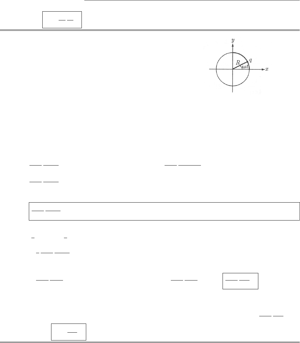
220 CHAPTER 10. POTENTIALS AND FIELDS
But v=I, so B=µ0
4⇡
2I
dˆ
(the same as we got in magnetostatics, Eq. 5.39 and Ex. 5.7).
Problem 10.23
w(t)=R[cos(!t)ˆx + sin(!t)ˆy ];
v(t)=R![sin(!t)ˆx + cos(!t)ˆy ];
a(t)=R!2[cos(!t)ˆx + sin(!t)ˆy ]=!2w(t);
r
=w(tr);
r
=R;
tr=tR/c;
ˆ
r
=[cos(!tr)ˆx + sin(!tr)ˆy ];
u=cˆ
r
v(tr)=c[cos(!tr)ˆx + sin(!tr)ˆy ]!R[sin(!tr)ˆx + cos(!tr)ˆy ]
={[ccos(!tr)!Rsin(!tr)] ˆx +[csin(!tr)+!Rcos(!tr)] ˆy };
r
⇥(u⇥a)=(
r
·a)u(
r
·u)a;
r
·a=w·(!2w)=!2R2;
r
·u=Rccos2(!tr)!Rsin(!tr) cos(!tr)+csin2(!tr)+!Rsin(!tr) cos(!tr)=Rc;
v2=(!R)2. So (Eq. 10.72):
E=q
4⇡✏0
R
(Rc)3uc2!2R2+u(!R)2a(Rc)=q
4⇡✏0
cuRa
(Rc)2
=q
4⇡✏0
1
(Rc)2[c2cos(!tr)!Rc sin(!tr)] ˆx [c2sin(!tr)+!Rc cos(!tr)] ˆy
+R2!2cos(!tr)ˆx +R2!2sin(!tr)ˆy
=q
4⇡✏0
1
(Rc)2!2R2c2cos(!tr)+!Rc sin(!tr)ˆx +!2R2c2sin(!tr)!Rc cos(!tr)ˆy .
B=1
cˆ
r
⇥E=1
cˆ
r
xEyˆ
r
yExˆz
=1
c
q
4⇡✏0
1
(Rc)2cos(!tr)!2R2c2sin(!tr)!Rc cos(!tr)
sin(!tr)!2R2c2cos(!tr)+!Rc sin(!tr)ˆz
=q
4⇡✏0
1
R2c3!Rc cos2(!tr)!Rc sin2(!tr)ˆz =q
4⇡✏0
1
R2c3!Rc ˆz =q
4⇡✏0
!
Rc2ˆz .
Notice that Bis constant in time.
To obtain the field at the center of a circular ring of charge, let q!(2⇡R); for this ring to carry current
I, we need I=v=!R,so=I/!R, and hence q!(I/!R)(2⇡R)=2⇡I/!. Thus B=2⇡I
4⇡✏0
1
Rc2ˆz , or,
since 1/c2=✏0µ0,B=µ0I
2Rˆz ,the same as Eq. 5.41, in the case z= 0.
c
2012 Pearson Education, Inc., Upper Saddle River, NJ. All rights reserved. This material is
protected under all copyright laws as they currently exist. No portion of this material may be
reproduced, in any form or by any means, without permission in writing from the publisher.

CHAPTER 10. POTENTIALS AND FIELDS 221
Problem 10.24
(,t)=0|sin(✓/2)|,where ✓=!t. So the (retarded) scalar potential at the center is (Eq. 10.26)
V(t)= 1
4⇡✏0
r
dl0=1
4⇡✏02⇡
0
0|sin[(!tr)/2]|
aad
=0
4⇡✏02⇡
0
sin(✓/2) d✓=0
4⇡✏0
[2 cos(✓/2)]
2⇡
0
=0
4⇡✏0
[2 (2)] = 0
⇡✏0
.
(Note: at fixed tr,d=d✓, and it goes through one full cycle of or ✓.)
Meanwhile I(,t)=v=0!a|sin[(!t)/2]|ˆ
. From Eq. 10.26 (again)
A(t)= µ0
4⇡I
r
dl0=µ0
4⇡2⇡
0
0!a|sin[(!tr)/2]|ˆ
aad.
But tr=ta/c is again constant,for the integration,and ˆ
=sin ˆx + cos ˆy .
=µ00!a
4⇡2⇡
0|sin[(!tr)/2]|(sin ˆx + cos ˆy )d.Again,switch variables to ✓=!tr,
and integrate from ✓= 0 to ✓=2⇡(so we don0t have to worry about the absolute value).
=µ00!a
4⇡2⇡
0
sin(✓/2) [sin(✓+!tr)ˆx + cos(✓+!tr)ˆy ]d✓.Now
2⇡
0
sin (✓/2) sin(✓+!tr)d✓=1
22⇡
0
[cos (✓/2+!tr)cos (3✓/2+!tr)] d✓
=1
22 sin (✓/2+!tr)2
3sin (3✓/2+!tr)
2⇡
0
= sin(⇡+!tr)sin(!tr)1
3sin(3⇡+!tr)+1
3sin(!tr)
=2 sin(!tr)+2
3sin(!tr)=4
3sin(!tr).
2⇡
0
sin (✓/2) cos(✓+!tr)d✓=1
22⇡
0
[sin (✓/2+!tr) + sin (3✓/2+!tr)] d✓
=1
22 cos (✓/2+!tr)2
3cos (3✓/2+!tr)
2⇡
0
= cos(⇡+!tr)cos(!tr)1
3cos(3⇡+!tr)+1
3cos(!tr)
=2 cos(!tr)+2
3cos(!tr)=4
3cos(!tr).So
A(t)=µ00!a
4⇡4
3[sin(!tr)ˆx cos(!tr)ˆy ]= µ00!a
3⇡{sin[!(ta/c)] ˆx cos[!(ta/c)] ˆy }.
c
2012 Pearson Education, Inc., Upper Saddle River, NJ. All rights reserved. This material is
protected under all copyright laws as they currently exist. No portion of this material may be
reproduced, in any form or by any means, without permission in writing from the publisher.

222 CHAPTER 10. POTENTIALS AND FIELDS
Problem 10.25
1
Hello
r·A=1
c2
@V
@t
c
2005 Pearson Education, Inc., Upper Saddle River, NJ. All rights reserved. This material is
protected under all copyright laws as they currently exist. No portion of this material may be
reproduced, in any form or by any means, without permission in writing from the publisher.
Problem 10.26
⇢(r,t)=
Q
(4/3)⇡R3=3Q
4⇡v3t3,(r<R=vt),
0,(otherwise).
For a point at the center, tr=tr/c,so
⇢(r,t
r)=
3Q
4⇡v3(tr/c)3=3Q
4⇡(v/c)3(ct r)3,r<v(tr/c))r< vt
1+v/c,
0,(otherwise).
Let a⌘vt/(1 + v/c); then
Qe↵=3Q
4⇡(v/c)3a
0
1
(ct r)34⇡r2dr =3Q
(v/c)3a
0
r2
(ct r)3dr
=3Q
(v/c)3ln(ct r)+ 2ct
(ct r)(ct)2
2(ct r)2
a
0
=3Q
(v/c)3ln(ct a)+ 2ct
(ct a)(ct)2
2(ct a)2ln(ct)2+1
2
=3Q
(v/c)33
2+ ln ct
ct a2ct
ct a+1
2ct
ct a2.
c
2012 Pearson Education, Inc., Upper Saddle River, NJ. All rights reserved. This material is
protected under all copyright laws as they currently exist. No portion of this material may be
reproduced, in any form or by any means, without permission in writing from the publisher.
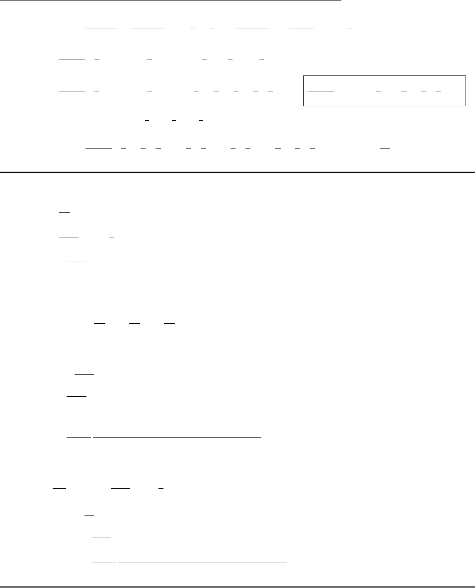
CHAPTER 10. POTENTIALS AND FIELDS 223
Now, ct a=ct vt
1+v/c =ct
1+v/c 1+v
cv
c=ct
1+v/c, so ct
ct a=1+v
c,and hence
Qe↵=3Q
(v/c)33
2+ ln 1+ v
c21+v
c+1
21+v
c2
=3Q
(v/c)33
2+ ln 1+ v
c22v
c+1
2+v
c+1
2v
c2=3Q
(v/c)3ln 1+v
cv
c+1
2v
c2.
If ✏⌧1, then ln(1 + ✏)=✏1
2✏2+1
3✏31
4✏4+..., so for v⌧c,
Qe↵⇡3Q
(v/c)3v
c1
2v
c2+1
3v
c31
4v
c4v
c+1
2v
c2=Q13v
4c.X
Problem 10.27
Using Product Rule #5, Eq. 10.50 )
r·A=µ0
4⇡qcv·r(c2tr·v)2+(c2v2)(r2c2t2)1/2
=µ0qc
4⇡v·1
2(c2tr·v)2+(c2v2)(r2c2t2)3/2r(c2tr·v)2+(c2v2)(r2c2t2)
=µ0qc
8⇡(c2tr·v)2+(c2v2)(r2c2t2)3/2v·2(c2tr·v)r(r·v)+(c2v2)r(r2).
Product Rule #4 )
r(r·v)=v⇥(r⇥r)+(v·r)r,but r⇥r=0,
(v·r)r=vx
@
@x+vy
@
@y+vz
@
@z(xˆx +yˆy +zˆz )=vxˆx +vyˆy +vzˆz =v,and
r(r2)=r(r·r)=2r⇥(r⇥r) + 2(r·r)r=2r.So
r·A=µ0qc
8⇡(c2tr·v)2+(c2v2)(r2c2t2)3/2v·2(c2tr·v)v+(c2v2)2r
=µ0qc
4⇡(c2tr·v)2+(c2v2)(r2c2t2)3/2(c2tr·v)v2(c2v2)(r·v).
But the term in curly brackets is : c2tv2v2(r·v)c2(r·v)+v2(r·v)=c2(v2tr·v).
=µ0qc3
4⇡
(v2tr·v)
[(c2tr·v)2+(c2v2)(r2c2t2)]3/2.
Meanwhile, from Eq. 10.49,
µ0✏0
@V
@t=µ0✏0
1
4⇡✏0
qc 1
2(c2tr·v)2+(c2v2)(r2c2t2)3/2⇥
@
@t(c2tr·v)2+(c2v2)(r2c2t2)
=µ0qc
8⇡(c2tr·v)2+(c2v2)(r2c2t2)3/22(c2tr·v)c2+(c2v2)(2c2t)
=µ0qc3
4⇡
(c2tr·vc2t+v2t)
[(c2tr·v)2+(c2v2)(r2c2t2)]3/2=r·A.X
c
2012 Pearson Education, Inc., Upper Saddle River, NJ. All rights reserved. This material is
protected under all copyright laws as they currently exist. No portion of this material may be
reproduced, in any form or by any means, without permission in writing from the publisher.
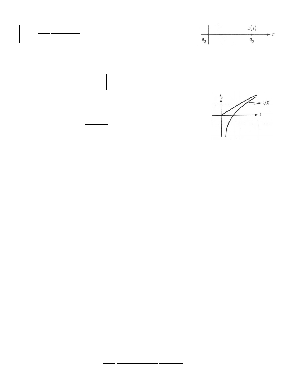
224 CHAPTER 10. POTENTIALS AND FIELDS
Problem 10.28
(a) F2=q1q2
4⇡✏0
1
(b2+c2t2)ˆx .
(This is just Coulomb’s law, since q1is at rest.)
(b) I2=q1q2
4⇡✏01
1
1
(b2+c2t2)dt =q1q2
4⇡✏01
bc tan1(ct/b)
1
1
=q1q2
4⇡✏0bc tan1(1)tan1(1)
=q1q2
4⇡✏0bc ⇡
2⇡
2=q1q2
4⇡✏0
⇡
bc.
(c) From Prob. 10.20, E=q2
4⇡✏0
1
x2cv
c+vˆx . Here x
and vare to be evaluated at the retarded time tr, which is
given by c(ttr)=x(tr)=b2+c2t2
r)c2t22cttr+
c2t2
r=b2+c2t2
r)tr=c2t2b2
2c2t.Note: As we found
in Prob. 10.17, q2first “comes into view” (for q1) at time
t= 0. Before that it can exert no force on q1, and there is
no retarded time. From the graph of trversus twe see that
trranges all the way from 1 to 1while t>0.
x(tr)=c(ttr)=2c2t2c2t2+b2
2ct =b2+c2t2
2ct (for t>0).v(t)=1
2
2c2t
pb2+c2t2=c2t
x,so
v(tr)=c2t2b2
2t 2ct
b2+c2t2=cc2t2b2
c2t2+b2(for t>0).Therefore
cv
c+v=(c2t2+b2)(c2t2b2)
(c2t2+b2)+(c2t2b2)=2b2
2c2t2=b2
c2t2(for t>0).E=q2
4⇡✏0
4c2t2
(b2+c2t2)2
b2
c2t2ˆx )
F1=
0,t<0;
q1q2
4⇡✏0
4b2
(b2+c2t2)2ˆx ,t>0.
(d) I1=q1q2
4⇡✏0
4b21
0
1
(b2+c2t2)2dt. The integral is
1
c41
0
1
[(b/c)2+t2]2dt =1
c4c2
2b2 t
(b/c)2+t2
1
0
+1
0
1
[(b/c)2+t2)] dt=1
2c2b2⇡c
2b=⇡
4cb3.
So I1=q1q2
4⇡✏0
⇡
bc.
(e) F16=F2, so Newton’s third law is not obeyed. On the other hand, I1=I2in this instance, which
suggests that the net momentum delivered from (1) to (2) is equal and opposite to the net momentum delivered
from (2) to (1), and hence that the total mechanical momentum is conserved. (In general the fields might carry
o↵some momentum, leaving the mechanical momentum altered; but that doesn’t happen in the present case.)
Problem 10.29
The electric field of q1at q2[Eq. 10.75, with ✓=45and R=(vt ˆx +vt ˆy )] is
E1=q1
4⇡✏0
1v2/c2
(1 v2/2c2)3/2
1
2p2(vt)2(ˆx +ˆy ).
c
2012 Pearson Education, Inc., Upper Saddle River, NJ. All rights reserved. This material is
protected under all copyright laws as they currently exist. No portion of this material may be
reproduced, in any form or by any means, without permission in writing from the publisher.

CHAPTER 10. POTENTIALS AND FIELDS 225
The magnetic field [Eq. 10.76, with v1=vˆx ] is
B1=1
c2(v1⇥E)=v
c2(ˆx ⇥E)=v
c2
q1
4⇡✏0
1v2/c2
(1 v2/2c2)3/2
1
2p2(vt)2ˆz .
The force on q2is therefore [Lorentz force law with v2=vˆy ]
F2=q2(E1+v2⇥B1)= q1q2
4⇡✏0
1v2/c2
(1 v2/2c2)3/2
1
2p2(vt)2ˆx +ˆy +v2
c2ˆx .
The electric field of q2at q1is reversed, E2=E1; so is the magnetic field B2=B1. The electric force
is also reversed, but the magnetic force now points in the ydirection instead of the xdirection. So the force
on q1is
F1=q1q2
4⇡✏0
1v2/c2
(1 v2/2c2)3/2
1
2p2(vt)2ˆx ˆy +v2
c2ˆy .
The forces are equal in magnitude, but not opposite in direction. No, Newton’s third law is not obeyed.
Problem 10.30
c(tt1)=vt1,t=t1(1 + v/c), t1=t
1+v/c. c(tt2)=vt2+L, t L/c =t2(1 + v/c), t2=tL/c
1+v/c .
x1=vt1=vt
1+v/c. x2=vt2+L=v(tL/c)
1+v/c +L=vt vL/c +L+vL/c
1+v/c =vt +L
1+v/c.
V(0,t)= 1
4⇡✏0x2
x1
xdx =
4⇡✏0
ln x2
x1=
4⇡✏0
ln vt +L
vt .
If L⌧vt,V=
4⇡✏0
ln 1+ L
vt⇡
4⇡✏0
L
vt =q
4⇡✏01
vt.The Li´enard-Wiechert potential is
V=q
4⇡✏0(
r
r
·v/c).Here (
r
r
·v/c)=vtr+v2tr/c =v(1 + v/c)tr=v(1 + v/c)t
1+v/c =vt.
(In the limit L!0, tr=t1=t2.) So V=q
4⇡✏01
vt.X
Problem 10.31
S=1
µ0
(E⇥B); B=1
c2(v⇥E) (Eq.10.76).
So S=1
µ0c2[E⇥(v⇥E)] = ✏0E2v(v·E)E.
The power crossing the plane is P=S·da,
c
2012 Pearson Education, Inc., Upper Saddle River, NJ. All rights reserved. This material is
protected under all copyright laws as they currently exist. No portion of this material may be
reproduced, in any form or by any means, without permission in writing from the publisher.

226 CHAPTER 10. POTENTIALS AND FIELDS
and da=2⇡rdrˆx (see diagram). So
P=✏0(E2vE2
xv)2⇡rdr;Ex=Ecos ✓,so E2E2
x=E2sin2✓.
=2⇡✏0vE2sin2✓rdr. From Eq.10.75,E=q
4⇡✏0
1
2
ˆ
R
R21(v/c)2sin2✓3/2where ⌘1
1v2/c2.
=2⇡✏0vq
4⇡✏021
21
0
rsin2✓
R41(v/c)2sin2✓3dr. Now r=atan ✓)dr =a1
cos2✓d✓;1
R=cos ✓
a.
=v
24
q2
4⇡✏0
1
a2⇡/2
0
sin3✓cos ✓
1(v/c)2sin2✓3d✓.Let u⌘sin2✓,so du =2sin✓cos ✓d✓.
=vq2
16⇡✏0a241
0
u
[1 (v/c)2u]3du =vq2
16⇡✏0a244
2=vq2
32⇡✏0a2.
Problem 10.32
(a) F12(t)= 1
4⇡✏0
q1q2
(vt)2ˆz .
(b) From Eq. 10.75, with ✓= 180,R=vt, and ˆ
R=ˆz :
F21(t)=1
4⇡✏0
q1q2(1 v2/c2)
(vt)2ˆz .
No, Newton’s third law does not hold: F12 6=F21,
because of the extra factor (1 v2/c2).
(c) From Eq. 8.28, p=✏0(E⇥B)d⌧. Here E=E1+E2, whereas B=B2,soE⇥B=(E1⇥B2)+(E2⇥B2).
But the latter, when integrated over all space, is independent of time. We want only the time-dependent part:
p(t)=✏0(E1⇥B2)d⌧.Now E1=1
4⇡✏0
q1
r2ˆr , while, from Eq. 10.76, B2=1
c2(v⇥E2), and (Eq. 10.75)
E2=q2
4⇡✏0
(1 v2/c2)
(1 v2sin2✓0/c2)3/2
ˆ
R
R2.But R=rvt;R2=r2+v2t22rvt cos ✓; sin ✓0=rsin ✓
R.So
E2=q2
4⇡✏0
(1 v2/c2)
[1 (vr sin ✓/Rc)2]3/2
(rvt)
R3. Finally, noting that v⇥(rvt)=v⇥r=vr sin ✓ˆ
, we get
B2=q2(1 v2/c2)
4⇡✏0c2
vr sin ✓
[R2(vr sin ✓/c)2]3/2ˆ
.So p(t)=✏0
q1
4⇡✏0
q2(1 v2/c2)v
4⇡✏0c21
r2
rsin ✓(ˆr ⇥ˆ
)
[R2(vr sin ✓/c)2]3/2.
But ˆr ⇥ˆ
=ˆ
✓=(cos ✓cos ˆx + cos ✓sin ˆy sin ✓ˆz ), and the xand ycomponents integrate to zero, so:
p(t)=q1q2v(1 v2/c2)ˆz
(4⇡c)2✏0sin2✓
r[r2+(vt)22rvt cos ✓(vr sin ✓/c)2]3/2r2sin ✓dr d✓d
=q1q2v(1 v2/c2)ˆz
8⇡c2✏0rsin3✓
[r2+(vt)22rvt cos ✓(vr sin ✓/c)2]3/2dr d✓.
c
2012 Pearson Education, Inc., Upper Saddle River, NJ. All rights reserved. This material is
protected under all copyright laws as they currently exist. No portion of this material may be
reproduced, in any form or by any means, without permission in writing from the publisher.
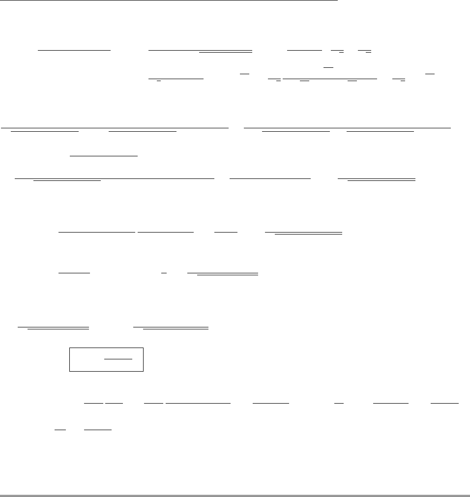
CHAPTER 10. POTENTIALS AND FIELDS 227
I’ll do the rintegral first. According to the CRC Tables,
1
0
x
(a+bx +cx2)3/2dx =2(bx +2a)
(4ac b2)pa+bx +cx2
1
0
=2
4ac b2b
pc2a
pa
=2
pc(4ac b2)b2pac=2
pc
(2pac b)
(2pac b) (2pac +b)=2
pc2pac +b1.
In this case x=r, a =(vt)2,b=2vt cos ✓,and c=1(v/c)2sin2✓. So the rintegral is
2
1(v/c)2sin2✓2vt1(v/c)2sin2✓2vt cos ✓=1
vt1(v/c)2sin2✓1(v/c)2sin2✓cos ✓
=1(v/c)2sin2✓+ cos ✓
vt1(v/c)2sin2✓1(v/c)2sin2✓cos2✓=1
vt sin2✓(1 v2/c2)
1+ cos ✓
1(v/c)2sin2✓
.
So
p(t)=q1q2v(1 v2/c2)ˆz
8⇡c2✏0
1
vt(1 v2/c2)⇡
0
1
sin2✓
1+ cos ✓
1(v/c)2sin2✓
sin3✓d✓
=q1q2ˆz
8⇡c2✏0t
⇡
0
sin ✓d✓+c
v⇡
0
cos ✓sin ✓
(c/v)2sin2✓
d✓
.
But ⇡
0sin ✓d✓= 2. In the second integral let u⌘cos ✓,sodu =sin ✓d✓:
⇡
0
cos ✓sin ✓
(c/v)2sin2✓
d✓=1
1
u
(c/v)21+u2du = 0 (the integrand is odd, and the interval is even).
Conclusion: p(t)=µ0q1q2
4⇡tˆz (plus a term constant in time).
(d)
F12 +F21 =1
4⇡✏0
q1q2
v2t2ˆz 1
4⇡✏0
q1q2(1 v2/c2)
v2t2ˆz =q1q2
4⇡✏0v2t211+ v2
c2ˆz =q1q2
4⇡✏0c2t2ˆz =µ0q1q2
4⇡t2ˆz .
dp
dt =µ0q1q2
4⇡t2ˆz =F12 +F21.qed
Since q1is at rest, and q2is moving at constant velocity, there must be another force (Fmech) acting on
them, to balance F12 +F21; what we have found is that Fmech =dpem/dt, which means that the impulse
imparted to the system by the external force ends up as momentum in the fields. [For further discussion of
this problem see J. J. G. Scanio, Am. J. Phys. 43, 258 (1975).]
c
2012 Pearson Education, Inc., Upper Saddle River, NJ. All rights reserved. This material is
protected under all copyright laws as they currently exist. No portion of this material may be
reproduced, in any form or by any means, without permission in writing from the publisher.
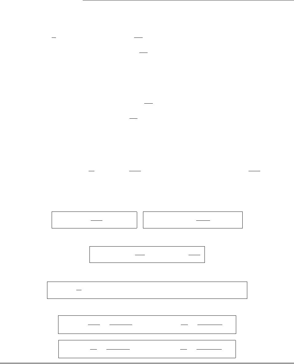
228 CHAPTER 10. POTENTIALS AND FIELDS
Problem 10.33
Maxwell’s equations with magnetic charge read:
(i) r·E=1
✏0⇢e,(iii) r⇥E=µ0Jm@B
@t,
(ii) r·B=µ0⇢m,(iv) r⇥B=µ0Je+µ0✏0
@E
@t,
where ⇢eis the electric charge density, ⇢mis the magnetic charge density, Jeis the electric current density,
and Jmis the magnetic current density.
If there are only electric charges and currents, then the usual potential formulation applies (Section 10.1.1),
with E=rVe@Ae/@t, B=r⇥Ae. If there are only magnetic charges and currents,
(i) r·E=0,(iii) r⇥E=µ0Jm@B
@t,
(ii) r·B=µ0⇢m,(iv) r⇥B=µ0✏0
@E
@t.
This time equation (i) says that Ecan be expressed as the curl of a vector potential: E=r⇥Am, and
plugging this into (iv) yields r⇥(B+µ0✏0@Am/@t)=0, which tells us that the quantity in parentheses can
be represented as the gradient of a scalar: B=rVmµ0✏0@Am/@t. [The signs of Vmand Amare arbitrary,
but I think this choice yields the most symmetrical formulation.] Putting these into (ii) and (iii) yields
22Vm=µ0⇢mµ0✏0
@
@tr·Am+@Vm
@t,22Am=µ0Jm+rr·Am+@Vm
@t.
The “Lorenz gauge” for the magnetic potentials, r·Am=@Vm/@t, kills the terms in parentheses.
In general, if there are both electric and magnetic charges and currents present, the total fields are the sums
(by the superposition principle):
E=rVe@Ae
@tr⇥Am,B=rVmµ0✏0
@Am
@t+r⇥Ae.
If we choose to work in the Lorenz gauge:
r·Ae=µ0✏0
@Ve
@t,r·Am=@Vm
@t,
Maxwell’s equations become (in terms of the potentials)
22Ve=1
✏0
⇢e,22Vm=µ0⇢m,22Ae=µ0Je,22Am=µ0Jm,
and the retarded solutions are
Ve(r,t)= 1
4⇡✏0⇢e(r0,t
r)
r
d⌧0,V
m(r,t)= µ0
4⇡⇢m(r0,t
r)
r
d⌧0,
Ae(r,t)= µ0
4⇡Je(r0,t
r)
r
d⌧0,Am(r,t)= µ0
4⇡Jm(r0,t
r)
r
d⌧0.
c
2012 Pearson Education, Inc., Upper Saddle River, NJ. All rights reserved. This material is
protected under all copyright laws as they currently exist. No portion of this material may be
reproduced, in any form or by any means, without permission in writing from the publisher.
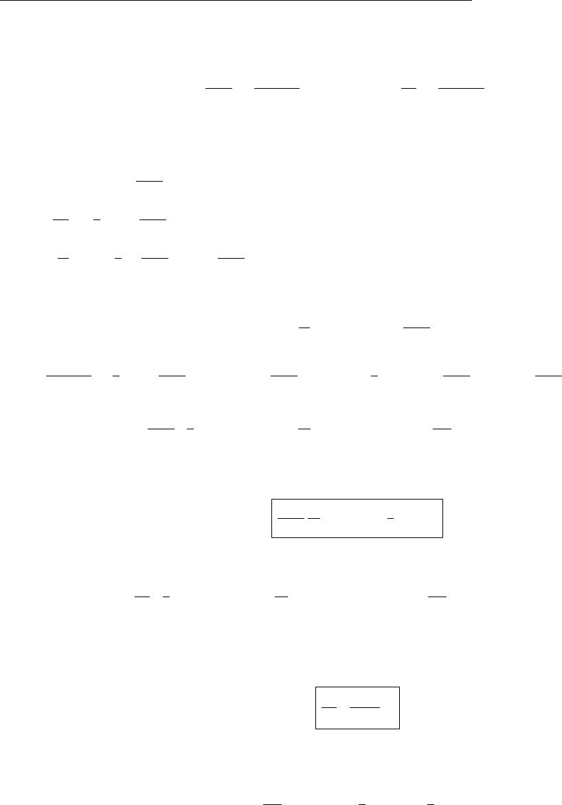
CHAPTER 10. POTENTIALS AND FIELDS 229
Problem 10.34
The retarded potentials are
V(r,t)= 1
4⇡✏0⇢(r0,t
r)
r
d⌧0,A(r,t)= µ0
4⇡J(r0,t
r)
r
d⌧0.
We want a source localized at the origin, so we expand in powers of r0, keeping terms up to first order:
r
2=(rr0)·(rr0)=r22r·r0+(r0)2,
r
⇡r1r·r0
r2,
1
r
⇡1
r1+r·r0
r2,
t
r
c⇡tr
c+r·r0
rc =t0+r·r0
rc ,
where t0⌘tr/c is the retarded time for a source at the origin. Thus (Taylor expanding about t0)
⇢(r0,t
r)=⇢r0,t
r
c⇡⇢(r0,t
0)+r·r0
rc ˙⇢(r0,t
0),
⇢(r0,t
r)
r
=1
r1+r·r0
r2⇢(r0,t
0)+r·r0
rc ˙⇢(r0,t
0)⇡1
r⇢(r0,t
0)+r·r0
r3⇢(r0,t
0)+r·r0
r2c˙⇢(r0,t
0),
and hence
V(r,t)= 1
4⇡✏01
r⇢(r0,t
0)d⌧0+r
r3·r0⇢(r0,t
0)d⌧0+r
r2c·r0˙⇢(r0,t
0)d⌧0.
The first integral is the total charge of the dipole, which is zero; the second integral is the dipole moment, and
the third is the time derivative of the dipole moment:
V(r,t)= 1
4⇡✏0
ˆr
r2·p(t0)+r
c˙
p(t0).
By the same reasoning, the vector potential is
A(r,t)= µ0
4⇡1
rJ(r0,t
0)d⌧0+1
r3(r·r0)J(r0,t
0)d⌧0+1
r2c(r·r0)˙
J(r0,t
0)d⌧0.
From Eq. 5.31 J(r0,t)d⌧0=˙
p(t),and J=⇢v0=⇢(dr0/dt) is already first order in r0, so the second and
third integrals are second order, and we drop them.
A(r,t)= µ0
4⇡˙
p(t0)
r.
In calculating the fields, remember that the dipole moments themselves depend on r, through their argument
(t0=tr/c). For a function of t0alone,
rf(t0)= df
dt0rt0=˙
f1
crr=1
c˙
fˆr ,
c
2012 Pearson Education, Inc., Upper Saddle River, NJ. All rights reserved. This material is
protected under all copyright laws as they currently exist. No portion of this material may be
reproduced, in any form or by any means, without permission in writing from the publisher.

230 CHAPTER 10. POTENTIALS AND FIELDS
so you simply replace rby ˆr
c
d
dt. For a structure of the form f(t0)+ r
c˙
f(t0)
rf(t0)+r
c˙
f(t0)=ˆr
c˙
f+r
cˆr
c¨
f+˙
f
cˆr =r
c2¨
f.
Using the product rule for r(A·B):
rV=1
4⇡✏0ˆr
r2⇥r⇥p+r
c˙
p+p+r
c˙
p⇥r⇥ˆr
r2+ˆr
r2·rp+r
c˙
p+p+r
c˙
p·rˆr
r2
=1
4⇡✏0ˆr
r2⇥r
c2⇥¨
p+0+ˆr
r2·r
c2¨
p+1
r3p+r
c˙
p3ˆr ˆr ·p+r
c˙
p
=1
4⇡✏0ˆr (ˆr ·¨
p)
rc2+[p+(r/c)˙
p]3ˆr (ˆr ·[p+(r/c)˙
p])
r3.
The others are easier:
r⇥A=µ0
4⇡1
r(r⇥˙
p)˙
p⇥r1
r=µ0
4⇡1
rˆr
c⇥¨
p+˙
p⇥ˆr
r2=µ0
4⇡ˆr ⇥[( ˙
p+(r/c)¨
p]
r2,
@A
@t=µ0
4⇡¨
p
r.
The fields are therefore
E(r,t)=rV@A
@t=µ0
4⇡¨
pˆr (ˆr ·¨
p)
r+c2[p+(r/c)˙
p]3ˆr (ˆr ·[p+(r/c)˙
p])
r3,
B(r,t)=r⇥A=µ0
4⇡ˆr ⇥[˙
p+(r/c)¨
p]
r2
(with all dipole moments evaluated at the retarded time t0=tr/c).
c
2012 Pearson Education, Inc., Upper Saddle River, NJ. All rights reserved. This material is
protected under all copyright laws as they currently exist. No portion of this material may be
reproduced, in any form or by any means, without permission in writing from the publisher.
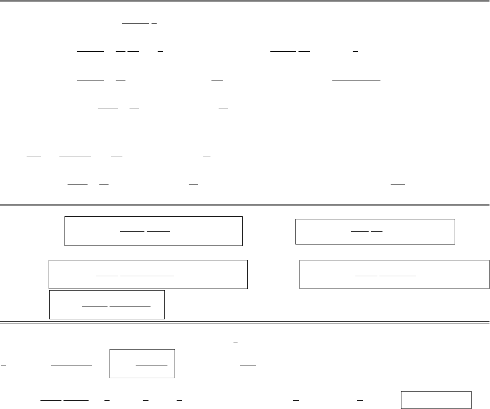
CHAPTER 11. RADIATION 231
Chapter 11
Radiation
Problem 11.1
From Eq. 11.17, A=µ0p0!
4⇡
1
rsin[!(tr/c)](cos ✓ˆr sin ✓ˆ
✓), so
r·A=µ0p0!
4⇡1
r2
@
@rr21
rsin[!(tr/c)] cos ✓+1
rsin ✓
@
@✓ sin2✓1
rsin[!(tr/c)]
=µ0p0!
4⇡1
r2sin[!(tr/c)] !r
ccos[!(tr/c)]cos ✓2 sin ✓cos ✓
r2sin ✓sin[!(tr/c)]
=µ0✏0p0!
4⇡✏01
r2sin[!(tr/c)] + !
rc cos[!(tr/c)]cos ✓.
Meanwhile, from Eq. 11.12,
@V
@t=p0cos ✓
4⇡✏0r!2
ccos[!(tr/c)] !
rsin[!(tr/c)]
=p0!
4⇡✏01
r2sin[!(tr/c)] + !
rc cos[!(tr/c)]cos ✓.So r·A=µ0✏0
@V
@t.qed
Problem 11.2
Eq. 11.14: V(r,t)=!
4⇡✏0c
p0·ˆr
rsin[!(tr/c)].Eq. 11.17: A(r,t)=µ0!
4⇡
p0
rsin[!(tr/c)].
Now p0⇥ˆr =p0sin ✓ˆ
and ˆr ⇥(p0⇥ˆr )=p0sin ✓(ˆr ⇥ˆ
)=p0sin ✓ˆ
✓, so
Eq. 11.18: E(r,t)=µ0!2
4⇡
ˆr ⇥(p0⇥ˆr )
rcos[!(tr/c)].Eq. 11.19: B(r,t)=µ0!2
4⇡c
(p0⇥ˆr )
rcos[!(tr/c)].
Eq. 11.21: hSi=µ0!4
32⇡2c
(p0⇥ˆr )2
r2ˆr .
Problem 11.3
P=I2R=q2
0!2sin2(!t)R(Eq.11.15) )hPi=1
2q2
0!2R. Equate this to Eq. 11.22:
1
2q2
0!2R=µ0q2
0d2!4
12⇡c)R=µ0d2!2
6⇡c; or, since !=2⇡c
,
R=µ0d2
6⇡c
4⇡2c2
2=2
3⇡µ0cd
2
=2
3⇡(4⇡⇥107)(3 ⇥108)d
2
= 80⇡2d
2
⌦= 789.6(d/)2⌦.
c
2012 Pearson Education, Inc., Upper Saddle River, NJ. All rights reserved. This material is
protected under all copyright laws as they currently exist. No portion of this material may be
reproduced, in any form or by any means, without permission in writing from the publisher.

232 CHAPTER 11. RADIATION
For the wires in an ordinary radio, with d=5⇥102m and (say) = 103m, R= 790(5 ⇥105)2=2⇥106⌦,
which is negligible compared to the Ohmic resistance.
Problem 11.4
By the superposition principle, we can add the potentials of the two dipoles. Let’s first express V(Eq. 11.14)
in Cartesian coordinates: V(x, y, z, t)=p0!
4⇡✏0cz
x2+y2+z2sin[!(tr/c)]. That’s for an oscillating dipole
along the zaxis. For one along xor y, we just change zto xor y. In the present case,
p=p0[cos(!t)ˆx + cos(!t⇡/2) ˆy ], so the one along yis delayed by a phase angle ⇡/2:
sin[!(tr/c)] !sin[!(tr/c)⇡/2] = cos[!(tr/c)] (just let !t!!t⇡/2). Thus
V=p0!
4⇡✏0cx
x2+y2+z2sin[!(tr/c)] y
x2+y2+z2cos[!(tr/c)]
=p0!
4⇡✏0c
sin ✓
r{cos sin[!(tr/c)] sin cos[!(tr/c)]}.Similarly,
A=µ0p0!
4⇡r{sin[!(tr/c)] ˆx cos[!(tr/c)] ˆy }.
We could get the fields by di↵erentiating these potentials, but I prefer to work with Eqs. 11.18 and 11.19,
using superposition. Since ˆz = cos ✓ˆr sin ✓ˆ
✓, and cos ✓=z/r, Eq. 11.18 can be written
E=µ0p0!2
4⇡rcos[!(tr/c)] ˆz z
rˆr . In the case of the rotating dipole, therefore,
E=µ0p0!2
4⇡rcos[!(tr/c)] ˆx x
rˆr + sin[!(tr/c)] ˆy y
rˆr ,
B=1
c(ˆr ⇥E).
S=1
µ0
(E⇥B)= 1
µ0c[E⇥(ˆr ⇥E)] = 1
µ0cE2ˆr (E·ˆr )E=E2
µ0cˆr (notice that E·ˆr = 0). Now
E2=µ0p0!2
4⇡r2a2cos2[!(tr/c)] + b2sin2[!(tr/c)] + 2(a·b) sin[!(tr/c)] cos[!(tr/c)],
where a⌘ˆx (x/r)ˆr and b⌘ˆy (y/r)ˆr . Noting that ˆx ·r=xand ˆy ·r=y, we have
c
2012 Pearson Education, Inc., Upper Saddle River, NJ. All rights reserved. This material is
protected under all copyright laws as they currently exist. No portion of this material may be
reproduced, in any form or by any means, without permission in writing from the publisher.

CHAPTER 11. RADIATION 233
a2=1+x2
r22x2
r2=1x2
r2;b2=1y2
r2;a·b=y
r
x
rx
r
y
r+xy
r2=xy
r2.
E2=µ0p0!2
4⇡r21x2
r2cos2[!(tr/c)] + 1y2
r2sin2[!(tr/c)]
2xy
r2sin[!(tr/c)] cos[!(tr/c)]
=µ0p0!2
4⇡r211
r2x2cos2[!(tr/c)] + 2xy sin[!(tr/c)] cos[!(tr/c)] + y2sin2[!(tr/c)]
=µ0p0!2
4⇡r211
r2(xcos[!(tr/c)] + ysin[!(tr/c)])2
But x=rsin ✓cos and y=rsin ✓sin .
=µ0p0!2
4⇡r21sin2✓(cos cos[!(tr/c)] + sin sin[!(tr/c)])2
=µ0p0!2
4⇡r21(sin ✓cos[!(tr/c)])2.
S=µ0
cp0!2
4⇡r21(sin ✓cos[!(tr/c)])2ˆr .
hSi=µ0
cp0!2
4⇡r211
2sin2✓ˆr .
P=hSi·da=µ0
cp0!2
4⇡21
r211
2sin2✓r2sin ✓d✓d
=µ0p2
0!4
16⇡2c2⇡⇡
0
sin ✓d✓1
2⇡
0
sin3✓d✓=µ0p2
0!4
8⇡c21
2·4
3=µ0p2
0!4
6⇡c.
This is twice the power radiated by either oscillating dipole alone (Eq. 11.22). In general, S=1
µ0
(E⇥B)=
1
µ0
[(E1+E2)⇥(B1+B2)] = 1
µ0
[(E1⇥B1)+(E2⇥B2)+(E1⇥B2)+(E2⇥B1)] = S1+S2+ cross terms.
In this particular case the fields of 1 and 2 are 90out of phase, so the cross terms go to zero in the time
averaging, and the total power radiated is just the sum of the two individual powers.
Problem 11.5
Go back to Eq. 11.33:
A=µ0m0
4⇡sin ✓
r1
rcos[!(tr/c)] !
csin[!(tr/c)]ˆ
.
c
2012 Pearson Education, Inc., Upper Saddle River, NJ. All rights reserved. This material is
protected under all copyright laws as they currently exist. No portion of this material may be
reproduced, in any form or by any means, without permission in writing from the publisher.

234 CHAPTER 11. RADIATION
Since V=0here,
E=@A
@t=µ0m0
4⇡sin ✓
r1
r(!) sin[!(tr/c)] !
c!cos[!(tr/c)]ˆ
=µ0m0!
4⇡sin ✓
r1
rsin[!(tr/c)] + !
ccos[!(tr/c)]ˆ
.
B=r⇥A=1
rsin ✓
@
@✓ (Asin ✓)ˆr 1
r
@
@r(rA)ˆ
✓
=µ0m0
4⇡1
rsin ✓
2 sin ✓cos ✓
r1
rcos[!(tr/c)] !
csin[!(tr/c)]ˆr
sin ✓
r1
r2cos[!(tr/c)] + !
rc sin[!(tr/c)] !
c!
ccos[!(tr/c)]ˆ
✓
=
µ0m0
4⇡2 cos ✓
r21
rcos[!(tr/c)] !
csin[!(tr/c)]ˆr
sin ✓
r1
r2cos[!(tr/c)] + !
rc sin[!(tr/c)] + !
c2cos[!(tr/c)]ˆ
✓.
These are precisely the fields we studied in Prob. 9.35, with A!µ0m0!2
4⇡c. The Poynting vector (quoting
the solution to that problem) is
S=µ0m2
0!3
16⇡2c2sin ✓
r22 cos ✓
r1c2
!2r2sin ucos u+c
!rcos2usin2uˆ
✓
sin ✓2
r+c2
!2r3sin ucos u+!
ccos2u+c
!r2sin2ucos2uˆr ,
where u⌘!(tr/c). The intensity is hSi=µ0m2
0!4
32⇡2c3
sin2✓
r2ˆr ,the same as Eq. 11.39.
Problem 11.6
I2R=I2
0Rcos2(!t))hPi=1
2I2
0R=µ0m2
0!4
12⇡c3=µ0⇡2b4I2
0!4
12⇡c3, so R=µ0⇡b4!4
6c3; or, since !=2⇡c
,
R=µ0⇡b4
6c3
16⇡4c4
4=8
3⇡5µ0cb
4
=8
3(⇡5)(4⇡⇥107)(3 ⇥108)(b/)4= 3.08 ⇥105(b/)4⌦.
Because b⌧, and Rgoes like the fourth power of this small number, Ris typically much smaller than the
electric radiative resistance (Prob. 11.3). For the dimensions we used in Prob. 11.3 (b= 5 cm and = 103m),
R=3⇥105(5 ⇥105)4=2⇥1012 ⌦, which is a millionth of the comparable electrical radiative resistance.
Problem 11.7
With ↵= 90, Eq. 7.68 )E0=cB,B0=E/c, q0
m=cqe)m0⌘q0
md=cqed=cp0. So
E0=cµ0(m0/c)!2
4⇡csin ✓
rcos[!(tr/c)] ˆ
=µ0m0!2
4⇡csin ✓
rcos[!(tr/c)] ˆ
.
B0=1
cµ0(m0/c)!2
4⇡sin ✓
rcos[!(tr/c)] ˆ
✓=µ0m0!2
4⇡c2sin ✓
rcos[!(tr/c)] ˆ
✓.
c
2012 Pearson Education, Inc., Upper Saddle River, NJ. All rights reserved. This material is
protected under all copyright laws as they currently exist. No portion of this material may be
reproduced, in any form or by any means, without permission in writing from the publisher.
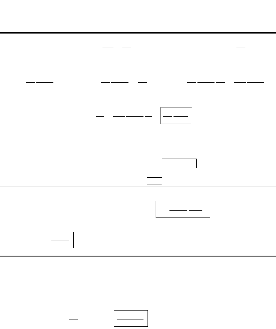
CHAPTER 11. RADIATION 235
These are identical to the fields of an Amp´ere dipole (Eqs. 11.36 and 11.37), which is consistent with our
general experience that the two models generate identical fields except right at the dipole (not relevant here,
since we’re in the radiation zone).
Problem 11.8
(a) The power radiated (Eq. 11.60) is dWr
dt =µ0
6⇡c¨p2.In this case p=Qd, so ¨p=¨
Qd =Q01
RC 2
et/RC d,
so dWr
dt =µ0
6⇡c
(Q0d)2
(RC)4e2t/RC , and the total energy radiated is
Wr=µ0
6⇡c
(Q0d)2
(RC)41
0
e2t/RC dt =µ0
6⇡c
(Q0d)2
(RC)4RC
2e2t/RC
1
0
=µ0
6⇡c
(Q0d)2
(RC)4
RC
2=µ0
12⇡c
(Q0d)2
(RC)3.
The fraction of the original energy that is radiated is therefore
f=Wr
W0
=µ0
12⇡c
(Q0d)2
(RC)3
2C
Q2
0
=µ0
6⇡c
d2
R3C2.
[Technically, ˙
Q(t) is discontinuous at t= 0, and ¨
Qpicks up a delta function. But any real circuit has some
(self-)inductance, which smoothes out the sudden change in ˙
Q.]
(b) With the parameters given,
f=4⇡⇥107
6⇡(3 ⇥108)
108
(106)(1024)= 2.22 ⇥106.
About a millionth of the total energy is radiated away, so yes, this is negligible.
Problem 11.9
p(t)=p0[cos(!t)ˆx + sin(!t)ˆy ])¨
p(t)=!2p0[cos(!t)ˆx + sin(!t)ˆy ])
[¨
p(t)]2=!4p2
0[cos2(!t) + sin2(!t)] = p2
0!4.So Eq. 11.59 says S=µ0p2
0!4
16⇡2c
sin2✓
r2ˆr .(This appears to disagree
with the answer to Prob. 11.4. The reason is that in Eq. 11.59 the polar axis is along the direction of ¨
p(t0);
as the dipole rotates, so do the axes. Thus the angle ✓here is not the same as in Prob. 11.4.) Meanwhile,
Eq. 11.60 says P=µ0p2
0!4
6⇡c.(This does agree with Prob. 11.4, because we have now integrated over all angles,
and the orientation of the polar axis irrelevant.)
Problem 11.10
At t= 0 the dipole moment of the ring is
p0=rdl =(0sin )(bsin ˆy +bcos ˆx )bd=0b2ˆy 2⇡
0
sin2d+ˆx 2⇡
0
sin cos d
=b2(⇡ˆy +0ˆx )=⇡b20ˆy .
As it rotates (counterclockwise, say) p(t)=p0[cos(!t)ˆy sin(!t)ˆx ], so ¨
p=!2p, and hence (¨
p)2=!4p2
0.
Therefore (Eq. 11.60) P=µ0
6⇡c!4(⇡b20)2=⇡µ0!4b42
0
6c.
c
2012 Pearson Education, Inc., Upper Saddle River, NJ. All rights reserved. This material is
protected under all copyright laws as they currently exist. No portion of this material may be
reproduced, in any form or by any means, without permission in writing from the publisher.
236 CHAPTER 11. RADIATION
Problem 11.11
Here V= 0 (since the ring is neutral), and the current depends only on t(not on position), so the retarded
vector potential (Eq. 11.52) is A(r,t)= µ0
4⇡I(t
r
/c)
r
dl0. But in this case it does not suffice to replace
r
by rin the denominator—that would lead to Eq. 11.54, and hence to A=0(since p=0). Instead, use
Eq. 11.30: 1
r
⇠
=1
r1+ b
rsin ✓cos 0. Meanwhile, dl0=bd0ˆ
=b(sin 0ˆx + cos 0ˆy )d0, and
I(t
r
/c)⇠
=I(tr/c +(b/c) sin ✓cos 0)=I(t0+(b/c) sin ✓cos 0)⇠
=I(t0)+ ˙
I(t0)b
csin ✓cos 0
(carrying all terms to first order in b). As always, t0=tr/c. (From now on I’ll suppress the argument: I,
˙
I, etc. are all to be evaluated at t0.) Then
A(r,t)= µ0
4⇡1
r1+ b
rsin ✓cos 0I+˙
Ib
csin ✓cos 0b(sin 0ˆx + cos 0ˆy )d0
⇠
=µ0b
4⇡r2⇡
0I+˙
Ib
csin ✓cos 0+Ib
rsin ✓cos 0(sin 0ˆx + cos 0ˆy )d0.
But 2⇡
0
sin 0d0=2⇡
0
cos 0d0=2⇡
0
sin 0cos 0d0=0,while 2⇡
0
cos20d0=⇡.
=µ0b
4⇡r(⇡ˆy )˙
Ib
csin ✓+Ib
rsin ✓=µ0b2
4r2sin ✓I+r
c˙
Iˆy .
In general (i.e. for points not on the xz plane) ˆy !ˆ
; moreover, in the radiation zone we are not interested
in terms that go like 1/r2,so A(r,t)=µ0b2
4c˙
I(tr/c)sin ✓
rˆ
.
E(r,t)=@A
@t=µ0b2
4c¨
I(tr/c)sin ✓
rˆ
.
B(r,t)=r⇥A=1
rsin ✓
@
@✓ (Asin ✓)ˆr 1
r
@
@r(rA)ˆ
✓
=µ0b2
4c˙
I
rsin ✓
1
r2 sin ✓cos ✓ˆr 1
r¨
I1
csin ✓ˆ
✓=µ0b2
4c2¨
Isin ✓
rˆ
✓.
S=1
µ0
(E⇥B)= 1
µ0cµ0b2
4c¨
Isin ✓
r2ˆ
⇥ˆ
✓=µ0
16c3b2¨
I2sin2✓
r2ˆr .
P=S·da=µ0
16c3b2¨
I2sin2✓
r2r2sin ✓d✓d=µ0
16c3b2¨
I2(2⇡)4
3=µ0⇡
6c3b2¨
I2
=µ0¨m2
6⇡c3.(Note that m=I⇡b2,so ¨m=¨
I⇡b2.)
Problem 11.12
p=ey ˆy ,y=1
2gt2,so p=1
2get2ˆy ;¨
p=ge ˆy .Therefore (Eq.11.60) :P=µ0
6⇡c(ge)2. Now, the time
it takes to fall a distance his given by h=1
2gt2)t=2h/g, so the energy radiated in falling a distance h
c
2012 Pearson Education, Inc., Upper Saddle River, NJ. All rights reserved. This material is
protected under all copyright laws as they currently exist. No portion of this material may be
reproduced, in any form or by any means, without permission in writing from the publisher.

CHAPTER 11. RADIATION 237
is Urad =Pt =µ0(ge)2
6⇡c2h/g. Meanwhile, the potential energy lost is Upot =mgh. So the fraction is
f=Urad
Upot
=µ0g2e2
6⇡c2h
g
1
mgh =µ0e2
6⇡mc2g
h.=(4⇡⇥107)(1.6⇥1019)2
6⇡(9.11 ⇥1031)(3 ⇥108)(2)(9.8)
(0.01) = 2.76 ⇥1022.
Evidently almost all the energy goes into kinetic form (as indeed I assumed in saying y=1
2gt2).
Problem 11.13
The power radiated (Eq. 11.70) is dWr
dt =µ0q2a2
6⇡c.Here F=1
4⇡✏0
qQ
x2=ma,soa=k
x2, where k⌘qQ
4⇡✏0m.
The energy radiated (twice that radiated on the way out) is
Wr=µ0q2
6⇡ck2
x4dt =µ0q2
6⇡c2k21
x0
1
x4
1
vdx,
where x0is the distance of closest approach. Conservation of energy (ignoring radiative losses, as suggested)
says 1
2mv2
0=1
2mv2+1
4⇡✏0
qQ
x)v2=v2
02qQ
4⇡✏0m
1
x=v2
02k
x,and x0=2k
v2
0
(note that qis at x0when v= 0). So
Wr=µ0q2
6⇡c2k21
x0
1
x4v2
02k/x dx =µ0q2
6⇡c
2k2
p2k1
x0
1
x4(1/x0)(1/x)dx =µ0q2
6⇡c
2k2
p2k
16
15x5/2
0
.
(I used Mathematica to do the integral.) Simplifying,
Wr=2µ0q2v5
0
45⇡ck =2µ0q2v5
0
45⇡c
4⇡✏0m
qQ =8qmv5
0
45c3Q)f=Wr
W0
=8qmv5
0
45c3Q
2
mv2
0
=16q
45Qv0
c3.
Problem 11.14
F=1
4⇡✏0
q2
r2=ma =mv2
r)v=1
4⇡✏0
q2
mr .At the beginning (r0=0.5˚
A),
v
c=(1.6⇥1019)2
4⇡(8.85 ⇥1012)(9.11 ⇥1031)(5 ⇥1011)1/21
3⇥108=0.0075,
and when the radius is one hundredth of this v/c is only 10 times greater (0.075), so for most of the trip the
velocity is safely nonrelativistic.
From the Larmor formula, P=µ0q2
6⇡cv2
r2
=µ0q2
6⇡c1
4⇡✏0
q2
mr22
(since a=v2/r), and P=dU/dt,
where Uis the (total) energy of the electron:
U=Ukin +Upot =1
2mv21
4⇡✏0
q2
r=1
21
4⇡✏0
q2
r1
4⇡✏0
q2
r=1
8⇡✏0
q2
r.
So dU
dt =1
8⇡✏0
q2
r2
dr
dt =P=q2
6⇡✏0c31
4⇡✏0
q2
mr22
,and hence dr
dt =1
3cq2
2⇡✏0mc 21
r2,or
c
2012 Pearson Education, Inc., Upper Saddle River, NJ. All rights reserved. This material is
protected under all copyright laws as they currently exist. No portion of this material may be
reproduced, in any form or by any means, without permission in writing from the publisher.
238 CHAPTER 11. RADIATION
dt =3c2⇡✏0mc
q22
r2dr )t=3c2⇡✏0mc
q220
r0
r2dr =c2⇡✏0mc
q22
r3
0
= (3 ⇥108)2⇡(8.85 ⇥1012)(9.11 ⇥1031)(3 ⇥108)
(1.6⇥1019)22
(5 ⇥1011)3= 1.3⇥1011 s. (Not very long!)
Problem 11.15
According to Eq. 11.74, the maximum occurs at d
d✓sin2✓
(1 cos ✓)5= 0. Thus
2 sin ✓cos ✓
(1 cos ✓)5 5 sin2✓(sin ✓)
(1 cos ✓)6=0)2 cos ✓(1 cos ✓)=5sin2✓=5(1 cos2✓);
2 cos ✓2cos2✓=55cos2✓,or 3cos2✓+ 2 cos ✓5=0.So
cos ✓=2±4 + 602
6=1
3±1 + 1521. We want the plus sign, since ✓m!90(cos ✓m= 0) when
!0 (Fig. 11.11): ✓max = cos11 + 1521
3.
For v⇡c, ⇡1; write =1✏(where ✏⌧1), and expand to first order in ✏:
1 + 1521
3=1
3(1 ✏)1 + 15(1 ✏)21⇠
=1
3(1 + ✏)1 + 15(1 2✏)1
=1
3(1 + ✏)p16 30✏1=1
3(1 + ✏)41(15✏/8) 1=1
3(1 + ✏)4115
16✏1
=1
3(1 + ✏)315
4✏= (1 + ✏)(1 5
4✏)⇠
=1+✏5
4✏=11
4✏.
Evidently ✓max ⇡0,so cos ✓max ⇠
=11
2✓2
max =11
4✏)✓2
max =1
2✏,or ✓max ⇠
=✏/2= (1 )/2.
Let f⌘(dP/d⌦|✓m)ur
(dP/d⌦|✓m)rest
=sin2✓max
(1 cos ✓max)5ur
. Now sin2✓max ⇠
=✏/2, and
(1 cos ✓max)⇠
=1(1 ✏)(1 1
4✏)⇠
=1(1 ✏1
4✏)=5
4✏. So f=✏/2
(5✏/4)5=4
551
2✏4.But
=1
12=1
1(1 ✏)2⇠
=1
1(1 2✏)=1
p2✏)✏=1
22. Therefore
f=4
551
2(22)4=1
48
55
8=2.628.
Problem 11.16
Equation 11.72 says dP
d⌦=q2
16⇡2✏0ˆ
r
⇥(u⇥a)2
(ˆ
r
·u)5. Let ⌘v/c.
u=cˆ
r
v=cˆ
r
vˆz )ˆ
r
·u=cv(ˆ
r
·ˆz )=cvcos ✓=c1v
ccos ✓=c(1 cos ✓);
c
2012 Pearson Education, Inc., Upper Saddle River, NJ. All rights reserved. This material is
protected under all copyright laws as they currently exist. No portion of this material may be
reproduced, in any form or by any means, without permission in writing from the publisher.

CHAPTER 11. RADIATION 239
a·u=ac(ˆx ·ˆ
r
)av(ˆx ·ˆz )=ac sin ✓cos ;u2=u·u=c22cv(ˆ
r
·ˆz )+v2=c2+v22cv cos ✓.
ˆ
r
⇥(u⇥a)=(ˆ
r
·a)u(ˆ
r
·u)a;
|ˆ
r
⇥(u⇥a)|2=(ˆ
r
·a)2u22(u·a)( ˆ
r
·a)( ˆ
r
·u)+(ˆ
r
·u)2a2
=(c2+v22cv cos ✓)(asin ✓cos )22(ac sin ✓cos )(asin ✓cos )(cvcos ✓)+a2c2(1 cos ✓)2
=a2c2(1 cos ✓)2+ (sin2✓cos2)(c2+v22cv cos ✓2c2+2cv cos ✓
=a2c2(1 cos ✓)2(1 2)(sin ✓cos )2.
dP
d⌦=µ0q2a2
16⇡2c(1 cos ✓)2(1 2) sin2✓cos2
(1 cos ✓)5.
The total power radiated (in all directions) is:
P=dP
d⌦d⌦=dP
d⌦sin ✓d✓d=µ0q2a2
16⇡2c(1 cos ✓)2(1 2) sin2✓cos2
(1 cos ✓)5sin ✓d✓d.
But 2⇡
0
d=2⇡and 2⇡
0
cos2d=⇡.
=µ0q2a2
16⇡2c⇡⇡
02(1 cos ✓)2(1 2) sin2✓
(1 cos ✓)5sin ✓d✓.
Let w⌘(1 cos ✓). Then (1 w)/= cos ✓; sin2✓=2(1 w)2/2, and the numerator becomes
2w2(1 2)
2(21+2ww2)= 1
22w22+ (1 2)22(1 2)w+w2(1 2)
=1
2(1 2)22(1 2)w+ (1 + 2)w2;
dw =sin ✓d✓)sin ✓d✓=1
dw. When ✓=0,w=(1); when ✓=⇡,w=(1+).
P=µ0q2a2
16⇡c
1
3(1+)
(1)
1
w5(1 2)22(1 2)w+ (1 + 2)w2dw. The integral is
Int = (1 2)21
w5dw 2(1 2)1
w4dw + (1 + 2)1
w3dw
=(1 2)21
4w42(1 2)1
3w3+ (1 + 2)1
2w2
1+
1
.
1
w2
1+
1=1
(1 + )21
(1 )2=(1 2+2)(1 + 2+2)
(1 + )2(1 )2=4
(1 2)2.
1
w3
1+
1=1
(1 + )31
(1 )3=(1 3+323)(1 + 3+32+3)
(1 + )3(1 )3=2(3 + 2)
(1 2)3.
1
w4
1+
1=1
(1 + )41
(1 )4=(1 4+6243+4)(1 + 4+62+43+4)
(1 + )4(1 )4=8(1 + 2)
(1 2)4.
c
2012 Pearson Education, Inc., Upper Saddle River, NJ. All rights reserved. This material is
protected under all copyright laws as they currently exist. No portion of this material may be
reproduced, in any form or by any means, without permission in writing from the publisher.
240 CHAPTER 11. RADIATION
Int = (1 2)21
48(1 + 2)
(1 2)42(1 2)1
32(3 + 2)
(1 2)3+ (1 + 2)1
24
(1 2)2
=2
(1 2)2(1 + 2)2
3(3 + 2)+(1+2)=8
3
3
(1 2)2.
P=µ0q2a2
16⇡c
1
3
8
3
3
(1 2)2=µ0q2a24
6⇡c,where =1
12.
Is this consistent with the Li´enard formula (Eq. 11.73)? Here v⇥a=va(ˆz ⇥ˆx )=va ˆy ,so
a2v
c⇥a2=a21v2
c2= (1 2)a2=1
2a2, so the Li´enard formula says P=µ0q26
6⇡c
a2
2.X
Problem 11.17
(a) To counteract the radiation reaction (Eq. 11.80), you must exert a force Fe=µ0q2
6⇡c˙
a.
For circular motion, r(t)=R[cos(!t)ˆx + sin(!t)ˆy ],v(t)=˙
r=R![sin(!t)ˆx + cos(!t)ˆy ];
a(t)= ˙
v=R!2[cos(!t)ˆx + sin(!t)ˆy ]=!2r;˙
a=!2˙
r=!2v. So Fe=µ0q2
6⇡c!2v.
Pe=Fe·v=µ0q2
6⇡c!2v2.This is the power you must supply.
Meanwhile, the power radiated is (Eq. 11.70) Prad =µ0q2a2
6⇡c, and a2=!4r2=!4R2=!2v2,so
Prad =µ0q2
6⇡c!2v2, and the two expressions agree.
(b) For simple harmonic motion, r(t)=Acos(!t)ˆz ;v=˙
r=A!sin(!t)ˆz ;a=˙
v=A!2cos(!t)ˆz =
!2r;˙
a=!2˙
r=!2v.SoFe=µ0q2
6⇡c!2v;Pe=µ0q2
6⇡c!2v2.But this time a2=!4r2=!4A2cos2(!t),
whereas !2v2=!4A2sin2(!t), so
Prad =µ0q2
6⇡c!4A2cos2(!t)6=Pe=µ0q2
6⇡c!4A2sin2(!t);
the power you deliver is not equal to the power radiated. However, since the time averages of sin2(!t) and
cos2(!t) are equal (to wit: 1/2), over a full cycle the energy radiated is the same as the energy input. (In the
mean time energy is evidently being stored temporarily in the nearby fields.)
(c) In free fall, v(t)= 1
2gt2ˆy ;v=gt ˆy ;a=gˆy ;˙
a= 0. So Fe=0; the radiation reaction is zero, and
hence Pe=0.But there is radiation: Prad =µ0q2
6⇡cg2.Evidently energy is being continuously extracted from
the nearby fields. This paradox persists even in the exact solution (where we do not assume v⌧c, as in the
Larmor formula and the Abraham-Lorentz formula)—see Prob. 11.34.
Problem 11.18
(a) From Eq. 11.80, Frad =µ0q2
6⇡c˙a=m⌧...
x(Eq. 11.82). The equation of motion is
F=m¨x=Fspring +Frad =kx +m⌧...
x, or ¨x+!2
0x⌧...
x=0,with !0=k/m.
c
2012 Pearson Education, Inc., Upper Saddle River, NJ. All rights reserved. This material is
protected under all copyright laws as they currently exist. No portion of this material may be
reproduced, in any form or by any means, without permission in writing from the publisher.
CHAPTER 11. RADIATION 241
Since the damping is small, it oscillates at the natural frequency !0, and hence ...
x=!2
0˙x, so ¨x+!2
0⌧˙x+!2
0x=0,
or ¨x+˙x+!2
0x= 0, with =!2
0⌧.The solution with x(0) = 0 is (for ⌧!0)
x(t)=Aet/2sin(!0t); v(t)=
2Aet/2sin(!0t)+!0Aet/2cos(!0t),so v(0) = A!0=v0)A=v0
!0
,
and x(t)= v0
!0
et/2sin(!0t).
According to the Larmor formula (Eq. 11.70), the power radiated is P=µ0q2a2
6⇡c.In this case (still assuming
⌧!0)
a=!2
0x=!2
0
v0
!0
et/2sin(!0t),P=µ0q2
6⇡c(!0v0)2etsin2(!0t).
Averaging over a full cycle (holding etconstant) hPi=µ0q2!2
0v2
0
6⇡cet1
2, and the total energy radiated is
1
0hPidt =µ0q2!2
0v2
0
12⇡c1
et
1
0
=µ0q2!2
0v2
0
12⇡c=µ0q2!2
0v2
0
12⇡c!2
0⌧=µ0q2v2
0
12⇡c6⇡mc
µ0q2=1
2mv2
0.X
(b) This “equivalent” single oscillator has twice the charge, and twice the mass, so ⌧(and hence ) is
doubled. Since hPidt goes like q2/, it also doubles. The power radiated is indeed four times as great, but
the oscillations die away faster, and the total energy radiated is just twice as much as for one oscillator.
Problem 11.19
(a) a=⌧˙a+F
m)dv
dt =⌧da
dt +F
m)dv
dt dt =⌧da
dt dt +1
mF dt.
[v(t0+✏)v(t0✏)] = ⌧[a(t0+✏)a(t0✏)] + 2✏
mFave, where Fave is the average force during the inter-
val. But vis continuous, so as long as Fis not a delta function, we are left (in the limit ✏!0) with
[a(t0+✏)a(t0✏)] = 0. Thus a, too, is continuous. qed
(b) (i) a=⌧˙a=⌧da
dt )da
a=1
⌧dt )da
a=1
⌧dt )ln a=t
⌧+ constant )a(t)=Aet/⌧,where A
is a constant.
(ii) a=⌧˙a+F
m)⌧da
dt =aF
m)da
aF/m =1
⌧dt )ln(aF/m)= t
⌧+ constant )aF
m=Bet/⌧)
a(t)= F
m+Bet/⌧,where Bis some other constant.
(iii) Same as (i): a(t)=Cet/⌧,where Cis a third constant.
(c) At t=0,A=F/m +B; at t=T,F/m +BeT/⌧=CeT/⌧)C=(F/m)eT/⌧+B. So
a(t)=
[(F/m)+B]et/⌧,t0;
(F/m)+Bet/⌧,0tT;
(F/m)eT/⌧+Bet/⌧,tT.
To eliminate the runaway in region (iii), we’d need B=(F/m)eT/⌧; to avoid preacceleration in region
(i), we’d need B=(F/m). Obviously, we cannot do both at once.
c
2012 Pearson Education, Inc., Upper Saddle River, NJ. All rights reserved. This material is
protected under all copyright laws as they currently exist. No portion of this material may be
reproduced, in any form or by any means, without permission in writing from the publisher.
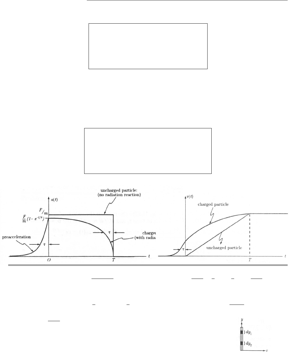
242 CHAPTER 11. RADIATION
(d) If we choose to eliminate the runaway, then
a(t)=
(F/m)1eT/⌧et/⌧,t0;
(F/m)1e(tT)/⌧,0tT;
0,tT.
(i) v=(F/m)1eT/⌧et/⌧dt =(F⌧/m)1eT/⌧et/⌧+D, where Dis a constant determined by the
condition v(1)=0)D=0.
(ii) v=(F/m)t⌧e(tT)/⌧+E, where Eis a constant determined by the continuity of vat t= 0:
(F⌧/m)1eT/⌧=(F/m)⌧eT/⌧+E)E=(F⌧/m).
(iii) vis a constant determined by the continuity of vat t=T:v=(F/m)[T+⌧⌧]=(F/m)T.
v(t)=
(F⌧/m)1eT/⌧et/⌧,t0;
(F/m)t+⌧⌧e(tT)/⌧,0tT;
(F/m)T, t T.
(e)
Problem 11.20
(a) From Eq.11.80, Fend
rad =µ0(q/2)2
6⇡c˙a, so Frad =Fint
rad +2Fend
rad =µ0q2
6⇡c˙a1
2+21
4=µ0q2
6⇡c˙a. X
(b) Following the suggested method:
F(q)=Fint(q)+21
4F(q))1
2F(q)=Fint(q))F(q)=2Fint(q)=µ0q2˙a
6⇡c.X
(c) Frad =µ0
12⇡c˙aL
0y1
0
2dy22dy1. (Running the y2
integral up to y1insures that y1y2, so we don’t count the
same pair twice. Alternatively, run both integrals from 0 to
L—intentionally double-counting—and divide the result by 2.)
c
2012 Pearson Education, Inc., Upper Saddle River, NJ. All rights reserved. This material is
protected under all copyright laws as they currently exist. No portion of this material may be
reproduced, in any form or by any means, without permission in writing from the publisher.
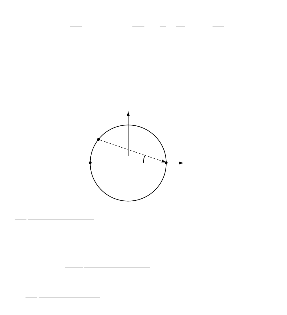
CHAPTER 11. RADIATION 243
Frad =µ0˙a
12⇡c(42)L
0
y1dy1=µ0˙a
12⇡c(42)L2
2=µ0
6⇡c(L)2˙a=µ0q2
6⇡c˙a. X
Problem 11.21
(a) The total torque is twice the torque on +q; we might as well calculate it at time t= 0. First we
need the electric field at +q, due to qwhen it was at the retarded point P(Eq. 10.72). From the figure,
ˆ
r
= cos ✓ˆx sin ✓ˆy ,
r
=2Rcos ✓.The velocity of q(at P) was v=!R(sin 2✓ˆx + cos 2✓ˆy ), and its
acceleration was a=!2R(cos 2✓ˆx sin 2✓ˆy ).Quantities we will need in Eq. 10.72 are:
u=cˆ
r
v=(ccos ✓+!Rsin 2✓)ˆx (csin ✓!Rcos 2✓)ˆy ,
r
·u=2Rcos ✓(c+!Rsin ✓),
r
·a=2(!Rcos ✓)2.
qx
y
P
q
-q R
r
E=q
4⇡✏0
2Rcos ✓
(2Rcos ✓)3(c+!Rsin ✓)3[c2(!R)2+ 2(!Rcos ✓)2][(ccos ✓+!Rsin 2✓)ˆx (csin ✓!Rcos 2✓)ˆy ]
2Rcos ✓(c+!Rsin ✓)!2R(cos 2✓ˆx sin 2✓ˆy )
The total torque (about the origin) is
N= 2(Rˆx )⇥(qE)=2q2R
4⇡✏0
ˆz
(2Rcos ✓)2(c+!Rsin ✓)3c2(!R)2+ 2(!Rcos ✓)2(csin ✓!Rcos 2✓)
+ 2(!R)2cos ✓(c+!Rsin ✓) sin 2✓
=q2
4⇡✏0
ˆz
2Rcos2✓(c+!Rsin ✓)3c3sin ✓+c2!R(2 cos2✓1) + c(!R)2(2 cos2✓+ 1) sin ✓+(!R)3
=q2
4⇡✏0
1
2Rcos2✓(1 + sin ✓)3sin ✓+(2 cos2✓1) + 2(2 cos2✓+ 1) sin ✓+3ˆz ,
where ⌘!R/c. [Since Eand
r
both lie in the xy plane, B=(1/c)ˆ
r
⇥Eis along the zdirection, v⇥Bis
radial, and hence the magnetic contribution to the torque is zero.]
The angle ✓is determined by the retarded time condition,
r
=ctr(note that tris negative, here), and
2✓is the angle through which the dipole rotates in time tr,so2Rcos ✓=ctr=c(2✓/!), or ✓=cos ✓.We
c
2012 Pearson Education, Inc., Upper Saddle River, NJ. All rights reserved. This material is
protected under all copyright laws as they currently exist. No portion of this material may be
reproduced, in any form or by any means, without permission in writing from the publisher.
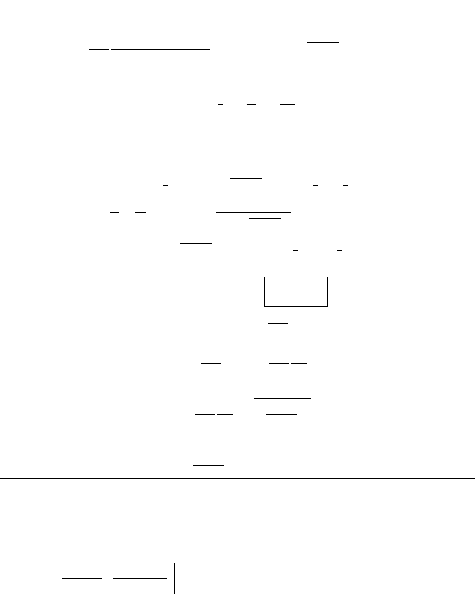
244 CHAPTER 11. RADIATION
can use this to eliminate the trig functions:
N=q2
4⇡✏0
2R✓21+2✓23(42+2✓2)+2✓2(2+2✓21)ˆz .
Meanwhile, expanding in powers of ✓:
=✓sec ✓=✓+1
2✓3+5
24✓5+61
720✓7+....
This can be “solved” (for ✓as a function of ) by reverting the series:
✓=1
23+13
245541
7207+....
Then
✓2=212+4
34+...
,2✓2=212
32+4
54+...
,
1
✓2=1
21+2+...
,1
1+2✓23=132+...,
(42+2✓2)+2✓2(2+2✓21)=8
3414
52+...
.
To leading order in , then,
N=q2
4⇡✏0
2R
1
2
84
3ˆz =q2
4⇡✏0
43
3Rˆz .
(b) The radiation reaction force on +qis (Eq. 11.80) F=µ0q2
6⇡c˙
a.In this case ˙
a=!2v=!3Rˆy , so the
net torque (counting both ends) is
N=2Rµ0q2
6⇡c!3Rˆz =q2
4⇡✏0
43
3Rˆz .
Adding this to the interaction torque from (a), the total is
N=q2
4⇡✏0
83
3Rˆz =µ0p2!3
6⇡cˆz .
(c) ¨
p=2q¨
r=2q(!2)r=!2p, so Eq. 11.60 says the power radiated is P=µ0
6⇡c!4p2.The power
associated with the torque in (b) is N!=µ0p2!3
6⇡c!, so they are in agreement. X
Problem 11.22
(a) This is an oscillating electric dipole, with amplitude p0=qd and frequency !=k/m. The (averaged)
Poynting vector is given by Eq. 11.21: hSi=µ0p2
0!4
32⇡2csin2✓
r2ˆr , so the power per unit area of floor is
If=hSi·ˆz =µ0p2
0!4
32⇡2csin2✓cos ✓
r2.But sin ✓=R
r,cos ✓=h
r,and r2=R2+h2.
=µ0q2d2!4
32⇡2cR2h
(R2+h2)5/2.
c
2012 Pearson Education, Inc., Upper Saddle River, NJ. All rights reserved. This material is
protected under all copyright laws as they currently exist. No portion of this material may be
reproduced, in any form or by any means, without permission in writing from the publisher.
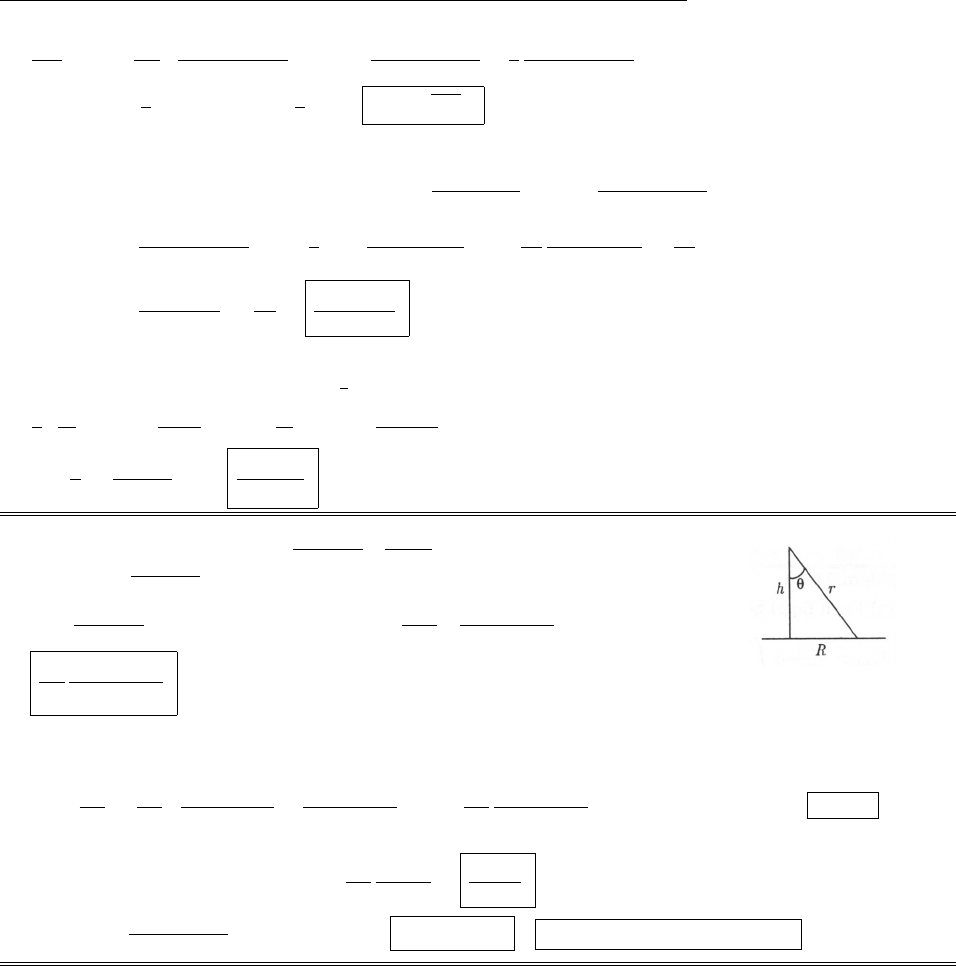
CHAPTER 11. RADIATION 245
dIf
dR =0)d
dR R2
(R2+h2)5/2=0)2R
(R2+h2)5/25
2
R2
(R2+h2)7/22R=0)
(R2+h2)5
2R2=0)h2=3
2R2)R=2/3h, for maximum intensity.
(b)
P=If(R)da =If(R)2⇡R dR =2⇡µ0(qd)2!4
32⇡2ch1
0
R3
(R2+h2)5/2dR. Let x⌘R2:
1
0
R3
(R2+h2)5/2dR =1
21
0
x
(x+h2)5/2dx =1
2h
(2)(1/2)
(5/2) =2
3h.
=2⇡µ0q2d2!4
32⇡2ch2
3h=µ0q2d2!4
24⇡c,
which should be (and is) half the total radiated power (Eq. 11.22)—the rest hits the ceiling, of course.
(c) The amplitude is x0(t), so U=1
2kx2
0is the energy, at time t, and dU/dt =2Pis the power radiated:
1
2kd
dt(x2
0)=µ0!4
12⇡cq2x2
0)d
dt(x2
0)=µ0!4q2
6⇡kc (x2
0)=x2
0)x2
0=d2etor x0(t)=det/2.
⌧=2
=12⇡kc
µ0q2k2m2=12⇡cm2
µ0q2k.
Problem 11.23
(a) From Eq. 11.39, hSi=µ0m2
0!4
32⇡2c3sin2✓
r2ˆr . Here sin ✓=
R/r, r =pR2+h2, and the total radiated power (Eq. 11.40) is
P=µ0m2
0!4
12⇡c3. So the intensity is I(R)=12P
32⇡R2
(R2+h2)2=
3P
8⇡
R2
(R2+h2)2.
(b) The intensity directly below the antenna (R= 0) would (ideally) have been zero. The engineer should
have measured it at the position of maximum intensity:
dI
dR =3P
8⇡2R
(R2+h2)22R2
(R2+h2)32R=3P
8⇡
2R
(R2+h2)3R2+h22R2=0)R=h.
At this location the intensity is I(h)=3P
8⇡
h2
(2h2)2=3P
32⇡h2.
(c) Imax =3(35 ⇥103)
32⇡(200)2=0.026 W/m2= 2.6 µW/cm2. Yes, KRUD is in compliance.
c
2012 Pearson Education, Inc., Upper Saddle River, NJ. All rights reserved. This material is
protected under all copyright laws as they currently exist. No portion of this material may be
reproduced, in any form or by any means, without permission in writing from the publisher.
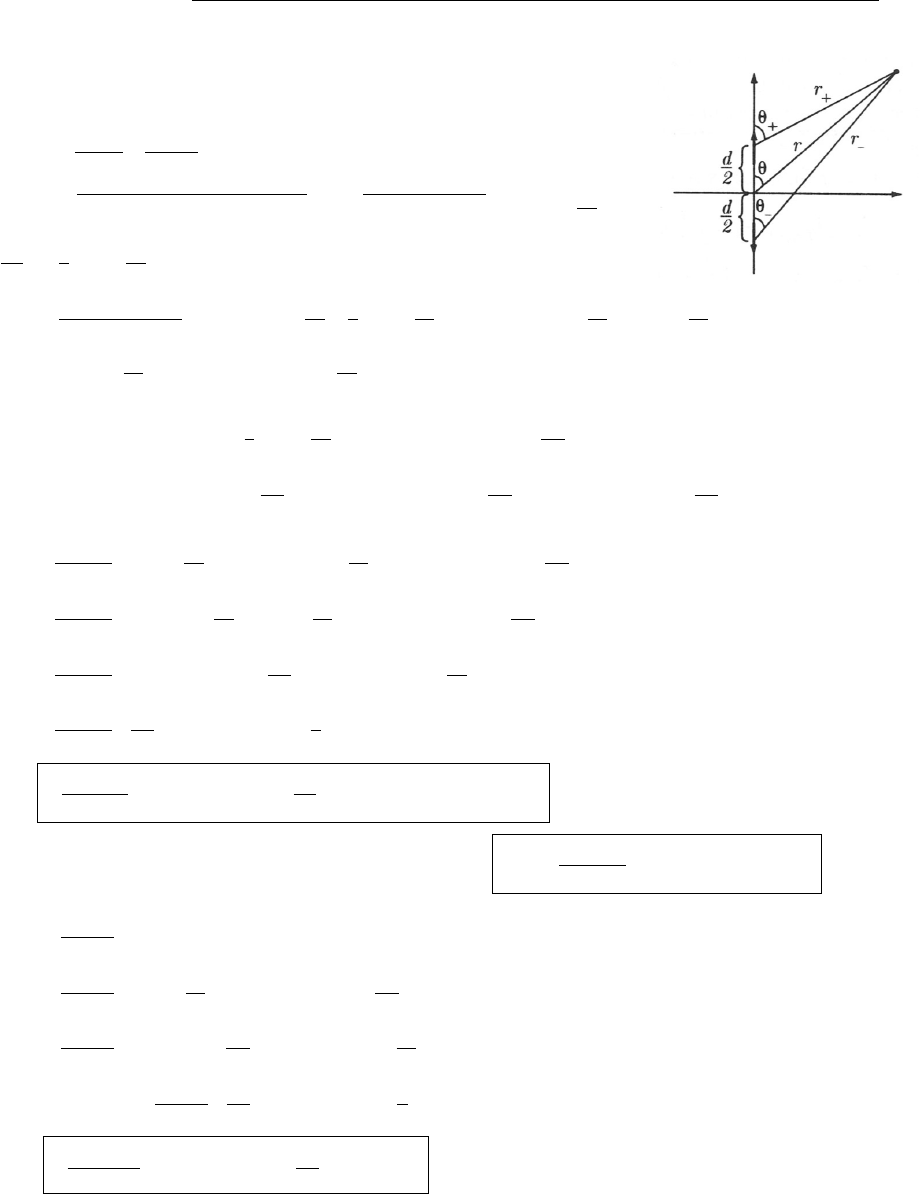
246 CHAPTER 11. RADIATION
Problem 11.24
(a)
V±=⌥p0!
4⇡✏0ccos ✓±
r±sin[!(tr±/c)].V
tot =V++V.
r±=r2+(d/2)2⌥2r(d/2) cos ✓⇠
=r1⌥(d/r) cos ✓⇠
=r1⌥d
2rcos ✓.
1
r±⇠
=1
r1±d
2rcos ✓.
cos ✓±=rcos ✓⌥(d/2)
r±
=rcos ✓⌥d
2r1
r1±d
2rcos ✓= cos ✓±d
2rcos2✓⌥d
2r
= cos ✓⌥d
2r(1 cos2✓) = cos ✓⌥d
2rsin2✓.
sin[!(tr±/c)] = sin !tr
c1⌥d
2rcos ✓= sin !t0±!d
2ccos ✓,where t0⌘tr/c.
= sin(!t0) cos !d
2ccos ✓±cos(!t0) sin !d
2ccos ✓⇠
=sin(!t0)±!d
2ccos ✓cos(!t0).
V±=⌥p0!
4⇡✏0cr 1±d
2rcos ✓cos ✓⌥d
2rsin2✓sin(!t0)±!d
2ccos ✓cos(!t0)
=⌥p0!
4⇡✏0cr cos ✓⌥d
2rsin2✓±d
2rcos2✓sin(!t0)±!d
2ccos ✓cos(!t0)
=⌥p0!
4⇡✏0cr cos ✓sin(!t0)±!d
2ccos2✓cos(!t0)±d
2rcos2✓sin2✓sin(!t0.
Vtot =p0!
4⇡✏0cr !d
ccos2✓cos(!t0)+d
rcos2✓sin2✓sin(!t0)
=p0!2d
4⇡✏0c2rcos2✓cos(!t0)+ c
!rcos2✓sin2✓sin(!t0.
In the radiation zone (r!/c) the second term is negligible, so V=p0!2d
4⇡✏0c2rcos2✓cos[!(tr/c)].
Meanwhile
A±=⌥µ0p0!
4⇡r±
sin[!(tr±/c)] ˆz
=⌥µ0p0!
4⇡r1±d
2rcos ✓sin(!t0)±!d
2ccos ✓cos(!t0)ˆz
=⌥µ0p0!
4⇡rsin(!t0)±!d
2ccos ✓cos(!t0)±d
2rcos ✓sin(!t0)ˆz .
Atot =A++A=µ0p0!
4⇡r!d
ccos ✓cos(!t0)+d
rcos ✓sin(!t0)ˆz
=µ0p0!2d
4⇡cr cos ✓cos(!t0)+ c
!rsin(!t0)ˆz .
c
2012 Pearson Education, Inc., Upper Saddle River, NJ. All rights reserved. This material is
protected under all copyright laws as they currently exist. No portion of this material may be
reproduced, in any form or by any means, without permission in writing from the publisher.
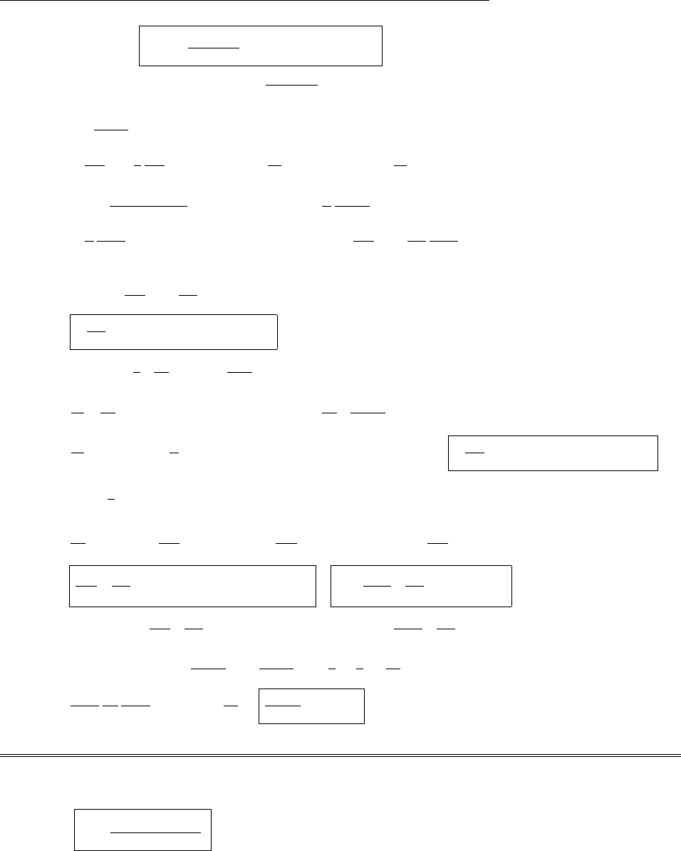
CHAPTER 11. RADIATION 247
In the radiation zone, A=µ0p0!2d
4⇡cr cos ✓cos[!(tr/c)] ˆz .
(b) To simplify the notation, let ↵⌘µ0p0!2d
4⇡. Then
V=↵cos2✓
rcos[!(tr/c)];
rV=@V
@rˆr +1
r
@V
@✓ ˆ
✓=↵cos2✓1
r2cos[!(tr/c)] + !
rc sin[!(tr/c)]ˆr
+↵2 cos ✓sin ✓
r2cos[!(tr/c)] ˆ
✓=↵!
c
cos2✓
rsin[!(tr/c)]ˆr (in the radiation zone).
A=↵
c
cos ✓
rcos[!(tr/c)] cos ✓ˆr sin ✓ˆ
✓.@A
@t=↵!
c
cos ✓
rsin[!(tr/c)] cos ✓ˆr sin ✓ˆ
✓.
E=rV@A
@t=↵!
cr sin[!(tr/c)] cos2✓ˆr cos2✓ˆr + sin ✓cos ✓ˆ
✓
=↵!
cr sin ✓cos ✓sin[!(tr/c)] ˆ
✓.
B=r⇥A=1
r@
@r(rA✓)@Ar
@✓ ˆ
=↵
cr @
@r(cos ✓cos[!(tr/c)](sin ✓)) @
@✓ cos2✓
rcos[!(tr/c)]ˆ
=↵
cr (sin ✓cos ✓)!
csin[!(tr/c)] ˆ
(in the radiation zone) = ↵!
c2rsin ✓cos ✓sin[!(tr/c)] ˆ
.
Notice that B=1
c(ˆr ⇥E) and E·ˆr =0.
S=1
µ0
(E⇥B)= 1
µ0cE⇥(ˆr ⇥E)= 1
µ0cE2ˆr (E·ˆr )E=E2
µ0cˆr
=1
µ0c↵!
rc sin ✓cos ✓sin[!(tr/c)]2ˆr . I =1
2µ0c↵!
rc sin ✓cos ✓2.
P=hSi·da=1
µ0c↵!
c2sin2✓cos2✓sin ✓d✓d=1
2µ0c↵!
c22⇡⇡
0
(1 cos2✓) cos2✓sin ✓d✓.
The integral is : cos3✓
3
⇡
0+cos5✓
5
⇡
0=2
32
5=4
15.
=1
2µ0c
!2
c2
µ2
0
16⇡2(p0d)2!42⇡4
15 =µ0
60⇡c3(p0d)2!6.
Notice that it goes like !6, whereas dipole radiation goes like !4.
Problem 11.25
(a) m(t)=Mcos ˆz +Msin [cos(!t)ˆx + sin(!t)ˆy ]. As in Prob. 11.4, the power radiated will be twice
that of an oscillating magnetic dipole with dipole moment of amplitude m0=Msin . Therefore (quoting
Eq. 11.40): P=µ0M2!4sin2
6⇡c3.(Alternatively, you can get this from the answer to Prob. 11.11.)
c
2012 Pearson Education, Inc., Upper Saddle River, NJ. All rights reserved. This material is
protected under all copyright laws as they currently exist. No portion of this material may be
reproduced, in any form or by any means, without permission in writing from the publisher.

248 CHAPTER 11. RADIATION
(b) From Eq. 5.88, with r!R,m!M, and ✓=⇡/2: B=µ0
4⇡
M
R3, so
M=4⇡R3
µ0
B=4⇡(6.4⇥106)3(5 ⇥105)
4⇡⇥107= 1.3⇥1023 Am
2.
(c) P=(4⇡⇥107)(1.3⇥1023)2sin2(11)
6⇡(3 ⇥108)32⇡
24 ⇥60 ⇥604
= 4 ⇥105W (not much).
(d) P=µ0(4⇡R3B/µ0)2!4sin2
6⇡c3=8⇡
3µ0c3!2R3Bsin 2. Using the average value (1/2) for sin2 ,
P=8⇡
3(4⇡⇥107)(3 ⇥108)32⇡
1032
(104)3(108)21
2= 2 ⇥1036 W (a lot).
Problem 11.26
(a) Write p(t)=q(t)dˆz , with q(t)=kt2, where kd =(1/2)¨p0.As in Eq. 11.5,
V(r,t)= 1
4⇡✏0k(t
r
+/c)2
r
+k(t
r
/c)2
r
=k
4⇡✏0t2(2t/c)
r
++
r
2
+/c2
r
+t2(2t/c)
r
+
r
2
+/c2
r
=k
4⇡✏0t21
r
+1
r
+1
c2(
r
+
r
).
From Eqs. 11.8 and 11.9,
r
±=r1⌥d
2rcos ✓,1
r
±
=1
r1±d
2rcos ✓,
so
V(r,t)= k
4⇡✏0t2
rd
rcos ✓r
c2d
rcos ✓=k
4⇡✏0c2dcos ✓ct
r2
1=µ0¨p0
8⇡cos ✓ct
r2
1.
As in Eq. 11.15, I(t)=(dq/dt)ˆz =2kt ˆz , so (following Eqs. 11.16, and 11.17),
A(r,t)= µ0
4⇡ˆz d/2
d/2
2k(t
r
/c)
r
dz =µ0
4⇡2k(tr/c)
rdˆz =µ0¨p0
4⇡cct
r1ˆz .
E=rV@A
@t=µ0¨p0
8⇡cos ✓2(ct)2
r3ˆr 1
rsin ✓ct
r2
1ˆ
✓µ0¨p0
4⇡cc
rˆz
=µ0¨p0
4⇡rcos ✓ct
r2
ˆr +1
2sin ✓ct
r2
ˆ
✓1
2sin ✓ˆ
✓(cos ✓ˆr sin ✓ˆ
✓)
=µ0¨p0
4⇡rct
r2
1cos ✓ˆr +1
2ct
r2
+1
sin ✓ˆ
✓.
c
2012 Pearson Education, Inc., Upper Saddle River, NJ. All rights reserved. This material is
protected under all copyright laws as they currently exist. No portion of this material may be
reproduced, in any form or by any means, without permission in writing from the publisher.
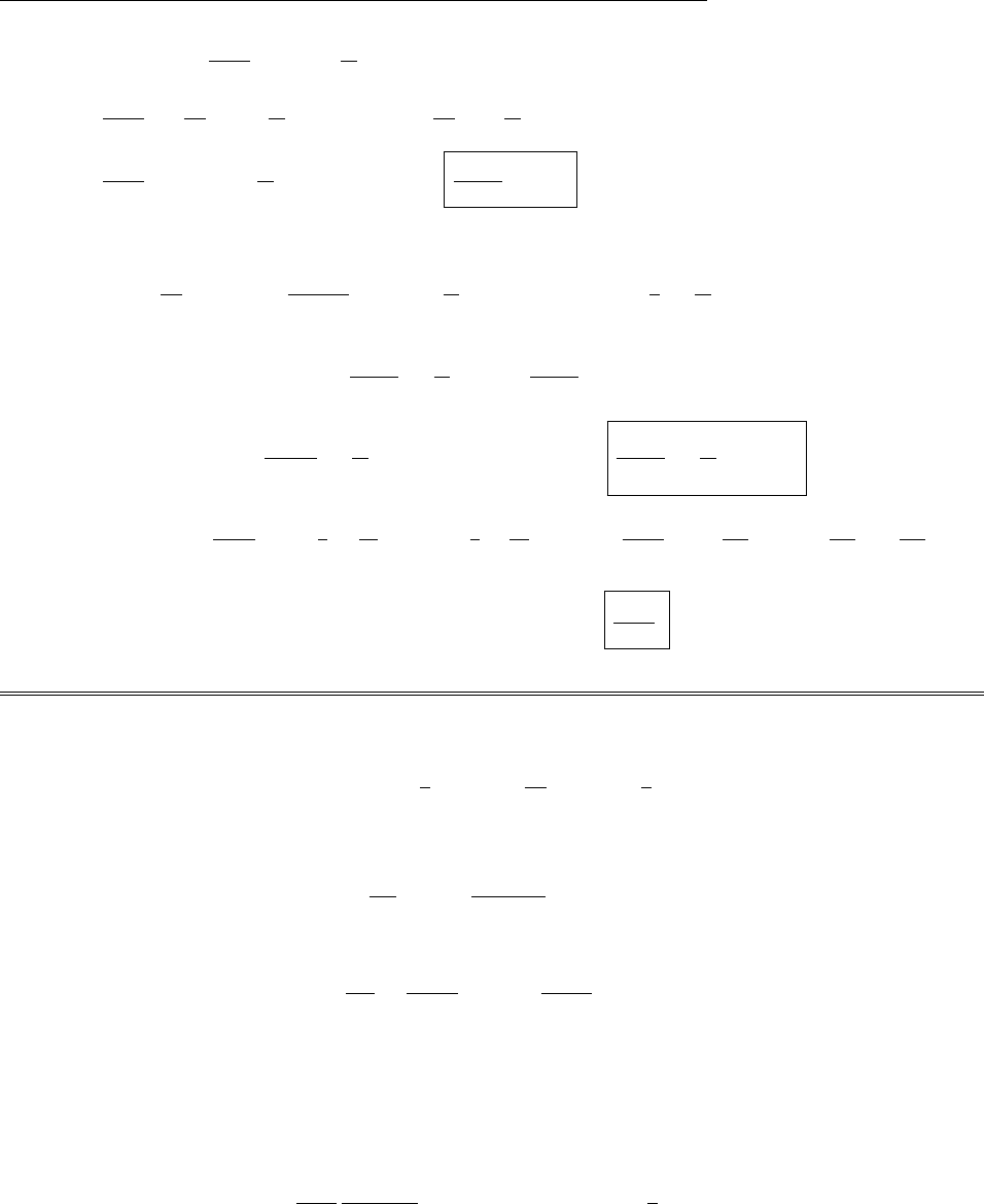
CHAPTER 11. RADIATION 249
B=r⇥A=µ0¨p0
4⇡cr⇥ct
r1(cos ✓ˆr sin ✓ˆ
✓)
=µ0¨p0
4⇡cr @
@rrct
r1sin ✓@
@✓ ct
r1cos ✓ ˆ
=µ0¨p0
4⇡cr sin ✓+ct
r1sin ✓ˆ
=µ0¨p0t
4⇡r2sin ✓ˆ
.
(b) The Poynting vector is
S=1
µ0
(E⇥B)= µ0¨p2
0t
16⇡2r3sin ✓ct
r2
1cos ✓(ˆ
✓)+1
2ct
r2
+1
sin ✓ˆr .
S·da=µ0¨p2
0t
32⇡2ct
r2
+1
sin2✓
r3(r2sin ✓d✓d).
P(r, t)= µ0¨p2
0t
32⇡2rct
r2
+1
2⇡⇡
0
sin3✓d✓=µ0¨p2
0t
12⇡rct
r2
+1
.
(c) P(r, t0+r/c)= µ0¨p2
0
12⇡rt0+r
cc2
r2t2
0+2t0
r
c+r2
c2+1
=µ0¨p2
0
12⇡c1+ct0
r2+2ct0
r+ct0
r2.
Prad(t0) = lim
r!1 P(r, t0+r/c)= µ0¨p2
0
6⇡c,
in agreement with Eq. 11.60.
Problem 11.27
The momentum flux density is (minus) the Maxwell stress tensor (Section 8.2.3),
Tij =✏0EiEj1
2ij E2+1
µ0BiBj1
2ij B2,
(Eq. 8.17) so the momentum radiated per unit (retarded) time is
dp
dtr
=1
(@tr/@t)$
T·dA,
where (Eq. 10.78)
@tr
@t=
r
c
r
·u=1ˆ
r
·v
c1
.
(This factor is 1, when v=0; it can be ignored in deriving the Larmor formula, but it does contribute to the
momentum radiated.) The integration is over a large spherical surface centered on the charge:
dA=
r
2sin ✓d✓dˆ
r
.
As in the case of the power radiated, only the radiation fields contribute (Eq. 11.66):
Erad =q
4⇡✏0
r
(
r
·u)3[
r
⇥(u⇥a)],Brad =1
cˆ
r
⇥Erad.
c
2012 Pearson Education, Inc., Upper Saddle River, NJ. All rights reserved. This material is
protected under all copyright laws as they currently exist. No portion of this material may be
reproduced, in any form or by any means, without permission in writing from the publisher.

250 CHAPTER 11. RADIATION
Thus
$
T·dA=✏0E(E·dA)1
2E2dA+1
µ0B(B·dA)1
2B2dA=1
2✏0E2+1
µ0
B2dA=✏0E2dA
(note that B·dA= 0, and, for radiation fields, E·dA= 0, (1/µ0)B2= (1/µ0c2)( ˆ
r
⇥E)·(ˆ
r
⇥E)=
✏0ˆ
r
·[E⇥(ˆ
r
⇥E)] = ✏0ˆ
r
·[ˆ
r
E2E(ˆ
r
·E)] = ✏0E2). So
dp
dtr
=✏0
r
·u
r
cE2dA=q2
16⇡2✏0c
r
(
r
·u)5[
r
⇥(u⇥a)]2dA.
We expand the integrand to first order in ⌘v/c:u=cˆ
r
v=cˆ
r
,
r
·u=c
r
(1 ˆ
r
·),
1
(
r
·u)5=1
r
5c5[1 + 5( ˆ
r
·)],
r
⇥(u⇥a)=u(
r
·a)a(
r
·u)=
r
cˆ
r
(ˆ
r
·a)a
r
c(1 ˆ
r
·)
=
r
cˆ
r
(ˆ
r
·a)a+a(ˆ
r
·)(ˆ
r
·a).
[
r
⇥(u⇥a)]2=
r
2c2(ˆ
r
·a)22( ˆ
r
·a)2+a2+ 2( ˆ
r
·a)2(ˆ
r
·)2( ˆ
r
·)( ˆ
r
·a)22a2(ˆ
r
·)
+ 2(a·)( ˆ
r
·a)=
r
2c2a2(ˆ
r
·a)22a2(ˆ
r
·) + 2( ˆ
r
·a)(a·).
r
(
r
·u)5[
r
⇥(u⇥a)]2=1
r
2c3[1 + 5( ˆ
r
·)] a2(ˆ
r
·a)22a2(ˆ
r
·) + 2( ˆ
r
·a)(a·)
=1
r
2c3a2(ˆ
r
·a)22a2(ˆ
r
·) + 2( ˆ
r
·a)(a·) + 5( ˆ
r
·)a25( ˆ
r
·)( ˆ
r
·a)2
=1
r
2c3a2(ˆ
r
·a)2+3a2(ˆ
r
·) + 2( ˆ
r
·a)(a·)5( ˆ
r
·)( ˆ
r
·a)2
=1
r
2c3(ˆ
r
⇥a)2+ˆ
r
·[3a2+ 2(a·)a]5( ˆ
r
·)( ˆ
r
·a)2.
To integrate the first term we set the polar axis along a,so(ˆ
r
⇥a)2=a2sin2✓, while ˆ
r
= sin ✓cos ˆ
x+
sin ✓sin ˆ
y+ cos ✓ˆ
z. The integral kills the ˆ
xand ˆ
ycomponents, leaving
1
r
2(ˆ
r
⇥a)2dA=2⇡a2ˆ
z⇡
0
sin3✓cos ✓d✓=0.
[Note that if v=0then dp/dtr= 0—a particle instantaneously at rest radiates no momentum. That’s why
we had to carry the expansion to first order in , whereas in deriving the Larmor formula we could a↵ord to
set v= 0.] The second term is of the form ( ˆ
r
·g), for a constant vector g. Setting the polar axis along g, so
ˆ
r
·g=gcos ✓, the xand ycomponents again vanish, leaving
1
r
2(ˆ
r
·g)dA=2⇡gˆ
z⇡
0
cos2✓sin ✓d✓=4⇡
3g.
The last term involves ( ˆ
r
·)( ˆ
r
·a)2; this time we orient the polar axis along aand let vlie in the xz plane:
=xˆ
x+zˆ
z, so ( ˆ
r
·)=xsin ✓cos +zcos ✓. Then
1
r
2(ˆ
r
·)( ˆ
r
·a)2dA=a2(xsin ✓cos +zcos ✓) cos2✓sin ✓cos ˆ
x+ sin ✓sin ˆ
y+ cos ✓ˆ
zsin ✓d✓d
c
2012 Pearson Education, Inc., Upper Saddle River, NJ. All rights reserved. This material is
protected under all copyright laws as they currently exist. No portion of this material may be
reproduced, in any form or by any means, without permission in writing from the publisher.

CHAPTER 11. RADIATION 251
=a2xˆ
xsin3✓cos2✓cos2d✓d+zˆ
zcos4✓sin ✓d✓d=4⇡
15 a2(xˆ
x+3zˆ
z)=4⇡
15 a2+ 2(a·)a.
Putting all this together,
dp
dtr
=q2
16⇡2✏0
1
c44⇡
32a(a·)+3a254⇡
15 a2+ 2(a·)a=µ0q2
6⇡c3a2v.
The angular momentum radiated is
dL
dtr
=1
(@tr/@t)
r
⇥$
T·dA.
Because of the “extra”
r
in the integrand, it seems at first glance that the radiation fields alone will produce a
result that grows without limit (as
r
!1); however, the coefficient of this term is precisely zero:
r
⇥$
T·
dA=✏0E2(
r
⇥dA) = 0 (for radiation fields). The finite contribution comes from the cross terms, in which
one field (in $
T) is a radiation field and the other a Coulomb field Ecoul ⌘q
4⇡✏0
r
(
r
·u)3(c2v2)u:
Tij =✏0E(r)
iE(c)
j+E(c)
iE(r)
jij E(r)·E(c)+1
µ0B(r)
iB(c)
j+B(c)
iB(r)
jij B(r)·B(c).
This time $
T·dA=✏0E(r)(E(c)·dA)E(r)·E(c)dA1
µ0B(r)·B(c)dA,
so
(
r
⇥$
T)·dA=✏0
r
⇥E(r)E(c)·dA.
Thus dL
dtr
=q2c
16⇡2✏02
r
(
r
·u)5
r
⇥[
r
⇥(u⇥a)] u·dA,where ⌘1
1(v/c)2.
Now, {
r
⇥[
r
⇥(u⇥a)]}=
r
[
r
·(u⇥a)](u⇥a)
r
2,and (u⇥a)=c(ˆ
r
)⇥a=c(ˆ
r
⇥a)(⇥a),
ˆ
r
·(u⇥a)=cˆ
r
·(⇥a), so {
r
⇥[
r
⇥(u⇥a)]}=
r
2c(ˆ
r
⇥a)(⇥a)+ ˆ
r
ˆ
r
·(⇥a).
Meanwhile u·dA=(u·ˆ
r
)
r
2d⌦, where d⌦⌘sin ✓d✓d. Expanding to first order in ,
dL
dtr
=µ0q2c3
16⇡2
r
(
r
·u)5(
r
2c)(ˆ
r
⇥a)(⇥a)+ ˆ
r
ˆ
r
·(⇥a)
r
(
r
·u)d⌦
=µ0q2
16⇡21 + 4( ˆ
r
·)(ˆ
r
⇥a)(⇥a)+ ˆ
r
ˆ
r
·(⇥a)d⌦
=µ0q2
16⇡2(ˆ
r
⇥a)(⇥a)+ ˆ
r
[ˆ
r
·(⇥a)] + 4( ˆ
r
·)( ˆ
r
⇥a)d⌦
The first integral is
a⇥ˆ
r
sin ✓d✓d=a⇥(sin ✓cos ˆ
x+ sin ✓sin ˆ
y+ cos ✓ˆ
z) sin ✓d✓d=0,
the second is
(⇥a)sin ✓d✓d=4⇡(⇥a),
c
2012 Pearson Education, Inc., Upper Saddle River, NJ. All rights reserved. This material is
protected under all copyright laws as they currently exist. No portion of this material may be
reproduced, in any form or by any means, without permission in writing from the publisher.

252 CHAPTER 11. RADIATION
for the third we set the polar axis along g⌘⇥aand get
gˆ
r
cos ✓sin ✓d✓d=2⇡gˆ
zcos2✓sin ✓d✓=4⇡
3g=4⇡
3(⇥a),
and for the last we put the polar axis along aand let =xˆ
x+zˆ
zlie in the xz plane:
4a(xsin ✓cos +zcos ✓) sin ✓(ˆ
) sin ✓d✓d
=4a(xsin ✓cos +zcos ✓)(sin ˆx cos ˆy ) sin2✓d✓d
=4axˆ
ycos2sin3✓d✓d=16⇡
3axˆ
y=16⇡
3(⇥a).
Putting this all together, we conclude
dL
dtr
=µ0q2
16⇡24⇡(⇥a)+4⇡
3(⇥a)+16⇡
3(⇥a)=µ0q2
6⇡c(v⇥a).
Problem 11.28
(a) A(x, t)= µ0
4⇡K(tr)
r
da
=µ0ˆz
4⇡K(tr)
pr2+x22⇡rdr
=µ0ˆz
2K(tpr2+x2/c)
pr2+x2r dr.
The maximum ris given by tpr2+x2/c = 0;
rmax =c2t2x2(since K(t) = 0 for t<0).
(i)
A(x, t)=µ0K0ˆz
2rm
0
r
pr2+x2dr =µ0K0ˆz
2r2+x2
rm
0=µ0K0ˆz
2r2
mx2x=µ0K0(ct x)
2ˆz .
E(x, t)=@A
@t=µ0K0c
2ˆz ,for ct > x, and 0,for ct < x.
B(x, t)=r⇥A=@Az
@xˆy =µ0K0
2ˆy ,for ct > x, and 0,for ct < x.
c
2012 Pearson Education, Inc., Upper Saddle River, NJ. All rights reserved. This material is
protected under all copyright laws as they currently exist. No portion of this material may be
reproduced, in any form or by any means, without permission in writing from the publisher.

CHAPTER 11. RADIATION 253
(ii)
A(x, t)=µ0↵ˆz
2rm
0tpr2+x2/c
pr2+x2r dr =µ0↵ˆz
2trm
0
r
pr2+x2dr 1
crm
0
r dr
=µ0↵ˆz
2t(ct x)1
2c(c2t2x2)=µ0↵ˆz
4c(x22ctx +c2t2)=µ0↵(xct)2
4cˆz .
E(x, t)=@A
@t=µ0↵(xct)
2ˆz ,for ct > x, and 0,for ct < x.
B(x, t)=r⇥A=@Az
@xˆy =µ0↵
2c(xct)ˆy ,for ct > x, and 0,for ct < x.
(b) Let u⌘1
cr2+x2x,sodu =1
c1
2
1
pr2+x22r dr=1
c
r
pr2+x2dr, and
tpr2+x2
c=tx
cu, and as r:0!1,u:0!1. Then A(x, t)= µ0cˆz
21
0
Ktx
cudu. qed
E(x, t)=@A
@t=µ0cˆz
21
0
@
@tKtx
cudu. But @
@tKtx
cu=@
@uKtx
cu.
=µ0c
2ˆz 1
0
@
@uKtx
cudu =µ0c
2ˆz Ktx
cu1
0=µ0c
2[K(tx/c)K(1)] ˆz
=µ0c
2K(tx/c)ˆz ,[if K(1) = 0].
Note that (i) and (ii) are consistent with this result. Meanwhile
B(x, t)=@Az
@xˆy =µ0c
cˆy 1
0
@
@xKtx
cudu. But @
@xKtx
cu=1
c
@
@uKtx
cu.
=µ0
2ˆy 1
0
@
@uKtx
cudu =µ0
2ˆy Ktx
cu1
0=µ0
2[K(tx/c)K(1)] ˆy
=µ0
2K(tx/c)ˆy ,[if K(1) = 0].
S=1
µ0
(E⇥B)= 1
µ0µ0c
2µ0
2K(tx/c)[ˆz ⇥ˆy ]= µ0c
4[K(tx/c)]2ˆx .
This is the power per unit area that reaches xat time t; it left the surface at time (tx/c). Moreover, an
equal amount of energy is radiated downward, so the total power leaving the surface at time tis µ0c
2[K(t)]2.
Problem 11.29
With ↵= 90, Eq. 7.68 gives E0=cB,B0=1
cE,q
0
m=cqe. Use this to “translate” Eqs. 10.72, 10.73,
c
2012 Pearson Education, Inc., Upper Saddle River, NJ. All rights reserved. This material is
protected under all copyright laws as they currently exist. No portion of this material may be
reproduced, in any form or by any means, without permission in writing from the publisher.

254 CHAPTER 11. RADIATION
and 11.70:
E0=c1
cˆ
r
⇥E=ˆ
r
⇥(cB0)=c(ˆ
r
⇥B0).
B0=1
cE=1
c
qe
4⇡✏0
r
(
r
·u)3(c2v2)u+
r
⇥(u⇥a)
=1
c
(q0
m/c)
4⇡✏0
r
(
r
·u)3(c2v2)u+
r
⇥(u⇥a)=µ0q0
m
4⇡
r
(
r
·u)3(c2v2)u+
r
⇥(u⇥a).
P=µ0a2
6⇡cq2
e=µ0a2
6⇡c1
cq0
m2
=µ0a2
6⇡c3(q0
m)2.
Or, dropping the primes,
B(r,t)=µ0qm
4⇡
r
(
r
·u)3(c2v2)u+
r
⇥(u⇥a).
E(r,t)=c(ˆ
r
⇥B).
P=µ0q2
ma2
6⇡c3.
Problem 11.30
(a) Wext =F dx =FT
0
v(t)dt. From Prob. 11.19, v(t)= F
mt+⌧⌧e(tT)/⌧. So
Wext =F2
mT
0
t dt +⌧T
0
dt ⌧eT/⌧T
0
et/⌧dt=F2
mt2
2+⌧t⌧eT/⌧⌧et/⌧
T
0
=F2
m1
2T2+⌧T⌧2eT/⌧eT/⌧1=F2
m1
2T2+⌧T⌧2+⌧2eT/⌧.
(b) From Prob. 11.19, the final velocity is vf=(F/m)T,soWkin =1
2mv2
f=1
2mF2
m2T2=F2T2
2m.
(c) Wrad =P dt. According to the Larmor formula, P=µ0q2a2
6⇡c, and (again from Prob. 11.19)
a(t)=
(F/m)1eT/⌧et/⌧,(t0);
(F/m)1e(tT)/⌧,(0 tT).
c
2012 Pearson Education, Inc., Upper Saddle River, NJ. All rights reserved. This material is
protected under all copyright laws as they currently exist. No portion of this material may be
reproduced, in any form or by any means, without permission in writing from the publisher.

CHAPTER 11. RADIATION 255
Wrad =µ0q2
6⇡c
F2
m21eT/⌧20
1
e2t/⌧dt +T
01e(tT)/⌧2dt
=⌧F2
m1eT/⌧2⌧
2e2t/⌧
0
1
+T
0
dt 2eT/⌧T
0
et/⌧dt +e2T/⌧T
0
e2t/⌧dt
=⌧F2
m⌧
21eT/⌧2+T2eT/⌧⌧et/⌧
T
0+e2T/⌧⌧
2e2t/⌧
T
0
=⌧F2
m⌧
212eT/⌧+e2T/⌧+T2⌧eT/⌧eT/⌧1+⌧
2e2T/⌧e2T/⌧1
=⌧F2
m⌧
2⌧eT/⌧+⌧
2e2T/⌧+T2⌧+2⌧eT/⌧+⌧
2⌧
2e2T/⌧=⌧F2
mT⌧+⌧eT/⌧.
Energy conservation requires that the work done by the external force equal the final kinetic energy plus
the energy radiated:
Wkin +Wrad =F2T2
2m+⌧F2
mT⌧+⌧eT/⌧=F2
m1
2T2+⌧T⌧2+⌧2eT/⌧=Wext.X
Problem 11.31
(a) a=⌧˙a+k
m(t))✏
✏
a(t)dt =v(✏)v(✏)=⌧✏
✏
da
dt dt +k
m✏
✏
(t)dt =⌧[a(✏)a(✏)] + k
m.
If the velocity is continuous, so v(✏)=v(✏), then a(✏)a(✏)=k
m⌧.
When t<0,a=⌧˙a)a(t)=Aet/⌧; when t>0,a=⌧˙a)a(t)=Bet/⌧;a=BA=k
m⌧
)B=Ak
m⌧, so the general solution is a(t)=Aet/⌧,(t<0);
[A(k/m⌧)] et/⌧,(t>0).
To eliminate the runaway we’d need A=k/m⌧; to eliminate preacceleration we’d need A= 0. Obviously,
you can’t do both. If you choose to eliminate the runaway, then a(t)=(k/m⌧)et/⌧,(t<0);
0,(t>0).
v(t)=t
1
a(t)dt =k
m⌧t
1
et/⌧dt =k
m⌧⌧et/⌧
t
1 =k
met/⌧(for t<0);
for t>0,v(t)=v(0) + t
0
a(t)dt =v(0) = k
m. So v(t)=(k/m)et/⌧,(t<0);
(k/m),(t>0).
For an uncharged particle we would have a(t)= k
m(t),v(t)=t
1
a(t)dt =0,(t<0);
(k/m),(t>0).
The graphs:
c
2012 Pearson Education, Inc., Upper Saddle River, NJ. All rights reserved. This material is
protected under all copyright laws as they currently exist. No portion of this material may be
reproduced, in any form or by any means, without permission in writing from the publisher.

256 CHAPTER 11. RADIATION
(b)
Wext =F dx =Fvdt =k(t)v(t)dt =kv(0) = k2
m.
Wkin =1
2mv2
f=1
2mk
m2
=k2
2m.
Wext =Prad dt =µ0q2
6⇡c[a(t)]2dt =⌧mk
m⌧20
1
e2t/⌧dt =k2
m⌧⌧
2e2t/⌧
0
1
=k2
m⌧
⌧
2=k2
2m.
Clearly, Wext =Wkin +Wrad.X
Problem 11.32
Our task is to solve the equation a=⌧˙a+U0
m[(x)+(xL)], subject to the boundary conditions
(1) xcontinuous at x= 0 and x=L;
(2) vcontinuous at x= 0 and x=L;
(3) a=±U0/m⌧v(plus at x= 0, minus at x=L).
The third of these follows from integrating the equation of motion:
dv
dt dt =⌧da
dt dt +U0
m[(x)+(xL)] dt,
v=⌧a+U0
m[(x)+(xL)] dt
dx dx =0,
a== U0
m⌧1
v[(x)+(xL)] dx =±U0
m⌧v.
In each of the three regions the force is zero (it acts only at x= 0 and x=L), and the general solution is
a(t)=Aet/⌧;v(t)=A⌧et/⌧+B;x(t)=A⌧2et/⌧+Bt +C.
(I’ll put subscripts on the constants A,B, and C, to distinguish the three regions.)
Region iii (x>L): To avoid the runaway we pick A3= 0; then a(t)=0,v(t)=B3,x(t)=B3t+C3. Let
the final velocity be vf(= B3), set the clock so that t= 0 when the particle is at x= 0, and let Tbe the time
it takes to traverse the barrier, so x(T)=L=vfT+C3, and hence C3=LvfT. Then
a(t) = 0; v(t)=vf,x(t)=L+vf(tT),(t<T).
Region ii (0 <x<L): a=A2et/⌧,v=A2⌧et/⌧+B2,x=A2⌧2et/⌧+B2t+C2.
c
2012 Pearson Education, Inc., Upper Saddle River, NJ. All rights reserved. This material is
protected under all copyright laws as they currently exist. No portion of this material may be
reproduced, in any form or by any means, without permission in writing from the publisher.
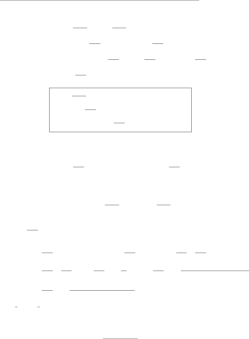
CHAPTER 11. RADIATION 257
(3) )0A2eT/⌧=U0
m⌧vf)A2=U0
m⌧vf
eT/⌧.
(2) )vf=A2⌧eT/⌧+B2=U0
mvf
+B2)B2=vfU0
mvf
.
(1) )L=A2⌧2eT/⌧+B2T+C2=U0⌧
mvf
+vfTU0T
mvf
+C2=vfT+U0
mvf
(⌧T)+C2)
C2=LvfT+U0
mvf
(T⌧).
a(t)= U0
m⌧vf
e(tT)/⌧;
v(t)=vf+U0
mvfe(tT)/⌧1;
x(t)=L+vf(tT)+ U0
mvf⌧e(tT)/⌧t+T⌧;
(0 <t<T).
[Note: if the barrier is sufficiently wide (or high) the particle may turn around before reaching L, but we’re
interested here in the r´egime where it does tunnel through.]
In particular, for t= 0 (when x= 0):
0=LvfT+U0
mvf⌧eT/⌧+T⌧)L=vfTU0
mvf⌧eT/⌧+T⌧.qed
Region i(x<0): a=A1et/⌧,v=A1⌧et/⌧+B1,x=A1⌧2et/⌧+B1t+C1. Let vibe the incident velocity
(at t!1); then B1=vi. Condition (3) says
U0
m⌧vf
eT/⌧A1=U0
m⌧v0
,
where v0is the speed of the particle as it passes x= 0. From the solution in region (ii) it follows that
v0=vf+U0
mvfeT/⌧1. But we can also express it in terms of the solution in region (i): v0=A1⌧+vi.
Therefore
vi=vf+U0
mvfeT/⌧1A1⌧=vf+U0
mvfeT/⌧1+U0
mv0U0
mvf
eT/⌧
=vfU0
mvf
+U0
mv0
=vfU0
mvf1vf
v0=vfU0
mvf1vf
vf+(U0/mvf)eT/⌧1
=vfU0
mvf11
1+(U0/mv2
f)eT/⌧1.qed
If 1
2mv2
f=1
2U0, then
L=vfTvf⌧eT/⌧+T⌧=vfT⌧eT/⌧T+⌧=⌧vf1eT/⌧;
vi=vfvf11
1+eT/⌧1=vf11+eT/⌧=vfeT/⌧.
c
2012 Pearson Education, Inc., Upper Saddle River, NJ. All rights reserved. This material is
protected under all copyright laws as they currently exist. No portion of this material may be
reproduced, in any form or by any means, without permission in writing from the publisher.

258 CHAPTER 11. RADIATION
Putting these together,
L
⌧vf
=1eT/⌧)eT/⌧=1L
⌧vf)eT/⌧=1
1(L/⌧vf))vi=vf
1(L/vf⌧).qed
In particular, for L=vf⌧/4, vi=vf
11/4=4
3vf, so KEi
KEf
=
1
2mv2
i
1
2mv2
f
=vi
vf2
=16
9)
KEi=16
9KEf=16
9
1
2U0=8
9U0.
Problem 11.33
(a) From Eq. 10.72, E1=(q/2)
4⇡✏0
r
(
r
·u)3(c2v2)u+(
r
·a)u(
r
·u)a. Here u=cˆ
r
v,
r
=
lˆx +dˆy ,v=vˆx ,a=aˆx , so
r
·v=lv,
r
·a=la,
r
·u=c
r
r
·v=c
r
lv. We want only the x
component. Noting that ux=(c/
r
)lv=(cl v
r
)/
r
, we have:
E1x=q
8⇡✏0
r
(c
r
lv)31
r
(cl v
r
)(c2v2+la)a(c
r
lv)
=q
8⇡✏0
1
(c
r
lv)3(cl v
r
)(c2v2)+cl2av
r
la ac
r
2+alv
r
.But
r
2=l2+d2.
=q
8⇡✏0
1
(c
r
lv)3(cl v
r
)(c2v2)acd2.
Fself =q2
8⇡✏0
1
(c
r
lv)3(cl v
r
)(c2v2)acd2ˆx .(This generalizes Eq.11.90.)
Now x(t)x(tr)=l=vT +1
2aT 2+1
6˙aT 3+···, where T=ttr, and v,a, and ˙aare all evaluated at the
retarded time tr.
(cT )2=
r
2=l2+d2=d2+(vT +1
2aT 2+1
6˙aT 3)2=d2+v2T2+vaT3+1
3v˙aT 4+1
4a2T4;
c2T2(1 v2/c2)=c2T2/2=d2+vaT3+1
3v˙a+1
4a2T4. Solve for Tas a power series in d:
T=d
c1+Ad +Bd2+···)c2
2
2d2
c21+2Ad +2Bd2+A2d2=d2+va3d3
c3(1+3Ad)+v˙a
3+a2
44
c4d4.
Comparing like powers of d:A=1
2va3
c3;2B+A2=3va3
c3A+v˙a
3+a2
44
c4.
2B=3va3
c3
1
2va3
c31
4v2a26
c6+v˙a
3
4
c4+a24
4c4=v˙a
3
4
c4+6a2
4c41
2v2
c2+3
2
v2a26
c6
=4
c4v˙a
3+a22
41v2
c2v2
c2+6v2
c2)B=4
2c4v˙a
3+2a2
41+4v2
c2.
T=d
c1+va
2
3
c3d+4
2c4v˙a
3+2a2
41+4v2
c2d2+()d4+··· (generalizing Eq.11.93).
c
2012 Pearson Education, Inc., Upper Saddle River, NJ. All rights reserved. This material is
protected under all copyright laws as they currently exist. No portion of this material may be
reproduced, in any form or by any means, without permission in writing from the publisher.

CHAPTER 11. RADIATION 259
l=vT +1
2aT 2+1
6˙aT 3+···
=vd
c1+va
2
3
c3d+4
2c4v˙a
3+2a2
41+4v2
c2d2+1
2a2d2
c21+va3
c3d+1
6˙a3
c3d3
=v
cd+a
2
4
c21v2
c2+v2
c2d2+v
2c
4
c4v˙a
3+2a2
41+4v2
c2+1
2a2
c2va3
c3+1
6˙a3
c3d3
=v
cd+a4
2c2d2+3
2c3˙a
31+2v2
c2+v4a2
c21
4+v2
c2+1v2
c2d3
=v
cd+a4
2c2d2+5
2c3˙a
3+5
4
v2a2
c2d3+()d4+···
r
=cT =d1+va
2
3
c3d+4
2c4v˙a
3+2a21
4+v2
c2d2+()d4+···
c
r
lv =cd+va4
2c2d2+5
2c3v˙a
3+2a21
4+v2
c2d3v2
cdav4
2c2d25v
2c3˙a
3+5
4
v2a2
c2d3+···
=cd1v2
c2+5
2c3v˙a
3+2a21
4+v2
c2v˙a
35
4
v22a2
c2d3+···
=c
d+5a2
8c3d3+()d4+···
cl v
r
=vd+a4
2cd2+5
2c2˙a
3+5
4
v2a2
c2d3vdv2a
2
4
c3d2v5
2c4v˙a
3+2a21
4+v2
c2d3
=a4
2c1v2
c2d2+5
2c2˙a
3+5
4
v2a2
c2v2
c2
˙a
3v2a2
c21
4+v2
c2d3+()d4+···
=a2
2cd2+5
2c2˙a
32+v2a2
c25
41
4v2
c2d3+()d4+···
=a2
2cd2+3
2c2˙a
3+v2a2
c2d3+()d4+···
(c
r
lv)3=cd
1+6a2
8c4d23
=
cd3136a2
8c4d2+···
Fself =q2
8⇡✏0
cd3136a2
8c4d2a2
2cd2+3
2c2˙a
3+v2a2
c2d3c2
2acd2ˆx
=q2
8⇡✏0
3
c3d13
8
6a2
c4d2ac
2+
2˙a
3+v2a2
c2dˆx
=q2
8⇡✏0
3
c3d
1
2ac +˙a
3+v2a2
c2d+()d2+···ˆx
=q2
4⇡✏03a
4c2d+4
4c3˙a
3+v2a2
c2+()d+···ˆx (generalizing Eq.11.95).
Switching to t:v(tr)=v(t)+ ˙v(t)(trt)+···=v(t)a(t)T=v(t)ad/c. (When multiplied by d, it
doesn’t matter—to this order—whether we evaluate at tor at tr.)
c
2012 Pearson Education, Inc., Upper Saddle River, NJ. All rights reserved. This material is
protected under all copyright laws as they currently exist. No portion of this material may be
reproduced, in any form or by any means, without permission in writing from the publisher.

260 CHAPTER 11. RADIATION
1v(tr)
c2
=1[v(t)22vad/c]
c2=1v(t)2
c21+2av3d
c3,so
=1v(tr)
c21/2
=(t)1va3
c3d;a(tr)=a(t)T˙a=a(t)˙a
cd.
Evaluating everything now at time t:
Fself =q2
4⇡✏0313va3d/c3(a˙ad/c)
4c2d+4
4c3˙a
3+v2a2
c2+()d2+···ˆx
=q2
4⇡✏03a
4c2d+3
4c2˙a
c+3va22
c3+4
4c3˙a
3+v2a2
c2+()d+···ˆx
=q2
4⇡✏03a
4c2d+4
4c3˙a+˙a
3+3va22
c2+v2a2
c2+()d+···ˆx
=q2
4⇡✏03a
4c2d+4
3c3˙a+3va22
c2+()d+···ˆx (generalizing Eq.11.96).
The first term is the electromagnetic mass; the radiation reaction itself is the second term:
Fint
rad =µ0q2
12⇡c4˙a+3va22
c2(generalizing Eq. 11.99), so the generalization of Eq. 11.100 is
Frad =µ0q2
6⇡c4˙a+3va22
c2.
(b) Frad =A4˙a+32a2v
c2, where A⌘µ0q2
6⇡c.P=Aa26(Eq. 11.75). What we must show is that
t2
t1
Fradvdt=t2
t1
P dt, or t2
t1
4˙av +3v2a22
c2dt =t2
t1
a26dt
(except for boundary terms—see Sect. 11.2.2).
Rewrite the first term: t2
t1
4˙av dt =t2
t1
(4v)da
dt dt =4va
t2
t1t2
t1
d
dt(4v)a dt.
Now d
dt(4v)=43d
dt v+4a;d
dt =d
dt 1
1v2/c2=1
2
1
(1 v2/c2)3/22va
c2=va3
c2.So
d
dt(4v)=43vva3
c2+4a=6a1v2
c2+4v2
c2=6a1+3v2
c2.
t2
t1
4˙av dt =4va
t2
t1t2
t1
6a21+3v2
c2dt, and hence
t2
t1
4˙av +32a2v2
c2dt =4va
t2
t1
+t2
t16a21+3v2
c2+36a2v2
c2dt =4va
t2
t1t2
t1
6a2dt. qed
Problem 11.34
(a) P=µ0q2a26
6⇡c(Eq.11.75).w=b2+c2t2(Eq.10.52); v=˙w=c2t
pb2+c2t2;
a=˙v=c2
pb2+c2t2c2t(c2t)
(b2+c2t2)3/2=c2
(b2+c2t2)3/2b2+c2t2c2t2=b2c2
(b2+c2t2)3/2;
c
2012 Pearson Education, Inc., Upper Saddle River, NJ. All rights reserved. This material is
protected under all copyright laws as they currently exist. No portion of this material may be
reproduced, in any form or by any means, without permission in writing from the publisher.

CHAPTER 11. RADIATION 261
2=1
1v2/c2=1
1[c2t2/(b2+c2t2)] =b2+c2t2
b2+c2t2c2t2=1
b2b2+c2t2.So
P=µ0q2
6⇡c
b4c4
(b2+c2t2)3
(b2+c2t2)3
b6=q2c
6⇡✏0b2.Yes, it radiates (in fact, at a constant rate).
(b) Frad =µ0q24
6⇡c˙a+32a2v
c2;˙a=3
2
b2c2(2c2t)
(b2+c2t2)5/2=3b2c4t
(b2+c2t2)5/2;˙a+32a2v
c2=
3b2c4t
(b2+c2t2)5/2+3
c2
(b2+c2t2)
b2
b4c4
(b2+c2t2)3
c2t
pb2+c2t2=0. Frad =0.No, the radiation reaction is zero.
Problem 11.35
The fields of a nonstatic ideal dipole (Problem 10.34) contain terms that go like 1/r,1/r2, and 1/r3, for
fixed t0⌘tr/c; radiation comes from the first of these:
Er=µ0
4⇡r[¨
pˆr (ˆr ·¨
p)],Br=µ0
4⇡rc(ˆr ⇥¨
p)
where the dipole moments are evaluated at time t0. The 1/r2term in the Poynting vector is
Sr=1
µ0
(Er⇥Br)= µ0
16⇡2cr2[¨
pˆr (ˆr ·¨
p)] ⇥(ˆr ⇥¨
p)= µ0
16⇡2cr2{¨
p⇥(ˆr ⇥¨
p)(ˆr ·¨
p)[ˆr ⇥(ˆr ⇥¨
p)]}
=µ0
16⇡2cr2ˆr ¨p2¨
p(ˆr ·¨
p)(ˆr ·¨
p)[ˆr (ˆr ·¨
p)¨
p]=µ0
16⇡2cr2¨p2(ˆr ·¨
p)2ˆr .
Setting the zaxis along ¨
p,¨p2(ˆr ·¨
p)2=¨p2sin2✓, and the power radiated is
P=Sr·da=µ0
16⇡2c¨p21
r2sin2✓r2sin ✓d✓d=µ0
8⇡c¨p2⇡
0
sin3✓d✓=µ0
6⇡c¨p2.
For the sinusoidal case, p=p0cos !t, we have ¨
p=!2p0cos !t,¨p2=!4p2
0cos2!t, and its time average
is (1/2)p2
0!4, so
hPi=µ0
12⇡c¨p2
0!4,
in agreement with Eq. 11.22. And in the case of quadratic time dependence our result agrees with the answer
to Problem 11.26.
c
2012 Pearson Education, Inc., Upper Saddle River, NJ. All rights reserved. This material is
protected under all copyright laws as they currently exist. No portion of this material may be
reproduced, in any form or by any means, without permission in writing from the publisher.

262 CHAPTER 12. ELECTRODYNAMICS AND RELATIVITY
Chapter 12
Electrodynamics and Relativity
Problem 12.1
Let ube the velocity of a particle in S,¯
uits velocity in ¯
S, and vthe velocity of ¯
Swith respect to S.
Galileo’s velocity addition rule says that u=¯
u+v. For a free particle, uis constant (that’s Newton’s first
law in S.
(a) If vis constant, then ¯
u=uvis also constant, so Newton’s first law holds in ¯
S, and hence ¯
Sis inertial.
(b) If ¯
Sis inertial, then ¯
uis also constant, so v=u¯
uis constant.
Problem 12.2
(a) mAuA+mBuB=mCuC+mDuD;ui=¯
ui+v.
mA(¯
uA+v)+mB(¯
uB+v)=mC(¯
uC+v)+mD(¯
uD+v),
mA¯
uA+mB¯
uB+(mA+mB)v=mC¯
uC+mD¯
uD+(mC+mD)v.
Assuming mass is conserved, (mA+mB)=(mC+mD), it follows that
mA¯
uA+mB¯
uB=mC¯
uC+mD¯
uD, so momentum is conserved in ¯
S.
(b)1
2mAu2
A+1
2mBu2
B=1
2mCu2
C+1
2mDu2
D)
1
2mA(¯u2
A+2
¯
uA·v+v2)+1
2mB(¯u2
B+2
¯
uB·v+v2)=1
2mC(¯u2
C+2
¯
uC·v+v2)+1
2mD(¯u2
D+2
¯
uD·v+v2)
1
2mA¯u2
A+1
2mB¯u2
B+v·(mA¯
uA+mB¯
uB)+1
2v2(mA+mB)
=1
2mC¯u2
C+1
2mD¯u2
D+v·(mC¯
uC+mD¯
uD)+1
2v2(mC+mD).
But the middle terms are equal by conservation of momentum, and the last terms are equal by conservation
of mass, so 1
2mA¯u2
A+1
2mB¯u2
B=1
2mC¯u2
C+1
2mD¯u2
D.qed
Problem 12.3
(a) vG=vAB +vBC;vE=vAB +vBC
1+vAB vBC/c2⇡vG1vAB vBC
c2;)vGvE
vG=vAB vBC
c2.
In mi/h, c= (186,000 mi/s) ⇥(3600 sec/hr) = 6.7⇥108mi/hr.
)vGvE
vG=(5)(60)
(6.7⇥108)2=6.7⇥1016.)6.7⇥1014% error (pretty small!)
(b) 1
2c+3
4c/1+1
2·3
4=5
4c/11
8=10
11c(still less than c)
(c) To simplify notation, let =vAC /c,1=vAB /c,2=vBC/c. Then Eq. 12.3 says: =1+2
1+12, or:
2=2
1+212+212+2
2
(1 + 212+2
12
2)=1+212+2
12
2
(1 + 212+2
12
2)(1 + 2
12
22
12
2)
(1 + 212+2
12
2)=1(1 2
1)(1 2
2)
(1 + 12)2=1,
c
2012 Pearson Education, Inc., Upper Saddle River, NJ. All rights reserved. This material is
protected under all copyright laws as they currently exist. No portion of this material may be
reproduced, in any form or by any means, without permission in writing from the publisher.

CHAPTER 12. ELECTRODYNAMICS AND RELATIVITY 263
where ⌘(1 2
1)(1 2
2)/(1 + 12)2is clearly a positive number. So 2<1, and hence |vAC |<c. qed.
Problem 12.4
(a) Velocity of bullet relative to ground is 1
2c+1
3c=5
6c=10
12 c.
Velocity of getaway car is 3
4c=9
12 c. Since vb>v
g, bullet does reach target .
(b) Velocity of bullet relative to ground is 1
2c+1
3c
1+ 1
2·1
3
=5
6c
7
6
=5
7c=20
28 c.
Velocity of getaway car is 3
4c=21
28 c. Since vg>v
b, bullet does not reach target .
Problem 12.5
(a) Light from 90th clock took 90⇥109m
3⇥108m= 300 sec = 5 min to reach me, so the time I see on the clock is
11:55 am .
(b) I observe 12 noon .
Problem 12.6
light signal leaves aat time t0
a; arrives at earth at time ta=t0
a+da
c
light signal leaves bat time t0
b; arrives at earth at time tb=t0
b+db
c
)t=tbta=t0
bt0
a+(dbda)
c=t0+(vt0cos ✓)
c=t01v
ccos ✓
(Here dais the distance from ato earth, and dbis the distance from bto earth.)
s=vt0sin ✓=vsin ✓t
(1t(1 v
ccos ✓))u=vsin ✓
(1 v
ccos ✓)is the the apparent velocity.
du
d✓=v(1 v
ccos ✓)(cos ✓)sin ✓(v
csin ✓)
(1 v
ccos ✓)2=0)(1 v
ccos ✓) cos ✓=v
csin2✓
)cos ✓=v
c(sin2✓+ cos2✓)=v
c
✓max = cos1(v/c) At this maximal angle, u=vp1v2/c2
1v2/c2=v
p1v2/c2
As v!c,u!1, because the denominator !0 — even though v<c.
Problem 12.7
The student has not taken into account time dilation of the muon’s “internal clock”. In the laboratory, the
muon lasts ⌧ =⌧
p1v2/c2, where ⌧is the “proper” lifetime, 2 ⇥106sec. Thus
v=d
t/1v2/c2=d
⌧1v2
c2,where d= 800 meters.
⌧
d2v2=1v2
c2;v2⌧
d2+1
c2= 1; v2=1
(⌧/d)2+ (1/c)2.
v2
c2=1
1+(⌧c/d)2;⌧c
d=(2 ⇥106)(3 ⇥108)
800 =6
8=3
4;v2
c2=1
1+9/16 =16
25;v=4
5c.
c
2012 Pearson Education, Inc., Upper Saddle River, NJ. All rights reserved. This material is
protected under all copyright laws as they currently exist. No portion of this material may be
reproduced, in any form or by any means, without permission in writing from the publisher.

264 CHAPTER 12. ELECTRODYNAMICS AND RELATIVITY
Problem 12.8
(a) Rocket clock runs slow; so earth clock reads t=1
p1v2/c2·1 hr. Here =1
p1v2/c2=1
p19/25 =5
4.
)According to earth clocks signal was sent 1 hr, 15 min after take-o↵.
(b) By earth observer, rocket is now a distance 3
5c5
4(1 hr) = 3
4chr (three-quarters of a light hour) away.
Light signal will therefore take 3
4hr to return to earth. Since it left 1 hr and 15 min after departure, light
signal reaches earth 2 hrs after takeo↵
(c) Earth clocks run slow: trocket =·(2 hrs) = 5
4·(2 hrs) = 2.5 hrs
Problem 12.9
Lc=2Lv;Lc
c=Lv
v;so 2
c=1
v=11
22=3
4;1
2
c=1v2
c2=v2
c2=3
16 .v2
c2=13
16 =13
16 ;v=p13
4c
Problem 12.10
Say length of mast (at rest) is ¯
l. To an observer on the boat, height of mast is ¯
lsin ¯
✓, horizontal projection
is ¯
lcos ¯
✓. To observer on dock, the former is una↵ected, but the latter is Lorentz contracted to 1
¯
lcos ¯
✓.
Therefore:
tan ✓=¯
lsin ¯
✓
1
¯
lcos ¯
✓=tan ¯
✓,or tan ✓=tan ¯
✓
1v2/c2
Problem 12.11
Naively, circumference/diameter = 1
(2⇡R)/(2R)=⇡/=⇡1(!R/c)2— but this is nonsense. Point
is: an accelerating object cannot remain rigid, in relativity. To decide what actually happens here, you need a
specific model for the internal forces holding the disc together.
Problem 12.12
(iv) )t=¯
t
+vx
c2. Put this into (i), and solve for x:
¯x=xxv¯
t
+vx
c2=x1v2
c2v¯
t=x1
2v¯
t=x
v¯
t;x=(¯x+v¯
t)X
Similarly, (i) )x=¯x
+vt. Put this into (iv) and solve for t:
¯
t=tv
c2¯x
+vt=t1v2
c2v
c2¯xt
v
c2¯x;t=¯
t+v
c2¯xX
Problem 12.13
Let brother’s accident occur at origin, time zero, in both frames. In system S(Sophie’s), the coordinates
of Sophie’s cry are x=5⇥105m, t= 0. In system ¯
S(scientist’s), ¯
t=(tv
c2x)=vx/c2. Since
this is negative, Sophie’s cry occurred before the accident, in ¯
S.=1
p1(12/13)2=13
p169144 =13
5. So
¯
t=13
512
13 c(5 ⇥105)/c2=12 ⇥105/3⇥108=10
3. 4 ⇥103seconds earlier
Problem 12.14
(a) In Sit moves a distance dy in time dt. In ¯
S, meanwhile, it moves a distance d¯y=dy in time d¯
t=
(dt v
c2dx).
)d¯y
d¯
t=dy
(dt v
c2dx)=(dy/dt)
1v
c2
dx
dt ; or ¯uy=uy
1vux
c2;¯uz=uz
1vux
c2
c
2012 Pearson Education, Inc., Upper Saddle River, NJ. All rights reserved. This material is
protected under all copyright laws as they currently exist. No portion of this material may be
reproduced, in any form or by any means, without permission in writing from the publisher.

CHAPTER 12. ELECTRODYNAMICS AND RELATIVITY 265
(b) S= dock frame; S0= boat frame; we need reverse transformations (v!v):
tan ✓=uy
ux
=¯uy/1+v¯ux
c2
(¯ux+v)/1+ v¯ux
c2=1
¯uy
(¯ux+v). In this case ¯ux=ccos ¯
✓;¯uy=csin ¯
✓, so
tan ✓=1
csin ¯
✓
(ccos ¯
✓+v)=1
sin ¯
✓
cos ¯
✓v/c
[Contrast tan ✓=sin ¯
✓
cos ¯
✓in Prob. 12.10. The point is that velocities are sensitive not only to the transfor-
mation of distances, but also of times. That’s why there is no universal rule for translating angles — you have
to know whether it’s an angle made by a velocity vector or a position vector.]
That’s how the velocity vector of an individual photon transforms. But the beam as a whole is a snapshot
of many di↵erent photons at one instant of time, and it transforms the same way the mast does.
Problem 12.15
Bullet relative to ground: 5
7c. Outlaws relative to police:
3
4c1
2c
13
4·1
2
=
1
4c
5
8
=2
5c.
Bullet relative to outlaws:
5
7c3
4c
15
7·3
4
=1
28 c
13
28
=1
13c. [Velocity of Arelative to Bis minus the velocity of
Brelative to A, so all entries below the diagonal are trivial. Note that in every case vbullet <v
outlaws, so no
matter how you look at it, the bad guys get away.]
speed of !
relative to #
Ground Police Outlaws Bullet Do they escape?
Ground 0 1
2c3
4c5
7cYes
Police 1
202
5c1
3cYes
Outlaws 3
4c2
5c01
13 cYes
Bullet 5
7c1
3c1
13 c0 Yes
Problem 12.16
(a) Moving clock runs slow, by a factor =1
p1(4/5)2=5
3. Since 18 years elapsed on the moving clock,
5
3⇥18 = 30 years elapsed on the stationary clock. 51 years old
(b) By earth clock, it took 15 years to get there, at 4
5c,sod=4
5c⇥15 years = 12cyears (12 light years)
(c) t= 15 yrs, x= 12cyrs
(d) ¯
t= 9 yrs, ¯x= 0. [She got on at the origin in ¯
S, and rode along on ¯
S, so she’s still at the origin. If you
doubt these values, use the Lorentz Transformations, with xand tin (c).]
(e) Lorentz Transformations: ˜x=(x+vt)
˜
t=(t+v
c2x)[note that vis negative, since ˜
Sus going to the left]
)˜x=5
3(12cyrs + 4
5c·15 yrs) = 5
3·24cyrs = 40cyears.
˜
t=5
3(15 yrs + 4
5
c
c2·12cyrs) = 5
315 + 48
5yrs = (25 + 16)yrs = 41 years.
(f) Set her clock ahead 32 years, from 9 to 41 (¯
t!˜
t). Return trip takes 9 years (moving time), so her clock
will now read 50 years at her arrival. Note that this is 5
3·30 years—precisely what she would calculate if the
stay-at-home had been the traveler, for 30 years of his own time.
c
2012 Pearson Education, Inc., Upper Saddle River, NJ. All rights reserved. This material is
protected under all copyright laws as they currently exist. No portion of this material may be
reproduced, in any form or by any means, without permission in writing from the publisher.

266 CHAPTER 12. ELECTRODYNAMICS AND RELATIVITY
(g) (i) ¯
t= 9 yrs, x= 0. What is t?t=v
c2x+¯
t
=3
5·9 yrs = 27
5=5.4 years, and he started at age 21, so he’s
26.4 years old (Younger than traveler (!) because to the traveller it’s the stay-at-home who’s moving.)
(ii) ˜
t= 41 yrs, x= 0. What is t? t=˜
t
=3
5·41 yrs, or 123
5yrs, or 24.6 yrs, and he started at 21, so he’s
45.6 years old.
(h) It will take another 5.4 years of earth time for the return, so when she gets back, she will say her twin’s
age is 45.6 + 5.4 = 51 years—which is what we found in (a). But note that to make it work from traveler’s
point of view you must take into account the jump in perceived age of the stay-at-home when she changes
coordinates from ¯
Sto ˜
S.)
Problem 12.17
¯a0¯
b0+¯a1¯
b1+¯a2¯
b2+¯a3¯
b3=2(a0a1)(b0b1)+2(a1a0)(b1a0)+a2b2+a3b3
=2(a0b0a0b1
a1b0
+2a1b1a1b1+a1b0
+a0b1
2a0b0)+a2b2+a3b3
=2a0b0(1 2)+2a1b1(1 2)+a2b2+a3b3
=a0b0+a1b1+a2b2+a3b3.qed [Note: 2(1 2) = 1.]
Problem 12.18
(a)
c¯
t
¯x
¯y
¯z
=
1000
100
0010
0001
ct
x
y
z
(using the notation of Eq. 12.24, for best comparison)
(b) ⇤=
0 0
0100
00
0001
(c) Multiply the matrices: ⇤=
¯0¯¯
0
0100
¯¯
0¯0
0001
00
00
0010
0001
=
¯¯ ¯¯
0
00
¯ ¯
¯ ¯
¯0
0001
Yes, the order does matter. In the other order “bars” and “no-bars” would be switched, and this would yield
adi↵erent matrix.
Problem 12.19
(a) Since tanh ✓=sinh ✓
cosh ✓, and cosh2✓sinh2✓= 1, we have:
=1
1v2/c2=1
1tanh2✓=cosh ✓
cosh2✓sinh2✓= cosh ✓; = cosh ✓tanh ✓= sinh ✓.
)⇤=
cosh ✓sinh ✓00
sinh ✓cosh ✓00
0010
0001
Compare: R=
cos sin 0
sin cos 0
001
c
2012 Pearson Education, Inc., Upper Saddle River, NJ. All rights reserved. This material is
protected under all copyright laws as they currently exist. No portion of this material may be
reproduced, in any form or by any means, without permission in writing from the publisher.

CHAPTER 12. ELECTRODYNAMICS AND RELATIVITY 267
(b) ¯u=uv
1uv
c2)¯u
c=u
cv
c
1u
cv
c)tanh ¯
=tanh tanh ✓
1tanh tanh ✓, where tanh =u/c, tanh ✓=v/c;
tanh ¯
=¯u/c. But a “trig” formula for hyperbolic functions (CRC Handbook, 18th Ed., p. 204) says:
tanh tanh ✓
1tanh tanh ✓= tanh(✓).)tanh ¯
= tanh(✓),or: ¯
=✓
Problem 12.20
(a) (i) I=c2t2+x2+y2+z2=(5 15)2+ (10 5)2+ (8 3)2+ (0 0)2=100 + 25 + 25 = 50
(ii) No. (In such a system ¯
t= 0, so Iwould have to be positive, which it isn’t.)
(iii) Yes.
1
✲x
✻
y
246810
2
4
6
8
A
B
❂
!"# $
5
!"# $
5
✻
ct
✲x
#
world line
of player 1 ✮
world line of
player 2
✲✛
10 ft
✠
world line of
the ball
✒
■
✒
■
✒
✲x
✻
ct
A
B
✶
✐
c
⃝2005 Pearson Education, Inc., Upper Saddle River, NJ. All rights reserved. This material is
protected under all copyright laws as they currently exist. No portion of this material may be
reproduced, in any form or by any means, without permission inwritingfromthepublisher.
¯
Stravels in the direction from Btoward A,
making the trip in time 10/c.
)v=5ˆx 5ˆy
10/c =c
2ˆx c
2ˆy
Note that v2
c2=1
4+1
4=1
2, so v=1
p2c, safely
less than c.
(b) (i) I=(3 1)2+ (5 2)2+0+0=4+9= 5
(ii) Yes. By Lorentz Transformation: (c¯
t)=(ct)(x). We want ¯
t= 0, so (ct)=(x); or
v
c=(ct)
(x)=(3 1)
(5 2) =2
3. So v=2
3cin the +xdirection.
(iii) No. (In such a system x=y=z= 0 so Iwould be negative, which it isn’t.)
Problem 12.21
Using Eq. 12.18 (iv): ¯
t=(tv
c2x)=0)t=v
c2x, or v=t
xc2=tBtA
xBxA
c2
c
2012 Pearson Education, Inc., Upper Saddle River, NJ. All rights reserved. This material is
protected under all copyright laws as they currently exist. No portion of this material may be
reproduced, in any form or by any means, without permission in writing from the publisher.

268 CHAPTER 12. ELECTRODYNAMICS AND RELATIVITY
Problem 12.22
(a)
1
✲x
✻
y
246810
2
4
6
8
A
B
❂
!"# $
5
!"# $
5
✻
ct
✲x
#
world line
of player 1 ✮
world line of
player 2
✲✛
10 ft
✠
world line of
the ball
✒
■
✒
■
✒
✲x
✻
ct
A
B
✶
✐
c
⃝2005 Pearson Education, Inc., Upper Saddle River, NJ. All rights reserved. This material is
protected under all copyright laws as they currently exist. No portion of this material may be
reproduced, in any form or by any means, without permission in writing from the publisher.
Truth is, you never do communicate with
the other person right now—you communicate
with the person he/she will be when the mes-
sage gets there; and the response comes back
to an older and wiser you.
(b) No way It is true that a moving observer
might say she arrived at Bbefore she left A,
but for the round trip everyone must agree
that she arrives back after she set out.
Problem 12.24
(a) 1u2
c2⌘2=u2;u21+⌘2
c2=⌘2;u=1
1+⌘2/c2⌘.
c
2012 Pearson Education, Inc., Upper Saddle River, NJ. All rights reserved. This material is
protected under all copyright laws as they currently exist. No portion of this material may be
reproduced, in any form or by any means, without permission in writing from the publisher.
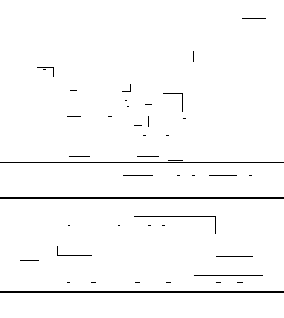
CHAPTER 12. ELECTRODYNAMICS AND RELATIVITY 269
(b) 1
p1u2/c2=1
p1tanh2✓=cosh ✓
pcosh2✓sinh2✓= cosh ✓)⌘=1
p1u2/c2u= cosh ✓ctanh ✓=csinh ✓.
Problem 12.25
(a) ux=uy=ucos 45=1
p2
2
p5c=2
5c.
(b) 1
p1u2/c2=1
p14/5=p5
p54=p5. )⌘=u
p1u2/c2)⌘x=⌘y=p2
(c) ⌘0=c=p5c.
(d) Eq. 12.45)
¯ux=uxv
1uxv
c2=p2
5cp2
5c
12
5
= 0.
¯uy=1
uy
1uxv
c2=12
5
p2
5c
12
5
=p2/5
p3/5c=2
3c.
(e) ¯⌘x=(⌘x⌘0)=12
5(p2c2
5p5c)= 0.¯⌘y=⌘y=p2c.
(f) 1
p1¯u2/c2=1
p12/3=p3; )¯⌘=p3¯u )¯⌘x=p3¯ux=0X
¯⌘y=p3¯uy=p2cX
Problem 12.26
⌘µ⌘µ=(⌘0)2+⌘2=1
(1u2/c2)(c2+u2)=c2(1u2/c2)
(1u2/c2)=c2.Timelike.
Problem 12.27
Use the result of Problem 12.24(a): u=1
1+⌘2/c2⌘.Here ⌘
c=4
3,so 1
1 + 16/9=3
5, and hence
u=3
5(4 ⇥108)=2.4⇥108m/s. Innocent.
Problem 12.28
(a) From Prob. 11.34 we have =1
bpb2+c2t2.)⌧=1
dt =bdt
pb2+c2t2=b
cln(ct +pb2+c2t2)+k; at
t= 0 we want ⌧=0: 0= b
cln b+k,sok=b
cln b;⌧=b
cln 1
b(ct +b2+c2t2)
(b) px2b2+x=bec⌧/b;px2b2=bec⌧/b x;x2b2=b2e2c⌧/b 2xbec⌧/b +x2;2xbec⌧/b =b2(1 + e2c⌧/b);
x=bec⌧/b+ec⌧/b
2=bcosh(c⌧/b) . Also from Prob. 11.34: v=c2t/pb2+c2t2.
v=c
xpx2b2=c
bcosh(c⌧/b)b2cosh2(c⌧/b)b2=cpcosh2(c⌧/b)1
cosh(c⌧/b)=csinh(c⌧/b)
cosh(c⌧/b)=ctanh c⌧
b.
(c) ⌘µ=(c, v, 0,0). =x
b= cosh c⌧
b,so⌘µ= cosh c⌧
bc, c tanh c⌧
b,0,0=ccosh c⌧
b,sinh c⌧
b,0,0.
Problem 12.29
(a) mAuA+mBuB=mCuC+mDuD;ui=¯ui+v
1+(¯uiv/c2).
mA
¯uA+v
1+(¯uAv/c2)+mB
¯uB+v
1+(¯uBv/c2)=mC
¯uC+v
1+(¯uCv/c2)+mD
¯uD+v
1+(¯uDv/c2).
This time, because the denominators are all di↵erent, we cannot conclude that
mA¯uA+mB¯uB=mC¯uC+mD¯uD.
As an explicit counterexample, suppose all the masses are equal, and uA=uB=v, uC=uD=0.This is
a symmetric “completely inelastic” collision in S, and momentum is clearly conserved (0=0). But the Einstein
c
2012 Pearson Education, Inc., Upper Saddle River, NJ. All rights reserved. This material is
protected under all copyright laws as they currently exist. No portion of this material may be
reproduced, in any form or by any means, without permission in writing from the publisher.

270 CHAPTER 12. ELECTRODYNAMICS AND RELATIVITY
velocity addition rule gives ¯uA=0,¯uB=2v/(1 + v2/c2),¯uC=¯uD=v, so in ¯
Sthe (incorrectly defined)
momentum is not conserved:
m2v
1+v2/c26=2mv.
(b) mA⌘A+mB⌘B=mC⌘C+mD⌘D;⌘i=(¯⌘i+¯⌘0
i).(The inverse Lorentz transformation.)
mA(¯⌘A+¯⌘0
A)+mB(¯⌘B+¯⌘0
B)=mC(¯⌘C+¯⌘0
C)+mD(¯⌘D+¯⌘0
D).The gamma’s cancel:
mA¯⌘A+mB¯⌘B+(mA¯⌘0
A+mB¯⌘0
B)=mC¯⌘C+mD¯⌘D+(mC¯⌘0
C+mD¯⌘0
D).
But mi⌘0
i=p0
i=Ei/c, so if energy is conserved in ¯
S(¯
EA+¯
EB=¯
EC+¯
ED), then so too is the momentum
(correctly defined):
mA¯⌘A+mB¯⌘B=mC¯⌘C+mD¯⌘D.qed
Problem 12.30
mc2mc2=nmc2)=n+1= 1
1pu2/c2)1u2
c2=1
(n+1)2
)u2
c2=11
(n+1)2=n2+2n+11
(n+1)2=n(n+2)
(n+1)2;u=n(n+ 2)
n+1 c
Problem 12.31
ET=E1+E2+···;pT=p1+p2+···;¯pT=(pTET/c)=0)=v/c =pTc/ET
v=c2pT/ET=c2(p1+p2+···)/(E1+E2+···)
Problem 12.32
Eµ=(m2
⇡+m2
µ)
2m⇡
c2=mµc2)=(m2
⇡+m2
µ)
2m⇡mµ
=1
1v2/c2;1v2
c2=1
2;
v2
c2=11
2=14m2
⇡m2
µ
(m2
⇡+m2
µ)2=m4
⇡+2m2
⇡m2
µ+m4
µ4m2
⇡m2
µ
(m2
⇡+m2
µ)2=(m2
⇡m2
µ)2
(m2
⇡+m2
µ)2;v=(m2
⇡m2
µ)
(m2
⇡+m2
µ)c.
Problem 12.33
Initial momentum: E2p2c2=m2c4)p2c2= (2mc2)2m2c4=3m2c4)p=p3mc.
Initial energy: 2mc2+mc2=3mc2.
Each is conserved, so final energy is 3mc2, final momentum is p3mc.
E2p2c2=(3mc2)2(p3mc)2c2=6m2c4=M2c4.)M=p6m⇡2.5m
(In this process some kinetic energy was converted into rest energy, so M>2m.)
v=pc2
E=p3mc c2
3mc2=c
p3=v.
Problem 12.34
First calculate pion’s energy: E2=p2c2+m2c4=9
16 m2c4+m2c4=25
16 m2c4)E=5
4mc2.
Conservation of energy: 5
4mc2=EA+EB
Conservation of momentum: 3
4mc =pA+pB=EA
cEB
c)3
4mc2=EAEB2EA=2mc2
)EA=mc2;EB=1
4mc2.
c
2012 Pearson Education, Inc., Upper Saddle River, NJ. All rights reserved. This material is
protected under all copyright laws as they currently exist. No portion of this material may be
reproduced, in any form or by any means, without permission in writing from the publisher.
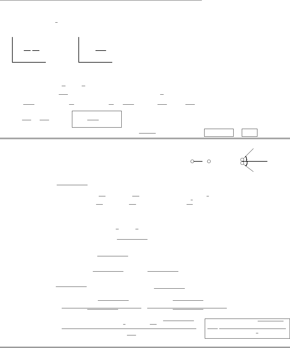
CHAPTER 12. ELECTRODYNAMICS AND RELATIVITY 271
Problem 12.35
Classically, E=1
2mv2. In a colliding beam experiment, the relative velocity (classically) is twice the
velocity of either one, so the relative energy is 4E.
2
✲x
✻
ct
¯x=−3
¯x=−2
¯x=−1
¯
x=0
¯
x=1
¯x=2
¯
x=3
c¯
t=−3
c¯
t=−2
c¯
t=−1
c¯
t=0
c¯
t=1
c¯
t=2
c¯
t=3
✒
✛ ✲
8.7
✻
❄
9.2
✲S
✻
1⃝✲2⃝
✛
EE
✲¯
S
✻
1⃝2⃝
✛
¯
E
=⇒
v
✲
mm
(before)
✒
EA
⑦
EB
60◦
θ
(after)
✲ct
✻
x
A✒
B
✒
c
⃝2005 Pearson Education, Inc., Upper Saddle River, NJ. All rights reserved. This material is
protected under all copyright laws as they currently exist. No portion of this material may be
reproduced, in any form or by any means, without permission inwritingfromthepublisher.
Let ¯
Sbe the system in which 1is at rest. Its
speed v, relative to S, is just the speed of 1
in S.
¯p0=(p0p1))¯
E
c=E
cp, where pis the momentum of 2in S.
E=Mc2,so=E
Mc2;p=MV =Mc.)¯
E=E
c+Mcc=(E+Mc22)
2=1
12)12=1
2)2=11
2=21
2.)¯
E=E
Mc2E+E
Mc221Mc2
¯
E=E2
Mc2+E2
Mc2Mc2;¯
E=2E2
Mc2Mc2.
For E= 30 GeV and Mc2= 1 GeV, we have ¯
E=(2)(900)
11 = 1800 1= 1799 GeV = 60E.
Problem 12.36
2
✲x
✻
ct
¯x=−3
¯x=−2
¯x=−1
¯
x=0
¯
x=1
¯x=2
¯
x=3
c¯
t=−3
c¯
t=−2
c¯
t=−1
c¯
t=0
c¯
t=1
c¯
t=2
c¯
t=3
✒
✛ ✲
8.7
✻
❄
9.2
✲S
✻
1⃝✲2⃝
✛
EE
✲¯
S
✻
1⃝2⃝
✛
¯
E
=⇒
v
✲
mm
(before)
✒
EA
⑦
EB
60◦
θ
(after)
✲ct
✻
x
A✒
B
✒
c
⃝2005 Pearson Education, Inc., Upper Saddle River, NJ. All rights reserved. This material is
protected under all copyright laws as they currently exist. No portion of this material may be
reproduced, in any form or by any means, without permission inwritingfromthepublisher.
One photon is impossible, because in the “center of mo-
mentum” frame (Prob. 12.31) we’d be left with a photon
at rest, whereas photons have to travel at speed c.
Cons. of energy: p0c2+m2c4+mc2=EA+EB
Cons. of mom.: horizontal: p0=EA
ccos 60+EB
ccos ✓)EBcos ✓=p0c1
2EA
vertical: 0 = EA
csin 60EB
csin ✓)EBsin ✓=p3
2EAsquare and add:
E2
B(cos2✓+ sin2✓)=p0c2p0cEA+1
4E2
A+3
4E2
A
)E2
B=p0c2p0cEA+E2
A=p2
0c2+m2c4+mc2EA2
=p0c2+m2c4+2
p2
0c2+m2c4(mc2EA)+m2c42EAmc2+E2
A.Or:
p0cEA=2m2c4+2mc2p2
0c2+m2c42EAp2
0c2+m2c42EAmc2;
)EA(mc2+p2
0c2+m2c4p0c/2) = m2c4+mc2p0c2+m2c4;
EA=mc2(mc2+p2
0c2+m2c4)
(mc2+p2
0c2+m2c4p0c/2) ·(mc2p2
0c2+m2c4p0c/2)
(mc2p2
0c2+m2c4p0c/2)
=mc2(m2c4
p2
0c2m2c4
1
2p0mc3p0c
2p2
0c2+m2c4)
(m2c4
p0mc3+p0c2
4p0c2m2c4
)
=mc2
2
(mc +2p0+p2
0+m2c2)
(mc +3
4p0).
c
2012 Pearson Education, Inc., Upper Saddle River, NJ. All rights reserved. This material is
protected under all copyright laws as they currently exist. No portion of this material may be
reproduced, in any form or by any means, without permission in writing from the publisher.
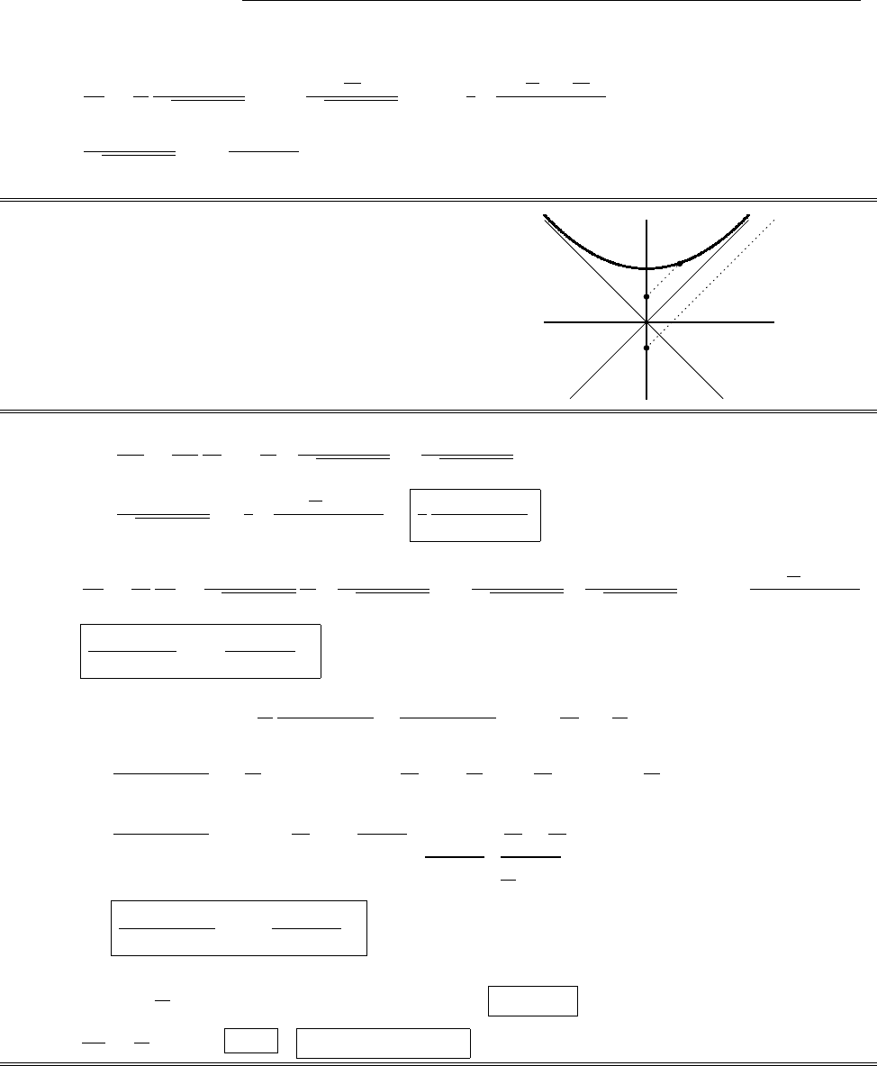
272 CHAPTER 12. ELECTRODYNAMICS AND RELATIVITY
Problem 12.37
F=dp
dt =d
dt
mu
1u2/c2=mdu
dt
1u2/c2+u1
21
c22u·du
dt
(1 u2/c2)3/2
=m
1u2/c2a+u(u·a)
(c2u2).qed
Problem 12.38
At constant force you go in “hyperbolic” mo-
tion. Photon A, which left the origin at t<0,
catches up with you, but photon B, which
passes the origin at t>0, never does.
2
✲x
✻
ct
¯x=−3
¯x=−2
¯x=−1
¯
x=0
¯
x=1
¯x=2
¯
x=3
c¯
t=−3
c¯
t=−2
c¯
t=−1
c¯
t=0
c¯
t=1
c¯
t=2
c¯
t=3
✒
✛ ✲
8.7
✻
❄
9.2
✲S
✻
1⃝✲2⃝
✛
EE
✲¯
S
✻
1⃝2⃝
✛
¯
E
=⇒
v
✲
mm
(before)
✒
EA
⑦
EB
60◦
θ
(after)
✲ct
✻
x
A✒
B
✒
c
⃝2005 Pearson Education, Inc., Upper Saddle River, NJ. All rights reserved. This material is
protected under all copyright laws as they currently exist. No portion of this material may be
reproduced, in any form or by any means, without permission inwritingfromthepublisher.
Problem 12.39
(a) ↵0=d⌘0
d⌧=d⌘0
dt
dt
d⌧=d
dt c
1u2/c2 1
1u2/c2
=c
1u2/c21
21
c22u·a
(1 u2/c2)3/2=1
c
u·a
(1 u2/c2)2.
↵↵↵=d⌘
d⌧=dt
d⌧
d⌘
dt =1
1u2/c2
d
dt u
1u2/c2=1
1u2/c2a
1u2/c2+u(t)1
c22u·a
(1 u2/c2)3/2
=1
(1 u2/c2)a+u(u·a)
(c2u2).
(b) ↵µ↵µ=(↵0)2+↵↵↵·↵↵↵=1
c2
(u·a)2
(1 u2/c2)4+1
(1 u2/c2)4a(1 u2
c2)+ 1
c2u(u·a)2
=1
(1 u2/c2)41
c2(u·a)2+a21u2
c22
+2
c21u2
c2(u·a)2+1
c4u2(u·a)2
=1
(1 u2/c2)4a21u2
c22
+(u·a)2
c21+22u2
c2+u2
c2
(1 u2
c2)
=1
(1 u2/c2)2a2+(u·a)2
(c2u2).
(c) ⌘µ⌘µ=c2,so d
d⌧(⌘µ⌘µ)=↵µ⌘µ+⌘µ↵µ=2↵µ⌘µ= 0, so ↵µ⌘µ=0.
(d) Kµ=d⇢µ
d⌧=d
d⌧(m⌘µ)= m↵µ. Kµ⌘µ=m↵µ⌘µ=0.
c
2012 Pearson Education, Inc., Upper Saddle River, NJ. All rights reserved. This material is
protected under all copyright laws as they currently exist. No portion of this material may be
reproduced, in any form or by any means, without permission in writing from the publisher.

CHAPTER 12. ELECTRODYNAMICS AND RELATIVITY 273
Problem 12.40
KµKµ=(K0)2+K·K. From Eq. 12.69, K·K=F2
(1u2/c2). From Eq. 12.70:
K0=1
c
dE
d⌧=1
c1u2/c2
d
dt mc2
1u2/c2=mc
1u2/c21
2
(1/c2)
(1 u2/c2)3/22u·a=m
c
(u·a)
(1 u2/c2)2
But Eq. 12.74: u·F=uF cos ✓=m
1u2/c2(u·a)+ u2(u·a)
c2(1 u2/c2)=m(u·a)
(1 u2/c2)3/2, so:
K0=uF cos ✓
c1u2/c2.)KµKµ=F2
(1 u2/c2)u2F2cos2✓
c2(1 u2/c2)=1(u2/c2) cos2✓
(1 u2/c2)F2.qed
Problem 12.41
F=m
1u2/c2a+u(u·a)
c2u2=q(E+u⇥B))a+u(u·a)
(c2u2)=q
m1u2/c2(E+u⇥B).
Dot in u:(u·a)+ u2(u·a)
c2(1 u2/c2)=u·a
(1 u2/c2)=q
m1u2/c2u·E+u·(u⇥B)
=0 ;
)u(u·a)
(c2u2)=q
m1u2
c2
u(u·E)
c2.So a=q
m1u2
c2E+u⇥B1
c2u(u·E).qed
Problem 12.42
One way to see it is to look back at the general formula for E(Eq. 10.36). For a uniform infinite plane of
charge, moving at constant velocity in the plane, ˙
J= 0 and ˙⇢= 0, while ⇢(or rather, ) is independent of t
(so retardation does nothing). Therefore the field is exactly the same as it would be for a plane at rest (except
that itself is altered by Lorentz contraction).
A more elegant argument exploits the fact that Eis a vector (whereas Bis a pseudovector). This means that
any given component changes sign if the configuration is reflected in a plane perpendicular to that direction.
But in Fig. 12.35(b), if we reflect in the xy plane the configuration is unaltered, so the zcomponent of Ewould
have to stay the same. Therefore it must in fact be zero. (By contrast, if you reflect in a plane perpendicular
to the ydirection the charges trade places, so it is perfectly appropriate that the ycomponent of Eshould
reverse its sign.)
Problem 12.43
(a) Field is 0/✏0, and it points perpendicular to the positive plate, so:
E0=0
✏0
(cos 45ˆx + sin 45ˆy )= 0
p2✏0
(ˆx +ˆy ).
(b) From Eq. 12.109, Ex=Ex0=0
p2✏0;Ey=Ey0=0
p2E0. So E=0
p2✏0
(ˆx +ˆy ).
(c) From Prob. 12.10: tan ✓=,so ✓= tan1.
(d) Let ˆn be a unit vector perpendicular to the plates in S— evidently
ˆn =sin ✓ˆx + cos ✓ˆy ;|E|=0
p2✏01+2.
c
2012 Pearson Education, Inc., Upper Saddle River, NJ. All rights reserved. This material is
protected under all copyright laws as they currently exist. No portion of this material may be
reproduced, in any form or by any means, without permission in writing from the publisher.

274 CHAPTER 12. ELECTRODYNAMICS AND RELATIVITY
3
✲x
✻
y
❨
ˆn
θ
✲x
✻
y
d
qA
qB
✲
v
✲¯x
✻
y
d
qA
qB
✛
v
✲x
✻
y
✯
vt
❑φ
❑
Y
✯
X
✯
¯
X
❑
¯
Y
❄
φ✲¯x
✻
¯y
c
⃝2005 Pearson Education, Inc., Upper Saddle River, NJ. All rights reserved. This material is
protected under all copyright laws as they currently exist. No portion of this material may be
reproduced, in any form or by any means, without permission inwritingfromthepublisher.
So the angle between ˆn and Eis:
E·ˆn
|E|= cos =1
1+2(sin ✓+cos ✓)= cos ✓
1+2(tan ✓+)= 2
1+2cos ✓
But = tan ✓=sin ✓
cos ✓=p1cos2✓
cos ✓=1
cos2✓1)1
cos
2✓=2+1)cos ✓=1
p1+2. So cos =2
1+2.
Evidently the field is not perpendicular to the plates in S.
Problem 12.44
(a) E=
2⇡✏0
ˆs
s=
2⇡✏0
x0ˆx +y0ˆy
(x2
0+y2
0).
(b) ¯
Ex=Ex=
2⇡✏0
x0
(x2
0+y2
0),¯
Ey=Ey=
2⇡✏0
y0
(x2
0+y2
0),¯
Ez=Ez=0,¯
E=
2⇡✏0
(x0ˆx +y0ˆy
(x2
0+y2
0).
Using the inverse Lorentz transformations (Eq. 12.19), x0=(x+vt),y
0=y,
¯
E=
2⇡✏0
(x+vt)ˆx +yˆy
[2(x+vt)2+y2]=
2⇡✏0
1
(x+vt)ˆx +yˆy
[(x+vt)2+y2/2].
Now S=(x+vt)ˆx +yˆy , and y=Ssin ✓, so [(x+vt)2+y2/2] = [(x+vt)2+y2(1v2/c2]=S2(v/c)2S2sin2✓=
S2[1 (v/c)2sin2✓], so
¯
E=
2⇡✏01(v/c)2
1v2sin2✓/c2ˆ
S
S.
This is reminiscent of Eq. 10.75. Yes, the field does point away from the present location of the wire.
Problem 12.45
(a) Fields of Aat B:E=1
4⇡✏0
qA
d2ˆy ;B=0. So force on qBis F=1
4⇡✏0
qAqB
d2ˆy .
3
✲x
✻
y
❨
ˆn
θ
✲x
✻
y
d
qA
qB
✲
v
✲¯x
✻
y
d
qA
qB
✛
v
✲x
✻
y
✯
vt
❑φ
❑
Y
✯
X
✯
¯
X
❑
¯
Y
❄
φ✲¯x
✻
¯y
c
⃝2005 Pearson Education, Inc., Upper Saddle River, NJ. All rights reserved. This material is
protected under all copyright laws as they currently exist. No portion of this material may be
reproduced, in any form or by any means, without permission inwritingfromthepublisher.
(b) (i) From Eq. 12.67: ¯
F=
4⇡✏0
qAqB
d2ˆy .(Note: here the particle is at rest in ¯
S.)
(ii) From Eq. 12.93, with ✓= 90:¯
E=1
4⇡✏0
qA(1 v2/c2)
(1 v2/c2)3/2
1
d2ˆy =
4⇡✏0
qA
d2ˆy
(this also follows from Eq. 12.109).
¯
B6= 0, but since vB= 0 in ¯
S, there is no magnetic force anyway, and ¯
F=
4⇡✏0
qAqB
d2ˆy (as before).
c
2012 Pearson Education, Inc., Upper Saddle River, NJ. All rights reserved. This material is
protected under all copyright laws as they currently exist. No portion of this material may be
reproduced, in any form or by any means, without permission in writing from the publisher.

CHAPTER 12. ELECTRODYNAMICS AND RELATIVITY 275
Problem 12.46
System A: Use Eqs. 12.93 and 12.112, with ✓= 90,R=dˆy , and ˆ
=ˆz :
E=q
4⇡✏0
d2ˆy ;B=q
4⇡✏0
v
c2
d2ˆz ; where =1
1v2/c2.
[Note that (E2B2c2)=q
4⇡✏0d2221v2
c2=q
4⇡✏0d22is invariant, since it doesn’t depend on v(see
Prob. 12.47b for the general proof). We’ll use this as a check.]
F=qE+(vˆx )⇥B=q2
4⇡✏0
d2ˆy v2
c2(ˆx ⇥ˆz )=q2
4⇡✏0
d21+v2
c2ˆy .
System B: The speed of qis vB=v+v
1+v2/c2=2v
(1 + v2/c2)
B=1
14v2/c2
(1+v2/c2)2
=(1 + v2/c2)
12v2
c2+v4
c4
=(1 + v2/c2)
(1 v2/c2)=21+v2
c2;vBB=2v2.
)E=q
4⇡✏0
1
d221+v2
c2ˆy ;B=q
4⇡✏0
2v
c2
2
d2ˆz .
Check:(E2B2c2)=q
4⇡✏0d2241+ 2v2
c2+v4
c44v2
c2=q
4⇡✏0d2241
4=q
4⇡✏0d22X
F=qE=q2
4⇡✏0
2
d21+v2
c2ˆy (+qat rest )no magnetic force). [Check: Eq. 12.67 )FA=1
FB.X]
System C :vC=0.E=q
4⇡✏0
1
d2ˆy ;B=0.F=qE=q2
4⇡✏0
1
d2ˆy .
[The relative velocity of Band Cis 2v/(1 + v2/c2), and corresponding is 2(1 + v2/c2). So Eq. 12.67
)FC=1
2(1+v2/c2)FB.X]
Summary:
q
4⇡✏0d2ˆy q
4⇡✏0d221+v2/c2ˆy q
4⇡✏0d2ˆy
q
4⇡✏0d2v
c2ˆz q
4⇡✏0d22v
c22ˆz 0
q2
4⇡✏0d21+v2/c2ˆy q2
4⇡✏0d221+v2/c2ˆy q2
4⇡✏0d2ˆy
Problem 12.47
(a) From Eq. 12.109:
¯
E·¯
B=¯
Ex¯
Bx+¯
Ey¯
By+¯
Ez¯
Bz=ExBx+2(EyvBz)(By+v
c2Ez)+(Ez+vBy)(Bzv
c2Ey)
=ExBx+2{EyBy+v
c2EyEz
vByBz
v2
c2EzBz+EzBzv
c2EyEz
+vByBz
v2
c2EyBy}
=ExBx+2EyBy1v2
c2+EzBz1v2
c2=ExBx+EyBy+EzBz=E·B.qed
c
2012 Pearson Education, Inc., Upper Saddle River, NJ. All rights reserved. This material is
protected under all copyright laws as they currently exist. No portion of this material may be
reproduced, in any form or by any means, without permission in writing from the publisher.

276 CHAPTER 12. ELECTRODYNAMICS AND RELATIVITY
(b) ¯
E2c2¯
B2=E2
x+2(EyvBz)2+2(Ez+vBy)2c2B2
x+2By+v
c2Ez2+2Bzv
c2Ey
=E2
x+2E2
y2EyvBz
+v2B2
z+E2
z+2EzvBy
+v2B2
yc2B2
yc22v
c2ByEz
c2v2
c4E2
zc2B2
z+c22v
c2BzEy
c2v2
c4E2
yc2B2
x
=E2
xc2B2
x+2E2
y1v2
c2+E2
z1v2
c2c2(B2
y)1v2
c2c2B2
z1v2
c2
=(E2
x+E2
y+E2
z)c2(B2
x+B2
y+B2
z)=E2B2c2.qed
(c) No. For if B=0in one system, then (E2c2B2) is positive. Since it is invariant, it must be positive in
any system. )E6=0in all systems.
Problem 12.48
(a) Making the appropriate modifications in Eq. 9.48 (and picking = 0 for convenience),
E(x, y, z, t)=E0cos(kx !t)ˆy ,B(x, y, z, t)=E0
ccos(kx !t)ˆz ,where k⌘!
c.
(b) Using Eq. 12.109 to transform the fields:
¯
Ex=¯
Ez=0,¯
Ey=(EyvBz)=E0cos(kx !t)v
ccos(kx !t)=↵E0cos(kx !t),
¯
Bx=¯
By=0,¯
Bz=(Bzv
c2Ey)=E01
ccos(kx !t)v
c2cos(kx !t)=↵E0
ccos(kx !t),
where ↵⌘1v
c=1v/c
1+v/c.
Now the inverse Lorentz transformations (Eq. 12.19) )x=(¯x+v¯
t) and t=¯
t+v
c2¯x, so
kx !t=k(¯x+v¯
t)!¯
t+v
c2¯x=k!v
c2¯x(!kv)¯
t=¯
k¯x¯!¯
t,
where, recalling that k=!/c): ¯
k⌘k!v
c2=k(1 v/c)=↵kand ¯!⌘!(1 v/c)=↵!.
Conclusion:
¯
E(¯x, ¯y, ¯z, ¯
t)= ¯
E0cos(¯
k¯x¯!¯
t)ˆy ,¯
B(¯x, ¯y, ¯z, ¯
t)= ¯
E0
ccos(¯
k¯x¯!¯
t)ˆz ,
where ¯
E0=↵E0,¯
k=↵k, ¯!=↵!,and ↵⌘1v/c
1+v/c.
(c) ¯!=!1v/c
1+v/c.This is the Doppler shift for light. ¯
=2⇡
¯
k=2⇡
↵k=
↵.The velocity of the wave
in ¯
Sis ¯v=¯!
2⇡¯
=!
2⇡=c. Yup, this is exactly what I expected (the velocity of a light wave is the same
in any inertial system).
c
2012 Pearson Education, Inc., Upper Saddle River, NJ. All rights reserved. This material is
protected under all copyright laws as they currently exist. No portion of this material may be
reproduced, in any form or by any means, without permission in writing from the publisher.

CHAPTER 12. ELECTRODYNAMICS AND RELATIVITY 277
(d) Since the intensity goes like E2, the ratio is ¯
I
I=¯
E2
0
E2
0
=↵2=1v/c
1+v/c.
Dear Al,
The amplitude, frequency, and intensity of the light will all decrease to zero as you run faster
and faster. It’ll get so faint you won’t be able to see it, and so red-shifted even your night-vision
goggles won’t help. But it’ll still be going 3 ⇥108m/s relative to you. Sorry about that.
Sincerely,
David
Problem 12.49
¯
t02 =⇤0
⇤2
t =⇤0
0⇤2
2t02 +⇤0
1⇤2
2t12 =t02 +()t12 =(t02 t12).
¯
t03 =⇤0
⇤3
t =⇤0
0⇤3
3t03 +⇤0
1⇤3
3t13 =t03 +()t13 =(t03 t13)=(t03 +t31).
¯
t23 =⇤2
⇤3
t =⇤2
2⇤3
3t23 =t23.
¯
t31 =⇤3
⇤1
t =⇤3
3⇤1
0t30 +⇤3
3⇤1
1t31 =()t30 +t31 =(t31 t03).
¯
t12 =⇤1
⇤2
t =⇤1
0⇤2
2t02 +⇤1
1⇤2
2t12 =()t02 +t12 =(t12 t02).
Problem 12.50
Suppose t⌫µ=±tµ⌫(+ for symmetric, for antisymmetric).
¯
t =⇤
µ⇤
⌫tµ⌫
¯
t =⇤
µ⇤
⌫tµ⌫=⇤
⌫⇤
µt⌫µ[Because µand ⌫are both summed from 0 !3,
it doesn’t matter which we call µand and which call ⌫.]
=⇤
µ⇤
µ(±tµ⌫) [Using symmetry of tµ⌫, and writing the ⇤’s in the other order.]
=±¯
t.qed
Problem 12.51
Fµ⌫Fµ⌫=F00F00 F01F01 F02F02 F03F03 F10F10 F20F20 F30F30
+F11F11 +F12F12 +F13F13 +F21F21 +F22F22 +F23F23 +F31F31 +F32F32 +F33F33
=(Ex/c)2(Ey/c)2(Ez/c)2(Ex/c)2(Ey/c)2(Ez/c)2+B2
z+B2
y+B2
z+B2
x+B2
y+B2
x
=2B22E2/c2= 2B2E2
c2,
which, apart from the constant factor 2/c2, is the invariant we found in Prob. 12.47(b).
Gµ⌫Gµ⌫= 2(E2/c2B2) (the same invariant).
Fµ⌫Gµ⌫=2(F01G01 +F02G02 +F03G03) + 2(F12G12 +F13G13 +F23G23)
=21
cExBx+1
cEyBy+1
cEzBz+ 2[Bz(Ez/c)+(By)(Ey/c)+Bx(Ex/c)]
=2
c(E·B)2
c(E·B)= 4
c(E·B),
c
2012 Pearson Education, Inc., Upper Saddle River, NJ. All rights reserved. This material is
protected under all copyright laws as they currently exist. No portion of this material may be
reproduced, in any form or by any means, without permission in writing from the publisher.

278 CHAPTER 12. ELECTRODYNAMICS AND RELATIVITY
which, apart from the factor 4/c, is the invariant we found of Prob. 12.47(a). [These are, incidentally, the
only fundamental invariants you can construct from Eand B.]
Problem 12.52
E=1
4⇡✏0
2
xˆx =µ0
2⇡
c2
xˆx
B=µ0
4⇡
2v
xˆy =µ0
2⇡
v
xˆy
Fµ⌫=µ0
2⇡x
0c00
c00v
0000
0v00
Gµ⌫=µ0
2⇡x
00v0
0000
v00c
00c0
Problem 12.53
@⌫Fµ⌫=µ0Jµ. Di↵erentiate: @µ@⌫Fµ⌫=µ0@µJµ.
But @µ@⌫=@⌫@µ(the combination is symmetric) while F⌫µ=Fµ⌫(antisymmetric).
)@µ@⌫Fµ⌫= 0. [Why? Well, these indices are both summed from 0 !3, so it doesn’t matter which we
call µ, which ⌫:@µ@⌫Fµ⌫=@⌫@µF⌫µ=@µ@⌫(Fµ⌫)=@µ@⌫Fµ⌫. But if a quantity is equal to minus itself,
it must be zero.] Conclusion: @µJµ= 0. qed
Problem 12.54
We know that @⌫Gµ⌫= 0 is equivalent to the two homogeneous Maxwell equations, r·B= 0 and r⇥E=
@B
@t. All we have to show, then, is that @Fµ⌫+@µF⌫ +@⌫Fµ= 0 is also equivalent to them. Now this
equation stands for 64 separate equations (µ=0!3, ⌫=0!3, =0!3, and 4 ⇥4⇥4 = 64). But many
of them are redundant, or trivial.
Suppose two indices are the same (say, µ=⌫). Then @Fµµ +@µFµ=@µFµ= 0. But Fµµ = 0 and
Fµ=Fµ, so this is trivial: 0 = 0. To get anything significant, then, µ,⌫,must all be di↵erent. They
could beall spatial (µ, ⌫,=1,2,3=x, y, z — or some permutation thereof), or one temporal and two spatial
(µ= 0, ⌫,=1,2 or 2,3, or 1,3 — or some permutation). Let’s examine these two cases separately.
All spatial:say,µ= 1, ⌫=2,= 3 (other permutations yield the same equation, or minus it.)
@3F12 +@1F23 +@2F31 =0)@
@z(Bz)+ @
@x(Bx)+ @
@y(By)=0)r·B=0.
One temporal:say,µ=0,⌫= 1, = 2 (other permutations of these indices yield same result, or minus it).
@2F01 +@0F12 +@1F31 =0)@
@yEx
c=@
@(ct)(Bz)+ @
@x+Ey
c=0.
or: @Bz
@t+@Ex
@y@Ey
@x= 0, which is the z-component of @B
@t=r⇥E.(Ifµ=0,⌫=1,= 2, we get the
ycomponent; for ⌫=2,= 3 we get the xcomponent.)
Conclusion:@Fµ⌫+@µF⌫ +@⌫Fµ= 0 is equivalent to r·B= 0 and @B
@t=r⇥E, and hence to
@⌫Gµ⌫= 0. qed
Problem 12.55
K0=q⌘⌫F0⌫q(⌘1F01 +⌘2F02 +⌘3F03)=q(⌘·E)/c =q
cu·E.Now from Eq. 12.70 we know that
K0=1
c
dW
d⌧, where Wis the energy of the particle. Since d⌧=1
dt, we have:
1
cdW
dt =q
c(u·E))dW
dt =q(u·E)
This says the power delivered to the particle is force (qE)times velocity (u) — which is as it should be.
c
2012 Pearson Education, Inc., Upper Saddle River, NJ. All rights reserved. This material is
protected under all copyright laws as they currently exist. No portion of this material may be
reproduced, in any form or by any means, without permission in writing from the publisher.

CHAPTER 12. ELECTRODYNAMICS AND RELATIVITY 279
Problem 12.56
@0=@
@¯x0
=1
c
@
@¯
t=1
c@
@t
@t
@¯
t+@
@x
@x
@¯
t+@
@y
@y
@¯
t+@
@z
@z
@¯
t
From Eq. 12.19, we have: @t
@¯
t=,@x
@¯
t=v,@y
@¯
t=@z
@¯
t= 0.
So @0=1
c@
@t+v@
@xor (since ct =x0=x0): @0=@
@x0v
c
@
@x1=(@0)(@1).
@1=@
@¯x=@
@t
@t
@x1+@
@x
@x
@¯x+@
@y
@y
@¯x+@
@z
@z
@¯x=v
c2
@
@t+@
@x=@
@x1v
c
@
@x0=(@1)(@0).
@2=@
@¯y=@
@t
@t
@¯y+@
@x
@x
@¯y+@
@y
@y
@¯y+@
@z
@z
@¯y=@
@y=@2.
@3=@
@¯z=@
@t
@t
@¯z+@
@x
@x
@¯z+@
@y
@y
@¯z+@
@z
@z
@¯z=@
@z=@3.
Conclusion: @µtransforms in the same way as aµ(Eq. 12.27)—and hence is a contravariant 4-vector. qed
Problem 12.57
According to Prob. 12.54, @Gµ⌫
@x⌫= 0 is equivalent to Eq. 12.130. Using Eq. 12.133, we find (in the notation
of Prob. 12.56):
@Fµ⌫
@x+@F⌫
@xµ+@Fµ
@x⌫=@Fµ⌫+@µF⌫ +@⌫Fµ
=@(@µA⌫@⌫Aµ)+@µ(@⌫A@A⌫)+@⌫(@Aµ@µA)
=(@@µA⌫@µ@A⌫)+(@µ@⌫A@⌫@µA)+(@⌫@Aµ@@⌫Aµ)=0.qed
[Note that @@µA⌫=@2A⌫
@x@x⌫=@2A⌫
@x⌫@x=@⌫@A⌫, by equality of cross-derivatives.]
Problem 12.58
From Eqs. 12.40 and 12.42, ⌘µ=(c, v), while
r
µ=(ct ctr,rw(tr)) = (
r
,
r
), so ⌘⌫
r
⌫=
c
r
+v·
r
=(
r
c
r
·v).
q
4⇡✏0c
⌘0
(⌘⌫
r
⌫)=q
4⇡✏0c
c
(
r
c
r
·v)=1
4⇡✏0c
qc
(
r
c
r
·v)=1
cV
(Eq. 10.46),
q
4⇡✏0c
⌘
(⌘⌫
r
⌫)=q
4⇡✏0c
v
(
r
c
r
·v)=1
4⇡✏0c
qv
(
r
c
r
·v)=A
(Eq. 10.47), so (Eq. 12.132)
q
4⇡✏0c
⌘µ
(⌘⌫
r
⌫)=Aµ.X
c
2012 Pearson Education, Inc., Upper Saddle River, NJ. All rights reserved. This material is
protected under all copyright laws as they currently exist. No portion of this material may be
reproduced, in any form or by any means, without permission in writing from the publisher.

280 CHAPTER 12. ELECTRODYNAMICS AND RELATIVITY
Problem 12.59
3
✲x
✻
y
❨
ˆn
θ
✲x
✻
y
d
qA
qB
✲
v
✲¯x
✻
y
d
qA
qB
✛
v
✲x
✻
y
✯
vt
❑φ
❑
Y
✯
X
✯
¯
X
❑
¯
Y
❄
φ✲¯x
✻
¯y
c
⃝2005 Pearson Education, Inc., Upper Saddle River, NJ. All rights reserved. This material is
protected under all copyright laws as they currently exist. No portion of this material may be
reproduced, in any form or by any means, without permission inwritingfromthepublisher.
Step 1 : rotate from xy to XY , using Eq. 1.29:
X= cos x+ sin y
Y=sin x+ cos y
Step 2 : Lorentz-transform from XY to ¯
X¯
Y, using
Eq. 12.18:
¯
X=(Xvt)=[cos x+ sin yct]
¯
Y=Y=sin x+ cos y
¯
Z=Z=z
c¯
t=(ct X)=ct (cos x+ sin y)
Step 3 : Rotate from ¯
X¯
Yto ¯x¯y, using Eq. 1.29 with negative :
¯x= cos ¯
Xsin ¯
Y=cos [cos x+ sin yct]sin [sin x+ cos y]
=(cos2+ sin2)x+(1) sin cos y cos (ct)
¯y= sin ¯
X+ cos ¯
Y=sin (cos x+ sin yct) + cos (sin c+ cos y)
=(1) sin cos x+(sin2+ cos2)y sin (ct)
In matrix form:
c¯
t
¯x
¯y
¯z
=
cos sin 0
cos (cos2+ sin2)(1) sin cos 0
sin (1) sin cos (sin2+ cos2)0
00 01
ct
x
y
z
Problem 12.60
4
✲
π✛pbefore (CM)
KΣafter (CM)
✲
πp
Before
✲
KΣ
After
In CM :✲ ✛
pp
Before
✒
✠
p
p
rµ
❘
sµ
■
φ
After
✲x
✻
y
(p= magnitude of 3-momentum
in CM, φ= CM scattering angle)
c
⃝2005 Pearson Education, Inc., Upper Saddle River, NJ. All rights reserved. This material is
protected under all copyright laws as they currently exist. No portion of this material may be
reproduced, in any form or by any means, without permission inwritingfromthepublisher.
In center-of-momentum system, threshold occurs when incident en-
ergy is just sufficient to cover the rest energy of the resulting particles,
with none “wasted” as kinetic energy. Thus, in lab system, we want
the outgoing Kand ⌃to have the same velocity, at threshold:
1
✲
π
✛
pbefore (CM)
KΣafter (CM)
✲
πp
Before
✲
KΣ
After
c
⃝2005 Pearson Education, Inc., Upper Saddle River, NJ. All rights reserved. This material is
protected under all copyright laws as they currently exist. No portion of this material may be
reproduced, in any form or by any means, without permission inwritingfromthepublisher.
Initial momentum: p⇡; Initial energy of ⇡:E2p2c2=m2c4)E2
⇡=m2
⇡c4+p2
⇡c2.
Total initial energy: mpc2=m2
⇡c4+p2
⇡c2. These are also the final energy and momentum: E2p2c2=
(mK+m⌃)2c4.
mpc2+m2
⇡c4+p2
⇡c22p2
⇡c2=(mK+m⌃)2c4
m2
pc4
+2mpc2
c4m2
⇡c2+p2
⇡c+m2
⇡c4
+p2
⇡c2
p2
⇡c2
=(mK+m⌃)2c4
2mp
cm2
⇡c2+p2
⇡=(mK+m⌃)2m2
pm2
⇡
c
2012 Pearson Education, Inc., Upper Saddle River, NJ. All rights reserved. This material is
protected under all copyright laws as they currently exist. No portion of this material may be
reproduced, in any form or by any means, without permission in writing from the publisher.

CHAPTER 12. ELECTRODYNAMICS AND RELATIVITY 281
(m2
⇡c2+p2
⇡)4m2
p
c2=(mK+m⌃)42(m2
p+m2
⇡)(mK+m⌃)2+m4
p+m4
⇡+2m2
pm2
⇡
4m2
p
c2p2
⇡=(mK+m⌃)42(m2
p+m2
⇡)(mK+m⌃)2+(m2
pm2
⇡)2
p⇡=c
2mp(mK+m⌃)42(m2
p+m2
⇡)(mK+m⌃)2+(m2
pm2
⇡)2
=1
(2mpc2)c(mKc2+m⌃c2)42(mpc2)2+(m⇡c2)2(mKc2+m⌃c2)2+(mpc2)2(m⇡c2)22
=1
2c(900) (1700)42(900)2+ (150)2(1700)2+(900)2(150)22
=1
1800c(8.35 ⇥1012)(4.81 ⇥1012) + (0.62 ⇥1012)= 1
1800c(2.04 ⇥106)= 1133 MeV/c
Problem 12.61
4
✲
π✛pbefore (CM)
KΣafter (CM)
✲
πp
Before
✲
KΣ
After
In CM :✲ ✛
pp
Before
✒
✠
p
p
rµ
❘
sµ
■
φ
After
✲x
✻
y
(p= magnitude of 3-momentum
in CM, φ= CM scattering angle)
c
⃝2005 Pearson Education, Inc., Upper Saddle River, NJ. All rights reserved. This material is
protected under all copyright laws as they currently exist. No portion of this material may be
reproduced, in any form or by any means, without permission inwritingfromthepublisher.
Outgoing 4-momentua: rµ=E
c,pcos ,psin ,0;sµ=E
c,pcos ,psin ,0.
5
In Lab:✲
Before
✒
❘
¯rµ
¯sµ
θProblem: calculate θ, in terms of p,φ.
θ
1
τ/sin φ
√1+(τ/sin φ)2
✲x
✻
y
d/2
−d/2
−q
+q
✕
l
!"# $
d
c
⃝2005 Pearson Education, Inc., Upper Saddle River, NJ. All rights reserved. This material is
protected under all copyright laws as they currently exist. No portion of this material may be
reproduced, in any form or by any means, without permission inwritingfromthepublisher.
Lorentz transformation: ¯rx=(rxr0); ¯ry=ry;¯sx=(sxs0); ¯sy=sy.
Now E=mc2;p=mv (vhere is to the left;E2p2c2=m2c4,so=pc
E.
)¯rx=pcos +pc
E
E
c=p(1 + cos ); ¯ry=psin ;¯sx=p(1 cos ); ¯sy=psin .
cos ✓=¯r ·¯s
¯r¯s=2p2(1 cos2)p2sin2
2p2(1 + cos )2+p2sin22p2(1 cos )2+p2sin2
=(21) sin2
2(1 + cos )2+ sin22(1 cos )2+ sin2
=(21)
21+cos
sin 2+1
21cos
sin 2+1
=(21)
2cot2
2+1
tan2
2+1
c
2012 Pearson Education, Inc., Upper Saddle River, NJ. All rights reserved. This material is
protected under all copyright laws as they currently exist. No portion of this material may be
reproduced, in any form or by any means, without permission in writing from the publisher.
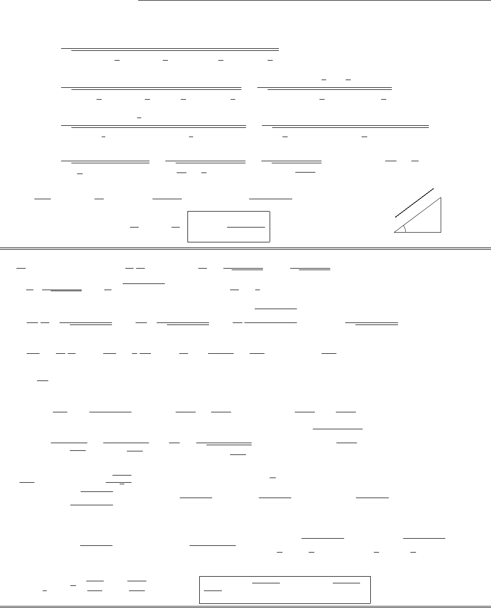
282 CHAPTER 12. ELECTRODYNAMICS AND RELATIVITY
cos ✓=!
1 + cot2
2+!cot2
21 + tan2
2+!tan2
2(where !⌘21)
=!
csc2
2+!cot2
2sec2
2+!tan2
2=!sin
2cos
2
1+!cos2
21+!sin2
2
=
1
2!sin
1+!1
2(1 + cos )1+!1
2(1 cos )=sin
2
!+1
+ cos 2
!+1
cos
=sin
2
!+1
2cos2
=sin
4
!2+4
!+ sin2
=1
1+⌧2
sin2,where ⌧2=4
!2+4
!.
sin ✓=⌧
sin .⌧2=4
!2(1 + !)= 4
(21)22, so tan ✓=2
(21) sin .
Or, since (21) = 211
2=2v2
c2, tan ✓=2c2
v2sin
5
In Lab:✲
Before
✒
❘
¯rµ
¯sµ
θProblem: calculate θ, in terms of p,φ.
θ
1
τ/sin φ
√1+(τ/sin φ)2
✲x
✻
y
d/2
−d/2
−q
+q
✕
l
!"# $
d
c
⃝2005 Pearson Education, Inc., Upper Saddle River, NJ. All rights reserved. This material is
protected under all copyright laws as they currently exist. No portion of this material may be
reproduced, in any form or by any means, without permission inwritingfromthepublisher.
Problem 12.62
dp
d⌧=K(a constant) )dp
dt
dt
d⌧=K.Butdt
d⌧=1
p1u2/c2;p=mu
p1u2/c2.
)d
dt u
p1u2/c2=K
m1u2/c2. Multiply by dt
dx =1
u:
dt
dx
d
dtu
1u2/c2=d
dxu
1u2/c2=K
m1u2/c2
u.Let w=u
1u2/c2.
dw
dx =K
m
1
w;wdw
dx =1
2
d
dxw2=k
m;d(w2)
dx =2K
m)d(w2)=2K
m(dx).
)w2=2K
mx+ constant. But at t= 0, x= 0 and u= 0 (so w= 0), and hence the constant is 0.
w2=2K
mx=u2
1u2/c2;u2=2Kx
m2Kx
mc2u2;u21+2Kx
mc2=2Kx
m.
u2=2Kx/m
1+2Kx
mc2
=c2
1+mc2
2Kx;dx
dt =c
1+mc2
2Kx;ct =1+mc2
2Kxdx
Let mc2
2K=a2;ct =px+a2
pxdx. Let x=y2;dx =2y dy;px=y.
ct =y2+a2
y2y dy =2y2+a2dy =yy2+a2+a2ln(y+y2+a2)+ constant.
At t= 0, x=0)y= 0. )0=a2ln a+ constant, so constant = a2ln a.
)ct =yy2+a2=a2lny/a +(y/a)2+1
=a2y
ay
a2+1+lny
a+y
a2+1
Let: z=y
a=px2K
mc2=2Kx
mc2=z. Then 2Kt
mc =z1+z2+ ln(z+1+z2).
c
2012 Pearson Education, Inc., Upper Saddle River, NJ. All rights reserved. This material is
protected under all copyright laws as they currently exist. No portion of this material may be
reproduced, in any form or by any means, without permission in writing from the publisher.
CHAPTER 12. ELECTRODYNAMICS AND RELATIVITY 283
Problem 12.63
5
In Lab:✲
Before
✒
❘
¯rµ
¯sµ
θProblem: calculate θ, in terms of p,φ.
θ
1
τ/sin φ
√1+(τ/sin φ)2
✲x
✻
y
d/2
−d/2
−q
+q
✕
l
!"# $
d
c
⃝2005 Pearson Education, Inc., Upper Saddle River, NJ. All rights reserved. This material is
protected under all copyright laws as they currently exist. No portion of this material may be
reproduced, in any form or by any means, without permission inwritingfromthepublisher.
r
(a) x(t)= c
↵1+(↵t)21, where ↵=F
mc . The force of +qon
qwill be the mirror image of the force of qon +q(in the x-axis),
so the net force is in the xdirection (the net magnetic force is zero).
So all we need is the x-component of E.
The field at +qdue to qis: (Eq. 10.72)
E=q
4⇡✏0
r
(
r
·u)3u(c2v2)+u(
r
·a)a(
r
·u).
u=c
r
v)ux=cl
r
v=1
r
(cl v
r
);
r
·u=c
r
r
·v=(c
r
lv);
r
·a=la. So:
Ex=q
4⇡✏0
r
(c
r
vl)31
r
(cl v
r
)(c2v2)= 1
r
(cl v
r
)la a(c
r
lv)
1
r
ca(l2
r
2)=cad2/
r
=q
4⇡✏0
1
(c
r
vl)3(cl v
r
)(c2v2)cad2.
The force on +qis qEx, and there is an equal force on q, so the net force on the dipole is:
F=2q2
4⇡✏0
1
(c
r
lv)3(cl v
r
)(c2v2)cad2ˆx It remains to determine
r
,l,
v, and a, and plug these in.
v(t)=dx
dt =c
↵
1
2
1
1+(↵t)22↵2t=c↵t
1(↵t)2;v=v(tr)=c↵tr
T,where T=1+(↵tr)2.
a(tr)= dv
dtr
=c↵
T+c↵tr1
22↵2tr
T3=c↵
T31+(↵tr)2(↵tr)2=c↵
T3
Now calculate tr:c2(ttr)2=
r
2=l2+d2;l=x(t)x(tr)= c
↵1+(↵t)21+(↵tr)2,so
t2
2ttr+t2
r
=1
↵21+(↵t)2
+1+(↵tr)2
21+(↵t)21+(↵tr)2+(d/c)2
(F)1+(↵t)21+(↵tr)2=1+↵2ttr+1
2↵d
c2. Square both sides:
1+(↵t)2+(↵tr)2+↵4t2t2
r
=1+↵4t2t2
r
+1
4↵d
c4+2↵2ttr+↵d
c2+↵2ttr↵d
c2
t2+t2
r2ttrttr↵d
c2d
c2↵2
4d
c4=0
At this point we could solve for tr(in terms of t), but since vand aare already expressed in terms of tr, it is
simpler to solve for t(in terms of tr), and express everything in terms of tr:
t2ttr2+↵d
c2+t2
rd
c2↵2
4d
c4=0=)
t=1
2tr2+↵d
c2±t2
r4+4
↵d
c2+↵d
c44t2
r
+4
d
c2+↵2d
c4
=tr1+1
2↵d
c)2±1+(↵tr)2d
c21+↵d
2c
c
2012 Pearson Education, Inc., Upper Saddle River, NJ. All rights reserved. This material is
protected under all copyright laws as they currently exist. No portion of this material may be
reproduced, in any form or by any means, without permission in writing from the publisher.
284 CHAPTER 12. ELECTRODYNAMICS AND RELATIVITY
Which sign? For small ↵we want t⇡tr+d/c, so we need the + sign:
t=tr1+1
2↵d
c2+d
cTD, where D=1+↵d
2c2
So
r
=c(ttr))
r
=ctr
2↵d
c2+dT D. Now go back to Eq. (F) and solve for 1+(↵t)2:
1+(↵t)2=1
T1+1
2↵d
c2+↵2trtr1+1
2↵d
c2+d
cTD
=1
T1+(↵tr)2
T21+1
2↵d
c2+↵2trd
cTD=1+ 1
2↵d
c2T+↵2trd
cD
l=c
↵1+(↵t2)1+(↵tr)2=c
↵1+1
2↵d
c2T+↵2trd
cDT=↵dd
2cT+trD
Putting all this in, the numerator in square brackets in Fbecomes:
[]=
c↵dd
2cT+trDc↵tr
Tctr
2↵d
c2+dT Dc2c2↵2t2
r
T2cc↵
T3
d2
=c↵dd
2cT+trDd(atr)2
2cT trDc2
T21+(↵tr)2
(↵tr)2
c2↵d2
T3
=c2↵d2
T31
2T21
2(↵tr)21=c2↵d2
2T31+(↵tr)2(↵tr)22=c2↵d2
2T3
)F=q2
4⇡✏0
c2↵d2
(c
r
lv)T3ˆx . It remains to compute the denominator:
(c
r
lv)T=cctr
2↵d
c2+dT D↵dd
2cT+trDc↵tr
TT
=1
2↵2trd2
+cdT D 1
2↵2trd2
cd(↵tr)2
TDT=cdDT2(↵tr)2
1+(↵tr)2
(↵tr)2
=dcD
)F=q2
4⇡✏0
c2d2↵
c3d3D3ˆx =q2
4⇡✏0
↵
cd1+↵d
2c23/2ˆx ↵=F
mc
Energy must come from the “reservoir” of energy stored in the electromagnetic fields.
(b) F=mc↵=1
2
"
q2
4⇡✏0
↵
cd1+↵d
2c23/2)1+↵d
2c23/2=q2
8⇡✏0mc2d=µ0q2
8⇡md.
(force on one end only)
)↵=2c
dµ0q2
8⇡md2/31,so F=2mc2
dµ0q2
8⇡md2/31.
c
2012 Pearson Education, Inc., Upper Saddle River, NJ. All rights reserved. This material is
protected under all copyright laws as they currently exist. No portion of this material may be
reproduced, in any form or by any means, without permission in writing from the publisher.
CHAPTER 12. ELECTRODYNAMICS AND RELATIVITY 285
Problem 12.64
(a) Aµ=(V/c, Ax,A
y,A
z) is a 4-vector (like xµ=(ct, x, y, z)), so (using Eq. 12.19): V=(¯
V+v¯
Ax). But
¯
V= 0, and
¯
Ax=µ0
4⇡
(m⇥¯r )x
¯r3
Now (m⇥¯r )x=my¯zmz¯y=myzmzy. So
V=vµ0
4⇡
(myzmzy)
¯r3
Now ¯x=(xvt)=Rx,¯y=y=Ry,¯z=z=Rz,whereRis the vector (in S) from the (instantaneous)
location of the dipole to the point of observation. Thus
¯r2=2R2
x+R2
y+R2
z=2(R2
x+R2
y+R2
z) + (1 2)(R2
y+R2
z)=2R2v2
c2R2sin2✓
(where ✓is the angle between Rand the x-axis, so that R2
y+R2
z=R2sin2✓).
)V=µ0
4⇡
v(myRzmzRy)
3R31v2
c2sin2✓3/2;v·(m⇥R)=v(m⇥R)x=v(myRzmzRy),so
V=µ0
4⇡
v·(m⇥R)1v2
c2
R31v2
c2sin2✓3/2,
or, using µ0=1
✏0c2and v·(m⇥R)=R·(v⇥m): V=1
4⇡✏0
R·(v⇥m)1v2
c2
c2R21v2
c2sin2✓3/2
(b) In the nonrelativistic limit (v2⌧c2):
V=1
4⇡✏0
R·(v⇥m)
c2R2=1
4⇡✏0
R·p
R2,with p=v⇥m
c2,
which is the potential of an electric dipole.
Problem 12.65
(a) B=µ0
2Kˆy (Eq. 5.58); N=m⇥B(Eq. 6.1), so N=µ0
2mK(ˆz ⇥ˆy ).
N=µ0
2mKˆx =µ0
2(vl2)(v)ˆx =µ0
2v2l2ˆx .
c
2012 Pearson Education, Inc., Upper Saddle River, NJ. All rights reserved. This material is
protected under all copyright laws as they currently exist. No portion of this material may be
reproduced, in any form or by any means, without permission in writing from the publisher.
286 CHAPTER 12. ELECTRODYNAMICS AND RELATIVITY
(b)
Charge density in the front side: 0(=0);
Charge density on the back side: ¯
=¯0, where ¯v=2v
1+v2/c2,
so ¯=1
14v2/c2
(1+v2/c2)2
=(1 + v2/c2)
1+2v2
c2+v4
c44v2
c2
=1+v2/c2
12v2
c2+v4
c4
=(1 + v2/c2)
(1 v2/c2)=21+v2
c2
Length of front and back sides in this frame: l/. So net charge on back side is:
q+=¯
l
=21+v2
c2
l
=1+v2
c2l
Net charge on front side is:
q=0
l
=
l
=1
2l
So dipole moment (note: charges on sides are equal):
p=(q+)l
2ˆy (q)l
2ˆy =1+v2
c2ll
21
2ll
2ˆy =l2
21+v2
c21+v2
c2ˆy =l2v2
c2ˆy .
E=0
2✏0ˆz , where =0,soN=p⇥E=l2v2
c2
2✏0(ˆy ⇥ˆz )= 1
µ0
2l2v2ˆx .
So apart from the relativistic factor of the torque is the same in both systems — but in Sit is the torque
exerted by a magnetic field on a magnetic dipole, whereas in ¯
Sit is the torque exerted by an electric field on
an electric dipole.
Problem 12.66
Choose axes so that Epoints in the zdirection and Bin the yz plane: E= (0,0,E); B=(0,Bcos ,Bsin ).
Go to a frame moving at speed vin the xdirection:
¯
E=0,vB sin ,(E+vB cos );¯
B0,(Bcos +v
c2E),Bsin .
(I used Eq. 12.109.) Parallel provided vB sin
(Bcos +v
c2E)=(E+vB cos )
Bsin ,or
vB2sin2=Bcos +v
c2E(E+vB cos )=EB cos +vB2cos2+v
c2E2+v2
c2EB cos
0=vB2+v
c2E2+EB cos 1+v2
c2;v
1+v2/c2=EB cos
B2+E2/c2
Now E⇥B=
ˆx ˆy ˆz
00 E
0Bcos Bsin =EB cos . So v
1+v2/c2=E⇥B
B2+E2/c2. qed
No, there can be no frame in which E?B, for (E·B) is invariant, and since it is not zero in Sit can’t be
zero in ¯
S.
c
2012 Pearson Education, Inc., Upper Saddle River, NJ. All rights reserved. This material is
protected under all copyright laws as they currently exist. No portion of this material may be
reproduced, in any form or by any means, without permission in writing from the publisher.
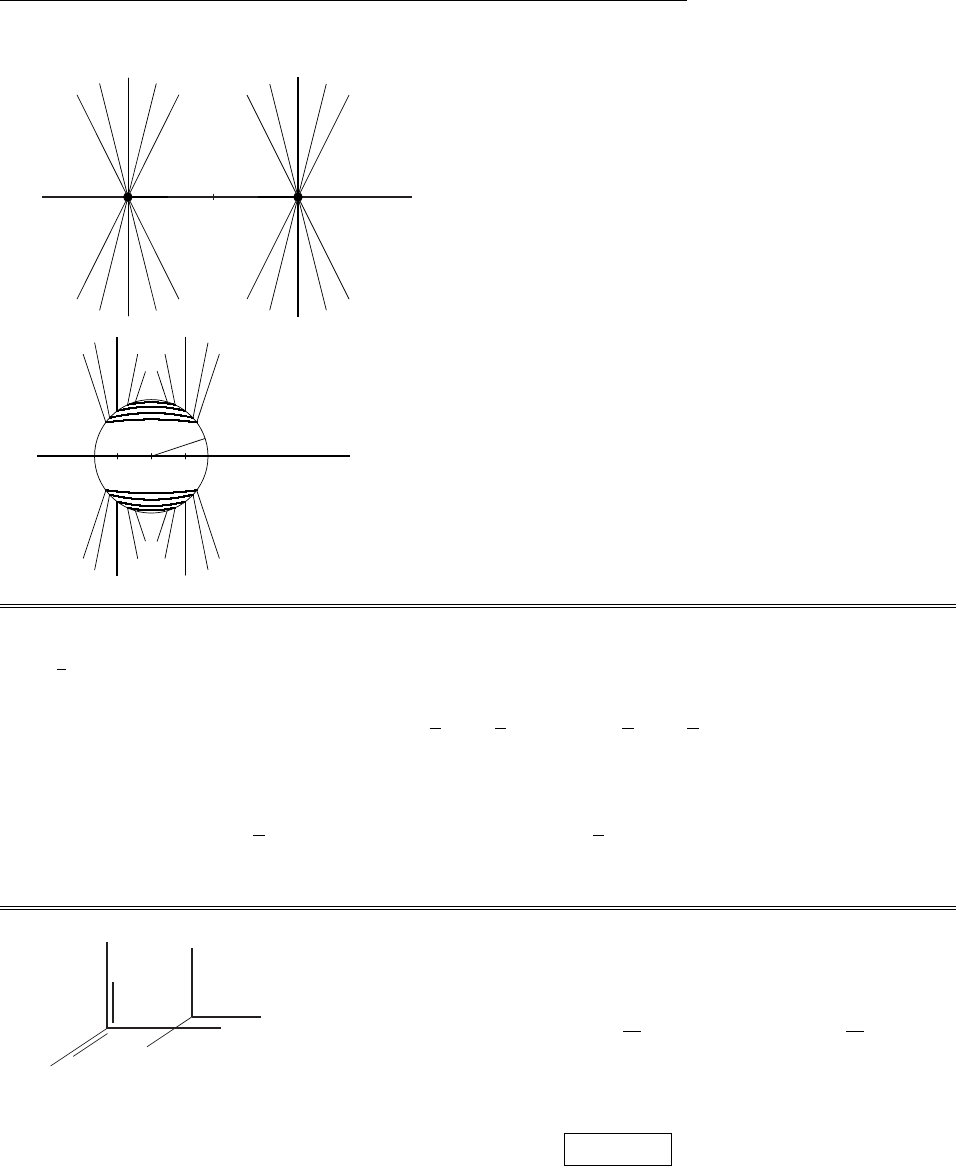
CHAPTER 12. ELECTRODYNAMICS AND RELATIVITY 287
Problem 12.67
6
✕v
☛
v
✛✛
¯v
✲x
−q✲
❄
✻
✎❲
✗ ❖
☛❯
✕ ❑
+q
✛
✻
❄
✗❖
✎ ❲
✕❑
☛ ❯
✻
❄
✗
❖
✎❲
✍
▼
✌◆
◆ ❲ ❄
✎✌
✍ ✗ ✻
❖▼
✲x
+−
✶
ct
!
E
!
E
c
⃝2005 Pearson Education, Inc., Upper Saddle River, NJ. All rights reserved. This material is
protected under all copyright laws as they currently exist. No portion of this material may be
reproduced, in any form or by any means, without permission inwritingfromthepublisher.
Just before:
Field lines emanate
from present position
of particle.
6
✕v
☛
v
✛✛
¯v
✲x
−q✲
❄
✻
✎❲
✗ ❖
☛❯
✕ ❑
+q
✛
✻
❄
✗❖
✎ ❲
✕❑
☛ ❯
✻
❄
✗
❖
✎❲
✍
▼
✌◆
◆ ❲ ❄
✎✌
✍ ✗ ✻
❖▼
✲x
+−
✶
ct
!
E
!
E
c
⃝2005 Pearson Education, Inc., Upper Saddle River, NJ. All rights reserved. This material is
protected under all copyright laws as they currently exist. No portion of this material may be
reproduced, in any form or by any means, without permission inwritingfromthepublisher.
Just after: Field lines outside sphere of radius ct emanate from
position particle would have reached, had it kept going on its
original “flight plan”. Inside the sphere E= 0. On the sur-
face the lines connect up (since they cannot simply terminate
in empty space), as suggested in the figure.
This produces a dense cluster of tangentially-directed field
lines, which expand with the spherical shell. This is a pic-
torial way of understanding the generation of electromagnetic
radiation.
Problem 12.68
Equation 12.67 assumes the particle is (instantaneously) at rest in S. Here the particle is at rest in ¯
S.So
F?=1
¯
F?,F
k=¯
Fk. Using ¯
F=q¯
E, then,
Fx=¯
Fx=q¯
Ex,F
y=1
¯
Fy=1
q¯
Ey,F
z=1
¯
Fz=1
q¯
Ez.
Invoking Eq. 12.109:
Fx=qEx,F
y=1
q(EyvBz)=q(EyvBz)Fz=1
q(Ez+vBy)=q(Ez+vBy).
But v⇥B=vBzˆx +vByˆz , so F=q(E+v⇥B). qed
Problem 12.69
1
✲y
✻
z
✰
x
✻
E
✰
B
✲¯y
✻
¯z
✰
¯x
=⇒v
✲¯y
✻
¯z
✰
¯x
✶
R
q
ωt
✒
c
⃝2005 Pearson Education, Inc., Upper Saddle River, NJ. All rights reserved. This material is
protected under all copyright laws as they currently exist. No portion of this material may be
reproduced, in any form or by any means, without permission inwritingfromthepublisher.
Rewrite Eq. 12.109 with x!y,y!z,z!x:
¯
Ey=Ey¯
Ez=(EzvBx)¯
Ex=(Ex+vBz)
¯
By=By¯
Bz=Bz+v
c2Ex¯
Bx=Bxv
c2Ez
This gives the fields in system ¯
Smoving in the ydirection at speed v.
Now E=(0,0,E
0); B=(B0,0,0), so ¯
Ey= 0, ¯
Ez=(E0vB0), ¯
Ex= 0.
If we want ¯
E=0, we must pick vso that E0vB0= 0; i.e. v=E0/B0
(The condition E0/B0<cguarantees that there is no problem getting to such a system.)
c
2012 Pearson Education, Inc., Upper Saddle River, NJ. All rights reserved. This material is
protected under all copyright laws as they currently exist. No portion of this material may be
reproduced, in any form or by any means, without permission in writing from the publisher.

288 CHAPTER 12. ELECTRODYNAMICS AND RELATIVITY
With this, ¯
By= 0, ¯
Bz= 0, ¯
Bx=(B0v
c2E0)=B01v2
c2=B01
2=1
B0;¯
B=1
B0ˆx .
The trajectory in ¯
S: Since the particle started out at rest at the origin
in S, it started out with velocity vˆy in ¯
S. According to Eq. 12.71
it will move in a circle of radius R, given by
p=qBR, or mv =q1
B0R)R=m2v
qB0
.
1
✲y
✻
z
✰
x
✻
E
✰
B
✲¯y
✻
¯z
✰
¯x
=⇒v
✲¯y
✻
¯z
✰
¯x
✶
R
q
ωt
✒
c
⃝2005 Pearson Education, Inc., Upper Saddle River, NJ. All rights reserved. This material is
protected under all copyright laws as they currently exist. No portion of this material may be
reproduced, in any form or by any means, without permission inwritingfromthepublisher.
The actual trajectory is given by ¯x=0; ¯y=Rsin !¯
t;¯z=R(1 cos !¯
t); where !=v
R.
The trajectory in S: The Lorentz transformations Eqs. 12.18 and 12.19, for the case of relative motion in
the y-direction, read:
¯x=xx=¯x
¯y=(yvt)y=(¯y+v¯
t)
¯z=zz=¯z
¯
t=tv
c2yt=¯
t+v
c2¯y
So the trajectory in Sis given by:
x=0;y=(Rsin !¯
t+v¯
t)=Rsin!tv
c2y+vtv
c2y,or
y1+2v2
c2
2y(1v2
c2+v2
c2)=2y
=2vt Rsin!tv
c2y(yvt)=Rsin!tv
c2y;
z=R(1 cos2!¯
t)=R1cos !tv
c2y.
So: x=0; y=vt R
sin!tv
c2y;z=RRcos!tv
c2.
We can get rid of the trigonometric terms by the usual trick:
(yvt)=Rsin !(tv
c2y)
zR=Rcos !(tv
c2y))2(yvt)2+(zR)2=R2.
Absent the 2, this would be the cycloid we found back in Ch. 5 (Eq. 5.9). The 2makes it, as it were, an
elliptical cycloid — same picture as Fig. 5.7, but with the horizontal axis stretched out.
Problem 12.70
(a) D=✏0E+Psuggests E!1
✏0D
H=1
µ0BMsuggests B!µ0Hbut it’s a little cleaner if we divide by µ0while we’re at it, so that
E!1
µ0✏0D=c2D,B!H. Then:
Dµ⌫=
0cDxcDycDz
cDx0HzHy
cDyHz0Hx
cDzHyHx0
c
2012 Pearson Education, Inc., Upper Saddle River, NJ. All rights reserved. This material is
protected under all copyright laws as they currently exist. No portion of this material may be
reproduced, in any form or by any means, without permission in writing from the publisher.
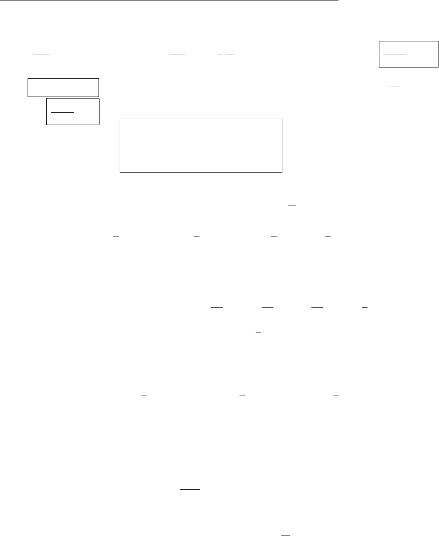
CHAPTER 12. ELECTRODYNAMICS AND RELATIVITY 289
Then (following the derivation in Sect. 12.3.4):
@
@x⌫D0⌫=cr·D=c⇢f=J0
f;@
@x⌫D1⌫=1
c
@
@t(cDx)+(r⇥H)x=(Jf)x; so @Dµ⌫
@x⌫=Jµ
f,
where Jµ
f=(c⇢f,Jf).Meanwhile, the homogeneous Maxwell equations r·B=0,E=@B
@tare unchanged,
and hence @Gµ⌫
@x⌫=0.
(b)
Hµ⌫=
0HxHyHz
Hx0cDzcDy
HycDz0cDx
HzcDycDx0
(c) If the material is at rest, ⌘⌫=(c, 0,0,0), and the sum over ⌫collapses to a single term:
Dµ0⌘0=c2✏Fµ0⌘0)Dµ0=c2✏Fµ0)cD=c2✏E
c)D=✏E(Eq.4.32),X
Hµ0⌘0=1
µGµ0⌘0)Hµ0=1
µGµ0)H=1
µB)H=1
µB(Eq.6.31).X
(d) In general, ⌘⌫=(c, u), so, for µ= 0:
D0⌫⌘⌫=D01⌘1+D02⌘2+D03⌘3=cDx(ux)+cDy(uy)+cDz(uz)=c(D·u),
F0⌫⌘⌫=F01⌘1+F02⌘2+F03⌘3=Ex
c(ux)+Ey
c(uy)+Ez
c(uz)=
c(E·u),so
D0⌫⌘⌫=c2✏F0⌫⌘⌫)c(D·u)=c2✏
c(E·u))D·u=✏(E·u).[1]
H0⌫⌘⌫=H01⌘1+H02⌘2+H03⌘3=Hx(ux)+Hy(uy)+Hz(uz)=(H·u),
G0⌫⌘⌫=G01⌘1+G02⌘2+G03⌘3=Bx(ux)+By(uy)+Bz(uz)=(B·u),so
H0⌫⌘⌫=1
µG0⌫⌘⌫)(H·u)= 1
µ(B·u))H·u=1
µ(B·u).[2]
Similarly, for µ=1:
D1⌫⌘⌫=D10⌘0+D12⌘2+D13⌘3=(cDx)(c)+Hz(uy)+(Hy)(uz)=(c2Dx+uyHzuzHy)
=c2D+(u⇥H)x,
F1⌫⌘⌫=F10⌘0+F12⌘2+F13⌘3=Ex
c(c)+Bz(uy)+(By)(uz)=(Ex+uyBzuzBy)
=[E+(u⇥B)]x,so D1⌫⌘⌫=c2✏F1⌫⌘⌫)
c2D+(u⇥H)x=c2✏ [E+(u⇥B)]x)D+1
c2(u⇥H)=✏[E+(u⇥B)] .[3]
H1⌫⌘⌫=H10⌘0+H12⌘2+H13⌘3=(Hx)(c)+(cDz)(uy)+(cDy)(uz)
=c(HxuyDz+uzDy)=c[H(u⇥D)]x,
c
2012 Pearson Education, Inc., Upper Saddle River, NJ. All rights reserved. This material is
protected under all copyright laws as they currently exist. No portion of this material may be
reproduced, in any form or by any means, without permission in writing from the publisher.

290 CHAPTER 12. ELECTRODYNAMICS AND RELATIVITY
G1⌫⌘⌫=G10⌘0+G12⌘2+G13⌘3=(Bx)(c)+Ez
c(uy)+Ey
c(uz)
=
c(c2BxuyEz+uzEy)=
cc2B(u⇥E)x,so H1⌫⌘⌫=1
µG1⌫⌘⌫)
c[H(u⇥D)]x=1
µ
cc2B(u⇥E)x)H(u⇥D)= 1
µB1
c2(u⇥E).[4]
Use Eq. [4] as an expression for H, plug this into Eq. [3], and solve for D:
D+1
c2u⇥(u⇥D)+ 1
µB1
c2(u⇥E)=✏[E+(u⇥B)] ;
D+1
c2(u·D)uu2D=✏[E+(u⇥B)] 1
µc2(u⇥B)+ 1
µc4[u⇥(u⇥E)] .
Using Eq. [1] to rewrite (u·D):
D1u2
c2=✏
c2(E·u)u+✏[E+(u⇥B)] 1
µc2(u⇥B)+ 1
µc4(E·u)uu2E
=✏1u2
✏µc4E1
c211
✏µc2(E·u)u+(u⇥B)11
✏µc2.
Let ⌘1
1u2/c2,v⌘1
p✏µ.Then
D=2✏1u2v2
c4E+1v2
c2(u⇥B)1
c2(E·u)u.
Now use Eq. [3] as an expression for D, plug this into Eq. [4], and solve for H:
Hu⇥1
c2(u⇥H)+✏[E+(u⇥B)]=1
µB1
c2(u⇥E);
H+1
c2(u·H)uu2H=1
µB1
c2(u⇥E)+✏(u⇥E)+✏[u⇥(u⇥B)].
Using Eq. [2] to rewrite (u·H):
H1u2
c2=1
µc2(B·u)u+1
µB1
c2(u⇥E)+✏(u⇥E)+✏(B·u)uu2B
=1
µ1µ✏u2B+✏µ1
c2[(u⇥E)+(B·u)u].
H=2
µ1u2
v2B+1
v21
c2[(u⇥E)+(B·u)u].
c
2012 Pearson Education, Inc., Upper Saddle River, NJ. All rights reserved. This material is
protected under all copyright laws as they currently exist. No portion of this material may be
reproduced, in any form or by any means, without permission in writing from the publisher.

CHAPTER 12. ELECTRODYNAMICS AND RELATIVITY 291
Problem 12.71
We know that (proper) power transforms as the zeroth component of a 4-vector K0=1
c
dW
d⌧. The Larmor
formula says that for v= 0, dW
d⌧=1
4⇡✏0
2
3
q2
c3a2(Eq. 11.70). Can we think of a 4-vector whose zeroth component
reduces to this when the velocity is zero?
Well, a2smells like (↵⌫↵⌫), but how do we get a 4-vector in here? How about ⌘µ, whose zeroth component
is just c, when v= 0? Try, then:
Kµ=1
4⇡✏0
2
3
q2
c5(↵⌫↵⌫)⌘µ
This has the right transformation properties, but we must check that it does reduce to the Larmor formula
when v= 0:
dW
dt =1
dW
d⌧=1
cK0=1
cµ0q2
6⇡c3(↵⌫↵⌫)⌘0, but ⌘0=c, so dW
dt =µ0q2
6⇡c(↵⌫↵⌫) . [Incidentally, this tells
us that the power itself (as opposed to proper power) is a scalar. If this had been obvious from the start, we
could simply have looked for a Lorentz scalar that generalizes the Larmor formula.]
In Prob. 12.39(b) we calculated (↵⌫↵⌫) in terms of ordinary velocity and acceleration:
↵⌫↵⌫=4a2+(v·a)2
(c2v2)=6a22+1
c2(v·a)2
=6a21v2
c2+1
c2(v·a)2=6a21
c2v2a2(v·a)2.
Now v·a=va cos ✓, where ✓is the angle between vand a, so:
v2a2(v·a)2=v2a2(1 cos2✓)=v2a2sin2✓=|v⇥a|2.
↵⌫↵⌫=6a2v⇥a
c
2.
dW
dt =µ0q2
6⇡c6a2v⇥a
c
2,which is Li´enard’s formula (Eq. 11.73).
Problem 12.72
(a) It’s inconsistent with the constraint ⌘µKµ= 0 (Prob. 12.39(d)).
(b) We want to find a 4-vector bµwith the property that d↵µ
d⌧+bµ⌘µ= 0. How about bµ=d↵⌫
d⌧⌘⌫⌘µ? Then
d↵⌫
d⌧+bµ⌘µ=d↵µ
d⌧⌘µ+d↵⌫
d⌧⌘⌫(⌘µ⌘µ). But ⌘µ⌘µ=c2, so this becomes d↵µ
d⌧⌘µc2d↵⌫
d⌧⌘⌫, which is zero,
if we pick =1/c2. This suggests Kµ
rad =µ0q2
6⇡cd↵µ
d⌧+1
c2
d↵⌫
d⌧⌘⌫⌘µ.Note that ⌘µ=(c, v), so the spatial
components of bµvanish in the nonrelativistic limit v⌧c, and hence this still reduces to the Abraham-Lorentz
formula. [Incidentally, ↵⌫⌘⌫=0)d
d⌧(↵⌫⌘⌫)=0)d↵⌫
d⌧⌘⌫+↵⌫d⌘⌫
d⌧= 0, so d↵⌫
d⌧⌘⌫=↵⌫↵⌫, and hence bµcan
just as well be written 1
c2(↵⌫↵⌫)⌘µ.]
Problem 12.73
Define the electric current 4-vector as before: Jµ
e=(c⇢e,Je), and the magnetic current analogously:
Jµ
m=(c⇢m,Jm). The fundamental laws are then
@⌫Fµ⌫=µ0Jµ
e,@⌫Gµ⌫=µ0
cJµ
m,K
µ=qeFµ⌫+qm
cGµ⌫⌘⌫.
c
2012 Pearson Education, Inc., Upper Saddle River, NJ. All rights reserved. This material is
protected under all copyright laws as they currently exist. No portion of this material may be
reproduced, in any form or by any means, without permission in writing from the publisher.

292 CHAPTER 12. ELECTRODYNAMICS AND RELATIVITY
The first of these reproduces r·E= (1/✏0)⇢eand r⇥B=µ0Je+µ0✏0@E/@t, just as before; the second
yields r·B=(µ0/c)(c⇢m)=µ0⇢mand (1/c)[@B/@t+r⇥E]=(µ0/c)Jm, or r⇥E=µ0Jm@B/@t
(generalizing Sec. 12.3.4). These are Maxwell’s equations with magnetic charge (Eq. 7.44). The third says
K1=qe
1u2/c2[E+(u⇥B)]x+qm
cc
1u2/c2(Bx)+ uy
1u2/c2Ez
c+uz
1u2/c2Ey
c,
K=1
1u2/c2qe[E+(u⇥B)] + qmB1
c2(u⇥E),or
F=qe[E+(u⇥B]+qmB1
c2(u⇥E),
which is the generalized Lorentz force law (Eq. 7.69).
c
2012 Pearson Education, Inc., Upper Saddle River, NJ. All rights reserved. This material is
protected under all copyright laws as they currently exist. No portion of this material may be
reproduced, in any form or by any means, without permission in writing from the publisher.

CONCORDANCE 293
4th ed Same? 3rd ed
1.1 X1.1
1.2 X1.2
1.3 X1.3
1.4 X1.4
1.5 X1.5
1.6 X1.6
1.7 X1.7
1.8 X1.8
1.9 X1.9
1.10 X1.10
1.11 X1.11
1.12 X1.12
1.13 X1.13
1.14 X1.14
1.15 X1.15
1.16 X1.16
1.17 X1.17
1.18 X1.18
1.19 new –
1.20 X1.19
1.21 X1.20
1.22 X1.21
1.23 X1.22
1.24 X1.23
1.25 X1.24
1.26 X1.25
1.27 X1.26
1.28 X1.27
1.29 X1.28
1.30 X1.29
1.31 X1.30
1.32 X1.31
1.33 X1.32
1.34 X1.33
1.35 X1.34
1.36 X1.35
1.37 X1.36
1.38 X1.37
1.39 X1.38
1.40 X1.39
1.41 X1.40
1.42 X1.41
1.43 X1.42
1.44 X1.43
1.45 X1.44
4th ed Same? 3rd ed
1.46 X1.45
1.47 X1.46
1.48 X1.47
1.49 X1.48
1.50 X1.49
1.51 X1.50
1.52 X1.51
1.53 X1.52
1.54 X1.53
1.55 X1.54
1.56 X1.55
1.57 X1.56
1.58 X1.57
1.59 X1.58
1.60 X1.59
1.61 X1.60
1.62 X1.61
1.63 X1.62
1.64 new –
2.1 X2.1
2.2 mod 2.2
2.3 X2.3
2.4 X2.4
2.5 X2.5
2.6 X2.6
2.7 X2.7
2.8 X2.8
2.9 X2.9
2.10 X2.10
2.11 X2.11
2.12 X2.12
2.13 X2.13
2.14 X2.14
2.15 mod 2.15
2.16 X2.16
2.17 X2.17
2.18 X2.18
2.19 X2.19
2.20 X2.20
2.21 X2.21
2.22 X2.22
2.23 X2.23
2.24 X2.24
2.25 X2.25
2.26 X2.26
4th ed Same? 3rd ed
2.27 X2.27
2.28 X2.28
2.29 X2.29
2.30 X2.30
2.31 X2.31
2.32 new –
2.33 new –
2.34 X2.32
2.35 X2.33
2.36 X2.34
2.37 new –
2.38 X2.35
2.39 X2.36
2.40 new –
2.41 X2.37
2.42 X2.38
2.43 X2.39
2.44 X2.40
2.45 X2.41
2.46 new –
2.47 X2.43
2.48 X2.44
2.49 X2.45
2.50 X2.46
2.51 new –
2.52 X2.47
2.53 X2.48
2.54 mod 2.49
2.55 X2.50
2.56 X2.51
2.57 X2.52
2.58 new –
2.59 new –
2.60 new –
2.61 new –
3.1 X3.1
3.2 X3.2
3.3 X3.3
3.4 new –
3.5 X3.4
3.6 X3.5
3.7 X3.6
3.8 X3.7
3.9 X3.8
3.10 X3.9
c
2012 Pearson Education, Inc., Upper Saddle River, NJ. All rights reserved. This material is
protected under all copyright laws as they currently exist. No portion of this material may be
reproduced, in any form or by any means, without permission in writing from the publisher.

294 CONCORDANCE
4th ed Same? 3rd ed
3.11 X3.10
3.12 X3.11
3.13 X3.12
3.14 X3.13
3.15 X3.14
3.16 mod 3.15
3.17 X3.16
3.18 X3.17
3.19 X3.18
3.20 X3.19
3.21 X3.20
3.22 X3.21
3.23 X3.22
3.24 X3.23
3.25 X3.24
3.26 X3.25
3.27 X3.26
3.28 new –
3.29 X3.27
3.30 X3.28
3.31 X3.29
3.32 X3.30
3.33 X3.31
3.34 X3.32
3.35 new –
3.36 X3.33
3.37 new –
3.38 new –
3.39 X3.35
3.40 X3.36
3.41 new –
3.42 new –
3.43 X3.37
3.44 X3.38
3.45 X3.39
3.46 X3.40
3.47 X3.41
3.48 X3.42
3.49 new –
3.50 X3.43
3.51 X3.44
3.52 mod 3.45
3.53 X3.46
3.54 X3.47
3.55 X3.48
4th ed Same? 3rd ed
3.56 X3.49
3.57 new –
3.58 new –
4.1 X4.1
4.2 X4.2
4.3 X4.3
4.4 X4.4
4.5 X4.5
4.6 X4.6
4.7 X4.7
4.8 X4.8
4.9 X4.9
4.10 X4.10
4.11 X4.11
4.12 X4.12
4.13 X4.13
4.14 X4.14
4.15 X4.15
4.16 mod 4.16
4.17 X4.17
4.18 X4.18
4.19 X4.19
4.20 X4.20
4.21 X4.21
4.22 X4.22
4.23 X4.23
4.24 X4.24
4.25 X4.25
4.26 X4.26
4.27 X4.27
4.28 X4.28
4.29 X4.29
4.30 X4.30
4.31 new –
4.32 new –
4.33 X4.31
4.34 new –
4.35 X4.32
4.36 X4.33
4.37 X4.34
4.38 X4.35
4.39 X4.36
4.40 X4.37
4.41 X4.38
4.42 X4.39
4th ed Same? 3rd ed
4.43 X4.40
5.1 X5.1
5.2 X5.2
5.3 X5.3
5.4 X5.4
5.5 X5.5
5.6 X5.6
5.7 X5.7
5.8 X5.8
5.9 X5.9
5.10 X5.10
5.11 X5.11
5.12 new –
5.13 X5.12
5.14 X5.13
5.15 X5.14
5.16 X5.15
5.17 X5.16
5.18 X5.17
5.19 X5.18
5.20 X5.19
5.21 X5.20
5.22 X5.21
5.23 X5.22
5.24 X5.23
5.25 X5.24
5.26 X5.25
5.27 X5.26
5.28 X5.27
5.29 X5.28
5.30 X5.29
5.31 X5.30
5.32 X5.31
5.33 X5.32
5.34 X5.33
5.35 X5.34
5.36 X5.37
5.37 mod 5.35, 5.36
5.38 X5.60
5.39 new –
5.40 X5.38
5.41 X5.39
5.42 X5.40
5.43 X5.41
5.44 X5.42
c
2012 Pearson Education, Inc., Upper Saddle River, NJ. All rights reserved. This material is
protected under all copyright laws as they currently exist. No portion of this material may be
reproduced, in any form or by any means, without permission in writing from the publisher.

CONCORDANCE 295
4th ed Same? 3rd ed
5.45 X5.43
5.46 X5.44
5.47 X5.46
5.48 mod 5.47
5.49 X5.48
5.50 X5.49
5.51 new –
5.52 X5.50
5.53 X5.51
5.54 X5.52
5.55 X5.53
5.56 X5.54
5.57 X5.55
5.58 X5.56
5.59 X5.57
5.60 X5.58
5.61 X5.59
5.62 X5.61
6.1 X6.1
6.2 X6.2
6.3 X6.3
6.4 X6.4
6.5 X6.5
6.6 X6.6
6.7 X6.7
6.8 X6.8
6.9 X6.9
6.10 X6.10
6.11 X6.11
6.12 X6.12
6.13 X6.13
6.14 X6.14
6.15 X6.15
6.16 X6.16
6.17 X6.17
6.18 X6.18
6.19 X6.19
6.20 X6.20
6.21 X6.21
6.22 X6.22
6.23 X6.25
6.24 new –
6.25 X6.23
4th ed Same? 3rd ed
6.26 X6.24
6.27 X6.26
6.28 X6.27
6.29 X6.28
7.1 X7.1
7.2 X7.2
7.3 X7.3
7.4 X7.4
7.5 X7.5
7.6 X7.6
7.7 X7.7
7.8 X7.8
7.9 X7.9
7.10 X7.10
7.11 X7.11
7.12 X7.12
7.13 X7.13
7.14 X7.14
7.15 X7.15
7.16 X7.16
7.17 X7.17
7.18 X7.18
7.19 X7.19
7.20 new –
7.21 new –
7.22 X7.20
7.23 X7.21
7.24 X7.22
7.25 X7.23
7.26 X7.24
7.27 X7.25
7.28 X7.26
7.29 X7.27
7.30 X7.28
7.31 X7.29
7.32 X7.30
7.33 new –
7.34 X7.31
7.35 X7.32
7.36 X7.33
7.37 X7.34
7.38 X7.35
7.39 X7.36
4th ed Same? 3rd ed
7.40 X7.37
7.41 X7.39
7.42 X7.41
7.43 X7.57
7.44 X7.42
7.45 X7.43
7.46 X7.44
7.47 X7.45
7.48 mod 7.46
7.49 mod 7.47
7.50 X7.48
7.51 new –
7.52 X7.49
7.53 X7.50
7.54 new –
7.55 X7.51
7.56 X7.52
7.57 X7.53
7.58 X7.54
7.59 new –
7.60 X7.55
7.61 X7.56
7.62 X7.58
7.63 X7.59
7.64 X7.60
8.1 X8.1
8.2 X8.2
8.3 X8.3
8.4 X8.4
8.5 new –
8.6 mod 8.6
8.7 mod 8.5
8.8 X8.7
8.9 new –
8.10 X8.8
8.11 new –
8.12 new –
8.13 X8.9
8.14 new –
8.15 new –
8.16 X8.10
8.17 X8.11
8.18 new –
c
2012 Pearson Education, Inc., Upper Saddle River, NJ. All rights reserved. This material is
protected under all copyright laws as they currently exist. No portion of this material may be
reproduced, in any form or by any means, without permission in writing from the publisher.

296 CONCORDANCE
4th ed Same? 3rd ed
8.19 X8.12
8.20 new –
8.21 mod 8.13
8.22 X8.14
8.23 X8.15
8.24 new –
9.1 X9.1
9.2 X9.2
9.3 X9.3
9.4 X9.4
9.5 X9.5
9.6 X9.6
9.7 X9.7
9.8 X9.8
9.9 X9.9
9.10 X9.10
9.11 new –
9.12 X9.11
9.13 X9.12
9.14 X9.13
9.15 X9.14
9.16 X9.15
9.17 X9.16
9.18 X9.17
9.19 X9.18
9.20 X9.19
9.21 X9.20
9.22 X9.21
9.23 X9.22
9.24 X9.23
9.25 X9.24
9.26 new –
9.27 X9.26
9.28 X9.27
9.29 X9.28
9.30 X9.29
9.31 X9.30
9.32 X9.31
9.33 X9.32
9.34 new –
9.35 X9.33
9.36 X9.34
9.37 X9.35
9.38 X9.36
9.39 X9.37
9.40 X9.38
4th ed Same? 3rd ed
10.1 X10.1
10.2 X10.2
10.3 mod 10.3, 10.5
10.4 X10.4
10.5 X10.6
10.6 X10.7
10.7 new –
10.8 new –
10.9 new –
10.10 X10.8
10.11 X10.9
10.12 X10.10
10.13 X10.11
10.14 X10.12
10.15 X10.13
10.16 X10.14
10.17 X10.15
10.18 X10.16
10.19 X10.17
10.20 X10.18
10.21 mod 12.43a
10.22 X10.19
10.23 X10.20
10.24 X10.21
10.25 X10.22
10.26 new –
10.27 X10.23
10.28 X10.24
10.29 new –
10.30 new –
10.31 X10.25
10.32 X10.26
10.33 new –
10.34 new –
11.1 X11.1
11.2 X11.2
11.3 X11.3
11.4 X11.4
11.5 X11.5
11.6 X11.6
11.7 X11.7
11.8 new –
11.9 X11.8
11.10 X11.9
11.11 X11.12
11.12 X11.10
4th ed Same? 3rd ed
11.13 new –
11.14 X11.14
11.15 X11.15
11.16 X11.16
11.17 X11.17
11.18 new –
11.19 X11.19
11.20 mod 11.20
11.21 new –
11.22 X11.21
11.23 X11.22
11.24 X11.11
11.25 X11.23
11.26 new –
11.27 new –
11.28 X11.24
11.29 X11.26
11.30 X11.27
11.31 X11.28
11.32 X11.29
11.33 X11.30
11.34 X11.31
11.35 new –
12.1 X12.1
12.2 X12.2
12.3 X12.3
12.4 X12.4
12.5 X12.5
12.6 X12.6
12.7 X12.7
12.8 X12.8
12.9 X12.9
12.10 X12.10
12.11 X12.11
12.12 X12.12
12.13 X12.13
12.14 mod 12.14
12.15 X12.15
12.16 X12.16
12.17 X12.17
12.18 X12.18
12.19 X11.19
12.20 X12.20
12.21 X12.21
12.22 X12.22
12.23 X12.23
c
2012 Pearson Education, Inc., Upper Saddle River, NJ. All rights reserved. This material is
protected under all copyright laws as they currently exist. No portion of this material may be
reproduced, in any form or by any means, without permission in writing from the publisher.

CHAPTER 12. ELECTRODYNAMICS AND RELATIVITY 297
4th ed Same? 3rd ed
12.24 X12.24
12.25 X12.25
12.26 mod 12.26
12.27 new –
12.28 X12.27
12.29 X12.28
12.30 X12.29
12.31 X12.30
12.32 X12.31
12.33 X12.32
12.34 X12.33
12.35 X12.34
12.36 X12.35
12.37 X12.36
12.38 X12.37
12.39 X12.38
12.40 X12.39
12.41 X12.40
12.42 X12.41
12.43 X12.42
12.44 new –
12.45 X12.44
12.46 X12.45
12.47 X12.46
12.48 X12.47
4th ed Same? 3rd ed
12.49 X12.48
12.50 X12.49
12.51 X12.50
12.52 X12.51
12.53 X12.52
12.54 X12.53
12.55 X12.54
12.56 X12.55
12.57 X12.56
12.58 new –
12.59 X12.57
12.60 X12.58
12.61 X12.59
12.62 X12.60
12.63 X12.61
12.64 X12.62
12.65 X12.63
12.66 X12.64
12.67 X12.65
12.68 X12.66
12.69 X12.67
12.70 X12.68
12.71 X12.69
12.72 X12.70
12.73 X12.71
c
2012 Pearson Education, Inc., Upper Saddle River, NJ. All rights reserved. This material is
protected under all copyright laws as they currently exist. No portion of this material may be
reproduced, in any form or by any means, without permission in writing from the publisher.
