JRCLUST Manual
User Manual:
Open the PDF directly: View PDF ![]() .
.
Page Count: 24
JRCLUST manual
Janelia Rocket Clust (ver. 3)
Updated on 2017 Jun 20
J. James Jun
Vidrio Technologies, LLC
HHMI - Janelia Research Campus
Installation instruction
[Requirements]
1. Matlab (R2014b+) and toolboxes: Parallel computing, Signal processing, Image processing.
2. RAM should be larger than ¼ of the recording file size.
3. Install Microsoft Visual Studio Express 2013 (V12) to compile the CUDA codes (C-code for GPU).
3. Install a correct version of the NVIDIA CUDA toolkit. You can find the version supported by the Parallel Computing
Toolbox by running "gpuDevice" in Matlab and check "ToolkitVersion".
Matlab version
NVIDIA CUDA Toolkit version
R2017a
V8.0: https://developer.nvidia.com/cuda-downloads
R2016a,b
V7.5: https://developer.nvidia.com/cuda-75-downloads-archive
R2015b
V7.0: https://developer.nvidia.com/cuda-toolkit-70
R2015a
V6.5: https://developer.nvidia.com/cuda-toolkit-65
R2014b
V6.0: https://developer.nvidia.com/cuda-toolkit-60
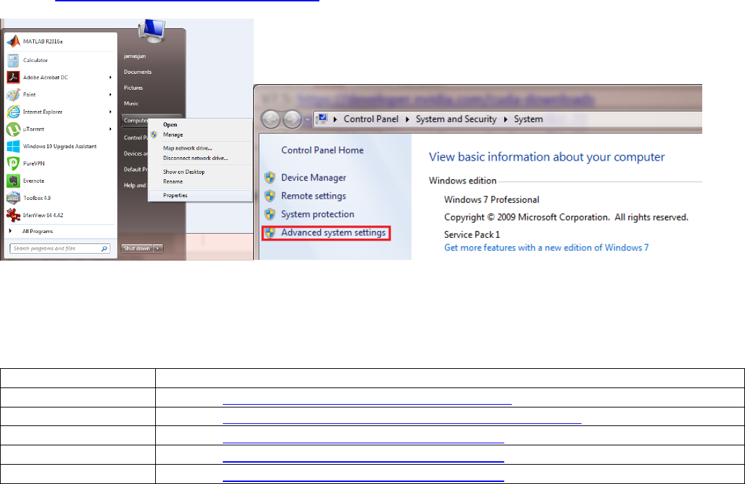
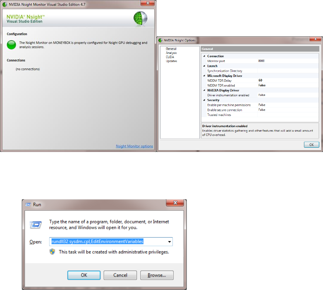
4. Disable the GPU timeout by running “Nsight Monitor”; navigate to “options” located at bottom-left; set "WDDM TDR
enabled" to “false”.
5. Add paths for the NVIDIA and Microsoft compilers in the system path. Each entry in path should be separated by “;”.
See below for the instructions for setting the system path in Windows:
Press win+R and type “rundll32.exe sysdm.cpl,EditEnvironmentVariables” and press OK.
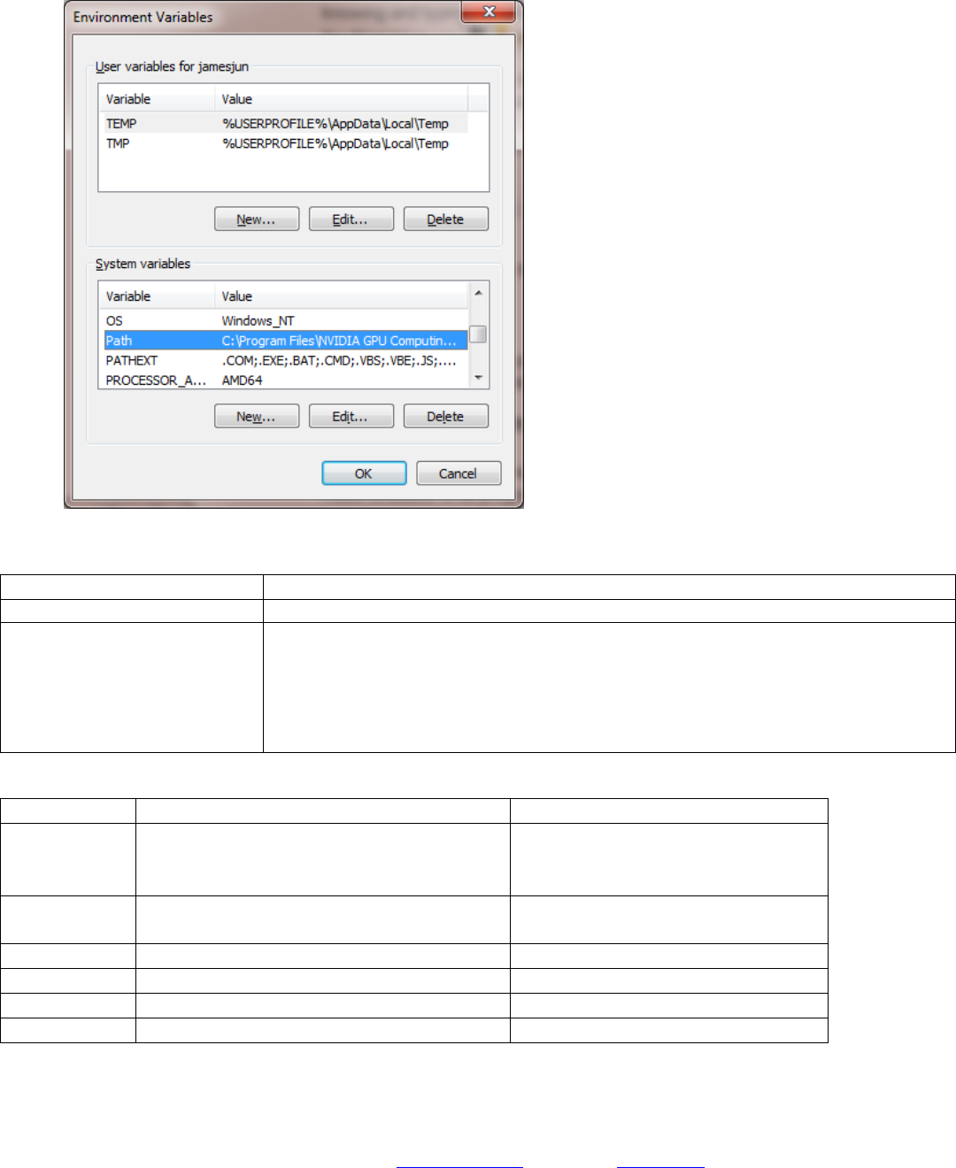
Select “Path” under System variables and add the following:
Program
Path
Microsoft Visual Studio 2013
C:\Program Files (x86)\Microsoft Visual Studio 12.0\VC\bin
NVIDIA CUDA Toolkit
select a correct version from below:
C:\program files\NVIDIA GPU Computing Toolkit\CUDA\v8.0\bin (Matlab R2017a)
C:\program files\NVIDIA GPU Computing Toolkit\CUDA\v7.5\bin (Matlab R2016a,b)
C:\program files\NVIDIA GPU Computing Toolkit\CUDA\v7.0\bin (Matlab R2015b)
C:\program files\NVIDIA GPU Computing Toolkit\CUDA\v6.5\bin (Matlab R2015a)
C:\program files\NVIDIA GPU Computing Toolkit\CUDA\v6.0\bin (Matlab R2014b)
Requirement
Comments
Tested
Matlab
Required toolboxes: parallel processing,
statistics and machine learning, signal
processing, image processing toolboxes
Version R2015b to R2017a
CUDA
Download NVidia CUDA toolkit
Set
Version 6.5 to 8.0
Graphics card
CUDA-compatible NVidia GPU
Titan X (12 GB) and GTX 980 Ti (6 GB)
CPU
Multi-core CPU runs multiple threads
Dual Xeon 3.0 GHz CPU (Quad-core)
RAM
Larger than ¼ of the recording file size
16 GB+ recommended
Hard drive
Fast I/O speed recommended
RAID or SSD
[Install JRCLUST]
1. Copy JRCLUST folder in the Dropbox folder (e.g. "C:\Dropbox\jrclust") to another location (e.g. "C:\jrclust_user").
Latest JRCLUST version can be also obtained from www.jrclust.org. Download the .zip file and extract to a folder (e.g.
“C:\jrclust_user”).
2. Start Matlab and "cd" to the copied location (e.g. "C:\jrclust_user").
3. Run "jrc install". This will compile all the CUDA codes. You can later recompile by running “jrc compile”
4. Edit "path_dropbox" in "user.cfg" and specify the path to the Dropbox folder containing JRCLUST (e.g.
"C:\Dropbox\jrclust").
5. (optional) Download example files (sample.bin and sample.meta) by running “jrc download sample”.
6. Further details can be found in “install.txt”.
A. Step-by-step tutorial
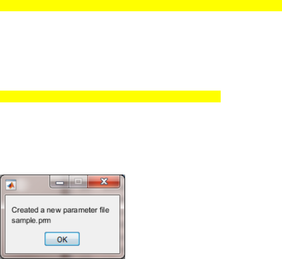
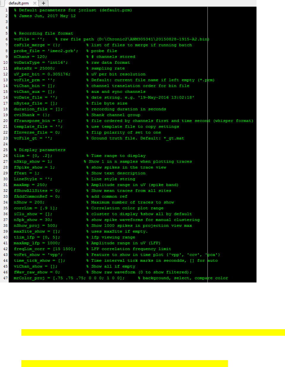
Step 1. Make a parameter file from a default template (default.prm)
Syntax:
>> jrc makeprm [myrecording.bin] [myprobe.prb]
This creates a new parameter file (myrecording_myprobe.prm) for a WHISPER recording (myrecording.bin) that uses a
probe configuration file (myprobe.prb).
Example:
>> jrc makeprm sample.bin sample.prb
Result:
Created a new parameter file
sample_sample.prm
Note:
1. JRCLUST will search within the current folder if full-path is not provided. Surround the full-path with a pair of
single quotation if it contains blank characters.
>> jrc makeprm 'C:\Dropbox (HHMI)\Git\jrclust_alpha\sample.bin' sample.prb
2. JRCLUST supports merging multiple binary files. If you provide a wild-card (“*” character), JRCLUST will replace
* with “all” and generate a merged binary file. See below example:
>> jrc makeprm 'D:\myfolder\myrecordings_*.bin' sample.prb
This command will generate following files: “myrecordings_all.bin”, “myrecordings_all.prm” and
“myrecordings_all.meta”.
3. JRCLUST opens the newly generated parameter file as shown above. This text file is interpreted by Matlab, and
thus it must follow a Matlab script format. The first section of the parameter values (“recording file format”) are
computed based on the meta file (.meta) generated by SpikeGL/X. If needed, edit “probe_file = ‘sample.prb’;” to
change the probe configuration. For recordings generated by other than SpikeGL/X, it needs to be edited
manually.
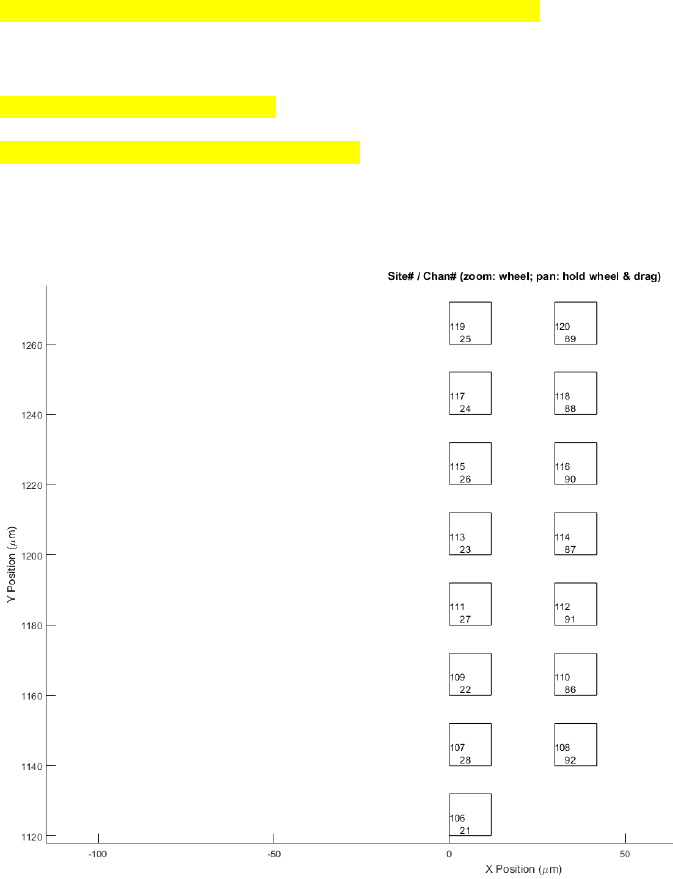
Step 2. Show the probe layout
Syntax:
>> jrc probe [myprobe.prb or myrecording.prm]
Example:
>> jrc probe sample.prb
>> jrc probe sample_sample.prm
Result:
Note:
1. To zoom, use a mouse wheel. To pan, hold down the wheel and move.
2. displays the probe configuration file (.prb) that is plotted above. Make necessary changes if a different channel
order is used. The above shows the IMEC Phase II probe configuration used in Janelia.
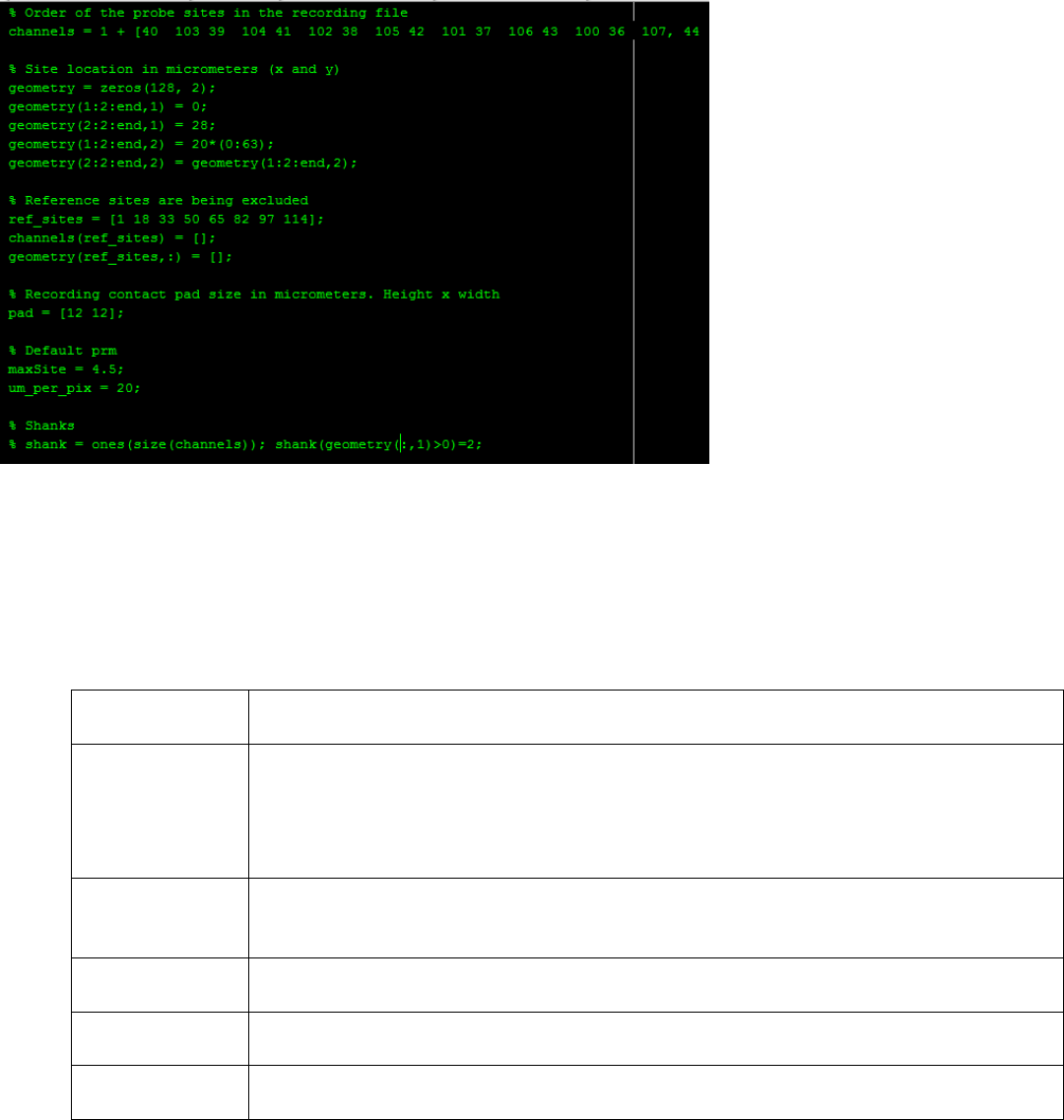
3. The probe configuration file (.prb) contains the following variables and is interpreted by MATLAB.
4. Write a command on a single line only. Do not use a Matlab line break “…”.
Variable
(case sensitive)
Description
channels:
[1, nSites]
A channel map to translate from the site number to the recorded order. Each number
corresponds to the order of appearance in the binary file. The sites are linearly arranged
from the bottom to top, left to right. For example, the first element in the “channels”
array corresponds to the bottom left site, the second element corresponds to the bottom
right sites, the third element corresponds to the second bottom left site.
geometry:
[nSites, 2]
Location of each site in micrometers. The first column corresponds to the width
dimension and the second column corresponds to the depth dimension (parallel to the
probe shank).
pad
[1, 2]
Dimensions of the recording pad (height by width in micrometers).
ref_sites
(optional)
This indicates reference or disconnected sites to eliminate.
shank
(optional)
Shank number for each site #. For example shank=[1,1,1,1,2,2,2,2] will assign site 1-4 to
shank 1 and site 5-8 to shank 2.
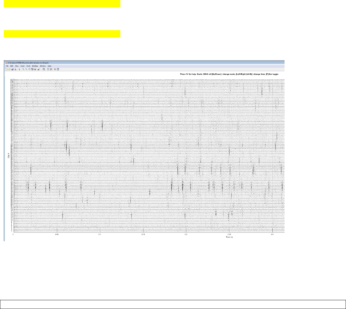
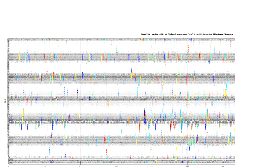
Step 3. Plot traces
Syntax:
>> jrc traces [myrecording.prm]
Example:
>> jrc traces sample_sample.prm
Result:
Note: Change the amplitude scale using up/down keys and change time using left/right keys. Zoom using mouse wheel
and pan by holding down the wheel and drag. Switch between spike-band vs. full-band by pressing ‘F’ key. Press ‘H’ for
further help.
You can change the time range to display (default 0.5 s) by editing a line in a .prm file:
tlim = [0, .5];

Step 4. Excluding bad sites manually
You can manually identify bad sites and exclude them from analysis by editing a .prm file. The below line excludes bad
sites #1 and #5:
viSiteZero = [1 5];
If there is no bad site to exclude then set:
viSiteZero = [];
If you wish to auto-detect the bad sites using a confidence threshold of 4.5, then edit as below:
fCheckSites = 1;
viSiteZero = [];
maxLfpSdZ = 4.5;
Step 5. Detect spikes
Syntax:
>> jrc detect sample_sample.prm
Output:
13:39:57 [W] Loading .\sample.bin
Loading .\sample.bin...took 5.3s (1950.0 MB, 365.5 MB/s)
Sites 1, 5, set to zero.
Filtering... Subtracting common ref...took 8.1s
took 22.6s
Exported to .\sample.spk (took 38.4s)
assigned 'mrWav' to workspace
13:40:36 [W] Wrote to .\sample.spk
Detecting spikes...
Detecting 1131433 spikes took 14.8s.
Merging spikes...
Merging 338263 spikes took 3.7s
assigned 'Sevt' to workspace
Saving to .\sample_evt.mat... took 9.1s
13:41:04 [W] Wrote to .\sample_evt.mat
assigned 'Sevt' to workspace
assigned 'mrWav' to workspace
Logged to .\sample.log
Note: Confirm the spike detection by plotting the traces:
>> jrc traces sample_sample.prm
Output:
Note: The traces from excluded sites are not shown (white gaps).
Step 6. Cluster automatically
Command:
>> jrc sort sample_sample.prm
Output:
14:00:02 [W] Loading .\sample.bin
Loaded .\sample_evt.mat from cache
Calculating rho...took 0.5s
Calculating delta...took 1.1 s
clustering took 2.2 s
.\sample.spk loaded from workspace cache
Computing cluster mean waveform... took 8.0s.
Saving to .\sample_clu.mat... took 1.1s
14:00:16 [W] wrote to .\sample_clu.mat
Recording file
Recording file .\sample.bin
Recording Duration 300.0s
#Sites 120
Event
#Spikes 338263
Feature amp
#Sites/event 6
Cluster
#Clusters 325
min. spk/clu 50
Cluster run-time 2.2s
assigned 'Sevt' to workspace
assigned 'Sclu' to workspace
assigned 'mrWav' to workspace
Logged to .\sample.log
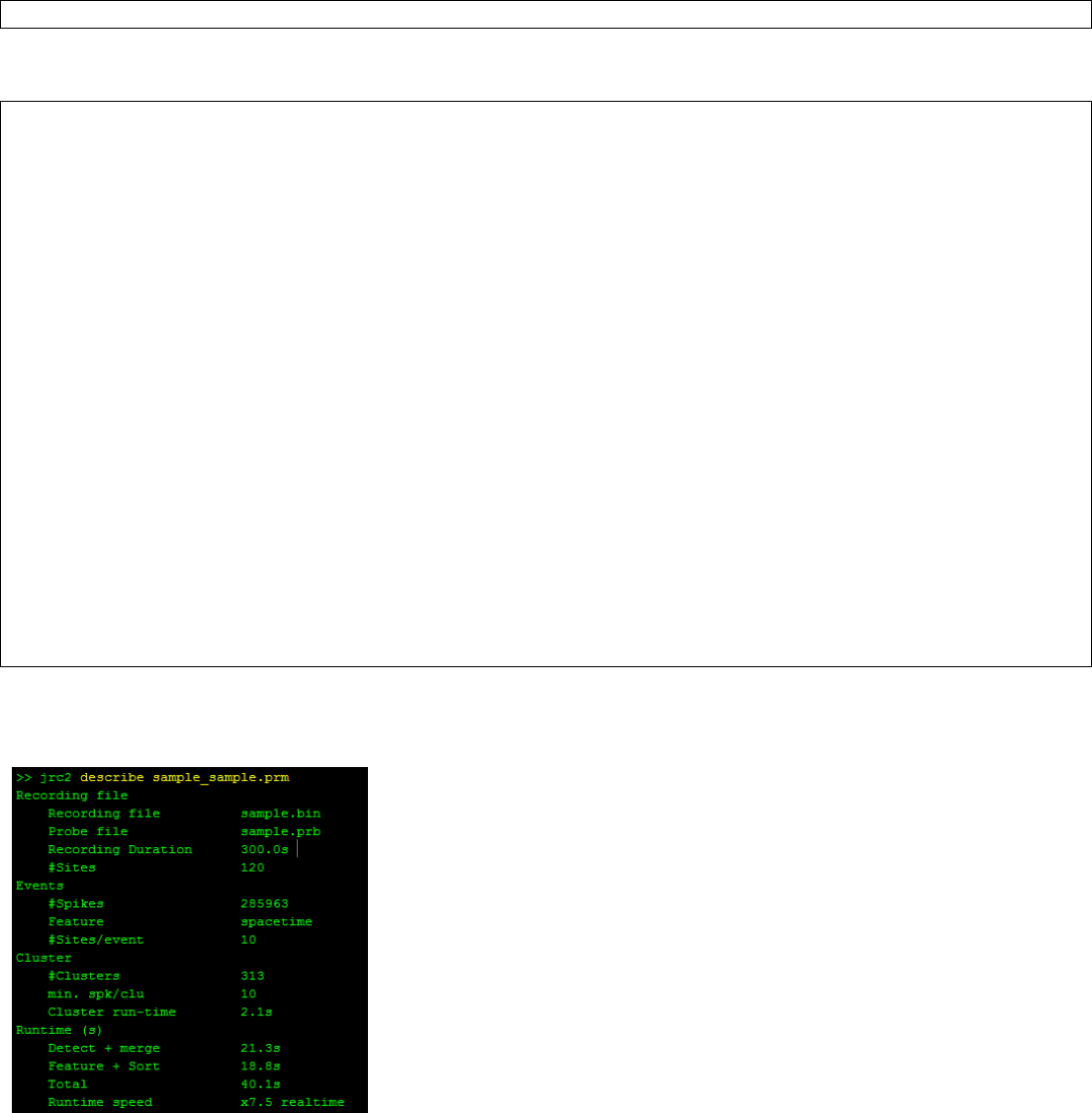
Note: Run “jrc describe sample_sample.prm” to display summary information
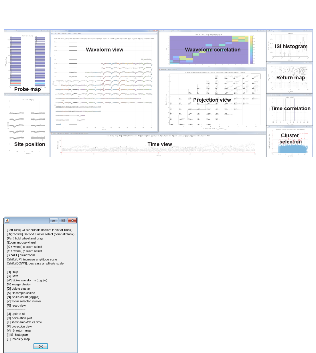
Step 7. Manual curation
Command:
>> jrc manual sample_sample.prm
Output:
Waveform view (Interactive):
Select a cluster by clicking with a left click. Click between traces and do not directly click on the traces. The selected
cluster is shown in black. Zoom in/out using a mouse wheel and pan by pressing down the wheel and drag.
Change scale by pressing Up/Down keys. Press ‘H’ to display help.
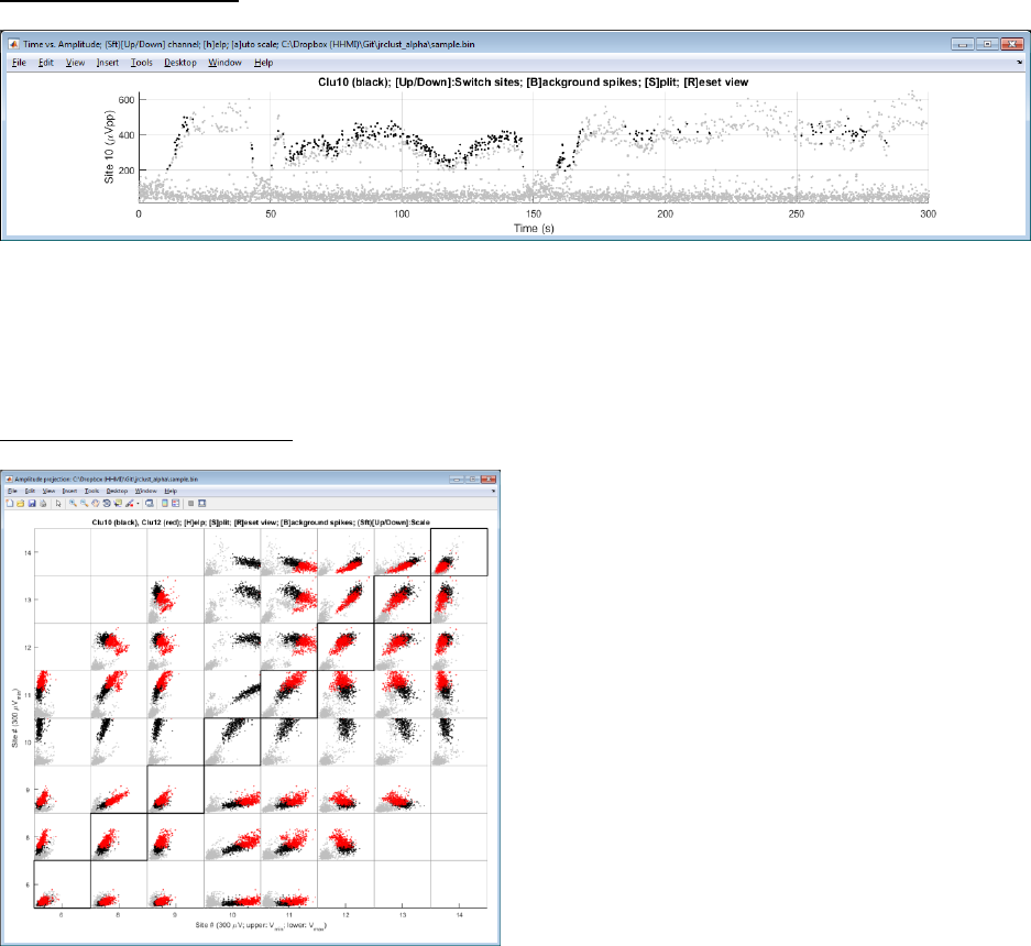
Time view (Interactive):
This view allows a check for probe drift over time. Press Up/Down arrows to switch sites.
Note: You can split a cluster by pressing ‘S’ and draw a polygon. Splitting is enabled when only one cluster is selected.
Press ‘B’ to show or hide the background spikes shown in gray. Press ‘M’ to merge two clusters.
Projection view (Interactive):
Press ‘S’ to split a cluster by drawing a polygon. Splitting is enabled when only one cluster is selected. Press ‘B’ to show
or hide the background spikes (gray). Press ‘M’ to merge two clusters.
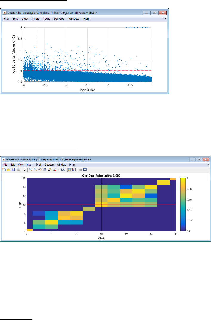
Cluster confidence view:
If over-split, increase “delta1_cut” value in .prm file (default 0.5). If recording is too noisy, increase “rho_cut” value
(default -3). Close and re-open the manual view by running “jrc manual myparam.prm”.
Waveform correlation view:
Diagonal entries show self-similarity. Low score indicates you need to split (press ‘S’ in the projection view). Off-diagonal
entries show between-cluster similarities. High score indicates you need to merge (press ‘m’ in the waveform view).
You can navigate using mouse (wheel to zoom, drag while pressing the wheel). If clusters appear over-split, increase the
“maxWavCor” value (default 0.975) in the .prm file.
Probe view:
This displays the peak-to-peak amplitude of the averaged cluster waveform in each sites on the probe.
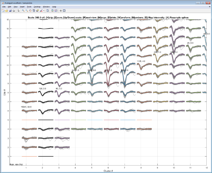
Step 8. Delete a noisy cluster
Select a cluster with a left click and hit ‘delete’ key.
The selected cluster waveform is shown in black.
Note: You must click the white space between lines. Nothing will happen when you click on the waveform lines. You can
hide the spike waveforms by pressing ‘W’ to only display the averaged waveforms.
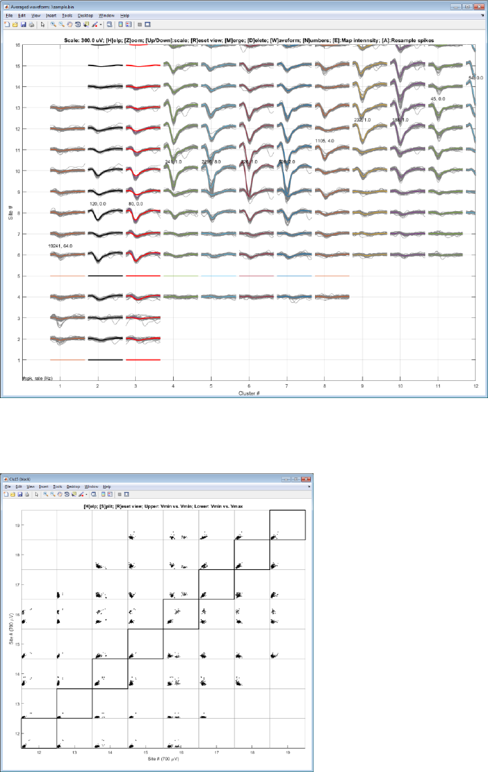
Step 8. Merge two clusters
Select a cluster with a left-click and a second cluster with a right-click and hit ‘M’ key. Mean waveforms of the black
cluster is copied to the red cluster for comparison.
Step 9. Split a cluster
Select a projection view and press ‘s’ to draw a polygon. Zoom in.
Draw a polygon
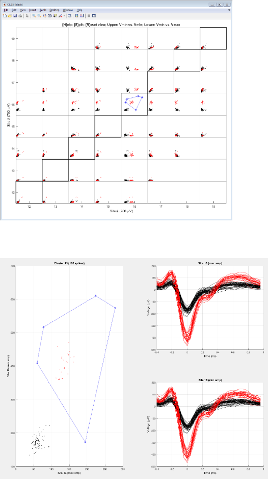
Edit and Confirm
*Note: Press ‘B’ to toggle all the background spikes.
*Note: Press ‘S’ in the waveform view to save results.
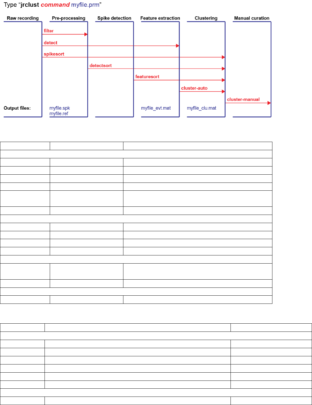
B. Command listing
Syntax: “jrc command input”
Command
Input
Output / behavior
General
help
Display help
probe
.prm or .prb file
Plot probe layout
traces
.prm file
Plot raw traces
detect
.prm file
Perform spike detection and feature extraction
exportcsv
.prm file
Spike timing, cluster number and max. site locations
are saved
describe
.prm file
Displays summary information about the analysis
Clustering
cluster
.prm file
Automatically cluster
manual
.prm file
Manual curation
spikesort
.prm file
Redo filtering, detection and sort
detectsort
.prm file
Redo spike detection to sort
Raster
maketrial
.prm file
Generate time alignment marker from a TTL channel
Output: “_trial.mat”
raster
.prm and _trial.mat
Plot rastergram and PSTH
Advanced
cluster-verify
.prm file and _gt.mat
Compare against ground truth file
C. File format
Extension
Content
Format
Input files
.prm
Parameter file
Plain text
.prb
Probe file
Plain text
.bin or .dat
Raw recording file
Binary file (SpikeGL)
.meta
Meta file for the raw recording (SpikeGL)
Binary file
_gt.mat
Ground truth file
Matlab data file
_trial.mat
Trial time
Matlab data file
Output files
.spkwav
Filtered spike waveforms from a subset of channels
Binary file (16-bit integer)

.spkraw
Raw spike waveforms from a subset of channels
Binary file (16-bit integer)
_jrc.mat
Spike timing, location and cluster numbers. Cluster-specific
information is stored in “S_clu” struct.
Matlab data file
_log.mat
Log file for manual operations
Matlab data file
.log
Program log file
Plan text
.csv
Spike time, cluster number, max site
Comma separated file
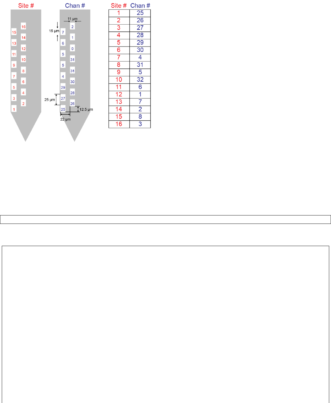
C1. Create a probe file
Probe file (.prb) describes channel ordering and site locations.
Site numbers are assigned from the bottom to top of the probe, and left to right order. Channel numbers specify the
order of file storage. For example, site #1 which appears at the bottom of the probe is stored in the 25th column of the
file. Note that channel numbers start from 1, not from zero.
Create a new probe file and type the information below:
Command:
>> edit example.prb
Content of example.prb:
% Order of the probe sites in the recording file
channels = [25 26 27 28 29 30 4 31 5 32 6 1 7 2 8 3];
% Site coordinate (x,y) in micrometers
geometry = [...
0, 0;
22, 12.5;
0, 25;
22, 37.5;
0, 50;
22, 62.5;
0, 75;
22, 87.5;
0, 100;
22, 112.5;
0, 125;
22, 137.5;
0, 150;
22, 162.5;
0, 175;
22, 187.5];
% Recording contact pad size in micrometers. Height x width

pad = [15 11];
% Single shank contains site 1-16
shank = ones(1,16);
Verify the probe layout by typing:
>> jrc probe example.prb
Note: Define a shank group by editing “shank”. The line below describes a two-shank probe containing 16 sites each:
shank = [repmat(1,1,16), repmat(2,1,16)];

D. Parameter settings (.prm file)
Name
Content
Values permitted
Recording file format
vcFile
File path to a raw recording or a directory
‘filepath.bin or .dat’
probe_file
File path to a probe settings
‘filepath.prb’
nChans
Number of channels recorded
Integer
vcDataType
Number precision recorded
‘int16’, ‘uint16’, ‘single’,
‘double’
uV_per_bit
Microvolts per bit
Positive real (set to 10 for
single or double precision)
Pre-processing
freqLim
Frequency range to filter in Hz
[low_cut, high_cut]
(default [500 3000])
freqLimNotch
Notch frequency range. You can specify
multiple ranges
{[low,high], [low,high], …}
Default {}
fElliptic
Use elliptic filter. Butterworth filter otherwise
0 or 1
vcCommonRef
Common reference method
‘mean’, ‘median’, ‘none’,
‘trimmean’, ‘holtzman’
viSiteZero
Bad recording sites to exclude
[array of integers] (default [])
fCheckSites
Flag for auto-detecting bad sites
0 or 1 (default 1)
maxLfpSdZ
Z-score cutoff for LFP-based bad site detection
Real number
fSaveSpk
Flag for saving filtered traces (.spk)
0 or 1 (default 1)
Spike detection/grouping
spkThresh_uV
Spike detection threshold in microvolts
Positive real ([]: auto)
spkThresh_max_uV
Maximum spike amplitude permitted
Positive real ([]: ignore)
qqFactor
Quian-Quiroga automatic threshold factor
Positive real (default 4.5)
qqSample
Quian-Quiroga median subsample
Positive integer (default 4)
spkRefrac_ms
Refractory period for spike in milliseconds
Positive real (default 1)
vcSpatialFilter
Denoise using neighboring sites
‘none’, ‘subtract’, ‘average’
maxSite
Max. distance to neighboring sites to consider
merging
Integer or half-integer
(default 2.5)
fSaveEvt
Flag for saving event file (_evt.mat)
0 or 1 (default 1)
Feature extraction
vcFet
Features to extract
‘vpp’, ‘amp’, ‘pca’, ‘slope’,
‘energy’
spkLim_ms
Spike time range in milliseconds
(0 at the negative peak)
[min, max] (default:
[-.40, .96])
nMinAmp_ms
Minimum amplitude search range in msec
Positive real (default 0)
nPcPerChan
Number of principal components per channel
Positive integer (default 3)
slopeLim_ms
Time range for slope calculation in msec
(0 at the negative peak)
[min, max] (default: [.1, .6])
Clustering
vcCluDist
Distance function
‘euclidean’, ‘citblock’,
‘correlation’
Default: euclidean
dc_factor
Controls merging or splitting. Higher means
more merging.
1 +/- .5
min_count
Minimum spikes allowed per cluster
Default:30
Set to [] to ignore

E. Output file format
“_jrc.mat” file
Contains S0 struct. You can obtain the current S0 struct by running “jrc export”. Run “jrc export varname” to export
specific variables within S0 struct.
Name
Content
Data format
General
viTime_spk
Spike timing in ADC sample unit
nSpikes x 1: int32
viSite_spk
File path to a probe settings
nSpikes x 1: int32
vrAmp_spk
Spike amplitude (local min. after filtering)
nSpikes x 1: int16
cviSpk_site
Cell of spike index (for _spk prefix) per site
Cell of vector of int32
vrThresh_site
Detection threshold per site
1 x nSites: single
dimm_spk
Dimensions for spike waveforms (stored in
_spkwav.bin file)
Vector of double
dimm_raw
Dimensions for the raw spike waveforms
(stored in _spkraw.bin file)
Vector of double
dimm_fet
Dimensions for the features (stored in
“_fet.bin” file)
Vector of double
dimm_fet_sites
Dimensions for the feature sites (stored in
“_fet_sites.bin” file)
Vector of double
runtime_detect
CPU time to run spike detection in sec
double
runtime_sort
CPU time to run spike sorting in sec
double
Cluster output: “S_clu” struct
nClu
Number of clusters
double
viClu
Cluster index for each spike (0 is a noise
cluster, negative numbers are deleted clusters)
nSpikes x 1: int32
viClu_auto
Automated output for cluster index
nSpikes x 1: int32
viSite_clu
Center site for each cluster
1 x nClu: double
vrPosX_clu
Center x position for each cluster
Vector of double
vrPosY_clu
Center y position for each cluster
Vector of double
csNote_clu
Manual annotation for each cluster
Cell string
trWav_spk_clu
Mean filtered waveforms for each cluster
(centered, nSites_spk=2 x maxSites + 1)
nSamples x nSites_spk x
nClusters: single
tmrWav_spk_clu
Mean filtered waveforms for each cluster (all
sites)
nSamples x nSites x nClu:
single
trWav_raw_clu
Mean raw waveforms for each cluster
(centered)
2xnSamples x nSites_spk x
nClu: single
tmrWav_raw_clu
Mean raw waveforms for each cluster (all
sites)
2xnSamples x nSites x nClu:
single
mrWavCor
Waveform correlation between clusters
nClu x nClu: double
vnSite_clu
Cluster quality: number of sites exceeding the
detection threshold
nClu x 1: double
vrVmin_clu
Cluster quality: negative peak voltage per
cluster
1 x nClu: single
vrSnr_clu
Signal to noise ration for each cluster
(SNR = Vpeak / Vrms)
nClu x 1: single
rho
DPCLUS density parameter
1 x nSpikes: single
delta
DPCLUS distance to the nearest neighbor
having a greater rho
1 x nSpikes: single
ordrho
DPCLUS index ordered by the density (rho)
1 x nSpikes: souble
dc
DPCLUS distance cut-off
1 x nSpikes: single

nneigh
DPCLUS nearest neighbor
1 x nSpikes: uint32
icl
DPCLUS
nClu x 1: double
P
Parameter struct used for automated
clustering
struct
Parameters: “P” struct (Copied from .prm file)
“_spkwav.bin” file
Binary file containing filtered waveforms per spike. Dimension is described in S0.dimm_spk
Format: nSamples x nSites_spk x nSpikes: real.
“_spkraw.bin” file
Binary file containing raw waveforms per spike. Dimension is described in S0.dimm_raw
Format: 2xnSamples x nSites_spk x nSpikes: real.
“_fet.bin” file
Binary file containing a feature matrix per spike.
Format: nFet x nSites_spk x nSpikes: real. Dimension is described in S0.dimm_fet
“_fet_sites.bin” file
Binary file containing site numbers for the feature matrix per spike.
Format: nFet x nSites_spk x nSpikes: real. Dimension is described in S0.dimm_fet_sites
“_log.mat” file
Stores the latest state of the program for each manual operation.
