Stocks For The Long Run 5/E Jeremy J. Siegel Definitive Guide To Financial Market Returns &
Jeremy%20J.%20Siegel-Stocks%20for%20the%20Long%20Run_%20%20The%20Definitive%20Guide%20to%20Financial%20Market%20Returns%20%26%20
User Manual:
Open the PDF directly: View PDF ![]() .
.
Page Count: 448 [warning: Documents this large are best viewed by clicking the View PDF Link!]
- Cover
- Title Page
- Copyright Page
- Contents
- Foreword
- Preface
- Acknowledgments
- Part I: Stock Returns: Past, Present, and Future
- Chapter 1 The Case for Equity: Historical Facts and Media Fiction
- Chapter 2 The Great Financial Crisis of 2008: Its Origins, Impact, and Legacy
- Chapter 3 The Markets, the Economy, and Government Policy in the Wake of the Crisis
- Chapter 4 The Entitlement Crisis: Will the Age Wave Drown the Stock Market?
- Part II: The Verdict of History
- Chapter 5 Stock and Bond Returns Since 1802
- Financial Market Data from 1802 to the Present
- Total Asset Returns
- The Long-Term Performance of Bonds
- Gold, the Dollar, and Inflation
- Total Real Returns
- Real Returns on Fixed-Income Assets
- The Continuing Decline in Fixed-Income Returns
- The Equity Premium
- Worldwide Equity and Bond Returns
- Conclusion: Stocks for the Long Run
- Appendix 1: Stocks from 1802 to 1870
- Chapter 6 Risk, Return, and Portfolio Allocation: Why Stocks Are Less Risky Than Bonds in the Long Run
- Chapter 7 Stock Indexes: Proxies for the Market
- Chapter 8 The S&P 500 Index: More Than a Half Century of U.S. Corporate History
- Chapter 9 The Impact of Taxes on Stock and Bond Returns: Stocks Have the Edge
- Chapter 10 Sources of Shareholder Value: Earnings and Dividends
- Chapter 11 Yardsticks to Value the Stock Market
- Chapter 12 Outperforming the Market: The Importance of Size, Dividend Yields, and Price/Earnings Ratios
- Stocks That Outperform the Market
- Small- and Large-Cap Stocks
- Valuation: “Value” Stocks Offer Higher Returns Than “Growth” Stocks
- Dividend Yields
- Price/Earnings Ratios
- Price/Book Ratios
- Combining Size and Valuation Criteria
- Initial Public Offerings: The Disappointing Overall Returns on New Small-Cap Growth Companies
- The Nature of Growth and Value Stocks
- Explanations of Size and Valuation Effects
- Conclusion
- Chapter 13 Global Investing
- Chapter 5 Stock and Bond Returns Since 1802
- Part III: How The Economic Environment Impacts Stocks
- Chapter 14 Gold, Monetary Policy, and inflation
- Money and Prices
- The Gold Standard
- The Establishment of the Federal Reserve
- The Fall of the Gold Standard
- Postdevaluation Monetary Policy
- Postgold Monetary Policy
- The Federal Reserve and Money Creation
- How the Fed’s Actions Affect Interest Rates
- Stock Prices and Central Bank Policy
- Stocks as Hedges Against Inflation
- Why Stocks Fail as a Short-Term Inflation Hedge
- Conclusion
- Chapter 15 Stocks and the Business Cycle
- Chapter 16 When World Events impact Financial Markets
- Chapter 17 Stocks, Bonds, and the Flow of Economic data
- Chapter 14 Gold, Monetary Policy, and inflation
- Part IV: Stock Fluctuations in The Short Run
- Chapter 18 Exchange-Traded Funds, Stock Index Futures, and Options
- Exchange-Traded Funds
- Stock Index Futures
- Basics of the Futures Markets
- Index Arbitrage
- Predicting the New York Open with Globex Trading
- Double and Triple Witching
- Margin and Leverage
- Tax Advantages of ETFS and Futures
- Where to Put Your Indexed Investments: ETFS, Futures, or Index Mutual Funds?
- Index Options
- The Importance of Indexed Products
- Chapter 19 Market Volatility
- The Stock Market Crash of October 1987
- The Causes of the October 1987 Crash
- Circuit Breakers
- Flash Crash—May 6, 2010
- The Nature of Market Volatility
- Historical Trends of Stock Volatility
- The Volatility Index
- The Distribution of Large Daily Changes
- The Economics of Market Volatility
- The Significance of Market Volatility
- Chapter 20 Technical Analysis and Investing with the Trend
- Chapter 21 Calendar Anomalies
- Chapter 22 Behavioral Finance and the Psychology of Investing
- Chapter 18 Exchange-Traded Funds, Stock Index Futures, and Options
- Part V: Building Wealth Through Stocks
- Chapter 23 Fund Performance, indexing, and Beating the Market
- The Performance of Equity Mutual Funds
- Finding Skilled Money Managers
- Reasons for Underperformance of Managed Money
- A Little Learning is a Dangerous Thing
- Profiting from Informed Trading
- How Costs Affect Returns
- The Increased Popularity of Passive Investing
- The Pitfalls of Capitalization-Weighted Indexing
- Fundamentally Weighted Versus Capitalization-Weighted Indexation
- The History of Fundamentally Weighted Indexation
- Conclusion
- Chapter 24 Structuring a Portfolio for Long-Term Growth
- Chapter 23 Fund Performance, indexing, and Beating the Market
- Notes
- Index
STOCKS
for the
LONG
RUN
This page intentionally left blank

FIFTH EDITION
STOCKS
for the
LONG
RUN
THE DEFINITIVE GUIDE TO FINANCIAL MARKET
RETURNS & LONG-TERM INVESTMENT STRATEGIES
JEREMY J. SIEGEL
Russell E. Palmer Professor of Finance
The Wharton School
University of Pennsylvania
New York Chicago San Francisco
Athens London Madrid Mexico City
Milan New Delhi Singapore Sydney Toronto
Copyright © 2014, 2008, 2002, 1998, 1994 by Jeremy J. Siegel. All rights reserved. Except as permited under the United States
Copyright Act of 1976, no part of this publication may be reproduced or distributed in any form or by any means, or stored in a
database or retrieval system, without the prior written permission of the publisher.
ISBN: 978-0-07-180052-5
MHID: 0-07-180052-2
The material in this eBook also appears in the print version of this title: ISBN: 978-0-07-180051-8,
MHID: 0-07-180051-4.
eBook conversion by codeMantra
Version 1.0
All trademarks are trademarks of their respective owners. Rather than put a trademark symbol after every occurrence of a
trademarked name, we use names in an editorial fashion only, and to the benet of the trademark owner, with no intention of infringe-
ment of the trademark. Where such designations appear in this book, they have been printed with initial caps.
McGraw-Hill Education eBooks are available at special quantity discounts to use as premiums and sales promotions or for use in
corporate training programs. To contact a representative, please visit the Contact Us page at www.mhprofessional.com.
This publication is designed to provide accurate and authoritative information in regard to the subject matter covered. It is sold
with the understanding that neither the author nor the publisher is engaged in rendering legal, accounting, futures/securities trading,
or other professional service. If legal advice or other expert assistance is required, the services of a competent professional person
should be sought.
—From a Declaration of Principles jointly adopted by a Committee
of the American Bar Association and a Committee of Publishers
TERMS OF USE
This is a copyrighted work and McGraw-Hill Education and its licensors reserve all rights in and to the work. Use of this work is
subject to these terms. Except as permitted under the Copyright Act of 1976 and the right to store and retrieve one copy of the work,
you may not decompile, disassemble, reverse engineer, reproduce, modify, create derivative works based upon, transmit, distribute,
disseminate, sell, publish or sublicense the work or any part of it without McGraw-Hill Education’s prior consent. You may use the
work for your own noncommercial and personal use; any other use of the work is strictly prohibited. Your right to use the work may
be terminated if you fail to comply with these terms.
THE WORK IS PROVIDED “AS IS.” McGRAW-HILL EDUCATION AND ITS LICENSORS MAKE NO GUARANTEES OR
WARRANTIES AS TO THE ACCURACY, ADEQUACY OR COMPLETENESS OF OR RESULTS TO BE OBTAINED FROM
USING THE WORK, INCLUDING ANY INFORMATION THAT CAN BE ACCESSED THROUGH THE WORK VIA
HYPERLINK OR OTHERWISE, AND EXPRESSLY DISCLAIM ANY WARRANTY, EXPRESS OR IMPLIED, INCLUDING
BUT NOT LIMITED TO IMPLIED WARRANTIES OF MERCHANTABILITY OR FITNESS FOR A PARTICULAR PURPOSE.
McGraw-Hill Education and its licensors do not warrant or guarantee that the functions contained in the work will meet your
requirements or that its operation will be uninterrupted or error free. Neither McGraw-Hill Education nor its licensors shall be liable
to you or anyone else for any inaccuracy, error or omission, regardless of cause, in the work or for any damages resulting therefrom.
McGraw-Hill Education has no responsibility for the content of any information accessed through the work. Under no circumstances
shall McGraw-Hill Education and/or its licensors be liable for any indirect, incidental, special, punitive, consequential or similar
damages that result from the use of or inability to use the work, even if any of them has been advised of the possibility of such
damages. This limitation of liability shall apply to any claim or cause whatsoever whether such claim or cause arises in contract,
tort or otherwise.

Foreword xvii
Preface xix
Acknowledgments xxiii
PART I
STOCK RETURNS: PAST, PRESENT, AND FUTURE
Chapter 1
The Case for Equity
Historical Facts and Media Fiction 3
“Everybody Ought to Be Rich” 3
Asset Returns Since 1802 5
Historical Perspectives on Stocks as Investments 7
The Influence of Smith’s Work 8
Common Stock Theory of Investment 8
The Market Peak 9
Irving Fisher’s “Permanently High Plateau” 9
A Radical Shift in Sentiment 10
The Postcrash View of Stock Returns 11
The Great Bull Market of 1982–2000 12
Warnings of Overvaluation 14
The Late Stage of the Great Bull Market, 1997–2000 15
The Top of the Market 16
The Tech Bubble Bursts 16
v
CONTENTS

Rumblings of the Financial Crisis 17
Beginning of the End for Lehman Brothers 18
Chapter 2
The Great Financial Crisis of 2008
Its Origins, Impact, and Legacy 21
The Week That Rocked World Markets 21
Could the Great Depression Happen Again? 22
The Cause of the Financial Crisis 23
The Great Moderation 23
Subprime Mortgages 24
The Crucial Rating Mistake 25
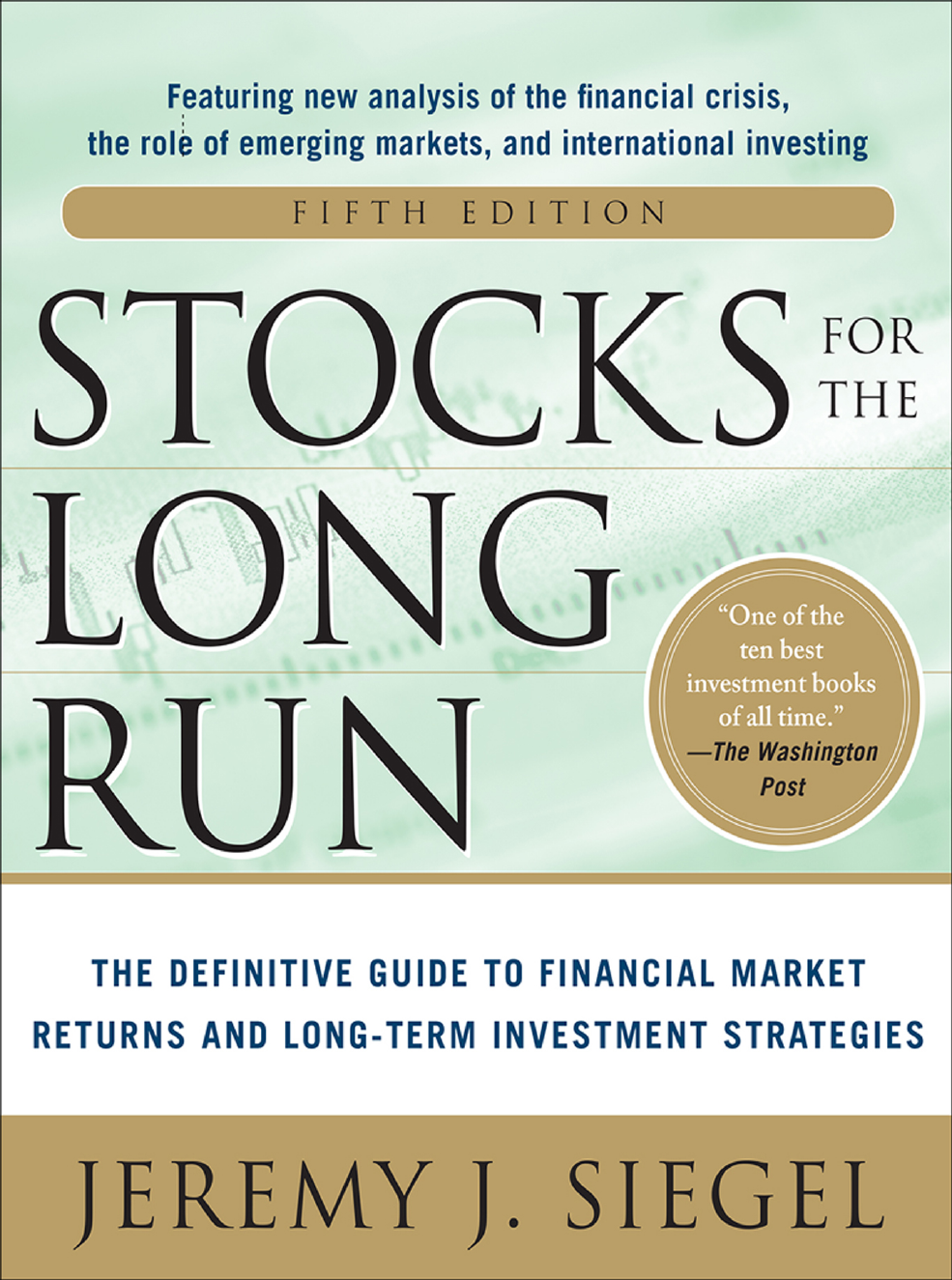
The Real Estate Bubble 28
Regulatory Failure 30
Overleverage by Financial Institutions in Risky Assets 31
The Role of the Federal Reserve in Mitigating the Crisis 32
The Lender of Last Resort Springs to Action 32
Should Lehman Brothers Have Been Saved? 34
Reflections on the Crisis 36
Chapter 3
The Markets, the Economy, and Government Policy
in the Wake of the Crisis 39
Avoiding Deflation 41
Reaction of the Financial Markets to the Financial Crisis 41
Stocks 41
Real Estate 45
Treasury Bond Markets 45
The LIBOR Market 46
Commodity Markets 47
Foreign Currency Markets 48
Impact of the Financial Crisis on Asset Returns and Correlations 48
Decreased Correlations 50
Legislative Fallout from the Financial Crisis 52
Concluding Comments 55
vi CONTENTS

Chapter 4
The Entitlement Crisis
Will the Age Wave Drown the Stock Market? 57
The Realities We Face 58
The Age Wave 58
Rising Life Expectancy 59
Falling Retirement Age 59
The Retirement Age Must Rise 60
World Demographics and the Age Wave 62
Fundamental Question 64
Emerging Economies Can Fill the Gap 68
Can Productivity Growth Keep Pace? 69
Conclusion 71
PART II
THE VERDICT OF HISTORY
Chapter 5
Stock and Bond Returns Since 1802 75
Financial Market Data from 1802 to the Present 75
Total Asset Returns 76
The Long-Term Performance of Bonds 78
Gold, the Dollar, and Inflation 79
Total Real Returns 81
Real Returns on Fixed-Income Assets 84
The Continuing Decline in Fixed-Income Returns 86
The Equity Premium 87
Worldwide Equity and Bond Returns 88
Conclusion: Stocks for the Long Run 90
Appendix 1: Stocks from 1802 to 1870 91
Chapter 6
Risk, Return, and Portfolio Allocation
Why Stocks Are Less Risky Than Bonds in the Long Run 93
Measuring Risk and Return 93
CONTENTS vii

Risk and Holding Period 94
Standard Measures of Risk 97
Varying Correlation Between Stock and Bond Returns 99
Efficient Frontiers 101
Conclusion 102
Chapter 7
Stock Indexes
Proxies for the Market 105
Market Averages 105
The Dow Jones Averages 106
Computation of the Dow Index 108
Long-Term Trends in the Dow Jones Industrial Average 108
Beware the Use of Trendlines to Predict Future Returns 109
Value-Weighted Indexes 110
Standard & Poor’s Index 110
Nasdaq Index 111
Other Stock Indexes: The Center for Research in Security Prices 113
Return Biases in Stock Indexes 113
Appendix: What Happened to the Original 12 Dow Industrials? 115
Chapter 8
The S&P 500 Index
More Than a Half Century of U.S. Corporate History 119
Sector Rotation in the S&P 500 Index 120
Top-Performing Firms 126
How Bad News for the Firm Becomes Good News for Investors 128
Top-Performing Survivor Firms 128
Other Firms That Turned Golden 129
Outperformance of Original S&P 500 Firms 130
Conclusion 131
Chapter 9
The Impact of Taxes on Stock and Bond Returns
Stocks Have the Edge 133
Historical Taxes on Income and Capital Gains 133
viii CONTENTS

Before- and After-Tax Rates of Return 135
The Benefits of Deferring Capital Gains Taxes 135
Inflation and the Capital Gains Tax 137
Increasingly Favorable Tax Factors for Equities 139
Stocks or Bonds in Tax-Deferred Accounts? 140
Conclusion 141
Appendix: History of the Tax Code 141
Chapter 10
Sources of Shareholder Value
Earnings and Dividends 143
Discounted Cash Flows 143
Sources of Shareholder Value 144
Historical Data on Dividends and Earnings Growth 145
The Gordon Dividend Growth Model of Stock Valuation 147
Discount Dividends, Not Earnings 149
Earnings Concepts 149
Earnings Reporting Methods 150
Operating Earnings and NIPA Profits 152
The Quarterly Earnings Report 154
Conclusion 155
Chapter 11
Yardsticks to Value the Stock Market 157
An Evil Omen Returns 157
Historical Yardsticks for Valuing the Market 159
Price/Earnings Ratio and the Earnings Yield 159
The Aggregation Bias 161
The Earnings Yield 161
The CAPE Ratio 162
The Fed Model, Earnings Yields, and Bond Yields 164
Corporate Profits and GDP 166
Book Value, Market Value, and Tobin’s Q 166
Profit Margins 168
Factors That May Raise Future Valuation Ratios 169
A Fall in Transaction Costs 170
Lower Real Returns on Fixed-Income Assets 170
CONTENTS ix

The Equity Risk Premium 171
Conclusion 172
Chapter 12
Outperforming the Market
The Importance of Size, Dividend Yields,
and Price/Earnings Ratios 173
Stocks That Outperform the Market 173
What Determines a Stock’s Return? 175
Small- and Large-Cap Stocks 176
Trends in Small-Cap Stock Returns 177
Valuation: “Value” Stocks Offer Higher Returns Than “Growth” Stocks 179
Dividend Yields 179
Other Dividend-Yield Strategies 181
Price/Earnings Ratios 183
Price/Book Ratios 185
Combining Size and Valuation Criteria 186
Initial Public Offerings: The Disappointing Overall
Returns on New Small-Cap Growth Companies 188
The Nature of Growth and Value Stocks 190
Explanations of Size and Valuation Effects 191
The Noisy Market Hypothesis 191
Liquidity Investing 192
Conclusion 193
Chapter 13
Global Investing 195
Foreign Investing and Economic Growth 196
Diversification in World Markets 198
International Stock Returns 199
The Japanese Market Bubble 199
Stock Risks 201
Should You Hedge Foreign Exchange Risk? 201
Diversification: Sector or Country? 202
Sector Allocation Around the World 203
Private and Public Capital 206
Conclusion 206
x CONTENTS

PART III
HOW THE ECONOMIC ENVIRONMENT IMPACTS STOCKS
Chapter 14
Gold, Monetary Policy, and Inflation 209
Money and Prices 210
The Gold Standard 213
The Establishment of the Federal Reserve 213
The Fall of the Gold Standard 214
Postdevaluation Monetary Policy 215
Postgold Monetary Policy 216
The Federal Reserve and Money Creation 217
How the Fed’s Actions Affect Interest Rates 218
Stock Prices and Central Bank Policy 218
Stocks as Hedges Against Inflation 220
Why Stocks Fail as a Short-Term Inflation Hedge 223
Higher Interest Rates 223
Nonneutral Inflation: Supply-Side Effects 223
Taxes on Corporate Earnings 224
Inflationary Biases in Interest Costs 225
Capital Gains Taxes 226
Conclusion 226
Chapter 15
Stocks and the Business Cycle 229
Who Calls the Business Cycle? 230
Stock Returns Around Business Cycle Turning Points 233
Gains Through Timing the Business Cycle 235
How Hard Is It to Predict the Business Cycle? 236
Conclusion 238
Chapter 16
When World Events Impact Financial Markets 241
What Moves the Market? 243
Uncertainty and the Market 246
Democrats and Republicans 247
CONTENTS xi

Stocks and War 250
Markets During the World Wars 252
Post-1945 Conflicts 253
Conclusion 255
Chapter 17
Stocks, Bonds, and the Flow of Economic Data 257
Economic Data and the Market 258
Principles of Market Reaction 258
Information Content of Data Releases 259
Economic Growth and Stock Prices 260
The Employment Report 261
The Cycle of Announcements 262
Inflation Reports 264
Core Inflation 265
Employment Costs 266
Impact on Financial Markets 266
Central Bank Policy 267
Conclusion 268
PART IV
STOCK FLUCTUATIONS IN THE SHORT RUN
Chapter 18
Exchange-Traded Funds, Stock Index Futures, and Options 271
Exchange-Traded Funds 272
Stock Index Futures 273
Basics of the Futures Markets 276
Index Arbitrage 278
Predicting the New York Open with Globex Trading 279
Double and Triple Witching 280
Margin and Leverage 281
Tax Advantages of ETFS and Futures 282
Where to Put Your Indexed Investments: ETFS, Futures, or Index Mutual
Funds? 282
Index Options 284
xii CONTENTS

Buying Index Options 286
Selling Index Options 286
The Importance of Indexed Products 287
Chapter 19
Market Volatility 289
The Stock Market Crash of October 1987 291
The Causes of the October 1987 Crash 293
Exchange Rate Policies 293
The Futures Market 294
Circuit Breakers 296
Flash Crash—May 6, 2010 297
The Nature of Market Volatility 300
Historical Trends of Stock Volatility 300
The Volatility Index 303
The Distribution of Large Daily Changes 305
The Economics of Market Volatility 307
The Significance of Market Volatility 308
Chapter 20
Technical Analysis and Investing with the Trend 311
The Nature of Technical Analysis 311
Charles Dow, Technical Analyst 312
The Randomness of Stock Prices 312
Simulations of Random Stock Prices 314
Trending Markets and Price Reversals 314
Moving Averages 316
Testing the Dow Jones Moving-Average Strategy 317
Back-Testing the 200-Day Moving Average 318
Avoiding Major Bear Markets 320
Distribution of Gains and Losses 321
Momentum Investing 322
Conclusion 323
Chapter 21
Calendar Anomalies 325
Seasonal Anomalies 326
CONTENTS xiii

The January Effect 326
Causes of the January Effect 328
The January Effect Weakened in Recent Years 329
Large Stock Monthly Returns 330
The September Effect 330
Other Seasonal Returns 334
Day-of-the-Week Effects 336
What’s an Investor to Do? 337
Chapter 22
Behavioral Finance and the Psychology of Investing 339
The Technology Bubble, 1999 to 2001 340
Behavioral Finance 342
Fads, Social Dynamics, and Stock Bubbles 343
Excessive Trading, Overconfidence, and the Representative Bias 345
Prospect Theory, Loss Aversion, and the Decision
to Hold on to Losing Trades 347
Rules for Avoiding Behavioral Traps 350
Myopic Loss Aversion, Portfolio Monitoring,
and the Equity Risk Premium 350
Contrarian Investing and Investor Sentiment:
Strategies to Enhance Portfolio Returns 352
Out-of-Favor Stocks and the Dow 10 Strategy 354
PART V
BUILDING WEALTH THROUGH STOCKS
Chapter 23
Fund Performance, Indexing, and Beating the Market 357
The Performance of Equity Mutual Funds 358
Finding Skilled Money Managers 363
Persistence of Superior Returns 364
Reasons for Underperformance of Managed Money 365
A Little Learning Is a Dangerous Thing 365
Profiting from Informed Trading 366
How Costs Affect Returns 367
xiv CONTENTS

The Increased Popularity of Passive Investing 367
The Pitfalls of Capitalization-Weighted Indexing 368
Fundamentally Weighted Versus Capitalization-Weighted Indexation 369
The History of Fundamentally Weighted Indexation 371
Conclusion 372
Chapter 24
Structuring a Portfolio for Long-Term Growth 373
Practical Aspects of Investing 373
Guides to Successful Investing 374
Implementing the Plan and the Role of an Investment Advisor 377
Concluding Comment 378
Notes 379
Index 405
CONTENTS
xv
This page intentionally left blank

In July 1997 I called Peter Bernstein and said I was going to be in New
York and would love to lunch with him. I had an ulterior motive. I
greatly enjoyed his book Capital Ideas: The Improbable Origins of Modern
Wall Street and the Journal of Portfolio Management, which he founded
and edited. I hoped there might be a slim chance he would consent to
write the preface to the second edition of Stocks for the Long Run.
His secretary set up a date at one of his favorite restaurants, Circus
on the Upper East Side. He arrived with his wife Barbara and a copy of
the first edition of my book tucked under his arm. As he approached, he
asked if I would sign it. I said “of course” and responded that I would be
honored if he wrote a foreword to the second edition. He smiled; “Of
course!” he exclaimed. The next hour was filled with a most fascinating
conversation about publishing, academic and professional trends in
finance, and even what we liked best about Philly and New York.
I thought back to our lunch when I learned, in June 2009, that he had
passed away at the age of 90. In the 12 years since our first meeting, Peter
had been more productive than ever, writing three more books, including
his most popular, The Remarkable Story of Risk. Despite the incredible pace
he maintained, he always found time to update the preface of my book
through the next two editions. As I read through his words in the fourth
edition, I found that his insights into the frustrations and rewards of
being a long-term investor are as relevant today as they were when he
first penned them nearly two decades ago. I can think of no better way to
honor Peter than to repeat his wisdom here.
Some people find the process of assembling data to be a deadly bore.
Others view it as a challenge. Jeremy Siegel has turned it into an art form.
You can only admire the scope, lucidity, and sheer delight with which
Professor Siegel serves up the evidence to support his case for investing in
stocks for the long run.
But this book is far more than its title suggests. You will learn a lot of
economic theory along the way, garnished with a fascinating history of
both the capital markets and the U.S. economy. By using history to maxi-
mum effect, Professor Siegel gives the numbers a life and meaning they
would never enjoy in a less compelling setting. Moreover, he boldly does
battle with all historical episodes that could contradict his thesis and
emerges victorious—and this includes the crazy years of the 1990s.
xvii
FOREWORD

With this fourth edition, Jeremy Siegel has continued on his merry
and remarkable way in producing works of great value about how best to
invest in the stock market. His additions on behavioral finance, globaliza-
tion, and exchange-traded funds have enriched the original material with
fresh insights into important issues. Revisions throughout the book have
added valuable factual material and powerful new arguments to make his
case for stocks for the long run. Whether you are a beginner at investing or
an old pro, you will learn a lot from reading this book.
Jeremy Siegel is never shy, and his arguments in this new edition
demonstrate he is as bold as ever. The most interesting feature of the whole
book is his twin conclusions of good news and bad news. First, today’s
globalized world warrants higher average price/earnings ratios than in the
past. But higher P/Es are a mixed blessing, for they would mean average
returns in the future are going to be lower than they were in the past.
I am not going to take issue with the forecast embodied in this view-
point. But similar cases could have been made in other environments of
the past, tragic environments as well as happy ones. One of the great les-
sons of history proclaims that no economic environment survives the long
run. We have no sense at all of what kinds of problems or victories lie in
the distant future, say, 20 years or more from now, and what influence
those forces will have on appropriate price/earnings ratios.
That’s all right. Professor Siegel’s most important observation about
the future goes beyond his controversial forecast of higher average P/Es
and lower realized returns. “Although these returns may be diminished
from the past,” he writes, “there is overwhelming reason to believe stocks
will remain the best investment for all those seeking steady, long-term
gains.
“[O]verwhelming reason” is an understatement. The risk premium
earned by equities over the long run must remain intact if the system is
going to survive. In the capitalist system, bonds cannot and should not out-
perform equities over the long run. Bonds are contracts enforceable in
courts of law. Equities promise their owners nothing—stocks are risky
investments, involving a high degree of faith in the future. Thus, equities
are not inherently “better” than bonds, but we demand a higher return
from equities to compensate for their greater risk. If the long-run expected
return on bonds were to be higher than the long-run expected return on
stocks, assets would be priced so that risk would earn no reward. That is an
unsustainable condition. Stocks must remain “the best investment for all
those seeking steady, long- term gains” or our system will come to an end,
and with a bang, not a whimper.
—Peter Bernstein
xviii FOREWORD

The fourth edition of Stocks for the Long Run was written in 2007. During
the last several years, as many of my colleagues my age had slowed the
pace of their research, I was often asked why I was working so hard on yet
another edition of this book. With a serious face I responded, “I believe
that a few events of significance have occurred over the past six years.”
A few events indeed! The years 2008 and 2009 witnessed the deep-
est economic recession and market collapse since the Great Depression
of the 1930s. The disruptions were so extensive that I put off writing this
edition until I gained better perspective on the causes and consequences
of the financial crisis from which we still have not completely recovered.
As a result, this edition is more thoroughly rewritten than any of
the previous editions were. This is not because the conclusions of the
earlier editions needed to be changed. Indeed the rise of U.S. equity mar-
kets to new all-time highs in 2013 only reinforces the central tenet of this
book: that stocks are indeed the best long-term investment for those who
learn to weather their short-term volatility. In fact, the long-term real
return on a diversified portfolio of common stocks has remained virtu-
ally identical to the 6.7 percent reported in the first edition of Stocks for
the Long Run, which examined returns through 1992.
CONFRONTING THE FINANCIAL CRISIS
Because of the severe impact of the crisis, I felt that what transpired
over the last several years had to be addressed front and center in this
edition. As a result I added two chapters that described the causes and
consequences of the financial meltdown. Chapter 1 now previews the
major conclusions of my research on stocks and bonds and traces how
investors, money managers, and academics regarded stocks over the
past century.
Chapter 2 describes the financial crisis, laying blame where blame
is due on the CEOs of the giant investment banks, the regulators, and
Congress. I lay out the series of fatal missteps that led Standard and
Poor’s, the world’s largest rating agency, to give its coveted AAA rating
to subprime mortgages, foolishly declaring them as safe as U.S. Treasury
bonds.
xix
PREFACE

Chapter 3 analyzes the extraordinary impact of the financial crisis
on the financial markets: the unprecedented surge of the “libor spread”
that measured cost of capital to the banks, the collapse of stock prices
that wiped out two-thirds of their value, and, for the time since the dark
days of the 1930s, Treasury bill yields falling to zero and even below.
Most economists believed that our system of deposit insurance,
margin requirements, and financial regulations rendered the above
events virtually impossible. The confluence of forces that led to the crisis
were remarkably similar to what happened following the 1929 stock
market crash, with mortgage-back securities replacing equities as the
main culprit.
Although the Fed failed miserably at predicting the crisis,
Chairman Ben Bernanke took unprecedented measures to keep financial
markets open by flooding the financial markets with liquidity and guar-
anteeing trillions of dollars of loans and short-term deposits. These
actions ballooned the Fed’s balance sheet to nearly $4 trillion, 5 times its
precrisis level, and raised many questions about how the Fed would
unwind this unprecedented stimulus.
The crisis also changed the correlation between asset classes. World
equity markets became much more correlated, reducing the diversifying
gains from global investing, while U.S. Treasury bonds and the dollar
became “safe haven” assets, spurring unprecedented demand for feder-
ally guaranteed debt. All commodities, including gold, suffered during
the worst stages of the economic downturn, but precious metals
rebounded on fear that the central bank’s expansionary policies would
generate high inflation.
Chapter 4 addresses longer-run issues impacting our economic well-
being. The economic downturn saw the U.S. budget deficit soar to $1.3
trillion, the highest level relative to GDP since World War II. The slow-
down in productivity growth generated fears that increase in living stan-
dards will slow markedly or even grind to a halt. This raises the question
of whether our children will be the first generation whose standard of liv-
ing will fall below that of their parents.
This chapter updates and extends the results of earlier editions by
using new data provided by the U.N. Population Commission and pro-
ductivity forecasts provided by the World Bank and the IMF. I now cal-
culate the distribution of world output of the major countries and
regions of the world to the end of the twenty-first century. This analysis
strongly suggests that although the developed world must increase the
age at which social security and medical benefits are offered by the gov-
xx PREFACE

ernment, such increases will be moderate if productivity growth in the
emerging economies remains strong.
OTHER NEW MATERIAL IN THE FIFTH EDITION
Although the financial crisis and its aftermath are front and center in this
fifth edition, I have made other significant changes as well. Not only
have all the charts and tables been updated through 2012, but the chap-
ter on the valuation of equities has been expanded to analyze such
important new forecasting models such as the CAPE ratio and the sig-
nificance of profit margins as a determinant of future equity returns.
Chapter 19, “Market Volatility,” analyzes the “Flash Crash” of
May 2010 and documents how the volatility associated with the finan-
cial crisis compares with the banking crisis of the 1930s. Chapter 20
shows that, once again, following a simple technical rule such as the
200-day moving average would have avoided the worst part of the
recent bear market.
This edition also addresses whether the well-known calendar anom-
alies, such as the “January effect, the “small stock effect,” and the
“September effect,” have survived over the two decades since they were
described in the first edition of this book. I also include for the first time a
description of “liquidity investing” and explain how it might supplement
the “size” and “value” effects that have been found by researchers to be
important determinants of individual stocks’ return.
CONCLUDING REMARKS
I am both honored and flattered by the tremendous reception that Stocks
for the Long Run has received. Since the publication of the first edition
nearly 20 years ago, I have given hundreds of lectures on the markets
and the economy around the world. I have listened closely to the ques-
tions that audiences pose, and I have contemplated the many letters,
phone calls, and e-mails from readers.
To be sure, there have been some extraordinary events in the capi-
tal markets in recent years. Even those who still believed in the long-
term superiority of equities were put to severe test during the financial
crisis. In 1937 John Maynard Keynes stated in The General Theory of
Employment, Interest and Money, “Investment based on genuine long-
term expectation is so difficult today as to be scarcely practicable.” It is
no easier 75 years later.
PREFACE xxi

But those who have persisted with equities have always been
rewarded. No one has made money in the long run from betting against
stocks or the future growth of our economy. It is the hope that this latest
edition will fortify those who will inevitably waver when pessimism
once again grips economists and investors. History convincingly
demonstrates that stocks have been and will remain the best investment
for all those seeking long-term gains.
Jeremy J. Siegel
November 2013
xxii
PREFACE

It is never possible to list all the individuals and organizations that have
praised Stocks for the Long Run and encouraged me to update and
expand past editions. Many who provided me with data for the first four
editions of Stocks for the Long Run willingly contributed their data again
for this fifth edition. David Bianco, Chief U.S. Equity Strategist at
Deutsche Bank, whose historical work on S&P 500 earnings and profit
margins was invaluable for my chapter on stock market valuation, and
Walter Lenhard, senior investment strategist at Vanguard, once again
obtained historical data on mutual fund performance for Chapter 23. My
new Wharton colleague, Jeremy Tobacman, helped me update the mate-
rial on behavioral finance.
This edition would not have been possible without the hard work
of Shaun Smith, who also did the research and data analysis for the first
edition of Stocks for the Long Run in the early 1990s. Jeremy Schwartz,
who was my principal researcher for The Future for Investors, also pro-
vided invaluable assistance for this edition.
A special thanks goes to the thousands of financial advisors from
dozens of financial firms, such as Merrill Lynch, Morgan Stanley, UBS,
Wells Fargo, and many others who have provided me with critical feed-
back in seminars and open forums on earlier editions of Stocks for the
Long Run.
As before, the support of my family was critical in my being able to
write this edition. Now that my sons are grown and out of the house, it
was my wife Ellen who had to pay the whole price of the long hours
spent revising this book. I set a deadline of September 1 to get my mate-
rial to McGraw-Hill so we could go on a well-deserved cruise from
Venice down the Adriatic. Although I couldn’t promise her that this
would be the last edition, I know that completing this project has freed
some very welcome time for both of us.
xxiii
ACKNOWLEDGMENTS
This page intentionally left blank

PART
STOCK RETURNS
Past, Present, and Future
I
This page intentionally left blank

The Case for Equity
Historical Facts and Media Fiction
The “new-era” doctrine—that “good” stocks (or “blue chips”) were
sound investments regardless of how high the price paid for them—
was at the bottom only a means of rationalizing under the title of
“investment” the well-nigh universal capitulation to the gambling
fever.
—BENJAMIN GRAHAM AND DAVID DODD,
SECURITY ANALYSIS1
Investing in stocks has become a national hobby and a national obses-
sion. To update Marx, it is the religion of the masses.
—ROGER LOWENSTEIN, “A COMMON MARKET:
THE PUBLIC’SZEAL TO INVEST”2
Stocks for the Long Run by Siegel? Yeah, all it’s good for now is a
doorstop.
—INVESTOR CALLING INTO CNBC, MARCH, 20093
“EVERYBODY OUGHT TO BE RICH”
In the summer of 1929, a journalist named Samuel Crowther inter-
viewed John J. Raskob, a senior financial executive at General Motors,
about how the typical individual could build wealth by investing in
stocks. In August of that year, Crowther published Raskob’s ideas in a
3
1

Ladies’ Home Journal article with the audacious title “Everybody Ought
to Be Rich.”
In the interview, Raskob claimed that America was on the verge of
a tremendous industrial expansion. He maintained that by putting just
$15 per month into good common stocks, investors could expect their
wealth to grow steadily to $80,000 over the next 20 years. Such a
return—24 percent per year—was unprecedented, but the prospect of
effortlessly amassing a great fortune seemed plausible in the atmos-
phere of the 1920s bull market. Stocks excited investors, and millions put
their savings into the market, seeking quick profit.
On September 3, 1929, a few days after Raskob’s plan appeared, the
Dow Jones Industrial Average hit a historic high of 381.17. Seven weeks
later, stocks crashed. The next 34 months saw the most devastating
decline in share values in U.S. history.
On July 8, 1932, when the carnage was finally over, the Dow
Industrials stood at 41.22. The market value of the world’s greatest cor-
porations had declined an incredible 89 percent. Millions of investors’
life savings were wiped out, and thousands of investors who had bor-
rowed money to buy stocks were forced into bankruptcy. America was
mired in the deepest economic depression in its history.
Raskob’s advice was ridiculed and denounced for years to come. It
was said to represent the insanity of those who believed that the market
could rise forever and the foolishness of those who ignored the tremen-
dous risks in stocks. Senator Arthur Robinson of Indiana publicly held
Raskob responsible for the stock crash by urging common people to buy
stock at the market peak.4In 1992, 63 years later, Forbes magazine
warned investors of the overvaluation of stocks in its issue headlined
“Popular Delusions and the Madness of Crowds.” In a review of the his-
tory of market cycles, Forbes fingered Raskob as the “worst offender” of
those who viewed the stock market as a guaranteed engine of wealth.5
Conventional wisdom holds that Raskob’s foolhardy advice epito-
mizes the mania that periodically overruns Wall Street. But is that ver-
dict fair? The answer is decidedly no. Investing over time in stocks has
been a winning strategy whether one starts such an investment plan at a
market top or not. If you calculate the value of the portfolio of an
investor who followed Raskob’s advice in 1929, patiently putting $15 a
month into the market, you find that his accumulation exceeded that of
someone who placed the same money in Treasury bills after less than 4
years. By 1949 his stock portfolio would have accumulated almost
$9,000, a return of 7.86 percent, more than double the annual return in
bonds. After 30 years the portfolio would have grown to over $60,000,
4 PART I Stock Returns: Past, Present, and Future

with an annual return rising to 12.72 percent. Although these returns
were not as high as Raskob had projected, the total return of the stock
portfolio over 30 years was more than eight times the accumulation in
bonds and more than nine times that in Treasury bills. Those who never
bought stock, citing the Great Crash as the vindication of their caution,
eventually found themselves far behind investors who had patiently
accumulated equity.6
The story of John Raskob’s infamous prediction illustrates an impor-
tant theme in the history of Wall Street. Bull markets and bear markets
lead to sensational stories of incredible gains and devastating losses. Yet
patient stock investors who can see past the scary headlines have always
outperformed those who flee to bonds or other assets. Even such calami-
tous events as the Great 1929 Stock Crash or the financial crisis of 2008 do
not negate the superiority of stocks as long-term investments.
Asset Returns Since 1802
Figure 1-1 is the most important chart in this book. It traces year by year
how real (after-inflation) wealth has accumulated for a hypothetical
investor who put a dollar in (1) stocks, (2) long-term government bonds,
(3) U.S. Treasury bills, (4) gold, and (5) U.S. currency over the last two
centuries. These returns are called total real returns and include income
distributed from the investment (if any) plus capital gains or losses, all
measured in constant purchasing power.
These returns are graphed on a ratio, or logarithmic scale. Economists
use this scale to depict long-term data since the same vertical distance
anywhere on the chart represents the same percentage change. On a log-
arithmic scale the slope of a trendline represents a constant after-inflation
rate of return.
The compound annual real returns for these asset classes are also
listed in the figure. Over the 210 years I have examined stock returns, the
real return on a broadly diversified portfolio of stocks has averaged 6.6
percent per year. This means that, on average, a diversified stock portfo-
lio, such as an index fund, has nearly doubled in purchasing power every
decade over the past two centuries. The real return on fixed-income
investments has averaged far less; on long-term government bonds the
average real return has been 3.6 percent per year and on short-term
bonds only 2.7 percent per year.
The average real return on gold has been only 0.7 percent per year.
In the long run, gold prices have remained just ahead of the inflation
rate, but little more. The dollar has lost, on average, 1.4 percent per year
CHAPTER 1 The Case for Equity 5

of purchasing power since 1802, but it has depreciated at a significantly
faster rate since World War II. In Chapter 5 we examine the details of
these return series and see how they are constructed.
I have fitted the best statistical trendline to the real stock returns in
Figure 1-1. The stability of real returns is striking; real stock returns in
the nineteenth century do not differ appreciably from the real returns in
the twentieth century. Note that stocks fluctuate both below and above
the trendline but eventually return to the trend. Economists call this
behavior mean reversion, a property that indicates that periods of above-
average returns tend to be followed by periods of below-average returns
and vice versa. No other asset class—bonds, commodities, or the dol-
lar—displays the stability of long-term real returns as do stocks.
In the short run, however, stock returns are very volatile, driven by
changes in earnings, interest rates, risk, and uncertainty, as well as psy-
6 PART I Stock Returns: Past, Present, and Future
FIGURE 1–1
Total Real Returns on U.S. Stocks, Bonds, Bills, Gold, and the Dollar, 1802–2012

chological factors, such as optimism and pessimism as well as fear and
greed. Yet these short-term swings in the market, which so preoccupy
investors and the financial press, are insignificant compared with the
broad upward movement in stock returns.
In the remainder of this chapter, I examine how economists and
investors have viewed the investment value of stocks over the course of
history and how the great bull and bear markets impact both the media
and the opinions of investment professionals.
HISTORICAL PERSPECTIVES ON STOCKS AS INVESTMENTS
Throughout the nineteenth century, stocks were deemed the province of
speculators and insiders but certainly not conservative investors. It was
not until the early twentieth century that researchers came to realize that
equities might be suitable investments under certain economic condi-
tions for investors outside those traditional channels.
In the first half of the twentieth century, the great U.S. economist
Irving Fisher, a professor at Yale University and an extremely successful
investor, believed that stocks were superior to bonds during inflationary
times but that common shares would likely underperform bonds during
periods of deflation, a view that became the conventional wisdom dur-
ing that time.7
Edgar Lawrence Smith, a financial analyst and investment manager
of the 1920s, researched historical stock prices and demolished this con-
ventional wisdom. Smith was the first to demonstrate that accumula-
tions in a diversified portfolio of common stocks outperformed bonds
not only when commodity prices were rising but also when prices were
falling. Smith published his studies in 1925 in a book entitled Common
Stocks as Long-Term Investments. In the introduction he stated:
These studies are a record of a failure—the failure of facts to sustain a pre-
conceived theory, . . . [the theory being] that high-grade bonds had proved
to be better investments during periods of [falling commodity prices].8
Smith maintained that stocks should be an essential part of an
investor’s portfolio. By examining stock returns back to the Civil War,
Smith discovered that there was a very small chance that an investor
would have to wait a long time (which he put at 6 to, at most, 15 years)
before being able to sell his stocks at a profit. Smith concluded:
We have found that there is a force at work in our common stock holdings
which tends ever toward increasing their principal value. . . . [U]nless we
CHAPTER 1 The Case for Equity 7

have had the extreme misfortune to invest at the very peak of a noteworthy
rise, those periods in which the average market value of our holding remains
less than the amount we paid for them are of comparatively short duration.
Our hazard even in such extreme cases appears to be that of time alone.9
Smith’s conclusion was right not only historically but also prospec-
tively. It took just over 15 years to recover the money invested at the 1929
peak, following a crash far worse than Smith had ever examined. And
since World War II, the recovery period for stocks has been even better.
Even including the recent financial crisis, which saw the worst bear mar-
ket since the 1930s, the longest it has ever taken an investor to recover an
original investment in the stock market (including reinvested divi-
dends) was the five-year, eight-month period from August 2000 through
April 2006.
The Influence of Smith’s Work
Smith wrote his book in the 1920s, at the outset of one of the greatest bull
markets in our history. Its conclusions caused a sensation in both aca-
demic and investing circles. The prestigious weekly The Economist
stated, “Every intelligent investor and stockbroker should study Mr.
Smith’s most interesting little book, and examine the tests individually
and their very surprising results.”10
Smith’s ideas quickly crossed the Atlantic and were the subject of
much discussion in Great Britain. John Maynard Keynes, the great
British economist and originator of the business cycle theory that
became the paradigm for future generations of economists, reviewed
Smith’s book with much excitement. Keynes stated:
The results are striking. Mr. Smith finds in almost every case, not only
when prices were rising, but also when they were falling, that common
stocks have turned out best in the long-run, indeed, markedly so. . . . This
actual experience in the United States over the past fifty years affords
prima facie evidence that the prejudice of investors and investing institu-
tions in favor of bonds as being “safe” and against common stocks as hav-
ing, even the best of them, a “speculative” flavor, has led to a relative
over-valuation of bonds and under-valuation of common stocks.11
Common Stock Theory of Investment
Smith’s writings gained academic credibility when they were published
in such prestigious journals as the Review of Economic Statistics and the
8 PART I Stock Returns: Past, Present, and Future

Journal of the American Statistical Association.12 Smith acquired an interna-
tional following when Siegfried Stern published an extensive study of
returns in common stock in 13 European countries from the onset of
World War I through 1928. Stern’s study showed that the advantage of
investing in common stocks over bonds and other financial investments
extended far beyond America’s financial markets.13 Research demon-
strating the superiority of stocks became known as the common stock the-
ory of investment.14
The Market Peak
Smith’s research also changed the mind of the renowned Yale economist
Irving Fisher, who saw Smith’s study as a confirmation of his own long-
held belief that bonds were overrated as safe investments in a world
with uncertain inflation. In 1925 Fisher summarized Smith’s findings
with these prescient observations of investors’ behavior:
It seems, then, that the market overrates the safety of “safe” securities and
pays too much for them, that it overrates the risk of risky securities and
pays too little for them, that it pays too much for immediate and too little
for remote returns, and finally, that it mistakes the steadiness of money
income from a bond for a steadiness of real income which it does not pos-
sess. In steadiness of real income, or purchasing power, a list of diversified
common stocks surpasses bonds.15
Irving Fisher’s “Permanently High Plateau”
Professor Fisher, cited by many as the greatest U.S. economist and the
father of capital theory, was no mere academic. He actively analyzed
and forecast financial market conditions, wrote dozens of newsletters on
topics ranging from health to investments, and created a highly success-
ful card-indexing firm based on one of his own patented inventions.
Although he hailed from a modest background, his personal wealth in
the summer of 1929 exceeded $10 million, which is over $100 million in
today’s dollars.16
Irving Fisher, as well as many other economists in the 1920s,
believed that the establishment of the Federal Reserve System in 1913
was critical to reducing the severity of economic fluctuations. Indeed
the 1920s were a period of remarkably stable growth, as the instability
in such economic variables as industrial production and producer
prices was greatly reduced, a factor that boosted the prices of risky
CHAPTER 1 The Case for Equity 9

assets such as stocks. As we shall see in the next chapter, there was a
remarkable similarity between the stability of the 1920s and the decade
that preceded the recent 2008 financial crisis. In both periods not only
had the business cycle moderated, but there was great confidence—
later shattered—that the Federal Reserve would be able to mitigate, if
not eliminate, the business cycle.
The 1920s bull market drew millions of Americans into stocks, and
Fisher’s own financial success and reputation as a market seer gained him
a large following among investors and analysts. The market turbulence in
early October 1929 greatly increased interest in his pronouncements.
Market followers were not surprised that on the evening of October
14, 1929, when Irving Fisher arrived at the Builders’ Exchange Club in
New York City to address the monthly meeting of the Purchasing
Agents Association, a large number of people, including news reporters,
pressed into the meeting hall. Investors’ anxiety had been rising since
early September when Roger Babson, businessman and market seer,
predicted a “terrific” crash in stock prices.17 Fisher had dismissed
Babson’s pessimism, noting that Babson had been bearish for some time.
But the public sought to be reassured by the great man who had cham-
pioned stocks for so long.
The audience was not disappointed. After a few introductory
remarks, Fisher uttered a sentence that, much to his regret, became
one of the most-quoted phrases in stock market history: “Stock
prices,” he proclaimed, “have reached what looks like a permanently
high plateau.”18
On October 29, two weeks to the day after Fisher’s speech, stocks
crashed. His “high plateau” turned into a bottomless abyss. The next
three years witnessed the most devastating market collapse in history.
Despite all of Irving Fisher’s many accomplishments, his reputation—
and the thesis that stocks were a sound way to accumulate wealth—was
shattered.
A RADICAL SHIFT IN SENTIMENT
The collapse of both the economy and the stock market in the 1930s left an
indelible mark on the psyches of investors. The common stock theory of
investment was attacked from all angles, and many summarily dismissed
the idea that stocks were fundamentally sound investments. Lawrence
Chamberlain, an author and well-known investment banker, stated,
“Common stocks, as such, are not superior to bonds as long-term investments,
because primarily they are not investments at all. They are speculations.”19
10 PART I Stock Returns: Past, Present, and Future

In 1934, Benjamin Graham, an investment fund manager, and
David Dodd, a finance professor at Columbia University, wrote Security
Analysis, which became the bible of the value-oriented approach to ana-
lyzing stocks and bonds. Through its many editions, the book has had a
lasting impact on students and market professionals alike.
Graham and Dodd clearly blamed Smith’s book for feeding the bull
market mania of the 1920s by proposing plausible-sounding but falla-
cious theories to justify the purchase of stocks.
They wrote:
The self-deception of the mass speculator must, however, have its element
of justification. . . . In the new-era bull market, the “rational” basis was the
record of long-term improvement shown by diversified common-stock
holdings. [There is] a small and rather sketchy volume from which the
new-era theory may be said to have sprung. The book is entitled Common
Stocks as Long-Term Investments by Edgar Lawrence Smith, published in
1924.20
THE POSTCRASH VIEW OF STOCK RETURNS
Following the Great Crash, both the media and analysts trashed both the
stock market and those who advocated stocks as investments.
Nevertheless, research on indexes of stock market returns received a big
boost in the 1930s when Alfred Cowles III, founder of the Cowles
Commission for Economic Research, constructed capitalization-
weighted stock indexes back to 1871 of all stocks traded on the New
York Stock Exchange. His total-return indexes included reinvested divi-
dends and are virtually identical to the methodology that is used today
to compute stock returns. Cowles confirmed the findings that Smith
reached before the stock crash and concluded that most of the time
stocks were undervalued and enabled investors to reap superior returns
by investing in them.21
After World War II, two professors from the University of
Michigan, Wilford J. Eiteman and Frank P. Smith, published a study of
the investment returns of actively traded industrial companies and
found that by regularly purchasing these 92 stocks without any regard
to the stock market cycle (a strategy called dollar cost averaging), stock
investors earned returns of 12.2 percent per year, far exceeding those in
fixed-income investments. Twelve years later they repeated the study,
using the same stocks they had used in their previous study. This time
the returns were even higher despite the fact that they made no adjust-
CHAPTER 1 The Case for Equity 11

ment for any of the new firms or new industries that had surfaced in the
interim. They wrote:
If a portfolio of common stocks selected by such obviously foolish meth-
ods as were employed in this study will show an annual compound rate
of return as high as 14.2 percent, then a small investor with limited knowl-
edge of market conditions can place his savings in a diversified list of
common stocks with some assurance that, given time, his holding will
provide him with safety of principal and an adequate annual yield.22
Many dismissed the Eiteman and Smith study because the period
studied did not include the Great Crash of 1929 to 1932. But in 1964, two
professors from the University of Chicago, Lawrence Fisher and James
H. Lorie, examined stock returns through the stock crash of 1929, the
Great Depression, and World War II.23 Fisher and Lorie concluded that
stocks offered significantly higher returns (which they reported at 9.0
percent per year) than any other investment media during the entire 35-
year period, 1926 through 1960. They even factored taxes and transac-
tion costs into their return calculations and concluded:
It will perhaps be surprising to many that the returns have consistently
been so high. . . . The fact that many persons choose investments with a
substantially lower average rate of return than that available on common
stocks suggests the essentially conservative nature of those investors and
the extent of their concern about the risk of loss inherent in common
stocks.24
Ten years later, in 1974, Roger Ibbotson and Rex Sinquefield pub-
lished an even more extensive review of returns in an article entitled
“Stocks, Bonds, Bills, and Inflation: Year-by-Year Historical Returns
(1926–74).”25 They acknowledged their indebtedness to the Lorie and
Fisher study and confirmed the superiority of stocks as long-term
investments. Their summary statistics, which are published annually in
yearbooks, are frequently quoted and have often served as the return
benchmarks for the securities industry.26
THE GREAT BULL MARKET OF 1982–2000
The 1970s were not good years for either stocks or the economy. Surging
inflation and sharply higher oil prices led to negative real stock returns
for the 15-year period from the end of 1966 through the summer of 1982.
But as the Fed’s tight money policy quashed inflation, interest rates fell
sharply and the stock market entered its greatest bull market ever, a
12 PART I Stock Returns: Past, Present, and Future

market that would eventually see stock prices appreciate by more than
tenfold. From a low of 790 in August 1982, stocks rose sharply, and the
Dow Industrial Average surged past 1,000 to a new record by the end of
1982, finally surpassing the 1973 highs it had reached nearly a decade
earlier.
Although many analysts expressed skepticism that the rise could
continue, a few were very bullish. Robert Foman, president and chair-
man of E.F. Hutton, proclaimed in October 1983 that we are “in the
dawning of a new age of equities” and boldly predicted the Dow Jones
average could hit 2,000 or more by the end of the decade.
But even Foman was too pessimistic, as the Dow Industrials broke
2,000 in January 1987 and surpassed 3,000 just before Saddam Hussein
invaded Kuwait in August 1990. The Gulf War and a real estate recession
precipitated a bear market, but this one, like the stock crash of October
1987, was short lived.
Iraq’s defeat in the Gulf War ushered in one of the most fabulous
decades in stock market history. The world witnessed the collapse of
communism and the diminished threat of global conflict. The transfer
of resources from military expenditures to domestic consumption
enabled the United States to increase economic growth while keeping
inflation low.
As stocks moved upward, few thought the bull market would last.
In 1992, Forbes warned investors in a cover story “The Crazy Things
People Say to Rationalize Stock Prices” that stocks were in the “midst of
a speculative buying panic” and cited Raskob’s foolish advice to invest
at the market peak in 1929.27
But such caution was ill advised. After a successful battle against
inflation in 1994, the Fed eased interest rates, and the Dow subsequently
moved above 4,000 in early 1995. Shortly thereafter, BusinessWeek
defended the durability of the bull market in an article on May 15, 1995,
entitled “Dow 5000? Don’t Laugh.” The Dow quickly crossed that bar-
rier by November and then reached 6,000 eleven months later.
By late 1995, the persistent rise in stock prices caused many more
analysts to sound the alarm. Michael Metz of Oppenheimer, Charles
Clough of Merrill Lynch, and Byron Wien of Morgan Stanley expressed
strong doubts about the underpinnings of the rally. In September 1995,
David Shulman, chief equity strategist for Salomon Brothers, wrote an
article entitled “Fear and Greed,” which compared the current market
climate with that of similar stock market peaks in 1929 and 1961.
Shulman claimed intellectual support was an important ingredient in
sustaining bull markets, noting Edgar Smith’s and Irving Fisher’s work
CHAPTER 1 The Case for Equity 13

in the 1920s, the Fisher-Lorie studies in the 1960s, and my Stocks for the
Long Run, published in 1994.28 But these bears had little impact as stocks
continued upward.
Warnings of Overvaluation
By 1996, price/earnings ratios on the S&P 500 Index reached 20, consid-
erably above its average postwar level. More warnings were issued.
Roger Lowenstein, a well-known author and financial writer, asserted in
the Wall Street Journal:
Investing in stocks has become a national hobby and a national obsession.
People may denigrate their government, their schools, their spoiled sports
stars. But belief in the market is almost universal. To update Marx, it is the
religion of the masses.29
Floyd Norris, lead financial writer for the New York Times, echoed
Lowenstein’s comments by penning an article in January 1997, “In the
Market We Trust.”30 Henry Kaufman, the Salomon Brothers guru whose
pronouncements on the fixed-income market had frequently rocked
bonds in the 1980s, declared that “the exaggerated financial euphoria is
increasingly conspicuous,” and he cited assurances offered by optimists
equivalent to Irving Fisher’s utterance that stocks had reached a perma-
nently high plateau.31
Warnings of the end of the bull market did not emanate just from
the media and Wall Street. Academicians were increasingly investigat-
ing this unprecedented rise in stock values. Robert Shiller of Yale
University and John Campbell of Harvard wrote a scholarly paper
showing that the market was significantly overvalued and presented
this research to the Board of Governors of the Federal Reserve System in
early December 1996.32
With the Dow surging past 6,400, Alan Greenspan, chairman of the
Federal Reserve, issued a warning in a speech before the annual dinner
for the American Enterprise Institute in Washington on December 5,
1996. He asked, “How do we know when irrational exuberance has
unduly escalated asset values, which then become subject to unexpected
and prolonged contractions as they have in Japan over the past decade?
And how do we factor that assessment into monetary policy?”
His words had an electrifying effect, and the term irrational exuber-
ance became the most celebrated utterance of Greenspan’s tenure as Fed
chairman. Asian and European markets fell dramatically as his words
14 PART I Stock Returns: Past, Present, and Future

were flashed across computer monitors, and the next morning Wall
Street opened dramatically lower. But investors quickly regained their
optimism, and stocks closed in New York with only moderate losses.
The Late Stage of the Great Bull Market, 1997–2000
From there it was onward and upward, with the Dow breaking 7,000 in
February 1997 and 8,000 in July. Even Newsweek’s cautious cover story
“Married to the Market,” depicting a Wall Street wedding between
America and a bull, did nothing to quell investor optimism.33
The market became an ever-increasing preoccupation of middle-
and upper-income Americans. Business books and magazines prolifer-
ated, and the all-business cable news stations, particularly CNBC, drew
huge audiences. Electronic tickers and all-business TV stations were
broadcast in lunchrooms, bars, and even lounges of the major business
schools throughout the country. Air travelers flying 35,000 feet above the
sea could view up-to-the-minute Dow and Nasdaq averages as they
were flashed from monitors on phones anchored to the backs of the seats
facing the travelers.
Adding impetus to the already surging market was the explosion of
communications technology. The Internet allowed investors to stay in
touch with markets and with their portfolios from anywhere in the
world. Whether it was from Internet chat rooms, financial websites, or e-
mail newsletters, investors found access to a plethora of information at
their fingertips. CNBC became so popular that major investment houses
made sure that all their brokers watched the station on television or their
desktop computers so that they could be one step ahead of clients call-
ing in with breaking business news.
The bull market psychology appeared impervious to financial and
economic shocks. The first wave of the Asian crisis sent the market down
a record 554 points on October 27, 1997, and closed trading temporarily.
But this did little to dent investors’ enthusiasm for stocks.
The following year, the Russian government defaulted on its
bonds, and Long-Term Capital Management, considered the world’s
premier hedge fund, found itself entangled in speculative positions
measured in the trillions of dollars that it could not trade. These events
sent the Dow Industrials down almost 2,000 points, or 20%, but three
quick Fed rate cuts sent the market soaring again. On March 29, 1999, the
Dow closed above 10,000, and it then went on to a record close of
11,722.98 on January 14, 2000.
CHAPTER 1 The Case for Equity 15

The Top of the Market
As has happened so many times, at the peak of the bull market the dis-
credited bears retreat while the bulls, whose egos have been reinforced
by the continued upward movement of stock prices, become even
bolder. In 1999, two economists, James Glassman and Kevin Hassett,
published a book entitled Dow 36,000. They claimed that the Dow Jones
Industrial Average, despite its meteoric rise, was still grossly underval-
ued, and its true valuation was three times higher at 36,000. Much to my
surprise, they asserted that the theoretical underpinning for their analy-
sis came from my book Stocks for the Long Run! They claimed that since I
showed that bonds were as risky as stocks over long horizons, then stock
prices must rise threefold to reduce their returns to those of bonds,
ignoring that the real comparison should be with the Treasury inflation-
protected bonds, whose yield was much higher at that time.34
Despite the upward march of the Dow Industrials, the real action in
the market was in the technology stocks that were listed on the Nasdaq,
which included such shares as Cisco, Sun Microsystems, Oracle, JDS
Uniphase, and other companies as well as the rising group of Internet
stocks. From November 1997 to March 2000, the Dow Industrials rose 40
percent, but the Nasdaq index rose 185 percent, and the dot-com index
of 24 online firms soared nearly tenfold from 142 to 1,350.
The Tech Bubble Bursts
The date March 10, 2000, marked the peak not only of the Nasdaq but
also of many Internet and technology stock indexes. Even I, a longtime
bull, wrote that the technology stocks were selling at ridiculous prices
that presaged a collapse.35
When technology spending unexpectedly slowed, the bubble burst,
and a severe bear market began. Stock values plunged by a record
$9 trillion, and the S&P 500 Index declined by 49.15 percent, eclipsing
the 48.2 percent decline in the 1972 to 1974 bear market and the worst
since the Great Depression. The Nasdaq fell 78 percent and the dot-com
index by more than 95 percent.
Just as the bull market spawned the irrational optimists, the col-
lapsing stock prices brought back the bears in droves. In September
2002, with the Dow hovering around 7,500 and just a few weeks before
the bear market low of 7,286, Bill Gross, the legendary head of the
PIMCO, home of the world’s largest mutual fund, came out with a piece
entitled “Dow 5,000” in which he stated that despite the market’s awful
16 PART I Stock Returns: Past, Present, and Future

decline, stocks were still nowhere near as low as they should be on the
basis of economic fundamentals. It was startling that within a period of
two years, one well-regarded forecaster claimed the right value for the
Dow was as high as 36,000, while another claimed it should fall to 5,000!
The bear market squelched the public’s fascination with stocks.
Televisions in public venues were no longer tuned to CNBC but instead
switched on sports and Hollywood gossip. As one bar owner colorfully
put it, “People are licking their wounds and they don’t want to talk
about stocks anymore. It’s back to sports, women, and who won the
game.”36
The declining market left many professionals deeply skeptical of
stocks, and yet bonds did not seem an attractive alternative, as their
yields had declined below 4 percent. Investors wondered whether there
might be attractive investments beyond the world of stocks and bonds.
David Swenson, chief investment officer at Yale University since
1985, seemed to provide that answer. At the peak of the bull market, he
wrote a book, Pioneering Portfolio Management: An Unconventional
Approach to Institutional Investment, that espoused the qualities of “non-
traditional” (and often illiquid) assets, such as private equity, venture
capital, real estate, timber, and hedge funds. As a result, hedge funds,
pools of investment money that can be invested in any way the fund
managers see fit, enjoyed a boom.37 From a mere $100 billion in 1990,
assets of hedge funds grew to over $1.5 trillion by 2007.
But the surge of assets into hedge funds drove the prices of many
unconventional assets to levels never before seen. Jeremy Grantham, a
successful money manager at GMO and a onetime big booster of uncon-
ventional investing, stated in April 2007, “After these moves, most
diversifying and exotic assets are badly overpriced.”38
RUMBLINGS OF THE FINANCIAL CRISIS
From the ashes of the technology bust of 2000–2002, the stock market
almost doubled from its low of 7,286 on October 9, 2002, to an all-time
high of 14,165 exactly five years later on October 9, 2007. In contrast to
the peak of the technology boom, when the S&P 500 was selling for 30
times earnings, there was no general overvaluation at the 2007 market
peak; stocks were selling for a much more modest 16 times earnings.
But there were signs that all was not well. The financial sector,
which in the bull market had become the largest sector of the S&P 500
Index, peaked in May 2007, and the price of many large banks, such as
Citi and BankAmerica, had been falling all year.
CHAPTER 1 The Case for Equity 17

More ominous developments came from the real estate market.
Real estate prices, after having nearly tripled in the previous decade,
peaked in the summer of 2006 and were heading downward. All of a
sudden, subprime mortgages experienced large delinquencies. In April
2007 New Century Financial, a leading subprime lender, filed for bank-
ruptcy, and in June Bear Stearns informed investors that it was suspend-
ing redemptions from its High-Grade Structured Credit Strategies
Enhanced Leverage Fund, a fund whose name is as complex as the secu-
rities that it held.
At first the market ignored these developments, but on August 9,
2007, BNP Paribas, when France’s largest bank, halted redemptions in its
mortgage funds, world equity markets sold off sharply. Stocks recovered
when the Fed lowered the Fed funds rate 50 basis points in an emer-
gency meeting in August and another 50 basis points at its regular
September meeting.
Yet 2008 brought no relief from subprime troubles. Bear Stearns,
which had to take an increasing volume of subprime mortgages back on
its own balance sheets, began to experience funding problems, and the
price of its shares plummeted. On March 17, 2008, the Federal Reserve,
in an effort to shield Bear from imminent bankruptcy, arranged an emer-
gency sale of all of Bear Stearns’s assets to JPMorgan at a price of $2
(later raised to $10) a share, almost 99 percent below its high of $172.61
reached in January of the prior year.
Beginning of the End for Lehman Brothers
But Bear Stearns was only the appetizer for this bear market, and the
main dish was not far behind. Lehman Brothers, founded in the 1850s,
had a storied history that included bringing such great companies as
Sears, Woolworth’s, Macy’s, and Studebaker public. Its profitability
soared after the firm went public in 1994, and in 2007 the firm reported
its fourth consecutive year of record profitability as net revenues
reached $19.2 billion and the number of employees neared 30,000.
But Lehman Brothers, like Bear Stearns, was involved in the sub-
prime market and other leveraged real estate investments. Its price had
sunk from over $40 to $20 a share when Bear was merged into JPMorgan
in March. Lehman was well known for financing large real estate deals,
booking significant fees as investors sold and refinanced commercial
real estate at ever higher prices. In July, Blackstone, another large invest-
ment house that went public in July 2007, had purchased Sam Zell’s
18 PART I Stock Returns: Past, Present, and Future

Equity Office Property for $22.9 billion, collecting high fees for placing
almost all of the properties before the market collapsed.
Lehman felt confident despite the chaos enveloping the subprime
market. Many analysts were convinced that commercial real estate did
not suffer from the overbuilding that plagued the residential sector. In
fact, commercial real estate prices continued to rise well after the general
market peaked. Reacting favorably to lower interest rates, the Dow
Jones REIT Index of all publicly traded real estate investment trusts
peaked in February 2008, four months after the general market and more
than a year after the major commercial banks hit their highs.39
In May, just after commercial real estate prices reached their peak,
Lehman financed a huge $22 billion stake in Archstone-Smith Trust, hop-
ing to flip the properties to buyers, just as Blackstone did a few months
earlier.40 But as in the child’s game of musical chairs, the music stopped
in the summer of 2008. Blackstone got the very last chair in the real estate
closing room, but Lehman was left standing. On September 15, 2008, as
Lehman CEO Richard Fuld thrashed about to find a last-minute buyer,
Lehman Brothers, an investment firm that had thrived for more than a
century and a half, filed for bankruptcy. It was the largest in U.S. history,
and Lehman listed a record $613 billion in liabilities. Just as the Great
Crash of 1929 launched the Great Depression of the 1930s, the fall of
Lehman Brothers in 2008 precipitated the greatest financial crisis and
deepest economic contraction that the world had seen in nearly a century.
CHAPTER 1 The Case for Equity 19
This page intentionally left blank

The Great Financial
Crisis of 2008
Its Origins, Impact, and Legacy
Regarding the Great Depression. You’re right, we did it. We’re very
sorry. But thanks to you, we won’t do it again.
—BEN BERNANKE, NOVEMBER 8, 2002,
ON THE NINETIETH BIRTHDAY CELEBRATION
FOR MILTON FRIEDMAN
THE WEEK THAT ROCKED WORLD MARKETS
It was only Wednesday, September 17, but I had already had an exhaust-
ing week trying to make sense of the upheaval in the financial markets.
On Monday, stocks surprised investors by opening higher despite the
Sunday night news of the bankruptcy of Lehman Brothers, the largest
bankruptcy filing in U.S. history. With no government aid forthcoming,
Lehman Brothers, a 150-year-old investment firm that had survived the
Great Depression, had no chance this time.
But that hopeful opening was quickly countered by rumors that
key firms would not clear trades for Lehman customers, throwing mar-
kets into a state of anxiety.1As Monday morning’s gains turned into
losses, fear enveloped the financial markets. Investors wondered: What
21
2

assets were safe? Which firm would be the next to fail? And could this
crisis be contained? Risk premiums soared as lenders backed away from
all credit markets except U.S. Treasury bonds.2By the end of the day, the
Dow Industrials had fallen more than 500 points.
The following day, speculators attacked AIG, the world’s largest
and most profitable insurance company. AIG’s stock price, which had
reached nearly $60 a share a year earlier, plunged below $3, down from
its closing price of over $10 the previous Friday. AIG’s collapse sent
stocks sharply lower; but some traders speculated, correctly as it turned
out, that the Fed could not risk letting another major financial firm go
under, and the market stabilized later in the day. Indeed, after the close of
trading, the Fed announced that it had loaned $85 billion to AIG, avoid-
ing another market-shaking bankruptcy. The Fed’s decision to bail out
AIG was a dramatic turnaround, as Chairman Ben Bernanke had rejected
the giant insurer’s request for a $40 billion loan just a week earlier.
But the crisis was far from over. After the markets closed on
Tuesday, the $36 billion Reserve Primary Money Market Fund made a
most ominous announcement. Because the Lehman securities that the
money fund held were marked down to zero, Reserve was going to
“break the buck” and pay investors only 97 cents on the dollar.3
Although other money funds reassured investors that they held no
Lehman debt and that they were honoring all withdrawals at full value,
it was clear that these declarations would do little to calm investor anxi-
ety. Bear Stearns had repeatedly reassured investors that everything was
fine before the Fed forced the failing firm to merge into JPMorgan six
months earlier. Similarly Lehman CEO Richard Fuld told investors just
a week before filing for bankruptcy that all was well and blamed short
sellers for driving down the price of his stock.
COULD THE GREAT DEPRESSION HAPPEN AGAIN?
I returned to my office after lunch that Wednesday and looked at my
Bloomberg screen. Yes, stocks were down again, and that didn’t surprise
me. But what caught my attention was the yield on U.S. Treasury bills. A
Treasury auction of three-month bills conducted that afternoon was so
heavily oversubscribed that buyers sent the interest rate down to 6 hun-
dredths of 1 percent.
I had monitored markets closely for almost 50 years, through the sav-
ings and loan crises of the 1970s, the 1987 stock market crash, the Asian
crisis, the Long-Term Capital Management crisis, the Russian default, the
9/11 terrorist attack, and many other crises. But I had never seen investors
22 PART I Stock Returns: Past, Present, and Future

rush to Treasuries like this. The last time Treasury bill yields had fallen
toward zero was during the Great Depression, 75 years earlier.4
My eyes returned to the screen in front of me, and a chill went
down my spine. Was this a replay of a period that we economists
thought was dead and gone? Could this be the start of the second “Great
Depression”? Can policy makers prevent a repeat of that financial and
economic catastrophe?
In the ensuing months the answers to these questions started to
emerge. The Federal Reserve did implement aggressive programs to
prevent another Depression. But the credit disruptions that followed the
Lehman bankruptcy caused the world’s deepest economic contraction
and the deepest decline in equity prices since the Great Depression. And
the recovery from the “Great Recession,” as the economic downturn
became known, was one of the slowest in U.S. history, causing many to
question whether the future of the U.S. economy could ever be as bright
as it appeared when the Dow Industrials crossed 14,000 in October 2007.
THE CAUSE OF THE FINANCIAL CRISIS
The Great Moderation
The economic backdrop for the financial crisis of 2008 was the “Great
Moderation,” the name that economists gave to the remarkably long and
stable economic period that preceded the Great Recession. The volatility
of key economic variables, such as the quarterly changes in real and nom-
inal GDP, fell by about one-half during the 1983–2005 period compared
with the average levels that existed since World War II.5Although part of
this stability was ascribed to the increase in the size of the service sector
and advances in inventory control that moderated the “inventory cycle,”
many attributed the reduction of economic volatility to the increasing
effectiveness of monetary policy, primarily as practiced during the tenure
of Alan Greenspan as Fed chairman from 1986 through 2006.
As one might expect, risk premiums on many financial instruments
declined markedly during the Great Moderation as investors believed
that prompt central bank action would counteract any severe shock to
the economy. Indeed, the 2001 recession reinforced the market’s opinion
that the economy was more stable. That recession was very mild by his-
torical standards despite the popping of the huge tech bubble in 2000
and the consumer retrenchment that followed the 9/11 terrorist attacks.
The unusual economic stability that preceded the Great Recession
was very similar to the 1920s, a period of calm that preceded the 1929
CHAPTER 2 The Great Financial Crisis of 2008 23

stock crash and the Great Depression. The standard deviation of changes
in industrial production from 1920 to 1929 was less than one-half of
what it was in the preceding 20 years, similar to what occurred during
the Great Moderation. During the 1920s, many economists, including
the influential Irving Fisher of Yale University, attributed the increased
stability to the Federal Reserve, as did economists before the recent
financial crisis. And in the 1920s, investors also believed that the Federal
Reserve, created in the preceding decade, would “backstop” the econ-
omy in the case of a crisis, moderating any downturn.
Unfortunately, the increased appetite for risky assets during a stable
economic environment may set the stage for a more severe crisis to fol-
low. A slowdown in business activity, which under normal times would
be well tolerated, can easily overwhelm highly leveraged borrowers who
have too little cushion to insulate them from a market decline.
Some economists believe that the cycle of falling risk premiums
and rising leverage is the major cause of economic fluctuations. Hyman
Minsky, an economics professor from Washington University in St.
Louis, formulated the “financial instability hypothesis,”6in which he
believed long periods of economic stability and rising asset prices drew
in not only speculators and “momentum” investors but also swindlers
who engage in Ponzi schemes that trap ordinary investors who wish to
ride the market’s upward breaks. Minsky’s theories never gained much
currency with mainstream economists because he did not formulate
them in a rigorous form. But Minsky had a strong impact on many,
including the late Charles Kindleberger, an economics professor at MIT
whose five editions of Manias, Panics, and Crashes: A History of Financial
Crises have drawn a large following.
Subprime Mortgages
In contrast to 1929, where rampant lending against a soaring stock mar-
ket contributed to the financial crisis, the primary cause of the 2008
financial crisis was the rapid growth of subprime mortgages and other
real estate securities that found their way into the balance sheets of very
large and highly leveraged financial institutions. When the real estate
market reversed direction and the prices of these securities plunged,
firms that had borrowed money were thrown into a crisis that sent some
into bankruptcy, others into forced mergers with stronger firms, and still
others to the government for capital to ensure their survival.7
Many investors welcomed these higher-yielding mortgage securi-
ties, believing that the Great Moderation and a Federal Reserve “safety
24 PART I Stock Returns: Past, Present, and Future

net” had significantly reduced their risks of default. But the proliferation
of these securities accelerated when the major rating agencies, such as
Standard & Poor’s and Moody’s, gave these subprime mortgages their
highest ratings. This allowed hundreds of billions of dollars of mortgage-
based securities to be marketed worldwide to pension funds, municipal-
ities, and other organizations that demanded only the highest-quality
fixed-income investments. And it also lured many Wall Street firms that
were seeking higher yields to buy, attracted by their AAA ratings.
Although some assume that the investment banks pressured the
rating agencies to give these securities investment-grade ratings so that
the banks could enlarge the pool of potential buyers, in fact these securi-
ties were rated by statistical techniques very similar to those used to
evaluate other securities. Unfortunately, these techniques were ill suited
to analyze default probabilities in a housing market where real estate
prices soared far above fundamentals.
The Crucial Rating Mistake
Figure 2-1 is a yearly plot of housing prices from the end of World War
II, measured both before and after inflation. The period from 1997
through 2006 was marked by an accelerating pace of real estate appreci-
ation, in both real and nominal terms. Over these years, nominal home
prices, as measured by the Case-Shiller Index of 20 metropolitan com-
munities, nearly tripled, and real home prices increased 130 percent,
well exceeding the increase during the 1970s and topping the previous
record-breaking increases that immediately followed World War II.
Before the housing price boom, conventional mortgages were
based on an 80 percent loan-to-market ratio, and the creditworthiness of
the borrower was important to the lender. This is because the price of an
individual home, or even the average price of homes in specific geo-
graphic regions, could fall more than 20 percent and thus impair the
value of the lender’s collateral.
But what if mortgages from many diverse localities could be bun-
dled together to form a security that would greatly reduce the risk of
local real estate fluctuations? Then the price of the underlying assets
backing the security should look more like the nominal home price
series shown in Figure 2-1, which—until 2006—showed very little
downside movement. In fact, prior to 1997 there were only three years
when the nominal national home index had declined: two of these
declines were less than 1.0 percent, and the third, from the second quar-
ter of 1990 to the second quarter of 1991, was 2.8 percent. Therefore,
CHAPTER 2 The Great Financial Crisis of 2008 25
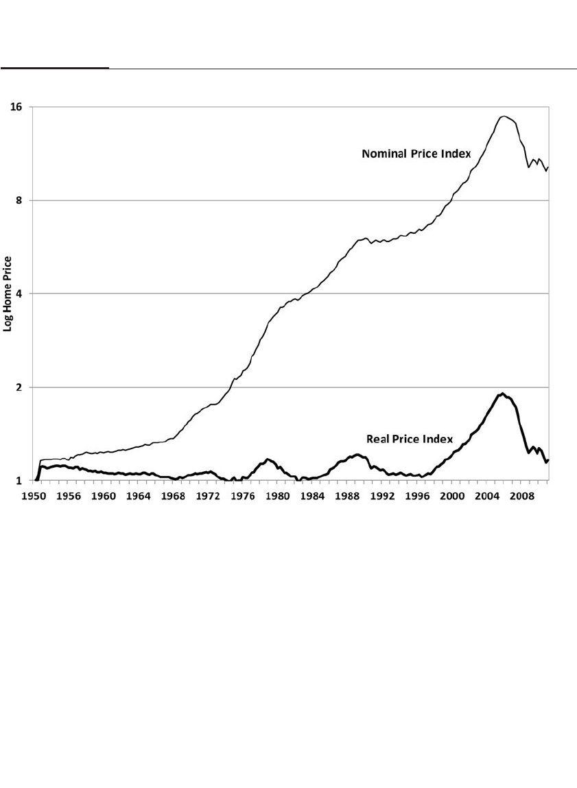
based on postwar historical data, there would have been no period
when the nationwide real estate price index even began to approach the
20 percent decline necessary to cut into the collateral of the standard
mortgage.8, 9
Standard & Poor’s, as well as Moody’s and other rating agencies,
analyzed these historical home price series and performed the standard
statistical tests that measure the risk and return of these securities. On
the basis of these studies, they reported that the probability that collat-
eral behind a nationally diversified portfolio of home mortgages would
be violated was virtually zero. The risk management departments of
many investment banks agreed with this conclusion.
An equally important conclusion reached by this analysis was that
as long as the real estate behind the mortgage was virtually always
going to be worth more than the mortgage, the creditworthiness of the
26 PART I Stock Returns: Past, Present, and Future
FIGURE 2–1
Nominal and Real U.S. Home Prices 1950–2012

borrower should not be important to the lender. If the borrower defaults,
the lender can take over the property and sell it for more than the value
of the loan. The rating agencies therefore stamped “AAA” on these secu-
rities, ignoring the creditworthiness of the home buyer. This assumption
provided the impetus for the sale of hundreds of billions of dollars of
subprime and other “nonconventional” mortgages backed by little or no
credit documentation as long as the loan was collateralized by a pool of
geographically diversified mortgages.
Some rating agencies knew that the high credit ratings for these
mortgages depended on the continued appreciation and negligible
downside risk of home prices. This was illustrated by the following
exchange between an associate of First Pacific Advisors, a California-
based investment advisory firm, and the Fitch rating agency in June
2007, as reported by First Pacific CEO Robert Rodriguez:
My associate asked [Fitch], “What are the key drivers of your rating
model?”
They [Fitch] responded, FICO [credit] scores and home price appre-
ciation of low single digit or mid single digit range, as appreciation has
been for the past 50 years.
My associate then asked, “What if home-price appreciation was flat
for an extended period of time?”
They responded that their model would start to break down.
He then asked, “What if home prices were to decline 1% to 2% for an
extended period of time?”
They responded that their models would break down completely.
He then asked, “With 2% depreciation, how far up the rating’s scale
would it harm?”
They responded that it might go as high as the AA or AAA tranches.10
It should be noted that by the time this exchange took place, homes
prices had already fallen 4 percent from a year earlier, a greater decline
than any previous postwar period, so that a scenario of falling home
prices became highly likely. Yet this likelihood was not built into the
credit ratings of these securities.
As Fitch predicted in the previous exchange, as home prices
declined, the ratings of these top mortgage securities deteriorated rap-
idly. In April 2006, a few months before the peak of housing prices,
Goldman Sachs sold investors 12 mortgage bonds, of which 10 were
originally rated investment grade and 3 were rated AAA. By September
2007, seven of the original ten investment-grade tranches were down-
graded to junk status, and four were totally wiped out.11
CHAPTER 2 The Great Financial Crisis of 2008 27
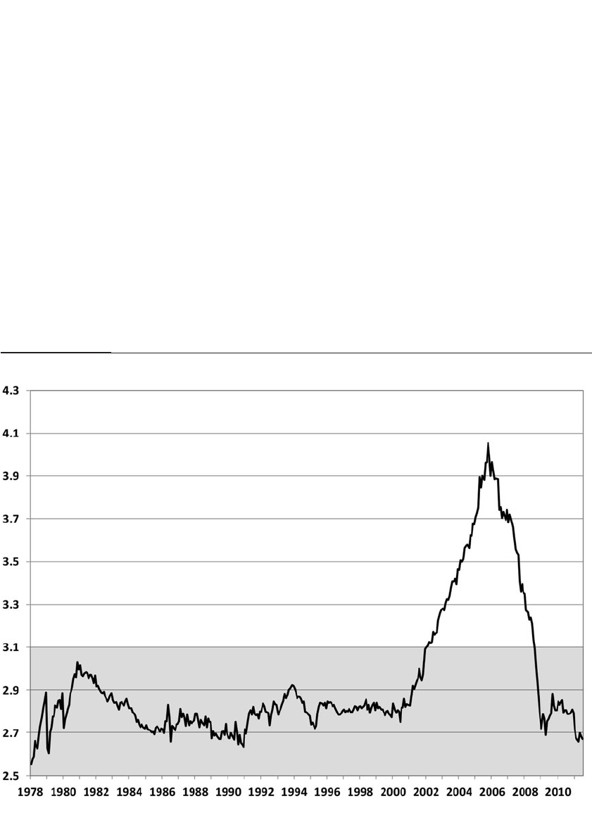
The Real Estate Bubble
What should have alerted the rating agencies that the sustained increase
in housing prices could not continue can be found in Figure 2-2. The
ratio of housing prices to median family income remained in a tight
range between 2.5 and 3.1 from 1978 to 2002 but then moved sharply
higher and eventually surpassed 4.0 in 2006, nearly 50 percent above
previous levels.
But even when the price of an asset moves beyond its economic fun-
damentals, this does not guarantee that there is a “bubble.” Investors
should recognize that there could be structural changes that justify the
price rise. Indeed there have been periods in history when prices have
moved away from fundamentals but were fully justified on the basis of
changes in the economic environment. One such episode that I will
describe in Chapter 11 is the relationship between the dividend yield on
28 PART I Stock Returns: Past, Present, and Future
FIGURE 2–2
Ratio of U.S. Home Prices to Median Family Income 1978–2012

stocks and the interest rate on long-term Treasury bonds. Between 1871
and 1956 the dividend yield was always above the bond yield, and this
was thought to be necessary since stocks were seen as riskier than bonds.
The strategy of selling stocks when the spread narrowed and buying
them when the spread widened was profitable for many decades.
But when the United States left the gold standard, chronic inflation
began to be factored into the interest rate, and in 1957 rates rose above
the dividend yield on stocks and remained that way for more than a half
century. Those who sold stocks and bought bonds in 1957 when this
fundamental-based indicator flashed “Sell!” experienced poor returns,
as stocks proved to be a much better hedge against inflation and pro-
vided far greater returns than fixed-income investments.
In a similar vein, there were plausible reasons why real estate prices
rose above their historical relation to median family income in the early
2000s. First there were significant declines in both nominal and real inter-
est rates that made the cost of home financing extremely low. Second,
there was the proliferation of new mortgage instruments, such as sub-
prime and “full-funding” mortgages, which loaned up to—and in some
cases more than—the purchase price of the home. These mortgages
opened the door to borrowers who previously did not qualify for a loan
and greatly expanded the demand for housing. The popularity of these
full-funding mortgages was driven home by the National Association of
Realtors (NAR) when in January 2006 the NAR announced that 43 per-
cent of first-time home buyers purchased their homes with no-money-
down loans and that the median down payment was a mere 2 percent of
a median-priced $150,000 home.12
There were well-known and highly respected economists, such as
Charles Himmelberg, senior economist of the Federal Reserve Bank of
New York, Chris Mayer, director of the Center for Real Estate at
Columbia University Business School, and Todd Sinai, an associate pro-
fessor of real estate at the Wharton School, who argued that the lower
interest rates justified the high level of real estate prices.13 Some also
pointed to the boom in second homes, a factor that many thought would
persist for many years as the baby boomers entered retirement.14
But many others questioned the sustainability of the housing price
increase. Professor Robert Shiller of Yale University and his colleague
Karl Case, who developed the Case-Shiller residential housing indexes
that have become the benchmark for the profession, first warned about
the bubble of real estate in a 2003 Brookings Papers article entitled, “Is
There a Housing Bubble?”15 Dean Baker, codirector of the Center for
Economic and Policy Research in Washington, also had written and lec-
CHAPTER 2 The Great Financial Crisis of 2008 29

tured extensively about the dangers of the housing bubble in 2005 and
early 2006.16, 17 The disagreement among experts about whether a real
estate bubble actually existed should have alerted the rating agencies to
refrain from rating these securities as if there were essentially no proba-
bility that they could default.18
Regulatory Failure
Despite these warnings, regulatory bodies in general, and the Federal
Reserve in particular, did not believe the house price inflation posed a
threat to the economy, and they did not question the high ratings given
to the subprime mortgage securities. Furthermore, they did not monitor
the buildup of risky mortgage-related securities in the balance sheet of
key financial institutions. These failures leave a serious blot on the
record of the U.S. Monetary Authority.
It is especially tragic that Federal Reserve Chairman Alan Greenspan,
by far the most influential public official in economic affairs, did not warn
the public of the increasing risks posed by the unprecedented rise in hous-
ing prices. Greenspan should have been aware of the burgeoning sub-
prime debt and the potential threat that it posed to the economy since one
of his fellow governors at the Federal Reserve, Edward Gramlich, wrote
extensively about these subprime instruments and published a book enti-
tled Subprime Mortgages: America’s Latest Boom and Bust in June 2007.19
Some have maintained that the Fed lacked oversight over nonbank
financial institutions and that the impact of higher real estate prices was
outside its purview. But why then did Greenspan worry sufficiently
about the rise in stock prices a decade earlier to fashion his famous “irra-
tional exuberance” speech before the Economic Club in Washington,
D.C., in December 1996? All matters impacting the stability of the finan-
cial sector are the responsibility of the Federal Reserve, whether they
originate in banks or not. Greenspan’s lack of concern about the buildup
of risky assets in the balance sheets of financial firms was revealed when
he declared before congressional committees in October 2008 that he
was in a state of “shocked disbelief” that the leading lending institutions
did not take measures to protect shareholders’ equity against a housing
meltdown, nor had they neutralized their exposure to risk by using
financial derivatives or credit default swaps.20, 21
Although Greenspan failed to foresee the financial crisis, I do not,
contrary to others,22 hold him responsible for creating the housing bubble.
That is because the Fed’s policy of slowly raising interest rates was not the
primary force driving real estate values upward. The fall in long-term
30 PART I Stock Returns: Past, Present, and Future

interest rates, driven by slowing of economic growth, the switch from
equities to bonds in corporate pension funds, the huge buildup of reserves
in Asian countries, particularly China, and the proliferation of subprime
and full-funding mortgages, were far more important in propelling real
estate prices higher than the level of the Fed funds rate set by Greenspan
and the Federal Open Market Committee. Furthermore, the forces push-
ing real estate prices upward asserted themselves on a worldwide basis
and in currencies of nations with completely independent central banks.
For example, housing prices soared in Spain and Greece, countries whose
monetary policy was set by the European Central Bank.
Overleverage by Financial Institutions in Risky Assets
It is unlikely that the rise and fall in real estate prices and the related
mortgage-backed securities by itself would have caused either the finan-
cial crisis or a severe recession had it not been for the buildup of these
securities in the balance sheets of key financial firms. The total value of
subprime, alt-A (slightly higher-quality debt than subprime), and jumbo
mortgages reached $2.8 trillion by the second quarter of 2007.23 Even if
the price of all these securities went to zero, the loss in value would be
less than the decline in the value of technology stocks during the crash
of the dot-com boom that occurred seven years earlier. And that stock
market collapse, even when followed by the economic disruptions that
occurred after the devastating 9/11 terrorist attacks, caused only a mild
recession.
The big difference between the two episodes is that at the peak of
the tech boom, brokerage houses and investment banks did not hold
large quantities of speculative stocks whose price was set to plummet.
This is because investment firms had sold off virtually all their risky
technology holdings to investors before the dot-com bubble burst.
In sharp contrast, at the peak of the real estate market, Wall Street
was up to its ears in housing-related debt. As noted earlier, in a declin-
ing interest rate environment, investors were hungry for yield, and these
mortgage-based securities carried interest rates that were higher than
comparably rated corporate and government debt. This tempted invest-
ment banks, such as Bear Stearns, to sell these bonds to investors with
the promise of higher yield with comparable safety.24 Although many
investment banks held these bonds for their own account, their holdings
of subprime debt grew substantially when they were forced to take back
the faltering subprime funds they sold to investors because of com-
plaints that investors were not fully informed of their risks.25
CHAPTER 2 The Great Financial Crisis of 2008 31

Risks to the financial system were compounded when AIG, the
world’s largest insurance company, offered to insure hundreds of bil-
lions of dollars of these mortgages against default through an instru-
ment called the credit default swap. When the prices of these mortgages
fell, AIG had to come up with billions of dollars of reserves that it did
not have. At the same time, the investment banks that had borrowed
heavily to purchase these mortgages found that their funding had dried
up when creditors called their loans that were pledged against these
assets. The decline in the value of these real estate–related securities pre-
cipitated the financial crisis. It is likely that had investment banks held
the tech stocks on margin when prices collapsed in late 2000, a similar
liquidity crisis would have occurred at that time. But they did not.
THE ROLE OF THE FEDERAL RESERVE IN MITIGATING THE CRISIS
Lending is the lifeblood, the oil that lubricates all large economies. In a
financial crisis, institutions that were once believed to be safe and trust-
worthy are suddenly viewed with suspicion. When Lehman failed, fears
spread that many other financial institutions were also in difficulty. This
prompted lenders to call their loans and cut their lines of credit at the
same time investors sold risky assets and attempted to increase the level
of “safe” assets in their portfolios.
But there is only one entity that can provide such liquidity in the
time of crisis, and that is the central bank—an institution that Walter
Bagehot, a nineteenth-century English journalist, dubbed “the Lender of
Last Resort.”26 The central bank creates liquidity by crediting reserves to
banks that either borrow from or sell securities to the central bank.
Banks can, on demand, turn these reserves into central bank notes or
“currency,” the ultimate liquid asset. In this way the central banks can
respond to a “run on a bank,” or the desire of depositors to withdraw
their deposits in the form of currency, by loaning such banks any quan-
tity of reserves against their assets, whether or not the quality or price of
these assets had declined.
The Lender of Last Resort Springs to Action
After the Lehman bankruptcy, the Fed did provide the liquidity the mar-
ket desired. On September 19, three days after the Reserve Primary Fund
announced it would break below a dollar, the Treasury announced that
it was insuring all participating money market funds to the full amount
of the investor’s balance. The Treasury indicated that it was using the
32 PART I Stock Returns: Past, Present, and Future

money in its Exchange Stabilization Fund, normally used for foreign
exchange transactions, to back its insurance plan. But since the Treasury
had only $50 billion in its fund, less than 2 percent of the assets in money
market funds, the Treasury would have had to rely on an unlimited line
of credit to the Fed to make good on its pledge. The Fed itself created a
credit facility to extend nonrecourse loans to banks buying commercial
paper from mutual funds,27 and a month later the Money Market
Investor Funding Facility was established.
On September 29, 2008, the Federal Deposit Insurance Corporation,
or FDIC, announced that it had entered into a loss-sharing arrangement
with Citigroup on a $312 billion pool of loans, with Citigroup absorbing
the first $42 billion of losses and the FDIC absorbing losses beyond that.
The Fed provided a nonrecourse loan on the remaining $270 billion of
the plan. This was followed in January by a similar agreement at about
one-third the size with Bank of America. In return, Citigroup issued the
FDIC $12 billion in preferred stock and warrants. On September 18 the
Fed entered into a $180 billion swap arrangement with leading world
central banks to improve liquidity within the global financial markets.
In addition to the money market mutual fund guarantees announced
immediately following the Lehman bankruptcy, the FDIC announced on
October 7 an increase in deposit insurance coverage to $250,000 per depos-
itor, which was authorized by the Emergency Economic Stabilization Act
of 2008 that Congress had passed four days earlier. On October 14 the FDIC
created a new Temporary Liquidity Guarantee Program to guarantee the
senior debt of all FDIC-insured institutions and their holding companies,
as well as deposits in non-interest-bearing deposit accounts.28 In effect, the
government’s guarantee of senior debt effectively guaranteed all deposits
since deposits have prior claim in the bankruptcy code.
The only way the FDIC was able to guarantee the funds provided
through these policy initiatives was with the full backing of the Federal
Reserve. The FDIC does have a trust fund, but its size is a tiny fraction of
the deposits it insures.29 The credibility of the FDIC to make good on its
promises, like that of the Exchange Stabilization Fund used to “insure”
the money market accounts, depends on an unlimited line of credit that
the agency has with the Federal Reserve.
Why did the Federal Reserve and Chairman Bernanke take all these
bold actions to ensure sufficient liquidity to the private sector? Because
of the lessons that he and other economists learned from what the cen-
tral banks did not do during the Great Depression.
Every macroeconomist has studied the 1963 work The Monetary
History of the United States written by the University of Chicago Nobel-
CHAPTER 2 The Great Financial Crisis of 2008 33

winning economist Milton Friedman. His research built a damning case
against the Federal Reserve for failing to provide reserves to the banking
system during the Great Depression. It was certain that Ben Bernanke,
who received his Ph.D. in economics with a specialty of monetary theory
and policy at the Massachusetts Institute of Technology, was acutely
aware of Friedman’s research and was determined to avoid repeating
the Fed’s mistakes.30 In a speech delivered at Milton Friedman’s nineti-
eth birthday celebration in 2002, six years before the financial crisis,
Bernanke, addressing Professor Friedman, said, “Regarding the Great
Depression. You’re right, we did it. We’re very sorry. But thanks to you,
we won’t do it again.”31
Should Lehman Brothers Have Been Saved?
Although the Federal Reserve sprang into action following the demise of
Lehman Brothers, economists and policy analysts will debate for years
whether the central bank should have bailed out the ailing investment
bank in the first place. Despite denials by the Federal Reserve that it did
not have full legal authority to rescue Lehman, the facts dictate other-
wise. In 1932 Congress amended the original Federal Reserve Act of
1913 by adding Section 13 (3), which stated:
In unusual and exigent circumstances, the Board of Governors of the
Federal Reserve System, by the affirmative vote of not less than five mem-
bers, may authorize any Federal reserve bank, during such periods as the
said board may determine, . . . to discount for any individual, partnership,
or corporation, notes, drafts, and bills of exchange when [they] are
secured to the satisfaction of the Federal Reserve bank: Provided, that
before discounting . . . the Federal Reserve bank shall obtain evidence that
such individual, partnership, or corporation is unable to secure adequate
credit accommodations from other banking institutions.32
There is no doubt that on the weekend before Lehman Brothers
declared bankruptcy, it qualified for Fed lending, as Lehman was clearly
“unable to secure adequate credit accommodations from other banking
institutions.”
The reason that the Fed did not bail out Lehman was more about
politics than economics. Earlier government bailouts of Bear Stearns,
Fannie Mae, and Freddie Mac garnered considerable criticism from the
public and particularly Republicans. After the March bailout of Bear
Stearns, the word went out from the Bush administration: “No More
Bailouts.” Secretary of Treasury Henry Paulson told Lehman Brothers
34 PART I Stock Returns: Past, Present, and Future

shortly after the Bear bailout that it should get its house in order and that
it should not expect help from the Fed. Just days before Lehman filed,
the Fed had rejected a $40 billion loan request from the firm. Treasury
Secretary Paulson and the Fed hoped that with so much advance notice,
a Lehman failure would be digested by the financial markets without
significant disruption.33
But the truth of the matter was that in March when Treasury warned
Lehman to clean up its balance sheet, it was already too late. Lehman not
only had borrowed heavily to buy subprime mortgages but had recently,
with the Bank of America, lent $17 billion to Tishman Speyer to buy the
Archstone-Smith Trust for $22.2 billion. Lehman was hoping to sell the
debt to new buyers for hefty fees, much as Blackstone did when it sold
Sam Zell’s properties at the peak of the market. But Lehman was left with
$5 billion in unsold real estate in what some describe as the worst deal
Lehman Brothers ever made.34 Although CEO Richard Fuld continued to
insist that Lehman was solvent, traders knew that because of the falling
real estate market, Lehman had little chance to survive. The path to bank-
ruptcy had been irrevocably set after Lehman plunged into mortgage-
related securities and the overheated property market.
The Fed’s decision to bail out AIG was necessitated by the unex-
pected financial chaos that immediately followed the Lehman bank-
ruptcy. The Fed and the Treasury, shocked by investors’ sudden rush to
cash and the surging risk premiums in international money markets,
believed that another bankruptcy that threw hundreds of billions of dol-
lars of bonds and credit default swaps into question would likely bring
down the global financial system. Despite the fact that AIG, as an insur-
ance company, was arguably further from the Federal Reserve’s sphere
of responsibility than Lehman, the Fed saved the insurance giant.35 I
have little doubt that had AIG failed first, the ensuing financial panic
would have forced the Fed to bail out Lehman the next day.
TARP, or the Troubled Asset Relief Program, described in detail in
the next chapter, was not at all essential in staving off the financial crisis.
That is because all the funds authorized by TARP, and even more, could
have been supplied by the Federal Reserve under existing legislation
without Congressional approval. TARP was pushed by Bernanke and
Paulson to gain political cover. They knew that the bailouts would be
very unpopular, and they wanted Congress to approve the actions that
they had taken.
Fed historian Allan Meltzer, an economics professor at Carnegie-
Mellon University, claimed that the Fed blundered by setting up expec-
tations that it would bail out systemic institutions, such as Bear Stearns,
CHAPTER 2 The Great Financial Crisis of 2008 35

whose failure threaten the financial system, but then standing aside and
letting Lehman collapse.36 This is echoed by Charles Plosser, president of
the Federal Reserve Bank of Philadelphia, who believed that a Bear
Stearns failure in March could have been absorbed by the market and
would have prompted other firms to increase their liquidity, stemming
further damage.
But I believe that it is far more likely that had Bear been allowed to
fail, it would have greatly accelerated the run on Lehman, precipitating
the crisis in March rather than September. It is inconceivable that finan-
cial firms took the Fed’s rescue of Bear Stearns as a signal to “lever up”
with more risky assets because the Fed would rescue those firms in trou-
ble. It should be noted that even the “rescue” of Bear meant breaking up
the firm and giving shareholders a tiny fraction of their book value. The
owners of AIG are still litigating the near total takeover of the insurance
giant by the federal government when it was rescued from certain bank-
ruptcy. In 2008, it was already too late for regulators to stem the crisis.
Regulators needed to take action years earlier, when the rating firms
were stamping AAA on subprime mortgages and banks, seeking higher
yields, began to increase their leverage in these securities.
Reflections on the Crisis
The overleveraging that took place prior to the financial crisis was moti-
vated by the decline in risk that took place during the long period of
financial stability that preceded the financial crisis, the misrating of
mortgage-related securities by the rating agencies, the approval by the
political establishment of the expansion of homeownership, and the lack
of oversight by critical regulatory organizations, particularly the Federal
Reserve. But it was the management of many of these financial firms
who should be held most accountable. They were unable to grasp the
threats that would befall their firms once the housing boom ended, and
they abdicated responsibility for assessing risks to technicians running
faulty statistical programs.
The financial crisis also punctured the myth that grew during
Greenspan’s tenure as Fed chairman that the Federal Reserve could fine-
tune the economy and eliminate the business cycle. Nevertheless,
despite having failed to see the crisis brewing, the Federal Reserve acted
quickly to assure liquidity and prevented the recession from becoming
far more severe than it turned out to be.
The financial crisis of 2008 is illustrated by the following analogy.
There is no doubt that the improvements in engineering have made the
36 PART I Stock Returns: Past, Present, and Future

passenger car safer than it was 50 years ago. But that does not mean that
the automobile is safe at any speed. A small bump on the road can flip the
most advanced passenger car speeding 120 mph today just as surely as
an older model traveling 80 mph. During the Great Moderation, risks
were indeed lower, and financial firms rationally leveraged their balance
sheets in response. But their leverage became too great, and all that was
needed was an unexpected increase in the default rate on subprime mort-
gages—that “bump on the road”—to catapult the economy into a crisis.
CHAPTER 2 The Great Financial Crisis of 2008 37
This page intentionally left blank

The Markets, the Economy,
and Government Policy in
the Wake of the Crisis
You don’t ever want a serious crisis to go to waste. It’s an opportu-
nity to do important things that you otherwise couldn’t get done.
—RAHM EMANUEL, WHITE HOUSE CHIEF
OF STAFF UNDER PRESIDENT OBAMA,
NOVEMBER 2008
The credit shock, sharply falling real estate prices, and plunging stock
markets precipitated the deepest recession in the developed world
economies since World War II. In the United States, real GDP declined
4.3 percent from the fourth quarter of 2007 through the second quarter of
2009, eclipsing the previous record of 3.1 percent during the 1973–1975
recession by a wide margin. The 18-month recession, which lasted from
December 2007 to June 2009, was also the longest since the 43-month
Great Depression of the early 1930s as unemployment reached 10.0 per-
cent in October 2009. Although this was 0.8 percentage points below the
record postwar level of 10.8 percent set in November 1982, the jobless
rate remained above 8 percent for three years, more than twice as long as
the 1981–1982 recession.
As Figure 3-1 shows, though the crisis originated in the United
States, the decline in U.S. GDP was less than in most of the developed
39
3
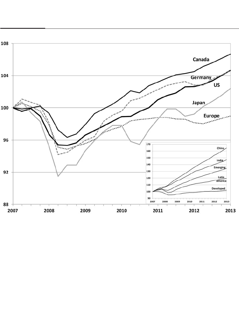
world: output declined 9.14 percent in Japan, 5.50 percent in the
Eurozone, and 6.80 percent in Germany, Europe’s largest economy.
Canada, whose banks never became as overleveraged in real estate
assets as in the United States, experienced the mildest downturn.
Figure 3-1 also shows that the emerging economies withstood the
economic shock much better than the developed world; real GDP
growth slowed but did not decline in fast-growing countries such as
China and India. For emerging economies as a whole, GDP declined
only 3 percent; and by the second quarter of 2009, their output had sur-
passed their previous high. In contrast, it was not until the end of 2011
that the United States regained the output lost, while Japan just
reached its peak output by the end of 2013 while Europe was still
below its peak.
40 PART I Stock Returns: Past, Present, and Future
FIGURE 3–1
International Comparisons of GDP Through the Financial Crisis and Great Recession (2007 Q4 = 100)

AVOIDING DEFLATION
Despite the severity of the Great Recession, its depth in no way com-
pares with the decline in economic activity that occurred during the
Great Depression of the 1930s. Real GDP in the United States fell 26.3
percent between 1929 and 1933, more than 5 times the decline in the
Great Recession, and unemployment soared to between 25 and 30 per-
cent.1, 2 One reason for the difference between the Great Depression of
1929–1933 and the Great Recession of 2007–2009 was the behavior of the
price level. Consumer prices declined by 27 percent between September
1929 and March 1933, while the maximum decline of the consumer price
index during the Great Recession was 3.5 percent.3By March 2010, the
CPI surpassed its precrisis peak, while it took 14 years for consumer
prices to recover to their 1929 level following the Great Depression.
Deflation worsens a business cycle, since a fall in wages and prices
increases the burden of debt, which increases in real value as prices
decline. Consumers were already burdened by record debt levels in 2007
before the financial crisis. Had wages and prices fallen as they did in the
Great Depression, the burden of consumer and mortgage debt would
have been more than one-third larger in real terms, greatly increasing
the number of insolvencies.4That is the reason that stabilization of the
price level was a priority for the Federal Reserve and is a major reason
why consumer and business spending did not decline as much in the
2007–2009 recession compared with what happened in the 1930s.5
The Federal Reserve was able to avoid deflation by stabilizing the
money supply. In the Great Depression, the money supply, measured as the
sum of demand and savings deposits (M2), fell by 29 percent between
August 1929 and March 1933.6In contrast, the money supply actually rose
during the 2008 financial crisis as the Federal Reserve increased the total
reserves by over $1 trillion. This action provided sufficient reserves so that
banks were not forced to call in loans as they were forced to in the 1930s.
Although one can certainly question whether the later injections of reserves
(called quantitative easing) aided the economy, there was little doubt that the
initial provisions of liquidity were critical to stabilizing the financial mar-
kets and preventing the downturn from becoming substantially worse.
REACTION OF THE FINANCIAL MARKETS TO THE FINANCIAL CRISIS
Stocks
Despite the actions taken by the Federal Reserve to moderate the eco-
nomic contraction, the credit disruption that followed the Lehman bank-
CHAPTER 3 The Markets, the Economy, and Government Policy in the Wake of the Crisis 41

ruptcy had a devastating impact on the equity markets, which suffered
their worst decline in 75 years. In the 9 weeks following September 15, the
S&P 500 Index fell 40 percent to an intraday low of 740 on November 21.
Ultimately this broad-based benchmark sank to a 12-year low of 676 on
March 9, 2009, nearly 57 percent below its closing peak reached 1½ years
earlier. Although the decline in the benchmark index exceeded the previ-
ous postwar record of 48 percent that occurred between January 1973 and
October 1974, it did not approach the decline that ushered in the Great
Depression, when stocks fell by more than 87 percent.7From the market
high of October 2007 through March 2009, U.S. stock market wealth had
declined $11 trillion, a sum of more than 70 percent of U.S. GDP.
The volatility of stock prices increased sharply, as it always does in
bear markets. The VIX volatility index, which measures the premium
built into put and calls on the stock market (in effect measuring the cost
of “insuring” a stock portfolio), soared from under 10 in March 2007,
before the crisis began, to nearly 90 immediately following the Lehman
bankruptcy. This level exceeded any other in the postwar period except
that immediately following the October 19, 1987, stock market crash.8
Another measure of volatility, the number of days that the stock
market rose or fell by 5 percent or more, increased sharply to levels not
reached since the early 1930s. Between the Lehman bankruptcy on
September 15 and December 1, there were 9 days when the Dow
Industrials dropped by at least 5 percent and 6 days when it rose by 5
percent or more. Except for the 1930s when a record 78 days saw
changes of 5 percent or more, these 15 days of changes of 5 percent or
more exceeded the total for any other decade since 1890.9
The plunge in the U.S. equity markets was echoed abroad. Around
the world, approximately $33 trillion of stock market wealth was lost,
about half the world’s annual GDP.10 In local currency, the Morgan
Stanley EAFE Index for non-U.S. developed markets declined by nearly
the same magnitude as in the United States, but because the dollar appre-
ciated during the period, the total decline was 62 percent in dollar terms.
The emerging market stocks fell 64 percent in dollar terms, although they
fell less in the local currency as the currencies of almost all emerging mar-
kets, except for the Chinese yuan, depreciated against the dollar.11
The decline in the emerging stock markets was nearly identical to
the decline suffered during the Asian financial crisis in 1997–1998. But
the emerging market indexes at their 2009 lows remained well above the
levels reached at the bottom of the 2002 bear market. This contrasted
with the United States and most other developed markets that fell below
their 2002 bear market lows.
42 PART I Stock Returns: Past, Present, and Future
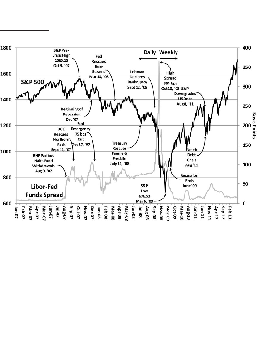
Certain equity sectors that held up well in the early stages of the
market decline fell sharply as credit markets froze. Real estate invest-
ment trusts (REITs) are a case in point. Buying them for their yield,
investors at first flocked to these stocks as interest rates fell and REITs
actually rallied in the week after Lehman went under. But when
investors feared that lenders would pull credit lines, REITs lost on aver-
age an astounding two-thirds of their value in the next 10 weeks and fell
a total of 75 percent by the time the bear market ended in March 2009.
Real estate trusts that were funded by short-term loans or that took on
extra leverage during the boom in an effort to boost yields to investors
were hit particularly hard.12
The financial sector of the S&P 500 declined 84 percent from its
peak in May 2007 to its trough in March 2009, wiping out about $2.5 tril-
lion of equity. The percentage decline exceeded the 82.2 percent decline
in the S&P 500 technology sector that occurred from 2000 to 2002, but
CHAPTER 3 The Markets, the Economy, and Government Policy in the Wake of the Crisis 43
FIGURE 3–2
The S&P 500 and the LIBOR—Fed Funds Spread Through the Financial Crisis, January 2007 – June 2013

since the tech sector had valuations at the peak more than three times
that of the financial sector, the equity values lost in the tech crash were a
much higher $4 trillion.13 Nevertheless, while the tech crash wiped out
the previous 5 years of total stock market gains, the financial crisis
wiped out 17 years, sending equity prices down to 1992 levels.
Many financial firms declined much more than the 84 percent aver-
age for the sector. Peak to trough, Bank of America lost 94.5 percent of the
market value of its equity, Citibank lost 98.3 percent, and AIG lost an
astounding 99.5 percent.14 The equity holders of Lehman Brothers,
Washington Mutual, and a large number of smaller financial institutions
lost everything, while shareholders of Fannie Mae and Freddie Mac, the
giant government-sponsored enterprises that went public in the early
1980s, hold on to a sliver of hope that they might recover some of their
capital.15 Many international banks fared just as poorly as U.S. banks.
From peak to trough, Barclays fell 93 percent, BNP Paribas 79 percent,
HSBC 75 percent, and UBS 88 percent. The Royal Bank of Scotland, which
needed a loan from the Bank of England to survive, fell 99 percent.
The percentage fall in the S&P 500 Index exceeded the decline in
operating earnings of firms in the index. S&P 500 operating earnings
declined 57 percent from a record $91.47 in the 12 months ending on
June 30, 1997, to $39.61 in the 12 months ending September 30, 2009. But
the decline in reported earnings was much greater: as a result of the
record $23.25 loss for S&P 500 firms in the fourth quarter of 2008, the S&P
500 12-month reported earnings fell from a high of $84.92 in 1997 to only
$6.86 for the 12 months ending March 31, 2009. This 92 percent decline in
earnings exceeds the 83 percent decline in earnings that took place in the
Great Depression from 1929 through 1932.16
The huge write-downs by the financial firms were the main cause
of the devastating earnings drop of the S&P 500 in 2008 and 2009. When
calculating earnings on the S&P 500 Index, it is the policy of Standard &
Poor’s to sum all the profits and losses of each firm dollar for dollar and
to compare the aggregate earnings with the aggregate value of the S&P
500 portfolio in order to compute the P/E ratio of the index. The $61 bil-
lion fourth-quarter 2008 loss of AIG, which had a weight of less than 0.2
percent in the index, more than wiped out the total profits of the 30 most
profitable firms in the S&P 500, which composed almost half the index
value. S&P’s method of aggregating firms’ earnings dollar for dollar
understates the earnings and vastly overstates the P/E ratio of the index
during recessions when a few firms report very large losses.17 In fact,
after-tax aggregate corporate profits taken from the national income and
44 PART I Stock Returns: Past, Present, and Future

product accounts fell by only 24 percent for the 12-month period ending
in June 30, 2007, to the year ending March 31, 2009.
Real Estate
I noted that the buildup of real estate and real estate–related assets in the
portfolios of highly leveraged financial institutions was the primary
cause of the financial crisis. The Federal Reserve reported in its quarterly
Flow of Funds Report that from the third quarter of 2007 through the
first quarter of 2009, the value of residential real estate fell from $24.2
trillion to $17.6 trillion, a decline of 27 percent. The price index of resi-
dential real estate declined by 26 percent as measured by the Case-
Shiller Index of 20 metropolitan areas,18 and commercial real estate
prices fell by 41 percent from October 2007 through November 2009.19
Fluctuations in real estate prices have a significant impact on the
economy. It has been estimated that consumers spent between 25 and 30
percent of the home equity borrowings during the real estate boom
between 2002 and 2006.20 Given that such borrowings averaged 2.8 per-
cent of GDP, the spending boost powered by the rise in home equity val-
ues contributed about a ¾ percentage point, or one quarter of the annual
growth rate of the U.S. economy during that period. After 2008, the fall
in real estate prices reduced consumption and contributed significantly
to the slow recovery from the Great Recession.
Treasury Bond Markets
After the Lehman bankruptcy, the rush to safety sent the yield on
Treasury bills to zero and even lower. On December 4, 2008, the 90-day-
bill rate fell to an all-time low of minus 1.6 basis points.21 The huge
demand for Treasury securities extended to the long end, as the 10-year
U.S. Treasury notes fell to near 2 percent at the end of 2008. The yield on
Treasury long bonds continued to fall for four more years, with the 10-
year bond reaching its low of 1.39 percent in July 2012.
During the crisis, the Federal Reserve not only provided liquidity
to the markets but also sharply lowered the fed funds rate. The Fed low-
ered the funds target rate from 2 to 1.5 percent in an emergency meeting
on October 23, 2008 and lowered it further to 1 percent at its regular
November meeting. On December 16, as conditions continued to
worsen, the Federal Open Market Committee reduced the federal funds
rate to an all-time low of between zero and 0.25 percent; and at the end
CHAPTER 3 The Markets, the Economy, and Government Policy in the Wake of the Crisis 45

of 2013, the funds rate remains at this level, the longest period since
World War II that the rate has remained unchanged.
Even though the Federal Reserve guarantees on bank deposits and
money market funds stopped the liquidity panic, the Fed could not pre-
vent the shock waves that reverberated through the credit markets.
While long-term Treasury rates fell substantially, interest rates on non-
Treasury debt rose. The spread between the lowest investment-grade
corporate bond and the 10-year Treasury reached 6.1 percent in
November 2008, the highest since the record 8.91 percent spread in May
1932 that was reached near the bottom of the Great Depression. The
spread between lower-rated 30-year B-rated industrial bonds and
Treasury bonds widened from 4 percentage points to nearly 8 percent-
age points after the rescue of Bear Stearns and to a record 15.1 percent-
age points in the first week of January 2009.
The LIBOR Market
One of the most watched spreads in the money market is that between
the rate set by the Federal Reserve in the fed funds market (a market to
facilitate the borrowing and lending of reserves between U.S. banks) and
the interbank lending rates outside the United States, called the London
Interbank Offered Rate, or LIBOR.
There are literally hundreds of trillions of dollars of loans and finan-
cial instruments around the world that are based on the LIBOR, includ-
ing almost one-half of all adjustable-rate mortgages. The history of the
LIBOR goes back to the 1960s, when the market for overseas dollar lend-
ing grew dramatically after the U.S. government put restrictions on dol-
lar outflows in a futile attempt to reverse its balance-of-payments deficit
and staunch its gold outflow. The LIBOR rate is computed for 15 time
periods from one day to one year in duration and for 10 different curren-
cies. By far, the dollar LIBOR is the most important of these fixings.
Return to Figure 3-2. Before the financial crisis, the LIBOR stayed
very close (usually within 10 basis points) to the federal funds target. The
first rumblings of trouble in the banking sector came in August 2007 when
the LIBOR–fed funds spread jumped above 50 basis points in response to
the BNP Paribas announcement of stopping fund redemptions and the
problems at Northern Rock in the United Kingdom. Over the next 12
months, as the subprime crisis grew, the LIBOR-funds spread remained
mostly between 50 and 100 basis points. But the LIBOR spread soared
after the Lehman bankruptcy, and on October 10 the difference between
the LIBOR and the fed funds rate reached an unheard-of 364 basis points.
46 PART I Stock Returns: Past, Present, and Future

It was extraordinarily frustrating to policy makers that the interest
rate upon which so many loans were based actually rose at the same
time the Fed was aggressively lowering the fed funds rate. After the
Federal Reserve flooded the financial system with reserves, the LIBOR
spread finally came down, but it did not fall decisively under 100 basis
points until the stock market began to recover from its bear market low
in March 2009, three months before the National Bureau of Economic
Research called the recession over.
For all its importance in setting loan rates, the LIBOR does not rep-
resent actual transactions but what a bank expects the cost of its own
noncollateralized borrowing to be, even if it does not borrow any funds.
Following the Lehman crisis, fears for the solvency of banks skyrock-
eted, and the interbank lending market between banks effectively froze.
But banks were still obligated to submit LIBOR rates to the British
Bankers Association although they had little actual data on which to
base such submissions. Mervyn King, governor of the Bank of England,
told the U.K. Parliament in November 2008 that “[the LIBOR rate] is, in
many ways, the rate at which banks do not lend to each other.”22
Many regulatory agencies, in both the United States and United
Kingdom, strongly suspected that several banks underreported their
cost of borrowing to avoid signaling to the market that creditors feared
for their solvency. Nevertheless, it was not until July 2012 that the British
government announced that it had fined Barclays bank $453 million for
submitting false interbank interest rates and intimated that other banks
also submitted false rates.23 The outcry over the scandal raised the call to
reform this multitrillion-dollar market, an effort that would require a
total restructuring of the way this benchmark rate is calculated or a shift
to alternative instruments.
Commodity Markets
In the early stages of the subprime crisis, the prices of commodities rose
rapidly as the emerging economies continued to grow strongly. Oil
(West Texas Intermediate) rose from $40 a barrel in January 2007 to an
all-time high of $147.27 in July 2008, and the Commodity Research
Bureau Index of 18 actively traded commodities rose by over 60 percent.
But following the Lehman crisis, the decline in economic activity sent
commodity prices down sharply. Oil fell to $32 a barrel in December, and
the CRB Index fell by 58 percent to its lowest level since 2002.
It is remarkable that the commodity price decline measured by the
CRB Index was almost the same magnitude as the decline in world stock
CHAPTER 3 The Markets, the Economy, and Government Policy in the Wake of the Crisis 47

markets. Investors who believed that commodities provided them a
hedge against a severe stock market decline were wrong. As we explore
later in this chapter, virtually no asset, except for long-term U.S.
Treasury bonds, served as an effective hedge against the sudden and
sharp decline in asset values that took place during the financial crisis.
Even gold, which had peaked just below $1,000 per ounce in July 2008,
fell below $700 after the Lehman bankruptcy.
Foreign Currency Markets
After hitting a 15-year high in the summer of 2001, the dollar declined
steadily against the currencies of the major developed countries and
continued to do so in the early stages of the financial crisis. In the imme-
diate wake of the Bear Stearns merger into JPMorgan, the dollar reached
its all-time low on March 17, 2008, a full 23 percent below its precrisis
high in November 2005 and 41 percent below its 25-year high reached in
2001. But as the financial crisis worsened, the dollar regained its “safe-
haven” status, and foreign investors switched back to dollar securities.
This caused the greenback to rise by over 26 percent against developed
world currencies, reaching its high on March 4, 2009, just a week before
the U.S. equity market reached its bear market low. Only the Japanese
yen advanced against the dollar during the financial crisis, as the market
tumult caused investors to unwind their “carry trade,” the name given
to the strategy of borrowing from Japan at the world’s lowest interest
rates in order to invest in riskier, higher-yielding currencies elsewhere.
As the crisis eased and the equity markets began to recover, the dollar
lost some of its safe-haven premium, and its price fell.
Impact of the Financial Crisis on Asset Returns and Correlations
One of the principal conclusions of financial theory is that to attain the
best return for a given risk, investors should seek to diversify their hold-
ings not only within an asset class but also among asset classes. For that
reason investors put a premium on assets whose prices are negatively
correlated with the market, and discount assets that are positively corre-
lated with the market.
Figure 3-3 shows the correlations of various asset classes with the S&P
500 over all five-year windows from 1970 through 2012. One can see that
the financial crisis had a significant impact on the correlation between asset
classes, in most cases accelerating trends that had taken place before the
crisis. The correlation between both developed economies’ equity markets
48 PART I Stock Returns: Past, Present, and Future
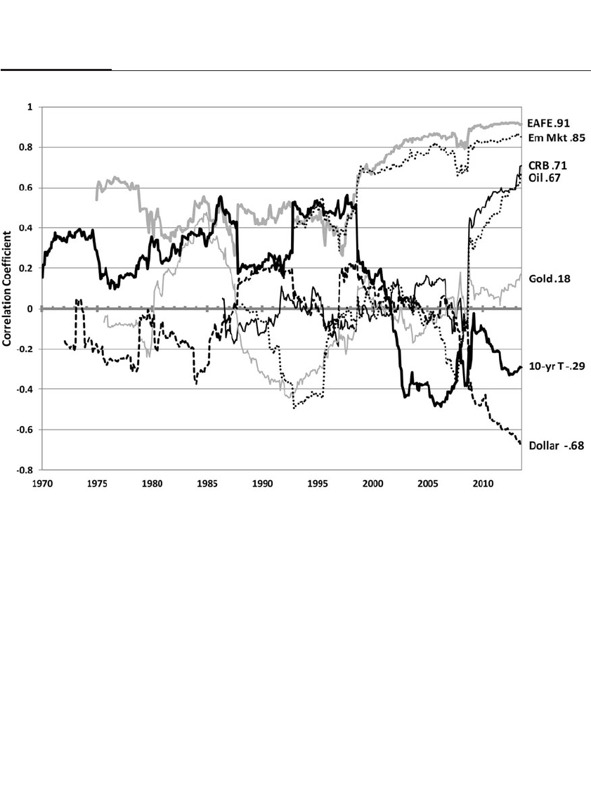
(EAFE) and emerging economies’ equity markets (EM) with the U.S. stock
market has grown significantly, reaching 0.91 for EAFE and 0.85 for EM.
There are good economic reasons why the correlation between
stock markets has become greater over recent years. First, there is an
increase in the economic interdependence as world trade constitutes an
ever-greater share of world output. The second is that traders and
investors operate in many different markets simultaneously so that
market sentiment is much less likely to be isolated to a given market.
And third, most of the shocks to the financial and commodity markets
since 2008 have been global in nature, overwhelming idiosyncratic
shocks that impact one country or one market.
Not only has the correlation between equity markets increased, but
Figure 3-3 shows the correlation between the equity markets and com-
modities, measured by either the CRB Index of commodity prices or the
price of oil, has increased sharply since the financial crisis.24 Commodity
prices are impacted by demand factors, such as the growth in the world
CHAPTER 3 The Markets, the Economy, and Government Policy in the Wake of the Crisis 49
FIGURE 3–3
Monthly Correlations of S&P 500 and Various Assets Classes from 1970–2012

economy, and supply factors, such as weather (for crops) and political
developments (for oil). Fluctuations in demand cause a positive correla-
tion between stock prices and commodity prices, while fluctuations in
supply induce a negative correlation. If the major source of disturbances
to the price of commodities arises from supply fluctuations, then hold-
ing commodities will serve as a good hedge against stocks. But when
global demand shocks predominate, then commodity prices will move
in tandem with stock prices, and commodities will serve as poor diver-
sifiers against equity fluctuations.
There are good reasons why the correlation between commodity
and equity prices may continue to be high. Recent developments in the
energy markets mean that OPEC is not likely to have as great an impact
on the supply of oil as in the past. Alternative sources of oil and gas from
non-OPEC countries arising from shale exploration, fracking, and other
extractive techniques are becoming more important. These develop-
ments mean that fluctuations in demand may take an upper hand in
determining the price of energy, leading to a positive correlation
between stock and commodity prices. And this means that commodities
will likely decline as an effective hedge against stocks.
Some argue that the increased correlation between world stock mar-
kets reduces or even eliminates the incentive to diversify one’s portfolio.
If international stocks move in tandem, the proponents of the argument
maintain, then investing in foreign markets will do little to offset the fluc-
tuations in one’s home market. But correlations are usually calculated
over relatively short periods of time, say one week or one month. Long-
term correlations between asset returns are significantly lower than
short-term correlations. This means that long-term investors should con-
tinue to diversify even though such diversification does not lead to sig-
nificant reductions in the short term volatility of portfolio returns.
Decreased Correlations
In contrast to commodities, which have increased their correlation with
stocks since the financial crisis, there are two notable asset classes whose
returns have become significantly less correlated with equities: U.S.
Treasury bonds and the U.S. dollar.
The price of a dollar in foreign exchange markets is impacted by the
strength of the U.S. economy and the safe-haven status that international
investors accord the U.S. dollar. The first factor leads to a positive corre-
lation between U.S. equities and the exchange rate: good or bad news
50 PART I Stock Returns: Past, Present, and Future

about the economy will impact stock prices and the exchange rate in the
same direction.
But the safe-haven status of the U.S. dollar leads to the opposite
correlation: bad economic news, particularly emanating from outside
the United States, will elicit a flight to the dollar, raising its value at the
same time that the news sends world and U.S. stock prices lower. Since
the onset of the financial crisis and particularly the European monetary
crisis, the safe-haven status of the U.S. dollar has increased dramatically.
Bad news about Europe negatively impacts world stock markets but
drives the euro downward and therefore the dollar higher in exchange
markets. The European crisis has led to a record negative correlation
between the U.S. dollar and U.S. stocks, as seen in Figure 3-3.
U.S. Treasury bonds have also enjoyed enhanced safe-haven status
since the financial crisis. Bad news, originating either within or outside
the United States, has prompted investors to purchase Treasury bonds
and has led to a strong negative correlation between Treasury bond
prices and stock prices. This negative correlation enhances the attrac-
tiveness of Treasury bonds to investors wishing to hedge their equity
portfolios and has no doubt supported the high prices and correspond-
ingly low yields on long-term U.S. Treasury securities during and imme-
diately following the financial crisis.
The ability of long-term U.S. Treasury bonds to hedge equity risk is
even stronger for the non-dollar-based investor. For non-dollar investors,
bad news increases the demand for dollar-denominated assets and in
particular Treasury bonds. This leads to an even higher negative correla-
tion of U.S. Treasury bonds and stock markets measured in non-dollar
currencies. Long-term Treasuries have de facto become the world’s ulti-
mate “hedge” asset, and this explains why so many sovereign wealth
funds hold a high percentage of their assets in Treasury bonds despite
their very low yields and expected returns.
The single asset class whose correlation with the equity markets has
not been impacted by the financial crisis is gold. The rise in the price of
gold after the financial crisis has been caused by the increased fear of
hyperinflation and financial collapse, but the correlation with the equity
markets has remained near zero over the past 50 years. By early 2013 the
price of gold had increased markedly since 2008, although it never was
as high, after inflation, as it was at the top of the 1980 bubble when it
reached $850 per ounce, or $2,545 in 2013 prices.
The positive correlations of equity markets with commodities and
oil and the negative correlation with Treasury bonds and the dollar have
CHAPTER 3 The Markets, the Economy, and Government Policy in the Wake of the Crisis 51

given rise to the term risk-on/risk-off market. A risk-on market occurs
when good news about the economy entices investors to buy stocks and
go long commodities and sell the U.S. dollar and Treasury bonds. In
such markets, stocks and commodity prices rise while U.S. Treasury
bond prices and the dollar fall. Risk-off markets are the opposite, where
bad economic news entices investors to buy U.S. Treasuries and the dol-
lar while selling commodities and stocks. Gold prices can either rise or
fall on these days.
But as Figure 3-3 shows, the correlation between asset classes has
not been stable. In particular, the correlation between stock prices and
Treasury bonds in the 1970s and 1980s was positive, not negative. This is
because the major threat to the economy in those years was inflation,
and lower inflation was good for both stocks and bond prices. It is only
when inflation is not a threat and the financial stability of the private sec-
tor is in question that the Treasury bonds take on safe-haven status and
become negatively correlated with equity prices.
Certainly under current monetary policy, the risk that inflation will
once again be a concern for policy makers is high. In that situation,
Treasury bonds will cease to be a hedge asset, and bond prices could fall
substantially since investors will require much higher yield for an asset
that no longer acts as a diversifier to the equities in their portfolios. The
unprecedented bull market in Treasury bonds, supported by the belief
that Treasury bonds are “insurance policies” in the case of financial col-
lapse, could end as badly as the bull market in technology stocks did at
the turn of the century. When economic growth increases, Treasury
bondholders will receive the double blow of rising interest rates and loss
of safe-haven status.
One of the prime lessons learned from long-term analysis is that no
asset class can stay permanently detached from fundamentals. Stocks
had their comeuppance when the technology bubble burst and the
financial system crashed. It is quite likely that bondholders will suffer a
similar fate as the liquidity created by the world’s central banks turns
into stronger economic growth and higher inflation.
Legislative Fallout from the Financial Crisis
Just as the Great Depression generated a host of legislation such as the
Securities and Exchange Act, which created the SEC, the Glass-Steagall
Act, which separated commercial and investment banks, and establish-
ment of the Federal Deposit Insurance Corporation, the financial crisis of
2008 spurred legislators to design laws to prevent a repeat of the financial
52 PART I Stock Returns: Past, Present, and Future

collapse. The result was embodied in a massive 849-page piece of legisla-
tion crafted by Senator Christopher Dodd (D-Conn) and Representative
Barney Frank (D-Mass), called the Dodd-Frank Wall Street Reform and
Consumer Protection Act, which was signed into law by President
Obama in July 2010. The act’s powers range from establishing the fees for
debit cards, to setting the regulations of hedge funds, restricting “preda-
tory lending,” addressing compensation of CEOs and other employees,
and formulating measures designed to stabilize the economy and finan-
cial system. The act comprises 16 titles and requires that regulators create
243 rules, conduct 67 studies, and issue 22 periodic reports.25
The three most important parts of the law that impact the overall
economy are (1) the “Volcker rule,” which limits the proprietary trading
of commercial banks, (2) Title II, which provides for the liquidation of
large financial firms not under the purview of the Federal Deposit
Insurance Corporation, and (3) Title XI, which adds responsibilities but
also places new restrictions on the Federal Reserve.
The Volcker rule was named after Paul Volcker, former chairman of
the Federal Reserve and chair of President Obama’s President’s
Economic Recovery Advisory Board, who argued that financial stability
required that Congress sharply limit the ability of banks to trade for
their own accounts. Such a provision was not in the original bill submit-
ted to Congress but inserted later. Originally the Volcker proposal
specifically prohibited a bank or an institution that owns a bank from
engaging in proprietary trading that is not at the behest of its clients and
from owning or investing in a hedge fund or private equity fund.
However, this proposal was later modified to allow up to 3 percent of
the capital of banks to go into proprietary trading and exempts hedging
operations as well as trading in U.S. Treasury debt. The Volker rule was
designed to restore the separation between investment banks and com-
mercial banks that was first mandated by the Glass-Steagall Act of 1933
but was effectively repealed by Congress in 1999 in the Gramm-Leach-
Bliley Act.
But would the Volcker amendment, had it been law in 2007, have
prevented the 2008 financial crisis? The financial crisis was caused by
the overleveraging of real estate–related securities in Bear Stearns and
Lehman Brothers, which were investment banks and would not have
fallen under the purview of the Volcker amendment. Nor would it have
applied to the insurance giant AIG, which the Fed chose to save after
seeing the turmoil unleashed by the Lehman bankruptcy. Furthermore,
banks that obtained loans from the Fed, specifically Citibank and Bank
of America, ran into trouble because of bad real estate loans, not propri-
CHAPTER 3 The Markets, the Economy, and Government Policy in the Wake of the Crisis 53

etary trading. Given this history, it is dubious that the Volcker amend-
ment, had it been in effect in 2007, would have changed the course of the
financial crisis.
Title II of the Dodd-Frank Act permits the government to dismantle
expeditiously financial firms that become a threat to the stability of the
financial system in order to minimize the risk of a financial crisis.
Although the Federal Deposit Insurance Corporation has rules for the
liquidation of commercial banks and the Securities Investor Protection
Corporation has powers to liquidate the assets of brokerage houses, the
government had no guidelines for dismantling investment banks, such
as Bear Stearns and Lehman, nor insurance companies such as AIG.
Under the usual bankruptcy laws, a determination of order of claims
may take months or years, far too long to calm the waters in a crisis.
Title II specifies that financial firms submit to the government the
order that assets should be liquidated if a firm cannot meet its financial
obligations and prohibits the government from taking equity positions
in the firm being dismembered. The law also specifies measures to avoid
exposing taxpayers to undue losses that can be absorbed by other credi-
tors to the firm. This part of the bill would have prohibited the Federal
Reserve taking the equity stakes that it did in AIG, Citibank, or any other
financial firm.
Title XI restricts the actions of the Federal Reserve by basically abol-
ishing the Section 13(3) amendments to the Federal Reserve Act that
gave the central bank virtually unlimited power to lend to any financial
firm in crisis. Under the new law, the Federal Reserve cannot lend to
individual firms, although it can use its powers to provide broad-based
liquidity to the financial system as long as it gets the approval of the sec-
retary of treasury. Furthermore the act requires that the Federal Reserve
disclose which financial firms are receiving assistance within seven days
of authorizing an emergency facility.26
Whether these restrictions prove to be detrimental in the next finan-
cial crisis remains to be seen. Most of these restrictions were inserted to
buy Republican support for passage of the bill, since a vast majority of
Republicans opposed both the Fed’s and Congress’s bailout of the finan-
cial institutions. Many were particularly unhappy about the Troubled
Asset Recovery Program, or TARP, signed into law on October 3, 2008,
that provided up to $700 billion to financial institutions but also was
used to provide funds to General Motors.27
The $700 billion TARP was a very controversial piece of legislation,
first proposed by Treasury Secretary Paulson and Fed Chairman
Bernanke just days after the Lehman bankruptcy. Although supported
54 PART I Stock Returns: Past, Present, and Future

by President Bush, the Republicans in the House voted down the legis-
lation on September 29, 2008, sending the Dow Industrials to a 777-point
(6.98 percent) loss. After minor changes were made (and undoubtedly
quite a few phone calls to Republican legislators from agitated
investors), many House Republicans reversed themselves and passed
the legislation four days later.
As noted in the last chapter, Bernanke did not need Congress to
pass TARP to extend credit to either financial or nonfinancial firms
stressed by credit developments, because Section 13(3) of the Federal
Reserve Act provided him with the authority to do so. But having taken
the heat for the Fed’s previous interventions, Bernanke and Paulson
felt they needed congressional approval to proceed. Had the restric-
tions in the Dodd-Frank Act been in effect in 2008, the Fed would not
have the ability to lend to individual firms like AIG, an action that
stanched the crisis.
Yet the Fed will still likely have enough flexibility to act in order to
calm the markets. Under Dodd-Frank the Federal Reserve can, with
Treasury approval, establish liquidity facilities for classes of institutions,
such as investment banks or even insurance companies. Certainly
Treasury Secretary Henry Paulson worked closely with Ben Bernanke
throughout all the stages of the financial crisis, and the two men devel-
oped a good working relationship. Bernanke would have most likely
obtained approval by Paulson of the general lending facilities that the
Fed established to provide liquidity to the market.
Nevertheless, the relationship between the treasury secretary and
the Fed chairman may not always be so cordial. There have been times
at which the administration has been critical of the Fed, and although
the treasury secretary can be removed by the president at any time, the
chairman of the Fed is appointed for a four-year term and can only be
removed by impeachment by the Senate.
Time will tell how effective—or harmful—the provisions of the
Dodd-Frank Act turn out to be. Most of the rules and regulations are yet
to be written by committees and groups of “experts” chosen by the gov-
ernment to craft the rulebooks and procedures. It has often been said
that the devil is in the details, and most of those details have yet to be
formulated.
Concluding Comments
The financial crisis and subsequent recession spawned the deepest bear
market in stocks and the greatest bull market in Treasury bonds since the
CHAPTER 3 The Markets, the Economy, and Government Policy in the Wake of the Crisis 55

Great Depression of the 1930s. And the sharp downturn in economic
activity that followed caused record peacetime government budget
deficits, one of the slowest economic recoveries in our nation’s history,
and a growing pessimism about the future of America.
But debt, deficits, and slow economic growth need not be the
legacy of the Great Recession. The next chapter peers into the future to
identify those trends that will dominate the economic landscape over
the remainder of this century and explains why there is significant cause
for optimism about the future of the U.S. and world economy.
56 PART I Stock Returns: Past, Present, and Future

The Entitlement Crisis
Will the Age Wave Drown
the Stock Market?
Demography is Destiny
—AUGUSTE COMTE
The Great Recession led to record peacetime government budget deficits
in the United States, Europe, and Japan and highlighted the unsustain-
ability of the generous and increasingly costly entitlement programs that
had been enacted years earlier. Furthermore, the housing and stock mar-
ket collapse erased trillions of dollars of wealth from consumer balance
sheets, leaving many with insufficient assets to realize the comfortable
retirement that they had once expected.
Against this backdrop of declining economic fortunes, pollsters
detected a marked loss of confidence in America’s future. In 2010 less
than half of the Americans responded yes to the question, “Do you think
that your children will be better off than you are?”1The faith in an ever-
rising standard of living, which served as a core belief for American fam-
ilies and a beacon for millions of immigrants throughout the country’s
history, was fading.
This chapter examines whether this pessimism is justified. Is it true
that our children, for the first time in our country’s history, have a bleaker
57
4

future than their parents, or are there forces that might renew the
American Dream and restore economic growth?
THE REALITIES WE FACE
Two conflicting forces will impact the world economy over the coming
decades. The first force, which gives rise to rising government budget
deficits and strains private and public pension programs, is the “age
wave,” or the unprecedented rise in the number of individuals in the
developed world who will enter retirement. The age wave poses two
fundamental questions: Who will produce the goods and services that
the retirees will consume, and who will buy their assets that they plan on
selling to finance their retirement? It can be shown that if the developed
world must rely solely on its own population to produce these goods,
then the age that people will be able to retire must increase significantly.
The second offsetting force is the strong growth of emerging
economies, particularly in India, China, and the rest of Asia, that will
soon produce the bulk of the world’s output. Is it possible that emerging
economies will be productive enough to produce the goods and gener-
ate enough saving to purchase the assets of these new retirees? This
chapter answers these questions and reveals what is ahead for the
United States and world economy.
THE AGE WAVE
August Comte’s famous quotation “Demography is Destiny” reminds
us how important the age wave is to the world’s future. After World War
II, population increased rapidly, as those who had delayed childbearing
during the Great Depression and war envisioned a future bright enough
to take on the burdens of parenthood. Between 1946 and 1964, birthrates
rose significantly above the average of the previous two decades,
spawning a cohort dubbed “the baby boom generation.”
But the baby boom was followed by the baby bust. The fertility rate,
the number of children born to a woman, fell dramatically in the mid-
1960s; and in most of the developed world, it has remained below the 2.1
level that stabilizes the population. The fertility rate in Europe fell from
more than 2.5 in 1960 to 1.8 in 2010, and in some countries, such as Spain,
Portugal, Italy, and Greece, fertility rates have fallen to well below 1.5.
The fertility rate fell even more in many Asian economies and is now 1.3
in Japan and South Korea, 1.1 in Taiwan, and below 1 in Shanghai. In
2011 the U.S. fertility rate fell below 2.0, and the birthrate (number of
58 PART I Stock Returns: Past, Present, and Future

births per 1,000 women aged 15–44) fell to an all-time low of 63.2, nearly
one-half the level that prevailed in 1957.
RISING LIFE EXPECTANCY
The period since World War II has also been marked by rising life
expectancy. When the United States passed the Social Security Act in
1935, which provided income benefits beginning at the age of 65, life
expectancy for males, who made up the vast majority of the workforce,
was only 60. By 1950, life expectancy of males reached 66.6; and in 2010
male life expectancy hit 76.2; and reached 81.1 for females.2
James Vaupel and James Oeppen of Cambridge University have
determined that since 1840 life expectancy in the developed world has
increased at a remarkably constant rate of 2.5 years per decade, a trend
that shows only slight signs of abating.3But until the middle of the twen-
tieth century, life expectancy rose primarily because infant and child-
hood deaths declined. Between 1901 and 1961, male life expectancy at
birth rose by more than 20 years, but the life expectancy for men age 60
rose by less than 2 years.
But in the last half century, the life expectancy of the elderly is
being extended significantly by medical advances. Throughout most of
history, there have been more young than old, as disease, wars, and nat-
ural forces depleted the population. But the drop in the mortality rate
among the baby boomers combined with the reduction in fertility rates
has dramatically changed the age distribution of the world’s developed
countries. By the middle of this century, the age profiles of Japan and
many of the southern European countries, such as Greece, Spain, and
Portugal, will be “inverted”; i.e., instead of the normal pattern of more
young than old that has ruled through most of history, the most heavily
populated age bracket will consist of those well into their seventies and
eighties, and the number of those over 80 will outnumber children
below age 15.
FALLING RETIREMENT AGE
Despite the increase in life expectancy, the retirement age continued to
fall in the developed world. In 1935 when social security was instituted
to give income benefits to individuals 65 and older, the average retire-
ment age was 67. In the postwar period, the fall in the retirement age
accelerated in 1961 when Congress allowed social security recipients to
begin collecting reduced benefits at age 62.
CHAPTER 4 The Entitlement Crisis 59

In Europe the decline in the retirement age was even greater than in
the United States. In the early 1970s many European governments low-
ered the minimum retirement age from 65 to 60 and in many cases to 55.4
In contrast to the United States, where social security payments are
increased if you continue to work, few if any incentives were created in
Europe for those considering a later retirement. In France, from 1970 to
1998, the proportion of the men in the workforce from age 60–64 fell
from about 70 percent to under 20 percent, and in West Germany it fell
from over 70 percent to 30 percent, while in the United States it remained
well above 50 percent.5
The twin forces of rising life expectancy and falling retirement age
resulted in a dramatic increase in the number of years the average
worker was retired, a period that I call the retirement period. In the United
States between 1950 and 2010, life expectancy increased from age 69 to
78, while the average age of retirement fell from 67 to 62. As a result, the
retirement period increased more than eightfold, from 1.6 to 15.8 years,
and the increase was even larger in Europe.
The rapid increase in the retirement period is an extremely signifi-
cant change in the lifestyle of the average worker. Before World War II,
very few workers enjoyed a lengthy retirement, and even fewer did so in
good health. Now there are millions in the United States, Europe, and
Japan who are enjoying retirement with generous health and income ben-
efits provided either by the state or through corporate retirement plans.
THE RETIREMENT AGE MUST RISE
But this golden trend of increasing life expectancy and falling retirement
age cannot continue. As Figure 4-1A shows, in 1950 there were 14 retired
persons for every 100 workers in the United States. This ratio rose to 28
retirees per 100 workers in 2013, and by 2060 it is expected to rise to 56.
In Japan the number of retirees will rise from 49 per 100 workers today
to 113 in 2060, while Europe’s ratio will rise to 75. And these ratios are
apt to understate the number of retirees, as they assume a retirement age
of 65, above that in the United States and Japan and well above the level
now in Europe.
Even though the demographic trends in Japan and Europe are more
severe than in the United States, the spending in those countries impacts
all retirees, no matter where they reside. Since goods and services are
traded in global markets, the future demands by the European and
Japanese retirees will drive up world prices and adversely influence
Americans as well.
60 PART I Stock Returns: Past, Present, and Future
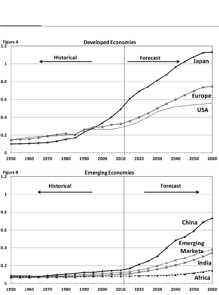
CHAPTER 4 The Entitlement Crisis 61
FIGURE 4–1
Ratio of Retirees to Workers in Developed and Emerging Economies 1950–2060

But the impact of the age wave reaches beyond raising the prices of
the goods and services that are traded on world markets. The age wave
also has a negative impact on the value of assets that workers accumu-
late to enable them to consume during retirement. This is because the
value of stocks and bonds, like the value of any good, is determined by
supply and demand. The buyers are savers, and the savers are the work-
ers who consume less than they earn, using the money they save to accu-
mulate assets that they can, in turn, sell in their retirement. The sellers of
assets are the retirees who need to generate funds to consume during the
period when they do not earn income from working.
An increase in the number of retirees generates an excess of sell-
ers over buyers, a situation that could depress asset prices substan-
tially. Lower asset prices are the market’s way of saying that the
economy cannot accommodate retirees’ expectations of early retire-
ment and generous health and income benefits. As the value of their
assets falls, baby boomers will have to work longer and retire later
than they had planned.
But how much longer will that be? The impact of the baby boomers
on the retirement age in the United States can be seen by referring to
Figure 4-2. Scenario A is the case where the developed world must rely
on the output produced by its own workers and not on increased
imports from abroad to supply the goods demanded by the retirees.
The impact on the retirement age is dramatic. The retirement age
must increase from the current age of 62 to 77 by the middle of this cen-
tury, a 15-year rise that easily outstrips the increase in life expectancy.
This scenario will reduce the retirement period from the current level of
15.8 years to 7 years, a reduction of more than 50 percent, and will
reverse most of the gains made by retirees in the postwar period.6
WORLD DEMOGRAPHICS AND THE AGE WAVE
It is analyses such as these that have led to the pessimistic forecasts of
asset returns by those evaluating the aging of the population. Some
researchers have used the specific demographics of each country to pre-
dict country asset returns based on these demand and supply conditions.7
But viewing the future through the lens of each country’s demo-
graphics is wrong. One must envision the world as one economy and
not as separate nations where each tries to match its own consumption
to its own production. In a world of expanding global trade, the young
of the developing nations can produce goods for—and buy assets
from—the retirees of the world’s developed nations.
62 PART I Stock Returns: Past, Present, and Future
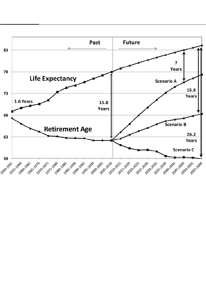
The reason that this could be significant is that although the devel-
oped world has a marked “age wave,” the rest of the world does not.
Outside Japan, Europe, and the United States, the emerging economies
have very young populations.
Figure 4-1B plots the retiree-to-worker ratio of the developing coun-
tries. To be sure, the ratio of retirees to workers rises in almost all coun-
tries. But with the exception of China, the rise in the number of retirees in
the emerging economies is much more gradual than in the developing
countries. From 2013 to 2033 when the majority of baby boomers in
developed countries retire, the number of retirees per 100 workers rises
from 11 to only 18 in the emerging economies, far less than the United
States, where the ratio increases from 27 to 45. For Africa, the number of
retirees per 100 workers is virtually unchanged at the extremely low level
of 7.5. And even for China, the most rapidly aging emerging economy
because of its one-child policy, the number of retirees per 100 workers
CHAPTER 4 The Entitlement Crisis 63
FIGURE 4–2
Life Expectancy and Retirement Age Under Different Growth Scenarios 1950–2060

rises from 14 to 30 over the next 20 years, and its retiree ratio does not
eclipse that of the United States until 2060.
FUNDAMENTAL QUESTION
The question is, can the workers in the emerging markets produce
enough goods to provide for the retirees of the developed world, and
can these workers save enough income to purchase the assets that must
be sold by the developed-world retirees to finance their retirement?
Right now, the answer is no. Although 80 percent of the world’s popula-
tion lives in the developing countries, those economies only produce
about one-half of the world’s output.
But that proportion is changing rapidly. In 1980 in China, Deng
Xiaoping altered the course of the Chinese economy, opened it to market
forces, and launched the country into a period of rapid and sustained
growth. Per capita income, measured in terms that equate the purchasing
power of the U.S. and Chinese currencies, has risen from only 2.1 percent
of the U.S. level in 1980 to 16.1 percent in 2010. Since China has nearly
four times the population as the United States, China will be the world’s
largest economy when its per capita income reaches 25 percent of that of
the United States, which is forecast to occur around 2016. And the econ-
omy of China will become twice the size of the U.S. economy in 2025 if
both countries’ per capita income continues to grow at recent rates.
A decade after China began its rapid growth, a similar transforma-
tion occurred in India. Prime Minister Narasimha Rao, along with his
finance minister Manmohan Singh, initiated the economic liberalization
of India in 1991. The reforms did away with many bureaucratic require-
ments, reduced tariffs and interest rates, and ended many public
monopolies. Since that time, India has begun growing more rapidly, and
although current growth is less than that of China, India’s total GDP will
likely exceed that of the United States in the 2030s and eventually exceed
China’s output.
Figure 4-3 shows how the distribution of world GDP will evolve
based on IMF and OECD forecasts of productivity growth and U.N. fore-
casts of population growth in each country. In 1980, the developed world
produced three-quarters of the world output, with the United States pro-
ducing one-quarter. Currently, the developed world produces about one-
half of the world’s GDP. In 20 years that will shrink to one-third, and by
the end of this century, it will fall to one-quarter. By contrast, the output
of the emerging economies will increase to three-quarters of the world
GDP by the end of this century.
64 PART I Stock Returns: Past, Present, and Future
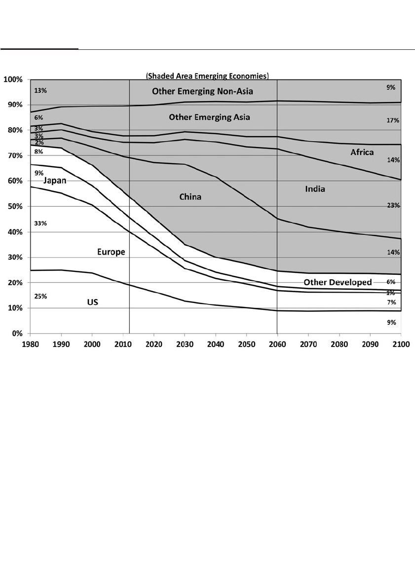
The GDP growth of China and India is particularly noteworthy.
China has grown from only 2 percent of world output in 1980 to 16 per-
cent today and is forecast to reach a maximum of 32 percent of world
output in 2032 before falling back to 14 percent by the end of the century.
This decline is due to China’s one-child policy plus the fact that as its per
capita GDP nears that of developed countries, its growth will slow. India
has grown from 3 percent of world GDP in 1980 to 6 percent today and
is forecast to be 11 percent of world GDP by 2032. By 2060, India’s econ-
omy is projected to be larger than China’s because of its greater popula-
tion growth. India is forecast to produce about one-quarter of world
GDP from 2040 through the rest of this century.
Africa remains a small part of the world economy until 2070, when
it begins to expand rapidly, reaching 14 percent, the same size as the
economy of China, by the end of the century. The assumptions used to
CHAPTER 4 The Entitlement Crisis 65
FIGURE 4–3
World GDP 1980-2100 Based on IMF, OECD, and U.N. Forecasts

project Africa’s growth are quite conservative and will likely understate
the importance of Africa in the second half of this century. It is very dif-
ficult to determine when and whether an underdeveloped economy will
take off, as China’s did in the 1980s and India’s did one decade later.
Current IMF assumptions assume a 5 percent growth rate for sub-
Saharan Africa, greater than that of the developed world but far below
what Asia has achieved. Since Africa is forecast to house nearly one-
third of the world’s population by the end of this century (and that
assumes that the fertility rate of Africa will decline markedly over this
period), if this continent can achieve rapid growth, it could potentially
overtake Asia as the world’s largest producer.
Other researchers have confirmed the importance of the emerging
nations to the world economy. Homi Khara, of the OECD Development
Centre, has estimated that the “middle class,” defined as those earning
between $3,650 and $36,500 per year, will increase by more than 3 bil-
lion, or 170 percent, between 2009 and 2030.8And their spending will
increase by 150 percent, rising by over $34 trillion, more than twice the
current size of the U.S. economy. More than 80 percent of that growth is
projected to occur in Asia. In contrast, total spending in Western Europe
and the United States will barely increase over that time.
The growth of the emerging economies has profound implications
for developed countries. First, many of the goods that will be demanded
by the retirees in the developed world will be produced by the workers
in the emerging world. And the income earned from selling those goods
will be used to increase not only the workers’ consumption but also their
saving. Asians are naturally high savers; even rich and aged countries
like Japan have national saving ratios of nearly 25 percent, well above
that of most Western economies and more than double that of the United
States.
The growth in savings by investors in the emerging economies sug-
gests that the financial markets in the developed world may not be over-
whelmed by assets sold by the aging boomers. If the growth of
productivity in the emerging markets can average 4.5 percent a year
over the next half century, which is equal to the average since 1990, then
the future retirement age in the United States will follow Scenario B in
Figure 4-2.
To be sure, Scenario B does not allow for a further decline in the
retirement age, nor does it stabilize the retirement age at its current level
of 62. But it does stabilize the number of years an average worker will
live in retirement—by increasing the retirement age at the same rate as
the increase in life expectancy.
66 PART I Stock Returns: Past, Present, and Future
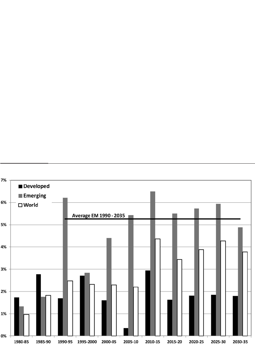
Figure 4-4 shows the past and future projected rates of productivity
growth in developed and developing countries from 1980 through 2035.
Productivity growth has averaged nearly 5 percent over the past 20
years in the emerging economies, a period that includes the Great
Recession.
Is it possible that the retirement age in the developed world could
continue to fall? Scenario C presents the extremely optimistic prospects
that would prevail if all the emerging economies can grow as fast as the
9 percent rate that China has grown over the past 20 years. In that case
there will be so many goods produced that the demands of the baby
boomers in the developed world will be completely offset by the surge
in production of goods and services by the developing world. The retire-
ment age in the United States would continue to decline and lead to a
retirement period that would exceed 26 years by 2060.
CHAPTER 4 The Entitlement Crisis 67
FIGURE 4–4
Historical and Forecast Productivity Growth of Developed and Emerging Economies 1980–2035

EMERGING ECONOMIES CAN FILL THE GAP
At the beginning of the chapter, I posed the question: Who will produce
the goods that the retirees will consume, and who will buy the assets
that they must sell to finance that consumption?
We now know the answer is the workers and investors from the
developing countries. As they sell their output to the developed
economies, they will be paid by the proceeds for selling the stocks and
bonds that are now held by the baby boom population. The extent to
which they can mitigate the age wave is directly linked to their economic
growth. If they continue to grow rapidly, it is likely that most of
the stocks and bonds issued by firms in the United States, Europe, and
Japan will be owned by investors in the developing world. By the mid-
dle of this century, Chinese, Indians, and other investors from these
young economies will gain majority ownership of most of the large
global corporations.
Some may question why investors from emerging economies will
buy Western assets when their countries are growing so rapidly. The
answer is that in a global environment, firms’ prospects are no longer
tied to their country of origin. The growth of the emerging markets gen-
erates huge opportunities for Western firms marketing to the new mid-
dle class. And growth in the emerging economies also puts tremendous
demands on their infrastructure. Infrastructure spending in emerging
economies is estimated to be between 2 and 3 percent of global GDP
over the next 20 years. This amounts to over $2 trillion per year, and U.S.
firms are leading beneficiaries of this spending.9
There is little doubt that consumers in rapidly expanding economies
are attracted to brand names, and Western brand names hold a special
appeal. This is illustrated by the 2013 Best Global Brands report from
Interbrand, a consulting company owned by the Omnicom Group. The
report ranks what it deems the 100 most valuable global brands on crite-
ria that include financial performance, the role the brand plays in influ-
encing the choices made by consumers, and the brand’s ability to help its
parent’s earnings. U.S.-headquartered firms own the top 7 brands (Apple,
Google, Coca-Cola, IBM, Microsoft, GE, and McDonald’s) and 14 of the
top 20.
What happens if Western firms do not compete effectively in the
global marketplace? In that case, one can be certain that foreign com-
petitors will step up to fill the void. But those Western firms with brand-
name recognition are more likely to be bought by foreign investors who
will supply the expertise needed to sell in these foreign markets.
68 PART I Stock Returns: Past, Present, and Future

CAN PRODUCTIVITY GROWTH KEEP PACE?
Productivity growth drives our standard of living.10 The rapid produc-
tivity growth in the emerging economies is based on borrowing and
using the technology that has already been developed by the most
advanced economies.
But productivity growth in the developed countries must rely on
innovation and invention since these economies are already operating at
the frontier of technological know-how. Historically, productivity in the
developed world has increased at a remarkably steady 2 to 2½ percent per
year, which means that every 35 years the standard of living doubles.11
But some economists, such a Professor Robert Gordon of
Northwestern University, believe that productivity growth is due to fall
dramatically in the United States.12 He cites the aging of the population,
growing income inequality, and faltering educational achievement,
among others factors, as the reasons for the decline. Except for the top 1
percent of the income distribution, Gordon predicts the vast majority of
the U.S. population will experience growth of only 0.5 percent per year,
less than one-quarter the long-term average.
Others have echoed Professor Gordon’s pessimism and complain
that discoveries today have not changed people’s lives as fundamentally
as they did a century ago. Tyler Cowen, an economist at George Mason
University and author of The Great Stagnation, has voiced his belief that
the developed world is on a technological plateau and that all the low-
hanging fruit has already been discovered.13
Indeed, look at Table 4-1. It shows the most important life-changing
inventions of the past 100 years. Those that took place in the first half of
that period appear far more important than those of the second half in
transforming the life of the average individual.14
There are some in Silicon Valley who also believe that the United
States is in a downtrend. Peter Thiel, founder of PayPal, has claimed that
innovation in America is “somewhere between dire straits and dead.”15
This downbeat view has spread to many in the investment community.
Bill Gross and Mohammed El-Erian, heads of the giant investment firm
PIMCO, coined the term new normal in 2009 to describe a condition
where U.S. economic growth will sink to 1 to 2 percent, well below the
3+ percent that it has averaged in the post–World War II period.16 Other
investment managers have also embraced the concept.17
Even if growth is slower in the United States, this does not mean that
growth rates will decline around the world. Although the life-changing
innovations cited in the first column of Table 4-1 have long existed in the
CHAPTER 4 The Entitlement Crisis 69

developed world, the developing world is just beginning to acquire the
conveniences of advanced economies. In 2006 the United Nations Human
Development Report estimated that 2.6 billion people, or 40 percent of the
world’s population, had no indoor plumbing. Electrification, refrigera-
tion, and basic healthcare still elude billions of people. Indeed, a large part
of the increase in the world’s income and wealth over the next several
decades involves the developing world acquiring the lifestyle that the
developed world has long possessed.
I do not believe that even the developed world’s productivity is
necessarily on a downward path. The digitization and instant availabil-
ity of information will combine to spur faster productivity growth.
When we study history, we find that inventions that hastened com-
munication, such as Ts’ai Lun’s discovery of paper in the first century
and Johannes Guttenberg’s invention of the printing press in the fif-
teenth century, preceded periods of rapid discovery and innovation.18 In
the nineteenth and twentieth centuries, the telegraph and then the tele-
phone spurred growth by enabling the first instant communication
between distant individuals.
But no recent discovery has as much potential to foster innovation
as the Internet. Soon virtually everything that has ever been written and
recorded—on tape, on film, in print, or digitally—will be instantly acces-
sible online. For the first time in human history, there is the real prospect
of virtually free and unlimited connectivity of every researcher to the
world’s body of knowledge on any subject.
70 PART I Stock Returns: Past, Present, and Future
T A B L E 4–1
Life-Changing Inventions of the Past 100 Years
1910–1960 1960–2010
Electricity Birth control
Indoor plumbing Mobile phone
Washing machine Internet
Refrigeration Personal computer
Automobile
Telephone
Television/movies
Large computers
Air travel
Antibiotics/vaccines
Atomic energy

Professor Charles Jones of Stanford University has conducted
extensive research on productivity growth and claims that 50 percent of
U.S. growth between 1950 and 1993 can be attributed to the rise in
worldwide—not just country specific—research intensity. His paper
“Sources of U.S. Economic Growth in a World of Ideas” claims that a sig-
nificant determination of productivity growth is “the implementation of
ideas that are discovered throughout the world . . . which in turn is pro-
portional to the total population of innovating countries.”19
It is, indeed, the growth in the number of the “innovating countries”
that paints a bright picture for our future. In the past century over 90 per-
cent of the Nobel Prize winners in the scientific discipline were European
and American, even though they constituted only a small fraction of the
world’s population. That is set to change radically. The opening of China
and India alone has more than doubled those with access to the world’s
research. And language barriers are disappearing as technology enables
instant translation. This implies that productivity growth will not decline
but will actually rise in the coming decades.20
CONCLUSION
If most high-income countries, including the United States, have to rely on
their own workers to produce goods and services for their aging popula-
tion, there must be a dramatic rise in the retirement age, an increase that
would far outstrip the expected increase in life expectancy. But as produc-
tivity rises in the world’s developing economies, there will likely be enough
workers to produce the goods and sufficient savers to buy the assets of the
retiring boomers with only moderate increases in the retirement age. This
growth will enable the future returns on equities to be near their historical
levels.
Clearly this favorable scenario may not come to pass. Trade wars,
restrictions on the flow of capital, and a pullback from the pro-growth
policies in Asia and elsewhere will have a negative impact on both the
economy and equity returns. Yet there are also good reasons why produc-
tivity may advance more rapidly, not only in the developing world, but
also in developed economies. The communications revolution has enabled
researchers to collaborate on a scale unthinkable just a few years ago. And
collaboration drives discovery, innovation, and invention. As Fed
Chairman Ben Bernanke stated in his 2013 graduation address at Bard
College at Simon’s Rock, “Both humanity’s capacity to innovate and the
incentives to innovate are greater today than at any other time in history.”21
CHAPTER 4 The Entitlement Crisis 71
This page intentionally left blank

PART
THE VERDICT
OF HISTORY
II
This page intentionally left blank

Stock and Bond Returns
Since 1802
I know of no way of judging the future but by the past.
—PATRICK HENRY, 1775 SPEECH IN THE VIRGINIA
CONVENTION, MARCH 23, 1775
FINANCIAL MARKET DATA FROM 1802 TO THE PRESENT
This chapter analyzes the returns on stocks, bonds, and other assets
classes over the last two centuries. U.S. history is divided here into three
subperiods. In the first subperiod, from 1802 through 1870, the United
States made a transition from an agrarian to an industrialized economy,
comparable to the changes that many “emerging markets” of Latin
America and Asia are making today. In the second subperiod, from 1871
through 1925, the United States became the foremost political and eco-
nomic power in the world. The third subperiod, from 1926 to the pres-
ent, covers the Great Depression, the postwar expansion, the tech
bubble, and the 2008 financial crisis.
These time periods are chosen not only because they are historically
significant, but because they also mark breaks in the quality and com-
prehensiveness of the historical data on stock returns. The most difficult
stock returns to collect were those from 1802 through 1871 because few
dividend data were available from that period. In prior editions of Stocks
for the Long Run I used a stock price index based on the research of
Professor William Schwert.1But his research did not include dividends,
75
5

so I estimated a dividend yield using dividend data and macroeconomic
information from the second subperiod. The dividend yields I obtained
for the first period were consistent with other historical information that
had been published about early-period dividend yields.2
In 2006, two of the prominent researchers in the field of U.S. stock
returns, Bill Goetzmann and Roger Ibbotson of Yale University, pub-
lished the most thoroughly documented research on stock returns before
1871.3Their research, which took more than a decade to complete, deter-
mined monthly price and dividend data on more than 600 individual
securities over more than a century of stock data. The 6.9 percent annual
stock return that I use in this volume for the 1802–1871 period is based
on this Goetzmann-Ibbotson research and is only 0.2 percentage points
below my earlier estimates of early-nineteenth-century stock returns.4
For the years 1871 through 1925, the returns on stocks are calcu-
lated using a capitalization-weighted index of all NYSE stocks (includ-
ing reinvested dividends) and are taken from the well-regarded indexes
compiled by the Cowles Foundation and reported in Shiller.5The data
from the third period, from 1925 to the present, are the most thoroughly
researched and are taken from the Center for Research in Security Prices.
These returns represent a capitalization-weighted index of all New York
Stock Exchange stocks and, starting in 1962, all American and Nasdaq
stocks. The behavior of stock and bond returns since 1925 has also been
researched by Roger Ibbotson, who has published yearbooks that have
become benchmarks for U.S. asset returns since 1972.6All the stock and
bond returns reported in this volume, including those from the early
nineteenth century, are free from “survivorship bias,” a bias that arises
from only using the returns from firms that have survived and ignoring
the lower returns from firms that have disappeared over time.
TOTAL ASSET RETURNS
The story of these assets is told in Figure 5-1. It depicts the total nominal
(not inflation adjusted) return indexes for stocks, long- and short-term
government bonds, gold, and commodities from 1802 through 2012.
Total return includes changes in the capital value plus interest or divi-
dends and assumes that all these cash flows are automatically rein-
vested in the asset over time.
It can be easily seen that over the last two centuries the total return
on equities dominates all other assets. The amount of $1 invested in a
capitalization-weighted portfolio in 1802, with reinvested dividends,
would have accumulated to almost $13.5 million by the end of 2012.
76 PART II The Verdict of History
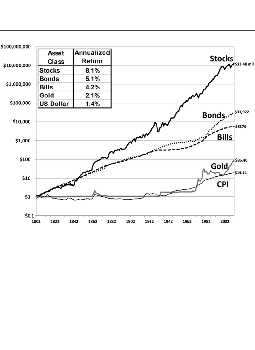
Even the cataclysmic stock crash of 1929, which caused a generation of
investors to shun stocks, appears as a mere blip in the total stock return
index. Bear markets, which so frighten those who hold equity invest-
ments, pale in the context of the upward thrust of stock returns.
It is important to understand that the total return on stocks
depicted in Figure 5-1 does not represent the growth in the total value of
the U.S. stock market. The wealth in stocks increases at a rate signifi-
cantly slower than that of total stock return. The reason that total return
grows faster than stock wealth is because investors consume most of the
dividends paid by stocks, and therefore these dividends are not rein-
vested and cannot be used by firms to create capital. It would take only
$1.33 million invested in the stock market in 1802 to grow, with divi-
dends reinvested, to about $18 trillion, the total value of U.S. stocks, by
the end of 2012. The sum of $1.33 million in 1802 is equivalent to roughly
CHAPTER 5 Stock and Bond Returns Since 1802 77
FIGURE 5–1
Total Nominal Returns and Inflation 1802–2012

78 PART II The Verdict of History
$25 million in today’s purchasing power, an amount far less than the
value of the stock market at that time.7
Although financial theory (and government regulations) require
that total return be calculated with reinvested dividends (or other cash
flows), it is rare for anyone to accumulate wealth for long periods of time
without consuming part of his or her return. The longest period of time
investors typically hold onto assets without touching the principal and
income occurs when they are accumulating wealth in pension plans for
their retirement or in insurance policies that are passed on to their heirs.
Even those who bequeath fortunes untouched during their lifetimes
must realize that these accumulations are often dissipated in the next
generation or spent by the foundations to which the money is
bequeathed. The stock market has the power to turn a single dollar into
millions by the forbearance of generations—but few will have the
patience or desire to endure the wait.
THE LONG-TERM PERFORMANCE OF BONDS
Fixed-income investments are the largest and most important financial
asset competing with stocks. Bonds promise fixed monetary payments
over time. In contrast to equity, the cash flows from bonds have a maxi-
mum monetary value set by the terms of the contract. Except in the case
of default, bond returns do not vary with the profitability of the firm.
The bond series shown in Figure 5-1 are based on long- and short-
term U.S. Treasury bonds, when available; if they were not available, as
occurred in some of the early years of our sample, the highest-grade
municipal bonds were chosen. Default premiums were estimated and
removed from the interest rates of riskier securities in order to obtain a
comparable high-grade sample over the entire period.8
The interest rates on long-term bonds and short-term bonds (called
bills), over the 210-year period, are displayed in Figure 5-2. Interest rate
fluctuations during the nineteenth and early twentieth centuries
remained within a narrow range. But from 1926 to the present, the
behavior of both long- and short-term interest rates changed dramati-
cally. During the Great Depression of the 1930s, short-term interest rates
fell to nearly zero, and in October 1941 the yield on the 20-year Treasury
bond fell to a record low of 1.82 percent. In order to finance record
wartime borrowings, the government maintained extraordinarily low
rates during World War II and the early postwar years.
The 1970s marked an unprecedented change in the behavior of
interest rates. Inflation reached double-digit levels, and interest rates
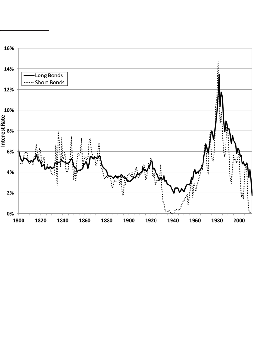
soared to heights that had not been seen since the debasing of the conti-
nental currency in the early years of the republic. Never before had infla-
tion, and therefore interest rates, been so high for so long.
The public clamored for government action to slow rising prices.
That cry was answered by Paul Volcker, chairman of the Federal Reserve
System since 1979, who sent interest to near 20 percent and eventually
brought inflation and interest rates down to moderate levels. The
change in the behavior of interest rates is directly related to the changes
in the determinants of the price level.
GOLD, THE DOLLAR, AND INFLATION
Consumer prices in the United States and the United Kingdom over the
past 200 years are depicted in Figure 5-3. In each country, the price level
CHAPTER 5 Stock and Bond Returns Since 1802 79
FIGURE 5–2
U.S. Long- and Short-Term Interest Rates 1800–2012
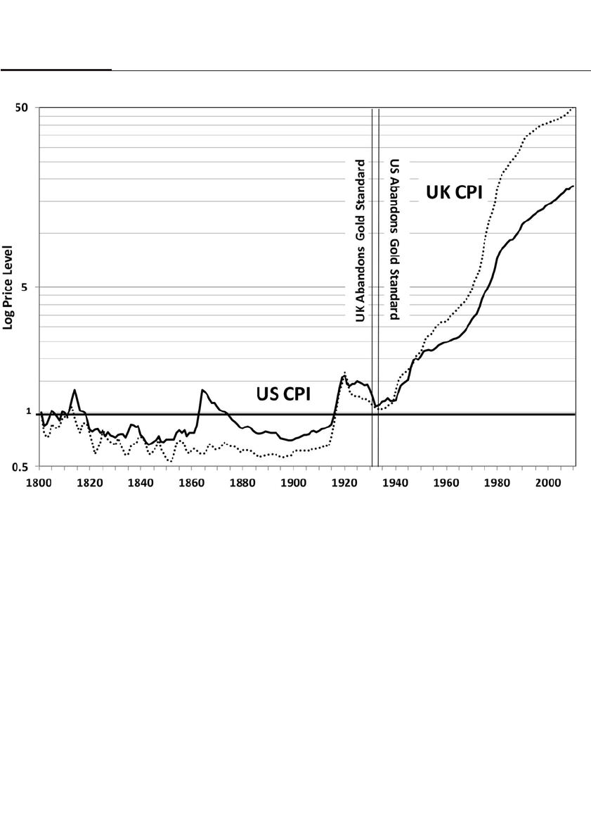
80 PART II The Verdict of History
at the beginning of World War II was essentially the same as it was 150
years earlier. But after World War II, the nature of inflation changed dra-
matically. The price level rose almost continuously after the war, often
gradually, but sometimes at double-digit rates, as in the 1970s.
Excluding wartime, the 1970s witnessed the first rapid and sustained
inflation ever experienced in U.S. or British history
The dramatic changes in the inflationary trend can be explained by
the change in the monetary standard. During the nineteenth and early
twentieth centuries, the United States, the United Kingdom, and the rest
of the industrialized world were on a gold standard. As shown in Figure
5-1, the price of gold and the price level were very closely linked during
this period. That is because the gold standard restricts the supply of
money and hence the inflation rate. But from the Great Depression
through World War II, the world shifted to a paper money standard.
Under a paper money standard there is no legal constraint on the
FIGURE 5–3
U.S. and U.K. Consumer Price Index 1800–2012

issuance of money, so inflation is subject to political as well as economic
forces. Price stability depends on the desire of central banks to limit the
growth of the supply of money in order to counteract deficit spending
and other inflationary forces that result from government spending and
regulation.9
The chronic inflation that the United States and other developed
economies have experienced since World War II does not mean that the
gold standard was superior to the current paper money standard. The
gold standard was abandoned because of its inflexibility in the face of
economic crises, particularly during the banking collapse of the 1930s.
The paper money standard, if properly administered, can prevent runs
on banks and severe depressions that plagued the gold standard while
maintaining inflation at low to moderate levels.
But monetary policy was not well run. Gold prices soared to $850
per ounce in January 1980, following the rapid inflation of the 1970s.
When inflation was finally brought under control, gold prices fell, but
they rose again after the 2008 financial crisis when the flood of credit
issued by central banks stoked fears of inflation. By the end of 2012, the
price of gold reached $1,675 per ounce, and $1 of gold bullion purchased
in 1802 was worth $86.40 at the end of 2012, while the price level itself
increased by a factor of 19.12. Nevertheless, although gold protects
investors against inflation, the yellow metal offers little more. Whatever
hedging property gold possesses, this precious metal will likely exert a
considerable drag on the return of a long-term investor’s portfolio.10
TOTAL REAL RETURNS
The focus of long-term investors should be the growth of purchasing
power of their investment—that is, the creation of wealth adjusted for
the effects of inflation. Figure 5-4 reproduces Figure 1-1 in Chapter 1 and
is constructed by taking the dollar returns shown in Figure 5-1 and cor-
recting (or “deflating”) them by the changes in the price level. The annu-
alized real returns for the various asset classes are found in the upper left
corner of the graph.
The compound annual real return on stocks is approximately 6.6
percent per year after inflation. Despite the addition of 20 years of stock
market data since the first edition of Stocks for the Long Run, this return is
just one-tenth of a percentage point lower than the 6.7 percent return
that I reported in 1994.11
Some have maintained that this return is not sustainable since it is
almost double the 3.0 to 3.5 percent growth rate of real GDP.12 But that is
CHAPTER 5 Stock and Bond Returns Since 1802 81
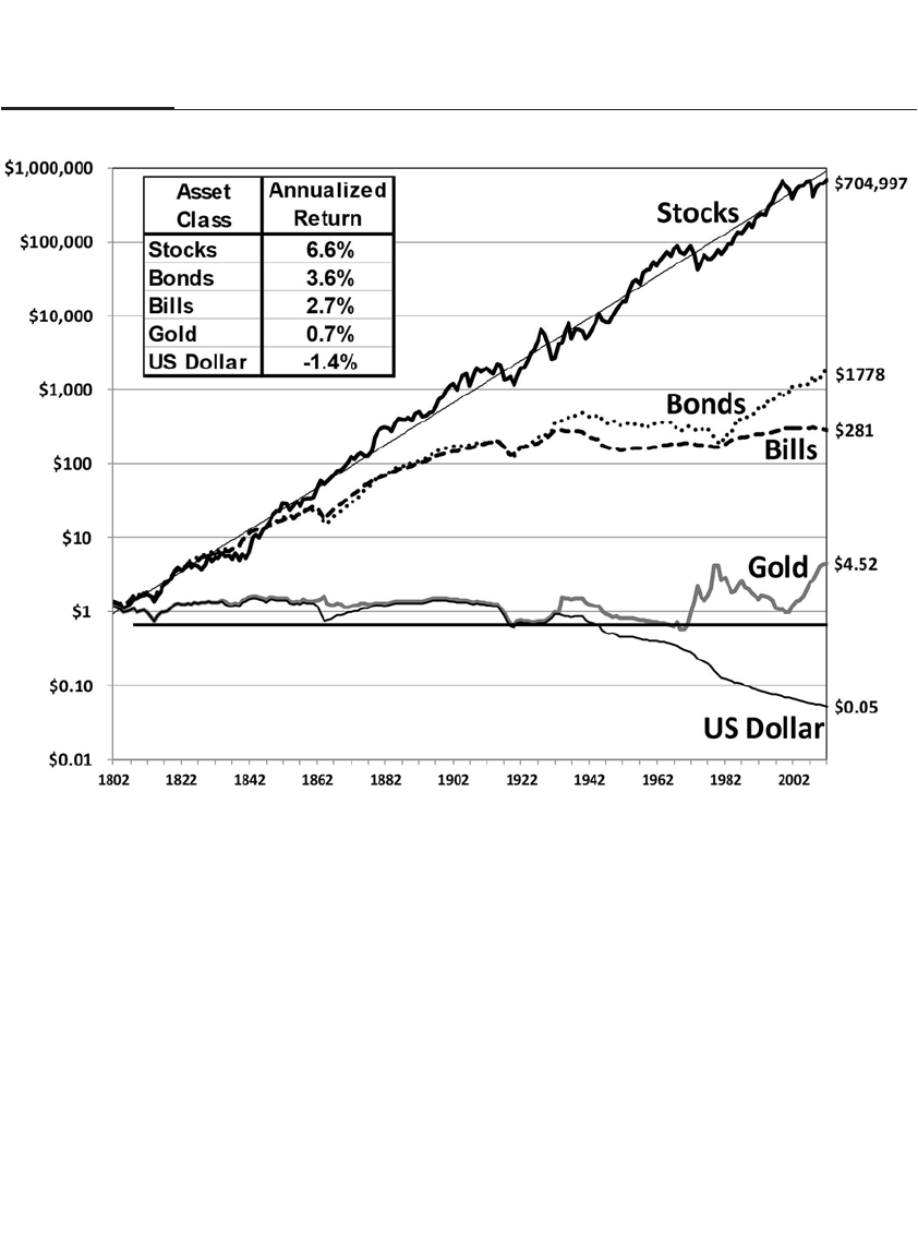
82 PART II The Verdict of History
incorrect. Even if the economy is not growing at all, capital will receive a
positive return because it is a scarce resource, just as labor will be paid
positive wages and land will be paid positive rents. As noted earlier, the
total real return on stocks assumes that all dividends and capital gains
are reinvested into the market, and this sum grows far faster than total
stock wealth or GDP.13
The annual returns on U.S. stocks over various time periods are
summarized in Table 5-1. Note the extraordinary stability of the real
return on stocks over all major subperiods: 6.7 percent per year from
1802 through 1870, 6.6 percent from 1871 through 1925, and 6.4 percent
per year from 1926 through 2012. Even since World War II, during which
all the inflation that the United States has experienced over the past 200
years occurred, the average real rate of return on stocks has been 6.4 per-
cent per year. This is virtually identical to the real return on stocks dur-
ing the previous 125 years, which saw no overall inflation. Stocks
FIGURE 5–4
Total Real Returns on U.S. Stocks, Bonds, Bills, Gold, and the Dollar, 1802–2012

83
TABLE 5–1
Real Returns on Stocks, Gold, and Inflation 1802–2012
Total Nominal Total Real
Nominal Capital Real Capital Real
Return Appreciation Dividend Return % Appreciation Gold Price
Return Risk Return Risk Yield Return Risk Return Risk Return Inflation
1802–2012 8.1 17.6 2.9 17.2 5.1 6.6 18.0 1.5 17.4 0.7 1.4
1871–2012 8.7 18.9 4.1 18.4 4.4 6.5 19.1 2.0 18.5 1.0 2.0
I 1802–1870 6.9 14.5 0.4 14.0 6.4 6.7 15.4 0.3 14.8 0.2 0.1
II 1871–1925 7.3 16.5 1.9 15.9 5.3 6.6 17.4 1.3 16.9 –0.8 0.6
III 1926–2012 9.6 20.3 5.5 19.6 3.9 6.4 20.2 2.5 19.6 2.1 3.0
1946–2012 10.5 17.5 6.8 16.9 3.5 6.4 17.8 2.9 17.2 2.0 3.9
1946–1965 13.1 16.5 8.2 15.7 4.6 10.0 18.0 5.2 17.2 –2.7 2.8
1966–1981 6.6 19.5 2.6 18.7 3.9 –0.4 18.7 –4.1 18.1 8.8 7.0
1982–1999 17.3 12.5 13.8 12.4 3.1 13.6 12.6 10.2 12.6 –4.9 3.3
2000–2012 2.7 20.6 0.8 20.1 1.9 0.3 19.9 –1.6 19.4 11.8 2.4
Return = compound annual return
Risk = standard deviation of arithmetic returns
All data in percent (%)
Major
Sub-
Periods
Postwar
Periods

represent real assets, which in the long run appreciate at the same rate as
inflation, so that real stock returns are not adversely affected by changes
in the price level.
The long-term stability of stock returns has persisted despite the
dramatic changes that have taken place in our society during the last two
centuries. The United States evolved from an agricultural to an industrial
economy and then to the postindustrial, service- and technology-
oriented economy it is today. The world shifted from a gold-based stan-
dard to a paper money standard. And information, which once took
weeks to cross the country, can now be instantaneously transmitted and
simultaneously broadcast around the world. Yet despite mammoth
changes in the basic factors generating wealth for shareholders, equity
returns have shown an astounding stability.
But stability in the long-run returns on stocks in no way guarantees
stability in the short run. From 1982 through 1999 during the greatest
bull market in U.S. history, stocks offered an extraordinary after-
inflation return of 13.6 percent per year, more than double the historical
average. These superior returns followed the dreadful returns realized
in stocks the previous 15 years, from 1966 through 1981, when stock
returns fell behind inflation 0.4 percent per year. Nevertheless, this great
bull market carried stocks too high, and the valuation of the market
reached record levels, which in turn led to the poor returns of the fol-
lowing decade. The subsequent bear market and financial crisis plunged
stocks once again well below trend as real stock returns have fallen to a
mere +0.3 percent in the 12 years following the bull market peak of 2000.
REAL RETURNS ON FIXED-INCOME ASSETS
As stable as the long-term real returns have been for equities, the same
cannot be said of fixed-income assets. As Table 5-2 indicates, the real
return on Treasury bills has dropped precipitously from 5.1 percent in
the early part of the nineteenth century to a bare 0.6 percent since 1926,
a return only slightly above inflation.
The real return on long-term bonds has shown a similar, but more
moderate, decline. Bond returns fell from a generous 4.8 percent in the
first subperiod to 3.7 percent in the second and then to only 2.6 percent
in the third. The decline in real yield on government bonds over time can
be partly explained by certain factors that boosted their demand: the
greatly improved liquidity of bonds and the fact that these bonds satisfy
many fiduciary requirements that other fixed-income assets do not.
These demand-boosting factors raised the prices of government bonds
84 PART II The Verdict of History

and therefore reduced their yields. The real returns on longer-term
bonds were also reduced by the unexpected inflation that investors
experienced in the post–World War II period.
The short-run volatility of stock returns from decade to decade is not
unexpected. What may surprise investors is that the volatility of the real
returns on government bonds is also quite large. For the 35-year-period
from 1946 through 1981, the real return on Treasury bonds was negative.
In other words, the coupon on the bonds did not offset the decline in bond
prices brought about by rising interest rates and inflation. As we shall see
in the next chapter, there never has been even a 20-year period, not to
speak of a 35-year period, where real stock returns were negative.
The decline in real returns on bonds since 1926 would have been
much greater if it were not for the stellar bond returns of the past three
decades. Since 1981, the decline in inflation and interest rates has
pushed bond prices upward and greatly improved bondholder returns.
Although bond returns fell well short of equities during stocks’ mega
bull market from 1981 through 1999, bonds easily outpaced stocks in the
following decade. In fact, for the entire three decades that followed the
peak in bond yields in the early 1980s, bond returns virtually matched
those of equities.
CHAPTER 5 Stock and Bond Returns Since 1802 85
T A B L E 5–2
Real Returns on Bonds and Inflation 1802–2012
Long-Term Governments Short-Term Governments
Nominal Real Real
Coupon Return Return Nominal Return Price
Rate Return Risk Return Risk Rate Return Risk Inflation
1802–2012 4.7 5.1 6.7 3.6 9.0 4.2 2.7 6.0 1.4
1871–2012 4.7 5.2 7.9 3.0 9.3 3.6 1.6 4.4 2.0
I 1802–1870 4.9 4.9 2.8 4.8 8.3 5.2 5.1 7.7 0.1
II 1871–1925 4.0 4.3 3.0 3.7 6.4 3.8 3.1 4.8 0.6
III 1926–2012 5.1 5.7 9.7 2.6 10.8 3.6 0.6 3.9 3.0
1946–2012 5.8 6.0 10.8 2.0 11.5 4.3 0.4 3.2 3.9
1946–1965 3.1 1.5 5.0 –1.2 7.1 2.0 –0.8 4.3 2.8
1966–1981 7.2 2.5 7.1 –4.2 8.1 6.8 –0.2 2.1 7.0
1982–1999 8.5 12.1 13.8 8.5 13.6 6.3 2.9 1.8 3.3
2000–2012 4.5 9.0 11.7 6.5 11.6 2.2 –0.2 1.8 2.4
Return = compound annual return
Risk = standard deviation of arithmetic returns
All data in percent (%)
Major
Sub-
Periods
Postwar
Periods
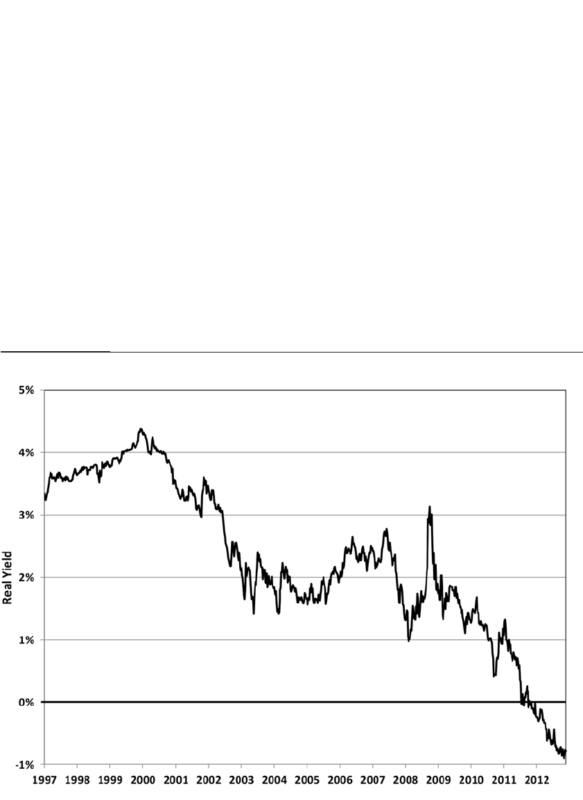
86 PART II The Verdict of History
THE CONTINUING DECLINE IN FIXED-INCOME RETURNS
But those spectacular bond returns cannot continue. Prospective real
returns for Treasury bonds became far easier to determine when, in
January 1997, the U.S. Treasury introduced TIPS, or Treasury inflation-
protected securities. The coupons and principal from these bonds,
backed by the full faith and credit of the U.S. government, are linked to
the U.S. consumer price index, so that the yield on these bonds is a real,
inflation-adjusted yield, shown in Figure 5-5.
The steady decline in the yields on these bonds is readily apparent.
When these bonds were first issued, their yield was just short of 3.5 per-
cent. That is almost identical to the historical real return on government
bonds that I had found in my research analyzing data dating from 1802.
After issuance, the yield on TIPS increased, reaching a high of 4.40 per-
FIGURE 5–5
Real Yield on 10-Year Treasury Inflation-Protected Securities (TIPS) 1997–2012

cent in January 2000, the month that also marked the peak of the tech
and Internet bubble.
From that date, the yield on TIPS began a relentless decline. From
2002 through 2007 the yield fell to 2 percent. As the financial crisis deep-
ened, the yield continued to decline and sank below zero in August
2011, reaching nearly –1 percent by December 2012.14 This negative real
yield was similar to the implied after-inflation yields on the standard
Treasury bonds. The yield on the 10-year Treasury bond fell to a 75-year
low of 1.39 percent in July 2012, well below the ongoing and forecast
rate of inflation.
The real yield on Treasury bonds is determined by many factors,
such as the state of the economy, fears of inflation, and the risk attitudes
of investors. But in almost all economic models, the most important fac-
tor influencing the real return on bonds is economic growth. Indeed, the
3.4 percent yield set at the first TIPS auction was almost exactly equal to
real GDP growth in the 1990s. As real economic growth slowed to about
2 percent from 2002 through 2007, the yields on TIPS fell accordingly.
But no forecaster in 2012 predicted real economic growth over the
next decade would be negative, as the yield on TIPS suggested. Only
extreme risk aversion can explain why investors were willing to accept
negative after-inflation returns on government bonds even though other
assets, such as equities, have consistently delivered long-term real
returns of 6 to 7 percent per year.
THE EQUITY PREMIUM
The excess return of stocks over bonds (either long or short) is referred
to as the equity risk premium, or simply the equity premium. It can be meas-
ured historically, as shown in Figure 5-6, or prospectively, on the basis of
current bond yields and stock valuations. Subtracting stock and bond
returns from Tables 5-1 and 5-2 shows that the equity premium has aver-
aged 3.0 percent against Treasury bonds and 3.9 percent against
Treasury bills over the entire 210 years.
Because of the extraordinary returns on long-term bonds over the
past 30 years, the historical equity premium of stocks over bonds has
shrunk to zero. But the forward-looking equity premium at the end of
2013 is far higher since the prospective real yields on long bonds have
fallen so low. If forward-looking equity returns match their historical
average, the forward-looking equity premium in 2013 could be 6 percent
or more.15
CHAPTER 5 Stock and Bond Returns Since 1802 87
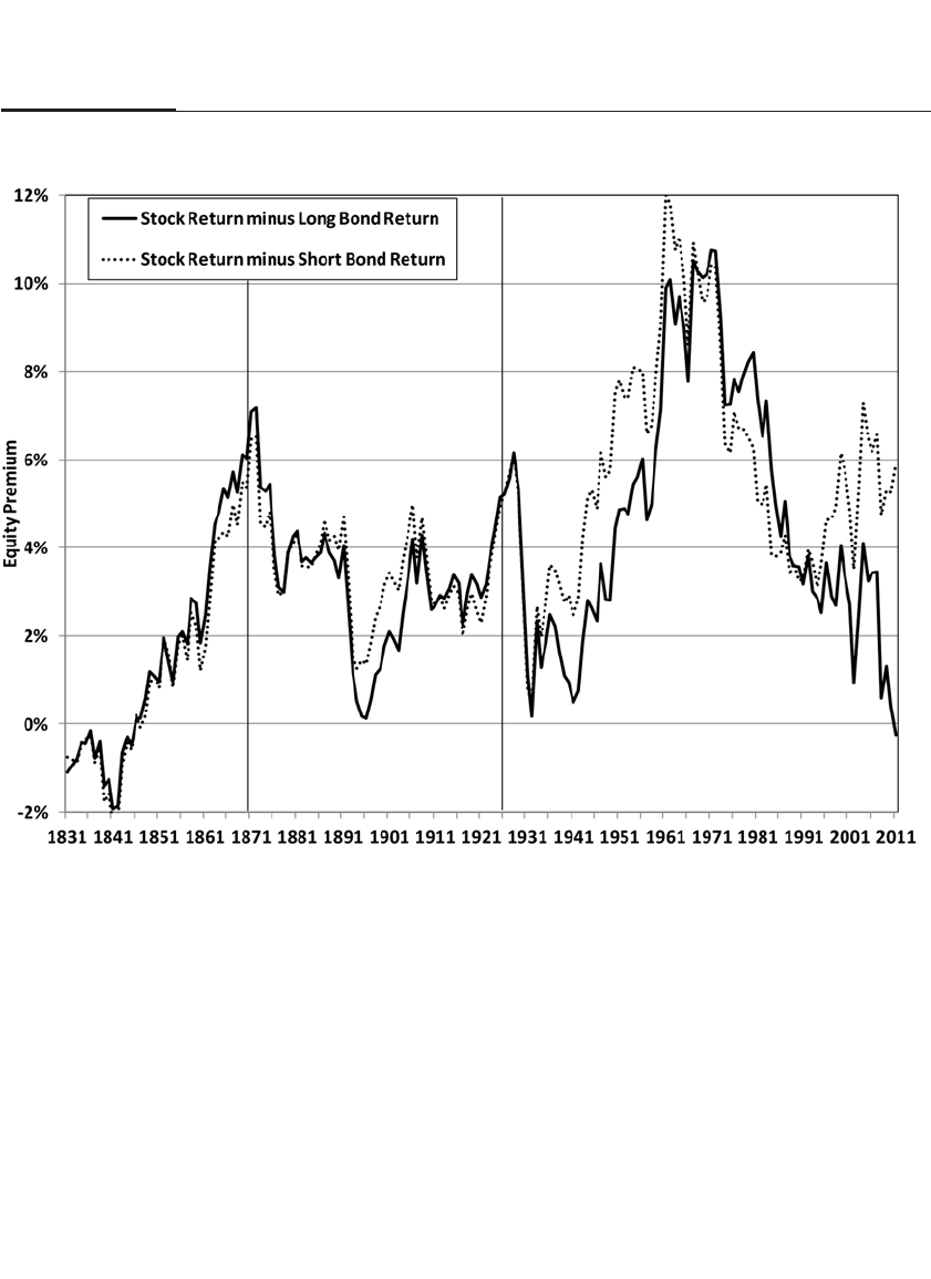
WORLDWIDE EQUITY AND BOND RETURNS
When I published Stocks for the Long Run in 1994, some economists ques-
tioned whether my conclusions, drawn from data from the United
States, might overstate historical equity returns measured on a world-
wide basis. They claimed that U.S. stock returns exhibited survivorship
bias, a bias caused by the fact that returns are collected from successful
equity markets, such as the United States, but ignored in countries
where stocks have faltered or disappeared outright, such as in Russia or
Argentina.16 This bias suggested that stock returns in the United States,
a country that over the last 200 years has been transformed from a small
British colony into the world’s greatest economic power, are unique and
that historical equity returns in other countries would be lower.
88 PART II The Verdict of History
FIGURE 5–6
The Equity Premium: Difference between 30 Year Return on Stocks and Bonds and Stocks
and Bills 1831–2012
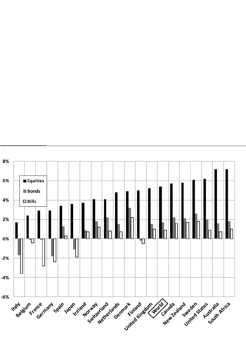
CHAPTER 5 Stock and Bond Returns Since 1802 89
Prodded by this question, three U.K. economists examined the his-
torical stock and bond returns from 19 countries since 1900. Elroy
Dimson and Paul Marsh, professors at the London Business School, and
Mike Staunton, director of the London Share Price Database, published
their research in 2002 in a book entitled Triumph of the Optimists: 101
Years of Global Investment Returns.17 This book provides a rigorous yet
readable account of worldwide financial market returns in 19 different
countries.
Updated returns from this study are given in Figure 5-7, which
shows the average historical real stock, bond, and bill returns of all 19
countries analyzed from 1900 through 2012. Despite the major disasters
visited on many of these countries, such as war, hyperinflation, and
depression, every one of them exhibited substantially positive after-
inflation stock returns.
FIGURE 5–7
International Real Returns on Stocks, Bonds, and Bills 1900–2012

Real equity returns ranged from a low of 1.7 percent in Italy to a
high of 7.2 percent in Australia and South Africa. Stock returns in the
United States, although quite good, were not exceptional. The simple
arithmetic mean of the returns of the 19 countries is 4.6 percent, and a
portfolio that put a single dollar in each of those countries’ stock markets
in 1900 would have produced a compound real return of 5.4 percent,
very close to the 6.2 percent that is found in the United States. And those
countries that had lower stock returns also had lower fixed-income
returns, so that the average equity premium against bonds was 3.7 per-
cent and against bills was 4.5 percent, actually higher than found in the
United States.
When all the information was analyzed, the authors concluded:
. . . that the US experience of equities outperforming bonds and bills has
been mirrored in all sixteen countries examined. . . . Every country
achieved equity performance that was better than that of bonds. Over the
101 years as a whole, there were only two bond markets and just one bill
market that provided a better return than our worst performing equity
market.
Furthermore:
While the US and the UK have indeed performed well, . . . there is no indi-
cation that they are hugely out of line with other countries. . . . Concerns
about success and survivorship bias, while legitimate, may therefore have
been somewhat overstated [and] investors may have not been materially
misled by a focus on the US.18, 19
This last statement is significant. More studies have been made of
the U.S. markets than the markets of any other country in the world.
Dimson, Marsh, and Staunton are saying that the results found in the
United States have relevance to all investors in all countries. The title
they chose for their book suggests their conclusions: it is the optimists,
not the pessimists, who take positions in the equity market, and they
have decidedly triumphed over more cautious investors over the last
century. International studies have reinforced, not diminished, the case
for equities.
CONCLUSION: STOCKS FOR THE LONG RUN
Over the past 210 years, the compound annual real return on a diversi-
fied portfolio of common stock has been between 6 and 7 percent in the
United States, and it has displayed a remarkable constancy over time.
90 PART II The Verdict of History

Certainly the returns on stocks are dependent on the quantity and qual-
ity of capital, productivity, and the return to risk taking. But the ability
to create value also springs from skillful management, a stable political
system that respects property rights, and the capacity to provide value
to consumers in a competitive environment. Swings in investor senti-
ment resulting from political or economic crises can throw stocks off
their long-term path, but the fundamental forces producing economic
growth have always enabled equities to regain their long-term trend.
Perhaps that is why stock returns have displayed such stability despite
the radical political, economic, and social changes that have impacted
the world over the past two centuries.
Yet one must be aware of the political, institutional, and legal frame-
work in which these returns were generated. The superior performance
of stocks over the past two centuries might be explained by the growing
dominance of nations committed to free market economics. Few
expected the triumph of market-oriented economies during the dark
days of the Great Depression and World War II. But if history is any
guide, government bonds in our paper money economies may fare far
worse than stocks in any political or economic upheaval. As the next
chapter shows, even in stable political environments, the risks in govern-
ment bonds actually outweigh those in stocks for long-term investors.
APPENDIX 1: STOCKS FROM 1802 TO 1870
The first actively traded U.S. stocks, floated in 1791, were issued by two
banks: the Bank of New York and the Bank of the United States.20 Both
offerings were enormously successful and were quickly bid to a pre-
mium. But they collapsed the following year when Alexander
Hamilton’s assistant at the Treasury, William Duer, attempted to manip-
ulate the market and precipitated a crash. It was from this crisis that the
antecedents of the New York Stock Exchange were born on May 17, 1792.
Joseph David, an expert on the eighteenth-century corporation,
claimed that equity capital was readily forthcoming not only for every
undertaking likely to be profitable but also, in his words, “for innumer-
able undertakings in which the risk was very great and the chances of
success were remote.”21 Although over 300 business corporations were
chartered by the states before 1801, fewer than 10 had securities that
traded on a regular basis. Two-thirds of those chartered before 1801 were
connected with transportation: wharves, canals, turnpikes, and bridges.
But the important stocks of the early nineteenth century were financial
institutions: banks and, later, insurance companies. Banks and insurance
CHAPTER 5 Stock and Bond Returns Since 1802 91

companies held loans and equity in many of the manufacturing firms
that, at that time, did not have the financial standing to issue equity. The
fluctuations in the stock prices of financial firms in the nineteenth cen-
tury reflected the health of the general economy and the profitability of
the firms to which they lent. One of the first large nonfinancial ventures
was the Delaware and Hudson Canal, issued in 1825, which also became
an original member of the Dow Jones Industrial Average 60 years later.22
In 1830, the first railroad, the Mohawk and Hudson, was listed; and for
the next 50 years, railroads dominated trading on the major exchanges.
92 PART II The Verdict of History

Risk, Return, and
Portfolio Allocation
Why Stocks Are Less Risky
Than Bonds in the Long Run
As a matter of fact, what investment can we find which offers real
fixity or certainty income? . . . As every reader of this book will clearly
see, the man or woman who invests in bonds is speculating in the
general level of prices, or the purchasing power of money.
—IRVING FISHER, 19121
MEASURING RISK AND RETURN
Risk and return are the building blocks of finance and portfolio manage-
ment. Once the risk, expected return, and correlations between asset
classes are specified, modern financial theory can help investors allocate
their portfolios. But the risk and return on stocks and bonds are not
physical constants, like the speed of light or gravitational force, waiting
to be discovered in the natural world. Investors cannot, as in the physi-
cal sciences, run repeated controlled experiments, holding all other fac-
tors constant, and home in on the “true” value of each variable. As
Nobel laureate Paul Samuelson was fond of saying, “We have but one
sample of history.”
93
6

This means that despite the overwhelming quantity of historical
data, one can never be certain that the underlying factors that generate
asset prices have remained unchanged. Indeed we saw in Chapter 3 that
the correlations between assets classes change substantially over time
Yet one must start by analyzing the past in order to plan for the
future. The last chapter showed that not only have fixed-income returns
lagged substantially behind those on equities, but because of the uncer-
tainty of inflation, bonds can be quite risky for long-term investors. In
this chapter investors will see that uncertain inflation will make their
portfolio allocations depend crucially on their planning horizon.
RISK AND HOLDING PERIOD
For many investors, the most meaningful way to describe risk is by por-
traying a worst-case scenario. The best and worst after-inflation returns
for stocks, bonds, and bills from 1802 over holding periods ranging from
1 to 30 years are displayed in Figure 6-1. Here stock returns are meas-
ured, as before, by dividends plus capital gains or losses on a broad-
based capitalization-weighted index of U.S. stocks. Note that the height
of the bars, which measures the difference between best and worst
returns, declines far more rapidly for equities than for fixed-income
securities as the holding period increases.
Stocks are unquestionably riskier than bonds or Treasury bills over
one- and two-year periods. However, in every five-year period since
1802, the worst performance in stocks, at –11.9 percent per year, has been
only slightly worse than the worst performance in bonds or bills. And
for 10-year holding periods, the worst stock performance has actually
been better than that for bonds or bills.
For 20-year holding periods, stock returns have never fallen below
inflation, while returns for bonds and bills once fell as much as 3 percent
per year below the inflation rate. During that inflationary episode, the
real value of a portfolio of Treasury bonds, including all reinvested
coupons, fell by nearly 50 percent. The worst 30-year return for stocks
remained comfortably ahead of inflation by 2.6 percent per year, a return
that is not far below the average performance of fixed-income assets.
It is very significant that stocks, in contrast to bonds or bills, have
never delivered to investors a negative real return over periods lasting
17 years or more. Although it might appear to be riskier to accumulate
wealth in stocks rather than in bonds over long periods of time, for the
preservation of purchasing power, precisely the opposite is true: the
94 PART II The Verdict of History
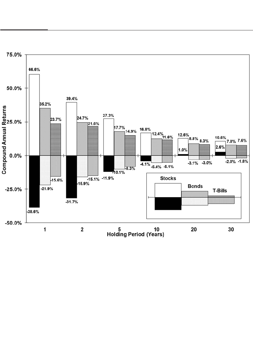
safest long-term investment has clearly been a diversified portfolio of
equities. There is no doubt that inflation-protected U.S. Treasury bonds
safeguard investors from unexpected inflation. But as noted in Chapter
5, the real yields on those securities, even for maturities as long as 20
years, fell below zero in 2012 and remain very low. Stocks, in contrast,
have never given investors a negative real return over a 20-year horizon.
Some investors question whether holding periods of 20 or 30 or
more years are relevant to their planning horizon. But one of the great-
est mistakes that investors make is to underestimate their holding
period. This is because many investors think about the holding periods
CHAPTER 6 Risk, Return, and Portfolio Allocation 95
FIGURE 6–1
Highest and Lowest Real Returns on Stocks, Bonds, and Bills over 1-, 2-, 5-, 10-, 20-, and 30-Year
Holding Periods 1802–2012

of a particular stock, bond, or mutual fund. But the holding period that
is relevant for portfolio allocation is the length of time the investors hold
any stocks or bonds, no matter how many changes are made among the
individual issues in their portfolio.
The percentage of times that stock returns outperform bond or bill
returns over various holding periods is shown in Table 6-1. As the hold-
ing period increases, the probability that stocks will outperform fixed-
income assets increases dramatically. For 10-year horizons, stocks beat
bonds about 80 percent of the time; for 20-year horizons, about 90 percent
of the time; and over 30-year horizons, nearly 100 percent of the time.
In the first four editions of Stocks for the Long Run, I noted that the
last 30-year period when the return on long-term bonds beat stocks
ended in 1861, at the onset of the U.S. Civil War. That is no longer true.
Because of the large drop in government bond yields over the past
decade, the 11.03 percent annual return on long-term government bonds
just surpassed the 10.98 percent on stocks for the 30-year period from
January 1, 1982, through the end of 2011. This striking event caused some
96 PART II The Verdict of History
T A B L E 6–1
Percentage of Time Stocks Outperform Bonds and Bills over Various Holding
Periods
Stocks Stocks
Outperform Outperform
Holding Period Time Period Bonds T-Bills
1 Year 1802–2012 58.8 62.1
1871–2012 61.3 66.9
2 Year 1802–2012 60.5 62.9
1871–2012 64.1 70.4
3 Year 1802–2012 67.2 70.2
1871–2012 68.7 73.3
5 Year 1802–2012 67.6 68.6
1871–2012 69.0 74.6
10 Year 1802–2012 72.3 73.3
1871–2012 78.2 83.8
20 Year 1802–2012 83.9 87.5
1871–2012 95.8 99.3
30 Year 1802–2012 91.2 91.2
1871–2012 99.3 100.0

researchers to conclude that stock returns can no longer be counted on to
surpass bond returns.2
But a closer look at why bonds outperformed stocks during this
period shows that it is almost impossible for bonds to repeat that feat in
the coming decades. In 1981 the interest rate on 10-year U.S. Treasury
bonds reached 16 percent. As interest rates fell, bondholders benefited
from both high coupons and capital gains on their bonds. This resulted
in a real return on bonds of 7.8 percent per year from 1981 to 2011,
approximately the same real return as on stocks. A 7.8 percent real return
is only about 1 percentage point above the stocks’ 210-year average, but
it is more than double the average historical real return on bonds and
more than 3 times its return over the last 75 years.
As interest rates have fallen to historic lows, bondholders face a
wholly different situation. At the end of 2012, the yield on nominal
bonds was about 2 percent. The only way that bonds could generate a
7.8 percent real return is if the consumer price index fell by nearly 6 per-
cent per year over the next 30 years. Yet a deflation of this magnitude has
never been sustained by any country in world history. In contrast, stocks
can easily repeat their performance over the last three decades and are
likely to do so given their favorable valuation at the end of 2012. As
noted in the last chapter, the prospective returns of stocks over bonds
will likely exceed their historical average by a wide margin.
Although the dominance of stocks over bonds is readily apparent
in the long-run data, it is also important to note that over one- and even
two-year periods, stocks outperform bonds or bills only about three out
of every five years. This means that nearly two out of every five years a
stockholder’s return will fall behind the return he or she would get on
Treasury bills or bank certificates. The high probability that bonds and
even bank accounts will outperform stocks in the short run is the pri-
mary reason why it is so difficult for many investors to stay in stocks.3
STANDARD MEASURES OF RISK
The risk—defined as the standard deviation of average real annual
returns—for stocks, bonds, and bills based on the historical sample of
over 200 years is displayed in Figure 6-2. Standard deviation is the meas-
ure of risk used in portfolio theory and asset allocation models.
Although the standard deviation of stock returns is higher than for
bond returns over short-term holding periods, once the holding period
increases to between 15 and 20 years, stocks become less risky than
bonds. Over 30-year periods, the standard deviation of the return on a
CHAPTER 6 Risk, Return, and Portfolio Allocation 97
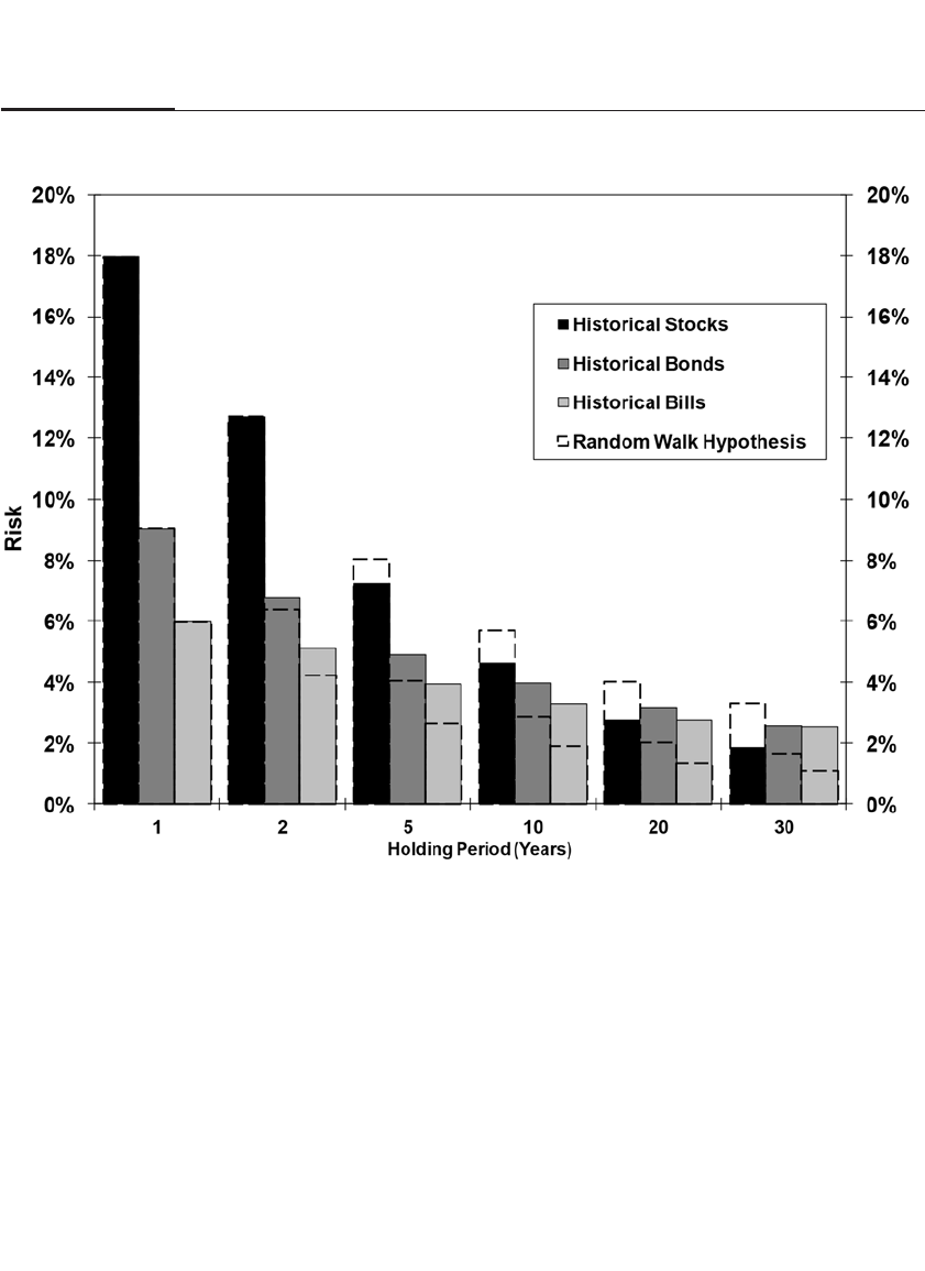
portfolio of equities falls to less than three-fourths that of bonds or bills.
The standard deviation of average returns falls nearly twice as fast for
stocks as for fixed-income assets as the holding period increases.
If asset returns follow a random walk, the standard deviation of
each asset class will fall by the square root of the holding period. A ran-
dom walk is a process whereby future returns are completely independ-
ent of past returns. The dashed bars in Figure 6-2 show the decline in
risk predicted under the random walk assumption.
But the historical data show that the random walk hypothesis can-
not be maintained for equities. This occurs since the actual risk of aver-
age stock returns declines far faster than predicted by the random walk
hypothesis because of the mean reversion of equity returns.
98 PART II The Verdict of History
FIGURE 6–2
Standard Deviation of Average Real Stock, Bond, and Bill Returns Over Various Holding Periods:
Historical Data and Random Walk Hypothesis 1802–2012

The standard deviation of average returns for fixed-income assets,
on the other hand, does not fall as fast as the random walk theory pre-
dicts. This is a manifestation of mean aversion of bond returns. Mean
aversion implies that once an asset’s return deviates from its long-run
average, there is an increased chance that it will deviate further, rather
than return to more normal levels. Mean aversion of bond returns is
especially characteristic of hyperinflations, where price changes proceed
at an accelerating pace, rendering paper assets worthless. But mean
aversion is also present in the more moderate inflations that have
impacted the United States and other developed economies. Once infla-
tion begins to accelerate, the inflationary process becomes cumulative,
and bondholders have virtually no chance of making up losses in their
purchasing power. In contrast, stockholders who hold claims on real
assets rarely suffer a permanent loss due to inflation.
Note that I am not claiming that the risk on a portfolio of stocks falls
as we extend the time period. The standard deviation of total stock
returns rises with time, but it does so at a diminishing rate. On the other
hand, because of uncertain inflation, the standard deviation of real bond
returns increases at an accelerating rate as the investment horizon
increases, and eventually bonds become riskier than a diversified port-
folio of common stocks.
VARYING CORRELATION BETWEEN STOCK AND BOND RETURNS
Even though the returns on bonds fall short of that on stocks, bonds may
still serve to diversify a portfolio and lower overall risk. This will be par-
ticularly true if bond and stock returns are negatively correlated, which
would happen if bond and stock prices move in the opposite direction.4
The diversifying strength of an asset is measured by the correlation coef-
ficient. The correlation coefficient ranges between –1 and +1 and measures
the co-movement between an asset’s return and the return of the rest of
the portfolio. The lower the correlation coefficient, the better the asset
serves as a portfolio diversifier. Assets with near-zero or especially neg-
ative correlations are particularly good diversifiers. As the correlation
coefficient between the asset and portfolio returns increases, the diversi-
fying quality of the asset declines.
In Chapter 3 we examined the changing correlation coefficient
between the return on 10-year Treasury bonds and stocks, represented
by the S&P 500 Index. Figure 6-3 displays the correlation coefficient
between annual stock and bond returns for three subperiods between
1926 and 2012. From 1926 through 1965 the correlation was only slightly
CHAPTER 6 Risk, Return, and Portfolio Allocation 99
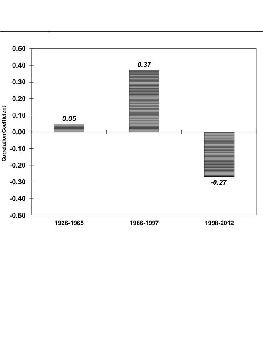
positive, indicating that bonds were fairly good diversifiers for stocks.
Bonds were good diversifiers in this period because it contained the
Great Depression, which was characterized by falling economic activity
and consumer prices, a situation that was bad for stocks but good for
U.S. government bonds.
However, under a paper money standard, bad economic times are
more likely to be associated with inflation, not deflation. This was true
from the mid-1960s through the mid-1990s, as the government
attempted to offset economic downturns with expansionary monetary
policy that was inflationary. Under these circumstances, stock and bond
prices tend to move together, sharply reducing the diversifying qualities
of government bonds.
But this positive correlation has switched again in recent decades.
Since 1998, stock prices have once again become negatively correlated
with government bond prices. The reason for this switch is twofold. In
100 PART II The Verdict of History
FIGURE 6–3
Correlation of Real Bond and Stock Returns Over Various Historical Periods

the early part of that period, the world markets were roiled by economic
and currency upheavals in Asia, the deflationary economy in Japan, and
then the terrorist events of September 11. Later the 2008 financial crisis
stoked fears of the 1930s, when deflation ruled and government bonds
were the only appreciating asset. These events led to the U.S. govern-
ment bond market becoming once again a safe haven for those investors
fearing more economic turmoil and lower stock prices.
Nevertheless, it is unlikely that Treasury bonds will remain good
long-term diversifiers, especially if the specter of inflation looms once
again. If inflation does indeed increase, the premium now enjoyed by
Treasury bonds as a hedge against deflation will again be lost, leading to
further losses for bondholders.
EFFICIENT FRONTIERS5
Modern portfolio theory describes how investors may alter the risk and
return of a portfolio by changing the mix between assets. Figure 6-4 dis-
plays the risks and returns that result from varying the proportion of
stocks and bonds in a portfolio over various holding periods ranging
from 1 to 30 years based on 210 years of historical data.
The “blank” square at the bottom of each curve represents the risk
and return of an all-bond portfolio, while the darkened square at the top
of the curve represents the risk and return of an all-stock portfolio. The
circle on the curve indicates the minimum risk achievable by combining
a varying proportion of stocks and bonds. The curve that connects these
points represents the risk and return of all blends of portfolios from 100
percent bonds to 100 percent stocks. This curve, called the efficient fron-
tier, is the heart of modern portfolio analysis and is the foundation of
asset allocation models.
Note that the allocation that achieves the minimum risk is a func-
tion of the investor’s holding period. Investors with a 1-year horizon
seeking to minimize their risk should hold almost their entire portfolio
in bonds, and that is also true for those with the 2-year horizon. At a 5-
year horizon, the allocation of stock rises to 25 percent in the minimum-
risk portfolio, and it further increases to more than one-third when
investors have a 10-year horizon. For 20-year horizons, the minimum-
risk portfolio is over 50 percent in stock, and for a 30-year horizon it is 68
percent.
Given these striking differences, it might seem puzzling that the
holding period has almost never been considered in standard portfolio
theory. This is because modern portfolio theory was established when
CHAPTER 6 Risk, Return, and Portfolio Allocation 101
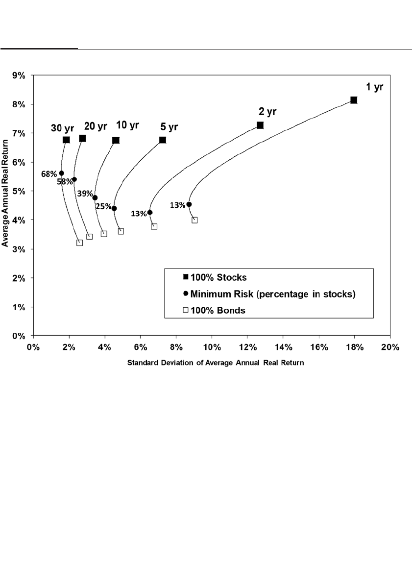
the vast majority of the academic profession supported the random walk
theory of security prices. As noted earlier, when prices are a random
walk, the risk over any holding period is a simple function of the risk
over a single period, so that the relative risk of different asset classes does
not depend on the holding period. In that case the efficient frontier is
invariant to the time period, and asset allocation does not depend on the
investment horizon of the investor. When security markets do not obey
random walks, that conclusion cannot be maintained.6
CONCLUSION
No one denies that, in the short run, stocks are riskier than fixed-income
assets. But in the long run, history has shown that stocks are actually
safer than bonds for long-term investors whose goal is to preserve the
102 PART II The Verdict of History
FIGURE 6–4
Risk-Return Tradeoffs (Efficient Frontiers) for Stocks and Bonds Over Various Holding Period 1802–2012

purchasing power of their wealth. The inflation uncertainty that is inher-
ent in a paper money standard means that “fixed income” and “fixed
purchasing power” are not the same thing, just as Irving Fisher conjec-
tured a century ago.
Despite the dramatic slowing in the rate of inflation over the past
decade, there is much uncertainty about what a dollar will be worth in
the future, especially given the large government deficits and easy mon-
etary policy followed by the world’s central banks. Historical data show
that we can be more certain of the purchasing power of a diversified
portfolio of common stocks 30 years hence than we can of the buying
power of the principal on a 30-year U.S. Treasury bond.
CHAPTER 6 Risk, Return, and Portfolio Allocation 103
This page intentionally left blank

Stock Indexes
Proxies for the Market
It has been said that figures rule the world.
—JOHANN WOLFGANG GOETHE, 1830
MARKET AVERAGES
“How’s the market doing?” one stock investor asks another.
“It’s having a good day—it’s up over 100 points.”
For those who follow the markets, no one would ask, “What’s up
100 points?” The Dow-Jones Industrial Average is still the way many
refer to how the market is doing, even though they well recognize the
limitations of this index. This index, popularly called the Dow, is so
renowned that the news media often called the Dow “the stock market.”
No matter how imperfectly the index describes the movement of share
prices—and virtually no money manager pegs his or her performance to
it—the Dow is the way that many investors describe the ups and downs
of the stock market.
But today there are many other, far more inclusive indexes. The
S&P 500, created in March 1957 by Standard & Poor’s, now a division of
the McGraw-Hill Financial, has become the uncontested benchmark
index for large U.S. stocks. And the Nasdaq, an automated electronic
market that began in 1971, has become the exchange of choice for tech-
nology companies. The Nasdaq Index measures the performance of such
large technology firms as Microsoft, Intel, Google, and Apple.
105
7

Although the term Industrials conjures up old-line manufacturing
companies, the Dow has become much more representative of firms that
dominate today’s landscape. In 1999, the Dow Industrials entered the
technological age when, for the first time, the company selected two
Nasdaq stocks—Microsoft and Intel—to join its venerable list of 30
stocks. Below is the story of these three very different indexes with three
unique reflections of the stock market.
THE DOW JONES AVERAGES
Charles Dow, one of the founders of Dow Jones & Co.—the company that
also publishes the Wall Street Journal—created the Dow Jones averages in
the late nineteenth century. On February 16, 1885, he began publishing a
daily average of 12 stocks (10 railroads and 2 industrials) that represented
active and highly capitalized stocks. Four years later, Dow published a
daily average based on 20 stocks—18 railroads and 2 industrials.
As industrial and manufacturing firms succeeded railroads in
importance, the Dow Jones Industrial Average was created on May 26,
1896, comprising the original 12 stocks shown in Table 7-1. The old index
created in 1889 was reconstituted and renamed the Rail Average on
October 26, 1896. In 1916, the Industrial Average was increased to 20
stocks, and in 1928 the number was expanded to 30, its present size. The
Rail Average, whose name was changed to the Transportation Average
in 1970, is composed of 20 stocks, as it has been for over a century.
The early Dow firms were centered on commodities: cotton, sugar,
tobacco, lead, leather, rubber, and so on. Six of the twelve companies
have survived in much the same form, but only one—General
Electric—has retained both its membership in the Dow Industrials and
its original name.1
Almost all the original Dow stocks thrived as large and successful
firms, even if they were eventually removed from the index (see the
Appendix at the end of this chapter for historical details). The only
exception was U.S. Leather Corp., which was liquidated in the 1950s.
Shareholders received $1.50 plus one share of Keta Oil & Gas, a firm
acquired earlier. But in 1955, the president, Lowell Birrell, who later fled
to Brazil to escape U.S. authorities, looted Keta’s assets. Shares in U.S.
Leather, which in 1909 was the seventh-largest corporation in the United
States, became worthless.
106 PART II The Verdict of History

107
TABLE 7–1
Stocks in Dow Jones Industrials 1886–2013
1896 1916 1928 1965 2013
American Cotton Oil American Sugar Allied Chemical Allied Chemical
3M Co.
American Sugar American Can American Can Aluminum Co. of America
American Express
American Tobacco American Car & American Smelting American Can
AT&T
Chicago Gas Foundry American Sugar American Tel. & Tel.
Boeing
Distilling & Cattle American Locomotive American Tobacco American Tobacco
Caterpillar
Feeding American Smelting Atlantic Refining Anaconda Copper
Chevron
General Electric American Sugar Bethlehem Steel Bethlehem Steel
Cisco Systems
Laclede Gas American Tel. & Tel. Chrysler Chrysler
Coca-Cola
National Lead Anaconda Copper General Electric DuPont
DuPont
North American Baldwin Locomotive General Motors Eastman Kodak
Exxon Mobil
Tennessee Coal and Iron Central Leather General Railway Signal General Electric
General Electric
U.S. Leather General Electric Goodrich General Foods
Goldman Sachs
U.S. Rubber Goodrich International Harvester General Motors
Home Depot
Republic Iron & Steel International Nickel GoodYear
Intel
Studebaker Mack Trucks International Harvester
IBM
Texas Co. Nash Motors International Nickel
Johnson & Johnson
U.S. Rubber North American International Paper Co.
JPMorgan Chase
U.S. Steel Paramount Publix Johns-Manville
McDonald’s
Utah Copper Postum, Inc. Owens-Illinois Glass
Merck
Westinghouse Radio Corp. Procter & Gamble
Microsoft
Western Union Sears, Roebuck Sears, Roebuck
Nike
Standard Oil (N.J.) Standard Oil of California
Pfizer
Texas Corp. Standard Oil (N.J.)
Procter & Gamble
Texas Gulf Sulphur Swift & Company
Travelers
Union Carbide Texaco Incorporated
United Technologies
U.S. Steel Union Carbide
UnitedHealth
Victor Talking Machine United Aircraft
Verizon Comm.
Westinghouse Electric U.S. Steel
Visa
Woolworth Westinghouse Electric
WalMart
Wright Aeronautical Woolworth
Walt Disney

Computation of the Dow Index
The original Dow Jones averages were simply the sum of the prices of
the component shares divided by the number of stocks in the index.
However, this divisor had to be adjusted over time to prevent jumps in
the index when there were changes in the companies that constituted the
average or stock splits. In October 2013, the divisor was about 0.1557, so
that a 1-point rise in any Dow stock caused the average to increase about
6½ points.2
The Dow Industrials is a price-weighted index, which means that the
prices of the component stocks are added together and then divided by
the number of firms in the index. As a result, proportional movements of
high-priced stocks in the Dow averages have a much greater impact
than movements of lower-priced stocks, regardless of the size of the
company. In November 2013, Visa, with a market price of $200 a share,
constitutes more than 8 percent of the index, while Cisco, the lowest-
priced stock, has a weight of less than 1 percent.3
Price-weighted indexes are uncommon since the impact of the
firm’s stock price on the index is unrelated to the size of the company.
This is in stark contrast to a capitalization-weighted index, such as
Standard & Poor’s 500 Index, in which each company’s weight in the
index is proportional to the market value of its shares. As of October 2013,
the 30 Dow stocks were valued at $4.5 trillion, which is a bit less than one-
quarter of the capitalization of the entire U.S. market. At the end of 2013,
the Dow Industrials did not contain the world’s largest market-value
stock, Apple, nor did it contain Google, which was also one of the top 10
highest-market-value stocks.
Long-Term Trends in the Dow Jones Industrial Average
Figure 7-1 plots the monthly high and low of the Dow Jones Industrial
Average from its inception in 1885, corrected for changes in the cost of
living. The inset shows the Dow Industrial Average uncorrected for
inflation.
A trendline and a channel are created by statistically fitting the Dow
on a time trend. The upper and lower bounds are 1 standard deviation,
or 50 percent, above and below the trend. The slope of the trendline, 1.94
percent per year, is the average compound rate at which the Dow stocks
have appreciated after inflation, since 1885. The Dow Jones average, like
most other popular averages, does not include dividends, so the appre-
ciation of the rise in the index greatly understates the total return on the
108 PART II The Verdict of History
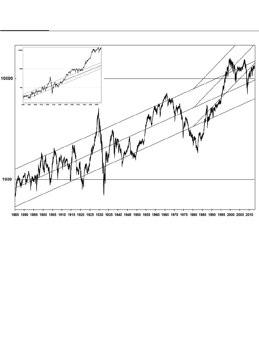
Dow stocks. Since the average dividend yield on all stocks was about 4.3
percent over this period, the total annual real compound return on the
Dow stocks was about 6.2 percent per year over this period.4
The inflation-corrected Dow average has stayed within the channel
about three-quarters of the time. When the Dow broke out of the chan-
nel to the upside, as it did in 1929, in the mid-1960s, and in 2000, stocks
subsequently suffered poor short-term returns. Likewise, when stocks
penetrated the channel on the downside, they subsequently experienced
superior short-term returns. As of August 2013, the inflation-corrected
all-time high of the Dow Industrials occurred in January 2000 at 16,130.
Beware the Use of Trendlines to Predict Future Returns
Using channels and trendlines to predict future returns, however tempt-
ing, can be misleading. Longstanding trends have been broken for good
CHAPTER 7 Stock Indexes 109
FIGURE 7–1
Nominal and Real Dow-Jones Industrial Average 1885–2012

economic reasons. Uncorrected for inflation, the Dow Industrials broke
and stayed above the trendline in the mid-1950s, as shown in the inset of
Figure 7-1. This is because inflation, caused by the shift to a paper money
standard, propelled nominal stock prices justifiably above their previous
trend, established during noninflationary times. Those who used trend-
line analysis and who failed to plot stock prices in real instead of nominal
terms would have sold in 1955 and never reentered the market.5
But there is now another justification why the channel may again
be penetrated on the upside. As noted above, stock indexes track only
capital appreciation and therefore understate total returns, which
include dividends. But firms have been paying an ever-lower fraction
of their earnings as dividends, using the difference to buy back their
shares and invest capital in their business. So in recent years a greater
part of the return on stocks now comes through capital gains instead of
dividend income. Because the average dividend yield on stocks has
fallen 2.88 percentage points since 1980, a new channel has been drawn
in Figure 7-1 with a slope that is 2.88 percentage points higher to rep-
resent the increase in the expected growth of capital gains. At the end
of 2012, the real Dow Industrials were above the mean, uncorrected for
the change in dividend yield but below the bottom of the dividend-
corrected channel.
VALUE-WEIGHTED INDEXES
Standard & Poor’s Index
Although the Dow Jones Industrial Average was published in 1885, it
was certainly not a comprehensive index of stock values, covering at
most 30 stocks. In 1906 the Standard Statistics Co. was formed, and in
1918 it began publishing the first index of stock values based on each
stock’s performance weighted by its capitalization, or market value,
instead of its price as Dow-Jones did. Capitalization weighting is now
recognized as giving the best indication of the return on the overall mar-
ket, and it is almost universally used in establishing market bench-
marks.6In 1939, Alfred Cowles, founder of the Cowles Commission for
Economic Research, used Standard & Poor’s market-weighting tech-
niques to construct indexes of stock values back to 1871 that consisted of
all stocks listed on the New York Stock Exchange.
The Standard & Poor’s stock price index began in 1923, and in 1926
it became the Standard & Poor’s Composite Index containing 90 stocks.
The index was expanded to 500 stocks on March 4, 1957, and became the
110 PART II The Verdict of History

S&P 500 Index. At that time, the value of the S&P 500 Index made up
about 90 percent of the value of all NYSE-listed stocks. The 500 stocks
contained exactly 425 industrial, 25 railroad, and 50 utility firms. Before
1988, the number of companies in each industry was restricted to these
guidelines, but since that date, there are no industry restrictions on the
firms selected.
A base value of 10 was chosen for the average value of the S&P Index
from 1941 to 1943, so that when the index was first published in 1957, the
average price of a share of stock (which stood between $45 and $50) was
approximately equal to the value of the index. An investor at that time
could easily identify with the changes in the S&P 500 Index since a 1-point
change approximated the price change for an average stock.
The S&P 500 Index contains a few firms that are quite small, repre-
senting companies that have fallen in value and have yet to be replaced.7
As of the end of 2012, the total value of all S&P 500 companies was about
$13.6 trillion, but this constituted less than 75 percent of the value of all
stocks traded in the United States, significantly less than the 90 percent
share it constituted when the index was first formulated. A history of the
S&P 500 Index, along with the insights that come from analyzing the
stocks in this world-famous index, is described in the next chapter.
Nasdaq Index
On February 8, 1971, the method of trading stocks underwent a revolu-
tionary change. On that date, an automated quotation system called the
Nasdaq (an acronym for National Association of Securities Dealers
Automated Quotations) provided up-to-date bid and asked prices on
2,400 leading over-the-counter stocks. Formerly, quotations for these
unlisted stocks were submitted by the principal trader or by brokerage
houses that carried an inventory. The Nasdaq linked the terminals of more
than 500 market makers nationwide to a centralized computer system.
In contrast to the Nasdaq, stocks traded on the New York or
American Stock Exchange are assigned to a Designated Market Maker
(used to be called “specialist”), who is charged with maintaining an
orderly market in that stock. The Nasdaq changed the way quotes were
disseminated and made trading these issues far more attractive to both
investors and traders.
At the time that the Nasdaq was created, it was clearly more presti-
gious to be listed with an exchange (and preferably the New York Stock
Exchange) than be traded on the Nasdaq. Nasdaq stocks tended to be
small or new firms that had recently gone public or did not meet the list-
CHAPTER 7 Stock Indexes 111

ing requirements of the larger exchanges. However, many young tech-
nology firms found the computerized Nasdaq system a natural home.
Some, such as Intel and Microsoft, chose not to migrate to the Big Board,
as the NYSE is termed, even when they qualified to do so.
The Nasdaq Index, which is a capitalization-weighted index of all
stocks traded on the Nasdaq, was set at 100 on the first day of trading in
1971. It took almost 10 years to double to 200 and another 10 years to
reach 500 in 1991. It reached its first major milestone of 1,000 in July 1995.
As the interest in technology stocks grew, the rise in the Nasdaq
Index accelerated, and it doubled its value to 2,000 in just three years. In
the fall of 1999, the technology stock boom sent the Nasdaq into orbit.
The index increased from 2,700 in October 1999 to its all-time peak of
5,048.62 on March 10, 2000.
The increase in popularity of technology stocks resulted in a
tremendous increase in volume on the Nasdaq. At the onset, the volume
on this electronic exchange was a small fraction of that on the New York
Stock Exchange. But by 1994 share volume on the Nasdaq exceeded that
on the NYSE, and five years later dollar volume on the Nasdaq sur-
passed the NYSE as well.8
No longer was the Nasdaq the home of small firms waiting to qual-
ify for Big Board membership. By 1998 the capitalization of the Nasdaq
had already exceeded that of the Tokyo Stock Exchange. At the market
peak in March 2000, the total market value of firms traded on the
Nasdaq reached nearly $6 trillion, more than one-half that of the NYSE
and more than any other stock exchange in the world. At the beginning
of the millennium, Nasdaq’s Microsoft and Cisco had the two largest
market values in the world, and Nasdaq-listed Intel and Oracle were
also among the top 10.
When the technology bubble burst, trading and prices on the
Nasdaq sank rapidly. The Nasdaq Index declined from over 5,000 in
March 2000 to 1,150 in October 2002 before rebounding to 3,000 at the
end of 2012. Trading also fell off from an average of over 2.5 billion
shares when prices peaked to approximately 2 billion shares in 2007.
Despite the decline in the Nasdaq Index, the Nasdaq still trades in some
of the world’s most active stocks.
But the importance of individual exchanges and “floor trading”
has declined precipitously, as the overwhelming percentage of shares
listed on the New York Stock Exchange is now traded electronically. In
2008 the NYSE bought the American Stock Exchange, and in late 2012,
the ICE, or Intercontinental Exchange, a 12-year-old Atlanta-based firm
112 PART II The Verdict of History

that trades futures contracts electronically, made an $8 billion bid to
acquire the NYSE. Even though it may seem exciting for news reporters
to broadcast from the floor of the New York Stock Exchange, the colon-
naded building, built at Broad and Wall Street in 1903 to trade the
world’s largest and most important companies, may soon go dark.
Other Stock Indexes: The Center for Research in Security Prices
In 1959, Professor James Lorie of the Graduate School of Business of the
University of Chicago received a request from the brokerage house
Merrill Lynch, Pierce, Fenner & Smith. The firm wanted to investigate
how well people had done investing in common stock, and it could not
find reliable historical data. Professor Lorie teamed up with colleague
Lawrence Fisher to build a database of securities data that could answer
that question.
With computer technology in its infancy, Lorie and Fisher created
the Center for Research in Security Prices (CRSP, pronounced “crisp”)
that compiled the first machine-readable file of stock prices dating from
1926 that was to become the accepted database for academic and profes-
sional research. The database currently contains all stocks traded on the
New York and American Stock Exchanges and the Nasdaq.
At the end of 2012, the market value of the nearly 5,000 stocks in the
database was near $19 trillion. The CRSP is the largest comprehensive
index of U.S. firms.
Figure 7-2 shows the size breakdown and total market capitaliza-
tion of the stocks in the CRSP. The top 500 firms, which closely mirror
the S&P 500 Index, constitute 78.6 percent of the market value of all
stocks. The top 1,000 firms in market value, which are virtually identical
to the Russell 1000 and published by the Russell Investment Group,
compose nearly 90 percent of the total value of equities. The Russell 2000
contains the next 2,000-largest companies, which adds an additional 9.6
percent to the market value of the total index. The Russell 3000, the sum
of the Russell 1000 and 2000 indexes, composes 99.1 percent of all U.S.
stocks. The remaining 1,788 stocks constitute 0.8 percent of the value of
all stocks traded.9
RETURN BIASES IN STOCK INDEXES
Because stock indexes such as the S&P 500 Index constantly add new
firms and delete old ones, some investors believe that the return calcu-
CHAPTER 7 Stock Indexes 113
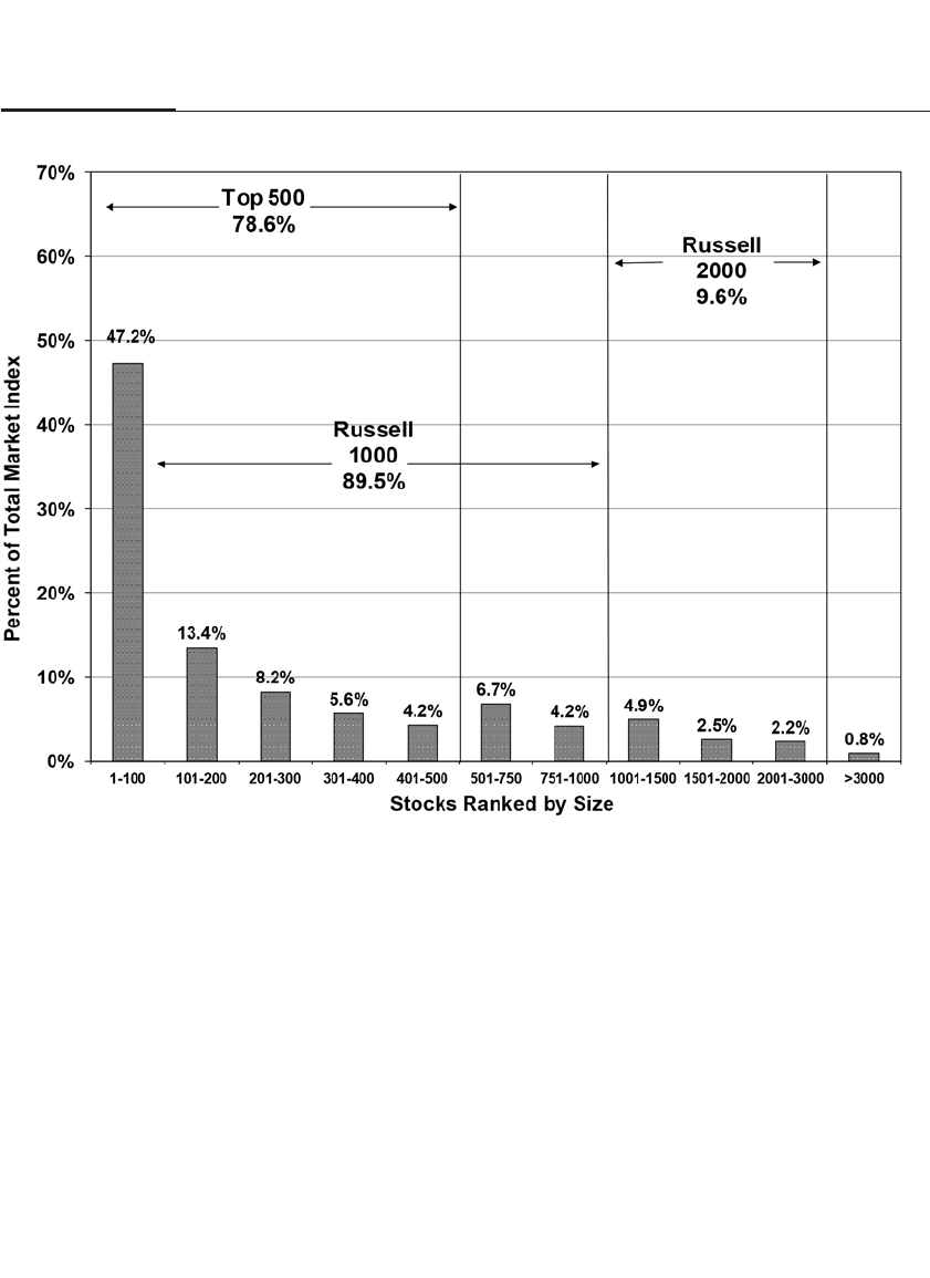
lated from these indexes will be higher than the return that can be
achieved by investors in the overall market.
But this is not the case. It is true that the best-performing stocks will
stay in the S&P 500 Index, but this index misses the powerful upside
move of many small and mid-sized issues. For example, Microsoft was
not added to the S&P 500 Index until June 1994, eight years after going
public. And while small stock indexes are the incubators of some of the
greatest growth stocks, they also contain those “fallen angels” that
dropped out of the large-cap indexes and are headed downward.
An index is not biased if its performance can be replicated or
matched by an investor. To replicate an index, the date of additions and
deletions to the index must be announced in advance so that new stocks
can be bought and deleted stocks can be sold. This is particularly impor-
tant for issues that enter into bankruptcy: the postbankrupt price (which
114 PART II The Verdict of History
FIGURE 7–2
CRSP Total Market Index, 2012

might be zero) must be factored into the index. All the major stock
indexes, such as Standard & Poor’s, Dow Jones, and the Nasdaq, can be
replicated by investors.10 Consequently, there is no statistical reason to
believe that these indexes give a biased representation of the return on
the market.
APPENDIX: WHAT HAPPENED TO THE
ORIGINAL 12 DOW INDUSTRIALS?
Two stocks (General Electric and Laclede) retained their original name
(and industry); five (American Cotton, American Tobacco, Chicago
Gas, National Lead, and North American) became large public compa-
nies in their original industries; one (Tennessee Coal and Iron) was
merged into the giant U.S. Steel; and two (American Sugar and U.S.
Rubber) went private—both in the 1980s. Surprisingly, only one
(Distilling & Cattle Feeding) changed its product line (from alcoholic
beverages to petrochemicals), and only one (U.S. Leather) was liqui-
dated. Here is a rundown of the original 12 stocks (market capitaliza-
tions as of December 2012):
■American Cotton Oil became Best Food in 1923, Corn Products
Refining in 1958, and finally CPC International in 1969—a major
food company with operations in 58 countries. In 1997, CPC
spun off its corn-refining business as Corn Products
International and changed its name to Bestfoods. Bestfoods was
acquired by Unilever in October 2000 for $20.3 billion. Unilever
(UN), which is headquartered in the Netherlands, has a current
market value of $115 billion.
■American Sugar became Amstar in 1970 and went private in
1984. In September 1991 the company changed its name to
Domino Foods, Inc., to reflect its world-famous Domino line of
sugar products.
■American Tobacco changed its name to American Brands (AMB)
in 1969 and to Fortune Brands (FO) in 1997, a global consumer
products holding company with core businesses in liquor, office
products, golf equipment, and home improvements. American
Brands sold its American Tobacco subsidiary, including the Pall
Mall and Lucky Strike brands, to one-time subsidiary B.A.T.
Industries in 1994. In 2011 Fortune Brands changed its name to
Beam Inc (BEAM), which operates as a distribution company in
the spirits industry. The market value is $9 billion.
CHAPTER 7 Stock Indexes 115

■Chicago Gas became Peoples Gas Light & Coke Co. in 1897 and
then Peoples Energy Corp., a utility holding company, in 1980.
Peoples Energy Corp. (PGL) was bought by WPS Resources and
changed its name in 2006 to Integrys Energy Group (TEG). It has
a market value of $4.1 billion. PGL was a member of the Dow
Jones Utility Average until May 1997.
■Distilling & Cattle Feeding went through a long and complicated
history. It changed its name to American Spirits Manufacturing
and then to Distiller’s Securities Corp. Two months after the
passage of Prohibition, the company changed its charter and
became U.S. Food Products Corp. and then changed its name
again to National Distillers and Chemical. The company became
Quantum Chemical Corp. in 1989, a leading producer of petro-
chemicals and propane. Nearing bankruptcy, it was purchased
for $3.4 billion by Hanson PLC, an Anglo-American conglomer-
ate. It was spun off as Millennium Chemicals (MCH) in October
1996. Lyondell Chemical (LYO) bought Millennium Chemicals
in November 2004. In 2007 Lyondell was taken over by the
Dutch firm that renamed itself Lyondell Basell Industries (LYB).
The current market value of Lyondell Basell is $28 billion.
■General Electric (GE), founded in 1892, is the only original stock
still in the Dow Industrials. GE is a huge manufacturing and
broadcasting conglomerate that owns NBC and CNBC. Its mar-
ket value of $218 billion is the third-highest capitalization stock
in the United States.
■Laclede Gas (LG) changed its name to Laclede Group, Inc., and it
is a retail distributor of natural gas in the St. Louis area. The
market value is $900 million.
■National Lead (NL) changed its name to NL Industries in 1971,
and it manufactures products relating to security and to preci-
sion ball bearings, as well as titanium dioxide and specialty
chemicals. The market value is $520 million.
■North American became Union Electric Co. (UEP) in 1956, pro-
viding electricity in Missouri and Illinois. In January 1998, UEP
merged with Cipsco (Central Illinois Public Service Co.) to form
Ameren (AEE) Corp. The market value is $72 billion.
■Tennessee Coal and Iron was bought out by U.S. Steel in 1907, and
it became USX-U.S. Steel Group (X) in May 1991. In January
2002, the company changed its name back to U.S. Steel Corp.
U.S. Steel has a market value of $3 billion.
116 PART II The Verdict of History

■U.S. Leather, one of the largest makers of shoes in the early part
of this century, liquidated in January 1952, paying its sharehold-
ers $1.50 plus stock in an oil and gas company that was to
become worthless.
■U.S. Rubber became Uniroyal in 1961, and it was taken private
in August 1985. In 1990 Uniroyal was purchased by the French
company Michelin Group, which has a market value of $15
billion.
CHAPTER 7 Stock Indexes 117
This page intentionally left blank

The S&P 500 Index
More Than a Half Century
of U.S. Corporate History
Most of the change we think we see in life is due to truths being in and
out of favor.
—ROBERT FROST, “THE BLACK COTTAGE,” 1914
Out of the three major U.S. stock market indexes, the Dow, the Nasdaq,
and the S&P 500, only one became the world standard for measuring the
performance for stocks. It was born on February 28, 1957, and it grew
out of Standard & Poor’s Composite Index, a capitalization-weighted
index begun in 1926 that contained 90 large stocks. Ironically, the 1926
index excluded the largest stock in the world at that time, American
Telephone and Telegraph, because S&P did not want to let the perform-
ance of such a large firm dominate the index. To correct this omission
and to recognize the growth of new firms in the postwar period,
Standard & Poor’s compiled an index of 500 of the largest industrial,
rail, and utility firms that traded on the New York Stock Exchange.
The S&P 500 Index made up nearly 90 percent of the total value of
firms traded on the Big Board in 1957. It soon became the standard
against which the performance of institutions and money managers
119
8

investing in large U.S. stocks was compared. The S&P 500 Index origi-
nally contained exactly 425 industrial, 25 rail, and 50 utility firms, but
these groupings were abandoned in 1988 in order to maintain, as
Standard & Poor’s claimed, an index that included “500 leading compa-
nies in leading industries of the economy.”
Since its creation, the index has been continually updated by adding
new firms that meet Standard & Poor’s criteria for market value, earn-
ings, and liquidity while deleting an equal number that fall below these
standards.1The total number of new firms added to the S&P 500 Index
from its inception in 1957 through 2012 was 1,159, an average of about 20
per year. On average, the new firms constitute about 5 percent of the mar-
ket value of the index.
The highest number of new firms added to the index in a single
year occurred in 1976, when Standard & Poor’s added 60 stocks includ-
ing 15 banks and 10 insurance carriers. Until that year, the only financial
stocks in the index were consumer finance companies, because banks
and insurance companies were traded in the over-the-counter market
and because timely price data were not available to compute the index
until the Nasdaq exchange began in 1971. In 2000, at the peak of the tech-
nology bubble, 49 new firms were added to the index, the highest since
Nasdaq stocks were included in 1976. In 2003, the number of additions
fell to a record-tying low of 8.
SECTOR ROTATION IN THE S&P 500 INDEX
The evolution of the U.S. economy during the past half century has
brought about profound changes in its industrial landscape. Steel, chemi-
cal, auto, and oil companies once dominated our economy. Today health-
care, technology, finance, and other consumer services firms hold sway.
Increasingly, active investors are using sector analysis to allocate
their portfolios. The most popular industry classification system was
formulated in 1999 when Standard & Poor’s joined Morgan Stanley to
create the Global Industrial Classification Standard (GICS). This system
arose from the earlier Standard Industrial Code (SIC) system devised by
the U.S. government that had grown less suited to our service-based
economy.2
The GICS divides the economy into 10 sectors: materials (chemicals,
papers, steel, and mining), industrials (capital goods, defense, trans-
portation, and commercial and environmental services), energy (explo-
ration, production, marketing, refining of oil and gas, and coal), utilities
(electric, gas, water, and nuclear generating or transmission firms),
120 PART II The Verdict of History
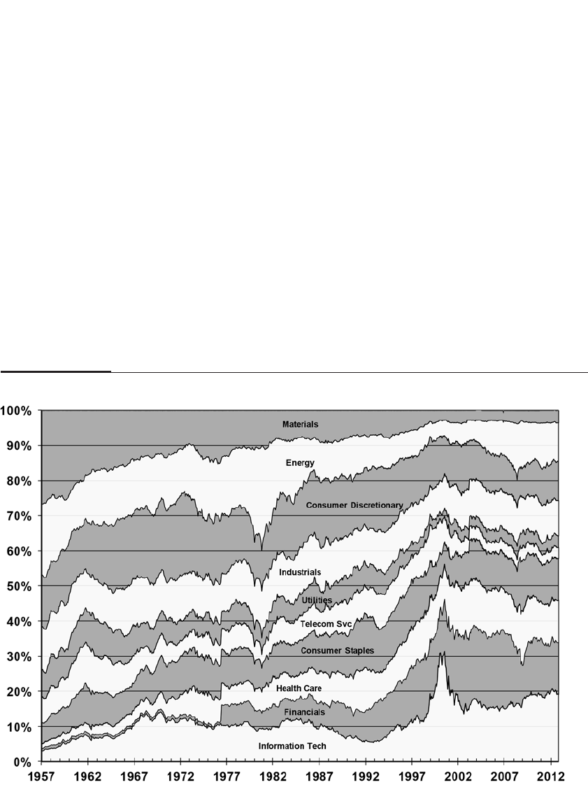
telecommunication services (fixed line, cellular, wireless, and bandwidth),
consumer discretionary (household durables, autos, apparel, hotels,
restaurants, media, and retailing), consumer staples (food, tobacco, per-
sonal products, retailing, and hypermarkets), healthcare (equipment pro-
ducers, healthcare providers, pharmaceuticals, and biotechs), financial
(commercial and investment banking, mortgages, brokerage, insurance,
and real estate [REITs]), and information technology (software services,
Internet, home entertainment, data processing, computers, and semi-
conductors).
The share of the market value of each of these sectors in the S&P 500
Index from 1957 through 2012 is displayed in Figure 8-1. Many of the
changes have been dramatic. The materials sector, by far the largest in
1957, had become one of the smallest (along with utilities and telecom)
by the end of 2012. The materials and energy sectors made up almost
one-half of the market value of the index in 1957, but by 2013 these two
CHAPTER 8 The S&P 500 Index 121
FIGURE 8–1
Market Value of S&P 500 Sectors as a Percentage of Total S&P 500 1957–2012

122 PART II The Verdict of History
sectors together constituted only 14 percent of the index. On the other
hand, the financial, healthcare, and technology sectors, which started off
as the three smallest sectors and constituted only 6 percent of the index
in 1957, commanded almost one-half of the market value of all S&P 500
firms by 2013.
It is important to realize that when measured over long periods of
time, the rising or falling market shares do not necessarily correlate with
rising or falling investor returns. That is because the change in sector
shares often reflects the change in the number of firms, not just the
change in the value of individual firms. This is especially true in the
financial sector, as commercial and investment banks, insurance compa-
nies, brokerage houses, and government-sponsored enterprises such as
Fannie Mae and Freddie Mac were added to the index.3The technology
share has also increased primarily because of the addition of new firms.
In 1957, IBM’s weight was two-thirds of the technology sector; in 2013,
IBM was only the third largest in a sector that contains 70 firms.
One can see in Figure 8-2 how little relation there is between the
change in the market value of a sector and its return. The fastest-
growing technology sector did have slightly above-average returns, but
the second-fastest-growing financials had the second-worst sector
returns. The weights of the financial and technology sectors increased
primarily because many new firms had been added to the sector, not
because individual stocks increased in value.
It is true that the healthcare and consumer staples sectors both
increased their weights and had above-average returns; but the energy
sector shrank significantly from 20 to 11 percent in market weight, and
yet its return of 11.76 percent was well above the S&P 500 Index.
Statistical analysis shows that over the past 50 years only 10 percent of
the return to a sector is related to whether the sector is expanding or con-
tracting. This means that 90 percent of the investor return of a sector is
based on the returns of the firms in the sector, not the relative growth of
the industry. Rapidly expanding sectors often induce investors to pay
too high a price, which results in lower returns. As a result, the best val-
ues are often found in stagnant or declining sectors that are ignored by
investors and whose price is low relative to fundamentals.
The performance of the 20 largest companies that Standard &
Poor’s put into its first list in 1957 is shown in Table 8-1. One feature that
stands out is that all 9 oil companies on the list finished in the top 10 and
that the returns on all the oil companies beat the S&P 500 by between 96
and 275 basis points per year.
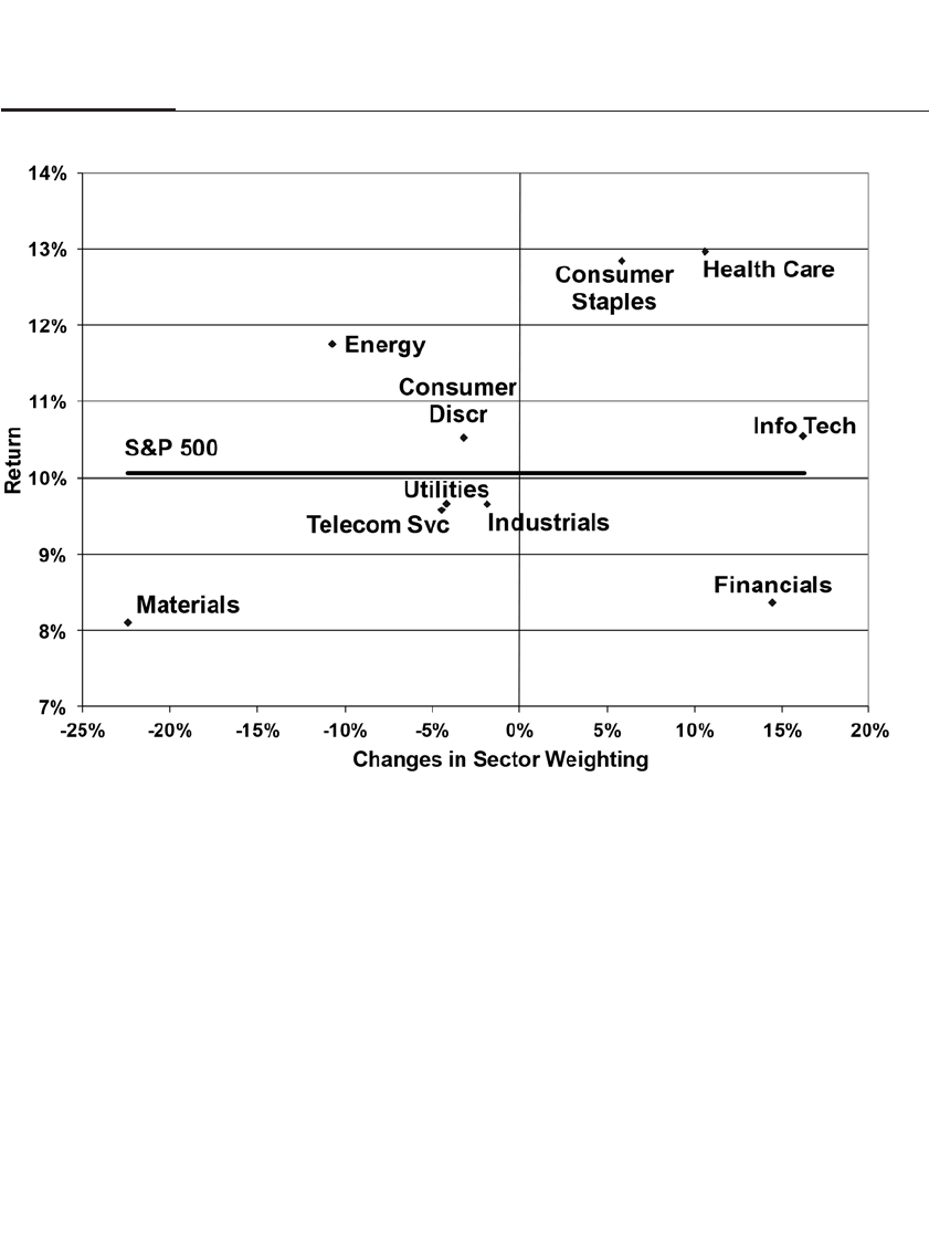
The top-performing firm of the original 20 largest stocks in the S&P
500 Index was Royal Dutch Petroleum, a firm founded in the
Netherlands and one of the companies that Standard & Poor’s deleted
from its index in 2002 when it purged all foreign-based firms. The
second-best-performing stock was Socony Mobil Oil, which dropped the
“Socony” (which stood for Standard Oil Company of New York) in 1966
and merged with Exxon in 1999. Third-ranking Gulf Oil, sixth-ranking
Standard Oil of California, and eighth-ranking Texas Co (Texaco) even-
tually merged to form ChevronTexaco, whose name was shortened to
Chevron. The fourth-best-performing stock was Shell Oil, a U.S.-based
company that was purchased by Royal Dutch in 1985 and is no longer in
the S&P 500 Index. The fifth-best performer was Standard Oil of New
Jersey, which changed its name to Exxon in 1972 and currently vies with
Apple as the world’s largest market-value stock. Ninth-ranked Standard
Oil of Indiana merged into BP Amoco in 1998, and tenth-ranking Phillips
CHAPTER 8 The S&P 500 Index 123
FIGURE 8–2
Relation Between Change in Sector Weight and Sector Return for S&P 500, 1957–2012

Petroleum merged with Conoco (Continental Oil Co.) to form
ConocoPhillips in 2002.
The only firm to beat any oil firm is IBM, incorporated in 1911 as C-
T-R (Computer-Tabulating-Recording) Company. IBM had the highest
weight in the S&P 500 Index (at over 6 percent) from 1983 through 1985
and in 2013 is still one of the top 10 most valuable companies.
Ten of the original twenty largest companies lagged the perform-
ance of the S&P 500 Index. U.S. Steel, AT&T, and General Motors were at
one time the largest corporations in the world. U.S. Steel and AT&T have
gone through tortuous paths of industrial changes and corporate divest-
ments and at one time had shrunk to a tiny fraction of their former size.
124 PART II The Verdict of History
T A B L E 8–1
Returns of 20 Largest original S&P 500 Firms, 1957-2012
Return 1957–2012 1957 Market
Rank 1957 Name Return Cap Rank
1 Royal Dutch Petroleum 12.82% 12
2 Socony Mobil Oil 12.76% 13
3 Gulf Oil 12.46% 6
4 Shell Oil 12.40% 14
5 Standard Oil Co NJ 12.28% 2
6 Standard Oil Co CA 12.02% 10
7 IBM 11.57% 11
8 Texaco 11.43% 8
9 Standard Oil Co Ind 11.26% 16
10 Phillips Petroleum 11.03% 20
11 AT&T 9.76% 1
12 Union Carbide 9.75% 7
13 General Electric 9.65% 5
14 Sears, Roebuck 8.04% 15
15 Du Pont 7.42% 4
16 Eastman Kodak 6.09% 19
17 USX Corp. 6.00% 9
18 Aluminum Co. Of America 4.24% 17
19 General Motors 3.71% 3
20 Bethlehem Steel — 18
Average Top 10 12.09%
Average Top 20 10.94%
S&P 500 10.07%

Yet both have come back, and as of 2013, AT&T is the thirteenth-largest
company by market value in the United States.
U.S. Steel was formed in 1901 from the merger of 10 steel compa-
nies, led by Andrew Carnegie and financed by J. P. Morgan. After the
merger, it was the first billion-dollar-sales company in history, and it
controlled two-thirds of the U.S. market. To cushion itself against rising
energy costs, it bought Marathon Oil Company in 1982 and renamed
itself USX Corporation. In 1991, U.S. Steel was spun off as a separate
firm, and in 2003, the value of its shares sank to just over $1 billion, the
same size as it was a century earlier. Aggressive cost cutting has brought
U.S. Steel back, and it is now the second-largest U.S. steel producer
behind Mittal Steel USA, which purchased, among other steel firms, the
bankrupt assets from Bethlehem Steel, the eighteenth-largest company
in the S&P 500 Index in 1957.
American Telephone and Telegraph Co. was the largest company
in the world when it joined the S&P 500 Index in 1957, and it remained
that way until 1975. The company boasted a market value of $11.2 bil-
lion in 1957, a capitalization that would rank in the bottom half of the
S&P 500 firms in 2012. The telephone monopoly known as “Ma Bell”
was broken up in 1984, giving birth to the “Baby Bell” regional
providers. But the stripped-down AT&T was bought by one of its chil-
dren, SBC Communications, in 2005, and through other acquisitions, it
worked itself back to the top 20 in market value in the United States by
2007. The 55-year return on AT&T, had you also held all the Baby Bells
when Ma Bell spun them off 23 years ago, would have given you a 9.76
percent annual return, virtually matching the index.
General Motors, which was formed by the consolidation of 17 auto
companies in 1908, was destined to become the largest auto producer in
the world. But the impact of foreign competition and mounting health-
care obligations forced GM into bankruptcy in 2009 during the Great
Recession. The company, however, has reemerged and vies with Toyota
as the largest auto manufacturer in the world. Although GM stock went
to zero, the value of Delphia, Raytheon, and Electronic Data Systems that
the giant automaker spun off before the bankruptcy gave shareholders a
meager 3.71 percent annual return since 1957. A slightly better return
was offered by Eastman Kodak, which declared bankruptcy in January
2012, but because it had spun off its holdings in the highly successful
Eastman Chemical Company in 1994, the parent company managed to
offer its shareholders since 1957 about a 6 percent return. This was not
the case for stockholders of Bethlehem Steel. The world’s second-largest
steel company went bankrupt in 2001, and the original stockholders
CHAPTER 8 The S&P 500 Index 125

have no assets to show for it. The remaining three firms belong to the
materials industry: the returns of Union Carbide (now part of Dow
Chemical) have slightly lagged the market, while the returns of DuPont
and Alcoa have fallen significantly behind the Index.
TOP-PERFORMING FIRMS
The 20 best-performing firms of the original S&P 500 that have survived
with their corporate structure intact are shown in Table 8-2, along with
their annual return, sector, and total return per dollar invested. Table 8-
3 lists the 20 best-performing firms whether they have survived intact or
have been merged into another firm.4
By far the best-performing stock is Philip Morris, which in 2003
changed its name to Altria Group and in 2008 spun off its international
division (Philip Morris International).5Philip Morris introduced the
126 PART II The Verdict of History
T A B L E 8–2
Returns of 20 Best Performing Original and Surviving S&P 500 Firms 1957–2012
Rank 1957 Name 2012 Name Ticker Return Sector Accum of $1
1 Philip Morris Altria Group Inc MO 19.47% Consumer staples $ 19,737.35
2 Abbott Labs Abbott Laboratories ABT 15.18% Healthcare $ 2,577.27
3 Coca-Cola Coca Cola Co. KO 14.68% Consumer staples $ 2,025.91
4 Colgate-Palmolive Colgate Palmolive Co. CL 14.64% Consumer staples $ 1,990.55
5 Bristol-Myers Bristol Myers Squibb Co. BMY 14.40% Healthcare $ 1,768.50
6 Pepsi-Cola Co. Pepsico Inc. PEP 14.13% Consumer staples $ 1,547.44
7 Merck & Co. Merck & Co. Inc. New MRK 13.95% Healthcare $ 1,419.26
8 Heinz Heinz H J Co. HNZ 13.80% Consumer staples $ 1,317.34
9 Melville Corp. C V S Caremark Corp. CVS 13.65% Consumer staples $ 1,224.81
10 Sweets Co. Tootsie Roll Inds. TR 13.57% Consumer staples $ 1,178.92
11 Crane Co. Crane Co. CR 13.57% Industrials $ 1,178.44
12 Hershey Foods Hershey Co. HSY 13.53% Consumer staples $ 1,154.02
13 Pfizer Inc. Pfizer Inc. PFE 13.38% Healthcare $ 1,072.61
14 Equitable Gas E Q T Corp. EQT 13.16% Energy $ 964.47
15 General Mills General Mills Inc. GIS 13.12% Consumer staples $ 947.03
16 Oklahoma Nat Gas Oneok Inc. New OKE 13.04% Utilities $ 907.42
17 Procter & Gamble Procter & Gamble Co. PG 13.00% Consumer staples $ 890.97
18 Deere & Co. Deere & Co. DE 12.86% Industrials $ 833.05
19 Kroger Co. Kroger Company KR 12.70% Consumer staples $ 768.88
20 McGraw-Hill Co. McGraw Hill Co. Inc. MHP 12.58% Consumer discretionary $ 725.52

world to the Marlboro Man, one of the world’s most recognized icons,
two years before the formulation of the S&P 500 Index. Marlboro ciga-
rettes subsequently became the world’s best-selling brand and propelled
Philip Morris stock upward.
The average annual return on Philip Morris over the past half cen-
tury, at 19.47 percent per year, almost doubled the 10.07 percent annual
return on the S&P 500 Index. This return means that $1,000 invested in
Philip Morris on March 1, 1957, would have accumulated to almost $20
million by the end of 2102, more than 100 times the $191,000 accumula-
tion in the S&P 500 Index.
Philip Morris’s outstanding performance does not just date from
midcentury. Philip Morris was also the best-performing stock since 1925,
the date when comprehensive returns on individual stocks were first
compiled. From the end of 1925 through the end of 2012, Philip Morris
delivered a 17.3 percent compound annual return, 7.7 percent greater
CHAPTER 8 The S&P 500 Index 127
T A B L E 8–3
Returns of 20 Best Performing Original S&P 500 Firms 1957–2012
Rank Original Company Surviving Company Ann. return
1 Philip Morris Altria Group, Philip Morris International 19.56%
2 Thatcher Glass Altria Group, Philip Morris International 18.43%
3 Lane Bryant Limited Group 17.84%
4 National Can Privatized 17.71%
5 Dr. Pepper Privatized 17.09%
6 General Foods Altria Group, Philip Morris International 17.03%
7 Del Monte Corp. Altria Group, Philip Morris International 16.51%
8 Standard Brands Altria Group, Philip Morris International 16.41%
9 National Dairy Altria Group, Philip Morris International 16.30%
10 Celanese Corp. Privatized 16.19%
11 RJ Reyonolds Tobacco Altria Group, Philip Morris International 15.78%
12 National Biscuit Altria Group, Philip Morris International 15.78%
13 Penick & Ford Altria Group, Philip Morris International 15.64%
14 Flintkote British American Tobacco 15.60%
15 Lorillard Loews Corp 15.29%
16 Abbott Labs Abbott Labs 15.12%
17 Columbia Pictures Coca-Cola 14.85%
18 Coca-Cola Coca-Cola 14.66%
19 Colgate-Palmolive Colgate-Palmolive 14.64%
20 Bristol-Myers Bristol-Myers 14.59%

than the market indexes. Had your grandmother bought 40 shares (cost
of $1,000) of Philip Morris in 1925 and joined its dividend investment
plan, her shares would have been worth over $1 billion dollars by the end
of 2012!
Philip Morris’s bounty did not extend to only its own stockholders.
Philip Morris eventually became the owner of 10 other original S&P 500
firms. Many investors became enormously wealthy because the shares
of their firms were exchanged with shares of successful companies such
as Philip Morris. Riding on the coattails of such winners is an unex-
pected bounty for many stockholders.
HOW BAD NEWS FOR THE FIRM BECOMES
GOOD NEWS FOR INVESTORS
Some readers may be surprised that Philip Morris is the top performer
for investors in the face of the onslaught of governmental restrictions
and legal actions that have cost the firm tens of billions of dollars and at
one time threatened the cigarette manufacturer with bankruptcy.
But in the capital markets, bad news for the firm often can be good
news for investors who hold onto the stock and reinvest their dividends.
If investors become overly pessimistic about the prospects for a stock,
the low price enables stockholders who reinvest their dividends to buy
the company on the cheap. These reinvested dividends have turned its
stock into a pile of gold for those who stuck with Philip Morris.
TOP-PERFORMING SURVIVOR FIRMS
Philip Morris is not the only firm that has served investors well. The
return on the other 19 best-performing surviving companies listed in
Table 8-2 has beaten the return on the S&P 500 Index by between 2½ and
5 percentage points per year. Of the top 20 firms, 15 belong to two indus-
tries: consumer staples, represented by internationally well-known con-
sumer brand-name companies, and healthcare, particularly large
pharmaceutical firms. Hershey chocolate, Heinz ketchup, and Tootsie
Roll, as well as Coca-Cola and Pepsi-Cola, have built up wide brand
equity and consumer trust.
Three other winners are Crane, a manufacturer of engineered
industrials products founded in 1855 by Richard Crane; Deere, a manu-
facturer of agricultural and construction machinery, established in 1840
by John Deere; and McGraw-Hill (now McGraw Hill Financial), a global
information provider, founded by James H. McGraw in 1899 and now
128 PART II The Verdict of History

the owner of Standard & Poor’s. In the last five years, this top 10 list has
been joined by gas producers EQT, formerly Equitable Gas (founded in
1888 in Pittsburgh), and ONEOK Inc., formerly Oklahoma Natural Gas
(founded in 1906).
One firm of particular note is CVS Corporation, which in 1957
entered the S&P 500 Index as Melville Shoe Corp., a company whose
name was taken from the founder, Frank Melville, who started a shoe
company in 1892 and incorporated as Melville Shoe in 1922. Shoe com-
panies have been among the worst investments over the past century,
and even Warren Buffett bemoans his purchase of Dexter Shoe in 1991.
But Melville Shoe was fortunate enough to buy the Consumer Value
Store chain in 1969, specializing in personal health products. The chain
quickly became the most profitable division of the company, and in 1996
Melville changed its name to CVS. So a shoe manufacturer, destined to
be a bad investment, turned to gold as a result of the management’s for-
tuitous purchase of a retail drug chain.
There are similar stories for the firms in Table 8-3, which, as noted
earlier, lists the 20 best-performing stocks whether they have survived in
their original corporate form or have been merged into another firm.
Thatcher Glass was the second-best performing of all the original S&P
500 stocks behind Philip Morris and was the leading milk bottle manu-
facturer in the early 1950s. But as the baby boom turned into the baby
bust and glass bottles were replaced by cardboard cartons, Thatcher’s
business sank. Fortunately for Thatcher shareholders, in 1966 the firm
was purchased by Rexall Drug, which became Dart Industries, which
merged with Kraft in 1980 and was eventually bought by Philip Morris
in 1988. An investor who purchased 100 shares of Thatcher Glass in 1957
and reinvested the dividends would have owned 140,000 shares of
Philip Morris stock and an equal number of shares of Phillip Morris
International, worth more than $16 million at the end of 2012.
OTHER FIRMS THAT TURNED GOLDEN
As the medical, legal, and popular assault on smoking accelerated
through the 1980s, Philip Morris, as well as the other giant tobacco
manufacturer, RJ Reynolds, diversified into brand-name food products.
In 1985 Philip Morris purchased General Food, and in 1988 it purchased
Kraft Foods for $13.5 billion, which had originally been called National
Dairy Products and was an original member of the S&P 500 Index.
Philip Morris completed its food acquisitions with Nabisco Group
Holdings in 2000.
CHAPTER 8 The S&P 500 Index 129

Nabisco Group Holdings was the company that Kohlberg Kravis
Roberts & Co. (KKR) spun off in 1991 after taking RJR Nabisco private in
1989 for $29 billion, at that time the largest leveraged buyout in history.
Under our methodology for computing long-term returns, if a firm is
taken private, the cash from the buyout is assumed to be invested in an
S&P 500 Index fund until the company is spun off, at which point the
shares are repurchased in the new IPO.6RJ Reynolds Tobacco Co. had
previously absorbed six original S&P companies: Penick & Ford,
California Packing, Del Monte Foods, Cream of Wheat (purchased in
1971 by Nabisco), Standard Brands, and finally National Biscuit Co. in
1985. All these companies became top-20 performers in large part
because of their ultimate purchase by Philip Morris.
OUTPERFORMANCE OF ORIGINAL S&P 500 FIRMS
One of the most remarkable aspects of these original 500 firms is that the
investor who purchased the original portfolio of 500 stocks and never
bought any of the more than 1,000 additional firms that have been added
by Standard & Poor’s in the subsequent 50 years would have outper-
formed the dynamic updated index. The return of the original 500 firms
is more than 1 percentage point higher than the updated index’s 10.07
percent annual return.7
Why did this happen? How could the new companies that fueled
our economic growth and made America the preeminent economy in the
world underperform the older firms? The answer is straightforward.
Although the earnings and sales of many of the new firms grew faster
than those of the older firms, the price that investors paid for these
stocks was simply too high to generate good returns.
Stocks that qualify for entry into the S&P 500 Index must have suf-
ficient market value to be among the 500 largest firms. But a market
value this high is often reached because of unwarranted optimism on
the part of investors. During the energy crisis of the early 1980s, firms
such as Global Marine and Western Co. were added to the energy sector,
and they subsequently went bankrupt. In fact, 12 of the 13 energy stocks
that were added to the S&P 500 Index during the late 1970s and early
1980s did not subsequently match the performance of either the energy
sector or the S&P 500 Index.
About 30 percent of the 125 firms that have been added to the tech-
nology sector of the S&P 500 Index since 1957 were added in 1999 and
2000. Needless to say, most of these firms have greatly underperformed
the market. The telecommunications sector added virtually no new
130 PART II The Verdict of History

firms from 1957 through the early 1990s. But in the late 1990s, firms such
as WorldCom, Global Crossing, and Quest Communications entered the
index with great fanfare, only to collapse afterward.
Of all 10 industrial sectors, only the consumer discretionary sector
has added firms that have outperformed the original firms put into the
index. This sector was dominated by the auto manufacturers (GM,
Chrysler, and then Ford), their suppliers (Firestone and Goodyear), and
large retailers, such as JCPenney and Woolworth’s.
CONCLUSION
The superior performance of the original S&P 500 firms surprises most
investors. But value investors (as described in Chapter 12) know that
growth stocks often are priced too high, and excitement over their
prospects often induces investors to pay too high a price. Profitable
firms that do not catch investors’ eyes are often underpriced. If investors
reinvest the dividends of such firms, they are buying undervalued
shares that will add significantly to their return.
The study of the original 500 companies also gives you an appreci-
ation of the dramatic changes that the U.S. economy has undergone in
the past half century. Although, many of the top performers are produc-
ing the same brands that they did 50 years earlier, most have aggres-
sively expanded their franchise internationally. Brands such as Heinz
ketchup, Coca-Cola, Pepsi-Cola, and Tootsie Roll are as profitable today
as they were when these products were launched, some over a hundred
years ago.
But we also see that many companies make good investments by
being merged into a stronger company. And four of the top-performing
original companies—Dr. Pepper, Celanese, National Can, and Flintkote—
are now owned by foreign companies. In fact, it is more likely than not
that many of the future winners will not be headquartered in the United
States. As we noted in Chapter 4, foreign firms, clearly of secondary
importance when the S&P 500 Index was founded in 1957, are apt to be
the ultimate owners of many of today’s top firms.
CHAPTER 8 The S&P 500 Index 131
This page intentionally left blank

The Impact of Taxes on
Stock and Bond Returns
Stocks Have the Edge
In this world nothing is certain but death and taxes.
—BENJAMIN FRANKLIN1
The power to tax involves the power to destroy.
—JOHN MARSHALL2
For all long-term investors, there is only one objective—maximum
total real return after taxes.
—JOHN TEMPLETON3
John Templeton’s objective to maximize total real return after taxes is an
essential investment strategy. And stocks are very well suited to this
purpose. In contrast to fixed-income investments, both capital gains and
dividends are treated favorably by the U.S. tax code. So in addition to
having superior before-tax returns, stocks often hold an even larger
after-tax advantage over bonds.
HISTORICAL TAXES ON INCOME AND CAPITAL GAINS
Figure 9-1 plots the historical marginal tax rate at three income levels:
the highest tax bracket, the tax rate for income of $150,000, and the tax
133
9

134 PART II The Verdict of History
FIGURE 9–1
Federal Tax Rates on Interest and Dividend Income and Capital Gains 1913–2012

rate for real income of $50,000 all adjusted to 2012 dollars. Figure 9-1A is
the tax rate for ordinary income (including interest income) from 1913,
when the federal income tax was established, and for dividends until
2003, when the dividend tax was set at the same rate as the capital gains
tax. Figure 9-1B plots the marginal tax rate for capital gains and (since
2003) dividend income. A history of the tax code applicable to stock
investors is provided in the Appendix at the end of this chapter.
BEFORE- AND AFTER-TAX RATES OF RETURN
The historical real after-tax returns for various asset classes are dis-
played in Table 9-1 for four tax brackets. Since 1913, when the federal
income tax was instituted, the after-tax real return on stocks has ranged
from 6.1 percent for untaxed investors to 2.7 percent for investors in the
highest bracket who realize their capital gains each year. For taxable
bonds, the real annual return ranges from 2.2 percent for the untaxed
investor to –0.3 for the investor in the maximum tax bracket, while the
real return on bills ranges from 0.4 to –2.3 percent. Municipal bonds
have realized a 1.3 percent annual real return since 1913.
Despite the debilitating effect of taxes on equity accumulations,
taxes cause the greatest damage to the returns on fixed-income invest-
ments. On an after-tax basis, an investor in the top tax bracket who put
$1,000 in Treasury bills at the beginning of 1946 would have $138 after
taxes and after inflation today, a loss in purchasing power of more than
86 percent. Instead, a highest-bracket investor would have turned
$1,000 into over $5,719 in stocks, a 470 percent increase in purchasing
power.
In fact, for someone in the highest tax bracket, short-term Treasury
bills have yielded a negative after-tax real return since 1871, even lower
if state and local taxes are taken into account. In contrast, top-bracket
taxable investors would have increased their purchasing power in
stocks 288-fold over the same period.
THE BENEFITS OF DEFERRING CAPITAL GAINS TAXES
In May 2003 President George W. Bush signed the Jobs and Growth
Reconciliation Act, which reduced the highest tax rate on qualified divi-
dends and capital gains to 15 percent. This is the first time that dividend
and capital gains taxes have been equalized for a significant length of
time at a preferential rate. In 2013 both taxes were set at 20 percent for
high-income investors. Nevertheless, effective taxes on capital gains are
CHAPTER 9 The Impact of Taxes on Stock and Bond Returns 135

136
TABLE 9–1
After-Tax Real Returns on Stocks, Bonds, and Bills for Various Income Levels, 1802–2012
Stocks Tax Bracket Bonds Tax Bracket Bills Tax Bracket
$0 $50K $150K Max $0 $50K $150K Max $0 $50K $150K Max Muni Bds Gold CPI
1802–2012 6.6 5.7 5.4 5.0 3.6 2.9 2.7 2.4 2.7 2.2 1.7 1.4 3.1 0.7 1.4
1871–2012 6.5 5.2 4.7 4.1 3.0 2.0 1.7 1.2 1.6 0.8 0.1 –0.4 2.2 1.0 2.0
1913–2012 6.1 4.2 3.6 2.7 2.2 0.8 0.3 –0.3 0.4 –0.7 –1.6 –2.3 1.3 1.2 3.2
I 1802–1870 6.7 6.7 6.7 6.7 4.8 4.8 4.8 4.8 5.1 5.1 5.1 5.1 5.0 0.2 0.1
II 1871–1925 6.6 6.6 6.5 6.2 3.7 3.7 3.6 3.4 3.1 3.1 3.0 2.7 3.3 –0.8 0.6
III 1926–2012 6.4 4.4 3.7 2.8 2.6 1.0 0.4 –0.2 0.6 –0.6 –1.7 –2.2 1.5 2.1 3.0
1946–2012 6.4 4.0 3.3 2.8 2.0 0.0 –0.5 –1.0 0.4 –1.1 –2.4 –3.1 1.1 2.0 3.9
1946–1965 10.0 7.0 5.2 3.9 –1.2 –2.0 –2.7 –3.5 –0.8 –1.5 –2.3 –2.7 –0.6 –2.7 2.8
1966–1981 –0.4 –2.2 –3.0 –3.3 –4.2 –6.2 –7.0 –7.5 –0.2 –3.0 –5.2 –6.1 –1.0 8.8 7.0
1982–1999 13.6 9.4 9.1 9.1 8.5 5.0 4.5 4.5 2.9 0.8 –0.8 –1.7 2.7 –4.9 3.3
1982–2012 7.8 5.5 5.3 5.3 7.6 4.8 4.4 4.3 1.6 0.1 –1.0 –1.7 3.4 1.8 2.9
*Federal income tax only. Assume 1-year holding period for capital gain portion of return.
Period
Major
Sub-
Periods
Postwar
Periods

still lower than on dividends since taxes on capital gains are paid only
when the asset is sold, not as the gain is accrued. The advantage of this
tax deferral is that the return from capital gains accumulates at the
higher before-tax rates rather than the after-tax rates, as would be the
case from reinvested dividends. I call the advantage of capital gains over
dividend income the “deferral benefit.”
For long-term investors the advantage of the deferral benefit can be
substantial. For example, take two stocks, one yielding 10 percent per
year in dividend income and the other yielding 10 percent per year
solely in capital gains. Assume an investor is taxed 20 percent on divi-
dends and capital gains. For an untaxed investor, both investments
would yield identical 10 percent returns. But the after-tax yield on the
dividend-paying stock is 8.0 percent per year, while, if the investor waits
for 30 years before selling the capital gains–paying stock, the after-tax
return is 9.24 percent per year. This is only 76 basis points less than the
return of an untaxed investor.
Therefore, from a tax standpoint, there is still a motivation for firms
to deliver capital gains as opposed to dividend income. This is unfortu-
nate since, as we shall note in Chapter 12, dividend-paying stocks
generally yield better before- and after-tax returns than non-dividend-
paying stocks. The government can put dividends on the same tax basis
as capital gains if the tax authorities allow investors to obtain a tax defer-
ral on reinvested dividends until the stock is sold.
INFLATION AND THE CAPITAL GAINS TAX
In the United States, capital gains taxes are paid on the difference
between the price of an asset when it is purchased (its nominal price) and
the value (price) of that asset when it is sold, with no adjustment made
for inflation. This nominally based tax system means that an asset that
appreciates by less than the rate of inflation—resulting in a loss of pur-
chasing power—will nevertheless be taxed upon sale.
Although the appreciation of stock prices generally compensates
investors for increases in the rate of inflation, especially in the long run,
a tax code based on nominal prices penalizes investors in an inflationary
environment. For a given real return, even a moderate inflation rate of 3
percent causes an investor with a five-year average holding period to
lose 60 basis points per year compared with the after-tax return that
would result if the inflation rate were zero. If the inflation rate rises to 6
percent, the decline in annual return rises to 112 basis points per year. I
call this effect the “inflation tax.” The inflation tax for various inflation
CHAPTER 9 The Impact of Taxes on Stock and Bond Returns 137

138 PART II The Verdict of History
rates and various holding periods under the current tax system is dis-
played in Figure 9-2.4
The inflation tax has a far more devastating effect on after-tax real
returns when the holding period is short than when it is long. This is
because the more frequently an investor buys and sells assets, the more
frequently the government can tax the nominal capital gain, which
might not be a real, after-inflation gain at all.
There is considerable support, both inside and outside govern-
ment, to make some adjustment for inflation in the tax system. In 1986,
the U.S. Treasury proposed the indexation of capital gains, but this pro-
vision was never enacted into law. In 1997, the House of Representatives
included capital gains indexation in its tax law, but it was removed by
House-Senate conferees under threat of a presidential veto. Under these
plans, investors would pay taxes on only that portion of the gain (if any)
FIGURE 9–2
Real After-Tax Return and Inflation for Various Holding Periods Under 2013 Tax Law

that exceeded the increase in the price level over the holding period of
the asset. Since inflation has remained low in recent years, there is less
pressure to adjust the capital gains tax for inflation, and legislation to
correct this defect is dormant.
INCREASINGLY FAVORABLE TAX FACTORS FOR EQUITIES
Despite the passage of the American Taxpayer Relief Act of 2012, which
raised the top rate on dividends and capital gains to 20 percent (23.8 per-
cent if the Medicare tax is included), there have been some very favor-
able tax developments for stockholders over the last several decades.
They include the following:
1. A reduction in the capital gains tax rate from a maximum of 35
percent in 1978 to 23.8 percent and comparable reductions for
lower-bracket taxpayers5
2. Lower inflation, which reduces the inflation tax imposed on
nominal capital gains
3. A switch to capital gains from dividends, which increases the
deferral benefit
Until 2003, when the tax rate on dividends was for the first time
decoupled from the tax rate on ordinary income, the tax rate on divi-
dends ranged as high as 90 percent in the immediate postwar period.
As noted above, since the tax law is based on only nominal values
unadjusted for inflation, inflation imposes an additional tax on capital
gains. The inflation rate has fallen from double-digit levels in 1979 to the
2 to 3 percent level in the past decade. Since tax brackets are indexed to
inflation, the tax rate on dividends is not directly affected by inflation.
Furthermore, since the capital gains tax is based on realizations instead
of accruals, firms have been buying back shares, in lieu of paying divi-
dends, and generating more capital gains income. As a result, the aver-
age dividend yield has fallen from about 5 percent before 1980 to only 2
percent in more recent years.
It can be calculated that all these factors have increased the real
after-tax return on stocks by about 2 percentage points over the past 30
years for a given before-tax return. Although the real after-tax return on
bonds has also increased as a result of the drop in the tax rates on ordi-
nary income, the increase in the real return on stocks has been greater. In
any equilibrium model of asset pricing, the favorable tax factors for
equities suggest that stocks should be priced at a higher multiple of
earnings, an issue that will be discussed in Chapter 10.
CHAPTER 9 The Impact of Taxes on Stock and Bond Returns 139

STOCKS OR BONDS IN TAX-DEFERRED ACCOUNTS?
The most important savings vehicles for many individuals are their tax-
deferred accounts (TDAs) such as Keogh, IRA, and 401(k) plans. Many
investors hold most of their stock (if they hold any at all) in their tax-
deferred accounts, while they hold primarily fixed-income assets in their
taxable accounts.
Yet many of the recent changes in the tax laws argue that investors
should do the opposite. Dividends will enjoy the lower tax rates, and
appreciation on shares will gain the lower capital gains tax advantage
only if they are held in taxable accounts. This is because when a tax-
deferred account is cashed out at retirement, an individual pays the full
ordinary income tax on the entire withdrawal regardless of how much of
the accumulation has been realized through capital gains and how much
through dividend income.
The above counsel, however, ignores two factors. First, if you are
an active trader or buy mutual funds that actively trade, then there
may be significant capital gains realized, some short run, that would
be best kept in a tax-deferred account. Trading in tax-deferred accounts
also does not require complicated tax computations since no taxes are
paid until money is withdrawn and the source of the profits is of no
consequence.
Second, although the government taxes capital gains and dividends
at ordinary rates when withdrawn from a TDA, the government also
shares more of the risk. If you realize a capital loss in a taxable account,
the government limits your ability to offset this loss against ordinary
income. However, when funds are withdrawn from a tax-deferred
account, the full withdrawal is treated as taxable income, so that all losses
become totally deductible from taxable income. Therefore, there is less
after-tax risk by putting one’s savings in tax-deferred accounts.
When all the factors are considered, it is better for most investors to
hold stocks in their taxable accounts, unless they are active traders. If
you have a long horizon, the possibility that you will have a loss in your
stock accounts is minimal, so the loss-sharing aspect of TDAs is less
important. It is advisable, though, to hold stocks that do not pay tax-
qualified dividends, such as REITs and other income trusts, in your tax-
deferred account to avoid current taxes. However, some risk-averse
investors who are reluctant to hold stocks in their personal accounts
because of short-term volatility find it easier to hold stocks in their
retirement accounts where they have a longer-term perspective and may
be better able to tolerate short-term losses.
140 PART II The Verdict of History

CONCLUSION
Tax planning is important to maximize returns from financial assets.
Because of favorable dividend and capital gains tax rates and the poten-
tial to defer those capital gains taxes, stocks hold a significant tax advan-
tage over fixed-income assets. These advantages have risen in recent
years, as capital gains and dividend taxes have been reduced, inflation
has remained low, and firms have repurchased shares to increase capital
gains. These favorable developments have increased the after-tax return
of equities by about 2 percentage points over the average after-tax return
of the past 50 years. As favorable as stocks are over bonds for long-term
investors, the tax advantage of equities is even greater.
APPENDIX: HISTORY OF THE TAX CODE
Federal income tax was first collected under the Revenue Act of 1913,
when the Sixteenth Amendment to the U.S. Constitution was ratified.
Until 1921 no tax preference was given to capital gains income. When tax
rates were increased sharply during World War I, investors refrained
from realizing gains and complained to Congress about the tax conse-
quences of selling their assets. Congress was persuaded that such “frozen
portfolios” were detrimental to the efficient allocation of capital, and so
in 1922 a maximum tax rate of 12.5 percent was established on capital
gains income. This rate became effective when taxable income reached
$30,000, which is equivalent to about $240,000 in today’s dollars.
In 1934, a new tax code was enacted that, for the first time, excluded
a portion of capital gains from taxable income. This exclusion allowed
middle-income investors, and not just the rich, to enjoy the tax benefits
of capital gains income. The excluded portion of the gain depended on
the length of time that the asset was held; there was no exclusion if the
asset was held 1 year or less, but the exclusion was increased to 70 per-
cent if the asset was held more than 10 years. Since marginal tax rates
ranged up to 79 percent in 1936, the effective maximum tax on very long-
term gains was reduced to about 24 percent.
In 1938, the tax code was amended again to provide for a 50 percent
exclusion of capital gains income if an asset was held more than 18
months, but in no case would the tax exceed 15 percent on such capital
gains. The maximum rate on capital gains income was raised to 25 per-
cent in 1942, but the holding period was reduced to 6 months. Except for
a 1 percent surtax that raised the maximum rate to 26 percent during the
Korean War, the 25 percent rate held until 1969.
CHAPTER 9 The Impact of Taxes on Stock and Bond Returns 141

In 1969, the maximum tax rate on capital gains in excess of $50,000
was phased out over a number of years, so ultimately the 50 percent
exclusion applied to all tax rates. Since the maximum rate on ordinary
income was 70 percent, this meant the maximum tax rate on capital
gains rose to 35 percent by 1973. In 1978, the exclusion was raised to 60
percent, which lowered the effective maximum tax rate on capital gains
to 28 percent. When the maximum tax rate on ordinary income was
reduced to 50 percent in 1982, the maximum tax rate on capital gains
was again reduced to 20 percent.
In 1986, the tax code was extensively altered to reduce and simplify
the tax structure and ultimately eliminate the distinction between capi-
tal gains and ordinary income. By 1988, the maximum tax rates for capi-
tal gains and ordinary income were identical, at 33 percent. For the first
time since 1922, there was no preference for capital gains income. In
1990, the top rate was lowered to 28 percent on both ordinary and capi-
tal gains income. In 1991, a slight wedge was reopened between capital
gains and ordinary income: the top rate on the latter was raised to 31
percent, while the former remained at 28 percent. In 1993, President
Clinton raised tax rates again, increasing the top rate on ordinary
income to 39.6 percent while keeping the capital gains tax unchanged. In
1997, Congress lowered the maximum capital gains tax to 20 percent for
assets held more than 18 months and the following year returned to the
12-month capital gains period. Starting in 2001, investors could take
advantage of a new 18 percent top capital gains rate for assets held at
least 5 years.
In 2003 President Bush signed into law legislation that lowered the
top rate on capital gains and qualified dividend income to 15 percent.
Qualified dividend income must come from taxable enterprises, not
“flow-through” organizations such as real estate investment trusts or
investment companies. In 2013 the top bracket on capital gains was
raised to 20 percent for married couples earning over $450,000, and for
the first time a Medicare surtax of 3.8 percent was applied to investment
income for couples earning more than $250,000. The tax rates on quali-
fied dividend income were set equal to the new capital gains tax rates.
142 PART II The Verdict of History

Sources of
Shareholder Value
Earnings and Dividends
The importance of dividends for providing wealth to investors is self-
evident. Dividends not only dwarf inflation, growth, and changing
valuations levels individually, but they also dwarf the combined
importance of inflation, growth, and changing valuation levels.
—ROBERT ARNOTT, 20031
It is just after 4 p.m. eastern time, and the major U.S. stock exchanges
have just closed. The anchorperson of one of the major financial net-
works excitedly proclaims: “Intel just out with its earnings! It ‘beat the
Street’ by 20 cents, and its price has jumped $2 in after-hours trading.”
Earnings drive stock prices, and their announcements are eagerly
awaited by Wall Street. But exactly how should we calculate earnings,
and how do firms turn these earnings into stockholder value? This chap-
ter addresses those questions.
DISCOUNTED CASH FLOWS
The fundamental source of asset values derives from the expected cash
flows that can be obtained from owning that asset. For stocks these cash
143
10

flows come from dividends or from cash distributions resulting from
earnings or the sale of the firm’s assets. Stock prices also depend on the
rate at which these future cash flows are discounted. Future cash flows
are discounted because cash received in the future is not valued as highly
as cash received in the present. The reasons investors discount the future
are (1) the existence of a risk-free rate, a yield on a safe alternative asset
such as government or other AAA-rated securities, which allows
investors the ability to transform a dollar invested today into a greater
sum tomorrow; (2) inflation, which reduces the purchasing power of cash
received in the future, and (3) the risk associated with the magnitudes of
expected cash flows, which induces investors of risky assets, such as
stocks, to demand a premium to that on safe securities. The sum of these
three factors—the risk-free rate, the inflation premium, and the equity
risk premium—determines the discount rate for equities. This discount
rate is also called the required return on equity or the cost of equity.
SOURCES OF SHAREHOLDER VALUE
Earnings are the source of cash flows to shareholders. Earnings (also
called profits or net income) are the difference between the revenues to the
firm and the costs of production. The costs of production include all
labor and material costs, interest on debt, taxes, and allowances for
depreciation.
Firms can transform these earnings into cash flows to shareholders
in a number of ways. The first and historically the most important is pay-
ment of cash dividends.
Earnings that are not used to pay dividends are called retained earn-
ings. Retained earnings create value by raising future cash flows
through:
■Retirement of debt, which reduces interest expense
■Investment in securities or other assets, including the acquisi-
tion of other firms
■Investment in capital projects designed to increase future profits
■Repurchase of the firm’s own shares (which is known as a buyback)
If a firm retires its debt, it reduces its interest expense and therefore
increases the profits available to pay dividends. If a firm buys assets, the
income from these assets is available to pay future dividends. Retained
earnings can be used to expand the capital of the firm in order to gener-
ate higher future revenues and/or reduce costs and thereby increase
144 PART II The Verdict of History

future cash flows to shareholders. Finally, if a firm repurchases its
shares, it reduces the number of shares outstanding and thus increases
per share earnings and permits an increase in per share dividends.
The last source of value, buybacks, deserves some elaboration.
Clearly shareholders who sell their shares to the company receive cash
for their stock. But those shareholders who do not sell will realize
greater per share earnings and per share dividends in the future as the
firm’s earnings are divided among a smaller number of shares. It should
be noted that at the time of the buyback, there is no change in the price
of shares as one asset is exchanged for another. But over time buybacks
increase the growth in per share earnings, and this increases the price of
shares, generating capital gains that replace the dividends the share-
holders would have received.
HISTORICAL DATA ON DIVIDENDS AND EARNINGS GROWTH
Figure 10-1 plots real per share reported earnings and real per share div-
idends in the United States from 1871 through 2012 for the S&P 500
Index and aggregate real corporate profits, which come from the
national income and product accounts (NIPA), which were first calcu-
lated for 1929. Table 10-1 summarizes these data. Over the whole period,
dividends are by far the most important source of shareholder return.
From 1871 the real return on stocks has averaged 6.48 percent, composed
of an average dividend yield of 4.40 percent and real capital gains of 1.99
percent. The capital gains have been generated almost entirely by the
growth of per share earnings, which have increased at an annual rate of
1.77 percent over the past 140 years.2
Table 10-1 also shows that there has been a significant change in the
mix of dividends and earnings since World War II. The growth rate of
per share earnings has increased, while the dividend payout ratio and
the dividend yield have decreased. Before World War II, firms paid two-
CHAPTER 10 Sources of Shareholder Value 145
TABLE 10–1
Dividends, Earnings, and Payout Data for Various Historical Periods
Reported Dividend Dividend Capital Stock Payout NIPA
Summary EPS Growth Growth Yield Gains Returns Ratio Profits
1871–2012 1.77% 1.35% 4.40% 1.99% 6.48% 61.3%
1871–1945 0.69% 0.77% 5.26% 1.03% 6.61% 71.8%
1946–2012 2.97% 1.99% 3.43% 3.07% 6.35% 49.6% 4.08%
1929–2012 1.85% 1.20% 3.85% 2.09% 5.69% 55.6% 3.22%
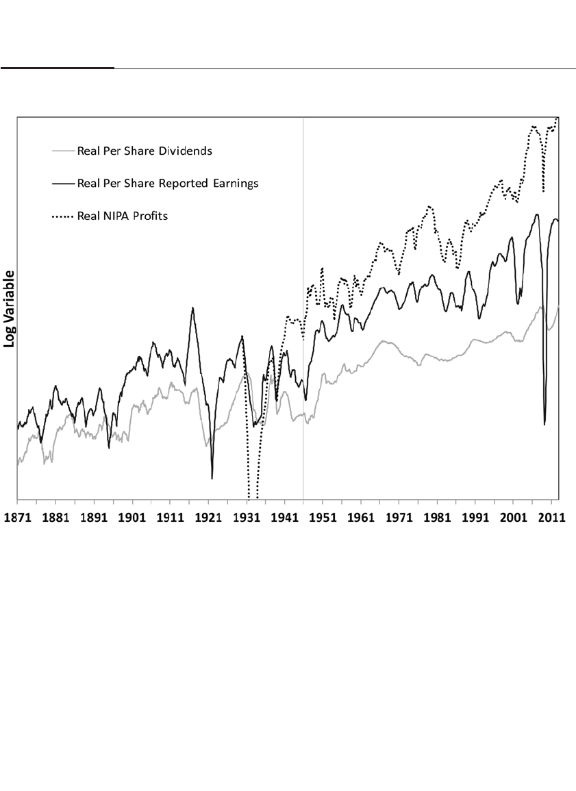
thirds of their earnings as dividends. Since retained earnings were too
small to fund expansion, firms issued more shares to obtained needed
capital, thereby reducing per share earnings growth. However, in the
postwar period, firms reduced dividends and generated sufficient earn-
ings so that the need to issue new shares to finance growth declined.
This is why in the postwar period per share earnings growth increased
significantly.
As noted earlier, from 1929 on, we have data on corporate profits
from NIPA.3These profits grow significantly faster than earnings per
share because over time firms increase the number of shares to finance
capital expansion.
There are several reasons why firms have reduced the dividend
payout ratio since World War II. After the war, tax rates on dividends
146 PART II The Verdict of History
FIGURE 10–1
Real per Share Reported Earnings, Dividends, and NIPA (National Income and Product Account)
Profits 1871–2012

increased sharply. Even when the tax rate on dividends is set equal to
the rate on capital gains, there is still a disadvantage since capital gains
taxes can be deferred while dividend taxes cannot. Second, since options
are based on share price alone, it is in the interest of management who
receive such options to follow a low-dividend policy, which boosts share
prices. These changes have reduced the share of dividends in the total
return to shareholders.
The Gordon Dividend Growth Model of Stock Valuation
To show how dividend policy impacts the price of a stock, we use the
Gordon dividend growth model developed by Roger Gordon in 1962.4Since
the price of a stock is the present value of all future dividends, it can be
shown that if future dividends per share grow at a constant rate g, then
the price per share of a stock P, which is the discounted value of all
future dividends, can be written as follows:
P⫽d/(1 ⫹r) ⫹d(1 ⫹g)/(1 ⫹r)2⫹d(1 ⫹g)2/(1 ⫹r)3⫹. . .
or
P⫽d/(r– g)
where dis the dividend per share, gis the rate of growth of future divi-
dends per share, and ris the required return on equity, which is the sum
of the risk-free rate, the expected rate of inflation, and the equity risk
premium.
Since the Gordon model formula is a function of the per share div-
idend and the per share dividend growth rate, it appears that dividend
policy is crucial to determining the value of the stock. But as long as one
specific condition holds—that the firm earns the same return on its retained
earnings as its required return on equity—then future dividend policy does
not impact the price of the stock or the market value of the firm.5This is
because dividends not paid today become retained earnings that gener-
ate higher dividends in the future, and it can be shown that the present
value of those dividends is unchanged, no matter when they are paid.
The management can, of course, influence the time path of divi-
dends. The lower the dividend payout ratio, which is the ratio of dividends
to earnings, the smaller the dividends will be in the near future. But
because a lower dividend today increases retained earnings, future div-
idends will rise and eventually exceed the level of dividends that would
have prevailed if the dividend payout ratio was not cut. Assuming the
firm earns the same return on its retained earnings as it does on its
CHAPTER 10 Sources of Shareholder Value 147

equity capital, the present value of these dividend streams will be iden-
tical no matter what payout ratio is chosen.
This equivalence can be shown by using the Gordon dividend
growth model. Let us assume that the discount rate ris 10 percent, that
there is no growth (g⫽0), that the dividend dis $10 per share, and that
the firm pays out all its earnings as dividends. In this case the price of
the shares would be $100. Now assume that the firm lowered its divi-
dend payout ratio from 100 percent to 90 percent, thereby reducing its
per share dividend (d) to $9 and increasing its retained earnings by $1.
If the firm earns 10 percent on its retained earnings, then earnings
per share next year will be $10.10, and the dividend, at a 90 percent pay-
out ratio, will be $9.09. If the firm maintains this payout ratio, the growth
rate in per share dividends will be 1 percent. Setting g⫽0.01 and d⫽$9
into the Gordon growth model yields the same $10 price of the stock as
before. As long as rremains at 10 percent, the price per share of the stock
will rise at 1 percent a year, identical to the growth of per share earnings
and per share dividends, and the total return to shareholders will
remain at 10 percent, with 9 percentage points of the return coming from
the dividend yield and 1 percentage point coming from stock apprecia-
tion. The firm can choose any proportion of the return that comes from
dividends and capital gains by varying the dividend payout ratio from
zero to 100 percent, but the return to stockholders remains at 10 percent.
The exact same result would hold if the firm used its retained earn-
ings to buy back shares. In the case above, the $1 not used to pay divi-
dends would be used to purchase 1 percent of the shares per year. The 1
percent reduction in the number of shares would mean that per share div-
idends (and per share earnings) will rise by 1 percent per year.
This theory is borne out by the long-run data shown in Table 10-1.
Before World War II, the average dividend payout ratio was 71.8 percent,
and since then, it has fallen to 49.6 percent. This reduced the dividend
yield from 5.26 to 3.43 percent, almost 2 percentage points. But capital
gains have risen by about 2 percentage points, so that the total returns
before and after World War II are approximately equal. The lower divi-
dend yield has resulted in an acceleration of per share earnings growth
from 0.69 to 2.8 percent.
It should be noted that although the rate of growth of the forward-
looking dividend per share increases after the dividend payout ratio is
cut, the rate of growth of dividends will for many years be less than the
growth rate of dividends if measured from a time period before the div-
idend cut. This is indeed what the historical data show in Table 10-1, as
the rate of growth of dividends per share has lagged behind that of per
148 PART II The Verdict of History

share earnings or price appreciation However, if the dividend payout
ratio does not continue to fall, theory dictates that the dividend growth
rate will accelerate in coming years.
Discount Dividends, Not Earnings
Although earnings determine the amount of dividends paid by the firm,
the price of the stock is always equal to the present value of all future
dividends and not the present value of future earnings. Earnings not paid
to investors can have value only if they are paid as dividends or other
cash disbursements at a later date. Valuing stock as the present dis-
counted value of future earnings is manifestly wrong and greatly over-
states the value of a firm.6
John Burr Williams, one of the greatest investment analysts of the
early part of the last century and the author of the classic Theory of
Investment Value, argued this point persuasively in 1938:
Most people will object at once to the foregoing formula for valuing
stocks by saying that it should use the present worth of future earnings,
not future dividends. But should not earnings and dividends both give
the same answer under the implicit assumptions of our critics? If earn-
ings not paid out in dividends are all successfully reinvested at com-
pound interest for the benefit of the stockholder, as the critics imply, then
these earnings should produce dividends later; if not, then they are
money lost. Earnings are only a means to an end, and the means should
not be mistaken for the end.7
EARNINGS CONCEPTS
Clearly dividends cannot be paid on a sustained basis unless the firm is
profitable. As a result, it is critical that a definition of earnings be devel-
oped that gives investors the best possible measure of the sustainable
cash that the firm can generate for the payment of dividends.
Earnings, which, as we noted, are also called net income or profit, are
the difference between revenues and costs. But the determination of
earnings is not just a “cash-in minus cash-out” calculation, since many
costs and revenues, such as capital expenditures, depreciation, and con-
tracts for future delivery, extend over many years. Furthermore, some
expenses and revenues are onetime or “extraordinary” items, such as
capital gains and losses or major restructurings, and they do not add
meaningfully to the picture of the ongoing profitability or sustainability
CHAPTER 10 Sources of Shareholder Value 149

of earnings that are so important in valuing a firm. Because of these
issues, there is no single “right” concept of earnings.
Earnings Reporting Methods
There are two principal ways that firms report their earnings. Net income or
reported earnings are those earnings sanctioned by the Financial Accounting
Standards Board (FASB), an organization founded in 1973 to establish
accounting standards. These standards are called the generally accepted
accounting principles (GAAP), and they are used to compute the earnings
that appear in the annual report and are filed with government agencies.8
The other, often more generous, concept of earnings is called operating
earnings, which often exclude onetime events such as restructuring charges
(expenses associated with a firm’s closing a plant or selling a division),
investment gains and losses, inventory write-offs, expenses associated with
mergers and spin-offs, and depreciation or impairment of “goodwill,”
among others. But the term operating earnings is not defined by FASB, and
this gives firms latitude to interpret what is and what is not excluded. There
are circumstances where the same specific type of charge may be included
in operating earnings for one company and omitted from another.
There are two principal versions of operating earnings. Standard &
Poor’s calculates a very strict version that differs from GAAP reported
earnings only by excluding asset impairments (including inventory
write-downs) and severance pay associated with such impairments.
However, when firms report their earnings, they frequently exclude
many more items, such as litigation costs, pension costs associated with
changing market rates or return assumptions, stock option expenses, etc.
We shall call the earnings that are reported by firms firm operating earn-
ings, although the terms non-GAAP earnings, pro forma earnings, and earn-
ings from continuing operations are also used.
Table 10-2 summarizes items that are included and excluded from
earnings for nonfinancial companies.9For financial companies, virtually
all these items are included in both S&P operating earnings and the
earnings reported by the firms, as well as GAAP earnings. Figure 10-2
plots these GAAP, S&P, and firm operating earnings for S&P 500 compa-
nies from 1967 to the present.
From 1988 forward, when all three earnings series were available,
S&P operating earnings averaged 16.5 percent above reported (GAAP)
earnings, and firm-reported operating earnings averaged 3.2 percent
above S&P operating earnings. During recessions, and particularly the
2007–2009 Great Recession, the gaps between these earnings concepts
150 PART II The Verdict of History
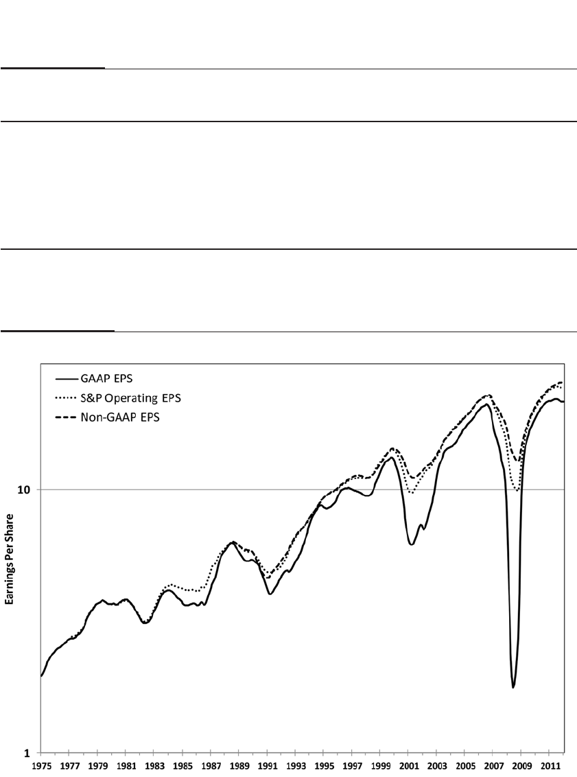
CHAPTER 10 Sources of Shareholder Value 151
T A B L E 10–2
Dividends, Earnings, and Payout Data for Various Historical Periods
GAAP EPS S&P Operating EPS Non-GAAP EPS
Asset Impairments
(incl. inventory write-down) Included Excluded Excluded
Severance costs Included Excluded* Excluded
Cash plant closing costs Included Included Excluded
Litigation Included Included Excluded
Pension fair value charges Included Included Excluded
Stock option expense Included Included Usually Included*
* Except when associated with asset impairment
FIGURE 10–2
Three Measures of Earnings Per Share: GAAP, S&P Operating, and Firm Operating, 1975–2012

widened significantly. In 2008, firm operating earnings were $50.84, and
S&P reported earnings were $39.61, while GAAP reported earnings fell
to $12.54.
It is often assumed that “reported earnings” better represent the true
earnings of a firm than operating earnings. But that is not necessarily true.
In fact, the increasing conservatism of FASB standards, especially as
related to the required write-down of asset values, has resulted in severe
downward biases to reported earnings. These write-downs were man-
dated by SFAS (Statement of Financial Account Standard) Rules 142 and
144, issued in 2001, which required any impairments to the value of prop-
erty, plant, equipment, and other intangibles (such as goodwill acquired
by purchasing stock above book value) be marked to market, and previ-
ously by Rule 115, issued in 1993, which stated that securities of financial
institutions held for trading or “available for sale” were required to be car-
ried at fair market value.10 These new standards required firms to “write
down” asset values regardless of whether the asset was sold or not. These
rules are especially severe in economic downturns when market prices are
depressed.11 On the other hand, firms are not allowed to write tangible
fixed assets back up, even if they recover from a previous markdown,
unless they are sold and recorded as “capital gains” income.12
A striking example of earnings distortion is Time Warner’s pur-
chase of America Online (AOL) for $214 billion in January 2000 at the
peak of the Internet boom. AOL, a member of the S&P 500 Index at that
time, registered a huge capital gain for shareholders when the firm was
acquired by Time Warner, also an S&P 500 member, as the purchase price
was far above book value. But that capital gain was never recorded in
the S&P earnings data. In 2002, after the Internet bubble popped, Time
Warner was forced to write down its investment in AOL by $99 billion,
at that time the largest loss ever recorded by an American corporation.
The combined profits and market value of AOL and Time Warner were
not materially different after the tech bubble than before, but because the
capital gain on AOL shares was never included as earnings, the aggre-
gate earnings of the S&P 500 Index fell dramatically when AOL’s market
price tumbled. Many other firms during that period also took large
write-downs on acquired assets while the profits realized by the
acquired firm upon purchase were never recorded.
Operating Earnings and NIPA Profits
Looking back at Figure 10-1, we can see that the outsized declines in
S&P reported earnings during the two most recent recessions differed
152 PART II The Verdict of History

sharply not only from the behavior of the S&P in previous recessions
but also from the behavior of after-tax corporate profits reported by the
Bureau of Economic Analysis (BEA), which computes NIPA. In every
recession before 1990 except 1937–1938, the decline in S&P reported
earnings was less than the decline in NIPA profits. In fact, the average
magnitude of the decline in S&P reported earnings in recessions before
1990 averaged just slightly over one-half that reported by NIPA profits.
But in the last three recessions, S&P reported profits fell by more than
twice as much as NIPA profits. In the 1990 recession, S&P reported
profits fell 43 percent while NIPA fell only 4 percent; in the 2001 reces-
sion, S&P reported profits fell 55 percent while NIPA declined 24 per-
cent; and in the Great Recession, NIPA fell 53 percent while S&P
reported earnings declined 92 percent. It is particularly striking that
the decline in S&P reported earnings in the 2008–2009 recession, where
the maximum decline in GDP was just over 5 percent, was much
greater than the 63 percent decline in S&P’s recorded earnings in the
Great Depression, which was five times as deep. In fact, NIPA corpo-
rate profits were negative in 1931 and 1932, which is not surprising
given the severity of the economic decline. These disparities suggest
that recent FASB rulings have resulted in much lower earnings, partic-
ularly in economic downturns.13
But recent FASB rulings are not the only reason GAAP often under-
states the true profitability of firms. Research and development costs are
routinely expensed, although there is good reason to capitalize these
expenditures and then depreciate them over time.14 This means that the
earnings of firms with a high level of R&D expenditures, such as the
pharmaceutical industry, may understate their economic earnings.
For example, Pfizer, one of the world’s largest pharmaceutical
firms, spent about $8 billion in 2012 on research and development and
about $1.5 billion on plant and equipment. Governed by current
accounting rules, Pfizer subtracted from its earnings only 5 percent of
the money it spent on plant and equipment as depreciation, and the
remainder would be deducted over the useful life of these “brick-and-
mortar” assets.
But 100 percent of the $8 billion Pfizer spent on research and devel-
opment must be subtracted from its earnings. This is because Pfizer’s
R&D is not considered an asset under GAAP accounting rules, and it
must be expensed. This treatment also applies to the technology sector.
The tangible, depreciable assets of Google and Facebook are a tiny frac-
tion of their market value. For many industries whose products are the
result of research and development and patentable innovations, all stan-
CHAPTER 10 Sources of Shareholder Value 153

dard earnings measures will understate the true earnings potential of
these firms.
Inflation also distorts GAAP earnings. As inflation rises, so do
interest rates. Nevertheless, all interest expenses are deducted from cor-
porate earnings even though inflation often causes an equal if not
greater reduction in the real value of corporate debt. In inflationary
times the impact of rising prices on fixed corporate liabilities can be sub-
stantial and can give rise to sharply lower accounting earnings than true
earnings of firms.
It is true that inflation also creates some upward biases to firms’
profits. Depreciation is based on historical prices, and hence in inflation-
ary times the charges taken for depreciation may be insufficient to cover
the cost of replacing and upgrading the capital. Also the capital gains
that firms earn on their inventories during inflation do not represent an
increase in earnings capability.15 That is why NIPA makes an adjustment
for depreciation and inventory profits when computing the profits
earned by corporations, although it doesn’t make any adjustment for the
change in the real value of the debt. When all factors are taken into con-
sideration, reported corporate profits during inflationary times likely
understate the true earnings of corporations.
The Quarterly Earnings Report
The difference between the operating earnings a firm reports and what
traders expect is what drives stock prices during the “earnings season,”
which occurs primarily in the three-week period following the end of
each quarter. When we hear that XYZ Corporation “beat the Street,” it
invariably means that its earnings came in above the consensus forecast
of operating earnings.16
But the published consensus estimates do not always match the
expectations built into the price of the stock at the time the announce-
ments are made. This is because analysts and traders who monitor com-
panies closely often come up with estimates that differ from the
consensus. These estimates, frequently referred to as the whisper esti-
mates because they are not widely disseminated, are the ones built into
the price of the stock. More often than not, these whisper estimates are
higher than the ones that circulate as the consensus, particularly for
technology stocks, which often have to beat the Street by a wide margin
to send their stock prices higher.
One reason whisper estimates are higher than consensus estimates is
that a firm’s earnings guidance to analysts is often tilted to the pessimistic
154 PART II The Verdict of History

side, so that the firm can “surprise” the Street on the upside and “beat the
consensus” in its quarterly reports. How else can one explain that over the
past 10 years approximately 65 percent of the quarterly earnings reports
beat the consensus estimate?17 Furthermore, a large number of firms beat
the Street by exactly one penny, far higher than one would calculate on a
statistical basis.
Earnings, although very important, are not the only data that traders
act on in the quarterly reports. Revenue is generally considered the next
most important indicator of a firm’s prospects and is considered even
more important than earnings by some traders. When the revenue data
are combined with the earnings data, one can compute the profit margin
on sales, another important piece of data.
But the earnings and revenue data are cut from different pieces of
cloth. Earnings are quoted on a per share basis, while revenue is not. It is
perfectly possible for firms to fall short of revenue estimates and fail to
meet their margin expectations, yet still beat on per share earnings
because over the past quarter the firm has reduced the number of shares
outstanding through corporate buybacks. Per share earnings can con-
tinue to grow even if overall revenues are stagnant.
Finally, investors are influenced by any earnings guidance that
firms give over the next quarter or year. Forward guidance below earlier
forecasts will certainly influence the stock price negatively. Years ago,
management would often tip off analysts when unexpected good or bad
news impacted the firm. But after tough new fair disclosure laws were
adopted by the SEC in 2000, such selected disclosure is no longer per-
mitted. The quarterly conference call is an ideal time for management to
release any and all important information to shareholders.
CONCLUSION
The fundamental determinant of stock values is the future expected cash
flows to investors. These cash flows, called dividends, are derived from
the earnings. If a firm earns the same rate of return on its retained earn-
ings that it does on the rest of its corporate capital, then the dividend
policy of a firm will not influence the current stock price, although it will
influence the future growth rate of per share earnings and dividends.
There are many earnings concepts. Firm operating earnings are
what are calculated and forecast by analysts and are the most important
data in the quarterly reports. These operating earnings are almost
always higher than reported or GAAP earnings. But recent rulings by
the FASB have led to a downward bias in reported earnings, especially
CHAPTER 10 Sources of Shareholder Value 155

during recessions when firms are required to record unrealized capital
losses in their earnings reports. The implications of these earnings data
for the valuation of the stock market are the subject of our next chapter.
156 PART II The Verdict of History

Yardsticks to Value
the Stock Market
Even when the underlying motive of purchase [of common stocks] is
mere speculative greed, human nature desires to conceal this unlovely
impulse behind a screen of apparent logic and good sense.
—BENJAMIN GRAHAM AND DAV ID DODD, 19401
AN EVIL OMEN RETURNS
In the summer of 1958, an event of great significance took place for those
who followed long-standing yardsticks of the stock market valuation.
For the first time in history, the interest rate on long-term government
bonds rose decidedly above the dividend yield on common stocks.
BusinessWeek noted this event in an August 1958 article entitled
“An Evil Omen Returns,” warning investors that when yields on stocks
approached those on bonds, a major market decline was in the offing.2
The stock market crash of 1929 occurred in a year when stock dividend
yields fell to the level of bond yields. The stock crashes of 1891 and 1907
also followed episodes when the yield on bonds came within 1 percent
of the dividend yield on stocks.
Until 1958, as Figure 11-1 indicates, the yearly dividend yield on
stocks had always been higher than long-term interest rates, and
investors thought that this was the way it was supposed to be. Stocks
were riskier than bonds and therefore should yield more in the market-
place. Under this criterion, whenever stock prices went too high and
sent dividend yields below the yields on bonds, it was time to sell.
157
11
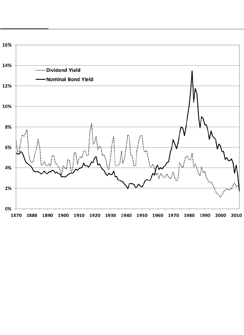
But things did not work that way in 1958. Stocks returned over 30
percent in the 12 months after dividend yields fell below bond yields,
and stocks continued to soar into the early 1960s.
It is now understood that there were good economic reasons why this
well-respected valuation indicator fell by the wayside. Inflation increased
the yield on bonds to compensate lenders for rising prices, while investors
bought stocks because they were claims on real assets. As early as
September 1958, BusinessWeek noted, “The relationship between stock and
bond yields was clearly posting a warning signal, but investors still believe
inflation is inevitable and stocks are the only hedge against it.”3
Yet many on Wall Street were troubled by the “great yield reversal.”
Nicholas Molodovsky, vice president of White, Weld & Co. and editor of
the Financial Analysts Journal, observed:
158 PART II The Verdict of History
FIGURE 11–1
Dividend Yield and Nominal Bond Yield 1870–2012

Some financial analysts called [the reversal of bond and stock yields] a finan-
cial revolution brought about by many complex causes. Others, on the con-
trary, made no attempt to explain the unexplainable. They showed readiness
to accept it as a manifestation of providence in the financial universe.4
Imagine the investor who followed this well-regarded indicator
and pulled all her money out of the stock market in August 1958, putting
it into bonds and vowing never to buy stocks until dividend yields rose
once again above bond yields. Such an investor would have to wait
another 50 years to get back into stocks, as it was not until the financial
crisis in 2009 that the dividend yield on stocks once again rose above the
yield on long-term Treasury bonds. Yet over that half century, real stock
returns averaged over 6 percent per year and overwhelmed the returns
on fixed-income securities.
This example illustrates that valuation yardsticks are valid only as
long as underlying economic and financial conditions do not change.
The chronic postwar inflation, resulting from a switch to a paper money
standard, changed forever the way investors judged the investment
merits of stocks and bonds. Stocks were claims on real assets whose
prices rose with inflation, while bonds were not. Those investors who
clung to the old ways of valuing equity never participated in one of his-
tory’s greatest bull markets.
HISTORICAL YARDSTICKS FOR VALUING THE MARKET
Many yardsticks have been used to evaluate whether stock prices are
overvalued or undervalued. Most of these measure the market value of
the shares outstanding relative to economic fundamentals, such as earn-
ings, dividends, or book values, or to some economic variable, such as
GDP or interest rates.
Price/Earnings Ratio and the Earnings Yield
The most basic and fundamental yardstick for valuing stocks is the
price/earnings ratio (or P/E ratio). The P/E ratio of a stock is simply the
ratio of its price to its earnings. The P/E ratio of the market is the ratio of
the aggregate earnings of the market to the aggregate value of the mar-
ket. The P/E ratio measures how much an investor is willing to pay for
a dollar’s worth of current earnings.
Figure 11-2 shows the historical P/E ratio of the market from 1871
through December 2012, based on the last 12 months of S&P reported
CHAPTER 11 Yardsticks to Value the Stock Market 159
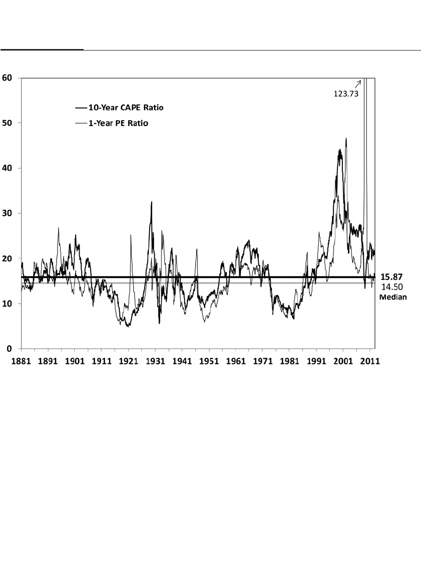
earnings and an alternative P/E ratio based on the last 10 years of
earnings, called the CAPE ratio, that will be discussed later in this
chapter. The P/E ratio based on 12-months earnings is marked by a
large spike, reaching 123.73 in the 2009 recession. This spike was not
caused by high stock prices but by extremely low aggregate earnings
that were caused by large losses concentrated in a few firms. A smaller
spike, also caused by a few firms reporting large losses, occurred in the
2000 recession. The median value of the P/E ratio, in contrast to the
arithmetic average, reduces the impact of these spikes and gives a bet-
ter guide to the historical valuation of the market. From 1871 through
2012, the median P/E ratio based on the last 12 months of earnings is
14.50, and based on the next 12 months of earnings, it is 15.09.
160 PART II The Verdict of History
FIGURE 11–2
One-year P/E and 10-Year CAPE Ratios 1881–2012

The Aggregation Bias
The traditional way of calculating the P/E of an index or a portfolio is by
adding the earnings of each firm in the index and dividing this sum into
the total market value of the index. Normally this gives a good picture of
the valuation. But when one or more firms reports a large loss, such a
procedure can give a very distorted view of the index’s valuation.
As a simple example, take two firms, A and B. Assume A is a
healthy firm earnings $10 billion and selling for an average P/E of 15,
giving it a market value of $150 billion. Assume firm B is not doing well,
reporting a $9 billion loss and having a market value of only $10 billion.
A capitalization weighted portfolio consists of approximately 94% of
firm A ($150 billion/$160 billion) and 6% of firm B. Yet using the tradi-
tional way of computing the P/E ratio of this portfolio would compute
the total earnings of the two firms of $1 billion and divide this into the
market value of these firms of $160 billion. This yields an extraordinar-
ily high P/E ratio of 160, even though over 94% of the portfolio is con-
centrated in a firm that has a P/E of 15. I call this distortion in index P/E
ratios the aggregation bias.
The reason why adding together profits and losses and then divid-
ing into aggregate market value is wrong is that losses in one firm do not
cancel the profits of another firm. Equity holders have unique rights to
the profits of their firms, unsullied by the losses in others.
The aggregation bias was particularly operative in the 2001–2002
recession and the recent financial crisis. The big dip in earnings in 2001 was
caused by the bust in the tech sector, and the large write-down that some
firms, such as Time Warner, were forced to take on their portfolio invest-
ments. In 2009 the large losses were in the financial industry, as Citibank,
BankAmerica, and particularly AIG took outsized losses that absorbed
most of the earnings from the profitable firms in the S&P 500 Index.
There is no easy fix to the aggregation bias. One method is to
weight the profits and losses of each firm by its market weight in the
index.5During normal periods when most firms are profitable and
losses of other firms are small, the aggregation bias is very small.
When a few firms experience large losses, the aggregation bias
becomes significant.
The Earnings Yield
Another variable of importance is the reciprocal of the P/E ratio, which
is called the earnings yield. The earnings yield is analogous to the divi-
CHAPTER 11 Yardsticks to Value the Stock Market 161

dend yield and measures the earnings generated per dollar of stock
market value.6
A median P/E ratio of approximately 15 for the U.S. market means
the median earnings yield is 1/15, or 6.67 percent, a value that is strik-
ingly close to the long-run real return on stocks. This is not a coincidence
and is indeed what would be predicted by finance theory. Stocks, in con-
trast to bonds, whose coupons and principal remain unchanged during
inflation, are claims on real assets, and real assets will rise in value with
an increase in the general level of prices. Therefore the earnings yield on
stocks is a real yield and should match the average real return that share-
holders receive for holding equities.
The CAPE Ratio
In 1998, Robert Shiller and his coauthor John Campbell published a
path-breaking article, “Valuation Ratios and the Long-Run Stock Market
Outlook.”7This article, following up on some of their earlier work on
stock market predictability, established that long-term stock market
returns were not random walks but could be forecast by a valuation
measure called the cyclically adjusted price/earnings ratio, or CAPE ratio.8
The CAPE ratio was calculated by taking a broad-based index of stock
market prices, such as the S&P 500, and dividing by the average of the
last 10 years of aggregate earnings, all measured in real terms. Its pur-
pose is to smooth out temporary fluctuations in profits caused by busi-
ness cycles. The CAPE ratio was then regressed against the future
10-year real returns on stocks, establishing that this ratio was a signifi-
cant variable predicting long-run stock returns.9The CAPE ratio is plot-
ted along with the one-year P/E ratio in Figure 11-2. Because the CAPE
ratio is based on 10-year average earnings, it does not display the spikes
that appear when plotting the one-year P/E ratio.
The ability of the CAPE ratio to predict real stock returns implied
that long-term equity returns were “mean reverting.” When the CAPE
ratio is above its long-run average, the model predicts below-average real
stock returns and above-average returns when the CAPE ratio is below
its average. The forecast and actual 10-year real stock returns for the
CAPE model are plotted in Figure 11-3.10
The CAPE ratio gained attention when Campbell and Shiller pre-
sented a preliminary version of their work to the Board of Governors of
the Federal Reserve on December 3, 1996, and warned that stock prices
in the late 1990s were running well ahead of earnings. Greenspan’s “irra-
tional exuberance speech,” delivered one week later, was said to have
162 PART II The Verdict of History
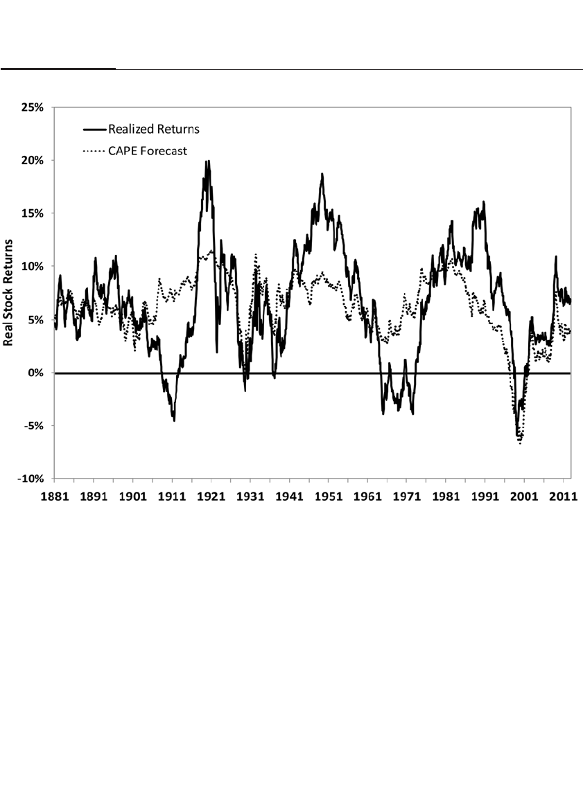
been based, in part, on their research.11 At the top of the bull market in
2000, the CAPE ratio hit an all-time high of 43, more than twice its his-
torical average, and correctly forecast the poor equity returns over the
next decade.
In January 2013, the CAPE ratio reached 20.68, about 30 percent
above its long-term average, and predicted a 10-year future annual real
stock return of 4.16 percent, about 2½ percentage points below its long-
run average. Although forecast stock returns were still significantly
higher than what was available at that time in the bond market, the bear-
ish CAPE prediction created concern among many stock market fore-
casters that the stock market at the end of 2012 had become overvalued
and that another bear market might be forthcoming.
But closer analysis suggests that the CAPE ratio based on S&P 500
reported earnings may be too bearish. There have been only 9 months
CHAPTER 11 Yardsticks to Value the Stock Market 163
FIGURE 11–3
CAPE Forecast and Realized 10-Year Real Stocks Returns 1881–2012

since January 1991 when the CAPE ratio has been below its long-term
average, but in 380 of the 384 months from 1981 through 2012, the actual
10-year real returns in the stock market have exceeded forecasts using
the CAPE model.
The unwarranted bearishness of the CAPE model can be attributed
to several sources: the most significant one is the distorted level of earn-
ings reported by Standard & Poor’s for its benchmark S&P 500 Index.12
As discussed in the last chapter, new FASB rulings have depressed S&P
reported earnings, particularly in recessions. Furthermore the aggrega-
tion bias makes the S&P methodology of determining the valuation of
the market particularly unrepresentative when a few firms report
extremely large losses. The outsized decline in S&P reported earnings in
2009 will bias the CAPE ratio upward until that year drops out of the
ten-year average in 2019.
When S&P operating earnings or adjusted real corporate profits
from NIPA are substituted for S&P reported earnings, a very different
picture emerges.13 Figure 11-4 displays the CAPE ratio relative to its
long-run average using S&P reported and operating earnings and NIPA
corporate profits. With these alternative measures, the overvaluation of
the stock market in recent years is eliminated or significantly reduced.
The Fed Model, Earnings Yields, and Bond Yields
In early 1997, in response to Federal Reserve Chairman Alan Greenspan’s
increasing concern about the impact of the rising stock market on the
economy, three researchers from the Federal Reserve produced a paper
entitled “Earnings Forecasts and the Predictability of Stock Returns:
Evidence from Trading the S&P.”14 This paper documented the remark-
able correspondence between the earnings yields on stocks and the 30-
year government bond rates.
Greenspan supported the results of this paper and suggested that the
central bank regarded the stock market as “overvalued” whenever this
earnings yield fell below the bond yield and “undervalued” whenever the
reverse occurred. The analysis showed that the market was most overval-
ued in August 1987, just before the October 1987 stock market crash, and
most undervalued in the early 1980s, when the great bull market began.
The basic idea behind the Fed model is similar to comparing the
dividend yield to the bond yield discussed at the onset of this chapter
but, recognizing that firms pay out only a fraction of their earnings as
dividends, uses the earnings yield and not the dividend yield. When the
bond yields rise above the earnings yields, stock prices fall because
164 PART II The Verdict of History
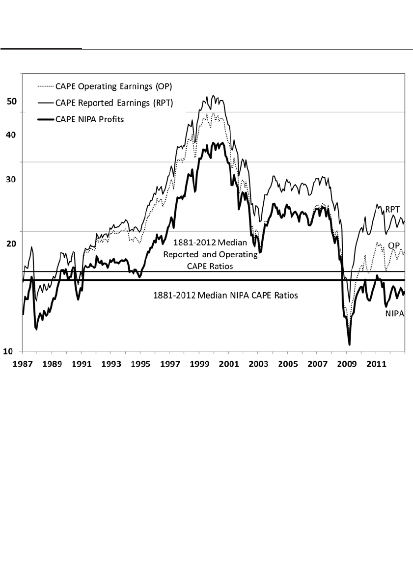
investors shift their portfolio holdings from stocks to bonds. On the
other hand, when the bond yields fall below the earnings yields,
investors shift to stocks from bonds.
But this model has the same shortcoming as the dividend
yield–bond yield yardstick described at the beginning of this chapter.
Government bonds have ironclad guarantees to pay a specified number
of dollars over time but bear the risk of inflation. Stocks, on the other
hand, are real assets whose prices will rise with inflation, but they bear
the risk of the uncertainty of earnings. The reason why the Fed model
worked is that the market rated these two risks as approximately equal
during this period.
But these two risks are not equal when inflation is low or when
deflation threatens. In those circumstances, bonds (especially U.S. gov-
CHAPTER 11 Yardsticks to Value the Stock Market 165
FIGURE 11–4
CAPE Ratios Based on Reported Earnings, Operating Earnings, and NIPA Profits 1987–2012

166 PART II The Verdict of History
ernment bonds) will do very well, but deflation undermines firms’ pric-
ing power and is bad for corporate profits. The Fed model did not do a
good job of predicting stock returns before inflation became a major con-
cern in the 1970s, nor has it done well in recent years as deflation became
a real concern following the financial crisis. For these reasons, the Fed
model has rightfully received less attention in recent years.
Corporate Profits and GDP
Another indicator of stock market valuation is the ratio of aggregate cor-
porate profits to GDP. The rise in this ratio in recent years has alarmed
some stock market analysts, who worry that if the share of profits to
national income falls to its long-term average, earnings and hence stock
prices will suffer.
However, closer examination of the data put those fears to rest.
Figure 11-5 displays the ratio of after-tax corporate profits and after-tax
profits plus proprietors’ income, beginning in 1929. Proprietors’ income
is profits of nonincorporated businesses, including profits to partner-
ships and individual owners.
One can see that although the ratio of corporate profits is high rela-
tive to GDP, the ratio of corporate profits plus proprietor’s income to
GDP is only 24.3 percent, less than 4 percentage points above its histori-
cal average. Over this time span, many brokerage houses, investment
banks, and other firms became publicly traded corporations, moving
from the proprietor’s income category to corporate profits. This has
boosted the corporate share of profits but not the total share of profits to
all capital, corporate and non-corporate.
Another factor raising the share of corporate profits is the increas-
ing fraction of earnings that come from abroad. In 2011, over 46 percent
of the sales of S&P 500 companies were foreign. As the U.S. economy
shrinks relative to the size of the world economy, the corporate profits of
U.S. multinational corporations should rise relative to U.S. GDP. This is
another reason why the rising share of corporate profits to US GDP is
not a cause for alarm.
Book Value, Market Value, and Tobin’s Q
The book value of a firm has often been used as a valuation yardstick. The
book value is the value of a firm’s assets minus its liabilities, evaluated
at historical costs. The use of aggregate book value as a measure of the
overall value of a firm is severely limited because book value uses his-
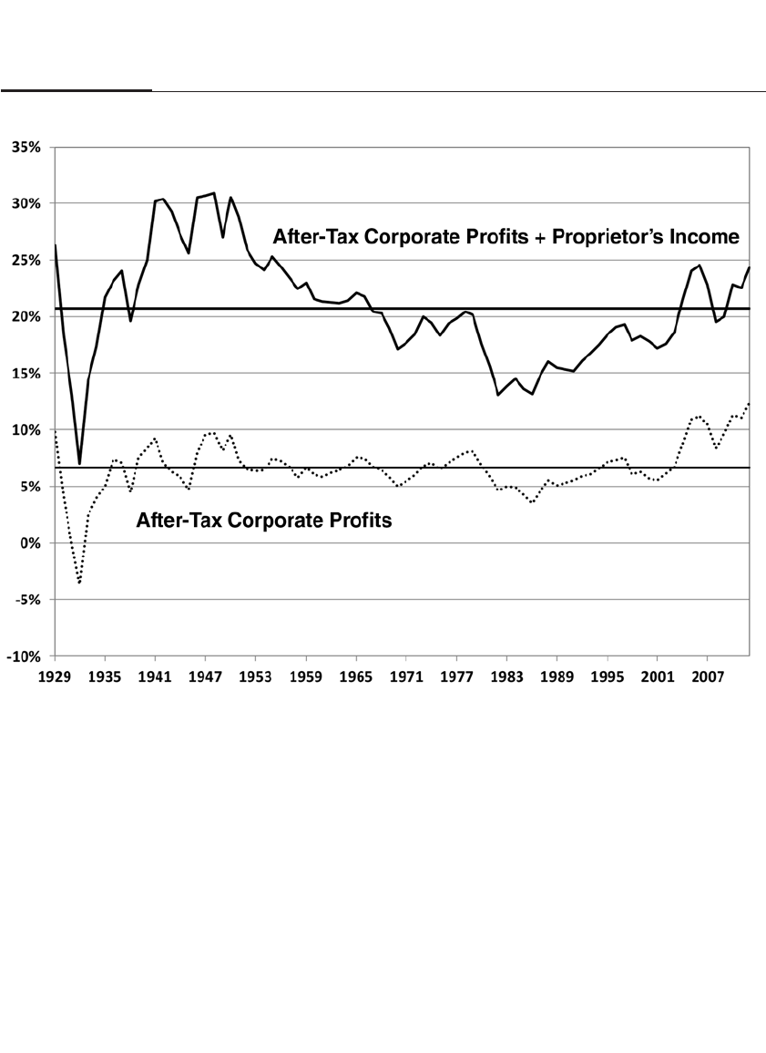
torical prices and thus ignores the effect of changing prices on the value
of the assets or liabilities. If a firm purchased a plot of land for $1 million
that is now worth $10 million, examining the book value will not reveal
this. Over time, the historical value of assets becomes less reliable as a
measure of current market value.
To help correct these distortions, James Tobin, former professor at
Yale University and a Nobel laureate, adjusted the book value for infla-
tion and computed the “replacement cost” of the assets and liabilities on
the balance sheets of U.S. corporations.15 He proposed that the “equilib-
rium” or “correct” market price of a firm should equal its assets minus
its liabilities adjusted for inflation. If the aggregate market value of a
firm exceeds the cost of capital, it would be profitable to create more cap-
ital, sell shares to finance it, and reap a profit. If the market value falls
CHAPTER 11 Yardsticks to Value the Stock Market 167
FIGURE 11–5
Corporate and Proprietor’s Income as a Percentage of GDP 1929–2012

168 PART II The Verdict of History
below the replacement cost, then it would be better for a firm to dis-
mantle and sell its capital or to stop investment and cut production.
Tobin designated the ratio of the market value to the replacement
cost with the letter Q, and he indicated that its ratio should be unity if
the stock market was properly valued. In 2000 Andrew Smithers and
Stephen Wright of the United Kingdom published the book Valuing Wall
Street,16 which maintained that Tobin’s Q was the best measure of value
and that the U.S. markets as well as the U.K. and many other European
markets were extremely overvalued by this criterion, a prediction also
made by those who monitored the P/E ratio.
But there are critics of the Q theory. Capital equipment and struc-
tures lack a good secondary market, and hence there is no realistic way
to value much of the capital stock independent of the value of the stock
market. In July 2013 the United States revised its national income
accounts to include research and development and other knowledge
investment (such as entertainment, literary, and artistic originals) in
the investment category. These changes added about $2 trillion to the
capital stock and certainly improved the relevance of the Q theory.
Nevertheless, book value is a construct of the past; market value derives
from prospective earnings and looks to the future. These prospective
earnings more accurately establish the basis of stock valuation than the
historical costs at which the firms purchased these assets.
Profit Margins
Another ratio that has generated concern in recent years is the level of
profit margins, the ratio of corporate profits to revenues. Figure 11-6
plots the profit margins on S&P 500 firms since 1967. One can see that
profit margins have recently risen to the highest levels in 45 years. Many
claim that these margins are “unsustainable” and that if the margins
retreat, that could lead to a significant decline in corporate profits and
hence stock prices.
But there are several reasons why corporate margins are high and
are not likely to retreat.17 One is the low leverage of American corpora-
tions, which reduces interest expenses and boosts margins. Second,
about one-third of the increase in the profit margins since the 1990s is
due to the increase in the share of profits coming from foreign sales.
Margins on foreign sales are higher than on domestic sales because the
foreign corporate tax rates abroad are almost all lower than in the United
States. Finally, much of the increase in profit margin is due to the
increase in the size of the technology sector, which has historically had
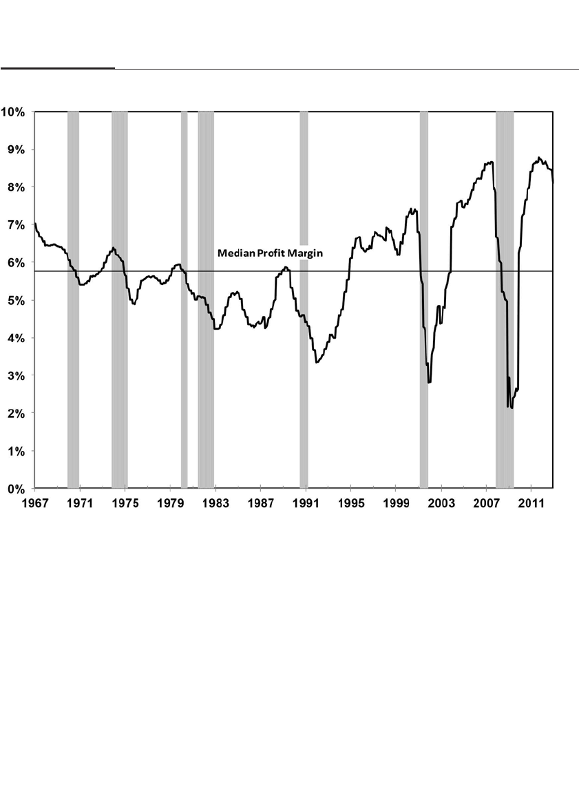
high margins. This is due to the large level of intellectual capital in tech-
nology firms and the high level of foreign sales.
These higher margins on the S&P 500 are unlikely to fall signifi-
cantly. Foreign sales will continue to contribute an increasing share of
S&P profits. Firms would lower their profit margin by increasing their
leverage, but with the interest rate so much lower than the earnings
yield, such actions will significantly boost earnings per share. In fact,
profit margins might rise further if the United States lowers its corporate
tax rates, a measure that has support in both parties.
FACTORS THAT MAY RAISE FUTURE VALUATION RATIOS
We have noted that the historical real return on equity has been between
6 and 7 percent per year over long periods and that this has coincided
CHAPTER 11 Yardsticks to Value the Stock Market 169
FIGURE 11–6
Profit Margin of S&P 500 Firms 1967–2012

with an average P/E ratio of approximately 15. But there have been
changes in the economy and financial markets that may raise the P/E
ratio in the future. These changes include a decrease in the cost of invest-
ing in equity indexes, a lower discount rate, and an increase in knowl-
edge about the advantages of equity versus fixed-income investments.
A Fall in Transaction Costs
Chapter 5 confirmed that the real return on equity as measured by stock
indexes was between 6 and 7 percent after inflation over the past two cen-
turies. But over the nineteenth century and the early part of the twentieth
century, it was extremely difficult, if not impossible, for an investor to
replicate these stock returns because of transactions costs.
Charles Jones of Columbia University has documented the decline
in stock trading costs over the last century.18 These costs include both the
fees paid to brokers and the bid-asked spread, or the difference between
the buying and selling price for stocks. His analysis shows that the aver-
age one-way cost to either buy or sell a stock has dropped from over 1
percent of value traded as late as 1975 (before the deregulation of bro-
kerage fees) to under 0.18 percent in 2002, and even lower today.
The fall in transaction costs implies that the price of obtaining and
maintaining a diversified portfolio of common stocks, which is necessary
to replicate index returns, could have easily cost investors from 1 to 2 per-
cent per year over much of the nineteenth and early twentieth centuries.
Because of these costs, investors in earlier years were less diversified and
assumed more risk than implied by stock indexes. Alternatively, if
investors attempted to buy all the stocks to replicate a broad-based index,
their real returns could have been as low as 5 percent per year after
deducting transaction costs. If the required real return on equity for
investors is only 5 percent, then a P/E ratio of 20, corresponding to an
earnings yield of 5 percent, will produce that return for today’s investors.19
Lower Real Returns on Fixed-Income Assets
We have noted that the real returns on fixed-income assets have fallen
dramatically over the past decade. When the 10-year TIPS were floated
in January 1997, their real return was almost 3.5 percent, and their yield
rose over 4 percent the following year. But since then, there has been a
steady decline in their real yield, which became negative in 2011 and fell
to almost −1 percent by the end of 2012. The implied real yield on stan-
dard Treasury bonds also fell below zero.
170 PART II The Verdict of History

There are many reasons for the decline in real returns available to
investors: the slowdown in economic growth, the aging of the popula-
tion, and the desire of pension funds to buy bonds to match their liabili-
ties to their retirees. Whatever the reasons, such a decline implies that
the real return on equity need not be as high as it had been historically in
order to attract buyers. We have noted that the historical premium (the
equity premium) on holding stocks over bonds has been approximately
3 to 3 ½ percent. If we assume that the long-run real rate settles at 2 per-
cent, about 1 to 1½ percent below its long-run average, then a 3 percent
equity premium will require a 5 percent real return on stocks, which, as
we noted above, arises from a 20 P/E multiple.
The Equity Risk Premium
The decline in transaction costs and the decline in discount rates may
each be used to justify a higher P/E ratio. Yet another reason is that the
equity risk premium itself may shrink. In 1985, economists Rajnish
Mehra and Edward Prescott published a paper entitled “The Equity
Premium: A Puzzle.”20 In their work they showed that given the stan-
dard models of risk and return that economists had developed over the
years, one could not explain the large gap between the returns on equi-
ties and fixed-income assets found in the historical data. They claimed
that economic models predicted that either the rate of return on stocks
should be lower, or the rate of return on fixed-income assets should be
higher, or both. In fact, according to their studies, an equity premium as
low as 1 percent or less could be justified.21
There is much literature that attempts to justify the 3 to 3½ percent
risk premium found in the historical data in the context of standard
macroeconomic models. Some of these are based on very high aversion
by individuals. Others are based on the myopic behavior of those who
dislike taking short-term losses on their investments even when they
have substantial long-run gains. Perhaps part of the explanation of the
size of the equity premium lies with the ignorance of the investing pub-
lic of the magnitude of the outperformance of equities.22 If indeed the
equity premium were fully recognized, the demand for stock would rise
and P/E ratios would increase from historical levels. This was precisely
the explanation that Professor Chelcie Bosland of Brown University had
made more than 75 years ago. He stated in 1937 that one of the conse-
quences of the spread of knowledge of superior stock returns, generated
by Edgar Lawrence Smith’s contributions, was the bull market of the
1920s and a narrowing of the equity premium:
CHAPTER 11 Yardsticks to Value the Stock Market 171

Paradoxical though it may seem, there is considerable truth in the state-
ment that widespread knowledge of the profitability of common stocks,
gained from the studies that have been made, tends to diminish the likeli-
hood that correspondingly large profits can be gained from stocks in the
future. The competitive bidding for stocks which results from this knowl-
edge causes prices at the time of purchase to be high, with the attendant
smaller possibilities of gain in the principal and high yield. The discount
process may do away with a large share of the gains from common stock
investment and returns to stockholders and investors in other securities
may tend to become equalized.23
CONCLUSION
Proper valuation of the equity market is necessary to project future stock
returns. Although those who wait long enough will eventually recoup
losses on a diversified portfolio of stocks, buying stocks at or below their
historical valuation is the best way to guarantee superior returns.
Nevertheless, there are persuasive reasons why the valuation of the mar-
ket may in the future rise above the historical average. This will lead to
lower long-term returns on stocks but higher returns during the transi-
tion to a higher valuation. Whether that transition takes place or not,
stocks remain the most attractive asset class for long-term investors.
172 PART II The Verdict of History

Outperforming the Market
The Importance of Size, Dividend
Yields, and Price/Earnings Ratios
Security analysis cannot presume to lay down general rules as to the
“proper value” of any given common stock. . . . The prices of common
stocks are not carefully thought out computations, but the resultants
of a welter of human reactions.
—BENJAMIN GRAHAM AND DAV ID DODD, 19401
STOCKS THAT OUTPERFORM THE MARKET
What criteria can investors use to choose stocks with superior returns
that will outperform the market? Investors are inevitably drawn to firms
able to generate high earnings and revenue growth. But empirical data
show this pursuit of growth often leads to subpar returns. To illustrate
how growth does not necessarily translate into superior returns, imag-
ine for a moment that you are an investor in 1950, at the dawn of the
computer age. You have $1,000 to invest and are given the choice of two
stocks: Standard Oil of New Jersey (now ExxonMobil) or a much
smaller, promising new company called IBM. You will instruct the firm
you choose to reinvest all dividends paid back into new shares, and you
will put your investment under lock and key for the next 62 years, to be
distributed at the end of 2012 to your great-grandchildren or to your
favorite charity.
173
12

Which firm should you buy? And why?
Let us assume that to help you with your decision, a genie pre-
sented you with Table 12-1, which displays the actual growth data of
these two firms over the next 62 years.
Table 12.1A shows that IBM beat Standard Oil by wide margins in
every growth measure that Wall Street uses to pick stocks: sales, earn-
ings, dividends, and sector expansion. IBM’s earnings per share growth,
Wall Street’s favorite stock-picking criterion, was more than 3 percent-
age points per year above the oil giant’s earnings growth over the next
six decades. As information technology advanced and technology
became more important to our economy, the technology sector rose from
3 percent of the market to nearly 20 percent.
In contrast, the oil industry’s share of the market shrank dramati-
cally over this period. Oil stocks made up about 20 percent of the market
value of all U.S. stocks in 1950 but fell to nearly half that value in 2012.
By these growth criteria, IBM stock should be a slam dunk to win
investors’ favor. But Standard Oil proved to be the best stock to buy.
174 PART II The Verdict of History
TABLE 12–1
Growth, Valuation, and Returns on IBM and Standard Oil (NJ) 1950–2012
Tab l e A
Growth Measures IBM Standard Oil of NJ Advantage
Revenue per share 10.03% 8.31% IBM
Dividends per share 10.73% 6.32% IBM
Earnings per share 11.14% 7.90% IBM
Sector growth* 16.10% –9.11% IBM
*Change in market share of technology and energy sectors 1957–2012
Table B
Valuation Measures IBM Standard Oil of NJ Advantage
Price appreciation 8.95% 7.58% IBM
Dividend return 2.17% 4.72% Standard Oil of NJ
Total return 11.32% 12.66% Standard Oil of NJ
Table C
Return Measures IBM Standard Oil of NJ Advantage
Average price/earnings ratio 25.06 14.08 Standard Oil of NJ
Average dividend yield 2.17% 4.21% Standard Oil of NJ
Returns measured year end 1957–2012

Although both stocks did well, investors in Standard Oil earned more
than 1 percentage point per year over IBM, as shown in Table 12-1B.
When your lockbox was opened 62 years later, the $1,000 you invested in
the oil giant would be worth $1,620,000, more than twice as much as IBM.
Why did Standard Oil beat IBM when it fell far short in every
growth category? One simple reason: valuation, the price you pay for the
earnings and dividends you receive. The price investors paid for IBM
was just too high. Even though the computer giant trumped Standard
Oil on growth, Standard Oil trumped IBM on valuation, and valuation
determines investor returns.
As you can see from Table 12.1C, the average price/earnings ratio
of Standard Oil was almost half of IBM’s ratio, and the oil company’s
average dividend yield was more than 2 percentage points higher.
Dividends are a critical factor driving investor returns. Because
Standard Oil’s price was low and its dividend yield much higher than that
of IBM, those who bought its stock and reinvested the oil company’s div-
idends accumulated 12.7 times the number of shares they started out with,
while investors in IBM accumulated only 3.3 times their original shares.
Although the price of Standard Oil’s stock appreciated at a rate that was
more than 2 percentage points lower than the price of IBM’s stock, its
higher dividend yield made the oil giant the winner for investors.
What Determines a Stock’s Return?
What does finance theory say about the importance of earnings growth
in determining investor returns? Finance theory has shown that if capi-
tal markets are “efficient” in the sense that known valuation criteria,
such as earnings, dividends, cash flows, book values, and other factors
are already factored into security prices, investing on the basis of these
fundamentals factors will not improve returns. In an efficient market,
the only way investors can consistently earn higher returns is to under-
take higher “risk,” where risk is defined as the correlation of an asset’s
return with the overall market, known as beta.2This is the fundamental
conclusion of the capital asset pricing model (CAPM), developed in the
1960s by William Sharpe and John Lintner.3
Beta can be estimated from historical data and represents the risk of
an asset’s return that cannot be eliminated in a well-diversified portfo-
lio; it is therefore the risk for which investors must be compensated. If
beta is greater than 1, the stock requires a return greater than that offered
by the overall stock market; and if it is less than 1, a lesser return is
required. Risk that is not correlated to the market can be eliminated
CHAPTER 12 Outperforming the Market 175

through diversification (called diversifiable or residual risk) and does not
warrant a higher return. The efficient market hypothesis and the CAPM
became the basis for stock return analysis in the 1970s and 1980s.
Unfortunately, as more data were analyzed, beta did not prove effec-
tive in explaining the differences in returns among individual stocks. In
fact, the beta of Standard Oil of New Jersey was far lower than the beta of
IBM, although Standard Oil’s return was greater.4In 1992, Eugene Fama
and Ken French wrote an article, published in the Journal of Finance, that
showed that there are two factors, one relating to the market capitaliza-
tion of the firm and the other to the valuation of stocks, that are far more
important in determining a stock’s return than the beta of a stock.5
After further analyzing returns, they claimed that the evidence
against the CAPM was “compelling” and that “the average return anom-
alies . . . are serious enough to infer that the [CAPM] model is not a use-
ful approximation” of a stock’s return, and they suggested researchers
investigate “alternative” asset pricing models or “irrational asset pricing
stories.”6
Fama and French’s findings prompted financial economists to classify
the stock universe along two dimensions: size, measured by the market value
of the stock, and valuation, or the price relative to “fundamentals” such as
earnings and dividends. The emphasis on valuation to gain an investment
edge did not originate with Fama and French. Valuation formed the corner-
stone of the principles that Benjamin Graham and David Dodd put forth
more than 70 years ago in their investment classic Security Analysis.7
SMALL- AND LARGE-CAP STOCKS
Cracks in the capital asset pricing model’s predictions of stock returns
appeared well before Fama and French’s research. In 1981, Rolf Banz, a
graduate student at the University of Chicago, investigated the returns
on stocks using the database that had been recently compiled by the
Center for Research in Security Prices (CRSP) located at the university.
He found that small stocks systematically outperformed large stocks,
even after adjusting for risk as defined within the framework of the cap-
ital asset pricing model.8
To analyze this claim, the returns from 1926 through 2012 on 10
groups of more than 4,000 stocks, sorted by market capitalization, are
shown in Table 12-2.
The compound annual return on the smallest decile of stock, at
17.03 percent per year, was more than 9½ percentage points over what
176 PART II The Verdict of History

would be predicted by the CAPM. The return of the second-smallest
decile of stocks, at 12.77 percent, was more than 3½ percentage points
above the CAPM prediction.9
Trends in Small-Cap Stock Returns
Although the historical return on small stocks has outpaced large stocks
since 1926, the magnitude of the small-cap stock outperformance has
waxed and waned unpredictably over the past 86 years. A comparison
of the cumulative returns on small stocks with those of the S&P 500
Index is shown in Figure 12-1.10
Small stocks, measured by the bottom quintile of market capitaliza-
tion, recovered smartly from their beating during the Great Depression,
but their performance only matched large stocks from 1926 to 1960. Even
by the end of 1974, the average annual compound return on small stocks
exceeded that of large stocks by only about 0.5 percent per year, not
nearly enough to compensate most investors for their extra risk and
trading costs.
But between 1975 and the end of 1983, small stocks exploded. During
these years, small stocks averaged a 35.3 percent compound annual
return, more than double the 15.7 percent return on large stocks.
Cumulative returns in small stocks during these nine years exceeded
CHAPTER 12 Outperforming the Market 177
TABLE 12–2
Return on Size Deciles of U.S. Stocks, 1926–2012
Size Decile
(Smallest to Geometric Beta Arithmetic Excess Return
Largest) Return Average Return Over CAPM
1 17.03% 1.38 25.56% 9.58%
2 12.77% 1.35 19.17% 3.56%
3 11.29% 1.26 16.50% 1.86%
4 11.31% 1.24 15.92% 1.58%
5 10.97% 1.22 14.89% 0.70%
6 10.97% 1.21 14.82% 0.74%
7 11.16% 1.18 14.39% 0.76%
8 10.24% 1.12 12.94% –0.09%
9 11.04% 1.09 13.41% 0.80%
10 9.28% 0.95 11.01% –0.02%
Total market 9.67% 1.00 11.59% 0.00%
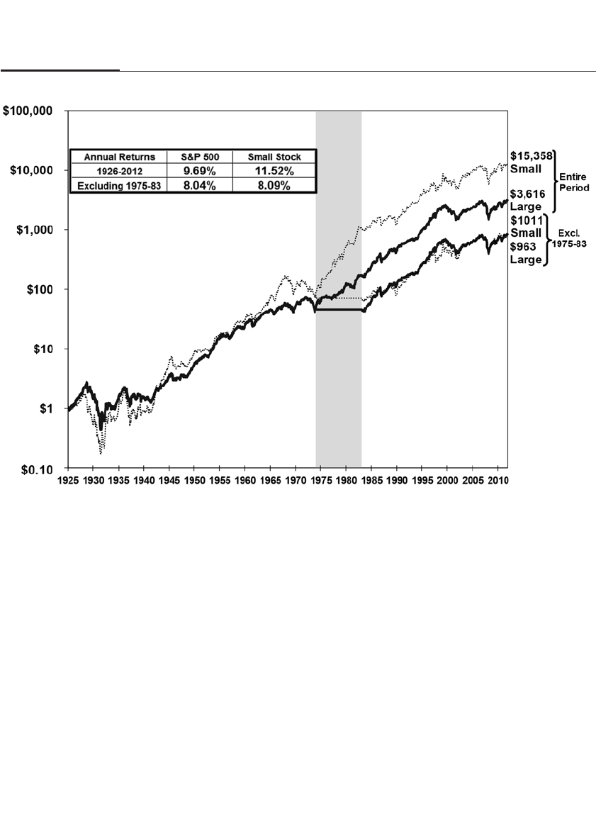
1,400 percent. Nevertheless, Figure 12-1 shows that if the nine-year period
from 1975 through 1983 is eliminated, the total accumulation in large
stocks over the entire period from 1926 through 2006 is virtually the same.
What caused the tremendous performance of small stocks during
the 1975-to-1983 period? In the late 1970s and early 1980s, pension and
institutional managers found themselves attracted to smaller stocks fol-
lowing the collapse of the large-growth stocks, known as the “Nifty
Fifty,” that were so popular in the preceding bull market. In addition, the
enactment of the Employee Retirement Income Security Act by Congress
in 1974 made it far easier for pension funds to diversify into small stocks,
boosting their holdings of these issues.
After 1983, small stocks hit a long dry period that lasted 17 years, as
they underperformed large stocks, especially in the late 1990s as the
technology boom gained momentum. But when the technology bubble
burst, small stocks strongly outperformed once again. From the March
2000 peak through 2012, despite the severe intervening bear market,
178 PART II The Verdict of History
FIGURE 12–1
Returns to Small and Large Stocks 1926–2012 Including and Excluding 1975–1983 Period

small stocks enjoyed a 7.2 percent annual return, while large stocks, rep-
resented by the S&P 500 Index, returned less than 1 percent per year.
Whatever the reasons for the small stock surges, the trendiness of
small stock returns does not mean that investors should avoid these
firms. Small- and mid-cap stocks constitute about 20 percent of the mar-
ket value of all U.S. stocks. One should be warned, however, that the
existence of the small stock premium does not mean that small stocks
will outperform large stocks every year, or even every decade.
VALUATION: “VALUE” STOCKS OFFER HIGHER
RETURNS THAN “GROWTH” STOCKS
The second dimension along which stocks are classified is by valuation—
that is, factors relating the price of the stock relative to some fundamen-
tal metric of firm worth, such as dividends, earnings, book values, and
cash flows. Fama and French determined that, like small-cap stocks,
stocks that were cheap relative to these fundamentals had higher returns
than would be predicted by the capital asset pricing model.
Stocks whose prices are low relative to these fundamentals are
called value stocks, while those with prices high relative to firm funda-
mentals are called growth stocks. Prior to the 1980s, value stocks were
often called cyclical stocks because low-P/E stocks were often found in
those industries whose profits were closely tied to the business cycle.
With the growth of style investing, equity managers that specialized in
these stocks were uncomfortable with the “cyclical” moniker and greatly
preferred the term value.
Value stocks generally occur in such industries as oil, motor, finance,
and utilities where investors have low expectations of future growth or
believe that profits are strongly tied to the business cycle, while growth
stocks are generally found in such industries as technology, brand-name
consumer products, and healthcare where investors expect profits either
to grow quickly or to be more resistant to the business cycle.
DIVIDEND YIELDS
Dividends have always been an important criterion for choosing stocks,
as Graham and Dodd stated in 1940:
Experience would confirm the established verdict of the stock market that a
dollar of earnings is worth more to the stockholder if paid him in dividends
than when carried to surplus. The common-stock investor should ordinar-
ily require both an adequate earning power and an adequate dividend.11
CHAPTER 12 Outperforming the Market 179
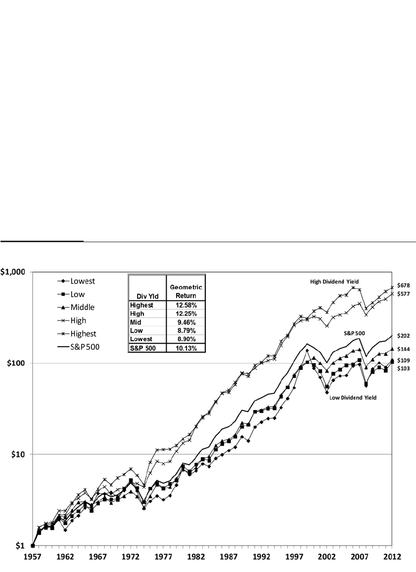
180 PART II The Verdict of History
Graham and Dodd’s claim has been supported by subsequent
research. In 1978, Krishna Ramaswamy and Robert Litzenberger estab-
lished a significant correlation between dividend yield and subsequent
returns.12 And more recently, James O’Shaughnessy has shown that in
the period 1951 through 1994, the 50 highest-dividend-yielding large-
capitalization stocks had a return that was 1.7 percentage points higher
than the market.13
The historical analysis of the S&P 500 Index supports the case for
using dividend yields to achieve higher stock returns. On December 31
of each year from 1957 onward, I sorted the firms in the S&P 500 Index
into five groups (or quintiles) ranked from the highest to the lowest div-
idend yields and then calculated the total returns over the next calendar
year. The striking results are shown in Figure 12-2.
FIGURE 12–2
Returns to S&P 500 Stocks Ranked by Dividend Yield, 1957–2012

The portfolios with higher dividend yields offered investors higher
total returns than the portfolios of stocks with lower dividend yields. If
an investor put $1,000 in an S&P 500 Index fund at the end of December
1957, she would have accumulated $201,760 by the end of 2012, for an
annual return of 10.13 percent. An identical investment in the 100 high-
est dividend yielders accumulated to over $678,000, with a return of
12.58 percent.
The highest dividend yielders also had a beta below 1, indicating
these stocks were more stable over market cycles, as shown in Table 12-3.
The lowest-dividend-yielding stocks not only had the lowest return
but also the highest beta. The annual return of the 100 highest dividend
yielders in the S&P 500 Index since the index was founded in 1957 was
3.42 percentage points per year above what would have been predicted
by the efficient market model, while the return of the 100 lowest divi-
dend yielders would have had a return that was 2.58 percentage points
per year lower.
Other Dividend-Yield Strategies
There are other high-dividend-yield strategies that have outperformed
the market. A well-known one is called the “Dogs of the Dow,” or the
“Dow 10” strategy, and is chosen from high-yielding stocks in the Dow
Jones Industrial Average.
The Dow 10 strategy has been regarded by some as one of the
simplest and most successful investment strategies of all time. James
Glassman of the Washington Post claimed that John Slatter, a Cleveland
investment advisor and writer, invented the Dow 10 system in the 1980s.14
Harvey Knowles and Damon Petty popularized the strategy in their book
CHAPTER 12 Outperforming the Market 181
TABLE 12–3
Return on S&P 500 Stocks Ranked by Dividend Yield, 1957–2012
Dividend Geometric Arithmetic Standard Excess Return
Yield Return Return Deviation Beta Over CAPM
Highest 12.58% 14.25% 19.34% 0.94 3.42%
High 12.25% 13.42% 16.26% 0.82 3.91%
Mid 9.46% 10.77% 16.64% 0.92 0.18%
Low 8.79% 10.64% 19.29% 1.07 –1.75%
Lowest 8.90% 11.62% 23.92% 1.23 –2.58%
S&P 500 10.13% 11.55% 17.15% 1.00 0.00%

The Dividend Investor, written in 1992, as did Michael O’Higgins and John
Downes in Beating the Dow.
The strategy calls for investors at year-end to buy the 10 highest-
yielding stocks in the Dow Jones Industrial Average and to hold them
for the subsequent year and then repeat the process each December 31.
These high-yielding stocks are often those that have fallen in price and
are out of favor with investors—which is the reason the strategy is often
called the Dogs of the Dow.
Another natural extension of the Dow 10 strategy is to choose the
10 highest-yielding stocks from among the 100 largest stocks in the S&P
500. The 100 largest stocks in the S&P 500 Index compose a much higher
percentage of the entire U.S. market than the 30 stocks in the Dow Jones
Industrial Average.
Indeed, both these strategies have excelled, as Figure 12-3 shows.15
Since 1957, the Dow 10 strategy returned 12.63 percent per year, and the
S&P 10 returned a dramatic 14.14 percent per year, consistently above
their respective benchmarks. And both of these strategies have a lower
beta than either the Dow Jones Industrial Average or the S&P 500 Index,
as shown in Figure 12-3.
The worst year for both the Dow 10 and S&P 10 strategies relative to
the benchmark indexes was 1999, when the high-capitalization tech stocks
reached their bubble peak. The Dow 10 underperformed the S&P 500
Index by 16.72 percent that year, and the S&P 10 underperformed by over
17 percentage points. It is during the later stages of a bull market, when
growth stocks catch the eye of speculative investors, that these value-
based strategies will underperform capitalization-weighted strategies.
But these strategies have gained these losses back—and more—
during subsequent bear markets. The Dow 30 was down by 26.5 percent,
and the S&P 500 Index was down 37.3 percent during the 1973-to-1974
bear markets. But the S&P 10 strategy fell only 12 percent, while the Dow
10 strategy actually gained 2.9 percent in these two years.
These dividend-based strategies also resisted the 2000-to-2002 bear
market. From the end of 2000 through the end of 2002, when the S&P 500
Index fell by more than 30 percent, the Dow 10 strategy fell by only less
than 10 percent, and the S&P 10 strategy fell by less than 5 percent. In the
bear market that followed the financial crisis, the Dow 10 and S&P 10
strategies did not cushion investors, as such high-profile dividend-paying
stocks as General Motors filed for bankruptcy. But over the entire market
cycle from 2007 through 2012, they only slightly underperformed their
respective benchmarks and did not significantly reduce their long-term
outperformance.
182 PART II The Verdict of History
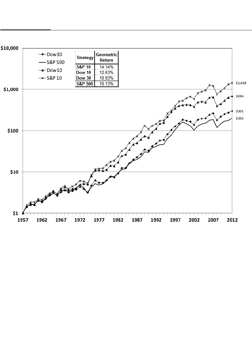
PRICE/EARNINGS RATIOS
Another important metric of value that can be used to formulate a win-
ning strategy is the P/E ratio—the price of a stock relative to its earnings.
The research into P/E ratios began in the late 1970s, when Sanjoy Basu,
building on the work of S. F. Nicholson in 1960, discovered that stocks
with low price/earnings ratios have significantly higher returns than
stocks with high price/earnings ratios, even after accounting for risk.16
Again, these results would not have surprised the value investors
Graham and Dodd, who, in their classic 1934 text Security Analysis,
stated the following:
Hence we may submit, as a corollary of no small practical importance, that
people who habitually purchase common stocks at more than about 16
CHAPTER 12 Outperforming the Market 183
FIGURE 12–3
Returns to S&P 500 and Dow Industrials and Their 10 Highest Yielding Stocks, 1957–2012
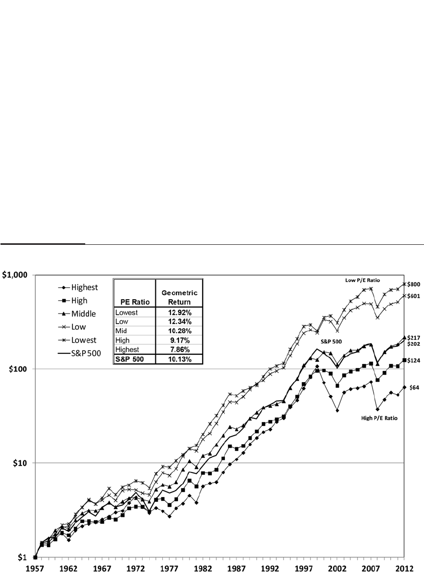
184 PART II The Verdict of History
times their average earnings are likely to lose considerable money in the
long run.17, 18
In a manner analogous to the research on dividend yields among
S&P 500 stocks, I computed the P/E ratios for all 500 firms in the index
on December 31 of each year by dividing the last 12 months of earnings
by the year-end prices. I then ranked these firms by P/E ratios and
divided them into five quintiles, computing their subsequent return
over the next 12 months.19 The results of this research are similar to that
reported on the dividend yield and are shown in Figure 12-4.
Stocks with high P/Es (or low earnings yields) are, on average,
overvalued and have given lower returns to investors. A $1,000 portfolio
of the highest-P/E stocks has accumulated to $64,116 by the end of 2012,
earning an annual return of 7.86 percent, while the lowest-P/E stocks
had a return of 12.92 percent and accumulated to almost $800,000.
FIGURE 12–4
Returns to S&P 500 Stocks Ranked by P/E Ratio, 1957–2012

In addition to a higher yield, the standard deviation of low-P/E
stocks was lower, and the beta was much lower, than that of the S&P 500
Index stocks, as shown in Table 12-4. In fact, the return on the 100
lowest-P/E stocks in the S&P 500 Index was more than 6 percentage
points per year above what would have been predicted on the basis of
the capital asset pricing model.
PRICE/BOOK RATIOS
Price/earnings ratios and dividend yields are not the only value-based
criteria. A number of academic papers, beginning with Dennis Stattman’s
in 1980 and later supported by Fama and French, suggested that price/
book ratios might be even more important than price/earnings ratios in
predicting future cross-sectional stock returns.20
Just as they did with P/E ratios and dividend yields, Graham and
Dodd considered book value to be an important factor in determining
returns:
[We] suggest rather forcibly that the book value deserves at least a fleeting
glance by the public before it buys or sells shares in a business undertak-
ing. . . . Let the stock buyer, if he lays any claim to intelligence, at least be
able to tell himself, first, how much he is actually paying for the business,
and secondly, what he is actually getting for his money in terms of tangi-
ble resources.21
Although Fama and French found that the ratio of book to market
value was a slightly better value metric than the dividend yield or P/E
ratio in explaining cross-sectional returns in their 1992 research, there
are conceptual problems with using book value as a value criterion.
CHAPTER 12 Outperforming the Market 185
TABLE 12–4
Return on S&P 500 Stocks Ranked by P/E Ratio 1957–2012
Geometric Arithmetic Standard Excess Return
PE Ratio Return Return Deviation Beta Over CAPM
Lowest 12.92% 14.20% 16.59% 0.71 6.01%
Low 12.34% 13.54% 16.23% 0.65 6.05%
Mid 10.28% 11.45% 15.67% 0.69 3.46%
High 9.17% 10.30% 15.49% 0.73 1.85%
Highest 7.86% 9.86% 19.84% 0.92 –0.78%
S&P 500 10.13% 11.55% 17.15% 1.00 0.00%

186 PART II The Verdict of History
Book value does not correct for changes in the market value of assets,
nor does it capitalize research and development expenditures. In fact,
over the time period 1987 through 2012, our studies showed that book
value underperformed either dividend yields, P/E ratios, or cash flows
in explaining returns.22 Since it is likely that an increasing fraction of a
firm’s worth will be captured by intellectual property, book value may
become an even more imperfect indicator of firm value in the future.
COMBINING SIZE AND VALUATION CRITERIA
The compound annual returns on stocks sorted into 25 quintiles along
size and book-to-market ratios from 1958 through 2006 are summarized
in Table 12-5.23
Historical returns on value stocks have surpassed the returns on
growth stocks, and this outperformance is especially true among smaller
stocks. The smallest value stocks returned 17.73 percent per year, the high-
est of any of the 25 quintiles analyzed, while the smallest growth stocks
returned only 4.70 percent, the lowest of any quintile. As firms become
larger, the difference between the returns on value and growth stocks
becomes much smaller. The largest value stocks returned 11.94 percent per
year, while the largest growth stocks returned about 9.38 percent.
TABLE 12–5
Returns Ranked by Size and Book-to-Market Ratios, 1958–2012
Size Quintiles
Entire Period Small 2 3 4 Large
Value 17.73% 16.39% 16.74% 14.15% 11.94%
2 16.24% 15.68% 15.18% 14.71% 10.67%
3 13.56% 14.84% 13.36% 12.92% 10.54%
4 12.53% 12.17% 13.14% 10.77% 10.21%
Growth 4.70% 7.88% 8.62% 10.37% 9.38%
Size Quintiles
Excluding 1975–1983 Small 2 3 4 Large
Value 13.83% 13.04% 13.97% 11.74% 10.71%
2 12.67% 12.28% 12.72% 13.01% 8.95%
3 9.66% 12.25% 10.64% 10.64% 9.50%
4 8.52% 8.81% 10.21% 8.78% 9.00%
Growth 0.56% 4.55% 6.02% 8.66% 9.01%
Book to
Market
Quintiles
Book to
Market
Quintiles
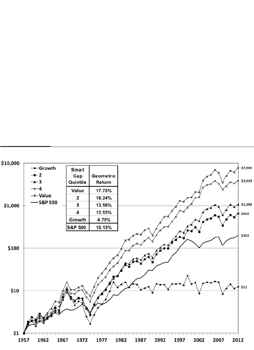
CHAPTER 12 Outperforming the Market 187
When the 1975-to-1983 period is removed, the return to small
stocks shrinks, as expected. But it is noteworthy that the difference in the
returns to small value and growth stocks remains large and virtually
unchanged.
The dramatic differences in the cumulative return to smallest quin-
tile growth and value stocks over the period from 1957 through 2012 are
shown in Figure 12-5. The sum of $1,000 invested in small growth stocks
since December 1997 has accumulated to $12,481 by the end of 2012. In
contrast, small value stocks have accumulated to an eye-opening $7.9
million.
Accentuating the difference in the performance of small growth
and value stocks is that the risk measured by the beta of the small-cap
value stocks is about 1, while that of the small growth stocks is over 1½.
FIGURE 12–5
Returns to Smallest Quintile Growth and Value Stocks 1957–2012

This means that the historical return to small value stocks is more than
7.5 percentage points above the efficient market prediction, while the
historical return to small growth stocks has been more than 7 percentage
points below its predicted level.
INITIAL PUBLIC OFFERINGS: THE DISAPPOINTING OVERALL
RETURNS ON NEW SMALL-CAP GROWTH COMPANIES
Some of the most sought-after small stocks are initial public offerings
(IPOs). New companies are launched with enthusiasm that excites
investors, who dream that the upstarts will turn into the next Microsofts
or Googles. The large demand for IPOs causes most IPOs to surge in
price after they are released into the secondary market, offering those
investors who were able to buy the stock at the offering prices immedi-
ate gains.24 As a result, the vast majority of these IPOs are classified as
growth stocks.
Certainly there have been some big winners among past IPOs.
Walmart, which went public in October 1970, turned a $1,000 investment
into more than $1,380,000 by the end of 2012. Investors who put $1,000
into Home Depot and Intel when they went public also turned into mil-
lionaires—if they held on to their stock. Cisco Systems was another win-
ner. Floated to the public in February 1990, the stock of this networking
supplier has delivered an average of 27 percent annual returns to
investors through December 2012, although all the gains were made in
the first 10 years after the IPO.
But can these big winners compensate for all the losers? To deter-
mine whether IPOs are good long-term investments, I examined the
buy-and-hold returns of almost 9,000 IPOs issued between 1968 and
2001. I calculated the returns based on whether investors purchased the
IPOs either at the end of the first month of trading or at the IPO offer
price and held these stocks until December 31, 2003.25
There is no question that the losing IPOs far outnumber the win-
ners. Of the 8,606 firms examined, the returns on 6,796 of these firms, or
79 percent, have subsequently underperformed the returns on a repre-
sentative small stock index, and almost half the firms have underper-
formed by more than 10 percent per year.
Unfortunately, the huge winners like Cisco and Walmart cannot
compensate for the thousands of losing IPOs. The differences in the returns
to a portfolio that buys an equal dollar amount of all the IPOs issued in
a given year and a portfolio in which an investor puts an equivalent dol-
lar amount into a Russell 2000 small-cap stock index are featured in
188 PART II The Verdict of History
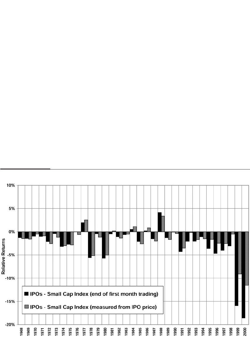
Figure 12-6. Returns are computed from two starting points: (1) from the
end of the month when the IPO was first issued and (2) from the usually
lower IPO offer price.
The returns on all yearly IPO portfolios issued from 1968 through
2000 were examined to December 31, 2003, to allow for at least three
years of subsequent returns to be calculated. The results are clear.
From 1968 through 2000, the yearly IPO portfolios underperformed a
small-cap stock index in 29 out of 33 years when measured either from
the last day of trading in the month they were issued or from the IPO
issue price.
Even in years such as 1971 when the big-winning stocks Southwest
Airlines, Intel, and Limited Stores all went public, a portfolio of all the
IPOs issued that year trailed the returns on a comparable small-cap
stock index when measured through 2003, and the same happened in
1981 when Home Depot went public.
Even in the banner year 1986, when Microsoft, Oracle, Adobe,
EMC, and Sun Microsystems all went public and delivered 30+ percent
CHAPTER 12 Outperforming the Market 189
FIGURE 12–6
Buy-and-Hold Returns of Almost 9,000 IPOs Issued Between 1968 and 2001

annual returns over the next 16 years, a portfolio of all the IPOs from
that year just barely managed to keep up with the small-cap stock index.
The performances of the mostly technology IPOs issued in the late
1990s were disastrous. The yearly IPO portfolios in 1999 and 2000 under-
performed the small-cap stock index by 8 and 12 percent per year,
respectively, if measured from the IPO price, and 17 and 19 percent per
year if measured from the end of the first month of trading.
Even stocks that doubled or more on the opening of trading were
very poor long-term investments. Corvis Corporation, which designs
products for the management of Internet traffic, went public on July 28,
2000. At the time of the offering, the firm had never sold a dollar’s worth
of goods and had $72 million in operating losses. Nevertheless, Corvis
had a market value of $28.7 billion at the end of the first trading day, a
capitalization that would place it in the top 100 most valuable firms in
the United States.
It is sobering to contrast Corvis Corporation with Cisco Systems,
which went public 10 years earlier. By the time of its IPO in February
1990, Cisco had already been a profitable company, earning healthy
profits of $13.9 million on annual sales of $69.7 million. The market
value of Cisco’s IPO at the end of the first trading day was $287 million,
exactly one-hundredth of the market value of Corvis Corporation,
which at the time had not yet had either sales or profits. Cisco would be
classified as a “growth” company in 1990 with a higher-than-average
P/E ratio, but Corvis was a “hypergrowth” company.
Corvis Corporation, with an IPO price of $360 (split adjusted) on
July 28, 2000, opened trading at $720 and later rose to $1,147 in early
August. Subsequently the stock fell to $3.46 in April 2005.
THE NATURE OF GROWTH AND VALUE STOCKS
When choosing “growth” and “value” stocks, investors should keep in
mind that these designations are not inherent in the product the firm
produces or the industry that the firm is in. The designations depend
solely on the market value relative to some fundamental measure of
enterprise value, such as earnings or dividends.
Therefore, a firm in the technology sector, which is considered to be an
industry with high growth prospects, could actually be classified as a value
stock if it is out of favor with investors and sells for a low price relative to
fundamentals. Alternatively, a promising auto manufacturer in a mature
industry with limited growth potential could be classified a growth stock if
its stock is in favor with investors and priced high relative to fundamentals.
190 PART II The Verdict of History

In fact, over time many firms and even industries are alternately character-
ized as “value” or “growth” as their market price fluctuates.
EXPLANATIONS OF SIZE AND VALUATION EFFECTS
There have been many attempts to explain the size and valuation factors
in stock returns. Fama and French had hypothesized that there might be
unusual financial stresses in value stocks that only appear during peri-
ods of extreme crisis, and that investors demand a premium to hold
value stocks in case those circumstances arise. Indeed, value stocks did
underperform growth stocks during the Great Depression and the stock
market crash of 1929 through 1932. But since then, value stocks have
actually done better than growth stocks during both bear markets and
economic recessions, so it is doubtful this is the answer.26
Another possible reason why value stocks outperform growth
stocks is that the use of beta to summarize the risk of a stock is too nar-
row. Beta is derived from the capital asset pricing theory, a static pricing
model that depends on an unchanged set of investment opportunities.
In a dynamic economy, real interest rates proxy changes in the opportu-
nity set for investors, and stock prices will respond not only to earnings
prospects but also to changes in interest rates.
In an article entitled “Bad Beta, Good Beta,” John Campbell sepa-
rates the beta related to interest rate fluctuations (which he called “good
beta”) from the beta related to business cycles (which he called “bad
beta”)27 based on historical evidence. But recent data are not supportive
of this theory, as growth stocks first rose relative to value stocks from
1997 to 2000 when real interest rates were rising, and then the stocks sub-
sequently underperformed as real interest rates dropped.
Another theory about why growth stocks have underperformed
value stocks is behavioral: investors get overexcited about the growth
prospects of firms with rapidly rising earnings and bid them up exces-
sively. “Story stocks” such as Intel or Microsoft, which in the past pro-
vided fantastic returns, capture the fancy of investors, while those firms
providing solid earnings with unexciting growth rates are neglected.28
The Noisy Market Hypothesis
A more general theory for the outperformance of value stocks is that
stock prices are constantly being impacted by buying and selling that are
unrelated to the fundamental value of the firm. These buyers and sellers
are called “liquidity” or “noise” traders in the academic literature. Their
CHAPTER 12 Outperforming the Market 191

transactions may be motivated by taxes, fiduciary responsibilities, rebal-
ancing of their portfolio, or other personal reasons. In order to explain
the value and size effects we see in the historical data, another assump-
tion needs to be added: that price movements caused by these liquidity
traders are not immediately reversed by those trading on fundamental
information.
This assumption is a deviation from the efficient market hypothesis
that claims that at all times the price of a security is the best unbiased
estimate of the underlying value of the enterprise. I have called the alter-
native assumption the “noisy market hypothesis” because the buying
and selling by noise or liquidity traders often obscure the fundamental
value of the firm.29
The noisy market hypothesis can provide an explanation for the
size and value effects.30 A positive liquidity shock raises the price of the
stock above its fundamental value and makes that stock more likely to
be classified as a “large” or “growth” stock. When this positive shock
disappears, these large growth stocks decline in price and thus have
lower returns. On the other hand, a negative liquidity shock lowers the
price and makes it more likely a stock will belong to the “small” or
“value” category, which is likely to be underpriced relative to its funda-
mentals. When the negative shock disappears, these value stocks have
higher returns.
Liquidity Investing
Recently another factor has been found to explain return: the “liquidity”
of a stock. Liquidity is a property of an asset that measures the discount
that sellers would encounter if they were forced to sell on short notice.
Assets with high liquidity are defined to have low discounts, while
assets with low liquidity have high discounts. One convenient measure
of liquidity is the ratio of the average daily volume of a stock compared
with the total number of shares outstanding, often referred to as the
turnover of the stock. Stocks with high turnover have higher liquidity
than stocks with lower turnover.
Recently Roger Ibbotson and others have determined that stocks
with low liquidity have significantly higher returns than stocks with
high liquidity.31 Analyzing all New York, Amex, and Nasdaq stocks from
1972 to the present, they determined that stocks with the lowest quartile
(25 percent) of turnover have a compound annual return of 14.74 percent
per year, almost double the return of stocks with the highest quartile of
liquidity. And they determined that this was not just because many of
192 PART II The Verdict of History

the small stocks have low turnover, and so the liquidity effect is not just
mimicking the size effect. In fact, among the smallest quartile of stocks,
measured by market value, the impact of liquidity was even more pro-
nounced, as the return on the lowest quartile of these small stocks aver-
aged 15.64 percent per year, against only a 1.11 percent return for those
with the highest turnover.32
There are several good reasons for the liquidity effect. It has been
long recognized that among assets with identical or near identical risk-
return profiles, those that are more actively traded sell at a higher price.
In the U.S. Treasury market, the “on-the-run” long-term government
bonds, which are considered benchmark and most actively traded, com-
mand a higher market price than virtually identical bonds with a matu-
rity just a few months’ difference. Traders and speculators are willing to
pay a premium for assets that they can buy and sell in quantity with low
transaction costs. All investors value flexibility—the ability to change
their mind or respond to altered circumstances quickly without paying
a substantial discount or premium if they wish to sell or buy their asset.
Furthermore, many large mutual funds would not be able to purchase
large quantities of relatively inactive firms since to do so would require
driving up their price to a point where the return is no longer attractive.
The presence of an even stronger liquidity premium among small
stocks can be explained since small stocks that are actively traded are
subject to speculation, particularly IPOs or those that catch the eye of
traders looking for unusual trading activity. After the speculative period
ends, these stocks often exhibit poor returns. There is no question that in
the post–World War II period, IBM generated more excitement and more
trading activity than Standard Oil, although as we showed at the begin-
ning of this chapter, Standard Oil delivered higher returns to investors.
CONCLUSION
Historical research shows that investors can achieve higher long-term
returns without taking on increased risk by focusing on the factors relat-
ing to the valuation of companies. Dividend yield has been one such fac-
tor, and the price/earnings ratio has been another. More recently,
liquidity has been identified as another factor. Over time, portfolios of
stocks with higher dividend yields, lower P/E ratios, and lower liquid-
ity have outperformed the market more than would be predicted by the
efficient market hypothesis.
Nevertheless, investors should be aware that no strategy will out-
perform the market all the time. Small stocks exhibit periodic surges that
CHAPTER 12 Outperforming the Market 193

have enabled their long-term performance to beat that of large stocks,
but most of the time their performance has only matched or fallen
behind that of large stocks. Furthermore, value stocks have generally
done well in bear markets, although in the last recession, value stocks,
because of the high preponderance of financials, underperformed
growth stocks. This means that investors must exercise patience if they
decide to pursue these return-enhancing strategies.
194 PART II The Verdict of History

Global Investing
Today let’s talk about a growth industry. Because investing world-
wide is a growth industry. The great growth industry is international
portfolio investing.
—JOHN TEMPLETON, 19841
Chapter 5 showed that the superior long-term returns of stocks were not
unique to the United States. Investors in other countries realized returns
that were near or even exceeded those in the United States. However,
until the late 1980s, foreign markets were almost exclusively the domains
of native investors and were considered too remote or risky to be enter-
tained by outsiders.
But no longer. The globalization of financial markets is not just a pre-
diction for the future; it is a fact right now. The United States, once the
unchallenged giant of capital markets, is today only one of many coun-
tries in which investors can accumulate wealth.
At the end of World War II, U.S. stocks composed almost 90 percent of
the world’s equity capitalization; in 1970, they still made up two-thirds. But
today, the U.S. market constitutes less than half of the world’s stock values,
and that fraction is shrinking. Figure 13-1 shows the percentage of the
world equity markets that are headquartered in each country in May 2013.
The developed world’s percentage is still high, at over 85.8 percent,
but that percentage is declining. As we learned in Chapter 4, the devel-
oping world is now producing more than one-half of the world’s GDP, a
fraction that will expand to two-thirds in the next 20 years. It is certain
that the percentage of equity headquartered in the emerging economies
will grow rapidly.
195
13
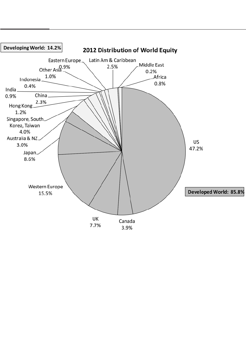
FOREIGN INVESTING AND ECONOMIC GROWTH
The tremendous growth in capital in the emerging economies might
prompt some investors to overweight that sector. But the prospect of
economic growth is not the reason why one should invest globally. In
fact, it will probably surprise readers to learn that there is a negative cor-
relation between economic growth and stock returns, and this finding
extends not only to those countries in the developed world but also to
those in the developing world.
Figure 13-2A plots the growth of real per capita GDP against dollar
returns in the 19 countries that were included in the data used by
Dimson, Staunton, and Marsh from 1900 to the present.2Australia had
196 PART II The Verdict of History
FIGURE 13–1
Distribution of World Equities by Market Value, 2012
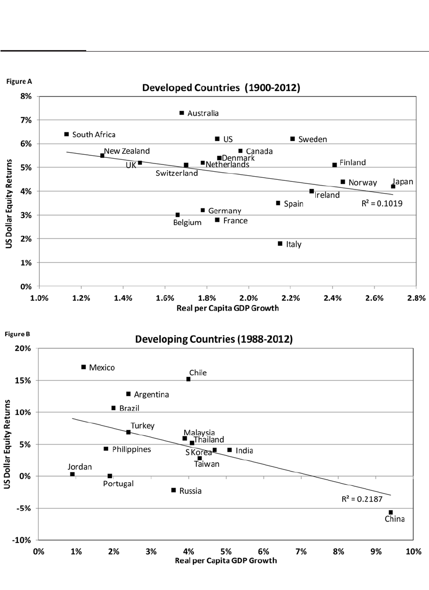
CHAPTER 13 Global Investing 197
FIGURE 13–2
Dollar Returns and per Capita Real GDP Growth in Developed and Developing Economies

the fifth-lowest growth rate but had the best returns, and South Africa
had the lowest growth rate and the second-best returns. Japan had by far
the highest growth rate but below-average stock returns.
As Figure 13-2B shows, the negative correlation between stock
returns and growth also extends to the developing countries. The fastest-
growing country by far, China, has had the worst returns. Mexico, Brazil,
and Argentina are among the slowest-growing countries but have gener-
ated excellent returns for investors.
How could this happen? For the same reason that Standard Oil of
New Jersey had better returns than IBM even though IBM beat Standard
Oil on every measure of growth. Low prices and high dividend yield
were among the keys to Standard Oil’s superior returns, the same reason
why investments in Mexican stocks outpaced those in Chinese stocks.
The conventional wisdom that investors should buy stocks in the
fastest-growing countries is wrong for the same reason that buying the
fastest-growing firms is wrong. China has indisputably been the world’s
fastest-growing country over the past three decades, but investors in
China realized poor returns because of the overvaluation of Chinese
equities. On the other hand, stock prices in Latin America were gener-
ally cheap, and the prices remained low relative to fundamental values.
Patient investors, buying value instead of hype, won out.
But this result begets the question: If faster growth is not the reason
to buy international stocks, what is?
DIVERSIFICATION IN WORLD MARKETS
The reason for investing internationally is to diversify your portfolio
and reduce risk. Foreign investing provides diversification in the same
way that investing in different sectors of the domestic economy provides
diversification. It would be poor investment strategy to pin your hopes
on just one stock or one sector of the economy. Similarly it is not a good
strategy to buy the stocks only in your own country, especially when
developed economies are becoming an ever smaller part of the world’s
market.
International diversification reduces risk because the stock prices
of different countries do not rise and fall in tandem, and this asynchro-
nous movement of returns dampens the volatility of the portfolio. As
long as two assets are not perfectly correlated, i.e., their correlation coef-
ficient is less than 1, then combining these assets will lower the risk of
your portfolio for a given return or, alternatively, raise the return for a
given risk.
198 PART II The Verdict of History

CHAPTER 13 Global Investing 199
International Stock Returns
Table 13-1 displays the historical risk and returns for dollar-based
investors in the international markets from 1970 to the present (1988 for
emerging market data). Over the entire period, the dollar returns among
different regions do not differ greatly.
Investors in U.S. stocks realized a 9.39 percent compound return;
those in EAFE (generally non-U.S. developed countries)3had a slightly
higher 9.74 percent return. Over the period, the correlation between
EAFE and U.S. returns was 65 percent, meaning that the risk to dollar
investors with an 80 percent U.S. and 20 percent EAFE portfolio would
be .175, which is 2 percent below the risk of holding U.S. stocks alone.
Since 1970, Europe realized slightly higher returns than the United
States, while Japan realized slightly lower returns. Comprehensive
emerging market returns are available from 1988 onward. The emerging
market returned 12.73 percent per year over that period, nearly 3 per-
centage points higher than the return to U.S. stocks, and U.S. stock
returns were less correlated with emerging market stock returns than
with EAFE returns. It should be noted that since 1988, EAFE returns
have trailed U.S. returns, almost entirely because Japan had negative
returns from 1988 through 2012.
The Japanese Market Bubble
The Japanese stock market in the last quarter of the twentieth century
stands as one of the most remarkable bubbles in world history. In the
TABLE 13–1
Dollar Risks and Returns in International Stocks 1970–2012
U.S. $ Returns
Country Domestic Exchange Total Correlation
or Region 1970–2012 1988–2012 Risk Risk Risk Coefficient*
World 9.39% 7.23% 17.48% 4.79% 18.17% 87.50%
EAFE 9.74% 5.49% 20.00% 9.62% 22.61% 65.27%
USA 9.63% 9.83% 17.80% — 17.80% —
Europe 10.33% 8.83% 20.73% 10.75% 22.13% 76.06%
Japan 9.15% –0.14% 28.08% 12.52% 33.29% 35.19%
Em Mkts** — 12.73% 68.77% 17.87% 35.89% 52.37%
*Correlation between U.S. dollar returns and foreign market US dollar returns.
**Data for emerging markets is from 1988 to 2012.

1970s and 1980s, Japanese stock returns averaged more than 10 percent-
age points per year above U.S. returns and surpassed those from every
other country. The bull market in Japan was so dramatic that by the end
of 1989, for the first time since the early 1900s, the market value of the
American stock market was no longer the world’s largest. Japan, a coun-
try whose economic base was totally destroyed in World War II and that
had only half the population and 4 percent of the land mass of the
United States, housed the world’s biggest stock market.
The superior returns in the Japanese market during the great bull
market attracted billions of dollars of foreign investment. By the end of
the 1980s, valuations on many Japanese stocks reached stratospheric lev-
els. Nippon Telephone and Telegraph, or NTT, the Japanese version of
America’s former telephone monopoly AT&T, sported a P/E ratio above
300. This company alone had a market value that dwarfed the aggregate
stock values of all but a handful of countries. Valuations reached and in
some cases exceeded those attained in the great U.S. technology stock
bubble of 2000 and were far above any valuations ever seen in the U.S.
or European markets.
During his travels to Japan in 1987, Leo Melamed, president of the
Chicago Mercantile Exchange, asked his hosts how such remarkably
high valuations could be warranted. “You don’t understand,” they
responded. “We’ve moved to an entirely new way of valuing stocks here
in Japan.” And that is when, as Martin Mayer reported, Melamed knew
Japanese stocks were doomed.4It is when investors cast aside the les-
sons of history that those lessons come back to haunt them.
When the Nikkei Dow Jones, which had surpassed 39,000 in
December 1989, fell sharply in the following years, the mystique of the
Japanese market was broken. Japanese stocks fell to 7,000 in 2008, less
than 20 percent of their value at the peak of the bull market two decades
earlier.
Many point to the Japanese market as a refutation of the thesis that in
the long run the stock market will always be the superior investment. But
there were glaring warnings of the Japanese bubble. At the peak of the
market, Japanese stocks sold for well over 100 times earnings, more than
3 times the level that our market sold at the top of its biggest bubble that
reached its height in 2000 when technology and Internet stocks peaked. In
contrast, Japanese stocks in 1970 sold at the same earnings multiple that
prevailed in the rest of the world stock markets, and indeed from 1970
onward Japanese stocks have matched the returns in other countries.
The bubble high of the Nasdaq Index in March 2000 was not unlike
that of the Japanese market. Price/earnings ratios in the tech-laden mar-
200 PART II The Verdict of History

ket topped 100, and dividend yields fell close to zero. It is not surprising
that in 2013, more than a decade after its peak, the Nasdaq Index, just
like the Nikkei, is still well below its high.
STOCK RISKS
The risks for dollar investors in foreign stocks are measured by the stan-
dard deviation of annual dollar returns. There are two components of
risk: fluctuations of stock prices calculated in their local currencies and
fluctuations in the exchange rate between the dollar and the local cur-
rency. In Table 13.1 these are described as the domestic risk and the
exchange risk.
For the non-U.S. developed countries (EAFE), local risk is 20 per-
cent, and exchange risk is almost half that number at 9.62 percent. But
the total dollar risk is only 13 percent higher than the local risk, at 22.61
percent. This is because exchange risk often moves in the opposite direc-
tion of local risk. Exchange rate risk for the dollar investor is somewhat
higher for Japanese stocks than for European stocks.
The interpretation of the dollar risk for the emerging markets
requires special care. The raw data show that exchange rate fluctuations
actually offset one-half of the domestic risk. But closer examination of
the data shows that this result is dominated by the high inflation rates in
the earlier data that sent local returns soaring while exchange rates were
depreciating rapidly. Since 2000, when most developing countries
brought down inflation to lower levels, fluctuations in the exchange rate
have actually added, and in some cases added substantially, to the local
stock risk.
Should You Hedge Foreign Exchange Risk?
Since foreign exchange risk generally adds to the local risk, it may be desir-
able for investors in foreign markets to hedge against currency movements.
Currency hedging means entering into a currency contract or purchasing a
security that automatically hedges foreign exchange fluctuations.
But hedging foreign exchange risk is not always the right strategy.
The cost of hedging depends on the difference between the interest rate
in the foreign country and the dollar interest rate; and if a country’s cur-
rency is expected to depreciate (typically because of high inflation), the
cost of hedging could be quite high.
For example, even though the British pound depreciated from $4.80
to about $1.60 over the past century, the cost of hedging this decline
CHAPTER 13 Global Investing 201

exceeded the depreciation in the pound. Thus the dollar returns to
British stocks were higher if investors did not hedge the decline in the
pound than if they did.
For investors with long-term horizons, hedging currency risk in for-
eign stock markets may not be important. In the long run, exchange rate
movements are determined primarily by differences in inflation between
countries, a phenomenon called purchasing power parity. Since equities are
claims on real assets, their long-term returns have compensated investors
for changes in inflation and thus protected investors from exchange
depreciation caused by higher inflation in the foreign countries.
Over shorter periods of time, investors may reduce their dollar risk
by hedging exchange risk. Often, bad economic news for a country
depresses both its stock market and currency value, and investors can
avoid the latter by hedging. Furthermore, if it is the policy of the central
bank to lower the currency value in order to stimulate exports and the
economy, hedged investors can take advantage of the latter without suf-
fering the losses of the former. For example, investors who took hedged
positions in Japanese stocks late in 2012, when Prime Minister Shinzo
Abe advocated yen depreciation to stimulate the economy, far outpaced
the gains made by those who did not hedge the depreciating yen.
Diversification: Sector or Country?
Although capital markets are becoming more global, there is one aspect of
international investing that stands in the way of that trend. International
investing today is allocated by the country in which the firm has its head-
quarters, even if the firm does not sell or even manufacture goods in its
headquarters country. To accommodate current practice, in the early 1990s
Standard & Poor’s announced that no non-U.S.-based companies would
be added to its benchmark S&P 500 Index, and in 2002 Standard & Poor’s
removed the remaining seven foreign-based firms, including such giants
as Royal Dutch Petroleum and Unilever, from the index.5
Supporters of the headquarters approach argue that government
regulations and legal structures of a particular country do matter, even
when most of the firm’s sales, earnings, and production come from
abroad. But these home-country influences will very likely diminish as
globalization advances. It is far more logical to pursue an investing strat-
egy by allocating wealth according to the industrial sector in which the
firm belongs, wherever its headquarters may be.
Sector investment strategies are popular in the U.S. equity markets
but not as popular internationally. But I believe that this will change. In
202 PART II The Verdict of History

CHAPTER 13 Global Investing 203
fact, I envision a future of international incorporations, where firms choose
to be governed by a set of international rules agreed upon among nations
and where the headquarters of the company resides will be of very little
or no importance. International incorporation standards will be similar to
the growing popularity of the accounting standards promulgated by the
International Accounting Standards Board over country-based stan-
dards. If international incorporation gained prominence, there would be
no meaning to “headquartered country,” and investment allocations
would have to be made on the basis of global sectors or by production
and distribution locations. In this future, a U.S.-only portfolio would be
very narrow indeed. In that case, a sector approach to international
investing may well supplant the country approach in coming years.
Sector Allocation Around the World
Let’s take a closer look at the importance of these industrial sectors by
region and by country. The 10 Global International Classification (GIC)
industrial sectors in five geographic regions (United States, EAFE,
Europe, Japan, and the emerging markets)6are shown in Table 13-2 by
the respective weight of each industrial sector.7The 20 largest firms by
market value headquartered in and outside the United States are shown
in Table 13-3.
Despite the meltdown that followed the financial crisis of 2008, the
Financials sector is the largest sector in the world, almost double the size of
TABLE 13–2
Sector Allocation by World Regions, June 2013
S&P 500 EAFE Japan Em Mkts Europe Global
Consumer Discretionary 11.8% 11.4% 21.4% 8.2% 9.6% 11.4%
Consumer Staples 10.6% 11.9% 6.6% 9.3% 14.6% 10.6%
Energy 10.6% 7.1% 1.2% 11.6% 9.7% 10.1%
Financials 16.7% 25.2% 20.7% 27.9% 21.4% 21.2%
Healthcare 12.6% 10.4% 6.3% 1.3% 12.8% 10.2%
Industrials 10.1% 12.5% 18.9% 6.4% 11.4% 10.5%
Info Tech 18.0% 4.4% 10.9% 14.6% 2.8% 12.2%
Materials 3.3% 8.3% 6.0% 9.7% 8.4% 6.1%
Telecom 2.8% 5.1% 4.9% 7.6% 5.3% 4.3%
Utilities 3.2% 3.7% 3.0% 3.5% 4.0% 3.3%

204
TABLE 13–3
Largest U.S. and Foreign Companies, June 2013
Market Foreign Market
Rank U.S. Companies Sector Cap ($B) # Companies Country Sector Cap ($B)
1 Apple Info Tech $415 1 PetroChina China Energy $243
2 Exxon Mobil Energy $407 2 I & C Bank of China China Financials $237
3 Microsoft Info Tech $298 3 Nestle Switzerland Consumer Staples $218
4 General Electric Industrials $247 4 Roche Switzerland Healthcare $213
5 Johnson & Johnson Healthcare $239 5 Royal Dutch Shell Netherlands Energy $211
6 Chevron Energy $236 6 HSBC Holdings Britain Financials $205
7 Google Info Tech $291 7 China Mobile Hong Kong Telecom $204
8 IBM Info Tech $229 8 China Constr. Bank China Financials $196
9 Procter & Gamble Consumer Staples $213 9 Novartis Switzerland Healthcare $194
10 Berkshire Hathaway Financials $284 10 Toyota Japan Cons Discr $194
11 JPMorgan Chase Financials $205 11 Samsung South Korea Info Tech $188
12 Pfizer Healthcare $200 12 BHP Billiton Australia Materials $160
13 Wells Fargo Financials $218 13 Anheuser-Busch Belgium Consumer Staples $152
14 AT&T Telecom $191 14 Vodafone Britain Telecom $145
15 Coca-Cola Consumer Staples $184 15 AG Bank of China China Financials $143
16 Citigroup Financials $157 16 Sanofi France Healthcare $142
17 Philip Morris Int Consumer Staples $151 17 BP Britain Energy $136
18 Merck Healthcare $146 18 Bank of China China Financials $129
19 Verizon Telecom $144 19 GlaxoSmithKline Britain Healthcare $127
20 Bank of America Financials $144 20 Total SA France Energy $119

the next-largest sector, Information Technology. In the United States, the
Financials sector is the second largest at 16.7 percent of market value, just
below that of Technology but well down from the 22 percent weight before
the financial crisis. The largest share of the financial market value sector is
found in the emerging markets, as four Chinese banks are in the top 20
non-U.S. firms, ranked by market value. Berkshire Hathaway, recently
admitted to the S&P 500, is the largest firm in the Financials sector;
Berkshire is classified as a financial because of its large stake in insurance
companies. In the United States, Buffett’s Berkshire is followed by
JPMorgan Chase. HSBC Holdings (headquartered in the United Kingdom)
and Commonwealth Bank of Australia are the largest EAFE financials.
In the Consumer Discretionary sector, Japan has by far the highest
weight of all geographic regions, primarily because of the presence of
Toyota Motors, one of the 10 largest non-U.S.-based corporations in the
world. In the United States, Walt Disney and Home Depot are the largest
firms in this sector, and in EAFE Daimler AG follows Toyota.
Europe has the largest weight in the Consumer Staples sector, with
Swiss Nestle and Belgian Anheuser-Busch Inbev both belonging to the
top 20 non-U.S. firms by market value. In the United States, Procter &
Gamble, Coca-Cola, and Philip Morris International all belong to the top
20 U.S. firms. The Brazilian company AmBev, specializing in soft drinks,
is the largest firm in the emerging markets.
In the Energy sector Exxon Mobil is the largest firm by market value
in the world. But the Chinese Petrochina is the largest non-U.S. company
in terms of market value. Chevron in the United States and Royal Dutch,
BP, and Total in Europe all belong to the top 20 non-U.S. firms.
In the Information Technology sector, Apple, which vies with
Exxon Mobil for the world’s largest firm by market value, is followed by
Google, IBM, and South Korean Samsung Electronics, while SAP is the
largest European technology firm. In the Health Care sector, Johnson &
Johnson is the largest in the world, followed by Roche Holdings and
Novartis of Switzerland and U.S. pharmaceutical giants Pfizer and
Merck. In the Industrials sector General Electric dominates the list,
which is followed by the German Siemens. In the Materials sector, only
the Australian BHP Billiton makes the top 20 list, with Monsanto being
the highest-valued materials firm in the United States. In Telecom, AT&T
and Verizon make the top 20 list in the United States, while China
Mobile and the British Vodafone Group make the top 20 non-U.S. firms.
Finally, no utility makes the top 20 list of either the U.S. or non-U.S.
firms, with Duke Energy being the largest in the United States and the
British National Grid being the largest in EAFE.
CHAPTER 13 Global Investing 205

Private and Public Capital
Exxon Mobil may be the largest company by market value in the world,
and it has the largest reserves of oil and gas (25 billion barrels estimated
in 2011) of any private company. But if one includes government-owned
companies, this U.S. giant falls far from the top of the list. Saudi Arabia’s
Aramco and Iran’s NIOC together have estimated reserves in excess of
600 billion barrels!8If one were to value these reserves at only $10 a bar-
rel, less than one-tenth the going market price, these two companies are
worth in excess of $6 trillion. This is just a fraction of the wealth that is
still owned by governments around the world. In many countries, gas,
electric, and water facilities are still owned and operated by govern-
ment, and governments have a large, if not a controlling, interest in
many other industries.
Even in such privatized countries as the United States, the federal,
state, and local governments own trillions of dollars of wealth in such
forms as land, natural resources, roads, dams, schools, and parks. There
is strong disagreement about how much of this wealth, if any, should be
privatized. But there is good evidence that privatized firms often do
experience efficiency gains. Growth of the world’s capital stock will
come not only from private entrepreneurs but from the privatization of
many government-owned assets.
CONCLUSION
The inexorable trend toward integration of the world’s economies and
markets will certainly continue in this new millennium. No country will
be able to dominate every market, and industry leaders are apt to
emerge from any place on the globe. The globalization of the world
economy means that the strength of management, product lines, and
marketing will be far more important factors in achieving success than
where the firm is headquartered.
Sticking only to U.S. equities is a risky strategy for investors. No
advisor would recommend investing only in those stocks whose name
begins with the letters Athrough F. But sticking only to U.S. equities
would be just such a bet since U.S.-based equity will continue to shrink
as a share of the world market. Only those investors who have a fully
diversified world portfolio will be able to reap the best returns with the
lowest risk.
206 PART II The Verdict of History

PART
HOW THE
ECONOMIC
ENVIRONMENT
IMPACTS STOCKS
III
This page intentionally left blank

Gold, Monetary Policy,
and Inflation
In the stock market, as with horse racing, money makes the mare go.
Monetary conditions exert an enormous influence on stock prices.
—MARTIN ZWEIG, 19901
If Fed Chairman Alan Greenspan were to whisper to me what his
monetary policy was going to be over the next two years, it wouldn’t
change one thing I do.
—WARREN BUFFETT, 19942
On September 20, 1931, the British government announced that England
was going off the gold standard. It would no longer exchange gold for
deposits at the Bank of England or for British currency, the pound ster-
ling. The government insisted that this action was only “temporary,”
that it had no intention of forever abolishing its commitment to
exchange its money for gold. Nevertheless, it was to mark the beginning
of the end of both Britain’s and the world’s gold standard—a standard
that had existed for over 200 years.
Fearing chaos in the currency market, the British government
ordered the London Stock Exchange closed. New York Stock Exchange
officials decided to keep the U.S. exchange open but also braced for
panic selling. The suspension of gold payments by Britain, the second-
greatest industrial power, raised fears that other industrial countries
209
14

might be forced to abandon gold. Central bankers called the suspension
“a world financial crisis of unprecedented dimensions.”3For the first
time ever, the New York Stock Exchange banned short selling in an effort
to shore up stock share prices.
But much to New York’s surprise, stocks rallied sharply after a
short sinking spell, and many issues ended the day higher. Clearly,
British suspension was not seen as negative for American equities.
Nor was this “unprecedented financial crisis” a problem for the
British stock market. When England reopened the exchange on
September 23, prices soared. The AP wire gave the following colorful
description of the reopening of the exchange:
Swarms of stock brokers, laughing and cheering like schoolboys, invaded
the Stock Exchange today for the resumption of trading after the two-day
compulsory close-down—and their buoyancy was reflected in the prices
of many securities.4
Despite the dire predictions of government officials, shareholders
viewed casting off the gold standard as good for the economy and even
better for stocks. As a result of the gold suspension, the British govern-
ment could expand credit by lending reserves to the banking system,
and the fall in the value of the British pound would increase the demand
for British exports. The stock market gave a ringing endorsement to the
actions that shocked conservative world financiers. In fact, September
1931 marked the low point of the British stock market, while the United
States and other countries that stayed on the gold standard continued to
sink into depression. The lessons from history: liquidity and easy credit
feed the stock market, and the ability of the central banks to provide liq-
uidity at will is a critical plus for stock values.
A year and a half later, the United States joined Britain in abandon-
ing the gold standard, and finally every nation eventually went to a fiat,
paper money standard. But despite the paper standard’s inflationary
bias, the world has become comfortable with the new monetary system,
and the stock market enjoys the flexibility it accords policy makers.
MONEY AND PRICES
In 1950, President Truman startled the nation in his State of the Union
address with a prediction that the typical American family income
would reach $12,000 by the year 2000. Considering that median family
income was about $3,300 at the time, $12,000 seemed like a princely sum
210 PART III How the Economic Environment Impacts Stocks

and implied that America was going to make unprecedented economic
progress in the next half century. In fact, President Truman’s prediction
has proved quite modest. The median family income in 2000 was
$41,349. However, in 2000 that sum bought less than $6,000 in 1950
prices, a testament to the inflation of the last half century. So instead of
the typical family income soaring over 12 times, from $3,300 to $41,349
in roughly half a century, real incomes have only doubled, from $3,300 to
$6,000, because of the inflation bite.
Inflation and deflation have characterized history as far back as econ-
omists have gathered data. However, since 1955 there has never been a
single year in which the U.S. consumer price index has declined.5What
has changed over the past 60 years that makes inflation the rule rather
than the exception? The answer is simple: control of the money supply has
shifted from gold to the government. With this shift, the government can
always provide enough liquidity so that prices do not decline.
We analyzed the overall price level in the United States and Great
Britain over the last 210 years in Chapter 5. There was no overall infla-
tion until World War II and then protracted inflation after the war. Before
the Great Depression, inflation occurred only because of war, crop fail-
ures, or other crises. But the behavior of prices in the postwar period has
been entirely different. The price level has almost never declined: the
only question is at what rate prices will rise.
Economists have long known that one variable is paramount in
determining the price level: the amount of money in circulation. The
robust relation between money and inflation is strongly supported by the
evidence. Take a look at Figure 14-1, which displays money and prices in
the United States since 1830. The overall trend of the price level has closely
tracked that of the money supply normalized for the level of output.
The strong relation between the money supply and consumer prices
is a worldwide phenomenon. No sustained inflation is possible without
continuous money creation, and every hyperinflation in history has been
associated with an explosion of the money supply. There is overwhelming
evidence that countries with high monetary growth experience high infla-
tion, while countries with restrained money growth have low inflation.
Why is the quantity of money so closely connected to the price
level? Because the price of money, like any good, is determined by sup-
ply and demand. The supply of deposits is closely controlled by the cen-
tral bank. The demand for dollars is derived from the demand of
households and firms transacting billions of dollars of goods and serv-
ices in a complex economy. If the supply of dollars increases more than
CHAPTER 14 Gold, Monetary Policy, and Inflation 211
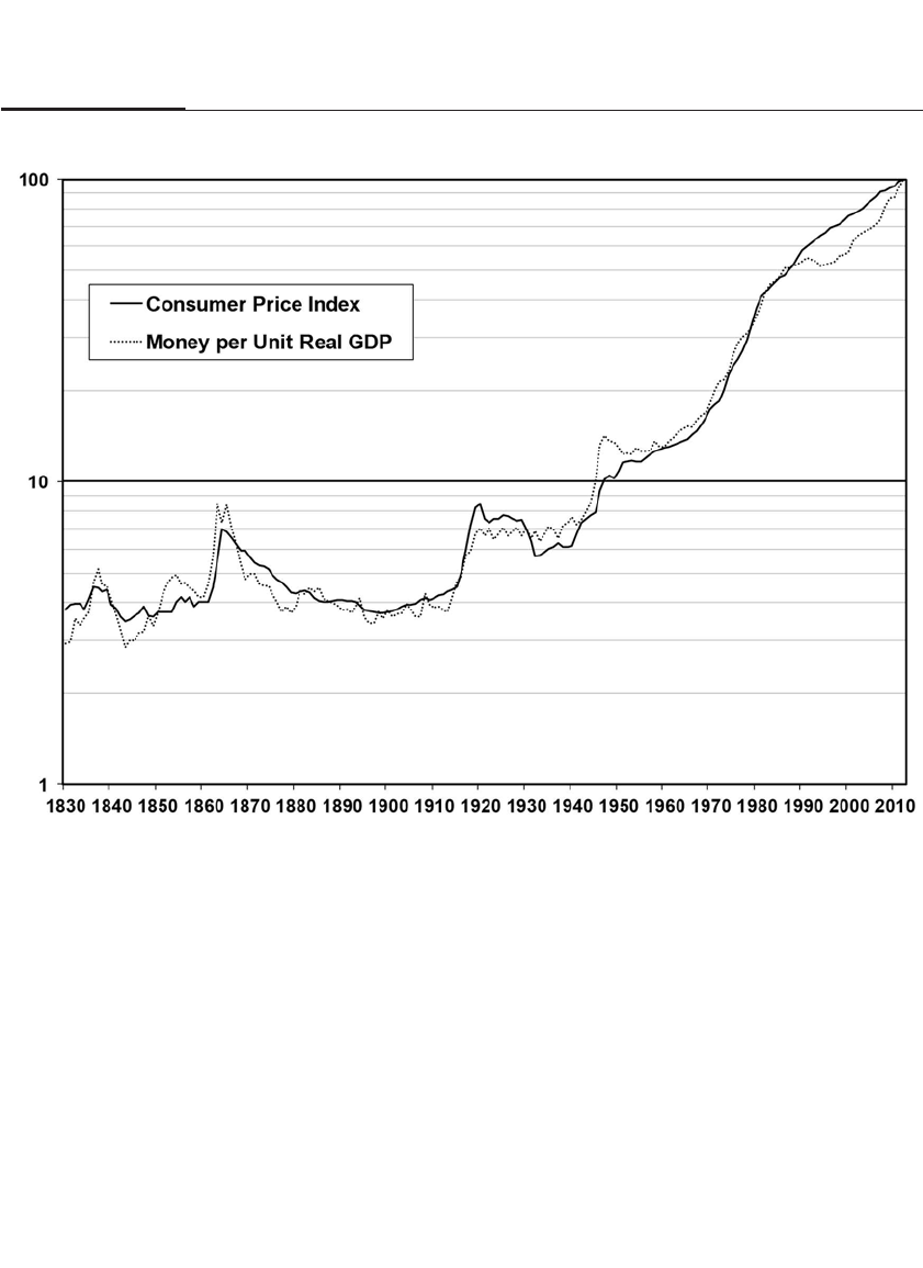
the number of goods produced, this leads to inflation. The classic
description of the inflationary process—“too many dollars chasing too
few goods”—is as apt today as ever.
One might wonder why the huge monetary expansion of the
Federal Reserve (and other central banks) since the monetary crisis has
not turned into inflation. Milton Friedman, in The Monetary History of the
United States, determined that it was the quantity of deposits plus cur-
rency, which he defined as M2, that had the closest link with inflation,
not the monetary base, which is the sum of reserves and currency. The
monetary base in the United States did triple from 2007 to 2013, but
almost all the increase went into excess reserves in the banking system
that had not been lent out and therefore did not create deposits. To be
sure, the Fed must monitor these reserves closely to prevent excess
credit creation from turning into inflation. But the low inflation, despite
212 PART III How the Economic Environment Impacts Stocks
FIGURE 14–1
Money and Prices in the United States, 1830–2012

the expansionary policies of the world central banks, has not contra-
dicted the historical link between money and prices.
THE GOLD STANDARD
For the nearly 200 years prior to the Great Depression, most of the indus-
trialized world was on a gold standard. This meant that central banks
were obligated to exchange the paper currency they issued for a fixed
amount of gold on demand. To do this, the U.S. and other governments
had to keep gold reserves in sufficient quantity to assure money holders
that the governments would always be able to make good on this
exchange. Since the total quantity of gold in the world increased at a
slow pace—new gold discoveries were relatively small compared with
the world’s total gold supply—prices of goods remained stable.
The only times the gold standard was suspended were during
crises, such as wars. Great Britain suspended the gold standard during
both the Napoleonic Wars and World War I, but in both cases it returned
to the gold standard at the original exchange rate. The United States
temporarily suspended the gold standard during the Civil War, but it
returned to the standard after the war ended.6
The adherence to the gold standard is the reason why the world
experienced no overall inflation during the nineteenth and early twenti-
eth centuries. But overall price stability was not achieved without cost.
Since the money in circulation had to equal the quantity of gold held by
the government, the central bank essentially relinquished control over
monetary conditions. This meant that the central bank was unable to
provide additional money during economic or financial crises. In the
1930s, adherence to the gold standard, which had restrained the govern-
ment from pursuing inflationary financial policies, turned into a strait-
jacket from which the government sought to escape.
THE ESTABLISHMENT OF THE FEDERAL RESERVE
Periodic liquidity crises caused by strict adherence to the gold stan-
dard prompted Congress in 1913 to pass the Federal Reserve Act that
created the Federal Reserve System. The responsibilities of the Fed
were to provide an “elastic” currency, which meant that in times of
banking crises the Fed would become the lender of last resort. In trying
times, the central bank would provide currency to enable depositors to
withdraw their deposits without forcing banks to liquidate loans and
other assets.
CHAPTER 14 Gold, Monetary Policy, and Inflation 213

In the long run, money creation by the Fed was still constrained by
the gold standard since the government’s paper currency, or Federal
Reserve notes, promised to pay a fixed amount of gold. But in the short
run, the Federal Reserve was free to create money as long as it did not
threaten the convertibility of Federal Reserve notes to gold at the
exchange rate of $20.67 per ounce that prevailed before the Great
Depression. Yet the Fed was never given any guidance by Congress or
by the Federal Reserve Act on how to conduct monetary policy and
determine the right quantity of money.
THE FALL OF THE GOLD STANDARD
This lack of guidance had disastrous consequences just two decades
later. In the wake of the stock crash of 1929, the world economies entered
a severe downturn. Falling asset prices and failing businesses made
depositors suspicious of banks’ assets. When word was received that a
few banks were having problems meeting depositors’ withdrawals, a
run on the banks ensued.
In an astounding display of institutional ineptitude, the Federal
Reserve failed to provide extra reserves in order to stem the banking
panic and prevent a crash of the financial system, even though the Fed
had the explicit power to do so under the Federal Reserve Act. In addi-
tion, those depositors who did receive their money sought even greater
safety by turning their notes back to the Treasury in exchange for gold, a
process that put extreme pressure on the government’s gold reserves.
The banking panic soon spread from the United States to Great Britain
and Continental Europe.
To prevent a steep loss of gold, Great Britain took the first step and
abandoned the gold standard on September 20, 1931, suspending the
payment of gold for sterling. Eighteen months later, on April 19, 1933,
the United States also suspended the gold standard as the Depression
and financial crisis worsened.
Investors loved the government’s newfound flexibility, and the reac-
tion of the U.S. stock market to gold’s overthrow was even more enthusi-
astic than that in Great Britain. Stocks soared over 9 percent on the day
the government left the gold standard and almost 6 percent the next day.
This constituted the greatest two-day rally in U.S. stock market history.
Investors felt the government could now provide the extra liquidity
needed to stabilize commodity prices and stimulate the economy, which
they regarded as a boon for stocks. Bonds, however, fell, as investors
214 PART III How the Economic Environment Impacts Stocks

feared the inflationary consequences of leaving the gold standard.
BusinessWeek, in a positive editorial on the suspension, asserted:
With one decisive gesture, [President Roosevelt] throws out of the win-
dow all the elaborate hocus-pocus of “defending the dollar.” He defies an
ancient superstition and takes his stand with the advocates of managed
money. . . . The job now is to manage our money effectively, wisely, with
self-restraint. It can be done.7
POSTDEVALUATION MONETARY POLICY
Ironically, while the right to redeem dollars for gold was denied U.S. cit-
izens, it was soon reinstated for foreign central banks at the devalued
price of $35 per ounce. As part of the Bretton Woods agreement, which
set up the rules of international exchange rates after the close of World
War II, the U.S. government promised to exchange all dollars for gold
held by foreign central banks at the fixed rate of $35 per ounce as long as
these countries fixed their currency to the dollar.
In the postwar period, as inflation increased and the dollar’s worth
declined, gold seemed more and more attractive to foreigners. U.S. gold
reserves began to dwindle, despite official claims that the United States
had no plans to change its gold exchange policy at the fixed price of $35
per ounce. As late as 1965, President Johnson stated unequivocally in the
Economic Report of the President: “There can be no question of our capac-
ity and determination to maintain the gold value of the dollar at $35.00
per ounce. The full resources of the Nation are pledged to that end.”8
But this was not so. As the gold reserves dwindled, Congress
removed the gold-backing requirement for U.S. currency in 1968. In next
year’s Economic Report of the President, President Johnson declared:
“Myths about gold die slowly. But progress can be made—as we have
demonstrated. In 1968, the Congress ended the obsolete gold-backing
requirement for our currency.”9
Myths about gold? Obsolete gold-backing requirement? What a
turnabout! The government finally admitted that domestic monetary
policy would not be subject to the discipline of gold, and the guiding
principle of international finance and monetary policy for almost two
centuries was summarily dismissed as a relic of incorrect thinking.
Despite the removal of gold backing, the United States continued to
redeem gold at $35 an ounce for foreign central banks, although indi-
viduals were paying over $40 in the private markets. Seeing that the end
CHAPTER 14 Gold, Monetary Policy, and Inflation 215

of this exchange option was near, foreign central banks accelerated their
exchange of dollars for gold. The United States, which held almost $30
billion of gold at the end of World War II, was left with $11 billion by the
summer of 1971, and hundreds of millions more were being withdrawn
each month.
Something dramatic had to happen. On August 15, 1971, President
Nixon, in one of the most extraordinary actions since Roosevelt’s 1933
declaration of a Bank Holiday, announced the “New Economic Policy,”
freezing wages and prices and closing the “gold window” that was
enabling foreigners to exchange U.S. currency for gold. The link of gold
to money was permanently—and irrevocably—broken.
Although conservatives were shocked at that action, few investors
shed a tear for the gold standard. The stock market responded enthusi-
astically to Nixon’s announcement, which was also coupled with wage
and price controls and higher tariffs, by jumping almost 4 percent on
record volume. But this should not have surprised those who studied
history. Suspensions of the gold standard and devaluations of currencies
have witnessed some of the most dramatic stock market rallies in his-
tory. Investors agreed that gold was a monetary relic.
POSTGOLD MONETARY POLICY
With the dismantling of the gold standard, there was no longer any con-
straint on monetary expansion, either in the United States or in foreign
countries. The first inflationary oil shock from 1973 to 1974 caught most
of the industrialized countries off guard, and all suffered significantly
higher inflation as governments vainly attempted to offset falling output
by expanding the money supply.
Because of the inflationary policies of the Federal Reserve, the U.S.
Congress tried to control monetary expansion by passing a congres-
sional resolution in 1975 that obliged the central bank to announce mon-
etary growth targets. Three years later, Congress passed the
Humphrey-Hawkins Act, which forced the Fed to testify on monetary
policy before Congress twice annually and establish monetary targets. It
was the first time since the passage of the Federal Reserve Act that
Congress instructed the central bank to take the control of the stock of
money. To this day, the financial markets closely watch the Fed chair-
man’s biannual congressional testimony, which takes place in February
and July.10
Unfortunately, the Fed largely ignored the money targets it set in
the 1970s. The surge of inflation in 1979 brought increased pressure on
216 PART III How the Economic Environment Impacts Stocks

the Federal Reserve to change its policy and seriously control inflation.
On Saturday, October 6, 1979, Paul Volcker, who had been appointed in
April to succeed G. William Miller as chairman of the board of the
Federal Reserve System, announced a radical change in the implemen-
tation of monetary policy. No longer would the Federal Reserve set
interest rates to guide policy. Instead, it would exercise control over the
supply of money without regard to interest rate movements. The market
knew that this meant sharply higher interest rates.
The prospect of sharply restricted liquidity was a shock to the
financial markets. Although Volcker’s Saturday night announcement
(later referred to as the “Saturday Night Massacre”) did not immediately
capture the popular headlines—in contrast to the abundant press cover-
age devoted to Nixon’s 1971 New Economic Policy that froze prices and
closed the gold window—it roiled the financial markets. Stocks went
into a tailspin, falling almost 8 percent on record volume in the 2½ days
following the announcement. Stockholders shuddered at the prospect of
sharply higher interest rates that would be necessary to tame inflation.
The tight monetary policy of the Volcker years eventually broke the
inflationary cycle. European central banks and the Bank of Japan joined
the Fed in calling inflation “public enemy number 1,” and they conse-
quently geared their monetary policies toward stable prices. Restricting
money growth proved to be the only real answer to controlling inflation.
THE FEDERAL RESERVE AND MONEY CREATION
The process by which the Fed changes the money supply and controls
credit conditions is straightforward. When the Fed wants to increase the
money supply, it buys a government bond in the open market—a market
where billions of dollars in bonds are transacted every day. What is
unique about the Federal Reserve is that when it buys government
bonds in what is called an open market purchase, it pays for them by cred-
iting the reserve account of the bank of the customer from whom the Fed
bought the bond—thereby creating money. A reserve account is a deposit
a bank maintains at the Federal Reserve to satisfy reserve requirements
and facilitate check clearing.
If the Federal Reserve wants to reduce the money supply, it sells gov-
ernment bonds from its portfolio. The buyer of these bonds instructs his or
her bank to pay the seller (the Fed) from the buyer’s account. The bank
then instructs the Fed to debit the bank’s reserve account, and that money
disappears from circulation. This is called an open market sale. Buying gov-
ernment bonds and selling them are called open market operations.
CHAPTER 14 Gold, Monetary Policy, and Inflation 217

HOW THE FED’S ACTIONS AFFECT INTEREST RATES
We have seen that when the Federal Reserve buys and sells government
securities, it influences the amount of reserves in the banking system.
There is an active market for these reserves among banks, where billions
of dollars are bought and sold each day. This market is called the federal
funds market, and the interest rate at which these funds are borrowed and
lent is called the federal funds rate.
Although this market is called the federal funds market, the market
is not run by the government, nor does it trade government securities.
The fed funds market is a private lending market among banks where
rates are dictated by supply and demand. However, the Federal Reserve
has powerful influence over the federal funds market. If the Fed buys
securities, then the supply of reserves is increased, and the interest rate
on federal funds goes down because banks then have ample reserves to
lend. Conversely, if the Fed sells securities, the supply of reserves is
reduced, and the federal funds rate goes up because banks scramble for
the remaining supply.
Although federal funds are lent overnight so the funds rate is an
overnight rate, the interest rate on federal funds forms the anchor for all
other short-term interest rates. These include the prime rate, which is the
benchmark rate for most consumer lending; the LIBOR, which is the
basis of short-term commercial lending; and rates on short-term
Treasury securities. The federal funds rate is the basis of literally trillions
of dollars of loans and securities.
Interest rates are an extremely important influence on stock prices
because interest rates discount the future cash flows from stocks. Bonds
become more attractive when interest rates rise, so investors sell stocks
until the returns on stocks again become attractive relative to the returns
on bonds. The opposite occurs when interest rates fall.
STOCK PRICES AND CENTRAL BANK POLICY
Given the enormous influence that monetary policy has on stock prices, it
is reasonable to expect that following central bank policy could provide
investors with superior returns. Indeed, from mid-1950 through the 1980s,
that was the case. Stock returns in the 3, 6, and 12 months following a
reduction in the federal funds rate were much higher than returns follow-
ing increases in the funds rate. By reducing stock holdings when the Fed
was tightening monetary policy and increasing them when the Fed was
loosening monetary policy, investors could achieve superior returns.
218 PART III How the Economic Environment Impacts Stocks
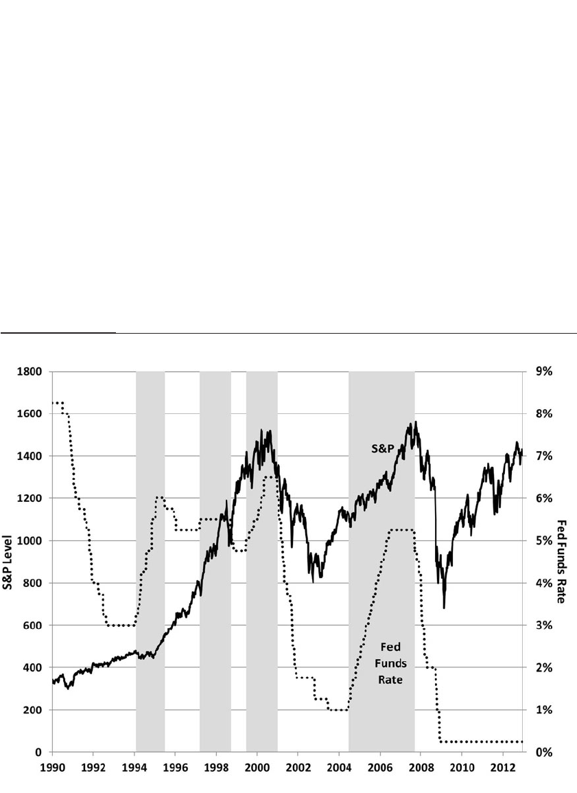
But since 1990 the pattern has not been so reliable. Figure 14-2 dis-
plays the S&P 500 Index and the fed funds rate from 1990 through 2012.
After a long period of easing through the 1990–1991 recession, the Fed
raised the fed funds target on February 4, 1994, when the S&P 500 Index
was 481. The reaction in the bond and stock market was immediate, as
stocks fell 2.5 percent and continued to slide another 7 percent by early
April. Bond prices were devastated, as the 10-year Treasury jumped
nearly 150 basis points in 1994, suffering its worst losses in years. But
after April, stocks stabilized and then rose despite accelerated Fed tight-
ening. By the time the Fed finally lowered rates on July 6, 1995, in
response to the weakening economy, the S&P 500 stood at 554, about 15
percent higher than on the day the Fed began to raise rates.
As the economy recovered and inflation threatened once again, the
Fed tightened 25 basis points on March 25, 1997; yet stocks continued to
CHAPTER 14 Gold, Monetary Policy, and Inflation 219
FIGURE 14–2
S&P 500 and Fed Funds Rate, 1990–2013

rise. In response to the Asian crisis and chaos in the Treasury market
caused by the failure of Long-Term Capital Management in August 1998,
the Fed lowered the funds rate on September 29, 1998. But the stock mar-
ket was 33.0 percent higher than it was 18 months earlier when the Fed
first raised rates.
As the U.S. economy sloughed off the Asian crisis, the Fed began
tightening again on June 30, 1999, when the S&P Index rose to 1,373. But
stocks continued upward, with the S&P 500 hitting its high on March 24,
2000, at 1,527, which was 12 percent higher than the previous June. In all
these episodes, investors who had been out of the stock market when the
Fed was raising rates would have given up large stock returns.
After the bull market peak in early 2000, the Fed did not start low-
ering the funds rate until January 3, 2001, after stocks had fallen back to
the level they were in June 1999 when the Fed started raising rates. But
January 2001 was far too early to get back into the market, as stocks con-
tinued to slide until October 2002, when the S&P 500 touched a five-year
low of 776.76. By the time the Fed began tightening on June 30, 2004, the
S&P 500 was at 1,141. But this was again far too early to get out of stocks,
as the bull market continued for more than three years, finally reaching
its peak in October 2007 at 1,565, more than 37 percent higher than when
the Fed started tightening. As the financial crisis began to impact the
economy, the Fed undertook its first easing on September 18, 2007, just
three weeks before the peak of the market, clearly not a time to load up
on equities.
All told, holding stocks from when the Fed first eased to when it
first tightened would have generated a 55 percent cumulative return on
the market (excluding dividends) over the period from February 1994
through the end of 2012. The buy-and-hold investors would have
achieved a 212 percent return, nearly four times as great.
There is a good reason why stocks are not reacting to Fed policy as
they have in the past. Investors have become so geared to watching and
anticipating Fed policy that the effect of its tightening and easing is
already discounted in the market. If investors expect the Fed to stabilize
the economy, this will be built into stock prices long before the Fed even
begins to take its stabilizing actions.
STOCKS AS HEDGES AGAINST INFLATION
Although the central bank has the power to moderate (but not eliminate)
the business cycle, its policy has the greatest influence on inflation. As
220 PART III How the Economic Environment Impacts Stocks

CHAPTER 14 Gold, Monetary Policy, and Inflation 221
noted above, the inflation of the 1970s was due to the overexpansion of
the money supply, which was an action the central bank took in the vain
hope that it could offset the impact of the OPEC oil supply restrictions.
This expansionary monetary policy brought inflation to double-digit
levels in most industrialized economies, peaking at 13 percent per year
in the United States and exceeding 24 percent in the United Kingdom.
In contrast to the returns of fixed-income assets, the historical evi-
dence is overwhelming that the returns on stocks over long time periods
have kept pace with inflation. Since stocks are claims on the earnings of
real assets—assets whose value is intrinsically related to the price of the
goods and services they produce—one should expect that their long-
term returns will not be harmed by inflation. For example, the period
since World War II has been the most inflationary period in our history,
and yet the real returns on stocks have matched that of the previous 150
years. The ability of an asset such as stocks to maintain its purchasing
power during periods of inflation makes equities an inflation hedge.
Indeed, stocks were widely praised in the 1950s as hedges against
rising consumer prices. As noted in Chapter 11, many investors stayed
with stocks at that time, despite seeing the dividend yield on equities fall
below the interest rate on long-term bonds. In the 1970s, however, stocks
were ravaged by inflation, and it became unfashionable to view equities
as an effective hedge against inflation.
What does the evidence say about the effectiveness of stocks as an
inflation hedge? The annual compound returns on stocks, bonds, and
Treasury bills against inflation over 1-year and 30-year holding periods
from 1871 to 2012 are shown in Figure 14-3.
The data indicate that neither stocks nor bonds nor bills are good
short-term hedges against inflation. Short-term real returns on these
financial assets are highest when the inflation rates are low, and their
returns fall as inflation increases. But the real returns on stocks are vir-
tually unaffected by the inflation rate over longer horizons. Bond
returns, on the other hand, fall behind the returns on stocks over every
holding period.
This was the principal conclusion of Edgar L. Smith’s 1924 book,
Common Stocks as Long Term Investments. Smith showed that stocks out-
perform bonds in times of falling as well as rising prices, taking the
period after the Civil War up to just before the turn of the century as his
test case. Smith’s results are robust and have held up over the next 90
years of data.
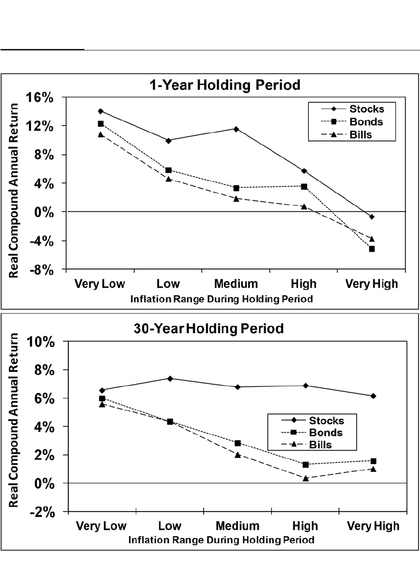
222 PART III How the Economic Environment Impacts Stocks
FIGURE 14–3
Holding Period Returns and Inflation, 1871–2012

WHY STOCKS FAIL AS A SHORT-TERM INFLATION HEDGE
Higher Interest Rates
If stocks represent real assets, why do they fail as a short-term inflation
hedge? A popular explanation is that inflation increases interest rates on
bonds, and higher interest rates on bonds depress stock prices. In other
words, inflation must send stock prices down sufficiently to increase their
dividends or earnings yields to match the higher rates available on bonds.
Indeed, this is the rationale of the Fed model described in Chapter 11.
However, this explanation is incorrect. Certainly, expectations of
rising prices do increase interest rates. Irving Fisher, the famous early-
twentieth-century American economist, noted that lenders seek to pro-
tect themselves against inflation by adding the expected inflation to the
real interest rate that they demand from borrowers. This proposition has
been called the Fisher equation, after its discoverer.11
But higher inflation also raises the expected future cash flows to
stockholders. Stocks are claims on the earnings of real assets, whether
these assets are the products of machines, labor, land, or ideas. Inflation
raises the costs of inputs and consequently the prices of outputs (and
those prices are, in fact, the measure of inflation). Therefore, future cash
flows will also rise with the rise in price levels.
It can be shown that when inflation impacts input and output
prices equally, the present value of the future cash flows from stocks is
not adversely affected by inflation even though interest rates rise.
Higher future cash flows will offset higher interest rates so that, over
time, the price of stocks—as well as earnings and dividends—will rise at
the rate of inflation. In theory the returns from stocks will be an ideal
inflation hedge.
Nonneutral Inflation: Supply-Side Effects
The invariance of stock prices to the inflation rate holds when inflation
is purely monetary in nature, influencing costs and revenues equally.
But there are many circumstances in which earnings cannot keep up
with inflation. Stocks declined during the 1970s because the restriction
in OPEC oil supplies dramatically increased energy costs. Firms were
not able to raise the prices of their output by as much as the soaring cost
of their energy inputs.
Earlier in the chapter it was noted that the inflation of the 1970s was
the result of bad monetary policy attempting to offset the contractionary
CHAPTER 14 Gold, Monetary Policy, and Inflation 223

effect of OPEC’s oil price hikes. Yet one should not minimize the damage
done by rising oil prices on U.S. corporate profits. U.S. manufacturers,
who for years had thrived on low energy prices, were totally unpre-
pared to deal with surging energy costs. The recession that followed the
first OPEC oil squeeze pummeled the stock market. Productivity plum-
meted, and by the end of 1974 real stock prices, measured by the Dow
Jones Industrial Average, had fallen 65 percent from the January 1966
high—the largest decline since the crash of 1929. Pessimism ran so deep
that nearly half of all Americans in August 1974 believed the economy
was heading toward a depression such as the one the nation had experi-
enced in the 1930s.12
Inflation may also lower stock prices when it increases investors’
fears that the central bank will take restrictive action by raising short-
term real interest rates. Such restrictive policies are often followed by an
economic slowdown that also depresses stock prices.
In many economies, inflation, especially in less developed coun-
tries, is also closely linked with large government budget deficits and
excessive government spending. Inflation therefore often signals that
the government is taking too large a role in the economy, which often
leads to lower growth, lower corporate profits, and lower stock prices.
In short, there are many good economic reasons why stock prices should
fall in response to increased inflation.
Taxes on Corporate Earnings
But economic factors are not the only reason stocks are not good short-
run hedges against inflation. The U.S. tax code also penalizes investors
during inflation. There are two significant areas in which the tax code
works to the detriment of shareholders: corporate profits and capital
gains.
Earnings are distorted by standard and accepted accounting prac-
tices that do not properly take into account the effects of inflation on cor-
porate profits. This distortion shows up primarily in the treatment of
depreciation, inventory valuation, and interest costs.
Depreciation of plant, equipment, and other capital investments is
based on historical costs. These depreciation schedules are not adjusted for
any change in the price of capital that might occur during the life of the
asset. Inflation increases the cost of the capital, but reported depreciation
does not make any adjustment for inflation, depreciation allowances are
understated, and taxable earnings are overstated, leaving corporations
with higher tax bills.
224 PART III How the Economic Environment Impacts Stocks

But depreciation is not the only source of bias in reported earnings.
In calculating the cost of goods sold, firms must use the historical cost,
with either “first-in–first-out” or “last-in–first-out” methods of inven-
tory accounting. In an inflationary environment, the gap between his-
torical costs and selling prices widens, producing inflationary profits for
the firm. These “profits” do not represent an increase in the real earning
power of the firm; instead, they represent just that part of the firm’s cap-
ital—namely, the inventory—that turns over and is realized as a mone-
tary profit. The accounting for inventories differs from the firm’s other
capital, such as plant and equipment, which are not revalued on an
ongoing basis for the purpose of calculating earnings.
The Department of Commerce, the government agency responsible
for gathering economic statistics, is well aware of these distortions and
has computed both a depreciation adjustment and an inventory valua-
tion adjustment in the national income and product accounts. But the
Internal Revenue Service does not recognize any of these adjustments
for tax purposes. Firms are required to pay taxes on reported profits,
even when these profits are biased upward by inflation. These biases
effectively increase the tax rate on capital.
Inflationary Biases in Interest Costs
There is another inflationary distortion to corporate profits that is not
reported in government statistics. This distortion is based on the infla-
tionary component of interest costs, and in contrast to depreciation and
inventory profits, it leads to a downward bias in reported corporate earn-
ings during periods of inflation.
Most firms raise capital by issuing fixed-income assets such as
bonds and bank loans. This borrowing leverages the firm’s assets, since
any profits above and beyond the debt service go to the stockholders. In
an inflationary environment, nominal interest costs rise, even if real
interest costs remain unchanged. But corporate profits are calculated by
deducting nominal interest costs, which overstates the real interest costs
to the firm. Hence, reported corporate profits are depressed compared
with true economic profits.
In fact, the firm is paying back debt with depreciated dollars, so the
higher nominal interest expense is exactly offset by the reduction in the
real value of the the firm’s bonds and loans. But this reduction in the real
indebtedness is not reported in any of the earnings reports released by
the firm. For highly leveraged firms, this bias could easily outweigh the
inventory and depreciation biases. Unfortunately, it is not easy to quan-
CHAPTER 14 Gold, Monetary Policy, and Inflation 225

tify the leverage bias because it is not easy to separate the share of inter-
est cost due to inflation from that due to real interest rates.
Capital Gains Taxes
In the United States, capital gains taxes are paid on the difference
between the cost of an asset and the sale price, with no adjustment made
for the impact of inflation on the amount of the real gain. Thus, if asset
values rise with inflation, the investor accrues a tax liability that must be
paid when the asset is sold, whether or not the investor has realized a
real gain. This means that an asset that appreciates by less than the rate
of inflation—meaning the investor is worse off in real terms—will still
be taxed upon sale.
Chapter 9 showed that the tax code has a dramatic impact on
investors’ realized after-tax real returns. For even a moderate inflation
rate of 3 percent, an investor with a five-year average holding period
suffers a 60-basis-point (hundredths of a percentage point) reduction in
average after-tax real returns compared with the after-tax returns that he
or she would have realized if the rate of inflation had been zero. If the
rate of inflation rises to 6 percent, the loss of returns is more than 112
basis points.
The inflation tax has a far more severe effect on realized after-tax
real returns when the holding period is short than when it is long. This
is because the more frequently an investor buys and sells assets, the
more the government can capture the tax on nominal capital gains.
Nevertheless, even for long-term investors, the capital gains tax reduces
real returns in inflationary times.
CONCLUSION
This chapter documents the role of money in the economy and financial
markets. Before World War II, persistent inflation in the United States
and other industrialized countries was nonexistent. But when the gold
standard was dethroned during the Great Depression, the control of
money passed to the central banks. And with the dollar no longer
pegged to gold, it was inflation, and not deflation, that proved to be the
major problem that central banks sought to control.
The message of this chapter is that stocks are not good hedges
against inflation in the short run. However, no financial asset is. In the
long run, stocks are extremely good hedges against inflation, while
bonds are not. Stocks are also the best financial asset if you fear rapid
226 PART III How the Economic Environment Impacts Stocks

inflation since many countries with high inflation can still have quite
viable, if not booming, stock markets. Fixed-income assets, on the other
hand, cannot protect investors from excessive government issuance of
money.
Fortunately for investors, central bankers around the world are
committed to keeping inflation low, and they have largely succeeded.
But if inflation again rears its head, investors will do much better in
stocks than in bonds.
CHAPTER 14 Gold, Monetary Policy, and Inflation 227
This page intentionally left blank

Stocks and the
Business Cycle
The stock market has predicted nine out of the last five recessions.
—PAUL SAMUELSON, 19661
I’d love to be able to predict markets and anticipate recessions, but
since that’s impossible, I’m as satisfied to search out profitable com-
panies as Buffett is.
—PETER LYNCH, 19892
A well-respected economist is about to address a large group of financial
analysts, investment advisors, and stockbrokers. There is obvious con-
cern in the audience. The stock market has been surging to new all-time
highs almost daily, driving down dividend yields to record lows and
sending price/earnings ratios skyward. Is this bullishness justified? The
audience wants to know if the economy is really going to do well
enough to support these high stock prices.
The economist’s address is highly optimistic. He predicts that the
real gross domestic product of the United States will increase over 4 per-
cent during the next four quarters, a very healthy growth rate. There will
be no recession for at least three years, and even if one occurs after that,
it will be very brief. Corporate profits, one of the major factors driving
229
15
This chapter is an adaptation of my paper “Does It Pay Stock Investors to Forecast the
Business Cycle?” in Journal of Portfolio Management, vol. 18 (Fall 1991), pp. 27–34. The
material benefited significantly from discussions with Professor Paul Samuelson.

stock prices, will increase at double-digit annual rates for at least the
next three years. To boot, he predicts that a Republican will easily win
the White House in next year’s presidential election, a situation obvi-
ously comforting to the overwhelmingly conservative audience. The
crowd obviously likes what it hears. The audience’s anxiety is quieted,
and many advisors are ready to recommend that their clients increase
their stake in stocks.
The time of this address is the summer of 1987, with the stock mar-
ket poised to take one of its sharpest falls in history, including the
record-breaking 23 percent decline on October 19, 1987. In just a few
weeks, most stocks can be bought for about half the price paid at the
time of the address. But the biggest irony of all is that the economist is
dead right in each and every one of his bullish economic predictions.
The lesson is that the markets and the economy are often out of
sync. It is not surprising that many investors dismiss economic forecasts
when planning their market strategy. The substance of Paul Samuelson’s
famous words, cited at the beginning of this chapter, still remains true
more than 45 years after they were first uttered.
But do not dismiss the business cycle too quickly when examining
your portfolio. The stock market still responds quite powerfully to
changes in economic activity. The reaction of the S&P 500 Index to the
business cycle from 1871 onward is displayed in Figure 15-1. Stocks fre-
quently begin to decline just before the shaded periods, which indicate
recessions, and rally rigorously at signs of an impending economic
recovery. If you can predict the business cycle, you can beat the buy-and-
hold strategy that has been advocated throughout this book.
But this is no easy task. To make money by predicting the business
cycle, one must be able to identify peaks and troughs of economic activity
before they actually occur, a skill very few if any economists possess. Yet
business cycle forecasting is a popular Wall Street endeavor not because it
is successful—most of the time it is not—but because the rewards are so
large if you can identify the turning point of the business cycle.
WHO CALLS THE BUSINESS CYCLE?
It is surprising to many that the dating of business cycles is not deter-
mined by any of the myriad government agencies that collect data on the
economy. Instead, the task falls to the National Bureau of Economic
Research (the NBER), a private research organization founded in 1920 for
the purpose of documenting business cycles and developing a series of
national income accounts. In the early years of its existence, the bureau’s
230 PART III How the Economic Environment Impacts Stocks
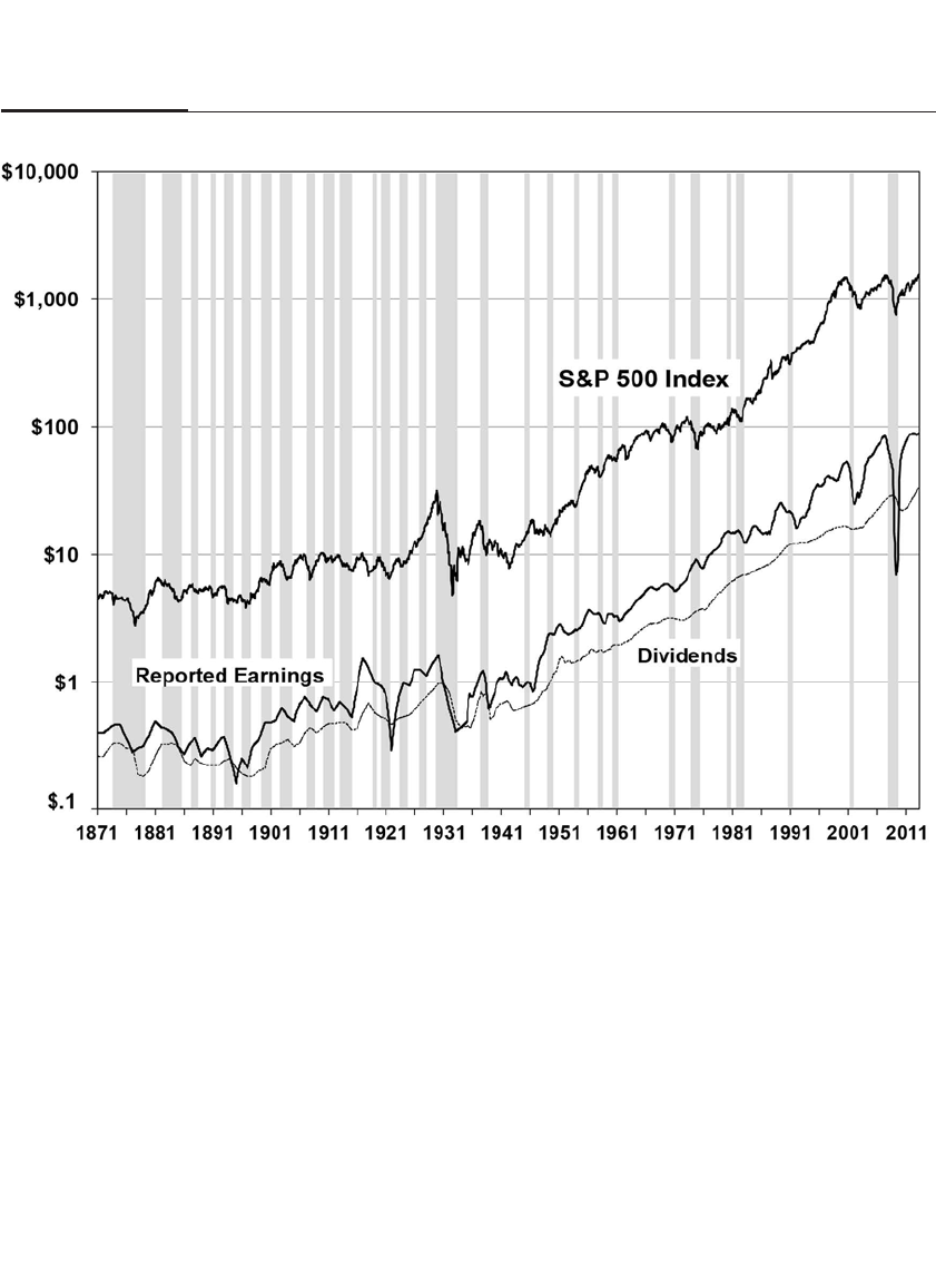
staff compiled comprehensive chronological records of the changes in
economic conditions in many of the industrialized economies. In particu-
lar, the bureau developed monthly series on business activity for the
United States and Great Britain back to 1854.
In a 1946 volume entitled Measuring Business Cycles, Wesley C.
Mitchell, one of the founders of the bureau, and Arthur Burns, a
renowned business cycle expert who later headed the Federal Reserve
Board, gave the following definition of a business cycle:
Business cycles are a type of fluctuation found in the aggregate economic
activity of nations that organize their work mainly in business enterprises:
a cycle consists of expansion occurring at about the same time in many
economic activities, followed by similarly general recessions, or contrac-
CHAPTER 15 Stocks and the Business Cycle 231
FIGURE 15–1
Stock Prices, Earnings, Dividends, and Recessions 1871–2012

tions, and revivals that merge into the expansion phase of the next cycle;
this sequence of changes is recurrent but not periodic; in duration busi-
ness cycles vary from more than one year to ten or twelve years and they
are not divisible into shorter cycles of similar character.3
It is commonly assumed that a recession occurs when real gross
domestic product, the most inclusive measure of economic output,
declines for two consecutive quarters. But this is not necessarily so.
Although this criterion is a reasonable rule of thumb for indicating a
recession, there is no single rule or measure used by the NBER. Rather
the bureau focuses on four different series to determine the turning
points in the economy: employment, industrial production, real per-
sonal income, and real manufacturing and trade sales.
The Business Cycle Dating Committee of the National Bureau of
Economic Research confirms the business cycle dates. This committee con-
sists of academic economists who are associated with the bureau and who
meet to examine economic data whenever conditions warrant. Over the
entire period from 1802 through 2012, the United States has experienced 47
recessions, and these recessions have averaged nearly 19 months in length,
while expansions have averaged 34 months.4This means that, over these
210 years, almost slightly more than one-third of the time the economy has
been in a recession. However, since World War II, there have been 11 reces-
sions, averaging 11.1 months in length, while the expansions have aver-
aged 58.4 months. So in the postwar period, the economy has been in a
recession less than one-sixth of the time, far less than the prewar average.
The dating of the business cycle is of great importance. The designa-
tion that the economy is in a recession or an expansion has political as well
as economic implications. For example, when the NBER called the onset
of the 1990 recession in July rather than August, it raised quite a few eye-
brows in Washington. This was so because the Bush administration had
told the public that the Iraqi invasion of Kuwait and the surge in oil prices
were responsible for the economic recession. This explanation was under-
mined when the bureau actually dated the onset of the recession a month
earlier. Similarly the 2001 recession began in March when technology
spending dropped sharply and well before the 9/11 terrorist attacks.
The Business Cycle Dating Committee is in no rush to call the turn-
ing points in the cycle. Never has a call been reversed because of new or
revised data that have become available—and the NBER wants to keep
it that way. As Robert E. Hall, current chair of the seven-member
Business Cycle Dating Committee, indicated, “The NBER has not made
an announcement on a business cycle peak or trough until there was
232 PART III How the Economic Environment Impacts Stocks

almost no doubt that the data would not be revised in light of subse-
quent availability of data.”5
Recent examples of the NBER’s dating make the point. The March
1991 trough was not called until 21 months later, in December 1992, and the
November bottom of the 2001 recession was not called until July 2003. The
peak of the 2002–2007 expansion was not called until December 2008, one
year after it began and well after the Lehman crisis had paralyzed financial
markets and set stocks tumbling. Clearly, waiting for the bureau to desig-
nate business cycles is far too late to be of any use in timing the market.
STOCK RETURNS AROUND BUSINESS CYCLE TURNING POINTS
Almost without exception, the stock market turns down prior to reces-
sions and rises before economic recoveries. In fact, out of the 47 reces-
sions recorded from 1802 on, 43 of them, or more than 9 out of 10, have
been preceded (or accompanied) by declines of 8 percent or more in the
total stock returns index. Two exceptions followed World War II: the
1948–1949 recession that immediately followed the war and the 1953
recession, when stocks fell just shy of the 8 percent criterion.
The return behaviors for the 11 post–World War II recessions are sum-
marized in Table 15-1. You can see that the stock return index peaked any-
CHAPTER 15 Stocks and the Business Cycle 233
TABLE 15–1
Stock Prices and Business Cycle Peaks, 1948–2012
Peak of Peak of Lead Time Decline in Stock Maximum 12
Stock Business between Index from Month Decline
Recession Index (1) Cycle (2) Peaks (3) (1) to (2) in Stocks
1948–1949 May 1948 Nov 1948 6 –8.91% –9.76%
1953–1954 Dec 1952 Jul 1953 7 –4.26% –9.04%
1957–1958 Jul 1957 Aug 1957 1 –4.86% –15.32%
1960–1961 Dec 1959 Apr 1960 4 –8.65% –8.65%
1970 Nov 1968 Dec 1969 13 –12.08% –29.16%
1973–1975 Dec 1972 Nov 1973 11 –16.29% –38.80%
1980 Jan 1980 Jan 1980 0 0.00% –9.55%
1981–1982 Nov 1980 Jul 1981 8 –4.08% –13.99%
1990–1991 Jul 1990 Jul 1990 0 0.00% –13.84%
2001 Aug 2000 Mar 2001 7 –22.94% –26.55%
2007–2009 Oct 2007 Dec 2007 2 –4.87% –47.50%
Average 5.4 –7.90% –20.20%

where from 0 to 13 months before the beginning of a recession. The reces-
sions that began in January 1980 and July 1990 are the only two for which
the stock market gave no advance warning of the economic downturn.
As the Samuelson quote at the beginning of this chapter indicates,
the stock market is also prone to false alarms, and these have increased
in the postwar period. Declines greater than 10 percent in the Dow Jones
Industrial Average during the postwar period that were not followed by
recessions (the “false alarms”) are listed in Table 15-2. The decline of 35.1
percent from August through early December 1987 is the largest decline
in the 210-year history of stock returns when the economy did not sub-
sequently fall into a recession.6
The trough in the stock return index and the trough in the NBER
business cycle are compared in Table 15-3.
The average lead time between the bottom of the market and the bot-
tom of an economic recovery has been 4.6 months, and in 8 of the 11 reces-
sions, the lead time has been in an extremely narrow range of 4 to 6
months. This compares to an average of 5.4 months that the peak in the
market precedes the peak in the business cycle. The time between the
peak of the market and the peak of the economy also has shown much
greater variability that the time between the trough of the market and the
trough of the economy.7
234 PART III How the Economic Environment Impacts Stocks
TABLE 15–2
False Alarms of Recession by Stock Market 1945–2012
Peak of Stock Index Trough of Stock Index % Decline
May 29, 1946 May 17, 1947 –23.2%
Dec 13, 1961 Jun 26, 1962 –27.1%
Jan 18, 1966 Sept 29, 1966 –22.3%
Sept 25, 1967 Mar 21, 1968 –12.5%
Apr 28, 1971 Nov 23, 1971 –16.1%
Aug 17,1978 Oct 27, 1978 –12.8%
Nov 29, 1983 Jul 24, 1984 –15.6%
Aug 25, 1987 Dec 4, 1987 –35.1%
Aug 6, 1997 Oct 27, 1997 –13.3%
Jul 17, 1998 Aug 31, 1998 –19.3%
Mar 19, 2002 Oct 9, 2002 –31.5%
Apr 26, 2010 Jul 02, 2010 –13.6%
Apr 29, 2011 Oct 03, 2011 –16.8%
Postwar declines of 10% or more in the Dow Jones Industrial Average when no recession
followed within 12 months.

It is important to note that by the time the economy has reached the
end of the recession, the stock market has risen 23.8 percent on average.
Therefore, an investor waiting for tangible evidence that the business
cycle has hit bottom has already missed a very substantial rise in the
market. And as noted above, the NBER does not announce the dates that
recessions end until many months after the economy turns up.
GAINS THROUGH TIMING THE BUSINESS CYCLE
My studies show that if investors could predict in advance when reces-
sions will begin and end, they could enjoy superior returns to the
returns earned by a buy-and-hold investor.8Specifically, if an investor
switched from stocks to cash (short-term bonds) four months before the
beginning of a recession and back to stocks four months before the end
of the recession, he would gain almost 5 percentage points per year on a
risk-corrected basis over the buy-and-hold investor. About two-thirds of
that gain is the result of predicting the end of the recession, where, as
Table 15-3 shows, the stock market hits bottom between four and five
months before the end of the economic downturn, and the other third
comes from selling stocks four months before the peak. Investors who
CHAPTER 15 Stocks and the Business Cycle 235
TABLE 15–3
Stock Prices and Business Cycle Troughs, 1948–2012
Trough of Lead Time Rise in Stock
Trough of Business between Index from
Recession Stock Index (1) Cycle (2) Troughs (3) (1) to (2)
1948–1949 May 1949 Oct 1949 5 15.59%
1953–1954 Aug 1953 May 1954 9 29.13%
1957–1958 Dec 1957 April 1958 4 10.27%
1960–1961 Oct 1960 Feb 1961 4 21.25%
1970 Jun 1970 Nov 1970 5 21.86%
1973–1975 Sep 1974 Mar 1975 6 35.60%
1980 Mar 1980 Jul 1980 4 22.60%
1981–1982 Jul 1982 Nov 1982 4 33.13%
1990–1991 Oct 1990 Mar 1991 5 25.28%
2001 Sep 2001 Nov 2001 2 9.72%
2007–09 Mar 2009 Jun 2009 3 37.44%
Average 4.6 23.81%
Std Dev 1.80 9.51%

switch between stocks and bonds just on the months the NBER identifies
(well after the fact) as the beginning and end of the recession gain a mere
½ percentage point return over the buy-and-hold investor.
HOW HARD IS IT TO PREDICT THE BUSINESS CYCLE?
If one could predict in advance when recessions will occur, the gains
would be substantial. That is perhaps why billions of dollars of resources
are spent trying to forecast the business cycle. But the record of predict-
ing business cycle turning points is extremely poor.
Stephen McNees, vice president of the Federal Reserve Bank of
Boston, has done extensive research into the accuracy of economic fore-
casters’ predictions. He claims that a major factor in forecast accuracy is
the time period over which the forecast was made, and it is precisely at
business cycle turning points that the errors were “enormous.”9Yet, as
noted above, it is precisely these business cycle turning points that
enable a forecaster to become a successful market timer.
The 1974–1975 recession was particularly tough for economists.
Almost every one of the nearly two dozen of the nation’s top economists
invited to President Ford’s anti-inflation conference in Washington in
September 1974 was unaware that the U.S. economy was in the midst of
its most severe postwar recession to date. McNees, studying the fore-
casts issued by five prominent forecasters in 1974, found that the median
forecast overestimated GNP growth by 6 percentage points and under-
estimated inflation by 4 percentage points. Early recognition of the 1974
recession was so poor that many economists jumped the gun on the next
recession, which didn’t strike until 1980—while most economists
thought it had begun early in 1979.
From 1976 to 1995, Robert J. Eggert and subsequently Randell
Moore documented and summarized the economic forecasts of a noted
panel of economic and business experts. These forecasts were compiled
and published in a monthly publication entitled Blue Chip Economic
Indicators.
In July 1979, the Blue Chip Economic Indicators report said that a
strong majority of forecasters believed that a recession had already
started—forecasting negative GNP growth in the second, third, and
fourth quarters of 1979. However, the NBER declared that the peak of
the business cycle did not occur until January 1980 and that the economy
expanded throughout 1979.
Forecasters’ ability to predict the severe 1981–1982 recession,
when unemployment reached a postwar high of 10.8 percent, was no
236 PART III How the Economic Environment Impacts Stocks

better. The headline of the July 1981 Blue Chip Economic Indicators
report read, “Economic Exuberance Envisioned for 1982.” Instead,
1982 was a disaster. By November 1981 the forecasters realized that the
economy had faltered, and optimism turned to pessimism. Most
thought that the economy had entered a recession (which it had done
four months earlier), nearly 70 percent thought that it would end by
the first quarter of 1982 (which it would not, instead tying the record
for the longest postwar recession, ending in November), and 90 per-
cent thought that it would be mild, like the 1971 recession, rather than
severe—wrong again!
In April 1985, with the expansion well under way, forecasters were
queried about how long the economy would be in an expansion. The
average response was for another 20 months, which would put the peak
at December 1986, more than 3.5 years before the cycle actually ended.
Even the most optimistic forecasters picked spring 1988 as the latest date
for the next recession to begin. This question was asked repeatedly
throughout 1985 and 1986, and no forecaster imagined that the 1980s
expansion would last as long as it did.
Following the stock market crash of October 1987, forecasters
reduced their GNP growth estimates of 1988 over 1987 from 2.8 percent
to 1.9 percent, the largest drop in the 11-year history of the survey.
Instead, economic growth in 1988 was nearly 4 percent, as the economy
grew strongly despite the stock market collapse.
As the expansion continued, the belief that a recession was imminent
turned into the belief that prosperity was here to stay. The continuing
expansion fostered a growing conviction that perhaps the business cycle
had been conquered—by either government policy or the “recession-
proof” nature of our service-oriented economy. Ed Yardeni, senior econo-
mist at Prudential-Bache Securities, wrote a “New Wave Manifesto” in
late 1988, concluding that self-repairing, growing economies were likely
through the rest of the decade.10 On the eve of one of the worst worldwide
recessions in the postwar era, Leonard Silk, senior economics editor of the
New York Times, stated in May 1990 in an article entitled “Is There Really a
Business Cycle?”:
Most economists foresee no recession in 1990 or 1991, and 1992 will be
another presidential year, when the odds tip strongly against recession.
Japan, West Germany, and most of the other capitalist countries of Europe
and Asia are also on a long upward roll, with no end in sight.11
However, by November 1990, Blue Chip Economic Indicators
reported that the majority of the panel believed the U.S. economy had
CHAPTER 15 Stocks and the Business Cycle 237

already slipped, or was about to slip, into a recession. But in November,
not only had the economy been in recession for four months, but the
stock market had already hit its bottom and was headed upward. Had
investors given in to the prevailing pessimism at the time when the
recession seemed confirmed, they would have sold after the low was
reached and stocks were headed for a strong three-year rally.
The record 10-year expansion of the U.S. economy from March 1991
through March 2001 again spawned talk of “new era economics” and
economies without recession.12 Even in early 2001, the vast majority of
forecasters did not see a recession. In fact, in September 2001, just before
the terrorist attack, only 13 percent of the economists surveyed by Blue
Chip Economic Indicators believed the United States was in a recession
even though the NBER subsequently indicated that the United States
recession had begun six months earlier in March.13 And by February
2002, less than 20 percent thought the recession had ended in 2001,
although the NBER eventually dated November 2001 as the end of the
recession.14 Once again, economists have been unable to call the turning
point of the business cycle until well after the date has passed.
Forecasters did no better predicting the Great Recession of
2007–2009. The National Bureau of Economic Research did not actually
call the beginning of the recession until December 2008, one year after it
began and when the S&P 500 Index had already fallen more than 40 per-
cent. The Federal Reserve did begin easing interest rates in September
2007, three months before the onset of the recession, but the Fed had no
concept that a recession was imminent. In the meeting of the Federal
Open Market Committee on December 11, 2007, the month the recession
began, Fed economist Dave Stockton gave the following summary of the
Federal Reserve forecast:
Obviously we’re not forecasting a business cycle peak. So in our forecast,
we’re not yet saying that we’re on the downside of a business cycle. We
have a “growth recession” [a slowdown in economic growth] in this fore-
cast and nothing more than that.15
CONCLUSION
Stock values are based on corporate earnings, and the business cycle is a
prime determinant of these earnings. The gains of being able to predict
the turning points of the economic cycle are large, and yet doing so with
any precision has eluded economists of all persuasions.
238 PART III How the Economic Environment Impacts Stocks

The worst course an investor can take is to follow the prevailing
sentiment about economic activity. That will lead investors to buy at
high prices when times are good and everyone is optimistic and sell at
the low.
The lessons to investors are clear. Beating the stock market by ana-
lyzing real economic activity requires a degree of prescience that fore-
casters do not yet have.
CHAPTER 15 Stocks and the Business Cycle 239
This page intentionally left blank

When World Events
Impact Financial Markets
I can predict the motion of heavenly bodies, but not the madness of
crowds.
—ISAAC NEWTON
As the sun rose over New York City on a beautiful Tuesday morning,
September 11, 2001, traders expected a dull day on Wall Street. There
were no economic data coming out of Washington, nor any earnings
releases scheduled. The previous Friday the markets had fallen on a hor-
rible employment report, but on Monday the markets had bounced back
slightly.
The U.S. equity markets had not yet opened, but contracts on the
S&P 500 Index futures had been trading all night as usual on the elec-
tronic Globex exchange. The futures markets were up, indicating that
Wall Street was expecting a firm opening. But then a report came at 8:48
a.m. on what was to be one of the most fateful days in world history: a
plane had crashed into the North Tower of the World Trade Center. The
pattern of trading over the next 27 minutes, before the market closed, is
shown in Figure 16-1.
The news of the plane crash spread quickly, but few imagined what
had really happened. Was it a large or small plane? Was it an accident?
Or was there something more sinister going on? Although nobody knew
the answers yet, immediately the stock index futures market traded
down a few points, as it often does when uncertainty increases. Within a
241
16
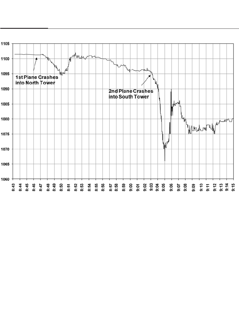
few minutes, however, buyers reappeared, and the index returned to its
previous level, as most traders concluded that nothing significant had
happened.
Fifteen minutes later, at 9:03, with news cameras focused on the
World Trade Center and millions around the world watching, a second
plane crashed into the South Tower. The entire world changed in that
moment. Americans’ worst fears had been realized. This was a terrorist
attack. For the first time since World War II, America was under direct
attack on its own soil.
By 9:05, two minutes after the second crash, the S&P futures
plunged 30 points, about 3 percent, indicating that if the exchanges had
been open, nearly $300 billion would have been wiped off U.S. stock val-
ues. But then, miraculously, buyers did appear. Despite the enormity of
the events unfolding, some traders bet that the market had overreacted
to these attacks and decided that this was a good time to buy stocks. The
futures firmed and ended the session at 9:15 down about 15 points, gain-
ing back one-half of the earlier loss.
242 PART III How the Economic Environment Impacts Stocks
FIGURE 16–1
S&P 500 Futures Market on Tuesday Morning, September 11, 2001

Despite this comeback, the gravity of this attack quickly sank in. All
the stock, bond, and commodity exchanges first delayed opening and
then canceled trading for the day. In fact, stock exchanges in the United
States would remain closed for the remainder of the week, the longest
closing since FDR declared a “Bank Holiday” in March 1933 to try to
restore America’s collapsing banking system.
Foreign stock exchanges, however, remained open. It was 2 p.m. in
London and 3 p.m. in Europe when the planes struck. The German DAX
index immediately fell more than 9 percent and ended the session around
that level. London stocks suffered but not as much. There was a feeling
that with the world’s financial center, the United States, vulnerable to
attack, some business might move to the United Kingdom. The British
pound rallied, as did the euro against the dollar. Normally it is the U.S.
dollar that gains in international crisis. But this time, with the attack cen-
tering on New York, foreign traders were unsure which direction to go.
When the New York Stock Exchange reopened the following
Monday, September 17, the Dow Industrials fell 685 points, or 7.13 per-
cent, the seventeenth-largest percentage drop in its history. The Dow con-
tinued to fall during the week and closed Friday, September 21, at
8,236—down more than 14 percent from its September 10 close and nearly
30 percent from its all-time high of 11,723 reached on January 14, 2000.
WHAT MOVES THE MARKET?
It was perfectly clear why the markets fell after the terrorist attacks. But it
might surprise investors that in the vast majority of cases, major market
movements are not accompanied by any news of sufficient importance to
explain the price change. Since 1885, when the Dow Jones averages were
first formulated, there have been 145 days when the Dow Jones Industrial
Average has changed by 5 percent or more. Fifteen of these moves took
place from September 2008 through March 2009 when the world economy
was in the grips of the financial crisis, and another drop occurred on August
8, 2011, when Standard & Poor’s downgraded U.S. government debt.
Of all the 145 large changes, only 35 can be identified with a signif-
icant world political or economic event, such as wars, political changes,
or governmental policy shifts. During and immediately following the
financial crisis of 2008, only 4 of the 15 large changes were associated
with specific events. Since 1885, less than 1 in 4 major market moves can
be clearly linked to a specific world event. A ranking of the 54 largest
changes is shown in Table 16-1,1and market changes greater than 5 per-
cent that are associated with specific events are shown in Table 16-2.2
CHAPTER 16 When World Events Impact Financial Markets 243

Monetary policy is the biggest single driver of these massive mar-
ket outbreaks of euphoria or fear. Out of the five largest moves in the
stock market over the past century for which there is a clearly identifi-
able cause, four have been directly associated with changes in monetary
policy. The top news-related changed was the 14.87 percent gain on
October 6, 1931, when Hoover proposed a $500 million pool to help
banks, and the second largest was the 11.08 percent gain that took place
on October 13, 2008, when the Federal Reserve offered unlimited liquid-
ity to foreign central banks to facilitate dollar exchanges.
If you focus in on just the 10 largest daily market moves since 1885,
only 2 can be attributed to a specific news event. The record 22.6 percent
one-day fall in the stock market on October 19, 1987, is not associated
with any one readily identifiable news event. From 1940 until the recent
financial crisis, there have been only four days of big moves where the
cause is identified: the 7.13 percent drop on September 17, 2001, when
the markets reopened after the terrorist attacks; the 7.18 percent drop on
244 PART III How the Economic Environment Impacts Stocks
TABLE 16–1
Largest Daily Market Changes, 1888–2012
Rank Date Change Rank Date Change Rank Date Change
1 Oct 19, 1987 –22.61% 19 Dec 18, 1899 –8.72% 37 Sep 24, 1931 –7.07%
2 Mar 15, 1933 15.34% 20 Oct 8, 1931 8.70% 38 Jul 20, 1933 –7.07%
3* Oct 6, 1931 14.87% 21 Aug 12, 1932 –8.40% 39* Sep 29, 2008 –6.98%
4 Oct 28, 1929 –12.82% 22 Mar 14, 1907 –8.29% 40* Oct 13, 1989 –6.91%
5 Oct 30, 1929 12.34% 23 Oct 26, 1987 –8.04% 41* Jul 30, 1914 –6.90%
6 Oct 29, 1929 –11.73% 24 Jun 10, 1932 7.99% 42 Jan 8, 1988 –6.85%
7 Sep 21, 1932 11.36% 25 Oct 15, 2008 –7.87% 43* Mar 23, 2009 6.84%
8* Oct 13, 2008 11.08% 26 Jul 21, 1933 –7.84% 44 Oct 14, 1932 6.83%
9 Oct 28, 2008 10.88% 27 Oct 18, 1937 –7.75% 45 Nov 11, 1929 –6.82%
10 Oct 21, 1987 10.15% 28 Dec 1, 2008 –7.70% 46* May 14, 1940 –6.80%
11 Nov 6, 1929 –9.92% 29 Oct 9, 2008 –7.33% 47 Oct 5, 1931 –6.78%
12 Aug 3, 1932 9.52% 30* Sep 5, 1939 7.26% 48* May 21, 1940 –6.78%
13* Feb 11, 1932 9.47% 31* Feb 1, 1917 –7.24% 49 Mar 15, 1907 6.70%
14* Nov 14, 1929 9.36% 32* Oct 27, 1997 –7.18% 50 Nov 13, 2008 6.67%
15 Dec 18, 1931 9.35% 33 Oct 5, 1932 –7.15% 51* Jun 20, 1931 6.64%
16 Feb 13, 1932 9.19% 34* Sep 17, 2001 –7.13% 52 Jul 24, 1933 6.63%
17* May 6, 1932 9.08% 35 Jun 3, 1931 7.12% 53* Jul 26, 1934 –6.62%
18* Apr 19, 1933 9.03% 36 Jan 6, 1932 7.12% 54 Dec 20, 1895 –6.61%
Asterisks are news related.

CHAPTER 16 When World Events Impact Financial Markets 245
TABLE 16–2
Largest News-Related Changes in Dow Jones Industrial Average, 1888–2012
Rank Date Change News Headline
3 Oct 6, 1931 14.87% Hoover urges $500M pool to help banks
8 Oct 13, 2008 11.08% Fed gives “unlimited liquidity” to foreign central banks
13 Feb 11, 1932 9.47% Liberalization of Fed discount policy
14 Nov 14, 1929 9.36% Fed lowers discount rate/tax cut proposed
17 May 6, 1932 9.08% U.S. steel negotiates 15% wage cut
18 Apr 19, 1933 9.03% U.S. drops gold standard
30 Sep 5, 1939 7.26% World War II begins in Europe
31 Feb 1, 1917 –7.24% Germany announces unrestricted submarine warfare
32 Oct 27, 1997 –7.18% Attack on Hong Kong dollar
34 Sep 17, 2001 –7.13% World Trade Center terrorist attack
39 Sep 29, 2008 –6.98% House voted down $700B bailout package
40 Oct 13, 1989 –6.91% United Airline buyout collapses
41 Jul 30, 1914 –6.90% Outbreak of World War I
43 Mar 23, 2009 6.84% Treasury announces $1T public-private plan to buy bad bank debt
46 May 14, 1940 –6.80% Germans invade Holland
48 May 21, 1940 –6.78% Allied reverses in France
51 Jun 20, 1931 6.64% Hoover advocates foreign debt moratorium
53 Jul 26, 1934 –6.62% Fighting in Austria; Italy mobilizes
56 Sep 26, 1955 –6.54% Eisenhower suffers heart attack
60 Jul 24, 2002 6.35% J.P. Morgan denies involvement with Enron scandal
63 July, 26, 1893 –6.31% Erie railroad bankrupt
77 Oct 31, 1929 5.82% Fed lowers discount rate
78 Jun 16, 1930 –5.81% Hoover to sign tariff bill
79 Apr 20, 1933 5.80% Continued rally on dropping of gold standard
87 May 2, 1898 5.64% Dewey defeats Spanish
91 Mar 28, 1898 5.56% Dispatches of armistice with Spain
93 Aug 8, 2011 –5.55% Standard and Poor’s downgrades U.S. treasury debt
100 Dec 22, 1916 5.47% Lansing denies U.S. near war
103 Dec 18, 1896 –5.42% Senate votes for free Cuba
105 Feb 25, 1933 –5.40% Maryland bank holiday
109 Oct 23, 1933 5.37% Roosevelt devalues dollar
111 Dec 21, 1916 –5.35% Sec. of State Lansing implies U.S. near war
120 Apr 9, 1938 5.25% Congress passes bill taxing U.S. government bond interest
139 Nov 5, 2008 –5.05% Democrats sweep Congress, presidency
144 Oct 20, 1931 5.03% ICC raises rail rates
145 Mar 31, 1932 –5.02% House proposes stock sales tax

October 27, 1997, when foreign exchange speculators attacked the Hong
Kong dollar; the 6.91 percent fall on Friday, October 13, 1989, when the
leveraged buyout of United Airlines collapsed; and the 6.54 percent
drop on September 26, 1955, when President Eisenhower suffered a
heart attack.3
During the financial crisis of 2008–2009, the other news-related
moves (in addition to the Fed liquidity provisions cited above) were the
6.8 percent jump on March 23, 2009, when the Obama administration
announced a trillion-dollar public-private partnership to buy “toxic”
assets from commercial banks; the 7.0 percent decline on August 29,
2008, when the U.S. House of Representatives rejected the $700 billion
TARP, or Troubled Asset Repurchase Program, proposed by Treasury
Secretary Paulson and Federal Reserve Chairman Bernanke of the Bush
administration; the 5.5 percent loss on August 8 following Standard &
Poor’s downgrade of U.S. government debt; and the 5.05 percent fall on
November 5, following the Democratic sweep of the White House and
Congress in the 2008 elections.
War is usually a big market mover. But the market drop on
September 17, 2001, following the terrorist attacks was more than twice
the 3.5 percent drop that occurred on the day following the attack on
Pearl Harbor, and it was more than that of any other one-day decline
during a period when the United States was at war.
Even when the day is filled with news events, there can be sharp
disagreement over what news caused the market change. On November
15, 1991, when the Dow fell more than 120 points, or nearly 4 percent,
Investor’s Business Daily ran an article about the market entitled “Dow
Plunges 120 in a Scary Stock Sell-Off: Biotechs, Programs, Expiration
and Congress Get the Blame.”4In contrast, the London-based Financial
Times published a front-page article written by a New York writer enti-
tled “Wall Street Drops 120 Points on Concern at Russian Moves.” What
is interesting is that such news, specifically that the Russian government
had suspended oil licenses and taken over the gold supplies, was not
mentioned even once in the Investor’s Business Daily article! That one
major newspaper can highlight “reasons” that another news outlet does
not even report illustrates the difficulty of finding fundamental explana-
tions for the movements of markets.
UNCERTAINTY AND THE MARKET
The stock market hates uncertainty, which is why events that jar investors
from their customary framework for analyzing the world can have devas-
246 PART III How the Economic Environment Impacts Stocks

tating effects. September 11 serves as the perfect example. Americans were
unsure what these terrorist attacks meant for the future. How severe
would the drop in air travel—or any travel—be? How big a hit would the
approximately $600 billion tourist industry take? Unanswered questions
generate anxiety and declining prices.
Uncertainty about the presidency is another downer for stocks. The
market almost always declines in reaction to sudden, unexpected
changes related to the presidency. As noted previously, President
Eisenhower’s heart attack on September 26, 1955, caused a 6.54 percent
decline in the Dow Industrials, the fifth largest in the postwar period.
The drop was a clear sign of Eisenhower’s popularity with investors.
The assassination of President Kennedy on Friday, November 22, 1963,
caused the Dow Industrials to drop 2.9 percent and persuaded the New
York Stock Exchange to close two hours early to prevent panic selling.
Trading remained suspended the following Monday, November 25, for
Kennedy’s funeral. Yet the following Tuesday, by which time Lyndon
Johnson had taken over the reins of government, the market soared 4.5
percent, representing one of the best days in the postwar period.
When William McKinley was shot on September 14, 1901, the mar-
ket dropped by more than 4 percent. But stocks regained all their losses
on the following trading day. The death of Warren Harding in 1923
caused a milder setback, which was soon erased. Sell-offs such as these
often provide good opportunities for investors to buy stocks since the
market usually reverses itself quickly following the change in leader-
ship. But there are politicians whom investors never forgive. Stocks ral-
lied over 4 percent in the week following the news of the death of
Franklin Roosevelt, never a favorite on Wall Street.
DEMOCRATS AND REPUBLICANS
It is well known that investors generally prefer Republicans to
Democrats. Most corporate executives and stock traders are Republicans,
and many Republican policies are perceived to be favorable to stocks and
capital formation. Democrats are perceived to be less amenable to favor-
able tax treatment of capital gains and dividends and more in favor of
regulation and income redistribution. Yet the stock market has actually
done better under Democrats than Republicans.
The performance of the Dow Jones Industrials during every admin-
istration since Grover Cleveland was elected in 1888 is shown in Figure
16-2. The greatest bear market in history occurred during Herbert
Hoover’s Republican administration, while stocks did quite well under
CHAPTER 16 When World Events Impact Financial Markets 247
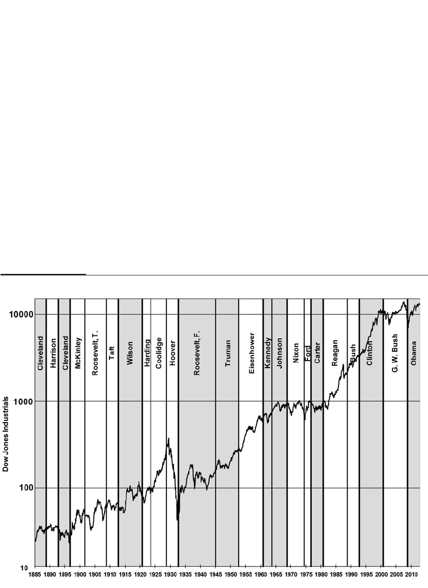
Franklin Roosevelt, despite the fact that the Democrat was frequently
reviled in boardrooms and brokerage houses around the country. The
immediate reaction of the market—the day before the election to the day
after—does indeed conform to the fact that investors like Republicans
better than Democrats. Since 1888, the market fell an average of 0.6 per-
cent on the day following a Democratic victory, but it rose by 0.7 percent
on the day following a Republican victory. But the market’s reaction to
the Republicans’ success in presidential elections has been muted since
World War II. There have been occasions, like Clinton’s second-term
election victory, when the market soared because the Republicans kept
control of Congress, not because Clinton, a Democrat, was reelected.
The returns in the first, second, third, and fourth years of a presi-
dential term are displayed in Table 16-3. The returns in the third year of
a presidential term are generally the best. This is striking since the third
year includes the disastrous 43.3 percent drop that occurred in 1931, dur-
ing the third year of Hoover’s ill-fated administration and the worst
248 PART III How the Economic Environment Impacts Stocks
FIGURE 16–2
Dow Jones Industrial Average and Presidential Terms (Shaded Areas Democratic) 1985–2012

CHAPTER 16 When World Events Impact Financial Markets 249
TABLE 16–3
Stock Returns During Presidential Elections and Year in Office 1888–2012
From: 1 First Second Third Fourth
President's Election Day Before Year Year Year Year
Name Party Date To: 1 Day After of Term of Term of Term of Term
Harrison R 11/6/1888 0.4 11.8 –6.6 16.6 13.5
Cleveland D 11/8/1892 –0.5 –15.3 11.9 11.3 –4.5
McKinley R 11/3/1896 2.7 18.9 11.0 9.9 –1.3
McKinley R 11/6/1900 3.3 35.3 0.3 –18.1 28.5
Roosevelt T. R 11/8/1904 1.3 25.2 2.0 –32.5 39.0
Taft R 11/3/1908 2.4 16.6 –0.6 0.5 11.7
Wilson D 11/5/1912 1.8 –13.0 –2.5 24.2 3.7
Wilson D 11/7/1916 –0.4 –30.9 –5.8 13.5 –19.3
Harding R 11/2/1920 –0.6 4.0 53.4 –11.1 21.5
Coolidge R 11/4/1924 1.2 33.3 15.8 36.0 36.5
Hoover R 11/6/1928 1.2 33.2 –29.6 –32.3 –13.6
Roosevelt F. D 11/8/1932 –4.5 43.3 –4.13 7.2 43.6
Roosevelt F. D 11/3/1936 2.3 –26.8 18.6 3.3 –11.8
Roosevelt F. D 11/5/1940 –2.4 –10.2 –6.1 28.9 12.4
Roosevelt F. D 11/7/1944 –0.3 30.6 –19.1 –0.5 4.3
Truman D 11/2/1948 –3.8 7.9 28.8 18.2 8.1
Eisenhower R 11/4/1952 0.4 3.4 42.3 35.7 11.5
Eisenhower R 11/6/1956 –0.9 –9.9 25.8 13.5 –3.8
Kennedy D 11/8/1960 0.8 29.6 –15.8 32.4 18.5
Johnson D 11/3/1964 –0.2 8.8 –16.0 25.0 6.8
Nixon R 11/5/1968 0.3 –10.1 –13.1 14.7 12.1
Nixon R 11/7/1972 –0.1 –4.3 –41.1 24.0 13.2
Carter D 11/2/1976 –1.0 –9.7 3.6 –2.4 16.2
Reagan R 11/4/1980 1.7 –12.2 11.6 28.4 –1.4
Reagan R 11/6/1984 –0.9 14.2 30.1 16.3 –1.6
Bush R 11/8/1988 –0.4 23.8 –13.9 26.5 6.5
Clinton D 11/3/1992 –0.9 12.5 0.2 25.4 19.4
Clinton D 11/5/1996 2.6 35.2 8.6 24.3 4.6
Bush, G.W. R 11/7/2000* –1.6 –23.1 –20.9 21.2 6.0
Bush, G.W. R 11/2/2004 1.1 4.0 14.9 11.0 –37.9
Obama D 11/4/2008 –1.3 13.7 10.6 1.4 19.0
Obama D 11/6/2012 –1.5
Average from Democratic –0.6 5.0 0.9 16.1 8.1
1888 to June 2012 Republican 0.7 9.6 4.8 9.4 8.3
Overall 0.1 7.7 3.0 13.0 8.4
Average from Democratic –0.7 12.3 2.5 15.5 11.6
1948 to June 2012 Republican 0.0 –1.6 4.0 21.2 0.5
Overall –0.3 5.2 3.5 19.7 6.1
*Outcome of race was officially undetermined until December 13, 2000.

250 PART III How the Economic Environment Impacts Stocks
1-year performance in more than 120 years. But the third year is not
always a charm. The third year of Obama’s first term was the worst third
year for stocks since Carter’s in 1979.
Why the third year of a presidential term stands out is not clear.
One would think that the fourth year, when the administration might
increase spending or put pressure on the Fed to stimulate the economy
for the upcoming election, would be the best year for stocks. But the
fourth year, although good, is clearly not the best. Perhaps the market
anticipates favorable economic policies in the election year, causing
stock prices to rise the year before.
The superior performance under the Democrats in recent years is
documented in Table 16-4. This table records the total real and nominal
returns in the stock market, as well as the rate of inflation, under
Democratic and Republican administrations. Since 1888, the market has
fared better in nominal terms under Democrats than under Republicans,
but since inflation has been lower when the Republicans have held office,
real stock returns have been about the same under each party. But this
has not been true over the past 60 years, when the market performed far
better under the Democrats whether or not inflation is taken into account.
Perhaps this is why the market’s reaction to a Democratic presidential
victory has not been as negative in recent years as it was in the past.
STOCKS AND WAR
Since 1885, the U.S. economy has been at war or on the sidelines of a
world war about one-fifth of the time. The stock market does equally
well in nominal returns whether there is war or peace. Inflation, how-
ever, has averaged nearly 6 percent during wartime and less than 2 per-
cent during peacetime, so the real returns on stocks during peacetime
greatly outstrip those during wars.
While returns are better during peacetime, the stock market has
actually been more volatile during peacetime than during war, as meas-
ured by the monthly standard deviation of the Dow Industrials. The
greatest volatility in U.S. markets occurred in the late 1920s and early
1930s, well before the United States was engaged in World War II, and in
2008 and 2009, during the recent financial crisis. Only during World War
I and the short Gulf War did stocks have higher volatility than the his-
torical average.
In theory, war should have a profound negative influence on stock
prices. Governments commandeer tremendous resources, while high
taxes and huge government borrowings compete with investors’ demand

for stocks. Whole industries are nationalized to further the war effort.
Moreover, if losing the war is deemed a possibility, stocks could well
decline as the victors impose sanctions on the vanquished. However, the
economies of Germany and Japan were quickly restored to health follow-
ing World War II, and stocks subsequently boomed.
CHAPTER 16 When World Events Impact Financial Markets 251
TABLE 16–4
Stock Returns During Presidential Administrations 1888–2012
Annualized
President’s Months Nominal Annualized Annualized
Name Party Date in Office Stock Return Inflation Real Return
Harrison R 11/88–10/92 48 5.48 –2.73 8.43
Cleveland D 11/92–10/96 48 –2.88 –3.06 0.19
McKinley R 11/96–8/01 58 19.42 3.69 15.18
Roosevelt, T. R 9/01–10/08 86 5.02 1.95 3.01
Taft R 11/08–10/12 48 9.56 2.59 6.80
Wilson D 11/12–10/20 96 3.55 9.26 –5.23
Harding R 11/20–7/23 33 7.43 –5.16 13.28
Coolidge R 8/23–10/28 63 26.99 0.00 26.99
Hoover R 11/28–10/32 48 –19.31 –6.23 –13.96
Roosevelt, F. D 11/32–3/45 149 11.42 2.37 8.83
Truman D 4/45–10/52 91 13.84 5.49 7.91
Eisenhower R 11/52–10/60 96 15.09 1.38 13.52
Kennedy D 11/60–10/63 36 14.3 11.11 13.06
Johnson D 11/63–10/68 60 10.64 2.76 7.66
Nixon R 11/68–7/74 69 –1.39 6.02 –6.99
Ford R 8/74–10/76 27 16.56 7.31 8.62
Carter D 11/76–10/80 48 11.66 10.01 1.50
Reagan R 11/80–10/88 96 14.64 4.46 9.75
Bush R 11/88–10/92 48 14.05 4.22 9.44
Clinton D 11/92–10/00 96 18.74 2.59 15.74
Bush, G.W. R 11/00–10/08 96 –2.75 2.77 –5.38
Obama D 11/08–12/12 50 12.10 1.41 10.54
Average from 1888 Democrat 674 10.80 3.86 6.80
to Dec 2012 Republican 816 8.47 1.90 6.45
Overall 100% 9.53 2.78 6.61
Average from 1952 Democrat 290 14.20 3.47 10.48
to Dec 2012 Republican 432 8.37 3.80 4.45
Overall 100% 10.71 3.67 6.87

Markets During the World Wars
The market was far more volatile during World War I than during World
War II. The market rose nearly 100 percent during the early stages of
World War I, then fell 40 percent when the United States became
involved in the hostilities, and finally rallied when the Great War ended.
In contrast, during the six years of World War II, the market never devi-
ated more than 32 percent from its prewar level.
The outbreak of World War I precipitated a panic, as European
investors scrambled to get out of stocks and into gold and cash. After
Austria-Hungary declared war on Serbia on July 28, 1914, all the major
European stock exchanges closed. The European panic spread to New
York, and the Dow Jones Industrials closed down nearly 7 percent on
Thursday, July 30, the most drastic decline since the 8.3 percent drop dur-
ing the Panic of 1907. Minutes before the opening of the New York Stock
Exchange on Friday, the exchange voted to close for an indefinite period.
The market did not reopen until December. Never before had the
New York Stock Exchange been closed for such an extended period, nor
has it since. Emergency trades were permitted, but only by approval of a
special committee and only at prices at or above the last trade before the
exchange closed. Even then, the trading prohibition was observed in the
breach, as illegal trades were made outside the exchange (on the curb) at
prices that continued to decline through October. Unofficially, by
autumn, prices were said to be 15 to 20 percent below the July closing.
It is ironic that the only extended period during which the New York
Stock Exchange was closed occurred when the United States was not yet
at war or in any degree of financial or economic distress. In fact, when the
exchange was closed, traders realized that the United States would be a
strong economic beneficiary of the European conflict. Once investors
realized that America was going to make the munitions and provide raw
materials to the belligerents, public interest in stocks soared.
By the time the exchange reopened on December 12, prices were ris-
ing rapidly. The Dow Industrials finished the historic Saturday session
about 5 percent higher than the closing prices the previous July. The rally
continued, and 1915 records the best single-year increase in the history of
the Dow Industrials, as stocks rose a record 82 percent. Stocks continued
to rise in 1916 and hit their peak in November, with prices more than
twice the level they were when the war had started more than two years
earlier. But then stocks settled back about 10 percent when the United
States formally entered the war on April 16, 1917, and fell another 10 per-
cent through November 1918, when the Armistice was signed.
252 PART III How the Economic Environment Impacts Stocks

The message of the great boom of 1915 was not lost on traders a
generation later. When World War II erupted, investors took their cue
from what happened at the beginning of the previous world war. When
Great Britain declared war on Germany on September 3, 1939, the rise
was so explosive that the Tokyo Stock Exchange was forced to close
early. When the market opened in New York, a buying panic erupted.
The Dow Industrials gained over 7 percent, and even the European stock
exchanges were firm when trading reopened.
The enthusiasm that followed the onset of World War II quickly
faded. President Roosevelt was determined not to let corporations earn
easy profits as they had in World War I. These profits had been a source
of public criticism, as Americans felt that the war costs were not being
borne equally as its young men died overseas while corporations earned
record income. An excess profits tax enacted by Congress during World
War II removed the wartime premium that investors had expected from
the conflict.
The day before the Japanese attacked Pearl Harbor, the Dow was
down 25 percent from its 1939 high and still less than one-third its 1929
peak. Stocks fell 3.5 percent on the day following Pearl Harbor and con-
tinued to fall until they hit a low on April 28, 1942, when the United
States suffered losses in the early months of the war in the Pacific.
But when the tide of war turned toward the Allies, the market began
to climb. By the time Germany signed its unconditional surrender on
May 7, 1945, the Dow Industrials were 20 percent above the prewar level.
The detonation of the atomic bomb over Hiroshima, a pivotal event in the
history of warfare, caused stocks to surge 1.7 percent as investors recog-
nized that the end of the war was near. But World War II did not prove as
profitable for investors as World War I, as the Dow was up only 30 per-
cent during the six years from the German invasion of Poland to V-J Day.
Post-1945 Conflicts
The Korean War took investors by surprise. When North Korea invaded
its southern neighbor on June 25, 1950, the Dow fell 4.65 percent, greater
than the day following Pearl Harbor. But the market reaction to the
growing conflict was contained, and stocks never fell more than 12 per-
cent below their prewar level.
The Vietnam War was the longest and one of the least popular of all
U.S. wars. The starting point for U.S. involvement in the conflict can be
placed at August 2, 1964, when two American destroyers were report-
edly attacked in the Gulf of Tonkin.
CHAPTER 16 When World Events Impact Financial Markets 253

A year and a half after the Gulf of Tonkin incident, the Dow reached
an all-time high of 995, more than 18 percent higher than before the
Tonkin attack. But it fell nearly 30 percent in the following months after
the Fed tightened credit to curb inflation. By the time American troop
strength reached its peak in early 1968, the market had recovered. Two
years later, when Nixon sent troops into Cambodia and interest rates
were soaring and a recession was looming, the market fell again, down
nearly 25 percent from its prewar point.
The peace pact between the North Vietnamese and the Americans
was signed in Paris on January 27, 1973. But the gains made by investors
over the eight years of war were quite small, as the market was held
back by rising inflation and interest rates as well as other problems not
directly related to the Vietnam War.
If the war in Vietnam was one of the longest American wars, the
1991 Gulf War against Iraq in the Middle East was the shortest. The trig-
ger occurred on August 2, 1990, when Iraq invaded Kuwait, sending oil
prices skyward and sparking a U.S. military buildup in Saudi Arabia.
The rise in oil prices combined with an already slowing U.S. economy to
drive the United States deeper into a recession. The stock market fell
precipitously, and on October 11, the Dow slumped over 18 percent from
its prewar levels.
The United States began its offensive action on January 17, 1991. It
was the first major war fought in a world where markets for oil, gold,
and U.S. government bonds were traded around the clock in Tokyo,
Singapore, London, and New York. The markets judged the victors in a
matter of hours. Bonds sold off in Tokyo for a few minutes following
the news of the U.S. bombing of Baghdad, but the stunning reports of
the United States and its allies’ successes sent bonds and Japanese
stocks straight upward in the next few minutes. Oil traded in the Far
East collapsed in price, as Brent crude fell from $29 a barrel before hos-
tilities to $20.
On the following day, stock prices soared around the world. The
Dow jumped 115 points, or 4.4 percent, and there were large gains
throughout Europe and Asia. By the time the United States deployed
ground troops to invade Kuwait, the market had known for two months
that victory was at hand. The war ended on February 28, and by the first
week in March, the Dow was more than 18 percent higher than when the
war started.
As noted at the outset of this chapter, the war on terrorism began
with the terrorists’ attacks on New York and the Pentagon on September
254 PART III How the Economic Environment Impacts Stocks

11, 2001. The Dow Industrials were down 16 percent from their close of
9,606 on September 10 to an intraday low of 8,062 reached on Friday,
September 21. But the market rebounded sharply by the next week, and
it had recovered to 9,120 by the time the United States began offensive
action against the Taliban in Afghanistan on October 7.
Because of aggressive easing policies by the Federal Reserve and
the successful early execution of the Afghanistan War, the Dow sur-
passed its September 10 level on November 13 and continued rising to
year-end. From its intraday low of 8,062 on September 21 to its intraday
high of 10,184 on December 28, the Dow rose an astounding 26.3 percent
in three months.
The market continued its rise to 10,673 on March 19, 2002, but the
bear market, which had begun two years earlier, was far from over. A
sluggish economy, combined with the accounting scandals of Enron,
WorldCom, and others, sent stocks into another dive that didn’t end
until October 10, 2002, when the Dow hit an intraday low of 7,197. From
the intraday high of 11,750 reached on January 14, 2000, through the low
of October 10, 2002, the Dow Industrials fell nearly 39 percent, a decline
far less than the S&P 500 Index that was bloated by overpriced technol-
ogy stocks.
The market subsequently rallied to over 9,000, but anxiety about a
second U.S. operation in Iraq sent stocks back down to 7,524 five months
later on March 11, 2003, just days before the invasion. But as it
responded 12 years earlier when the Gulf War started, the market rallied
on news of the invasion and continued to rise despite the growing insur-
gency in Iraq that made the war particularly unpopular.
Notwithstanding the Republican defeat in Congress in November
2006, stocks hit new all-time highs in the summer of 2007, more than
recovering all the ground that had been lost during the 2000-to-2002
bear market. From the end of March 2003, the first month of the Iraq
invasion, through June 2007, the annual return on the market was an
extremely strong 17.5 percent per year until all these gains were derailed
by the financial crisis.
CONCLUSION
When investigating the causes of major market movements, it is sober-
ing to realize that less than one in four can be linked to a news event of
major political or economic import. This confirms the unpredictability of
the market and the difficulty in forecasting market moves. Those who
CHAPTER 16 When World Events Impact Financial Markets 255

sold in panic at the outbreak of World War I missed out on 1915, the best
year ever in the stock market. But those who bought at the onset of
World War II, believing there would be a replay of the World War I gains,
were sorely disappointed because of the government’s determination to
cap wartime profits. World events may shock the market in the short
run, but thankfully they have proved unable to dent the long-term
returns that have become characteristic of stocks over the long run.
256 PART III How the Economic Environment Impacts Stocks

Stocks, Bonds, and the
Flow of Economic Data
The thing that most affects the stock market is everything.
—JAMES PALYSTED WOOD, 1966
It’s 8:28 a.m. eastern daylight time, Friday, July 5, 1996. Normally a trad-
ing day wedged between a major U.S. holiday and a weekend is slow,
with little volume or price movement. But not today. Traders around the
world are anxiously glued to their terminals, eyes riveted on the scroll-
ing news that displays thousands of headlines daily. All week, stock,
bond, and currency traders have anticipated this day. It is just two min-
utes before the most important announcement each month—the U.S.
employment statistics. The Dow has been trading within a few points of
its all-time high, reached at the end of May. But interest rates have been
rising, giving traders cause for concern. The seconds tick down. At 8:30
sharp, the headlines scroll across the screen:
PAYROLL UP 239,000, UNEMPLOYMENT AT SIX-YEAR LOW OF 5.3
PERCENT, WAGES UP 9 CENTS AN HOUR, BIGGEST INCREASE IN 30
YEARS.
President Clinton hailed the economic news, claiming, “We have
the most solid American economy in a generation; wages for American
workers are finally on the rise again.”
But the financial markets were stunned. Long-term bond prices
immediately collapsed as traders expected the Fed to tighten, and inter-
257
17

est rates rose by nearly a quarter point. Although the stock market
would not open for an hour, the S&P 500 Index futures, which represent
claims on this benchmark index and are described in detail in the next
chapter, fell from about 2 percent. European stock markets, which had
been open for hours, sold off immediately. The benchmark DAX index in
Germany, CAC in France, and FT-SE in Britain instantly fell almost 2
percent. Within seconds, world equity markets lost $200 billion, and
world bond markets fell at least as much.
This episode demonstrates that what Main Street interprets as good
news is often bad news on Wall Street. This is because it is more than mere
profits that move stocks; interest rates, inflation, and the future direction
of the Federal Reserve’s monetary policy also have a major impact.
ECONOMIC DATA AND THE MARKET
News moves markets. The timing of much news is unpredictable—like
war, political developments, and natural disasters. In contrast, news
based on data about the economy comes at preannounced times that are
set a year or more in advance. In the United States, there are hundreds of
scheduled releases of economic data each year—mostly by government
agencies, but increasingly by private firms. Virtually all the announce-
ments deal with the economy, particularly economic growth and infla-
tion, and all have the potential to move the market significantly.
Economic data not only frame the way traders view the economy
but also impact traders’ expectations of how the central bank will imple-
ment its monetary policy. Stronger economic growth or higher inflation
increases the probability that the central bank will either tighten or stop
easing monetary policy. All these data influence traders’ expectations
about the future course of interest rates, the economy, and ultimately
stock prices.
PRINCIPLES OF MARKET REACTION
Markets do not directly respond to what is announced; rather, they
respond to the difference between what the traders expect to happen and
what actually happens. Whether the news is good or bad for the econ-
omy is of no importance. If the market expects that 200,000 jobs were lost
last month but the report shows that only 100,000 jobs were lost, this will
be considered “stronger-than-expected” economic news by the financial
markets—having about the same effect on markets as a gain of 200,000
jobs would when the market expected a gain of only 100,000.
258 PART III How the Economic Environment Impacts Stocks

The reason why markets react only to the difference between expec-
tations and what actually occurs is that the prices of securities already
incorporate all the information that is expected. If a firm is expected to
report bad earnings, the market has already priced this gloomy informa-
tion into the stock price. If the earnings report is not as bad as antici-
pated, the price will rise on the announcement. The same principle
applies to the reaction of bond and foreign exchange prices to economic
data.
Therefore, to understand why the market moves the way it does,
you must identify the market expectation for the data released. The mar-
ket expectation, often referred to as the consensus estimate, is gathered by
news and research organizations. They poll economists, professional
forecasters, traders, and other market participants for their predictions
for an upcoming government or private release. The results of their sur-
veys are sent to the financial press and are widely reported online and in
many other news outlets.1
INFORMATION CONTENT OF DATA RELEASES
The economic data are analyzed for their implications for future eco-
nomic growth, inflation, and central bank policy. The following princi-
ple summarizes the reaction of the bond markets to the release of data
relating to economic growth:
Stronger-than-expected economic growth causes both long- and short-
term interest rates to rise. Weaker-than-expected economic growth causes
interest rates to fall.
Faster-than-expected economic growth raises interest rates for sev-
eral reasons. First, stronger economic activity makes consumers feel
more confident and more willing to borrow against future income,
increasing loan demand. Faster economic growth also motivates firms to
expand production. As a result, both firms and consumers will likely
increase their demand for credit and push interest rates higher.
A second reason why interest rates rise in tandem with a stronger-
than-expected economic report is that such growth might be inflationary,
especially if it is near the end of an economic expansion. Economic
growth associated with increases in productivity, which often occur in
the early and middle stages of a business expansion, is rarely inflationary.
Going back to the example above, inflationary fears were the prin-
cipal reason why interest rates soared when the Labor Department
released its report on July 5, 1996. Traders feared that the large increase
CHAPTER 17 Stocks, Bonds, and the Flow of Economic Data 259

in wages caused by the tight labor markets and falling unemployment
would cause inflation, a nemesis to both the bond and the stock markets.
Reports on economic growth also have significant implications for
the actions of central banks. The threat of inflation from an overly strong
economy will make it likely that the central bank will tighten credit. If
the aggregate demand is expanding too rapidly relative to the supply of
goods and services, the monetary authority can raise interest rates to
prevent the economy from overheating.
Of course, in the case of a weaker-than-expected employment
report, the bond market will rise as interest rates decline in response to
weaker credit demand and lower inflationary pressures. Recall that the
price of bonds moves in the opposite direction of interest rates.
An important principle is that the market reacts more strongly after
several similar reports move in the same direction. For example, if an
inflation report is higher than expected, then the following month the
market will react even more strongly to another higher-than-expected
reading. The reason for this is that there is a lot of noise in individual
reports, and a single month’s observation may be reversed in subse-
quent data. But if the subsequent data confirm the original report, then
it is more likely that a new trend has been established, and the market
will move accordingly.
ECONOMIC GROWTH AND STOCK PRICES
It surprises the general public and even the financial press when a strong
economic report sends the stock market lower. But stronger-than-expected
economic growth has two important implications for the stock market, and
each tugs in the opposite direction. A strong economy increases future cor-
porate earnings, which is bullish for stocks. But it also raises interest rates,
which raises the discount rate at which these future profits are discounted.
Similarly, a weak economic report may lower expected earnings; but if
interest rates decline, stock prices could possibly move up because of the
decline in the rate at which these profits are discounted. It is a struggle, in
asset pricing terms, between the numerator, which contains future cash
flows, and the denominator, which discounts those cash flows.
Which effect is stronger—the change in the interest rate or the
change in corporate profits— often depends on where the economy is in
the business cycle. Recent analysis shows that in a recession, a stronger-
than-expected economic report increases stock prices since the implica-
tions for corporate profits are more important than the change in interest
260 PART III How the Economic Environment Impacts Stocks

rates at this stage in the business cycle.2Inversely, a weaker-than-
expected report depresses stock prices. During economic expansions,
and particularly toward the end of an expansion, the interest rate effect
is usually stronger since inflation is a greater threat.
Many stock traders look at the movements in the bond market to
guide their trading. This is particularly true of portfolio managers who
actively apportion their portfolio between stocks and bonds on the basis
of changes in interest rates and expected stock returns. When interest
rates fall after a weak economic report, these investors are immediately
ready to increase the proportion of stocks that they hold, since the rela-
tive returns on stocks or bonds have, at that moment, turned in favor of
stocks. On the other hand, investors who recognize that the weak
employment report means lower future earnings may sell stocks. The
stock market often gyrates throughout the day as investors digest the
implications of the data for earnings and interest rates.
THE EMPLOYMENT REPORT
The employment report, compiled by the Bureau of Labor Statistics (BLS),
is the single most important data report released by the government
each month. To measure employment, the BLS does two entirely differ-
ent surveys, one that measures employment and the other that measures
unemployment. The payroll survey counts the total number of jobs that
companies have on their payrolls, while the household survey counts
the number of people who have and are looking for jobs. The payroll sur-
vey, sometimes called the establishment survey, collects payroll data from
nearly 400,000 business establishments and government workers, cover-
ing nearly 50 million workers, about 40 percent of the total workforce. It
is this survey that most forecasters use to judge the future course of the
economy. Of the greatest importance to traders is the change in the non-
farm payroll (the number of farm workers is excluded since it is very
volatile and not associated with cyclical economic trends).
The unemployment rate is determined from an entirely different sur-
vey than the payroll survey. It is the unemployment rate, however, that
often gets the top billing in the evening news. The unemployment rate is
calculated from a “household survey” in which data from about 60,000
households are accumulated. It asks, among other questions, whether
anyone in the household has “actively” sought work over the past four
weeks. Those who answer yes are classified as unemployed. The result-
ing number of unemployed people is divided by the number of people
CHAPTER 17 Stocks, Bonds, and the Flow of Economic Data 261

in the total labor force, which yields the unemployment rate. The labor
force in the United States, defined as those employed plus those unem-
ployed, constitutes about two-thirds of the adult population. This ratio
had risen steadily in the 1980s and 1990s as more women have success-
fully sought work, but it has fallen recently.
The BLS statistics can be very tricky to interpret. Because the pay-
roll and household data are based on totally different surveys, it is not
unusual for payroll employment to go up at the same time that the
unemployment rate rises and vice versa. One reason is because the pay-
roll survey counts jobs, while the household survey counts people. So
workers with two jobs are counted only once in the household survey
but twice in the payroll survey. Furthermore, self-employed individuals
are not counted in the payroll survey but are counted in the household
survey. Finally, increases in the number seeking work in the early stage
of an economic recovery may increase the unemployment rate due to the
influx of job seekers into an improved labor market.
For these reasons, many economists and forecasters downplay the
importance of the unemployment rate in forecasting the business cycle.
But this does not diminish the political impact of this number. The
unemployment rate is an easily understood figure that represents the
fraction of the workforce looking for but not finding work. Much of the
public looks more to this statistic than any other to judge the health of
the economy. Furthermore, Fed Chairman Ben Bernanke made the
unemployment rate a threshold for when the Federal Reserve would
begin to raise interest rates following the financial crisis and Great
Recession. As a result, the unemployment rate is now considered very
important by traders and market watchers.
Since 2005, the Automatic Data Processing (ADP) Corporation has
released its own payroll data, called The ADP National Employment
Report, two days before the BLS labor report. The ADP report is a meas-
ure of nonfarm private employment, based on approximately one-half
of ADP’s 500,000 U.S. business clients and approximately 23 million
employees. Because ADP processes the paychecks for one out of every
six private-sector employees in the United States every pay period
across a broad range of industries, firm sizes, and geographies, ADP’s
numbers provide a good clue for the upcoming labor data.
THE CYCLE OF ANNOUNCEMENTS
The employment report is just one of several dozen economic announce-
ments that come out every month. The usual release dates for the vari-
262 PART III How the Economic Environment Impacts Stocks

ous data reports in a typical month are displayed in Figure 17-1. The
number of asterisks represents the importance of the report to the finan-
cial market.
ADP’s payroll report is the culmination of important data on eco-
nomic growth that come out around the turn of the month. On the first
business day of each month, a survey by the Institute for Supply
Management (ISM, formerly the National Association of Purchasing
Managers) called the purchasing managers index (PMI) is released.
The institute’s report surveys 250 purchasing agents of manufac-
turing companies and inquires about whether orders, production,
employment, or other indicators are rising or falling, and it forms an
index from these data. A reading of 50 means that half the managers
report rising activity and half report falling activity. A reading of 52 or 53
is the sign of a normally expanding economy. A reading of 60 represents
a strong economy in which three-fifths of the managers report growth. A
reading below 50 represents a contracting manufacturing sector, and a
reading below 40 is almost always a sign of recession. Two days later, on
CHAPTER 17 Stocks, Bonds, and the Flow of Economic Data 263
FIGURE 17–1
Typical Monthly Economic Data Calendar

the third business day of the month, the ISM publishes a similar index
for the service sector of the economy.
There are other releases of timely data reports on manufacturing
activity. The Chicago Purchasing Managers report comes out on the last
business day of the month, the day before the national PMI report. The
Chicago area is well diversified in manufacturing, so about two-thirds of
the time the Chicago index will move in the same direction as the
national index. Since 1968, the Philadelphia Fed Manufacturing Report
has been published on the third Thursday of every month, which had
made it the first manufacturing report to be published each month. But
in recent years, the New York Fed, not to be outdone by its southern
neighbor, has published the Empire State report on New York manufac-
turing a few days earlier. And since 2008, Markit Group Limited, a
London-based financial information service corporation, has published
Purchasing Managers’ Reports for many international countries (includ-
ing the United States), which comes out before the ISM report.
Also of importance are the consumer sentiment indicators: one
from the University of Michigan and another from the Conference
Board, a business trade association. These surveys query consumers
about their current financial situation and their expectations of the
future. The Conference Board survey, released on the last Tuesday of the
month, is considered a good early indicator of consumer spending. For
many years, the University of Michigan monthly index was not pub-
lished until after the Conference Board release, but pressure for early
data reports has persuaded the university to release a preliminary report
before the Conference Board.
INFLATION REPORTS
Although the employment report forms the capstone of the news about
economic growth, the market knows that the Federal Reserve is equally
if not more interested in the inflation data. That’s because inflation is the
primary variable that the central bank can control in the long run. Some
of the earliest signals of inflationary pressures arrive with the midmonth
inflation statistics.
The first monthly inflation release is the producer price index (PPI),
which was known before 1978 as the “wholesale price index.” The PPI,
first published in 1902, is one of the oldest continuous series of statistical
data published by the government.
The PPI measures the prices received by producers for goods sold at
the wholesale level, the stage before the goods are resold to the public.
264 PART III How the Economic Environment Impacts Stocks

About one-quarter of the PPI comes from the price of capital goods sold
to manufacturers, and about 15 percent of the PPI is energy related. There
are no services in the producer price index. At the same time the PPI is
announced, indexes for the prices of intermediate and crude goods (often
called “pipeline inflation”) are released, both of which track inflation at
earlier stages of production.
The second monthly inflation announcement, which follows the
PPI by a day or so, is the all-important consumer price index (CPI). The
CPI does cover the prices of services as well as goods. Services, which
include rent, housing, transportation, and medical services, now make
up over half the weight of the CPI.
The consumer price index is considered the benchmark measure of
inflation. When price-level comparisons are made, on both a historical
and an international basis, the consumer price index is almost always
the chosen index. The CPI is also the price index to which so many pri-
vate and public contracts, as well as social security and government tax
brackets, are linked.
The financial market probably gives a bit more weight to the con-
sumer price index than to the producer price index because of the CPI’s
widespread use in indexing and political importance. But many econo-
mists regard the producer price index as more sensitive to early price
trends, as inflation often shows up at the wholesale level before it shows
up at the retail level.
Core Inflation
Of importance to the market is not only the overall inflation rate but infla-
tion that excludes the volatile food and energy sectors. Since weather has
a great influence on food prices, a rise or fall in the price of food over a
month does not have much meaning for the overall inflationary trend.
Similarly, the fluctuations of oil and natural gas prices are due to weather
conditions, temporary supply disruptions, and speculative trading that
do not necessarily persist into future months. To obtain an index of infla-
tion that measures the more persistent and long-term trends of inflation,
the government also computes the core consumer and producer price
indexes, which measure inflation excluding food and energy.
The core rate of inflation is more important to the central banks in
the overall index, which includes food and energy, because it better
identifies the underlying trend of prices. Forecasters are usually able to
predict the core rate of inflation better than the overall rate since the lat-
ter is influenced by the volatile food and energy sectors. An error of
CHAPTER 17 Stocks, Bonds, and the Flow of Economic Data 265

three-tenths of a percentage point in the consensus forecast for the
month-to-month rate of inflation might not be that serious, but such an
error would be considered quite large for the core rate of inflation and
would significantly affect the financial markets.
The index the Federal Reserve has used as its prime inflation indi-
cator is the personal consumption expenditure (PCE) deflator, which is a
price index calculated for the consumption component of the GDP
accounts. The PCE deflator differs from the consumer price index in that
the PCE deflator uses a more up-to-date weighting scheme and includes
the cost of the employer-paid as well as the employee-paid medical
insurance. The PCE deflator generally runs about ¼ to ½ percentage
point below the CPI and is the index that the Fed refers to in its 2 percent
inflation target.
Employment Costs
Other important releases bearing on inflation relate to labor costs. The
monthly employment report issued by the BLS contains data on the
hourly wage rate and sheds light on cost pressures arising in the labor
market. Since labor costs average nearly two-thirds of a firm’s produc-
tion costs, increases in the hourly wage not matched by increases in pro-
ductivity will increase labor costs and threaten to cause inflation. Every
calendar quarter, the government also releases the employment cost
index. This index includes benefit costs as well as wages, and it is con-
sidered the most comprehensive report of labor costs.
IMPACT ON FINANCIAL MARKETS
The following summarizes the impact of inflation on the financial markets:
A lower-than-expected inflation report lowers interest rates and boosts
bond and stock prices. Inflation worse than expected raises interest rates
and depresses stock and bond prices.
That inflation is bad for bonds should come as no surprise. Bonds
are fixed-income investments whose cash flows are not adjusted for
inflation. Bondholders demand higher interest rates to protect their pur-
chasing power when inflation increases.
Worse-than-expected inflation is also bad for the stock market. As
noted in Chapter 14, stocks have proved to be poor hedges against
inflation in the short run. Stock investors know that worsening infla-
tion increases the effective tax rate on both corporate earnings and cap-
266 PART III How the Economic Environment Impacts Stocks

ital gains and induces the central bank to tighten credit, raising real
interest rates.
CENTRAL BANK POLICY
Central bank policy is of primary importance to financial markets.
Martin Zweig, a noted money manager, described the relationship this
way:
In the stock market, as with horse racing, money makes the mare go.
Monetary conditions exert an enormous influence on stock prices. Indeed,
the monetary climate—primarily the trend in interest rates and Federal
Reserve policy—is the dominant factor in determining the stock market’s
major direction.3
Chapter 16 showed that four of the top five largest one-day rallies
in Wall Street history were involved with monetary policy. Lowering
short-term interest rates and providing more credit to the banking sys-
tem are actions that are almost always extremely welcome by stock
investors. When the central bank eases credit, it lowers the rate at which
stock future cash flows are discounted and stimulates demand, which
increases future earnings.
The Federal Reserve holds eight scheduled meetings of the Federal
Open Market Committee per year, and after each one a statement is
released. The last meeting of each quarter, when the Fed holds a news
conference, is of particular importance. Fed testimony to Congress, par-
ticularly the semiannual testimony to the House and Senate in February
and July, is very significant. But the chairman can drop hints about a
change in the direction of policy at any time, so any speech has the capa-
bility of moving markets.
Chapter 14 indicated that from the 1950s through the 1980s, tight-
ening by the Fed was associated with poor returns over the next year,
whereas easing boosted the market. Because changes in the Fed’s mone-
tary authority are now anticipated far in advance, changes in the rate
have not been as reliable in recent years. But surprise intermeeting
moves by the central bank are as powerful as ever. The unexpected ½-
point cut in the funds rate from 6.5 to 6 percent that took place on
January 3, 2001, sent the S&P 500 Index up 5 percent and the tech-heavy
Nasdaq up an all-time record 14.2 percent. And when Fed Chairman Ben
Bernanke announced that the Fed was planning to phase out its quanti-
tative easing on June 19, 2013, the stock and bond markets suffered their
largest loss in almost two years.
CHAPTER 17 Stocks, Bonds, and the Flow of Economic Data 267

The only case in which stocks will react poorly to central bank eas-
ing is if the monetary authority eases excessively, so that the market
fears an increase in inflation. But if the central bank eases excessively, an
investor would prefer to be in stocks than bonds, because fixed-income
assets are hurt more than stocks by unexpected inflation.
CONCLUSION
The reactions of financial markets to the release of economic data are not
random but instead can be predicted by economic analysis. Strong eco-
nomic growth invariably raises interest rates, but it has an ambiguous
effect on stock prices, especially in the late states of an economic expan-
sion as higher interest rates battle against stronger corporate profits.
Higher inflation is bad for both the stock and bond markets. Central
bank easing is very positive for stocks and has historically sparked some
of the strongest stock rallies.
This chapter emphasizes the short-run reaction of financial markets
to economic data. Although it is fascinating to observe and understand
the market’s reaction, investing on the basis of these data releases is a
tricky game that is best left to speculators who can stomach the short-
term volatility. Most investors will do well to watch from the sidelines
and stick to an investment strategy for the long run.
268 PART III How the Economic Environment Impacts Stocks

PART
STOCK
FLUCTUATIONS IN
THE SHORT RUN
IV
This page intentionally left blank

Exchange-Traded Funds,
Stock Index Futures,
and Options
When I was a kid—a runner for Merrill Lynch at 25 dollars a week—
I’d heard an old timer say, “The greatest thing to trade would be stock
futures—but you can’t do that, it’s gambling.”
—LEO MELAMED, 19881
Warren Buffett thinks that stock futures and options ought to be out-
lawed, and I agree with him.
—PETER LYNCH, 19892
If someone were to ask what security traded on a stock exchange had the
largest dollar volume in the United States in 2012, what would you
guess? Apple, Google, Exxon-Mobil? The surprising answer is a security
that was not in existence before 1993 and does not even represent a com-
pany. The security with the highest dollar volume is spiders, the nickname
given to the S&P 500 Depository Receipts (SPDRs), an exchange-traded
fund that represents the value of the S&P 500 Index. In 2012, over 50 bil-
lion shares were traded, representing a value of over $7 trillion.
271
18
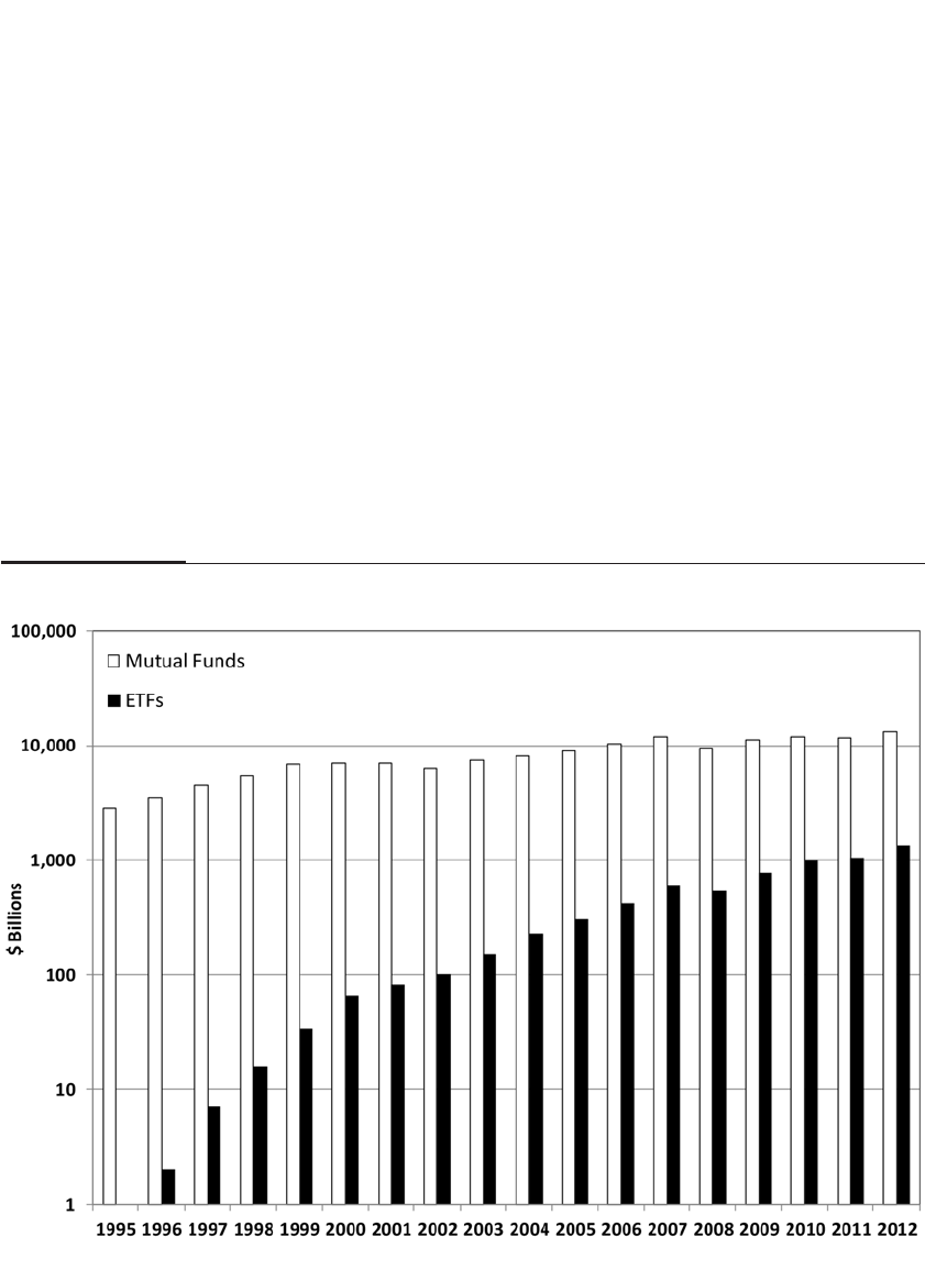
EXCHANGE-TRADED FUNDS
Exchange-traded funds (ETFs) are the most innovative and successful new
financial instruments since stock index futures contracts debuted two
decades earlier. ETFs are shares issued by an investment company that
represent an underlying portfolio. They are traded throughout the day
on an exchange where the prices are determined by supply and demand.
Most ETFs issued in the 1990s tracked only well-known stock indexes,
but more recently they have been tracking new customized indexes and
even actively managed portfolios.
The growth of exchange-traded funds has been explosive. Figure
18-1 shows the growth of mutual fund assets and ETFs since 1995.3At
the end of 2012, ETF assets totaled over $1.3 trillion, and although only
10 percent of the $134 trillion in standard mutual funds, ETFs have
grown thirteenfold since 2002.
272 PART IV Stock Fluctuations in the Short Run
FIGURE 18–1
Growth of Mutual Fund and ETF Assets 1995–2012

Spiders were the first and most successful ETF, launched in 1993.
But spiders were soon joined by others, with nicknames like cubes, a cor-
ruption of the QQQ ticker symbol given to the Nasdaq-100 Index, and
diamonds, with the ticker symbol DIA, which represents the Dow Jones
Industrial Average.
These ETFs track their respective indexes extremely closely. That’s
because designated institutions, market makers, and large investors,
called authorized participants, can buy the underlying shares of the stocks
in the index and deliver them to the issuer in exchange for units of ETFs
and deliver units of ETFs in exchange for the underlying shares. The
minimum size for such an exchange, called a creation unit, is usually
50,000 shares. For example, an authorized participant who delivers
50,000 shares of spiders to State Street Bank & Trust will receive a pro-
rated number of shares of each member of the S&P 500 Index. These
authorized participants keep the prices of the ETFs extremely close to
the value of the index. For the active ETFs, such as spiders and cubes, the
bid-asked spread is as low as 1 cent.
There are several advantages of ETFs over mutual funds. ETFs,
unlike mutual funds, can be bought or sold at any time during the day.
Second, an investor can sell ETFs short, hoping to make a profit by buy-
ing them back at a lower price. This proves to be a very convenient way
of hedging portfolio gains if an investor fears the market may fall. And
finally, ETFs are extremely tax efficient since, unlike mutual funds, they
generate almost no capital gains either from the sales of other investors or
from portfolio changes to the index. This is because swaps between the
ETFs and underlying shares are considered exchanges in kind and are not
taxable events. Later in this chapter we will list the advantages and dis-
advantages of ETFs compared with alternative forms of index investing.
STOCK INDEX FUTURES
ETFs are really the outgrowth of one of the most important trading inno-
vations of the last 50 years—the development of stock index futures in
the early 1980s. Despite the enormous popularity of these new exchange-
traded funds, the total dollar volume in ETFs is still dwarfed by the dol-
lar volume represented by trading in index futures, most of which began
trading in Chicago but are now traded on electronic exchanges. Shifts in
overall market sentiment often impact the index futures market first and
then are transmitted to stocks traded in New York.
To understand how important index futures were to stock prices in
the 1980s and 1990s, one need only look at what happened on April 13,
CHAPTER 18 Exchange-Traded Funds, Stock Index Futures, and Options 273

1992. It began as an ordinary trading day, but at about 11:45 in the morn-
ing, the two big Chicago futures exchanges, the Board of Trade and the
Mercantile Exchange, were closed when a massive leak from the
Chicago River coursed through the tunnels under the financial district
and triggered extensive power outages. The intraday movement of the
Dow Industrials and the S&P futures is shown in Figure 18-2. As soon as
the Chicago futures trading was halted, the volatility of the stock market
declined significantly.
It almost looks as if the New York Stock Exchange went “brain
dead” when there was no lead from Chicago. The volume in New York
dropped by more than 25 percent on the day the Chicago futures market
was closed; and some dealers claimed that if the futures exchange
remained inoperative, it would cause liquidity problems and difficulty
in executing some trades in New York.4Michael Metz, a market strate-
gist at Oppenheimer & Co., declared: “It’s been absolutely delightful; it
seems so sedate. It reminds me of the halcyon days on Wall Street before
the program traders took hold.”5
Who are these program traders that investors hear so much about,
and what do they do? The floor of the New York Stock Exchange has
always been alive with a constant din of people scurrying about deliver-
ing orders and making deals. But in the mid-1980s, just a few years after
index futures were introduced, the background noise was punctuated
every so often by the rat-tat-tat of dozens of automated machines print-
ing hundreds of buy or sell tickets. These orders were almost always
from stock index futures arbitrageurs—that is, program traders who rely
on differences between the prices of stock index futures traded in
Chicago and the prices of the component stocks traded in New York.
The noise signaled that the futures market was moving quickly in
Chicago and that stock prices would soon change accordingly in New
York. It was an eerie warning, something akin to the buzz of locusts in
biblical times, portending decimated crops and famine. And famine it
might be, for during the 1980s and early 1990s some of the most vicious
declines in stock prices have been preceded by computers tapping out
orders emanating from the futures markets.
In those days, most of the changes in the overall level of stocks did
not originate on Wall Street but on Wacker Drive at the Chicago
Mercantile Exchange. Specialists on the New York Stock Exchange, those
dealers assigned to make and supervise markets in specific stocks, kept
their eyes glued on the futures markets to find out where stocks would
be heading. These dealers learned from experience not to stand in the
way of index futures when they are moving quickly. If they did, they
274 PART IV Stock Fluctuations in the Short Run
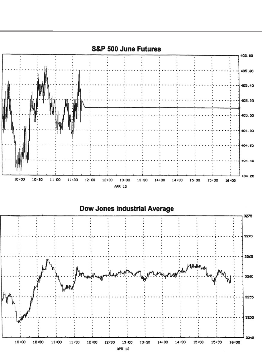
CHAPTER 18 Exchange-Traded Funds, Stock Index Futures, and Options 275
FIGURE 18–2
When Stock Index Futures Closed Down, April 13, 1992

might get caught in an avalanche of trading such as the one that buried
several specialists on October 19, 1987, that fateful day when the Dow
crashed nearly 23 percent.
BASICS OF THE FUTURES MARKETS
Most investors regard index futures and exchange-traded funds as eso-
teric securities that have little to do with the market in which stocks are
bought and sold. Many investors do very well trading stocks without
any knowledge of these new instruments. But no one can comprehend
the short-run market movements without an understanding of stock
index futures and ETFs.
Futures trading goes back hundreds of years. The term futures was
derived from the promise to buy or deliver a commodity at some future
date at some specified price. Futures trading first flourished in agricul-
tural crops, where farmers wanted to have a guaranteed price for the
crops they would harvest at a later date. Markets developed where buy-
ers and sellers who wanted to avoid uncertainty could come to an agree-
ment on the price for future delivery. The commitments to honor these
agreements, called futures contracts, were freely transferable, and mar-
kets developed where they were actively traded.
Stock index futures were launched in February 1982 by the Kansas
City Board of Trade using the Value Line Index of about 1,700 stocks.
Two months later, at the Mercantile Exchange in Chicago, the world’s
most successful stock index future, based on the S&P 500 Index, was
introduced. By 1984, the value of the contracts traded on this index
future surpassed the dollar volume on the New York Stock Exchange for
all stocks. Today, the value of stocks represented by S&P 500 futures
trading exceeds $100 billion per day.
All stock index futures are constructed similarly. In the case of the
seller, the S&P Index future is a promise to deliver a fixed multiple of the
value of the S&P 500 Index at some date in the future, called a settlement
date. In the case of the buyer, the S&P Index future is a promise to receive
a fixed multiple of the S&P 500 Index’s value. The multiple for the S&P
Index future is 250, so if the S&P 500 Index is 1,700, the value of one con-
tract is $425,000. In 1998, a miniversion of the contract (called an e-mini),
with a multiple of 50 times the index, was offered, and it trades on the
electronic markets. The dollar volume of these minis now far exceeds
that of the larger-sized contracts.
There are four evenly spaced settlement dates each year. They fall
on the third Friday of March, June, September, and December. Each set-
276 PART IV Stock Fluctuations in the Short Run

tlement date corresponds to a contract. If you buy a futures contract, you
are entitled to receive (if positive) or obligated to pay (if negative) 250
times the difference between the value of the S&P 500 Index on the set-
tlement date and the price at which you purchased the contract.
For example, if you buy one September S&P futures contract at
1,700, and on that third Friday of September the S&P 500 Index is at
1,410, you have made 10 points, which translates into $2,500 profit ($250
times 10 points). Of course, if the index has fallen to 1,690 on the settle-
ment date, you will lose $2,500. For every point the S&P 500 Index goes
up or down, you make or lose $250 per contract.
On the other hand, the returns to the seller of an S&P 500 futures
contract are the mirror image of the returns to the buyer. The seller
makes money when the index falls. In the previous example, the seller of
the S&P 500 futures contract at 1,700 will lose $2,500 if the index at set-
tlement date rises to 1,710, while he would make the same amount if the
index fell to 1,690.
One source of the popularity of stock index futures is their unique
settlement procedure. If you bought a standard futures contract, you
would be entitled at settlement to receive, or if you sold it, to deliver, a
specified quantity of the good for which you have contracted. Many
apocryphal stories abound about how traders, forgetting to close out
their contract, find bushels of wheat, corn, or frozen pork bellies
dumped on their lawn on settlement day.
If commodity delivery rules applied to the S&P 500 Index futures
contracts, delivery would require a specified number of shares for each of
the 500 firms in the index. Surely this would be extraordinarily cumber-
some and costly. To avoid this problem, the designers of the stock index
futures contract specified that settlement be made in cash, computed sim-
ply by taking the difference between the contract price at the time of the
trade and the value of the index on the settlement date. No delivery of
stock takes place. If a trader does not close a contract before settlement,
his or her account would just be debited or credited on settlement date.
The creation of cash-settled futures contracts was no easy matter. In
most states, particularly Illinois where the large futures exchanges are
located, settling a futures contract in cash was considered a wager—and
wagering, except in some special circumstances, was illegal. In 1974,
however, the Commodity Futures Trading Commission, a federal
agency, was established by Congress to regulate all futures trading.
Since futures trading was now governed by this new federal agency and
since there was no federal prohibition against wagering, the prohibitory
state laws were superseded.
CHAPTER 18 Exchange-Traded Funds, Stock Index Futures, and Options 277

INDEX ARBITRAGE
The prices of commodities (or financial assets) in the futures market do
not stand apart from the prices of the underlying commodity. If the
value of a futures contract rises sufficiently above the price of the com-
modity that can be purchased for immediate delivery in the open mar-
ket, often called the cash or spot market, traders can buy the commodity,
store it, and then deliver it at a profit against the higher-priced futures
contract on the settlement date. If the price of a futures contract falls too
far below its current spot price, owners of the commodity can sell it
today, buy the futures contract, and take delivery of the commodity later
at a lower price—in essence, earning a return on goods that would be in
storage anyway.
Such a process of buying and selling commodities against their
futures contracts is one type of arbitrage. Arbitrage involves traders
called arbitrageurs who take advantage of temporary discrepancies in
the prices of identical or nearly identical goods or assets. Arbitrage is
very common in both the stock index futures market and the ETF mar-
ket. If the price of futures contracts sufficiently exceeds that of the
underlying S&P 500 Index, it pays for arbitrageurs to buy the underlying
stocks and sell the futures contracts. If the futures price falls sufficiently
below that of the index, arbitrageurs will sell the underlying stocks and
buy the futures. On the settlement date, the futures price must equal the
underlying index by the terms of the contract, so the difference between
the futures price and the index—called a premium if it is positive and a
discount if it is negative—is an opportunity for profit.
Arbitrage in the ETF market is similar, except here an arbitrageur
must buy or sell all the stocks in the index and simultaneously make an
offsetting transaction in the ETF in the open market. An arbitrageur in
the ETF makes a profit when the prices of the stocks that she buys to cre-
ate the ETF are less than the funds that she receives by selling the ETF.
Alternatively, if the prices she receives from selling the stocks in the
index exceed the cost of buying the ETF, the arbitrageur will buy the
ETF, exchange it into its component stocks, and sell them in the open
market.
Index arbitrage has become a finely tuned art. The prices of stock
index futures and ETFs usually stay within very narrow bands of the
index value based on the price of the underlying shares. When the buy-
ing or selling of stock index futures or ETFs drives the price outside this
band, arbitrageurs step in, and a flood of orders to buy or sell are imme-
diately transmitted to the exchanges that trade the underlying stocks in
278 PART IV Stock Fluctuations in the Short Run

the index. These simultaneously placed orders are called programmed
trading, and they consist of either buy programs or sell programs. When
market commentators talk about “sell programs hitting the market,”
they mean that index arbitrageurs are selling stock and buying futures
or ETFs that have fallen to a discount.
PREDICTING THE NEW YORK OPEN WITH GLOBEX TRADING
Although trading in index futures closes at 4:15 p.m. eastern time, 15
minutes after the close of the New York stock exchanges, trading reopens
in index futures at 4:30 p.m. in an electronic market called Globex. Globex
has no centralized floor, and traders post their bids and offers on com-
puter screens where all interested parties have instant access. Trading in
Globex proceeds all night until 9:15 the next morning, 15 minutes before
the start of stock trading in New York.
Index futures trading can be active just after the close of regular
trading on the NYSE and Nasdaq. Trading is especially popular in the
weeks following the end of a quarter, when many firms release their
earnings reports and give guidance about future earnings and revenues.
Unless there is breaking news, trading is usually slow during the night
hours, although activity can pick up if there is dramatic movement on the
Tokyo or European stock exchanges. Trading again becomes very active
around 8:30 a.m., when many of the government economic data, such as
the employment report and the consumer price index, are announced.
Market watchers can use the Globex futures in the S&P, the Nasdaq,
and the Dow to predict how the market will open in New York. The fair
market value of these index futures is calculated based on the arbitrage
conditions between the future and current prices of stocks.
The fair market value for the futures contract is determined on the
basis of the current index value when markets are open and on the pre-
vious closing level when markets are closed. Because of the continuous
stream of news, the futures price overnight will usually be either above
or below the fair market value computed at the close. If, for instance,
China reports better-than-expected data or the European markets are
up, then the U.S. stock futures prices will often trade above fair market
value computed on the basis of previous closing prices. The amount by
which the futures contracts trade above or below their fair market value
will be the best estimate of where stocks will trade when the exchanges
open in New York. Many financial news channels post the overnight
prices of the S&P 500, Dow, and Nasdaq futures to inform viewers of the
likely opening of the market.
CHAPTER 18 Exchange-Traded Funds, Stock Index Futures, and Options 279

The formula to calculate the fair market value of the futures con-
tracts depends on two variables: the dividend yield on stocks and the
interest rate. If an investor puts a sum of money today in risk-free bonds,
that sum will earn interest at the ongoing interest rate. If instead the
investor buys a portfolio of stocks and simultaneously sells a one-year
futures contract that guarantees the price of those stocks one year from
now, the investor will earn the dividend yield on stocks and be guaran-
teed a return on his stocks that is the difference between the futures price
and the current price.
Since both these investments deliver a guaranteed, riskless sum,
they must earn the same rate of return. Whether the futures price trades
above or below the current (or spot) value of the index depends on the
difference between the short-term interest rate and the dividend yield.
Before the financial crisis, when interest rates almost always exceeded
the dividend yield, the future price of stocks was above the spot price.
Since the financial crisis, as short-term rates have hovered near zero, the
futures price of stock indexes is below the spot price.
DOUBLE AND TRIPLE WITCHING
Index futures play some strange games with stock prices on the days
when futures contracts expire. Recall that index arbitrage works through
the simultaneous buying or selling of stocks against futures contracts.
On the day that contracts expire, arbitrageurs unwind their stock posi-
tions at precisely the same time that the futures contracts expire.
As noted earlier, index futures contracts expire on the third Friday of
the last month of each quarter: in March, June, September, and December.
Index options and options on individual stocks, which are described later
in the chapter, settle on the third Friday of every month. Hence four times
a year, all three types of contracts expire at once. This expiration has, in the
past, often produced violent price movements in the market, and it has
consequently been termed a triple witching hour. The third Friday of a
month when there are no futures contract settlements is called a double
witching, and it displays less volatility than triple witching.
There is no mystery why the market is volatile during double or
triple witching dates. On these days, the specialists on the New York
Stock Exchange and the market makers on the Nasdaq are instructed to
buy or sell large blocks of stock on the close, whatever the price, because
institutional investors are closing out their arbitrage positions. If there is
a huge imbalance of buy orders, prices will soar; if sell orders predomi-
nate, prices will plunge. These swings, however, do not matter to arbi-
280 PART IV Stock Fluctuations in the Short Run

trageurs, since the profit on the future position will offset losses on the
stock position and vice versa.
In 1988, the New York Stock Exchange persuaded the Chicago
Mercantile Exchange to change its procedures and stop futures trading
at the close of Thursday’s trading and settle the contracts at Friday open-
ing prices rather than at Friday closing prices. This change gave special-
ists more time to seek out balancing bids and offers, and it has greatly
moderated the movements in stock prices on triple witching dates.
MARGIN AND LEVERAGE
One of the reasons for the popularity of futures contracts is that the
cash needed to enter into the trade is a very small part of the value of
the contract. Unlike stocks, there is no money that transfers between
the buyer and seller when a futures contract is bought or sold. A small
amount of good-faith collateral, or margin, is required by the broker
from both the buyer and seller to ensure that both parties will honor
the contract at settlement. For the S&P 500 Index, the current initial
margin is about 5 percent of the value of the contract. This margin can
be kept in Treasury bills with interest accruing to the investor, so trad-
ing a futures contract involves neither a transfer of cash nor a loss of
interest income.
The leverage, or the amount of stock that you control relative to the
amount of margin you have to put down with a futures contract, is enor-
mous. For every dollar of cash (or Treasury bills) that you put in margin
against an S&P futures contract, you command about $20 of stock value.
And for day trading, when you close your positions by the end of the day,
the margin requirements are significantly less. These low margins con-
trast with the 50 percent margin requirement for the purchase of indi-
vidual stocks or ETFs that has prevailed since 1974.
This ability to control $20 or more of stock with $1 of cash is remi-
niscent of the rampant speculation that existed in the 1920s before the
establishment of minimum stock margin requirements. In the 1920s,
individual stocks were frequently purchased with a 10 percent margin.
It was popular to speculate with such borrowed money, because as long
as the market was rising, few investors lost money. But if the market
dropped precipitously, margin buyers often found that not only did they
lose their equity, but they were also indebted to the brokerage firm.
Buying futures contracts with low margins can result in similar reper-
cussions today. The tendency of low margins to fuel market volatility is
discussed in the next chapter.
CHAPTER 18 Exchange-Traded Funds, Stock Index Futures, and Options 281

TAX ADVANTAGES OF ETFS AND FUTURES
The use of ETFs or index futures greatly increases an investor’s flexibil-
ity to manage portfolios. Suppose an investor has built up gains in indi-
vidual stocks but is now getting nervous about the market. Selling one’s
individual stocks may trigger a large tax liability.
But by using ETFs (or futures), a good solution is available. The
investor sells enough ETFs to cover the value of the portfolio that he
seeks to hedge and continues to hold his individual stocks. If the mar-
ket declines, the investor profits on his ETF position, offsetting the
losses of the stock portfolio. If the market instead goes up, contrary to
expectation, the loss on ETFs will be offset by the gains on the individ-
ual stock holdings. This is called hedging stock market risk. Since the
investor never sells his individual stocks, he triggers no tax liability
from these positions.
Another advantage of ETFs is that they can yield a profit from a
decline in the market even if one does not own any stock. Selling ETFs
substitutes for shorting stock, or selling stock you do not own in anticipa-
tion that the price will fall and you can buy it back at a lower price.
Using ETFs to bet on a falling market is much more convenient than
shorting a portfolio of stocks since regulations prohibit individual stocks
from being shorted if their price has declined by more than 10 percent.6
WHERE TO PUT YOUR INDEXED INVESTMENTS:
ETFS, FUTURES, OR INDEX MUTUAL FUNDS?
With the development of index futures and ETFs, investors have three
major choices to match the performance of one of many stock indexes:
exchange-traded funds, index futures, and index mutual funds, which
are described in detail in Chapter 23. The important characteristics of
each type of investment are given in Table 18-1.
As far as trading flexibility, ETFs and index futures far outshine
mutual funds. ETFs and index futures can be bought or sold any time
during the trading day and after hours on the Globex and other
exchanges. In contrast, mutual funds can be bought or sold only at the
market close, and the investor’s order must often be in several hours ear-
lier. ETFs and index futures can also be shorted to hedge one’s portfolio
or speculate on a market decline, which mutual funds cannot. And ETFs
can be margined like any stock (with current Fed regulations at 50 per-
cent), while index futures possess the highest degree of leverage, as
investors can control stocks worth 20 or more times the margin deposit.
282 PART IV Stock Fluctuations in the Short Run

CHAPTER 18 Exchange-Traded Funds, Stock Index Futures, and Options 283
The trading flexibility of ETFs or futures can be either a bane or a
boon to investors. It is easy to overreact to the continuous stream of opti-
mistic and pessimistic news, causing an investor to sell near the low or
buy near the high. Furthermore, the ability to short stocks (except for
hedging) or to leverage might tempt investors to play their short-term
hunches on the market. This is a very dangerous game. For most
investors, restricting the frequency of trades and reducing leverage will
be beneficial to their total returns.
On the cost side, all these vehicles are very efficient. Index mutual
funds are available at an annual cost of 15 basis points or less a year, and
most ETFs are even cheaper. But both ETFs and futures must be bought
through a brokerage account, and this involves paying both a commis-
sion and a bid-asked spread, although these are quite low for actively
traded ETFs. On the other hand, most index funds are no-load funds,
meaning there is no commission when the fund is bought or sold.
Furthermore, although index futures involve no annual costs, these con-
tracts must be rolled over into new contracts at least once a year, entail-
ing additional commissions.
It is on the tax side that ETFs really shine. Because of the structure
of ETFs, these funds generate very few if any capital gains. Index mutual
funds are also very tax efficient, but they do throw off capital gains. This
means funds must sell individual shares from their portfolio if investors
redeem their shares or if stocks are removed from the index. Although
capital gains have been small for most index funds, they are larger than
ETFs.7Futures are not tax efficient since any gains or losses must be real-
ized at the end of the year whether the contracts are sold or not.
Of course, these tax differences between ETFs and index mutual
funds do not matter if an investor holds these funds in a tax-sheltered
TABLE 18–1
Comparison of Indexed Investments
ETFs Index Futures Indexed Mutual Funds
Continuous trading Yes Yes No
Can be sold short Yes Yes No
Leverage Can borrow 50% Can borrow over 90% None
Expense ratio Extremely low None Very low
Trading costs Stock Futures commission None
Dividend reinvestment No No Yes
Tax efficiency Extremely good Poor Very good

account, such as an individual retirement account (IRA) or a Keogh plan
(futures are not allowed in these accounts). However, if these funds are
held in taxable accounts, the after-tax return on ETFs is apt to be higher
than it would be for even the most efficient index fund.
The bottom line is that unless you like to speculate and leverage
your cash, you will want to avoid index futures. However, if you want to
speculate on the direction of the market, I recommend index options,
which are described below and which limit an investor’s loss.
Whether to hold ETFs or low-cost index mutual funds is a very
close decision. If you like to trade in and out of the market frequently,
ETFs are for you. If you like to invest in the market on a monthly basis or
automatically reinvest your dividends, then no-load index funds may be
the better instrument. However, automatic reinvestment of dividends is
now widespread for stocks and ETFs if you request that option to your
brokerage firm. This development further tips the scale in favor of ETFs
over index mutual funds.
INDEX OPTIONS
Although ETFs and index futures are very important to investment pro-
fessionals and institutions, the options market has caught the fancy of
many investors. And this is not surprising. The beauty of an option is
embedded in its very name: you have the option, but not the obligation,
to buy or sell stocks or indexes at a given price by a given time. For the
option buyer, this option, in contrast to the futures, automatically limits
your maximum liability to the amount you invested.
There are two major types of options: puts and calls. Calls give you
the right to buy a stock (or stocks) at a fixed price within a given period
of time. Puts give you the right to sell a stock. Puts and calls have existed
on individual stocks for decades, but they were not bought and sold
through an organized trading system until the establishment of the
Chicago Board Options Exchange (CBOE) in 1974.
What attracts investors to puts and calls is that liability is strictly
limited. If the market moves against options buyers, they can forfeit the
purchase price, forgoing the option to buy or sell. This contrasts sharply
with futures contracts, with which, if the market goes against buyers,
losses can mount quickly. In a volatile market, futures can be extremely
risky, and it could be impossible for investors to exit a contract without
substantial losses.
In 1978, the CBOE began trading options on the popular stock
indexes, such as the S&P 500 Index.8The CBOE options trade in multi-
284 PART IV Stock Fluctuations in the Short Run

ples of $100 per point of index value—cheaper than the $250-per-point
multiple on the popular S&P 500 Index futures.
An index allows investors to buy the stock index at a set price
within a given period of time. Assume that the S&P 500 Index is now
selling for 1,700, but you believe that the market is going to rise. Let us
assume you can purchase a call option at 1,750 for three months for 30
points, or $3,000. The purchase price of the option is called the premium,
and the price at which the option has value when it expires—in this case
1,750—is called the strike price. At any time within the next three months
you can, if you choose, exercise your option and receive $100 for every
point that the S&P 500 Index is above 1,750.
You need not exercise your option to make a profit. There is an
extremely active market for options, and you can always sell them
before expiration to other investors. In this example, the S&P 500 Index
will have to rise above 1,780 for you to show a profit if you hold until the
expiration, since you paid $3,000 for the option. But the beauty of
options is that, if you guessed wrong and the market falls, the most you
can lose is the $3,000 premium you paid.
An index put works exactly the same way as a call, but in this case
the buyer makes money if the market goes down. Assume you buy a put
on the S&P 500 Index at 1,650, paying a $3,000 premium. Every point the
S&P 500 Index is below 1,650 at expiration will recoup $100 of your ini-
tial premium. If the index falls to 1,620 by expiration, you have broken
even. Every point below 1,620 gives you a profit on your option.
The price that you pay for an index option is determined by the mar-
ket and depends on many factors, including interest rates and dividend
yields. But the most important factor is the expected volatility of the mar-
ket itself. Clearly, the more volatile the market, the more expensive it is to
buy either puts or calls. In a dull market, it is unlikely that the market will
move sufficiently high (in the case of a call) or low (in the case of a put) to
give options buyers a profit. If this low volatility is expected to continue,
the prices of options will be low. In contrast, in volatile markets, the pre-
miums on puts and calls are bid up as traders consider it more likely that
the options will have value by the time of their expiration.9
The price of options depends on the judgments of traders about the
likelihood that the market will move sufficiently to make the rights to
buy or sell stock at a fixed price valuable. But the theory of options pric-
ing was given a big boost in the 1970s when two academic economists,
Fischer Black and Myron Scholes, developed the first mathematical for-
mula to price options. The Black-Scholes formula was an instant success. It
gave traders a benchmark for valuation where previously they used
CHAPTER 18 Exchange-Traded Funds, Stock Index Futures, and Options 285

only their intuition. The formula was programmed on traders’ handheld
calculators and PCs around the world. Although there are conditions
when the formula must be modified, empirical research has shown that
the Black-Scholes formula closely approximates the price of traded
options. Myron Scholes won the Nobel Prize in Economics in 1997 for
his discovery.10
Buying Index Options
Options are actually more basic instruments than futures or ETFs. You
can replicate any future or ETF with options, but the reverse is not true.
Options offer the investor far more strategies than futures. Such strate-
gies can range from the very speculative to the extremely conservative.
Suppose you want to be protected against a decline in the market.
You can buy an index put, which increases in value as the market
declines. Of course, you have to pay a premium for this option, very
much like an insurance premium. If the market does not decline, you
have forfeited your premium. But if it does decline, the increase in the
value of your put has cushioned, if not completely offset, the decline in
your stock portfolio.
Another advantage of puts is that you can buy just the amount of
protection that you like. If you want to protect yourself against only a
total collapse in the market, you can buy a put that is way out-of-the-
money, in other words, a put whose strike price is far below that of the
current level of the index. This option pays off only if the market
declines precipitously. In addition, you can also buy puts with a strike
price above the current market, so the option retains some value even if
the market does not decline. Of course, these in-the-money puts are far
more expensive.
There are many recorded examples of fantastic gains in puts and
calls. But for every option that gains so spectacularly in value, there are
thousands of options that expire worthless. Some market professionals
estimate that 85 percent of individual investors who play the options
market lose money. Not only do options buyers have to be right about
the direction of the market, but also their timing must be nearly perfect,
and their selection of the strike price must be appropriate.
Selling Index Options
Of course, for anyone who buys an option, someone must sell—or
write—an options contract. The sellers, or writers, of call options
286 PART IV Stock Fluctuations in the Short Run

believe that the market will not rise sufficiently to make a profit for
options buyers. Sellers of call options usually make money when they
sell options since the vast majority of options expire worthless. But
should the market move sharply against the options sellers, their losses
could be enormous.
For that reason, most sellers of call options are investors who
already own stock. This strategy, called buy and write, is popular with
many investors since it is seen as a win-win proposition. If stocks go
down, they collect a premium from buyers of the call, and so the
investors are better off than if they had not written the option. If stocks
do nothing, they also collect the premium on the call, and they are still
better off. If stocks go up, call writers still gain more on the stocks they
own than they lose on the call they wrote, so they are still ahead. Of
course, if stocks go up strongly, they miss some of the rally since they
have promised to deliver stock at a fixed price. In that case, call writers
certainly would have been better off if they had not sold the call. But
they still make more money than if they had not owned the stocks at all.
The buyers of put options are insuring their stock against price
declines. But who are the sellers of these options? They are primarily
those who are willing to buy the stock, but only if the price declines. A
seller of a put collects a premium, but she receives the stock only if it falls
sufficiently to go below the strike price. Since put sellers are not as com-
mon as call sellers, premiums on puts that are out-of-the-money are fre-
quently quite high.
THE IMPORTANCE OF INDEXED PRODUCTS
The development of stock index futures and options in the 1980s was a
major development for investors and money managers. Heavily capital-
ized firms, such as those represented in the Dow Jones Industrial
Average, have always attracted money because of their outstanding liq-
uidity. But with stock index futures, investors were able to buy the
whole market, as represented by the popular indexes.
Ten years later, exchange-traded funds gave investors still another
way to diversify across all markets at low cost. These ETFs had the
familiarity of stocks but, like index futures, much higher liquidity and
superior tax efficiency. Today when investors want to take a position in
the market, it is most easily done with stock index futures or exchange-
traded funds. Index options give investors the ability to insure the value
of their portfolio at the lowest possible price and save on transaction
costs and taxes.
CHAPTER 18 Exchange-Traded Funds, Stock Index Futures, and Options 287

Despite the opposition of such notable investors as Warren Buffett
and Peter Lynch, there is no hard evidence that these index products
have increased volatility or harmed investors. In fact, it is my belief that
these index products have increased the liquidity of the world’s stock
markets, enabled better diversification, and led to higher stock prices
than would have prevailed without them.
288 PART IV Stock Fluctuations in the Short Run

Market Volatility
The word crisis in Chinese is composed of two characters: the first,
the symbol of danger, . . . the second, of opportunity.
Does the past portend the future? The Dow Jones Industrial Average
from 1922 through 1932 and from 1980 through 1990 is shown in Figure
19-1A and B. There is an uncanny similarity between these two bull mar-
kets. In October 1987, the editors of the Wall Street Journal, looking at the
stock chart up to that time, felt the similarity was so portentous that they
printed a similar graph in their paper that hit the streets on Monday
morning, October 19, 1987. Little did they know that that day would wit-
ness the greatest one-day drop in U.S. stock market history, far exceed-
ing the great crash of October 29, 1929. Ominously, the market continued
to trade very much like 1929 for the remainder of the year. Many fore-
casters, citing the similarities between the two periods, were certain that
disaster loomed and advised their clients to sell.
But the similarity between the 1929 and the 1987 episodes stopped
at year’s end. The stock market recovered from its October 1987 crash,
and by August 1989, it hit new high ground. In contrast, two years after
the October 1929 crash, the Dow, in the throes of the greatest bear mar-
ket in U.S. history, had lost more than two-thirds of its value and was
about to lose two-thirds more.
What was different? Why did the eerie similarities between these
two events diverge so dramatically? The simple answer is that in 1987
the central bank had the power to control the ultimate source of liquid-
ity in the economy—the supply of money. And in contrast to 1929, it did
289
19
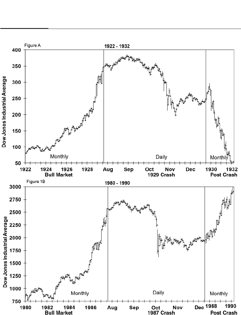
290 PART IV Stock Fluctuations in the Short Run
FIGURE 19–1
1929 and 1987 Stock Crashes

not hesitate to use it. Heeding the painful lessons of its mistakes in the
early 1930s, the Fed temporarily flooded the economy with money and
pledged to stand by all bank deposits to ensure that all aspects of the
financial system would function properly.
The public was assured. There were no runs on banks, no contrac-
tion of the money supply, and no deflation in commodity and asset val-
ues. Indeed, the economy itself expanded despite the market collapse.
The October 1987 stock market crash taught investors an important les-
son—the world was indeed different from 1929, and a sharp sell-off can
be an opportunity for profit, not a time to panic
THE STOCK MARKET CRASH OF OCTOBER 1987
The stock crash of Monday, October 19, 1987, was one of the most dra-
matic financial events of the postwar era. The 508-point, or 22.6 percent,
decline in the Dow Jones Industrials from 2,247 to 1,739 was by far the
largest point drop up to that time and the largest one-day percentage
drop in all history. Volume on the New York Stock Exchange soared to a
record, exceeding 600 million shares on both Monday and Tuesday, and
for that fateful week the number of shares traded exceeded the volume
for all of 1966.
The crash on Wall Street reverberated around the world. Tokyo,
which two years later was going to enter its own massive bear market,
fell the least, but it still experienced a record one-day drop of 15.6 per-
cent. Stocks in New Zealand fell nearly 40 percent, and the Hong Kong
market closed because collapsing prices brought massive defaults in the
stock index futures market. In the United States alone, stock values on
that infamous day dropped about $500 billion, and the total worldwide
decline in stock values exceeded $1 trillion. A similar percentage decline
in today’s market would wipe out $10 trillion worldwide, a sum greater
than the gross domestic product of every country but the United States.1
The stock market decline began in earnest the week prior to “Black
Monday,” as October 19 came to be called. At 8:30 a.m. on the preceding
Wednesday, the Department of Commerce reported that the United
States suffered a $15.7 billion merchandise trade deficit, which at that
time was one of the largest in U.S. history and far in excess of market
expectations. The reaction in the financial markets was immediate.
Yields on long government bonds rose to over 10 percent for the first
time since November 1985, and the dollar declined sharply. The Dow
Industrials fell 95 points, or 4 percent, on Wednesday, a record point
drop at that time.
CHAPTER 19 Market Volatility 291

The situation continued to worsen on Thursday and Friday as the
Dow fell 166 points, or 7 percent, to 2,246. Late Friday afternoon, about
15 minutes prior to close, heavy selling hit the stock index futures mar-
kets in Chicago. The indexes had fallen below crucial support levels,
which led to the barrage of selling in Chicago by those wanting to get
out of stocks at almost any price.
The December S&P 500 futures contract fell to an unprecedented 3
percent below the spot index. The development of such a wide discount
meant that money managers were willing to sell large orders at a signif-
icant concession in order to sell fast, rather than risk that their sell orders
for individual stocks might sit in New York, unexecuted. At the close of
trading on Friday, the stock market had experienced its worst week in
nearly five decades.
Before New York opened the following Monday, there were omi-
nous portents from the world markets. Overnight in Tokyo, the Nikkei
average fell 2½ percent, and there were sharp declines in Sydney and
Hong Kong. In London, prices had fallen by 10 percent as many money
managers were trying to sell U.S. stocks trading there before the antici-
pated decline hit New York.
Trading on the New York Stock Exchange on Black Monday was
chaotic. No Dow Jones Industrial stock traded near the 9:30 opening bell,
and only 7 Dow stocks traded before 9:45. By 10:30 that morning, 11 Dow
stocks still had not opened. “Portfolio insurers,” described later in this
chapter, heavily sold stock index futures, trying to insulate their clients’
exposure to the plunging market. By late afternoon, the S&P 500 Index
futures were selling at a 25-point, or 12 percent, discount to the spot mar-
ket, a spread that was previously considered inconceivable. By the late
afternoon, huge sell orders transmitted by program sellers cascaded onto
the New York Exchange through the computerized system. The Dow
Industrials collapsed almost 300 points in the final hour of trading, bring-
ing the toll for the day to a record 508 points, or 22.6 percent.
Although October 19 is remembered in history as the day of the
great stock crash, it was actually the next day—“Terrible Tuesday,” as it
has become known—that the market almost failed. After opening up
over 10 percent from Monday’s low, the market began to plunge by mid-
morning, and shortly after noon it fell below its Monday close. The S&P
500 Index futures market collapsed to 181—an incredible 40 points, or 22
percent, under the reported index value. If index arbitrage had been pos-
sible, the futures prices would have dictated a Dow at 1,450. Stock prices
in the world’s largest market, on this calculation, were off nearly 50 per-
cent from their high of 2,722 set just seven weeks earlier.
292 PART IV Stock Fluctuations in the Short Run

It was at this time that near meltdown hit the market. The NYSE
did not close, but trading was halted in almost 200 stocks. For the first
time, trading was also halted in the S&P 500 Index futures in Chicago.
The only futures market of any size that remained open was the
Major Market Index that traded on the Chicago Board of Trade and rep-
resented blue chip stocks similar to the Dow Industrials. These blue
chips were selling at such deep discounts to the prices in New York that
values proved irresistible to some investors. And since it was the only
market that remained open, these brave buyers stepped in, and futures
shot up an equivalent of 120 Dow points, or almost 10 percent, in a mat-
ter of minutes. When traders and the exchange specialists saw the buy-
ing come back into the blue chips, prices rallied in New York, and the
worst of the market panic passed. A subsequent investigative report by
the Wall Street Journal indicated that this futures market was a key to
reversing the catastrophic market collapse.2
THE CAUSES OF THE OCTOBER 1987 CRASH
There was no single precipitating event—such as a declaration of war, a
terrorist act, an assassination, or a bankruptcy—that caused Black
Monday. However, worrying trends had threatened the rising stock
market for some time: sharply higher long-term rates caused by a falling
dollar and the rapid development of a new strategy, called portfolio insur-
ance, that was designed to insulate portfolios from a decline in the over-
all market. The latter was born from the explosive growth of stock index
futures markets detailed in the previous chapter, markets that did not
even exist six years earlier.
Exchange Rate Policies
The roots of the surge in interest rates that preceded the October 1987
stock market crash are found in the futile attempts by the United States
and other G7 countries (Japan, the United Kingdom, Germany, France,
Italy, and Canada) to prevent the dollar from falling in the international
exchange markets.
The dollar had bounded to unprecedented levels in the middle of
the 1980s on the heels of huge Japanese and European purchases of dol-
lar securities and a strong U.S. economy. Foreign investors were attracted
to high dollar interest rates, in part driven by record U.S. budget deficits
but also by a strengthening of the U.S. economy and the capital-friendly
presidency of Ronald Reagan. By February 1985, the dollar became mas-
CHAPTER 19 Market Volatility 293

sively overvalued, and U.S. exports became very uncompetitive, severely
worsening the U.S. trade deficit. The dollar then reversed course and
began a steep decline.
Central bankers initially cheered the fall of the overpriced dollar, but
they grew concerned when the dollar continued to decline and the U.S.
trade deficit, instead of improving, worsened. Finance ministers met in
February 1987 in Paris with the goal of supporting the dollar. They worried
that if the dollar became too cheap, their own exports to the United States,
which had grown substantially when the dollar was high, would suffer.
The Federal Reserve reluctantly participated in the dollar stabiliza-
tion program, whose success depended on either an improvement in the
U.S. trade position or, absent that, a commitment by the Federal Reserve
to raise interest rates to support the dollar.
But the trade deficit did not improve; in fact, it worsened after the initi-
ation of the exchange stabilization policies. Traders, nervous about the dete-
riorating U.S. trade balance, demanded ever higher interest rates to hold U.S.
assets. Leo Melamed, chairman of the Chicago Mercantile Exchange, was
blunt when asked about the origins of Black Monday: “What caused the
crash was all that f— around with the currencies of the world.”3
The stock market initially ignored rising interest rates. The U.S. mar-
ket, like most equity markets around the world, was booming. The Dow
Jones Industrials, which started 1987 at 1,933, reached an all-time high of
2,725 on August 22—250 percent above the August 1982 low reached five
years earlier. All world markets participated. Over the same five-year
period, the British stock market was up 164 percent; the Swiss, 209 per-
cent; German, 217 percent; Japanese, 288 percent; and Italian, 421 percent.
But rising bond rates, coupled with higher stock prices, spelled
trouble for the equity markets. The long-term government bond rate,
which began the year at 7 percent, topped 9 percent in September and
continued to rise. As stocks rose, the dividend and earnings yield fell,
and the gap between the real yield on bonds and the earnings and divi-
dend yields on stocks reached a postwar high. By the morning of
October 19, the long-term bond yield had reached 10.47 percent despite
the fact that inflation was well under control. The record gap between
the yields on stocks and the real yields on bonds set the stage for the
stock market crash.
The Futures Market
The S&P 500 futures market also clearly contributed to the market crash.
Since the introduction of the stock index futures market, a new trading
294 PART IV Stock Fluctuations in the Short Run

technique, called portfolio insurance, had been introduced into portfolio
management.
Portfolio insurance was, in concept, not much different from an oft-
used technique called a stop-loss order. If an investor buys a stock and
wants to protect herself from a loss (or if it has gone up, protect her
profit), it is possible to place a sell order below the current price that will
be triggered when and if the price falls to or below this specified level.
But stop-loss orders are not guarantees that you can get out of the
market. If the stock falls below your specified price, your stop-loss order
becomes a market order to be executed at the next best price. If the stock
gaps, or declines dramatically, your order could be executed far below
your hoped-for price. This means a panic might develop if many
investors place stop-loss orders around the same price. A price decline
could trigger a flood of sell orders, overwhelming the market.
Portfolio insurers, who sold the stock index futures against large
portfolios to protect them against market decline, felt they were immune
to such problems. It seemed extremely unlikely that the S&P 500 Index
futures would ever decline dramatically in price and that the whole U.S.
capital market, the world’s largest, could fail to find buyers. This is one
reason why the stock market continued to rise in the face of sharply
higher long-term rates.
But the entire market did gap on October 19, 1987. During the week
of October 12, the market declined by 10 percent, and a large number of
sell orders flooded the markets. So many traders and money managers
using portfolio insurance strategies tried to sell index futures to protect
their clients’ profits that the futures market collapsed. There were
absolutely no buyers, and liquidity vanished.
What the overwhelming majority of stock traders once thought
inconceivable became a reality. Since the prices of index futures were so
far below the prices of the stocks selling in New York, investors halted
their buying of shares in New York altogether. The world’s largest mar-
ket failed to attract any buyers.
Portfolio insurance withered rapidly after the crash. It was not an
insurance scheme at all, because the continuity and liquidity of the mar-
ket could not be assured. There was, however, an alternative form of
portfolio protection: index options. With the introduction of these
options markets in the 1980s, investors could explicitly purchase insur-
ance against market declines by buying puts on a market index. Options
buyers never needed to worry about suffering price gaps or being able
to get out of their position since the price of the insurance was specified
at the time of purchase.
CHAPTER 19 Market Volatility 295

Certainly there were factors other than portfolio insurance con-
tributing to Black Monday. But portfolio insurance and its ancestor, the
stop-loss order, abetted the fall. All these schemes are rooted in the basic
trading philosophy of letting profits ride and cutting losses short.
Whether implemented with stop-loss orders, index futures, or just a
mental note to get out of a stock once it declines by a certain amount, this
philosophy can set the stage for dramatic market moves.
CIRCUIT BREAKERS
As a result of the crash, the Chicago Mercantile Exchange, where the
S&P 500 Index futures traded, and the New York Stock Exchange imple-
mented rules that restricted or halted trading when certain price limits
were triggered. To prevent destabilizing speculation when the Dow
Jones Industrial Average changes by at least 2 percent, the New York
Stock Exchange’s Rule 80a placed “trading curbs” on index arbitrage
between the futures market and the New York Stock Exchange.4
But of greater importance were measures that sharply restricted or
stopped trading on both the futures market and the New York Stock
Exchange when market moves are very large. From 1988 through early
2013, new rules dictated that trading must be halted 1 hour, 2 hours, and
the rest of the trading day if the Dow Industrials fell by 10 percent,
20 percent, and 30 percent, respectively. In April 2013 the SEC altered
the circuit breaker rules to provide for a 15-minute break when the S&P
500 fell by 7 percent and another when the market fell 13 percent.
Trading would be halted for the entire day if the market fell by 20 per-
cent. Futures trading must stop when the New York Stock Exchange
is closed.5
The rationale behind these circuit breakers is that halting trading
gives investors time to reassess the situation and formulate their strat-
egy based on rapidly changing prices. This time-out could bring buyers
into the market and help market makers maintain liquidity.
The argument against halts is that they increase volatility by dis-
couraging short-term traders from buying when prices fall sharply
since they might be prevented from unwinding their position if trad-
ing is subsequently halted. This could lead to an acceleration of price
declines toward the price limits, thereby increasing short-term volatil-
ity, as occurred when prices fell to these limits on October 27, 1997.6
296 PART IV Stock Fluctuations in the Short Run

FLASH CRASH—MAY 6, 2010
Monday October 19, 1987, and the following Tuesday stand as the most
volatile days in U.S. stock market history. But investors were equally
unnerved by the market collapse on May 6, 2010, an event that became
known as the “flash crash.” Just after 2:30 p.m. eastern time, the Dow
Industrials collapsed by more than 600 points or about 6 percent in a mat-
ter of minutes and recovered just as quickly. There was no economic or
financial news that could account for the decline. Furthermore, thousands
of individual stocks traded at prices that were more than 60 percent below
(and a few far above) the prices they sold at just a few minutes earlier;
some shares in well-known stocks traded as low as a penny a share.
Stock prices had been under pressure all day because of the
European debt crisis. At 2:42 p.m., with no significant news forthcoming
and the Dow Industrials down by more than 300 points, stocks hit an “air
pocket.” The benchmark index fell more than 600 points in just 5 minutes,
hitting a low at 2:47 p.m., 999 points, or nearly 10 percent, below the pre-
vious day’s close. In 5 minutes, over $800 billion was erased from U.S.
equity values. In the next 30 minutes the market rallied by 700 points
before closing the day at 10,520, down 348 points. Figure 19-2 traces the
market minute by minute through the day, a pattern of price volatility
that eerily resembles the October 1987 stock market crash depicted in
Figure 19-1A but taking place over a much shorter period of time.
After almost 5 months of investigations, the U.S. Securities and
Exchange Commission and Commodity Futures Trading Commission
issued a joint report7blaming an unusually large, $4 billion sale of S&P
500 futures by a large mutual fund that began at 2:41 p.m. and lasted 3
minutes, sending the market down quickly by another 3 percent.8Many
of these sales were initially absorbed by high-frequency traders (HFTs),
who are directed by computer programs to buy and sell securities rap-
idly to gauge market depth and predict future prices. But as the market
continued to fall, many HFTs began to sell into a very thin and unstable
market, precipitating further price declines.9At 2:45:28 p.m., trading on
the e-mini was halted for five seconds when the Chicago Mercantile
Exchange circuit breaker was triggered, and during that short pause
buyers appeared and prices recovered quickly.
The fall in the broad-based market averages was unnerving enough,
but what caught the eye of many traders were the extraordinary low
prices that some blue chips fell to just after the S&P futures contracts hit
their low. Procter & Gamble recorded a trade of $39.37, more than 50 per-
cent below its opening price of $86, and the consulting firm Accenture,
CHAPTER 19 Market Volatility 297
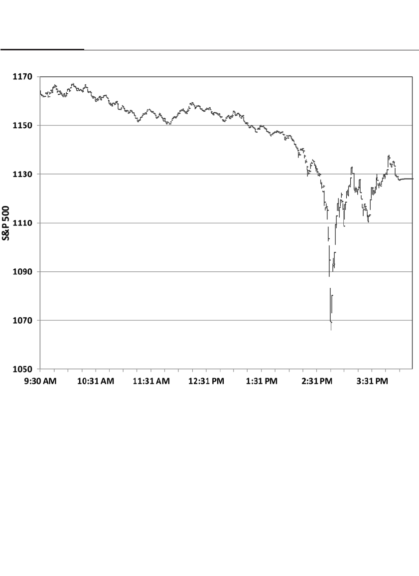
also a member of the S&P 500, which had traded at $38 at 2:47, fell to one
penny a share just two minutes later! Accenture was not alone. There were
eight other stocks in the broad-based S&P 1500 Index that traded at one
cent per share.10 All told, there were 20,000 trades in 300 securities that
were 60 percent or more away from the price they traded at just minutes
earlier. After the close, the NYSE, in consultation with the Financial
Industry Regulatory Authority (FINRA), “broke,” or canceled, all trades
that were 60 percent or more above or below their previous price.
It is very likely that these extreme prices would not have been real-
ized if specialists, those exchange representatives who maintained mar-
kets in assigned stocks before the advent of computerized trading, still
298 PART IV Stock Fluctuations in the Short Run
FIGURE 19–2
“Flash Crash,” May 6, 2010

controlled the flow of buy and sell orders. These specialists would have
stepped in to buy these stocks at prices well above the absurdly low
price they traded at. But most modern computerized trading systems
were programmed to react very differently than the specialists would
have. When prices begin to fall steeply, the programs are instructed to
withdraw from the market. This is because large moves in individual
stocks are almost always associated with company-specific news that
computerized traders do not have access to. These computers are pro-
grammed to profit from the normal ebb and flow of trading activity that
clearly was absent that day.
When stock prices tumbled, a system of trading pauses that had
been instituted by the New York Stock Exchange, termed liquidity replen-
ishment points, kicked in. But instead of providing liquidity, the pause
sent some sell orders to other markets where dealers maintained stub
quotes. Stub quotes are “placeholders,” i.e., quotes far from the market
price (usually at a penny bid, $100,000 asked), and are not meant to be
traded against. But with no other orders on the books, these stub quotes
were executed for many stocks.
In response to the flash crash, the SEC staff worked with the
exchanges and FINRA to promptly implement a circuit breaker pilot
program for trading in individual securities that would apply across all
markets. These new rules pause trading in a security for five minutes if
that security has experienced a 10 percent price change over the preced-
ing five minutes. On June 10, 2010, the SEC approved the application of
the circuit breakers to stocks included in the S&P 500 Index, and on
September 10, the SEC approved an expansion of the program to securi-
ties included in the Russell 1000 Index and certain ETFs. In April 2013,
the SEC changed the 10 percent price change trigger to a “limit-up and
limit-down” rule that was tailored to the volatility of the individual
security. For stocks trading over $3 a share (except leveraged ETFs), the
limit remains at 10 percent, except for the first and last 15 minutes of
trading, when the limit is expanded to 20 percent.11
The flash crash, coming just a year after the deepest bear market in
75 years, eroded the public’s trust in a fair and orderly market for equi-
ties. Many cited the SEC indictment of high-frequency traders as evi-
dence that the market is rigged against the small investor. But
high-frequency trading declined after the flash crash, and a number of
researchers questioned whether the trading played a significant role in
that day’s decline. New rules established by the SEC have virtually elim-
inated the kind of “errant” and extreme trades that took place during the
flash crash.
CHAPTER 19 Market Volatility 299

But from a broader perspective, individual investors should not
fear short-term market volatility. Should you not want to shop in a store
where every so often it announces “10 percent to 20 percent off the price
of all items for the next 30 minutes?” Short-run volatility has always
been part of the stock market, and the flash crash had no lasting effect on
the recovery from the 2007–2009 bear market.
THE NATURE OF MARKET VOLATILITY
Although most investors express a strong distaste for market fluctua-
tions, volatility must be accepted to reap the superior returns offered by
stocks. Accepting risk is required for above-average returns: investors
cannot make any more than the risk-free rate unless there is some possi-
bility that they can make less.
While the volatility of the stock market deters many investors, it
fascinates others. The ability to monitor a position on a minute-by-
minute basis fulfills the need of many to quickly validate their judg-
ment. For many the stock market is truly the world’s largest casino.
Yet this ability to know exactly how much one is worth at any given
moment can also provoke anxiety. Many investors do not like the instan-
taneous verdict of the financial market. Some retreat into investments
such as real estate, for which daily quotations are not available. Others
believe that not knowing the current price somehow makes an invest-
ment less risky. As Keynes stated 75 years ago about the investing atti-
tudes of the endowment committee at Cambridge University:
Some Bursars will buy without a tremor unquoted and unmarketable
investments in real estate which, if they had a selling quotation for imme-
diate cash available at each audit, would turn their hair grey. The fact that
you do not know how much its ready money quotation fluctuates does
not, as is commonly supposed, make an investment a safe one.12
HISTORICAL TRENDS OF STOCK VOLATILITY
The annual variability of the U.S. stock, measured by the standard devia-
tion of the monthly returns, from 1834 to 2012 is plotted in Figure 19-3. It
is striking that there is so little overall trend in the volatility of the market.
The period of greatest volatility was during the Great Depression,
and the year of highest volatility was 1932. The annualized volatility of
1932 was 63.7 percent, nearly 20 times higher than 1993, which is the least
volatile year on record with a standard deviation of 3.36. The volatility of
300 PART IV Stock Fluctuations in the Short Run
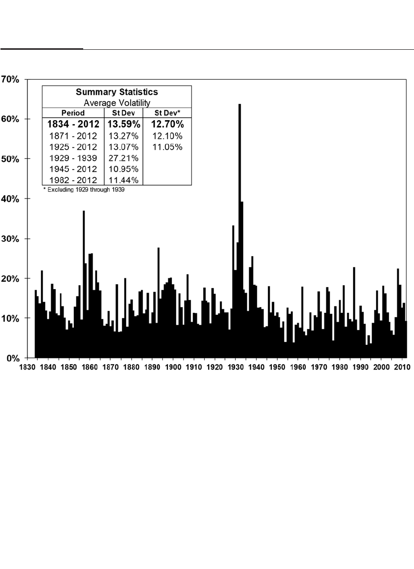
1987 was the highest since the Great Depression, just edging out 2008, the
year of the financial crisis. Excluding the 1929-to-1939 period, volatility
has averaged about 12 percent and has remained remarkably stable at
between 13 and 14 percent over the past 180 years.
Figure 19-4A displays the average daily percentage change in the
Dow Jones Industrial Average for each year from 1896 to the present.
The average daily change over the past 117 years is 0.74 percent. Except
for the 1930s, there was a downtrend in volatility from 1896 to 1960 and
a subsequent uptrend. Some of the uptrend is due to the faster response
of markets to economic developments; information that used to take
hours if not days to be fully reflected in market averages is now
processed in minutes if not seconds. Some of the downward trend in the
Dow volatility in the early twentieth century is due to the increase in the
CHAPTER 19 Market Volatility 301
FIGURE 19–3
Volatility of Stock Market 1834–2012 Measured as Standard Deviation of Monthly Returns
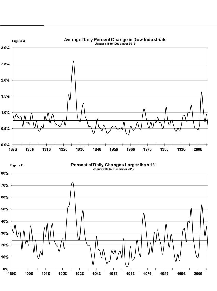
302 PART IV Stock Fluctuations in the Short Run
FIGURE 19–4
Daily Volatility of Dow-Jones Industrial Average 1896–2012

number of stocks in the Dow Industrials from 12 to 20 and then to 30 in
1928. The daily volatility during the crisis year 2008 at 1.63 percent was
the highest since the Great Depression.
The percentage of trading days when the Dow Industrials changed
by more than 1 percent is shown in Figure 19-4B. It has averaged 24 per-
cent over the period, or about once per week. But it has ranged from as
low as 1.2 percent in 1964 to a high of 67.6 percent in 1932, when the
Dow changed by more than 1 percent in more than two out of every
three trading days. The financial crisis generated the highest volatility,
and the deepest recession, since the Great Depression of the 1930s.
Most of the periods of high volatility occur during bear markets. The
standard deviation of daily returns is more than 25 percent higher in reces-
sions than in expansions. There are two reasons why volatility increases in
a recession. First, recessions, being the exception rather than the rule, are
marked by greater economic uncertainty than expansions. The second is
that if earnings fall, then the burden of fixed costs causes greater volatility
of profits. This leads to increased volatility in stock prices.
If earnings turn into losses, then the equity value of the firms is like
an out-of-the-money call option that pays off only if the firm eventually
earns enough profits to cover its costs. Otherwise, it is worthless. It is not
a puzzle why stock volatility was the greatest during the Great
Depression when, with aggregate profits negative, the equity market
was trading like an out-of-the-money call.
THE VOLATILITY INDEX
Measuring historical volatility is a simple matter, but it is far more impor-
tant to measure the volatility that investors expect in the market. This is
because expected volatility is a signal of the level of anxiety in the mar-
ket, and periods of high anxiety have often marked turning points for
stocks.
By examining the prices of put and call options on the major stock
market indexes, one can determine the volatility that is built into the
market, which is called the implied volatility.13 In 1993, the Chicago Board
Options Exchange introduced the CBOE Volatility Index, also called the
VIX Index or the VIX (first mentioned in Chapter 3), based on actual
index options prices on the S&P 500 Index, and it calculated this index
back to the mid-1980s.14 A weekly plot of the VIX from 1986 appears in
Figure 19-5.
In the short run, there is a strong negative correlation between the
VIX and the level of the market. When the market is falling, investors are
CHAPTER 19 Market Volatility 303
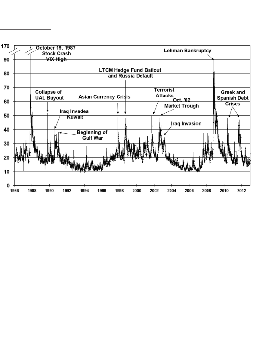
willing to pay more for downside protection, and they purchase puts,
causing the VIX to rise. When the market is rising, the VIX typically falls
as investors gain confidence and are less anxious to insure their portfo-
lio against a loss.
This correlation may seem puzzling since one might expect
investors to seek more protection when the market is high rather than
low. One explanation of the behavior of the VIX is that historical volatil-
ity is higher in bear markets than bull markets, so falling markets cause
the VIX to rise. But a more persuasive argument is that changes in
investor confidence change investors’ willingness to hedge through
buying puts. As put prices are driven up, arbitrageurs who sell will sell
stocks to hedge their position, sending stock prices down. The reverse
occurs when investors feel more confident of stock returns.
It is easy to see in Figure 19-5 that the peaks in the VIX corre-
sponded to periods of extreme uncertainty and sharply lower stock
prices. The VIX peaked at 172 on the Tuesday following the October 19,
1987, stock market crash, far eclipsing any other high.
304 PART IV Stock Fluctuations in the Short Run
FIGURE 19–5
The Volatility Index (VIX) 1986–2012

In the early and mid-1990s, the VIX sank to between 10 and 20. But
with the onset of the Asian crises in 1997, the VIX moved up to a 20-to-
30 range. Spikes between 40 and 50 in the VIX occurred on three occa-
sions: in October 1987 when the Dow fell 550 points during the attack on
the Hong Kong dollar, in August 1998 when Long-Term Capital
Management was liquidated, and in the week following the terrorist
attacks of September 11, 2001. After the 1987 stock market crash, the
highest VIX was 90, reached shortly after Lehman Brothers went bank-
rupt in September 2008. The VIX peaked again during the Greek and
Spanish sovereign debt crises. The all-time low value of the VIX
occurred in December 1993 when the volatility index fell to 8.89.
In recent years, buying when the VIX is high and selling when it is
low has proved to be a profitable strategy for the short term. But so has
buying during market spills and selling during market peaks. The real
question is how high is high and how low is low. For instance, an
investor might have been tempted to buy into the market on Friday,
October 16, 1987, when the VIX reached 40. Yet such a purchase would
have proved disastrous given the record one-day collapse that followed
on Monday.
THE DISTRIBUTION OF LARGE DAILY CHANGES
Chapter 16 noted that there were 145 days from 1885 through 2012 when
the Dow Jones Industrials changed by 5 percent or more: 68 up and 77
down. Seventy-nine of these days, or nearly two-thirds of the total,
occurred from 1929 through 1933. The most volatile year by far in terms
of daily changes was 1932, which contained 35 days when the Dow
moved by at least 5 percent. The longest period of time between two suc-
cessive changes of at least 5 percent was the 17-year period that pre-
ceded the October 19, 1987, stock crash.
The calendar properties of large daily changes are displayed in
Figure 19-6. Most of the large changes have occurred on Monday, while
Tuesday has experienced by far the least (excluding Saturday). Monday
has the largest number of down days, and Wednesday has by far the
highest number of up days.
Thirty-six of the large changes occurred in October, which has wit-
nessed more than twice the number of large moves as any other month.
October’s reputation as a volatile month is fully justified. Not only has
October witnessed nearly one-quarter of all big moves, but it has also
seen the two greatest stock crashes in history, in October 1929 and
October 1987. It is interesting to note that nearly two-thirds of the large
CHAPTER 19 Market Volatility 305
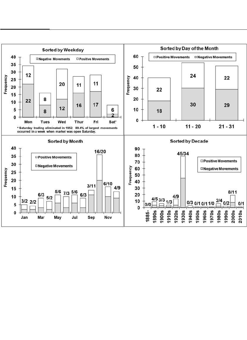
declines have occurred in the last four months of the year. Chapter 21
examines other seasonal properties of stock returns.
One of the most surprising bits of information about large market
moves relates to the period of the greatest stock market collapse. From
September 3, 1929, through July 8, 1932, the Dow Jones Industrials fell
nearly 89 percent. During that period, there were 37 episodes when the
Dow changed by 5 percent or more. Surprisingly, 21 of those episodes
were increases! Many of these sharp rallies were the result of short cover-
ing, which occurred as speculators who thought the market was on a one-
way street rushed to sell stock they did not own and were then forced to
buy it back, or cover their positions, once the market rallied.
It is not uncommon for markets that appear to be trending in one
direction to experience occasional sharp moves in the other direction. In
306 PART IV Stock Fluctuations in the Short Run
FIGURE 19–6
Distribution of Dow-Industrial Changes Over 5 Percent, 1885–2012

a bull market, the expression “up the staircase, down the elevator” is an
apt description of market behavior. Ordinary investors must beware: it
is not as easy to make money in trending markets as it looks, and
investors who try to play these markets must be ready to bail out quickly
when they see the market change direction.
THE ECONOMICS OF MARKET VOLATILITY
Many of the complaints about market volatility are grounded in the
belief that the market reacts excessively to changes in news. But how
news should impact the market is so difficult to determine that few can
quantify the proper impact of an event on the price of a stock. As a result,
traders often “follow the crowd” and try to predict how other traders
will react when news happens.
Over half a century ago, Keynes illustrated the problem of
investors who try to value stock by economic fundamentals as opposed
to following the crowd:
Investment based on genuine long-term expectation is so difficult today as
to be scarcely practicable. He who attempts it must surely lead much more
laborious days and run greater risk than he who tries to guess better than
the crowd how the crowd will behave; and, given equal intelligence, he
may make more disastrous mistakes.15
In 1981, Robert Shiller of Yale University devised a method of
determining whether stock investors tended to overreact to changes in
dividends and interest rates, the fundamental building blocks of stock
values.16 From the examination of historical data, he calculated what the
value of the S&P 500 Index should have been given the subsequent real-
ization of dividends and interest rates. We know what this value is
because, as shown in Chapter 10, stock prices are the present discounted
value of future cash flows.
What he found was that stock prices were far too variable to be
explained merely by the subsequent behavior of dividends and interest
rates. Stock prices appeared to overreact to changes in dividends, failing
to take into account that most of the changes in dividend payouts were
only temporary.17 For example, investors priced stocks in a recession as
if they expected dividends to go much lower, completely contrary to his-
torical experience.
The word cycle in business cycle implies that ups in economic activ-
ity will be followed by downs and vice versa. Since earnings and profits
tend to follow the business cycle, they too should behave in a cyclical
CHAPTER 19 Market Volatility 307

308 PART IV Stock Fluctuations in the Short Run
manner, returning to some average value over time. Under these cir-
cumstances, a temporary drop in dividends (or earnings) during a reces-
sion should have a very minor effect on the price of a stock, which
discounts dividends into the infinite future.
When stocks are collapsing, worst-case scenarios loom large in
investors’ minds. On May 6, 1932, after stocks had plummeted 85 per-
cent from their 1929 high, Dean Witter issued the following memo to its
clients:
There are only two premises which are tenable as to the future. Either we
are going to have chaos or else recovery. The former theory is foolish. If
chaos ensues nothing will maintain value; neither bonds nor stocks nor
bank deposits nor gold will remain valuable. Real estate will be a worth-
less asset because titles will be insecure. No policy can be based upon this
impossible contingency. Policy must therefore be predicated upon the the-
ory of recovery. The present is not the first depression; it may be the worst,
but just as surely as conditions have righted themselves in the past and
have gradually readjusted to normal, so this will again occur. The only
uncertainty is when it will occur. . . . I wish to say emphatically that in a
few years present prices will appear as ridiculously low as 1929 values
appear fantastically high.18
Two months later the stock market hit its all-time low and rallied
strongly. In retrospect, these words reflected great wisdom and sound
judgment about the temporary dislocations of stock prices. Yet at the
time they were uttered, investors were so disenchanted with stocks and
so filled with doom and gloom that the message fell on deaf ears.
Chapter 22 discusses why investors often overreact to short-term events
and fail to take the long view of the market.
THE SIGNIFICANCE OF MARKET VOLATILITY
Despite the drama of the October 1987 market collapse, there was amaz-
ingly little lasting effect on the world economy or even the financial mar-
kets. Because the 1987 episode did not augur either a further collapse in
stock prices or a decline in economic activity, it will never attain the
notoriety of the crash of 1929. Yet its lesson is perhaps more important.
Economic safeguards, such as prompt Federal Reserve action to provide
liquidity to the economy and assure the proper functioning of the finan-
cial markets, can prevent an economic debacle of the kind that beset our
economy during the Great Depression.

This does not mean that the markets are exempt from violent fluc-
tuations. Since the future will always be uncertain, psychology and sen-
timent often dominate economic fundamentals. As Keynes perceptively
stated more than 70 years ago in The General Theory, “The outstanding
fact is the extreme precariousness of the basis of knowledge on which
our estimates of prospective yield have to be made.”19 Precarious esti-
mates are subject to sudden change, so prices in free markets will be
volatile. But history has shown that investors who are willing to step
into the market when others are running to the exits reap the benefits of
market volatility.
CHAPTER 19 Market Volatility 309
This page intentionally left blank

Technical Analysis and
Investing with the Trend
Many skeptics, it is true, are inclined to dismiss the whole procedure
[chart reading] as akin to astrology or necromancy; but the sheer
weight of its importance in Wall Street requires that its pretensions
be examined with some degree of care.
—BENJAMIN GRAHAM AND DAV ID DODD, 19341
THE NATURE OF TECHNICAL ANALYSIS
Flags, pennants, saucers, and head-and-shoulders formations. Stochastics,
moving-average convergence-divergence indicators, and candlesticks. Such is
the arcane language of the technical analyst, an investor who forecasts
future returns by the use of past price trends. Few areas of investment
analysis have attracted more critics; yet no other area has a core of such
dedicated, ardent supporters. Technical analysis, often dismissed by
academic economists as being as useful as astrology, is being given a
new look, and some of the recent evidence is surprisingly positive.
Technical analysts, or chartists as they are sometimes called, stand in
sharp contrast to fundamental analysts, who use such variables as divi-
dends, earnings, and book values to forecast stock returns. Chartists
ignore these fundamental variables, maintaining that information
important to predicting future price movements can be gleaned by ana-
lyzing past price patterns. Some of these patterns are the result of shifts
in market psychology that tend to repeat themselves, whereas others are
311
20

caused by informed investors who have special knowledge of the
prospects of the firm. If these patterns are read properly, chartists main-
tain, investors can use them to outperform the market and share in the
gains of those who are more knowledgeable about a stock’s prospects.
CHARLES DOW, TECHNICAL ANALYST
The first well-publicized technical analyst was Charles Dow, the creator
of the Dow Jones Industrial Average. But Charles Dow did not analyze
only charts. In conjunction with his interest in market movements, Dow
founded the Wall Street Journal and published his strategy in editorials in
the early 1900s. Dow’s successor, William Hamilton, extended Dow’s
technical approach and published the Stock Market Barometer in 1922. Ten
years later, Charles Rhea formalized Dow’s concepts in a book entitled
Dow Theory.
Charles Dow likened the ebb and flow of stock prices to waves in
an ocean. He claimed that there was a primary wave, which, like the tide,
determined the overall trend. Upon this trend were superimposed sec-
ondary waves and minor ripples. He also claimed you could identify
which trend the market was in by analyzing a chart of the Dow Jones
Industrial Average, the volume in the market, and the Dow Jones Rail
(now called the Transportation) Average.
Those who follow the Dow’s theory acknowledge that the strategy
would have gotten an investor out of the stock market before the
October 1929 stock crash. Martin J. Pring, a noted technical analyst,
argues that, starting in 1897, investors who purchased stock in the Dow
Jones Industrial Average and followed each Dow theory buy-and-sell
signal would have seen an original investment of $100 reach $116,508 by
January 1990, as opposed to $5,682 with a buy-and-hold strategy (these
calculations exclude reinvested dividends).2But confirming profits that
come from trading based on the Dow theory is difficult because the buy-
and-sell signals are purely subjective and cannot be determined by pre-
cise numerical rules.
THE RANDOMNESS OF STOCK PRICES
Although the Dow theory might not be as popular as it once was, tech-
nical analysis is still alive and well. The idea that you can identify the
major trends in the market, riding bull markets while avoiding bear
markets, is still the fundamental goal of technical analysts.
312 PART IV Stock Fluctuations in the Short Run

Yet most economists still attack the fundamental tenet of the
chartists—that stock prices follow predictable patterns. To these aca-
demic researchers, the movements of prices in the market more closely
conform to a pattern called a random walk than to special formations that
forecast future returns.
The first economist to come to this conclusion was Frederick
MacCauley, an economist in the early part of the twentieth century. His
comments at a 1925 dinner meeting of the American Statistical
Association on the topic of “forecasting security prices” were reported in
the association’s official journal:
MacCauley observed that there was a striking similarity between the fluc-
tuations of the stock market and those of a chance curve which may be
obtained by throwing dice. Everyone will admit that the course of such a
purely chance curve cannot be predicted. If the stock market can be fore-
cast from a graph of its movements, it must be because of its difference
from the chance curve.3
More than 30 years later, Harry Roberts, a professor at the
University of Chicago, simulated movements in the market by plotting
price changes that resulted from completely random events, such as
flips of a coin. These simulations looked like the charts of actual stock
prices, forming shapes and following trends that are considered by
chartists to be significant predictors of future returns. But since the next
period’s price change was, by construction, a completely random event,
such patterns could not logically have any predictive content. This early
research supported the belief that the apparent patterns in past stock
prices were the result of completely random movements.
But does the randomness of stock prices make economic sense?
Factors influencing supply and demand do not occur randomly and are
often quite predictable from one period to the next. Shouldn’t these pre-
dictable factors make stock prices move in nonrandom patterns?
In 1965, Professor Paul Samuelson of MIT showed that the ran-
domness in security prices did not contradict the laws of supply and
demand.4In fact, such randomness was a result of a free and efficient
market in which investors had already incorporated all the known fac-
tors influencing the price of the stock. This is the crux of the efficient mar-
ket hypothesis.
If the market is efficient, prices will change only when new, unan-
ticipated information is released to the market. Since unanticipated
information is as likely to be better than expected as it is to be worse than
CHAPTER 20 Technical Analysis and Investing with the Trend 313

expected, the resulting movement in stock prices is random. Price charts
will therefore look like a random walk and cannot be predicted.5
SIMULATIONS OF RANDOM STOCK PRICES
If stock prices are indeed random, their movements should not be distin-
guishable from simulations generated randomly by a computer. Figure
20-1 extends the experiment conceived by Professor Roberts 60 years ago.
Instead of generating only closing prices, I programmed the computer to
generate intraday prices, creating the popular high-low-close bar graphs
that are found in most newspapers and chart publications.
There are eight charts in Figure 20-1. Four have been generated by
a random-number generator. In these charts, there is absolutely no way
to predict the future from the past, because future movements are
designed to be totally independent from the past. The other four charts
were chosen from actual data of the Dow Jones Industrial Average.
Before reading further, try to determine which four are actual historical
prices and which are computer generated.
Such a task is quite difficult. In fact, most of the top brokers at a
leading Wall Street firm found it impossible to tell the difference
between the real and counterfeit data. Two-thirds of brokers did cor-
rectly identify Figure 20-1D, which depicts the period around the
October 19, 1987, stock crash. For the remaining seven charts, the bro-
kers showed no ability to distinguish actual from computer-generated
data. The true historical prices are represented by charts B, D, E, and H,
while the computer-generated data are charts A, C, F, and G.6
TRENDING MARKETS AND PRICE REVERSALS
Despite the fact that many “trends” are in fact the result of the totally
random movement of stock prices, many traders will not invest against
a trend that they believe they have identified. Two of the most well-
known sayings of market timers are “Make the trend your friend” and
“Trust the thrust.”
Martin Zweig, a well-known market timer who used fundamental
and technical variables to forecast market trends, forcefully stated: “I
can’t overemphasize the importance of staying with the trend of the
market, being in gear with the tape, and not fighting the major move-
ments. Fighting the tape is an open invitation to disaster.”7
When a trend appears established, technical analysts draw chan-
nels consisting of parallel upper and lower bounds within which the
314 PART IV Stock Fluctuations in the Short Run
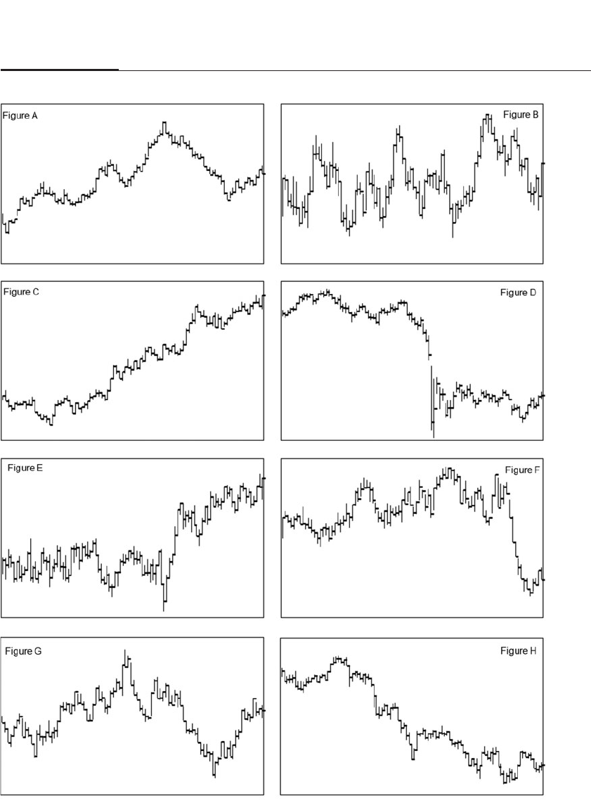
CHAPTER 20 Technical Analysis and Investing with the Trend 315
FIGURE 20–1
Real and Simulated Stock Indexes

market has traded. The lower bound of a channel is frequently called a
support level and the upper bound a resistance level. When the market
breaks the bounds of the channel, a large market move often follows.
The very fact that many traders believe in the importance of trends
can induce behavior that makes trend following so popular. While the
trend is intact, traders sell when prices reach the upper end of the chan-
nel and buy when they reach the lower end, attempting to take advan-
tage of the apparent fluctuations of stock prices within the channel. If the
trendline is broken, many of these traders will reverse their positions:
buying if the market penetrates the top of the trendline or selling if it
falls through the bottom. This behavior often accelerates the movement
of stock prices and reinforces the importance of the trend.
Options trading by trend followers also reinforces the behavior of
market timers. When the market is trading within a channel, traders
will sell put and call options at strike prices that represent the lower and
upper bounds of the channel. As long as the market remains within
the channel, these speculators collect premiums as the options expire
worthless.
If the market penetrates the trading range, options sellers are
exposed to great risks. Recall that sellers of options (as long as they do
not own the underlying stock) face a huge potential liability, a liability
that can be many times the premium that they collected upon sale of the
option. When such unlimited losses loom, these options writers “run for
cover,” or buy back their options, accelerating the movement of prices.
MOVING AVERAGES
Successful technical trading requires not only identifying the trend but,
more important, identifying when the trend is about to reverse. A popu-
lar tool for determining when the trend might change examines the rela-
tionship between the current price and a moving average of past price
movements, a technique that goes back to at least the 1930s.8
A moving average is simply the arithmetic average of a given num-
ber of past closing prices of a stock or index. For each new trading day,
the oldest price is dropped and the most recent price is added to com-
pute the average.
Moving averages are far less volatile than daily prices. When prices
are rising, the moving average is below the market price and, technical
analysts claim, forms a support level for stock prices. When prices are
falling, the moving average is above current prices and forms a resist-
316 PART IV Stock Fluctuations in the Short Run

ance level. Analysts claim that a moving average allows investors to
identify the basic market trend without being distracted by the day-to-
day volatility of the market. When prices penetrate the moving average,
this indicates that powerful underlying forces are signaling a reversal of
the basic trend.
The most popular moving average uses prices for the past 200 trading
days, and it is therefore called the 200-day moving average. It is frequently
plotted in newspapers and investment letters as a key determinant of
investment trends. One of the early supporters of this strategy was William
Gordon, who indicated that, over the period from 1897 to 1967, buying
stocks when the Dow broke above the moving average produced nearly
seven times the return as buying when the Dow broke below the average.9
Robert Colby and Thomas Meyers claim that for the United States the best
time period for a moving average of weekly data is 45 weeks, just slightly
longer than the 200-day moving average.10
Testing the Dow Jones Moving-Average Strategy
In order to test the 200-day moving-average strategy, I examined the
daily record of the Dow Jones Industrial Average from 1885 to the pres-
ent. In contrast to the previous studies on moving-average strategies, the
holding-period returns include the reinvestment of dividends when the
strategy calls for investing in the market and calls for investing in short-
term interest-bearing securities when one is not. Annualized returns are
examined over the entire period as well as the subperiods.
I adopted the following criteria to determine the buy-sell strategy:
Whenever the Dow Jones Industrial Average closed by at least 1 percent
above its 200-day moving average (not including the current day),
stocks were purchased at the current day’s closing prices; and whenever
the Dow Industrials closed by at least 1 percent below its 200-day mov-
ing average, stocks were sold at the closing prices. When sold, the port-
folio was invested in Treasury bills.
There are two noteworthy aspects of this strategy. The 1 percent
band around the 200-day moving average is used in order to reduce the
number of times an investor would have to move in and out of the mar-
ket. The smaller the band, the greater the number of buys and sells.11 A
very small band would cause traders to be “whipsawed,” a term used to
describe the alternate buying and then selling of stocks in an attempt to
beat the market. Whipsawing dramatically lowers investor returns
because of the large increase in transaction costs.
CHAPTER 20 Technical Analysis and Investing with the Trend 317

The second aspect of this strategy assumes that an investor buys or
sells stocks at the closing price rather than during the trading day. Only in
recent years has the exact intraday level of the popular averages been
computed. Using historical data, it is impossible to determine times when
the market average penetrated the 200-day moving average during the
day. By specifying that the average must close above or below the average
of the two hundred preceding closes, I present a theory that could have
been implemented in practice through the whole time period.12
Back-Testing the 200-Day Moving Average
Figure 20-2 displays the daily and 200-day moving averages of the Dow
Jones Industrial Average during two select periods: from 1924 to 1936
and 2001 to 2012. The time periods when investors are out of the stock
market (and in short-term bonds) are shaded; otherwise, investors are
fully invested in stocks.
The returns from the 200-day moving-average strategy and a buy-
and-hold strategy over the whole period are summarized in Table 20-1.
From January 1886 through December 2012, the 9.73 percent annual
return from the timing strategy beat the annual return on the holding
strategy of 9.39 percent. As noted earlier, the timing strategy had its
biggest success avoiding the 1929-to-1932 crash. If that period is excluded,
318 PART IV Stock Fluctuations in the Short Run
TABLE 20–1
Annualized Returns of Timing and Holding Strategies, 1886–2012
Holding Strategy Timing Strategy
No Trans Costs Net Trans Costs % in # of
Period Return Risk Return Risk Return Risk Market Switches
1886–2012 9.39% 21.4% 9.73% 16.5% 8.11% 17.2% 62.4% 376
Subperiods
1886–1925 9.08% 23.7% 9.77% 17.7% 8.10% 18.0% 56.6% 122
1926–1945 6.25% 31.0% 11.13% 21.8% 9.47% 22.7% 62.2% 60
1946–2012 10.53% 16.2% 9.28% 14.1% 7.71% 15.0% 66.5% 194
1990–2012 9.57% 15.7% 4.92% 15.6% 2.66% 16.8% 70.1% 100
2001–2012 4.07% 16.4% 1.33% 12.3% –1.09% 13.2% 60.5% 58
Excl. 1929–1932 Crash
1886–2012 10.60% 20.1% 9.92% 16.3% 8.38% 16.9% 63.6% 358
1926–1945 13.94% 24.5% 12.38% 20.3% 11.21% 20.8% 70.8% 42
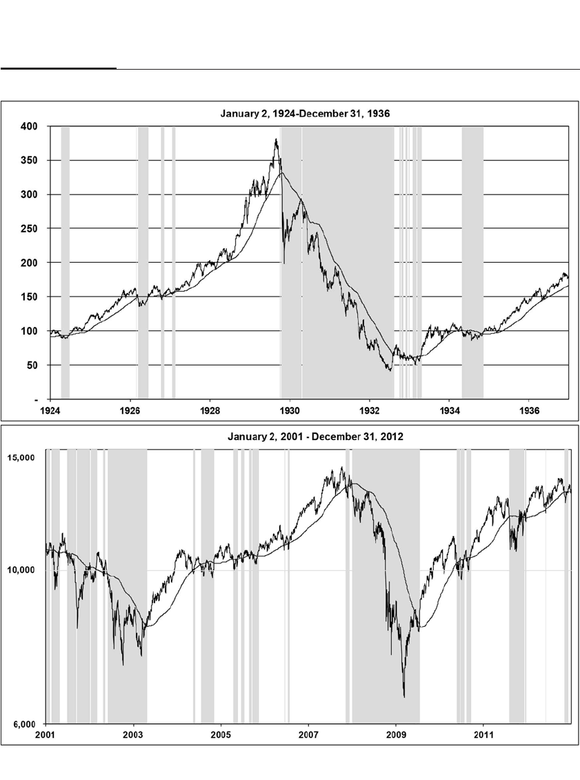
CHAPTER 20 Technical Analysis and Investing with the Trend 319
FIGURE 20–2
Dow-Jones Industrials and the 200-Day Moving-Average Strategy
Shaded areas are out of the market.

the returns of the timing strategy are 68 basis points per year behind the
holding strategy, although the timing strategy has lower risk.
Moreover, if the transaction costs of implementing the timing strat-
egy are included in the calculations, the excess returns over the whole
period, including the 1929-to-1932 Great Crash, more than vanish.
Transaction costs include brokerage costs and bid-asked spreads, as well
as the capital gains tax incurred when stocks are sold, and are assumed
to be on average half a percent when buying or selling the market. This
number probably underestimates such costs, especially in the earlier
years, but likely overstates these costs in more recent years.
Looks are deceiving. When examining the returns from 2001 onward
in Figure 20-2, it appears as if the returns from the timing strategy would
swamp the buy-and-hold strategy, but that is not the case. The buy-and-
hold strategy from 2001 to 2012 beats the timing strategy by more than
2 percentage points per year even before transaction costs are factored in.
This is because the poor returns from the timing strategy occur when mar-
kets are not in a strong uptrend or downtrend and the market crosses the
200-day moving average many times, incurring large costs.
Although the returns from the timing strategy often fall behind that
of a buy-and-hold investor, the major gain from the timing strategy is
that the timing investor is out of stocks before the bottom of every major
bear market. Since the market timer is in the market less than two-thirds
of the time, the standard deviation of returns is reduced by about one-
quarter over the returns of a buy-and-hold investor. This means that on
an annual risk-adjusted basis, the return on the 200-day moving-average
strategy is still impressive, even when transaction costs are included.
Avoiding Major Bear Markets
I noted that over the 126-year history of the Dow Jones Industrial
Average, the 200-day moving-average strategy had its greatest triumph
during the boom and crash of the 1920s and early 1930s. Using the crite-
ria outlined above, investors would have bought stocks on June 27, 1924,
when the Dow was at 95.33 and, with only two minor interruptions, rid-
den the bull market to the top at 381.17 on September 3, 1929. Investors
would have exited the market on October 19, 1929, at 323.87, just 10 days
before the Great Crash. Except for a brief period in 1930, the strategy
would have kept investors out of stocks through the worst bear market in
history. They would have finally reentered the market on August 6, 1932,
when the Dow was 66.56, just 25 points higher than its absolute low.
320 PART IV Stock Fluctuations in the Short Run

Investors following the 200-day moving-average strategy would
also have avoided the October 19, 1987, crash, selling out at the close of
the previous Friday, October 16. However, in contrast to the 1929 crash,
stocks did not continue downward. Although the market fell 23 percent
on October 19, investors would not have reentered the market until the
following June when the Dow was only about 5 percent below the exit
level of October 16. Nonetheless, following the 200-day moving-average
strategy would have avoided October 19 and 20, traumatic days for
many investors who held stocks.
Moreover, investors using the 200-day moving average did avoid
most of the terrible 2007–2009 bear market, as timing investors exited
stocks on January 2, 2008, when the Dow Industrials was at 13,044, about
8 percent below its October 2007 peak, and did not reenter the market
until July 15, 2009, when the Dow was 8,616, about 40 percent lower. But
in 2010, 2011, and 2012, these investors were whipsawed, switching in
and out of stocks 20 times, which caused about 20 percentage points to
be clipped from the investors’ returns before transaction costs.
Distribution of Gains and Losses
The 200-day moving-average strategy does avoid large losses, but it suf-
fers many small declines. Figure 20-3 shows the distribution of yearly
gains and losses (after transaction costs) of the timing and the holding
strategy for the Dow Industrials for every year from 1886 through 2012.
The timing strategist participates in most bull markets and avoids bear
markets, but the losses suffered when the market fluctuates with little
trend are significant.
The distribution of gains and losses is quite similar to that of a buy-
and-hold investor who has purchased index puts to cushion market
declines. As noted in Chapter 18, purchasing index puts is equivalent
to buying an insurance policy on the market. If no losses are realized,
the cost of the puts drains returns. Similarly, the timing strategy
involves a large number of small losses that come from moving in and
out of the market. That is why the modal annual return for the timing
strategy is from zero to minus 5 percent, while the modal return for a
buy-and-hold investor is plus 5 to 10 percent. The most negative yearly
return from the timing strategy occurred in 2000, when investors had to
execute 16 switches and suffered a negative return that exceeded 33
percent, far below the negative 5 percent return realized by the buy-
and-hold investor.
CHAPTER 20 Technical Analysis and Investing with the Trend 321
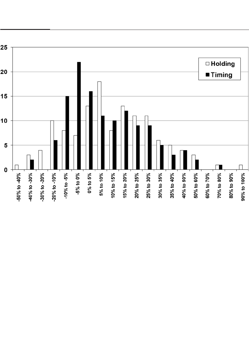
322 PART IV Stock Fluctuations in the Short Run
MOMENTUM INVESTING
Technical analysis can also be used to buy individual stocks. Academic
economists call this momentum investing, and it has received increasing
attention. Momentum strategies, unlike fundamental strategies, rely
purely on past returns, regardless of earnings, dividends, or other valu-
ation criteria. Momentum investors buy stocks that have recently risen
in price and sell stocks that have recently fallen, expecting that the stock
price will, for a time, continue to move in the same direction.
While this may seem at odds with the old maxim of “buy low, sell
high,” there is substantial research to support this “buy-high, sell-
higher” strategy. In 1993, Narasimhan Jegadeesh and Sheridan Titman
found that stocks with the highest 10 percent returns over the past six
months outperformed stocks with the lowest 10 percent returns by
about 1 percent per month over the next six months.13, 14 Other technical
strategies, such as buying stocks priced near their 52-week high, have
also been shown to be successful.15
FIGURE 20–3
Distribution of Annual Gains and Losses: Dow Industrials: Timing Versus Buy-and-Hold Strategy

It should be emphasized that these momentum strategies work
only in the short term and should not be part of a long-term strategy. In
the Jegadeesh and Titman study, more than half of the excess returns
generated in the first 12 months were lost over the following two years.
Over the longer periods, the advantage of buying “winning” stocks is
completely eliminated. In fact, an earlier study by Werner De Bondt and
Richard Thaler found that stocks that performed poorly over the previ-
ous three- to five-year period significantly outperformed, over the next
three to five years, those stocks that had done well, implying a mean
reversion of longer-run stock returns.16
The success of momentum investing cannot be explained within an
efficient market framework. It appears that investors initially underreact
to information, which causes the stock price to continue to respond to
the news over time rather than adjusting instantaneously to the new
information. Unfortunately momentum investing does not guarantee
success: recent evidence suggests that while professional investors
achieve excess returns with a momentum strategy, individual investors
tend to underperform the market. This may be because individual
investors often focus on the very best performing stocks, which tend to
become overpriced quickly and suffer poor returns, while those well-
performing stocks that do not make it to the very top of the list and are
bought by professionals tend to have the best momentum returns.17
CONCLUSION
Proponents claim that technical analysis can identify the major trends of
the market and determine when those trends might reverse. Yet there is
considerable debate about whether such trends exist or whether they are
just runs of good and bad returns that are the result of random price
movements.
Burton Malkiel has been quite clear in his denunciation of technical
analysis. In his bestselling work A Random Walk Down Wall Street, he
proclaims:
Technical rules have been tested exhaustively by using stock price data on
both major exchanges, going back as far as the beginning of the 20th cen-
tury. The results reveal conclusively that past movements in stock prices
cannot be used to foretell future movements. The stock market has no
memory. The central proposition of charting is absolutely false, and
investors who follow its precepts will accomplish nothing but increasing
substantially the brokerage charges they pay.18
CHAPTER 20 Technical Analysis and Investing with the Trend 323

Yet this contention, once supported nearly unanimously by aca-
demic economists, is cracking. Recent econometric research has shown
that such simple trading rules as 200-day moving averages or short-term
price momentum can be used to improve returns.19
Despite the ongoing academic debate, technical analysis has a huge
number of adherents on Wall Street and among many savvy investors.
The analysis in this chapter gives a cautious nod to these strategies, as
long as transaction costs are not high. But as I have noted throughout
this book, actions by investors to take advantage of the past may change
returns in the future. As Benjamin Graham stated so well more than 70
years ago:
A moment’s thought will show that there can be no such thing as a scientific
prediction of economic events under human control. The very “dependabil-
ity” of such a prediction will cause human actions which will invalidate it.
Hence thoughtful chartists admit that continued success is dependent upon
keeping the successful method known to only a few people.20
A final word: Technical analysis requires the full-time attention of
the investor. On October 16, 1987, the Dow fell below its 200-day moving
average at the very end of trading on the Friday before the crash. But if
you failed to sell your stocks that afternoon, you would have been swept
downward by the 22 percent nightmare of Black Monday.
324 PART IV Stock Fluctuations in the Short Run

Calendar Anomalies
October. This is one of the peculiarly dangerous months to speculate
in stocks. The others are July, January, September, April, November,
May, March, June, December, August, and February.
—MARK TWAIN
The dictionary defines anomaly as something inconsistent with what is
naturally expected. And what is more unnatural than to expect to beat
the market by predicting stock prices based solely on the day or week or
month of the year? Yet it appears that you can. Research has revealed
that there are predictable times during which the stock market, and cer-
tain groups of stocks in particular, do particularly well.
The analysis in the first edition of Stocks for the Long Run, published
in 1994, was based on long data series analyzed through the early 1990s.
The calendar anomalies reported in that edition invited investors to out-
perform the market by adopting strategies to these unusual calendar
events. However, as more investors learn of and act on these anomalies,
the prices of stocks may adjust so that much, if not all, of the anomaly is
eliminated. That certainly would be the prediction of the efficient mar-
ket hypothesis.
In this edition of Stocks for the Long Run, I also look at the evidence
since 1994 to determine whether the anomaly survived or not. The results
are surprising. Some anomalies have weakened and even reversed, while
others remain as strong as they have always been. Here is a rundown.
325
21

SEASONAL ANOMALIES
The most important historical calendar anomaly is that small-capitalization
stocks have far outperformed larger stocks in January. This effect is so
strong that without January’s return, small stocks would have a lower
return than large stocks since 1925.1
This outperformance of small stocks in January has been dubbed
the January effect. It was discovered in the early 1980s by Donald Keim,2
based on research he did as a graduate student at the University of
Chicago. It was the first significant finding that flew in the face of the
efficient market hypothesis that claimed there was no predictable pat-
tern to stock prices.
The January effect might be the granddaddy of all calendar anom-
alies, but it is not the only one. Stocks generally do much better in the
first half of the month than the second half, do well before holidays, and
plunge in the month of September. Furthermore, they do exceptionally
well between Christmas and New Year’s Day; and until very recently,
they have soared on the last trading day of December, which is actually
the day that launches the January effect.
THE JANUARY EFFECT
Of all the calendar-related anomalies, the January effect has been the most
publicized. From 1925 through 2012, the average arithmetic return on the
S&P 500 Index in the month of January was 1.00 percent, while the aver-
age returns on the small stocks came to 5.36 percent. The 4.36-percentage-
point excess return of small stocks in January far exceeds the difference in
annual returns between large and small stocks. In other words, from
February through December, the average returns on small stocks have
fallen short of the returns on large stocks. On the basis of history, the only
advantageous time to hold small stocks is the month of January.
To see how important the January effect is, examine Figure 21-1. It
shows the total returns index on large and small stocks and on small
stocks if the January return on small stocks is replaced with that of the
S&P 500 Index in January. A single dollar invested in small stocks in 1926
would grow to $11,480 by the end of 2012, while the same dollar would
grow to only $3,063 in large stocks. Yet if the small stocks’ return in
January is eliminated, the total return to small stocks accumulates to
only $469, less than one-sixth of the cumulative return on large stocks.
Figure 21-1 also shows that if the large January small stock returns
persist in the future, it could lead to some astounding investment
326 PART IV Stock Fluctuations in the Short Run
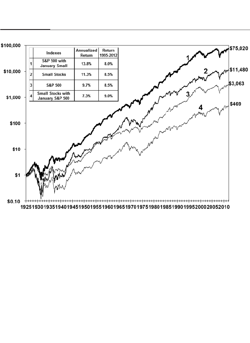
results. By buying small stocks at the end of December and transferring
them back to the S&P 500 Index at the end of January, a $1 investment in
this strategy at the end of 1925 would have grown to $75,020 by the end
of 2012, a striking 13.8 percent annual rate of return.
There have been only 20 years since 1925 when large stocks have
outperformed small stocks in January. Furthermore, when small stocks
underperform large stocks, it is usually not by much: the worst under-
performance was 5.1 percent in January 1929. In contrast, since 1925,
returns on small stocks have exceeded returns on large stocks in January
by at least 5 percent for 28 years, by at least 10 percent for 13 years, and
by over 20 percent for 2 years.
The January effect also prevailed during the most powerful bear
market in our history. From August 1929 through the summer of 1932,
when small stocks lost over 90 percent of their value, small stocks posted
consecutive January monthly returns of plus 13 percent, 21 percent, and
CHAPTER 21 Calendar Anomalies 327
FIGURE 21–1
Small and Large Stocks, With and Without the January Effect, 1926–2012

10 percent in 1930, 1931, and 1932, respectively. It is testimony to the
power of the January effect that investors could have increased their
wealth by 50 percent during the greatest stock crash in history by buying
small stocks at the end of December in those three years and selling
them at the end of the following January, putting their money in cash for
the rest of the year!
A fascinating feature of the January effect is that you do not have to
wait the entire month to see the big returns from small stocks roll in.
Most of the buying in small stocks begins on the last trading day of
December (often in the late afternoon), as some investors pick up the
bargain stocks that are dumped by others on New Year’s Eve. Strong
gains in small stocks continue on the first trading day of January and
with declining force through the first week of trading. On the basis of
research published in 1989, on the first trading day of January alone,
small stocks earned nearly 4 percentage points more than large stocks.3
By the middle of the month, the January effect is largely exhausted.
When any anomaly such as the January effect is found, it is impor-
tant to examine its international reach. When researchers turned to for-
eign markets, they found that the January effect was not just a U.S.
phenomenon. In Japan, the world’s second-largest capital market, the
excess returns on small stocks in January came to 7.2 percent per year,
more than in the United States.4As you shall see later in the chapter,
January is the best month for both large and small stocks in many other
countries of the world.5
How could such a phenomenon go unnoticed for so long by
investors, portfolio managers, and financial economists? Because in the
United States, the returns in January are nothing special for large stocks
that form the bulk of those indexes that are analyzed. That’s not to say
that January is not a good month for large stocks, as large stocks do quite
well in January, particularly in foreign markets. But in the United States,
January is by no means the best month for stocks of large firms.
Causes of the January Effect
Why have investors favored small stocks in January? No one knows for
sure, but there are several hypotheses. In contrast to institutions, indi-
vidual investors hold a disproportionate amount of small stocks, and
they are more sensitive to the tax consequences of their trading. Small
stocks, especially those that have declined in the preceding 11 months,
are subject to tax-motivated selling in December. This selling depresses
328 PART IV Stock Fluctuations in the Short Run

the price of individual issues. In January after the selling ends, these
stocks bounce back in price.
There is some evidence to support this explanation. Stocks that have
fallen throughout the year fall even more in December and then often rise
dramatically in January. Furthermore, there is some evidence that before
the introduction of the U.S. income tax in 1913, there was no January
effect. And in Australia, where the tax year runs from July 1 through June
30, there are abnormally large returns to small stocks in July.
If taxes are a factor, however, they cannot be the only one, for the
January effect holds in countries that do not have a capital gains tax.
Japan did not tax capital gains for individual investors until 1989, but the
January effect existed prior to that date. Furthermore, capital gains were
not taxed in Canada before 1972, and yet there was a January effect in that
country as well. Finally, stocks that have risen throughout the previous
year and should not be subject to tax-loss selling still rise in January,
although not by as much as stocks that have fallen the previous year.
There are other potential explanations for the January effect.
Workers often receive extra income, such as from bonuses and other
forms of compensation, at year-end. These individuals often invest their
cash in stocks in the first week of January. Data show that there is a sharp
increase in the ratio of public buy orders to public sell orders around the
turn of the year. Since the public holds a large fraction of small stocks,
this could be an important clue to understanding the January effect.6
Although all these explanations appear quite reasonable, none jibes
with what is called an “efficient capital market.” If money managers
know that small stocks will surge in January, these stocks should be
bought well before New Year’s Day to capture these spectacular returns.
That would cause the price of small stocks to rise in December, which
would prompt other managers to buy them in November, and so on. In
the process of acting on the January effect, the price of stocks would be
smoothed out over the year, and the phenomenon would disappear.
The January Effect Weakened in Recent Years
Perhaps all the publicity about the January effect has motivated
investors and traders to take advantage of this calendar anomaly, since
the effect has largely disappeared since 1994. From 1995 through
January 2012, the average January return on the Russell 2000 Index of
small stocks has been 1.36 percent, only slightly more than the 0.70 per-
cent return on the S&P 500 Index. Furthermore, the return on the Russell
CHAPTER 21 Calendar Anomalies 329

2000 on the last trading day of December and the first trading day of
January, which had previously been so high, has been no higher than
that of the S&P 500 Index, and both have been approximately zero.
Finally, the excess return on small stocks during the first seven trading
days in January, which had been so large before 1995, has also vanished.
LARGE STOCK MONTHLY RETURNS
Other seasonal patterns are associated with stock returns besides the
January effect. The monthly returns on the Dow Industrials and S&P 500
Index are displayed in Figure 21-2. November and December have been
good months, and according to recent data, they continue to be. But
January’s return, formerly one of the best, has faltered in recent years.
April has also been an excellent month, but except for July, the rest of the
summer through early fall has returns well below normal. The expres-
sion “Sell in May and go away” certainly has some empirical justifica-
tion. Since World War II, there has been no evidence of the “summer
rally” that used to be much trumpeted by brokers and investment advi-
sors in the 1950s and 1960s.
These monthly patterns of returns have a worldwide reach. January
historically has been an excellent month in foreign countries. The
January returns for the 20 countries covered by the Morgan Stanley
Capital Market Index, shown in Figure 21-3, have all exceeded the aver-
age return.
In every country, January returns are greater than average, and on
average the January return more than doubles the return for the other
11 months. But January has lost its magic abroad, as it has in the United
States. Since 1994, January returns have actually been negative and
have fallen short of the yearly average in 14 countries, including the
United States.
THE SEPTEMBER EFFECT
While July has good returns, watch out for the rest of the summer, espe-
cially September. September is by far the worst month of the year, and in
the United States, it is the only month to have a negative return includ-
ing reinvested dividends. September is followed closely by October,
which, as Chapter 19 indicated already, has a disproportionate percent-
age of crashes.
Figure 21-4 tracks the Dow Jones Industrial Averages from 1885
through 2012, both including and excluding the month of September. An
330 PART IV Stock Fluctuations in the Short Run
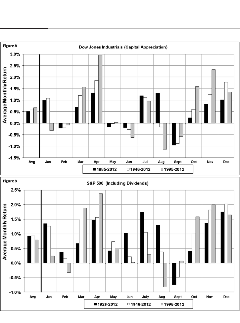
CHAPTER 21 Calendar Anomalies 331
FIGURE 21–2
Monthly Returns on Dow Jones Industrials and S&P 500
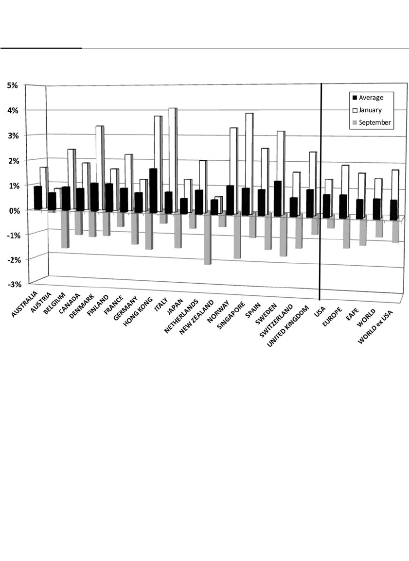
investment of $1 in the Dow Jones Average in 1885 would be worth $511 by
the end of 2012 (dividends excluded). In contrast, $1 invested in the Dow
only in the month of September would be worth only 23 cents! On the
other hand, if you put your money in the stock market every month except
September, your dollar would have been worth $2,201 at the end of 2012.
The poor returns in September also prevail in the rest of the world.
It is amazing that September is the only month of the year that has neg-
ative returns in a value-weighted index. That means that in September
investors would do better holding zero-interest currency than putting
their assets in the stock market. September has had negative returns in
all 20 of the countries covered by the Morgan Stanley developed market
indexes, as well as the major world indexes, including the EAFE Index
and the Morgan Stanley all-world index.
In contrast to the January effect, which has largely disappeared
in recent data, the September effect is still running full steam ahead,
332 PART IV Stock Fluctuations in the Short Run
FIGURE 21–3
International January and September Effects, 1970–2012
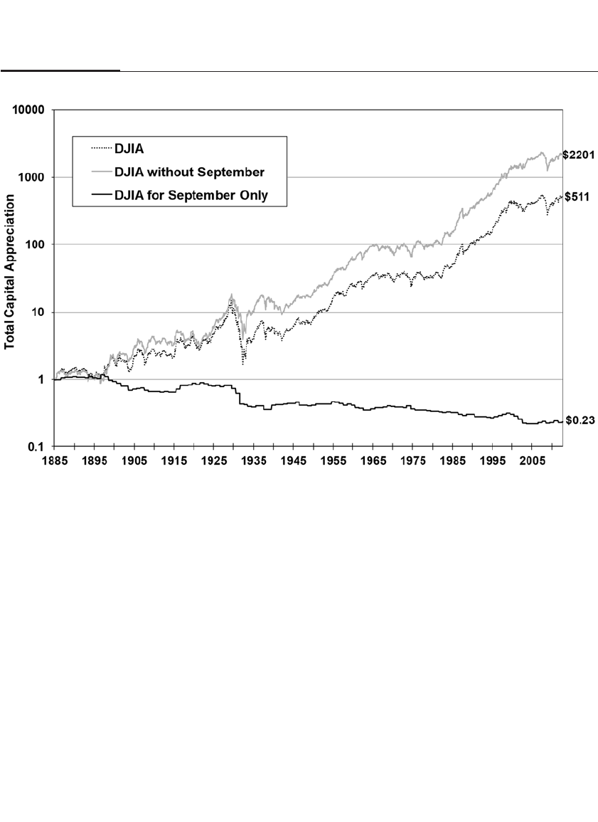
although in the United States much of the market’s decline has now
been brought forward into August since the first edition of Stocks for the
Long Run was published. In fact, since 1995, September returns, meas-
ured by the S&P 500 index, have become slightly positive in the United
States, but September returns have remained negative in 17 of the other
19 developed countries.
We can only speculate on why returns are so poor in September.
Maybe the poor returns are related to the approach of winter and the
depressing effect of rapidly shortening daylight. Psychologists stress that
sunlight is an essential ingredient to well-being: recent research has con-
firmed that the New York Stock Exchange does significantly worse on
cloudy days than it does on sunny days.7But this explanation falters
“down under,” as September is also a poor month in Australia and New
Zealand, where the month marks the beginning of spring and longer days.8
Perhaps the poor returns in September are the result of investors’
liquidating stocks (or holding off buying more stocks) to pay for their
summer vacations. As discussed below, until recently Monday was by far
CHAPTER 21 Calendar Anomalies 333
FIGURE 21–4
The September Effect: Dow-Jones Industrial Average, 1885–2012

334 PART IV Stock Fluctuations in the Short Run
the worst-performing day of the week. For many, September is the
monthly version of Monday, the time you face work after a period of
leisure. But even the September effect may in the future succumb to the
efficient market. As noted above, investors in the United States are begin-
ning to sell stocks earlier, dropping August to the worst-performing
month since 1995.
OTHER SEASONAL RETURNS
Although psychologists say that many silently suffer depression around
Christmas and New Year’s, stock investors believe ’tis the season to be
jolly. Table 21-1 displays the daily price returns, as measured by the Dow
Jones Industrial Average, for various times in the year and in the month.
TABLE 21–1
Dow-Jones Industrial Average Daily Price Returns 1885–2012
1885–2012 1885–1925 1926–1945 1946–1989 1946–2012 1995–2012
Overall Averages
Whole month 0.0233% 0.0192% 0.0147% 0.0273% 0.0293% 0.0342%
First half of month 0.0402% 0.0203% 0.0621% 0.0500% 0.0465% 0.0365%
Second half of month 0.0062% 0.0182% –0.0316% 0.0040% 0.0112% 0.0316%
Last day of month 0.0926% 0.0875% 0.1633% 0.1460% 0.0746% –0.0923%
Days of the Week
Monday –0.0902% –0.0874% –0.2106% –0.1313% –0.0558% 0.0741%
Tuesday 0.0415% 0.0375% 0.0473% 0.0307% 0.0422% 0.0870%
Wednesday 0.0566% 0.0280% 0.0814% 0.0909% 0.0665% 0.0092%
Thursday 0.0246% 0.0012% 0.0627% 0.0398% 0.0274% 0.0091%
Friday 0.0630% 0.0994% 0.0064% 0.0942% 0.0577% –0.0063%
With Sat 0.0539% 0.0858% –0.0169% 0.0747% NA NA
Without Sat 0.0714% 0.3827% 0.3485% 0.0961% 0.0566% –0.0063%
Saturday 0.0578% 0.0348% 0.0964% 0.0962% NA NA
Holiday Returns
Day before holiday
July 4th 0.2989% 0.2118% 0.8168% 0.2746% 0.1976% 0.1598%
Christmas 0.3544% 0.4523% 0.3634% 0.3110% 0.2918% 0.2582%
New Year's 0.2964% 0.5964% 0.3931% 0.2446% 0.0840% –0.2394%
Holiday avg 0.3165% 0.4201% 0.5244% 0.2767% 0.1911% 0.0595%
Christmas week 0.2247% 0.3242% 0.2875% 0.1661% 0.1331% 0.0425%
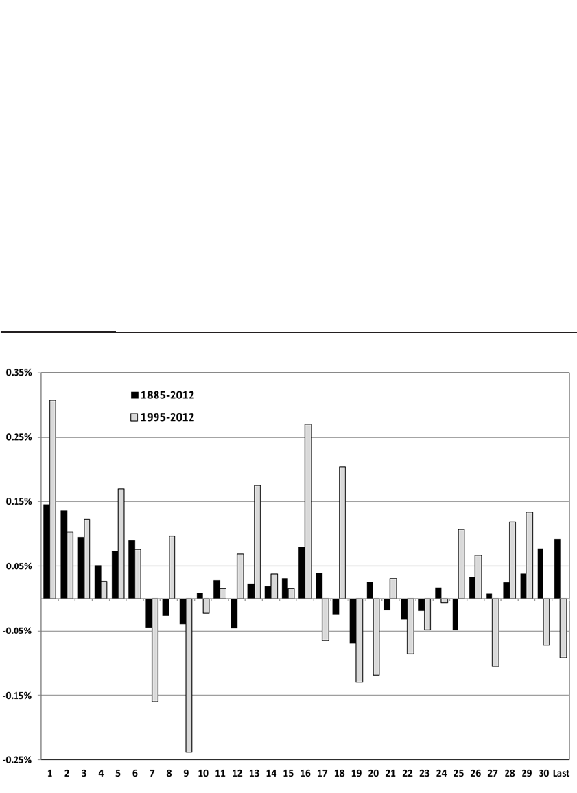
Over the past 127 years, daily price returns, between Christmas and
New Year’s, have averaged nearly 10 times the average return.
Even more striking is the difference between stock returns in the
first and second half of the month.9Over the entire 127-year period stud-
ied, the percentage change in the Dow Jones Industrial Average during
the first half of the month—which includes the last trading day of the
previous month up to and including the fourteenth day of the current
month—is almost seven times the gain that occurs during the second
half.10 The average percentage changes in the Dow Jones Industrial
Average over every calendar day of the month are shown in Figure 21-5.
Over the whole period it is striking how the average percentage
gain on the last trading day of the month (and the thirtieth calendar day,
when that is not the last trading day) and the first six calendar days is
CHAPTER 21 Calendar Anomalies 335
FIGURE 21–5
Daily Price Returns on the Dow Industrial Average, 1885–2012

more than equal to the entire return for the month! The net change in the
Dow Industrials is negative for all the other days.
But this pattern has changed somewhat in recent years. Although
the gains on the first six days of the month have actually become greater,
the change on the last day of the month has turned sharply negative,
while the first day of the month is even more positive.
The strong gains at the beginning of the month are likely related to
the inflow of funds into the equity market from workers who automati-
cally have part of their pay invested directly into the market on the first
day of the month. One notices another gain on the sixteenth of the
month, where workers who are paid twice per month put funds into
stocks. Yet since 1995, the return in the first half of the month now only
slightly exceeds that of the second half.
DAY-OF-THE-WEEK EFFECTS
Many people hate Mondays. After two days of relaxing and doing pretty
much what you like, having to face work on Monday is a drag. And
stock investors apparently feel the same way. Monday has been by far
the worst day of the week for the market. Over the past 127 years, the
returns on Monday have been decisively negative—so negative that if
Monday returns were instead like Tuesday through Friday, the historical
real return on the stocks would exceed 13 percent per year, nearly dou-
ble the historical average!
Although investors hate Mondays, they have relished Fridays.
Friday has been the best day of the week, yielding price returns about
three times the daily average. Even when markets were open on
Saturday (every month before 1946 and nonsummer months before
1953), Friday price returns were the best.
But these daily patterns have changed dramatically in recent years.
Since 1995, Monday has gone from the worst to second best, just trailing
Tuesday. And Friday has not only gone from the best to the worst day
but has actually recorded negative average returns. One reason for this
change is that many stock traders like to hedge their equity positions
over the weekend and sell their long positions at or near Friday’s close.
Friday’s negative returns might also be caused by traders who, having
learned that Monday is usually a bad day, sell on Friday. Traders then
reestablish their stock positions on Monday, causing returns on those
days to increase. Whatever the reasons, the change demonstrates that
well-publicized anomalies are often arbitraged out of the market.
336 PART IV Stock Fluctuations in the Short Run

Another calendar anomaly is that stocks do very well before major
holidays, as shown in Table 21-1. Price returns before the Fourth of July,
Christmas, and New Year’s Eve are, on average, almost 14 times the aver-
age daily price return. But some of these anomalies, like the day-of-the-
week effect, have changed in recent years. Although stock returns on the
day before July Fourth and Christmas have remained strong, returns on
the last day of the trading year have switched from a strongly positive
0.30 percent to a decisively negative 0.24 percent since 1994. The negative
returns on the last trading day in recent years are probably caused by a
large number of “sell-on-close” orders that are automatically executed to
offset positions in stock index futures, ETFs, and other customized hedge
instruments. The downward movement of stock prices generally occurs
in the last 30 minutes of trading. Of course, it is possible that once this
pattern becomes widely known, it too will disappear.
Finally, there appears to be a diurnal pattern of stock returns.
Evidence has shown that there is usually a sinking spell in the morning,
especially on Monday. During lunch the market firms, then pauses or
declines in the midafternoon before rising strongly in the last half hour of
trading. This often leads the market to close at the highest levels of the day.
WHAT’S AN INVESTOR TO DO?
These anomalies are an extremely tempting guide to formulating an
investing strategy. But these calendar-related returns do not always
occur, and as investors become more aware of them, some have moder-
ated while others have disappeared altogether. The famous January
effect has been mostly absent over the past two decades. Still other
anomalies have completely reversed, such as the returns of stocks on the
last trading day of the year and the returns on Mondays and Fridays. But
some, such as the large returns early in the month and the poor returns
in September, remain.
Trying to take advantage of these anomalies requires the buying
and selling of stock, which incurs transaction costs and (unless you are
trading within tax-sheltered funds) may realize capital gains taxes.
Nevertheless, investors who have already decided to buy or sell, but
have some latitude in choosing the timing of such a transaction, might
wish to take these calendar anomalies into account before making their
trades.
CHAPTER 21 Calendar Anomalies 337
This page intentionally left blank

Behavioral Finance and the
Psychology of Investing
The rational man—like the Loch Ness monster—is sighted often, but
photographed rarely.
—DAVID DREMAN, 19981
The market is most dangerous when it looks best; it is most inviting
when it looks worst.
—FRANK J. WILLIAMS, 19302
This book is filled with data, figures, and charts that support an interna-
tionally diversified, long-term strategy for stock investors. Yet advice is
much easier to take in theory than to put in practice. The finance profes-
sion is increasingly aware that psychological factors can thwart rational
analysis and prevent investors from achieving the best results. The
study of these psychological factors has burgeoned into the field of
behavioral finance.
This chapter is written as a narrative to make it easier to under-
stand the basic research and issues of behavioral finance. Dave is an
investor who falls into psychological traps that prevent him from being
effective. You may notice similarities between his behavior and your
own. If so, the advice given in this chapter should help you become a
more successful investor. Dave first talks to his wife, Jennifer, and then
to an investment counselor who understands behavioral finance. The
339
22

narrative begins in the fall of 1999, several months prior to the peak in
the technology and Internet bubble that dominated markets at the turn
of the century.
THE TECHNOLOGY BUBBLE, 1999 TO 2001
TIME: OCTOBER 1999
Dave: Jen, I’ve made some important investment decisions. Our portfo-
lio contains nothing but these “old fogy” stocks like Philip Morris,
Procter & Gamble, and Exxon. These stocks just aren’t doing anything
right now. My friends Bob and Paul at work have been making a fortune
in Internet stocks. I talked with my broker, Allan, about the prospects of
these stocks. He said the experts think the Internet is the wave of the
future. I’m selling some of our stocks that just aren’t moving, and then
I’m getting into the Internet stocks like AOL, Yahoo!, and Inktomi.
Jennifer: I’ve heard that those stocks are very speculative. Are you sure
you know what you’re doing?
Dave: Allan says that we are entering a “New Economy,” spurred by a
communications revolution that is going to completely change the way
we do business. Those stocks that we owned are Old Economy stocks.
They had their day, but we should be investing for the future. I know
these Internet stocks are volatile, and I’ll watch them very carefully so
we won’t lose money. Trust me. I think we’re finally on the right track.
TIME: MARCH 2000
Dave: Jen, have you seen our latest financial statements? We’re up 60
percent since October. The Nasdaq crossed 5,000, and no one I’ve heard
believes it will stop there. The excitement about the market is spreading,
and it has become the topic of conversation around the office.
Jen: You seem to be trading in and out of stocks a lot more than you did
before. I can’t follow what we own!
Dave: Information is hitting the market faster and faster. I have to con-
tinually adjust my portfolio. Commissions are now so cheap that it pays
to trade on any news affecting stocks. Trust me—look how well we’re
doing.
TIME: JULY 2000
Jen: Dave, I’ve looked at our broker’s statement. We don’t hold those
Internet stocks any more. Now we own (she reads from the statement)
340 PART IV Stock Fluctuations in the Short Run

Cisco, EMC, Oracle, Sun Microsystems, Nortel Networks, JDS Uniphase.
I don’t know what any of these companies do. Do you?
Dave: When the Internet stocks crashed in April, I sold out right before
we lost all our gains. Unfortunately, we didn’t make much on those
stocks, but we didn’t lose either.
I know we’re on the right track now. Those Internet companies
weren’t making any money. All the new firms we now own form the back-
bone of the Internet, and all are profitable. Allan told me an important
principle: Do you know who made the most money in the California gold
rush of the 1850s? Not the gold miners. Some of the early diggers found
gold, but most found nothing. The real winners from the gold rush were
those who sold supplies to the miners—pickaxes, boots, pans, and hiking
gear. The lesson is very clear; most of the Internet companies are going to
fail, but those supplying the backbone of the Internet—those supplying
the routers, software, and fiber-optic cables—will be the big winners.
Jen: But I think I heard some economist say those companies are way
overpriced now; they’re selling for hundreds of times earnings.
Dave: Yes, but look at their growth over the last five years—no one has
ever seen this before. The economy is changing, and many of the tradi-
tional yardsticks of valuation don’t apply. Trust me; I’ll monitor these
stocks. I got us out of those Internet stocks in time, didn’t I?
TIME: NOVEMBER 2000
Dave (to himself): What should I do? The last few months have been
dreadful. I’m down about 20 percent. Just over two months ago, Nortel
was over 80. Now it is around 40. Sun Microsystems was 65, and now it
is around 40. These prices are so cheap. I think I’ll use some of my
remaining cash to buy more shares at these lower prices. Then my stocks
don’t have to go up as much for me to get even.
TIME: AUGUST 2001
Jen: Dave, I’ve just looked at our brokerage statement. We’ve been dev-
astated! Almost three-quarters of our retirement money is gone. I
thought you were going to monitor our investments closely. Our portfo-
lio shows nothing but huge losses.
Dave: I know; I feel terrible. All the experts said these stocks would
rebound, but they kept going down.
Jen: This has happened before. I don’t understand why you do so badly.
For years you watch the market closely, study all these financial reports,
CHAPTER 22 Behavioral Finance and the Psychology of Investing 341

and seem to be very well informed. Yet you still make the wrong deci-
sions. You buy near the highs and sell near the lows. You hold on to los-
ers while selling your winners. You . . .
Dave: I know, I know. My stock investments always go wrong. I think
I’m giving up on stocks and sticking with bonds.
Jen: Listen, Dave. I have talked to a few other people about your invest-
ing troubles, and I want you to go see an investment counselor.
Investment counselors use behavioral psychology to help investors
understand why they do poorly. An investment counselor will help you
correct this behavior. Dave, I made you an appointment already. Please
go see him.
BEHAVIORAL FINANCE
TIME: NEXT WEEK
Dave was skeptical. He thought that understanding stocks required
knowledge of economics, accounting, and mathematics. Dave never
heard the word psychology used in any of those subjects. Yet he knew he
needed help, and it couldn’t hurt to check it out.
Investment Counselor (IC): I have read your profile and talked to your
wife extensively. You are very typical of the investor that we counsel
here. I adhere to a new branch of economics called behavioral finance.
Many of the ideas my profession explores are based on psychological
concepts that have rarely before been applied to the stock market and
portfolio management.
Let me give you some background. Until recently, finance was
dominated by theories that assumed investors maximized their
expected utility, or well-being, and always acted rationally. This was an
extension of the rational theory of consumer choice under certainty
applied to uncertain outcomes.
In the 1970s two psychologists, Daniel Kahneman and Amos
Tversky, noted that many individuals did not behave as this theory pre-
dicted. Kahneman and Tversky developed a new model—called
prospect theory—of how individuals actually behave and make deci-
sions when faced with uncertainty.3Their model established them as the
pioneers of behavioral finance, and their research has been making
much headway in the finance profession.
342 PART IV Stock Fluctuations in the Short Run

Fads, Social Dynamics, and Stock Bubbles
IC: Let us first discuss your decision to get into the Internet stocks. Think
back to October 1999. Do you remember why you decided to buy those
stocks?
Dave: Yes. My stocks were simply not going anywhere. My friends at
work were investing in the Internet and making a lot of money. There
was so much excitement about these stocks; everyone claimed that the
Internet was a communications revolution that would change business
forever.
IC: When everyone is excited about the market, you should be extremely
cautious. Stock prices are not based just on economic values but on psy-
chological factors that influence the market. Yale economist Robert
Shiller, one of the leaders of the behavioral finance movement, has
emphasized that fads and social dynamics play a large role in the deter-
mination of asset prices.4Shiller showed that stock prices have been far
too volatile to be explained by fluctuations in economic factors, such as
dividends or earnings.5He has hypothesized that much of the extra
volatility can be explained by fads and fashions that have a large impact
on investor decisions.
Dave: I did have my doubts about these Internet stocks, but everyone
else seemed so sure they were winners.
IC: Note how others influenced your decision against your better judg-
ment. Psychologists have long known how hard it is to remain separate
from a crowd. This was confirmed by a social psychologist named
Solomon Asch. He conducted a famous experiment where subjects were
presented with four lines and asked to pick the two that were the same
length. The right answer was obvious, but when confederates of Dr. Asch
presented conflicting views, the subjects often gave the incorrect answer.6
Follow-up experiments confirmed that it was not social pressure
that led the subjects to act against their own best judgment but their dis-
belief that a large group of people could be wrong.7
Dave: Exactly. So many people were hyping these stocks that I felt there
had to be something there. If I didn’t buy the Internet stocks, I thought
that I was missing out.
IC: I know. The Internet/technology bubble is a perfect example of
social pressures influencing stock prices. The conversations around the
office, the newspaper headlines, and the analysts’ predictions—they all
CHAPTER 22 Behavioral Finance and the Psychology of Investing 343

fed the craze to invest in these stocks. Psychologists call this penchant to
follow the crowd the herding instinct—the tendency of individuals to
adapt their thinking to the prevailing opinion.
The Internet bubble has many precedents. In 1852, Charles Mackay
wrote the classic Extraordinary Delusions and the Madness of Crowds,
which chronicled a number of financial bubbles during which specula-
tors were driven into a frenzy by the upward movement of prices: the
South Sea bubble in England and the Mississippi bubble in France
around 1720 and the tulip mania in Holland a century earlier.8Let me
read you my favorite passage from the book. See if you can relate to this:
We find that whole communities suddenly fix their minds upon one sub-
ject, and go mad in its pursuit; that millions of people become simultane-
ously impressed with one delusion and run after it. . . . Sober nations have
all at once become desperate gamblers, and risked most of their existence
upon the turn of a piece of paper. . . . Men, it has been well said, think in
herds. . . . They go mad in herds, while they only recover their senses
slowly and one by one.
Dave (shaking his head): This happens again and again through history.
Even though others were pointing to those very same excesses last year,
I was convinced that “this time is different.”
IC: As were many others. The propensity of investors to follow the
crowd is a permanent fixture of financial history. There are many times
when the “crowd” is right,9but often following the crowd can lead you
astray.
Dave, have you ever been in a new town and found yourself choos-
ing between two restaurants? One perfectly rational way of deciding, if
they are close in distance, is to see which restaurant is busier since
there’s a good chance that at least some of those patrons have tried both
restaurants and have chosen to eat at the better one. But when you eat at
the busier restaurant, you are increasing the chance that the next diner,
using the same reasoning, will also eat there, and so on. Eventually,
everybody will be eating at that one restaurant even though the other
one could be much better.
Economists call this decision-making process an information cascade,
and they believe that it happens often in financial markets.10 For exam-
ple, when one company bids for another, often other suitors will join in.
When an IPO gets a strong following, other investors join in. Individuals
have a feeling that “someone knows something” and that they shouldn’t
miss out. Sometimes that’s right, but very often that is wrong.
344 PART IV Stock Fluctuations in the Short Run

Excessive Trading, Overconfidence, and the Representative Bias
IC: Dave, let me shift the subject. From examining your trading records,
I see that you were an extremely active trader.
Dave: I had to be. Information was constantly bombarding the market; I
felt I had to reposition my portfolio constantly to reflect the new infor-
mation.
IC: Let me tell you something. Trading does nothing but cause extra anx-
iety and lower returns. A couple of economists published an article in
2000 called “Trading Is Hazardous to Your Wealth.” (And, I may add, to
your health also.) Examining the records of tens of thousands of traders,
they showed that the returns of the heaviest traders were 7.1 percent
below the returns of those who traded infrequently.11
Dave: You’re right. I think trading has hurt my returns. I thought that I
was one step ahead of the other guy, but I guess I wasn’t.
IC: It is extraordinarily difficult to be a successful trader. Even bright
people who devote their entire energies to trading stocks rarely make
superior returns. The problem is that most people are simply overconfi-
dent in their own abilities. To put it another way, the average individ-
ual—whether a student, a trader, a driver, or anything else—believes he
or she is better than average, which of course is statistically impossible.12
Dave: What causes this overconfidence?
IC: Overconfidence comes from several sources. First, there is what we
call a self-attribution bias that causes one to take credit for a favorable turn
of events when credit is not due.13
Dave: Does this ever ring true! I remember in March 2000 bragging to
my wife about how smart I was to have bought those Internet stocks.
And was I wrong!
IC: Your early success fed your overconfidence.14 You and your friends
attributed your stock gains to skillful investing, even though those out-
comes were frequently the result of chance.
Another source of overconfidence comes from the tendency to see
too many parallels between events that seem the same.15 This is called
the representative bias. This bias actually arises because of the human
learning process. When we see something that looks familiar, we form a
representative heuristic to help us learn. But the parallels we see are
often not valid, and our conclusions are misguided.
Dave: The investment newsletters I get say that every time such-and-
such event has occurred in the past, the market has moved in a certain
CHAPTER 22 Behavioral Finance and the Psychology of Investing 345

direction, implying that it is bound to do so again. But when I try to use
that advice, it never works.
IC: Conventional finance economists have been warning for years about
finding patterns in the data when, in fact, there are none. Searching past
data for patterns is called “data mining,” and it is easier than ever to do,
with computing power becoming so cheap.16 Throw in a load of vari-
ables to explain stock price movements, and you are sure to find some
spectacular fits—like over the past 100 years stocks have risen on every
third Thursday of the month when the moon is full!
The representative bias has been responsible for some spectacularly
wrong moves in the stock market, even when the situations seem
remarkably similar. When World War I broke out in July 1914, officials at
the New York Stock Exchange thought it was such a calamity, that the
exchange closed down for five months. Wrong! The United States
became the arms merchant for Europe; business boomed, and 1915 was
one of the single best years in stock market history.
When Germany invaded Poland in September 1939, investors
looked at the behavior of the market when World War I broke out.
Noting the fantastic returns, they bought stocks like mad and sent the
market up by more than 7 percent on the next day’s trading! But this was
wrong again. FDR was determined not to let the corporations prosper
from World War II as they had from World War I. After a few more up
days, the stock market headed into a severe bear market, and it wasn’t
until nearly six years later that the market returned to its September 1939
level. Clearly, the representative bias was the culprit for this error, and
the two events weren’t as similar as people thought.
Psychologically, human beings are not designed to accept all the
randomness that is out there.17 It is very discomforting to learn that most
movements in the market are random and do not have any identifiable
cause or reason. Individuals possess a deep psychological need to know
why something happens. That is where the reporters and “experts”
come in. They are more than happy to fill the holes in our knowledge
with explanations that are wrong more often than not.
Dave: I can relate personally to this bias. I remember that before I
bought the technology stocks in July 2000, my broker compared these
companies to the suppliers providing the gear for the gold rushers of
the 1850s. It seemed like an insightful comparison at the time, but in fact
the situations were very different. It is interesting that my broker, who
is supposed to be the expert, is subject to the same overconfidence that
I am.
346 PART IV Stock Fluctuations in the Short Run

IC: There is actually evidence that experts are even more subject to over-
confidence than the nonexperts. The so-called experts have been trained
to analyze the world in a particular way, and they sell their advice based
on finding supporting—not contradictory—evidence.18
Recall the failure of analysts in 2000 to change their earnings fore-
casts for the technology sector despite the news that suggested that
something was seriously wrong with their view of the whole industry.
After being fed an upbeat outlook by corporations for many years, ana-
lysts had no idea how to interpret the downbeat news, so most just
ignored it.
The propensity to shut out bad news was even more pronounced
among analysts in the Internet sector. Many were so convinced that
these stocks were the wave of the future that, despite the flood of ghastly
news, many downgraded these stocks only after they had fallen 80 or 90
percent!
Confronting news that does not correspond to one’s worldview cre-
ates what is called cognitive dissonance. Cognitive dissonance is the dis-
comfort we encounter when we address evidence that conflicts with our
view or suggests that our abilities or actions are not as a good as we
thought. We all display a natural tendency to minimize this discomfort,
which makes it difficult for us to recognize our overconfidence.
Prospect Theory, Loss Aversion, and the Decision
to Hold on to Losing Trades
Dave: I see. Can we talk about individual stocks? Why do I end up hold-
ing so many losers in my portfolio?
IC: Remember I said before that Kahneman and Tversky had kicked off
behavioral finance with prospect theory? A key concept in their theory
was that individuals form a reference point from which they judge their
performance. Kahneman and Tversky found that from that reference
point individuals are much more upset about losing a given amount of
money than about gaining the same amount. The researchers called this
behavior loss aversion, and they suggested that the decision to hold or
sell an investment will be dramatically influenced by whether your
stock has gone up or down—in other words, whether you have had a
gain or loss.
Dave: One step at a time. What is this “reference point” you talk about?
IC: Let me ask you a question. When you buy a stock, how do you track
its performance?
CHAPTER 22 Behavioral Finance and the Psychology of Investing 347

Dave: I calculate how much the stock has gone up or down since I
bought it.
IC: Exactly. Often the reference point is the purchase price that investors
pay for the stock. Investors become fixated on this reference point to the
exclusion of any other information. Richard Thaler from the University
of Chicago, who has done seminal work in investor behavior, refers to
this as mental accounting or narrow framing.19
When you buy a stock, you open a mental account, with the pur-
chase price as the reference point. Similarly, when you buy a group of
stocks together, either you will think of the stocks individually, or you
may aggregate the accounts together.20 Whether your stocks are showing
a gain or loss will influence your decision to hold or sell the stock.
Moreover, in accounts with multiple losses, you are likely to aggregate
individual losses together because thinking about one big loss is an eas-
ier pill for you to swallow than thinking of many smaller losses.
Avoiding the realization of losses becomes the primary goal of many
investors.
Dave: You’re right. The thought of realizing those losses on my technol-
ogy stocks petrified me.
IC: That is a completely natural reaction. Your pride is one of the main
reasons why you avoided selling at a loss. Every investment involves an
emotional as well as financial commitment that makes it hard to evalu-
ate objectively. You felt good that you sold out of your Internet stocks
with a small gain, but the networking stocks you subsequently bought
never showed a gain. Even as prospects dimmed, you not only hung on
to those stocks but bought more, hoping against hope that they would
recover.
Prospect theory predicts that many investors will do as you did—
increase your position, and consequently your risk, in an attempt to get
even.21 Interestingly, researchers have found that individuals do sell
mutual funds that have lost money, and chase those that record gains.
But behavioral finance also has a good explanation for that. With funds,
investors can always blame the fund manager for picking bad stocks,
which you can’t do if you make your own decisions about which stock
to buy.22
Dave: I never bought any mutual funds, so I only had myself to blame
for my losses. I thought that buying more shares when the price sank
would increase my chances of recouping my losses when the price went
back up.
348 PART IV Stock Fluctuations in the Short Run

IC: You and millions of other investors. In 1982, Leroy Gross wrote a
manual for stockbrokers in which he called this phenomenon the “get-
even-itis disease.”23 He claimed get-even-itis has probably caused more
destruction to portfolios than any other mistake.
It is hard for us to admit we’ve made a bad investment, and it is
even harder for us to admit that mistake to others. But to be a successful
investor, you have no choice but to do so. Decisions on your portfolio
must be made on a forward-looking basis. What has happened in the
past cannot be changed. It is a “sunk cost,” as economists say. When
prospects don’t look good, sell the stock whether or not you have a loss.
Dave: I thought the stocks were cheap when I bought more shares.
Many were down 50 percent or more from their highs.
IC: Cheap relative to what? Cheap relative to their past price or their
future prospects? You thought that a price of 40 for a stock that had been
80 made the stock cheap; what you never considered is the possibility
that 40 was still too high. This demonstrates another one of Kahneman
and Tversky’s behavioral findings: anchoring, or the tendency of people
facing complex decisions to use an “anchor” or a suggested number to
form their judgment.24 Figuring out the “correct” stock price is such a
complex task that it is natural to use the recently remembered stock price
as an anchor and then judge the current price a bargain.
Dave: If I follow your advice and sell my losers whenever prospects are
dim, I’m going to register a lot more losses on my trades.
IC: Good! Most investors do exactly the opposite, to their detriment.
Research has shown that investors sell stocks for a gain 50 percent more
frequently than they sell stocks for a loss.25 This means that stocks that
are above their purchase price are 50 percent more likely to be sold than
stocks that show a loss. Traders do this even though it is a bad strategy
from a trading standpoint and a tax standpoint.
Let me tell you of one short-term trader I successfully counseled.
He showed me that 80 percent of his trades made money, but he was
down overall since he had lost so much money on his losing trades that
they drowned out his winners.
After I counseled him, he became a successful trader. Now he says
that only one-third of his trades make money, but overall he’s way
ahead. When things don’t work out as he planned, he gets rid of losing
trades quickly while holding on to his winners. There is an old adage on
Wall Street that sums up successful trading: “Cut your losers short and
let your winners ride.”
CHAPTER 22 Behavioral Finance and the Psychology of Investing 349

Rules for Avoiding Behavioral Traps
Dave: I don’t feel secure enough to trade again soon. I just want to learn
the right long-term strategy. How can I get over these behavioral traps
and be a successful long-term investor?
IC: Dave, I’m glad you are not trading, since trading is right for only a
very small fraction of my clients.
To be a successful long-term investor, you must set up rules and
incentives to keep your investments on track—this is called precommit-
ment.26 Set an asset allocation rule and then stick to it. If you have enough
knowledge, you can do this yourself, or else you can do it with an invest-
ment advisor. Don’t try to second-guess your rule. Remember that the
basic factors generating returns change far less than we think as we
watch the day-to-day ups and downs of the market. A disciplined
investment strategy is almost always a winning strategy.
If you wish, you don’t have to eliminate your trading altogether. If
you do buy stocks for a short-term trade, establish an absolute selling
point to minimize your losses. You don’t want to let your losses mount,
rationalizing that the stock will eventually come back. Also, don’t tell
your friends about your trades. Living up to their expectations will
make you even more reluctant to take a loss and admit that you were
wrong.
Dave: I have to admit that I often enjoyed trading.
IC: If you really enjoy trading, set up a small trading account that is com-
pletely separate from the rest of your portfolio. All brokerage costs and
all taxes must be paid from this account. Consider that the money you
put into this trading account may be completely lost, because it very
well may be. And you should never consider exceeding the rigid limit
you place on how much money you put into that account.
If that doesn’t work, or if you feel nervous about the market or have
a compulsion to trade, call me; I can help. And according to news
reports, there are some reformed traders who are establishing Traders’
Anonymous programs designed to help people who cannot resist the
temptations of trading too frequently.27 Maybe you should look into
those programs.
Myopic Loss Aversion, Portfolio Monitoring,
and the Equity Risk Premium
Dave: Because of how badly I was doing in the market, I even consid-
ered giving up on stocks and sticking with bonds, although I know that
350 PART IV Stock Fluctuations in the Short Run

in the long run that is a very bad idea. How often do you suggest that I
monitor my stock portfolio?
IC: Important question. If you buy stocks, it is very likely that the value
will drop below the price you paid, if but for a short time after your pur-
chase. We have already spoken about how loss aversion makes this
decline very disturbing. However, since the long-term trend in stocks is
upward, if you wait a period of time before checking your portfolio, the
probability that you will see a loss decreases.
Two economists, Shlomo Bernartzi and Richard Thaler, tested
whether the “monitoring interval” affected the choice between stocks
and bonds.28 They conducted a “learning experiment” in which they
allowed individuals to see the returns on two unidentified asset classes.
One group was shown the yearly returns on stocks and bonds, and other
groups were shown the same returns, but instead of annually, the
returns were aggregated over periods of 5, 10, and 20 years. The groups
were then asked to pick an allocation between stocks and bonds.
The group that saw yearly returns invested a much smaller fraction
in stocks than the groups that saw returns aggregated into longer inter-
vals. This was because the short-term volatility of stocks dissuaded peo-
ple from choosing that asset class, even though over longer periods it
was clearly a better choice.
This tendency to base decisions on the short-term fluctuations in
the market has been referred to as myopic loss aversion. Since over longer
periods, the probability of stocks showing a loss is much smaller,
investors influenced by loss aversion would be more likely to hold
stocks if they monitored their performance less frequently.
Dave: That’s so true. When I look at stocks in the very short run, they
seem so risky that I wonder why anyone holds them. But over the long
run, the superior performance of equities is so overwhelming, I wonder
why anyone doesn’t hold stocks!
IC: Exactly. Bernartzi and Thaler claim that myopic loss aversion is the
key to solving the equity premium puzzle.29 For years, economists have
been trying to figure out why stocks have returned so much more than
fixed-income investments. Studies show that over periods of 20 years or
more, a diversified portfolio of equities not only offers higher after-
inflation returns but is actually safer than government bonds. But
because investors concentrate on an investment horizon that is too short,
stocks seem very risky, and investors must be enticed to hold stocks with
a fat premium. If investors evaluated their portfolio less frequently, the
equity premium might fall dramatically.
CHAPTER 22 Behavioral Finance and the Psychology of Investing 351

Bernartzi and Thaler have shown that the high equity premium is
consistent with myopic loss aversion and yearly monitoring of returns.
But they also showed that if investors had evaluated their portfolio allo-
cation only once every 10 years, the equity premium needed to be only 2
percent to entice investors into stocks. With an evaluation period of 20
years, the premium fell to only 1.4 percent, and it would have been close
to 1 percent if the evaluation period were 30 years. Stock prices would
have had to rise dramatically to reduce the premium to these low levels.
Dave: Are you saying that perhaps I should not look at my stocks too
frequently?
IC: You can look at them all you want, but don’t alter your long-term
strategy. Remember to set up rules and incentives. Commit to a long-run
portfolio allocation, and do not alter it unless there is significant evi-
dence that a certain sector is becoming greatly overpriced relative to its
fundamentals, as the technology stocks did at the top of the bubble.
Contrarian Investing and Investor Sentiment:
Strategies to Enhance Portfolio Returns
Dave: Is there a way for an investor to take advantage of others’ behav-
ioral weakness and earn superior returns from them?
IC: Standing apart from the crowd might be quite profitable. An investor
who takes a different view is said to be a contrarian, one who dissents
from the prevailing opinion. Contrarian strategy was first put forth by
Humphrey B. Neill in a pamphlet called “It Pays to Be Contrary,” first
circulated in 1951 and later turned into a book entitled The Art of
Contrary Thinking. In it Neill declared: “When everyone thinks alike,
everyone is likely to be wrong.”30
Some contrarian approaches are based on psychologically driven
indicators such as investor “sentiment.” The underlying idea is that
most investors are unduly optimistic when stock prices are high and
unduly pessimistic when they are low.
This is not a new concept either. The great investor Benjamin
Graham stated almost 80 years ago, “[T]he psychology of the speculator
militates strongly against his success. For by relation of cause and effect,
he is most optimistic when prices are high and most despondent when
they are at bottom.”31
Dave: But how do I know when the market is too pessimistic and too
optimistic? Is that not subjective?
352 PART IV Stock Fluctuations in the Short Run
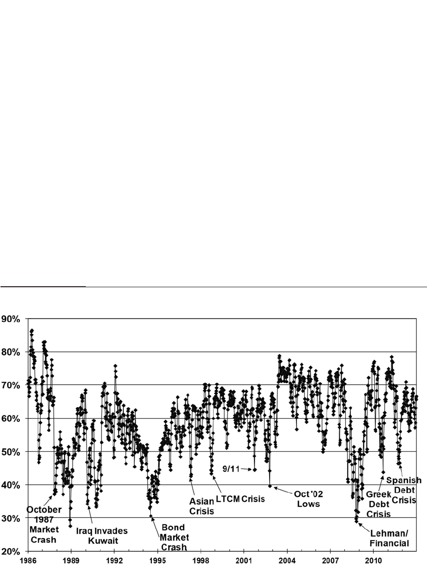
IC: Not entirely. Investors Intelligence, a firm based in New Rochelle,
New York, publishes one of the long-standing indicators of investment
sentiment. Over the past 50 years, the company has evaluated scores of
market newsletters, determining whether each letter is bullish, bearish,
or neutral about the future direction of stocks.
From Investors Intelligence data, I computed an index of investor
sentiment by finding the ratio of bullish newsletters to bullish plus bear-
ish newsletters (omitting the neutral category). I then measured the
returns on stocks subsequent to these sentiment readings.
The investor sentiment indicator since January 1986 is plotted in
Figure 22-1. The crash of October 1987 was accompanied by investor
pessimism. For the next few years, whenever the market went down, as
it did in May and December 1988 and February 1990, investors feared
another crash, and sentiment dropped sharply. Bullish sentiment also
fell below 50 percent during the Iraqi invasion of Kuwait, the bond mar-
ket collapse of 1994, the Asian crisis of October 1997, the LTCM bailout
of the late summer of 1998, the terrorist attacks of September 2001, and
CHAPTER 22 Behavioral Finance and the Psychology of Investing 353
FIGURE 22–1
Investor Intelligence Sentiment Indicator 1986–2012

the market bottom of October 2002. Sentiment also plunged at the bot-
tom of the great bear market that followed the financial crisis of 2008,
and it also dipped during the Greek and Spanish sovereign debt crises
These have all been excellent times to invest.
It is of note that the VIX, the measure of implied market volatility
computed from options prices, spikes upward at virtually the same time
investor sentiment plunges.32 Anxiety in the market, which can be meas-
ured from the premiums on put options, is strongly negatively corre-
lated with investor sentiment.
Out-of-Favor Stocks and the Dow 10 Strategy
Dave: Can you use contrarian strategy to pick individual stocks?
IC: Yes. Contrarians believe that the swings of optimism and pessimism
infect individual stocks as well as the overall markets. Therefore, buying
out-of-favor stocks can be a winning strategy.
Werner De Bondt and Richard Thaler examined portfolios of both
past stock winners and losers to see if investors became overly opti-
mistic or pessimistic about future returns from studying the returns of
the recent past.33 Portfolios of winning and losing stocks were analyzed
over five-year intervals. Portfolios that had been winners in the past five
years subsequently lagged the market by 10 percent, while the subse-
quent returns on the loser portfolio beat the market by 30 percent.
One of the explanations for why this strategy works relates to the
representativeness heuristic we talked about before. People extrapolate
recent trends in stock prices too far into the future. Although there is
some evidence that short-term momentum is positive in stock returns,
over the longer term many stocks that have done poorly outperform, and
stocks that have done well underperform. Another strategy based on out-
of-favor stocks is called the Dogs of the Dow or the Dow 10 strategy.34
Dave: There has been so much to absorb from today’s session. It seems
like I fell into almost all of these behavioral traps. The comforting news is
that I’m not alone and that your counseling has helped other investors.
IC: Not only have they been helped, but they have also prospered. For
many people, success in investing requires a much deeper knowledge of
themselves than does success in their jobs or even in their personal rela-
tionships. There is much truth to an old Wall Street adage, “The stock
market is a very expensive place to find out who you are.”
354 PART IV Stock Fluctuations in the Short Run

PART
BUILDING WEALTH
THROUGH STOCKS
V
This page intentionally left blank

Fund Performance,
Indexing, and Beating
the Market
I have little confidence even in the ability of analysts, let alone
untrained investors, to select common stocks that will give better
than average results. Consequently, I feel that the standard portfolio
should be to duplicate, more or less, the DJIA.
—BENJAMIN GRAHAM, 19341
How can institutional investors hope to outperform the market . . .
when, in effect, they are the market?
—CHARLES D. ELLIS, 19752
There is an old story on Wall Street. Two managers of large equity funds
go camping in a national park. After setting up camp, the first manager
mentions to the other that he overheard the park ranger warning that
black bears had been seen around this campsite. The second manager
smiles and says, “I’m not worried; I’m a pretty fast runner.” The first
manager shakes his head and says, “You can’t outrun black bears;
they’ve been known to sprint over 25 miles an hour to capture their
prey!” The second manager responds, “Of course I know that I can’t out-
run the bear. The only thing that’s important is that I can outrun you!”
357
23

In the competitive world of money management, performance is
measured not by absolute returns but the returns relative to some
benchmark. For stocks these benchmarks include the S&P 500 Index,
the Wilshire 5000, global stock indexes, or the latest “style” indexes
popular on Wall Street. But there is a crucially important difference
about investing compared with virtually any other competitive activity:
Most of us have no chance of being as good as the group of individuals
who practice for hours to hone their skills. But anyone can be as good as
the average investor in the stock market with no practice at all.
The reason for this surprising statement is based on a very simple
fact: the sum of all investors’ holdings must be equal to the market, and
the performance of the market must, by definition, be the average dollar-
weighted performance of each and every investor. Therefore, for each
investor’s dollar that outperforms the market, there must be another
investor’s dollar that underperforms the market. By just matching the
performance of the overall market, you are guaranteed to do no worse
than average.
But how do you match the performance of the whole market? Until
1975, this goal would have been virtually impossible for all but the most
affluent investors. Who can hold shares in each of the thousands of firms
listed on U.S. exchanges?
However, since the mid-1970s, index mutual funds and then
exchange-traded funds have been developed to match the performance
of these broad stock indexes. Over the last several decades, the average
investor could match the performance of a wide variety of market
indexes with very low costs and a very modest investment. And over the
last several years, new indexes have been developed, based on the
research discussed in Chapter 12, that may allow investors to outper-
form the averages.
THE PERFORMANCE OF EQUITY MUTUAL FUNDS
Many claim that striving for average market performance is not the best
strategy. If there are enough poorly informed traders who consistently
underperform the market, then it might be possible for informed
investors or professionals who study stocks to outperform the market.
Unfortunately, the past record of the vast majority of such actively
managed funds does not support this contention. There are two ways to
measure long-term fund returns. One is to compute the returns of all
funds that have survived over the period examined. But the long-term
358 PART V Building Wealth Through Stocks

returns on these funds suffer from survivorship bias that overestimates
the returns available to investors. This survivorship bias exists because
poorly performing funds are often terminated, leaving only the more
successful ones with superior track records to be included in the data.
The second, and more accurate, method is to compute, year by year, the
average performance of all equity mutual funds that were available to
investors in that year.
Both of these computations are shown in Table 23-1. From January
1971 through December 2012, the average U.S. equity mutual fund
returned 9.23 percent annually, 1 percentage point behind the Wilshire
5000 and 0.88 percentage point behind the S&P 500 Index.
Indeed, the survivor funds returned 0.25 percent more per year
than the Wilshire 5000, but there were only 86 such funds out of thou-
sands. And all these fund returns exclude sales and redemption fees that
would reduce their net returns to investors even more.3
The underperformance of mutual funds does not happen every
year. Actively managed equity funds did, on average, outperform the
Wilshire 5000 and the S&P 500 Indexes during the period from 1975
through 1983 when small stocks returned a spectacular 35.32 percent per
year. Equity mutual funds generally do well when small stocks outper-
form large stocks, as many money managers seek to boost performance
by buying smaller-sized firms. But since 1983, when the small stocks
surge ended, the performance of the average mutual fund has been
worse than over the whole period. Even survivor funds have underper-
formed the Wilshire 5000 Index over the last three decades.
CHAPTER 23 Fund Performance, Indexing, and Beating the Market 359
TABLE 23–1
Equity Mutual Funds and Benchmark Returns, 1971–2012
All Funds "Survivor"
Minus Funds Minus
"Survivor" Wilshire Small Wilshire Wilshire
All Funds Funds 5000 S&P 500 Stocks 5000 5000
1971–2012 9.23% 10.48% 10.23% 10.11% 11.85% –0.99% 0.25%
(17.67%) (17.27%) (18.18%) (17.74%) (21.93%)
1975–198318.83% 20.28% 17.94% 15.84% 35.32% 0.89% 2.34%
(12.92%) (13.06%) (14.98%) (15.59%) (14.35%)
1984–2012 8.92% 9.72% 10.19% 10.44% 8.54% –1.27% –0.47%
(17.05%) (16.56%) (17.63%) (17.44%) (18.93%)
Std. deviation in parentheses
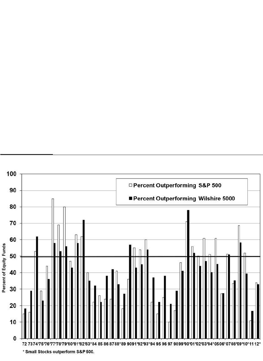
The percentage of general equity funds that has outperformed the
Wilshire 5000 and the S&P 500 Index each year from 1972 to 2012 is dis-
played in Figure 23-1.
During this 40-year period, there were only 12 years when a major-
ity of mutual funds beat the Wilshire 5000. All but two of these years
occurred during a period when small stocks outperformed large stocks.
In the last 25 years, there have been only 6 years when more than one-
half of equity mutual funds outperformed the broad market.
The underperformance of mutual funds did not begin in the 1970s.
In 1970, Becker Securities Corporation startled Wall Street by compiling
the track record of managers of corporate pension funds. Becker showed
that the median performance of these managers lagged behind the S&P
500 by 1 percentage point and that only one-quarter of them were able to
outperform the market.4This study followed on the heels of academic
360 PART V Building Wealth Through Stocks
FIGURE 23–1
Percentage of Equity Funds that Outperform Market Indexes, 1972–2012
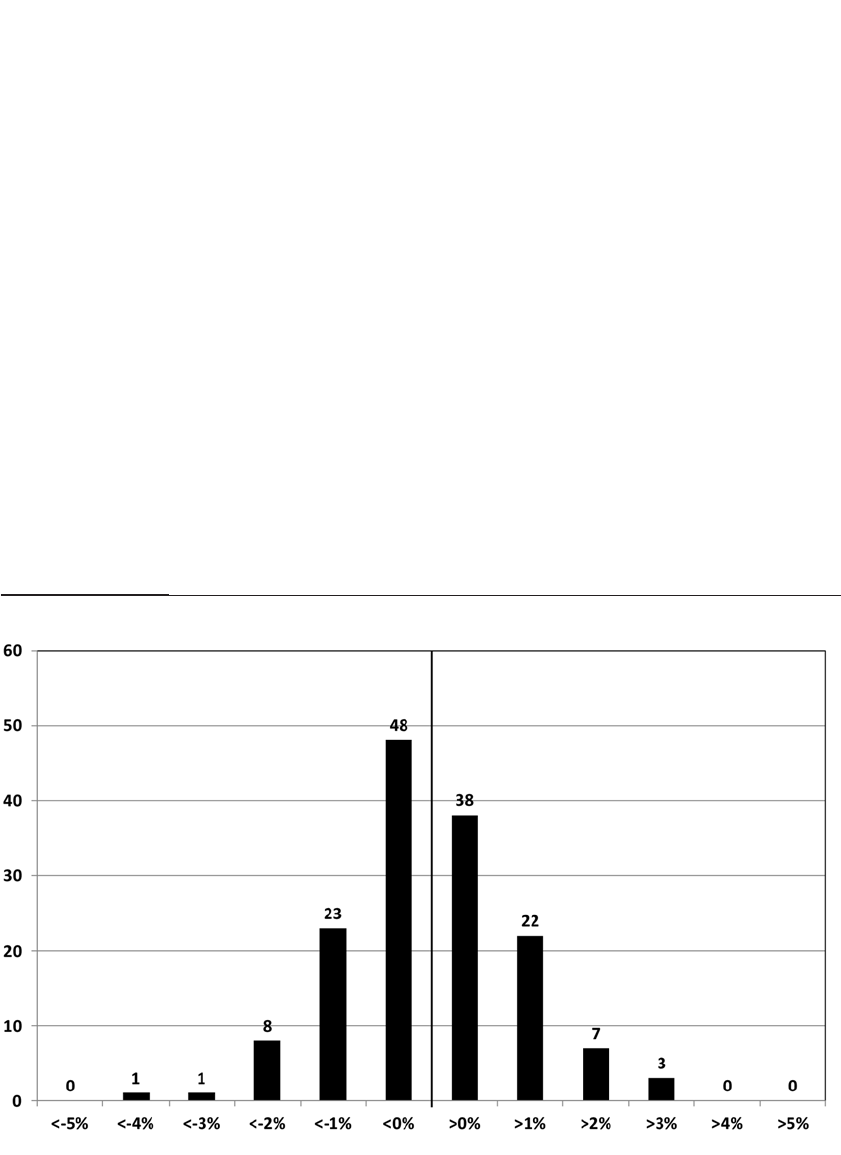
articles, particularly those by William Sharpe and Michael Jensen, that
also confirmed the underperformance of equity mutual funds.
Figure 23-2 displays the distribution of the difference between the
returns of 86 mutual funds that have survived since January 1972 and
the Wilshire 5000.
Only 38, or less than one-half, of the 86 funds that have survived
over the past 35 years have been able to outperform the Wilshire 5000.
Only 22 have been able to outperform the market by more than 1 percent
per year, while only 7 have bettered the market by at least 2 percent. On
the other hand, over half of the surviving funds underperformed the
market, and almost half of those underperformed by more than 1 per-
cent per year. And as noted above for Table 23-1, the actual returns on
many of these funds are worse since these returns exclude sales and
redemption fees.
Despite the generally poor performance of equity mutual funds,
there are some winners as shown in Table 23-2. The best-performing
mutual fund over the entire period is the Sequoia Fund, run by the
investment firm of Ruane, Cunniff, & Goldfarb, which gave investors a
CHAPTER 23 Fund Performance, Indexing, and Beating the Market 361
FIGURE 23–2
Performance of Surviving Mutual Funds Relative to the Wilshire 5000, 1972–2012

14.2% annual return from 1972 through 2012, beating the Wilshire 5000
Return by 4 percentage points per year. The fund closely follows Warren
Buffett’s philosophy and has a large portion of its holdings in Berkshire
Hathaway. In second place is Mutual Shares Z Fund, run by Franklin
Templeton, with a return of 13.7 percent per year. Fidelity’s Magellan
Fund occupies third place by posting a 13.6 percent annual return from
1971 through December 2012, followed by the Columbia Acorn Fund
(previously known as the Liberty Acorn Fund), run by Charles McQuaid
and Robert Mohn, posting a 12.9% return.
Despite these sparkling returns, chance may have played a large
role in these outperformers. The probability that a fund would beat the
Wilshire 5000 by 4 percentage points or more over this period by chance
alone is 1 in 12. That means out of the 86 funds examined, one would
expect 7 to have done this well, but only one did.
Yet luck could not explain Magellan’s performance from 1977
through 1990. During that period, the legendary stock picker Peter Lynch
ran the Magellan Fund and outperformed the market by an incredible 13
percent per year. Magellan took somewhat greater risks in achieving this
return,5but the probability that Magellan would outperform the Wilshire
5000 by this margin over that 14-year period by luck alone is only 1 in
500,000!
An even longer record of outperformance belongs to Warren
Buffett, the legendary investor in Berkshire Hathaway, a small textile
362 PART V Building Wealth Through Stocks
TABLE 23–2
Top Performing Mutual Funds 1972–2012
Mutual Fund Annual Return
Sequoia Fund 14.2%
Mutual Shares Z 13.7%
Fidelity Magellan Fund 13.6%
Columbia Acorn Fund 12.9%
T Rowe Price Small Cap 12.9%
Fidelity Contrafund 12.4%
Davis NY Venture A 12.4%
Invesco Comstock A 12.3%
Fidelity Adv Diversified O 12.2%
Janus Fund D 12.1%
Wilshire 5000 10.2%
S&P 500 Index 10.1%

firm that he purchased in 1965. Berkshire was not part of the universe
examined above since it is a “closed-end” fund, which contains both
traded and nontraded assets. Buffett’s annualized return from 1972
through 2012 is 20.1percent per year, more than 10 percentage points per
year in excess of the S&P 500. The probability that this return was
achieved purely by chance is less than one in a billion.
In 1984, in honor of the fiftieth anniversary of the publication of
Graham and Dodd’s Security Analysis, Buffett delivered a speech at
Columbia University entitled the “The Superinvestors of Graham-and-
Doddsville,” which detailed nine money managers who have greatly out-
performed the market by using the value-oriented approach advocated by
Graham and Dodd.6Buffett’s claim is supported by the data presented in
Chapter 12 that show the outperformance of value-tilted strategies.
FINDING SKILLED MONEY MANAGERS
It is easy to determine that Warren Buffett’s and Peter Lynch’s perform-
ances were due to their skill in picking stocks. But for more mortal port-
folio managers, it is extremely difficult to determine with any degree of
confidence whether the superior returns of money managers are due to
skill or luck. Table 23-3 computes the probability that managers with
better-than-average stock-picking ability will outperform the market.7
The results are surprising. Even if money managers choose stocks
that have an expected return of 1 percent per year better than the market,
there is only a 62.7 percent probability that they will exceed the average
market return after 10 years and only a 71.2 percent probability that they
will exceed the average market return after 30 years. If managers pick
CHAPTER 23 Fund Performance, Indexing, and Beating the Market 363
TABLE 23–3
Probability of Outperforming Market Given Historical Risks and Returns from
1972–2012
Expected Holding Period (Years)
Excess
Return 1235102030
1% 54.1% 55.7% 57.0% 59.0% 62.7% 67.6% 71.2%
2% 58.1% 61.3% 63.8% 67.5% 74.0% 81.9% 86.7%
3% 61.9% 66.6% 70.1% 75.2% 83.2% 91.3% 95.2%
4% 65.7% 71.6% 75.8%81.7% 89.9% 96.4% 98.6%
5% 69.2% 76.1% 80.8%86.9% 94.4% 98.8% 99.7%

stocks that will outperform the market by 2 percent per year, there is still
only a 74.0 percent chance that they will outperform the market after 10
years. This means there is a 1-in-4 chance that they will still fall short of
the average market performance. The length of time needed to be rea-
sonably certain that superior managers will outperform the market will
most surely outlive their trial period for determining their real worth.
Detecting a bad manager is an equally difficult task. In fact, a
money manager would have to underperform the market by 4 percent a
year for almost 15 years before you could be statistically certain (defined
to mean being less than 1 chance in 20 of being wrong) that the manager
is actually poor and not just having bad luck. By that time, your assets
would have fallen to half of what you would have had by indexing to
the market.
Even extreme cases are hard to identify. Surely you would think that
a manager who picks stocks that are expected to outperform the market
by an average of 5 percent per year, a feat achieved by no surviving
mutual fund since 1970, would quickly stand out. But that is not neces-
sarily so. After one year there is only a 7-in-10 chance that such a manager
will outperform the market. And the probability rises to only 76.8 percent
that the manager will outperform the market after two years.
Assume you gave a young, undiscovered Peter Lynch—someone
who over the long run will outperform the market with a 5 percent per
year edge—an ultimatum: that he will be fired if he does not at least
match the market after two years. Table 23-3 shows that the probabil-
ity he will beat the market over two years is only 76.1 percent. This
means there is almost a 1-in-4 chance that he will still underperform
the market and you will fire Lynch, judging him incapable of picking
winning stocks!
Persistence of Superior Returns
Do some money managers have “hot hands,” meaning that if they out-
performed the averages in the past, they are likely to do it again in the
future? The conclusions of numerous studies are not clear-cut. There is
some evidence that funds that outperform in one year are more likely to
outperform the next.8This short-run persistence is probably because
managers follow a particular “style” of investing, and styles often stay in
favor over several years.
But over longer periods, the ability of fund managers to continue to
outperform the market finds less support. Edward Elton, Martin Gruber,
and Christopher Blake claim that outperformance persists over three-
364 PART V Building Wealth Through Stocks

year periods,9but Burton Malkiel, Jack Bogle, and others disagree.10, 11 In
any case, performance can change suddenly and unpredictably. Perhaps
Magellan’s underperformance after Peter Lynch left the fund did not sur-
prise some investors. But Bill Miller’s hot hand with Legg Mason’s Value
Trust, which recorded a record 15 consecutive years of beating the S&P
500 Index, suddenly and unexpectedly turned cold in 2006 and 2007.
REASONS FOR UNDERPERFORMANCE OF MANAGED MONEY
The generally poor performance of funds relative to the market is not
because the fund managers are picking losing stocks. Their performance
lags the benchmarks largely because funds impose fees and trading
costs that are often as high as 2 percent or more per year. First, in seek-
ing superior returns, a manager buys and sells stocks, which involves
paying brokerage commissions and also paying the bid-asked spread, or
the difference between the buying and the selling price of shares.
Second, investors pay management fees (and possibly sales, or “load,”
fees) to the organizations and individuals that sell these funds. Finally,
managers are often competing with other managers with equal or supe-
rior skills at choosing stocks. As noted earlier, it is a mathematical
impossibility for everyone to do better than the market—for every dol-
lar that outperforms the average, some other investor’s dollar must
underperform the average.
A LITTLE LEARNING IS A DANGEROUS THING
It is interesting that an investor who has some knowledge of the princi-
ples of equity valuations often performs worse than someone with no
knowledge who decides to index his portfolio. For example, take the
novice—an investor who is just learning about stock valuation. This is
the investor to whom most of the books entitled How to Beat the Market
are sold. A novice might note that the stock has just reported very good
earnings but its price is not rising as much as he believes is justified by
this good news, and so he buys the stock.
Yet informed investors know that special circumstances caused the
earnings to increase and that these circumstances will not likely be
repeated in the future. Informed investors are therefore more than
happy to sell the stock to novices, realizing that the rise in the price of the
stock is not justified. Informed investors make a return on their special
knowledge. They make their return from novices who believe they have
found a bargain. Uninformed indexed investors, who do not even know
CHAPTER 23 Fund Performance, Indexing, and Beating the Market 365

what the earnings of the company are, often do better than the investor
who is just beginning to learn about equities.
The saying “a little learning is a dangerous thing” proves itself to be
quite apt in financial markets. Many seeming anomalies or discrepan-
cies in the prices of stocks (or most other financial assets, for that matter)
are due to the trading of informed investors with special information
that is not easily processed by others. When a stock looks too cheap or
too dear, the easy explanation—that emotional or ignorant traders have
incorrectly priced the stock—is usually wrong. Most often there is a
good reason why stocks are priced as they are. This is why beginners
who buy individual stocks on the basis of their own research often do
quite badly.
PROFITING FROM INFORMED TRADING
As novices become more informed, they will no doubt find some stocks
that are genuinely undervalued or overvalued. Trading these stocks will
begin to offset their transaction costs and their poorly informed, losing
trades. At some point, a trader might become well enough informed to
overcome the transaction costs and match, or perhaps exceed the market
return. The key word here is might, because the number of investors who
have consistently been able to outperform the market is small indeed.
And for individuals who do not devote much time to analyzing stocks,
the possibility of consistently outperforming the averages is remote.
Yet the apparent simplicity of picking winners and avoiding losers
lures many investors into active trading. We learned in Chapter 22 that
there is an inherent tendency of individuals to view themselves and
their performance as above average. The investment game draws some
of the best minds in the world. Many investors are wrongly convinced
that they are smarter than the next guy who is playing the same invest-
ing game. But even being just as smart as the next investor is not good
enough. Being average at the game of finding market winners will result
in underperforming the market as transaction costs diminish returns.
In 1975, Charles D. Ellis, a managing partner at Greenwood
Associates, wrote an influential article called “The Loser’s Game.” In it
he showed that, with transaction costs taken into account, average
money managers must outperform the market by margins that are not
possible, given that they themselves are the major market players. Ellis
concludes: “Contrary to their oft articulated goal of outperforming the
market averages, investment managers are not beating the market; the
market is beating them.”12
366 PART V Building Wealth Through Stocks

HOW COSTS AFFECT RETURNS
Trading and managerial costs of 2 or 3 percent a year might seem small
compared with the year-to-year volatility of the market and, as well,
might seem small to investors who are gunning for 20 or 30 percent
annual returns. But such costs are extremely detrimental to long-term
wealth accumulation. Investing $1,000 at a compound return of 11 per-
cent per year, near the average nominal return on stocks since World
War II, will accumulate $23,000 over 30 years. A 1 percent annual fee will
reduce the final accumulation by almost a third. With a 3 percent annual
fee, the accumulation amounts to just over $10,000, less than half the
market return. Every extra percentage point of annual costs requires
investors aged 25 to retire 2 years later than they would have in the
absence of such costs.
THE INCREASED POPULARITY OF PASSIVE INVESTING
Many investors have realized that the poor performance of actively
managed funds relative to benchmark indexes strongly implies that they
would do very well to just equal the market return of one of the broad-
based indexes. Thus, the 1990s witnessed an enormous increase in pas-
sive investing, the placement of funds whose sole purpose was to match
the performance of an index.
The oldest and most popular of the index funds is the Vanguard 500
Index Fund.13 The fund, started by visionary John Bogle, raised only
$11.4 million when it debuted in 1976, and few thought the concept
would survive. But slowly and surely, indexing gathered momentum,
and the fund’s assets reached $17 billion at the end of 1995.
In the latter stages of the 1990s bull market, the popularity of index-
ing soared. By March 2000, when the S&P 500 Index reached its all-time
high, the fund claimed the title of the world’s largest equity fund, with
assets over $100 billion. Indexing became so popular that in the first six
months of 1999 nearly 70 percent of the money that was invested went
into index funds.14 By 2013, all Vanguard 500 Index funds had attracted
over $275 billion in assets, and Vanguard’s Total Stock Market Funds,
which include smaller stocks, attracted $250 billion.
One of the attractions of index funds is their extremely low cost.
The total annual cost in the Vanguard 500 Index Fund is only 0.15 per-
cent of market value (and as low as 2 basis points for large institutional
investors). Because of proprietary trading techniques and interest
income from loaning securities, Vanguard S&P 500 Index funds for indi-
CHAPTER 23 Fund Performance, Indexing, and Beating the Market 367

vidual investors have fallen only 9 basis points behind the index over
the last 10 years, and its S&P 500 Index fund for institutional investors
has actually outperformed the benchmark index.15
THE PITFALLS OF CAPITALIZATION-WEIGHTED INDEXING
Despite the past success of index funds, their popularity, especially
those funds linked to the S&P 500 Index, may cause problems for index
investors in the future. The reason is simple. If a firm’s mere entry into
the S&P 500 causes the price of its stock to rise, due to the anticipated
buying by index funds, index funds will hold a number of overpriced
stocks that will depress future returns.
An extreme example of overpricing occurred when Yahoo!, the
well-known Internet firm, was added to the S&P 500 Index in
December 1999. Standard & Poor’s announced after the close of trad-
ing on November 30 that Yahoo! would be added to the index on
December 8. The next morning, Yahoo! opened at $115—up almost $9
per share from its close the day before—and continued upward to close
at $174 a share on December 7, when index funds had to buy the shares
in order to match the index. In just 5 trading days between the
announcement of Yahoo!’s inclusion in the index until it formally
became a member, the stock surged 64 percent. Volume during those 5
days averaged 37 million shares, more than three times the average on
the previous 30 days. On December 7, when index funds had to own
the stock, volume hit 132 million shares, representing $22 billion of
Yahoo! stock traded.
This story is repeated with most stocks added to the index,
although the average size of the gain is considerably less than Yahoo!’s.
Standard & Poor’s published a study in September 2000 that had deter-
mined how adding a stock to an S&P index influenced the price. This
study noted that from the announcement date to the effective date of
admission in the S&P 500 Index, shares rose by an average of 8.49 per-
cent.16 During the next 10 days following their entrance, these stocks fell
by an average of 3.23 percent, or about one-third of the preentry gain. Yet
one year after the announcement, these postentry losses were wiped out,
and the average gain of new entrants was 8.98 percent. All these per-
centages were corrected for movements in the overall market. A later
study has shown that although the preentry gain has fallen in recent
years, the price of stocks admitted to the S&P 500 still has jumped over 4
percent in response to the announcement.17
368 PART V Building Wealth Through Stocks

FUNDAMENTALLY WEIGHTED VERSUS
CAPITALIZATION-WEIGHTED INDEXATION
Despite the overpricing of new entrants into the S&P 500 Index, virtually
all indexes that have a significant investment following, such as those
created by Standard & Poor’s, the Russell Investment Group, or Wilshire
Associates, are capitalization weighted. That means that each firm in the
index is weighted by the market value, or the current price times the num-
ber of shares outstanding. More recently, most of these indexes adjust
the quantity of shares by excluding insider holdings, which consist of
large positions held by insiders and governments from the total shares
outstanding. Government holdings can be especially large in the emerg-
ing economies. The number of shares after this adjustment is called float-
adjusted shares, where float refers to the number of shares that are readily
available to buy.18
To be sure, capitalization-weighted indexes have some very good
properties. First, as noted earlier in the chapter, these indexes represent
the average dollar-weighted performance of all investors, so that for any-
one who does better than the index, someone else must do worse.
Furthermore, these portfolios, under the assumptions of an efficient
market, give investors the “best” trade-off between risk and return. This
means that for any given risk level, these capitalization-weighted port-
folios give the highest returns; and for any given return, these portfolios
give the lowest risk. This property is called mean-variance efficiency.
But the assumptions under which these desirable properties pre-
vail are very stringent. Capitalization-weighted portfolios are optimal
only if the market is efficient in the sense that the price of each stock is at
all points in time an unbiased estimate of the true underlying value of
the enterprise. This does not mean that the price of each stock is always
right; but it does mean that there is no easily obtainable information that
allows investors to make a better estimate of its true value. Under effi-
cient markets, if a stock goes from $20 to $25 a share, the best estimate of
the change in the underlying value of the enterprise is also 25 percent,
and there are no factors unrelated to fundamental value that could
change the stock price.
But as we learned in Chapter 12, there are many reasons why stock
prices change that do not reflect changes in the underlying value of the
firm. Transactions made for liquidity, fiduciary, or tax reasons can impact
stock prices, as well as speculators acting on unfounded or exaggerated
information. When stock price movements can be caused by factors unre-
lated to fundamental changes in firm value, market prices are “noisy”
CHAPTER 23 Fund Performance, Indexing, and Beating the Market 369

and are no longer unbiased estimates of true value. As noted earlier in the
book, I call this way of looking at the market the noisy market hypothe-
sis, and I find it an attractive alternative to the efficient market hypothe-
sis that has dominated the finance profession over the last 40 years.
If the noisy market hypothesis is a better representation of how
markets work, the capitalization-weighted indexes are no longer the
best portfolios for investors. A better index is a fundamentally weighted
index, in which each stock is weighted by some measure of a firm’s fun-
damental financial data, such as dividends, earnings, cash flows, and
book value, instead of the market capitalization of its stock.19
Fundamentally weighted indexes work in the following manner.
Assume earnings are chosen as the measure of firm value. If Erepresents
the total dollar earnings of the stocks chosen for the index, and Ejis the
earnings from a particular firm j, then the weight given to firm jin the
fundamental index is Ej/E, its share of total earnings rather than its share
of the market value as is done in capitalization-weighted indexes.
In a capitalization-weighted index, stocks are never sold no matter
what price they reach. This is because if markets are efficient, the price
represents the fundamental value of the firm, and no purchase or sale is
warranted.
However, in a fundamentally weighted index, if a stock price rises
but the fundamental, such as earnings, does not, then shares are sold
until the value of the stock in the index is brought down to the original
levels. The opposite happens when a stock falls for reasons not related to
fundamentals—in this case shares are purchased at the lower price to
bring the stock’s value back to the original levels. Making these sales or
purchases is called rebalancing the fundamentally weighted portfolio,
and it usually takes place once per year.
One of the advantages of fundamentally weighted portfolios is that
they avoid “bubbles,” those meteoric increases in the prices of stocks
that are not accompanied by increases in dividends, earnings, or other
objective metrics of firm values. This was certainly the case in 1999 and
early 2000 when the technology and Internet stocks jumped to extraor-
dinary valuations based on the hope that their profits would eventually
justify their price. Any fundamentally weighted portfolio would have
sold these stocks as their prices rose, while capitalization-weighted
indexes continued to hold them because the efficient market hypothesis
assumes that all price increases are justified.
Note that fundamental indexation does not identify which stocks
are overvalued or undervalued. It is a “passive” index, and the purchases
and sales of individual stocks are made according to a predetermined for-
370 PART V Building Wealth Through Stocks

mula. Certainly some overpriced stocks will be bought and some under-
priced stocks sold. But it can be shown that if prices are determined by
the noisy market hypothesis, then, on average, a portfolio that buys
stocks that go down more than fundamentals and sells stocks that go
up more than fundamentals will boost returns over a capitalization-
weighted index and reduce risk.20
THE HISTORY OF FUNDAMENTALLY WEIGHTED INDEXATION
The motivation for fundamentally weighted indexation began in the
international markets. In the 1980s, when Japan’s stock market was in a
bubble, many investors with internationally diversified portfolios were
seeking a consistent way to reduce the weight of Japanese stocks. At that
time Morgan Stanley Capital International (MSCI) formulated an inter-
national index that weighted each country by GDP rather than market
capitalization and fortunately reduced the allocation to Japanese stocks.21
In 1987 Robert Jones of Goldman Sachs’s quantitative asset man-
agement group developed and managed a U.S. stock index in which the
weights of each firm in the index were corporate profits. Jones referred
to his strategy as “economic investing” because the proportion of each
firm in the index was related to its economic importance rather its mar-
ket capitalization.22 Later David Morris, founder and CEO of Global
Wealth Allocation, devised a strategy that combined several fundamen-
tal factors into one “wealth” variable.
In 2003, Paul Wood and Richard Evans published research on a fun-
damentally based approach that evaluated a profit-weighted index of
the 100 largest companies.23 In early 2005, Robert D. Arnott of Research
Affiliates, along with Jason Hsu and Philip Moore, published a paper in
the Financial Analysts Journal entitled “Fundamental Indexation” that
exposed the flaws of capitalization-weighted indexes and laid the case
for fundamentally based strategies.24 In December 2005, the first funda-
mentally weighted ETF was launched by Powershares (FTSE RAFI
US1000) to track an index constructed by Research Affiliates based on
sales, cash flows, book values, and dividends. Six months later,
WisdomTree Investments launched 20 ETFs based on dividends and fol-
lowed up in 2007 with six more based on earnings.
The historical evidence to support fundamentally weighted indexa-
tion is impressive. From 1964 through 2012, the compound annual return
on a dividend-weighted index based on virtually all U.S. stocks was 10.84
percent per year, 117 basis points above a similar capitalization-weighted
portfolio based on the same stocks, while the volatility and beta of the
CHAPTER 23 Fund Performance, Indexing, and Beating the Market 371

dividend-weighted portfolio were less than the capitalization-weighted
portfolio. This return outperformance with lower volatility was reported
across size sectors and internationally. Specifically, from 1996 through
2012, a dividend-weighted MSCI EAFE Index outperformed an EAFE
Index by nearly 3½ percentage points per year.
The long-term outperformance of fundamentally weighted indexes
principally relies on their emphasis of value-based strategies. Stocks
with higher-than-average dividend yields or lower-than-average P/E
ratios receive greater weights in fundamentally weighted indexes
than capitalization-weighted indexes. But fundamentally weighted
indexes are better diversified than portfolios of only value stocks, and
historically they have had better risk-returns trade-offs. In short, funda-
mentally weighted indexes have very attractive characteristics that chal-
lenge the supremacy of capitalization-weighted indexes for long-term
investors.
CONCLUSION
The past performance of actively managed equity funds is not encour-
aging. The fees that most funds charge do not provide investors with
superior returns and can be a significant drag on wealth accumulation.
Furthermore, a good money manager is extremely difficult to identify,
for luck plays a role in all successful investment outcomes.
When costs are taken into account, a large percentage of actively
managed equity funds significantly lag the benchmark indexes, and
most investors would be better off in capitalization-weighted or funda-
mentally weighted index funds.
372 PART V Building Wealth Through Stocks

Structuring a Portfolio for
Long-Term Growth
[The] long run is a misleading guide to current affairs. In the long
run we are all dead. Economists set themselves too easy, too useless a
task if in tempestuous seasons they can only tell us when the storm is
long past, the ocean will be flat.
—JOHN MAYNARD KEYNES, 19241
My favorite holding period is forever.
—WARREN BUFFETT, 19942
No one can argue with Keynes’s statement that in the long run we are all
dead. But a vision of the long run must serve as a guide for action today.
Those who keep their focus and perspective during trying times are far
more likely to emerge as successful investors. Knowing that the sea will
be flat after the storm passes is not useless, as Keynes asserted, but enor-
mously comforting.
PRACTICAL ASPECTS OF INVESTING
To be a successful long-term investor is easy in principle but difficult in
practice. It is easy in principle because the strategy of buying and hold-
ing a diversified portfolio of stocks, forgoing any forecasting ability, is
available to all investors, no matter what their intelligence, judgment, or
373
24

financial status. Yet it is difficult in practice, because we are all vulnera-
ble to emotional forces that can lead us astray. Tales of those who have
quickly achieved great wealth in the market tempt us to play a game
very different from what we had intended.
Selective memory also pushes us in the wrong direction. Those
who follow the market closely often exclaim: “I knew that stock (or the
market) was going up! If I had only acted on my judgment, I would have
made a mint!” But hindsight plays tricks on our minds. We forget the
doubts we had when we made the decision not to buy. Hindsight can
distort our past experiences and affect our judgment, encouraging us to
play hunches and try to outsmart other investors, who in turn are play-
ing the same game.
For most investors, going down this path leads to disastrous
results. We take far too many risks, our transactions costs are high, and
we find ourselves giving in to the emotions of the moment—pessimism
when the market is down and optimism when the market is high. This
leads to frustration as our misguided actions result in substantially
lower returns than we could have achieved by just staying in the market.
GUIDES TO SUCCESSFUL INVESTING
Achieving good returns in stocks requires keeping a long-term focus
and a disciplined investment strategy. The principles enumerated below
are taken from the research described in this book and enable both new
and seasoned investors to better achieve their investing goals.
1. Keep your expectations in line with history. Historically stocks have
returned between 6 and 7 percent after inflation over the last two cen-
turies and have sold at an average P/E ratio of about 15.
A 6.5 percent annual real return, which includes reinvested divi-
dends, will nearly double the purchasing power of your stock portfolio
every decade. If inflation stays within the 2 to 3 percent range, nominal
stock returns will be 9 percent per year, which doubles the money value
of your stock portfolio every eight years.
Despite this excellent long-run record, stock returns are not inde-
pendent of their valuation. A 6 to 7 percent real return is consistent with
a market that trades at about 15 times estimated earnings.
But there is no reason why a 15 P/E ratio will always be the “right”
ratio for stock prices. Chapter 12 maintains that there may be reasons,
such as lower transaction costs and lower returns on bonds, why the
stock market may rise to a higher P/E ratio in the future.
374 PART V Building Wealth Through Stocks

2. Stock returns are much more stable in the long run than in the short
run. Over time stocks, in contrast to bonds, compensate investors for
higher inflation. Therefore, as your investment horizon becomes
longer, put a larger fraction of your assets in equities.
The percentage of your portfolio that you should hold in equities
depends on individual circumstances. But based on historical data, an
investor with a long-term horizon should keep an overwhelming por-
tion of his or her financial assets in equities. Chapter 6 showed that over
holding periods of 20 years or longer, stocks have both a higher return
and lower after-inflation risk than bonds.
The only long-term risk-free assets are Treasury inflation-protected
securities. In recent years the real yield on these bonds has ranged
between minus 1 percent and plus 1 percent, which is considerably below
the historical returns on stocks. The difference between the returns on
stocks and the returns on bonds is called the equity premium, and histor-
ically it has favored stocks in all countries where data are available.
3. Invest the largest percentage of your stock portfolio in low-cost
stock index funds.
Chapter 23 showed that the broad-based indexes, such as the
Wilshire 5000 and the S&P 500 Index, have outperformed nearly two out
of three mutual funds since 1971. By matching the market year after
year, an indexed investor is likely to be near the top of the pack when the
long-term returns are tallied.
There are many exchange-traded and indexed mutual funds that
closely track the major stock market indexes. Investors in capitalization-
weighted index funds should insist on a total annual expense ratio
under 0.15 percent.
4. Invest at least one-third of your equity portfolio in international
stocks, currently defined as those not headquartered in the United
States. Stocks in high-growth countries often become overpriced and
yield poor returns for investors.
Today the United States has only about one-half of the world’s
equity capital, and that fraction is declining rapidly. Owning foreign
stocks is a must in today’s global economy. In the future, the geographic
location of the firm’s headquarters will lose its importance as an invest-
ment factor. What, where, and to whom a firm sells its products will
dominate a new classification system.
Despite the increase in the short-term correlation between country
returns, the case for international investing is persuasive. In all countries
CHAPTER 24 Structuring a Portfolio for Long-Term Growth 375

studied, the return on stocks has handily beaten that on bonds and
fixed-income assets over the last century. Do not overweight high-
growth countries whose valuation ratio exceeds 20 times earnings. The
data presented in Chapter 13 show that investors often overpay for
such growth.
5. Historically, value stocks—those with lower P/E ratios and higher
dividend yields—have superior returns and lower risk than growth
stocks. Tilt your portfolio toward value by buying passive indexed
portfolios of value stocks or, fundamentally weighted index funds.
Chapter 12 demonstrated that stocks with low P/E ratios and high
dividend yields have outperformed the market over the past 50 years
and have done so with lower risk. One reason for this outperformance is
that prices of stocks are often influenced by factors not related to their
true value, such as liquidity and tax-motivated transactions, rumor-
based speculation, and buying and selling by momentum traders. In
these circumstances, stocks priced low relative to their fundamentals
will likely offer investors a better risk-return profile.
Investors can take advantage of this mispricing by buying low-cost
passively managed portfolios of value stocks or fundamentally
weighted indexes that weight each stock by its share of dividends or
earnings rather than by its market value. Historically, fundamentally
weighted indexes have had higher returns and lower risks than capital-
ization-weighted indexes.
6. Finally, establish firm rules to keep your portfolio on track, espe-
cially if you find yourself giving in to the emotion of the moment. If
you are particularly anxious about the market, sit down and reread the
first chapter of this book.
Swings in investor emotion often send stock prices above and
below their fundamental values. The temptations to buy when everyone
is bullish and sell when everyone is bearish are hard to resist. Since it is
so difficult to stand apart from this market sentiment, most investors
who trade frequently have poor returns. Chapter 22 shows how behav-
ioral finance helps investors understand and avoid common psycholog-
ical pitfalls that cause poor market performance. Chapters 1 and 5 keep
investors focused on the big picture about risk and return.
376 PART V Building Wealth Through Stocks

IMPLEMENTING THE PLAN AND THE ROLE
OF AN INVESTMENT ADVISOR
I wrote Stocks for the Long Run to spell out what returns could be expected
on stocks and bonds and to analyze the major factors influencing those
returns. Many investors will consider this book a “do-it-yourself guide”
to choosing stocks and structuring a portfolio. But knowing the right
investments is not the same as implementing the right investment strat-
egy. As Peter Bernstein so aptly indicated in the Foreword, there are
many pitfalls on the path to successful investing that prevent investors
from achieving their intended goals.
The first pitfall is trading frequently in an attempt to “beat the mar-
ket.” Many investors are not satisfied earning a 9 percent annual return
on stocks when they know there are always stocks that will double or
triple in price over the next 12 months. Finding such gems is extremely
gratifying, and many dream of buying the next corporate giant in its
infancy. But the evidence is overwhelming that investors seeking these
winners suffer poor returns as transaction costs and bad timing sink
returns.
Investors who have been burned by picking individual stocks often
turn to mutual funds in their search for higher returns. But choosing a
mutual fund poses similar obstacles. “Hot managers” with superior past
performance replace “hot stocks” as the new strategy to beat the market.
As a result, many investors end up playing the same game as they had
with individual stocks and also suffer below-average returns.
Those who finally abandon trying to pick the best funds are
tempted to pursue an even more difficult strategy. They attempt to beat
the market by timing market cycles. Surprisingly, it is often the best-
informed investors who fall into this trap. With the abundance of finan-
cial news, information, and commentary at our beck and call, it is
extraordinarily difficult to stay aloof from market opinion. As a result,
one’s impulse is to capitulate to fear when the market is plunging or to
greed when stocks are soaring.
Many try to resist this impulse. The intellect may say “Stay the
course!” but this is not easy to do when one hears so many others—
including well-respected “experts”—advising investors to beat a hasty
retreat. It is easier to follow what everyone else is doing rather than act
independently. And as John Maynard Keynes aptly stated in The General
Theory, “Worldly wisdom teaches that it is better for reputation to fail
conventionally than to succeed unconventionally.”3Failing by following
CHAPTER 24 Structuring a Portfolio for Long-Term Growth 377

the advice of “experts” is far easier than failing by rejecting the invest-
ment consensus and standing apart from the crowd.
What does all this mean to the reader of this book? Proper invest-
ment strategy is as much of a psychological as an intellectual challenge.
As with other challenges in life, it is often best to seek professional help
to structure and maintain a well-diversified portfolio. If you should
decide to seek help, be sure to select a professional investment advisor
who agrees with the basic principles of diversification and long-term
investing that I have espoused in these chapters. It is within the grasp of
all to avoid investing pitfalls and reap the generous rewards that are
available in equities.
CONCLUDING COMMENT
The stock market is exciting. Its daily movements dominate the financial
press and mark the flows of billions of dollars of investment capital. But
stock markets are far more than the quintessential symbol of capitalism.
Stock markets are now found in virtually every country in the world,
and they are the driving forces behind the allocation of the world’s cap-
ital and the fundamental engines of economic growth. The main thesis
of this book, that stocks represent the best way to accumulate wealth in
the long run, remains as true today as it was when I published the first
edition of Stocks for the Long Run in 1994.
378 PART V Building Wealth Through Stocks

Chapter 1
1. Benjamin Graham and David Dodd, Security Analysis, New York: McGraw-Hill,
1934, p. 11.
2. Roger Lowenstein, “A Common Market: The Public’s Zeal to Invest,” Wall Street
Journal, September 9, 1996, p. A11.
3. Comment on a CNBC show in March 2009, at the bottom of the 2008–2009 bear mar-
ket.
4. Irving Fisher, The Stock Market Crash and After, New York: Macmillan, 1930, p. xi.
5. “The Crazy Things People Say to Rationalize Stock Prices,” Forbes, April 27, 1992,
p. 150.
6. Raskob catered to investors who wanted to get rich quickly by devising an alterna-
tive scheme by which investors borrowed $300, adding $200 of personal capital, to
invest $500 in stocks. Although in 1929 this was certainly not as good as putting
money gradually into the market, even this plan beat investment in Treasury bills
after 20 years.
7. Irving Fisher, How to Invest When Prices Are Rising, Scranton, PA: G. Lynn Sumner &
Co., 1912.
8. Edgar L. Smith, Common Stocks as Long-Term Investments, New York: Macmillan,
1925, p. v.
9. Ibid., p. 81.
10. “Ordinary Shares as Investments,” The Economist, June 6, 1925, p. 1141.
11. John Maynard Keynes, “An American Study of Shares Versus Bonds as Permanent
Investments,” The Nation & The Athenaeum, May 2, 1925, p. 157.
12. Edgar Lawrence Smith, “Market Value of Industrial Equities,” Review of Economic
Statistics, vol. 9 (January 1927), pp. 37–40, and “Tests Applied to an Index of the Price
Level for Industrial Stocks,” Journal of the American Statistical Association,
Supplement, March 1931, pp. 127–135.
13. Siegfried Stern, Fourteen Years of European Investments, 1914–1928, London: Bankers’
Publishing Co., 1929.
14. Chelcie C. Bosland, The Common Stock Theory of Investment, Its Development and
Significance, New York: Ronald Press, 1937.
15. From the Foreword by Irving Fisher in Kenneth S. Van Strum, Investing in Purchasing
Power, New York: Barron’s, 1925, p. vii. Van Strum was a writer for Barron’s weekly
and confirmed Smith’s research.
16. Robert Loring Allen, Irving Fisher: A Biography, Cambridge: Blackwell, 1993, p. 206.
17. Commercial and Financial Chronicle, September 7, 1929.
18. “Fisher Sees Stocks Permanently High,” New York Times, October 16, 1929, p. 2.
19. Lawrence Chamberlain and William W. Hay, Investment and Speculations, New York:
Henry Holt & Co., 1931, p. 55, emphasis his.
20. Benjamin Graham and David Dodd, Security Analysis, 2nd ed., New York: McGraw-
Hill, 1940, p. 357.
379
NOTES

21. He estimated the undervaluation at approximately 25 percent of “intrinsic value.”
Alfred Cowles III and Associates, Common Stock Indexes 1871–1937, Bloomington,
IN: Principia Press, 1938, p. 50.
22. Wilford J. Eiteman and Frank P. Smith, Common Stock Values and Yields, Ann Arbor:
University of Michigan Press, 1962, p. 40.
23. “Rates of Return on Investment in Common Stocks,” Journal of Business, vol. 37
(January 1964), pp. 1–21.
24. Ibid., p. 20.
25. Journal of Business, vol. 49 (January 1976), pp. 11–43.
26. Stocks, Bonds, Bills, and Inflation Yearbooks, 1983–1997, Chicago: Ibbotson and
Associates.
27. William Baldwin, “The Crazy Things People Say to Rationalize Stock Prices,” Forbes,
April 27, 1992, pp. 140–150.
28. Three months later, in December 1995, Shulman capitulated to the bullish side,
claiming his longtime emphasis on dividend yields was incorrect.
29. Roger Lowenstein, “A Common Market: The Public’s Zeal to Invest,” Wall Street
Journal, September 9, 1996, p. A1.
30. Floyd Norris, “In the Market We Trust,” New York Times, January 12, 1997.
31. Henry Kaufman, “Today’s Financial Euphoria Can’t Last,” Wall Street Journal,
November 25, 1996, p. A18.
32. Robert Shiller and John Campbell, “Valuation Ratios and the Long-Run Stock
Market Outlook,” Journal of Portfolio Management, vol. 24 (Winter 1997). The Shiller
model is discussed in more detail in Chapter 11.
33. Newsweek, April 27, 1998. Cover stories about the stock market in major newsweek-
lies have often been poorly timed. BusinessWeek’s cover article “The Death of
Equities” on August 13, 1979, occurred 14 years after the market had peaked and 3
years before the beginning of the greatest bull market in stocks.
34. I immediately rebutted their arguments in the Wall Street Journal (see the Jonathan
Clements interview of me in “Throwing Cold Water on Dow 36,000 View,” Wall
Street Journal, September 21, 1999), stating that their analysis was faulty and that
stocks must have real returns exceeding those on U.S. Treasury inflation-protected
bonds, whose yield had reached 4 percent at that time.
35. “Big Cap Tech Stocks Are a Sucker’s Bet,” Wall Street Journal, March 14, 2000, p. A8.
36. Paul Sloan, “The Craze Collapses,” U.S. News &World Report Online, November 30,
2000.
37. The word hedge means “to offset,” as someone making an investment in a foreign
market may want to hedge, or offset, adverse currency movements with a transac-
tion in the forward market. Hedge funds often, but not always, took positions that
were contrary to the stock market.
38. Jeremy Grantham, “A Global Bubble Warns Against the Stampede to Diversify,”
Financial Times, April 24, 2007, p. 38.
39. In fact, just days before the Lehman bankruptcy, the REIT Index was only 25 percent
below its record level that it reached in July 2007. In contrast, homebuilder stocks
peaked in July 2005 and were already down more than 60 percent by the time the
Lehman crisis broke.
40. See “At Lehman, How a Real-Estate Start’s Reversal of Fortune Contributed to
Collapse,” Wall Street Journal, October 1, 2008.
380 Notes

Chapter 2
1. As early as June, Natixis, a French investment bank, had cut off all activity with
Lehman, and in early September, it was reported by The Financial Crisis Inquiry
Report that JPMorgan, Citigroup, and Bank of America all demanded more collateral
from Lehman with the threat that they might “cut Lehman off if they don’t receive
it.”
2. Risk spreads, such as the TED spread (Treasuries over Eurodollars), the LIBOR-OIS
spread (LIBOR over Fed funds), commercial paper over Treasuries, and others
jumped dramatically. By Wednesday the Bloomberg Financial Conditions Index of
Risk had deteriorated to four to five standard deviations below normal levels based
on the past 16 years of data. (See Michael G. Rosenberg, “Financial Conditions
Watch,” Bloomberg, September 18, 2008.)
3. On Monday, September 15, the Primary Fund valued Lehman’s commercial paper
at 80 cents on the dollar. On Tuesday it posted on its website, “The value of the debt
securities issued by Lehman Brothers Holdings, Inc (face value $785 million) and
held by the Primary Fund has been valued at zero effective as of 4:00 p.m. New York
time today. As a result, the NAV of the Primary Fund, effective as of 4:00 p.m. is
$0.97 per share.”
4. I recalled lecturing my students in the 1980s, when Treasury bill rates were 16 per-
cent, that investors were thrilled to get yields as high as 10 basis points in the 1930s.
Students shook their heads in disbelief, and we all laughed about this curious piece
of history that we thought could never happen again.
5. The standard deviation of quarterly changes in nominal GDP fell from 5.73 percent
from 1947 to 1983 to 2.91 percent from 1983 to 2009.
6. The Jerome Levy Economics Institute of Bard College, Working Paper No. 74, May
1992; see also Robert Pollin, “The Relevance of Hyman Minsky,” Challenge, March/
April 1997.
7. Subprime mortgages were not solely the creation of Wall Street firms. Politicians
who wanted to give millions of Americans their first chance to realize the
“American Dream” of home ownership encouraged the government-sponsored
lenders Fannie Mae and Freddie Mac to issue these loans to those who would not
ordinarily qualify for conventional mortgages.
8. Since mortgages are denominated in dollars, it is the nominal, not the real, index
that is of interest to bond buyers.
9. It is true that there were substantial declines in nominal house prices during the
Great Depression and that the real estate price index declined 25.9 percent between
1928 and 1932. But that was entirely due to a deflation in the general price index, as
the CPI fell almost exactly the same percentage. Since the Federal Reserve had com-
mitted to avoid deflation and could do so through the power of money creation, it
would be quite reasonable to assume that researchers would ignore those data.
10. “Absence of Fear,” CFA Society of Chicago Speech, June 28, 2007, reported by Robert
Rodriguez, CEO of First Pacific, http://www.fpafunds.com/docs/special
-commentaries/absence_of_fear.pdf?sfvrsn=2.
11. Deutsche Bank Trustee Reports, http://csmoney.cnn.com/2007/10/15/markets
/junk_mortgages.fortune/index.htm?postversion=2007101609.
12. Noelle Knox, “43% of first time home buyers put no money down,” USA Today,
January 18, 2006, p. 1A.
Notes 381

13. Charles Himmelberg, Chris Mayer, and Todd Sinai, “Assessing High House Prices,
Bubbles, Fundamentals and Misperceptions,” Journal of Economic Perspectives, vol.
19, no. 4 (Fall 2005), pp. 67–92. They also wrote an article, “Bubble Trouble? Not
Likely,” which appeared on the editorial page of the Wall Street Journal (September
19, 2005) at the peak of housing prices.
14. According to Home Mortgage Disclosure Act data, the national share of purchase
loans for second homes—defined as “other than owner-occupied as a principal
dwelling”—increased from 8.6 to 14.2 percent from 2000 to 2004. That represents an
annual average growth rate of 16 percent during that time period. The actual num-
ber of purchase loans doubled, increasing from 405,000 to 881,200. See Keunwon
Chung, Second-Home Boom, at http://www.realtor.org/resorts/resorts/reisecond
homeresearch. Chung is a statistical economist at the National Association of
Realtors
15. Robert Shiller, Irrational Exuberance, 2nd ed., Princeton, NJ: Princeton University
Press, 2005, Chap. 2. Also see Forbes columnist Gary Shilling, e.g., “End of the
Bubble Bailouts,” Forbes, August 29, 2006.
16. Dean Baker, “The Menace of an Unchecked Housing Bubble,” Economists’ Voice, vol.
3, no. 4 (2006), article 1; “The Run-Up in Home Prices: Is It Real or Is It Another
Bubble?,” CEPR, August 2002; and “The Housing Bubble and the Financial Crisis,”
Real-World Economics Review, no. 46, March 20, 2008.
17. Others who warned about the economic crisis were Gary Shilling (“End of the
Bubble Bailouts,” Forbes, August 29, 2006), an economic consultant and Forbes
columnist, and George Magnus (“What This Minsky Moment Means,” FT, August
22, 2007), senior economic advisor to UBS.
18. Many who questioned the sustainability of the price rise noted that when increases
in demand bring about a rise in the price of real estate, the consequent increase in
supply dampens and reverses price increases. Only factors that are fixed in supply,
such as scarce land, will experience a sustained increase in prices if demand perma-
nently rises. Since land costs for residential real estate are only about 20 percent of
the total price of a home, land prices would have to rise fivefold in order for the
price of a home to double in value.
19. This was just published three months shy of his untimely death at age 68.
20. Testimony of Dr. Alan Greenspan before the Committee of Government Oversight
and Reform, October 23, 2008, p. 2.
21. Some blame Greenspan’s naïve belief in the market and the efficient market hypoth-
esis (EMH) for his silence. But if Greenspan always thought market prices were
right, he would have never made his “irrational exuberance” speech in December
1996. Furthermore EMH does not say that prices are “always right”; in fact, they are
most always wrong based on all future information that becomes available. The
EMH does imply, because of the interaction of informed traders, that market prices
are not “obviously” wrong in a way that makes it easy for the average investor to
profit. As noted above, there was widespread disagreement, even among experts,
about whether there was a paradigm shift in the housing market that justified
higher prices.
22. John G. Taylor, professor at Stanford and author of Getting off Track: How Government
Actions and Invention Caused, Prolonged, and Worsened the Financial Crisis, blamed
Greenspan’s Fed for keeping interest rates too low too long. Other who blamed the
Fed for causing the housing crisis included Gerald O’Driscoll, Jr., of the Cato
382 Notes

Institute, David Malpass, president of Encima Global, and Representative Ron Paul
of Texas, a steadfast critic of the Fed.
23. BBC news sourcing Federal Reserve, Bank of England, and SIFMA, news.bbc.co.uk
/2/hi/business/7073131.stm.
24. These funds carried fancy names such as High-Grade Structured Credit Strategies
Enhanced Leverage Fund.
25. Bear Stearns and Citibank tried to insulate themselves by issuing funds and special
investment vehicles that were off-balance-sheet items. As defaults mounted,
investors complained that they were not fully apprised of the risks of these securi-
ties, and the firms’ legal counsel recommended that they take back many of these
mortgages onto their own balance sheets.
26. When federal government debt is not explicitly backed by the central bank, it is no
longer assumed “riskless,” as was illustrated in the Eurozone crisis of 2011–2012.
27. The new facility was called the Asset-Backed Commercial Paper Money Market
Mutual Fund Liquidity Facility.
28. Non-interest-bearing accounts (demand deposits) were used by business to process
wage and other payments. Their security was deemed of paramount importance by
the Fed in order to keep the payments systems functioning.
29. In 1996 the ratio of the FDIC’s trust fund to deposits, called the designated deposit
ratio, was set at 1.25 percent, but by September 2008 it fell below 1.0 percent.
30. Bernanke earned his doctorate eight years after I received mine in the same specialty
from the Department of Economics. Although the economics department at MIT.
was known to have a “Keynesian” orientation, monetarist thought and, in particu-
lar, monetary history were well covered.
31. Reported on November 8, 2002. Chapter 14 gives a more extensive description of
monetary policy.
32. 12 USC 343. As added by act of July 21, 1932 (47 Stat. 715); and amended by acts of
Aug. 23, 1935 (49 Stat. 714) and Dec. 19, 1991 (105 Stat. 2386).
33. See Chapter 8 in Henry M. Paulson, Jr., On the Brink, New York: Hachette Book
Group, 2010.
34. See Peter Chapman, The Last of the Imperious Rich: Lehman Brothers 1844–2008, New
York: Penguin Group, 2010, pp. 262–263.
35. Bernanke, a Republican, did not relish bailing out these financial firms. At a town
hall meeting in Kansas City in July 2009, he stated, “I was not going to be the Federal
Reserve Chairman who presided over the second Great Depression. I had to hold
my nose . . . I’m as disgusted as you are [when I had to bail out these financial com-
panies].” Reported by the Associated Press, Monday, July 27, 2009, “Bernanke Had
to ‘Hold My Nose’ over Bailouts.”
36. Allan Meltzer, “What Happened to the ‘Depression’?” Wall Street Journal, August 31,
2009.
Chapter 3
1. The decline would be greater if quarterly data were available. Quarterly GDP was
not available until 1946.
2. Joseph Swanson and Samuel Williamson, “Estimates of National Product and
Income for the United States Economy, 1919–1941,” Explorations in Economic History,
vol. 10, no. 1 (1972); and Enrique Martínez-García and Janet Koech, “A Historical
Notes 383

Look at the Labor Market During Recessions,” Federal Reserve Bank of Dallas,
Economic Letter, vol. 5, no. 1 (January 2010).
3. That decline occurred between July 2008 and December 2008 as oil prices plum-
meted.
4. This is calculated from the 27 percent price-level decline (1/.73) noted above.
5. There were other factors moderating the fall in GDP during the Great Contraction
that were absent during the Great Depression: the existence of FDIC deposit insur-
ance; generous unemployment compensation; the automatic reduction of tax rev-
enues as income and asset prices fell, which cushioned the decline in disposable
income; and the expansion of federal government spending.
6. From Table A-1, in Milton Friedman and Anna Schwartz, A Monetary History of the
United States, 1867–1960, Princeton, NJ: Princeton University Press, 1963.
7. In real terms, the 1974 and 2008 stock market declines were almost identical due to
the far greater inflation that occurred in the 1973–1974 episode.
8. On the morning of October 20, the VIX (computed using slightly different index
options) hit almost 170. Since then, the VIX reached 50 in 1997 during the Asian
monetary crisis, in 1998 when Long-Term Capital Management collapsed, in 2001
immediately following the 9/11 terrorist strikes, and at the bottom of the previous
bear market in 2002. See Chapter 19 for more details.
9. See Chapters 16 and 19 for a more detailed analysis of market volatility and the
events that caused it.
10. In dollar terms, all markets fell by at least 50 percent. Italy, Finland, Belgium, Russia,
Greece, and Austria fell by at least 70 percent, and Ireland fell by more than 80 per-
cent. After rallying from their March 2009 lows, a number of European markets fell
to new lows during the euro crisis, including Italy, Portugal, Spain, and Greece. The
Athens Stock Exchange Index fell 92.7 percent from its high in September 1999 to
June 2012.
11. The JPMorgan Index of emerging market currencies fell about 19 percent relative to
the dollar from October 2007 through March 2009. On average, in local currencies,
emerging markets fell about 53 percent, approximately the same as developed
markets.
12. General Growth Properties, containing some of the highest-quality malls in the
United States, fell from over $20 a share when Lehman went under to less than 20
cents as creditors demanded repayment of loans extended.
13. The more speculative Morgan Stanley Dot Com Index fell 96 percent from January
2000 through March 2002.
14. By September 2012, two and one-half years after the bear market bottom, these
stocks were still down 89 percent, 95 percent, and 98 percent, respectively, from their
highs.
15. Banks that largely avoided the financial crisis, such as Wells Fargo, which had lost
up to 80 percent of its equity value at the bottom of the bear market, and JPMorgan,
which has lost over 70%, both rebounded to new highs in 2013.
16. Because of the decline in the price level in the Great Depression, the decline in real
earnings was even less severe in the 1930s. See Chapter 10 for more discussion.
17. See Chapter 11 for a more complete explanation.
18. According to the Case-Shiller indexes, real estate prices peaked in May 2006 and
had already fallen about 8 percent by the time that the stock market peaked in
October 2007. Residential real estate prices peaked in May 2006.
384 Notes

19. MIT Center for Real Estate prices, all commercial index.
20. Atif Mian and Amir Sufi, “Household Leverage and the Recession of 2007–09,” IMF
Economic Review, vol. 58, no. 1 (2010), pp. 74–117.
21. Even though Federal Reserve notes (currency) offer investors a zero return,
investors considered a small negative return a small price to pay for holding mil-
lions of dollars in a convenient and safe monetary instrument.
22. Despite this quote, King denied that he had any knowledge that the rate was manip-
ulated during the financial crisis.
23. Barclays claimed that the U.K. Financial Services Authority approved its low submis-
sion rates in order to prop up faith in the financial system during the financial crisis.
24. This is based on an arithmetic average of 19 commodities, with petroleum produc-
tions given a weight of one-third.
25. According to the law firm Davis Polk & Wardwell LLP in its “Summary of the
Dodd-Frank Wall Street Reform and Consumer Protection Act, Enacted into Law on
July 21, 2010.”
26. The Dodd-Frank Act also prohibits the use of other funds, such as the Stabilization
Fund, which was used to guarantee $50 billion for money market mutual funds
shortly after Lehman filed for bankruptcy.
27. According to a Treasury report issued in January 2013, as of December 31, 2012, the
Treasury had received over $405 billion in total cash back on TARP investments,
equaling nearly 97 percent of the $418 billion disbursed under the program.
Chapter 4
1. Pew Research Center, “The Impact of Long-Term Unemployment,” July 26, 2010.
2. This comes from the National Center for Health Statistics: National Vital Statistics
Reports, www.cd.gov/nchs. Nonwhite life expectancies have lagged that of whites,
but the difference is narrowing and is now about 4 years.
3. James Vaupel, “Setting the Stage: A Generation of Centenarians?,” Washington
Quarterly, vol. 23, no. 3 (2000), pp. 197–200.
4. “Forever Young,”Economist, page 15, March 27, 2004.
5. Pauline Givord and Jean-Yves Fournier, “Decreasing Participation Rates for Old and
Young People in France,” Institute of Economics and Statistics, 2001.
6. Of course, individuals could retire earlier than this if they curtail their consumption
sufficiently during their retirement period. The retirement period noted above is
derived assuming that retirees consume at a rate of 80 percent of their level before
retirement.
7. See Robert D Arnott and Denis B Chaves, “Demographic Changes, Financial
Markets, and the Economy,” Financial Analysts Journal, vol. 68, no. 1 (January/
February 2012), p. 23; and Zheng Liu and Mark M. Spiegel, “Boomer Retirement:
Headwinds for U.S. Equity Markets?,” Federal Reserve of San Francisco Economic
Letter, August 22, 2011. The first popular work that described the impact of demo-
graphics on stock prices was written by Harry Dent, The Great Boom Ahead, in 1989.
His dire predictions based on individual-country demographics are revealed in The
Great Depression Ahead, published in 2009.
8. Homi Khara, “The Emerging Middle Class in Developing Countries,” Working
Paper No. 285, OECD Development Centre.
Notes 385

9. Charles Tansey, “Expanding U.S. Sales Overseas with Export Financing,” Trade and
Industry Development, February 29, 2012, http://www.tradeandindustrydev.com
/Industry/Manufacturing/expanding-us-sales-overseas-export-financing-6169.
10. In the United States, productivity is defined as output per hour worked, although in
Europe it is often defined as output per worker.
11. Productivity growth was slightly higher immediately following World War II, but
since 1960, productivity growth in the United States has shown no significant down-
ward trend.
12. Robert Gordon, “Is U.S. Economic Growth Over? Faltering Innovation Confronts
Six Headwinds,” NBER #18315, August 2012. For a rejoinder, see the response by
John Cochrane of the University of Chicago in his blog at http://johnhcochrane
.blogspot.com/2012/08/gordon-on-growth.html.
13. Tyler Cowen, The Great Stagnation: How America Ate All the Low-Hanging Fruit of
Modern History, Got Sick, and Will (Eventually) Feel Better, New York: Dutton Adult,
2011.
14. These are not the dates when these items were discovered but when they became
operational or widespread in the general population in the United States and most
other advanced economies.
15. As quoted in The Economist, January 12, 2013, p. 21.
16. El-Erian wrote “The New Normal,” which appeared in May 2009 monthly PIMCO
Newsletter, and Bill Gross followed up a month later with “Staying Rich in the New
Normal,” where he specified the growth parameters in the new normal.
17. Jeremy Grantham of GMO and Christopher Brightman of Research Affiliates.
18. Michael Rothschild, Bionomics, New York: Henry Holt, 1990.
19. Charles I. Jones, “Sources of U.S. Economic Growth in a World of Ideas,” American
Economic Review, vol. 92, no. 1 (March 2002), p. 234; and Charles I. Jones and Paul M.
Romer, “The New Kaldor Facts: Ideas, Institutions, Population, and Human Capital,
American Economic Journal: Macroeconomics, vol. 2 (January 2010), pp. 224–245.
20. For another optimistic take, see Martin Neil Baily, James M. Manyika, and Shalabh
Gupta, “U.S. Productivity Growth: An Optimistic Perspective,” International
Productivity Monitor, Spring 2013, pp. 3–12.
21. Ben Bernanke, Graduation Address, Bard College at Simon’s Rock, MA, May 18,
2013.
Chapter 5
1. G. William Schwert, “Indexes of United States Stock Prices from 1802 to 1897,”
Journal of Business, vol. 63 (July 1990), pp. 399–426.
2. See Walter Werner and Steven Smith, Wall Street, New York: Columbia University
Press, 1991, for a description of some early dividend yields. See also earlier work by
William Goetzmann and Phillipe Jorion, “A Longer Look at Dividend Yields,”
Journal of Business, vol. 68, no. 4 (1995), pp. 483–508, and William Goetzmann,
“Patterns in Three Centuries of Stock Market Prices,” Journal of Business, vol. 66, no.
2 (1993), pp. 249–270. A brief description of the early stock market is found in
Appendix 1 at the end of this chapter.
3. William Goetzmann and Roger G. Ibbotson, “A New Historical Database for NYSE
1815–1925: Performance and Predictability,” reprinted in The Equity Risk Premium,
New York: Oxford University Press, 2006, pp. 73–106.
386 Notes

4. Goetzmann and Ibbotson formed two stock return series, one assuming that those
stocks for which they could not find dividends had zero dividends (their “low-
dividend-yield” estimate) and another that assumes those stocks for which they
could not find dividends had the same average dividend yield as those for which
they did have dividends (their “high-dividend-yield” estimate). The midpoint of
their high and low estimate is 6.52 percent, slightly higher than the 6.4 percent that
I had originally assumed.
5. Robert Shiller, Market Volatility, Cambridge, MA: MIT Press, 1989.
6. Ibbotson Stocks, Bonds, Bills, and Inflation (SBBI) Classic Yearbook, published annually
by Morningstar, Chicago.
7. Blodget, an early-nineteenth-century economist, estimated the wealth of the United
States at that time to be nearly $2.5 billion, so that $1.33 million would be only about
one-half of 1 percent of the total wealth; from S. Blodget, Jr., Economica, A Statistical
Manual for the United States of America, 1806 ed., p. 68.
8. See Jeremy Siegel, “The Real Rate of Interest from 1800–1990: A Study of the U.S. and
the U.K.,” Journal of Monetary Economics, vol. 29 (1992), pp. 227–252, for a detailed
description of the process by which a historical yield series was constructed.
9. This is explored in more detail in Chapter 14.
10. Ironically, despite the inflationary bias of a paper money system, well-preserved
paper money from the early nineteenth century is worth many times its face value
on the collectors’ market, far surpassing gold bullion as a long-term investment. An
old mattress found containing nineteenth-century paper money is a better find for
an antiquarian than an equivalent sum hoarded in gold bars!
11. This long-run real return on U.S. stock was dubbed “Siegel’s constant” by Andrew
Smithers and Stephen Wright, Valuing Wall Street: Protecting Wealth in Turbulent
Markets, New York: McGraw-Hill, 2000.
12. Bill Gross, “The Death of the Cult of Equities,” PIMCO Newsletter, August 2012.
13. GDP growth is consistent with investors consuming about one-half the annual 6.6
percent long-term real return from stocks.
14. TIPS yields briefly shot up to 3 percent as the fears of another Great Depression sent
investors scurrying to buy nonlinked bonds that would protect them against deflation.
15. For a rigorous analysis of the equity premium, see Jeremy Siegel and Richard Thaler,
“The Equity Premium Puzzle,” Journal of Economic Perspectives, vol. 11, no. 1 (Winter
1997), pp. 191–200; and more recently, “Perspectives on the Equity Risk Premium,”
Financial Analysts Journal, vol. 61, no. 1 (November/December 2005), pp. 61–73,
reprinted in Rodney N. Sullivan, Bold Thinking on Investment Management, CFA
Institute, 2005, pp. 202–217.
16. See Stephen J. Brown, William N. Goetzmann, and Stephen A. Ross, “Survival,”
Journal of Finance, vol. 50 (1995), pp. 853–873.
17. Elroy Dimson, Paul Marsh, and Michael Staunton, Triumph of the Optimists: 101 Years
of Global Investment Returns, Princeton, NJ: Princeton University Press, 2002.
18. Dimson, Marsh, and Staunton, Triumph of the Optimists. The researchers added three
countries to their list since publication.
19. In fact, Triumph of the Optimists may have actually understated long-term interna-
tional stock returns. The U.S. stock markets and other world markets for which we
have data did very well in the 30 years prior to 1900, when the Triumph study begins.
U.S. stock returns measured from 1871 significantly outperform those returns taken
from 1900. Data from the United Kingdom show similar returns.
Notes 387

20. Until recently, the oldest continuously operating firm was Dexter Corp., founded in
1767, a Connecticut maker of special materials that was purchased in September
2000 by Invitrogen Corp., which in 2008 merged with Applied Biosystems to form
Life Technologies Inc. The second oldest was Bowne & Co. (1775), which specializes
in printing. RR Donnelley acquired Bowne in 2010. The oldest banks with active
markets for their shares are the First National Bank of Pennsylvania, founded in
1782 (now owned by Wells Fargo), and the Bank of New York Corp. (now BNY-
Mellon), founded in 1784.
21. Werner and Smith, Wall Street, p. 82.
22. Two other canals, the Chesapeake and Delaware and the Schuylkill, were both joint-
stock companies, and both had sold over $1 million in stock by 1825. I owe this
observation to Stephen Skye, president of the Neversink Valley Museum of History
and Innovation.
Chapter 6
1. Irving Fisher, et al., How to Invest When Prices Are Rising, Scranton, PA: G. Lynn
Sumner & Co., 1912, p. 6.
2. R. Arnott, “Bonds, Why Bother?,” Journal of Indexes, May/June 2009.
3. Chapter 22 on behavioral economics analyzes how investors’ aversion to taking
losses, no matter how small, affects portfolio performance.
4. This would mean that bond yields and stock prices move in the same direction.
5. This section, which contains some advanced material, can be skipped without loss
of continuity.
6. For an excellent review of this literature, see Luis M. Viceira and John Y. Campbell,
Strategic Asset Allocation: Portfolio Choice for Long-Term Investors, New York: Oxford
University Press, 2002. Also see Nicholas Barberis, “Investing for the Long Run
When Returns Are Predictable,” Journal of Finance, vol. 55 (2000), pp. 225–264. Paul
Samuelson has shown that mean reversion will increase equity holdings if investors
have a risk-aversion coefficient greater than unity, which most researchers find is
the case. See Paul Samuelson, “Long-Run Risk Tolerance When Equity Returns Are
Mean Regressing: Pseudoparadoxes and Vindications of ‘Businessmen’s Risk,’” in
W. C. Brainard, W. D. Nordhaus, and H. W. Watts, eds., Money, Macroeconomics, and
Public Policy, Cambridge, MA: MIT Press, 1991, pp. 181–200. See also Zvi Bodie,
Robert Merton, and William Samuelson, “Labor Supply Flexibility and Portfolio
Choice in a Lifecycle Model,” Journal of Economic Dynamics and Control, vol. 16, no. 3
(July–October 1992), pp. 427–450. Bodie, Merton, and Samuelson have shown that
equity holdings can vary with age because stock returns can be correlated with
labor income.
Chapter 7
1. Chicago Gas Company, an original member of the 12 Dow stocks, became Peoples
Energy, Inc., and was a member of the Dow Utilities Average until May 1997.
2. The procedure for computing the Dow Jones averages when a new (or split) stock is
substituted is as follows: the component stock prices are added up before and after
the change, and a new divisor is determined that yields the same average as before
388 Notes

the change. Because of stock splits, the divisor generally moves downward over
time, but the divisor could increase if higher-priced stocks are substituted for a
lower-priced ones, as occurred in September 2013.
3. A price-weighted index has the property that when a component stock splits, the
split stock has a reduced impact on the average, and all the other stocks have a
slightly increased impact. Before 1914, the divisor was left unchanged when a stock
split, and the stock price was multiplied by the split ratio when computing the
index. This led to rising stocks having greater weight in the average, something akin
to value-weighted stock indexes today.
4. This return is probably an underestimate, since the average yield on Dow stocks
tends to be higher than the overall market.
5. For a related situation in which a long-standing benchmark was broken because of
inflation, see the first section in Chapter 11, “An Evil Omen Returns.”
6. In 2004 Standard & Poor’s went to a “float-adjusted” weighting of shares that
excluded shares held by insiders, other corporations, and governments. This
reduced the weights of such large corporations as Walmart in the S&P 500 Index,
where many shares are owned by the Walton family.
7. The 2013 criteria for admission include (1) the market capitalization must be at least
$4 billion, (2) the U.S. portion of fixed assets and revenues must be the largest of all
the assets and revenues (need not exceed 50 percent), (3) there must be four consec-
utive quarters of positive earnings as reported (GAAP earnings), and (4) the corpo-
rate governance structure must be consistent with U.S. practice.
8. There is admittedly some double counting of volume in the Nasdaq dealer system
because the dealer buys the security rather than acts as an auctioneer. See Anne M.
Anderson and Edward A. Dyl, “Trading Volume: NASDAQ and the NYSE,”
Financial Analysts Journal, vol. 63, no. 3 (May/June 2007), p. 79.
9. Closely related to the CRSP indexes is the Dow Jones Wilshire 5000 Index, which
was founded in 1974 and contains approximately 5,000 firms.
10. The original Value Line Index of 1,700 stocks, which was based on a geometric aver-
age of the changes in the individual stocks, was biased downward. This eventually
led Value Line to abandon the geometric average in favor of the arithmetic one,
which could be replicated.
Chapter 8
1. Criteria for listing and other information are found on Standard & Poor’s website.
2. In 1997 the SIC codes were expanded to include firms in Canada and Mexico, and
the revised list was renamed the North American Industrial Classification System
(NAICS).
3. Fannie Mae and Freddie Mac were removed from the index when the two firms
went into receivership in July 2008.
4. The calculations in Table 8-3 include the return from all the spin-offs and distribu-
tions, while those in Table 8-2 assume all stock distributions are sold and reinvested
in the surviving company.
5. The firm retained its ticker symbol MO, or “Big Mo,” as traders affectionately call
Philip Morris.
6. If the firm remains private, the returns are assumed to accumulate at the same level
as that of the S&P 500 Index.
Notes 389

7. This is an estimate based on detailed research that showed an 89-basis-point out-
performance from the index origin to the end of 2006. Since that time, the financial
companies, almost all of which were added since 1957, have greatly underper-
formed the market.
Chapter 9
1. Letter to M. Leroy, 1789.
2. McCulloch v. Maryland, 1819.
3. Excerpts from “The Templeton Touch” by William Proctor, quoted in Charles D.
Ellis, ed., Classics, Homewood, IL: Dow Jones-Irwin, 1989, p. 738.
4. Figure 9-2 assumes a total real return of 7 percent (real appreciation of 5 percent, a
dividend yield of 2 percent) and tax rates of 23.8 percent on capital gains and divi-
dend income. If inflation is 3 percent, the total before-tax return on stocks will be 10
percent in nominal terms. The increase in the maximum capital gains tax from 15
percent to 23.8 percent has nearly doubled the inflation tax on capital gains.
5. For married couples filing in 2013, the marginal capital gains tax (including the
Medicare tax) is 0 up to $72,500, 15 percent up to $250,000, 18.8 percent up to
$450,000, and 23.8 percent over $450,000.
Chapter 10
1. Robert Arnott, “Dividends and the Three Dwarfs,” Financial Analysts Journal, vol. 59,
no. 2 (March/April 2003), p. 4.
2. Real per share earnings have increased at about one-half the rate of real GDP, while
NIPA corporate profits grow at the same rate as GDP.
3. After-tax corporate profits are taken from Table 1.12, line 45, of NIPA. “National”
income (as opposed to “domestic income”) includes the return from U.S. capital
earnings in foreign markets.
4. Myron J. Gordon, The Investment, Financing, and Valuation of the Corporation,
Homewood, IL: Irwin, 1962.
5. This also assumes that there is no differential tax on capital gains and dividends. See
Chapter 9 for more discussion of this issue.
6. Firms that pay no dividends, such as Warren Buffett’s Berkshire Hathaway, have
value because their assets, which earn cash returns, can be liquidated and disbursed
to shareholders in the future.
7. John Burr Williams, The Theory of Investment Value, Cambridge, MA: Harvard
University Press, 1938, p. 30.
8. Although earnings filed with the IRS may differ from these.
9. I am indebted to David Bianco, chief U.S. equity strategist from Deutsche Bank, for
much of this information.
10. These standards are no long called SFAS. All rules are now organized in one
“accounting standard codification” (ASC), and FASB now issues an “accounting
standard update,” or ASU.
11. See Dan Givoly and Carla Hayn, “Rising Conservatism: Implications for Financial
Analysis,” Financial Analysts Journal, vol. 58, no. 1 (January–February 2002), pp.
56–74.
390 Notes

12. International Financial Reporting Standards (IFRS) allow the write-ups of asset val-
ues in some situations.
13. These differences in the two series prompted the BEA to put out a brief entitled
“Comparing NIPA Profits with the S&P 500 Profits” written by Andrew W. Hodge
in Survey of Current Business, vol. 91 (March 2011). The BEA defines corporate profits
as the income earned from the current production by U.S. corporations based on
“adjusting, supplementing, and integrating financial based and tax-based source
data.” Hodges indicates that Table 1.12, line 45, provides the most comparable data
to the S&P 500 earnings.
14. This undercapitalization takes place both in accounting and in the GDP accounts.
See Leonard Nakamura, “Investing in Intangibles: Is a Trillion Dollars Missing from
GDP?,” Business Review, Federal Reserve Bank of Philadelphia, Fourth Quarter 2001,
pp. 27–37. In 2013 the BEA began to count research and development as investment
in the GDP accounts.
15. These issues are also discussed in Chapter 14.
16. Wall Street analysts forecast operating earnings knowing which items those firms
have traditionally included or excluded from their reports. GAAP earnings are
rarely forecast since it is difficult to predict when firms will take special charges for
restructuring or report onetime items such as capital gains.
17. The 65 percent number is often taken as the benchmark to analyze how good the
quarter was for earnings in general.
Chapter 11
1. Graham and Dodd, “The Theory of Common-Stock Investment,” Security Analysis,
New York: McGraw-Hill, 1940, 2nd ed., p. 343.
2. BusinessWeek, August 9, 1958, p. 81.
3. “In the Markets,” BusinessWeek, September 13, 1958, p. 91.
4. Molodovsky, “The Many Aspects of Yields,” Financial Analysts Journal, vol. 18, no. 2
(March–April 1962), pp. 49–62.
5. See, Siegel, Jeremy J., “The S&P Gets Its Earnings Wrong,” The Wall Street Journal,”
February 25, 2009, p. A13.
6. If all earnings were paid as dividends, the dividend yield would equal the earnings
yield. The earnings yield may differ from the commonly cited ROE, or return on
equity, which usually measures the ratio of profits to the book value of equity rather
than its market value.
7. In 2013 Robert Shiller was awarded the Nobel Prize in Economics in part because of
his work on stock market volatility and behavioral finance.
8. J. Y. Campbell and R. J. Shiller, “Valuation Ratios and the Long-Run Stock Market
Outlook,” Journal of Portfolio Management, Winter 1998, pp. 11–26. Their earlier paper
was Campbell and Shiller, “Stock Prices, Earnings and Expected Dividends,” Journal
of Finance, vol. 43, no. 3 (July 1988), pp. 661-676. Robert Shiller posted a paper, “Price
Earnings Ratios as Forecasters of Returns: The Stock Market Outlook in 1996,” on
his website on July 21, 1996, which served as the basis for his presentation to the
Federal Reserve.
9. The CAPE model is able to explain just under one-third of the variation in future 10-
year real stock returns, a high value for stock forecasting equations.
Notes 391

10. In Figure 11-3, the 10-year forward real stock returns are set at 6.54 percent (the long-
run average) from January 2013 onward. The Shiller CAPE model predicts a 10-year
average real return of 4.16 percent from 2013 to 2023. If that prediction is substituted for
the next 10 years, the forecast and actual returns would converge at the end of 2012.
11. In that July 1996 paper, Shiller forecast that the real S&P 500 would decline by 38.07 per-
cent over the next 10 years. Although the S&P 500 appreciated by 41 percent after infla-
tion over that period and real stock returns were 5.6 percent, the CAPE ratios warnings
became more accurate as the bull market progressed. In fact from March 1999, the real
S&P 500 Index fell by more than 50 percent, vindicating Shiller’s bearishness.
12. Other sources include an increase in the trend rate of growth of earnings and the
“aggregation bias” that results because a few firms account for much of the losses in
a recession. See Jeremy J. Siegel, “The CAPE Ratio: A New Look,” working paper,
May 2013.
13. NIPA profits have been deflated by the identical divisor used from S&P 500 earnings
during the period 1967–2012 and extended back to 1928.
14. Joel Lander, Athanasios Orphanides, and Martha Douvogiannis, “Earnings
Forecasts and the Predictability of Stock Returns: Evidence from Trading the S&P,”
Federal Reserve, January 1997. Reprinted in the Journal of Portfolio Management, vol.
23 (Summer 1997), pp. 24–35. It refers to an earlier version that was presented in
October 1996.
15. James Tobin, “A General Equilibrium Approach to Monetary Theory,” Journal of
Money, Credit, and Banking, vol. 1 (February 1969), pp. 15–29.
16. Andrew Smithers and Stephen Wright, Valuing Wall Street: Protecting Wealth in
Turbulent Markets, New York: McGraw-Hill, 2000.
17. Much of this material has come from exhaustive studies by David Bianco of
Deutsche Bank on the S&P 500 margin. See Bianco, “S&P 500 Margins: Facts and
Fiction,” DB Markets Research, May 17, 2013, and Bianco, Monthly US Strategy Update,
January 24, 2013, p. 26.
18. Charles M. Jones, “A Century of Stock Market Liquidity and Trading Costs,” work-
ing paper, May 23, 2002.
19. John B. Carlson and Eduard A. Pelz, “Investor Expectations and Fundamentals:
Disappointment Ahead?,” Federal Reserve Bank of Cleveland, Economic Commentary,
May 1, 2000.
20. Rajnish Mehra and Edward C. Prescott, “The Equity Premium: A Puzzle,” Journal of
Monetary Economics, vol. 15 (March 1985), pp. 145–162.
21. Mehra and Prescott used the Cowles Foundation data going back to 1872. In their
research, they did not even mention the mean reversion characteristics of stock
returns that would have shrunk the equity premium even more.
22. See Jeremy Siegel, “Perspectives on the Equity Risk Premium,” Financial Analysts
Journal, vol. 61, no. 1 (November/December 2005), pp. 61–73. Reprinted in Rodney
N. Sullivan, ed., Bold Thinking on Investment Management, The FAJ 60th Anniversary
Anthology, Charlottesville, VA: CFA Institute, 2005, pp. 202–217.
23. Chelcie C. Bosland, The Common Stock Theory of Investment, New York: Ronald Press,
1937, p. 132.
Chapter 12
1. Graham and Dodd, “Price Earnings Ratios for Common Stocks,” Security Analysis,
2nd ed., New York: McGraw-Hill, 1940, p. 530.
392 Notes

2. Greek letters are used to designate the coefficients of regression equations. Beta, the
second coefficient, is calculated from the correlation of an individual stock’s (or
portfolio’s) return with a capitalization-weighted market portfolio. The first coeffi-
cient, alpha, is the average historical return on the stock or portfolio above or below
the return on the market.
3. See William Sharpe, “Capital Asset Prices: A Theory of Market Equilibrium Under
Conditions of Risk,” Journal of Finance, vol. 19, no. 3 (September 1964), p. 442, and
John Lintner, “The Valuation of Risk Assets and the Selection of Risky Investment in
Stock Portfolios and Capital Budgets,” Review of Economics and Statistics, vol. 47, no.
1 (1965), pp. 221–245.
4. From 1980 the beta of Exxon-Mobil was 0.60 versus 0.93 for IBM.
5. Eugene Fama and Ken French, “The Cross Section of Expected Stock Returns,”
Journal of Finance, vol. 47 (1992), pp. 427–466.
6. Eugene Fama and Ken French, “The CAPM Is Wanted, Dead or Alive,” Journal of
Finance, vol. 51, no. 5 (December 1996), pp. 1947–1958.
7. Benjamin Graham and David Dodd, Security Analysis, New York: McGraw Hill,
1934.
8. Rolf Banz, “The Relationship Between Return and Market Value of Common Stock,”
Journal of Financial Economics, vol. 9 (1981), pp. 3–18.
9. These data are adapted from Stocks, Bonds, Bills, and Inflation (SBBI) 2007 Yearbook,
Chicago: Morningstar Publications, Chap. 7.
10. The small-cap stock index is the bottom-quintile (20 percent) size of the NYSE stocks
until 1981, then it is the performance of the Dimensional Fund Advisors Small
Company Fund from 1982 through 2000, and then it is the Russell 2000 Index from
2001 onward.
11. Graham and Dodd, Security Analysis, 2nd ed., 1940, p. 381.
12. See Robert Litzenberger and Krishna Ramaswamy, “The Effects of Personal Taxes
and Dividends on Capital Asset Prices: Theory and Empirical Evidence,” Journal of
Financial Economics, 1979, pp. 163–195.
13. James P. O’Shaughnessy, What Works on Wall Street, 3rd ed., New York: McGraw-
Hill, 2003.
14. John R. Dorfman, “Study of Industrial Averages Finds Stocks with High Dividends
Are Big Winners,” Wall Street Journal, August 11, 1988, p. C2.
15. Interestingly, an equal investment in the 30 Dow Jones Industrial stocks beats the
performance of the S&P 500 Index from 1957 through 2012 by 80 basis points even
though the Dow’s beta is less than 1. The managing editor of the Wall Street Journal
has the primary responsibility for the selection of the Dow stocks. As noted in
Chapter 7, the companies in the S&P 500 Index are chosen primarily on the basis of
market value, assuming that the firm is profitable.
16. S. F. Nicholson, “Price-Earnings Ratios,” Financial Analysts Journal, July/August
1960, pp. 43–50; and Sanjoy Basu, “Investment Performance of Common Stocks in
Relation to Their Price-Earnings Ratio: A Test of the Efficient Market Hypothesis,”
Journal of Finance, vol. 32 (June 1977), pp. 663–682.
17. Graham and Dodd, Security Analysis, 1934, p. 453. Emphasis theirs.
18. Yet even Graham and Dodd must have felt a need to be flexible on the issue of what
constituted an “excessive” P/E ratio. In their second edition, published in 1940, the
same sentence appears with the number 20 substituted for 16 as the upper limit of a
reasonable P/E ratio! (Graham and Dodd, Security Analysis, 2nd ed., 1940, p. 533.)
Notes 393

19. Firms with zero or negative earnings were put into the high-P/E-ratio quintile.
Returns were calculated from February 1 to February 1 so that investors could use
actual instead of projected earnings for the fourth quarter.
20. Dennis Stattman, “Book Values and Expected Stock Returns,” unpublished MBA
honors paper, University of Chicago; and Fama and French, “The Cross Section of
Expected Stock Returns.”
21. Graham and Dodd, Security Analysis, 1934, pp. 493–494.
22. Unpublished work estimating the alpha from quintile selection of value strategies
from 1987 through 2006 using the data on the Fama-French website, http://
mba.tuck.dartmouth.edu/pages/ faculty/ken.french/data_library.html.
23. These data come from the Fama-French website cited in the preceding note.
24. Obtaining IPOs at the offering prices, especially ones that are in great demand, is
very difficult, as investment banks and brokerage firms ration these shares to their
best customers.
25. About one-third of these firms survived in their current corporate form through
December 31, 2003. If they did not, I substituted the return on the Ibbotson small-
cap stock index (see note 9).
26. John Y. Campbell (with Jens Hilscher and Jan Szilagyi), “In Search of Distress Risk,”
revision of National Bureau of Economic Research Working Paper No. 12362,
Cambridge, MA, March 2007.
27. John Y. Campbell and Tuomo Vuolteenaho, “Bad Beta, Good Beta,” American
Economic Review, vol. 94, no. 5 (December 2004), pp. 1249–1275.
28. Behavioral finance is the topic of Chapter 22.
29. See Jeremy Siegel, “The Noisy Market Hypothesis,” Wall Street Journal, June 14, 2006.
30. September 2006. Robert D. Arnott, Jason C. Hsu, Jun Liu, and Harry Markowitz,
“Can Noise Create Size and Value Effects?” (October 24, 2011), AFA 2008 New
Orleans Meetings Paper, available at SSRN, http://ssrn.com/abstract=936272 or
http://dx.doi.org/10.2139/ssrn.936272.
31. Roger G Ibbotson, Zhiwu Chen, Daniel Y. J. Kim, and Wendy Y. Hu, “Liquidity as an
Investment Style,” forthcoming, Financial Analysts Journal.
32. For more information, see Chapter 9, “Liquidity Investing,” in SBBI, 2013 Classic
Handbook.
Chapter 13
1. From a transcript of an address delivered to the Annual Conference of the Financial
Analysts Federation, May 2, 1984.
2. See the section on worldwide equity and bond returns in Chapter 5.
3. EAFE stands for Europe, Australasia, and the Far East, and as of June 2013 it con-
tained Australia, Austria, Belgium, Denmark, Finland, France, Germany, Hong
Kong, Ireland, Israel, Italy, Japan, Netherlands, New Zealand, Norway, Portugal,
Singapore, Spain, Sweden, Switzerland, and the United Kingdom. The list excludes
Canada. Greece was demoted to an emerging nation in June 2013.
4. Martin Mayer, Markets, New York: Norton, 1988, p. 60.
5. The other five were the Canadian companies Nortel Networks, Alcan, Barrick Gold,
Placer Dome, and Inco.
6. The United States is represented by the S&P 500 Index, and the non-U.S. developed
regions are represented by the EAFE Index (described in note 3), Europe (iShares
394 Notes

S&P Europe 350, symbol IEU), and the emerging markets (iShares MSCI Emerging
Markets Index, symbol EEM).
7. All these firms are ranked by the market value of the equity and do not include any
debt. Rankings by total assets would thus differ from what is shown on the follow-
ing tables.
8. Economist, “Supermajordammerung,” August 3, 2013, p. 22.
Chapter 14
1. Martin Zweig, Winning on Wall Street, updated ed., New York: Warner Books, 1990,
p. 43.
2. Linda Grant, “Striking Out at Wall Street,” U.S. News & World Report, June 30, 1994,
p. 59.
3. “World Crisis Seen by Vienna Bankers,” New York Times, September 21, 1931, p. 2.
4. “British Stocks Rise, Pound Goes Lower,” New York Times, September 24, 1931, p. 2.
5. The year-over-year inflation declined to minus 2.1 percent in July 2008 on the heels
of the collapse in oil prices, but for the full calendar year there was no deflation dur-
ing the recession that followed the financial crisis.
6. When the government issued non-gold-backed money during the Civil War, the
notes were called “greenbacks” because the only “backing” was the green ink
printed on the notes. Yet just 20 years afterward, the government redeemed every
one of those notes in gold, completely reversing the inflation of the Civil War period.
7. “We Start,” BusinessWeek, April 26, 1933, p. 32.
8. Economic Report of the President, Washington, D.C.: Government Printing Office,
1965, p. 7.
9. Economic Report of the President, Washington, D.C.: Government Printing Office,
1969, p. 16.
10. In 2000, Congress allowed the Humphrey-Hawkins Act to lapse, but legislation still
required the Federal Reserve chairman to report biannually to Congress.
11. See Irving Fisher, The Rate of Interest, New York: Macmillan, 1907. The exact Fisher
equation for the nominal rate of interest is the sum of the real rate plus the expected
rate of inflation plus the cross product of the real rate and the expected rate of infla-
tion. If inflation is not too high, this last term can often be ignored.
12. Gallup poll taken August 2–5, 1974.
Chapter 15
1. “Science and Stocks,” Newsweek, September 19, 1966, p. 92.
2. Peter Lynch, One Up on Wall Street, New York: Penguin Books, 1989, p. 14.
3. Wesley C. Mitchell and Arthur Burns, “Measuring Business Cycles,” NBER Reporter,
1946, p. 3.
4. The data from 1802 through 1854 are taken from Wesley C. Mitchell, Business Cycles:
The Problem and Its Setting, Studies in Business Cycles No. 1, Cambridge, MA:
National Bureau of Economic Research, 1927, p. 444. The data on U.S. recessions are
taken from the NBER’s website (http://www.nber.org), which lists business cycles
from 1854 onward.
5. Robert Hall, “Economic Fluctuations,” NBER Reporter, Summer 1991, p. 1.
Notes 395

6. Chapter 19 will discuss the 1987 stock crash and explain why it did not lead to an
economic downturn.
7. There are two ways to treat the 2000-to-2002 bear market. The first interpretation is
that there was one bear market that peaked on a total return basis on September 1,
2000, and bottomed on October 9, 2002, for a loss of 47.4 percent. The second is that
there were two bear markets: one bear market with a drop of 35.7 percent from
September 1, 2000, through September 21, 2001, just 10 days after the 9/11 terrorist
attacks, then a subsequent rally of 22.1 percent to March 19, 2002; and finally
another bear market of 33.0 percent, ending in October.
8. See “Does It Pay Stock Investors to Forecast the Business Cycle?” Journal of Portfolio
Management, vol. 18 (Fall 1991), pp. 27–34
9. Stephen K. McNees, “How Large Are Economic Forecast Errors?,” New England
Economic Review, July/August 1992, p. 33.
10. “New Wave Economist,” Los Angeles Times, March 18, 1990, Business Section, p. 22.
11. Leonard Silk, “Is There Really a Business Cycle?,” New York Times, May 22, 1992, p. D2.
12. See Steven Weber, “The End of the Business Cycle?,” Foreign Affairs, July/August 1997.
13. Blue Chip Economic Indicators, September 10, 2001, p. 14.
14. Blue Chip Economic Indicators, February 10, 2002, p. 16.
15. Transcript of Federal Open Market Committee meeting on December 11, 2007, p. 35.
Chapter 16
1. Table 16-1 excludes the 15.34 percent change from March 3 to March 15, 1933, to
account for the U.S. Bank Holiday.
2. This expands the research originally published in David M. Cutler, James M.
Poterba, and Lawrence H. Summers, “What Moves Stock Prices,” Journal of Portfolio
Management, Spring 1989, pp. 4–12.
3. The decline in October 1989, although often attributed to the collapse of the lever-
aged buyout, can be questioned since the market was already down substantially on
very little news before the collapse was announced.
4. Virginia Munger Kahn, Investor’s Business Daily, November 16, 1991, p. 1.
Chapter 17
1. Usually both the median and range of estimates are reported. The consensus esti-
mate does vary a bit from service to service, but the estimates are usually quite close.
2. John H. Boyd, Jian Hu, and Ravi Jagannathan, “The Stock Market’s Reaction to
Unemployment News: ‘Why Bad News Is Usually Good for Stocks,’’’ EFA 2003
Annual Conference, December 2002, Paper No. 699.
3. Martin Zweig, Winning on Wall Street, New York: Warner Books, 1986, p. 43.
Chapter 18
1. Leo Melamed is the founder of the International Money Market, the home of the
world’s most successful stock index futures market. Quoted in Martin Mayer,
Markets, New York: Norton, 1988, p. 111.
396 Notes

2. Peter Lynch, One Up on Wall Street, New York: Penguin, 1989, p. 280.
3. 2013 Investment Company Fact Book, Investment Company Institute, p. 9.
4. Robert Steiner, “Industrials Gain 14.53 in Trading Muted by Futures Halt in
Chicago,” Wall Street Journal, April 14, 1992, p. C2.
5. “Flood in Chicago Waters Down Trading on Wall Street,” Wall Street Journal, April
14, 1992, p. C1. Today the proliferation of electronic trading has made it impossible
for an incident such as the one that crippled the Chicago exchange 20 years ago to
happen again.
6. The SEC eliminated the “uptick rule” (shorting prohibited unless the last change
was an uptick) in 2007, but in February 2010 the SEC reinstated the rule to apply
when the price declines by 10 percent or more.
7. From 1997 through 2012, there was no capital gain distribution from spiders (S&P
500 ETFs), while the Vanguard 500 Index Fund has had several (although none since
2000).
8. In fact, the largest 100 stocks of the S&P 500 Index, called the S&P 100, compose the
most popularly traded index options. Options based on the S&P 500 Index are more
widely used by institutional investors.
9. Chapter 19 will discuss the VIX, a valuable index of option volatility.
10. The original article was published in 1973: Fischer Black and Myron Scholes, “The
Pricing of Options and Corporate Liabilities,” Journal of Political Economy, vol. 81, no.
3, pp. 637–654. Fischer Black was deceased when the Nobel Prize was awarded in
1997. Myron Scholes shared the Nobel Prize with William Sharpe and Bob Merton,
the latter contributing to the discovery of the formula.
Chapter 19
1. This is based on a $55 trillion worldwide total stock value at the end of 2012.
2. James Stewart and Daniel Hertzberg, “How the Stock Market Almost Disintegrated
a Day After the Crash,” Wall Street Journal, November 20, 1987, p. 1.
3. Martin Mayer, Markets, New York: Norton, 1988, p. 62.
4. The New York Stock Exchange Index replaced the Dow Jones Industrials to com-
pute the 2 percent rule.
5. Before 1998, the New York Stock Exchange suspended trading for one-half hour when
the Dow fell by 350 points and closed the exchange when the Dow fell by 550 points.
Both of these halts were triggered on October 27, 1997, when the Dow Industrials fell
by 554 points in response to the Asian currency crisis. Because of intense criticism of
these closings, the NYSE sharply widened the limits to keep trading open. The new
trading limits for closing the exchange have never yet been breached.
6. When the markets reopened after the 350-point limit was reached, traders were so
anxious to exit that the 550-point limit was reached in a matter of minutes. See also
note 5.
7. SEC and CFTC, Findings Regarding the Market Events of May 6, 2010, September 30,
2010.
8. These were sold through the e-mini market, valued at about $50,000 per contract.
9. These explanations were immediately challenged by the Chicago Monetary
Exchange, which claimed that the large sell order represented less than 5 percent of
the total volume in the S&P futures market during the 3½ minutes that preceded the
Notes 397

market bottom at 1:45:28. The CME response can be found on its website at http://
cmegroup.mediaroom.com/index.php?s=43&item=3068.
10. Tom Lauricella and Peter McKay, “Dow Takes a Harrowing 1010.14 Point Trip,” Wall
Street Journal, May 7, 2010.
11. For leveraged securities or securities trading under $3, the limits are higher.
12. Charles D. Ellis, ed., “Memo for the Estates Committee, King’s College, Cambridge,
May 8, 1938,” Classics, Homewood, IL: Dow Jones-Irwin, 1989, p. 79.
13. This is done by solving for the volatility using the Black-Scholes options pricing for-
mula. See Chapter 18.
14. Until 2003, the VIX was based on the S&P 100 (the largest 100 stocks in the S&P 500
Index).
15. John Maynard Keynes, The General Theory of Employment, Interest, and Money, First
Harbinger Edition, New York: Harcourt, Brace & World, 1965, p. 157. (This book was
originally published in 1936 by Macmillan & Co.)
16. Robert Shiller, Market Volatility, Cambridge, MA: MIT Press, 1989. The seminal arti-
cle that spawned the excess volatility literature was “Do Stock Prices Move Too
Much to Be Justified by Subsequent Changes in Dividends?,” American Economic
Review, vol. 71 (1981), pp. 421–435
17. Robert Shiller was awarded the 2013 Nobel Prize in Economics in part for this
research on market volatility.
18. Memorandum from Dean Witter, May 6, 1932.
19. Keynes, The General Theory, p. 149.
Chapter 20
1. Benjamin Graham and David Dodd, Security Analysis, New York: McGraw-Hill,
1934, p. 618.
2. Martin Pring, Technical Analysis Explained, 3rd ed., New York: McGraw-Hill, 1991, p.
31. Also see David Glickstein and Rolf Wubbels, “Dow Theory Is Alive and Well!,”
Journal of Portfolio Management, April 1983, pp. 28–32.
3. Journal of the American Statistical Association, vol. 20 (June 1925), p. 248. Comments
made at the Aldine Club in New York on April 17, 1925.
4. Paul Samuelson, “Proof That Properly Anticipated Prices Fluctuate Randomly,”
Industrial Management Review, vol. 6 (1965), p. 49.
5. More generally, the sum of the product of each possible price change times the prob-
ability of its occurrence is zero. This is called a martingale, of which a random walk
(50 percent probability up, 50 percent probability down) is a special case.
6. Figure 20-1B covers February 15 to July 1, 1991; Figure 20-1E covers January 15 to
June 1, 1992; and Figure 20-1H covers June 15 to November 1, 1990.
7. Martin Zweig, Winning on Wall Street, New York: Warner Books, 1990, p. 121.
8. See William Brock, Josef Lakonishok, and Blake LeBaron, “Simple Technical Trading
Rules and the Stochastic Properties of Stock Returns,” Journal of Finance, vol. 47, no.
5 (December 1992), pp. 1731–1764. The first definitive analysis of moving averages
comes from a book by H. M. Gartley, Profits in the Stock Market, New York: H. M.
Gartley, 1930.
9. William Gordon, The Stock Market Indicators, Palisades, NJ: Investors Press, 1968.
10. Robert W. Colby and Thomas A. Meyers, The Encyclopedia of Technical Market
Indicators, Homewood, IL: Dow Jones-Irwin, 1988.
398 Notes

11. In fact, if stock prices are random walks, the number of buy and sell is inversely pro-
portional to the size of the band.
12. Historically, the daily high and low levels of stock averages were calculated on the
basis of the highest or lowest price each stock reached at any time during the day.
This is called the theoretical high or low. The actual high is the highest level reached at
any given time by the stocks in the average.
13. Narasimhan Jegadeesh and Sheridan Titman, “Returns to Buying Winners and
Selling Losers: Implications for Stock Market Efficiency,” Journal of Finance, vol. 48,
no. 1 (March 1993), pp. 65–91.
14. Moskowitz and Grinblatt have found that much of the success of these strategies is
due to the price momentum in industries rather than of individual stocks. See
Tobias Moskowitz and Mark Grinblatt, “Do Industries Explain Momentum?,”
Journal of Finance, vol. 54, no. 4 (August 1999), pp. 1249–1290.
15. Thomas J. George and Chuan-Yang Hwang, “The 52-Week High and Momentum
Investing,” Journal of Finance, vol. 59, no. 5 (October 2004), pp. 2145–2176.
16. Werner F. M. De Bondt and Richard Thaler, “Does the Stock Market Overreact?,”
Journal of Finance, vol. 40, no. 3 (July 1985), pp. 793–805.
17. Glenn N. Pettengill, Susan M. Edwards, and Dennis E. Schmitt, “Is Momentum
Investing a Viable Strategy for Individual Investors?,” Financial Services Review, vol.
15, no. 3 (2006), pp. 181–197.
18. Burton Malkiel, A Random Walk Down Wall Street, New York: Norton, 1990, p. 133.
19. See William Brock, Josef Lakonishok, and Blake LeBaron, “Simple Technical Trading
Rules and the Stochastic Properties of Stock Returns,” Journal of Finance, vol. 47, no. 5
(December 1992), pp. 1731–1764, and Andrew Lo, Harry Mamaysky, and Jiang Wang,
“Foundations of Technical Analysis: Computational Algorithms, Statistical Inference,
and Empirical Implementation,” Journal of Finance, vol. 55 (2000), pp 1705–1765.
20. Benjamin Graham and David Dodd, Security Analysis, 2nd ed., New York: McGraw-
Hill, 1940, pp. 715–716.
Chapter 21
1. This includes the dramatic 1975-to-1983 period during which small stocks returned
over 30 percent per year.
2. Donald Keim, “Size-Related Anomalies and Stock Return Seasonality: Further
Empirical Evidence,” Journal of Financial Economics, vol. 12 (1983), pp. 13–32.
3. Robert Haugen and Josef Lakonishok, The Incredible January Effect, Homewood, IL:
Dow Jones-Irwin, 1989, p. 47.
4. See Gabriel Hawawini and Donald Keim, “On the Predictability of Common Stock
Returns: World-Wide Evidence,” in Robert A. Yarrow, Vojislav Macsimovic, and
William T. Ziemba, eds., Handbooks in Operations Research and Management Science,
vol. 9, North Holland, 1995, Chap. 17, pp. 497–544.
5. For an excellent summary of all this evidence, see Gabriel Hawawini and Donald
Keim, “The Cross Section of Common Stock Returns: A Review of the Evidence and
Some New Findings,” in Donald B. Keim and William T. Ziemba, eds., Security
Market Imperfections in Worldwide Equity Markets, Cambridge: Cambridge University
Press, 2000.
6. Jay Ritter, “The Buying and Selling Behavior of Individual Investors at the End of
the Year,” Journal of Finance, vol. 43 (1988), pp. 701–717.
Notes 399

7. Edward M. Saunders, Jr., “Stock Prices and Wall Street Weather,” American Economic
Review, vol. 83 (December 1993), pp. 1337–1345.
8. Of course, many investors in the Australian and New Zealand market live north of
the equator.
9. R. A. Ariel, “A Monthly Effect in Stock Returns,” Journal of Financial Economics, vol.
18 (1987), pp. 161–174.
10. The difference in the returns to the Dow stocks between the first and second halves
of the month is accentuated by the inclusion of dividends. Currently, about two-
thirds of the Dow Industrial stocks pay dividends in the first half of the month,
which means that the difference between the first- and second-half returns is greater
than reported here.
Chapter 22
1. David Dreman, Contrarian Investment Strategies: The Next Generation, New York:
Simon & Schuster, 1998.
2. Frank J. Williams, If You Must Speculate, Learn the Rules, Burlington, VT: Freiser Press,
1930.
3. Daniel Kahneman and Amos Tversky, “Prospect Theory: An Analysis of Decision
Under Risk,” Econometrica, vol. 47, no. 2 (March 1979).
4. Robert Shiller, “Stock Prices and Social Dynamics,” Brookings Papers on Economic
Activity, Washington, DC: Brookings Institution, 1984.
5. Robert Shiller, “Do Stock Prices Move Too Much to Be Justified by Subsequent
Movements in Dividends?” American Economic Review, vol. 71, no. 3 (1981), pp.
421–436. See Chapter 19 for further discussion.
6. Solomon Asch, Social Psychology, Englewood Cliffs, NJ: Prentice Hall, 1952.
7. Morton Deutsch and Harold B. Gerard, “A Study of Normative and Informational
Social Influences upon Individual Judgment,” Journal of Abnormal and Social
Psychology, vol. 51 (1955), pp. 629–636.
8. Charles Mackay, Memoirs of Extraordinary Popular Delusions and the Madness of
Crowds, London: Bentley, 1841.
9. See James Surowiecki, The Wisdom of Crowds, New York: Anchor Books, 2005.
10. Robert Shiller, “Conversation, Information, and Herd Behavior,” American Economic
Review, vol. 85, no. 2 (1995), pp. 181–185; S. D. Bikhchandani, David Hirshleifer, and
Ivo Welch, “A Theory of Fashion, Social Custom and Cultural Change,” Journal of
Political Economy, vol. 81 (1992), pp. 637–654; and Abhijit V. Banerjee, “A Simple Model
of Herd Behavior,” Quarterly Journal of Economics, vol. 107, no. 3 (1992), pp. 797–817.
11. Brad Barber and Terrance Odean, “Trading Is Hazardous to Your Wealth: The
Common Stock Investment Performance of Individual Investors,” Journal of Finance,
vol. 55 (2000), pp. 773–806.
12. B. Fischhoff, P. Slovic, and S. Lichtenstein, “Knowing with Uncertainty: The
Appropriateness of Extreme Confidence,” Journal of Experimental Psychology: Human
Perception and Performance, vol. 3 (1977), pp. 552–564.
13. A. H. Hastorf, D. J. Schneider, and J. Polefka, Person Perception, Reading, MA:
Addison-Wesley, 1970. This is also called the Fundamental Attribution Error.
14. For reference to a model that incorporates success as a source of overconfidence, see
Simon Gervais and Terrance Odean, “Learning to Be Overconfident,” Review of
Financial Studies, vol. 14, no. 1 (2001), pp. 1–27.
400 Notes

15. For references to models that incorporate the representative heuristic as a source of
overconfidence, see either N. Barberis, A. Shleifer, and R. Vishny, “A Model of
Investor Sentiment,” National Bureau of Economic Research (NBER) Working
Paper No. 5926, NBER, Cambridge, MA, 1997, or Kent Daniel, David Hirshleifer,
and Avandihar Subrahmanyam, “Investor Psychology and Security Market Under-
and Overreactions,” Journal of Finance, vol. 53, no. 6 (1998), pp. 1839–1886.
16. For a reference to data mining, see Andrew Lo and Craig MacKinlay, “Data-
Snooping Biases in Tests of Financial Asset Pricing Models,” Review of Financial
Studies, vol. 3, no. 3 (Fall 1999), pp. 431–467.
17. See Nassim Taleb, Fooled by Randomness: The Hidden Role of Chance in Life and the
Markets, 2005.
18. Dreman, Contrarian Investment Strategies.
19. Richard Thaler, “Mental Accounting and Consumer Choice,” Marketing Science, vol.
4, no. 3 (Summer 1985), pp. 199–214 and Nicholas Barberis, Ming Huang and
Richard H. Thaler, “Individual Preferences, Monetary Gambles, and Stock Market
Participation: A Case for Narrow Framing,” The American Economic Review, vol.
96, no. 4 (Sep., 2006), pp. 1069-1090.
20. Richard H. Thaler, “Mental Accounting Matters,” Journal of Behavioral Decision
Making, vol. 12 (1999), pp. 183–206.
21. Hersh Shefrin and Meir Statman, “The Disposition to Sell Winners Too Early and
Ride Losers Too Long: Theory and Evidence,” Journal of Finance, vol. 40, no. 3 (1985),
pp. 777–792.
22. See Tom Chang, David Solomon, and Mark Westerfield, “Looking for Someone
to Blame: Delegation, Cognitive Dissonance, and the Disposition Effect,” May
2013.
23. Leroy Gross, The Art of Selling Intangibles, New York: New York Institute of Finance,
1982.
24. Amos Tversky and Daniel Kahneman, “Judgment Under Uncertainty: Heuristics
and Biases,” Science, vol. 185 (1974), pp. 1124–1131.
25. Terrance Odean, “Are Investors Reluctant to Realize Their Losses?” Journal of
Finance, vol. 53, no. 5 (October 1998), p. 1786.
26. Hersh Shefrin and Richard Thaler, “An Economic Theory of Self-Control,” Journal of
Political Economy, vol. 89, no. 21 (1981), pp. 392–406.
27. See Paul Sloan, “Can’t Stop Checking Your Stock Quotes,” U.S. News & World
Report, July 10, 2000.
28. Shlomo Bernartzi and Richard Thaler, “Myopic Loss Aversion and the Equity
Premium Puzzle,” Quarterly Journal of Economics, 1995, pp. 73–91.
29. See Chapter 5 for a further description of the equity premium puzzle.
30. Humphrey B. Neill, The Art of Contrary Thinking, Caldwell, ID: Caxton Printers,
1954, p. 1.
31. Benjamin Graham and David Dodd, Security Analysis, New York: McGraw-Hill,
1934, p. 12.
32. A discussion of the VIX is found in Chapter 19.
33. Werner F. M. De Bondt and Richard H. Thaler, “Does the Stock Market Overreact?”
Journal of Finance, vol. 49, no. 3 (1985), pp. 793–805.
34. This strategy is discussed in great detail in Chapter 12.
Notes 401

Chapter 23
1. Benjamin Graham and Seymour Chatman, ed., Benjamin Graham: The Memoirs of the
Dean of Wall Street, New York: McGraw-Hill, 1996, p. 273.
2. Charles D. Ellis, “The Loser’s Game,” Financial Analysts Journal, vol. 31, no. 4
(July/August 1975).
3. Fund data provided by Walter Lenhard of the Vanguard Group. See John C. Bogle,
Bogle on Mutual Funds, Burr Ridge, IL: Irwin Professional Publishing, 1994, for a
fuller description of these data.
4. Burton G. Malkiel, A Random Walk Down Wall Street: The Time-Tested Strategy for
Successful Investing, 5th ed., New York: Norton, 1990, p. 362.
5. The standard deviation of the Magellan Fund over Lynch’s period was 21.38 per-
cent, compared with 13.88 percent for the Wilshire 5000, while its correlation coeffi-
cient with the Wilshire was .86.
6. “The Superinvestors of Graham-and-Doddsville,” Hermes, the Columbia Business
School Magazine, 1984 (reprinted 2004).
7. Money managers are assumed to expose their clients to the same risk as would the
market, and the money managers have a correlation coefficient of .88 with market
returns, which has been typical of equity mutual funds since 1971.
8. Darryll Hendricks, Jayendu Patel, and Richard Zeckhauser, “Hot Hands in Mutual
Funds: Short-Run Persistence of Relative Performance, 1974–1988,” Journal of
Finance, vol. 48, no. 1 (March 1993), pp. 93–130.
9. Edwin J. Elton, Martin J. Gruber, and Christopher R. Blake, “The Persistence of Risk-
Adjusted Mutual Fund Performance,” Journal of Business, vol. 69, no. 2 (April 1996),
pp. 133–157.
10. Burton G. Malkiel, A Random Walk Down Wall Street, 8th ed., New York: Norton,
2003, pp. 372–274.
11. John C. Bogle, The Little Book of Common Sense Investing, Hoboken, NJ: Wiley, 2007,
Chap. 9.
12. Ellis, “The Loser’s Game,” Financial Analysts Journal, p. 19.
13. Five years before the Vanguard 500 Index Fund, Wells Fargo created an equally
weighted index fund called “Samsonite,” but its assets remained relatively small.
14. Heather Bell, “Vanguard 500 Turns 25, Legacy in Passive Investing,” Journal of Index
Issues, Fourth Quarter 2001, pp. 8–10.
15. The Vanguard Institutional Index Fund Plus shares, with a minimum investment of
$200 million, have outperformed the S&P 500 Index by 3 basis points over the 10
years ending June 30, 2013.
16. Roger J. Bos, Event Study: Quantifying the Effect of Being Added to an S&P Index, New
York: McGraw-Hill, Standard & Poor’s, September 2000.
17. See David Blitzer and Srikant Dash, “Index Effect Revisited,” Standard & Poor’s,
September 20, 2004.
18. Practically, there is no bright line between those shares “readily available” and those
that are not. Holdings by index funds may actually be less available than those of
close family members.
19. As a matter of full disclosure, I am a senior investment strategy advisor at
WisdomTree Investment, Inc., a company that issues fundamentally weighted ETFs.
20. Robert D. Arnott, Jason C. Hsu, and Philip Moore, “Fundamental Indexation,”
Financial Analysts Journal, vol. 61, no. 2 (March/April 2005). Also Social Science
Research Network (SSRN).
402 Notes

21. Henry Fernandez, “Straight Talk,” Journal of Indexes, July/August 2007.
22. Robert Jones, “Earnings Basis for Weighting Stock Portfolios,” Pensions and
Investments, August 6, 1990.
23. Paul C. Wood and Richard E. Evans, “Fundamental Profit-Based Equity Indexation,”
Journal of Indexes, Second Quarter 2003.
24. Arnott, Hsu, and Moore, “Fundamental Indexation.” Financial Analysts Journal.
Chapter 24
1. John Maynard Keynes, A Tract on Monetary Reform, London: Macmillan, 1924, p. 80.
2. Linda Grant, “Striking Out at Wall Street,” U.S. News & World Report, June 20, 1994,
p. 58.
3. John Maynard Keynes, The General Theory of Employment, Interest, and Money, New
York: Harcourt, Brace & World, 1965, First Harbinger Edition, p. 158.
Notes 403
This page intentionally left blank

AAA ratings, 27, 36, 144
Abe, Prime Minister Shinzo, 202
Accenture, 298
ADP (Automatic Data
Processing) Corporation,
262–263
The ADP National Employment
Report, 262–263
Advisors, 377–378
AEE (Ameren) Corp., 116
Afghanistan War, 255
Africa, 63, 65–66
Age wave, 58–59, 62–64
Aggregation bias, 161
AIG (American International
Group)
in 2008 financial crisis, 22,
32, 35–36
after 2008 financial crisis, 44
aggregation bias and, 161
Title II and, 54
Volcker rule and, 53
Alcoa, 108
Altria Group, 126
AmBev, 205
Ameren (AEE) Corp., 116
America Online (AOL), 152
American Cotton Oil, 115
American International Group
(AIG). See AIG (American
International Group)
American Statistical
Association, 313
American Stock Exchange, 112
American Sugar, 115
American Taxpayer Relief Act,
139
American Telephone and
Telegraph (AT&T), 119,
124–125, 205
American Tobacco, 115
Amoco, 123–124
Anheuser-Busch Inbev, 205
AOL (America Online), 152
Apple, 108, 205
April 13, 1992, 274–275
Aramco, 206
Arbitrage, 278–279
Arbitrageurs, 274
Archstone-Smith Trust, 35
Argentina, 197
Arnott, Robert, 143, 371
Asia. See also specific countries
1997–1998 financial crisis
in, 42
entitlement crisis in, 58
financial crisis in, 15, 220
savings rate in, 66
Asset allocation, 101
Asset returns. See also Returns,
5–7, 48–50
AT&T (American Telephone
and Telegraph), 119, 124–125,
205
Authorized participants, 273
Auto manufacturers, 131
Automatic Data Processing
(ADP) Corporation, 262–263
Average dollar-weighted
performance, 358
Avoiding behavioral traps. See
also Behavioral finance, 350
Babson, Roger, 10
Baby boom vs. baby bust, 58
“Bad Beta, Good Beta,” 190–191
Bad news for firms, 128
Bagehot, Walter, 32
Baker, Dean, 29
Bank Holiday, 215, 243
Bank of America
in 2008 financial crisis, 33, 35
after 2008 financial crisis, 44
Volcker rule and, 53
Bank of England, 46, 47
Bank of New York, 91
Bank of United States, 91
Banz, Rolf, 176
Barclays, 44, 47
Basu, Sanjoy, 183
B.A.T. Industries, 115
BEA (Bureau of Economic
Analysis), 153
Beam Inc., 115
Bear markets
after crash of 1929, 289
after crash of 1987, 291
after financial crisis of 2008,
42–48, 55
avoiding, 320–321
dividend-yield strategies
and, 182
before flash crash of 2010,
299–300
during Hoover’s presidence,
247
small stocks in, 178–179
speculation and, 4–5
in technology sector, 16–18
value vs. growth stocks in,
190, 193
volatility in, 42–43, 303–304
Bear Stearns
in 2008 financial crisis,
generally, 18
bailout of, 34–36
overleverage in, 31
Title II and, 54
Volcker rule and, 53
Beating the market. See Fund
performance
Becker Securities Corporation,
360
Behavioral finance
avoiding behavioral traps
in, 350
405
INDEX

Behavioral finance (continued)
contrarian investing in,
352–354
Dow 10 strategy in, 354
enhancing portfolio returns
in, 352–354
equity risk premiums in,
350–352
excessive trading in, 345–347
fads in, 343–344
holding on to losing trades
in, 347–349
introduction to, 339–340, 342
investor sentiment in,
352–354
loss aversion in, 347–352
myopic loss aversion in,
350–352
out of favor stocks in, 354
overconfidence in, 345–347
portfolio monitoring in,
350–352
prospect theory in, 347–349
representative bias in,
345–347
rules vs., 376
social dynamics in, 343–344
stock bubbles in, 343–344
technology bubble,
1999–2001 in, 340–342
Benchmarks, 358–359
Berkshire Hathaway, 203–205,
362–363
Bernanke, Fed Chairman Ben
on central banks, 33–35
on innovation, 71
on quantitative easing, 267
on TARP, 246
TARP and, 54–55
on unemployment rates,
262
on world markets, 21–22
Best Global Brands, 68
Beta, 175, 190–191
BHP Billiton, 205
Birrell, Lowell, 106
Birthrates, 58–59
Black, Fischer, 285
Black Monday. See also Stock
market crash of 1987, 291–294
Black-Scholes formula, 285–286
Blackstone, 18–19
Blake, Christopher, 364
BLS (Bureau of Labor Statistics),
261–262, 266
Blue Chip Economic Indicators,
236–238
BNP Paribas, 18, 44, 46
Bogle, Jack, 365
Bogle, John, 367
Bond market
1802–present. See Bonds
since 1802
flow of economic data and.
See Economic data
stocks vs. See Bonds vs.
stocks
yields in, 164–166
Bonds since 1802
the dollar and, 79–81
equity premiums in, 87–88
fixed-income assets in,
84–87
gold and, 79–81
inflation and, 79–81
international real returns
on, 89
introduction to, 75–76
long-term performance of,
78–79
real returns in, 81–87
total asset returns, 76–78
worldwide equity and,
88–90
Bonds vs. stocks
correlation of returns, 99–101
efficient frontiers in, 101–102
holding periods in, 94–97,
101–102
performance of, 221–222
portfolio mix and, 101–102
risk, standard measures of,
97–99
risk vs. return, generally,
93–94
yield reversals and, 157–159
Book-to-market ratios, 185–186
Book values, 166–168
Bosland, Chelcie, 171
BP (British Petroleum), 123–124,
205
Brands, 68
Brazil, 197
Bretton Woods agreement, 215
British Petroleum (BP), 123–124,
205
British pound, 201–202
Brookings Papers, 29
Bubbles
fundamentally weighted
portfolios vs., 370
Japanese market, 199–200
real estate, 28–30
stock market, 343–344, 371
technology, 16–17, 340–342
Buffett, Warren
on holding periods, 373
on index products, 271, 288
on mutual funds, 362–363
Bull markets
in 1920s, 4–5, 8–11, 171
of 1982-2000, 12–17, 84–85,
163, 367
CAPE ratios in, 163
before financial crisis of
2008, 220
in Japan, 200–201
in Treasury bonds, 52, 55–56
Bureau of Economic Analysis
(BEA), 153
Bureau of Labor Statistics (BLS),
261–262, 266
Burns, Arthur, 231
Bush, President George W., 55,
135
Business Cycle Dating
Committee, 232–233
Business cycles
conclusions about, 237–238
gains through timing of,
235–236
introduction to, 229–230
market volatility and,
307–308
406 Index

NBER calling, 230–233
prediction of, 236–237
stock returns in, 233–235
theory of, 8
turning points in, 233–235
Business Week, 13, 157–158, 215
Buy and write strategy, 287
Buy programs, 279
Buybacks, 144–145
Buying index options, 286
Calendar anomalies
day-of-the-week effects,
336–337
introduction to, 325
investor choices and, 337
January effect, 326–330
large monthly returns and,
330
seasonal, 326
September effect, 330–334
times of month and, 335–336
winter holidays and,
334–335
Calls, 284–287
Campbell, John, 14, 162,
190–191
CAPE (cyclically adjusted
price/earnings) ratios,
160–165
Capital asset pricing model
(CAPM), 175–177
Capital gains taxes
deferring, generally, 135–137
deferring on stocks vs.
bonds, 140
history of, 133–135, 141–142
inflation and, 137–139
in monetary policy, 226
Capital theory, 9
Capitalization-weighted
indexes. See also S&P
(Standard & Poor’s) 500 Index
as best indicator of returns,
110
fund performance and,
368–371
history of, 76
price-weighted indexes vs.,
108
short-term holding periods
and, 94–95
CAPM (capital asset pricing
model), 175–177
Carnegie, Andrew, 125
Carry trade, 48
Carter, President Jimmy, 250
Case-Shiller Index, 25
Cash dividends. See Dividends
Cash markets, 278
CBOE (Chicago Board Options
Exchange), 284–285, 303–305
Center for Research in Security
Prices, 76
Center for Research in Security
Prices (CRSP), 113, 176
Central banks. See also Federal
Reserve System (Fed)
in 2008 financial crisis, 23,
32–37
Bernanke on, 33–35
economic data and,
267–268
Chamberlain, Lawrence, 10
Channels, 108–110
Chartists. See also Technical
analysis, 311–312
Chase, 205
Chevron, 123–124, 205
Chicago Board of Trade, 274
Chicago Board Options
Exchange (CBOE), 284–285,
303–305
Chicago Gas, 116
Chicago Mercantile Exchange
futures and, 274–276, 281
global investing and, 200
market volatility and,
296–297
Chicago Purchasing Managers,
264
China
after 2008 financial crisis, 40
economic growth of, 64–66
in entitlement crisis, generally,
58
retiree-to-worker ratios in,
63–64
stock returns in, 197
China Mobile, 205
Christmas. See also Calendar
anomalies, 326, 334–335, 337
Circuit breakers, 296–299
Cisco Systems, 112, 188
Citibank
after 2008 financial crisis, 44
aggregation bias and, 161
Title II and, 54
Volcker rule and, 53
Citigroup, 33
Cleveland, President Grover,
247
Clinton, President William, 142,
248, 257
Clough, Charles, 13
CNBC, 3, 15, 17
Coca-Cola, 205
Colby, Robert, 316
Columbia Acorn Fund, 362
Commodity Futures Trading
Commission, 277, 297
Commodity markets, 47–48
Commodity Research Bureau
(CRB) Index, 47–49
“A Common Market: The
Public’s Zeal to Invest,” 3
Common stock theory, 8–9
Common Stocks as Long-Term
Investments, 7–8, 11, 221
Commonwealth Bank of
Australia, 205
Computation of DJIA. See also
Dow Jones Industrial Average
(DJIA), 108
Comte, Auguste, 57
Conference Board, 264
ConocoPhillips, 123–124
Consensus estimates, 259
Consumer discretionary sector,
121–125, 131, 205
Consumer Price Index (CPI),
79–80, 265
Consumer sentiment indicators,
264
Index 407

Consumer staples sector,
121–125, 205
Contrarian investing, 352–354
Core inflation reports,
265–266
Corporate profits, 166
Corporate taxes, 224–225
Correlation coefficients, 99
Correlations
of asset classes, 48–52
negative, 99–101
positive, 100
of returns, 99–101
Corvis Corporation, 189–190
Costs
of employees, 265
of equity, 144
inflation of, 224
of interest, 225
returns. vs., 366–367
of transactions, 170
Cowen, Tyler, 69
Cowles Commission for
Economic Research, 11, 76
Cowles III, Alfred, 11
CPI (Consumer Price Index),
79–80, 265
Crane, Richard, 128
“The Crazy Things People
Say to Rationalize Stock
Prices,” 13
CRB (Commodity Research
Bureau) Index, 47–49
Creation units, 273
Credit default swaps, 32
Crowther, Samuel, 3–4
CRSP (Center for Research in
Security Prices), 113, 176
Cubes, 273
Currency hedging, 201
CVS Corporation, 129
Cycle of economic data,
262–264, 307
Cycles of business. See Business
cycles
Cyclically adjusted price/
earnings (CAPE) ratios,
160–165
Daimler AG, 205
David, Joseph, 91
Day-of-the-week effects,
336–337
Day trading, 281
De Bondt, Werner, 323
Dean Witter, 308
December effect. See also
Calendar anomalies, 326–330
Deere, John, 128
Deflation, 41
Delaware and Hudson Canal, 92
Democrats, 247–250
Demography as destiny. See also
Entitlement crisis, 57–58
Department of Commerce, 225
Depression. See Great
Depression
Developed economies
age wave in, 63
distribution of world equity
in, 195–196
emerging economies and, 68
GDP in, 197
real GDP in, 67
retiree-to-worker ratios in,
60–64
stock returns in, 199
Developing countries. See also
Emerging economies
distribution of world equity
in, 195–196
GDP in, 197
stock returns in, 199
DIA ticker symbols, 273
Diamonds, 273
Difference between expectation/
actuality, 258–261
Dimson, Elroy, 89–90
Discounted cash flows, 143–144
Discounts, 278
Distilling & Cattle Feeding, 116
Diversifiable risk, 176
Diversification, 198–205
The Dividend Investor, 182
Dividends
of bonds vs. stocks, 157–159
discounting, 149
Gordon growth model for,
147–149
history of, 144–145
outperforming the market
and, 179–183
payout ratios for, 147–149
per share, 145
DJIA (Dow Jones Industrial
Average). See Dow Jones
Industrial Average (DJIA)
Dodd, David
Buffett on, 363
on dividends, 179–180
on gambling fever, 3
on price/book ratios, 185
on price/earnings ratios,
183–184
on security analysis, 173, 176
on speculation, 157
on technical analysis, 311
value-oriented approach
of, 11
Dodd-Frank Wall Street Reform
and Consumer Protection Act,
53–55
Dodd, Senator Christopher, 53
“Dogs of the Dow,” 181–182
Dollar. See U.S. dollar
Dollar cost averaging, 11
Domino Foods, Inc., 115
Double witching, 280–281
“Dow 5,000,” 17
“Dow 10,” 181–182
Dow 10 strategy, 354
Dow 36,000, 16–17
Dow, Charles, 106, 312
Dow Jones Industrial Average
(DJIA)
200-day moving averages in,
317–322
in 1929, 4
in 1982-2000, 13
in 1987 stock market crash,
291–293
in 2008, 19
on April 13, 1992, 275
average daily percentage
change in, 301–305
408 Index

circuit breakers and, 296
computation of, 108
dividend yield strategies
and, 181–182
founding of, 312
historical patterns in, 289–290
holiday returns and, 334–335
introduction to, 105–107
large daily changes in,
305–307
large monthly return and, 330
long-term trends in, 108–109
in May 2010, 297
news-related changes in,
245–246
OPEC oil squeeze and, 224
in postwar period, 234,
253–255
predicting future returns in,
109–110
presidential terms and, 248
after September 11, 2001,
243, 254–255
September effect and, 330–333
start of, 92
TARP and, 55
trendlines in, 109–110
World War I and, 252
World War II and, 253
“Dow Plunges 120 in a Scary
Stock Sell-Off: Biotechs,
Programs, Expiration and
Congress Get the Blame,” 246
Dow Theory, 312
Downes, John, 182
Downward bias, 225
Dreman, David, 339
Duer, William, 91
Duke Energy, 205
E-minis, 276
EAFE (Europe, Australasia,
Far East) Index
fundamentally weighted
indexation and, 372
introduction to, 48–49
stock returns in, 199
stock risks in, 201
Earnings
concepts for, 149–155
discounting, 149
guidance, 154–155
historical growth of, 145–149
operating, 152–154
per share, 145
quarterly reports on,
154–155
reporting methods for,
150–152
retained, 144–145
as shareholder value, gener-
ally, 144–145
yields, 159–162, 164–166
“Earnings Forecasts and the
Predictability of Stock
Returns: Evidence from
Trading the S&P,” 164
Economic data
announcements of, 262–264
central bank policy and,
267–268
conclusions about, 268
core inflation in, 265–266
economic growth in, 260–261
employment costs in, 265
employment reports in,
261–262
financial markets and, 258,
266–267
flow of, generally, 257–258
inflation reports in, 264–266
information content of,
259–260
market reaction to, 258–259
stock prices and, 260–261
“Economic Exuberance
Envisioned for 1982,” 237
Economic growth
data on, 260–261
expectations and, 259
in global investing, 64–66,
196–198
Economic Recovery Advisory
Board, 53
Economic Report of the President,
215
The Economist, 8
E.F. Hutton, 13
Efficiency of markets, defined,
369
Efficient market hypothesis,
313, 329
Eggert, Robert J., 236
Eisenhower, President, 246, 247
Eiteman, Wilford J., 11–12
El-Erian, Mohammed, 69
“Elastic” currency, 213
Ellis, Charles D., 357, 365
Elton, Edward, 364
Emanual, Rahm, 39
Emergency Economic
Stabilization Act, 33
Emerging economies. See also
Developing countries
entitlement crisis and, 58–59,
64–68
equity markets in, 49
in global investing, 195–196
real GDP in, 67
retiree-to-worker ratios in,
60–64
Employee Retirement Income
Security Act, 178
Employment costs, 265
Employment reports, 261–262
Energy sector, 120–125
England. See also United
Kingdom, 209–210
Entitlement crisis
age wave in, 58–59, 62–64
conclusions about, 71
emerging economies and,
58–59, 64–68
introduction to, 57–58
life expectancies in, 59
productivity growth in,
69–71
retirement ages in, 59–62,
64–67
world demographics and,
62–64
Equity
since 1802, generally, 5–7
during 1982-2000, 12–17
Index 409

Equity (continued)
common stock theory and,
8–9
“Everybody Ought to Be
Rich” on, 3–5
favorable factors for, 139
financial crises and, 17–19
Fisher on, 9
globally, 196
historical facts about, 3–19
Lehman Brothers and, 18–19
market peaks and, 9
media fiction about, 3–19
mutual funds, 358–363
overvaluation and, 14–15
“permanently high plateau”
of, 9–10
in postcrash views, 11–12
premiums, 87–88
real return on, 170
required return on, 144,
147–148
risk premiums, 171–172,
350–352
sentiments about, 10–11
Smith on, 8
stocks and, historically, 7–10
tech bubble and, 16–17
top of the market and, 16
worldwide, 88–90
Equity mutual funds, 358–363
“The Equity Premium: A
Puzzle,” 171
Equity risk premiums, 171–172,
350–352
Establishment surveys, 261–262
ETFs (Exchange-traded funds).
See Exchange-traded funds
(ETFs)
Europe
after 2008 financial crisis, 40
age wave in, 58–60, 68
consumer staples sector in,
205
debt crisis in, 297
exchange rate policies and,
293–294
falling retirement ages in, 60
monetary crisis in, 51
stock returns in, 199–204
World Wars in, 252–253
Europe, Australasia, Far East
(EAFE) Index. See EAFE
(Europe, Australasia, Far East)
Index
European Central Bank, 31
Evans, Richard, 371
“Everybody Ought to Be Rich,”
3–5
“An Evil Omen Returns,”
157–159
Excessive trading, 345–347
Exchange rate policies, 293–294
Exchange Stabilization Fund,
33
Exchange-traded funds (ETFs)
advantages of, 282–284
arbitrage in, 278–279
fundamentally weighted,
371
introduction to, 271
overview of, 272–273
tax advantages of, 282
Exchanges in kind, 273
Expectations
actuality vs., 258–261
history and, 374
of inflation, 266–267
volatility and, 303
Exxon, 123–124, 205, 206
Facebook, 153
Fads, 343–344
Fair market values, 279–280
Fallen angels, 113
False alarms, 234
Fama, Eugene, 176, 185, 190
Fannie Mae, 34, 44, 122
FASB (Financial Accounting
Standards Board), 150–156, 164
Faster-than-expected economic
growth, 259
FDIC (Federal Deposit
Insurance Corporation), 33,
52–54
“Fear and Greed,” 13
Federal Deposit Insurance
Corporation (FDIC), 33, 52–54
Federal funds market, 218
Federal funds rate, 218–219
Federal income tax, 141–142
Federal Open Market
Committee
in 2008 financial crisis, 31
after 2008 financial crisis, 45
business cycles and, 238
inflation and, 267
Federal Reserve Act. See also
Federal Reserve System (Fed),
34, 54–55, 213
Federal Reserve System (Fed)
in 1982-2000, 12–14
in 2008 financial crisis, 18,
22–25, 32–37
after 2008 financial crisis, 41
creation of, 9–10, 213–214
deflation and, 41
dollar stabilization by, 294
economic environment and,
267–268
inflation and, 79, 218–222
interest rates and, 79, 218
LIBOR market and, 47
monetary policy and,
213–214
money creation and, 217
notes of, 214
real estate market and, 45
regulatory failure of, 30–31
stock market valuation and,
164–166, 218–220
TARP and, 54–55
Title II and, 54
Title XI, 54
Treasury bond market and,
45–46
Fertility rates, 58
Fidelity, 362
52-week highs, 322
Finance theory, 175
Financial Accounting Standards
Board (FASB), 150–156, 164
Financial Analysts Journal, 158,
371
410 Index

Financial crisis of 2008
asset returns after, 48–50
causes of, 23–32, 36–37
commodity markets after,
47–48
correlations of asset classes
after, 48–52
deflation after, 41
economy after, generally,
39–40, 55–56
Federal Reserve mitigating,
32–37
financial markets after,
generally, 39–40, 55–56
foreign currency markets
after, 48
government policy in wake
of. See Government policy
Great Depression vs., 22–23
Great Moderation and, 23–24
legislation fallout after,
52–55
Lehman Brothers in, 34–36
lenders of last resort in,
32–34
LIBOR market after, 46–47
overleverage in, 31–32
rating mistakes in, 25–27
real estate market in, 18–19,
28–30, 45
recession following. See
Great Recession
regulatory failure in, 30–31
risky assets in, 31–32
rumblings of, 17–19
stock market after, 41–45
subprime mortgages in, 24–25
summary of, 36–37
Treasury bonds after, 45–46
world markets in, 21–22
Financial Industry Regulatory
Authority (FINRA), 298–299
Financial instability hypothesis,
24
Financial markets. See Bond
market; Stock market
Financial sector, 121–125,
203–205
Financial Times, 246
FINRA (Financial Industry
Regulatory Authority), 298–299
“First-in–first-out” inventory
accounting, 225
First Pacific Advisors, 27
Fisher equation, 223
Fisher, Irving
CRSP and, 113
on equity, 9
on inflation, 223
on “permanently high
plateau,” 9–14
on purchasing power, 93, 103
Fitch rating agency, 27
Fixed-income assets, 94,
170–171
Flash crash of 2010, 297–300
Float-adjusted shares, 369
Flow of economic data. See
Economic data
Flow of Funds Report, 44–45
Foman, Robert, 13
Forbes magazine, 4, 13
Ford, President Gerald, 236
Foreign currency markets, 48
Foreign exchange risk, 201–202
Foreign investing. See Global
investing
France, 18
Frank, Barney, 53
Franklin, Benjamin, 133
Freddie Mac, 34, 44, 122
French, Ken, 176, 185, 190
Fridays, 336
Friedman, Milton, 21, 34, 212
Frost, Robert, 119
Fuld, Richard, 19, 22, 35
Full-funding mortgages, 29
Fund performance. See also
Outperforming the market
capitalization-weighted
indexes in, 368–371
costs vs. returns in, 366–367
of equity mutual funds,
358–363
fundamentally weighted
indexes in, 369–372
informed trading and, 366
insufficient information in,
364–365
introduction to, 357
money managers for,
363–364
passive investing in, 367–368
underperformance of man-
aged money in, 363–365
Fundamental analysts, 311
“Fundamental Indexation,” 371
Fundamentally weighted
indexes, 369–372, 376
Fundamentals of economics,
defined, 159
Future of stock market valua-
tion, 169–172
Futures contracts, defined, 276
Futures, defined, 276
Futures market, 294–296
GAAP (Generally accepted
accounting principles),
150–156
Gaps, 295
Gas producers, 129
GDP (gross domestic product)
in 1980-2035, 67
after 2008 financial crisis,
39–42
future of, 64–65
globally, 197
in stock market valuation,
166
General Electric, 106, 115–116,
205
General Food, 129
General Motors (GM), 54–55,
125–126, 182
The General Theory, 309, 377
Generally accepted accounting
principles (GAAP), 150–156
GICS (Global Industrial
Classification Standard), 120,
203–205
Given before-tax returns, 139
Glass-Steagall Act, 52–53
Glassman, James, 16, 181
Index 411

Global Industrial Classification
Standard (GICS), 120, 203–205
Global investing
conclusions about, 206
countries in, 202–203
diversification in, 198–205
economic growth and,
196–198
foreign exchange risk and,
201–202
GDP and, 40–42
international incorporations
in, 203
international stock returns
in, 199
introduction to, 195–196
as investment strategy,
375–376
market bubbles and, 199–200
private vs. public capital in,
206
sector allocation in, 202–205
September effect and,
330–333
stock risks in, 201–206
Global Wealth Allocation, 371
Globex, 279–280
GM (General Motors), 54–55,
125–126, 182
Goethe, Johann Wolfgang, 105
Goetzmann, Bill, 76
Gold
after 2008 financial crisis, 48,
51–52
backing by. See Gold standard
as economic factor, generally,
209–210
financial markets and, 79–81
inflation and, 81
real returns on, 82–83
Gold standard
2008 financial crisis and, 29,
80–81
in England, 209–210, 214
fall of, 213–214
historically, 79–81
monetary policy and,
213–217
Goldman Sachs, 27, 371
Good news for investors, 128
Google, 108, 153, 205
Gordon dividend growth
model, 147–149
Gordon, Robert, 69
Gordon, Roger, 147
Gordon, Wiliam, 316
Government bonds. See
Treasury bonds
Government policy. See
Government policy
Graham, Benjamin
Buffett on, 363
on dividends, 179–180
on gambling fever, 3
on price/book ratios, 185
on price/earnings ratios,
183–184
on security analysis, 173, 176
on speculation, 157
on stock performance, 357
on technical analysis, 311,
324
value-oriented approach of,
11
Gramlich, Edward, 30
Gramm-Leach-Bliley Act, 53
Grantham, Jeremy, 17
Great Crash of 1929, 3–5,
289–291
Great Depression
Federal Reserve System and,
214–215
financial crisis of 2008 and,
22–23, 33–34
gold standard and, 213–215
Great Recession vs., 39–46,
56
inflation and, 211
stock volatility and, 300–303
U.S. Treasury bonds in, 23
Great Financial Crisis. See
Financial crisis of 2008
Great Moderation, 23–24, 37
Great Recession
crisis of 2008 and, 23
deflation in, 41
forecasting, 238
GDP in, 40
government budget deficits
in, 57
Great Depression vs., 39–46,
56
real estate market in, 45
shareholder value in, 153
Great Stagnation, 69
Greenspan, Alan
in 2008 financial crisis,
30–31, 36
on “irrational exuberance,”
14, 162
on rising stock market, 164
Greenwood Associates, 366
Gross, Bill, 16, 69
Gross domestic product (GDP).
See GDP (gross domestic
product)
Gruber, Martin, 364
Gulf of Tonkin, 253–254
Guttenberg, Johannes, 70
Hall, Robert E., 232–233
Hamilton, Alexander, 91
Hamilton, William, 312
Harding, President Warren, 247
Hassett, Kevin, 16
Healthcare sector, 121–125, 205
Hedge funds, 17
Hedging against risk, 220–221,
282
Henry, Patrick, 75
HFTs (High-frequency traders),
297
High-frequency traders (HFTs),
297
Himmelberg, Charles, 29
Hiroshima, 253
History
of aggregation bias, 161
of bond yields, 164–166
of book values, 166–168
of CAPE ratios, 162–164
of corporate profits, 166
of earnings yield, 159–162
of earnings yields, 164–166
412 Index

of equity, 3–19
expectations and, 374
of Federal Reserve, 164–166,
213–214
of fundamentally weighted
indexation, 371–372
of GDP, 166
of inflation, 209–210
of operating earnings,
150–152
of price/earnings ratios,
159–160
of profit margins, 168–169
of S&P 500, 119–120, 145–146
of stock market valuation,
157–169
of stock volatility, 300–303
of stocks as investments,
7–10
of tax code, 141–142
Holding on to losing trades,
347–349
Holding periods, 101–102
Holiday effect. See also Calendar
anomalies, 334–335, 337
Home Depot, 188–189, 205
Hoover, President Herbert,
247–248
Horizons, 94–97
Hot hands, 364–365
How to Beat the Market, 365
HSBC, 44, 205
Hsu, Jason, 371
Humphrey-Hawkins Act, 216
Hussein, Saddam, 13
Ibbotson, Roger, 12, 76, 192
IBM
internationally, 205
market price of, 108
performance of, 173–176, 193
in S&P 500 Index, 124
in technology sector, 122
ICE (Intercontinental
Exchange), 112–113
Implied volatility, 303
In-the-money puts, 286
Income tax, 141–142
Index mutual funds, 282–284
Index options
buying, 286
importance of, 287–288
introduction to, 267, 284–286
selling, 286–287
Indexing
capitalization-weighted,
368–371
fund performance and. See
Fund performance
fundamentally weighted,
369–372, 376
introduction to, 347–349
India, 58, 64–66
Individual retirement accounts
(IRAs), 284
Industrials. See also Dow Jones
Industrial Average (DJIA), 106
Industrials sector, 120–125, 205
Inflation
bond market and, 79–81,
84–85
GAAP earnings and, 154
historically, 209–210
money in circulation and,
210–213
paper money standard and,
100
prices and, 211
reports on, 264–266
shareholder value and, 144
stock market and, 76–83
taxes and, 137–139
Inflation tax, 137–138
Information technology sector,
121–125, 205
Informed trading, 366
Initial public offerings (IPOs),
188–190
Innovation, 69–71
Insider holdings, 369
Institute for Supply
Management (ISM), 263–264
Insufficient information,
364–365
Integrys Energy Group, 116
Intel, 112, 188–191
Interbrand, 68
Intercontinental Exchange (ICE),
112–113
Interest rates
Federal Reserve and, 218
historically, 78–79
in monetary policy, 223,
225–226
Internal Revenue Service (IRS),
225
International Accounting
Standards Board, 203
International investing. See
Global investing
Internet, 15–17, 70–71
Inventions, 69–70
Inventory control, 23
Investment advisors, 377–378
Investor sentiment, 352–354
Investor’s Business Daily, 246
IPOs (Initial public offerings),
188–190
Iraq, 13, 232, 254–255
IRAs (Individual retirement
accounts), 284
Irrational exuberance, 14, 30,
162
IRS (Internal Revenue Service),
225
“Is There a Housing Bubble?,”
29
“Is There Really a Business
Cycle?,” 237
ISM (Institute for Supply
Management), 263–264
January effect
causes of, 328–329
introduction to, 326–328
weakening of, 329–330
Japan
after 2008 financial crisis, 40,
48
bull market in, 200–201
consumer discretionary
sector in, 205
currency hedging and, 202
January effect in, 328
Index 413

Japan (continued)
savings of, 66
stock market bubble in,
199–200, 371
Jegadeesh, Narasimhan, 322–323
Jensen, Michael, 361
Jobs and Growth Reconciliation
Act, 135, 142
Johnson & Johnson, 205
Johnson, President Lyndon, 215,
247
Jones, Charles, 71, 170
Jones, Robert, 371
Journal of Finance, 176
Journal of the American Statistical
Association, 9
JPMorgan, 18, 22, 205
July Fourth, 337
Kansas City Board of Trade, 276
Kaufman, Henry, 14
Keim, Donald, 326
Kennedy, President John F., 247
Keogh plans, 284
Keta Oil & Gas, 106
Keynes, John Maynard
on Common Stocks as Long-
Term Investments, 8
on conventions, 377
on the long run, 373
on market volatility, 300
on trends in market, 307
on yield estimations, 309
Khara, Homi, 65–66
Kindleberger, Charles, 24
King, Mervyn, 47
KKR (Kohlberg Kravis Roberts
& Co.), 130
Knowles, Harvey, 181
Kohlberg Kravis Roberts & Co.
(KKR), 130
Korean War, 253
Kraft Foods, 129
Kuwait, 13, 232, 254
Labor Department, 259
Laclede Gas, 115–116
Ladies’ Home Journal, 4
Large-cap stocks, 176–177
Large daily changes, 305–307
Large monthly returns, 330
Largest daily market moves,
244–245
“Last-in–first-out” inventory
accounting, 225
Latin America, 197
Legg Mason’s Value Trust, 365
Legislation. See also specific Acts,
52–55
Lehman Brothers
2008 financial crisis and,
18–19
allowing failure of, 34–36
bankruptcy of, 21–23
stock market and, 41–42
Title II and, 54
Volcker rule and, 53
Lenders of last resort, 32–37
Level of markets, 303–305
Leverage, 281
LIBOR (London Interbank
Offered Rate), 43, 46–47, 218
Life-changing inventions,
69–70
Life expectancies, 59–60, 63
Limited Stores, 189
Lintner, John, 175
Liquidity investing, 191–193
Liquidity replenishment points,
299
Litzenberger, Robert, 180
Logarithmic scales, 5
London Interbank Offered Rate
(LIBOR), 43, 46–47, 218
Long-Term Capital
Management, 15, 220
Long-term investing
bonds in, 78–79, 85, 101
Dow Jones Industrial
Average in, 108–109
growth of portfolios in,
generally, 373, 378
guidelines for, 374–376
holding periods in, 94–95
implementing plans for,
377–378
investment advisors for,
377–378
practical aspects of, 373–374
real returns in, 85
“on-the-run” bonds in, 192
stocks in, 7–15, 90–92
trends in, 108–109
Lorie, James H., 12, 14, 113
“The Loser’s Game,” 366
Losing trades, 347–349
Loss aversion, 347–349
Low-cost stock indexes, 375
Lowenstein, Roger, 3, 14
Lower bounds, 314–316
Lower-than-expected inflation,
266
Lun, Ts’ai, 70
Lynch, Peter
on Buffett, 271
on business cycles, 229
on index products, 271, 288
on mutual funds, 362–365
Lyondell Basell Industries, 116
MacCauley, Frederick, 313
Magellan Fund, 362, 365
Magnitudes of cash flows, 144
Main Street vs. Wall Street, 258
Major Market Index, 292
Malkiel, Burton, 323, 365
Manias, Panics, and Crashes: A
History of Financial Crises, 24
Margins, 281
Market expectations. See
Expectations
Market orders, 295
Market peaks, 9
Market performance. See
Outperforming the market
Market values, 166–168, 369
Market volatility. See Volatility
of markets
Markit Group Limited, 264
Marlboro Man, 126
“Married to the Market,” 15
Marsh, Paul, 89–90
Marshall, John, 133
Materials sector, 120–126, 205
414 Index

May 2010, 297–300
Mayer, Chris, 29
Mayer, Martin, 200
McGraw, James H., 128
McKinley, President William, 247
McNees, Stephen, 236
McQuaid, Charles, 362
Mean aversion of returns, 99
Mean reversion, 6, 162
Mean-variance efficiency, 369
Measuring Business Cycles, 231
Media fiction, 3–19
Median family incomes, 28–29,
210–211
Mehra, Rajnish, 171
Melamed, Leo, 200, 294
Meltzer, Allan, 35
Melville, Frank, 129
Merrill Lynch, Pierce, Fenner &
Smith, 13, 113
Metz, Michael, 13, 274
Mexico, 197
Meyers, Thomas, 316
Michelin Group, 117
Microsoft Corp., 112, 191
Mid-cap stocks, 179
Middle class, 66
Miller, G. William, 217
Miniversions, 276
Minsky, Hyman, 24
Mitchell, Wesley C., 231
Mohawk and Hudson Railroad,
92
Mohn, Robert, 362
Molodovsky, Nicholas, 158–159
Mondays. See also Calendar
anomalies, 336
The Monetary History of the
United States, 33–34, 212
Monetary policy
capital gains taxes in, 226
conclusions about, 226–227
corporate taxes, 224–225
Federal Reserve and, 213–214,
217
gold standard and, 213–217
inflation in, 220–226
interest rates in, 223, 225–226
introduction to, 209–210
market outbreaks and, 244
money in circulation and,
210–213
postdevaluation, 215–216
postgold, 216–217
prices in, 210–213
stocks and inflation in,
220–226
supply-side effects in,
223–224
Money creation, 217
Money in circulation, 210–213
Money managers, 363–364
Money Market Investor
Funding Facility, 33
Monsanto, 205
Moody’s, 25–26
Moore, Philip, 371
Moore, Randell, 236
Morgan, J.P., 125
Morgan Stanley Capital
International (MSCI), 13, 42,
330–332, 371–372
Morris, David, 371
Mortgage-backed securities,
25–31
Moving averages
200-day, 318–320
back-testing, 318
bear market avoidance in,
320–321
Dow Jones strategy for,
317–318
gains/losses distributions in,
321–322
introduction to, 316
testing, 317–318
MSCI (Morgan Stanley Capital
International), 13, 42, 330–332,
371–372
Mutual funds
from 1995-2012, 272
equity, 358–363
ETFs vs., 273
index, 282–284
Mutual Shares Z Fund, 362
Myopic loss aversion, 350–352
Nabisco Group Holdings,
129–130
NAR (National Association of
Realtors), 29
Nasdaq
in 1999, 16–17
global investing and,
200–201
introduction to, 105
New York Stock Exchange
and, 111–113
S&P 500 Index and, 120
National Association of
Realtors (NAR), 29
National Association of
Securities Dealers Automated
Quotations (Nasdaq). See
Nasdaq
National Bureau of Economic
Research, 47
National Bureau of Economic
Research (NBER), 230–236, 238
National Grid, 205
National income and product
accounts (NIPA), 145–146,
152–154, 164–165
National Lead, 116
NBER (National Bureau of
Economic Research), 230–236,
238
Negative correlations, 99–101
Negative futures contracts, 277
Nestle, 205
Net income. See Earnings
New Century Financial, 18
New Economic Policy, 216
New normal, 69
“New Wave Manifesto,” 237
New Year’s Eve. See also
Calendar anomalies, 326,
334–335, 337
New York Federal Reserve, 264
New York Stock Exchange
(NYSE)
1987 stock market crash and,
292–293
Chicago futures exchanges
and, 274–276
Index 415

New York Stock Exchange
(NYSE) (continued)
circuit breakers at, 296
equity and, 11
gold standard and, 209–210
introduction to, 76
Kennedy assassination and,
247
in May 2010, 298
Nadsaq and, 111–113
S&P 500 Index and, 119
after September 11, 2001, 243
specialists on, 274–275, 281
start of, 91
World War I and, 252
New York Times, 14, 237
News-related market moves.
See also World events, 243–246
Newsweek, 15
Newton, Isaac, 241
Next best price, 295
Nicholson, S.F., 183
“Nifty Fifty,” 178
Nikkei Dow Jones, 200–201
NIPA (national income and
product accounts), 145–146,
152–154, 164–165
Nippon Telephone and
Telegraph (NTT), 200
Nixon, President Richard, 216,
254
No-load funds, 283
Nobel Prize, 71, 286
NOIC, 206
Noisy market hypothesis, 191,
369–371
Nominal interest costs, 225
Nominal prices, 25–26, 137–139
Nonfarm payrolls, 261
Norris, Floyd, 14
North American, 116
Novartis, 205
NTT (Nippon Telephone and
Telegraph), 200
Number vs. value of firms, 122
NYSE (New York Stock
Exchange). See New York
Stock Exchange (NYSE)
Obama, President Barak, 53,
250
October 1987. See Stock market
crash of 1987
Oeppen, James, 59
O’Higgins, Michael, 182
Oil
2008 financial crisis and, 47,
49–51
invasion of Kuwait and,
254
market performance and,
174
S&P 500 Index and, 122–124
“on-the-run” long-term govern-
ment bonds, 192
OPEC, 50, 223–224
Open markets, 217
Operating earnings. See also
Earnings, 150–154, 165
Options. See Index options
Oracle Corp., 112
O’Shaughnessy, James, 180
Out of favor stocks, 354
Out-of-the-money puts, 286
Outperforming the market. See
also Fund performance
conclusions about, 193
dividend yields in, 179–183
initial public offerings and,
188–190
by large-cap stocks, 176–177
liquidity investing in, 192–193
momentum investing in,
323
noisy market hypothesis in,
191
price/book ratios in, 185–186
price/earnings ratios in,
183–185
size and valuation criteria in,
186–188, 190–193
by small-cap stocks, 176–178,
188
by stocks, generally, 173–176
by “value” vs. “growth”
stocks, 179, 190
Overconfidence, 345–347
Overleverage, 31–32
Overvaluation, 14–15
P/E (price/earnings) ratios. See
Price/earnings (P/E) ratios
Paper money standard, 80–81,
100, 210
Passive investing, 367–368, 376
Paulson, Treasury Secretary
Henry, 34–35, 54–55, 246
Payout ratios, 147–149
PayPal, 69
Payroll surveys, 261–262
PCE (Personal consumption
expenditure) deflator, 266
Pearl Harbor, 253
Per share earnings/dividends,
145, 155
“Permanently high plateau,”
9–10
Personal consumption expendi-
ture (PCE) deflator, 266
Pessimism, 57–58, 62
Petrochina, 205
Petty, Damon, 181
Pfizer, 153
Philadelphia Fed
Manufacturing Report, 264
Phillip Morris, 126–129, 205
PIMCO, 16, 69
Pioneering Portfolio Management:
An Unconventional Approach to
Institutional Investment, 17
Plossser, Charles, 36
PMI (purchasing managers
index), 263–264
Ponzi schemes, 24
Portfolios
insuring, 293–296
monitoring, 350–352
rebalancing, 370
returns of, 352–354
Positive correlations, 100
Positive futures contracts, 277
Post-1945 conflicts, 253–255
Postcrash views, 11–12
Postdevaluation monetary
policy, 215–216
416 Index

Postgold monetary policy,
216–217
Pound. See also England,
201–202
Powershares, 371
PPI (producer price index),
264–265
Predictions, 109–110, 236–237
Premiums, 278, 285
Prescott, Edward, 171
Presidencies, 247–250
Price/book ratios, 185–186
Price/earnings (P/E) ratios
after 2008 financial crisis,
44–45
aggregation bias and, 161
cyclically adjusted, 160–165
earnings yields and, 161–162
outperforming the market
and, 183–185
performance of, 376
in stock market valuation,
159–160
Price reversals, 314–316
Price-weighted indexes. See also
Dow Jones Industrial Average
(DJIA), 108
Prices, in monetary policy. See
also Costs, 210–213
Primary waves, 312
Pring, Martin J., 312
Private vs. public capital, 206
Procter & Gamble, 205, 297
Producer price index (PPI),
264–265
Productivity growth, 69–71
Profit margins, 168–169
Profits. See Earnings
Programmed trading, 274, 279
Prospect theory, 347–349
Psychology of investing. See
Behavioral finance
Public vs. private capital, 206
Purchasing managers index
(PMI), 263–264
Purchasing power, 5, 93, 103
Purchasing power parity, 202
Puts, 284–287
Q theory, 168
QQQ ticker symbols, 273
Quantitative easing, 41
Rail Average, 106
Railroads, 92
Ramaswamy, Krishna, 180
A Random Walk Down Wall
Street, 323
Random walk hypothesis, 98,
313–314
Randomness of stock prices,
312–314
Rao, Prime Minister
Narasimha, 64
Raskob, John J., 3–5
Ratings, 25–27
Ratios. See also Price/earnings
(P/E) ratios, 5, 147–149,
185–186
Reagan, President Ronald, 293
Real Estate Investment Trusts
(REIT) Index, 19, 43
Real estate market
in 2007-2008, 18–19
after 2008 financial crisis, 45
bubble in 2008, 28–30
credit ratings in, 25–27
housing price boom in,
25–28
subprime mortgages in,
24–25, 29
Real GDP (gross domestic prod-
uct). See also GDP (gross
domestic product), 67
Real home prices, 25–26
Real returns, 84–87, 135,
170–171
Real yields, defined, 162
Rebalancing portfolios, 370
Recessions. See also Great
Recession, 231–238
Regulatory failure, 30–31
REIT (Real Estate Investment
Trusts) Index, 19, 43
Reported earnings. See also
Earnings, 150–152
Representative bias, 345–347
Republicans, 229–230, 247–250
Required return on equity, 144,
147–148
Research Affiliates, 371
Research intensity, 71
Reserve accounts, 217
Reserve Primary Fund, 32
Residual risk, 176
Resistance levels, 316
Retailers, 131
Retained earnings. See also
Dividends, 147–148
Retirement ages, 59–67
Retirement periods, 60–62
Return biases, 113–115
Returns
asset, 5–7, 48–50, 76–78
business cycles and, 233–235
large monthly, 330
mean aversion of, 99
nominal, 76–77
of portfolios, 352–354
real, 5–7, 81–87, 135, 170–171
risk vs. See Risk vs. return
standard deviation of, 97–99
Revenue Act of 1913, 141
Review of Economic Statistics, 8
Rhea, Charles, 312
Risk-free rates, 144
Risk-on/risk-off markets, 52
Risk vs. return
conclusions about, 102–103
in correlations of stock vs.
bond returns, 99–101
efficient frontiers and,
101–102
global investing and, 199,
201–206
holding periods and, 94–97
measurement of, 93–94
portfolio mix and, 101–102
standard risk measures in,
97–99
in stock valuation, 175–176
Risky assets, 31–32
RJ Reynolds Tobacco Co.,
129–130
Roberts, Harry, 313–314
Index 417

Robinson, Senator Arther, 4
Roche Holdings, 205
Rodriguez, Robert, 27
Roosevelt, President Franklin
D., 215, 247–248
Royal Bank of Scotland, 44
Royal Dutch Petroleum,
123–124, 202, 205
Ruane, Cunniff, & Goldfarb,
361
Russell indexes, 113, 188,
329–330
Russian bonds, 15
S&P 500 Depository Receipts
(SPDRs), 271
S&P (Standard & Poor’s) 500
Index
in 1987 stock market crash,
292
in 2007, 17
in 2008 financial crisis, 25–26
after 2008 financial crisis,
42–45
all-time high of, 367
AOL in, 152
on April 13, 1992, 275
asset classes in, 48–49
bad news vs. good news in,
128
Berkshire Hathaway in, 205
business cycles and, 231
capitalization-weighted
indexing in, 368–369
dividend yields and,
145–146, 180–183
earnings reported in,
145–146, 150–153
equity mutual funds in,
359–360
federal funds rate, 218–220
in flash crash of May 2010,
297–299
futures in, 258, 276–277
global investing vs., 202
history of, generally, 119–120
index options vs., 285
introduction to, 105
January effect and, 326–330
large monthly return in, 330
large stock returns and, 179
operating/reported earnings
in, 150–153
performance of, generally,
130–131, 375
price/earnings ratios and,
184–185
price-weighted indexes vs.,
108
sector rotation in, 120–126
on September 11, 2001,
241–243
September effect and,
330–331
small-cap stock return and,
177–178, 182
survivor firms in, 128
top-performing firms in,
126–130
value-weighted, 110–111
Safe-haven status, 51–52
Salomon Brothers, 13–14
Samsung, 205
Samuelson, Paul
on business cycles, 229–230,
234
of efficient market hypothesis,
313
on purchasing power, 93
SAP, 205
Saturday Night Massacre, 217
Savings rates, 66
Savings vehicles, 140
Scholes, Myron, 285–286
Schwert, William, 75
Seasonal anomalies. See also
Calendar anomalies, 326
SEC (Securities and Exchange
Commission), 52, 297, 299
Sector allocation, 203–205
Sector rotation, 120–126
Securities and Exchange Act, 52
Securities and Exchange
Commission (SEC), 52, 297, 299
Securities Investor Protection
Corporation, 54
Security Analysis
Buffett on, 363
on gambling fever, 3
on price/earnings ratios,
183–184
value-oriented approach of,
11, 176
Sell programs, 279
Selling index options, 286–287
September 11, 2001, 241–243,
254–255
September effect, 330–334
Sequoia Fund, 361
Settlement dates, 276–277, 280
SFAS (Statement of Financial
Account Standard), 152
Shareholder value
buybacks in, 144–145
conclusions about, 155–156
discount dividends, 149
discounted cash flows in,
143–144
dividends, historically,
144–145
earnings, concepts of,
149–155
earnings growth, historically,
145–149
earnings in, generally, 144–145
earnings, not discounted, 149
earnings, operating, 152–154
earnings, quarterly reports
on, 154–155
earnings, reporting methods
for, 150–152
Gordon dividend growth
model on, 147–149
introduction to, 143
NIPA profits in, 152–154
stock valuation of, 147–149
Sharpe, William, 175, 361
Shell Oil, 123–124
Shiller, Robert
on overvaluation of market,
14
on real estate bubble, 29
on stock market valuation, 162
on stock price variability, 307
418 Index

Short-term investing
bonds in, 78, 85
holding periods in, 94–95
inflation and, 222–226
long run vs. See Long-term
investing
monetary policy and,
222–226
Shorting stocks, 282
Shulman, David, 13
SIC (Standard Industrial Code),
120
Siemens, 205
Silk, Leonard, 237
Simulations, 314
Sinai, Todd, 29
Sinquefield, Rex, 12
Sixteenth Amendment, 141
Size criteria, 186–188, 190–193
Size of stock market, 176
Slatter, John, 181
Small-cap stocks, 176–178, 188
Smith, Edgar Lawrence
Bosland on, 171
Graham and Dodd on, 11
Shulman on, 13
on stock performance, 7–8,
221
Smith, Frank P., 11–12
Smithers, Andrew, 168
Social dynamics, 343–344
Social Security Act, 58–59
Socony Mobil Oil, 123–124
“Sources of U.S. Economic
Growth in a World of Ideas,”
71
Southwest Airlines, 189
SPDRs (S&P 500 Depository
Receipts), 271
Spiders, 271, 273
Spot markets, 278, 280
Standard & Poor’s (S&P) 500
Index. See S&P (Standard &
Poor’s) 500 Index
Standard deviation of returns,
97–99
Standard Industrial Code (SIC),
120
Standard Oil, 123–124, 173–176,
193
Standard Statistics Co., 110
Statement of Financial Account
Standard (SFAS), 152
Stattman, Dennis, 185
Staunton, Mike, 89–90
Stock bubbles, 343–344
Stock index futures
advantages of, 282–284
double witching and, 280–281
Globex and, 279–280
importance of, 287–288
introduction to, 267
leverage and, 281
margins in, 281
markets, arbitrage in, 278–279
markets, generally, 276–277
overview of, 273–276
tax advantages of, 282
triple witching and, 280–281
Stock indexes, defined. See also
specific indexes
CRSP, 113
Dow Jones Industrial
Average, 106–110, 115–117
market averages in, gener-
ally, 105–106
Nasdaq, 111–113
original stocks in, 115–117
return biases in, 113–115
S&P 500, 110–111
value-weighted, 110–113, 376
Stock market
since 1802. See Stocks since
1802
1929 crash of, 3–5, 289–291
1987 crash of. See Stock mar-
ket crash of 1987
in 2008 financial crisis, 21–22
after 2008 financial crisis,
41–45
age wave and, 62
bonds vs. See Bonds vs. stocks
business cycles and. See
Business cycles
economic data and. See
Economic data
flash crash of 2010, 297–300
historical patterns in, 7–10,
289–291
inflation and, 218–226
internationally. See Global
investing
largest daily moves in,
244–245
monetary policy and, 220–226
outperforming. See
Outperforming the market
presidential terms and, 249,
251
price of stocks in, 218–220,
260–261
S&P 500 Index of. See S&P
(Standard & Poor’s) 500
Index
since 1802. See Stocks since
1802
valuation of. See Stock market
valuation
world events and. See World
events
Stock Market Barometer, 312
Stock market crash of 1987
causes of, 293–296
exchange rate policies and,
293–294
futures market and, 294–296
overview of, 291–293
Stock market valuation
aggregation bias in, 161
bond yields in, 164–166
book values in, 166–168
CAPE ratios in, 162–164
conclusions about, 172
corporate profits in, 166
criteria for, 186–188
earnings yields in, 159–162,
164–166
equity risk premiums and,
171–172
evil omens for in, 157–159
Federal Reserve model for,
164–166
fixed-income assets real
returns and, 170–171
Index 419

Stock market valuation
(continued)
future of, 169–172
GDP in, 166
historically, 159–169
introduction to, 175–176, 179
market values in, 166–168
outperforming the market
and. See Outperforming the
market
price/earnings ratios in,
159–160
profit margins in, 168–169
shareholder value and,
147–149
Tobin’s Q in, 166–168
transaction costs falling and,
170
yield reversals in, 157–159
“Stocks, Bonds, Bills, and
Inflation: Year-by-Year
Historical Returns (1926–74),”
12
Stocks for the Long Run, previous
editions
on calendar anomalies, 325
Glassman and Hassett on, 16
on investment advisors, 377
on long-term bonds, 96
real returns on stocks in, 81
Shulman on, 14
stock price indexes in, 75
on U.S. vs. global equity
returns, 88
on wealth-building, 377
Stocks since 1802
the dollar and, 79–81
equity premiums in, 87–88
gold and, 79–81
inflation and, 79–81
international real returns
on, 89
introduction to, 75–76
long-term returns in, 90–92
real returns on fixed-income
assets, 84–87
total asset returns, 76–78
total real returns and, 81–84
worldwide equity and,
88–90
Stockton, Dave, 238
Stop-loss orders, 295–296
Story stocks, 190–191
Strike prices, 285
Stronger-than-expected economic
growth, 259
Stub quotes, 299
Subprime mortgages, 24–25, 29
Subprime Mortgages: America’s
Latest Boom and Bust, 30
“The Superinvestors of
Graham-and-Doddsville,”
363
Supply-side effects, 223–224
Survivor firms, 128
Survivorship bias, 76, 88, 359
Swenson, David, 17
TARP (Troubled Asset Relief
Program), 35, 54–55, 246
Tax-deferred accounts (TDAs),
140
Taxes
on capital gains, deferring,
135–137
on capital gains, historically,
133–135
on capital gains, inflation
and, 137–139
conclusions about, 141
deferring on stocks vs.
bonds, 140
on dividends vs. capital
gains, 146–147
equities and, 139
ETFs and, 282–284
history of code for, 141–142
inflation and, 137–139
introduction to, 133
real after-tax returns and,
135
stock index futures and,
282–284
tax-deferred accounts, 140
TDAs (tax-deferred accounts),
140
Technical analysis
200-day moving averages in,
318–320
bear market avoidance in,
320–321
by Charles Dow, 312
conclusions about, 323–324
Dow Jones move-average
strategy in, 317–318
gains/losses distributions in,
321–322
momentum investing and,
322–323
moving averages in, 316–322
nature of, 311–312
price reversals in, 314–316
randomness of stock prices,
generally, 312–314
simulations in, 314
trending markets in, 314–316
Technology in emerging
economies, 69
Technology stocks, 16–17
Telecommunications services,
121–125, 205
Templeton, Franklin, 362
Templeton, John, 133, 195
Tennessee Coal and Iron, 116
Terrible Tuesday, 292
Thaler, Robert, 323
Thatcher Glass, 129
Theory of Investment Value, 149
Thiel, Peter, 69
Time Warner, 152, 161
Times of month, 335–336
Timing of business cycle, 235–236
TIPS (Treasury inflation pro-
tected securities), 86–87, 170,
375
Tishman Speyer, 35
Title II, 53–54
Title XI, 53–54
Titman, Sheridan, 322–323
Tobin, James, 167–168
Tobin’s Q, 166–168
Tokyo Stock Exchange, 112, 253
Top of the market, 16
Total asset returns, 76–78
420 Index

Total nominal returns, 76–77
Total real returns, 5–7, 81–84
Total S.A., 205
Toyota Motors, 205
Transaction costs, 170
Treasury bonds
in 2008 financial crisis, 22–23
after 2008 financial crisis,
45–46
correlation with equities of,
50–52
decline of returns on, 86–87
holding periods and, 94–97
inflation and, 78
real returns on, 84–85
taxes and, 135
Treasury inflation protected
securities (TIPS), 86–87, 170,
375
Trending markets, 314–316
Trendlines, 108–110
Triple witching, 280–281
Triumph of the Optimists: 101
Years of Global Investment
Returns, 89
Troubled Asset Relief Program
(TARP), 35, 54–55, 246
Troughs, 234–235
Truman, President Harry, 210
Turning points, 233–235
Turnover, 192
Twain, Mark, 325
200-day moving averages,
316–322, 324
U. S. Congress. See also specific
Acts by, 33, 34
Uncertainty, 246–247
Underperformance of managed
money, 363–365
Unemployment rates, 261–262
Unilever, 115, 202
United Kingdom. See also
England, 79–80
United Nations Human
Development Report, 70
United States (U.S.)
Civil War of, 96
Constitution of, 141
consumer prices in, 79–80
currency of. See U.S. dollar
GDP of, 39–42
government bonds of. See
Treasury bonds
Treasury of, 32–33
University of Michigan, 264
Upper bounds, 314–316
U.S. dollar
bonds since 1802 and, 79–81
correlation with equities of,
50–51
exchange rates and, 293–294
global investing and, 199
real returns on, 82
stocks since 1802 and, 79–81
value after 2008, 48
U.S. Leather Corp., 106, 117
U.S. Rubber, 117
U.S. Steel Corp., 116, 125
U.S. (United States). See United
States (U.S.)
Utilities sector, 120–125, 205
Valuation of stock market. See
Stock market valuation
“Valuation Ratios and the
Long-Run Stock Market
Outlook,” 162
“value” vs. “growth” stocks,
179, 190
Value-weighted stock indexes,
110–113, 376
Valuing Wall Street, 168
Vanguard 500 Index, 367–368
Vaupel, James, 59
Verizon, 205
Vietnam War, 253
VIX (Volatility Index), 42,
303–305
Vodafone Group, 205
Volatility Index (VIX), 42,
303–305
Volatility of markets
in 1987 stock market crash,
291–296
business cycles and, 307–308
circuit breakers and, 296
economics of, 307–308
exchange rate policies and,
293–294
flash crash of May 2010,
297–300
futures market and, 294–296
historical trends of, 300–303
introduction to, 289–291
large daily changes distribu-
tion in, 305–307
nature of, 300
significance of, 308–309
of stocks, 300–303
Volatility Index and, 303–305
Volcker rule, 53–54
Volker, Paul, 53, 79, 217
“Wall Street Drops 120 Points
on Concern at Russian
Move.,” 246
Wall Street Journal, 14, 289, 293,
312
Walmart, 185–186
Walt Disney, 205
WaMu (Washington Mutual), 44
Wars
Afghanistan, 255
gold standard during, 213
Korean, 253
stock market and, 250–255
U.S. Civil, 96
Vietnam, 253
World War I, 252
World War II, 253
Washington Mutual (WaMu), 44
Washington Post, 181
Weaker-than-expected eco-
nomic reports, 260–261
Western brands, 68
Whipsawing, 317
Whisper estimates, 154
Wien, Bryon, 13
Williams, Frank J., 339
Williams, John Burr, 149
Wilshire 5000, 358–362, 375
Winter holidays, 334–335
WisdomTree Investments, 371
Index 421

Witching, 280–281
Wood, James Palysted, 257
Wood, Paul, 371
World demographics, 62–64
World events
conclusions about, 255–256
financial markets and,
241–246
political parties and, 247–250
post-1945 conflicts in,
253–255
uncertainty and, 246–247
war in, 250–255
World GDP (gross domestic
product), 64–65
World markets. See Global
investing
World wars, 252–253
Worldwide equity, 88–90
Worse-than-expected inflation,
266–267
Wright, Stephen, 168
Xiaoping, Deng, 64
Yahoo! 368
Yardeni, Ed, 237
Yardsticks for valuation. See
Stock market valuation
Yen. See also Japan, 48, 202
Yield reversals, 157–159
Zell, Sam, 18–19, 35
Zweig, Martin, 209, 267, 313
422 Index
ABOUT THE AUTHOR
Jeremy J. Siegel is the Russell E. Palmer Professor of Finance at The
Wharton School of the University of Pennsylvania, the academic direc-
tor of the Securities Industry Institute, and a senior investment strat-
egy advisor to WisdomTree Investments, which creates and markets
exchange-traded funds.
