K Means Instructions
User Manual:
Open the PDF directly: View PDF ![]() .
.
Page Count: 11

Back to Week 3 Lessons This Course: Parallel programming Prev Next
Programming Assignment:K-Means
Deadline Pass this assignment by June 10, 11:59 PM PDT
You have not submitted. You must earn 8/10 points to pass.
Instructions
My submission
Discussions
Note: If you have paid for the Certicate, please make sure you are
submitting to the required assessment and not the optional assessment. If
you mistakenly use the token from the wrong assignment, your grades will
not appear
K-Means
You can nd the starting les for this assignment here.
In this assignment, you will implement the K-means algorithm for cluster
detection, which is used to partition
n
vectors into
k
clusters. Here, vectors are
separated into clusters based on their mutual similarity -- vectors that are closer
to each other in space are more likely to end up in the same cluster, and the
distant vectors are likely to be in dierent clusters. K-means has many
applications: it is used in data mining, image ltering and signal processing.
Here is a simple example -- let's say that we have a set of vectors in 2D space, as
shown in the following gure:
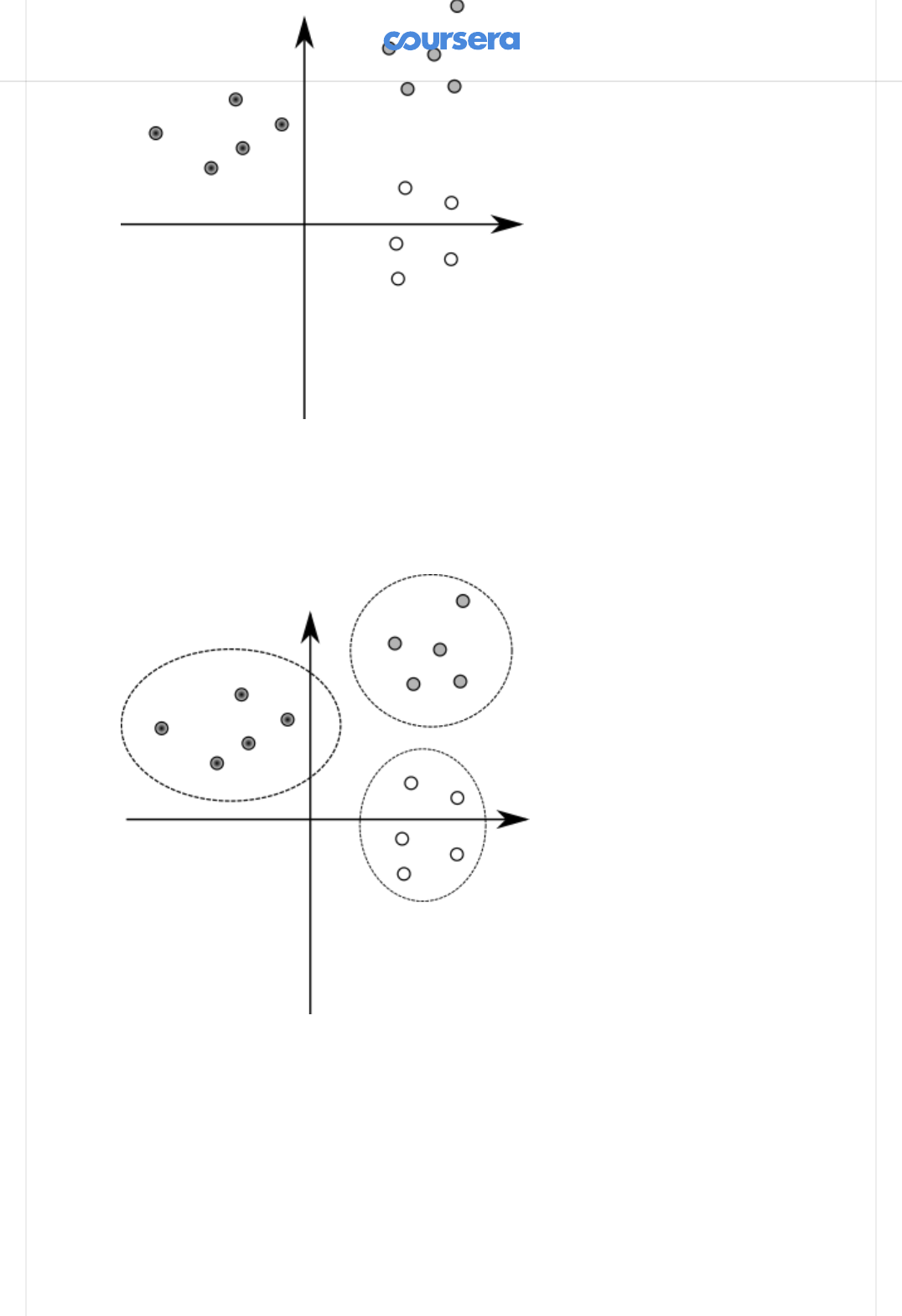
As a human, you can visually distinguish the three clusters of points in the
image:
When the number of clusters, dimensions and vectors grows, it becomes
dicult and even impossible to manually determine the clusters. K-means is a
simple algorithm that takes a set of vectors (called
points
) and outputs as set of
clusters as follows:
1. Pick k points called
means
. This is called
initialization
.
2. Associate each input point with the
mean
that is closest to it. We obtain k
clusters
of points, and we refer to this process as
classifying
the points.
3. Update each mean to have the average value of the corresponding cluster.
4. If the k means have signicantly changed, go back to step 2. If they did not,
we say that the algorithm
converged
.
5. The k means represent dierent clusters -- every point is in the cluster
corresponding to the closest mean.
Above, two steps need additional discussion. First, how do we pick the initial k
means? The initialization step can be done in many dierent ways -- we will just
randomly pick some of the input vectors. Second, how do we know that the
algorithm converged? We will check that, for each mean, the square distance
between the old value of the mean and the new value of the mean is less than
or equal to some value eta.
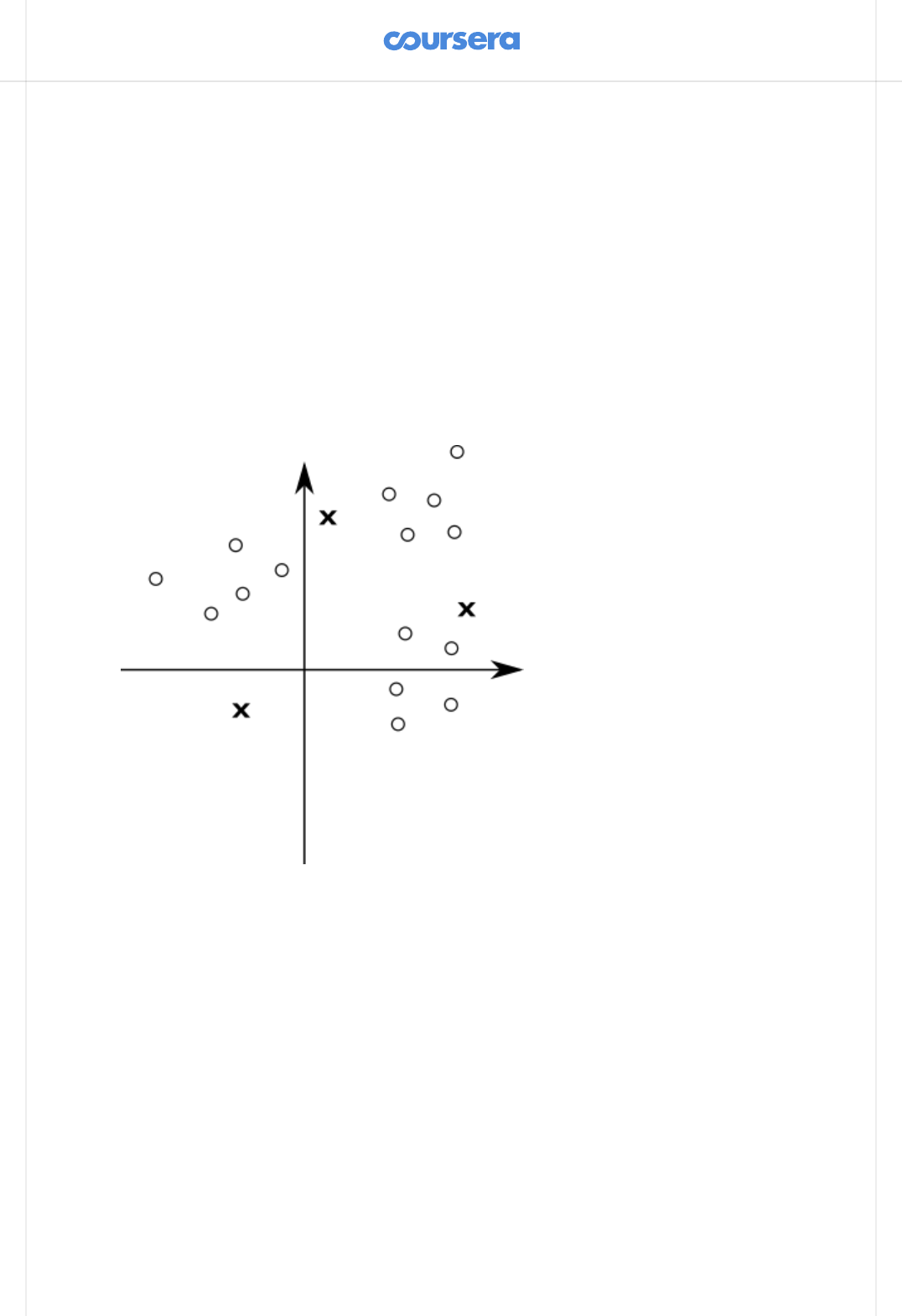
For a better illustration, here are a few steps of the K-means algorithm. Initially,
we pick a random set of means, shown with "X" in the gure:
Then, we classify the points according to the closest mean ("X"). The means
divide the space into regions, where each point is closer to the corresponding
mean than any other mean -- in the gure, the dotted line depicts the borders of
dierent regions:
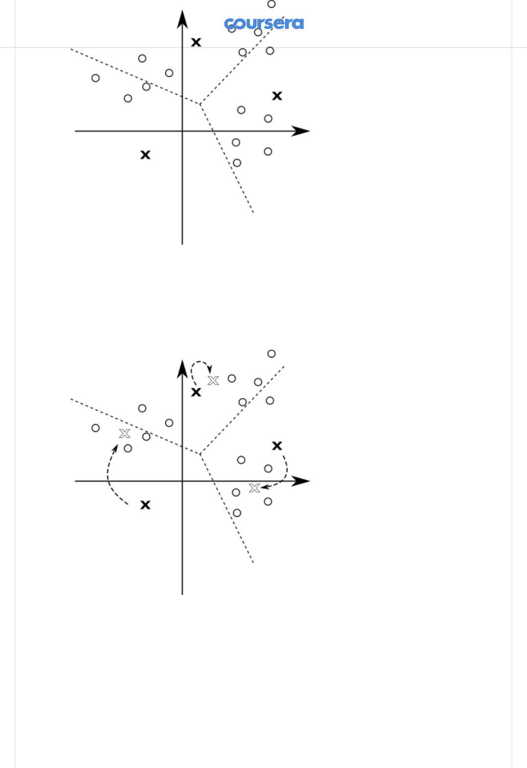
All the points in the same region form one cluster. After having classied the
points, we can update the mean values to the average of all the points in the
cluster:
Each of the means was signicantly updated. This is a good indication that the
algorithm did not yet converge, so we repeat the steps again -- we rst classify
all the points:
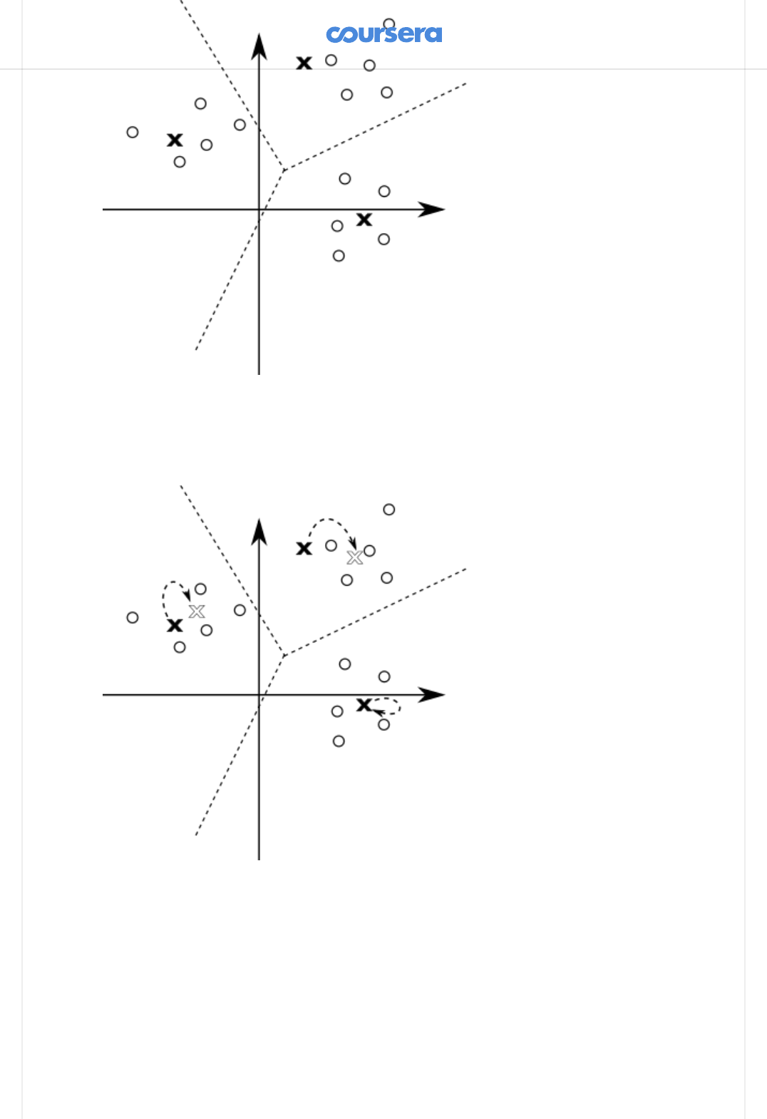
And then we update the means again:
One of the means did not change at all in the last step. Still, other means have
changed so we continue this process until the change in the position of each
point drops below the eta value.
At each iteration of K-means, we can associate multiple points to clusters, and
compute the average of the k clusters, in parallel. Note that the association of a
point to its cluster is independent of the other points in the input, and similarly,
the computation of the average of a cluster is independent of the other clusters.
Once all parallel tasks of the current iteration complete, the algorithm can
proceed to the next iteration.
K-means is an example of a
bulk synchronous parallel
algorithm (BSP). BSP
algorithms are composed from a sequence of supersteps, each of which
contains:
parallel computation
, in which processes independently perform local
computations and produce some values
communication
, in which processes exchange data
barrier synchronisation
, during which processes wait until every process
nishes
Data-parallel programming models are typically a good t for BSP algorithms, as
each bulk synchronous phase can correspond to some number of data-parallel
operations.
Classifying the points
In the rst part of this assignment, you will classify the input points according to
the square distance to the means. Input points are described with the following
Point data-type:
You will start by implementing the classify method:
This method takes a generic sequence of points and a generic sequence of
means. It returns a generic map collection, which maps each mean to the
sequence of points in the corresponding cluster.
Recall from the lectures that generic collection type, such as GenSeq or
GenMap, can be implemented either with a parallel or a sequential collection.
This means that the classify method will either run sequentially or in parallel,
depending on the type of the collection that is passed to it, and returns a
sequential or a parallel map, respectively. The method is
oblivious
to whether
the algorithm is parallel or not.
Hint: Use groupBy and the ndClosest method, which is already dened for
you. After that, make sure that all the means are in the GenMap, even if their
sequences are empty.
Updating the means
In the second part of this assignment, you will update the means corresponding
to dierent clusters.
class Point(val x: Double, val y: Double, val z: Double)
def classify(points: GenSeq[Point], means: GenSeq[Point]):
GenMap[Point, GenSeq[Point]]
1
1

Implement the method update, which takes the map of classied points
produced in the previous step, and the sequence of previous means. The
method returns the new sequence of means:
Once more, the method takes and returns generic collections.
Take care to preserve order in the resulting generic sequence -- the mean i in
the resulting sequence must correspond to the mean i from oldMeans.
Hint: Make sure you use the ndAverage method that is predened for you.
Detecting convergence
Finally, you will implement convergence detection. The convergence detection
method takes a sequence of old means and the sequence of updated means,
and returns a boolean indicating if the algorithm converged or not. Given an eta
parameter, oldMeans and newMeans, it returns true if the algorithm
converged, and false otherwise:
The algorithm converged i the square distance between the old and the new
mean is less than or equal to eta, for all means.
Note: the means in the two lists are ordered -- the mean at i in oldMeans is the
previous value of the mean at i in newMeans.
Implement converged!
Running the algorithm
We now have everything we need to run the K-means algorithm. We only need
to combine the previously dened methods in the right way.
The tail-recursive kMeans method takes a sequence of points points, previously
computed sequence of means means, and the eta value:
The kMeans method should return the sequence of means, each corresponding
to a specic cluster.
Hint: kMeans implements the steps 2-4 from the K-means pseudocode.
Run the algorithm and report the speedup:
def update(classified: GenMap[Point, GenSeq[Point]], oldMeans:
GenSeq[Point]): GenSeq[Point]
def converged(eta: Double)(oldMeans: GenSeq[Point], newMeans:
GenSeq[Point])
@tailrec final def kMeans(points: GenSeq[Point],
means: GenSeq[Point], eta: Double): GenSeq[Point]
1
1
1
2
Use cases
And now for the fun part -- the K-means algorithm has a lot of use-cases!
In image processing applications, it can be used to reduce the size of the color
palette, thus compressing the image. This is done by turning a true color image,
where each pixel is encoded into 32 bits, into indexed color, where each pixel
can be encoded with just a few bits. This is done by using k-means to "cluster"
the important colors in the image, thus reducing its palette from 24-bit (2^24
colors) to just 32 indexed colors, chosen from the 24-bit palette. Here, pixels
from the image are the input vectors, and their coordinates are the dierent
color channels.
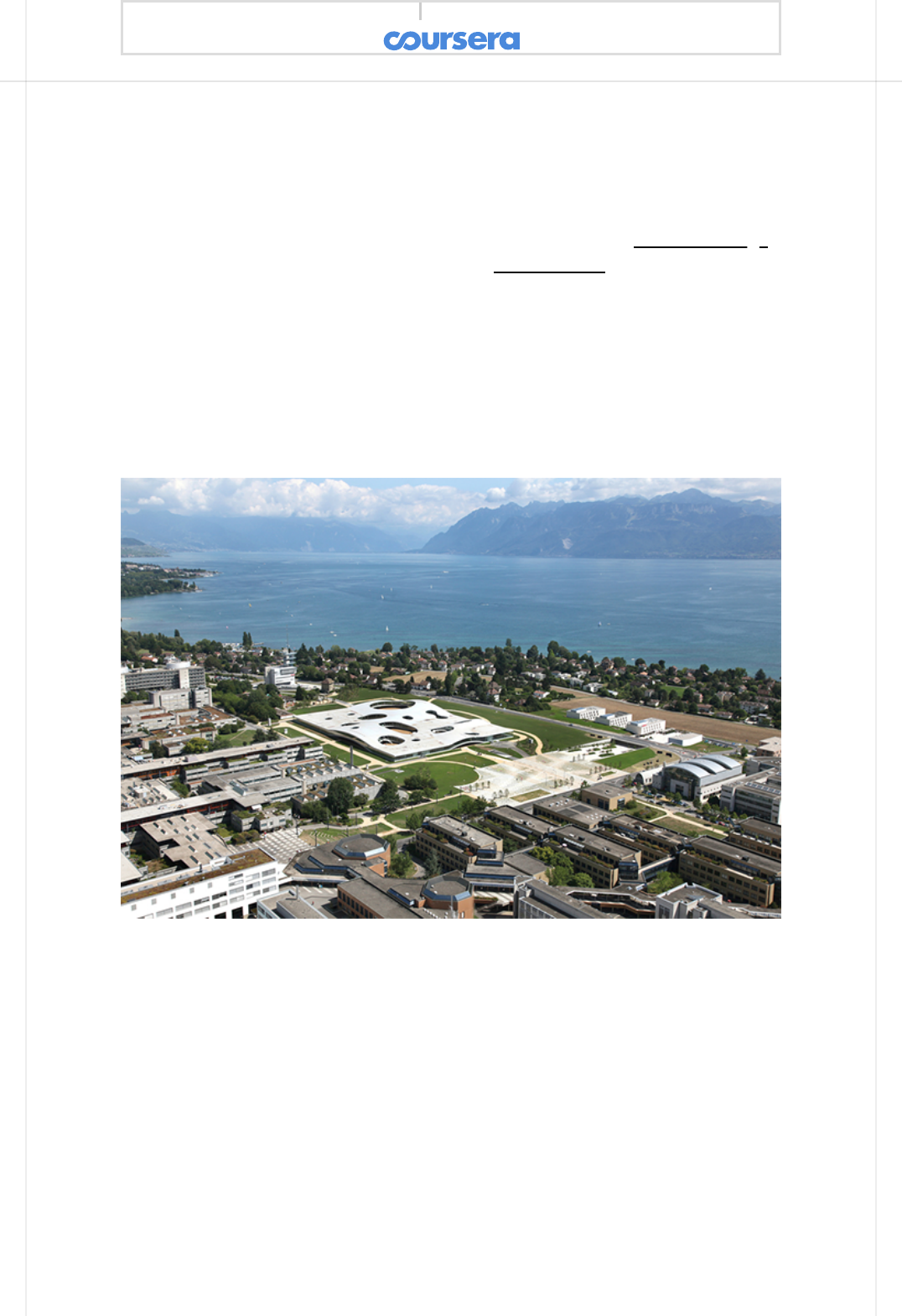
This is the original true color (24-bit) image:
And this is the indexed color (32 colors) version of it:
> runMain kmeans.KMeansRunner1

So, thanks to your k-means implementation, ScalaShop can now compress
images! You can start ScalaShop by invoking:
in sbt.
But before you get to the fun part, you'll need to solve a mystery: why is
ScalaShop so slow? Have a look at the source code, in the fun package.
If you can't nd it,
scroll down for a hint.
Hint 1: look at the top of
fun/IndexedColors.scala
and see the comment.
Scroll down for another hint.
Hint 2: You should be able to make it almost x times faster, where x is the
number of cores in your computer :)
Scroll down for the nal hint.
Hint 3: The two collections could use a .par call, to make them parallel.
After your changes, ScalaShop should be much faster. So, let's play!
> run-main kmeans.fun.ScalaShop1
The k-means algorithm is very sensitive to the initial choice of means. There are
three choice strategies implemented in ScalaShop:
Uniform Choice is the simplest strategy. It chooses n colors uniformly in the
entire color space, regardless of the colors used in the image. If the image
has a dominant color, the means created by this strategy will likely be very far
away from the clusters formed by this dominant color. You can try setting the
Uniform Choice strategy with 1, 10 and 30 steps. You will notice the initial
choice is quite bad, but the quality improves as the k-means algorithm is
applied in more steps.
Random Sampling is another simple strategy, but with better results. For the
initial means, it randomly samples n colors from the image. This yields good
results if the image has few dominant colors, but it cannot handle subtle
nuances in the image. Again, if you try this strategy with 1, 10 and 30 k-means
iteration steps, you will notice improvements as the k-means algorithm is ran
more.
Uniform Random is the most complex strategy to pick means, but it also
produces the best results. It works by uniformly splitting the color space in
sub-spaces. It then counts the number of pixels that have colors belonging to
that sub-space. Based on this number, it chooses a proportional number of
means in the sub-space, by randomly sampling from the pixels in that sub-
space. Therefore, if your image has dominant colors, this strategy will drop a
proportional number of means for each dominant color, thus allowing the k-
means algorithm to capture ne nuances.
In the EPFL image now available in ScalaShop, the mountains are a good way to
see how well each initial choice of means fares. You also have dierent
strategies for deciding convergence:
Steps allows to run a xed number of steps. After this, the k-means algorithm
is stopped.
Eta corresponds to the means stability, as we showed earlier: if the means
did not move much since the last iteration, the result is considered stable.
Sound-to-noise ratio is a more rened convergence strategy, which does not
settle for stability but tries to minimize the dierence between the true color
image and the index color one. This strategy goes beyond Eta, but high
Sound-to-noise ratios will prevent the k-means algorithm from nishing!
With this in mind, enjoy ScalaShop, the ultimate image manipulation tool and
the nice, warm, sunny photo of EPFL!
How to submit
