Kafka: The Definitive Guide Kafka
Kafka%20The%20Definitive%20Guide
Kafka%20The%20Definitive%20Guide
Kafka%20The%20Definitive%20Guide
User Manual:
Open the PDF directly: View PDF ![]() .
.
Page Count: 322 [warning: Documents this large are best viewed by clicking the View PDF Link!]
- Cover
- Confluent
- Copyright
- Table of Contents
- Foreword
- Preface
- Chapter 1. Meet Kafka
- Chapter 2. Installing Kafka
- Chapter 3. Kafka Producers: Writing Messages to Kafka
- Chapter 4. Kafka Consumers: Reading Data from Kafka
- Kafka Consumer Concepts
- Creating a Kafka Consumer
- Subscribing to Topics
- The Poll Loop
- Configuring Consumers
- Commits and Offsets
- Rebalance Listeners
- Consuming Records with Specific Offsets
- But How Do We Exit?
- Deserializers
- Standalone Consumer: Why and How to Use a Consumer Without a Group
- Older Consumer APIs
- Summary
- Chapter 5. Kafka Internals
- Chapter 6. Reliable Data Delivery
- Chapter 7. Building Data Pipelines
- Chapter 8. Cross-Cluster Data Mirroring
- Chapter 9. Administering Kafka
- Chapter 10. Monitoring Kafka
- Chapter 11. Stream Processing
- Appendix A. Installing Kafka on Other Operating Systems
- Index
- About the Authors
- Colophon


Get Started With
Apache Kafka™ Today
• Thoroughly tested and quality assured
• Additional client support, including Python, C/C++ and .NET
• Easy upgrade path to Confluent Enterprise
CONFLUENT OPEN SOURCE
CONNECTORS CLIENTS
SCHEMA REGISTRY REST PROXY
Start today at confluent.io/download
A 100% open source Apache Kafka distribution for building robust
streaming applications.
www.allitebooks.com

978-1-491-99065-0
[LSI]
Kafka: The Denitive Guide
by Neha Narkhede, Gwen Shapira, and Todd Palino
Copyright © 2017 Neha Narkhede, Gwen Shapira, Todd Palino. All rights reserved.
Printed in the United States of America.
Published by O’Reilly Media, Inc., 1005 Gravenstein Highway North, Sebastopol, CA 95472.
O’Reilly books may be purchased for educational, business, or sales promotional use. Online editions are
also available for most titles (http://oreilly.com/safari). For more information, contact our corporate/insti‐
tutional sales department: 800-998-9938 or corporate@oreilly.com.
Editor: Shannon Cutt
Production Editor: Shiny Kalapurakkel
Copyeditor: Christina Edwards
Proofreader: Amanda Kersey
Indexer: WordCo Indexing Services, Inc.
Interior Designer: David Futato
Cover Designer: Karen Montgomery
Illustrator: Rebecca Demarest
July 2017: First Edition
Revision History for the First Edition
2017-07-07: First Release
See http://oreilly.com/catalog/errata.csp?isbn=9781491936160 for release details.
The O’Reilly logo is a registered trademark of O’Reilly Media, Inc. Kaa: e Denitive Guide, the cover
image, and related trade dress are trademarks of O’Reilly Media, Inc.
While the publisher and the authors have used good faith efforts to ensure that the information and
instructions contained in this work are accurate, the publisher and the authors disclaim all responsibility
for errors or omissions, including without limitation responsibility for damages resulting from the use of
or reliance on this work. Use of the information and instructions contained in this work is at your own
risk. If any code samples or other technology this work contains or describes is subject to open source
licenses or the intellectual property rights of others, it is your responsibility to ensure that your use
thereof complies with such licenses and/or rights.
www.allitebooks.com

Table of Contents
Foreword. . . . . . . . . . . . . . . . . . . . . . . . . . . . . . . . . . . . . . . . . . . . . . . . . . . . . . . . . . . . . . . . . . . . xiii
Preface. . . . . . . . . . . . . . . . . . . . . . . . . . . . . . . . . . . . . . . . . . . . . . . . . . . . . . . . . . . . . . . . . . . . . . xvii
1. Meet Kafka. . . . . . . . . . . . . . . . . . . . . . . . . . . . . . . . . . . . . . . . . . . . . . . . . . . . . . . . . . . . . . . . . 1
Publish/Subscribe Messaging 1
How It Starts 2
Individual Queue Systems 3
Enter Kafka 4
Messages and Batches 4
Schemas 5
Topics and Partitions 5
Producers and Consumers 6
Brokers and Clusters 7
Multiple Clusters 8
Why Kafka? 10
Multiple Producers 10
Multiple Consumers 10
Disk-Based Retention 10
Scalable 10
High Performance 11
The Data Ecosystem 11
Use Cases 12
Kafka’s Origin 14
LinkedIn’s Problem 14
The Birth of Kafka 15
Open Source 15
The Name 16
v
www.allitebooks.com

Getting Started with Kafka 16
2. Installing Kafka. . . . . . . . . . . . . . . . . . . . . . . . . . . . . . . . . . . . . . . . . . . . . . . . . . . . . . . . . . . . 17
First Things First 17
Choosing an Operating System 17
Installing Java 17
Installing Zookeeper 18
Installing a Kafka Broker 20
Broker Configuration 21
General Broker 21
Topic Defaults 24
Hardware Selection 28
Disk Throughput 29
Disk Capacity 29
Memory 29
Networking 30
CPU 30
Kafka in the Cloud 30
Kafka Clusters 31
How Many Brokers? 32
Broker Configuration 32
OS Tuning 32
Production Concerns 36
Garbage Collector Options 36
Datacenter Layout 37
Colocating Applications on Zookeeper 37
Summary 39
3. Kafka Producers: Writing Messages to Kafka. . . . . . . . . . . . . . . . . . . . . . . . . . . . . . . . . . . . 41
Producer Overview 42
Constructing a Kafka Producer 44
Sending a Message to Kafka 46
Sending a Message Synchronously 46
Sending a Message Asynchronously 47
Configuring Producers 48
Serializers 52
Custom Serializers 52
Serializing Using Apache Avro 54
Using Avro Records with Kafka 56
Partitions 59
Old Producer APIs 61
Summary 62
vi | Table of Contents
www.allitebooks.com

4. Kafka Consumers: Reading Data from Kafka. . . . . . . . . . . . . . . . . . . . . . . . . . . . . . . . . . . . 63
Kafka Consumer Concepts 63
Consumers and Consumer Groups 63
Consumer Groups and Partition Rebalance 66
Creating a Kafka Consumer 68
Subscribing to Topics 69
The Poll Loop 70
Configuring Consumers 72
Commits and Offsets 75
Automatic Commit 76
Commit Current Offset 77
Asynchronous Commit 78
Combining Synchronous and Asynchronous Commits 80
Commit Specified Offset 80
Rebalance Listeners 82
Consuming Records with Specific Offsets 84
But How Do We Exit? 86
Deserializers 88
Standalone Consumer: Why and How to Use a Consumer Without a Group 92
Older Consumer APIs 93
Summary 93
5. Kafka Internals. . . . . . . . . . . . . . . . . . . . . . . . . . . . . . . . . . . . . . . . . . . . . . . . . . . . . . . . . . . . . 95
Cluster Membership 95
The Controller 96
Replication 97
Request Processing 99
Produce Requests 101
Fetch Requests 102
Other Requests 104
Physical Storage 105
Partition Allocation 106
File Management 107
File Format 108
Indexes 109
Compaction 110
How Compaction Works 110
Deleted Events 112
When Are Topics Compacted? 112
Summary 113
Table of Contents | vii
www.allitebooks.com

6. Reliable Data Delivery. . . . . . . . . . . . . . . . . . . . . . . . . . . . . . . . . . . . . . . . . . . . . . . . . . . . . 115
Reliability Guarantees 116
Replication 117
Broker Configuration 118
Replication Factor 118
Unclean Leader Election 119
Minimum In-Sync Replicas 121
Using Producers in a Reliable System 121
Send Acknowledgments 122
Configuring Producer Retries 123
Additional Error Handling 124
Using Consumers in a Reliable System 125
Important Consumer Configuration Properties for Reliable Processing 126
Explicitly Committing Offsets in Consumers 127
Validating System Reliability 129
Validating Configuration 130
Validating Applications 131
Monitoring Reliability in Production 131
Summary 133
7. Building Data Pipelines. . . . . . . . . . . . . . . . . . . . . . . . . . . . . . . . . . . . . . . . . . . . . . . . . . . . 135
Considerations When Building Data Pipelines 136
Timeliness 136
Reliability 137
High and Varying Throughput 137
Data Formats 138
Transformations 139
Security 139
Failure Handling 140
Coupling and Agility 140
When to Use Kafka Connect Versus Producer and Consumer 141
Kafka Connect 142
Running Connect 142
Connector Example: File Source and File Sink 144
Connector Example: MySQL to Elasticsearch 146
A Deeper Look at Connect 151
Alternatives to Kafka Connect 154
Ingest Frameworks for Other Datastores 155
GUI-Based ETL Tools 155
Stream-Processing Frameworks 155
Summary 156
viii | Table of Contents
www.allitebooks.com

8. Cross-Cluster Data Mirroring. . . . . . . . . . . . . . . . . . . . . . . . . . . . . . . . . . . . . . . . . . . . . . . . 157
Use Cases of Cross-Cluster Mirroring 158
Multicluster Architectures 158
Some Realities of Cross-Datacenter Communication 159
Hub-and-Spokes Architecture 160
Active-Active Architecture 161
Active-Standby Architecture 163
Stretch Clusters 169
Apache Kafka’s MirrorMaker 170
How to Configure 171
Deploying MirrorMaker in Production 172
Tuning MirrorMaker 175
Other Cross-Cluster Mirroring Solutions 178
Uber uReplicator 178
Confluent’s Replicator 179
Summary 180
9. Administering Kafka. . . . . . . . . . . . . . . . . . . . . . . . . . . . . . . . . . . . . . . . . . . . . . . . . . . . . . . 181
Topic Operations 181
Creating a New Topic 182
Adding Partitions 183
Deleting a Topic 184
Listing All Topics in a Cluster 185
Describing Topic Details 185
Consumer Groups 186
List and Describe Groups 186
Delete Group 188
Offset Management 188
Dynamic Configuration Changes 190
Overriding Topic Configuration Defaults 190
Overriding Client Configuration Defaults 192
Describing Configuration Overrides 192
Removing Configuration Overrides 193
Partition Management 193
Preferred Replica Election 193
Changing a Partition’s Replicas 195
Changing Replication Factor 198
Dumping Log Segments 199
Replica Verification 201
Consuming and Producing 202
Console Consumer 202
Console Producer 205
Table of Contents | ix
www.allitebooks.com

Client ACLs 207
Unsafe Operations 207
Moving the Cluster Controller 208
Killing a Partition Move 208
Removing Topics to Be Deleted 209
Deleting Topics Manually 209
Summary 210
10. Monitoring Kafka. . . . . . . . . . . . . . . . . . . . . . . . . . . . . . . . . . . . . . . . . . . . . . . . . . . . . . . . . 211
Metric Basics 211
Where Are the Metrics? 211
Internal or External Measurements 212
Application Health Checks 213
Metric Coverage 213
Kafka Broker Metrics 213
Under-Replicated Partitions 214
Broker Metrics 220
Topic and Partition Metrics 229
JVM Monitoring 231
OS Monitoring 232
Logging 235
Client Monitoring 236
Producer Metrics 236
Consumer Metrics 239
Quotas 242
Lag Monitoring 243
End-to-End Monitoring 244
Summary 244
11. Stream Processing. . . . . . . . . . . . . . . . . . . . . . . . . . . . . . . . . . . . . . . . . . . . . . . . . . . . . . . . . 247
What Is Stream Processing? 248
Stream-Processing Concepts 251
Time 251
State 252
Stream-Table Duality 253
Time Windows 254
Stream-Processing Design Patterns 256
Single-Event Processing 256
Processing with Local State 257
Multiphase Processing/Repartitioning 258
Processing with External Lookup: Stream-Table Join 259
Streaming Join 261
x | Table of Contents

Out-of-Sequence Events 262
Reprocessing 264
Kafka Streams by Example 264
Word Count 265
Stock Market Statistics 268
Click Stream Enrichment 270
Kafka Streams: Architecture Overview 272
Building a Topology 272
Scaling the Topology 273
Surviving Failures 276
Stream Processing Use Cases 277
How to Choose a Stream-Processing Framework 278
Summary 280
A. Installing Kafka on Other Operating Systems. . . . . . . . . . . . . . . . . . . . . . . . . . . . . . . . . . 281
Index. . . . . . . . . . . . . . . . . . . . . . . . . . . . . . . . . . . . . . . . . . . . . . . . . . . . . . . . . . . . . . . . . . . . . . . 287
Table of Contents | xi

Foreword
It’s an exciting time for Apache Kafka. Kafka is being used by tens of thousands of
organizations, including over a third of the Fortune 500 companies. It’s among the
fastest growing open source projects and has spawned an immense ecosystem around
it. It’s at the heart of a movement towards managing and processing streams of data.
So where did Kafka come from? Why did we build it? And what exactly is it?
Kafka got its start as an internal infrastructure system we built at LinkedIn. Our
observation was really simple: there were lots of databases and other systems built to
store data, but what was missing in our architecture was something that would help
us to handle the continuous ow of data. Prior to building Kafka, we experimented
with all kinds of off the shelf options; from messaging systems to log aggregation and
ETL tools, but none of them gave us what we wanted.
We eventually decided to build something from scratch. Our idea was that instead of
focusing on holding piles of data like our relational databases, key-value stores, search
indexes, or caches, we would focus on treating data as a continually evolving and ever
growing stream, and build a data system—and indeed a data architecture—oriented
around that idea.
This idea turned out to be even more broadly applicable than we expected. Though
Kafka got its start powering real-time applications and data flow behind the scenes of
a social network, you can now see it at the heart of next-generation architectures in
every industry imaginable. Big retailers are re-working their fundamental business
processes around continuous data streams; car companies are collecting and process‐
ing real-time data streams from internet-connected cars; and banks are rethinking
their fundamental processes and systems around Kafka as well.
So what is this Kafka thing all about? How does it compare to the systems you already
know and use?
We’ve come to think of Kafka as a streaming platform: a system that lets you publish
and subscribe to streams of data, store them, and process them, and that is exactly
xiii

what Apache Kafka is built to be. Getting used to this way of thinking about data
might be a little different than what you’re used to, but it turns out to be an incredibly
powerful abstraction for building applications and architectures. Kafka is often com‐
pared to a couple of existing technology categories: enterprise messaging systems, big
data systems like Hadoop, and data integration or ETL tools. Each of these compari‐
sons has some validity but also falls a little short.
Kafka is like a messaging system in that it lets you publish and subscribe to streams of
messages. In this way, it is similar to products like ActiveMQ, RabbitMQ, IBM’s
MQSeries, and other products. But even with these similarities, Kafka has a number
of core differences from traditional messaging systems that make it another kind of
animal entirely. Here are the big three differences: first, it works as a modern dis‐
tributed system that runs as a cluster and can scale to handle all the applications in
even the most massive of companies. Rather than running dozens of individual mes‐
saging brokers, hand wired to different apps, this lets you have a central platform that
can scale elastically to handle all the streams of data in a company. Secondly, Kafka is
a true storage system built to store data for as long as you might like. This has huge
advantages in using it as a connecting layer as it provides real delivery guarantees—its
data is replicated, persistent, and can be kept around as long as you like. Finally, the
world of stream processing raises the level of abstraction quite significantly. Messag‐
ing systems mostly just hand out messages. The stream processing capabilities in
Kafka let you compute derived streams and datasets dynamically off of your streams
with far less code. These differences make Kafka enough of its own thing that it
doesn’t really make sense to think of it as “yet another queue.”
Another view on Kafka—and one of our motivating lenses in designing and building
it—was to think of it as a kind of real-time version of Hadoop. Hadoop lets you store
and periodically process file data at a very large scale. Kafka lets you store and contin‐
uously process streams of data, also at a large scale. At a technical level, there are defi‐
nitely similarities, and many people see the emerging area of stream processing as a
superset of the kind of batch processing people have done with Hadoop and its vari‐
ous processing layers. What this comparison misses is that the use cases that continu‐
ous, low-latency processing opens up are quite different from those that naturally fall
on a batch processing system. Whereas Hadoop and big data targeted analytics appli‐
cations, often in the data warehousing space, the low latency nature of Kafka makes it
applicable for the kind of core applications that directly power a business. This makes
sense: events in a business are happening all the time and the ability to react to them
as they occur makes it much easier to build services that directly power the operation
of the business, feed back into customer experiences, and so on.
The final area Kafka gets compared to is ETL or data integration tools. After all, these
tools move data around, and Kafka moves data around. There is some validity to this
as well, but I think the core difference is that Kafka has inverted the problem. Rather
than a tool for scraping data out of one system and inserting it into another, Kafka is
xiv | Foreword

a platform oriented around real-time streams of events. This means that not only can
it connect off-the-shelf applications and data systems, it can power custom applica‐
tions built to trigger off of these same data streams. We think this architecture cen‐
tered around streams of events is a really important thing. In some ways these flows
of data are the most central aspect of a modern digital company, as important as the
cash flows you’d see in a financial statement.
The ability to combine these three areas—to bring all the streams of data together
across all the use cases—is what makes the idea of a streaming platform so appealing
to people.
Still, all of this is a bit different, and learning how to think and build applications ori‐
ented around continuous streams of data is quite a mindshift if you are coming from
the world of request/response style applications and relational databases. This book is
absolutely the best way to learn about Kafka; from internals to APIs, written by some
of the people who know it best. I hope you enjoy reading it as much as I have!
— Jay Kreps
Cofounder and CEO at Conuent
Foreword | xv

Preface
The greatest compliment you can give an author of a technical book is “This is the
book I wish I had when I got started with this subject.” This is the goal we set for our‐
selves when we started writing this book. We looked back at our experience writing
Kafka, running Kafka in production, and helping many companies use Kafka to build
software architectures and manage their data pipelines and we asked ourselves,
“What are the most useful things we can share with new users to take them from
beginner to experts?” This book is a reflection of the work we do every day: run
Apache Kafka and help others use it in the best ways.
We included what we believe you need to know in order to successfully run Apache
Kafka in production and build robust and performant applications on top of it. We
highlighted the popular use cases: message bus for event-driven microservices,
stream-processing applications, and large-scale data pipelines. We also focused on
making the book general and comprehensive enough so it will be useful to anyone
using Kafka, no matter the use case or architecture. We cover practical matters such
as how to install and configure Kafka and how to use the Kafka APIs, and we also
dedicated space to Kafka’s design principles and reliability guarantees, and explore
several of Kafka’s delightful architecture details: the replication protocol, controller,
and storage layer. We believe that knowledge of Kafka’s design and internals is not
only a fun read for those interested in distributed systems, but it is also incredibly
useful for those who are seeking to make informed decisions when they deploy Kafka
in production and design applications that use Kafka. The better you understand how
Kafka works, the more you can make informed decisions regarding the many trade-
offs that are involved in engineering.
One of the problems in software engineering is that there is always more than one
way to do anything. Platforms such as Apache Kafka provide plenty of flexibility,
which is great for experts but makes for a steep learning curve for beginners. Very
often, Apache Kafka tells you how to use a feature but not why you should or
shouldn’t use it. Whenever possible, we try to clarify the existing choices, the trade‐
xvii

offs involved, and when you should and shouldn’t use the different options presented
by Apache Kafka.
Who Should Read This Book
Kaa: e Denitive Guide was written for software engineers who develop applica‐
tions that use Kafka’s APIs and for production engineers (also called SREs, devops, or
sysadmins) who install, configure, tune, and monitor Kafka in production. We also
wrote the book with data architects and data engineers in mind—those responsible
for designing and building an organization’s entire data infrastructure. Some of the
chapters, especially chapters 3, 4, and 11 are geared toward Java developers. Those
chapters assume that the reader is familiar with the basics of the Java programming
language, including topics such as exception handling and concurrency. Other chap‐
ters, especially chapters 2, 8, 9, and 10, assume the reader has some experience run‐
ning Linux and some familiarity with storage and network configuration in Linux.
The rest of the book discusses Kafka and software architectures in more general
terms and does not assume special knowledge.
Another category of people who may find this book interesting are the managers and
architects who don’t work directly with Kafka but work with the people who do. It is
just as important that they understand the guarantees that Kafka provides and the
trade-offs that their employees and coworkers will need to make while building
Kafka-based systems. The book can provide ammunition to managers who would
like to get their staff trained in Apache Kafka or ensure that their teams know what
they need to know.
Conventions Used in This Book
The following typographical conventions are used in this book:
Italic
Indicates new terms, URLs, email addresses, filenames, and file extensions.
Constant width
Used for program listings, as well as within paragraphs to refer to program ele‐
ments such as variable or function names, databases, data types, environment
variables, statements, and keywords.
Constant width bold
Shows commands or other text that should be typed literally by the user.
Constant width italic
Shows text that should be replaced with user-supplied values or by values deter‐
mined by context.
xviii | Preface

This element signifies a tip or suggestion.
This element signifies a general note.
This element indicates a warning or caution.
Using Code Examples
This book is here to help you get your job done. In general, if example code is offered
with this book, you may use it in your programs and documentation. You do not
need to contact us for permission unless you’re reproducing a significant portion of
the code. For example, writing a program that uses several chunks of code from this
book does not require permission. Selling or distributing a CD-ROM of examples
from O’Reilly books does require permission. Answering a question by citing this
book and quoting example code does not require permission. Incorporating a signifi‐
cant amount of example code from this book into your product’s documentation does
require permission.
We appreciate, but do not require, attribution. An attribution usually includes the
title, author, publisher, and ISBN. For example: “Kaa: e Denitive Guide by Neha
Narkhede, Gwen Shapira, and Todd Palino (O’Reilly). Copyright 2017 Neha Nar‐
khede, Gwen Shapira, and Todd Palino, 978-1-491-93616-0.”
If you feel your use of code examples falls outside fair use or the permission given
above, feel free to contact us at permissions@oreilly.com.
O’Reilly Safari
Safari (formerly Safari Books Online) is a membership-based
training and reference platform for enterprise, government,
educators, and individuals.
Preface | xix

Members have access to thousands of books, training videos, Learning Paths, interac‐
tive tutorials, and curated playlists from over 250 publishers, including O’Reilly
Media, Harvard Business Review, Prentice Hall Professional, Addison-Wesley Profes‐
sional, Microsoft Press, Sams, Que, Peachpit Press, Adobe, Focal Press, Cisco Press,
John Wiley & Sons, Syngress, Morgan Kaufmann, IBM Redbooks, Packt, Adobe
Press, FT Press, Apress, Manning, New Riders, McGraw-Hill, Jones & Bartlett, and
Course Technology, among others.
For more information, please visit http://oreilly.com/safari.
How to Contact Us
Please address comments and questions concerning this book to the publisher:
O’Reilly Media, Inc.
1005 Gravenstein Highway North
Sebastopol, CA 95472
800-998-9938 (in the United States or Canada)
707-829-0515 (international or local)
707-829-0104 (fax)
We have a web page for this book, where we list errata, examples, and any additional
information. You can access this page at http://oreil.ly/2tVmYjk.
To comment or ask technical questions about this book, send email to bookques‐
tions@oreilly.com.
For more information about our books, courses, conferences, and news, see our web‐
site at http://www.oreilly.com.
Find us on Facebook: http://facebook.com/oreilly
Follow us on Twitter: http://twitter.com/oreillymedia
Watch us on YouTube: http://www.youtube.com/oreillymedia
Acknowledgments
We would like to thank the many contributors to Apache Kafka and its ecosystem.
Without their work, this book would not exist. Special thanks to Jay Kreps, Neha Nar‐
khede, and Jun Rao, as well as their colleagues and the leadership at LinkedIn, for
cocreating Kafka and contributing it to the Apache Software Foundation.
Many people provided valuable feedback on early versions of the book and we appre‐
ciate their time and expertise: Apurva Mehta, Arseniy Tashoyan, Dylan Scott, Ewen
Cheslack-Postava, Grant Henke, Ismael Juma, James Cheng, Jason Gustafson, Jeff
xx | Preface

Holoman, Joel Koshy, Jonathan Seidman, Matthias Sax, Michael Noll, Paolo Castagna,
and Jesse Anderson. We also want to thank the many readers who left comments and
feedback via the rough-cuts feedback site.
Many reviewers helped us out and greatly improved the quality of this book, so any
mistakes left are our own.
We’d like to thank our O’Reilly editor Shannon Cutt for her encouragement and
patience, and for being far more on top of things than we were. Working with
O’Reilly is a great experience for an author—the support they provide, from tools to
book signings is unparallel. We are grateful to everyone involved in making this hap‐
pen and we appreciate their choice to work with us.
And we’d like to thank our managers and colleagues for enabling and encouraging us
while writing the book.
Gwen wants to thank her husband, Omer Shapira, for his support and patience dur‐
ing the many months spent writing yet another book; her cats, Luke and Lea for being
cuddly; and her dad, Lior Shapira, for teaching her to always say yes to opportunities,
even when it seems daunting.
Todd would be nowhere without his wife, Marcy, and daughters, Bella and Kaylee,
behind him all the way. Their support for all the extra time writing, and long hours
running to clear his head, keeps him going.
Preface | xxi

CHAPTER 1
Meet Kafka
Every enterprise is powered by data. We take information in, analyze it, manipulate it,
and create more as output. Every application creates data, whether it is log messages,
metrics, user activity, outgoing messages, or something else. Every byte of data has a
story to tell, something of importance that will inform the next thing to be done. In
order to know what that is, we need to get the data from where it is created to where
it can be analyzed. We see this every day on websites like Amazon, where our clicks
on items of interest to us are turned into recommendations that are shown to us a
little later.
The faster we can do this, the more agile and responsive our organizations can be.
The less effort we spend on moving data around, the more we can focus on the core
business at hand. This is why the pipeline is a critical component in the data-driven
enterprise. How we move the data becomes nearly as important as the data itself.
Any time scientists disagree, it’s because we have insufficient data. Then we can agree
on what kind of data to get; we get the data; and the data solves the problem. Either I’m
right, or you’re right, or we’re both wrong. And we move on.
—Neil deGrasse Tyson
Publish/Subscribe Messaging
Before discussing the specifics of Apache Kafka, it is important for us to understand
the concept of publish/subscribe messaging and why it is important. Publish/subscribe
messaging is a pattern that is characterized by the sender (publisher) of a piece of data
(message) not specifically directing it to a receiver. Instead, the publisher classifies the
message somehow, and that receiver (subscriber) subscribes to receive certain classes
of messages. Pub/sub systems often have a broker, a central point where messages are
published, to facilitate this.
1
How It Starts
Many use cases for publish/subscribe start out the same way: with a simple message
queue or interprocess communication channel. For example, you create an applica‐
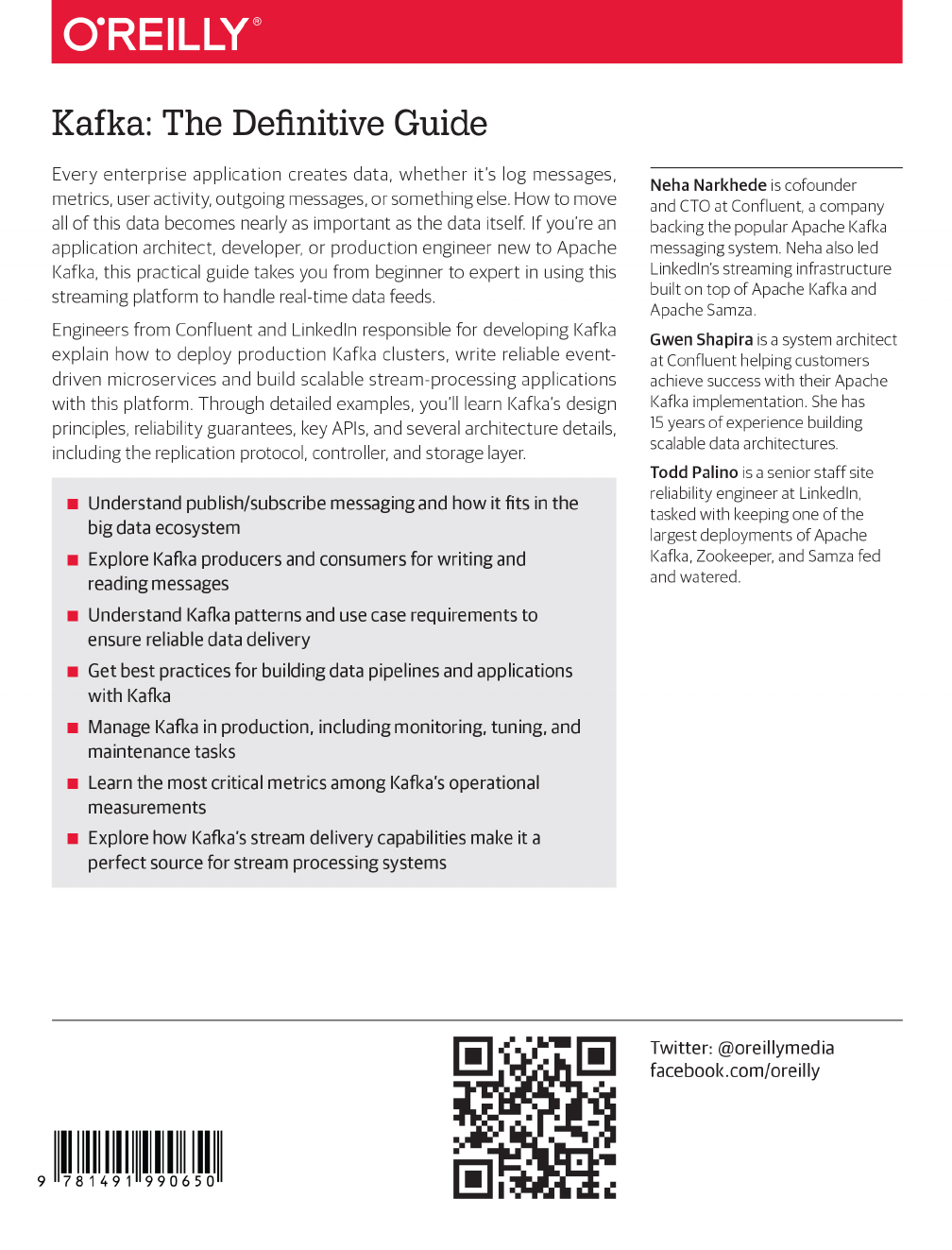
tion that needs to send monitoring information somewhere, so you write in a direct
connection from your application to an app that displays your metrics on a dash‐
board, and push metrics over that connection, as seen in Figure 1-1.
Figure 1-1. A single, direct metrics publisher
This is a simple solution to a simple problem that works when you are getting started
with monitoring. Before long, you decide you would like to analyze your metrics over
a longer term, and that doesn’t work well in the dashboard. You start a new service
that can receive metrics, store them, and analyze them. In order to support this, you
modify your application to write metrics to both systems. By now you have three
more applications that are generating metrics, and they all make the same connec‐
tions to these two services. Your coworker thinks it would be a good idea to do active
polling of the services for alerting as well, so you add a server on each of the applica‐
tions to provide metrics on request. After a while, you have more applications that
are using those servers to get individual metrics and use them for various purposes.
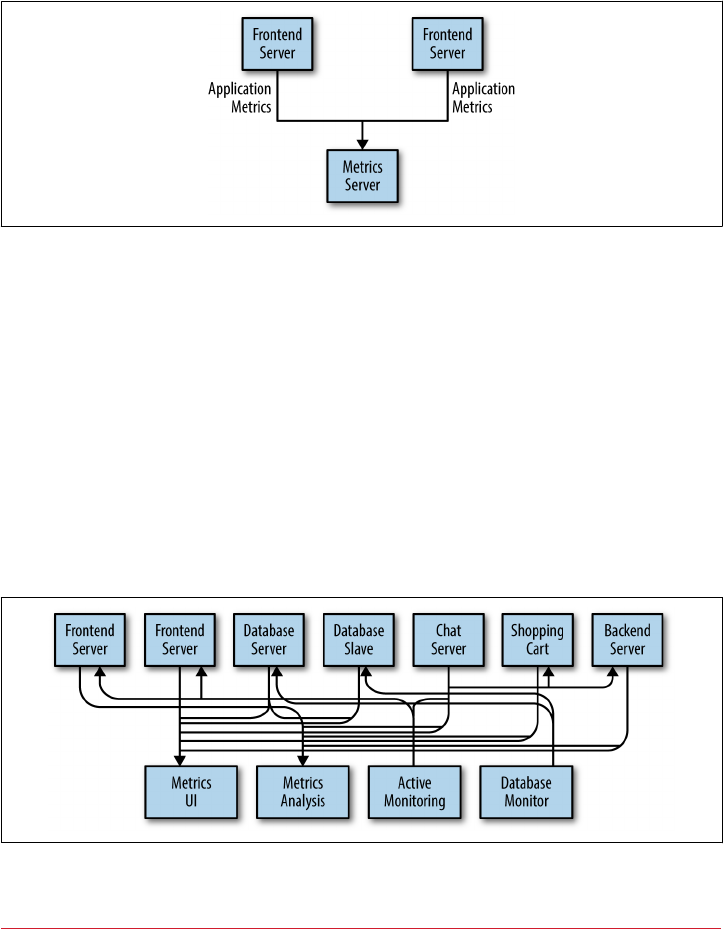
This architecture can look much like Figure 1-2, with connections that are even
harder to trace.
Figure 1-2. Many metrics publishers, using direct connections
2 | Chapter 1: Meet Kafka
The technical debt built up here is obvious, so you decide to pay some of it back. You
set up a single application that receives metrics from all the applications out there,
and provide a server to query those metrics for any system that needs them. This
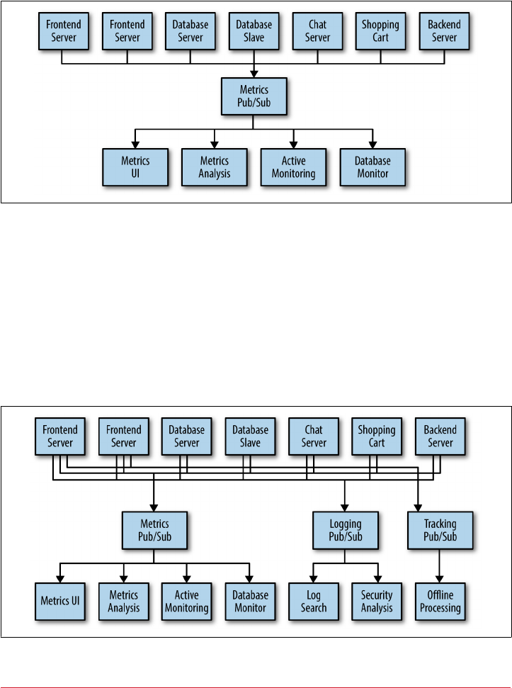
reduces the complexity of the architecture to something similar to Figure 1-3. Con‐
gratulations, you have built a publish-subscribe messaging system!
Figure 1-3. A metrics publish/subscribe system
Individual Queue Systems
At the same time that you have been waging this war with metrics, one of your cow‐
orkers has been doing similar work with log messages. Another has been working on
tracking user behavior on the frontend website and providing that information to
developers who are working on machine learning, as well as creating some reports for
management. You have all followed a similar path of building out systems that decou‐
ple the publishers of the information from the subscribers to that information.
Figure 1-4 shows such an infrastructure, with three separate pub/sub systems.
Figure 1-4. Multiple publish/subscribe systems
Publish/Subscribe Messaging | 3

This is certainly a lot better than utilizing point-to-point connections (as in
Figure 1-2), but there is a lot of duplication. Your company is maintaining multiple
systems for queuing data, all of which have their own individual bugs and limitations.
You also know that there will be more use cases for messaging coming soon. What
you would like to have is a single centralized system that allows for publishing generic
types of data, which will grow as your business grows.
Enter Kafka
Apache Kafka is a publish/subscribe messaging system designed to solve this prob‐
lem. It is often described as a “distributed commit log” or more recently as a “distrib‐
uting streaming platform.” A filesystem or database commit log is designed to
provide a durable record of all transactions so that they can be replayed to consis‐
tently build the state of a system. Similarly, data within Kafka is stored durably, in
order, and can be read deterministically. In addition, the data can be distributed
within the system to provide additional protections against failures, as well as signifi‐
cant opportunities for scaling performance.
Messages and Batches
The unit of data within Kafka is called a message. If you are approaching Kafka from a
database background, you can think of this as similar to a row or a record. A message
is simply an array of bytes as far as Kafka is concerned, so the data contained within it
does not have a specific format or meaning to Kafka. A message can have an optional
bit of metadata, which is referred to as a key. The key is also a byte array and, as with
the message, has no specific meaning to Kafka. Keys are used when messages are to
be written to partitions in a more controlled manner. The simplest such scheme is to
generate a consistent hash of the key, and then select the partition number for that
message by taking the result of the hash modulo, the total number of partitions in the
topic. This assures that messages with the same key are always written to the same
partition. Keys are discussed in more detail in Chapter 3.
For efficiency, messages are written into Kafka in batches. A batch is just a collection
of messages, all of which are being produced to the same topic and partition. An indi‐
vidual roundtrip across the network for each message would result in excessive over‐
head, and collecting messages together into a batch reduces this. Of course, this is a
tradeoff between latency and throughput: the larger the batches, the more messages
that can be handled per unit of time, but the longer it takes an individual message to
propagate. Batches are also typically compressed, providing more efficient data trans‐
fer and storage at the cost of some processing power.
4 | Chapter 1: Meet Kafka

Schemas
While messages are opaque byte arrays to Kafka itself, it is recommended that addi‐
tional structure, or schema, be imposed on the message content so that it can be easily
understood. There are many options available for message schema, depending on
your application’s individual needs. Simplistic systems, such as Javascript Object
Notation (JSON) and Extensible Markup Language (XML), are easy to use and
human-readable. However, they lack features such as robust type handling and com‐
patibility between schema versions. Many Kafka developers favor the use of Apache
Avro, which is a serialization framework originally developed for Hadoop. Avro pro‐
vides a compact serialization format; schemas that are separate from the message pay‐
loads and that do not require code to be generated when they change; and strong data
typing and schema evolution, with both backward and forward compatibility.
A consistent data format is important in Kafka, as it allows writing and reading mes‐
sages to be decoupled. When these tasks are tightly coupled, applications that sub‐
scribe to messages must be updated to handle the new data format, in parallel with
the old format. Only then can the applications that publish the messages be updated
to utilize the new format. By using well-defined schemas and storing them in a com‐
mon repository, the messages in Kafka can be understood without coordination.
Schemas and serialization are covered in more detail in Chapter 3.
Topics and Partitions
Messages in Kafka are categorized into topics. The closest analogies for a topic are a
database table or a folder in a filesystem. Topics are additionally broken down into a
number of partitions. Going back to the “commit log” description, a partition is a sin‐
gle log. Messages are written to it in an append-only fashion, and are read in order
from beginning to end. Note that as a topic typically has multiple partitions, there is
no guarantee of message time-ordering across the entire topic, just within a single
partition. Figure 1-5 shows a topic with four partitions, with writes being appended
to the end of each one. Partitions are also the way that Kafka provides redundancy
and scalability. Each partition can be hosted on a different server, which means that a
single topic can be scaled horizontally across multiple servers to provide performance
far beyond the ability of a single server.
Enter Kafka | 5
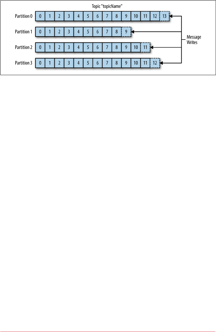
Figure 1-5. Representation of a topic with multiple partitions
The term stream is often used when discussing data within systems like Kafka. Most
often, a stream is considered to be a single topic of data, regardless of the number of
partitions. This represents a single stream of data moving from the producers to the
consumers. This way of referring to messages is most common when discussing
stream processing, which is when frameworks—some of which are Kafka Streams,
Apache Samza, and Storm—operate on the messages in real time. This method of
operation can be compared to the way offline frameworks, namely Hadoop, are
designed to work on bulk data at a later time. An overview of stream processing is
provided in Chapter 11.
Producers and Consumers
Kafka clients are users of the system, and there are two basic types: producers and
consumers. There are also advanced client APIs—Kafka Connect API for data inte‐
gration and Kafka Streams for stream processing. The advanced clients use producers
and consumers as building blocks and provide higher-level functionality on top.
Producers create new messages. In other publish/subscribe systems, these may be
called publishers or writers. In general, a message will be produced to a specific topic.
By default, the producer does not care what partition a specific message is written to
and will balance messages over all partitions of a topic evenly. In some cases, the pro‐
ducer will direct messages to specific partitions. This is typically done using the mes‐
sage key and a partitioner that will generate a hash of the key and map it to a specific
partition. This assures that all messages produced with a given key will get written to
the same partition. The producer could also use a custom partitioner that follows
other business rules for mapping messages to partitions. Producers are covered in
more detail in Chapter 3.
Consumers read messages. In other publish/subscribe systems, these clients may be
called subscribers or readers. The consumer subscribes to one or more topics and
reads the messages in the order in which they were produced. The consumer keeps
track of which messages it has already consumed by keeping track of the offset of
6 | Chapter 1: Meet Kafka
messages. The oset is another bit of metadata—an integer value that continually
increases—that Kafka adds to each message as it is produced. Each message in a given
partition has a unique offset. By storing the offset of the last consumed message for
each partition, either in Zookeeper or in Kafka itself, a consumer can stop and restart
without losing its place.
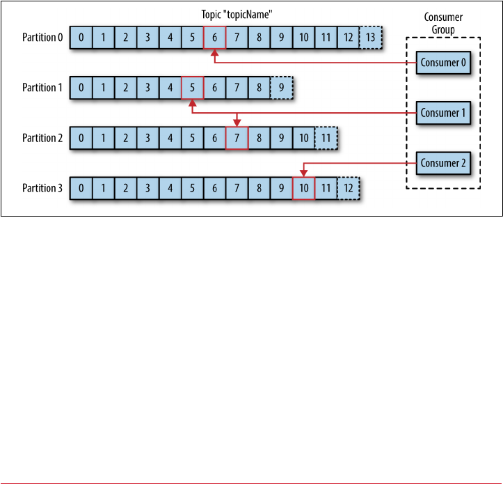
Consumers work as part of a consumer group, which is one or more consumers that
work together to consume a topic. The group assures that each partition is only con‐
sumed by one member. In Figure 1-6, there are three consumers in a single group
consuming a topic. Two of the consumers are working from one partition each, while
the third consumer is working from two partitions. The mapping of a consumer to a
partition is often called ownership of the partition by the consumer.
In this way, consumers can horizontally scale to consume topics with a large number
of messages. Additionally, if a single consumer fails, the remaining members of the
group will rebalance the partitions being consumed to take over for the missing
member. Consumers and consumer groups are discussed in more detail in Chapter 4.
Figure 1-6. A consumer group reading from a topic
Brokers and Clusters
A single Kafka server is called a broker. The broker receives messages from producers,
assigns offsets to them, and commits the messages to storage on disk. It also services
consumers, responding to fetch requests for partitions and responding with the mes‐
sages that have been committed to disk. Depending on the specific hardware and its
performance characteristics, a single broker can easily handle thousands of partitions
and millions of messages per second.
Kafka brokers are designed to operate as part of a cluster. Within a cluster of brokers,
one broker will also function as the cluster controller (elected automatically from the
live members of the cluster). The controller is responsible for administrative opera‐
Enter Kafka | 7
www.allitebooks.com
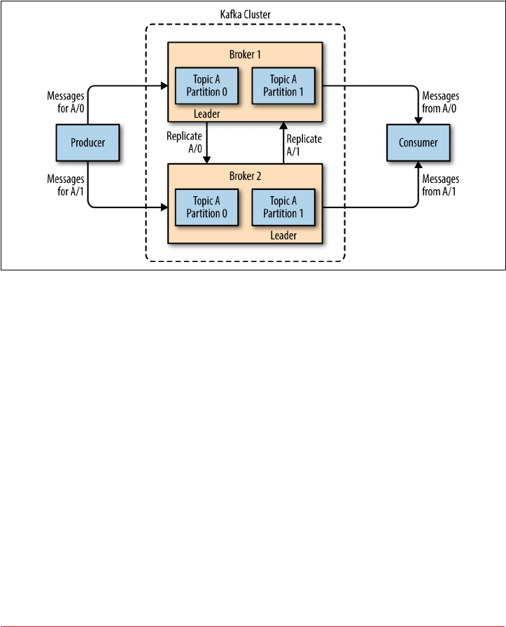
tions, including assigning partitions to brokers and monitoring for broker failures. A
partition is owned by a single broker in the cluster, and that broker is called the leader
of the partition. A partition may be assigned to multiple brokers, which will result in
the partition being replicated (as seen in Figure 1-7). This provides redundancy of
messages in the partition, such that another broker can take over leadership if there is
a broker failure. However, all consumers and producers operating on that partition
must connect to the leader. Cluster operations, including partition replication, are
covered in detail in Chapter 6.
Figure 1-7. Replication of partitions in a cluster
A key feature of Apache Kafka is that of retention, which is the durable storage of
messages for some period of time. Kafka brokers are configured with a default reten‐
tion setting for topics, either retaining messages for some period of time (e.g., 7 days)
or until the topic reaches a certain size in bytes (e.g., 1 GB). Once these limits are
reached, messages are expired and deleted so that the retention configuration is a
minimum amount of data available at any time. Individual topics can also be config‐
ured with their own retention settings so that messages are stored for only as long as
they are useful. For example, a tracking topic might be retained for several days,
whereas application metrics might be retained for only a few hours. Topics can also
be configured as log compacted, which means that Kafka will retain only the last mes‐
sage produced with a specific key. This can be useful for changelog-type data, where
only the last update is interesting.
Multiple Clusters
As Kafka deployments grow, it is often advantageous to have multiple clusters. There
are several reasons why this can be useful:
8 | Chapter 1: Meet Kafka
• Segregation of types of data
• Isolation for security requirements
• Multiple datacenters (disaster recovery)
When working with multiple datacenters in particular, it is often required that mes‐
sages be copied between them. In this way, online applications can have access to user
activity at both sites. For example, if a user changes public information in their pro‐
file, that change will need to be visible regardless of the datacenter in which search
results are displayed. Or, monitoring data can be collected from many sites into a sin‐
gle central location where the analysis and alerting systems are hosted. The replica‐
tion mechanisms within the Kafka clusters are designed only to work within a single
cluster, not between multiple clusters.
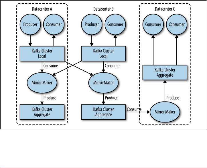
The Kafka project includes a tool called MirrorMaker, used for this purpose. At its
core, MirrorMaker is simply a Kafka consumer and producer, linked together with a
queue. Messages are consumed from one Kafka cluster and produced for another.
Figure 1-8 shows an example of an architecture that uses MirrorMaker, aggregating
messages from two local clusters into an aggregate cluster, and then copying that
cluster to other datacenters. The simple nature of the application belies its power in
creating sophisticated data pipelines, which will be detailed further in Chapter 7.
Figure 1-8. Multiple datacenter architecture
Enter Kafka | 9

Why Kafka?
There are many choices for publish/subscribe messaging systems, so what makes
Apache Kafka a good choice?
Multiple Producers
Kafka is able to seamlessly handle multiple producers, whether those clients are using
many topics or the same topic. This makes the system ideal for aggregating data from
many frontend systems and making it consistent. For example, a site that serves con‐
tent to users via a number of microservices can have a single topic for page views that
all services can write to using a common format. Consumer applications can then
receive a single stream of page views for all applications on the site without having to
coordinate consuming from multiple topics, one for each application.
Multiple Consumers
In addition to multiple producers, Kafka is designed for multiple consumers to read
any single stream of messages without interfering with each other. This is in contrast
to many queuing systems where once a message is consumed by one client, it is not
available to any other. Multiple Kafka consumers can choose to operate as part of a
group and share a stream, assuring that the entire group processes a given message
only once.
Disk-Based Retention
Not only can Kafka handle multiple consumers, but durable message retention means
that consumers do not always need to work in real time. Messages are committed to
disk, and will be stored with configurable retention rules. These options can be
selected on a per-topic basis, allowing for different streams of messages to have differ‐
ent amounts of retention depending on the consumer needs. Durable retention
means that if a consumer falls behind, either due to slow processing or a burst in traf‐
fic, there is no danger of losing data. It also means that maintenance can be per‐
formed on consumers, taking applications offline for a short period of time, with no
concern about messages backing up on the producer or getting lost. Consumers can
be stopped, and the messages will be retained in Kafka. This allows them to restart
and pick up processing messages where they left off with no data loss.
Scalable
Kafka’s flexible scalability makes it easy to handle any amount of data. Users can start
with a single broker as a proof of concept, expand to a small development cluster of
three brokers, and move into production with a larger cluster of tens or even hun‐
dreds of brokers that grows over time as the data scales up. Expansions can be per‐
10 | Chapter 1: Meet Kafka

formed while the cluster is online, with no impact on the availability of the system as
a whole. This also means that a cluster of multiple brokers can handle the failure of
an individual broker, and continue servicing clients. Clusters that need to tolerate
more simultaneous failures can be configured with higher replication factors. Repli‐
cation is discussed in more detail in Chapter 6.
High Performance
All of these features come together to make Apache Kafka a publish/subscribe mes‐
saging system with excellent performance under high load. Producers, consumers,
and brokers can all be scaled out to handle very large message streams with ease. This
can be done while still providing subsecond message latency from producing a mes‐
sage to availability to consumers.
The Data Ecosystem
Many applications participate in the environments we build for data processing. We
have defined inputs in the form of applications that create data or otherwise intro‐
duce it to the system. We have defined outputs in the form of metrics, reports, and
other data products. We create loops, with some components reading data from the
system, transforming it using data from other sources, and then introducing it back
into the data infrastructure to be used elsewhere. This is done for numerous types of
data, with each having unique qualities of content, size, and usage.
Apache Kafka provides the circulatory system for the data ecosystem, as shown in
Figure 1-9. It carries messages between the various members of the infrastructure,
providing a consistent interface for all clients. When coupled with a system to pro‐
vide message schemas, producers and consumers no longer require tight coupling or
direct connections of any sort. Components can be added and removed as business
cases are created and dissolved, and producers do not need to be concerned about
who is using the data or the number of consuming applications.
The Data Ecosystem | 11
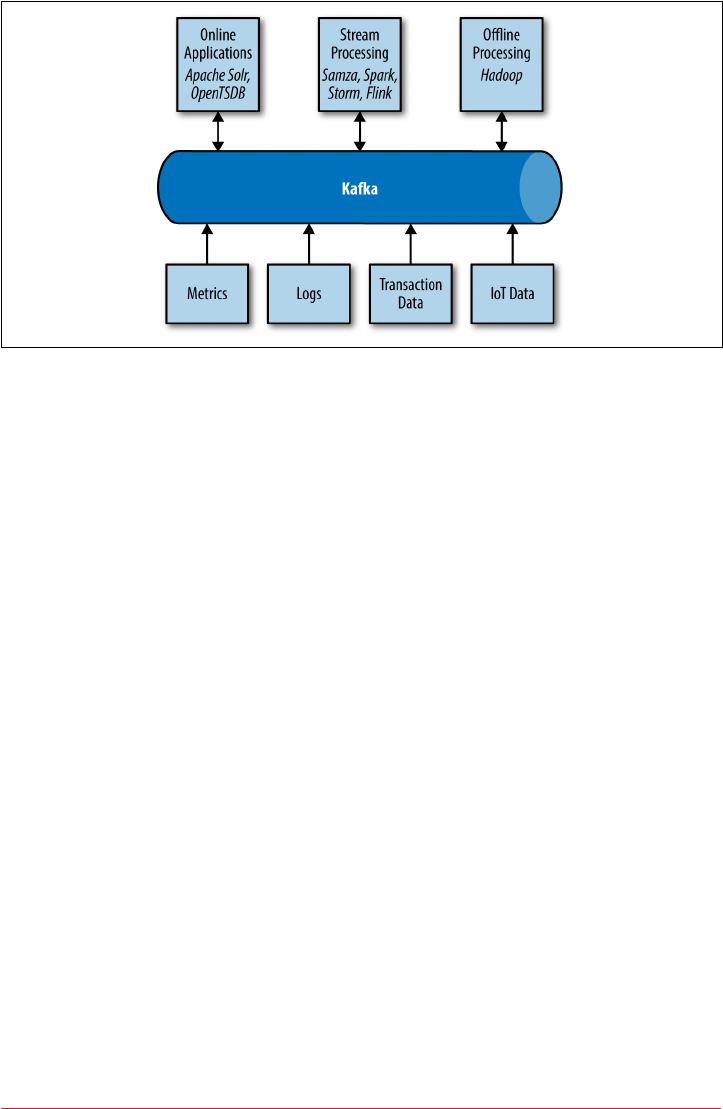
Figure 1-9. A big data ecosystem
Use Cases
Activity tracking
The original use case for Kafka, as it was designed at LinkedIn, is that of user activity
tracking. A website’s users interact with frontend applications, which generate mes‐
sages regarding actions the user is taking. This can be passive information, such as
page views and click tracking, or it can be more complex actions, such as information
that a user adds to their profile. The messages are published to one or more topics,
which are then consumed by applications on the backend. These applications may be
generating reports, feeding machine learning systems, updating search results, or per‐
forming other operations that are necessary to provide a rich user experience.
Messaging
Kafka is also used for messaging, where applications need to send notifications (such
as emails) to users. Those applications can produce messages without needing to be
concerned about formatting or how the messages will actually be sent. A single appli‐
cation can then read all the messages to be sent and handle them consistently,
including:
•Formatting the messages (also known as decorating) using a common look and
feel
•Collecting multiple messages into a single notification to be sent
• Applying a user’s preferences for how they want to receive messages
12 | Chapter 1: Meet Kafka

Using a single application for this avoids the need to duplicate functionality in multi‐
ple applications, as well as allows operations like aggregation which would not other‐
wise be possible.
Metrics and logging
Kafka is also ideal for collecting application and system metrics and logs. This is a use
case in which the ability to have multiple applications producing the same type of
message shines. Applications publish metrics on a regular basis to a Kafka topic, and
those metrics can be consumed by systems for monitoring and alerting. They can also
be used in an offline system like Hadoop to perform longer-term analysis, such as
growth projections. Log messages can be published in the same way, and can be
routed to dedicated log search systems like Elastisearch or security analysis applica‐
tions. Another added benefit of Kafka is that when the destination system needs to
change (e.g., it’s time to update the log storage system), there is no need to alter the
frontend applications or the means of aggregation.
Commit log
Since Kafka is based on the concept of a commit log, database changes can be pub‐
lished to Kafka and applications can easily monitor this stream to receive live updates
as they happen. This changelog stream can also be used for replicating database
updates to a remote system, or for consolidating changes from multiple applications
into a single database view. Durable retention is useful here for providing a buffer for
the changelog, meaning it can be replayed in the event of a failure of the consuming
applications. Alternately, log-compacted topics can be used to provide longer reten‐
tion by only retaining a single change per key.
Stream processing
Another area that provides numerous types of applications is stream processing.
While almost all usage of Kafka can be thought of as stream processing, the term is
typically used to refer to applications that provide similar functionality to map/reduce
processing in Hadoop. Hadoop usually relies on aggregation of data over a long time
frame, either hours or days. Stream processing operates on data in real time, as
quickly as messages are produced. Stream frameworks allow users to write small
applications to operate on Kafka messages, performing tasks such as counting met‐
rics, partitioning messages for efficient processing by other applications, or trans‐
forming messages using data from multiple sources. Stream processing is covered in
Chapter 11.
The Data Ecosystem | 13

Kafka’s Origin
Kafka was created to address the data pipeline problem at LinkedIn. It was designed
to provide a high-performance messaging system that can handle many types of data
and provide clean, structured data about user activity and system metrics in real time.
Data really powers everything that we do.
—Jeff Weiner, CEO of LinkedIn
LinkedIn’s Problem
Similar to the example described at the beginning of this chapter, LinkedIn had a sys‐
tem for collecting system and application metrics that used custom collectors and
open source tools for storing and presenting data internally. In addition to traditional
metrics, such as CPU usage and application performance, there was a sophisticated
request-tracing feature that used the monitoring system and could provide introspec‐
tion into how a single user request propagated through internal applications. The
monitoring system had many faults, however. This included metrics collection based
on polling, large intervals between metrics, and no ability for application owners to
manage their own metrics. The system was high-touch, requiring human interven‐
tion for most simple tasks, and inconsistent, with differing metric names for the same
measurement across different systems.
At the same time, there was a system created for tracking user activity information.
This was an HTTP service that frontend servers would connect to periodically and
publish a batch of messages (in XML format) to the HTTP service. These batches
were then moved to offline processing, which is where the files were parsed and colla‐
ted. This system had many faults. The XML formatting was inconsistent, and parsing
it was computationally expensive. Changing the type of user activity that was tracked
required a significant amount of coordinated work between frontends and offline
processing. Even then, the system would break constantly due to changing schemas.
Tracking was built on hourly batching, so it could not be used in real-time.
Monitoring and user-activity tracking could not use the same backend service. The
monitoring service was too clunky, the data format was not oriented for activity
tracking, and the polling model for monitoring was not compatible with the push
model for tracking. At the same time, the tracking service was too fragile to use for
metrics, and the batch-oriented processing was not the right model for real-time
monitoring and alerting. However, the monitoring and tracking data shared many
traits, and correlation of the information (such as how specific types of user activity
affected application performance) was highly desirable. A drop in specific types of
user activity could indicate problems with the application that serviced it, but hours
of delay in processing activity batches meant a slow response to these types of issues.
14 | Chapter 1: Meet Kafka

At first, existing off-the-shelf open source solutions were thoroughly investigated to
find a new system that would provide real-time access to the data and scale out to
handle the amount of message traffic needed. Prototype systems were set up using
ActiveMQ, but at the time it could not handle the scale. It was also a fragile solution
for the way LinkedIn needed to use it, discovering many flaws in ActiveMQ that
would cause the brokers to pause. This would back up connections to clients and
interfere with the ability of the applications to serve requests to users. The decision
was made to move forward with a custom infrastructure for the data pipeline.
The Birth of Kafka
The development team at LinkedIn was led by Jay Kreps, a principal software engi‐
neer who was previously responsible for the development and open source release of
Voldemort, a distributed key-value storage system. The initial team also included
Neha Narkhede and, later, Jun Rao. Together, they set out to create a messaging sys‐
tem that could meet the needs of both the monitoring and tracking systems, and scale
for the future. The primary goals were to:
• Decouple producers and consumers by using a push-pull model
•Provide persistence for message data within the messaging system to allow multi‐
ple consumers
•Optimize for high throughput of messages
• Allow for horizontal scaling of the system to grow as the data streams grew
The result was a publish/subscribe messaging system that had an interface typical of
messaging systems but a storage layer more like a log-aggregation system. Combined
with the adoption of Apache Avro for message serialization, Kafka was effective for
handling both metrics and user-activity tracking at a scale of billions of messages per
day. The scalability of Kafka has helped LinkedIn’s usage grow in excess of one trillion
messages produced (as of August 2015) and over a petabyte of data consumed daily.
Open Source
Kafka was released as an open source project on GitHub in late 2010. As it started to
gain attention in the open source community, it was proposed and accepted as an
Apache Software Foundation incubator project in July of 2011. Apache Kafka gradu‐
ated from the incubator in October of 2012. Since then, it has continuously been
worked on and has found a robust community of contributors and committers out‐
side of LinkedIn. Kafka is now used in some of the largest data pipelines in the world.
In the fall of 2014, Jay Kreps, Neha Narkhede, and Jun Rao left LinkedIn to found
Confluent, a company centered around providing development, enterprise support,
and training for Apache Kafka. The two companies, along with ever-growing contri‐
Kafka’s Origin | 15

butions from others in the open source community, continue to develop and main‐
tain Kafka, making it the first choice for big data pipelines.
The Name
People often ask how Kafka got its name and if it has anything to do with the applica‐
tion itself. Jay Kreps offered the following insight:
I thought that since Kafka was a system optimized for writing, using a writer’s name
would make sense. I had taken a lot of lit classes in college and liked Franz Kafka. Plus
the name sounded cool for an open source project.
So basically there is not much of a relationship.
Getting Started with Kafka
Now that we know all about Kafka and its history, we can set it up and build our own
data pipeline. In the next chapter, we will explore installing and configuring Kafka.
We will also cover selecting the right hardware to run Kafka on, and some things to
keep in mind when moving to production operations.
16 | Chapter 1: Meet Kafka

CHAPTER 2
Installing Kafka
This chapter describes how to get started with the Apache Kafka broker, including
how to set up Apache Zookeeper, which is used by Kafka for storing metadata for the
brokers. The chapter will also cover the basic configuration options for a Kafka
deployment, as well as criteria for selecting the correct hardware to run the brokers
on. Finally, we cover how to install multiple Kafka brokers as part of a single cluster
and some specific concerns when using Kafka in a production environment.
First Things First
There are a few things that need to happen before using Apache Kafka. The following
sections tell you what those things are.
Choosing an Operating System
Apache Kafka is a Java application, and can run on many operating systems. This
includes Windows, MacOS, Linux, and others. The installation steps in this chapter
will be focused on setting up and using Kafka in a Linux environment, as this is the
most common OS on which it is installed. This is also the recommended OS for
deploying Kafka for general use. For information on installing Kafka on Windows
and MacOS, see Appendix A.
Installing Java
Prior to installing either Zookeeper or Kafka, you will need a Java environment set up
and functioning. This should be a Java 8 version, and can be the version provided by
your OS or one directly downloaded from java.com. Though Zookeeper and Kafka
will work with a runtime edition of Java, it may be more convenient when developing
tools and applications to have the full Java Development Kit (JDK). The installation
17
steps will assume you have installed JDK version 8 update 51 in /usr/java/
jdk1.8.0_51.
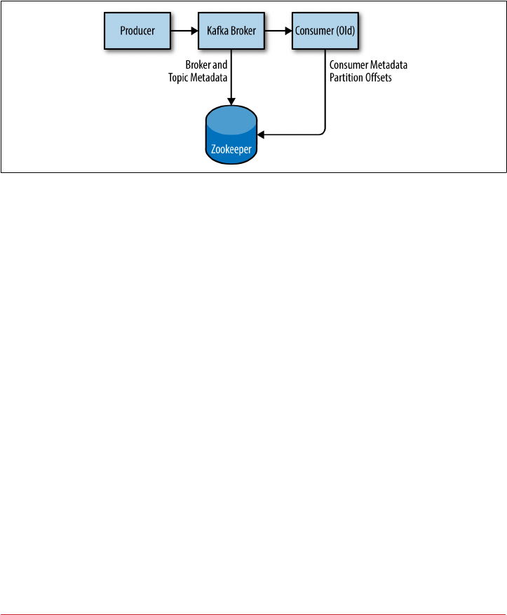
Installing Zookeeper
Apache Kafka uses Zookeeper to store metadata about the Kafka cluster, as well as
consumer client details, as shown in Figure 2-1. While it is possible to run a Zoo‐
keeper server using scripts contained in the Kafka distribution, it is trivial to install a
full version of Zookeeper from the distribution.
Figure 2-1. Kaa and Zookeeper
Kafka has been tested extensively with the stable 3.4.6 release of Zookeeper, which
can be downloaded from apache.org at http://bit.ly/2sDWSgJ.
Standalone Server
The following example installs Zookeeper with a basic configuration in /usr/local/
zookeeper, storing its data in /var/lib/zookeeper:
# tar -zxf zookeeper-3.4.6.tar.gz
# mv zookeeper-3.4.6 /usr/local/zookeeper
# mkdir -p /var/lib/zookeeper
# cat > /usr/local/zookeeper/conf/zoo.cfg << EOF
> tickTime=2000
> dataDir=/var/lib/zookeeper
> clientPort=2181
> EOF
# export JAVA_HOME=/usr/java/jdk1.8.0_51
# /usr/local/zookeeper/bin/zkServer.sh start
JMX enabled by default
Using config: /usr/local/zookeeper/bin/../conf/zoo.cfg
Starting zookeeper ... STARTED
#
You can now validate that Zookeeper is running correctly in standalone mode by
connecting to the client port and sending the four-letter command srvr:
18 | Chapter 2: Installing Kafka

# telnet localhost 2181
Trying ::1...
Connected to localhost.
Escape character is '^]'.
srvr
Zookeeper version: 3.4.6-1569965, built on 02/20/2014 09:09 GMT
Latency min/avg/max: 0/0/0
Received: 1
Sent: 0
Connections: 1
Outstanding: 0
Zxid: 0x0
Mode: standalone
Node count: 4
Connection closed by foreign host.
#
Zookeeper ensemble
A Zookeeper cluster is called an ensemble. Due to the algorithm used, it is recom‐
mended that ensembles contain an odd number of servers (e.g., 3, 5, etc.) as a major‐
ity of ensemble members (a quorum) must be working in order for Zookeeper to
respond to requests. This means that in a three-node ensemble, you can run with one
node missing. With a five-node ensemble, you can run with two nodes missing.
Sizing Your Zookeeper Ensemble
Consider running Zookeeper in a five-node ensemble. In order to
make configuration changes to the ensemble, including swapping a
node, you will need to reload nodes one at a time. If your ensemble
cannot tolerate more than one node being down, doing mainte‐
nance work introduces additional risk. It is also not recommended
to run more than seven nodes, as performance can start to degrade
due to the nature of the consensus protocol.
To configure Zookeeper servers in an ensemble, they must have a common configu‐
ration that lists all servers, and each server needs a myid file in the data directory that
specifies the ID number of the server. If the hostnames of the servers in the ensemble
are zoo1.example.com, zoo2.example.com, and zoo3.example.com, the configura‐
tion file might look like this:
tickTime=2000
dataDir=/var/lib/zookeeper
clientPort=2181
initLimit=20
syncLimit=5
server.1=zoo1.example.com:2888:3888
server.2=zoo2.example.com:2888:3888
server.3=zoo3.example.com:2888:3888
First Things First | 19

In this configuration, the initLimit is the amount of time to allow followers to con‐
nect with a leader. The syncLimit value limits how out-of-sync followers can be with
the leader. Both values are a number of tickTime units, which makes the initLimit
20 * 2000 ms, or 40 seconds. The configuration also lists each server in the ensemble.
The servers are specified in the format server.X=hostname:peerPort:leaderPort, with
the following parameters:
XThe ID number of the server. This must be an integer, but it does not need to be
zero-based or sequential.
hostname
The hostname or IP address of the server.
peerPort
The TCP port over which servers in the ensemble communicate with each other.
leaderPort
The TCP port over which leader election is performed.
Clients only need to be able to connect to the ensemble over the clientPort, but the
members of the ensemble must be able to communicate with each other over all three
ports.
In addition to the shared configuration file, each server must have a file in the data
Dir directory with the name myid. This file must contain the ID number of the server,
which must match the configuration file. Once these steps are complete, the servers
will start up and communicate with each other in an ensemble.
Installing a Kafka Broker
Once Java and Zookeeper are configured, you are ready to install Apache Kafka. The
current release of Kafka can be downloaded at http://kaa.apache.org/down
loads.html. At press time, that version is 0.9.0.1 running under Scala version 2.11.0.
The following example installs Kafka in /usr/local/kafka, configured to use the
Zookeeper server started previously and to store the message log segments stored
in /tmp/kafka-logs:
# tar -zxf kafka_2.11-0.9.0.1.tgz
# mv kafka_2.11-0.9.0.1 /usr/local/kafka
# mkdir /tmp/kafka-logs
# export JAVA_HOME=/usr/java/jdk1.8.0_51
# /usr/local/kafka/bin/kafka-server-start.sh -daemon
/usr/local/kafka/config/server.properties
#
20 | Chapter 2: Installing Kafka

Once the Kafka broker is started, we can verify that it is working by performing some
simple operations against the cluster creating a test topic, producing some messages,
and consuming the same messages.
Create and verify a topic:
# /usr/local/kafka/bin/kafka-topics.sh --create --zookeeper localhost:2181
--replication-factor 1 --partitions 1 --topic test
Created topic "test".
# /usr/local/kafka/bin/kafka-topics.sh --zookeeper localhost:2181
--describe --topic test
Topic:test PartitionCount:1 ReplicationFactor:1 Configs:
Topic: test Partition: 0 Leader: 0 Replicas: 0 Isr: 0
#
Produce messages to a test topic:
# /usr/local/kafka/bin/kafka-console-producer.sh --broker-list
localhost:9092 --topic test
Test Message 1
Test Message 2
^D
#
Consume messages from a test topic:
# /usr/local/kafka/bin/kafka-console-consumer.sh --zookeeper
localhost:2181 --topic test --from-beginning
Test Message 1
Test Message 2
^C
Consumed 2 messages
#
Broker Conguration
The example configuration provided with the Kafka distribution is sufficient to run a
standalone server as a proof of concept, but it will not be sufficient for most installa‐
tions. There are numerous configuration options for Kafka that control all aspects of
setup and tuning. Many options can be left to the default settings, as they deal with
tuning aspects of the Kafka broker that will not be applicable until you have a specific
use case to work with and a specific use case that requires adjusting these settings.
General Broker
There are several broker configurations that should be reviewed when deploying
Kafka for any environment other than a standalone broker on a single server. These
parameters deal with the basic configuration of the broker, and most of them must be
changed to run properly in a cluster with other brokers.
Broker Conguration | 21

broker.id
Every Kafka broker must have an integer identifier, which is set using the broker.id
configuration. By default, this integer is set to 0, but it can be any value. The most
important thing is that the integer must be unique within a single Kafka cluster. The
selection of this number is arbitrary, and it can be moved between brokers if neces‐
sary for maintenance tasks. A good guideline is to set this value to something intrin‐
sic to the host so that when performing maintenance it is not onerous to map broker
ID numbers to hosts. For example, if your hostnames contain a unique number (such
as host1.example.com, host2.example.com, etc.), that is a good choice for the
broker.id value.
port
The example configuration file starts Kafka with a listener on TCP port 9092. This
can be set to any available port by changing the port configuration parameter. Keep
in mind that if a port lower than 1024 is chosen, Kafka must be started as root. Run‐
ning Kafka as root is not a recommended configuration.
zookeeper.connect
The location of the Zookeeper used for storing the broker metadata is set using the
zookeeper.connect configuration parameter. The example configuration uses a Zoo‐
keeper running on port 2181 on the local host, which is specified as localhost:2181.
The format for this parameter is a semicolon-separated list of hostname:port/path
strings, which include:
•hostname, the hostname or IP address of the Zookeeper server.
•port, the client port number for the server.
•/path, an optional Zookeeper path to use as a chroot environment for the Kafka
cluster. If it is omitted, the root path is used.
If a chroot path is specified and does not exist, it will be created by the broker when it
starts up.
Why Use a Chroot Path
It is generally considered to be good practice to use a chroot path
for the Kafka cluster. This allows the Zookeeper ensemble to be
shared with other applications, including other Kafka clusters,
without a conflict. It is also best to specify multiple Zookeeper
servers (which are all part of the same ensemble) in this configura‐
tion. This allows the Kafka broker to connect to another member
of the Zookeeper ensemble in the event of server failure.
22 | Chapter 2: Installing Kafka

log.dirs
Kafka persists all messages to disk, and these log segments are stored in the directo‐
ries specified in the log.dirs configuration. This is a comma-separated list of paths on
the local system. If more than one path is specified, the broker will store partitions on
them in a “least-used” fashion with one partition’s log segments stored within the
same path. Note that the broker will place a new partition in the path that has the
least number of partitions currently stored in it, not the least amount of disk space
used in the following situations:
num.recovery.threads.per.data.dir
Kafka uses a configurable pool of threads for handling log segments. Currently, this
thread pool is used:
• When starting normally, to open each partition’s log segments
• When starting after a failure, to check and truncate each partition’s log segments
• When shutting down, to cleanly close log segments
By default, only one thread per log directory is used. As these threads are only used
during startup and shutdown, it is reasonable to set a larger number of threads in
order to parallelize operations. Specifically, when recovering from an unclean shut‐
down, this can mean the difference of several hours when restarting a broker with a
large number of partitions! When setting this parameter, remember that the number
configured is per log directory specified with log.dirs. This means that if num.recov
ery.threads.per.data.dir is set to 8, and there are 3 paths specified in log.dirs,
this is a total of 24 threads.
auto.create.topics.enable
The default Kafka configuration specifies that the broker should automatically create
a topic under the following circumstances:
•When a producer starts writing messages to the topic
• When a consumer starts reading messages from the topic
• When any client requests metadata for the topic
In many situations, this can be undesirable behavior, especially as there is no way to
validate the existence of a topic through the Kafka protocol without causing it to be
created. If you are managing topic creation explicitly, whether manually or through a
provisioning system, you can set the auto.create.topics.enable configuration to
false.
Broker Conguration | 23

Topic Defaults
The Kafka server configuration specifies many default configurations for topics that
are created. Several of these parameters, including partition counts and message
retention, can be set per-topic using the administrative tools (covered in Chapter 9).
The defaults in the server configuration should be set to baseline values that are
appropriate for the majority of the topics in the cluster.
Using Per-Topic Overrides
In previous versions of Kafka, it was possible to specify per-topic
overrides for these configurations in the broker configuration
using the parameters log.retention.hours.per.topic,
log.retention.bytes.per.topic, and log.seg
ment.bytes.per.topic. These parameters are no longer sup‐
ported, and overrides must be specified using the administrative
tools.
num.partitions
The num.partitions parameter determines how many partitions a new topic is cre‐
ated with, primarily when automatic topic creation is enabled (which is the default
setting). This parameter defaults to one partition. Keep in mind that the number of
partitions for a topic can only be increased, never decreased. This means that if a
topic needs to have fewer partitions than num.partitions, care will need to be taken
to manually create the topic (discussed in Chapter 9).
As described in Chapter 1, partitions are the way a topic is scaled within a Kafka clus‐
ter, which makes it important to use partition counts that will balance the message
load across the entire cluster as brokers are added. Many users will have the partition
count for a topic be equal to, or a multiple of, the number of brokers in the cluster.
This allows the partitions to be evenly distributed to the brokers, which will evenly
distribute the message load. This is not a requirement, however, as you can also bal‐
ance message load by having multiple topics.
24 | Chapter 2: Installing Kafka

How to Choose the Number of Partitions
There are several factors to consider when choosing the number of
partitions:
•What is the throughput you expect to achieve for the topic?
For example, do you expect to write 100 KB per second or 1
GB per second?
•What is the maximum throughput you expect to achieve when
consuming from a single partition? You will always have, at
most, one consumer reading from a partition, so if you know
that your slower consumer writes the data to a database and
this database never handles more than 50 MB per second from
each thread writing to it, then you know you are limited to
60MB throughput when consuming from a partition.
•You can go through the same exercise to estimate the maxi‐
mum throughput per producer for a single partition, but since
producers are typically much faster than consumers, it is usu‐
ally safe to skip this.
•If you are sending messages to partitions based on keys,
adding partitions later can be very challenging, so calculate
throughput based on your expected future usage, not the cur‐
rent usage.
•Consider the number of partitions you will place on each
broker and available diskspace and network bandwidth per
broker.
•Avoid overestimating, as each partition uses memory and
other resources on the broker and will increase the time for
leader elections.
With all this in mind, it’s clear that you want many partitions but
not too many. If you have some estimate regarding the target
throughput of the topic and the expected throughput of the con‐
sumers, you can divide the target throughput by the expected con‐
sumer throughput and derive the number of partitions this way. So
if I want to be able to write and read 1 GB/sec from a topic, and I
know each consumer can only process 50 MB/s, then I know I need
at least 20 partitions. This way, I can have 20 consumers reading
from the topic and achieve 1 GB/sec.
If you don’t have this detailed information, our experience suggests
that limiting the size of the partition on the disk to less than 6 GB
per day of retention often gives satisfactory results.
Broker Conguration | 25

log.retention.ms
The most common configuration for how long Kafka will retain messages is by time.
The default is specified in the configuration file using the log.retention.hours
parameter, and it is set to 168 hours, or one week. However, there are two other
parameters allowed, log.retention.minutes and log.retention.ms. All three of
these specify the same configuration—the amount of time after which messages may
be deleted—but the recommended parameter to use is log.retention.ms, as the
smaller unit size will take precedence if more than one is specified. This will make
sure that the value set for log.retention.ms is always the one used. If more than one
is specified, the smaller unit size will take precedence.
Retention By Time and Last Modied Times
Retention by time is performed by examining the last modified
time (mtime) on each log segment file on disk. Under normal clus‐
ter operations, this is the time that the log segment was closed, and
represents the timestamp of the last message in the file. However,
when using administrative tools to move partitions between brok‐
ers, this time is not accurate and will result in excess retention for
these partitions. More information on this is provided in Chapter 9
when discussing partition moves.
log.retention.bytes
Another way to expire messages is based on the total number of bytes of messages
retained. This value is set using the log.retention.bytes parameter, and it is
applied per-partition. This means that if you have a topic with 8 partitions, and
log.retention.bytes is set to 1 GB, the amount of data retained for the topic will be
8 GB at most. Note that all retention is performed for individual partitions, not the
topic. This means that should the number of partitions for a topic be expanded, the
retention will also increase if log.retention.bytes is used.
Conguring Retention by Size and Time
If you have specified a value for both log.retention.bytes and
log.retention.ms (or another parameter for retention by time),
messages may be removed when either criteria is met. For example,
if log.retention.ms is set to 86400000 (1 day) and log.reten
tion.bytes is set to 1000000000 (1 GB), it is possible for messages
that are less than 1 day old to get deleted if the total volume of mes‐
sages over the course of the day is greater than 1 GB. Conversely, if
the volume is less than 1 GB, messages can be deleted after 1 day
even if the total size of the partition is less than 1 GB.
26 | Chapter 2: Installing Kafka

log.segment.bytes
The log-retention settings previously mentioned operate on log segments, not indi‐
vidual messages. As messages are produced to the Kafka broker, they are appended to
the current log segment for the partition. Once the log segment has reached the size
specified by the log.segment.bytes parameter, which defaults to 1 GB, the log seg‐
ment is closed and a new one is opened. Once a log segment has been closed, it can be
considered for expiration. A smaller log-segment size means that files must be closed
and allocated more often, which reduces the overall efficiency of disk writes.
Adjusting the size of the log segments can be important if topics have a low produce
rate. For example, if a topic receives only 100 megabytes per day of messages, and
log.segment.bytes is set to the default, it will take 10 days to fill one segment. As
messages cannot be expired until the log segment is closed, if log.retention.ms is
set to 604800000 (1 week), there will actually be up to 17 days of messages retained
until the closed log segment expires. This is because once the log segment is closed
with the current 10 days of messages, that log segment must be retained for 7 days
before it expires based on the time policy (as the segment cannot be removed until
the last message in the segment can be expired).
Retrieving Osets by Timestamp
The size of the log segment also affects the behavior of fetching off‐
sets by timestamp. When requesting offsets for a partition at a spe‐
cific timestamp, Kafka finds the log segment file that was being
written at that time. It does this by using the creation and last
modified time of the file, and looking for a file that was created
before the timestamp specified and last modified after the time‐
stamp. The offset at the beginning of that log segment (which is
also the filename) is returned in the response.
log.segment.ms
Another way to control when log segments are closed is by using the log.segment.ms
parameter, which specifies the amount of time after which a log segment should be
closed. As with the log.retention.bytes and log.retention.ms parameters,
log.segment.bytes and log.segment.ms are not mutually exclusive properties.
Kafka will close a log segment either when the size limit is reached or when the time
limit is reached, whichever comes first. By default, there is no setting for log.seg
ment.ms, which results in only closing log segments by size.
Broker Conguration | 27
www.allitebooks.com

Disk Performance When Using Time-Based Segments
When using a time-based log segment limit, it is important to con‐
sider the impact on disk performance when multiple log segments
are closed simultaneously. This can happen when there are many
partitions that never reach the size limit for log segments, as the
clock for the time limit will start when the broker starts and will
always execute at the same time for these low-volume partitions.
message.max.bytes
The Kafka broker limits the maximum size of a message that can be produced, con‐
figured by the message.max.bytes parameter, which defaults to 1000000, or 1 MB. A
producer that tries to send a message larger than this will receive an error back from
the broker, and the message will not be accepted. As with all byte sizes specified on
the broker, this configuration deals with compressed message size, which means that
producers can send messages that are much larger than this value uncompressed,
provided they compress to under the configured message.max.bytes size.
There are noticeable performance impacts from increasing the allowable message
size. Larger messages will mean that the broker threads that deal with processing net‐
work connections and requests will be working longer on each request. Larger mes‐
sages also increase the size of disk writes, which will impact I/O throughput.
Coordinating Message Size Congurations
The message size configured on the Kafka broker must be coordi‐
nated with the fetch.message.max.bytes configuration on con‐
sumer clients. If this value is smaller than message.max.bytes,
then consumers that encounter larger messages will fail to fetch
those messages, resulting in a situation where the consumer gets
stuck and cannot proceed. The same rule applies to the rep
lica.fetch.max.bytes configuration on the brokers when config‐
ured in a cluster.
Hardware Selection
Selecting an appropriate hardware configuration for a Kafka broker can be more art
than science. Kafka itself has no strict requirement on a specific hardware configura‐
tion, and will run without issue on any system. Once performance becomes a con‐
cern, however, there are several factors that will contribute to the overall
performance: disk throughput and capacity, memory, networking, and CPU. Once
you have determined which types of performance are the most critical for your envi‐
ronment, you will be able to select an optimized hardware configuration that fits
within your budget.
28 | Chapter 2: Installing Kafka

Disk Throughput
The performance of producer clients will be most directly influenced by the through‐
put of the broker disk that is used for storing log segments. Kafka messages must be
committed to local storage when they are produced, and most clients will wait until at
least one broker has confirmed that messages have been committed before consider‐
ing the send successful. This means that faster disk writes will equal lower produce
latency.
The obvious decision when it comes to disk throughput is whether to use traditional
spinning hard drives (HDD) or solid-state disks (SSD). SSDs have drastically lower
seek and access times and will provide the best performance. HDDs, on the other
hand, are more economical and provide more capacity per unit. You can also improve
the performance of HDDs by using more of them in a broker, whether by having
multiple data directories or by setting up the drives in a redundant array of independ‐
ent disks (RAID) configuration. Other factors, such as the specific drive technology
(e.g., serial attached storage or serial ATA), as well as the quality of the drive control‐
ler, will affect throughput.
Disk Capacity
Capacity is the other side of the storage discussion. The amount of disk capacity that
is needed is determined by how many messages need to be retained at any time. If the
broker is expected to receive 1 TB of traffic each day, with 7 days of retention, then
the broker will need a minimum of 7 TB of useable storage for log segments. You
should also factor in at least 10% overhead for other files, in addition to any buffer
that you wish to maintain for fluctuations in traffic or growth over time.
Storage capacity is one of the factors to consider when sizing a Kafka cluster and
determining when to expand it. The total traffic for a cluster can be balanced across it
by having multiple partitions per topic, which will allow additional brokers to aug‐
ment the available capacity if the density on a single broker will not suffice. The deci‐
sion on how much disk capacity is needed will also be informed by the replication
strategy chosen for the cluster (which is discussed in more detail in Chapter 6).
Memory
The normal mode of operation for a Kafka consumer is reading from the end of the
partitions, where the consumer is caught up and lagging behind the producers very
little, if at all. In this situation, the messages the consumer is reading are optimally
stored in the system’s page cache, resulting in faster reads than if the broker has to
reread the messages from disk. Therefore, having more memory available to the sys‐
tem for page cache will improve the performance of consumer clients.
Hardware Selection | 29

Kafka itself does not need much heap memory configured for the Java Virtual
Machine (JVM). Even a broker that is handling X messages per second and a data rate
of X megabits per second can run with a 5 GB heap. The rest of the system memory
will be used by the page cache and will benefit Kafka by allowing the system to cache
log segments in use. This is the main reason it is not recommended to have Kafka
collocated on a system with any other significant application, as they will have to
share the use of the page cache. This will decrease the consumer performance for
Kafka.
Networking
The available network throughput will specify the maximum amount of traffic that
Kafka can handle. This is often the governing factor, combined with disk storage, for
cluster sizing. This is complicated by the inherent imbalance between inbound and
outbound network usage that is created by Kafka’s support for multiple consumers. A
producer may write 1 MB per second for a given topic, but there could be any num‐
ber of consumers that create a multiplier on the outbound network usage. Other
operations such as cluster replication (covered in Chapter 6) and mirroring (dis‐
cussed in Chapter 8) will also increase requirements. Should the network interface
become saturated, it is not uncommon for cluster replication to fall behind, which
can leave the cluster in a vulnerable state.
CPU
Processing power is not as important as disk and memory, but it will affect overall
performance of the broker to some extent. Ideally, clients should compress messages
to optimize network and disk usage. The Kafka broker must decompress all message
batches, however, in order to validate the checksum of the individual messages and
assign offsets. It then needs to recompress the message batch in order to store it on
disk. This is where the majority of Kafka’s requirement for processing power comes
from. This should not be the primary factor in selecting hardware, however.
Kafka in the Cloud
A common installation for Kafka is within cloud computing environments, such as
Amazon Web Services (AWS). AWS provides many compute instances, each with a
different combination of CPU, memory, and disk, and so the various performance
characteristics of Kafka must be prioritized in order to select the correct instance
configuration to use. A good place to start is with the amount of data retention
required, followed by the performance needed from the producers. If very low
latency is necessary, I/O optimized instances that have local SSD storage might be
required. Otherwise, ephemeral storage (such as the AWS Elastic Block Store) might
30 | Chapter 2: Installing Kafka
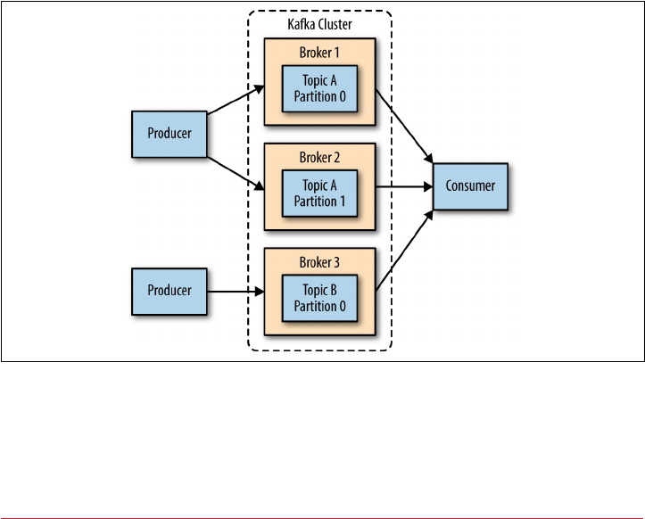
be sufficient. Once these decisions are made, the CPU and memory options available
will be appropriate for the performance.
In real terms, this will mean that for AWS either the m4 or r3 instance types are a
common choice. The m4 instance will allow for greater retention periods, but the
throughput to the disk will be less because it is on elastic block storage. The r3
instance will have much better throughput with local SSD drives, but those drives will
limit the amount of data that can be retained. For the best of both worlds, it is neces‐
sary to move up to either the i2 or d2 instance types, which are significantly more
expensive.
Kafka Clusters
A single Kafka server works well for local development work, or for a proof-of-
concept system, but there are significant benefits to having multiple brokers config‐
ured as a cluster, as shown in Figure 2-2. The biggest benefit is the ability to scale the
load across multiple servers. A close second is using replication to guard against data
loss due to single system failures. Replication will also allow for performing mainte‐
nance work on Kafka or the underlying systems while still maintaining availability for
clients. This section focuses on configuring only a Kafka cluster. Chapter 6 contains
more more information on replication of data.
Figure 2-2. A simple Kaa cluster
Kafka Clusters | 31

How Many Brokers?
The appropriate size for a Kafka cluster is determined by several factors. The first fac‐
tor to consider is how much disk capacity is required for retaining messages and how
much storage is available on a single broker. If the cluster is required to retain 10 TB
of data and a single broker can store 2 TB, then the minimum cluster size is five brok‐
ers. In addition, using replication will increase the storage requirements by at least
100%, depending on the replication factor chosen (see Chapter 6). This means that
this same cluster, configured with replication, now needs to contain at least 10 brok‐
ers.
The other factor to consider is the capacity of the cluster to handle requests. For
example, what is the capacity of the network interfaces, and can they handle the client
traffic if there are multiple consumers of the data or if the traffic is not consistent
over the retention period of the data (e.g., bursts of traffic during peak times). If the
network interface on a single broker is used to 80% capacity at peak, and there are
two consumers of that data, the consumers will not be able to keep up with peak traf‐
fic unless there are two brokers. If replication is being used in the cluster, this is an
additional consumer of the data that must be taken into account. It may also be desir‐
able to scale out to more brokers in a cluster in order to handle performance con‐
cerns caused by lesser disk throughput or system memory available.
Broker Conguration
There are only two requirements in the broker configuration to allow multiple Kafka
brokers to join a single cluster. The first is that all brokers must have the same config‐
uration for the zookeeper.connect parameter. This specifies the Zookeeper ensemble
and path where the cluster stores metadata. The second requirement is that all brok‐
ers in the cluster must have a unique value for the broker.id parameter. If two brok‐
ers attempt to join the same cluster with the same broker.id, the second broker will
log an error and fail to start. There are other configuration parameters used when
running a cluster—specifically, parameters that control replication, which are covered
in later chapters.
OS Tuning
While most Linux distributions have an out-of-the-box configuration for the kernel-
tuning parameters that will work fairly well for most applications, there are a few
changes that can be made for a Kafka broker that will improve performance. These
primarily revolve around the virtual memory and networking subsystems, as well as
specific concerns for the disk mount point that is used for storing log segments.
These parameters are typically configured in the /etc/sysctl.conf file, but you should
refer to your Linux distribution’s documentation for specific details regarding how to
adjust the kernel configuration.
32 | Chapter 2: Installing Kafka

Virtual Memory
In general, the Linux virtual memory system will automatically adjust itself for the
workload of the system. We can make some adjustments to both how swap space is
handled, as well as to dirty memory pages, to tune it for Kafka’s workload.
As with most applications—specifically ones where throughput is a concern—it is
best to avoid swapping at (almost) all costs. The cost incurred by having pages of
memory swapped to disk will show up as a noticeable impact on all aspects of perfor‐
mance in Kafka. In addition, Kafka makes heavy use of the system page cache, and if
the VM system is swapping to disk, there is not enough memory being allocated to
page cache.
One way to avoid swapping is just to not configure any swap space at all. Having swap
is not a requirement, but it does provide a safety net if something catastrophic hap‐
pens on the system. Having swap can prevent the OS from abruptly killing a process
due to an out-of-memory condition. For this reason, the recommendation is to set
the vm.swappiness parameter to a very low value, such as 1. The parameter is a per‐
centage of how likely the VM subsystem is to use swap space rather than dropping
pages from the page cache. It is preferable to reduce the size of the page cache rather
than swap.
Why Not Set Swappiness to Zero?
Previously, the recommendation for vm.swappiness was always to
set it to 0. This value used to have the meaning “do not swap unless
there is an out-of-memory condition.” However, the meaning of
this value changed as of Linux kernel version 3.5-rc1, and that
change was backported into many distributions, including Red Hat
Enterprise Linux kernels as of version 2.6.32-303. This changed the
meaning of the value 0 to “never swap under any circumstances.” It
is for this reason that a value of 1 is now recommended.
There is also a benefit to adjusting how the kernel handles dirty pages that must be
flushed to disk. Kafka relies on disk I/O performance to provide good response times
to producers. This is also the reason that the log segments are usually put on a fast
disk, whether that is an individual disk with a fast response time (e.g., SSD) or a disk
subsystem with significant NVRAM for caching (e.g., RAID). The result is that the
number of dirty pages that are allowed, before the flush background process starts
writing them to disk, can be reduced. This is accomplished by setting the
=vm.dirty_background_ratio value lower than the default of 10. The value is a per‐
centage of the total amount of system memory, and setting this value to 5 is appropri‐
ate in many situations. This setting should not be set to zero, however, as that would
cause the kernel to continually flush pages, which would then eliminate the ability of
Kafka Clusters | 33

the kernel to buffer disk writes against temporary spikes in the underlying device per‐
formance.
The total number of dirty pages that are allowed before the kernel forces synchronous
operations to flush them to disk can also be increased by changing the value of
vm.dirty_ratio, increasing it to above the default of 20 (also a percentage of total
system memory). There is a wide range of possible values for this setting, but between
60 and 80 is a reasonable number. This setting does introduce a small amount of risk,
both in regards to the amount of unflushed disk activity as well as the potential for
long I/O pauses if synchronous flushes are forced. If a higher setting for
vm.dirty_ratio is chosen, it is highly recommended that replication be used in the
Kafka cluster to guard against system failures.
When choosing values for these parameters, it is wise to review the number of dirty
pages over time while the Kafka cluster is running under load, whether in production
or simulated. The current number of dirty pages can be determined by checking
the /proc/vmstat file:
# cat /proc/vmstat | egrep "dirty|writeback"
nr_dirty 3875
nr_writeback 29
nr_writeback_temp 0
#
Disk
Outside of selecting the disk device hardware, as well as the configuration of RAID if
it is used, the choice of filesystem used for this disk can have the next largest impact
on performance. There are many different filesystems available, but the most com‐
mon choices for local filesystems are either EXT4 (fourth extended file system) or
Extents File System (XFS). Recently, XFS has become the default filesystem for many
Linux distributions, and this is for good reason—it outperforms EXT4 for most
workloads with minimal tuning required. EXT4 can perform well, but it requires
using tuning parameters that are considered less safe. This includes setting the com‐
mit interval to a longer time than the default of five to force less frequent flushes.
EXT4 also introduced delayed allocation of blocks, which brings with it a greater
chance of data loss and filesystem corruption in the case of a system failure. The XFS
filesystem also uses a delayed allocation algorithm, but it is generally safer than the
one used by EXT4. XFS also has better performance for Kafka’s workload without
requiring tuning beyond the automatic tuning performed by the filesystem. It is also
more efficient when batching disk writes, all of which combine to give better overall
I/O throughput.
Regardless of which filesystem is chosen for the mount that holds the log segments, it
is advisable to set the noatime mount option for the mount point. File metadata con‐
tains three timestamps: creation time (ctime), last modified time (mtime), and last
34 | Chapter 2: Installing Kafka

access time (atime). By default, the atime is updated every time a file is read. This
generates a large number of disk writes. The atime attribute is generally considered to
be of little use, unless an application needs to know if a file has been accessed since it
was last modified (in which case the realtime option can be used). The atime is not
used by Kafka at all, so disabling it is safe to do. Setting noatime on the mount will
prevent these timestamp updates from happening, but will not affect the proper han‐
dling of the ctime and mtime attributes.
Networking
Adjusting the default tuning of the Linux networking stack is common for any appli‐
cation that generates a high amount of network traffic, as the kernel is not tuned by
default for large, high-speed data transfers. In fact, the recommended changes for
Kafka are the same as those suggested for most web servers and other networking
applications. The first adjustment is to change the default and maximum amount of
memory allocated for the send and receive buffers for each socket. This will signifi‐
cantly increase performance for large transfers. The relevant parameters for the send
and receive buffer default size per socket are net.core.wmem_default and
net.core.rmem_default, and a reasonable setting for these parameters is 131072, or
128 KiB. The parameters for the send and receive buffer maximum sizes are
net.core.wmem_max and net.core.rmem_max, and a reasonable setting is 2097152, or
2 MiB. Keep in mind that the maximum size does not indicate that every socket will
have this much buffer space allocated; it only allows up to that much if needed.
In addition to the socket settings, the send and receive buffer sizes for TCP sockets
must be set separately using the net.ipv4.tcp_wmem and net.ipv4.tcp_rmem param‐
eters. These are set using three space-separated integers that specify the minimum,
default, and maximum sizes, respectively. The maximum size cannot be larger than
the values specified for all sockets using net.core.wmem_max and
net.core.rmem_max. An example setting for each of these parameters is “4096 65536
2048000,” which is a 4 KiB minimum, 64 KiB default, and 2 MiB maximum buffer.
Based on the actual workload of your Kafka brokers, you may want to increase the
maximum sizes to allow for greater buffering of the network connections.
There are several other network tuning parameters that are useful to set. Enabling
TCP window scaling by setting net.ipv4.tcp_window_scaling to 1 will allow clients
to transfer data more efficiently, and allow that data to be buffered on the broker side.
Increasing the value of net.ipv4.tcp_max_syn_backlog above the default of 1024
will allow a greater number of simultaneous connections to be accepted. Increasing
the value of net.core.netdev_max_backlog to greater than the default of 1000 can
assist with bursts of network traffic, specifically when using multigigabit network
connection speeds, by allowing more packets to be queued for the kernel to process
them.
Kafka Clusters | 35

Production Concerns
Once you are ready to move your Kafka environment out of testing and into your
production operations, there are a few more things to think about that will assist with
setting up a reliable messaging service.
Garbage Collector Options
Tuning the Java garbage-collection options for an application has always been some‐
thing of an art, requiring detailed information about how the application uses mem‐
ory and a significant amount of observation and trial and error. Thankfully, this has
changed with Java 7 and the introduction of the Garbage First (or G1) garbage collec‐
tor. G1 is designed to automatically adjust to different workloads and provide consis‐
tent pause times for garbage collection over the lifetime of the application. It also
handles large heap sizes with ease by segmenting the heap into smaller zones and not
collecting over the entire heap in each pause.
G1 does all of this with a minimal amount of configuration in normal operation.
There are two configuration options for G1 used to adjust its performance:
MaxGCPauseMillis
This option specifies the preferred pause time for each garbage-collection cycle.
It is not a fixed maximum—G1 can and will exceed this time if it is required. This
value defaults to 200 milliseconds. This means that G1 will attempt to schedule
the frequency of GC cycles, as well as the number of zones that are collected in
each cycle, such that each cycle will take approximately 200ms.
InitiatingHeapOccupancyPercent
This option specifies the percentage of the total heap that may be in use before
G1 will start a collection cycle. The default value is 45. This means that G1 will
not start a collection cycle until after 45% of the heap is in use. This includes both
the new (Eden) and old zone usage in total.
The Kafka broker is fairly efficient with the way it utilizes heap memory and creates
garbage objects, so it is possible to set these options lower. The GC tuning options
provided in this section have been found to be appropriate for a server with 64 GB of
memory, running Kafka in a 5GB heap. For MaxGCPauseMillis, this broker can be
configured with a value of 20 ms. The value for InitiatingHeapOccupancyPercent is
set to 35, which causes garbage collection to run slightly earlier than with the default
value.
The start script for Kafka does not use the G1 collector, instead defaulting to using
parallel new and concurrent mark and sweep garbage collection. The change is easy
to make via environment variables. Using the start command from earlier in the
chapter, modify it as follows:
36 | Chapter 2: Installing Kafka

# export JAVA_HOME=/usr/java/jdk1.8.0_51
# export KAFKA_JVM_PERFORMANCE_OPTS="-server -XX:+UseG1GC
-XX:MaxGCPauseMillis=20 -XX:InitiatingHeapOccupancyPercent=35
-XX:+DisableExplicitGC -Djava.awt.headless=true"
# /usr/local/kafka/bin/kafka-server-start.sh -daemon
/usr/local/kafka/config/server.properties
#
Datacenter Layout
For development systems, the physical location of the Kafka brokers within a data‐
center is not as much of a concern, as there is not as severe an impact if the cluster is
partially or completely unavailable for short periods of time. When serving produc‐
tion traffic, however, downtime means dollars lost, whether through loss of services
to users or loss of telemetry on what the users are doing. This is when it becomes crit‐
ical to configure replication within the Kafka cluster (see Chapter 6), which is also
when it is important to consider the physical location of brokers in their racks in the
datacenter. If not addressed prior to deploying Kafka, expensive maintenance to
move servers around may be needed.
The Kafka broker has no rack-awareness when assigning new partitions to brokers.
This means that it cannot take into account that two brokers may be located in the
same physical rack, or in the same availability zone (if running in a cloud service like
AWS), and therefore can easily assign all replicas for a partition to brokers that share
the same power and network connections in the same rack. Should that rack have a
failure, these partitions would be offline and inaccessible to clients. In addition, it can
result in additional lost data on recovery due to an unclean leader election (more
about this in Chapter 6).
The best practice is to have each Kafka broker in a cluster installed in a different rack,
or at the very least not share single points of failure for infrastructure services such as
power and network. This typically means at least deploying the servers that will run
brokers with dual power connections (to two different circuits) and dual network
switches (with a bonded interface on the servers themselves to failover seamlessly).
Even with dual connections, there is a benefit to having brokers in completely sepa‐
rate racks. From time to time, it may be neccessary to perform physical maintenance
on a rack or cabinet that requires it to be offline (such as moving servers around, or
rewiring power connections).
Colocating Applications on Zookeeper
Kafka utilizes Zookeeper for storing metadata information about the brokers, topics,
and partitions. Writes to Zookeeper are only performed on changes to the member‐
ship of consumer groups or on changes to the Kafka cluster itself. This amount of
traffic is minimal, and it does not justify the use of a dedicated Zookeeper ensemble
Production Concerns | 37

for a single Kafka cluster. In fact, many deployments will use a single Zookeeper
ensemble for multiple Kafka clusters (using a chroot Zookeeper path for each cluster,
as described earlier in this chapter).
Kafka Consumers and Zookeeper
Prior to Apache Kafka 0.9.0.0, consumers, in addition to the brok‐
ers, utilized Zookeeper to directly store information about the
composition of the consumer group, what topics it was consuming,
and to periodically commit offsets for each partition being con‐
sumed (to enable failover between consumers in the group). With
version 0.9.0.0, a new consumer interface was introduced which
allows this to be managed directly with the Kafka brokers. This is
the consumer discussed in Chapter 4.
However, there is a concern with consumers and Zookeeper under certain configura‐
tions. Consumers have a configurable choice to use either Zookeeper or Kafka for
committing offsets, and they can also configure the interval between commits. If the
consumer uses Zookeeper for offsets, each consumer will perform a Zookeeper write
at every interval for every partition it consumes. A reasonable interval for offset com‐
mits is 1 minute, as this is the period of time over which a consumer group will read
duplicate messages in the case of a consumer failure. These commits can be a signifi‐
cant amount of Zookeeper traffic, especially in a cluster with many consumers, and
will need to be taken into account. It may be neccessary to use a longer commit inter‐
val if the Zookeeper ensemble is not able to handle the traffic. However, it is recom‐
mended that consumers using the latest Kafka libraries use Kafka for committing
offsets, removing the dependency on Zookeeper.
Outside of using a single ensemble for multiple Kafka clusters, it is not recommended
to share the ensemble with other applications, if it can be avoided. Kafka is sensitive
to Zookeeper latency and timeouts, and an interruption in communications with the
ensemble will cause the brokers to behave unpredictably. This can easily cause multi‐
ple brokers to go offline at the same time, should they lose Zookeeper connections,
which will result in offline partitions. It also puts stress on the cluster controller,
which can show up as subtle errors long after the interruption has passed, such as
when trying to perform a controlled shutdown of a broker. Other applications that
can put stress on the Zookeeper ensemble, either through heavy usage or improper
operations, should be segregated to their own ensemble.
38 | Chapter 2: Installing Kafka

Summary
In this chapter we learned how to get Apache Kafka up and running. We also covered
picking the right hardware for your brokers, and specific concerns around getting set
up in a production environment. Now that you have a Kafka cluster, we will walk
through the basics of Kafka client applications. The next two chapters will cover how
to create clients for both producing messages to Kafka (Chapter 3), as well as con‐
suming those messages out again (Chapter 4).
Summary | 39

CHAPTER 3
Kafka Producers: Writing Messages
to Kafka
Whether you use Kafka as a queue, message bus, or data storage platform, you will
always use Kafka by writing a producer that writes data to Kafka, a consumer that
reads data from Kafka, or an application that serves both roles.
For example, in a credit card transaction processing system, there will be a client
application, perhaps an online store, responsible for sending each transaction to
Kafka immediately when a payment is made. Another application is responsible for
immediately checking this transaction against a rules engine and determining
whether the transaction is approved or denied. The approve/deny response can then
be written back to Kafka and the response can propagate back to the online store
where the transaction was initiated. A third application can read both transactions
and the approval status from Kafka and store them in a database where analysts can
later review the decisions and perhaps improve the rules engine.
Apache Kafka ships with built-in client APIs that developers can use when developing
applications that interact with Kafka.
In this chapter we will learn how to use the Kafka producer, starting with an overview
of its design and components. We will show how to create KafkaProducer and Produ
cerRecord objects, how to send records to Kafka, and how to handle the errors that
Kafka may return. We’ll then review the most important configuration options used
to control the producer behavior. We’ll conclude with a deeper look at how to use dif‐
ferent partitioning methods and serializers, and how to write your own serializers
and partitioners.
In Chapter 4 we will look at Kafka’s consumer client and reading data from Kafka.
41

Third-Party Clients
In addition to the built-in clients, Kafka has a binary wire protocol.
This means that it is possible for applications to read messages
from Kafka or write messages to Kafka simply by sending the cor‐
rect byte sequences to Kafka’s network port. There are multiple cli‐
ents that implement Kafka’s wire protocol in different
programming languages, giving simple ways to use Kafka not just
in Java applications but also in languages like C++, Python, Go,
and many more. Those clients are not part of Apache Kafka
project, but a list of non-Java clients is maintained in the project
wiki. The wire protocol and the external clients are outside the
scope of the chapter.
Producer Overview
There are many reasons an application might need to write messages to Kafka:
recording user activities for auditing or analysis, recording metrics, storing log mes‐
sages, recording information from smart appliances, communicating asynchronously
with other applications, buffering information before writing to a database, and much
more.
Those diverse use cases also imply diverse requirements: is every message critical, or
can we tolerate loss of messages? Are we OK with accidentally duplicating messages?
Are there any strict latency or throughput requirements we need to support?
In the credit card transaction processing example we introduced earlier, we can see
that it is critical to never lose a single message nor duplicate any messages. Latency
should be low but latencies up to 500ms can be tolerated, and throughput should be
very high—we expect to process up to a million messages a second.
A different use case might be to store click information from a website. In that case,
some message loss or a few duplicates can be tolerated; latency can be high as long as
there is no impact on the user experience. In other words, we don’t mind if it takes a
few seconds for the message to arrive at Kafka, as long as the next page loads immedi‐
ately after the user clicked on a link. Throughput will depend on the level of activity
we anticipate on our website.
The different requirements will influence the way you use the producer API to write
messages to Kafka and the configuration you use.
While the producer APIs are very simple, there is a bit more that goes on under the
hood of the producer when we send data. Figure 3-1 shows the main steps involved in
sending data to Kafka.
42 | Chapter 3: Kafka Producers: Writing Messages to Kafka
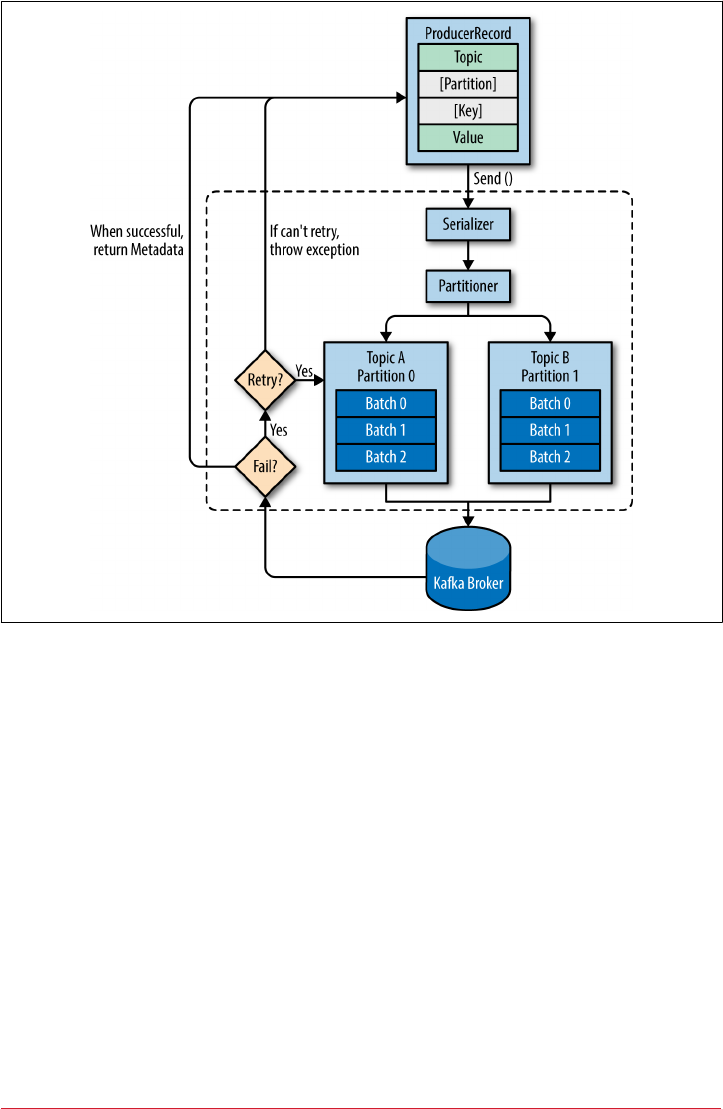
Figure 3-1. High-level overview of Kaa producer components
We start producing messages to Kafka by creating a ProducerRecord, which must
include the topic we want to send the record to and a value. Optionally, we can also
specify a key and/or a partition. Once we send the ProducerRecord, the first thing the
producer will do is serialize the key and value objects to ByteArrays so they can be
sent over the network.
Next, the data is sent to a partitioner. If we specified a partition in the
ProducerRecord, the partitioner doesn’t do anything and simply returns the partition
we specified. If we didn’t, the partitioner will choose a partition for us, usually based
on the ProducerRecord key. Once a partition is selected, the producer knows which
topic and partition the record will go to. It then adds the record to a batch of records
that will also be sent to the same topic and partition. A separate thread is responsible
for sending those batches of records to the appropriate Kafka brokers.
When the broker receives the messages, it sends back a response. If the messages
were successfully written to Kafka, it will return a RecordMetadata object with the
Producer Overview | 43

topic, partition, and the offset of the record within the partition. If the broker failed
to write the messages, it will return an error. When the producer receives an error, it
may retry sending the message a few more times before giving up and returning an
error.
Constructing a Kafka Producer
The first step in writing messages to Kafka is to create a producer object with the
properties you want to pass to the producer. A Kafka producer has three mandatory
properties:
bootstrap.servers
List of host:port pairs of brokers that the producer will use to establish initial
connection to the Kafka cluster. This list doesn’t need to include all brokers, since
the producer will get more information after the initial connection. But it is rec‐
ommended to include at least two, so in case one broker goes down, the producer
will still be able to connect to the cluster.
key.serializer
Name of a class that will be used to serialize the keys of the records we will pro‐
duce to Kafka. Kafka brokers expect byte arrays as keys and values of messages.
However, the producer interface allows, using parameterized types, any Java
object to be sent as a key and value. This makes for very readable code, but it also
means that the producer has to know how to convert these objects to byte arrays.
key.serializer should be set to a name of a class that implements the
org.apache.kafka.common.serialization.Serializer interface. The producer
will use this class to serialize the key object to a byte array. The Kafka client pack‐
age includes ByteArraySerializer (which doesn’t do much),
StringSerializer, and IntegerSerializer, so if you use common types, there
is no need to implement your own serializers. Setting key.serializer is
required even if you intend to send only values.
value.serializer
Name of a class that will be used to serialize the values of the records we will pro‐
duce to Kafka. The same way you set key.serializer to a name of a class that
will serialize the message key object to a byte array, you set value.serializer to
a class that will serialize the message value object.
The following code snippet shows how to create a new producer by setting just the
mandatory parameters and using defaults for everything else:
private Properties kafkaProps = new Properties();
kafkaProps.put("bootstrap.servers", "broker1:9092,broker2:9092");
kafkaProps.put("key.serializer",
44 | Chapter 3: Kafka Producers: Writing Messages to Kafka

"org.apache.kafka.common.serialization.StringSerializer");
kafkaProps.put("value.serializer",
"org.apache.kafka.common.serialization.StringSerializer");
producer = new KafkaProducer<String, String>(kafkaProps);
We start with a Properties object.
Since we plan on using strings for message key and value, we use the built-in
StringSerializer.
Here we create a new producer by setting the appropriate key and value types
and passing the Properties object.
With such a simple interface, it is clear that most of the control over producer behav‐
ior is done by setting the correct configuration properties. Apache Kafka documenta‐
tion covers all the configuration options, and we will go over the important ones later
in this chapter.
Once we instantiate a producer, it is time to start sending messages. There are three
primary methods of sending messages:
Fire-and-forget
We send a message to the server and don’t really care if it arrives succesfully or
not. Most of the time, it will arrive successfully, since Kafka is highly available
and the producer will retry sending messages automatically. However, some mes‐
sages will get lost using this method.
Synchronous send
We send a message, the send() method returns a Future object, and we use get()
to wait on the future and see if the send() was successful or not.
Asynchronous send
We call the send() method with a callback function, which gets triggered when it
receives a response from the Kafka broker.
In the examples that follow, we will see how to send messages using these methods
and how to handle the different types of errors that might occur.
While all the examples in this chapter are single threaded, a producer object can be
used by multiple threads to send messages. You will probably want to start with one
producer and one thread. If you need better throughput, you can add more threads
that use the same producer. Once this ceases to increase throughput, you can add
more producers to the application to achieve even higher throughput.
Constructing a Kafka Producer | 45
Sending a Message to Kafka
The simplest way to send a message is as follows:
ProducerRecord<String, String> record =
new ProducerRecord<>("CustomerCountry", "Precision Products",
"France");
try {
producer.send(record);
} catch (Exception e) {
e.printStackTrace();
}
The producer accepts ProducerRecord objects, so we start by creating one.
ProducerRecord has multiple constructors, which we will discuss later. Here we
use one that requires the name of the topic we are sending data to, which is
always a string, and the key and value we are sending to Kafka, which in this case
are also strings. The types of the key and value must match our serializer and
producer objects.
We use the producer object send() method to send the ProducerRecord. As
we’ve seen in the producer architecture diagram in Figure 3-1, the message will
be placed in a buffer and will be sent to the broker in a separate thread. The
send() method returns a Java Future object with RecordMetadata, but since we
simply ignore the returned value, we have no way of knowing whether the mes‐
sage was sent successfully or not. This method of sending messages can be used
when dropping a message silently is acceptable. This is not typically the case in
production applications.
While we ignore errors that may occur while sending messages to Kafka brokers
or in the brokers themselves, we may still get an exception if the producer
encountered errors before sending the message to Kafka. Those can be a
SerializationException when it fails to serialize the message, a BufferExhaus
tedException or TimeoutException if the buffer is full, or an InterruptException
if the sending thread was interrupted.
Sending a Message Synchronously
The simplest way to send a message synchronously is as follows:
ProducerRecord<String, String> record =
new ProducerRecord<>("CustomerCountry", "Precision Products", "France");
try {
producer.send(record).get();
} catch (Exception e) {
46 | Chapter 3: Kafka Producers: Writing Messages to Kafka

e.printStackTrace();
}
Here, we are using Future.get() to wait for a reply from Kafka. This method
will throw an exception if the record is not sent successfully to Kafka. If there
were no errors, we will get a RecordMetadata object that we can use to retrieve
the offset the message was written to.
If there were any errors before sending data to Kafka, while sending, if the Kafka
brokers returned a nonretriable exceptions or if we exhausted the available
retries, we will encounter an exception. In this case, we just print any exception
we ran into.
KafkaProducer has two types of errors. Retriable errors are those that can be resolved
by sending the message again. For example, a connection error can be resolved
because the connection may get reestablished. A “no leader” error can be resolved
when a new leader is elected for the partition. KafkaProducer can be configured to
retry those errors automatically, so the application code will get retriable exceptions
only when the number of retries was exhausted and the error was not resolved. Some
errors will not be resolved by retrying. For example, “message size too large.” In those
cases, KafkaProducer will not attempt a retry and will return the exception immedi‐
ately.
Sending a Message Asynchronously
Suppose the network roundtrip time between our application and the Kafka cluster is
10ms. If we wait for a reply after sending each message, sending 100 messages will
take around 1 second. On the other hand, if we just send all our messages and not
wait for any replies, then sending 100 messages will barely take any time at all. In
most cases, we really don’t need a reply—Kafka sends back the topic, partition, and
offset of the record after it was written, which is usually not required by the sending
app. On the other hand, we do need to know when we failed to send a message com‐
pletely so we can throw an exception, log an error, or perhaps write the message to an
“errors” file for later analysis.
In order to send messages asynchronously and still handle error scenarios, the pro‐
ducer supports adding a callback when sending a record. Here is an example of how
we use a callback:
Sending a Message to Kafka | 47
private class DemoProducerCallback implements Callback {
@Override
public void onCompletion(RecordMetadata recordMetadata, Exception e) {
if (e != null) {
e.printStackTrace();
}
}
}
ProducerRecord<String, String> record =
new ProducerRecord<>("CustomerCountry", "Biomedical Materials", "USA");
producer.send(record, new DemoProducerCallback());
To use callbacks, you need a class that implements the org.apache.kafka.
clients.producer.Callback interface, which has a single function—onComple
tion().
If Kafka returned an error, onCompletion() will have a nonnull exception. Here
we “handle” it by printing, but production code will probably have more robust
error handling functions.
The records are the same as before.
And we pass a Callback object along when sending the record.
Conguring Producers
So far we’ve seen very few configuration parameters for the producers—just the
mandatory bootstrap.servers URI and serializers.
The producer has a large number of configuration parameters; most are documented
in Apache Kafka documentation and many have reasonable defaults so there is no
reason to tinker with every single parameter. However, some of the parameters have a
significant impact on memory use, performance, and reliability of the producers. We
will review those here.
acks
The acks parameter controls how many partition replicas must receive the record
before the producer can consider the write successful. This option has a significant
impact on how likely messages are to be lost. There are three allowed values for the
acks parameter:
• If acks=0, the producer will not wait for a reply from the broker before assuming
the message was sent successfully. This means that if something went wrong and
48 | Chapter 3: Kafka Producers: Writing Messages to Kafka

the broker did not receive the message, the producer will not know about it and
the message will be lost. However, because the producer is not waiting for any
response from the server, it can send messages as fast as the network will support,
so this setting can be used to achieve very high throughput.
•If acks=1, the producer will receive a success response from the broker the
moment the leader replica received the message. If the message can’t be written
to the leader (e.g., if the leader crashed and a new leader was not elected yet), the
producer will receive an error response and can retry sending the message,
avoiding potential loss of data. The message can still get lost if the leader crashes
and a replica without this message gets elected as the new leader (via unclean
leader election). In this case, throughput depends on whether we send messages
synchronously or asynchronously. If our client code waits for a reply from the
server (by calling the get() method of the Future object returned when sending
a message) it will obviously increase latency significantly (at least by a network
roundtrip). If the client uses callbacks, latency will be hidden, but throughput will
be limited by the number of in-flight messages (i.e., how many messages the pro‐
ducer will send before receiving replies from the server).
• If acks=all, the producer will receive a success response from the broker once all
in-sync replicas received the message. This is the safest mode since you can make
sure more than one broker has the message and that the message will survive
even in the case of crash (more information on this in Chapter 5). However, the
latency we discussed in the acks=1 case will be even higher, since we will be wait‐
ing for more than just one broker to receive the message.
buer.memory
This sets the amount of memory the producer will use to buffer messages waiting to
be sent to brokers. If messages are sent by the application faster than they can be
delivered to the server, the producer may run out of space and additional send() calls
will either block or throw an exception, based on the block.on.buffer.full param‐
eter (replaced with max.block.ms in release 0.9.0.0, which allows blocking for a cer‐
tain time and then throwing an exception).
compression.type
By default, messages are sent uncompressed. This parameter can be set to snappy,
gzip, or lz4, in which case the corresponding compression algorithms will be used to
compress the data before sending it to the brokers. Snappy compression was invented
by Google to provide decent compression ratios with low CPU overhead and good
performance, so it is recommended in cases where both performance and bandwidth
are a concern. Gzip compression will typically use more CPU and time but result in
better compression ratios, so it recommended in cases where network bandwidth is
Conguring Producers | 49

more restricted. By enabling compression, you reduce network utilization and stor‐
age, which is often a bottleneck when sending messages to Kafka.
retries
When the producer receives an error message from the server, the error could be
transient (e.g., a lack of leader for a partition). In this case, the value of the retries
parameter will control how many times the producer will retry sending the message
before giving up and notifying the client of an issue. By default, the producer will wait
100ms between retries, but you can control this using the retry.backoff.ms parame‐
ter. We recommend testing how long it takes to recover from a crashed broker (i.e.,
how long until all partitions get new leaders) and setting the number of retries and
delay between them such that the total amount of time spent retrying will be longer
than the time it takes the Kafka cluster to recover from the crash—otherwise, the pro‐
ducer will give up too soon. Not all errors will be retried by the producer. Some errors
are not transient and will not cause retries (e.g., “message too large” error). In general,
because the producer handles retries for you, there is no point in handling retries
within your own application logic. You will want to focus your efforts on handling
nonretriable errors or cases where retry attempts were exhausted.
batch.size
When multiple records are sent to the same partition, the producer will batch them
together. This parameter controls the amount of memory in bytes (not messages!)
that will be used for each batch. When the batch is full, all the messages in the batch
will be sent. However, this does not mean that the producer will wait for the batch to
become full. The producer will send half-full batches and even batches with just a sin‐
gle message in them. Therefore, setting the batch size too large will not cause delays
in sending messages; it will just use more memory for the batches. Setting the batch
size too small will add some overhead because the producer will need to send mes‐
sages more frequently.
linger.ms
linger.ms controls the amount of time to wait for additional messages before send‐
ing the current batch. KafkaProducer sends a batch of messages either when the cur‐
rent batch is full or when the linger.ms limit is reached. By default, the producer will
send messages as soon as there is a sender thread available to send them, even if
there’s just one message in the batch. By setting linger.ms higher than 0, we instruct
the producer to wait a few milliseconds to add additional messages to the batch
before sending it to the brokers. This increases latency but also increases throughput
(because we send more messages at once, there is less overhead per message).
50 | Chapter 3: Kafka Producers: Writing Messages to Kafka

client.id
This can be any string, and will be used by the brokers to identify messages sent from
the client. It is used in logging and metrics, and for quotas.
max.in.ight.requests.per.connection
This controls how many messages the producer will send to the server without
receiving responses. Setting this high can increase memory usage while improving
throughput, but setting it too high can reduce throughput as batching becomes less
efficient. Setting this to 1 will guarantee that messages will be written to the broker in
the order in which they were sent, even when retries occur.
timeout.ms, request.timeout.ms, and metadata.fetch.timeout.ms
These parameters control how long the producer will wait for a reply from the server
when sending data (request.timeout.ms) and when requesting metadata such as the
current leaders for the partitions we are writing to (metadata.fetch.timeout.ms). If
the timeout is reached without reply, the producer will either retry sending or
respond with an error (either through exception or the send callback). timeout.ms
controls the time the broker will wait for in-sync replicas to acknowledge the message
in order to meet the acks configuration—the broker will return an error if the time
elapses without the necessary acknowledgments.
max.block.ms
This parameter controls how long the producer will block when calling send() and
when explicitly requesting metadata via partitionsFor(). Those methods block
when the producer’s send buffer is full or when metadata is not available. When
max.block.ms is reached, a timeout exception is thrown.
max.request.size
This setting controls the size of a produce request sent by the producer. It caps both
the size of the largest message that can be sent and the number of messages that the
producer can send in one request. For example, with a default maximum request size
of 1 MB, the largest message you can send is 1 MB or the producer can batch 1,000
messages of size 1 K each into one request. In addition, the broker has its own limit
on the size of the largest message it will accept (message.max.bytes). It is usually a
good idea to have these configurations match, so the producer will not attempt to
send messages of a size that will be rejected by the broker.
receive.buer.bytes and send.buer.bytes
These are the sizes of the TCP send and receive buffers used by the sockets when
writing and reading data. If these are set to -1, the OS defaults will be used. It is a
Conguring Producers | 51

good idea to increase those when producers or consumers communicate with brokers
in a different datacenter because those network links typically have higher latency and
lower bandwidth.
Ordering Guarantees
Apache Kafka preserves the order of messages within a partition.
This means that if messages were sent from the producer in a spe‐
cific order, the broker will write them to a partition in that order
and all consumers will read them in that order. For some use cases,
order is very important. There is a big difference between deposit‐
ing $100 in an account and later withdrawing it, and the other way
around! However, some use cases are less sensitive.
Setting the retries parameter to nonzero and the
max.in.flights.requests.per.session to more than one means
that it is possible that the broker will fail to write the first batch of
messages, succeed to write the second (which was already in-
flight), and then retry the first batch and succeed, thereby reversing
the order.
Usually, setting the number of retries to zero is not an option in a
reliable system, so if guaranteeing order is critical, we recommend
setting in.flight.requests.per.session=1 to make sure that
while a batch of messages is retrying, additional messages will not
be sent (because this has the potential to reverse the correct order).
This will severely limit the throughput of the producer, so only use
this when order is important.
Serializers
As seen in previous examples, producer configuration includes mandatory serializers.
We’ve seen how to use the default String serializer. Kafka also includes serializers for
integers and ByteArrays, but this does not cover most use cases. Eventually, you will
want to be able to serialize more generic records.
We will start by showing how to write your own serializer and then introduce the
Avro serializer as a recommended alternative.
Custom Serializers
When the object you need to send to Kafka is not a simple string or integer, you have
a choice of either using a generic serialization library like Avro, Thrift, or Protobuf to
create records, or creating a custom serialization for objects you are already using. We
highly recommend using a generic serialization library. In order to understand how
52 | Chapter 3: Kafka Producers: Writing Messages to Kafka

the serializers work and why it is a good idea to use a serialization library, let’s see
what it takes to write your own custom serializer.
Suppose that instead of recording just the customer name, you create a simple class to
represent customers:
public class Customer {
private int customerID;
private String customerName;
public Customer(int ID, String name) {
this.customerID = ID;
this.customerName = name;
}
public int getID() {
return customerID;
}
public String getName() {
return customerName;
}
}
Now suppose we want to create a custom serializer for this class. It will look some‐
thing like this:
import org.apache.kafka.common.errors.SerializationException;
import java.nio.ByteBuffer;
import java.util.Map;
public class CustomerSerializer implements Serializer<Customer> {
@Override
public void configure(Map configs, boolean isKey) {
// nothing to configure
}
@Override
/**
We are serializing Customer as:
4 byte int representing customerId
4 byte int representing length of customerName in UTF-8 bytes (0 if name is
Null)
N bytes representing customerName in UTF-8
*/
public byte[] serialize(String topic, Customer data) {
try {
byte[] serializedName;
int stringSize;
if (data == null)
return null;
Serializers | 53

else {
if (data.getName() != null) {
serializeName = data.getName().getBytes("UTF-8");
stringSize = serializedName.length;
} else {
serializedName = new byte[0];
stringSize = 0;
}
}
ByteBuffer buffer = ByteBuffer.allocate(4 + 4 + stringSize);
buffer.putInt(data.getID());
buffer.putInt(stringSize);
buffer.put(serializedName);
return buffer.array();
} catch (Exception e) {
throw new SerializationException("Error when serializing Customer to
byte[] " + e);
}
}
@Override
public void close() {
// nothing to close
}
}
Configuring a producer with this CustomerSerializer will allow you to define
ProducerRecord<String, Customer>, and send Customer data and pass Customer
objects directly to the producer. This example is pretty simple, but you can see how
fragile the code is. If we ever have too many customers, for example, and need to
change customerID to Long, or if we ever decide to add a startDate field to Cus
tomer, we will have a serious issue in maintaining compatibility between old and new
messages. Debugging compatibility issues between different versions of serializers
and deserializers is fairly challenging—you need to compare arrays of raw bytes. To
make matters even worse, if multiple teams in the same company end up writing Cus
tomer data to Kafka, they will all need to use the same serializers and modify the code
at the exact same time.
For these reasons, we recommend using existing serializers and deserializers such as
JSON, Apache Avro, Thrift, or Protobuf. In the following section we will describe
Apache Avro and then show how to serialize Avro records and send them to Kafka.
Serializing Using Apache Avro
Apache Avro is a language-neutral data serialization format. The project was created
by Doug Cutting to provide a way to share data files with a large audience.
54 | Chapter 3: Kafka Producers: Writing Messages to Kafka
Avro data is described in a language-independent schema. The schema is usually
described in JSON and the serialization is usually to binary files, although serializing
to JSON is also supported. Avro assumes that the schema is present when reading and
writing files, usually by embedding the schema in the files themselves.
One of the most interesting features of Avro, and what makes it a good fit for use in a
messaging system like Kafka, is that when the application that is writing messages
switches to a new schema, the applications reading the data can continue processing
messages without requiring any change or update.
Suppose the original schema was:
{"namespace": "customerManagement.avro",
"type": "record",
"name": "Customer",
"fields": [
{"name": "id", "type": "int"},
{"name": "name", "type": "string""},
{"name": "faxNumber", "type": ["null", "string"], "default": "null"}
]
}
id and name fields are mandatory, while fax number is optional and defaults to
null.
We used this schema for a few months and generated a few terabytes of data in this
format. Now suppose that we decide that in the new version, we will upgrade to the
twenty-first century and will no longer include a fax number field and will instead use
an email field.
The new schema would be:
{"namespace": "customerManagement.avro",
"type": "record",
"name": "Customer",
"fields": [
{"name": "id", "type": "int"},
{"name": "name", "type": "string"},
{"name": "email", "type": ["null", "string"], "default": "null"}
]
}
Now, after upgrading to the new version, old records will contain “faxNumber” and
new records will contain “email.” In many organizations, upgrades are done slowly
and over many months. So we need to consider how preupgrade applications that still
use the fax numbers and postupgrade applications that use email will be able to han‐
dle all the events in Kafka.
The reading application will contain calls to methods similar to getName(), getId(),
and getFaxNumber. If it encounters a message written with the new schema, get
Serializers | 55

Name() and getId() will continue working with no modification, but getFax
Number() will return null because the message will not contain a fax number.
Now suppose we upgrade our reading application and it no longer has the getFax
Number() method but rather getEmail(). If it encounters a message written with the
old schema, getEmail() will return null because the older messages do not contain
an email address.
This example illustrates the benefit of using Avro: even though we changed the
schema in the messages without changing all the applications reading the data, there
will be no exceptions or breaking errors and no need for expensive updates of exist‐
ing data.
However, there are two caveats to this scenario:
•The schema used for writing the data and the schema expected by the reading
application must be compatible. The Avro documentation includes compatibility
rules.
•The deserializer will need access to the schema that was used when writing the
data, even when it is different than the schema expected by the application that
accesses the data. In Avro files, the writing schema is included in the file itself,
but there is a better way to handle this for Kafka messages. We will look at that
next.
Using Avro Records with Kafka
Unlike Avro files, where storing the entire schema in the data file is associated with a
fairly reasonable overhead, storing the entire schema in each record will usually more
than double the record size. However, Avro still requires the entire schema to be
present when reading the record, so we need to locate the schema elsewhere. To ach‐
ieve this, we follow a common architecture pattern and use a Schema Registry. The
Schema Registry is not part of Apache Kafka but there are several open source
options to choose from. We’ll use the Confluent Schema Registry for this example.
You can find the Schema Registry code on GitHub, or you can install it as part of the
Confluent Platform. If you decide to use the Schema Registry, then we recommend
checking the documentation.
The idea is to store all the schemas used to write data to Kafka in the registry. Then
we simply store the identifier for the schema in the record we produce to Kafka. The
consumers can then use the identifier to pull the record out of the schema registry
and deserialize the data. The key is that all this work—storing the schema in the reg‐
istry and pulling it up when required—is done in the serializers and deserializers. The
code that produces data to Kafka simply uses the Avro serializer just like it would any
other serializer. Figure 3-2 demonstrates this process.
56 | Chapter 3: Kafka Producers: Writing Messages to Kafka
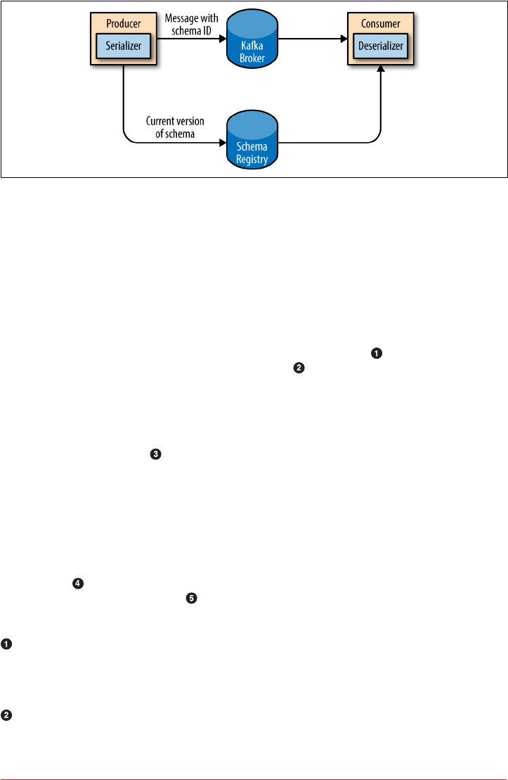
Figure 3-2. Flow diagram of serialization and deserialization of Avro records
Here is an example of how to produce generated Avro objects to Kafka (see the Avro
Documentation for how to use code generation with Avro):
Properties props = new Properties();
props.put("bootstrap.servers", "localhost:9092");
props.put("key.serializer",
"io.confluent.kafka.serializers.KafkaAvroSerializer");
props.put("value.serializer",
"io.confluent.kafka.serializers.KafkaAvroSerializer");
props.put("schema.registry.url", schemaUrl);
String topic = "customerContacts";
int wait = 500;
Producer<String, Customer> producer = new KafkaProducer<String,
Customer>(props);
// We keep producing new events until someone ctrl-c
while (true) {
Customer customer = CustomerGenerator.getNext();
System.out.println("Generated customer " +
customer.toString());
ProducerRecord<String, Customer> record =
new ProducerRecord<>(topic, customer.getId(), cus-
tomer);
producer.send(record);
}
We use the KafkaAvroSerializer to serialize our objects with Avro. Note that
the AvroSerializer can also handle primitives, which is why we can later use
String as the record key and our Customer object as the value.
schema.registry.url is a new parameter. This simply points to where we store
the schemas.
Serializers | 57
Customer is our generated object. We tell the producer that our records will con‐
tain Customer as the value.
We also instantiate ProducerRecord with Customer as the value type, and pass a
Customer object when creating the new record.
That’s it. We send the record with our Customer object and KafkaAvroSerial
izer will handle the rest.
What if you prefer to use generic Avro objects rather than the generated Avro objects?
No worries. In this case, you just need to provide the schema:
Properties props = new Properties();
props.put("bootstrap.servers", "localhost:9092");
props.put("key.serializer",
"io.confluent.kafka.serializers.KafkaAvroSerializer");
props.put("value.serializer",
"io.confluent.kafka.serializers.KafkaAvroSerializer");
props.put("schema.registry.url", url);
String schemaString = "{\"namespace\": \"customerManagement.avro\",
\"type\": \"record\", " +
"\"name\": \"Customer\"," +
"\"fields\": [" +
"{\"name\": \"id\", \"type\": \"int\"}," +
"{\"name\": \"name\", \"type\": \"string\"}," +
"{\"name\": \"email\", \"type\": [\"null\",\"string
\"], \"default\":\"null\" }" +
"]}";
Producer<String, GenericRecord> producer =
new KafkaProducer<String, GenericRecord>(props);
Schema.Parser parser = new Schema.Parser();
Schema schema = parser.parse(schemaString);
for (int nCustomers = 0; nCustomers < customers; nCustomers++) {
String name = "exampleCustomer" + nCustomers;
String email = "example " + nCustomers + "@example.com"
GenericRecord customer = new GenericData.Record(schema);
customer.put("id", nCustomer);
customer.put("name", name);
customer.put("email", email);
ProducerRecord<String, GenericRecord> data =
new ProducerRecord<String,
GenericRecord>("customerContacts",
name, customer);
producer.send(data);
58 | Chapter 3: Kafka Producers: Writing Messages to Kafka

}
}
We still use the same KafkaAvroSerializer.
And we provide the URI of the same schema registry.
But now we also need to provide the Avro schema, since it is not provided by the
Avro-generated object.
Our object type is an Avro GenericRecord, which we initialize with our schema
and the data we want to write.
Then the value of the ProducerRecord is simply a GenericRecord that countains
our schema and data. The serializer will know how to get the schema from this
record, store it in the schema registry, and serialize the object data.
Partitions
In previous examples, the ProducerRecord objects we created included a topic name,
key, and value. Kafka messages are key-value pairs and while it is possible to create a
ProducerRecord with just a topic and a value, with the key set to null by default,
most applications produce records with keys. Keys serve two goals: they are addi‐
tional information that gets stored with the message, and they are also used to decide
which one of the topic partitions the message will be written to. All messages with the
same key will go to the same partition. This means that if a process is reading only a
subset of the partitions in a topic (more on that in Chapter 4), all the records for a
single key will be read by the same process. To create a key-value record, you simply
create a ProducerRecord as follows:
ProducerRecord<Integer, String> record =
new ProducerRecord<>("CustomerCountry", "Laboratory Equipment", "USA");
When creating messages with a null key, you can simply leave the key out:
ProducerRecord<Integer, String> record =
new ProducerRecord<>("CustomerCountry", "USA");
Here, the key will simply be set to null, which may indicate that a customer
name was missing on a form.
When the key is null and the default partitioner is used, the record will be sent to
one of the available partitions of the topic at random. A round-robin algorithm will
be used to balance the messages among the partitions.
Partitions | 59

If a key exists and the default partitioner is used, Kafka will hash the key (using its
own hash algorithm, so hash values will not change when Java is upgraded), and use
the result to map the message to a specific partition. Since it is important that a key is
always mapped to the same partition, we use all the partitions in the topic to calculate
the mapping—not just the available partitions. This means that if a specific partition
is unavailable when you write data to it, you might get an error. This is fairly rare, as
you will see in Chapter 6 when we discuss Kafka’s replication and availability.
The mapping of keys to partitions is consistent only as long as the number of parti‐
tions in a topic does not change. So as long as the number of partitions is constant,
you can be sure that, for example, records regarding user 045189 will always get writ‐
ten to partition 34. This allows all kinds of optimization when reading data from par‐
titions. However, the moment you add new partitions to the topic, this is no longer
guaranteed—the old records will stay in partition 34 while new records will get writ‐
ten to a different partition. When partitioning keys is important, the easiest solution
is to create topics with sufficient partitions (Chapter 2 includes suggestions for how
to determine a good number of partitions) and never add partitions.
Implementing a custom partitioning strategy
So far, we have discussed the traits of the default partitioner, which is the one most
commonly used. However, Kafka does not limit you to just hash partitions, and
sometimes there are good reasons to partition data differently. For example, suppose
that you are a B2B vendor and your biggest customer is a company that manufactures
handheld devices called Bananas. Suppose that you do so much business with cus‐
tomer “Banana” that over 10% of your daily transactions are with this customer. If
you use default hash partitioning, the Banana records will get allocated to the same
partition as other accounts, resulting in one partition being about twice as large as the
rest. This can cause servers to run out of space, processing to slow down, etc. What
we really want is to give Banana its own partition and then use hash partitioning to
map the rest of the accounts to partitions.
60 | Chapter 3: Kafka Producers: Writing Messages to Kafka
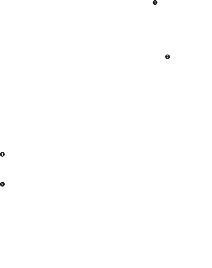
Here is an example of a custom partitioner:
import org.apache.kafka.clients.producer.Partitioner;
import org.apache.kafka.common.Cluster;
import org.apache.kafka.common.PartitionInfo;
import org.apache.kafka.common.record.InvalidRecordException;
import org.apache.kafka.common.utils.Utils;
public class BananaPartitioner implements Partitioner {
public void configure(Map<String, ?> configs) {}
public int partition(String topic, Object key, byte[] keyBytes,
Object value, byte[] valueBytes,
Cluster cluster) {
List<PartitionInfo> partitions =
cluster.partitionsForTopic(topic);
int numPartitions = partitions.size();
if ((keyBytes == null) || (!(key instanceOf String)))
throw new InvalidRecordException("We expect all messages
to have customer name as key")
if (((String) key).equals("Banana"))
return numPartitions; // Banana will always go to last
partition
// Other records will get hashed to the rest of the
partitions
return (Math.abs(Utils.murmur2(keyBytes)) % (numPartitions - 1))
}
public void close() {}
}
Partitioner interface includes configure, partition, and close methods. Here
we only implement partition, although we really should have passed the special
customer name through configure instead of hard-coding it in partition.
We only expect String keys, so we throw an exception if that is not the case.
Old Producer APIs
In this chapter we’ve discussed the Java producer client that is part of the
org.apache.kafka.clients package. However, Apache Kafka still has two older cli‐
ents written in Scala that are part of the kafka.producer package and the core Kafka
module. These producers are called SyncProducers (which, depending on the value
of the acks parameter, may wait for the server to ack each message or batch of mes‐
sages before sending additional messages) and AsyncProducer (which batches mes‐
Old Producer APIs | 61

sages in the background, sends them in a separate thread, and does not provide
feedback regarding success to the client).
Because the current producer supports both behaviors and provides much more reli‐
ability and control to the developer, we will not discuss the older APIs. If you are
interested in using them, think twice and then refer to Apache Kafka documentation
to learn more.
Summary
We began this chapter with a simple example of a producer—just 10 lines of code that
send events to Kafka. We added to the simple example by adding error handling and
experimenting with synchronous and asynchronous producing. We then explored the
most important producer configuration parameters and saw how they modify the
behavior of the producers. We discussed serializers, which let us control the format of
the events we write to Kafka. We looked in-depth at Avro, one of many ways to serial‐
ize events, but one that is very commonly used with Kafka. We concluded the chapter
with a discussion of partitioning in Kafka and an example of an advanced custom
partitioning technique.
Now that we know how to write events to Kafka, in Chapter 4 we’ll learn all about
consuming events from Kafka.
62 | Chapter 3: Kafka Producers: Writing Messages to Kafka

CHAPTER 4
Kafka Consumers: Reading Data from Kafka
Applications that need to read data from Kafka use a KafkaConsumer to subscribe to
Kafka topics and receive messages from these topics. Reading data from Kafka is a bit
different than reading data from other messaging systems, and there are few unique
concepts and ideas involved. It is difficult to understand how to use the consumer
API without understanding these concepts first. We’ll start by explaining some of the
important concepts, and then we’ll go through some examples that show the different
ways consumer APIs can be used to implement applications with varying require‐
ments.
Kafka Consumer Concepts
In order to understand how to read data from Kafka, you first need to understand its
consumers and consumer groups. The following sections cover those concepts.
Consumers and Consumer Groups
Suppose you have an application that needs to read messages from a Kafka topic, run
some validations against them, and write the results to another data store. In this case
your application will create a consumer object, subscribe to the appropriate topic, and
start receiving messages, validating them and writing the results. This may work well
for a while, but what if the rate at which producers write messages to the topic
exceeds the rate at which your application can validate them? If you are limited to a
single consumer reading and processing the data, your application may fall farther
and farther behind, unable to keep up with the rate of incoming messages. Obviously
there is a need to scale consumption from topics. Just like multiple producers can
write to the same topic, we need to allow multiple consumers to read from the same
topic, splitting the data between them.
63
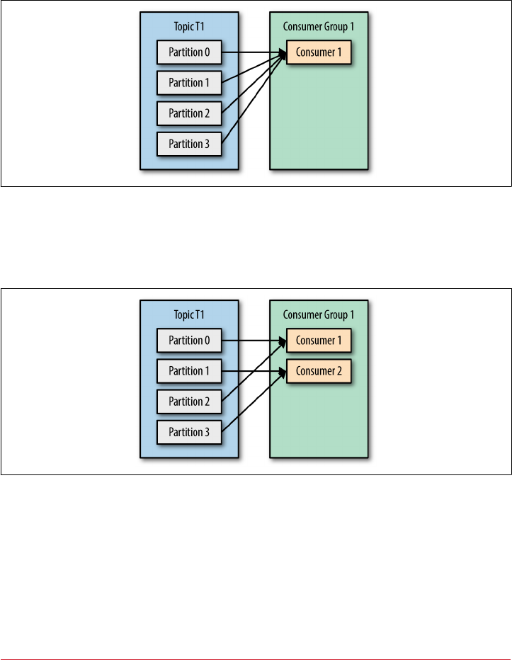
Kafka consumers are typically part of a consumer group. When multiple consumers
are subscribed to a topic and belong to the same consumer group, each consumer in
the group will receive messages from a different subset of the partitions in the topic.
Let’s take topic T1 with four partitions. Now suppose we created a new consumer, C1,
which is the only consumer in group G1, and use it to subscribe to topic T1. Con‐
sumer C1 will get all messages from all four t1 partitions. See Figure 4-1.
Figure 4-1. One Consumer group with four partitions
If we add another consumer, C2, to group G1, each consumer will only get messages
from two partitions. Perhaps messages from partition 0 and 2 go to C1 and messages
from partitions 1 and 3 go to consumer C2. See Figure 4-2.
Figure 4-2. Four partitions split to two consumer groups
If G1 has four consumers, then each will read messages from a single partition. See
Figure 4-3.
64 | Chapter 4: Kafka Consumers: Reading Data from Kafka
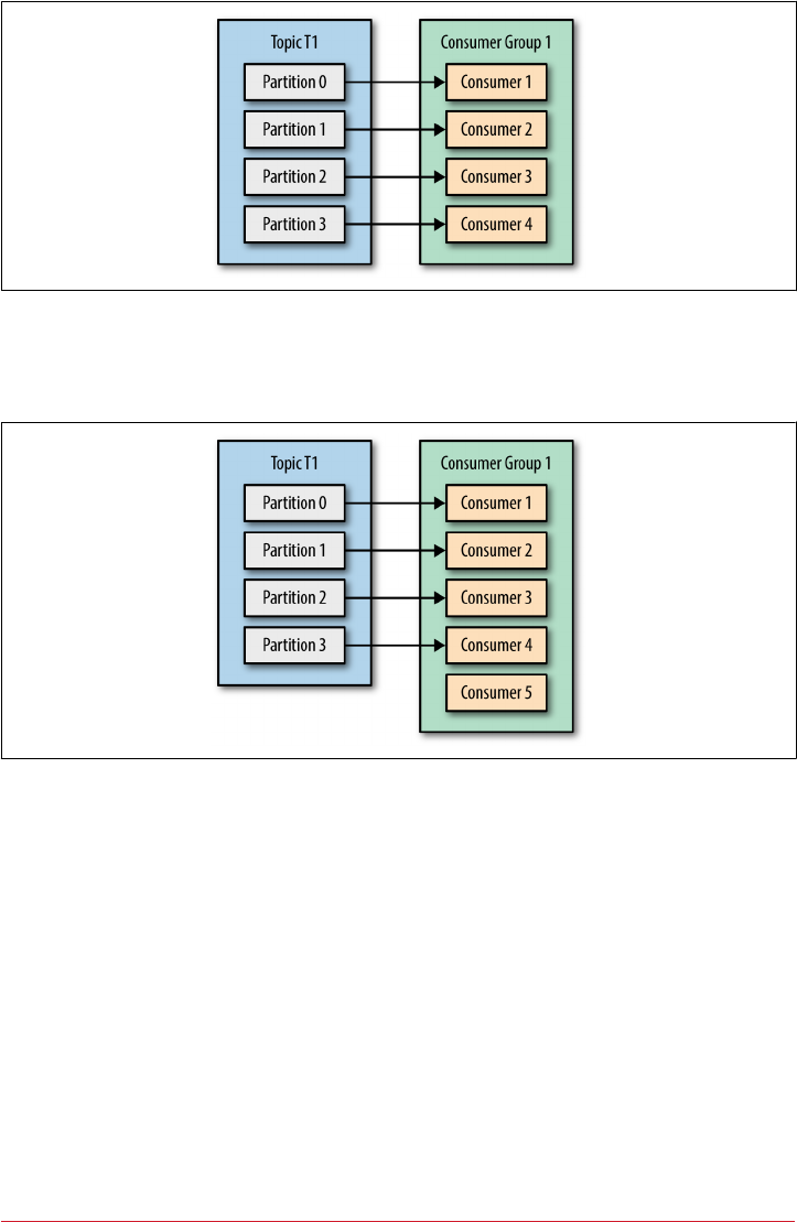
Figure 4-3. Four consumer groups to one partition each
If we add more consumers to a single group with a single topic than we have parti‐
tions, some of the consumers will be idle and get no messages at all. See Figure 4-4.
Figure 4-4. More consumer groups than partitions means missed messages
The main way we scale data consumption from a Kafka topic is by adding more con‐
sumers to a consumer group. It is common for Kafka consumers to do high-latency
operations such as write to a database or a time-consuming computation on the data.
In these cases, a single consumer can’t possibly keep up with the rate data flows into a
topic, and adding more consumers that share the load by having each consumer own
just a subset of the partitions and messages is our main method of scaling. This is a
good reason to create topics with a large number of partitions—it allows adding more
consumers when the load increases. Keep in mind that there is no point in adding
more consumers than you have partitions in a topic—some of the consumers will just
be idle. Chapter 2 includes some suggestions on how to choose the number of parti‐
tions in a topic.
Kafka Consumer Concepts | 65
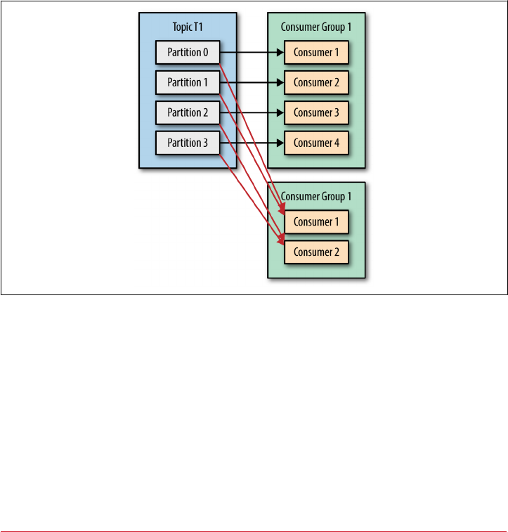
In addition to adding consumers in order to scale a single application, it is very com‐
mon to have multiple applications that need to read data from the same topic. In fact,
one of the main design goals in Kafka was to make the data produced to Kafka topics
available for many use cases throughout the organization. In those cases, we want
each application to get all of the messages, rather than just a subset. To make sure an
application gets all the messages in a topic, ensure the application has its own con‐
sumer group. Unlike many traditional messaging systems, Kafka scales to a large
number of consumers and consumer groups without reducing performance.
In the previous example, if we add a new consumer group G2 with a single consumer,
this consumer will get all the messages in topic T1 independent of what G1 is doing.
G2 can have more than a single consumer, in which case they will each get a subset of
partitions, just like we showed for G1, but G2 as a whole will still get all the messages
regardless of other consumer groups. See Figure 4-5.
Figure 4-5. Adding a new consumer group ensures no messages are missed
To summarize, you create a new consumer group for each application that needs all
the messages from one or more topics. You add consumers to an existing consumer
group to scale the reading and processing of messages from the topics, so each addi‐
tional consumer in a group will only get a subset of the messages.
Consumer Groups and Partition Rebalance
As we saw in the previous section, consumers in a consumer group share ownership
of the partitions in the topics they subscribe to. When we add a new consumer to the
group, it starts consuming messages from partitions previously consumed by another
66 | Chapter 4: Kafka Consumers: Reading Data from Kafka

consumer. The same thing happens when a consumer shuts down or crashes; it leaves
the group, and the partitions it used to consume will be consumed by one of the
remaining consumers. Reassignment of partitions to consumers also happen when
the topics the consumer group is consuming are modified (e.g., if an administrator
adds new partitions).
Moving partition ownership from one consumer to another is called a rebalance.
Rebalances are important because they provide the consumer group with high availa‐
bility and scalability (allowing us to easily and safely add and remove consumers), but
in the normal course of events they are fairly undesirable. During a rebalance, con‐
sumers can’t consume messages, so a rebalance is basically a short window of unavail‐
ability of the entire consumer group. In addition, when partitions are moved from
one consumer to another, the consumer loses its current state; if it was caching any
data, it will need to refresh its caches—slowing down the application until the con‐
sumer sets up its state again. Throughout this chapter we will discuss how to safely
handle rebalances and how to avoid unnecessary ones.
The way consumers maintain membership in a consumer group and ownership of
the partitions assigned to them is by sending heartbeats to a Kafka broker designated
as the group coordinator (this broker can be different for different consumer groups).
As long as the consumer is sending heartbeats at regular intervals, it is assumed to be
alive, well, and processing messages from its partitions. Heartbeats are sent when the
consumer polls (i.e., retrieves records) and when it commits records it has consumed.
If the consumer stops sending heartbeats for long enough, its session will time out
and the group coordinator will consider it dead and trigger a rebalance. If a consumer
crashed and stopped processing messages, it will take the group coordinator a few
seconds without heartbeats to decide it is dead and trigger the rebalance. During
those seconds, no messages will be processed from the partitions owned by the dead
consumer. When closing a consumer cleanly, the consumer will notify the group
coordinator that it is leaving, and the group coordinator will trigger a rebalance
immediately, reducing the gap in processing. Later in this chapter we will discuss con‐
figuration options that control heartbeat frequency and session timeouts and how to
set those to match your requirements.
Changes to Heartbeat Behavior in Recent Kafka Versions
In release 0.10.1, the Kafka community introduced a separate heartbeat thread that
will send heartbeats in between polls as well. This allows you to separate the heartbeat
frequency (and therefore how long it takes for the consumer group to detect that a
consumer crashed and is no longer sending heartbeats) from the frequency of polling
(which is determined by the time it takes to process the data returned from the brok‐
ers). With newer versions of Kafka, you can configure how long the application can
go without polling before it will leave the group and trigger a rebalance. This configu‐
Kafka Consumer Concepts | 67

ration is used to prevent a livelock, where the application did not crash but fails to
make progress for some reason. This configuration is separate from session.time
out.ms, which controls the time it takes to detect a consumer crash and stop sending
heartbeats.
The rest of the chapter will discuss some of the challenges with older behaviors and
how the programmer can handle them. This chapter includes discussion about how
to handle applications that take longer to process records. This is less relevant to
readers running Apache Kafka 0.10.1 or later. If you are using a new version and need
to handle records that take longer to process, you simply need to tune
max.poll.interval.ms so it will handle longer delays between polling for new
records.
How Does the Process of Assigning Partitions to Brokers Work?
When a consumer wants to join a group, it sends a JoinGroup
request to the group coordinator. The first consumer to join the
group becomes the group leader. The leader receives a list of all
consumers in the group from the group coordinator (this will
include all consumers that sent a heartbeat recently and which are
therefore considered alive) and is responsible for assigning a subset
of partitions to each consumer. It uses an implementation of Parti
tionAssignor to decide which partitions should be handled by
which consumer.
Kafka has two built-in partition assignment policies, which we will
discuss in more depth in the configuration section. After deciding
on the partition assignment, the consumer leader sends the list of
assignments to the GroupCoordinator, which sends this informa‐
tion to all the consumers. Each consumer only sees his own assign‐
ment—the leader is the only client process that has the full list of
consumers in the group and their assignments. This process
repeats every time a rebalance happens.
Creating a Kafka Consumer
The first step to start consuming records is to create a KafkaConsumer instance. Cre‐
ating a KafkaConsumer is very similar to creating a KafkaProducer—you create a Java
Properties instance with the properties you want to pass to the consumer. We will
discuss all the properties in depth later in the chapter. To start we just need to use the
three mandatory properties: bootstrap.servers, key.deserializer, and
value.deserializer.
The first property, bootstrap.servers, is the connection string to a Kafka cluster. It
is used the exact same way as in KafkaProducer (you can refer to Chapter 3 for
68 | Chapter 4: Kafka Consumers: Reading Data from Kafka

details on how this is defined). The other two properties, key.deserializer and
value.deserializer, are similar to the serializers defined for the producer, but
rather than specifying classes that turn Java objects to byte arrays, you need to specify
classes that can take a byte array and turn it into a Java object.
There is a fourth property, which is not strictly mandatory, but for now we will pre‐
tend it is. The property is group.id and it specifies the consumer group the
KafkaConsumer instance belongs to. While it is possible to create consumers that do
not belong to any consumer group, this is uncommon, so for most of the chapter we
will assume the consumer is part of a group.
The following code snippet shows how to create a KafkaConsumer:
Properties props = new Properties();
props.put("bootstrap.servers", "broker1:9092,broker2:9092");
props.put("group.id", "CountryCounter");
props.put("key.deserializer",
"org.apache.kafka.common.serialization.StringDeserializer");
props.put("value.deserializer",
"org.apache.kafka.common.serialization.StringDeserializer");
KafkaConsumer<String, String> consumer = new KafkaConsumer<String,
String>(props);
Most of what you see here should be familiar if you’ve read Chapter 3 on creating
producers. We assume that the records we consume will have String objects as both
the key and the value of the record. The only new property here is group.id, which is
the name of the consumer group this consumer belong to.
Subscribing to Topics
Once we create a consumer, the next step is to subscribe to one or more topics. The
subcribe() method takes a list of topics as a parameter, so it’s pretty simple to use:
consumer.subscribe(Collections.singletonList("customerCountries"));
Here we simply create a list with a single element: the topic name
customerCountries.
It is also possible to call subscribe with a regular expression. The expression can
match multiple topic names, and if someone creates a new topic with a name that
matches, a rebalance will happen almost immediately and the consumers will start
consuming from the new topic. This is useful for applications that need to consume
from multiple topics and can handle the different types of data the topics will contain.
Subscribing to multiple topics using a regular expression is most commonly used in
applications that replicate data between Kafka and another system.
Subscribing to Topics | 69
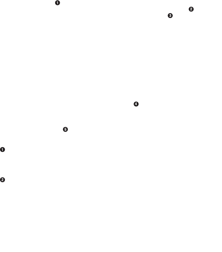
To subscribe to all test topics, we can call:
consumer.subscribe("test.*");
The Poll Loop
At the heart of the consumer API is a simple loop for polling the server for more data.
Once the consumer subscribes to topics, the poll loop handles all details of coordina‐
tion, partition rebalances, heartbeats, and data fetching, leaving the developer with a
clean API that simply returns available data from the assigned partitions. The main
body of a consumer will look as follows:
try {
while (true) {
ConsumerRecords<String, String> records = consumer.poll(100);
for (ConsumerRecord<String, String> record : records)
{
log.debug("topic = %s, partition = %s, offset = %d,
customer = %s, country = %s\n",
record.topic(), record.partition(), record.offset(),
record.key(), record.value());
int updatedCount = 1;
if (custCountryMap.countainsValue(record.value())) {
updatedCount = custCountryMap.get(record.value()) + 1;
}
custCountryMap.put(record.value(), updatedCount)
JSONObject json = new JSONObject(custCountryMap);
System.out.println(json.toString(4))
}
}
} finally {
consumer.close();
}
This is indeed an infinite loop. Consumers are usually long-running applications
that continuously poll Kafka for more data. We will show later in the chapter how
to cleanly exit the loop and close the consumer.
This is the most important line in the chapter. The same way that sharks must
keep moving or they die, consumers must keep polling Kafka or they will be con‐
sidered dead and the partitions they are consuming will be handed to another
consumer in the group to continue consuming. The parameter we pass, poll(),
is a timeout interval and controls how long poll() will block if data is not avail‐
able in the consumer buffer. If this is set to 0, poll() will return immediately;
otherwise, it will wait for the specified number of milliseconds for data to arrive
from the broker.
70 | Chapter 4: Kafka Consumers: Reading Data from Kafka

poll() returns a list of records. Each record contains the topic and partition the
record came from, the offset of the record within the partition, and of course the
key and the value of the record. Typically we want to iterate over the list and pro‐
cess the records individually. The poll() method takes a timeout parameter. This
specifies how long it will take poll to return, with or without data. The value is
typically driven by application needs for quick responses—how fast do you want
to return control to the thread that does the polling?
Processing usually ends in writing a result in a data store or updating a stored
record. Here, the goal is to keep a running count of customers from each county,
so we update a hashtable and print the result as JSON. A more realistic example
would store the updates result in a data store.
Always close() the consumer before exiting. This will close the network connec‐
tions and sockets. It will also trigger a rebalance immediately rather than wait for
the group coordinator to discover that the consumer stopped sending heartbeats
and is likely dead, which will take longer and therefore result in a longer period
of time in which consumers can’t consume messages from a subset of the parti‐
tions.
The poll loop does a lot more than just get data. The first time you call poll() with a
new consumer, it is responsible for finding the GroupCoordinator, joining the con‐
sumer group, and receiving a partition assignment. If a rebalance is triggered, it will
be handled inside the poll loop as well. And of course the heartbeats that keep con‐
sumers alive are sent from within the poll loop. For this reason, we try to make sure
that whatever processing we do between iterations is fast and efficient.
Thread Safety
You can’t have multiple consumers that belong to the same group
in one thread and you can’t have multiple threads safely use the
same consumer. One consumer per thread is the rule. To run mul‐
tiple consumers in the same group in one application, you will
need to run each in its own thread. It is useful to wrap the con‐
sumer logic in its own object and then use Java’s ExecutorService
to start multiple threads each with its own consumer. The Conflu‐
ent blog has a tutorial that shows how to do just that.
The Poll Loop | 71

Conguring Consumers
So far we have focused on learning the consumer API, but we’ve only looked at a few
of the configuration properties—just the mandatory bootstrap.servers, group.id,
key.deserializer, and value.deserializer. All the consumer configuration is
documented in Apache Kafka documentation. Most of the parameters have reason‐
able defaults and do not require modification, but some have implications on the per‐
formance and availability of the consumers. Let’s take a look at some of the more
important properties.
fetch.min.bytes
This property allows a consumer to specify the minimum amount of data that it
wants to receive from the broker when fetching records. If a broker receives a request
for records from a consumer but the new records amount to fewer bytes than
min.fetch.bytes, the broker will wait until more messages are available before send‐
ing the records back to the consumer. This reduces the load on both the consumer
and the broker as they have to handle fewer back-and-forth messages in cases where
the topics don’t have much new activity (or for lower activity hours of the day). You
will want to set this parameter higher than the default if the consumer is using too
much CPU when there isn’t much data available, or reduce load on the brokers when
you have large number of consumers.
fetch.max.wait.ms
By setting fetch.min.bytes, you tell Kafka to wait until it has enough data to send
before responding to the consumer. fetch.max.wait.ms lets you control how long to
wait. By default, Kafka will wait up to 500 ms. This results in up to 500 ms of extra
latency in case there is not enough data flowing to the Kafka topic to satisfy the mini‐
mum amount of data to return. If you want to limit the potential latency (usually due
to SLAs controlling the maximum latency of the application), you can set
fetch.max.wait.ms to a lower value. If you set fetch.max.wait.ms to 100 ms and
fetch.min.bytes to 1 MB, Kafka will recieve a fetch request from the consumer and
will respond with data either when it has 1 MB of data to return or after 100 ms,
whichever happens first.
max.partition.fetch.bytes
This property controls the maximum number of bytes the server will return per parti‐
tion. The default is 1 MB, which means that when KafkaConsumer.poll() returns
ConsumerRecords, the record object will use at most max.partition.fetch.bytes
per partition assigned to the consumer. So if a topic has 20 partitions, and you have 5
consumers, each consumer will need to have 4 MB of memory available for Consumer
72 | Chapter 4: Kafka Consumers: Reading Data from Kafka

Records. In practice, you will want to allocate more memory as each consumer will
need to handle more partitions if other consumers in the group fail. max.
partition.fetch.bytes must be larger than the largest message a broker will accept
(determined by the max.message.size property in the broker configuration), or the
broker may have messages that the consumer will be unable to consume, in which
case the consumer will hang trying to read them. Another important consideration
when setting max.partition.fetch.bytes is the amount of time it takes the con‐
sumer to process data. As you recall, the consumer must call poll() frequently
enough to avoid session timeout and subsequent rebalance. If the amount of data a
single poll() returns is very large, it may take the consumer longer to process, which
means it will not get to the next iteration of the poll loop in time to avoid a session
timeout. If this occurs, the two options are either to lower max.
partition.fetch.bytes or to increase the session timeout.
session.timeout.ms
The amount of time a consumer can be out of contact with the brokers while still
considered alive defaults to 3 seconds. If more than session.timeout.ms passes
without the consumer sending a heartbeat to the group coordinator, it is considered
dead and the group coordinator will trigger a rebalance of the consumer group to
allocate partitions from the dead consumer to the other consumers in the group. This
property is closely related to heartbeat.interval.ms. heartbeat.interval.ms con‐
trols how frequently the KafkaConsumer poll() method will send a heartbeat to the
group coordinator, whereas session.timeout.ms controls how long a consumer can
go without sending a heartbeat. Therefore, those two properties are typically modi‐
fied together—heatbeat.interval.ms must be lower than session.timeout.ms, and
is usually set to one-third of the timeout value. So if session.timeout.ms is 3 sec‐
onds, heartbeat.interval.ms should be 1 second. Setting session.timeout.ms
lower than the default will allow consumer groups to detect and recover from failure
sooner, but may also cause unwanted rebalances as a result of consumers taking
longer to complete the poll loop or garbage collection. Setting session.timeout.ms
higher will reduce the chance of accidental rebalance, but also means it will take
longer to detect a real failure.
auto.oset.reset
This property controls the behavior of the consumer when it starts reading a partition
for which it doesn’t have a committed offset or if the committed offset it has is invalid
(usually because the consumer was down for so long that the record with that offset
was already aged out of the broker). The default is “latest,” which means that lacking a
valid offset, the consumer will start reading from the newest records (records that
were written after the consumer started running). The alternative is “earliest,” which
Conguring Consumers | 73

means that lacking a valid offset, the consumer will read all the data in the partition,
starting from the very beginning.
enable.auto.commit
We discussed the different options for committing offsets earlier in this chapter. This
parameter controls whether the consumer will commit offsets automatically, and
defaults to true. Set it to false if you prefer to control when offsets are committed,
which is necessary to minimize duplicates and avoid missing data. If you set
enable.auto.commit to true, then you might also want to control how frequently
offsets will be committed using auto.commit.interval.ms.
partition.assignment.strategy
We learned that partitions are assigned to consumers in a consumer group. A
PartitionAssignor is a class that, given consumers and topics they subscribed to,
decides which partitions will be assigned to which consumer. By default, Kafka has
two assignment strategies:
Range
Assigns to each consumer a consecutive subset of partitions from each topic it
subscribes to. So if consumers C1 and C2 are subscribed to two topics, T1 and
T2, and each of the topics has three partitions, then C1 will be assigned partitions
0 and 1 from topics T1 and T2, while C2 will be assigned partition 2 from those
topics. Because each topic has an uneven number of partitions and the assign‐
ment is done for each topic independently, the first consumer ends up with more
partitions than the second. This happens whenever Range assignment is used and
the number of consumers does not divide the number of partitions in each topic
neatly.
RoundRobin
Takes all the partitions from all subscribed topics and assigns them to consumers
sequentially, one by one. If C1 and C2 described previously used RoundRobin
assignment, C1 would have partitions 0 and 2 from topic T1 and partition 1 from
topic T2. C2 would have partition 1 from topic T1 and partitions 0 and 2 from
topic T2. In general, if all consumers are subscribed to the same topics (a very
common scenario), RoundRobin assignment will end up with all consumers hav‐
ing the same number of partitions (or at most 1 partition difference).
The partition.assignment.strategy allows you to choose a partition-assignment
strategy. The default is org.apache.kafka.clients.consumer.RangeAssignor,
which implements the Range strategy described above. You can replace it with
org.apache.kafka.clients.consumer.RoundRobinAssignor. A more advanced
option is to implement your own assignment strategy, in which case
partition.assignment.strategy should point to the name of your class.
74 | Chapter 4: Kafka Consumers: Reading Data from Kafka

client.id
This can be any string, and will be used by the brokers to identify messages sent from
the client. It is used in logging and metrics, and for quotas.
max.poll.records
This controls the maximum number of records that a single call to poll() will return.
This is useful to help control the amount of data your application will need to process
in the polling loop.
receive.buer.bytes and send.buer.bytes
These are the sizes of the TCP send and receive buffers used by the sockets when
writing and reading data. If these are set to -1, the OS defaults will be used. It can be a
good idea to increase those when producers or consumers communicate with brokers
in a different datacenter, because those network links typically have higher latency
and lower bandwidth.
Commits and Osets
Whenever we call poll(), it returns records written to Kafka that consumers in our
group have not read yet. This means that we have a way of tracking which records
were read by a consumer of the group. As discussed before, one of Kafka’s unique
characteristics is that it does not track acknowledgments from consumers the way
many JMS queues do. Instead, it allows consumers to use Kafka to track their posi‐
tion (offset) in each partition.
We call the action of updating the current position in the partition a commit.
How does a consumer commit an offset? It produces a message to Kafka, to a special
__consumer_offsets topic, with the committed offset for each partition. As long as all
your consumers are up, running, and churning away, this will have no impact. How‐
ever, if a consumer crashes or a new consumer joins the consumer group, this will
trigger a rebalance. After a rebalance, each consumer may be assigned a new set of
partitions than the one it processed before. In order to know where to pick up the
work, the consumer will read the latest committed offset of each partition and con‐
tinue from there.
If the committed offset is smaller than the offset of the last message the client pro‐
cessed, the messages between the last processed offset and the committed offset will
be processed twice. See Figure 4-6.
Commits and Osets | 75
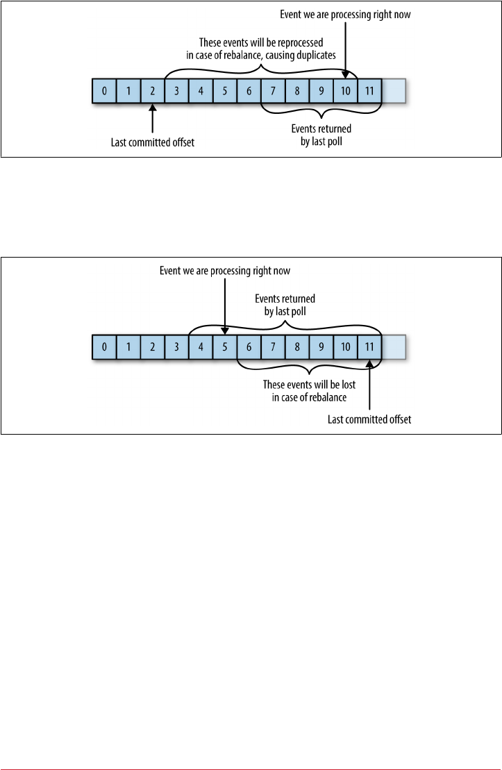
Figure 4-6. Re-processed messages
If the committed offset is larger than the offset of the last message the client actually
processed, all messages between the last processed offset and the committed offset
will be missed by the consumer group. See Figure 4-7.
Figure 4-7. Missed messages between osets
Clearly, managing offsets has a big impact on the client application. The
KafkaConsumer API provides multiple ways of committing offsets:
Automatic Commit
The easiest way to commit offsets is to allow the consumer to do it for you. If you
configure enable.auto.commit=true, then every five seconds the consumer will
commit the largest offset your client received from poll(). The five-second interval
is the default and is controlled by setting auto.commit.interval.ms. Just like every‐
thing else in the consumer, the automatic commits are driven by the poll loop. When‐
ever you poll, the consumer checks if it is time to commit, and if it is, it will commit
the offsets it returned in the last poll.
Before using this convenient option, however, it is important to understand the con‐
sequences.
76 | Chapter 4: Kafka Consumers: Reading Data from Kafka

Consider that, by default, automatic commits occur every five seconds. Suppose that
we are three seconds after the most recent commit and a rebalance is triggered. After
the rebalancing, all consumers will start consuming from the last offset committed. In
this case, the offset is three seconds old, so all the events that arrived in those three
seconds will be processed twice. It is possible to configure the commit interval to
commit more frequently and reduce the window in which records will be duplicated,
but it is impossible to completely eliminate them.
With autocommit enabled, a call to poll will always commit the last offset returned by
the previous poll. It doesn’t know which events were actually processed, so it is critical
to always process all the events returned by poll() before calling poll() again. (Just
like poll(), close() also commits offsets automatically.) This is usually not an issue,
but pay attention when you handle exceptions or exit the poll loop prematurely.
Automatic commits are convenient, but they don’t give developers enough control to
avoid duplicate messages.
Commit Current Oset
Most developers exercise more control over the time at which offsets are committed
—both to eliminate the possibility of missing messages and to reduce the number of
messages duplicated during rebalancing. The consumer API has the option of com‐
mitting the current offset at a point that makes sense to the application developer
rather than based on a timer.
By setting auto.commit.offset=false, offsets will only be committed when the
application explicitly chooses to do so. The simplest and most reliable of the commit
APIs is commitSync(). This API will commit the latest offset returned by poll() and
return once the offset is committed, throwing an exception if commit fails for some
reason.
It is important to remember that commitSync() will commit the latest offset returned
by poll(), so make sure you call commitSync() after you are done processing all the
records in the collection, or you risk missing messages as described previously. When
rebalance is triggered, all the messages from the beginning of the most recent batch
until the time of the rebalance will be processed twice.
Here is how we would use commitSync to commit offsets after we finished processing
the latest batch of messages:
while (true) {
ConsumerRecords<String, String> records = consumer.poll(100);
for (ConsumerRecord<String, String> record : records)
{
System.out.printf("topic = %s, partition = %s, offset =
%d, customer = %s, country = %s\n",
record.topic(), record.partition(),
Commits and Osets | 77
www.allitebooks.com
record.offset(), record.key(), record.value());
}
try {
consumer.commitSync();
} catch (CommitFailedException e) {
log.error("commit failed", e)
}
}
Let’s assume that by printing the contents of a record, we are done processing it.
Your application will likely do a lot more with the records—modify them, enrich
them, aggregate them, display them on a dashboard, or notify users of important
events. You should determine when you are “done” with a record according to
your use case.
Once we are done “processing” all the records in the current batch, we call com
mitSync to commit the last offset in the batch, before polling for additional mes‐
sages.
commitSync retries committing as long as there is no error that can’t be recov‐
ered. If this happens, there is not much we can do except log an error.
Asynchronous Commit
One drawback of manual commit is that the application is blocked until the broker
responds to the commit request. This will limit the throughput of the application.
Throughput can be improved by committing less frequently, but then we are increas‐
ing the number of potential duplicates that a rebalance will create.
Another option is the asynchronous commit API. Instead of waiting for the broker to
respond to a commit, we just send the request and continue on:
while (true) {
ConsumerRecords<String, String> records = consumer.poll(100);
for (ConsumerRecord<String, String> record : records)
{
System.out.printf("topic = %s, partition = %s,
offset = %d, customer = %s, country = %s\n",
record.topic(), record.partition(), record.offset(),
record.key(), record.value());
}
consumer.commitAsync();
}
Commit the last offset and carry on.
The drawback is that while commitSync() will retry the commit until it either suc‐
ceeds or encounters a nonretriable failure, commitAsync() will not retry. The reason
78 | Chapter 4: Kafka Consumers: Reading Data from Kafka
it does not retry is that by the time commitAsync() receives a response from the
server, there may have been a later commit that was already successful. Imagine that
we sent a request to commit offset 2000. There is a temporary communication prob‐
lem, so the broker never gets the request and therefore never responds. Meanwhile,
we processed another batch and successfully committed offset 3000. If commitA
sync() now retries the previously failed commit, it might succeed in committing off‐
set 2000 aer offset 3000 was already processed and committed. In the case of a
rebalance, this will cause more duplicates.
We mention this complication and the importance of correct order of commits,
because commitAsync() also gives you an option to pass in a callback that will be trig‐
gered when the broker responds. It is common to use the callback to log commit
errors or to count them in a metric, but if you want to use the callback for retries, you
need to be aware of the problem with commit order:
while (true) {
ConsumerRecords<String, String> records = consumer.poll(100);
for (ConsumerRecord<String, String> record : records) {
System.out.printf("topic = %s, partition = %s,
offset = %d, customer = %s, country = %s\n",
record.topic(), record.partition(), record.offset(),
record.key(), record.value());
}
consumer.commitAsync(new OffsetCommitCallback() {
public void onComplete(Map<TopicPartition,
OffsetAndMetadata> offsets, Exception exception) {
if (e != null)
log.error("Commit failed for offsets {}", offsets, e);
}
});
}
We send the commit and carry on, but if the commit fails, the failure and the off‐
sets will be logged.
Retrying Async Commits
A simple pattern to get commit order right for asynchronous
retries is to use a monotonically increasing sequence number.
Increase the sequence number every time you commit and add the
sequence number at the time of the commit to the commitAsync
callback. When you’re getting ready to send a retry, check if the
commit sequence number the callback got is equal to the instance
variable; if it is, there was no newer commit and it is safe to retry. If
the instance sequence number is higher, don’t retry because a
newer commit was already sent.
Commits and Osets | 79

Combining Synchronous and Asynchronous Commits
Normally, occasional failures to commit without retrying are not a huge problem
because if the problem is temporary, the following commit will be successful. But if
we know that this is the last commit before we close the consumer, or before a reba‐
lance, we want to make extra sure that the commit succeeds.
Therefore, a common pattern is to combine commitAsync() with commitSync() just
before shutdown. Here is how it works (we will discuss how to commit just before
rebalance when we get to the section about rebalance listeners):
try {
while (true) {
ConsumerRecords<String, String> records = consumer.poll(100);
for (ConsumerRecord<String, String> record : records) {
System.out.printf("topic = %s, partition = %s, offset = %d,
customer = %s, country = %s\n",
record.topic(), record.partition(),
record.offset(), record.key(), record.value());
}
consumer.commitAsync();
}
} catch (Exception e) {
log.error("Unexpected error", e);
} finally {
try {
consumer.commitSync();
} finally {
consumer.close();
}
}
While everything is fine, we use commitAsync. It is faster, and if one commit fails,
the next commit will serve as a retry.
But if we are closing, there is no “next commit.” We call commitSync(), because it
will retry until it succeeds or suffers unrecoverable failure.
Commit Specied Oset
Committing the latest offset only allows you to commit as often as you finish process‐
ing batches. But what if you want to commit more frequently than that? What if
poll() returns a huge batch and you want to commit offsets in the middle of the
batch to avoid having to process all those rows again if a rebalance occurs? You can’t
just call commitSync() or commitAsync()—this will commit the last offset returned,
which you didn’t get to process yet.
80 | Chapter 4: Kafka Consumers: Reading Data from Kafka
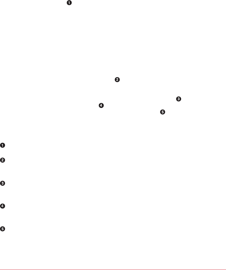
Fortunately, the consumer API allows you to call commitSync() and commitAsync()
and pass a map of partitions and offsets that you wish to commit. If you are in the
middle of processing a batch of records, and the last message you got from partition 3
in topic “customers” has offset 5000, you can call commitSync() to commit offset
5000 for partition 3 in topic “customers.” Since your consumer may be consuming
more than a single partition, you will need to track offsets on all of them, which adds
complexity to your code.
Here is what a commit of specific offsets looks like:
private Map<TopicPartition, OffsetAndMetadata> currentOffsets =
new HashMap<>();
int count = 0;
....
while (true) {
ConsumerRecords<String, String> records = consumer.poll(100);
for (ConsumerRecord<String, String> record : records)
{
System.out.printf("topic = %s, partition = %s, offset = %d,
customer = %s, country = %s\n",
record.topic(), record.partition(), record.offset(),
record.key(), record.value());
currentOffsets.put(new TopicPartition(record.topic(),
record.partition()), new
OffsetAndMetadata(record.offset()+1, "no metadata"));
if (count % 1000 == 0)
consumer.commitAsync(currentOffsets, null);
count++;
}
}
This is the map we will use to manually track offsets.
Remember, println is a stand-in for whatever processing you do for the records
you consume.
After reading each record, we update the offsets map with the offset of the next
message we expect to process. This is where we’ll start reading next time we start.
Here, we decide to commit current offsets every 1,000 records. In your applica‐
tion, you can commit based on time or perhaps content of the records.
I chose to call commitAsync(), but commitSync() is also completely valid here. Of
course, when committing specific offsets you still need to perform all the error
handling we’ve seen in previous sections.
Commits and Osets | 81
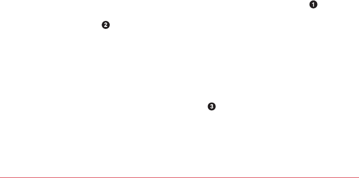
Rebalance Listeners
As we mentioned in the previous section about committing offsets, a consumer will
want to do some cleanup work before exiting and also before partition rebalancing.
If you know your consumer is about to lose ownership of a partition, you will want to
commit offsets of the last event you’ve processed. If your consumer maintained a
buffer with events that it only processes occasionally (e.g., the currentRecords map
we used when explaining pause() functionality), you will want to process the events
you accumulated before losing ownership of the partition. Perhaps you also need to
close file handles, database connections, and such.
The consumer API allows you to run your own code when partitions are added or
removed from the consumer. You do this by passing a ConsumerRebalanceListener
when calling the subscribe() method we discussed previously. ConsumerRebalance
Listener has two methods you can implement:
public void onPartitionsRevoked(Collection<TopicPartition> partitions)
Called before the rebalancing starts and after the consumer stopped consuming
messages. This is where you want to commit offsets, so whoever gets this parti‐
tion next will know where to start.
public void onPartitionsAssigned(Collection<TopicPartition> partitions)
Called after partitions have been reassigned to the broker, but before the con‐
sumer starts consuming messages.
This example will show how to use onPartitionsRevoked() to commit offsets before
losing ownership of a partition. In the next section we will show a more involved
example that also demonstrates the use of onPartitionsAssigned():
private Map<TopicPartition, OffsetAndMetadata> currentOffsets =
new HashMap<>();
private class HandleRebalance implements ConsumerRebalanceListener {
public void onPartitionsAssigned(Collection<TopicPartition>
partitions) {
}
public void onPartitionsRevoked(Collection<TopicPartition>
partitions) {
System.out.println("Lost partitions in rebalance.
Committing current
offsets:" + currentOffsets);
consumer.commitSync(currentOffsets);
}
}
try {
82 | Chapter 4: Kafka Consumers: Reading Data from Kafka
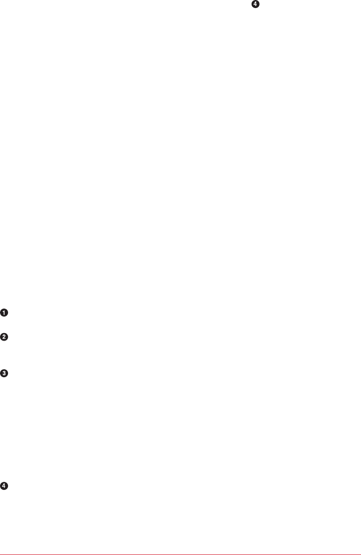
consumer.subscribe(topics, new HandleRebalance());
while (true) {
ConsumerRecords<String, String> records =
consumer.poll(100);
for (ConsumerRecord<String, String> record : records)
{
System.out.printf("topic = %s, partition = %s, offset = %d,
customer = %s, country = %s\n",
record.topic(), record.partition(), record.offset(),
record.key(), record.value());
currentOffsets.put(new TopicPartition(record.topic(),
record.partition()), new
OffsetAndMetadata(record.offset()+1, "no metadata"));
}
consumer.commitAsync(currentOffsets, null);
}
} catch (WakeupException e) {
// ignore, we're closing
} catch (Exception e) {
log.error("Unexpected error", e);
} finally {
try {
consumer.commitSync(currentOffsets);
} finally {
consumer.close();
System.out.println("Closed consumer and we are done");
}
}
We start by implementing a ConsumerRebalanceListener.
In this example we don’t need to do anything when we get a new partition; we’ll
just start consuming messages.
However, when we are about to lose a partition due to rebalancing, we need to
commit offsets. Note that we are committing the latest offsets we’ve processed,
not the latest offsets in the batch we are still processing. This is because a parti‐
tion could get revoked while we are still in the middle of a batch. We are commit‐
ting offsets for all partitions, not just the partitions we are about to lose—because
the offsets are for events that were already processed, there is no harm in that.
And we are using commitSync() to make sure the offsets are committed before
the rebalance proceeds.
The most important part: pass the ConsumerRebalanceListener to the sub
scribe() method so it will get invoked by the consumer.
Rebalance Listeners | 83

Consuming Records with Specic Osets
So far we’ve seen how to use poll() to start consuming messages from the last com‐
mitted offset in each partition and to proceed in processing all messages in sequence.
However, sometimes you want to start reading at a different offset.
If you want to start reading all messages from the beginning of the partition, or you
want to skip all the way to the end of the partition and start consuming only new
messages, there are APIs specifically for that: seekToBeginning(TopicPartition tp)
and seekToEnd(TopicPartition tp).
However, the Kafka API also lets you seek a specific offset. This ability can be used in
a variety of ways; for example, to go back a few messages or skip ahead a few mes‐
sages (perhaps a time-sensitive application that is falling behind will want to skip
ahead to more relevant messages). The most exciting use case for this ability is when
offsets are stored in a system other than Kafka.
Think about this common scenario: Your application is reading events from Kafka
(perhaps a clickstream of users in a website), processes the data (perhaps remove
records that indicate clicks from automated programs rather than users), and then
stores the results in a database, NoSQL store, or Hadoop. Suppose that we really don’t
want to lose any data, nor do we want to store the same results in the database twice.
In these cases, the consumer loop may look a bit like this:
while (true) {
ConsumerRecords<String, String> records = consumer.poll(100);
for (ConsumerRecord<String, String> record : records)
{
currentOffsets.put(new TopicPartition(record.topic(),
record.partition()),
record.offset());
processRecord(record);
storeRecordInDB(record);
consumer.commitAsync(currentOffsets);
}
}
In this example, we are very paranoid, so we commit offsets after processing each
record. However, there is still a chance that our application will crash after the record
was stored in the database but before we committed offsets, causing the record to be
processed again and the database to contain duplicates.
This could be avoided if there was a way to store both the record and the offset in one
atomic action. Either both the record and the offset are committed, or neither of
them are committed. As long as the records are written to a database and the offsets
to Kafka, this is impossible.
84 | Chapter 4: Kafka Consumers: Reading Data from Kafka
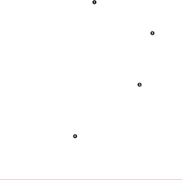
But what if we wrote both the record and the offset to the database, in one transac‐
tion? Then we’ll know that either we are done with the record and the offset is com‐
mitted or we are not and the record will be reprocessed.
Now the only problem is if the record is stored in a database and not in Kafka, how
will our consumer know where to start reading when it is assigned a partition? This is
exactly what seek() can be used for. When the consumer starts or when new parti‐
tions are assigned, it can look up the offset in the database and seek() to that loca‐
tion.
Here is a skeleton example of how this may work. We use ConsumerRebalanceLister
and seek() to make sure we start processing at the offsets stored in the database:
public class SaveOffsetsOnRebalance implements
ConsumerRebalanceListener {
public void onPartitionsRevoked(Collection<TopicPartition>
partitions) {
commitDBTransaction();
}
public void onPartitionsAssigned(Collection<TopicPartition>
partitions) {
for(TopicPartition partition: partitions)
consumer.seek(partition, getOffsetFromDB(partition));
}
}
}
consumer.subscribe(topics, new SaveOffsetOnRebalance(consumer));
consumer.poll(0);
for (TopicPartition partition: consumer.assignment())
consumer.seek(partition, getOffsetFromDB(partition));
while (true) {
ConsumerRecords<String, String> records =
consumer.poll(100);
for (ConsumerRecord<String, String> record : records)
{
processRecord(record);
storeRecordInDB(record);
storeOffsetInDB(record.topic(), record.partition(),
record.offset());
}
commitDBTransaction();
}
Consuming Records with Specic Osets | 85

We use an imaginary method here to commit the transaction in the database.
The idea here is that the database records and offsets will be inserted to the data‐
base as we process the records, and we just need to commit the transactions
when we are about to lose the partition to make sure this information is persis‐
ted.
We also have an imaginary method to fetch the offsets from the database, and
then we seek() to those records when we get ownership of new partitions.
When the consumer first starts, after we subscribe to topics, we call poll() once
to make sure we join a consumer group and get assigned partitions, and then we
immediately seek() to the correct offset in the partitions we are assigned to.
Keep in mind that seek() only updates the position we are consuming from, so
the next poll() will fetch the right messages. If there was an error in seek()
(e.g., the offset does not exist), the exception will be thrown by poll().
Another imaginary method: this time we update a table storing the offsets in our
database. Here we assume that updating records is fast, so we do an update on
every record, but commits are slow, so we only commit at the end of the batch.
However, this can be optimized in different ways.
There are many different ways to implement exactly-once semantics by storing offsets
and data in an external store, but all of them will need to use the ConsumerRebalance
Listener and seek() to make sure offsets are stored in time and that the consumer
starts reading messages from the correct location.
But How Do We Exit?
Earlier in this chapter, when we discussed the poll loop, I told you not to worry about
the fact that the consumer polls in an infinite loop and that we would discuss how to
exit the loop cleanly. So, let’s discuss how to exit cleanly.
When you decide to exit the poll loop, you will need another thread to call con
sumer.wakeup(). If you are running the consumer loop in the main thread, this can
be done from ShutdownHook. Note that consumer.wakeup() is the only consumer
method that is safe to call from a different thread. Calling wakeup will cause poll()
to exit with WakeupException, or if consumer.wakeup() was called while the thread
was not waiting on poll, the exception will be thrown on the next iteration when
poll() is called. The WakeupException doesn’t need to be handled, but before exiting
the thread, you must call consumer.close(). Closing the consumer will commit off‐
sets if needed and will send the group coordinator a message that the consumer is
leaving the group. The consumer coordinator will trigger rebalancing immediately
86 | Chapter 4: Kafka Consumers: Reading Data from Kafka
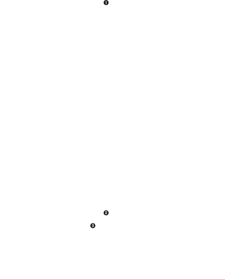
and you won’t need to wait for the session to time out before partitions from the con‐
sumer you are closing will be assigned to another consumer in the group.
Here is what the exit code will look like if the consumer is running in the main appli‐
cation thread. This example is a bit truncated, but you can view the full example at
http://bit.ly/2u47e9A.
Runtime.getRuntime().addShutdownHook(new Thread() {
public void run() {
System.out.println("Starting exit...");
consumer.wakeup();
try {
mainThread.join();
} catch (InterruptedException e) {
e.printStackTrace();
}
}
});
...
try {
// looping until ctrl-c, the shutdown hook will
cleanup on exit
while (true) {
ConsumerRecords<String, String> records =
movingAvg.consumer.poll(1000);
System.out.println(System.currentTimeMillis() + "
-- waiting for data...");
for (ConsumerRecord<String, String> record :
records) {
System.out.printf("offset = %d, key = %s,
value = %s\n",
record.offset(), record.key(),
record.value());
}
for (TopicPartition tp: consumer.assignment())
System.out.println("Committing offset at
position:" +
consumer.position(tp));
movingAvg.consumer.commitSync();
}
} catch (WakeupException e) {
// ignore for shutdown
} finally {
consumer.close();
System.out.println("Closed consumer and we are done");
}
}
But How Do We Exit? | 87

ShutdownHook runs in a seperate thread, so the only safe action we can take is to
call wakeup to break out of the poll loop.
Another thread calling wakeup will cause poll to throw a WakeupException. You’ll
want to catch the exception to make sure your application doesn’t exit unexpect‐
edly, but there is no need to do anything with it.
Before exiting the consumer, make sure you close it cleanly.
Deserializers
As discussed in the previous chapter, Kafka producers require serializers to convert
objects into byte arrays that are then sent to Kafka. Similarly, Kafka consumers
require deserializers to convert byte arrays recieved from Kafka into Java objects. In
previous examples, we just assumed that both the key and the value of each message
are strings and we used the default StringDeserializer in the consumer configura‐
tion.
In Chapter 3 about the Kafka producer, we saw how to serialize custom types and
how to use Avro and AvroSerializers to generate Avro objects from schema defini‐
tions and then serialize them when producing messages to Kafka. We will now look at
how to create custom deserializers for your own objects and how to use Avro and its
deserializers.
It should be obvious that the serializer used to produce events to Kafka must match
the deserializer that will be used when consuming events. Serializing with IntSerial
izer and then deserializing with StringDeserializer will not end well. This means
that as a developer you need to keep track of which serializers were used to write into
each topic, and make sure each topic only contains data that the deserializers you use
can interpret. This is one of the benefits of using Avro and the Schema Repository for
serializing and deserializing—the AvroSerializer can make sure that all the data
written to a specific topic is compatible with the schema of the topic, which means it
can be deserialized with the matching deserializer and schema. Any errors in compat‐
ibility—on the producer or the consumer side—will be caught easily with an appro‐
priate error message, which means you will not need to try to debug byte arrays for
serialization errors.
We will start by quickly showing how to write a custom deserializer, even though this
is the less common method, and then we will move on to an example of how to use
Avro to deserialize message keys and values.
88 | Chapter 4: Kafka Consumers: Reading Data from Kafka
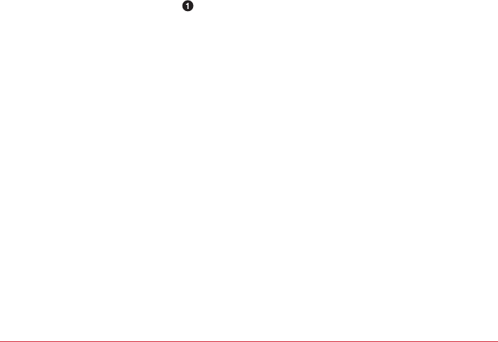
Custom deserializers
Let’s take the same custom object we serialized in Chapter 3, and write a deserializer
for it:
public class Customer {
private int customerID;
private String customerName;
public Customer(int ID, String name) {
this.customerID = ID;
this.customerName = name;
}
public int getID() {
return customerID;
}
public String getName() {
return customerName;
}
}
The custom deserializer will look as follows:
import org.apache.kafka.common.errors.SerializationException;
import java.nio.ByteBuffer;
import java.util.Map;
public class CustomerDeserializer implements
Deserializer<Customer> {
@Override
public void configure(Map configs, boolean isKey) {
// nothing to configure
}
@Override
public Customer deserialize(String topic, byte[] data) {
int id;
int nameSize;
String name;
try {
if (data == null)
return null;
if (data.length < 8)
throw new SerializationException("Size of data received by
IntegerDeserializer is shorter than expected");
ByteBuffer buffer = ByteBuffer.wrap(data);
Deserializers | 89
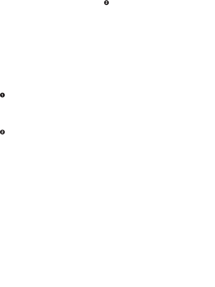
id = buffer.getInt();
String nameSize = buffer.getInt();
byte[] nameBytes = new Array[Byte](nameSize);
buffer.get(nameBytes);
name = new String(nameBytes, 'UTF-8');
return new Customer(id, name);
} catch (Exception e) {
throw new SerializationException("Error when serializing
Customer
to byte[] " + e);
}
}
@Override
public void close() {
// nothing to close
}
}
The consumer also needs the implementation of the Customer class, and both the
class and the serializer need to match on the producing and consuming applica‐
tions. In a large organization with many consumers and producers sharing access
to the data, this can become challenging.
We are just reversing the logic of the serializer here—we get the customer ID and
name out of the byte array and use them to construct the object we need.
The consumer code that uses this serializer will look similar to this example:
Properties props = new Properties();
props.put("bootstrap.servers", "broker1:9092,broker2:9092");
props.put("group.id", "CountryCounter");
props.put("key.deserializer",
"org.apache.kafka.common.serialization.StringDeserializer");
props.put("value.deserializer",
"org.apache.kafka.common.serialization.CustomerDeserializer");
KafkaConsumer<String, Customer> consumer =
new KafkaConsumer<>(props);
consumer.subscribe("customerCountries")
while (true) {
ConsumerRecords<String, Customer> records =
consumer.poll(100);
for (ConsumerRecord<String, Customer> record : records)
{
System.out.println("current customer Id: " +
90 | Chapter 4: Kafka Consumers: Reading Data from Kafka
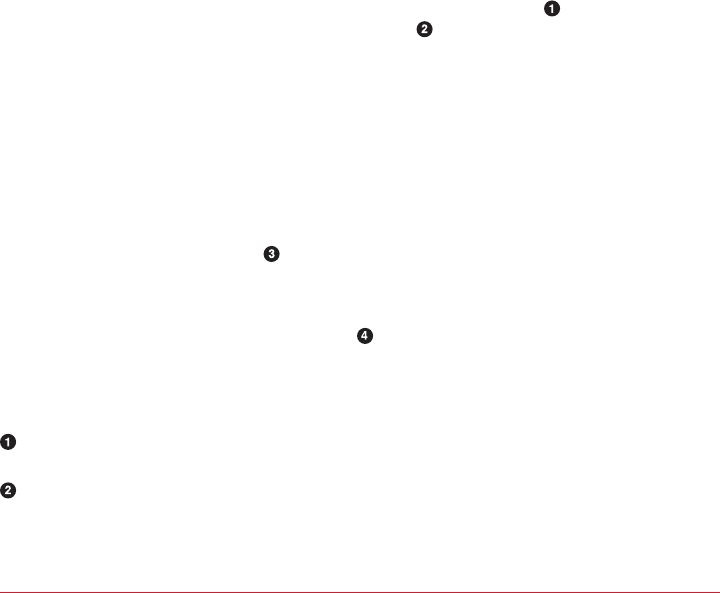
record.value().getId() + " and
current customer name: " + record.value().getName());
}
}
Again, it is important to note that implementing a custom serializer and deserializer
is not recommended. It tightly couples producers and consumers and is fragile and
error-prone. A better solution would be to use a standard message format such as
JSON, Thrift, Protobuf, or Avro. We’ll now see how to use Avro deserializers with the
Kafka consumer. For background on Apache Avro, its schemas, and schema-
compatibility capabilities, refer back to Chapter 3.
Using Avro deserialization with Kafka consumer
Let’s assume we are using the implementation of the Customer class in Avro that was
shown in Chapter 3. In order to consume those objects from Kafka, you want to
implement a consuming application similar to this:
Properties props = new Properties();
props.put("bootstrap.servers", "broker1:9092,broker2:9092");
props.put("group.id", "CountryCounter");
props.put("key.serializer",
"org.apache.kafka.common.serialization.StringDeserializer");
props.put("value.serializer",
"io.confluent.kafka.serializers.KafkaAvroDeserializer");
props.put("schema.registry.url", schemaUrl);
String topic = "customerContacts"
KafkaConsumer consumer = new
KafkaConsumer(createConsumerConfig(brokers, groupId, url));
consumer.subscribe(Collections.singletonList(topic));
System.out.println("Reading topic:" + topic);
while (true) {
ConsumerRecords<String, Customer> records =
consumer.poll(1000);
for (ConsumerRecord<String, Customer> record: records) {
System.out.println("Current customer name is: " +
record.value().getName());
}
consumer.commitSync();
}
We use KafkaAvroDeserializer to deserialize the Avro messages.
schema.registry.url is a new parameter. This simply points to where we store
the schemas. This way the consumer can use the schema that was registered by
the producer to deserialize the message.
Deserializers | 91

We specify the generated class, Customer, as the type for the record value.
record.value() is a Customer instance and we can use it accordingly.
Standalone Consumer: Why and How to Use a Consumer
Without a Group
So far, we have discussed consumer groups, which are where partitions are assigned
automatically to consumers and are rebalanced automatically when consumers are
added or removed from the group. Typically, this behavior is just what you want, but
in some cases you want something much simpler. Sometimes you know you have a
single consumer that always needs to read data from all the partitions in a topic, or
from a specific partition in a topic. In this case, there is no reason for groups or reba‐
lances—just assign the consumer-specific topic and/or partitions, consume messages,
and commit offsets on occasion.
When you know exactly which partitions the consumer should read, you don’t sub‐
scribe to a topic—instead, you assign yourself a few partitions. A consumer can either
subscribe to topics (and be part of a consumer group), or assign itself partitions, but
not both at the same time.
Here is an example of how a consumer can assign itself all partitions of a specific
topic and consume from them:
List<PartitionInfo> partitionInfos = null;
partitionInfos = consumer.partitionsFor("topic");
if (partitionInfos != null) {
for (PartitionInfo partition : partitionInfos)
partitions.add(new TopicPartition(partition.topic(),
partition.partition()));
consumer.assign(partitions);
while (true) {
ConsumerRecords<String, String> records =
consumer.poll(1000);
for (ConsumerRecord<String, String> record: records) {
System.out.printf("topic = %s, partition = %s, offset = %d,
customer = %s, country = %s\n",
record.topic(), record.partition(), record.offset(),
record.key(), record.value());
}
consumer.commitSync();
}
}
92 | Chapter 4: Kafka Consumers: Reading Data from Kafka

We start by asking the cluster for the partitions available in the topic. If you only
plan on consuming a specific partition, you can skip this part.
Once we know which partitions we want, we call assign() with the list.
Other than the lack of rebalances and the need to manually find the partitions, every‐
thing else is business as usual. Keep in mind that if someone adds new partitions to
the topic, the consumer will not be notified. You will need to handle this by checking
consumer.partitionsFor() periodically or simply by bouncing the application
whenever partitions are added.
Older Consumer APIs
In this chapter we discussed the Java KafkaConsumer client that is part of the
org.apache.kafka.clients package. At the time of writing, Apache Kafka still has
two older clients written in Scala that are part of the kafka.consumer package, which
is part of the core Kafka module. These consumers are called SimpleConsumer (which
is not very simple). SimpleConsumer is a thin wrapper around the Kafka APIs that
allows you to consume from specific partitions and offsets. The other old API is
called high-level consumer or ZookeeperConsumerConnector. The high-level con‐
sumer is somewhat similar to the current consumer in that it has consumer groups
and it rebalances partitions, but it uses Zookeeper to manage consumer groups and
does not give you the same control over commits and rebalances as we have now.
Because the current consumer supports both behaviors and provides much more reli‐
ability and control to the developer, we will not discuss the older APIs. If you are
interested in using them, please think twice and then refer to Apache Kafka docu‐
mentation to learn more.
Summary
We started this chapter with an in-depth explanation of Kafka’s consumer groups and
the way they allow multiple consumers to share the work of reading events from top‐
ics. We followed the theoretical discussion with a practical example of a consumer
subscribing to a topic and continuously reading events. We then looked into the most
important consumer configuration parameters and how they affect consumer behav‐
ior. We dedicated a large part of the chapter to discussing offsets and how consumers
keep track of them. Understanding how consumers commit offsets is critical when
writing reliable consumers, so we took time to explain the different ways this can be
done. We then discussed additional parts of the consumer APIs, handling rebalances
and closing the consumer.
Older Consumer APIs | 93

We concluded by discussing the deserializers used by consumers to turn bytes stored
in Kafka into Java objects that the applications can process. We discussed Avro deser‐
ializers in some detail, even though they are just one type of deserializer you can use,
because these are most commonly used with Kafka.
Now that you know how to produce and consume events with Kafka, the next chapter
explains some of the internals of a Kafka implementation.
94 | Chapter 4: Kafka Consumers: Reading Data from Kafka

CHAPTER 5
Kafka Internals
It is not strictly necessary to understand Kafka’s internals in order to run Kafka in
production or write applications that use it. However, knowing how Kafka works
does provide context when troubleshooting or trying to understand why Kafka
behaves the way it does. Since covering every single implementation detail and design
decision is beyond the scope of this book, in this chapter we focus on three topics that
are especially relevant to Kafka practitioners:
• How Kafka replication works
• How Kafka handles requests from producers and consumers
• How Kafka handles storage such as file format and indexes
Understanding these topics in-depth will be especially useful when tuning Kafka—
understanding the mechanisms that the tuning knobs control goes a long way toward
using them with precise intent rather than fiddling with them randomly.
Cluster Membership
Kafka uses Apache Zookeeper to maintain the list of brokers that are currently mem‐
bers of a cluster. Every broker has a unique identifier that is either set in the broker
configuration file or automatically generated. Every time a broker process starts, it
registers itself with its ID in Zookeeper by creating an ephemeral node. Different
Kafka components subscribe to the /brokers/ids path in Zookeeper where brokers
are registered so they get notified when brokers are added or removed.
If you try to start another broker with the same ID, you will get an error—the new
broker will try to register, but fail because we already have a Zookeeper node for the
same broker ID.
95

When a broker loses connectivity to Zookeeper (usually as a result of the broker stop‐
ping, but this can also happen as a result of network partition or a long garbage-
collection pause), the ephemeral node that the broker created when starting will be
automatically removed from Zookeeper. Kafka components that are watching the list
of brokers will be notified that the broker is gone.
Even though the node representing the broker is gone when the broker is stopped,
the broker ID still exists in other data structures. For example, the list of replicas of
each topic (see “Replication” on page 97) contains the broker IDs for the replica. This
way, if you completely lose a broker and start a brand new broker with the ID of the
old one, it will immediately join the cluster in place of the missing broker with the
same partitions and topics assigned to it.
The Controller
The controller is one of the Kafka brokers that, in addition to the usual broker func‐
tionality, is responsible for electing partition leaders (we’ll discuss partition leaders
and what they do in the next section). The first broker that starts in the cluster
becomes the controller by creating an ephemeral node in ZooKeeper called /control
ler. When other brokers start, they also try to create this node, but receive a “node
already exists” exception, which causes them to “realize” that the controller node
already exists and that the cluster already has a controller. The brokers create a Zoo‐
keeper watch on the controller node so they get notified of changes to this node. This
way, we guarantee that the cluster will only have one controller at a time.
When the controller broker is stopped or loses connectivity to Zookeeper, the ephem‐
eral node will disappear. Other brokers in the cluster will be notified through the
Zookeeper watch that the controller is gone and will attempt to create the controller
node in Zookeeper themselves. The first node to create the new controller in Zoo‐
keeper is the new controller, while the other nodes will receive a “node already exists”
exception and re-create the watch on the new controller node. Each time a controller
is elected, it receives a new, higher controller epoch number through a Zookeeper con‐
ditional increment operation. The brokers know the current controller epoch and if
they receive a message from a controller with an older number, they know to ignore
it.
When the controller notices that a broker left the cluster (by watching the relevant
Zookeeper path), it knows that all the partitions that had a leader on that broker will
need a new leader. It goes over all the partitions that need a new leader, determines
who the new leader should be (simply the next replica in the replica list of that parti‐
tion), and sends a request to all the brokers that contain either the new leaders or the
existing followers for those partitions. The request contains information on the new
leader and the followers for the partitions. Each new leader knows that it needs to
96 | Chapter 5: Kafka Internals

start serving producer and consumer requests from clients while the followers know
that they need to start replicating messages from the new leader.
When the controller notices that a broker joined the cluster, it uses the broker ID to
check if there are replicas that exist on this broker. If there are, the controller notifies
both new and existing brokers of the change, and the replicas on the new broker start
replicating messages from the existing leaders.
To summarize, Kafka uses Zookeeper’s ephemeral node feature to elect a controller
and to notify the controller when nodes join and leave the cluster. The controller is
responsible for electing leaders among the partitions and replicas whenever it notices
nodes join and leave the cluster. The controller uses the epoch number to prevent a
“split brain” scenario where two nodes believe each is the current controller.
Replication
Replication is at the heart of Kafka’s architecture. The very first sentence in Kafka’s
documentation describes it as “a distributed, partitioned, replicated commit log ser‐
vice.” Replication is critical because it is the way Kafka guarantees availability and
durability when individual nodes inevitably fail.
As we’ve already discussed, data in Kafka is organized by topics. Each topic is parti‐
tioned, and each partition can have multiple replicas. Those replicas are stored on
brokers, and each broker typically stores hundreds or even thousands of replicas
belonging to different topics and partitions.
There are two types of replicas:
Leader replica
Each partition has a single replica designated as the leader. All produce and con‐
sume requests go through the leader, in order to guarantee consistency.
Follower replica
All replicas for a partition that are not leaders are called followers. Followers
don’t serve client requests; their only job is to replicate messages from the leader
and stay up-to-date with the most recent messages the leader has. In the event
that a leader replica for a partition crashes, one of the follower replicas will be
promoted to become the new leader for the partition.
Another task the leader is responsible for is knowing which of the follower replicas is
up-to-date with the leader. Followers attempt to stay up-to-date by replicating all the
messages from the leader as the messages arrive, but they can fail to stay in sync for
various reasons, such as when network congestion slows down replication or when a
broker crashes and all replicas on that broker start falling behind until we start the
broker and they can start replicating again.
Replication | 97

In order to stay in sync with the leader, the replicas send the leader Fetch requests,
the exact same type of requests that consumers send in order to consume messages.
In response to those requests, the leader sends the messages to the replicas. Those
Fetch requests contain the offset of the message that the replica wants to receive next,
and will always be in order.
A replica will request message 1, then message 2, and then message 3, and it will not
request message 4 before it gets all the previous messages. This means that the leader
can know that a replica got all messages up to message 3 when the replica requests
message 4. By looking at the last offset requested by each replica, the leader can tell
how far behind each replica is. If a replica hasn’t requested a message in more than 10
seconds or if it has requested messages but hasn’t caught up to the most recent mes‐
sage in more than 10 seconds, the replica is considered out of sync. If a replica fails to
keep up with the leader, it can no longer become the new leader in the event of failure
—after all, it does not contain all the messages.
The inverse of this, replicas that are consistently asking for the latest messages, is
called in-sync replicas. Only in-sync replicas are eligible to be elected as partition lead‐
ers in case the existing leader fails.
The amount of time a follower can be inactive or behind before it is considered out of
sync is controlled by the replica.lag.time.max.ms configuration parameter. This
allowed lag has implications on client behavior and data retention during leader elec‐
tion. We will discuss this in depth in Chapter 6, when we discuss reliability guaran‐
tees.
In addition to the current leader, each partition has a preferred leader—the replica
that was the leader when the topic was originally created. It is preferred because when
partitions are first created, the leaders are balanced between brokers (we explain the
algorithm for distributing replicas and leaders among brokers later in the chapter).
As a result, we expect that when the preferred leader is indeed the leader for all parti‐
tions in the cluster, load will be evenly balanced between brokers. By default, Kafka is
configured with auto.leader.rebalance.enable=true, which will check if the pre‐
ferred leader replica is not the current leader but is in-sync and trigger leader election
to make the preferred leader the current leader.
98 | Chapter 5: Kafka Internals

Finding the Preferred Leaders
The best way to identify the current preferred leader is by looking
at the list of replicas for a partition (You can see details of partitions
and replicas in the output of the kafka-topics.sh tool. We’ll dis‐
cuss this and other admin tools in Chapter 10.) The first replica in
the list is always the preferred leader. This is true no matter who is
the current leader and even if the replicas were reassigned to differ‐
ent brokers using the replica reassignment tool. In fact, if you man‐
ually reassign replicas, it is important to remember that the replica
you specify first will be the preferred replica, so make sure you
spread those around different brokers to avoid overloading some
brokers with leaders while other brokers are not handling their fair
share of the work.
Request Processing
Most of what a Kafka broker does is process requests sent to the partition leaders
from clients, partition replicas, and the controller. Kafka has a binary protocol (over
TCP) that specifies the format of the requests and how brokers respond to them—
both when the request is processed successfully or when the broker encounters errors
while processing the request. Clients always initiate connections and send requests,
and the broker processes the requests and responds to them. All requests sent to the
broker from a specific client will be processed in the order in which they were
received—this guarantee is what allows Kafka to behave as a message queue and pro‐
vide ordering guarantees on the messages it stores.
All requests have a standard header that includes:
• Request type (also called API key)
•Request version (so the brokers can handle clients of different versions and
respond accordingly)
•Correlation ID: a number that uniquely identifies the request and also appears in
the response and in the error logs (the ID is used for troubleshooting)
• Client ID: used to identify the application that sent the request
We will not describe the protocol here because it is described in significant detail in
the Kafka documentation. However, it is helpful to take a look at how requests are
processed by the broker—later, when we discuss how to monitor Kafka and the vari‐
ous configuration options, you will have context about which queues and threads the
metrics and configuration parameters refer to.
For each port the broker listens on, the broker runs an acceptor thread that creates a
connection and hands it over to a processor thread for handling. The number of pro‐
Request Processing | 99
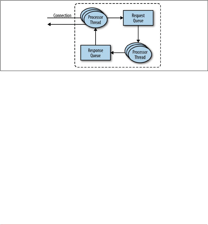
cessor threads (also called network threads) is configurable. The network threads are
responsible for taking requests from client connections, placing them in a request
queue, and picking up responses from a response queue and sending them back to cli‐
ents. See Figure 5-1 for a visual of this process.
Once requests are placed on the request queue, IO threads are responsible for picking
them up and processing them. The most common types of requests are:
Produce requests
Sent by producers and contain messages the clients write to Kafka brokers.
Fetch requests
Sent by consumers and follower replicas when they read messages from Kafka
brokers.
Figure 5-1. Request processing inside Apache Kaa
Both produce requests and fetch requests have to be sent to the leader replica of a
partition. If a broker receives a produce request for a specific partition and the leader
for this partition is on a different broker, the client that sent the produce request will
get an error response of “Not a Leader for Partition.” The same error will occur if a
fetch request for a specific partition arrives at a broker that does not have the leader
for that partition. Kafka’s clients are responsible for sending produce and fetch
requests to the broker that contains the leader for the relevant partition for the
request.
How do the clients know where to send the requests? Kafka clients use another
request type called a metadata request, which includes a list of topics the client is
interested in. The server response specifies which partitions exist in the topics, the
replicas for each partition, and which replica is the leader. Metadata requests can be
sent to any broker because all brokers have a metadata cache that contains this infor‐
mation.
Clients typically cache this information and use it to direct produce and fetch
requests to the correct broker for each partition. They also need to occasionally
100 | Chapter 5: Kafka Internals
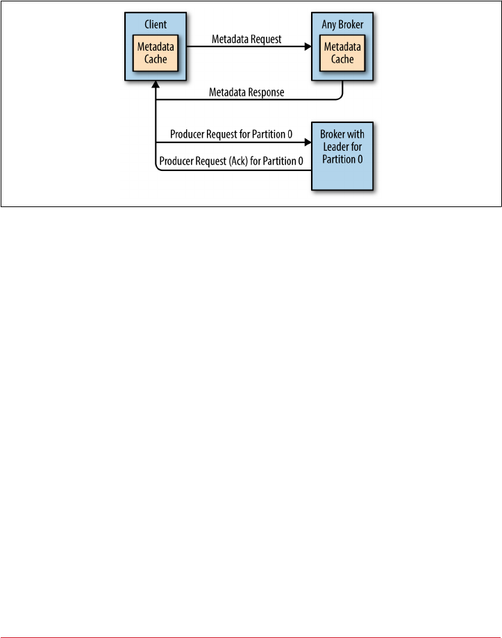
refresh this information (refresh intervals are controlled by the meta
data.max.age.ms configuration parameter) by sending another metadata request so
they know if the topic metadata changed—for example, if a new broker was added or
some replicas were moved to a new broker (Figure 5-2). In addition, if a client
receives the “Not a Leader” error to one of its requests, it will refresh its metadata
before trying to send the request again, since the error indicates that the client is
using outdated information and is sending requests to the wrong broker.
Figure 5-2. Client routing requests
Produce Requests
As we saw in Chapter 3, a configuration parameter called acks is the number of brok‐
ers who need to acknowledge receiving the message before it is considered a success‐
ful write. Producers can be configured to consider messages as “written successfully”
when the message was accepted by just the leader (acks=1), all in-sync replicas
(acks=all), or the moment the message was sent without waiting for the broker to
accept it at all (acks=0).
When the broker that contains the lead replica for a partition receives a produce
request for this partition, it will start by running a few validations:
•Does the user sending the data have write privileges on the topic?
•Is the number of acks specified in the request valid (only 0, 1, and “all” are
allowed)?
•If acks is set to all, are there enough in-sync replicas for safely writing the mes‐
sage? (Brokers can be configured to refuse new messages if the number of in-sync
replicas falls below a configurable number; we will discuss this in more detail in
Chapter 6, when we discuss Kafka’s durability and reliability guarantees.)
Request Processing | 101

Then it will write the new messages to local disk. On Linux, the messages are written
to the filesystem cache and there is no guarantee about when they will be written to
disk. Kafka does not wait for the data to get persisted to disk—it relies on replication
for message durability.
Once the message is written to the leader of the partition, the broker examines the
acks configuration—if acks is set to 0 or 1, the broker will respond immediately; if
acks is set to all, the request will be stored in a buffer called purgatory until the
leader observes that the follower replicas replicated the message, at which point a
response is sent to the client.
Fetch Requests
Brokers process fetch requests in a way that is very similar to the way produce
requests are handled. The client sends a request, asking the broker to send messages
from a list of topics, partitions, and offsets—something like “Please send me messages
starting at offset 53 in partition 0 of topic Test and messages starting at offset 64 in
partition 3 of topic Test.” Clients also specify a limit to how much data the broker can
return for each partition. The limit is important because clients need to allocate
memory that will hold the response sent back from the broker. Without this limit,
brokers could send back replies large enough to cause clients to run out of memory.
As we’ve discussed earlier, the request has to arrive to the leaders of the partitions
specified in the request and the client will make the necessary metadata requests to
make sure it is routing the fetch requests correctly. When the leader receives the
request, it first checks if the request is valid—does this offset even exist for this partic‐
ular partition? If the client is asking for a message that is so old that it got deleted
from the partition or an offset that does not exist yet, the broker will respond with an
error.
If the offset exists, the broker will read messages from the partition, up to the limit set
by the client in the request, and send the messages to the client. Kafka famously uses a
zero-copy method to send the messages to the clients—this means that Kafka sends
messages from the file (or more likely, the Linux filesystem cache) directly to the net‐
work channel without any intermediate buffers. This is different than most databases
where data is stored in a local cache before being sent to clients. This technique
removes the overhead of copying bytes and managing buffers in memory, and results
in much improved performance.
In addition to setting an upper boundary on the amount of data the broker can
return, clients can also set a lower boundary on the amount of data returned. Setting
the lower boundary to 10K, for example, is the client’s way of telling the broker “Only
return results once you have at least 10K bytes to send me.” This is a great way to
reduce CPU and network utilization when clients are reading from topics that are not
seeing much traffic. Instead of the clients sending requests to the brokers every few
102 | Chapter 5: Kafka Internals
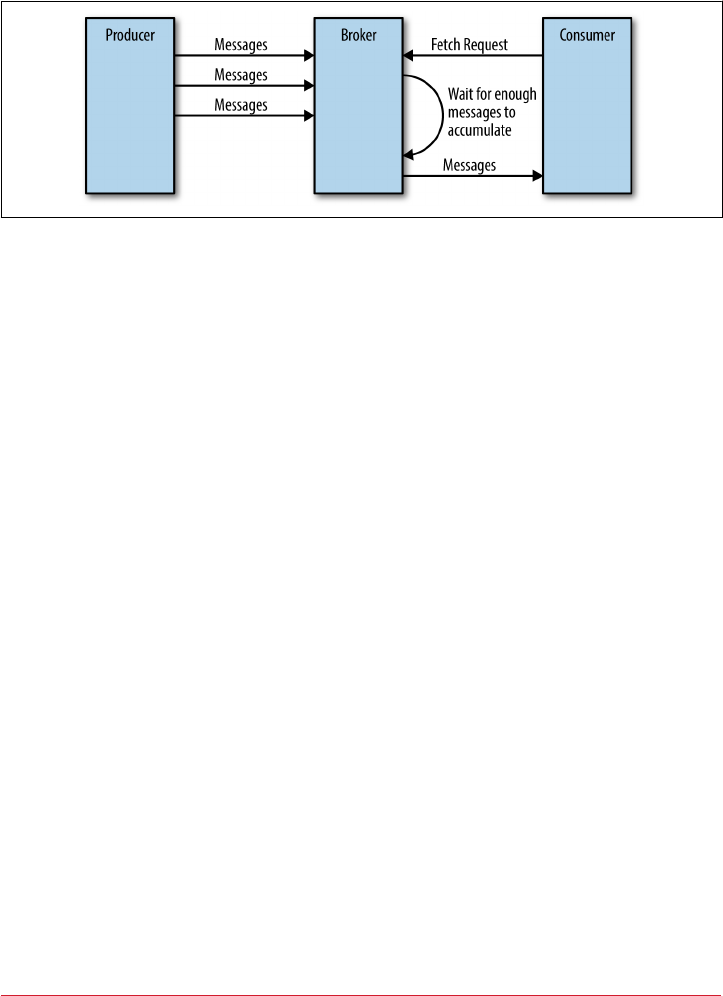
milliseconds asking for data and getting very few or no messages in return, the clients
send a request, the broker waits until there is a decent amount of data and returns the
data, and only then will the client ask for more (Figure 5-3). The same amount of data
is read overall but with much less back and forth and therefore less overhead.
Figure 5-3. Broker delaying response until enough data accumulated
Of course, we wouldn’t want clients to wait forever for the broker to have enough
data. After a while, it makes sense to just take the data that exists and process that
instead of waiting for more. Therefore, clients can also define a timeout to tell the
broker “If you didn’t satisfy the minimum amount of data to send within x milli‐
seconds, just send what you got.”
It is also interesting to note that not all the data that exists on the leader of the parti‐
tion is available for clients to read. Most clients can only read messages that were
written to all in-sync replicas (follower replicas, even though they are consumers, are
exempt from this—otherwise replication would not work). We already discussed that
the leader of the partition knows which messages were replicated to which replica,
and until a message was written to all in-sync replicas, it will not be sent to consum‐
ers—attempts to fetch those messages will result in an empty response rather than an
error.
The reason for this behavior is that messages not replicated to enough replicas yet are
considered “unsafe”—if the leader crashes and another replica takes its place, these
messages will no longer exist in Kafka. If we allowed clients to read messages that
only exist on the leader, we could see inconsistent behavior. For example, if a con‐
sumer reads a message and the leader crashed and no other broker contained this
message, the message is gone. No other consumer will be able to read this message,
which can cause inconsistency with the consumer who did read it. Instead, we wait
until all the in-sync replicas get the message and only then allow consumers to read it
(Figure 5-4). This behavior also means that if replication between brokers is slow for
some reason, it will take longer for new messages to arrive to consumers (since we
wait for the messages to replicate first). This delay is limited to
replica.lag.time.max.ms—the amount of time a replica can be delayed in replicat‐
ing new messages while still being considered in-sync.
Request Processing | 103
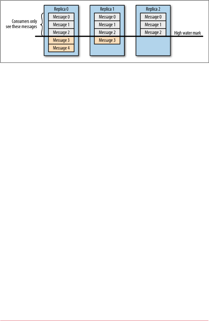
Figure 5-4. Consumers only see messages that were replicated to in-sync replicas
Other Requests
We just discussed the most common types of requests used by Kafka clients: Meta
data, Produce, and Fetch. It is important to remember that we are talking about a
generic binary protocol used by clients over the network. Whereas Kafka includes
Java clients that were implemented and maintained by contributors to the Apache
Kafka project, there are also clients in other languages such as C, Python, Go, and
many others. You can see the full list on the Apache Kafka website and they all com‐
municate with Kafka brokers using this protocol.
In addition, the same protocol is used to communicate between the Kafka brokers
themselves. Those requests are internal and should not be used by clients. For exam‐
ple, when the controller announces that a partition has a new leader, it sends a Leader
AndIsr request to the new leader (so it will know to start accepting client requests)
and to the followers (so they will know to follow the new leader).
The Kafka protocol currently handles 20 different request types, and more will be
added. The protocol is ever-evolving—as we add more client capabilities, we need to
grow the protocol to match. For example, in the past, Kafka Consumers used Apache
Zookeeper to keep track of the offsets they receive from Kafka. So when a consumer
is started, it can check Zookeeper for the last offset that was read from its partitions
and know where to start processing. For various reasons, we decided to stop using
Zookeeper for this, and instead store those offsets in a special Kafka topic. In order to
do this, we had to add several requests to the protocol: OffsetCommitRequest, Offset
FetchRequest, and ListOffsetsRequest. Now when an application calls the
commitOffset() client API, the client no longer writes to Zookeeper; instead, it sends
OffsetCommitRequest to Kafka.
Topic creation is still done by command-line tools that update the list of topics in
Zookeeper directly, and brokers watch the topic list in Zookeeper to know when new
topics are added. We are working on improving Kafka and adding a Create
TopicRequest that will allow all clients (even in languages that don’t have a Zoo‐
keeper library) to create topics by asking Kafka brokers directly.
104 | Chapter 5: Kafka Internals

In addition to evolving the protocol by adding new request types, we sometimes
choose to modify existing requests to add some capabilities. For example, between
Kafka 0.9.0 and Kafka 0.10.0, we decided to let clients know who the current control‐
ler is by adding the information to the Metadata response. As a result, we added a
new version to the Metadata request and response. Now, 0.9.0 clients send Metadata
requests of version 0 (because version 1 did not exist in 0.9.0 clients) and the brokers,
whether they are 0.9.0 or 0.10.0 know to respond with a version 0 response, which
does not have the controller information. This is fine, because 0.9.0 clients don’t
expect the controller information and wouldn’t know how to parse it anyway. If you
have the 0.10.0 client, it will send a version 1 Metadata request and 0.10.0 brokers will
respond with a version 1 response that contains the controller information, which the
0.10.0 clients can use. If a 0.10.0 client sends a version 1 Metadata request to a 0.9.0
broker, the broker will not know how to handle the newer version of the request and
will respond with an error. This is the reason we recommend upgrading the brokers
before upgrading any of the clients—new brokers know how to handle old requests,
but not vice versa.
In release 0.10.0 we added ApiVersionRequest, which allows clients to ask the broker
which versions of each request is supported and to use the correct version accord‐
ingly. Clients that use this new capability correctly will be able to talk to older brokers
by using a version of the protocol that is supported by the broker they are connecting
to.
Physical Storage
The basic storage unit of Kafka is a partition replica. Partitions cannot be split
between multiple brokers and not even between multiple disks on the same broker.
So the size of a partition is limited by the space available on a single mount point. (A
mount point will consist of either a single disk, if JBOD configuration is used, or mul‐
tiple disks, if RAID is configured. See Chapter 2.)
When configuring Kafka, the administrator defines a list of directories in which the
partitions will be stored—this is the log.dirs parameter (not to be confused with the
location in which Kafka stores its error log, which is configured in the log4j.properties
file). The usual configuration includes a directory for each mount point that Kafka
will use.
Let’s look at how Kafka uses the available directories to store data. First, we want to
look at how data is allocated to the brokers in the cluster and the directories in the
broker. Then we will look at how the broker manages the files—especially how the
retention guarantees are handled. We will then dive inside the files and look at the file
and index formats. Lastly we will look at Log Compaction, an advanced feature that
allows turning Kafka into a long-term data store, and describe how it works.
Physical Storage | 105

Partition Allocation
When you create a topic, Kafka first decides how to allocate the partitions between
brokers. Suppose you have 6 brokers and you decide to create a topic with 10 parti‐
tions and a replication factor of 3. Kafka now has 30 partition replicas to allocate to 6
brokers. When doing the allocations, the goals are:
•To spread replicas evenly among brokers—in our example, to make sure we allo‐
cate 5 replicas per broker.
•To make sure that for each partition, each replica is on a different broker. If parti‐
tion 0 has the leader on broker 2, we can place the followers on brokers 3 and 4,
but not on 2 and not both on 3.
•If the brokers have rack information (available in Kafka release 0.10.0 and
higher), then assign the replicas for each partition to different racks if possible.
This ensures that an event that causes downtime for an entire rack does not cause
complete unavailability for partitions.
To do this, we start with a random broker (let’s say, 4) and start assigning partitions to
each broker in round-robin manner to determine the location for the leaders. So par‐
tition leader 0 will be on broker 4, partition 1 leader will be on broker 5, partition 2
will be on broker 0 (because we only have 6 brokers), and so on. Then, for each parti‐
tion, we place the replicas at increasing offsets from the leader. If the leader for parti‐
tion 0 is on broker 4, the first follower will be on broker 5 and the second on broker
0. The leader for partition 1 is on broker 5, so the first replica is on broker 0 and the
second on broker 1.
When rack awareness is taken into account, instead of picking brokers in numerical
order, we prepare a rack-alternating broker list. Suppose that we know that brokers 0,
1, and 2 are on the same rack, and brokers 3, 4, and 5 are on a separate rack. Instead
of picking brokers in the order of 0 to 5, we order them as 0, 3, 1, 4, 2, 5—each broker
is followed by a broker from a different rack (Figure 5-5). In this case, if the leader for
partition 0 is on broker 4, the first replica will be on broker 2, which is on a com‐
pletely different rack. This is great, because if the first rack goes offline, we know that
we still have a surviving replica and therefore the partition is still available. This will
be true for all our replicas, so we have guaranteed availability in the case of rack fail‐
ure.
106 | Chapter 5: Kafka Internals
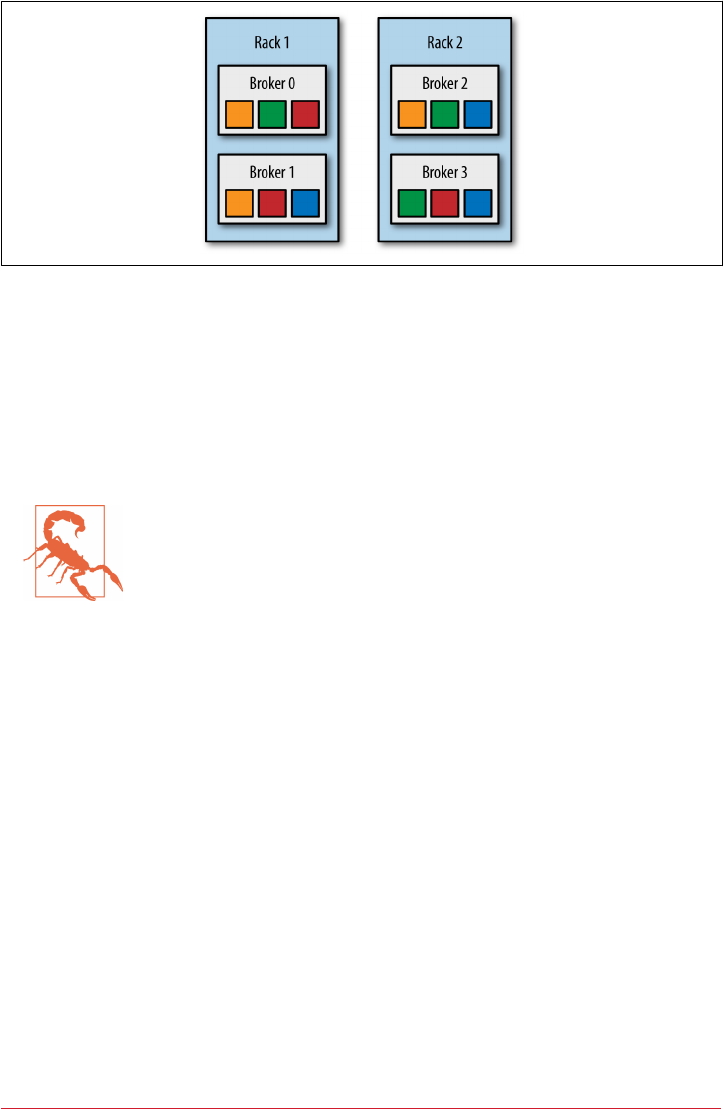
Figure 5-5. Partitions and replicas assigned to brokers on dierent racks
Once we choose the correct brokers for each partition and replica, it is time to decide
which directory to use for the new partitions. We do this independently for each par‐
tition, and the rule is very simple: we count the number of partitions on each direc‐
tory and add the new partition to the directory with the fewest partitions. This means
that if you add a new disk, all the new partitions will be created on that disk. This is
because, until things balance out, the new disk will always have the fewest partitions.
Mind the Disk Space
Note that the allocation of partitions to brokers does not take avail‐
able space or existing load into account, and that allocation of par‐
titions to disks takes the number of partitions into account, but not
the size of the partitions. This means that if some brokers have
more disk space than others (perhaps because the cluster is a mix
of older and newer servers), some partitions are abnormally large,
or you have disks of different sizes on the same broker, you need to
be careful with the partition allocation.
File Management
Retention is an important concept in Kafka—Kafka does not keep data forever, nor
does it wait for all consumers to read a message before deleting it. Instead, the Kafka
administrator configures a retention period for each topic—either the amount of time
to store messages before deleting them or how much data to store before older mes‐
sages are purged.
Because finding the messages that need purging in a large file and then deleting a
portion of the file is both time-consuming and error-prone, we instead split each par‐
tition into segments. By default, each segment contains either 1 GB of data or a week
of data, whichever is smaller. As a Kafka broker is writing to a partition, if the seg‐
ment limit is reached, we close the file and start a new one.
Physical Storage | 107

The segment we are currently writing to is called an active segment. The active seg‐
ment is never deleted, so if you set log retention to only store a day of data but each
segment contains five days of data, you will really keep data for five days because we
can’t delete the data before the segment is closed. If you choose to store data for a
week and roll a new segment every day, you will see that every day we will roll a new
segment while deleting the oldest segment—so most of the time the partition will
have seven segments.
As you learned in Chapter 2, a Kafka broker will keep an open file handle to every
segment in every partition—even inactive segments. This leads to an usually high
number of open file handles, and the OS must be tuned accordingly.
File Format
Each segment is stored in a single data file. Inside the file, we store Kafka messages
and their offsets. The format of the data on the disk is identical to the format of the
messages that we send from the producer to the broker and later from the broker to
the consumers. Using the same message format on disk and over the wire is what
allows Kafka to use zero-copy optimization when sending messages to consumers
and also avoid decompressing and recompressing messages that the producer already
compressed.
Each message contains—in addition to its key, value, and offset—things like the mes‐
sage size, checksum code that allows us to detect corruption, magic byte that indicates
the version of the message format, compression codec (Snappy, GZip, or LZ4), and a
timestamp (added in release 0.10.0). The timestamp is given either by the producer
when the message was sent or by the broker when the message arrived—depending
on configuration.
If the producer is sending compressed messages, all the messages in a single producer
batch are compressed together and sent as the “value” of a “wrapper message”
(Figure 5-6). So the broker receives a single message, which it sends to the consumer.
But when the consumer decompresses the message value, it will see all the messages
that were contained in the batch, with their own timestamps and offsets.
This means that if you are using compression on the producer (recommended!),
sending larger batches means better compression both over the network and on the
broker disks. This also means that if we decide to change the message format that
consumers use (e.g., add a timestamp to the message), both the wire protocol and the
on-disk format need to change, and Kafka brokers need to know how to handle cases
in which files contain messages of two formats due to upgrades.
108 | Chapter 5: Kafka Internals
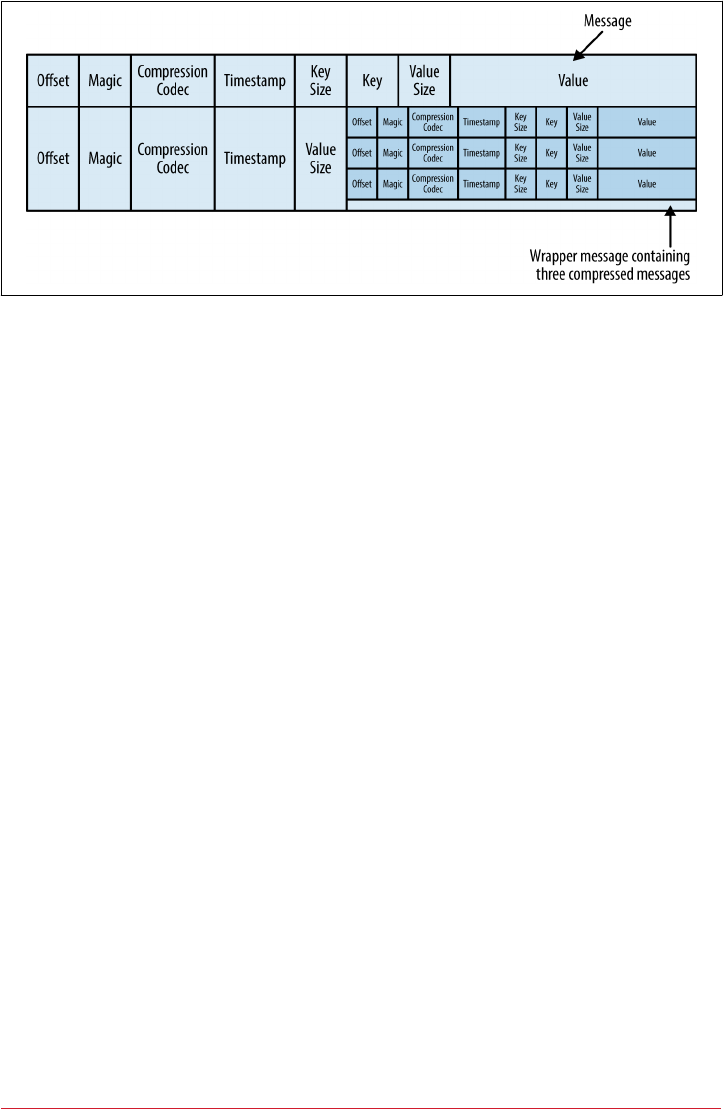
Figure 5-6. A normal message and a wrapper message
Kafka brokers ship with the DumpLogSegment tool, which allows you to look at a parti‐
tion segment in the filesystem and examine its contents. It will show you the offset,
checksum, magic byte, size, and compression codec for each message. You can run
the tool using:
bin/kafka-run-class.sh kafka.tools.DumpLogSegments
If you choose the --deep-iteration parameter, it will show you information about
messages compressed inside the wrapper messages.
Indexes
Kafka allows consumers to start fetching messages from any available offset. This
means that if a consumer asks for 1 MB messages starting at offset 100, the broker
must be able to quickly locate the message for offset 100 (which can be in any of the
segments for the partition) and start reading the messages from that offset on. In
order to help brokers quickly locate the message for a given offset, Kafka maintains
an index for each partition. The index maps offsets to segment files and positions
within the file.
Indexes are also broken into segments, so we can delete old index entries when the
messages are purged. Kafka does not attempt to maintain checksums of the index. If
the index becomes corrupted, it will get regenerated from the matching log segment
simply by rereading the messages and recording the offsets and locations. It is also
completely safe for an administrator to delete index segments if needed—they will be
regenerated automatically.
Physical Storage | 109
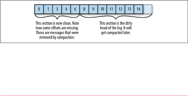
Compaction
Normally, Kafka will store messages for a set amount of time and purge messages
older than the retention period. However, imagine a case where you use Kafka to
store shipping addresses for your customers. In that case, it makes more sense to
store the last address for each customer rather than data for just the last week or year.
This way, you don’t have to worry about old addresses and you still retain the address
for customers who haven’t moved in a while. Another use case can be an application
that uses Kafka to store its current state. Every time the state changes, the application
writes the new state into Kafka. When recovering from a crash, the application reads
those messages from Kafka to recover its latest state. In this case, it only cares about
the latest state before the crash, not all the changes that occurred while it was run‐
ning.
Kafka supports such use cases by allowing the retention policy on a topic to be delete,
which deletes events older than retention time, to compact, which only stores the
most recent value for each key in the topic. Obviously, setting the policy to compact
only makes sense on topics for which applications produce events that contain both a
key and a value. If the topic contains null keys, compaction will fail.
How Compaction Works
Each log is viewed as split into two portions (see Figure 5-7):
Clean
Messages that have been compacted before. This section contains only one value
for each key, which is the latest value at the time of the pervious compaction
Dirty
Messages that were written after the last compaction.
Figure 5-7. Partition with clean and dirty portions
If compaction is enabled when Kafka starts (using the awkwardly named
log.cleaner.enabled configuration), each broker will start a compaction manager
thread and a number of compaction threads. These are responsible for performing
110 | Chapter 5: Kafka Internals

the compaction tasks. Each of these threads chooses the partition with the highest
ratio of dirty messages to total partition size and cleans this partition.
To compact a partition, the cleaner thread reads the dirty section of the partition and
creates an in-memory map. Each map entry is comprised of a 16-byte hash of a mes‐
sage key and the 8-byte offset of the previous message that had this same key. This
means each map entry only uses 24 bytes. If we look at a 1 GB segment and assume
that each message in the segment takes up 1 KB, the segment will contain 1 million
such messages and we will only need a 24 MB map to compact the segment (we may
need a lot less—if the keys repeat themselves, we will reuse the same hash entries
often and use less memory). This is quite efficient!
When configuring Kafka, the administrator configures how much memory compac‐
tion threads can use for this offset map. Even though each thread has its own map,
the configuration is for total memory across all threads. If you configured 1 GB for
the compaction offset map and you have five cleaner threads, each thread will get 200
MB for its own offset map. Kafka doesn’t require the entire dirty section of the parti‐
tion to fit into the size allocated for this map, but at least one full segment has to fit. If
it doesn’t, Kafka will log an error and the administrator will need to either allocate
more memory for the offset maps or use fewer cleaner threads. If only a few segments
fit, Kafka will start by compacting the oldest segments that fit into the map. The rest
will remain dirty and wait for the next compaction.
Once the cleaner thread builds the offset map, it will start reading off the clean seg‐
ments, starting with the oldest, and check their contents against the offset map. For
each message it checks, if the key of the message exists in the offset map. If the key
does not exist in the map, the value of the message we’ve just read is still the latest and
we copy over the message to a replacement segment. If the key does exist in the map,
we omit the message because there is a message with an identical key but newer value
later in the partition. Once we’ve copied over all the messages that still contain the
latest value for their key, we swap the replacement segment for the original and move
on to the next segment. At the end of the process, we are left with one message per
key—the one with the latest value. See Figure 5-8.
Physical Storage | 111
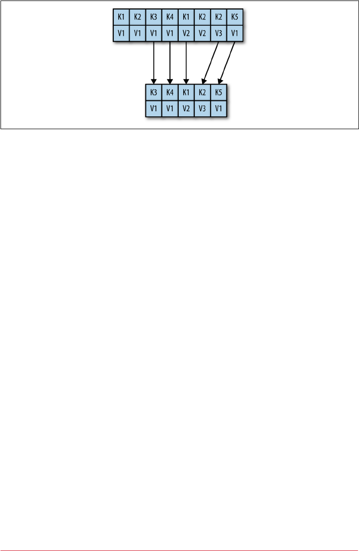
Figure 5-8. Partition segment before and aer compaction
Deleted Events
If we always keep the latest message for each key, what do we do when we really want
to delete all messages for a specific key, such as if a user left our service and we are
legally obligated to remove all traces of that user from our system?
In order to delete a key from the system completely, not even saving the last message,
the application must produce a message that contains that key and a null value. When
the cleaner thread finds such a message, it will first do a normal compaction and
retain only the message with the null value. It will keep this special message (known
as a tombstone) around for a configurable amount of time. During this time, consum‐
ers will be able to see this message and know that the value is deleted. So if a con‐
sumer copies data from Kafka to a relational database, it will see the tombstone
message and know to delete the user from the database. After this set amount of time,
the cleaner thread will remove the tombstone message, and the key will be gone from
the partition in Kafka. It is important to give consumers enough time to see the
tombstone message, because if our consumer was down for a few hours and missed
the tombstone message, it will simply not see the key when consuming and therefore
not know that it was deleted from Kafka or to delete it from the database.
When Are Topics Compacted?
In the same way that the delete policy never deletes the current active segments, the
compact policy never compacts the current segment. Messages are eligble for compac‐
tion only on inactive segments.
In version 0.10.0 and older, Kafka will start compacting when 50% of the topic con‐
tains dirty records. The goal is not to compact too often (since compaction can
impact the read/write performance on a topic), but also not leave too many dirty
records around (since they consume disk space). Wasting 50% of the disk space used
112 | Chapter 5: Kafka Internals

by a topic on dirty records and then compacting them in one go seems like a reason‐
able trade-off, and it can be tuned by the administrator.
In future versions, we are planning to add a grace period during which we guarantee
that messages will remain uncompacted. This will allow applications that need to see
every message that was written to the topic enough time to be sure they indeed saw
those messages even if they are lagging a bit.
Summary
There is obviously more to Kafka than we could cover in this chapter, but we hope
this gave you a taste of the kind of design decisions and optimizations we’ve made
when working on the project and perhaps explained some of the more obscure
behaviors and configurations you’ve run into while using Kafka.
If you are really interested in Kafka internals, there is no substitute for reading the
code. The Kafka developer mailing list (dev@kaa.apache.org) is a very friendly com‐
munity and there is always someone willing to answer questions regarding how Kafka
really works. And while you are reading the code, perhaps you can fix a bug or two—
open source projects always welcome contributions.
Summary | 113

CHAPTER 6
Reliable Data Delivery
Reliable data delivery is one of the attributes of a system that cannot be left as an
afterthought. Like performance, it has to be designed into a system from its very first
whiteboard diagram. You cannot bolt on reliability after the fact. More so, reliability
is a property of a system—not of a single component—so even when we are talking
about the reliability guarantees of Apache Kafka, you will need to keep the entire sys‐
tem and its use cases in mind. When it comes to reliability, the systems that integrate
with Kafka are as important as Kafka itself. And because reliability is a system con‐
cern, it cannot be the responsibility of just one person. Everyone—Kafka administra‐
tors, Linux administrators, network and storage administrators, and the application
developers—must work together to build a reliable system.
Apache Kafka is very flexible about reliable data delivery. We understand that Kafka
has many use cases, from tracking clicks in a website to credit card payments. Some
of the use cases require utmost reliability while others prioritize speed and simplicity
over reliability. Kafka was written to be configurable enough and its client API flexi‐
ble enough to allow all kinds of reliability trade-offs.
Because of its flexibility, it is also easy to accidentally shoot yourself in the foot when
using Kafka—believing that your system is reliable when in fact it is not. In this chap‐
ter, we will start by talking about different kinds of reliability and what they mean in
the context of Apache Kafka. Then we will talk about Kafka’s replication mechanism
and how it contributes to the reliability of the system. We will then discuss Kafka’s
brokers and topics and how they should be configured for different use cases. Then
we will discuss the clients, producer, and consumer, and how they should be used in
different reliability scenarios. Last, we will discuss the topic of validating the system
reliability, because it is not enough to believe a system is reliable—the assumption
must be thoroughly tested.
115

Reliability Guarantees
When we talk about reliability, we usually talk in terms of guarantees, which are the
behaviors a system is guaranteed to preserve under different circumstances.
Probably the best known reliability guarantee is ACID, which is the standard reliabil‐
ity guarantee that relational databases universally support. ACID stands for atomicity,
consistency, isolation, and durability. When a vendor explains that their database is
ACID-compliant, it means the database guarantees certain behaviors regarding trans‐
action behavior.
Those guarantees are the reason people trust relational databases with their most crit‐
ical applications—they know exactly what the system promises and how it will behave
in different conditions. They understand the guarantees and can write safe applica‐
tions by relying on those guarantees.
Understanding the guarantees Kafka provides is critical for those seeking to build
reliable applications. This understanding allows the developers of the system to figure
out how it will behave under different failure conditions. So, what does Apache Kafka
guarantee?
•Kafka provides order guarantee of messages in a partition. If message B was writ‐
ten after message A, using the same producer in the same partition, then Kafka
guarantees that the offset of message B will be higher than message A, and that
consumers will read message B after message A.
•Produced messages are considered “committed” when they were written to the
partition on all its in-sync replicas (but not necessarily flushed to disk). Produc‐
ers can choose to receive acknowledgments of sent messages when the message
was fully committed, when it was written to the leader, or when it was sent over
the network.
•Messages that are committed will not be lost as long as at least one replica
remains alive.
• Consumers can only read messages that are committed.
These basic guarantees can be used while building a reliable system, but in them‐
selves, don’t make the system fully reliable. There are trade-offs involved in building a
reliable system, and Kafka was built to allow administrators and developers to decide
how much reliability they need by providing configuration parameters that allow
controlling these trade-offs. The trade-offs usually involve how important it is to reli‐
ably and consistently store messages versus other important considerations such as
availability, high throughput, low latency, and hardware costs. We next review Kafka’s
replication mechanism, introduce terminology, and discuss how reliability is built
into Kafka. After that, we go over the configuration parameters we just mentioned.
116 | Chapter 6: Reliable Data Delivery

Replication
Kafka’s replication mechanism, with its multiple replicas per partition, is at the core
of all of Kafka’s reliability guarantees. Having a message written in multiple replicas is
how Kafka provides durability of messages in the event of a crash.
We explained Kafka’s replication mechanism in depth in Chapter 5, but let’s recap the
highlights here.
Each Kafka topic is broken down into partitions, which are the basic data building
blocks. A partition is stored on a single disk. Kafka guarantees order of events within
a partition and a partition can be either online (available) or offline (unavailable).
Each partition can have multiple replicas, one of which is a designated leader. All
events are produced to and consumed from the leader replica. Other replicas just
need to stay in sync with the leader and replicate all the recent events on time. If the
leader becomes unavailable, one of the in-sync replicas becomes the new leader.
A replica is considered in-sync if it is the leader for a partition, or if it is a follower
that:
•Has an active session with Zookeeper—meaning, it sent a heartbeat to Zookeeper
in the last 6 seconds (configurable).
• Fetched messages from the leader in the last 10 seconds (configurable).
•Fetched the most recent messages from the leader in the last 10 seconds. That is,
it isn’t enough that the follower is still getting messages from the leader; it must
have almost no lag.
If a replica loses connection to Zookeeper, stops fetching new messages, or falls
behind and can’t catch up within 10 seconds, the replica is considered out-of-sync.
An out-of-sync replica gets back into sync when it connects to Zookeeper again and
catches up to the most recent message written to the leader. This usually happens
quickly after a temporary network glitch is healed but can take a while if the broker
the replica is stored on was down for a longer period of time.
Out-of-Sync Replicas
Seeing one or more replicas rapidly flip between in-sync and out-
of-sync status is a sure sign that something is wrong with the clus‐
ter. The cause is often a misconfiguration of Java’s garbage
collection on a broker. Misconfigured garbage collection can cause
the broker to pause for a few seconds, during which it will lose con‐
nectivity to Zookeeper. When a broker loses connectivity to Zoo‐
keeper, it is considered out-of-sync with the cluster, which causes
the flipping behavior.
Replication | 117

An in-sync replica that is slightly behind can slow down producers and consumers—
since they wait for all the in-sync replicas to get the message before it is committed.
Once a replica falls out of sync, we no longer wait for it to get messages. It is still
behind, but now there is no performance impact. The catch is that with fewer in-sync
replicas, the effective replication factor of the partition is lower and therefore there is
a higher risk for downtime or data loss.
In the next section, we will look at what this means in practice.
Broker Conguration
There are three configuration parameters in the broker that change Kafka’s behavior
regarding reliable message storage. Like many broker configuration variables, these
can apply at the broker level, controlling configuration for all topics in the system,
and at the topic level, controlling behavior for a specific topic.
Being able to control reliability trade-offs at the topic level means that the same Kafka
cluster can be used to host reliable and nonreliable topics. For example, at a bank, the
administrator will probably want to set very reliable defaults for the entire cluster but
make an exception to the topic that stores customer complaints where some data loss
is acceptable.
Let’s look at these configuration parameters one by one and see how they affect relia‐
bility of message storage in Kafka and the trade-offs involved.
Replication Factor
The topic-level configuration is replication.factor. At the broker level, you control
the default.replication.factor for automatically created topics.
Until this point, throughout the book, we always assumed that topics had a replica‐
tion factor of three, meaning that each partition is replicated three times on three dif‐
ferent brokers. This was a reasonable assumption, as this is Kafka’s default, but this is
also a configuration that users can modify. Even after a topic exists, you can choose to
add or remove replicas and thereby modify the replication factor.
A replication factor of N allows you to lose N-1 brokers while still being able to read
and write data to the topic reliably. So a higher replication factor leads to higher avail‐
ability, higher reliability, and fewer disasters. On the flip side, for a replication factor
of N, you will need at least N brokers and you will store N copies of the data, meaning
you will need N times as much disk space. We are basically trading availability for
hardware.
So how do you determine the right number of replicas for a topic? The answer is
based on how critical a topic is and how much you are willing to pay for higher avail‐
ability. It also depends a bit on how paranoid you are.
118 | Chapter 6: Reliable Data Delivery

If you are totally OK with a specific topic being unavailable when a single broker is
restarted (which is part of the normal operations of a cluster), then a replication fac‐
tor of 1 may be enough. Don’t forget to make sure your management and users are
also OK with this trade-off—you are saving on disks or servers, but losing high avail‐
ability. A replication factor of 2 means you can lose one broker and still be OK, which
sounds like enough, but keep in mind that losing one broker can sometimes (mostly
on older versions of Kafka) send the cluster into an unstable state, forcing you to
restart another broker—the Kafka Controller. This means that with a replication fac‐
tor of 2, you may be forced to go into unavailability in order to recover from an
operational issue. This can be a tough choice.
For those reasons, we recommend a replication factor of 3 for any topic where availa‐
bility is an issue. In rare cases, this is considered not safe enough—we’ve seen banks
run critical topics with five replicas, just in case.
Placement of replicas is also very important. By default, Kafka will make sure each
replica for a partition is on a separate broker. However, in some cases, this is not safe
enough. If all replicas for a partition are placed on brokers that are on the same rack
and the top-of-rack switch misbehaves, you will lose availability of the partition
regardless of the replication factor. To protect against rack-level misfortune, we rec‐
ommend placing brokers in multiple racks and using the broker.rack broker config‐
uration parameter to configure the rack name for each broker. If rack names are
configured, Kafka will make sure replicas for a partition are spread across multiple
racks in order to guarantee even higher availability. In Chapter 5 we provided details
on how Kafka places replicas on brokers and racks, if you are interested in under‐
standing more.
Unclean Leader Election
This configuration is only available at the broker (and in practice, cluster-wide) level.
The parameter name is unclean.leader.election.enable and by default it is set to
true.
As explained earlier, when the leader for a partition is no longer available, one of the
in-sync replicas will be chosen as the new leader. This leader election is “clean” in the
sense that it guarantees no loss of committed data—by definition, committed data
exists on all in-sync replicas.
But what do we do when no in-sync replica exists except for the leader that just
became unavailable?
This situation can happen in one of two scenarios:
•The partition had three replicas, and the two followers became unavailable (let’s
say two brokers crashed). In this situation, as producers continue writing to the
Broker Conguration | 119

leader, all the messages are acknowledged and committed (since the leader is the
one and only in-sync replica). Now let’s say that the leader becomes unavailable
(oops, another broker crash). In this scenario, if one of the out-of-sync followers
starts first, we have an out-of-sync replica as the only available replica for the
partition.
•The partition had three replicas and, due to network issues, the two followers fell
behind so that even though they are up and replicating, they are no longer in
sync. The leader keeps accepting messages as the only in-sync replica. Now if the
leader becomes unavailable, the two available replicas are no longer in-sync.
In both these scenarios, we need to make a difficult decision:
•If we don’t allow the out-of-sync replica to become the new leader, the partition
will remain offline until we bring the old leader (and the last in-sync replica)
back online. In some cases (e.g., memory chip needs replacement), this can take
many hours.
•If we do allow the out-of-sync replica to become the new leader, we are going to
lose all messages that were written to the old leader while that replica was out of
sync and also cause some inconsistencies in consumers. Why? Imagine that while
replicas 0 and 1 were not available, we wrote messages with offsets 100-200 to
replica 2 (then the leader). Now replica 3 is unavailable and replica 0 is back
online. Replica 0 only has messages 0-100 but not 100-200. If we allow replica 0
to become the new leader, it will allow producers to write new messages and
allow consumers to read them. So, now the new leader has completely new mes‐
sages 100-200. First, let’s note that some consumers may have read the old mes‐
sages 100-200, some consumers got the new 100-200, and some got a mix of
both. This can lead to pretty bad consequences when looking at things like
downstream reports. In addition, replica 2 will come back online and become a
follower of the new leader. At that point, it will delete any messages it got that are
ahead of the current leader. Those messages will not be available to any consumer
in the future.
In summary, if we allow out-of-sync replicas to become leaders, we risk data loss and
data inconsistencies. If we don’t allow them to become leaders, we face lower availa‐
bility as we must wait for the original leader to become available before the partition
is back online.
Setting unclean.leader.election.enable to true means we allow out-of-sync repli‐
cas to become leaders (knowns as unclean election), knowing that we will lose mes‐
sages when this occurs. If we set it to false, we choose to wait for the original leader to
come back online, resulting in lower availability. We typically see unclean leader elec‐
tion disabled (configuration set to false) in systems where data quality and consis‐
tency are critical—banking systems are a good example (most banks would rather be
120 | Chapter 6: Reliable Data Delivery

unable to process credit card payments for few minutes or even hours than risk pro‐
cessing a payment incorrectly). In systems where availability is more important, such
as real-time clickstream analysis, unclean leader election is often enabled.
Minimum In-Sync Replicas
Both the topic and the broker-level configuration are called min.insync.replicas.
As we’ve seen, there are cases where even though we configured a topic to have three
replicas, we may be left with a single in-sync replica. If this replica becomes unavail‐
able, we may have to choose between availability and consistency. This is never an
easy choice. Note that part of the problem is that, per Kafka reliability guarantees,
data is considered committed when it is written to all in-sync replicas, even when all
means just one replica and the data could be lost if that replica is unavailable.
If you would like to be sure that committed data is written to more than one replica,
you need to set the minimum number of in-sync replicas to a higher value. If a topic
has three replicas and you set min.insync.replicas to 2, then you can only write to
a partition in the topic if at least two out of the three replicas are in-sync.
When all three replicas are in-sync, everything proceeds normally. This is also true if
one of the replicas becomes unavailable. However, if two out of three replicas are not
available, the brokers will no longer accept produce requests. Instead, producers that
attempt to send data will receive NotEnoughReplicasException. Consumers can con‐
tinue reading existing data. In effect, with this configuation, a single in-sync replica
becomes read-only. This prevents the undesirable situation where data is produced
and consumed, only to disappear when unclean election occurs. In order to recover
from this read-only situation, we must make one of the two unavailable partitions
available again (maybe restart the broker) and wait for it to catch up and get in-sync.
Using Producers in a Reliable System
Even if we configure the brokers in the most reliable configuration possible, the sys‐
tem as a whole can still accidentally lose data if we don’t configure the producers to be
reliable as well.
Here are two example scenarios to demonstrate this:
•We configured the brokers with three replicas, and unclean leader election is dis‐
abled. So we should never lose a single message that was committed to the Kafka
cluster. However, we configured the producer to send messages with acks=1. We
send a message from the producer and it was written to the leader, but not yet to
the in-sync replicas. The leader sent back a response to the producer saying
“Message was written successfully” and immediately crashes before the data was
replicated to the other replicas. The other replicas are still considered in-sync
Using Producers in a Reliable System | 121

(remember that it takes a while before we declare a replica out of sync) and one
of them will become the leader. Since the message was not written to the replicas,
it will be lost. But the producing application thinks it was written successfully.
The system is consistent because no consumer saw the message (it was never
committed because the replicas never got it), but from the producer perspective,
a message was lost.
•We configured the brokers with three replicas, and unclean leader election is dis‐
abled. We learned from our mistakes and started producing messages with
acks=all. Suppose that we are attempting to write a message to Kafka, but the
leader for the partition we are writing to just crashed and a new one is still get‐
ting elected. Kafka will respond with “Leader not Available.” At this point, if the
producer doesn’t handle the error correctly and doesn’t retry until the write is
successful, the message may be lost. Once again, this is not a broker reliability
issue because the broker never got the message; and it is not a consistency issue
because the consumers never got the message either. But if producers don’t han‐
dle errors correctly, they may cause message loss.
So how do we avoid these tragic results? As the examples show, there are two impor‐
tant things that everyone who writes applications that produce to Kafka must pay
attention to:
• Use the correct acks configuration to match reliability requirements
•Handle errors correctly both in configuration and in code
We discussed producer modes in depth in Chapter 3, but let’s go over the important
points again.
Send Acknowledgments
Producers can choose between three different acknowledgment modes:
•acks=0 means that a message is considered to be written successfully to Kafka if
the producer managed to send it over the network. You will still get errors if the
object you are sending cannot be serialized or if the network card failed, but you
won’t get any error if the partition is offline or if the entire Kafka cluster decided
to take a long vacation. This means that even in the expected case of a clean
leader election, your producer will lose messages because it won’t know that the
leader is unavailable while a new leader is being elected. Running with acks=0 is
very fast (which is why you see a lot of benchmarks with this configuration). You
can get amazing throughput and utilize most of your bandwidth, but you are
guaranteed to lose some messages if you choose this route.
122 | Chapter 6: Reliable Data Delivery

•acks=1 means that the leader will send either an acknowledgment or an error the
moment it got the message and wrote it to the partition data file (but not neces‐
sarily synced to disk). This means that under normal circumstances of leader
election, your producer will get LeaderNotAvailableException while a leader is
getting elected, and if the producer handles this error correctly (see next section),
it will retry sending the message and the message will arrive safely to the new
leader. You can lose data if the leader crashes and some messages that were suc‐
cessfully written to the leader and acknowledged were not replicated to the fol‐
lowers before the crash.
•acks=all means that the leader will wait until all in-sync replicas got the message
before sending back an acknowledgment or an error. In conjunction with the
min.insync.replica configuration on the broker, this lets you control how
many replicas get the message before it is acknowledged. This is the safest option
—the producer won’t stop trying to send the message before it is fully committed.
This is also the slowest option—the producer waits for all replicas to get all the
messages before it can mark the message batch as “done” and carry on. The
effects can be mitigated by using async mode for the producer and by sending
larger batches, but this option will typically get you lower throughput.
Conguring Producer Retries
There are two parts to handling errors in the producer: the errors that the producers
handle automatically for you and the errors that you as the developer using the pro‐
ducer library must handle.
The producer can handle retriable errors that are returned by the broker for you.
When the producer sends messages to a broker, the broker can return either a success
or an error code. Those error codes belong to two categories—errors that can be
resolved after retrying and errors that won’t be resolved. For example, if the broker
returns the error code LEADER_NOT_AVAILABLE, the producer can try sending the
error again—maybe a new broker was elected and the second attempt will succeed.
This means that LEADER_NOT_AVAILABLE is a retriable error. On the other hand, if a
broker returns an INVALID_CONFIG exception, trying the same message again will not
change the configuration. This is an example of a nonretriable error.
In general, if your goal is to never lose a message, your best approach is to configure
the producer to keep trying to send the messages when it encounters a retriable error.
Why? Because things like lack of leader or network connectivity issues often take a
few seconds to resolve—and if you just let the producer keep trying until it succeeds,
you don’t need to handle these issues yourself. I frequently get asked “how many
times should I configure the producer to retry?” and the answer really depends on
what you are planning on doing after the producer throws an exception that it retried
Using Producers in a Reliable System | 123

N times and gave up. If your answer is “I’ll catch the exception and retry some more,”
then you definitely need to set the number of retries higher and let the producer con‐
tinue trying. You want to stop retrying when the answer is either “I’ll just drop the
message; there’s no point to continue retrying” or “I’ll just write it somewhere else
and handle it later.” Note that Kafka’s cross-DC replication tool (MirrorMaker, which
we’ll discuss in Chapter 8) is configured by default to retry endlessly (i.e., retries =
MAX_INT)—because as a highly reliable replication tool, it should never just drop mes‐
sages.
Note that retrying to send a failed message often includes a small risk that both mes‐
sages were successfully written to the broker, leading to duplicates. For example, if
network issues prevented the broker acknowledgment from reaching the producer,
but the message was successfully written and replicated, the producer will treat the
lack of acknowledgment as a temporary network issue and will retry sending the
message (since it can’t know that it was received). In that case, the broker will end up
having the same message twice. Retries and careful error handling can guarantee that
each message will be stored at least once, but in the current version of Apache Kafka
(0.10.0), we can’t guarantee it will be stored exactly once. Many real-world applica‐
tions add a unique identifier to each message to allow detecting duplicates and clean‐
ing them when consuming the messages. Other applications make the messages
idempotent—meaning that even if the same message is sent twice, it has no negative
impact on correctness. For example, the message “Account value is 110$” is idempo‐
tent, since sending it several times doesn’t change the result. The message “Add $10 to
the account” is not idempotent, since it changes the result every time you send it.
Additional Error Handling
Using the built-in producer retries is an easy way to correctly handle a large variety of
errors without loss of messages, but as a developer, you must still be able to handle
other types of errors. These include:
•Nonretriable broker errors such as errors regarding message size, authorization
errors, etc.
•Errors that occur before the message was sent to the broker—for example, seriali‐
zation errors
•Errors that occur when the producer exhausted all retry attempts or when the
available memory used by the producer is filled to the limit due to using all of it
to store messages while retrying
In Chapter 3 we discussed how to write error handlers for both sync and async
message-sending methods. The content of these error handlers is specific to the appli‐
cation and its goals—do you throw away “bad messages”? Log errors? Store these
messages in a directory on the local disk? Trigger a callback to another application?
124 | Chapter 6: Reliable Data Delivery

These decisions are specific to your architecture. Just note that if all your error han‐
dler is doing is retrying to send the message, you are better off relying on the produc‐
er’s retry functionality.
Using Consumers in a Reliable System
Now that we have learned how to produce data while taking Kafka’s reliability guar‐
antees into account, it is time to see how to consume data.
As we saw in the first part of this chapter, data is only available to consumers after it
has been committed to Kafka—meaning it was written to all in-sync replicas. This
means that consumers get data that is guaranteed to be consistent. The only thing
consumers are left to do is make sure they keep track of which messages they’ve read
and which messages they haven’t. This is key to not losing messages while consuming
them.
When reading data from a partition, a consumer is fetching a batch of events, check‐
ing the last offset in the batch, and then requesting another batch of events starting
from the last offset received. This guarantees that a Kafka consumer will always get
new data in correct order without missing any events.
When a consumer stops, another consumer needs to know where to pick up the work
—what was the last offset that the previous consumer processed before it stopped?
The “other” consumer can even be the original one after a restart. It doesn’t really
matter—some consumer is going to pick up consuming from that partition, and it
needs to know in which offset to start. This is why consumers need to “commit” their
offsets. For each partition it is consuming, the consumer stores its current location, so
they or another consumer will know where to continue after a restart. The main way
consumers can lose messages is when committing offsets for events they’ve read but
didn’t completely process yet. This way, when another consumer picks up the work, it
will skip those events and they will never get processed. This is why paying careful
attention to when and how offsets get committed is critical.
Committed Messages Versus Commited Osets
This is different from a committed message, which, as discussed
previously, is a message that was written to all in-sync replicas and
is available to consumers. Committed osets are offsets the con‐
sumer sent to Kafka to acknowledge that it received and processed
all the messages in a partition up to this specific offset.
In Chapter 4 we discussed the consumer API in detail and covered the many methods
for committing offsets. Here we will cover some important considerations and
choices, but refer you back to Chapter 4 for details on using the APIs.
Using Consumers in a Reliable System | 125

Important Consumer Conguration Properties for Reliable Processing
There are four consumer configuration properties that are important to understand
in order to configure your consumer for a desired reliability behavior.
The first is group.id, as explained in great detail in Chapter 4. The basic idea is that if
two consumers have the same group ID and subscribe to the same topic, each will be
assigned a subset of the partitions in the topic and will therefore only read a subset of
the messages individually (but all the messages will be read by the group as a whole).
If you need a consumer to see, on its own, every single message in the topics it is sub‐
scribed to—it will need a unique group.id.
The second relevant configuration is auto.offset.reset. This parameter controls
what the consumer will do when no offsets were committed (e.g., when the consumer
first starts) or when the consumer asks for offsets that don’t exist in the broker (Chap‐
ter 4 explains how this can happen). There are only two options here. If you choose
earliest, the consumer will start from the beginning of the partition whenever it
doesn’t have a valid offset. This can lead to the consumer processing a lot of messages
twice, but it guarantees to minimize data loss. If you choose latest, the consumer
will start at the end of the partition. This minimizes duplicate processing by the con‐
sumer but almost certainly leads to some messages getting missed by the consumer.
The third relevant configuration is enable.auto.commit. This is a big decision: are
you going to let the consumer commit offsets for you based on schedule, or are you
planning on committing offsets manually in your code? The main benefit of auto‐
matic offset commits is that it’s one less thing to worry about when implementing
your consumers. If you do all the processing of consumed records within the con‐
sumer poll loop, then the automatic offset commit guarantees you will never commit
an offset that you didn’t process. (If you are not sure what the consumer poll loop
is, refer back to Chapter 4.) The main drawbacks of automatic offset commits is that
you have no control over the number of duplicate records you may need to process
(because your consumer stopped after processing some records but before the auto‐
mated commit kicked in). If you do anything fancy like pass records to another
thread to process in the background, the automatic commit may commit offsets for
records the consumer has read but perhaps did not process yet.
The fourth relevant configuration is tied to the third, and is auto.com
mit.interval.ms. If you choose to commit offsets automatically, this configuration
lets you configure how frequently they will be committed. The default is every five
seconds. In general, committing more frequently adds some overhead but reduces the
number of duplicates that can occur when a consumer stops.
126 | Chapter 6: Reliable Data Delivery

Explicitly Committing Osets in Consumers
If you go with the automatic offset commits, you don’t need to worry about explicitly
committing offsets. But you do need to think about how you will commit offsets if
you decide you need more control over the timing of offset commits—either in order
to minimize duplicates or because you are doing event processing outside the main
consumer poll loop.
We will not go over the mechanics and APIs involved in committing offsets here,
since they were covered in great depth in Chapter 4. Instead, we will review impor‐
tant considerations when developing a consumer to handle data reliably. We’ll start
with the simple and perhaps obvious points and move on to more complex patterns.
Always commit osets after events were processed
If you do all the processing within the poll loop and don’t maintain state between poll
loops (e.g., for aggregation), this should be easy. You can use the auto-commit config‐
uration or commit events at the end of the poll loop.
Commit frequency is a trade-o between performance and number of duplicates in the event
of a crash
Even in the simplest case where you do all the processing within the poll loop and
don’t maintain state between poll loops, you can choose to commit multiple times
within a loop (perhaps even after every event) or choose to only commit every several
loops. Committing has some performance overhead (similar to produce with
acks=all), so it all depends on the trade-offs that work for you.
Make sure you know exactly what osets you are committing
A common pitfall when committing in the middle of the poll loop is accidentally
committing the last offset read when polling and not the last offset processed.
Remember that it is critical to always commit offsets for messages after they were
processed—committing offsets for messages read but not processed can lead to the
consumer missing messages. Chapter 4 has examples that show how to do just that.
Rebalances
When designing your application, remember that consumer rebalances will happen
and you need to handle them properly. Chapter 4 contains a few examples, but the
bigger picture is that this usually involves committing offsets before partitions are
revoked and cleaning any state you maintain when you are assigned new partitions.
Using Consumers in a Reliable System | 127

Consumers may need to retry
In some cases, after calling poll and processing records, some records are not fully
processed and will need to be processed later. For example, you may try to write
records from Kafka to a database, but find that the database is not available at that
moment and you may wish to retry later. Note that unlike traditional pub/sub mes‐
saging systems, you commit offsets and not ack individual messages. This means that
if you failed to process record #30 and succeeded in processing record #31, you
should not commit record #31—this would result in committing all the records up to
#31 including #30, which is usually not what you want. Instead, try following one of
the following two patterns.
One option, when you encounter a retriable error, is to commit the last record you
processed successfully. Then store the records that still need to be processed in a
buffer (so the next poll won’t override them) and keep trying to process the records.
You may need to keep polling while trying to process all the records (refer to Chap‐
ter 4 for an explanation). You can use the consumer pause() method to ensure that
additional polls won’t return additional data to make retrying easier.
A second option is, when encountering a retriable error, to write it to a separate topic
and continue. A separate consumer group can be used to handle retries from the
retry topic, or one consumer can subscribe to both the main topic and to the retry
topic, but pause the retry topic between retries. This pattern is similar to the dead-
letter-queue system used in many messaging systems.
Consumers may need to maintain state
In some applications, you need to maintain state across multiple calls to poll. For
example, if you want to calculate moving average, you’ll want to update the average
after every time you poll Kafka for new events. If your process is restarted, you will
need to not just start consuming from the last offset, but you’ll also need to recover
the matching moving average. One way to do this is to write the latest accumulated
value to a “results” topic at the same time you are committing the offset. This means
that when a thread is starting up, it can pick up the latest accumulated value when it
starts and pick up right where it left off. However, this doesn’t completely solve the
problem, as Kafka does not offer transactions yet. You could crash after you wrote the
latest result and before you committed offsets, or vice versa. In general, this is a rather
complex problem to solve, and rather than solving it on your own, we recommend
looking at a library like Kafka Streams, which provides high level DSL-like APIs for
aggregation, joins, windows, and other complex analytics.
Handling long processing times
Sometimes processing records takes a long time. Maybe you are interacting with a
service that can block or doing a very complex calculation, for example. Remember
128 | Chapter 6: Reliable Data Delivery

that in some versions of the Kafka consumer, you can’t stop polling for more than a
few seconds (see Chapter 4 for details). Even if you don’t want to process additional
records, you must continue polling so the client can send heartbeats to the broker. A
common pattern in these cases is to hand off the data to a thread-pool when possible
with multiple threads to speed things up a bit by processing in parallel. After handing
off the records to the worker threads, you can pause the consumer and keep polling
without actually fetching additional data until the worker threads finish. Once they
are done, you can resume the consumer. Because the consumer never stops polling,
the heartbeat will be sent as planned and rebalancing will not be triggered.
Exactly-once delivery
Some applications require not just at-least-once semantics (meaning no data loss),
but also exactly-once semantics. While Kafka does not provide full exactly-once sup‐
port at this time, consumers have few tricks available that allow them to guarantee
that each message in Kafka will be written to an external system exactly once (note
that this doesn’t handle duplications that may have occurred while the data was pro‐
duced into Kafka).
The easiest and probably most common way to do exactly-once is by writing results
to a system that has some support for unique keys. This includes all key-value stores,
all relational databases, Elasticsearch, and probably many more data stores. When
writing results to a system like a relational database or Elastic search, either the
record itself contains a unique key (this is fairly common), or you can create a unique
key using the topic, partition, and offset combination, which uniquely identifies a
Kafka record. If you write the record as a value with a unique key, and later you acci‐
dentally consume the same record again, you will just write the exact same key and
value. The data store will override the existing one, and you will get the same result
that you would without the accidental duplicate. This pattern is called idempotent
writes and is very common and useful.
Another option is available when writing to a system that has transactions. Relational
databases are the easiest example, but HDFS has atomic renames that are often used
for the same purpose. The idea is to write the records and their offsets in the same
transaction so they will be in-sync. When starting up, retrieve the offsets of the latest
records written to the external store and then use consumer.seek() to start consum‐
ing again from those offsets. Chapter 4 contains an example of how this can be done.
Validating System Reliability
Once you have gone through the process of figuring out your reliability require‐
ments, configuring the brokers, configuring the clients, and using the APIs in the best
way for your use case, you can just relax and run everything in production, confident
that no event will ever be missed, right?
Validating System Reliability | 129

You could do that, but we recommend doing some validation first. We suggest three
layers of validation: validate the configuration, validate the application, and monitor
the application in production. Let’s look at each of these steps and see what you need
to validate and how.
Validating Conguration
It is easy to test the broker and client configuration in isolation from the application
logic, and it is recommended to do so for two reasons:
• It helps to test if the configuration you’ve chosen can meet your requirements.
•It is good exercise to reason through the expected behavior of the system. This
chapter was a bit theoretical, so checking your understanding of how the theory
applies in practice is important.
Kafka includes two important tools to help with this validation. The
org.apache.kafka.tools package includes VerifiableProducer and Verifiable
Consumer classes. These can run as command-line tools, or be embedded in an auto‐
mated testing framework.
The idea is that the verifiable producer produces a sequence of messages containing
numbers from 1 to a value you choose. You can configure it the same way you config‐
ure your own producer, setting the right number of acks, retries, and rate at which
the messages will be produced. When you run it, it will print success or error for each
message sent to the broker, based on the acks received. The verifiable consumer per‐
forms the complementary check. It consumes events (usually those produced by the
verifiable producer) and prints out the events it consumed in order. It also prints
information regarding commits and rebalances.
You should also consider which tests you want to run. For example:
•Leader election: what happens if I kill the leader? How long does it take the pro‐
ducer and consumer to start working as usual again?
•Controller election: how long does it take the system to resume after a restart of
the controller?
• Rolling restart: can I restart the brokers one by one without losing any messages?
•Unclean leader election test: what happens when we kill all the replicas for a par‐
tition one by one (to make sure each goes out of sync) and then start a broker
that was out of sync? What needs to happen in order to resume operations? Is
this acceptable?
Then you pick a scenario, start the verifiable producer, start the verifiable consumer,
and run through the scenario—for example, kill the leader of the partition you are
130 | Chapter 6: Reliable Data Delivery

producing data into. If you expected a short pause and then everything to resume
normally with no message loss, make sure the number of messages produced by the
producer and the number of messages consumed by the consumer match.
The Apache Kafka source repository includes an extensive test suite. Many of the
tests in the suite are based on the same principle—use the verifiable producer and
consumer to make sure rolling upgrades work, for example.
Validating Applications
Once you are sure your broker and client configuration meet your requirements, it is
time to test whether your application provides the guarantees you need. This will
check things like your custom error-handling code, offset commits, and rebalance lis‐
teners and similar places where your application logic interacts with Kafka’s client
libraries.
Naturally, because it is your application, there is only so much guidance we can pro‐
vide on how to test it. Hopefully you have integration tests for your application as
part of your development process. However you validate your application, we recom‐
mend running tests under a variety of failure conditions:
•Clients lose connectivity to the server (your system administrator can assist you
in simulating network failures)
•Leader election
• Rolling restart of brokers
• Rolling restart of consumers
• Rolling restart of producers
For each scenario, you will have expected behavior, which is what you planned on see‐
ing when you developed your application, and then you can run the test to see what
actually happens. For example, when planning for a rolling restart of consumers, you
may plan for a short pause as consumers rebalance and then continue consumption
with no more than 1,000 duplicate values. Your test will show whether the way the
application commits offsets and handles rebalances actually works this way.
Monitoring Reliability in Production
Testing the application is important, but it does not replace the need to continuously
monitor your production systems to make sure data is flowing as expected. Chapter 9
will cover detailed suggestions on how to monitor the Kafka cluster, but in addition
to monitoring the health of the cluster, it is important to also monitor the clients and
the flow of data through the system.
Validating System Reliability | 131

First, Kafka’s Java clients include JMX metrics that allow monitoring client-side status
and events. For the producers, the two metrics most important for reliability are
error-rate and retry-rate per record (aggregated). Keep an eye on those, since error or
retry rates going up can indicate an issue with the system. Also monitor the producer
logs for errors that occur while sending events that are logged at WARN level, and say
something along the lines of “Got error produce response with correlation id 5689 on
topic-partition [topic-1,3], retrying (two attempts left). Error: …”. If you see events
with 0 attempts left, the producer is running out of retries. Based on the discussion in
the section “Using Producers in a Reliable System” on page 121, you may want to
increase the number of retries—or solve the problem that caused the errors in the
first place.
On the consumer side, the most important metric is consumer lag. This metric indi‐
cates how far the consumer is from the latest message committed to the partition on
the broker. Ideally, the lag would always be zero and the consumer will always read
the latest message. In practice, because calling poll() returns multiple messages and
then the consumer spends time processing them before fetching more messages, the
lag will always fluctuate a bit. What is important is to make sure consumers do even‐
tually catch up rather than fall farther and farther behind. Because of the expected
fluctuation in consumer lag, setting traditional alerts on the metric can be challeng‐
ing. Burrow is a consumer lag checker by LinkedIn and can make this easier.
Monitoring the flow of data also means making sure all produced data is consumed
in a timely manner (your requirements will dictate what “timely manner” means). In
order to make sure data is consumed in a timely manner, you need to know when the
data was produced. Kafka assists in this: starting with version 0.10.0, all messages
include a timestamp that indicates when the event was produced. If you are running
clients with an earlier version, we recommend recording the timestamp, name of the
app producing the message, and hostname where the message was created, for each
event. This will help track down sources of issues later on.
In order to make sure all produced messages are consumed within a reasonable
amount of time, you will need the application producing the code to record the num‐
ber of events produced (usually as events per second). The consumers need to both
record the number of events consumed (also events per second) and also record lags
from the time events were produced to the time they were consumed, using the event
timestamp. Then you will need a system to reconcile the events per second numbers
from both the producer and the consumer (to make sure no messages were lost on
the way) and to make sure the time gaps between the time events were produced in a
reasonable amount of time. For even better monitoring, you can add a monitoring
consumer on critical topics that will count events and compare them to the events
produced, so you will get accurate monitoring of producers even if no one is consum‐
ing the events at a given point in time. These type of end-to-end monitoring systems
can be challenging and time-consuming to implement. To the best of our knowledge,
132 | Chapter 6: Reliable Data Delivery

there is no open source implementation of this type of system, but Confluent pro‐
vides a commercial implementation as part of the Confluent Control Center.
Summary
As we said in the beginning of the chapter, reliability is not just a matter of specific
Kafka features. You need to build an entire reliable system, including your application
architecture, the way your application uses the producer and consumer APIs, pro‐
ducer and consumer configuration, topic configuration, and broker configuration.
Making the system more reliable always has trade-offs in application complexity, per‐
formance, availability, or disk-space usage. By understanding all the options and
common patterns and understanding requirements for your use case, you can make
informed decisions regarding how reliable your application and Kafka deployment
needs to be and which trade-offs make sense for you.
Summary | 133

CHAPTER 7
Building Data Pipelines
When people discuss building data pipelines using Apache Kafka, they are usuallly
referring to a couple of use cases. The first is building a data pipeline where Apache
Kafka is one of the two end points. For example, getting data from Kafka to S3 or
getting data from MongoDB into Kafka. The second use case involves building a
pipeline between two different systems but using Kafka as an intermediary. An exam‐
ple of this is getting data from Twitter to Elasticsearch by sending the data first from
Twitter to Kafka and then from Kafka to Elasticsearch.
When we added Kafka Connect to Apache Kafka in version 0.9, it was after we saw
Kafka used in both use cases at LinkedIn and other large organizations. We noticed
that there were specific challenges in integrating Kafka into data pipelines that every
organization had to solve, and decided to add APIs to Kafka that solve some of those
challenges rather than force every organization to figure them out from scratch.
The main value Kafka provides to data pipelines is its ability to serve as a very large,
reliable buffer between various stages in the pipeline, effectively decoupling produc‐
ers and consumers of data within the pipeline. This decoupling, combined with relia‐
bility security and efficiency, makes Kafka a good fit for most data pipelines.
135

Putting Data Integrating in Context
Some organizations think of Kafka as an end point of a pipeline.
They look at problems such as “How do I get data from Kafka to
Elastic?” This is a valid question to ask—especially if there is data
you need in Elastic and it is currently in Kafka—and we will look at
ways to do exactly this. But we are going to start the discussion by
looking at the use of Kafka within a larger context that includes at
least two (and possibly many more) end points that are not Kafka
itself. We encourage anyone faced with a data-integration problem
to consider the bigger picture and not focus only on the immediate
end points. Focusing on short-term integrations is how you end up
with a complex and expensive-to-maintain data integration mess.
In this chapter, we’ll discuss some of the common issues that you need to take into
account when building data pipelines. Those challenges are not specific to Kafka, but
rather general data integration problems. Nonetheless, we will show why Kafka is a
good fit for data integration use cases and how it addresses many of those challenges.
We will discuss how the Kafka Connect APIs are different from the normal producer
and consumer clients, and when each client type should be used. Then we’ll jump
into some details of Kafka Connect. While a full discussion of Kafka Connect is out‐
side the scope of this chapter, we will show examples of basic usage to get you started
and give you pointers on where to learn more. Finally, we’ll discuss other data inte‐
gration systems and how they integrate with Kafka.
Considerations When Building Data Pipelines
While we can’t get into all the details on building data pipelines here, we would like to
highlight some of the most important things to take into account when designing
software architectures with the intent of integrating multiple systems.
Timeliness
Some systems expect their data to arrive in large bulks once a day; others expect the
data to arrive a few milliseconds after it is generated. Most data pipelines fit some‐
where in between these two extremes. Good data integration systems can support dif‐
ferent timeliness requirements for different pipelines and also make the migration
between different timetables easier as business requirements can change. Kafka, being
a streaming data platform with scalable and reliable storage, can be used to support
anything from near-real-time pipelines to hourly batches. Producers can write to
Kafka as frequently and infrequently as needed and consumers can also read and
deliver the latest events as they arrive. Or consumers can work in batches: run every
hour, connect to Kafka, and read the events that accumulated during the previous
hour.
136 | Chapter 7: Building Data Pipelines

A useful way to look at Kafka in this context is that it acts as a giant buffer that decou‐
ples the time-sensitivity requirements between producers and consumers. Producers
can write events in real-time while consumers process batches of events, or vice versa.
This also makes it trivial to apply back-pressure—Kafka itself applies back-pressure
on producers (by delaying acks when needed) since consumption rate is driven
entirely by the consumers.
Reliability
We want to avoid single points of failure and allow for fast and automatic recovery
from all sorts of failure events. Data pipelines are often the way data arrives to busi‐
ness critical systems; failure for more than a few seconds can be hugely disruptive,
especially when the timeliness requirement is closer to the few-milliseconds end of
the spectrum. Another important consideration for reliability is delivery guarantees
—some systems can afford to lose data, but most of the time there is a requirement
for at-least-once delivery, which means every event from the source system will reach
its destination, but sometimes retries will cause duplicates. Often, there is even a
requirement for exactly-once delivery—every event from the source system will reach
the destination with no possibility for loss or duplication.
We discussed Kafka’s availability and reliability guarantees in depth in Chapter 6. As
we discussed, Kafka can provide at-least-once on its own, and exactly-once when
combined with an external data store that has a transactional model or unique keys.
Since many of the end points are data stores that provide the right semantics for
exactly-once delivery, a Kafka-based pipeline can often be implemented as exactly-
once. It is worth highlighting that Kafka’s Connect APIs make it easier for connectors
to build an end-to-end exactly-once pipeline by providing APIs for integrating with
the external systems when handling offsets. Indeed, many of the available open
source connectors support exactly-once delivery.
High and Varying Throughput
The data pipelines we are building should be able to scale to very high throughputs as
is often required in modern data systems. Even more importantly, they should be able
to adapt if throughput suddenly increases.
With Kafka acting as a buffer between producers and consumers, we no longer need
to couple consumer throughput to the producer throughput. We no longer need to
implement a complex back-pressure mechanism because if producer throughput
exceeds that of the consumer, data will accumulate in Kafka until the consumer can
catch up. Kafka’s ability to scale by adding consumers or producers independently
allows us to scale either side of the pipeline dynamically and independently to match
the changing requirements.
Considerations When Building Data Pipelines | 137

Kafka is a high-throughput distributed system—capable of processing hundreds of
megabytes per second on even modest clusters—so there is no concern that our pipe‐
line will not scale as demand grows. In addition, the Kafka Connect API focuses on
parallelizing the work and not just scaling it out. We’ll describe in the following sec‐
tions how the platform allows data sources and sinks to split the work between multi‐
ple threads of execution and use the available CPU resources even when running on a
single machine.
Kafka also supports several types of compression, allowing users and admins to con‐
trol the use of network and storage resources as the throughput requirements
increase.
Data Formats
One of the most important considerations in a data pipeline is reconciling different
data formats and data types. The data types supported vary among different databases
and other storage systems. You may be loading XMLs and relational data into Kafka,
using Avro within Kafka, and then need to convert data to JSON when writing it to
Elasticsearch, to Parquet when writing to HDFS, and to CSV when writing to S3.
Kafka itself and the Connect APIs are completely agnostic when it comes to data for‐
mats. As we’ve seen in previous chapters, producers and consumers can use any seri‐
alizer to represent data in any format that works for you. Kafka Connect has its own
in-memory objects that include data types and schemas, but as we’ll soon discuss, it
allows for pluggable converters to allow storing these records in any format. This
means that no matter which data format you use for Kafka, it does not restrict your
choice of connectors.
Many sources and sinks have a schema; we can read the schema from the source with
the data, store it, and use it to validate compatibility or even update the schema in the
sink database. A classic example is a data pipeline from MySQL to Hive. If someone
added a column in MySQL, a great pipeline will make sure the column gets added to
Hive too as we are loading new data into it.
In addition, when writing data from Kafka to external systems, Sink connectors are
responsible for the format in which the data is written to the external system. Some
connectors choose to make this format pluggable. For example, the HDFS connector
allows a choice between Avro and Parquet formats.
It is not enough to support different types of data; a generic data integration frame‐
work should also handle differences in behavior between various sources and sinks.
For example, Syslog is a source that pushes data while relational databases require the
framework to pull data out. HDFS is append-only and we can only write data to it,
while most systems allow us to both append data and update existing records.
138 | Chapter 7: Building Data Pipelines

Transformations
Transformations are more controversial than other requirements. There are generally
two schools of building data pipelines: ETL and ELT. ETL, which stands for Extract-
Transform-Load, means the data pipeline is responsible for making modifications to
the data as it passes through. It has the perceived benefit of saving time and storage
because you don’t need to store the data, modify it, and store it again. Depending on
the transformations, this benefit is sometimes real but sometimes shifts the burden of
computation and storage to the data pipeline itself, which may or may not be desira‐
ble. The main drawback of this approach is that the transformations that happen to
the data in the pipeline tie the hands of those who wish to process the data farther
down the pipe. If the person who built the pipeline between MongoDB and MySQL
decided to filter certain events or remove fields from records, all the users and appli‐
cations who access the data in MySQL will only have access to partial data. If they
require access to the missing fields, the pipeline needs to be rebuilt and historical data
will require reprocessing (assuming it is available).
ELT stands for Extract-Load-Transform and means the data pipeline does only mini‐
mal transformation (mostly around data type conversion), with the goal of making
sure the data that arrives at the target is as similar as possible to the source data.
These are also called high-fidelity pipelines or data-lake architecture. In these sys‐
tems, the target system collects “raw data” and all required processing is done at the
target system. The benefit here is that the system provides maximum flexibility to
users of the target system, since they have access to all the data. These systems also
tend to be easier to troubleshoot since all data processing is limited to one system
rather than split between the pipeline and additional applications. The drawback is
that the transformations take CPU and storage resources at the target system. In
some cases, these systems are expensive and there is strong motivation to move com‐
putation off those systems when possible.
Security
Security is always a concern. In terms of data pipelines, the main security concerns
are:
•Can we make sure the data going through the pipe is encrypted? This is mainly a
concern for data pipelines that cross datacenter boundaries.
• Who is allowed to make modifications to the pipelines?
•If the data pipeline needs to read or write from access-controlled locations, can it
authenticate properly?
Kafka allows encrypting data on the wire, as it is piped from sources to Kafka and
from Kafka to sinks. It also supports authentication (via SASL) and authorization—so
Considerations When Building Data Pipelines | 139

you can be sure that if a topic contains sensitive information, it can’t be piped into
less secured systems by someone unauthorized. Kafka also provides an audit log to
track access—unauthorized and authorized. With some extra coding, it is also possi‐
ble to track where the events in each topic came from and who modified them, so you
can provide the entire lineage for each record.
Failure Handling
Assuming that all data will be perfect all the time is dangerous. It is important to plan
for failure handling in advance. Can we prevent faulty records from ever making it
into the pipeline? Can we recover from records that cannot be parsed? Can bad
records get fixed (perhaps by a human) and reprocessed? What if the bad event looks
exactly like a normal event and you only discover the problem a few days later?
Because Kafka stores all events for long periods of time, it is possible to go back in
time and recover from errors when needed.
Coupling and Agility
One of the most important goals of data pipelines is to decouple the data sources and
data targets. There are multiple ways accidental coupling can happen:
Ad-hoc pipelines
Some companies end up building a custom pipeline for each pair of applications
they want to connect. For example, they use Logstash to dump logs to Elastic‐
search, Flume to dump logs to HDFS, GoldenGate to get data from Oracle to
HDFS, Informatica to get data from MySQL and XMLs to Oracle, and so on. This
tightly couples the data pipeline to the specific end points and creates a mess of
integration points that requires significant effort to deploy, maintain, and moni‐
tor. It also means that every new system the company adopts will require building
additional pipelines, increasing the cost of adopting new technology, and inhibit‐
ing innovation.
Loss of metadata
If the data pipeline doesn’t preserve schema metadata and does not allow for
schema evolution, you end up tightly coupling the software producing the data at
the source and the software that uses it at the destination. Without schema infor‐
mation, both software products need to include information on how to parse the
data and interpret it. If data flows from Oracle to HDFS and a DBA added a new
field in Oracle without preserving schema information and allowing schema evo‐
lution, either every app that reads data from HDFS will break or all the develop‐
ers will need to upgrade their applications at the same time. Neither option is
agile. With support for schema evolution in the pipeline, each team can modify
140 | Chapter 7: Building Data Pipelines

their applications at their own pace without worrying that things will break down
the line.
Extreme processing
As we mentioned when discussing data transformations, some processing of data
is inherent to data pipelines. After all, we are moving data between different sys‐
tems where different data formats make sense and different use cases are sup‐
ported. However, too much processing ties all the downstream systems to
decisions made when building the pipelines. Decisions about which fields to pre‐
serve, how to aggregate data, etc. This often leads to constant changes to the
pipeline as requirements of downstream applications change, which isn’t agile,
efficient, or safe. The more agile way is to preserve as much of the raw data as
possible and allow downstream apps to make their own decisions regarding data
processing and aggregation.
When to Use Kafka Connect Versus Producer and
Consumer
When writing to Kafka or reading from Kafka, you have the choice between using
traditional producer and consumer clients, as described in Chapters 3 and 4, or using
the Connect APIs and the connectors as we’ll describe below. Before we start diving
into the details of Connect, it makes sense to stop and ask yourself: “When do I use
which?”
As we’ve seen, Kafka clients are clients embedded in your own application. It allows
your application to write data to Kafka or to read data from Kafka. Use Kafka clients
when you can modify the code of the application that you want to connect an appli‐
cation to and when you want to either push data into Kafka or pull data from Kafka.
You will use Connect to connect Kafka to datastores that you did not write and whose
code you cannot or will not modify. Connect will be used to pull data from the exter‐
nal datastore into Kafka or push data from Kafka to an external store. For datastores
where a connector already exists, Connect can be used by nondevelopers, who will
only need to configure the connectors.
If you need to connect Kafka to a datastore and a connector does not exist yet, you
can choose between writing an app using the Kafka clients or the Connect API. Con‐
nect is recommended because it provides out-of-the-box features like configuration
management, offset storage, parallelization, error handling, support for different data
types, and standard management REST APIs. Writing a small app that connects
Kafka to a datastore sounds simple, but there are many little details you will need to
handle concerning data types and configuration that make the task nontrivial. Kafka
Connect handles most of this for you, allowing you to focus on transporting data to
and from the external stores.
When to Use Kafka Connect Versus Producer and Consumer | 141

Kafka Connect
Kafka Connect is a part of Apache Kafka and provides a scalable and reliable way to
move data between Kafka and other datastores. It provides APIs and a runtime to
develop and run connector plugins—libraries that Kafka Connect executes and
which are responsible for moving the data. Kafka Connect runs as a cluster of worker
processes. You install the connector plugins on the workers and then use a REST API
to configure and manage connectors, which run with a specific configuration. Connec‐
tors start additional tasks to move large amounts of data in parallel and use the avail‐
able resources on the worker nodes more efficiently. Source connector tasks just need
to read data from the source system and provide Connect data objects to the worker
processes. Sink connector tasks get connector data objects from the workers and are
responsible for writing them to the target data system. Kafka Connect uses conver
tors to support storing those data objects in Kafka in different formats—JSON for‐
mat support is part of Apache Kafka, and the Confluent Schema Registry provides
Avro converters. This allows users to choose the format in which data is stored in
Kafka independent of the connectors they use.
This chapter cannot possibly get into all the details of Kafka Connect and its many
connectors. This could fill an entire book on its own. We will, however, give an over‐
view of Kafka Connect and how to use it, and point to additional resources for refer‐
ence.
Running Connect
Kafka Connect ships with Apache Kafka, so there is no need to install it separately.
For production use, especially if you are planning to use Connect to move large
amounts of data or run many connectors, you should run Connect on separate
servers. In this case, install Apache Kafka on all the machines, and simply start the
brokers on some servers and start Connect on other servers.
Starting a Connect worker is very similar to starting a broker—you call the start
script with a properties file:
bin/connect-distributed.sh config/connect-distributed.properties
There are a few key configurations for Connect workers:
•bootstrap.servers:: A list of Kafka brokers that Connect will work with.
Connectors will pipe their data either to or from those brokers. You don’t need to
specify every broker in the cluster, but it’s recommended to specify at least three.
•group.id:: All workers with the same group ID are part of the same Connect
cluster. A connector started on the cluster will run on any worker and so will its
tasks.
142 | Chapter 7: Building Data Pipelines

•key.converter and value.converter:: Connect can handle multiple data for‐
mats stored in Kafka. The two configurations set the converter for the key and
value part of the message that will be stored in Kafka. The default is JSON format
using the JSONConverter included in Apache Kafka. These configurations can
also be set to AvroConverter, which is part of the Confluent Schema Registry.
Some converters include converter-specific configuration parameters. For example,
JSON messages can include a schema or be schema-less. To support either, you can
set key.converter.schema.enable=true or false, respectively. The same configura‐
tion can be used for the value converter by setting value.converter.schema.enable
to true or false. Avro messages also contain a schema, but you need to configure the
location of the Schema Registry using key.converter.schema.registry.url and
value.converter.schema.registry.url.
rest.host.name and rest.port Connectors are typically configured and monitored
through the REST API of Kafka Connect. You can configure the specific port for the
REST API.
Once the workers are up and you have a cluster, make sure it is up and running by
checking the REST API:
gwen$ curl http://localhost:8083/
{"version":"0.10.1.0-SNAPSHOT","commit":"561f45d747cd2a8c"}
Accessing the base REST URI should return the current version you are running. We
are running a snapshot of Kafka 0.10.1.0 (prerelease). We can also check which con‐
nector plugins are available:
gwen$ curl http://localhost:8083/connector-plugins
[{"class":"org.apache.kafka.connect.file.FileStreamSourceConnector"},
{"class":"org.apache.kafka.connect.file.FileStreamSinkConnector"}]
We are running plain Apache Kafka, so the only available connector plugins are the
file source and file sink.
Let’s see how to configure and use these example connectors, and then we’ll dive into
more advanced examples that require setting up external data systems to connect to.
Kafka Connect | 143

Standalone Mode
Take note that Kafka Connect also has a standalone mode. It is sim‐
ilar to distributed mode—you just run bin/connect-
standalone.sh instead of bin/connect-distributed.sh. You can
also pass in a connector configuration file on the command line
instead of through the REST API. In this mode, all the connectors
and tasks run on the one standalone worker. It is usually easier to
use Connect in standalone mode for development and trouble‐
shooting as well as in cases where connectors and tasks need to run
on a specific machine (e.g., syslog connector listens on a port, so
you need to know which machines it is running on).
Connector Example: File Source and File Sink
This example will use the file connectors and JSON converter that are part of Apache
Kafka. To follow along, make sure you have Zookeeper and Kafka up and running.
To start, let’s run a distributed Connect worker. In a real production environment,
you’ll want at least two or three of these running to provide high availability. In this
example, I’ll only start one:
bin/connect-distributed.sh config/connect-distributed.properties &
Now it’s time to start a file source. As an example, we will configure it to read the
Kafka configuration file—basically piping Kafka’s configuration into a Kafka topic:
echo '{"name":"load-kafka-config", "config":{"connector.class":"FileStream-
Source","file":"config/server.properties","topic":"kafka-config-topic"}}' |
curl -X POST -d @- http://localhost:8083/connectors --header "content-
Type:application/json"
{"name":"load-kafka-config","config":{"connector.class":"FileStream-
Source","file":"config/server.properties","topic":"kafka-config-
topic","name":"load-kafka-config"},"tasks":[]}
To create a connector, we wrote a JSON that includes a connector name, load-kafka-
config, and a connector configuration map, which includes the connector class, the
file we want to load, and the topic we want to load the file into.
Let’s use the Kafka Console consumer to check that we have loaded the configuration
into a topic:
gwen$ bin/kafka-console-consumer.sh --new --bootstrap-server=localhost:9092 --
topic kafka-config-topic --from-beginning
If all went well, you should see something along the lines of:
{"schema":{"type":"string","optional":false},"payload":"# Licensed to the
Apache Software Foundation (ASF) under one or more"}
144 | Chapter 7: Building Data Pipelines

<more stuff here>
{"schema":{"type":"string","optional":false},"pay-
load":"############################# Server Basics
#############################"}
{"schema":{"type":"string","optional":false},"payload":""}
{"schema":{"type":"string","optional":false},"payload":"# The id of the broker.
This must be set to a unique integer for each broker."}
{"schema":{"type":"string","optional":false},"payload":"broker.id=0"}
{"schema":{"type":"string","optional":false},"payload":""}
<more stuff here>
This is literally the contents of the cong/server.properties file, as it was converted to
JSON line by line and placed in kafka-config-topic by our connector. Note that by
default, the JSON converter places a schema in each record. In this specific case, the
schema is very simple—there is only a single column, named payload of type string,
and it contains a single line from the file for each record.
Now let’s use the file sink converter to dump the contents of that topic into a file. The
resulting file should be completely identical to the original server.properties file, as
the JSON converter will convert the JSON records back into simple text lines:
echo '{"name":"dump-kafka-config", "config":
{"connector.class":"FileStreamSink","file":"copy-of-server-
properties","topics":"kafka-config-topic"}}' | curl -X POST -d @- http://local-
host:8083/connectors --header "content-Type:application/json"
{"name":"dump-kafka-config","config":
{"connector.class":"FileStreamSink","file":"copy-of-server-
properties","topics":"kafka-config-topic","name":"dump-kafka-config"},"tasks":
[]}
Note the changes from the source configuration: the class we are using is now File
StreamSink rather than FileStreamSource. We still have a file property but now it
refers to the destination file rather than the source of the records, and instead of spec‐
ifying a topic, you specify topics. Note the plurality—you can write multiple topics
into one file with the sink, while the source only allows writing into one topic.
If all went well, you should have a file named copy-of-server-properties, which is com‐
pletely identical to the cong/server.properties we used to populate kafka-config-
topic.
To delete a connector, you can run:
curl -X DELETE http://localhost:8083/connectors/dump-kafka-config
If you look at the Connect worker log after deleting a connector, you should see all
other connectors restarting their tasks. They are restarting in order to rebalance the
Kafka Connect | 145

remaining tasks between the workers and ensure equivalent workloads after a con‐
nector was removed.
Connector Example: MySQL to Elasticsearch
Now that we have a simple example working, let’s do something more useful. Let’s
take a MySQL table, stream it to a Kafka topic and from there load it to Elasticsearch
and index its contents.
We are running tests on a MacBook. To install MySQL and Elasticsearch, we simply
run:
brew install mysql
brew install elasticsearch
The next step is to make sure you have the connectors. If you are running Confluent
OpenSource, you should have the connectors already installed as part of the platform.
Otherwise, you can just build the connectors from GitHub:
1. Go to https://github.com/conuentinc/kaa-connect-elasticsearch
2. Clone the repository
3. Run mvn install to build the project
4. Repeat with the JDBC connector
Now take the jars that were created under the target directory where you built each
connector and copy them into Kafka Connect’s class path:
gwen$ mkdir libs
gwen$ cp ../kafka-connect-jdbc/target/kafka-connect-jdbc-3.1.0-SNAPSHOT.jar
libs/
gwen$ cp ../kafka-connect-elasticsearch/target/kafka-connect-
elasticsearch-3.2.0-SNAPSHOT-package/share/java/kafka-connect-elasticsearch/*
libs/
If the Kafka Connect workers are not already running, make sure to start them, and
check that the new connector plugins are listed:
gwen$ bin/connect-distributed.sh config/connect-distributed.properties &
gwen$ curl http://localhost:8083/connector-plugins
[{"class":"org.apache.kafka.connect.file.FileStreamSourceConnector"},
{"class":"io.confluent.connect.elasticsearch.ElasticsearchSinkConnector"},
{"class":"org.apache.kafka.connect.file.FileStreamSinkConnector"},
{"class":"io.confluent.connect.jdbc.JdbcSourceConnector"}]
We can see that we now have additional connector plugins available in our Connect
cluster. The JDBC source requires a MySQL driver in order to work with MySQL. We
downloaded the JDBC driver for MySQL from the Oracle website, unzipped the
146 | Chapter 7: Building Data Pipelines

package, and copied mysql-connector-java-5.1.40-bin.jar to the libs/ directory when
we copied the connectors.
The next step is to create a table in MySQL that we can stream into Kafka using our
JDBC connector:
gwen$ mysql.server restart
mysql> create database test;
Query OK, 1 row affected (0.00 sec)
mysql> use test;
Database changed
mysql> create table login (username varchar(30), login_time datetime);
Query OK, 0 rows affected (0.02 sec)
mysql> insert into login values ('gwenshap', now());
Query OK, 1 row affected (0.01 sec)
mysql> insert into login values ('tpalino', now());
Query OK, 1 row affected (0.00 sec)
mysql> commit;
Query OK, 0 rows affected (0.01 sec)
As you can see, we created a database, a table, and inserted a few rows as an example.
The next step is to configure our JDBC source connector. We can find out which con‐
figuration options are available by looking at the documentation, but we can also use
the REST API to find the available configuration options:
gwen$ curl -X PUT -d "{}" localhost:8083/connector-plugins/JdbcSourceConnector/
config/validate --header "content-Type:application/json" | python -m json.tool
{
"configs": [
{
"definition": {
"default_value": "",
"dependents": [],
"display_name": "Timestamp Column Name",
"documentation": "The name of the timestamp column to use
to detect new or modified rows. This column may not be
nullable.",
"group": "Mode",
"importance": "MEDIUM",
"name": "timestamp.column.name",
"order": 3,
"required": false,
"type": "STRING",
"width": "MEDIUM"
},
<more stuff>
Kafka Connect | 147

We basically asked the REST API to validate configuration for a connector and sent it
an empty configuration. As a response, we got the JSON definition of all available
configurations. We piped the output through Python to make the JSON more reada‐
ble.
With this information in mind, it’s time to create and configure our JDBC connector:
echo '{"name":"mysql-login-connector", "config":{"connector.class":"JdbcSource-
Connector","connection.url":"jdbc:mysql://127.0.0.1:3306/test?
user=root","mode":"timestamp","table.whitelist":"login","vali-
date.non.null":false,"timestamp.column.name":"login_time","topic.pre-
fix":"mysql."}}' | curl -X POST -d @- http://localhost:8083/connectors --header
"content-Type:application/json"
{"name":"mysql-login-connector","config":{"connector.class":"JdbcSourceConnec-
tor","connection.url":"jdbc:mysql://127.0.0.1:3306/test?
user=root","mode":"timestamp","table.whitelist":"login","validate.non.null":"fal
se","timestamp.column.name":"login_time","topic.prefix":"mysql.","name":"mysql-
login-connector"},"tasks":[]}
Let’s make sure it worked by reading data from the mysql.login topic:
gwen$ bin/kafka-console-consumer.sh --new --bootstrap-server=localhost:9092 --
topic mysql.login --from-beginning
<more stuff>
{"schema":{"type":"struct","fields":
[{"type":"string","optional":true,"field":"username"},
{"type":"int64","optional":true,"name":"org.apache.kafka.connect.data.Time-
stamp","version":1,"field":"login_time"}],"optional":false,"name":"login"},"pay-
load":{"username":"gwenshap","login_time":1476423962000}}
{"schema":{"type":"struct","fields":
[{"type":"string","optional":true,"field":"username"},
{"type":"int64","optional":true,"name":"org.apache.kafka.connect.data.Time-
stamp","version":1,"field":"login_time"}],"optional":false,"name":"login"},"pay-
load":{"username":"tpalino","login_time":1476423981000}}
If you get errors saying the topic doesn’t exist or you see no data, check the Connect
worker logs for errors such as:
[2016-10-16 19:39:40,482] ERROR Error while starting connector mysql-login-
connector (org.apache.kafka.connect.runtime.WorkerConnector:108)
org.apache.kafka.connect.errors.ConnectException: java.sql.SQLException: Access
denied for user 'root;'@'localhost' (using password: NO)
at io.confluent.connect.jdbc.JdbcSourceConnector.start(JdbcSourceConnec-
tor.java:78)
It took multiple attempts to get the connection string right. Other issues can involve
the existence of the driver in the classpath or permissions to read the table.
148 | Chapter 7: Building Data Pipelines

Note that while the connector is running, if you insert additional rows in the login
table, you should immediately see them reflected in the mysql.login topic.
Getting MySQL data to Kafka is useful in itself, but let’s make things more fun by
writing the data to Elasticsearch.
First, we start Elasticsearch and verify it is up by accessing its local port:
gwen$ elasticsearch &
gwen$ curl http://localhost:9200/
{
"name" : "Hammerhead",
"cluster_name" : "elasticsearch_gwen",
"cluster_uuid" : "42D5GrxOQFebf83DYgNl-g",
"version" : {
"number" : "2.4.1",
"build_hash" : "c67dc32e24162035d18d6fe1e952c4cbcbe79d16",
"build_timestamp" : "2016-09-27T18:57:55Z",
"build_snapshot" : false,
"lucene_version" : "5.5.2"
},
"tagline" : "You Know, for Search"
}
Now let’s start the connector:
echo '{"name":"elastic-login-connector", "config":{"connector.class":"Elastic-
searchSinkConnector","connection.url":"http://localhost:
9200","type.name":"mysql-data","topics":"mysql.login","key.ignore":true}}' |
curl -X POST -d @- http://localhost:8083/connectors --header "content-
Type:application/json"
{"name":"elastic-login-connector","config":{"connector.class":"Elasticsearch-
SinkConnector","connection.url":"http://localhost:9200","type.name":"mysql-
data","topics":"mysql.login","key.ignore":"true","name":"elastic-login-
connector"},"tasks":[{"connector":"elastic-login-connector","task":0}]}
There are few configurations we need to explain here. The connection.url is simply
the URL of the local Elasticsearch server we configured earlier. Each topic in Kafka
will become, by default, a separate Elasticsearch index, with the same name as the
topic. Within the topic, we need to define a type for the data we are writing. We
assume all the events in a topic will be of the same type, so we just hardcode
type.name=mysql-data. The only topic we are writing to Elasticsearch is
mysql.login. When we defined the table in MySQL we didn’t give it a primary key.
As a result, the events in Kafka have null keys. Because the events in Kafka lack keys,
we need to tell the Elasticsearch connector to use the topic name, partition ID, and
offset as the key for each event.
Let’s check that the index with mysql.login data was created:
Kafka Connect | 149

gwen$ curl 'localhost:9200/_cat/indices?v'
health status index pri rep docs.count docs.deleted store.size
pri.store.size
yellow open mysql.login 5 1 3 0 10.7kb
10.7kb
If the index isn’t there, look for errors in the Connect worker log. Missing configura‐
tions or libraries are common causes for errors. If all is well, we can search the index
for our records:
gwen$ curl -s -X "GET" "http://localhost:9200/mysql.login/_search?pretty=true"
{
"took" : 29,
"timed_out" : false,
"_shards" : {
"total" : 5,
"successful" : 5,
"failed" : 0
},
"hits" : {
"total" : 3,
"max_score" : 1.0,
"hits" : [ {
"_index" : "mysql.login",
"_type" : "mysql-data",
"_id" : "mysql.login+0+1",
"_score" : 1.0,
"_source" : {
"username" : "tpalino",
"login_time" : 1476423981000
}
}, {
"_index" : "mysql.login",
"_type" : "mysql-data",
"_id" : "mysql.login+0+2",
"_score" : 1.0,
"_source" : {
"username" : "nnarkede",
"login_time" : 1476672246000
}
}, {
"_index" : "mysql.login",
"_type" : "mysql-data",
"_id" : "mysql.login+0+0",
"_score" : 1.0,
"_source" : {
"username" : "gwenshap",
"login_time" : 1476423962000
}
} ]
}
}
150 | Chapter 7: Building Data Pipelines

If you add new records to the table in MySQL, they will automatically appear in the
mysql.login topic in Kafka and in the corresponding Elasticsearch index.
Now that we’ve seen how to build and install the JDBC source and Elasticsearch sink,
we can build and use any pair of connectors that suits our use case. Confluent main‐
tains a list of all connectors we know about, including both those written and sup‐
ported by companies and community connectors. You can pick any connector on the
list that you wish to try out, build it from the GitHub repository, configure it—either
based on the documentation or by pulling the configuration from the REST API—
and run it on your Connect worker cluster.
Build Your Own Connectors
The Connector API is public and anyone can create a new connec‐
tor. In fact, this is how most of the connectors became part of the
Connector Hub—people built connectors and told us about them.
So if the datastore you wish to integrate with is not available in the
hub, we encourage you to write your own. You can even contribute
it to the community so others can discover and use it. It is beyond
the scope of this chapter to discuss all the details involved in build‐
ing a connector, but you can learn about it in the official documen‐
tation. We also recommend looking at the existing connectors as a
starting point and perhaps jumpstarting using a maven archtype.
We always encourage you to ask for assistance or show off your lat‐
est connectors on the Apache Kafka community mailing list
(users@kaa.apache.org).
A Deeper Look at Connect
To understand how Connect works, you need to understand three basic concepts and
how they interact. As we explained earlier and demonstrated with examples, to use
Connect you need to run a cluster of workers and start/stop connectors. An addi‐
tional detail we did not dive into before is the handling of data by convertors—these
are the components that convert MySQL rows to JSON records, which the connector
wrote into Kafka.
Let’s look a bit deeper into each system and how they interact with each other.
Connectors and tasks
Connector plugins implement the connector API, which includes two parts:
Connectors
The connector is responsible for three important things:
•Determining how many tasks will run for the connector
Kafka Connect | 151

• Deciding how to split the data-copying work between the tasks
• Getting configurations for the tasks from the workers and passing it along
For example, the JDBC source connector will connect to the database, dis‐
cover the existing tables to copy, and based on that decide how many tasks
are needed—choosing the lower of max.tasks configuration and the number
of tables. Once it decides how many tasks will run, it will generate a configu‐
ration for each task—using both the connector configuration (e.g., connec
tion.url) and a list of tables it assigns for each task to copy. The
taskConfigs() method returns a list of maps (i.e., a configuration for each
task we want to run). The workers are then responsible for starting the tasks
and giving each one its own unique configuration so that it will copy a
unique subset of tables from the database. Note that when you start the con‐
nector via the REST API, it may start on any node and subsequently the tasks
it starts may also execute on any node.
Tasks
Tasks are responsible for actually getting the data in and out of Kafka. All tasks
are initialized by receiving a context from the worker. Source context includes an
object that allows the source task to store the offsets of source records (e.g., in the
file connector, the offsets are positions in the file; in the JDBC source connector,
the offsets can be primary key IDs in a table). Context for the sink connector
includes methods that allow the connector to control the records it receives from
Kafka—this is used for things like applying back-pressure, and retrying and stor‐
ing offsets externally for exactly-once delivery. After tasks are initialized, the are
started with a Properties object that contains the configuration the Connector
created for the task. Once tasks are started, source tasks poll an external system
and return lists of records that the worker sends to Kafka brokers. Sink tasks
receive records from Kafka through the worker and are responsible for writing
the records to an external system.
Workers
Kafka Connect’s worker processes are the “container” processes that execute the con‐
nectors and tasks. They are responsible for handling the HTTP requests that define
connectors and their configuration, as well as for storing the connector configura‐
tion, starting the connectors and their tasks, and passing the appropriate configura‐
tions along. If a worker process is stopped or crashes, other workers in a Connect
cluster will recognize that (using the heartbeats in Kafka’s consumer protocol) and
reassign the connectors and tasks that ran on that worker to the remaining workers.
If a new worker joins a Connect cluster, other workers will notice that and assign
connectors or tasks to it to make sure load is balanced among all workers fairly.
152 | Chapter 7: Building Data Pipelines

Workers are also responsible for automatically committing offsets for both source
and sink connectors and for handling retries when tasks throw errors.
The best way to understand workers is to realize that connectors and tasks are
responsible for the “moving data” part of data integration, while the workers are
responsible for the REST API, configuration management, reliability, high availabil‐
ity, scaling, and load balancing.
This separation of concerns is the main benefit of using Connect APIs versus the clas‐
sic consumer/producer APIs. Experienced developers know that writing code that
reads data from Kafka and inserts it into a database takes maybe a day or two, but if
you need to handle configuration, errors, REST APIs, monitoring, deployment, scal‐
ing up and down, and handling failures, it can take a few months to get right. If you
implement data copying with a connector, your connector plugs into workers that
handle a bunch of complicated operational issues that you don’t need to worry about.
Converters and Connect’s data model
The last piece of the Connect API puzzle is the connector data model and the con‐
verters. Kafka’s Connect APIs includes a data API, which includes both data objects
and a schema that describes that data. For example, the JDBC source reads a column
from a database and constructs a Connect Schema object based on the data types of
the columns returned by the database. It then uses the schema to construct a Struct
that contains all the fields in the database record. For each column, we store the col‐
umn name and the value in that column. Every source connector does something
similar—read an event from the source system and generate a pair of Schema and
Value. Sink connectors do the opposite—get a Schema and Value pair and use the
Schema to parse the values and insert them into the target system.
Though source connectors know how to generate objects based on the Data API,
there is still a question of how Connect workers store these objects in Kafka. This is
where the converters come in. When users configure the worker (or the connector),
they choose which converter they want to use to store data in Kafka. At the moment
the available choices are Avro, JSON, or strings. The JSON converter can be config‐
ured to either include a schema in the result record or not include one—so we can
support both structured and semistructured data. When the connector returns a Data
API record to the worker, the worker then uses the configured converter to convert
the record to either an Avro object, JSON object, or a string, and the result is then
stored into Kafka.
The opposite process happens for sink connectors. When the Connect worker reads a
record from Kafka, it uses the configured converter to convert the record from the
format in Kafka (i.e., Avro, JSON, or string) to the Connect Data API record and then
passes it to the sink connector, which inserts it into the destination system.
Kafka Connect | 153

This allows the Connect API to support different types of data stored in Kafka, inde‐
pendent of the connector implementation (i.e., any connector can be used with any
record type, as long as a converter is available).
Oset management
Offset management is one of the convenient services the workers perform for the
connectors (in addition to deployment and configuration management via the REST
API). The idea is that connectors need to know which data they have already pro‐
cessed, and they can use APIs provided by Kafka to maintain information on which
events were already processed.
For source connectors, this means that the records the connector returns to the Con‐
nect workers include a logical partition and a logical offset. Those are not Kafka par‐
titions and Kafka offsets, but rather partitions and offsets as needed in the source
system. For example, in the file source, a partition can be a file and an offset can be a
line number or character number in the file. In a JDBC source, a partition can be a
database table and the offset can be an ID of a record in the table. One of the most
important design decisions involved in writing a source connector is deciding on a
good way to partition the data in the source system and to track offsets—this will
impact the level of parallelism the connector can achieve and whether it can deliver
at-least-once or exactly-once semantics.
When the source connector returns a list of records, which includes the source parti‐
tion and offset for each record, the worker sends the records to Kafka brokers. If the
brokers successfully acknowledge the records, the worker then stores the offsets of
the records it sent to Kafka. The storage mechanism is pluggable and is usually a
Kafka topic. This allows connectors to start processing events from the most recently
stored offset after a restart or a crash.
Sink connectors have an opposite but similar workflow: they read Kafka records,
which already have a topic, partition, and offset identifiers. Then they call the
connector put() method that should store those records in the destination system. If
the connector reports success, they commit the offsets they’ve given to the connector
back to Kafka, using the usual consumer commit methods.
Offset tracking provided by the framework itself should make it easier for developers
to write connectors and guarantee some level of consistent behavior when using dif‐
ferent connectors.
Alternatives to Kafka Connect
So far we’ve looked at Kafka’s Connect APIs in great detail. While we love the conve‐
nience and reliability the Connect APIs provide, they are not the only method for
154 | Chapter 7: Building Data Pipelines

getting data in and out of Kafka. Let’s look at other alternatives and when they are
commonly used.
Ingest Frameworks for Other Datastores
While we like to think that Kafka is the center of the universe, some people disagree.
Some people build most of their data architectures around systems like Hadoop or
Elasticsearch. Those systems have their own data ingestion tools—Flume for Hadoop
and Logstash or Fluentd for Elasticsearch. We recommend Kafka’s Connect APIs
when Kafka is an integral part of the architecture and when the goal is to connect
large numbers of sources and sinks. If you are actually building an Hadoop-centric or
Elastic-centric system and Kafka is just one of many inputs into that system, then
using Flume or Logstash makes sense.
GUI-Based ETL Tools
From old-school systems like Informatica, open source alternatives like Talend and
Pentaho, and even newer alternatives such as Apache NiFi and StreamSets, support
Apache Kafka as both a data source and a destination. Using these systems makes
sense if you are already using them—if you already do everything using Pentaho, for
example, you may not be interested in adding another data integration system just for
Kafka. They also make sense if you are using a GUI-based approach to building ETL
pipelines. The main drawback of these systems is that they are usually built for
involved workflows and will be a somewhat heavy and involved solution if all you
want to do is get data in and out of Kafka. As mentioned in the section “Transforma‐
tions” on page 139, we believe that data integration should focus on faithful delivery
of messages under all conditions, while most ETL tools add unnecessary complexity.
We do encourage you to look at Kafka as a platform that can handle both data inte‐
gration (with Connect), application integration (with producers and consumers), and
stream processing. Kafka could be a viable replacement for an ETL tool that only
integrates data stores.
Stream-Processing Frameworks
Almost all stream-processing frameworks include the ability to read events from
Kafka and write them to a few other systems. If your destination system is supported
and you already intend to use that stream-processing framework to process events
from Kafka, it seems reasonable to use the same framework for data integration as
well. This often saves a step in the stream-processing workflow (no need to store pro‐
cessed events in Kafka—just read them out and write them to another system), with
the drawback that it can be more difficult to troubleshoot things like lost and corrup‐
ted messages.
Alternatives to Kafka Connect | 155

Summary
In this chapter we discussed the use of Kafka for data integration. Starting with rea‐
sons to use Kafka for data integration, we covered general considerations for data
integration solutions. We showed why we think Kafka and its Connect APIs are a
good fit. We then gave several examples of how to use Kafka Connect in different sce‐
narios, spent some time looking at how Connect works, and then discussed a few
alternatives to Kafka Connect.
Whatever data integration solution you eventually land with, the most important fea‐
ture will always be its ability to deliver all messages under all failure conditions. We
believe that Kafka Connect is extremely reliable—based on its integration with Kafka’s
tried and true reliability features—but it is important that you test the system of your
choice, just like we do. Make sure your data integration system of choice can survive
stopped processes, crashed machines, network delays, and high loads without missing
a message. After all, data integration systems only have one job—delivering those
messages.
Of course, while reliability is usually the most important requirement when integrat‐
ing data systems, it is only one requirement. When choosing a data system, it is
important to first review your requirements (refer to “Considerations When Building
Data Pipelines” on page 136 for examples) and then make sure your system of choice
satisfies them. But this isn’t enough—you must also learn your data integration solu‐
tion well enough to be certain that you are using it in a way that supports your
requirements. It isn’t enough that Kafka supports at-least-once semantics; you must
be sure you aren’t accidentally configuring it in a way that may end up with less than
complete reliability.
156 | Chapter 7: Building Data Pipelines

CHAPTER 8
Cross-Cluster Data Mirroring
For most of the book we discuss the setup, maintenance, and use of a single Kafka
cluster. There are, however, a few scenarios in which an architecture may need more
than one cluster.
In some cases, the clusters are completely separated. They belong to different depart‐
ments or different use cases and there is no reason to copy data from one cluster to
another. Sometimes, different SLAs or workloads make it difficult to tune a single
cluster to serve multiple use cases. Other times, there are different security require‐
ments. Those use cases are fairly easy—managing multiple distinct clusters is the
same as running a single cluster multiple times.
In other use cases, the different clusters are interdependent and the administrators
need to continuously copy data between the clusters. In most databases, continuously
copying data between database servers is called replication. Since we’ve used “replica‐
tion” to describe movement of data between Kafka nodes that are part of the same
cluster, we’ll call copying of data between Kafka clusters mirroring. Apache Kafka’s
built-in cross-cluster replicator is called MirrorMaker.
In this chapter we will discuss cross-cluster mirroring of all or part of the data. We’ll
start by discussing some of the common use cases for cross-cluster mirroring. Then
we’ll show a few architectures that are used to implement these use cases and discuss
the pros and cons of each architecture pattern. We’ll then discuss MirrorMaker itself
and how to use it. We’ll share operational tips, including deployment and perfor‐
mance tuning. We’ll finish by discussing a few alternatives to MirrorMaker.
157

Use Cases of Cross-Cluster Mirroring
The following is a list of examples of when cross-cluster mirroring would be used.
Regional and central clusters
In some cases, the company has one or more datacenters in different geographi‐
cal regions, cities, or continents. Each datacenter has its own Kafka cluster. Some
applications can work just by communicating with the local cluster, but some
applications require data from multiple datacenters (otherwise, you wouldn’t be
looking at cross data-center replication solutions). There are many cases when
this is a requirement, but the classic example is a company that modifies prices
based on supply and demand. This company can have a datacenter in each city in
which it has a presence, collects information about local supply and demand, and
adjusts prices accordingly. All this information will then be mirrored to a central
cluster where business analysts can run company-wide reports on its revenue.
Redundancy (DR)
The applications run on just one Kafka cluster and don’t need data from other
locations, but you are concerned about the possibility of the entire cluster
becoming unavailable for some reason. You’d like to have a second Kafka cluster
with all the data that exists in the first cluster, so in case of emergency you can
direct your applications to the second cluster and continue as usual.
Cloud migrations
Many companies these days run their business in both an on-premise datacenter
and a cloud provider. Often, applications run on multiple regions of the cloud
provider, for redundancy, and sometimes multiple cloud providers are used. In
these cases, there is often at least one Kafka cluster in each on-premise datacenter
and each cloud region. Those Kafka clusters are used by applications in each
datacenter and region to transfer data efficiently between the datacenters. For
example, if a new application is deployed in the cloud but requires some data that
is updated by applications running in the on-premise datacenter and stored in an
on-premise database, you can use Kafka Connect to capture database changes to
the local Kafka cluster and then mirror these changes to the cloud Kafka cluster
where the new application can use them. This helps control the costs of cross-
datacenter traffic as well as improve governance and security of the traffic.
Multicluster Architectures
Now that we’ve seen a few use cases that require multiple Kafka clusters, let’s look at
some common architectural patterns that we’ve successfully used when implementing
these use cases. Before we go into the architectures, we’ll give a brief overview of the
realities of cross-datacenter communications. The solutions we’ll discuss may seem
158 | Chapter 8: Cross-Cluster Data Mirroring

overly complicated without understanding that they represent trade-offs in the face of
specific network conditions.
Some Realities of Cross-Datacenter Communication
The following is a list of some things to consider when it comes to cross-datacenter
communication:
High latencies
Latency of communication between two Kafka clusters increases as the distance
and the number of network hops between the two clusters increase.
Limited bandwidth
Wide area networks (WANs) typically have far lower available bandwidth than
what you’ll see inside a single datacenter, and the available bandwidth can vary
minute to minute. In addition, higher latencies make it more challenging to uti‐
lize all the available bandwith.
Higher costs
Regardless of whether you are running Kafka on-premise or in the cloud, there
are higher costs to communicate between clusters. This is partly because the
bandwidth is limited and adding bandwidth can be prohibitively expensive, and
also because of the prices vendors charge for transferring data between datacen‐
ters, regions, and clouds.
Apache Kafka’s brokers and clients were designed, developed, tested, and tuned all
within a single datacenter. We assumed low latency and high bandwidth between
brokers and clients. This is apparent in default timeouts and sizing of various buffers.
For this reason, it is not recommended (except in specific cases, which we’ll discuss
later) to install some Kafka brokers in one datacenter and others in another datacen‐
ter.
In most cases, it’s best to avoid producing data to a remote datacenter, and when you
do, you need to account for higher latency and the potential for more network errors.
You can handle the errors by increasing the number of producer retries and handle
the higher latency by increasing the size of the buffers that hold records between
attempts to send them.
If we need any kind of replication between clusters and we ruled out inter-broker
communication and producer-broker communication, then we must allow for
broker-consumer communication. Indeed, this is the safest form of cross-cluster
communication because in the event of network partition that prevents a consumer
from reading data, the records remain safe inside the Kafka brokers until communi‐
cations resume and consumers can read them. There is no risk of accidental data loss
due to network partitions. Still, because bandwidth is limited, if there are multiple
applications in one datacenter that need to read data from Kafka brokers in another
Multicluster Architectures | 159
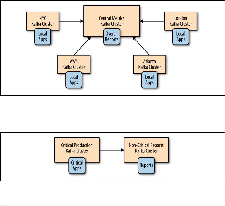
datacenter, we prefer to install a Kafka cluster in each datacenter and mirror the nec‐
essary data between them once rather than have multiple applications consume the
same data across the WAN.
We’ll talk more about tuning Kafka for cross-datacenter communication, but the fol‐
lowing principles will guide most of the architectures we’ll discuss next:
•No less than one cluster per datacenter
•Replicate each event exactly once (barring retries due to errors) between each
pair of datacenters
•When possible, consume from a remote datacenter rather than produce to a
remote datacenter
Hub-and-Spokes Architecture
This architecture is intended for the case where there are multiple local Kafka clusters
and one central Kafka cluster. See Figure 8-1.
Figure 8-1. e hub-and-spokes architecture
There is also a simpler variation of this architecture with just two clusters—a leader
and a follower. See Figure 8-2.
Figure 8-2. A simpler version of the hub-and-spokes architecture
160 | Chapter 8: Cross-Cluster Data Mirroring

This architecture is used when data is produced in multiple datacenters and some
consumers need access to the entire data set. The architecture also allows for applica‐
tions in each datacenter to only process data local to that specific datacenter. But it
does not give access to the entire data set from each datacenter.
The main benefit of this architecture is that data is always produced to the local data-
center and that events from each datacenter are only mirrored once—to the central
datacenter. Applications that process data from a single datacenter can be located at
that datacenter. Applications that need to process data from multiple datacenters will
be located at the central datacenter where all the events are mirrored. Because replica‐
tion always goes in one direction and because each consumer always reads from the
same cluster, this architecture is simple to deploy, configure, and monitor.
The main drawbacks of this architecture are the direct results of its benefits and sim‐
plicity. Processors in one regional datacenter can’t access data in another. To under‐
stand better why this is a limitation, let’s look at an example of this architecture.
Suppose that we are a large bank and have branches in multiple cities. Let’s say that
we decide to store user profiles and their account history in a Kafka cluster in each
city. We replicate all this information to a central cluster that is used to run the bank’s
business analytics. When users connect to the bank website or visit their local branch,
they are routed to send events to their local cluster and read events from the same
local cluster. However, suppose that a user visits a branch in a different city. Because
the user information doesn’t exist in the city he is visiting, the branch will be forced to
interact with a remote cluster (not recommended) or have no way to access the user’s
information (really embarrassing). For this reason, use of this pattern is usually limi‐
ted to only parts of the data set that can be completely separated between regional
datacenters.
When implementing this architecture, for each regional datacenter you need at least
one mirroring process on the central datacenter. This process will consume data from
each remote regional cluster and produce it to the central cluster. If the same topic
exists in multiple datacenters, you can write all the events from this topic to one topic
with the same name in the central cluster, or write events from each datacenter to a
separate topic.
Active-Active Architecture
This architecture is used when two or more datacenters share some or all of the data
and each datacenter is able to both produce and consume events. See Figure 8-3.
Multicluster Architectures | 161
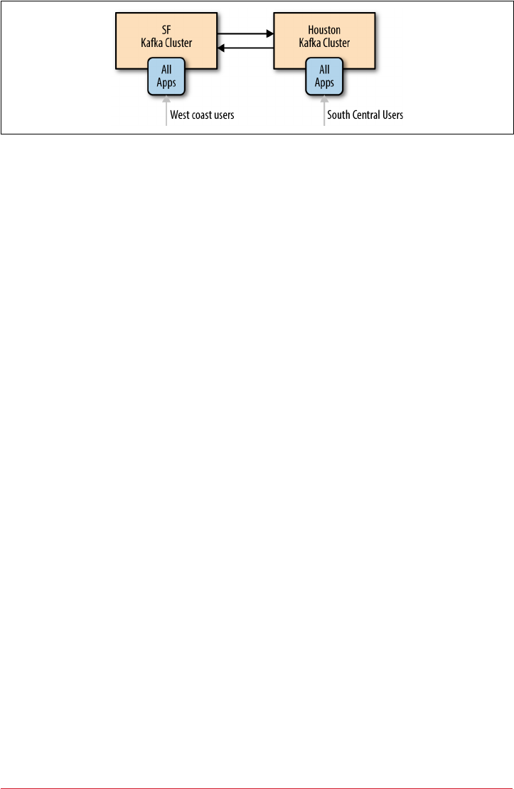
Figure 8-3. e active-active architecture model
The main benefits of this architecture are the ability to serve users from a nearby
datacenter, which typically has performance benefits, without sacrificing functionality
due to limited availability of data (as we’ve seen happen in the hub-and-spokes archi‐
tecture). A secondary benefit is redundancy and resilience. Since every datacenter has
all the functionality, if one datacenter is unavailable you can direct users to a remain‐
ing datacenter. This type of failover only requires network redirects of users, typically
the easiest and most transparent type of failover.
The main drawback of this architecture is the challenges in avoiding conflicts when
data is read and updated asynchronously in multiple locations. This includes techni‐
cal challenges in mirroring events—for example, how do we make sure the same
event isn’t mirrored back and forth endlessly? But more important, maintaining data
consistency between the two datacenters will be difficult. Here are few examples of
the difficulties you will encounter:
•If a user sends an event to one datacenter and reads events from another datacen‐
ter, it is possible that the event they wrote hasn’t arrived the second datacenter
yet. To the user, it will look like he just added a book to his wish list, clicked on
the wish list, but the book isn’t there. For this reason, when this architecture is
used, the developers usually find a way to “stick” each user to a specific datacen‐
ter and make sure they use the same cluster most of the time (unless they connect
from a remote location or the datacenter becomes unavailable).
•An event from one datacenter says user ordered book A and an event from more
or less the same time at a second datacenter says that the same user ordered book
B. After mirroring, both datacenters have both events and thus we can say that
each datacenter has two conflicting events. Applications on both datacenters
need to know how to deal with this situation. Do we pick one event as the “cor‐
rect” one? If so, we need consistent rules on how to pick one so applications on
both datacenters will arrive at the same conclusion. Do we decide that both are
true and simply send the user two books and have another department deal with
returns? Amazon used to resolve conflicts that way, but organizations dealing
with stock trades, for example, can’t. The specific method for minimizing con‐
flicts and handling them when they occur is specific to each use case. It is impor‐
162 | Chapter 8: Cross-Cluster Data Mirroring

tant to keep in mind that if you use this architecture, you will have conflicts and
will need to deal with them.
If you find ways to handle the challenges of asynchronous reads and writes to the
same data set from multiple locations, then this architecture is highly recommended.
It is the most scalable, resilient, flexible, and cost-effective option we are aware of. So
it is well worth the effort to figure out solutions for avoiding replication cycles, keep‐
ing users mostly in the same datacenter, and handling conflicts when they occur.
Part of the challenge of active-active mirroring, especially with more than two data‐
centers, is that you will need a mirroring process for each pair of datacenters and each
direction. With five datacenters, you need to maintain at least 20 mirroring processes
—and more likely 40, since each process needs redundancy for high availability.
In addition, you will want to avoid loops in which the same event is mirrored back-
and-forth endlessly. You can do this by giving each “logical topic” a separate topic for
each datacenter and making sure to avoid replicating topics that originated in remote
datacenters. For example, logical topic users will be topic SF.users in one datacenter
and NYC.users in another datacenter. The mirroring processes will mirror topic
SF.users from SF to NYC and topic NYC.users from NYC to SF. As a result, each event
will only be mirrored once, but each datacenter will contain both SF.users and
NYC.users, which means each datacenter will have information for all the users. Con‐
sumers will need to consume events from .users if they wish to consume all user
events. Another way to think of this setup is to see it as a separate namespace for each
datacenter that contains all the topics for the specific datacenter. In our example, we’ll
have the NYC and the SF namespaces.
Note that in the near future (and perhaps before you read this book), Apache Kafka
will add record headers. This will allow tagging events with their originating datacen‐
ter and using this header information to avoid endless mirroring loops and also to
allow processing events from different datacenters separately. You can still implement
this feature by using a structured data format for the record values (Avro is our favor‐
ite example) and use this to include tags and headers in the event itself. However, this
does require extra effort when mirroring, since none of the existing mirroring tools
will support your specific header format.
Active-Standby Architecture
In some cases, the only requirement for multiple clusters is to support some kind of
disaster scenario. Perhaps you have two clusters in the same datacenter. You use one
cluster for all the applications, but you want a second cluster that contains (almost)
all the events in the original cluster that you can use if the original cluster is com‐
pletely unavailable. Or perhaps you need geographic resiliency. Your entire business is
running from a datacenter in California, but you need a second datacenter in Texas
Multicluster Architectures | 163
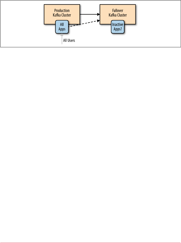
that usually doesn’t do much and that you can use in case of an earthquake. The Texas
datacenter will probably have an inactive (“cold”) copy of all the applications that
admins can start up in case of emergency and that will use the second cluster
(Figure 8-4). This is often a legal requirement rather than something that the business
is actually planning on doing—but you still need to be ready.
Figure 8-4. e active-standby architecture
The benefits of this setup is simplicity in setup and the fact that it can be used in
pretty much any use case. You simply install a second cluster and set up a mirroring
process that streams all the events from one cluster to another. No need to worry
about access to data, handling conflicts, and other architectural complexities.
The disadvantages are waste of a good cluster and the fact that failover between Kafka
clusters is, in fact, much harder than it looks. The bottom line is that it is currently
not possible to perform cluster failover in Kafka without either losing data or having
duplicate events. Often both. You can minimize them, but never fully eliminate them.
It should be obvious that a cluster that does nothing except wait around for a disaster
is a waste of resources. Since disasters are (or should be) rare, most of the time we are
looking at a cluster of machines that does nothing at all. Some organizations try to
fight this issue by having a DR (disaster recovery) cluster that is much smaller than
the production cluster. But this is a risky decision because you can’t be sure that this
minimally sized cluster will hold up during an emergency. Other organizations prefer
to make the cluster useful during non-disasters by shifting some read-only workloads
to run on the DR cluster, which means they are really running a small version of a
hub-and-spoke architecture with a single spoke.
The more serious issue is, how do you failover to a DR cluster in Apache Kafka?
First, it should go without saying that whichever failover method you choose, your
SRE team must practice it on a regular basis. A plan that works today may stop work‐
ing after an upgrade, or perhaps new use cases make the existing tooling obsolete.
Once a quarter is usually the bare minimum for failover practices. Strong SRE teams
practice far more frequently. Netflix’s famous Chaos Monkey, a service that randomly
causes disasters, is the extreme—any day may become failover practice day.
Now, let’s take a look at what is involved in a failover.
164 | Chapter 8: Cross-Cluster Data Mirroring

Data loss and inconsistencies in unplanned failover
Because Kafka’s various mirroring solutions are all asynchronous (we’ll discuss a syn‐
chronous solution in the next section), the DR cluster will not have the latest mes‐
sages from the primary cluster. You should always monitor how far behind the DR
cluster is and never let it fall too far behind. But in a busy system you should expect
the DR cluster to be a few hundred or even a few thousand messages behind the pri‐
mary. If your Kafka cluster handles 1 million messages a second and there is a 5 milli‐
second lag between the primary and the DR cluster is 5 milliseconds, your DR cluster
will be 5,000 messages behind the primary in the best-case scenario. So prepare for
unplanned failover to include some data loss. In planned failover, you can stop the
primary cluster and wait for the mirroring process to mirror the remaining messages
before failing over applications to the DR cluster, thus avoiding this data loss. When
unplanned failover occurs and you lose a few thousand messages, note that Kafka
currently has no concept of transactions, which means that if some events in multiple
topics are related to each other (e.g., sales and line-items), you can have some events
arrive to the DR site in time for the failover and others that don’t. Your applications
will need to be able to handle a line item without a corresponding sale after you fail‐
over to the DR cluster.
Start oset for applications after failover
Perhaps the most challenging part in failing over to another cluster is making sure
applications know where to start consuming data. There are several common
approaches. Some are simple but can cause additional data loss or duplicate process‐
ing; others are more involved but minimize additional data loss and reprocessing.
Let’s take a look at a few:
Auto oset reset
Apache Kafka consumers have a configuration for how to behave when they
don’t have a previously committed offset—they either start reading from the
beginning of the partition or from the end of the partition. If you are using old
consumers that are committing offsets to Zookeeper and you are not somehow
mirroring these offsets as part of the DR plan, you need to choose one of these
options. Either start reading from the beginning of available data and handle
large amounts of duplicates or skip to the end and miss an unknown (and hope‐
fully small) number of events. If your application handles duplicates with no
issues, or missing some data is no big deal, this option is by far the easiest. Simply
skipping to the end of the topic on failover is probably still the most popular fail‐
over method.
Replicate osets topic
If you are using new (0.9 and above) Kafka consumers, the consumers will com‐
mit their offsets to a special topic: __consumer_offsets. If you mirror this topic
Multicluster Architectures | 165
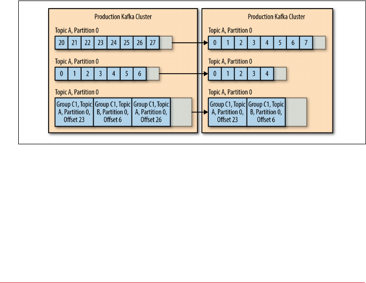
to your DR cluster, when consumers start consuming from the DR cluster they
will be able to pick up their old offsets and continue from where they left off. It is
simple, but there is a long list of caveats involved.
First, there is no guarantee that offsets in the primary cluster will match those in
the secondary cluster. Suppose you only store data in the primary cluster for
three days and you start mirroring a topic a week after it was created. In this case
the first offset available in the primary cluster may be offset 57000000 (older
events were from the first 4 days and were removed already), but the first offset
in the DR cluster will be 0. So a consumer that tries to read offset 57000003
(because that’s its next event to read) from the DR cluster will fail to do this.
Second, even if you started mirroring immediately when the topic was first cre‐
ated and both the primary and the DR topics start with 0, producer retries can
cause offsets to diverge. Simply put, there is no existing Kafka mirroring solution
that preserves offsets between primary and DR clusters.
Third, even if the offsets were perfectly preserved, because of the lag between pri‐
mary and DR clusters and because Kafka currently lacks transactions, an offset
committed by a Kafka consumer may arrive ahead or behind the record with this
offset. A consumer that fails over may find committed offsets without matching
records. Or it may find that the latest committed offset in the DR site is older
than the latest committed offset in the primary site. See Figure 8-5.
Figure 8-5. A fail over causes committed osets without matching records
In these cases, you need to accept some duplicates if the latest committed offset
in the DR site is older than the one committed on the primary or if the offsets in
the records in the DR site are ahead of the primary due to retries. You will also
need to figure out how to handle cases where the latest committed offset in the
DR site doesn’t have a matching record—do you start processing from the begin‐
ning of the topic, or skip to the end?
166 | Chapter 8: Cross-Cluster Data Mirroring

As you can see, this approach has its limitations. Still, this option lets you failover
to another DR with a reduced number of duplicated or missing events compared
to other approaches, while still being simple to implement.
Time-based failover
If you are using really new (0.10.0 and above) Kafka consumers, each message
includes a timestamp indicating the time the message was sent to Kafka. In really
new Kafka versions (0.10.1.0 and above), the brokers include an index and an
API for looking up offsets by the timestamp. So, if you failover to the DR cluster
and you know that your trouble started at 4:05 A.M., you can tell consumers to
start processing data from 4:03 A.M. There will be some duplicates from those
two minutes, but it is probably better than other alternatives and the behavior is
much easier to explain to everyone in the company—“We failed back to 4:03
A.M.” sounds better than “We failed back to what may or may not be the latest
committed offsets.” So this is often a good compromise. The only question is:
how do we tell consumers to start processing data from 4:03 A.M.?
One option is to bake it right into your app. Have a user-configurable option to
specify the start time for the app. If this is configured, the app can use the new
APIs to fetch offset by time, seek to that time, and start consuming from the right
point, committing offsets as usual.
This option is great if you wrote all your applications this way in advance. But
what if you didn’t? It is fairly straightforward to write a small tool that will take a
timestamp, use the new APIs to fetch offsets for this timestamp, and then commit
these offsets for a list of topics and partitions as a specific consumer group. We
hope to add this tool to Kafka in the near future, but it is possible to write one
yourself. The consumer group should be stopped while running this type of tool
and started immediately after.
This option is recommended for those using new versions of Kafka who like
some certainty in their failover and are willing to write a bit of custom tooling
around the process.
External oset mapping
When discussing mirroring the offsets topic, one of the biggest challenges with
that approach is the fact that offsets in primary and DR clusters can diverge.
With this in mind, some organizations choose to use an external data store, such
as Apache Cassandra, to store mapping of offsets from one cluster to another.
They build their Kafka mirroring tool so that whenever an event is produced to
the DR cluster, both offsets are sent to the external datastore. Or they only store
both offsets whenever the difference between the two offsets changed. For exam‐
ple, if offset 495 on primary mapped to offset 500 on the DR cluster, we’ll record
(495,500) in the external store. If the difference changes later due to duplicates
and offset 596 is mapped to 600, then we’ll record the new mapping (596,600).
Multicluster Architectures | 167

There is no need to store all the offset mappings between 495 and 596; we just
assume that the difference remains the same and so offset 550 in the primary
cluster will map to 555 in the DR. Then when failover occurs, instead of mapping
timestamps (which are always a bit inaccurate) to offsets, they map primary off‐
sets to DR offsets and use those. They use one of the two techniques listed above
to force consumers to start using the new offsets from the mapping. This still has
an issue with offset commits that arrived ahead of the records themselves and
offset commits that didn’t get mirrored to the DR on time, but it covers some
cases.
This solution is quite complex and in my opinion almost never worth the extra
effort. It dates back to before time indexes existed and could be used for failover.
These days I’d opt to upgrade the cluster and use the time-based solution rather
than go through the effort of mapping offsets, which still doesn’t cover all failover
cases.
After the failover
Let’s say that failover was successful. Everything is working just fine on the DR clus‐
ter. Now we need to do something with the primary cluster. Perhaps turn it into a DR.
It is tempting to simply modify the mirroring processes to reverse their direction and
simply start mirroring from the new primary to the old one. However, this leads to
two important questions:
•How do we know where to start mirroring? We need to solve the same problem
we have for all our consumers for the mirroring application itself. And remember
that all our solutions have cases where they either cause duplicates or miss data—
often both.
•In addition, for reasons we discussed above, it is likely that your original primary
will have events that the DR cluster does not. If you just start mirroring new data
back, the extra history will remain and the two clusters will be inconsistent.
For this reason, the simplest solution is to first scrape the original cluster—delete all
the data and committed offsets and then start mirroring from the new primary back
to what is now the new DR cluster. This gives you a clean slate that is identical to the
new primary.
A few words on cluster discovery
One of the important points to consider when planning a standby cluster is that in
the event of failover, your applications will need to know how to start communicating
with the failover cluster. If you hardcoded the hostnames of your primary cluster
brokers in the producer and consumer properties, this will be challenging. Most
organizations keep it simple and create a DNS name that usually points to the pri‐
168 | Chapter 8: Cross-Cluster Data Mirroring

mary brokers. In case of an emergency, the DNS name can be pointed to the standby
cluster. The discovery service (DNS or other) doesn’t need to include all the brokers
—Kafka clients only need to access a single broker successfully in order to get meta‐
data about the cluster and discover the other brokers. So including just three brokers
is usually fine. Regardless of the discovery method, most failover scenarios do require
bouncing consumer applications after failover so they can find the new offsets they
need to start consuming.
Stretch Clusters
Active-standby architectures are used to protect the business against the failure of a
Kafka cluster, by moving applications to communicate with another cluster in case of
cluster failure. Stretch clusters are intended to protect the Kafka cluster from failure
in the event an entire datacenter failed. They do this by installing a single Kafka clus‐
ter across multiple datacenters.
Stretch clusters are fundamentally different from other multi-datacenter scenarios. To
start with, they are not multicluster—it is just one cluster. As a result, we don’t need a
mirroring process to keep two clusters in sync. Kafka’s normal replication mechanism
is used, as usual, to keep all brokers in the cluster in sync. This setup can include syn‐
chronous replication. Producers normally receive an acknowledgment from a Kafka
broker after the message was successfully written to Kafka. In the Stretch cluster case,
we can configure things so the acknowledgment will be sent after the message is writ‐
ten successfully to Kafka brokers in two datacenters. This involves using rack defini‐
tions to make sure each partition has replicas in multiple datacenters and the use of
min.isr and acks=all to ensure that every write is acknowledged from at least two
datacenters.
The advantages of this architecture are in the synchronous replication—some types
of business simply require that their DR site is always 100% synchronized with the
primary site. This is often a legal requirement and is applied to any data-store across
the company—Kafka included. The other advantage is that both datacenters and all
brokers in the cluster are used. There is no waste like the one we saw in active-
standby architectures.
This architecture is limited in the type of disasters it protects against. It only protects
from datacenter failures, not any kind of application or Kafka failures. The opera‐
tional complexity is also limited. This architecture demands physical infrastructure
that not all companies can provide.
This architecture is feasible if you can install Kafka (and Zookeeper) in at least three
datacenters with high bandwidth and low latency between them. This can be done if
your company owns three buildings on the same street, or—more commonly—by
using three availability zones inside one region of your cloud provider.
Multicluster Architectures | 169
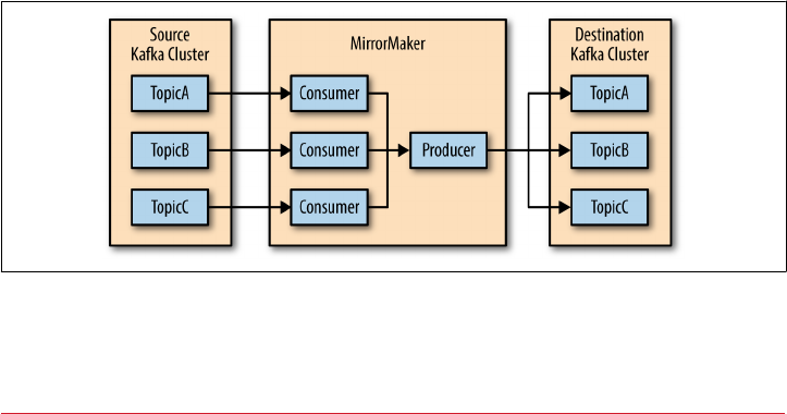
The reason three datacenters are important is because Zookeeper requires an uneven
number of nodes in a cluster and will remain available if a majority of the nodes are
available. With two datacenters and an uneven number of nodes, one datacenter will
always contain a majority, which means that if this datacenter is unavailable, Zoo‐
keeper is unavailable, and Kafka is unavailable. With three datacenters, you can easily
allocate nodes so no single datacenter has a majority. So if one datacenter is unavail‐
able, a majority of nodes exist in the other two datacenters and the Zookeeper cluster
will remain available. Therefore, so will the Kafka cluster.
It is possible to run Zookeeper and Kafka in two datacenters using a Zookeeper group
configuration that allows for manual failover between two datacenters. However, this
setup is uncommon.
Apache Kafka’s MirrorMaker
Apache Kafka contains a simple tool for mirroring data between two datacenters. It is
called MirrorMaker and at its core, it is a collection of consumers (called streams in
MirrorMaker documentation, for historical reasons), which are all part of the same
consumer group and read data from the set of topics you chose to replicate. Each
MirrorMaker process has a single producer. The workflow is pretty simple: Mirror‐
Maker runs a thread for each consumer. Each consumer consumes events from the
topics and partitions it was assigned on the source cluster and uses the shared pro‐
ducer to send those events to the target cluster. Every 60 seconds (by default), the
consumers will tell the producer to send all the events it has to Kafka and wait until
Kafka acknowledges these events. Then the consumers contact the source Kafka clus‐
ter to commit the offsets for those events. This guarantees no data loss (messages are
acknowledged by Kafka before offsets are committed to the source) and there is no
more than 60 seconds’ worth of duplicates if the MirrorMaker process crashes. See
Figure 8-6.
Figure 8-6. e MirrorMaker process in Kaa
170 | Chapter 8: Cross-Cluster Data Mirroring

More about MirrorMaker
MirrorMaker sounds very simple, but because we were trying to be
very efficient and get very close to exactly-once delivery, it turned
out to be tricky to implement correctly. By release 0.10.0.0 of
Apache Kafka, MirrorMaker had been rewritten four times. Addi‐
tional writes may happen in the future as well. The description here
and the details in the following sections apply to MirrorMaker as it
existed from release 0.9.0.0 to release 0.10.2.0.
How to Congure
MirrorMaker is highly configurable. First, it uses one producer and multiple consum‐
ers, so every configuration property of producers and consumers can be used when
configuring MirrorMaker. In addition, MirrorMaker itself has a sizable list of config‐
uration options, sometimes with complex dependencies between them. We will show
a few examples here and highlight some of the important configuration options, but
exhaustive documentation of MirrorMaker is outside our scope.
With that in mind, let’s take a look at a MirrorMaker example:
bin/kafka-mirror-maker --consumer.config etc/kafka/consumer.properties --
producer.config etc/kafka/producer.properties --new.consumer --num.streams=2 --
whitelist ".*"
Let’s look at MirrorMaker’s basic command-line arguments one by one:
consumer.config
This is the configuration for all the consumers that will be fetching data from the
source cluster. They all share one configuration file, which means you can only
have one source cluster and one group.id. So all the consumers will be part of
the same consumer group, which is exactly what we want. The mandatory con‐
figurations in the file are the bootstrap.servers (for the source cluster) and the
group.id. But you can use any additional configuration you want for the con‐
sumers. The one configuration you don’t want to touch is auto.com
mit.enable=false. MirrorMaker depends on its ability to commit its own offsets
after they safely arrive to the target Kafka cluster. Changing this setting can result
in data loss. One configuration you do want to change is auto.offset.reset.
This defaults to latest, which means MirrorMaker will only mirror events that
arrived to the source cluster after MirrorMaker started. If you want to mirror
existing data as well, change this to earliest. We will discuss additional configu‐
ration properties in the section “Tuning MirrorMaker” on page 175.
producer.config
The configuration for the producer used by MirrorMaker to write to the target
cluster. The only mandatory configuration is bootstrap.servers (for the target
Apache Kafka’s MirrorMaker | 171

cluster). We will discuss additional configuration properties in the section “Tun‐
ing MirrorMaker” on page 175.
new.consumer
MirrorMaker can use the 0.8 consumer or the new 0.9 consumer. We recom‐
mend the 0.9 consumer because it is more stable at this point.
num.streams
As we explained previously, each stream is another consumer reading from the
source cluster. Remember that all consumers in the same MirrorMaker process
share the same producers. It will take multiple streams to saturate a producer. If
you need additional throughput after this point, you’ll need another Mirror‐
Maker process.
whitelist
A regular expression for the topic names that will be mirrored. All topic names
that match the regular expression will be mirrored. In this example, we chose to
replicate every topic, but it is often good practice to use something like prod.*
and avoid replicating test topics. Or in active-active architecture, MirrorMaker
replicating from a NYC datacenter to a SF datacenter will configure white
list="NYC.\*" and avoid replicating back topics that originated in SF.
Deploying MirrorMaker in Production
In the previously given example, we ran MirrorMaker as a command-line utility.
Usually when running MirrorMaker in a production environment, you will want to
run MirrorMaker as a service, running in the background with nohup and redirecting
its console output to a log file. Technically, the tool has -daemon as a command-line
option that should do all of the above for you, but in practice, this hasn’t worked as
expected in recent releases.
Most companies that use MirrorMaker have their own startup scripts that also
include the configuration parameters they use. Production deployment systems like
Ansible, Puppet, Chef, and Salt are often used to automate deployment and manage
the many configuration options and files.
A more advanced deployment option that is becoming very popular is to run Mirror‐
Maker inside a Docker container. MirrorMaker is completely stateless and doesn’t
require any disk storage (all the data and state is stored in Kafka itself). Wrapping
MirrorMaker in Docker also allows running multiple instances on a single machine.
Since a single MirrorMaker instance is limited to the throughput of a single producer,
this is often important to launch multiple instances of MirrorMaker, and Docker
makes it much easier. It also makes it easier to scale up and down—spin additional
containers when more throughput is needed at peak time and spin them down when
there is less traffic. If you are running MirrorMaker in a cloud environment, you can
172 | Chapter 8: Cross-Cluster Data Mirroring

even spin up additional servers on which to run the containers based on throughput
and demand.
If at all possible, run MirrorMaker at the destination datacenter. So if you are sending
data from NYC to SF, MirrorMaker should run in SF and consume data across the US
from NYC. The reason for this is that long-distance networks can be a bit less reliable
than those inside a datacenter. If there is a network partition and you lose connectiv‐
ity between the datacenters, having a consumer that is unable to connect to a cluster
is much safer than a producer that can’t connect. If the consumer can’t connect, it
simply won’t be able to read events, but the events will still be stored in the source
Kafka cluster and can remain there for a long time. There is no risk of losing events.
On the other hand, if the events were already consumed and MirrorMaker can’t pro‐
duce them due to network partition, there is always a risk that these events will acci‐
dentally get lost by MirrorMaker. So remote consuming is safer than remote
producing.
When do you have to consume locally and produce remotely? The answer is when
you need to encrypt the data while it is transferred between the datacenters but you
don’t need to encrypt the data inside the datacenter. Consumers take a significant
performance hit when connecting to Kafka with SSL encryption—much more so
than producers. And this performance hit also affects the Kafka brokers themselves.
If your cross datacenter traffic requires encryption, you are better off placing Mirror‐
Maker at the source datacenter, having it consume unencrypted data locally, and then
producing it to the remote datacenter through an SSL encrypted connection. This
way, the producer connects to Kafka with SSL but not the consumer, which doesn’t
impact performance as much. If you use this consume locally and produce remotely,
make sure MirrorMaker is configured to never lose events by configuring it with
acks=all and a sufficient number of retries. Also, configure MirrorMaker to exit
when it fails to send events, which is typically safer to do than to continue and risk
data loss.
If having very low lag between the source and target clusters is important, you will
probably want to run at least two MirrorMaker instances on two different servers and
have both use the same consumer group. If one server is stopped for whatever reason,
the MirrorMaker instance can continue mirroring the data.
When deploying MirrorMaker in production, it is important to remember to monitor
it as follows:
Lag monitoring
You will definitely want to know if the destination cluster is falling behind the
source. The lag is the difference in offsets between the latest message in the
source Kafka and the latest message in the destination. See Figure 8-7.
Apache Kafka’s MirrorMaker | 173
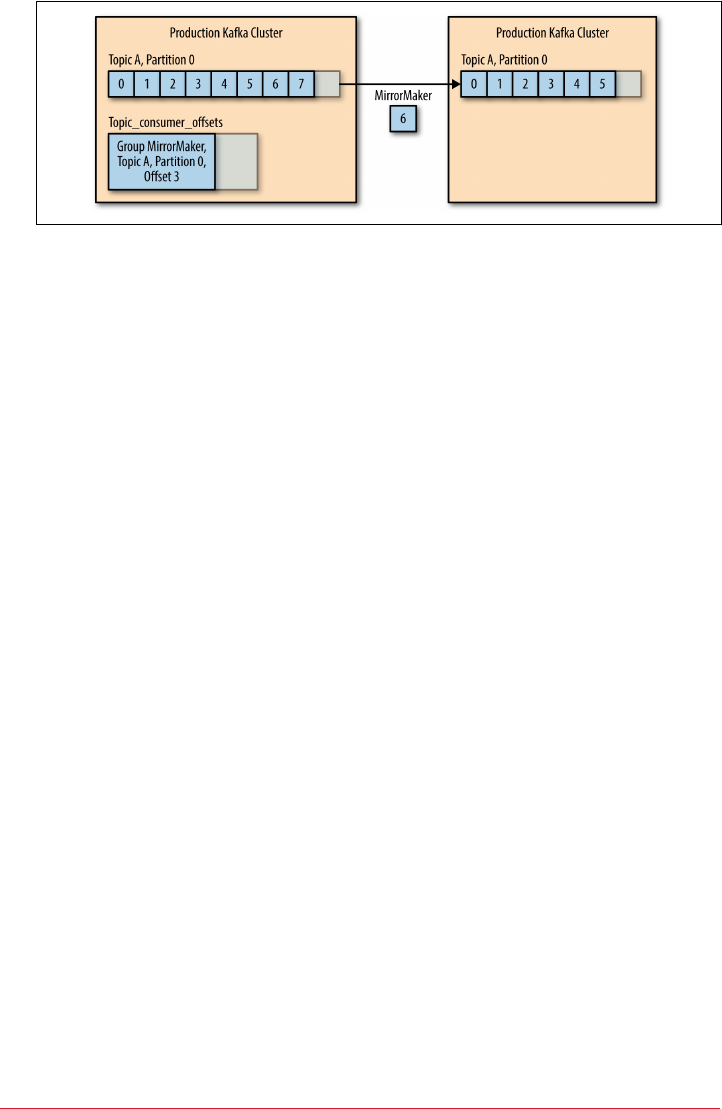
Figure 8-7. Monitoring the lag dierence in osets
In Figure 8-7, the last offset in the source cluster is 7 and the last offset in the
destination is 5—meaning there is a lag of 2 messages.
There are two ways to track this lag, and neither is perfect:
•Check the latest offset committed by MirrorMaker to the source Kafka clus‐
ter. You can use the kafka-consumer-groups tool to check for each partition
MirrorMaker is reading— the offset of the last event in the partition, the last
offset MirrorMaker committed, and the lag between them. This indicator is
not 100% accurate because MirrorMaker doesn’t commit offsets all the time.
It commits offsets every minute by default so you will see the lag grow for a
minute and then suddenly drop. In the diagram, the real lag is 2, but the
kafka-consumer-groups tool will report a lag of 4 because MirrorMaker
hasn’t committed offsets for more recent messages yet. LinkedIn’s Burrow
monitors the same information but has a more sophisticated method to
determine whether the lag represents a real problem, so you won’t get false
alerts.
•Check the latest offset read by MirrorMaker (even if it isn’t committed). The
consumers embedded in MirrorMaker publish key metrics in JMX. One of
them is the consumer maximum lag (over all the partitions it is consuming).
This lag is also not 100% accurate because it is updated based on what the
consumer read but doesn’t take into account whether the producer managed
to send those messages to the destination Kafka cluster and whether they
were acknowledged successfully. In this example, the MirrorMaker con‐
sumer will report a lag of 1 message rather than 2, because it already read
message 6—even though the message wasn’t produced to the destination yet.
Note that if MirrorMaker skips or drops messages, neither method will detect an
issue because they just track the latest offset. Confluent’s Control Center moni‐
tors message counts and checksums and closes this monitoring gap.
174 | Chapter 8: Cross-Cluster Data Mirroring

Metrics monitoring
MirrorMaker contains a producer and a consumer. Both have many available
metrics and we recommend collecting and tracking them. Kafka documentation
lists all the available metrics. Here are a few metrics that proved useful in tuning
MirrorMaker performance:
Consumer
fetch-size-avg, fetch-size-max, fetch-rate, fetch-throttle-time-avg,
and fetch-throttle-time-max
Producer
batch-size-avg, batch-size-max, requests-in-flight, and record-
retry-rate
Both
io-ratio and io-wait-ratio
Canary
If you monitor everything else, a canary isn’t strictly necessary, but we like to add
it in for multiple layers of monitoring. It provides a process that, every minute,
sends an event to a special topic in the source cluster and tries to read the event
from the destination cluster. It also alerts you if the event takes more than an
acceptable amount of time to arrive. This can mean MirrorMaker is lagging or
that it isn’t around at all.
Tuning MirrorMaker
Sizing of the MirrorMaker cluster depends on the throughput you need and the lag
you can tolerate. If you can’t tolerate any lag, you have to size MirrorMaker with
enough capacity to keep up with your top throughput. If you can tolerate some lag,
you can size MirrorMaker to be 75-80% utilized 95-99% of the time. Then, expect
some lag to develop when you are at peak throughput. Because MirrorMaker has
spare capacity most of the time, it will catch up once the peak is over.
Then you want to measure the throughput you get from MirrorMaker with a differ‐
ent number of consumer threads—configured with num.streams parameter. We can
give you some ballpark numbers (LinkedIn gets 6MB/s with 8 consumer threads and
12MB/s with 16), but since this depends a lot on your hardware, datacenter, or cloud
provider, you will want to run your own tests. Kafka ships with the kafka-
performance-producer tool. Use it to generate load on a source cluster and then con‐
nect MirrorMaker and start mirroring this load. Test MirrorMaker with 1, 2, 4, 8, 16,
24, and 32 consumer threads. Watch where performance tapers off and set
num.streams just below this point. If you are consuming or producing compressed
events (recommended, since bandwidth is the main bottleneck for cross-datacenter
mirroring), MirrorMaker will have to decompress and recompress the events. This
Apache Kafka’s MirrorMaker | 175

uses a lot of CPU, so keep an eye on CPU utilization as you increase the number of
threads. Using this process, you will find the maximum throughput you can get with
a single MirrorMaker instance. If it is not enough, you will want to experiment with
additional instances and after that, additional servers.
In addition, you may want to separate sensitive topics—those that absolutely require
low latency and where the mirror must be as close to the source as possible—to a sep‐
arate MirrorMaker cluster with its own consumer group. This will prevent a bloated
topic or an out of control producer from slowing down your most sensitive data pipe‐
line.
This is pretty much all the tuning you can do to MirrorMaker itself. However, you
can still increase the throughput of each consumer thread and each MirrorMaker
instance.
If you are running MirrorMaker across datacenters, you want to optimize the net‐
work configuration in Linux as follows:
•Increase TCP buffer size (net.core.rmem_default, net.core.rmem_max,
net.core.wmem_default, net.core.wmem_max, net.core.optmem_max)
•Enable automatic window scaling (sysctl –w net.ipv4.tcp_window_scaling=1
or add net.ipv4.tcp_window_scaling=1 to /etc/sysctl.conf)
•Reduce the TCP slow start time (set /proc/sys/net/ipv4/
tcp_slow_start_after_idle to 0)
Note that tuning the Linux network is a large and complex topic. To understand more
about these parameters and others, we recommend reading a network tuning guide
such as Performance Tuning for Linux Servers by Sandra K. Johnson, et al. (IBM
Press).
In addition, you may want to tune the producers and consumers that are running in
MirrorMaker. First, you will want decide whether the producer or the consumer is
the bottleneck—is the producer waiting for the consumer to bring more data or the
other way around? One way to decide is to look at the producer and consumer met‐
rics you are monitoring. If one process is idle while the other is fully utilized, you
know which one needs tuning. Another method is to do several thread dumps (using
jstack) and see if the MirrorMaker threads are spending most of the time in poll or in
send—more time spent polling usually means the consumer is the bottleneck, while
more time spent sending shift points to the producer.
176 | Chapter 8: Cross-Cluster Data Mirroring

If you need to tune the producer, the following configuration settings can be useful:
max.in.flight.requests.per.connection
By default, MirrorMaker only allows one in-flight request. This means every
request that was sent by the producer has to be acknowledged by the destination
cluster before the next message will be sent. This can limit throughput, especially
if there is significant latency before the brokers acknowledge the messages. The
reason MirrorMaker limits the number of in-flight requests is because this is the
only way to guarantee that Kafka will preserve message order in the event that
some messages will require multiple retries before they are successfully acknowl‐
edged. If message order is not critical for your use case, increasing
max.in.flight.requests.per.connection can significantly increase your
throughput.
linger.ms and batch.size
If your monitoring shows that the producer consistently sends partially empty
batches (i.e., batch-size-avg and batch-size-max metrics are lower than con‐
figured batch.size), you can increase throughput by introducing a bit of latency.
Increase latency.ms and the producer will wait a few milliseconds for the
batches to fill up before sending them. If you are sending full batches and have
memory to spare, you can increase batch.size and send larger batches.
The following consumer configurations can increase throughput for the consumer:
•The partition assignment strategy in MirrorMaker (i.e., the algorithm that
decides which consumer is assigned which partitions) defaults to range. There
are benefits to range strategy, which is why it is the normal default for consum‐
ers, but it can lead to uneven assignment of partitions to consumers. For Mirror‐
Maker, it is usually better to change the strategy to round robin, especially when
mirroring a large number of topics and partitions. You set this by adding parti
tion.assignment.strategy=org.apache.kafka.clients.consumer.RoundRobi
nAssignor to the consumer properties file.
•fetch.max.bytes—if the metrics you are collecting show that fetch-size-avg
and fetch-size-max are close to the fetch.max.bytes configuration, the con‐
sumer is reading as much data from the broker as it is allowed. If you have avail‐
able memory, try increasing fetch.max.bytes to allow the consumer to read
more data in each request.
•fetch.min.bytes and fetch.max.wait—if you see in the consumer metrics that
fetch-rate is high, the consumer is sending too many requests to the brokers
and not receiving enough data in each request. Try increasing both
fetch.min.bytes and fetch.max.wait so the consumer will receive more data
Apache Kafka’s MirrorMaker | 177

in each request and the broker will wait until enough data is available before
responding to the consumer request.
Other Cross-Cluster Mirroring Solutions
We looked in depth at MirrorMaker because this mirroring software arrives as part of
Apache Kafka. However, MirrorMaker also has some limitations when used in prac‐
tice. It is worthwhile to look at some of the alternatives to MirrorMaker and the ways
they address MirrorMaker limitations and complexities.
Uber uReplicator
Uber ran MirrorMaker at very large scale, and as the number of topics and partitions
grew and the cluster throughput increased, they started running into the following
problems:
Rebalancing delays
MirrorMaker consumers are just consumers. Adding MirrorMaker threads,
adding MirrorMaker instances, bouncing MirrorMaker instances, or even adding
new topics that match the regular expression used in the whitelist all cause con‐
sumers to rebalance. As we saw in Chapter 4, rebalancing stops all the consumers
until new partitions can be assigned to each consumer. With a very large number
of topics and partitions, this can take a while. This is especially true when using
old consumers like Uber did. In some cases this caused 5-10 minutes of inactiv‐
ity, causing mirroring to fall behind and accumulate a large backlog of events to
mirror, which can take a long time to recover from. This caused very high latency
for consumers reading events from the destination cluster.
Diculty adding topics
Using a regular expression as the topic whitelist means that MirrorMaker will
rebalance every time someone adds a matching topic to the source cluster. We’ve
already seen that rebalances were particularly painful for Uber. To avoid this,
they decided to simply list every topic they need to mirror and avoid surprise
rebalances. But this means that they need to manually add new topics that they
want to mirror to the whitelist on all MirrorMaker instances and bounce the
instances, which leads to rebalances. At least those rebalances happen on sched‐
uled maintenance and not every time someone adds a topic, but it is still lots of
maintenance. This also means that if the maintenance isn’t done correctly and
different instances have different topic lists, MirrorMaker will start and endlessly
rebalance as the consumers won’t be able to agree on the topics they subscribe to.
Given these issues, Uber decided to write their own MirrorMaker clone, called uRe
plicator. They decided to use Apache Helix as a central (but highly available) con‐
178 | Chapter 8: Cross-Cluster Data Mirroring

troller that will manage the topic list and the partitions assigned to each uReplicator
instance. Administrators use a REST API to add new topics to the list in Helix and
uReplicator is responsible for assigning partitions to the different consumers. To ach‐
ieve this, Uber replaced the Kafka consumers used in MirrorMaker with a Kafka con‐
sumer they wrote themselves called Helix consumer. This consumer takes its
partition assignment from the Apache Helix controller rather than as a result of an
agreement between the consumers (see Chapter 4 for details on how this is done in
Kafka). As a result, the Helix consumer can avoid rebalances and instead listen to
changes in the assigned partitions that arrive from Helix.
Uber wrote a blog post describing the architecture in more detail and showing the
improvements they experienced. At the time of writing, we are not aware of any com‐
pany besides Uber that uses the uReplicator. This is possibly because most companies
don’t operate at Uber’s scale and don’t run into the same issues, or perhaps because
the dependency on Apache Helix introduces a completely new component to learn
and manage, which adds complexity to the entire project.
Conuent’s Replicator
At the same time that Uber developed their uReplicator, Confluent independently
developed Replicator. Despite the similarities in names, the projects have almost
nothing in common—they are different solutions to two different sets of Mirror‐
Maker problems. Confluent’s Replicator was developed to address issues their enter‐
prise customers encountered when using MirrorMaker to manage their multicluster
deployments.
Diverging cluster conguration
While MirrorMaker keeps data in sync between source and destination, this is
the only thing it keeps in sync. Topics can end up with different numbers of par‐
titions, replication factors, and topic-level settings. Increasing topic retention
from one to three weeks on the source cluster and forgetting about the DR clus‐
ter can lead to a rather nasty surprise when you failover to the second cluster and
discover that a few weeks of data are now missing. Trying to manually keep all
these settings in sync is error-prone and can cause downstream applications, or
even replication itself, to fail if the systems fall out of sync.
Cluster management challenges
We’ve already seen that MirrorMaker is typically deployed as a cluster of multiple
instances. This means yet another cluster to figure out how to deploy, monitor,
and manage. With two configuration files and a large number of parameters,
configuration management for MirrorMaker itself can be a challenge. This
increases if there are more than two clusters and one-direction replication. If you
have three active-active clusters, you have six MirrorMaker clusters to deploy,
Other Cross-Cluster Mirroring Solutions | 179

monitor, and configure, and each of those likely has at least three instances. With
five active-active clusters, the number of MirrorMaker clusters increases to 20.
With the goal of minimizing administration overhead for busy enterprise IT depart‐
ments, Confluent decided to implement Replicator as a source connector for the
Kafka Connect framework, a source connector that reads data from another Kafka
cluster rather than from a database. If you recall the Kafka Connect architecture from
Chapter 7, you remember that each connector divides the work between a configura‐
ble number of tasks. In Replicator, each task is a consumer and a producer pair. The
Connect framework assigns those tasks to different Connect worker nodes as needed
—so you may have multiple tasks on one server or have the tasks spread out to multi‐
ple servers. This replaces the manual work of figuring out how many MirrorMaker
streams should run per instance and how many instances per machine. Connect also
has a REST API to centrally manage the configuration for the connectors and tasks. If
we assume that most Kafka deployments include Kafka Connect for other reasons
(sending database change events into Kafka is a very popular use case), then by run‐
ning Replicator inside Connect, we can cut down on the number of clusters we need
to manage. The other significant improvement is that the Replicator connector, in
addition to replicating data from a list of Kafka topics, also replicates the configura‐
tion for those topics from Zookeeper.
Summary
We started the chapter by describing the reasons you may need to manage more than
a single Kafka cluster and then proceeded to describe several common multicluster
architectures, ranging from the simple to the very complex. We went into the details
of implementing failover architecture for Kafka and compared the different options
currently available. Then we proceeded to discuss the available tools. Starting with
Apache Kafka’s MirrorMaker, we went into many details of using it in production. We
finished by reviewing two alternative options that solve some of the issues you might
encounter with MirrorMaker.
Whichever architecture and tools you end up using—remember that multicluster
configuration and mirroring pipelines should be monitored and tested just like
everything else you take into production. Because multicluster management in Kafka
can be easier than it is with relational databases, some organizations treat it as an
afterthought and neglect to apply proper design, planning, testing, deployment auto‐
mation, monitoring, and maintenance. By taking multicluster management seriously,
preferably as part of a holistic disaster or geodiversity plan for the entire organization
that involves mutliple applications and datastores, you will greatly increase the chan‐
ces of successfully managing multiple Kafka clusters.
180 | Chapter 8: Cross-Cluster Data Mirroring

CHAPTER 9
Administering Kafka
Kafka provides several command-line interface (CLI) utilities that are useful for mak‐
ing administrative changes to your clusters. The tools are implemented in Java
classes, and a set of scripts are provided to call those classes properly. These tools pro‐
vide basic functions, but you may find they are lacking for more complex operations.
This chapter will describe the tools that are available as part of the Apache Kafka
open source project. More information about advanced tools that have been devel‐
oped in the community, outside of the core project, can be found on the Apache
Kafka website.
Authorizing Admin Operations
While Apache Kafka implements authentication and authorization
to control topic operations, most cluster operations are not yet sup‐
ported. This means that these CLI tools can be used without any
authentication required, which will allow operations such as topic
changes to be executed with no security check or audit. This func‐
tionality is under development and should be added soon.
Topic Operations
The kafka-topics.sh tool provides easy access to most topic operations (configura‐
tion changes have been deprecated and moved to the kafka-configs.sh tool). It
allows you to create, modify, delete, and list information about topics in the cluster.
To use this command, you are required to provide the Zookeeper connect string for
the cluster with the --zookeeper argument. In the examples that follow, the Zoo‐
keeper connect string is assumed to be zoo1.example.com:2181/kafka-cluster.
181

Check the Version
Many of the command-line tools for Kafka operate directly on the
metadata stored in Zookeeper rather than connecting to the brok‐
ers themselves. For this reason, it is important to make sure the
version of the tools that you are using matches the version of the
brokers in the cluster. The safest approach is to run the tools on the
Kafka brokers themselves, using the deployed version.
Creating a New Topic
You need three arguments to create a new topic in a cluster (these arguments must be
provided, even though some of them have broker-level defaults configured already):
Topic name
The name of the topic that you wish to create.
Replication Factor
The number of replicas of the topic to maintain within the cluster.
Partitions
The number of partitions to create for the topic.
Specifying Topic Congurations
It is also possible to explicitly set the replicas for a topic during cre‐
ation, or set configuration overrides for the topic. Neither of these
operations will be covered here. Configuration overrides can be
found later in this chapter, and they can be provided to kafka-
topics.sh using the --config command-line parameter. Partiton
reassignment is also covered later in this chapter.
Topic names may contain alphanumeric characters, as well as underscores, dashes,
and periods.
Naming Topics
It is permitted, but not recommended, to have topic names that
start with two underscores. Topics of this form are considered
internal topics for the cluster (such as the __consumer_offsets
topic for the consumer group offset storage). It is also not recom‐
mended to use both periods and underscores in a single cluster
because when the topic names are used in metric names inside
Kafka, periods are changed to underscores (e.g., “topic.1” becomes
“topic_1” in metrics).
182 | Chapter 9: Administering Kafka

Execute kafka-topics.sh as follows:
kafka-topics.sh --zookeeper <zookeeper connect> --create --topic <string>
--replication-factor <integer> --partitions <integer>
The command will cause the cluster to create a topic with the specified name and
number of partitions. For each partition, the cluster will select the specified number
of replicas appropriately. This means that if the cluster is set up for rack-aware replica
assignment, the replicas for each partition will be in separate racks. If rack-aware
assignment is not desired, specify the --disable-rack-aware command-line argu‐
ment.
For example, create a topic named “my-topic” with eight partitions that have two rep‐
licas each:
# kafka-topics.sh --zookeeper zoo1.example.com:2181/kafka-cluster --create
--topic my-topic --replication-factor 2 --partitions 8
Created topic "my-topic".
#
Skipping Errors for Existing Topics
When using this script in automation, you may want to use the --
if-not-exists argument, which will not return an error if the
topic already exists.
Adding Partitions
It is sometimes necessary to increase the number of partitions for a topic. Partitions
are the way topics are scaled and replicated across a cluster, and the most common
reason to increase the partition count is to spread out a topic further, or decrease the
throughput for a single partition. Topics may also be increased if a consumer needs to
expand to run more copies in a single group, as a partition can only be consumed by
a single member in a group.
Adjusting Keyed Topics
Topics that are produced with keyed messages can be very difficult
to add partitions to from a consumer’s point of view. This is
because the mapping of keys to partitions will change when the
number of partitions is changed. For this reason, it is advisable to
set the number of partitions for a topic that will contain keyed mes‐
sages once, when the topic is created, and avoid resizing the topic.
Topic Operations | 183

Skipping Errors for Nonexistent Topics
While an --if-exists argument is provided for the --alter com‐
mand, using it is not recommended. Using this argument will cause
the command to not return an error if the topic being changed
does not exist. This can mask problems where a topic does not
exist that should have been created.
For example, increase the number of partitions for a topic named “my-topic” to 16:
# kafka-topics.sh --zookeeper zoo1.example.com:2181/kafka-cluster
--alter --topic my-topic --partitions 16
WARNING: If partitions are increased for a topic that has a key,
the partition logic or ordering of the messages will be affected
Adding partitions succeeded!
#
Reducing Partition Counts
It is not possible to reduce the number of partitions for a topic. The
reason this is not supported is because deleting a partition from a
topic would cause part of the data in that topic to be deleted as well,
which would be inconsistent from a client point of view. In addi‐
tion, trying to redistribute the data to remaining partitions would
be difficult and result in out-of-order messages. Should you need to
reduce the number of partitions, you will need to delete the topic
and recreate it.
Deleting a Topic
Even a topic with no messages in it uses cluster resources, including disk space, open
filehandles, and memory. If a topic is no longer needed, it can be deleted in order to
free up these resources. In order to perform this action, the brokers in the cluster
must have been configured with the delete.topic.enable option set to true. If this
option has been set to false, then the request to delete the topic will be ignored.
Data Loss Ahead
Deleting a topic will also delete all its messages. This is not a
reversible operation, so make sure it executed carefully.
For example, delete the topic named “my-topic”:
# kafka-topics.sh --zookeeper zoo1.example.com:2181/kafka-cluster
--delete --topic my-topic
Topic my-topic is marked for deletion.
184 | Chapter 9: Administering Kafka

Note: This will have no impact if delete.topic.enable is not set
to true.
#
Listing All Topics in a Cluster
The topics tool can list all topics in a cluster. The list is formatted with one topic per
line, in no particular order.
For example, list topics in the cluster:
# kafka-topics.sh --zookeeper zoo1.example.com:2181/kafka-cluster
--list
my-topic - marked for deletion
other-topic
#
Describing Topic Details
It is also possible to get detailed information on one or more topics in the cluster. The
output includes the partition count, topic configuration overrides, and a listing of
each partition with its replica assignments. This can be limited to a single topic by
providing a --topic argument to the command.
For example, describe all topics in the cluster:
# kafka-topics.sh --zookeeper zoo1.example.com:2181/kafka-cluster --describe
Topic:other-topic PartitionCount:8 ReplicationFactor:2 Configs:
Topic:other-topic Partition: 0 ... Replicas: 1,0 Isr: 1,0
Topic:other-topic Partition: 1 ... Replicas: 0,1 Isr: 0,1
Topic:other-topic Partition: 2 ... Replicas: 1,0 Isr: 1,0
Topic:other-topic Partition: 3 ... Replicas: 0,1 Isr: 0,1
Topic:other-topic Partition: 4 ... Replicas: 1,0 Isr: 1,0
Topic:other-topic Partition: 5 ... Replicas: 0,1 Isr: 0,1
Topic:other-topic Partition: 6 ... Replicas: 1,0 Isr: 1,0
Topic:other-topic Partition: 7 ... Replicas: 0,1 Isr: 0,1
#
The describe command also has several useful options for filtering the output. These
can be helpful for diagnosing cluster issues. For each of these, do not specify the
--topic argument (because the intention is to find all topics or partitions in a cluster
that match the criteria). These options will not work with the list command
(detailed in the previous section).
In order to find all topics that have configuration overrides, use the --topics-with-
overrides argument. This will describe only the topics that have configurations that
differ from the cluster defaults.
Topic Operations | 185

There are two filters used to find partitions that have problems. The --under-
replicated-partitions argument will show all partitions where one or more of the
replicas for the partition are not in-sync with the leader. The --unavailable-
partitions argument shows all partitions without a leader. This is a more serious sit‐
uation that means that the partition is currently offline and unavailable for produce
or consume clients.
For example, show under-replicated partitions:
# kafka-topics.sh --zookeeper zoo1.example.com:2181/kafka-cluster
--describe --under-replicated-partitions
Topic: other-topic Partition: 2 Leader: 0 Replicas: 1,0
Isr: 0
Topic: other-topic Partition: 4 Leader: 0 Replicas: 1,0
Isr: 0
#
Consumer Groups
Consumer groups in Kafka are managed in two places: for older consumers, the
information is maintained in Zookeeper, whereas for the new consumer it is main‐
tained within the Kafka brokers. The kafka-consumer-groups.sh tool can be used to
list and describe both types of groups. It can also be used to delete consumer groups
and offset information, but only for groups running under the old consumer (main‐
tained in Zookeeper). When working with older consumer groups, you will access the
Kafka cluster by specifying the --zookeeper command-line parameter for the tool.
For new consumer groups, you will need to use the --bootstrap-server parameter
with the hostname and port number of the Kafka broker to connect to instead.
List and Describe Groups
To list consumer groups using the older consumer clients, execute with the
--zookeeper and --list parameters. For the new consumer, use the --bootstrap-
server, --list, and --new-consumer parameters.
For example, list old consumer groups:
# kafka-consumer-groups.sh --zookeeper
zoo1.example.com:2181/kafka-cluster --list
console-consumer-79697
myconsumer
#
For example, list new consumer groups:
# kafka-consumer-groups.sh --new-consumer --bootstrap-server
kafka1.example.com:9092/kafka-cluster --list
kafka-python-test
186 | Chapter 9: Administering Kafka

my-new-consumer
#
For any group listed, you can get more details by changing the --list parameter to
--describe and adding the --group parameter. This will list all the topics that the
group is consuming, as well as the offsets for each topic partition.
For example, get consumer group details for the old consumer group named
“testgroup”:
# kafka-consumer-groups.sh --zookeeper zoo1.example.com:2181/kafka-cluster
--describe --group testgroup
GROUP TOPIC PARTITION
CURRENT-OFFSET LOG-END-OFFSET LAG OWNER
myconsumer my-topic 0
1688 1688 0
myconsumer_host1.example.com-1478188622741-7dab5ca7-0
myconsumer my-topic 1
1418 1418 0
myconsumer_host1.example.com-1478188622741-7dab5ca7-0
myconsumer my-topic 2
1314 1315 1
myconsumer_host1.example.com-1478188622741-7dab5ca7-0
myconsumer my-topic 3
2012 2012 0
myconsumer_host1.example.com-1478188622741-7dab5ca7-0
myconsumer my-topic 4
1089 1089 0
myconsumer_host1.example.com-1478188622741-7dab5ca7-0
myconsumer my-topic 5
1429 1432 3
myconsumer_host1.example.com-1478188622741-7dab5ca7-0
myconsumer my-topic 6
1634 1634 0
myconsumer_host1.example.com-1478188622741-7dab5ca7-0
myconsumer my-topic 7
2261 2261 0
myconsumer_host1.example.com-1478188622741-7dab5ca7-0
#
Table 9-1 shows the fields provided in the output.
Table 9-1. Fields provided for old consumer group named “testgroup”
Field Description
GROUP The name of the consumer group.
TOPIC The name of the topic being consumed.
PARTITION The ID number of the partition being consumed.
CURRENT-
OFFSET The last oset committed by the consumer group for this topic partition. This is the position of the consumer
within the partition.
Consumer Groups | 187

Field Description
LOG-END-
OFFSET The current high-water mark oset from the broker for the topic partition. This is the oset of the last
message produced and committed to the cluster.
LAG The dierence between the consumer Current-Oset and the broker Log-End-Oset for this topic partition.
OWNER The member of the consumer group that is currently consuming this topic partition. This is an arbitrary ID
provided by the group member, and does not necessarily contain the hostname of the consumer.
Delete Group
Deletion of consumer groups is only supported for old consumer clients. This will
remove the entire group from Zookeeper, including all stored offsets for all topics
that the group is consuming. In order to perform this action, all consumers in the
group should be shut down. If this step is not performed first, you may have unde‐
fined behavior from the consumer as the Zookeeper metadata for the group will be
removed while it is using it.
For example, delete the consumer group named “testgroup”:
# kafka-consumer-groups.sh --zookeeper
zoo1.example.com:2181/kafka-cluster --delete --group testgroup
Deleted all consumer group information for group testgroup in
zookeeper.
#
It is also possible to use the same command to delete offsets for a single topic that the
group is consuming without deleting the entire group. Again, it is recommended that
the consumer group be stopped, or configured to not consume the topic to be
deleted, before performing this action.
For example, delete the offsets for the topic “my-topic” from the consumer group
named “testgroup”:
# kafka-consumer-groups.sh --zookeeper
zoo1.example.com:2181/kafka-cluster --delete --group testgroup
--topic my-topic
Deleted consumer group information for group testgroup topic
my-topic in zookeeper.
#
Oset Management
In addition to displaying and deleting the offsets for a consumer group using the old
consumer client, it is also possible to retrieve the offsets and store new offsets in a
batch. This is useful for resetting the offsets for a consumer when there is a problem
that requires messages to be reread, or for advancing offsets past a message that the
consumer is having a problem with (e.g., if there is a badly formatted message that
the consumer cannot handle).
188 | Chapter 9: Administering Kafka

Managing Osets Committed to Kafka
There is currently no tool available to manage the offsets for a con‐
sumer client that is committing offsets to Kafka. This function is
only available for consumers that are committing offsets to Zoo‐
keeper. In order to manage offsets for a group that is committing to
Kafka, you must use the APIs available in the client to commit off‐
sets for the group.
Export Osets
There is no named script to export offsets, but we are able to use the kafka-run-
class.sh script to execute the underlying Java class for the tool in the proper envi‐
ronment. Exporting offsets will produce a file that contains each topic partition for
the group and its offsets in a defined format that the import tool can read. The file
that is created will have one topic partition per line, with the following for‐
mat:
/consumers/GROUPNAME/osets/topic/TOPICNAME/PARTITIONID-0:OFFSET.
For example, export the offsets for the consumer group named “testgroup” to a file
named osets:
# kafka-run-class.sh kafka.tools.ExportZkOffsets
--zkconnect zoo1.example.com:2181/kafka-cluster --group testgroup
--output-file offsets
# cat offsets
/consumers/testgroup/offsets/my-topic/0:8905
/consumers/testgroup/offsets/my-topic/1:8915
/consumers/testgroup/offsets/my-topic/2:9845
/consumers/testgroup/offsets/my-topic/3:8072
/consumers/testgroup/offsets/my-topic/4:8008
/consumers/testgroup/offsets/my-topic/5:8319
/consumers/testgroup/offsets/my-topic/6:8102
/consumers/testgroup/offsets/my-topic/7:12739
#
Import Osets
The import offset tool is the opposite of exporting. It takes the file produced by
exporting offsets in the previous section and uses it to set the current offsets for the
consumer group. A common practice is to export the current offsets for the con‐
sumer group, make a copy of the file (such that you preserve a backup), and edit the
copy to replace the offsets with the desired values. Note that for the import com‐
mand, the --group option is not used. This is because the consumer group name is
embedded in the file to be imported.
Consumer Groups | 189

Stop Consumers First
Before performing this step, it is important that all consumers in
the group are stopped. They will not read the new offsets if they are
written while the consumer group is active. The consumers will
just overwrite the imported offsets.
For example, import the offsets for the consumer group named “testgroup” from a file
named osets:
# kafka-run-class.sh kafka.tools.ImportZkOffsets --zkconnect
zoo1.example.com:2181/kafka-cluster --input-file offsets
#
Dynamic Conguration Changes
Configurations can be overridden while the cluster is running for topics and for cli‐
ent quotas. There is the intention to add more dynamic configurations in the future,
which is why these changes have been put in a separate CLI tool, kafka-configs.sh.
This allows you to set configurations for specific topics and client IDs. Once set, these
configurations are permanent for the cluster. They are stored in Zookeeper, and they
are read by each broker when it starts. In tools and documentation, dynamic configu‐
rations like this are referred to as per-topic or per-client configurations, as well as over‐
rides.
As with the previous tools, you are required to provide the Zookeeper connect string
for the cluster with the --zookeeper argument. In the examples that follow, the Zoo‐
keeper connect string is assumed to be zoo1.example.com:2181/kafka-cluster.
Overriding Topic Conguration Defaults
There are many configurations that apply to topics that can be changed for individual
topics in order to accommodate different use cases within a single cluster. Most of
these configurations have a default specified in the broker configuration, which will
apply unless an override is set.
The format of the command to change a topic configuration is:
kafka-configs.sh --zookeeper zoo1.example.com:2181/kafka-cluster
--alter --entity-type topics --entity-name <topic name>
--add-config <key>=<value>[,<key>=<value>...]
Table 9-2 shows the valid configurations (keys) for topics.
190 | Chapter 9: Administering Kafka

Table 9-2. Valid keys for topics
Conguration Key Description
cleanup.policy If set to compact, the messages in this topic will be discarded such that only the most
recent message with a given key is retained (log compacted).
compression.type The compression type used by the broker when writing message batches for this topic
to disk. Current values are gzip, snappy, and lz4.
delete.retention.ms How long, in milliseconds, deleted tombstones will be retained for this topic. Only valid
for log compacted topics.
file.delete.delay.ms How long, in milliseconds, to wait before deleting log segments and indices for this
topic from disk.
flush.messages How many messages are received before forcing a ush of this topic’s messages to disk.
flush.ms How long, in milliseconds, before forcing a ush of this topic’s messages to disk.
index.interval.bytes How many bytes of messages can be produced between entries in the log segment’s
index.
max.message.bytes The maximum size of a single message for this topic, in bytes.
message.format.version The message format version that the broker will use when writing messages to disk.
Must be a valid API version number (e.g., “0.10.0”).
message.timestamp.
difference.max.ms
The maximum allowed dierence, in milliseconds, between the message timestamp
and the broker timestamp when the message is received. This is only valid if the mes
sage.timestamp.type is set to CreateTime.
message.timestamp.type Which timestamp to use when writing messages to disk. Current values are
CreateTime for the timestamp specied by the client and LogAppendTime for
the time when the message is written to the partition by the broker.
min.cleana
ble.dirty.ratio
How frequently the log compactor will attempt to compact partitions for this topic,
expressed as a ratio of the number of uncompacted log segments to the total number of
log segments. Only valid for log compacted topics.
min.insync.replicas The minimum number of replicas that must be in-sync for a partition of the topic to be
considered available.
preallocate If set to true, log segments for this topic should be preallocated when a new segment
is rolled.
retention.bytes The amount of messages, in bytes, to retain for this topic.
retention.ms How long messages should be retained for this topic, in milliseconds.
segment.bytes The amount of messages, in bytes, that should be written to a single log segment in a
partition.
segment.index.bytes The maximum size, in bytes, of a single log segment index.
segment.jitter.ms A maximum number of milliseconds that is randomized and added to segment.ms
when rolling log segments.
segment.ms How frequently, in milliseconds, the log segment for each partition should be rotated.
unclean.leader.
election.enable
If set to false, unclean leader elections will not be permitted for this topic.
For example, set the retention for the topic named “my-topic” to 1 hour (3,600,000
ms):
Dynamic Conguration Changes | 191
# kafka-configs.sh --zookeeper zoo1.example.com:2181/kafka-cluster
--alter --entity-type topics --entity-name my-topic --add-config
retention.ms=3600000
Updated config for topic: "my-topic".
#
Overriding Client Conguration Defaults
For Kafka clients, the only configurations that can be overridden are the producer
and consumer quotas. These are both a rate, in bytes per second, that all clients with
the specified client ID are allowed to either produce or consume on a per-broker
basis. This means that if you have five brokers in a cluster, and you specify a producer
quota of 10 MB/sec for a client, that client will be allowed to produce 10 MB/sec on
each broker at the same time for a total of 50 MB/sec.
Client ID Versus Consumer Group
The client ID is not necessarily the same as the consumer group
name. Consumers can set their own client ID, and you may have
many consumers that are in different groups that specify the same
client ID. It is considered a best practice to set the client ID for each
consumer group to something unique that identifies that group.
This allows a single consumer group to share a quota, and it makes
it easier to identify in logs what group is responsible for requests.
The format of the command to change a client configuration is:
kafka-configs.sh --zookeeper zoo1.example.com:2181/kafka-cluster
--alter --entity-type clients --entity-name <client ID>
--add-config <key>=<value>[,<key>=<value>...]
Table 9-3 shows the configurations (keys) for clients.
Table 9-3. e congurations (keys) for clients
Conguration Key Description
producer_bytes_rate The amount of messages, in bytes, that a singe client ID is allowed to produce to a single
broker in one second.
consumer_bytes_rate The amount of messages, in bytes, that a single client ID is allowed to consume from a single
broker in one second.
Describing Conguration Overrides
All configuration overrides can be listed using the command-line tool. This will allow
you to examine the specific configuration for a topic or client. Similar to other tools,
this is done using the --describe command.
For example, show all configuration overrides for the topic named “my-topic”:
192 | Chapter 9: Administering Kafka

# kafka-configs.sh --zookeeper zoo1.example.com:2181/kafka-cluster
--describe --entity-type topics --entity-name my-topic
Configs for topics:my-topic are
retention.ms=3600000,segment.ms=3600000
#
Topic Overrides Only
The configuration description will only show overrides—it does
not include the cluster default configurations. Currently, there is no
way to dynamically discover, either via Zookeeper or the Kafka
protocol, the configuration of the brokers themselves. This means
that when using this tool to discover topic or client settings in auto‐
mation, the tool must have separate knowledge of the cluster
default configuration.
Removing Conguration Overrides
Dynamic configurations can be removed entirely, which will cause the entity to revert
back to the cluster defaults. To delete a configuration override, use the --alter com‐
mand along with the --delete-config parameter.
For example, delete a configuration override for retention.ms for a topic named
“my-topic”:
# kafka-configs.sh --zookeeper zoo1.example.com:2181/kafka-cluster
--alter --entity-type topics --entity-name my-topic
--delete-config retention.ms
Updated config for topic: "my-topic".
#
Partition Management
The Kafka tools contain two scripts for working with the management of partitions—
one allows for the reelection of leader replicas, and the other is a low-level utility for
assigning partitions to brokers. Together, these tools can assist with the proper bal‐
ancing of message traffic within a cluster of Kafka brokers.
Preferred Replica Election
As described in Chapter 6, partitions can have multiple replicas for reliability. How‐
ever, only one of these replicas can be the leader for the partition, and all produce and
consume operations happen on that broker. This is defined by Kafka internals as the
first in-sync replica in the replica list, but when a broker is stopped and restarted, it
does not resume leadership of any partitions automatically.
Partition Management | 193

Automatic Leader Rebalancing
There is a broker configuration for automatic leader rebalancing,
but it is not recommended for production use. There are signifi‐
cant performance impacts caused by the automatic balancing mod‐
ule, and it can cause a lengthy pause in client traffic for larger
clusters.
One way to cause brokers to resume leadership is to trigger a preferred replica elec‐
tion. This tells the cluster controller to select the ideal leader for partitions. The oper‐
ation is generally nonimpacting, as the clients can track leadership changes
automatically. This can be manually ordered using the kafka-preferred-replica-
election.sh utility.
For example, start a preferred replica election for all topics in a cluster with one topic
that has eight partitions:
# kafka-preferred-replica-election.sh --zookeeper
zoo1.example.com:2181/kafka-cluster
Successfully started preferred replica election for partitions
Set([my-topic,5], [my-topic,0], [my-topic,7], [my-topic,4],
[my-topic,6], [my-topic,2], [my-topic,3], [my-topic,1])
#
For clusters with a large number of partitions, it is possible that a single preferred
replica election will not be able to run. The request must be written to a Zookeeper
znode within the cluster metadata, and if the request is larger than the size for a
znode (by default, 1 MB), it will fail. In this case, you will need to create a file that
contains a JSON object listing the partitions to elect for and break the request into
multiple steps. The format for the JSON file is:
{
"partitions": [
{
"partition": 1,
"topic": "foo"
},
{
"partition": 2,
"topic": "foobar"
}
]
}
For example, start a preferred replica election with a specified list of partitions in a
file named “partitions.json”:
# kafka-preferred-replica-election.sh --zookeeper
zoo1.example.com:2181/kafka-cluster --path-to-json-file
partitions.json
194 | Chapter 9: Administering Kafka

Successfully started preferred replica election for partitions
Set([my-topic,1], [my-topic,2], [my-topic,3])
#
Changing a Partition’s Replicas
From time to time, it may be necessary to change the replica assignments for a parti‐
tion. Some examples of when this might be needed are:
•If a topic’s partitions are not balanced across the cluster, causing uneven load on
brokers
•If a broker is taken offline and the partition is under-replicated
• If a new broker is added and needs to receive a share of the cluster load
The kafka-reassign-partitions.sh can be used to perform this operation. This
tool must be used in at least two steps. The first step uses a broker list and a topic list
to generate a set of moves. The second step executes the moves that were generated.
There is an optional third step that uses the generated list to verify the progress or
completion of the partition reassignments.
To generate a set of partition moves, you must create a file that contains a JSON
object listing the topics. The JSON object is formatted as follows (the version number
is currently always 1):
{
"topics": [
{
"topic": "foo"
},
{
"topic": "foo1"
}
],
"version": 1
}
For example, generate a set of partition moves to move the topics listed in the file
“topics.json” to the brokers with IDs 0 and 1:
# kafka-reassign-partitions.sh --zookeeper
zoo1.example.com:2181/kafka-cluster --generate
--topics-to-move-json-file topics.json --broker-list 0,1
Current partition replica assignment
{"version":1,"partitions":[{"topic":"my-topic","partition":5,"replicas":[0,1]},
{"topic":"my-topic","partition":10,"replicas":[1,0]},{"topic":"my-
topic","partition":1,"replicas":[0,1]},{"topic":"my-topic","partition":4,"repli
cas":[1,0]},{"topic":"my-topic","partition":7,"replicas":[0,1]},{"topic":"my-
topic","partition":6,"replicas":[1,0]},{"topic":"my-topic","partition":
Partition Management | 195

3,"replicas":[0,1]},{"topic":"my-topic","partition":15,"replicas":[0,1]},
{"topic":"my-topic","partition":0,"replicas":[1,0]},{"topic":"my-
topic","partition":11,"replicas":[0,1]},{"topic":"my-topic","partition":8,"repli
cas":[1,0]},{"topic":"my-topic","partition":12,"replicas":[1,0]},{"topic":"my-
topic","partition":2,"replicas":[1,0]},{"topic":"my-topic","partition":
13,"replicas":[0,1]},{"topic":"my-topic","partition":14,"replicas":[1,0]},
{"topic":"my-topic","partition":9,"replicas":[0,1]}]}
Proposed partition reassignment configuration
{"version":1,"partitions":[{"topic":"my-topic","partition":5,"replicas":[0,1]},
{"topic":"my-topic","partition":10,"replicas":[1,0]},{"topic":"my-
topic","partition":1,"replicas":[0,1]},{"topic":"my-topic","partition":4,"repli
cas":[1,0]},{"topic":"my-topic","partition":7,"replicas":[0,1]},{"topic":"my-
topic","partition":6,"replicas":[1,0]},{"topic":"my-topic","partition":
15,"replicas":[0,1]},{"topic":"my-topic","partition":0,"replicas":[1,0]},
{"topic":"my-topic","partition":3,"replicas":[0,1]},{"topic":"my-
topic","partition":11,"replicas":[0,1]},{"topic":"my-topic","partition":8,"repli
cas":[1,0]},{"topic":"my-topic","partition":12,"replicas":[1,0]},{"topic":"my-
topic","partition":13,"replicas":[0,1]},{"topic":"my-topic","partition":
2,"replicas":[1,0]},{"topic":"my-topic","partition":14,"replicas":[1,0]},
{"topic":"my-topic","partition":9,"replicas":[0,1]}]}
#
The broker list is provided on the tool command line as a comma-separated list of
broker IDs. The tool will output, on standard output, two JSON objects describing
the current partition assignment for the topics and the proposed partition assign‐
ment. The format of these JSON objects is: {"partitions": [{"topic": "my-
topic", "partition": 0, "replicas": [1,2] }], "version":_1_}.
The first JSON object can be saved in case the reassignment needs to be reverted. The
second JSON object—the one that shows the proposed assignment—should be saved
to a new file. This file is then provided back to the kafka-reassign-partitions.sh
tool for the second step.
For example, execute a proposed partition reassignment from the file “reassign.json”.
# kafka-reassign-partitions.sh --zookeeper
zoo1.example.com:2181/kafka-cluster --execute
--reassignment-json-file reassign.json
Current partition replica assignment
{"version":1,"partitions":[{"topic":"my-topic","partition":5,"replicas":[0,1]},
{"topic":"my-topic","partition":10,"replicas":[1,0]},{"topic":"my-
topic","partition":1,"replicas":[0,1]},{"topic":"my-topic","partition":4,"repli
cas":[1,0]},{"topic":"my-topic","partition":7,"replicas":[0,1]},{"topic":"my-
topic","partition":6,"replicas":[1,0]},{"topic":"my-topic","partition":
3,"replicas":[0,1]},{"topic":"my-topic","partition":15,"replicas":[0,1]},
{"topic":"my-topic","partition":0,"replicas":[1,0]},{"topic":"my-
topic","partition":11,"replicas":[0,1]},{"topic":"my-topic","partition":8,"repli
cas":[1,0]},{"topic":"my-topic","partition":12,"replicas":[1,0]},{"topic":"my-
topic","partition":2,"replicas":[1,0]},{"topic":"my-topic","partition":
196 | Chapter 9: Administering Kafka

13,"replicas":[0,1]},{"topic":"my-topic","partition":14,"replicas":[1,0]},
{"topic":"my-topic","partition":9,"replicas":[0,1]}]}
Save this to use as the --reassignment-json-file option during
rollback
Successfully started reassignment of partitions {"version":1,"partitions":
[{"topic":"my-topic","partition":5,"replicas":[0,1]},{"topic":"my-
topic","partition":0,"replicas":[1,0]},{"topic":"my-topic","partition":7,"repli
cas":[0,1]},{"topic":"my-topic","partition":13,"replicas":[0,1]},{"topic":"my-
topic","partition":4,"replicas":[1,0]},{"topic":"my-topic","partition":
12,"replicas":[1,0]},{"topic":"my-topic","partition":6,"replicas":[1,0]},
{"topic":"my-topic","partition":11,"replicas":[0,1]},{"topic":"my-
topic","partition":10,"replicas":[1,0]},{"topic":"my-topic","partition":9,"repli
cas":[0,1]},{"topic":"my-topic","partition":2,"replicas":[1,0]},{"topic":"my-
topic","partition":14,"replicas":[1,0]},{"topic":"my-topic","partition":
3,"replicas":[0,1]},{"topic":"my-topic","partition":1,"replicas":[0,1]},
{"topic":"my-topic","partition":15,"replicas":[0,1]},{"topic":"my-
topic","partition":8,"replicas":[1,0]}]}
#
This will start the reassignment of the specified partition replicas to the new brokers.
The cluster controller performs this action by adding the new replicas to the replica
list for each partition (increasing the replication factor). The new replicas will then
copy all existing messages for each partition from the current leader. Depending on
the size of the partitions on disk, this can take a significant amount of time as the data
is copied across the network to the new replicas. Once replication is complete, the
controller removes the old replicas from the replica list (reducing the replication fac‐
tor to the original size).
Improving Network Utilization When Reassigning Replicas
When removing many partitions from a single broker, such as if
that broker is being removed from the cluster, it is a best practice to
shut down and restart the broker before starting the reassignment.
This will move leadership for the partitions on that particular
broker to other brokers in the cluster (as long as automatic leader
elections are not enabled). This can significantly increase the per‐
formance of reassignments and reduce the impact on the cluster as
the replication traffic will be distributed to many brokers.
While the reassignment is running, and after it is complete, the kafka-reassign-
partitions.sh tool can be used to verify the status of the reassignment. This will
show what reassignments are currently in progress, what reassignments have comple‐
ted, and, if there was an error, what reassignments have failed. In order to do this, you
must have the file with the JSON object that was used in the execute step.
For example, verify a running partition reassignment from the file “reassign.json”:
Partition Management | 197

# kafka-reassign-partitions.sh --zookeeper
zoo1.example.com:2181/kafka-cluster --verify
--reassignment-json-file reassign.json
Status of partition reassignment:
Reassignment of partition [my-topic,5] completed successfully
Reassignment of partition [my-topic,0] completed successfully
Reassignment of partition [my-topic,7] completed successfully
Reassignment of partition [my-topic,13] completed successfully
Reassignment of partition [my-topic,4] completed successfully
Reassignment of partition [my-topic,12] completed successfully
Reassignment of partition [my-topic,6] completed successfully
Reassignment of partition [my-topic,11] completed successfully
Reassignment of partition [my-topic,10] completed successfully
Reassignment of partition [my-topic,9] completed successfully
Reassignment of partition [my-topic,2] completed successfully
Reassignment of partition [my-topic,14] completed successfully
Reassignment of partition [my-topic,3] completed successfully
Reassignment of partition [my-topic,1] completed successfully
Reassignment of partition [my-topic,15] completed successfully
Reassignment of partition [my-topic,8] completed successfully
#
Batching Reassignments
Partition reassignments have a big impact on the performance of
your cluster, as they will cause changes in the consistency of the
memory page cache and use network and disk I/O. Breaking reas‐
signments into many small steps is a good idea to keep this to a
minimum.
Changing Replication Factor
There is an undocumented feature of the partition reassignment tool that will allow
you to increase or decrease the replication factor for a partition. This may be neces‐
sary in situations where a partition was created with the wrong replication factor
(such as if there were not enough brokers available when the topic was created). This
can be done by creating a JSON object with the format used in the execute step of
partition reassignment that adds or removes replicas to set the replication factor cor‐
rectly. The cluster will complete the reassignment and keep the replication factor at
the new size.
For example, consider the current assignment for a topic named “my-topic” with one
partition and a replication factor of 1:
{
"partitions": [
{
"topic": "my-topic",
"partition": 0,
198 | Chapter 9: Administering Kafka

"replicas": [
1
]
}
],
"version": 1
}
Providing the following JSON object in the execute step of partition reassignment
will result in the replication factor being increased to 2:
{
"partitions": [
{
"partition": 0,
"replicas": [
1,
2
],
"topic": "my-topic"
}
],
"version": 1
}
Similarly, the replication factor for a partition can be reduced by providing a JSON
object with a smaller list of replicas.
Dumping Log Segments
If you have to go looking for the specific content of a message, perhaps because you
ended up with a “poison pill” message in your topic that the consumer cannot handle,
there is a helper tool you can use to decode the log segments for a partition. This will
allow you to view individual messages without needing to consume and decode them.
The tool takes a comma-separated list of log segment files as an argument and can
print out either message summary information or detailed message data.
For example, decode the log segment file named 00000000000052368601.log, showing
the message summaries:
Partition Management | 199

# kafka-run-class.sh kafka.tools.DumpLogSegments --files
00000000000052368601.log
Dumping 00000000000052368601.log
Starting offset: 52368601
offset: 52368601 position: 0 NoTimestampType: -1 isvalid: true
payloadsize: 661 magic: 0 compresscodec: GZIPCompressionCodec crc:
1194341321
offset: 52368603 position: 687 NoTimestampType: -1 isvalid: true
payloadsize: 895 magic: 0 compresscodec: GZIPCompressionCodec crc:
278946641
offset: 52368604 position: 1608 NoTimestampType: -1 isvalid: true
payloadsize: 665 magic: 0 compresscodec: GZIPCompressionCodec crc:
3767466431
offset: 52368606 position: 2299 NoTimestampType: -1 isvalid: true
payloadsize: 932 magic: 0 compresscodec: GZIPCompressionCodec crc:
2444301359
...
For example, decode the log segment file named 00000000000052368601.log, showing
the message data:
# kafka-run-class.sh kafka.tools.DumpLogSegments --files
00000000000052368601.log --print-data-log
offset: 52368601 position: 0 NoTimestampType: -1 isvalid: true
payloadsize: 661 magic: 0 compresscodec: GZIPCompressionCodec crc:
1194341321 payload: test message 1
offset: 52368603 position: 687 NoTimestampType: -1 isvalid: true
payloadsize: 895 magic: 0 compresscodec: GZIPCompressionCodec crc:
278946641 payload: test message 2
offset: 52368604 position: 1608 NoTimestampType: -1 isvalid: true
payloadsize: 665 magic: 0 compresscodec: GZIPCompressionCodec crc:
3767466431 payload: test message 3
offset: 52368606 position: 2299 NoTimestampType: -1 isvalid: true
payloadsize: 932 magic: 0 compresscodec: GZIPCompressionCodec crc:
2444301359 payload: test message 4
...
It is also possible to use this tool to validate the index file that goes along with a log
segment. The index is used for finding messages within a log segment, and if corrup‐
ted will cause errors in consumption. Validation is performed whenever a broker
starts up in an unclean state (i.e., it was not stopped normally), but it can be per‐
formed manually as well. There are two options for checking indices, depending on
how much checking you want to do. The option --index-sanity-check will just
check that the index is in a useable state, while --verify-index-only will check for
mismatches in the index without printing out all the index entries.
For example, validate that the index file for the log segment file named
00000000000052368601.log is not corrupted:
# kafka-run-class.sh kafka.tools.DumpLogSegments --files
00000000000052368601.index,00000000000052368601.log
200 | Chapter 9: Administering Kafka

--index-sanity-check
Dumping 00000000000052368601.index
00000000000052368601.index passed sanity check.
Dumping 00000000000052368601.log
Starting offset: 52368601
offset: 52368601 position: 0 NoTimestampType: -1 isvalid: true
payloadsize: 661 magic: 0 compresscodec: GZIPCompressionCodec crc:
1194341321
offset: 52368603 position: 687 NoTimestampType: -1 isvalid: true
payloadsize: 895 magic: 0 compresscodec: GZIPCompressionCodec crc:
278946641
offset: 52368604 position: 1608 NoTimestampType: -1 isvalid: true
payloadsize: 665 magic: 0 compresscodec: GZIPCompressionCodec crc:
3767466431
...
Replica Verication
Partition replication works similar to a regular Kafka consumer client: the follower
broker starts replicating at the oldest offset and checkpoints the current offset to disk
periodically. When replication stops and restarts, it picks up from the last checkpoint.
It is possible for previously replicated log segments to get deleted from a broker, and
the follower will not fill in the gaps in this case.
To validate that the replicas for a topic’s partitions are the same across the cluster, you
can use the kafka-replica-verification.sh tool for verification. This tool will
fetch messages from all the replicas for a given set of topic partitions and check that
all messages exist on all replicas. You must provide the tool with a regular expression
that matches the topics you wish to validate. If none is provided, all topics are valida‐
ted. You must also provide an explicit list of brokers to connect to.
Caution: Cluster Impact Ahead
The replica verification tool will have an impact on your cluster
similar to reassigning partitions, as it must read all messages from
the oldest offset in order to verify the replica. In addition, it reads
from all replicas for a partition in parallel, so it should be used with
caution.
For example, verify the replicas for the topics starting with “my-” on brokers 1 and 2:
# kafka-replica-verification.sh --broker-list
kafka1.example.com:9092,kafka2.example.com:9092 --topic-white-list 'my-.*'
2016-11-23 18:42:08,838: verification process is started.
2016-11-23 18:42:38,789: max lag is 0 for partition [my-topic,7]
at offset 53827844 among 10 partitions
2016-11-23 18:43:08,790: max lag is 0 for partition [my-topic,7]
at offset 53827878 among 10 partitions
Partition Management | 201

Consuming and Producing
While working with Apache Kafka, you will often find it is necessary to manually
consume messages, or produce some sample messages, in order to validate what’s
going on with your applications. There are two utilities provided to help with this:
kafka-console-consumer.sh and kafka-console-producer.sh. These are wrappers
around the Java client libraries that allow you to interact with Kafka topics without
having to write an entire application to do it.
Piping Output to Another Application
While it is possible to write applications that wrap around the con‐
sole consumer or producer (e.g., to consume messages and pipe
them to another application for processing), this type of applica‐
tion is quite fragile and should be avoided. It is difficult to interact
with the console consumer in a way that does not lose messages.
Likewise, the console producer does not allow for using all features,
and properly sending bytes is tricky. It is best to use either the Java
client libraries directly, or a third-party client library for other lan‐
guages that use the Kafka protocol directly.
Console Consumer
The kafka-console-consumer.sh tool provides a means to consume messages out of
one or more topics in your Kafka cluster. The messages are printed in standard out‐
put, delimited by a new line. By default, it outputs the raw bytes in the message with
no formatting (using the DefaultFormatter). The required options are described in
the following paragraphs.
Checking Tool Versions
It is very important to use a consumer that is the same version as
your Kafka cluster. Older console consumers can potentially dam‐
age the cluster by interacting with Zookeeper in incorrect ways.
The first option that is required is to specify whether or not to use the new consumer,
and for the configuration to point to the Kafka cluster itself. When using the older
consumer, the only argument required for this is the --zookeeper option followed by
the connect string for the cluster. From the above examples, this might be
--zookeeper zoo1.example.com:2181/kafka-cluster. If you are using the new con‐
sumer, you must specify both the --new-consumer flag as well as the --broker-list
option followed by a comma-separated broker list, such as --broker-list
kafka1.example.com:9092,kafka2.example.com:9092.
202 | Chapter 9: Administering Kafka

Next, you must specify the topics to consume. Three options are provided for this:
--topic, --whitelist, and --blacklist. One, and only one, may be provided. The
--topic option specifies a single topic to consume. The --whitelist and
--blacklist options each are followed by a regular expression (remember to prop‐
erly escape the regular expression so that it is not changed by the shell command
line). The whitelist will consume all topics that match the regular expression, whereas
the blacklist will consume all topics except those matched by the regular expression.
For example, consume a single topic named “my-topic” using the old consumer:
# kafka-console-consumer.sh --zookeeper
zoo1.example.com:2181/kafka-cluster --topic my-topic
sample message 1
sample message 2
^CProcessed a total of 2 messages
#
In addition to the basic command-line options, it is possible to pass any normal con‐
sumer configuration options to the console consumer as well. This can be done in
two ways, depending on how many options you need to pass and how you prefer to
do it. The first is to provide a consumer configuration file by specifying
--consumer.config CONFIGFILE, where _CONFIGFILE_ is the full path to a file that
contains the configuration options. The other way is to specify the options on the
command line with one or more arguments of the form --consumer-property
KEY=VALUE, where _KEY_ is the configuration option name and _VALUE_ is the value to
set it to. This can be useful for consumer options like setting the consumer group ID.
Confusing Command-Line Options
There is a --property command-line option for both the console
consumer and the console producer, but this should not be con‐
fused with the --consumer-property and --producer-property
options. The --property option is only used for passing configura‐
tions to the message formatter, and not the client itself.
There are a few other commonly used options for the console consumer that you
should know:
--formatter CLASSNAME
Specifies a message formatter class to be used to decode the messages. This
defaults to kafka.tools.DefaultFormatter.
--from-beginning
Consume messages in the topic(s) specified from the oldest offset. Otherwise,
consumption starts from the latest offset.
Consuming and Producing | 203

--max-messages NUM
Consume at most NUM messages before exiting.
--partition NUM
Consume only from the partition with ID NUM (requires the new consumer).
Message formatter options
There are three message formatters available to use besides the default:
kafka.tools.LoggingMessageFormatter
Outputs messages using the logger, rather than standard out. Messages are
printed at the INFO level, and include the timestamp, key, and value.
kafka.tools.ChecksumMessageFormatter
Prints only message checksums.
kafka.tools.NoOpMessageFormatter
Consumes messages but does not output them at all.
The kafka.tools.DefaultMessageFormatter also has several useful options that can
be passed using the --property command-line option:
print.timestamp
Set to “true” to display the timestamp of each message (if available).
print.key
Set to “true” to display the message key in addition to the value.
key.separator
Specify the delimiter character to use between the message key and message
value when printing.
line.separator
Specify the delimiter character to use between messages.
key.deserializer
Provide a class name that is used to deserialize the message key before printing.
value.deserializer
Provide a class name that is used to deserialize the message value before printing.
The deserializer classes must implement
org.apache.kafka.common.serialization.Deserializer and the console con‐
sumer will call the toString method on them to get the output to display. Typically,
you would implement these deserializers as a Java class that you would insert into the
classpath for the console consumer by setting the CLASSPATH environment variable
before executing kafka_console_consumer.sh.
204 | Chapter 9: Administering Kafka

Consuming the osets topics
It is sometimes useful to see what offsets are being committed for the cluster’s con‐
sumer groups. You may want to see if a particular group is committing offsets at all,
or how often offsets are being committed. This can be done by using the console con‐
sumer to consume the special internal topic called __consumer_offsets. All con‐
sumer offsets are written as messages to this topic. In order to decode the messages in
this topic, you must use the formatter class kafka.coordinator.GroupMeta
dataManager$OffsetsMessageFormatter.
For example, consume a single message from the offsets topic:
# kafka-console-consumer.sh --zookeeper
zoo1.example.com:2181/kafka-cluster --topic __consumer_offsets
--formatter 'kafka.coordinator.GroupMetadataManager$OffsetsMessage
Formatter' --max-messages 1
[my-group-name,my-topic,0]::[OffsetMetadata[481690879,NO_METADATA]
,CommitTime 1479708539051,ExpirationTime 1480313339051]
Processed a total of 1 messages
#
Console Producer
Similar to the console consumer, the kakfa-console-producer.sh tool can be used
to write messages into a Kafka topic in your cluster. By default, messages are read one
per line, with a tab character separating the key and the value (if no tab character is
present, the key is null).
Changing Line-Reading Behavior
You can provide your own class for reading lines in order to do
custom things. The class that you create must extend kafka.com
mon.MessageReader and will be responsible for creating the Produ
cerRecord. Specify your class on the command line with the
--line-reader option, and make sure the JAR containing your
class is in the classpath.
The console producer requires that two arguments are provided at a minimum. The
parameter --broker-list specifies one or more brokers, as a comma-separated list
of hostname:port entries for your cluster. The other required parameter is the
--topic option to specify the topic that you are producing messages to. When you
are done producing, send an end-of-file (EOF) character to close the client.
For example, produce two messages to a topic named “my-topic”:
Consuming and Producing | 205

# kafka-console-producer.sh --broker-list
kafka1.example.com:9092,kafka2.example.com:9092 --topic my-topic
sample message 1
sample message 2
^D
#
Just like the console consumer, it is possible to pass any normal producer configura‐
tion options to the console producer as well. This can be done in two ways, depend‐
ing on how many options you need to pass and how you prefer to do it. The first is to
provide a producer configuration file by specifying --producer.config CONFIGFILE,
where CONFIGFILE is the full path to a file that contains the configuration options.
The other way is to specify the options on the command line with one or more argu‐
ments of the form --producer-property KEY=VALUE, where KEY is the configuration
option name and VALUE is the value to set it to. This can be useful for producer
options like message-batching configurations (such as linger.ms or batch.size).
The console producer has many command-line arguments available for adjusting its
behavior. Some of the more useful options are:
--key-serializer CLASSNAME
Specifies a message encoder class to be used to serialize the message key. This
defaults to kafka.serializer.DefaultEncoder.
--value-serializer CLASSNAME
Specifies a message encoder class to be used to serialize the message value. This
defaults to kafka.serializer.DefaultEncoder.
--compression-codec STRING
Specify the type of compression to be used when producing messages. This can
be one of none, gzip, snappy, or lz4. The default value is gzip.
--sync
Produce messages synchronously, waiting for each message to be acknowledged
before sending the next one.
Creating a Custom Serializer
Custom serializers must extend kafka.serializer.Encoder. This
can be used to take the strings from standard input and convert
them to an encoding, such as Avro or Protobuf, which is appropri‐
ate for the topic.
206 | Chapter 9: Administering Kafka

Line-Reader Options
The kafka.tools.LineMessageReader class, which is responsible for reading stan‐
dard input and creating producer records, also has several useful options that can be
passed to the console producer using the --property command-line option:
ignore.error
Set to “false” to throw an exception when parse.key is set to true and a key sep‐
arator is not present. Defaults to true.
parse.key
Set to false to always set the key to null. Defaults to true.
key.separator
Specify the delimiter character to use between the message key and message
value when reading. Defaults to a tab character.
When producing messages, the LineMessageReader will split the input on the first
instance of the key.separator. If there are no characters remaining after that, the
value of the message will be empty. If no key separator character is present on the
line, or if parse.key is false, the key will be null.
Client ACLs
There is a command-line tool, kafka-acls.sh, provided for interacting with access
controls for Kafka clients. Additional documentation on ACLs and security is pro‐
vided on the Apache Kafka website.
Unsafe Operations
There are some administrative tasks that are technically possible to do but should not
be attempted except in the most extreme situations. Often this is when you are diag‐
nosing a problem and have run out of options, or you have found a specific bug that
you need to work around temporarily. These tasks are usually undocumented, unsup‐
ported, and pose some amount of risk to your application.
Several of the more common of these tasks are documented here so that in an emer‐
gency situation, there is a potential option for recovery. Their use is not recom‐
mended under normal cluster operations, and should be considered carefully before
being executed.
Client ACLs | 207

Danger: Here Be Dragons
The operations in this section involve working with the cluster
metadata stored in Zookeeper directly. This can be a very danger‐
ous operation, so you must be very careful to not modify the infor‐
mation in Zookeeper directly, except as noted.
Moving the Cluster Controller
Every Kafka cluster has a controller, which is a thread running within one of the
brokers. The controller is responsible for overseeing cluster operations, and from
time to time it is desirable to forcibly move the controller to a different broker. One
such example is when the controller has suffered an exception or other problem that
has left it running but not functional. Moving the controller in these situations does
not have a high risk, but it is not a normal task and should not be performed regu‐
larly.
The broker that is currently the controller registers itself using a Zookeeper node at
the top level of the cluster path that is named /controller. Deleting this Zookeeper
node manually will cause the current controller to resign, and the cluster will select a
new controller.
Killing a Partition Move
The normal operational flow for a partition reassignment is:
1. Reassignment is requested (Zookeeper node is created).
2. Cluster controller adds partitions to new brokers being added.
3. New brokers begin replicating each partition until it is in-sync.
4. Cluster controller removes the old brokers from the partition replica list.
Because all the reassignments are started in parallel when requested, there is normally
no reason to attempt to cancel an in-progress reassignment. One of the exceptions is
when a broker fails in the middle of a reassignment and cannot immediately be
restarted. This results in a reassignment that will never finish, which precludes start‐
ing any additional reassignments (such as to remove partitions from the failed broker
and assign them to other brokers). In a case like this, it is possible to make the cluster
forget about the existing reassignment.
To remove an in-progress partition reassignment:
1. Remove the /admin/reassign_partitions Zookeeper node from the Kafka clus‐
ter path.
208 | Chapter 9: Administering Kafka

2. Force a controller move (see “Moving the Cluster Controller” on page 208 for
more detail).
Checking Replication Factors
When removing an in-progress partition move, any partitions that
have not yet completed will not go through the step of having the
old brokers removed from the replica list. This means that the rep‐
lication factor for some partitions may be greater than intended.
The broker will not allow some admin operations for topics that
have partitions with inconsistent replication factors (such as
increasing partitions). It is advisable to review the partitions that
were still in progress and make sure their replication factor is cor‐
rect with another partition reassignment.
Removing Topics to Be Deleted
When using the command-line tools to delete a topic, a Zookeeper node requests that
the deletion is created. Under normal circumstances, this is executed by the cluster
immediately. However, the command-line tool has no way of knowing whether topic
deletion is enabled in the cluster. As a result, it will request deletion of topics regard‐
less, which can result in a surprise if deletion is disabled. It is possible to delete the
requests pending for deletion of topics to avoid this.
Topics are requested for deletion by creating a Zookeeper node as a child
under /admin/delete_topic, which is named with the topic name. Deleting these
Zookeeper nodes (but not the parent /admin/delete_topic node) will remove the
pending requests.
Deleting Topics Manually
If you are running a cluster with delete topics disabled, or if you find yourself in need
of deleting some topics outside of the normal flow of operations, it is possible to
manually delete them from the cluster. This requires a full shutdown of all brokers in
the cluster, however, and cannot be done while any of the brokers in the cluster are
running.
Shut Down Brokers First
Modifying the cluster metadata in Zookeeper when the cluster is
online is a very dangerous operation, and can put the cluster into
an unstable state. Never attempt to delete or modify topic metadata
in Zookeeper while the cluster is online.
Unsafe Operations | 209

To delete a topic from the cluster:
1. Shut down all brokers in the cluster.
2. Remove the Zookeeper path /brokers/topics/TOPICNAME from the Kafka cluster
path. Note that this node has child nodes that must be deleted first.
3. Remove the partition directories from the log directories on each broker. These
will be named TOPICNAME-NUM, where NUM is the partition ID.
4. Restart all brokers.
Summary
Running a Kafka cluster can be a daunting endeavor, with numerous configurations
and maintenance tasks to keep the systems running at peak performance. In this
chapter, we discussed many of the routine tasks, such as managing topic and client
configurations that you will need to handle frequently. We also covered some of the
more esoteric tasks that you’ll need for debugging problems, like examining log seg‐
ments. Finally, we covered a few of the operations that, while not safe or routine, can
be used to get you out of a sticky situation. All together, these tools will help you to
manage your Kafka cluster.
Of course, managing the cluster is impossible without proper monitoring in place.
Chapter 10 will discuss ways to monitor broker and cluster health and operations so
you can be sure Kafka is working well (and know when it isn’t). We will also offer best
practices for monitoring your clients, including both producers and consumers.
210 | Chapter 9: Administering Kafka

CHAPTER 10
Monitoring Kafka
The Apache Kafka applications have numerous measurements for their operation—
so many, in fact, that it can easily become confusing as to what is important to watch
and what can be set aside. These range from simple metrics about the overall rate of
traffic, to detailed timing metrics for every request type, to per-topic and per-
partition metrics. They provide a detailed view into every operation in the broker, but
they can also make you the bane of whomever is responsible for managing your mon‐
itoring system.
This section will detail the most critical metrics to monitor all the time, and how to
respond to them. We’ll also describe some of the more important metrics to have on
hand when debugging problems. This is not an exhaustive list of the metrics that are
available, however, because the list changes frequently, and many will only be infor‐
mative to a hardcode Kafka developer.
Metric Basics
Before getting into the specific metrics provided by the Kafka broker and clients, let’s
discuss the basics of how to monitor Java applications and some best practices around
monitoring and alerting. This will provide a basis for understanding how to monitor
the applications and why the specific metrics described later in this chapter have been
chosen as the most important.
Where Are the Metrics?
All of the metrics exposed by Kafka can be accessed via the Java Management Exten‐
sions (JMX) interface. The easiest way to use them in an external monitoring system
is to use a collection agent provided by your monitoring system and attach it to the
Kafka process. This may be a separate process that runs on the system and connects
211

to the JMX interface, such as with the Nagios XI check_jmx plugin or jmxtrans. You
can also utilize a JMX agent that runs directly in the Kafka process to access metrics
via an HTTP connection, such as Jolokia or MX4J.
An in-depth discussion of how to set up monitoring agents is outside the scope of
this chapter, and there are far too many choices to do justice to all of them. If your
organization does not currently have experience with monitoring Java applications, it
may be worthwhile to instead consider monitoring as a service. There are many com‐
panies that offer monitoring agents, metrics collection points, storage, graphing, and
alerting in a services package. They can assist you further with setting up the moni‐
toring agents required.
Finding the JMX Port
To aid with configuring applications that connect to JMX on the
Kafka broker directly, such as monitoring systems, the broker sets
the configured JMX port in the broker information that is stored in
Zookeeper. The /brokers/ids/<ID> znode contains JSON-
formatted data for the broker, including hostname and jmx_port
keys.
Internal or External Measurements
Metrics provided via an interface such as JMX are internal metrics: they are created
and provided by the application that is being monitored. For many internal measure‐
ments, such as timing of individual request stages, this is the best choice. Nothing
other than the application itself has that level of detail. There are other metrics, such
as the overall time for a request or the availability of a particular request type, that
can be measured externally. This would mean that a Kafka client, or some other
third-party application, provides the metrics for the server (the broker, in our case).
These are often metrics like availability (is the broker reachable?) or latency (how
long does a request take?). These provide an external view of the application that is
often more informative.
A familiar example for the value of external measurements is monitoring the health
of a website. The web server is running properly, and all of the metrics it is reporting
say that it is working. However, there is a problem with the network between your
web server and your external users, which means that none of your users can reach
the web server. External monitoring, which is running outside your network, that
checks the accessibility of the website would detect this and alert you to the situation.
212 | Chapter 10: Monitoring Kafka

Application Health Checks
No matter how you collect metrics from Kafka, you should make sure that you have a
way to also monitor the overall health of the application process via a simple health‐
check. This can be done in two ways:
• An external process that reports whether the broker is up or down (health check)
•Alerting on the lack of metrics being reported by the Kafka broker (sometimes
called stale metrics)
Though the second method works, it can make it difficult to differentiate between a
failure of the Kafka broker and a failure of the monitoring system itself.
For the Kafka broker, this can simply be connecting to the external port (the same
port that clients use to connect to the broker) to check that it responds. For client
applications, it can be more complex, ranging from a simple check of whether the
process is running to an internal method that determines application health.
Metric Coverage
Especially when considering the number of measurements exposed by Kafka, it is
important to pick and choose what you look at. This becomes even more important
when defining alerts based on those measurements. It is far too easy to succumb to
“alert fatigue,” where there are so many alerts going off that it is difficult to know how
severe the problem is. It is also hard to properly define thresholds for every metric
and keep them up-to-date. When the alerts are overwhelming or often incorrect, we
begin to not trust that the alerts are correctly describing the state of our applications.
It is more advantageous to have a few alerts that have high-level coverage. For exam‐
ple, you could have one alert that indicates that there is a big problem but you may
have to gather additional data to determine the exact nature of that problem. Think of
this like the Check Engine light on a car. It would be confusing to have 100 different
indicators on the dashboard that show individual problems with the air filter, oil,
exhaust, and so on. Instead, one indicator tells you that there is a problem, and there
is a way to find out more detailed information to tell you exactly what the problem is.
Throughout this chapter, we will identify the metrics that will provide the highest
amount of coverage to keep your alerting simple.
Kafka Broker Metrics
There are many Kafka broker metrics. Many of them are low-level measurements,
added by developers when investigating a specific issue or in anticipation of needing
information for debugging purposes later. There are metrics providing information
Kafka Broker Metrics | 213

about nearly every function within the broker, but the most common ones provide
the information needed to run Kafka on a daily basis.
Who Watches the Watchers?
Many organizations use Kafka for collecting application metrics,
system metrics, and logs for consumption by a central monitoring
system. This is an excellent way to decouple the applications from
the monitoring system, but it presents a specific concern for Kafka
itself. If you use this same system for monitoring Kafka itself, it is
very likely that you will never know when Kafka is broken because
the data flow for your monitoring system will be broken as well.
There are many ways that this can be addressed. One way is to use
a separate monitoring system for Kafka that does not have a
dependency on Kafka. Another way, if you have multiple datacen‐
ters, is to make sure that the metrics for the Kafka cluster in data‐
center A are produced to datacenter B, and vice versa. However
you decide to handle it, make sure that the monitoring and alerting
for Kafka does not depend on Kafka working.
In this section, we’ll start by discussing the underreplicated partitions metric as an
overall performance measurement, as well as how to respond to it. The other metrics
discussed will round out the view of the broker at a high level. This is by no means an
exhaustive list of broker metrics, but rather several “must have” metrics for checking
on the health of the broker and the cluster. We’ll wrap up with a discussion on log‐
ging before moving on to client metrics.
Under-Replicated Partitions
If there is only one metric that you are able to monitor from the Kafka broker, it
should be the number of under-replicated partitions. This measurement, provided on
each broker in a cluster, gives a count of the number of partitions for which the
broker is the leader replica, where the follower replicas are not caught up. This single
measurement provides insight into a number of problems with the Kafka cluster,
from a broker being down to resource exhaustion. With the wide variety of problems
that this metric can indicate, it is worthy of an in depth look at how to respond to a
value other than zero. Many of the metrics used in diagnosing these types of prob‐
lems will be described later in this chapter. See Table 10-1 for more details on under-
replicated partitions.
214 | Chapter 10: Monitoring Kafka

Table 10-1. Metrics and their corresponding under-replicated partitions
Metric name Under-replicated partitions
JMX MBean kafka.server:type=ReplicaManager,name=UnderReplicatedPartitions
Value range Integer, zero or greater
A steady (unchanging) number of under-replicated partitions reported by many of
the brokers in a cluster normally indicates that one of the brokers in the cluster is off‐
line. The count of under-replicated partitions across the entire cluster will equal the
number of partitions that are assigned to that broker, and the broker that is down will
not report a metric. In this case, you will need to investigate what has happened to
that broker and resolve that situation. This is often a hardware failure, but could also
be an OS or Java issue that has caused the problem.
Preferred Replica Elections
The first step before trying to diagnose a problem further is to
assure that you have run a preferred replica election (see Chap‐
ter 9) recently. Kafka brokers do not automatically take partition
leadership back (unless auto leader rebalance is enabled, but this
configuration is not recommended) after they have released leader‐
ship (e.g., when the broker has failed or been shut down). This
means that it’s very easy for leader replicas to become unbalanced
in a cluster. The preferred replica election is safe and easy to run, so
it’s a good idea to do that first and see if the problem goes away.
If the number of underreplicated partitions is fluctuating, or if the number is steady
but there are no brokers offline, this typically indicates a performance issue in the
cluster. These types of problems are much harder to diagnose due to their variety, but
there are several steps you can work through to narrow it down to the most likely
causes. The first step to try and determine if the problem relates to a single broker or
to the entire cluster. This can sometimes be a difficult question to answer. If the
under-replicated partitions are on a single broker, then that broker is typically the
problem. The error shows that other brokers are having a problem replicating mes‐
sages from that one.
If several brokers have under-replicated partitions, it could be a cluster problem, but
it might still be a single broker. In that case, it would be because a single broker is
having problems replicating messages from everywhere, and you’ll have to figure out
which broker it is. One way to do this is to get a list of under-replicated partitions for
the cluster and see if there is a specific broker that is common to all of the partitions
that are under-replicated. Using the kafka-topics.sh tool (discussed in detail in
Kafka Broker Metrics | 215

Chapter 9), you can get a list of under-replicated partitions to look for a common
thread.
For example, list under-replicated partitions in a cluster:
# kafka-topics.sh --zookeeper zoo1.example.com:2181/kafka-cluster --describe
--under-replicated
Topic: topicOne Partition: 5 Leader: 1 Replicas: 1,2 Isr: 1
Topic: topicOne Partition: 6 Leader: 3 Replicas: 2,3 Isr: 3
Topic: topicTwo Partition: 3 Leader: 4 Replicas: 2,4 Isr: 4
Topic: topicTwo Partition: 7 Leader: 5 Replicas: 5,2 Isr: 5
Topic: topicSix Partition: 1 Leader: 3 Replicas: 2,3 Isr: 3
Topic: topicSix Partition: 2 Leader: 1 Replicas: 1,2 Isr: 1
Topic: topicSix Partition: 5 Leader: 6 Replicas: 2,6 Isr: 6
Topic: topicSix Partition: 7 Leader: 7 Replicas: 7,2 Isr: 7
Topic: topicNine Partition: 1 Leader: 1 Replicas: 1,2 Isr: 1
Topic: topicNine Partition: 3 Leader: 3 Replicas: 2,3 Isr: 3
Topic: topicNine Partition: 4 Leader: 3 Replicas: 3,2 Isr: 3
Topic: topicNine Partition: 7 Leader: 3 Replicas: 2,3 Isr: 3
Topic: topicNine Partition: 0 Leader: 3 Replicas: 2,3 Isr: 3
Topic: topicNine Partition: 5 Leader: 6 Replicas: 6,2 Isr: 6
#
In this example, the common broker is number 2. This indicates that this broker is
having a problem with message replication, and will lead us to focus our investigation
on that one broker. If there is no common broker, there is likely a cluster-wide prob‐
lem.
Cluster-level problems
Cluster problems usually fall into one of two categories:
• Unbalanced load
•Resource exhaustion
The first problem, unbalanced partitions or leadership, is the easiest to find even
though fixing it can be an involved process. In order to diagnose this problem, you
will need several metrics from the brokers in the cluster:
• Partition count
•Leader partition count
• All topics bytes in rate
• All topics messages in rate
Examine these metrics. In a perfectly balanced cluster, the numbers will be even
across all brokers in the cluster, as in Table 10-2.
216 | Chapter 10: Monitoring Kafka

Table 10-2. Utilization Metrics
Broker Partitions Leaders Bytes in Bytes out
1 100 50 3.56 MB/s 9.45 MB/s
2 101 49 3.66 MB/s 9.25 MB/s
3 100 50 3.23 MB/s 9.82 MB/s
This indicates that all the brokers are taking approximately the same amount of traf‐
fic. Assuming you have already run a preferred replica election, a large deviation
indicates that the traffic is not balanced within the cluster. To resolve this, you will
need to move partitions from the heavily loaded brokers to the less heavily loaded
brokers. This is done using the kafka-reassign-partitions.sh tool described in
Chapter 9.
Helpers for Balancing Clusters
The Kafka broker itself does not provide for automatic reassign‐
ment of partitions in a cluster. This means that balancing traffic
within a Kafka cluster can be a mind-numbing process of manually
reviewing long lists of metrics and trying to come up with a replica
assignment that works. In order to help with this, some organiza‐
tions have developed automated tools for performing this task. One
example is the kafka-assigner tool that LinkedIn has released in
the open source kafka-tools repository on GitHub. Some enterprise
offerings for Kafka support also provide this feature.
Another common cluster performance issue is exceeding the capacity of the brokers
to serve requests. There are many possible bottlenecks that could slow things down:
CPU, disk IO, and network throughput are a few of the most common. Disk utiliza‐
tion is not one of them, as the brokers will operate properly right up until the disk is
filled, and then this disk will fail abruptly. In order to diagnose a capacity problem,
there are many metrics you can track at the OS level, including:
•CPU utilization
• Inbound network throughput
• Outbound network throughput
• Disk average wait time
• Disk percent utilization
Exhausting any of these resources will typically show up as the same problem: under-
replicated partitions. It’s critical to remember that the broker replication process
operates in exactly the same way that other Kafka clients do. If your cluster is having
problems with replication, then your customers are having problems with producing
Kafka Broker Metrics | 217

and consuming messages as well. It makes sense to develop a baseline for these met‐
rics when your cluster is operating correctly and then set thresholds that indicate a
developing problem long before you run out of capacity. You will also want to review
the trend for these metrics as the traffic to your cluster increases over time. As far as
Kafka broker metrics are concerned, the All Topics Bytes In Rate is a good guide‐
line to show cluster usage.
Host-level problems
If the performance problem with Kafka is not present in the entire cluster and can be
isolated to one or two brokers, it’s time to examine that server and see what makes it
different from the rest of the cluster. These types of problems fall into several general
categories:
•Hardware failures
• Conflicts with another process
• Local configuration differences
Typical Servers and Problems
A server and its OS is a complex machine with thousands of com‐
ponents, any of which could have problems and cause either a
complete failure or just a performance degradation. It’s impossible
for us to cover everything that can fail in this book—numerous vol‐
umes have been written, and will continue to be, on this subject.
But we can discuss some of the most common problems that are
seen. This section will focus on issues with a typical server running
a Linux OS.
Hardware failures are sometimes obvious, like when the server just stops working,
but it’s the less obvious problems that cause performance issues. These are usually
soft failures that allow the system to keep running but degrade operation. This could
be a bad bit of memory, where the system has detected the problem and bypassed that
segment (reducing the overall available memory). The same can happen with a CPU
failure. For problems such as these, you should be using the facilities that your hard‐
ware provides, such as an intelligent platform management interface (IPMI) to moni‐
tor hardware health. When there’s an active problem, looking at the kernel ring buffer
using dmesg will help you to see log messages that are getting thrown to the system
console.
The more common type of hardware failure that leads to a performance degradation
in Kafka is a disk failure. Apache Kafka is dependent on the disk for persistence of
messages, and producer performance is directly tied to how fast your disks commit
218 | Chapter 10: Monitoring Kafka

those writes. Any deviation in this will show up as problems with the performance of
the producers and the replica fetchers. The latter is what leads to under-replicated
partitions. As such, it is important to monitor the health of the disks at all times and
address any problems quickly.
One Bad Egg
A single disk failure on a single broker can destroy the perfor‐
mance of an entire cluster. This is because the producer clients will
connect to all brokers that lead partitions for a topic, and if you
have followed best practices, those partitions will be evenly spread
over the entire cluster. If one broker starts performing poorly and
slowing down produce requests, this will cause back-pressure in
the producers, slowing down requests to all brokers.
To begin with, make sure you are monitoring hardware status information for the
disks from the IPMI, or the interface provided by your hardware. In addition, within
the OS you should be running SMART (Self-Monitoring, Analysis and Reporting
Technology) tools to both monitor and test the disks on a regular basis. This will alert
you to a failure that is about to happen. It is also important to keep an eye on the disk
controller, especially if it has RAID functionality, whether you are using hardware
RAID or not. Many controllers have an onboard cache that is only used when the
controller is healthy and the battery backup unit (BBU) is working. A failure of the
BBU can result in the cache being disabled, degrading disk performance.
Networking is another area where partial failures will cause problems. Some of these
problems are hardware issues, such as a bad network cable or connector. Some are
configuration issues, which is usually a change in the speed or duplex settings for the
connection, either on the server side or upstream on the networking hardware. Net‐
work configuration problems could also be OS issues, such as having the network
buffers undersized, or too many network connections taking up too much of the
overall memory footprint. One of the key indicators of problems in this area will be
the number of errors detected on the network interfaces. If the error count is increas‐
ing, there is probably an unaddressed issue.
If there are no hardware problems, another common problem to look for is another
application running on the system that is consuming resources and putting pressure
on the Kafka broker. This could be something that was installed in error, or it could
be a process that is supposed to be running, such as a monitoring agent, but is having
problems. Use the tools on your system, such as top, to identify if there is a process
that is using more CPU or memory than expected.
If the other options have been exhausted and you have not yet found the source of the
discrepancy on the host, a configuration difference has likely crept in, either with the
broker or the system itself. Given the number of applications that are running on any
Kafka Broker Metrics | 219

single server and the number of configuration options for each of them, it can be a
daunting task to find a discrepancy. This is why it is crucial that you utilize a configu‐
ration management system, such as Chef or Puppet, in order to maintain consistent
configurations across your OSes and applications (including Kafka).
Broker Metrics
In addition to underreplicated partitions, there are other metrics that are present at
the overall broker level that should be monitored. While you may not be inclined to
set alert thresholds for all of them, they provide valuable information about your
brokers and your cluster. They should be present in any monitoring dashboard you
create.
Active controller count
The active controller count metric indicates whether the broker is currently the con‐
troller for the cluster. The metric will either be 0 or 1, with 1 showing that the broker
is currently the controller. At all times, only one broker should be the controller, and
one broker must always be the controller in the cluster. If two brokers say that they
are currently the controller, this means that you have a problem where a controller
thread that should have exited has become stuck. This can cause problems with not
being able to execute administrative tasks, such as partition moves, properly. To rem‐
edy this, you will need to restart both brokers at the very least. However, when there
is an extra controller in the cluster, there will often be problems performing a con‐
trolled shutdown of a broker. See Table 10-3 for more details on active controller
count.
Table 10-3. Acive controller count metric
Metric name Active controller count
JMX MBean kafka.controller:type=KafkaController,name=ActiveControllerCount
Value range Zero or one
If no broker claims to be the controller in the cluster, the cluster will fail to respond
properly in the face of state changes, including topic or partition creation, or broker
failures. In this situation, you must investigate further to find out why the controller
threads are not working properly. For example, a network partition from the Zoo‐
keeper cluster could result in a problem like this. Once that underlying problem is
fixed, it is wise to restart all the brokers in the cluster in order to reset state for the
controller threads.
220 | Chapter 10: Monitoring Kafka

Request handler idle ratio
Kafka uses two thread pools for handling all client requests: network handlers and
request handlers. The network handler threads are responsible for reading and writ‐
ing data to the clients across the network. This does not require significant process‐
ing, which means that exhaustion of the network handlers is less of a concern. The
request handler threads, however, are responsible for servicing the client request
itself, which includes reading or writing the messages to disk. As such, as the brokers
get more heavily loaded, there is a significant impact on this thread pool. See
Table 10-4 for more details on the request handler idle ratio.
Table 10-4. Request handler idle ratio
Metric name Request handler average idle percentage
JMX MBean kafka.server:type=KafkaRequestHandlerPool,name=RequestHandlerAvgIdlePer
cent
Value range Float, between zero and one inclusive
Intelligent Thread Usage
While it may seem like you will need hundreds of request handler
threads, in reality you do not need to configure any more threads
than you have CPUs in the broker. Apache Kafka is very smart
about the way it uses the request handlers, making sure to offload
requests that will take a long time to process to purgatory. This is
used, for example, when requests are being quoted or when more
than one acknowledgment of produce requests is required.
The request handler idle ratio metric indicates the percentage of time the request
handlers are not in use. The lower this number, the more loaded the broker is. Expe‐
rience tells us that idle ratios lower than 20% indicate a potential problem, and lower
than 10% is usually an active performance problem. Besides the cluster being under‐
sized, there are two reasons for high thread utilization in this pool. The first is that
there are not enough threads in the pool. In general, you should set the number of
request handler threads equal to the number of processors in the system (including
hyperthreaded processors).
The other common reason for high request handler thread utilization is that the
threads are doing unnecessary work for each request. Prior to Kafka 0.10, the request
handler thread was responsible for decompressing every incoming message batch,
validating the messages and assigning offsets, and then recompressing the message
batch with offsets before writing it to disk. To make matters worse, the compression
methods were all behind a synchronous lock. As of version 0.10, there is a new mes‐
sage format that allows for relative offsets in a message batch. This means that newer
producers will set relative offsets prior to sending the message batch, which allows the
Kafka Broker Metrics | 221

broker to skip recompression of the message batch. One of the single largest perfor‐
mance improvements you can make is to ensure that all producer and consumer cli‐
ents support the 0.10 message format, and to change the message format version on
the brokers to 0.10 as well. This will greatly reduce the utilization of the request han‐
dler threads.
All topics bytes in
The all topics bytes in rate, expressed in bytes per second, is useful as a measurement
of how much message traffic your brokers are receiving from producing clients. This
is a good metric to trend over time to help you determine when you need to expand
the cluster or do other growth-related work. It is also useful for evaluating if one
broker in a cluster is receiving more traffic than the others, which would indicate that
it is necessary to rebalance the partitions in the cluster. See Table 10-5 for more
details.
Table 10-5. Details on all topics bytes in metric
Metric name Bytes in per second
JMX MBean kafka.server:type=BrokerTopicMetrics,name=BytesInPerSec
Value range Rates as doubles, count as integer
As this is the first rate metric discussed, it is worth a short discussion of the attributes
that are provided by these types of metrics. All of the rate metrics have seven
attributes, and choosing which ones to use depends on what type of measurement
you want. The attributes provide a discrete count of events, as well as an average of
the number of events over various periods of time. Make sure to use the metrics
appropriately, or you will end up with a flawed view of the broker.
The first two attributes are not measurements, but they will help you understand the
metric you are looking at:
EventType
This is the unit of measurement for all the attributes. In this case, it is “bytes.”
RateUnit
For the rate attributes, this is the time period for the rate. In this case, it is “SEC‐
ONDS.”
These two descriptive attributes tell us that the rates, regardless of the period of time
they average over, are presented as a value of bytes per second. There are four rate
attributes provided with different granularities:
OneMinuteRate
An average over the previous 1 minute.
222 | Chapter 10: Monitoring Kafka

FiveMinuteRate
An average over the previous 5 minutes.
FifteenMinuteRate
An average over the previous 15 minutes.
MeanRate
An average since the broker was started.
The OneMinuteRate will fluctuate quickly and provides more of a “point in time” view
of the measurement. This is useful for seeing short spikes in traffic. The MeanRate will
not vary much at all and provides an overall trend. Though MeanRate has its uses, it is
probably not the metric you want to be alerted on. The FiveMinuteRate and Fifteen
MinuteRate provide a compromise between the two.
In addition to the rate attributes, there is a Count attribute as well. This is a constantly
increasing value for the metric since the time the broker was started. For this metric,
all topics bytes in, the Count represents the total number of bytes produced to the
broker since the process was started. Utilized with a metrics system that supports
countermetrics, this can give you an absolute view of the measurement instead of an
averaged rate.
All topics bytes out
The all topics bytes out rate, similar to the bytes in rate, is another overall growth
metric. In this case, the bytes out rate shows the rate at which consumers are reading
messages out. The outbound bytes rate may scale differently than the inbound bytes
rate, thanks to Kafka’s capacity to handle multiple consumers with ease. There are
many deployments of Kafka where the outbound rate can easily be six times the
inbound rate! This is why it is important to observe and trend the outbound bytes
rate separately. See Table 10-6 for more details.
Table 10-6. Details on all topics bytes out metric
Metric name Bytes out per second
JMX MBean kafka.server:type=BrokerTopicMetrics,name=BytesOutPerSec
Value range Rates as doubles, count as integer
Kafka Broker Metrics | 223
Replica Fetchers Included
The outbound bytes rate also includes the replica traffic. This
means that if all of the topics are configured with a replication fac‐
tor of 2, you will see a bytes out rate equal to the bytes in rate when
there are no consumer clients. If you have one consumer client
reading all the messages in the cluster, then the bytes out rate will
be twice the bytes in rate. This can be confusing when looking at
the metrics if you’re not aware of what is counted.
All topics messages in
While the bytes rates described previously show the broker traffic in absolute terms
of bytes, the messages in rate shows the number of individual messages, regardless of
their size, produced per second. This is useful as a growth metric as a different meas‐
ure of producer traffic. It can also be used in conjunction with the bytes in rate to
determine an average message size. You may also see an imbalance in the brokers, just
like with the bytes in rate, that will alert you to maintenance work that is needed. See
Table 10-7 for more details.
Table 10-7. Details on all topics messages in metric
Metric name Messages in per second
JMX MBean kafka.server:type=BrokerTopicMetrics,name=MessagesInPerSec
Value range Rates as doubles, count as integer
Why No Messages Out?
People often ask why there is no messages out metric for the Kafka
broker. The reason is that when messages are consumed, the broker
just sends the next batch to the consumer without expanding it to
find out how many messages are inside. Therefore, the broker
doesn’t really know how many messages were sent out. The only
metric that can be provided is the number of fetches per second,
which is a request rate, not a messages count.
Partition count
The partition count for a broker generally doesn’t change that much, as it is the total
number of partitions assigned to that broker. This includes every replica the broker
has, regardless of whether it is a leader or follower for that partition. Monitoring this
is often more interesting in a cluster that has automatic topic creation enabled, as that
can leave the creation of topics outside of the control of the person running the clus‐
ter. See Table 10-8 for more details.
224 | Chapter 10: Monitoring Kafka
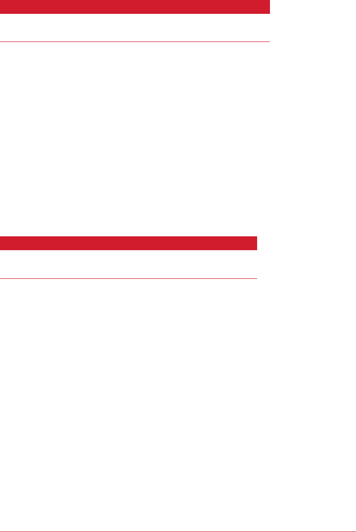
Table 10-8. Details on partition count metric
Metric name Partition count
JMX MBean kafka.server:type=ReplicaManager,name=PartitionCount
Value range Integer, zero or greater
Leader count
The leader count metric shows the number of partitions that the broker is currently
the leader for. As with most other measurements in the brokers, this one should be
generally even across the brokers in the cluster. It is much more important to check
the leader count on a regular basis, possibly alerting on it, as it will indicate when the
cluster is imbalanced even if the number of replicas are perfectly balanced in count
and size across the cluster. This is because a broker can drop leadership for a partition
for many reasons, such as a Zookeeper session expiration, and it will not automati‐
cally take leadership back once it recovers (except if you have enabled automatic
leader rebalancing). In these cases, this metric will show fewer leaders, or often zero,
which indicates that you need to run a preferred replica election to rebalance leader‐
ship in the cluster. See Table 10-9 for more details.
Table 10-9. Details on leader count metric
Metric name Leader count
JMX MBean kafka.server:type=ReplicaManager,name=LeaderCount
Value range Integer, zero or greater
A useful way to consume this metric is to use it along with the partition count to
show a percentage of partitions that the broker is the leader for. In a well-balanced
cluster that is using a replication factor of 2, all brokers should be leaders for approxi‐
mately 50% of their partitions. If the replication factor in use is 3, this percentage
drops to 33%.
Oine partitions
Along with the under-replicated partitions count, the offline partitions count is a crit‐
ical metric for monitoring (see Table 10-10). This measurement is only provided by
the broker that is the controller for the cluster (all other brokers will report 0), and
shows the number of partitions in the cluster that currently have no leader. Partitions
without leaders can happen for two main reasons:
• All brokers hosting replicas for this partition are down
•No in-sync replica can take leadership due to message-count mismatches (with
unclean leader election disabled)
Kafka Broker Metrics | 225

Table 10-10. Oine partitions count metric
Metric name Oine partitions count
JMX MBean kafka.controller:type=KafkaController,name=OfflinePartitionsCount
Value range Integer, zero or greater
In a production Kafka cluster, an offline partition may be impacting the producer cli‐
ents, losing messages or causing back-pressure in the application. This is most often a
“site down” type of problem and will need to be addressed immediately.
Request metrics
The Kafka protocol, described in Chapter 5, has many different requests. Metrics are
provided for how each of those requests performs. The following requests have met‐
rics provided:
•ApiVersions
•ControlledShutdown
•CreateTopics
•DeleteTopics
•DescribeGroups
•Fetch
•FetchConsumer
•FetchFollower
•GroupCoordinator
•Heartbeat
•JoinGroup
•LeaderAndIsr
•LeaveGroup
•ListGroups
•Metadata
•OffsetCommit
•OffsetFetch
•Offsets
•Produce
•SaslHandshake
226 | Chapter 10: Monitoring Kafka

•StopReplica
•SyncGroup
•UpdateMetadata
For each of these requests, there are eight metrics provided, providing insight into
each of the phases of the request processing. For example, for the Fetch request, the
metrics shown in Table 10-11 are available.
Table 10-11. Request Metrics
Name JMX MBean
Total time kafka.network:type=RequestMetrics,name=TotalTimeMs,request=Fetch
Request queue time kafka.network:type=RequestMetrics,name=RequestQueueTi
meMs,request=Fetch
Local time kafka.network:type=RequestMetrics,name=LocalTimeMs,request=Fetch
Remote time kafka.network:type=RequestMetrics,name=RemoteTimeMs,request=Fetch
Throttle time kafka.network:type=RequestMetrics,name=ThrottleTimeMs,request=Fetch
Response queue time kafka.network:type=RequestMetrics,name=ResponseQueueTi
meMs,request=Fetch
Response send time kafka.network:type=RequestMetrics,name=ResponseSendTi
meMs,request=Fetch
Requests per second kafka.network:type=RequestMetrics,name=RequestsPerSec,request=Fetch
The requests per second metric is a rate metric, as discussed earlier, and shows the
total number of that type of request that has been received and processed over the
time unit. This provides a view into the frequency of each request time, though it
should be noted that many of the requests, such as StopReplica and UpdateMeta
data, are infrequent.
The seven time metrics each provide a set of percentiles for requests, as well as a dis‐
crete Count attribute, similar to rate metrics. The metrics are all calculated since the
broker was started, so keep that in mind when looking at metrics that do not change
for long periods of time, the longer your broker has been running, the more stable
the numbers will be. The parts of request processing they represent are:
Total time
Measures the total amount of time the broker spends processing the request,
from receiving it to sending the response back to the requestor.
Request queue time
The amount of time the request spends in queue after it has been received but
before processing starts.
Kafka Broker Metrics | 227

Local time
The amount of time the partition leader spends processing a request, including
sending it to disk (but not necessarily flushing it).
Remote time
The amount of time spent waiting for the followers before request processing can
complete.
rottle time
The amount of time the response must be held in order to slow the requestor
down to satisfy client quota settings.
Response queue time
The amount of time the response to the request spends in the queue before it can
be sent to the requestor.
Response send time
The amount of time spent actually sending the response.
The attributes provided for each metric are:
Percentiles
50thPercentile, 75thPercentile, 95thPercentile, 98thPercentile, 99thPer
centile, 999thPercentile
Count
Absolute count of number of requests since process start
Min
Minimum value for all requests
Max
Maximum value for all requests
Mean
Average value for all requests
StdDev
The standard deviation of the request timing measurements as a whole
228 | Chapter 10: Monitoring Kafka

What Is a Percentile?
Percentiles are a common way of looking at timing measurement.
A 99th percentile measurement tells us that 99% of all values in the
sample group (request timings, in this case) are less than the value
of the metric. This means that 1% of the values are greater than the
value specified. A common pattern is to view the average value and
the 99% or 99.9% value. In this way, you can understand how the
average request performs and what the outliers are.
Out of all of these metrics and attributes for requests, which are the important ones to
monitor? At a minimum, you should collect at least the average and one of the higher
percentiles (either 99% or 99.9%) for the total time metric, as well as the requests per
second metric, for every request type. This gives a view into the overall performance
of requests to the Kafka broker. If you can, you should also collect those measure‐
ments for the other six timing metrics for each request type, as this will allow you to
narrow down any performance problems to a specific phase of request processing.
For setting alert thresholds, the timing metrics can be difficult. The timing for a
Fetch request, for example, can vary wildly depending on many factors, including
settings on the client for how long it will wait for messages, how busy the particular
topic being fetched is, and the speed of the network connection between the client
and the broker. It can be very useful, however, to develop a baseline value for the
99.9th percentile measurement for at least the total time, especially for Produce
requests, and alert on this. Much like the under-replicated partitions metric, a sharp
increase in the 99.9th percentile for Produce requests can alert you to a wide range of
performance problems.
Topic and Partition Metrics
In addition to the many metrics available on the broker that describe the operation of
the Kafka broker in general, there are topic- and partition-specific metrics. In larger
clusters these can be numerous, and it may not be possible to collect all of them into a
metrics system as a matter of normal operations. However, they are quite useful for
debugging specific issues with a client. For example, the topic metrics can be used to
identify a specific topic that is causing a large increase in traffic to the cluster. It also
may be important to provide these metrics so that users of Kafka (the producer and
consumer clients) are able to access them. Regardless of whether you are able to col‐
lect these metrics regularly, you should be aware of what is useful.
For all the examples in Table 10-12, we will be using the example topic name TOPIC
NAME, as well as partition 0. When accessing the metrics described, make sure to sub‐
stitute the topic name and partition number that are appropriate for your cluster.
Kafka Broker Metrics | 229

Per-topic metrics
For all the per-topic metrics, the measurements are very similar to the broker metrics
described previously. In fact, the only difference is the provided topic name, and that
the metrics will be specific to the named topic. Given the sheer number of metrics
available, depending on the number of topics present in your cluster, these will
almost certainly be metrics that you will not want to set up monitoring and alerts for.
They are useful to provide to clients, however, so that they can evaluate and debug
their own usage of Kafka.
Table 10-12. Metrics for Each Topic
Name JMX MBean
Bytes in rate kafka.server:type=BrokerTopicMetrics,name=BytesInPerSec,topic=TOPIC
NAME
Bytes out rate kafka.server:type=BrokerTopicMetrics,name=BytesOutPerSec,topic=TOP
ICNAME
Failed fetch rate kafka.server:type=BrokerTopicMetrics,name=FailedFetchRequestsPer
Sec,topic=TOPICNAME
Failed produce rate kafka.server:type=BrokerTopicMetrics,name=FailedProduceRequestsPer
Sec,topic=TOPICNAME
Messages in rate kafka.server:type=BrokerTopicMetrics,name=MessagesInPer
Sec,topic=TOPICNAME
Fetch request rate kafka.server:type=BrokerTopicMetrics,name=TotalFetchRequestsPer
Sec,topic=TOPICNAME
Produce request rate kafka.server:type=BrokerTopicMetrics,name=TotalProduceRequestsPer
Sec,topic=TOPICNAME
Per-partition metrics
The per-partition metrics tend to be less useful on an ongoing basis than the per-
topic metrics. Additionally, they are quite numerous as hundreds of topics can easily
be thousands of partitions. Nevertheless, they can be useful in some limited situa‐
tions. In particular, the partition-size metric indicates the amount of data (in bytes)
that is currently being retained on disk for the partition (Table 10-13). Combined,
these will indicate the amount of data retained for a single topic, which can be useful
in allocating costs for Kafka to individual clients. A discrepancy between the size of
two partitions for the same topic can indicate a problem where the messages are not
evenly distributed across the key that is being used when producing. The log-segment
count metric shows the number of log-segment files on disk for the partition. This
may be useful along with the partition size for resource tracking.
230 | Chapter 10: Monitoring Kafka

Table 10-13. Metrics for Each Topic
Name JMX MBean
Partition size kafka.log:type=Log,name=Size,topic=TOPICNAME,partition=0
Log segment count kafka.log:type=Log,name=NumLogSegments,topic=TOPICNAME,partition=0
Log end oset kafka.log:type=Log,name=LogEndOffset,topic=TOPICNAME,partition=0
Log start oset kafka.log:type=Log,name=LogStartOffset,topic=TOPICNAME,partition=0
The log end offset and log start offset metrics are the highest and lowest offsets for
messages in that partition, respectively. It should be noted, however, that the differ‐
ence between these two numbers does not necessarily indicate the number of mes‐
sages in the partition, as log compaction can result in “missing” offsets that have been
removed from the partition due to newer messages with the same key. In some envi‐
ronments, it could be useful to track these offsets for a partition. One such use case is
to provide a more granular mapping of timestamp to offset, allowing for consumer
clients to easily roll back offsets to a specific time (though this is less important with
time-based index searching, introduced in Kafka 0.10.1).
Under-replicated Partition Metrics
There is a per-partition metric provided to indicate whether or not
the partition is underreplicated. In general, this is not very useful in
day-to-day operations, as there are too many metrics to gather and
watch. It is much easier to monitor the broker-wide under-
replicated partition count and then use the command-line tools
(described in Chapter 9) to determine the specific partitions that
are under-replicated.
JVM Monitoring
In addition to the metrics provided by the Kafka broker, you should be monitoring a
standard suite of measurements for all of your servers, as well as the Java Virtual
Machine (JVM) itself. These will be useful to alert you to a situation, such as increas‐
ing garbage collection activity, that will degrade the performance of the broker. They
will also provide insight into why you see changes in metrics downstream in the
broker.
Garbage collection
For the JVM, the critical thing to monitor is the status of garbage collection (GC).
The particular beans that you must monitor for this information will vary depending
on the particular Java Runtime Environment (JRE) that you are using, as well as the
specific GC settings in use. For an Oracle Java 1.8 JRE running with G1 garbage col‐
lection, the beans to use are shown in Table 10-14.
Kafka Broker Metrics | 231

Table 10-14. G1 Garbage Collection Metrics
Name JMX MBean
Full GC cycles java.lang:type=GarbageCollector,name=G1 Old Generation
Young GC cycles java.lang:type=GarbageCollector,name=G1 Young Generation
Note that in the semantics of GC, “Old” and “Full” are the same thing. For each of
these metrics, the two attributes to watch are CollectionCount and CollectionTime.
The CollectionCount is the number of GC cycles of that type (full or young) since
the JVM was started. The CollectionTime is the amount of time, in milliseconds,
spent in that type of GC cycle since the JVM was started. As these measurements are
counters, they can be used by a metrics system to tell you an absolute number of GC
cycles and time spent in GC per unit of time. They can also be used to provide an
average amount of time per GC cycle, though this is less useful in normal operations.
Each of these metrics also has a LastGcInfo attribute. This is a composite value,
made up of five fields, that gives you information on the last GC cycle for the type of
GC described by the bean. The important value to look at is the duration value, as
this tells you how long, in milliseconds, the last GC cycle took. The other values in
the composite (GcThreadCount, id, startTime, and endTime) are informational and
not very useful. It’s important to note that you will not be able to see the timing of
every GC cycle using this attribute, as young GC cycles in particular can happen fre‐
quently.
Java OS monitoring
The JVM can provide you with some information on the OS through the
java.lang:type=OperatingSystem bean. However, this information is limited and
does not represent everything you need to know about the system running your
broker. The two attributes that can be collected here that are of use, which are diffi‐
cult to collect in the OS, are the MaxFileDescriptorCount and OpenFileDescriptor
Count attributes. MaxFileDescriptorCount will tell you the maximum number of file
descriptors (FDs) that the JVM is allowed to have open. The OpenFileDescriptor
Count attribute tells you the number of FDs that are currently open. There will be
FDs open for every log segment and network connection, and they can add up
quickly. A problem closing network connections properly could cause the broker to
rapidly exhaust the number allowed.
OS Monitoring
The JVM cannot provide us with all the information that we need to know about the
system it is running on. For this reason, we must not only collect metrics from the
broker but also from the OS itself. Most monitoring systems will provide agents that
will collect more OS information than you could possibly be interested in. The main
232 | Chapter 10: Monitoring Kafka

areas that are necessary to watch are CPU usage, memory usage, disk usage, disk IO,
and network usage.
For CPU utilization, you will want to look at the system load average at the very least.
This provides a single number that will indicate the relative utilization of the process‐
ors. In addition, it may also be useful to capture the percent usage of the CPU broken
down by type. Depending on the method of collection and your particular OS, you
may have some or all of the following CPU percentage breakdowns (provided with
the abbreviation used):
us
The time spent in user space.
sy
The time spent in kernel space.
ni
The time spent on low-priority processes.
id
The time spent idle.
wa
The time spent in wait (on disk).
hi
The time spent handling hardware interrupts.
si
The time spent handling software interrupts.
st
The time waiting for the hypervisor.
Kafka Broker Metrics | 233

What Is System Load?
While many know that system load is a measure of CPU usage on a
system, most people misunderstand how it is measured. The load
average is a count of the number of processes that are runnable and
are waiting for a processor to execute on. Linux also includes
threads that are in an uninterruptable sleep state, such as waiting
for the disk. The load is presented as three numbers, which is the
count averaged over the last minute, 5 minutes, and 15 minutes. In
a single CPU system, a value of 1 would mean the system is 100%
loaded, with a thread always waiting to execute. This means that on
a multiple CPU system, the load average number that indicates
100% is equal to the number of CPUs in the system. For example, if
there are 24 processors in the system, 100% would be a load aver‐
age of 24.
The Kafka broker uses a significant amount of processing for handling requests. For
this reason, keeping track of the CPU utilization is important when monitoring
Kafka. Memory is less important to track for the broker itself, as Kafka will normally
be run with a relatively small JVM heap size. It will use a small amount of memory
outside of the heap for compression functions, but most of the system memory will
be left to be used for cache. All the same, you should keep track of memory utiliza‐
tion to make sure other applications do not infringe on the broker. You will also want
to make sure that swap memory is not being used by monitoring the amount of total
and free swap memory.
Disk is by far the most important subsystem when it comes to Kafka. All messages are
persisted to disk, so the performance of Kafka depends heavily on the performance of
the disks. Monitoring usage of both disk space and inodes (inodes are the file and
directory metadata objects for Unix filesystems) is important, as you need to assure
that you are not running out of space. This is especially true for the partitions where
Kafka data is being stored. It is also necessary to monitor the disk IO statistics, as this
will tell us that the disk is being used efficiently. For at least the disks where Kafka
data is stored, monitor the reads and writes per second, the average read and write
queue sizes, the average wait time, and the utilization percentage of the disk.
Finally, monitor the network utilization on the brokers. This is simply the amount of
inbound and outbound network traffic, normally reported in bits per second. Keep in
mind that every bit inbound to the Kafka broker will be a number of bits outbound
equal to the replication factor of the topics, with no consumers. Depending on the
number of consumers, inbound network traffic could easily become an order of mag‐
nitude larger on outbound traffic. Keep this in mind when setting thresholds for
alerts.
234 | Chapter 10: Monitoring Kafka

Logging
No discussion of monitoring is complete without a word about logging. Like many
applications, the Kafka broker will fill disks with log messages in minutes if you let it.
In order to get useful information from logging, it is important to enable the right
loggers at the right levels. By simply logging all messages at the INFO level, you will
capture a significant amount of important information about the state of the broker.
It is useful to separate a couple of loggers from this, however, in order to provide a
cleaner set of log files.
There are two loggers writing to separate files on disk. The first is kafka.controller,
still at the INFO level. This logger is used to provide messages specifically regarding
the cluster controller. At any time, only one broker will be the controller, and there‐
fore only one broker will be writing to this logger. The information includes topic
creation and modification, broker status changes, and cluster activities such as prefer‐
red replica elections and partition moves. The other logger to separate is
kafka.server.ClientQuotaManager, also at the INFO level. This logger is used to
show messages related to produce and consume quota activities. While this is useful
information, it is better to not have it in the main broker log file.
It is also helpful to log information regarding the status of the log compaction
threads. There is no single metric to show the health of these threads, and it is possi‐
ble for failure in compaction of a single partition to halt the log compaction threads
entirely, and silently. Enabling the kafka.log.LogCleaner, kafka.log.Cleaner, and
kafka.log.LogCleanerManager loggers at the DEBUG level will output information
about the status of these threads. This will include information about each partition
being compacted, including the size and number of messages in each. Under normal
operations, this is not a lot of logging, which means that it can be enabled by default
without overwhelming you.
There is also some logging that may be useful to turn on when debugging issues with
Kafka. One such logger is kafka.request.logger, turned on at either DEBUG or TRACE
levels. This logs information about every request sent to the broker. At DEBUG level,
the log includes connection end points, request timings, and summary information.
At the TRACE level, it will also include topic and partition information—nearly all
request information short of the message payload itself. At either level, this logger
generates a significant amount of data, and it is not recommended to enable it unless
necessary for debugging.
Kafka Broker Metrics | 235

Client Monitoring
All applications need monitoring. Those that instantiate a Kafka client, either a pro‐
ducer or consumer, have metrics specific to the client that should be captured. This
section covers the official Java client libraries, though other implementations should
have their own measurements available.
Producer Metrics
The new Kafka producer client has greatly compacted the metrics available by mak‐
ing them available as attributes on a small number of mbeans. In contrast, the previ‐
ous version of the producer client (which is no longer supported) used a larger
number of mbeans but had more detail in many of the metrics (providing a greater
number of percentile measurements and different moving averages). As a result, the
overall number of metrics provided covers a wider surface area, but it can be more
difficult to track outliers.
All of the producer metrics have the client ID of the producer client in the bean
names. In the examples provided, this has been replaced with CLIENTID. Where a
bean name contains a broker ID, this has been replaced with BROKERID. Topic names
have been replaced with TOPICNAME. See Table 10-15 for an example.
Table 10-15. Kaa Producer Metric MBeans
Name JMX MBean
Overall Producer kafka.producer:type=producer-metrics,client-id=CLIENTID
Per-Broker kafka.producer:type=producer-node-metrics,client-id=CLIENTID,node-
id=node-BROKERID
Per-Topic kafka.producer:type=producer-topic-metrics,client-id=CLIEN
TID,topic=TOPICNAME
Each of the metric beans in Table 10-15 have multiple attributes available to describe
the state of the producer. The particular attributes that are of the most use are
described in “Overall producer metrics” on page 236. Before proceeding, be sure you
understand the semantics of how the producer works, as described in Chapter 3.
Overall producer metrics
The overall producer metrics bean provides attributes describing everything from the
sizes of the message batches to the memory buffer utilization. While all of these
measurements have their place in debugging, there are only a handful needed on a
regular basis, and only a couple of those that should be monitored and have alerts.
Note that while we will discuss several metrics that are averages (ending in -avg),
236 | Chapter 10: Monitoring Kafka

there are also maximum values for each metric (ending in -max) that have limited
usefulness.
The record-error-rate is one attribute that you will definitely want to set an alert
for. This metric should always be zero, and if it is anything greater than that, the pro‐
ducer is dropping messages it is trying to send to the Kafka brokers. The producer
has a configured number of retries and a backoff between those, and once that has
been exhausted, the messages (called records here) will be dropped. There is also a
record-retry-rate attribute that can be tracked, but it is less critical than the error
rate because retries are normal.
The other metric to alert on is the request-latency-avg. This is the average amount
of time a produce request sent to the brokers takes. You should be able to establish a
baseline value for what this number should be in normal operations, and set an alert
threshold above that. An increase in the request latency means that produce requests
are getting slower. This could be due to networking issues, or it could indicate prob‐
lems on the brokers. Either way, it’s a performance issue that will cause back-pressure
and other problems in your producing application.
In addition to these critical metrics, it is always good to know how much message
traffic your producer is sending. Three attributes will provide three different views of
this. The outgoing-byte-rate describes the messages in absolute size in bytes per
second. The record-send-rate describes the traffic in terms of the number of mes‐
sages produced per second. Finally, the request-rate provides the number of pro‐
duce requests sent to the brokers per second. A single request contains one or more
batches. A single batch contains one or more messages. And, of course, each message
is made up of some number of bytes. These metrics are all useful to have on an appli‐
cation dashboard.
Why Not ProducerRequestMetrics?
There is a producer metric bean called ProducerRequestMetrics
that provides both percentiles for request latency as well as several
moving averages for the request rate. So why is it not one of the
recommended metrics to use? The problem is that this metric is
provided separately for each producer thread. In applications
where there are multiple threads used for performance reasons it
will be difficult to reconcile these metrics. It is normally sufficient
to use the attributes provided by the single overall producer bean.
There are also metrics that describe the size of both records, requests, and batches.
The request-size-avg metric provides the average size of the produce requests
being sent to the brokers in bytes. The batch-size-avg provides the average size of a
single message batch (which, by definition, is comprised of messages for a single topic
Client Monitoring | 237

partition) in bytes. The record-size-avg shows the average size of a single record in
bytes. For a single-topic producer, this provides useful information about the mes‐
sages being produced. For multiple-topic producers, such as Mirror Maker, it is less
informative. Besides these three metrics, there is a records-per-request-avg metric
that describes the average number of messages that are in a single produce request.
The last overall producer metric attribute that is recommended is record-queue-
time-avg. This measurement is the average amount of time, in milliseconds, that a
single message waits in the producer, after the application sends it, before it is actually
produced to Kafka. After an application calls the producer client to send a message
(by calling the send method), the producer waits until one of two things happens:
•It has enough messages to fill a batch based on the max.partition.bytes config‐
uration
•It has been long enough since the last batch was sent based on the linger.ms
configuration
Either of these two will cause the producer client to close the current batch it is build‐
ing and send it to the brokers. The easiest way to understand it is that for busy topics
the first condition will apply, whereas for slow topics the second will apply. The
record-queue-time-avg measurement will indicate how long messages take to be
produced, and therefore is helpful when tuning these two configurations to meet the
latency requirements for your application.
Per-broker and per-topic metrics
In addition to the overall producer metrics, there are metric beans that provide a
limited set of attributes for the connection to each Kafka broker, as well as for each
topic that is being produced. These measurements are useful for debugging problems
in some cases, but they are not metrics that you are going to want to review on an
ongoing basis. All of the attributes on these beans are the same as the attributes for
the overall producer beans described previously, and have the same meaning as
described previously (except that they apply either to a specific broker or a specific
topic).
The most useful metric that is provided by the per-broker producer metrics is the
request-latency-avg measurement. This is because this metric will be mostly stable
(given stable batching of messages) and can still show a problem with connections to
a specific broker. The other attributes, such as outgoing-byte-rate and request-
latency-avg, tend to vary depending on what partitions each broker is leading. This
means that what these measurements “should” be at any point in time can quickly
change, depending on the state of the Kafka cluster.
238 | Chapter 10: Monitoring Kafka

The topic metrics are a little more interesting than the per-broker metrics, but they
will only be useful for producers that are working with more than one topic. They
will also only be useable on a regular basis if the producer is not working with a lot of
topics. For example, a MirrorMaker could be producing hundreds, or thousands, of
topics. It is difficult to review all of those metrics, and nearly impossible to set reason‐
able alert thresholds on them. As with the per-broker metrics, the per-topic measure‐
ments are best used when investigating a specific problem. The record-send-rate
and record-error-rate attributes, for example, can be used to isolate dropped mes‐
sages to a specific topic (or validated to be across all topics). In addition, there is a
byte-rate metric that provides the overall messages rate in bytes per second for the
topic.
Consumer Metrics
Similar to the new producer client, the new consumer in Kafka consolidates many of
the metrics into attributes on just a few metric beans. These metrics have also elimi‐
nated the percentiles for latencies and the moving averages for rates, similar to the
producer client. In the consumer, because the logic around consuming messages is a
little more complex than just firing messages into the Kafka brokers, there are a few
more metrics to deal with as well. See Table 10-16.
Table 10-16. Kaa Consumer Metric MBeans
Name JMX MBean
Overall Consumer kafka.consumer:type=consumer-metrics,client-id=CLIENTID
Fetch Manager kafka.consumer:type=consumer-fetch-manager-metrics,client-id=CLIENTID
Per-Topic kafka.consumer:type=consumer-fetch-manager-metrics,client-id=CLIEN
TID,topic=TOPICNAME
Per-Broker kafka.consumer:type=consumer-node-metrics,client-id=CLIENTID,node-
id=node-BROKERID
Coordinator kafka.consumer:type=consumer-coordinator-metrics,client-id=CLIENTID
Fetch manager metrics
In the consumer client, the overall consumer metric bean is less useful for us because
the metrics of interest are located in the fetch manager beans instead. The overall
consumer bean has metrics regarding the lower-level network operations, but the
fetch manager bean has metrics regarding bytes, request, and record rates. Unlike the
producer client, the metrics provided by the consumer are useful to look at but not
useful for setting up alerts on.
For the fetch manager, the one attribute you may want to set up monitoring and
alerts for is fetch-latency-avg. As with the equivalent request-latency-avg in the
producer client, this metric tells us how long fetch requests to the brokers take. The
Client Monitoring | 239

problem with alerting on this metric is that the latency is governed by the consumer
configurations fetch.min.bytes and fetch.max.wait.ms. A slow topic will have
erratic latencies, as sometimes the broker will respond quickly (when there are mes‐
sages available), and sometimes it will not respond for fetch.max.wait.ms (when
there are no messages available). When consuming topics that have more regular, and
abundant, message traffic, this metric may be more useful to look at.
Wait! No Lag?
The best advice for all consumers is that you must monitor the
consumer lag. So why do we not recommend monitoring the
records-lag-max attribute on the fetch manager bean? This metric
shows the current lag (number of messages behind the broker) for
the partition that is the most behind.
The problem with this is twofold: it only shows the lag for one par‐
tition, and it relies on proper functioning of the consumer. If you
have no other option, use this attribute for lag and set up alerting
for it. But the best practice is to use external lag monitoring, as will
be described in “Lag Monitoring” on page 243.
In order to know how much message traffic your consumer client is handling, you
should capture the bytes-consumed-rate or the records-consumed-rate, or prefera‐
bly both. These metrics describe the message traffic consumed by this client instance
in bytes per second and messages per second, respectively. Some users set minimum
thresholds on these metrics for alerting, so that they are notified if the consumer is
not doing enough work. You should be careful when doing this, however. Kafka is
intended to decouple the consumer and producer clients, allowing them to operate
independently. The rate at which the consumer is able to consume messages is often
dependent on whether or not the producer is working correctly, so monitoring these
metrics on the consumer makes assumptions about the state of the producer. This
can lead to false alerts on the consumer clients.
It is also good to understand the relationship between bytes, messages, and requests,
and the fetch manager provides metrics to help with this. The fetch-rate measure‐
ment tells us the number of fetch requests per second that the consumer is perform‐
ing. The fetch-size-avg metric gives the average size of those fetch requests in
bytes. Finally, the records-per-request-avg metric gives us the average number of
messages in each fetch request. Note that the consumer does not provide an equiva‐
lent to the producer record-size-avg metric to let us know what the average size of
a message is. If this is important, you will need to infer it from the other metrics avail‐
able, or capture it in your application after receiving messages from the consumer cli‐
ent library.
240 | Chapter 10: Monitoring Kafka

Per-broker and per-topic metrics
The metrics that are provided by the consumer client for each of the broker connec‐
tions and each of the topics being consumed, as with the producer client, are useful
for debugging issues with consumption, but will probably not be measurements that
you review daily. As with the fetch manager, the request-latency-avg attribute pro‐
vided by the per-broker metrics bean has limited usefulness, depending on the mes‐
sage traffic in the topics you are consuming. The incoming-byte-rate and request-
rate metrics break down the consumed message metrics provided by the fetch
manager into per-broker bytes per second and requests per second measurements,
respectively. These can be used to help isolate problems that the consumer is having
with the connection to a specific broker.
Per-topic metrics provided by the consumer client are useful if more than one topic is
being consumed. Otherwise, these metrics will be the same as the fetch manager’s
metrics and redundant to collect. On the other end of the spectrum, if the client is
consuming many topics (Kafka MirrorMaker, for example) these metrics will be diffi‐
cult to review. If you plan on collecting them, the most important metrics to gather
are the bytes-consumed-rate, the records-consumed-rate, and the fetch-size-
avg. The bytes-consumed-rate shows the absolute size in bytes consumed per sec‐
ond for the specific topic, while the records-consumed-rate shows the same
information in terms of the number of messages. The fetch-size-avg provides the
average size of each fetch request for the topic in bytes.
Consumer coordinator metrics
As described in Chapter 4, consumer clients generally work together as part of a con‐
sumer group. This group has coordination activities, such as group members joining
and heartbeat messages to the brokers to maintain group membership. The consumer
coordinator is the part of the consumer client that is responsible for handling this
work, and it maintains its own set of metrics. As with all metrics, there are many
numbers provided, but only a few key ones that you should monitor regularly.
The biggest problem that consumers can run into due to coordinator activities is a
pause in consumption while the consumer group synchronizes. This is when the con‐
sumer instances in a group negotiate which partitions will be consumed by which
individual client instances. Depending on the number of partitions that are being
consumed, this can take some time. The coordinator provides the metric attribute
sync-time-avg, which is the average amount of time, in milliseconds, that the sync
activity takes. It is also useful to capture the sync-rate attribute, which is the number
of group syncs that happen every second. For a stable consumer group, this number
should be zero most of the time.
The consumer needs to commit offsets to checkpoint its progress in consuming mes‐
sages, either automatically on a regular interval, or by manual checkpoints triggered
Client Monitoring | 241

in the application code. These commits are essentially just produce requests (though
they have their own request type), in that the offset commit is a message produced to
a special topic. The consumer coordinator provides the commit-latency-avg
attribute, which measures the average amount of time that offset commits take. You
should monitor this value just as you would the request latency in the producer. It
should be possible to establish a baseline expected value for this metric, and set rea‐
sonable thresholds for alerting above that value.
One final coordinator metric that can be useful to collect is assigned-partitions.
This is a count of the number of partitions that the consumer client (as a single
instance in the consumer group) has been assigned to consume. This is helpful
because, when compared to this metric from other consumer clients in the group, it is
possible to see the balance of load across the entire consumer group. We can use this
to identify imbalances that might be caused by problems in the algorithm used by the
consumer coordinator for distributing partitions to group members.
Quotas
Apache Kafka has the ability to throttle client requests in order to prevent one client
from overwhelming the entire cluster. This is configurable for both producer and
consumer clients, and is expressed in terms of the permitted amount of traffic from
an individual client ID to an individual broker in bytes per second. There is a broker
configuration, which sets a default value for all clients, as well as per-client overrides
that can be dynamically set. When the broker calculates that a client has exceeded its
quota, it slows the client down by holding the response back to the client for enough
time to keep the client under the quota.
The Kafka broker does not use error codes in the response to indicate that the client
is being throttled. This means that it is not obvious to the application that throttling
is happening without monitoring the metrics that are provided to show the amount
of time that the client is being throttled. The metrics that must be monitored are
shown in Table 10-17.
Table 10-17. Metrics to monitor
Client Bean name
Consumer bean kafka.consumer:type=consumer-fetch-manager-metrics,client-id=CLIENTID,
attribute fetch-throttle-time-avg
Producer bean kafka.producer:type=producer-metrics,client-id=CLIENTID, attribute produce-
throttle-time-avg
Quotas are not enabled by default on the Kafka brokers, but it is safe to monitor these
metrics irrespective of whether or not you are currently using quotas. Monitoring
242 | Chapter 10: Monitoring Kafka

them is a good practice as they may be enabled at some point in the future, and it’s
easier to start with monitoring them as opposed to adding metrics later.
Lag Monitoring
For Kafka consumers, the most important thing to monitor is the consumer lag.
Measured in number of messages, this is the difference between the last message pro‐
duced in a specific partition and the last message processed by the consumer. While
this topic would normally be covered in the previous section on consumer client
monitoring, it is one of the cases where external monitoring far surpasses what is
available from the client itself. As mentioned previously, there is a lag metric in the
consumer client, but using it is problematic. It only represents a single partition, the
one that has the most lag, so it does not accurately show how far behind the con‐
sumer is. In addition, it requires proper operation of the consumer, because the met‐
ric is calculated by the consumer on each fetch request. If the consumer is broken or
offline, the metric is either inaccurate or not available.
The preferred method of consumer lag monitoring is to have an external process that
can watch both the state of the partition on the broker, tracking the offset of the most
recently produced message, and the state of the consumer, tracking the last offset the
consumer group has committed for the partition. This provides an objective view that
can be updated regardless of the status of the consumer itself. This checking must be
performed for every partition that the consumer group consumes. For a large con‐
sumer, like MirrorMaker, this may mean tens of thousands of partitions.
Chapter 9 provided information on using the command-line utilities to get consumer
group information, including committed offsets and lag. Monitoring lag like this,
however, presents its own problems. First, you must understand for each partition
what is a reasonable amount of lag. A topic that receives 100 messages an hour will
need a different threshold than a topic that receives 100,000 messages per second.
Then, you must be able to consume all of the lag metrics into a monitoring system
and set alerts on them. If you have a consumer group that consumes 100,000 parti‐
tions over 1,500 topics, you may find this to be a daunting task.
One way to monitor consumer groups in order to reduce this complexity is to use
Burrow. This is an open source application, originally developed by LinkedIn, which
provides consumer status monitoring by gathering lag information for all consumer
groups in a cluster and calculating a single status for each group saying whether the
consumer group is working properly, falling behind, or is stalled or stopped entirely.
It does this without requiring thresholds by monitoring the progress that the con‐
sumer group is making on processing messages, though you can also get the message
lag as an absolute number. There is an in-depth discussion of the reasoning and
methodology behind how Burrow works on the LinkedIn Engineering Blog. Deploy‐
ing Burrow can be an easy way to provide monitoring for all consumers in a cluster,
Lag Monitoring | 243

as well as in multiple clusters, and it can be easily integrated with your existing moni‐
toring and alerting system.
If there is no other option, the records-lag-max metric from the consumer client
will provide at least a partial view of the consumer status. It is strongly suggested,
however, that you utilize an external monitoring system like Burrow.
End-to-End Monitoring
Another type of external monitoring that is recommended to determine if your Kafka
clusters are working properly is an end-to-end monitoring system that provides a cli‐
ent point of view on the health of the Kafka cluster. Consumer and producer clients
have metrics that can indicate that there might be a problem with the Kafka cluster,
but this can be a guessing game as to whether increased latency is due to a problem
with the client, the network, or Kafka itself. In addition, it means that if you are
responsible for running the Kafka cluster, and not the clients, you would now have to
monitor all of the clients as well. What you really need to know is:
• Can I produce messages to the Kafka cluster?
• Can I consume messages from the Kafka cluster?
In an ideal world, you would be able to monitor this for every topic individually.
However, in most situations it is not reasonable to inject synthetic traffic into every
topic in order to do this. We can, however, at least provide those answers for every
broker in the cluster, and that is what Kafka Monitor does. This tool, open sourced by
the Kafka team at LinkedIn, continually produces and consumes data from a topic
that is spread across all brokers in a cluster. It measures the availability of both pro‐
duce and consume requests on each broker, as well as the total produce to consume
latency. This type of monitoring is invaluable to be able to externally verify that the
Kafka cluster is operating as intended, since just like consumer lag monitoring, the
Kafka broker cannot report whether or not clients are able to use the cluster properly.
Summary
Monitoring is a key aspect of running Apache Kafka properly, which explains why so
many teams spend a significant amount of their time perfecting that part of opera‐
tions. Many organizations use Kafka to handle petabyte-scale data flows. Assuring
that the data does not stop, and that messages are not lost, is a critical business
requirement. It is also our responsibility to assist users with monitoring how their
applications use Kafka by providing the metrics that they need to do this.
In this chapter we covered the basics of how to monitor Java applications, and specifi‐
cally the Kafka applications. We reviewed a subset of the numerous metrics available
244 | Chapter 10: Monitoring Kafka

in the Kafka broker, also touching on Java and OS monitoring, as well as logging. We
then detailed the monitoring available in the Kafka client libraries, including quota
monitoring. Finally, we discussed the use of external monitoring systems for con‐
sumer lag monitoring and end-to-end cluster availability. While certainly not an
exhaustive list of the metrics that are available, this chapter has reviewed the most
critical ones to keep an eye on.
Summary | 245

CHAPTER 11
Stream Processing
Kafka was traditionally seen as a powerful message bus, capable of delivering streams
of events but without processing or transformation capabilities. Kafka’s reliable
stream delivery capabilities make it a perfect source of data for stream-processing
systems. Apache Storm, Apache Spark Streaming, Apache Flink, Apache Samza, and
many more stream-processing systems were built with Kafka often being their only
reliable data source.
Industry analysts sometimes claim that all those stream-processing systems are just
like the complex event processing (CEP) systems that have been around for 20 years.
We think stream processing became more popular because it was created after Kafka
and therefore could use Kafka as a reliable source of event streams to process. With
the increased popularity of Apache Kafka, first as a simple message bus and later as a
data integration system, many companies had a system containing many streams of
interesting data, stored for long amounts of time and perfectly ordered, just waiting
for some stream-processing framework to show up and process them. In other
words, in the same way that data processing was significantly more difficult before
databases were invented, stream processing was held back by lack of a stream-
processing platform.
Starting from version 0.10.0, Kafka does more than provide a reliable source of data
streams to every popular stream-processing framework. Now Kafka includes a pow‐
erful stream-processing library as part of its collection of client libraries. This allows
developers to consume, process, and produce events in their own apps, without rely‐
ing on an external processing framework.
We’ll begin the chapter by explaining what we mean by stream processing (since this
term is frequently misunderstood), then discuss some of the basic concepts of stream
processing and the design patterns that are common to all stream-processing sys‐
tems. We’ll then dive into Apache Kafka’s stream-processing library—its goals and
247

architecture. We’ll give a small example of how to use Kafka Streams to calculate a
moving average of stock prices. We’ll then discuss other examples for good stream-
processing use cases and finish off the chapter by providing a few criteria you can use
when choosing which stream-processing framework (if any) to use with Apache
Kafka. This chapter is intended as a brief introduction to stream processing and will
not cover every Kafka Streams feature or attempt to discuss and compare every
stream-processing framework in existence—those topics deserve entire books on
their own, possibly several.
What Is Stream Processing?
There is a lot of confusion about what stream processing means. Many definitions
mix up implementation details, performance requirements, data models, and many
other aspects of software engineering. I’ve seen the same thing play out in the world
of relational databases—the abstract definitions of the relational model are getting
forever entangled in the implementation details and specific limitations of the popu‐
lar database engines.
The world of stream processing is still evolving, and just because a specific popular
implementation does things in specific ways or has specific limitations doesn’t mean
that those details are an inherent part of processing streams of data.
Let’s start at the beginning: What is a data stream (also called an event stream or
streaming data)? First and foremost, a data stream is an abstraction representing an
unbounded dataset. Unbounded means infinite and ever growing. The dataset is
unbounded because over time, new records keep arriving. This definition is used by
Google, Amazon, and pretty much everyone else.
Note that this simple model (a stream of events) can be used to represent pretty much
every business activity we care to analyze. We can look at a stream of credit card
transactions, stock trades, package deliveries, network events going through a switch,
events reported by sensors in manufacturing equipment, emails sent, moves in a
game, etc. The list of examples is endless because pretty much everything can be seen
as a sequence of events.
There are few other attributes of event streams model, in addition to their unboun‐
ded nature:
Event streams are ordered
There is an inherent notion of which events occur before or after other events.
This is clearest when looking at financial events. A sequence in which I first put
money in my account and later spend the money is very different from a
sequence at which I first spend the money and later cover my debt by depositing
money back. The latter will incur overdraft charges while the former will not.
Note that this is one of the differences between an event stream and a database
248 | Chapter 11: Stream Processing

table—records in a table are always considered unordered and the “order by”
clause of SQL is not part of the relational model; it was added to assist in report‐
ing.
Immutable data records
Events, once occured, can never be modified. A financial transaction that is can‐
celled does not disapear. Instead, an additional event is written to the stream,
recording a cancellation of previous transaction. When a customer returns mer‐
chandise to a shop, we don’t delete the fact that the merchandise was sold to him
earlier, rather we record the return as an additional event. This is another differ‐
ence between a data stream and a database table—we can delete or update
records in a table, but those are all additional transactions that occur in the data‐
base, and as such can be recorded in a stream of events that records all transac‐
tions. If you are familiar with binlogs, WALs, or redo logs in databases you can
see that if we insert a record into a table and later delete it, the table will no
longer contain the record, but the redo log will contain two transactions—the
insert and the delete.
Event streams are replayable
This is a desirable property. While it is easy to imagine nonreplayable streams
(TCP packets streaming through a socket are generally nonreplayable), for most
business applications, it is critical to be able to replay a raw stream of events that
occured months (and sometimes years) earlier. This is required in order to cor‐
rect errors, try new methods of analysis, or perform audits. This is the reason we
believe Kafka made stream processing so successful in modern businesses—it
allows capturing and replaying a stream of events. Without this capability, stream
processing would not be more than a lab toy for data scientists.
It is worth noting that neither the definition of event streams nor the attributes we
later listed say anything about the data contained in the events or the number of
events per second. The data differs from system to system—events can be tiny (some‐
times only a few bytes) or very large (XML messages with many headers); they can
also be completely unstructured, key-value pairs, semi-structured JSON, or struc‐
tured Avro or Protobuf messages. While it is often assumed that data streams are “big
data” and involve millions of events per second, the same techniques we’ll discuss
apply equally well (and often better) to smaller streams of events with only a few
events per second or minute.
Now that we know what event streams are, it’s time to make sure we understand
stream processing. Stream processing refers to the ongoing processing of one or more
event streams. Stream processing is a programming paradigm—just like request-
response and batch processing. Let’s look at how different programming paradigms
compare to get a better understanding of how stream processing fits into software
architectures:
What Is Stream Processing? | 249

Request-response
This is the lowest latency paradigm, with response times ranging from submilli‐
seconds to a few milliseconds, usually with the expectation that response times
will be highly consistent. The mode of processing is usually blocking—an app
sends a request and waits for the processing system to respond. In the database
world, this paradigm is known as online transaction processing (OLTP). Point-of-
sale systems, credit card processing, and time-tracking systems typically work in
this paradigm.
Batch processing
This is the high-latency/high-throughput option. The processing system wakes
up at set times—every day at 2:00 A.M., every hour on the hour, etc. It reads all
required input (either all data available since last execution, all data from begin‐
ning of month, etc.), writes all required output, and goes away until the next time
it is scheduled to run. Processing times range from minutes to hours and users
expect to read stale data when they are looking at results. In the database world,
these are the data warehouse and business intelligence systems—data is loaded in
huge batches once a day, reports are generated, and users look at the same reports
until the next data load occurs. This paradigm often has great efficiency and
economy of scale, but in recent years, businesses need the data available in
shorter timeframes in order to make decision-making more timely and efficient.
This puts huge pressure on systems that were written to exploit economy of scale
—not to provide low-latency reporting.
Stream processing
This is a contentious and nonblocking option. Filling the gap between the
request-response world where we wait for events that take two milliseconds to
process and the batch processing world where data is processed once a day and
takes eight hours to complete. Most business processes don’t require an immedi‐
ate response within milliseconds but can’t wait for the next day either. Most busi‐
ness processes happen continuously, and as long as the business reports are
updated continuously and the line of business apps can continuously respond,
the processing can proceed without anyone waiting for a specific response within
milliseconds. Business processes like alerting on suspicious credit transactions or
network activity, adjusting prices in real-time based on supply and demand, or
tracking deliveries of packages are all natural fit for continuous but nonblocking
processing.
It is important to note that the definition doesn’t mandate any specific framework,
API, or feature. As long as you are continuously reading data from an unbounded
dataset, doing something to it, and emitting output, you are doing stream processing.
But the processing has to be continuous and ongoing. A process that starts every day
at 2:00 A.M., reads 500 records from the stream, outputs a result, and goes away
doesn’t quite cut it as far as stream processing goes.
250 | Chapter 11: Stream Processing

Stream-Processing Concepts
Stream processing is very similar to any type of data processing—you write code that
receives data, does something with the data—a few transformations, aggregates,
enrichments, etc.—and then place the result somewhere. However, there are some
key concepts that are unique to stream processing and often cause confusion when
someone who has data processing experience first attempts to write stream-
processing applications. Let’s take a look at a few of those concepts.
Time
Time is probably the most important concept in stream processing and often the
most confusing. For an idea of how complex time can get when discussing distributed
systems, we recommend Justin Sheehy’s excellent “There is No Now” paper. In the
context of stream processing, having a common notion of time is critical because
most stream applications perform operations on time windows. For example, our
stream application might calculate a moving five-minute average of stock prices. In
that case, we need to know what to do when one of our producers goes offline for two
hours due to network issues and returns with two hours worth of data—most of the
data will be relevant for five-minute time windows that have long passed and for
which the result was already calculated and stored.
Stream-processing systems typically refer to the following notions of time:
Event time
This is the time the events we are tracking occurred and the record was created—
the time a measurement was taken, an item at was sold at a shop, a user viewed a
page on our website, etc. In versions 0.10.0 and later, Kafka automatically adds
the current time to producer records at the time they are created. If this does not
match your application’s notion of event time, such as in cases where the Kafka
record is created based on a database record some time after the event occurred,
you should add the event time as a field in the record itself. Event time is usually
the time that matters most when processing stream data.
Log append time
This is the time the event arrived to the Kafka broker and was stored there. In
versions 0.10.0 and higher, Kafka brokers will automatically add this time to
records they receive if Kafka is configured to do so or if the records arrive from
older producers and contain no timestamps. This notion of time is typically less
relevant for stream processing, since we are usually interested in the times the
events occurred. For example, if we calculate number of devices produced per
day, we want to count devices that were actually produced on that day, even if
there were network issues and the event only arrived to Kafka the following day.
However, in cases where the real event time was not recorded, log append time
Stream-Processing Concepts | 251

can still be used consistently because it does not change after the record was cre‐
ated.
Processing time
This is the time at which a stream-processing application received the event in
order to perform some calculation. This time can be milliseconds, hours, or days
after the event occurred. This notion of time assigns different timestamps to the
same event depending on exactly when each stream processing application hap‐
pened to read the event. It can even differ for two threads in the same applica‐
tion! Therefore, this notion of time is highly unreliable and best avoided.
Mind the Time Zone
When working with time, it is important to be mindful of time
zones. The entire data pipeline should standardize on a single time
zones; otherwise, results of stream operations will be confusing and
often meaningless. If you must handle data streams with different
time zones, you need to make sure you can convert events to a sin‐
gle time zone before performing operations on time windows.
Often this means storing the time zone in the record itself.
State
As long as you only need to process each event individually, stream processing is a
very simple activity. For example, if all you need to do is read a stream of online shop‐
ping transactions from Kafka, find the transactions over $10,000 and email the rele‐
vant salesperson, you can probably write this in just few lines of code using a Kafka
consumer and SMTP library.
Stream processing becomes really interesting when you have operations that involve
multiple events: counting the number of events by type, moving averages, joining two
streams to create an enriched stream of information, etc. In those cases, it is not
enough to look at each event by itself; you need to keep track of more information—
how many events of each type did we see this hour, all events that require joining,
sums, averages, etc. We call the information that is stored between events a state.
It is often tempting to store the state in variables that are local to the stream-
processing app, such as a simple hash-table to store moving counts. In fact, we did
just that in many examples in this book. However, this is not a reliable approach for
managing state in stream processing because when the stream-processing application
is stopped, the state is lost, which changes the results. This is usually not the desired
outcome, so care should be taken to persist the most recent state and recover it when
starting the application.
Stream processing refers to several types of state:
252 | Chapter 11: Stream Processing

Local or internal state
State that is accessible only by a specific instance of the stream-processing appli‐
cation. This state is usually maintained and managed with an embedded, in-
memory database running within the application. The advantage of local state is
that it is extremely fast. The disadvantage is that you are limited to the amount of
memory available. As a result, many of the design patterns in stream processing
focus on ways to partition the data into substreams that can be processed using a
limited amount of local state.
External state
State that is maintained in an external datastore, often a NoSQL system like Cas‐
sandra. The advantages of an external state are its virtually unlimited size and the
fact that it can be accessed from multiple instances of the application or even
from different applications. The downside is the extra latency and complexity
introduced with an additional system. Most stream-processing apps try to avoid
having to deal with an external store, or at least limit the latency overhead by
caching information in the local state and communicating with the external store
as rarely as possible. This usually introduces challenges with maintaining consis‐
tency between the internal and external state.
Stream-Table Duality
We are all familiar with database tables. A table is a collection of records, each identi‐
fied by its primary key and containing a set of attributes as defined by a schema.
Table records are mutable (i.e., tables allow update and delete operations). Querying a
table allows checking the state of the data at a specific point in time. For example, by
querying the CUSTOMERS_CONTACTS table in a database, we expect to find cur‐
rent contact details for all our customers. Unless the table was specifically designed to
include history, we will not find their past contacts in the table.
Unlike tables, streams contain a history of changes. Streams are a string of events
wherein each event caused a change. A table contains a current state of the world,
which is the result of many changes. From this description, it is clear that streams and
tables are two sides of the same coin—the world always changes, and sometimes we
are interested in the events that caused those changes, whereas other times we are
interested in the current state of the world. Systems that allow you to transition back
and forth between the two ways of looking at data are more powerful than systems
that support just one.
In order to convert a table to a stream, we need to capture the changes that modify
the table. Take all those insert, update, and delete events and store them in a
stream. Most databases offer change data capture (CDC) solutions for capturing these
changes and there are many Kafka connectors that can pipe those changes into Kafka
where they will be available for stream processing.
Stream-Processing Concepts | 253
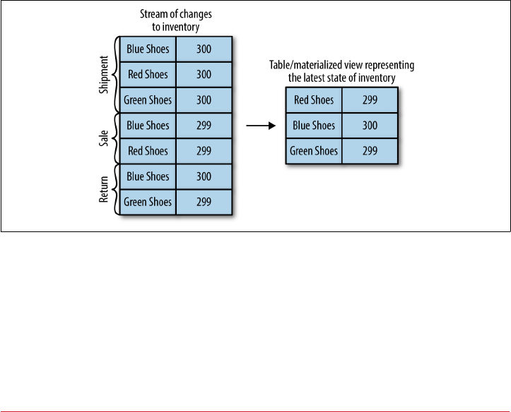
In order to convert a stream to a table, we need to apply all the changes that the
stream contains. This is also called materializing the stream. We create a table, either
in memory, in an internal state store, or in an external database, and start going over
all the events in the stream from beginning to end, changing the state as we go. When
we finish, we have a table representing a state at a specific time that we can use.
Suppose we have a store selling shoes. A stream representation of our retail activity
can be a stream of events:
“Shipment arrived with red, blue, and green shoes”
“Blue shoes sold”
“Red shoes sold”
“Blue shoes returned”
“Green shoes sold”
If we want to know what our inventory contains right now or how much money we
made until now, we need to materialize the view. Figure 11-1 shows that we currently
have blue and yellow shoes and $170 in the bank. If we want to know how busy the
store is, we can look at the entire stream and see that there were five transactions. We
may also want to investigate why the blue shoes were returned.
Figure 11-1. Materializing inventory changes
Time Windows
Most operations on streams are windowed operations—operating on slices of time:
moving averages, top products sold this week, 99th percentile load on the system, etc.
Join operations on two streams are also windowed—we join events that occurred at
the same slice of time. Very few people stop and think about the type of window they
254 | Chapter 11: Stream Processing
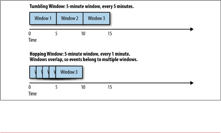
want for their operations. For example, when calculating moving averages, we want to
know:
•Size of the window: do we want to calculate the average of all events in every five-
minute window? Every 15-minute window? Or the entire day? Larger windows
are smoother but they lag more—if price increases, it will take longer to notice
than with a smaller window.
•How often the window moves (advance interval): five-minute averages can
update every minute, second, or every time there is a new event. When the
advance interval is equal to the window size, this is sometimes called a tumbling
window. When the window moves on every record, this is sometimes called a
sliding window.
•How long the window remains updatable: our five-minute moving average calcu‐
lated the average for 00:00-00:05 window. Now an hour later, we are getting a few
more results with their event time showing 00:02. Do we update the result for the
00:00-00:05 period? Or do we let bygones be bygones? Ideally, we’ll be able to
define a certain time period during which events will get added to their respec‐
tive time-slice. For example, if the events were up to four hours late, we should
recalculate the results and update. If events arrive later than that, we can ignore
them.
Windows can be aligned to clock time—i.e., a five-minute window that moves every
minute will have the first slice as 00:00-00:05 and the second as 00:01-00:06. Or it can
be unaligned and simply start whenever the app started and then the first slice can be
03:17-03:22. Sliding windows are never aligned because they move whenever there is
a new record. See Figure 11-2 for the difference between two types of these windows.
Figure 11-2. Tumbling window versus Hopping window
Stream-Processing Concepts | 255
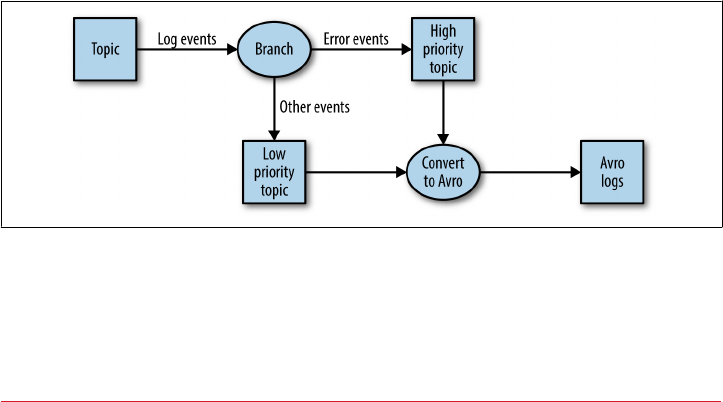
Stream-Processing Design Patterns
Every stream-processing system is different—from the basic combination of a con‐
sumer, processing logic, and producer to involved clusters like Spark Streaming with
its machine learning libraries, and much in between. But there are some basic design
patterns, which are known solutions to common requirements of stream-processing
architectures. We’ll review a few of those well-known patterns and show how they are
used with a few examples.
Single-Event Processing
The most basic pattern of stream processing is the processing of each event in isola‐
tion. This is also known as a map/filter pattern because it is commonly used to filter
unnecessary events from the stream or transform each event. (The term “map” is
based on the map/reduce pattern in which the map stage transforms events and the
reduce stage aggregates them.)
In this pattern, the stream-processing app consumes events from the stream, modifies
each event, and then produces the events to another stream. An example is an app
that reads log messages from a stream and writes ERROR events into a high-priority
stream and the rest of the events into a low-priority stream. Another example is an
application that reads events from a stream and modifies them from JSON to Avro.
Such applications need to maintain state within the application because each event
can be handled independently. This means that recovering from app failures or load-
balancing is incredibly easy as there is no need to recover state; you can simply hand
off the events to another instance of the app to process.
This pattern can be easily handled with a simple producer and consumer, as seen in
Figure 11-3.
Figure 11-3. Single-event processing topology
256 | Chapter 11: Stream Processing
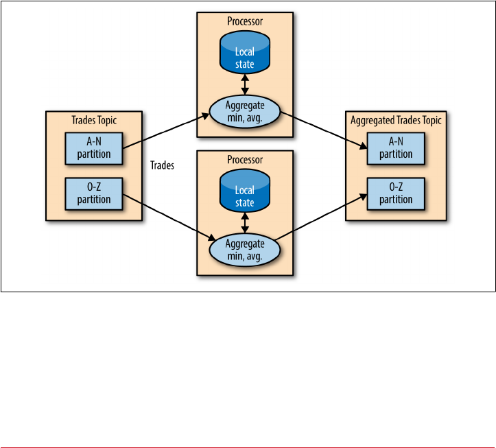
Processing with Local State
Most stream-processing applications are concerned with aggregating information,
especially time-window aggregation. An example of this is finding the minimum and
maximum stock prices for each day of trading and calculating a moving average.
These aggregations require maintaining a state for the stream. In our example, in
order to calculate the minimum and average price each day, we need to store the min‐
imum and maximum values we’ve seen up until the current time and compare each
new value in the stream to the stored minimum and maximum.
All these can be done using local state (rather than a shared state) because each opera‐
tion in our example is a group by aggregate. That is, we perform the aggregation per
stock symbol, not on the entire stock market in general. We use a Kafka partitioner to
make sure that all events with the same stock symbol are written to the same parti‐
tion. Then, each instance of the application will get all the events from the partitions
that are assigned to it (this is a Kafka consumer guarantee). This means that each
instance of the application can maintain state for the subset of stock symbols that are
written to the partitions that are assigned to it. See Figure 11-4.
Figure 11-4. Topology for event processing with local state
Stream-processing applications become significantly more complicated when the
application has local state and there are several issues a stream-processing application
must address:
Memory usage
The local state must fit into the memory available to the application instance.
Stream-Processing Design Patterns | 257

Persistence
We need to make sure the state is not lost when an application instance shuts
down, and that the state can be recovered when the instance starts again or is
replaced by a different instance. This is something that Kafka Streams handles
very well—local state is stored in-memory using embedded RocksDB, which also
persists the data to disk for quick recovery after restarts. But all the changes to
the local state are also sent to a Kafka topic. If a stream’s node goes down, the
local state is not lost—it can be easily recreated by rereading the events from the
Kafka topic. For example, if the local state contains “current minimum for
IBM=167.19,” we store this in Kafka, so that later we can repopulate the local
cache from this data. Kafka uses log compaction for these topics to make sure
they don’t grow endlessly and that recreating the state is always feasible.
Rebalancing
Partitions sometimes get reassigned to a different consumer. When this happens,
the instance that loses the partition must store the last good state, and the
instance that receives the partition must know to recover the correct state.
Stream-processing frameworks differ in how much they help the developer manage
the local state they need. If your application requires maintaining local state, be sure
to check the framework and its guarantees. We’ll include a short comparison guide at
the end of the chapter, but as we all know, software changes quickly and stream-
processing frameworks doubly so.
Multiphase Processing/Repartitioning
Local state is great if you need a group by type of aggregate. But what if you need a
result that uses all available information? For example, suppose we want to publish
the top 10 stocks each day—the 10 stocks that gained the most from opening to clos‐
ing during each day of trading. Obviously, nothing we do locally on each application
instance is enough because all the top 10 stocks could be in partitions assigned to
other instances. What we need is a two-phase approach. First, we calculate the daily
gain/loss for each stock symbol. We can do this on each instance with a local state.
Then we write the results to a new topic with a single partition. This partition will be
read by a single application instance that can then find the top 10 stocks for the day.
The second topic, which contains just the daily summary for each stock symbol, is
obviously much smaller with significantly less traffic than the topics that contain the
trades themselves, and therefore it can be processed by a single instance of the appli‐
cation. Sometimes more steps are needed to produce the result. See Figure 11-5.
258 | Chapter 11: Stream Processing
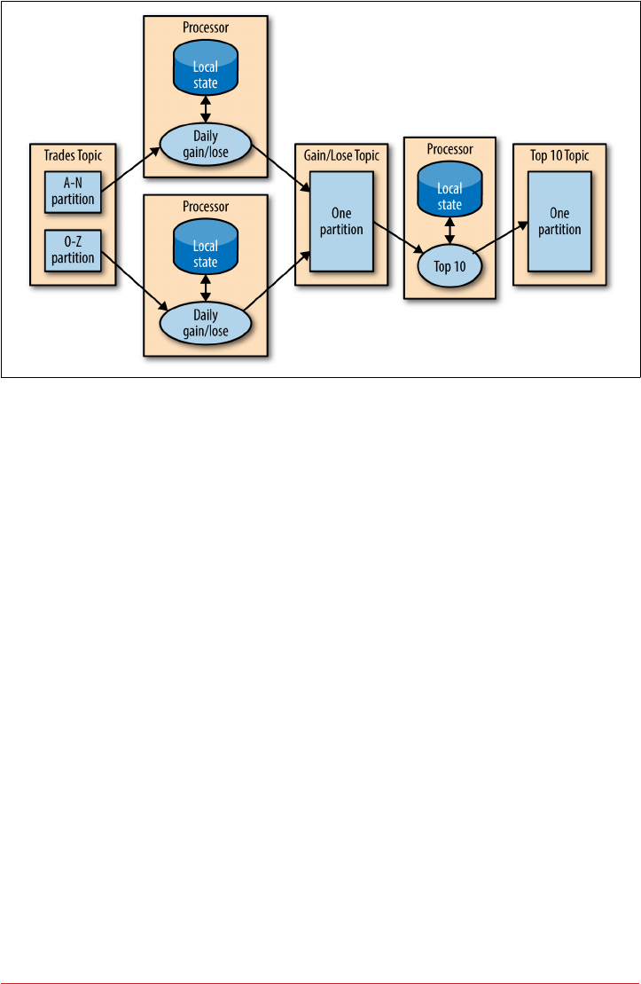
Figure 11-5. Topology that includes both local state and repartitioning steps
This type of multiphase processing is very familiar to those who write map-reduce
code, where you often have to resort to multiple reduce phases. If you’ve ever written
map-reduce code, you’ll remember that you needed a separate app for each reduce
step. Unlike MapReduce, most stream-processing frameworks allow including all
steps in a single app, with the framework handling the details of which application
instance (or worker) will run reach step.
Processing with External Lookup: Stream-Table Join
Sometimes stream processing requires integration with data external to the stream—
validating transactions against a set of rules stored in a database, or enriching click‐
stream information with data about the users who clicked.
The obvious idea on how to perform an external lookup for data enrichment is some‐
thing like this: for every click event in the stream, look up the user in the profile data‐
base and write an event that includes the original click plus the user age and gender
to another topic. See Figure 11-6.
Stream-Processing Design Patterns | 259
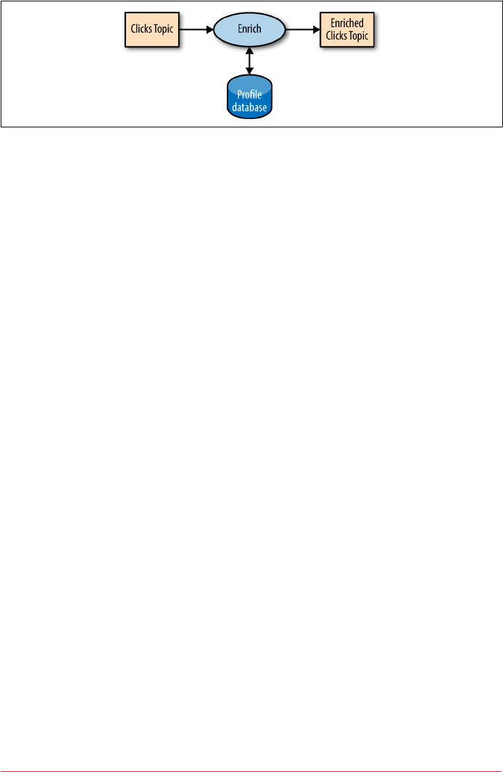
Figure 11-6. Stream processing that includes an external data source
The problem with this obvious idea is that an external lookup adds significant latency
to the processing of every record—usually between 5-15 milliseconds. In many cases,
this is not feasible. Often the additional load this places on the external datastore is
also not acceptable—stream-processing systems can often handle 100K-500K events
per second, but the database can only handle perhaps 10K events per second at rea‐
sonable performance. We want a solution that scales better.
In order to get good performance and scale, we need to cache the information from
the database in our stream-processing application. Managing this cache can be chal‐
lenging though—how do we prevent the information in the cache from getting stale?
If we refresh events too often, we are still hammering the database and the cache isn’t
helping much. If we wait too long to get new events, we are doing stream processing
with stale information.
But if we can capture all the changes that happen to the database table in a stream of
events, we can have our stream-processing job listen to this stream and update the
cache based on database change events. Capturing changes to the database as events
in a stream is known as CDC, and if you use Kafka Connect you will find multiple
connectors capable of performing CDC and converting database tables to a stream of
change events. This allows you to keep your own private copy of the table, and you
will be notified whenever there is a database change event so you can update your
own copy accordingly. See Figure 11-7.
260 | Chapter 11: Stream Processing
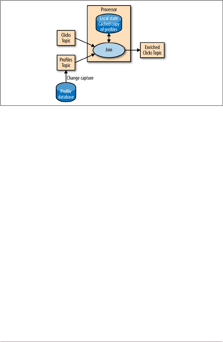
Figure 11-7. Topology joining a table and a stream of events, removing the need to
involve an external data source in stream processing
Then, when you get click events, you can look up the user_id at your local cache and
enrich the event. And because you are using a local cache, this scales a lot better and
will not affect the database and other apps using it.
We refer to this as a stream-table join because one of the streams represents changes
to a locally cached table.
Streaming Join
Sometimes you want to join two real event streams rather than a stream with a table.
What makes a stream “real”? If you recall the discussion at the beginning of the chap‐
ter, streams are unbounded. When you use a stream to represent a table, you can
ignore most of the history in the stream because you only care about the current state
in the table. But when you join two streams, you are joining the entire history, trying
to match events in one stream with events in the other stream that have the same key
and happened in the same time-windows. This is why a streaming-join is also called a
windowed-join.
For example, let’s say that we have one stream with search queries that people entered
into our website and another stream with clicks, which include clicks on search
results. We want to match search queries with the results they clicked on so that we
will know which result is most popular for which query. Obviously we want to match
results based on the search term but only match them within a certain time-window.
We assume the result is clicked seconds after the query was entered into our search
engine. So we keep a small, few-seconds-long window on each stream and match the
results from each window. See Figure 11-8.
Stream-Processing Design Patterns | 261
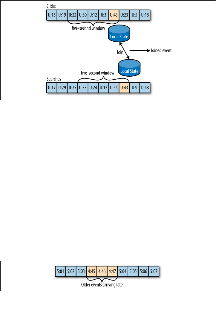
Figure 11-8. Joining two streams of events; these joins always involve a moving time win‐
dow
The way this works in Kafka Streams is that both streams, queries and clicks, are par‐
titioned on the same keys, which are also the join keys. This way, all the click events
from user_id:42 end up in partition 5 of the clicks topic, and all the search events for
user_id:42 end up in partition 5 of the search topic. Kafka Streams then makes sure
that partition 5 of both topics is assigned to the same task. So this task sees all the
relevant events for user_id:42. It maintains the join-window for both topics in its
embedded RocksDB cache, and this is how it can perform the join.
Out-of-Sequence Events
Handling events that arrive at the stream at the wrong time is a challenge not just in
stream processing but also in traditional ETL systems. Out-of-sequence events hap‐
pen quite frequently and expectedly in IoT (Internet of Things) scenarios
(Figure 11-9). For example, a mobile device loses WiFi signal for a few hours and
sends a few hours’ worth of events when it reconnects. This also happens when moni‐
toring network equipment (a faulty switch doesn’t send diagnostics signals until it is
repaired) or manufacturing (network connectivity in plants is notoriously unreliable,
especially in developing countries).
Figure 11-9. Out of sequence events
262 | Chapter 11: Stream Processing

Our streams applications need to be able to handle those scenarios. This typically
means the application has to do the following:
•Recognize that an event is out of sequence—this requires that the application
examine the event time and discover that it is older than the current time.
•Define a time period during which it will attempt to reconcile out-of-sequence
events. Perhaps a three-hour delay should be reconciled and events over three
weeks old can be thrown away.
•Have an in-band capability to reconcile this event. This is the main difference
between streaming apps and batch jobs. If we have a daily batch job and a few
events arrived after the job completed, we can usually just rerun yesterday’s job
and update the events. With stream processing, there is no “rerun yesterday’s job”
—the same continuous process needs to handle both old and new events at any
given moment.
•Be able to update results. If the results of the stream processing are written into a
database, a put or update is enough to update the results. If the stream app sends
results by email, updates may be trickier.
Several stream-processing frameworks, including Google’s Dataflow and Kafka
Streams, have built-in support for the notion of event time independent of the pro‐
cessing time and the ability to handle events with event times that are older or newer
than the current processing time. This is typically done by maintaining multiple
aggregation windows available for update in the local state and giving developers the
ability to configure how long to keep those window aggregates available for updates.
Of course, the longer the aggregation windows are kept available for updates, the
more memory is required to maintain the local state.
The Kafka’s Streams API always writes aggregation results to result topics. Those are
usually compacted topics, which means that only the latest value for each key is pre‐
served. In case the results of an aggregation window need to be updated as a result of
a late event, Kafka Streams will simply write a new result for this aggregation window,
which will overwrite the previous result.
Stream-Processing Design Patterns | 263

Reprocessing
The last important pattern is processing events. There are two variants of this pattern:
•We have an improved version of our stream-processing application. We want to
run the new version of the application on the same event stream as the old, pro‐
duce a new stream of results that does not replace the first version, compare the
results between the two versions, and at some point move clients to use the new
results instead of the existing ones.
•The existing stream-processing app is buggy. We fix the bug and we want to
reprocess the event stream and recalculate our results
The first use case is made simple by the fact that Apache Kafka stores the event
streams in their entirety for long periods of time in a scalable datastore. This means
that having two versions of a stream processing-application writing two result
streams only requires the following:
•Spinning up the new version of the application as a new consumer group
•Configuring the new version to start processing from the first offset of the input
topics (so it will get its own copy of all events in the input streams)
•Letting the new application continue processing and switching the client applica‐
tions to the new result stream when the new version of the processing job has
caught up
The second use case is more challenging—it requires “resetting” an existing app to
start processing back at the beginning of the input streams, resetting the local state
(so we won’t mix results from the two versions of the app), and possibly cleaning the
previous output stream. While Kafka Streams has a tool for resetting the state for a
stream-processing app, our recommendation is to try to use the first method when‐
ever sufficient capacity exists to run two copies of the app and generate two result
streams. The first method is much safer—it allows switching back and forth between
multiple versions and comparing results between versions, and doesn’t risk losing
critical data or introducing errors during the cleanup process.
Kafka Streams by Example
In order to demonstrate how these patterns are implemented in practice, we’ll show a
few examples using Apache Kafka’s Streams API. We are using this specific API
because it is relatively simple to use and it ships with Apache Kafka, which you
already have access to. It is important to remember that the patterns can be imple‐
mented in any stream-processing framework and library—the patterns are universal
but the examples are specific.
264 | Chapter 11: Stream Processing

Apache Kafka has two streams APIs—a low-level Processor API and a high-level
Streams DSL. We will use Kafka Streams DSL in our examples. The DSL allows you to
define the stream-processing application by defining a chain of transformations to
events in the streams. Transformations can be as simple as a filter or as complex as a
stream-to-stream join. The lower level API allows you to create your own transfor‐
mations, but as you’ll see, this is rarely required.
An application that uses the DSL API always starts with using the StreamBuilder to
create a processing topology—a directed graph (DAG) of transformations that are
applied to the events in the streams. Then you create a KafkaStreams execution
object from the topology. Starting the KafkaStreams object will start multiple threads,
each applying the processing topology to events in the stream. The processing will
conclude when you close the KafkaStreams object.
We’ll look at few examples that use Kafka Streams to implement some of the design
patterns we just discussed. A simple word count example will be used to demonstrate
the map/filter pattern and simple aggregates. Then we’ll move to an example where
we calculate different statistics on stock market trades, which will allow us to demon‐
strate window aggregations. Finally we’ll use ClickStream Enrichment as an example
to demonstrate streaming joins.
Word Count
Let’s walk through an abbreviated word count example for Kafka Streams. You can
find the full example on GitHub.
The first thing you do when creating a stream-processing app is configure Kafka
Streams. Kafka Streams has a large number of possible configurations, which we
won’t discuss here, but you can find them in the documentation. In addition, you can
also configure the producer and consumer embedded in Kafka Streams by adding
any producer or consumer config to the Properties object:
public class WordCountExample {
public static void main(String[] args) throws Exception{
Properties props = new Properties();
props.put(StreamsConfig.APPLICATION_ID_CONFIG,
"wordcount");
props.put(StreamsConfig.BOOTSTRAP_SERVERS_CONFIG,
"localhost:9092");
props.put(StreamsConfig.KEY_SERDE_CLASS_CONFIG,
Serdes.String().getClass().getName());
props.put(StreamsConfig.VALUE_SERDE_CLASS_CONFIG,
Serdes.String().getClass().getName());
Kafka Streams by Example | 265
Every Kafka Streams application must have an application ID. This is used to
coordinate the instances of the application and also when naming the internal
local stores and the topics related to them. This name must be unique for each
Kafka Streams application working with the same Kafka cluster.
The Kafka Streams application always reads data from Kafka topics and writes its
output to Kafka topics. As we’ll discuss later, Kafka Streams applications also use
Kafka for coordination. So we had better tell our app where to find Kafka.
When reading and writing data, our app will need to serialize and deserialize, so
we provide default Serde classes. If needed, we can override these defaults later
when building the streams topology.
Now that we have the configuration, let’s build our streams topology:
KStreamBuilder builder = new KStreamBuilder();
KStream<String, String> source =
builder.stream("wordcount-input");
final Pattern pattern = Pattern.compile("\\W+");
KStream counts = source.flatMapValues(value->
Arrays.asList(pattern.split(value.toLowerCase())))
.map((key, value) -> new KeyValue<Object,
Object>(value, value))
.filter((key, value) -> (!value.equals("the")))
.groupByKey()
.count("CountStore").mapValues(value->
Long.toString(value)).toStream();
counts.to("wordcount-output");
We create a KStreamBuilder object and start defining a stream by pointing at the
topic we’ll use as our input.
Each event we read from the source topic is a line of words; we split it up using a
regular expression into a series of individual words. Then we take each word
(currently a value of the event record) and put it in the event record key so it can
be used in a group-by operation.
We filter out the word “the,” just to show how easy filtering is.
And we group by key, so we now have a collection of events for each unique
word.
266 | Chapter 11: Stream Processing
We count how many events we have in each collection. The result of counting is a
Long data type. We convert it to a String so it will be easier for humans to read
the results.
Only one thing left–write the results back to Kafka.
Now that we have defined the flow of transformations that our application will run,
we just need to… run it:
KafkaStreams streams = new KafkaStreams(builder, props);
streams.start();
// usually the stream application would be running
forever,
// in this example we just let it run for some time and
stop since the input data is finite.
Thread.sleep(5000L);
streams.close();
}
}
Define a KafkaStreams object based on our topology and the properties we
defined.
Start Kafka Streams.
After a while, stop it.
Thats it! In just a few short lines, we demonstrated how easy it is to implement a sin‐
gle event processing pattern (we applied a map and a filter on the events). We reparti‐
tioned the data by adding a group-by operator and then maintained simple local state
when we counted the number of records that have each word as a key. Then we main‐
tained simple local state when we counted the number of times each word appeared.
At this point, we recommend running the full example. The README in the GitHub
repository contains instructions on how to run the example.
One thing you’ll notice is that you can run the entire example on your machine
without installing anything except Apache Kafka. This is similar to the experience
you may have seen when using Spark in something like Local Mode. The main differ‐
ence is that if your input topic contains multiple partitions, you can run multiple
instances of the WordCount application (just run the app in several different terminal
tabs) and you have your first Kafka Streams processing cluster. The instances of the
WordCount application talk to each other and coordinate the work. One of the biggest
Kafka Streams by Example | 267

barriers to entry with Spark is that local mode is very easy to use, but then to run a
production cluster, you need to install YARN or Mesos and then install Spark on all
those machines, and then learn how to submit your app to the cluster. With the Kaf‐
ka’s Streams API, you just start multiple instances of your app—and you have a clus‐
ter. The exact same app is running on your development machine and in production.
Stock Market Statistics
The next example is more involved—we will read a stream of stock market trading
events that include the stock ticker, ask price, and ask size. In stock market trades, ask
price is what a seller is asking for whereas bid price is what the buyer is suggesting to
pay. Ask size is the number of shares the seller is willing to sell at that price. For sim‐
plicity of the example, we’ll ignore bids completely. We also won’t include a time‐
stamp in our data; instead, we’ll rely on event time populated by our Kafka producer.
We will then create output streams that contains a few windowed statistics:
• Best (i.e., minimum) ask price for every five-second window
•Number of trades for every five-second window
• Average ask price for every five-second window
All statistics will be updated every second.
For simplicity, we’ll assume our exchange only has 10 stock tickers trading in it. The
setup and configuration are very similar to those we used in the “Word Count” on
page 265:
Properties props = new Properties();
props.put(StreamsConfig.APPLICATION_ID_CONFIG, "stockstat");
props.put(StreamsConfig.BOOTSTRAP_SERVERS_CONFIG,
Constants.BROKER);
props.put(StreamsConfig.KEY_SERDE_CLASS_CONFIG,
Serdes.String().getClass().getName());
props.put(StreamsConfig.VALUE_SERDE_CLASS_CONFIG,
TradeSerde.class.getName());
The main difference is the Serde classes used. In the “Word Count” on page 265, we
used strings for both key and value and therefore used the Serdes.String() class as a
serializer and deserializer for both. In this example, the key is still a string, but the
value is a Trade object that contains the ticker symbol, ask price, and ask size. In
order to serialize and deserialize this object (and a few other objects we used in this
small app), we used the Gson library from Google to generate a JSon serializer and
deserializer from our Java object. Then created a small wrapper that created a Serde
object from those. Here is how we created the Serde:
268 | Chapter 11: Stream Processing
static public final class TradeSerde extends WrapperSerde<Trade> {
public TradeSerde() {
super(new JsonSerializer<Trade>(),
new JsonDeserializer<Trade>(Trade.class));
}
}
Nothing fancy, but you need to remember to provide a Serde object for every object
you want to store in Kafka—input, output, and in some cases, also intermediate
results. To make this easier, we recommend generating these Serdes through projects
like GSon, Avro, Protobufs, or similar.
Now that we have everything configured, it’s time to build our topology:
KStream<TickerWindow, TradeStats> stats = source.groupByKey()
.aggregate(TradeStats::new,
(k, v, tradestats) -> tradestats.add(v),
TimeWindows.of(5000).advanceBy(1000),
new TradeStatsSerde(),
"trade-stats-store")
.toStream((key, value) -> new TickerWindow(key.key(),
key.window().start()))
.mapValues((trade) -> trade.computeAvgPrice());
stats.to(new TickerWindowSerde(), new TradeStatsSerde(),
"stockstats-output");
We start by reading events from the input topic and performing a groupByKey()
operation. Despite its name, this operation does not do any grouping. Rather, it
ensures that the stream of events is partitioned based on the record key. Since we
wrote the data into a topic with a key and didn’t modify the key before calling
groupByKey(), the data is still partitioned by its key—so this method does noth‐
ing in this case.
After we ensure correct partitioning, we start the windowed aggregation. The
“aggregate” method will split the stream into overlapping windows (a five-second
window every second), and then apply an aggregate method on all the events in
the window. The first parameter this method takes is a new object that will con‐
tain the results of the aggregation—Tradestats in our case. This is an object we
created to contain all the statistics we are interested in for each time window—
minimum price, average price, and number of trades.
We then supply a method for actually aggregating the records—in this case, an
add method of the Tradestats object is used to update the minimum price, num‐
ber of trades, and total prices in the window with the new record.
Kafka Streams by Example | 269

We define the window—in this case, a window of five seconds (5,000 ms),
advancing every second.
Then we provide a Serde object for serializing and deserializing the results of the
aggregation (the Tradestats object).
As mentioned in “Stream-Processing Design Patterns” on page 256, windowing
aggregation requires maintaining a state and a local store in which the state will
be maintained. The last parameter of the aggregate method is the name of the
state store. This can be any unique name.
The results of the aggregation is a table with the ticker and the time window as
the primary key and the aggregation result as the value. We are turning the table
back into a stream of events and replacing the key that contains the entire time
window definition with our own key that contains just the ticker and the start
time of the window. This toStream method converts the table into a stream and
also converts the key into my TickerWindow object.
The last step is to update the average price—right now the aggregation results
include the sum of prices and number of trades. We go over these records and
use the existing statistics to calculate average price so we can include it in the out‐
put stream.
And finally, we write the results back to the stockstats-output stream.
After we define the flow, we use it to generate a KafkaStreams object and run it, just
like we did in the “Word Count” on page 265.
This example shows how to perform windowed aggregation on a stream—probably
the most popular use case of stream processing. One thing to notice is how little work
was needed to maintain the local state of the aggregation—just provide a Serde and
name the state store. Yet this application will scale to multiple instances and automat‐
ically recover from a failure of each instance by shifting processing of some partitions
to one of the surviving instances. We will see more on how it is done in “Kafka
Streams: Architecture Overview” on page 272.
As usual, you can find the complete example including instructions for running it on
GitHub.
Click Stream Enrichment
The last example will demonstrate streaming joins by enriching a stream of clicks on
a website. We will generate a stream of simulated clicks, a stream of updates to a fic‐
tional profile database table, and a stream of web searches. We will then join all three
270 | Chapter 11: Stream Processing
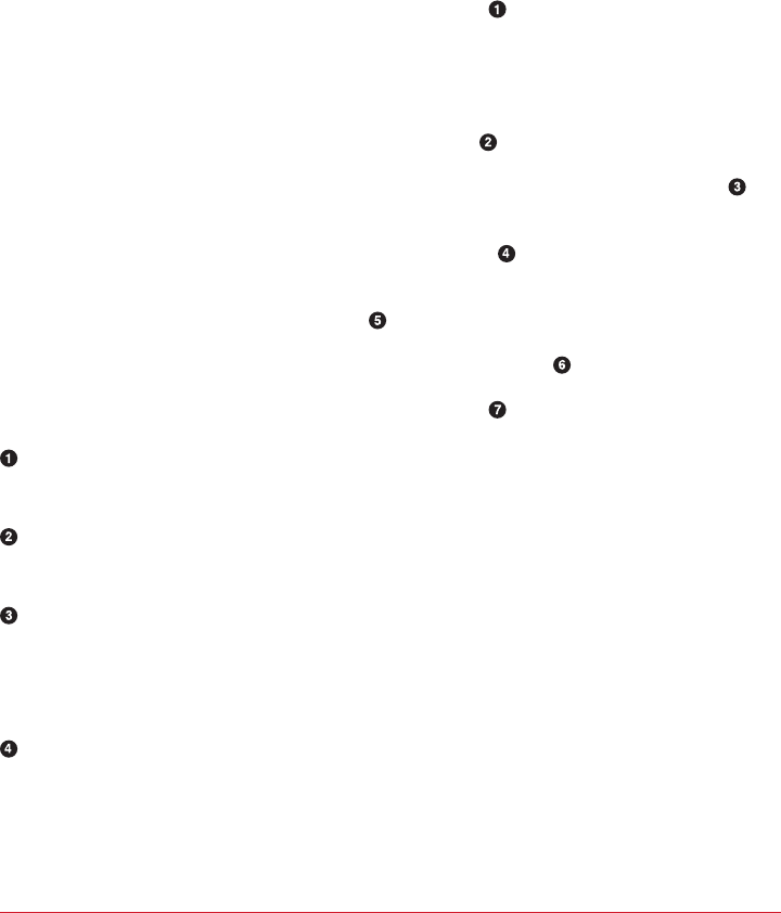
streams to get a 360-view into each user activity. What did the users search for? What
did they click as a result? Did they change their “interests” in their user profile? These
kinds of joins provide a rich data collection for analytics. Product recommendations
are often based on this kind of information—user searched for bikes, clicked on links
for “Trek,” and is interested in travel, so we can advertise bikes from Trek, helmets,
and bike tours to exotic locations like Nebraska.
Since configuring the app is similar to the previous examples, let’s skip this part and
take a look at the topology for joining multiple streams:
KStream<Integer, PageView> views =
builder.stream(Serdes.Integer(),
new PageViewSerde(), Constants.PAGE_VIEW_TOPIC);
KStream<Integer, Search> searches =
builder.stream(Serdes.Integer(), new SearchSerde(),
Constants.SEARCH_TOPIC);
KTable<Integer, UserProfile> profiles =
builder.table(Serdes.Integer(), new ProfileSerde(),
Constants.USER_PROFILE_TOPIC, "profile-store");
KStream<Integer, UserActivity> viewsWithProfile = views.leftJoin(profiles,
(page, profile) -> new UserActivity(profile.getUserID(),
profile.getUserName(), profile.getZipcode(),
profile.getInterests(), "", page.getPage()));
KStream<Integer, UserActivity> userActivityKStream =
viewsWithProfile.leftJoin(searches,
(userActivity, search) ->
userActivity.updateSearch(search.getSearchTerms()),
JoinWindows.of(1000), Serdes.Integer(),
new UserActivitySerde(), new SearchSerde());
First, we create a streams objects for the two streams we want to join—clicks and
searches.
We also define a KTable for the user profiles. A KTable is a local cache that is
updated through a stream of changes.
Then we enrich the stream of clicks with user-profile information by joining the
stream of events with the profile table. In a stream-table join, each event in the
stream receives information from the cached copy of the profile table. We are
doing a left-join, so clicks without a known user will be preserved.
This is the join method—it takes two values, one from the stream and one from
the record, and returns a third value. Unlike in databases, you get to decide how
to combine the two values into one result. In this case, we created one activity
object that contains both the user details and the page viewed.
Kafka Streams by Example | 271

Next, we want to join the click information with searches performed by the same
user. This is still a left join, but now we are joining two streams, not streaming to
a table.
This is the join method—we simply add the search terms to all the matching
page views.
This is the interesting part—a stream-to-stream join is a join with a time window.
Joining all clicks and searches for each user doesn’t make much sense—we want
to join each search with clicks that are related to it—that is, click that occurred a
short period of time after the search. So we define a join window of one second.
Clicks that happen within one second of the search are considered relevant, and
the search terms will be included in the activity record that contains the click and
the user profile. This will allow a full analysis of searches and their results.
After we define the flow, we use it to generate a KafkaStreams object and run it, just
like we did in the “Word Count” on page 265.
This example shows two different join patterns possible in stream processing. One
joins a stream with a table to enrich all streaming events with information in the
table. This is similar to joining a fact table with a dimension when running queries on
a data warehouse. The second example joins two streams based on a time window.
This operation is unique to stream processing.
As usual, you can find the complete example including instructions for running it on
GitHub.
Kafka Streams: Architecture Overview
The examples in the previous section demonstrated how to use the Kafka Streams
API to implement a few well-known stream-processing design patterns. But to
understand better how Kafka’s Streams library actually works and scales, we need to
peek under the covers and understand some of the design principles behind the API.
Building a Topology
Every streams application implements and executes at least one topology. Topology
(also called DAG, or directed acyclic graph, in other stream-processing frameworks)
is a set of operations and transitions that every event moves through from input to
output. Figure 11-10 shows the topology in the “Word Count” on page 265.
272 | Chapter 11: Stream Processing
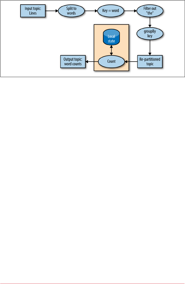
Figure 11-10. Topology for the word-count stream processing example
Even a simple app has a nontrivial topology. The topology is made up of processors—
those are the nodes in the topology graph (represented by circles in our diagram).
Most processors implement an operation of the data—filter, map, aggregate, etc.
There are also source processors, which consume data from a topic and pass it on,
and sink processors, which take data from earlier processors and produce it to a
topic. A topology always starts with one or more source processors and finishes with
one or more sink processors.
Scaling the Topology
Kafka Streams scales by allowing multiple threads of executions within one instance
of the application and by supporting load balancing between distributed instances of
the application. You can run the Streams application on one machine with multiple
threads or on multiple machines; in either case, all active threads in the application
will balance the work involved in data processing.
The Streams engine parallelizes execution of a topology by splitting it into tasks. The
number of tasks is determined by the Streams engine and depends on the number of
partitions in the topics that the application processes. Each task is responsible for a
subset of the partitions: the task will subscribe to those partitions and consume events
from them. For every event it consumes, the task will execute all the processing steps
that apply to this partition in order before eventually writing the result to the sink.
Those tasks are the basic unit of parallelism in Kafka Streams, because each task can
execute independently of others. See Figure 11-11.
Kafka Streams: Architecture Overview | 273
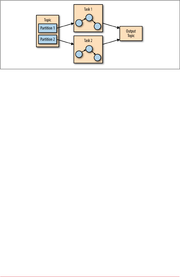
Figure 11-11. Two tasks running the same topology—one for each partition in the input
topic
The developer of the application can choose the number of threads each application
instance will execute. If multiple threads are available, every thread will execute a
subset of the tasks that the application creates. If multiple instances of the application
are running on multiple servers, different tasks will execute for each thread on each
server. This is the way streaming applications scale: you will have as many tasks as
you have partitions in the topics you are processing. If you want to process faster, add
more threads. If you run out of resources on the server, start another instance of the
application on another server. Kafka will automatically coordinate work—it will
assign each task its own subset of partitions and each task will independently process
events from those partitions and maintain its own local state with relevant aggregates
if the topology requires this. See Figure 11-12.
274 | Chapter 11: Stream Processing
Figure 11-12. e stream processing tasks can run on multiple threads and multiple
servers
You may have noticed that sometimes a processing step may require results from
multiple partitions, which could create dependencies between tasks. For example, if
we join two streams, as we did in the ClickStream example in “Click Stream Enrich‐
ment” on page 270, we need data from a partition in each stream before we can emit a
result. Kafka Streams handles this situation by assigning all the partitions needed for
one join to the same task so that the task can consume from all the relevant partitions
and perform the join independently. This is why Kafka Streams currently requires
that all topics that participate in a join operation will have the same number of parti‐
tions and be partitioned based on the join key.
Another example of dependencies between tasks is when our application requires
repartitioning. For instance, in the ClickStream example, all our events are keyed by
the user ID. But what if we want to generate statistics per page? Or per zip code? We’ll
need to repartition the data by the zip code and run an aggregation of the data with
the new partitions. If task 1 processes the data from partition 1 and reaches a pro‐
cessor that repartitions the data (groupBy operation), it will need to shue, which
means sending them the events—send events to other tasks to process them. Unlike
Kafka Streams: Architecture Overview | 275
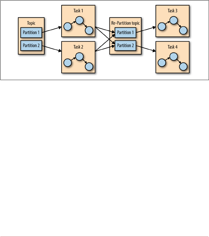
other stream processor frameworks, Kafka Streams repartitions by writing the events
to a new topic with new keys and partitions. Then another set of tasks reads events
from the new topic and continues processing. The repartitioning steps break our top‐
ology into two subtopologies, each with its own tasks. The second set of tasks
depends on the first, because it processes the results of the first subtopology. How‐
ever, the first and second sets of tasks can still run independently and in parallel
because the first set of tasks writes data into a topic at its own rate and the second set
consumes from the topic and processes the events on its own. There is no communi‐
cation and no shared resources between the tasks and they don’t need to run on the
same threads or servers. This is one of the more useful things Kafka does—reduce
dependencies between different parts of a pipeline. See Figure 11-13.
Figure 11-13. Two sets of tasks processing events with a topic for re-partitioning events
between them
Surviving Failures
The same model that allows us to scale our application also allows us to gracefully
handle failures. First, Kafka is highly available, and therefore the data we persist to
Kafka is also highly available. So if the application fails and needs to restart, it can
look up its last position in the stream from Kafka and continue its processing from
the last offset it committed before failing. Note that if the local state store is lost (e.g.,
because we needed to replace the server it was stored on), the streams application can
always re-create it from the change log it stores in Kafka.
Kafka Streams also leverages Kafka’s consumer coordination to provide high availa‐
bility for tasks. If a task failed but there are threads or other instances of the streams
application that are active, the task will restart on one of the available threads. This is
similar to how consumer groups handle the failure of one of the consumers in the
group by assigning partitions to one of the remaining consumers.
276 | Chapter 11: Stream Processing

Stream Processing Use Cases
Throughout this chapter we’ve learned how to do stream processing—from general
concepts and patterns to specific examples in Kafka Streams. At this point it may be
worth looking at the common stream processing use cases. As explained in the begin‐
ning of the chapter, stream processing—or continuous processing—is useful in cases
where you want your events to be processed in quick order rather than wait for hours
until the next batch, but also where you are not expecting a response to arrive in
milliseconds. This is all true but also very abstract. Let’s look at a few real scenarios
that can be solved with stream processing:
Customer Service
Suppose that you just reserved a room at a large hotel chain and you expect an
email confirmation and receipt. A few minutes after reserving, when the confir‐
mation still hasn’t arrived, you call customer service to confirm your reservation.
Suppose the customer service desk tells you “I don’t see the order in our system,
but the batch job that loads the data from the reservation system to the hotels
and the customer service desk only runs once a day, so please call back tomorrow.
You should see the email within 2-3 business days.” This doesn’t sound like very
good service, yet I’ve had this conversation more than once with a large hotel
chain. What we really want is every system in the hotel chain to get an update
about a new reservations seconds or minutes after the reservation is made,
including the customer service center, the hotel, the system that sends email con‐
firmations, the website, etc. You also want the customer service center to be able
to immediately pull up all the details about any of your past visits to any of the
hotels in the chain, and the reception desk at the hotel to know that you are a
loyal customer so they can give you an upgrade. Building all those systems using
stream-processing applications allows them to receive and process updates in
near real time, which makes for a better customer experience. With such a sys‐
tem, I’d receive a confirmation email within minutes, my credit card would be
charged on time, the receipt would be sent, and the service desk could immedi‐
ately answer my questions regarding the reservation.
Internet of ings
Internet of Things can mean many things—from a home device for adjusting
temperature and ordering refills of laundry detergent to real-time quality control
of pharmaceutical manufacturing. A very common use case when applying
stream processing to sensors and devices is to try to predict when preventive
maintenance is needed. This is similar to application monitoring but applied to
hardware and is common in many industries, including manufacturing, telecom‐
munications (identifying faulty cellphone towers), cable TV (identifying faulty
box-top devices before users complain), and many more. Every case has its own
pattern, but the goal is similar: process events arriving from devices at a large
Stream Processing Use Cases | 277

scale and identify patterns that signal that a device requires maintenance. These
patterns can be dropped packets for a switch, more force required to tighten
screws in manufacturing, or users restarting the box more frequently for cable
TV.
•Fraud Detection: Also known as anomaly detection, is a very wide field that
focuses on catching “cheaters” or bad actors in the system. Examples of
fraud-detection applications include detecting credit card fraud, stock trad‐
ing fraud, video-game cheaters, and cybersecurity risks. In all these fields,
there are large benefits to catching fraud as early as possible, so a near real-
time system that is capable of responding to events quickly—perhaps stop‐
ping a bad transaction before it is even approved—is much preferred to a
batch job that detects fraud three days after the fact when cleanup is much
more complicated. This is again a problem of identifying patterns in a large-
scale stream of events.
In cyber security, there is a method known as beaconing. When the hacker plants mal‐
ware inside the organization, it will occasionally reach outside to receive commands.
It can be difficult to detect this activity since it can happen at any time and any fre‐
quency. Typically, networks are well defended against external attacks but more vul‐
nerable to someone inside the organization reaching out. By processing the large
stream of network connection events and recognizing a pattern of communication as
abnormal (for example, detecting that this host typically doesn’t access those specific
IPs), the security organization can be alerted early, before more harm is done.
How to Choose a Stream-Processing Framework
When choosing a stream-processing framework, it is important to consider the type
of application you are planning on writing. Different types of applications call for dif‐
ferent stream-processing solutions:
Ingest
Where the goal is to get data from one system to another, with some modifica‐
tion to the data on how it will make it conform to the target system.
Low milliseconds actions
Any application that requires almost immediate response. Some fraud detection
use cases fall within this bucket.
Asynchronous microservices
These microservices perform a simple action on behalf of a larger business pro‐
cess, such as updating the inventory of a store. These applications may need to
maintain a local state caching events as a way to improve performance.
278 | Chapter 11: Stream Processing

Near real-time data analytics
These streaming applications perform complex aggregations and joins in order to
slice and dice the data and generate interesting business-relevant insights.
The stream-processing system you will choose will depend a lot on the problem you
are solving.
•If you are trying to solve an ingest problem, you should reconsider whether you
want a stream processing system or a simpler ingest-focused system like Kafka
Connect. If you are sure you want a stream processing system, you need to make
sure it has both a good selection of connectors and high-quality connectors for
the systems you are targeting.
•If you are trying to solve a problem that requires low milliseconds actions, you
should also reconsider your choice of streams. Request-response patterns are
often better suited to this task. If you are sure you want a stream-processing sys‐
tem, then you need to opt for one that supports an event-by-event low-latency
model rather than one that focuses on microbatches.
•If you are building asynchronous microservices, you need a stream processing
system that integrates well with your message bus of choice (Kafka, hopefully),
has change capture capabilities that easily deliver upstream changes to the micro‐
service local caches, and has the good support of a local store that can serve as a
cache or materialized view of the microservice data.
•If you are building a complex analytics engine, you also need a stream-processing
system with great support for a local store—this time, not for maintenance of
local caches and materialized views but rather to support advanced aggregations,
windows, and joins that are otherwise difficult to implement. The APIs should
include support for custom aggregations, window operations, and multiple join
types.
In addition to use-case specific considerations, there are a few global considerations
you should take into account:
Operability of the system
Is it easy to deploy to production? Is it easy to monitor and troubleshoot? Is it
easy to scale up and down when needed? Does it integrate well with your existing
infrastructure? What if there is a mistake and you need to reprocess data?
Usability of APIs and ease of debugging
I’ve seen orders of magnitude differences in the time it takes to write a high-
quality application among different versions of the same framework. Develop‐
ment time and time-to-market is important so you need to choose a system that
makes you efficient.
How to Choose a Stream-Processing Framework | 279

Makes hard things easy
Almost every system will claim they can do advanced windowed aggregations
and maintain local caches, but the question is: do they make it easy for you? Do
they handle gritty details around scale and recovery, or do they supply leaky
abstractions and make you handle most of the mess? The more a system exposes
clean APIs and abstractions and handles the gritty details on its own, the more
productive developers will be.
Community
Most stream processing applications you consider are going to be open source,
and there’s no replacement for a vibrant and active community. Good commu‐
nity means you get new and exciting features on a regular basis, the quality is rel‐
atively good (no one wants to work on bad software), bugs get fixed quickly, and
user questions get answers in timely manner. It also means that if you get a
strange error and Google it, you will find information about it because other peo‐
ple are using this system and seeing the same issues.
Summary
We started the chapter by explaining stream processing. We gave a formal definition
and discussed the common attributes of the stream-processing paradigm. We also
compared it to other programming paradigms.
We then discussed important stream-processing concepts. Those concepts were
demonstrated with three example applications written with Kafka Streams.
After going over all the details of these example applications, we gave an overview of
the Kafka Streams architecture and explained how it works under the covers. We
conclude the chapter, and the book, with several examples of stream-processing use
cases and advice on how to compare different stream-processing frameworks.
280 | Chapter 11: Stream Processing

APPENDIX A
Installing Kafka on Other
Operating Systems
Apache Kafka is primarily a Java application, and therefore should be able to run on
any system where you are able to install a JRE. It has, however, been optimized for
Linux-based operating systems so that is where it will perform best. Running on other
operating systems may result in bugs specific to the OS. For this reason, when using
Kafka for development or test purposes on a common desktop OS, it is a good idea to
consider running in a virtual machine that matches your eventual production envi‐
ronment.
Installing on Windows
As of Microsoft Windows 10, there are now two ways that you can run Kafka. The
traditional way is using a native Java installation. Windows 10 users also have the
option to use the Windows Subsystem for Linux. The latter method is highly prefer‐
red because it provides a much simpler setup that more closely matches the typical
production environment, so we will review it first.
Using Windows Subsystem for Linux
If you are running Windows 10, you can install native Ubuntu support under Win‐
dows using Windows Subsystem for Linux (WSL). At the time of publication, Micro‐
soft still considers WSL to be an experimental feature. Though it acts similar to a
virtual machine, it does not require the resources of a full VM and provides richer
integration with the Windows OS.
281

In order to install WSL, you should follow the instructions available from the Micro‐
soft Developer Network at the Bash on Ubuntu on Windows page. Once that is done,
you will need to install a JDK using apt-get:
$ sudo apt-get install openjdk-7-jre-headless
[sudo] password for username:
Reading package lists... Done
Building dependency tree
Reading state information... Done
[...]
done.
$
Once you have installed the JDK, you can proceed to install Apache Kafka using the
instructions in Chapter 2.
Using Native Java
For older versions of Windows, or if you prefer not to use the WSL environment, you
can run Kafka natively with a Java environment for Windows. Be aware, however,
that this can introduce bugs specific to the Windows environment. These bugs may
not get the attention in the Apache Kafka development community as similar prob‐
lems on Linux might.
Before installing Zookeeper and Kafka, you must have a Java environment set up. You
should install the latest version of Oracle Java 8, which can be found on the Oracle
Java SE Download page. Download a full JDK package, so that you have all the Java
tools available, and follow the instructions for installation.
Be Careful with Paths
When installing Java and Kafka, it is highly recommended that you
stick to installation paths that do not contain spaces. While Win‐
dows allows spaces in paths, applications that are designed to run
in Unix environments are not set up this way and specifying paths
will be difficult. When installing Java, make sure to set the installa‐
tion path with this in mind. For example, if installing JDK 1.8
update 121, a good choice would be to use the path C:\Java
\jdk1.8.0_121.
Once Java is installed, you should set up the environment variables so that it can be
used. This is done in the Control Panel for Windows, though the exact location will
depend on your version of the OS. In Windows 10, you must select System and Secu‐
rity, then System, and then click Change settings under the Computer name, domain,
and workgroup settings section. This will open the System Properties window, where
you can select the Advanced tab and then finally click the Environment Variables…
282 | Appendix A: Installing Kafka on Other Operating Systems
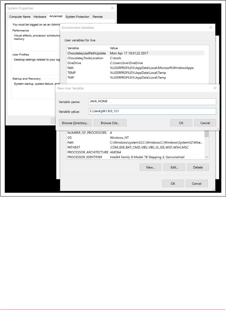
button. Use this section to add a new user variable named JAVA_HOME (Figure A-1)
and set to the path where you installed Java. Then edit the system variable named
Path and add a new entry which is %JAVA_HOME%\bin. Save these settings and exit out
of the Control Panel.
Figure A-1. Adding the JAVA_HOME variable
Now you can proceed to install Apache Kafka. The installation includes Zookeeper,
so you do not have to install it separately. The current release of Kafka can be down‐
loaded. At publication time, that version is 0.10.1.0 running under Scala version
2.11.0. The downloaded file will be GZip compressed and packaged with the tar util‐
ity, so you will need to use a Windows application such as 8Zip to uncompress it.
Similar to installing on Linux, you must choose a directory to extract Kafka into. For
this example, we will assume Kafka is extracted into C:\kafka_2.11-0.10.1.0.
Running Zookeeper and Kafka under Windows is a little different, as you must use
the batch files designed for Windows rather than the shell scripts for other platforms.
Installing Kafka on Other Operating Systems | 283

These batch files also do not support backgrounding the application, so you will need
a separate shell for each application. First, start Zookeeper:
PS C:\> cd kafka_2.11-0.10.2.0
PS C:\kafka_2.11-0.10.2.0> bin/windows/zookeeper-server-start.bat C:
\kafka_2.11-0.10.2.0\config\zookeeper.properties
[2017-04-26 16:41:51,529] INFO Reading configuration from: C:
\kafka_2.11-0.10.2.0\config\zookeeper.properties (org.apache.zoo
keeper.server.quorum.QuorumPeerConfig)
[...]
[2017-04-26 16:41:51,595] INFO minSessionTimeout set to -1 (org.apache.zoo
keeper.server.ZooKeeperServer)
[2017-04-26 16:41:51,596] INFO maxSessionTimeout set to -1 (org.apache.zoo
keeper.server.ZooKeeperServer)
[2017-04-26 16:41:51,673] INFO binding to port 0.0.0.0/0.0.0.0:2181
(org.apache.zookeeper.server.NIOServerCnxnFactory)
Once Zookeeper is running, you can open another window to start Kafka:
PS C:\> cd kafka_2.11-0.10.2.0
PS C:\kafka_2.11-0.10.2.0> .\bin\windows\kafka-server-start.bat C:
\kafka_2.11-0.10.2.0\config\server.properties
[2017-04-26 16:45:19,804] INFO KafkaConfig values:
[...]
[2017-04-26 16:45:20,697] INFO Kafka version : 0.10.2.0 (org.apache.kafka.com
mon.utils.AppInfoParser)
[2017-04-26 16:45:20,706] INFO Kafka commitId : 576d93a8dc0cf421
(org.apache.kafka.common.utils.AppInfoParser)
[2017-04-26 16:45:20,717] INFO [Kafka Server 0], started (kafka.server.Kafka
Server)
Installing on MacOS
MacOS runs on Darwin, a Unix OS that is derived, in part, from FreeBSD. This
means that many of the expectations of running on a Unix OS hold true, and instal‐
ling applications designed for Unix, like Apache Kafka, is not too difficult. You can
either keep the installation simple by using a package manager (like Homebrew), or
you can install Java and Kafka manually for greater control over versions.
Using Homebrew
If you have already installed Homebrew for MacOS, you can use it to install Kafka in
one step. This will assure that you have Java installed first, and it will then install
Apache Kafka 0.10.2.0 (as the time of writing).
If you have not yet installed Homebrew, do that first by following the directions on
the installation page. Then you can install Kafka itself. The Homebrew package man‐
ager will ensure that you have all the dependencies installed first, including Java:
284 | Appendix A: Installing Kafka on Other Operating Systems

$ brew install kafka
==> Installing kafka dependency: zookeeper
[...]
==> Summary
/usr/local/Cellar/kafka/0.10.2.0: 132 files, 37.2MB
$
Homebrew will install Kafka under /usr/local/Cellar, but the files will be linked into
other directories:
• Binaries and scripts will be in /usr/local/bin
•Kafka configurations will be in /usr/local/etc/kafka
• Zookeeper configuration will be in /usr/local/etc/zookeeper
•The log.dirs config (the location for Kafka data) will be set to /usr/
local/var/lib/kafka-logs
After installation is complete, you can start Zookeeper and Kafka (this example starts
Kafka in the foreground):
$ /usr/local/bin/zkServer start
JMX enabled by default
Using config: /usr/local/etc/zookeeper/zoo.cfg
Starting zookeeper ... STARTED
$ kafka-server-start.sh /usr/local/etc/kafka/server.properties
[...]
[2017-02-09 20:48:22,485] INFO [Kafka Server 0], started (kafka.server.Kafka
Server)
Installing Manually
Similar to a manual installation for the Windows OS, when installing Kafka on
MacOS you must first install a JDK. The same Oracle Java SE Download page can be
used to get the proper version for MacOS. You can then download Apache Kafka,
similar to Windows again. For this example, we will assume that the Kafka download
is expanded into the /usr/local/kafka_2.11-0.10.2.0 directory.
Starting Zookeeper and Kafka looks just like starting them when using Linux, though
you will need to make sure your JAVA_HOME directory is set first:
$ export JAVA_HOME=`/usr/libexec/java_home`
$ echo $JAVA_HOME
/Library/Java/JavaVirtualMachines/jdk1.8.0._131.jdk/Contents/Home
$ /usr/local/kafka_2.11-0.10.2.0/bin/zookeeper-server-start.sh -daemon /usr/
local/kafka_2.11-0.10.2.0/config/zookeeper.properties
$ /usr/local/kafka_2.11-0.10.2.0/bin/kafka-server-start.sh /usr/local/etc/kafka/
server.properties
[2017-04-26 16:45:19,804] INFO KafkaConfig values:
[...]
Installing Kafka on Other Operating Systems | 285

[2017-04-26 16:45:20,697] INFO Kafka version : 0.10.2.0 (org.apache.kafka.com
mon.utils.AppInfoParser)
[2017-04-26 16:45:20,706] INFO Kafka commitId : 576d93a8dc0cf421
(org.apache.kafka.common.utils.AppInfoParser)
[2017-04-26 16:45:20,717] INFO [Kafka Server 0], started (kafka.server.Kafka
Server)
286 | Appendix A: Installing Kafka on Other Operating Systems

Index
A
acceptor threads, 99
ACID reliability guarantee, 116
acks parameter, 48
acknowledgment modes, 122
produce requests, 101
ACLs, client, 207
active controller count metric, 220
active segments, 108
active-active datacenter architecture, 161-163
active-standby datacenter architecture, 163-169
data loss and inconsistencies in unplanned
failover, 165
start offset for applications after failover,
165-168
activity tracking (use case), 12
administration, 181-210
authorization admin operations, 181
client ACLs, 207
console consumer, 202-205
console producer, 205-207
consumer groups, 186-190
consuming and producing, 202-207
dynamic configuration changes, 190-193
partition management, 193-201
topic operations, 181-186
unsafe operations, 207-210
advance interval, 255
alerts, 213
all topic bytes in rate, 222-223
all topic bytes out rate, 223
all topic messages in rate, 224
Amazon Web Services (AWS), 30
Apache Avro (see Avro)
APIs
consumer, 93
producer, 61
streams (see see Kafka Streams API)
applications
health checks for, 213
validating for system reliability, 131
assignment
strategies, 74
subscription vs., 92
asynchronous commits, 78, 80
Asynchronous Send, 45, 47
AsyncProducer, 61
at-least-once delivery, 137
authorization of admin operations, 181
auto offset reset, 165
auto.commit.interval.ms, 76, 126
auto.create.topics.enable parameter, 23
auto.offset.reset parameter, 73, 126
automatic commits, 76
automatic leader rebalancing, 194
Avro
advantages of, 5
deserialization with Kafka consumer, 91
serializing using, 54-56
using Avro records with Kafka, 56-59
B
batch, 4
batch processing, 250
batch.size parameter, 50
binary wire protocol, 42
bootstrap.servers property, 44
broker
287

about, 7
active controller count metric, 220
all topic bytes in rate, 222-223
all topic bytes out rate, 223
all topic messages in rate, 224
application health checks, 213
choosing number of partitions per, 25
cluster membership, 95
configuration, 21-28
configuration for cluster, 32
consumer metrics, 241
controller, 96
CPU utilization, 234
general parameters, 21-23
in clusters, 31
(see also clusters id=ix_ch02-asciidoc9)
installation, 20
leader count, 225
message size configurations, 28
metrics, 213-235
number per cluster, 32
offline partitions count, 225
partition allocation, 106
partition assignment, 68
partition count, 224
producer metrics, 238
quotas, 242
reliable message storage configuration,
118-121
request handler idle ratio metric, 221
request metrics, 226-229
request processing, 99-105
topic defaults, 24-28
underreplicated partitions metric, 214-220
broker configuration, 118-121
minimum in-sync replicas, 121
replication factor, 118
unclean leader election, 119-121
broker disk, 29
broker.id parameter, 22
buffer.memory parameter, 49
Burrow, 243
bytes in per second, 222-223
bytes out per second, 223
C
callbacks, 47
chroot path, 22
clickstream enrichment, 270-272
client
ACLs, 207
configuration overrides, 192
monitoring, 236-243
client ID, 192
client monitoring, 236-243
consumer metrics, 239-242
producer metrics, 236-239
quotas, 242
client.id parameter, 51, 75
cloud
cross-cluster data mirroring, 158
Kafka installation, 30
cluster controller (see controller)
clusters
about, 7
broker configuration for, 32
chroot path for, 22
configuration, 31-35
cross-cluster data mirroring (see cross-
cluster data mirroring)
membership, 95
multiple, 8
number of brokers per, 32
OS tuning, 32-35
commit log, 13
commits and offsets, 75-81
asynchronous commit, 78
automatic commit, 76
combining synchronous and asynchronous
commits, 80
commit current offset, 77
commit order and sequence numbers, 79
commiting specified offsets, 80
consuming records with specific offsets,
84-86
explicitly committing offsets in consumers,
127-129
committed offsets, 125
compacted topics, 112, 263
compaction, 110-111
compression.type parameter, 49
Confluent Replicator, 179
Connect
about, 142
alternatives to, 154
and data ingestion tools from other systems,
155
and GUI-based ETL tools, 155
288 | Index

basic concepts, 151-154
Connectors, 151
converters and Connect's data model, 153
file source/file sink example, 144-146
key configurations for workers, 142
MySQL to Elasticsearch example, 146-151
offset management, 154
running, 142-144
stand-alone mode, 144
stream-processing frameworks, 155
tasks, 152
traditional producer/consumer vs., 141
workers, 152
Connectors
building your own, 151
Connect, 151
console consumer, 202-205
consuming the offsets topic, 205
message formatter options, 204
console producer, 205-207
consumer groups
about, 7
administration, 186-190
basics, 63-66
client ID vs. consumer group name, 192
consumers without, 92
deleting, 188
heartbeats and, 67
listing and describing, 186
offset management, 188
partition rebalance, 66-68
thread rule, 71
consumer lag
metric, 132
monitoring, 243
consumer metrics, 239-242
coordinator metrics, 241
fetch manager metrics, 239
per-broker/per-topic metrics, 241
consumer offsets, 165
ConsumerRebalanceListener, 82-83
consumers, 63-94
about, 6
administration, 202-207
commits and offsets, 75-81
concepts, 63-68
configuring, 72-75
console consumer, 202-205
consumer groups, 63-66
consuming records with specific offsets,
84-86
creating, 68
deserializers, 88-92
exiting the poll loop, 86
explicitly committing offsets in, 127-129
groups (see consumer groups)
Kafka's ability to handle multiple, 10
mandatory properties, 68
metrics (see consumer metrics)
monitoring, 239-242
older APIs, 93
poll loop, 70-71
properties for reliable processing, 126
rebalancing listeners, 82-83
reliable system, 125-129
subscribing to topics, 69
thread rule, 71
without consumer group, 92
Zookeeper and, 38
controller, 96
active controller count metric, 220
moving, 208
responsibilities of, 7
controller epoch, 96
coupling
data formats and, 5
data pipelines, 140
CPU
hardware considerations, 30
system load metrics, 234
cross-cluster data mirroring, 157-180
active-active architecture, 161-163
active-standby architecture, 163-169
Confluent's Replicator, 179
hub-and-spokes architecture, 160
issues with cross datacenter communica‐
tion, 159
MirrorMaker, 170-178
MirrorMaker alternatives, 178-180
multicluster architectures, 158-170
stretch clusters, 169
Uber uReplicator, 178
use cases, 158
custom deserializers, 89-91
custom serializers, 52-54, 206
customer service (stream processing use case),
277
Index | 289

D
data ecosystem, Kafka, 11-13
activity tracking, 12
commit log, 13
messaging, 12
metrics and logging, 13
stream processing, 13
use cases, 12
data formats, data pipelines and, 138
data mirroring (see cross-cluster data mirror‐
ing)
data pipelines, 135-156
considerations when building, 136-141
coupling and agility, 140
data formats, 138
failure handling, 140
high/varying throughput, 137
Kafka Connect vs. traditional producer/
consumer, 141
reliability, 137
security, 139
timeliness requirements, 136
transformations, 139
data stream, 248
data, reading from Kafka (see consumers)
data-lake architecture, 139
datacenter failure, stretch clusters and, 169
decoupling
data formats and, 5
data pipelines, 140
deleted events, 112
deletions
consumer groups, 188
topics, 184, 209
deserializers, 88-92
custom, 89-91
using Avro deserialization with Kafka con‐
sumer, 91
dirty pages, 33
dirty records, 110, 112
disaster recovery (DR), 158, 164
disk
filesystem choice, 34
HDD vs. SSD, 29
monitoring usage of, 234
performance when using time-based log
segment limits, 28
disk capacity, 29
disk failures, effects of, 218
disk throughput, 29
disk-based retention, 10
distributed commit log, 4
distributed streaming platform, 4
dynamic configuration changes
overriding client configuration defaults, 192
overriding topic defaults, 190
removing configuration overrides, 193
E
Elasticsearch, loading MySQL table into,
146-151
ELT (Extract-Load-Transform), 139
enable.auto.commit parameter, 74, 126
end-to-end monitoring, 244
ensemble (Zookeeper), 19
error messages
for nonexistent topics, 184
retries, 50
error-rate per record, 132
ETL (Extract-Transform-Load), 139
event stream, 248
event time, stream processing and, 251
events, deleted, 112
exactly-once delivery, 129, 137
EXT4 (fourth extended file system), 34
Extents File System (XFS), 34
external metrics
end-to-end monitoring, 244
internal metrics vs., 212
external offset mapping, 167
external state, 253
F
failure handling
in data pipelines, 140
Kafka Streams API, 276
fetch manager metrics, 239
fetch requests, 102
fetch.max.wait.ms parameter, 72
fetch.message.max.bytes parameter, 28
fetch.min.bytes parameter, 72
file management, 107
filesystem, 34
fire-and-forget, 45
follower replicas, 97
fraud detection (use case), 278
290 | Index

G
garbage collection (GC)
monitoring, 231
options, 36
Garbage First (G1) collector, 36
group coordinator, 67
group leader, 68
group.id, 69, 126, 142
guarantees, reliable data delivery, 116
H
hard drives, HDD vs. SSD, 29
hardware
CPU, 30
disk capacity, 29
disk throughput, 29
memory, 29
networking, 30
selection, 28-30
health checks, 213
heap memory, 30
heartbeats, 67
high-fidelity pipelines, 139
Homebrew, Kafka installation on OS X using,
284
hub-and-spokes architecture, 160
I
idempotent writes, 129
in-sync replicas, 98
and unclean leader election, 119
minimum, 121
topics and, 117
indexes, 109
installation (Kafka), 17-39
broker installation, 20
cloud computing environments, 30
cluster configuration, 31-35
colocating applications on Zookeeper, 37
datacenter layout, 37
disk capacity, 29
disk throughput, 29
garbage collector options, 36
hardware selection, 28-30
installation on OS other than Linux,
281-285
Java installation, 17
OS choice, 17
OS X, 284
production concerns, 36-38
using WSL, 281
Windows, 281-284
Zookeeper installation, 18-20
instance configuration, 30
internal metrics, 212
internal state, 253
internals, 95-113
cluster membership, 95
controller, 96
physical storage, 105-113
replication, 97-99
request processing, 99-105
Internet of Things (use case), 277
IO threads, 100
J
Java
garbage collector tuning, 36
installation, 17
Kafka installation on Windows, 282
Java Management Extensions (JMX), 211
JMX (Java Management Extensions), 132, 211,
212
JVM (Java Virtual Machine)
garbage collection monitoring, 231
heap memory, 30
monitoring, 231
OS monitoring, 232
K
Kafka (basics), 1-16
batches, 4
birth of, 15
brokers and clusters, 7
data ecosystem, 11-13
first release, 15
installation on OS other than Linux,
281-285
installation on OS X, 284
installation on Windows, 281-284
internals (see internals)
LinkedIn and, 14
manual installation on OS X, 285
messages, 4
multiple clusters, 8
name's origin, 16
origins, 14-16
Index | 291

producers and consumers, 6
publish-subscribe messaging before Kafka,
1-4
publish-subscribe messaging with, 4-9
reasons to use, 10
scalability of, 10
schemas, 5
topics and partitions, 5
Kafka Connect (see Connect)
Kafka Streams API
architecture overview, 272-276
building a topology, 272
ClickStream enrichment example, 270-272
examples, 264-272
scaling a topology, 273-276
stock market statistics example, 268-270
surviving failures, 276
word count example, 265-268
kafka-acls.sh, 207
kafka-console-consumer.sh tool, 202-205
consuming the offsets topic, 205
message formatter options, 204
kafka.console.producer.sh tool, 205-207
KafkaConsumer, 68
(see also consumers)
KafkaProducer (see producers)
key-value pairs, 59
key.serializer class, 44
keyed topics, partitions and, 183
keys
mapping to partitions, 60
purposes of, 59
Kreps, Jay, 15
L
lag monitoring, 173, 243
leader count metric, 225
leaders
automatic rebalancing, 194
controller and, 96
leader count metric, 225
no leader error, 47
preferred, 98
replicas, 97
unclean leader election, 119-121, 119
line-reader options, 205, 207
linger.ms parameter, 50
LinkedIn, 14
Linux
networking configuration, 35, 176
swappiness, 33
tuning, 32
Windows subsystem for, 281
listeners, rebalancing, 82-83
livelock, 67
local state
defined, 253
stream processing with, 257
log append time, 251
log compacted topics, 8
log segments, dumping, 199
log, clean/dirty portions of, 110
log.dirs parameter, 23
log.retention.bytes parameter, 26
log.retention.ms parameter, 26
log.segment.bytes parameter, 27
log.segment.ms parameter, 27
logging
and data ecosystem, 13
monitoring and, 235
M
map-filter pattern, 256
max.block.ms parameter, 51
max.in.flight.requests.per.connection parame‐
ter, 51
max.partition.fetch.bytes parameter, 72
max.poll.records parameter, 75
max.request.size parameter, 51
membership, cluster, 95
memory, hardware considerations, 29
message retention (see retention)
message size configurations, 28
message.max.bytes parameter, 28
messages, 4
(see also producers)
acks parameter, 48
asynchronous transmission, 47
file format, 108
ordering guarantees, 52
primary methods of sending, 45
sending, 46-48
synchronous transmission, 47
topics and partitions, 5
messages in per second, 224
messaging (use case), 12
metadata requests, 100
metadata.fetch.timeout.ms parameter, 51
292 | Index

metrics
accessing, 211
and data ecosystem, 13
basics, 211-213
broker, 213-235
consumer coordinator, 241
coverage, 213
underreplicated partitions, 214-220
metrics monitoring, MirrorMaker, 175
min.insync.replicas, 121
mirroring, 157
(see also cross-cluster data mirroring)
MirrorMaker, 170-178
about, 9
command-line arguments, 171
configuring, 171
deploying in production, 172-175
lag monitoring, 173
metrics monitoring, 175
tuning, 175-178
monitoring, 211-245
accessing metrics, 211
application health checks, 213
client, 236-243
end-to-end, 244
internal vs. external metrics, 212
JVM, 231
lag, 243
logging, 235
metric basics, 211-213
metric coverage, 213
of Kafka's own performance, 214
OS monitoring, 232
topic and partition metrics, 229-231
underreplicated partitions metric, 214-220
MySQL, loading table into Elasticsearch,
146-151
N
Narkhede, Neha, 15
network threads, 100
network/networking
hardware considerations, 30
operating system configuration, 35
partial failures, 219
utilization monitoring, 234
no leader error, 47
num.partitions parameter, 24
num.recovery.threads.per.data.dir parameter,
23
O
offline partitions count, 225
offset management
cluster discovery, 168
Connect, 154
consumer groups, 188
exporting offsets, 189
importing offsets, 189
primary cluster after failover, 168
start offset for applications after failover,
165-168
offsets, 125
(see also commits and offsets)
consuming the offsets topic, 205
defined, 7
deleting, 188
retrieving by timestamp, 27
online transaction processing (OLTP), 250
operating systems
and Kafka installation, 17
filesystem choice, 34
networking configuration, 35
tuning for clusters, 32-35
virtual memory configuration, 33
ordering guarantees, 52
OS X
installing Kafka manually, 285
installing Kafka on, 284
installing Kafka using Homebrew, 284
out-of-sequence events, 262
out-of-sync replicas, 117, 119
overrides
client configuration defaults, 192
describing configuration overrides, 192
dynamic configuration changes, 190-193
per-topic overrides, 24
removing configuration overrides, 193
topic configuration defaults, 190
ownership of partition, 7
P
partition count metric, 224
partition leader (see leader)
partition management, 193-201
automatic leader rebalancing, 194
changing replicas, 195-198
Index | 293

changing replication factor, 198
dumping log segments, 199
preferred replica election, 193
replica verification, 201
partition reassignment
automated tools for, 217
improving network utilization during, 197
removing an in-process assignment, 208
partition.assignment.strategy parameter, 74
partitions
about, 5
allocation, 106
assigning to brokers, 68
choosing number of, 25
custom strategies, 60
disk performance when using time-based
log segments, 28
increasing number for topic, 183
keys and, 60
metrics, 229-231
offline partitions count metric, 225
producers and, 59-61
rebalancing (see rebalance)
reducing number of, 184
replication, 117
replication verification, 201
topics with keyed messages, 183
unbalanced, 216
underreplicated partitions metric, 214-220
per-topic overrides, 24
percentiles (time measurement), 229
physical storage, 105-113
compaction, 110-111
deleted events, 112
file format, 108
file management, 107
indexes, 109
partition allocation, 106
poll loop
consumers and, 70-71
exiting, 86
port parameter, 22
preferred leaders, 98
preferred replica election, 193, 215
processing power, 30
processing time, stream processing and, 252
processor threads, 99
produce requests, 101
producers, 41-62
about, 6
acknowledgment modes, 122
administration, 202-207
configuring, 48-52
console producer, 205-207
constructing, 44
general error handling, 123
in reliable system, 121-125
Kafka's ability to handle multiple, 10
mandatory properties, 44
monitoring, 236-239
old APIs, 61
ordering guarantees, 52
overall metrics, 236
overview, 42-44
partitions, 59-61
per-broker/per-topic metrics, 238
retries, 123
sending messages, 46-48
serializers, 52-59
production operations
colocating applications on Zookeeper, 37
datacenter layout, 37
garbage collector options, 36
installation issues, 36-38
program paradigms and, 249
publish-subscribe messaging
defined, 1
individual queue systems for, 3
Kafka approach to, 4-9
publish/subscribe messaging
basics, 1-4
before development of Kafka, 1-4
simple use case for, 2
publishers, 6
(see also producers)
purgatory, 102
R
rack location, 37
Range assignment strategy, 74
Rao, Jun, 15
readers, 6
(see also consumers)
rebalance
consumer groups and, 66-68
defined, 67
listeners, 82-83
offsets and, 75
294 | Index

when explicitly committing offsets in con‐
sumers, 127
receive.buffer.bytes parameter, 51, 75
record-error-rate, 237
regular expressions, subscribe() and, 69
reliability, data pipeline, 137
reliable data delivery, 115-133
broker configuration, 118-121
consumers, 125-129
guarantees, 116
monitoring reliability in production, 131
producers, 121-125
replication, 117
validating applications, 131
validating configuration, 130
validating system reliability, 129-133
replicas
changing assignments, 195-198
in-sync (see in-sync replicas)
outbound bytes rate and, 224
preferred replica election, 193, 215
verification, 201
replication, 97-99
defined, 157
reliable data delivery and, 117
replication factor
changing, 198
replication.factor parameter, 118
Replicator (Confluent), 179
request handler idle ratio metric, 221
request metrics, 226-229
request processing, 99-105
fetch requests, 102
produce requests, 101
various requests, 104
request queue, 100
request-latency-avg, 237, 238
request-response paradigm, 250
request.timeout.ms parameter, 51
requests per second, 227
resource exhaustion, 217
response queue, 100
retention
by time/last modified time, 26
configuring by size and time, 26
defined, 8
disk-based, 10
file management and, 107
retriable errors
about, 47
configuring producer retries, 123
when explicitly committing offsets in con‐
sumers, 128
retries parameter, 50
configuring for reliable systems, 123
ordering guarantees, 52
retry-rate per record, 132
RoundRobin assignment strategy, 74
S
scalability, 10
Schema Registry, 56-59
schemas
about, 5
Avro and, 55-56
using Avro records with Kafka, 56-59
validating data compatibility with, 138
security
data pipeline, 139
fraud detection, 278
segments (partition), 107
send.buffer.bytes parameter, 51, 75
serializers, 52-59
custom, 52-54, 206
serializing using Avro, 54-56
using Avro records with Kafka, 56-59
session.timeout.ms parameter, 73
SimpleConsumer, 93
single-event processing, 256
sliding window, 255
soft failures, 218
stand-alone mode (Connect), 144
state, 253
(see also local state)
maintaining when committing offsets, 128
stream processing, 252
storage capacity, 29
storage, physical (see physical storage)
stream processing, 247-280
about, 248-250
as program paradigm, 250
choosing a framework, 278-280
ClickStream enrichment example, 270-272
concepts, 251-255
Connect and, 155
customer service use case, 277
data ecosystem, 13
defined, 249
Index | 295

design patterns, 256-264
fraud detection use case, 278
Internet of Things use case, 277
Kafka Streams API examples, 264-272
Kafka Streams architecture overview,
272-276
multiphase processing/repartitioning, 258
out-of-sequence events, 262
program paradigms and, 249
reprocessing, 264
single-event processing, 256
state, 252
stock market statistics example, 268-270
stream-table duality, 253
streaming join, 261
time in, 251
time windows, 254
use cases, 277
with external lookup (stream-table join),
259-261
with local state, 257
word count example, 265-268
stream, defined, 6
stream-table join, 259-261
streaming data, defined, 248
streaming join, 261
stretch clusters, 169
subscribers, 6
(see also consumers)
subscription, assignment vs., 92
swappiness, 33
swapping, 33
synchronous commits, 80
Synchronous Send, 45, 47
SyncProducers, 61
system load metrics, 234
T
tables, streams vs., 253
tasks, Connect, 152
throughput
broker disk, 29
data pipelines, 137
partitions and, 25
time metrics, 227
time windows, 254
time, stream processing and, 251
time-based failover, 167
time-based log segment limits, 28
timeout.ms parameter, 51
timestamps, fetching offsets by, 27
timezones, stream processing and, 252
tombstone message, 112
topic configuration
minimum in-sync replicas, 121
overriding defaults, 190
topic operations
adding partitions, 183
administration, 181-186
creating new topic, 182
deleting a topic, 184
describing topic details, 185
listing all topics in a cluster, 185
topics
about, 5
compaction of, 112
configuration overrides, 190
consumer metrics, 241
default configurations, 24-28
deleting, 184, 209
log compacted, 8
metrics, 229-231
naming, 182
nonexistent, 184
per-partition metrics, 230
per-topic metrics, 230
producer metrics, 238
removing topics to be deleted, 209
subscribing consumer to, 69
with keyed messages, 183
topology (Kafka Streams API)
building, 272
scaling, 273-276
transformations, data pipelines and, 139
tumbling window, 255
U
Uber uReplicator, 178
unclean.leader.election parameter, 119-121
underreplicated partitions metric, 214-220
cluster-level problems, 216
host-level problems, 218-220
per-partition metric, 231
preferred replica elections, 215
resource exhaustion, 217
unsafe messages, 103
unsafe operations
administering, 207-210
296 | Index

deleting topics manually, 209
killing a partition move, 208
moving the cluster controller, 208
removing topics to be deleted, 209
uReplicator, 178
V
value.serializer class, 44
virtual memory, 33
vm.swappiness, 33
W
windowed operations, 254
windowed-join, 261
Windows, Kafka installation, 281-284
using native Java, 282
using WSL, 281
wire protocol, 42
word count, 265-268
workers
Connect, 152
key configurations for, 142
wrapper message, 108
writers, 6
(see also producers)
Z
Zookeeper
broker list of cluster members, 95
chroot path, 22
colocating applications on, 37
consumers and, 38
ensemble, 19
for standalone server, 18
installation, 18-20
zookeeper.connect parameter, 22
ZookeeperConsumerConnector, 93
Index | 297

About the Authors
Neha Narkhede is cofounder and head of engineering at Confluent, a company back‐
ing the popular Apache Kafka messaging system. Prior to founding Confluent, Neha
led streams infrastructure at LinkedIn, where she was responsible for LinkedIn’s peta‐
byte scale-streaming infrastructure built on top of Apache Kafka and Apache Samza.
Neha specializes in building and scaling large distributed systems and is one of the
initial authors of Apache Kafka. In the past she has worked on searching within the
database at Oracle and holds a masters in computer science from Georgia Tech.
Gwen Shapira is a product manager at Confluent. She is a PMC member of the
Apache Kafka project, has contributed Kafka integration to Apache Flume, and is a
committer on Apache Sqoop. Gwen has 15 years of experience working with custom‐
ers to design scalable data architectures. Formerly a software engineer at Cloudera,
senior consultant at Pythian, Oracle ACE Director, and board member at NoCOUG.
Gwen is a frequent speaker at industry conferences and contributes to multiple
industry blogs including O’Reilly Radar.
Todd Palino is a senior staff site reliability engineer at LinkedIn, tasked with keeping
the largest deployment of Apache Kafka, Zookeeper, and Samza fed and watered. He
is responsible for architecture, day-to-day operations, and tools development, includ‐
ing the creation of an advanced monitoring and notification system. Todd is the
developer of the open source project Burrow, a Kafka consumer monitoring tool, and
can be found sharing his experience with Apache Kafka at industry conferences and
tech talks. Todd has spent more than 20 years in the technology industry running
infrastructure services, most recently as a systems engineer at Verisign, developing
service management automation for DNS, networking, and hardware management,
as well as managing hardware and software standards across the company.
Colophon
The animal on the cover of Kaa: e Denitive Guide is a blue-winged kookaburra
(Dacelo leachii). It is part of the Alcedinidae family and can be found in southern
New Guinea and the less dry area of northern Australia. They are considered to be
river kingfisher birds.
The male kookaburra has a colorful look. The lower wing and tail feathers are blue,
hence its name, but tails of females are reddish-brown with black bars. Both sexes
have cream colored undersides with streaks of brown, and white irises in their eyes.
Adult kookaburras are smaller than other kingfishers at just 15 to 17 inches in length
and, on average, weigh about 260 to 330 grams.
The diet of the blue-winged kookaburra is heavily carnivorous, with prey varying
slightly given changing seasons. For example, in the summer months there is a larger
abundance of lizards, insects, and frogs that this bird feeds on, but drier months
introduce more crayfish, fish, rodents, and even smaller birds into their diet. They’re
not alone in eating other birds, however, as red goshawks and rufous owls have the
blue-winged kookaburra on their menu when in season.
Breeding for the blue-winged kookaburra occurs in the months of September
through December. Nests are hollows in the high parts of trees. Raising young is a
community effort, as there is at least one helper bird to help mom and dad. Three to
four eggs are laid and incubated for about 26 days. Chicks will fledge around 36 days
after hatching—if they survive. Older siblings have been known to kill the younger
ones in their aggressive and competitive first week of life. Those who aren’t victims of
fratricide or other causes of death will be trained by their parents to hunt for 6 to 10
weeks before heading off on their own.
Many of the animals on O’Reilly covers are endangered; all of them are important to
the world. To learn more about how you can help, go to animals.oreilly.com.
The cover image is from English Cyclopedia. The cover fonts are URW Typewriter and
Guardian Sans. The text font is Adobe Minion Pro; the heading font is Adobe Myriad
Condensed; and the code font is Dalton Maag’s Ubuntu Mono.
