P533 Introduction To Bayesian Data Analysis – Solutions Chapter 2 Exercises Kruschke Doing Manual
User Manual:
Open the PDF directly: View PDF ![]() .
.
Page Count: 187 [warning: Documents this large are best viewed by clicking the View PDF Link!]

Solutions Manual for Doing Bayesian Data Analysis by John K. Kruschke Page 1
Solutions Manual (Complete)
for
Doing Bayesian Data Analysis: A Tutorial with R and BUGS
John K. Kruschke
Academic Press / Elsevier, 2011. ISBN: 9780123814852
Solutions Manual written by John K. Kruschke
Revision of March 30, 2011

Solutions Manual for Doing Bayesian Data Analysis by John K. Kruschke Page 2
Chapter 2.
Exercise 2.1. [Purpose: To get you to think about what beliefs can be altered by inference
from data.] Suppose I believe that exactly 47 angels can dance on my head. (These angels
cannot be seen or felt in any way.) Can you provide any evidence that would change my
belief?
No. By assumption, the belief has no observable consequences, and therefore no observable data
can affect the belief.
Suppose I believe that exactly 47 anglers can dance on the floor of the bait shop. Is there
any evidence you could provide that would change my belief?
Yes. Because dancing anglers and bait–shop floors have measurable spatial extents, data from
observed anglers and floors can influence the belief.
Exercise 2.2. [Purpose: To get you to actively manipulate mathematical models of
probabilities. Notice, however, that these models have no parameters.] Suppose we have a
four–sided die from a board game. (On a tetrahedral die, each face is an equilateral
triangle. When you roll the die, it lands with one face down and the other three visible as
the faces of a three–sided pyramid. To read the value of the roll, you pick up the die and
see what landed face down.) One side has one dot, the second side has two dots, the third
side has three dots, and the fourth side has four dots. Denote the value of the bottom face as
x. Consider the following three mathematical descriptions of the probabilities of x. Model
A: p(x)=1/4. Model B: p(x)=x/10. Model C: p(x)=12/(25x). For each model, determine the
value of p(x) for each value of x. Describe in words what kind of bias (or lack of bias) is
expressed by each model.
Model A: p(x=1) = 1/4, p(x=2) = 1/4, p(x=3) = 1/4, p(x=4) = 1/4. This model is unbiased, in that
every value has the same probability.
Model B: p(x=1) = 1/10, p(x=2) = 2/10, p(x=3) = 3/10, p(x=4) = 4/10. This model is biased
toward higher values of x.
Model C: p(x=1) = 12/25, p(x=2) = 12/50, p(x=3) = 12/75, p(x=4) = 12/100. (Notice that the
probabilities sum to 1.) This model is biased toward lower values of x.
Exercise 2.3. [Purpose: To get you to think actively about how data cause beliefs to shift.]
Suppose we have the tetrahedral die introduced in the previous exercise, along with the
three candidate models of the die‘s probabilities. Suppose that initially we are not sure
what to believe about the die. On the one hand, the die might be fair, with each face landing
with the same probability. On the other hand, the die might be biased, with the faces that
have more dots landing down more often (because the dots are created by embedding
heavy jewels in the die, so that the sides with more dots are more likely to land on the
bottom). On yet another hand, the die might be biased such that more dots on a face make
it less likely to land down (because maybe the dots are bouncy rubber or protrude from the

Solutions Manual for Doing Bayesian Data Analysis by John K. Kruschke Page 3
surface). So, initially, our beliefs about the three models can be described as p(A) = p(B) =
p(C) = 1/3. Now we roll the die 100 times and find these results: #1‘s D 25, #2‘s = 25, #3‘s =
25, and #4‘s = 25. Do these data change our beliefs about the models? Which model now
seems most likely?
The data are consistent with Model A, which predicts equal numbers of each outcome.
Therefore, after observing the data, we should re–allocate belief toward Model A and away from
Model B and Model C. Model A seems most likely.
Suppose when we rolled the die 100 times, we found these results: #1‘s = 48, #2‘s = 24, #3‘s
= 16, and #4‘s = 12. Now which model seems most likely?
The data are most consistent with Model C. Therefore, after observing the data, we should re–
allocate belief toward Model C and away from Model A and Model B. Model C seems most
likely.
Exercise 2.4. [Purpose: To actually do Bayesian statistics, eventually, and the next
exercises, immediately.] Install R on your computer. (And if that‘s not exercise, I don‘t
know what is.)
No written answer needed.
Exercise 2.5. [Purpose: To be able to record and communicate the results of your analyses.]
Run the code named SimpleGraph.R. The last line of the code saves the graph to a file in a
format called ―encapsulated PostScript‖ (abbreviated as eps), which your favorite word
processor might be able to import. If your favorite word processor does not import eps
files, then read the R documentation and find some other format that your word processor
likes better; try help(‗dev.copy2eps‘). You may find that you can just copy and paste the
displayed graph directly into your document, but it can be useful to save the graph as a
stand–alone file for future reference. Include the code listing and the resulting graph in a
document that you compose using a word processor of your choice.
The answer depends on individual software preferences. EPS files can be imported into many
typesetting programs, and so no modification to the code is necessary. Some people may find
that storing the file in PDF format is more desirable, in which case the command dev.copy2pdf is
useful instead of dev.copy2eps.
Solutions Manual for Doing Bayesian Data Analysis by John K. Kruschke Page 4
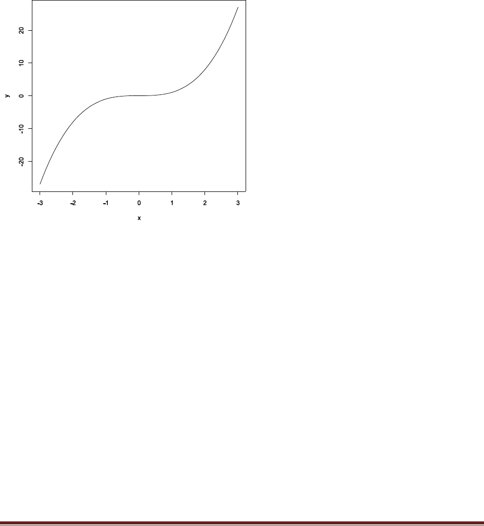
Exercise 2.6. [Purpose: To gain experience with the details of the command syntax within
R.] Adapt the code of SimpleGraph.R so that it plots a cubic function (y = x3) over the
interval x in [–3,+3]. Save the graph in a file format of your choice. Include a listing of your
code, commented, and the resulting graph.
x = seq( from = –3 , to = 3 , by = 0.1 ) # Specify vector of x values.
y = x^3 # Specify corresponding y values.
plot( x , y , type = "l" ) # Make a graph of the x,y points.
dev.copy2eps( file = "CubicGraph.eps" ) # Save the plot to an EPS file.

Solutions Manual for Doing Bayesian Data Analysis by John K. Kruschke Page 5
Chapter 3.
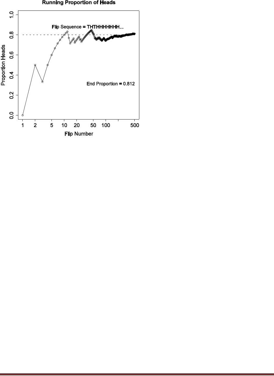
Exercise 3.1. [Purpose: To give you some experience with random number generation in
R.] Modify the coin–flipping program in Section Subsection 3.5.1 (RunningProportion.R)
to simulate a biased coin that has p(H) = 0.8. Change the height of the reference line in the
plot to match p(H). Comment your code. Hint: Read the help for sample.
# Goal: Toss a coin N times and compute the running proportion of heads.
N = 500 # Specify the total number of flips, denoted N.
# Generate a random sample of N flips for a fair coin (heads=1, tails=0);
# the function "sample" is part of R:
#set.seed(47405) # Uncomment to set the "seed" for random number generator.
flipsequence = sample( x=c(0,1) , prob=c(.2,.8) , size=N , replace=TRUE )
# Compute the running proportion of heads:
r = cumsum( flipsequence ) # The function "cumsum" is built in to R.
n = 1:N # n is a vector.
runprop = r / n # component by component division.
# Graph the running proportion:
# To learn about the parameters of the plot function,
# type help('par') at the R command prompt.
# Note that "c" is a function in R.
plot( n , runprop , type="o" , log="x" ,
xlim=c(1,N) , ylim=c(0.0,1.0) , cex.axis=1.5 ,
xlab="Flip Number" , ylab="Proportion Heads" , cex.lab=1.5 ,
main="Running Proportion of Heads" , cex.main=1.5 )
# Plot a dotted horizontal line at y=.8, just as a reference line:
lines( c(1,N) , c(.8,.8) , lty=2 , lwd=2 )
# Display the beginning of the flip sequence. These string and character
# manipulations may seem mysterious, but you can de–mystify by unpacking
# the commands starting with the innermost parentheses or brackets and
# moving to the outermost.
flipletters = paste( c("T","H")[ flipsequence[ 1:10 ] + 1 ] , collapse="" )
displaystring = paste( "Flip Sequence = " , flipletters , "..." , sep="" )
text( 5 , .9 , displaystring , adj=c(0,1) , cex=1.3 )
# Display the relative frequency at the end of the sequence.
text( N , .3 , paste("End Proportion =",runprop[N]) , adj=c(1,0) , cex=1.3 )
# Save the plot to an EPS file.
dev.copy2eps( file = "Exercise3.1.eps" )
Below is an exemplary graph; displays will differ across runs because the flip sequence is
random.
Solutions Manual for Doing Bayesian Data Analysis by John K. Kruschke Page 6
Exercise 3.2. [Purpose: To have you work through an example of the logic presented in
Section 3.2.1.2.] Determine the exact probability of drawing a 10 from a shuffled pinochle
deck. (A pinochle deck has 48 cards. There are six values: 9, 10, jack, queen, king, and ace.
There are two copies of each value in each of the standard four suits: hearts, diamonds,
clubs, and spades.)
(A) What is the probability of getting a 10?
There are 8 10’s in 48 cards, hence p(10) = 8/48.
(B) What is the probability of getting a 10 or jack?
There are 8 10’s and 8 jacks and they are mutually exclusive. Hence p(10 or jack) = (8+8)/48.
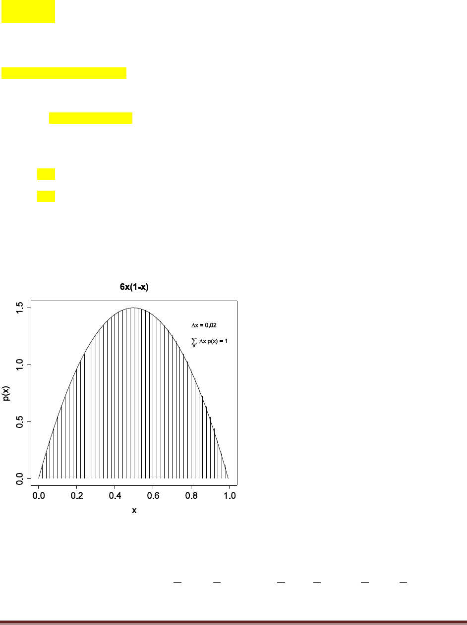
Exercise 3.3. [Purpose: To give you hands–on experience with a simple probability density
function, in R and in calculus, and to reemphasize that density functions can have values
larger than 1.] Consider a spinner with a [0,1] scale on its circumference. Suppose that the
spinner is slanted or magnetized or bent in some way such that it is biased, and its
probability density function is p(x) = 6x(1–x) over the interval x in [0, 1].
(A) Adapt the code from Section Subsection 3.5.2 (IntegralOfDensity.R) to plot this density
function and approximate its integral. Comment your code. Be careful to consider values of
x only in the interval [0, 1]. Hint: You can omit the first couple lines regarding meanval
and sdval, because those parameter values pertain only to the normal distribution. Then set
xlow=0 and xhigh=1.
Solutions Manual for Doing Bayesian Data Analysis by John K. Kruschke Page 7
# Graph of normal probability density function, with comb of intervals.
xlow = 0 # Specify low end of x–axis.
xhigh = 1 # Specify high end of x–axis.
dx = 0.02 # Specify interval width on x–axis
# Specify comb points along the x axis:
x = seq( from = xlow , to = xhigh , by = dx )
# Compute y values, i.e., probability density at each value of x:
y = 6 * x * ( 1 – x )
# Plot the function. "plot" draws the intervals. "lines" draws the curve.
plot( x , y , type="h" , lwd=1 , cex.axis=1.5
, xlab="x" , ylab="p(x)" , cex.lab=1.5
, main="6x(1–x)" , cex.main=1.5 )
lines( x , y )
# Approximate the integral as the sum of width * height for each interval.
area = sum( dx * y )
# Display info in the graph.
text( 0.8 , .9*max(y) , bquote( paste(Delta , "x = " ,.(dx)) )
, adj=c(0,.5) )
text( 0.8 , .8*max(y) ,
bquote(
paste( sum(,x,) , " " , Delta , "x p(x) = " , .(signif(area,3)) )
) , adj=c(0,.5) )
# Save the plot to an EPS file.
dev.copy2eps( file = "Exercise3.3.eps" )
(B) Derive the exact integral using calculus. Hint: See the example, Equation 3.7.
1
3
3
1
2
2
1
3
3
1
2
2
1
6
3
3
1
2
2
1
6)(6))1(6( ]00[]11[][ 1
0
1
0
2
1
0
xx
xxdxxxdx

Solutions Manual for Doing Bayesian Data Analysis by John K. Kruschke Page 8
(C) Does this function satisfy Equation 3.3?
Yes, the integral of the function across its domain is 1, just as it should be for a probability
density function.
(D) From inspecting the graph, what is the maximal value of p(x)?
Visual inspection of the graph suggests that p(x) is maximal at x=0.5. This is also the mean,
because the distribution is symmetric.
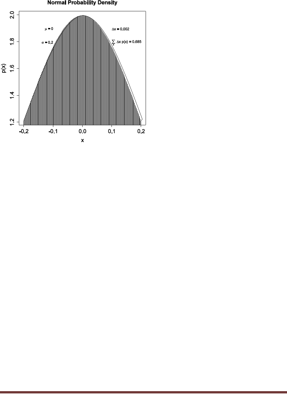
Exercise 3.4. [Purpose: To have you use a normal curve to describe beliefs. It‘s also handy
to know the area under the normal curve between and .]
(A) Adapt the code from Section Subsection 3.5.2 (IntegralOfDensity.R) to determine
(approximately) the probability mass under the normal curve from x = – to x = + .
Comment your code. Hint: Just change xlow and xhigh appropriately, and change the text
location so that the area still appears within the plot.
# Graph of normal probability density function, with comb of intervals.
meanval = 0.0 # Specify mean of distribution.
sdval = 0.2 # Specify standard deviation of distribution.
xlow = meanval – 1*sdval # Specify low end of x–axis.
xhigh = meanval + 1*sdval # Specify high end of x–axis.
dx = 0.002 # Specify interval width on x–axis
# Specify comb points along the x axis:
x = seq( from = xlow , to = xhigh , by = dx )
# Compute y values, i.e., probability density at each value of x:
y = ( 1/(sdval*sqrt(2*pi)) ) * exp( –.5 * ((x–meanval)/sdval)^2 )
# Plot the function. "plot" draws the intervals. "lines" draws the bell
curve.
plot( x , y , type="h" , lwd=1 , cex.axis=1.5
, xlab="x" , ylab="p(x)" , cex.lab=1.5
, main="Normal Probability Density" , cex.main=1.5 )
lines( x , y )
# Approximate the integral as the sum of width * height for each interval.
area = sum( dx * y )
# Display info in the graph.
text( –0.5*sdval , .95*max(y) , bquote( paste(mu ," = " ,.(meanval)) )
, adj=c(1,.5) )
text( –0.5*sdval , .9*max(y) , bquote( paste(sigma ," = " ,.(sdval)) )
, adj=c(1,.5) )
text( 0.5*sdval , .95*max(y) , bquote( paste(Delta , "x = " ,.(dx)) )
, adj=c(0,.5) )
text( 0.5*sdval , .9*max(y) ,
bquote(
paste( sum(,x,) , " " , Delta , "x p(x) = " , .(signif(area,3)) )
) , adj=c(0,.5) )
# Save the plot to an EPS file.
dev.copy2eps( file = "Exercise3.4.eps" )
Solutions Manual for Doing Bayesian Data Analysis by John K. Kruschke Page 9
The graph indicates that the area under the normal curve between and is about 34%.
(B) Now use the normal curve to describe the following belief. Suppose you believe that
women‘s heights follow a bell–shaped distribution, centered at 162 cm with about two–
thirds of all women having heights between 147 cm and 177 cm.
The previous part indicates that about two–thirds of the normal distribution falls between –
and + Therefore we can describe the belief as a normal distribution with mean at 162 and
standard deviation of 177–162=15 (which is the same as 162–147).
Exercise 3.5. [Purpose: To recognize and work with the fact that Equation 3.11 can be
solved for the conjoint probability, which will be crucial for developing Bayes‘ theorem.]
School children were surveyed regarding their favorite foods. Of the total sample, 20%
were 1st graders, 20% were 6th graders, and 60% were 11th graders. For each grade, the
following table shows the proportion of respondents that chose each of three foods as their
favorite:
Ice Cream Fruit French Fries
1st graders 0.3 0.6 0.1
6th graders 0.6 0.3 0.1
11th graders 0.3 0.1 0.6
From that information, construct a table of conjoint probabilities of grade and favorite
food. Also, say whether grade and favorite food are independent and how you ascertained
the answer. Hint: You are given p(grade) and p(food|grade). You need to determine
p(grade, food).

Solutions Manual for Doing Bayesian Data Analysis by John K. Kruschke Page 10
By definition, p(food|grade) = p(grade,food)/p(grade). Therefore p(grade,food) =
p(food|grade)*p(grade). Therefore we multiply each row of the table by its corresponding
marginal distribution to get the conjoint probabilities:
Ice Cream Fruit French Fries
1st graders 0.3*0.2=0.06 0.6*0.2=0.12 0.1*0.2=0.02
6th graders 0.6*0.2=0.12 0.3*0.2=0.06 0.1*0.2=0.02
11th graders 0.3*0.6=0.18 0.1*0.6=0.06 0.6*0.6=0.36
If the attributes were independent, then we could multiply the marginal probabilities to get the
conjoint probabilities. Any cell that violates that equality indicates lack of independence.
Consider, for example, the top left cell. Its conjoint probability is p(1stGrade,IceCream) = 0.06.
On the other hand, the product of the marginals is p(1stGrade) * p(IceCream) = 0.20 * 0.36 =
0.072, which does not equal the conjoint probability.

Solutions Manual for Doing Bayesian Data Analysis by John K. Kruschke Page 11
Chapter 4.
Exercise 4.1. [Purpose: Application of Bayes‘ rule to disease diagnosis, to see the important
role of prior probabilities.] Suppose that in the general population, the probability of
having a particular rare disease is 1 in a 1000. We denote the true presence or absence of
the disease as the value of a parameter, , that can have the value = if disease is
present, or the value = if the disease is absent. The base rate of the disease is therefore
denoted p(= ) = 0.001. This is our prior belief that a person selected at random has the
disease.
Suppose that there is a test for the disease that has a 99% hit rate, which means that if a
person has the disease, then the test result is positive 99% of the time. We denote a positive
test result as D = + and a negative test result as D = –. The observed test result is a bit of
data that we will use to modify our belief about the value of the underlying disease
parameter. The hit rate is expressed as p( D = + | = ) = 0.99. The test also has a false
alarm rate of 5%. This means that 5% of the time when the disease is not present, the test
falsely indicates that the disease is present. We denote the false alarm rate as p( D = + | =
) = 0.05.
Suppose we sample a person at random from the population, administer the test, and it
comes up positive. What is the posterior probability that the person has the disease?
Mathematically expressed, we are asking, what is p(= | D = + )? Before determining the
answer from Bayes‘ rule, generate an intuitive answer and see if your intuition matches the
Bayesian answer. Most people have an intuition that the probability of having the disease is
near the hit rate of the test (which in this case is 0.99).
Hint: The following table of conjoint probabilities might help you understand the possible
combinations of events. (The following table is a specific case of Table 4.2, p. 57.) The prior
probabilities of the disease are on the bottom marginal. When we know that the test result
is positive, we restrict our attention the row marked D = +.
[The table is not reproduced here.]
By Bayes’ rule,
p(= | D = + ) = p(D = + | = ) p(= ) / p(D = +)
= p(D = + | = ) p(= ) / [ p(D=+|=) p(=) + p(D=+|=) p(=) ]
= 0.99 * 0.001 / [ 0.99 * 0.001 + 0.05 * 0.999 ]
= 0.0194 (rounded to three significant digits)
Thus, despite the high hit rate of the test, the small prior and non–negligible false–alarm rate
make the posterior probability less than 2%. (This analysis assumes that there were no other
symptoms and that the person was selected at random so that the prior is applicable.)

Solutions Manual for Doing Bayesian Data Analysis by John K. Kruschke Page 12
Exercise 4.2. [Purpose: Iterative application of Bayes‘ rule, to see how posterior
probabilities change with inclusion of more data.] Continuing from the previous exercise,
suppose that the same randomly selected person as in the previous exercise is retested after
the first test comes back positive, and on the retest the result is negative. Now what is the
probability that the person has the disease? Hint: For the prior probability of the retest,
use the posterior computed from the previous exercise. Also notice that
p(D = – | = ) = 1 – p(D = + | = ) and p(D = – | = ) = 1 – p(D = + | = ).
To avoid rounding error, it is important to retain many significant digits for the prior. From the
previous exercise, p(= ) = 0.0194346289753. Then, by Bayes’ rule,
p(= | D = – ) = p(D = – | = ) p(= ) / p(D = –)
= p(D = – | = ) p(= ) / [ p(D=–|=) p(=) + p(D=–|=) p(=) ]
where p(= ) is the posterior from the previous exercise. Hence
p(= | D = – ) = (1–0.99)*0.0194… / [ (1–0.99)*0.0194… + (1–.05)*( 1–0.0194… ) ]
= 0.000209 (rounded to three significant digits)
Exercise 4.3. [Purpose: To get an intuition for the previous results by using ―natural
frequency‖ and ―Markov‖ representations.]
(A) Suppose that the population consists of 100,000 people. Compute how many people
should fall into each cell of the table in the hint shown in Exercise 4.1. To compute the
expected frequency of people in a cell, just multiply the cell probability by the size of the
population. To get you started, a few of the cells of the frequency table are filled in [below].
… Your job for this part of the exercise is to fill in the frequencies of the remaining cells of
the table.
θ =
θ =
D = +
freq(D = + , = )
= p(D = + , = ) N
= p(D = + | = ) p(= ) N
= .99 * .001 * 100000
= 99
freq(D = + , = )
= p(D = + , = ) N
= p(D = + | = ) p(= ) N
= .05 * (1-.001) * 100000
= 4,995
5,094
D = –
freq(D = – , = )
= p(D = – , = ) N
= p(D = – | = ) p(= ) N
= (1-.99) * .001 * 100000
= 1
freq(D = – , = )
= p(D = – , = ) N
= p(D = – | = ) p(= ) N
= (1-.05) * (1-.001) * 100000
= 94,905
94,906
100
99,900
N=100,000
(B) Take a good look at the frequencies in the table you just computed for the previous
part. These are the so-called ―natural frequencies‖ of the events, as opposed to the
somewhat unintuitive expression in terms of conditional probabilities (Gigerenzer &
Hoffrage, 1995). From the cell frequencies alone, determine the proportion of people who
have the disease, given that their test result is positive. Before computing the exact answer
Solutions Manual for Doing Bayesian Data Analysis by John K. Kruschke Page 13
arithmetically, first give a rough intuitive answer merely by looking at the relative
frequencies in the row D = +. Does your intuitive answer match the intuitive answer you
provided back in Exercise 4.1? Probably not. Your intuitive answer here is probably much
closer to the correct answer. Now compute the exact answer arithmetically. It should match
the result from applying Bayes‘ rule in Exercise 4.1.
The result is positive, so we focus attention on the row D = +, which has a total of 5,094 people
of whom 99 have the disease. Hence
p(= | D = + ) = 99 / 5094 = 0.01943463
This exactly matches the result of Exercise 4.1.
(C) Now we‘ll consider a related representation of the probabilities in terms of natural
frequencies, which is especially useful when we accumulate more data. Krauss, Martignon,
& Hoffrage (1999) called this type of representation a ―Markov‖ representation. Suppose
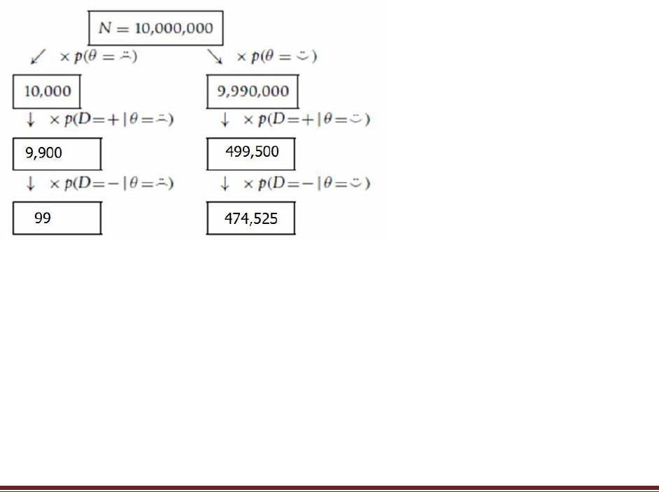
now we start with a population of N D 10,000,000 people. We expect 99.9% of them (i.e.,
9,990,000) not to have the disease, and just 0.1% (i.e., 10,000) to have the disease. Now
consider how many people we expect to test positive. Of the 10,000 people who have the
disease, 99% (i.e., 9900), will be expected to test positive. Of the 9,990,000 people who do
not have the disease, 5%, (i.e., 499,500) will be expected to test positive. Now consider
retesting everyone who has tested positive on the first test. How many of them are expected
to show a negative result on the retest? Use this diagram to compute your answer:
(D) Use the diagram in the previous part to answer this question: What proportion of
people who test positive at first and then negative on retest actually have the disease? In
other words, of the total number of people at the bottom of the diagram in the previous
part (those are the people who tested positive then negative), what proportion of them are
in the left branch of the tree? How does the result compare with your answer to Exercise
4.2?
Notice that the total of the bottom is 99 + 474,525 = 474,624 people who test positive and
negative. The proportion of those who actually have the disease is 99 / 474,624 = 0.000209
(rounded to three significant digits). This matches the result from Exercise 4.2.

Solutions Manual for Doing Bayesian Data Analysis by John K. Kruschke Page 14
Exercise 4.4. [Purpose: To see a hands-on example of data-order invariance.] Consider
again the disease and diagnostic test of the previous two exercises. Suppose that a person
selected at random from the population gets the test and it comes back negative. Compute
the probability that the person has the disease. The person then is retested, and on the
second test the result is positive. Compute the probability that the person has the disease.
How does the result compare with your answer to Exercise 4.2?
As noted in the answer to Exercise 4.2, retention of many significant digits is important to avoid
rounding error.
After the first (negative) test,
p(= | D = – ) = p(D = – | = ) p(= ) / p(D = –)
= p(D = – | = ) p(= ) / [ p(D=–|=) p(=) + p(D=–|=) p(=) ]
= (1–0.99)*0.001 / [ (1–0.99)*0.001 + (1–.05)*( 1–0.001 ) ]
= 0.0000105367416180
After the second (positive) test,
p(= | D = + ) = p(D = + | = ) p(= ) / p(D = +)
= p(D = + | = ) p(= ) / [ p(D=+|=) p(=) + p(D=+|=) p(=) ]
= 0.99 * 0.0000105… / [ 0.99 * 0.0000105… + 0.05 * (1-0.0000105…) ]
= 0.000209 (rounded to three significant digits)
This result matches the previous exercises.
Exercise 4.5. [Purpose: An application of Bayes‘ rule to neuroscience, to infer cognitive
function from brain activation.] Cognitive neuroscientists investigate which areas of the
brain are active during particular mental tasks. In many situations, researchers observe
that a certain region of the brain is active and infer that a particular cognitive function is
therefore being carried out. Poldrack (2006) cautioned that such inferences are not
necessarily firm and need to be made with Bayes‘ rule in mind. Poldrack (2006) reported
the following frequency table of previous studies that involved any language-related task
(specifically phonological and semantic processing) and whether or not a particular region
of interest (ROI) in the brain was activated:
Language Study Not Language Study
Activated 166 199
Not activated 703 2154
Suppose that a new study is conducted and finds that the ROI is activated. If the prior
probability that the task involves language processing is 0.5, what is the posterior
probability, given that the ROI is activated? (Hint: Poldrack (2006) reports that it is 0.69.
You job is to derive this number.)
p( Lang. | ROI Act. ) = p( ROI Act. | Lang. ) p( Lang. )
/ (p(ROI Act. | Lang.) p(Lang.) + p(ROI Act. | NotLang.) p(NotLang.) )
= 166/(166+703)*0.5 / (166/(166+703)*0.5 + 199/(199+2154)*0.5 )
= 0.693
Notice that the posterior probability of involving language is only a little higher than the prior.

Solutions Manual for Doing Bayesian Data Analysis by John K. Kruschke Page 15
Exercise 4.6. [Purpose: To make sure you really understand what is being shown in Figure
4.1.] Derive the posterior distribution in Figure 4.1 by hand. The prior has p(= .25) = .25,
p(= .50) = .50, and p(= .75) = .25. The data consist of a specific sequence of flips with
three heads and nine tails, so p(D|) = 3(1-. Hint: Check that your posterior
probabilities sum to 1.
p(=.25|D) = p(D|=.25) p(=.25)
/ [p(D|=.25) p(=.25) + p(D|=.50) p(=.50) + p(D|=.75) p(=.75) ]
= .253(1-.25)9*.25
/ [ .253(1-.25)9*.25 + .503(1-.50)9*.50 + .753(1-.75)9*.25 ]
= 0.705
Similarly, p(=.50|D) = 0.294 and p(=.75|D) = 0.001.
(For future reference, the denominator in the equation above is 0.0004158, rounded to four
significant digits.)
Exercise 4.7. [Purpose: For you to see, hands on, that p(D) lives in the denominator of
Bayes‘ rule.] Compute p(D) in Figure 4.1 by hand. Hint: Did you notice that you already
computed p(D) in the previous exercise?
p(D) = p(D|=.25) p(=.25) + p(D|=.50) p(=.50) + p(D|=.75) p(=.75)
which is the denominator from the previous exercise, where we found that p(D)=0.0004158.
Solutions Manual for Doing Bayesian Data Analysis by John K. Kruschke Page 16
Chapter 5.
Exercise 5.1. [Purpose: To see the influence of the prior in each successive flip, and to see
another demonstration that the posterior is invariant under reorderings of the data.] For
this exercise, use the R function of Section 5.5.1 (BernBeta.R). (Read the comments at the
top of the code for an example of how to use it, and don‘t forget to source the function
before calling it.) Notice that the function returns the posterior beta values each time it is
called, so you can use the returned values as the prior values for the next function call.
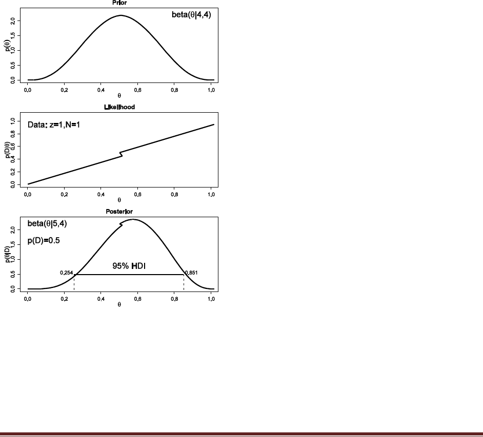
(A) Start with a prior distribution that expresses some uncertainty that a coin is fair:
beta(|4, 4). Flip the coin once; suppose we get a head. What is the posterior distribution?
At the R command prompt, typing
post = BernBeta( c(4,4) , c(1) )
yields this figure:
(The jagged bits in the curve are artifacts of how Microsoft Word incorrectly renders EPS
figures. The curves are actually smooth.)
Solutions Manual for Doing Bayesian Data Analysis by John K. Kruschke Page 17
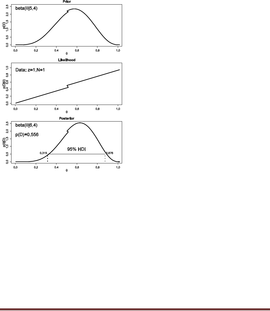
(B) Use the posterior from the previous flip as the prior for the next flip. Suppose we flip
again and get a head. Now what is the new posterior? (Hint: If you type post = BernBeta(
c(4,4) , c(1) ) for the first part, then you can type post = BernBeta( post , c(1) ) for the next
part.)
At the R command prompt, typing
post = BernBeta( post , c(1) )
yields this figure:
(The jagged bits in the curve are artifacts of how Microsoft Word incorrectly renders EPS
figures. The curves are actually smooth.)
Solutions Manual for Doing Bayesian Data Analysis by John K. Kruschke Page 18
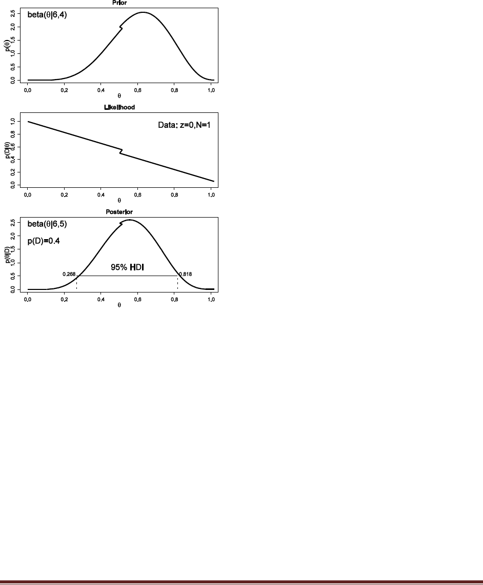
(C) Using that posterior as the prior for the next flip, flip a third time and get T. Now what
is the new posterior? (Hint: Type post = BernBeta( post , c(0) ).)
At the R command prompt, typing
post = BernBeta( post , c(0) )
yields this figure:
(The jagged bits in the curve are artifacts of how Microsoft Word incorrectly renders EPS
figures. The curves are actually smooth.)
Solutions Manual for Doing Bayesian Data Analysis by John K. Kruschke Page 19
(D) Do the same three updates but in the order T, H, H instead of H, H, T. Is the final
posterior distribution the same for both orderings of the flip results?
The sequence of commands is
post = BernBeta( c(4,4) , c(0) )
post = BernBeta( post , c(1) )
post = BernBeta( post , c(1) )
and the final graph looks like this:
Notice that the ultimate posterior is the same as Part C, but the prior leading up to it is different
because of the different sequence of updating. (The jagged bits in the curve are artifacts of how
Microsoft Word incorrectly renders EPS figures. The curves are actually smooth.)
Solutions Manual for Doing Bayesian Data Analysis by John K. Kruschke Page 20
Exercise 5.2. [Purpose: To connect HDIs to the real world, with iterative data collection.]
Suppose an election is approaching, and you are interested in knowing whether the general
population prefers candidate A or candidate B. A just published poll in the newspaper
states that of 100 randomly sampled people, 58 preferred candidate A and the remainder
preferred candidate B.
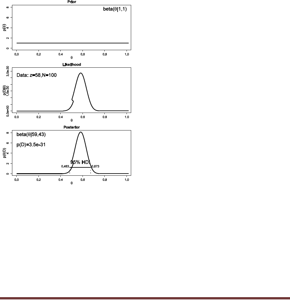
(A) Suppose that before the newspaper poll, your prior belief was a uniform distribution.
What is the 95% HDI on your beliefs after learning of the newspaper poll results?
The R command
post = BernBeta( c(1,1) , c( rep(1,58) , rep(0,42) ) )
yields
which has a 95% HDI from 0.483 to 0.673. (The jagged bits in the curve are artifacts of how
Microsoft Word incorrectly renders EPS figures. The curves are actually smooth.)
(B) Based in the newspaper poll, is it credible to believe that the population is equally
divided in its preferences among candidates?
The HDI from Part A shows that =0.5 is among the credible values, hence it is credible to
believe that the population is equally divided in its preferences.
Solutions Manual for Doing Bayesian Data Analysis by John K. Kruschke Page 21
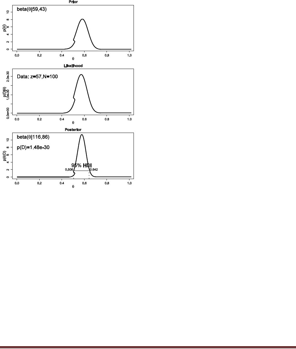
(C) You want to conduct a follow-up poll to narrow down your estimate of the population‘s
preference. In your follow-up poll, you randomly sample 100 people and find that 57 prefer
candidate A and the remainder prefer candidate B. Assuming that peoples‘ opinions have
not changed between polls, what is the 95% HDI on the posterior?
The R command
post = BernBeta( post , c( rep(1,57) , rep(0,43) ) )
yields
which has a 95% HDI from 0.506 to 0.642 (The jagged bits in the curve are artifacts of how
Microsoft Word incorrectly renders EPS figures. The curves are actually smooth.)
(D) Based on your follow-up poll, is it credible to believe that the population is equally
divided in its preferences among candidates?
The HDI from Part C excludes =0.5, hence we could decide that the population is not equally
divided (and prefers candidate A).
Exercise 5.3. [Purpose: To apply the Bayesian method to real data analysis. These data are
representative of real data (Kruschke, 2009).] Suppose you train people in a simple
learning experiment, as follows. When people see the two words ―radio‖ and ―ocean,‖ on
the computer screen, they should press the F key on the computer keyboard. They see
several repetitions and learn the response well. Then you introduce another
correspondence for them to learn: Whenever the words ―radio‖ and ―mountain‖ appear,
Solutions Manual for Doing Bayesian Data Analysis by John K. Kruschke Page 22
they should press the J key on the computer keyboard. You keep training them until they
know both correspondences well. Now you probe what they‘ve learned by asking them
about two novel test items. For the first test, you show them the word ―radio‖ by itself and
instruct them to make the best response (F or J) based on what they learned before. For the
second test, you show them the two words ―ocean‖ and ‖mountain‖ and ask them to make
the best response. You do this procedure with 50 people. Your data show that for ―radio‖
by itself, 40 people chose F and 10 chose J. For the word combination ―ocean‖ and
―mountain,‖ 15 chose F and 35 chose J. Are people biased toward F or toward J for either
of the two probe types? To answer this question, assume a uniform prior, and use a 95%
HDI to decide which biases can be declared to be credible.
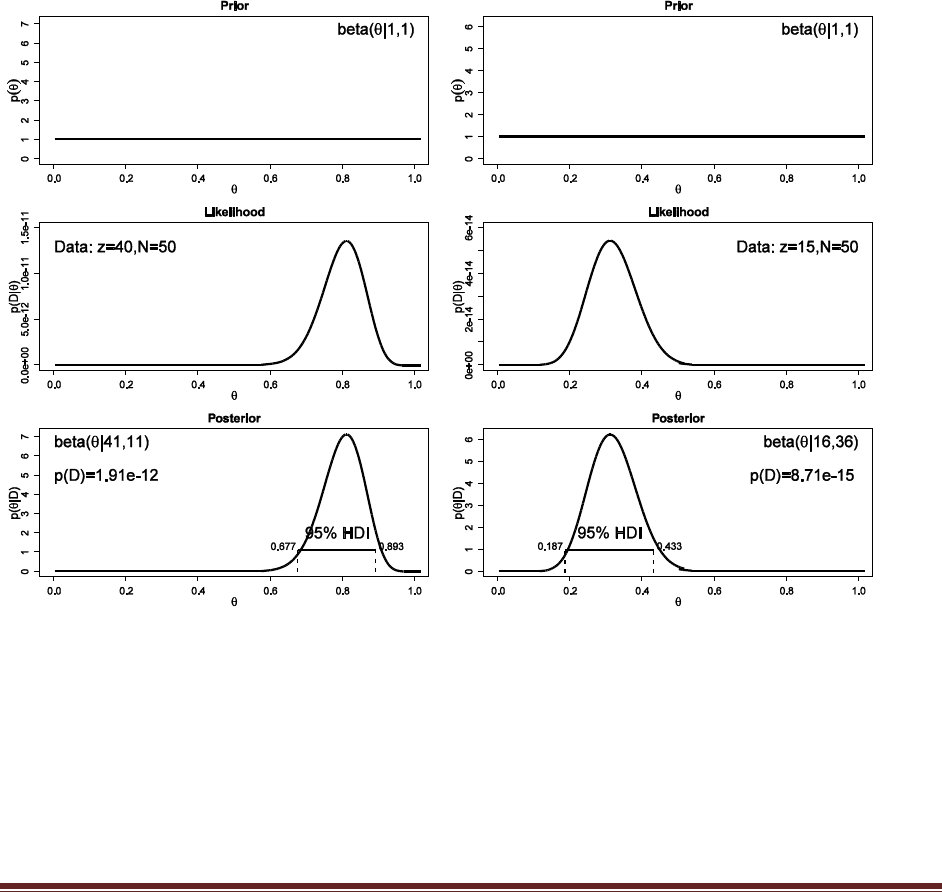
The commands
post = BernBeta( c(1,1) , c( rep(1,40) , rep(0,10) ) )
post = BernBeta( c(1,1) , c( rep(1,15) , rep(0,35) ) )
yield these graphs:
In both cases, the 95% HDI excludes =0.5, and so we can decide that people are indeed biased
in their responses, toward F in the first case but toward J in the second case.
Solutions Manual for Doing Bayesian Data Analysis by John K. Kruschke Page 23
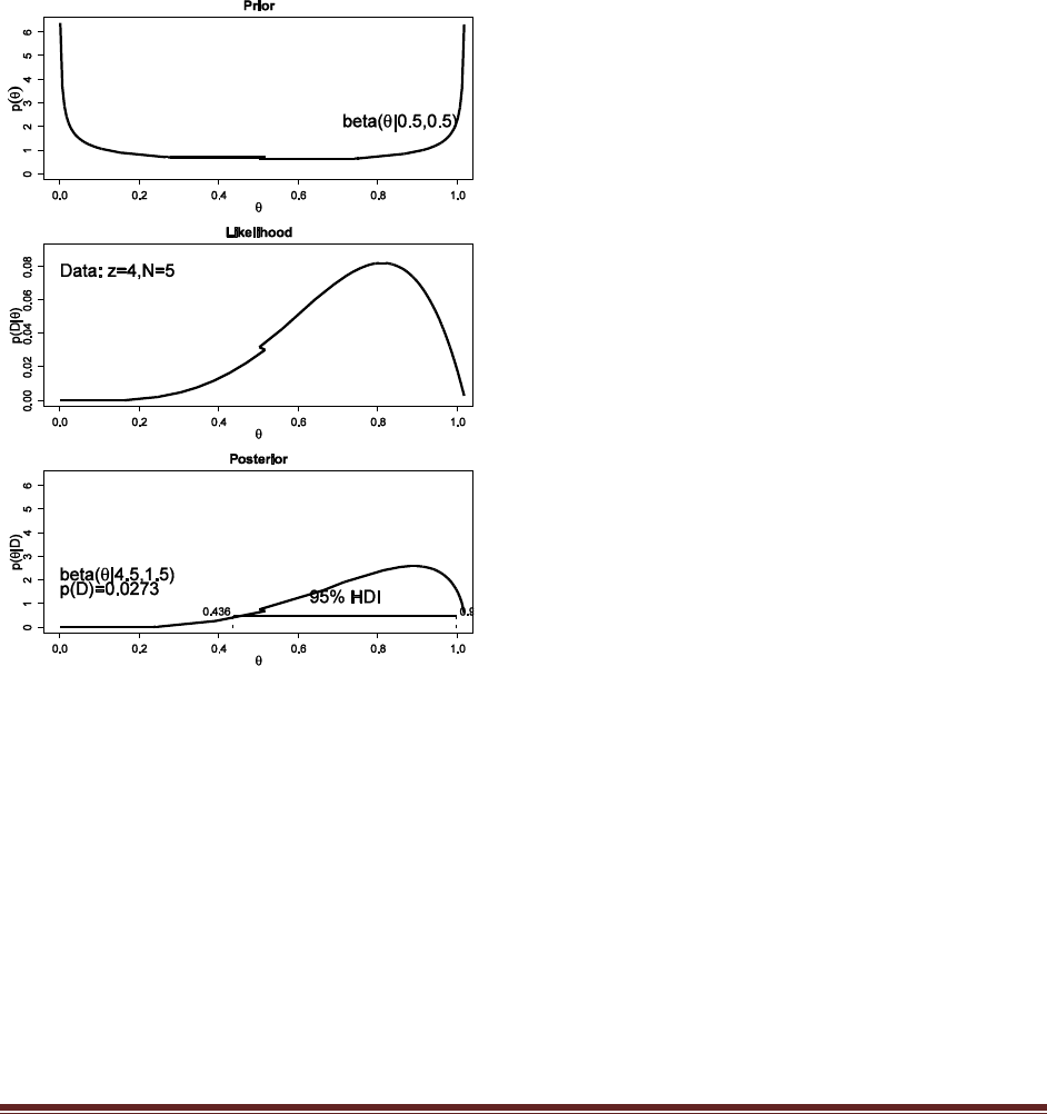
Exercise 5.4. [Purpose: To explore an unusual prior and learn about the beta distribution
in the process.] Suppose we have a coin that we know comes from a magic-trick store, and
therefore we believe that the coin is strongly biased either usually to come up heads or
usually to come up tails, but we don‘t know which. Express this belief as a beta prior.
(Hint: See Figure 5.1, upper-left panel.) Now we flip the coin five times and it comes up
heads in four of the five flips. What is the posterior distribution? (Use the R function of
Section 5.5.1 (BernBeta.R) to see graphs of the prior and posterior.)
The R command
post = BernBeta( c(.5,.5) , c(1,1,1,1,0) )
yields
(The jagged bits in the curve are artifacts of how Microsoft Word incorrectly renders EPS
figures. The curves are actually smooth.)

Solutions Manual for Doing Bayesian Data Analysis by John K. Kruschke Page 24
Exercise 5.5. [Purpose: To get hands-on experience with the goal of predicting the next
datum, and to see how the prior influences that prediction.]
(A) Suppose you have a coin that you know is minted by the federal government and has
not been tampered with. Therefore, you have a strong prior belief that the coin is fair. You
flip the coin 10 times and get 9 heads. What is your predicted probability of heads for the
11th flip? Explain your answer carefully; justify your choice of prior.
To justify a prior, we might say that our strength of fairness is equivalent to having previously
seen the coin flipped 100 times and coming up heads in 50% of those flips. Hence the prior
would be beta(|,50,50). (This is not the only correct answer; you might instead be more
confident, and use a beta(|,500,500) if you suppose you’ve previously seen 1,000 flips with
50% heads.)
The posterior is beta(|,50+9,50+1), which has a mean of 59/(59+51) = 0.536. This is the
predicted probability of heads for the next, i.e., 11th, flip.
(B) Now you have a different coin, this one made of some strange material and marked (in
fine print) ―Patent Pending, International Magic, Inc.‖ You flip the coin 10 times and get 9
heads. What is your predicted probability of heads for the 11th flip? Explain your answer
carefully; justify your choice of prior. Hint: Use the prior from Exercise 5.4.
We use a beta(|0.5,0.5) prior, like Exercise 5.4, because it expresses a belief that the coin is
either head biased or tail biased. The posterior is beta(|,0.5+9,0.5+1), which has a mean of
9.5/(9.5+1.5) = 0.863. This is the predicted probability of heads for the next, i.e., 11th, flip.
Notice that it is quite different than the conclusion from Part A.
Solutions Manual for Doing Bayesian Data Analysis by John K. Kruschke Page 25
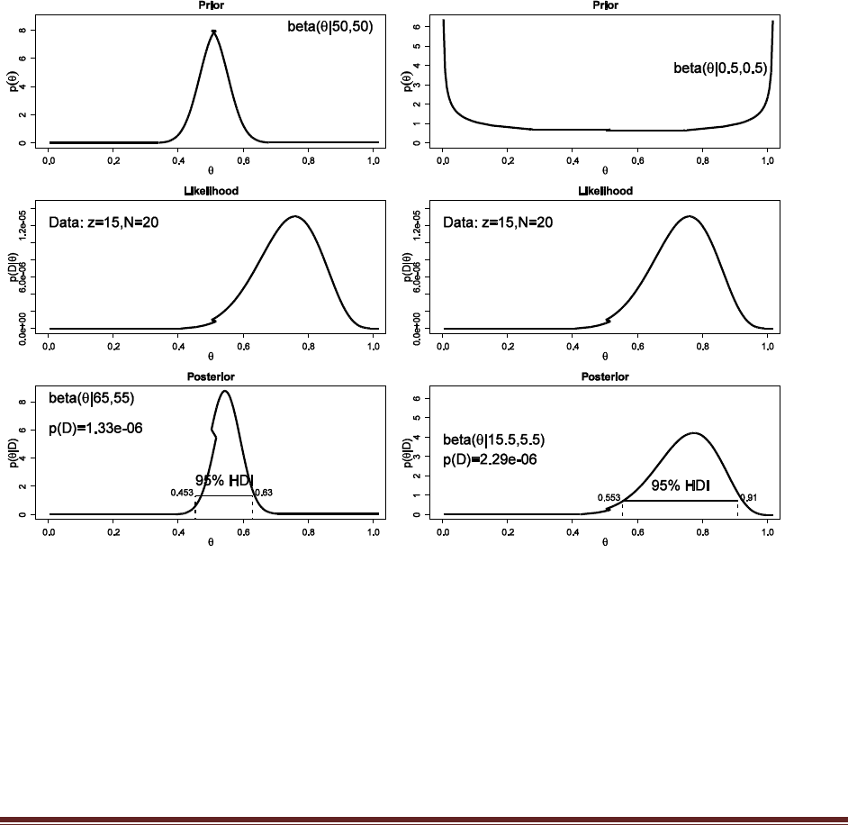
Exercise 5.6. [Purpose: To get hands-on experience with the goal of model comparison.]
Suppose we have a coin, but we‘re not sure whether it‘s a fair coin or a trick coin. We flip it
20 times and get 15 heads. Is it more likely to be fair or trick? To answer this question,
consider the value of the Bayes factor (i.e., the ratio of the evidences of the two models).
When answering this question, justify your choice of priors to express the two hypotheses.
Use the R function of Section 5.5.1 (BernBeta.R) to graph the priors and check that they
reflect your beliefs; the R function will also determine the evidences from Equation 5.10.
For the fair coin, we’ll use a beta(|50,50) prior to be consistent with Exercise 5.5(A), and for the
trick coin we’ll use a beta(|0.5,0.5) prior to be consistent with Exercise 5.4 (and both of those
Exercises had justifications for those priors). Typing the R commands
post = BernBeta( c(50,50) , c( rep(1,15) , rep(0,5) ) )
post = BernBeta( c(0.5,0.5) , c( rep(1,15) , rep(0,5) ) )
yields
The posteriors show that p(D) is somewhat higher for the trick-coin prior than for the fair-coin
prior. (Note: If the priors are different, the conclusion might be different!) (The jagged bits in the
curve are artifacts of how Microsoft Word incorrectly renders EPS figures. The curves are
actually smooth.)
Solutions Manual for Doing Bayesian Data Analysis by John K. Kruschke Page 26
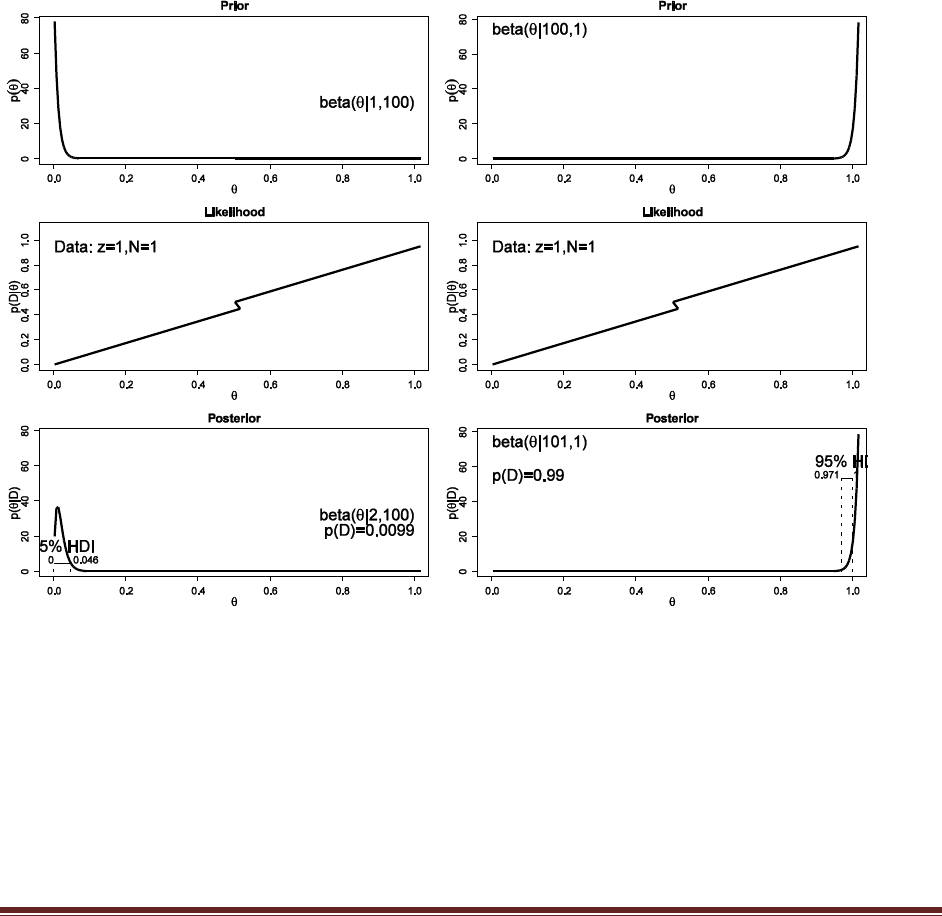
Exercise 5.7. [Purpose: To see how very small data sets can give strong leverage in model
comparison when the model predictions are very different.] Suppose we have a coin that we
strongly believe is a trick coin, so it almost always comes up heads or it almost always
comes up tails; we just don‘t know if the coin is the head-biased type or the tail-biased type.
Thus, one model is a beta prior heavily biased toward tails, beta(|1,100), and the other
model is a beta prior heavily biased toward heads, beta(|100,1). We flip the coin once and
it comes up heads. Based on that single flip, what is the value of the Bayes factor (i.e., the
ratio of the evidences of the two models)? Use the R function of Section 5.5.1 (BernBeta.R)
to determine the evidences from Equation 5.10.
The R commands
post = BernBeta( c(1,100) , c(1) )
post = BernBeta( c(100,1) , c(1) )
yield the following graphs:
The head-biased prior is favored by a Bayes factor of 0.9900/0.0099 = 100, based on this single
flip. (The jagged bits in the curve are artifacts of how Microsoft Word incorrectly renders EPS
figures. The curves are actually smooth.)

Solutions Manual for Doing Bayesian Data Analysis by John K. Kruschke Page 27
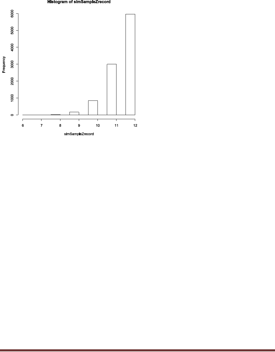
Exercise 5.8. [Purpose: Hands-on learning about the method of posterior predictive
checking.] Following the scenario of the previous exercise, suppose we flip the coin a total
of N=12 times and it comes up heads in z=8 of those flips. Suppose we let a beta(|100,1)
distribution describe the head-biased trick coin, and we let a beta(|1,100) distribution
describe the tail-biased trick coin.
(A) What are the evidences for the two models, and what is the value of the Bayes factor?
Running BernBeta in R shows that for the 100,1 prior, p(D)=1.49e-07, and for the 1,100 prior,
p(D)=2.02e-12. The Bayes factor is 1.49e-07 / 2.02e-12 = 73,800 (rounded). In other words, the
head-biased prior is favored by a factor of more than 73,000 relative to the tail-biased prior!
Now for the new part, a posterior predictive check. Is the winning model actually a good
model of the data? In other words, one model can be whoppingly better than the other, but
that does not necessarily mean that the winning model is a good model; it might mean
merely that the winning model is less bad than the losing model. One way to examine the
veracity of the winning model is to simulate data sampled from the winning model and see
if the simulated data ―look like‖ the actual data. To simulate data generated by the winning
model, we do the following: First, we will randomly generate a value of from the posterior
distribution of the winning model. Second, using that value of , we will generate a sample of
coin flips. Third, we will count the number of heads in the sample, as a summary of the
sample. Finally, we determine whether the number of heads in a typical simulated sample
is close to the number of heads in our actual sample. The following program carries out
these steps. Study it, run it, and answer the questions that follow.
[program excluded to save space]
(B) How many samples (each of size N) were simulated?
The program line
nSimSamples = 10000
sets the number of simulated samples to 10000.
(C) Was the same value of used for every simulated sample, or were different values of
used in different samples? Why?
The program line
sampleTheta = rbeta( 1 , postA , postB )
randomly generates a different value for theta in every sample. This is because the various theta
values are representative of the entire posterior distribution.
Solutions Manual for Doing Bayesian Data Analysis by John K. Kruschke Page 28
(D) Based on the simulation results, does the winning model seem to be a good model? Why
or why not?
The program creates the histogram shown above, in which we can see that the model almost
never generates simulated data in which z=8. The reason is that the head-biased model is
extremely head-biased, but the result, 8 heads out of 12 flips, is only moderately head biased.
Thus, despite the fact that the extremely head-biased model is far better than the extremely tail-
biased model, the extremely head-biased model is a poor model of the actual data.

Solutions Manual for Doing Bayesian Data Analysis by John K. Kruschke Page 29
Chapter 6.
Exercise 6.1. [Purpose: To understand the discretization used for the priors in the R
functions of Section 6.7.1 (BernGrid.R) and throughout this chapter.] Consider this R code
for discretizing a beta(|8,4) distribution:
nIntervals = 10
width = 1 / nIntervals
Theta = seq( from = width/2 , to = 1-width/2 , by = width )
approxMass = dbeta( Theta , 8 , 4 ) * width
pTheta = approxMass / sum( approxMass )
(A) What is the value of sum(approxMass)? Why is it not exactly 1?
0.9991421. This is not exactly 1.0 because this is, after all, a discrete approximation. We are
lucky, in fact, that the sum is so close to 1.0 when using such wide intervals. As the width of the
bins gets smaller, the sum will tend to get closer to 1.0.
(B) Suppose we use instead the following code to define the grid of points:
Theta = seq( from = 0 , to = 1 , by = width )
Why is this not appropriate? (Hint: Consider exactly what intervals are represented by the
first and last values in Theta. Do those first and last intervals have the same widths as the
other intervals? If they do, do they fall entirely within the domain of the beta distribution?)
This definition of intervals is infelicitous because the first and last intervals are centered at the
end points of the domain, and therefore half of those intervals refer to values of theta that are
invalid. In the limit, as the bin width goes toward zero, this problem becomes negligible. Another
problem is that sometimes --- in particular for beta distributions with shape parameters less than
1 --- the density of the distribution at 0 or 1 can be infinite. We will stick to the method of Part A
to be sure to avoid these problems.
Exercise 6.2. [Purpose: To practice specifying a nonbeta prior.] Suppose we have a coin
that has a head on one side and a tail on the other. We think it might be fair, or it might be
a trick coin that is heavily biased toward heads or tails. We want to express this prior belief
with a single prior over . Therefore, the prior needs to have three peaks: one near zero, one
around 0.5, and near 1.0. But these peaks are not just isolated spikes, because we have
uncertainty about the actual value of .
(A) Express your prior belief as a list of probability masses over a fairly dense grid of
values. Remember to set a gradual decline around the three peaks. Briefly justify your
choice. Hint: You can specify the peaks however you want, but one simple way is something
like this:
pTheta = c( 50:1 , rep(1,50) , 1:50 , 50:1 , ...
pTheta = pTheta / sum( pTheta )
width = 1 / length(pTheta)
Solutions Manual for Doing Bayesian Data Analysis by John K. Kruschke Page 30
Theta = seq( from = width/2 , to = 1-width/2 , by = width )
The exercise does not demand one specific answer. One reasonable answer completes the code in
the Hint above, and is illustrated in the graph of Part B below.
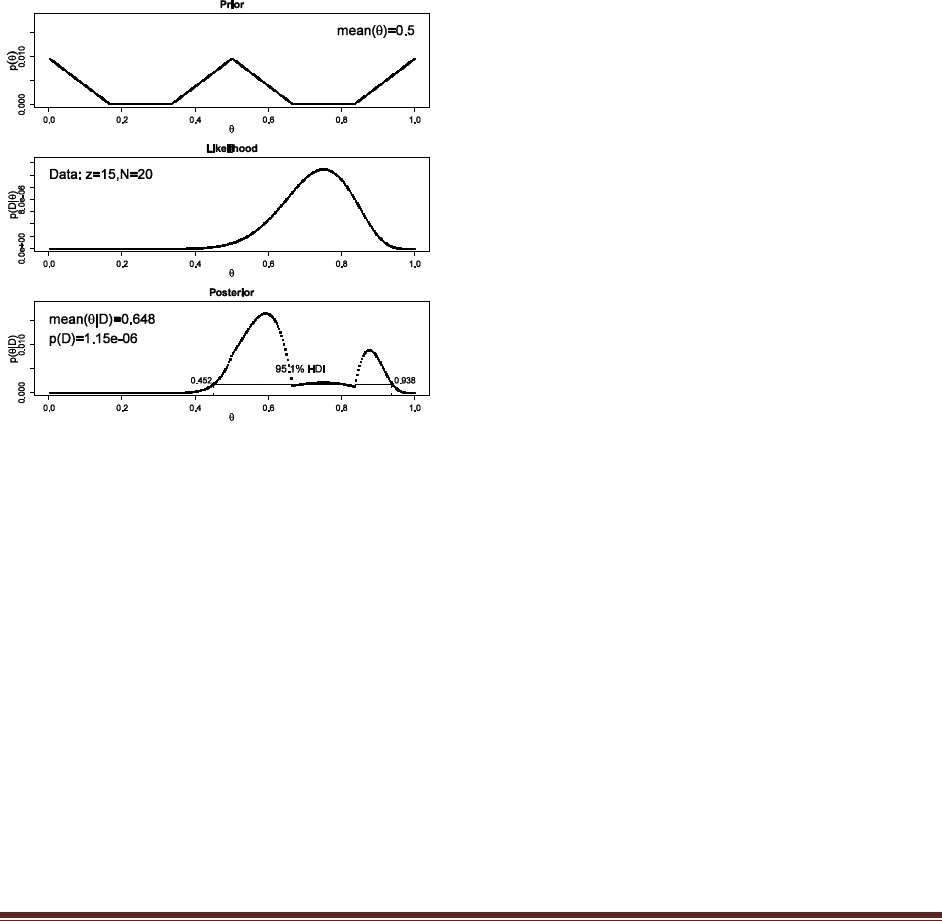
(B) Suppose you flip the coin 20 times and get 15 heads. Use the R function of Section 6.7.1
(BernGrid.R) to display the posterior beliefs. Include the R code you used to specify the
prior values.
pTheta = c( 50:1 , rep(1,50) , 1:50 , 50:1 , rep(1,50) , 1:50 )
pTheta = pTheta / sum( pTheta )
width = 1 / length(pTheta)
Theta = seq( from = width/2 , to = 1-width/2 , by = width )
post = BernGrid( Theta , pTheta , c(rep(1,15),rep(0,5)) )
Exercise 6.3. [Purpose: To use the function of Section 6.7.1 (BernGrid.R) for sequential
updating (i.e., use output of one function call as the prior for the next function call).
Observe that data ordering does not matter]
(A) Using the same prior that you used for the previous exercise, suppose you flip the coin
just 4 times and get 3 heads. Use the R function of Section 6.7.1 (BernGrid.R) to display the
posterior.
(B) Suppose we flip the coin an additional 16 times and get 12 heads. Now what is the
posterior distribution? To answer this question, use the posterior distribution that is output
by the function in the previous part as the prior for this part. Show the R commands you
used to call the function. (Hint: The final posterior should match the posterior of Exercise
6.2, except that the graph of the prior should look like the posterior from the previous part.
Figure 6.5 shows an example.)
pTheta = c( 50:1 , rep(1,50) , 1:50 , 50:1 , rep(1,50) , 1:50 )
pTheta = pTheta / sum( pTheta )
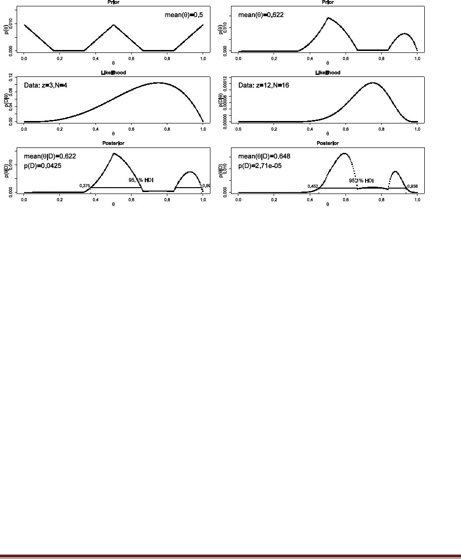
Solutions Manual for Doing Bayesian Data Analysis by John K. Kruschke Page 31
width = 1 / length(pTheta)
Theta = seq( from = width/2 , to = 1-width/2 , by = width )
post = BernGrid( Theta , pTheta , c(rep(1,3),rep(0,1)) )
post = BernGrid( Theta , post , c(rep(1,12),rep(0,4)) )
# Notice that post from the first call to BernGrid was used as the prior for
# the second call to BernGrid.
Notice that the ultimate posterior matches the one from the previous exercise.
Exercise 6.4. [Purpose: To connect HDIs to the real world, with iterative data collection.]
Suppose an election is approaching, and you are interested in knowing whether the general
population prefers candidate A or candidate B. A just-published poll in the newspaper
states that of 100 randomly sampled people, 58 preferred candidate A and the remainder
preferred candidate B.
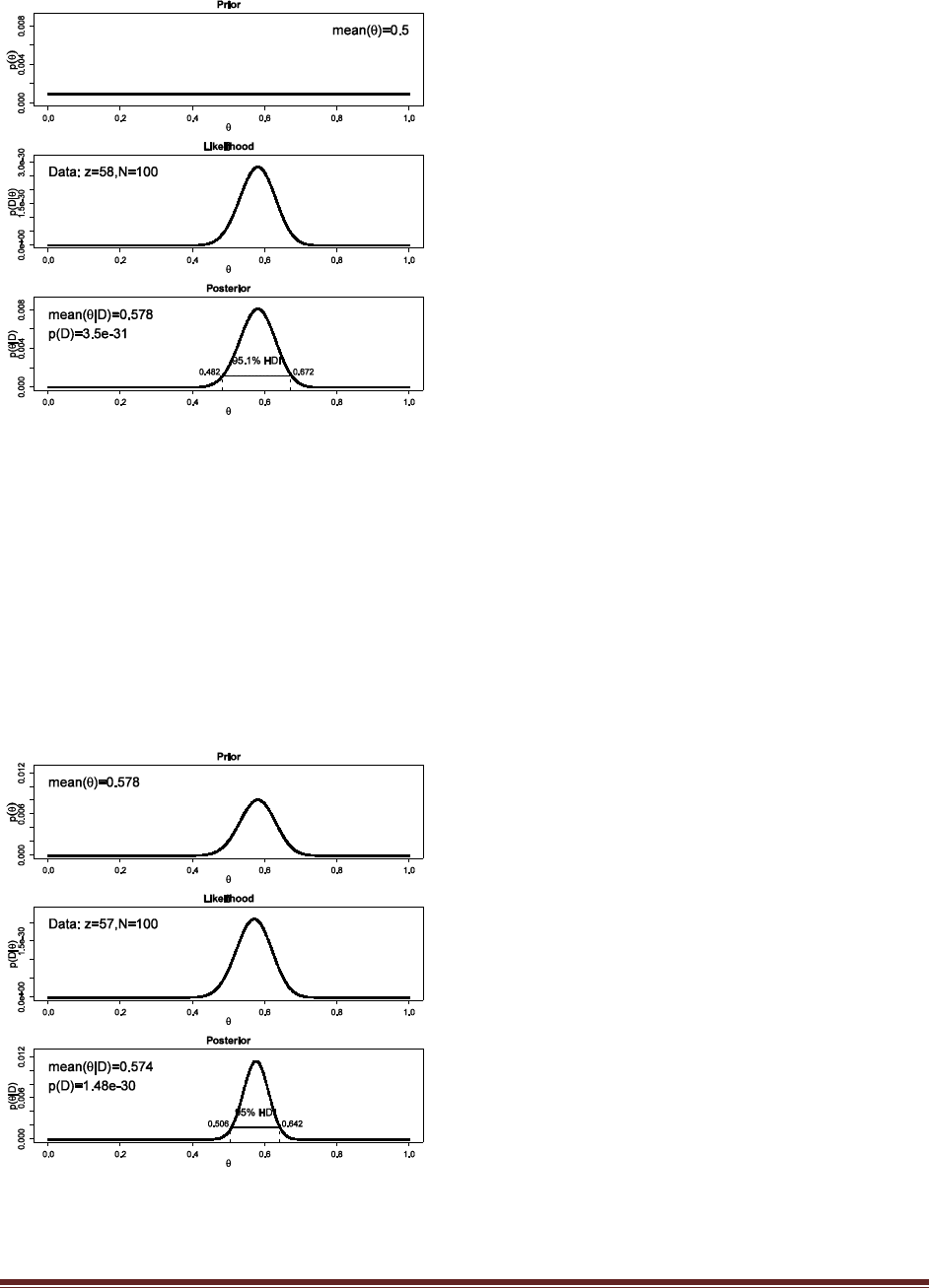
(A) Suppose that before the newspaper poll, your prior belief was a uniform distribution.
What is the 95% HDI on your beliefs after learning of the newspaper poll results? Use the
function of Section 6.7.1 (BernGrid.R) to determine your answer.
pTheta = rep(1,1000)
pTheta = pTheta / sum( pTheta )
width = 1 / length(pTheta)
Theta = seq( from = width/2 , to = 1-width/2 , by = width )
post = BernGrid( Theta , pTheta , c(rep(1,58),rep(0,42)) )
Solutions Manual for Doing Bayesian Data Analysis by John K. Kruschke Page 32
(B) Based in the newspaper poll, is it credible to believe that the population is equally
divided in its preferences among candidates?
The 95% HDI includes 0.50, so an equally divided population is still credible.
(C) You want to conduct a follow-up poll to narrow down your estimate of the population‘s
preference. In your follow-up poll, you randomly sample 100 people and find that 57 prefer
candidate A and the remainder prefer candidate B. Assuming that peoples‘ opinions have
not changed between polls, what is the 95% HDI on the posterior?
post = BernGrid( Theta , post , c(rep(1,57),rep(0,43)) )
Solutions Manual for Doing Bayesian Data Analysis by John K. Kruschke Page 33
(D) Based on your follow-up poll, is it credible to believe that the population is equally
divided in its preferences among candidates? (Hint: Compare your answer here to your
answer for Exercise 5.2.)
The 95% HDI now excludes 0.5, and therefore we might decide to declare that an equally-
divided population is not credible. Notice that the posterior found here by grid approximation
closely matches the one found in Exercise 5.2 by analytical mathematics.
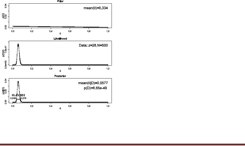
Exercise 6.5. [Purpose: To explore HDIs in the (almost) real world.] Suppose that the newly
hired quality control manager at the Acme Widget factory is trying to convince the CEO
that the proportion of defective widgets coming off the assembly line is less than 10%. No
previous data are available regarding the defect rate at the factory. The manager randomly
samples 500 widgets, and she finds that 28 of them are defective. What do you conclude
about the defect rate? Justify your choice of prior. Include graphs to explain/support your
conclusion.
There is no uniquely correct prior for this exercise. We can imagine that the CEO is very
skeptical about quality, and believes that even very high defect rates are possible, although not as
probable as low defect rates. Therefore the prior used here is linearly decreasing across the
domain.
pTheta = 1000:1 # linearly decreasing prior
pTheta = pTheta / sum( pTheta )
width = 1 / length(pTheta)
Theta = seq( from = width/2 , to = 1-width/2 , by = width )
post = BernGrid( Theta , pTheta , c(rep(1,28),rep(0,500-28)) )
The 95% HDI falls entirely below 0.10, hence it is reasonable to decide that a defect rate of 10%
is not credible (and that the actual defect rate is near 5.8%).
Solutions Manual for Doing Bayesian Data Analysis by John K. Kruschke Page 34
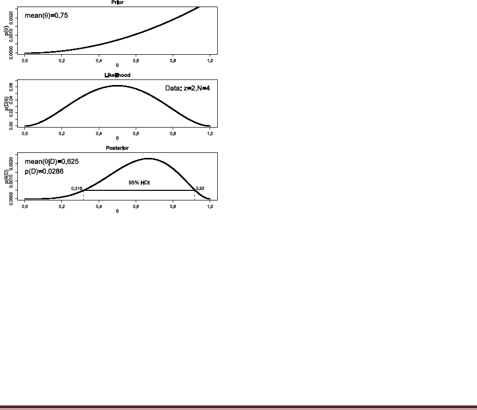
Exercise 6.6. [Purpose: To use grid approximation for prediction of subsequent data.]
Suppose we believe that a coin is biased to come up heads, and we describe our prior belief
as quadratically increasing: p(theta) is proportional to theta squared. Suppose we flip the
coin four times and observe two heads and two tails. Based on the posterior distribution,
what is the predicted probability that the next flip will yield a head? To answer this
question, use the function of Section 6.7.1 (BernGrid.R). Define thetagrid as in the example
in the comments at the beginning of the function. Then define relprob = thetagrid^2, and
normalize it to specify the prior. The function returns a vector of discrete posterior masses,
which you might call posterior. Apply Equation 6.4 by computing sum( thetagrid *
posterior ). (Bonus hint: The answer is also displayed in the output graphics.)
binwidth = 1/1000
thetagrid = seq( from=binwidth/2 , to=1-binwidth/2 , by=binwidth )
relprob = thetagrid^2
prior = relprob / sum(relprob)
posterior = BernGrid( thetagrid , prior , c(rep(1,2),rep(0,2)) )
predprob = sum( thetagrid * posterior )
show( predprob )
The predicted probability of heads for the next flip is the value of predprob, also shown in the
graph of the posterior, which equals 0.625.
Solutions Manual for Doing Bayesian Data Analysis by John K. Kruschke Page 35
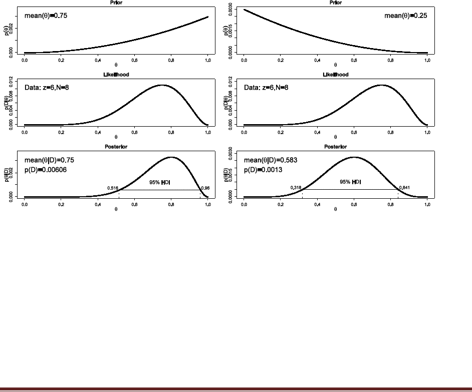
Exercise 6.7. [Purpose: To use grid approximation to compare models.] Suppose we have
competing beliefs about the bias of a coin: One person believes the coin is head biased, and
the second person believes the coin is tail biased. To make this specific, suppose the head-
biased prior is p(theta|M1) proportional to theta^2 and the tail-biased prior is p(theta|M2)
proportional to (1-theta)^2. Suppose that we are equally willing to entertain the two
models, so p(M1) = p(M2) = 0.5. We flip the coin N = 8 times and observe z = 6 heads. What
is the ratio of posterior beliefs? To answer this question, read the coding suggestion in
Exercise 6.6 and look at p(D) in the graphical output.
binwidth = 1/1000
thetagrid = seq( from=binwidth/2 , to=1-binwidth/2 , by=binwidth )
relprob = thetagrid^2
prior = relprob / sum(relprob)
posterior = BernGrid( thetagrid , prior , c(rep(1,6),rep(0,2)) )
relprob = (1-thetagrid)^2
prior = relprob / sum(relprob)
posterior = BernGrid( thetagrid , prior , c(rep(1,6),rep(0,2)) )
The posteriors reveal that p(D|M1)=0.00606 and p(D|M2)=0.00130, and therefore the Bayes
factor is 4.66 in favor of M1. Because the prior on the models was 50-50, the Bayes factor is also
the posterior odds.

Solutions Manual for Doing Bayesian Data Analysis by John K. Kruschke Page 36
Exercise 6.8. [Purpose: To model comparison in the (almost) real world.] A pharmaceutical
company claims that its new drug increases the probability that couples who take the drug
will conceive a boy. The company has published no studies regarding this claim, so there is
no public knowledge regarding the efficacy of the drug. Suppose you conduct a study in
which 50 couples, sampled at random from the general population, take the drug during a
period of time while trying to conceive a baby. Suppose that eventually all couples
conceive; there are 30 boys and 20 girls (no multiple births).
(A) You want to estimate the probability of conceiving a boy for couples who take the drug.
What is an appropriate prior belief distribution? It cannot be the general population
probability, because that is a highly peaked distribution near 0.5 that refers to nondrugged
couples. Instead, the prior needs to reflect our preexperiment uncertainty in the effect of
the drug. Discuss your choice of prior with this in mind.
The most skeptical prior for drugged couples would be the nondrugged population prior. This
prior would be sharply peaked around 0.5 and it would take a large amount of data to reallocate
beliefs away from it. A less skeptical prior would be gently peaked at 0.5, with some modest
prior belief in probabilities above and below 0.5. Ultimately, the analysis needs to convince your
audience, and therefore the prior needs to be agreeable to your audience. Suppose we have
some theoretical reason to believe that the drug may indeed alter the probability of conceiving a
boy or girl, and the audience of the analysis would agree. Therefore we use, say, a
beta(theta|5,5) prior. This is not the only correct answer; the point is to think carefully about
where the prior comes from and what your audience would agree with.
Solutions Manual for Doing Bayesian Data Analysis by John K. Kruschke Page 37
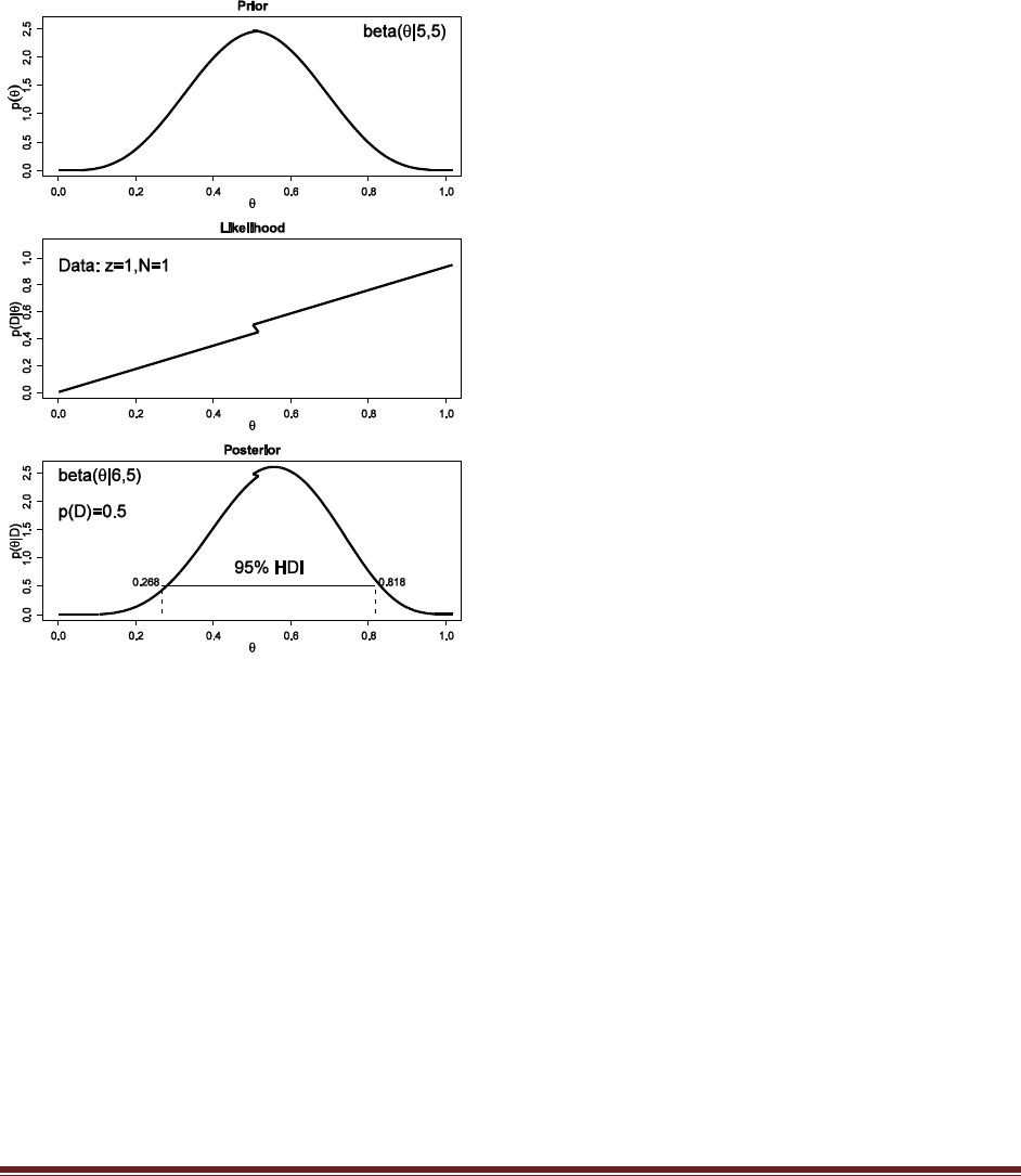
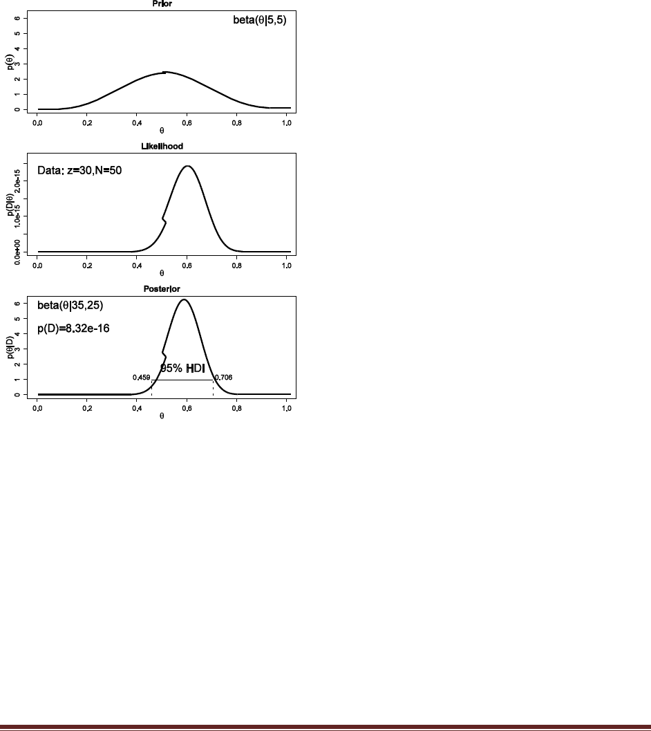
(B) Using your prior from the previous part, show a graph of the posterior and decide
whether it is credible that couples who take the drug have a 50% chance of conceiving a
boy.
Because we’re using beta priors, we can use BernBeta.R instead of BernGrid.R. The two
programs should yield essentially identical results, of course.
post = BernBeta( c(5,5) , c(rep(1,30),rep(0,20)) )
yields a posterior 95% HDI that includes 0.50, as shown below, so we decide not to believe the
manufacturer’s claim.
(The jagged parts of the graphs are caused by Word not rendering EPS correctly.)
Solutions Manual for Doing Bayesian Data Analysis by John K. Kruschke Page 38
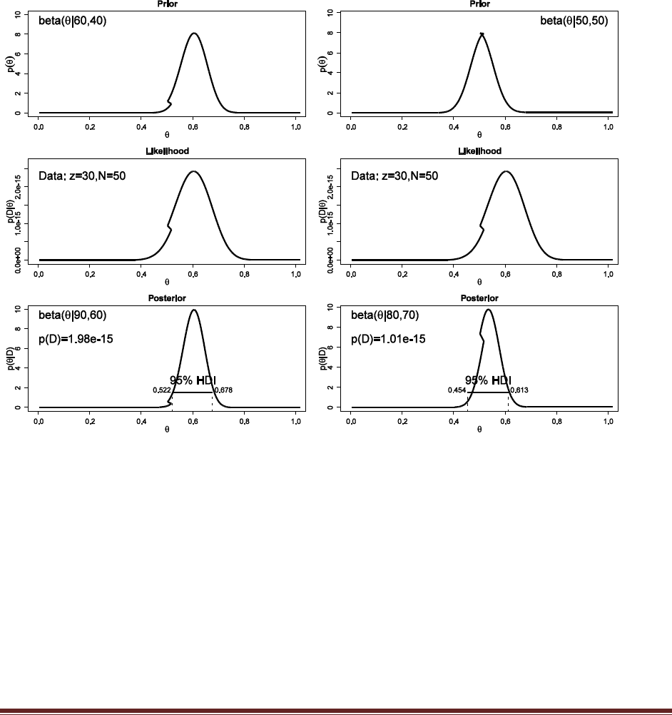
(C) Suppose that the drug manufacturers make a strong claim that their drug sets the
probability of conceiving a boy to nearly 60%, with high certainty. Suppose you represent
that claim by a beta(theta|60,40) prior. Compare that claim against the skeptic who says
there is no effect of the drug, and the probability of conceiving a boy is represented by a
beta(theta|50,50) prior. What is the value of p(D) for each prior? What is the posterior
belief in each claim? (Hint: Be careful when computing the posterior belief in each model,
because you need to take into account the prior belief in each model. Is the prior belief in
the manufacturer‘s claim as strong as the prior belief in the skeptical claim?)
post = BernBeta( c(60,40) , c(rep(1,30),rep(0,20)) )
post = BernBeta( c(50,50) , c(rep(1,30),rep(0,20)) )
The Bayes factor is 1.98e-15 / 1.01e-15 = 1.96 in favor of the 60-40 prior. This is not the
posterior odds, however, because we have to factor in the prior odds of the model priors.
Suppose, for example, that p( 60-40 prior ) is 0.33, and p( 50-50 prior ) is 0.67. Then the
posterior odds are
p( 60-40 prior | D ) / p( 50-50 prior | D)
= p( D | 60-40 prior ) / p( D | 50-50 prior ) * p( 60-40 prior ) / p( 50-50 prior )
= 1.96 * 0.33/0.67
= 0.97
In other words, for the slightly skeptical prior odds, the posterior odds are essentially equal for
the two models. Again, this is not the single “correct” answer, but illustrates the process.
Solutions Manual for Doing Bayesian Data Analysis by John K. Kruschke Page 39
Chapter 7.
Exercise 7.1. [Purpose: To see what happens in the Metropolis algorithm with different
proposal distributions, and to get a sense how the proposal distribution must be ―tuned‖ to
the target distribution.] Use the home-grown Metropolis algorithm in the R script of
Section 7.6.1 (BernMetropolisTemplate.R) for this exercise. See Figure 7.6 for examples of
what your output might look like.
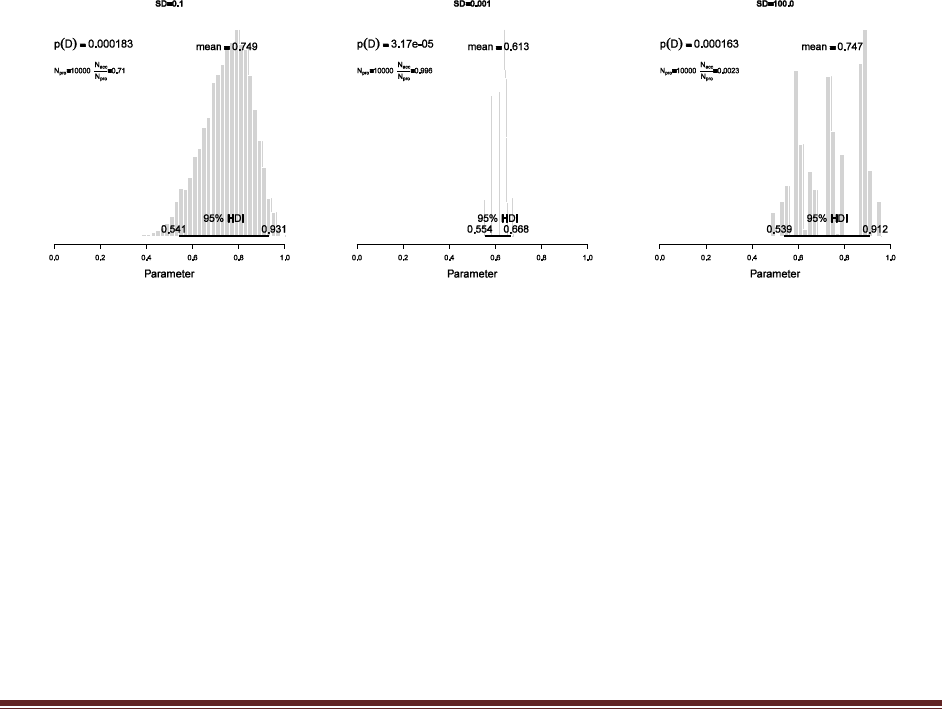
(A) The proposal distribution generates candidate jumps that are normally distributed
with mean zero. Set the standard deviation of the proposal distribution to 0.1 (if it isn‘t
already) and run the script. Save/print the graph and annotate it with SD = 0.1.
(B) Set the standard deviation of the proposal distribution to 0.001 and run the script.
Save/print the graph and annotate it with SD = 0.001.
(C) Set the standard deviation of the proposal distribution to 100.0 and run the script.
Save/print the graph and annotate it with SD = 100.0.
The line of code
proposedJump = rnorm( 1 , mean = 0 , sd = 0.1 )
is the only line that needs changing to adjust the SD of the proposal. The graphs below had titles
included by specifying the argument main in plotPost, e.g.,
plotPost( acceptedTraj , xlim=c(0,1) , breaks=30 , main="SD=0.1" )
(D) Which proposal distribution gave the most accurate representation of the posterior?
Which proposal distribution had the fewest rejected proposals? Which proposal
distribution had the most rejected proposals?
The proposal with SD=0.1 gave the most accurate representation of the posterior. The fewest
rejected proposals came when SD=0.001 (because all proposals were so close to the current
position and therefore the acceptance probability was usually close to 1.0) and the most rejected
proposals came when SD=100.0 (because most proposals were far outside the range of
acceptability and therefore rejected).
(E) If we didn‘t know from other techniques what the true posterior looked like, how would
we know which proposal distribution generated the most accurate representation of the
Solutions Manual for Doing Bayesian Data Analysis by John K. Kruschke Page 40
posterior? (This does not have a quick answer; it‘s meant mostly as a question for
pondering and motivating techniques introduced in later chapters.)
One signature of a representative sample chain is that it is not “clumpy” across steps. Both of the
bad distributions above don’t move around much from one step to the next. This lingering and
clumping is called large “autocorrelation”. We want to avoid sample chains that have large
autocorrelation.
Exercise 7.2. [Purpose: To understand the influence of the starting point of the random
walk, and why the walk doesn‘t necessarily go back to that region.] Edit the homegrown
Metropolis algorithm of Section 7.6.1 (BernMetropolisTemplate.R) for this exercise. It is
best to save it as a differently named script so you don‘t mess up the original version. Set
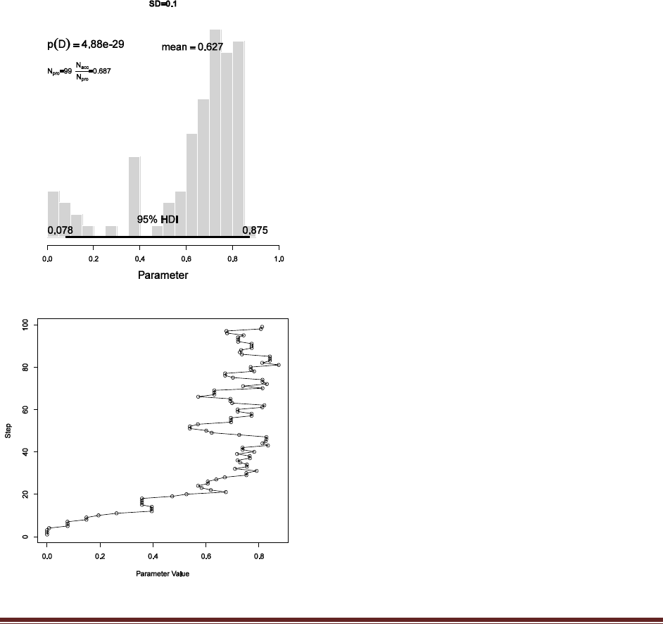
trajlength = 100 and set burnin = ceiling(0.01 *trajlength). Finally, set trajectory[1] =
0.001. Now run the script and save the resulting histogram.
(A) How many jumps are proposed? How
many steps are excluded as part of the burn-in
portion? At what value of does the random
walk start?
The resulting histogram is shown at the left. With
trajlength=100, there are 100 steps proposed.
With burnin = ceiling(0.01 *trajlength), there is
only 1 burn-in step. The walk starts at 0.001
because trajectory[1]=0.001
(B) Why does the histogram have so many
points below 0.5? That is, why does the chain
stay below 0.5 as long as it does?
The initial value is 0.001, so the chain starts at the
far left. It stays to the left side of 0.5 for quite a
number of steps because the proposal distribution
has a fairly small SD of 0.1, so proposed jumps
are fairly small.
(C) Why does the histogram have so few points
below 0.5? That is, why does the chain not go
back below 0.5?
The chain eventually stays to the right of 0.5
because the posterior probability of values to the
left of 0.5 is small.
These points might be made clearer by plotting
the trajectory instead of histogram, as shown at

Solutions Manual for Doing Bayesian Data Analysis by John K. Kruschke Page 41
left, using the command
plot( acceptedTraj , 1:length(acceptedTraj) , type="o" , ylab="Step" , xlab="Parameter Value")
Exercise 7.3. [Purpose: To get some hands-on experience with applying the Metropolis
algorithm, and to compare its results with the other methods we‘ve learned about.]
Suppose you have a coin that you believe is either fair, or biased to come up heads, or
biased to come up tails. As an expression of your prior belief, you define your prior on
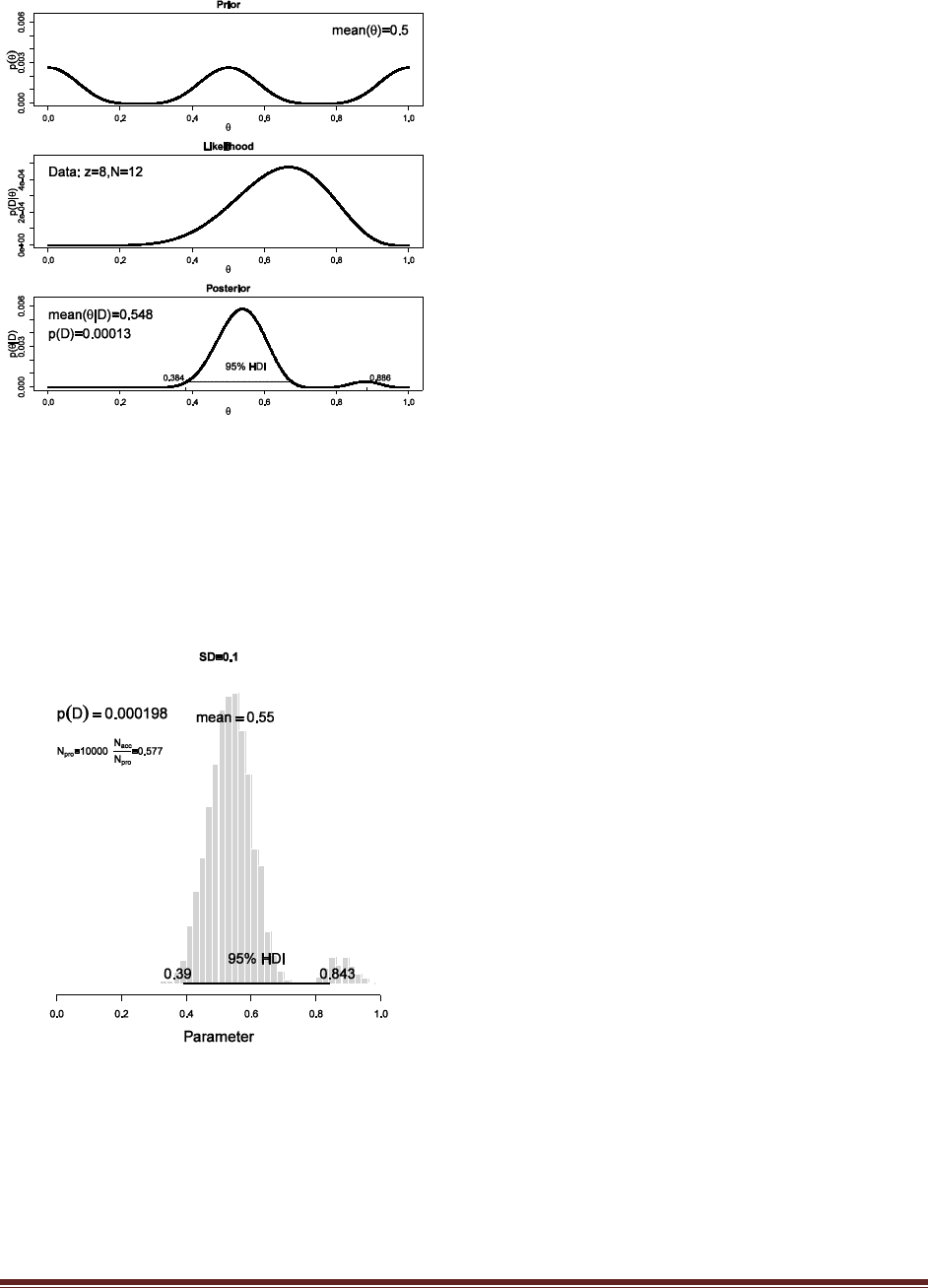
theta (the probability of heads) to be proportional to [cos(4)+1]2. In other words, p() =
[cos(4)+1]2 /Z, where Z is the appropriate normalizing constant. We flip the coin 12
times and we get 8 heads. See Figure 7.7 to see the prior, likelihood, and posterior.
(A) Determine the formula for the posterior distribution exactly, using formal integration
in Bayes‘ rule. Just kidding. Instead, do the following: Explain the initial setup if you
wanted to try to determine the exact formula for the posterior. Show the explicit formulas
involving the likelihood and prior in Bayes‘ rule. Do you think that the prior and likelihood
are conjugate? That is, would the formula for the posterior have the ―same form‖ as the
formula for the prior?
248248 )1)4(cos()1( )1)4(cos()1(
| ||
d
pDpdpDpDp
(Z does not appear in the formula above because it cancels out in the numerator and
denominator.) It is doubtful that a formula for the posterior would have the same form as the
prior. Also evident from the formula is that an analytical solution is not trivial if it is possible at
all.
(B) Use a fine grid over and approximate the posterior. Use the R function of Section 6.7.1
(BernGrid.R), p. 109. (The R function also plots the prior distribution, so you can see that
it really is trimodal.)
binwidth = 1/1000
thetagrid = seq( from=binwidth/2 , to=1-binwidth/2 , by=binwidth )
relprob = ( cos( 4*pi*thetagrid ) + 1 )^2
prior = relprob / sum(relprob)
datavec = c( rep(1,8) , rep(0,4) )
posterior = BernGrid( Theta=thetagrid , pTheta=prior , Data=datavec )
Solutions Manual for Doing Bayesian Data Analysis by John K. Kruschke Page 42
(C) Use a Metropolis algorithm to approximate the posterior. Use the R script of Section
7.6.1, (BernMetropolisTemplate.R) adapted appropriately for the prior function. You‘ll
need to alter the definitions of the likelihood and prior functions in the R script; include
that portion of the code with what you hand in (but don‘t include the rest of the code).
Must you normalize the prior to generate a sample from the posterior? Is the value of p.D/
displayed in the graph correct?
There are only two program changes that need to
be made. One is the specification of the data and
the other is the specification of the prior:
myData = c( 1, 1, 1, 1, 1, 1, 1, 1, 0, 0, 0, 0 )
prior = function( theta ) {
prior = ( cos( 4 * pi * theta ) + 1 )^2
prior[ theta > 1 | theta < 0 ] = 0
return( prior )
}
(Be sure that a long chain is generated, with
sufficient burn-in!) This produces the following
histogram:
Notice that the histogram shows bimodality, just like the grid approximation. Also note that the
HDI marked in the histogram is not appropriate, because the algorithm for approximating the
HDI assumes a unimodal distribution.
(D) Could you apply BUGS to this situation? In particular, can you think of a way to
specify the prior density in terms of distributions that BUGS knows about?
Solutions Manual for Doing Bayesian Data Analysis by John K. Kruschke Page 43
There is no simple way to specify this prior in BUGS.
Exercise 7.4. [Purpose: To approximate p.D/, explore other choices for h./ in Equation 7.8,
and note that the one used in the R script of Section 7.6.1 (Bern- MetropolisTemplate.R) is
a good one.] Edit the R script of Section 7.6.1 (BernMetropolisTemplate.R) for this
exercise. It is best to save it as a differently named script so you don‘t mess up the original
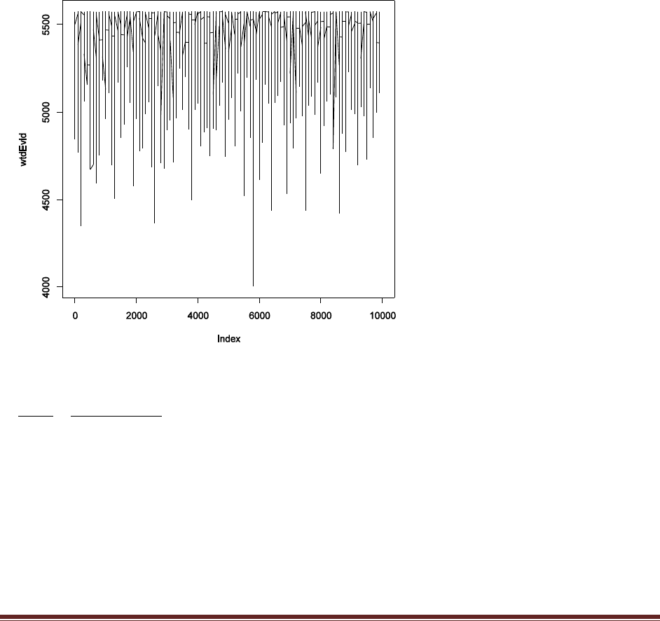
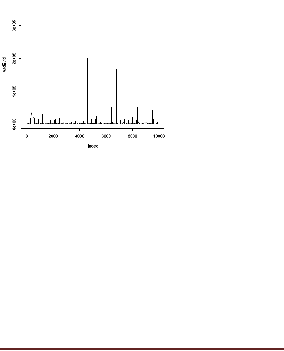
version. At the end of the script, add this line: windows() ; plot(wtdEvid,type="l").
(A) Select (i.e., highlight with the cursor) that line in the R editor and run it. Save the plot.
Explain what the plot is plotting. That is, what is wtdEvid (on the y axis) and what is on the
x axis?
The plot shows the weighted evidence, denoted wtdEvid, at each step in the chain. The step in
the chain is denoted “Index” on the x axis. The weighted evidence at step i is
1
p(D)h(
i)
p(D|
i)p(
i)
where h(θ) is a beta distribution with the same mean and standard deviation as the sampled
posterior. Notice that the value of wtdEvid is usually between 4700 and 5700.
(B) Consider a different choice for the h() in Equation 7.8. To do this, we‘ll leave it as a
beta function, but change the choice of its a and b values. Find where a and b are specified
in the R program (near the end, just before wtdEvid is defined), and type in a=1 and b=1
instead. Now select (i.e., highlight with the cursor) the portion of the program from the new
Solutions Manual for Doing Bayesian Data Analysis by John K. Kruschke Page 44
a and b definitions, through the computation of wtdEvid, and the new plot command. Run
the selection, and save the resulting plot.
The plot above shows the result. Notice that there are spikes that shoot to extreme values, far
beyond the usual magnitude of wtdEvid. Notice the scale on the y axis: 3e+05 is 300,000!
(C) Repeat, but this time with a=10 and b=10.
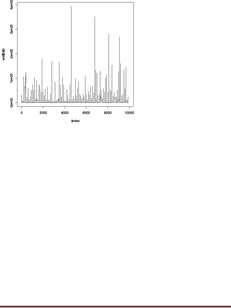
Solutions Manual for Doing Bayesian Data Analysis by John K. Kruschke Page 45
The plot above shows that wtdEvid shoots to extreme values, even more extreme than the
previous part, up to 400,000.
(D) For which values of a and b are the values of wtdEvid most stable across the random
walk? Which values of a and b would produce the most stable estimate of p(D)?
The most stable estimate of wtdEvid comes from using a,b values that produce h() similar to the
actual posterior.
Exercise 7.5. [Purpose: To explore the use of BUGS and consider model comparison.]
Suppose there are three people with different beliefs about a coin. One person (M1)
believes that the coin is biased toward tails; we‘ll model this person‘s beliefs as a uniform
distribution over values between 0 and 0.4. The second person (M2) believes that the coin is
approximately fair; we‘ll model this person‘s beliefs as a uniform distribution between 0.4
and 0.6. The third person (M3) believes that the coin is biased toward heads; we‘ll model
this person‘s beliefs as a uniform distribution over values between 0.6 and 1.0. We won‘t
favor any person a priori, and therefore we start by assuming that p(M1) = p(M2) = p(M3)
= 1/3. We now flip the coin 14 times and observe 11 heads. Use BUGS to determine the
evidences for the three models. Hints: For each person, compute p(D) by adapting the
program BernBetaBugsFull.R of Section 7.4.1 in two steps. First, modify the model
specification so that the prior is uniform over the limited range, instead of beta. Appendix I
of the OpenBUGS User Manual (see Section 7.4) explains how to specify uniform
distributions in BUGS. Second, include a new section at the end of the BUGS program that
will compute p(D). Do this by copying the last section of the program
BernMetropolisTemplate.R that computes p(D), pasting it onto the end of your BUGS
program, and making additional necessary changes so that the output of BUGS can be

Solutions Manual for Doing Bayesian Data Analysis by John K. Kruschke Page 46
processed by the newly added code. In particular, before the newly added code, you‘ll have
to include these lines:
acceptedTraj = thetaSample
meanTraj = mean( thetaSample )
sdTraj = sd( thetaSample )
The complete code is below. The major changes have been highlighted.
graphics.off()
rm(list=ls(all=TRUE))
library(BRugs) # Kruschke, J. K. (2010). Doing Bayesian data analysis:
# A Tutorial with R and BUGS. Academic Press / Elsevier.
#------------------------------------------------------------------------------
# THE MODEL.
# Specify the model in BUGS language, but save it as a string in R:
modelString = "
# BUGS model specification begins ...
model {
# Likelihood:
for ( i in 1:nFlips ) {
y[i] ~ dbern( theta )
}
# Prior distribution:
theta ~ dunif( 0.6 , 1.0 )
}
# ... BUGS model specification ends.
" # close quote to end modelString
# Write the modelString to a file, using R commands:
writeLines(modelString,con="model.txt")
# Use BRugs to send the model.txt file to BUGS, which checks the model syntax:
modelCheck( "model.txt" )
#------------------------------------------------------------------------------
# THE DATA.
# Specify the data in R, using a list format compatible with BUGS:
dataList = list(
nFlips = 14 ,
y = c( 1,1,1,1,1,1,1,1,1,1,1,0,0,0 )
)
# Use BRugs commands to put the data into a file and ship the file to BUGS:
modelData( bugsData( dataList ) )
#------------------------------------------------------------------------------
# INTIALIZE THE CHAIN.
modelCompile() # BRugs command tells BUGS to compile the model.
modelGenInits() # BRugs command tells BUGS to randomly initialize a chain.
#------------------------------------------------------------------------------
# RUN THE CHAINS.
# BRugs tells BUGS to keep a record of the sampled "theta" values:
samplesSet( "theta" )
# R command defines a new variable that specifies an arbitrary chain length:
chainLength = 10000
# BRugs tells BUGS to generate a MCMC chain:

Solutions Manual for Doing Bayesian Data Analysis by John K. Kruschke Page 47
modelUpdate( chainLength )
#------------------------------------------------------------------------------
# EXAMINE THE RESULTS.
thetaSample = samplesSample( "theta" ) # BRugs asks BUGS for the sample values.
thetaSummary = samplesStats( "theta" ) # BRugs asks BUGS for summary statistics.
# Make a graph using R commands:
windows(10,6)
layout( matrix( c(1,2) , nrow=1 ) )
plot( thetaSample[1:500] , 1:length(thetaSample[1:500]) , type="o" ,
xlim=c(0,1) , xlab=bquote(theta) , ylab="Position in Chain" ,
cex.lab=1.25 , main="BUGS Results" )
source("plotPost.R")
histInfo = plotPost( thetaSample , xlim=c(0,1) )
## Posterior prediction:
## For each step in the chain, use posterior theta to flip a coin:
#chainLength = length( thetaSample )
#yPred = rep( NULL , chainLength ) # define placeholder for flip results
#for ( stepIdx in 1:chainLength ) {
# pHead = thetaSample[stepIdx]
# yPred[stepIdx] = sample( x=c(0,1), prob=c(1-pHead,pHead), size=1 )
#}
## Jitter the 0,1 y values for plotting purposes:
#yPredJittered = yPred + runif( length(yPred) , -.05 , +.05 )
## Now plot the jittered values:
#windows(5,5.5)
#plot( thetaSample[1:500] , yPredJittered[1:500] , xlim=c(0,1) ,
# main="posterior predictive sample" ,
# xlab=expression(theta) , ylab="y (jittered)" )
#points( mean(thetaSample) , mean(yPred) , pch="+" , cex=2 )
#text( mean(thetaSample) , mean(yPred) ,
# bquote( mean(y) == .(signif(mean(yPred),2)) ) ,
# adj=c(1.2,.5) )
#text( mean(thetaSample) , mean(yPred) , srt=90 ,
# bquote( mean(theta) == .(signif(mean(thetaSample),2)) ) ,
# adj=c(1.2,.5) )
#abline( 0 , 1 , lty="dashed" , lwd=2 )
# Rename variables above so they are compatible with code pasted below
acceptedTraj = thetaSample
meanTraj = mean( thetaSample )
sdTraj = sd( thetaSample )
myData = dataList$y
# Code below is copied from BernMetropolisTemplate.R
likelihood = function( theta , data ) {
z = sum( data == 1 )
N = length( data )
pDataGivenTheta = theta^z * (1-theta)^(N-z)
pDataGivenTheta[ theta > 1 | theta < 0 ] = 0
return( pDataGivenTheta )
}
prior = function( theta ) {
prior = dunif( theta , min=0.6 , max=1.0 ) # uniform density
prior[ theta > 1 | theta < 0 ] = 0
return( prior )
}

Solutions Manual for Doing Bayesian Data Analysis by John K. Kruschke Page 48
# Compute evidence for model, p(D):
a = meanTraj * ( (meanTraj*(1-meanTraj)/sdTraj^2) - 1 )
b = (1-meanTraj) * ( (meanTraj*(1-meanTraj)/sdTraj^2) - 1 )
wtdEvid = dbeta( acceptedTraj , a , b ) / (
likelihood( acceptedTraj , myData ) * prior( acceptedTraj ) )
pData = 1 / mean( wtdEvid )
# Display p(D) in the graph
if ( meanTraj > .5 ) { xpos = 0.0 ; xadj = 0.0
} else { xpos = 1.0 ; xadj = 1.0 }
densMax = max( histInfo$density )
text( xpos , 0.75*densMax , bquote( p(D)==.( signif(pData,3) ) ) ,
adj=c(xadj,0) , cex=1.5 )
dev.copy2eps(file="Exercise7.5.eps")
The only changes from one model to the next involve the prior in both the BUGS model
specification and the appended code for computing p(D):
M1:
theta ~ dunif( 0.0 , 0.4 )
prior = dunif( theta , min=0.0 , max=0.4 )
M2:
theta ~ dunif( 0.4 , 0.6 )
prior = dunif( theta , min=0.4 , max=0.6 )
M3:
theta ~ dunif( 0.6 , 1.0 )
prior = dunif( theta , min=0.6 , max=1.0 )
The graphs on the next page are the result. We see that p(D|M1)=1.03e-06, p(D|M2)=9.02e-05,
p(D|M3)=0.000432. Thus, M3 is strongly preferred over the other models.
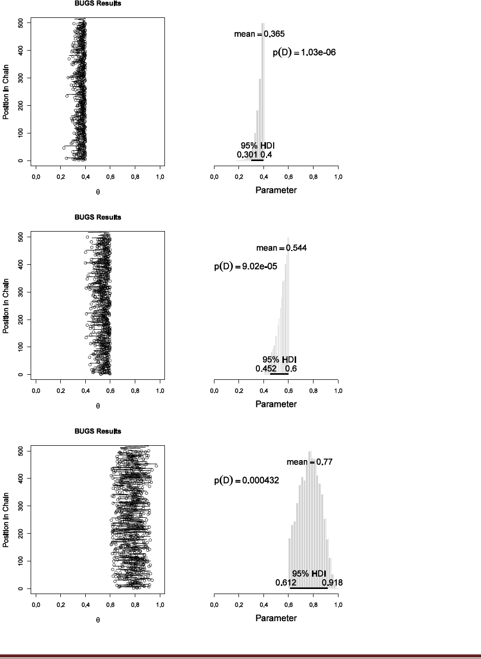
Solutions Manual for Doing Bayesian Data Analysis by John K. Kruschke Page 49
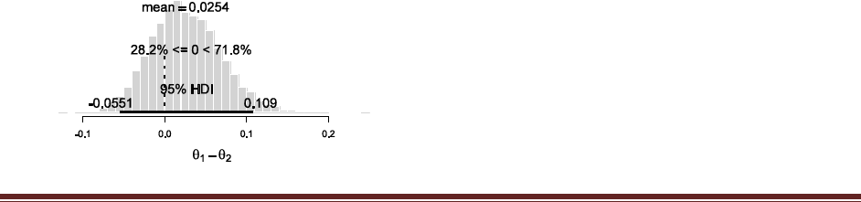
Solutions Manual for Doing Bayesian Data Analysis by John K. Kruschke Page 50
Chapter 8.
Exercise 8.1. [Purpose: To explore a real-world application about the difference of
proportions.] Is there a ―hot hand‖ in basketball? This question has been addressed in a
frequently cited article by Gilovich, Vallone, & Tversky (1985).The idea of a hot hand is
that the success of a shot depends on the success of a previous shot, as opposed to each shot
being an independent flip of a coin (or toss of a ball). One way to address this idea is to
consider pairs of free throws taken after fouls. If the player has a hot hand, then he should
be more likely to make the second shot after a successful first shot than after a failed first
shot. If the two shots are independent, however, then the probability of making the second
shot after a successful first shot should equal the probability of making the second shot
after failing the first shot. Thus, there is a hot hand if the probability of success after a
success is better than the probability of success after failure.
During 1980–1982, Larry Bird of the Boston Celtics had 338 pairs of free throws. He
was successful on 285 first shots and failed on the remaining 53 first shots. After the 285
successful first shots, he was successful on 251 second shots (and failed on the other 34
second shots). After the 53 failed first shots, he was successful on 48 second shots (and
failed on the other 5 second shots). Thus, we want to know if 251/285 (success after success)
is different than 48/53 (success after failure).
Let 1 represent the proportion of success after a successful shot, and let 2
represent the proportion of success after a failed first shot. Suppose we have priors of
beta(|30,10) on both, representing the belief that we think that professional players make
about 75% of their free throws, regardless of when they are made.
(A) Modify the BRugs program of Section 8.8.3 (BernTwoBugs.R) to generate a histogram
of credible differences between success-after-success and success-after-failure. Explain
what modifications you made to the R code. (Hint: Your result should look like something
like Figure 12.2, p. 299).
The model specification should include these priors:
theta1 ~ dbeta( 30 , 10 )
theta2 ~ dbeta( 30 , 10 )
The data specification should include the following inside its list:
N1 = 285,
y1 = c( rep(1,251) , rep(0,285-251) ),
N2 = 53,
y2 = c( rep(1,48) , rep(0,53-48) )
The resulting posterior distribution of differences looks like this:
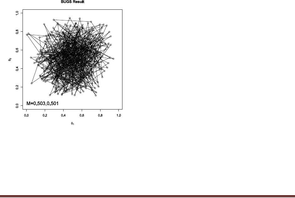
Solutions Manual for Doing Bayesian Data Analysis by John K. Kruschke Page 51
(B) Based on your results from the previous part, does Larry Bird seem to have a hot
hand? In other words, are almost all of the credible differences between success-after-
success and success-after-failure well above zero, or is a difference of zero among the
credible differences?
A difference of zero lies well within the 95% HDI, which means that a difference of zero is
among the credible values, and there is not strong evidence for a hot hand.
Exercise 8.2. [Purpose: To examine the prior in BUGS by omitting references to data.]
Reproduce and run the BUGS code that generated the chains in Figure 8.7. Show the
sections of code that you modified from the program in Section 8.8.3 (BernTwoBugs.R),
and show the resulting graphical output.
As shown on p. 175 of the textbook, the data list has the y1 and y2 values commented out, as
follows:
N1 = 7 ,
# y1 = c( 1,1,1,1,1,0,0 ) ,
N2 = 7 #,
# y2 = c( 1,1,0,0,0,0,0 )
Notice that the N1 and N2 values remain specified, because those values are still used in the
model specification. Notice also that the final comma is commented out, so that the list structure
has the proper syntax. When the program is run, the resulting posterior sample looks much like
Figure 8.7, as follows:
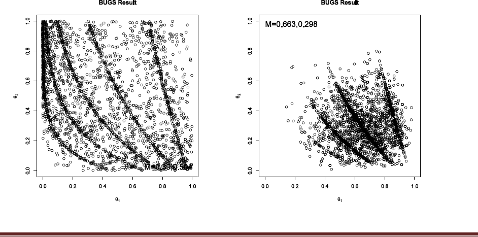
Solutions Manual for Doing Bayesian Data Analysis by John K. Kruschke Page 52
Exercise 8.3. [Purpose: To understand the limitations of prior specification in BUGS.] In
BUGS, all priors must be specified in terms of probability distributions that BUGS knows
about. These distributions include the beta, gamma, normal, uniform, and so on, as
specified in the appendix of the BUGS User Manual. There are ways to program novel
distributions into BUGS, but explaining how would take us too far afield at this point.
Instead, we‘ll consider how unusual priors can be constructed from the built-in
distributions. The left panel of Figure 8.9 shows the prior that results from this model
specification (BernTwoFurrowsBugs.R):
model {
# Likelihood. Each flip is Bernoulli.
for ( i in 1 : N1 ) { y1[i] ~ dbern( theta1 ) }
for ( i in 1 : N2 ) { y2[i] ~ dbern( theta2 ) }
# Prior. Curved scallops!
x ~ dunif(0,1)
y ~ dunif(0,1)
N <- 4
xt <- sin( 2*3.141593*N * x ) / (2*3.141593*N) + x
yt <- 3 * y + (1/3)
xtt <- pow( xt , yt )
theta1 <- xtt
theta2 <- y
}
Adapt the program in Section 8.8.3 (BernTwoBugs.R) to use this prior, but with N set to 5
instead of 4. (Don‘t confuse N with N1 or N2.) Produce a graph of the prior and of the
posterior, like those shown in Figure 8.9. This particular furrowed prior would never be
used in actual research that I‘m aware of; the point is that you can specify unusual priors if
you need to.
The result when N<-5 is shown below (prior on left, posterior on right). Notice that there are
five ridges in the prior, not four ridges as in Figure 8.9 of the textbook.
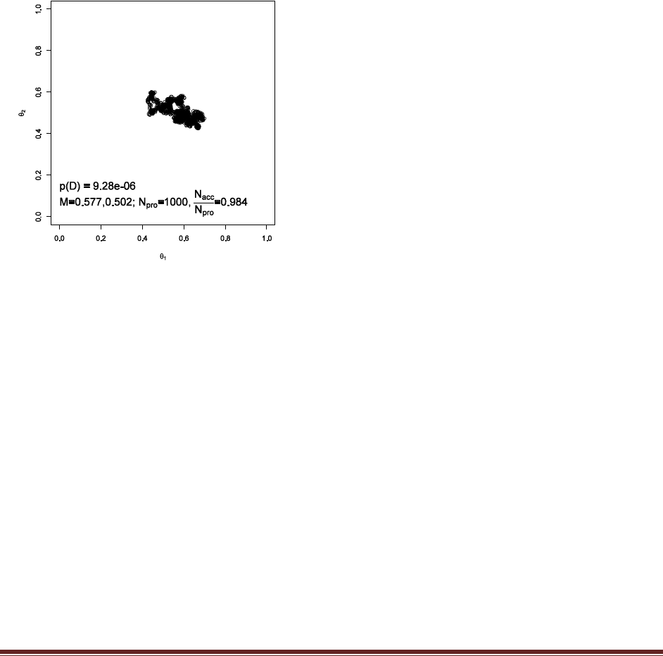
Solutions Manual for Doing Bayesian Data Analysis by John K. Kruschke Page 53
Exercise 8.4. [Purpose: To understand Metropolis sampling, and to see the importance of
tuning the proposal distribution.] For this exercise, assume the prior and data used in
Figure 8.1.
(A) In the R code of Section 8.8.2 (BernTwoMetropolis.R), set the standard deviations
(both sd1 and sd2) of the proposal distribution to 0.005, and run the program. Does the
resulting distribution of sampled values resemble Figures 8.1 or 8.3? What is wrong with
the choice of standard deviations?
Changing line 57 of the program to
nDim = 2 ; sd1 = 0.005 ; sd2 = 0.005 # was 0.2
yields
which is a very clumpy, autocorrelated chain. The standard deviation for the proposal
distribution is much too small, yielding successive steps too close to each other. Notice that the
acceptance proportion is 98.4%, meaning that almost every proposal is accepted.
(B) In the R code of Section 8.8.2 (BernTwoMetropolis.R), set the standard deviations (both
sd1 and sd2) of the proposal distribution to 5.0, and run the program. Does the resulting
distribution of sampled values resemble Figures 8.1 or 8.3? What is wrong with the choice
of standard deviations?
Changing line 57 of the program to
nDim = 2 ; sd1 = 5.0 ; sd2 = 5.0 # was 0.2
yields

Solutions Manual for Doing Bayesian Data Analysis by John K. Kruschke Page 54
Notice that the acceptance proportion is zero, meaning that no proposal is ever accepted, and the
chain remains stuck at its starting point. This results from the proposals all being far beyond the
reasonable range of the posterior.
Exercise 8.5. [Purpose: To remember how to do posterior prediction with BUGS.] For this
exercise, assume the prior and data used in Figure 8.1. From the posterior, what is the
probability that the next flip of the two coins will have y1* = 1 and y2* = 0? To answer this
question, expand the code of Section 8.5 so that it includes posterior predictions. See the
example in Section 7.4.2, (p. 143), and simply repeat the same structure for each theta and
y value. Include your code with your answer.
Starting with the program BernTwoBugs.R, we add the following lines of code and the end of
the program:
# Posterior prediction. For each step in the chain, use the posterior thetas
# to flip the coins.
chainLength = length( theta1Sample )
# Create matrix to hold results of simulated flips:
yPred = matrix( NA , nrow=2 , ncol=chainLength )
for ( stepIdx in 1:chainLength ) { # step through the chain
# flip the first coin:
pHead1 = theta1Sample[stepIdx]
yPred[1,stepIdx] = sample( x=c(0,1), prob=c(1-pHead1,pHead1), size=1 )
# flip the second coin:
pHead2 = theta2Sample[stepIdx]
yPred[2,stepIdx] = sample( x=c(0,1), prob=c(1-pHead2,pHead2), size=1 )
}
# Now determine the proportion of times that y1==1 and y2==0
pY1eq1andY2eq0 = sum( yPred[1,]==1 & yPred[2,]==0 ) / chainLength
The result is that pY1eq1andY2eq0 is 0.37. (The code above is merely suggestive. You may
have more elegant code that accomplishes the same result.)

Solutions Manual for Doing Bayesian Data Analysis by John K. Kruschke Page 55
Chapter 9.
Exercise 9.1. [Purpose: To investigate research design—more coins versus more flips per
coin.] In Section 9.2.5, p. 219, it was argued that if the goal of the research is to get a good
estimate of the group average , then it is better to collect data from more coins than to
collect more flips per coin. This exercise has you generate simulated data to bolster this
conclusion.
(A) Use the R code of Section 9.5.1 (BernBetaMuKappaBugs.R) for this exercise. In the
data section of that program, comment out the lines that specify N and z. Insert the
following lines:
ncoins = 50 ; nflipspercoin = 5
muAct = .7 ; kappaAct = 20
thetaAct = rbeta( ncoins , muAct*kappaAct , (1-muAct)*kappaAct )
z = rbinom( n=ncoins , size=nflipspercoin , prob=thetaAct )
N = rep( nflipspercoin , ncoins )
Explain in words what that code does. This is important; if you don‘t understand this code,
the rest of the exercise will not make much sense. (Hint: It‘s generating random data, for
specific ―actual‖ parameter values; explain in detail.)
thetaAct is a vector of length ncoins (i.e., 50). Each component of thetaAct is the actual bias of
the corresponding coin. The theta values are sampled randomly from a beta distribution with
mean muAct and certainty kappaAct.
z is a vector of number of heads randomly generated when each coin is flipped nflipspercoin
with actual probability thetaAct.
N is the vector of number of flips for each coin. For example, when the above code is run, it
produces (randomly) the following:
thetaAct
[1] 0.7853951 0.8073966 0.4982677 0.8523268 0.7040792 0.6331948 0.6236083
[8] 0.8444975 0.8437521 0.6940055 0.6072397 0.4525766 0.7907075 0.8159670
[15] 0.6158728 0.6934655 0.7720326 0.7363004 0.6251704 0.7225201 0.7853685
[22] 0.6898285 0.7206907 0.7581194 0.6733569 0.7329841 0.7543905 0.6074791
[29] 0.7277989 0.8674680 0.5884220 0.6229580 0.6880705 0.6004323 0.6318800
[36] 0.7357017 0.8505620 0.5595014 0.8726786 0.7874657 0.5362301 0.8735407
[43] 0.8071881 0.6113401 0.5950920 0.8011553 0.8088236 0.7643088 0.4644073
[50] 0.7772480
z
[1] 4 3 3 5 3 2 2 5 4 3 2 3 5 5 2 2 4 5 4 4 4 2 2 2 3 4 4 4 5 5 3 2 1 1 3 5 3 3
[39] 5 5 4 4 4 1 3 3 5 4 2 3
N
[1] 5 5 5 5 5 5 5 5 5 5 5 5 5 5 5 5 5 5 5 5 5 5 5 5 5 5 5 5 5 5 5 5 5 5 5 5 5 5
[39] 5 5 5 5 5 5 5 5 5 5 5 5
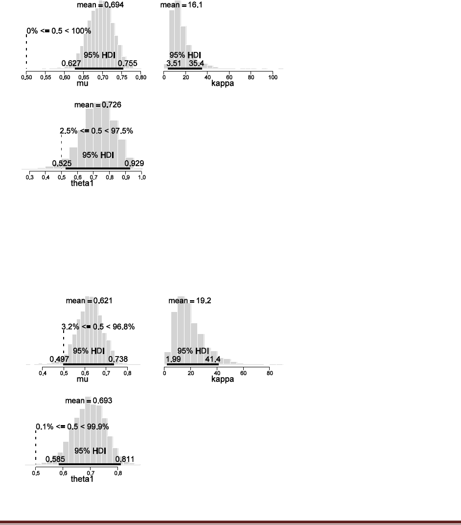
Solutions Manual for Doing Bayesian Data Analysis by John K. Kruschke Page 56
(B) At the bottom of the program, UNcomment the lines that plot the posteriors of
muSample, kappaSample, and thetaSample[1,]. (Don‘t plot thetaSample[28,], because it
doesn‘t exist.) You should also Uncomment the windows() and layout(. . .) command, so
that the plots don‘t overwrite each other. Run the program a few times and include the
graphs of one typical run in your write-up.
Notice that the HDI for mu is always well above .5, but the HDI for theta1 has its left edge near
.5.
(C) Now change the data-generation code so that the number of coins is 5 (instead of 50)
and the number of flips per coin is 50 (instead of 5). Run the program a few times and
include the graphs of one typical run in your write-up.
Notice that the HDI for mu has its left edge near .5, but the HDI for theta1 is always well above
.5.

Solutions Manual for Doing Bayesian Data Analysis by John K. Kruschke Page 57
(D) Is the posterior estimate of more certain for 5 coins or for 50 coins? Is the posterior
estimate of 1 more certain for 5 coins (50 flips per coin) or for 50 coins (5 flips per coin)?
Is it better to use more coins or more flips per coin if the goal is to estimate ?
As mentioned in the descriptions of the posterior distributions, the uncertainty on mu is smaller
when there are more coins, but the posterior uncertainty of theta1 is smaller when there are more
flips per coin. If the goal is to estimate mu, then there should be more coins.
Exercise 9.2. [Purpose: To examine the effect of different assumptions about across-group
constraints. Specifically, different assumptions about c in the analysis of data from the
filtration-condensation experiment.] For this exercise, we will perform alternative analyses
of the data from the filtration-condensation experiment described in Section 9.3.1. You will
adapt the code listed in Section 9.5.2 (FilconBrugs.R), which implements the hierarchical
model diagrammed in Figure 9.7, to implement the alternative hierarchical models
diagrammed in Figure 9.17.
(A) The left side of Figure 9.17 shows a model in which the same value is used for all
groups simultaneously. The idea here is that accuracies of individuals in each group
depend on the group mean accuracy, and we are going to estimate the magnitude of that
dependency of individuals on the group mean, but we assume that whatever the degree of
dependency is, it is the same in every group. This assumption can be thought of as saying
that the category structure (e.g., filtration or condensation) affects the mean accuracy of
the group, but individual variation from the mean accuracy is caused only by other factors
that are the same across groups, not by the category structure. To implement this
assumption in the program, do the following: In the model specification, because
does not depend on the group (i.e., the condition), move the line that specifies the
distribution of outside the for loop that cycles through the conditions. Moreover, because
there is only one , remove the index from (i.e., change kappa[condIdx] to kappa). Then,
in the initialization of the chains, make sure that kappa is initialized to a single value
instead of a vector of four values. To do this, set kappa to the mean of the four condition
kappas. Now run the modified program. (Hint: For an example of results, see Figures 9.18
and 9.19, and compare the results with those in Figure 9.16.) In your answer: (1) Report
the modified model-specification section of your code; (2) Show the graph of the estimated
differences; (3) Answer this question: Why is the 95% HDI of the 1 - differences
farther away from zero than in the original analysis?
The modified model specification:
model {
for ( subjIdx in 1:nSubj ) {
# Likelihood:
z[subjIdx] ~ dbin( theta[subjIdx] , N[subjIdx] )
# Prior on theta: Notice nested indexing.
theta[subjIdx] ~ dbeta( a[cond[subjIdx]] , b[cond[subjIdx]]
)I(0.001,0.999)
}
for ( condIdx in 1:nCond ) {
a[condIdx] <- mu[condIdx] * kappa
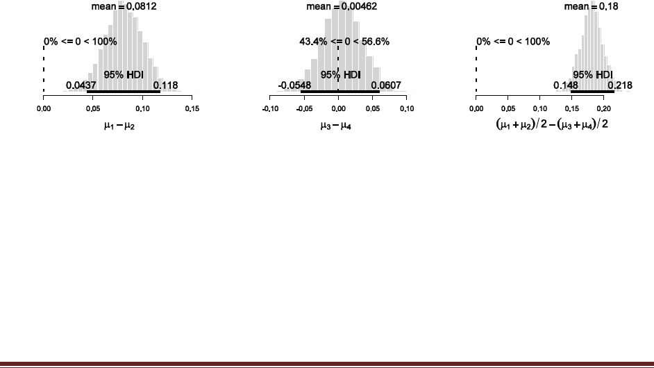
Solutions Manual for Doing Bayesian Data Analysis by John K. Kruschke Page 58
b[condIdx] <- (1-mu[condIdx]) * kappa
# Hyperprior on mu and kappa:
mu[condIdx] ~ dbeta( Amu , Bmu )
}
kappa ~ dgamma( Skappa , Rkappa )
# Constants for hyperprior:
Amu <- 1
Bmu <- 1
Skappa <- pow(meanGamma,2)/pow(sdGamma,2)
Rkappa <- meanGamma/pow(sdGamma,2)
meanGamma <- 10
sdGamma <- 10
}
The modified initialization function:
genInitList <- function() {
sqzData = .01+.98*datalist$z/datalist$N
mu = aggregate( sqzData , list(datalist$cond) , mean )[,"x"]
sd = aggregate( sqzData , list(datalist$cond) , sd )[,"x"]
kappa = mu*(1-mu)/sd^2 - 1
return(
list(
theta = sqzData ,
mu = mu ,
kappa = mean( kappa )
)
)
}
Graph of mu differences:
And here is a graph of the mu and kappa values, just for completeness:
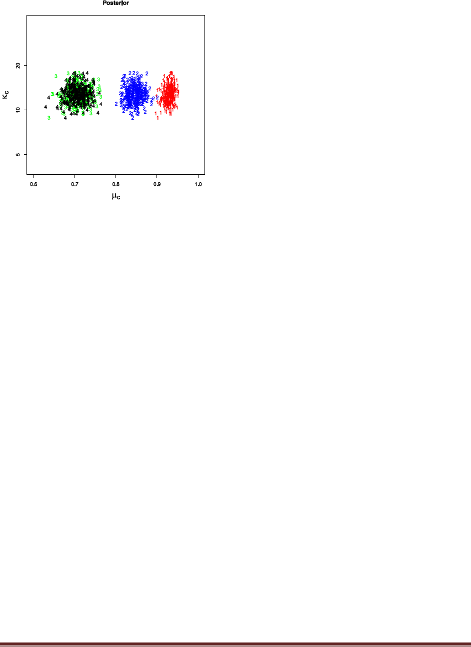
Solutions Manual for Doing Bayesian Data Analysis by John K. Kruschke Page 59
In the scatterplot, the value of kappa is the same for all four groups at any step in the chain. The
value of kappa changes from step to step.
Why are the mu differences farther away from zero than in the original analysis?
The difference, mu1-mu2, has a slightly higher mean than for the original analysis, and a
narrower 95%HDI. Thus, constraining kappa to be the same in each group has made the mu1-
mu2 difference apparently stronger. The reason is a bit subtle, but can be best explained by
looking at the scatterplots in Figure 9.19 of the textbook. Notice that the scatter of kappa1 by
mu1, and the scatter of kappa2 by mu2, shows positive correlation. In other words, if kappa1 is
bigger, then the most credible mu1 is also a little bigger. Moreover, there is no constraint from
one group to the other, so kappa1 is free to be large when kappa2 is randomly selected to be
small. Thus, when considering only the difference mu1-mu2 and collapsing across kappa, the
high variability of the two kappa’s and the correlations of kappa’s with mu’s produces a bit of
smearing of the mu difference. (So, you may ask, why are kappa1 and mu1 correlated? The
answer is that the individual accuracies in group 1 are a bit skewed toward small values, so that
if kappa increases, the data are better accommodated by a higher mu, where the bulk of the
individuals are. Same for group 2.)
(B) The right side of Figure 9.17 shows a model in which thec values for the different
groups come an overarching distribution, the parameters of which are estimated by
considering all the groups. The idea here is that accuracies of individuals in each group
depend on the group mean accuracy, and we are going to estimate the magnitude of that
dependency of individuals on group mean, but we assume that whatever the degree of
dependency is, it will tend to be similar across groups, and we let the data inform our
estimate of that similarity. To implement this assumption in the program, do the following:
First, starting with the original program, in the model specification, change the lines that
specify the mean and standard deviation of the gamma distribution, from constants to
uniform distributions. Use ranges from 0.01 to 30. For example, change meanGamma <- 10
to meanGammadunif(0.01,30), and do the same for sdGamma. The resulting model
specification could look like this (FilconCoKappaBrugs.R): […] Second, be sure that the

Solutions Manual for Doing Bayesian Data Analysis by John K. Kruschke Page 60
initialization of the chains give initial values to meanGamma and sdGamma; such as
mean(kappa[]) and sd(kappa[]), respectively, where kappa[] are data-derived kappas for
the four groups. Now run the modified program. (Hint: For an example of results, see
Figures 9.18 and 9.19, and compare the results with those in Figure 9.16). In your answer:
(1) Report the modified model-specification section of your code; (2) Show the graph of the
estimated differences; (3) Answer this question: Why is the 95% HDI of the 1 -
differences farther away from zero than in the original analysis, but not as far away
from zero as when assuming the same for all conditions?
The modified model specification and the initialization:
model {
for ( subjIdx in 1:nSubj ) {
# Likelihood:
z[subjIdx] ~ dbin( theta[subjIdx] , N[subjIdx] )
# Prior on theta: Notice nested indexing.
theta[subjIdx] ~ dbeta( a[cond[subjIdx]] , b[cond[subjIdx]]
)I(0.001,0.999)
}
for ( condIdx in 1:nCond ) {
a[condIdx] <- mu[condIdx] * kappa[condIdx]
b[condIdx] <- (1-mu[condIdx]) * kappa[condIdx]
# Hyperprior on mu and kappa:
mu[condIdx] ~ dbeta( Amu , Bmu )
kappa[condIdx] ~ dgamma( Skappa , Rkappa )
}
# Constants for hyperprior:
Amu <- 1
Bmu <- 1
Skappa <- pow(meanGamma,2)/pow(sdGamma,2)
Rkappa <- meanGamma/pow(sdGamma,2)
meanGamma ~ dunif( 0.01 , 30 )
sdGamma ~ dunif( 0.01 , 30 )
}
genInitList <- function() {
sqzData = .01+.98*datalist$z/datalist$N
mu = aggregate( sqzData , list(datalist$cond) , mean )[,"x"]
sd = aggregate( sqzData , list(datalist$cond) , sd )[,"x"]
kappa = mu*(1-mu)/sd^2 - 1
return(
list(
theta = sqzData ,
mu = mu ,
kappa = kappa ,
meanGamma = mean( kappa ),
sdGamma = sd( kappa )
)
)
}
Graph of mu differences:
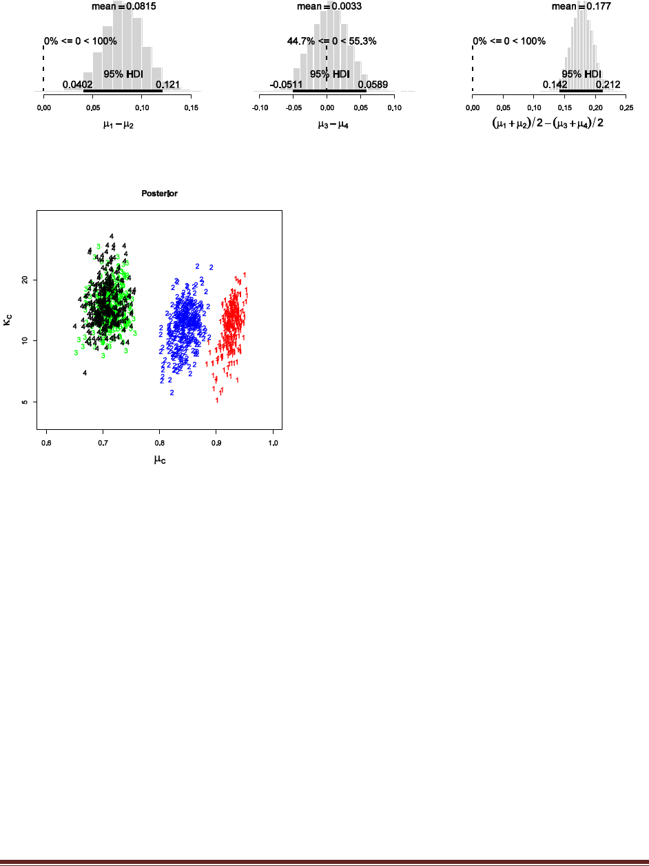
Solutions Manual for Doing Bayesian Data Analysis by John K. Kruschke Page 61
And here is the scatterplot of kappa’s and mu’s:
Why are the mu differences farther away from zero than in the original analysis, but not as far
away as in the equal-kappa model?
As explained in the previous part, the variability of the kappa’s and the correlation of kappa with
mu produces greater variability in the mu’s, hence weaker differences between mu’s. The scatter
plots of mu and kappa (all shown in Figure 9.19 in the textbook) reveal that the variability of the
kappa’s is slightly less for this model than for the independent-kappa’s model. This makes sense,
because the current model has the four groups mutually inform each other’s kappa values. Thus,
because this model has intermediate constraint on the kappa values, and the kappa’s are
correlated with the mu’s, this model also has intermediate sensitivity on the mu1-mu2 difference.
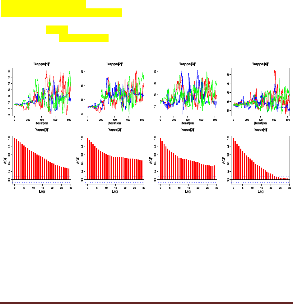
Solutions Manual for Doing Bayesian Data Analysis by John K. Kruschke Page 62
Exercise 9.3. [Purpose: To see, graphically, the importance of burning-in the chains, and
the meaning of autocorrelation.] This exercise uses the BUGS program you created in the
last part of the previous exercise (i.e., the model for the right side of Figure 9.17). You
might find it useful to refer to Section 23.2, p. 623, when doing this exercise. Set the burn-in
to zero and the thinning to zero. In other words, don‘t burn-in at all, and remove the the
thin argument. Have the model go for 800 steps. What do the graphs of the chains look like,
in particular for kappa? See, for example, Figure 9.20. Are the chains thoroughly
overlapping? Include a relevant graph and discuss both burn-in and autocorrelation.
Change the modelUpdate section to this:
#burninSteps = 2000
#modelUpdate( burninSteps )
samplesSet( c("mu","kappa","theta","meanGamma","sdGamma") )
nPerChain = 800 # was ceiling(5000/nChain)
modelUpdate( nPerChain ) # was ,thin=10
The resulting chains for the kappa’s look like this:
Notice that it takes a few hundred steps for the chains to diverge from their equal starting values,
and to settle into their group-specific values. Notice also that the chains can get stuck and
clumpy, as revealed also by the large autocorrelation function (ACF) values shown in the second
row of graphs above. Thus, these chains show the need for burn-in (the period of time it takes for
the chains to diverge and independently sample their posterior-appropriate values) and thinning
(to reduce unrepresentative clumpiness in the posterior sample).
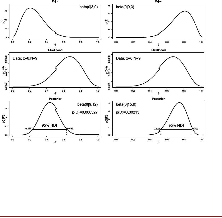
Solutions Manual for Doing Bayesian Data Analysis by John K. Kruschke Page 63
Chapter 10.
Exercise 10.1. [Purpose: To see how first-level model comparison is like hierarchical
modeling with just two values of a hyperparameter.]
(A) Use the R code of Section 5.5.1 (BernBeta.R) (p. 91) to compare the model M1 :
beta(|3,9) and the model M2 : beta(|9,3), when the observed data are z = 6 heads in N = 9
flips. What is the Bayes factor for the two models?
The R commands
postShape = BernBeta( priorShape=c(3,9) , dataVec=c(rep(1,6),rep(0,9-6)) )
postShape = BernBeta( priorShape=c(9,3) , dataVec=c(rep(1,6),rep(0,9-6)) )
yield these graphs:
(The original graphs are smooth but the EPS graphics are rendered incorrectly by Word.)
The Bayes factor is p(D|M2) / p(D|M1) = 0.00213/0.000327 = 6.51.
(B) Verify the values of p(D) by using Equation 5.10, p. 88.
Eqn 5.10 is p(z,N) = B(z+a,N−z+b) / B(a,b). Hence
p(6,9|M2) = B(6+9,9-6+3) / B(9,3) = 0.002128483
p(6,9|M1) = B(6+3,9-6+9) / B(3,9) = 0.000327459

Solutions Manual for Doing Bayesian Data Analysis by John K. Kruschke Page 64
(C) From the right panel of the fourth row of Figure 10.1 (p. 243), visually estimate
p(=0.75|D) and p(=0.25|D), and compute their ratio. Does that ratio nearly match the
Bayes factor that you computed in the first two parts? (It should.)
Visual inspection reveals that the value of p(=0.75|D) is about 26, and p(=0.75|D) is about 4.
The ratio is 26/4 = 6.5, which is nearly the same as what was computed in parts A and B.
Exercise 10.2. [Purpose: To see that the prior can strongly affect the outcome of a model
comparison.] In this exercise we consider a ―toy‖ model comparison to illustrate how the
priors on the parameters in two models can strongly affect the outcome of the comparison.
The models: Consider two models for the bias of a coin. For both models, the probability of
getting a ―head‖ is a Bernoulli distribution of the bias , but each model has a different
expression for determining the value of in terms of a different parameter:
M1 : = 1/(1 + exp(-)), where is any real value (―‖ is Greek ―nu‖), and
M2 : = exp(-), where is non-negative (―‖ is Greek ―eta‖).
(You can easily graph those two function in R if you want to see what they look like.
Figure 14.6, p. 375, shows variations of model M1.) For model 1, we put a normal prior on
, and for model 2, we put a gamma prior on . The data: Suppose we flip the coin and find
that we get 8 heads out of 30 flips.
(A) Suppose the prior on is normal with mean 0 and precision 0.1, whereas the prior on
is gamma with shape 0.1 and rate 0.1. What are the resulting posterior probabilities of the
models (if the prior on the models is 50/50)? […]
The following model specification
model {
for ( i in 1:nFlip ) {
# Likelihood:
y[i] ~ dbern( theta )
}
# Prior
theta <- ( (2-mdlIdx) * 1/(1+exp( -nu )) # theta from model index 1
+ (mdlIdx-1) * exp( -eta ) ) # theta from model index 2
nu ~ dnorm(0,.1) # 0,.1 vs 1,1
eta ~ dgamma(.1,.1) # .1,.1 vs 1,1
# Hyperprior on model index:
mdlIdx ~ dcat( modelProb[] )
modelProb[1] <- .5
modelProb[2] <- .5
}
yields
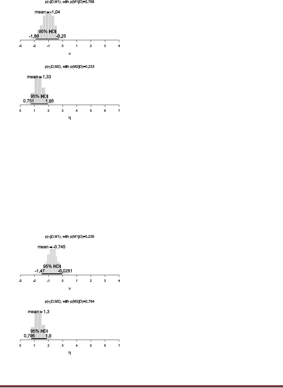
Solutions Manual for Doing Bayesian Data Analysis by John K. Kruschke Page 65
which is a preference for M1.
(B) Suppose the prior on is normal with mean 1 and precision 1, while the prior on is
gamma with shape 1 and rate 1. What are the resulting posterior probabilities of the
models (if the prior on the models is 50/50)? Which model is preferred? (Hint: See Figure
10.7 for the posterior on the parameters and the model probabilities.
Changing the prior specification to
nu ~ dnorm(1,1) # 0,.1 vs 1,1
eta ~ dgamma(1,1) # .1,.1 vs 1,1
yields
which favors M2.

Solutions Manual for Doing Bayesian Data Analysis by John K. Kruschke Page 66
(C) Why does the choice of prior within each model (when the prior on p(M1) and p(M2)
remains unchanged) have such a big influence on the posterior of the model believabilities?
(Hint: Notice in Figure 10.7 that the posterior on the parameter values is in roughly the
same place regardless of the prior—that is, the location of the posterior on the parameter
values is dominated by the data. But notice that the prior probabilities at those posterior-
favored values are rather different, and remember that p(D|M) = …
Inspection of the prior distributions in Figure 10.7 shows that for part A, the prior on (M1) is
high around -1, which is the value that best accommodates the data, but for part B the prior on
is very low around -1. On the other hand, for part A, the prior on is very small around
1.3, which is the value that best accommodates the data, but for part B the prior on is much
larger around 1.3.
(D) Discuss how we might decide which choice of priors on and would put the priors on
an equal playing field. (Technically, in this case, the priors can be reparameterized to yield
exact equivalence, but that‘s not the answer being sought for this exercise. In general,
different models cannot be reparameterized into equivalence. Your discussion should
address what to do in the general case, when models cannot be reparameterized to
equivalence, but be motivated by considering the present toy example.) Here‘s one scheme
to consider: Suppose we have some modest pilot data, or even some audience-agreeable
plausible fictitious data, that in 7 flips there were 2 heads. To generate a prior for the
subsequent new data, we start each model with an extremely vague proto-prior and update
it with the modest pilot data. For example, suppose that the proto-prior on is normal with
mean zero and precision of 0.0001 (i.e., standard deviation of 100), and the proto-prior on
has rate = 0.01 and shape = 0.01. Notice that both of the resulting priors (i.e., the extremely
vague protopriors updated with the modest pilot data) are now reasonably ―in the
ballpark‖ of realistic data, and therefore the models are starting on a more equal playing
field.
We specify the vague “proto-prior”
nu ~ dnorm( 0 , 0.0001 ) # 0,.1 vs 1,1
eta ~ dgamma( 0.01 , 0.01 ) # .1,.1 vs 1,1
and the hypothetical data
N = 7 # 30
z = 2 # 8
datalist = list(
y = c( rep(1,z) , rep(0,N-z) ) ,
nFlip = N
)
It turns out that the chains are badly outcorrelated, so we thin them to saving 1 step in 20.
The resulting posterior looks like this:
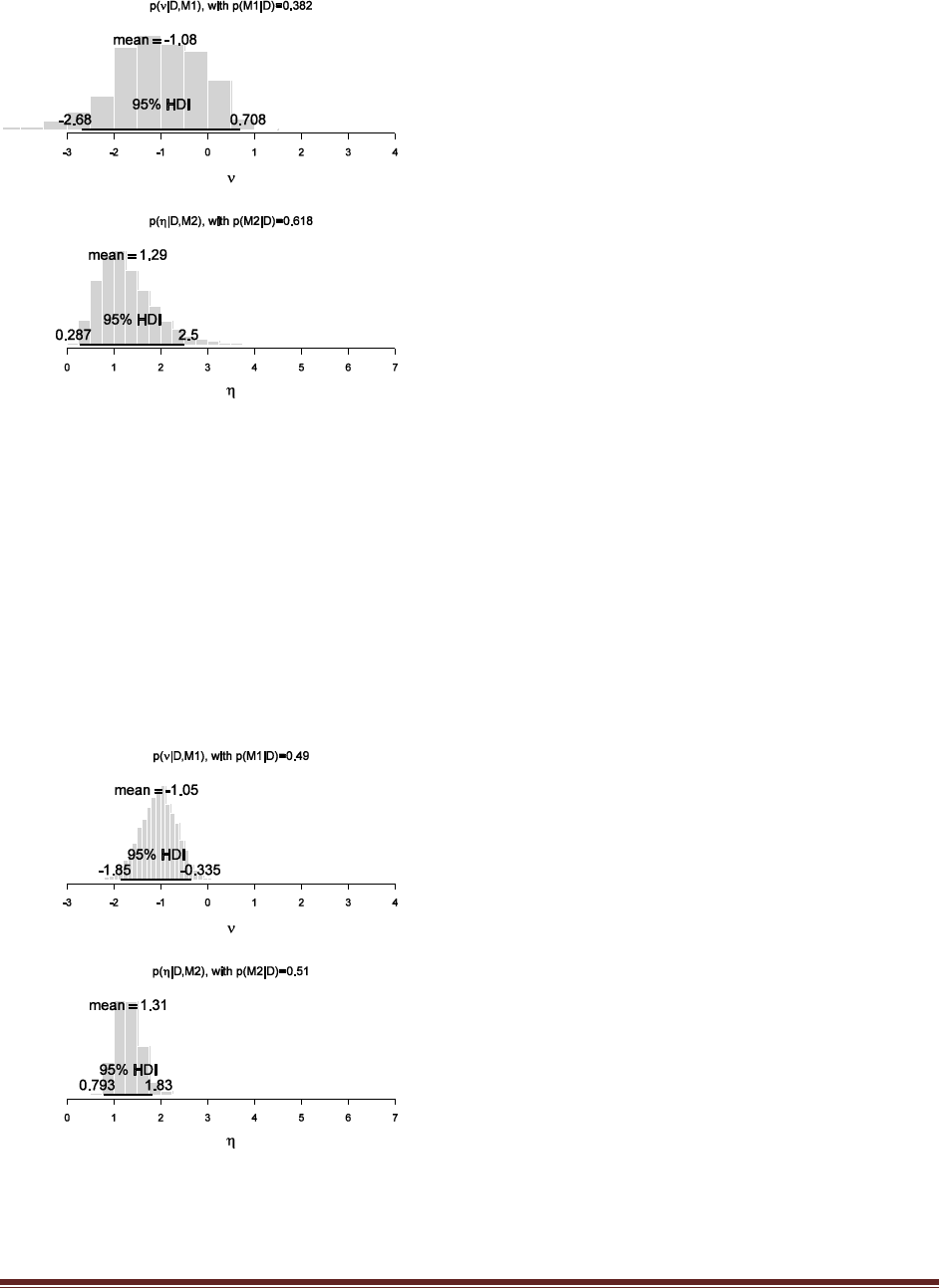
Solutions Manual for Doing Bayesian Data Analysis by John K. Kruschke Page 67
The p(M|D) values displayed in the graph are irrelevant because the protopriors are not of
interest to us. The nu distribution for M1 looks roughly normal and has mean = -1.08 and a
precision (1/var) = 1.14. The eta distribution for M2 looks roughly gamma and has mean = 1.29
and SD = 0.62, which corresponds to a gamma with shape = 4.33 and rate = 3.35 (see Figure 9.8,
p. 209). These posteriors could then be used as the priors for subsequent real data. The priors are
much more comparable for the two models because they were comparably informed by prior
knowledge.
If those priors are used, i.e.,
nu ~ dnorm(-1.08,1.14) # 0,.1 vs 1,1
eta ~ dgamma(4.33,3.35) # .1,.1 vs 1,1
with the actual data, then the posterior is
Notice that p(M1|D) nearly equals p(M2|D)!

Solutions Manual for Doing Bayesian Data Analysis by John K. Kruschke Page 68
Exercise 10.3. [Purpose: To gain hands-on experience with the pseudopriors approach.]
For this exercise, we‘ll consider a situation very similar to the filtration-condensation
experiment that has been used repeatedly in recent pages, and was introduced in Section
9.3.1. The new experiment also involved people learning to categorize shapes. There were
again four different groups, but this time the groups differed on the type of structural shift
from an initial category structure to a new category structure (Kruschke, 1996). Theories
of learning are concerned with this type of situation because different theories predict
different types of transfer from one phase to the next. Our goal in this exercise is to
determine whether the kappa values for the four groups are equivalent, just as we asked
this question of the filtration-condensation data in Section 10.2.2, p. 246. Modify the
program FilconModelCompPseudoPriorBrugs.R for this exercise. […]
(A) Run the program. Notice that the pseudopriors are not well matched to the posterior
distribution. Change the pseudopriors so that they have the same mean and standard
deviation as the posterior. Show this section of your modified code (i.e., the lines that set the
shape and rate constants of the pseudopriors). (Hint: Use mean(kappa1sampleM1) and
sd(kappa1sampleM1) to get the mean and standard deviation of the posterior. Then use the
identities described in Figure 9.8 to determine the shape and rate parameters of a gamma
distribution with that mean and standard deviation.)
Your results might differ a bit from the following, but should be near these values:
Shape for kappa0 is mean(kappa0sampleM2)^2 / sd(kappa0sampleM2)^2 which is
approximately 62.8. Rate for kappa0 is mean(kappa0sampleM2) /
sd(kappa0sampleM2)^2 which is approximately 5.13.
Shape for kappa1 is mean(kappa1sampleM1)^2 / sd(kappa1sampleM1)^2 which is
approximately 8.81. Rate for kappa1 is mean(kappa1sampleM1) /
sd(kappa1sampleM1)^2 which is approximately 0.213.
Shape for kappa2 is mean(kappa2sampleM1)^2 / sd(kappa2sampleM1)^2 which is
approximately 19.3. Rate for kappa2 is mean(kappa2sampleM1) /
sd(kappa2sampleM1)^2 which is approximately 2.17.
Shape for kappa3 is mean(kappa3sampleM1)^2 / sd(kappa3sampleM1)^2 which is
approximately 21.2. Rate for kappa3 is mean(kappa3sampleM1) /
sd(kappa3sampleM1)^2 which is approximately 2.59.
Shape for kappa4 is mean(kappa4sampleM1)^2 / sd(kappa4sampleM1)^2 which is
approximately 14.9. Rate for kappa4 is mean(kappa4sampleM1) /
sd(kappa4sampleM1)^2 which is approximately 1.05.
These values get coded into the pseudo priors of the model as follows:
# Pseudo priors:
# shape, rate kappa0[ model ]
shk0[1] <- 62.8
rak0[1] <- 5.13
# shape kappa[ condition , model ]
shk[1,2] <- 8.81
shk[2,2] <- 19.3
shk[3,2] <- 21.2
shk[4,2] <- 14.9
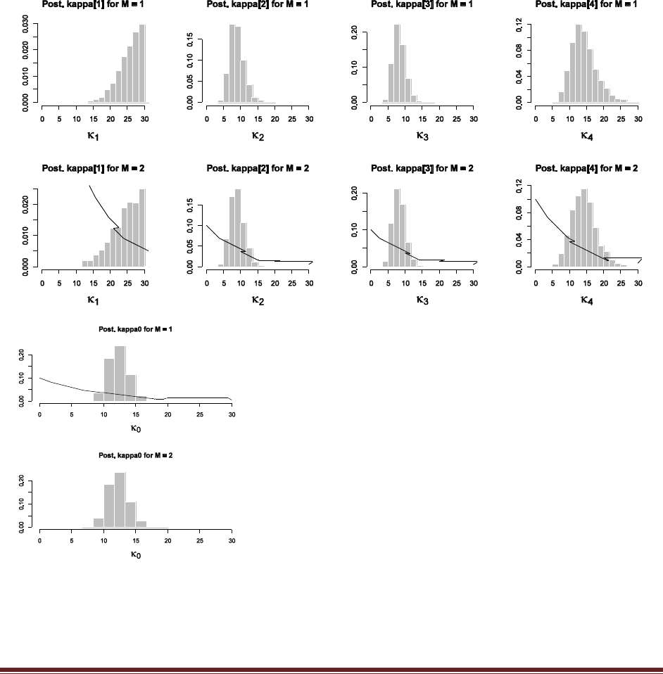
Solutions Manual for Doing Bayesian Data Analysis by John K. Kruschke Page 69
# rate kappa[ condition , model ]
rak[1,2] <- 0.213
rak[2,2] <- 2.17
rak[3,2] <- 2.59
rak[4,2] <- 1.05
(B) Rerun the program with the better-tuned pseudopriors that you determined in the
previous part. Show histograms of the kappa distributions like those in Figure 10.4. (Hint:
Your histograms in the top and bottom rows should be similar, because the pseudoprior is
supposed to mimic the actual posterior. You will find that the histogram for kappa1 falls
largely above 30; that is, it exceeds the right limit of the x axis as it is presently set.)
(The curves representing the vague prior are smooth in the original but rendered incorrectly by
Word.) The distributions in the two rows look very similar, as intended by the setting of the
pseudoprior.
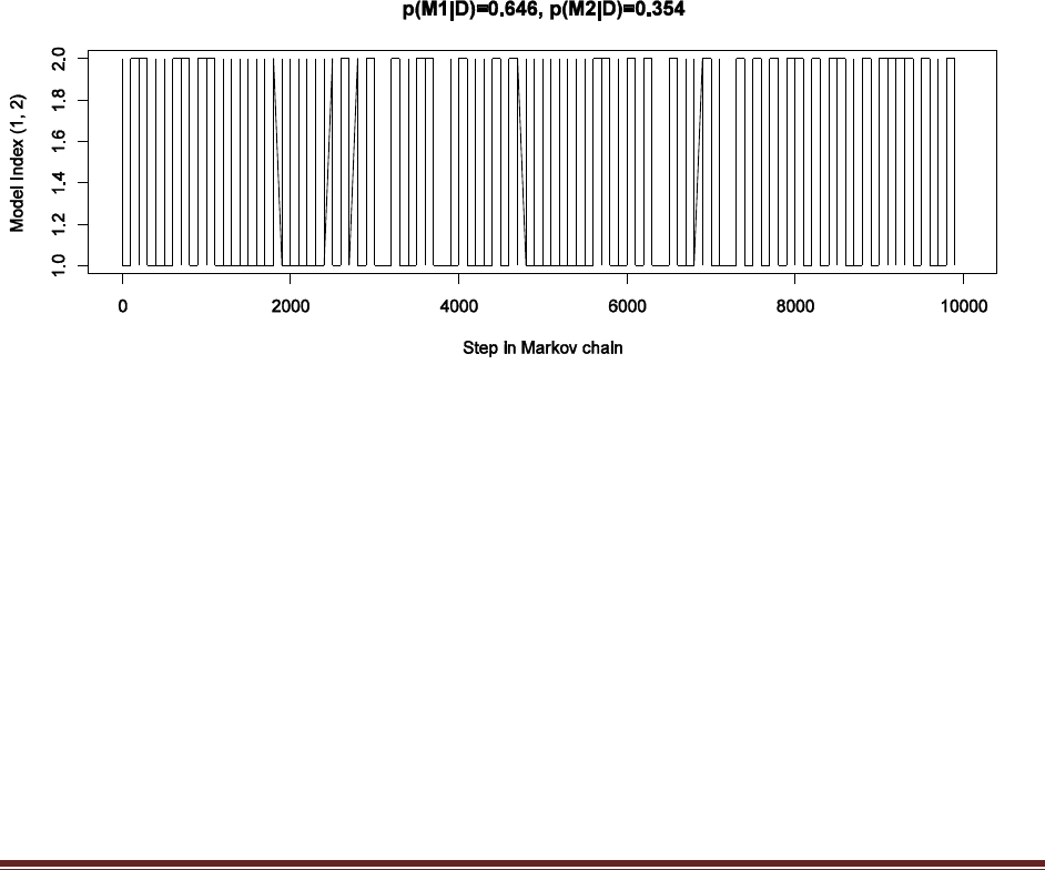
Solutions Manual for Doing Bayesian Data Analysis by John K. Kruschke Page 70
(C) Are the kappa values of the four groups the same or different? Answer this question
two ways, as follows. First, what is the value of the Bayes factor in favor of the different-
kappa model? Be careful to take into account that the BUGS simulation used priors that
were not 50-50. (Hint: It‘s about 600 to 1. Explain how to get that value.) Does the Bayes
factor alone tell us anything about which groups are different? (The correct answer to that
last question is no. Briefly explain why.) Second, considering only the different-kappa
model, what are the distributions of the differences between kappas for model 1?
Specifically, which kappas are different from which other kappas? Does the Bayes factor
tell us anything that the kappa estimates do not? (The correct answer to that last question
is no. Briefly explain why.) (Hint: Your histograms of kappa differences should look
something like Figure 10.8).
First, according to the model-index posterior (see figure below – still a bit autocorrelated;
thinning would help), the posterior odds are p(M1|D)/p(M2|D) = .646/.354 = 1.82. The Bayes
factor is not the posterior, however. Recall that the prior was set at p(M1)=.003 and p(M2)=.997.
Hence the Bayes factor is [p(M1|D)/p(M2|D)] [p(M2)/p(M1)] = 1.82 x .997/.003 = 608, i.e., M1
is favored by about 600 to 1. In other words, the model comparison strongly favors the different-
kappa model.
Second, considering only the different-kappa model, the posterior reveals differences of kappa’s
as shown below:
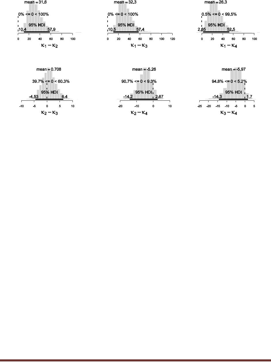
Solutions Manual for Doing Bayesian Data Analysis by John K. Kruschke Page 71
We see that k1 is credibly different from all the other kappas, but the other kappas are not
credibly different from each other. Thus, the estimates of the four kappas tell us that the kappas
are different, which is the same conclusion as the model comparison, but the four-kappa model
tells us more: We have explicit posterior estimates of all four kappas (and their conjoint
distribution).

Solutions Manual for Doing Bayesian Data Analysis by John K. Kruschke Page 72
Chapter 11.
Exercise 11.1. [Purpose: To determine critical values for a two-tailed test, conduct the test,
and notice the dependence of the conclusion on the intended stopping rule.] Suppose we flip
a coin N = 17 times. Our goal is to determine what values for the number of heads would be
extreme enough to reject the hypothesis that the coin is fair. We want the total probability
of false alarm to be less than 5%. In other words, if the null hypothesis is really true, we
will mistakenly reject it less than 5% of the time. Therefore, we desire critical values zlow
and zhigh for the number of observed heads…
(A) What is the value of zlow? Explain how you got your answer. Hint: Try
cumsum( dbinom( 0:17 , 17 , .5 ) ) < .025 and carefully explain what that does!
dbinom( 0:17 , 17 , .5 )
yields the binomial probability for z in 0:17 for N=17 and theta=.5, which is the vector
7.629395e-06 1.296997e-04 1.037598e-03 5.187988e-03 1.815796e-02
4.721069e-02 9.442139e-02 1.483765e-01 1.854706e-01 1.854706e-01
1.483765e-01 9.442139e-02 4.721069e-02 1.815796e-02 5.187988e-03
1.037598e-03 1.296997e-04 7.629395e-06
cumsum( dbinom( 0:17 , 17 , .5 ) )
yields the cumulative sum of the binomial density for z in 0:17 for N=17 and theta=.5, which is
the vector
7.629395e-06 1.373291e-04 1.174927e-03 6.362915e-03 2.452087e-02
7.173157e-02 1.661530e-01 3.145294e-01 5.000000e-01 6.854706e-01
8.338470e-01 9.282684e-01 9.754791e-01 9.936371e-01 9.988251e-01
9.998627e-01 9.999924e-01 1.000000e+00
Notice that its last component is exactly 1.0, as it should be for the sum of a probability
distribution.
cumsum( dbinom( 0:17 , 17 , .5 ) ) < .025
indicates whether each component of the cumulative sum vector is less than .025, which yields
the vector
TRUE TRUE TRUE TRUE TRUE FALSE FALSE FALSE FALSE FALSE FALSE FALSE
FALSE FALSE FALSE FALSE FALSE FALSE.
The 5th component is the largest component that is TRUE, which corresponds to z=4 (because z
starts at 0). Hence zlow is 4, which means that when z is 4 or less, the null hypothesis is rejected.
(B) What is the value of zhigh? Explain how you got your answer. Hint: Try
cumsum( dbinom( 17:0 , 17 , .5 ) ) < .025 and carefully explain what that does!
cumsum( dbinom( 17:0 , 17 , .5 ) ) < .025
is analogous to part A above, but orders the z values from 17 to 0 (instead of from 0 to 17). This
way the cumulative sum starts at the high end of z and works down. The result is
TRUE TRUE TRUE TRUE TRUE FALSE FALSE FALSE FALSE FALSE FALSE FALSE
FALSE FALSE FALSE FALSE FALSE FALSE.

Solutions Manual for Doing Bayesian Data Analysis by John K. Kruschke Page 73
The 5th component is the largest that is TRUE, which corresponds to z=13 (because z starts at
17). Hence zhigh is 13, which means that when z is 13 or higher, the null hypothesis is rejected.
(C) Suppose we flip the coin 17 times and get 4 heads. How many heads would we expect to
get if the coin were fair? Can we reject the null hypothesis ―at the 0.05 level‖ (which means,
with two-tailed false alarm rate less than 0.05)?
If the coin were fair, we would expect to get .5 * 17 = 8.5 heads. The observed value of z=4 is
less than the expected value, so we want to know if z is less than or equal to the critical zlow
determined in part A. Because observed z=4 is indeed less than or equal to zlow=4, we reject the
null hypothesis, with p<.05 two-tailed.
(D) New scenario: We have a six-sided die, and we want to know whether the probability
that the six-dotted face comes up is fair. Thus, we are considering two possible outcomes:
six dots or not six dots. If the die is fair, the probability of the six-dot face is 1/6. Suppose
we roll the die N = 45 times, intending to stop at that number of rolls. What are the values
of zlow and zhigh, using a two-tailed false alarm rate of 5%? Explain how you got your
answer. Suppose we get 3 six-dot rolls. Can we reject the null hypothesis that the die is
fair? (See the upper panel of Figure 11.7 for guidance.)
cumsum( dbinom( 0:45 , 45 , 1/6 ) ) < .025
yields TRUE up to its third component, which is z=2, hence zlow is 2.
cumsum( dbinom( 45:0 , 45 , 1/6 ) ) < .025
yields TRUE up to its 32nd component, which is z=14, hence zhigh is 14.
If the observed z=3, then we do not reject the null, because it is not as low as zlow=2.
(E) Suppose we roll the die until we get 3 six-dot outcomes. It takes 45 rolls. (Notice this is
the same result as the previous part.) How many six-dot outcomes would we expect to get if
the coin were fair? Can we reject the null hypothesis that the die is fair, at the 0.05 level?
(See the lower panel of Figure 11.7 for guidance.)
A plot much like the lower-right of Figure 11.7 can be created by the following two lines of
code:
nbin = function( N , z , theta ) { z * dbinom(z,N,theta) / N }
plot( 3:52 , nbin( 3:52 , 3 , 1/6 ) , type="h" )
We can use the nbin function, defined above, to find the critical values:
cumsum( nbin( 3:52 , 3 , 1/6 ) ) < .025
is TRUE only to its second component, which corresponds to Nlow=4.
sum( nbin( 3:41 , 3 , 1/6 ) )
is 0.9761868, which means that N=42 is the smallest N in the high rejection tail, i.e., Nhigh=42.

Solutions Manual for Doing Bayesian Data Analysis by John K. Kruschke Page 74
The observed N=45 exceeds Nhigh, therefore we reject the null hypothesis. Notice that this
contradicts the conclusion from the previous part.
Exercise 11.2. [Purpose: To determine NHST confidence intervals and notice that they
depend on the experimenter‘s intention.] Suppose we flip a coin N = 26 times and observe z
= 8 heads. Assume that the intention was to stop when N = 26.
(A) Show that when =0.144, the probability of z ≥8 is just over 2.5%, but for smaller
values of , the probability of z ≥ 8 is less than 2.5%. Hint: Try
for( theta in seq( .140 , .150 , .001 ))
{ show( c( theta , sum( dbinom( 8:26 ,26 , theta )) )) }
and explain carefully what that does.
The code increments theta in steps of .001 and shows the sum of the binomial distribution from 8
to 26. A more elaborate version of the code produces graphs along with the sum:
windows(7,7)
layout( matrix( 1:6 , ncol=2 , byrow=T ) )
par( mar=c(4,4,2.5,1) , mgp=c(2,0.7,0) )
for( theta in seq( .141 , .146 , 0.001 ) ) {
plot( 0:26 , dbinom( 0:26 , 26 , theta ) , type="h" , lwd=3 ,
xlab="z" , ylab="dbinom(z,N=26,theta)" ,
main=bquote( list(
theta==.(theta) ,
"p(z >= 8) = "*.(round(sum(dbinom(8:26,26,theta)),4))
)) )
abline( v=7.5 , lty="dashed" )
}
which yields this graph:
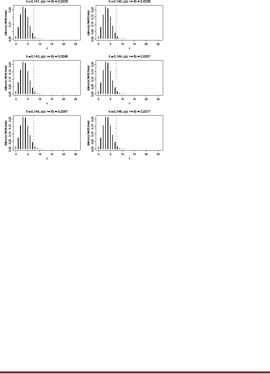
Solutions Manual for Doing Bayesian Data Analysis by John K. Kruschke Page 75
You can see in the middle row that as theta increases from .143 to .144, p(z>=8) increases from
.0248 to .0257. In other words, a result of z=8 does reject theta=.143, but does not reject
theta=.144.
(B) Show that when theta = 0.517, the probability of z <= 8 is just over 2.5%, but when
theta exceeds 0.517, then p(z<=8) drops below 2.5%.
Analogously to the answer of the previous part, we can graph the binomial as theta increments:
windows(7,7)
layout( matrix( 1:6 , ncol=2 , byrow=T ) )
par( mar=c(4,4,2.5,1) , mgp=c(2,0.7,0) )
for( theta in seq( .515 , .520 , 0.001 ) ) {
plot( 0:26 , dbinom( 0:26 , 26 , theta ) , type="h" , lwd=3 ,
xlab="z" , ylab="dbinom(z,N=26,theta)" ,
main=bquote( list(
theta==.(theta) ,
"p(z <= 8) = "*.(round(sum(dbinom(0:8,26,theta)),4))
)) )
abline( v=8.5 , lty="dashed" )
}
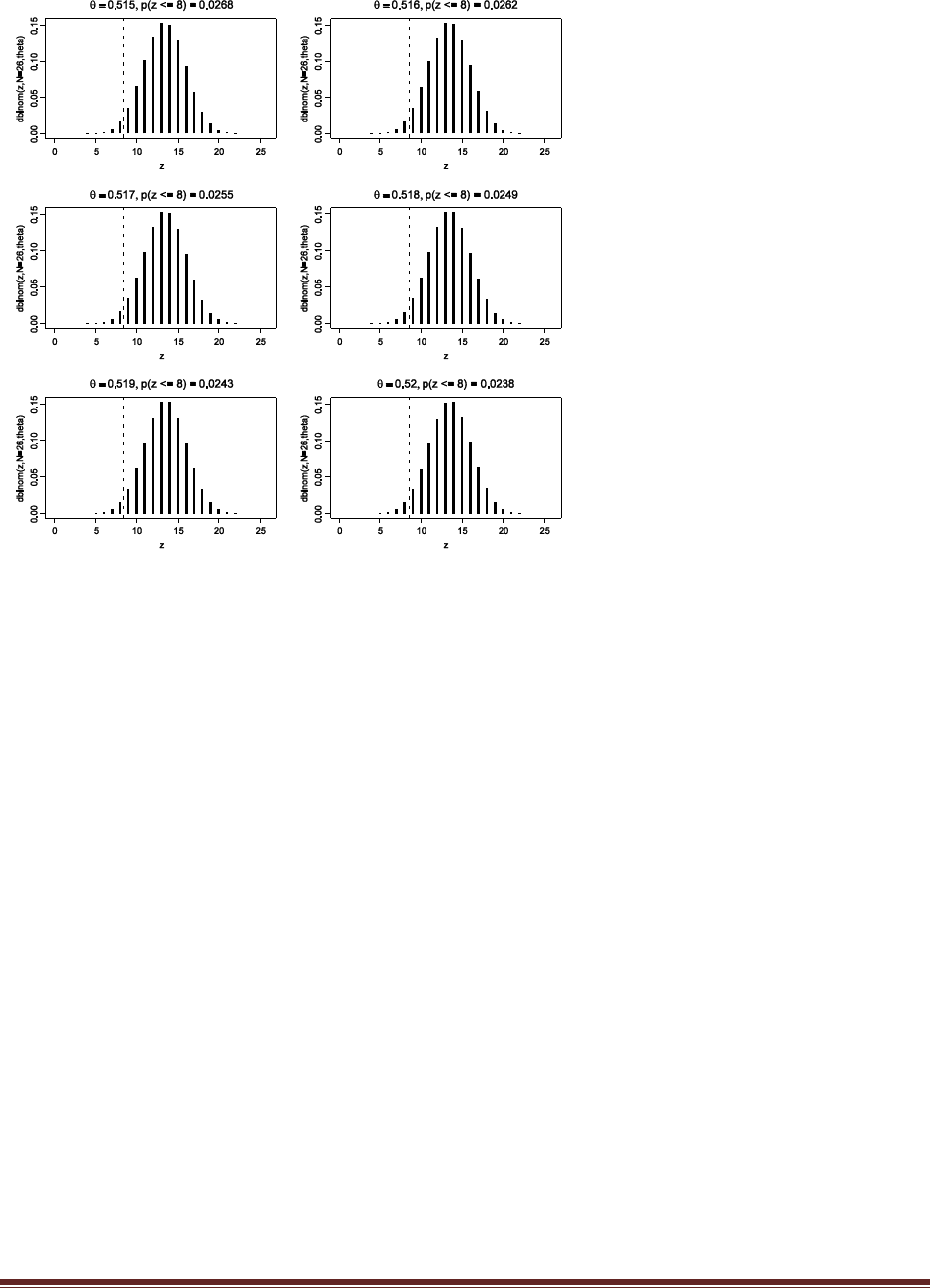
Solutions Manual for Doing Bayesian Data Analysis by John K. Kruschke Page 76
It can be seen in the middle row that as theta goes from .517 to .518, the left-tail probability goes
from .0255 to .0249. Hence z=8 rejects theta=.518, but z=8 does not reject theta=.517.
(C) What is the 95% confidence interval for theta? (Just summarize the results of the
previous two parts.)
The range of theta’s that is not rejected by z=8 (with N=26) extends from theta=.144 to
theta=.517.
(D) Suppose that the intention was to stop when z = 8 heads. Explain how to determine the
NHST confidence interval, and include R code as appropriate. (Compare to Figure 11.5.)
This code, analogous to the previous parts, produces the graphs that follow:
windows(7,7)
layout( matrix( 1:6 , ncol=2 , byrow=T ) )
par( mar=c(4,4,2.5,1) , mgp=c(2,0.7,0) )
for( theta in seq( .141 , .146 , 0.001 ) ) {
plot( 8:114 , nbin( 8:114 , 8 , theta ) , type="h" , lwd=1 ,
xlab="z" , ylab="nbin(N,z=8,theta)" ,
main=bquote( list(
theta==.(theta) ,
"p(N <= 26) = "*.(round(sum(nbin(8:26,8,theta)),4))
)) )
abline( v=26.5 , lty="dashed" )
}
windows(7,7)
layout( matrix( 1:6 , ncol=2 , byrow=T ) )
par( mar=c(4,4,2.5,1) , mgp=c(2,0.7,0) )
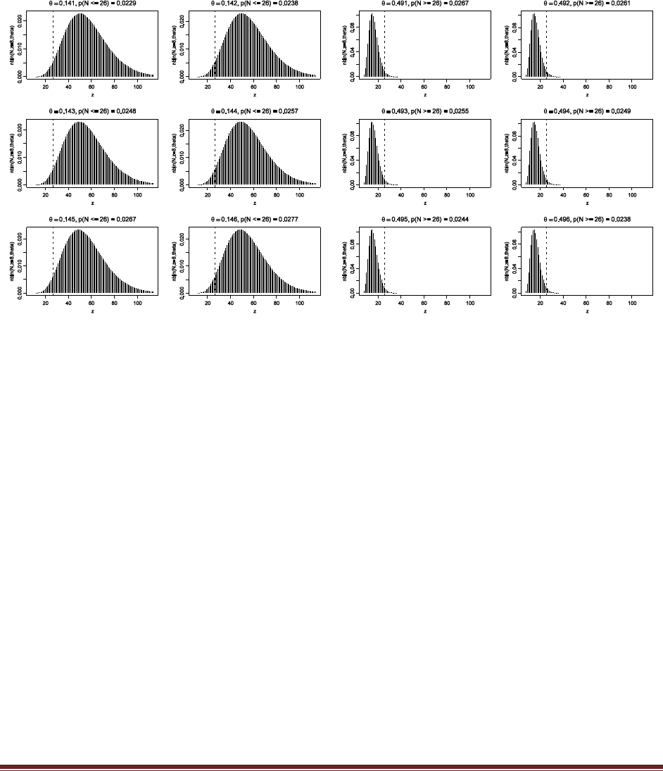
Solutions Manual for Doing Bayesian Data Analysis by John K. Kruschke Page 77
for( theta in seq( .491 , .496 , 0.001 ) ) {
plot( 8:114 , nbin( 8:114 , 8 , theta ) , type="h" , lwd=1 ,
xlab="z" , ylab="nbin(N,z=8,theta)" ,
main=bquote( list(
theta==.(theta) ,
"p(N >= 26) = "*.(round(1-sum(nbin(8:25,8,theta)),4))
)) )
abline( v=25.5 , lty="dashed" )
}
The left panels show that theta=.144 is not rejected, but theta=.143 is rejected.
The right panels show that theta=.493 is not rejected, but theta=.494 is rejected.
Hence the confidence interval, of values not rejected by N=26 (for fixed z=8), goes from
theta=.144 to theta=.493. Notice that this is different than the confidence interval for z=8 with
fixed N=26, computed in the previous part.
Exercise 11.3. [Purpose: To determine the p value if a coin is flipped for a fixed period of
time instead of for a fixed number of flips.] (For another example of NHST for fixed-
duration samples, see Kruschke, 2010a.) An experimenter is investigating whether there
are more conservatives or liberals in her subject pool. She recruits 46 subjects and finds
that 30 of them are liberal. We are interested in testing the null hypothesis that the
population is split 50-50; (i.e., theta = 0.5).
(A) If we assume that the experimenter intended to stop when N = 46, what is the
probability of getting 30 or more liberals in a sample according to the null hypothesis? Do
we reject the null hypothesis? Hint: sum( dbinom( 30:46 , 46 , .5 ) ) < 0.025
The Hint code indicates whether the probability of getting 30 or more flips out of N=46 is less
than .025. The result is FALSE, because sum(dbinom(30:46,46,.5)) = .0270. Therefore we do not
reject the null hypothesis. (We ask about 30 or more because 30 is larger than the expected value
of 23.)

Solutions Manual for Doing Bayesian Data Analysis by John K. Kruschke Page 78
(B) We ask the experimenter why she chose N = 46. She replies that she didn‘t; in fact, she
chose to run the experiment for 1 week, and she just happened to get 46 subjects. (This is
typical in real-world research. There is nothing wrong with this procedure because we are
assuming that every person polled is independent of every other person polled and
uninfluenced by the poller‘s intentions.) With these intentions regarding duration, we
cannot assume that N is fixed at 46, and therefore the space of possible experiment
outcomes is much larger. … Is the probability of getting the observed proportion less than
2.5%? Do we reject the null hypothesis? How does this compare with the conclusion from
the previous part of the exercise?
The code stated in the exercise, namely
z_obs = 30 ; N_obs = 46
nulltheta = .5
tail_prob = 0 # Zero initial value for accumulation over possible N.
for ( N in 1 : (3*N_obs) ) { # Start at 1 to avoid /0. 3*N_obs is arbitrary.
# Create vector of z values such that z/N >= z_obs/N_obs
zvec = (0:N)[ (0:N)/N >= z_obs/N_obs ]
tail_prob = tail_prob + (
dpois( N , N_obs ) * sum( dbinom( zvec , N , nulltheta ) ) )
}
show( tail_prob )
yields p=.0209, which is <.025. In other words, contrary to the conclusion of the previous part,
this analysis says we do reject the null hypothesis when the intention is to run the experiment for
1 week.
(C) Repeat the previous two parts, for z = 26 and N = 39.
When N=39 is fixed, we get p = sum( dbinom( 26:39 , 39 , .5 ) ) = 0.02662, hence we do not
reject the null hypothesis.
When the duration is fixed with a mean rate of 26/39, then the code above produces p=.0229,
hence we do reject the null hypothesis, contrary to when N is fixed.
Exercise 11.4. [Purpose: To determine the false alarm rate for a two-tiered data collection
process (compare to Berger & Berry, 1988).] …
(A) For N = 30, what are zlow and zhigh, assuming a two-tailed false alarm rate of .05 or
less? (See Exercise 11.1.) (Hint: The answer is 9 and 21; your job is to explain how to get
that answer.)
Using the techniques of Exercise 11.1, we simply see which indices of the vector 0:30 or 30:0
have cumulative sums less than .025:
max( (0:30)[ cumsum( dbinom( 0:30 , 30 , .5 ) ) < .025 ] ) = 9
min( (30:0)[ cumsum( dbinom( 30:0 , 30 , .5 ) ) < .025 ] ) = 21
(B) For N = 45, what are zlow and zhigh, assuming a two-tailed false alarm rate of .05 or
less? (See Exercise 11.1.) (Hint: The answer is 15 and 30; your job is to explain how to get
that answer.)

Solutions Manual for Doing Bayesian Data Analysis by John K. Kruschke Page 79
As in the previous part:
max( (0:45)[ cumsum( dbinom( 0:45 , 45 , .5 ) ) < .025 ] ) = 15
min( (45:0)[ cumsum( dbinom( 45:0 , 45 , .5 ) ) < .025 ] ) = 30
For the next parts of the exercise, consider Table 11.1. Each cell of Table 11.1 corresponds
to a certain outcome from the first 30 flips and a certain outcome from the second 15 flips.
A cell is marked by a dagger, †, if it has a result for the first 30 flips that would reject the
null hypothesis. A cell is marked by a double dagger, ‡, if it has a result for the total of 45
flips that would reject the null hypothesis. For example, the cell with 10 heads from the
first 30 flips and 1 head from the second 15 flips is marked with a ‡ because the total
number of heads for that cell, 10 + 1 = 11, is less than 15 (which is zlow for N = 45). That
cell has no single dagger, †, because getting 10 heads in the first 30 flips is not extreme
enough to reject the null.
(C) Denote the number of heads in the first 30 flips as z1, and the number of heads in the
second 15 flips as z2. Explain why it it true that the z1, z2 cell of the table has conjoint
probability equal to dbinom(z1,30,.5) * dbinom(z2,15,.5).
The first 30 flips (event 1) and the next 15 flips (event 2) are independent of each other. Hence
the conjoint probability of the outcomes of the two events is simply the product of the individual
event probabilities.
(D) What is the sum of the probabilities of all the cells that contain a † (whether or not it
contains a ‡)? Explain how you got your answer! (Hint: The answer is not greater than
0.05. See also the Hint at the end of the exercise).
The Hint provides this R code:
N1 = 30 # Number of flips for first test. Try 17.
N2 = 15 # Number of _additional_ flips for second test. Try 27 or 50.
theta = .5 # Hypothesized bias of coin.
FAmax = .05 # False Alarm maximum for a single test.
NT = N1 + N2 # Total number of flips.
# Determine critical values for N1:
# EXPLAIN what each function does and why, including
# dbinom, cumsum, which, max, and (0:N)[...]
loCritN1 = (0:N1)[ max( which( cumsum( dbinom(0:N1,N1,theta) ) <= FAmax/2 ) ) ]
hiCritN1 = (N1:0)[ max( which( cumsum( dbinom(N1:0,N1,theta) ) <= FAmax/2 ) ) ]
# Compute actual false alarm rate for those critical values.
# EXPLAIN what this does and why.
FA1 = sum( ( 0:N1 <= loCritN1 | 0:N1 >= hiCritN1 ) * dbinom(0:N1,N1,theta) )
cat( "N1:",N1 , ", lo:",loCritN1 , ", hi:",hiCritN1 , ", FA:",FA1 , "\n" )
# Determine critical values for NT:
# EXPLAIN what each function does and why, including
# dbinom, cumsum, which, max, and (0:N)[...]
loCritNT = (0:NT)[ max( which( cumsum( dbinom(0:NT,NT,theta) ) <= FAmax/2 ) ) ]
hiCritNT = (NT:0)[ max( which( cumsum( dbinom(NT:0,NT,theta) ) <= FAmax/2 ) ) ]
# Compute actual false alarm rate for those critical values.
# EXPLAIN what this does and why.
FAT = sum( ( 0:NT <= loCritNT | 0:NT >= hiCritNT ) * dbinom(0:NT,NT,theta) )
cat( "NT:",NT , ", lo:",loCritNT , ", hi:",hiCritNT , ", FA:",FAT , "\n" )

Solutions Manual for Doing Bayesian Data Analysis by John K. Kruschke Page 80
# Determine actual false alarm rate for the two-tier test:
# EXPLAIN each of the matrices below --- what is in each one?
Z1mat = matrix( 0:N1 , nrow=N2+1 , ncol=N1+1 , byrow=TRUE )
ZTmat = outer( 0:N2 , 0:N1 , "+" )
pZTmat = outer( dbinom( 0:N2 , N2 , theta ) , dbinom( 0:N1 , N1 , theta ) )
# EXPLAIN the matrices in computation below.
FA1or2 = sum( ( ( ZTmat <= loCritNT | ZTmat >= hiCritNT ) # double dagger matrix
| ( Z1mat <= loCritN1 | Z1mat >= hiCritN1 ) # single dagger matrix
) * pZTmat )
cat( "Two tier FA:" , FA1or2 , "\n" )
The first sections of the code simply find the critical values, as was done in parts A and B of this
exercise. Those sections also compute the actual false alarm rate when using those critical
values, by summing the tail probabilities of the binomial distributions.
For 30 flips, the rejection-tail probability is .0428.
(E) What is the sum of the probabilities of all the cells that contain a ‡ (whether or not it
contains a †)? Explain how you got your answer! (Hint: The answer is not greater than
0.05. See also the Hint at the end of the exercise.)
From the middle section of the code, we find that the rejection-tail probability for the 15 flips is
.0357.
(F) What is the sum of the probabilities of all the cells that contain either a † or a ‡? Note:
This is the false alarm rate for the two-stage design, because these are all the ways you
would decide to reject the null even when it‘s true. Explain how you got your answer!
(Hint: The answer is greater than 0.05. See also the Hint at the end of the exercise.)
The last section of code is the important part for the two-tier procedure. The matrix Z1mat
represents the outcome of the first 30 flips. Its size is 16x31 and has all 0’s in its first column, all
1’s in its second column, and so on, with all 30’s in its 31st column. The ZTmat matrix
represents the sum total of the all 45 flips. Its size is also 16x31. It has a 0 in the top left cell, 1’s
in cells [1,2] and [2,1], 2’s in the next diagonal, and so on, until cell [16,31] contains the value
45.
The matrix pZTmat contains the probability of each outcome, namely, the product of the
binomial probability of the first 30 flips and the binomial probability of the next 15 flips. The
matrix is constructed by using R’s outer() function.
The single-dagger matrix is computed as
Z1mat <= loCritN1 | Z1mat >= hiCritN1
which yields TRUE only where Z1mat has entries below loCritN1 or above hiCritN1.
The double-dagger matrix is similarly computed as
ZTmat <= loCritNT | ZTmat >= hiCritNT
By taking the logical OR of those two matrices, the result is TRUE anywhere there is a single or
double dagger. That matrix is component-multiplied by pZTmat to isolate only the probabilities
of the single or double-dagger cells. The matix is then summed.

Solutions Manual for Doing Bayesian Data Analysis by John K. Kruschke Page 81
The resulting sum is p=.061. Thus, the two-tier procedure has a false alarm rate greater than .05.
(G) Suppose that the researcher intends to run an experiment using this two-stage stopping
criterion. She collects the first 30 flips and finds 8 heads. She therefore rejects the null
hypothesis and reports that p < 0.05. Is that correct? Explain. (Hint: The answer is no, it‘s
not correct, because the design of the experiment included a larger potential sampling
space.)
Even though the researcher stopped after the first 30 flips, the design of experiment considered
the larger sample space involving the second 15 flips. Thus, because the researcher intended to
continue if the first 30 did not yield a significant result, the researcher must report the probability
of false alarm from the intended design. Thus, the researcher should report that p<.061.
(H) Whenever we run an experiment and get a result that trends away from the null
expectation, but isn‘t quite significant, it‘s natural to consider collecting more data. We saw
in the previous part that even intending to collect more data, but not actually doing it,
inflates the false alarm rate. Doesn‘t the fact that we always consider collecting more data
mean that we always have a much higher false alarm risk than we pretend we do? Doesn‘t
the actual false alarm rate of an experiment depend on the maximal number of data points
we‘d be willing to collect over the course of our lifetimes?
Yes! And that is another reason why NHST is so strange --- the p value depends on our
(un-)willingness to collect more data.
This is another manifestation of the same problem that arose in the context of multiple
comparisons (section 11.4.1). When we contemplate including another condition in a study,
which will be compared with existing conditions, we enlarge the space of possible comparisons
and therefore inflate the false alarm rate. We don’t actually need to have collected the data in the
addition condition, we merely need to intend to compare with that condition once we collect the
data. That situation is analogous to the present scenario; it’s just that here we merely intend to
collect more data in the same condition instead of in a different condition.

Solutions Manual for Doing Bayesian Data Analysis by John K. Kruschke Page 82
Chapter 12.
Exercise 12.1. [Purpose: To investigate model comparison for different partitions of group
means.] The program in Section 12.4.1(OneOddGroupModelComp.R) does a model
comparison in which M1 has different means for every group and M2 has the same mean
for all groups. In this exercise, we consider a different model comparison, with a different
partition of the conditions.
(A) Consider a comparison for which M1 has one mean for condition 1 and a second mean
for conditions 2 through 4, and M2 has the same mean for all groups. A quick-and-dirty
way to program this is by changing the model specification to
(OneOddGroupModelCompEx12.1.R)
24 for ( j in 1:2 ) {
25 mu[j] ~ dbeta( a[j,mdlIdx] , b[j,mdlIdx] )
26 }
27 mu[3] <- mu[2]
28 mu[4] <- mu[2]
Explain in English what the modified code does.
Answer: The code puts beta priors on mu[1] and mu[2], but sets mu[3] and mu[4] equal to
mu[2].
Unfortunately, the modified model structure is not amenable to automatic initialization in
BUGS. We can ―manually‖ initialize it this way (OneOddGroupModelCompEx12.1.R):
120 genInitList <- function() {
121 sqzData = .01+.98*datalist$nCorrOfSubj/datalist$nTrlOfSubj
122 mu = aggregate( sqzData , list(datalist$CondOfSubj) , "mean" )[,"x"]
123 sd = aggregate( sqzData , list(datalist$CondOfSubj) , "sd" )[,"x"]
124 kappa = mu*(1-mu)/sdˆ2 - 1
125 return(
126 list(
127 theta = sqzData ,
128 mu = c( mu[1] , mean( mu[2:4] ) , NA , NA ) ,
129 mu0 = mean(mu) ,
130 kappa = kappa ,
131 mdlIdx = 1
132 )
133 )
134 }
135 for ( chainIdx in 1 : nchain ) {
136 modelInits( bugsInits( genInitList ) )
137 }
The initialization uses the same technique introduced in Section 9.5.2 (FilconBrugs.R), with
only one novel nuance: The last two components of mu are specified as NA because those
components are not stochastic, but are instead fixed (in the model specification) to equal
mu[2]. …
Run the modified program, and show the resulting graphs analogous to those in Figure
12.5. Why are the upper histograms all the same, and why are the lower histograms (e.g.,
mu2 - mu3) so strange looking?
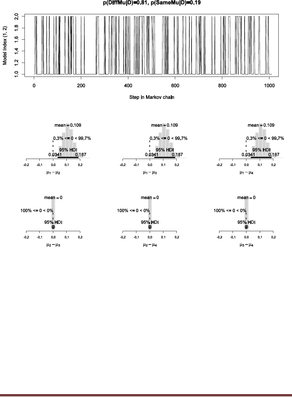
Solutions Manual for Doing Bayesian Data Analysis by John K. Kruschke Page 83
The upper histograms are all the same because mu2 = mu3 = mu4, hence mu1-mu2 = mu1-mu3
= mu1-mu4.
The lower histograms are strange looking because the differences are all zero. That is, because
mu2=mu3=mu4, mu2-mu3=0 and mu2-mu4=0 and mu3-mu4=0. Hence the histograms must be
spikes over zero.
(B) What should we conclude from the model comparison of the previous part? (Be careful
to express your conclusion as a statement about relative believabilities.) Should we
conclude that the means of conditions 2 through 4 are actually equal?
The prior on the two model indices was 50/50, and the posterior of the index (shown in the chain
above) shows 81% vs 19% in favor of the different-mu model. This means that of these two
models, the different-mu model is more than four times more believable than the same-mu
model. But this does not imply that the different-mu model is correct, it merely implies that it is

Solutions Manual for Doing Bayesian Data Analysis by John K. Kruschke Page 84
better than the same-mu model. In particular, the different-mu model asserts that
mu2=mu3=mu4, but this might not be an accurate description of the groups.
Exercise 12.2. [Purpose: To estimate a difference, including a ROPE (and the hot hand
example with a better prior).]
(A) Consider again the hot hand example from Exercise 8.1, p. 188. In this part of the
exercise we establish a better prior: We know from general basketball statistics that
professional players tend to make about 75% of their free throws, with some players
almost as low as 50% and some players almost as high as 95%. A beta(theta|16,6)
distribution nicely captures this prior knowledge. But what we do not know from prior
statistics is the difference between success after success and success after failure in pairs of
free throws. To be as vague as possible about the difference, we‘ll put a uniform
distribution on the difference. Notice that when the overall success rate is, say, 90%, the
difference could be anything from +20% (i.e., 100% versus 80%) to -20% (i.e., 80% versus
100%), but when the overall success rate is, say, 70%, then the difference could be
anything from +60% to -60%. The specification of the prior needs to accommodate this
range that depends on the overall success. Here is one way to specify this in the BUGS
model:
theta1 <- mu + deflect
theta2 <- mu - deflect
mu ~ dbeta( 16 , 6 )
delta ~ dbeta( 1 , 1 )
deflect <- (delta-.5)*2 * min(mu,1-mu)
The variable mu is the overall success rate. The variable deflect is the deflection away from
mu created by a previous success or a previous failure. The value of deflect is just a linearly
transformed value of the random variable delta, which has a uniform prior. Incorporate
this code into the model and run without the data, so you can see the prior. Show your
complete model specification and a graph of the MCMC sample, which should look much
like the upper row of Figure 12.6.
Here is the complete program used to generate Figure 12.6:
graphics.off()
library(BRugs)
priorOnly = T # Kruschke, J. K. (2010). Doing Bayesian data analysis:
# A Tutorial with R and BUGS. Academic Press / Elsevier.
#------------------------------------------------------------------------------
# THE MODEL.
modelstring = "
# BUGS model specification begins here...
model {
# Likelihood. Each flip is Bernoulli.
for ( i in 1 : N1 ) { y1[i] ~ dbern( theta1 ) }
for ( i in 1 : N2 ) { y2[i] ~ dbern( theta2 ) }
# Prior.
theta1 <- mu + deflect
theta2 <- mu - deflect
mu ~ dbeta( 16 , 6 ) # mean about 75%, range about 50% to 95%
delta ~ dbeta(1,1) # prior on hot-hand difference is uniform
deflect <- (delta-.5)*2 * min(mu,1-mu)
}

Solutions Manual for Doing Bayesian Data Analysis by John K. Kruschke Page 85
# ... end BUGS model specification
" # close quote for modelstring
# Write model to a file:
.temp = file("model.txt","w") ; writeLines(modelstring,con=.temp) ; close(.temp)
# Load model file into BRugs and check its syntax:
modelCheck( "model.txt" )
#------------------------------------------------------------------------------
# THE DATA.
# Specify the data in a form that is compatible with BRugs model, as a list:
z1 = 251 ; N1 = 285 ; z2 = 48 ; N2 = 53 # data are specified here
if ( priorOnly ) {
datalist = list(
N1 = N1 ,
#y1 = c( rep(1,z1) , rep(0,N1-z1) ) ,
N2 = N2 #,
#y2 = c( rep(1,z2) , rep(0,N2-z2) )
)
} else {
datalist = list(
N1 = N1 ,
y1 = c( rep(1,z1) , rep(0,N1-z1) ) ,
N2 = N2 ,
y2 = c( rep(1,z2) , rep(0,N2-z2) )
)
}
# Get the data into BRugs:
modelData( bugsData( datalist ) )
#------------------------------------------------------------------------------
# INTIALIZE THE CHAIN.
modelCompile()
modelGenInits()
#------------------------------------------------------------------------------
# RUN THE CHAINS.
samplesSet( c( "theta1" , "theta2" ) ) # Keep a record of sampled "theta" values
chainlength = 10000 # Arbitrary length of chain to generate.
modelUpdate( chainlength ) # Actually generate the chain.
#------------------------------------------------------------------------------
# EXAMINE THE RESULTS.
if ( priorOnly ) {
fnrt = "Exercise12.2.prior"
} else {
fnrt = "Exercise12.2.post"
}
theta1Sample = samplesSample( "theta1" ) # Put sampled values in a vector.
theta2Sample = samplesSample( "theta2" ) # Put sampled values in a vector.
# Plot a histogram of the posterior differences of theta values.
source("plotPost.R")
windows(10,5.5)
layout( matrix( 1:2 , ncol=2 ) )
thetaDiff = theta1Sample - theta2Sample
thindex = round(seq(1,length(theta1Sample),len=700))
if ( priorOnly ) {
xlimits = c(0,1) ; ylimits = c(0,1)
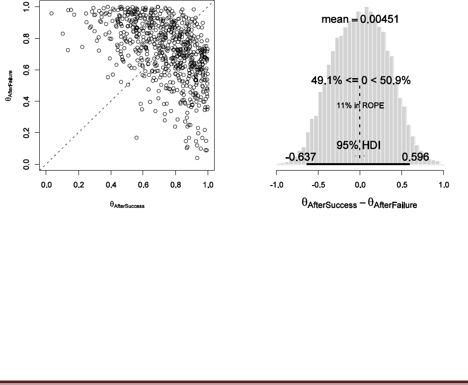
Solutions Manual for Doing Bayesian Data Analysis by John K. Kruschke Page 86
} else {
xlimits = c(.7,1) ; ylimits = c(.7,1)
}
plot( theta1Sample[thindex] , theta2Sample[thindex] ,
ylab=expression(theta[AfterFailure]) , xlim=xlimits ,
xlab=expression(theta[AfterSuccess]) , ylim=ylimits )
abline(0,1,lty="dashed")
plotPost( thetaDiff , xlab=expression(theta[AfterSuccess]-theta[AfterFailure]) ,
breaks=30 , compVal=0.0 , main="" , ROPE=c(-.05,.05) )
rope = c(-0.05,0.05)
probPracEqZero = ( sum( thetaDiff > rope[1] & thetaDiff < rope[2] )
/ length( thetaDiff ) )
cat( paste( "ROPE:" , rope[1] , "," , rope[2] , "\n" ,
"Proportion in ROPE:" , signif(probPracEqZero,3) , "\n" ,
"Ratio in ROPE to out of ROPE:" ,
signif(probPracEqZero/(1-probPracEqZero),3) , "\n" ) )
dev.copy2eps(file=paste(fnrt,".eps",sep=""))
The resulting graphs look like this (just like Figure 12.6). First, the prior:
And the posterior:
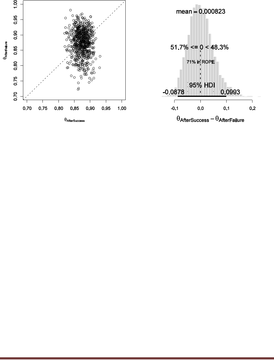
Solutions Manual for Doing Bayesian Data Analysis by John K. Kruschke Page 87
(B) Suppose we establish a ROPE on the difference of success after success and success
after failure. We will arbitrarily set it at +/-5%. Run the program with the data included,
and display the posterior. The plotPost.R function allows specification of a ROPE, with
output as shown in Figure 12.6. Include your output graph, and say in English what the
ROPE indicates.
The plots with the ROPE are included above (see the specification in the code above, too). The
ROPE indicates that in the posterior 71% of the credible differences are practically equivalent to
zero, where “practically equivalent” means within 5 percentage points.
Exercise 12.3. [Purpose: To apply the approaches to a real-world example.] The thematic
apperception test (TAT) is a method for assessing personality and other aspects of
interpersonal attitudes. The subject is shown pictures of people in ambiguous scenes, and
the subject is asked to make up a story about what the pictured people are doing. In a
study reported by Werner, Stabenau, & Pollin (1970, Table 4),2 pictures showing parent-
child interactions were shown to women who had children. The stories invented by the
mothers were scored for whether or not they expressed ―personally involved, child-
centered, flexible interactions.‖ Twenty mothers of normal children and 20 mothers of
schizophrenic children were each shown 10 pictures. The number of stories, out of 10, that
expressed a flexible interaction, were as follows:
Mothers of normal children: 8, 4, 6, 3, 1, 4, 4, 6, 4, 2, 2, 1, 1, 4, 3, 3, 2, 6, 3, 4.
Mothers of schizophrenic children: 2, 1, 1, 3, 2, 7, 2, 1, 3, 1, 0, 2, 4, 2, 3, 3, 0, 1, 2, 2.
For purposes of this exercise, we will assume that the prior is informed from previous
research, which indicates that the typical number of stories that express flexible
interactions for this picture set is around 3 or 4, and can be well described by a

Solutions Manual for Doing Bayesian Data Analysis by John K. Kruschke Page 88
beta(3.5,6.5) distribution. This is the distribution of flexible-narrative tendencies across
mothers.
(A) Estimate the difference between TAT scores of the two groups of mothers. Be sure to
use the prior knowledge. Is zero among the credible differences? If you assume that the
difference has a ROPE from -0.1 to +0.1, is the ROPE excluded from the 95% HDI? (Hints:
Set up a hierarchical model in BUGS, using the filtration-condensation example as a guide.
The prior applies to the distribution of individual theta[i] values, and the data are
distributed as a binomial with bias theta[i].)
The prior knowledge stated in the exercise needs to be extended in some reasonable way so that
it can be expressed in the model structure. The stated prior knowledge (i.e., about 3.5 flexible
interactions out of 10) suggests that the shape parameters of the hyperdistribution that generates
mu[j] should have a mean of .35 = 3.5/(3.5+6.5), but with only modest certainty, say kappa=2.
Hence, perhaps
mu[j] ~ dbeta( .35*2 , .65*2 )
But BUGS won't parse the multiplication inside a density function, so we say
mu[j] ~ dbeta( .7 , 1.3 )
Analogously, shapeGamma and rateGamma should yield a beta distribution with mean of
10=3.5+6.5, but not with much certainty, say SD=10. Hence, perhaps
kappa[j] ~ dgamma( 10^2/10^2 , 10/10^2 ) # BUGS won't parse this --- put in (1,.1)
The resulting program looks like this:
graphics.off()
rm(list=ls(all=TRUE))
fileNameRoot=”Exercise12.3.A" # for constructing output filenames
#install.packages("BRugs")
library(BRugs)
#------------------------------------------------------------------------------
# THE MODEL.
modelstring = "
# BUGS model specification begins here...
model {
for ( subjIdx in 1:nSubj ) {
# Likelihood:
z[subjIdx] ~ dbin( theta[subjIdx] , N[subjIdx] )
# Prior on theta: Notice nested indexing.
theta[subjIdx] ~ dbeta( a[cond[subjIdx]] , b[cond[subjIdx]] )
}
for ( condIdx in 1:nCond ) {
a[condIdx] <- mu[condIdx] * kappa[condIdx]
b[condIdx] <- (1-mu[condIdx]) * kappa[condIdx]
# Hyperprior on mu and kappa:
mu[condIdx] ~ dbeta( Amu , Bmu )
kappa[condIdx] ~ dgamma( Skappa , Rkappa )
}
# Constants for hyperprior:
Amu <- 0.35 * 2
Bmu <- 0.65 * 2
Skappa <- pow(meanGamma,2)/pow(sdGamma,2)
Rkappa <- meanGamma/pow(sdGamma,2)
meanGamma <- 10

Solutions Manual for Doing Bayesian Data Analysis by John K. Kruschke Page 89
sdGamma <- 10
}
# ... end BUGS model specification
" # close quote for modelstring
# Write model to a file:
writeLines(modelstring,con="model.txt")
# Load model file into BRugs and check its syntax:
modelCheck( "model.txt" )
#------------------------------------------------------------------------------
# THE DATA.
nCorrOfSubj = c( 8, 4, 6, 3, 1, 4, 4, 6, 4, 2, 2, 1, 1, 4, 3 ,3 ,2 ,6, 3, 4,
2, 1, 1, 3, 2, 7, 2, 1, 3, 1, 0, 2, 4, 2, 3, 3, 0, 1, 2, 2 )
CondOfSubj = c( rep(1,20) , rep(2,20) )
nTrlOfSubj = rep(10,40)
nSubj = length(CondOfSubj)
nCond = length(unique(CondOfSubj))
# Specify the data in a form that is compatible with BRugs model, as a list:
datalist = list(
nCond = nCond ,
nSubj = nSubj ,
cond = CondOfSubj ,
N = nTrlOfSubj ,
z = nCorrOfSubj
)
# Get the data into BRugs:
# Function bugsData stores the data file (default filename is data.txt).
# Function modelData loads data file into BRugs (default filename is data.txt).
modelData( bugsData( datalist ) )
#------------------------------------------------------------------------------
# INTIALIZE THE CHAINS.
modelCompile( numChains=3 )
modelGenInits()
#------------------------------------------------------------------------------
# RUN THE CHAINS.
burninSteps = 1000
modelUpdate( burninSteps )
samplesSet( c("mu","kappa","theta") )
nPerChain = 1000
modelUpdate( nPerChain , thin=5 )
#------------------------------------------------------------------------------
# EXAMINE THE RESULTS.
source("plotPost.R")
source("plotChains.R")
# Check for convergence, mixing and autocorrelation:
plotChains( "mu" , saveplots=T , fileNameRoot )
plotChains( "kappa" , saveplots=F )
plotChains( "theta[1]" , saveplots=F )
# Extract parameter values and save them.
mu = NULL
kappa = NULL
for ( condIdx in 1:nCond ) {
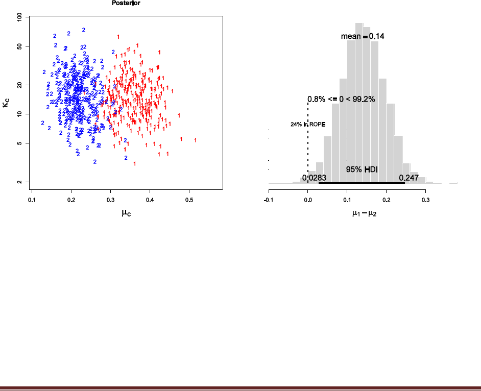
Solutions Manual for Doing Bayesian Data Analysis by John K. Kruschke Page 90
mu = rbind( mu , samplesSample( paste("mu[",condIdx,"]",sep="") ) )
kappa = rbind( kappa , samplesSample( paste("kappa[",condIdx,"]",sep="") ) )
}
save( mu , kappa , file=paste(fileNameRoot,"MuKappa.Rdata",sep="") )
chainLength = NCOL(mu)
# Histograms of mu differences:
windows()
plotPost( mu[1,]-mu[2,] , xlab=expression(mu[1]-mu[2]) , main="" ,
breaks=20 , compVal=0 , ROPE=c(-.1,.1) )
dev.copy2eps(file=paste(fileNameRoot,"MuDiffs.eps",sep=""))
# Scatterplot of mu,kappa in each condition:
windows()
muLim = c(min(mu),max(mu))
kappaLim = c(min(kappa),max(kappa))
mainLab="Posterior"
thindex = round( seq( 1 , chainLength , len=300 ) )
plot( mu[1,thindex] , kappa[1,thindex] , main=mainLab ,
xlab=expression(mu[c]) , ylab=expression(kappa[c]) , cex.lab=1.75 ,
xlim=muLim , ylim=kappaLim , log="y" , col="red" , pch="1" )
points( mu[2,thindex] , kappa[2,thindex] , col="blue" , pch="2" )
dev.copy2eps(file=paste(fileNameRoot,"Scatter.eps",sep=""))
The results look like this:
The posterior on the difference of mu’s indicates that the 95% HDI excludes zero, but the 95%
HDI does not fall outside the ROPE. Indeed, 24% of the posterior falls inside the ROPE. Thus,
depending on how wide a ROPE we use, we may or may not declare that zero difference is
credible.
(B) Using model compareson, determine the posterior probability of a model that uses one
hyperparameter to describe both groups, relative to a model that uses a different
hyperparameter for each group. For this application, the prior on the hyperparameters
should not be informed, but instead should be extremely vague and broad, because the
model comparison is supposed to be ―automatic.‖ What is the posterior probability of the
different-hyperparameter model? If it is the preferred model, can we use it to estimate the

Solutions Manual for Doing Bayesian Data Analysis by John K. Kruschke Page 91
difference between groups? (Answer: Not necessarily, because it does not use the prior
knowledge.)
Running the program (below) once with vague pseudopriors yields a sample for resetting to more
plausible pseudopriors. For example, the first run with vague pseudopriors yields the mean and
SD of mu0 in model 2:
m = mean(mu0sampleM2) = 0.2875809
s = sd(mu0sampleM2) = 0.02942183
Converting those to shape parameters for the beta distribution, using Eqn. 5.6 p. 83, yields
a = m*(m*(1-m)/s^2 - 1) = 67.77622
b = (1-m)*(m*(1-m)/s^2 - 1) = 167.9008
These values are used in the pseudoprior on the second run.
Analogously, for mu1 in model 1:
> m = mean(mu1sampleM1)
> s = sd(mu1sampleM1)
> m*(m*(1-m)/s^2 - 1) yields 42.13674
> (1-m)*(m*(1-m)/s^2 - 1) yields 75.26989
And so forth. For the kappa values, use the gamma-conversion equations from Figure 9.8, p. 209.
For example,
> m = mean(kappa0sampleM2)
> s = sd(kappa0sampleM2)
> m^2/s^2 ; m/s^2 yields 5.495545, 0.3886324
Then be careful to put those constants in the correct place in the model specification! The
complete program is shown below:
graphics.off()
rm(list=ls(all=TRUE))
#install.packages("BRugs")
library(BRugs)
filenamebase = "Exercise12.3.B"
#------------------------------------------------------------------------------
# THE MODEL.
modelstring = "
# BUGS model specification begins here...
model {
for ( i in 1:nSubj ) {
# Likelihood:
nCorrOfSubj[i] ~ dbin( theta[i] , nTrlOfSubj[i] )
# Prior on theta: Notice nested indexing.
theta[i] ~ dbeta( aBeta[ CondOfSubj[i] ] , bBeta[ CondOfSubj[i] ] )
}
# Hyperprior on mu and kappa:
mu0 ~ dbeta( aMu0[mdlIdx] , bMu0[mdlIdx] )
kappa0 ~ dgamma( shk0[mdlIdx] , rak0[mdlIdx] )
for ( j in 1:nCond ) {
mu[j] ~ dbeta( aMu[j,mdlIdx] , bMu[j,mdlIdx] )
kappa[j] ~ dgamma( shk[j,mdlIdx] , rak[j,mdlIdx] )
}
for ( j in 1:nCond ) {
aBeta[j] <- ( ( (mu[j]*(2-mdlIdx))+(mu0*(mdlIdx-1)) )

Solutions Manual for Doing Bayesian Data Analysis by John K. Kruschke Page 92
* ((kappa[j]*(2-mdlIdx))+(kappa0*(mdlIdx-1))) )
bBeta[j] <- ( ( 1 - ( (mu[j]*(2-mdlIdx))+(mu0*(mdlIdx-1)) ) )
* ((kappa[j]*(2-mdlIdx))+(kappa0*(mdlIdx-1))) )
}
# Constants for hyperprior true models:
aP <- 1
bP <- 1
shP <- 1.0
raP <- 0.1
# Prior for true model:
aMu0[2] <- aP
bMu0[2] <- bP
shk0[2] <- shP
rak0[2] <- raP
aMu[1,1] <- aP
aMu[2,1] <- aP
bMu[1,1] <- bP
bMu[2,1] <- bP
shk[1,1] <- shP
shk[2,1] <- shP
rak[1,1] <- raP
rak[2,1] <- raP
# Pseudo-prior for place-holding model:
aMu0[1] <- 67.8
bMu0[1] <- 167.9
shk0[1] <- 5.49
rak0[1] <- 0.389
aMu[1,2] <- 42.1
aMu[2,2] <- 27.4
bMu[1,2] <- 75.3
bMu[2,2] <- 97.3
shk[1,2] <- 3.04
shk[2,2] <- 2.75
rak[1,2] <- 0.197
rak[2,2] <- 0.154
# Hyperprior on model index:
mdlIdx ~ dcat( modelProb[] )
modelProb[1] <- .5
modelProb[2] <- .5
}
# ... end BUGS model specification
" # close quote for modelstring
# Write model to a file:
.temp = file("model.txt","w") ; writeLines(modelstring,con=.temp) ; close(.temp)
# Load model file into BRugs and check its syntax:
modelCheck( "model.txt" )
#------------------------------------------------------------------------------
# THE DATA.
# For each subject, specify the condition she was in,
# the number of trials she experienced, and the number correct.
nCorrOfSubj = c( 8, 4, 6, 3, 1, 4, 4, 6, 4, 2, 2, 1, 1, 4, 3 ,3 ,2 ,6, 3, 4,
2, 1, 1, 3, 2, 7, 2, 1, 3, 1, 0, 2, 4, 2, 3, 3, 0, 1, 2, 2 )
CondOfSubj = c( rep(1,20) , rep(2,20) )
nTrlOfSubj = rep(10,40)
nSubj = length(CondOfSubj)
nCond = length(unique(CondOfSubj))

Solutions Manual for Doing Bayesian Data Analysis by John K. Kruschke Page 93
# Specify the data in a form that is compatible with BRugs model, as a list:
datalist = list(
nCond = nCond ,
nSubj = nSubj ,
CondOfSubj = CondOfSubj ,
nTrlOfSubj = nTrlOfSubj ,
nCorrOfSubj = nCorrOfSubj
)
# Get the data into BRugs:
# Function bugsData stores the data file (default filename is data.txt).
# Function modelData loads data file into BRugs (default filename is data.txt).
modelData( bugsData( datalist ) )
#------------------------------------------------------------------------------
# INTIALIZE THE CHAINS.
nchain = 1
modelCompile( numChains=nchain )
modelGenInits()
#------------------------------------------------------------------------------
# RUN THE CHAINS.
burninSteps = 1000
modelUpdate( burninSteps )
samplesSet( c("mu","mu0","kappa","kappa0","theta","mdlIdx") )
nPerChain = ceiling(10000/nchain)
modelUpdate( nPerChain , thin=5 ) # takes nPerChain * thin steps
#------------------------------------------------------------------------------
# EXAMINE THE RESULTS.
source("plotChains.R")
source("plotPost.R")
modelIdxSample = samplesSample( "mdlIdx" )
pM1 = sum( modelIdxSample == 1 ) / length( modelIdxSample )
pM2 = 1 - pM1
string1 =paste("p(M1:DiffMu|D)=",round(pM1,3),sep="")
string2 =paste("p(M2:SameMu|D)=",round(pM2,3),sep="")
windows(10,4)
nStepsToPlot = length(modelIdxSample)
plot( 1:nStepsToPlot , modelIdxSample[1:nStepsToPlot] , type="l" ,
xlab="Step in Markov chain" , ylab="Model Index (1, 2)" ,
main=paste(string1,", ",string2,sep="") )
dev.copy2eps(file=paste(filenamebase,"_mdlIdx",".eps",sep=""))
mu0sampleM1 = samplesSample( "mu0" )[ modelIdxSample == 1 ]
mu0sampleM2 = samplesSample( "mu0" )[ modelIdxSample == 2 ]
windows()
layout( matrix(1:2,nrow=2) )
hist( mu0sampleM1 , main="Post. mu0 for M1 (Diff)" ,
xlab=expression(mu[0]) , xlim=c(0,1) ,
freq=F , col="grey" , border="white" )
#lines( seq(0,30,.1) , dgamma( seq(0,30,.1) , 1 , .1 ) )
hist( mu0sampleM2 , main="Post. mu0 for M2 (Same)" ,
xlab=expression(mu[0]) , xlim=c(0,1) ,
freq=F , col="grey" , border="white" )
dev.copy2eps(file=paste(filenamebase,"_mu0",".eps",sep=""))
kappa0sampleM1 = samplesSample( "kappa0" )[ modelIdxSample == 1 ]

Solutions Manual for Doing Bayesian Data Analysis by John K. Kruschke Page 94
kappa0sampleM2 = samplesSample( "kappa0" )[ modelIdxSample == 2 ]
windows()
layout( matrix(1:2,nrow=2) )
hist( kappa0sampleM1 , main="Post. kappa0 for M1 (Diff)" ,
xlab=expression(kappa[0]) , xlim=c(0,30) ,
freq=F , col="grey" , border="white" )
#lines( seq(0,30,.1) , dgamma( seq(0,30,.1) , 1 , .1 ) )
hist( kappa0sampleM2 , main="Post. kappa0 for M2 (Same)" ,
xlab=expression(kappa[0]) , xlim=c(0,30) ,
freq=F , col="grey" , border="white" )
dev.copy2eps(file=paste(filenamebase,"_kappa0",".eps",sep=""))
mu1sampleM1 = samplesSample( "mu[1]" )[ modelIdxSample == 1 ]
mu2sampleM1 = samplesSample( "mu[2]" )[ modelIdxSample == 1 ]
mu1sampleM2 = samplesSample( "mu[1]" )[ modelIdxSample == 2 ]
mu2sampleM2 = samplesSample( "mu[2]" )[ modelIdxSample == 2 ]
windows(10,5)
layout( matrix(1:4,nrow=2,byrow=T) )
hist( mu1sampleM1 , main="Post. mu[1] for M = 1" ,
xlab=expression(mu[1]) , xlim=c(0,1) ,
freq=F , col="grey" , border="white" )
hist( mu2sampleM1 , main="Post. mu[2] for M = 1" ,
xlab=expression(mu[2]) , xlim=c(0,1) ,
freq=F , col="grey" , border="white" )
hist( mu1sampleM2 , main="Post. mu[1] for M = 2" ,
xlab=expression(mu[1]) , xlim=c(0,1) ,
freq=F , col="grey" , border="white" )
#lines( seq(0,30,.1) , dgamma( seq(0,30,.1) , 1 , .1 ) )
hist( mu2sampleM2 , main="Post. mu[2] for M = 2" ,
xlab=expression(mu[2]) , xlim=c(0,1) ,
freq=F , col="grey" , border="white" )
#lines( seq(0,30,.1) , dgamma( seq(0,30,.1) , 1 , .1 ) )
dev.copy2eps(file=paste(filenamebase,"_mucond",".eps",sep=""))
kappa1sampleM1 = samplesSample( "kappa[1]" )[ modelIdxSample == 1 ]
kappa2sampleM1 = samplesSample( "kappa[2]" )[ modelIdxSample == 1 ]
kappa1sampleM2 = samplesSample( "kappa[1]" )[ modelIdxSample == 2 ]
kappa2sampleM2 = samplesSample( "kappa[2]" )[ modelIdxSample == 2 ]
windows(10,5)
layout( matrix(1:4,nrow=2,byrow=T) )
hist( kappa1sampleM1 , main="Post. kappa[1] for M = 1" ,
xlab=expression(kappa[1]) , xlim=c(0,30) , freq=F ,
col="grey" , border="white" )
hist( kappa2sampleM1 , main="Post. kappa[2] for M = 1" ,
xlab=expression(kappa[2]) , xlim=c(0,30) , freq=F ,
col="grey" , border="white" )
hist( kappa1sampleM2 , main="Post. kappa[1] for M = 2" ,
xlab=expression(kappa[1]) , xlim=c(0,30) , freq=F ,
col="grey" , border="white" )
#lines( seq(0,30,.1) , dgamma( seq(0,30,.1) , 1 , .1 ) )
hist( kappa2sampleM2 , main="Post. kappa[2] for M = 2" ,
xlab=expression(kappa[2]) , xlim=c(0,30) , freq=F ,
col="grey" , border="white" )
#lines( seq(0,30,.1) , dgamma( seq(0,30,.1) , 1 , .1 ) )
dev.copy2eps(file=paste(filenamebase,"_kcond",".eps",sep=""))
muSample = rbind( mu1sampleM1 , mu2sampleM1 )
windows()
plotPost( muSample[1,]-muSample[2,] , xlab=bquote(mu[.(1)]-mu[.(2)]) ,
breaks=20 , main="M1" )
dev.copy2eps(file=paste(filenamebase,"_mudiff",".eps",sep=""))
kSample = rbind( kappa1sampleM1 , kappa2sampleM1 )
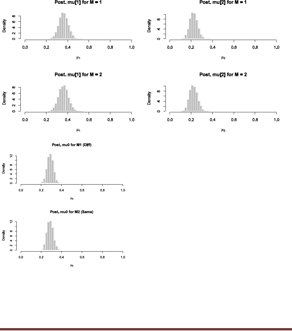
Solutions Manual for Doing Bayesian Data Analysis by John K. Kruschke Page 95
windows()
plotPost( kSample[1,]-kSample[2,] , xlab=bquote(kappa[.(1)]-kappa[.(2)]) ,
breaks=20 , xlim=c(-25,25) , main="M1" )
dev.copy2eps(file=paste(filenamebase,"_kdiff",".eps",sep=""))
The results are shown below. First, notice that the pseudopriors do indeed well match the actual
posteriors:
Next, notice that the Different-Means model is only a little preferred to the Same-Means model:
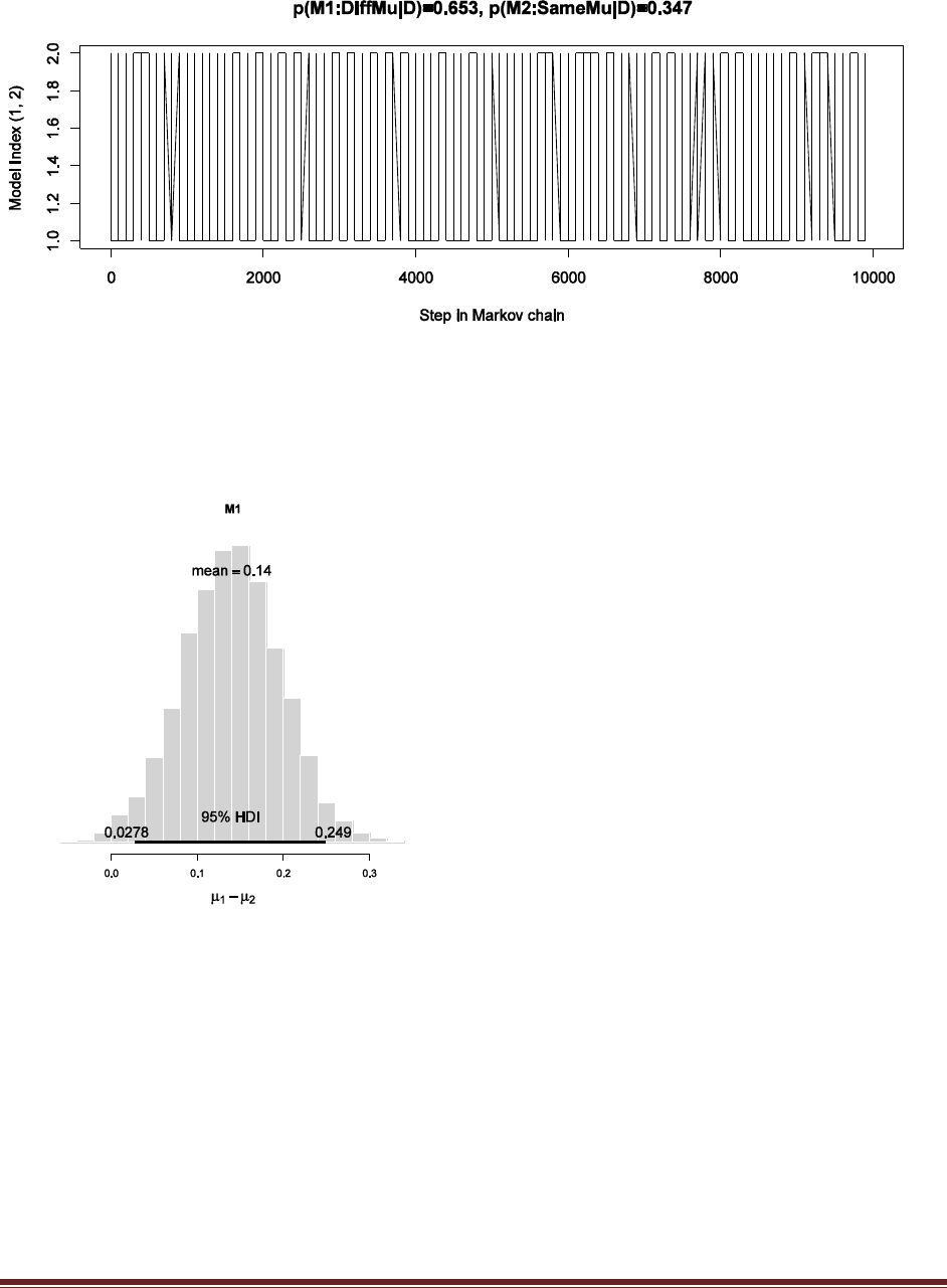
Solutions Manual for Doing Bayesian Data Analysis by John K. Kruschke Page 96
The prior on the model index was set to 50/50, so the probability displayed in the title of the
chain is the posterior probability of the models.
Even though the different-means model is not strongly preferred, if we use it as the “winning”
model we can examine the difference of the means, which looks like this:
It is very similar to the posterior found in the previous part A of this exercise, but it is a little
different. Other than random sampling in the MCMC chain, the difference between the posteriors
is caused by different priors. Here, the prior was vague. In part A, the prior was informed. The
part A posterior is therefore more appropriate (assuming that our audience agrees to the informed
prior).

Solutions Manual for Doing Bayesian Data Analysis by John K. Kruschke Page 97
Chapter 13.
Exercise 13.2. [Purpose: To understand power for flipping a single coin in Tables 13.1 and
13.2.] For this exercise, consider flipping a single coin and inferring its bias.
(A) Table 13.2 indicates that when the data-generating distribution is vague, with kappa =
10 and theta = 0.80, then 85 flips are needed for an 80% chance of getting the 95% HDI
width to be less than 0.2. What is the minimal N needed if the data-generating distribution
is certain, with kappa = 2000? Show the command you used, and report the exact power
for the smallest N that has power greater than 0.8.
minNforHDIpower( genPriorMean=.80 , genPriorN=2000 , HDImaxwid=.2 )
…
For sample size = 67, power = 0.823923
(B) Regarding the previous part, why might a researcher pursue a goal of precision if the
data-generating hypothesis is already precise? (Hint: The audience prior may be different
than the data-generating hypothesis. Discuss briefly, perhaps with an example.)
The audience may have a more diffuse prior than the researcher. (The minNforHDIpower
function defaults to an audience prior that is uniform, i.e., beta(1,1).) So the researcher wants to
know how big a sample size is needed to convince an audience, even though the researcher has a
fairly precise data-generating hypothesis.
(C) Table 13.1 indicates that when the data-generating distribution is highly certain, with
kappa = 2000 and theta = 0.80, then 18 flips are needed for an 80% chance of getting the
95% HDI to exclude theta = 0.5. What is the minimal N needed if the data-generating
distribution is vague, with kappa = 2? Show the command you used, and report the exact
power for the smallest N that has power greater than 0.8.
minNforHDIpower( genPriorMean=.8 , genPriorN=2 , nullVal=.5 )
…
For sample size = 21, power = 0.803802
(D) For the previous part, the goal was for the HDI to exclude the null value (i.e., 0.5).
Notice that the goal can be satisfied if the HDI is above the null value or if the HDI is below
the null value. (1) When the data generating prior is a beta distribution with theta = 0.8
and kappa = 2, as in the previous part, what proportion of the data-generating biases are
greater than the null value? (2) If the goal is for the HDI to fall entirely above the null
value, what sample size is needed to achieve a power of 0.8? (Hint: Use
minNforHDIpower.R with the argument ROPEHc(0,.5).) Watch the sample size increase
and increase and increase, with the power creeping toward an asymptote. Why does the
power never exceed the proportion you computed for (1)?
Please note an error in the statement of the exercise! The desired power should be 0.9, not 0.8.
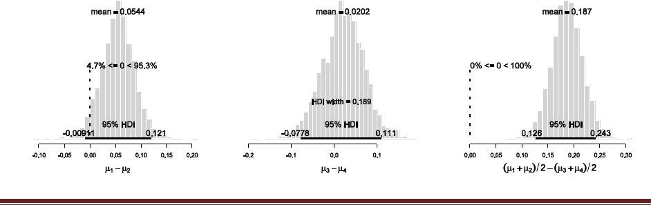
Solutions Manual for Doing Bayesian Data Analysis by John K. Kruschke Page 98
(1) The proportion of data-generating biases greater than the null value of .8 is given by the
amount of the data-generating beta distribution, beta( .8*2 , (1-.8)*2 ), above theta=.5. In R, the
cumulative beta distribution is the function pbeta(theta,a,b). It returns the probability between
zero and theta. We want the probability above theta. Hence we want
1 - pbeta( .5 , 0.8*2 , (1-0.8)*2 ) which is 0.8681836.
(2) We use a desired power of 0.9 in minNforHDIpower(), as follows:
minNforHDIpower( genPriorMean=.8 , genPriorN=2 , nullVal=.5 , ROPE=c(0,.5) ,
desiredPower=0.9 )
…
For sample size = 500, power = 0.8450405
…
The power never exceeds 0.868, computed in (1), because even an infinite sample size can only
reveal the data-generating theta value. Because the data-generating theta values are above .5 only
86.8% of the time, the power can never exceed that.
Exercise 13.3. [Purpose: To determine power for groups of coins, when the goal is
precision.] Consider the filtration-condensation experiment summarized in Section 13.3.
Suppose we want the 95% HDI on the difference, mu3 - mu4, to have a width less than
0.20. What sample size (N per group) is needed to achieve this goal at least 80% of the
time? Determine the answer by running the program in Section 13.6.2
(FilconBrugsPower.R) with various values for nPerGroup. (Hint: N is about 17; your job is
to find the minimal N and discuss how you did it.)
Notice that the third goal checked in the program FilconBrugsPower.R is the goal sought here.
See lines 141-143 of the program (p. 344 of the textbook). The number of simulated subjects per
condition is specified on line 170. It is set at nSubjPerCond=15, but you can change it to other
values to explore power as a function of number of subjects. Beware, this takes time, because a
stable estimate of power takes a couple hundred simulated experiments, which must be
conducted for every sample size. When N=17, the proportion of times that the third goal is
achieved hovers around .8, which is the desired power. When N is less than 17, the estimated
power tends to be less than .8. Although not asked for by the exercise, here are a couple posterior
distributions from simulated data when N=17:
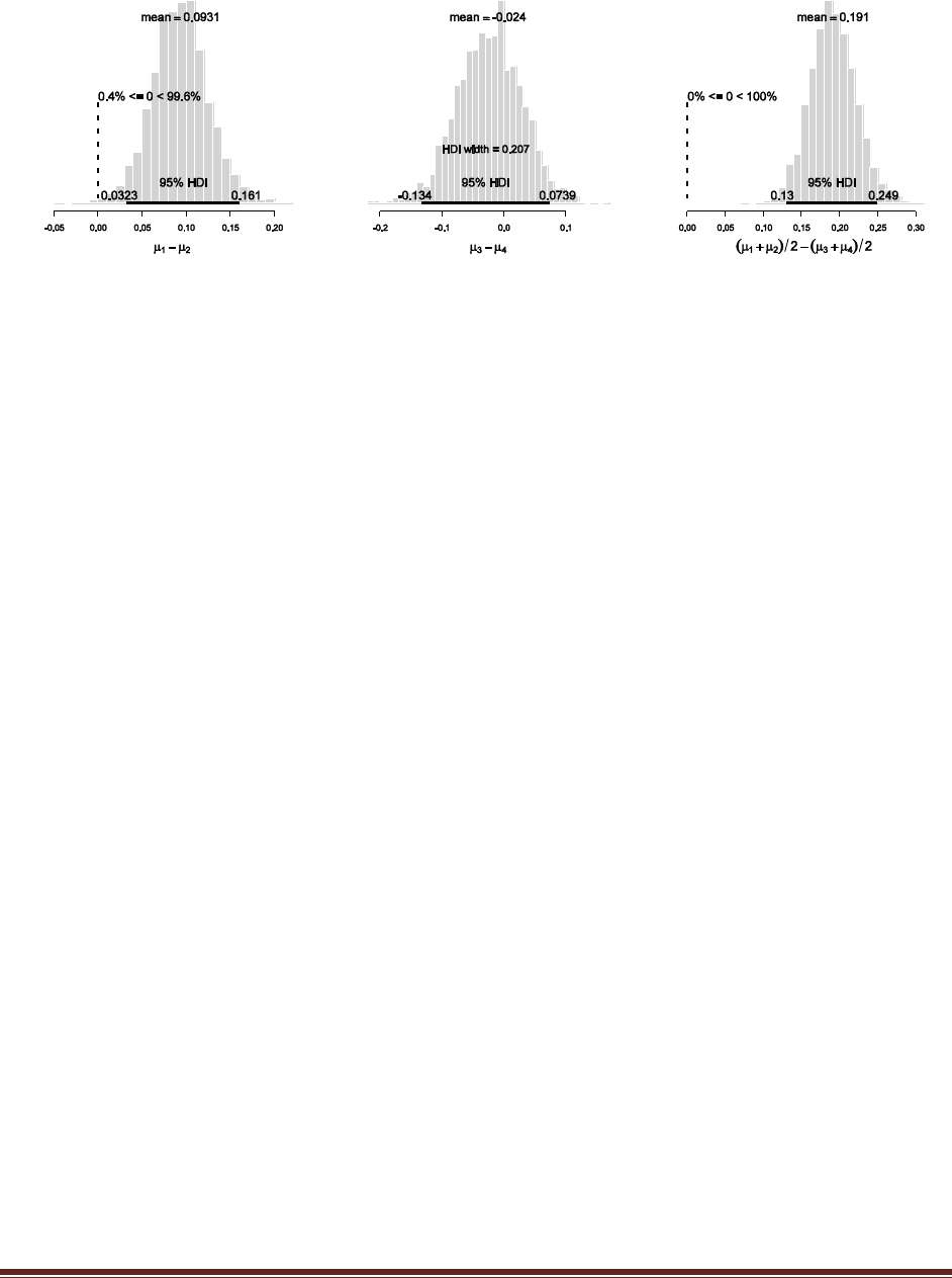
Solutions Manual for Doing Bayesian Data Analysis by John K. Kruschke Page 99
You can see that in the first one, the 95%HDI of mu3-mu4 is less than .2, but in the second one,
the 95%HDI of mu3-mu4 is larger than .2.
Exercise 13.4. [Purpose: This is a capstone exercise that uses real data to review many
techniques of the previous chapters, including generating priors in BUGS, checking
credibility of null values, estimating retrospective power, and conducting a posterior
predictive check.] This exercise examines a learning experiment that investigated how easy
it is for people to learn new category structures after having previously learned an initial
structure (Kruschke, 1996). Some new structures had relevant stimulus dimensions that
were also previously relevant in the initial structure, while other new structures had
relevant stimulus dimensions that were previously irrelevant in the initial structure. […]
(A) [Purpose: To create a BUGS model that has an estimated hyperprior on c and on c.]
[…] Discuss why we would want to estimate higher-level distributions across the c and c.
You may want to mention commonalities across conditions, such as all the learners being
the same species, and all learners experiencing the same sort of stimuli on the same
computer display. It is also important to discuss shrinkage of estimates. Finally, discuss
why the particular higher-level distribution might not be appropriate.
It is reasonable to model all the condition means (and certainties) as coming from a common
hyperdistribution because all the conditions used the same task (predictive learning with
feedback) with the same stimuli (schematic box cars) and the same type of learners (college
students). Without a specific theory of the different conditions, therefore, the conditions should
be roughly the same, or at least share enough that they can be mutually informative. The
hyperdistribution therefore provides some shrinkage on the estimates of the condition means and
certainties, attenuating outlying conditions especially if they have a small sample size.
It would be unreasonable to put a hyperprior on the condition means and certainties if we have
prior belief that the conditions are radically different or have subclusters or are otherwise not
mutually informative. For example, if we have prior knowledge that some of the conditions
produce very low performance while others produce very high performance, we might not want
to put all the conditions under one hyperdistribution because that would be contrary to our prior
knowledge.

Solutions Manual for Doing Bayesian Data Analysis by John K. Kruschke Page 100
(B) [Purpose: To check for convergence, mixing, and autocorrelation.] With the data
included, run the BUGS model and check for convergence, mixing, and autocorrelation.
The model can be initialized automatically, using modelGenInits(), but unfortunately it
takes forever for the chains to converge because some are initialized too far away from the
mode of the posterior. Instead, manually initialize the chains at reasonable values, as
indicated by the data. The same method as was used in Section 9.5.2 (FilconBrugs.R) is
used and extended here (Kruschke1996CSbugs.R): […] Run the model and determine
reasonable burn-in and thinning. Show the autocorrelation and chain plots for c and c.
You may find it useful to refer to Section 23.2, p. 623.
For completeness, here are excerpts of the code that was used to generate the plots:
model {
for ( i in 1:nSubj ) {
nCorrOfSubj[i] ~ dbin( theta[i] , nTrlOfSubj[i] )
theta[i] ~ dbeta( a[ CondOfSubj[i] ] , b[ CondOfSubj[i] ] )I(0.0001,0.9999)
}
for ( cond in 1:nCond ) {
a[cond] <- mu[cond] * kappa[cond]
b[cond] <- (1-mu[cond]) * kappa[cond]
mu[cond] ~ dbeta( aMu , bMu )
kappa[cond] ~ dgamma( sGamma , rGamma )
}
aMu <- max( .01 , mMu * kMu )
bMu <- max( .01 , (1-mMu) * kMu )
mMu ~ dunif(0,1)
kMu ~ dgamma(1,.1)
sGamma <- max( .005 , pow(muGamma,2)/pow(sigmaGamma,2) )
rGamma <- max( .005 , muGamma/pow(sigmaGamma,2) )
muGamma ~ dgamma(1,.1)
sigmaGamma ~ dgamma(1,.1)
}
…
genInitList <- function() {
sqzData = .01+.98*datalist$nCorrOfSubj/datalist$nTrlOfSubj
mu = aggregate( sqzData , list(datalist$CondOfSubj) , "mean" )[,"x"]
sd = aggregate( sqzData , list(datalist$CondOfSubj) , "sd" )[,"x"]
kappa = mu*(1-mu)/sd^2 - 1
mMu = mean( mu )
kMu = mMu * (1-mMu) / sd(mu)^2
muGamma = mean( kappa )
sigmaGamma = sd( kappa )
return( list( theta = sqzData ,
mu = mu ,
kappa = kappa ,
mMu = mMu ,
kMu = kMu ,
muGamma = muGamma ,
sigmaGamma = sigmaGamma ) )
}
…
burninSteps = 1000 # Because initialization is good, doesn't need much burnin
modelUpdate( burninSteps )
samplesSet( c("mu","kappa","theta","mMu","kMu","muGamma","sigmaGamma") )
thinStep = 20
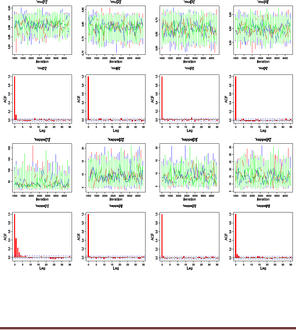
Solutions Manual for Doing Bayesian Data Analysis by John K. Kruschke Page 101
stepsPerChain = ceiling(10000/nchain)
modelUpdate( stepsPerChain , thin=thinStep )
…
sumInfo = plotChains( "mu" , saveplots=T , filenameroot=fileNameRoot )
sumInfo = plotChains( "kappa" , saveplots=T , filenameroot=fileNameRoot )
Below are the autocorrelation and chain plots for the condition means and certainties. The plots
indicate that the chains are well burned-in, converged, and not autocorrelated.
(C) [Purpose: To examine and interpret the posterior distribution of differences.] Which
groups are different from each other, on which parameters? (Hint: See Figure 13.4.)
Here is a scatter plot of the condition mu’s and kappa’s:
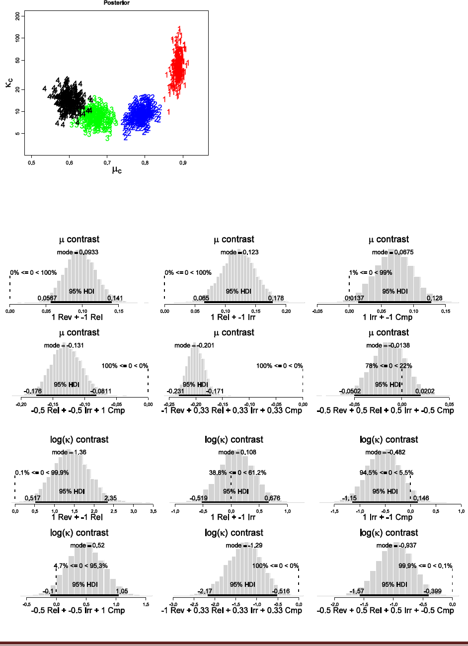
Solutions Manual for Doing Bayesian Data Analysis by John K. Kruschke Page 102
Note that the scatter does not reveal which points at at the same step in the chain; i.e., the plot
does not indicate which point marked “1” is at the same step in the chain as a point marked “2”
or “3” or “4”. The marginals of that distribution are used in the plots below.

Solutions Manual for Doing Bayesian Data Analysis by John K. Kruschke Page 103
The graphs of the kappa differences use log(kappa) merely to make the distributions more
readable. The conclusions are the same in this case when using the original scale. It should be
noted, however, that HDIs can change when the scale is non-linearly transformed, because
dense regions might be stretched into not-dense regions and not-dense regions might be
compressed into dense regions. Thus, when the edge of an HDI is near the null value or ROPE,
use the most meaningful scale for the parameter, which is presumably the scale on which its
prior was defined.
The posterior histograms indicate that the four group’s mu’s are very credibly different from
each other, with REV > REL > IRR > CMP. For the kappa’s, only the kappa of the Reversal
conditions is credibly higher than the others, which are roughly the same (i.e., their differences
are small compared to the uncertainty in their estimates).
(D) [Purpose: To check the robustness of the posterior when the prior is changed in
reasonable ways.] Do the posterior differences change much if the prior changes? (1)
Specifically, try this alternative vague prior: Wherever the top-level prior specifies
dgamma(1,.1), change it to dgamma(0.1,.1). (2) Also, try this prior that forces all c to be
close to 15:
muGamma ~ dgamma(22500,1500)
sigmaGamma ~ dgamma(25,250)
Show your results. Which prior is more reasonable, and why?
(1) Results for
muGamma ~ dgamma(.1,.1)
sigmaGamma ~ dgamma(.1,.1)
are remarkably similar to the results shown in previous parts. In other words, this change of prior
from one vague prior to another has no notable effect on the posterior.
(2) Results for
muGamma ~ dgamma(22500,1500)
sigmaGamma ~ dgamma(25,250)
are quite different, of course, because of the strong prior constraint on kappa. The chains are
converged and well mixed, but noticeably autocorrelated. Because the chains are fairly long,
however, and there is more than one chain, the autocorrelation will be tolerated for purposes of
this exercise. Here are plots of the posterior:
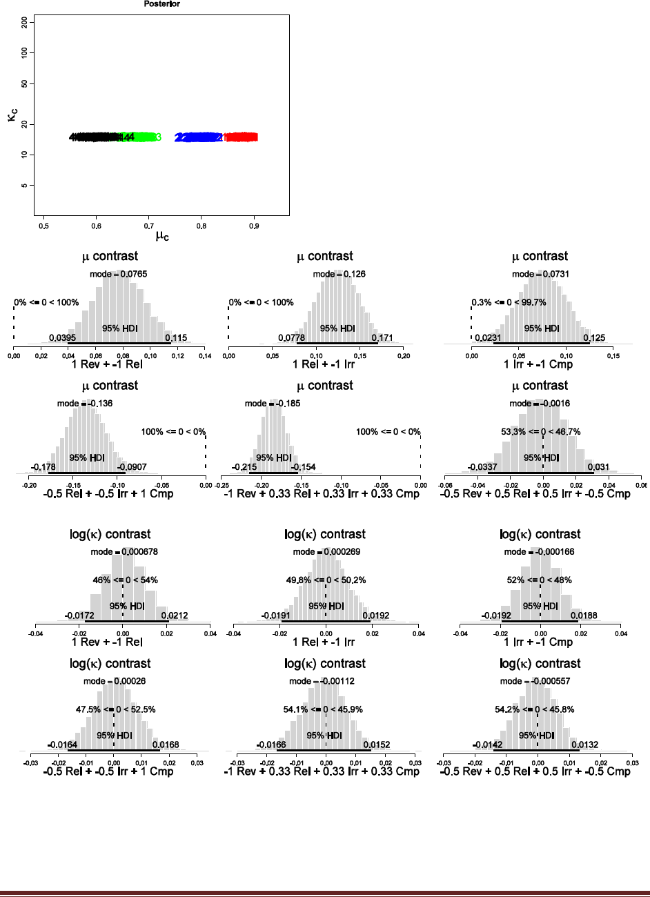
Solutions Manual for Doing Bayesian Data Analysis by John K. Kruschke Page 104
Notice that all kappa values are nearly 15, as demanded by the prior. Hence the kappa
differences, in the lower histograms, are very small. The differences in the mu values, across
conditions, are qualitatively the same as with the vague prior, but slightly different
quantitatively.

Solutions Manual for Doing Bayesian Data Analysis by John K. Kruschke Page 105
(E) [Purpose: To conduct a posterior predictive check.] For this part, use the plausible
dgamma(1,.1) prior, not the less-plausible other priors explored in the previous part.
Conduct a posterior predictive check by generating simulated data from the sampled
posterior parameter values. This can be done in R as follows (Kruschke1996CSbugs.R):
[…] This code puts each randomly generated sample of data into a row of the matrix
nCorrOfSubjPredMat. Figure 13.5 shows histograms of simulated data. The preceding
code relied on previously extracting the parameter chains from BUGS, as follows
(Kruschke1996CSbugs.R): […]
# Extract chains from BUGS for subsequent examination
mu = NULL
kappa = NULL
for ( condIdx in 1:nCond ) {
nodeName = paste( "mu[" , condIdx , "]" , sep="" )
mu = rbind( mu , samplesSample( nodeName ) )
nodeName = paste( "kappa[" , condIdx , "]" , sep="" )
kappa = rbind( kappa , samplesSample( nodeName ) )
}
save( mu , kappa , file=paste(fileNameRoot,"MuKappa.Rdata",sep="") )
chainLength = NCOL(mu)
# Posterior predictive check.
# This code allows specification of different number of subjects, trials.
nSimExps = min(500,chainLength) # number of simulated experiments
nSubjPerCond = sum( CondOfSubj == 1 ) # number of subjects per condition
nTrlPerSubj = nTrlOfSubj[1] # number of trials per subject
nCorrOfSubjPredMat = matrix( 0 , nrow=nSimExps , ncol=nSubjPerCond*nCond )
CondOfSubjPredMat = matrix( 0 , nrow=nSimExps , ncol=nSubjPerCond*nCond )
nTrlOfSubjPredMat = matrix( 0 , nrow=nSimExps , ncol=nSubjPerCond*nCond )
for ( stepIdx in 1:nSimExps ) {
for ( condIdx in 1:nCond ) {
m = mu[condIdx,stepIdx]
k = kappa[condIdx,stepIdx]
a = m*k
b = (1-m)*k
for ( subjIdx in 1:nSubjPerCond ) {
colIdx = (condIdx-1)*nSubjPerCond + subjIdx
theta = rbeta( 1 , a , b )
nCorrOfSubjPredMat[stepIdx,colIdx] = rbinom( 1 ,
size=nTrlPerSubj , prob=theta )
CondOfSubjPredMat[stepIdx,colIdx] = condIdx
nTrlOfSubjPredMat[stepIdx,colIdx] = nTrlPerSubj
}
}
}
save( nCorrOfSubjPredMat , nTrlOfSubjPredMat , CondOfSubjPredMat ,
file=paste(fileNameRoot,"PredData.Rdata",sep="") )
# Make plots
nToPlot = 5 # number of simulated data sets to plot
stepIdx = round(seq(1,nSimExps,len=nToPlot)) # which steps in chain to plot
for ( plotIdx in 1:nToPlot ) {
# Display predicted data summary:
windows(4,10)
layout( matrix( 1:4 , nrow=4 , byrow=T ) )
for ( condIdx in 1:4 ) {
dataToPlot = nCorrOfSubjPredMat[ stepIdx[plotIdx] ,
CondOfSubjPredMat[stepIdx[plotIdx],]==condIdx ]
maxTrl = max(nTrlOfSubjPredMat[stepIdx[plotIdx],])
hist( dataToPlot , xlim=c(0,maxTrl) , breaks=0:maxTrl ,
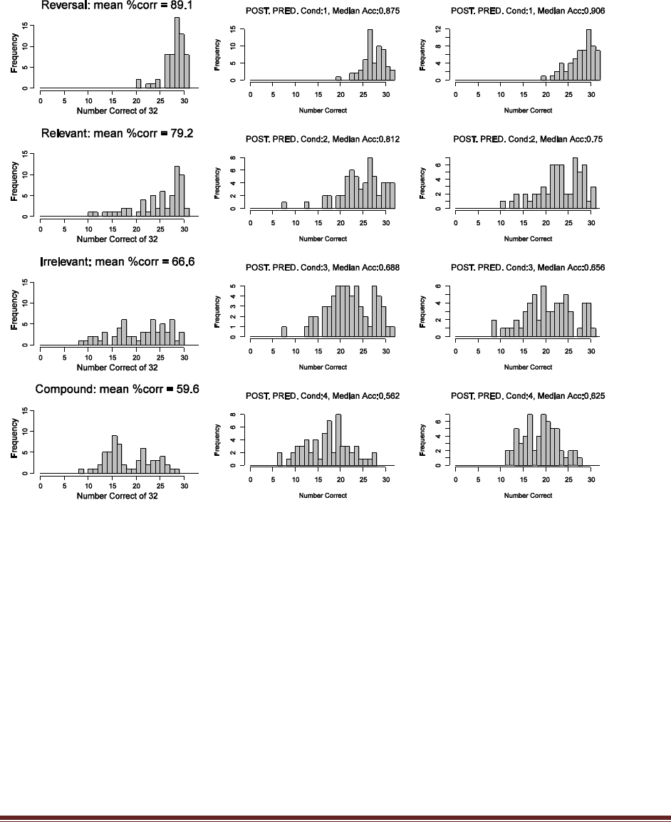
Solutions Manual for Doing Bayesian Data Analysis by John K. Kruschke Page 106
xlab="Number Correct" , col="grey" ,
main=bquote("POST. PRED. Cond:"*.(condIdx)*
", Median Acc:"*.( round( median(dataToPlot)/maxTrl , 3 ) ) ) )
}
dev.copy2eps(file=paste(fileNameRoot,"Pred",plotIdx,".eps",sep=""))
}
The actual data are shown in the left column above, and two posterior-predicted data sets are
shown in the middle and right columns. The conclusion to be drawn is that the simulated data
“look” fairly similar to the actual data, and therefore the model seems to be a fairly good
description of the data.
The only possible point of discrepancy is that the data for the Compound shift (lower left graph)
look like they might possibly be bimodal. Such bimodality does occur from time to time in
simulated data sets, however, so it is not clear that the apparent bimodality in the data is caused
by chance or by two different kinds of learners.
The verisimilitude of the simulated data (i.e., resemblance with the actual data) is important for
the next parts of the exercise, which consider power analysis based on simulated data. If the
simulated data did not mimic the actual data, then the power analysis would not be very
meaningful.

Solutions Manual for Doing Bayesian Data Analysis by John K. Kruschke Page 107
(F) [Purpose: To do a retrospective power analysis.] Using the method of Figure 13.3,
which is exemplified by the code explained in Section 13.6.2 (FilconBrugsPower.R),
conduct a retrospective power analysis, and estimate the power of four goals:
REV - REL > 0, REL - IRR > 0, IRR - CMP > 0, REV - REL > 0 (condition 1 is Reversal,
condition 2 is Relevant, condition 3 is Irrelevant, and condition 4 is Compound). To do this,
… Run at least 100 simulated data sets, and report your tally for how many times the goals
were achieved. …
For 200 simulated data sets, the estimated probability of achieving the four goals is 0.985,
0.935, 0.630, and 0.390. For the mu goals, the Reversal versus Relevant comparison may have
been uselessly overpowered, while the Irrelevant versus Compound comparison was
underpowered. Thus, if the primary purpose was evaluating the mu values of the groups, the
experiment may have been more efficiently conducted with fewer subjects in the Reversal
condition but more subjects in the Compound condition. If the primary purpose was evaluating
the kappa values of groups (which it was not), then the experiment was very underpowered.
Some of the code for the analysis is reproduced here:
GoalAchievedForSample = function( dataList , plotResults=F ,
fileNameRoot="DeleteMe" ) {
library(BRugs)
#------------------------------------------------------------------------------
# THE MODEL.
modelstring = "
# BUGS model specification begins ...
model {
for ( i in 1:nSubj ) {
nCorrOfSubj[i] ~ dbin( theta[i] , nTrlOfSubj[i] )
theta[i] ~ dbeta( a[ CondOfSubj[i] ] , b[ CondOfSubj[i] ] )
}
for ( cond in 1:nCond ) {
a[cond] <- max( .01 , mu[cond] * kappa[cond] )
b[cond] <- max( .01 , (1-mu[cond]) * kappa[cond] )
mu[cond] ~ dbeta( aMu , bMu )
kappa[cond] ~ dgamma( sGamma , rGamma )
}
aMu <- max( .01 , mMu * kMu )
bMu <- max( .01 , (1-mMu) * kMu )
mMu ~ dunif(0,1)
kMu ~ dgamma(1,.1)
sGamma <- max( .005 , pow(muGamma,2)/pow(sigmaGamma,2) )
rGamma <- max( .005 , muGamma/pow(sigmaGamma,2) )
muGamma ~ dgamma(1,.1)
sigmaGamma ~ dgamma(1,.1)
}
# ... end of BUGS model specification
" # close quote for modelstring
writeLines(modelstring,con="model.txt") # write model to a file.
modelCheck( "model.txt" ) # Load model file into BRugs and check its syntax.
#------------------------------------------------------------------------------
# THE DATA.
modelData( bugsData( dataList ) )

Solutions Manual for Doing Bayesian Data Analysis by John K. Kruschke Page 108
#------------------------------------------------------------------------------
# INTIALIZE THE CHAINS.
nchain = 1 # instead of 3, to prevent BUGS crashes?
modelCompile( numChains=nchain )
genInitList <- function() {
theta = .01 + .98 * dataList$nCorrOfSubj / dataList$nTrlOfSubj
mu = rep( 0 , dataList$nCond )
kappa = rep( 0 , dataList$nCond )
for ( condIdx in 1:dataList$nCond ) {
mu[condIdx] = mean( theta[ dataList$CondOfSubj == condIdx ] )
kappa[condIdx] = ( mu[condIdx] * (1-mu[condIdx])
/ sd( theta[ dataList$CondOfSubj == condIdx ] )^2 )
}
mMu = mean( mu )
kMu = mMu * (1-mMu) / sd(mu)^2
muGamma = mean( kappa )
sigmaGamma = sd( kappa )
return( list(
theta = theta ,
mu = mu ,
kappa = kappa ,
mMu = mMu ,
kMu = kMu ,
muGamma = muGamma ,
sigmaGamma = sigmaGamma
))
}
for ( chainIdx in 1 : nchain ) {
modelInits( bugsInits( genInitList ) )
}
#------------------------------------------------------------------------------
# RUN THE CHAINS.
burninSteps = 1000 # Because initialization is good, doesn't need much burnin
modelUpdate( burninSteps )
samplesSet( c("mu","kappa","theta","mMu","kMu","muGamma","sigmaGamma") )
stepsPerChain = ceiling(5000/nchain)
thinStep = 20
modelUpdate( stepsPerChain , thin=thinStep )
#------------------------------------------------------------------------------
# EXAMINE THE RESULTS.
source("plotPost.R")
# Extract chains from BUGS for subsequent examination
mu = NULL
kappa = NULL
for ( condIdx in 1:nCond ) {
nodeName = paste( "mu[" , condIdx , "]" , sep="" )
mu = rbind( mu , samplesSample( nodeName ) )
nodeName = paste( "kappa[" , condIdx , "]" , sep="" )
kappa = rbind( kappa , samplesSample( nodeName ) )
}
chainLength = NCOL(mu)
if ( plotResults ) {
# show graphs of posterior …
} # end if plotResults

Solutions Manual for Doing Bayesian Data Analysis by John K. Kruschke Page 109
# Specify goals and check whether they are achieved:
source("HDIofMCMC.R")
# Goal is Reversal Mu minus Relevant Mu 95% HDI exceeds zero:
goal1Ach = ( HDIofMCMC( mu[1,] - mu[2,] )[1] > 0.0 )
# Goal is Relevant Mu minus Irrelevant Mu 95% HDI exceeds zero:
goal2Ach = ( HDIofMCMC( mu[2,] - mu[3,] )[1] > 0.0 )
goal3Ach = ( HDIofMCMC( mu[3,] - mu[4,] )[1] > 0.0 )
goal4Ach = ( HDIofMCMC( kappa[1,] - kappa[2,] )[1] > 0.0 )
goalAchieved = c( goal1Ach , goal2Ach , goal3Ach , goal4Ach )
return( goalAchieved )
} # end of function GoalAchievedForSample
#==============================================================================
# Now call the function defined above, using simulated data.
analysisType = c("Retro","Repli")[1] # specify [1] or [2]
fileNameRoot = paste("Kruschke1996CSbugsPower",analysisType,sep="")
# Load original data, for use in replication probability analysis:
load("Kruschke1996CSdatsum.Rdata") # loads CondOfSubj, nCorrOfSubj, nTrlOfSubj
# Rename the original data so they don't get overwritten:
CondOfSubjOrig = CondOfSubj
nCorrOfSubjOrig = nCorrOfSubj
nTrlOfSubjOrig = nTrlOfSubj
nSubjOrig = length(CondOfSubjOrig)
nCondOrig = length(unique(CondOfSubjOrig))
# Load previously computed posterior mu[cond,step], kappa[cond,step] values.
load( file="Kruschke1996CSbugsPostMuKappa.Rdata" )
chainLength = NCOL(mu)
nCond = NROW(mu) # should be 4, of course
# SPECIFY NUMBER OF SUBJECTS PER GROUP FOR SIMULATED DATA:
nSubjPerCond = 60
fileNameRoot = paste(fileNameRoot,"N",nSubjPerCond,sep="")
# Specify number of simulated experiments:
nSimExperiments = min(200,chainLength)
nSubj = nSubjPerCond * nCond # Number of subjects total.
nTrlPerSubj = 32 # Number of trials per subject; fixed by design at 32.
nGoal=4 # Determined in function above.
# If previous record of power estimation exists, load it and continue the runs.
filelist = dir( pattern=paste(fileNameRoot,"Result.Rdata",sep="") )
if ( length( filelist ) > 0 ) {
load(paste(fileNameRoot,"Result.Rdata",sep="")) # loads expIdx and nSuccess
prevExpIdx = expIdx
chainIdxVec = round(seq(1,chainLength,len=(prevExpIdx+nSimExperiments))) # Use
these chains.
} else {
prevExpIdx = 0
nSuccess = rep(0,nGoal) # Initialize success counter.
chainIdxVec = round(seq(1,chainLength,len=nSimExperiments)) # Use these chains.
}
# Simulated experiment loop begins here:
for ( expIdx in (1+prevExpIdx):(nSimExperiments+prevExpIdx) ) {
# Generate random data from posterior parameters
chainIdx=chainIdxVec[expIdx]
CondOfSubj = sort( rep( 1:nCond , nSubjPerCond ) )
nTrlOfSubj = rep( nTrlPerSubj , nSubj )

Solutions Manual for Doing Bayesian Data Analysis by John K. Kruschke Page 110
nCorrOfSubj = rep( 0 , nSubj )
for ( condIdx in 1:nCond ) {
m = mu[condIdx,chainIdx]
k = kappa[condIdx,chainIdx]
a = m*k
b = (1-m)*k
# Generate random theta and z values for simulated subjects:
thetaVec = rbeta( nSubjPerCond , a , b )
zVec = rbinom( n=nSubjPerCond , size=nTrlPerSubj , prob=thetaVec )
nCorrOfSubj[ CondOfSubj==condIdx ] = zVec
}
# Put data into list for BUGS program
if ( analysisType == "Retro" ) { # retrospective power
dataList = list(
nCond = nCond ,
nSubj = nSubj ,
CondOfSubj = CondOfSubj ,
nTrlOfSubj = nTrlOfSubj ,
nCorrOfSubj = nCorrOfSubj
)
}
if ( analysisType == "Repli" ) { # replication probability
dataList = list(
nCond = nCond ,
nSubj = nSubj + nSubjOrig ,
CondOfSubj = c( CondOfSubj , CondOfSubjOrig ) ,
nTrlOfSubj = c( nTrlOfSubj , nTrlOfSubjOrig ) ,
nCorrOfSubj = c( nCorrOfSubj , nCorrOfSubjOrig )
)
}
# For monitoring, make plots for first 5 simulated experiments:
if ( expIdx <= 5 ) { plotRes = T } else { plotRes = F }
# Call BUGS program and tally number of successes:
nSuccess = nSuccess + GoalAchievedForSample( dataList ,
plotRes , fileNameRoot )
estPower = nSuccess / expIdx
cat( "\n*** nSubjPerCond:",nSubjPerCond, ", nSimExp:",expIdx,
" , nSuccess:",nSuccess, ", estPower:",round(estPower,2), "\n\n" )
flush.console()
save( nSuccess , expIdx , estPower ,
file=paste(fileNameRoot,"Result.Rdata",sep="") )
} # end of simulated experiment loop.
(G) [Purpose: To do a replication power analysis.] Suppose you repeat the experiment,
using the posterior of the first experiment as the prior for the second experiment. Estimate
the probability of achieving the four goals of the previous part. … This task is easy to do if
you successfully accomplished the previous part. In each step of the chain, instead of using
only the simulated data, concatenate the simulated data to the actual data. …
Code for this part is included in the listing of the previous part; notice near the end of listing the
section beginning with
if ( analysisType == "Repli" ) { # replication probability
Results from 200 simulated experiments show that the probabilities of achieving the fours goals
are 1.000, 0.995, 0.850, and 0.960. In other words, if the posterior from the first experiment is

Solutions Manual for Doing Bayesian Data Analysis by John K. Kruschke Page 111
used as the prior for a replication, there is very high probability of achieving any of the four
goals in the replication.

Solutions Manual for Doing Bayesian Data Analysis by John K. Kruschke Page 112
Chapter 14.
Exercise 14.1. [Purpose: For real-world examples of research, to identify which statistical
model is relevant.] For each of the following examples, identify the predicted variable and
its scale type, identify the predictor variable(s) and its scale type, and identify the cell of
Table 14.1 to which the example belongs.
(A) Guber (1999) examined average performance by public high school students on the
Scholastic Aptitude Test (SAT) as a function of how much money was spent per pupil by
the state and what percentage of eligible students actually took the exam.
Predicted Variable: SAT Score: Metric
Predictor Variable(s): How much money was spent by the state per pupil (metric), and the
percentage of students who took the test (metric).
Cell: y(Metric) & Two or More Metric x factors.
(B) Hahn, Chater, & Richardson (2003) were interested in perceived similarity of simple
geometric patterns. Human observers rated pairs of patterns for how similar the patterns
appeared, by circling one of the digits 1 to 7 printed on the page, where 1 meant ―very
dissimilar‖ and 7 meant ―very similar.‖ The authors presented a theory of perceived
similarity, in which patterns are perceived to be dissimilar to the extent that it takes more
geometric transformations to produce one pattern from the other. The theory specified the
exact number of transformations needed to get from one pattern to the other.
Predicted Variable: Geometric/Shape similarity: Ordinal
Predictor Variable(s): The number of transformations needed to get from one shape to the other:
Metric
Cell: y(Ordinal) & Single Metric x factor.
(C) R.L. Berger et al. (1988) were interested in the longevity of rats, measured in days, as a
function of the rats‘ diet. One group of rats fed freely, another group of rats had a very low
calorie diet.
Predicted Variable: Longevity of rats in days: Metric
Predictor Variable(s): Diet (free feeding vs. low calorie dies): Nominal
Cell: y(Metric) & Single Nominal x factor.
(D) McIntyre (1994) was interested in predicting the tar content of a cigarette (measured in
milligrams) from the weight of the cigarette.
Predicted Variable: Tar Content of Cigarette (milligrams): Metric
Predictor Variable(s): Weight of the cigarette: Metric
Cell: y(Metric) & Single Metric x factor.
(E) You are interested in predicting the gender of a person, based on the person‘s height
and weight.

Solutions Manual for Doing Bayesian Data Analysis by John K. Kruschke Page 113
Predicted Variable: Gender: Dichotomous
Predictor Variable(s): Height and Weight: Metric
Cell: y(Dichotomous) & Two or More Metric x factors.
(F) You are interested in predicting whether a respondent will agree or disagree with the
statement ―The United States needs a federal health care plan with a public option,‖ on the
basis of the respondent‘s political party affiliation.
Predicted Variable: Will respondents Agree Or Disagree with the statement: Dichotomous
Predictor Variable(s): Political Party Affiliation: Nominal
Cell: y(Dichotomous) & Single nominal x factor.
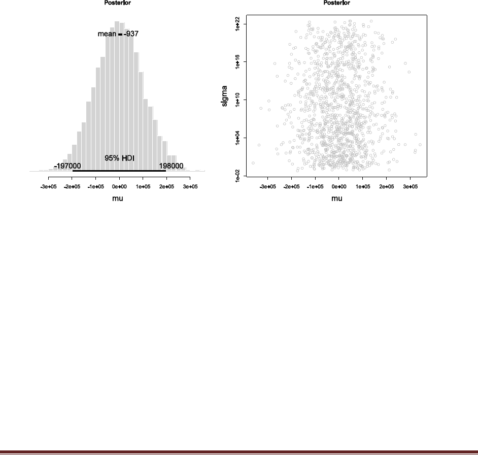
Solutions Manual for Doing Bayesian Data Analysis by John K. Kruschke Page 114
Chapter 15.
Exercise 15.1. [Purpose: To view the prior from BUGS.] For the program in Section 15.4.1
(YmetricXsingleBrugs.R), generate graphs of prior distribution, analogous to Figure 15.3.
To do this, comment out the data in the data specification, as explained in Section 8.5.1, p.
174. But also beware of the following: Automatically initialize the chains from the prior,
and, when plotting the results, comment out the plotChains commands because the MCMC
sigma values are too extreme for some of the BUGS graphics routines.
Notice the huge values of the scales below. In particular, notice that the prior on mu was
specified as mu ~ dnorm( 0 , 1.0E-10 ), which means that the SD on mu should be 1/sqrt(1.0E-
10) = 1e+05 = 100000. For a normal distribution with SD=100000, the 95%HDI should go from
about -196000 to +196000, which is very nearly what the posterior sample shows.
Exercise 15.2. [Purpose: To explore a realistic example of estimating a single mean, with
consideration of priors.] University students who agreed to participate in a problem-solving
experiment were also tested for their vocabulary level, using the Wechsler Adult
Intelligence Scale Revised (WAIS-R), which is normed to have a general-population mean
of 10 and standard deviation of 3. Here are the data from the university students (data
from Hand et al., 1994, set #392, p. 322):
14 11 13 13 13 15 11 16 10 13 14 11 13 12 10 14 10 14 16 14 14 11 11 11
13 12 13 11 11 15 14 16 12 17 9 16 11 19 14 12 12 10 11 12 13 13 14 11
11 15 12 16 15 11
(A) Are the data roughly normal, that is, essentially unimodal and symmetrically
distributed? (No formal analysis is required here; only an ―eyeball‖ assessment is
expected.) Therefore, can a normal likelihood function be applied?
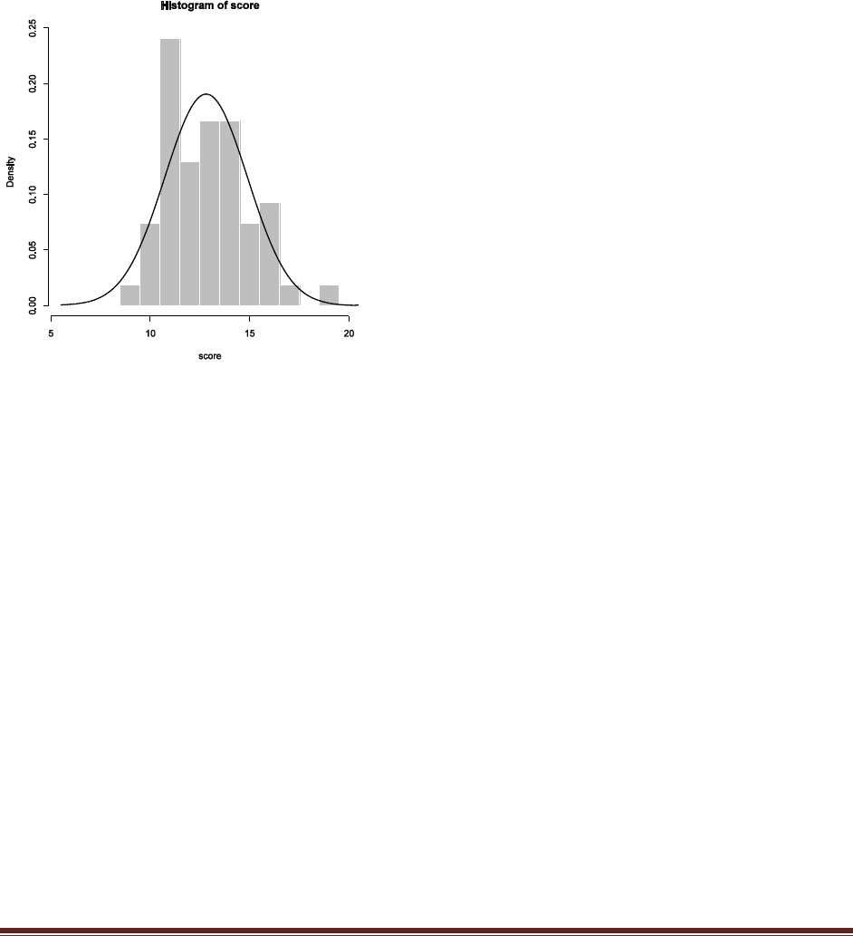
Solutions Manual for Doing Bayesian Data Analysis by John K. Kruschke Page 115
The code below generated the accompanying graph:
score = c( 14, 11, 13, 13, 13, 15, 11, 16, 10, 13, 14, 11, 13, 12, 10, 14, 10, 14, 16,
14, 14, 11, 11, 11, 13, 12, 13, 11, 11, 15, 14, 16, 12, 17, 9, 16, 11, 19, 14, 12, 12,
10, 11, 12, 13, 13, 14, 11, 11, 15, 12, 16, 15, 11 )
m = mean( score )
s = sd( score )
hist( score , breaks=seq(5.5,20.5,1) , prob=T , col="grey" , border="white" )
xVals = seq(5.5,20.5,len=101)
lines( xVals , dnorm( xVals, m , s ) , lwd=2 )
dev.copy2eps(file="Exercise15.2.A.eps")
The graph plots a histrogram of the data, with a superimposed normal curve that has the same
mean and SD as the data. Visual inspection show a bit of a spike in the data at 11, and perhaps an
outlier on the high end, but the data are not wildly non-normal. Therefore a normal distribution
may be used as a default model of the data unless other (e.g., theoretical) considerations suggest
otherwise.
(B) Discuss the rationale for a prior distribution. Justify the constants you choose for the
hyperprior. (Hint: The results of the analysis will be presented to a skeptical audience, who
may doubt any claims about how prior knowledge of the general population informs an
analysis of university students. Therefore, your prior should be very vague and widely
dispersed around the general population values.)
Because this is a subgroup (i.e., university students) and not the general population, the prior
knowledge about the general population is only indirectly applicable to the group. Therefore we
might suppose that mu is somewhere around 10, but because we are uncertain, we might give the
prior on mu a large uncertainty, such as 10 (this makes negative values possible in the prior,
which is not really appropriate for this application, but negative values will be rendered unlikely
by the data). Thus, the prior on mu might be mu ~ dnorm( 10 , 1/10^2 ).
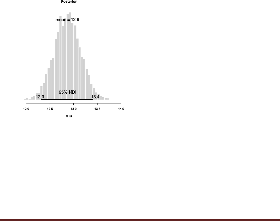
Solutions Manual for Doing Bayesian Data Analysis by John K. Kruschke Page 116
For the prior on the precision, tau, the general population has tau=1/3^2 (because SD=3), but our
special group might have a larger or smaller precision. To be encompassing, we might suppose
that the prior on tau is a gamma distribution with mean 3 and standard deviation 3, hence tau ~
dgamma( 3^2/3^2 , 3/3^2 ).
These are not the only “correct” answers, but your justification should be similar.
(C) Is the mean vocabulary score of the university students credibly different from the
general population mean of 10? Report the 95% HDI on mu for the various priors you
considered in the previous part.
model {
# Likelihood:
for( i in 1 : N ) {
y[i] ~ dnorm( mu , tau ) # tau is precision, not SD
}
# Prior:
tau ~ dgamma( 1 , 0.333 )
mu ~ dnorm( 10 , 0.01 )
}
yields
The 95% HDI is far above 10.0, which the general population mean.
Exercise 15.3. [Purpose: To observe a realistic example of estimating a mean, with
consideration of whether a normal likelihood distribution is appropriate.] Suppose we
know that the mean life time of rats that eat ad lib is 700 days. This value is, in fact, about
right for lab rats; see Figure 15.10, which shows data from R.L. Berger et al. (1988), as
reported in Hand et al. (1994, data set #242), and which are available in the file
RatLives.Rdata. This is an Rdata file, which stores values in compressed format, not text
format. To get the data into R, type load("RatLives.Rdata"). It will look like nothing
happens when you type that command, but the variables are now loaded into R; you can
see the variables that R knows about by typing ls(). You will see listed the two vectors
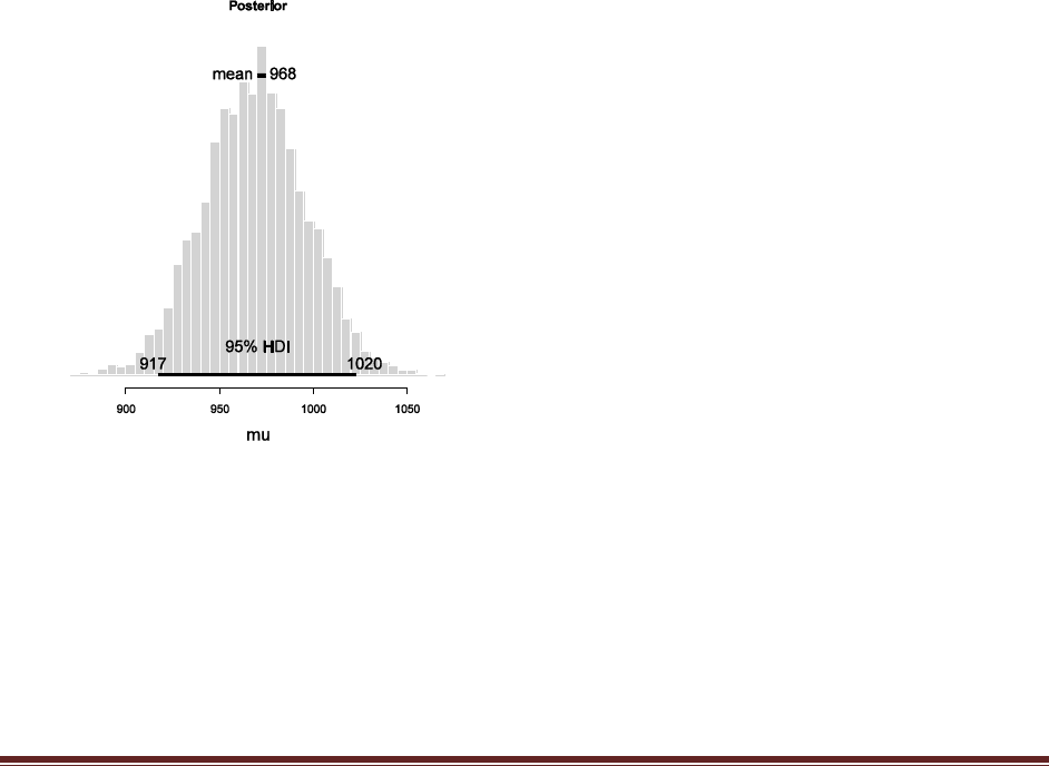
Solutions Manual for Doing Bayesian Data Analysis by John K. Kruschke Page 117
adlibDiet and restrictedDiet. When rats are placed on a restricted diet, their longevity can
be affected. Figure 15.10 shows the results.
(A) Using the raw data from the restricted-diet longevities, estimate mu and its 95% HDI.
Be sure to report the prior you used. (Hint: The HDI extends from about 917 to 1020 days.)
Using the data from the ad-lib diet as a source of prior information (assuming that previous
experiments have revealed similar data --- it’s the restricted diet that’s not known yet), we set on
prior on mu centered at the ad lib mean of 700, but leave it very broad, with an SD of 700 (or
something of your own choice motivated the same way), and we set the prior on tau centered at
the ad lib precision of 5.6E-05, but leave it very broad, with an SD also of 5.6E-05. This yields:
model {
# Likelihood:
for( i in 1 : N ) {
y[i] ~ dnorm( mu , tau ) # tau is precision, not SD
}
# Prior for Exercise 15.3
tau ~ dgamma( 1 , 18000 ) # m = s = 5.6E-05
mu ~ dnorm( 700 , 2.0E-06 ) # precision = 1/700^2
}
…
load("RatLives.Rdata")
y = restrictedDiet
(B) Is it appropriate to apply a normal likelihood function to these data? Transform the
data by squaring the longevities. Estimate mu and its 95% HDI (now in days squared). Be
careful to use an appropriate prior! (Hint: The HDI extends from about 967^2 to 1053^2
days.)
The squared data look like this:
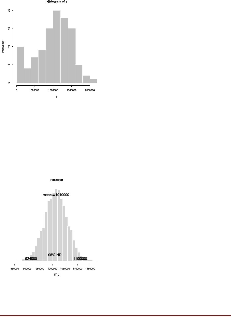
Solutions Manual for Doing Bayesian Data Analysis by John K. Kruschke Page 118
The transformed data are far less skewed to the left than that original data. They are better
described by a normal than the original data.
We use the transformed ad lib data to inform the priors. The transformed ad lib data have a mean
of about 486000 and a precision of about 4.3E-11.
tau ~ dgamma( 1 , 2.3E+10 ) # m = s = 4.3E-11
mu ~ dnorm( 486000 , 4.2E-12 ) # precision = 1/486000^2
…
load("RatLives.Rdata")
y = restrictedDiet^2
The 95%HDI limits in days, computed as sqrt(HDIofMCMC(muSample)), are 961.5 to 1048.3.
(C) Why is the first estimate lower than the second estimate? Which estimate is more
appropriate and why?
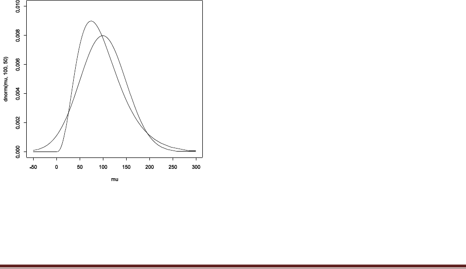
Solutions Manual for Doing Bayesian Data Analysis by John K. Kruschke Page 119
The first estimate, using original-scale data, is lower because of the extreme leftward skew in the
original data. The normal model is pulled down by the left-skew in the data. Because the original
data are not very well modeled by a normal, the estimate from the transformed data is more
trustworthy.
Exercise 15.4. [Purpose: To think about specifying an informed prior, and non-normal,
non-gamma priors.] In the program of Section 15.4.1 (YmetricXsingleBrugs.R), the prior
on the group mean uses an extremely small precision. This diffuse prior is silly, because we
know that individual IQ scores from the general population should be near 100 with a
standard deviation of about 15. Special populations might have IQ scores consistently
above or below 100 but almost certainly within, say, 100 points above or below 100.
Consider the following expressions of the prior belief on mu:
(1) mu ~ dnorm( 100 , sd=50 ) # that‘s sd=50, so tau=pow (50,-2)
(2) mu ~ dgamma( 4 , 0.04 )
(3) mu ~ dunif( 0 , 200 )
(4) mu ~ dgamma( 3 , 0.03 )
(A) Plot the densities of (1) and (2) on the same graph, superimposed. (Hint:
mu = seq( -50 , 300 , length=501 )
plot( mu , dnorm( mu , 100 , 50 ) , type="l" , ylim=c(0,0.01))
lines( mu , dgamma( mu , 4 , 0.04 ) )
What do the densities of (1) and (2) have in common? (Hint: Compute the mean and sd of
the gamma distribution.) Should either of (1) or (2) be preferred over the other? (Hint:
Consider negative IQ scores, which should not be allowed.)
The mean of the gamma distribution is s/r = 4/0.04 = 100, and the sd of the gamma distribution is
sqrt(s)/r = 2/0.04 = 50 (see Fig. 9.8, p. 209). In other words, the gamma and normal have the
same mean and SD.
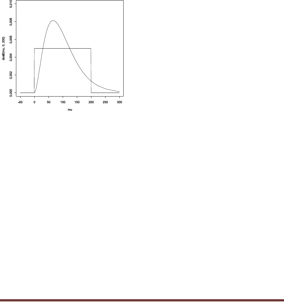
Solutions Manual for Doing Bayesian Data Analysis by John K. Kruschke Page 120
Despite that similarity, the gamma is to be preferred as a prior for IQ scores because IQ scores
can not be negative. The graph shows that the normal distribution givess negative scores some
credibility.
(B) Plot the densities of (3) and (4) on the same graph, superimposed. What do the densities
of (3) and (4) have in common? Should one of (3) or (4) be preferred over the other? (Hint:
Consider IQ scores greater than 200, which should be allowed.)
plot( mu , dunif( mu , 0 , 200 ) , type="l" , ylim=c(0,0.01))
lines( mu , dgamma( mu , 3 , 0.03 ) )
The mean of the gamma is 3/0.03 = 100, and the sd of the gamma is sqrt(3)/0.03 = 57.7.
The mean of the uniform is 100 (obviously), and its sd can be easily approximated by a large
random sample, sd(runif(1000000,0,200)), which yields 57.7. In other words, the two
distributions have very nearly the same mean and SD.
Despite the similarity, the gamma distribution is a better prior for IQ because the uniform makes
IQ scores above 200 impossible, which should be allowed.
In the program of Section 15.4.1 (YmetricXsingleBrugs.R), the prior on the group precision
is a general diffuse distribution. This diffuse prior is silly, because we know that individual
IQ scores have a standard deviation around 15 (i.e., a precision of 1/15^2 = 0.00444...) in
the general population. The SD might be a bit smaller within special populations.
(C) Suppose we believe that the smallest SD we would find in a specialized population is 5.
What is the corresponding precision? (Notice that it is larger than 1/15^2.)
The corresponding precision is 1/5^2 = 0.04. That’s the smallest SD, hence the largest precision.
(D) We want to create a gamma distribution for precision that has a mean corresponding
to 1/15^2, such that most of the gamma distribution is less than the precision
corresponding to an IQ precision of 1/5^2, because, as mentioned in the previous part, we
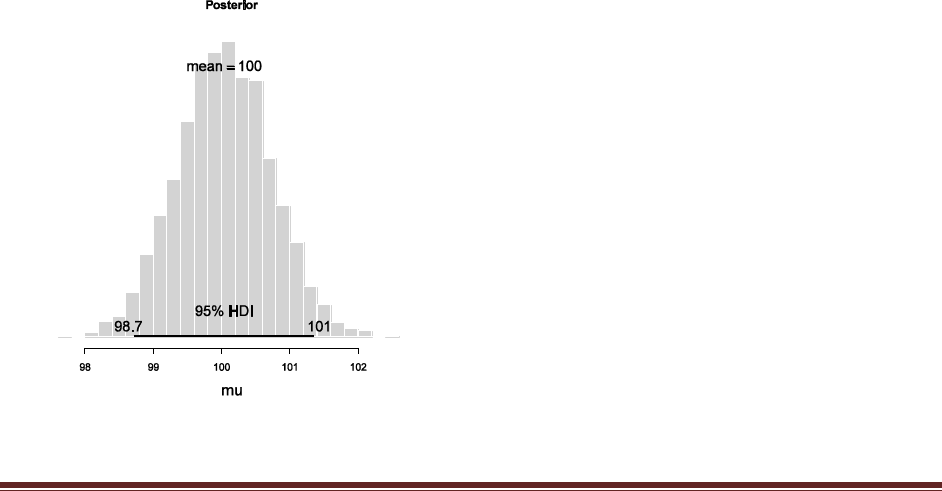
Solutions Manual for Doing Bayesian Data Analysis by John K. Kruschke Page 121
don‘t think that precisions much greater than 1/5^2 are tenable. Therefore, to be sure that
our prior encompasses that maximum but still allows for considerable uncertainty, we will
set the standard deviation of the gamma distribution to half of the difference between the
precisions determined in the previous two parts. What is the value of half of the difference
between the precisions determined in the previous two parts? (Hint: The answer is
0.01777… . Explain.)
The largest precision is 0.04, and the mean precision is 0.00444. Half the difference is
0.5 * ( 1/5^2 - 1/15^2 ) which yields 0.01777…
(E) What are the values of the shape and rate parameters for a gamma distribution that
has mean of 0.00444 and standard deviation of 0.01777?
s = m^2/sd^2 = 0.625
r = m/sd^2 = 14.0625
(F) Rerun the program of Section 15.4.1 (YmetricXsingleBrugs.R) using a prior for tau
from the previous part, and a prior for mu that is the most appropriate from (1)–(4) above.
Include the posterior histogram of mu with your answer. Does the conclusion differ
noticeably from the diffuse priors?
The most appropriate prior on mu is either of the gamma distributions; I’ll use gamma(3,.03)
because it is more vague.
tau ~ dgamma( 0.625 , 14.0625 )
mu ~ dgamma( 3 , 0.03 )
yields
The posterior is essentially the same as diffuse priors. In this case there are so many data points
that the prior is overwhelmed.

Solutions Manual for Doing Bayesian Data Analysis by John K. Kruschke Page 122
Exercise 15.5. [Purpose: With repeated measures, to see how the group estimate and
individual estimates reflect different sources of variation in the data.] Consider the data, y,
with different assignments to subjects, s, as follows:
y values: 1 2 3 21 22 23 41 42 43
s, large between subj. var.: 1 1 1 2 2 2 3 3 3
s, small between subj. var.: 1 2 3 1 2 3 1 2 3
The first row shows nine data values. The second row indicates a situation in which the
first three data points come from subject 1, the second three data points come from subject
2, and so on. The third row indicates a different situation, in which the first, fourth, and
seventh data points come from subject 1, and so forth. The assignment of data to subjects
in the second row produces large between-subject variance, whereas the assignment of data
to subjects in the third row produces small between-subject variance. Notice that for both
situations, however, the overall mean is the same because the data are the same. We are
interested in which situation gives a more precise estimate of the group-level mean. Modify
the program of Section 15.4.2 (SystemsBrugs.R) for use with these data. (No need to be too
fancy. For example, in the datalist, just type in y = c( 1, 2, 3, 21, 22, 23, 41, 42, 43 ) and subj
= c( 1,1,1, 2,2,2, 3,3,3 ).) Be sure to make the prior appropriate for these data. Run the
program twice, once for each assignment of data to subjects (using the same prior for both
runs). (Hint: Your results should look something like those in Figure 15.11). Notice that the
mean of the posterior of muG is essentially the same for both runs, but the HDI widths are
quite different. Explain why.
The prior on muG should be appropriate for data in the range 0-50, without being very certain.
Hence we could set muG ~ dnorm( 25 , 0.0001 ).
The prior on tauG should be appropriate for groups that have between-group SDs in the range of
1 to 20 (because the two sets of data do). So we could set a prior on SD with a mean of 10 and a
very uncertain. So, we could use a gamma distribution on precision with a mean of 0.01 (i.e.,
SD=10) and a sd the same: tauG ~ dgamma( .01^2/.01^2 , .01/.01^2 ).
The within-group SDs also range from 1 to 20 across data sets, so the prior on tau[j] should have
a mean m around 1/10^2. The hyperprior on m can therefore be set analogous to the prior on
tauG, namely m ~ dgamma( .01^2/.01^2 , .01/.01^2 ).
Finally, the within-group variances are identical across groups for these fictitious data sets
(which would never happen in the real world), and therefore care must be taken when setting the
prior on d, so that the posterior does not collapse into degeneracy with d=0. We’ll put a prior on
d such that the sd of the gamma distribution is slightly less than the mean, thereby prohibiting
d=0. For example, d ~ dgamma( 1 , 1.23 ), as shown in this graph:
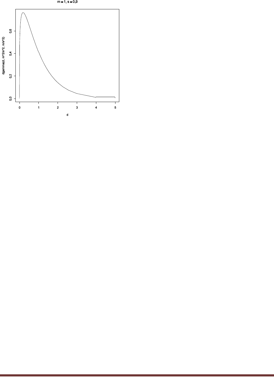
Solutions Manual for Doing Bayesian Data Analysis by John K. Kruschke Page 123
It is worth emphasizing that this choice of prior is not uniquely correct. Other priors could also
be justified. Indeed, other priors will yield different posteriors because the data are so few! The
graphs in Figure 15.11 of the textbook were generated from different priors.
The full model specification is
model {
for( i in 1 : Ndata ) {
y[i] ~ dnorm( mu[ subj[i] ] , tau[ subj[i] ] )
}
for ( j in 1 : Nsubj ) {
mu[j] ~ dnorm( muG , tauG )
tau[j] ~ dgamma( sG , rG )
}
muG ~ dnorm( 25 , 0.0001 )
tauG ~ dgamma( 1 , 100 )
sG <- pow(m,2) / pow(d,2)
rG <- m / pow(d,2)
m ~ dgamma( 1 , 100 )
d ~ dgamma( 1 , 1.23 )
}
The data can be specified thus:
datalist = list(
y = c( 1,2,3, 21,22,23, 41,42,43 ) ,
subj = c( 1,1,1, 2, 2, 2, 3, 3, 3 ) ,
#subj = c( 1,2,3, 1, 2, 3, 1, 2, 3 ) ,
Ndata = 9 ,
Nsubj = 3
)
Unfortunately, BUGS does not always like automatically initializing the chains when the priors
are vague. Therefore we can manually start the chains at values consistent with the data:
y = datalist$y
s = datalist$s
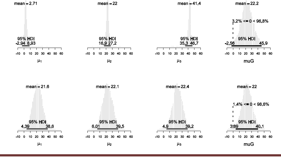
Solutions Manual for Doing Bayesian Data Analysis by John K. Kruschke Page 124
# Overall mean:
muGinit = mean( y )
# Group means:
muVec = aggregate( y ~ as.factor(s), data=cbind(y,s), mean )[,2]
# Precision across group means:
tauGinit = 1 / sd( muVec )^2
# Groups SDs:
sdVec = aggregate( y ~ as.factor(s), data=cbind(y,s), sd )[,2]
dInit = max( 0.01 , sd( sdVec ) )
# manually initialize chains near the data:
genInitList <- function() {
list( muG = muGinit ,
tauG = tauGinit ,
m = mean(1/sdVec^2) ,
d = dInit ,
mu = muVec ,
tau = 1/sdVec^2 )
}
for ( chainIdx in 1 : nchain ) {
modelInits( bugsInits( genInitList ) )
}
The posterior mu values can be plotted thus
windows(10,3)
layout( matrix( 1:4 , nrow=1 , byrow=T ) )
for ( sIdx in 1:3 ) {
histInfo = plotPost( muSample[sIdx,] , xlab=bquote(mu[.(sIdx)]) ,
xlim=c(-10,60) , breaks=c(-5000,seq(-10,50,len=61),5000) )
}
histInfo = plotPost( muGsample , xlab=bquote(muG) , xlim=c(-10,60) ,
breaks=c(-5000,seq(-10,50,len=61),5000) , compVal=0 )
which yields, for the two data sets, the following graphs:

Solutions Manual for Doing Bayesian Data Analysis by John K. Kruschke Page 125
These graphs differ from Figure 15.11 of the textbook because different priors were used. But
the qualitative nature is the same: When the data are re-assigned to subjects/groups such that
there is larger between group variance, then the estimate of muG is larger.

Solutions Manual for Doing Bayesian Data Analysis by John K. Kruschke Page 126
Chapter 16.
Exercise 16.1. [Purpose: To see the influence of individual slope differences on the estimate
of the group-average slope.] The data shown in Figure 16.10 indicate that all subjects had
similar rates of decline in retention, and therefore the estimate of the group average is
fairly certain. In this exercise, we change the data so that the individual slopes differ more
dramatically and examine the effect on the estimate of the group average.
(A) Alter the data as follows: In the program listed in Section 16.5.3
(SimpleLinearRegressionRepeatedBrugs.R), just before the data are renamed from
dataMat to x and y (at about line 65), subtract .030x from subject 1, subtract .015x from
subject 2, do nothing to subject 3, and add .015x to subject 4. Here is an example of code
for subject 1:
subjRowVec H ( dataMat[,subjColName] HH 1 )
dataMat[ subjRowVec , yColName ] H ( dataMat [ subjRowVec , yColName ]
- .030 * dataMat[ subjRowVec , xColName ] )
Repeat and modify for the remaining subjects. Run the program and include the plot of the
data. (See Figure 16.12.) The data curves for the four subjects should have four very
different slopes.
Here is the complete data-modification code, executed after the conversion to log10:
subjRowVec = ( dataMat[,"subjID"] == 1 )
dataMat[ subjRowVec , "retention" ] = ( dataMat[ subjRowVec , "retention" ]
- .030 * dataMat[ subjRowVec , "time" ] )
subjRowVec = ( dataMat[,"subjID"] == 2 )
dataMat[ subjRowVec , "retention" ] = ( dataMat[ subjRowVec , "retention" ]
- .015 * dataMat[ subjRowVec , "time" ] )
subjRowVec = ( dataMat[,"subjID"] == 4 )
dataMat[ subjRowVec , "retention" ] = ( dataMat[ subjRowVec , "retention" ]
+ .015 * dataMat[ subjRowVec , "time" ] )
And here is the resulting graph:
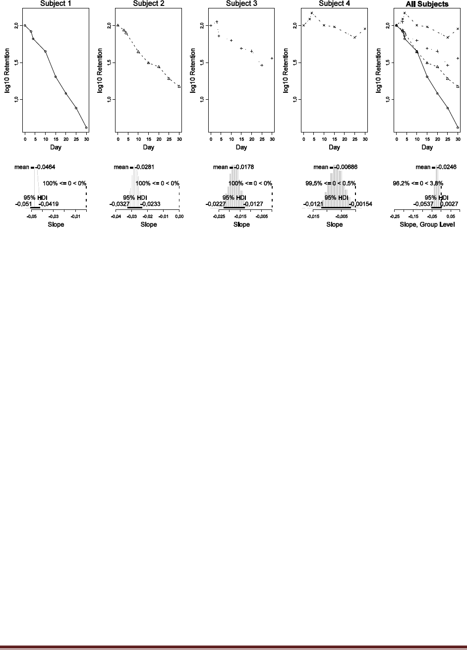
Solutions Manual for Doing Bayesian Data Analysis by John K. Kruschke Page 127
(B) Relative to the original data, has the posterior mean of the group slopes gotten farther
away from zero or closer to zero? Include the histogram of the posterior in your write-up.
Are all the individual slopes believably different from zero (according to the 95% HDI)? Is
the group slope believably different from zero (according to the 95% HDI)? Why is the
group-level slope, which is now farther away from zero on average, less believably different
from zero than in the original data?
The posterior mean of the group slopes (lower right of graph above) has gotten farther away
from zero, i.e., more negative. And all the individual slopes are credibly below zero, as shown by
the posterior histograms in columns 1-4 above. But the 95%HDI of the group-level slope
includes zero, i.e., the group-level slope is very uncertain and might even include zero. This
seems like a contradiction: All the individual slopes are less than zero, but the group slope might
include zero. It’s not a contradiction, though. The reason is that the individual slopes differ from
each other very much. Hence there is lots of uncertainty in the group average slope. This
uncertainty means that the 95%HDI at the group level is wide.
Exercise 16.2. [Purpose: To see the influence of differences in individual intercepts on the
estimate of group-average slope.] The data shown in Figure 16.10 all start at 2.0 because
that is log10(100), and the data were measured as percentage of original value. Suppose
that the data were kept in their raw magnitudes instead of converted to percentage of first
magnitude. This would merely change the intercepts of the individual data curves, without
changing their slopes …. In this exercise we find out whether this change would have any
effect on the estimate of the group slope.
(A) Alter the data as follows: In the program listed in Section 16.5.3
(SimpleLinearRegressionRepeatedBrugs.R), right before the data are converted to log10
on line 42, insert this code: … Run the program and include the plot of the data. (See
Figure 16.13.) The data curves for the four subjects should have four very different
intercepts.
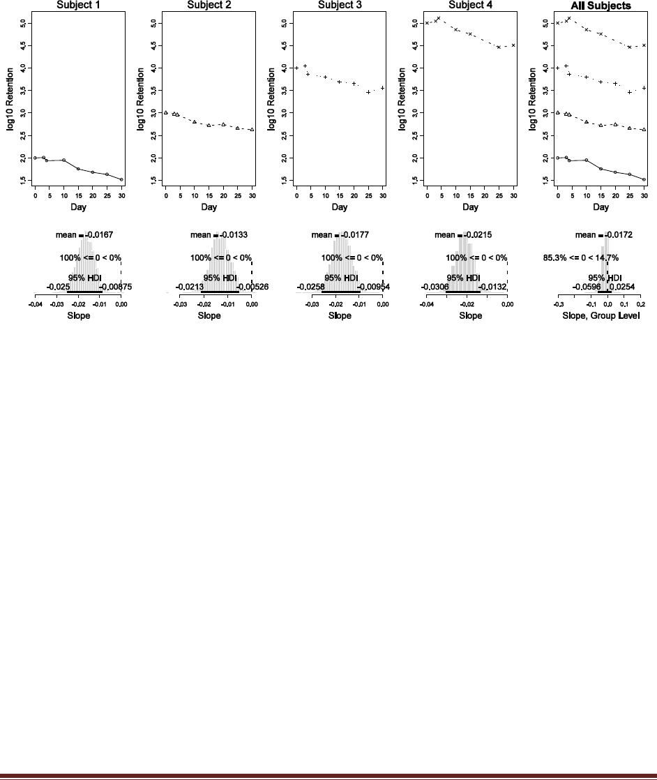
Solutions Manual for Doing Bayesian Data Analysis by John K. Kruschke Page 128
Before the conversion to log10, include this transformation:
for ( subjIdx in 1:4 ) {
rowIdx = ( dataMat[,"subjID"] == subjIdx )
dataMat[rowIdx,"retention"] = dataMat[rowIdx,"retention"] * 10^(subjIdx-1)
}
The resulting data and posterior look like this:
(B) Relative to the original data, are the estimates of the individual slopes different?
Relative to the original data, is the posterior mean of the estimated group slope different?
Include the histogram of the posterior of the group slope. Is the group slope believably
different from zero (according to the 95% HDI)? Why is the group-level slope less
believably different from zero, compared to the original data? (Hint: The individual
intercepts affect the certainty of the group-average intercept. The group-average intercept
trades off with the group-average slope; consider scatter plots of mu0G and mu1G.)
For the individual slope estimates, the means of the posteriors are about the same as in the
original data, which makes sense because the individual slopes in the data are unchanged. But
the uncertainties of the estimates have increased. For example, Subject 4 in the original data had
a slope estimate with 95%HDI from -0.0256 to -0.0164, but in the intercept-altered data the HDI
goes from -0.0306 to -0.0132. For the group-level slope, the mean of the posterior is the same for
the original and intercept-altered data, which makes sense because there has been no change in
the individual slopes. But, the uncertainty on the group-level slope has increased; in particular,
the 95%HDI now includes zero! The reason is provided by the hint in the statement of the
exercise. Because the individual intercepts are now very different, the estimate of the group-level
intercept is now very uncertain. The uncertainty in the group-level intercept implies that the
group-level slope also has more flexibility, because different group-level intercepts can trade-off
with more extreme group-level slopes. Hence the group-level slope is more uncertain. Plots of
the group-level slope and intercept are shown below. First, for the original data:
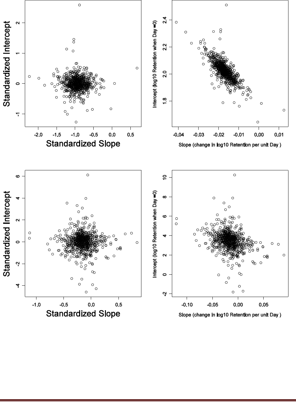
Solutions Manual for Doing Bayesian Data Analysis by John K. Kruschke Page 129
Next, for the intercept-altered data:
Notice that the group-level intercept (vertical axis) is much more uncertain in the intercept-
altered data.
Exercise 16.3. [Purpose: To observe real data for repeated measures of individual
regression, with an outlying individual and nonlinear trend.] Suppose we are interested in
whether families with more members have higher incomes. The U.S. Census Bureau has
published data that indicate the median family income as a function of number of persons
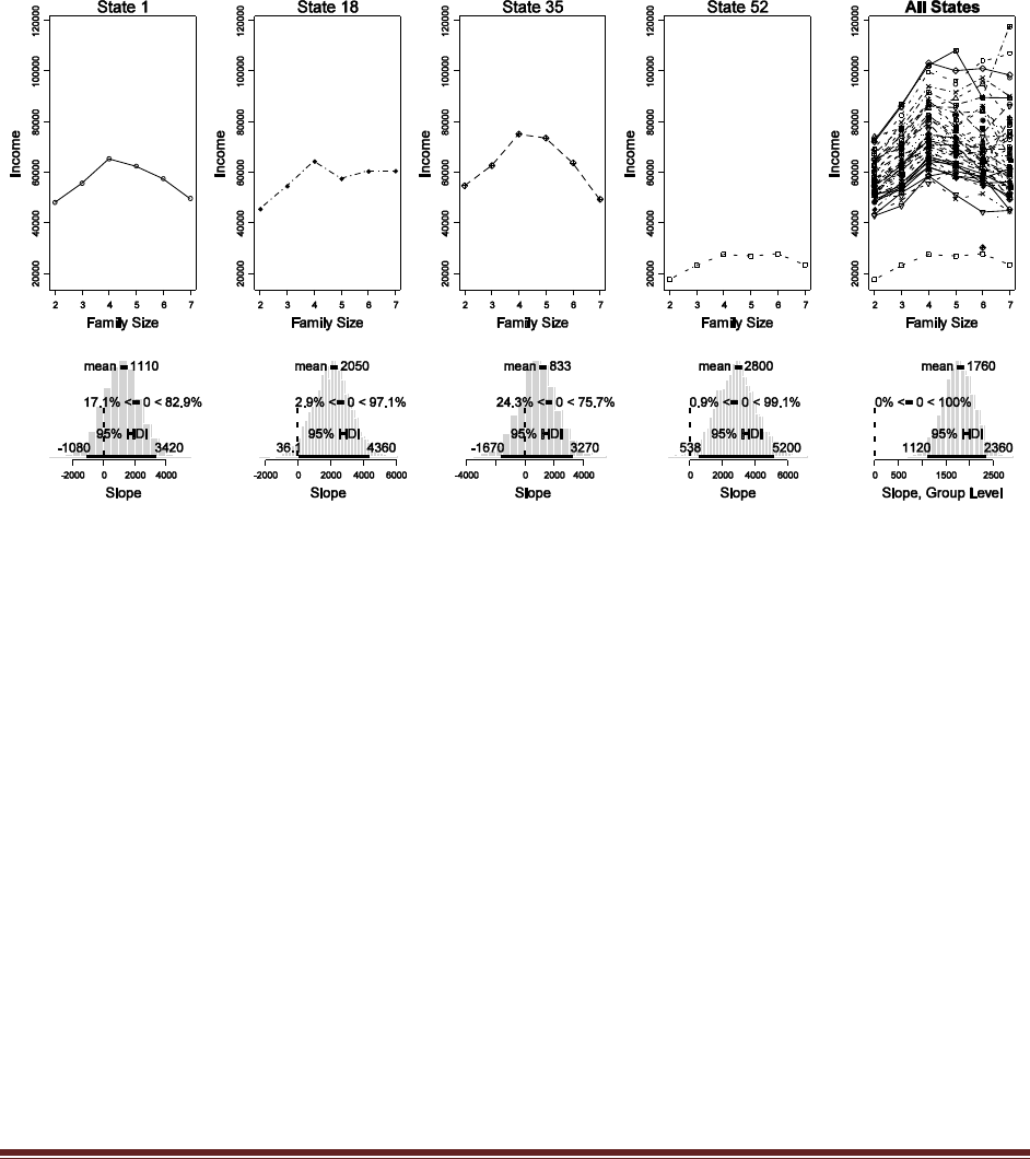
Solutions Manual for Doing Bayesian Data Analysis by John K. Kruschke Page 130
in the family, for all 50 states and the District of Columbia and Puerto Rico. The data are
plotted in Figure 16.14.
(A) Run the program of Section 16.5.3 (SimpleLinearRegressionRepeatedBrugs.R) with
the income data. Examine the data section of the program, and you will find that the
necessary lines of code are already available. The program should generate a figure much
like Figure 16.14, p. 451.
Here is the resulting figure:
For lack of space, the figure does not plot all 52 individual “States” (50 States plus D.C. and
Puerto Rico).
(B) There is suggestion of outliers in these data. One curve (for Puerto Rico) falls barely
above 20,000, which is far lower than all the others. This suggests an outlier for the
distribution of intercepts. Some single data points fall far from the individual linear trends.
For example, the six-person family in the District of Columbia has an income of only about
30,000, whereas the five-person family has an income of more than 80,000. This suggests an
outlier for points around linear trends. Finally, some individual slopes might seem quite
steep compared to others. For example, the income in Hawaii rises about $50,000 from
twoperson to seven-person families. This increase might or might not be an outlier relative
to other states. Which distributions in the hierarchical model of Figure 16.11 should be
changed to t distributions to address these outliers? Change the model specification to
accommodate these t distributions. Use the example in Section 16.5.2
(SimpleRobustLinearRegressionBrugs. R) as a guide. Report your model specification in
your write-up. Show the posterior estimate of the intercept of Puerto Rico for small-df t
bias and for large-df t bias. Show the posterior estimate of the slope of Hawaii for small-df t
bias and for large-df t bias.
The low curve suggests that the subject intercepts, b0[s], have an outlier and could use a t
distributed prior. The outlying single data point suggests that the single data points, y[r], could
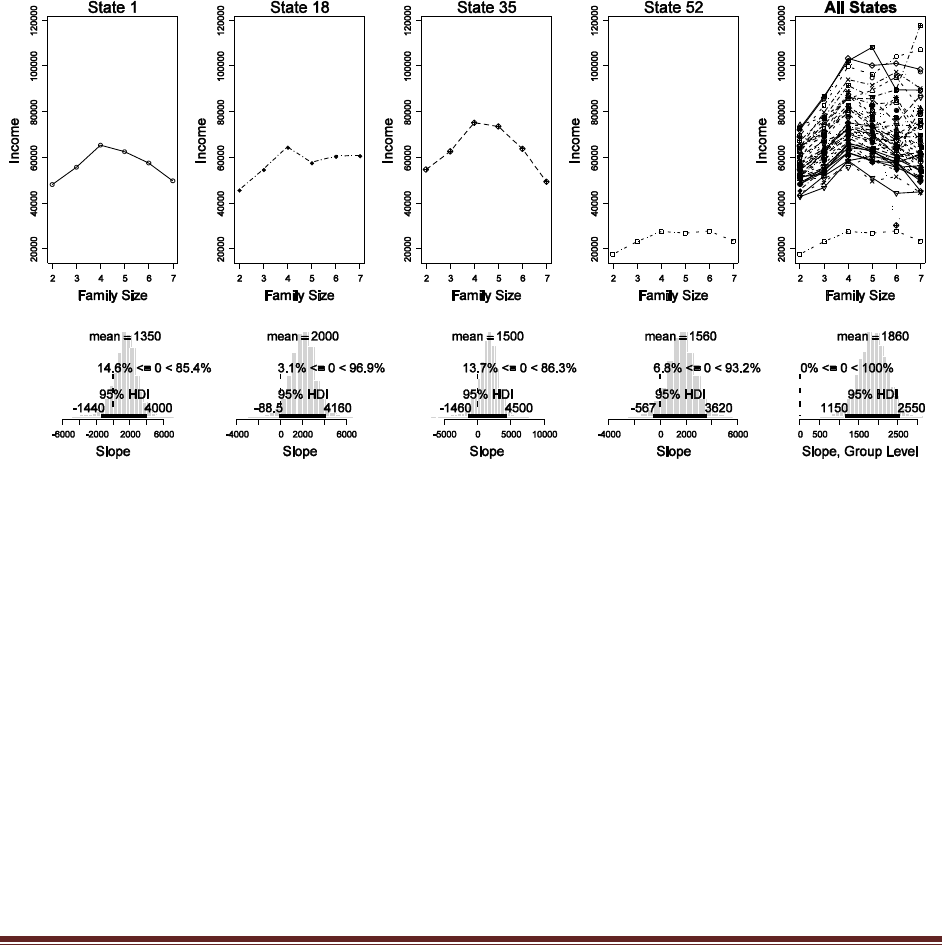
Solutions Manual for Doing Bayesian Data Analysis by John K. Kruschke Page 131
use a t distributed likelihood. And the outlying slope suggests that subject slopes, b1[s], could
use a t distributed prior. Therefore, the parameters that were originally given normal priors, as
y[r] ~ dnorm( mu[r] , tau[ subj[r] ])
b0[s] ~ dnorm( mu0G , tau0G )
b1[s] ~ dnorm( mu1G , tau1G )
should be changed to
y[r] ~ dt( mu[r] , tau[subj[r]] , tdf )
b0[s] ~ dt( mu0G , tau0G , tdf )
b1[s] ~ dt( mu1G , tau1G , tdf )
with
tdf <- 2 # for low, or 100 for high
The specific tdf values could be different, or even specified with a hyperdistribution that favors
small or large values.
When tdf=2, the result looks like this:
For tdf=100, the results look like this:
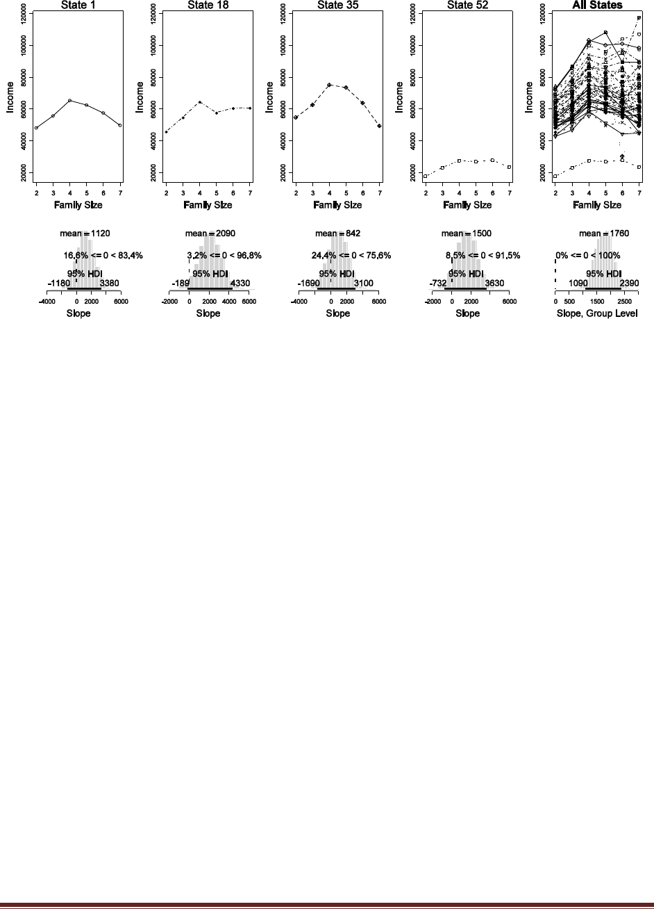
Solutions Manual for Doing Bayesian Data Analysis by John K. Kruschke Page 132
To answer the specific questions about Hawaii and Puerto Rico, we need to determine the index
value of those states. Then we can plot the relevant parameter values. One way to do that appears
below (this code is appended to the end of the program):
windows()
layout( matrix( 1:4 , nrow=2 ) )
# Hawaii:
HawaiiIdx = which( unique(dataMat[,"State"]) == "Hawaii" )
histInfo = plotPost( b1samp[HawaiiIdx,] , xlab=paste("Slope, Hawaii (tdf=",tdf,")",sep="") ,
compVal=0.0 , breaks=30 )
histInfo = plotPost( b0samp[HawaiiIdx,] , xlab=paste("Interc., Hawaii (tdf=",tdf,")",sep="") ,
compVal=0.0 , breaks=30 )
# Puerto Rico:
PRIdx = which( unique(dataMat[,"State"]) == "Puerto Rico" )
histInfo = plotPost( b1samp[PRIdx,] , xlab=paste("Slope, Puerto Rico (tdf=",tdf,")",sep="") ,
compVal=0 , breaks=30 )
histInfo = plotPost( b0samp[PRIdx,] , xlab=paste("Intercept, Puerto Rico (tdf=",tdf,")",sep="") ,
compVal=0 , breaks=30 )
The resulting histograms look like the following:

Solutions Manual for Doing Bayesian Data Analysis by John K. Kruschke Page 133
The results for tdf=2 are on the left, and the results for tdf=100 are on the right. Notice that the
mean credible slope for Hawaii is steeper (farther from the group mean slope) when tdf=2, and
the mean credible intercept for Puerto Rico is smaller (farther from the group mean intercept)
when tdf=2. In other words, there appears to be less shrinkage of outliers when tdf=2 than when
tdf=100.
(C) The data also suggest a nonlinear trend in the data. Incomes appear to rise for two-,
three-, and four-person families, but they then level off and decline as family size gets
larger. Include in the original (non-t) model another term that can capture ―quadratic
curvature‖ in the income level … . The prior on b2 is analogous to the prior on b1. Is the
group-average estimate of curvature credibly nonzero?
Here’s the model statement. The new parts are in bold font.
model {
for( r in 1 : Ndata ) {
y[r] ~ dnorm( mu[r] , tau[ subj[r] ] )
mu[r] <- b0[subj[r]] + b1[subj[r]] * x[r] + b2[subj[r]] * pow(x[r],2)
}
for ( s in 1 : Nsubj ) {
b0[s] ~ dnorm( mu0G , tau0G )
b1[s] ~ dnorm( mu1G , tau1G )
b2[s] ~ dnorm( mu2G , tau2G )
tau[s] ~ dgamma( sG , rG )
}
mu0G ~ dnorm(0,.01)
tau0G ~ dgamma(.1,.1)
mu1G ~ dnorm(0,.01)
tau1G ~ dgamma(.1,.1)
mu2G ~ dnorm(0,.01)
tau2G ~ dgamma(.1,.1)
sG <- pow(m,2)/pow(d,2)
rG <- m/pow(d,2)
m ~ dgamma(1,.1)

Solutions Manual for Doing Bayesian Data Analysis by John K. Kruschke Page 134
d ~ dgamma(1,.1)
}
The model must also be initialized with the new variables. Although there is a simple way to get
R’s lm() function to do regression on quadratic terms, that’s not the purpose of this exercise, and
so we’ll do lazy initialization and let burn-in do the work of finding the posterior.
genInitList <- function() {
b0 = b1 = tau = rep(0,length=Nsubj)
for ( sIdx in 1:Nsubj ) {
yVec = datalist$y[datalist$subj==sIdx]
xVec = datalist$x[datalist$subj==sIdx]
lmInfo = lm( yVec ~ xVec )
b0[sIdx] = lmInfo$coef[1]
b1[sIdx] = lmInfo$coef[2]
tau[sIdx] = length(yVec) / sum(lmInfo$res^2)
}
mu0G = mean(b0)
tau0G = 1/sd(b0)^2
mu1G = mean(b1)
tau1G = 1/sd(b1)^2
m = mean(tau)
d = sd(tau)
list( b0=b0 , b1=b1 ,
b2=0*b1 , # lazy
tau=tau ,
mu0G=mu0G , tau0G=tau0G ,
mu1G=mu1G , tau1G=tau1G ,
mu2G=0 , tau2G=.5*tau1G , # lazy
m=m , d=d )
}
for ( chainIdx in 1 : nchain ) {
modelInits( bugsInits( genInitList ) )
}
The new variables must also be monitored and extracted:
samplesSet( c( "b0","b1","b2","tau" , "mu0G","tau0G", "mu1G","tau1G", "mu2G","tau2G",
"m","d" ) )
…
zmu2Gsamp = samplesSample( "mu2G" )
The resulting posterior on mu2G looks like this:
histInfo = plotPost( zmu2Gsamp , xlab="Standardized Quadratic Coef" ,
compVal=0 , breaks=30 )
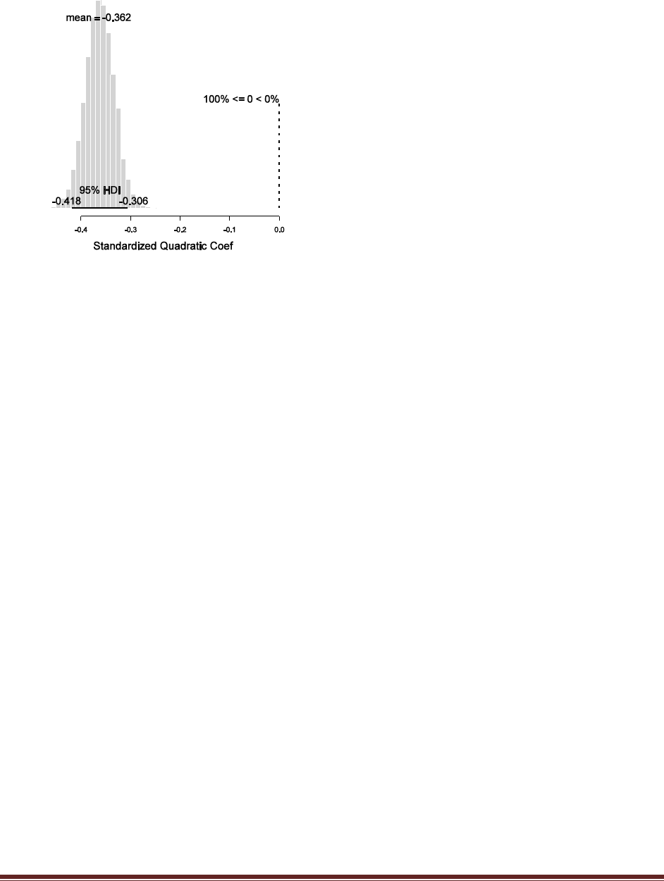
Solutions Manual for Doing Bayesian Data Analysis by John K. Kruschke Page 135
Thus, there does indeed appear to be a credible quadratic trend, on average, across the 52 states.

Solutions Manual for Doing Bayesian Data Analysis by John K. Kruschke Page 136
Chapter 17.
Exercise 17.1. [Purpose: To view the prior on the regression coefficients, when there is a
hyperprior.] The hyperprior on regression coefficients in Figure 17.6 may be difficult to
intuit. Therefore, generate graphs of the prior distribution on the regression coefficients for
the program in Section 17.5.2 (MultiLinRegressHyperBrugs.R), when tdf is set at different
values. To accomplish this, do the following: … Run the program and display the prior for
tdfBgain=1 and for tdfBgain=100. Point out and discuss any differences in the priors for
those different hyperprior constants.
Please note that the suggested change for the plotting limits is appropriate for the randomly
generated data.
The changes to the code are listed here:
model {
for( i in 1 : nData ) {
y[i] ~ dnorm( mu[i] , tau )
mu[i] <- b0 + inprod( b[] , x[i,] )
}
tau ~ dgamma(.01,.01)I(0.0001,10000)
b0 ~ dnorm(0,1.0E-12)
for ( j in 1:nPredictors ) {
b[j] ~ dt( muB , tauB , tdfB )
}
muB ~ dnorm( 0 , .100 )
tauB ~ dgamma(.01,.01)I(0.0001,10000)
udfB ~ dunif(0,1)
tdfB <- 1 + tdfBgain * ( -log( 1 - udfB ) )
}
…
tdfBgain = 100 # or 1
…
datalist = list(
x = zx ,
# y = as.vector( zy ) ,
nPredictors = nPredictors ,
nData = nData ,
tdfBgain = tdfBgain
)
…
#genInitList <- function(nPred=nPredictors) {
# lmInfo = lm( y ~ x ) # R function returns least-squares (normal MLE) fit.
# bInit = lmInfo$coef[-1] * apply(x,2,sd) / sd(y)
# tauInit = (length(y)*sd(y)^2)/sum(lmInfo$res^2)
# list(
# b0 = 0 ,
# b = bInit ,
# tau = tauInit ,
# muB = mean( bInit ) ,

Solutions Manual for Doing Bayesian Data Analysis by John K. Kruschke Page 137
# tauB = 1 / sd( bInit )^2 ,
# udfB = 0.95 # tdfB = 4
# )
#}
#for ( chainIdx in 1 : nChain ) {
# modelInits( bugsInits( genInitList ) )
#}
modelGenInits()
…
checkConvergence = F
if ( checkConvergence ) {
b0Sum = plotChains( "b0" , saveplots=F , filenameroot=fname )
bSum = plotChains( "b" , saveplots=F , filenameroot=fname )
tauSum = plotChains( "tau" , saveplots=F , filenameroot=fname )
muBSum = plotChains( "muB" , saveplots=F , filenameroot=fname )
tauBSum = plotChains( "tauB" , saveplots=F , filenameroot=fname )
tdfBSum = plotChains( "tdfB" , saveplots=F , filenameroot=fname )
}
…
# Display the posterior:
nPlotPerRow = 5
nPlotRow = ceiling((2+nPredictors)/nPlotPerRow)
nPlotCol = ceiling((2+nPredictors)/nPlotRow)
windows(3.5*nPlotCol,2.25*nPlotRow)
layout( matrix(1:(nPlotRow*nPlotCol),nrow=nPlotRow,ncol=nPlotCol,byrow=T) )
par( mar=c(4,3,2.5,0) , mgp=c(2,0.7,0) )
histInfo = plotPost( sigmaSamp , xlab="Sigma Value" , compVal=NULL ,
breaks=30 , main=bquote(sigma[y]) ,
cex.main=1.67 , cex.lab=1.33 )
histInfo = plotPost( b0Samp , xlab="Intercept Value" , compVal=NULL ,
breaks=30 , main=bquote(.(predictedName) *" at "* x==0) ,
cex.main=1.67 , cex.lab=1.33 )
for ( sIdx in 1:nPredictors ) {
histInfo = plotPost( bSamp[,sIdx] , xlab="Slope Value" , compVal=0.0 ,
breaks=c(-1000000,seq(-400,400,21),1000000) , xlim=c(-400,400) ,
main=bquote( Delta * .(predictedName) /
Delta * .(predictorNames[sIdx]) ) ,
cex.main=1.67 , cex.lab=1.33 )
}
Please note that the suggested change for the plotting limits is appropriate for the randomly
generated data.
The posterior for tdfBgain=1 looks like this:

Solutions Manual for Doing Bayesian Data Analysis by John K. Kruschke Page 138
The posterior for tdfBgain=100 looks like the following. Notice that the 95%HDI on the slopes
extends from roughly -150 to +150, which is much less than when tdfBgain=1 (above). The
means of the intercept and slope are all very close to zero relative to the widths of the
distributions. The means are thrown off from zero because there are some extreme outliers in
these prior distributions.

Solutions Manual for Doing Bayesian Data Analysis by John K. Kruschke Page 139
Notice that for either prior, the priors distributions are extremely broad compared to the
posteriors displayed in Figure 17.7 (pp. 465-466) of the textbook. Thus, these priors are very
vague indeed.
Exercise 17.2. [Purpose: To conduct a power analysis for multiple regression.] Consider the
SAT data shown in Figure 17.3, p. 457, and the posterior for a linear regression model
(with no interaction) shown in Figure 17.5, p. 461. The marginal posterior distribution for
the slope on spending per pupil has a 95% HDI that excludes zero, and has a width of very
nearly 17. Consider two different goals for the research. One goal is to show that the 95%
HDI on spending per pupil excludes a ROPE of [-1,+1], and the second goal is to show that
the width of the 95% HDI is less than 10. … Answer these questions:
What is the retrospective power for each of the two goals? (Hint: It‘s about 0.67 and 0.00,
when the x points are randomly sampled with replacement from the 50 actual points.)
The hint gives the answer. You need to show how to get the answer. Here’s the code:
GoalAchievedForSample = function( xOrig , yOrig , plotResults=F ,
fileNameRoot="DeleteMe" ) {
fname=fileNameRoot
library(BRugs)
#------------------------------------------------------------------------------
# THE MODEL.

Solutions Manual for Doing Bayesian Data Analysis by John K. Kruschke Page 140
modelstring = "
# BUGS model specification begins here...
model {
for( i in 1 : nData ) {
y[i] ~ dnorm( mu[i] , tau )
mu[i] <- b0 + inprod( b[] , x[i,] )
}
tau ~ dgamma(.01,.01)
b0 ~ dnorm(0,1.0E-12)
for ( j in 1:nPredictors ) {
b[j] ~ dnorm(0,1.0E-12)
}
}
# ... end BUGS model specification
" # close quote for modelstring
writeLines(modelstring,con="model.txt")
modelCheck( "model.txt" )
#------------------------------------------------------------------------------
# THE DATA.
# Takes raw data as input so that program can convert back to original scale,
# and goals can be expressed on original scale.
nPredictors = NCOL(xOrig)
nData = NROW(xOrig)
# Re-center data at mean, to reduce autocorrelation in MCMC sampling.
# Standardize (divide by SD) to make prior specification easier.
standardizeCols = function( dataMat ) {
zDataMat = dataMat
for ( colIdx in 1:NCOL( dataMat ) ) {
mCol = mean( dataMat[,colIdx] )
sdCol = sd( dataMat[,colIdx] )
zDataMat[,colIdx] = ( dataMat[,colIdx] - mCol ) / sdCol
}
return( zDataMat )
}
zx = standardizeCols( xOrig )
zy = standardizeCols( yOrig )
# Get the data into BUGS:
datalist = list(
x = zx ,
y = as.vector( zy ) , # BUGS does not treat 1-column mat as vector
nPredictors = nPredictors ,
nData = nData
)
modelData( bugsData( datalist ) )
#------------------------------------------------------------------------------
# INTIALIZE THE CHAINS.
nChain = 3
modelCompile( numChains = nChain )
genInitList <- function(nPred=nPredictors) {
lmInfo = lm( datalist$y ~ datalist$x ) # R function returns MLE
bInit = lmInfo$coef[-1]
tauInit = length(datalist$y) / sum(lmInfo$res^2)
list(
b0 = 0 ,
b = bInit ,
tau = tauInit

Solutions Manual for Doing Bayesian Data Analysis by John K. Kruschke Page 141
)
}
for ( chainIdx in 1 : nChain ) {
modelInits( bugsInits( genInitList ) )
}
#------------------------------------------------------------------------------
# RUN THE CHAINS
# burn in
BurnInSteps = 100
modelUpdate( BurnInSteps )
# actual samples
samplesSet( c( "b0" , "b" , "tau" ) )
stepsPerChain = ceiling(50000/nChain)
thinStep = 2
modelUpdate( stepsPerChain , thin=thinStep )
#------------------------------------------------------------------------------
# EXAMINE THE RESULTS
source("plotPost.R")
# Extract chain values:
zb0Samp = matrix( samplesSample( "b0" ) )
zbSamp = NULL
for ( j in 1:nPredictors ) {
zbSamp = cbind( zbSamp , samplesSample( paste("b[",j,"]",sep="") ) )
}
zTauSamp = matrix( samplesSample( "tau" ) )
zSigmaSamp = 1 / sqrt( zTauSamp ) # Convert precision to SD
chainLength = length(zTauSamp)
# Convert to original scale:
bSamp = zbSamp * matrix( sd(yOrig)/apply(xOrig,2,sd) , byrow=TRUE ,
ncol=nPredictors , nrow=NROW(zbSamp) )
b0Samp = ( zb0Samp * sd(yOrig)
+ mean(yOrig)
- rowSums( zbSamp
* matrix( sd(yOrig)/apply(xOrig,2,sd) , byrow=TRUE ,
ncol=nPredictors , nrow=NROW(zbSamp) )
* matrix( apply(xOrig,2,mean) , byrow=TRUE ,
ncol=nPredictors , nrow=NROW(zbSamp) ) ) )
sigmaSamp = zSigmaSamp * sd(yOrig)
# Display the posterior:
if ( plotResults ) {
nPlotPerRow = 5
nPlotRow = ceiling((2+nPredictors)/nPlotPerRow)
nPlotCol = ceiling((2+nPredictors)/nPlotRow)
windows(3.5*nPlotCol,2.25*nPlotRow)
layout( matrix(1:(nPlotRow*nPlotCol),nrow=nPlotRow,ncol=nPlotCol,byrow=T) )
par( mar=c(4,3,2.5,0) , mgp=c(2,0.7,0) )
histInfo = plotPost( sigmaSamp , xlab="Sigma Value" , compVal=NULL ,
breaks=30 , main=bquote(sigma[y]) ,
cex.main=1.67 , cex.lab=1.33 )
histInfo = plotPost( b0Samp , xlab="Intercept Value" , compVal=NULL ,
breaks=30 , main=bquote(.(predictedName) *" at "* x==0) ,
cex.main=1.67 , cex.lab=1.33 )
for ( sIdx in 1:nPredictors ) {
histInfo = plotPost( bSamp[,sIdx] , xlab="Slope Value" , compVal=0.0 ,
breaks=30 , cex.main=1.67 , cex.lab=1.33 ,
main=bquote( Delta * .(predictedName) /

Solutions Manual for Doing Bayesian Data Analysis by John K. Kruschke Page 142
Delta * .(predictorNames[sIdx]) ) )
}
}
#------------------------------------------------------------------------------
source("HDIofMCMC.R")
# Goal 1 is HDI of b1 excludes ROPE .
# Goal 2 is HDI of b1 has desired precision .
HDIlims = HDIofMCMC( bSamp[,1] )
ROPE = c(-1,1)
goalAch1 = ( HDIlims[1] > ROPE[2] | HDIlims[2] < ROPE[1] )
#goalAch1 = ( HDIlims[1] > ROPE[2] ) # If you want HDI to fall ABOVE the ROPE
goalAch2 = ( HDIlims[2] - HDIlims[1] < 10 ) # 10
goalAchieved = c( goalAch1 , goalAch2 )
return( goalAchieved )
} # end of function GoalAchievedForSample
#==============================================================================
# Now call the function defined above, using simulated data.
analysisType = c("Retro","Repli")[1] # specify [1] or [2]
fileNameRoot = paste("Exercise17.2",analysisType,sep="")
# Load original data, for use in replication probability analysis:
dataMat = read.table( file="Guber1999data.txt" ,
col.names = c( "State","Spend","StuTchRat","Salary",
"PrcntTake","SATV","SATM","SATT") )
predictedName = "SATT"
predictorNames = c( "Spend" , "PrcntTake" )
nData = NROW( dataMat )
yActual = as.matrix( dataMat[,predictedName] )
xActual = as.matrix( dataMat[,predictorNames] )
# Load previously computed posterior chains for parameters
# b0Samp , bSamp , sigmaSamp
load( file="MultipleLinearRegressionBrugsGuber1999.Rdata" )
chainLength = length(b0Samp)
# SPECIFY NUMBER OF (ADDITIONAL) DATA POINTS:
nPts = 50
# Specify number of simulated experiments:
nSimExperiments = min(200,chainLength)
nGoal=2 # Determined in function above.
# If previous record of power estimation exists, load it and continue the runs.
filelist = dir( pattern=paste( fileNameRoot, "N",nPts, "Result.Rdata",
sep="") )
if ( length( filelist ) > 0 ) { # if the file already exists...
# load previous expIdx, nSuccess
load(paste(fileNameRoot,"N",nPts,"Result.Rdata",sep=""))
prevExpIdx = expIdx
# Use just some of the MCMC steps, distributed among the whole chain:
chainIdxVec = round(seq(1,chainLength,len=(prevExpIdx+nSimExperiments)))
} else { # ... otherwise, start a new record
prevExpIdx = 0
nSuccess = rep(0,nGoal) # Initialize success counter.
chainIdxVec = round(seq(1,chainLength,len=nSimExperiments))
}

Solutions Manual for Doing Bayesian Data Analysis by John K. Kruschke Page 143
# Simulated experiment loop begins here:
for ( expIdx in (1+prevExpIdx):(nSimExperiments+prevExpIdx) ) {
# Generate random data from posterior parameters
chainIdx=chainIdxVec[expIdx]
b0 = b0Samp[chainIdx]
b1 = bSamp[chainIdx,1]
b2 = bSamp[chainIdx,2]
sigma = sigmaSamp[chainIdx]
cat( "b0=",b0, ", b1=",b1, ", b2=",b2, ", sigma=",sigma, "\n")
flush.console()
ySim = cbind( rep(0,nPts) )
xSim = matrix( 0 , nrow=nPts , ncol=NCOL(xActual) )
for ( ptIdx in 1:nPts ) {
xIdx = sample( NROW(xActual) , size=1 ) # selects randomly from xActual
x1 = xActual[xIdx,1]
x2 = xActual[xIdx,2]
ySim[ptIdx] = b0 + b1*x1 + b2*x2 + rnorm(1,0,sd=sigma)
xSim[ptIdx,] = c(x1,x2)
}
if ( analysisType == "Repli" ) { # if replication probability
xSim = rbind( xActual , xSim )
ySim = rbind( yActual , ySim )
}
# Make plots for first 10 simulated experiments:
if ( expIdx <= 10 ) { plotRes = T } else { plotRes = F }
# Call BUGS program and tally number of successes:
nSuccess = ( nSuccess
+ GoalAchievedForSample( xSim , ySim , plotRes, fileNameRoot ))
estPower = nSuccess / expIdx
cat( "\n*** nPts:",nPts, ", nSimExp:",expIdx,
" , nSuccess:",nSuccess, ", estPower:",round(estPower,2), "\n\n" )
flush.console()
save( nSuccess , expIdx , estPower ,
file=paste(fileNameRoot,"N",nPts,"Result.Rdata",sep="") )
} # end of simulated experiment loop.
What is the power for each of the two goals when N = 130? (Hint: It‘s about 0.85 and 0.30.)
The hint provides the answer. But your answer should include the number of simulated
experiments you ran and the number of times each goal was achieved.
What‘s the minimal N needed to achieve a power of 0.80 for the second goal?
It’s about 180. Again, your answer should include the number of simulated experiments you ran
and the number of times each goal was achieved.
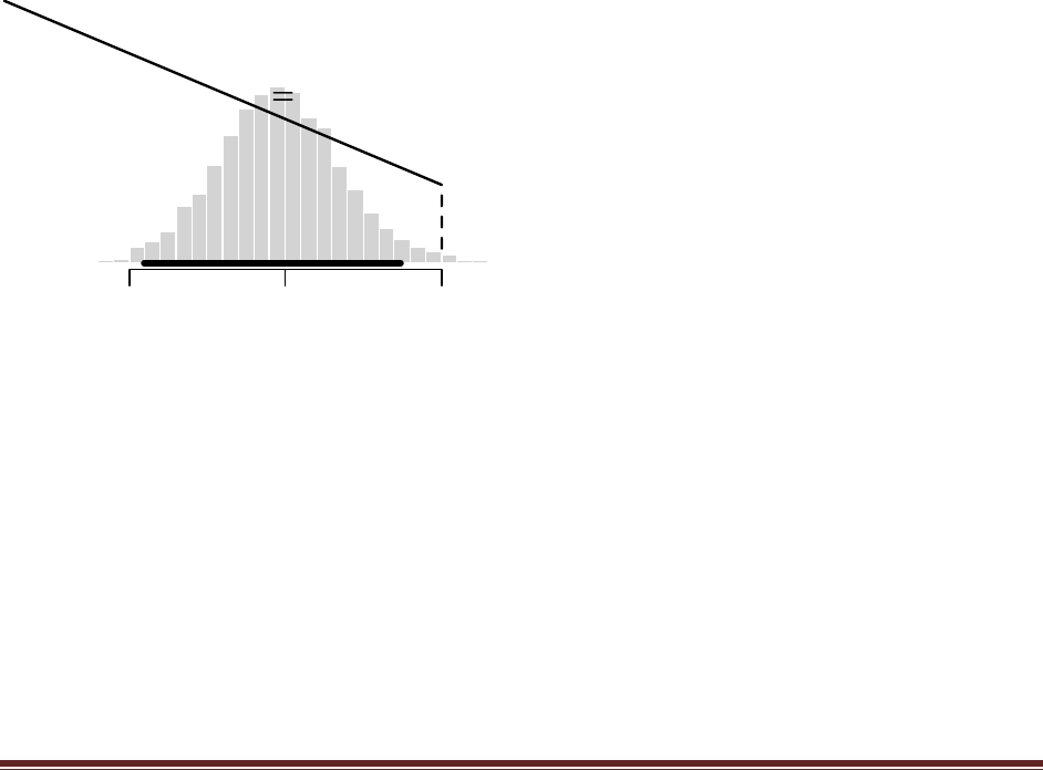
Solutions Manual for Doing Bayesian Data Analysis by John K. Kruschke Page 144
Chapter 18.
Exercise 18.1. [Purpose: To notice that Bayesian ANOVA with two groups tends to agree
with an NHST t test.] The BRugs program of Section 18.4.1 (ANOVAonewayBRugs.R)
allows you to specify random data. It executes a Bayesian ANOVA, and at the end of the
program it also conducts an NHST ANOVA and t tests (using R‘s aov and t.test functions).
Run the program ten times with different random data by commenting out the set.seed
command. Specify ysdtrue = 4.0, atrue = c(2,-2) (which implies two groups because there
are two deflections) and npercell = 8. For each run, record, by hand,
(1) how much of the posterior difference between means falls on one side of zero (see the
posterior histogram with the main title ―X Contrast‖ and x axis labeled ―-1 1 + 1 2‖),
(2) whether the 95% HDI excludes zero, and
(3) the confidence interval and p value of the NHST t test.
Do the t test and the BANOVA usually agree in their decisions about whether the group
means are different?
Here are results from 10 runs. The t-test is shown first, followed by the Bayesian posterior. Your
results may differ, because the data are randomly generated.
1. M2-M1 = -5.410669
t = -3.0047, df = 14, p-value = 0.009464
95 percent confidence interval: -9.272914 -1.548425
X Contrast:
-1 1 + 1 2
-10 -5 0
mean -5.19
99% <= 0 < 1%
95% HDI
-9.49 -1.31
2. M2-M1 = -6.222964
t = -5.1686, df = 14, p-value = 0.0001426
95 percent confidence interval: -8.805289 -3.640639
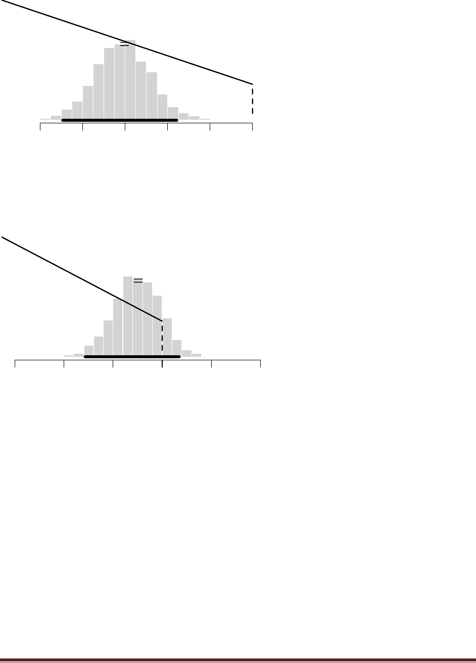
Solutions Manual for Doing Bayesian Data Analysis by John K. Kruschke Page 145
X Contrast:
-1 1 + 1 2
-10 -8 -6 -4 -2 0
mean -6.11
100% <= 0 < 0%
95% HDI
-8.94 -3.57
3. M2-M1 = -2.902464
t = -1.298, df = 14, p-value = 0.2153
95 percent confidence interval: -7.698286 1.893359
X Contrast:
-1 1 + 1 2
-15 -10 -5 0 5 10
mean -2.59
86.2% <= 0 < 13.8%
95% HDI
-7.84 1.71
4. M2-M1 = -0.5305656
t = -0.222, df = 14, p-value = 0.8275
95 percent confidence interval: -5.657225 4.596094
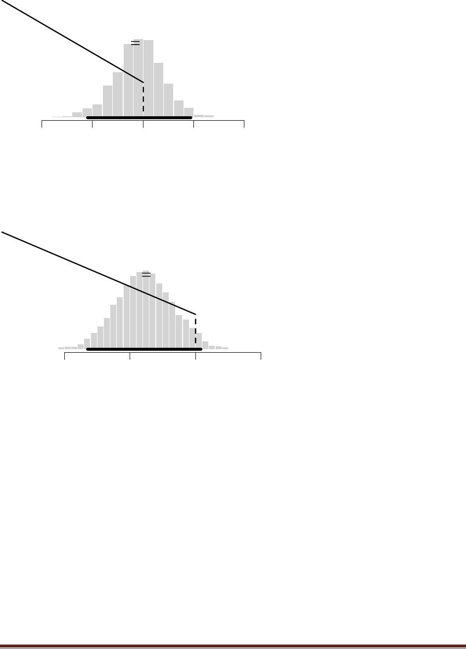
Solutions Manual for Doing Bayesian Data Analysis by John K. Kruschke Page 146
X Contrast:
-1 1 + 1 2
-10 -5 0 5 10
mean -0.452
56.6% <= 0 < 43.4%
95% HDI
-5.5 4.71
5. M2-M1 = -4.198784
t = -2.115, df = 14, p-value = 0.05284
95 percent confidence interval: -8.45665094 0.05908298
X Contrast:
-1 1 + 1 2
-10 -5 0 5
mean -3.86
95.7% <= 0 < 4.3%
95% HDI
-8.22 0.43
6. M2-M1 = -6.570604
t = -4.0425, df = 14, p-value = 0.001211
95 percent confidence interval: -10.056668 -3.084539
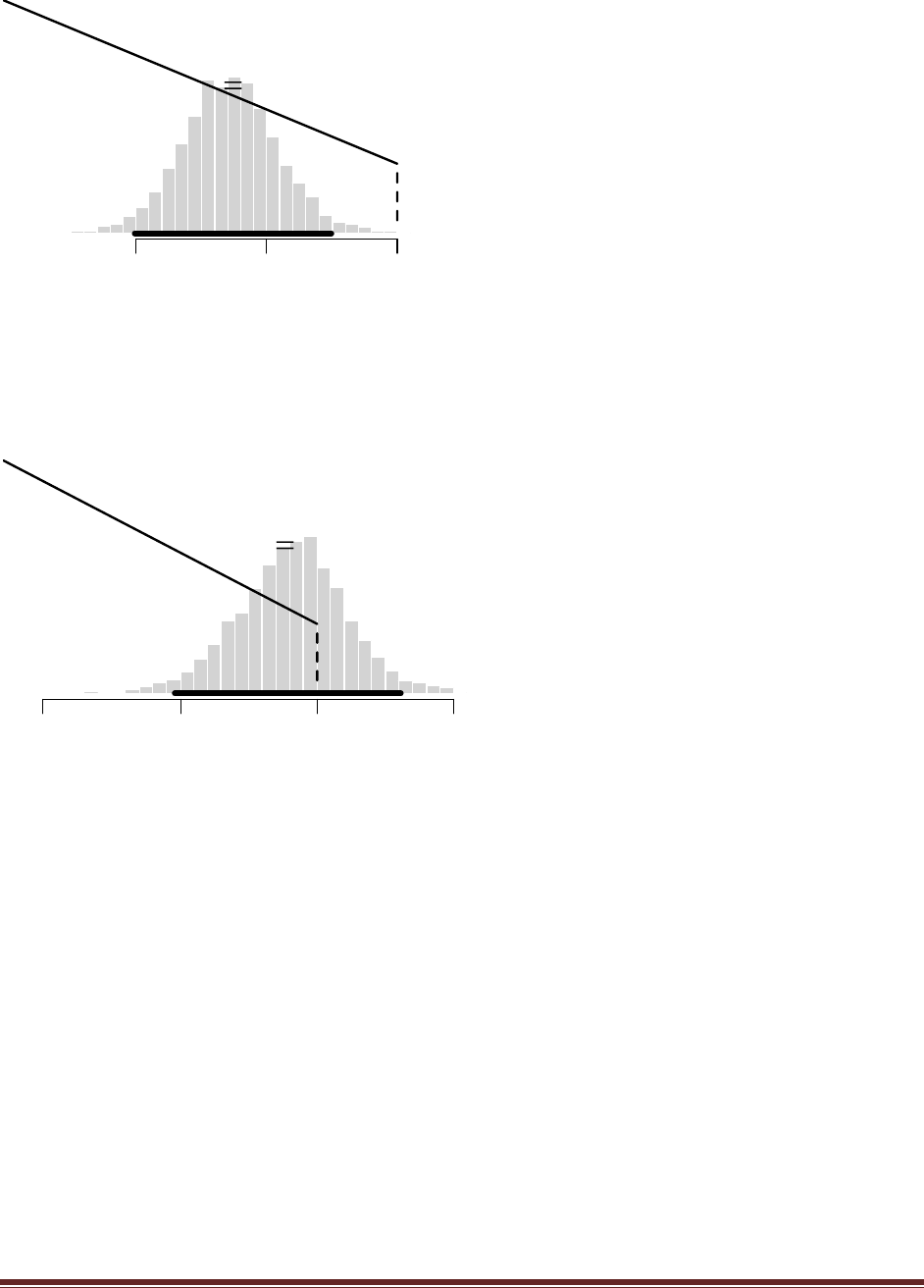
Solutions Manual for Doing Bayesian Data Analysis by John K. Kruschke Page 147
X Contrast:
-1 1 + 1 2
-10 -5 0
mean -6.39
99.9% <= 0 < 0.1%
95% HDI
-10.1 -2.53
7. M2-M1 = -1.071621
t = -0.5287, df = 14, p-value = 0.6053
95 percent confidence interval: -5.418663 3.275421
X Contrast:
-1 1 + 1 2
-10 -5 0 5
mean -0.925
68.4% <= 0 < 31.6%
95% HDI
-5.18 3.07
8. M2-M1 = -4.763127
t = -3.3178, df = 14, p-value = 0.005079
95 percent confidence interval: -7.842266 -1.683988
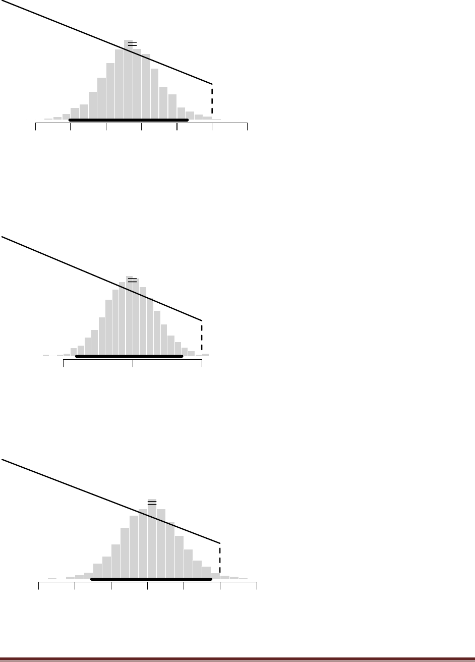
Solutions Manual for Doing Bayesian Data Analysis by John K. Kruschke Page 148
X Contrast:
-1 1 + 1 2
-10 -8 -6 -4 -2 0 2
mean -4.59
99.5% <= 0 < 0.5%
95% HDI
-8.04 -1.41
9. M2-M1 = -5.308085
t = -3.2347, df = 14, p-value = 0.005993
95 percent confidence interval: -8.827658 -1.788511
X Contrast:
-1 1 + 1 2
-10 -5 0
mean -5.14
99.2% <= 0 < 0.8%
95% HDI
-9.04 -1.47
10. M2-M1 = -4.022563
t = -2.7984, df = 14, p-value = 0.01422
95 percent confidence interval: -7.105540 -0.939587
X Contrast:
-1 1 + 1 2
-10 -8 -6 -4 -2 0 2
mean -3.85
98.6% <= 0 < 1.4%
95% HDI
-7.06 -0.531
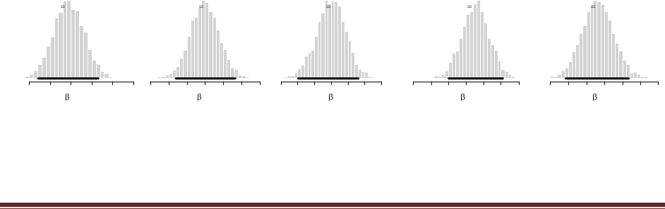
Solutions Manual for Doing Bayesian Data Analysis by John K. Kruschke Page 149
In all ten cases, the conclusion regarding the null value is the same for the t-test and the Bayesian
HDI. Typically, the 95%HDI is a bit more conservative, i.e., wider, than the 95% confidence
interval. The Bayesian conclusion comes without ever computing a p value.
Exercise 18.2. [Purpose: To understand the influence of the prior in Bayesian ANOVA.] In
the model section of the BRugs program of Section 18.4.1 (ANOVAonewayBRugs.R), and
correspondingly in the diagram of Figure 18.1, there are several constants that determine
the prior. These constants include the mean value of the baseline (M0 in the diagram), the
precision on the baseline (T0 in the diagram), the precision of the folded-t distribution (Tt
in the diagram), and the upper value of the uniform distribution on y (Hy in the diagram).
Because the data are standardized, M0 should be set at zero, and T0 can be modest (not
terribly small). Hy also can be set to a modest value because the data are standardized. But
what about the precision of the folded-t distribution, Tt? This constant modulates the
degree of shrinkage: A large value of Tt indicates prior knowledge that the groups do not
differ much, and it imposes a high degree of shrinkage that must be overcome by the data.
Run the program on the mussel data using a small value of Tt , such as 1.0E-6, and a large
value of Tt , such as 1000. Are the results very different? Discuss which prior value might
be appropriate.
Using a small precision on Tt:
model {
for ( i in 1:Ntotal ) {
y[i] ~ dnorm( mu[i] , tau )
mu[i] <- a0 + a[x[i]]
}
#
tau <- pow( sigma , -2 )
sigma ~ dunif(0,10) # y values are assumed to be standardized
#
a0 ~ dnorm(0,0.001) # y values are assumed to be standardized
#
for ( j in 1:NxLvl ) { a[j] ~ dnorm( 0.0 , atau ) }
atau <- 1 / pow( aSD , 2 )
aSD <- abs( aSDunabs ) + .1
aSDunabs ~ dt( 0 , 1.0E-6 , 2 )
}
yields
x: 1
11
-0.015 -0.010 -0.005 0.000 0.005 0.010
mean -0.00557
95% HDI
-0.0129 0.00161
x: 2
12
-0.025 -0.015 -0.005 0.000 0.005
mean -0.0102
95% HDI
-0.0181 -0.00171
x: 3
13
0.000 0.010 0.020 0.030
mean 0.0149
95% HDI
0.00515 0.0231
x: 4
14
-0.025 -0.015 -0.005 0.005
mean -0.00733
95% HDI
-0.0151 0.000527
x: 5
15
-0.005 0.005 0.010 0.015 0.020 0.025
mean 0.00814
95% HDI
-0.000837 0.0169
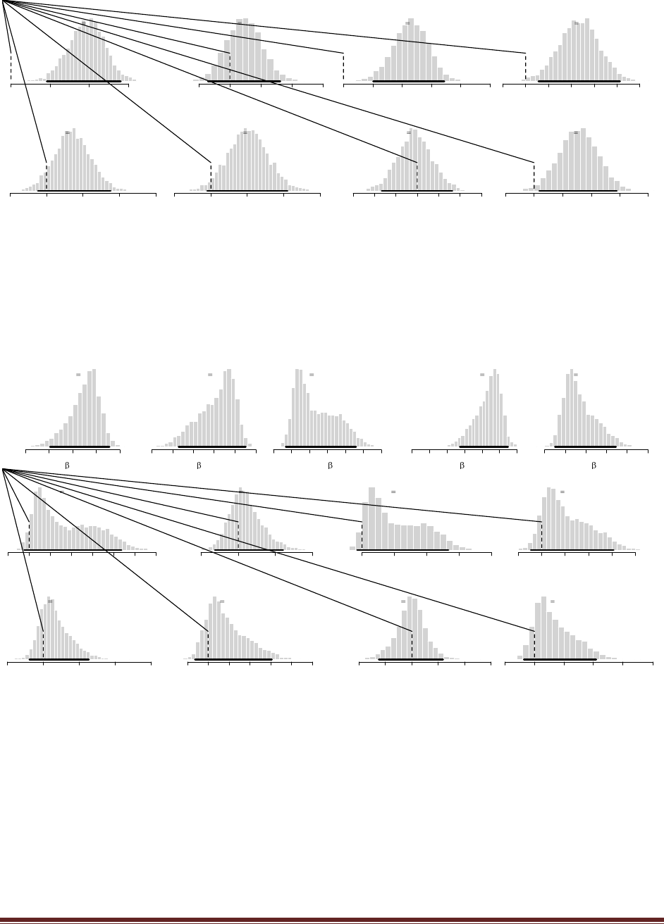
Solutions Manual for Doing Bayesian Data Analysis by John K. Kruschke Page 150
X Contrast: BIGvSMALL
-0.33 1 + -0.33 2 + 0.5 3 + -0.33 4 + 0.5 5
0.00 0.01 0.02 0.03
mean 0.0192
0% <= 0 < 100%
95% HDI
0.0092 0.0281
X Contrast: ORE1vORE2
1 1 + -1 2
-0.01 0.00 0.01 0.02 0.03
mean 0.00462
21.9% <= 0 < 78.1%
95% HDI
-0.00698 0.0163
X Contrast: ALAvORE
-0.5 1 + -0.5 2 + 1 3
0.00 0.01 0.02 0.03 0.04 0.05
mean 0.0228
0% <= 0 < 100%
95% HDI
0.0101 0.0344
X Contrast: NPACvORE
-0.5 1 + -0.5 2 + 0.5 3 + 0.5 4
-0.005 0.000 0.005 0.010 0.015 0.020 0.025
mean 0.0117
0.5% <= 0 < 99.5%
95% HDI
0.00278 0.0207
X Contrast: USAvRUS
0.33 1 + 0.33 2 + 0.33 3 + -1 4
-0.01 0.00 0.01 0.02 0.03
mean 0.00705
8.2% <= 0 < 91.8%
95% HDI
-0.00232 0.0176
X Contrast: FINvPAC
-0.25 1 + -0.25 2 + -0.25 3 + -0.25 4 + 1 5
-0.01 0.00 0.01 0.02 0.03
mean 0.0102
3.4% <= 0 < 96.6%
95% HDI
-0.00105 0.0211
X Contrast: ENGvOTH
0.33 1 + 0.33 2 + 0.33 3 + -0.5 4 + -0.5 5
-0.015 -0.010 -0.005 0.000 0.005 0.010 0.015
mean -0.00068
57.3% <= 0 < 42.7%
95% HDI
-0.00825 0.00821
X Contrast: FINvRUS
-1 4 + 1 5
-0.01 0.00 0.01 0.02 0.03 0.04
mean 0.0155
1.3% <= 0 < 98.7%
95% HDI
0.00172 0.0289
Using a large precision on Tt:
aSDunabs ~ dt( 0 , 1000 , 2 )
yields
x: 1
11
-0.015 -0.010 -0.005 0.000 0.005
mean -0.00256
95% HDI
-0.00981 0.0028
x: 2
12
-0.020 -0.015 -0.010 -0.005 0.000 0.005
mean -0.00461
95% HDI
-0.0135 0.00245
x: 3
13
-0.005 0.005 0.010 0.015 0.020 0.025
mean 0.00694
95% HDI
-0.00152 0.0179
x: 4
14
-0.025 -0.015 -0.005 0.005
mean -0.00334
95% HDI
-0.0113 0.00244
x: 5
15
-0.005 0.000 0.005 0.010 0.015 0.020
mean 0.00357
95% HDI
-0.00251 0.0122
X Contrast: BIGvSMALL
-0.33 1 + -0.33 2 + 0.5 3 + -0.33 4 + 0.5 5
-0.005 0.000 0.005 0.010 0.015 0.020 0.025 0.030
mean 0.00876
4.1% <= 0 < 95.9%
95% HDI
-0.00121 0.0218
X Contrast: ORE1vORE2
1 1 + -1 2
-0.01 0.00 0.01 0.02
mean 0.00206
33.8% <= 0 < 66.2%
95% HDI
-0.00619 0.0121
X Contrast: ALAvORE
-0.5 1 + -0.5 2 + 1 3
0.00 0.01 0.02 0.03 0.04
mean 0.0105
4.9% <= 0 < 95.1%
95% HDI
-0.00149 0.0267
X Contrast: NPACvORE
-0.5 1 + -0.5 2 + 0.5 3 + 0.5 4
-0.005 0.000 0.005 0.010 0.015 0.020
mean 0.00539
10.4% <= 0 < 89.6%
95% HDI
-0.00232 0.0153
X Contrast: USAvRUS
0.33 1 + 0.33 2 + 0.33 3 + -1 4
-0.01 0.00 0.01 0.02 0.03
mean 0.00326
22.5% <= 0 < 77.5%
95% HDI
-0.00373 0.0127
X Contrast: FINvPAC
-0.25 1 + -0.25 2 + -0.25 3 + -0.25 4 + 1 5
-0.005 0.000 0.005 0.010 0.015 0.020 0.025
mean 0.00446
16.8% <= 0 < 83.2%
95% HDI
-0.00313 0.0153
X Contrast: ENGvOTH
0.33 1 + 0.33 2 + 0.33 3 + -0.5 4 + -0.5 5
-0.010 -0.005 0.000 0.005 0.010 0.015
mean -0.000192
51.9% <= 0 < 48.1%
95% HDI
-0.00624 0.00587
X Contrast: FINvRUS
-1 4 + 1 5
-0.01 0.00 0.01 0.02 0.03 0.04
mean 0.0069
12.7% <= 0 < 87.3%
95% HDI
-0.00351 0.021
The results are dramatically different. In particular, the extremely large precision in the prior
essentially insists that there is no variation between groups, and therefore the credible group
deflections are all near zero, and therefore the differences between groups are all near zero.
The low-precision prior is much more appropriate here, unless for some reason we really do have
an extremely strong prior belief that there can be no differences between groups. In that case, it
would take an enormous sample size to overcome the prior.

Solutions Manual for Doing Bayesian Data Analysis by John K. Kruschke Page 151
Exercise 18.3. [Purpose: To understand Bayesian ANOVA without assuming equal
variances.] Modify the program in Section 18.4.1 (ANOVAonewayBRugs.R) so that it
allows a different variance for each group, with the different variances coming from a
hyperdistribution that has its precision informed by the data. In other words, instead of
assuming the same tauy for all the levels of x, we allow each group to have its own variance.
Denote the precision of the jth group as tauj, analogous to the deflection betaj. Just as the
group deflections are assumed to come from a higher-level distribution, we will assume that
the group SDs come from a higher-level distribution. Because SDs must be non-negative,
use a gamma density for the higher-level distribution. The gamma distribution has two
parameters for which you need to establish a prior. See the right side of Figure 16.11 for
guidance. Corresponding code is offered in a hint, below. Run the program on the mussel
muscle data. Are the conclusions about the group means any different than when assuming
equal variances across groups?
Hint regarding the conclusion: The posteriors on the group means are only a little different
in this case, because the group variances are roughly the same. But because the group
variances are less constrained when they are all allowed to be different, they are less
certain. Therefore, the group means are a little less certain, and thus the differences of
means are a little less certain.
model {
for ( i in 1:Ntotal ) {
y[i] ~ dnorm( mu[i] , tau[x[i]] )
mu[i] <- a0 + a[x[i]]
}
a0 ~ dnorm(0,0.001)
for ( j in 1:NxLvl ) {
a[j] ~ dnorm( 0.0 , atau )
tau[j] ~ dgamma( sG , rG )
}
sG <- pow(m,2)/pow(d,2)
rG <- m/pow(d,2)
m ~ dgamma(1,1)
d ~ dgamma(1,1)
atau <- 1 / pow( aSD , 2 )
aSD <- abs( aSDunabs ) + .1
aSDunabs ~ dt( 0 , 0.001 , 2 )
}
…
theData = data.frame( y=datalist$y , x=factor(x,labels=xnames) )
a0 = mean( theData$y )
a = aggregate( theData$y , list( theData$x ) , mean )[,2] - a0
tau = 1/(aggregate( theData$y , list( theData$x ) , sd )[,2])^2
genInitList <- function() {
return(
list(
a0 = a0 ,
a = a ,
tau = tau ,
m = mean( tau ) ,
d = sd( tau ) ,
aSDunabs = sd(a)
)
)
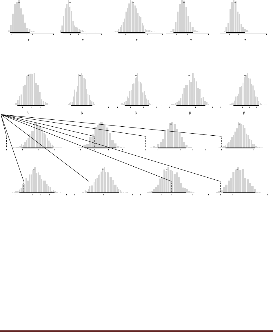
Solutions Manual for Doing Bayesian Data Analysis by John K. Kruschke Page 152
}
for ( chainIdx in 1 : nchain ) {
modelInits( bugsInits( genInitList ) )
}
Here are the posterior tau values:
x: 1
1
1 2 3 4 5
mean 1.66
95% HDI
0.872 2.7
x: 2
2
1 2 3 4 5 6
mean 1.85
95% HDI
0.749 3.25
x: 3
3
0.5 1.0 1.5 2.0 2.5 3.0 3.5
mean 1.49
95% HDI
0.544 2.33
x: 4
4
0 1 2 3 4
mean 1.63
95% HDI
0.729 2.54
x: 5
5
0 1 2 3 4 5
mean 1.61
95% HDI
0.69 2.66
They are fairly homogeneous because the groups happen to have similar SDs for these data.
Here are the posterior group deflections and contrasts:
x: 1
11
-0.020 -0.015 -0.010 -0.005 0.000 0.005
mean -0.00543
95% HDI
-0.0125 0.00196
x: 2
12
-0.02 -0.01 0.00 0.01
mean -0.0103
95% HDI
-0.0181 -0.00244
x: 3
13
0.00 0.01 0.02 0.03
mean 0.0148
95% HDI
0.00576 0.024
x: 4
14
-0.020 -0.015 -0.010 -0.005 0.000 0.005
mean -0.00717
95% HDI
-0.0158 0.000574
x: 5
15
-0.010 0.000 0.005 0.010 0.015 0.020 0.025
mean 0.00813
95% HDI
-0.000947 0.0165
X Contrast: BIGvSMALL
-0.33 1 + -0.33 2 + 0.5 3 + -0.33 4 + 0.5 5
0.00 0.01 0.02 0.03
mean 0.0191
0.1% <= 0 < 99.9%
95% HDI
0.00956 0.0287
X Contrast: ORE1vORE2
1 1 + -1 2
-0.01 0.00 0.01 0.02
mean 0.00491
19% <= 0 < 81%
95% HDI
-0.00677 0.0156
X Contrast: ALAvORE
-0.5 1 + -0.5 2 + 1 3
0.00 0.01 0.02 0.03 0.04
mean 0.0227
0.2% <= 0 < 99.8%
95% HDI
0.0104 0.0348
X Contrast: NPACvORE
-0.5 1 + -0.5 2 + 0.5 3 + 0.5 4
-0.01 0.00 0.01 0.02 0.03
mean 0.0117
0.7% <= 0 < 99.3%
95% HDI
0.00269 0.0205
X Contrast: USAvRUS
0.33 1 + 0.33 2 + 0.33 3 + -1 4
-0.010 -0.005 0.000 0.005 0.010 0.015 0.020 0.025
mean 0.00685
9% <= 0 < 91%
95% HDI
-0.00241 0.0181
X Contrast: FINvPAC
-0.25 1 + -0.25 2 + -0.25 3 + -0.25 4 + 1 5
-0.01 0.00 0.01 0.02 0.03
mean 0.0102
3.7% <= 0 < 96.3%
95% HDI
-0.00118 0.0206
X Contrast: ENGvOTH
0.33 1 + 0.33 2 + 0.33 3 + -0.5 4 + -0.5 5
-0.015 -0.010 -0.005 0.000 0.005 0.010
mean -0.000798
58.2% <= 0 < 41.8%
95% HDI
-0.00916 0.00707
X Contrast: FINvRUS
-1 4 + 1 5
-0.01 0.00 0.01 0.02 0.03 0.04
mean 0.0153
1.8% <= 0 < 98.2%
95% HDI
0.00244 0.0295
They do not differ much from the homogeneous-variance results (Figure 18.2, p. 498 of the
textbook) because there is not much heterogeneity of variance. The group deflections are,
however, slightly less deviant from zero, and their HDIs are slightly wider. This is caused by the
larger freedom (uncertainty) in the group precisions allowing larger uncertainty in the group
deflections.
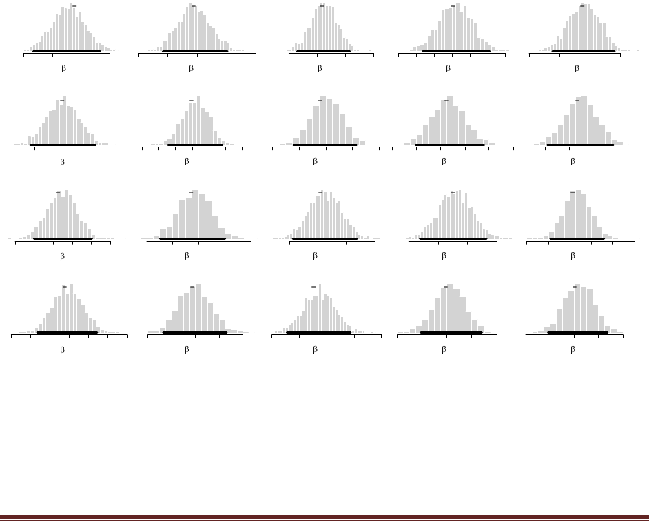
Solutions Manual for Doing Bayesian Data Analysis by John K. Kruschke Page 153
Chapter 19.
Exercise 19.1. [Purpose: To inspect an interaction for transformed data.] Consider the data
plotted in Figure 19.3, p. 521.
(A) Is the interaction a crossover interaction or not? Briefly explain your answer.
The interaction is not a crossover interaction. The reason is that the ordering of levels on one
factor is always the same at any level of the other factor. Specifically, the ordering of
departments (x1) is THTR, CEDP, CHEM, BFIN at every level of seniority (x2). And, the
ordering of seniority is FT3, FT2, FT1 in every department.
(B) Suppose we are interested in salaries thought of in terms of percentage (i.e., ratio)
differences rather than additive differences. Therefore we take the logarithm, base 10, of
the individual salaries (the R code has this option built into to the data section, where the
salary data are loaded). Run the analysis on the transformed data, producing the results
and contrasts analogous to those in Figures 19.4 and 19.5. Do any of the conclusions
change?
Baseline
0
4.98 4.99 5.00 5.01
mean 5
95% HDI
4.98 5.01
x1: BFIN
11
0.26 0.28 0.30 0.32 0.34
mean 0.298
95% HDI
0.276 0.321
x1: CEDP
12
-0.16 -0.14 -0.12 -0.10
mean -0.135
95% HDI
-0.154 -0.117
x1: CHEM
13
-0.01 0.00 0.01 0.02 0.03 0.04 0.05
mean 0.0217
95% HDI
0.0035 0.0411
x1: THTR
14
-0.22 -0.20 -0.18 -0.16
mean -0.184
95% HDI
-0.205 -0.164
x2: FT1
21
0.08 0.09 0.10 0.11 0.12 0.13 0.14
mean 0.106
95% HDI
0.0877 0.124
x2: FT2
22
-0.04 -0.03 -0.02 -0.01 0.00 0.01
mean -0.0154
95% HDI
-0.0301 0.000257
x2: FT3
23
-0.12 -0.11 -0.10 -0.09 -0.08 -0.07 -0.06
mean -0.0907
95% HDI
-0.107 -0.0755
x1: BFIN , x2: FT1
121,1
-0.08 -0.06 -0.04 -0.02 0.00 0.02 0.04
mean -0.0165
95% HDI
-0.049 0.0168
x1: CEDP , x2: FT1
122,1
-0.04 -0.02 0.00 0.02 0.04
mean 0.000415
95% HDI
-0.0242 0.0232
x1: CHEM , x2: FT1
123,1
-0.02 0.00 0.02 0.04 0.06 0.08
mean 0.0265
95% HDI
-0.000614 0.056
x1: THTR , x2: FT1
124,1
-0.06 -0.04 -0.02 0.00 0.02 0.04
mean -0.0104
95% HDI
-0.0384 0.0169
x1: BFIN , x2: FT2
121,2
-0.06 -0.04 -0.02 0.00 0.02
mean -0.0231
95% HDI
-0.0495 0.000304
x1: CEDP , x2: FT2
122,2
-0.02 0.00 0.02 0.04
mean 0.00486
95% HDI
-0.0178 0.0274
x1: CHEM , x2: FT2
123,2
-0.02 0.00 0.02 0.04
mean 0.0116
95% HDI
-0.0123 0.0331
x1: THTR , x2: FT2
124,2
-0.04 -0.02 0.00 0.02 0.04 0.06
mean 0.00665
95% HDI
-0.0182 0.0314
x1: BFIN , x2: FT3
121,3
0.00 0.02 0.04 0.06 0.08
mean 0.0397
95% HDI
0.0129 0.0664
x1: CEDP , x2: FT3
122,3
-0.04 -0.02 0.00 0.02 0.04
mean -0.00528
95% HDI
-0.0291 0.0176
x1: CHEM , x2: FT3
123,3
-0.08 -0.06 -0.04 -0.02 0.00
mean -0.0381
95% HDI
-0.061 -0.0118
x1: THTR , x2: FT3
124,3
-0.04 -0.02 0.00 0.02 0.04
mean 0.00374
95% HDI
-0.0215 0.0274
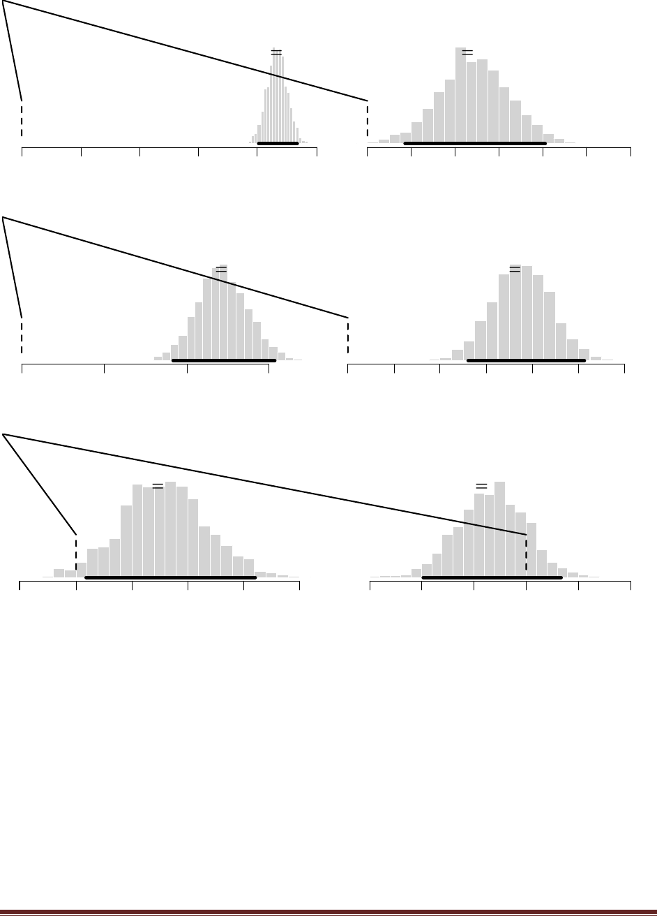
Solutions Manual for Doing Bayesian Data Analysis by John K. Kruschke Page 154
X1 Contrast: BFINvCEDP
1 BFIN + -1 CEDP
0.0 0.1 0.2 0.3 0.4 0.5
mean 0.433
0% <= 0 < 100%95% HDI
0.401 0.467
X1 Contrast: CEDPvTHTR
1 CEDP + -1 THTR
0.00 0.02 0.04 0.06 0.08 0.10 0.12
mean 0.0486
0.2% <= 0 < 99.8%
95% HDI
0.0173 0.081
X2 Contrast: FT1vFT2
1 FT1 + -1 FT2
0.00 0.05 0.10 0.15
mean 0.122
0% <= 0 < 100%95% HDI
0.0918 0.153
X2 Contrast: FT2vFT3
1 FT2 + -1 FT3
0.00 0.02 0.04 0.06 0.08 0.10 0.12
mean 0.0752
0% <= 0 < 100%
95% HDI
0.0521 0.102
CHEMvTHTRxFT1vFT3
+ 1 CHEM FT1 + -1 CHEM FT3 + -1 THTR FT1 + 1 THTR FT3
-0.05 0.00 0.05 0.10 0.15 0.20
mean 0.0787
2% <= 0 < 98%
95% HDI
0.00916 0.16
BFINvOTHxFT1vOTH
+ 1 BFIN FT1 + -0.5 BFIN FT2 + -0.5 BFIN FT3 + -0.33 CEDP FT1 + 0.17 CEDP FT2 + 0.17 CEDP FT3 + -0.33 CHEM FT1 + 0.17 CHEM FT2 + 0.17 CHEM FT3 + -0.33 THTR FT1 + 0.17 THTR FT2 + 0.17 THTR FT3
-0.15 -0.10 -0.05 0.00 0.05 0.10
mean -0.0331
83.9% <= 0 < 16.1%
95% HDI
-0.0981 0.0336
In terms of contrasts excluding zero, only one conclusion changes: For the logarithmic data, the
contrast of CEDP vs THTR now excludes zero, whereas it did not for the original data (see top
right of Figure 19.5, p. 524 of textbook).
(C) Examine the within-cell variances in the original and in the transformed data. (Hint:
Try using the aggregate function on the data. As a guide, see how the function is used to
initialize a1a2. Instead of applying the mean to the aggregated data, apply the standard
deviation. The result is the within-cell standard deviations. Are they all roughly the same?)
Do the original or the transformed data better respect the assumption of homogeneous
variances?
For the logarithmically transformed data,
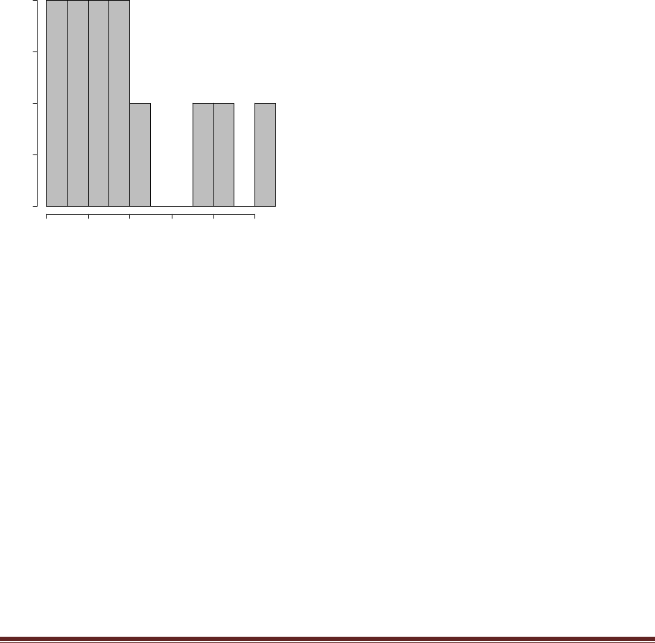
Solutions Manual for Doing Bayesian Data Analysis by John K. Kruschke Page 155
aggregate( y, list(x1,x2), sd )
Group.1 Group.2 x
1 1 1 0.005205083
2 2 1 0.037983957
3 3 1 0.101059931
4 4 1 0.033128985
5 1 2 0.072478142
6 2 2 0.048125947
7 3 2 0.085013176
8 4 2 0.027603123
9 1 3 0.018893844
10 2 3 0.007116409
11 3 3 0.020676694
12 4 3 0.014695818
hist( aggregate( y, list(x1,x2), sd )[,3] , breaks=12 , col="grey" )
Histogram of aggregate(y, list(x1, x2), sd)[, 3]
aggregate(y, list(x1, x2), sd)[, 3]
Frequency
0.00 0.02 0.04 0.06 0.08 0.10
0.0 0.5 1.0 1.5 2.0
Original data:
aggregate( y, list(x1,x2), sd )
Group.1 Group.2 x
1 1 1 2828.4271
2 2 1 8191.0448
3 3 1 33969.2412
4 4 1 6020.9431
5 1 2 28794.5307
6 2 2 8062.0340
7 3 2 20566.9204
8 4 2 4183.0417
9 1 3 7736.9963
10 2 3 953.7838
11 3 3 3570.9237
12 4 3 1838.3906
hist( aggregate( y, list(x1,x2), sd )[,3] , breaks=12 , col="grey" )
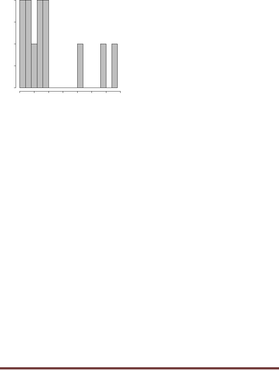
Solutions Manual for Doing Bayesian Data Analysis by John K. Kruschke Page 156
Histogram of aggregate(y, list(x1, x2), sd)[, 3]
aggregate(y, list(x1, x2), sd)[, 3]
Frequency
05000 10000 15000 20000 25000 30000 35000
0.0 0.5 1.0 1.5 2.0
For both the original and logarithmically transformed data, the cell SDs show some outliers. But
the degree of skew in the distribution of cell SDs seems to be a bit less for the logarithmically
transformed data. By using this criterion alone, it seems that the transformed data better respect
the assumption of homogeneous variances in the 12 cells.
We would also want to look at the distributions of data within cells to see if they are consistent
with the assumption of normally distributed data. Because salaries tend to be skewed to the right,
with a few people making very high salaries, the logarithmic transformation is likely to help the
normality assumption too.
Exercise 19.2. [Purpose: To investigate a case of two-factor Bayesian ANOVA.] In the data
specification of the program in Section 19.3.1 (ANOVAtwowayBRugs), you can load data
from Qian & Shen (2007), regarding how quickly seaweed regenerates when in the
presence of different types of grazers. Data were collected from eight different tidal areas
of the Oregon coast; this predictor (x2) is referred to as the Block. In each of the eight
Blocks, there were six different combinations of seaweed grazers established by the
researchers. This predictor (x1) had six levels: control, with no grazers allowed; only small
fish allowed; small and large fish allowed; only limpets allowed; limpets and small fish
allowed; and all three grazers allowed. The predicted variable was the percentage of the
plot covered by regenerated seaweed, logarithmically transformed.
(A) Load the data and run the program. You will find that there are too many levels of the
two predictors to fit all the posterior histograms into a single multipanel display.
Therefore, modify the plotPost.R program so that it produces only the mean and HDI
limits, marked by a horizontal bar with a circle at the mean (without a histogram) and
perhaps without a main title. Name your program something other than plotPost.R, and
use it in the plotting section at the end of the program instead of plotPost.R. Show your
results. (A secondary goal of this part of the exercise is to give you experience modifying
graphics in R to suit your own purposes.) Hints: …
Solutions Manual for Doing Bayesian Data Analysis by John K. Kruschke Page 157
0
mean -1.23
o
95% HDI
-1.35 -1.13
11
mean 1.4
o
95% HDI
1.16 1.63
12
mean 0.907
o
95% HDI
0.651 1.15
13
mean 0.403
o
95% HDI
0.167 0.637
14
mean -0.475
o
95% HDI
-0.722 -0.224
15
mean -0.766
o
95% HDI
-1 -0.513
16
mean -1.47
o
95% HDI
-1.7 -1.22
21
mean -1.37
o
95% HDI
-1.64 -1.07
22
mean -0.921
o
95% HDI
-1.22 -0.632
23
mean 0.683
o
95% HDI
0.389 0.968
24
mean 1.54
o
95% HDI
1.23 1.83
25
mean -0.184
o
95% HDI
-0.509 0.0997
26
mean 0.608
o
95% HDI
0.321 0.893
27
mean -0.286
o
95% HDI
-0.579 -0.00619
28
mean -0.071
o
95% HDI
-0.366 0.23
121,1
mean -0.098
o
95% HDI
-0.477 0.299
122,1
mean 0.0308
o
95% HDI
-0.351 0.42
123,1
mean 0.0602
o
95% HDI
-0.35 0.412
124,1
mean -0.0285
o
95% HDI
-0.385 0.39
125,1
mean 0.0723
o
95% HDI
-0.339 0.437
126,1
mean -0.0367
o
95% HDI
-0.431 0.339
121,2
mean -0.063
o
95% HDI
-0.465 0.31
122,2
mean -0.0137
o
95% HDI
-0.416 0.356
123,2
mean -0.0758
o
95% HDI
-0.499 0.293
124,2
mean 0.0497
o
95% HDI
-0.331 0.451
125,2
mean -0.0556
o
95% HDI
-0.51 0.275
126,2
mean 0.158
o
95% HDI
-0.226 0.586
121,3
mean 0.0747
o
95% HDI
-0.308 0.47
122,3
mean -0.0583
o
95% HDI
-0.443 0.325
123,3
mean -0.00403
o
95% HDI
-0.348 0.414
124,3
mean 0.246
o
95% HDI
-0.136 0.721
125,3
mean -0.0839
o
95% HDI
-0.481 0.297
126,3
mean -0.175
o
95% HDI
-0.588 0.207
121,4
mean 0.374
o
95% HDI
-0.0715 0.935
122,4
mean 0.192
o
95% HDI
-0.198 0.573
123,4
mean -0.0357
o
95% HDI
-0.422 0.369
124,4
mean -0.227
o
95% HDI
-0.712 0.145
125,4
mean -0.0328
o
95% HDI
-0.405 0.364
126,4
mean -0.269
o
95% HDI
-0.722 0.137
121,5
mean -0.0837
o
95% HDI
-0.465 0.291
122,5
mean -0.0569
o
95% HDI
-0.441 0.327
123,5
mean 0.115
o
95% HDI
-0.279 0.495
124,5
mean 0.163
o
95% HDI
-0.21 0.594
125,5
mean -0.154
o
95% HDI
-0.579 0.223
126,5
mean 0.016
o
95% HDI
-0.357 0.392
121,6
mean -0.0287
o
95% HDI
-0.419 0.358
122,6
mean -0.177
o
95% HDI
-0.584 0.224
123,6
mean -0.0681
o
95% HDI
-0.489 0.292
124,6
mean -0.047
o
95% HDI
-0.484 0.3
125,6
mean 0.242
o
95% HDI
-0.17 0.668
126,6
mean 0.0798
o
95% HDI
-0.312 0.454
121,7
mean -0.233
o
95% HDI
-0.646 0.188
122,7
mean 0.186
o
95% HDI
-0.213 0.61
123,7
mean 0.126
o
95% HDI
-0.297 0.513
124,7
mean -0.201
o
95% HDI
-0.613 0.185
125,7
mean -0.098
o
95% HDI
-0.512 0.287
126,7
mean 0.221
o
95% HDI
-0.182 0.664
121,8
mean 0.0583
o
95% HDI
-0.34 0.458
122,8
mean -0.102
o
95% HDI
-0.52 0.258
123,8
mean -0.117
o
95% HDI
-0.522 0.254
124,8
mean 0.0451
o
95% HDI
-0.354 0.42
125,8
mean 0.11
o
95% HDI
-0.283 0.485
126,8
mean 0.00602
o
95% HDI
-0.36 0.41
The above plot was generated with the following code. First, in the main program, the plotting
commands were altered as indicated by the bold highlighted text:
source("plotPost19.2.R")
windows((datalist$Nx1Lvl+1)*2.75,(datalist$Nx2Lvl+1)*2.0)
layoutMat = matrix( 0 , nrow=(datalist$Nx2Lvl+1) , ncol=(datalist$Nx1Lvl+1) )
layoutMat[1,1] = 1
layoutMat[1,2:(datalist$Nx1Lvl+1)] = 1:datalist$Nx1Lvl + 1
layoutMat[2:(datalist$Nx2Lvl+1),1] = 1:datalist$Nx2Lvl + (datalist$Nx1Lvl + 1)
layoutMat[2:(datalist$Nx2Lvl+1),2:(datalist$Nx1Lvl+1)] = matrix(
1:(datalist$Nx1Lvl*datalist$Nx2Lvl) + (datalist$Nx2Lvl+datalist$Nx1Lvl+1) ,
ncol=datalist$Nx1Lvl , byrow=T )
layout( layoutMat )
par( mar=c(4,0.5,2.5,0.5) , mgp=c(1,0.7,0) )
histinfo = plotPost19.2( b0Sample , xlab=expression(beta * 0) , main="Baseline" ,
breaks=30 )
for ( x1idx in 1:datalist$Nx1Lvl ) {
histinfo = plotPost19.2( b1Sample[x1idx,] , xlab=bquote(beta*1[.(x1idx)]) ,
main=paste("x1:",x1names[x1idx]) , breaks=30 )

Solutions Manual for Doing Bayesian Data Analysis by John K. Kruschke Page 158
}
for ( x2idx in 1:datalist$Nx2Lvl ) {
histinfo = plotPost19.2( b2Sample[x2idx,] , xlab=bquote(beta*2[.(x2idx)]) ,
main=paste("x2:",x2names[x2idx]) , breaks=30 )
}
for ( x2idx in 1:datalist$Nx2Lvl ) {
for ( x1idx in 1:datalist$Nx1Lvl ) {
histinfo = plotPost19.2( b1b2Sample[x1idx,x2idx,] , breaks=30 ,
xlab=bquote(beta*12[.(x1idx)*","*.(x2idx)]) ,
main=paste("x1:",x1names[x1idx],", x2:",x2names[x2idx]) )
}
}
The plotPost19.2.R function was adapted from plotPost.R as indicated by the bold highlighted
text:
plotPost19.2 = function( paramSampleVec , credMass=0.95 , compVal=NULL ,
HDItextPlace=0.7 , ROPE=NULL , yaxt=NULL , ylab=NULL ,
xlab=NULL , cex.lab=NULL , cex=NULL , xlim=NULL , main=NULL ,
showMode=F , ... ) {
# Override defaults of hist function, if not specified by user:
# (additional arguments "..." are passed to the hist function)
if ( is.null(xlab) ) xlab="Parameter"
if ( is.null(cex.lab) ) cex.lab=1.0
if ( is.null(cex) ) cex=1.0
if ( is.null(xlim) ) xlim=range( c( compVal , paramSampleVec ) )
if ( is.null(main) ) main=""
if ( is.null(yaxt) ) yaxt="n"
if ( is.null(ylab) ) ylab=""
# Plot histogram.
par(xpd=NA)
histinfo = hist( paramSampleVec , xlab=xlab , yaxt=yaxt , ylab=ylab ,
freq=F , col="lightgrey" , border="white" ,
xlim=xlim , main=main , cex=cex , cex.lab=cex.lab ,
plot=F ,
... )
plot( 0 , type="n" , bty="n" , xlim=xlim , xaxt="n" , yaxt="n" ,
xlab=xlab , ylab=ylab ) # creates empty plot
# Display mean or mode:
if ( showMode==F ) {
meanParam = mean( paramSampleVec )
text( meanParam , 0*max(histinfo$density) ,
bquote(mean==.(signif(meanParam,3))) , adj=c(.5,1.5) , cex=cex )
points( meanParam , 0 , pch="o" , cex=1.5 )
} else {
dres = density( paramSampleVec )
modeParam = dres$x[which.max(dres$y)]
text( modeParam , 0*max(histinfo$density) ,
bquote(mode==.(signif(modeParam,3))) , adj=c(.5,1.5) , cex=cex )
points( modeParam , 0 , pch="o" , cex=1.5 )
}
…# remainder is unchanged
}
(B) The program already includes contrasts that consider whether there is an effect of
small fish, an effect of large fish, and an effect of limpets. What conclusions do you reach
from the posteriors of these contrasts?
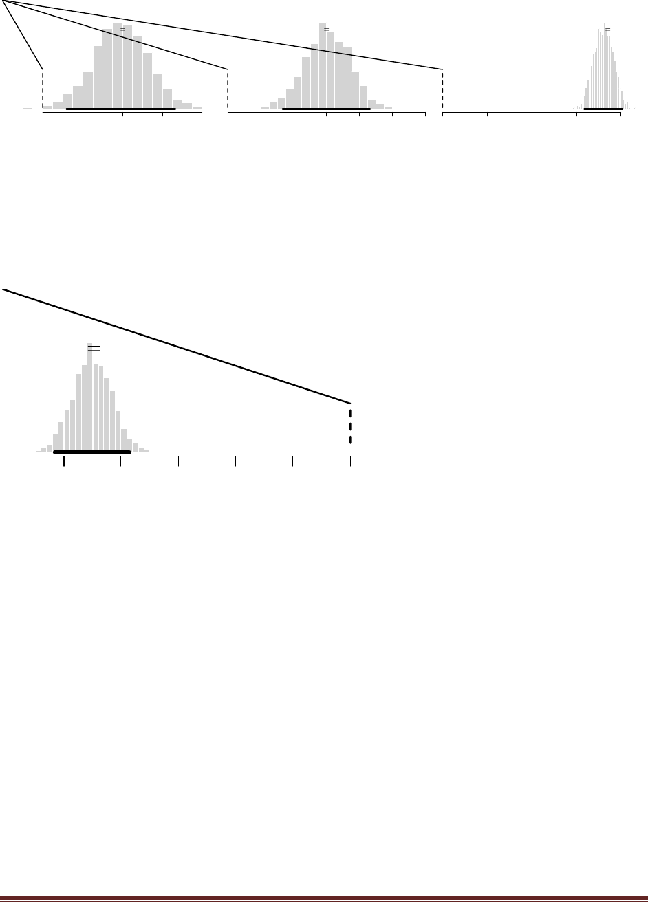
Solutions Manual for Doing Bayesian Data Analysis by John K. Kruschke Page 159
X1 Contrast: f_Effect
0.5 CONTROL + -0.5 f + 0.5 L + -0.5 Lf
0.0 0.2 0.4 0.6 0.8
mean 0.39
0.3% <= 0 < 99.7%
95% HDI
0.119 0.666
X1 Contrast: F_Effect
0.5 f + -0.5 fF + 0.5 Lf + -0.5 LfF
0.0 0.2 0.4 0.6 0.8 1.0 1.2
mean 0.602
0% <= 0 < 100%
95% HDI
0.333 0.864
X1 Contrast: L_Effect
0.33 CONTROL + 0.33 f + 0.33 fF + -0.33 L + -0.33 Lf + -0.33 LfF
0.0 0.5 1.0 1.5 2.0
mean 1.8
0% <= 0 < 100%
95% HDI
1.59 2.01
The posterior histograms indicate clearly that all three effects are credibly greater than zero.
(C) Construct a contrast of the average of Blocks 3 and 4 versus the average of Blocks 1
and 2. Show your specification, the graph of the posterior on the contrast, and state your
conclusion.
x2contrastList = list( B12vB34 = c( 1/2 , 1/2 , -1/2 , -1/2 ,0,0,0,0) )
yields
X2 Contrast: B12vB34
0.5 BLOCK 1 + 0.5 BLOCK 2 + -0.5 BLOCK 3 + -0.5 BLOCK 4
-2.5 -2.0 -1.5 -1.0 -0.5 0.0
mean -2.25
100% <= 0 < 0%
95% HDI
-2.58 -1.93
which indicates that there is a highly credible difference between the average of blocks 1 & 2
and the average of blocks 3 & 4.
(D) Is the effect of limpets different in Block 6 than in Block 7? To answer this question,
construct an interaction contrast using an outer product (Hint: refer to the already-coded
L effect for the contrast that specifies the effect of limpets). Is the effect of small fish
different in Blocks 1 and 7 than in Blocks 3 and 5? For both questions, show the contrast
vectors that you constructed and show the posterior of the contrast, and state your
conclusion.
x1x2contrastList = list(
L_EffxB6vB7 = outer( c(1/3,1/3,1/3,-1/3,-1/3,-1/3) , c(0,0,0,0,0,1,-1,0) ) ,
f_EffxB17vB35 = outer( c(1/2,-1/2,0,1/2,-1/2,0) , c(1/2,0,-1/2,0,-1/2,0,1/2,0) ) )
yields the posterior histograms below
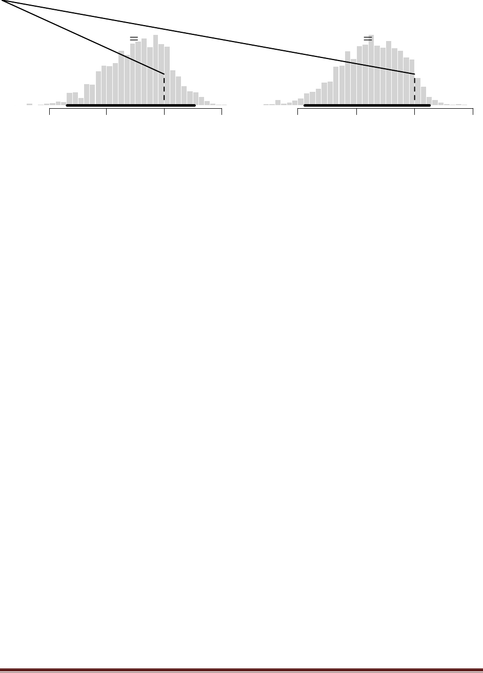
Solutions Manual for Doing Bayesian Data Analysis by John K. Kruschke Page 160
L_EffxB6vB7
+ 0.33 CONTROL BLOCK 6 + -0.33 CONTROL BLOCK 7 + 0.33 f BLOCK 6 + -0.33 f BLOCK 7 + 0.33 fF BLOCK 6 + -0.33 fF BLOCK 7 + -0.33 L BLOCK 6 + 0.33 L BLOCK 7 + -0.33 Lf BLOCK 6 + 0.33 Lf BLOCK 7 + -0.33 LfF BLOCK 6 + 0.33 LfF BLOCK 7
-1.0 -0.5 0.0 0.5
mean -0.235
79.6% <= 0 < 20.4%
95% HDI
-0.846 0.266
f_EffxB17vB35
+ 0.25 CONTROL BLOCK 1 + -0.25 CONTROL BLOCK 3 + -0.25 CONTROL BLOCK 5 + 0.25 CONTROL BLOCK 7 + -0.25 f BLOCK 1 + 0.25 f BLOCK 3 + 0.25 f BLOCK 5 + -0.25 f BLOCK 7 + 0.25 L BLOCK 1 + -0.25 L BLOCK 3 + -0.25 L BLOCK 5 + 0.25 L BLOCK 7 + -0.25 Lf BLOCK 1 + 0.25 Lf BLOCK 3 + 0.25 Lf BLOCK 5 + -0.25 Lf BLOCK 7
-1.0 -0.5 0.0 0.5
mean -0.376
92.7% <= 0 < 7.3%
95% HDI
-0.941 0.126
hence both interaction contrasts include zero among their credible values.
Exercise 19.3. [Purpose: To notice that within-subject designs can be more sensitive (hence
more powerful) than between-subject designs.] Consider these data: …
(A) Ignoring the last column, which indicates the subject who generated the data, conduct
a Bayesian ANOVA using x1 and x2 as predictors of y. Show the code you used to load the
data, and show the resulting posterior histograms of . Also show the posterior of the
contrast (i.e., the marginal difference between levels 1 and 2 of factor 1, also called the
main effect of factor 1) and the posterior of the contrast (i.e., the marginal difference
between levels 1 and 2 of factor 2, also called the main effect of factor 2).
y = c( 101,102,103,105,104, 104,105,107,106,108, 105,107,106,108,109,
109,108,110,111,112 )
x1 = c( 1,1,1,1,1, 1,1,1,1,1, 2,2,2,2,2, 2,2,2,2,2 )
x2 = c( 1,1,1,1,1, 2,2,2,2,2, 1,1,1,1,1, 2,2,2,2,2 )
# S = c( 1,2,3,4,5, 1,2,3,4,5, 1,2,3,4,5, 1,2,3,4,5 )
x1names = c("x1.1","x1.2")
x2names = c("x2.1","x2.2")
# Snames = c("S1","S2","S3","S4","S5")
Ntotal = length(y)
Nx1Lvl = length(unique(x1))
Nx2Lvl = length(unique(x2))
# NSLvl = length(unique(S))
x1contrastList = list( X1.2vX1.1 = c( -1 , 1 ) )
x2contrastList = list( X2.2vX2.1 = c( -1 , 1 ) )
x1x2contrastList = NULL # list( matrix( 1:(Nx1Lvl*Nx2Lvl) , nrow=Nx1Lvl ) )
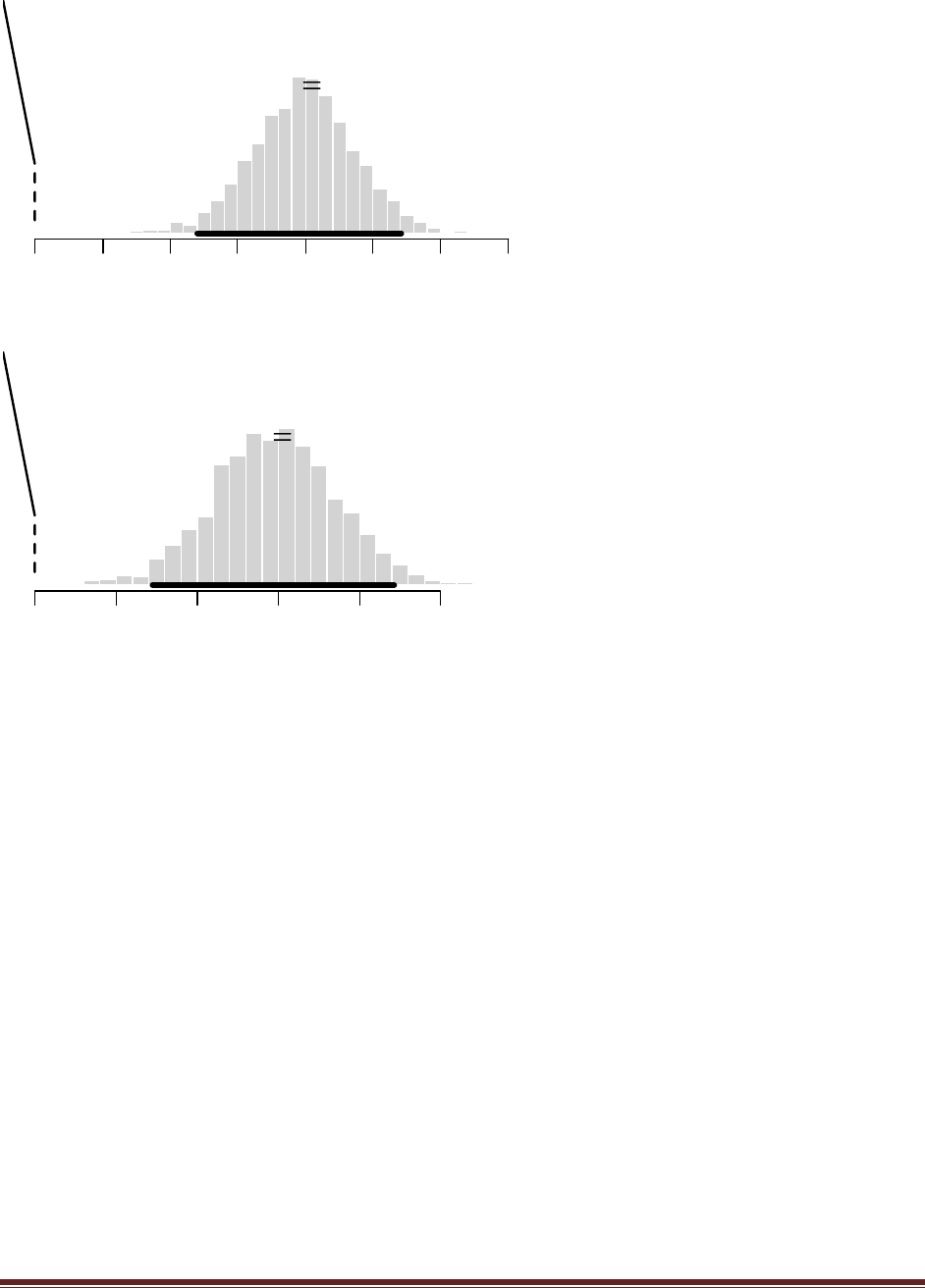
Solutions Manual for Doing Bayesian Data Analysis by John K. Kruschke Page 161
X1 Contrast: X1.2vX1.1
-1 x1.1 + 1 x1.2
0 1 2 3 4 5 6 7
mean 3.98
0% <= 0 < 100%
95% HDI
2.41 5.41
X2 Contrast: X2.2vX2.1
-1 x2.1 + 1 x2.2
0 1 2 3 4 5
mean 2.95
0% <= 0 < 100%
95% HDI
1.45 4.43
(B) Now include the subject as a predictor by expanding the model to include a deflection
from baseline due to subject. (Do not include any subject interaction terms.) Again show
the posteriors of the beta‘s requested in the previous part. Are the certainties on the
estimates and contrasts different than in the previous part? In what way, and why? (Hint
regarding the answer: Figure 19.7 shows posterior histograms for the main effect of factor
2, when the data are considered to be between subject or within subject. Notice that the
means are essentially the same in both histograms, but the uncertainties are very different!
Programming hints: … )
Here are sections of the modified code:
model {
for ( i in 1:Ntotal ) {
y[i] ~ dnorm( mu[i] , tau )
mu[i] <- a0 + a1[x1[i]] + a2[x2[i]] + a1a2[x1[i],x2[i]] + aS[S[i]]
}
#
tau <- pow( sigma , -2 )
sigma ~ dunif(0,10) # y values are assumed to be standardized
#
a0 ~ dnorm(0,0.001) # y values are assumed to be standardized
#
for ( j1 in 1:Nx1Lvl ) { a1[j1] ~ dnorm( 0.0 , a1tau ) }

Solutions Manual for Doing Bayesian Data Analysis by John K. Kruschke Page 162
a1tau <- 1 / pow( a1SD , 2 )
a1SD <- abs( a1SDunabs ) + .1
a1SDunabs ~ dt( 0 , 0.001 , 2 )
#
for ( j2 in 1:Nx2Lvl ) { a2[j2] ~ dnorm( 0.0 , a2tau ) }
a2tau <- 1 / pow( a2SD , 2 )
a2SD <- abs( a2SDunabs ) + .1
a2SDunabs ~ dt( 0 , 0.001 , 2 )
#
for ( j1 in 1:Nx1Lvl ) { for ( j2 in 1:Nx2Lvl ) {
a1a2[j1,j2] ~ dnorm( 0.0 , a1a2tau )
} }
a1a2tau <- 1 / pow( a1a2SD , 2 )
a1a2SD <- abs( a1a2SDunabs ) + .1
a1a2SDunabs ~ dt( 0 , 0.001 , 2 )
#
for ( jS in 1:NSLvl ) { aS[jS] ~ dnorm( 0.0 , aStau ) }
aStau <- 1 / pow( aSSD , 2 )
aSSD <- abs( aSSDunabs ) + .1
aSSDunabs ~ dt( 0 , 0.001 , 2 )
}
…
# initialization based on data
theData = data.frame( y=datalist$y , x1=factor(x1,labels=x1names) ,
x2=factor(x2,labels=x2names) , S=factor(S,labels=Snames) )
a0 = mean( theData$y )
a1 = aggregate( theData$y , list( theData$x1 ) , mean )[,2] - a0
a2 = aggregate( theData$y , list( theData$x2 ) , mean )[,2] - a0
aS = aggregate( theData$y , list( theData$S ) , mean )[,2] - a0
linpred = as.vector( outer( a1 , a2 , "+" ) + a0 )
a1a2 = aggregate( theData$y, list(theData$x1,theData$x2), mean)[,3] - linpred
genInitList <- function() {
return(
list(
a0 = a0 ,
a1 = a1 ,
a2 = a2 ,
aS = aS ,
a1a2 = matrix( a1a2 , nrow=Nx1Lvl , ncol=Nx2Lvl ) ,
sigma = sd(theData$y)/2 , # lazy
a1SDunabs = sd(a1) ,
a2SDunabs = sd(a2) ,
a1a2SDunabs = sd(a1a2) ,
aSSDunabs = sd(aS)
)
)
}
for ( chainIdx in 1 : nchain ) {
modelInits( bugsInits( genInitList ) )
}
…
# Convert the a values to zero-centered b values.
# m12Sample is predicted cell means at every step in MCMC chain:
m12Sample = array( 0, dim=c( datalist$Nx1Lvl , datalist$Nx2Lvl ,
datalist$NSLvl , chainLength ) )
for ( stepIdx in 1:chainLength ) {
for ( a1idx in 1:Nx1Lvl ) {
for ( a2idx in 1:Nx2Lvl ) {
for ( aSidx in 1:NSLvl ) {

Solutions Manual for Doing Bayesian Data Analysis by John K. Kruschke Page 163
m12Sample[ a1idx , a2idx , aSidx , stepIdx ] = (
a0Sample[stepIdx]
+ a1Sample[a1idx,stepIdx]
+ a2Sample[a2idx,stepIdx]
+ a1a2Sample[a1idx,a2idx,stepIdx]
+ aSSample[aSidx,stepIdx] )
}
}
}
}
# b0Sample is mean of the cell means at every step in chain:
b0Sample = apply( m12Sample , 4 , mean )
# b1Sample is deflections of factor 1 marginal means from b0Sample:
b1Sample = ( apply( m12Sample , c(1,4) , mean )
- matrix(rep( b0Sample ,Nx1Lvl),nrow=Nx1Lvl,byrow=T) )
# b2Sample is deflections of factor 2 marginal means from b0Sample:
b2Sample = ( apply( m12Sample , c(2,4) , mean )
- matrix(rep( b0Sample ,Nx2Lvl),nrow=Nx2Lvl,byrow=T) )
# bSSample is deflections of factor S marginal means from b0Sample:
bSSample = ( apply( m12Sample , c(3,4) , mean )
- matrix(rep( b0Sample ,NSLvl),nrow=NSLvl,byrow=T) )
# linpredSample is linear combination of the marginal effects:
linpredSample = 0*m12Sample
for ( stepIdx in 1:chainLength ) {
for ( a1idx in 1:Nx1Lvl ) {
for ( a2idx in 1:Nx2Lvl ) {
for ( aSidx in 1:NSLvl ) {
linpredSample[a1idx,a2idx,aSidx,stepIdx ] = (
b0Sample[stepIdx]
+ b1Sample[a1idx,stepIdx]
+ b2Sample[a2idx,stepIdx]
+ bSSample[aSidx,stepIdx] )
}
}
}
}
# b1b2Sample is the interaction deflection, i.e., the difference
# between the cell means and the linear combination:
b1b2Sample = apply( m12Sample - linpredSample , c(1,2,4) , mean )
# Convert from standardized b values to original scale b values:
b0Sample = b0Sample * ySDorig + yMorig
b1Sample = b1Sample * ySDorig
b2Sample = b2Sample * ySDorig
bSSample = bSSample * ySDorig
b1b2Sample = b1b2Sample * ySDorig
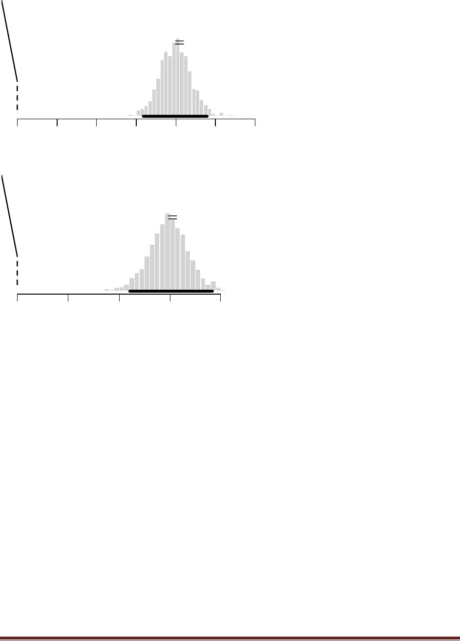
Solutions Manual for Doing Bayesian Data Analysis by John K. Kruschke Page 164
X1 Contrast: X1.2vX1.1
-1 x1.1 + 1 x1.2
0 1 2 3 4 5 6
mean 3.99
0% <= 0 < 100%95% HDI
3.18 4.79
X2 Contrast: X2.2vX2.1
-1 x2.1 + 1 x2.2
0 1 2 3 4
mean 2.98
0% <= 0 < 100%95% HDI
2.22 3.84
For both main effects, the means are the same whether or not the subject variable is included, but
the HDI widths are dramatically different. By including the subject factor, the certainty of the
main effects has greatly increased.
Why? Because subject 1 tends to have low scores, subject 5 tends to have high scores, and so on.
When the subject identity is excluded, then the variation between subjects can only be attributed
to within-cell noise. But when the subject identity is included, then the variation between
subjects can be attributed to the subject factor, and the residual noise is much less.
Exercise 19.4. [Purpose: To conduct a power analysis for Bayesian ANOVA, for within-
subject versus between-subject designs.] Conduct power analyses for the between-subject
and within-subject versions of the previous exercise. Specifically, suppose the goal is for the
95% HDI of the contrast on factor 2 to have a width of 2.0 or less. Conduct a retrospective
power analysis for this goal, for the within-subject version and the between-subject version.
Caution: This exercise demands a lot of programming and could be time consuming, but
the results drive home the point that within-subject designs can be more powerful than
between-subject designs.
Answer to be included in a future edition of this solutions manual. Stay tuned.

Solutions Manual for Doing Bayesian Data Analysis by John K. Kruschke Page 165
Chapter 20.
Exercise 20.1. [Purpose: To observe correlated predictors in logistic regression.] For this
exercise, we‘ll use some fictitious data regarding whether or not a patient suffered a heart
attack within a year after a check-up that included measurements of systolic and diastolic
blood pressures, cholesterol, weight, height, and age. The data are completely fabricated
and fictional, for illustrative purposes only. The data are generated by the program
BloodDataGenerator.R
(A) For this part, we will generate two data sets. In one set, the six predictors have
correlations of zero with each other. In the second set, the first two predictors have a strong
positive correlation, but still zero correlation with all the other predictors. For both sets,
the true regression coefficient on the first predictor is zero, but the true regression
coefficient on the second predictor is positive. Use the program BloodDataGenerator.R to
generate these two data sets by selecting the relevant correlation matrix at the top of the
program. For each data set, conduct a Bayesian analysis using the program in Section
20.5.1 (MultipleLogisticRegressionBrugs.R). Be sure to specify that the only predictors are
the first two, namely, systolic and diastolic pressure. Include the posterior contour plots,
which should look similar to those in Figure 20.7. Be sure also to include the histograms of
the marginal posterior distributions. In which case are the HDIs narrower?
In the data generating program, for the first data set we specify the TRUE and FALSE conditions
as follows:
if ( T ) { # zero correlations everywhere
rMat = matrix( c( 1 , 0 , 0 , 0 , 0 , 0 ,
0 , 1 , 0 , 0 , 0 , 0 ,
0 , 0 , 1 , 0 , 0 , 0 ,
0 , 0 , 0 , 1 , 0 , 0 ,
0 , 0 , 0 , 0 , 1 , 0 ,
0 , 0 , 0 , 0 , 0 , 1 ) , ncol=nX ) }
if ( F ) { # first two predictors strongly correlated
rMat = matrix( c( 1 , .95, 0 , 0 , 0 , 0 ,
.95, 1 , 0 , 0 , 0 , 0 ,
0 , 0 , 1 , 0 , 0 , 0 ,
0 , 0 , 0 , 1 , 0 , 0 ,
0 , 0 , 0 , 0 , 1 , 0 ,
0 , 0 , 0 , 0 , 0 , 1 ) , ncol=nX ) }
In the logistic regression program, we set the data specification to use only the first two
predictors, as follows:
dataSource = c( "HtWt" , "Cars" , "HeartAttack" )[3]
…
if ( dataSource == "HeartAttack" ) {
fname = paste( fname , dataSource , sep="" )
dataMat = read.table(file="BloodDataGeneratorOutput.txt",header=T,sep=" ")
predictedName = "HeartAttack"
# predictorNames = c( "Systolic", "Diastolic", "Weight", "Cholesterol",
# "Height", "Age" )
predictorNames = c( "Systolic", "Diastolic" )
nData = NROW( dataMat )
y = as.matrix( dataMat[,predictedName] )
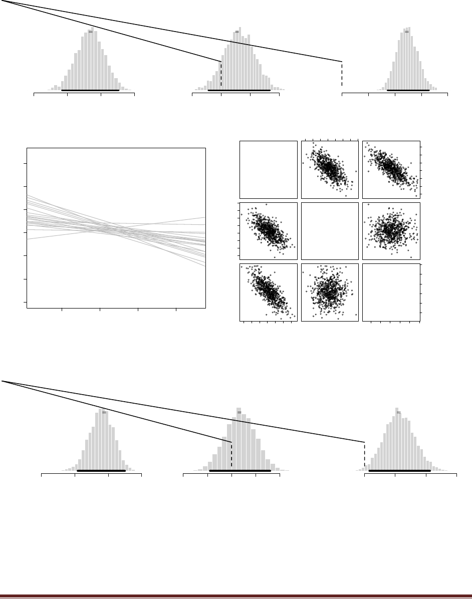
Solutions Manual for Doing Bayesian Data Analysis by John K. Kruschke Page 166
x = as.matrix( dataMat[,predictorNames] )
nPredictors = NCOL( x )
}
For the zero-correlated predictors, the posterior looks like this:
logit(p(HeartAttack=1)) when predictors = zero
b0 Value
-20 -15 -10 -5
mean -11.6
95% HDI
-15.8 -7.39
Systolic
b1 Value
-0.02 0.00 0.02 0.04
mean 0.0126
12.2% <= 0 < 87.8%
95% HDI
-0.0087 0.0336
Diastolic
b2 Value
0.00 0.05 0.10 0.15 0.20
mean 0.123
0% <= 0 < 100%
95% HDI
0.086 0.164
100 120 140 160
50 60 70 80 90 100 110
HeartAttack
Systolic
Diastolic
0
0
0 0
00
0
00
0
0
0
0
0
0
00
0
0
0
0
0
0
0
0
0
0
0
0
0
00
0
00
0
00
0 0
0
0
00 0
0
0
00
0
00
0
0
0
0
0
0
0
00
0
0
0
0
0
0
0
0
0
0
0
0
00
0
0
0
0
0
0
0
0
0
0
0
0
0
0
0
0
0
0
0
0
00
00
0
0
0
0 0
0
0
1
1
11
1
1
1
1
1
1
1
1
1
1
1
1
1
1
1
1 1
1
1
1
1
1
1
1
1
1
1
1
1
11
1
1
1
1
1
1
1
1
1
1
1
1
1
1
1
1
1
1
1
11
1
1
1
1
1
1
1
1
1
1
1
11
1
1 1 1
1
1
1
1
1
11
1
1
1
1
1
1
1
1
11
1
1
11
b0
-0.02 0.00 0.02 0.04
-18 -16 -14 -12 -10 -8 -6
-0.02 0.00 0.02 0.04
b_Systolic
-18 -16 -14 -12 -10 -8 -6 0.08 0.10 0.12 0.14 0.16 0.18
0.08 0.10 0.12 0.14 0.16 0.18
b_Diastolic
We re-run using correlated predictors by simply exchanging the TRUE and FALSE settings in
the data generating program. For the correlated predictors, the posterior looks like this:
logit(p(HeartAttack=1)) when predictors = zero
b0 Value
-20 -15 -10 -5
mean -11
95% HDI
-14.5 -7.5
Systolic
b1 Value
-0.10 -0.05 0.00 0.05 0.10
mean 0.018
28.8% <= 0 < 71.2%
95% HDI
-0.0442 0.0804
Diastolic
b2 Value
0.0 0.1 0.2 0.3
mean 0.113
1.1% <= 0 < 98.9%
95% HDI
0.0165 0.213
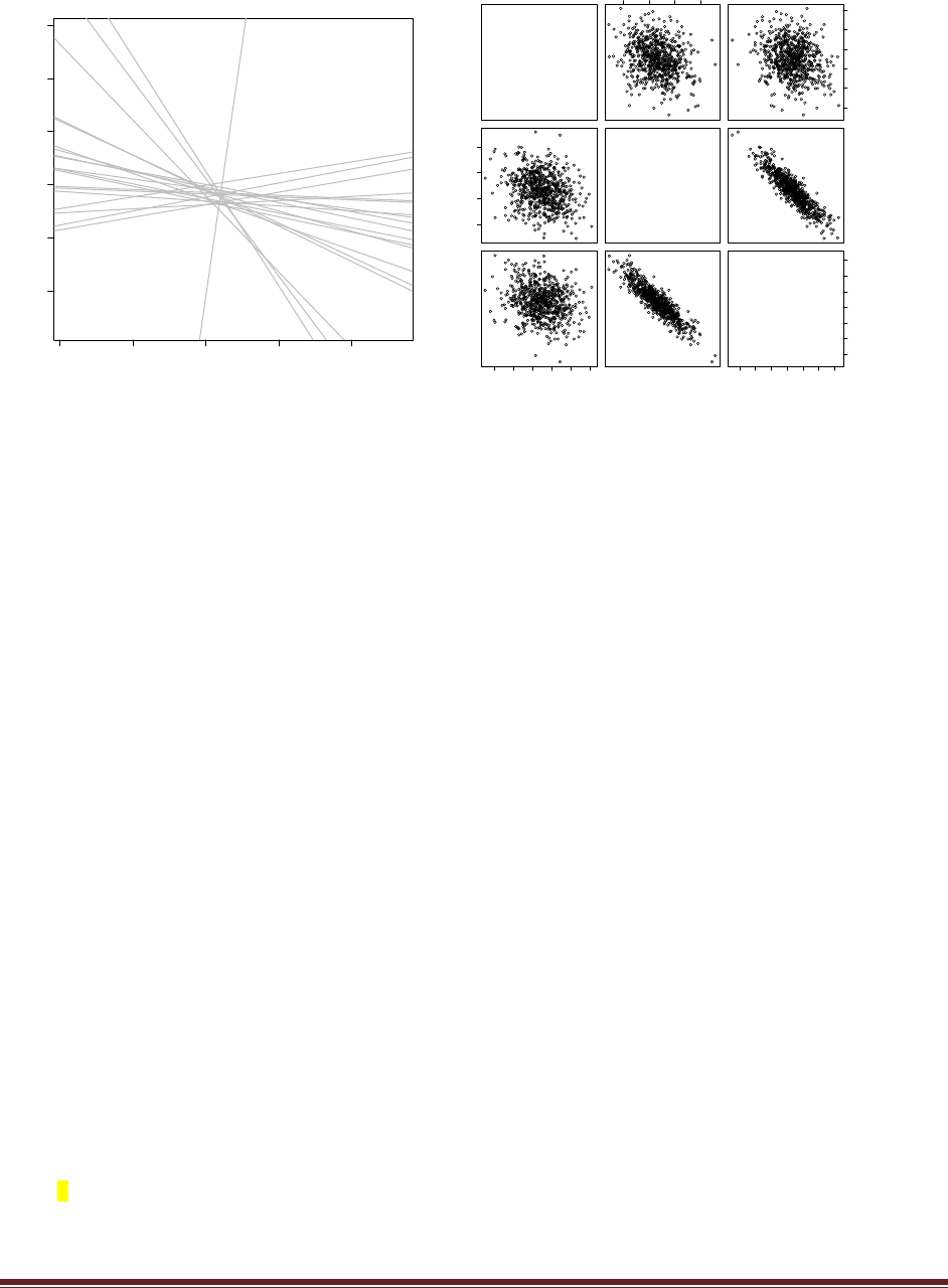
Solutions Manual for Doing Bayesian Data Analysis by John K. Kruschke Page 167
80 100 120 140 160
60 70 80 90 100 110
HeartAttack
Systolic
Diastolic
0
0
0
0
0
0
0
00
0
0
0
0
00
0
0
0
00
0
00
0
00
0
0
00
0
0
0
0
0
0
0
0
0
0
0
0
00
0
0
0
0
0
0
00
0
00
0
0
0
0
0
0
0
0
0
00
0
0
0
0
0
0
0
0
0
0
0
0
00
0
0
0
0
0
0
0
0
11
1
1
1
1
1
11
1
1
1
1
1
1
11
1111
1
1
1
1
11
1
1
1
1
1
1
11
11
1
11
11
1
1
1
1 1
1
1
11
1
1
1
1
1
1
1
1
1
1
1
1
1
1
1
1
1
1
1
1
1
11
1
1
1
1
1
11
1
1
1
1
11
1
1
1
1
1
1
1
1
1
1
1
1
11
1
11
1
1
1
1
11
1 1
b0
-0.05 0.00 0.05 0.10
-16 -14 -12 -10 -8 -6
-0.05 0.00 0.05 0.10
b_Systolic
-16 -14 -12 -10 -8 -6 -0.05 0.05 0.15 0.25
-0.05 0.05 0.15 0.25
b_Diastolic
You can see that for the correlated predictors, there is a dramatic increase in the uncertainty of
the estimated regression coefficients. The 95%HDIs are much wider on the b1 and b2 values for
the correlated predictors than for the uncorrelated predictors. This increased uncertainty is
clearly visible in the plot of the data with the logistic level contours, because the level contours
are fairly tightly bundled for the uncorrelated predictors, but splayed at widely different angles
for the correlated predictors.
Also notice that the regression coefficients, b1 and b2, are strongly anticorrelated when the
predictors are correlated. This anticorrlation indicates that uncertainty in the two regression
coefficients trades off: If the slope on one predictor is large, the slope on the other must be small,
if the logistic “surface” is to accommodate the data.
(B) For this part, we generate a different fictitious data set, in which the first two
predictors (systolic and diastolic) have zero correlation with each other, but they are
correlated with another predictor (weight). The first predictor (systolic) has a true
regression coefficient of zero, but the second (diastolic) and third (weight) predictors have
positive regression coefficients. Run the Bayesian logistic regression analysis using only the
first two predictors. What is the estimate of the regression coefficient on the first
predictor? Include the histograms of the marginals of the posterior. Now rerun the
Bayesian logistic regression analysis including all six predictors. What is the estimate of the
regression coefficient on the first predictor? Include the histograms of the marginals of the
posterior (for which you might need to manually stretch the graph window or change the
character sizes in the plot). Why are the estimates of the regression coefficient for the first
predictor different in the two analyses?
We use this correlation matrix in the data generating program:
if ( T ) { # first two uncorrelated, but other predictors correlated
rMat = matrix( c( 1 , 0 , .6 , .2 , .1 , .1 ,
0 , 1 , .6 , .2 , .1 , .1 ,
.6 , .6 , 1 , .4 , .2 , .2 ,
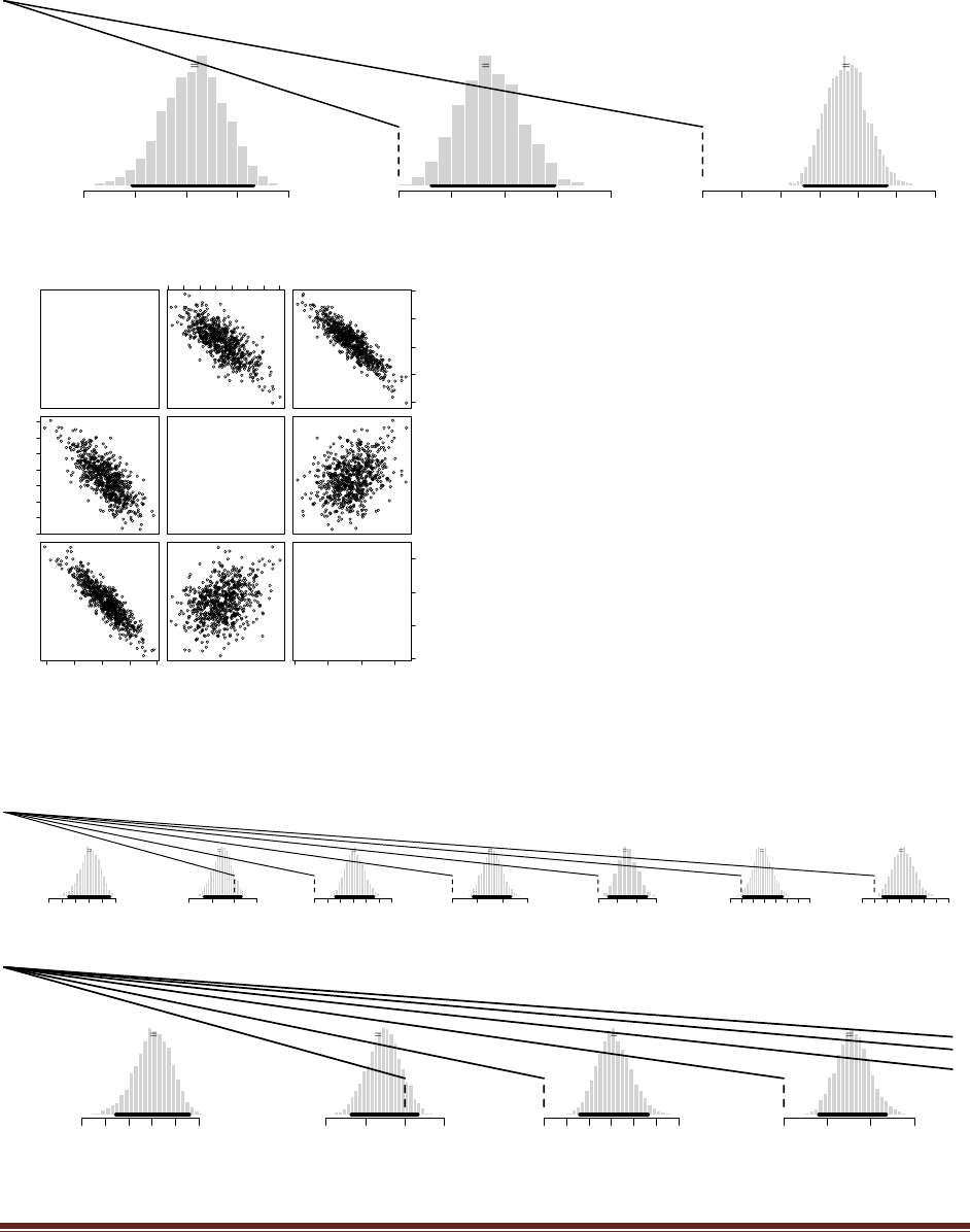
Solutions Manual for Doing Bayesian Data Analysis by John K. Kruschke Page 168
.2 , .2 , .4 , 1 , 0 , .3 ,
.1 , .1 , .2 , 0 , 1 , 0 ,
.1 , .1 , .2 , .3 , 0 , 1 ) , ncol=nX ) }
Using only the first two predictors in the regression, as in the previous part, yields:
logit(p(HeartAttack=1)) when predictors = zero
b0 Value
-30 -25 -20 -15 -10
mean -19.3
95% HDI
-25.3 -13.4
Systolic
b1 Value
0.00 0.02 0.04 0.06 0.08
mean 0.0344
0.2% <= 0 < 99.8%
95% HDI
0.0125 0.0589
Diastolic
b2 Value
0.00 0.05 0.10 0.15 0.20 0.25 0.30
mean 0.185
0% <= 0 < 100%
95% HDI
0.131 0.237
b0
0.00 0.02 0.04 0.06
-30 -25 -20 -15 -10
0.00 0.02 0.04 0.06
b_Systolic
-30 -25 -20 -15 -10 0.10 0.15 0.20 0.25
0.10 0.15 0.20 0.25
b_Diastolic
When using all six predictors, by uncommenting the predictorNames in the data specification
(see code in previous part), the result is:
logit(p(HeartAttack=1)) when predictors = zero
b0 Value
-70 -50 -30
mean -39.7
95% HDI
-55.1 -24.4
Systolic
b1 Value
-0.10 -0.05 0.00 0.05
mean -0.0269
89.2% <= 0 < 10.8%
95% HDI
-0.0677 0.0159
Diastolic
b2 Value
0.00 0.10 0.20 0.30
mean 0.156
0% <= 0 < 100%
95% HDI
0.0803 0.23
Weight
b3 Value
0.00 0.05 0.10 0.15
mean 0.0797
0% <= 0 < 100%
95% HDI
0.0405 0.117
Cholesterol
b4 Value
0.00 0.02 0.04 0.06
mean 0.0303
0.1% <= 0 < 99.9%
95% HDI
0.0107 0.051
Height
b5 Value
-0.1 0.1 0.3 0.5
mean 0.186
1.3% <= 0 < 98.7%
95% HDI
0.0153 0.359
Age
b6 Value
-0.02 0.02 0.06 0.10
mean 0.0468
0.2% <= 0 < 99.8%
95% HDI
0.0129 0.0832
Enlarging the first few histograms:
logit(p(HeartAttack=1)) when predictors = zero
b0 Value
-70 -50 -30
mean -39.7
95% HDI
-55.1 -24.4
Systolic
b1 Value
-0.10 -0.05 0.00 0.05
mean -0.0269
89.2% <= 0 < 10.8%
95% HDI
-0.0677 0.0159
Diastolic
b2 Value
0.00 0.10 0.20 0.30
mean 0.156
0% <= 0 < 100%
95% HDI
0.0803 0.23
Weight
b3 Value
0.00 0.05 0.10 0.15
mean 0.0797
0% <= 0 < 100%
95% HDI
0.0405 0.117
Cholesterol
b4 Value
0.00 0.02 0.04 0.06
mean 0.0303
0.1% <= 0 < 99.9%
95% HDI
0.0107 0.051
Height
b5 Value
-0.1 0.1 0.3 0.5
mean 0.186
1.3% <= 0 < 98.7%
95% HDI
0.0153 0.359
Age
b6 Value
-0.02 0.02 0.06 0.10
mean 0.0468
0.2% <= 0 < 99.8%
95% HDI
0.0129 0.0832

Solutions Manual for Doing Bayesian Data Analysis by John K. Kruschke Page 169
We see that the estimated regression coefficient on b1 (Systolic) has changed dramatically.
When including only the first two predictors, the estimate of b1 was positive and excluded zero.
When all the predictors are included, the estimate of b1 is slightly negative and credible values
include zero, which is the true generating value. The reason for the false estimation in the first
case is that the first two predictors are correlated. Because the second predictor has an influence
on the predicted value, and the first predictor is correlated with the second predictor, the data are
consistent with the first predictor having an influence on the predicted value too. It is only by
including other predictors that the true zero influence of the first predictor can be discerned.
Exercise 20.2. [Purpose: To observe the consequences of a small proportion of 1‘s in logistic
regression.] For this exercise, we again use fictitious data generated by the program
BloodDataGenerator.R. Set all the inter-predictor correlations to zero by selecting the
appropriate correlation matrix at the top of the program. Change the proportionOnes
constant to 0.02. This causes the proportion of 1‘s in the data to be very small. In other
words, the threshold for the sigmoidal function is set very high, so that the weighted sum of
the predictors must be very large before p(y=1) gets very large. This sort of situation, in
which there are few 1‘s, is not unusual in real data. In heart attack data, for example, there
will be few people who have a heart attack in the year following a routine check-up. Run a
Bayesian logistic regression on the data, using only the first two predictors. What are the
estimates of the regression coefficients? Include the histograms of the marginals of the
posterior, and include the posterior contour plot, which should look similar to the right
panel of Figure 20.7. Compare the widths of the HDIs to the results of the first part of the
previous exercise.
In the data generating program, set all correlation matrices to FALSE except
if ( T ) { # zero correlations everywhere
rMat = matrix( c( 1 , 0 , 0 , 0 , 0 , 0 ,
0 , 1 , 0 , 0 , 0 , 0 ,
0 , 0 , 1 , 0 , 0 , 0 ,
0 , 0 , 0 , 1 , 0 , 0 ,
0 , 0 , 0 , 0 , 1 , 0 ,
0 , 0 , 0 , 0 , 0 , 1 ) , ncol=nX ) }
and set
proportionOnes = 0.02 # e.g., about .05 for actual .10
In the logistic regression program, set
dataSource = c( "HtWt" , "Cars" , "HeartAttack" )[3]
…
if ( dataSource == "HeartAttack" ) {
fname = paste( fname , dataSource , sep="" )
dataMat = read.table(file="BloodDataGeneratorOutput.txt",header=T,sep=" ")
predictedName = "HeartAttack"
# predictorNames = c( "Systolic", "Diastolic", "Weight", "Cholesterol",
# "Height", "Age" )
predictorNames = c( "Systolic", "Diastolic" )
…
The result is:
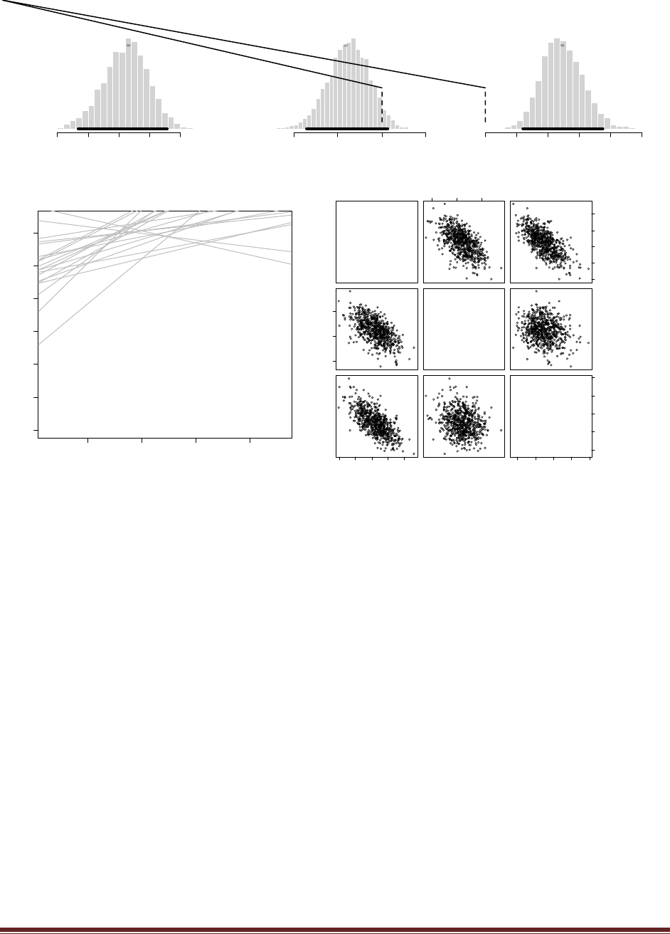
Solutions Manual for Doing Bayesian Data Analysis by John K. Kruschke Page 170
logit(p(HeartAttack=1)) when predictors = zero
b0 Value
-20 -15 -10 -5 0
mean -8.9
95% HDI
-16.6 -2.14
Systolic
b1 Value
-0.10 -0.05 0.00 0.05
mean -0.0376
95.1% <= 0 < 4.9%
95% HDI
-0.0855 0.00697
Diastolic
b2 Value
0.00 0.05 0.10 0.15 0.20 0.25
mean 0.124
0% <= 0 < 100%
95% HDI
0.0601 0.189
100 120 140 160
50 60 70 80 90 100 110
HeartAttack
Systolic
Diastolic
0
0
0
0
0
0
0
00
0
0
0
0
0
0
0
0
0
0
0
0
0
0
0
0
0
0
0
0
0
0
0
0
0
0
0
0
0
0
0
0
0
0
0
00
0
0
0
0
0
0
0
0
0
0
0
0
0
0
00 0
0
0
0
00
0
0
0
0
0
00
0
0
0
0
0
0
0
0
0
0
0
0
0
0
0
0
0
0
0
0
0
0
0
00
0
0
00
0
0
0
0
0
0
0
0
0
0
0
0
0
0
0
0
0
0
0
00
0
0
0
0
0
0
0
0
0
0
0
0
0
0
0
0
0
0
00
0
00
0
0
0
0
0
0
0
0
0
00 0
0
0
0
0
0
0
0
0
0
00
0
0
0
0
0
00
0
00
0
0
0
0
0
0
0
1
1
1
1
1
1
11
1
1
1
1
b0
-0.10 -0.05 0.00
-20 -15 -10 -5 0
-0.10 -0.05 0.00
b_Systolic
-20 -15 -10 -5 0 0.05 0.10 0.15 0.20 0.25
0.05 0.10 0.15 0.20 0.25
b_Diastolic
Compared with the result of Exercise 20.1.A, the estimates here are less certain, even though the
generating coefficients are the same. Most dramatically, the 95%HDI on the intercept extends
from -16.6 to -2.14 here, but was much narrower, from -15.8 to -7.39, when the proportion of
ones was 50%.
Exercise 20.3. [Purpose: To observe logistic ANOVA without assuming homogeneity of
variance.] Extend the program of Section 20.5.2 (LogisticOnewayAnovaBrugs.R) so that it
allows different certainty (kappa) parameters for each condition, with a hyperdistribution
across conditions, just as in the model on the right side of Figure 9.17, p. 226. Apply the
model to the filtration-condensation data, and compare the results with the results of
Exercise 9.2, p. 236. If you already did Exercise 18.3, you can simply modify your program
from that exercise. Programming hint: The model specification might look like this:
(LogisticOnewayAnovaHeteroVarBrugs.R) …
Model specification and chain initialization could look like this:
model {
for ( i in 1:Ntotal ) {
z[i] ~ dbin( theta[i] , n[i] )
theta[i] ~ dbeta( aBeta[x[i]] , bBeta[x[i]] )I(0.001,0.999)
}
for ( j in 1:NxLvl ) {
aBeta[j] <- mu[j] * k[j]
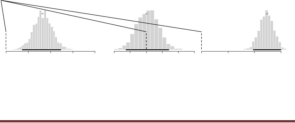
Solutions Manual for Doing Bayesian Data Analysis by John K. Kruschke Page 171
bBeta[j] <- (1-mu[j]) * k[j]
mu[j] <- 1 / ( 1 + exp( -( a0 + a[j] ) ) )
a[j] ~ dnorm( 0.0 , atau )
k[j] ~ dgamma( skappa , rkappa )
}
a0 ~ dnorm( 0 , 0.001 )
atau <- 1 / pow( aSD , 2 )
aSD <- abs( aSDunabs ) + .1
aSDunabs ~ dt( 0 , 0.001 , 2 )
skappa <- pow(mg,2)/pow(sg,2)
rkappa <- mg/pow(sg,2)
mg ~ dunif(0,50)
sg ~ dunif(0,30)
}
…
theData = data.frame( pr=.01+.98*datalist$z/datalist$n ,
x=factor(x,labels=xnames) )
a0 = mean( logit(theData$pr) )
a = aggregate( logit(theData$pr) , list( theData$x ) , mean )[,2] - a0
mGrp = aggregate( theData$pr , list( theData$x ) , mean )[,2]
sdGrp = aggregate( theData$pr , list( theData$x ) , sd )[,2]
kGrp = mGrp*(1-mGrp)/sdGrp^2 - 1
k = mean(kGrp)
genInitList <- function() {
return(
list(
a0 = a0 ,
a = a ,
aSDunabs = sd(a) ,
theta = theData$pr ,
k = kGrp ,
mg = 10 ,
sg = 10
)
)
}
for ( chainIdx in 1 : nchain ) {
modelInits( bugsInits( genInitList ) )
}
The resulting contrasts look like this:
Contrast: FiltLRvFiltHt
1 FiltLR + -1 FiltHt
0.0 0.5 1.0 1.5 2.0
mean 0.825
0% <= 0 < 100%
95% HDI
0.367 1.23
Contrast: Cond1vCond2
1 Condns1 + -1 Condns2
-0.4 -0.2 0.0 0.2 0.4 0.6
mean 0.0176
44.5% <= 0 < 55.5%
95% HDI
-0.252 0.278
Contrast: FiltvCond
0.5 FiltLR + 0.5 FiltHt + -0.5 Condns1 + -0.5 Condns2
0.0 0.5 1.0 1.5
mean 1.22
0% <= 0 < 100%
95% HDI
0.977 1.49
In comparison with Figure 20.6, p. 560 of the textbook, we see that the basic qualitative
conclusions are the same, in terms of excluding or not excluding zero difference. The magnitudes
of the contrasts are slightly smaller here, however, because the added uncertainty of separate
group precisions bleeds over into uncertainty in the group deflection values. As discussed on p.
560 of the textbook, although the “direct” model of chapter 9 and the logistic-ANOVA model of

Solutions Manual for Doing Bayesian Data Analysis by John K. Kruschke Page 172
chapter 20 yield similar results, the logistic-ANOVA model is more easily generalized to two or
more predictor variables.
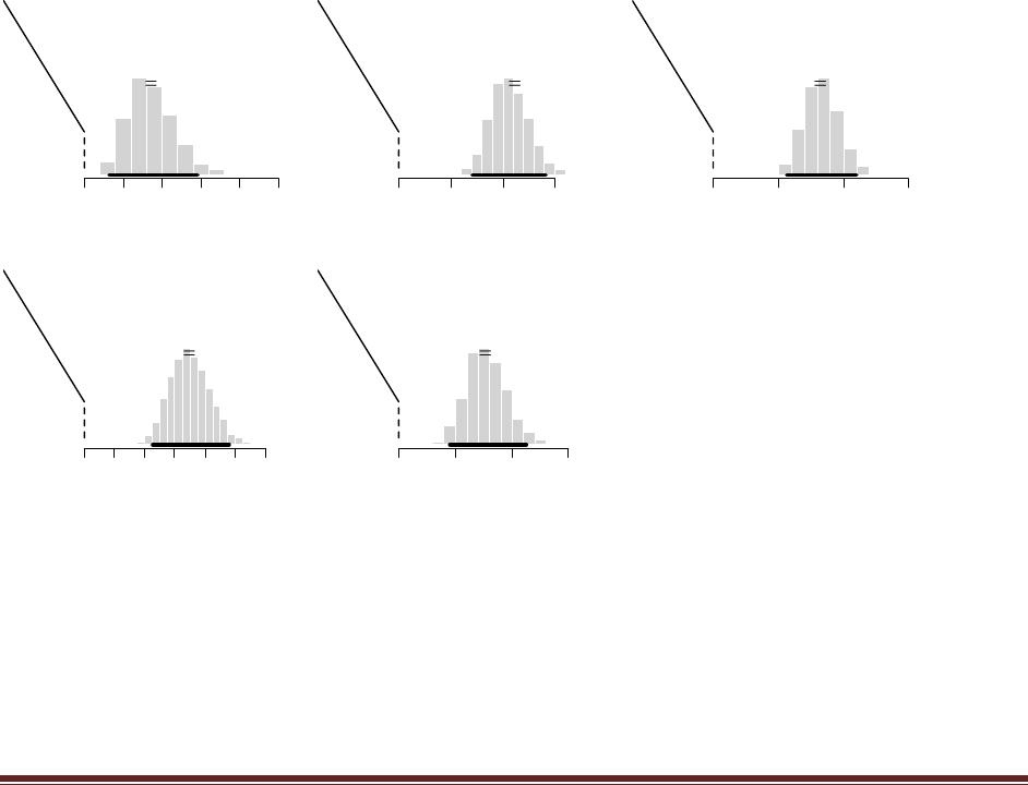
Solutions Manual for Doing Bayesian Data Analysis by John K. Kruschke Page 173
Chapter 21.
Exercise 21.1. [Purpose: To investigate posterior differences of thresholds.] Run the
program in Section 21.5 (OrdinalProbitRegressionBrugs.R) on the Movies data (Moore,
2006). At the end of the program, notice that the posterior thresholds are stored in a matrix
named threshSamp, one column per threshold.
(A) Make histograms of the differences between every pair of adjacent thresholds (i.e.,
threshSamp[,n]-threshSamp[,n-1], for n in 2:nYlevels). (Hint: Use plotPost with
compVal=0.) Are any differences between adjacent thresholds close to zero?
windows(3.5,3)
t=6 ; histInfo=plotPost(threshSamp[,t]-threshSamp[,t-1],compVal=0,
xlab=bquote("Thresh"*.(t)*"-Thresh"*.(t-1)))
t=5 ; histInfo=plotPost(threshSamp[,t]-threshSamp[,t-1],compVal=0,
xlab=bquote("Thresh"*.(t)*"-Thresh"*.(t-1)))
t=4 ; histInfo=plotPost(threshSamp[,t]-threshSamp[,t-1],compVal=0,
xlab=bquote("Thresh"*.(t)*"-Thresh"*.(t-1)))
t=3 ; histInfo=plotPost(threshSamp[,t]-threshSamp[,t-1],compVal=0,
xlab=bquote("Thresh"*.(t)*"-Thresh"*.(t-1)))
t=2 ; histInfo=plotPost(threshSamp[,t]-threshSamp[,t-1],compVal=0,
xlab=bquote("Thresh"*.(t)*"-Thresh"*.(t-1)))
yields
Thresh6-Thresh5
0.0 0.5 1.0 1.5 2.0 2.5
mean 0.864
0% <= 0 < 100%
95% HDI
0.323 1.46
Thresh5-Thresh4
0.0 0.5 1.0 1.5
mean 1.06
0% <= 0 < 100%
95% HDI
0.706 1.42
Thresh4-Thresh3
0.0 0.5 1.0 1.5
mean 0.828
0% <= 0 < 100%
95% HDI
0.567 1.1
Thresh3-Thresh2
0.0 0.4 0.8 1.2
mean 0.701
0% <= 0 < 100%
95% HDI
0.453 0.96
Thresh2-Thresh1
0.0 0.5 1.0 1.5
mean 0.772
0% <= 0 < 100%
95% HDI
0.448 1.13
Clearly none of the adjacent threshold samples have overlapping values (i.e., no differences are
less than zero).
(B) Make a scatter plot of theta4 against theta3. (Hint: plot(threshSamp[,4],
threshSamp[,3]).) Superimpose a line that marks theta4 = theta3. (Hint: abline(0,1).) What
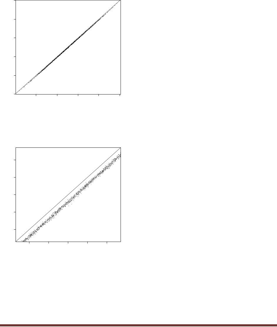
Solutions Manual for Doing Bayesian Data Analysis by John K. Kruschke Page 174
is the relation of this scatter plot to the histogram you made in the previous part? In
particular, what is the relation of the line in the scatter plot to the histogram?
plot( threshSamp[,4] , threshSamp[,3] , pch="." )
abline(0,1)
yields
-80 -60 -40 -20 0
-100 -80 -60 -40 -20 0
threshSamp[, 4]
threshSamp[, 3]
Zooming in lets us see better:
plot( threshSamp[,4] , threshSamp[,3] , pch="." , xlim=c(-55,-45) , ylim=c(-55,-45) )
abline(0,1)
-54 -52 -50 -48 -46
-54 -52 -50 -48 -46
threshSamp[, 4]
threshSamp[, 3]
Notice that all the point lie below the diagonal line. The histogram in the previous part, which
plots thresh4-thresh3, is just this scatterplot collapsed along the diagonal. The diagonal line here
corresponds to the dashed line at compVal=0 in the histogram.
Exercise 21.2. [Purpose: To examine robustness when the prior is changed.] In the program
in Section 21.5 (OrdinalProbitRegressionBrugs.R), the priors on the regression coefficients
and thresholds are mildly informed. Consider the precision of the normal prior for the
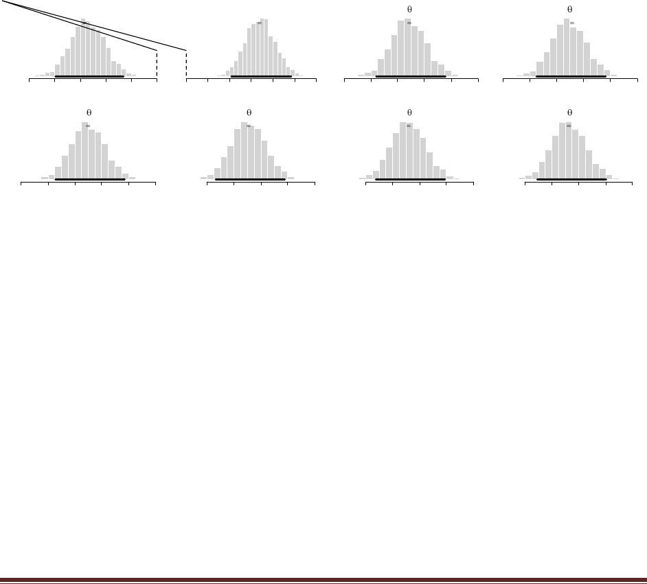
Solutions Manual for Doing Bayesian Data Analysis by John K. Kruschke Page 175
regression coefficients. Because the predictors are standardized, their range is
approximately -2 to +2. If we have a prior assumption that the steepest possible
relationship between x and y maps the lowest value of x to the lowest value of y and the
highest value of x to the highest value of y, then the steepest regression line would rise
nYlevels as x goes from -2 to +2. Hence the steepest plausible slope is nYlevels/4, and the
program makes that value the standard deviation of the prior on each regression
coefficient. Consider now the prior on the thresholds. Because the thresholds are separated
in the prior by 1 unit, and the thresholds should not violate consecutive ordering, it is
reasonable to set their standard deviations no larger than 1.
(A) Set the prior on the regression coefficients so that the precision is very small, say, 1.0E-
6. Run the program on the Movies data. Is the posterior much different?
In the model specification, change the prior as follows:
bPrec <- 1.0E-06 # was pow( nYlevels/4 , -2 )
The resulting posterior is
bYear
Slope Value
-0.05 -0.04 -0.03 -0.02 -0.01 0.00
mean -0.0271
100% <= 0 < 0%
95% HDI
-0.0398 -0.0131
bLength
Slope Value
0.00 0.01 0.02 0.03 0.04 0.05 0.06
mean 0.034
0% <= 0 < 100%
95% HDI
0.0209 0.0484
1
Thresh Value
-100 -80 -60 -40 -20 0
mean -51.7
95% HDI
-75.7 -24.2
2
Thresh Value
-100 -80 -60 -40 -20 0
mean -51
95% HDI
-74.9 -23.5
3
Thresh Value
-100 -80 -60 -40 -20 0
mean -50.3
95% HDI
-74.2 -22.9
4
Thresh Value
-80 -60 -40 -20 0
mean -49.4
95% HDI
-73.4 -22.2
5
Thresh Value
-80 -60 -40 -20 0
mean -48.4
95% HDI
-72.4 -21.1
6
Thresh Value
-80 -60 -40 -20 0
mean -47.5
95% HDI
-70.9 -19.6
which is only very slightly different than the original posterior (see Figure 21.4, p. 585 of the
textbook).
(B) Set the prior on the thresholds so that the precision is very small, say, 1.0E-6. (Set the
prior on the regression coefficients back to the original setting.) Run the program on the
Movies data. Is the posterior much different?
In the model specification, set the bPrec back to what it was, but change the following:
threshPriorPrec <- 1.0E-6 # was 1
The resulting posterior is
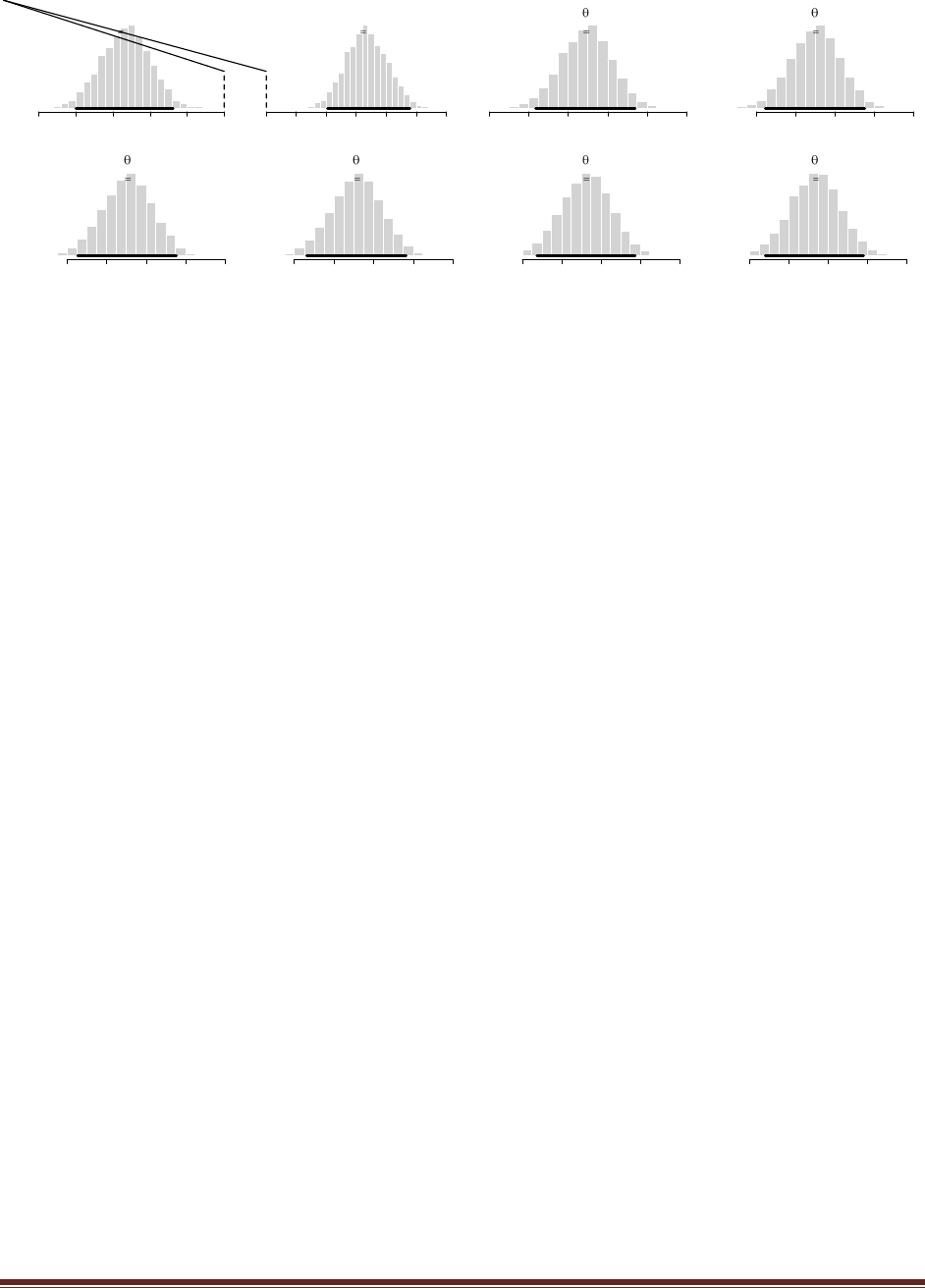
Solutions Manual for Doing Bayesian Data Analysis by John K. Kruschke Page 176
bYear
Slope Value
-0.05 -0.04 -0.03 -0.02 -0.01 0.00
mean -0.0266
100% <= 0 < 0%
95% HDI
-0.04 -0.0138
bLength
Slope Value
0.00 0.01 0.02 0.03 0.04 0.05 0.06
mean 0.0335
0% <= 0 < 100%
95% HDI
0.0204 0.0479
1
Thresh Value
-100 -80 -60 -40 -20 0
mean -50.8
95% HDI
-76.4 -25.9
2
Thresh Value
-80 -60 -40 -20 0
mean -50.1
95% HDI
-75.3 -25
3
Thresh Value
-80 -60 -40 -20 0
mean -49.4
95% HDI
-74.7 -24.6
4
Thresh Value
-80 -60 -40 -20 0
mean -48.5
95% HDI
-73.9 -23.7
5
Thresh Value
-80 -60 -40 -20 0
mean -47.5
95% HDI
-72.6 -22.5
6
Thresh Value
-80 -60 -40 -20 0
mean -46.6
95% HDI
-72 -21.7
which is only very slightly different than the original posterior (see Figure 21.4, p. 585 of the
textbook). Thus, the posterior is very robust against changes in ways to specify a vague prior,
and the mildly informed prior had no noticeable effect on the posterior relative to the extremely
broad priors.
Exercise 21.3. [Purpose: To observe predicted values for novel predictor values.] Run the
program in Section 21.5 (OrdinalProbitRegressionBrugs.R) on the movies data (Moore,
2006). Consider a movie that was not included in the rated movies. Suppose it was made in
1991, and had a length of 94 minutes. What is the probability of each rating for the movie?
In other words, what is the probability that it would be rated 7, what is the probability that
it would be rated 6, and so on. Answer the same question for a movie that had a length of
94 minutes but was made in 1931. (Hint: Use Equation 21.3, averaging the result across all
the steps in the MCMC chain. Extra special bonus hint: Code for doing this is already
included at the end of the program; your job is to understand what it‘s doing.)
The code at the end of the program below. The comments explain the code.
# Posterior prediction.
xProbe = c( 1991 , 94 ) # Note order of values: x1 is year and x2 is duration.
Added comment: xProbe, above, is the novel movie we want to make a prediction for.
# Set up a matrix for storing the values of p(y|xProbe) at each step in chain.
py = matrix( 0 , nrow=chainLength , ncol=nYlevels )
Added comment: py, above, has one row per MCMC step, and 7 columns for 7 possible rating
values. Each column is the probability of the corresponding rating, for the parameter values at
the step in the MCMC chain.
# Step through chain and compute p(y|xProbe) and each step:
for ( chainIdx in 1:chainLength ) {
yValue = 1
py[chainIdx,yValue] = (
pnorm( threshSamp[chainIdx,yValue]
- sum( bSamp[chainIdx,] * xProbe ) ) )
for ( yValue in 2:(nYlevels-1) ) {
py[chainIdx,yValue] = (
pnorm( threshSamp[chainIdx,yValue]
- sum( bSamp[chainIdx,] * xProbe ) )
- pnorm( threshSamp[chainIdx,yValue-1]
- sum( bSamp[chainIdx,] * xProbe ) ) )
}
yValue = nYlevels
py[chainIdx,yValue] = ( 1 -
pnorm( threshSamp[chainIdx,yValue-1]
- sum( bSamp[chainIdx,] * xProbe ) ) )

Solutions Manual for Doing Bayesian Data Analysis by John K. Kruschke Page 177
}
# Now average across the chain:
pyAve = colMeans( py )
Added comment: pyAve, above is the average predicted probability of each rating, collapsed
across all steps in the chain. In other words, that’s the answer we’re looking for!
round( pyAve , 3 )
yields
[1] 0.166 0.247 0.266 0.219 0.091 0.010 0.001
In other words, there is a 16.6% probability of rating “1”, a 24.7% probability of rating “2”, a
26.6% probability of rating “3”, and so forth.
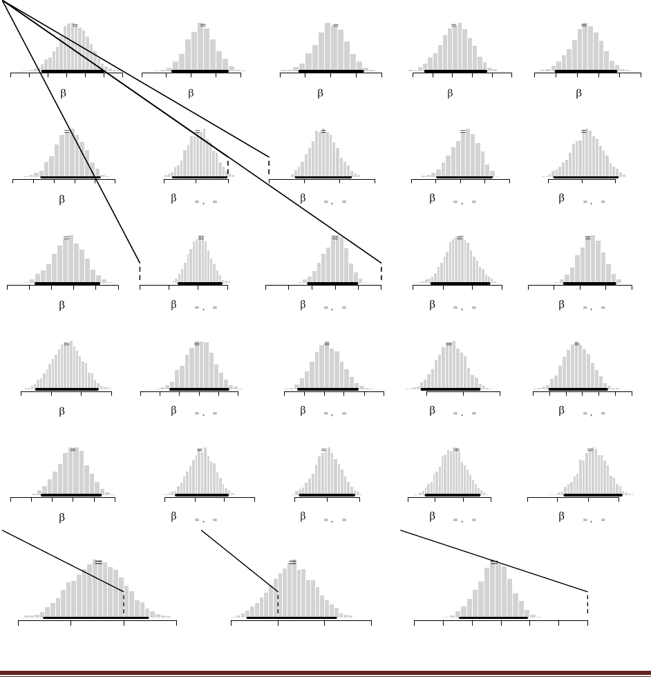
Solutions Manual for Doing Bayesian Data Analysis by John K. Kruschke Page 178
Chapter 22.
Exercise 22.1. [Purpose: To observe the influence of sample size on the precision of the
estimate.] Consider the data regarding hair color and eye color in Table 22.1, which is
available for use in the code of Section 22.4 (PoissonExponentialBrugs.R).
(A) Divide the original data frequencies by 2 and take the ceiling() of the result. Thus, the
modified data are ceiling( c(68,...,16) / 2 ). This modification (nearly) preserves the relative
proportions in each cell but halves the sample size. Run the program with these modified
data, show the histograms, and compute the width of the 95% HDIs for the contrasts.
Freq = ceiling( c(68,119,26,7,20,84,17,94,15,54,14,10,5,29,14,16) /2 ),
Baseline
0
2.2 2.3 2.4 2.5 2.6 2.7 2.8
mean 2.54
95% HDI
2.37 2.69
x1: Blue
11
0.0 0.2 0.4 0.6 0.8
mean 0.48
95% HDI
0.248 0.699
x1: Brown
12
0.0 0.2 0.4 0.6 0.8
mean 0.4
95% HDI
0.155 0.65
x1: Green
13
-1.0 -0.8 -0.6 -0.4 -0.2 0.0
mean -0.565
95% HDI
-0.872 -0.259
x1: Hazel
14
-0.8 -0.6 -0.4 -0.2 0.0 0.2
mean -0.315
95% HDI
-0.601 -0.0333
x2: Black
21
-0.8 -0.6 -0.4 -0.2 0.0 0.2
mean -0.249
95% HDI
-0.521 0.0468
x2: Blond
22
-0.8 -0.6 -0.4 -0.2 0.0 0.2
mean -0.247
95% HDI
-0.541 0.0315
x2: Brunette
23
0.6 0.8 1.0 1.2
mean 0.906
95% HDI
0.701 1.11
x2: Red
24
-1.0 -0.8 -0.6 -0.4 -0.2 0.0
mean -0.41
95% HDI
-0.701 -0.14
x1: Blue , x2: Black
12x1 1 x2 1
-1.0 -0.5 0.0
mean -0.441
98.2% <= 0 < 1.8%
95% HDI
-0.861 -0.0275
x1: Brown , x2: Black
12x1 2 x2 1
0.0 0.5 1.0 1.5
mean 0.777
0% <= 0 < 100%
95% HDI
0.382 1.16
x1: Green , x2: Black
12x1 3 x2 1
-1.5 -1.0 -0.5 0.0 0.5
mean -0.411
95% HDI
-0.976 0.136
x1: Hazel , x2: Black
12x1 4 x2 1
-0.5 0.0 0.5
mean 0.0753
95% HDI
-0.408 0.531
x1: Blue , x2: Blond
12x1 1 x2 2
0.0 0.5 1.0 1.5
mean 1.02
0% <= 0 < 100%
95% HDI
0.668 1.4
x1: Brown , x2: Blond
12x1 2 x2 2
-2.5 -2.0 -1.5 -1.0 -0.5 0.0
mean -1.01
100% <= 0 < 0%
95% HDI
-1.57 -0.523
x1: Green , x2: Blond
12x1 3 x2 2
-0.5 0.0 0.5 1.0
mean 0.283
95% HDI
-0.192 0.778
x1: Hazel , x2: Blond
12x1 4 x2 2
-1.5 -1.0 -0.5 0.0 0.5
mean -0.295
95% HDI
-0.802 0.183
x1: Blue , x2: Brunette
12x1 1 x2 3
-0.8 -0.6 -0.4 -0.2 0.0 0.2
mean -0.197
95% HDI
-0.492 0.0988
x1: Brown , x2: Brunette
12x1 2 x2 3
-0.2 0.0 0.2 0.4 0.6 0.8
mean 0.232
95% HDI
-0.0589 0.534
x1: Green , x2: Brunette
12x1 3 x2 3
-0.5 0.0 0.5
mean -0.172
95% HDI
-0.573 0.217
x1: Hazel , x2: Brunette
12x1 4 x2 3
-0.4 0.0 0.2 0.4 0.6 0.8
mean 0.137
95% HDI
-0.201 0.491
x1: Blue , x2: Red
12x1 1 x2 4
-1.0 -0.5 0.0 0.5
mean -0.383
95% HDI
-0.806 0.0491
x1: Brown , x2: Red
12x1 2 x2 4
-0.5 0.0 0.5
mean 0.0011
95% HDI
-0.424 0.409
x1: Green , x2: Red
12x1 3 x2 4
-0.5 0.0 0.5 1.0
mean 0.3
95% HDI
-0.176 0.787
x1: Hazel , x2: Red
12x1 4 x2 4
-1.0 -0.5 0.0 0.5
mean 0.0823
95% HDI
-0.384 0.549
X1 Contrast: GREENvHAZEL
1 Green + -1 Hazel
-1.0 -0.5 0.0 0.5
mean -0.25
83.6% <= 0 < 16.4%
95% HDI
-0.76 0.23
X2 Contrast: BLONDvRED
1 Blond + -1 Red
-0.5 0.0 0.5 1.0
mean 0.163
25.2% <= 0 < 74.8%
95% HDI
-0.326 0.623
BLUE.BROWNxBLACK.BLOND
+ 1 Blue Black + -1 Blue Blond + -1 Brown Black + 1 Brown Blond
-6 -5 -4 -3 -2 -1 0
mean -3.25
100% <= 0 < 0%
95% HDI
-4.43 -2.09
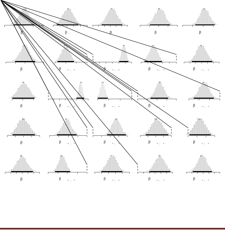
Solutions Manual for Doing Bayesian Data Analysis by John K. Kruschke Page 179
The HDIs are much wider for the halved frequencies than for the original data set (which are
shown in Figure 22.3, p. 604 of the textbook). For example, the 95%HDI on the x2:Red
deflection goes from -0.701 to -0.14 (a width of 0.561) for these halved frequencies, but from -
0.575 to -0.174 (a width of 0.401) in the original frequencies.
(B) Multiply the original data vector by 5 so that all the cell frequencies are five times
larger than the original. This modification preserves the relative proportions in each cell
but quintuples the sample size. Run the program again. Show the histograms. Compute the
width of the 95% HDIs for the contrasts. How do the precisions of the contrasts differ for
the reduced and the enlarged data?
Freq = 5 * c(68,119,26,7,20,84,17,94,15,54,14,10,5,29,14,16) ,
Baseline
0
4.70 4.75 4.80 4.85 4.90
mean 4.8
95% HDI
4.75 4.86
x1: Blue
11
0.40 0.45 0.50 0.55 0.60 0.65
mean 0.508
95% HDI
0.428 0.582
x1: Brown
12
0.20 0.30 0.40 0.50
mean 0.366
95% HDI
0.278 0.451
x1: Green
13
-0.8 -0.7 -0.6 -0.5 -0.4
mean -0.589
95% HDI
-0.691 -0.481
x1: Hazel
14
-0.5 -0.4 -0.3 -0.2
mean -0.285
95% HDI
-0.373 -0.188
x2: Black
21
-0.5 -0.4 -0.3 -0.2 -0.1
mean -0.301
95% HDI
-0.4 -0.196
x2: Blond
22
-0.4 -0.3 -0.2
mean -0.293
95% HDI
-0.394 -0.194
x2: Brunette
23
0.85 0.90 0.95 1.00 1.05
mean 0.948
95% HDI
0.885 1.02
x2: Red
24
-0.50 -0.40 -0.30 -0.20
mean -0.354
95% HDI
-0.446 -0.261
x1: Blue , x2: Black
12x1 1 x2 1
-0.6 -0.4 -0.2 0.0
mean -0.402
100% <= 0 < 0%
95% HDI
-0.545 -0.25
x1: Brown , x2: Black
12x1 2 x2 1
0.0 0.2 0.4 0.6 0.8 1.0 1.2
mean 0.958
0% <= 0 < 100%
95% HDI
0.824 1.09
x1: Green , x2: Black
12x1 3 x2 1
-1.0 -0.8 -0.6 -0.4 -0.2 0.0
mean -0.652
100% <= 0 < 0%
95% HDI
-0.888 -0.417
x1: Hazel , x2: Black
12x1 4 x2 1
-0.2 0.0 0.1 0.2 0.3 0.4
mean 0.097
95% HDI
-0.0627 0.278
x1: Blue , x2: Blond
12x1 1 x2 2
0.0 0.2 0.4 0.6 0.8 1.0 1.2 1.4
mean 1.13
0% <= 0 < 100%
95% HDI
1 1.25
x1: Brown , x2: Blond
12x1 2 x2 2
-1.5 -1.0 -0.5 0.0
mean -1.28
100% <= 0 < 0%
95% HDI
-1.47 -1.06
x1: Green , x2: Blond
12x1 3 x2 2
0.0 0.2 0.4 0.6 0.8
mean 0.456
0% <= 0 < 100%
95% HDI
0.272 0.624
x1: Hazel , x2: Blond
12x1 4 x2 2
-0.6 -0.4 -0.2 0.0
mean -0.309
100% <= 0 < 0%
95% HDI
-0.496 -0.123
x1: Blue , x2: Brunette
12x1 1 x2 3
-0.4 -0.3 -0.2 -0.1 0.0
mean -0.218
100% <= 0 < 0%
95% HDI
-0.318 -0.116
x1: Brown , x2: Brunette
12x1 2 x2 3
0.0 0.1 0.2 0.3 0.4
mean 0.271
0% <= 0 < 100%
95% HDI
0.17 0.379
x1: Green , x2: Brunette
12x1 3 x2 3
-0.4 -0.3 -0.2 -0.1 0.0
mean -0.184
99.2% <= 0 < 0.8%
95% HDI
-0.324 -0.0436
x1: Hazel , x2: Brunette
12x1 4 x2 3
0.0 0.1 0.2 0.3
mean 0.131
1.5% <= 0 < 98.5%
95% HDI
0.0191 0.25
x1: Blue , x2: Red
12x1 1 x2 4
-0.8 -0.6 -0.4 -0.2 0.0
mean -0.511
100% <= 0 < 0%
95% HDI
-0.651 -0.354
x1: Brown , x2: Red
12x1 2 x2 4
-0.2 -0.1 0.0 0.1 0.2 0.3
mean 0.0494
95% HDI
-0.098 0.191
x1: Green , x2: Red
12x1 3 x2 4
0.0 0.1 0.2 0.3 0.4 0.5 0.6
mean 0.381
0% <= 0 < 100%
95% HDI
0.208 0.556
x1: Hazel , x2: Red
12x1 4 x2 4
-0.2 0.0 0.1 0.2 0.3 0.4
mean 0.0807
95% HDI
-0.0802 0.25
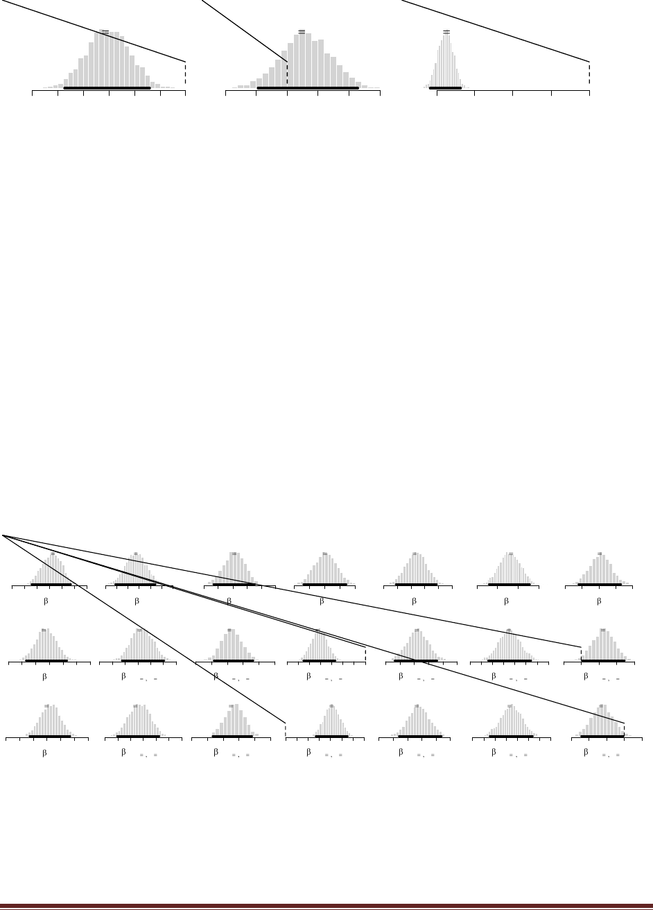
Solutions Manual for Doing Bayesian Data Analysis by John K. Kruschke Page 180
X1 Contrast: GREENvHAZEL
1 Green + -1 Hazel
-0.6 -0.5 -0.4 -0.3 -0.2 -0.1 0.0
mean -0.304
100% <= 0 < 0%
95% HDI
-0.474 -0.14
X2 Contrast: BLONDvRED
1 Blond + -1 Red
-0.2 -0.1 0.0 0.1 0.2 0.3
mean 0.0605
22.8% <= 0 < 77.2%
95% HDI
-0.0938 0.229
BLUE.BROWNxBLACK.BLOND
+ 1 Blue Black + -1 Blue Blond + -1 Brown Black + 1 Brown Blond
-4 -3 -2 -1 0
mean -3.77
100% <= 0 < 0%
95% HDI
-4.17 -3.37
The HDIs are much narrower for the quintipled frequencies than for the original data set (which
are shown in Figure 22.3, p. 604 of the textbook). For example, the 95%HDI on the x2:Red
deflection goes from -0.446 to -0.261 (a width of 0.185) for these halved frequencies, but from -
0.575 to -0.174 (a width of 0.401) in the original frequencies.
The contrasts have also had their HDIs greatly reduced. For example, in the halved data, the
GREENvHAZEL contrast has an HDI that includes zero, but for the quintupled data, this
contrast excludes zero. Thus, even though the relative proportions in the cells are the same as the
original data, the increased sample size improves the certainty of the estimates and reduces the
widths of the HDIs.
Exercise 22.2. [Purpose: To explore main effects and interactions in a contingency
table.] The data section of the program in Section 22.4 (PoissonExponentialBrugs.R)
includes data regarding the type of crime committed by convicted criminals and whether
or not the criminal is a regular drinker of alcoholic beverages (Snee, 1974).
(A) Run the program with these data selected. Is there a credible nonindependence of the
attributes? Describe the interaction in terms of the actual levels of the attributes (i.e., type
of crime and drinker or nondrinker).
Baseline
0
4.20 4.30 4.40 4.50
mean 4.36
95% HDI
4.28 4.44
x1: Arson
11
-0.8 -0.6 -0.4 -0.2
mean -0.53
95% HDI
-0.714 -0.352
x1: Coining
12
-2.0 -1.8 -1.6 -1.4 -1.2 -1.0
mean -1.58
95% HDI
-1.87 -1.29
x1: Fraud
13
0.0 0.1 0.2 0.3 0.4
mean 0.205
95% HDI
0.0597 0.344
x1: Rape
14
-0.3 -0.2 -0.1 0.0 0.1 0.2
mean -0.062
95% HDI
-0.212 0.0907
x1: Theft
15
1.3 1.4 1.5 1.6
mean 1.46
95% HDI
1.36 1.56
x1: Violence
16
0.3 0.4 0.5 0.6 0.7
mean 0.509
95% HDI
0.378 0.634
x2: Drinker
21
-0.10 0.00 0.10 0.20
mean 0.0383
95% HDI
-0.0351 0.115
x2: Nondrink
22
-0.20 -0.10 0.00 0.10
mean -0.0383
95% HDI
-0.115 0.0351
x1: Arson , x2: Drinker
12x1 1 x2 1
-0.3 -0.1 0.0 0.1 0.2 0.3
mean 0.0323
95% HDI
-0.127 0.206
x1: Coining , x2: Drinker
12x1 2 x2 1
-0.4 -0.2 0.0 0.2 0.4 0.6
mean 0.0567
95% HDI
-0.169 0.332
x1: Fraud , x2: Drinker
12x1 3 x2 1
-0.7 -0.5 -0.3 -0.1
mean -0.415
100% <= 0 < 0%
95% HDI
-0.555 -0.269
x1: Rape , x2: Drinker
12x1 4 x2 1
-0.1 0.0 0.1 0.2 0.3 0.4
mean 0.122
95% HDI
-0.0387 0.261
x1: Theft , x2: Drinker
12x1 5 x2 1
-0.10 0.00 0.10 0.20
mean 0.077
95% HDI
-0.0202 0.175
x1: Violence , x2: Drinker
12x1 6 x2 1
-0.1 0.0 0.1 0.2 0.3
mean 0.126
2% <= 0 < 98%
95% HDI
0.00474 0.245
x1: Arson , x2: Nondrink
12x1 1 x2 2
-0.3 -0.1 0.0 0.1 0.2 0.3
mean -0.0323
95% HDI
-0.206 0.127
x1: Coining , x2: Nondrink
12x1 2 x2 2
-0.6 -0.4 -0.2 0.0 0.2 0.4
mean -0.0567
95% HDI
-0.332 0.169
x1: Fraud , x2: Nondrink
12x1 3 x2 2
0.0 0.2 0.4 0.6
mean 0.415
0% <= 0 < 100%
95% HDI
0.269 0.555
x1: Rape , x2: Nondrink
12x1 4 x2 2
-0.4 -0.3 -0.2 -0.1 0.0 0.1
mean -0.122
95% HDI
-0.261 0.0387
x1: Theft , x2: Nondrink
12x1 5 x2 2
-0.25 -0.15 -0.05 0.05
mean -0.077
95% HDI
-0.175 0.0202
x1: Violence , x2: Nondrink
12x1 6 x2 2
-0.3 -0.2 -0.1 0.0 0.1
mean -0.126
98% <= 0 < 2%
95% HDI
-0.245 -0.00474
Yes, several of the interaction deflections exclude zero. (That is not a necessary condition for
nonindependence, but it is sufficient.) For example, among criminals who committed fraud, there
are fewer drinkers, i.e., more nondrinkers, than would be expected if the attributes were
independent. In the opposite direction, among criminals who committed a violent crime (other
than rape), there were more drinkers than would be expected if the attributes were independent.
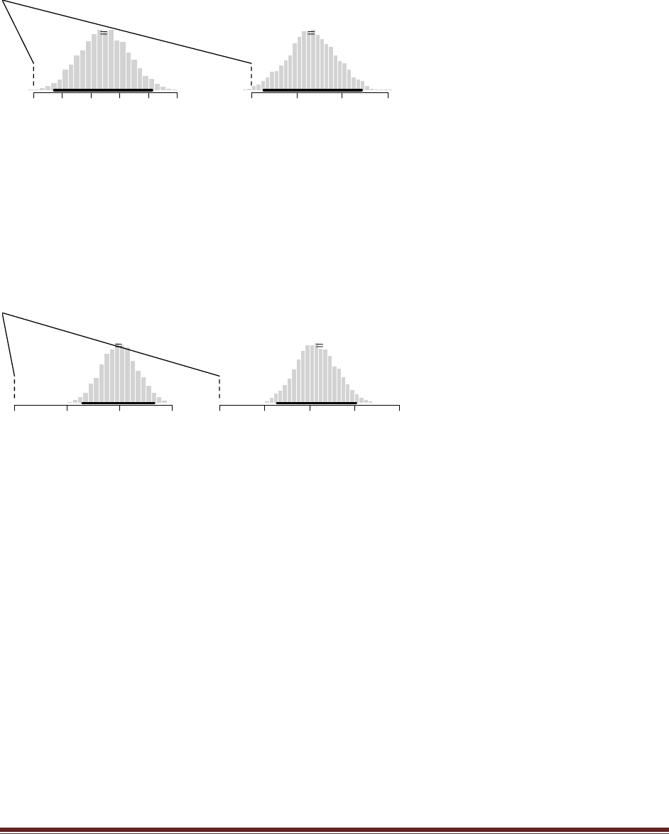
Solutions Manual for Doing Bayesian Data Analysis by John K. Kruschke Page 181
(B) Is there a (―simple‖) main effect of fraud versus rape? That is, marginalizing across
drinking, is there a credible difference in the proportion of criminals who committed fraud
or committed rape? Show the results of an appropriate contrast.
The program already has this contrast coded, and the result looks like this:
X1 Contrast: FRAUDvOTHER
-0.2 Arson + -0.2 Coining + 1 Fraud + -0.2 Rape + -0.2 Theft + -0.2 Violence
0.0 0.1 0.2 0.3 0.4 0.5
mean 0.246
0.3% <= 0 < 99.7%
95% HDI
0.0717 0.413
X1 Contrast: FRAUDvRAPE
1 Fraud + -1 Rape
0.0 0.2 0.4 0.6
mean 0.267
0.5% <= 0 < 99.5%
95% HDI
0.0549 0.485
Thus, because the 95%HDI excludes zero, we say that it is highly credible that more criminals
committed fraud than rape. (In fact, the contrast on the left shows that there was more fraud than
the average of all the other categories of crimes.)
(C) Is the difference from the previous part the same among drinkers and nondrinkers? In
other words, is the effect of criminal type the same at all levels of drinking? Show the
results of an appropriate interaction contrast.
Again the contrast is already coded, and the result looks like this:
FRAUD.OTHERxDRINKER.NON
+ 0.2 Arson Drinker + -0.2 Arson Nondrink + 0.2 Coining Drinker + -0.2 Coining Nondrink + -1 Fraud Drinker + 1 Fraud Nondrink + 0.2 Rape Drinker + -0.2 Rape Nondrink + 0.2 Theft Drinker + -0.2 Theft Nondrink + 0.2 Violence Drinker + -0.2 Violence Nondrink
0.0 0.5 1.0 1.5
mean 0.995
0% <= 0 < 100%
95% HDI
0.646 1.33
FRAUD.RAPExDRINKER.NON
+ -1 Fraud Drinker + 1 Fraud Nondrink + 1 Rape Drinker + -1 Rape Nondrink
0.0 0.5 1.0 1.5 2.0
mean 1.07
0% <= 0 < 100%
95% HDI
0.64 1.52
The right histogram shows the interaction contrast of fraud vs rape against drinker vs nondrinker.
The distribution entirely excludes zero, and therefore we conclude that the interaction contrast is
very credibly nonzero. There are two ways to state the interaction: Within these criminals, the
ratio of rapists to fraud-committers is higher for drinkers than for nondrinker, or, the ratio of
drinkers to nondrinkers is higher for rapists than for fraud-committers.
Exercise 22.3. [Purpose: To compare Bayesian analysis with chi-square test of
independence.] This exercise assumes that you have some familiarity with traditional chi-
square tests of independence. In the code of Section 22.4 (PoissonExponentialBrugs.R), the
data section includes some simple fictitious data, which we can manipulate and then
compare with results of Bayesian and chi-square analyses.
(A) Set the dataMultiplier to 6, and run the program. Include the histograms of the beta
parameters and of the interaction contrast. Does the 95% HDI of the contrast include zero?
The end of the program runs a chi-square test. What is the p value from the test? (Hint:
See Figure 22.6.)
With the dataMultiplier set to 6, the data look like this (as shown in the R console window at the
end of the run):
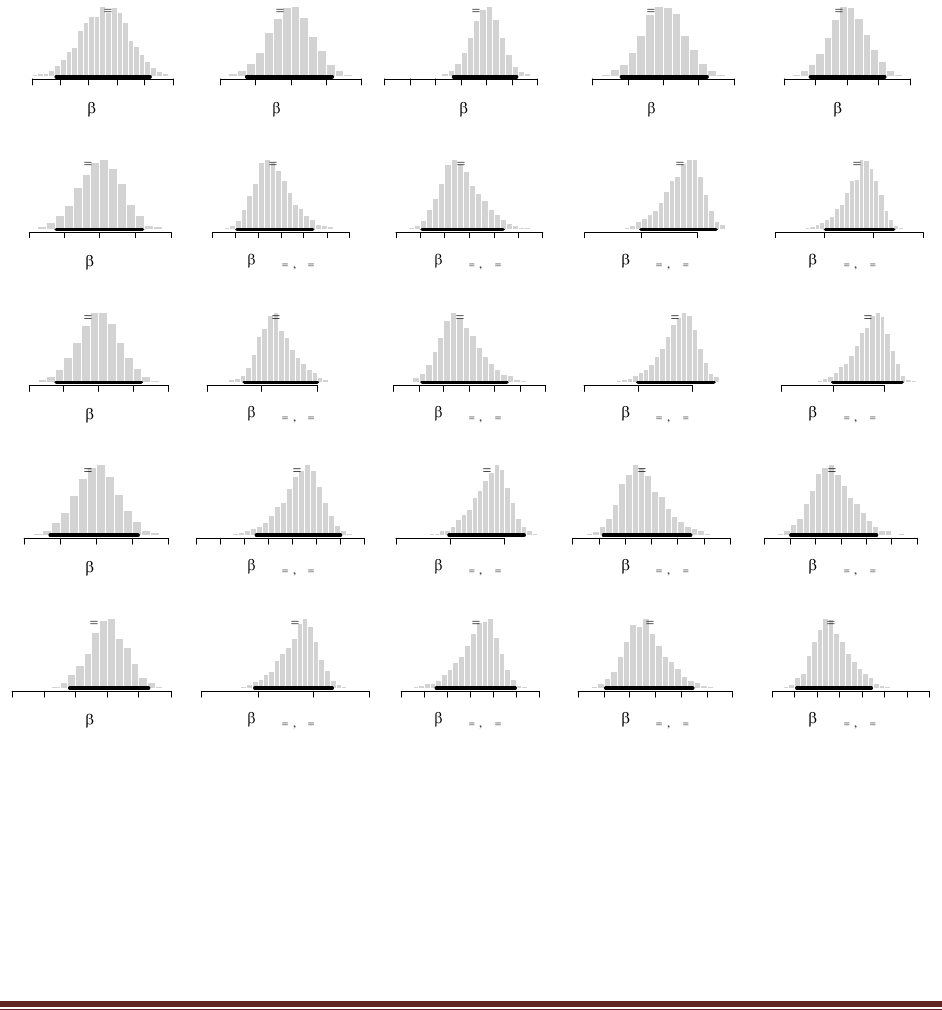
Solutions Manual for Doing Bayesian Data Analysis by John K. Kruschke Page 182
[,1] [,2] [,3] [,4]
[1,] 12 12 6 6
[2,] 12 12 6 6
[3,] 6 6 12 12
[4,] 6 6 12 12
Notice that the marginals are uniform, i.e., all marginals have frequencies of 36. Only the
interaction is not uniform. The question is whether the interaction is big enough that we can be
very certain it is not zero.
The Bayesian posterior looks like this:
Baseline
0
1.9 2.0 2.1 2.2 2.3 2.4
mean 2.16
95% HDI
1.99 2.32
x1: C1
11
-0.4 -0.2 0.0 0.2 0.4
mean -0.00187
95% HDI
-0.248 0.234
x1: C2
12
-0.8 -0.6 -0.4 -0.2 0.0 0.2 0.4
mean -0.00352
95% HDI
-0.256 0.234
x1: C3
13
-0.4 -0.2 0.0 0.2 0.4
mean 0.000316
95% HDI
-0.236 0.248
x1: C4
14
-0.4 -0.2 0.0 0.2 0.4
mean 0.00508
95% HDI
-0.236 0.241
x2: R1
21
-0.4 -0.2 0.0 0.2 0.4
mean 0.000933
95% HDI
-0.247 0.239
x2: R2
22
-0.4 -0.2 0.0 0.2 0.4
mean -0.00172
95% HDI
-0.245 0.246
x2: R3
23
-0.4 -0.2 0.0 0.2 0.4
mean 0.00109
95% HDI
-0.255 0.23
x2: R4
24
-0.6 -0.4 -0.2 0.0 0.2 0.4
mean -0.000306
95% HDI
-0.237 0.259
x1: C1 , x2: R1
12x1 1 x2 1
-0.4 0.0 0.2 0.4 0.6 0.8
mean 0.132
95% HDI
-0.184 0.474
x1: C2 , x2: R1
12x1 2 x2 1
-0.4 0.0 0.2 0.4 0.6 0.8
mean 0.134
95% HDI
-0.184 0.477
x1: C3 , x2: R1
12x1 3 x2 1
-1.0 -0.5 0.0
mean -0.133
95% HDI
-0.504 0.165
x1: C4 , x2: R1
12x1 4 x2 1
-1.0 -0.5 0.0 0.5
mean -0.133
95% HDI
-0.493 0.2
x1: C1 , x2: R2
12x1 1 x2 2
-0.5 0.0 0.5
mean 0.135
95% HDI
-0.157 0.501
x1: C2 , x2: R2
12x1 2 x2 2
-0.4 -0.2 0.0 0.2 0.4 0.6 0.8
mean 0.131
95% HDI
-0.175 0.493
x1: C3 , x2: R2
12x1 3 x2 2
-1.0 -0.5 0.0
mean -0.131
95% HDI
-0.501 0.2
x1: C4 , x2: R2
12x1 4 x2 2
-1.0 -0.5 0.0
mean -0.136
95% HDI
-0.499 0.159
x1: C1 , x2: R3
12x1 1 x2 3
-1.0 -0.6 -0.2 0.0 0.2 0.4
mean -0.133
95% HDI
-0.498 0.202
x1: C2 , x2: R3
12x1 2 x2 3
-1.0 -0.5 0.0
mean -0.136
95% HDI
-0.509 0.178
x1: C3 , x2: R3
12x1 3 x2 3
-0.4 -0.2 0.0 0.2 0.4 0.6 0.8
mean 0.133
95% HDI
-0.165 0.497
x1: C4 , x2: R3
12x1 4 x2 3
-0.4 -0.2 0.0 0.2 0.4 0.6 0.8
mean 0.136
95% HDI
-0.193 0.481
x1: C1 , x2: R4
12x1 1 x2 4
-1.0 -0.5 0.0 0.5
mean -0.134
95% HDI
-0.524 0.168
x1: C2 , x2: R4
12x1 2 x2 4
-0.8 -0.4 0.0 0.2 0.4
mean -0.128
95% HDI
-0.493 0.191
x1: C3 , x2: R4
12x1 3 x2 4
-0.4 -0.2 0.0 0.2 0.4 0.6 0.8
mean 0.13
95% HDI
-0.187 0.488
x1: C4 , x2: R4
12x1 4 x2 4
-0.4 0.0 0.2 0.4 0.6 0.8 1.0
mean 0.132
95% HDI
-0.179 0.477
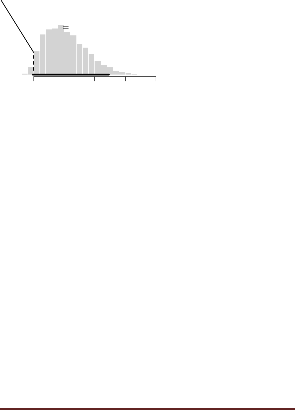
Solutions Manual for Doing Bayesian Data Analysis by John K. Kruschke Page 183
R12.R34xC12.C34
+ 0.25 C1 R1 + 0.25 C1 R2 + -0.25 C1 R3 + -0.25 C1 R4 + 0.25 C2 R1 + 0.25 C2 R2 + -0.25 C2 R3 + -0.25 C2 R4 + -0.25 C3 R1 + -0.25 C3 R2 + 0.25 C3 R3 + 0.25 C3 R4 + -0.25 C4 R1 + -0.25 C4 R2 + 0.25 C4 R3 + 0.25 C4 R4
0.0 0.5 1.0 1.5 2.0
mean 0.532
2.1% <= 0 < 97.9%
95% HDI
-0.0127 1.23
The marginal posteriors of the individual interaction deflections all include zero. The posterior of
the interaction contrast includes zero in its 95%HDI (barely).
The chi-squared test at the end yields this result:
Pearson's Chi-squared test
data: obsFreq
X-squared = 16, df = 9, p-value = 0.06688
The p value is greater than .05, which means that the null hypothesis of independence is not
rejected.
(B) Set the dataMultiplier to 7, and run the program. Include the histograms of the beta
parameters and of the interaction contrast. Does the 95% HDI of the contrast include zero?
The end of the program runs a chi-square test. What is the p value from the test? (Hint:
See Figure 22.6.)
The data now look like this:
[,1] [,2] [,3] [,4]
[1,] 14 14 7 7
[2,] 14 14 7 7
[3,] 7 7 14 14
[4,] 7 7 14 14
Like the previous part, the marginals are uniform.
The posterior now looks like this:
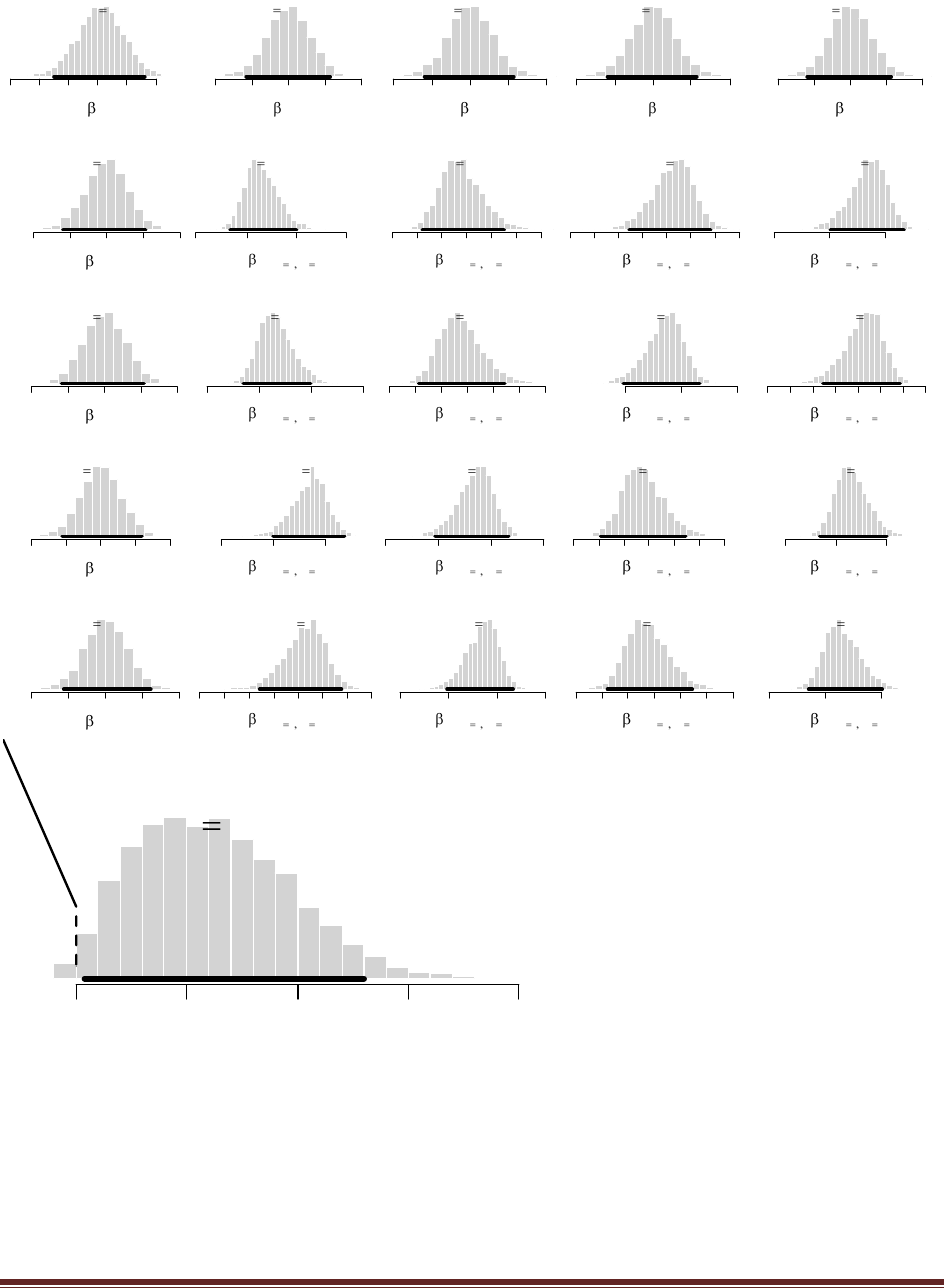
Solutions Manual for Doing Bayesian Data Analysis by John K. Kruschke Page 184
Baseline
0
2.0 2.1 2.2 2.3 2.4 2.5
mean 2.31
95% HDI
2.15 2.46
x1: C1
11
-0.4 -0.2 0.0 0.2 0.4
mean -0.00202
95% HDI
-0.234 0.229
x1: C2
12
-0.4 -0.2 0.0 0.2 0.4
mean 0.000367
95% HDI
-0.235 0.229
x1: C3
13
-0.4 -0.2 0.0 0.2 0.4
mean 0.00199
95% HDI
-0.239 0.23
x1: C4
14
-0.4 -0.2 0.0 0.2 0.4
mean -0.000329
95% HDI
-0.237 0.228
x2: R1
21
-0.4 -0.2 0.0 0.2 0.4
mean -0.00126
95% HDI
-0.241 0.214
x2: R2
22
-0.4 -0.2 0.0 0.2 0.4
mean 0.00054
95% HDI
-0.236 0.218
x2: R3
23
-0.4 -0.2 0.0 0.2 0.4
mean -0.000591
95% HDI
-0.223 0.237
x2: R4
24
-0.4 -0.2 0.0 0.2 0.4
mean 0.00131
95% HDI
-0.223 0.243
x1: C1 , x2: R1
12x1 1 x2 1
-0.5 0.0 0.5 1.0
mean 0.152
95% HDI
-0.154 0.499
x1: C2 , x2: R1
12x1 2 x2 1
-0.4 -0.2 0.0 0.2 0.4 0.6 0.8
mean 0.156
95% HDI
-0.157 0.503
x1: C3 , x2: R1
12x1 3 x2 1
-1.0 -0.6 -0.2 0.0 0.2 0.4
mean -0.154
95% HDI
-0.515 0.157
x1: C4 , x2: R1
12x1 4 x2 1
-1.0 -0.5 0.0
mean -0.154
95% HDI
-0.49 0.175
x1: C1 , x2: R2
12x1 1 x2 2
-0.5 0.0 0.5 1.0
mean 0.156
95% HDI
-0.164 0.495
x1: C2 , x2: R2
12x1 2 x2 2
-0.4 -0.2 0.0 0.2 0.4 0.6 0.8
mean 0.151
95% HDI
-0.173 0.49
x1: C3 , x2: R2
12x1 3 x2 2
-0.5 0.0 0.5
mean -0.153
95% HDI
-0.515 0.169
x1: C4 , x2: R2
12x1 4 x2 2
-1.0 -0.6 -0.2 0.2 0.4
mean -0.155
95% HDI
-0.509 0.172
x1: C1 , x2: R3
12x1 1 x2 3
-1.0 -0.5 0.0
mean -0.155
95% HDI
-0.501 0.187
x1: C2 , x2: R3
12x1 2 x2 3
-1.0 -0.5 0.0 0.5
mean -0.153
95% HDI
-0.528 0.167
x1: C3 , x2: R3
12x1 3 x2 3
-0.4 -0.2 0.0 0.2 0.4 0.6 0.8
mean 0.154
95% HDI
-0.186 0.491
x1: C4 , x2: R3
12x1 4 x2 3
-0.5 0.0 0.5
mean 0.153
95% HDI
-0.157 0.5
x1: C1 , x2: R4
12x1 1 x2 4
-1.0 -0.6 -0.2 0.0 0.2 0.4
mean -0.154
95% HDI
-0.514 0.155
x1: C2 , x2: R4
12x1 2 x2 4
-1.0 -0.5 0.0 0.5
mean -0.155
95% HDI
-0.514 0.165
x1: C3 , x2: R4
12x1 3 x2 4
-0.4 -0.2 0.0 0.2 0.4 0.6 0.8
mean 0.153
95% HDI
-0.159 0.491
x1: C4 , x2: R4
12x1 4 x2 4
-0.5 0.0 0.5
mean 0.156
95% HDI
-0.145 0.507
R12.R34xC12.C34
+ 0.25 C1 R1 + 0.25 C1 R2 + -0.25 C1 R3 + -0.25 C1 R4 + 0.25 C2 R1 + 0.25 C2 R2 + -0.25 C2 R3 + -0.25 C2 R4 + -0.25 C3 R1 + -0.25 C3 R2 + 0.25 C3 R3 + 0.25 C3 R4 + -0.25 C4 R1 + -0.25 C4 R2 + 0.25 C4 R3 + 0.25 C4 R4
0.0 0.5 1.0 1.5 2.0
mean 0.616
1.1% <= 0 < 98.9%
95% HDI
0.0408 1.3
The individual cell interaction deflections all include zero, but the interaction contrast has a
95%HDI that excludes zero. In other words, by pooling across individual cells and computing an
appropriate interaction contrast, we can see that there is variation across individual cells that is
credibly different than pure independence or additivity.
The Pearson chi-squared test has these results:

Solutions Manual for Doing Bayesian Data Analysis by John K. Kruschke Page 185
Pearson's Chi-squared test
data: obsFreq
X-squared = 18.6667, df = 9, p-value = 0.02818
With p<.05, the user of NHST would reject the null hypothesis of independent attributes.
Across parts A and B, we see that the Bayesian and NHST analyses agree in their conclusions
about whether or not nonindependence can be concluded from the data. The Bayesian analysis
provides far more information, however, by showing individual cell posteriors and explicitly
where the nonindependence arises. The Bayesian analysis also never computes a p value.
(C) Typical chi-square tests rely on approximating the sampling distribution of discrete
Pearson chi-square values … with the continuous chi-square distribution (which derives
from the sum of standardized normal samples). When the expected frequencies are too
small, then the approximation is not good and the estimated p value may be wrong. A usual
heuristic for declaring the chi-square test to be suspect is when (at least 10% of the)
expected frequencies are less than 5. This is why computer packages issue warnings when
expected values are too small. Bayesian analysis has no such problems. Set the
dataMultiplier to 2, and run the program. Does the Bayesian analysis complain or do
anything wrong? (No.) The end of the program runs a chi-square test. Is there a warning
message? (Yes; report what it is.)
The data now are as follows:
[,1] [,2] [,3] [,4]
[1,] 4 4 2 2
[2,] 4 4 2 2
[3,] 2 2 4 4
[4,] 2 2 4 4
The Bayesian posterior:
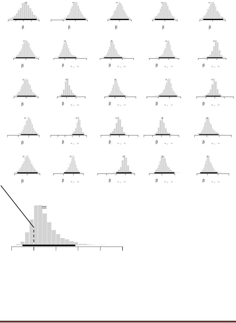
Solutions Manual for Doing Bayesian Data Analysis by John K. Kruschke Page 186
Baseline
0
0.6 0.8 1.0 1.2 1.4
mean 1.03
95% HDI
0.746 1.33
x1: C1
11
-1.0 -0.5 0.0 0.5
mean 0.00331
95% HDI
-0.364 0.416
x1: C2
12
-0.5 0.0 0.5
mean -0.00134
95% HDI
-0.376 0.372
x1: C3
13
-0.5 0.0 0.5
mean -0.00209
95% HDI
-0.382 0.368
x1: C4
14
-0.5 0.0 0.5
mean 0.000124
95% HDI
-0.349 0.397
x2: R1
21
-0.5 0.0 0.5
mean 0.00332
95% HDI
-0.399 0.353
x2: R2
22
-0.5 0.0 0.5
mean -0.00248
95% HDI
-0.357 0.393
x2: R3
23
-1.0 -0.5 0.0 0.5
mean -0.000117
95% HDI
-0.349 0.392
x2: R4
24
-0.5 0.0 0.5
mean -0.000724
95% HDI
-0.369 0.39
x1: C1 , x2: R1
12x1 1 x2 1
-0.5 0.0 0.5 1.0
mean 0.0585
95% HDI
-0.257 0.521
x1: C2 , x2: R1
12x1 2 x2 1
-0.5 0.0 0.5 1.0
mean 0.0617
95% HDI
-0.305 0.475
x1: C3 , x2: R1
12x1 3 x2 1
-1.0 -0.5 0.0 0.5
mean -0.0605
95% HDI
-0.488 0.298
x1: C4 , x2: R1
12x1 4 x2 1
-1.0 -0.5 0.0 0.5
mean -0.0597
95% HDI
-0.499 0.294
x1: C1 , x2: R2
12x1 1 x2 2
-0.5 0.0 0.5 1.0
mean 0.0579
95% HDI
-0.28 0.473
x1: C2 , x2: R2
12x1 2 x2 2
-0.5 0.0 0.5 1.0
mean 0.0625
95% HDI
-0.283 0.475
x1: C3 , x2: R2
12x1 3 x2 2
-1.0 -0.5 0.0 0.5
mean -0.0592
95% HDI
-0.452 0.321
x1: C4 , x2: R2
12x1 4 x2 2
-1.0 -0.5 0.0 0.5 1.0
mean -0.0611
95% HDI
-0.482 0.291
x1: C1 , x2: R3
12x1 1 x2 3
-2.0 -1.5 -1.0 -0.5 0.0 0.5
mean -0.0627
95% HDI
-0.453 0.313
x1: C2 , x2: R3
12x1 2 x2 3
-1.0 -0.5 0.0 0.5 1.0
mean -0.0612
95% HDI
-0.474 0.292
x1: C3 , x2: R3
12x1 3 x2 3
-1.0 -0.5 0.0 0.5 1.0
mean 0.061
95% HDI
-0.306 0.475
x1: C4 , x2: R3
12x1 4 x2 3
-0.5 0.0 0.5 1.0
mean 0.0629
95% HDI
-0.308 0.466
x1: C1 , x2: R4
12x1 1 x2 4
-1.0 -0.5 0.0 0.5
mean -0.0537
95% HDI
-0.46 0.298
x1: C2 , x2: R4
12x1 2 x2 4
-1.5 -1.0 -0.5 0.0 0.5
mean -0.063
95% HDI
-0.468 0.32
x1: C3 , x2: R4
12x1 3 x2 4
-0.5 0.0 0.5
mean 0.0588
95% HDI
-0.281 0.47
x1: C4 , x2: R4
12x1 4 x2 4
-0.5 0.0 0.5 1.0
mean 0.0579
95% HDI
-0.322 0.454
R12.R34xC12.C34
+ 0.25 C1 R1 + 0.25 C1 R2 + -0.25 C1 R3 + -0.25 C1 R4 + 0.25 C2 R1 + 0.25 C2 R2 + -0.25 C2 R3 + -0.25 C2 R4 + -0.25 C3 R1 + -0.25 C3 R2 + 0.25 C3 R3 + 0.25 C3 R4 + -0.25 C4 R1 + -0.25 C4 R2 + 0.25 C4 R3 + 0.25 C4 R4
-0.5 0.0 0.5 1.0 1.5 2.0
mean 0.241
19.2% <= 0 < 80.8%
95% HDI
-0.242 0.923
The point of showing the Bayesian posterior is that the Bayesian analysis proceeds as before,
with no problems. The posterior shows that there is high uncertainty in the parameter estimates
(because there data frequencies are so small).
The Pearson chi-squared test, however, gives this output with a warning message:

Solutions Manual for Doing Bayesian Data Analysis by John K. Kruschke Page 187
> chisqtest = chisq.test( obsFreq )
Warning message:
In chisq.test(obsFreq) : Chi-squared approximation may be incorrect
Pearson's Chi-squared test
data: obsFreq
X-squared = 5.3333, df = 9, p-value = 0.8043
The warning message is saying that the p value may be incorrect because it relies on
approximating the discrete Pearson chi-square with the continuous chi-square, and the
approximation is poor for small frequencies. The Bayesian analysis has no such problem with
small frequencies.
