LB100 ESS D200 LIDAR MANUAL
User Manual:
Open the PDF directly: View PDF ![]() .
.
Page Count: 216 [warning: Documents this large are best viewed by clicking the View PDF Link!]
- PREFACE
- QUALITY CONTROL
- TABLE OF ABBREVIATIONS
- 1. LASER SAFETY
- 2. INTRODUCTION TO THE LIDAR TECHNIQUE
- 3. LIDAR SYSTEM HARDWARE COMPONENTS
- 4. LIDAR SYSTEM SOFTWARE
- 5. UNPACKING AND INSTALLATION
- 6. LIDAR OPERATION
- 7. LIDAR DATA PROCESSING
- 7.1 DATA FILES HANDLING
- 7.2. DATA PREVIEW
- 7.3. DATA ANALYSIS
- 7.3.1 How to Plot Data
- 7.3.2 How to Calculate Backscatter Coefficient
- 7.3.3 How to Calculate Aerosol Extinction Coefficient
- 7.3.4 How to Check Lidar Alignment
- 7.3.5 How to Calculate Water Vapor Profiles
- 7.3.6 How to subtract the Background
- 7.3.7 How to Glue Analog and Photon Counting signals
- 7.3.8 How to make a 3D Graph
- 7.3.9 How to use soundings from global model data
- 7.4. SCANNING DATA ANALYSIS
- 8. LIDAR SYSTEM MAINTENANCE
- 9. TROUBLESHOOTING
- 10. LIDAR SYSTEM TECHNICAL SPECIFICATIONS
- 11. LIMITED GUARANTEE
- REFERENCES
- APPENDIX A
- APPENDIX B
USER’S MANUAL
DOC 0201
September 2013
© Raymetrics SA
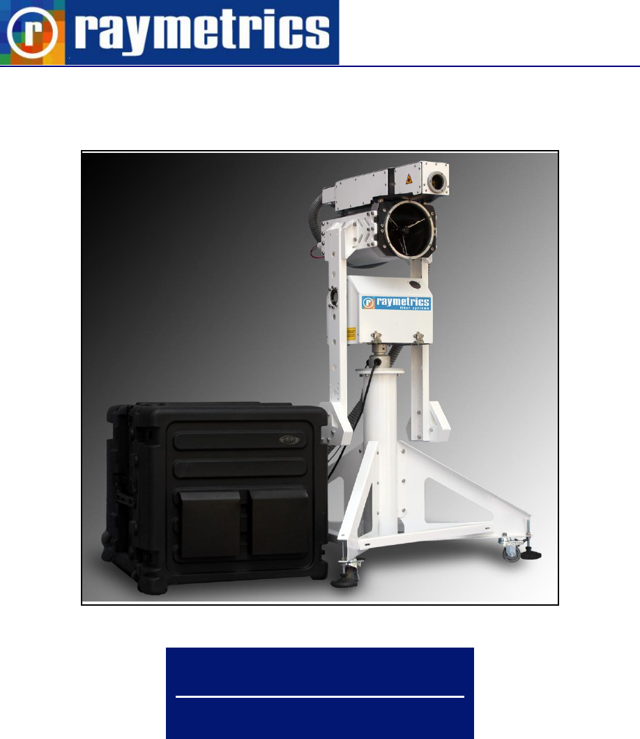
LB100-ESS-D200
Backscatter Scanning LIDAR
PREFACE
2
PREFACE
This User's Manual contains the technical information needed to properly operate and
maintain RAYMETRICS Backscatter Scanning LIDAR system. It provides instructions for
set operation, service and preventive maintenance, and a troubleshooting (fault-isolation)
guide.
The Lidar system consists of four major sub-assemblies: (1) the Lidar receiver
(including optical telescope and detection unit), (2) the transmitter (including the laser
head, the power supply and cooler unit), (3) the Transient recorder unit and (4) the PC,
which includes all the software modules for data acquisition, analysis and visualization.
Caution and warning labels, in accordance with CDRH and CE requirements, are
prominently displayed on the Laser Head and power supply of the laser unit, as well as in
the front and rear panel of the Lidar telescope. For safety, the maximum ratings indicated
on the system labels are in excess of the normal operating parameters.
The laser system produces laser radiation, which is hazardous to eyes and skin, can
cause burning and fires and can vaporize substances. The laser safety chapter in the
User’s Manual contains essential information and user guidance about these hazards.

QUALITY CONTROL
3
QUALITY CONTROL
FINAL TEST DATA SHEET
Model: LB100-ESS-D200
S/N: 200-01-13
Test Date: 19/04/2013
Telescope Calibration:
Laser Beam Calibration:
Lidar Alignment :
Lidar signals
355 nm:
Polarization Calibration:
Laser Security Interlocks:
Any suggestions to be returned to:
Raymetrics S.A.
12 Papathanasiou str., Paiania
GR-19002 Attika - GREECE
Tel: +30 210 6655869
Fax: +30 210 6639031
info@raymetrics.gr
For technical queries and support:
support@raymetrics.gr
Visit www.raymetrics.gr for more info

TABLE OF ABBREVIATIONS
4
TABLE OF ABBREVIATIONS
ABREVIATION
EXPLANATION
A/D ADC
Analog to Digital Conversion
AN
Analog
APD
Avalanche PhotoDiode
AR
Anti Reflection
ASCII
American Standard Code for Information Interchange
BG
Background
CGU
Coolant Group Unit
CNC
Computer Numerical Control
DAQ
Data Acquisition
DB
Database
EXT
External
FOV
Filed Of View
GL
Glued
HR
High Reflecting
HT
High Transmitting
HV
High Voltage
HVAC
Heating Ventilation and Air Cooling
IFF
Interference Filter
INT
Internal
IP
Internet Protocol
LAN
Local Area Network
LCD
Liquid Crystal Display
LED
Light Emitting Diode
Lidar
Laser Interferometry Detection and Ranging
LR
Lidar Ratio
LSB
Least Significant Bit
ND
Neutral Density
OU
Optical Unit
PBC
Polarizing Beamsplitter Cube
PC
Photon counting

TABLE OF ABBREVIATIONS
5
PCC
Power supply Cooling unit Cabinet
PMT
Photo Multiplier Tube
PSU
Power Supply Unit
QS
Q-Switch
RAM
Random Access Memory
RCS
Range Corrected Signal
RDP
Remote Desktop
SAU
Signal Acquisition Unit
SHG
Second Harmonic Generator
SNR
Signal To Noise Ratio
TCP
Transmission Control Protocol
THG
Third Harmonic Generator
TR
Transient Recorder
TTL
Transistor–Transistor logic
WOL
Wake On Lan
WSU
Wavelegth Saparation Unit

TABLE OF CONTENTS
6
TABLE OF CONTENTS
PREFACE ............................................................................................................................. 2
QUALITY CONTROL ............................................................................................................ 3
TABLE OF ABBREVIATIONS .............................................................................................. 4
1. LASER SAFETY ............................................................................................................... 9
2. INTRODUCTION TO THE LIDAR TECHNIQUE .............................................................. 12
3. LIDAR SYSTEM HARDWARE COMPONENTS.............................................................. 14
3.1. TRANSMITTER ....................................................................................................................... 15
3.1.1. Laser .............................................................................................................................. 15
3.1.2. Beam Splitter .................................................................................................................. 17
3.1.3. Beam Expander ............................................................................................................. 18
3.2. RECEIVING SYSTEM ............................................................................................................. 19
3.2.1. Telescope ....................................................................................................................... 19
3.2.2. Wavelength separation unit............................................................................................ 21
3.2.3. Depolarization Technique .............................................................................................. 22
3.2.4. Light Detectors ............................................................................................................... 24
3.3 CONTROL UNIT ....................................................................................................................... 27
3.3.1 Laser control and power supply ...................................................................................... 27
3.3.2 Detection electronics ....................................................................................................... 29
3.3.3 Industrial Computer ......................................................................................................... 33
3.3.4 Electrical Cabinet ............................................................................................................ 34
4. LIDAR SYSTEM SOFTWARE ......................................................................................... 38
4.1. OPERATION SOFTWARE ...................................................................................................... 39
4.1.1 Acquisition ....................................................................................................................... 39
4.1.2 Scheduler ........................................................................................................................ 41
4.1.3 Scanning autonomous and Time scheduler.................................................................... 42
4.1.4 Database and Working Directory .................................................................................... 44
4.2. POST PROCESSING SOFTWARE ........................................................................................ 44
4.3. SOFTWARE TOOLS ............................................................................................................... 48
4.3.1 Lidar Alignment Software ................................................................................................ 48
4.3.2 Configure other hardware ............................................................................................... 49
4.3.3 Laser Control Interface .................................................................................................... 50
4.3.4 Licel Software .................................................................................................................. 50
5. UNPACKING AND INSTALLATION ............................................................................... 52
5.1. UNPACKING THE LIDAR SYSTEM ........................................................................................ 52
5.2 INSTALLATION OF THE LIDAR SYSTEM .............................................................................. 52
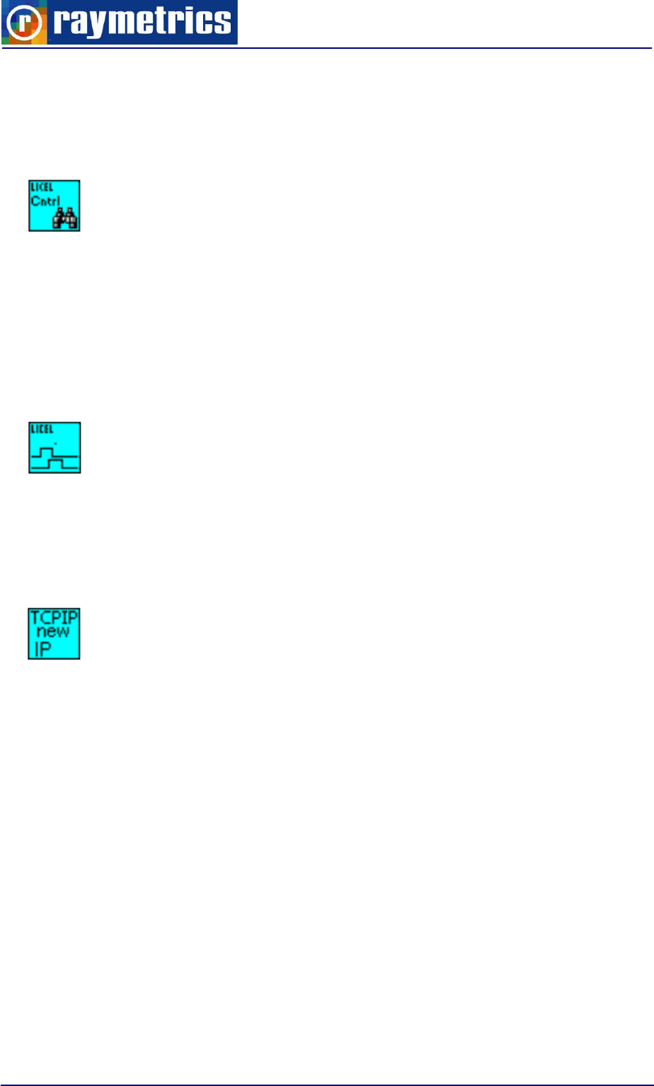
5.2.1 Assembly ......................................................................................................................... 54
5.2.2 Cable Connections .......................................................................................................... 56
5.2.3 Water Filling .................................................................................................................... 59
5.2.4 Software Installation ........................................................................................................ 60
5.3 STORAGE AND SERVICE ....................................................................................................... 61

TABLE OF CONTENTS
7
6. LIDAR OPERATION ....................................................................................................... 62
6.1. START-UP ............................................................................................................................... 62
6.1.1 Manual Operation ............................................................................................................ 63
6.1.2 Automated Operation ...................................................................................................... 64
6.2 LIDAR ALIGNMENT ................................................................................................................. 65
6.2.1 Laser Beam Kinematic .................................................................................................... 67
6.2.2 Lidar Alignment Procedure.............................................................................................. 69
6.2.3 Using the Alignment Software ......................................................................................... 75
6.2.4 Signal Intensity Reduction............................................................................................... 79
6.3. DATA ACQUISITION ............................................................................................................... 83
6.3.1 Introduction to the Acquisition Interface .......................................................................... 83
6.3.2 Configure Measurements ................................................................................................ 83
6.3.2 Configure the Working Directory ..................................................................................... 87
6.3.3 Lidar Measurements ....................................................................................................... 88
6.4. MEASUREMENT SCHEDULING ............................................................................................ 90
6.5. SCANNING OPERATION........................................................................................................ 93
6.5.1 Creating a Configuration File .......................................................................................... 93
6.5.2 Scanning Autonomous .................................................................................................... 96
6.5.3 Time scheduler for Scanning .......................................................................................... 97
6.6. REMOTE LIDAR ...................................................................................................................... 99
6.6.1 Establishing a connection ............................................................................................... 99
6.6.2 Shut down and WOL ..................................................................................................... 101
6.6.3 Remote Connection ...................................................................................................... 103
7. LIDAR DATA PROCESSING ........................................................................................ 106
7.1 DATA FILES HANDLING........................................................................................................ 106
7.2. DATA PREVIEW .................................................................................................................... 109
7.2.1 Database Interface ........................................................................................................ 109
7.2.2 How to copy raw data files to create a new datalog file ................................................ 111
7.2.3 How to Create Manually a New Record at the Datalog.Dat .......................................... 112
7.2.4 How to Select a Different Database .............................................................................. 114
7.2.5 Converting Binary Files to ASCII .................................................................................. 116
7.3. DATA ANALYSIS ................................................................................................................... 117
7.3.1 How to Plot Data ........................................................................................................... 118
7.3.2 How to Calculate Backscatter Coefficient ..................................................................... 125
7.3.3 How to Calculate Aerosol Extinction Coefficient ........................................................... 128
7.3.4 How to Check Lidar Alignment ...................................................................................... 129
7.3.5 How to Calculate Water Vapor Profiles ......................................................................... 131
7.3.6 How to subtract the Background ................................................................................... 135
7.3.7 How to Glue Analog and Photon Counting signals ....................................................... 138
7.3.8 How to make a 3D Graph.............................................................................................. 141
7.3.9 How to use soundings from global model data ............................................................. 143
7.4. SCANNING DATA ANALYSIS .............................................................................................. 146
7.4.1 How to use the Advanced Viewer Extra ........................................................................ 146
7.4.1 How to Display Scans in Google Earth ......................................................................... 148
8. LIDAR SYSTEM MAINTENANCE ................................................................................. 154
8.1. LASER SYSTEM ................................................................................................................... 154
8.2. REFLECTIVE MIRRORS....................................................................................................... 154
8.3. TELESCOPE ......................................................................................................................... 154
8.4 CLEANING OF OPTICAL COMPONENTS ............................................................................ 154

TABLE OF CONTENTS
8
8.5 POSITIONER .......................................................................................................................... 155
9. TROUBLESHOOTING .................................................................................................. 156
9.1 EMISSION .............................................................................................................................. 156
9.2 DETECTION ........................................................................................................................... 158
10. LIDAR SYSTEM TECHNICAL SPECIFICATIONS ...................................................... 159
11. LIMITED GUARANTEE ............................................................................................... 161
REFERENCES .................................................................................................................. 163
APPENDIX A .................................................................................................................... 164
A1 HOW TO CONTROL THE LASER .......................................................................................... 164
A1.1 Manual Laser Operation Mode ...................................................................................... 165
A1.2 Laser Control Program .................................................................................................. 165
A1.3 Flashlamp in Internal Mode and Q-switch in External Mode ......................................... 168
A1.4 Flashlamp and Q-switch in External Mode Mode .......................................................... 169
A2 HOW TO USE ANOTHER COMPUTER ................................................................................. 171
APPENDIX B .................................................................................................................... 173
B1 INTRODUCTION ..................................................................................................................... 174
B1.1 About Backscatter Coefficient β(R,λ) ............................................................................. 176
B1.2 About Extinction Coefficient, α(R,λ) ............................................................................... 176
B1.3 The Lidar Equation ........................................................................................................ 177
B2 SUMMARY OF LIDAR PROBLEM SOLUTIONS .................................................................... 178
B2.1 The Slope Method. ........................................................................................................ 178
B2.2 Inver Klett-Fernard method (Raymetrics Software) ....................................................... 179
B3 AN INTRODUCTION TO RAMAN LIDAR ............................................................................... 180
B3.1 Molecular backscatter coefficient .................................................................................. 182
B3.2 Other Lidar Equation Solution ....................................................................................... 183
B4 SIGNAL TO NOISE RATIO ..................................................................................................... 187
B5 CALIBRATION METHODS ..................................................................................................... 190
B6 POLARIZATION LIDAR BASICS ............................................................................................ 200
B6.1 Introduction .................................................................................................................... 200
B6.2 Experiments And Results (From Samum Field Campaign) [11].................................... 206
LASER SAFETY
9
1. LASER SAFETY
DANGER
VISIBLE AND/OR INVISIBLE LASER RADIATION
The Model LB100-ESS-D200 Lidar System carries a Class IV laser. Its output beam is,
by definition, a safety and fire hazard. Precautions must be taken to prevent accidental
exposure to both direct and reflected beams. Raymetrics S.A. shall not be held responsible
for accidents to the user or to third parties caused by non-compliant use of the equipment.
The warning symbols below will be used throughout this document and on equipment
to warn the user of important instructions which, if not followed, could lead to potential
danger.
WARNING - LASER RADIATION, avoid exposure of eyes or skin to direct or diffused rays.
Permanent ocular lesions may occur.
WARNING - HIGH VOLTAGE, electric shocks and burns from capacitor discharge or
power circuits could lead to serious injury or even death.
Class IV laser systems may produce lesions both by the direct beam or its spectacular
reflections and by diffuse reflections. These systems must only be implemented by
personnel with sufficient experience with their operation; these personnel must be
approved by the laser safety officer. The safety rules explained below must be read and
followed by everyone who uses the laser.
1. Always wear protective eyewear
2. Never look at the direct beam from the laser or from a hand piece or one of its
reflections.

LASER SAFETY
10
3. Avoid exposing any part of the body to the beam. Limit access to the work area to the
required personnel only. Evacuate all objects with a reflecting or shiny surface from the
work area, as well as all inflammable materials.
4. The laser beam emission area must be lit correctly in order that the eye pupils of the
people present open as little as possible, which limits the amount of light which
penetrates into the eye and reduces the risks of lesions.
5. Only use the laser in supervised areas, which are clearly marked and have supervised
access. It is recommended that access ways to work areas be equipped with
contactors connected with the external safety loop of the laser. The sign supports must
be appropriate and clearly visible.
6. During normal operation, a warning area limited by barriers is necessary to warn all
people of the potential risk that lies within the laser area.
7. Only qualified people may operate the lasers. When not in use, the Lidar must be
completely inoperable and it must be made impossible for unauthorized people to
operate them, for example, by removing the door key or the laser key.
8. Using laser radiation to aim at individuals, vehicles, aircraft or any other flying object is
formally prohibited.
9. Due to the risk of electric shock, the power supplies must be switched off and the
power supplies must be disconnected from the flashlamp prior to any maintenance
operation. Electric shocks or burns resulting from the power supply of the network or
from condenser discharges may cause serious wounds and traumas. They may be
fatal.
Precautions for Safe Operation of Class IV Lasers
10. Keep the protective covers on the Laser Head as much as possible. Do not operate the
laser with the covers removed for any reason.
11. Avoid looking at the laser output beam.
12. Do not wear reflective jewelry while using the laser, as it might cause inadvertent
hazardous reflections.
13. Use protective eyewear at all times
14. Operate the laser at the lowest possible beam intensity, given the requirements of the
intended application.
15. Increase the beam diameter wherever possible to reduce beam intensity and thus
reduce the hazard.
16. Avoid blocking the laser beam with any part of the body.

LASER SAFETY
11
17. Establish a controlled access area for laser operation. Limit access to those trained in
the principles of laser safety.
18. Maintain a high ambient light level in the laser operation area so the eye pupil remains
constricted, thus reducing the possibility of hazardous exposure.
19. Post prominent warning signs near the laser operation area.
20. Provide enclosures for the beam path whenever possible.
21. Set up an energy absorber to capture the laser beam, preventing unnecessary
reflections or scattering.
WARNING: Use of controls or adjustments, or performance of procedures other than
those specified in this User's Manual may result in hazardous radiation exposure.
Follow the instructions within this manual carefully to ensure the safe operation of
your laser.
INTRODUCTION TO THE LIDAR TECHNIQUE
12
2. INTRODUCTION TO THE LIDAR TECHNIQUE
The atmospheric laser remote sensing implies the so-called Light Detection And
Ranging (LIDAR) technique, to probe the atmosphere up to altitudes as high as ~120 km.
The development of matured pulsed laser sources has enabled the range-resolved
measurements of the principal atmospheric gases1 and atmospheric/meteorological
parameters, in a manner somewhat analogous to the radar technique. In this mode of
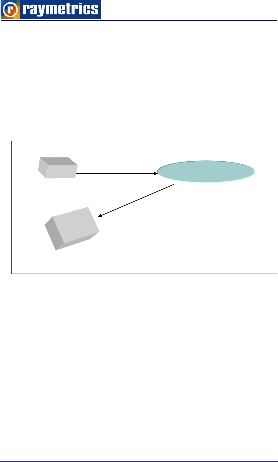
operation a short laser light pulse is transmitted to the atmosphere in one or more
wavelengths (Fig. 2.1).
Fig. 2.1: The principle of operation of the Lidar technique.
The time between the transmission of the laser pulse and the arrival of the
backscattered return signal is directly related to the range at which the scattering occurred.
The most common processes related to laser pulse scattering by the suspended aerosol
particles include the elastic Mie and Rayleigh scattering and the inelastic Raman
scattering2.
The atmospheric volume being probed backscatters the laser radiation and a receiving
telescope is used to collect all the backscattered laser light occurring through elastic and
inelastic processes. Wavelength-separation units are used to spectrally separate the Lidar
signals at various wavelengths and to reject the atmospheric background radiation. The
Lidar signals are then fed to fast detectors (photomultiplier tubes: PMTs). The PMT output
signals after amplification and digitization are sent to a central computer machine for
further processing and storage.
atmosphere
Laser (λ1, λ2)
Telescope + Detector

INTRODUCTION TO THE LIDAR TECHNIQUE
13
The Lidar observations of suspended aerosol particles can be made remotely with high
spatial and temporal resolution using the Lidar technique. The Lidar systems can be
operated from ground or mobile platforms, such as aircrafts, helicopters or satellites.
The basic Lidar equation is given below:
*
z
0
*
2
telo dzza2exp
z
1
zΟAzβ
2
cτ
PzP
(1)
where, P(z) is the power incident on the receiving optics from distance z,
o
P
is the
laser output power, τ is the duration of the laser pulse, c is the velocity of light,
zβ
is the
volume backscattering coefficient,
za
is the extinction coefficient of the atmosphere
and
tel
A
is the receiving telescope aperture.
zΟ
is the so-called geometrical form factor
(or overlap factor). This factor represents the probability of radiation in the target plane at
range z reaching the detector, based on geometrical considerations. The 1/z2 dependence
leads in many applications to a signal-amplitude dynamic range that extends over several
decades. Therefore, two detection modes are used: the analog detection mode and the
photon counting operation mode (paragraph 3.3.2).
The detection of the suspended aerosol particles can be performed by an elastic Lidar
system (single or two-wavelengths) or by an inelastic (Raman) Lidar system. The elastic
backscattered Lidar signals can be inverted using the Klett’s inversion algorithm3, while the
inelastically backscattered Lidar signals can be inverted using the Raman inversion
technique, as presented by Ansmann et al. (1992)4.
LIDAR SUB-SYSTEMS
14
3. LIDAR SYSTEM HARDWARE COMPONENTS
A typical LIDAR contains a transmitter, a receiver, a data acquisition system (DAQ)
and a computer that controls the transmitter and receiver and also stores the acquired
data. A power distribution unit is used to protect and power the various systems. To make
things more operational everything is contained in an industrial enclosure.
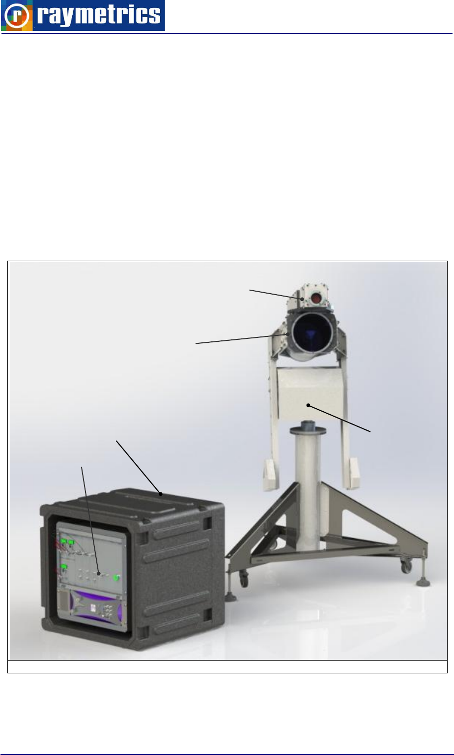
In addition this lidar is a scanning lidar which means that the lidar head (transmitter –
telescope) are separated from the enclosure and placed on a positioner. All these are
mounted on a tripod base.
At the image below a typical Lidar with its main components is illustrated.
Fig. 3. 1: Typical Scanning Lidar
All these components are described in detail below.
Enclosure
Receiver
Transmitter
Electronics
Positioner
LIDAR SUB-SYSTEMS
15
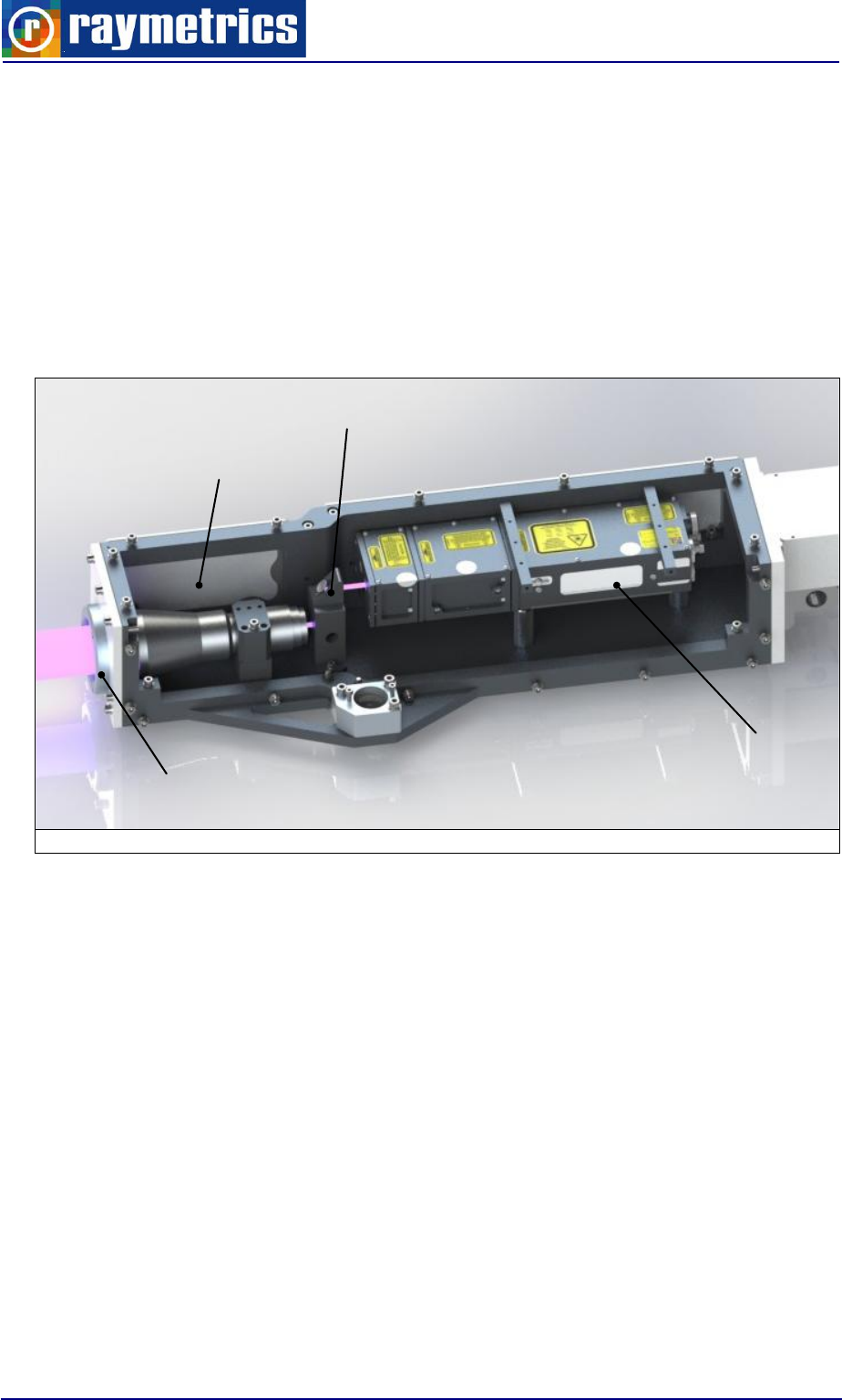
3.1. TRANSMITTER
The Lidar transmitter consists of five sub-units: a laser, a beam splitter, a Beam
expander, a beam trap and a high reflective mirror.
The transmitter along with the light path is enclosed in a case that protects the user
from direct contract with the laser beam and also prevents light to enter the receiver. The
special high energy laser glass (window) with antireflection coating and λ/10 surface
ensures that no dust or humidity enters the emitter enclosure and its high specifications
minimize the emission losses.
Fig. 3. 2: Lidar Transmitter Layout
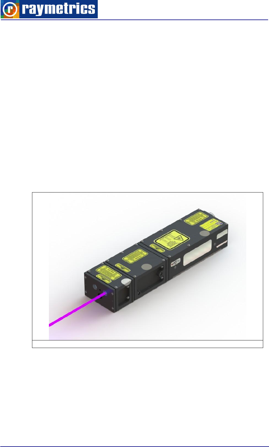
3.1.1. Laser
The laser source used is a water cooled pulsed Nd:YAG laser transmitting short pulses
at 1064nm. The pulse repetition rate is typically 20Hz. The pulse duration is of the order of
6-9 ns. Trough the Second Harmonic Generation (SHG) 532nm wavelength is produced
and through the Third Harmonic Generation (THG) 355nm wavelength is produced. This
specific laser 355nm and rejects the rest. The laser is factory preset for maximum energy
output at its third (THG) frequency (355). Therefore, the user should not change, remove
or alter any of the laser parts or sub-units. The laser consists of two major components:
the optical head and the power supply unit (PSU). They are connected together by power
and signal cables and water hoses for cooling the head. The laser model is a ULTRA100
by Quantel which includes the PSU model ICE450 standard version.
A detailed description of the characteristics, specifications and operation mode of the
laser source is given in the laser’s instruction manual DOC00040.pdf.
Laser
Beam Splitter
Beam Expander
High Transmission Window
LIDAR SUB-SYSTEMS
16
Safety Instructions
The user is requested to wear the laser protective eyewear during the laser
operation. Do not stare into the laser beam even when using your laser protective
eyewear goggles. It may be too dangerous for your eyes!
Do not place any obstacle or reflective object in the transmitted laser beam.
Primary or secondary reflections may damage your eyes or reflected back to the
laser causing damage!
Before you turn off the laser, you should leave the water circulation pump in the ON
position for at least 10-15 min. to cool down the laser optical head.
Always respect the instructions of the laser manufacturer regarding the minimum
number of laser shots requiring the replacement of the laser head flash lamps (see
laser’s instruction manual DOC00040.pdf).
Always respect the instructions of the laser manufacturer regarding the
replacement of the de-ionizing filter/unit of the laser system (see laser’s instruction
manual DOC00040.pdf).
Fig. 3. 3: The laser head
Attention!
Do not stare into the laser beams, even when using your laser protective eyewear
goggles. It may be too dangerous for your eyes!
Do not touch the optical components of the Lidar system (laser mirrors, laser
windows, protective windows, etc.). It may lead to a complete destruction of their
optical coatings and to a misalignment of the Lidar optics.
LIDAR SUB-SYSTEMS
17
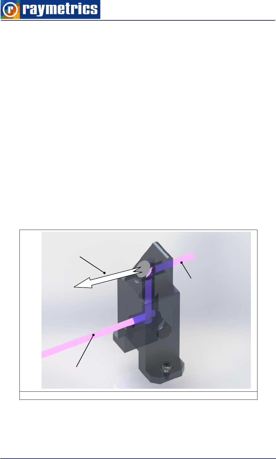
3.1.2. Beam Splitter
As previously noted the laser transmits 355nm and rejects the rest. However there are
still some residuals from the rejected 532nm and 1064nm. In order to comply with the laser
eye safety regulations these residuals must be rejected and for this we use the beam
splitter. The beam splitter is a pair of HR reflective mirrors at 355nm and HT at 532 and
1064. They are mounted at a 45°deg angle on a CNC machined mirror mount. This also
ensures that no reflections return into the laser that could cause permanent damage and
mainly it ensures that only primary wavelength 355nm is transmitted.
The high reflective mirrors (HR) of the Lidar system are conceived to provide a high
reflection (>98%) at the reflected wavelength (355nm) and high transmission at 355nm
and 1064nm due to the special coating on the front side suitable for high laser energy. At
the back side there is antireflection coating to ensure that no back reflection will be
transmitted.
Attention!
The reflective mirrors are aligned during the construction of the Lidar system. This
system is designed so that the mirrors don’t need any alignment. For that reason be very
cautious not to move the HR mirrors, as it may lead on total misalignment of the system.
Fig. 3. 4: The beam splitter
Incoming light
Useful light
Residual light
LIDAR SUB-SYSTEMS
18
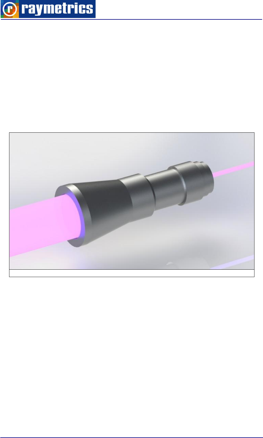
3.1.3. Beam Expander
The beam expander serves tow main purposes; it reduces the light’s divergence and
reduces the energy concentration.
As the name indicates it expands the beam’s diameter by 10 times. With this way the
energy per square centimeter is reduced while the total power remains the same. This is a
smart way to make an eye-safe lidar without reducing its power.
Moreover the beam expander improves the divergence of the laser beam. This means
that it makes the beam as parallel as possible and eventually it improves the maximum
range and the precision of the system.
Fig. 3. 5: Beam expander
LIDAR SUB-SYSTEMS
19
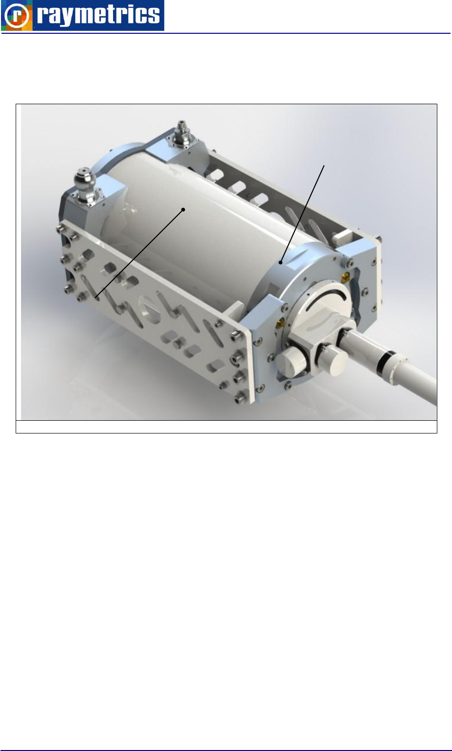
3.2. RECEIVING SYSTEM
The receiving system consists of two sub-units: a receiving telescope (T) and a
wavelength separation unit (WSU) (Fig. 3.6).
Fig. 3. 6: Receiver Components
3.2.1. Telescope
The signal that returns in terms of light is very weak and the only way to amplify it is by
collecting as much light as possible with a telescope. In this LIDAR a powerful 200mm
diameter Cassegrain telescope is used. The primary reflective mirror has a diameter of
200mm and is coated with a durable high reflective coating suitable for the 350-1100 nm
spectral region. The optical material selected shows a very low thermal expansion
coefficient, similar to that of Zerodur® optical properties.
The secondary reflective mirror has a diameter of 48mm and is coated similarly to the
primary mirror. The received Lidar beams are then collected and focused on an Optical
Unit (OU) placed on the telescope’s focal point. At the exit of the OU the Lidar beams are
then collimated by using an achromat technique
Receiving
Telescope
Wavelength
Separation
Unit
LIDAR SUB-SYSTEMS
20
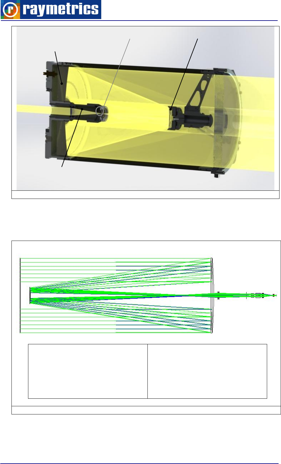
Fig. 3. 7 Telescope main components
Each telescope is thoroughly designed and simulated at Zemax. Each distance is very
critical. A small change can alter the focus of the telescope.
Fig. 3. 8: Telescope Characteristics
Telescope
o Type: Cassegrain
o F4
o Focal Length: 800mm
Primary Diam.: 200mm
Secondary Diam.: 48mm
Primary
mirror
Secondary mirror
Focal Point
Optical Unit
LIDAR SUB-SYSTEMS
21
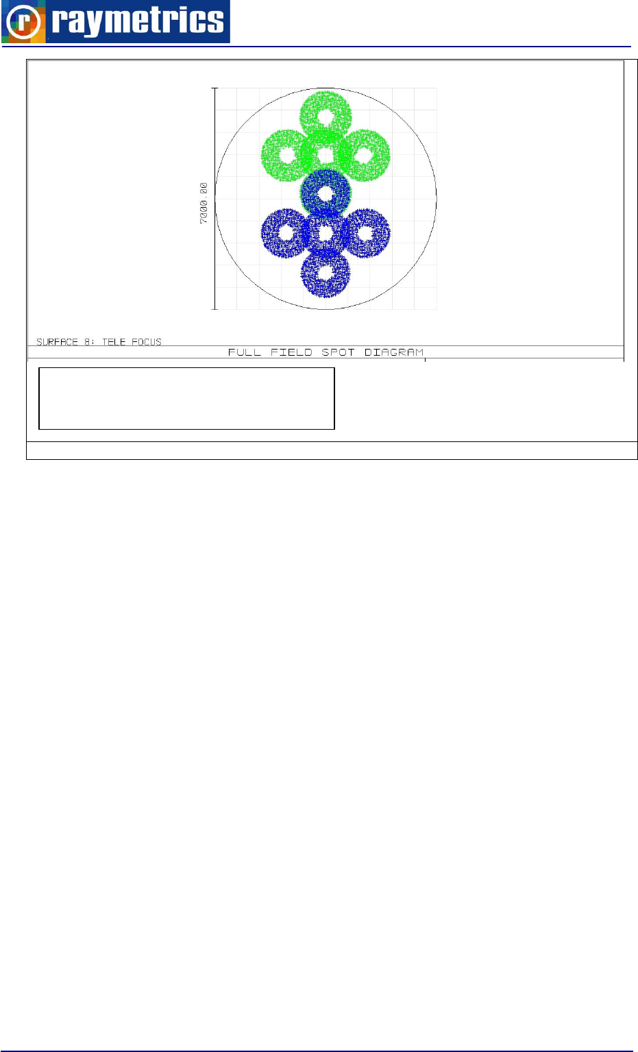
Fig. 3. 9: Typical Light simulation from far and near field at the field stop
The special Telescope glass (window) with antireflection coating and λ/10 surface,
ensures that no dust or humidity will enter the telescope while with its high performance
the Lidar signal remains intact.
3.2.2. Wavelength separation unit
At the entrance of the Wavelength Separation Unit (WSU) of the Lidar system the
received Lidar beams are collimated to one parallel beam. A series of factory preset
custom-made dichroic reflective mirrors and one polarization cube perform the wavelength
separation at the various wavelengths and polarizations received [355P, 355S, 387nm].
At each wavelength exit specially designed interference filters (IFF) are used to select
the Lidar wavelengths and to reject the atmospheric background radiation during daytime
and nighttime operation. The current configuration detects only 355nm but the WSU can
accommodate all three channels (355nmP&S and/or 387nm).
Green : Far Field (25 Km),
Blue : Near Field (0.5 Km)
LIDAR SUB-SYSTEMS
22
Fig. 3. 10: WSU
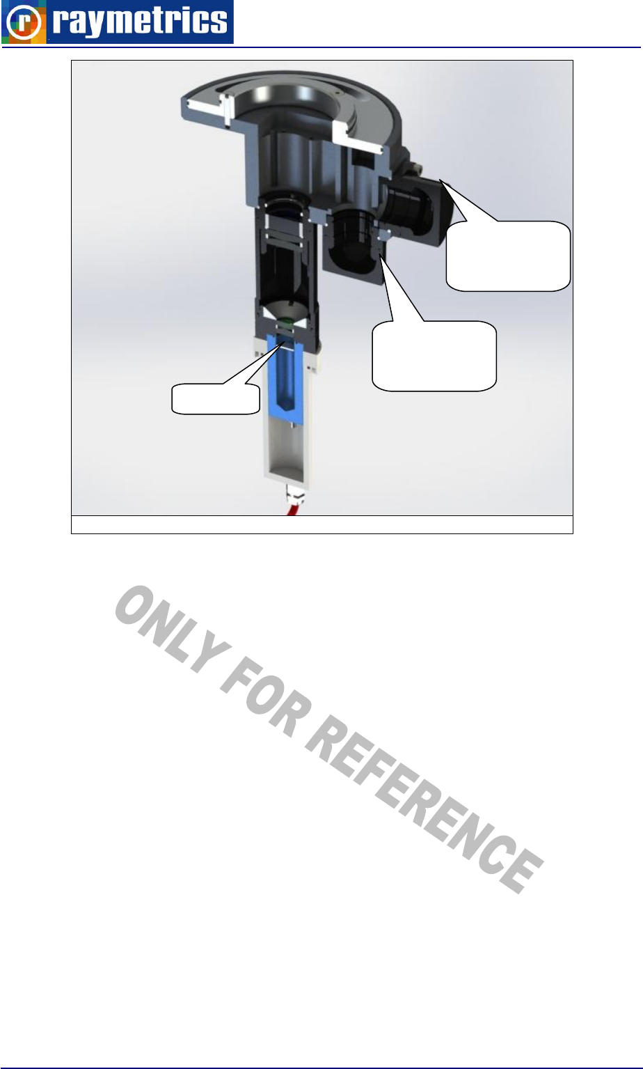
3.2.3. Depolarization Technique
The laser transmits a narrow, fully polarized beam of light in which light waves all
oscillate in the same plane. The receiver measures the polarization of light scattered in the
backward direction. For a cloud of spherical water droplets, the backscattered light is fully
polarized in the same direction as the transmitted beam; i.e., it has only a "co-polarized" or
parallel component. However, for a cloud composed of non-spherical ice crystals, the
backscattered light can be partially depolarized; i.e., it can have a "cross-polarized"
component which vibrates perpendicularly to the transmitted polarization.
This system has the ability to measure simultaneously both the parallel (P) and the
cross-polarized (S) component at the backscatter wavelength which is at 355nm. This is
achieved by separating the parallel and the cross-polarized components, with a
depolarization cube, and each component measured by a PMT. From the combination of
these two signals the user can extract the depolarization ratio. The depolarization ratio can
show the existence of non-spherical particles.
Free Space
for Extra
Channel
355nm
Free Space
for Extra
Channel
LIDAR SUB-SYSTEMS
23
Fig. 3. 11: Depolarization Module
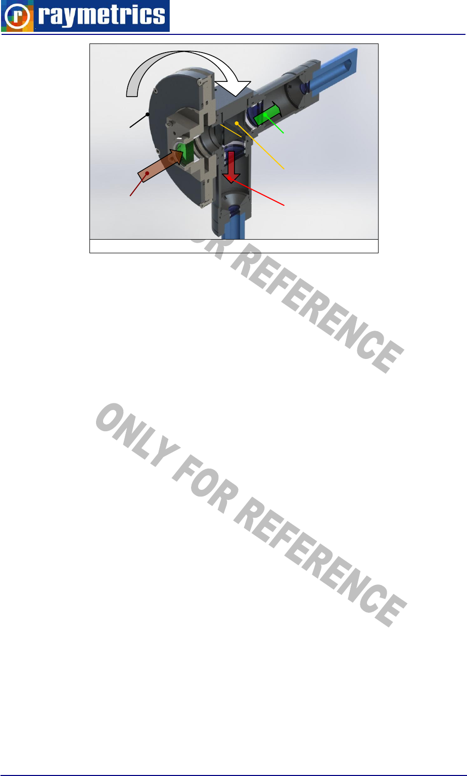
In order to calculate the depolarization ratio the user has to calculate the depolarization
calibration constant. This constant depends on various things such as the atmosphere the
temperature and the system itself, thus it is impossible to calculate this analytically. More
specifically this is measured by comparing measurements taken with the depolarization
module turned at ±45° degrees around the normal position. When the depolarization
module is turned the parallel signal is decreased and the cross is increased.
The swivel unit is machined in CNC mills from one part so that the best precision is
achieved even when it is turned. Moreover the sophisticated design makes this procedure
as easy as possible. The procedure can be outlined in three steps.
1. Pull the pins A and B shown in the image below.
2. Turn the depolarization module slightly, release the pins and turn at 45 degrees until
you hear a clicking sound from the pin.
3. Now you can start the measurement.
If the rotation is not very easy you may have to loosen the screws located at the other
side of the swivel unit.
Depolarization
Cube
Parallel
polarized
light
Cross
polarized
light
Incoming
light
Swivel
Unit
LIDAR SUB-SYSTEMS
24
Fig. 3. 12: WSU ±45° polarization calibration procedure
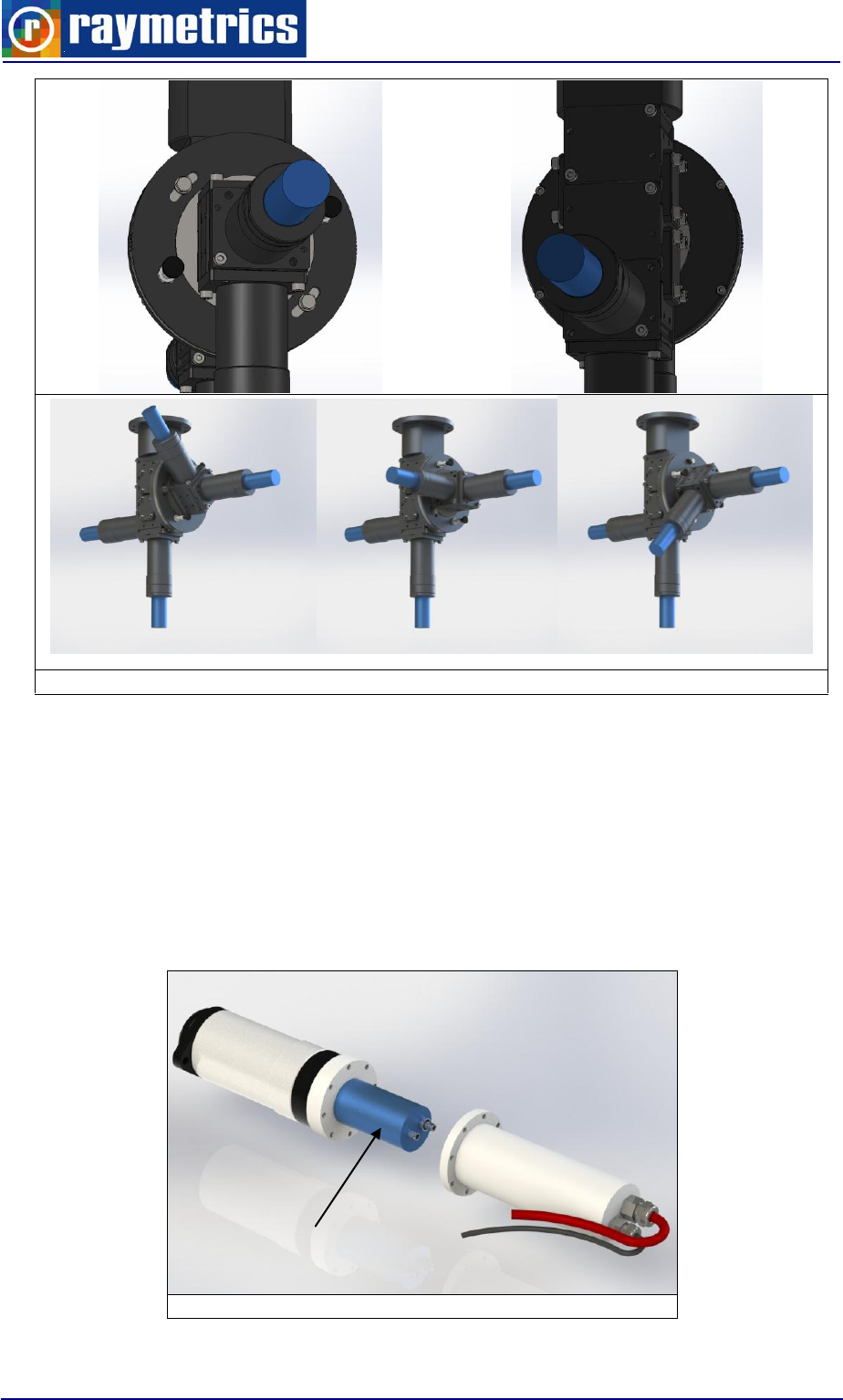
3.2.4. Light Detectors
The light is detected from the photomultiplier tubes (PMT) and converted into a signal
that goes to the detection electronics. The electronics are synchronized with the laser
control and the signal is recorded in relation to the time. The electronics communicate via
Ethernet with the PC where the data are saved. The detection electronics are presented at
paragraph 3.3.2. The detectors along with the electronics are called Signal Acquisition Unit
(SAU).
Fig. 3. 13: WSU and PhotoMultiplier Tubes (PMT).
+45° deg
0° deg
-45° deg
Detector
LIDAR SUB-SYSTEMS
25
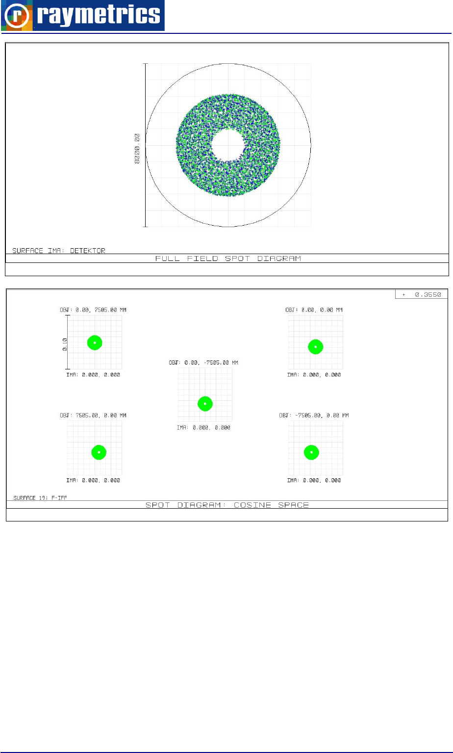
Fig. 3. 14: Image of the Cathode for 355 nm
Fig. 3. 15: Max Angle for IFF 355 : typ 1.54 degrees
The spectrally resolved Lidar signals inside the WSU are detected by photomultiplier
tubes (PMTs) directly mounted at the respective exits of the WSU. The PMTs used are
selected to be compact and to provide optimum operation in the spectral range 355-532
nm. The PMTs work in the pulse mode regime and are characterized by a short rise time
constant.
The PMTs have been tested prior to shipment. The PMTs optimum working voltage (for
linear operation) is between 750-900V, depending on the amplitude of the received signal
and the atmospheric conditions (background skylight conditions during daytime or
nighttime conditions and/or cloud presence). Usually, during daytime conditions the PMT
working voltage is slightly lower than during nighttime operation.

LIDAR SUB-SYSTEMS
26
Technical Specs
Part Number
R9880U-110
PM Type
Hamamatsu
PM High Voltage (V)
0-1000
Supply Voltages (V)
+15
Current Limit (mA)
200
Resistance Anode-GND (Mohm)
1.0
Output Connector
BNC (50 Ohm)
All the details for your PMTs are inside Licel printed manual.
Attention!
For optimum operation the temperature and humidity conditions should be kept
unchanged during field operation.
Operation at HV higher than 900 V should lead to PMT saturation, thus to a non
linear operation and/or possibly to PMT permanent failure.
Reed carefully below the environmental conditions of the PMTs.
Humidity: Operation in a very damp atmosphere may lead to insulation problems,
because of the high voltages (HV) used. Condensation gives rise to leakage currents
which in turn increase the PMTs dark current. Therefore, the PMTs should be operated
under the environmental conditions given in Licel’s user manual.
Light conditions: The PMTs are highly sensitive to ambient light conditions; therefore
never expose the PMTs to ambient light, even when no HV is applied. If high voltage is
applied to the PMTs which are exposed to ambient light, the PMTs are permanently
destroyed.
Mechanical stress: Like all electronic devices, PMTs should be protected against
mechanical and thermal stress. Vibration or shock transmitted to the PMT dynodes can
modulate the PMTs gain.
Magnetic fields: Never expose the PMTs to magnetic fields, even as weak as the
earth’s one. They may affect the PMT’s performances. Strong fields may permanently
magnetize some parts of the PMTs, thus affecting their performance.
LIDAR SUB-SYSTEMS
27
3.3 CONTROL UNIT
The control unit consists of four main components; the laser control and power supply
(ICE450 standard version), the transient recorders and PMT power supply, the PC and the
electrical cabinet.
3.3.1 Laser control and power supply
This device controls all the functions of the laser and supplies the laser head with
power and deionised water.
Fig. 3.16:
Laser power supply and
controller
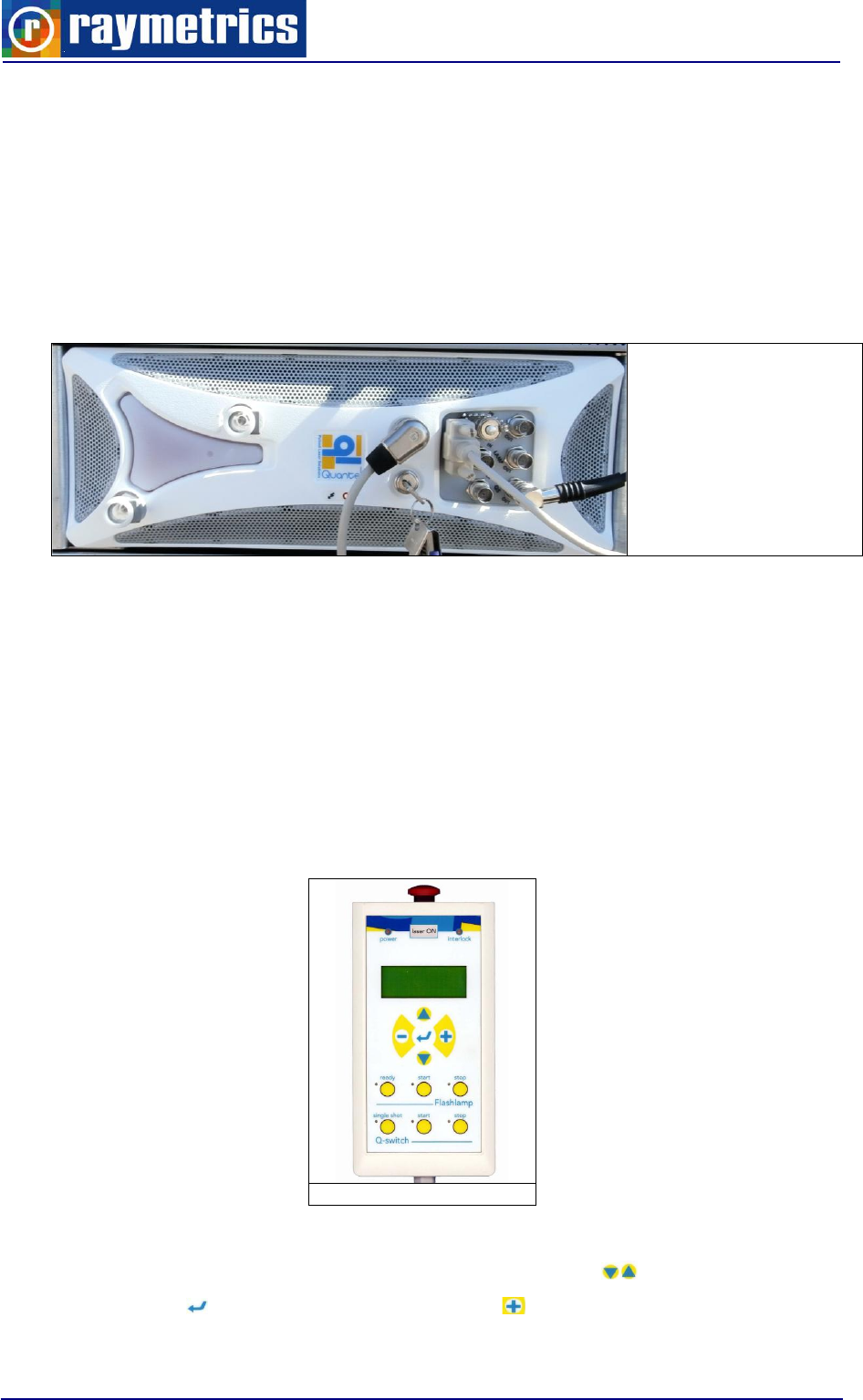
3.3.1.1. Control
Through the control the user can operate the laser and check its status. The operation
mainly is the flashlamp/Q-switch start and stop and the Q-switch delay (that reduces the
laser beam energy). Regarding the status the user can obtain various information about
the laserhead such as the counted number of shots, the temperature, the flow of the pump
etc. All interlocks appear at the control with a short explanation.
The device has two interfaces; one remote control box and a RS232 that is connected
to the PC. That means that user can control the laser either from the control box or the PC.
Fig. 3.17: Control Box
Note that in order to control the laser from the PC the user has to switch manually from
the control box the serial link. In order to do that navigate with choose “System Info”
and validate with . Choose serial link and with the button change the status from “off”
LIDAR SUB-SYSTEMS
28
to “on”. Each time the user presses a button on the control box the serial link automatically
turns to “off”.
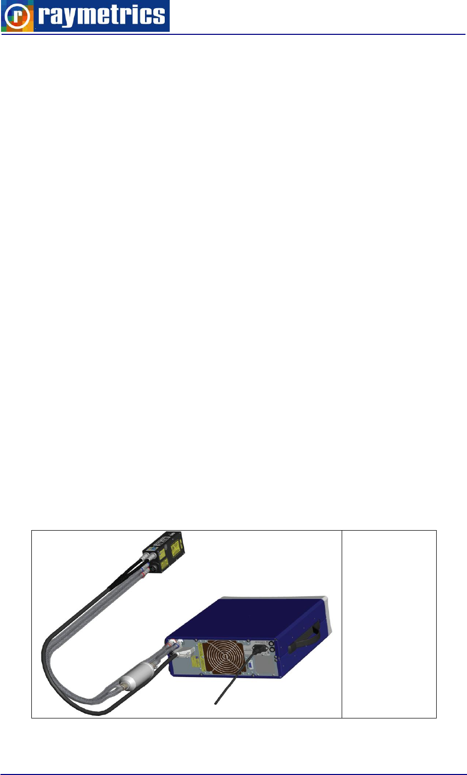
3.3.1.2. Power and water Supply
The laser apart from the power supply needs water supply as well since the head is
water cooled. This is achieved from an individual unit inside the ICE450 called Coolant
Group Unit (CGU). The CGU cools the flashlamp(s) and the laser rod with a closed loop of
de-ionized coolant. This temperature regulated coolant also provides thermal stabilization
of the oscillator's structure.
A thermostatic electronic circuit, which regulates the fan's speed and airflow rate
through the exchanger, provides thermal stabilization of the coolant. The temperature
stabilization is within ± 1 °C. The ambient air temperature can range from 15 °C to 28 °C
with no effect on laser operation.
The CGU includes a de-ionizing system that, with proper maintenance, can maintain
the conductivity of the coolant at less than 1.0 μS⋅cm-1 (resistivity ≥ 1.0 MΩ⋅cm). The
CGU has coolant level, flow, and heat-sensing switches to interlock with the Power Supply
Unit to prevent damage to the laser head in the event of a cooling system failure.
The CGU requires approximately 1.5 liters (0.4 US gal.) of coolant for standard
systems incorporating three-meter coolant lines. Use only distilled water with 1MΩ-cm
to 5MΩ-cm resistivity. The water is transferred to the laserhead though two hoses which
are along with the power and signal cords components of the umbilical cord. Even though
the CGU contain a powerful pump, if the umbilical cord is bended above a certain level
then an interlock will appear and the laser will not operate. For further information refer to
laser’s manual.
Fig. 3. 18:
Control Unit
With coolant
hoses, power
and signals
cables.
LIDAR SUB-SYSTEMS
29
3.3.2 Detection electronics
The detection electronics receive a analogue signal from the PMTs and transform it to
a Lidar signal. This device is designed to work in two modes: the analog detection mode
and the photon counting detection mode.
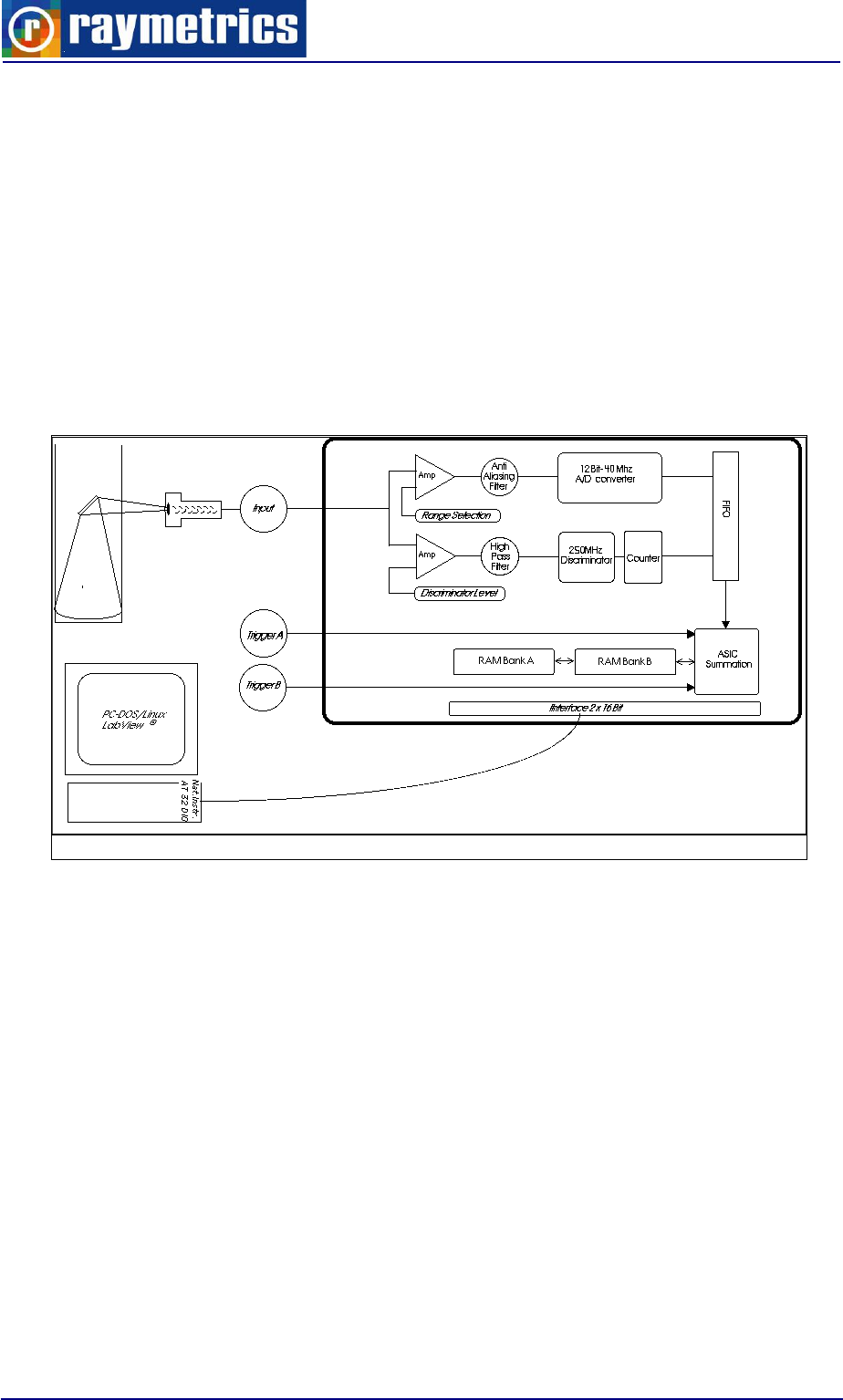
3.3.2.1. Concept
The Licel transient recorder is a powerful data acquisition system, especially designed
for remote sensing applications. To meet the demanding requirements of optical signal
detection, a new concept was developed to reach the best dynamic range together with
high temporal resolution at fast signal repetition rates.
Fig. 3. 19: Electronics concept
For the first time analog detection of the photomultiplier current and single photon
counting is combined in one acquisition system. The combination of a powerful A/D
converter (12 Bit at 40 MHz) with a 250 MHz fast photon counting system increases the
dynamic range of the acquired signal substantially compared to conventional systems.
Signal averaging is performed by specially designed ASIC's which outperform any CISC-
or RISC-processor based solution. A high speed data interface to the host computer allows
readout of the acquired signal even between two laser shots. At figure 22 the connectivity
of the transient recorder is explained. The implementation of this concept makes the Licel
transient recorder the state of the art solution for all applications where fast and accurate
detection of photomultiplier, photodiode or other electrical signals is required at high
repetition rates.
LIDAR SUB-SYSTEMS
30
3.3.2.2. Principle of operation
The Licel transient recorder is comprised of a fast transient digitizer with on board
signal averaging, a discriminator for single photon detection and a multichannel scaler
combined with preamplifiers for both systems. For analog detection the signal is amplified
according to the input range selected and digitized by a 12-Bit-20/40 MHz A/D converter. A
hardware adder is used to write the summed signal into a 24-Bit wide RAM. Depending on
whether trigger A or B is used, the signal is added to RAM A or B, which allows
acquisitions of two repetitive channels if these signals can be measured sequentially.
At the same time the signal part in the high frequency domain is amplified and a 250
MHz fast discriminator detects single photon events above the selected threshold voltage.
64 different discriminator levels and two different settings of the preamplifier can be
selected by using the acquisition software supplied. The photon counting signal is written
to a 16-Bit wide summation RAM which allows averaging of up to 4094 acquisition cycles.
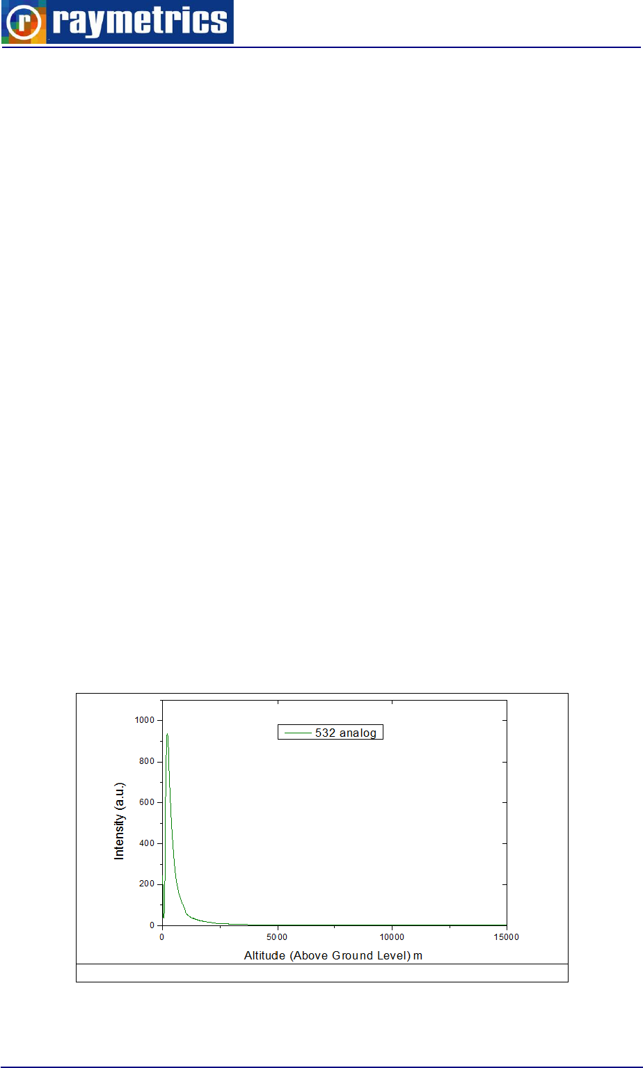
3.3.2.3. Analog detection
The analog detection mode is used to detect intense Lidar signals coming from
relatively short distances (typically less than 8-10 km). A transient recorder operating in the
analog detection mode is based on an analog-to-digital converter (ADC), which samples
and digitizes the Lidar signals with a sampling rate of 20-40 MHz (depending on the type of
the transient recorder used) with a 12-bit resolution. A memory length up to 8192 or 16000
time bins (Tr-xx-80 or Tr-xx-160) depending on the transient recorder type) can be
selected. Each time bin corresponds to a spatial resolution of 3.75 or 7.5 m (depending on
the sampling rate of the transient recorder used, Tr-20-yy or Tr-40-yy). For instance the 20
MHz sampling rate corresponds to a 7.5 m spatial resolution.
Fig. 3. 20: Typical Lidar signal acquired in the analog mode.
LIDAR SUB-SYSTEMS
31
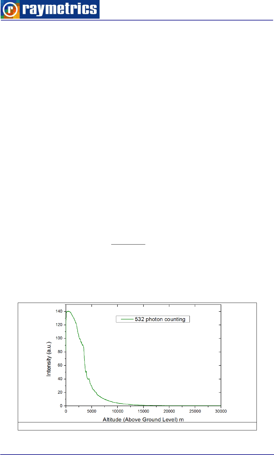
3.3.2.4. Photon counting detection
The photon counting detection mode is used to detect very low intensity Lidar signals
coming from relatively large distances (typically higher than 8-10 km). Thus, the PMT is
operated under single electron conditions. Flux levels as low as a few tens of photons per
second can be measured. In the photon counting mode the level of the incident flux is such
that the cathode transmits only single electrons. The individual anode charges due to
single photons are integrated to produce proportional voltage pulses, which are passed by
a discriminator to a pulse counter, whose output over a pre-set time period is a measure of
the incident flux.
Because of statistical fluctuations in the electron multiplication, the amplitude of the
single-electron pulses is distributed according to the Poisson statistics. To obtain a
satisfactory signal-to-noise ratio (SNR) of the Lidar signal in the photon counting mode, a
sufficiently large number of laser shots should be obtained (normally more than 1000). If
the received Lidar signal is higher than 60-100 MHz the PMT output signal should be
corrected to take into account the dead-time effect. If the dead-time of the counter (τd) is
comparable to the mean interval separating two successive pulses, the counting error may
be appreciable. If a dead-time correction has to be applied, then if the Nobs is the observed
count rate, then the true count rate (Ntrue) corrected for the dead-time effect is given by:
dobs
obs
true N
N
N
1
(2)
Note: The value of τd depends on the type of the PMT module used (i.e. τd = 4 ns).
Specific environmental effects may increase or decrease the count rate. For instance,
background radioactivity increases it.
Fig. 3. 21: Typical Lidar signal acquired in the photon counting mode.

LIDAR SUB-SYSTEMS
32
3.3.2.5. Signal processing
The Lidar data processing is fulfilled in two steps: (i) Lidar data pre-processing and (ii)
Lidar inversion algorithm, which are explained hereafter.
Step I- Lidar data pre-processing
The Lidar data pre-processing is performed on the raw Lidar signals. Each Lidar data
file (containing the average of a certain number of backscattered Lidar signals S(z) coming
from a distance z) is corrected for the background noise contribution (BG) due to
atmospheric skylight and electronic noise of the instrumentation used. A distance square-
law correction (z2) is applied to each data point (time bin) to compensate for range-related
attenuation from the atmosphere. Then, the natural logarithm of the resulting quantity is
calculated. On the resulting log range-corrected signal SLOG where
2
zBGzSlnSLOG
, a running low-pass derivative digital filter, with variable path is
applied. The smoothing method is a running least-square fit of the dataset to the second-
order polynomial, which represents a good fit for the vertically decreasing atmospheric
scale height (Ancellet al., 1989)1. The spatial resolution of the measurement is related to
the number 2n+1 of data points fitted to the second-order polynomial.
Step II- Lidar inversion algorithm
To retrieve the vertical profile of the aerosol backscatter coefficient (baer) at 532 nm the
improved Klett inversion technique is used. This technique is based on a far-end backward
iterative technique, taking into account also the atmospheric molecular contribution as
described by Klett (1985)3. The uncertainties associated with this technique have been
discussed in detail by Chazette et al.(1995)5 and by Boesenberg et al. (1997)6, while the
limitations of this technique arise from an ill-posed mathematical problem (one set of
signals measured with two sets of parameters to be retrieved: the aerosol extinction and
backscatter coefficients) in conjunction with the a priori assumptions made for the Lidar
inversion, such as the fixing of the ‘reference height’ (where the atmosphere is purely
molecular), and of the so called aerosol ‘Lidar ratio’ LR where
11
1
srkm
kma
srLR
aer
aer
.
At 355 nm the inelastically backscattered Lidar signals can be inverted using the
Raman inversion technique, as presented by Ansmann et al. (1992)4. This technique is
applicable mostly under low light conditions (during early evening and nighttime) since the
Raman Lidar signal is sensitive to the presence of daytime background skylight.
LIDAR SUB-SYSTEMS
33
Fig. 3. 22: Transient Recorders and High-Voltage power suppliers of the PMTs.
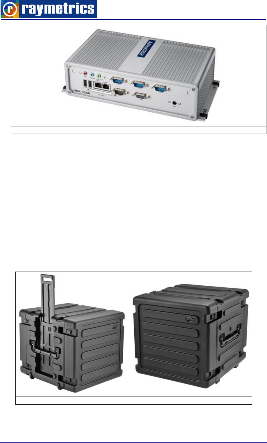
3.3.3 Industrial Computer
The LIDAR system uses an industrial touch panel computer as a Controlling Unit,
which features industrial grade robust mechanical design and reliability. All LIDAR
subcomponents (LASER, DAQ) can be controlled from this Unit. Controlling Unit also acts
as storage unit and as a communication interface as well.
Features
The ARK3360L Embedded Box Industrial Computers are state-of-the-art Human
Machine Interfaces with Intel Atom processors 500 Series with Intel 82801HM I/O
Controller and the following key features:
Fanless
By using a low-power processor, the system does not have to rely on fans, which often
are unreliable and causes dust to circulate inside the equipment.
Windows CE Support
In addition to the OS support of Windows XP, Advantech offers platform support for
WES7 and Windows XP embedded. The optional Windows CE operating system,
specifically for Industrial Touch Panel Computers is also available.
Energy Star Certified
PMT
High
Voltage
Power
Supply
Device
Transient
Recorder
Device
LIDAR SUB-SYSTEMS
34
Fig. 3. 23: Advantech Industrial Computer
3.3.4 Electrical Cabinet
The electrical cabinet is separated from the Lidar head and provides protection for the
electronics. It contains the laser power supply the Licel electronics and the industrial
computer. Furthermore it communicates with the Lidar head through an umbilical cord
which can be separated for the transportation.
Having two doors one in front and another on back, the electrical cabinet provides easy
access to every component.
The cabinet is made from molded plastic that makes it robust and lightweight. It is also
shock and water resistant. The side latches hold the lids firmly and are very easy to
release. Finally with the build-in wheels, the low profile pull handle and the side handles
the enclosure is very easy to lift and transport.
Fig. 3. 24: Electrical Cabinet
LIDAR SUB-SYSTEMS
35
3.3.4.1 Features
Weather protection
Internal heater
Fans for air circulation
Easy access to all components
Castors and handles for easy transportation
Door locks
Robust and lightweight
Connectors and plugs for quick connection
Energy box with circuit breakers for every part
Embedded industrial Ethernet switch
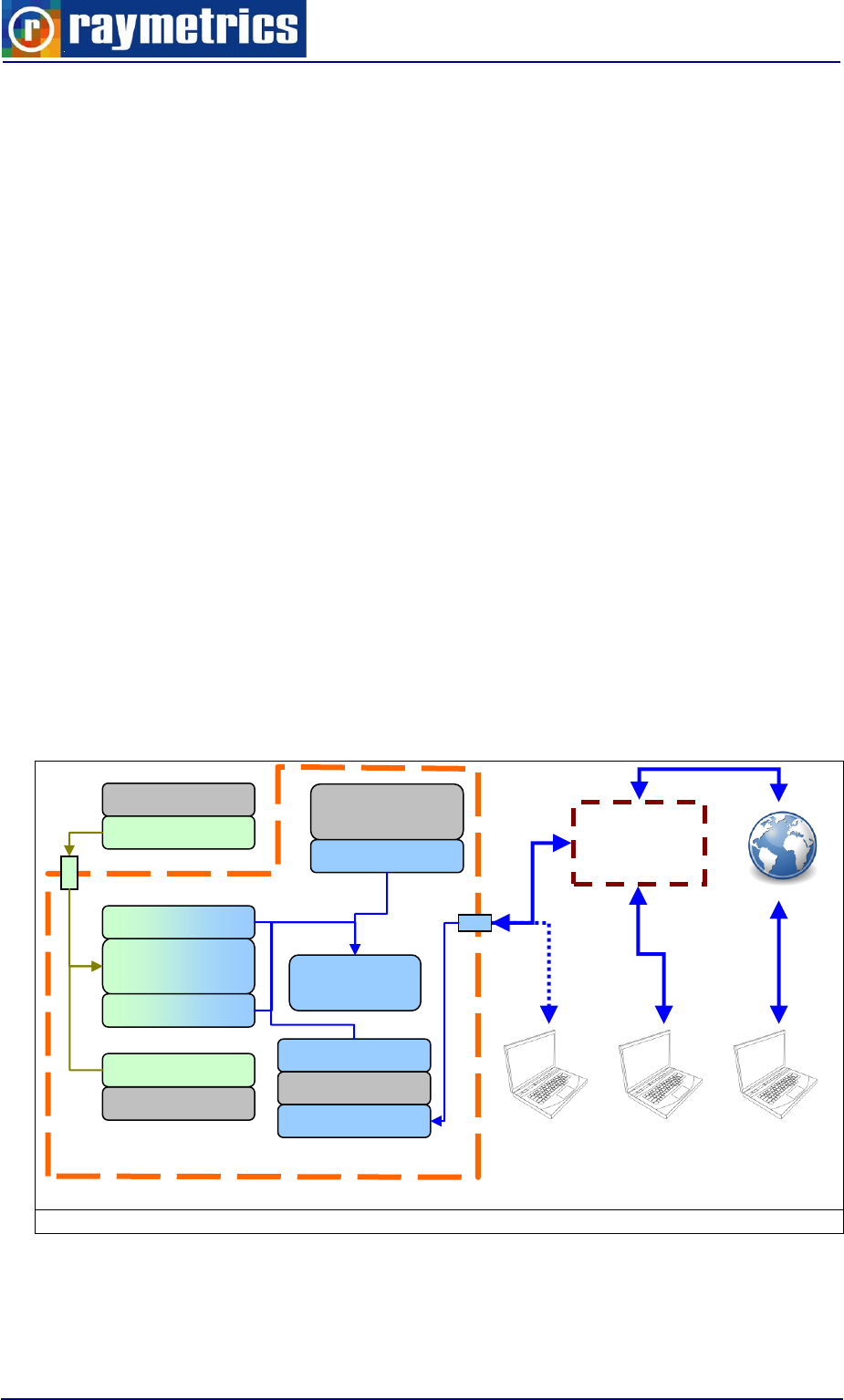
3.3.4.2 Connections
The Licel transient recorder communicates with the PC VIA an Ethernet network with
the PC and to an external host. By default the network IP is set as shown in figure below.
The user can easily connect to the Lidar and control remotely the instrument simply by
using windows remote desktop. As illustrated below the internal computer has two
Ethernet ports. One is used from the Lidar Local Network while the other is connected to
the external Ethernet socket. This gives the option to connect in a local network (LAN) or
directly to another computer with a cross link cable. If the local network gives access to
this computer through the firewall, then it can be reached from anywhere in the word.
At the image below the connections between all components are shown.
Fig. 3. 25: LIDAR Local Network
The transient recorders are externally triggered from the ICE450 through a BNC cable.
The laser creates TTL pulse to trigger the flashlamp for every shot. In order to achieve the
maximum energy the Q-switch needs to have a small delay with the Flashlamp which is
DAQ
ELECTRONICS
LASER
POSITIONER
10.49.234.230
COM5
COM6
COMPUTER
192.168.X.X
10.49.234.234
ETHERNET
SWITCH
SERIAL TO
ETHERNET
10.49.234.231
10.49.234.232
LOCAL (LIDAR) NETWORK
External
Network
192.168.X.X
EXTERNAL
REMOTE
COMPUTER
DIRECTLY
CONNECTED
COMPUTER
EXTERNAL
NETWORK
COMPUTER
LIDAR SUB-SYSTEMS
36
factory preset for optimum energy, however the user can increase the delay to reduce the
energy. For this reason another TTL pulse is produced to trigger the Q-Switch with the
required delay. The transient recorders need to be triggered from the Q-Switch TTL pulse,
so that the laser emission is synchronized with the acquisition start time.
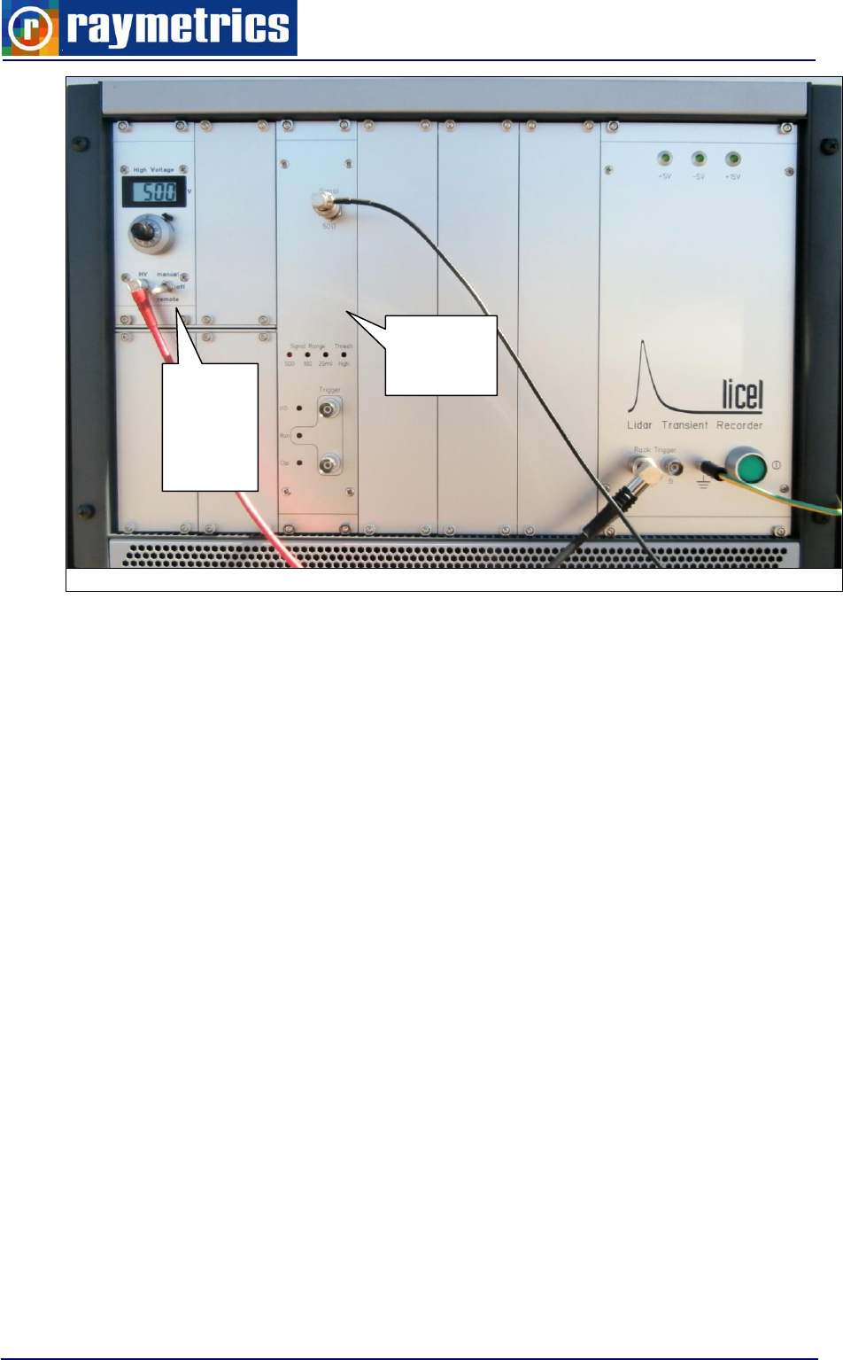
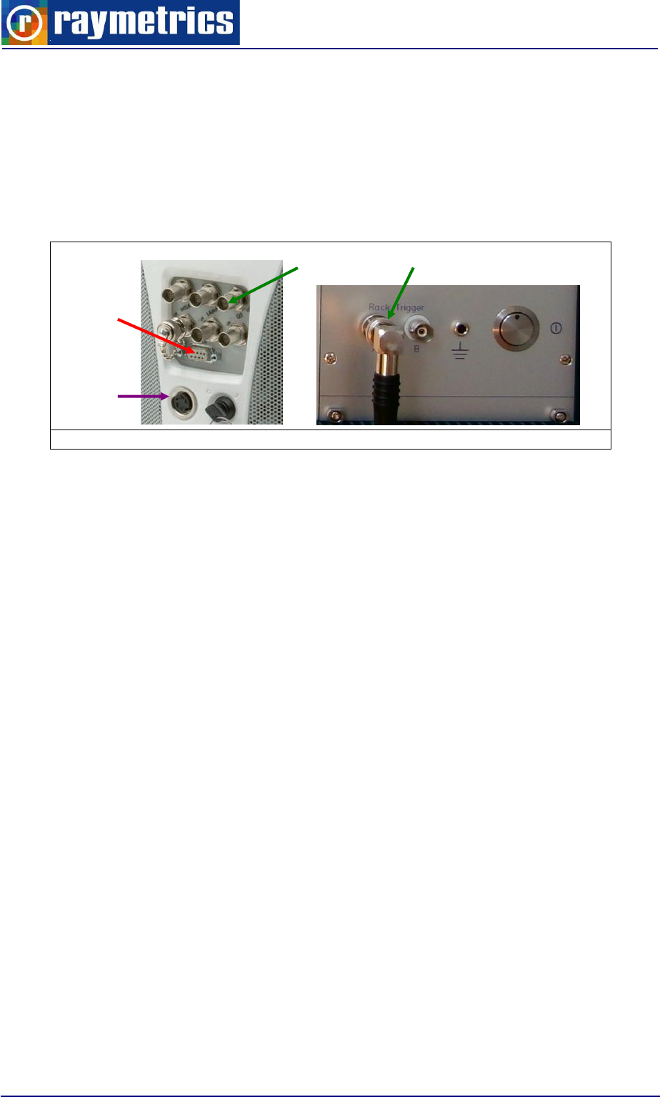
As shown in the image below default connection is at memory A on Transient recorder
and at “QS OUT” on the laser.
Fig. 3. 26: Trigger Connection
There are also two trigger inputs for the Transient recorder and there are several
outputs and inputs for the laser. These are for triggering externally or using the flashlamp
TTL pulse to trigger something. How to use these features is explained in A1 HOW TO
CONTROL THE LASER
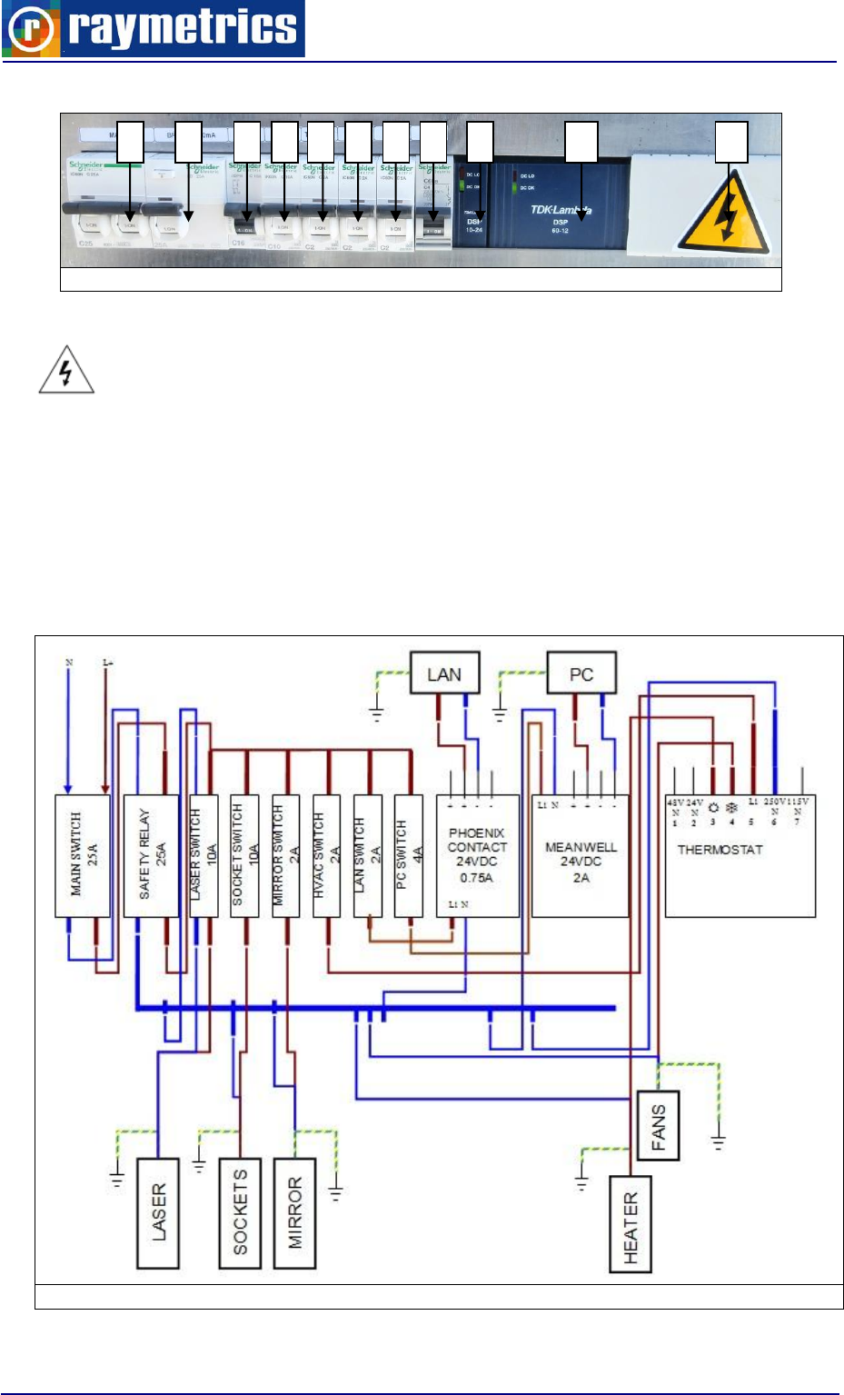
3.3.4.3 Electrical drawing
The electrical cabinet has a power distribution unit which contains the switches for the
components of the control unit. Furthermore inside there is the thermostat which is
covered for protection but the user can remove the cover strip in order to set the
temperature of the thermostat.
1. “Main” Switch. This gives power to the rest of the components.
2. Circuit protection breaker 30mA. In case of a short circuit this will automatically shut
down the mains.
3. “Laser”. Switch for the laser.
4. “TR” Switch for the Transient recorder and PMT power Supply
5. “Tracker” Switch for the positioner.
6. “HVAC”. Switches on the Ventilation Fans or the Heater.
7. “LAN”. Switch for the power supply [11] of the industrial Ethernet switch.
8. “PC”. Switches the power supply [12] of the panel computer.
9. PSU for the Industrial Ethernet switch
10. PSU for the Industrial Panel Computer
11. Thermostat (Beneath Cover)
Q-switch out
Rack trigger A
Remote
control
box
RS232
serial
port
LIDAR SUB-SYSTEMS
37
Fig. 3. 27: Energy box
WARNING – HIGH VOLTAGE: Do not operate the Lidar without the protective
cover. Keep away from liquids. Electric shocks could lead to serious injury or
even death.
To set the desired temperature on the thermostat unplug the instrument and remove
the plastic cover next to item 10 in Fig. 3. 27.
At the figure below is shown a simplified electrical drawing of the power distribution
unit. Note that this is only for reference. Do not apply any changes before consulting us.
Fig. 3. 28: Wiring Diagram
5
6
7
8
9
10
11
1
2
3
4
LIDAR SYSTEM SOFTWARE
38
4. LIDAR SYSTEM SOFTWARE
The Lidar comes with a series of software programs. These can be grouped in three
main categories; Operating, post processing, tools. Operational software are used to
acquire the Lidar raw data, the post processing is used to analyze the raw data and the
tools are used for maintaining the Lidar in it’s peak performance, customization and
diagnostics.
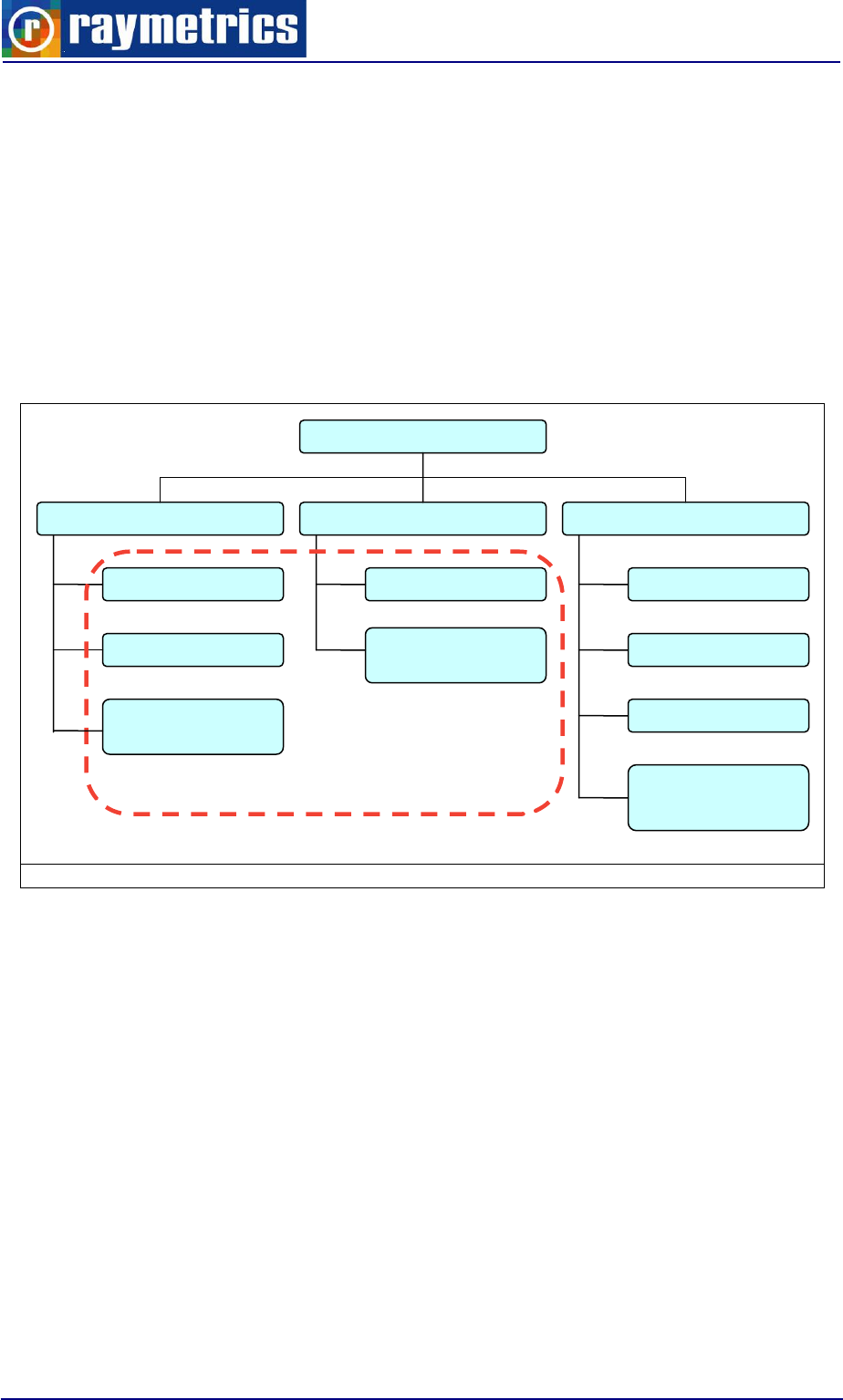
Below is a diagram with some of the basic software modules.
Fig. 4.1: Software Modules
The data from the measurements (raw data) are saved in a database. This database is
shared with the analysis software which can also edit it. It is important to understand how
this database works so that the measurements are registered normally. You can create
more that one databases but keep in mind that the data are bulky and not easy to handle.
All raw data in one database are saved in one folder with a unique datalog file which
contains all information for the records (measurements).
In the next paragraphs are presented the main software modules. Use this only as a
reference, some features may not be available in you system. Refer to the applications
user manual for further information.
APPLICATIONS
OPERATING
POST PROCESSING
TOOLS
SCHEDULER
ACQUISITION
ANALYSIS
ALIGNMENT
LASER
CONTROL etc.
PMT CONTROL
CONFIG. SW
DATABASE
SCANNING
AUTONOMOUS
SCANNING
ANALYSIS
LIDAR SYSTEM SOFTWARE
39
4.1. OPERATION SOFTWARE
As previously noted the operation software is used to acquire the Lidar data. In other
words this program will start, stop and save a measurement. This means that the software
controls the devices that are used for the measurement and data logs the output of the
measurement. Raymetrics has combined all different software from each device in a single
program to make the process of measurement as easy as possible.
The acquisition software simultaneously does the following:
Transient recorders control
PMTs control
Laser control
Data logging
While the scheduler gives the user the ability to schedule a series of weekly
measurements.
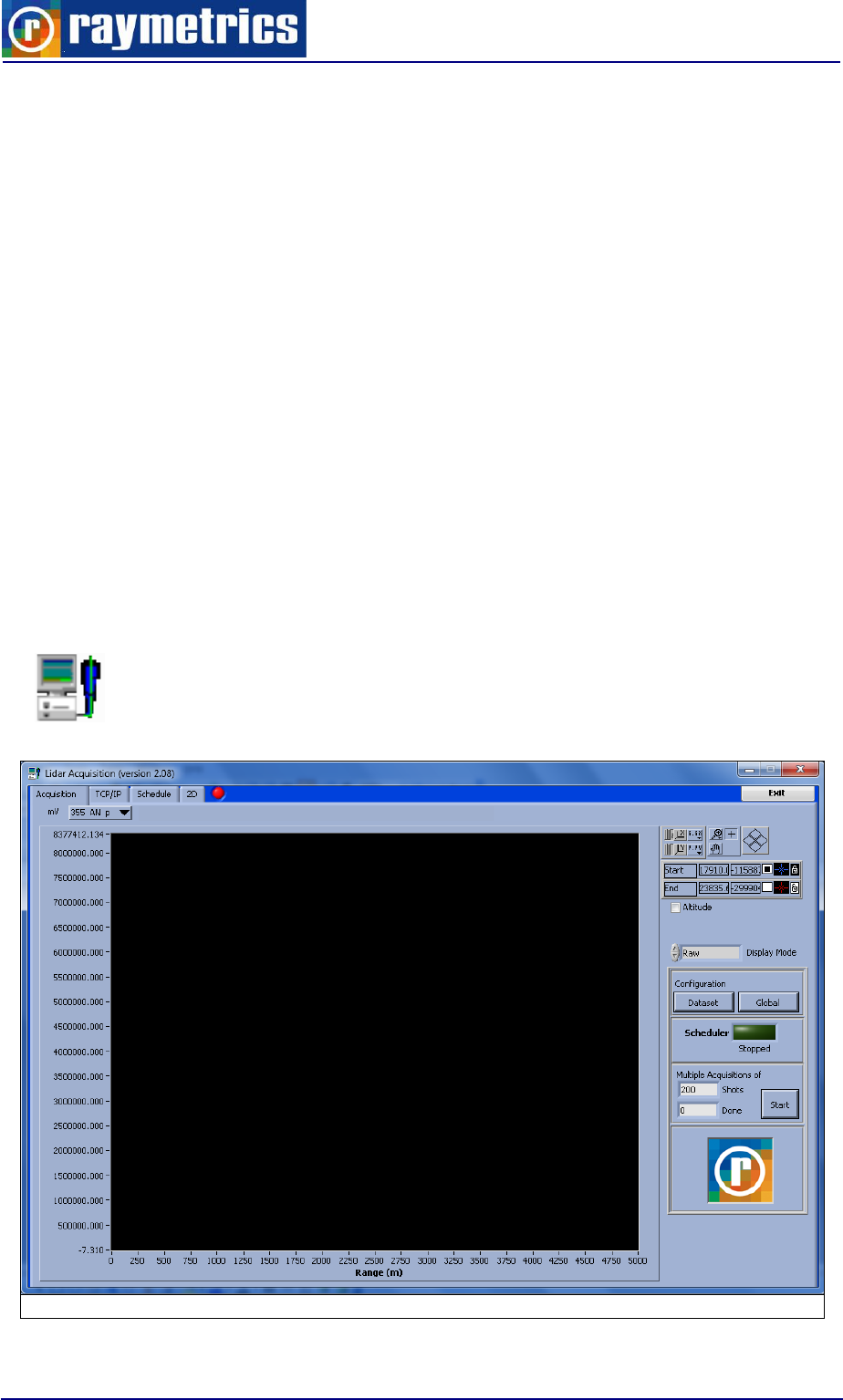
4.1.1 Acquisition
The acquisition program is the most important program for the Lidar. Knowing
how to acquire good Lidar data is more important than analysing the data, as the
operator will not miss any data. Below is the interface of “Lidar Acquisition.exe”.
Fig. 4.2: Lidar Acquisition.exe
LIDAR SYSTEM SOFTWARE
40
The GUI contains three main tabs. The Acquisition tab the TCP/IP tab and the 2D Tab.
Here only the Acquisition tab is presented which is the main one. The TPC/IP is used only
for the configuration of the connection with the transient recorder while the 2D tab shows a
2D graph of the time evolution of the acquired measurements.
The main features in the Acquisition tab are:
a graph that displays in real time the acquired profiles
various controls for the graph
two configuration buttons “Dataset” and “Global”
and a Star/Stop button
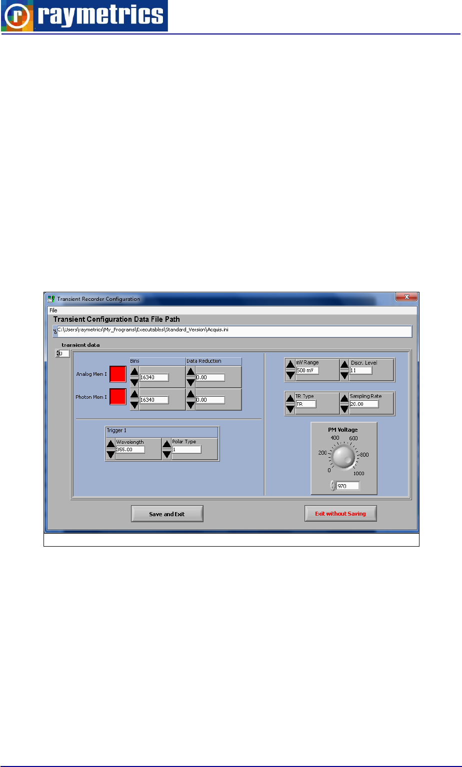
The dataset button opens a new window that allows you to set the parameters for each
channel. Below is presented the interface and the main parameters.
Fig. 4.3: Dataset window
On the menu under File there is the option to load and save a configuration file. Below
the selected file is shown. Next to the Transient Data frame there is a numeric control that
indicates the selected device
The parameters and settings here are:
Memory selection button and measurement size for Analog and Photon counting
separately.
TR parameters such as mV range, TR type and sampling rate.
LIDAR SYSTEM SOFTWARE
41
PMT high voltage setting. This not only sets the header file but also sets the
desired voltage to be used for the specific PMT throughout the measurement.
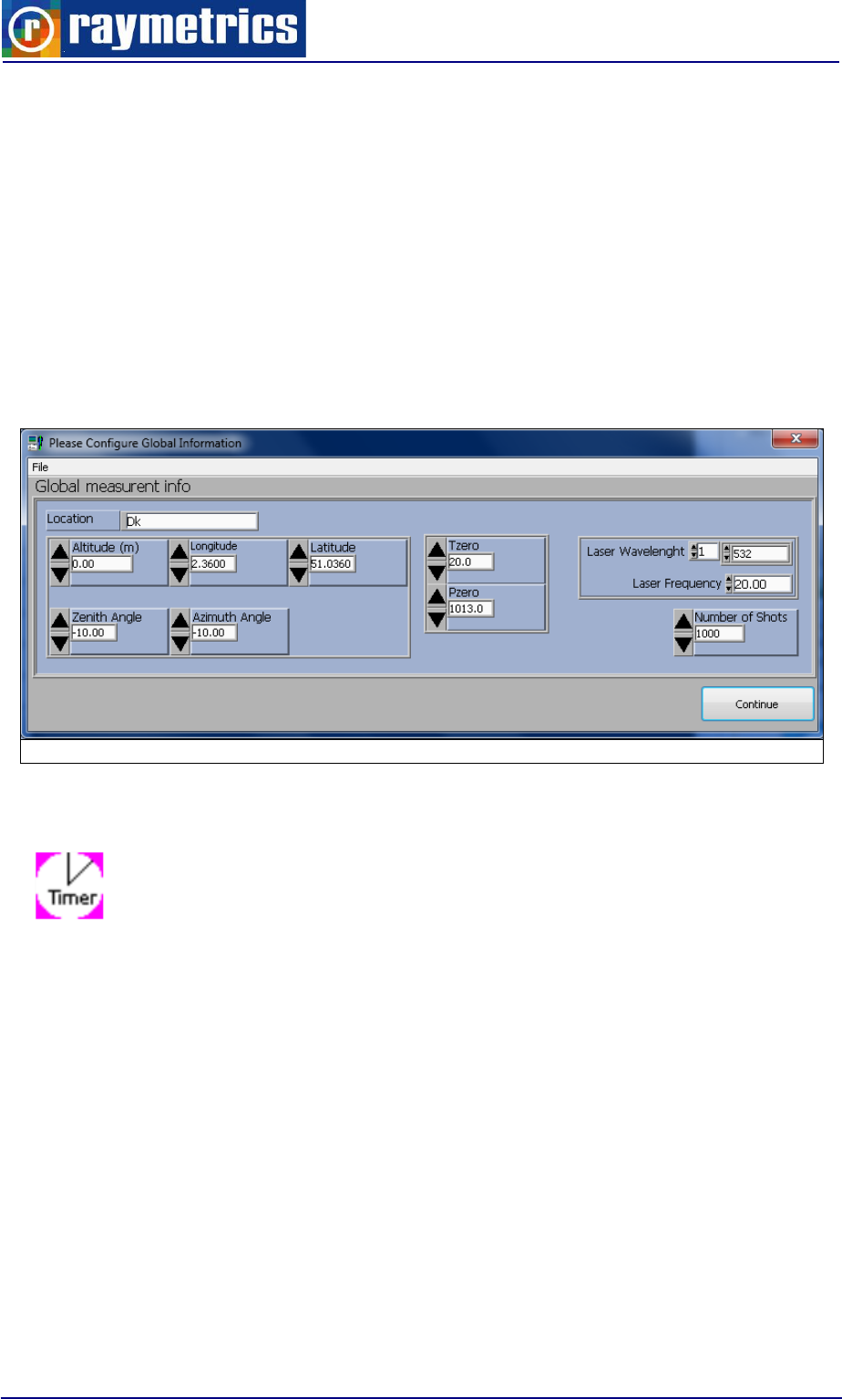
The Global button opens a dialog to set general settings regarding the measurent. As
shown below the user can set:
the location parameters (Name, Altitude, Longitude and Latitude)
The ambient temperature and pressure
The laser’s information (wavelengths and frequency)
And the most important the number of shots for each profile.
Fig. 4.4: Global settings dialog
4.1.2 Scheduler
The Time scheduler.exe allows you to program the Lidar to perform
scheduled measurements. This is quite useful when the instrument is at a remote
location without a fast internet connection. The user sets a daily plan of
measurements and selects which days of the week will use this plan.
The concept of this software is to use the Lidar in a fully automated mode. There is no
actual need for an operator since the Lidar will start and stop and save all the data
automatically. Furthermore if a mobile phone is installed the software can produce text
messages that will prompt the user in case of an emergency or a failure. All these features
combined make a fully remotely controlled Lidar.
Here is only presented the main interface of the program for more information please
refer to paragraph 6.4. MEASUREMENT SCHEDULING.
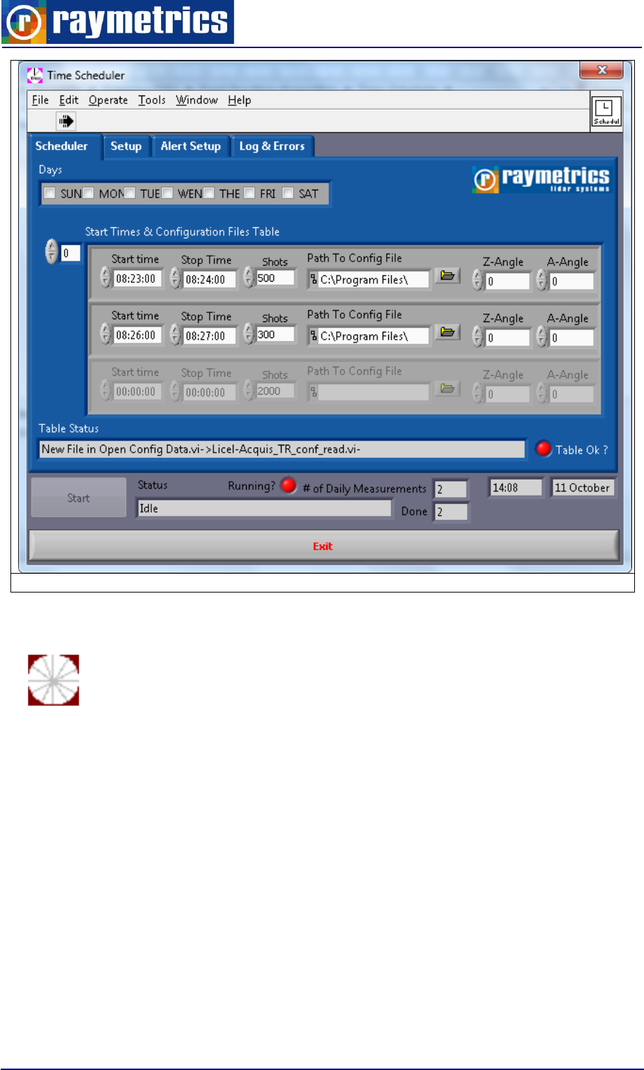
LIDAR SYSTEM SOFTWARE
42
Fig. 4.5: Time scheduler main interface
4.1.3 Scanning autonomous and Time scheduler
For a scanning lidar there is the ability to scan an area or even schedule to scan
multiple areas. There are two main programs available; scanning autonomous
and Time Scheduler Scanning. Both programs use configuration files as the fixed point
time scheduler but these files contain geometrical information regarding the scan. To
create such a file there is an extra tool called acquisition configurator. This set of programs
make a full scanning lidar operation software pack which gives the user all the possible
options one could ask. To make this software complete there the equivalent data
processing program for scanning measurements. This is totally necessary while the
volume of data when scanning is vast.
Below are only presented the main interfaces of the configurator and the scanning
autonomous. The Time Scheduler Scanning differs very little from the one presenteted
above and thus is skipped. You can find more information fro these programs in paragraph
6.5. SCANNING OPERATION.
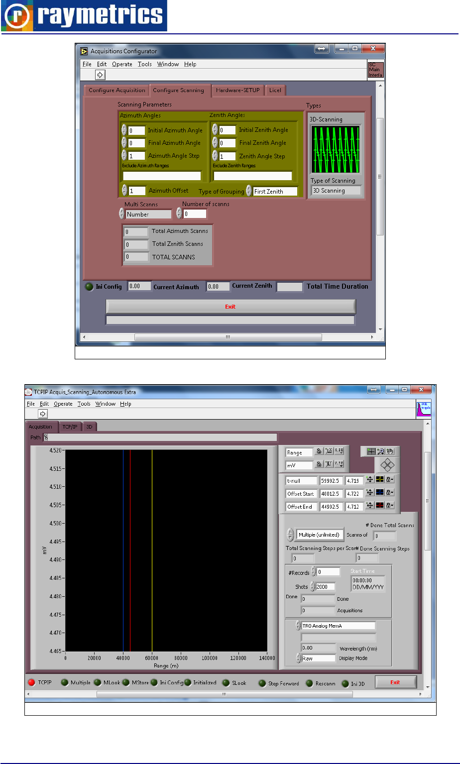
LIDAR SYSTEM SOFTWARE
43
Fig. 4.6: Scanning Configurator main interface
Fig. 4.7: Scanning Autonomous main interface

LIDAR SYSTEM SOFTWARE
44
4.1.4 Database and Working Directory
The measurement produces a series of binary files with the raw data. The volume of
data is normally enormous which makes it absolutely necessary to use a program that will
arrange the data in databases.
As previously explained all raw data files are saved in one working directory (one
single folder) which forms along with the datalog file one unique database. At first site this
looks not very easy to handle since one folder can contain thousands of data files.
However these files are not comprehensive for the user since they are in a binary form and
there is no actual need to go through this folder anyway. These files are already organized
well in the database, don’t alter the folder and keep a regular backup of your data.
You can create a new database by changing the working directory with a new one. You
may make as many databases as you wish but keep in mind that you won’t be able to
have an overview of the measurements.
4.2. POST PROCESSING SOFTWARE
Now is obvious the need to use a program that can organize the database and will at
the same time process and plot the data. The Lidar computer has preinstalled a powerful
program, named Lidar Data Preview and Analysis for post processing the Lidar raw data.
Many users prefer to use another computer for the data analysis. For this reason, this
software is open source code software and can be easily installed in any other computer.
The software was compiled in Labview and thus you will need to install the Labview
runtime engine which is supplied for free from the National Instruments website.
However there are some users that use their own software to post process the data. In
this case we provide the tool to translate the data from binary to ASCII and also the
encoding method to use directly the binary files.
The Data preview and analysis software was created based on the needs of
the Lidar users. Through the years this software was developed so much that
today the users can find many features embedded. However in this paragraph it is only
presented. To use the analysis software please refer to paragraphs

LIDAR SYSTEM SOFTWARE
45
7.2. DATA PREVIEW for using the database and for the data analysis. With this software
the user can:
Preview and edit a database
Analyse the raw data and extract various information such as the range corrected
signal the backscatter coefficient the beta molecular, the water vapour and many
other
Use a worksheet to perform additional calculations which may not be included in
the main analysis.
Use advanced Lidar techniques such as data Gluing
Present the data in 2D, surface (time evolution) and 3D plots.
Use this software as a health diagnostic tool for the system i.e. Lidar Alignment
state.
Convert data to ASCII form binary files
The program also supports radiosonde data import, or background noise files.
Raymetrics also provides the methods that the software uses for the analysis, so that
the user can be aware of the theory that lies beneath.
The software contains an extra module for the Lidar analysis. Each time the user
selects to perform a plot or a process of the raw data a series of widows appear to select
the data set that will be used for the analysis, then another window where the user has to
select what will be the output of the analysis and finally the main analysis window appears.
In this window there are many, user or automatically selected parameters, that provide a
totally precise analysis.

LIDAR SYSTEM SOFTWARE
46
Fig. 4.8: Lidar Data preview and Analysis Interface
Another useful tool is the Advanced Viwer Extra which is specially designed to handle
scanning data. With this program the user can group scanning data analyse plot save and
many more. This software also cooperates with Google SketchUp to create 3D
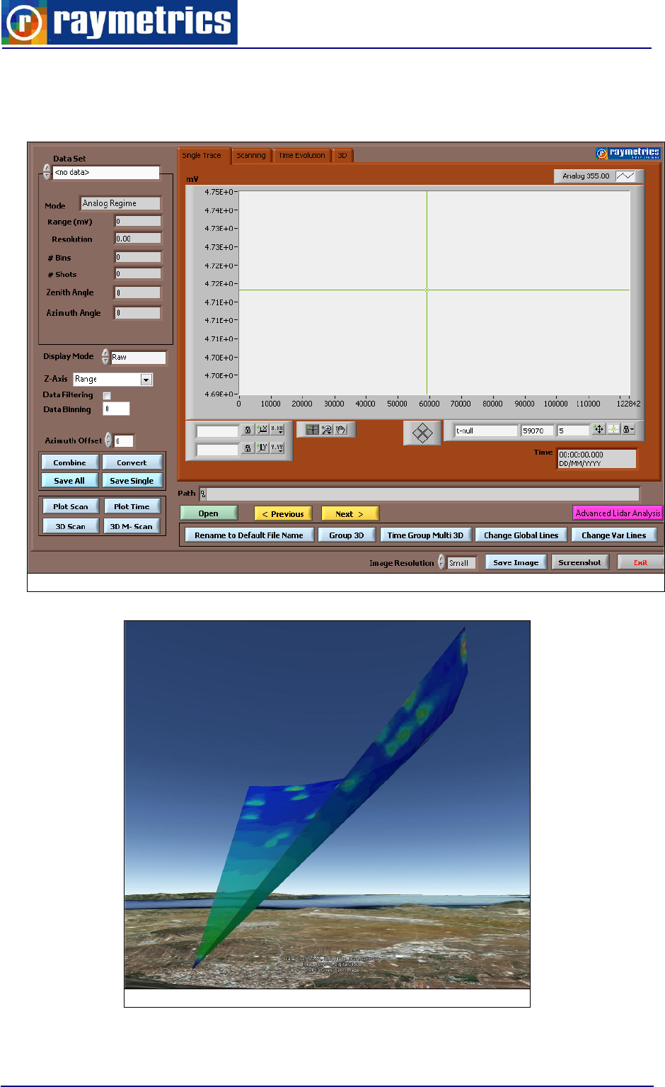
LIDAR SYSTEM SOFTWARE
48
4.3. SOFTWARE TOOLS
There are some software tools that will become very useful to the Lidar operator. To
begin with a very useful tool is Lidar alignment, used to align the Lidar. Then there are a
series of software modules to control different devices individually, and finally there are
some software used for diagnostics and for the configuration of the Lidar’s components.
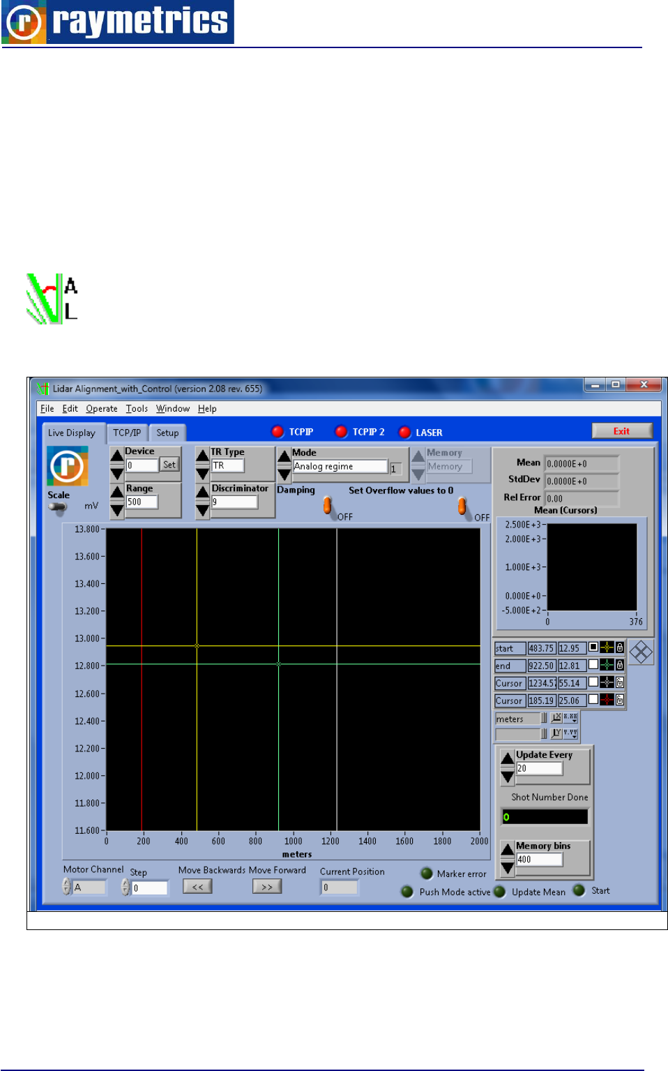
4.3.1 Lidar Alignment Software
This software is a real-time acquisition software that doesn’t save any raw data
files but is only for viewing the signal. It is suggested to check the signal regularly
to make sure that the data you acquire are the best possible. Reed more about
the alignment in paragraph 6.2 LIDAR ALIGNMENT.
Fig. 4.11: Lidar Data alignment Interface
The interface looks alike with the Lidar Acquisition program. However there are some
important differences which make this alignment tool unique. Starting with the common
LIDAR SYSTEM SOFTWARE
49
features there is a graph with its controls and also four cursors instead of two that the
acquisition program has. There are also the same numeric inputs all together in the same
interface and these are the shot number, the memory bins, the discriminator, the range,
TR Type, the mode and the device. The device has also a set button which allows the user
to set the PMT high Voltage value. Another extra is a small graph on the right side and
above this a series of numeric outputs. These objects are used to verify the process of the
alignment.
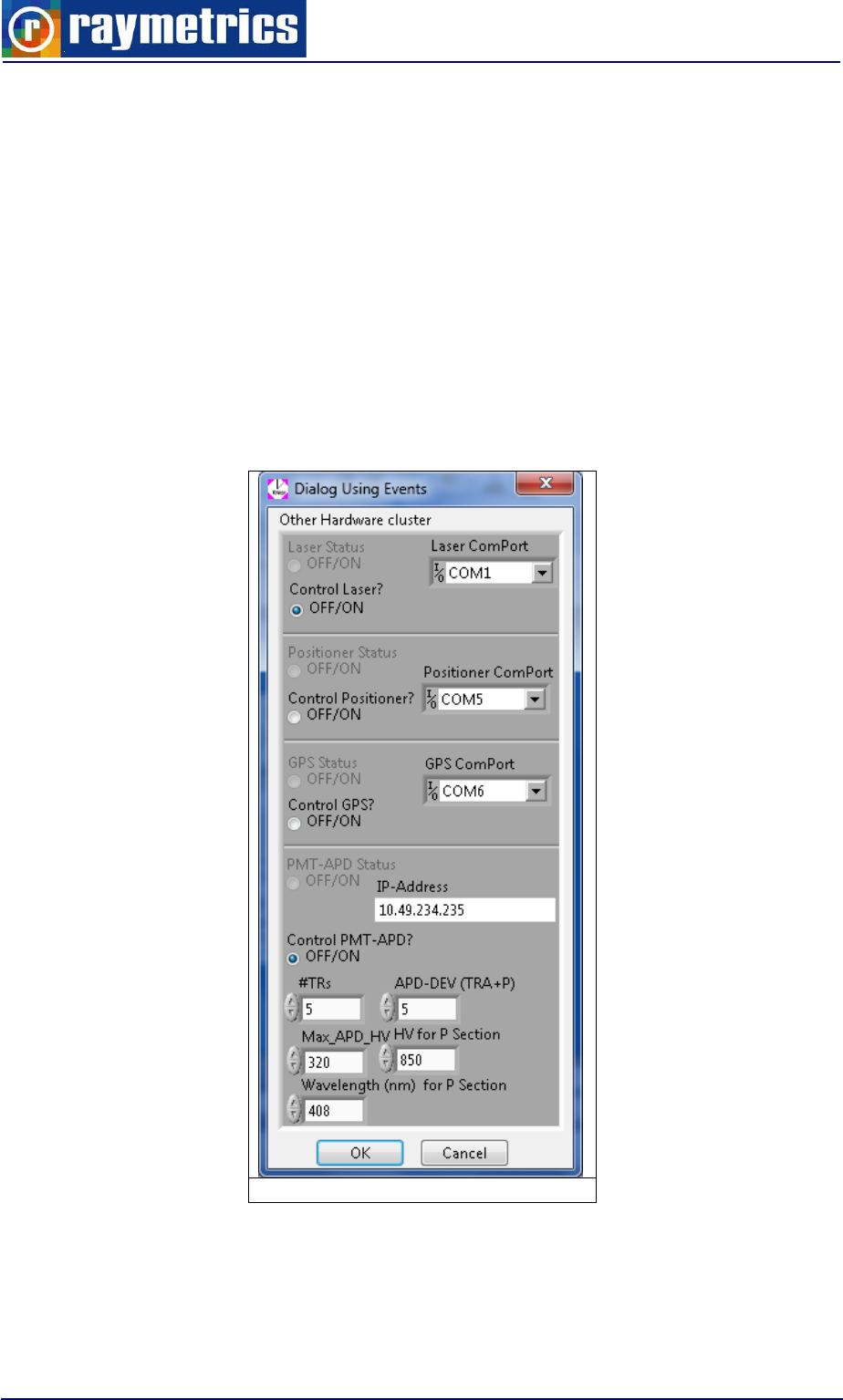
4.3.2 Configure other hardware
One configuration tool is the “configure other hardware.exe”. With this program the
user can select what devices will be controlled automatically from the acquisition software
and also to change the communication port for the device.
Fig. 4.12: Configure Other hardware
For example in Fig. 4.12 it is selected to control the laser via COM1 and the PMT-HV
device through the IP address 10.49.234.235.
LIDAR SYSTEM SOFTWARE
50
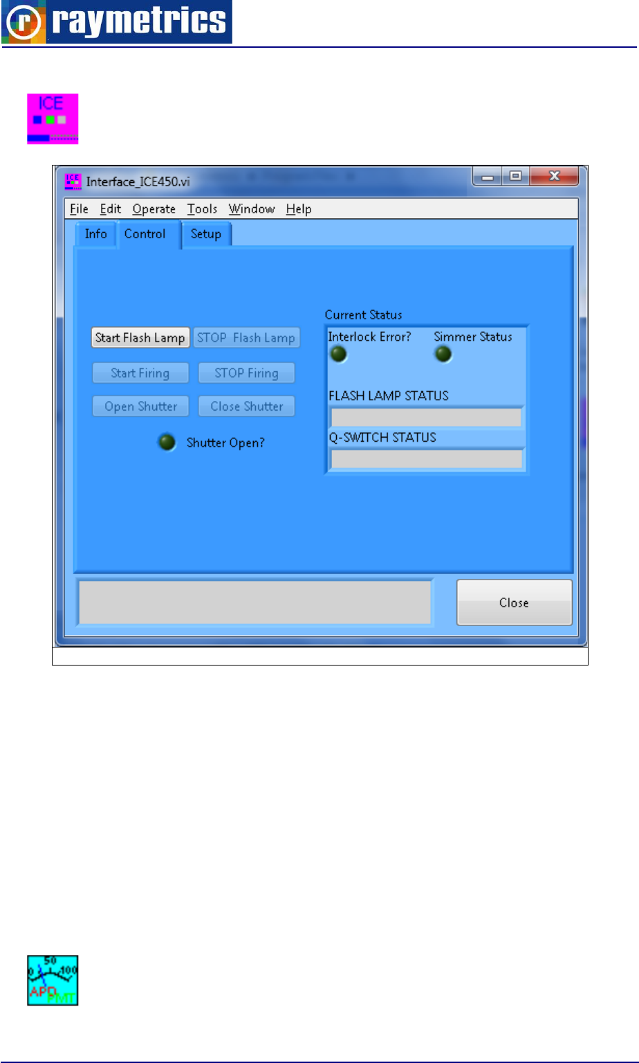
4.3.3 Laser Control Interface
This software module is used in case that the user may need to control the laser
individually. Furthermore it provides plenty information about the laser state
(flashlamp shots, water level and flow etc).
Fig. 4.13: Laser Control Interface
4.3.4 Licel Software
Apart from Raymetrics software there is also installed Licel’s software which can be
used alternatively to control the Transient recorder the PMTs HV device and also some
other devices such as the trigger generator. It also provides some diagnostics tools like the
“Track.exe” or the “search controllers.exe”.
With this set of programs an advanced Lidar user has the ability to control separately
the devices and also perform advanced Lidar measurements. Since these programs have
their own documentation, here are only presented just the most commonly used.
4.3.4.1. Control PMT APD program
In order to run a non-automated but remote measurement the user also needs to
control the PMTs High voltage. Licel provides among other a program to control
LIDAR SYSTEM SOFTWARE
51
the PMTs. The interface is close to the device’s interface, the only thing the user has to set
is the number of the PMT’s - APD’s and the IP address of the device.
4.3.4.2. Search Controllers program
This tool is useful when the user has a communication issue and wants to debug.
If for some reason the computer doesn’t communicate with the Transient
recorder or the PMT HV device then when the user runs the acquisition or the
alignment software it will show an error message and the TCP/IP led will turn red. This
problem may be caused from a bad cable or an Ethernet card overflow. The “search
controllers.exe” searches for Licel devices that are in the same network and gives
information about their status and the IP address.
4.3.4.3. Control Timing program
The Lidar is equipped with a trigger generator which is used to trigger the laser
and the electronics individually. This option is handy when a special study needs
to be performed where there must be a time delay in between the laser pulse
and the recorder. When using this option the acquisition becomes a non-automated
procedure and the user has to use all control programs separately.
4.3.4.4. TCPIP Set Fixed IP Address program
For users with advanced network knowledge it may be needed to change the IP
addresses of Licel devices. In this case you can use the “TCPIP Set Fixed IP
Address.exe” to set a new fixed IP address for each device. Note here that the
external trigger is a different device and has a unique IP address.

UNPACKING AND INSTALLATION
52
5. UNPACKING AND INSTALLATION
5.1. UNPACKING THE LIDAR SYSTEM
The Lidar system has been carefully packaged to assure its secure delivery to the
customer.
Inspection after shipment
Check carefully the crate for damage before uncrating the Lidar system. Take notes of
all visible external damage. If you notice any damage caused during the
transportation please advice Raymetrics before sign the delivery note.
Unpacking
The Lidar system should be unpacked only by the authorized personnel of
Raymetrics S.A. during the Lidar installation on site. Any damage caused by the
user in an attempt to unpack and install the Lidar is not covered by the warranty.
If you have permission to unpack the Lidar system, remove the external film, and open
the crate by removing all screws. Remove the straps. Some systems are shipped without
the wheels to reduce space. The wheels are usually inside the crate or inside the Lidar
enclosure. There is a key usually above the Lidar. In case that there are no wheels pull
one corner of the enclosure each time out of the crate and place all wheels. If the Lidar is
shipped with the wheels on then lift from the base of the enclosure with a forklift and place
it gently on the ground.
IMPORTANT: Make sure that the Lidar is always safe from falling by tilting; avoid at any
time and impacts sudden movements.
5.2 INSTALLATION OF THE LIDAR SYSTEM
Site:
For proper operation of the Lidar system the ambient temperature should range
between 18 and 28oC.
It is preferable that the Lidar system is positioned and secured on a solid horizontal
surface. When choosing a place for your Lidar system other than an open-air site, make
sure that the housing has an opening (hatch) over the Lidar, with an area 15-20% larger

UNPACKING AND INSTALLATION
53
than the total area of the transmitting/receiving windows of the Lidar system. The housing
must have an air condition.
Keep always in mind:
- Access should be available from all sides of the Lidar system, especially in the front
where the control unit is,
- Choose a location for the laser and power supply and cooling unit, cabinet (PCC), such
that each side of the cabinet is not less than 25-30 cm away from a wall or obstacle.
Front and rear panels of the instrument should be placed at least 50 cm away from a
wall or other obstacle, to allow efficient cooling of the instrument.
- Power:
Power is to be 110 V (50/60 Hz) with available operation current up to 6.7A and a peak
current capacity up to 13.4A. Make sure that the power is stable and no large motors are
on the same line. If for any reason the power has large peaks the laser will not function. If
there are often power failures it is strongly suggested to install an external on-line UPS for
safe shut down of the instrument. The on-line UPS stabilizes the power as well. For the
installation make sure that there is a socket rated for at least 13.4A and the
appropriate plug to fit this socket and to the power cable (Fig. 5.8). The power cable
type is 3x2,5mm2.
- Water services:
The laser cooling unit is a water/air heat exchanger and does not require any external
water service. However the user must make sure that there is distilled water with 1MΩ-
cm to 5MΩ-cm resistivity always available at any time and especially during the
installation.
The on-site installation and Lidar system alignment will be totally assured by the
Raymetrics S.A. personnel.
Attention!
No attempt should be made by the user to install the Lidar system. Damage occurring
due to the non-respect of the previously mentioned instructions will not be covered under
our warranty.
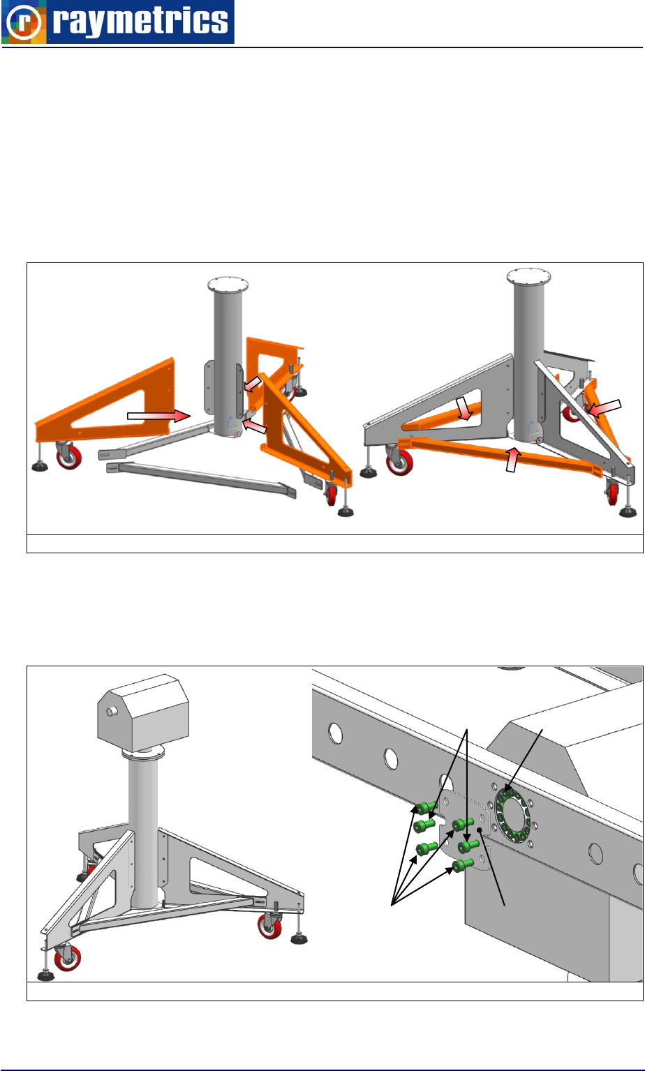
UNPACKING AND INSTALLATION
54
5.2.1 Assembly
The lidar before shipment is packed carefully in components. The control unit has the
umbilical cord attached. The positioner is placed separately with the Lidarhead while the
tripod base is dismantled to reduce space.
Start by assembling the tripod base. Place the main tube horizontally in the ground and
mount the legs. Then place the support bars and hold them together with the supplied
screws.
Fig. 5.1: Tripod Assembly
Next install the positioner on the base and place the counterweight side brackets on
the positioner shaft. Don’t tight the connex screws yet because you will have to move the
brackets in order to fit the Lidarhead.
Fig. 5.2: Positioner and Brackets Mount
M8x16
Protective Cover
M8x20
Connex
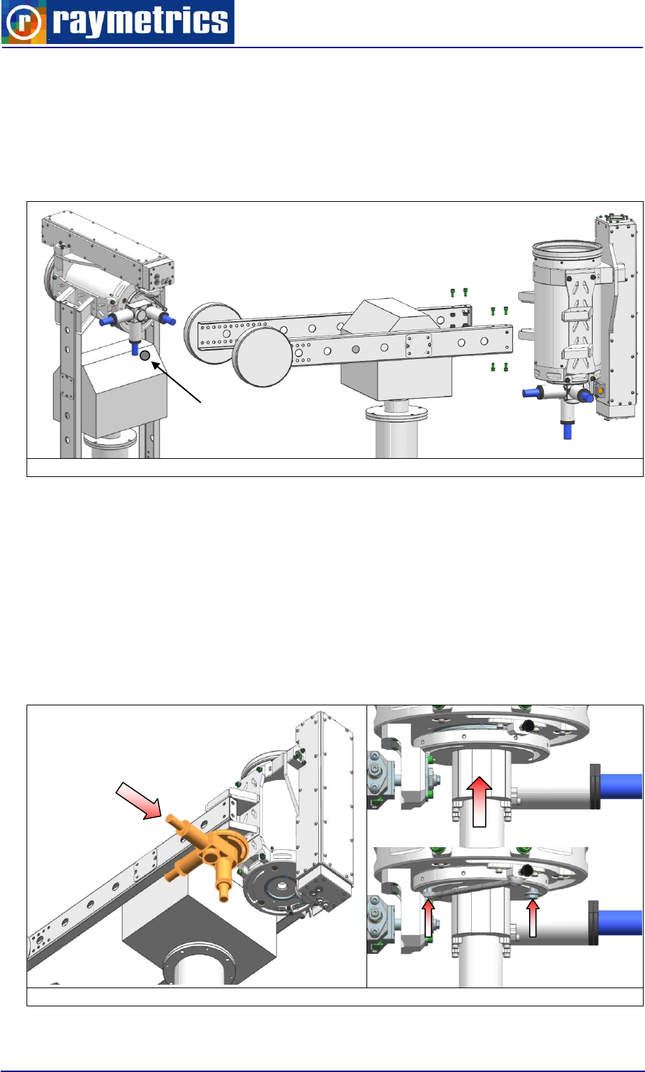
UNPACKING AND INSTALLATION
55
Now place the lidar head to the side brackets carefully. Before the placing Lidarhead
you should indicate which one is the correct side. On the positioner there is a small round
window where the bubble level is. This side must face the side of the telescope as shown
in fig.36. It is more convenient to turn the brackets at vertical position and then fit the
Lidarhead’s mounts on them.
Fig. 5.3: Lidarhead Installation
CAUTION! When installing the LIDAR head one must hold the brackets which should be
free to rotate and translate on the positioner’s shaft. After the head is installed fix the
screws of the Connex to secure the brackets in a horizontal position.
For extra precaution the WSU should be separated from the Lidarhead during
transportation. Place the WSU underneath the telescope and press it to fit into the
telescope’s hole. Place the hexagon screws, screw them first by hand and tight them with
a no.10 spanner.
Fig. 5.4: WSU Installation
Window
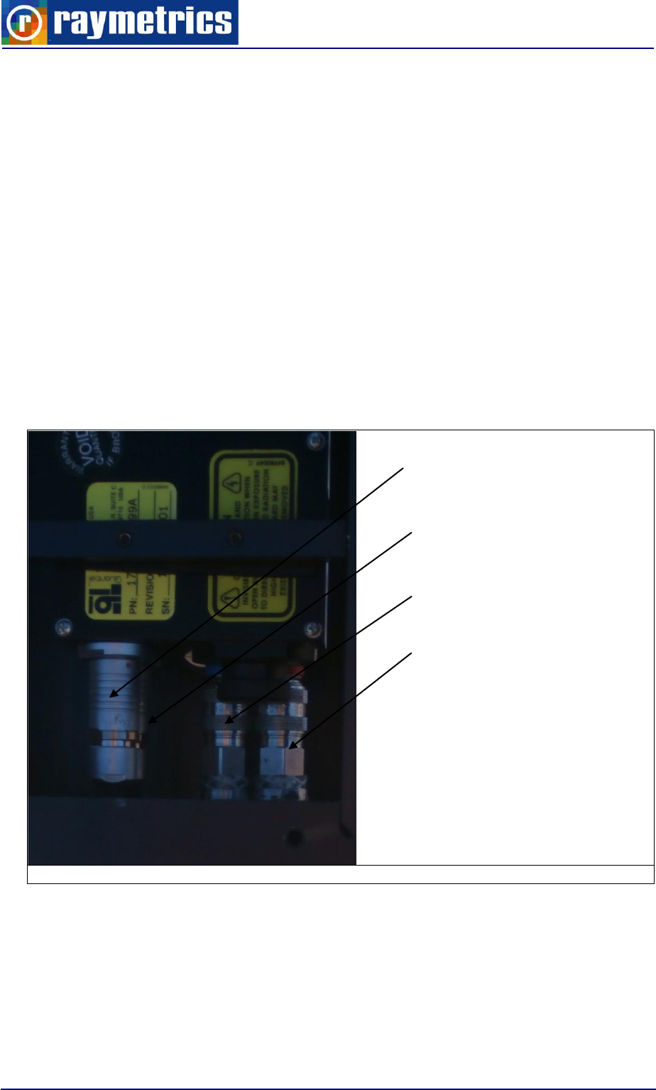
UNPACKING AND INSTALLATION
56
NOTE: The WSU unit needs also extra caution when handling and it is very important for
the optical not to be dirtied. It is strongly recommended to use sterile gloves in this phase.
5.2.2 Cable Connections
5.2.2.1 Umbilical Cord
The Lidarhead umbilical is fed into the cabinet through cable conduit and thus it is
attached to it while the other end has connectors that mate at the back of the Laser head.
To have access to the laser head remove the top cover of the transmitter.
Find which connector goes to which receptacle; one cable has a 19pin connector and
the other has a 2+2pin connector. Then locate the red spot on the connector and on the
receptacle. This spot indicates the orientation of the connector.
The water hoses have quick coupling fittings. The red is for the warm and the blue is
for cold. On one of the hoses is written “cold” the other is for warm.
Fig. 5.5: Laser Umbilical Connection
Once the cables are in place back the cover and tight the screws of the conduit end
cap.
19 Pin Signal Connector
2+2 Pin Power Connector
Blue Cold water Fitting
Red Warm water Fitting
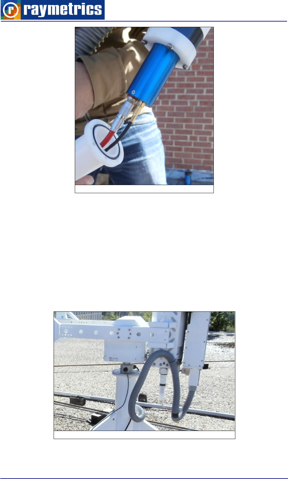
UNPACKING AND INSTALLATION
57
Fig. 5.6: PMT Connection
Next connect the cables on the back of the PMT and mount the protective cap. Make
sure that you place each cable set to the corresponding PMT and that the cables are not
stretched.
Finally with some cable ties fix the umbilical on the side of the telescope’s bracket.
Make sure that the cable has enough length to move along with the positioner and that it is
does not interfere with the tripod. When joining the umbilical place the laser umbilical in
between the red and the black cables of the WSU. The red cables are for the high voltage
of the PMTs and the red are for the signal. If these two are very close it is likely that the
signal will be affected.
Fig. 5.7: Umbilical Tie Down
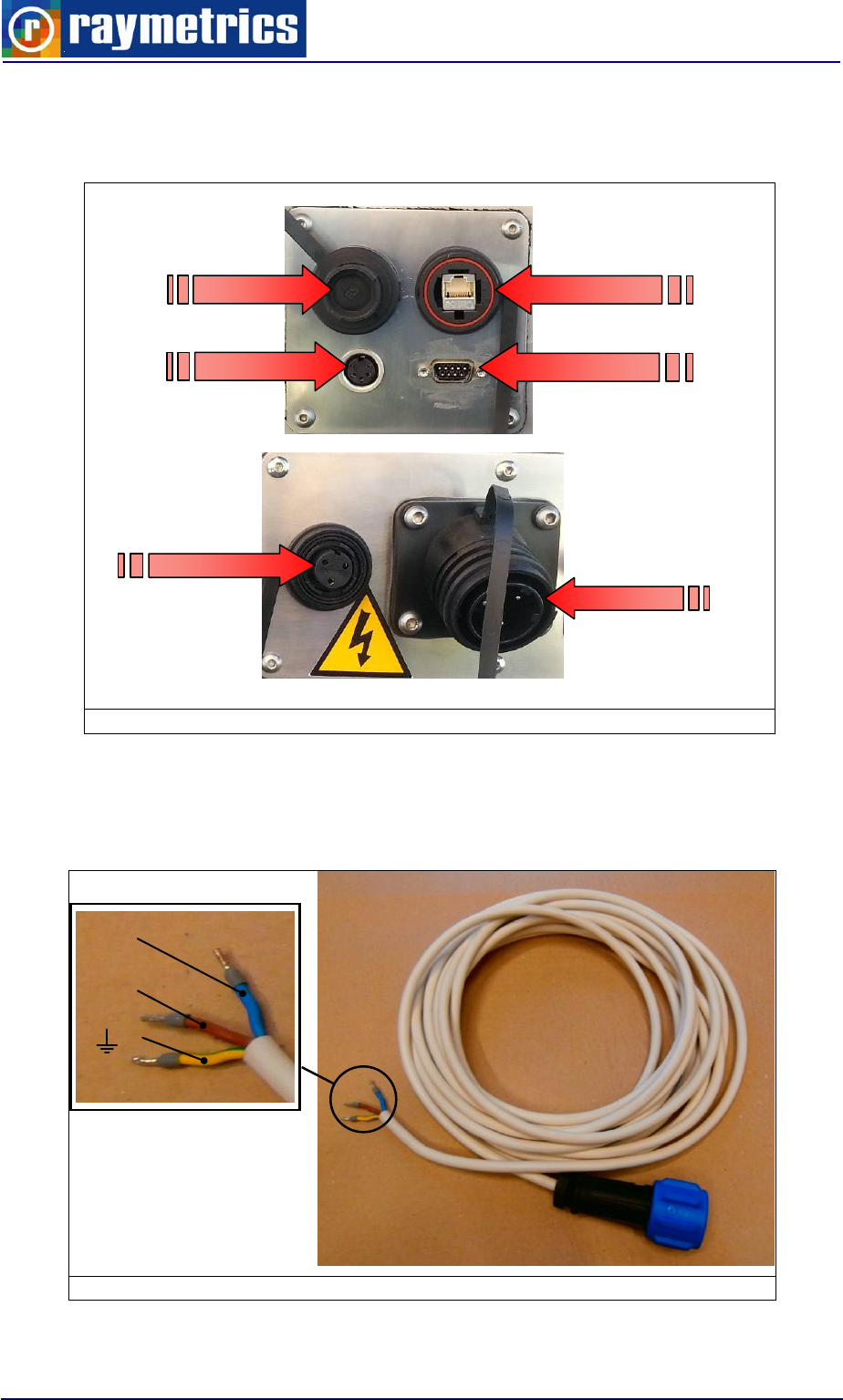
UNPACKING AND INSTALLATION
58
5.2.2.2 Other Connections
In addition connect the positioner’s power supply and signal cable, the laser’s remote
control box, the external Ethernet cable and the system’s power supply to the cabinet.
Fig. 4.8: Other Connections
Finally assemble the plug on the power cable (Fig. 5.8) which fits the socket of the
installation site. Make sure that the plug and socket meets the requirements of the Lidar
power consumption
Fig. 5.8: Plug assembly
Main Power
Positioner power
USB Port
Ethernet Port
Remote box
Positioner RS232
N
L
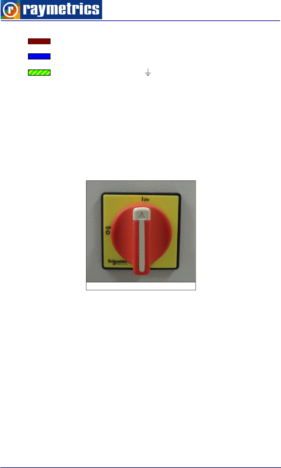
UNPACKING AND INSTALLATION
59
Note: The cables colours are explained below:
Brown cable goes to “L” (Live)
Blue cable goes to “N” (Neutral)
Yellow-Green cable goes to “ ” or “G” or “E” (Ground or Earth)
Connect the power cable to the Lidar’s socket. You may also use the other ports the
Ethernet port to connect the Lidar with a network or the USB port to connect a USB device.
5.2.3 Water Filling
For shipping the Lidar, a Raymetrics’ technician drained the coolant from the coolant
reservoir of the laser. Before use, the customer must fill the coolant reservoir with about
1,5 litres of distilled water with 1MΩ-cm to 5MΩ-cm resistivity.
1. Turn on the red main switch at the side of the electrical cabinet.
Fig. 5.9: Main Switch
2. Open the front and back lid of the cabin.
3. Switch on all the switches at the energy box at the back of the cabin.
4. Please follow the instruction that you can find at page 11 of the User's Manual Quantel.
IMPORTANT: Each time the Lidar is transported by plane the coolant must be drained off
the reservoir and especially off the Laserhead to avoid freezing that will destroy the Laser.
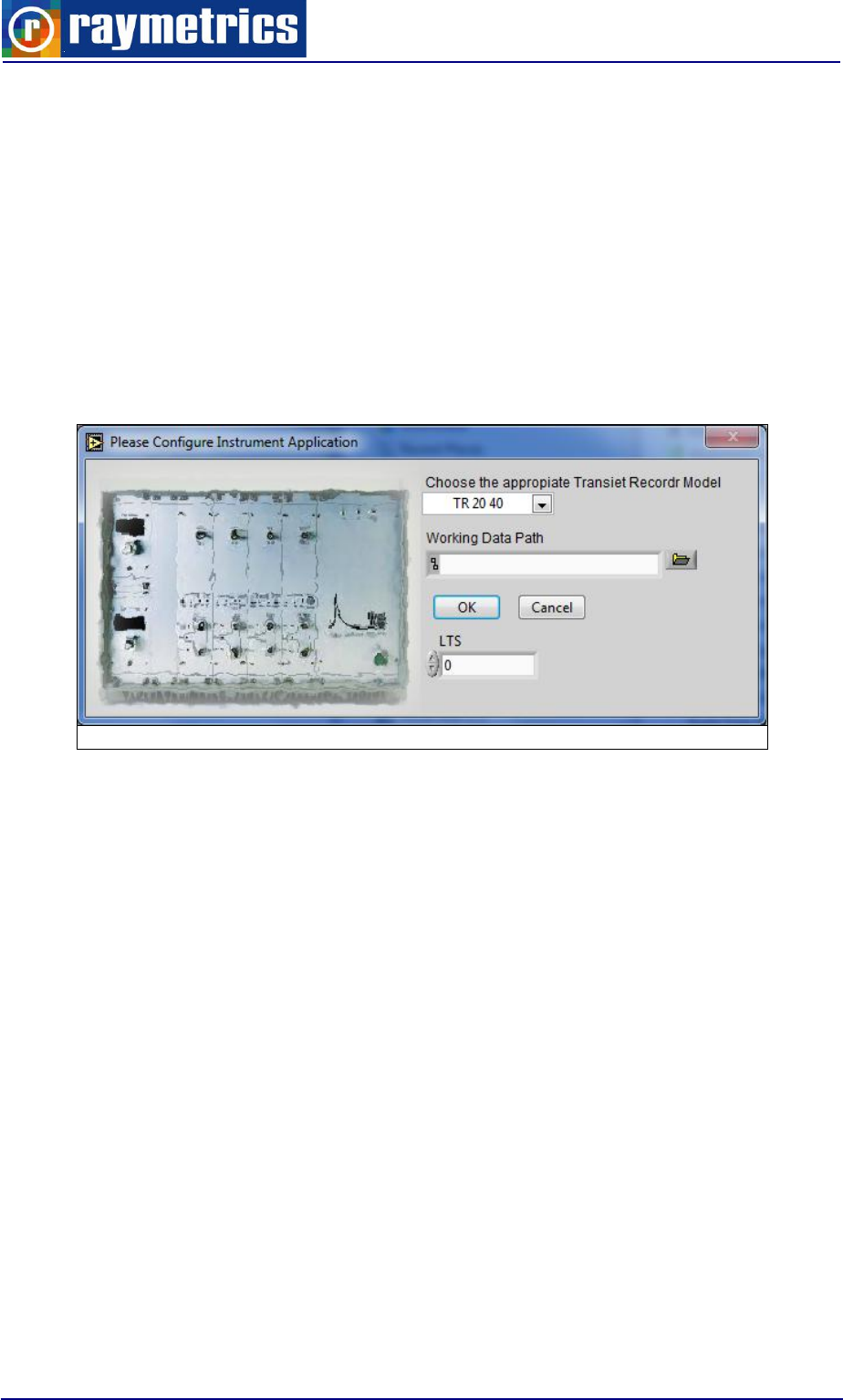
UNPACKING AND INSTALLATION
60
5.2.4 Software Installation
Raymetric’s Lidar systems are supplied with a computer system which has already
installed all the necessary software for apparatus alignment, data acquisition and data
preview and analysis.
At any time you can install the executables files that will come with the instrument.
5.2.4.1 Configuration Utility for your Lidar
For manually run configuration utility just open <installation path\Registry Tools\Config
Application.vi>
This is an autorun vi.
Fig. 5.10: Software Configuration
Select type of Transient Recorder Tr-xx-yy
xx: Sample rate
20 MHz (7.5 range resolution)
40 MHz (3.75 range resolution)
yy: FIFO memory Length
160 (16384 databins)
80 (8192 databins)
Select default location (folder) for saving raw data during data acquisition
Select default location (folder) for ASCII data when converting raw files to ASCII format
Select default location (folder) for backup raw data.
Press Ok to confirm or cancel to quit.
Caution: For proper use of the supplied VI’s uncheck “Use localized decimal Point” option
Step by step procedure:
1. Open Labview
2. Select new vi
UNPACKING AND INSTALLATION
61
3. Go to Tools menu
4. Select options
5. Go to front panel section
6. Uncheck (if checked) “Use localized decimal Point” option
5.3 STORAGE AND SERVICE
Storage
Turn all the electrical units OFF.
Disconnect the power cord from the Lidar system.
Even if you don’t use the Lidar turn on the laser’s ICE450 every month for
30minutes.
If you plan to store your Lidar for an extended period of time, protect it against
intense rain and humidity. Place it indoors or cover it up with a waterproof material.
CAUTION: If you are planning to ship your Lidar by air or install it in a
cold environment, your laser system must be completely drained
before transporting, since the coolant could freeze. Follow very
carefully the instruction at laser manuals.
Service
If returning your Lidar to Raymetrics, please carefully pack the Lidar using the original
package material that came with the unit.
WARNING: Follow the instruction for every unit on your instrument
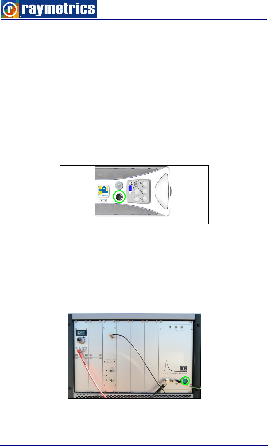
LIDAR OPERATION
62
6. LIDAR OPERATION
6.1. START-UP
There are two ways to use the Lidar; manually and automatically through the software.
The user can choose which one is more convenient to use however here are presented
both. The next steps will guide you through the safe operation. The first steps are common
for either manual or automated operation.
1. Plug in the power cord (Error! Reference source not found.), and turn on the main
switch (Fig. 5.9) on the side panel. Turn on the switches of the power distribution unit
2. Turn the “Power Key Switch” on the front panel of the PCC to the ON ("I”) position
(Fig. 6.1). The "power" and the "interlock" indicators on the Remote Box will illuminate.
If not, check for interlock fault messages on the Remote Control Box LCD Display.
Fig. 6.1: Laser Power Up
3. Wait approximately 10-15 minutes, depending on the environmental conditions and
amount of coolant in the system (coolant line length), until the coolant temperature
reaches the preset value for flashlamp operation.
4. The computer whenever you power up the Lidar turns on automatically. In case it is
turned off switch off the power switch on the power distribution unit, wait for 10secons
and switch it back on.
5. Power up the Licel electronics (TR, PMT).
Fig. 6.2: Electronics Power Up
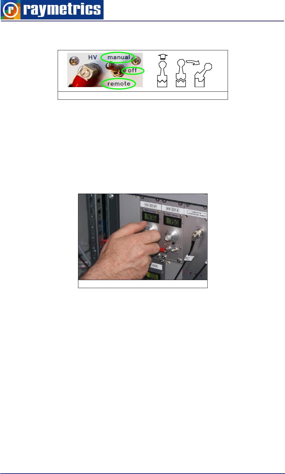
LIDAR OPERATION
63
6. Select the desired control mode for all PMTs High Voltage. To do so lift the switch and
then turn. Set to manual for manual operation or remote for automated operation.
Fig. 6.3: Control Mode selection
6.1.1 Manual Operation
7. Set the switch on each PMT HV to manual. Adjust the applied high voltage to the
PMTs. Check signal, HV and trigger cables if they are at the right position. Turn on the
HV by switching the HV switch to the manual position for each HV power supply you
are willing to work with. (For remote operation through software, switch to the remote
position). Turn the HV potentiometer counter clockwise up to the desired value. (High
voltages values should be 750-900V, linear range of operation)
Fig. 6.4: PMT High Voltage Adjustment
8. Press the “Flashlamp Ready” button on the Remote Control Box. The corresponding
“ready” LED and “LASER ON” indicators illuminate. Wait for a couple of seconds and if
no interlock appears press the “Flashlamp Start” button on the Remote Box. The
corresponding flashlamp “start” LED will blink and (in internal mode) the flashlamp will
start flashing.
9. The PCC requires a safety delay of up to 8 seconds after the flashlamp starts before it
enables Q-Switch operation. This stands for both Internal and External Q-Switch
operation modes.
WARNING: The following steps result in laser light emission from the output aperture
of the laser head. Do NOT look directly the laser beam. Before you press the Q-Switch
make sure that nothing is blocking the light path.
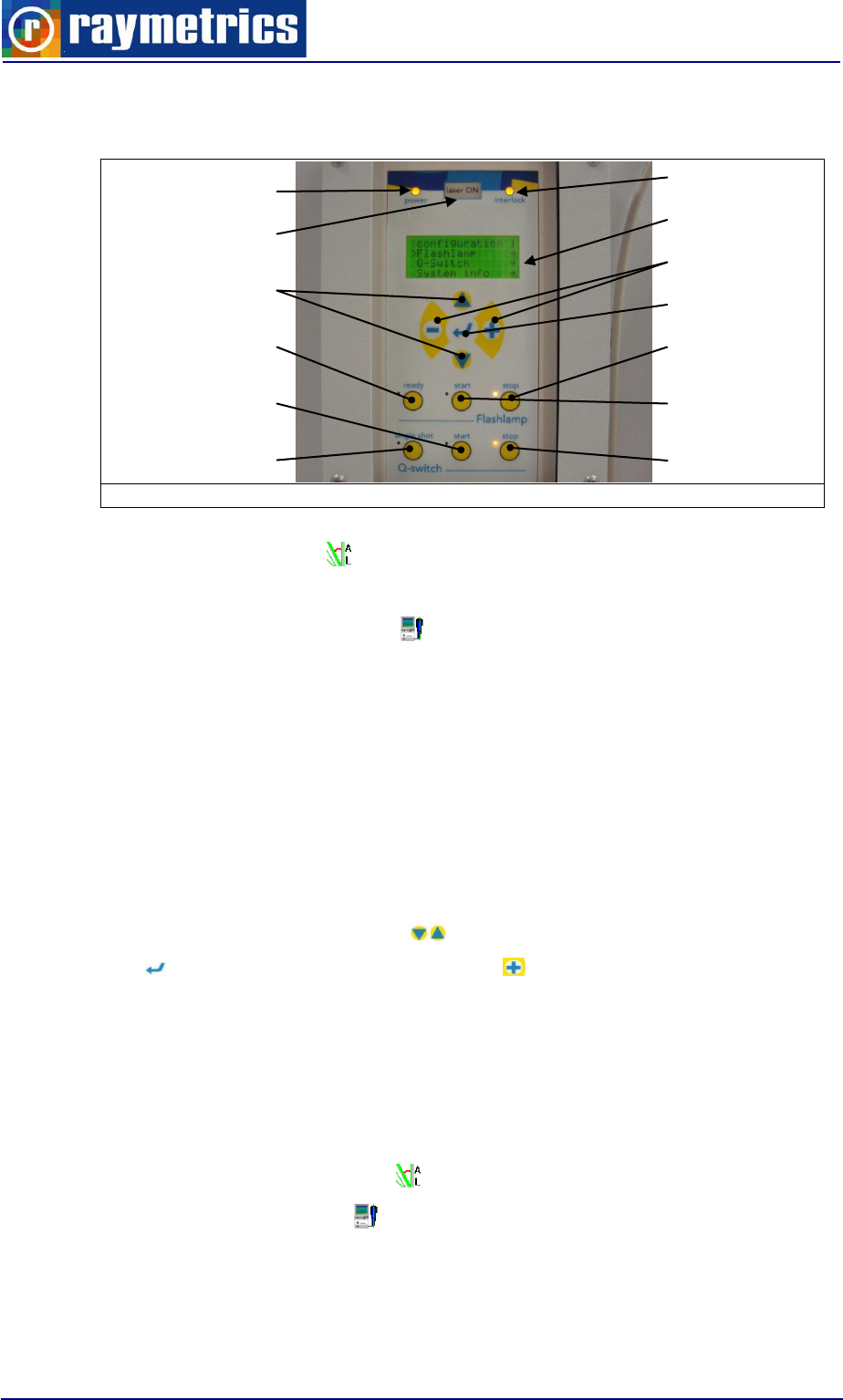
LIDAR OPERATION
64
10. Press the “Q-Switch Start” button to activate the Q-Switch. Verify that the
corresponding Q-Switch “start” LED blinks and the “Laser ON” sign illuminates.
Fig. 6.5: Remote Control Box Indications
11. Run the Lidar Alignment.exe (Live display from Licel)
12. Watch the signal and fine align if necessary (see paragraph 6.2 LIDAR ALIGNMENT )
13. Run the Lidar Acquisition executable
14. To stop laser emission, press the “Q-Switch Stop” button. Verify that the Q-Switch
“start” LED turns off. To stop the flashlamp, press the “Flashlamp Stop” button. Verify
that the flashlamp “start” and “ready” LEDs turn off.
6.1.2 Automated Operation
7. Set the switch on each PMT HV to remote.
8. Whenever the user presses any button on the remote control of the laser the
serial communication with the computer is lost. To set the serial communication
navigate through the menu using the buttons, choose “System Info” and validate
with the button. Go to serial link and with the button change the status from “off”
to “on”.
WARNING: The following steps result in laser light emission from the output aperture
of the laser head. Do NOT look directly the laser beam. Before you press the Q-Switch
make sure that nothing is blocking the light path.
9. Run the Lidar alignment executable to check the signals and align if necessary, or
directly run the Acquisition.exe to perform a single measurement or the scheduler
to program a series of daily measurements. When you wish to stop the measurement
press the “stop” button to stop the laser and PMTs as well.
Interlock LED
LCD Display
Set Buttons
Enter Button
Flashlamp
Stop Button
Flashlamp
Start Button
Q-Switch Stop
Button
Flashlamp
Ready Button
Q-Switch Start
Button
Q-Switch Single
Shot Button
Navigation
Buttons
Transmitting
indicator
Power
LED
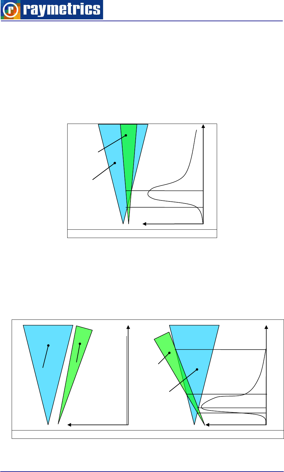
LIDAR OPERATION
65
6.2 LIDAR ALIGNMENT
In order to acquire the best possible Lidar signal the user has to align the laser beam
to the telescopes field of view. Measurements acquired with a misaligned Lidar can lead to
fault results. Normally the Lidar is aligned as illustrated in Fig. 6.6. You can see that the
signal starts to rise when the light of the laser beam inserts into the telescope’s Field Of
View (FOV) (point A) and reaches its peak value when the entire beam is inside the field of
view (point B). After that point the signal starts to decrease because the light is attenuated
easily when in low range.
Fig. 6.6: Aligned Lidar
There are two cases of misalignment. Both are shown in Fig. 6.7. In the first case the
laser beam is tilted at the opposite direction and there is no Lidar signal. However there is
still some noise from the electronics and the background. In the second case the laser
beam enters the telescope’s FOV (point A-B) but exits after a certain point (point C-D). The
second case is more difficult to distinct as the signal looks like a normal Lidar signal.
However there are techniques to perfectly align the Lidar such as the telecover test.
Fig. 6.7: Misaligned Lidar
Laser
Beam
Telescope’s
FOV
A
B
Range
Signal Intensity
Laser
Beam
Telescope’s
FOV
Range
Signal Intensity
Laser
Beam
Telescope’s
FOV
Range
Signal Intensity
A
C
B
D
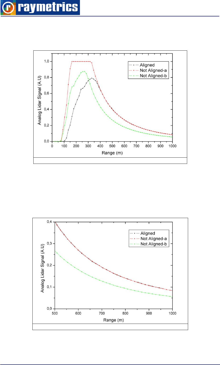
LIDAR OPERATION
66
In the next figure you can see how the real Lidar signals for these cases. Black curve
corresponds to a good aligned Lidar setup, while the Red and Green curves (same
alignment but reduced signal intensity) correspond to a case similar to Fig. 6.7b.
Fig. 6.8: Alignment Example Real Signals
In many cases an inexperienced user will consider the red curve as a very good
aligned signal since this signal is very strong (even has saturation between 150 and 350
meters). However if we reduce the signal intensity (see 6.2.4 Signal Intensity Reduction) in
order to get rid the saturation, we get the signal of the green curve and we can see that at
the far field the black curve has almost double value compared to greed curve.
Fig. 6.9: Alignment Example Real Signals far filed
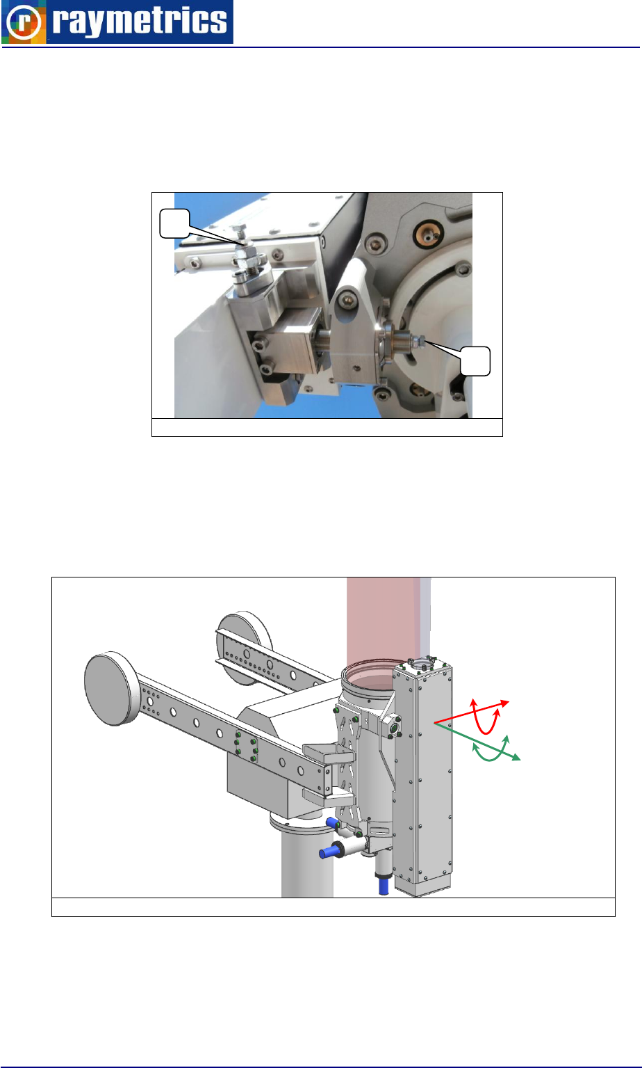
LIDAR OPERATION
67
6.2.1 Laser Beam Kinematic
The Lidar alignment is done by moving the transmitter. Using two actuators the laser
beam steers to meet the axis of the telescope’s FOV. To choose which actuator should
move is not always easily understood so here is presented the effect of each actuator.
These two will be conventionally named “A” and “B”
Fig. 6.10: Transmitter actuators
Because of the small allowable angle the actuators have a very small resolution so that
the movement is also small and the Lidar signal is not very sensitive to the actuator
movement. This give the user the ability to micro align the Lidar.
In the next figure is shown the effect of actuator A and B on the laser’s beam direction.
Fig. 6.11: Transmitter kinematics from A and B Actuators
Below is a schematic representation of the laser beam movement caused by each
actuator in relation to the telescope. To sum up actuator “B” a moves the beam in a vertical
way while actuator “A” moves the beam in a horizontal way.
A
B
YAW
PITCH
Actuator
B
Actuator
A
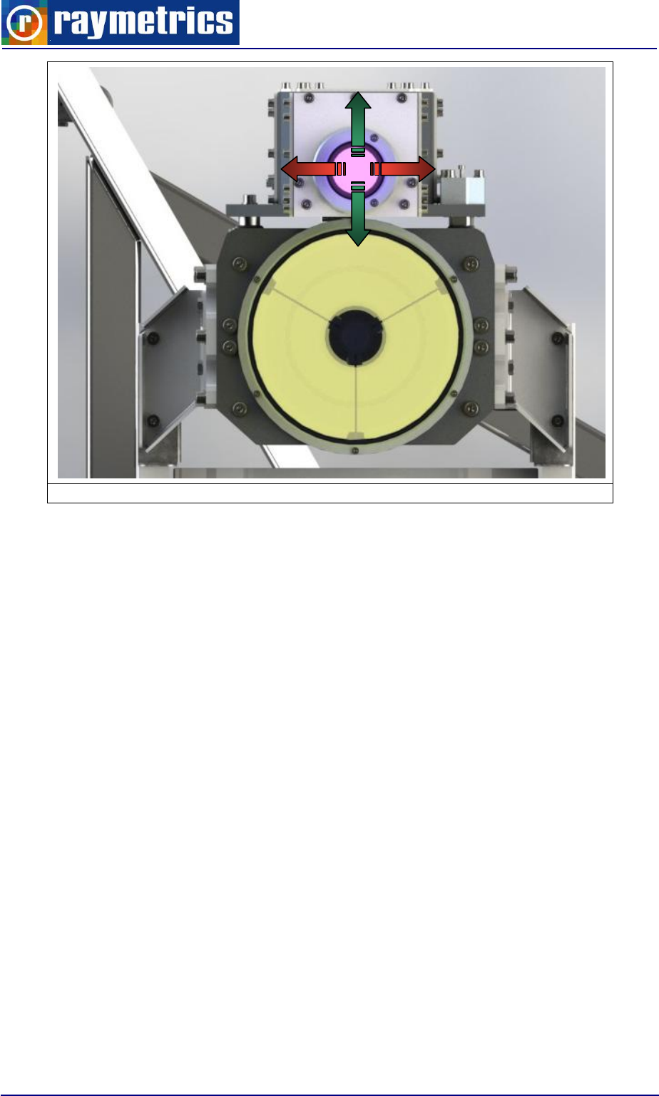
LIDAR OPERATION
68
Fig. 6.12: Laser Beam kinematics
-A
+A
-B
+B
LIDAR OPERATION
69
6.2.2 Lidar Alignment Procedure
The Lidar alignment is achieved in two steps. During the first step (coarse alignment),
the far-range signal is monitored and the optical axes are fixed in a position where that
signal is maximum. The second step (fine alignment) can be done in two different ways.
One is by increasing the intensity of the signal in far range and the other is by performing a
fast telecover test. To verify also the alignment the user can perform a comparison with a
pure molecular atmosphere model in the analysis software. For more information see
paragraph 7.3.4 How to Check Lidar Alignment.
6.2.2.1 Intensity Maximization at far range
When the intensity of the signal increases in general it means that more light enters the
FOV of the telescope. It is very easy to increase the signal in the near range but it is also
easy to misalign the Lidar as shown in case II in Fig. 6.7. When the intensity of the signal
is maximized in the far range then it means that as far the telescope can see there is a
laser beam.
The alignment procedure is quite simple; the user selects an area on the slope as far
as possible and tries to maximize the mean value of this area by using the actuators. Once
the mean value reaches its peak, another area further that the initial is selected and the
process is repeated with a smaller actuator step. When the value doesn’t change for the
selected step size it means that the Lidar is aligned. In more detail the procedure can be
described in these steps:
1. Run Lidar Alignment.exe. If you run in automated mode the laser will start the emission
and prompt for the HV value of the selected PMT. On top there are three red LEDs
these should turn green. If not there is a communication problem.
2. Notice on the right the controls for the cursors . Click the and select bring to
center. Click the and select lock to plot if not selected.
3. Place the yellow cursor (start) on the graph somewhere before the end of the graphs
slope.
4. Next do the same with the green cursor (end) and place it closer to the edge of the
graphs slope.
5. You can also zoom to the area by using the axes scale controls . The scale is
either automatically adjusted to the maximum value or it can be fixed in a specific
range. Click on the switch to toggle between these two states. When the axes are
fixed set the lowest and highest values close to where the selected area is.
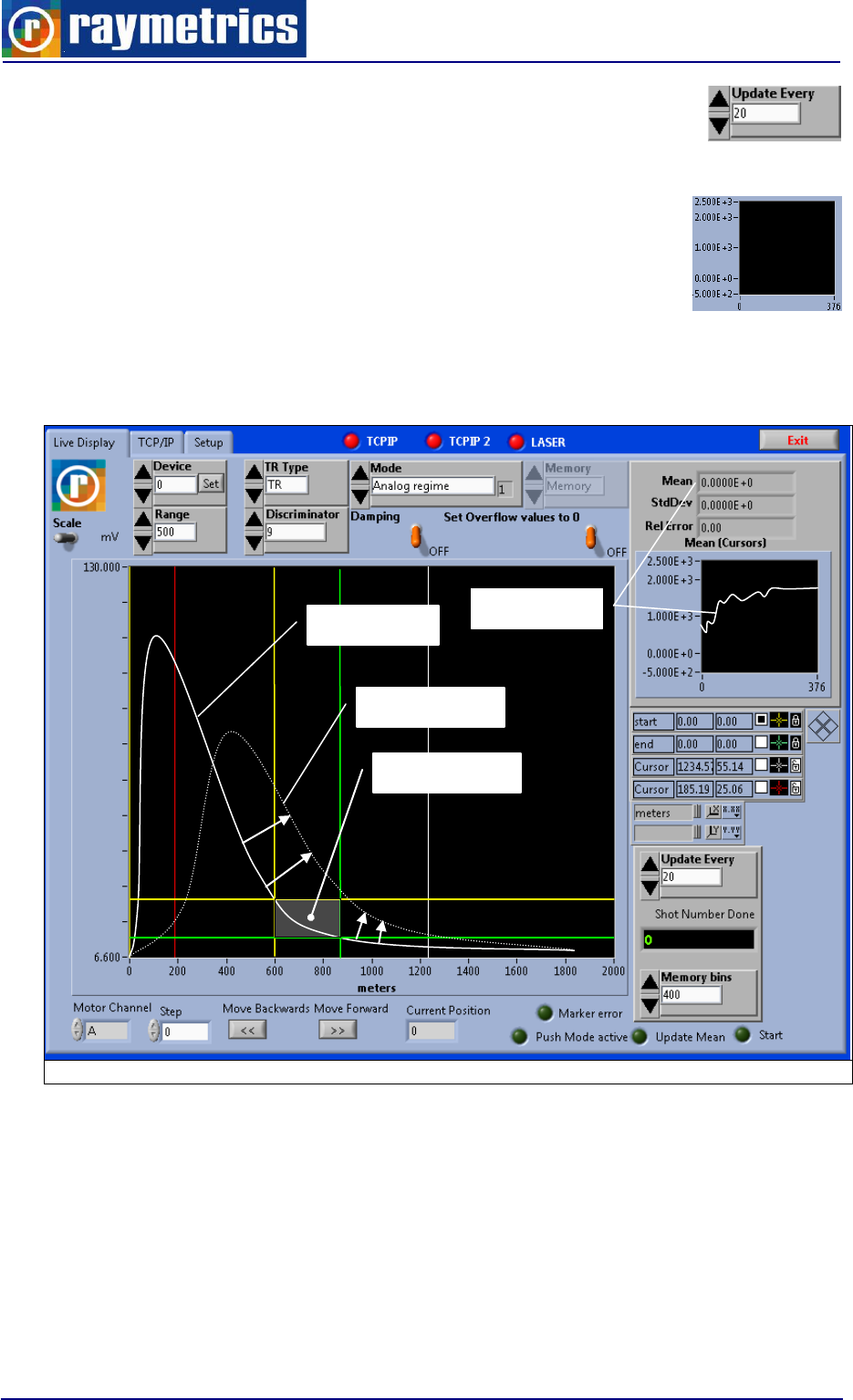
LIDAR OPERATION
70
6. You can set the shots number for each profile to the right in the
“Update Every” input. Set the number so that the image is good and is
refreshed in less than 5 seconds.
7. Once everything is set click on the small graph on the right and
select clear graph. This will empty all previous values. Remember to
do so each time you change the selected area. Wait for a couple of
profiles to be taken so that you will have a starting view.
8. Select one actuator A or B. It doesn’t matter which one you select since this is a try
and error procedure. As for the step size begin with a rather big step and gradually
reduce it when close.
Fig. 6.13: Intensity Maximization Alignment method
9. Move forward and backwards the actuator. You will notice the changes in the signal.
Wait for the signal to be stabilized for one or two profiles and notice the change in the
small graph. If the mean value is getting higher then continue to move this actuator at
the same direction. If the mean value is reduced then go to the opposite direction and
check if the value gets better.
Initial Signal
Aligned Signal
Selected Area
Mean Value
Mean Value
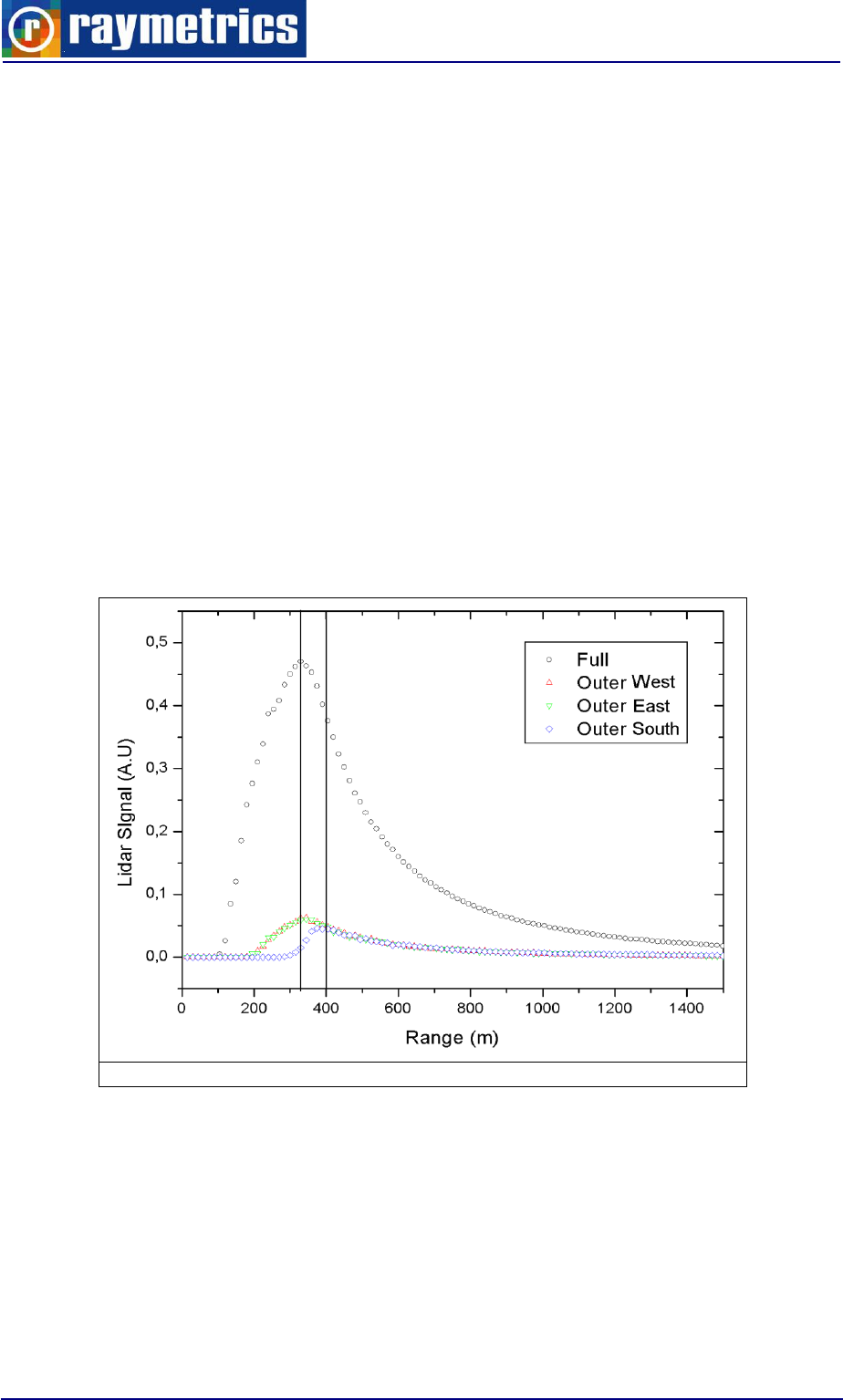
LIDAR OPERATION
71
10. After repeating this process the mean value will reach a point that moving the actuator
in both directions will only be reduced or remain the same. At this point change the
selected actuator to the other one.
11. Continue with the same procedure as described with the other actuator.
12. You may have to swift between the actuators a coupe of times until you will reach a
point that no is improvement of the mean value. At this point select an area even
further than the current, clear the graph, reduce the step size and continue with the
same logic used above.
6.2.2.2 Telecover Test
With this test you simply isolate the critical areas of the telescope and check at each
area the signal. For this reason we divide the telescope at four quarters. Each quarter is
named after the cardinal points for unification reasons. The north is always looking at the
laser beam. At an aligned Lidar the west and the east quarter should have identical signal
shapes while the one that is at the south gives the full overlap.
Fig. 6.14: Telecover Signals
In Fig. 6.14 you can see an example of Telecover test for D400 Lidar. Although the
peak signal for the full telescope is appeared around 320 meters the real overall is around
400 meters at it can be seen from the Outer South part test. In addition we can see that
the OW and OE signals are almost identical.
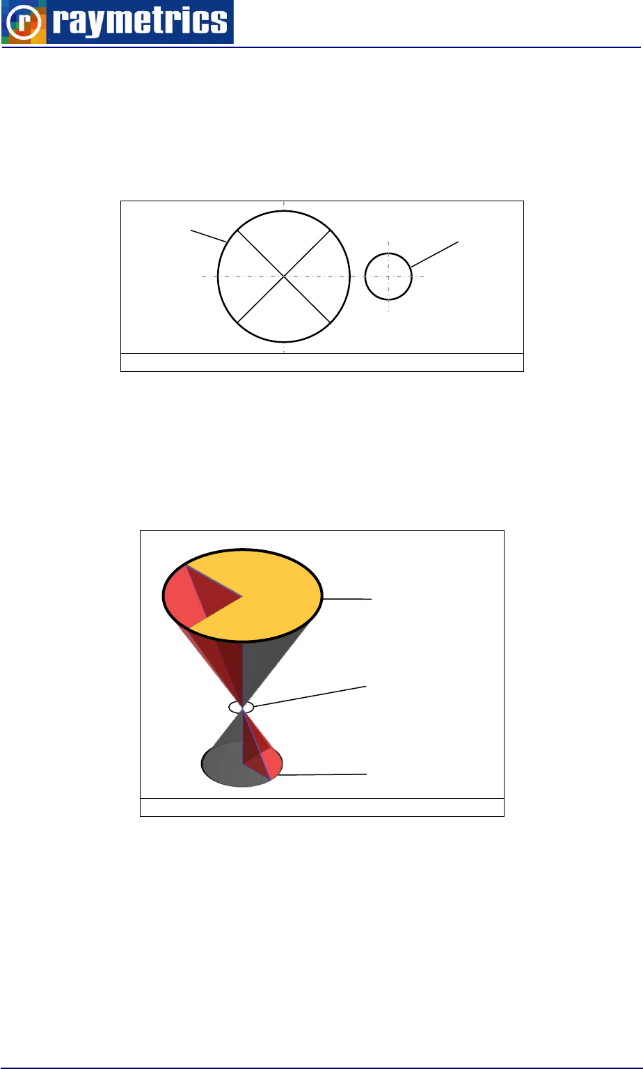
LIDAR OPERATION
72
The east and west parts in theory are identical but in reality these two can never be
identical because of the inhomogeneity of the optics and the PMT cathode. Most typical
reason of inhomogeneity is dirt on the windows or in the telescope. This means that the
signal intensity cannot be used as a criterion for the comparison but the overlap on the
other hand is absolute.
Fig. 6.15: Telescope Division
Normally we would expect that the part that gives the overlap should be the one that is
close to the laser beam (inner quarter). This is true but the image at the cathode is
reversed. The light focuses at the field stop and defocuses resulting to an upside down
and mirrored image. This will help us to understand why moving the laser beam towards
the obvious desired direction has the opposite effect on the signal.
Fig. 6.16: Image Inversion
To make this telecover even more precise we can divide each quarter to two equal
areas; inner and outer. To do so we need to take into account the blind spot of the
telescope created from the secondary mirror. We symbolize these parts with two letters:
the first letter is ether O for outer and I for inner, while the second letter can be W, E, S
and N that stand for West, East, South and North respectively. Now imagine an axis from
the center of the telescope to the center of the laser beam. This axis is not always
Telescope
West
East
South
North
Laser
Beam
Image at Window
Focal Point
Image at Cathode
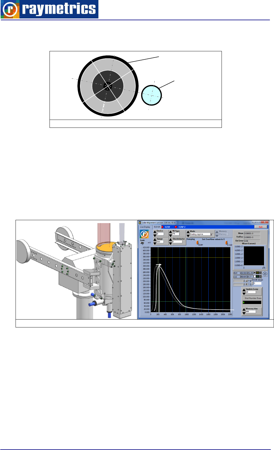
LIDAR OPERATION
73
horizontal or vertical. So when placing the telecover you have to align the center of the
clear area with the imaginary axis.
Fig. 6.17: Detailed Telescope Division
The fine alignment procedure with this method is described below.
1. Open the “Lidar alignment” program.
2. Place the cover on the telescope’s window letting the light only from the south side.
NOTE THAT THE LASER IS NOW TRANSMITTING, FOLLOW CAREFULLY THE
SAFETY INSTRUCTIONS.
3. Using the actuators shift the peak of the curve at live display to reach the desired full
overlap. This systems full overlap is at 200meters.
Fig. 6.18: Full Overlap Alignment
4. Turn the cover letting the light only from the east side and place a cursor on the peak
of the curve at the graph but make sure that the cursor is unlocked.
5. Flip the cover to the opposite side (west side).
6. Using the actuators try to reach the same overlap as the cursor placed before on the
curve. Once you are close place another cursor there.
7. Turn the cover to the opposite side (east side) and repeat the last steps until the two
curves have the same overlap. This means that the telescope is symmetrical to the
laser beam.
IW
IN
Telescope
Laser
Beam
ON
OE
OS
OW
IE
IS
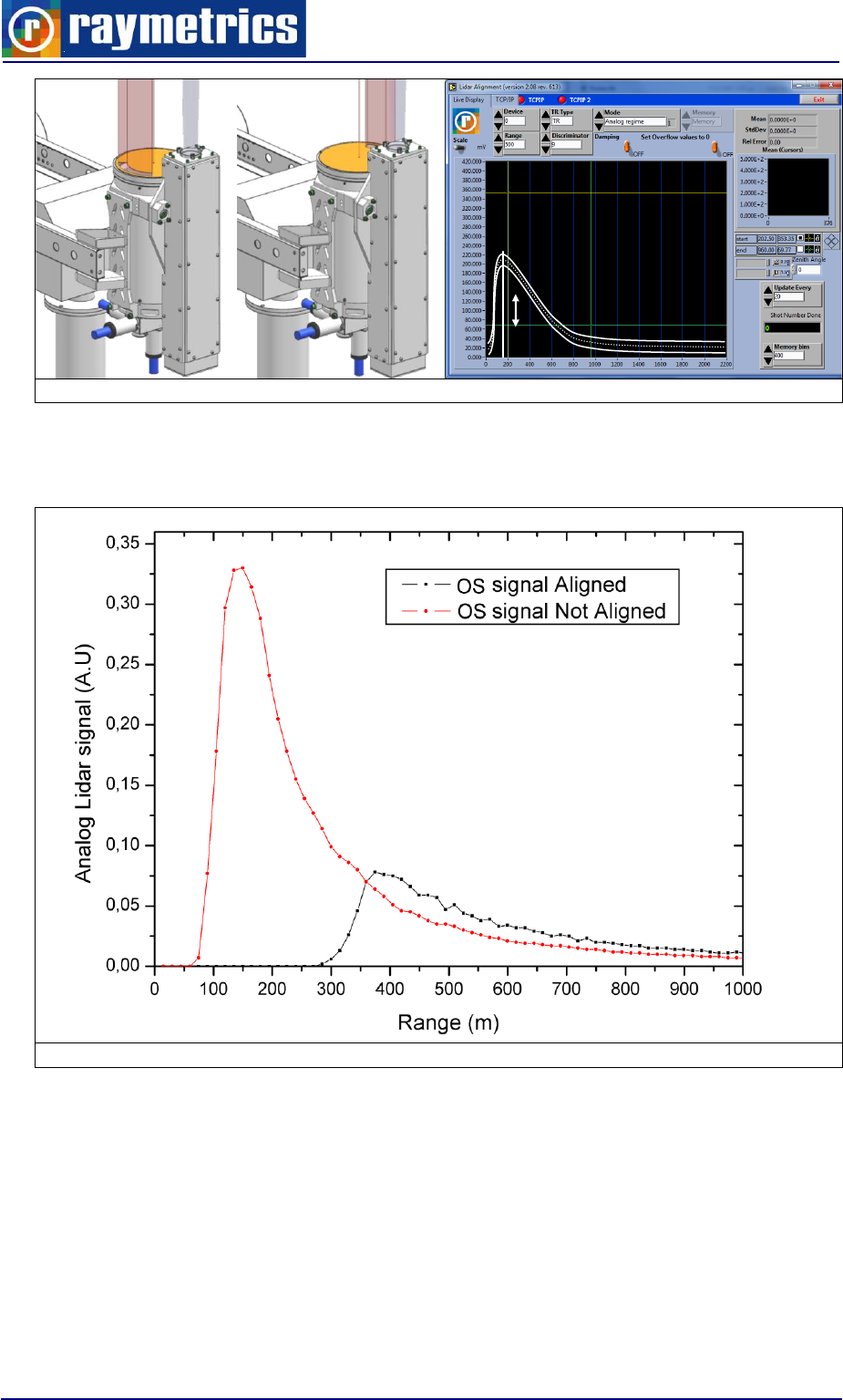
LIDAR OPERATION
74
Fig. 6.19: Symmetry Alignment
A fast way to find out if the alignment is roughly good or not, is to make a telecover test
with the OS part. If we do so we are going to see Lidar signals as the image below
Fig. 6.20: Symmetry Alignment
The OS (outer south) part of the not aligned signal gives an overlap at around 180
meters while the good aligned signal gives an overlap around meters 380 which is the
value that we expect
For this specific Lidar configuration the overlap is close to 200meters.
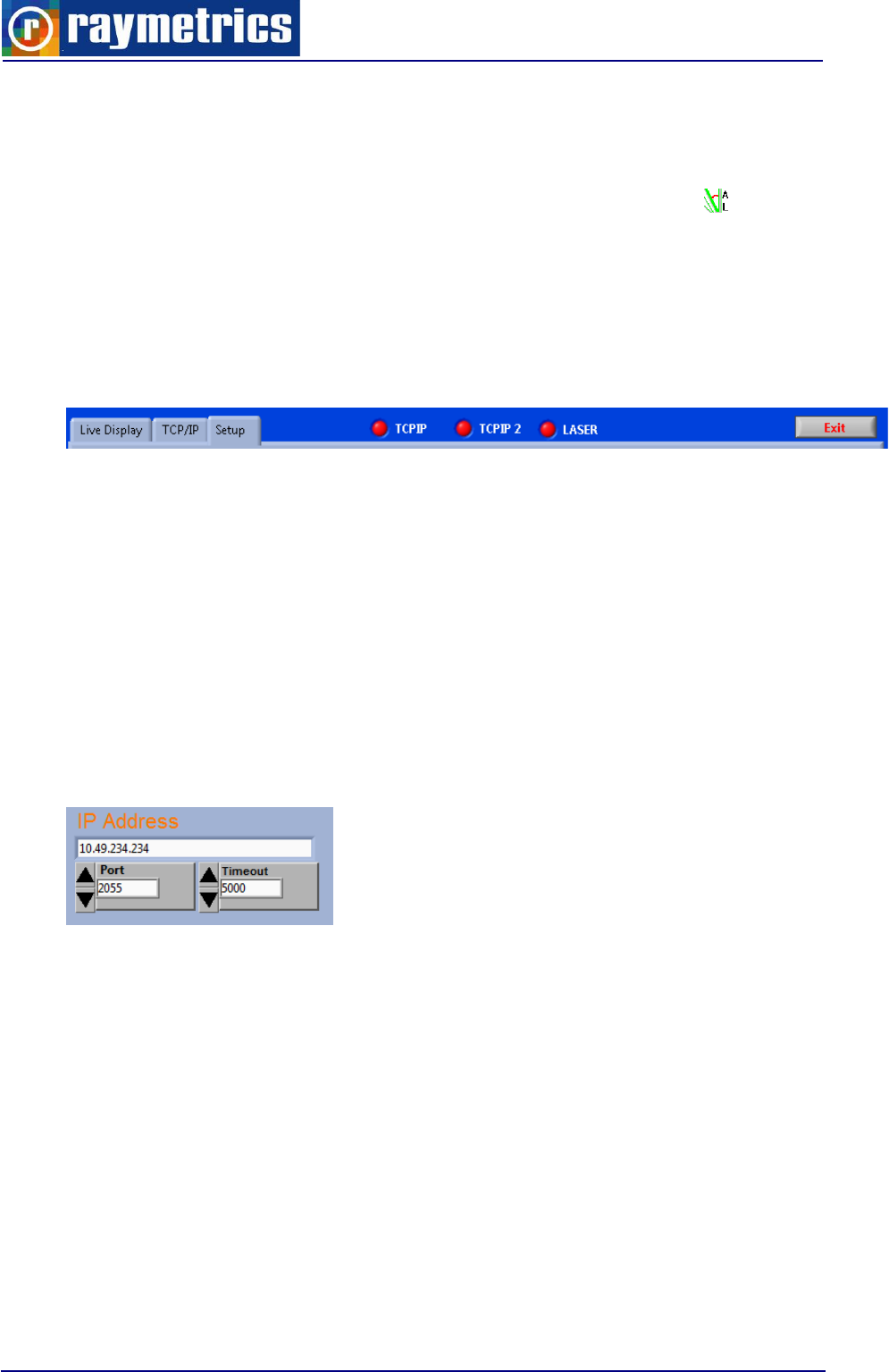
LIDAR OPERATION
75
6.2.3 Using the Alignment Software
In paragraph 4.3.1 Lidar Alignment the Lidar alignment software was introduced. Here
lies a complete guide how to use the software.
To open the alignment software, click the “Lidar alignment” shortcut. When the
program starts it tries to communicate with all devices. In this case there are four devices
to communicate with:
1. Transient recorder
2. PMT High voltage device
3. Laser
When the Licel devices and the laser communicate with the computer then the LEDs
on the top of the window turn to green. If for any reason they remain red consult the
trouble shooting section communication errors.
The last tab named Setup refers to the motorized mirror mount, if the Lidar is equipped
with one. The parameters here are for the communication port etc and for the speed and
acceleration of the mirror mount. Don’t change these parameters unless you are an
experienced user.
At the TCP/IP tab you can select the communication port but the IP address has to be
changed from Licel’s “TCPIP Set Fixed IP Address” program.
After the connection has been established with all devices the program asks the user
to start firing the laser. Verify by pressing “OK” but if for any reason you don’t want to start
the laser press “Cancel”.
Next another dialog appears where the user is prompted to input the high voltage value
for the selected PMT. By default device 0 is selected. After closing this dialog the “Live
Display” tab appears by default.
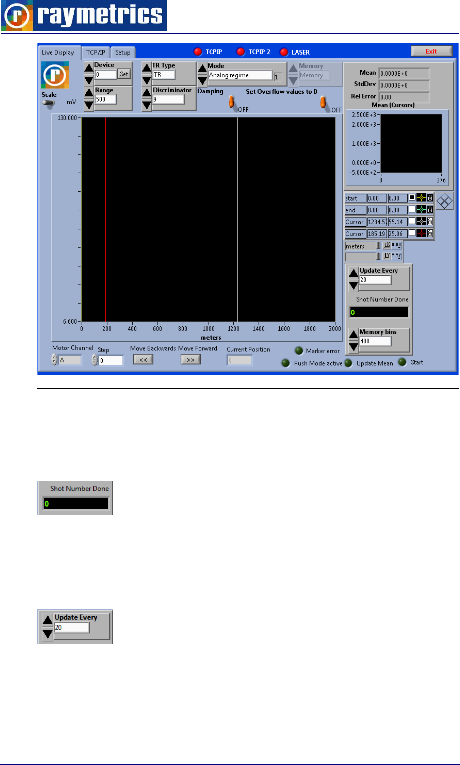
LIDAR OPERATION
76
Fig. 6.21: Live Display Interface
The laser needs a small delay time to start the q-switch for self protection. You may
have to wait until it starts and then the “Shot Number Done” indicator will increase for
every trigger pulse transient recorder receives (or a laser pulse if the recorder is triggered
from the laser source).
Set the desired value on the “Update Every” indicator. Setting this number to high will
result in a very slow response to the changes graph, but if the number is too low the graph
will be affected strongly by the laser’s energy oscillations resulting to a bad quality image.
Suggested value is close to the laser repletion rate (20Hz).
When “Shot Number Done” is equal to “Update Every” value the data are read from the
recorder, are displayed at the graph and the procedure starts over until the exit button is
pressed.
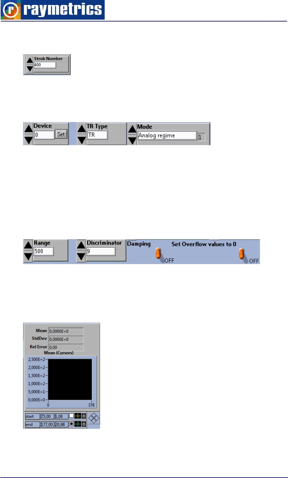
LIDAR OPERATION
77
The “Strob Number” indicator stands for the number of bins to be transferred from the
transient recorder and to be displayed.
The dataset which is displayed to the graph depends on the selections you make.
Select device, TR type, and mode. If you want to change the High voltage value for the
selected PMT (device) click in “Set”, located next to the device setting.
Set discriminator level, and the analog input range of the preamplifier (Range). The
signal starts at 0 and extends to -20, -100, or -500mV. Turn on the overflow switch, to
display all bins with overflow as 0. According to the EARLINET suggestions the range has
to be twice the peak signal. When the signal is too strong there is saturation in the signal
and the range must be increased, otherwise the PMT will be damaged. If the maximum
range is selected and the signal remains saturated refer to 6.2.4 Signal Intensity Reduction
paragraph to solve this issue.
The small graph at the right corner of the interface shows the average of the region of
interest on the waveform graph that is selected by using the cursors. The cursors at the
right of the waveform graph allow for the selection of a region to average over. The
average of the region selected is displayed in small graph at the right upper corner.
The x and y controls at the left allow the user to autoscale the x or y axis. By clicking
these buttons the scale is automatically adjusted to the highest value. The slide next to it
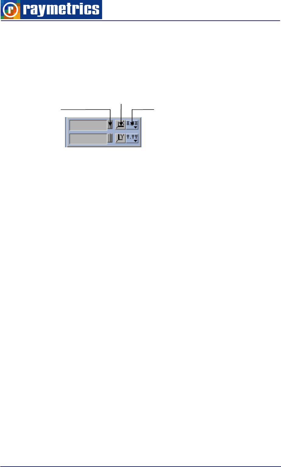
LIDAR OPERATION
78
changes from autoscale mode to fix. On autoscale mode the scale is adjusted to the
highest value each time it is changed. On fix mode the scale remains constant unless the
user presses the x or y controls (Autoscale Button). Defaults are autoscale for the y axis
and fix values for the x axis. The x.xx and y.yy controls allow for the specification of the
format precision and mapping modes of the x and y axis.
For more information about wave-graph refer to Labview manual.
WARNING:
NEVER BLOCK THE TRANSMITTED LASER BEAM, WHILE THE PHOTOMULTIPLIERS
ARE SWITCHED ON. THE REFLECTIONS FROM THE BLOCKING OBJECT WILL
DAMAGE THE PMTs. IF YOU WANT TO BLOCK THE LASER BEAM (e.g. for screening
purposes during alignment) ALWAYS SWITCH OFF THE POWER SUPPLY OF THE
PMT’s AND APD AND COVER THE TELESCOPE (with a piece of soft black cloth) IN
ORDER TO PREVENT THE ENTRANCE OF REFLECTIONS INSIDE THE TELESCOPE.
Axis
Autoscale
slide
Axis
Format
Menu
button
Autoscale Button
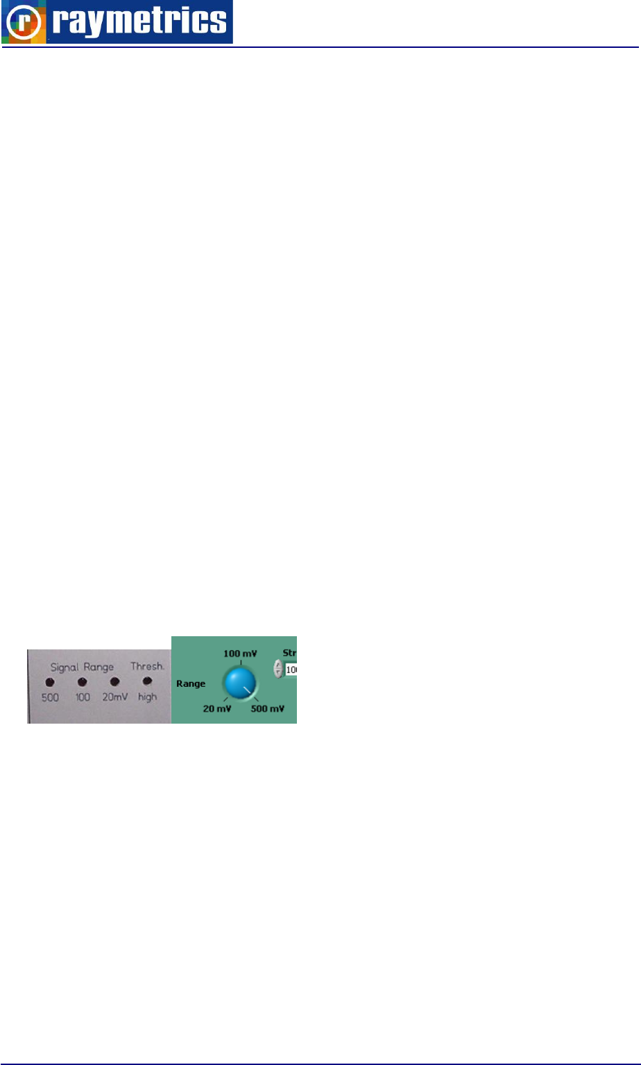
LIDAR OPERATION
79
6.2.4 Signal Intensity Reduction
Having a strong signal may seem ideal but in fact it can damage the PMT. The high
voltage setting must be in compliance with the average maximum anode current of the
PMT. This average current for Raymetrics Lidar systems are 100 μA which means 5 mV.
So, the value of 5 mV should not be exceeded for more than 30 seconds.
However the peak signal can significantly exceed the background average level as
long as the integral current is below 100 μA. The analog signal should fit into the input
range of the preamplifier and the ADC. Due to the fluctuations of the Lidar signal the
following rule of thumb will keep the signal inside the ADC range.
The analog backscatter signal should be about half (+/-10%) of the preamplifier
full range. Check this after fully align the Lidar.
For a 20 mV range this corresponds to 10 mV, for a 100mV input range this
corresponds to 50mV and for 500mV input range 250 mV.
Peak signals should not exceed 500 mV for more than 10 μs (i.e. 3000 meters or
400 memory bins) or 100 mV for more than 50 μs (i.e. 15000 meters or 1200 memory
bins)
The signal input range is user selectable by using the software. Before concluding that
the signal is too strong, make sure that the range is properly selected. By default the range
is up to 100mV not allowing voltages above that and thus it will look as if the signal is
saturated. In this case turn the knob to 500mV.
The max. cathode voltage of 1000V (High Voltage HV) should not be applied for
more than 30 seconds.
Too high background signals and peak signals introduce artefacts and decrease the
life of time of the PMTs. There are four ways to reduce the signal intensity:
Laser energy reduction
Field stop diameter reduction
PMT HV reduction
Use of filters in the eyepiece

LIDAR OPERATION
80
The two first are not the best solutions because they affect all detected wavelengths
and also the Raman signals which are by nature weak. If how ever you only have
backscatter signals then this is the easiest solution. Reducing the field stop will increase
the overlap and minimize the Lidar effective range.
Reducing the applied HV can help on the first glance but is not the optimal solution as
a long term solution. The PMT cathode can provide a limited amount of photons over its
lifetime, exposing the tube to a constant DC light will shorten this lifetime. This concludes
that the best way is by placing neutral density filters (or a color filter) in front of the PMT or
by using a narrower interference filter (costly solution).
Below are presented all solutions as the most effective depends on the Lidar type and
also on the user.
1. Decreasing the Laser Output Energy
Operation at a decreased energy level is useful when starting an experimental setup or
testing equipment and you detect extensive saturation at your Lidar signal. A simple way to
decrease the energy is to increase the flashlamp to Q-Switch delay to a value that is
higher than the optimum (highest power) delay using the Remote Box.
WARNING: Laser manufacturer advises NOT to decrease the high voltage of the
flashlamp(s) to reduce the output energy. Decreasing the high voltage of the
flashlamp(s) will cause a change in beam characteristics. Divergence and position
of the focal points alter may cause damage to the laser’s internal optics.
To adjust the output energy:
1. Select Q-Switch from the Main menu on the Remote Box.
2. Press the “Enter Menu” button.
3. Select Flashlamp / Q-Switch delay (FLQS Dly) from the Q-Switch menu.
4. Press the “Increase Value” and “Decrease Value” buttons on the Remote Box to
adjust the output energy to the desired value.
WARNING: Do not attempt to modify the pumping power by increasing the
flashlamp energy with the Remote Box of the PCC. This energy has been factory-set
for optimal laser performance. Adjust the flashlamp energy with the Remote Box
only if the flashlamp efficiency decreases. Please contact Quantel Customer Service
Department to ascertain the origin of the efficiency decrease.
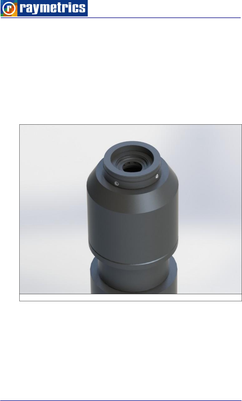
LIDAR OPERATION
81
2. Field stop diameter reduction.
This is only suggested to users who have advanced Lidar knowledge as reducing the
field stop will affect the range and the overlap. In this case you may affect the Lidar’s
performance for which Raymetrics has no responsibility.
As shown in Fig. 3. 7 Telescope main components on top of the optical unit lies the
focal plane. There you will find an adjustable calibrated iris. Use an Allen key to unlock and
turn the external ring to reduce or increase the diameter. Be careful not to turn the Optical
unit as this will result to telescope defocus.
Fig. 6.22: Optical Unit with Iris
3. Decrease the HV power supply of the PMTs.
This is a good solution when you are close to the signal intensity that you desire. You
can scientifically increase or decrease the signal by changing the HV but in order to have a
linear behaviour of the PMTs the minimum value should not be lower than the suggested
range (750-900V) for every detected channel.
4. Use colour or ND filters
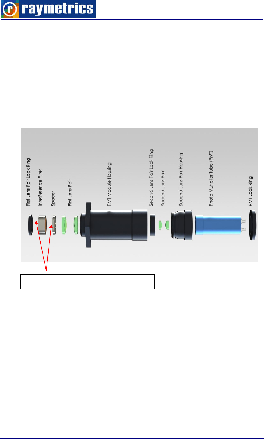
LIDAR OPERATION
82
Αbsorptive ND filters are the suggested solution, although reflective ND is good as
well. Another good solution is to use colour filters. Interference filters can also be used
which will decrease the OD as well but in this case it is a costly solution. Please contact
Raymetrics for the best suggestions. However before contacting us, send raw datafiles.
1. Unplug both cables from the PMT.
2. Remove the Detection Module from the Wavelength Separation Unit.
3. Place carefully the colour filter at the appropriate position
4. Place back the Detection Module to its position.
Attention: It is recommended that photomultipliers are protected from excessive light
during installation of the colour filters. After illumination the dark current will be temporarily
increased
Do not remove the interference filter which is located just in front of the PMT.
Note: Final optimization of you system will be done in-situ from Raymetrics engineers
during installation and training period.
Place where you can install a ND filter.
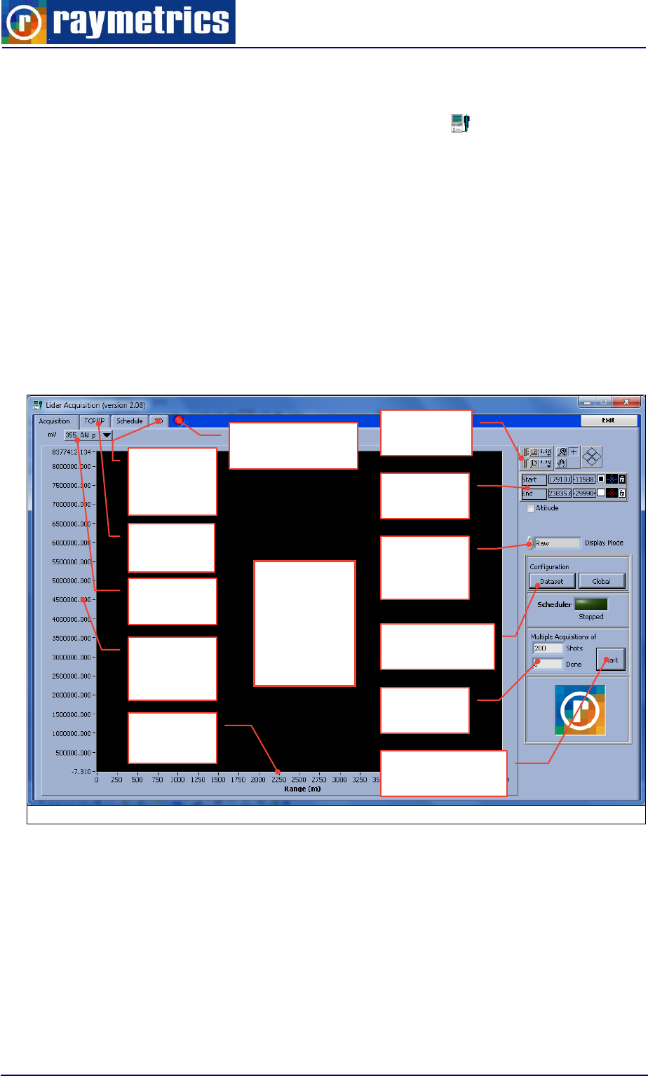
LIDAR OPERATION
83
6.3. DATA ACQUISITION
6.3.1 Introduction to the Acquisition Interface
Exit the alignment program click on Lidar Acquisition icon. Keep in mind that:
This interface is for multiple measurements.
Before starting a measurement all parameters have to be configured (see below).
By default the system is set to automated mode. This means that once you press
the Start button the laser will start firing without any notice. Follow the safety
rules.
Exiting program without previously stop a running multiple acquisition, may
cause unpredictable entries into the main database.
Below the main features of the “Acquisition” tab are presented.
Fig. 6.23: Lidar Acquisition Interface
6.3.2 Configure Measurements
You can set the parameters needed with the Dataset and Global buttons. The dataset
parameters are actually those which are related to the channels that you wish to use. The
global parameters are more general and not very likely to be changed. The global
parameters are saved by default while the dataset can be saved as a configuration file
which can also be loaded. Usually the operators make a couple of different datasets (for
LIDAR
SIGNAL
PREVIEW
GRAPH
Channel
Selection
Graph
Controls
Cursor
Controls
Signal
Intensity
Axis
Display
Mode
Control
Configuration
Buttons
Shots
indicators
Range
Axis
Start / Stop
measurement
Comms
tab
Comms
Indicator
Time
evolution
Tab
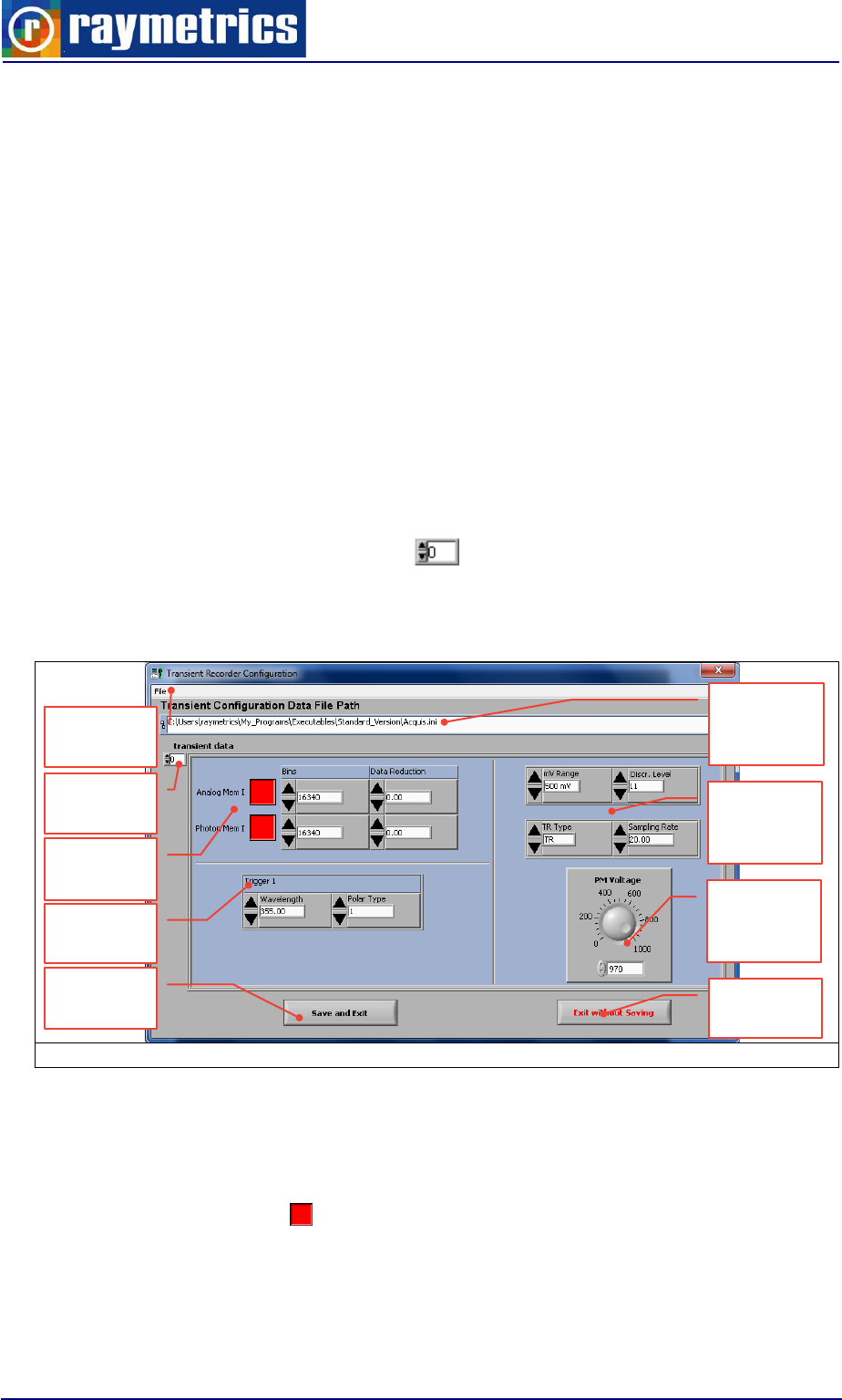
LIDAR OPERATION
84
example day time and night time) which are loaded each time to save time and avoid
mistakes.
Configure Transient Recorder
Start with the dataset. Click the dataset button and a new window will appear. On top
there is the menu item file that contains four sub-items that the user can choose from. If
you would like to edit an existing file, choose "Load transient information" and select a file.
After you have edited the data, you can save the information by choosing "Save transient
information as..." and either you choose the same file name, which overwrites the old file,
or give a new name. If you have edited the data and have made a mistake, you can reload
the original information by pressing Reset Information. The current configuration file is
shown at the display below the menu. If you select “Exit without saving” the dataset used
will be the original one that was selected initially.
Below this there is a numeric control. This selects the device that you currently
set. Pressing the up and down arrow will navigate though the devices. For instance here
device 0 is selected.
In the Transient data frame there are several inputs and controls. The values set here
have to be different for each device, as each device measures a unique wavelength.
The memory settings are those which send the command to write on the memory or
not. When the button is red the memory is activated and when grey deactivated. Here
you can choose separately which memory you want photon or analog. For the elastic
backscatter channels you need both in Raman you may need only photon if the signal is
weak. If you don’t want to use a channel uncheck (gray) both buttons. This may be useful
Fig. 6.24: Lidar Acquisition Interface
Device
Selection
Memory
Settings
Transient
Recorder
Settings
PMT
Voltage
setting
Save
Changes
Discard
Changes
Channel
Info
Config.
File
Indicator
File
Menu
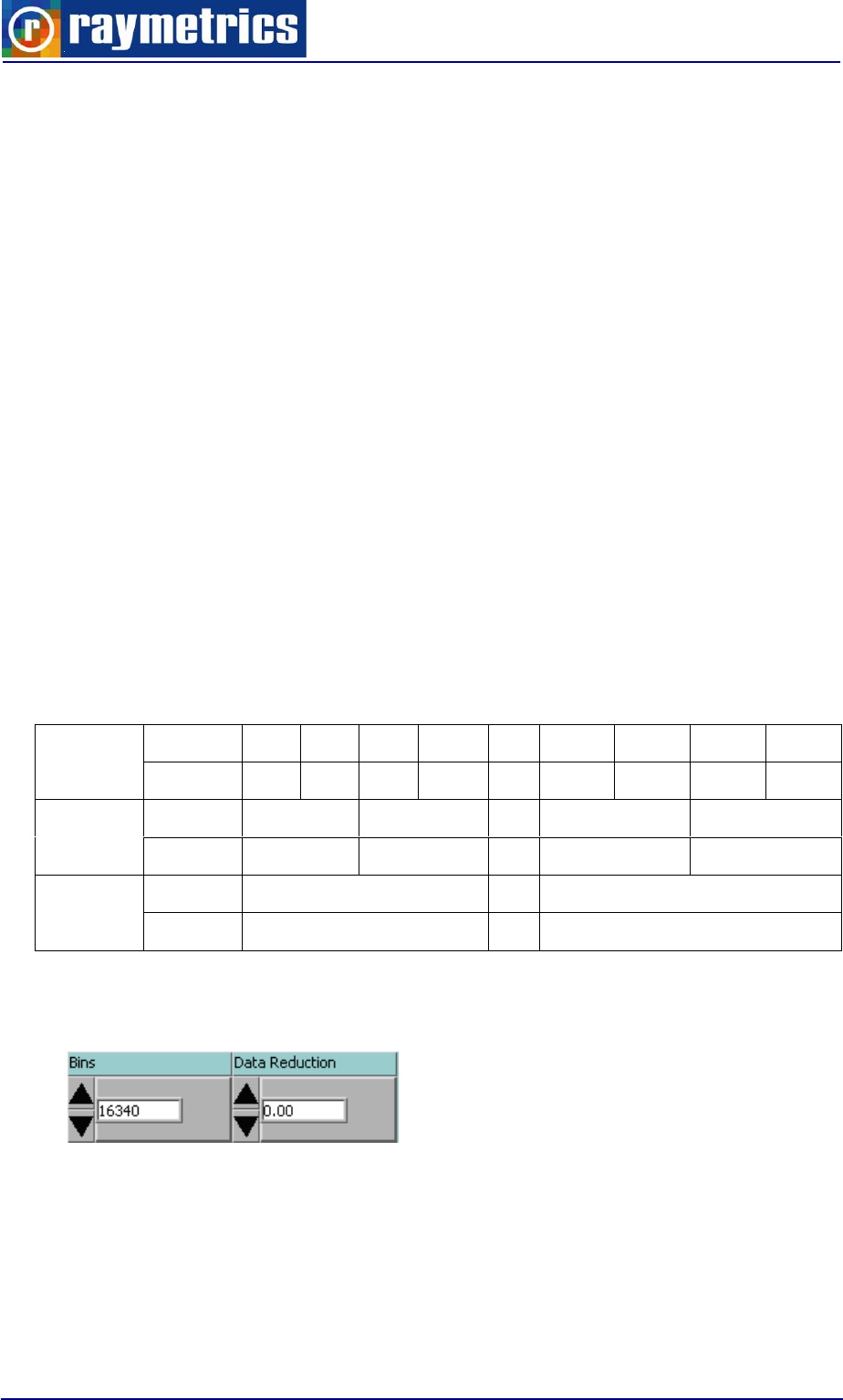
LIDAR OPERATION
85
for a Raman channel during day time that you don’t want to use to save data space. You
may also save space by reducing the memory bins. As already explained the memory bins
are related to the range. The spatial resolution of the recorder depends on the sampling
rate or in other words the recoding frequency. This system has a 20MHz recorder which
means that every 0.050μs writes a memory bin. When a laser pulse is transmitted the
recorder starts the time counter. The first photons will that arrive back are recorded after
0.050μs but this time was spent for the photon to reach the target and reflect back. So
actually the time that the photon needed to reach the target was 0.0250μs. The speed of
light on the other hand is approximately 3x10⁸ m/s so we calculate that the distance is 300
x 0.0250 = 7.50m. This is the minimum distance that the recorder can record, known as
the spatial resolution. The memory limit of the 12bit TR is 16384bins. This gives a total of
16384 x 7.50 = 122880m which in most of the cases is not needed.
Another way to reduce the data size is by using the data reduction function. This
function groups bins together to make a superbin. One level of reduction in value reduces
the height resolution by 1/2 and doubles the number of bins that are combined together. A
data reduction level of 0, 1 and 2 corresponds to 1, 2, and 4 bins per data point
respectively. In this way the spatial resolution increased but the maximum range is the
same. This also means that the maximum number of bins is reduced.
0 Data
reduction
Bins
1
2
3
4
…
16381
16382
16383
16384
meters
7.50
7.50
7.50
7.50
…
7.50
1 Data
reduction
Bins
1
2
…
8191
8192
meters
15.00
15.00
…
15.00
15.00
2 Data
reduction
Bins
1
…
4096
meters
30.00
…
30.00
Set the data reduction and the Bins number to read out from the memory bank keeping
in mind that the maximum number of bins is given by 32168 / (2^data reduction).
Below the memory setting there is the channel info. Here you have to specify the
detected wavelength and the polarization type. The polarization types are:
0 ........ No Polarization
1 ........ Parallel Polarization
2 ........ Cross Polarization
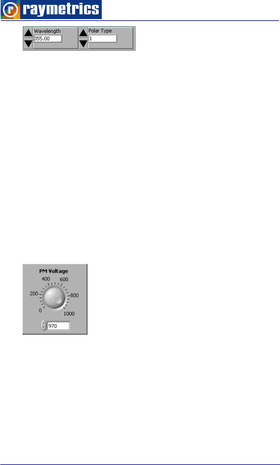
LIDAR OPERATION
86
Move on to the transient recorder settings. Here you have to set the range values of
the transient recorder, the discriminator level, the TR type and the sampling rate. The
ranges values are 0-20mV, 0-100mV and 0-500mV. These are selected based on the
signal intensity that you have noticed in the Lidar Alignment software. According to
EARLINET the range has to be twice the signal peak. For example if the signal peak is
close to 50mV you select 0-100nV range, or if close to 250mV select 0-500mV. Setting
the wrong range may result to signal saturation and eventually to PMT damage.
There are 64 discriminator levels (values 0-63) which correspond to either a range of 0-
24mV without gain reduction or 0-96mV with gain reduction.
Based on the model that you have the transient recording devices can be of different
type. You will have to set for each device the correct type TR (analog and photon) or PR
(only Photon) and also the sampling rate for each. You may find this information at section
10. LIDAR SYSTEM TECHNICAL SPECIFICATIONS.
The final setting that you have to set is the PMT Voltage that will be applied to the PMT
during the measurement. The allowable range of linear behavior is 750-900V. This
similarly to the range is set based on the signals intensity that you have noticed in the
Lidar Alignment software.
After finishing configuration of the transient recorder units, you can exit the
configuration program by either pressing the Save and Exit button, if you would like to save
the information to the actual file path as shown, or, alternatively, you can press Exit without
Saving if you would like to exit without saving your changes. Please note that when you
exit the program without saving, any unsaved data is lost! Thus if you have configured the
data and wish to keep it, you need to either choose Save and Exit or choose File->Save
transient information as... from the pull down menu before you exit the program. If you
want the current transient recorder configuration to be used as the default transient
recorder information, you must save this data as Acquis.ini in the installation path.
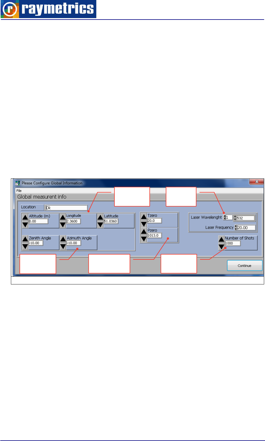
LIDAR OPERATION
87
Configure Global Parameters
Next setting is the global parameters. These are more general here you can set:
the Location information of the measurement site (8 characters length), longitude,
latitude and altitude (in meters),
The ground temperature (in Celsius) and ground pressure (in mhA)
The transmitted wavelengths and frequency from laser source
Finally the number of shots for each profile. Here you set in other words how many
profiles will be averaged to create a single one. The higher you set the best Lidar
data you get but slowly evolving. The number of shots should be set high enough
so that data files are not written more quickly than every ten seconds (i.e. 100
shots at 10Hz, 200 shots at 20Hz, etc.). This is due to a limitation of the naming
convention. The maximum allowable value is 4094 due to transient recorder ram
limitations.
Every parameter is now set. Note there two types of parameters; those who are for
information purpose and those who configure actually the measurement. All informational
parameters are stored as a header in the data files, so that the user can see what
parameters were used to take the data. The information entered in these fields has no
affect whatsoever upon the data acquisition. It is used purely to store information about the
experimental setup in the data files.
6.3.2 Configure the Working Directory
The working directory is the default directory where the data are saved. If you want to
set or change the working directory you just have to run the program: Config Lidar
Acquis.exe.
Fig. 6.25: Lidar Acquisition Interface
Ambient
Info
parameters
Profile
Setting
Scanning
Settings
Location
Info
Laser
Info
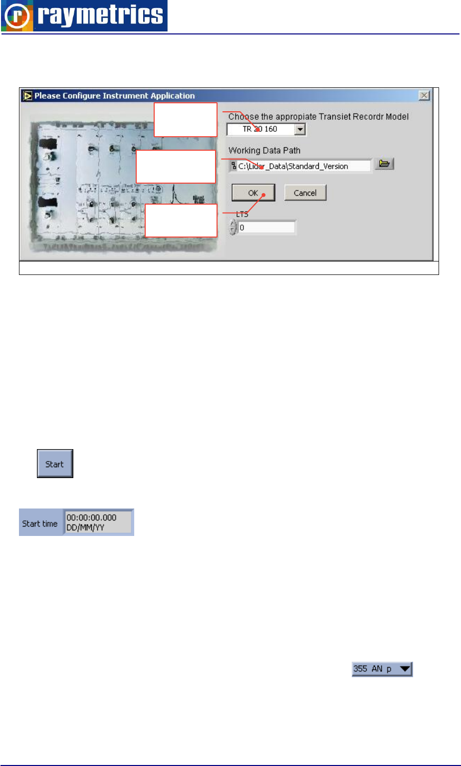
LIDAR OPERATION
88
As displayed at Fig. 6.26 it is a very simple program that changes the most basic
information for the Acquisition. That is the TR Model and the working directory.
Choose the TR 20 12bit and then select a working data path.
If the working data path that you will select already exists and contains a datalog.dat
file then the software will ask you if you like to overwrite this file. If you choose yes then a
new “empty” datalog.dat will be created. Make sure that the path doesn’t contain
spaces; you can replace them with underscores.
6.3.3 Lidar Measurements
After configuration press start button to start the measurement.
The start time field is automatically updated with the current date and time.
The transient recorders, in which you have activated data sets, should now acquire
data. If the acquisition has been started successfully, the number of shots done in the
shots indicator group should start increasing. When this number reaches the number
above, a new profile is shown in the graph area and a new unique file is save with the raw
data. The naming convention is explained in paragraph 7.1 DATA FILES HANDLING. The
waveform graph is refreshed with the newly saved data and starts a new measurement.
Select the desired dataset from the drop down list to be displayed. You may
also select at the display mode to see the raw signal (raw), the offset corrected signal or
the range corrected signal (Pr2).
Fig. 6.26: Config. Lidar Aquis. Interface
Confirm
and save
TR Model
setting
Working
path setting
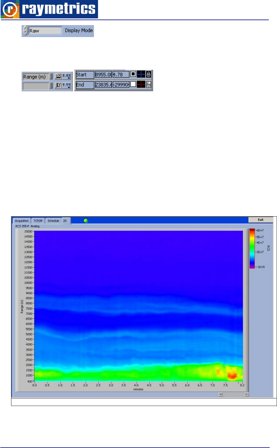
LIDAR OPERATION
89
You can change the axis scale and place cursors on the graph by using the controls on
right.
Press stop button to stop data acquisition. The waveform graph will be refreshed and
will display the dataset that the user has specified. Save acquired data to a unique file for
further analysis. By pressing the stop button a new record into the database will be added
with the same values into the start and stop time fields. If you exit the program without
stopping the measurement the database will not be updated, and the data will not be
available in the Analysis software. This doesn’t mean that the data are lost but they
need to be manually inserted at the database which is a time consuming process.
Finally you can have an overview of the data in the 2D tab which shows the time
evolution of the acquired profiles. Here the vertical axis is the height and the horizontal is
the time. The signal intensity s represented with a color scale which you can also alter.
Fig. 6.27: 2D Graph Tab interface
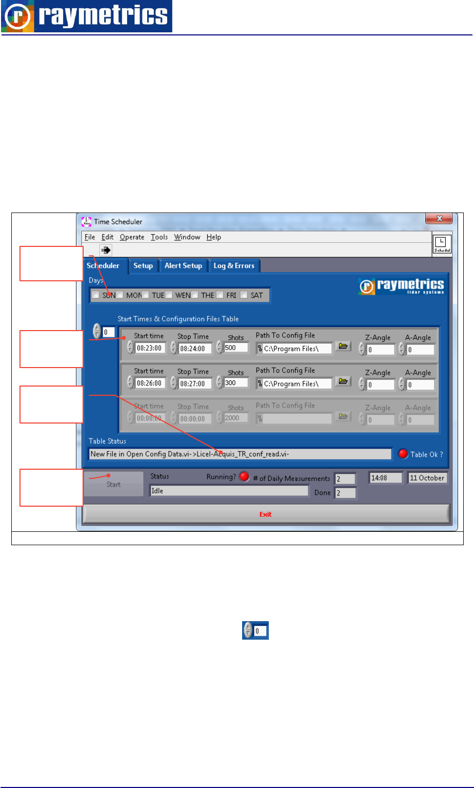
LIDAR OPERATION
90
6.4. MEASUREMENT SCHEDULING
A very useful tool is the Lidar Scheduler. With this software you can set a series of
programmed measurements on a daily basis. The main purpose of this tool is to perform
Lidar measurements without the need of an operator. This in combination to the remote
setting and alert setup makes a fully remotely operated Lidar. The software shares the
same acquisition module and thus the configuration parameters are already known.
The interface has four Tabs. The main tab is the “Scheduler” Tab. This contains the
time table and the scheduler status information.
Fig. 6.28: Time scheduler main interface
On top there is the day selection area. Select here which day of the week you will run
the programmed schedule below.
The Timetable is an array of inputs. You may add as many as you wish. To navigate
though the table use the control on the side.
Each measurement needs six main parameters:
Start time
Stop time
Number of shots for each profile
Day
selection
Time
Table
Start
schedule
Status
info
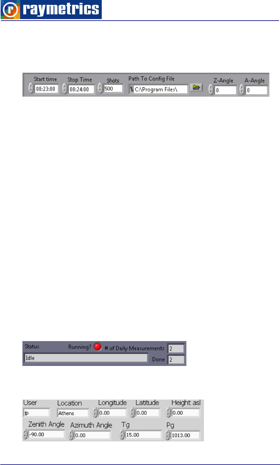
LIDAR OPERATION
91
Configuration (Dataset) file to be used
Zenith angle (Z-Angle)
Azimuth angle (A-Angle)
To make a correct table you have to keep in mind some simple rules.
The start time has to be earlier than the stop time.
The number of shots divided by the laser repetition must not exceed the run time of
the measurement.
The configuration file and path have to be valid.
The Start time of the next measurement has to be later than the stop time of the
previous one.
For example at the table in Fig. 6.28 the stop time of the first measurement is bigger by
two minutes or 120 seconds, which is okay, and also the shots are only 200 which divided
by the laser’s frequency 20Hz gives 10 seconds for each profile, which is enough to
acquire 12 profiles. If however the shots where set more than 2400 the table would show
an error and the green led “Table Ok?” will turn red. The same will happen if you set the
start time of the next measurement earlier than the last or if the configuration file is not
correct.
The user can create a configuration file on the setup tab. The scheduler starts when
the user presses the start button.
You can check the status of the scheduler on the bottom of the tab where information
about errors and the measurements done is available.
At the setup tab you can find all the global settings like the acquisition software except
from the shots number, as previously explained.
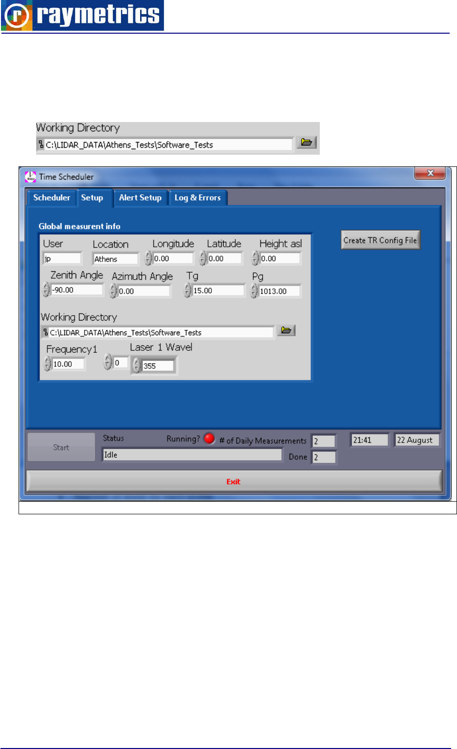
LIDAR OPERATION
92
Below this you will find the working directory setting, which is actually the selection
where the data will be saved. To select a folder click on the folder icon to open a windows
dialog, and select the directory by pressing the “select current Dir.”. Make sure that the
path doesn’t contain spaces; you can replace them with underscores.
Fig. 6.29: Setup Tab
On the left there is a button “Create TR Config file”, which is creates the configuration
Dataset file. When this button is pressed two windows open sequentially. The first window,
“config other hardware” is used to select the devices to be controlled by the software along
with their communication ports and some parameters which have to be set for the system.
This software module is presented in the tools section in Fig. 4.12. Once the user presses
OK another window opens that is very similar to the Dataset window (see Fig. 4.3). The
main difference is the communication port which has to be set there. By default the port is
2055. For the IP address refer to the connections paragraph at Fig. 3. 25: LIDAR Local
Network.
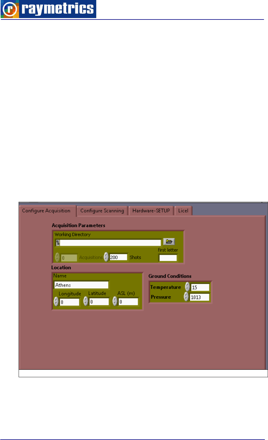
LIDAR OPERATION
93
6.5. SCANNING OPERATION
Until now all programs presented are used to acquire data in a fixed position. Here is
presented a set of program to use the lidar in scanning mode. The set contains three
programs fro the acquisition. The idea remains the same as previously noted; the user has
to make a configuration file to specify the type of measurement(s) that will be performed.
Here this file contains also geometrical and kinematic information about the scan. Once
the file is created it is loaded either at the scanning autonomous or the Time scheduler
Scanning program.
6.5.1 Creating a Configuration File
To make things easier there is a software module that guides the user to create the
configuration file. This runs alone as an executable or is called through the scanning
autonomous and time Scheduler programs.
At the image below is the main interface of the acquisition configuration tab. This is
more or less similar to the setup window from acquisition program.
Fig. 6.30: Configure Acquisition Tab
Next to this is the scanning configuration tab. Here the user sets all the parameter that
will be used for the scanning.
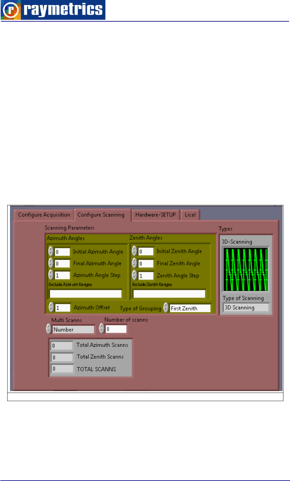
LIDAR OPERATION
94
Starting with the scanning parameters the user has to set the angles that define a
scan. For example setting the initial azimuth angle to 0 and the final to 90 degrees the lidar
will perform an azimuth scan in horizontal position (0deg at zenith) which practically is a
quarter of a circular scan. The step angle is the resolution of the scan. Setting this too low
will increase the resolution but degrease the speed of the scan. Similarly to this example
the user can set only the angles for a zenith scan but also can set the limits angles for both
zenith and azimuth to perform a 3D scan. Furthermore in a 3D scan there are options of
how the positioner will move from point to point. The options are four; Zenith or Azimuth
first (zigzag type of scan) and Snake zenith or azimuth (snake type of scan).
There is also the option to set an offset for the azimuth orientation. If for example the
instrument is not directed to the east at the home position but has an offset , you can set
this number here.
Finally the scan that you set here can run as many times you wish. At the text boxes
below you can see the summarize of the azimuth and zenith scans.
.
Fig. 6.31: Configure Scanning Tab
Next tab sets the hardware control, i.e. if the laser is controlled from the software, or
the positioner (2AP) etc.
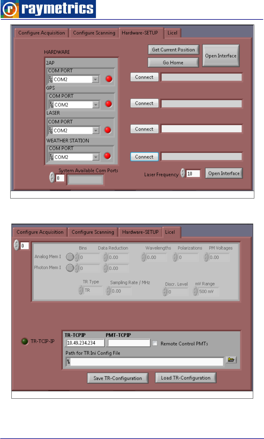
LIDAR OPERATION
95
Fig. 6.32: Configure Hardware Tab
Finally the last tab contains all information for the dataset which is already explained.
Fig. 6.33: Dataset Tab
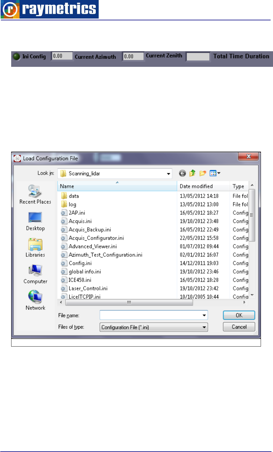
LIDAR OPERATION
96
Once all necessary parameters are set the bar on the bottom shows information about
the estimated duration and also you can see the current position.
6.5.2 Scanning Autonomous
With this program the user can acquire scanning data with the lidar. The interface is
very similar to the fixed point acquisition program.
When the program starts it prompts to load a configuration file. Select the file that you
created with the configurator and click ok to load.
Fig. 6.34: Configure Scanning Tab
The main interface is very similar to the acquisition interface the main difference here
are the indicators on the bottom that shows some information regarding the type of the
scan to be performed. Note that you have the option here to set to run the same scan
scenario continuously until the user press the stop button. The counter nex to this option
indicates how many scans have already performed and the counters below shows the
number of scan steps per scan and those that are currently done.
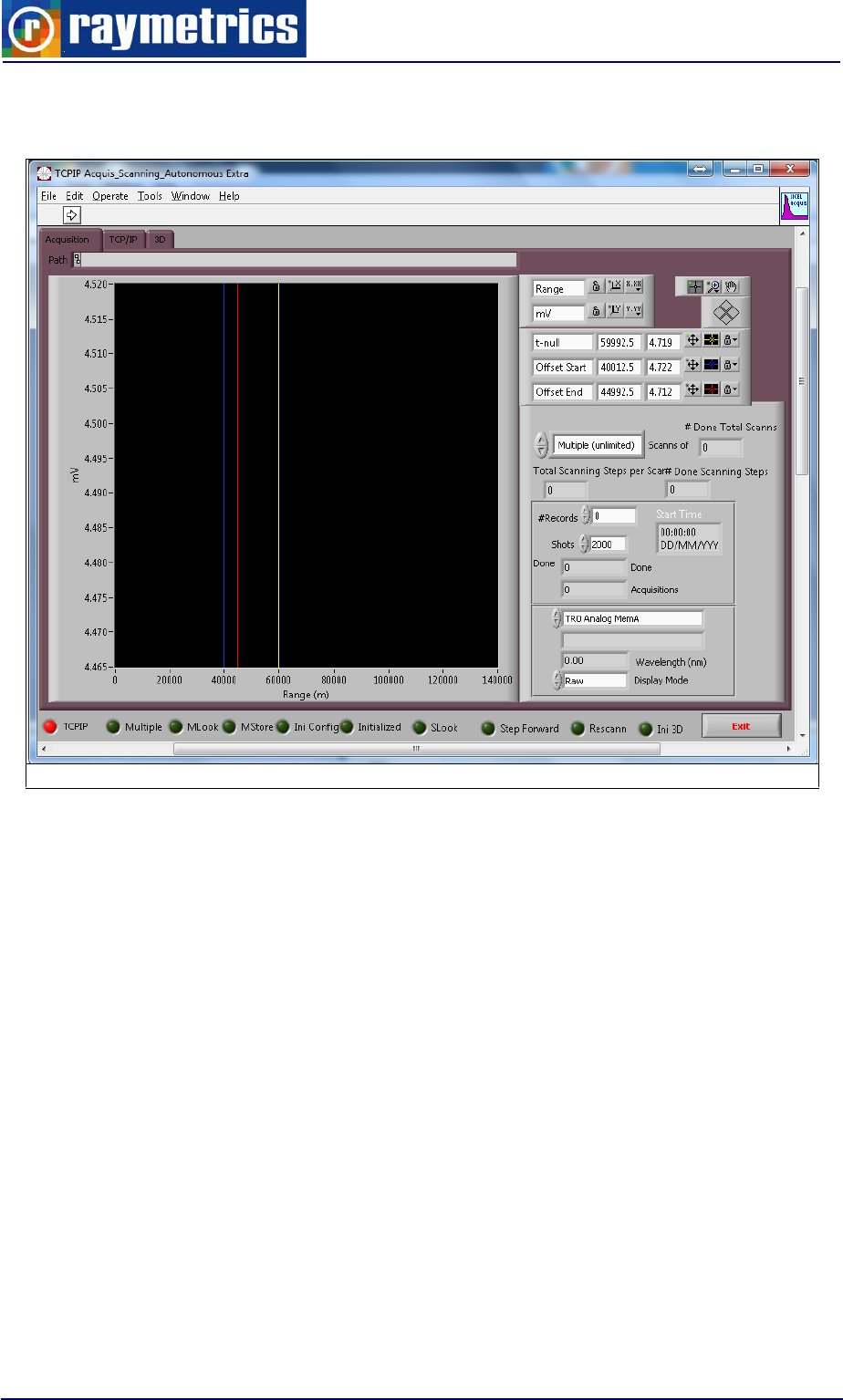
LIDAR OPERATION
97
At the 3D tab the user can have a quick look of the scan as this was acquired in a 3D
graph.
Fig. 6.35: Scanning autonomous Main Interface
6.5.3 Time scheduler for Scanning
This program as already explained is used to make a schedule of measurements. The
difference with the fixed point time scheduler is that this can run scanning acquisitions
instead of fixed pointed ones. The same logic is used whit the scanning autonomous you
can use the configurator to create a scanning configuration file or you can call this program
by clicking on create TR config file at the set up tab.
Once you have the configurations files that you will use, go to the scheduler tab and
select the days of the week to run or none to run only once, below that set the start time
and the configuration file, press the start button and the scheduler will start measuring the
scheduled measurements. Notice that there is no stop time here as this is estimated from
the configuration file. Make sure that the next measurement will not overlap with the
previous. If this happens the Table Ok LED remains red and the Start button grayed out.
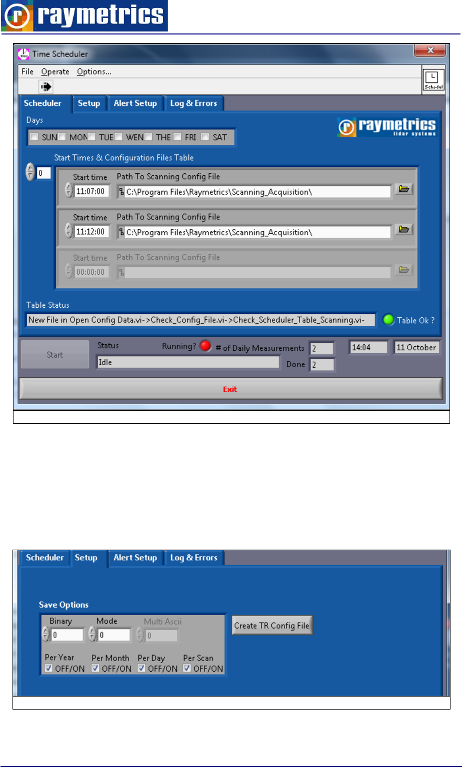
LIDAR OPERATION
98
Fig. 6.36: Scanning Scheduler Tab
At the setup tab you get all different options on how to save the data. This is very
useful while the scanning data are too many to be saved in a single folder. This way you
can group the data in folders by date or/and scan and have a much more organized data
base. Finally there is an option to save data in ASCII format if the user intends to use a
non Raymetrics program for the data analysis.
Fig. 6.37: Scheduler Scanning Setup Tab
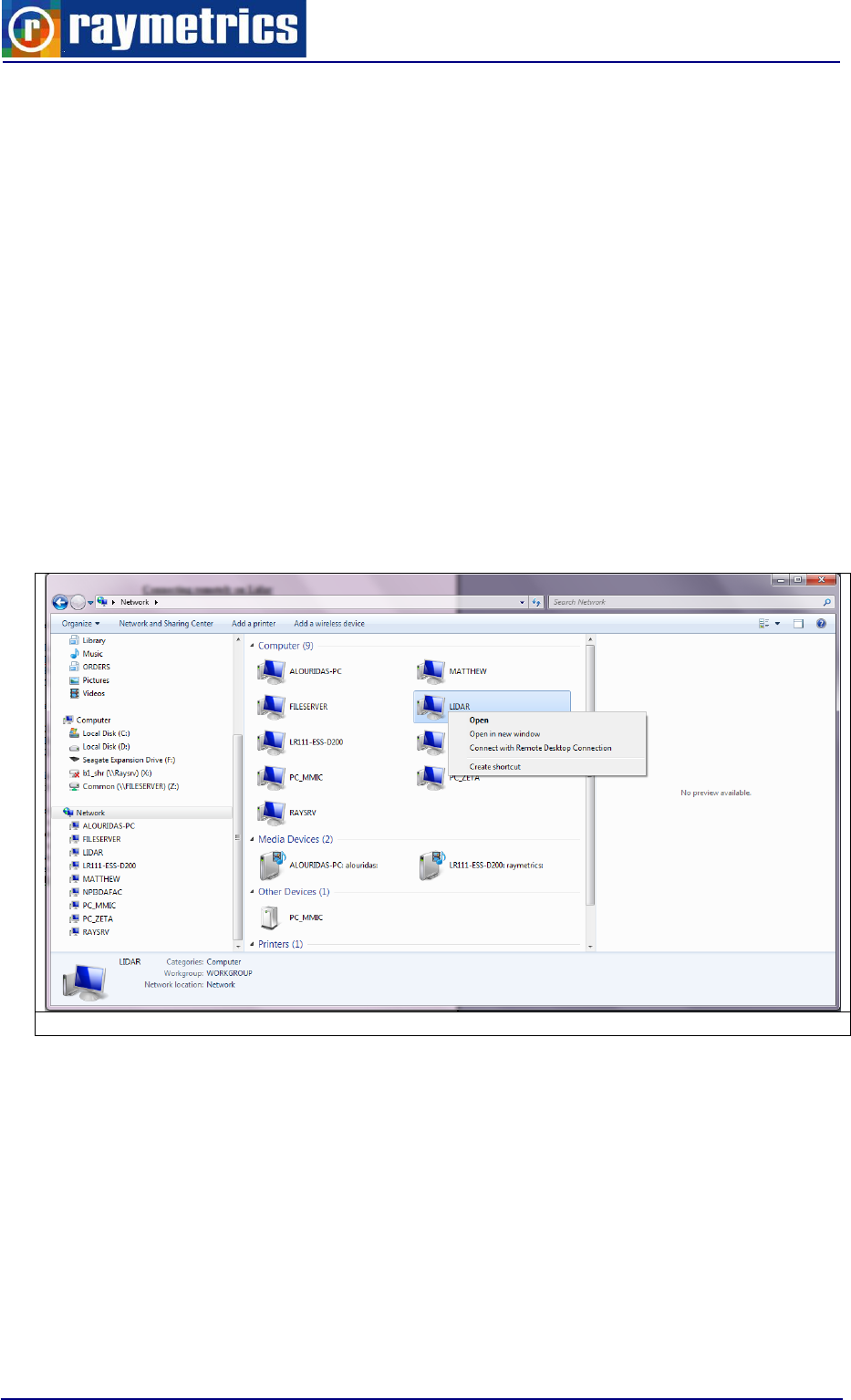
LIDAR OPERATION
99
6.6. REMOTE LIDAR
The Lidar can be fully remotely controlled. When it is plugged to a network it
automatically acquires an IP address. Any user in the same network should be able to
connect to the Lidar’s computer. If this network also has internet access with the
appropriate permission from the network administrator you can connect externally to the
Lidar from anywhere in the world. In this paragraph there are some practical guides how to
connect and operate the computer remotely.
6.6.1 Establishing a connection
Once the Lidar is connected to an external network, you can use the windows remote
desktop to control the Lidar’s computer. Follow the steps below to establish a connection
from a windows 7 operating system.
1. Open the network to browse all computers connected to your network.
Fig. 6.38: Lidar Computer On A Network
2. Locate the computer named “LIDAR” and right click. “LIDAR” Is a generic name you
can see in the computer properties the computer name.
3. In case you cannot find the Lidar computer, make sure that the Lidar is powered on,
and that the connection cable is well placed at the Lidar and at the wall. If this doesn’t
fix the problem use another cable or another wall socket.
4. Select “Connect with Remote Desktop Connection” (RDP).
5. When you click the window below appears.
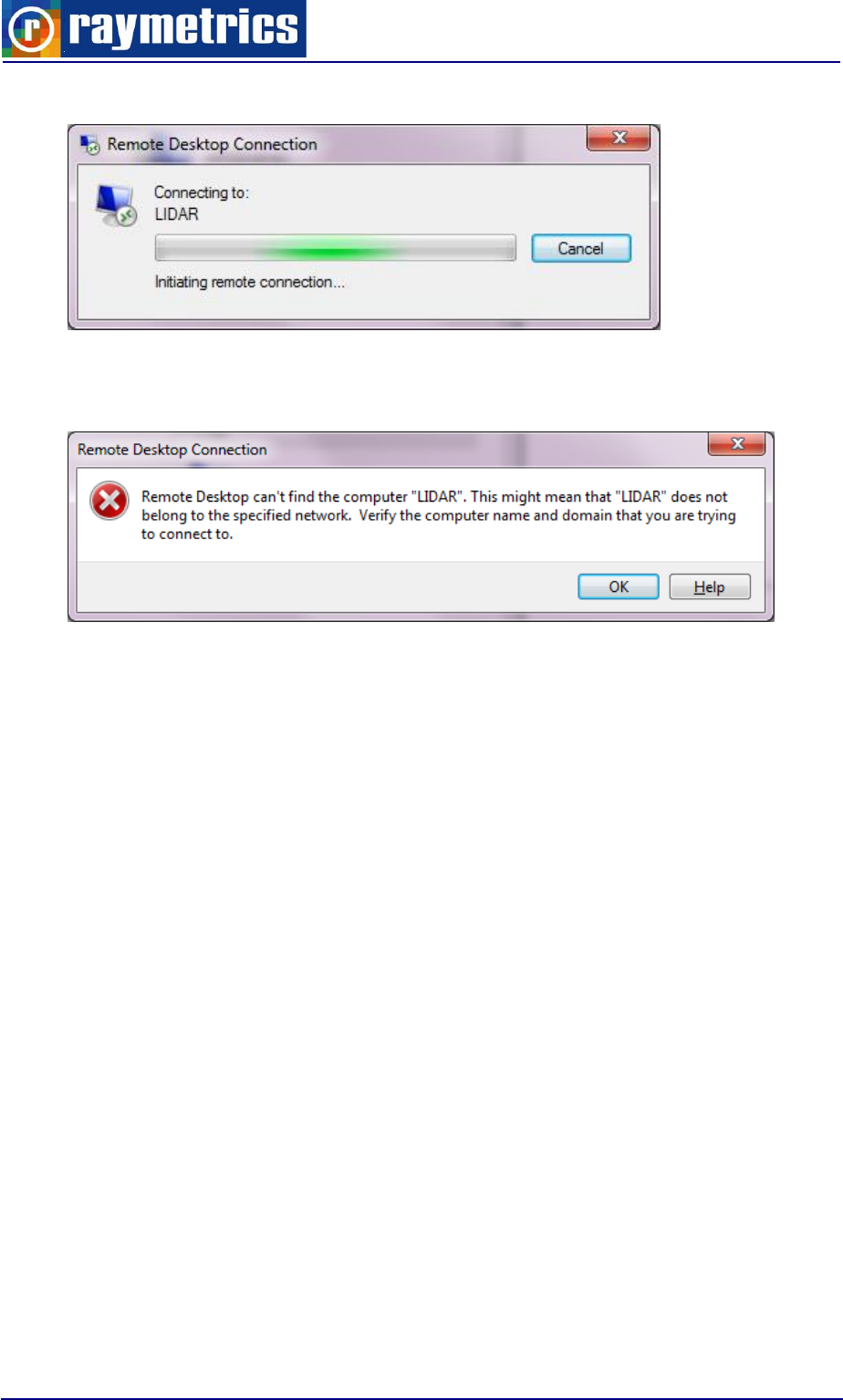
LIDAR OPERATION
100
6. Normally you will have to wait for a couple of seconds. If it takes longer that one minute
then probably the connection cannot be established and the window below appears.
7. The most common reason for this is that the computer is turned off. You can see how
to remotely wake up the computer at “6.6.2 Shut down and WOL” paragraph. If the
problem is still there refer to the “6.6.3 Remote Connection” paragraph.
8. Key in the user name and password when prompted and check “Remember my
Credentials”.
By default the account used has the credentials below:
Username: User
Password: Lidar
9. A new window will open showing the Lidar’s desktop. Use the mouse and keyboard
and control the Lidar.
Note that this is a window which you can resize, minimize and close like all windows.
When you resize keep in mind that you don’t view the whole screen. There might be icons
missing or the taskbar which you can view by using the scroll bars.
Also keep in mind that when you close the window you don’t close the Lidar computer
but only the connection. The computer logs off and remains turned on. If you want to shut
down the computer refer to “6.6.2 Shut down and WOL” paragraph
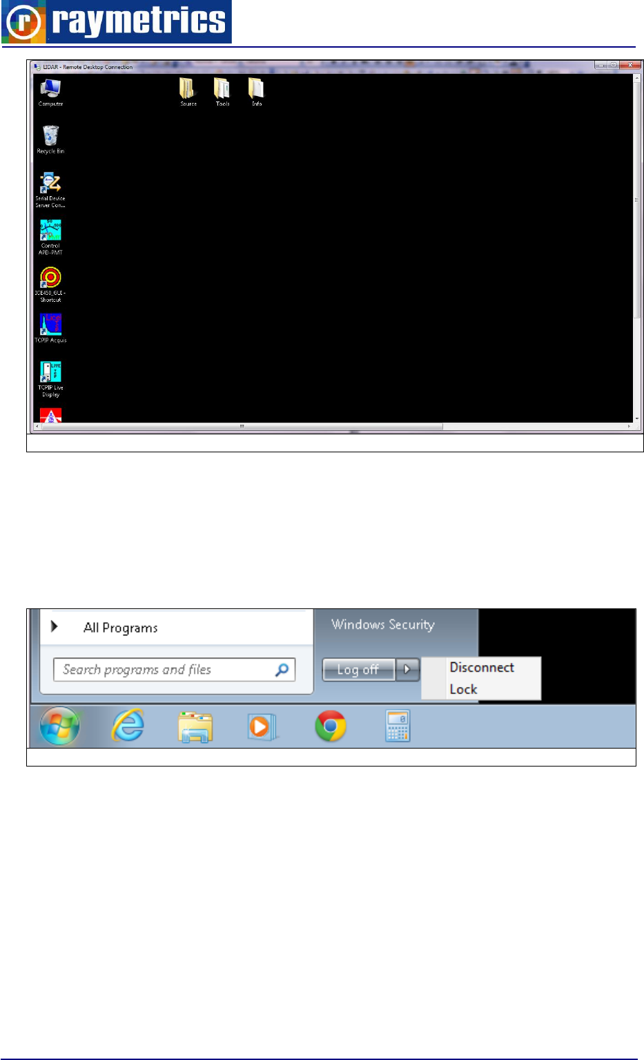
LIDAR OPERATION
101
Fig. 6.39: Remote Desktop Window
6.6.2 Shut down and WOL
Once connected, you will notice that the options in “Start” are limited to “Disconnect”
and “Lock”.
Fig. 6.40: Limited Shutdown Options
In order to shut down the computer, click “Windows Security” right above the “Log off”
button. This will show you a new screen which is shown when you press “Alt+Ctrl+Delete”
in windows 7. From there you can select to shut down safely the Lidar computer.
Note that if you try with the key shortcut “Alt+Ctrl+Delete” the screen that is shown
refers to your computer and not the Lidar’s computer. There is however the option to use
this shortcut also in the remote connection. Please refer to the “6.6.3 Remote Connection”
paragraph.
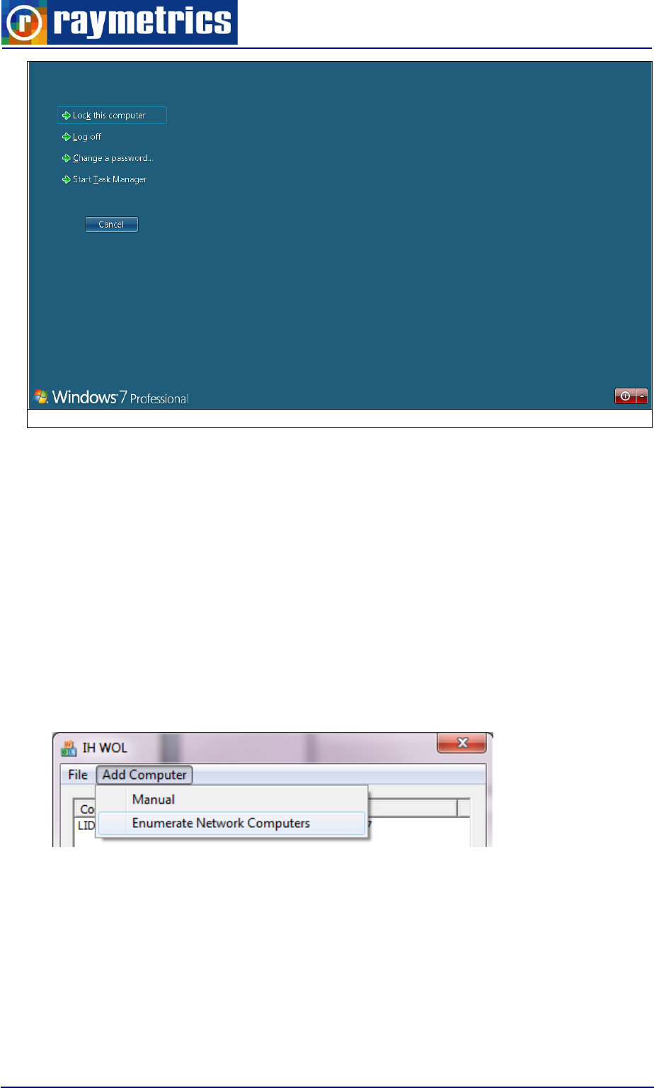
LIDAR OPERATION
102
Fig. 6.41: Windows Security
The next thing now is to turn the computer on remotely through the LAN. This
procedure is called “Wake on LAN” and it is an event that wakes up the computer using
the local network or even the internet. To do this a packet of codes must be send from
your computer to the Lidar’s computer, which is called “Magic Packet”. This packet is
produced and sent with very simple software which is called in general “Magic Packet
Sender”. You can find many free programs over the internet. All of these programs need
the Lidar’s IP and MAC address to work however some require more information.
Many of these programs can scan the network and find all computers which are
currently turned on and acquire automatically the Name, IP and MAC address. Below is an
example of such a program.
Note: The program will not find the computer if it turned off. If you want for the first time
to scan to find the Lidar computer, turn it on and then you can save the information needed
to the program so that you can use the next time.
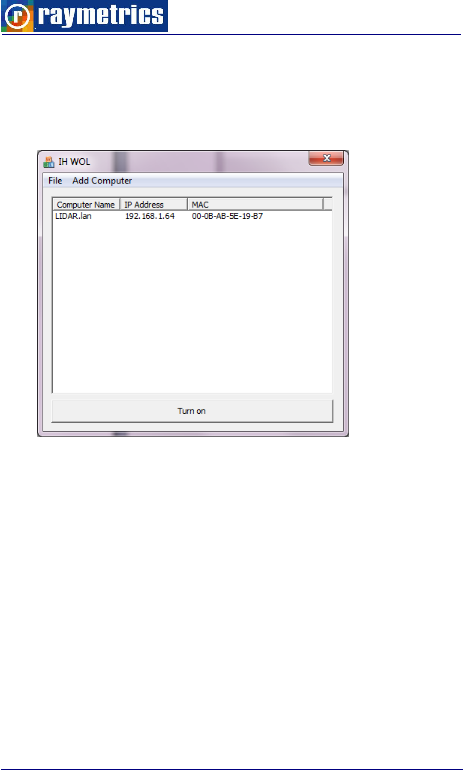
LIDAR OPERATION
103
Note: You have to give permission from windows to scan the network. If you are
prompted for security issues for this operation check the option to allow the program to
perform the scan.
Once you have the computer’s information you simply have to select the correct name
and turn it on.
Note: You will have to wait for a moment to let the computer start windows, before you
can connect to it.
There is also the option to perform this from this task from a distant computer over the
internet but in this case you will need to set a static external IP address for the Lidar at the
network router’s options and also to set an access port at the firewall options. Please
consult your IT department before performing such a task.
6.6.3 Remote Connection
The procedure described in the paragraph “Establishing a connection” is the fast way
to connect. However you don’t get all the options with this way. You can see more options
if you go to “Start -> All Programs -> Accessories -> Remote Desktop Connection” or
simply if you type at Start “Remote”.
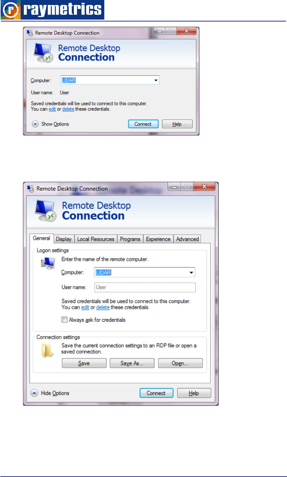
LIDAR OPERATION
104
Click at “Show Options” to view the options tabs. Here you can do many things such as
save the connection setting, select the quality of the connection, set the local resources
options and set more advanced options.
On the local resources tab you can choose how the key combinations behave such as
the “Alt+Ctrl+Delete”. If you press the “More” button you can select to share a drive while
connected, which come in hand when transferring data.
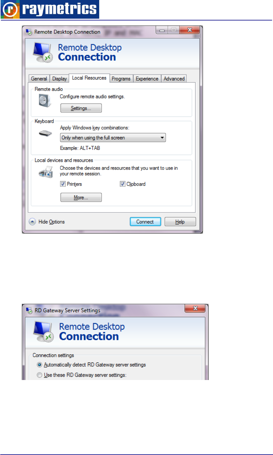
LIDAR OPERATION
105
At the experience tab you can select the performance depending on you connection.
Note if you face connection problems check at the advanced tab the settings for the
“Connect from Anywhere Option”. When you use a local network select the “Automatically
detect RD Gateway server Settings”. In some cases this might change on its own and
cause a connection problem.
The interface has four Tabs. The main tab is the “Scheduler” Tab. This contains the
time table and the scheduler status information.
LIDAR DATA PROCESSING
106
7. LIDAR DATA PROCESSING
The data processing is not always an easy task. Here is first explained the form of the
data and also it is provided a guide how to work and edit the database and also to perform
a basic analysis using the Data preview and analysis software. Performing a really precise
Lidar analysis lies on the verge of art since the user has to select through many
parameters that eventually alter the final result. Experience in combination with the
capabilities of the analysis software can create exceptional Lidar results.
The first paragraph refers to the data file format which is useful when the Lidar analyst
wants to use another program for the analysis. The data are saved in binary form to
reduce space. Even though the format is given there is also an extra tool embedded in the
Data preview and analysis software that converts the binary files to ASCII.
However you decide to work make sure that the database is not affected and always
keep a back up of Lidar data. Remember that raw data are irreplaceable.
7.1 DATA FILES HANDLING
The data files are saved in the folder set by the user. Apart from the data files there is
also saved a datalog file which contains the main information of each data file. This is
automatically saved whenever the user presses the Stop button. If the user presses the
Exit button while measuring the file is not created and thus the data need to be manually
selected.
The name of the data files is given by the acquisition software automatically using the
date and time of the measurement. The general format is RMyyMddhh.mms and is
explained below.
Fig. 7.1: Data File name explanation
First letters indicating the
acquisition software used
two numbers showing the
years in the century
one number for the month
as a hexadecimal number
two numbers containing
the hours since midnight
two numbers for the
minutes
one number containing the
seconds divided by ten.
two numbers containing the day of month
RM
yy
.
M
s
dd
hh
mm
LIDAR DATA PROCESSING
107
For example the file RM12C2815.572 is created by Raymetrics software (RM), in year
2012 (12), month December (C), day 28th (28) at 15:57 (15.57) past 20 seconds (2).
The file format is a mixed ASCII-binary format where the first lines describe the
measurement situation, below follow the dataset description and then raw data as 32-bit
integer values itself.
Fig. 7.2: Sample file header
The first line contains the measurement’s name which is exactly the same with the File
name, as explained above.
The second line contains more information about the location, start and stop time and
the extrenal conditions.
Location String with 8 Letters
Start Time dd/mm/yyyy hh:mm:ss
Stop Time dd/mm/yyyy hh:mm:ss
Height asl. four digits (meter)
Longitude four digits (including - sign). One digit for decimal grades.
Latitude four digits (including - sign). One digit for decimal grades.
Zenith angle two digits in degrees
Azimuth angle two digits in degrees
Ground Temperature (Celsius)
Ground Pressure (hPa)
RM12C2815.572
ATHENS 28/12/2012 15:57:02 28/12/2012 15:57:22 0180 0029.0 0032.0 -90 00 20.0 1013.0
0000200 0010 0000200 0010 08
1 0 1 16380 1 0850 7.50 00355.p 0 0 00 000 12 000200 0.500 BT0
1 1 1 16380 1 0850 7.50 00355.p 0 0 00 000 00 000200 4.3651 BC0
1 0 1 16380 1 0850 7.50 00355.s 0 0 00 000 12 000200 0.500 BT1
1 1 1 16380 1 0850 7.50 00355.s 0 0 00 000 00 000200 4.3651 BC1
1 0 2 16380 1 0850 7.50 00387.o 0 0 00 000 12 000200 0.500 BT2
1 1 2 16380 1 0850 7.50 00387.o 0 0 00 000 00 000200 4.3651 BC2
1 0 2 16380 1 0850 7.50 00408.o 0 0 00 000 12 000200 0.500 BT3
1 1 2 16380 1 0850 7.50 00408.o 0 0 00 000 00 000200 4.3651 BC3

LIDAR DATA PROCESSING
108
The third line contains information for the laser.
Laser 1 Number of shots integer 7 digits (how many laser shots were averaged in
one profile)
Pulse repetition frequency for Laser 1 integer 4 digits (Usually 10 or 20)*
Laser 2 Number of shots integer 7 digits
Pulse repetition frequency for Laser 2 integer 4 digits
number of datasets in the file integer 2 digits
The next lines that are in ASCII format are the dataset description. The parameters are
divided by space.
1 digit integer: 1 if dataset is present, 0 otherwise
1 digit integer: 0 for Analog / Photon counting, 1 for Photon counting
1 digit integer: 1 for Laser source 1, 2 for Laser source 2.
5 digits integer: Number of bins (example 16380 x 7.5m each bin = 122.850m)
1 digit integer: N/A
4 digits integer: PMT high voltage in Volt
2 digit real with 2 decimal: Bin width in meters
String with 5 digits: Laser wavelength in nm
dot and letter: Polarisation, o _ no polarisation, s _ perpendicular, p _ parallel
0 0 00 000 backward compatibility
2 digits integer: number of ADC bits in case of an analogue dataset, otherwise 0
6 digits integer: number of shots
1 digit real with 3 decimal: input range in mVolt in case of analog dataset,
discriminator level in case of photon counting.
String with 2 letters: Dataset descriptor BT=analog dataset, BC=photon counting
And one hexadecimal number: the transient recorder number.
The data set description is followed by an extra CRLF. The datasets are 32bit integer
values. Datasets are separated by CRLF. The last dataset is followed by a CRLF. These
CRLF are used as markers and can be used as check points for file integrity.
Using the analysis software presented below the user can translate all binary files to
ASCII so that any program can be used for the data analysis.

LIDAR DATA PROCESSING
109
7.2. DATA PREVIEW
Once you open the Data preview and analysis software you see the main interface.
The window consists of a menu bar and a toolbar
Click the preview DB to open the Main DB interface.
With Preview DB you can have a quick look of the database and through the DB
interface you can edit the database. Furthermore under tools in the main menu you can
convert automatically database files to an ASCII format to use them with other programs.
7.2.1 Database Interface
The Database Interface is consisted of:
the measurements table on top which shows all measurements in this database,
a list on the right with the data files that there were written during this
measurement,
an information field below the measurements table, that contains the global
information of the measurement,
another table with the recovered channels right above the measurement table
on the right of the window there are two dropdown lists and a text box which are
used as filters,
below this the edit database, the play and the close buttons
and at the bottom a graph to preview the raw data of each selected channel
At the measurement table, every record represents a set of measurements. Each
record has the following fields:
User Name: is the username that is entered when someone call data acquisition
interface.
Location: Is the Location which is entered during global information configuration
procedure.
Start, Stop Time and Date
Whenever a measurement is finished, a new record is added to the main table with the
start date and time from the first filename of the measurements’ set and stop date and time
fields from the last saved file.
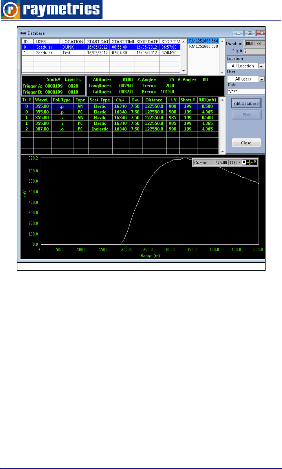
LIDAR DATA PROCESSING
110
Fig. 7.3: Database Interface
Choose the file on the right that you want to preview and see below at the table the
dataset description of the selected file, or in other words which channels where recorded
during each measurement. Select a row to view corresponding plot. Every row consists of
eleven shells that are:
Tr.: Transient recorder device
Wave L.: Detected wavelength
Polarization Type: p-parallel, s – cross, o – no polarization
Type: AN-analog, PC – photon counting
Scat. Type: scattering type, elastic (transmitted wavelength equal to detected
wavelength) inelastic (transmitted wavelength not equal to detected wavelength)
Ch#: Number of channels recorded
Bw.: Bin width = 2 ^ (reduction number) * resolution (in meters)
Distance: maximum distance in meters
H. V: PMT High voltage (V)
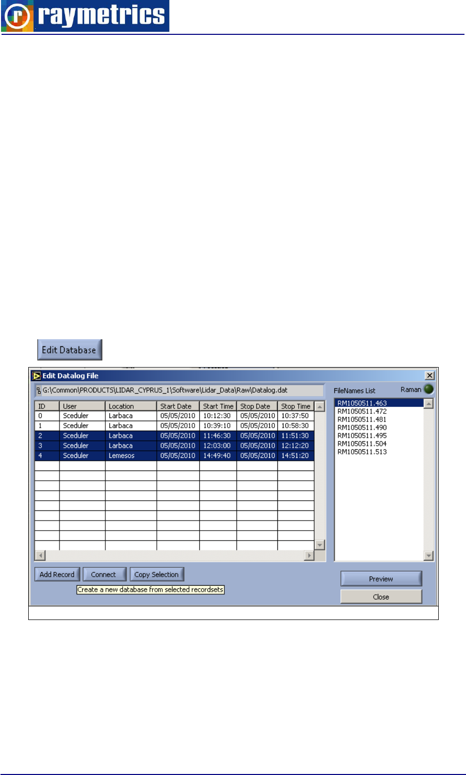
LIDAR DATA PROCESSING
111
Shots#: Number of shots
R/D: For analog: input range (mV), for photon counting discriminator level.
In the next paragraphs there are step by step tutorials on how to edit the database.
How to copy raw data files to create a new datalog file.
How to work with a different database
How To Create Manually A New Record At The Datalog.Dat
Exporting and converting data from a data base
For context help just click <Control>+H
For getting help for the active window click <Control>+<Shift>+H
7.2.2 How to copy raw data files to create a new datalog file
Open the “Preview DB” window and click on the “Edit Database” Button on the right.
Fig. 7.4: Edit Datalog File Interface
In order to create a new datalog file with part of your database (for example to
distribute it to your partners) you have first to select one or more (by keeping pressed the
"left Shift" button at your keyboard) records and then press the "Copy Selection" button at
the "Edit Datalog File" interface. A “Save As” common explorer interface appears. Choose
an empty directory (or create a new one where ever you like).
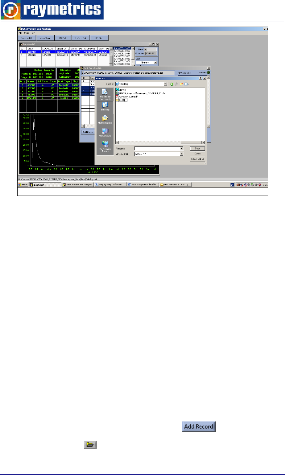
LIDAR DATA PROCESSING
112
Fig. 7.5: Select Directory For the New Database
Double click on the icon of this directory (in order to get into it) and then click on
"Select Cur Dir" button.
Then a new datalog.dat file will be created with only the previously selected records
and all the associated raw datafiles will be copied inside this newly created folder
(directory).
7.2.3 How to Create Manually a New Record at the Datalog.Dat
Many times users forget to click on “Stop” button before they exit the acquisition
program (or in case of a power failure). In that case, although all the acquired raw data
files have been saved to the default location, software failures to add a new record at the
datalog.dat file that describes the measurement that user just did.
So user has to add manually this new record by following the procedure below.
Note: It is suggested to make a backup of your datalog.dat file before you proceed.
Open Preview DB window and click on the “Edit Database button as in paragraph 7.2.2
How to copy raw data files to create a new datalog file.
Click the “Add Record” button as you see in Fig. 7.4
Click the folder icon to open a windows selection dialog.
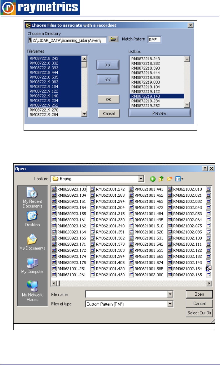
LIDAR DATA PROCESSING
113
Fig. 7.6: Add Data Files to Recordset
Choose the directory that your raw data files are located (For example
C:\lidar_data\Raw\), step into it and click on "Select Cur Dir" button.
Fig. 7.7: Directory Of Measurements Selection Dialog
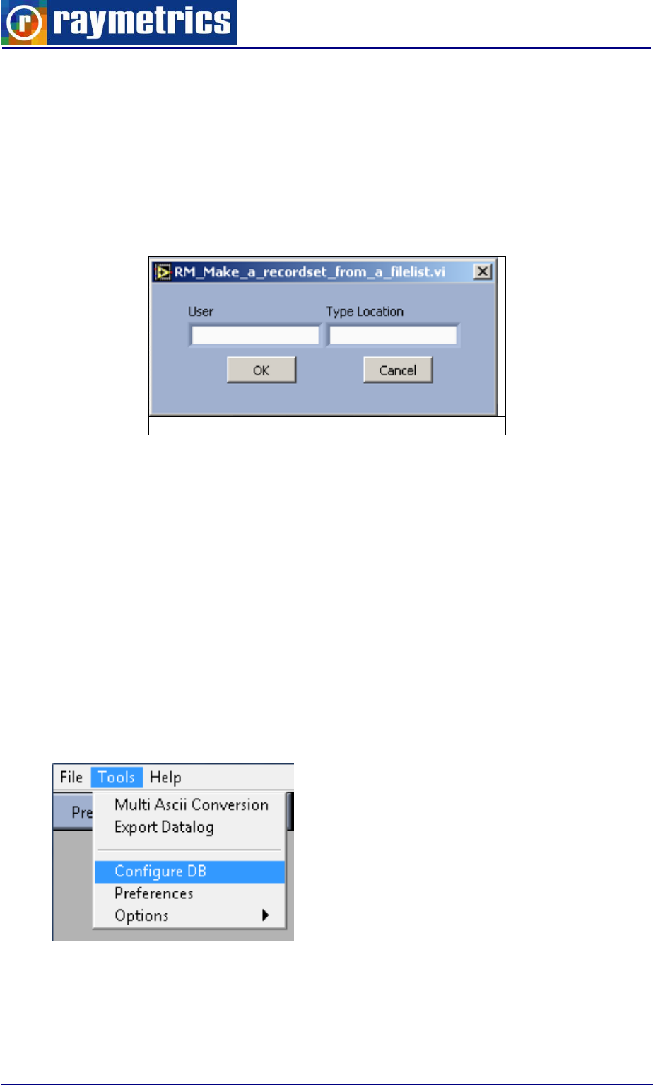
LIDAR DATA PROCESSING
114
All the RM files will be displayed at the list box on the left.
Select all the files you want (be sure that they are sequential and belong to the same
measurement)
Click the >> button to transfer them at the right list and click Ok
Then software asks to type a User and a Location. Type whatever you like but keep it
less than 10 characters without spaces and click ok.
Fig. 7.8: Add Data Files to Recordset
Click once more the OK button at the “Edit Datalog File” interface (Fig. 7.4)
If you now reopen the Preview DB window the new record will also appear.
7.2.4 How to Select a Different Database
When you have multiple databases saved in different folders you can work with any
you wish at a time. Go through these steps to select another database to wok with.
Close the “Preview DB” window if it is open and go to Menu Bar and click Tools-
>Configure DB
A dialog opens that prompts you to configure the Preview Application.
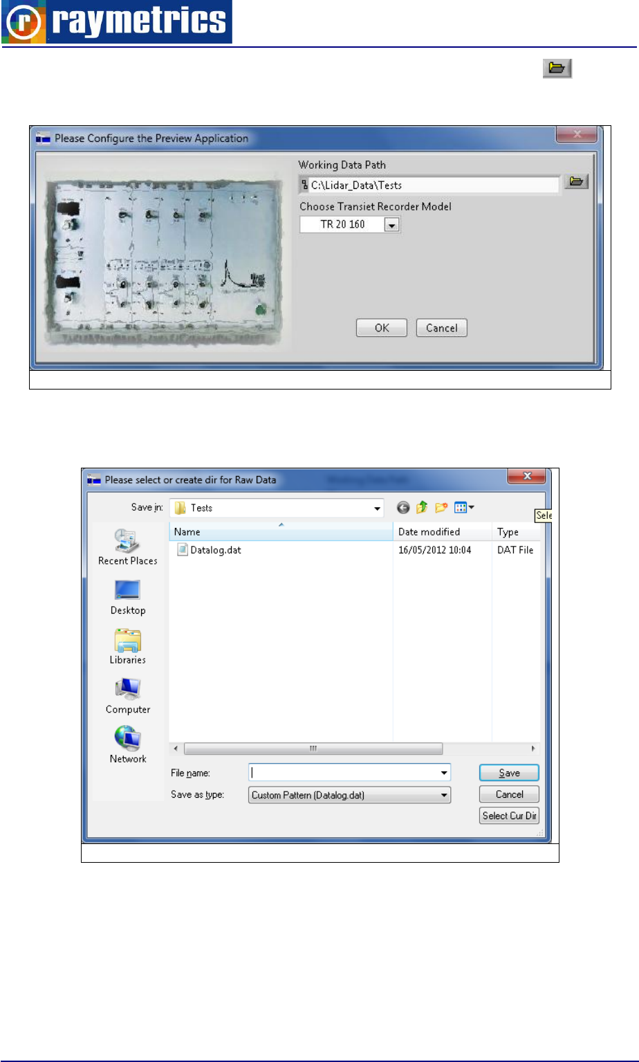
LIDAR DATA PROCESSING
115
Click the Folder Icon (right up corner) of the Working Data Path text box. A normal
windows selection dialog opens and asks to select the directory.
Fig. 7.9: Configure Preview Application Interface
Locate the directory where another datalog.dat file (with all the raw data files) exists.
Note that by default there is a filter and you can only see the .dat files.
Fig. 7.10: Database Directory Selection
Double click the icon of that folder in order to get into it and click the “Select Cur Dir”
Button.
Note: Please do not forget to choose the right type of your transient recorder
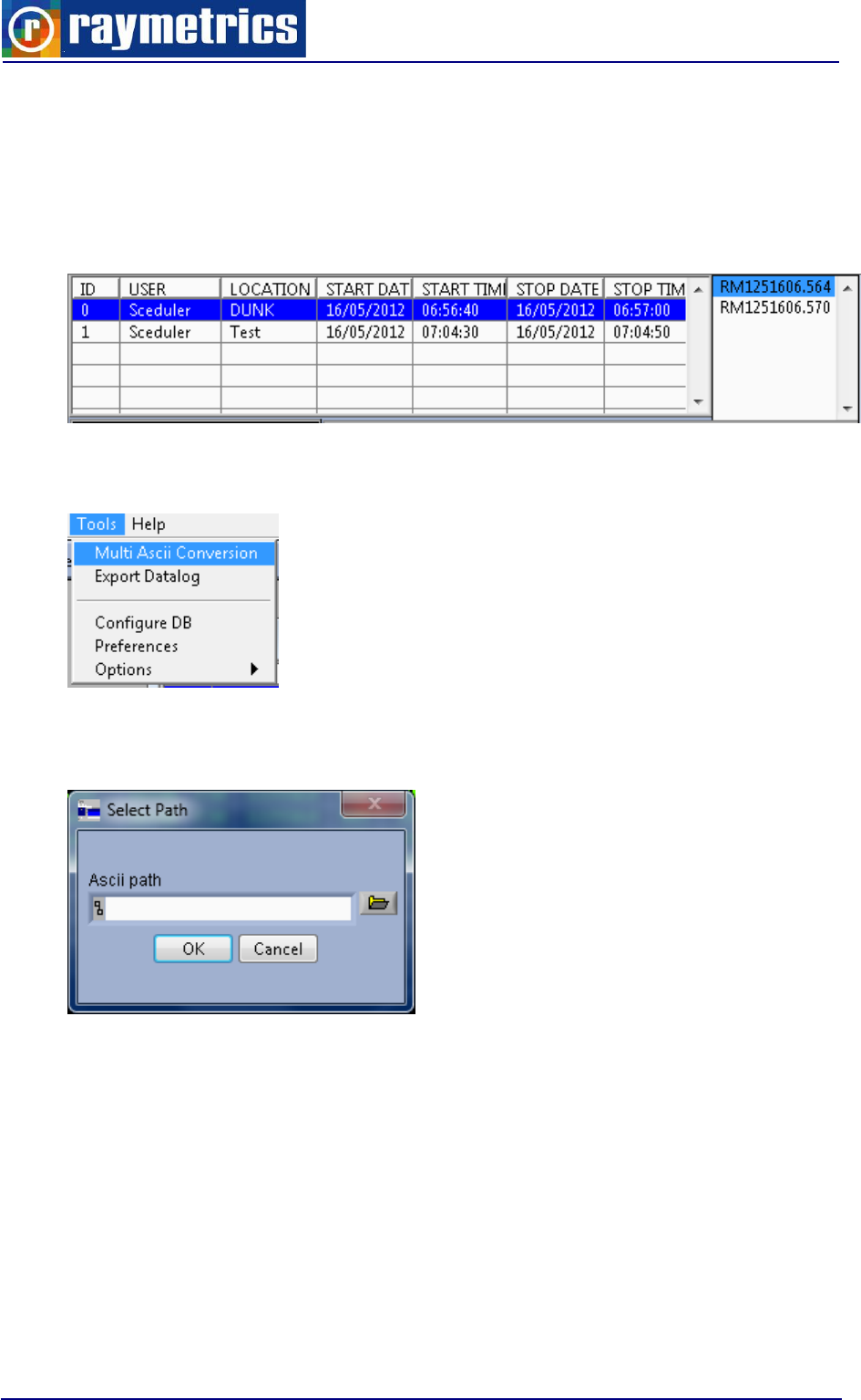
LIDAR DATA PROCESSING
116
7.2.5 Converting Binary Files to ASCII
The software provides a function to convert all files of a record (measurement) from
binary to ASCII format. This is useful when you want to read the files with software.
Click first the Preview DB button to open the database. On top select at the
measurement table which record you want to convert.
Next go to “Menu” -> “Tools” -> “Multi ASCII Conversion”.
A window opens that prompt’s you to select the folder where the converted data will be
stored. Select a folder and click “select Current Dir.”
Wait until the status bar reaches the end and the data are now saved in an ASCII
format. You can verify if they are written correctly if you choose to open one file with
notepad. These files have actually no extension so they don’t belong to any program.
Because there is a dot before the last three digits on the filename windows recognize the
last three digits as the type of the file.
You may also save as a text file the datalog file to use it with the converted files if you
go to “Menu” -> “Tools” -> “Export Datalog”

LIDAR DATA PROCESSING
117
7.3. DATA ANALYSIS
As already explained the analysis software is what analyst use to extract all the useful
information from their Lidar data. Even though it provides a lot of information and functions
the user has to first understand the theory that lies beneath the software so to understand
the way things are calculated.
With the series of button shown above the user can:
Use worksheet interface to insert data from external files or database into a
worksheet.
Plot directly database data or from external files using 2D Plot interface.
Create surface graphs from acquired data using Surface Graph Interface
With 3D Plot you can plot the temporal data in a 3D graph.
For more information about worksheet and plots refer to electronic form of Raymetrics
user manuals.
Here in the next paragraphs there is a series of tutorials on:
How to Plot Data
How to Calculate Backscatter Coefficient
How to Calculate Aerosol Extinction Coefficient
How to Check Lidar Alignment
How to Calculate Water Vapor Profiles
How to subtract the Background
How to Glue Analog and Photon Counting signals
How to make a 3D Graph
How to use soundings from global model data
With these 9 tutorial lessons the user will understand fully how to use the program. As
deeper the analyst goes in the software’s capabilities the biggest the theory background is
required. In some lessons the basic theory required is given as introduction, but the
analyst should look into the references and build a stronger Lidar knowledge.
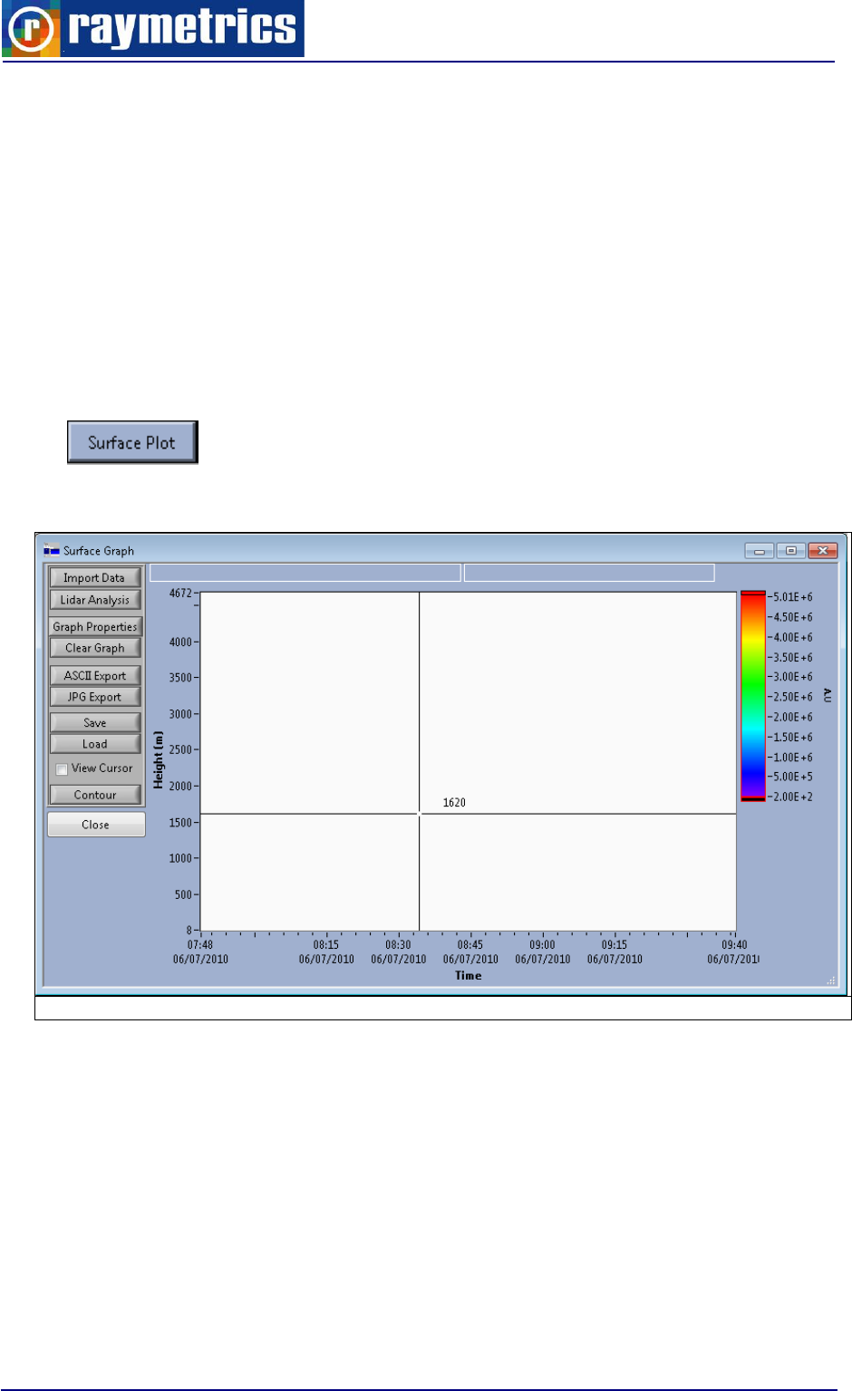
LIDAR DATA PROCESSING
118
7.3.1 How to Plot Data
Here is shown the way to plot your data. There are three ways to represent the data.
One is a single 2D graph which can be data from a single file or a summation of multiple
files. Another way is to plot the data on a surface that shows actually multiple files one next
to the other as they evolve by time. The last is a 3D plot which also shows multiple files but
in a 3D graph.
In this paragraph you will learn how to make a surface plot. Once you understand this
you can easily also plot a 2D graph.
1. Click “Surface Plot”.
2. Click “Import Data”.
Fig. 7.11: Surface Graph Interface
3. Scroll up in the table if you do not see your data. Select the data in the table you
wish to plot. In the right-hand column, hold the shift key to select the
measurements you wish to plot. Click “Next”.
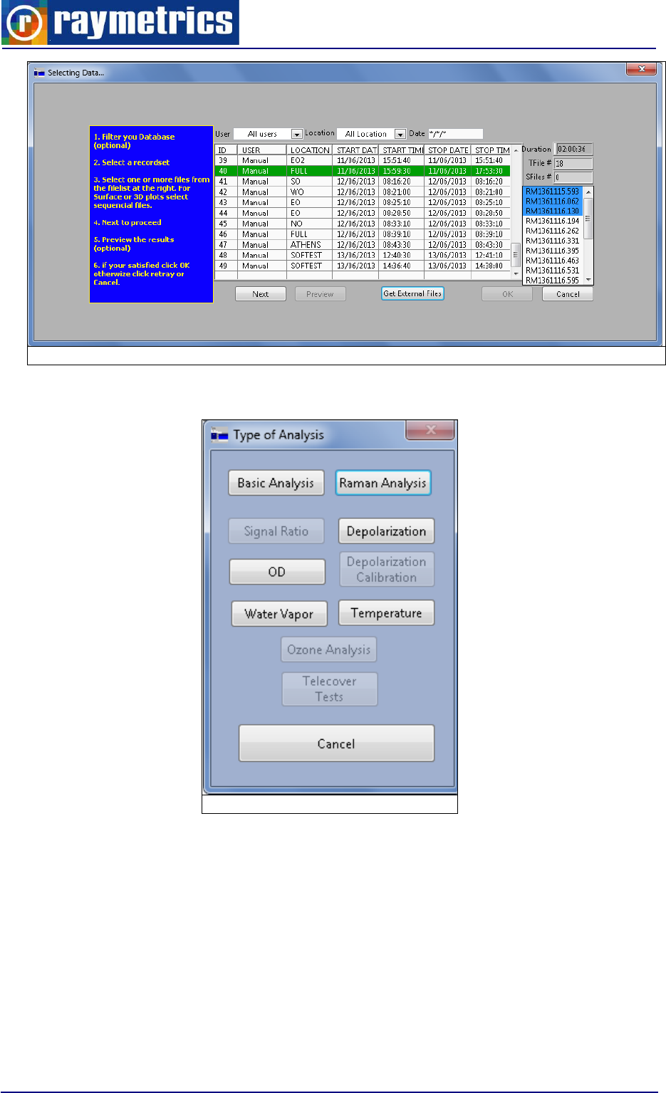
LIDAR DATA PROCESSING
119
Fig. 7.12: Select Data Interface
4. Click “Basic Analysis” option.
Fig. 7.13: Analysis Type Selection
5. Select the data type you wish to plot. For example “355.00.p.AN” from the list on
the left. From the list on the right, select “RCS”.
Note: “532.00.p.AN” – 532.00 = wavelength in nm, p = primary (as opposed to
secondary - depolarization), AN = analogue (as opposed to Photon Counting or Glued –
PC and GL). Other options include calibrated signal for depolarization (b). RCS = Range
Corrected Signal.
Note: Hold down the “Ctrl” key and press “h” for help.
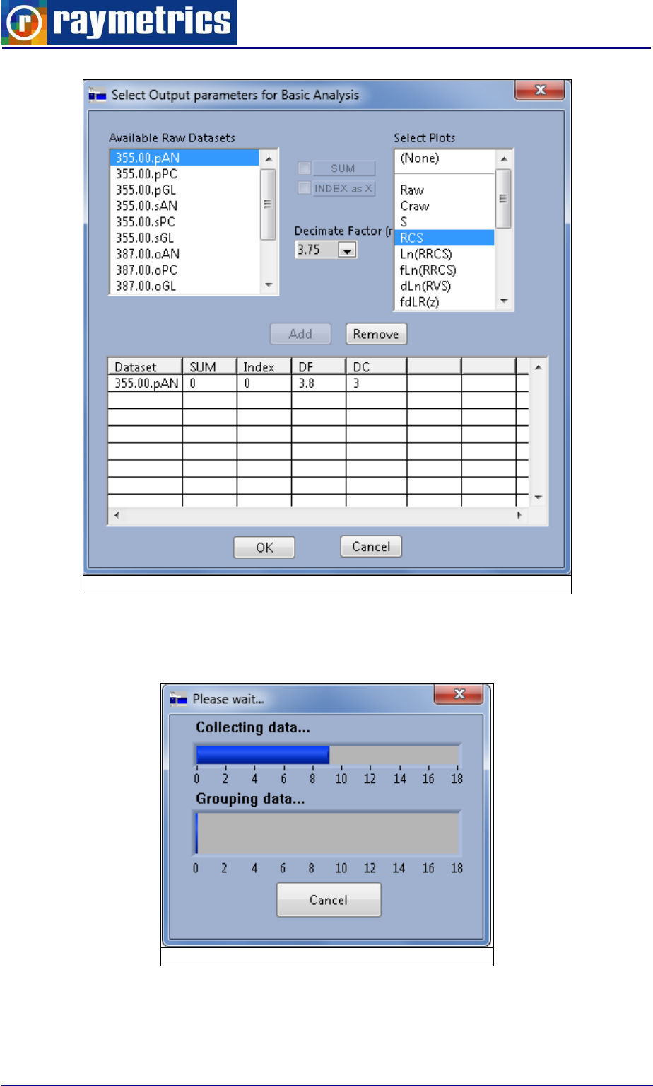
LIDAR DATA PROCESSING
120
Fig. 7.14: Output Selection Interface
6. Click the “Add” button. Your selection will now appear in the small data table.
7. Click “OK” button. The software will now load your requested data.
Fig. 7.15: Data Collection
8. After a few seconds, you will see the following blank graph.
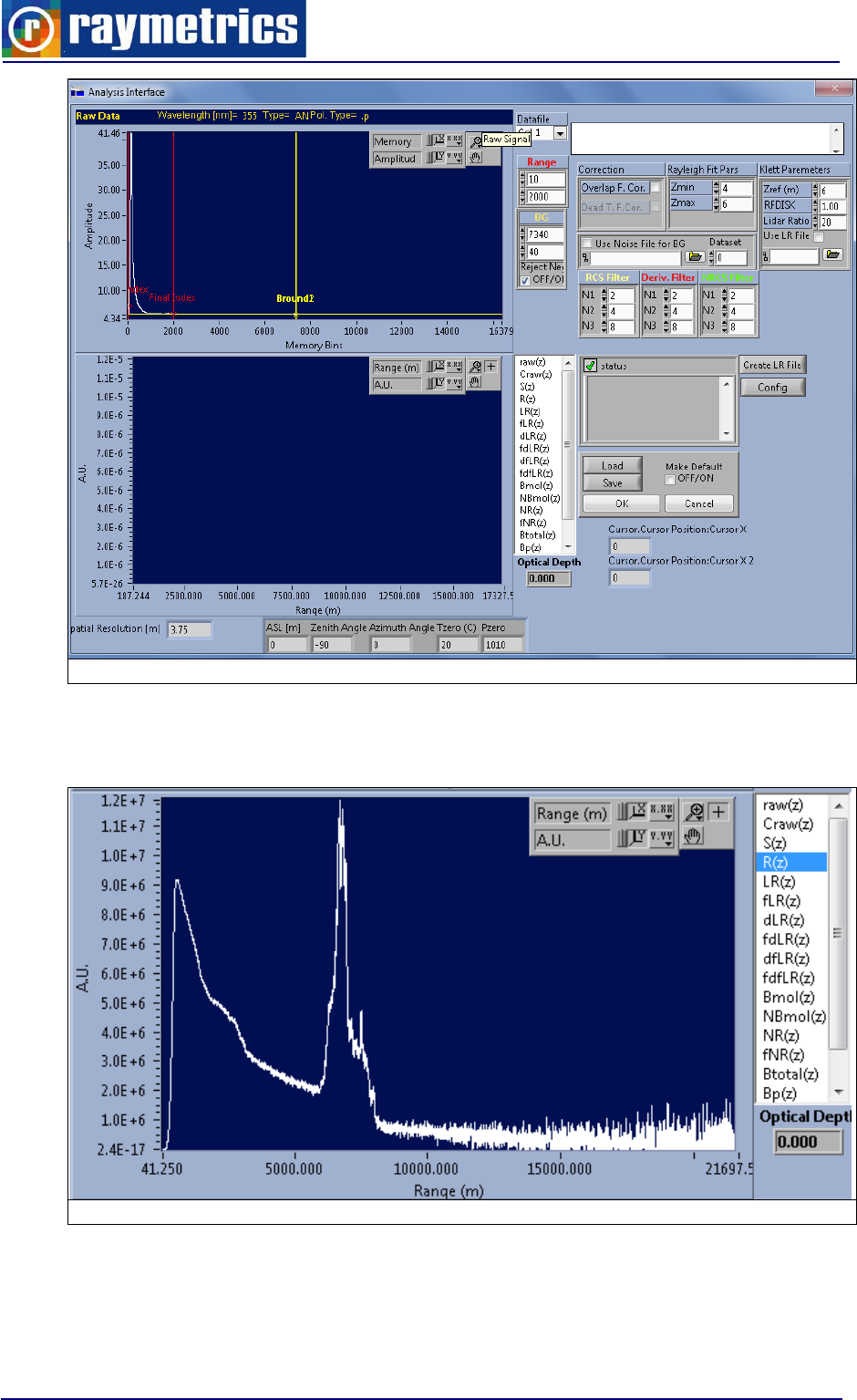
LIDAR DATA PROCESSING
121
Fig. 7.16: Analysis Interface
9. In order to see the results, select a parameter from the parameter list to the right of
the bottom graph (e.g. R(z) – range corrected signal).
Fig. 7.17: Output Preview Graph
10. Click on the two red bars on the top graph and drag them to define the range
(height) of interest. As you drag the bars, you will see the data change on the
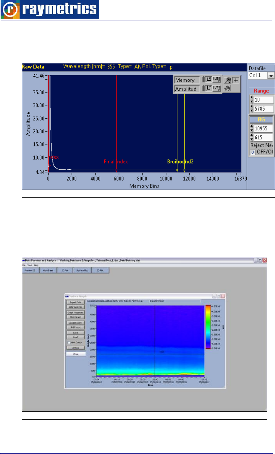
LIDAR DATA PROCESSING
122
bottom graph. You can also change the scales of the graph by simply clicking on
any value on the x or y axis and typing a new value. The graph will then re-scale
automatically
Fig. 7.18: Raw Data Graph – Limits and Background Selection
11. When you have the range desired, click the “OK” button. The previous window
“Selecting Data…” (See Fig. 7.12) will appear back. Click the “OK” button again.
12. The selected data and parameters will now be displayed on a graph. Time is on the
x axis, range on the y axis, with color values showing the intensity of the signal.
Fig. 7.19: Output Surface Graph
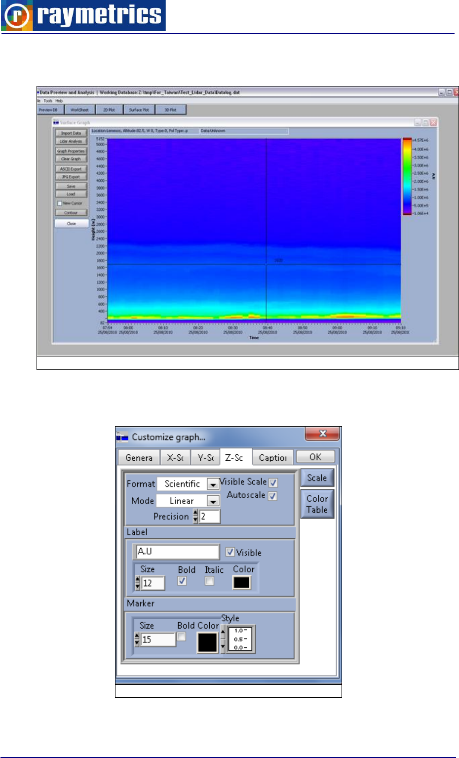
LIDAR DATA PROCESSING
123
13. The image on the screen can be re-scaled by dragging on the bottom right corner
of the window.
Fig. 7.20: Window Resize
14. Adjust the color scale of the graph by clicking on “Graph Properties” on the left and
selecting the tab “Z-sc” (z scale).
Fig. 7.21: Customize Graph
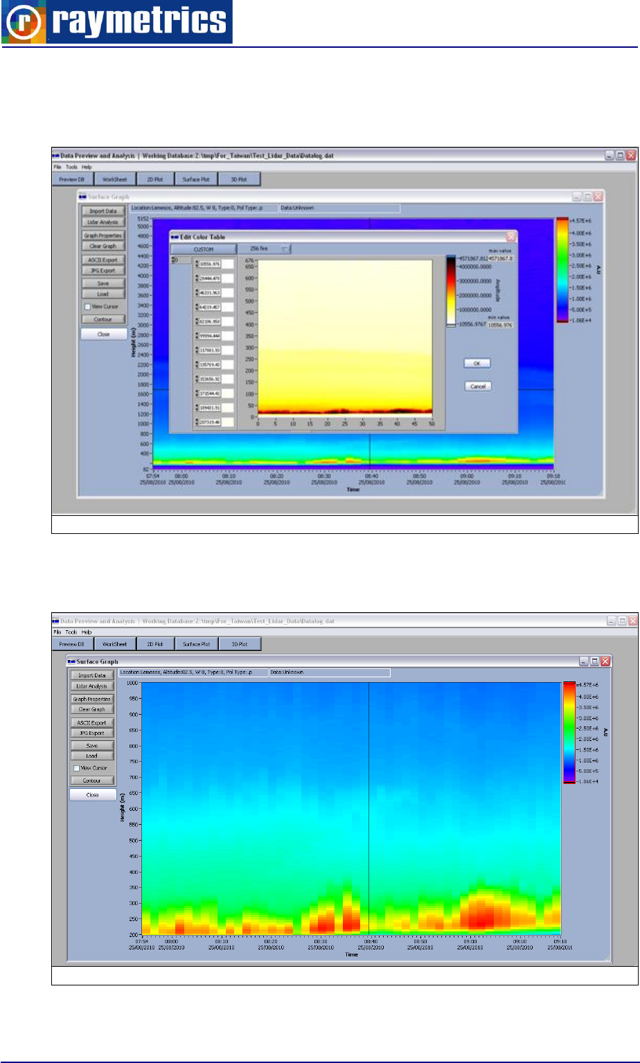
LIDAR DATA PROCESSING
124
15. Click on the “Color Table” button on the right. At the top of the window, click
“Choose C. Table”. Select a new color scheme (if desired) from the options (e.g.
“fire” or “rainbow”). Click “OK” and “OK” again.
Fig. 7.22: Edit Color Table
16. If required, manually change values of range and signal intensity by clicking on the
values on the graph axes and/or on the z scale to the right of the graph.
Fig. 7.23: Range Rescale
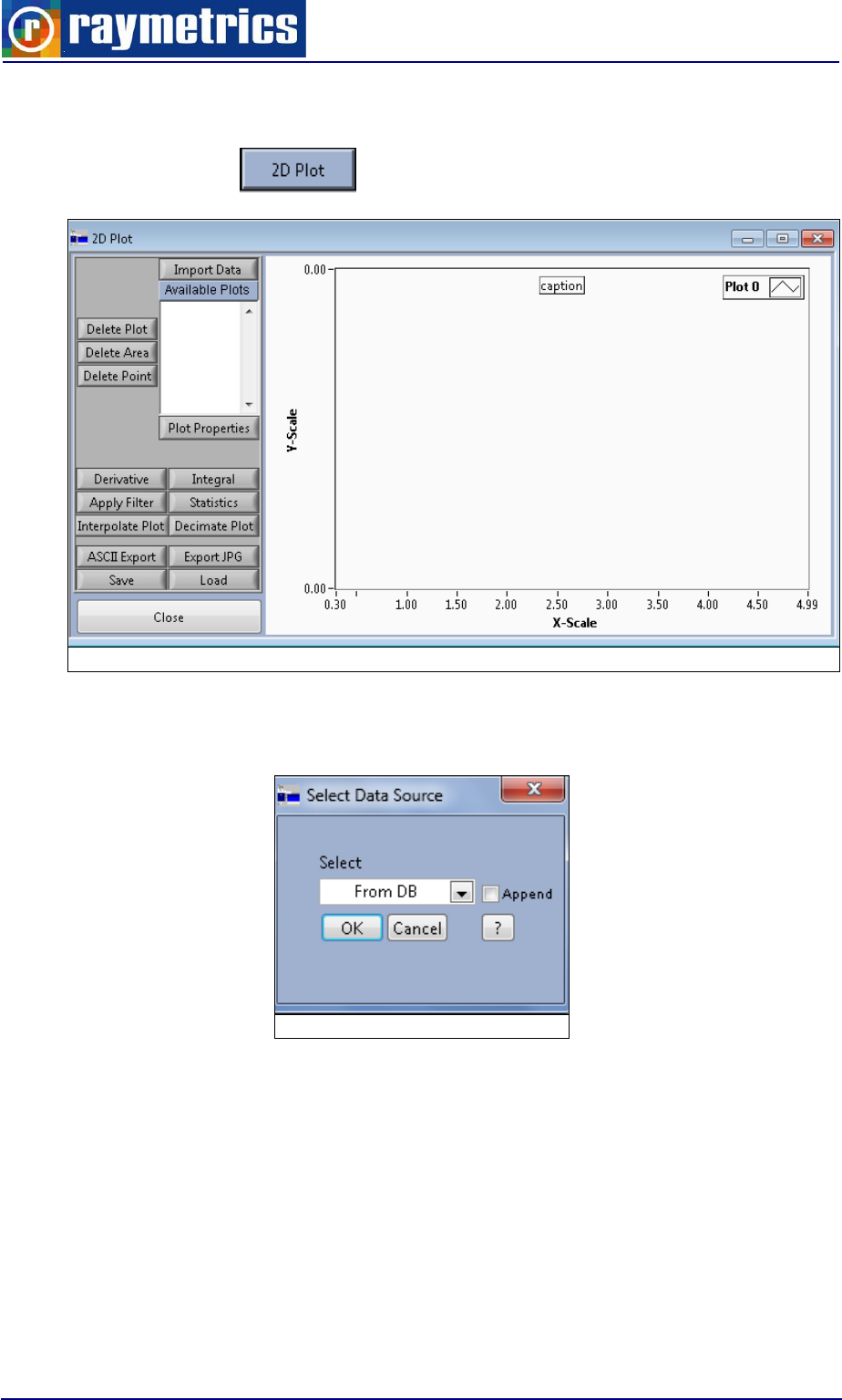
LIDAR DATA PROCESSING
125
7.3.2 How to Calculate Backscatter Coefficient
10. Click “2D Plot”.
Fig. 7.24: 2D Plot Interface
11. Click “Import Data” and ensure Data Source is set to “From DB” in the drop-down
list. Click “OK”.
Fig. 7.25: Data Source
12. Select the record and the data you want to calculate aerosol backscatter coef for
(as in previous tutorial Fig. 7.12). Make sure that the data files that you select are
free of clouds. By holding the shift key you can select multiple files which are going
to be averaged if you select it in the next step. Click “Next” and select “Basic
Analysis” option (as in previous tutorial Fig. 7.13).
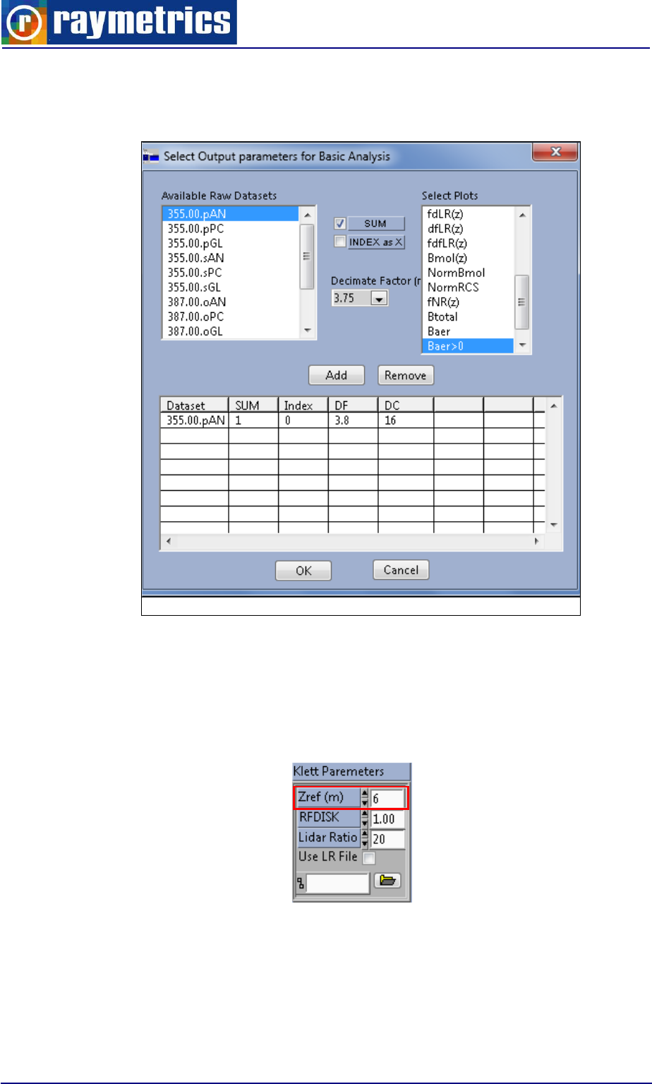
LIDAR DATA PROCESSING
126
13. Select “355.00.p.AN” dataset. Click “Sum” check box (if you need the average over
time). Select “Baer>0” (backscatter aerosols – positive values only) from the light
on the right. Click “Add” button and then “OK” button.
Fig. 7.26: Data Source
14. Define the range of interest with the two red cursors from the top graph (as in
previous tutorial Fig. 7.18).
15. Insert the maximum range (altitude in kilometers) for calculating Aerosol
Backscatter coef in the Zref (km) box in the top right corner of the window.
16. Select Bp(z) from the list in order to preview the Backscatter coef on the bottom
graph. (Re-scale the graph if required by clicking on any value and typing a new
value.)
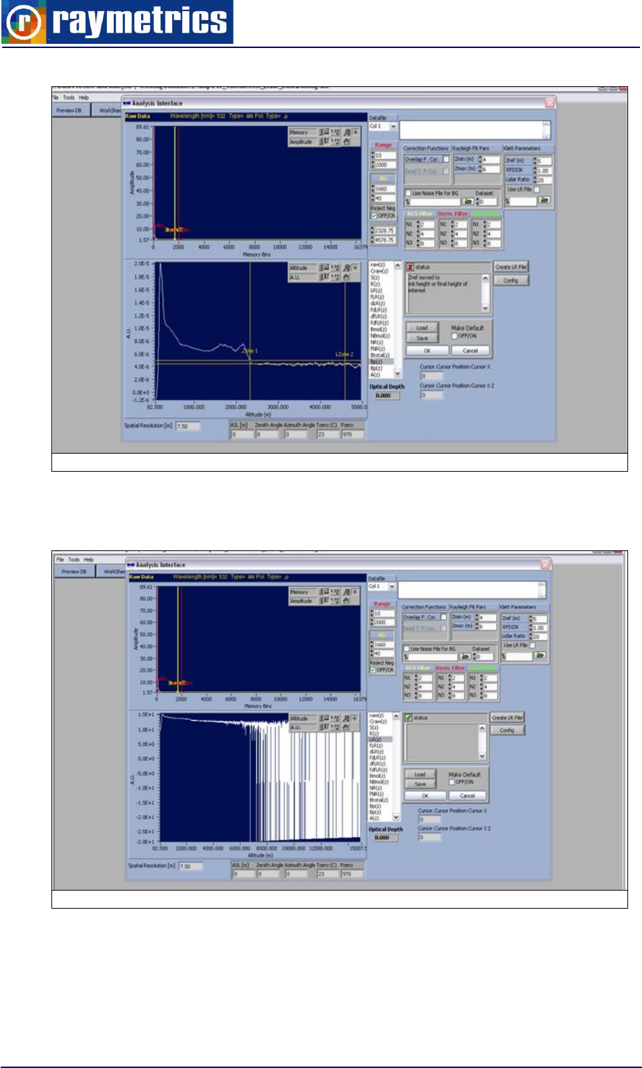
LIDAR DATA PROCESSING
127
Fig. 7.27: Back Scatter Coefficient Preview
17. In order to check the maximum altitude to which Backscatter coef. can be
calculated without errors, click the LR(z) from the list.
Fig. 7.28: Back Scatter Coefficient max Altitude
18. Locate the altitude where the first negative values appear (for example close to 7
km at Fig. 7.28). This is the maximum altitude to which you can calculate
backscatter coef. without errors for the selected data.
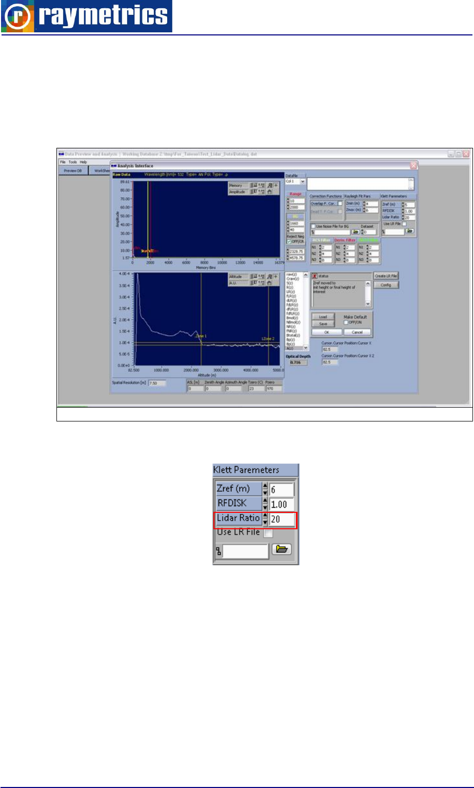
LIDAR DATA PROCESSING
128
7.3.3 How to Calculate Aerosol Extinction Coefficient
1. The procedure is the same in the above tutorial 7.3.2 How to Calculate Backscatter
Coefficient until point 16. At this stage, instead of selecting Bp(z) the user has to
select A(z).
Fig. 7.29: Aerosol Extinction Coefficient
2. Please notice that A(z) depends strongly on the assumption of the Lidar ratio.
3. Continue with the rest of the procedure as described at the previous tutorials.
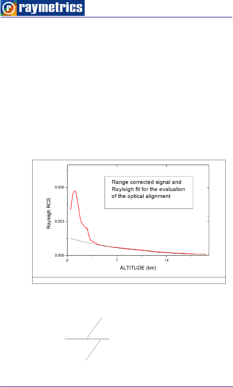
LIDAR DATA PROCESSING
129
7.3.4 How to Check Lidar Alignment
For the fine alignment, the range-corrected Lidar signal (RCS)
2
cor zzPP
is
compared to the range corrected exponentially attenuated Rayleigh backscattered
coefficient
dzaexpzββ Ray
2
Raycor
, at a range interval, which is considered free
of any aerosol loading (pure molecular atmosphere). The molecular backscatter and
extinction coefficients (
Ray
β
and
Ray
a
, respectively) can be calculated either from a
Standard Atmosphere (U.S.S.A 1976)7 or more accurately from available local radiosonde
data. The advantages of this method are that it does not require any extra equipment; it
can be performed during daytime or night-time measurements and is very accurate.
Note: clear sky without clouds is important, since in that case the Lidar signal extinct
very fast and is not possible to calculate the molecular signal from experimental results.
In Fig. 7.30 a typical Lidar aligned signal ‘matching’ the pure molecular atmosphere.
Fig. 7.30: Lidar signal ‘matching’ the pure molecular atmosphere.
Now in the software NBr(z) is actually the
cor
β
from the equation above and NR(z) is
the normalized Range Corrected Signal. RCS(z) is the range-corrected Lidar signal Pcor.
12
2
1
12
2
1
)(
)(
)()(
ZZ
z
ZZ
zRCS
zRCSzNR Z
Z
cor
Z
Z
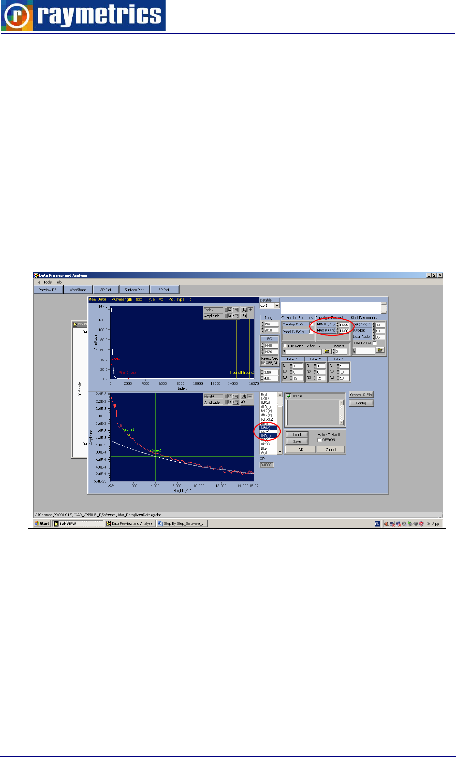
LIDAR DATA PROCESSING
130
Where Z2 and Z1 define a range clear of aerosols (From Rayleigh Parameters Section:
MinR(km), MaxR(km))
To check the alignment of the Lidar, follow the steps below.
1. Follow the same steps in tutorial 7.3.2 How to Calculate Backscatter Coefficient
until point 13. Then select 355.pPC (Photon Counting Data at 355nm). Select
NBmol and fNr(z) parameters to plot (by holding <Ctrl> to select multiple options).
2. Define a range in atmosphere where you assume it is free of aerosols (for example
10 to 14 km at the above image-example).
Fig. 7.31: Lidar signal ‘matching’ the pure molecular atmosphere.
A. You can notice that the Lidar signal fits the molecular atmosphere up to 15 km
B. All the signal bellow 10 km is higher than the molecular atmosphere.

LIDAR DATA PROCESSING
131
7.3.5 How to Calculate Water Vapor Profiles
Before you go through this document make sure that your system can measure
water vapor. To measure water vapor your Lidar should measure 408nm and 387nm
Raman backscatter wavelengths.
Intro:
Water vapour profile is calculated by using the following equation:
K
zP
zP
K
zP
zP
zm
N
OH
)(
)(
)(
)(
)(
387,
408,
,
,
2
2
-
-
-
-
eq.1
Where K is the overall system calibration constant, and P(z) is the range corrected
signals.
The overall system calibration constant (K) can in principle be deduced from the known
Raman cross sections and the measured properties of the spectrometer used, but in
practice it is determined from the comparison of the Lidar measurement with critically
evaluated data from a radiosonde ascent. In the calculation of the transmission ratio, there
is an effect of the particle extinction which can be negligible on the mixing ratio
determination under clear air conditions but must be taking into account if an optically
dense medium like a water cloud is present.
A new and easier way for the calculation of water vapor profile have been developed,
which is embedded in the software. Here is shown a tutorial how to plot a 2D graph. If you
want to display the temporal evolution of water vapor profile, open a surface graph, or if
you wish to analyze and do additional calculation open a worksheet.
1. Follow the same steps in tutorial 7.3.2 How to Calculate Backscatter Coefficient
until point 12. tutorial, but select water vapor Analysis in the “Type of Analysis”
dialog shown in Fig. 7.13. If the record set you selected doesn’t contain any Water
Vapor info (channel 408nm) the “water vapor analysis” button will not be available.
2. Then select 355.pPC (Photon Counting Data at 355nm). Select NBmol and fNr(z)
parameters to plot (by holding <Ctrl> to select multiple options).
3. A new interface appears. Using this interface is straight forward and easy.
Depending on the detected channels and the type of detection several options can
appear at the Data Type list box at the top left corner of the window. For example if
your system detects only Photon Counting signals for 408nm channel and only
Photon Counting signals for 387nm channel. Then you have only one option to
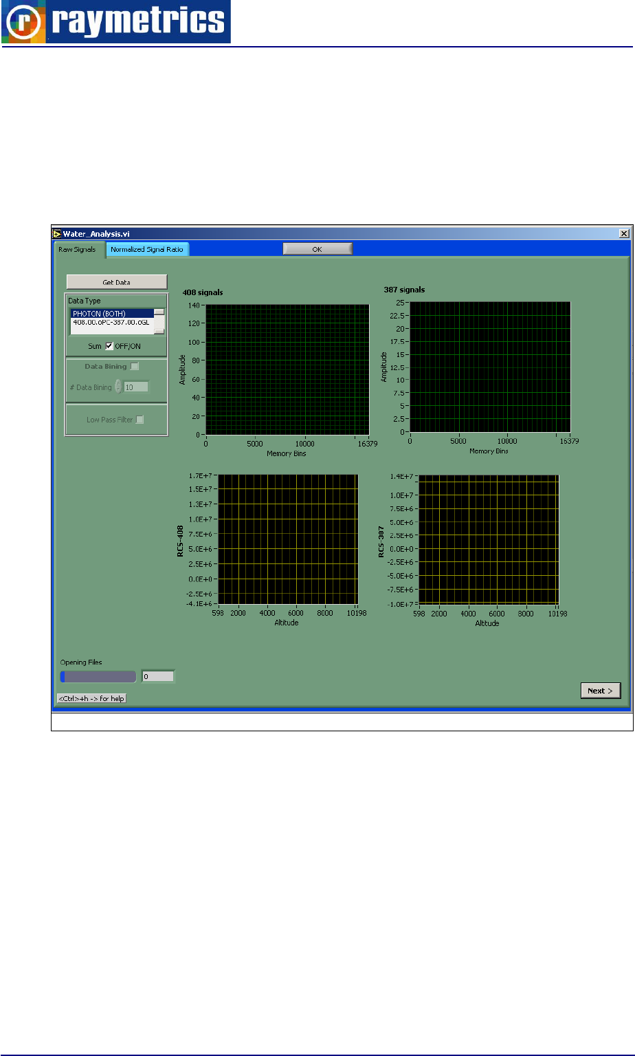
LIDAR DATA PROCESSING
132
calculate water vapor profile by using only Photon Counting signals. If for example
your system detects Analog and Photon Counting signals for 387 nm then you
have two options to calculate the water vapor profile. One by using only the photon
counting signals for both channels and one by using Photon Counting for 408 nm
channel and Glue data for 387nm (about Gluing please take a look at Licel manual
and at paragraph 7.3.7 How to Glue Analog and Photon Counting signals).
Fig. 7.32: Water Vapour Analysis Interface – “Raw Signal” Tab
4. Click on the “Sum” check box to average all the selected datafiles. In that case the
temporal resolution decreases but the signal to noise ratio is getting much better so
the effective range of the profile will be increased.
Note: For surface plot (temporal evolution) this options is deactivated.
5. After that click on the ‘Get Data” button and a new interface will appear (Data Pre-
process) where you can subtract the background and select the range of interest
(by using the two red cursor from the top graph). This process will be done twice.
One for 387nm and one for 408. After that the range corrected signal will be
calculated for both channels.
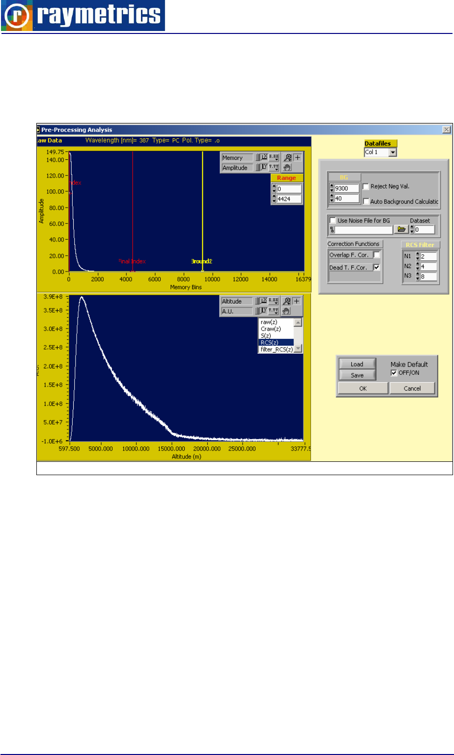
LIDAR DATA PROCESSING
133
Note: Take into consideration that both Range Corrected signal is calculated at the
same range of interest. An easy way to do that is to click on the “Make Default” check box
and then on the Save button. The next time that this interface will appear will have the
same range of interest.
Fig. 7.33: Pre-processing Analysis Interface
6. When both of range corrected signals have been calculated the Pre-processing
Analysis Interface closes and the program returns to the main interface. The
graphs are updated and you can preview all in one the 387nm and 408nm - Raw
and RCS signals. Click on the “Next” button or just the Normalized Signal Ratio
Tab.
7. There are two graphs at this Tab. The top one shows the signal ratio while the
second one shows the calculated water vapor profile. Use the two yellow cursors
from the top graph in order to zoom in the range where you ratio profile is strong
enough to calculate the water vapor profile.
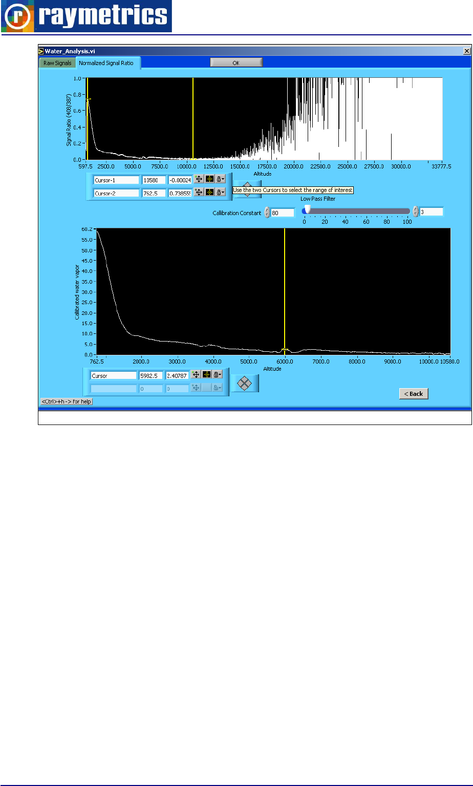
LIDAR DATA PROCESSING
134
Fig. 7.34: Water Vapour Analysis Interface – “Norm Signal Ratio” Tab
8. At this Tab you can adjust the calibration constant or even to apply a low pass filter
at the final product (zero means no filter). Finally click on the OK button located at
the top of this interface.
Note: In cases that the signal to noise ratio is to low you can try improving it by data
binning of raw signals or even to apply a low pass filter. You can do that at the “Raw Data”
tab.
How data binning works:
Every value of the input signals corresponds to 7.5 metes (one bin) by calculated the
average signal of a number of sequential bins (number of data binning) then the resulting
signal has a special resolution of 7.5*(number of data binning).
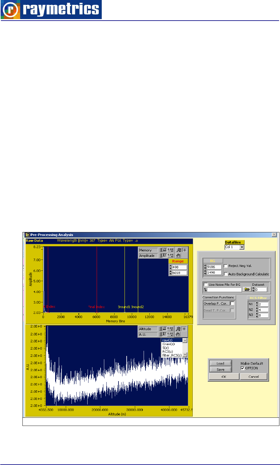
LIDAR DATA PROCESSING
135
7.3.6 How to subtract the Background
Intro:
Background noise is due to atmosphere (solar or lunar background light) and due to
electronic noise.
There several methods for removing the background signal from a Lidar signal. The
most common method is to locate a range that there is no Lidar signal and calculate the
mean value at that range. Then this value is subtracted from the Lidar signal. Usually this
range is at the far range (very high altitude) or at the very first meters if you Lidar supports
pre-triggering.
However using always very high altitudes is not the best practise. Experience shows
that some times when the signal (analog) is two weak or decreases very fast (after a
cloud) suffers from no linearity. In that case for calculating the background is better to
select a range where the signal is quite stable and the mean value at that range is
minimum.
Of course in that case the effective range of the signal is restricted until that range.
Fig. 7.35: Example of a signal with non linear behaviour
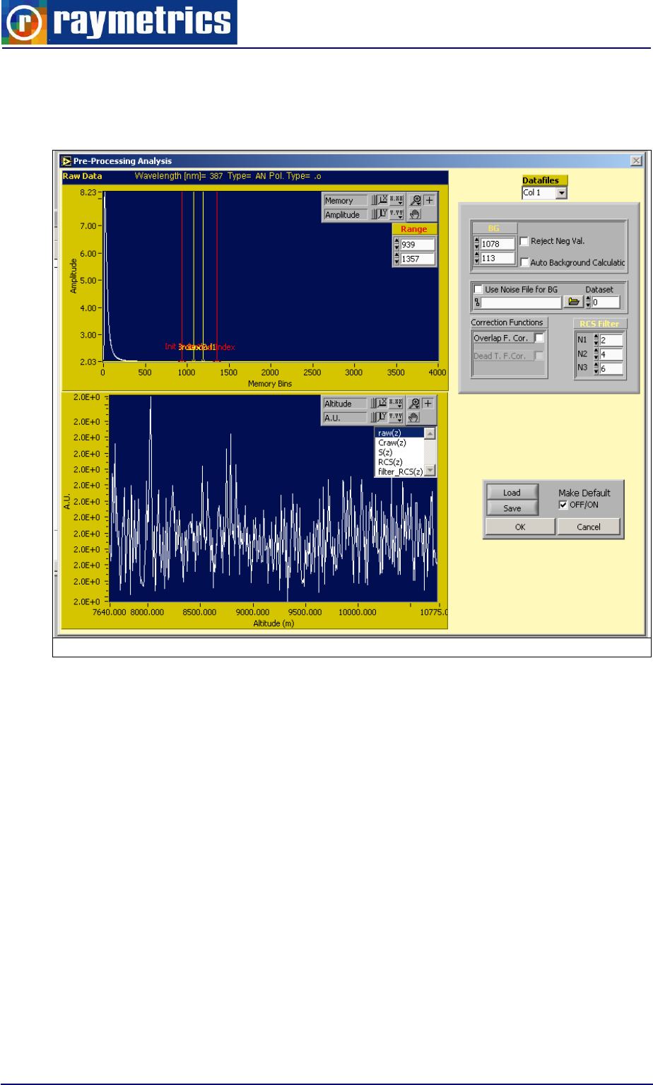
LIDAR DATA PROCESSING
136
In the case it is suggested to locate a range where the signal is minimum and to
calculate the background mean value at that range (you can do that easily by using the
two red cursors to zoom.
Fig. 7.36: Boundaries Selection
Then place the two yellow cursors somewhere in between (as shown in Fig. 7.36) in
order to calculate the mean value.
For analog measurements it is suggested to use a background profile to avoid ADC
slopes or electromagnetic interference taken as real atmosphere response. A background
profile can be taken by covering the telescope and starting a normal measurement. If no
light enters through the telescope the only thing that is measured is the noise from the
electronics. Alternatively you can use an external trigger to initiate a measurement without
using the laser at all. In this case you measure the electronics’ noise and the sun’s
radiation.
Make sure that you know which measurement it is so that you can select it afterwards
at the software interface in order to subtract the background profile (Is called noise file)
from the signals that you want to work.
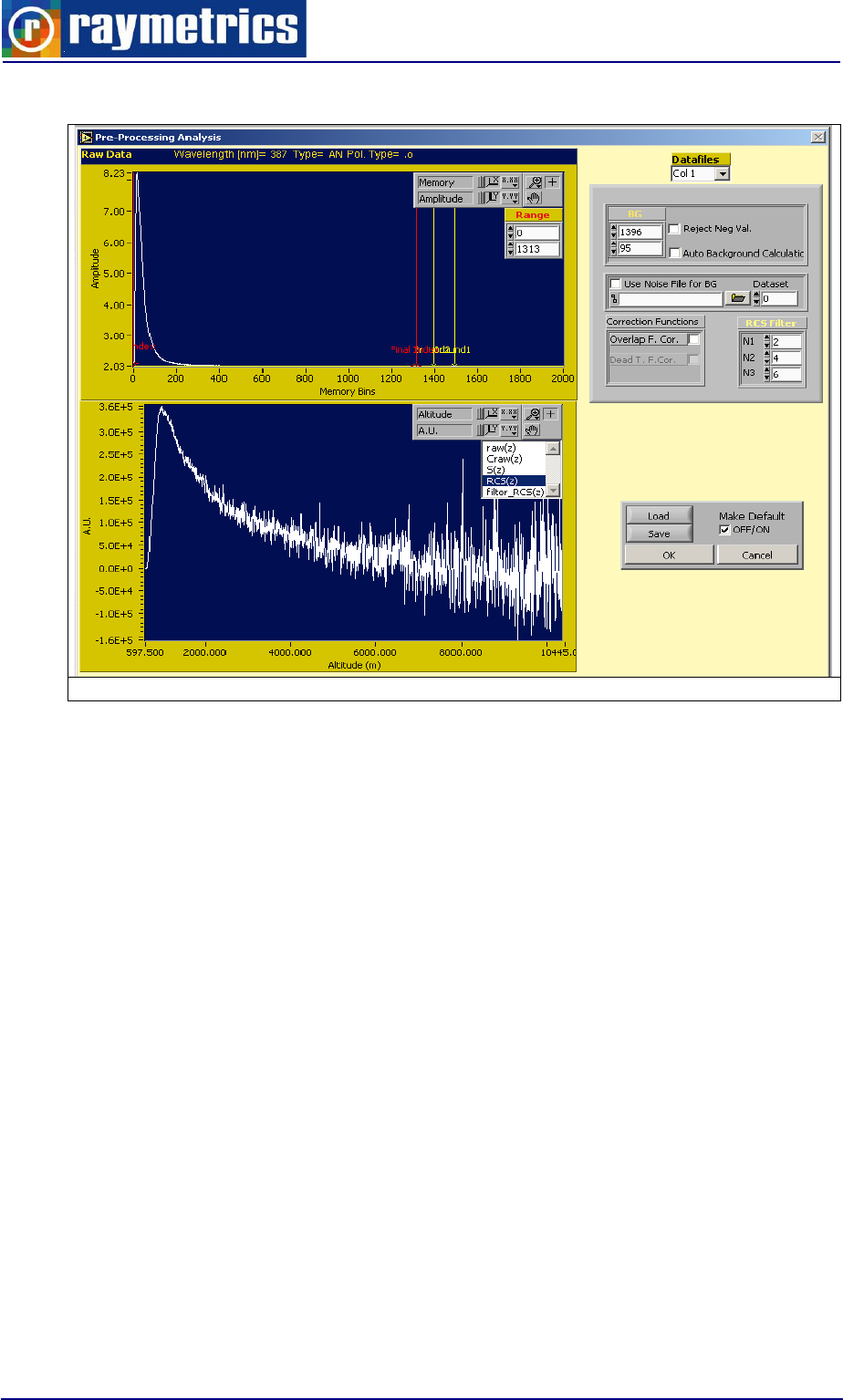

LIDAR DATA PROCESSING
138
7.3.7 How to Glue Analog and Photon Counting signals
Intro:
Depending on your Lidar configuration many detected signals are recorded
simultaneously by two methods; Analog and Photon Counting method.
The combination of both signals allows using the high linearity of the analog signals for
strong signals (near fields) and the high sensitivity of the photon counting for weak signals
(far fields). The idea is to combine the signals, at a region where both signals (analog and
photon) are valid and have a good signal to noise ratio. For a typical case this region
extends from 0.5 to 20 Hz in photon counting mode.
Before we glue signals the photon counting data should be dead time corrected
(Raymetrics software does that). There are two typical dead-time scenarios, while the Licel
photon counter can be best described as nonparalyzable.
In that case the dead time corrected photon counting signal is given by the following
equation:
d
N
N
S
*1
Where S is the corrected counties, N is the observed count rate and τd is the system
dead time. Raymetrics software uses a value of 260 MHz for τd
For detailed discussion of the theory of photon counting dead time correction please
see the following paper: D. P. Donovan, et.al. “Appl. Opt. 32, 6742-6753 (1993).
The gluing
In the region where both signals are valid (between the lower toggle frequency –
typical 0.5 MHz and the upper toggle frequency – typical 20 MHz) one seeks the linear
regression coefficient to transfer the analog data into photon counting data.
After transferring analog to photon the scaled analog signal is used above the upper
toggle frequency and the photon counting signal
When gluing is possible:
The peak value of the dead time corrected photon counting signal is above the
maximum toggle frequency (save values for maximum toggle frequency is between 10
MHz and 70 MHz for the dead time corrected signal) and the background of the dead time
corrected photon signal is below the minimum toggle frequency.
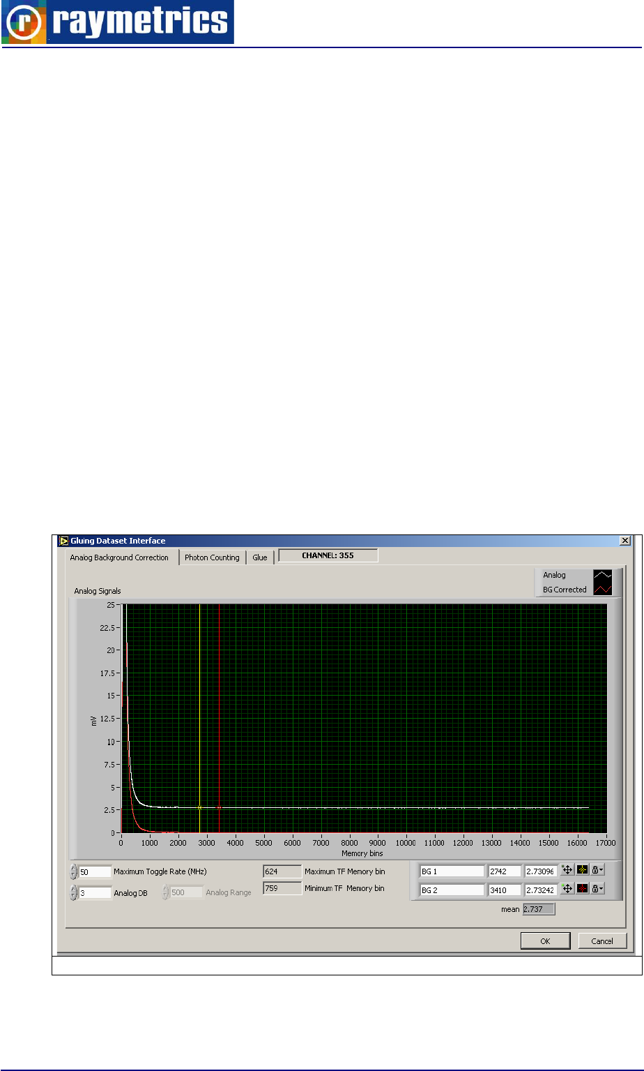
LIDAR DATA PROCESSING
139
If the signal is too weak (maximum peak of photon counting signal less than 20 Hz) use
only photon (gluing is not useful)
If the signal is too strong (background of the dead time corrected signal more than 20
MHz)
Raymetrics software
The first step is to figure out until what range the analog signal has good signal to
noise ratio. A suggested way is to remove the background noise and then to figure out until
what point the signal is 2 to 5 times more than LSB. The value of LSB (The minimum
change in voltage required to guarantee a change in the output code level is called the
least significant bit (LSB) voltage. The resolution Q of the ADC is equal to the LSB voltage
and depends on the full range of the pre-amplifier that you have select during the
measurements. There are three possible values for the full range, 500, 100 and 20 mV and
the LSB is 500/212=122 mV, 100/212=24.4 mV, 20/212=4.8 mV.
Let assume that the maximum memory bin that the signal is 5 times the LSB is Xa.
In addition let assume that the Photon Counting signal has a value of 50 MHz at
memory bin Xp. If Xp < Xa then gluing is possible. If not then gluing is not suggested.
Fig. 7.38: Analog Background Correction
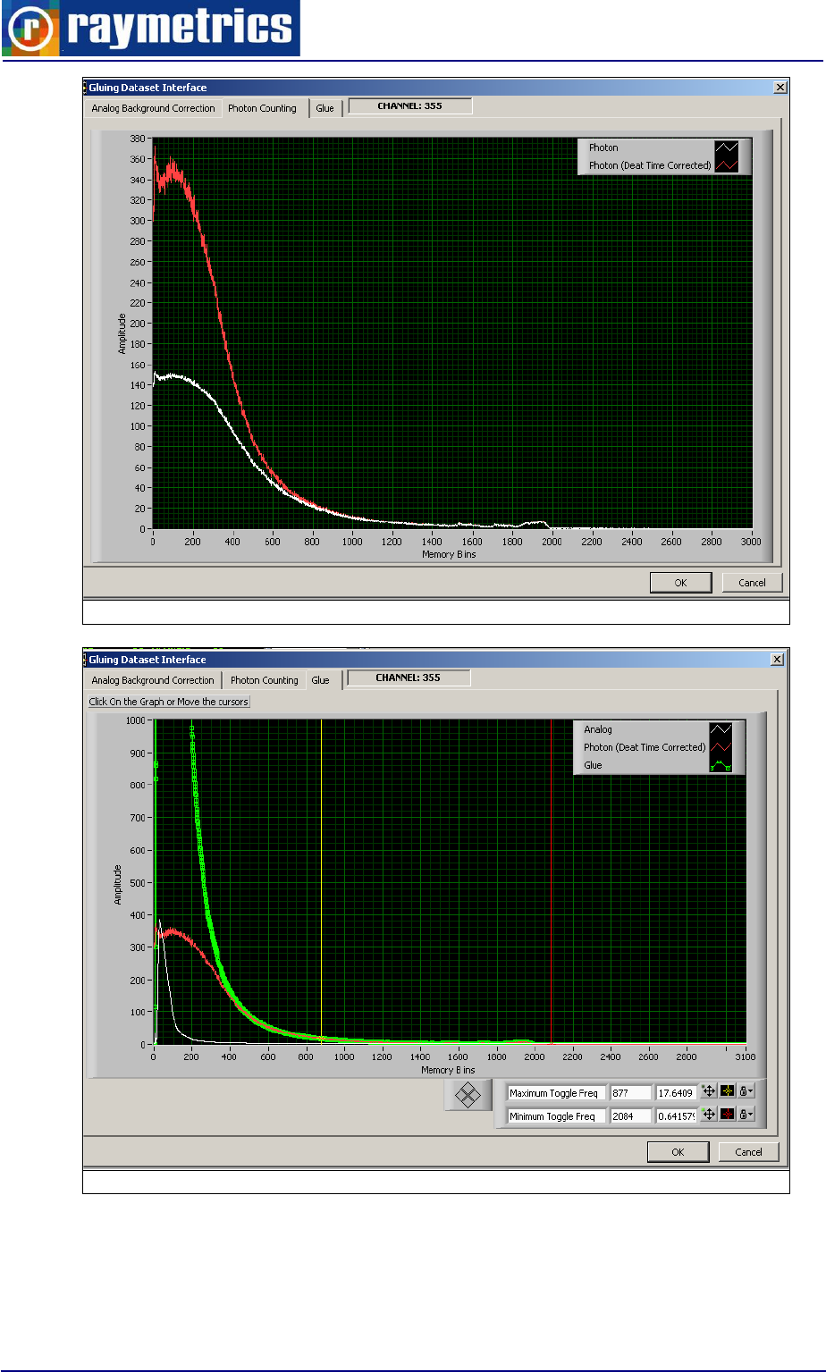
LIDAR DATA PROCESSING
140
Fig. 7.39: Photon Counting and Dead time photon counting
Fig. 7.40: Glued Signal
Use the two cursor to change Maximum or/and Minimum Toggle Frequency (if you
want), or just click on the graph and then OK button.
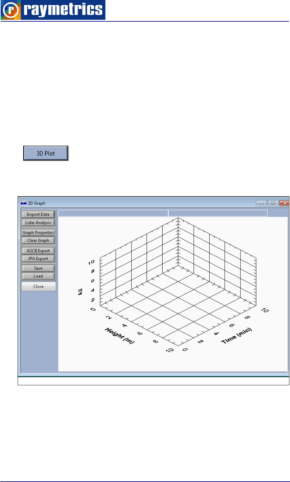
LIDAR DATA PROCESSING
141
7.3.8 How to make a 3D Graph
In many studies analysts are interested in structures that usually come from clouds. In
most of the cases these are represented in a surface plot that shows the time evolution of
the phenomenon. There is another way to illustrate the measurement by plotting the data
in a 3D graph which can be rotated, panned and zoomed. This may give a better
understanding of the structures. This tutorial will teach you how you can make such a plot.
1. Preview the database and find a record that has interesting cloud structures. Close
the Preview and click the “3D Plot” Button.
2. A new interface appears with an empty 3D Graph. Click on the Insert Data from DB
button (as you can see in Fig. 7.41)
Fig. 7.41: 3D Graph Interface
3. Follow the same procedure explained earlier in paragraph 7.3.1 How to Plot Data
to make the analysis and plot. Keep in mind that since you are interested in the
area where the structures are you can select with the red cursors the boundaries of
the graph from the beginning. This way the plot is going to be focused where you
want.
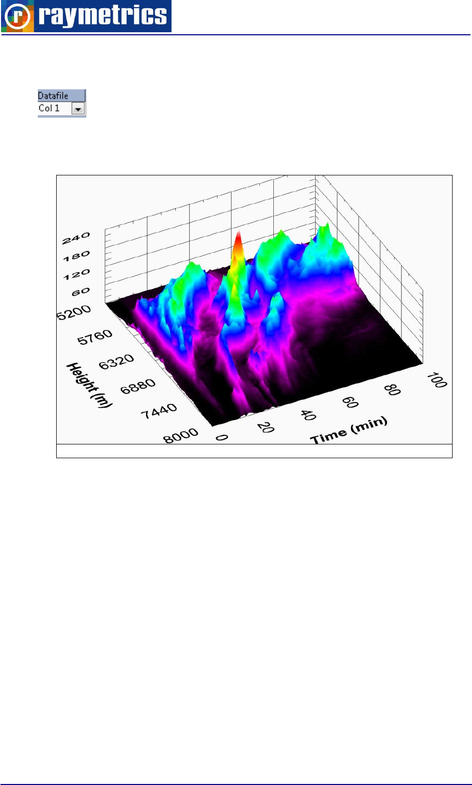
LIDAR DATA PROCESSING
142
Note: In the analysis interface you can see all the files that are selected for plotting if
you select the data file in the list box right next to the raw signal graph.
4. Once you complete the analysis you can have an image that looks like the one in
Fig. 7.42
Fig. 7.42: 3D Plot
5. Hold the mouse left button down and drag to rotate the graph.
6. Hold “Alt” key with Left Mouse and drag to resize.
7. Hold “Shift” key with Left Mouse and drag to pan.
You can modify the properties of the graph at “Graph Properties” or save the graph as
an image at “JPG Export”.
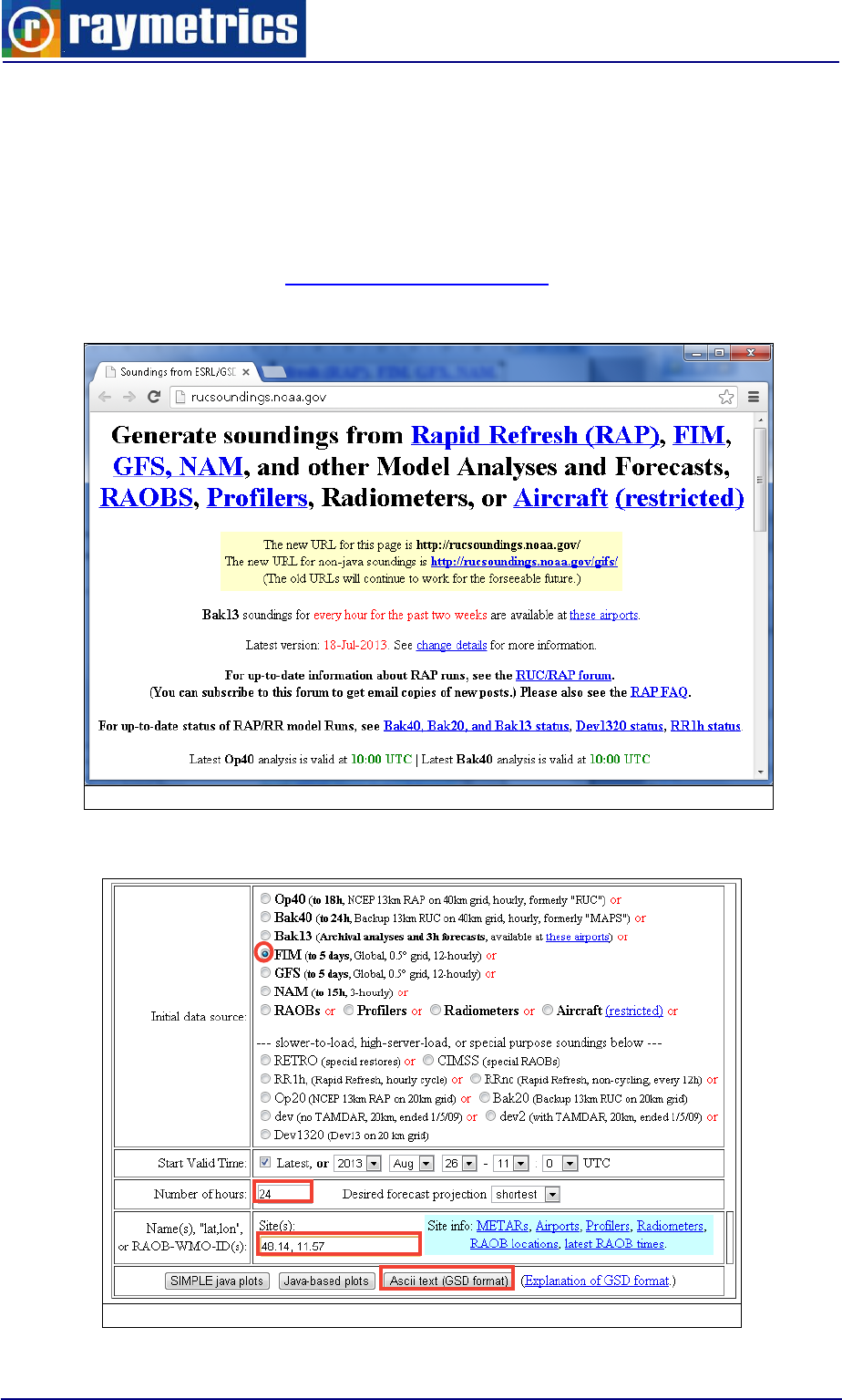
LIDAR DATA PROCESSING
143
7.3.9 How to use soundings from global model data
Accurate radiosonde data from model analyses (and forecasted data), are much better
than data calculated with standard atmospheres. You can find this information for free at
the internet. Here is presented where you can find and how you can use the data.
1. Load the website: http://rucsoundings.noaa.gov/, to get model data for every
location on earth on a 0.5° grid.
Fig. 7.43: rucsoundings
2. Select, FIM, 24, 12 or 8 for No. of Hours, your lat and lon (like: 34.7, 33.07)
Fig. 7.44: rucsoundings
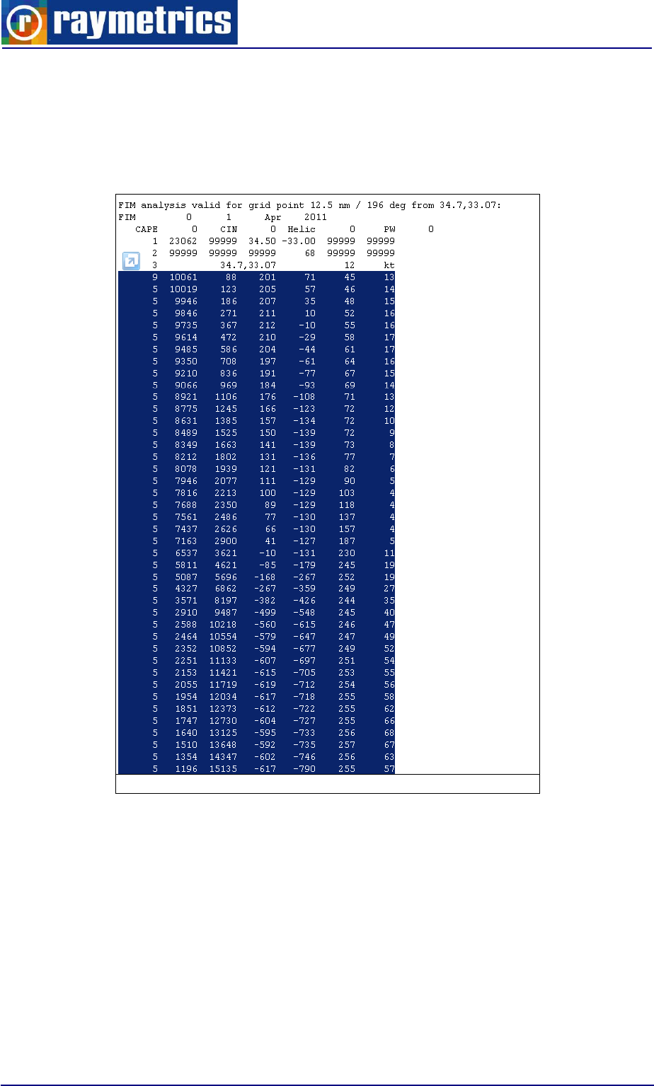
LIDAR DATA PROCESSING
144
3. Click on the ASCII Format (GSD).
4. At the new page that will appear use your mouse to select the data that you want
like below
Fig. 7.45: Results page
5. Copy the data (Select and right click to copy)
6. Open a text editor and past the data. Save the file with a name that you want (like
Road_Data.txt). The columns that we are interesting for are the column 2 (pressure
in tenths of milibars), column 3 (altitude in meters) and the column 2 (temperature
in tenths of Celsius). Raymetrics software needs to read an ASCII file with three
columns separated by tab.
a. First Column: Altitude in meters
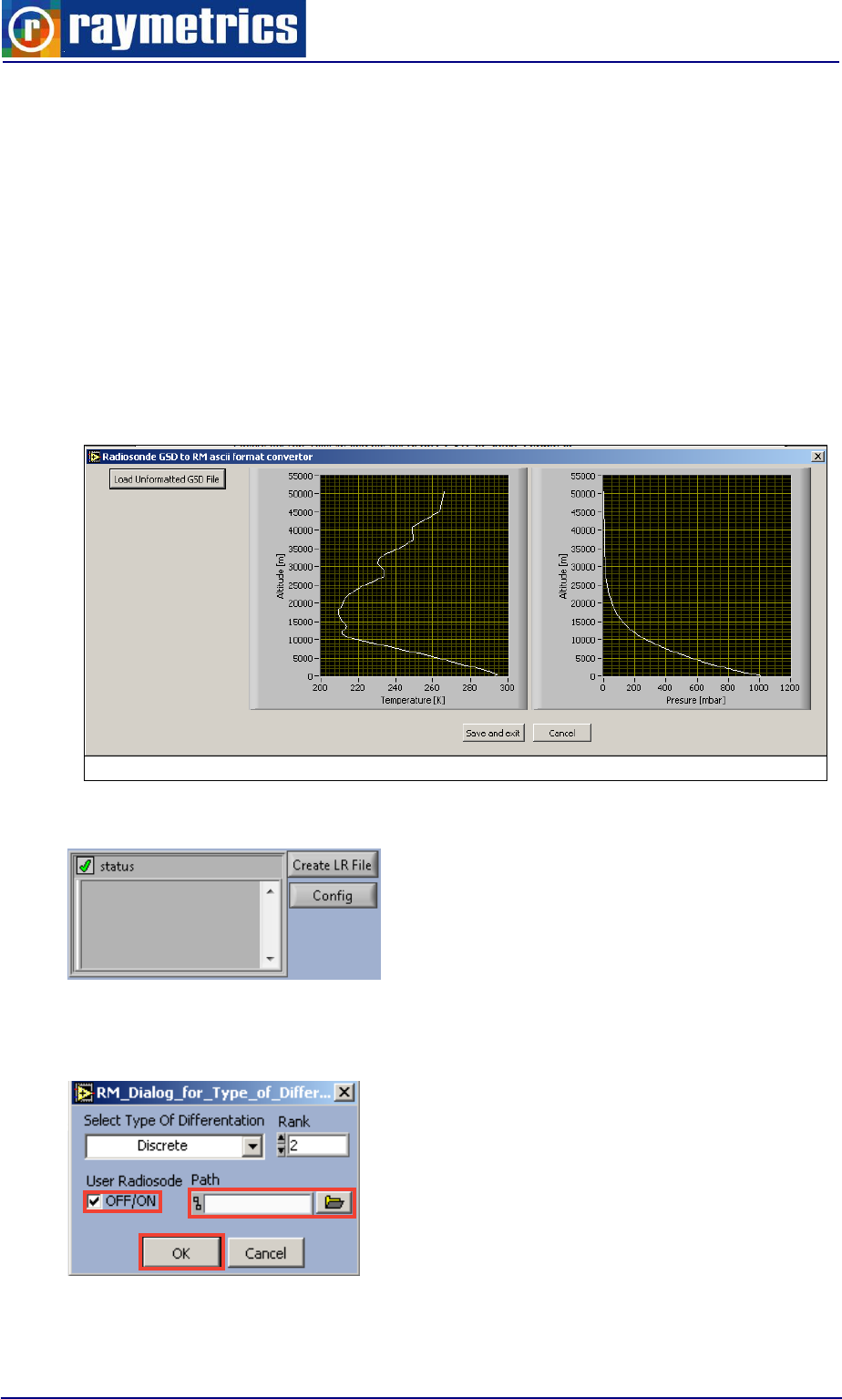
LIDAR DATA PROCESSING
145
b. Second Column: Temperature in K
c. Third Column: Pressure in hPa.
7. Now we need to convert the Road_Data.txt file to another ASCII formatted file
suitable to be read by Raymetrics software. To do so locate the Rm_Utils.llb and
run the ROAD_GSD_to_Ascii_Format.vi.
8. Select the file that you want to convert e.g. Road_Data.txt.
9. The software will ask to save the formatted data to another file. Then give another
filename for the formatted file eq. Road_Data_formated.txt (if you like you can
overwrite the original one).
Fig. 7.46: Radiosonde File Convertor
10. Now at the analysis interface you can click on the Config button
11. Then click on the Use Radiosonde Check box and then load the formatted ASCII
file by clicking on the folders icon. Then Click ok.
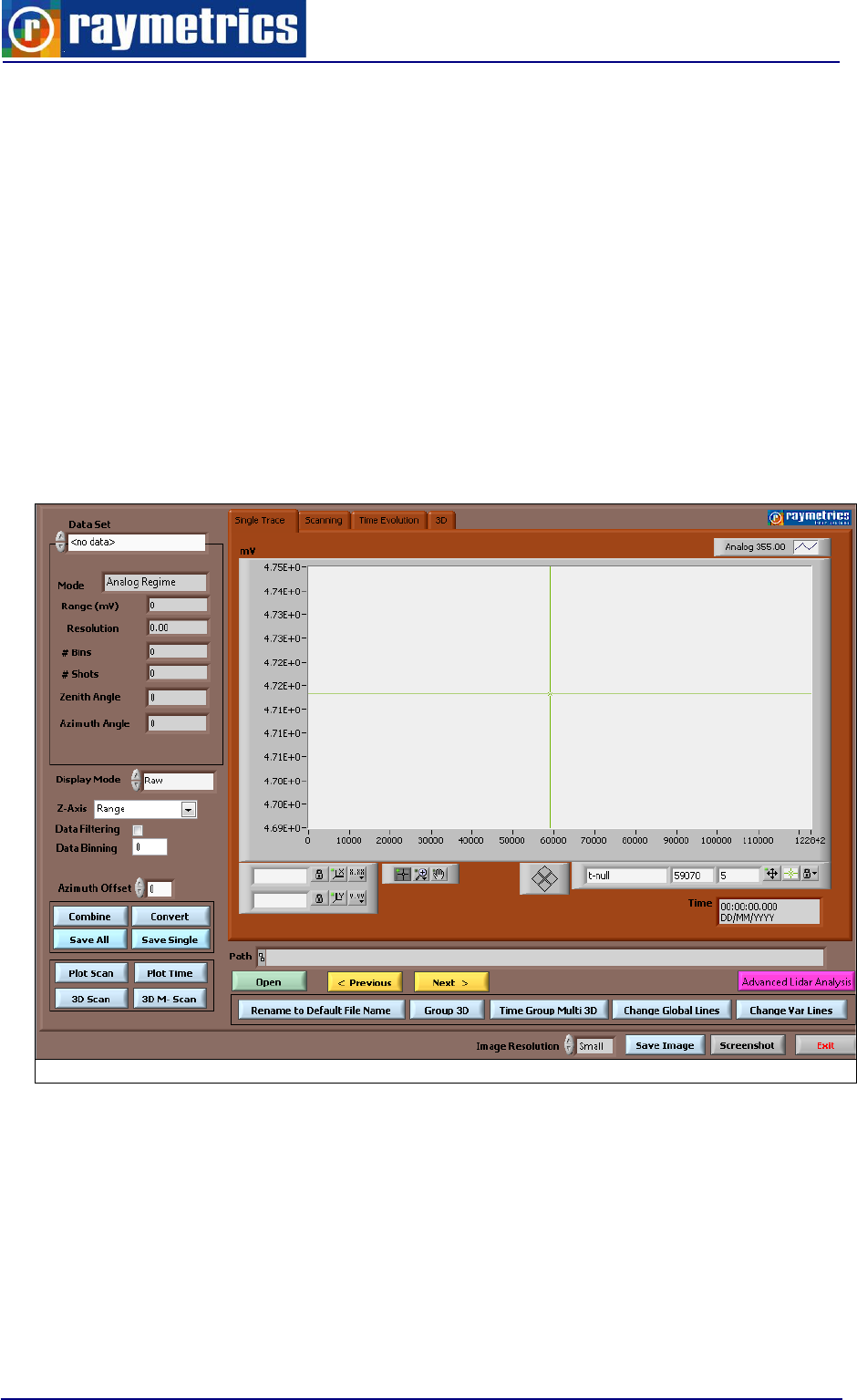
LIDAR DATA PROCESSING
146
7.4. SCANNING DATA ANALYSIS
As previously noted the scanning data are usually too many to handle in a traditional
way. For this the user needs software that will automatically recognize the type of the
scan, the angles and then manipulate them to make different types of analysis.
Furthermore the representation of scanning data is also very important to be in a
comprehensive form. Through a series of freeware and in combination of scripts written
from Raymetrics, the user ca easily extract the data to Google Earth files.
7.4.1 How to use the Advanced Viewer Extra
The advanced viewer extra is a program used for the analysis of scanning data. Below
is a short tutorial on how you can use this program.
Fig. 7.47: Advanced Viewer Extra
When the program starts it prompts to load the data. Select the first file of the data in
the folder where you scanning data are saved and press ok to select the last file of your
data set.
If you skip this step or if you want to load different data, you can open by pressing the
open button. Once they are loaded you can preview the records at the single trace tab,
one by one by pressing the < and > buttons.
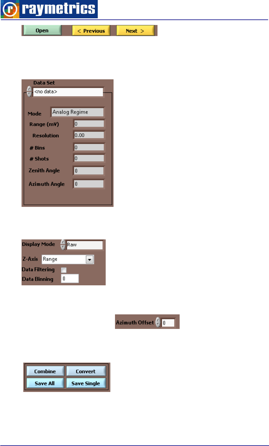
LIDAR DATA PROCESSING
147
Next you can see all information regarding the acquisition as in the mode, range
resolution, Number of bins Number of shots zenith and azimuth angle. All tehese change
according to the selected file that is currently previewed.
Below this you can chose how you wish to view the chosen data file. For example raw
or range corrected signal or range and altitude etc.
Here you can set the azimuth offset to compensate the direction offset during the
installation of the lidar with the east. If you choose to correct then the data will not
correspond to the actual orientation.
Below this you have multiple operations for the database manipulation. You can either
save one or all files convert them or even combine them to a single one.
And finally you have the options of what to do with these data. You can plot them either
in a scan plot or as a time evolution plot. You can also plot a 3D scan which basically
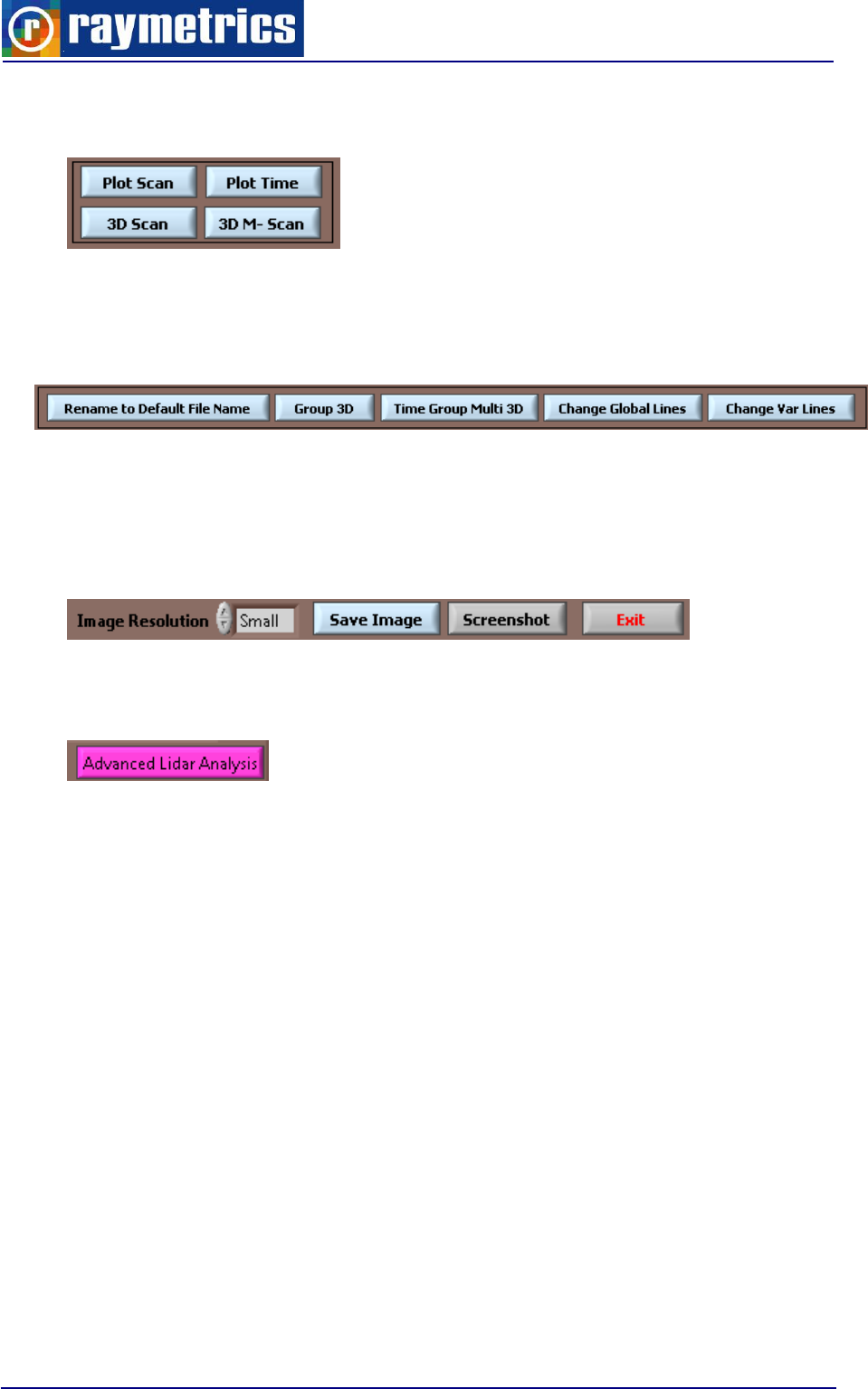
LIDAR DATA PROCESSING
148
means that the data of the 3D scan will be grouped either in set of azimuth or zenith scans.
Finally in multiple 3D scans you also get the option of time evolution of the same scans.
One useful tool is below the open button. Here are a set of button that can change
things in your data. You can rename the files, group them in a 3D scan, group them as
time evolution 3D scans, change the global information or the variables of the files
On the bottom of the interface there are options to save the image of the 3d graph or
just a screenshot and of course the exit button. When the user saves an image a text file is
also saved that contains all the information of the plotted scan. This file is used from the
Sketchup script to create the geometry of the scan.
Finally what makes this program even more powerful is the option to run the advanced
analysis as this was explained in the previous paragraph.
7.4.1 How to Display Scans in Google Earth
This is a guide how to use both the advanced viewer to make a scan plot and also how
to use the Raymetrics script that runs on Google Sketchup. These two programs in
combination can easily produce impressive representation of your data in Google Earth.
Start by running the Advanced Viewer extra and select the data to be analyzed.
Click on the Plot Scan button. Select the first file of the scan you want to plot and then
the last file of the scan you want to plot.
Then select the ray data set and the parameter you want to plot.
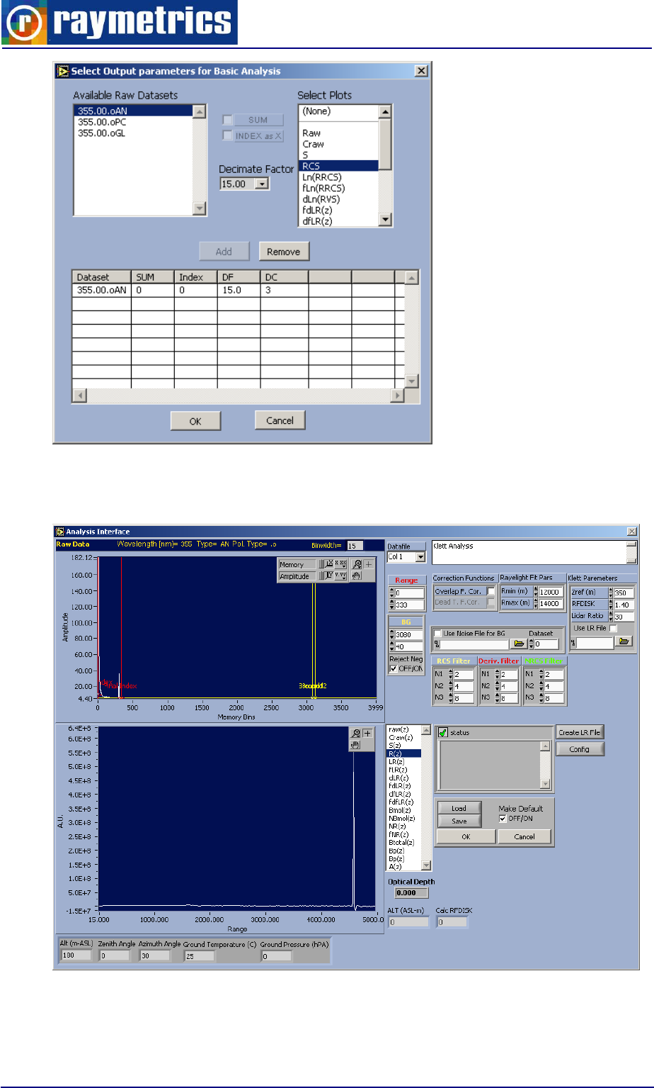
LIDAR DATA PROCESSING
149
Define the range of interest make the analysis and click the ok button (make a note
about the range that you have selected eg: 5000 meters
Now the analysis is done and the program returns to the main interface. If you go to the
3D tab you can see the plotted data in a 3D graph.
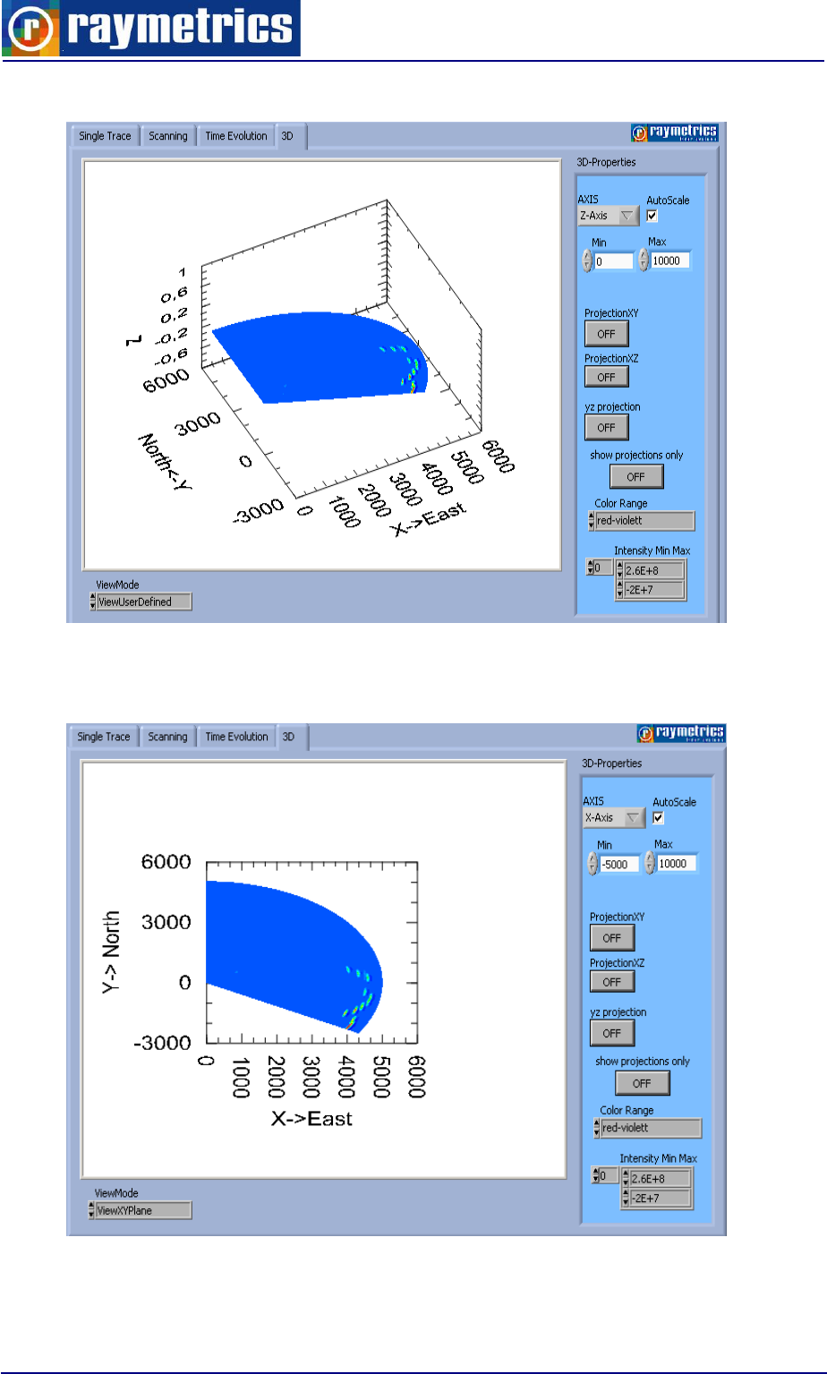
LIDAR DATA PROCESSING
150
To make this image compatible with the Sketchup script you need to view the XY-
plane. At the 3D-properties pane press the ProjectionXY button.
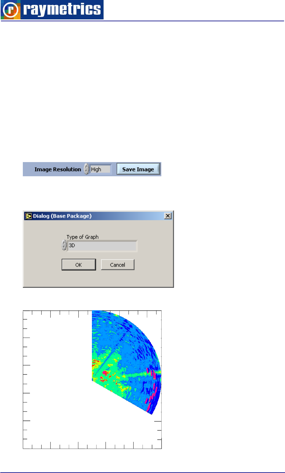
LIDAR DATA PROCESSING
151
Press the Define the scales for X and Y axis to have the same length and equally
spaced. For example select the x-axis and set the min to -5000 and max to 5000m, then
select the Y-axis and set the same values (do not forget to uncheck AutoScale)
Now the image should be in the middle. Make sure that the plot is not cropped but it
also no too small.
Then select Min Max values for color scale. If you intend to represent several scans
make a note of the color scale so that you the images can be comparable.
Then use the Alt+Click and move your mouse to Zoom – UnZoom and Shift+Click and
move your mouse to move the graph.
Then select High Resolution Option and Click on the Save Image.
At the pop-up window select 3D and click Ok. At the pop-up dialog set the information
for the geo-coding and the azimuth offset.
Now the saved image should look like this.
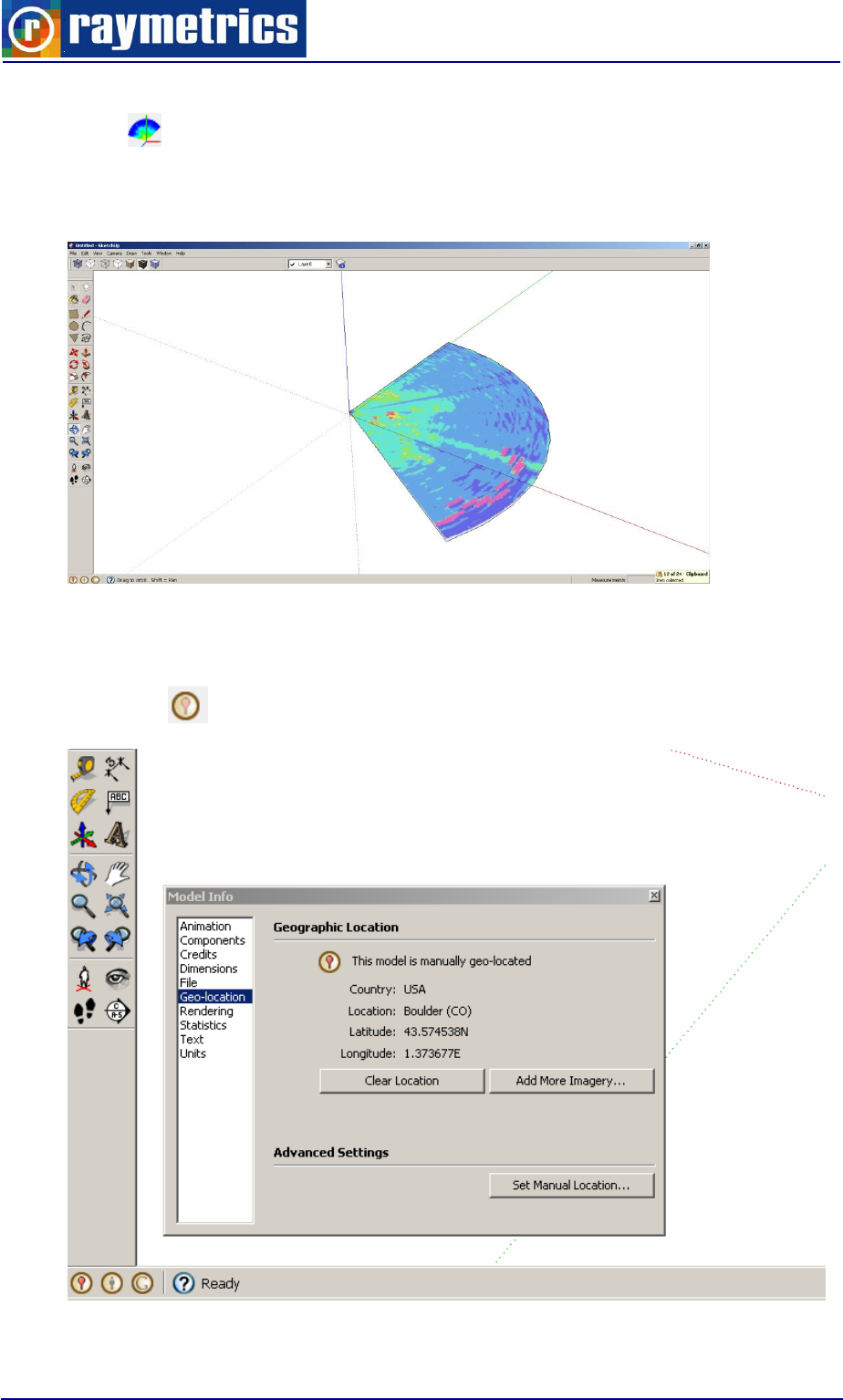
LIDAR DATA PROCESSING
152
Next open Google Sketch-up with the installed script and click on the toolbar the draw
scan icon . The script promots the user to load the info file. Select the txt file that has
the same name with the image that you have saved. Once you click ok the program
automatically creates a 3D model with the scan.
If you choose not to use the geo location information you can set them manually by
clicking on the icon at the bottom of the window.
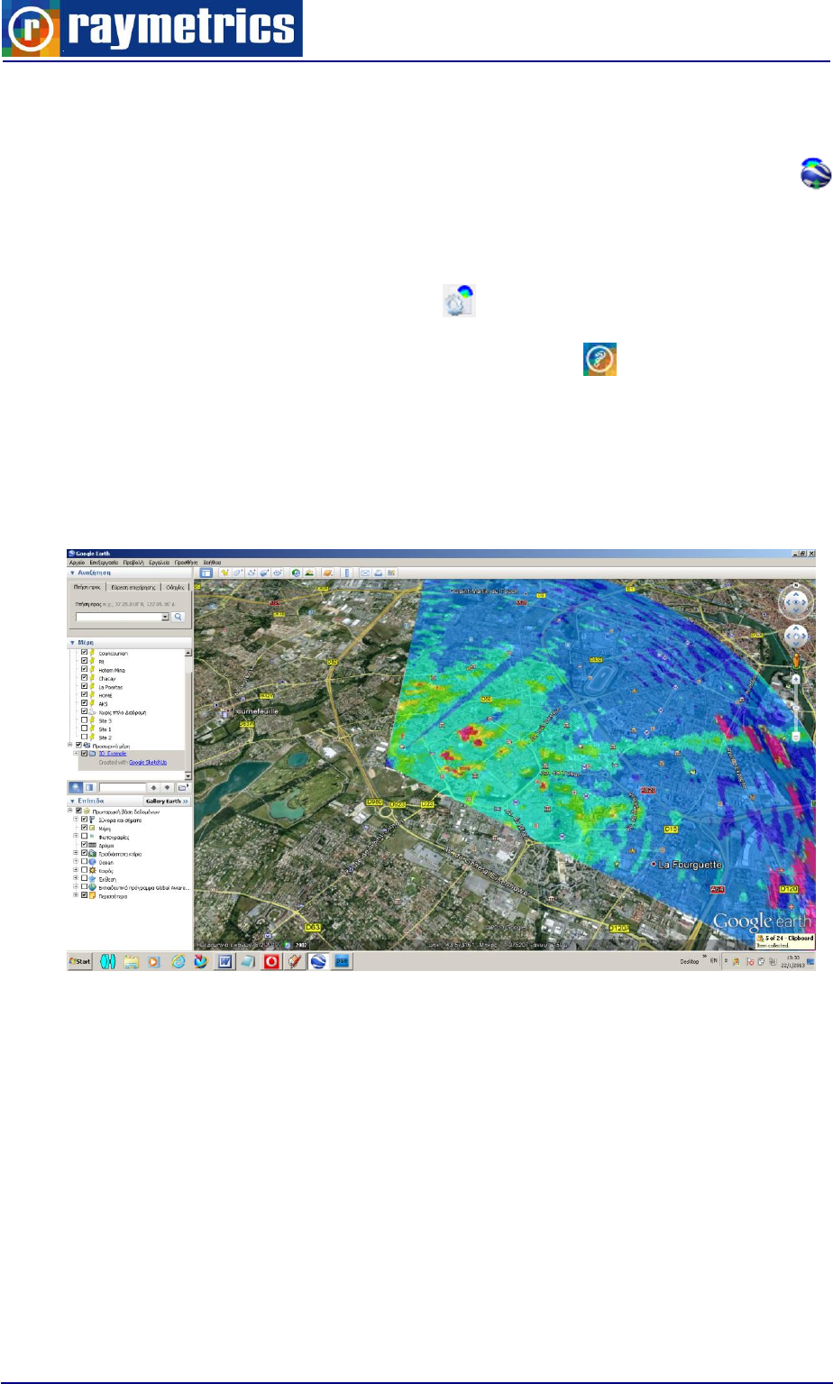
LIDAR DATA PROCESSING
153
Select Geo-Location and click on the Set Manual Location. Give Long and Lat. Now
your sketch is geocoded and you can save it as a kmz file either by pressing the
button on the Raymetrics toolbar or go to menu File->Export->3D Model.
If you want you can change the opacity of the model or select to draw a geometry
without using an info file at the options button.
For more information about the script click the help button.
If you exported the image by using the toolbar a kmz file is created in the same folder
with the image and with the same name with the image. Open the exported file and Google
earth will take you to the location set from Sketchup and show the measurement as a 3D
model. (For the last actions you have to have internet access).
You can draw as many scans as you want in the same SketchUp file, but note that in
this case you may need to name the kmz file in a name of your choice.
Follow the same steps and refer to the help file to make a zenith scan model.

LIDAR SYSTEM MAINTENANCE
154
8. LIDAR SYSTEM MAINTENANCE
8.1. LASER SYSTEM
The laser system requires minimal maintenance, if it is operated in a standard
laboratory environment with specified power line and ambient temperature conditions (see
10. LIDAR SYSTEM TECHNICAL SPECIFICATIONS. Please, refer to the Laser’s
INSTRUCTION MANUAL for a detailed description of the laser’s maintenance procedure
(alignment verification, flash lamps replacement, cooling group unit, etc.).
8.2. REFLECTIVE MIRRORS
Although the closed Lidar structure provides a dust-free operation for optical
components, the Lidar should never be operated without the protective housing. In case
the reflecting mirrors become dusty, they should be cleaned with absolute ethanol using
flint-free optical paper. If this is done by non-specialized personnel, serious damage may
occur on the optical components and the warranty will not be further valid. Therefore, it is
strongly recommended that you sign an after sales Servicing Contract with Raymetrics
S.A. for a trouble-free maintenance of your Lidar system.
8.3. TELESCOPE
Although the Lidar structure provides a dust-free operation for optical components, it is
preferable that in open air the Lidar system should be operated with the protective housing
on. In case the telescope becomes dusty, it should be cleaned with absolute ethanol using
flint-free optical paper. If this is done by non-specialized personnel, serious damage may
occur on the optical components and the warranty will not be further valid.
8.4 CLEANING OF OPTICAL COMPONENTS
All optical elements are delicate and should be handled as carefully as possible. The
glass and antireflective (AR) coated surfaces will be damaged by any contact, especially if
abrasive particles have come into contact with the surface. In most cases, it is best to
leave minor debris on the surface.
Use of oil-free dry air or nitrogen under moderate pressure is the best tool for removing
excessive debris from an optical surface. In the case that the contamination is not
dislodged by the flow of gas, please use the following protocol for cleaning the part:

LIDAR SYSTEM MAINTENANCE
155
1. Clean the part using an absorbent towel such as Kimwipes™, not lens paper. Use
enough towelling so that solvents do not dissolve oils from your hands which can make
their way through the towelling onto the coated surface.
2. Wet the towel with an anhydrous reagent grade ethanol.
3. The use of powder-free gloves will help to keep fingerprints off the part while cleaning.
4. Drag the trailing edge of the ethanol soaked Kim wipe across the surface of the
component, moving in a single direction. A minimal amount of pressure can be applied
while wiping. However, too much pressure will damage the component.
5. If the surface requires additional cleaning, always switch to a new Kimwipes before
repeating the process.
The purpose of the solvent is only to dissolve any adhesive contamination that is
holding the debris on the surface. The towel needs to absorb both the excessive solvent
and entrap the debris so that it can be removed from the surface. Surface coatings on
interference filters and dichroics are typically less hard than the substrate. It is reasonable
to expect that any cleaning will degrade the surface at an atomic level. Consideration
should be given as to whether the contamination in question is more significant to the
application than the damage that may result from cleaning the surface.
In many cases, the AR coatings that are provided to give maximum light transmission
amplify the appearance of contamination on the surface.
8.5 POSITIONER
The positioner’s model is 2AP sun tracker and is made by Kipp & Zoenen. You can find
the full documentation of this device in the Lidar’s computer for a proper operation. In short
the positioner needs greasing once per six months depending on the usage. To do so you
will have to turn vertically the lidar to remove the cover.

TROUBLESHOOTING
156
9. TROUBLESHOOTING
This chapter addresses some of the problems you might encounter while running your
Lidar system and indicates ways how to solve these problems.
9.1 EMISSION
PROBLEM
POSSIBLE CAUSES
CORRECTIVE ACTION
Dead (no power)
AC mains
Check power source. Inspect power cord
Blown fuse(s)
Check fuses on back panel T10A/250V, QTY
2 and replace if necessary.
NO Simmer, NO Interlocks
Three audible clicks from
ICE450
Faulty laser I/O cable
Verify laser I/O cable connectors are fully
inserted and thumbscrews are tightened.
Visually inspect high current contacts on both
ends of the laser I/O cable for carbon film or
pits caused by poor connector insertion and
arcing.
The control unit starts and
after a few seconds turns off.
Low coolant level
If the reservoir is not filled a flow interlock
appears in the LCD screen. Add coolant to
the reservoir.
Flashlamp does not lamp.
Flashlamp is not enabled
Verify that both the “flashlamp ready” light and
the “flashlamp start” light on the Remote Box
are illuminated.
Simmer Problem
Either ionized, or contaminated coolant, or a
degraded flashlamp may be the cause.
Coolant should indicate a resistivity of 100kΩ-
cm to 5MΩ-cm for proper operation. If coolant
resistivity is less than 100kΩ-cm, replace the
coolant. If the lamp still does not simmer
replace the flashlamp.
Charger Latch-up
If the ICE450 makes a squealing or hissing
sound when the high voltage is enabled, and
the simmer LED is illuminated but the
flashlamp does not flash, disable the high
voltage immediately. A component inside
the ICE450 has most likely failed and the high
voltage charger is attempting to charge into a
short circuit. If the ICE450 is operated in this
mode for longer than a few seconds additional
electronics damage may occur.
Flashlamp does not fire. NO
Interlocks
Flashlamp is not in
Internal Mode
Verify that Internal sync is selected in the
flashlamp menu.
Flashlamp is broken
If, after pressing the “Flashlamp Ready”
button, the “ready” light does not light, nor is
there a visible flashlamp flash, the flashlamp
may need to be replaced.
Flashlamp does not fire.
Interlock “emergency stop
button pushed”
The red button on Remote
Box is pushed in.
Pull the button out. If that does not work, there
may be an open circuit in the Remote Box,
cable, or internal harness.
Flashlamp does not fire.
Interlock “BNC Intlk in on
ICE450 front panel”
The “INTLK In” connector
on the front panel is open.
Connect a shorting plug, to the “Interlock In”
BNC on the front panel. If that does not work,
there may be a problem with the shorting
plug.
Flashlamp does not fire.
Interlock “thermal sensor
on Laser Head”
The thermostat in the
Laser Head is open.
Allow the head to cool down. If that does not
work, there may be an open
circuit in the Laser Head or in the Laser Head
I/O cable
Flashlamp does not fire.
Interlock “flashlamp
disabled time out delay
The flashlamp timeout has
expired.
Either disable timeouts or change the
flashlamp timeout to 00:00.

TROUBLESHOOTING
157
expired”
Flashlamp does not fire.
Interlock “heater over
temp”
The coolant heater is too
hot.
Turn off power to the ICE450 and allow it to
cool down. If that does not work, contact
Raymetrics.
Flashlamp does not fire.
Interlock “charger/simmer
over temp”
The Charger inductor is
too hot.
Turn off power to the ICE450 and allow it to
cool down. Verify that air flow is not
obstructed at the front or back of the ICE450
and correct if necessary. If that does not work,
contact Raymetrics.
Flashlamp does not fire.
Interlock “low coolant
temperature”
The coolant is not warm
enough for proper
operation.
Give the ICE450 time to warm the coolant. If
that doesn’t work increase the temperature of
the cabinet’s thermostat.
Flashlamp does not fire.
Interlock “high coolant
temperature”
The coolant is too warm
for proper operation.
Turn off the ICE450 and allow it to cool down
and decrease the temperature of the cabinet’s
thermostat.
Flashlamp does not fire.
Interlock “low coolant flow”
The coolant is not flowing
properly.
There may be an obstruction in the coolant
lines. Examine the lines and make sure they
are not kinked or otherwise obstructed.
Q-Switch doesn’t start.
Interlock “Q-S disabled
Please wait for 8 seconds”
There is no problem. This
is normal.
Wait until the 8 second timeout expires, then
activate the Q-Switch.
Q-Switch doesn’t start.
Interlock “Q-S disabled
coolant temperature under
limit”
The coolant temperature
is below the minimum Q-
Switch operating
temperature.
Allow the coolant to warm up.
Q-Switch doesn’t start.
Interlock “Q-S disabled time
out delay expired”
The user-set timeout
period expired.
Disable timeouts or set the Q-Switch timeout
to 00:00.
Energy is low
Cold Flashlamp
This is normal wait for 10 minutes to reach the
desired energy.
Flashlamp Degradation
If output energy is slightly below normal level,
it may suggest gradual lamp degradation. If
significant lamp degradation is suspected,
replace the flashlamp.
Coolant Degradation
Inspect the coolant for clarity.
Incorrect Q-Switch Delay
Check that the Q-Switch delay is set to 135μs
with respect to the flashlamp.
Resonator Misaligned
If beam quality has degraded, it may suggest
that the resonator needs realignment. Contact
Quantel USA for more details.
Coolant leak
DI Cartridge installation
Verify that DI cartridge is locked in place and
fittings are fully inserted.
Laser Head o-rings
Inspect o-rings on coolant line connectors at
Laser Head for damage and replace if
necessary.
RS232 port does not
operate: no
communications.
Serial port disabled
For safety reasons, the serial port is disabled
when any button is pressed on the Remote
Box. In the “system” menu, turn serial port
ON.
Baud rate incorrect.
See ICE450 User’s manual Chapter 5, Serial
Protocol Description for correct baud rate
setting.
For further information on laser troubleshooting please refer to the laser’s instruction
manual for a relevant troubleshooting list for any problems you may encounter when using
your solid state Nd:YAG laser.

TROUBLESHOOTING
158
9.2 DETECTION
PROBLEM
POSSIBLE
CAUSES
CORRECTIVE ACTION
Dead (no power)
AC mains
Check power source. Inspect power cord
Blown fuse(s)
Check fuses on back panel and replace if necessary.
No signal at all
channels
HV Power supply off.
Turn on the PMT power supply and apply the specified
voltage.
No connection.
Check that all connectors are in place.
Laser is not
transmitting.
Turn on the laser (flashlamp – Q-switch)
Lidar is misaligned.
Reduce the energy of the laser so that the light can be
hardly seen when placing a white paper in above the
widow of the emission unit. Raise the paper and tilt it in
a way so that the light is reflected directly into the
telescope. If the Lidar is misaligned then you should
see the signal changing. Realign the Lidar (see
paragraph 6.2 LIDAR ALIGNMENT) CAUTION! If the
energy is high the PMTs will be destroyed.
No signal at one of the
channels.
Broken connector or
cable.
To verify which cable is fault, connect the HV and signal
cable (one at a time) to another working device.
HV power supply
broken.
If the cables are okay connect the HV cable of a
working channel to the HV power supply that is not
working. If there is no signal at the working channel
then the HV power supply is broken.
TR Device broken.
If the cables are okay connect the signal cable of a
working channel to the TR device that is not working. If
there is no signal at the non-working channel then the
TR is broken.
The PMT is burned.
If the cables, the HV power supply and the TR device
are okay then the PMT is burned probably due to
excess of light exposure.
No acquisition in one of
the channels
Wrong dataset
configuration.
Verify that the button is red next to “analog or photon
Mem I” at the corresponding device in the dataset at the
acquisition program.
Cannot change high
voltage
HV power supply
switch.
Switch to manual position for manual HV application or
to remote for application VIA the computer
High voltage is unstable
Bad connection.
If the variation is higher that 5 volts switch off
immediately the HV power supplies. The connector is
broken.
No TCP/IP connection
Ethernet switch off.
Turn on the “LAN” switch on the energy box. Make sure
that the green light at the Power supply illuminates
Communication crash
Run Licel’s “Search Controllers.exe. If all devices are
detected the buffer is full. Restart all the devices.
Wrong IP address.
Run Licel’s “Search Controllers.exe. If the devices are
not detected make sure that the computer’s IP address
belongs to the same network of the Licel’s and change
the computer‘s IP if necessary.
Broken connector or
cable.
Check that the lights illuminate at the Ethernet switch,
make sure that the cable clicks when it is placed on the
switch, if not change the cable.
For further information on Licel electronics please refer to Licel’s instruction manual for
a relevant troubleshooting list for any problems you may encounter when using your
detection electronics unit (digitization and detection of Lidar signals).
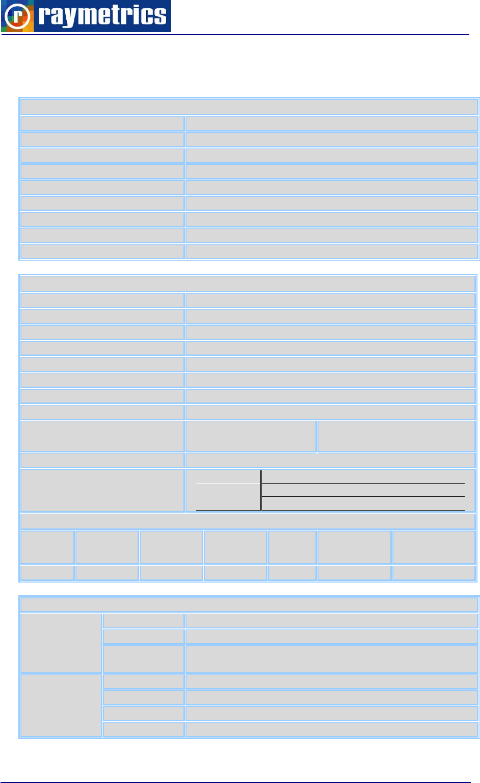
LIDAR SYSTEM TECHNICAL SPECIFICATIONS
159
10. LIDAR SYSTEM TECHNICAL SPECIFICATIONS
Transmitter
Pulsed Laser Source
Nd:YAG (Quantel ULTRA100 Series)
Laser Class
IV
Primary Wavelength
355 nm
Energy / Pulse
32.5 mJ
Repetition Rate
20Hz
Near Field Beam Diameter
3.37mm
Beam Expansion
X10
Laser Beam Divergence
<0.4 mrad
Motorized Alignment
No
Receiver
Telescope Type
Cassegrain
Primary Diameter
200mm
Secondary Diameter
48mm
F Num
F4
Focal Length
800mm
Transmitter–Receiver Distance
152 mm
Default Field Of View
1,75 mrad (adjustable from 0.5 to 3mrad)
Overlap
200m
Detected Elastic Backscatter
Wavelengths
355nm
Analog + Photon Counting
Detected Raman Wavelengths
N/A
Interference Filter Bandwidth
IFF355
CWL 354,7nm
BW 0,9 nm
OD<1
PMT Characteristics
SERIAL
TYPE
CATHODE
LUMINOUS
SEN (μΑ/lm)
ANODE
LUM. SENS
A/lm
ANODE
DARK C
(nA)
CATHODE
BLUE SEND
INDEX
REC.
OPERATING
VOLTAGE Volts
BAC0220
R9880U-110
125
246
0.09
13.0
750-900V
Control Unit
Transient
recorder
Manufacturer
Licel
Type
20-12bit
Raw Spatial
Resolution
7.50m
Computer
Manufacturer
Advantech
Model
ARK3360L
CPU:
Intel® Atom™ D525 1.8GHz
VGA:
Integrated in ICH8M

LIDAR SYSTEM TECHNICAL SPECIFICATIONS
160
Ethernet:
10/100/1000Base-T
Storage:
SATA HDD 360Gb
RAM:
4Gb
Safety:
FCC Class A
CE certificated
The front bezel is compliant with NEMA 4 and IP65
Software
OS:
MS Windows 7 Professional
Backup:
Software for data backup
Alignment:
Lidar System Checking and Alignment
Acquisition:
Data Acquisition (with real time data display)
Analysis:
Data Analysis
Control SW
Laser Control, Scheduler, PMT HV Control
Enclosure
Manufacturer:
SKB CASES
Material:
High stiffness roto molded
Ethernet:
Advantech EKI-2525 5-port Industrial Switch
Main Plug:
Bulgin IP68 panel mount industrial plug 32A
Main Switch:
Schneider electric IP66 industrial emergency switch
External USB
Bulgin IP68 panel mount USB A Type
Ext. Ethernet
Bulgin IP68 panel mount RJ45
General
IP protection:
IP56 to EN 60 529/10.91
Dimensions:
500mm x 500mm x 620mm WxHxD
Weight:
55 kg
Voltage
110VAC 50/60Hz
Power
740 Watt (Nominal) 1500Watt (Peak)
Temperature
Operating: +5 to 45oC Storage: +5 to 50oC
Humidity
Operating: 10 to 80% non condensing (+5 to 28oC)
Storage: 10 to 90% non condensing (+5 to 28oC)
LIDAR Performance
Lidar type
Biaxial
Depolarization Calibration (+/-
45 degrees)
Mechanical
Depolarization offset
correction
Mechanical
Upgradable
YES Depolarization and 3787nm Ready
Scanning 3D
Yes
Max Backscatter Effective
range*
8-12Km
*Depending on the atmosphere’s conditions and integration time.

LIMITED GUARANTEE
161
11. LIMITED GUARANTEE
NOTICE
Raymetrics SA reserves the right to make improvements of the products described in
this Manual at any time and without notice. Thus, all specifications of this Lidar system or
sub-systems are subject to change at any time and without notice.
Raymetrics SA shall not be liable for errors contained in this Manual or for incidental or
consequential damages in connection with the furnishing, performance or use of this
material.
WARRANTIES
Raymetrics SA, as well as the Lidar-components providers (laser source, acquisition
electronics, photo-multiplier tube (PMT), personal computer, Digital acquisition PC-card
and cables) warrant the products or sub-systems of this Lidar system to be free from
defects in materials and faulty workmanship under normal use for a period of 12 months
after the date of the original purchase and following the delivery to the FOB site (for details
see the Instruction Manuals of the Lidar sub-systems providers and comments therein).
Laser flash lamps are guaranteed for 25 millions shots or 1 year whichever comes first.
This warranty does not cover:
- equipments or components where the original identification markings have been
altered or removed or if any parts have been replaced by other components
- equipment or components that have become defective due to mishandling, erroneous
use, accidental alteration, improper operation, or any other cause, without the prior
written agreement of Raymetrics SA.
The cost and terms of non-warranty service are fixed by Raymetrics SA and the Lidar
sub-systems providers and are subject to change.
RETURNS, ADJUSTMENTS AND SERVICE
If warranty, service or general repair of a Raymetrics SA Lidar system is requested by
the customer that leads to the product’s return to Raymetrics SA, the terms of such return
include the following:

LIMITED GUARANTEE
162
a) Freight and insurance (CIF) charges are pre-paid by the customer, who also takes all
the risks of loss, damage or delay in shipment,
b) The Lidar system must be packed in the original containers provided by Raymetrics
SA. All water must have been drained from the laser head according to the laser
manufacturer rules, prior to packing.
c) Prior to sending the product back to Raymetrics SA the customer must obtain a written
authorization for the product return for service.
d) After the product receipt Raymetrics SA reserves the right to fully inspect the Lidar
system and determine the cause of failure and warranty status. The same is valid for
the laser provider. If the product has suffered damage during the shipment Raymetrics
SA has no obligation to perform a warranty repair.
e) If the warranty of the product has expired the customer will be advised of the cost of
such repair and a written purchase order for the repair and service work will be
required before the performance of the work.
f) If the product is still under warranty status it will be repaired or replaced free of charge
in accordance with the terms of the Raymetrics SA and Lidar components providers.
Finally, the warranty period for a replaced or repaired component will be only the
period remaining on the original product, thus no extra warranty is provided by such
repair.

REFERENCES
163
REFERENCES
1. Ancellet, G., A. Papayannis, G. Mégie, J. Pelon, "Tropospheric Ozone Measurements
Using a Nd:YAG Laser and the Raman Shifting Technique", Journal of Oceanic and
Atmospheric Technology, 6, 832-839, 1989.
2. Measures, R., Laser Remote Sensing: Fundamentals and Applications, Wiley, New
York, 1984.
3. Klett, J., “Lidar inversion with variable backscatter/extinction ratios”, Applied Optics, 24,
1638-1643, 1985.
4. Ansmann, A., U. Wandinger, M. Riebesell, C. Weitkamp, and W. Michaelis,
“Independent measurements of extinction and backscatter profiles in cirrus clouds
using a combined Raman elastic-backscatter Lidar,” Applied Optics, 22, 2257-2264,
1992.
5. Chazette, P., David, C., Lefrere, J., Godin, S., Pelon, J. and Megie, G., Comparative
Lidar study of the optical and dynamical properties of stratospheric post-volcanic
aerosols following the eruption of the El Chichon and Mount Pinatubo, J. Geophys.
Res., 100, 23, 195-207, 1995.
6. Boesenberg, J., Timm, R., and Wulfmeyer, V., Study of retrieval algorithms for a
backscatter Lidar. Final Report, MPI Report No 226, pp. 1-66, 1997.
7. U.S. Standard Atmosphere, NOAA, NASA, USAF, U.S. Government Printing Office,
Washington D.C., 227, (1976).
Also
8. V. Matthias, V. Freudethaler, A. Amodeo, I. Balin, D. Balis, J. Bosenberg, G.
Chourdakis, A. Comeron, “Aerosol Lidar intercomparison in the framework of
EARLINET: Part I- Instruments”, Applied Optics, 43, 961-976, 2004.
9. G. Chourdakis, A. Papayannis and J. Porteneuve, “Analysis of the receiver response
for a non-coaxial Lidar system with fiber-optic output”, Applied Optics, 41, 2715-2723,
2002.
10. Α. Papayannis, G. Chourdakis, “The EOLE project, Part II: Aerosols measurements
over Athens, Greece”, International Journal of Remote Sensing, 23, 179-196, 2002.
11. D. Balis, C. Zerefos, V. Amoiridis, C. Meleti, A. Bais, A. Kazantzidis, A. Papayannis, G.
Chourdakis, G. Tsaknakis and T. Trickl, “Study of the aerosol effect on the UV-B
irradiance at the earth’s surface cases studies selected from urban sites in the frame of
the Εarlinet project”, Journal of Aerosol Science, 32, 391-392, 2001.
12. V. Matthias, V. Freudethaler, A. Amodeo, I. Balin, D. Balis, J. Bosenberg, A.
Chaikovski, G. Chourdakis, A. Comeron, Arnoud Delaval, F. Di Tomasi, R. Eixman, A.
Hagard, L. Komguem, S. Kreipl, R. Matthey, V. Richi, J. A. Rodrigues, U. Wandiger, X.
Wang, “Intercomparison of 15 aerosol Lidar systems in the frame of EARLINET”,
Journal of Aerosol Science, 32, 397-398, 2001.

APPENDIX A
164
APPENDIX A
A1 HOW TO CONTROL THE LASER
Intro
Basically there are three major ways to control laser. First to use the Remote Box,
second way is to use LaserControl.exe from Raymetrics the third is to use the external
trigger. Here is mainly presented the second and the third option. For more info about the
Remote Box please read the Laser Manuals that have been supplied to you.
Note: For optimum laser energy
1. The resulting Q-Switch Delay should be 135μs.
2. Do not change the frequency. For GRM laser should be 20Hz.
Communication
The primary communications and control is via the RS-232 port located on the ICE450
front panel (Rack ICE450 back panel). The ICE can be set to lock out ront panel key
control and avoid conflict with RS-232 communications.
The serial communications configuration is:
9600 baud
8 data bits
no parity
1 stop bit
no flow control
The Ultra uses only Tx and Rx for its communications.
No hardware handshaking is utilized.
Important Note: Usually ICE450 is connected physically (through RS-232) to the Lidar
computer. In that case you have to use remote desktop to connect to lidar’s computer and
then use the LaserControl.exe (or the CE450_GUE.exe). In some cases Laser is
connected to a Serial To Ethernet Server. If this is the case you have to create a virtual
com port to your computer (by using Serial Device Server Configuration Utility) and run the

APPENDIX A
165
LaserControl.exe program from your computer. In most of the cases the Laser is
connected to Port 2 of the Serial to Ethernet Server Device with IP address 10.49.234.232.
A1.1 Manual Laser Operation Mode
Use Manual Mode for the normal operation of the Power Supply and flashlamp. Press
the “ready” button on the Remote Box to initiate simmer current in the flashlamp. The PCC
generates a flashlamp discharge as part of establishing simmer. Verify that the LASER ON
indicator is illuminated on the front panel of the PCC. Please be advised not to perform
laser emission (Q-switching) in this mode.
1. Press the Flashlamp Start button.
2. The PCC generates flashlamp pulses at the rate specified by the “frequency” setting in
the Flashlamp menu. This setting is adjustable.
3. For Gaussian Resonator (GRM) type Laser Heads, the frequency is set at Big Sky
Laser Technologies. Please do not adjust the frequency setting for GRM heads.
4. Wait for 2 Seconds
5. Press the Q-switch Start button (Figure 5, [7]).
6. The PCC starts generating Q-switch pulses internally. They occur after the flashlamp
pulse at a time specified by the “FLQS delay” setting in the Q-switch menu.
Adjusting this delay is one method of adjusting the optical energy of a laser
pulse.
Note: For this mode the only necessary physical connection between the PCC
and the transient recorder is a BNC 50-Ohm cable from Q-Switch out to Rack Trigger
input of the Transient Recorder
Note: Q-Switch Out: This BNC Connector allows synchronization to the laser Q-
Switch trigger. The Q-Switch trigger corresponds to the rising edge of this positive signal
(5V, 50 mA max, and > 10 μS pulse width).
A1.2 Laser Control Program
Laser control Program provides a user friendly GUI for every day operation and control
of the laser. The program actually does not need any installation to your computer. Just
copy exe and ini file to your computer and run it.
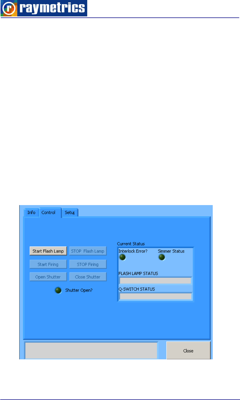
APPENDIX A
166
Note: if your pc does not have installed labview runtime library (LVRunTimeEng.exe)
version 7 or later you have to install it. You can downloawd this file from www.ni.com or
you can find usually into Laser folder that Raymetrics supplies to users.
In addition, If user’s pc does not have installed visa301 runtime library
(visa301runtime.exe) you have to install it. You can down lowed this file from www.ni.com
or you can find usually into Laser folder that Raymetrics supplies to users.
When program start first it is trying to find the laser at the serial port that it saved in the
ini file. In our example COM8
Example of Laser_Control.ini
[Laser_Control]
prefDlgTestData=1234
useLocaleDecimalPt=False
postScriptLevel2=False
[Communication]
Com Port=ASRL8::INSTR
If successfully connected, the program starts and you get the version of the laser and
its status.
ICE450 3.03
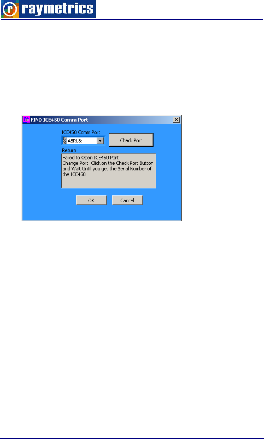
APPENDIX A
167
Then you can just click “Start Flash Lamp” button to start the flash lamp. Wait until
Simmer Status Led is getting green. Wait a couple of seconds more and then click on the
activated “Start Firing” button to start emission of laser pulses. To stop the laser follow the
opposite direction. In case that your laser is equipped with an automated shutter just not
forget to click on the “Open Shutter” button in order to start emission.
However if the program fails to connect with the laser then another window appears
giving user the option to try a different COM port.
Select an available COM port from the drop down list and click the “Check Port” button.
If successfully connected (Return message should be like CE450 x.xx) click the OK button.
If not successfully connected try a different COM port.
For more info about INFO and Setup TABS please read the Laser manual.
Troubleshooting
1. The software fails to start
Make sure that you computer has installed the appropriate Labview runtime
engine.
2. The software starts successfully but can not communicate with the laser.
Make sure that your laser is powered on.
Make sure that you have assign the right COM port
Make sure that laser serial cable is correctly attached to the lidar’s computer or
to the serial to Ethernet server device or finally to your computer.

APPENDIX A
168
3. Software runs and communicates successfully but I can not start firing (Or you get an
interlock error message)
In these cases please try to control your laser manually (by using the remote box
or the software provided by laser manufacturer). Consult Laser user manual.
Before contactng Raymetrics please try to indentify the problem and send screen shot
and a detailed description of the message that you can on the LCD display of the Lasers
Remote Box.
A1.3 Flashlamp in Internal Mode and Q-switch in External Mode
In this configuration, the PCC generates the flashlamp pulse signals and an external
source (Trigger Generator) generates the Q-switch trigger signals. This may be useful
when you:
a. Require better resolution for the Q-switch delay than is available using the PCC since
the Lamp Out signal is a copy of the actual flashlamp trigger.
b. Require pretrigger function of your Lidar.
To use this mode, select internal flashlamp sync and external Q-switch sync as follows:
1. From the main menu, go into the Flashlamp menu and select flash sync “INT”.
2. Return to the main menu.
3. Enter into the Q-switch menu and select QS Sync “EXT”.
4. Open Control Timing exe (from Licel menu)
5. Click on the Acquisition Timing Tap.
6. Switch Master Trigger to External (up Position)
For optimum laser energy the resulting Q-Switch Delay should be 135μs. For example
if you need 20 μs of pretriggering then Lamp to Acquisition should be 115μs + 20μs
Acquisition to Q-Switch. If no pretrigger is required then put Lamp to Acquisition at 135μs
and Acquisition to Q-Switch at 0 μs.
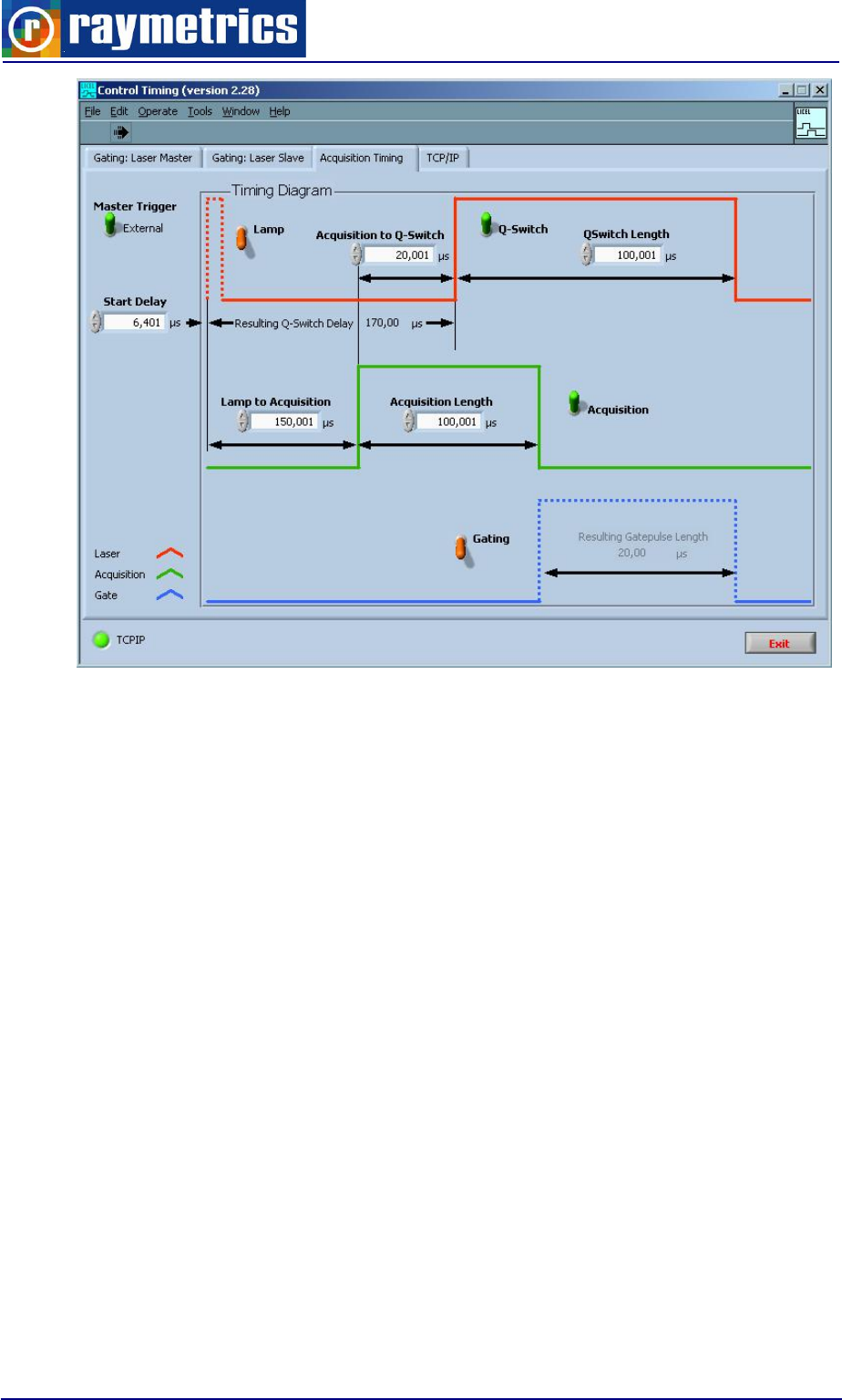
APPENDIX A
169
Now you can switch on and off the laser by switching the Q-Switch numb.
A1.4 Flashlamp and Q-switch in External Mode Mode
In this configuration, an external source (Trigger Generator) generates both the
flashlamp trigger and the Q-switch trigger.
To use this mode, select external flashlamp sync and external Q-switch sync as
follows:
1. From the main menu, go into the Flashlamp menu, and select flash sync “EXT”.
2. Return to the main menu.
3. Enter into the Q-switch menu and select QS Sync “EXT”.
4. Open Control Timing exe (from Licel menu)
5. Click on the Acquisition Timing Tap.
6. Switch Master Trigger to Internal (up Position)
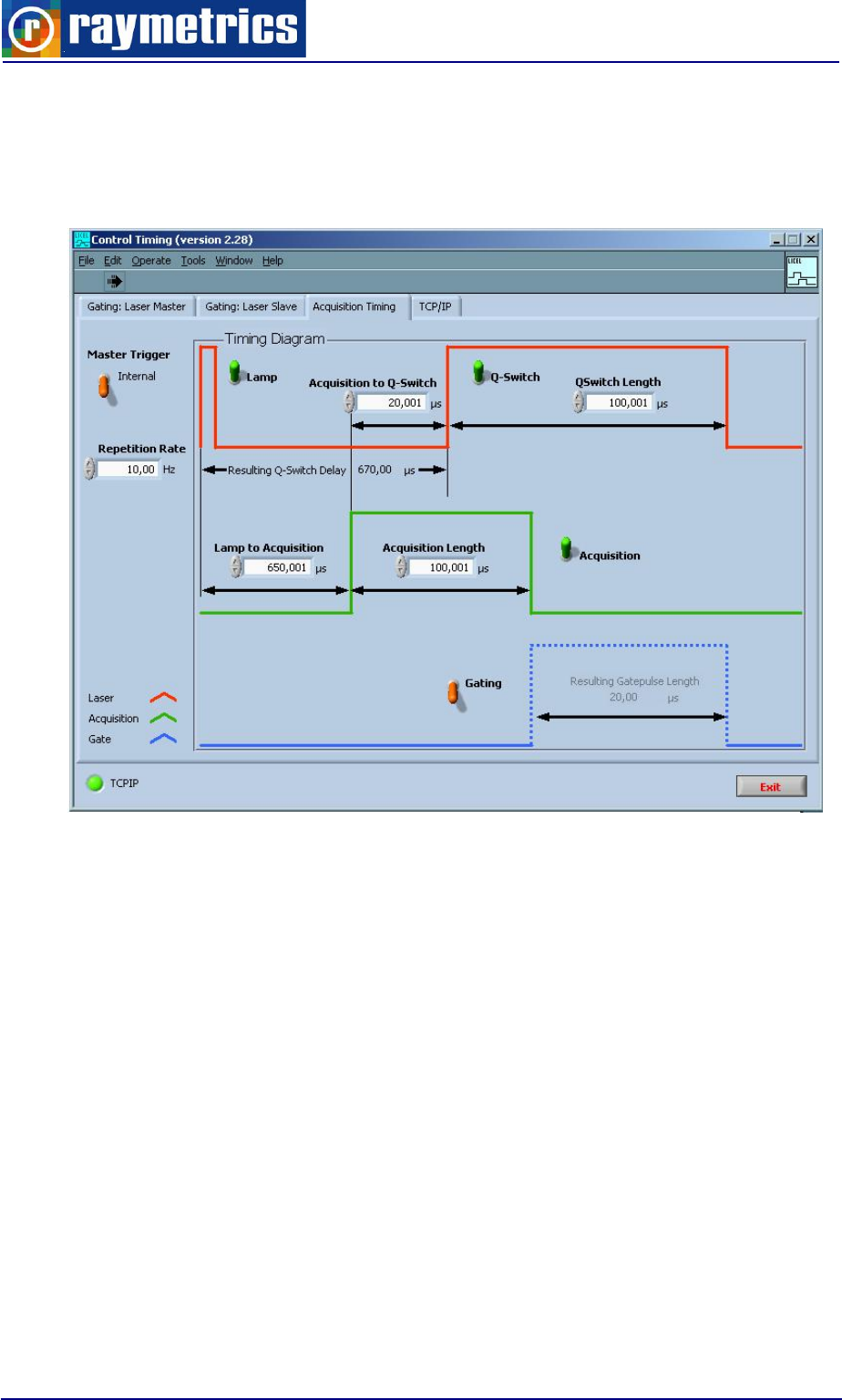
APPENDIX A
170
For example if you need 20μs pretriggering then Lamp to Acquisition should be 615μs
+ 20μs Acquisition to Q-Switch. If no pretrigger is required then put Lamp to Acquisition at
635μs and Acquisition to Q-Switch at 0μs. Note: There is a processing delay of 500μsec
between the external flashlamp trigger input and the actual flashlamp activation.
Note: Please always switch off the Q-Switch knob before you switch off the
Lamp knob.
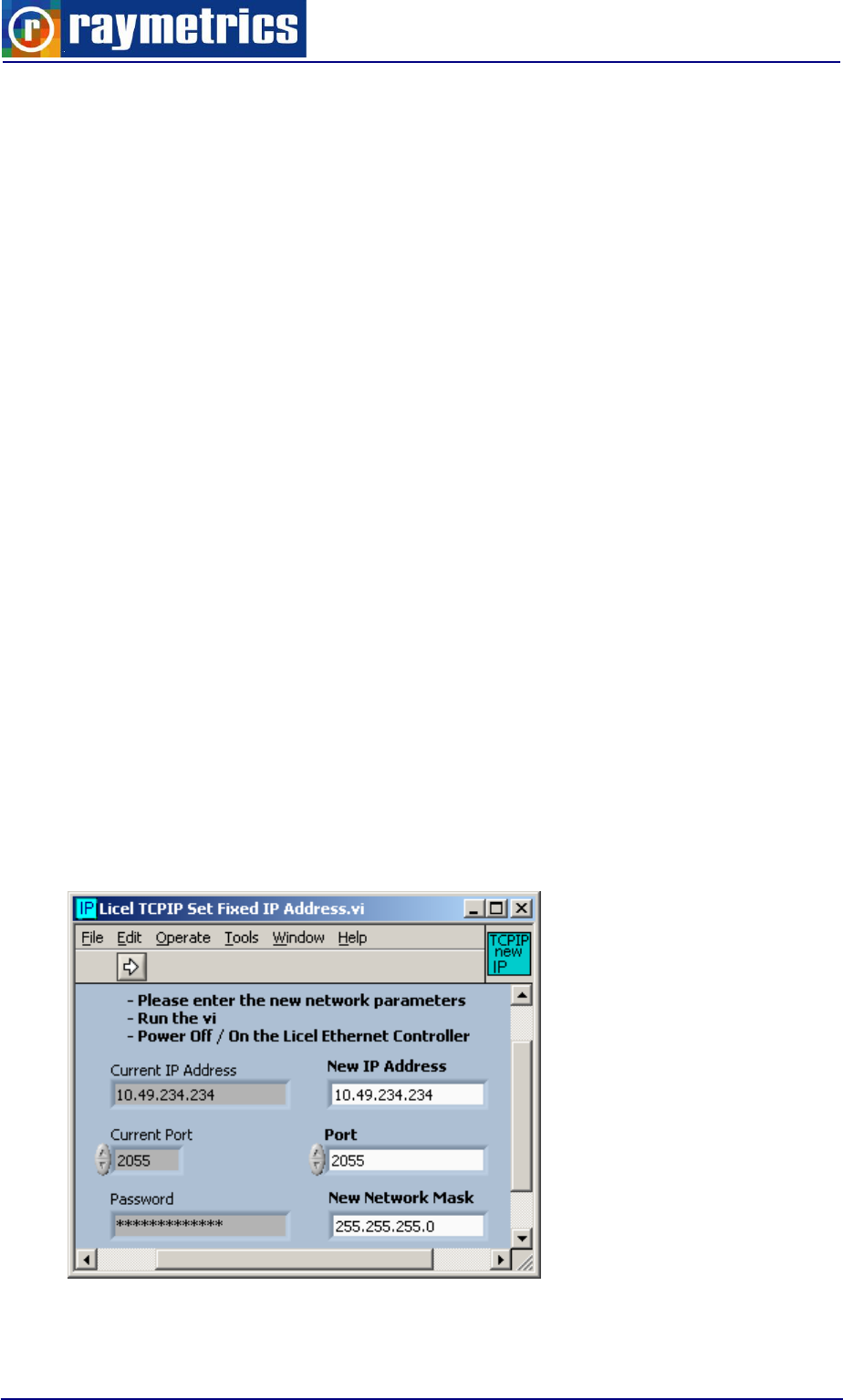
APPENDIX A
171
A2 HOW TO USE ANOTHER COMPUTER
If for any reason you want to use another computer you have to setup the
communications and install the programs for the Lidar. You can use any computer that you
want that has Windows XP OS and later.
Communications Setup
The communications are with the Licel’s controllers, the Laser and positioner (tracker)
if your system is equipped.
Licel has a LAN based communication. Lidar’s TR IP address is by default:
10.49.234.234. So user’s pc should belong to the same subnet class:
10.49.234. xxx
Where xxx any number for 0 to 254.
Note: Make sure that you do not use numbers for xxx from 230 up to 237. These
ranges are reserved for Lidar hardware.
To change users or Lidar’s PC TCP IP address, read windows documentation or
consult your system administrator
To change Transient Recorder TCP IP address, run the program TCPIP Set Fixed
IP Address.exe
Usually located at C:\Program Files\Licel\Configure\ TCPIP Set Fixed IP Address.exe
For more info please read carefully Licel Documentation

APPENDIX A
172
The laser and tracker have an RS232 communication so they require serial ports
unless there is installed in your system an RS232 to Ethernet converter. This device needs
separate installation but gives you the option to connect all devices on an Ethernet switch
to which you also connect your computer. This makes the connection very easy, other
wise you have to use the external USB port with an RS232 to USB adaptor to connect to
your computers USB port. If there are more than one devices with RS232 port use a hub
and separate RS232 to USB adaptors for each device.
Lidar software installation
First install Licel software (this step is not necessary but it is suggested)
If user’s pc does not have installed Labview runtime library (LVRunTimeEng.exe)
version 7 or later you have to install it. You can download this file from www.ni.com or you
can find usually into Laser folder that Raymetrics supplies to users.
If user’s pc does not have installed visa301runtime library (visa301runtime.exe) you
have to install it. You can download this file from www.ni.com or you can find usually into
Laser folder that Raymetrics supplies to users.
If your Lidar comes with a positioner (tracker) then install Win2AP software. Unzip the
KippZonen_Win2AP-V3R2.zip file and then run setup.
Make a copy from the Lidar’s pc the win2ap.ini file
Copy this file to the same folder where you just installed the Win2AP software

APPENDIX B
173
APPENDIX B
SUMMARY OF LIDAR THEORY
CONTENTS
INTRODUCTION
About Backscatter coefficient β(R,λ)
About extinction coefficient, α(R,λ)
The Lidar equation
SUMMARY OF LIDAR PROBLEM SOLUTIONS
1. The slope method.
2. Inver Klett-Fernard method (Raymetrics Software)
AN INTRODUCTION TO RAMAN LIDAR
Molecular backscatter coefficient
Other Lidar equation solution
Solutions for one component atmospheres
Solutions for Two component atmospheres
SIGNAL TO NOISE RATIO
CALIBRATION METHODS
POLARIZATION LIDAR BASICS
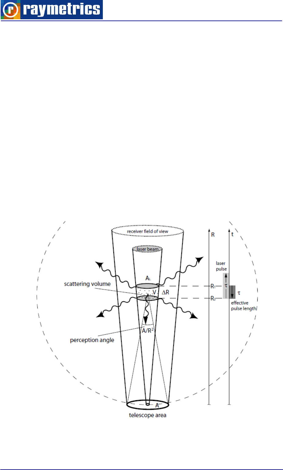
APPENDIX B
174
B1 INTRODUCTION
In the simplest from, the detected Lidar signal can be written as
)()()()( RTRRKGRP
eq. 1
The power P received from a distance R is made up of four factors.
1. The first factor, K , summarizes the performance of the Lidar system
2. The second, G(R), describes the range-dependent measurement geometry
Note: These two first factors are completely determined by the Lidar setup and can
thus be controlled by the experimentalist. The information on the atmosphere,
and thus all the measurable quantities, are contained in the last two factors.
3. The term β (R) is the backscatter coefficient at distance R.
4. The term T (R) is the transmission term and describes how much light gets lost on
the way from the Lidar to distance R and back.
Fig. B1

APPENDIX B
175
In a more analytic form the term K is given by the following equation
An
c
PK 2
0
eq. 2
Po is the average power of a single laser pulse and τ is the temporal pulse length.
Hence Eo = Po * τ, is the pulse energy and c*τα is the length of the volume illuminated
by the laser pulse at a fixed time. The factor ½ appears because of an apparent “folding” of
the laser pulse through the backscatter process. A is the area of the primary receiver
optics responsible for the collection of backscattered light (usually the primary mirror of a
telescope) and n is the overall system efficiency which includes the optical efficiency of all
the elements that transmit and receive light.
The geometric factor G(R) can be given from the following equation:
2
)(
)( R
RO
RG
eq. 3
and includes the laser-beam receiver-field-of-view overlap function O(R) described
before and the term R-2. The quadratic decrease 1/R2 of the signal intensity with distance
is due to the fact that the receiver telescope area makes up a part of a sphere’s surface
with radius R that encloses the scattering volume. If we imagine an isotropic scattered at
distance R, the telescope area A will collect the fraction IC:
2
4R
A
I
I
S
C
eq. 4
of the overall intensity IS scattered into the solid angle 4π . In other words, the solid
angle A/R2 is the perception angle of the Lidar for light scattered at distance R. The factor
4π does not appear explicitly in the Lidar equation because it cancels out by the definition
of the backscatter coefficient β as we will see below. It is primarily the 1/R2 dependence
that is responsible for the large dynamic range of the Lidar signal. If we start detecting a
signal with O(R)=1 at a distance of 10 m, the signal will be 6 orders of magnitude lower at
10 km distance just because of the geometry effect. To what extent Lidar is a range-
resolving and remote measurement technique depends on our ability to compensate for
this effect.
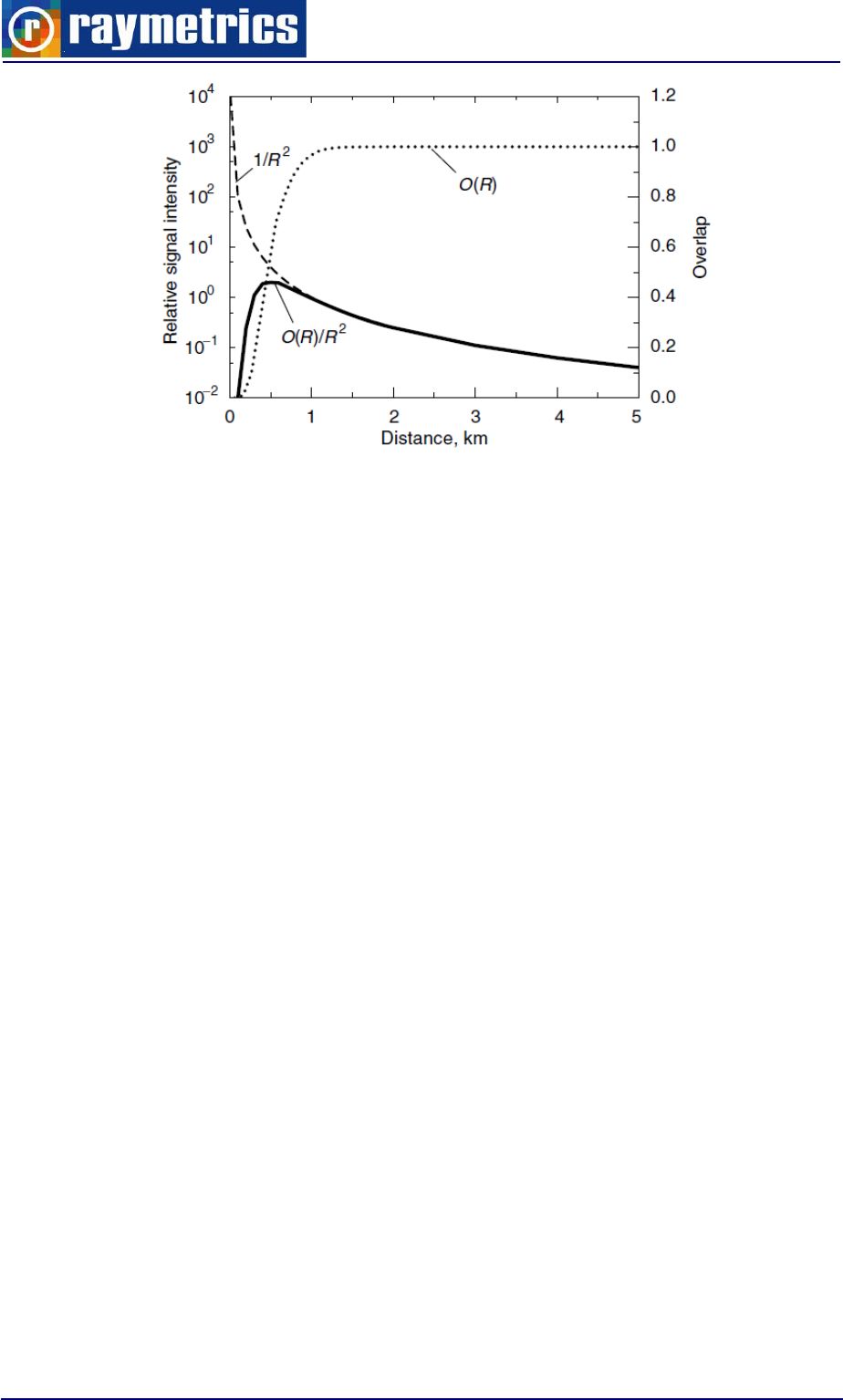
APPENDIX B
176
Graph 1: Influence of overlap function O(R), at Lidar signal
B1.1 About Backscatter Coefficient β(R,λ)
The backscatter coefficient β(R, λ) is the primary atmospheric parameter that
determines the strength of the Lidar signal. It describes how much light is scattered into
the backward direction, i.e., towards the Lidar receiver. In the atmosphere, the laser light is
scattered by air molecules and particulate matter, i.e., β (R, λ) can be written as
),(),(),(
---
RRR aermol
eq.5
Molecular scattering (index mol), mainly occurring from nitrogen and oxygen
molecules, primarily depends on air density and thus decreases with height, i.e.,
backscattering decreases with distance if the observation is made from the ground.
Particulate scattering (index aer for aerosol particles) is highly variable in the atmosphere
on all spatial and temporal scales. Particles represent a great variety of scatterers: tiny
liquid and solid air-pollution particles consisting of, e.g., sulfates, soot and organic
compounds, larger mineral-dust and sea-salt particles, pollen and other biogenic material,
as well as comparably large hydrometeors such as cloud and rain droplets, ice crystals,
hail.
B1.2 About Extinction Coefficient, α(R,λ)
The last term in the Lidar equation, we have to consider the fraction of light that gets
lost on the way from the Lidar to the scattering volume and back. The transmission term
T(R) can take values between 0 and 1 and is given by

APPENDIX B
177
R
drraRT
0
),(2exp),(
--
eq. 6
This term results from the specific form of the Lambert–Beer–Bouguer law for Lidar.
The integral considers the path from the Lidar to distance R. The factor 2 stands for the
two-way transmission path. The sum of all transmission losses is called light extinction,
and α(R,λ) is the extinction coefficient. Extinction can occur because of scattering and
absorption of light by molecules and particles.
B1.3 The Lidar Equation
Below is the extensive form of the well known Lidar equitation
R
drraR
R
RO
An
c
PRP
0
2
0),(2exp),(
)(
2
),(
--
-
eq. 7.1
Or
bgr
R
aermolaermolo
P
R
drraraRRROAPn
RP
20
)]()([2exp[)]()([)(
)(
eq. 7.2
In equation 7.2 wavelength dependence λ have been omitted for simplicity. In addition
a new term Pbgr is the background noise that comes from atmospheric defused light
(daytime) and the electronic noise.
In any form of the eq. 7 has two unknown quantities (β and α). So this is an intrinsic
problem of an elastic backscatter Lidar. One has to measure two quantities with only one
equation. Several solutions (depending on different assumptions) have been proposed in
literature in order to solve the Lidar equation.
Note: Raymetrics Software uses the Inver Klett-Fernard method (Far-end
solution)

APPENDIX B
178
B2 SUMMARY OF LIDAR PROBLEM SOLUTIONS
There are three basic inversion methods commonly used to find extinction coefficient.
These methods are:
B2.1 The Slope Method.
This method is useful for homogeneous atmospheres. In many cases, atmospheric
horizontal homogeneity is a reasonable assumption. With the slope method, a mean value
of the extinction coefficient over the examined range in a homogeneous atmosphere is
obtained.
One can reform the eq. 7.1 at the following form:
R
R
drra
R
R
TCRP
0
),(2exp
),(
)( 2
00
-
-
eq. 8
C0 is the system constant and T0 is an unknown, two-way transmission term from
ground to R0 (R0 is where the overlap function O(R)=1).
0
0
0),(2exp)(
R
drraRT
-
In a homogeneous atmosphere we can assume that
α(r)=α=constant and β(r)=β=constant
In that case we get
aRR
R
R
TCRP )(2exp
),(
)( 0
2
00
-
Then we define the Range Corrected Signal as:
aR
eCRRPRRCS 2
0
2
)()(
,
Taking the natural logarithm we get the following (singe β and α are assumed range
independed for homogeneous atmospheres:
RBRZ
2)(
eq. 9
Where

APPENDIX B
179
)ln( 0
CB
The linear dependence of Z(R) on range R, is a key factor when seeking the simplest
solution to the Lidar equation. It allows determination of the α by linear square fit. In
addition the estimate of the standard deviation of the linear fit for Z(R) can be used to
estimate the degree to which the assumption of atmospheric homogeneity is valid.
Note: As always before you apply such a solution you have first to subtract
background noise from the Lidar signals
B2.2 Inver Klett-Fernard method (Raymetrics Software)
ref ref
ref
R
R
R
R
molmol
refmol
ref
R
R
molmol
RdRdRLLRRCSL
RC
RRCS
drrLLRRCS
R
)(**2exp***2
)(*
)(
)(**2exp*
)(
eq.10
Where
)(
)()(
r
RR
C
mol
refaerrefmol
eq.11
if the reference point Rref is in a clean atmosphere (for example free troposphere
without aerosols) then it is safe to assume that βaer(Rref)=0 so C=1
3
8
)(
)(
)(
r
ra
rL
mol
mol
mol
eq.12
and
const
R
Ra
RL
aer
aer )(
)(
)(
eq.13
L(R) is the aerosol Lidar ratio and depends on particle size distribution, complex
refractive index, the shape of aerosols, relative humidity height and wavelength.

APPENDIX B
180
B3 AN INTRODUCTION TO RAMAN LIDAR
As we saw above by measuring only the elastically backscattered signal we have to
make an assumption for the Lidar ratio in order to solve the Lidar equation. This introduces
errors since we know that the Lidar ratio in not constant and depends on height relative
humidity (which varies strongly by height) and other microphysical parameters.
However by measuring simultaneously the inelastically (Raman) backscattered signal
by Nitrogen we get two equations with two unknowns. So the problem now can be solved.
The determination of the particle extinction coefficient from molecular backscatter signal is
rather straightforward and there is no need for Lidar-Ratio assumptions. However it should
be pointing out that Raman signals can be 1000 times weaker than elastic signals so the
background noise reduce significantly the range of measurements of such signals.
Practically Raman signals can detect only at night time.
As we show previously the power received from the distance R for an elastic channel is
given by the equation:
bgr
R
aermolaermolo
P
R
drraraRRROAPn
RP
20
)]()([2exp[)]()([)(
)(
7.2
For simplicity we rewrite the equation in the following form (for the R>R0 where
O(R)=1)
2
0
)],(),([2exp[)],(),([
),( R
drraraRRC
RP
R
R
LaerLmolLaerLmol
L
----
-
eq. 14
where λL is the laser emitted wavelength.
The power received from distance R from a Raman channel is given from the following
equation:
R
RL
RL
Rdrrara
R
RC
RP
0
2),(),(exp
),,(
),(
--
--
-
eq. 15
d
d
RNR RL
RRL
),,(
)(),,(
--
--
eq. 16

APPENDIX B
181
Where λR is the Raman shifted wavelength from the Raman-active gas (usually
nitrogen at 387 nm)
The eq.15 has two main differences from eq. 14. First there is not the -2 factor since
the extinction in that case happens only one way (backwards to the Lidar receiver). The
Raman backscatter coefficient (eq.16) is given by the molecular number density N(R) of
the Raman-active gas (usually nitrogen at 387 nm) and the differential Raman cross
section for the backward direction.
By using the above three equation we can get:
k
R
L
LmolLmol
R
Lp
RaRa
RPR
RN
dr
d
Ra
-
-
--
-
1
),(),(
)(
)(
ln
),(
2
eq. 17
The above equation is valid for R>Ro in other worlds where O(R) = 1
In addition:
),(),(),( RaRaRa LmolLaerL
---
and
),(),(),( RaRaRa RmolRaerR
---
and
k
L
R
Raer
Laer
Ra
Ra
-
-
-
-
),(
),(
The aerosol backscatter coefficient is given from the following equation:
R
R
LmolLaer
R
R
RmolRaer
refRRrefL
RLrefR
refLmolrefLaerLmolLaer
ref
ref
drrara
drrara
RNRPRP
RNRPRP
RRRR
),(),(exp
),(),(exp
)(),(),(
)(),(),(
),(),(),(),(
--
--
--
--
----
Eq.18
Once more usually at Rref
),(),(),( refLmolrefLmolrefLp RRR
---

APPENDIX B
182
B3.1 Molecular backscatter coefficient
In any case (elastic or Raman backscatter liars) one has to calculate the molecular
backscatter coefficient.
k
s
s
s
mF
n
n
N
RRNRa 2
2
2
2
24
3
2)(
1)(24
)()()(
-
-
-
Since
3
8
m
m
mol
a
L
Then
k
s
s
s
mF
n
n
N
RR 2
2
2
2
24
2
2)(
1)(9
)()(
-
-
-
Eq.19
The values for ns and Fk can be taken from the table below
Λ
ns-1
Fk
ns
(ns^2-1)^2/(ns^2+2)^2
nm
x1E-8
266
1,06
1,000294650
3,85823E-08
289
1,057
1,000291880
3,78603E-08
299
1,056
1,000290860
3,75961E-08
308
29047,7
1,05575
1,000290513
3,75065E-08
316
1,0551
1,000289140
3,71528E-08
351
28602,7
1,05308
1,000285983
3,63460E-08
354,814
28572,4
1,0529
1,000285745
3,62854E-08
355
28570,2
1,05289
1,000285745
3,62854E-08
386,8
28350,2
1,05166
1,000283480
3,57125E-08
400
28275,2
1,05126
1,000282764
3,55325E-08
407,663
28235,1
1,05105
1,000282407
3,54427E-08
510,6
27869,4
1,04922
1,000278711
3,45212E-08
532
27819,9
1,04899
1,000278235
3,44032E-08
532,221
27819,4
1,04899
1,000278235
3,44032E-08
607,6
27686,3
1,04839
1,000276804
3,40504E-08
710
27570,4
1,0479
1,000275731
3,37870E-08
800
27503,8
1,04763
1,000275016
3,36119E-08
1064
27397,5
1,04721
1,000273943
3,33502E-08
1064,442
27397,4
1,04721
1,000273943
3,33502E-08

APPENDIX B
183
N(R) is the atmospheric number density and can be easily calculated by using several
atmospheric models or by using Radiosonde measurements.
)(
)(
)( RT
RP
P
T
R
o
o
s
Ns molecular number density for standard atmospheric conditions at ground lever.
Ns=2.5477*1019cm-3, Po=1013.25 hPa and To=15 oC
B3.2 Other Lidar Equation Solution
B3.2.1 Solutions for one component atmospheres:
In a more generic form the equation 8 can be written as below:
R
R
molaer
molaer drrara
R
RR
TCRP
0
)()(2exp
)()(
)( 2
00
Eq. 20
Now we define two new quantities
)(
)(
)( Ra
R
RL
aer
aer
Where
),()(
RR aeraer
backscatter coefficient (θ=π) and
)(),()( RRRa A
aeraeraer
.
So we can write
)(),(
)(
)( RaR
R
RL A
aeraer
aer
Here the extinction is split to scattering at all direction and to extinction because the
absorption processes. In the same way we define
)(),(
)(
)( RaR
R
RL A
molmol
mol
mol

APPENDIX B
184
In the case of one component atmosphere with no absorption. The solution of the Lidar
equation can be written as
R
R
aer
drrRCSC
RRCS
Ra
0
)(2
)(
)(
eq.21
Where
aer
LTCC 00
eq. 22
for a single component atmosphere well mixed
aer
L
does not depend on range (R).
To find aerosol extinction coefficient from eq. 21 we need to know C’ (which called
sometimes Lidar calibration constant). This is not an easy task. Even if we know C0 the
other two parameters can be determined only during measurements. However in order to
calculate αaer we need two know only the product which means only the C’ and not the
individual components of eq. 22. The simplest way to determine the C’ is to establish a
boundary condition of the equation at some point of the Lidar measurement range. This
makes possible to find the constant C’ and then to use it to determine αaer over the total
measurement range.
If we know the value of αaer at a specific point Rref which is inside the measuring range
then
Rref
R
refaer
ref
drrRCSRa
RRCS
C
0
)(2exp)(
)(
we remind here that R0 is the range where O(R)=1
by replacing C’ into the eq. 21 we get finally
ref
R
R
refaer
ref
aer
drrRCS
Ra
RRCS
RRCS
Ra
)(2
)(
)(
)(
)(
Far range solution Rref > R

APPENDIX B
185
R
Rref
refaer
ref
aer
drrRCS
Ra
RRCS
RRCS
Ra
)(2
)(
)(
)(
)(
Near range solution Rref < R (and close to R0)
Eq. 23
The most stable solution for αaer is the far range solution. Such solution is given by
Klett).
Optical Depth Solution
Another way to solve the problem is to use total path transmittance over the Lidar
operating range as a boundary solution. Once more this solution applied with the
assumption that the Lidar ratio is constant (one component atmosphere). We define the
upper Lidar measuring limit Rmax which is usually taken as the range at which the signal-to-
noise ratio reaches a certain threshold value. In this solution the two way transmittance
Tmax is used as a boundary solution.
max
0
)(2exp
max
R
R
aer drrT
eq. 24
R
R
aer
drrRCS
T
I
RRCS
Ra
0
)(
1
)(
2
1
)(
max
max
eq. 25
max
0
)(
max
R
R
drrRCSI
eq. 26
If we define the aerosol optical depth as
max
0
)(
R
R
aer drrAOD
eq.27
Then we get
)2exp(
max AODT
Tmax is the quantity we need to know in order to calculate αaer. For real atmospheric
conditions is a finite positive value (0<Tmax<1).

APPENDIX B
186
B3.2.2 Solutions for Two component atmospheres:
R
R
molaer
molmolaeraer drrara
R
RaRLRaRL
TCRP
0
)()(2exp
)(*)()(*)(
)( 2
00
Far-end boundary point solution
ref
R
R
ref
ref drrRCS
Ra
RRCS
RRCS
Ra
)(2
)(
)(
)(
)(
eq.28
where
)()()()( RRLRaRa maer
eq.29
In case that Rref is in free troposphere (atmosphere without aerosols) then
0)(
refaer Ra
and
)()()( refmrefref RRLRa
Optical Depth Solution:
R
R
aer
drrRCS
V
I
RRCS
Ra
0
)(
1
)(
2
1
)(
2
max
max
Where once more the Imax is given from eq.26 and
max
0
)()1
)(
(exp
maxmax
R
R
m
m
drra
L
RL
TV
max
0
)(exp
max
R
R
drraT
if we know the Optical Depth
max
0
)(
R
R
drraOD
Then we can calculate Tmax and Vmax

APPENDIX B
187
B4 SIGNAL TO NOISE RATIO
Theory
The SNR of the echo Lidar signal is obtained by the following equation:
)(2
/IdIpbIpseFB
Ips
NS
Where Id is the PMT’s anode dark current (with typical values of about 1nA), Ipb is the
anode current due to background radiation signal, Ips is the anode average output current
of the echo Lidar signal, B is the bandwidth of the system, e is the electric charge and F is
the noise component (noise figure) produced in the multiplication process in the PMT. F
indicates how much the signal to noise ratio will degrade between the input and the output
of the PMT.
Usually
1
F
where δ is the secondary emission ratio and is a function of the
interstate voltage of dynodes. Typical values for δ are between 3 and 7.
The output current at the anode Ip=μ*Ιc where μ is the gain and changes in relation to
the supply voltage V to the PMT. Typical values are around 2x10⁶.
Ic is the photocurrent produced at the photocathode of the PMT and is calculated from
the following equation.
PSI cc
(A),
Where P is the incident radiant flux (W) and Sc is the cathode radiant sensitivity (A/W).
Typical values for Sc are around 120 mA/W
The radiation power (W) arising from natural sources (background radiation) accepted
by the receiver optics can be expressed in the form:
)()( 0
--
KSP bb

APPENDIX B
188
χ is overall optical system efficiency, A is the area of primary receiver optics
responsible for the collection of backscattering light (m2), Ω is its acceptance solid angle,
and K0(λ) is termed the filter function of the receiver system.
-
---
dK )()(
0
The Sb represents the spectral radiance of the sky background (Wm-2sr-1nm-1).
At wavelengths within the visible range, a typical value for Sb is about 0.1 (Pratt, 1969)
at sea level for a zenith angle of 45 degrees, with excellent visibility (for moonlight its value
is approximately 1x10-12). For 355nm it is about 1x10⁻⁴.
The power of the echo Lidar signal corresponding to a distance R for a Raman channel
can be written as:
R
R
NmolNaerLmolLaer
N
Ndxxaxaxaxa
R
d
d
cNRAQE
RP
0
),(),(),(),(exp
)(
)( 22
2
2
20
2
----
E0 is the energy of a single laser pulse (J), c is the velocity of light (m/s). The term Q(R)
is the laser beam receiver field of view overlap function, describing the range-dependent
measurement geometry, and can take values from 0 to 1. N is the atmospheric number
density of Nitrogen (for simulation we use the USSA76 standard atmospheric model) and
dσ/dΩ is the Raman backscatter cross section (1000 times smaller than elastic backscatter
cross section).
αmol(R,λ) is the extinction coefficient for laser and Raman wavelengths and is estimated
from USS76 standard atmospheric models.
Extinction at the Raman wavelength is estimated from the following equation.
-
-
-
-
L
Laer
aer
Ra
Ra
2
2
),(
),(

APPENDIX B
189
For the simulation the following equation was used for calculating the backscatter
coefficient:
-
532
36
20
1000
exp1013.5
2000
exp1047.2
2
96
R
R
aer
(Horst Jager, et. al., Appl. Opt., 30(1), pp. 127-136, 1991)
In the next step we introduced the particle extinction to backscatter ratio (Lidar Ratio):
),(
),(
),( R
R
RL
aer
aer
aer
-
-
-
in analogy to molecular Lidar ratio
srL
mol
mol
mol 3
8
)(
)(
)(
-
-
-
In contrast to the molecular Lidar ratio, the particle Lidar ratio in general is range
dependent because it depends on the size distribution, shape and chemical composition of
the particles. For our simulation we used a constant value of 35 sr.
For horizontal measurement simulation we used the following equation:
-
532
1024
aer
a
for λ=355 nm
This gives a value of:
αaer=3x10⁻⁴ (1/m) and βaer=8.5x10⁻⁶ [1/(m*sr)]

APPENDIX B
190
B5 CALIBRATION METHODS
A Lidar system can be divided in two main functional units: the opto-mechanical
transmitter-receiver unit, and the electronic data acquisition, each of which needs special
tools for testing. The main problem of the transmitter-receiver unit is the a priori unknown
range-dependent transmission, which enters as a factor into the Lidar equation. Usually
only the incomplete overlap between the fields of view of the transmitter and the receiver is
considered by the so-called overlap function, but in reality several other opto-mechanical
features potentially have an influence, e.g. the incident angle dependence of the
transmission of optical coatings of beam splitters and interference filters, vignetting of the
light beam by mechanical apertures, and the spatial inhomogeneity of the sensitivity of the
light detectors.
Methods that Raymetrics follows to calibrate and test its instruments:
Rayleigh fit / Matching method
The transmitter-receiver overlap has its main impact in the near range of the signal, but
if the transmitter is not well aligned, the far range of the signal might also be affected. A
well known check for the latter problem is a fit of the far range Lidar signal, assuming clear
air in the upper troposphere, to the calculated clear air Rayleigh signal, the so called
"Rayleigh fit" or "matching method". Raymetrics provides software tools for easy Rayleigh
fit calibration. This calibration procedure can be done in the field very easily and takes less
than one minute.
Telecover Checkup tool
Before the shipment of any of our Lidar systems, extensive performance tests and
calibration procedures are performed. One of the tools that Raymetrics uses for checking
Lidar instrumentation is the newly developed "telecover test", which is strongly suggested
by EARLINET.
Raymetrics in addition provides all of the hardware and software required for such tests
with all of our Lidar systems.
Electronic data acquisition

APPENDIX B
191
Light measurement is done in two ways in Lidar systems: in analogue mode,
measuring the electron current from a detector after sufficient amplification with
preamplifiers, and/or by means of counting amplified pulses of individual photons (photon
counting method). Raymetrics uses special pulse generator techniques to calibrate and
adjust analogue and photon counting measurements. It is well known, especially in
analogue detection mode, that the main problem is various signals inducing signal
distortions. If these distortions are neglected, errors of the Lidar signal inversion on the
order of magnitude of 100% can result, although the distortion might be very small
compared to the maximum signal. The Lidar signal should only be used over ranges where
these errors are acceptable. This can be tested with a specially designed pulse generator.
Calibrating the “ranging”
In Lidar technologies two errors commonly occur if special attention is not paid:
There is always a delay between the emitted pulse and the data acquisition process,
especially for analogue mode due to delays at the pre-amplification process. But this is
true as well in Photon Counting mode, although the phenomenon is not so pronounced.
These delays reduce the accuracy of ranging of a Lidar.
Raymetrics uses special optical triggering that eliminates any delay in photon counting
mode. In addition we use a near range target with a defined distance to the Lidar that
produces a signal peak for Zero-bin calibration in analogue and photon counting modes. If
such a target is not available we use a special procedure with an optical fibre to calibrate
the “ranging” of our systems.
Calibration method for depolarization Lidar
For calibration of the linear depolarization channels there are several methods, such
as:
1. Rayleigh method (0o)
2. 45o method
3. +/- 45o method
4. Multi-rotation-angle fit method
5. Three signal method
6. Unpolarized light source

APPENDIX B
192
1) Rayleigh method (0o)
This method is based on knowledge of the molecular linear depolarization ratio in an
aerosol-free calibration range. However, since we can never be sure that the aerosol free
region that we have assumed really is free, this method introduces many errors. It has
been proved that this can give errors up to 260%. In addition this method cannot provide a
range dependent calibration factor.
2) 45o method
With this method a 45o angle is produced between the laser polarization plane and the
PBC. Rotation can be achieved mechanically, by using a half-wave plate or by the rotating
of a polarizing sheet filter. This method is fast and has relatively few errors. However it
gives large errors when there is a small angle difference between the laser polarization
plane and the PBC at the default position (0o).
3) +/- 45o method
With this method the polarization plane of the PBC is turned +45 and -45 degrees from
the default position (0 o). This method is fast accurate and it is 100 times less sensitive to
errors produced by a small angle γ from the default position (0 o) compared to the 45o
method.
4) Multi-rotation-angle fit method
With this method the PBC is rotated to several angles. It is a good method but it is time
consuming and sensitive to atmospheric changes during the calibration procedure. In
addition it exhibits low accuracy of the calibration constant.
5) Three signal method (detection of the total, cross and parallel signals
separately)
With this method the Lidar detects a fraction of incoming light and the rest is beam-split
by a Polarizing Beam Splitter. However such a set-up increases the cost of the instrument
significantly (three deferred detected channels instead of two) and depends on large
differences in δ(R).

APPENDIX B
193
6) Unpolarized light source
The beam path of rays from an unpolarized light source through the receiver optics is
used. This method has many disadvantages and introduces errors.
Summary of theory for depolarization calibration
The total backscattering power P(r) is given by the Lidar equation:
2
0
2
),(),()(
)( R
RRcRQ
RP
--
For simplicity we form the equation in the following way:
2
)()(
)( r
rr
CrP
The backscatter power before the PBC can be written as:
22
)()(
)( r
r
C
r
r
CrP
molaermolaer
II
The linear volume depolarization ratio δv is given by:
)(
)(
)(
)(
)( rP
rP
r
r
r
However the measured signal ratio δ* is given by:
)(
)(
)(
*
rP
rP
r
T
R
Where PR and PT are the reflected and transmitted signals from the PBC and are the
ones which are recorded.
RssppR VRPRPP )()()(
and
TssppT VTPTPP )()()(

APPENDIX B
194
Where VR and VT include the optical transmittances of the receiver and the electronic
amplification in each channel.
In addition the power components with respect to the incident plane of the PCB are:
)(cos)(sin)( 22
PPP IIs
and
)(sin)(cos)( 22
PPP IIp
Φ is the angle between the plane of polarization of the laser and the incident plane of
the PCB.
Combining the above equations we get:
sp
sp
TT
RR
V)(tan)(tan1
)(tan)(tan1
)( 22
22
**
Where V*=VR/VT and R, T are the transmittance and reflectance of the PBC.
In order to retrieve the total backscatter power P and δν from the measurements we
need to know the V* which is the calibration constant and we can get it through several
methods.
For φ=0 we get:
)0(*
)(
0*
sp
sp
RR
TT
V
If we know δν for some range of the Lidar signal, we can determine V* (for example by
using the linear depolarization ratio of air molecules). However a very low amount of
strong depolarization aerosols, in the assumed clean range, causes very big errors on δν
and thus of V*. So this method cannot be used for reliable data.
Another method is to turn 45 degrees (45-calibration method). φ=45 in that case:
)45(*
*
sp
sp
RR
TT
V

APPENDIX B
195
As can be seen, the calibration constant does not depend on δν. However it is very
difficult and practically impossible to measure exactly the angle between the laser and the
PBC. An error γ of the order of 1 degree causes a large error in V*.
With the proposed method we calculate V* from two subsequent measurements at
exactly 90 degrees (φ=45+γ and φ=-45+γ) in that case:
)45(*)45(*
*
sp
sp
RR
TT
V
With this method (+/- 45 calibration method) it can be shown that the errors γ
compensate each either over a large range of γ.
Retrieving of the linear depolarization ratio δv and linear aerosol depolarization ratio
δp
If we know the calibration constant then:
ss
pp
p
s
T
rV
r
R
RT
rV
r
rP
rP
rP
rP
r
)(
)(
)(
)(
)(
)(
)(
)(
)(
*
*
*
*
The total echo power is given by:
P(r)=V*(r)PT(r)+PR(r)
)1()1(
)1()1(
R
R
m
mm
aer
δm can be determined with high accuracy from radiosonde data (or by using a model).
m
aerm
R
Where βaer is retrieved from the total signal P using the Fernald/Klett inversion with a
reference value βaer(rref) at a reference range and known range dependent Lidar ratio L(r)
(retrieved by an additional measurement with a Raman Channel).

APPENDIX B
196
Theory and the Inversion Problem of Lidar technique
The power of the echo Lidar signal corresponding to a distance R can be written as
2
0
2
),(),()(
)( R
RRcRQ
RP
--
eq. 1
E0 is the energy of a single laser pulse (J), c is the velocity of light, m/s. The term Q(R)
is the laser beam receiver field of view overlap function, describing the range-dependent
measurement geometry and can take values from 0 to 1. The β(R,λ) is the backscatter
coefficient (1/(m*sr)) and it stands for the ability of the atmosphere to scatter light
backwards. T(R) is the transmission term and describes how much light gets lost on the
way from the Lidar to distance R and back.
R
RdRRT
0
),(2exp),(
--
The factor 2 stands for the two-way transmission path.
β(R,λ) = βmol(R,λ)+βaer(R,λ) and α(R,λ) = αmol(R,λ)+αaer(R,λ)
α(R,λ) is the extinction coefficient.
Here we can rewrite the Lidar equation as
R
dxxRa
R
R
CRP
0
2
0),(2exp
),(
)(
-
The factor C0 is the Lidar system constant. One of the limitations of this equation is that
includes more than one unknowns. Therefore, it is considered to be mathematically ill
posed and thus indeterminate. Such an equation cannot be solved without either a priori
assumption about atmospheric properties along the Lidar range or the use of independent
measurements of the unknown atmospheric parameters. Usually the use of a priori
assumptions is the most common method.
Generally, the extinction coef. profile is the parameter of primary interest. A potential
way to overcome this problem might be to make independent measurements of
backscattering by the use of a combined Raman-elastic backscatter Lidar method (This
method is used at our Raman Lidar Systems).

APPENDIX B
197
In order to extract a α(R) profile the calibration factor C0 must be known and in
addition, the relationship between backscatter and total extinction must in some way be
established (Raman Lidar) or assumed (Klett solution)
R
R
odxxRa
R
R
TCRP
0
),(2exp
),(
)( 2
2
0
-
eq. 2
Where
0
0
),(exp
R
odxxRaT
Methods-Solution for the inversion of Lidar equation and Lidar calibration
Intro
The simplest method is based on an absolute calibration of the Lidar system can use
only Co, whereas the other factors in the Lidar equation remains unknown (for example the
two way atmospheric transmittance over the incomplete overlap zone). All self-sufficient
elastic Lidar signal inversion methods developed to date require the use of one or more a
priori assumptions that are chosen according to the particular optical situation. There are
three basic inversion methods that Raymetrics uses depending an the Lidar type and the
applications:
1. Slope method: This method is used for homogeneous atmospheres. In many of the
cases, horizontal homogeneity is a reasonable assumption. With the slope method a
mean value of α over the examined range in a homogeneous atmosphere is obtained.
2. The boundary point solution: This requires knowledge of or an a priori estimate of α at
some point within the measurement range.
3. The optical depth solution: Here the total optical depth or transmittance over the Lidar
measurement range should be known or assumed. In case of a clear and moderately
turbid atmosphere the total α (or optical depth) is found be a solar radiometer.
In case of a two component atmosphere (with is the most usual case especially
for vertical pointing systems)
The Lidar equation can be written as:

APPENDIX B
198
R
R
molaer
molaer
odxxaxa
R
RR
TCRP
0
)()(2exp
)()(
)( 2
2
0
In that case the backscatter coefficient can be found from the following
equation:
Rref
R
Rref
x
molaeraer
Rref
R
molaer
molaer
dxdzzzLxRCSxLC
dxxRLRRCS
RR
)(
3
8
)(exp)()(2
)(
3
8
)(2exp)(
)()(
This equation is solved iteratively downwards and gives the calibration constant of the
instrument
)()(
)(
refmolrefaer
ref
RR
RRCS
C
Calibration at height Rref gives the system constant C.
Hardware solution to the inversion problem
Use of Nitrogen Raman scattering for extinction measurements
Similar to an elastic Lidar, a Raman channel detects the inelastic backscatter Raman
shifted radiation. Atmospheric gases like nitrogen and oxygen interact with the emitted
radiation via the Raman Scattering process, causing light of longer wavelengths to be
scattered. Thus in addition to elastically backscattered signal an extra backscattered wave-
shifted component is detected. Because of the small value for the cross-sections of Raman
scattering (so the small backscatter coefficient) the number of photons returning to the
Lidar is small. Because the probability of Raman scattering is proportional to λ-4 the
use of short wavelengths increases the magnitude of signal.
In addition the discrimination of Raman Photons from the background light is a
problem. So operating at UV where the background radiation is smaller, it is strongly
suggested. Since deep UV is strongly absorbed by Ozone and because the molecular
scattering is reduced at longer wavelengths the optimum solution is around 350 nm.
However discriminating Raman scattered photons from solar background is still an issue
and requiring special measures. If the system is expected to operate during the day, the
use of extremely narrow field of view in the receiving optics is required. For biaxial system
this is almost impossible since the overlap is getting too high. In addition the system is

APPENDIX B
199
getting susceptible to misalignments which are not good for an operational Lidar that have
to be moved.
R
R
NmolNaerLmolLaer
N
NN dxxaxaxaxa
R
d
d
NRQ
CRP
0
),(),(),(),(2exp
)(
)( 22
2
2
2
22
----
Finally we can get
-
-
--
-
2
2
2
2
1
),(),(
)(
ln
),(
N
L
NmolLmol
N
N
Laer
xaxa
RRCS
N
dR
d
Ra
αmol are well known and can be found from Rayleigh scattering theory. The dominator
corrects for the small difference in particulate attenuation between the laser and Raman
scattered wavelengths. In horizontal direction for visibility from 3 to 20 km it is close to 1.3.
Finally when the Raman technique is used, the aerosol backscatter coef can be
determined by reference to the signal at some height. The conventional assumption is
made of the existence of a aerosol free area somewhere within Lidar measurements range
βaer(Rref)=0.
ref
R
R
NtotalLtotal
refNNLref
NLref
LrefmolLrefaerLmolLaer dxxaxa
RNRPRP
RNRPRP
RRRR ),(),(exp
)(),(),(
)(),(),(
),(),(),(),( 2
22
22
--
--
--
----
Usually at Rref
),(),(),( LrefmolLrefmolLrefaer RRR
---

APPENDIX B
200
B6 POLARIZATION LIDAR BASICS
B6.1 Introduction
B6.1.1 Aerosols’ Properties And Depolarization
Shape, size distribution and composition of aerosol particles influence their
scattering characteristics and thus the radiative impact. The polarization Lidar
technique (Sassen, 1991; Sassen, 2005) is a well-established method to distinguish ice
clouds from water clouds and to identify layers with ice crystals in mixed–phase clouds.
Freudenthaler et al. (1996) applied a scanning polarization Lidar to study the evolution of
contrails. The technique has been used to identify the type of polar stratospheric clouds
(Sassen, 2005) and volcanic ash in the troposphere and stratosphere (Sassen et al.,
2007). The polarization Lidar is also well suited for aerosol profiling and allows us to
unambiguously discriminate desert dust from other aerosols. Based on model calculations,
it has been demonstrated that the spectral dependence of the dust linear depolarization
ratio is sensitive to the size distribution of the nonspherical scatterers. Thus, observations
of the linear depolarization ratio at several wavelengths may be used in retrieval schemes
(Dubovik et al., 2006) to improve the estimation of the microphysical properties of dust
from optical measurements (Wiegner et al., 2008). First dual-wavelength aerosol
polarization Lidar measurements were presented by Sugimoto et al. (2002).
B6.1.2 Overview of Lidar Linear Depolarization
Lidar often uses polarized laser beams for sounding the atmosphere, and
depolarization measurements have long been used in lidar investigation. The main
application of depolarization measurements is the discrimination and the extent of
liquid and solid phase clouds and aerosols. Lidar signal is the superposition of
scattering that is due to molecules and scattering that is due to particles that are greater
than the typical dimensions of atmospheric molecules. Molecular backscattering follows
Rayleigh theory, in which case changes in polarization are due only to the polarizability of
molecules: The contribution to the orthogonal polarization is ;1%.2 Scattering processes
on aerosols must be treated by means of Mie theory if particles are spherical or with

APPENDIX B
201
Stokes matrix if particles are non-spherical. From Mie theory the polarization of incident
light is conserved after backscattering, whereas backscattering on solid particles can
change the polarization direction. If a laser beam is emitted with a definite polarization, the
presence of polarized light in the perpendicular component denotes the presence of
backscattering from nonspherical particles. Hence polarized backscattering, parallel to the
laser polarization is considered, and depolarization is used to refer to the perpendicular
component of polarized backscattered light. Three points must be taken into account
during treatment with depolarization studies: 1. multiple scattering processes induce
depolarized backscattering even in the presence of spherical scatterers, 2. particles with
small dimensions compared with the lidar wavelength do not show depolarization even if
they are not spherical and 3. emitted light polarization must remain stable throughout the
measurement.
B6.1.3 Polarization Method Applied To Modern Lidar Systems: Theory and Methodology
Measurements of the linear depolarization ratio δ with lidars are often performed with
the aim to just discern between the dry, the liquid and the ice phase of aerosols and clouds
in the profiles of one lidar system, which requires only a relative measure of δ with a low
accuracy of the absolute values. The total backscattered power P(r) with their dependence
on the distance r from the lidar is described by the lidar equation
2
2
( ) ( )rr
Pr
(1)
where η is the system constant, β the backscatter coefficient and the factor τ2 accounts
for the atmospheric transmittance on the way from the lidar to the scattering volume, and
back. For the determination of δ the lidars used in this study measure the atmospheric
backscatter signals in two receiver channels, parallel- and cross-polarized with respect to
the plane of the linear polarized output of the laser beam. The two polarization
components are separated in the receiver by means of polarizing beam splitter cubes
(PBC). But this separation is not perfect. Furthermore the polarizing beam splitter might be
misaligned with respect to the plane of polarization of the emitted laser beam, and
additionally, a rotation of the polarization plane is used for the relative calibration of the two
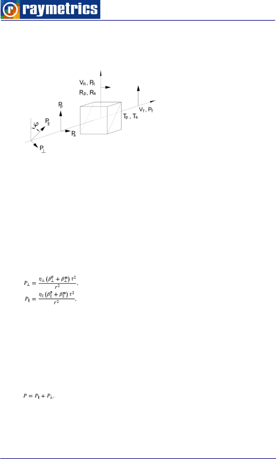
APPENDIX B
202
receiver channels. Therefore, we show the necessary equations of the angle ϕ between
the plane of polarization of the laser and the incident plane of the polarizing beam splitter
cube, according to Fig. B2.
Fig. B2. Signal power components in a receiver of a depolarization lidar with a
polarizing beam splitter cube with reflectivity Rp and Rs and transmittances Tp and
Ts for linearly polarized light parallel (p) and perpendicular (s) to the incident plane
of the polarizing beam splitter. PR and PT are the measured quantities in the
reflected and transmitted path, respectively, and VR and VT are the corresponding
amplification factors including the optical transmittances.
The backscatter powers before the PBC are (skipping the range dependence in the
following for convenience)
(2)
with the system constants η|| and η⊥ including here only the laser power and the
telescope aperture, assuming negligible diattenuation of the optics before the PBC, for
example, a telescope or dichroic beam splitters. The backscatter coefficient β is split up in
the parallel- (β_) and cross-polarized (β⊥) components of the backscatter from particles
(βp) and from molecules (βm). The total backscatter power P and the total backscatter
coefficient β are the sum of both polarized components:
(3)
The ratio of the total backscatter coefficient to the molecular component is called the
backscatter ratio R

APPENDIX B
203
R = βm + βp βm , (4)
and the ratio of the total cross- to the total parallel-polarized backscatter coefficient is
called the linear volume depolarization ratio δv:
(5)
The power components with respect to the incident plane of the PBC are
(6)
The subscripts p and s denote the planes parallel and perpendicular to the incident
plane of the PBC (see Fig. 1), respectively, and ϕ is the angle between the plane of
polarization of the laser and the incident plane of the PBC. Depending on this angle, the
cross polarized signal P⊥ can be measured in the reflected (for ϕ = 0◦) or in the
transmitted path (ϕ = 90◦). Hence, we denote the power measured in the reflected and
transmitted paths with the subscripts R and T, respectively. Behind the PBC the total
reflected (PR) and transmitted (PT) power components are
(7)
The amplification factors VR and VT include the optical transmittances of the receiver
and the electronic amplification in each channel. PR and PT are the quantities we actually
record with the data acquisition. For the following it is convenient to introduce a relative
amplification factor V∗ and the measured signal ratio δ∗
(8)
With eqs. (6)–(8), we achieve
(9)
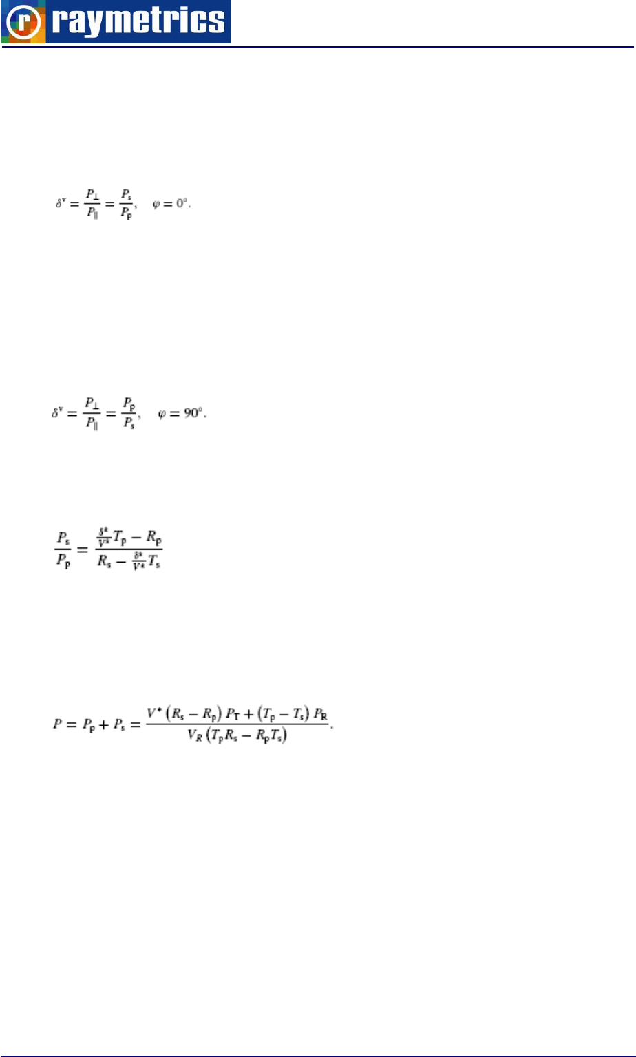
APPENDIX B
204
B6.1.4 Retrieval of the Linear Volume Depolarization Ratio δν
Once V∗ is known, we get δv with eqs. (5) and (6), for a regular measurements at ϕ =
0◦:
(10)
As for commercial PBCs, Rs is usually much closer to 1 than Tp, the noise and error
caused by the cross-talk from the strong parallel-polarized signal to the weaker cross-
polarized signal are reduced if the parallel polarized signal is detected in the reflected s-
branch of the PBC. For this setup ϕ = 90◦, and we get
(11)
From eqs. (5)–(8) follows
(12)
And
(13)
The knowledge of VR is not necessary, as we only need a relative signal for the lidar
signal inversion with the Fernald/Klett retrieval (Klett, 1985; Fernald, 1984), and thus we
can set it to VR = 1. In case the parameters of the polarizing beamsplitter cube are
Ts = 1 − Rs, Rp = 1 − Tp, (14)

APPENDIX B
205
B6.1.5 Retrieval of the Linear Particle Depolarization Ratio δP
The δp can be calculated from eqs. (2)–(5) using
(15)
with the height in dependent linear depolarization ratio of air molecules:
(16)
which can be determined with high accuracy (Behrendt and Nakamura, 2002). The
backscatter ratio R can be retrieved from the total signal P using, for example, the
Fernald/Klett inversion with a reference value βp(r0) at a reference range r0 and known
range-dependent lidar ratios S
(17)
where αp is the particle extinction coefficient. S(r) must be retrieved by an additional
measurement, for example, with a Raman channel. The values of δv and R are subject to
systematic and statistical (noise) errors.
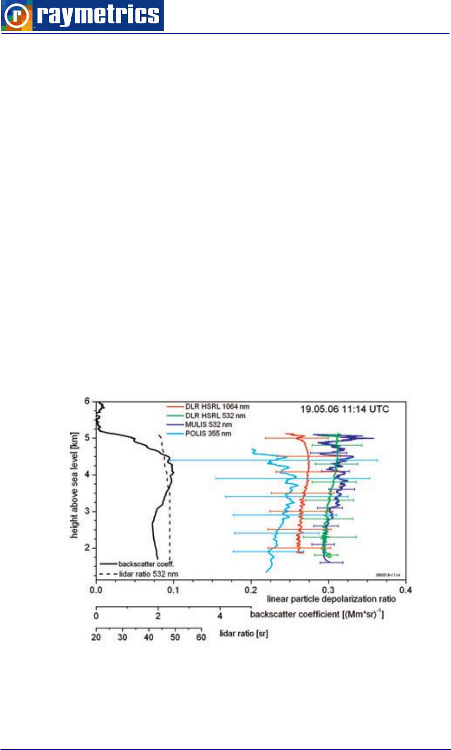
APPENDIX B
206
B6.2 Experiments And Results (From Samum Field Campaign) [11]
B6.2.1 Results and Comparison
During Saharan Mineral Dust Experiment (SAMUM), it was attempted to measure a
possible wavelength dependence of the dust particle linear depolarization ratio δp, with
four different lidar systems at four wavelengths as inputs for model calculations of δp
regarding the particles shapes and size distribution. Thus, the uncertainty of the absolute
values must be known and should be small compared with the expected natural variance.
The paper presents linear particle depolarization ratio δp measurements at four
wavelengths. However, MULIS (532 nm) and the airborne DLR-HSRL (532 and 1064 nm)
provided the most accurate measurements of the linear depolarization ratio. These lidar
measurements represent the backbone of the entire SAMUM polarization lidar activity.
First, we compare the height resolved profiles of δp of all lidars at four dates with
coincident measurements in Fig. B3. The lidar ratios S used for the depolarization retrieval
of MULIS at 532 nm were adopted from the coincident DLR-HSRL measurements
(displayed in Fig. 6 as broken lines) with errors in the range of ±5 sr. For non-coincident
measurements S is assumed to be 50 sr ± 10 sr.
Fig. B3. Particle linear depolarization ratio profiles on 19 June 2006 at several
wavelengths. The error bars indicate the systematic uncertainties
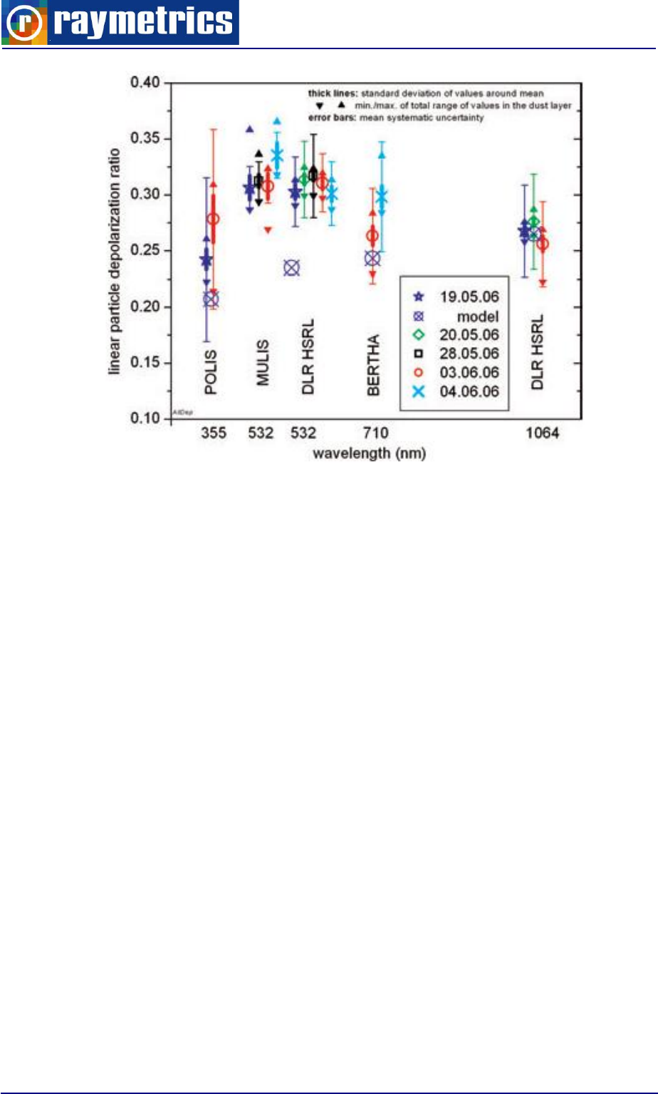
APPENDIX B
207
Fig. B4. Mean linear depolarization ratio of particles in the dust layer over the
wavelength of the four lidar systems at four different dates during SAMUM 2006 and
results of model calculations for the reference case 19 May 2006 (Wiegner et al.,
2008).
The linear depolarization ratio was measured with MULIS continuously during SAMUM.
Retrievals of the linear particle depolarization ratio δp at selected dates, together with error
bars and statistical information are displayed in Fig. B5 and listed in Table 2, together with
the measurements from the other lidars
from Fig. B4. The full ranges of the δp values are often asymmetric to the mean
towards smaller δp. These smaller values mostly stem from the dust layer top caused by
temporal averaging of the lidar measurements with changing dust layer top height.
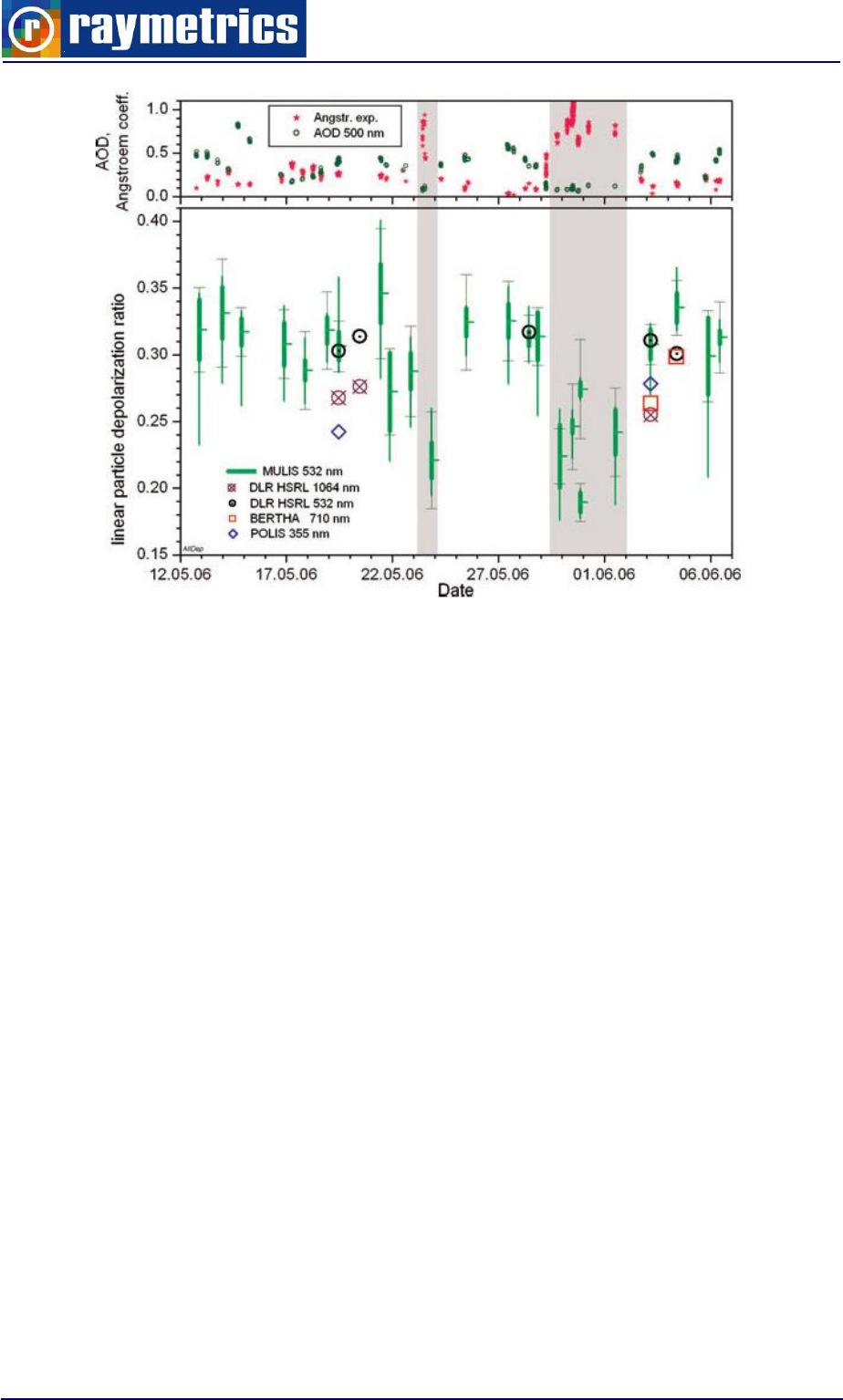
APPENDIX B
208
Fig. B5. Mean linear particle depolarization ratio δp in the dust layer over
Quarzazate during the SAMUM 2006 period for selected dates (lower plot) and
aerosol optical thickness at 500 nm and Ångstr¨om exponent (440–870 nm) from
SSARA sun photometer at Quarzazate (upper plot).
The AOD at 500 nm and the AE (440–870 nm) derived from the SSARA
measurements temporally closest to the MULIS measurements are displayed on top of
Fig. B5. For night time, when no sun photometer data were available, the AE values were
interpolated and the AE errors show the slope. Comparing the time-series in Fig. B5 we
see low δp and high AE in the shaded time periods, and high δp and low AE else, whereas
there is no evidence for a correlation between δp and AOD, as expected.
More details and information about this field campaign can be found at [11].

APPENDIX B
209
1. REFERENCES
[1] Sassen, K. 2005. Polarization in lidar. In: Lidar (ed. C. Weitkamp). Springer, New
York, 19–42.
[2] Sassen, K. 1991. “The polarization lidar technique for cloud research: a review and
current assessments. Bull. Am. Meteorol. Soc. 72, 1848– 1866.
[3] Freudenthaler V. et al, “Depolarization ratio profiling at several wavelengths in pure
Saharan dust during SAMUM 2006”, Tellus (2009), 61B, 165–179.
[4] Cairo F., Donfrancesco G. Di, Adriani A., Lucio Pulvirenti, and F. Fierli, Comparison
of various linear depolarization parameters measured by lidar, APPLIED OPTICS, 20 July
1999 y Vol. 38, No. 21, pp. 4425-4432.
[5] Sassen, K., Zhu, J., Webley, P., Dean, K. and Cobb, P. 2007. Volcanic ash plume
identification using polarization lidar: Augustine eruption, Alaska. Geophys. Res. Lett. 34,
doi:10.1029/2006GL027237.
[6] Freudenthaler, V., Homburg, F. and J¨ager, H. 1996. Optical parameters of contrails
from lidar measurements: linear depolarization. Geophys. Res. Lett. 23, 3715–3718.
[7] Dubovik, O., Sinyuk, A., Lapyonok, T., Holben, B. N., Mishchenko, M. and co-
authors. 2006. Application of spheroid models to account for aerosol particle nonsphericity
in remote sensing of desert dust. J. Geophys. Res. 111, doi:10.1029/2005JD006619.
[8] Wiegner, M., Gasteiger, J., Kandler, K.,Weinzierl, B., Rasp, K. and coauthors. 2008.
Numerical simulations of optical properties of Saharan dust aerosols with special emphasis
on the linear depolarization ratio. Tellus 61B, doi:10.1111/j.1600-0889.2008.00381.x.

APPENDIX B
210
[9] R. Agishev, B. Gross, F. Moshary, A. Gilerson, “Development of a SNR
parameterization scheme for general lidar assessment,” Appl. Phys. B 00, 1–12, 2005.
[10] QIU Zong-jia, CHEN Si-ying*, ZHANG Yin-chao, WANG Yu-zhao, NI Guo-qiang,
“Weak signal detection system and noise analysis for aerosol detection Lidar,”
International Symposium on Photoelectronic Detection and Imaging 2009: Laser Sensing
and Imaging, SPIE 2009.
[11] R.M. Measures, Laser Remote Sensing: Fundamentals and Applications, Wiley,
New York, 1994.
[12] Hamamatsu Photonics, Photomultiplier Tubes, Technical Manual.

APPENDIX B
211

APPENDIX B
212
Summary of equations for backscatter coef. calculation
Invert Klett Technique (Far – end solution)
ref ref
ref
r
r
r
r
molmol
refmol
ref
r
r
molmol
rrdrLRLRrRCSLR
rC
rRCS
rdrLRLRrRCS
r
)(**2exp***2
)(*
)(
)(**2exp*
)(
)()()( rrr pmol
Where
p is for particles (aerosols) and mol for molecular (Rayleigh)

APPENDIX B
213
3
8
)(
)(
)(
r
ra
rLR
mol
mol
mol
,
LRconst
r
ra
rLR
p
p )(
)(
)(
2
*)()( rrPrRCS c
This is the range corrected signal.
)(rP
c
is the background corrected lidar signal.
)(
)()(
refmol
refmolrefp
r
rr
C
Usually at rref we assume that
0)(
refp r
so C=1.
In any other case you can try different values for C.
How you can calculate the
)(r
mol

APPENDIX B
214
r
LR
r
r
rT
rp
p
T
rN
N
m
r
mol
mol
mol
mol
S
S
air
mol
-
8
3
76
361
3
8
0
0
2
4
2
2
3
T0 = 288.15 K
p0 = 1013 hPa
10641048.5
532105647.5
355107148.5
1
4
4
4
2
air
m

APPENDIX B
215
10640273.0
5320284.0
3550301.0
10200
exp
0
0
0
r
p
T
T
p
NrN
g
g
SS
NS0 = 2.547 1025 molecule/m3
in troposfera (0 → 12000 m):
rTrT g
γ= 0.0065 K/km

APPENDIX B
216
R
gM
g
gT
rT
prp
1
unde: M = 0.0289644 kg/mol
g = 9.81 m/s2
R = 8.31432 J/K
Tropopause (12000 → 15000 m)
constrrTrT troposhere
troposhere
troposhere
troposhere rr
RrrT
gM
rrprp exp
