LC 3 Assembly Lab Manual LC3 And Examples

LC3-AssemblyManualAndExamples

User Manual:

Open the PDF directly: View PDF .
Page Count: 56

Contents
List of Code Listings
List of Figures
Programming in LC-3
LC-3 Quick Reference Guide
ALU Operations
Arithmetic functions
Days of the week
Fibonacci Numbers
Subroutines: multiplication, division, modulus
Faster Multiplication
Compute Day of the Week
Random Number Generator
Recursive subroutines

111110001001110010010110100000101100100000011011000101000101100011111110110111101010001100101111000000010001001000011101000010

011000100111000101110000101100100010010100001110101110001010111100010111011001111001101001011010111000100011000011010111110000

000011001100010101001010010011010011010000110110100100111011011001011110001111001010011101001000101001010011101111001110010001

111001001110000110001101111101101101101111100000001100010000001001001010100111010111000010110100110001000011000100110111100101

100111101111010110101111101101010101110011111111100110101101101000000110101110101100100010101010111111101111010111100000110001

101000011011001101001000000010011000001101011010100000010010001111110111110001010110111010011100101000111111101111010111111111

001011000011100010001001110101110000100011111110000100011010101011001000001110110110001100001101101001110110011110000000011001

001000011000001001101011110100110001100000100100011011011100001011100000010011110000010001000010000100000100001001000000111101

000101100101111010101011010000101101110011010110111001010010011010011010111111101000111010001010110100111110110111111000011101

001100001010011111011100111110101001010111001110001001100000000001111101100001000101010111110100111101110010100101000100000100

100011101011001101000101101100100110100001110010101110110101011110110100010110001011000000000100100111000011100011101011111111

110100011010110111001000101000101111001010111100111100111100011011110101100100110100010101010110011111010001000011110100111110

111100111100111101000000010010100111001100101011000110101001010001010001111001110000010010001110010000000110110011000011000101

001111111111100011000101100011011100110110000111010000110101010100001111101101101100010110110110111001110000101001100111001001

011111011101011101110110010101000101111101011011000101110111010001100110001001011001001000000011110001110010110011110100100001

George M. Georgiou and Brian Strader

California State University, San Bernardino

August 2005

CONTENTS

Contents ii

List of Code Listings v

List of Figures vi

Programming in LC-3 vii

LC-3 Quick Reference Guide x

1 ALU Operations 1–1

1.1 Problem Statement .................................. 1–1

1.1.1 Inputs ..................................... 1–1

1.1.2 Outputs .................................... 1–1

1.2 Instructions in LC-3 .................................. 1–2

1.2.1 Addition ................................... 1–2

1.2.2 Bitwise AND ................................. 1–2

1.2.3 Bitwise NOT ................................. 1–2

1.2.4 Bitwise OR .................................. 1–3

1.2.5 Loading and storing with LDR and STR ................... 1–3

1.3 How to determine whether an integer is even or odd ................. 1–3

1.4 Testing ......................................... 1–3

1.5 What to turn in .................................... 1–4

2 Arithmetic functions 2–1

2.1 Problem Statement .................................. 2–1

2.1.1 Inputs ..................................... 2–1

2.1.2 Outputs .................................... 2–1

2.2 Operations in LC-3 .................................. 2–2

2.2.1 Loading and storing with LDI and STI .................... 2–2

2.2.2 Subtraction .................................. 2–2

2.2.3 Branches ................................... 2–3

2.2.4 Absolute value ................................ 2–3

2.3 Example ........................................ 2–4

2.4 Testing ......................................... 2–4

2.5 What to turn in .................................... 2–4

Revision: 1.17, January 20, 2007 ii

CONTENTS CONTENTS

3 Days of the week 3–1

3.1 Problem Statement .................................. 3–1

3.1.1 Inputs ..................................... 3–1

3.1.2 Outputs .................................... 3–1

3.2 The lab ........................................ 3–1

3.2.1 Strings in LC-3 ................................ 3–1

3.2.2 How to output a string on the display .................... 3–2

3.2.3 How to read an input value .......................... 3–2

3.2.4 Deﬁning the days of the week ........................ 3–3

3.3 Testing ......................................... 3–4

3.4 What to turn in .................................... 3–4

4 Fibonacci Numbers 4–1

4.1 Problem Statement .................................. 4–1

4.1.1 Inputs ..................................... 4–1

4.1.2 Outputs .................................... 4–1

4.2 Example ........................................ 4–1

4.3 Fibonacci Numbers .................................. 4–1

4.4 Pseudo-code ...................................... 4–2

4.5 Notes ......................................... 4–2

4.6 Testing ......................................... 4–3

4.7 What to turn in .................................... 4–3

5 Subroutines: multiplication, division, modulus 5–1

5.1 Problem Statement .................................. 5–1

5.1.1 Inputs ..................................... 5–1

5.1.2 Outputs .................................... 5–1

5.2 The program ...................................... 5–1

5.2.1 Subroutines .................................. 5–1

5.2.2 Saving and restoring registers ........................ 5–2

5.2.3 Structure of the assembly program ...................... 5–2

5.2.4 Multiplication ................................. 5–3

5.2.5 Division and modulus ............................ 5–3

5.3 Testing ......................................... 5–5

5.4 What to turn in .................................... 5–5

6 Faster Multiplication 6–1

6.1 Problem Statement .................................. 6–1

6.1.1 Inputs ..................................... 6–1

6.1.2 Outputs .................................... 6–1

6.2 The program ...................................... 6–1

6.2.1 The shift-and-add algorithm ......................... 6–1

6.2.2 Examining a single bit in LC-3 ........................ 6–2

6.2.3 The MULT1 subroutine ........................... 6–2

6.3 Testing ......................................... 6–2

6.4 What to turn in .................................... 6–2

7 Compute Day of the Week 7–1

7.1 Problem Statement .................................. 7–1

7.1.1 Inputs ..................................... 7–1

7.1.2 Outputs .................................... 7–1

7.1.3 Example ................................... 7–1

7.2 Zeller’s formula .................................... 7–2

7.3 Subroutines ...................................... 7–2

7.3.1 Structure of program ............................. 7–2

iii

CONTENTS CONTENTS

7.4 Testing: some example dates ............................. 7–3

7.5 What to turn in .................................... 7–3

8 Random Number Generator 8–1

8.1 Problem Statement .................................. 8–1

8.1.1 Inputs and Outputs .............................. 8–1

8.2 Linear Congruential Random Number Generators .................. 8–1

8.3 How to output numbers in decimal .......................... 8–2

8.3.1 A rudimentary stack ............................. 8–3

8.4 Testing ......................................... 8–3

8.5 What to turn in .................................... 8–3

9 Recursive subroutines 9–1

9.1 Problem Statement .................................. 9–1

9.1.1 Inputs ..................................... 9–1

9.1.2 Output .................................... 9–1

9.2 Recursive Subroutines ................................ 9–1

9.2.1 The Fibonacci numbers ............................ 9–1

9.2.2 Factorial ................................... 9–1

9.2.3 Catalan numbers ............................... 9–2

9.2.4 The recursive square function. ........................ 9–2

9.3 Stack Frames ..................................... 9–3

9.4 The McCarthy 91 function: an example in LC-3 ................... 9–5

9.4.1 Deﬁnition ................................... 9–5

9.4.2 Some facts about the McCarthy 91 function ................. 9–5

9.4.3 Implementation of McCarthy 91 in LC-3 .................. 9–5

9.5 Testing ......................................... 9–7

9.6 What to turn in .................................... 9–7

LIST OF CODE LISTINGS

1 “Hello World!” in LC-3. ............................... vii

1.1 The ADD instruction. ................................. 1–2

1.2 The AND instruction. ................................. 1–3

1.3 The NOT instruction. ................................. 1–3

1.4 Implementing the OR operation. ........................... 1–3

1.5 Loading and storing examples. ............................ 1–4

1.6 Determining whether a number is even or odd. .................... 1–4

2.1 Loading into a register. ................................ 2–2

2.2 Storing a register. ................................... 2–2

2.3 Subtraction: 5 −3=2. ................................ 2–2

2.4 Condition bits are set. ................................. 2–3

2.5 Branch if result was zero. ............................... 2–3

2.6 Absolute value. .................................... 2–4

3.1 Days of the week data. ................................ 3–3

3.2 Display the day. .................................... 3–3

4.1 Pseudo-code for computing the Fibonacci number Fniteratively .......... 4–2

4.2 Pseudo-code for computing the largest n=Nsuch that FNcan be held in 16 bits . . 4–3

5.1 A subroutine for the function f(n) = 2n+3. ..................... 5–2

5.2 Saving and restoring registers R5 and R6....................... 5–3

5.3 General structure of assembly program. ....................... 5–3

5.4 Pseudo-code for multiplication. ............................ 5–4

5.5 Pseudo-code for integer division and modulus. .................... 5–4

6.1 The shift-and-add multiplication. ........................... 6–2

7.1 Structure of the program. ............................... 7–3

8.1 Generating 20 random numbers using Schrage’s method. .............. 8–2

8.2 Displaying a digit. ................................... 8–2

8.3 Output a decimal number. ............................... 8–3

8.4 The code for the stack. ................................ 8–4

9.1 The pseudo-code for the recursive version of the Fibonacci numbers function. . . . 9–2

9.2 The pseudo-code for the algorithm that implements recursive subroutines. . . . . . 9–4

9.3 The pseudo-code for the recursive McCarthy 91 function. .............. 9–5

9.4 The pseudo-code for the McCarthy 91 recursive subroutine. ............. 9–7

9.5 The program that calls the McCarthy 91 subroutine. ................. 9–8

9.6 The stack subroutines PUSH and POP. ........................ 9–9

9.7 The McCarthy 91 subroutine ............................. 9–9

Revision: 1.17, January 20, 2007 v

LIST OF FIGURES

1 LC-3 memory map: the various regions. ....................... ix

1.1 Example run. ..................................... 1–4

1.2 The steps taken during the execution of the instruction LEA R2, xFF........ 1–5

2.1 The versions of the BR instruction. .......................... 2–3

2.2 The steps taken during the execution of the instruction LDI R1, X.......... 2–5

2.3 The steps taken during the execution of the instruction STI R2, Y.......... 2–5

2.4 Decimal numbers with their corresponding 2’s complement representation . . . . . 2–6

3.1 The string ”Sunday” in assembly and its corresponding binary representation . . . 3–2

4.1 Contents of memory ................................. 4–2

4.2 Fibonacci numbers table ............................... 4–4

5.1 The steps taken during execution of JSR. ...................... 5–2

5.2 Input parameters and returned results for DIV..................... 5–4

6.1 Shift-and-add multiplication ............................. 6–1

8.1 Sequences of random numbers generated for various seeds x0............ 8–4

9.1 The ﬁrst few values of f(n) = n!. ........................... 9–2

9.2 The ﬁrst few Catalan numbers Cn........................... 9–2

9.3 Some values of square(n)............................... 9–3

9.4 The structure of the stack. ............................... 9–3

9.5 A typical frame .................................... 9–4

9.6 Stack size in frames during execution. ........................ 9–6

9.7 Table that shows how many times the function M(n)is executed before it returns the

value for various n................................... 9–6

9.8 Maximum size of stack in terms of frames for n. ................... 9–8

Revision: 1.17, January 20, 2007 vi

Programming in LC-3

Parts of an LC-3 Program

1; LC−3 Program t h a t d i s p l a y s

2; ” H e ll o World ! ” t o t h e c o n s o l e

3.ORIG x3000

4LEA R0 , HW ; l o ad a d d r e s s o f s t r i n g

5PUTS ; o u t p u t s t r i n g t o c o n s o l e

6HALT ; end pro g ram

7HW .STRINGZ ” H e l l o World ! ”

8.END

Listing 1: “Hello World!” in LC-3.

The above listing is a typical hello world program written in LC-3 assembly language. The program

outputs “Hello World!” to the console and quits. We will now look at the composition of this

program.

Lines 1 and 2 of the program are comments. LC-3 uses the semi-colon to denote the beginning

of a comment, the same way C++ uses “//” to start a comment on a line. As you probably already

know, comments are very helpful in programming in high-level languages such as C++ or Java. You

will ﬁnd that they are even more necessary when writing assembly programs. For example in C++,

the subtraction of two numbers would only take one statement, while in LC-3 subtraction usually

takes three instructions, creating a need for further clarity through commenting.

Line 3 contains the .ORIG pseudo-op. A pseudo-op is an instruction that you can use when

writing LC-3 assembly programs, but there is no corresponding instruction in LC-3’s instruction

set. All pseudo-ops start with a period. The best way to think of pseudo-ops are the same way you

would think of preprocessing directives in C++. In C++, the #include statement is really not a C++

statement, but it is a directive that helps a C++ complier do its job. The .ORIG pseudo-op, with its

numeric parameter, tells the assembler where to place the code in memory.

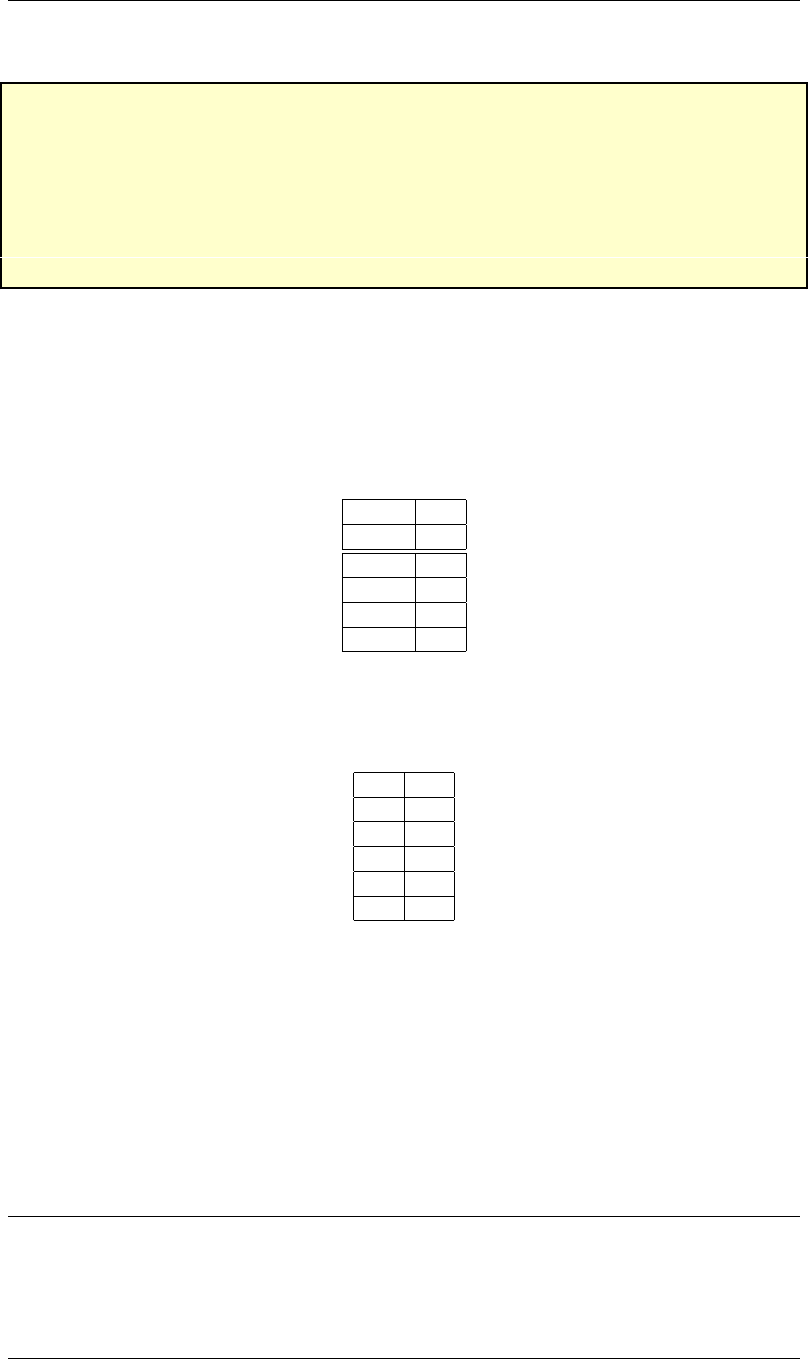
Memory in LC-3 can be thought of as one large 16-bit array. This array can hold LC-3 instruc-

tions or it can hold data values that those instructions will manipulate. The standard place for code

to begin at is memory location x3000. Note that the “x” in front of the number indicates it is in

hexadecimal. This means that the “.ORIG x3000” statement will put “LEA R0, HW” in memory

location x3000, “PUTS” will go into memory location x3001, “HALT” into memory location x3002,

and so on until the entire program has been placed into memory. All LC-3 programs begin with the

.ORIG pseudo-op.

Lines 4 and 5 are LC-3 instructions. The ﬁrst instruction, loads the address of the “Hello World!”

Revision: 1.17, January 20, 2007 vii

Programming in LC-3

string and the next instruction prints the string to the console. It is not important to know how these

instructions actually work right now, as they will be covered in the labs.

Line 6 is the HALT instruction. This instruction tells the LC-3 simulator to stop running the

program. You should put this in the spot where you want to end your program.

Line 7 is another pseudo-op .STRINGZ. After the main program code section, that was ended

by HALT, you can use the pseudo-ops, .STRINGZ, .FILL, and .BLKW to save space for data that

you would like to manipulate in the program. This is a similar idea to declaring variables in C++.

The .STRINGZ pseudo-op in this program saves space in memory for the “Hello World!” string.

Line 8 contains the .END pseudo-op. This tells the assembler that there is no more code to as-

semble. This should be the very last instruction in your assembly code ﬁle. .END can be sometimes

confused with the HALT instruction. HALT tells the simulator to stop a program that is running.

.END indicates where the assembler should stop assembling your code into a program.

Syntax of an LC-3 Instruction

Each LC-3 instruction appears on line of its own and can have up to four parts. These parts in order

are the label, the opcode, the operands, and the comment.

Each instruction can start with a label, which can be used for a variety of reasons. One reason

is that it makes it easier to reference a data variable. In the hello world example, line 7 contains

the label “HW.” The program uses this label to reference the “Hello World!” string. Labels are also

used for branching, which are similar to labels and goto’s in C++. Labels are optional and if an

instruction does not have a label, usually empty space is left where one would be.

The second part of an instruction is the opcode. This indicates to the assembler what kind of

instruction it will be. For example in line 4, LEA indicates that the instruction is a load effective

address instruction. Another example would be ADD, to indicate that the instruction is an addition

instruction. The opcode is mandatory for any instruction.

Operands are required by most instructions. These operands indicate what data the instruction

will be manipulating. The operands are usually registers, labels, or immediate values. Some instruc-

tions like HALT do not require operands. If an instruction uses more than one operand like LEA in

the example program, then they are separated by commas.

Lastly an instruction can also have a comment attached to it, which is optional. The operand

section of an instruction is separated from the comment section by a semicolon.

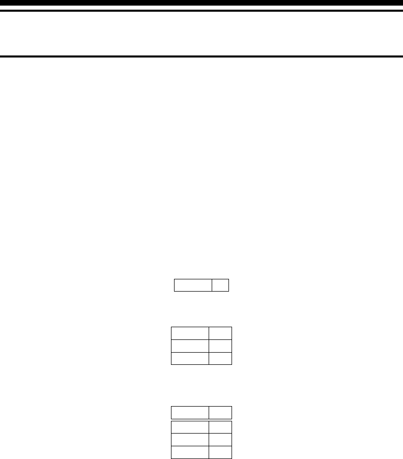
LC-3 Memory

LC-3 memory consists of 216 locations, each being 16 bits wide. Each location is identiﬁed with an

address, a positive integer in the range 0 through 216 −1. More often we use 4-digit hexadecimal

numbers for the addresses. Hence, addresses range from x0000 to xFFFF.

The LC-3 memory with its various regions is shown in ﬁgure 1on page ix.

viii

Programming in LC-3

xE000

x0000 − x00FF Trap Vector Table

x0100 − x01FF Interrupt Vector Table

x0200 − x2FFF OS and Supervisor Stack

x3000 − xFDFF User Program Area

xFE00 − xFFFF Device Register Addresses

Key

x0000

x1000

x2000

x3000

x4000

x5000

x6000

x7000

x8000

x9000

xA000

xB000

xC000

xD000

xFFFF

xF000

Figure 1: LC-3 memory map: the various regions.

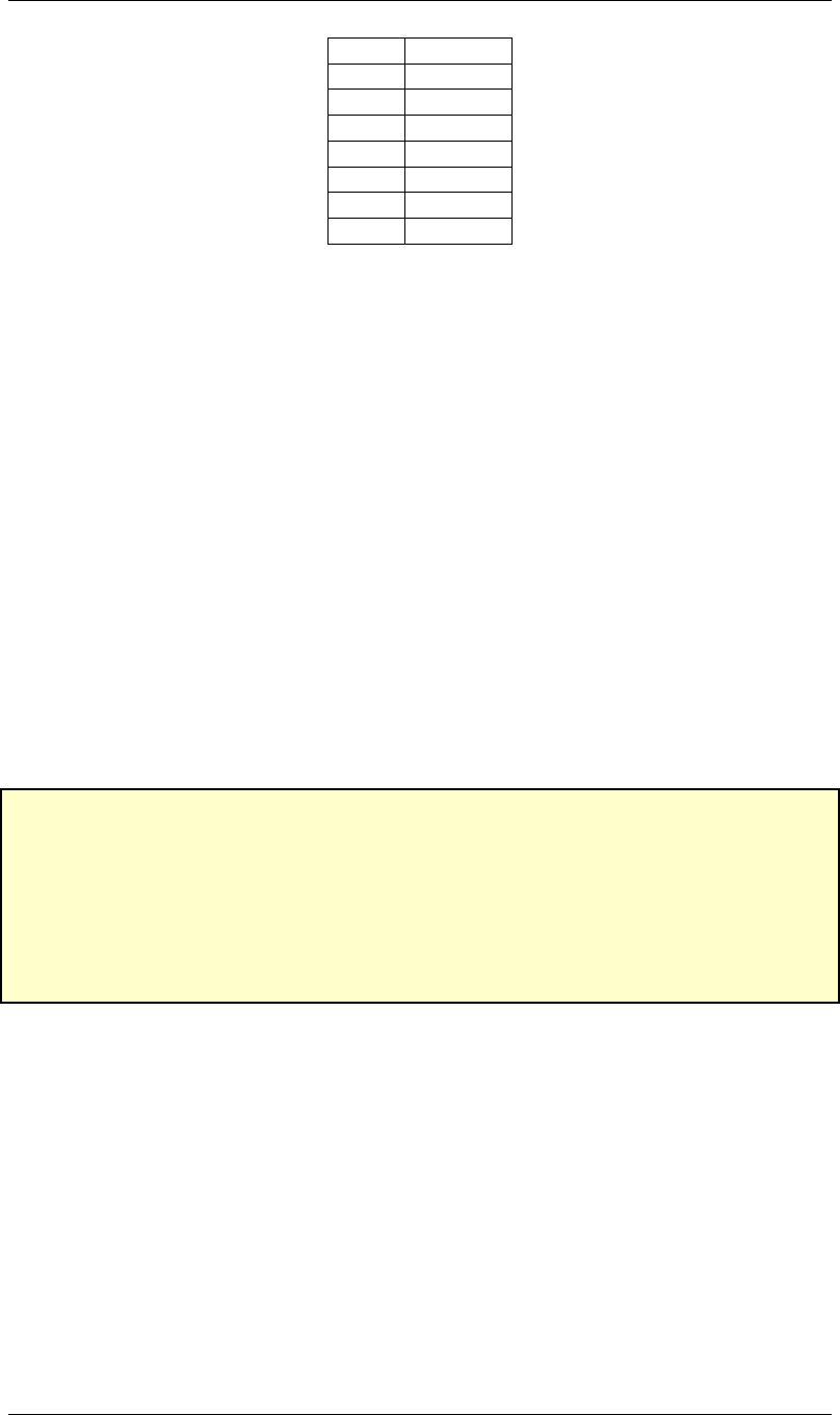
LC3 Quick Reference Guide

Instruction Set

Format

Description

Example

ADD

ADD DR, SR1, SR2

ADD DR, SR1, imm5

Adds the values in SR1 and

SR2/imm5 and sets DR to that

value.

ADD R1, R2, #5

The value 5 is added to the value in

R2 and stored in R1.

AND

AND DR, SR1, SR2

AND DR, SR1, imm5

Performs a bitwise and on the

values in SR1 and SR2/imm5

and sets DR to the result.

AND R0, R1, R2

A bitwise and is preformed on the

values in R1 and R2 and the result

stored in R0.

BR(n/z/p) LABEL

Note: (n/z/p) means

any combination of

those letters can appear

there, but must be in

that order.

Branch to the code section

indicated by LABEL, if the bit

indicated by (n/z/p) has been set

by a previous instruction. n:

negative bit, z: zero bit, p:

positive bit. Note that some

instructions do not set condition

codes bits.

BRz LPBODY

Branch to LPBODY if the last

instruction that modified the

condition codes resulted in zero.

BRnp ALT1

Branch to ALT1 if last instruction

that modified the condition codes

resulted in a positive or negative

(non-zero) number.

JMP

JMP SR1

Unconditionally jump to the

instruction based upon the

address in SR1.

JMP R1

Jump to the code indicated by the

address in R1.

JSR

JSR LABEL

Put the address of the next

instruction after the JSR

instruction into R7 and jump to

the subroutine indicated by

LABEL.

JSR POP

Store the address of the next

instruction into R7 and jump to the

subroutine POP.

JSRR

JSSR SR1

Similar to JSR except the

address stored in SR1 is used

instead of using a LABEL.

JSSR R3

Store the address of the next

instruction into R7 and jump to the

subroutine indicated by R3’s value.

LD DR, LABEL

Load the value indicated by

LABEL into the DR register.

LD R2, VAR1

Load the value at VAR1 into R2.

LDI

LDI DR, LABEL

Load the value indicated by the

address at LABEL’s memory

location into the DR register.

LDI R3, ADDR1

Suppose ADDR1 points to a

memory location with the value

x3100. Suppose also that memory

location x3100 has the value 8. 8

then would be loaded into R3.

LDR

LDR DR, SR1, offset6

Load the value from the memory

location found by adding the

value of SR1 to offset6 into DR.

LDR R3, R4, #-2

Load the value found at the address

(R4 –2) into R3.

LEA

LEA DR, LABEL

Load the address of LABEL into

DR.

LEA R1, DATA1

Load the address of DATA1 into

R1.

NOT

NOT DR, SR1

Performs a bitwise not on SR1

and stores the result in DR.

NOT R0, R1

A bitwise not is preformed on R1

and the result is stored in R0.

RET

Return from a subroutine using

the value in R7 as the base

address.

RET

Equivalent to JMP R7.

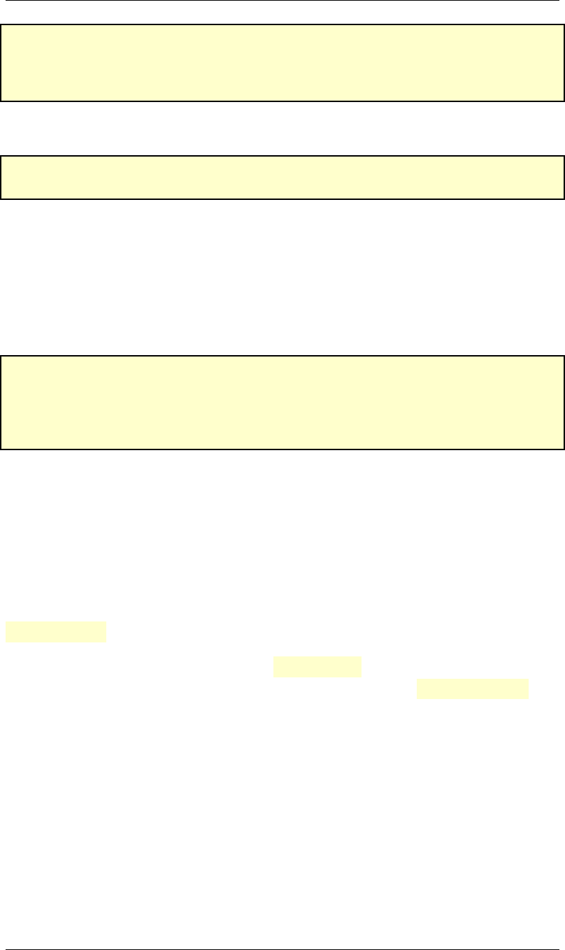
LC-3 Quick Reference Guide

RTI

Return from an interrupt to the

code that was interrupted. The

address to return to is obtained

by popping it off the supervisor

stack, which is automatically

done by RTI.

RTI

Note: RTI can only be used if the

processor is in supervisor mode.

ST SR1, LABEL

Store the value in SR1 into the

memory location indicated by

LABEL.

ST R1, VAR3

Store R1’s value into the memory

location of VAR3.

STI

STI SR1, LABEL

Store the value in SR1 into the

memory location indicated by

the value that LABEL’s memory

location contains.

STI R2, ADDR2

Suppose ADDR2’s memory

location contains the value x3101.

R2’s value would then be stored

into memory location x3101.

STR

STR SR1, SR2, offset6

The value in SR1 is stored in the

memory location found by

adding SR2 and offest6 together.

STR R2, R1, #4

The value of R2 is stored in

memory location (R1 + 4).

TRAP

TRAP trapvector8

Performs the trap service

specified by trapvector8. Each

trapvector8 service has its own

assembly instruction that can

replace the trap instruction.

TRAP x25

Calls a trap service to end the

program. The assembly instruction

HALT can also be used to replace

TRAP x25.

Symbol Legend

Symbol

Description

Symbol

Description

SR1, SR2

Source registers used by instruction.

LABEL

Label used by instruction.

Destination register that will hold

the instruction’s result.

trapvector8

8 bit value that specifies trap service

routine.

imm5

Immediate value with the size of 5

bits.

offset6

Offset value with the size of 6 bits.

TRAP Routines

Trap Vector

Equivalent Assembly

Instruction

Description

x20

GETC

Read one input character from the keyboard and store it into R0

without echoing the character to the console.

x21

OUT

Output character in R0 to the console.

x22

PUTS

Output null terminating string to the console starting at address

contained in R0.

x23

Read one input character from the keyboard and store it into R0 and

echo the character to the console.

x24

PUTSP

Same as PUTS except that it outputs null terminated strings with

two ASCII characters packed into a single memory location, with

the low 8 bits outputted first then the high 8 bits.

x25

HALT

Ends a user’s program.

Pseudo-ops

Pseudo-op

Format

Description

.ORIG

.ORIG #

Tells the LC-3 simulator where it should place the segment of

code starting at address #.

.FILL

.FILL #

Place value # at that code line.

.BLKW

.BLKW #

Reserve # memory locations for data at that line of code.

.STRINGZ

.STRINGZ “<String>”

Place a null terminating string <String> starting at that location.

.END

Tells the LC-3 assembler to stop assembling your code.

LC-3 Quick Reference Guide

xii

LAB 1

ALU Operations

1.1 Problem Statement

The numbers Xand Yare found at locations x3100 and x3101, respectively. Write an LC-3 assembly

language program that does the following.

•Compute the sum X+Yand place it at location x3102.

•Compute XAND Yand place it at location x3103.

•Compute XOR Yand place it at location x3104.

•Compute NOT(X)and place it at location x3105.

•Compute NOT(Y)and place it at location x3106.

•Compute X+3 and place it at location x3107.

•Compute Y−3 and place it at location x3108.

•If the Xis even, place 0 at location x3109. If the number is odd, place 1 at the same location.

The operations AND,OR, and NOT are bitwise. The operation signiﬁed by +is the usual

arithmetic addition.

1.1.1 Inputs

The numbers Xand Yare in locations x3100 and x3101, respectively:

x3100 X

x3101 Y

1.1.2 Outputs

The outputs at their corresponding locations are as follows:

Revision: 1.12, January 20, 2007 1–1

LAB 1 1.2. INSTRUCTIONS IN LC-3

x3102 X+Y

x3103 XAND Y

x3104 XOR Y

x3105 NOT(X)

x3106 NOT(Y)

x3107 X+3

x3108 Y−3

x3109 Z

where Zis deﬁned as

Z=(0 if Xis even

1 if Xis odd.(1.1)

1.2 Instructions in LC-3

LC-3 has available these ALU instructions: ADD (arithmetic addition), AND (bitwise and), NOT

(bitwise not).

1.2.1 Addition

Adding two integers is done using the ADD instruction. In listing 1.1, the contents of registers R1

and R2 and added and the result is placed in R3. Note the values of integers can be negative as well,

since they are in two’s complement format. ADD also comes in immediate version, where the second

operand can be a constant integer. For example, we can use it to add 4 to register R1 and place the

result in register R3. See listing 1.1. The constant is limited to 5 bits two’s complement format.

Note, as with all other ALU instructions, the same register can serve both as a source operand and

the destination register.

1; Adding two r e g i s t e r s

2ADD R3 , R1 , R2 ; R3 ←R1 + R2

3; Adding a r e g i s t e r and a c o n s t a n t

4ADD R3 , R1 , #4 ; R3 ←R1 + 4

5; Adding a r e g i s t e r and a n e g a t i v e c o n s t a n t

6ADD R3 , R1 , #−4; R3 ←R1 −4

7; Adding a r e g i s t e r t o i t s e l f

8ADD R1 , R1 , R1 ; R1 ←R1 + R1

Listing 1.1: The ADD instruction.

1.2.2 Bitwise AND

Two registers can be bitwise ANDed using the AND instruction, as in listing 1.2 on page 1–3.AND

also comes in the immediate version. Note that an immediate operand can be given in hexadecimal

form using xfollowed by the number.

1.2.3 Bitwise NOT

The bits of a register can be inverted (ﬂipped) using the bitwise NOT instruction, as in listing 1.3 on

page 1–3.

1–2

LAB 1 1.3. HOW TO DETERMINE WHETHER AN INTEGER IS EVEN OR ODD

1; Anding two r e g i s t e r s

2AND R3 , R1 , R2 ; R3 ←R1 AND R2

3; Anding a r e g i s t e r and a c o n s t a n t

4ADD R3 , R1 , xA ; R3 ←R1 AND 0000000000001010

Listing 1.2: The AND instruction.

1; I n v e r t i n g t h e b i t s o f r e g i s t e r R1

2NOT R2 , R1 ; R2 ←NOT( R1 )

Listing 1.3: The NOT instruction.

1.2.4 Bitwise OR

LC-3 does not provide the bitwise OR instruction. We can use, however, AND and NOT to built it.

For this purpose, we make use of De Morgan’s rule: XOR Y=NOT(NOT(X)AND NOT(Y)). See

listing 1.4.

1; ORing two r e g i s t e r s

2NOT R1 , R1 ; R1 ←NOT( R1 )

3NOT R2 , R2 ; R2 ←NOT( R2 )

4AND R3 , R1 , R2 ; R3 ←NOT( R1 ) AND NOT( R2 )

5NOT R3 , R3 ; R3 ←R1 OR R2

Listing 1.4: Implementing the OR operation.

1.2.5 Loading and storing with LDR and STR

The instruction LDR can be used to load the contents of a memory location into a register. Knowing

that Xand Yare at locations x3100 and x3101, respectively, we can use the code in listing 1.5 on

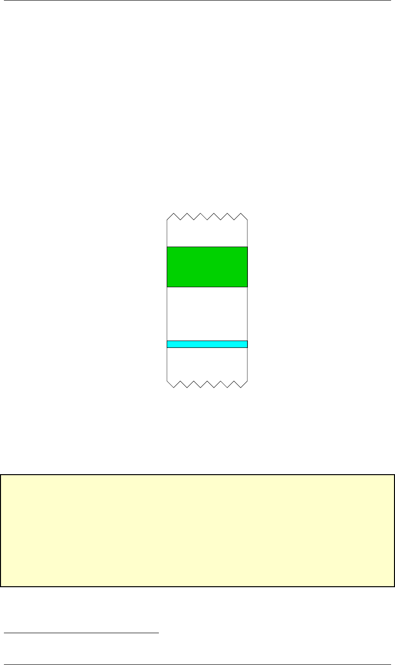
page 1–4 to load them in registers R1 and R3, respectively. In the same ﬁgure one can see how

the instruction STR is used store the contents of a register to a memory location. The instruction

LEA R2, Offset loads register R2 with the address (PC + 1 + Offset), where PC is the address

of the instruction LEA and Offset is a numerical value, i.e. the immediate operand. Figure 1.2 on

page 1–5 shows the steps it takes to execute the LEA R2, xFF instruction.

If instead of a numerical value, a label is given, such as in instruction LEA R2, LABEL , then

the value of the immediate operand, i.e. the offset, is automatically computed so that R2 is loaded

with the address of the instruction with label LABEL.

1.3 How to determine whether an integer is even or odd

In binary, when a number is even it ends with a 0, and when it is odd, it ends with a 1. We can obtain

0 or 1, correspondingly, by using the AND instruction as in listing 1.6 on page 1–4. This method is

valid for numbers in two’s complement format, which includes negative numbers.

1.4 Testing

Test your program for several input pairs of Xand Y. In ﬁgure 1.1 on page 1–4 an example is shown

of how memory should look after the program is run. The contents of memory are shown in decimal,

1–3

LAB 1 1.5. WHAT TO TURN IN

1; V a l u e s X and Y a r e l o a d e d i n t o r e g i s t e r s R1 and R3.

2.ORIG x3000 ; A d d r e s s w he re p r og r am c o de b e g i n s

3; R2 i s l o a d ed w i th t h e b e g i n n i n g a d d r e s s o f t h e d a t a

4LEA R2 , xFF ; R2 ←x3000 + x1 + xFF ( = x3100 )

5; X, which i s l o c a t e d a t x3100 , i s l o a d e d i n t o R1

6LDR R1 , R2 , x0 ; R1 ←MEM[ x3100 ]

7; Y, which i s l o c a t e d a t x3101 , i s l o a d e d i n t o R3

8LDR R3 , R2 , x1 ; R3 ←MEM[ x3100 + x1 ]

9. . .

10 ; S t o r i n g 5 i n memory l o c a t i o n x3101

11 AND R4 , R4 , x0 ; C l e a r R4

12 ADD R4 , R4 , x5 ; R4 ←5

13 STR R4 , R2 , x1 ; MEM[ x3100 + x1 ] ←R4

Listing 1.5: Loading and storing examples.

1AND R2 , R1 , x0001 ; R2 h a s t h e v a l u e o f t h e l e a s t

2; s i g n i f i c a n t b i t o f R1 .

Listing 1.6: Determining whether a number is even or odd.

hexadecimal, and binary format.

Address Decimal Hex Binary Contents

x3100 9 0009 0000 0000 0000 1001 X

x3101 -13 FFF3 1111 1111 1111 0011 Y

x3102 -4 FFFC 1111 1111 1111 1100 X+Y

x3103 1 0001 0000 0000 0000 0001 XAND Y

x3104 -5 FFFB 1111 1111 1111 1011 XOR Y

x3105 65526 FFF6 1111 1111 1111 0110 NOT(X)

x3106 12 000C 0000 0000 0000 1100 NOT(Y)

x3107 12 000C 0000 0000 0000 1100 X+3

x3108 -16 FFF0 1111 1111 1111 0000 Y−3

x3108 1 0001 0000 0000 0000 0001 z

Figure 1.1: Example run.

1.5 What to turn in

•A hardcopy of the assembly source code.

•Electronic version of the assembly code.

•For each of the (X,Y)pairs (10,20),(−11,15),(11,−15),(9,12), screenshots that show the

contents of location x3100 through x3108.

1–4

LAB 1 1.5. WHAT TO TURN IN

and storing the result into R2.

Step 1

Memory

x3000

. . .

x3001

x3002

LEA R2, xFF

Initial State of LC3 Simulator

LEA R2, xFF

x3002

x3001

. . .

x3000

Memory

x3000

. . .

x3001

x3002

LEA R2, xFF

x3002

x3001

. . .

x3000

Memory

Step 2

Step 3 Step 4

3000 3000

3001 3001

Use PC to get instruction at x3000

and load it into IR.

Increment PC for the next instruction.

3100

Execute LEA in IR by adding PC and the offset

Figure 1.2: The steps taken during the execution of the instruction LEA R2, xFF.

1–5

LAB 2

Arithmetic functions

2.1 Problem Statement

The numbers Xand Yare found at locations x3120 and x3121, respectively. Write a program in

LC-3 assembly language that does the following:

•Compute the difference X−Yand place it at location x3122.

•Place the absolute values |X|and |Y|at locations x3123 and x3124, respectively.

•Determine which of |X|and |Y|is larger. Place 1 at location x3125 if |X|is, a 2 if |Y|is, or a

0 if they are equal.

2.1.1 Inputs

The integers Xand Yare in locations x3120 and x3121, respectively:

x3120 X

x3121 Y

2.1.2 Outputs

The outputs at their corresponding locations are as follows:

x3122 X−Y

x3123 |X|

x3124 |Y|

x3125 Z

where Zis deﬁned as

Z=









1 if |X|−|Y|>0

2 if |X|−|Y|<0

0 if |X|−|Y|=0

(2.1)

Revision: 1.11, January 26, 2007 2–1

LAB 2 2.2. OPERATIONS IN LC-3

2.2 Operations in LC-3

2.2.1 Loading and storing with LDI and STI

In the previous lab, loading and storing was done using the LDR and STR instructions. In this lab,

the similar but distinct instructions LDI and STI will be used. Number Xalready stored at location

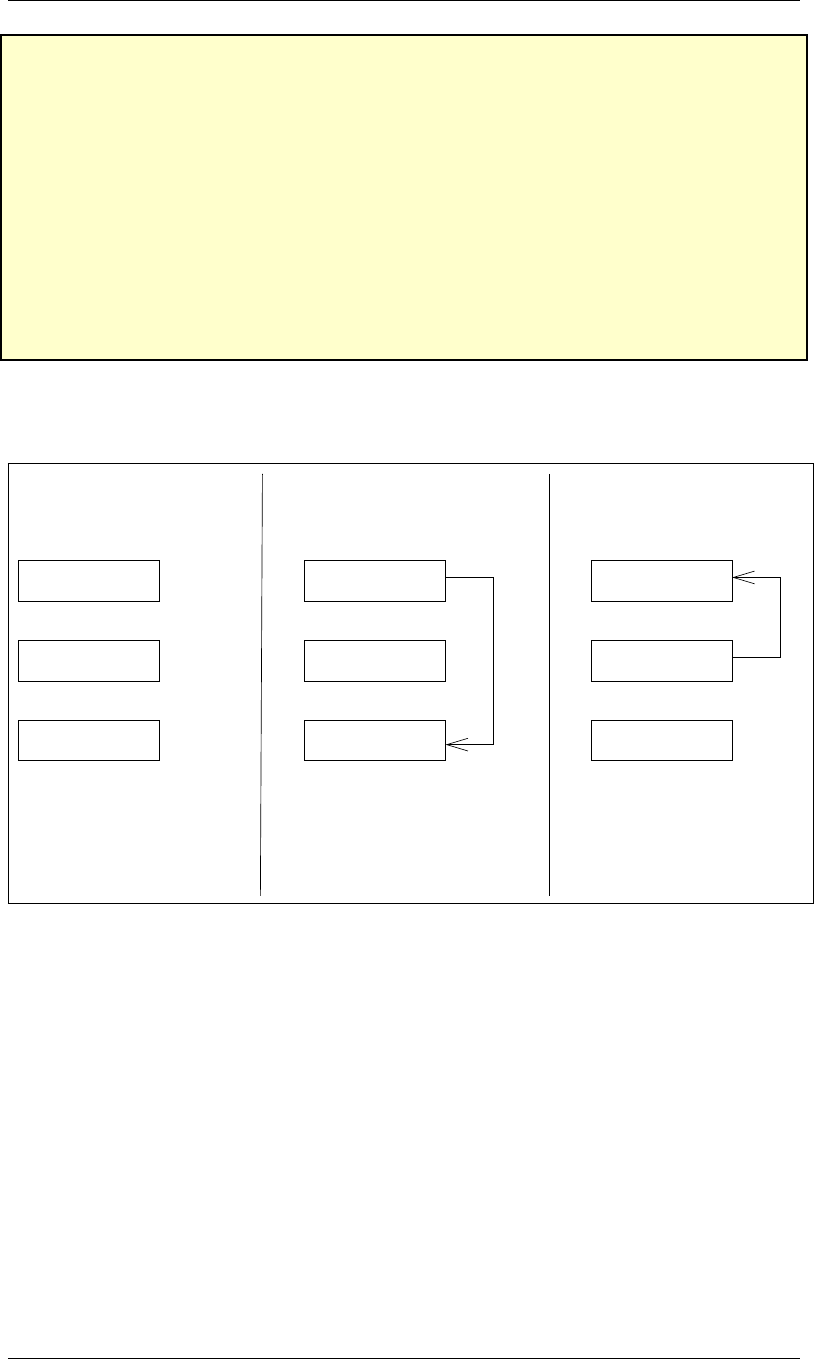
x3120 can be loaded into a register, say, R1 as in listing 2.1. The Load Indirect instruction, LDI, is

used. The steps taken to execute LDI R1, X are shown in ﬁgure 2.2 on page 2–5.

1LDI R1 , X

2. . .

3. . .

4HALT

5. . .

6X.FI L L x3120

Listing 2.1: Loading into a register.

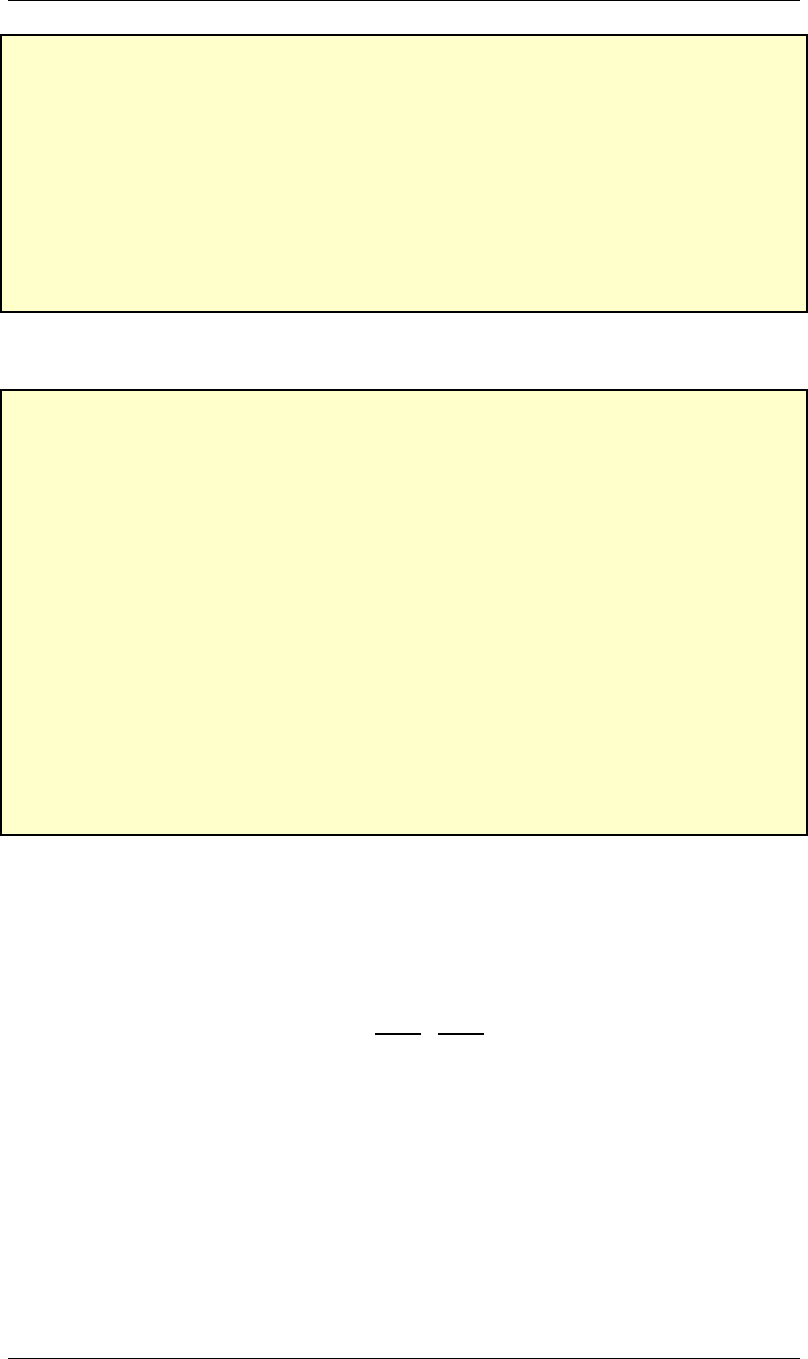
In listing 2.2, the contents of register R2 are stored at location x3121. The instruction Store

Indirect,STI, is used. The steps taken to execute STI R2, Y instruction are shown in ﬁgure 2.3 on

page 2–5.

1STI R2 , Y

2. . .

3. . .

4HALT

5. . .

6Y.FI L L x3121

Listing 2.2: Storing a register.

2.2.2 Subtraction

LC-3 does not provide a subtraction instruction. However, we can build one using existing instruc-

tions. The idea here is to negate the subtrahend1, which is done by taking its two complement, and

then adding it to the minuend.

As an example, in listing 2.3 the result of the subtraction 5 −3=5+ (−3) = 2 is placed in

1; R e g i s t e r R1 h a s 5 and r e g i s t e r R2 h a s 3

2; R4 i s u s ed a s a t e m p o r a r y r e g i s t e r . R2 c o u l d h av e b ee n u se d

3; i n t h e p l a c e o f R4 , b u t t h e o r i g i n a l c o n t e n t s o f R2 would

4; ha v e be e n l o s t . The r e s u l t o f 5−3=2 g o e s i n t o R3 .

5NOT R4 , R2

6ADD R4 , R4 , #1 ; R4 ← −R2

7ADD R3 , R1 , R4 ; R3 ←R1 −R2

Listing 2.3: Subtraction: 5 −3=2.

1Subtrahend is a quantity which is subtracted from another, the minuend.

2–2

LAB 2 2.2. OPERATIONS IN LC-3

2.2.3 Branches

The usual linear ﬂow of executing instructions can be altered by using branches. This enables us

to choose code fragments to execute and code fragments to ignore. Many branch instructions are

conditional which means that the branch is taken only if a certain condition is satisﬁed. For example

the instruction BRz TARGET means the following: if the result of a previous instruction was zero,

the next instruction to be executed is the one with label TARGET. If the result was not zero, the

instruction that follows BRz TARGET is executed and execution continues as normal.

The exact condition for a branch instructions depends on three Condition Bits: N (negative), Z

(zero), and P (positive). The value (0 or 1) of each condition bit is determined by the nature of the

result that was placed in a destination register of an earlier instruction. For example, in listing 2.4

we note that at the execution of the instruction BRz LABEL N is 0, and therefore the branch is not

taken.

1. . .

2AND R1 , R1 , x0 ; S i n c e R1 ←0 , N = 0 , Z = 1 , P = 0

3ADD R2 , R1 , x1 ; S i n c e R2 ←1 , N = 0 , Z = 0 , P = 1

4BRz LABEL

5. . .

6LABEL . . .

Listing 2.4: Condition bits are set.

Table ﬁgure 2.1 shows a list of the available versions of the branch instruction. As an example

BR branch unconditionally BRnz branch if result was negative or zero

BRz branch if result was zero BRnp branch if result was negative or positive

BRn branch if result was negative BRzp branch if result was zero or positive

BRp branch is result was positive BRnzp branch unconditionally

Figure 2.1: The versions of the BR instruction.

consider the code fragment in listing 2.5. The next instruction after the branch instruction to be

executed will be the ADD instruction, since the result placed in R2 was 0, and thus bit Zwas set.

The NOT instruction, and the ones that follow it up to the instruction before the ADD will never be

executed.

1AND R2 , R5 , x0 ; r e s u l t p l a c e d i n R2 i s z e r o

2BRz TARGET ; B ran ch i f r e s u l t was z e r o ( i t was )

3NOT R1 , R3

4. . .

5. . .

6TARGET ADD R5 , R1 , R2

7. . .

Listing 2.5: Branch if result was zero.

2.2.4 Absolute value

The absolute value of an integer Xis deﬁned as follows:

|X|=(Xif X≥0

−Xif X<0.(2.2)

2–3

LAB 2 2.3. EXAMPLE

One way to implement absolute value is seen in listing 2.6.

1; I n p u t : R1 h as v a l u e X.

2; O u t p u t : R2 h a s v a l u e |X|.

3ADD R2 , R1 , #0 ; R2 ←R1 , c an now u s e c o n d i t i o n c o d es

4BRzp ZP ; I f z e r o o r p o s i t i v e , do n o t n e g a t e

5NOT R2 , R2

6ADD R2 , R2 , #1 ; R2 = −R1

7ZP . . . ; At t h i s p o i n t R2 = |R1 |

8. . .

Listing 2.6: Absolute value.

2.3 Example

At the end of a run, the memory locations of interest might look like this:

x3120 9

x3121 -13

x3122 22

x3123 9

x3124 13

x3125 2

2.4 Testing

Test your program for these Xand Ypairs:

X Y

10 12

13 10

-10 12

10 -12

-12 -12

Figure 2.4 on page 2–6 is table that shows the binary representations the integers -32 to 32, that can

helpful in testing.

2.5 What to turn in

•A hardcopy of the assembly source code.

•Electronic version of the assembly code.

•For each of the (X,Y)pairs (10,20),(−11,15),(11,−15),(12,12), screenshots that show the

contents of location x3120 through x3125.

2–4

LAB 2 2.5. WHAT TO TURN IN

Instruction loads MAR with X’s Address.

Use MAR to access memory.

Value 3120 is loaded from memory and copied to MDR.

Copy MDR to MAR.

Use MAR to access memory.

Value 17 is loaded into MDR from memory.

Copy MDR to R1.

Addr X

3120

x3121

x311F

. . .

Addr X

x3120

MDR

MAR

Memory

Step 2Step 1 Memory

MAR

MDR

x3120

Addr X

. . .

x311F

x3121

3120

Addr X

3120

x3121

x311F

. . .

Addr X

x3120

MDR

MAR

Memory Memory

MAR

MDR

x3120

Addr X

. . .

x311F

x3121

3120

Addr X

Step 3 Step 4

X Addr X Addr

3120

Figure 2.2: The steps taken during the execution of the instruction LDI R1, X.

Value 3121 is loaded from memory and copied to MDR.

x3121

x3122 x3122

x3121

x3120

x3121

x3122 x3122

x3121

x3120

Copy value 82 from R2 to MDR.

Use MAR to access memory.

Store MDR’s value into memory.

MDR

8282

Use MAR to access memory.

Copy MDR to MAR.

. . .

MDR

MAR Memory

Step 2Step 1 Memory

MAR

MDR . . .

. . .

MAR Memory Memory

MAR

MDR . . .

Step 3 Step 4

3121 3121

Y Addr Y Addr

Addr Y Addr Y

Addr YAddr Y

3121

Instruction loads MAR with Addr Y’s Address.

x3120

Figure 2.3: The steps taken during the execution of the instruction STI R2, Y.

2–5

LAB 2 2.5. WHAT TO TURN IN

Decimal 2’s Complement Decimal 2’s Complement

0 0000000000000000 -0 0000000000000000

1 0000000000000001 -1 1111111111111111

2 0000000000000010 -2 1111111111111110

3 0000000000000011 -3 1111111111111101

4 0000000000000100 -4 1111111111111100

5 0000000000000101 -5 1111111111111011

6 0000000000000110 -6 1111111111111010

7 0000000000000111 -7 1111111111111001

8 0000000000001000 -8 1111111111111000

9 0000000000001001 -9 1111111111110111

10 0000000000001010 -10 1111111111110110

11 0000000000001011 -11 1111111111110101

12 0000000000001100 -12 1111111111110100

13 0000000000001101 -13 1111111111110011

14 0000000000001110 -14 1111111111110010

15 0000000000001111 -15 1111111111110001

16 0000000000010000 -16 1111111111110000

17 0000000000010001 -17 1111111111101111

18 0000000000010010 -18 1111111111101110

19 0000000000010011 -19 1111111111101101

20 0000000000010100 -20 1111111111101100

21 0000000000010101 -21 1111111111101011

22 0000000000010110 -22 1111111111101010

23 0000000000010111 -23 1111111111101001

24 0000000000011000 -24 1111111111101000

25 0000000000011001 -25 1111111111100111

26 0000000000011010 -26 1111111111100110

27 0000000000011011 -27 1111111111100101

28 0000000000011100 -28 1111111111100100

29 0000000000011101 -29 1111111111100011

30 0000000000011110 -30 1111111111100010

31 0000000000011111 -31 1111111111100001

32 0000000000100000 -32 1111111111100000

Figure 2.4: Decimal numbers with their corresponding 2’s complement representation

2–6

LAB 3

Days of the week

3.1 Problem Statement

•Write a program in LC-3 assembly language that keeps prompting for an integer in the range

0-6, and each time it outputs the corresponding name of the day. If a key other than ’0’ through

’6’ is pressed, the program exits.

3.1.1 Inputs

At the prompt “Please enter number: ,” a key is pressed.

3.1.2 Outputs

If the key pressed is ’0’ through ’6’, the corresponding name of the day of the week appears on the

screen. Precisely, the correspondence is according to this table:

Code Day

0 Sunday

1 Monday

2 Tuesday

3 Wednesday

4 Thursday

5 Friday

6 Saturday

When the day is displayed, the prompt “Please enter number: ” appears again and the program

expects another input. If any key other that ’0’ through ’6’ is pressed, the program exits.

3.2 The lab

3.2.1 Strings in LC-3

It will be necessary to deﬁne the prompt “Please enter number: ” and the days of the week as

strings in memory. All strings should terminate with the NUL character (ASCII 0). In LC-3 one

character per memory location is stored. Each location is 16 bits wide. The 8 most signiﬁcant bits

are 0, while the 8 least signiﬁcant bits hold the ASCII value of the character. Strings terminated with

the NUL character can be conveniently deﬁned using the directive .STRINGZ ”ABC” , where

Revision: 1.6, August 4, 2005 3–1

LAB 3 3.2. THE LAB

“ABC” is any alphanumeric string. It automatically appends the NUL character to the string. As

an example, a string deﬁned in assembly language and the corresponding contents of memory are

shown in ﬁgure 3.1.

1.ORIG x3100

2.STRINGZ ” Sunday ”

x3100 0053 ; S

x3101 0075 ; u

x3102 006 e ; n

x3103 0064 ; d

x3104 0061 ; a

x3105 0079 ; y

x3106 0000 ; NUL

Figure 3.1: The string ”Sunday” in assembly and its corresponding binary representation

3.2.2 How to output a string on the display

To output is a string on the screen, one needs to place the beginning address of the string in reg-

ister R0, and then call the PUTS assembly command, which is another name for the instruction

TRAP x22 . For example, to output “ABC”, one can do the following:

1LEA R0 , ABCLBL ; L oads a d d r e s s o f ABC s t r i n g i n t o R0

2PUTS

3. . .

4HALT

5. . .

6ABCLBL .STRINGZ ”ABC”

7. . .

The PUTS command calls a system trap routine which outputs the NUL terminated string the

address of its ﬁrst character is found in register R0.

3.2.3 How to read an input value

The assembly command GETC , which is another name for TRAP x20 , reads a single character

from the keyboard and places its ASCII value in register R0. The 8 most signiﬁcant bits of R0 are

cleared. There is no echo of the read character. For example, one may use the following code to

read a single numerical character, 0 through 9, and place its value in register R3:

1GETC ; P l a c e ASCII v a l u e o f i n p u t c h a r a c t e r i n t o R0

2ADD R3 , R0 , x0 ; Copy R0 i n t o R3

3ADD R3 , R3 , #−16 ; S u b t r a c t 4 8 , t h e ASCII v a l u e o f 0

4ADD R3 , R3 , #−16

5ADD R3 , R3 , #−16 ; R3 now c o n t a i n s t h e a c t u a l v a l u e

Notice that it was necessary to use three instructions to subtract 48, since the maximum possible

value of the immediate operand of ADD is 5 bits, in two’s complement format. Thus, -16 is the

most we can subtract with the immediate version of the ADD instruction. As an example, if the

pressed key was “5”, its ASCII value 53 will be placed in R0. Subtracting 48 from 53, the value 5

results, as expected, and is placed in register R3.

3–2

LAB 3 3.2. THE LAB

3.2.4 Deﬁning the days of the week

For ease of programming one may deﬁne the days of the week so the they have the same length. We

note that “Wednesday” has the largest string length: 9. As a NUL terminated string, it occupies 10

locations in memory. In listing 3.1 deﬁne all days so that they have the same length.

1. . .

2HALT

3. . .

4DAYS .STRINGZ ” Sunday ”

5.STRINGZ ” Monday ”

6.STRINGZ ” Tue sda y ”

7.STRINGZ ” Wednesday ”

8.STRINGZ ” T h u r s d a y ”

9.STRINGZ ” F r i d a y ”

10 .STRINGZ ” S a t u r d a y ”

Listing 3.1: Days of the week data.

If the numerical code for a day is i(a value in the range 0 through 6, see section 7.1.2 on page 7–

1), the address of the corresponding day is found by this formula:

Address of(DAYS) +i∗10 (3.1)

Address of(DAYS) is the address of label DAYS, which is the beginning address of the string “Sun-

day.” Since LC-3 does not provide multiplication, one has to implement it. One can display the

day that corresponds to iby means of the code in listing 3.2, which includes the code of listing 3.1.

1. . .

2; R3 a l r e a d y c o n t a i n s t h e n u m e r i c a l c ode o f t h e day i

3LEA R0 , DAYS ; A d d r e s s o f ” Su nday ” i n R0

4ADD R3 , R3 , x0 ; To be a b l e t o u s e c o n d i t i o n c ode s

5; The l o o p ( 4 i n s t r u c t i o n s ) i m p l e m e n t s R0 ←R0 + 10 ∗i

6LOOP BRz DISPLAY

7ADD R0 , R0 , #10 ; Go t o n e x t day

8ADD R3 , R3 , #−1; D ecre men t l o o p v a r i a b l e

9BR LOOP

10 DISPLAY PUTS

11 . . .

12 HALT

13 . . .

14 DAYS .STRINGZ ” Sunday ”

15 .STRINGZ ” Monday ”

16 .STRINGZ ” Tue sda y ”

17 .STRINGZ ” Wednesday ”

18 .STRINGZ ” T h u r s d a y ”

19 .STRINGZ ” F r i d a y ”

20 .STRINGZ ” S a t u r d a y ”

Listing 3.2: Display the day.

3–3

LAB 3 3.3. TESTING

3.3 Testing

Test the program with all input keys ’0’ through ’6’ to make sure the correct day is displayed, and

with several keys outside that range, to ascertain that the program terminates.

3.4 What to turn in

•A hardcopy of the assembly source code.

•Electronic version of the assembly code.

•For each of the input i=0,1,4,6, screenshots that show the output.

3–4

LAB 4

Fibonacci Numbers

4.1 Problem Statement

1. Write a program in LC-3 assembly language that computes Fn, the n−th Fibonacci number.

2. Find the largest Fnsuch that no overﬂow occurs, i.e. ﬁnd n=Nsuch that FNis the largest

Fibonacci number to be correctly represented with 16 bits in two’s complement format.

4.1.1 Inputs

The integer nis in memory location x3100:

x3100 n

4.1.2 Outputs

x3101 Fn

x3102 N

x3103 FN

4.2 Example

x3100 6

x3101 8

x3102 N

x3103 FN

Starting with 6 in location x3100 means that we intend to compute F6and place that result in location

x3101. Indeed, F6=8. (See below.) The actual values of Nand FNshould be found by your

program, and be placed in their corresponding locations.

4.3 Fibonacci Numbers

The Fibonacci Finumbers are the members of the Fibonacci sequence: 1,1,2,3,5,8,.... The ﬁrst

two are explicitly deﬁned: F1=F2=1. The rest are deﬁned according to this recursive formula:

Fn=Fn−1+Fn−2. In words, each Fibonacci number is the sum of the two previous ones in the

Fibonacci sequence. From the sequence above we see that F6=8.

Revision: 1.8, August 14, 2005 4–1

LAB 4 4.4. PSEUDO-CODE

4.4 Pseudo-code

Quite often algorithms are described using pseudo-code. Pseudo-code is not real computer language

code in the sense that it is not intended to be compiled or run. Instead, it is intended to describe

the steps of algorithms at a high level so that they are easily understood. Following the steps in the

pseudo-code, an algorithm can be implemented to programs in a straight forward way. We will use

pseudo-code1in some of the labs that is reminiscent of high level languages such as C/C++, Java,

and Pascal. As opposed to C/C++, where group of statements are enclosed the curly brackets “{”

and “}” to make up a compound statement, in the pseudo-code the same is indicated via the use of

indentation. Consecutive statements that begin at the same level of indentation are understood to

make up a compound statement.

4.5 Notes

•Figure 4.1 is a schematic of the contents of memory.

Inputs and Outputs

3000

3100

LC3 Code

Figure 4.1: Contents of memory

•The problem should be solved by iteration using loops as opposed to using recursion.

•The pseudo-code for the algorithm to compute Fnis in listing 4.1. It is assumed that n>0.

1i f n≤2t h e n

2F←1

3else

4a←1/ / Fn−2

5b←1/ / Fn−1

6f o r i←3t o ndo

7F←b + a / / Fn=Fn−1+Fn−2

8a←b

9b←F

Listing 4.1: Pseudo-code for computing the Fibonacci number Fniteratively

1The pseudo-code is close to the one used in Fundamentals of Algorithmics by G. Brassard and P. Bratley, Prentice Hall,

1996.

4–2

LAB 4 4.6. TESTING

•The way to detect overﬂow is to use a similar for-loop to the one in listing 4.1 on page 4–2

which checks when Fﬁrst becomes negative, i.e. bit 16 becomes 1. See listing 4.2.

Caution: upon exit from the loop, Fdoes not have the value of FN. To obtain FNyou have to

slightly modify the algorithm in listing 4.2.

1a←1/ / Fn−2

2b←1/ / Fn−1

3i←2/ / l o o p i n d e x

4repeat

5F←b + a / / Fn=Fn−1+Fn−2

6i f F<0t h e n

7N = i

8exit

9a←b

10 b←F

11 i←i + 1

Listing 4.2: Pseudo-code for computing the largest n=Nsuch that FNcan be held in 16 bits

4.6 Testing

The table in ﬁgure 4.2 on page 4–4 will help you in testing your program.

4.7 What to turn in

•A hardcopy of the assembly source code.

•Electronic version of the assembly code.

•For each of n=15 and n=19, screen shots that show the contents of locations x3100, x3101,

x3102 and x3103, which show the values for F15 and F19, respectively, and the values of N

and FN.

4–3

LAB 4 4.7. WHAT TO TURN IN

n FnFnin binary

1 1 0000000000000001

2 1 0000000000000001

3 2 0000000000000010

4 3 0000000000000011

5 5 0000000000000101

6 8 0000000000001000

7 13 0000000000001101

8 21 0000000000010101

9 34 0000000000100010

10 55 0000000000110111

11 89 0000000001011001

12 144 0000000010010000

13 233 0000000011101001

14 377 0000000101111001

15 610 0000001001100010

16 987 0000001111011011

17 1597 0000011000111101

18 2584 0000101000011000

19 4181 0001000001010101

20 6765 0001101001101101

21 10946 0010101011000010

22 17711 0100010100101111

23 28657 0110111111110001

24 46368 1011010100100000

25 75025 0010010100010001

Figure 4.2: Fibonacci numbers table

4–4

LAB 5

Subroutines: multiplication, division,

modulus

5.1 Problem Statement

•Given two integers Xand Ycompute the product XY (multiplication), the quotient X/Y(inte-

ger division), and the modulus X(mod Y)(remainder).

5.1.1 Inputs

The integers Xand Yare stored at locations 3100 and 3101, respectively.

5.1.2 Outputs

The product XY , the quotient X/Y, and modulus X(mod Y)are stored at locations 3102,3103, and

3104, respectively. If X,Yinputs are invalid for X/Yand X(mod Y)(see section 5.2.5 on page 5–3)

place 0 in both locations 3103 and 3104.

5.2 The program

5.2.1 Subroutines

Subroutines in assembly language correspond to functions in C/C++ and other computer languages:

they form a group of code that is intended to be used multiple times. They perform a logical task

by operating on parameters passed to them, and at the end they return one or more results. As an

example consider the simple subroutine in listing 5.1 on page 5–2 which implements the function

f n =2n+3. The integer nis located at 3120, and the result Fn is stored at location 3121. Register

R0 is used to pass parameter nto the subroutine, and R1 is used to pass the return value f n from the

subroutine to the calling program.

Execution is transfered to the subroutine using the JSR (“jump to subroutine”) instruction. This

instruction also saves the return address, that is the address of the instruction that follows JSR, in

terminates execution via the RET “return from subroutine” instruction. It simply assigns the return

value in R7 to the PC.

The program will have two subroutines: MULT for the multiplication and DIV for division and

modulus.

Revision: 1.8, August 14, 2005 5–1

LAB 5 5.2. THE PROGRAM

1LDI R0 , N ; Argument N i s now i n R0

2JSR F; Jump t o s u b r o u t i n e F .

3STI R1 , FN

4HALT

5N.FI L L 3120 ; A ddr e s s wh er e n i s l o c a t e d

6FN .FIL L 3121 ; Ad d r e s s where f n w i l l be s t o r e d .

7; S u b r o u t i n e F b e g i n s

8FAND R1 , R1 , x0 ; C l e a r R1

9ADD R1 , R0 , x0 ; R1 ←R0

10 ADD R1 , R1 , R1 ; R1 ←R1 + R1

11 ADD R1 , R1 , x3 ; R1 ←R1 + 3 . R e s u l t i s i n R1

12 RET ; R et u r n from s u b r o u t i n e

13 END

Listing 5.1: A subroutine for the function f(n) = 2n+3.

will proceed from there.

execution of JSR.

LC3 state right before

F Addr

JSR Addr + 1

Copy PC to R7

for the RET instruction.

JSR Addr + 1

IR to PC so execution

Copy F’s address from

Step 3Step 2

JSR F

IRIR

JSR F

JSR Addr + 1

JSR F

Step 1

Figure 5.1: The steps taken during execution of JSR.

5.2.2 Saving and restoring registers

Make sure that at the beginning of your subroutines you save all registers that will be destroyed in

the course of the subroutine. Before returning to the calling program, restore saved registers. As an

example, listing 5.2 on page 5–3 shows how to save and restore registers R5 and R6 in a subroutine.

5.2.3 Structure of the assembly program

The general structure of the assembly program for this problem can be seen in listing 5.3 on page 5–

5–2

LAB 5 5.2. THE PROGRAM

1SUB . . . ; S u b r o u t i n e i s e n t e r e d

2ST R5 , SaveReg5 ; Sa ve R5

3ST R6 , SaveReg6 ; Sa ve R6

4. . . ; u s e R5 a nd R6

5. . .

7LD R5 , SaveReg5 ; R e s t o r e R5

8LD R6 , SaveReg6 ; R e s t o r e R6

9RET ; Back t o t h e c a l l i n g p r ogr am

10 SaveReg5 .FI L L x0

11 SaveReg6 .FI L L x0

Listing 5.2: Saving and restoring registers R5 and R6.

1. . .

2JSR MULT; Jump t o t h e m u l t i p l i c a t i o n s u b r o u t i n e

3. . . ; Here p r o d u c t XY i s i n R2

4JSR DIV ; Jump t o t h e d i v i s i o n and mod s u b r o u t i n e

6HALT

7. . .

8. . . ; M u l t i p l i c a t i o n s u b r o u t i n e b e g i n s

9MULT . . . ; Save r e g i s t e r s t h a t w i l l be o v e r w r i t t e n

10 . . . ; M u l t i p l i c a t i o n A l g o r i t h m

11 . . . ; R e s t o r e s a v e d r e g i s t e r s

12 . . . ; R2 h as t h e p r o d u c t .

13 RET ; R et u rn fro m s u b r o u t i n e

14 ; D i v i s i o n and mod s u b r o u t i n e b e g i n s

15 DIV . . .

16 . . .

17 RET

18 END

Listing 5.3: General structure of assembly program.

5.2.4 Multiplication

Multiplication is achieved via addition:

XY =X+X+...+X

| {z }

Ytimes

(5.1)

Listing 5.4 on page 5–4 shows the pseudo-code for the multiplication algorithm. Parameters Xand

Yare passed to the multiplication subroutine MULT via registers R0 and R1. The result is in R2.

5.2.5 Division and modulus

Integer division X/Yand modulus X(mod Y)satisfy this formula:

X=X/Y∗Y+X(mod Y)(5.2)

Where X/Yis the quotient and X(mod Y)is the remainder. For example, if X=41 and Y=7, the

equation becomes

41 =5∗7+6 (5.3)

5–3

LAB 5 5.2. THE PROGRAM

1/ / M u l t i p l y i n g XY. P r o d u c t i s i n v a r i a b l e p r o d .

2s i g n ←1/ / The s i g n o f t h e p r o d u c t

3i f X<0t h e n

4X = −X/ / C o n v e r t X t o p o s i t i v e

5s i g n = −s i g n

6i f Y<0t h e n

7Y = −Y/ / C o n v e r t Y t o p o s i t i v e

8s i g n = −s i g n

9p r o d ←0/ / I n i t i a l i z e p r o d u c t

10 while Y6=0do

11 p r o d ←p r o d + X

12 Y←Y−1

13 i f s i g n <0t h e n

14 p r o d ← −p r o d / / A d j us t s i g n o f p r o d u c t

Listing 5.4: Pseudo-code for multiplication.

Subroutine DIV will compute both the quotient and remainder. Parameter Xis passed to DIV

through R0 and Ythrough R1. For simplicity division and modulus are deﬁned only for X≥0 and

Y>0. Subroutine DIV should check if these conditions are satisﬁed. If, not it should return with

R2 = 0, indicating that the results are not valid. If they are satisﬁed, R2 = 1, to indicate that the

results are valid. Overﬂow conditions need not be checked at this time. Figure 5.2 summarizes the

input arguments and results that should be returned.

R0 X X/Yor 0 if invalid

R1 Y X (mod Y)or 0 if invalid

R2 1 if results valid, 0 otherwise

Figure 5.2: Input parameters and returned results for DIV.

Listing 5.5 shows the pseudo-code for the algorithm that performs integer division and modulus

functions. The quotient is computed by successively subtracting Yfrom X. The leftover quantity is

the remainder.

1/ / F i n d i n g t h e q u o t i e n t X /Y and r e m a i n d e r X mod Y .

2quotient ←0/ / I n i t i a l i z e q u o t i e n t

3remainder ←0/ / I n i t i a l i z e r e m a i n d e r ( i n c a s e i n p u t i n v a l i d )

4valid ←0/ / I n i t i a l i z e v a l i d

5i f X<0 o r Y ≤0t h e n

6exit

7v a l i d = 1

8temp ←X/ / Hol ds q u a n t i t y l e f t

9while temp ≥Ydo

10 temp = temp −Y

11 quotient ←quotient + 1

12 remainder ←temp

Listing 5.5: Pseudo-code for integer division and modulus.

5–4

LAB 5 5.3. TESTING

5.3 Testing

You should ﬁrst write the MULT subroutine, thoroughly test it, and then proceed to implement the

DIV subroutine. Thoroughly test DIV. Finally, test the program as a whole for various inputs.

5.4 What to turn in

•A hardcopy of the assembly source code.

•Electronic version of the assembly code.

•For each of the (X,Y)pairs (100,17),(211,4),(11,−15),(12,0), screenshots that show the

contents of locations 3100 through 3104.

5–5

LAB 6

Faster Multiplication

6.1 Problem Statement

Write a faster multiplication subroutine using the shift-and-add method.

6.1.1 Inputs

The integers Xand Yare stored at locations 3100 and 3101, respectively.

6.1.2 Outputs

The product XY is stored at location x3102.

6.2 The program

The program should perform multiplication by subroutine MULT1, which is an implementation of

the so-called shift-and-add algorithm. Overﬂow is not checked.

6.2.1 The shift-and-add algorithm

Before giving the algorithm, we consider an example multiplication. We would like to multiply

X=1101 and Y=101011. This can be done with the shift-and-add method which resembles

multiplication by hand. Figure 6.1 shows the steps. The bold bits are the bits of the multiplier

scanned right-to-left. The result is initialized to zero, and then we consider the bits of the multiplier

from right to left: if the bit is 1 the multiplicand is added to the product and then shifted to the left

by one position. If the bit is 0, the multiplicand is shifted to the left, but no addition is performed.

101011 ←Multiplicand

1101 ←Multiplier

101011 1: Add and shift

10101100: Shift (not added)

10101100 1: Add and shift

101011000 1: Add and shift

1000101111 ←Result

Figure 6.1: Shift-and-add multiplication

Revision: 1.8, August 14, 2005 6–1

LAB 6 6.3. TESTING

Let X=x15x14x13 ...x1x0and Y=y15y14y13 ...y1y0be the bit representations of multiplier X

and multiplicand Y. We would like to compute the product P=XY . For the time, we assume that

both Xand Yare positive, i.e. x15 =y15 =0. The multiplication algorithm is described in listing 6.1.

Recall that in binary, multiplication by 2 is equivalent to a left shift.

1/ / Compute p r o d u c t P ←XY

2/ / Y i s t h e m u l t i p l i c a n d

3/ / X=x15x14x13 ...x1x0i s t h e m u l t i p l i e r

4P←0/ / I n i t i a l i z e p r o d u c t

5f o r i =0 t o 14 do / / E x c l u d e t h e s i g n b i t

6i f xi= 1 t h e n

7P←P + Y / / Add

8Y←Y+Y / / S h i f t l e f t

Listing 6.1: The shift-and-add multiplication.

6.2.2 Examining a single bit in LC-3

Suppose we would like to check whether the least signiﬁcant bit (LSB) of R1 is 0 or 1. We can do

that with these instructions:

1AND R2 , R2 , x0 ;

2ADD R2 , R2 , x1 ; I n i t i a l i z e R2 t o 1

3AND R0 , R1 , R2 ;

4BRz ISZERO ; B ra nc h i f LSB o f R1 i s 0

5. . .

6ISZERO . . .

7. . .

To test the next bit of R1, we shift to the left the 1 in R2 with ADD R2, R2, R2 , and then again

we do:

1AND R0 , R1 , R2 ;

2BRz ISZERO ; Bra nc h i f n e x t b i t o f R1 i s 0

We notice that by adding R2 to itself, the only bit in R2 that is 1 shifts to the left by one position.

6.2.3 The MULT1 subroutine

Subroutine MULT1 to be written should be used to perform the multiplication. Parameters Xand

Yare passed to MULT1 via registers R0 and R1. The result is in R2. The multiplication should

work even if the parameters are negative numbers. To achieve this, use the same technique of the

algorithm in listing 5.4 on page 5–4 to handle the signs.

Registers that are used in the subroutine should be saved and then restored.

6.3 Testing

Test the MULT1 subroutine for various inputs, positive and negative.

6.4 What to turn in

•A hardcopy of the assembly source code.

6–2

LAB 6 6.4. WHAT TO TURN IN

•Electronic version of the assembly code.

•For each of the (X,Y)pairs (100,17),(−211,−4),(11,−15),(12,0), screenshots that show

the contents of locations 3100 through 3102.

6–3

LAB 7

Compute Day of the Week

7.1 Problem Statement

Write an LC-3 program that given the day, month and year will return the day of the week.

7.1.1 Inputs

Before execution begins, it is assumed that locations x31F0, 31F1, and x31F2 contain the following

inputs:

x31F0 The usual number of the month

x31F1 The day of the month

x31F2 The year

For the example we have been using, June 1, 2005, we could use this code fragment in a different

module:

.ORIG x31F0

.FILL #6

.FILL #1

.FILL #2005

7.1.2 Outputs

The outputs are:

•A number between 0 and 6 that corresponds to the days of the week, starting with Sunday,

should be stored in location x31F3.

•The corresponding name of the day is displayed on the screen.

7.1.3 Example

The program to be written answers this question: what was the day of the week on January 1, 1900?

Answer:

Monday

Revision: 1.6, August 26, 2005 7–1

LAB 7 7.2. ZELLER’S FORMULA

7.2 Zeller’s formula

The day of the week can be found by using Zeller’s formula1:

f=k+ (13m−1)/5+D+D/4+C/4−2C,(7.1)

where the symbol “/” represents integer division. For example 9/2=4. Using as example the date

June 1, 2005, the symbols in the formula have the following meaning:

•kis the day of the month. In the example, k=1.

•mis the month number designated in a special way: March is 1, April is 2, . . . , December is

10; January is 11, and February is 12. If xis the usual month number, i.e. for January xis 1, for

February xis 2, and so on; then mcan be computed with this formula: m= (x+21)%12 +1,

where % is the usual modulus (i.e. remainder) function. Alternatively, mcan be computed in

this way:

m=(x+10,if x≤2

x−2,otherwise. (7.2)

In our example, m=4.

•Dis the last two digits of the year, but if it is January or February those of the previous year

are used. In our example, D=05.

•Cis for century, and it is the ﬁrst two digits of year. In our example, C=20.

•From the result fwe can obtain the day of the week based on this code:

f%7 Day

0 Sunday

1 Monday

2 Tuesday

3 Wednesday

4 Thursday

5 Friday

6 Saturday

For example, if f=123, then f%7 =4, and thus the day was Thursday. Again, % is the

modulus function.

7.3 Subroutines

To compute the modulus (%), integer division (/), and multiplication, subroutines MULT and DIV,

which were written for a previous lab, should be used.

Make sure that MULT and DIV subroutines save and restore all registers they use, except those

that are used to return results. Use R0 and R1 to pass parameters, and R0, R1 and R2 to return the

results.

7.3.1 Structure of program

The general structure of the program appears in listing 7.1 on page 7–3. The problem of displaying

the name of the day on the screen was solved in Lab 3.

1“Kalender-Formeln” von Rektor Chr. Zeller in Markgr¨

oningen, Mathematisch-naturwissenschaftliche Mitteilungen des

mathematisch-naturwissenschaftlichen Vereins in Wrttemberg, ser. 1, 1 (1885), pp.54-58 – in German.

7–2

LAB 7 7.4. TESTING: SOME EXAMPLE DATES

1.ORIG x3000

2. . .

3. . . ; MULT and DIV a r e c a l l e d a number o f t i m e s

4. . .

5. . .

6PUTS ; D i s p l a y day o f t h e week on s c r e e n

7HALT

8DAYS .STRINGZ ” Sunday ”

9.STRINGZ ” Monday ”

10 .STRINGZ ” Tue sda y ”

11 .STRINGZ ” Wednesday ”

12 .STRINGZ ” T h u r s d a y ”

13 .STRINGZ ” F r i d a y ”

14 .STRINGZ ” S a t u r d a y ”

15 . . .

17 MULT . . . ; B e g i n n i n g o f MULT s u b r o u t i n e

19 . . .

20 RET

21 DIV . . . ; B e g i n n i n g o f DIV s u b r o u t i n e

23 . . .

24 RET

25 .END

Listing 7.1: Structure of the program.

7.4 Testing: some example dates

Test your program using these dates:

September 11, 2001 Tuesday

June 6, 1944 Tuesday

September 1, 1939 Friday

November 22, 1963 Friday

August 8, 1974 Thursday

7.5 What to turn in

•A hardcopy of the assembly source code.

•Electronic version of the assembly code.

•For each of the random dates in the table below, screenshots that show the contents of memory

locations x31F0 through x31F3.

Date Day of the week

January 3, 1905

June 6, 1938

June 23, 1941

May 7, 1961

Date this lab is due

7–3

LAB 8

Random Number Generator

8.1 Problem Statement

•Generate random numbers using a Linear Congruential Random Number Generator (LCRNG).

8.1.1 Inputs and Outputs

The seed, which is an integer in the range 1 to 32766, is found at location x3100. When the program

is executed, 20 random numbers in the interval 1 to 215 −2 are generated and displayed.

8.2 Linear Congruential Random Number Generators

A LCRNG is deﬁned by the this recurrence equation:

xn←a xn−1+cmod m(8.1)

The multiplicative constant a, the constant c, and modulus mare integers that are chosen and ﬁxed.

Given the seed x0, a random number sequence is generated: x1,x2,x3,..., with the xi’s being in the

range 0 to m−1. Eventually the sequence will repeat itself. In most cases, it is desirable that the

period of repetition is as long as possible.

Using the subroutines MULT and DIV, used in earlier labs, one can write a program in LC-

3 to generate random numbers based on equation (8.1). There is, however, the possibility that

intermediate operations, such as a xn−1, cause an overﬂow. In the case where c=0, to avoid overﬂow

we use Schrage’s method1. In this method, the recurrence is

xn←a xn−1mod m,(8.2)

and multiplication a x is performed in the following fashion:

a x mod m=(a(xmod q)−r(x/q)if ≥0

a(xmod q)−r(x/q) + motherwise,(8.3)

where

q=m/a,r=mmod a.(8.4)

As always, “/” denotes integer division. To ensure no overﬂow while performing the computations

in equation (8.3), multiplier aand modulus mmust be chosen so that 0 ≤r<q. Listing 8.1 on

page 8–2 has the algorithm to generate 20 random numbers.

1Schrage, L. 1979, ACM Transactions on Mathematical Software, vol. 5, pp. 132–138.

Revision: 1.6, August 4, 2005 8–1

LAB 8 8.3. HOW TO OUTPUT NUMBERS IN DECIMAL

1/ / A l g o r i t h m f o r t h e i t e r a t i o n x ←a x mod m

2/ / u s i n g S ch rag e ’ s method

3a←7/ / a , t h e m u l t i p l i c a t i v e c o n s t a n t i s g i v e n

4m←32767 / / m = 2 ˆ 1 5 −1 , t h e m odu lus i s g i v e n

5x←10 / / x , t h e s e e d i s g i v e n

6q = m/ a

7r = m mod a

8f o r 1t o 20 do

9x←a∗( x mod q ) −r∗( x / q )

10 i f x<0t h e n

11 x←x + m

12 output x

Listing 8.1: Generating 20 random numbers using Schrage’s method.

For two’s complement 16-bit arithmetic, which is the LC-3 case, the largest possible mis 215 −1.

Using this value for m, to produce a maximal non-repeating sequence2of random numbers one can

choose a=7.The seed x0should never be 0; it should be any number from 1 to 215 −2=32766.

Your program should implement equation (8.2)on page 8–1 with the algorithm found in

listing 8.1.

8.3 How to output numbers in decimal

The assembly command OUT, which is shorthand for TRAP x21, outputs the single ASCII char-

acter found in the 8 least signiﬁcant bits of R0. (See listing 8.2 for an example.) We can use OUT,

1; We would l i k e t o d i s p l a y i n d e c i m a l t h e d i g i t i n r e g i s t e r R3

2; which h a p p e ns t o be n e g a t i v e

3. . .

4NOT R3 , R3 ; N egate R3 t o o b t a i n p o s i t i v e v e r s i o n

5ADD R3 , R3 , #1

6LD R0 , MINUS ; O u t p u t ’ −’

7OUT

8LD R0 , OFFSET ; O u t p u t d i g i t

9ADD R0 , R0 , R3

10 OUT

11 . . .

12 HALT

13 MINUS . F I LL x2D ; Minus s i g n i n ASCII

14 OFFSET .F I L L x30 ; 0 i n ASCII

Listing 8.2: Displaying a digit.

therefore, to output the decimal digits of a number one by one. We can obtain the digits by suc-

cessively applying the mod 10 on the number and truncating, until we obtain 0. This produces

the digits from right to left. For example if the number we would like to output is x219 =537, by

applying the above procedure we obtain the digits in this order: 7,3,5. Thus, we have to output them

in reverse order of their generation. For this purpose we can use a stack, with operations PUSH and

POP.

2I.e., all integers in the range 1 to 215 −2, will be generated before the sequence will repeat itself.

8–2

LAB 8 8.4. TESTING

1/ / We woul d l i k e t o o u t p u t n a s a d e c i m a l

2l e f t ←n/ / r e m a i n i n g v a l u e

3s i g n ←1/ / s i g n o f n

4i f n<0t h e n

5s i g n = −s i g n / / n i s n e g a t i v e

6l e f t ← −n

7i f l e f t = 0 t h e n

8digit ←0/ / i n c a s e n = 0

9pu s h digit

10 while l e f t 6=0do

11 digit ←l e f t mod 10 / / g e n e r a t e a d i g i t

12 pu s h digit / / p ush d i g i t on s t a c k

13 l e f t ←l e f t / 1 0

14 i f s i g n <0t h e n

15 output ’−’/ / number i s n e g a t i v e

16 while n o t ( s t a c k e m p t y ) do

17 pop digit

18 output digit

Listing 8.3: Output a decimal number.

8.3.1 A rudimentary stack

The stack that is described here is a rudimentary one3. It is intended for this problem only. There

are three operations, i.e. subroutines, that involve the stack: PUSH, POP, and ISEMPTY.PUSH

pushes the contents of register R0 on the stack, POP pops the top of the stack in register R0, and

ISEMPTY returns 1 in R0 if the stack is empty and 0 if the stack is non-empty. Register R6 points

to the top of the stack. The following have to be borne in mind when writing your program:

•R6 should be initialized to x4000, the base of the stack, and not be overwritten while manip-

ulating the stack.

•R7 will be used (implicitly) to store the return address when calling a subroutine.

•Always ISEMPTY should be called before proceeding to call POP, to check whether the

stack is empty. If empty, POP should not be called.

Listing 8.4 on page 8–4 shows the implementation of the stack subroutines.

8.4 Testing

Using a=7, m=32767 in equation (8.2) on page 8–1, and starting with various seeds x0, the ﬁrst

10 random numbers generated in each case are listed in ﬁgure 8.1 on page 8–4.

8.5 What to turn in

•A hardcopy of the assembly source code.

•Electronic version of the assembly code.

•For a=7, m=32767 and seed x0=10010, a screenshot showing the ﬁrst 20 random numbers

generated.

3For a more sophisticated implementation of a stack see Chapter 10 of the textbook Introduction to Computing Systems

by Patt and Patel

8–3

LAB 8 8.5. WHAT TO TURN IN

1.ORIG x3000

2; Your p rogr am g oes h e r e

3. . .

4. . .

5LD R6 , BASE ; Top o f s t a c k p o i n t s t o b a se

6. . .

7JSR PUSH ; Jump t o PUSH s u b r o u t i n e

8. . .

9HALT ; Your pro gr am e nd s h e r e

10 BASE .F I L L x4000

11 . . . ; More pro gr am d a t a h e r e

12 . . .

13 . . . ; S u b r o u t i n e s f o r s t a c k b eg i n

14 PUSH ADD R6 , R6 , #−1; Move t o p o f t h e s t a c k up

15 STR R0 , R6 , #0 ; S t o r e R0 t h e r e

16 RET

17 POP LDR R0 , R6 , #0 ; Load R0 w i t h t o p o f s t a c k

18 ADD R6 , R6 , #1 ; Move t op o f s t a c k down

19 RET

20 ISEMPTY LD R0 , EMPTY

21 ADD R0 , R6 , R0

22 BRz I S ; B ra nc h i f a t b a s e o f s t a c k

23 ADD R0 , R0 , #0 ; R0 ←0 , s t a c k i s n ot empty

24 RET

25 IS AND R0 , R0 , #0

26 ADD R0 , R0 , #1 ; R0 ←1 , s t a c k i s empty

27 RET

28 EMPTY . F I LL xC000 ;−x4000

29 END

Listing 8.4: The code for the stack.

x0x1x2x3x4x5x6x7x8x9x10

Decimal 1 7 49 343 2401 16807 19348 4368 30576 17430 23709

Hex 0001 0007 0031 0157 0961 41A7 4B94 1110 7770 4416 5C9D

Decimal 6 42 294 2058 14406 2541 17787 26208 19621 6279 11186

Hex 0006 002A 0126 080A 3846 09ED 457B 6660 4CA5 1887 2BB2

Decimal 9 63 441 3087 21609 20195 10297 6545 13048 25802 16779

Hex 0009 003F 01B9 0C0F 5469 4EE3 2839 1991 32F8 64CA 418B

Decimal 10 70 490 3430 24010 4235 29645 10913 10857 10465 7721

Hex 000A 0046 01EA 0D66 5DCA 108B 73CD 2AA1 2A69 28E1 1E29

Decimal 178 1246 8722 28287 1407 9849 3409 23863 3206 22442 26026

Hex 00B2 04DE 2212 6E7F 057F 2679 0D51 5D37 0C86 57AA 65AA

Decimal 1000 7000 16233 15330 9009 30296 15470 9989 4389 30723 18459

Hex 03E8 1B58 3F69 3BE2 2331 7658 3C6E 2705 1125 7803 481B

Figure 8.1: Sequences of random numbers generated for various seeds x0.

8–4

LAB 9

Recursive subroutines

9.1 Problem Statement

Implement the recursive square function in LC-3 as it is described in section 9.2.4 on page 9–2.

9.1.1 Inputs

The value nis found at location x3100.

9.1.2 Output

The value f(n) = n2is saved at location x3101.

9.2 Recursive Subroutines

A subroutine, or function, is recursive when it calls itself. Mathematically, a recursive function is

one that is being used in its own deﬁnition. In what follows we will give the mathematical deﬁnitions

of some well-known recursive functions.

9.2.1 The Fibonacci numbers

The Fibonacci numbers Fn, which were encountered in an earlier lab, are deﬁned as follows:

F(n) = (n,if n≤2

F(n−1) + F(n−2)otherwise. (9.1)

Using pseudo-code, the algorithm for Fnis shown in listing 9.1 on page 9–2.

9.2.2 Factorial

The factorial function f(n) = n!,n≥0,is deﬁned as follows:

f(n) = (1,if n=0

n∗f(n−1)if n>0. (9.2)

Revision: 1.3, August 14, 2005 9–1

LAB 9 9.2. RECURSIVE SUBROUTINES

1/ / Compute t h e F i b o n a c c i number F ( n ) , n ≥1

2function F ( n )

3i f n≤2

4return 1

5else

6return F ( n −1) + F ( n −2)

Listing 9.1: The pseudo-code for the recursive version of the Fibonacci numbers function.

Non-recursively, the factorial function is deﬁned as follows:

f(n) = (1,if n=0

n∗(n−1)∗...∗1,if n>0. (9.3)

The ﬁrst few values of f(n) = n! are shown in ﬁgure 9.1.

n0 1 2 3 4 5 6 7 8 9 10

n! 1 1 2 6 24 120 720 5040 40320 362880 3628800

Figure 9.1: The ﬁrst few values of f(n) = n!.

9.2.3 Catalan numbers

Catalan numbers Cn,n≥0,are deﬁned as follows:

Cn≡1

n+1n

2n=(2n)!

(n+1)!n!.(9.4)

Recursively, the Catalan numbers can be deﬁned as

Cn+1=2(2n+1)

n+2Cn,(9.5)

with C0=1. An alternative recursive deﬁnition is

Cn=









1,if n=0

n−1

∑

i=0

CiCn−1−i,if n>0. (9.6)

The ﬁrst few values of Cnare shown in ﬁgure 9.2.

n0 1 2 3 4 5 6 7 8 9 10

Cn1 1 2 5 14 42 132 429 1430 4862 16796

Figure 9.2: The ﬁrst few Catalan numbers Cn.

9.2.4 The recursive square function.

The familiar square function square(n) = n2can be deﬁned recursively as well:

square(n) = (0,if n=0

square(n−1) + 2n−1,if n>0. (9.7)

9–2

LAB 9 9.3. STACK FRAMES

n0 1 2 3 4 5 6 7 8 9 10

square(n)0 1 4 9 16 25 36 49 64 81 100

Figure 9.3: Some values of square(n).

The ﬁrst few values of square(n)are shown in ﬁgure 9.3.

In this lab, you asked to implement the recursive square function as a subroutine, and call it from

the main program. Your program should work for negative numbers as well, however the square(n)

subroutine should never be called with a negative argument: there will be a stack overﬂow, which is

explained in the section that follows. In that and the other sections that follow you will ﬁnd details

that will help you in the implementation of the square(n)subroutine.

9.3 Stack Frames

When a program (or subroutine) A calls a subroutine B with one of either instruction JSR and JSRR,

automatically the return address to A is saved in register R7. While executing, if subroutine B calls

another subroutine C, then the return address to B will again be saved in R7, which would overwrite

the previous value. When it is time to return to A, there will be no record of the proper return address.

This situation shows the need to have a bookkeeping method that will save return addresses. This

need is further demonstrated when having a subroutine that calls itself, i.e. a recursive subroutine.

In this case, beyond the return address other information, such as parameters and return value, needs

to be allocated for each invocation of the subroutine. The efﬁcient solution to this problem is to have

that information saved on a stack.

The space on the stack associated with the invocation of a subroutine is called frame. The stack

consists of many frames, stacked in the order by which they are called from their corresponding

subroutines. If subroutine A calls subroutine, B calls subroutine C, and C calls itself two times, the

stack will have the structure of ﬁgure 9.4. When a subroutine returns, its corresponding frame is

removed from the stack.

Frame C

Frame B

Frame A

Figure 9.4: The structure of the stack.

A typical frame has the structure in ﬁgure 9.5 on page 9–4. The frame pointer, also known

known as dynamic link, points to the ﬁrst parameter and is used to refer to items within the frame

via offsets. Register R5 is used hold the value of the current frame pointer. The frame pointer of

the calling subroutine is saved on the frame of the called subroutine. When the called subroutine

returns, the frame pointer is restored in R5, and is ready to be used in referring to items within the

current frame.

During the execution of a program, while subroutines are called and return, the stack grows and

shrinks accordingly. Every time a subroutine is entered, a frame is created; by the time a subroutine

returns, all the elements of the frame will have been popped from the stack, and the frame will

not exist anymore. If the size of the stack grows too large, i.e. there are too many outstanding

subroutines, there is the danger of not having sufﬁcient space to accommodate it, and it will cause

an error, which is commonly referred to as stack overﬂow.

The pseudo-code algorithm to implement recursive subroutines is shown in listing 9.2 on page 9–

4. It demonstrates how subroutine frames are created on the run-time stack, and destroyed. It is a

9–3

LAB 9 9.3. STACK FRAMES

Local Variable 2

Local Variable 1

Frame Pointer

Return Address

Return Value

Parameter 2

Parameter 1











Frame

Figure 9.5: A typical frame

summary of the description in the textbook1.

1/ / The c a l l i n g prog ram

2. . .

3PUSH P a r a m e t e r 1 / / r e p e a t a s n eeded f o r a d d i t i o n a l

// parameters

4CALL F ( ) / / jump t o F ’ s c ode

5ReturnValue ←POP / / pop t h e r e t u r n v a l u e o f f t h e s t a c k

6POP / / pop t h e p a r a m e t e r s o f f t h e s t ac k ,

// r e p e a t a s needed

7. . .

8/ / The f u n c t i o n ( s u b r o u t i n e ) F

10 F ( ) / / b e g i n n i n g o f f u n c t i o n F

11 PUSH ReturnValue / / c r e a t e a p l a c e on t h e s t a c k f o r t h e

// r e t u r n v a l u e

12 PUSH ReturnAddress / / p ush t h e r e t u r n a d d r e s s o n to t h e s t a c k

13 PUSH FramePointer / / p us h t h e F r a m e P o i n t e r f o r p r e v i o u s

// function

14 FramePointer ←StackPointer −1/ / s e t t h e new frame p o i n t e r t o

// t h e

15 / / l o c a t i o n o f t h e f i r s t l o c a l

// v a r i a b l e

16 PUSH LocalVar1 / / pus h l o c a l f u n c t i o n v a r i a b l e s , r e p e a t

// a s n e e de d

17 . . . / / f u n c t i o n body

18 LocalVar1 ←POP / / pop l o c a l v a r i a b l e s o f f t h e s t a c k , r e p e a t a s

//neede d

19 FramePointer ←POP / / r e s t o r e t h e o l d f r a m e p o i n t e r

20 ReturnAddress ←POP / / r e s t o r e R e t u r n A d d r e s s s o t h e c a l l e r c an

// be

21 / / r e t u r n e d t o

22 return / / r e t u r n t o t h e c a l l e r , end o f F ( )

Listing 9.2: The pseudo-code for the algorithm that implements recursive subroutines.

variable on the stack, one should access it through reference to the Frame Pointer, which is Register

R5. For example, suppose the function is nearly complete and the return value is in R0 and it is

1Introduction to Computing System, by Yale N. Patt and Sanjay J. Patel, pages 385–393

9–4

LAB 9 9.4. THE MCCARTHY 91 FUNCTION: AN EXAMPLE IN LC-3

desired to store it at the Return Value location on the stack. Assuming only one parameter and only

one register saved on the stack, the offset will be 3, as seen by the ﬁgure below:

Offset Ptr Location Stack

0 Current FramePointer −→ Register1

1 FramePointer (for last function)

2 ReturnAddress

3 ReturnValue

4 Parameter1

To store R0 at the ReturnValue location, following instruction is used:

1STR R0 , R5 , #3 ; s t o r e t h e r e t u r n v a l u e on t h e s t a c k

9.4 The McCarthy 91 function: an example in LC-3

9.4.1 Deﬁnition

The McCarthy 91 function M(n)has been invented by John McCarthy, the inventor of the Lisp

programming language (late 1950’s). It is deﬁned for n=1,2,3,..., as follows:

M(n) = (M(M(n+11)),if 1 ≤n≤100

n−10,if n>100. (9.8)

Remarkably, M(n)takes the value 91 for 1 ≤n≤101. For values n≥102 it takes the value n−10.

In listing 9.3 the algorithm of M(n)is speciﬁed in pseudo-code.

1/ / Compute t h e McCarthy 91 f u n c t i o n M( n ) , n i s a p o s i t i v e i n t e g e r

2function M( n )

3/ / n i s ≥1

4i f n≤100

5return M(M( n +11 ) )

6else

7return n−10

Listing 9.3: The pseudo-code for the recursive McCarthy 91 function.

9.4.2 Some facts about the McCarthy 91 function

The McCarthy 91 M(n)function for some numbers, 1 ≤n≤100, while executing calls itself a

number of times, while for n>100 M(n)is called once. Figure 9.6 on page 9–6 shows the growth

and shrinkage of the stack during execution for n=1,20,50,80,and 99. A unit of time corresponds

to either creation or destruction of a frame on the stack.

For n=1, since the curve becomes 0 at time =402, M(n)is executed 201 times. Figure 9.7 on

page 9–6 shows the number of times M(n)is executed for various n.

The size of the stack measured as the number of frames on it for each nin the range 1..123 is

shown in ﬁgure 9.8 on page 9–8.

9.4.3 Implementation of McCarthy 91 in LC-3

As an example, in this section we give the implementation of the McCarthy 91 function in LC-3.

The general algorithm of listing 9.2 on page 9–4 is (slightly) modiﬁed in two ways:

9–5

LAB 9 9.4. THE MCCARTHY 91 FUNCTION: AN EXAMPLE IN LC-3

0 50 100 150 200 250 300 350 400

Stack Size (Frames)

Time

n = 1

n = 20

n = 50

n = 80

n = 99

Figure 9.6: Stack size in frames during execution.

nNumber of times M(n)called

1 201

20 163

50 103

80 43

99 5

100 3

101 1

102 1

Figure 9.7: Table that shows how many times the function M(n)is executed before it returns the

value for various n.

•The Return Address register R7 is saved to a temporary location (R0) immediately after the

function F() is called because PUSH and POP will overwrite R7.

•The second change is that registers will be used for temporary storage, as opposed to using

local variables, and thus registers used will be saved and then restored.

The modiﬁed algorithm with these changes is shown in listing 9.4 on page 9–7.

The source code for the program that calls the McCarthy 91 subroutine appears in listing 9.5 on

page 9–8, the push and pop subroutines in listing 9.6 on page 9–9, and the McCarthy 91 subroutine

itself on listing 9.7 on page 9–9. The complete program, which is a concatenation of the code in

the three aforementioned ﬁgures, can be saved on your disk, if your pdf browser supports it, by

right-clicking here →.

9–6

LAB 9 9.5. TESTING

1/ / The c a l l i n g prog ram

2. . .

3PUSH P a r a m e t e r 1 / / r e p e a t a s n eeded f o r a d d i t i o n a l

// parameters

4CALL F ( ) / / jump t o F ’ s c ode

5ReturnValue ←POP / / pop t h e r e t u r n v a l u e o f f t h e s t a c k

6POP / / pop t h e p a r a m e t e r s o f f t h e s t ac k ,

// r e p e a t a s needed

8. . .

10 / / The f u n c t i o n ( s u b r o u t i n e ) F

12 F ( ) / / b e g i n n i n g o f f u n c t i o n F

13 TempVar ←ReturnAddress / / s a v e R e t u r n A d d r e s s ( R7 ) t o a temp

// v a r i a b l e ( R0 )

14 PUSH ReturnValue / / c r e a t e a p l a c e on t h e s t a c k f o r t h e

// r e t u r n v a l u e

15 PUSH TempVar / / p us h t h e R e t u r n A d d r e s s o n t o t h e s t a c k

16 PUSH FramePointer / / p us h t h e F r a m e P o i n t e r f o r p r e v i o u s

// function

17 FramePointer ←StackPointer −1/ / s e t t h e new frame p o i n t e r t o

// t h e l o c a t i o n o f t h e

18 / / f i r s t r e g i s t e r v a l u e

19 PUSH Register1 / / p u sh r e g i s t e r s f o r s a v i n g , r e p e a t a s

//neede d

20 . . . / / f u n c t i o n body

21 Register1 ←POP / / pop r e g i s t e r v a l u e s o f f t h e s t a c k , r e p e a t a s

//neede d

22 FramePointer ←POP / / r e s t o r e t h e o l d f r a m e p o i n t e r

23 ReturnAddress ←POP / / r e s t o r e R e t u r n A d d r e s s s o t h e c a l l e r c an

// be

24 / / r e t u r n e d t o

25 return / / r e t u r n t o t h e c a l l e r , end o f F ( )

Listing 9.4: The pseudo-code for the McCarthy 91 recursive subroutine.

9.5 Testing

Test the square(n)subroutine for various inputs, positive and negative. Reminder: You should

never pass a negative parameter to square(n). First convert it to positive.

9.6 What to turn in

•A hardcopy of the assembly source code.

•Electronic version of the assembly code.

•For each of the inputs 0,1,7,−35, screenshots that show the contents of locations x3100

through x3101.

•Answer of this question: for each input above what is the maximum size of the stack in terms

of frames?

9–7

LAB 9 9.6. WHAT TO TURN IN

0 20 40 60 80 100 120

Stack Size (Frames)

maximum

Figure 9.8: Maximum size of stack in terms of frames for n.

1; Program t h a t u s e s McCarthy 91 s u b r o u t i n e MC91

2; I t t a k e s t h e i n p u t from x3100

3; I t s t o r e s t h e o u t p u t a t x3101

4; and o u t p u t s t h e ASCII c h a r a c t e r o f t h e v a l u e t o t h e c o n s o l e

5.ORIG x3000

6LD R6 , STKBASE ; s e t t h e i n i t i a l s t a c k p o i n t e r

8; Push ( P a r a m e t e r 1 )

9LDI R0 , INPUT ; l o a d f u n c t i o n i n p u t i n t o R0

10 JSR PUSH ; p ush INPUT on s t a c k a s p a r a m e t e r 1

11 ; cal l McCarthy91

12 JSR MC91

13 ; ReturnValue <−Pop ( )

14 JSR POP ;

15 OUT ; p r i n t ASCII v a l u e o f r e t u r n v a l u e

16 ; n o t e : ASCII ( 9 1 ) = [

17 STI R0 , OUTPUT ; s t o r e t h e v a l u e a t x3101

19 ; Pop ( )

20 JSR POP ; pop o f f p a r a m e t e r

21 HALT

22 STKBASE .F I L L x4000 ; s t a c k b a se a d d r e s s

23 INPUT .FI L L x3100 ; McCarthy91 i n p u t

24 OUTPUT . F I LL x3101 ; McCarthy91 o u t p u t

Listing 9.5: The program that calls the McCarthy 91 subroutine.

9–8

LAB 9 9.6. WHAT TO TURN IN

1; pu sh an d pop s u b s

2PUSH ADD R6 , R6 , #−1; Move t o p o f t h e s t a c k up

3STR R0 , R6 , #0 ; S t o r e R0 t h e r e

4RET

5POP LDR R0 , R6 , #0 ; Load R0 w i t h t o p o f s t a c k

6ADD R6 , R6 , #1 ; Move t o p o f s t a c k down

7RET

Listing 9.6: The stack subroutines PUSH and POP.

1; McCarthy91 f u n c t i o n

2; TempVar <−ReturnAddress

3MC91 ADD R0 , R7 , #0 ; s a v e R7 t o R0 s o i t c an be p u s he d

;on t h e s t a c k l a t e r

4; P ush ( R e t u r n V a l u e )

5JSR PUSH ; an y v a l u e w i l l do f o r R e t u r n V a l u e

;space

6; Push ( TempVar )

7JSR PUSH ; R e t u r n A d d r e s s i s a l r e a d y i n R0

8; Push( FramePointer )

9ADD R0 , R5 , #0 ; t r a n s f e r f r a m e p o i n t e r t o R0

10 JSR PUSH ; s a ve f r a m e p o i n t e r

11 ; FramePointer <−StackPointer −1

12 ADD R5 , R6 , #−1; c r e a t e a new f r a m e p o i n t e r b a s e d

;on R6

13 ; Push ( R e g i s t e r 1 )

14 ADD R0 , R1 , #0 ; s a v e R1 by p u s h i n g i t on t h e

;s t a c k

15 JSR PUSH ; s a ve f r a m e p o i n t e r

17 ; l o a d P a r a m e t e r 1 i n t o R0

18 LD R1 , PARAM1 ; l o a d o f f s e t

19 ADD R1 , R5 , R1 ; g e t a d d r e s s o f P a r a m e t e r 1

20 LDR R0 , R1 , #0 ; l o a d P a r a m e t e r 1 i n t o R0

22 ; t e s t t o s e e i f P a r a m e t e r 1 ≤100

23 LD R1 , NEG100 ; l o a d −100

24 ADD R1 , R0 , R1 ; R1 <−P a r a m e t e r 1 −100

25 BRnz LESS100 ; i f i t i s ≤100 jump t o t h a t cod e

27 ; s i n c e P a r a m e t e r 1 >100 , add −10 t o R0 and c l e a n u p

28 OVER100 ADD R0 , R0 , #−10 ; R0 w i l l be s t o r e d i n t h e

;R e t u r n V a l u e s p a c e

29 ; a t c l e a n u p

30 BRnzp CLEANUP

32 ; s i n c e P a r a m e t e r 1 ≤1 0 0 , c a l l r e c u r s i v e l y MC91( MC91(

;P a r a m e t e r 1 +1 1) )

33 LESS100 ADD R0 , R0 , #11 ; add 11 t o p a r a m e t e r 1 and p a s s i t

;t o MC91

35 ; c a l l MC91( P a r a m e t e r 1 +1 1)

9–9

LAB 9 9.6. WHAT TO TURN IN

36 ; Push ( P a r a m e t e r 1 )

37 JSR PUSH ; p us h R0 on s t a c k a s P a r a m e t e r 1

38 ; cal l McCarthy91

39 JSR MC91

40 ; ReturnValue <−Pop ( )

41 JSR POP ; t h e r e t u r n v a l u e i s now i n R0

42 ADD R1 , R0 , #0 ; s a v e t h e r e t u r n v a l u e i n t o R1

43 ; Pop ( )

44 JSR POP ; pop o f f P a r a m e t e r 1

46 ; now c a l l MC(MC91 ( P a r a m e t e r 1 + 11) ) = MC( R1 )

47 ; Push ( P a r a m e t e r 1 )

48 ADD R0 , R1 , #0 ; move t h e r e t u r n v a l u e o f MC91(

;P a r a m e t e r 1 +1 1) b ac k t o R0

49 JSR PUSH ; p us h R0 on s t a c k a s P a r a m e t e r 1

50 ; cal l McCarthy91

51 JSR MC91

52 ; ReturnValue <−Pop ( )

53 JSR POP ; t h e r e t u r n v a l u e i s now i n R0

54 ADD R1 , R0 , #0 ; s a v e t h e r e t u r n v a l u e i n t o R1

55 ; Pop ( )

56 JSR POP ; pop o f f P a r a m e t e r 1

57 ADD R0 , R1 , #0 ; move t h e r e t u r n v a l u e o f MC91(

;P a r a m e t e r 1 +1 1) b ac k t o R0

58 ; f o r c l e a n u p

60 ; s t o r e w hat i s i n R0 i n t o t h e R e t u r n A d d r e s s s p a c e on t h e s t a c k

61 CLEANUP LD R1 , RETVAL ; l o a d o f f s e t

62 ADD R1 , R5 , R1 ; g e t a d d r e s s o f R e t u r n A d d r e s s

63 STR R0 , R1 , #0 ; s t o r e R0 a t R e t u r n A d d r e s s

65 ; R e g i s t e r 1 <−Pop ( )

66 JSR POP

67 ADD R1 , R0 , #0 ; r e s t o r e R1 f rom s t a c k

68 ; FramePointer <−Pop ( )

69 JSR POP

70 ADD R5 , R0 , #0 ; r e s t o r e R5 f rom s t a c k

71 ; ReturnAddress <−Pop ( )

72 JSR POP

73 ADD R7 , R0 , #0 ; r e s t o r e R e t u r n A d d r e s s fr om s t a c k

74 RET

75 ; r e f e r t o v a r i a b l e s by o f f s e t s from t h e f r a m e p o i n t e r

76 RETVAL . F I LL #3

77 PARAM1 . F I L L #4

78 NEG100 .FI L L #−100

80 .END

Listing 9.7: The McCarthy 91 subroutine

9–10

LC 3 Assembly Lab Manual LC3 And Examples

LC3-AssemblyManualAndExamples

Navigation menu

Versions of this User Manual:

Views

Navigation