La Te X Beginner's Guide
User Manual:
Open the PDF directly: View PDF ![]() .
.
Page Count: 336 [warning: Documents this large are best viewed by clicking the View PDF Link!]
- Cover
- Copyright
- Credits
- About the Author
- About the Reviewers
- www.PacktPub.com
- Table of Contents
- Preface
- Chapter 1: Getting Started with LaTeX
- Chapter 2: Formatting Words, Lines, and Paragraphs
- Understanding logical formatting
- Time for action – titling your document
- How LaTeX reads your input
- Time for action – trying out the effect of spaces, line
- breaks, and empty lines
- Time for action – writing special characters in our text
- Formatting text—fonts, shapes, and styles
- Time for action – tuning the font shape
- Time for action – switching to sans-serif and to typewriter fonts
- Time for action – switching the font family
- Time for action – exploring grouping by braces
- Time for action – exploring font sizes
- Time for action – using an environment to adjust the font size
- Saving time and effort—creating your own commands
- Time for action – creating our first command using it as an
- abbreviation
- Time for action – adding intelligent spacing to command output
- Time for action – creating a macro for formatting keywords
- Time for action – marking keywords with optional formatting
- Using boxes to limit the width of paragraphs
- Time for action – creating a narrow text column
- Time for action – using the minipage environment
- Breaking lines and paragraphs
- Time for action – stating division points for words
- Time for action – using microtype
- Time for action – using line breaks
- Exploring the fine details
- Time for action – exploring ligatures
- Time for action – using differently spaced dots
- Time for action – comparing dots to ellipsis
- Time for action – experimenting with accents
- Time for action – using accents directly
- Turning off full justification
- Time for action – justifying a paragraph to the left
- Time for action – centering a title
- Time for action – centering verses
- Displaying quotes
- Time for action – quoting a scientist
- Time for action – quoting TeX's benefits
- Time for action – spacing between paragraphs instead of
- indentation
- Summary
- Chapter 3: Designing Pages
- Defining the overall layout
- Time for action – writing a book with chapters
- Time for action – specifying margins
- Time for action – finding the geometry package manual
- Time for action – increasing line spacing
- Using class options to configure the document style
- Time for action – creating a two-column landscape document
- Creating a table of contents
- Time for action – adding a table of contents
- Time for action – shortening the table of content entries
- Designing headers and footers
- Time for action – customizing headers with the
- fancyhdr package
- Breaking pages
- Time for action – inserting page breaks
- Enlarging a page
- Time for action – sparing an almost empty page
- Using footnotes
- Time for action – using footnotes in text and in headings
- Time for action –redefining the footnote line
- Summary
- Chapter 4: Creating Lists
- Building a bulleted list
- Time for action – listing LaTeX packages
- Time for action – listing packages by topic
- Creating a numbered list
- Time for action – writing a step-by-step tutorial
- Customizing lists
- Time for action – shrinking our tutorial
- Time for action – modifying lists using enumitem
- Producing a definition list
- Time for action – explaining capabilities of packages
- Summary
- Chapter 5: Creating Tables and Inserting Pictures
- Writing in columns
- Time for action – lining up information using the tabbing
- environment
- Time for action – lining up font commands
- Typesetting tables
- Time for action – building a table of font family commands
- Time for action – adding nicer horizontal lines with the
- booktabs package
- Time for action – merging cells
- Time for action – using the array package
- Time for action – merging cells using the multirow package
- Time for action – adding a caption to our font table
- Inserting pictures
- Time for action – including a picture
- Managing floating environments
- Time for action – letting a figure float
- Time for action – embedding a picture within text
- Summary
- Chapter 6: Cross-Referencing
- Chapter 7: Listing Content and References
- Customizing the table of contents
- Time for action – refining an extensive table of contents
- Creating and customizing lists of figures
- Time for action – creating a list of diagrams
- Creating a list of tables
- Using packages for customization
- Generating an index
- Time for action – marking words and building the index
- Creating a bibliography
- Time for action – citing texts and listing the references
- Time for action – creating and using a BibTeX database
- Changing the headings
- Summary
- Chapter 8: Typing Math Formulas
- Chapter 9: Using Fonts
- Chapter 10: Developing Large Documents
- Chapter 11: Enhancing Your Documents Further
- Using hyperlinks and bookmarks
- Time for action – adding hyperlinks
- Time for action – customizing the hyperlink appearance
- Time for action – editing PDF metadata
- Benefitting from other packages
- Time for action – visiting the TeX Catalogue Online
- Time for action – installing a LaTeX package
- Designing headings
- Time for action – designing chapter and section headings
- Coloring your document
- Summary
- Chapter 12: Troubleshooting
- Chapter 13: Using Online Resources
- Appendix: Pop Quiz Answers
- Chapter 2: Formatting Words, Lines, and Paragraphs
- Chapter 3: Designing Pages
- Chapter 4: Creating Lists
- Chapter 5: Creating Tables and Inserting Pictures
- Chapter 6: Cross-Referencing
- Chapter 7: Listing Content and References
- Chapter 8: Typing Math Formulas
- Chapter 9: Using Fonts
- Chapter 10: Developing Large Documents
- Chapter 11: Enhancing Your Documents Further
- Chapter 12: Troubleshooting
- Chapter 13: Using Online Resources
- Index


LaTeX
Beginner's Guide
Create high-quality and professional-looking texts, arcles,
and books for business and science using LaTeX
Stefan Kowitz
BIRMINGHAM - MUMBAI
LaTeX
Beginner's Guide
Copyright © 2011 Packt Publishing
All rights reserved. No part of this book may be reproduced, stored in a retrieval system,
or transmied in any form or by any means, without the prior wrien permission of the
publisher, except in the case of brief quotaons embedded in crical arcles or reviews.
Every eort has been made in the preparaon of this book to ensure the accuracy of the
informaon presented. However, the informaon contained in this book is sold without
warranty, either express or implied. Neither the author, nor Packt Publishing, and its dealers
and distributors will be held liable for any damages caused or alleged to be caused directly or
indirectly by this book.
Packt Publishing has endeavored to provide trademark informaon about all of the
companies and products menoned in this book by the appropriate use of capitals.
However, Packt Publishing cannot guarantee the accuracy of this informaon.
First published: March 2011
Producon Reference: 1150311
Published by Packt Publishing Ltd.
32 Lincoln Road
Olton
Birmingham, B27 6PA, UK.
ISBN 978-1-847199-86-7
www.packtpub.com
Cover Image by Asher Wishkerman (a.wishkerman@mpic.de)

Credits
Author
Stefan Kowitz
Reviewers
Kevin C. Klement
Joseph Wright
Acquision Editor
Eleanor Duy
Development Editor
Hyacintha D'Souza
Technical Editor
Sakina Kaydawala
Copy Editor
Leonard D'Silva
Indexer
Hemangini Bari
Editorial Team Leader
Mithun Sehgal
Project Team Leader
Lata Basantani
Project Coordinator
Vishal Bodwani
Proofreader
Aaron Nash
Graphics
Nilesh Mohite
Producon Coordinator
Adline Swetha Jesuthas
Cover Work
Adline Swetha Jesuthas

About the Author
Stefan Kowitz studied mathemacs in Jena and Hamburg. Aerwards, he worked as an
IT Administrator and Communicaon Ocer onboard cruise ships for AIDA Cruises and for
Hapag-Lloyd Cruises. Following 10 years of sailing around the world, he is now employed as
a Network & IT Security Engineer for AIDA Cruises, focusing on network infrastructure and
security such as managing rewall systems for headquarters and eet.
In between contracts, he worked as a freelance programmer and typography designer. For
many years he has been providing LaTeX support in online forums. He became a moderator
of the web forum http://latex-community.org/ and of the site http://golatex.
de/. Recently, he began supporng the newly established Q&A site http://tex.
stackexchange.com/ as a moderator.
He publishes ideas and news from the TeX world on his blog at http://texblog.net.
I would like to thank Joseph Wright and Kevin C. Klement for reviewing
this book. Special thanks go to Markus Kohm for his great valuable input. I
would also like to thank the people of Packt Publishing, who worked with
me on this book, in parcular my development editor Hyacintha D'Souza.
About the Reviewers
Kevin C. Klement is an Associate Professor of Philosophy at the University of
Massachuses, Amherst. Besides using LaTeX in his academic work in the history of logic and
analyc philosophy, he is a maintainer of the PhilTeX blog, and an acve parcipant in many
online LaTeX communies, including PhilTeX, LaTeX Community, and TeX.SE.
Joseph Wright is a research assistant at the University of East Anglia. As well as using
LaTeX for his academic work as a chemist, he is a member of the LaTeX3 Project, runs the
blog Some TeX Developments and is one of the moderators on the TeX.SE site.

www.PacktPub.com
Support les, eBooks, discount offers, and more
You might want to visit www.PacktPub.com for support les and downloads related to your
book.
Did you know that Packt oers eBook versions of every book published, with PDF and ePub
les available? You can upgrade to the eBook version at www.PacktPub.com and as a print
book customer, you are entled to a discount on the eBook copy. Get in touch with us at
service@packtpub.com for more details.
At www.PacktPub.com, you can also read a collecon of free technical arcles, sign up for
a range of free newsleers, and receive exclusive discounts and oers on Packt books and
eBooks.
http://PacktLib.PacktPub.com
Do you need instant soluons to your IT quesons? PacktLib is Packt's online digital book
library. Here, you can access, read, and search across Packt's enre library of books.
Why Subscribe?
Fully searchable across every book published by Packt
Copy and paste, print, and bookmark content
On demand and accessible via web browser
Free Access for Packt account holders
If you have an account with Packt at www.PacktPub.com, you can use this to access
PacktLib today and view nine enrely free books. Simply use your login credenals for
immediate access.

Table of Contents
Preface 1
Chapter 1: Geng Started with LaTeX 9
What is LaTeX? 9
How we can benet 10
The virtues of open source 10
Separaon of form and content 11
Portability 11
Protecon for your work 11
Comparing it to word processor soware 12
What are the challenges? 12
Installing LaTeX 12
Time for acon – installing TeX Live using the net installer wizard 14
Time for acon – installing TeX Live oine 20
Installaon on other operang systems 20
Creang our rst document 21
Time for acon – wring our rst document with TeXworks 21
Summary 23
Chapter 2: Formang Words, Lines, and Paragraphs 25
Understanding logical formang 25
Time for acon – tling your document 26
Exploring the document structure 27
Understanding LaTeX commands 28
How LaTeX reads your input 28
Time for acon – trying out the eect of spaces, line breaks, and empty lines 29
Commenng your source text 30
Prinng out special symbols 30
Time for acon – wring special characters in our text 31
Formang text – fonts, shapes, and styles 31

Table of Contents
[ ii ]
Time for acon – tuning the font shape 32
Choosing the font family 33
Time for acon – switching to sans-serif and to typewriter fonts 33
Switching fonts 34
Time for acon – switching the font family 35
Summarizing font commands and declaraons 36
Deliming the eect of commands 36
Time for acon – exploring grouping by braces 36
Time for acon – exploring font sizes 37
Using environments 38
Time for acon – using an environment to adjust the font size 38
Saving me and eort – creang your own commands 39
Time for acon – creang our rst command using it as an abbreviaon 40
Gentle spacing aer commands 41
Time for acon – adding intelligent spacing to command output 41
Creang more universal commands – using arguments 42
Time for acon – creang a macro for formang keywords 42
Using oponal arguments 43
Time for acon – marking keywords with oponal formang 43
Using boxes to limit the width of paragraphs 45
Time for acon – creang a narrow text column 46
Common paragraph boxes 46
Boxes containing more text 48
Time for acon – using the minipage environment 48
Understanding environments 49
Breaking lines and paragraphs 50
Improving hyphenaon 50
Time for acon – stang division points for words 51
Improving the juscaon further 52
Time for acon – using microtype 52
Breaking lines manually 53
Time for acon – using line breaks 53
Prevenng line breaks 54
Managing line breaks wisely 55
Exploring the ne details 55
Time for acon – exploring ligatures 56
Understanding ligatures 57
Choosing the right dash 57
Seng dots 57
Time for acon – using dierently spaced dots 58

Table of Contents
[ iii ]
Time for acon – comparing dots to ellipsis 59
Seng accents 60
Time for acon – experimenng with accents 60
Using special characters directly in the editor 61
Time for acon – using accents directly 61
Turning o full juscaon 62
Time for acon – jusfying a paragraph to the le 62
Creang ragged-le text 62
Time for acon – centering a tle 63
Using environments for juscaon 63
Time for acon – centering verses 64
Displaying quotes 65
Time for acon – quong a scienst 65
Quong longer text 66
Time for acon – quong TeX's benets 66
Time for acon – spacing between paragraphs instead of indentaon 67
Summary 69
Chapter 3: Designing Pages 71
Dening the overall layout 71
Time for acon – wring a book with chapters 72
Reviewing LaTeX's default page layout 73
Dening the margins yourself 74
Time for acon – specifying margins 74
Using the geometry package 75
Choosing the paper size 76
Specifying the text area 76
Seng the margins 77
Obtaining package documentaon 78
Time for acon – nding the geometry package manual 78
Changing the line spacing 79
Time for acon – increasing line spacing 80
Using class opons to congure the document style 82
Time for acon – creang a two-column landscape document 82
Creang a table of contents 84
Time for acon – adding a table of contents 85
Seconing and the contents 86
Time for acon – shortening the table of content entries 86
Designing headers and footers 88
Time for acon – customizing headers with the fancyhdr package 88
Understanding page styles 90
Customizing header and footer 90

Table of Contents
[ iv ]
Using decorave lines in header or footer 91
Changing LaTeX's header marks 92
Breaking pages 92
Time for acon – inserng page breaks 92
Enlarging a page 95
Time for acon – sparing an almost empty page 96
Using footnotes 98
Time for acon – using footnotes in text and in headings 98
Modifying the dividing line 100
Time for acon – redening the footnote line 101
Using packages to expand footnote styles 102
Summary 103
Chapter 4: Creang Lists 105
Building a bulleted list 105
Time for acon – lisng LaTeX packages 105
Nesng lists 106
Time for acon – lisng packages by topic 106
Creang a numbered list 107
Time for acon – wring a step-by-step tutorial 108
Customizing lists 109
Saving space with compact lists 109
Time for acon – shrinking our tutorial 109
Choosing bullets and numbering format 111
Time for acon – modifying lists using enumitem 112
Suspending and connuing lists 115
Producing a denion list 115
Time for acon – explaining capabilies of packages 116
Summary 119
Chapter 5: Creang Tables and Inserng Pictures 121
Wring in columns 121
Time for acon – lining up informaon using the tabbing environment 122
Time for acon – lining up font commands 123
Typeseng tables 125
Time for acon – building a table of font family commands 125
Drawing lines in tables 126
Understanding formang arguments 126
Increasing the row height 128
Beaufying tables 129
Time for acon – adding nicer horizontal lines with the booktabs package 129
Spanning entries over mulple columns 131

Table of Contents
[ v ]
Time for acon – merging cells 131
Inserng code column-wise 132
Time for acon – using the array package 132
Spanning entries over mulple rows 133
Time for acon – merging cells using the mulrow package 134
Adding capons to tables 134
Time for acon – adding a capon to our font table 135
Placing capons above 136
Auto-ng columns to the table width 137
Generang mul-page tables 138
Coloring tables 139
Using landscape orientaon 139
Aligning columns at the decimal point 139
Handling narrow columns 139
Inserng pictures 140
Time for acon – including a picture 140
Scaling pictures 142
Choosing the opmal le type 143
Including whole pages 144
Pung images behind the text 144
Managing oang environments 144
Time for acon – leng a gure oat 144
Understanding oat placement opons 145
Forcing the output of oats 146
Liming oang 146
Avoiding oang at all 147
Spanning gures and tables over text columns 148
Leng text ow around gures 148
Time for acon – embedding a picture within text 148
Breaking gures and tables into pieces 150
Summary 150
Chapter 6: Cross-Referencing 153
Seng labels and referencing 154
Time for acon – referencing items of a top list 154
Assigning a key 155
Referring to a key 156
Referring to a page 156
Producing intelligent page references 157
Time for acon – introducing variable references 157
Fine-tuning page references 158

Table of Contents
[ vi ]
Referring to page ranges 159
Using automac reference names 160
Time for acon – referring cleverly 160
Combing cleveref and varioref 162
Referring to labels in other documents 162
Summary 163
Chapter 7: Lisng Content and References 165
Customizing the table of contents 165
Time for acon – rening an extensive table of contents 166
Adjusng the depth of the TOC 168
Shortening entries 168
Adding entries manually 169
Creang and customizing lists of gures 170
Time for acon – creang a list of diagrams 170
Creang a list of tables 171
Using packages for customizaon 171
Generang an index 172
Time for acon – marking words and building the index 172
Dening index entries and subentries 174
Specifying page ranges 174
Using symbols and macros in the index 174
Referring to other index entries 175
Fine-tuning page numbers 175
Designing the index layout 176
Creang a bibliography 177
Time for acon – cing texts and lisng the references 177
Using the standard bibliography environment 178
Using bibliography databases with BibTeX 179
Time for acon – creang and using a BibTeX database 179
Looking at the BibTeX entry elds 181
Understanding BibTeX entry types 182
Choosing the bibliography style 184
Lisng references without cing 184
Changing the headings 185
Summary 187
Chapter 8: Typing Math Formulas 189
Wring basic formulas 190
Time for acon – discussing quadrac equaons and roots 190
Embedding math expressions within text 192
Displaying formulas 193

Table of Contents
[ vii ]
Numbering equaons 193
Adding subscripts and superscripts 194
Extracng roots 194
Wring fracons 194
Greek leers 195
Script leers 196
Producing an ellipsis 196
Comparing in-line formulas to displayed formulas 196
Changing the font, style, and size 196
Customizing displayed formulas 198
Time for acon – typeseng mul-line formulas 199
Aligning mul-line equaons 200
Numbering rows in mul-line formulas 201
Inserng text into formulas 201
Fine-tuning formulas 201
Using operators 202
Exploring the wealth of math symbols 202
Binary operaon symbols 202
Binary relaon symbols 203
Inequality relaon symbols 203
Subset and superset symbols 203
Variable sized operators 204
Arrows 204
Harpoons 204
Symbols derived from leers 205
Variable sized delimiters 205
Miscellaneous symbols 206
Wring units 206
Building math structures 206
Creang arrays 207
Wring binomial coecients: 207
Typeseng matrices 207
Stacking expressions 208
Underlining and overlining 208
Seng accents 209
Pung a symbol above another 209
Wring theorems and denions 209
Summary 212
Chapter 9: Using Fonts 213
Preparing the encoding 214
Time for acon – directly using special characters 214
Installing addional fonts 216

Table of Contents
[ viii ]
Choosing the main font 217
Time for acon – comparing Computer Modern to Lan Modern 217
Loading font packages 218
Lan Modern – a replacement for the standard font 218
Kp-fonts – a full set of fonts 218
Serif fonts 219
Times Roman 219
Charter 220
Palano 220
Bookman 221
New Century Schoolbook 221
Concrete Roman 221
Sans-serif fonts 221
Helveca 222
Bera Sans 222
Computer Modern Bright 222
Kurier 222
Typewriter fonts 223
Courier 223
Inconsolata 223
Bera Mono 223
Exploring the world of LaTeX fonts 224
Summary 225
Chapter 10: Developing Large Documents 227
Spling the input 228
Time for acon – swapping out preamble and chapter contents 228
Including small pieces of code 230
Including bigger parts of a document 231
Compiling parts of a document 232
Creang front and back maer 232
Time for acon – adding a dedicaon and an appendix 233
Designing a tle page 235
Time for acon – creang a tle page 235
Working with templates 237
Time for acon – starng with a template 238
Summary 242
Chapter 11: Enhancing Your Documents Further 243
Using hyperlinks and bookmarks 243
Time for acon – adding hyperlinks 244
Time for acon – customizing the hyperlink appearance 246
Time for acon – eding PDF metadata 248
Creang hyperlinks manually 250
Creang bookmarks manually 250

Table of Contents
[ ix ]
Math formulas and special symbols in bookmarks 251
Beneng from other packages 251
Time for acon – vising the TeX Catalogue Online 252
Time for acon – installing a LaTeX package 255
Designing headings 256
Time for acon – designing chapter and secon headings 257
Coloring your document 260
Summary 264
Chapter 12: Troubleshoong 265
Understanding and xing errors 265
Time for acon – interpreng and xing an error 266
Using commands and environments 267
Wring math formulas 268
Handling the preamble and document body 268
Working with les 269
Creang tables and arrays 270
Working with lists 270
Working with oang gures and tables 271
General syntax errors 271
Handling warnings 272
Time for acon – emphasizing on a sans-serif font 272
Jusfying text 273
Referencing 274
Choosing fonts 274
Placing gures and tables 274
Customizing the document class 275
Avoiding obsolete classes and packages 275
General troubleshoong 277
Summary 279
Chapter 13: Using Online Resources 281
Web forums, discussion boards, and Q&A sites 281
Usenet groups 282
comp.text.tex 282
Newsgroups in other languages 282
Web forums 282
LaTeX-Community.org 282
TeX and LaTeX on Stack Exchange 283
Time for acon – asking a queson online 284
Frequently Asked Quesons 287
UK TeX FAQ 287
Visual LaTeX FAQ 287

Table of Contents
[ x ]
MacTeX FAQ 287
AMS-Math FAQ 288
LaTeX Picture FAQ 288
Mailing lists 288
texhax 288
tex-live 288
texworks 289
List collecons 289
TeX user group sites 289
TUG – the TeX users group 289
The LaTeX project 289
UK TUG – TeX in the United Kingdom 290
Local user groups 290
Homepages of LaTeX soware and editors 290
LaTeX distribuons 290
LaTeX editors 290
Cross-plaorm 291
Windows 291
Linux 291
Mac OS X 292
LaTeX archives and catalogs 292
CTAN – the Comprehensive TeX Archive Network 292
The TeX Catalogue Online 292
The LaTeX Font Catalogue 292
TeX Resources on the Web 293
Friends of LaTeX 293
XeTeX 293
LuaTeX 293
ConTeXt 293
LyX 294
LaTeX blogs 294
The TeXblog 294
Some TeX Developments 294
LaTeX Alive 294
LaTeX for Humans 294
The TeX community aggregator 295
Summary 295
Appendix: Pop Quiz Answers 297
Chapter 2: Formang Words, Lines, and Paragraphs 297
Commands 297
Lines and paragraphs 297

Table of Contents
[ xi ]
Chapter 3: Designing Pages 297
Chapter 4: Creang Lists 298
Chapter 5: Creang Tables and Inserng Pictures 298
Tables 298
Pictures and oats 298
Chapter 6: Cross-Referencing 298
Chapter 7: Lisng Content and References 298
Chapter 8: Typing Math Formulas 299
Chapter 9: Using Fonts 299
Chapter 10: Developing Large Documents 299
Chapter 11: Enhancing Your Documents Further 299
Chapter 12: Troubleshoong 299
Chapter 13: Using Online Resources 300
Index 301
Preface
LaTeX is a high-quality open source typeseng soware that produces professional prints
and PDF les. However, as LaTeX is a powerful and complex tool, geng started can be
inmidang. There is no ocial support and certain aspects such as layout modicaons can
seem rather complicated. It may seem more straighorward to use Word or other WYSIWG
programs, but once you've become acquainted, LaTeX's capabilies far outweigh any inial
dicules. This book guides you through these challenges and makes beginning with LaTeX
easy. If you are wring mathemacal, scienc, or business papers, then this is the perfect
book for you.
LaTeX Beginner's Guide oers you a praccal introducon to LaTeX. Beginning with the
installaon and basic usage, you will learn to typeset documents containing tables, gures,
formulas, and common book elements like bibliographies, glossaries, and indexes. Lots of
step-by-step examples start with ne-tuning text, formulas and page layout and go on to
managing complex documents and using modern PDF features. It's easy to use LaTeX, when
you have LaTeX Beginner's Guide at hand.
This praccal book will guide you through the essenal steps of Latex, from installing LaTeX,
formang, and juscaon, to page design. Finally, you will learn how to manage complex
documents and how to benet from modern PDF features. Right from the beginning, you
will learn to use macros and styles to maintain a consistent document structure while saving
typing work. This book will help you learn to create professional looking tables as well
as include gures and write complex mathemac formulas. You will see how to generate
bibliographies and indexes with ease. Detailed informaon about online resources like
soware archives, web forums, and online compilers complement this introductory guide.

Preface
[ 2 ]
What this book covers
Chapter 1, Geng Started with LaTeX, introduces LaTeX and explains its benets. It guides
you through the download and installaon of a comprehensive LaTeX distribuon and
shows you how to create your rst LaTeX document.
Chapter 2, Formang Words, Lines, and Paragraphs, explains how to vary font, shape, and
style of text. It deals with centering and juscaon of paragraphs and how you can improve
line breaks and hyphenaon. It introduces the concept of logical formang and teaches you
how to dene macros and how to use environments and packages.
Chapter 3, Designing Pages, shows how you can adjust the margins and change the line
spacing. It demonstrates portrait, landscape, and two-column layout. In this chapter, we will
create dynamic headers and footers and learn how to control page breaking and how to use
footnotes. Along the way, you will also learn about redening exisng commands and using
class opons. Furthermore, you will get familiar with accessing package documentaon.
Chapter 4, Creang Lists, deals with arranging text in bulleted, numbered, and denion
lists. We will learn how to choose bullets and numbering style and how to design the overall
layout of lists.
Chapter 5, Creang Tables and Inserng Pictures, shows you how to create
professional-looking tables and how to include external pictures in your documents.
It deals with typeseng capons to tables and gures. We will learn how to benet
from LaTeX's automated tables and gures placement and how to ne-tune it.
Chapter 6, Cross-Referencing, introduces means of intelligent referencing to secons,
footnotes, tables, gures, and numbered environments in general.
Chapter 7, Lisng Content and References, deals with creang and customizing of a table of
contents and lists of gures and tables. Furthermore, it teaches how to cite books, how to
create bibliographies, and how to generate an index.
Chapter 8, Typing Math Formulas, explains mathemacal typeseng in depth. It starts with
basic formulas and connues with centered and numbered equaons. It shows how to align
mul-line equaons. In detail, it shows how to typeset math symbols such as roots, arrows,
Greek leers, and operators. Moreover, you will learn how to build complex math structures
such as fracons, stacked expressions, and matrices.
Chapter 9, Using Fonts, takes us into the world of fonts and demonstrates various fonts for
Roman, sans-serif, and typewriter fonts in dierent shapes. By the way, you will learn about
character encoding and font encoding.

Preface
[ 3 ]
Chapter 10, Developing Large Documents, helps in managing large documents by spling
them into several les. It shows how to swap out sengs, how to reuse code, and how to
compile just parts of a bigger documents. Aer reading this chapter, you will be able to
create complex projects building upon sub-les. Furthermore, we deal with front maer
and back maer with dierent page numbering and separate tle pages. We will work it
out by creang an example book. By doing this, you will get familiar with using document
templates, nally being able to write our own thesis, book, or report.
Chapter 11, Enhancing Your Documents Further, brings color into your documents. It shows
you how to modify headings of chapters and all kinds of secons. We will learn how to
create feature-rich PDF documents with bookmarks, hyperlinks, and meta-data. While doing
this, we visit the TeX Catalogue Online to look out for further useful LaTeX packages and we
will go through a package installaon.
Chapter 12, Troubleshoong, provides us with tools for problem-solving. We will learn
about dierent kinds of LaTeX's errors and warnings and how to deal with them. Aer
reading this chapter, you will understand LaTeX's messages and you will know how to
use them for xing errors.
Chapter 13, Using Online Resources, guides you through the vast amount of LaTeX
informaon on the Internet. We will visit a LaTeX online forum and a LaTeX Queson &
Answer site. This chapter points the way to huge LaTeX soware archives, to homepages of
TeX user groups, to mailing lists, Usenet groups, and LaTeX blogs. It tells you where you can
download LaTeX capable editors and where you can nd enhanced versions of TeX, such
as XeTeX, LuaTeX, and ConTeXt. Finally, you will know how to access the knowledge of the
world-wide LaTeX community and how to become a part of it.
What you need for this book
You need access to a computer with LaTeX on it. An online connecon would be helpful
regarding installaon and updates. LaTeX can be installed on most operang systems, so
you can use Windows, Linux, Mac OS X, or Unix.
This book uses the freely available TeX Live distribuon, which runs on all menoned
plaorms. You just need an online connecon or the TeX Live DVD to install it. In the book,
we work with the cross-plaorm editor TeXworks, but you could use any editor you like.

Preface
[ 4 ]
Who this book is for
If you are about to write mathemacal or scienc papers, seminar handouts, or even
plan to write a thesis, then this book oers you a fast-paced and praccal introducon.
Parcularly when studying in school and university you will benet a lot, as a mathemacian
and a physicist as well as an engineer or a humanist. Everybody with high expectaons who
plans to write a paper or a book may be delighted by this stable soware.
Conventions
In this book, you will nd several headings appearing frequently. To give clear instrucons of
how to complete a procedure or task, we use:
Time for action - heading
1. Acon 1
2. Acon 2
3. Acon 3
Instrucons oen need some extra explanaon so that they make sense, so they are
followed with:
What just happened?
This heading explains the working of tasks or instrucons that you have just completed.
You will also nd some other learning aids in the book, including:
Pop quiz
These are short mulple choice quesons intended to help you test your own understanding.
Have a go hero - heading
These set praccal challenges and give you ideas for experimenng with what you have
learned.
You will also nd a number of styles of text that disnguish between dierent kinds of
informaon. Here are some examples of these styles, and an explanaon of their meaning.
Code words in text are shown as follows: "The command \chapter produced a large
heading. This command will always begin on a new page."

Preface
[ 5 ]
A block of code is set as follows:
\documentclass[a4paper,12pt]{book}
\usepackage[english]{babel}
\usepackage{blindtext}
\begin{document}
\chapter{Exploring the page layout}
In this chapter we will study the layout of pages.
\section{Some filler text}
\blindtext
\section{A lot more filler text}
More dummy text will follow.
\subsection{Plenty of filler text}
\blindtext[10]
\end{document}
When we wish to draw your aenon to a parcular part of a code block, the relevant lines
or items are set in bold:
\documentclass[a4paper,11pt]{book}
\usepackage[english]{babel}
\usepackage{blindtext}
\usepackage[a4paper, inner=1.5cm, outer=3cm, top=2cm,
bottom=3cm, bindingoffset=1cm]{geometry}
\begin{document}
\chapter{Exploring the page layout}
In this chapter we will study the layout of pages.
\section{Some filler text}
\blindtext
\section{A lot more filler text}
More dummy text will follow.
\subsection{Plenty of filler text}
\blindtext[3]
\end{document}
Any command-line input or output is wrien as follows:
texdoc geometry
New terms and important words are shown in bold. Words that you see on the screen, in
menus or dialog boxes for example, appear in the text like this: "Save the document and
Typeset it."
Preface
[ 6 ]
Warnings or important notes appear in a box like this.
Tips and tricks appear like this.
Reader feedback
Feedback from our readers is always welcome. Let us know what you think about this
book—what you liked or may have disliked. Reader feedback is important for us to
develop tles that you really get the most out of.
To send us general feedback, simply send an e-mail to feedback@packtpub.com, and
menon the book tle via the subject of your message.
If there is a book that you need and would like to see us publish, please send us a note in
the SUGGEST A TITLE form on www.packtpub.com or e-mail suggest@packtpub.com.
If there is a topic that you have experse in and you are interested in either wring or
contribung to a book on, see our author guide on www.packtpub.com/authors.
Customer support
Now that you are the proud owner of a Packt book, we have a number of things to help you
to get the most from your purchase.
Downloading the example code
You can download the example code les for all Packt books you have purchased from your
account at http://www.PacktPub.com. If you purchased this book elsewhere, you can
visit http://www.PacktPub.com/support and register to have the les e-mailed directly
to you.

Preface
[ 7 ]
Errata
Although we have taken every care to ensure the accuracy of our content, mistakes do
happen. If you nd a mistake in one of our books—maybe a mistake in the text or the code—
we would be grateful if you would report this to us. By doing so, you can save other readers
from frustraon and help us improve subsequent versions of this book. If you nd any
errata, please report them by vising http://www.packtpub.com/support, selecng
your book, clicking on the errata submission form link, and entering the details of your
errata. Once your errata are veried, your submission will be accepted and the errata will
be uploaded on our website, or added to any list of exisng errata, under the Errata secon
of that tle. Any exisng errata can be viewed by selecng your tle from http://www.
packtpub.com/support.
Piracy
Piracy of copyright material on the Internet is an ongoing problem across all media. At Packt,
we take the protecon of our copyright and licenses very seriously. If you come across any
illegal copies of our works, in any form, on the Internet, please provide us with the locaon
address or website name immediately so that we can pursue a remedy.
Please contact us at copyright@packtpub.com with a link to the suspected
pirated material.
We appreciate your help in protecng our authors, and our ability to bring you
valuable content.
Questions
You can contact us at questions@packtpub.com if you are having a problem with any
aspect of the book, and we will do our best to address it.
1
Getting Started with LaTeX
Are you ready to leave those "what you see is what you get" word processors
behind and to enter the world of real, reliable, and high-quality typeseng?
Then let's go together!
It's great that you decided to learn LaTeX. This book will guide you along the way to help you
get the most out of it. Let's speak briey about LaTeX's benets and the challenges, and then
we shall prepare our tools.
In this chapter, we will:
Get to know LaTeX and talk about the pros and cons compared to word processors
Install a complete LaTeX soware bundle, including an editor
Write our rst LaTeX document
So, let's get started.
What is LaTeX?
LaTeX is a soware for typeseng documents. In other words, it's a document preparaon
system. LaTeX is not a word processor, but is used as a document markup language.
LaTeX is a free, open source soware. It was originally wrien by Leslie Lamport and is based
on the TeX typeseng engine by Donald Knuth. People oen refer to it as just TeX, meaning
LaTeX. It has a long history; you can read about it at http://www.tug.org/whatis.html.
For now, let's connue by looking at how we can make the best use of it.

Geng Started with LaTeX
[ 10 ]
How we can benet
LaTeX is especially well-suited for scienc and technical documents. Its superior typeseng
of mathemacal formulas is legendary. If you are a student or a scienst, then LaTeX is by far
the best choice, and even if you don't need its scienc capabilies, there are other uses —
it produces very high quality output, it is extremely stable, and handles complex documents
easily no maer how large they are.
Further remarkable strengths of LaTeX are its cross-referencing capabilies, its automac
numbering and generaon of lists of contents, gures and tables, indexes, glossaries,
and bibliographies. It is mullingual with language-specic features, and it is able to use
PostScript and PDF features.
Apart from being perfect for sciensts, LaTeX is incredibly exible—there are templates for
leers, presentaons, bills, philosophy books, law texts, music scores, and even for chess
game notaons. Hundreds of LaTeX users have wrien thousands of templates, styles, and
tools useful for every possible purpose. It is collected and categorized online on archiving
servers.
You could benet from its impressive high quality by starng with its default styles relying
on its intelligent formang, but you are free to customize and to modify everything. People
of the TeX community have already wrien a lot of extensions addressing nearly every
formang need.
The virtues of open source
The sources of LaTeX are completely free and readable for everyone. This enables you to
study and to change everything, from the core of LaTeX to the latest extension packages.
But what does this mean for you as a beginner? There's a huge LaTeX community with a lot
of friendly, helpful people. Even if you cannot benet from the open source code directly,
they can read the sources and assist you. Just join a LaTeX web forum and ask your quesons
there. Helpers will, if necessary, dig into LaTeX sources and in all probability nd a soluon
for you, somemes by recommending a suitable package, oen providing a redenion of a
default command.
Today, we're already prong from about 30 years of development by the TeX community.
The open source philosophy made it possible, as every user is invited to study and improve
the soware and develop it further. Chapter 13, Using Online Resources, will point the way
to the community.

Chapter 1
[ 11 ]
Separation of form and content
A basic principle of LaTeX is that the author should not be distracted too much by the
formang issues. Usually, the author focuses on the content and formats logically, for
example, instead of wring a chapter tle in big bold leers, you just tell LaTeX that it's a
chapter heading—you could let LaTeX design the heading or you decide in the document's
sengs what the headings will look like—just once for the whole document.
LaTeX uses style les extensively called classes and packages, making it easy to design
and to modify the appearance of the whole document and all of its details.
Portability
LaTeX is available for nearly every operang system, like Windows, Linux, Mac OS X, and
many more. Its le format is plain text—readable and editable, on all operang systems.
LaTeX will produce the same output on all systems. Though there are dierent LaTeX
soware packages, so called TeX distribuons, we will focus on TeX Live, because this
distribuon is available for Windows, Linux, and Mac OS X.
LaTeX itself doesn't have a graphical user interface; that's one of the reasons why it's so
portable. You can choose any text editor. There are many editors, even specialized in LaTeX,
for every operang system. Some editors are available for several systems. For instance,
TeXworks runs on Windows, Linux, and Mac OS X; that's one of the reasons why we will use
it in our book. Another very important reason is that it's probably best-suited for beginners.
LaTeX generates PDF output—printable and readable, on most computers and looks idencal
regardless of the operang system. Besides PDF, it supports DVI, PostScript, and HTML
output, preparing the ground for distribuon both in print and online, on screen, electronic
book readers, or smart phones.
To sum up, LaTeX is portable in three ways—source, its implementaon, and output.
Protection for your work
LaTeX documents are stored in human readable text format, not in some obscure word
processing format, that may be altered in a dierent version of the same soware. Try to
open a 20 year old document wrien with a commercial word processor. What might your
modern soware show? Even if you can read the le, its visual appearance would certainly
be dierent than before. LaTeX promises that the document will always be readable and
will result in the same output. Though it's being further developed, it will remain backwards
compable.
Word processor documents could be infected with viruses, malicious macros could
destroy the data. Did you ever hear of a virus "hiding" in a text le? LaTeX is not
threatened by viruses.

Geng Started with LaTeX
[ 12 ]
Comparing it to word processor software
We've already described some advantages of the typeseng system LaTeX compared
to word processing soware. While LaTeX encourages structured wring, other word
processors may compel you to work inconsistently. They might hide the real formang
structure and encrypt your document in some proprietary le format. Compability is a big
problem, even between versions of the same soware.
There are some interesng arcles available online comparing LaTeX to other soware. Of
course, they are expressions of opinion. Some are years old and therefore do not cover the
most recent soware, but they discuss important points that are sll valid today. You will nd
them listed in Chapter 13, Using Online Resources.
What are the challenges?
The learning curve could be steep, but this book will to help you master it.
Though wring LaTeX looks like programming, don't be afraid. Soon you will know the
frequently used commands. Text editors with auto compleon and keyword highlighng
will support you. They might even provide menus and dialogs with commands for you.
Do you now think it will take a long me unl you would learn to achieve creditable results?
Don't worry; this book will give you a quick start. You will learn by praccing with a lot
of examples. Many more examples can be read and downloaded from the Internet. In
Chapter 13, we will explore the Internet resources.
We shall connue with the setup of LaTeX on our computer.
Installing LaTeX
Let's start o with the installaon of the LaTeX distribuon–TeX Live. This distribuon is
available for Windows, Linux, Mac OS X, and other Unix-like operang systems. TeX Live is
well maintained and it is being acvely developed.
Another very good and user-friendly LaTeX distribuon for Windows is
MiKTeX. It's easy to install like any other Windows applicaon, but it's not
available for other systems like Linux or Mac OS X. You can download it
from http://miktex.org.
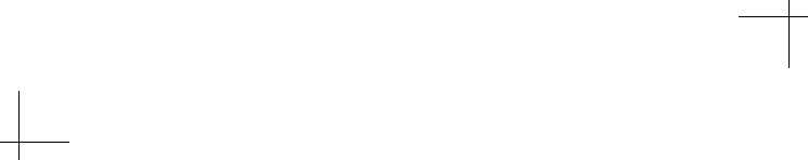
At rst, we will visit the TeX Live homepage and take a survey of the installaon possibilies.
Feel free to explore the homepage in depth to study the informaon oered there.
Open the TeX Live homepage at http://tug.org/texlive.
Chapter 1
[ 13 ]
We will cover two ways of installaon. The rst will be online and requires an Internet
connecon. The other method starts with a huge download, but may be nished oine.
Let's check out the two installaon methods.
Geng Started with LaTeX
[ 14 ]
Time for action – installing TeX Live using the net
installer wizard
We will download the TeX Live net installer and install the complete TeX Live distribuon on
our computer.
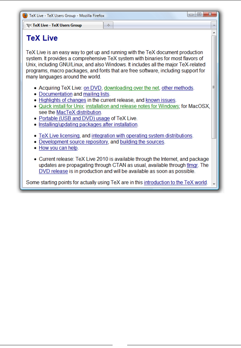
1. Click on downloading over the net or navigate to http://
tug.org/texlive/acquire-netinstall.
2. Download the net installer for Windows by clicking on install-tl.zip.
3. Extract the le install-tl.zip using your favorite archiving program.
For example, WinZip, WinRar, or 7-Zip can do it for you.
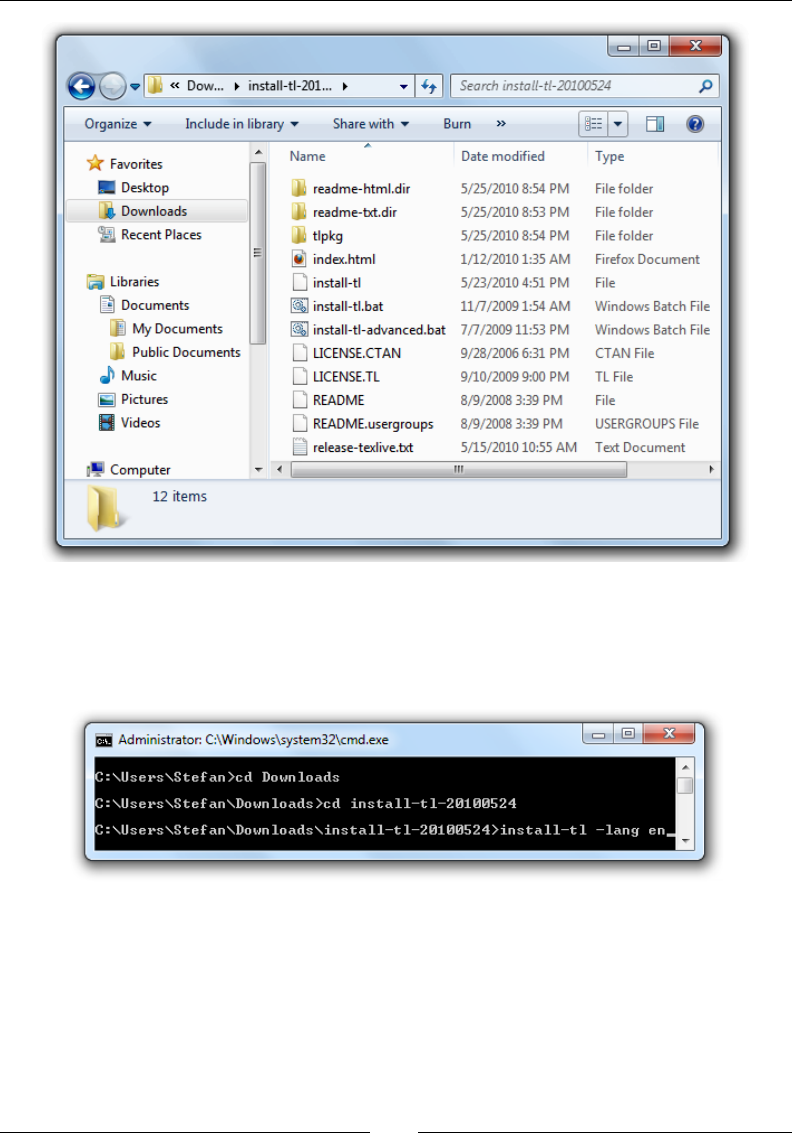
4. Open the folder install-tl-*and double-click the Windows
batch le install-tl:
Chapter 1
[ 15 ]
5. The net installer will automacally detect your language. If it's showing the
wrong language, you can force the choice of the language using the lang
opon at the command prompt such as install-tl –lang=en:
Geng Started with LaTeX
[ 16 ]
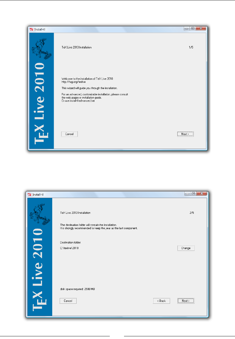
6. The installaon wizard will pop up, as shown in the following screenshot:
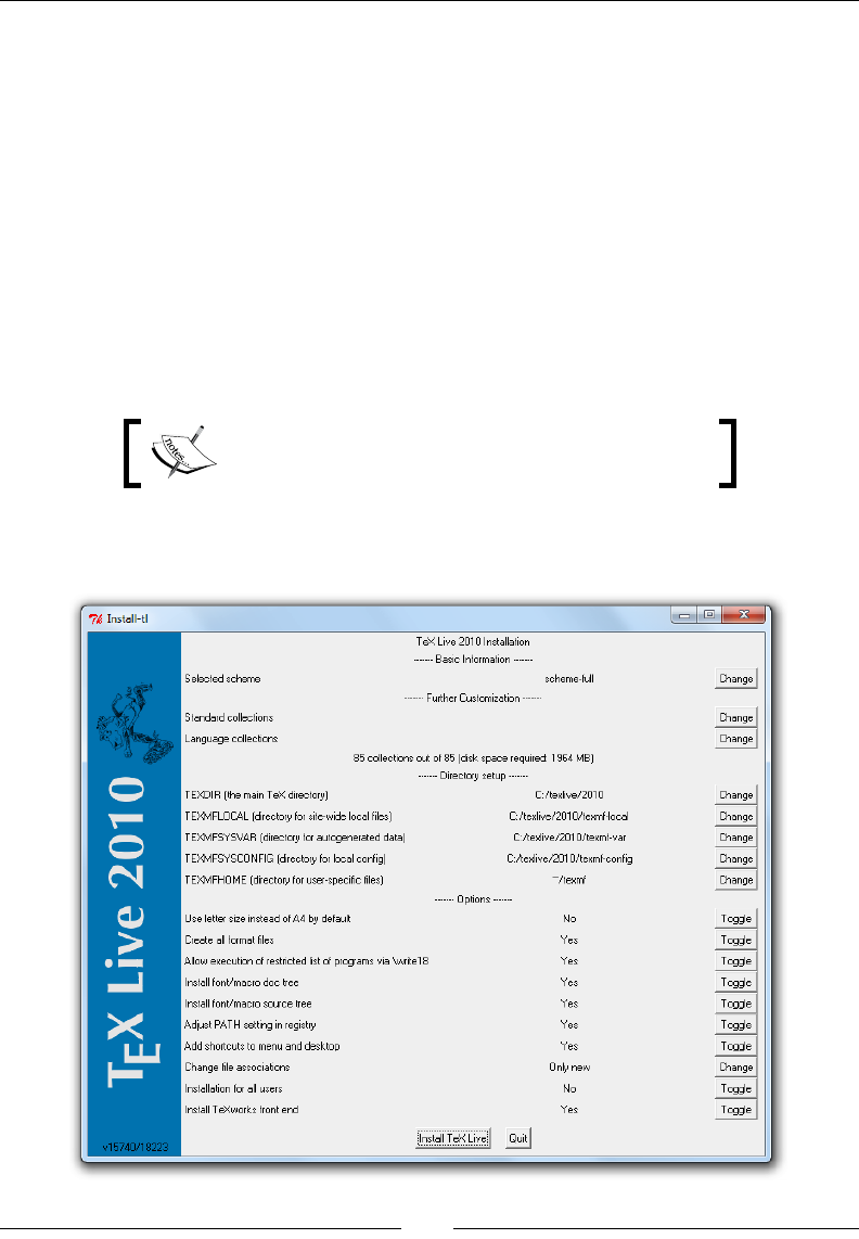
7. Click on the Next buon, now it oers to change the installaon folder, but
it's ne to retain it. In our book, we will refer to this default locaon:
Chapter 1
[ 17 ]
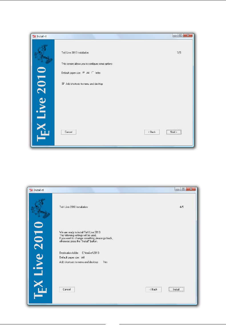
8. Click on the Next buon. As shown in the following screenshot, choose
one of the opons, for example, for the creaon of shortcuts:
9. Click on the Next buon. You can then conrm the sengs and
actually start the installaon by clicking on the Install buon:
Geng Started with LaTeX
[ 18 ]
10. The next screenshot shows how you can monitor the installaon progress:
11. Finally, click on the Finish buon and you're done.
What just happened?
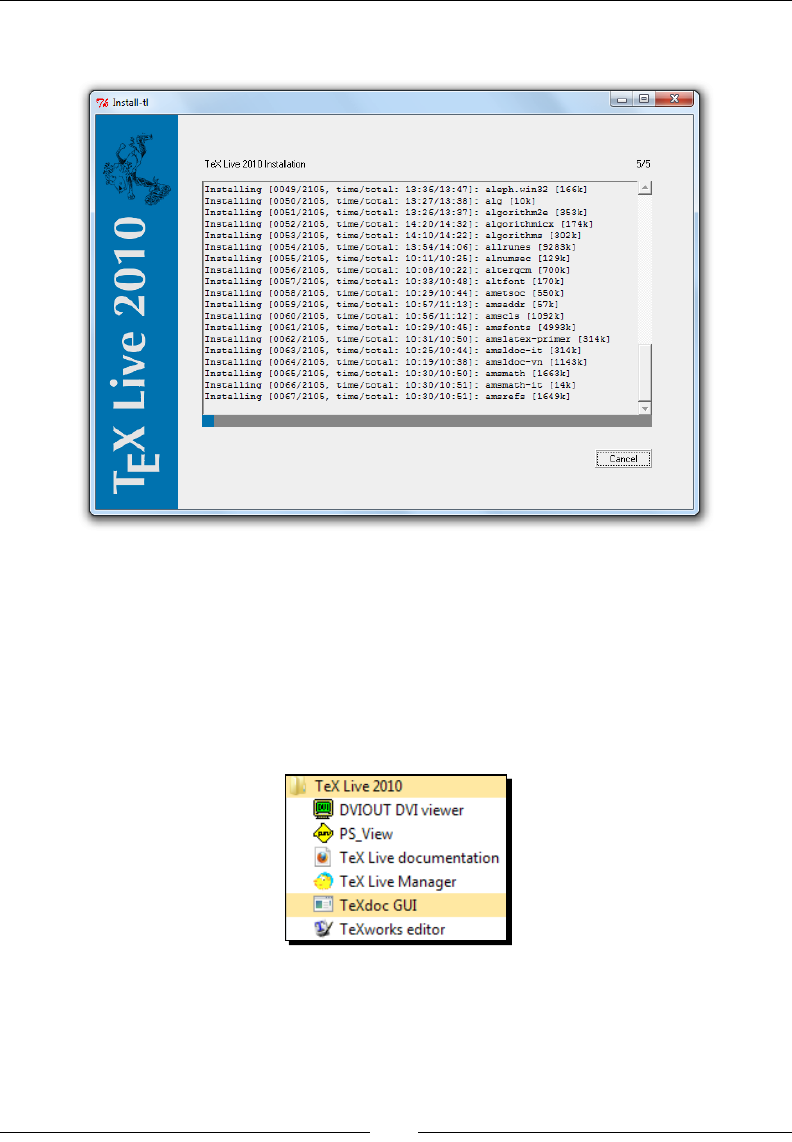
You have completed the installaon of TeX Live 2010. Now your Start menu contains
a folder called TeX Live 2010 containing six programs:
DVIOUT DVI viewer—a viewer program for the classic LaTeX output format DVI.
Today, most people choose PDF output, so you probably won't need it.
Chapter 1
[ 19 ]
PS_VIEW—a viewer program for the PostScript format; again you probably
won't need it, except if you would like to use the PostScript language or read
such documents.
TeX Live documentaon—well, that's useful regarding setup and use of your
soware!
TeX Live Manager—that's your tool for package management, for example,
installaon and update of LaTeX packages.
TeXdoc GUI—it's a graphical user interface oering access to a huge amount of
LaTeX-related informaon. There's a lot of it stored in your computer by now. Use it
to gather informaon whenever needed; it could be quicker than searching online.
TeXworks editor—this is an editor developed to create LaTeX documents
comfortably. We will make extensive use of it.
TeXworks is also shipped with MiKTeX 2.8 and higher.
If you would like to stay in control over what should be installed on your computer, start the
install-tl-advanced batch le instead of install-tl:
Geng Started with LaTeX
[ 20 ]
The TeX documentaon available online contains more informaon for advanced users.
Now, we will go through the oine installaon of TeX Live 2010.
Time for action – installing TeX Live ofine
We will download a compressed ISO image of TeX Live 2010 with a size of about 1.2
gigabytes. Aer extracon, we can choose to burn it on DVD or to extract it to our hard
disk drive and run the installaon from there:
1. Visit the download area at http://www.tug.org/texlive/acquire-iso.html.
2. Download texlive2010.xz. If possible, use a download manager,
especially if your Internet connecon is not stable.
3. Extract texlive2010.xz and you will get the le texlive2010.iso. If your
archiving program doesn't support the .xz le format, obtain, for instance, the
program 7-Zip version 9 or later from http://7zip.org and use it for extracon.
4. Either burn the ISO le on a DVD using a burning soware supporng the ISO format
or extract it to your hard disk drive. 7-Zip is also capable of doing that for you.
5. Among the extracted les or on your DVD, you will nd the installer batch les
install-tl and install-tl-advanced that we've already seen. Choose
one, start it, and go through the installaon like in the previous installaon.
What just happened?
It was similar to the rst installaon, but this me you've got all the data and you won't
need an Internet connecon. This complete download is especially recommended if it's
foreseeable that you will do another installaon of TeX Live later or if you would like to
give it to friends or colleagues.
Aer an oine installaon, it's recommended to run an update of TeX Live soon,
because packages on a DVD or within an image could already be outdated. Use
the TeX Live Manager to keep your system up-to-date if you are connected to
the Internet.
Installation on other operating systems
If you work on Mac OS X, you may download a customized version of TeX Live at http://
www.tug.org/mactex/. Download the huge .zip le and double-click on it to install.

Chapter 1
[ 21 ]
On most Linux systems, installaon is easy. Use your system's package manager. With
Ubuntu, you may use Synapc, on SUSE systems use YaST, with Red Hat a RPM frontend, and
on Debian systems use Aptude. In the respecve package manager, look out for texlive.
If you want to stay on the edge, you could download and install the most current version of
TeX Live from its homepage, instead of the version from the operang system's repositories.
But be aware that installing third party sources may harm the integrity of your system.
Now that we've prepared the ground, let's start to write LaTeX!
Creating our rst document
We have installed TeX and launched the editor; now let's jump in at the deep end by wring
our rst LaTeX document.
Time for action – writing our rst document with TeXworks
Our rst goal is to create a document that's prinng out just one sentence. We want to use it
to understand the basic structure of a LaTeX document.
1. Launch the TeXworks editor by clicking on the desktop icon or open it in the
Start menu.
2. Click on the New buon.
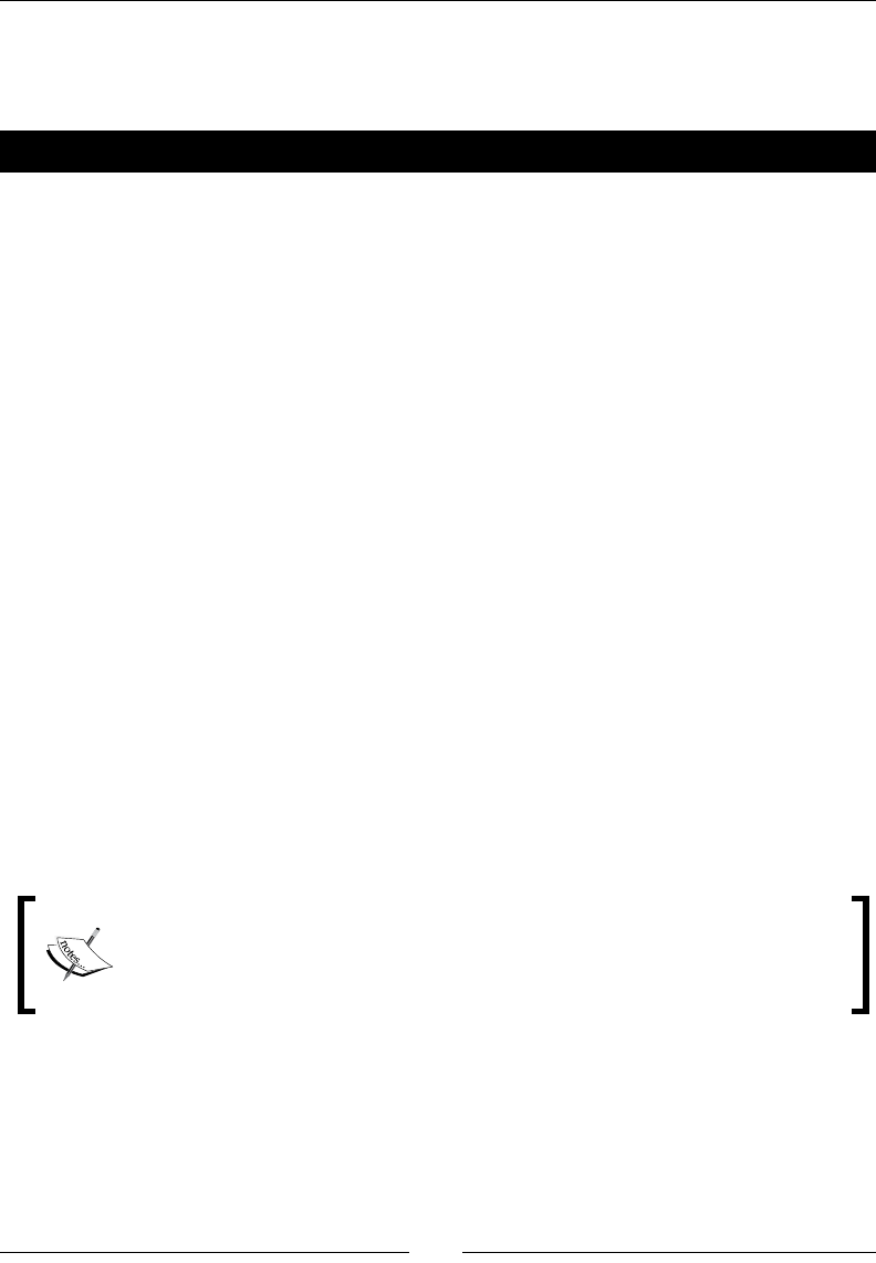
3. Enter the following lines:
\documentclass{article}
\begin{document}
This is our first document.
\end{document}
4. Click on the Save buon and save the document. Choose a locaon where
you want to store your LaTeX documents, ideally in its own folder.
Geng Started with LaTeX
[ 22 ]
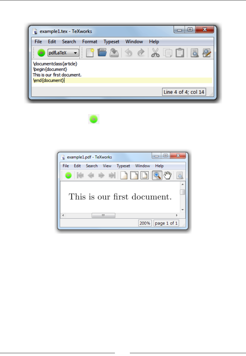
5. In the drop-down eld in the TeXworks toolbar, choose pdfLaTeX:
6. Click the Typeset buon .
7. The output window will automacally open. Have a look at it:
What just happened?
You have just seen the rst few minutes of the life of a LaTeX document. Its following hours
and days will be determined by eding, typeseng, and so on. Don't forget to save your
document frequently.
As announced in contrary to the classic word processor soware, you cannot see the eect
of changes immediately—but the result is just one click away.

Chapter 1
[ 23 ]
Have a go hero – checking out advanced LaTeX editors
Do you have experience in working with complex programs? Do you like using a feature-rich
and powerful editor? Then have a look at these LaTeX editors. Visit their websites to nd
screenshots and to read about their features:
TeXnicCenter— a very powerful editor for Windows, http://texniccenter.
org/
Kile— a user-friendly editor for operang systems with KDE, such as Linux,
http://kile.sourceforge.net/
TeXShop—an easy-to-use and very popular editor for Mac OS X, http://pages.
uoregon.edu/koch/texshop/
Texmaker—a cross-plaorm editor running on Linux, Mac OS X, Unix, and
Windows systems, http://www.xm1math.net/texmaker/
The menoned editors are free open source soware.
Summary
We learned in this chapter about the benets of LaTeX. It will be our turn to use the virtues
of LaTeX to achieve the best possible results.
Furthermore, we covered:
Installaon of TeX Live
Using the editor TeXworks
Creaon of a LaTeX document and generaon of output
Now that we've got a funconal and tested LaTeX system, we're ready to write our own
LaTeX documents. In the next chapter, we will work out the formang of text in detail.
2
Formatting Words, Lines, and
Paragraphs
In the last chapter, we installed LaTeX and used the TeXworks editor to write our
rst document. Now we will speak about the structure of a document and we
will focus on the text details and its formang.
In this chapter, we shall:
Speak about logical formang
Learn how to modify font, shape, and style of text
Use boxes to limit the text width
See how to break lines and how to improve hyphenaon
Explore juscaon and formang of paragraphs
By working with examples and trying out new features, we shall learn some basic concepts
of LaTeX. By the end of this chapter, we will be familiar with commands and environments.
You will even be able to dene your own commands.
Understanding logical formatting
In the previous chapter, we wrote a small example document. Let's extend it a bit to get an
illustrave example for understanding the typical document structure.
Formang Words, Lines, and Paragraphs
[ 26 ]
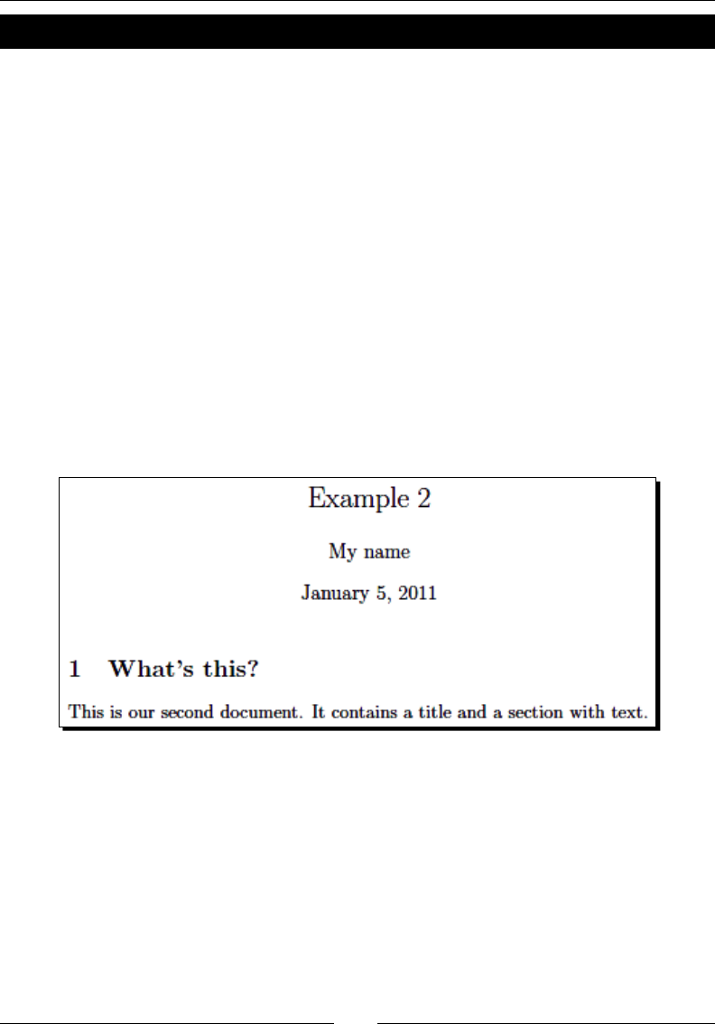
Time for action – titling your document
We will take the rst example and insert some commands that will produce a
nice-looking tle.
1. Type the following code in the editor; modify the previous example if you like:
\documentclass[a4paper,11pt]{article}
\begin{document}
\title{Example 2}
\author{My name}
\date{January 5, 2011}
\maketitle
\section{What's this?}
This is our second document. It contains a title and a section
with text.
\end{document}
2. Click the Typeset buon.
3. View the output:
What just happened?
In the rst chapter, we talked about logical formang. First, let's look at this example
from that point of view. We told LaTeX that:
Our document is of the type article. It will be printed on A4 paper using a size
of 11 points for the base font.
The tle is "Example 2".
You are the author.
The document was wrien on January 5, 2011.
Chapter 2
[ 27 ]
Concerning the content of the document:
It begins with a tle.
The rst secon shall have the heading "What's this?"
The following text is "This is our second document."
Note, we did not choose the font size of the tle or heading; neither did we make something
bold or centered. Such formang is done by LaTeX but nevertheless you're free to tell LaTeX
how it actually should look.
We did not need to press the Save buon. TeXworks automacally saves
the document if we click the Typeset buon.
Exploring the document structure
Let's look at the details. A LaTeX document doesn't stand alone—commonly the document
is based on a versale template. Such a fundamental template is called a class. It provides
customizable features, usually built for a certain purpose. There are classes for books, for
journal arcles, for leers, for presentaons, for posters, and many more; hundreds of
reliable classes can be found in Internet archives but also on your computer now, aer
you've installed TeX Live. Here we have chosen the arcle class, a standard LaTeX class
suitable for smaller documents.
The rst line starts with \documentclass. This word begins with a backslash; such a
word is called a command. We used commands to specify the class and to state document
properes: title, author, and date.
This rst part of the document is called the preamble of the document. This is where we
choose the class, specify properes, and in general, make document-wide denions.
\begin{document} marks the end of the preamble and the beginning of the actual
document. \end{document} marks the end of it. Everything that follows would be
ignored by LaTeX. Such a piece of code, framed by a \begin … \end command pair,
is called an environment.
In the actual document, we've used the command \maketitle that prints the tle, author,
and date in a nicely formaed manner. By the \section command, we produced a heading,
bigger and bolder than normal text. Then we let some text follow. What we wrote here, in
the document environment, will be printed out. On the contrary, the preamble will never
produce any output.
Let's look at commands in detail.
Formang Words, Lines, and Paragraphs
[ 28 ]
Understanding LaTeX commands
LaTeX commands begin with a backslash, followed by big or small leers. LaTeX commands
are usually named with small leers and in a descripve way. There are excepons: you will
see some commands consisng of a backslash and just one special character.
Commands may have arguments, given in curly braces or in square brackets.
Calling a command looks like the following:
\command
Or:
\command{argument}
Or:
\command[optional argument]{argument}
There could be several arguments, each of them in braces or brackets. Arguments in curly
braces are mandatory. If a command is dened to require an argument, one has to be given.
For example, calling \documentclass would be fule if we hadn't stated a class name.
Arguments in square brackets are oponal; they may be given but it's not a
must. If no oponal argument is provided, the command will use a default
one. For instance, in the rst example in Chapter 1, Geng Started with LaTeX,
we wrote \documentclass{article}. This document has been typeset
with a base font size of 10pt, because this is the class default base font size.
In the second document, we wrote \documentclass[a4paper,11pt]
{article}; this way, we replaced default values with the given values, so now
the document will be adjusted for A4 paper using a base font size of 11pt.
There are commands generang output—try \LaTeX—and commands seng properes,
changing fonts or layout. Generally, the names of commands are chosen according to their
purpose. We will have a more detailed look in this chapter, but rst let's see how LaTeX
treats what we type.
How LaTeX reads your input
Before we connue wring, let's look at how LaTeX understands what you've wrien in
the editor.
Chapter 2
[ 29 ]
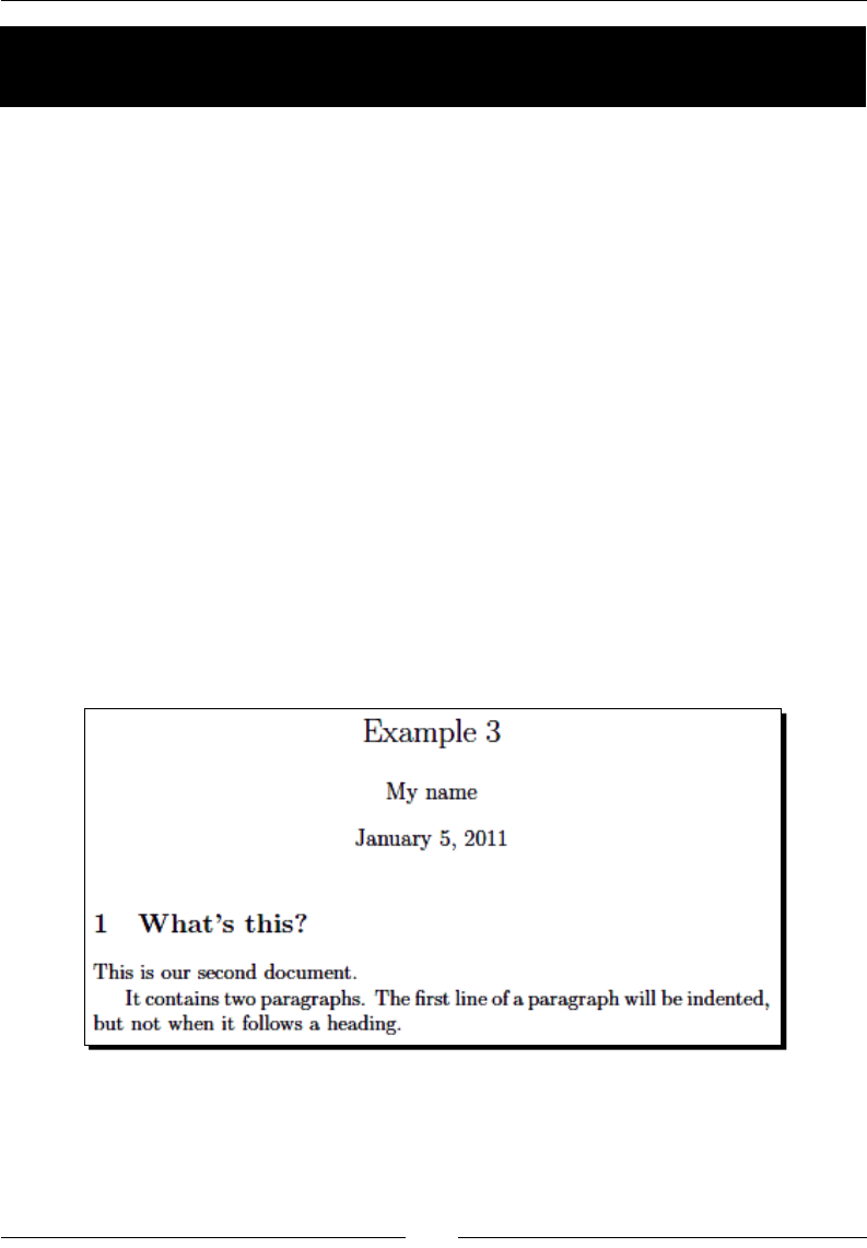
Time for action – trying out the effect of spaces, line
breaks, and empty lines
We will take the rst example and insert spaces and line breaks.
1. Modify the previous example as follows:
\documentclass[a4paper,11pt]{article}
\begin{document}
\title{Example 3}
\author{My name}
\date{January 5, 2011}
\maketitle
\section{What's this?}
This is our
second document.
It contains two paragraphs. The first line of a paragraph will be
indented, but not when it follows a heading.
% Here's a comment.
\end{document}
2. Typeset.
3. View the output:
Formang Words, Lines, and Paragraphs
[ 30 ]
What just happened?
Though we've inserted some spaces, the distances between the words in the output
remained the same. The reason is that LaTeX treats mulple spaces just like a single space.
Also, a single line break has the same eect like a single space. It doesn't maer how you
arrange your text in the editor using spaces or breaks, the output will stay the same.
A blank line denotes a paragraph break. Like spaces, mulple empty lines are treated as one.
Briey said, spaces separate words, empty lines separate paragraphs.
Commenting your source text
You've seen that the last line seems to be missing in the output. That's because the percent
sign introduces a comment. Everything following a percent sign unl the end of the line
will be ignored by LaTeX and won't be printed out. This enables you to insert notes into
your document. It's oen used in templates to inform the user what the template does at
that certain place. Note also that the end of the line, normally behaving like a space, will be
ignored aer a percent sign.
Easing experimenng by trial and error
If you want to disable a command temporarily, it may be favorable to insert a
percent sign instead of deleng the command. That way, you're able to undo this
change easily by removing the %.
If the percent sign behaves that way, what should we do if we want to write 100% in our
text? Let's gure out how to do it.
Printing out special symbols
Common text mostly contains upper and lowercase leers, digits, and punctuaon
characters. Simply type them with your editor. However, some characters are reserved for
LaTeX commands; they cannot be used directly. We already encountered such characters,
and besides the percent sign, there are the curly braces and so on. There are LaTeX
commands to print such symbols.
Chapter 2
[ 31 ]
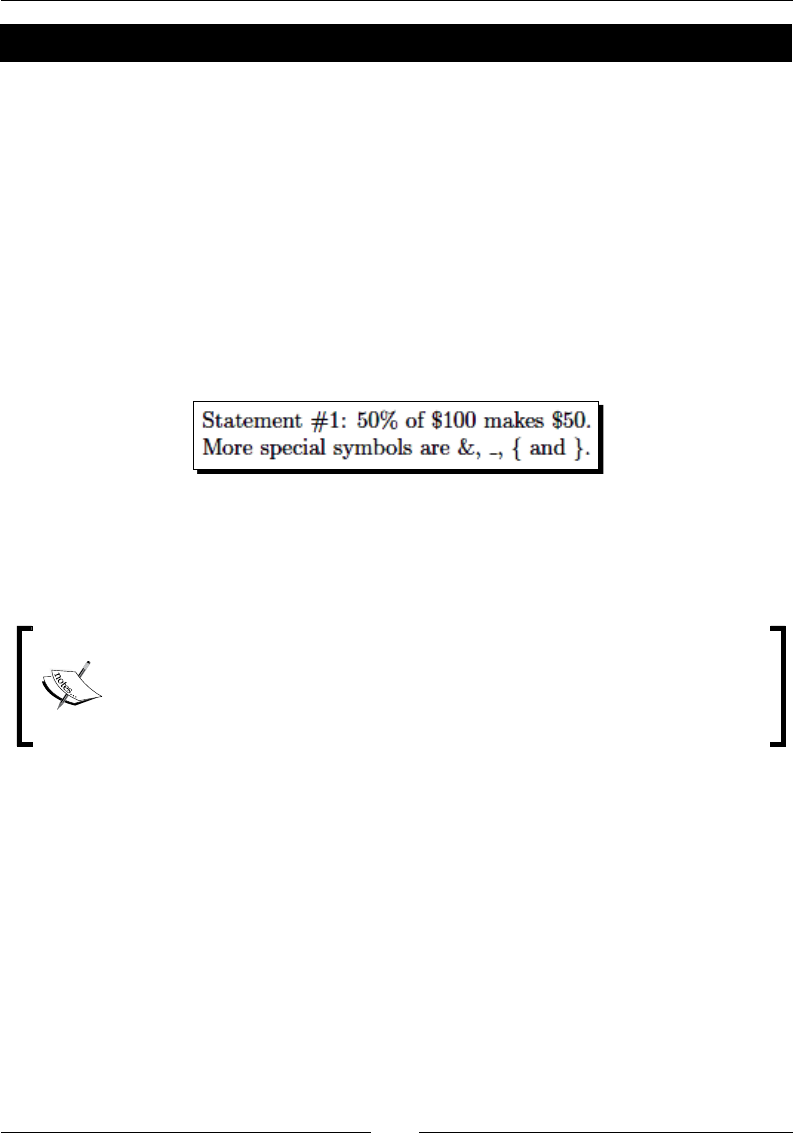
Time for action – writing special characters in our text
We will write a very short example prinng out an amount of dollars and a percent number,
then we shall try more symbols:
1. Create a new document and enter the following lines:
\documentclass{article}
\begin{document}
Statement \#1:
50\% of \$100 makes \$50.
More special symbols are \&, \_, \{ and \}.
\end{document}
2. Typeset and view the output:
What just happened?
By pung a backslash before such a special symbol, we turned it into a LaTeX command.
This command has the only purpose of prinng out that symbol.
The command for prinng a backslash is \textbackslash. If you would
like to know what \\ might be used for, it is used as a shortcut for a line break
command. That's a bit odd, but line breaks occur frequently whereas backslashes
are rarely needed in the output, therefore this shortcut has been chosen.
There's a wealth of symbols that we can use for math formulas, chess notaon, zodiac signs,
music scores, and more. We don't need to deal with those symbols for now, but we shall
return to that subject in Chapter 8, Typing Math Formulas, when we will need symbols to
typeset math formulas.
Now that we know how to enter pure text, let's nd out how we can format it.
Formatting text – fonts, shapes, and styles
LaTeX already does some formang. For example, we've seen that secon headings are
bigger than normal text and bold faced. Now we will learn how to modify the appearance
of the text ourselves.
Formang Words, Lines, and Paragraphs
[ 32 ]
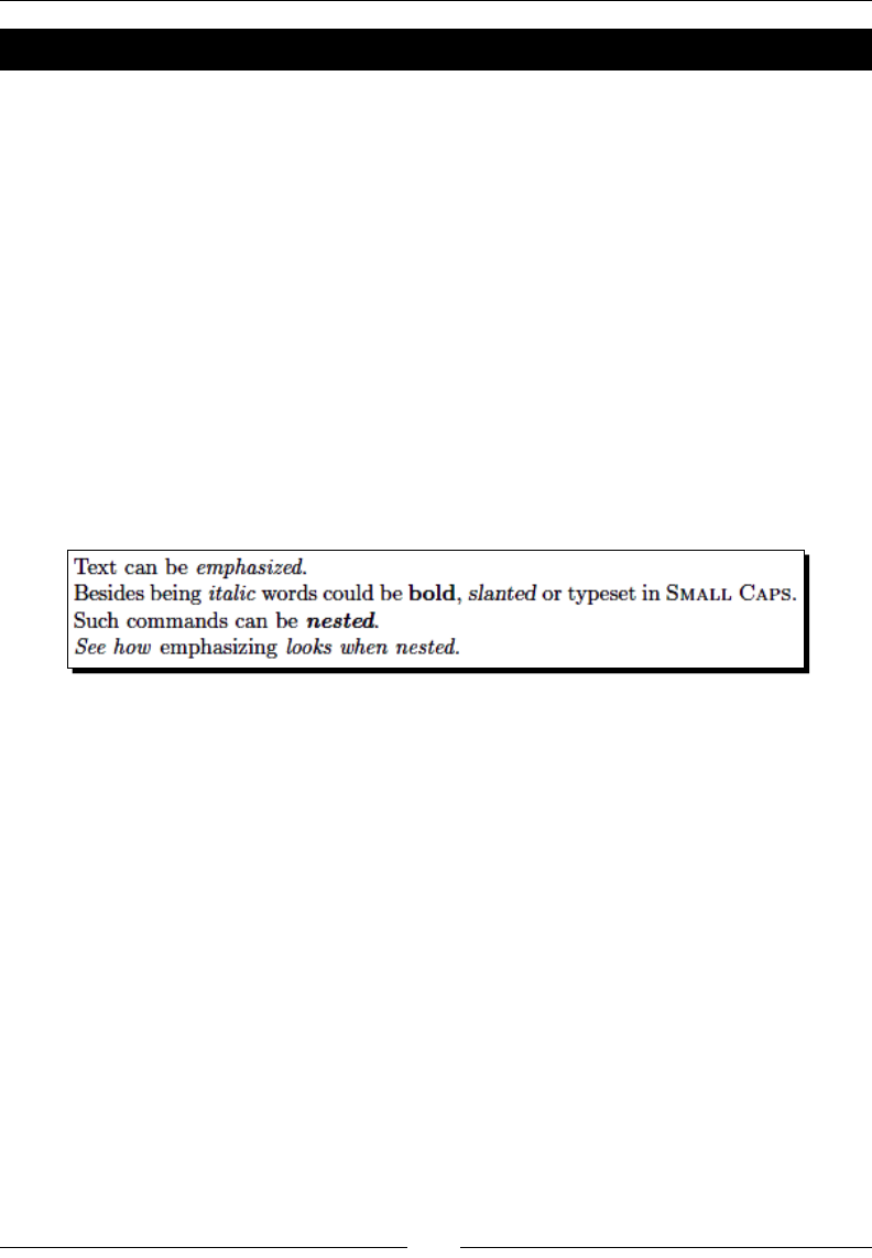
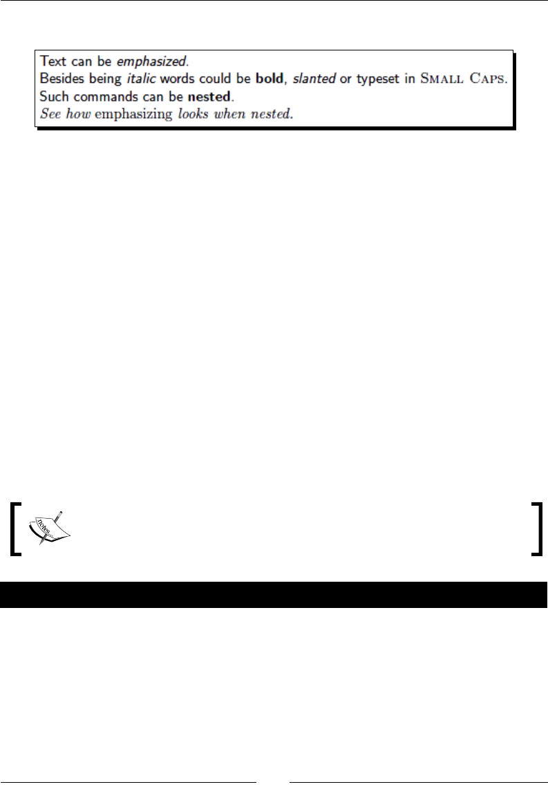
Time for action – tuning the font shape
We will emphasize an important word in a text and we will see how to make words appear
bold, italic, or slanted. We shall gure out how to highlight words in a part of some text
that's already emphasized:
1. Create a new document containing the following code:
\documentclass{article}
\begin{document}
Text can be \emph{emphasized}.
Besides being \textit{italic} words could be \textbf{bold},
\textsl{slanted} or typeset in \textsc{Small Caps}.
Such commands can be \textit{\textbf{nested}}.
\emph{See how \emph{emphasizing} looks when nested.}
\end{document}
2. Typeset and have a look at the output:
What just happened?
At rst, we used the command \emph, giving one word as an argument to this command.
This argument will be typeset in italic shape, because this is the default way how LaTeX
emphasizes text.
Text-formang commands usually look like \text**{argument}, where ** stands for a
two leer abbreviaon like bf for bold face, it for italic, and sl for slanted. The argument
will then be formaed accordingly like we've seen. Aer the command, the subsequent
text will be typeset as it was before the command—precisely aer the closing curly brace
marking the end of the argument. We checked it out.
We've nested the commands \textit and \textbf, which allowed us to achieve a
combinaon of those styles, and the text appears both italic and bold.
Chapter 2
[ 33 ]
Most font commands will show the same eect if they are applied twice like
\textbf{\textbf{words}}: the words won't become bolder. Only \emph behaves
dierently. We've seen that emphasized text will be italic, but if we use \emph onto a
piece of this text again, it will change from italic to normal font. Imagine an important
theorem completely typeset in italics—you should sll have the opportunity to highlight
words inside this theorem.
\emph is so called semanc markup, because it refers to the meaning, not just to the
appearance of text.
Emphasizing twice, such as marking bold and italic at the same
me, might be considered to be a quesonable style. Change
the font shape wisely—and consistently.
Choosing the font family
Compare the font of our examples and the standard font you see in this book. While the
LaTeX font has a decorave appearance, the text font of this book looks simple and clean.
Our code examples are dierent in another way: every leer has the same width. Let's see
how we can implement this in our wrings.
Time for action – switching to sans-serif and to typewriter fonts
Imagine that we start to write an arcle about LaTeX's Internet resources. To get a clearly
readable heading, we shall use a font without frills. The body text will contain a web address;
we choose a typewriter font to stress it:
1. Create a LaTeX document with the following code:
\documentclass{article}
\begin{document}
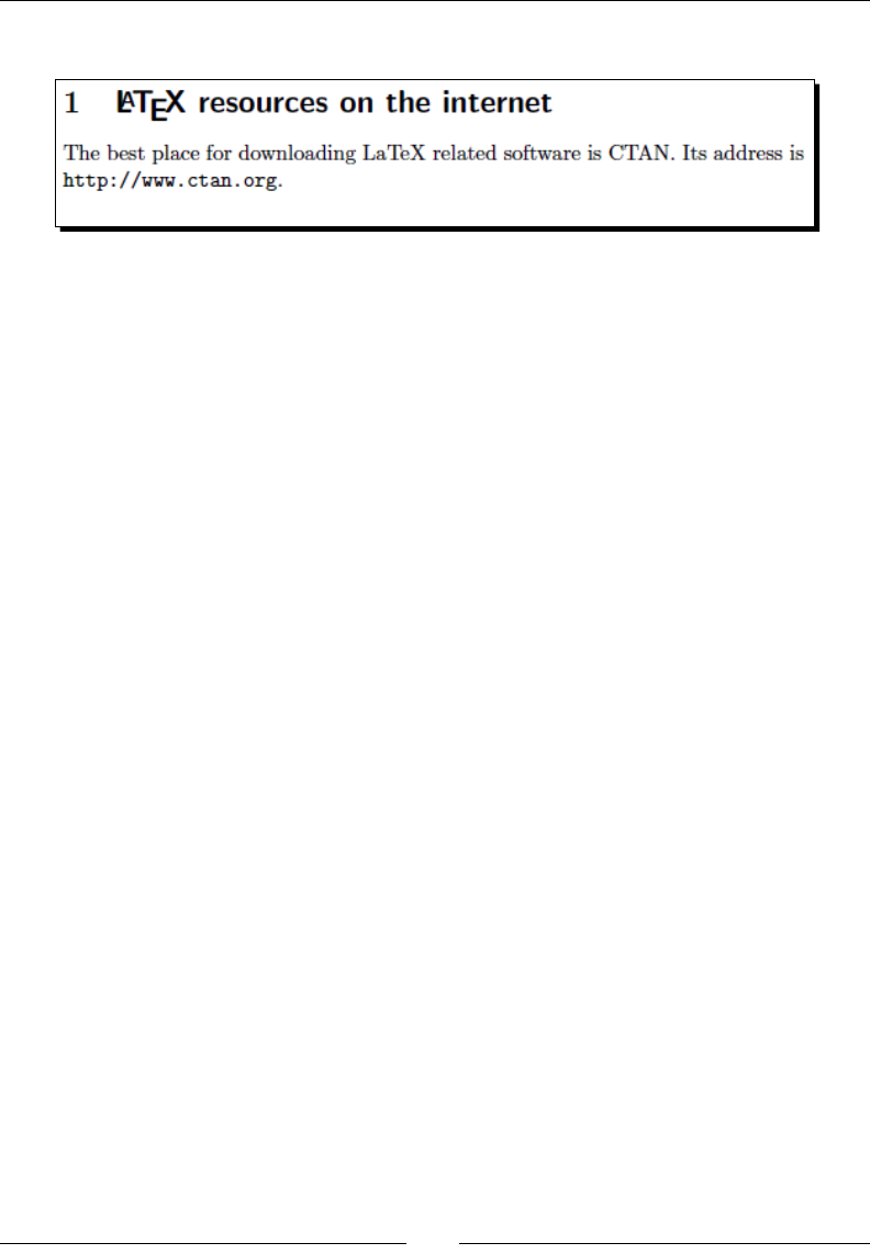
\section{\textsf{\LaTeX\ resources on the internet}}
The best place for downloading LaTeX related software is CTAN.
Its address is \texttt{http://www.ctan.org}.
\end{document}
Formang Words, Lines, and Paragraphs
[ 34 ]
2. Typeset and look at the result:
What just happened?
We encountered more font commands. By using\textsf, we've chosen the sans-serif font in
the secon heading. We used the command \texttt to get the typewriter font for the web
address. Those commands can be used just like the font commands we've learned before.
The leers in the LaTeX standard font have so-called serifs, those small decorave details
at the end of a leer's strokes. Serifs shall improve readability by leading the reader's eyes
along the line. Therefore, they are widely used in body text. Such fonts are also called
Roman fonts. This name led to the command \textrm for the Roman text—the default
font with serifs.
Headings are oen done without serifs; the used font is called a sans-serif font. Such fonts
are also a good choice for screen text because of the beer readability on lower resoluons.
So you might want to choose a sans-serif font when you produce an e-book.
If every leer of a font has the same width, the font is called monospaced or a typewriter
font. Besides, on typewriters, such fonts were used with early computers; today they are sll
preferred for wring source code of computer programs, both in print and in text editors.
So if you want to typeset a program lisng or LaTeX source code, consider using a typewriter
font. Like we did in the previous example, this book is using a typewriter font to disnguish
code and web addresses from the normal text.
Switching fonts
Pung too much text into a command's argument could be unhandy. Somemes we would
like to set font properes of longer passages of text. LaTeX provides other commands, which
work like switches.

Chapter 2
[ 35 ]
Time for action – switching the font family
We will modify the previous example using font family switching commands:
1. Modify the example to get the following code:
\documentclass{article}
\begin{document}
\section{\sffamily\LaTeX\ resources in the internet}
The best place for downloading LaTeX related software is CTAN.
Its address is \ttfamily http://www.ctan.org\rmfamily.
\end{document}
2. Typeset and compare the output to the previous one; it's the same.
What just happened?
By using the command \sffamily, we switched over to sans serif font. This change has
been made inside an argument, so it's valid only there.
We used the command \ttfamily to switch to a typewriter font. The typewriter font will
be used from this point onwards. By using\rmfamily, we returned to Roman font.
These commands don't produce any output, but they will aect the following text. We will
call such a command a declaraon.
Now have a closer look at the secon number: it's a digit with serifs, which doesn't match
the remaining sans-serif heading. Moreover, changing the font within a\section command
feels wrong—and rightly so! The beer way is to declare the secon heading font once for
the complete document. We will learn how to globally modify heading fonts in Chapter 11,
Enhancing Your Documents Further, aer we prepared some more tools.
Formang Words, Lines, and Paragraphs
[ 36 ]
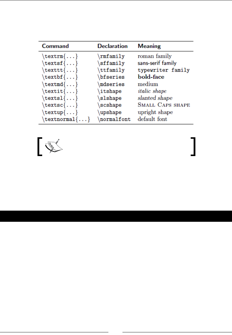
Summarizing font commands and declarations
Let's list the font commands and their corresponding declaraons together with
their meanings:
The corresponding declaraon to \emph is \em.
Delimiting the effect of commands
In the previous example, we've reversed the eect of \ttfamily by wring \rmfamily. To
be safe, we could write \normalfont to switch back to the base font. However, there's an
easier way.
Time for action – exploring grouping by braces
We shall use curly braces to tell LaTeX where to apply a command and where to stop that:
1. Modify our rst font shape example to get this code:
\documentclass{article}
\begin{document}
{\sffamily
Text can be {\em emphasized}.
Besides being {\itshape italic} words could be {\bfseries bold},
{\slshape slanted} or typeset in {\scshape Small Caps}.
Such commands can be {\itshape\bfseries nested}.}
{\em See how {\em emphasizing} looks when nested.}
\end{document}
Chapter 2
[ 37 ]
2. Typeset and check out the output:
What just happened?
We started with an opening curly brace. The eect of the following command \sffamily
lasted unl we stopped it with the corresponding closing brace. That closing brace came
at the end of the highlighted code. This highlighng shows the area of the code where
\sffamily is valid.
We replaced every font command by the corresponding declaraon. Remember, \em is
the declaraon version of \emph. Further, we surrounded every declaraon and the
aected text by curly braces.
An opening curly brace tells LaTeX to begin a so called group. The following commands
are valid for the subsequent text unl a closing curly brace appears causing LaTeX to stop
using the commands or declaraons wrien in this group. Till a command is valid, that's
called its scope.
Groups can be nested as follows:
Normal text, {\sffamily sans serif text {\bfseries and bold}}.
We have to be careful to close each group; opening and closing braces should match.
Braces which enclose an argument of a command don't form a group. Together
with the argument, these braces are gobbled by the command. If necessary, use
addional braces.
Time for action – exploring font sizes
We will try out every font size available by LaTeX's default font size commands. For tesng,
we exceponally use them in the body text—their main use is in the macro denions:
1. Create a document with the following code:
\documentclass{article}
\begin{document}
\noindent\tiny We \scriptsize start \footnotesize \small small,
\normalsize get \large big \Large and \LARGE bigger,
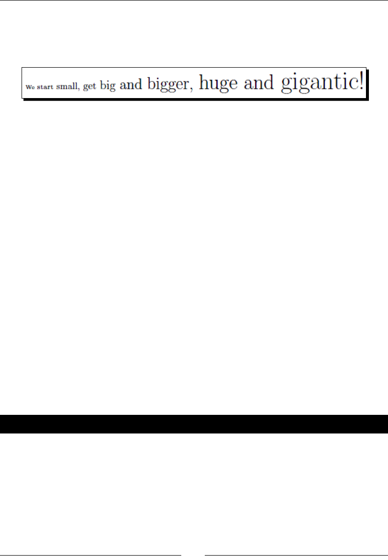
Formang Words, Lines, and Paragraphs
[ 38 ]
\huge huge and \Huge gigantic!
\end{document}
2. Typeset and observe the output:
What just happened?
At rst, we used \noindent. This command suppresses the paragraph indentaon. Then we
used all 10 available size declaraons, starng small with \tiny and ending really big with
\Huge. There are no corresponding commands taking arguments, so we would have to use
curly braces to delimit their scope, as we learned to before.
The actual resulng font size depends on the base font. If your document has a base font
of 12 pt, then \tiny would result in text bigger than with a base font of 10 pt. We have to
see it in relaon. Use \footnotesize, if you wish to get the same size like LaTeX uses for
footnotes; use \scriptsize, if you create a style with a size matching LaTeX subscripts and
superscripts. It's sll a kind of logical formang though they are quite low-level commands.
Normally, font size declaraons are used only in denions of macros in the preamble, just
as it does apply to the other font commands. You will rarely encounter font size or shape
commands in good body texts, except freely designed passages like tle pages—and test
examples like the ones here.
Using environments
When you use several declaraons and you group them by curly braces, will you always
know which closing brace matches which of the previously entered declaraons? An
environment forms a group. Using an environment instead of just curly braces improves
the readability of your code.
Time for action – using an environment to adjust the font size
We will produce a tle with a larger and bigger font:
1. Create another small document with this code:
\documentclass{article}
\begin{document}
\begin{huge}
\bfseries
A small example
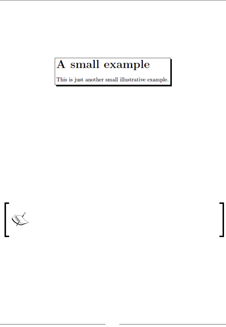
Chapter 2
[ 39 ]
\end{huge}
\bigskip
This is just another small illustrative example.
\end{document}
2. Typeset to see the result:
What just happened?
By wring \begin{huge}, we told LaTeX to switch to a huge font size just like with the
\huge command. \end{huge} informs LaTeX that this size change should end now.
From this point onwards, the font size is the same as before \begin{huge}.
Inside this environment, we use the declaraon \bfseries. Note that the eect of this
declaraon ended together with the end of the environment.
The empty line before \end{huge} denotes a paragraph break. Using the command
\bigskip, we skipped some space vercally.
For every declaraon there's a corresponding environment carrying the same name except
the backslash. Using environments instead of braces might make complex code easily
understandable.
Commonly it's advisable to end the paragraph before a font size change, not
aer it. That's because TeX calculates the interline spacing depending on the
current font size when it reaches the end of the paragraph. That's the reason we
used the blank line before \end{huge} instead of aerwards.
Saving time and effort – creating your own commands
If you're frequently using the same term in your document, it would be annoying to type
it again and again. What if you later decided to change that term or its formang? To
avoid searching and replacing in the whole document, LaTeX allows you to dene your
own commands in your preamble. They are also called macros. Give it a name. Later in the
document you just need to use this name whenever you want to change this term. We need
to do it just once in the macro denion. This will aect the whole document. Let's see how
it works.
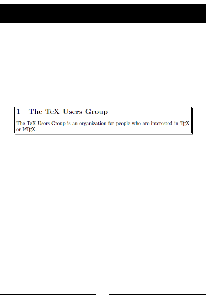
Formang Words, Lines, and Paragraphs
[ 40 ]
Time for action – creating our rst command using it as an
abbreviation
We will dene a short command prinng out the name of the TeX Users Group:
1. Type this code into a new document:
\documentclass{article}
\newcommand{\TUG}{TeX Users Group}
\begin{document}
\section{The \TUG}
The \TUG\ is an organization for people who are interested in
\TeX\ or \LaTeX.
\end{document}
2. Typeset and look at the result:
What just happened?
\newcommand in the highlighted line denes our command. The rst argument is the name
we chose for it, and the second argument is the text we want it to put out in the document.
Now, whenever we type \TUG in our document, the complete name will appear. If we later
decide to change the name or its formang, we just need to change this \newcommand line.
Then it will be applied for the complete document.
You may use formang commands inside your command denion. Let's say you would
like to change the formang of all occurrences of this name to be typeset in small caps;
just change the denion to the following:
\newcommand{\TUG}{\textsc{TeX Users Group}}
You have also seen that we've used the command \TeX. This command just prints out the
name of the basic typeseng system formaed like in its logo. It's an abbreviaon command
like we've wrien now and \LaTeX works similarly. Note that we had to use a backslash
aer \TeX! The following space would just separate the command from the following text;
it won't produce a space in the output. Using the backslash followed by a space forces the
output of the space that would otherwise be ignored. You may try oming that backslash to
be convinced.
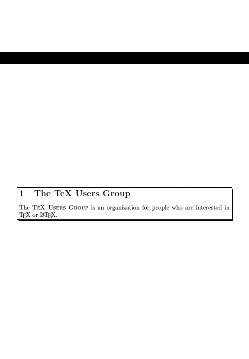
Chapter 2
[ 41 ]
Gentle spacing after commands
A backslash following a command could easily be forgoen. Can't we modify the command
in order to automate that? Tasks like this, which aren't supported by LaTeX directly, could be
solved by using packages. These are collecons of styles and commands.
Time for action – adding intelligent spacing to command output
We will load the package xspace. Its only purpose is to fulll this need.
1. Modify the previous example to get the following code:
\documentclass{article}
\usepackage{xspace}
\newcommand{\TUG}{\textsc{TeX Users Group}\xspace}
\begin{document}
\section{The \TUG}
The \TUG is an organization for people who are interested in \TeX\
or \LaTeX.
\end{document}
2. Typeset, see that the spacing between the words is correct, even without
the backslash:
What just happened?
\usepackage{xspace} tells LaTeX to load the package called xspace and to read in all
of its denions. From now on we may use all commands contained in that package. This
package provides the command \xspace that inserts a space depending on the following
character: If a dot, a comma, an exclamaon, or a quotaon mark follows, it won't insert a
space, but if a normal leer follows, then it will. Usually, that's exactly what we want.
Formang Words, Lines, and Paragraphs
[ 42 ]
Imagine you've menoned the TUG several mes in your document and now you've got
the idea to use the TeX logo style in its name. There's no need for changes in the document.
Now only the command in the preamble needs adjustment:
\newcommand{\TUG}{\textsc{\TeX\ Users Group}\xspace}
The heading in our last example doesn't contain small caps—have you seen it?
Not all font properes can be combined, depending on the chosen font. For
instance, fonts with small caps together with variaons like bold and italic are
rare. Therefore, some people even fake small caps if they don't want to change
to a more complex font.
By dening and using commands, you can ensure that the formang remains consistent
throughout your whole document.
Creating more universal commands – using arguments
Imagine that your text contains a lot of keywords that you want to be printed in bold. If you
use the \textbf{} command on all the keywords, what would happen if you later decide
to use an italic shape instead or a typewriter font? You would have to change that formang
for each keyword. There's a beer way: dening your own macro and using \textbf{} only
inside that.
Time for action – creating a macro for formatting keywords
We will use \newcommand again, but this me we will introduce a parameter that will
contain our keyword. Let's just use it on some terms that we've got to know in this chapter:
1. Type this code example:
\documentclass{article}
\newcommand{\keyword}[1]{\textbf{#1}}
\begin{document}
\keyword{Grouping} by curly braces limits the
\keyword{scope} of \keyword{declarations}.
\end{document}
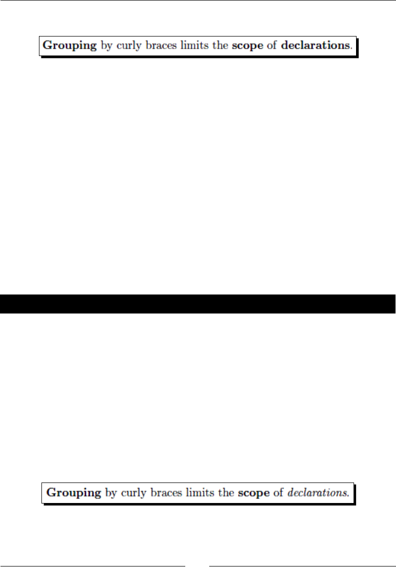
Chapter 2
[ 43 ]
2. Typeset and noce the look of the keywords in the output:
What just happened?
Let's look at the highlighted line in the code. The number 1 in the square brackets marks the
number of arguments that we want to use in the command. #1 will be replaced by the value
of the rst argument. #2 would refer to a second argument, and so on.
Now if you want to modify the appearance of all keywords to be italic, just modify the
denion of \keyword and the change will be global.
Using optional arguments
In one preceding example, we've used \newcommand with two arguments. In the previous
example, there were three arguments. The addional argument has been put in square
brackets. That's the way we mark oponal arguments: those arguments may be given or
may be omied. If omied, they would have a default value. We've already noced that
with the \documentclass command. But how can we dene a command with oponal
arguments ourselves?
Time for action – marking keywords with optional formatting
We will use \newcommand another me, this me with an oponal parameter concerning
the formang and a mandatory argument for the keyword:
1. Modify the previous example to get this code:
\documentclass{article}
\newcommand{\keyword}[2][\bfseries]{{#1#2}}
\begin{document}
\keyword{Grouping} by curly braces limits the
\keyword{scope} of \keyword[\itshape]{declarations}.
\end{document}
2. Typeset and check out the result:

Formang Words, Lines, and Paragraphs
[ 44 ]
What just happened?
Let's look again at the bold marked line in the code. By using [\bfseries], we introduced
an oponal parameter. We refer to it with #1. Its default value is \bfseries. Since we used
a declaraon this me, we added a pair of braces to ensure that only the keyword is aected
by the declaraon.
Later in the document, we gave [\itshape] to \keyword, changing the default formang
to italics.
Here's the denion of the\newcommand:
\newcommand{command}[arguments][optional]{definition}
command The name of the new command, starng with a backslash followed by lowercase
and/or uppercase leers or a backslash followed by a single non-leer symbol.
That name must not be already dened and is not allowed to begin with \end.
arguments An integer from 1 to 9, the number of arguments of the new command. If
omied, the command will have no arguments.
optional If this is present, then the rst of the arguments would be oponal with a default
value given here. Otherwise all arguments are mandatory.
definition Every occurrence of the command will be replaced by definition and every
occurrence of the form #n will then be replaced by the nth argument.
\newcommand is our key to introduce logical formang. We should avoid using LaTeX
font commands inside the document—you are on the right track if they appear only in the
preamble of the document. Use \newcommand to create styles for keywords, code snippets,
web addresses, names, notes, informaon boxes, or dierently emphasized text. How did we
achieve the consistent structure of this book? Using styles is the key!
Pop quiz – commands
1. Imagine your document contains some addresses of websites. Let's say we want
them to be typeset in typewriter font. According to this book, which of the following
possibilies would be the best way to print out, for instance, http://ctan.org?
a. \texttt{http://ctan.org}
b. {\ttfamilyhttp://ctan.org}
c. \newcommand{\CTAN}{\texttt{http://ctan.org}} in the preamble
and \CTAN in the body text
d. \newcommand{\site}[1]{\texttt{#1}} and \newcommand{\CTAN}
{http://ctan.org} in the preamble and \site{\CTAN} in the body text
Chapter 2
[ 45 ]
2. Which kind of punctuaon marks are used to enclose oponal arguments?
a. Parentheses: ()
b. Square brackets: []
c. Curly braces: {}
Have a go hero – saving effort using optional arguments
Most website addresses begin with http://. But there are sites that dier—some may
start with ftp://, so called FTP server, some sites begin with https://, so called secure
web server. Visit, for instance, ftp://ctan.org, and you will enter a le server instead
of a web server.
Extend the denion of \site of our last pop quiz. Introduce an oponal argument
denong the protocol of the site, that is, how the address starts. Default should start with
http://. It shall work like the following:
\site{www.tug.org} prints out http://www.tug.org in typewriter font
\site[ftp]{ctan.org} prints out ftp://ctan.org in typewriter font
Web addresses in texts
There's a package called url designed for typeseng web addresses.
Write \usepackage{url} in your preamble; this will provide the
command \url. This command takes an address for the argument and
will print it out with typewriter font. Furthermore, it is able to handle
special characters in addresses like underscores and percent signs. It even
enables hyphenaon in addresses, which is useful for websites with a very
long name.
Using boxes to limit the width of paragraphs
We won't always write the text just from le to right over the complete text width.
Somemes, we'd like a paragraph to have a smaller width, for instance, when we would
like to put text and a picture side-by-side.
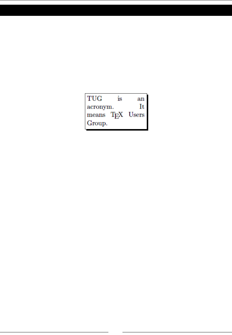
Formang Words, Lines, and Paragraphs
[ 46 ]
Time for action – creating a narrow text column
We would like to explain the acronym TUG in a text column of only 3 cm width:
1. Create a new document containing these four lines:
\documentclass{article}
\begin{document}
\parbox{3cm}{TUG is an acronym. It means \TeX\ Users Group.}
\end{document}
2. Typeset and take a crical look at the output:
What just happened?
We used the command \parbox to create a column. We stated the width of 3 cm in the
rst argument and the contained text in the second argument to \parbox.
\parbox takes the argument text and formats the output to t the specied width. We
see that the text is fully jused. Our example shows an obvious problem: insisng on full
juscaon could lead to undesirable big gaps in the text. Possible soluons are:
Introducing hyphenaon: the word acronym could easily be divided
Improving juscaon: LaTeX could do beer
Giving up full juscaon: narrow text could look beer when it's only le jused
We will check out all of these opons. But rst, let's see how \parbox is working.
Common paragraph boxes
Usually we just need a text box with a certain width; occasionally we would like to have
some addional alignment to the surrounding text. So the common denion of the
\parbox command is:
\parbox[alignment]{width}{text}
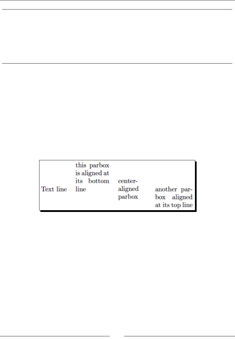
Chapter 2
[ 47 ]
alignment Oponal argument for the vercal alignment. State t to align at the top line of
the box; write b to align at its boom line. The default behavior is to place the
box such that its center is in line with the center of the current text line.
width The width of the box. It can be given for example in ISO units like 3 cm, 44 mm,
or 2 in.
text The text that you want to put in that box. It should be a short piece of common
text. For complicated contents, we will get to know other methods.
Here's a demonstraon of the eect of the alignment parameters:
\documentclass{article}
\begin{document}
Text line
\quad\parbox[b]{1.8cm}{this parbox is aligned at its bottom line}
\quad\parbox{1.5cm}{center-aligned parbox}
\quad\parbox[t]{2cm}{another parbox aligned at its top line}
\end{document}
The command \quad produces some space; we used it to separate the boxes a bit. Here's
the output:
From now on we will call such a box a parbox.

Formang Words, Lines, and Paragraphs
[ 48 ]
Have a go hero – exploring further features of \parbox
\parbox is capable of doing even more. Here's the complete denion:
\parbox[alignment][height][inner alignment]{width}{text}
height If this oponal argument isn't given, the box will have just the natural
height of the text inside. Use this argument if you want to change the
height of the box to make it bigger or smaller.
inner alignment Especially, if the height of the box is dierent to the natural height of
the contained text, you might want to adjust the text posion. The
argument means:
c—vercally center the text in the box
t—place text at the top of the box
b—place text at its boom
s—stretch the text vercally if possible
If you omit this argument, the alignment argument will be
used here as the default value.
Take our previous demonstraon example and try the eect of the oponal arguments. Use
the command \fbox that helps to visualize the eect; if you write \fbox{\parbox[...]
{...}{text}}, the complete parbox will be framed.
Boxes containing more text
Parboxes are suitable for boxes with only a lile text inside. In case of a box containing
a large amount of text, the closing brace could easily be forgoen or overlooked. The
minipage environment would then be a beer choice.
Time for action – using the minipage environment
We will use the minipage environment instead of \parbox to get a text with a width of just
3 cm.
1. Modify the parbox example to get the following code:
\documentclass{article}
\begin{document}
\begin{minipage}{3cm}
TUG is an acronym. It means \TeX\ Users Group.
\end{minipage}
\end{document}
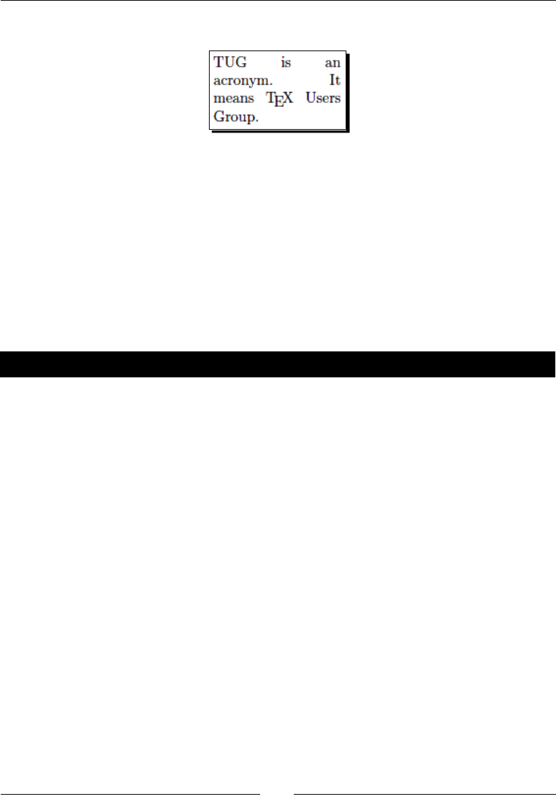
Chapter 2
[ 49 ]
2. Typeset and look at the output:
What just happened?
By using\begin{minipage}, we started a "page in a page". We specied the width of 3cm
by the mandatory argument. From this point onwards, the text lines will have a width of
3cm. They will be automacally wrapped and fully jused. We ended this restricon with
\end{minipage}. Any text typed aerwards would run over the complete body text width.
Note: There won't be a page break in such a "minipage".
Have you been a hero struggling with the \parbox and all of its oponal arguments? The
minipage environment accepts all those arguments as well with the same meaning.
Have a go hero – creating a footnote inside a minipage
Of course, LaTeX supports footnotes. You guessed it right—the corresponding command is
called \footnote{text}. Try it in one of our examples. You will get a footnote mark inside
the text and the text of the footnote will be put into the boom of the page.
A minipage is like a small page inside a normal page. Think of using a footnote inside
such a "page"; do you want to see the footnote text inside this small page? The minipage
environment supports it, just try it—use \footnote inside the minipage in the previous
example.
Understanding environments
LaTeX environments are started with \begin and ended with \end. Both commands require
the name of the environment as their argument.
Simple environments look like the following:
\begin{name}
…
\end{name}
Such environments can be used for each declaraon called \name.

Formang Words, Lines, and Paragraphs
[ 50 ]
Like commands, environments may also have arguments. Exactly like in the case of
commands, mandatory arguments are wrien in curly braces and oponal arguments in
square brackets. So you will encounter:
\begin{name}{argument}
…
\end{name}
And:
\begin{name}[optional argument]{argument}
…
\end{name}
Environments are like declaraons with a built-in scope. With \begin, the environment
introduces a change in layout, font, or other properes. There must be an\end command,
where this change will be canceled. The eect of the environment name is delimited to the
piece of code between \begin{name} and \end{name}.
Furthermore, the eect of all local declaraons used inside an environment will end together
with the surrounding environment.
Breaking lines and paragraphs
Generally, when you're wring text, you don't need to care about the line wrapping.
Just type the text with your editor; LaTeX will make it t to the line and take care of the
juscaon. If you want to begin a new paragraph, in consequence of geng a line break
in the output, just insert an empty line before you connue with your text.
Now we will nd out how to control the line wrapping. First we will see how to improve the
automac line breaking. Then we will learn commands to insert breaks directly.
Improving hyphenation
If you look at longer texts, you will noce that it's outstanding how the text is fully jused
by LaTeX and how the spacing between words is evenly distributed on the lines. If necessary,
LaTeX will divide words and put hyphens at the end of the line in order to break the lines in a
beer way. LaTeX already uses very good algorithms to hyphenate words, but it may happen
that it can't nd an acceptable way to divide a word. The previous example pointed out this
problem: breaking the word acronym would improve the output, but LaTeX does not know
where to divide it. We shall nd out how to solve that.
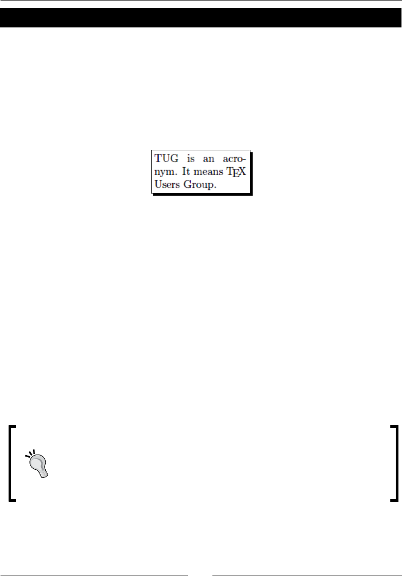
Chapter 2
[ 51 ]
Time for action – stating division points for words
No maer how good the juscaon skill is, text in very narrow columns is extremely hard
to jusfy. The previous example showed it piless. We will tell LaTeX how a word could be
divided:
1. Insert the following line into the preamble of the previous example:
\hyphenation{acro-nym}
2. Typeset and look at the output:
What just happened?
We've told LaTeX that the word acronym may have a division point between acro and nym.
That means a hyphen might be put aer acro at the end of the line and nym goes to the
following line.
The \hyphenation command tells LaTeX where the division points of a word may be. Its
argument may contain several words separated by spaces. For each word, we can indicate
several points. For instance we could extend the argument by more division points and more
word variants like this:
\hyphenation{ac-ro-nym ac-ro-nym-ic a-cro-nym-i-cal-ly}
You could also indicate division points in the body text by inserng a backslash followed
by a hyphen, like ac\-ro\-nym. But if you do it in the preamble, you'll collect all rules
there and they will be used consistently. Use it especially in the rare cases when LaTeX's
automaon fails.
Prevenng hyphenaon
If you want to prevent the hyphenaon of a certain word at all, there are two
ways: either declare it in the preamble by using it in the \hyphenation
argument without any division points, like \hyphenation{indivisible},
or you protect it inside the text using the \mbox command: The following
word is \mbox{indivisible}.
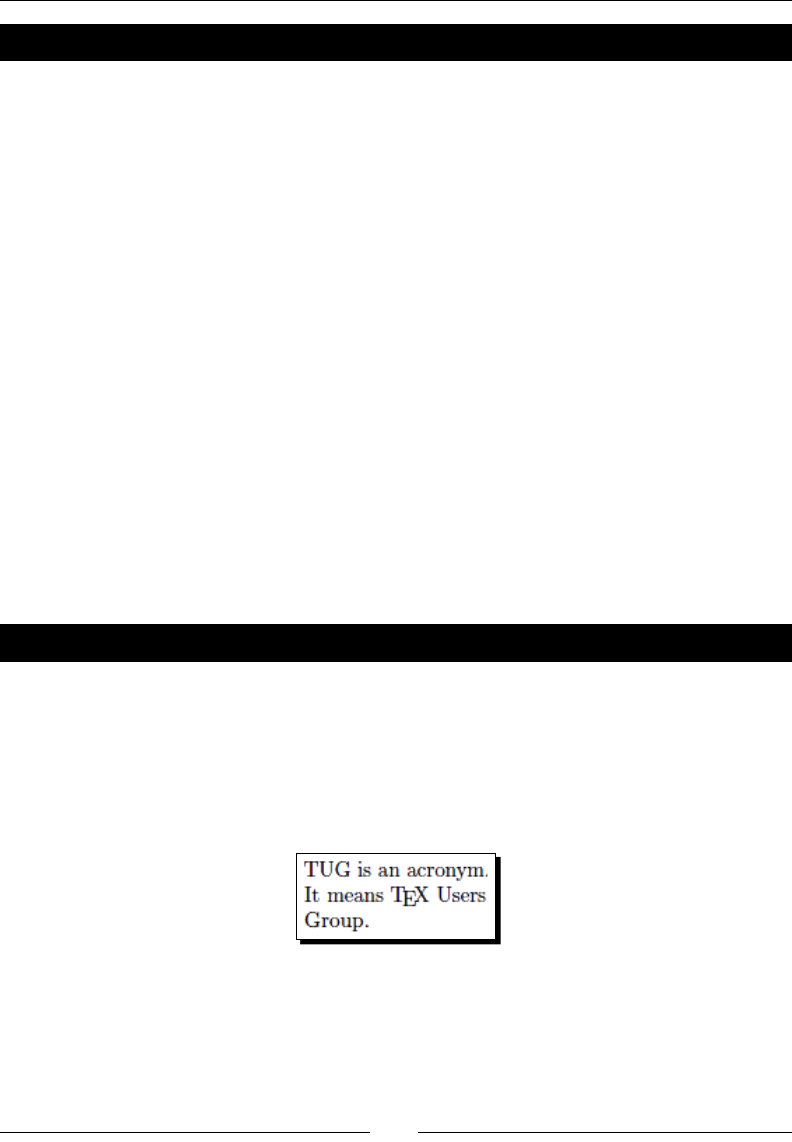
Formang Words, Lines, and Paragraphs
[ 52 ]
Have a go hero – exploiting the hyphenat package
The hyphenat package extends the possibilies:
\usepackage[none]{hyphenat} prevents hyphenaon throughout the
document.
\usepackage[htt]{hyphenat} enables hyphenaon for typewriter text.
Otherwise such monospaced fonts won't be hyphenated by LaTeX.
Such oponal arguments to \usepackage are called package opons. They congure the
behavior of a package. The menoned opons may be combined, separated by commas.
Even if you don't use the opon none, you can disable hyphenaon for short pieces of text
using the command \nohyphens{text}. Try out these features if you want to prot from
them. The package documentaon explains more features that you might need somemes,
such as hyphenaon aer special characters like numerals and punctuaon characters—TeX
would not break there.
Improving the justication further
Today's most popular TeX compiler is pdfTeX, which directly produces PDF output. When
Hàn Thế Thành developed pdfTeX, he extended TeX by micro-typographic capabilies. When
we typeset directly to PDF, we're actually using pdfLaTeX and we can benet from the new
features by using the microtype package.
Time for action – using microtype
We will improve our previous example by loading the microtype package:
1. Insert the following line into the preamble of the previous example:
\usepackage{microtype}
2. Typeset and look at the output:
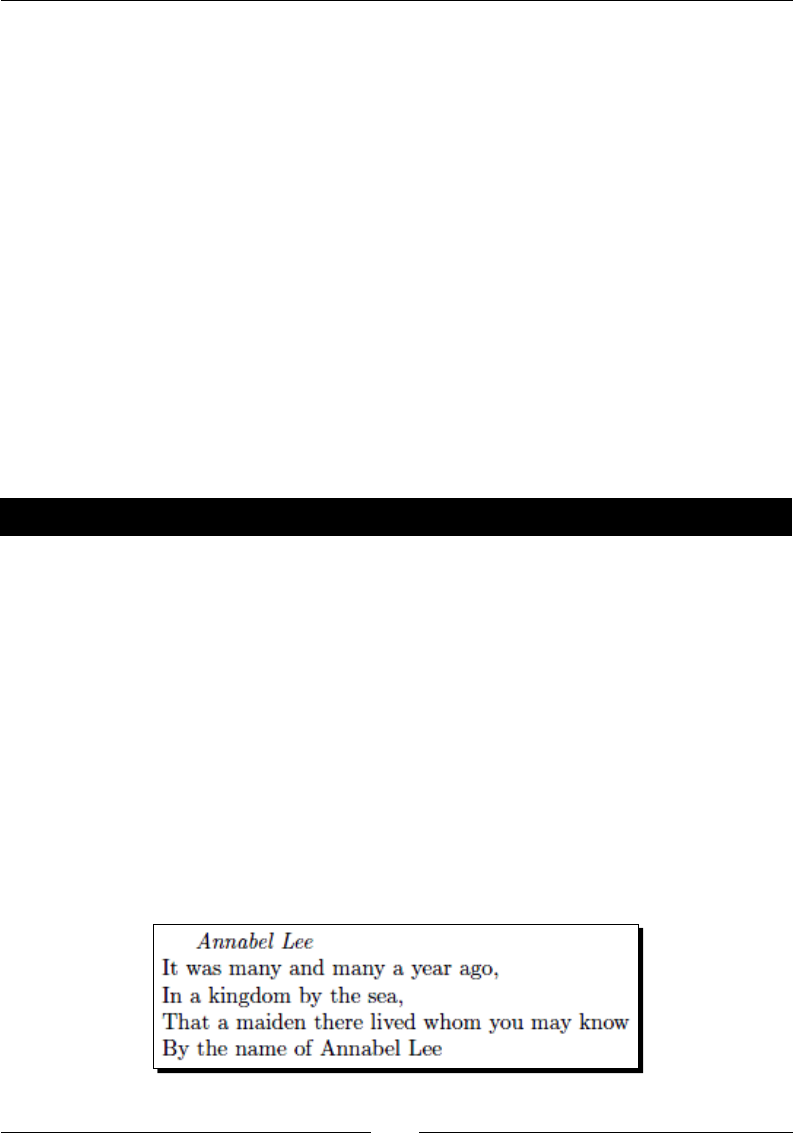
Chapter 2
[ 53 ]
What just happened?
We have loaded the microtype package without any opons, relying on its default
behavior. It introduces font expansion to tweak the juscaon and uses hanging
punctuaon to improve the opcal appearance of the margins. This may reduce the need of
hyphenaon and improves the "grayness" of the output. You've seen its eect on a narrow
column—imagine the improvement on wide text—keep that in mind and try it out later!
Though microtype provides powerful features and opons for the advanced typeseer,
we usually won't need to do more than just load it to prot from it. There's an extensive
package documentaon if you want to study it in depth.
microtype does nice tweaking, but it's not a cure-all; we should sll take care of proper
hyphenaon.
Breaking lines manually
We might choose to end a line overriding the automasm. There are several commands with
dierent eects.
Time for action – using line breaks
We will type the beginning of a famous poem by Edgar Allan Poe. As the author has specied
where a verse has to end, we shall insert line breaks there.
1. Create a document containing these lines:
\documentclass{article}
\begin{document}
\emph{Annabel Lee}\\
It was many and many a year ago,\\
In a kingdom by the sea,\\
That a maiden there lived whom you may know\\
By the name of Annabel Lee
\end{document}
2. Typeset and view the output:

Formang Words, Lines, and Paragraphs
[ 54 ]
What just happened?
The very short command \\ ended a line; the following text was put to the next line.
That's dierent to a paragraph break: we're sll in the same paragraph. The command
called \newline has the same eect.
There's another command called \linebreak, which tells LaTeX to end the line but to keep
the full juscaon. Therefore, the space between the words would be stretched to reach
the right margin. This could cause unpleasant gaps—that's why that command is rarely used.
Have a go hero – exploring line breaking options
Both introduced commands understand oponal arguments.
\\[value] would insert addional vercal space aer the break depending on the
value, like \\[3mm].
\\*[value] is a variaon of the same but prevents a page break before the next
line of text.
\linebreak[number] can be used to inuence the line break slightly or strongly:
If number is 0, a line break is allowed, 1 means it's desired, 2 and 3 mark more
insistent requests, and 4 will force it. The laer is the default behavior if no number
was given.
Change the heading of our poem example to the following:
\emph{Annabel Lee}\\[3mm]
This will insert some space between our heading and the poem fragment. Try the opons
further and check out their eects. If you're daring, try \linebreak instead of \\ to end a
poem line just to see its eect.
Preventing line breaks
The command \linebreak has a direct counterpart: \nolinebreak. This command
prevents a line break at the current posion. Like its counterpart, it takes an oponal
argument. If you write \nolinebreak[0], you recommend to not break the line there.
Using 1, 2, or even 3 makes the request stronger and \nolinebreak[4] forbids it
completely. The laer will be presumed if you don't provide an argument.
The already menoned command, \mbox[text], does not only disable hyphenaon
of a word, it will also prevent a line break for the complete text.

Chapter 2
[ 55 ]
LaTeX will break lines at spaces between words if meaningful. The symbol ~ stands for an
interword space where no break is allowed: if you would write Dr.~Watson, the tle Dr.
would never stand lonely at the end of a line.
Managing line breaks wisely
Bad hyphenaon could sll disappear as the document grows, so stang some sensible
hyphenaon rules would not do any harm but could prove to be useful.
But only use \\, \newline, and \linebreak for line adjustment when you're working
on the nal version of your document! While you're sll eding your text, you don't need
to worry about line breaks. They sll may change during the wring process. Bad looking
juscaon could sll change and become beer without intervenon. On the other hand,
if you break a line manually but later insert text before, the result could be an unwanted
short line.
So don't waste your energy on formang while you're wring.
Exploring the ne details
Typographic convenons may require paying aenon to small details; there are dierent
dashes, and the space around a dot may vary depending on the context. The space aer
some leers may depend on the following one, so much so that some leers may even
be joined to a single one. Such construcons are called ligatures. Let's have a closer look
at them.
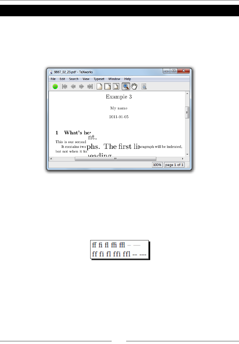
Formang Words, Lines, and Paragraphs
[ 56 ]
Time for action – exploring ligatures
We will check out Example 3 to discover a ligature. Aerwards, we will have a close look at
the default ligatures:
1. Open Example 3 in TeXworks, click the Typeset buon. Move the mouse pointer into
the output window, right over the word rst, and then click the le buon.
2. Go to the editor window, and then add a paragraph break by with empty line and
the following leer combinaons: ff fi flffiffl -- ---
3. Add a paragraph break, repeat the preceding line, but this me insert \/ between
the leers: f\/f f\/i f\/l f\/f\/i f\/f\/l -\/- -\/-\/-
4. Typeset and compare the leers in the output:
What just happened?
By le-clicking the mouse in the output window, you acvated TeXworks' magnifying glass. It
allows inspecng the output in detail as the area around the mouse pointer will be enlarged.
You can see that two or even three leers have been joined, but not in the last line: the
command \/ prevented this.
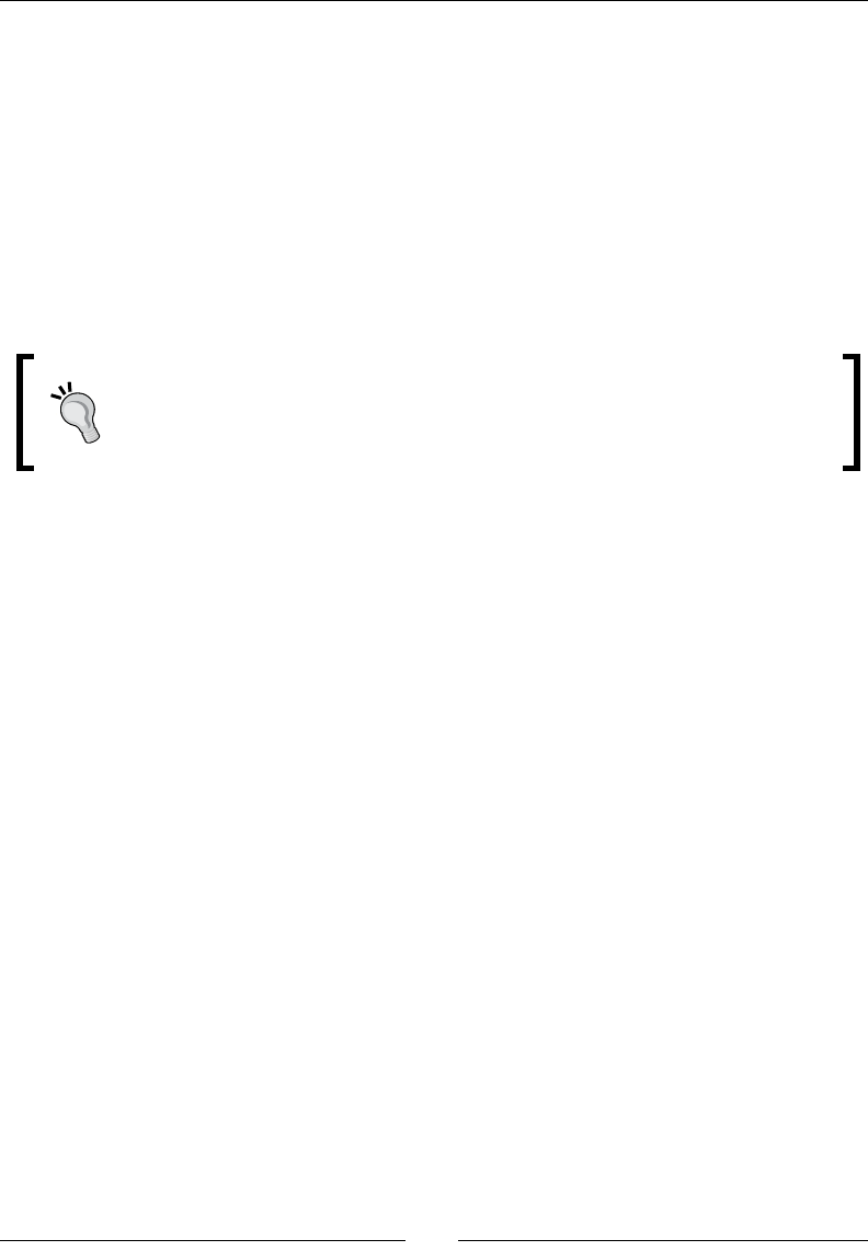
Chapter 2
[ 57 ]
Understanding ligatures
If the leer i follows the leer f, the dot of the leer i could collide with the head of the f. It
could be avoided in two ways: either by increasing the space between those two leers or by
combining them. The laer will result in a ligature. This will automacally be done by LaTeX
when the used font provides such ligatures.
Somemes this behavior might be undesirable, for instance, in compound words like
"halife". In this case, you can suppress this behavior by inserng \/ geng half\/life.
Curly braces can be used to achieve the same eect. For instance, in -{}- and {-}{-}, the
dashes cannot be joined because this would cross group boundaries.
If you don't like ligatures, for instance, because your PDF reader doesn't support
search or copy and paste of ligatures, completely suppressing ligatures could be
done easily by passing the opon noligatures to the microtype package:
\usepackage[noligatures]{microtype}.
Choosing the right dash
We've seen several kinds of dashes up unl now. Let's sort them out:
A short dash is used to mark hyphenaon or compound words. In LaTeX: -
A longer dash is used to indicate a range of some values, such as 2-3 hours.
Generally this dash has the same width like a digit. In LaTeX: --
Even wider is the dash commonly used to mark a parenthecal thought. In LaTeX:
---
Hyphenaon is always done using the short dash. Regarding the wider dashes, it's a maer
of style which kind of dash should be used, and further whether there should be a space
around the dash or not. You decide—but now you know how to typeset those dashes.
Setting dots
How wide is the space following a dot? Some styles require addional space aer the period
that ends a sentence, but not aer the period marking an abbreviaon. Furthermore, three
consecuve dots, forming an ellipsis, aren't usually wrien by just typing three dots. Let's
gure this out.
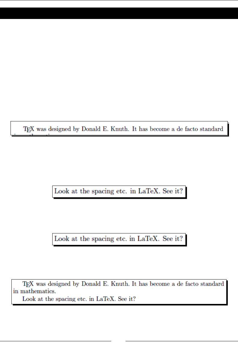
Formang Words, Lines, and Paragraphs
[ 58 ]
Time for action – using differently spaced dots
We shall typeset a short text containing periods to see the default behavior. Aerwards, we
will create an example where LaTeX's automaon fails; we shall see how to correct it. We will
learn how to simplify all this spacing using a dierent style.
1. Create a new document in TeXworks:
\documentclass{article}
\begin{document}
\TeX\ was designed by Donald E. Knuth.
It has become a de facto standard in mathematics.
\end{document}
2. Typeset to see the output:
3. Now add a paragraph break followed by this line:
Look at the spacing etc. in LaTeX. See it?
4. Check out the spacing aer the two periods in the output:
5. Correct the spacing by inserng a backslash and \@:
Look at the spacing etc.\ in LaTeX\@. See it?
6. Now remove the extra \ and \@ we've added, insert the declaraon
\frenchspacing into the preamble, and typeset to see the dierence:

Chapter 2
[ 59 ]
What just happened?
The rst step shows typical text and its output. As you can see, LaTeX adds a lile space aer
the period ending a sentence. But not following the leer E: in case of periods aer capital
leers, LaTeX assumes that it's an abbreviaon, therefore it doesn't add the extra space.
Generally, this automasm is helpful. However, you might encounter excepons: in step 3,
we constructed such a situaon where LaTeX's assumpons are wrong. We've got unwanted
extra space aer etc. and missed a space aer the last period.
In step 5, we corrected it: the backslash followed by a space (a "quoted space") produces the
normal interword space, the \@ before the dot states that the following dot stands at the
end of a sentence. Now the spacing is correct.
If you prefer to avoid this extra space or if the style you're following requires it, you could
switch o this default sentence spacing. We've done it in step 6 with the declaraon
\frenchspacing. Now the spacing aer sentences will be as it is between words.
The counterpart to \frenchspacing is \nonfrenchspacing, which is default.
Time for action – comparing dots to ellipsis
We will write an ellipsis in two ways: rstly by simply wring dots, secondly by using a
dedicated command. Let's compare!
1. Create a new document in TeXworks:
\documentclass{article}
\begin{document}
Here are three dots... compare them to the ellipsis\ldots
\end{document}
2. Check out the dierence:
What just happened?
We used the command \ldots to print out an ellipsis—three consecuve dots with a wider
spacing. Such dots may indicate a pause, an unnished thought, or an omied word. When
we just accumulated dots, they were typeset ghtly together. However, it's common to print
those dots wider.
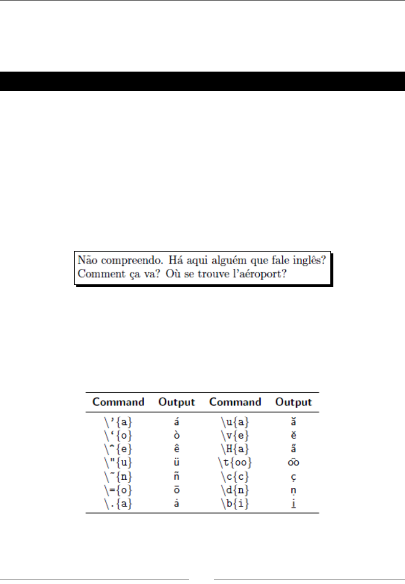
Formang Words, Lines, and Paragraphs
[ 60 ]
Setting accents
Some languages have leers with accents that you can't simply type with your editor. In case
you need to write such leers: let's see how to do it.
Time for action – experimenting with accents
We will write some words having leers with accents in Portuguese and in French.
1. Create a new document:
\documentclass{article}
\begin{document}
N\~{a}o compreendo. H\'{a} aqui algu\'{e}mque fale ingl\^{e}s?
Comment \c{c}a va? O\`{u} se trouve l'a\'{e}roport?
\end{document}
2. Typeset to see the generated accents:
What just happened?
LaTeX provides some special commands to produce a variety of accents. They may be
combined with any leer. Such a command consists of a backslash followed by one
character. The accent will be put above or below the leer that has to follow in curly
braces. The following table will list these commands and their eect:
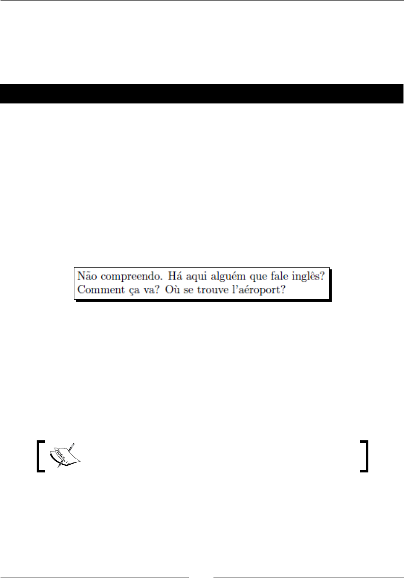
Chapter 2
[ 61 ]
Using special characters directly in the editor
It might be a bit cumbersome to use those accent commands. There's a package that extends
LaTeX basic capabilies. It allows you to enter at least some commonly used accented and
other special characters directly.
Time for action – using accents directly
We will modify the previous example daring to enter accented leers directly in the editor.
1. Create a new document:
\documentclass{article}
\usepackage[utf8]{inputenc}
\begin{document}
Não compreendo. Há aqui alguém que fale inglês?
Comment çava? Où se trouve l'aéroport?
\end{document}
2. Typeset and compare to the previous output:
What just happened?
We loaded the inputenc package. The opon utf8 tells the package to use Unicode input
encoding, which provides many more symbols than just the ASCII code. Now we just need
to nd the symbol on the keyboard and to type it.
TeXworks supports Unicode/UTF-8. Depending on operang system and editor, you might
need to use another opon when loading inputenc. A rule of thumb: utf8 works on most
Linux and Unix systems, like Mac OS X, and latin1 works with most Windows editors.
Today, many Windows editors move to UTF-8. This is seemingly
becoming the cross-plaorm standard.
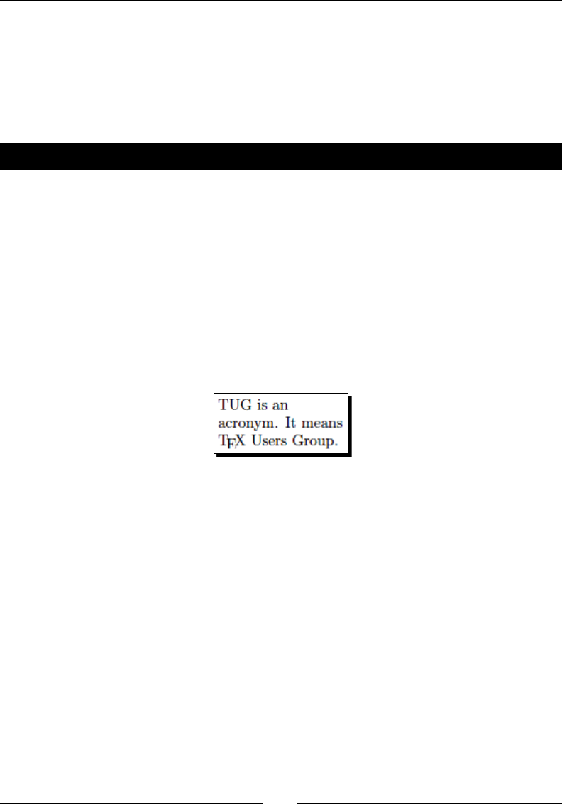
Formang Words, Lines, and Paragraphs
[ 62 ]
Turning off full justication
Though commonly your text will look ne if full juscaon is used, there may be occasions
when it's not the opmum. For instance, full juscaon could be displeasing if the text lines
are short. In such a case, it could be sucient to jusfy only to the le side. We shall see
how to put this into pracce, further how to right-jusfy, and how to get centered lines.
Time for action – justifying a paragraph to the left
Remember the rst parbox example which was fully jused but had those big gaps between
the words. We shall give up juscaon to the right side to avoid such gaps.
1. Create a new document containing these lines:
\documentclass{article}
\begin{document}
\parbox{3cm}{\raggedright
TUG is an acronym. It means \TeX\ Users Group.}
\end{document}
2. Typeset and look at the output:
What just happened?
We inserted the declaraon \raggedright. From this point onwards, the text will be
ragged-right. In other words, the text will be moved to the le margin - "ushed-le".
There won't be hyphenaon.
Because we used this declaraon inside a box, it's only valid there, like inside environments.
Aer the box, the text will be fully jused again.
If we want the whole document to be ragged-right, we just need to use \raggedright in
our preamble.
Creating ragged-left text
There might be occasions when we would like to achieve the opposite eect: ushing the
text to the right margin. We can do it similarly by inserng the declaraon \raggedleft.
Remember, you're able to control where lines are broken by inserng \\.
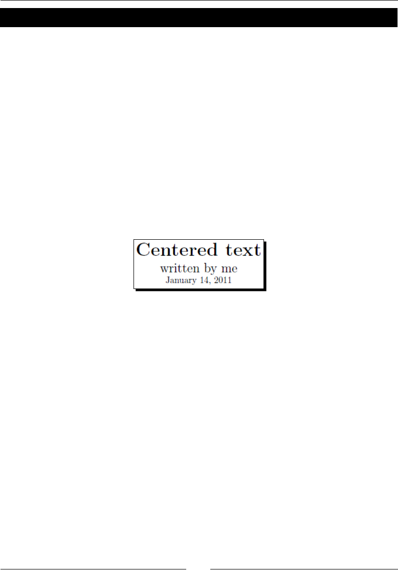
Chapter 2
[ 63 ]
Time for action – centering a title
We shall create a nice looking tle for our document. It should contain the tle, the author,
and the date. All those lines have to be centered.
1. Write a document containing this code:
\documentclass{article}
\pagestyle{empty}
\begin{document}
{\centering
\huge\bfseries Centered text \\
\Large\normalfont written by me \\
\normalsize\today
}
\end{document}
2. Typeset to see the output:
What just happened?
Because only the tle should be centered, we opened a group to limit the centering. Through
the declaraon \centering, we made the remaining text of this group horizontally aligned
to the center. We inserted a paragraph break: it's always a good idea to do it before ending
the group when paragraph-aecng commands were used. By the brace aer \today, we
ended the group. If you complement some following text, it will be typeset normally, not
centered.
\centering is commonly used when pictures or tables are inserted, further on tle pages
and somemes for headings.
Using environments for justication
As there's a corresponding environment for every declaraon, as we learned, we could
have wrien \begin{centering} … \end{centering} in our previous example. It
could be done similarly for ragged-right and ragged-le text. There's a couple of predened
environments acng similarly but starng a new paragraph at the same me.
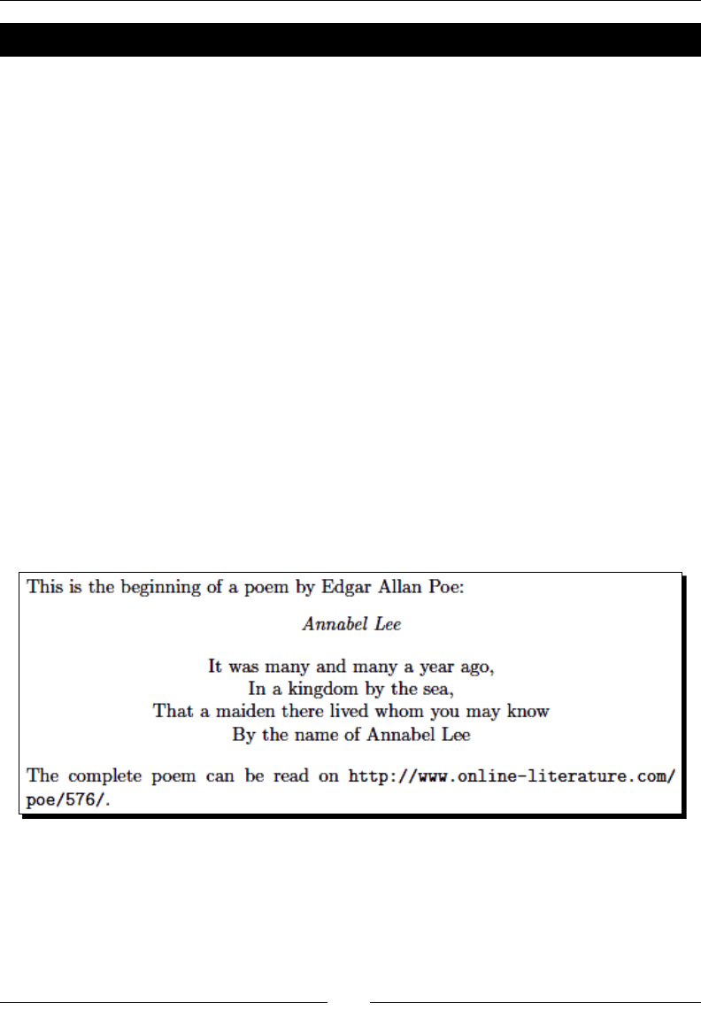
Formang Words, Lines, and Paragraphs
[ 64 ]
Time for action – centering verses
Let's reuse the fragment of the poem "Annabel Lee". This me we shall center all verses:
1. Create a document containing these lines:
\documentclass{article}
\usepackage{url}
\begin{document}
\noindent This is the beginning of a poem
by Edgar Allan Poe:
\begin{center}
\emph{Annabel Lee}
\end{center}
\begin{center}
It was many and many a year ago,\\
In a kingdom by the sea,\\
That a maiden there lived whom you may know\\
By the name of Annabel Lee
\end{center}
The complete poem can be read on
\url{http://www.online-literature.com/poe/576/}.
\end{document}
2. Typeset and see the output:
What just happened?
We began with \noindent avoiding the paragraph indentaon. \begin{center} started
the center environment. It begins a new paragraph, leaving some space to the preceding
text. \end{center} ended this environment. We used the environment twice. In the
second one, we inserted \\ to end the verses.
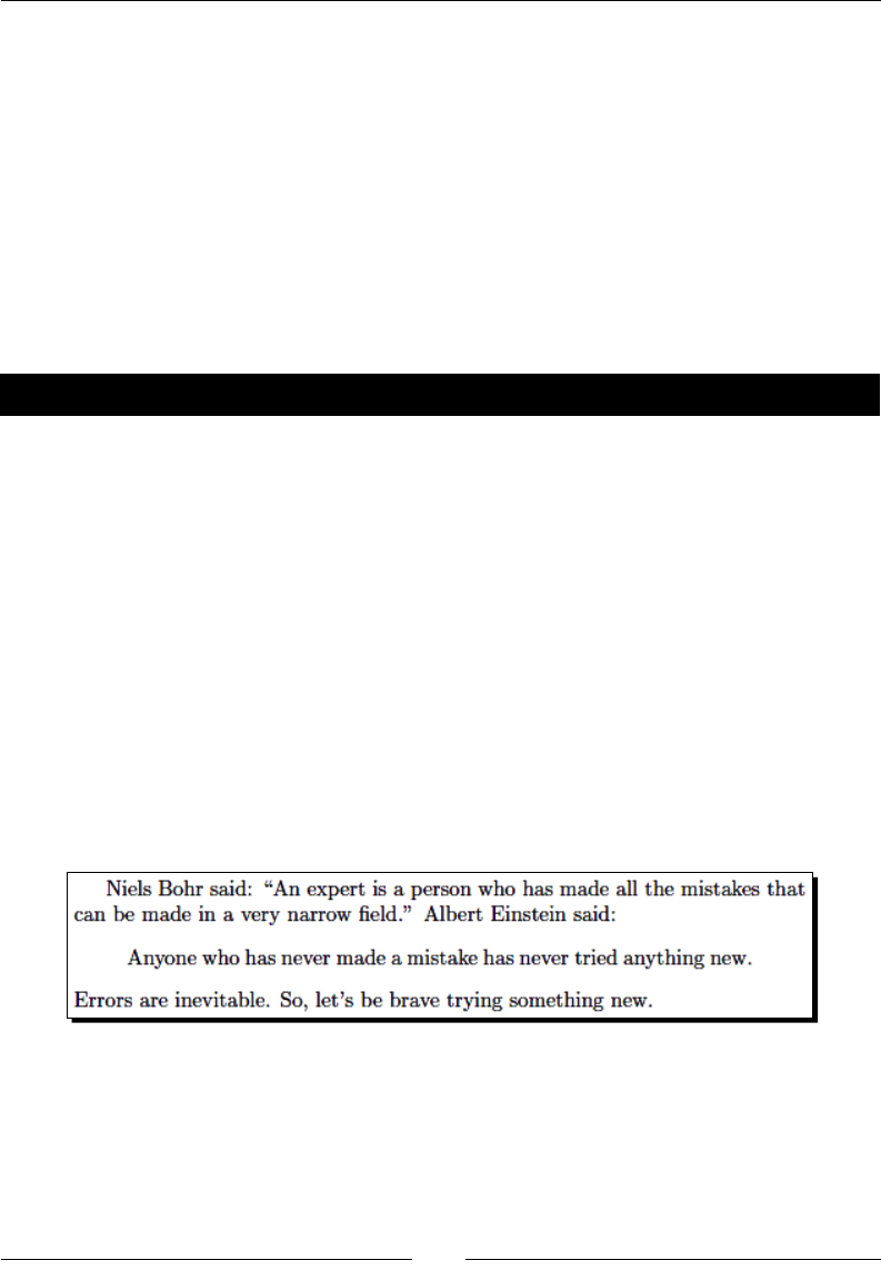
Chapter 2
[ 65 ]
Aer the center environment ended, some space followed and the next paragraph began
at the le margin.
The corresponding environment for ragged-right text is called ushle, and for ragged-le
text it's ushright.
Displaying quotes
Imagine your text contains a quotaon of another author. It might be hard to read if it's just
embedded in your words. A common way to improve the readability is displaying: seng the
text o by indenng on both margins.
Time for action – quoting a scientist
We will quote thoughts of famous physicists.
1. Create a new document containing these lines:
\documentclass{article}
\begin{document}
Niels Bohr said: ``An expert is a person who has made
all the mistakes that can be made in a very narrow field.''
Albert Einstein said:
\begin{quote}
Anyone who has never made a mistake has never tried anything new.
\end{quote}
Errors are inevitable. So, let's be brave trying something new.
\end{document}
2. Typeset to see the result:
What just happened?
Firstly we quoted inline. `produced a le quotaon mark; the character is also called a
backck. 'gave a right quotaon mark. We just typed two such symbols to get double
quotes.

Formang Words, Lines, and Paragraphs
[ 66 ]
Then we used the quote environment to display a quotaon. We did not begin a new
paragraph for it, because the quotaon is already set a bit o. That's the reason we
don't use a blank line before and aer the environment.
Quoting longer text
When wring short quotaons, the quote environment looks very good. However, when
you would like to quote a text containing several paragraphs, you might wish to have the
same paragraph indentaon like in your surrounding text. The quotaon environment will
do it for you.
Time for action – quoting TeX's benets
We will quote some of the benets of TeX and LaTeX found on a web page on CTAN.
1. Start a new document. This me, it will be a bit longer:
\documentclass{article}
\usepackage{url}
\begin{document}
The authors of the CTAN team listed ten good reasons
for using \TeX. Among them are:
\begin{quotation}
\TeX\ has the best output. What you end with,
the symbols on the page, is as useable, and beautiful,
as a non-professional can produce.
\TeX\ knows typesetting. As those plain text samples
show, \TeX's has more sophisticated typographical algorithms
such as those for making paragraphs and for hyphenating.
\TeX\ is fast. On today's machines \TeX\ is very fast.
It is easy on memory and disk space, too.
\TeX\ is stable. It is in wide use, with a long history.
It has been tested by millions of users, on demanding input.
It will never eat your document. Never.
\end{quotation}
The original text can be found on
\url{ http://www.ctan.org/what_is_tex.html}.
\end{document}
2. Typeset and look at the output:
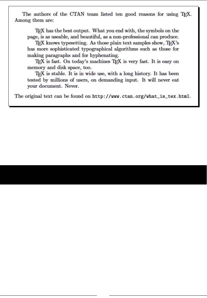
Chapter 2
[ 67 ]
What just happened?
This me, we used the quotation environment to display some paragraphs. As in normal
text, blank lines separate the paragraphs. They are le-indented at their beginning just like in
all our body text.
But what if we don't like that paragraph indentaon? Let's check out an alternave.
Time for action – spacing between paragraphs instead of
indentation
We like to avoid the paragraph indentaon. Instead, we shall separate the paragraphs by
some vercal space.
1. Create copy of the previous example and reuse most of it this way:
\documentclass{article}
\usepackage{parskip}
\usepackage{url}
\begin{document}
The authors of the CTAN team listed ten good reasons
for using \TeX. Among them are:
\TeX\ has the best output. What you end with,
the symbols on the page, is as useable, and beautiful,
as a non-professional can produce\ldots
The original text can be found on
\url{ http://www.ctan.org/what_is_tex.html}.
\end{document}
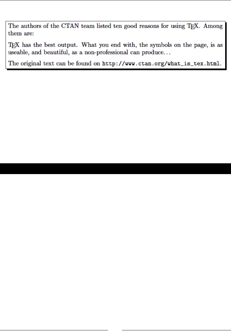
Formang Words, Lines, and Paragraphs
[ 68 ]
2. See the eect:
What just happened?
The highlighted line shows that we've loaded the parskip package. Its only purpose is to
remove the paragraph indentaon completely. At the same me, this package introduces
a skip between paragraphs. But this package doesn't aect the denion of the quotaon
environment—you sll could use the quote environment.
In order to disnguish paragraphs, there are two common ways. One is to indent the
beginning of each paragraph; this is the default LaTeX style. The other way is to insert vercal
space between paragraphs while oming the indentaon, which is suitable for narrow
columns where indenng would cost too much width.
Pop quiz – lines and paragraphs
1. Which of the following designates the end of a paragraph?
a. \newline
b. \\
c. A blank line
2. How do the words in a \hyphenation command be separated?
a. By commas
b. By semicolons
c. By spaces
3. Which command switches to le-aligned text?
a. \raggedleft
b. \raggedright
c. \flushright

Chapter 2
[ 69 ]
Summary
In this chapter, we developed the basics: eding, arranging, and formang of text.
Specically, we covered:
Modifying shape and style of text and its font
Breaking lines and improving hyphenaon
Controlling juscaon of text
We got to know the basic LaTeX concepts:
Commands and declaraons, mandatory and oponal arguments
Denion of new commands
Using environments
Using packages, how they can be loaded and opons to packages
Keep in mind that even though we've used formang commands directly in the text when
exploring them, you should use them inside command denions in the preamble to allow
easy changes for the future. During your learning and wring process, you probably will get
to know further useful commands and packages that could improve your previously wrien
commands.
We've learned general pracces:
As oen as possible, create your own macros to achieve a logical structure. You
will be rewarded with consistent formang and changes could easily be applied
to the whole document.
Deal with line or page breaking issues at the earliest when you go for your nal
version.
Now that we've learned about the detailed formang of text, we're ready to enter the next
chapter that deals with formang and layout of whole pages and documents.
3
Designing Pages
Aer the previous chapter, formang text should be easy for us. So, let's turn
to whole pages!
In this chapter, we will learn how to:
Adjust the margins
Change the line spacing
Secon the document
Create a table of contents
Design headers and footers
Control page breaking
Set footnotes and modify their appearance
In learning this, we shall gain a deeper insight into classes and packages.
Dening the overall layout
We shall write an example document spanning over several pages. This will be our test
object for modifying margins, line spacing, headers, footers, and more.
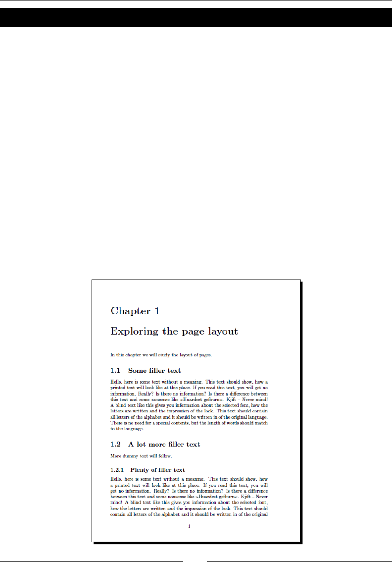
Designing Pages
[ 72 ]
Time for action – writing a book with chapters
We will start to write a book. At rst, we shall choose a class, further we will use some ller
text to work out the page layout.
1. Create a new document with the following code:
\documentclass[a4paper,12pt]{book}
\usepackage[english]{babel}
\usepackage{blindtext}
\begin{document}
\chapter{Exploring the page layout}
In this chapter we will study the layout of pages.
\section{Some filler text}
\blindtext
\section{A lot more filler text}
More dummy text will follow.
\subsection{Plenty of filler text}
\blindtext[10]
\end{document}
2. Save the document and Typeset it. Look at the rst page:
Chapter 3
[ 73 ]
What just happened?
We have chosen the document class book. As the name implies, this class is suitable for
book-like documents. Books are commonly two-sided and consist of chapters which usually
start at right-hand pages. They may have a front maer with one or more tle pages and a
back maer with bibliography, index, and so on. The book class supports all of this.
We loaded the babel package. This is useful especially for typeseng in other languages
than English regarding hyphenaon, language-specic characters, and more.
Even for English language, there are several opons: USenglish, american, english,
UKenglish, british, canadian, australian, and newzealand. Obviously, some mean
the same, such as UKenglish and british. However, there are dierences in hyphenaon
rules between USenglish (american, english) and UKenglish (british).
For now, we just need babel to load blindtext: this package has been developed to produce
ller text. It requires babel to detect the language of the document. We stated the language
English to babel, which means American English.
The command \chapter produced a large heading. This command will always begin on a
new page.
We've already seen the \section command. It's our second seconing level and generates
a smaller heading than \chapter. It's automacally numbered per chapter. The command
\blindtext followed, prinng some dummy text just to ll the space with some text.
At last, we rened the seconing with a \subsection command followed by more dummy
text to ll up the page.
There's another popular package for generang dummy text. It's called lipsum
and it produces the famous LoremIpsum text which has been the typeseer's
dummy text for hundreds of years.
Reviewing LaTeX's default page layout
For the example in the current chapter, we used A4 paper and a font size of 12 pt. We let
LaTeX dene the margins. Let's look at them:
The right margin is the outer margin of the book, because the chapter starts on a
right-hand page. It might seem to be a bit wide—but good text isn't just intended to
ll as much space as possible: it should be well-readable for our eyes. Therefore the
lines shouldn't be too long.

Designing Pages
[ 74 ]
The le margin is the inner margin on such a right-hand page. A user asked why the
inner margin is smaller than the outer, even further some space will get lost because
of the binding. The explanaon is simple, if we imagine the book lies opened right
before us: the inner margins would look joined. It's a good idea to aim at equal
margins—le, middle, and right. In this sense, we could choose the inner margin to
be half of the size of the outer margin—plus some oset for the binding.
The boom margin contains the page number.
The top margin looks very tall. It's caused by the chapter heading, there's always
more space le above. By looking at the second page, you will see that normal
pages have a smaller top margin.
If you ever doubt LaTeX's design, look at some books in your shelves and compare, whether
it's regarding margins, ligatures, numbering, or anything else.
Dening the margins yourself
A publisher or a supervisor may request you to follow his specicaons. Besides font size,
interline spacing, and other style issues, this might also apply to the margins. In this case,
you would need to override LaTeX's recommendaons specifying the margins precisely.
There's a package fullling these demands.
Time for action – specifying margins
We shall load the geometry package and state the exact width and height of all margins.
1. Extend the preamble of the previous example with this command:
\usepackage[a4paper, inner=1.5cm, outer=3cm, top=2cm,
bottom=3cm, bindingoffset=1cm]{geometry}
2. Typeset and examine the margins:
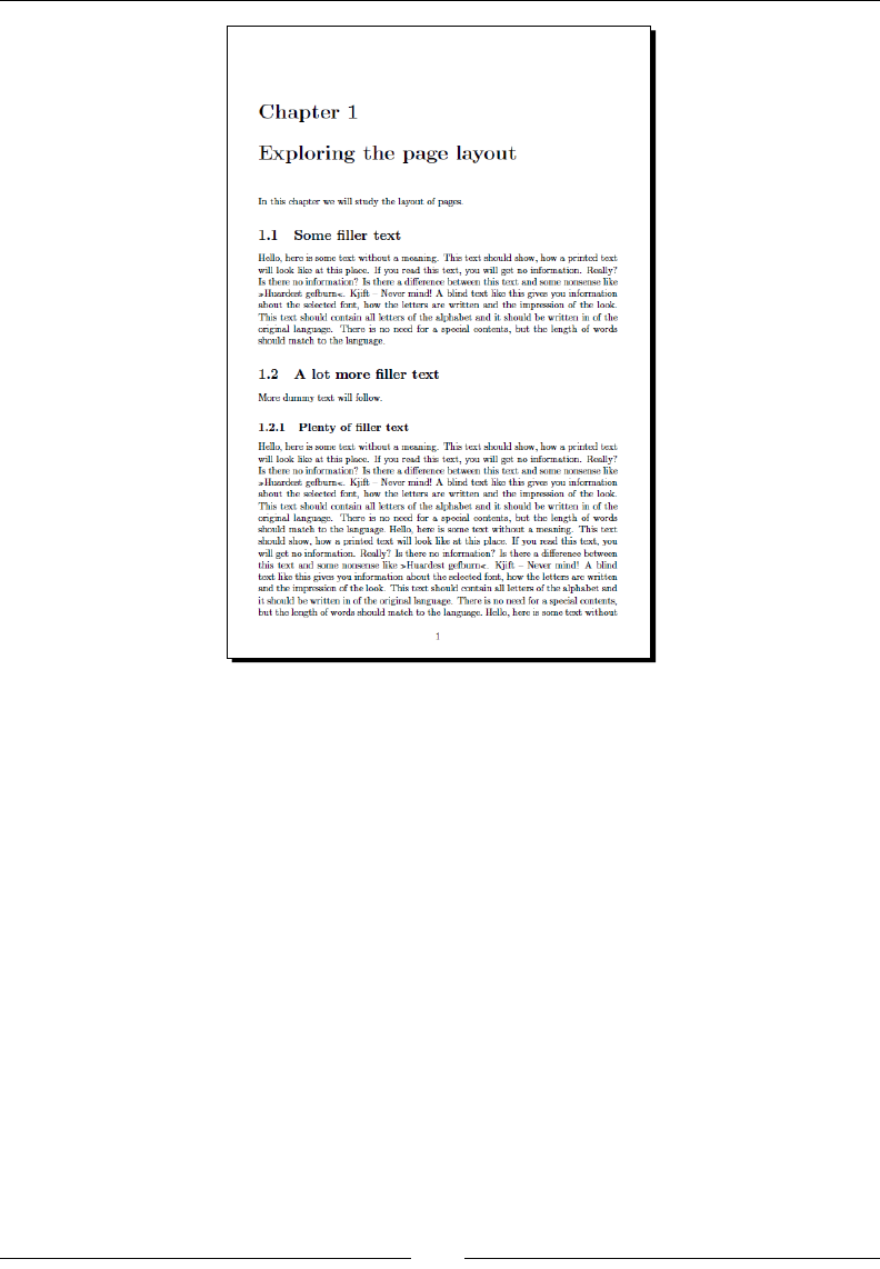
Chapter 3
[ 75 ]
What just happened?
We loaded another package with the name geometry. This package takes care of our layout
regarding the paper size, margins, and more dimensions. We chose A4 paper size, an outer
margin of 3 cm, and an inner margin of just 1.5 cm, remembering that the two inner margins
will be perceived as one space when the two-sided book is opened. We stated the top and
the boom margin. At last, we specied a value of 1 cm for the binding correcon. We need
the inner margins to be wider because we expect to lose this space later because of the
binding like gluing or stapling.
Using the geometry package
In the early days of LaTeX, it was common to manipulate the layout dimensions directly. This
approach had some disadvantages. We could easily make mistakes in calculang the lengths,
for instance le margin + right margin + text width might not t to the paper width. The
geometry package comes to the rescue. It provides a comfortable interface for specifying
layout parameters. Further, it provides auto-compleon. It calculates missing values to match
the paper size. It even adds missing lengths using a heurisc approach to achieve a good
layout. Let's look at it in detail.
Designing Pages
[ 76 ]
The geometry package understands arguments of the form "key=value", separated by
commas. If you load geometry without arguments, those arguments could alternavely
be used by calling \geometry{argument list}. We shall look at some of them.
Choosing the paper size
Geometry provides several opons to set the paper size and orientaon:
paper=name states the paper name, for example, paper=a4paper. It may be
abbreviated like we did in our example. The package supports a lot of paper sizes,
such as letterpaper, executivepaper, legalpaper, a0paper, … ,a6paper,
b0paper, … , b6paper, and more.
paperwidth, paperheight allow you to choose the paper dimensions freely,
like paperwidth=7in, paperheight=10in.
papersize={width,height} sets width and height of the paper like
papersize={7in,10in}. This is an example of a double-valued argument.
landscape changes the paper orientaon to landscape mode.
portrait switches to portrait mode. This is the default.
If you already specied the paper name to the document class, geometry will
inherit it. That's valid in general: all document class opons will be automacally
given to the packages that recognize them.
Specifying the text area
The text area may be adjusted by these opons:
textwidth sets the width of the text area, like textwidth=140mm.
textheight states the height of the text area, like textheight=180mm.
lines gives another way to specify the text height by the number of lines, like
lines=25.
includehead causes the header of the page to be included into the body area;
set false by default.
includefoot causes the footer of the page to be included into the body area;
set false by default.

Chapter 3
[ 77 ]
Setting the margins
The size of the visible margins can be specied by these opons:
left, right set the width of the le and the right margin, like left=2cm.
Use it for one-sided documents.
inner, outer set the width of the inner and the outer margin, like inner=2cm.
Use it for two-sided documents.
top, bottom set the height of the top and the boom margin, like top=25mm.
twoside switches to two-sided mode. This means that le and right margins
would be swapped on le-hand pages, also called verso pages.
bindingoffset reserves space on the le margin (one-side), respecvely the
inner margin (two-sided) for the binding.
That's just a selecon of commonly used opons—there are many more. You could choose
and set some opons intuively—for instance, \usepackage[margin=3cm]{geometry}
will result in a 3 cm margin on each edge of the paper and the paper size comes from the
document class opon.
The auto-compleon works like this:
paperwidth = left + width + right, where width=textwidth by default
paperheight = top + height + bottom, where height=textheight by default
If you decide to include marginal notes within the text body when calculang, width could
get wider than textwidth. If two dimensions of the right side of each formula are given,
the missing dimension would be calculated. That's why it may be enough to specify left
and right, top and bottom, respecvely. Even if just one margin is specied, the other
dimensions would be determined using default margin raos:
top:bottom = 2:3
left:right = 1:1 for one-sided documents
inner:outer = 2:3 for two-sided documents
Sounds complicated? That's just intended to help you to achieve praccal dimensions even if
some values were missing.
In 2010, version 5 of geometry introduced the commands
\newgeometry{argument list} and \restoregeometry,
allowing users to change margin dimensions in the middle of a document.
Their auto-compleon may also dier a bit from previous versions.
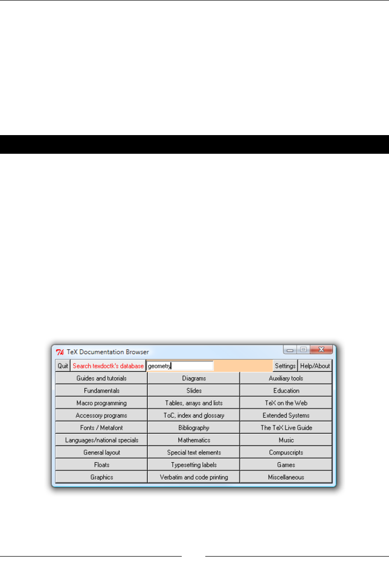
Designing Pages
[ 78 ]
The geometry package provides an extensive manual. Don't be worried by the amount of
documentaon: it's an oer to guide you through the variety of features.
Obtaining package documentation
There are hundreds of LaTeX packages available. No book could ever explain all of their
features on its own. But most of those packages oer good documentaon that you can read
for free. If you work your way through this book and supplement it with the documentaon
of the menoned packages, you're on the right track to become a LaTeX power user.
Time for action – nding the geometry package manual
We would like to examine the documentaon of the geometry package. At rst, we shall look
for it locally on our computer. Aerwards, we will see how to nd the documentaon online:
1. Click the Start buon and choose All Programs| Accessories |Command prompt
2. Type the following:
texdoc geometry
3. A PDF viewer should start and show the package manual. The same command works
at the command prompt on Linux/Unix computers.
4. Hit the Start buon again; this me, choose All Programs | TeX Live 2010 |TeXdoc
GUI. Click on Search texdoctk's database, enter the keyword geometry, and
press Enter:
5. Have a look at the search result. Open it by double-clicking or hit the View buon.
A viewer should open the documentaon.
Chapter 3
[ 79 ]
6. Open an Internet browser and visit the site http://ctan.org/pkg/geometry.
Scroll down to Documentaon on CTAN and hit the link User's manual. Again, your
PDF viewer or a browser plug-in will show the documentaon.
What just happened?
We've tried three ways of obtaining the documentaon. At rst, we used texdoc. This is a
tool to nd and to view LaTeX documentaon. It can be used at the command prompt; just
type texdoc followed by a keyword. For this, it's required to be in the operang system's
search path. The TeX distribuon installer takes care of it. The argument to texdoc doesn't
have to be the package name, as texdoc understands aliases. Further, we used a GUI for
texdoc providing a search feature supplemented by a category classicaon. Perhaps
browse for a lile while through the categories.
If texdoc doesn't help you, there's another opportunity: visit CTAN. You
just need to know the package name. Simply visit http://ctan.org/
pkg/packagename to get to the package homepage, there you may nd
documentaon.
In case you don't know the package name or you just have a vague idea what
you're looking for, visit the TeX Catalogue Online on http://texcatalogue.
sarovar.org/bytopic.html. It lists hundreds of packages sorted by topic.
Note: The online documentaon might match a dierent package version than
the one on your computer.
Have a go hero – constructing the page layout with typearea
Now that you know how to open package documentaon, you could gure out if you want
to benet from the typearea package. While the geometry package allows you to control
all margins yourself, typearea provides a dierent approach. It supports you in creang
a page layout based on proven typography standards. typearea is explained within the
KOMA-Script manual, so the keywords for texdoc and CTAN would be koma-script or
typearea. Reading Chapter 2 of the manual on Page Layout could give you an insight into
typography, even if you decide not to use typearea.
Changing the line spacing
Without some vercal space between the lines, the readability of a text could suer.
Adding such space would help lead the eye along the line.
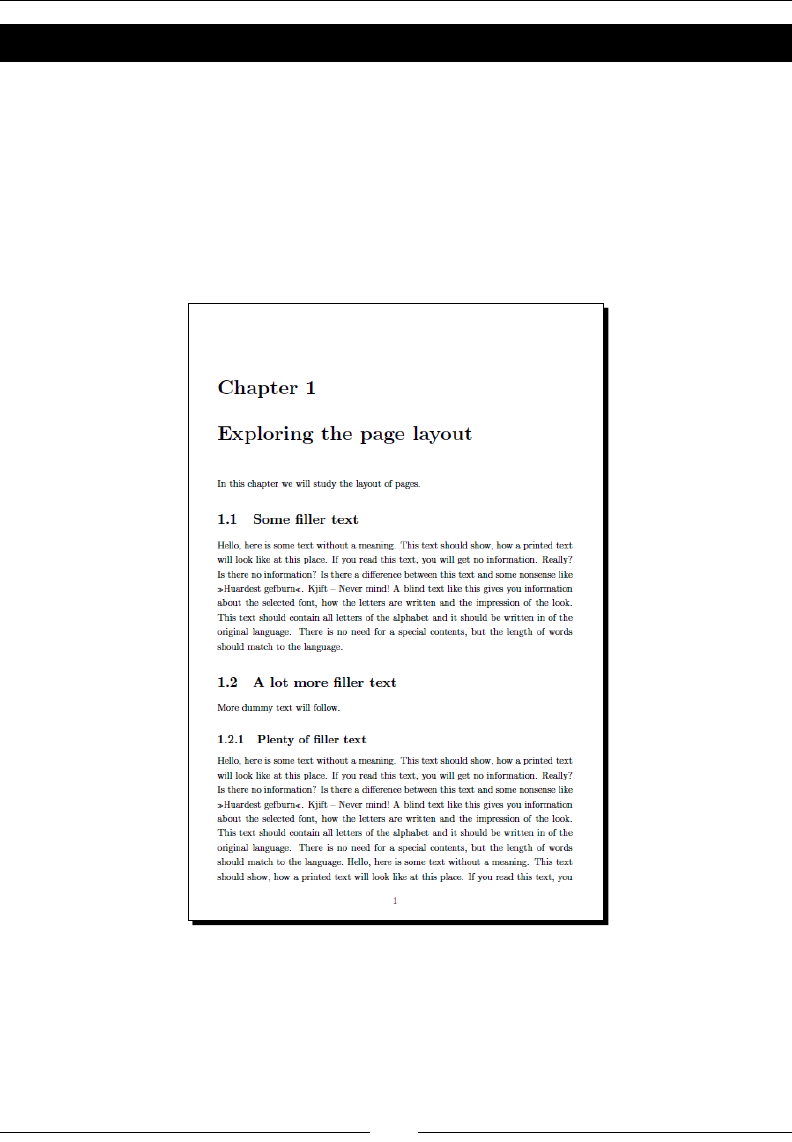
Designing Pages
[ 80 ]
Time for action – increasing line spacing
Though LaTeX already takes care of good readability by choosing a meaningful interline
spacing, publishers might require dierent spacing. We shall modify our example by adding
half of a line height to the line spacing.
1. Extend the preamble of our example with this command:
\usepackage[onehalfspacing]{setspace}
2. Typeset to see the change:
What just happened?
We loaded the setspace package. Its only purpose is to adjust the line spacing. We provided
the opon onehalfspacing. This increases the spacing by half of a line height for the
whole document.
Chapter 3
[ 81 ]
setspace understands three opons:
singlespacing is the default. No addional space will be inserted. The text will
be typeset with LaTeX's default interline spacing, which is about 20 percent of the
line height.
onehalfspacing means one-and-a-half spacing like in our example.
doublespacing can be used for even more spacing: the distance between the
baselines of successive text lines would be twice as high as a single line.
Commonly, we choose the spacing for the complete document. In that case, such an opon
would be sucient. For each of the opons, there's a corresponding environment. They are
called singlespace, onehalfspace, and doublespace. Those environments may be
used to adjust the spacing within the document. They shouldn't be nested. For the need of
a dierent stretching factor, the spacing environment is provided. It may be used like the
following:
\begin{spacing}{2.4}
This text is stretched by a factor of 2.4.
\end{spacing}
In typeseer's jargon, the distance between the baselines of consecuve text
lines is called leading.
Have a go hero – examining a package source le
In some cases the documentaon of a package is not easily accessible. This applies to
setspace: the explanaon of the opons, commands, and environments is contained in the
package source le itself. How can we obtain it? We could visit CTAN, as we described before,
or locate the le on our computer. A package lename usually ends with .sty, standing for
style le. TeX Live provides a tool for locang such source les. Try it: open the command
prompt, that is, hit the Start buon and click All Programs |Accessories |Command prompt.
Then type the following:
kpsewhich setspace.sty
And press Enter. The program will print the locaon of the le, as follows:
c:/texlive/2010/texmf-dist/tex/latex/setspace/setspace.sty
Open the le using TeXworks or any text editor. There are a lot of comment lines explaining
the package features.
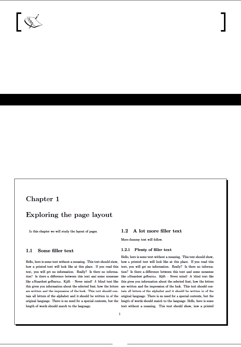
Designing Pages
[ 82 ]
The kpsewhich tool belongs to the kpathsea library. kpathsea's
fundamental purpose is lename lookup.
Using class options to congure the document style
We already know that a document class is the basis of our document. It provides commands
and environments extending the LaTeX standard features. Though the class provides a
default style, it's sll customizable with opons.
Time for action – creating a two-column landscape document
We shall change the orientaon of our example to landscape. We would also like to typeset
our text in two columns:
1. Add the opons landscape and twocolumn to the \documentclass statement
of our example, as follows:
\documentclass[a4paper,12pt,landscape,twocolumn]{book}
2. Typeset and see how the layout has changed:

Chapter 3
[ 83 ]
What just happened?
By using the landscape opon, we switched the orientaon. By stang the twocolumn
opon, we caused the body text to be divided into two columns.
There's a command\twocolumn[opening text] starng a two-column
page with oponal opening text over the whole width. \onecolumn begins a
one-column page.
If you'd like to balance the columns on the last page or if you wish to have
more than two columns, use the mulcols package.
The LaTeX base classes are arcle, book, report, slides, and leer. As the name suggests, the
last one can be used to write leers, though there are further suitable classes like scrlr2.
slides can be used to create presentaons, but today there are more powerful and feature
rich classes like beamer and powerdot.
Let's sum up the opons of the base classes:
a4paper, a5paper, b5paper, letterpaper, legalpaper, or executivepaper:
The output will be formaed according to this paper size, that is, A4: 210 mm x 297
mm. letterpaper (8.5 in x 11 in) is the default. Loading the geometry package
allows more sizes.
10pt, 11pt, or 12pt: The size of normal text in the document; the default is ten
points (10pt). The size of headings, footnotes, indexes, and so on, will be adjusted
accordingly.
landscape: Switches to landscape format; width and height of the output size
will be interchanged.
onecolumn or twocolumn: Decides whether the pages will be one-column
(default) or two-column. It's not supported by the leer class.
oneside or twoside: Formang for prinng on one side or both sides of a page.
oneside is the default, except for the book class. twoside is not usable with the
slides class and the letter class.
openright or openany: The rst decides that chapters have to begin on a right-
hand page (the default for the book class), openany allows chapters to start on any
page (default for the report class). These opons are only supported by the book
and the report class because the other classes don't provide chapters.
titlepage or notitlepage: The rst causes a separate tle page when
\maketitle is used and is the default, except for the article class. The
default of article is notitlepage, which means that normal text may follow
the tle on the same page.
Designing Pages
[ 84 ]
final or draft: If draft is set, then LaTeX will mark overfull lines with a black
box, which is helpful in reviewing and improving the output. Some packages support
these opon as well, behaving dierently then, such as oming embedding of
graphics and lisngs when draft has been chosen. final is the default.
openbib: When this opon is set, a bibliography would be formaed in open style
instead of compressed style.
fleqn: Causes displayed formulas to be le-aligned.
leqno: For numbered displayed formulas, the number would be put to the le side.
The right side is the default.
Many other classes support these opons as well and even more. For
the need of an uncommon base font size, the classes extarticle,
extbook, extreport, and extletter provide base font sizes from
8 pts to 20 pts. The so called KOMA-Script classes allow arbitrary base
font sizes. They understand such a large amount of opons that they're
addionally supporng a "key=value" interface like we've seen with the
geometry package.
Have a go hero – trying KOMA-Script classes
Have you been so brave to check out the typearea package documentaon? Then you've
already seen the KOMA-Script manual accessible by texdoc koma-script. Open it again;
this me, read it with the idea of choosing KOMA classes for your documents. They may be
used like the base classes: for each base class, there's a corresponding KOMA class. They
dier in some meaningful presets; for instance, headings use a sans-serif font by default.
However, the presets can easily be changed. Those classes extend the base classes very
much, providing a huge amount of commands. Web forums frequently show user quesons
being hard to solve using base classes, but being easily achievable by a single KOMA class
command.
Creating a table of contents
A book commonly begins with a table of contents, so let's create one.
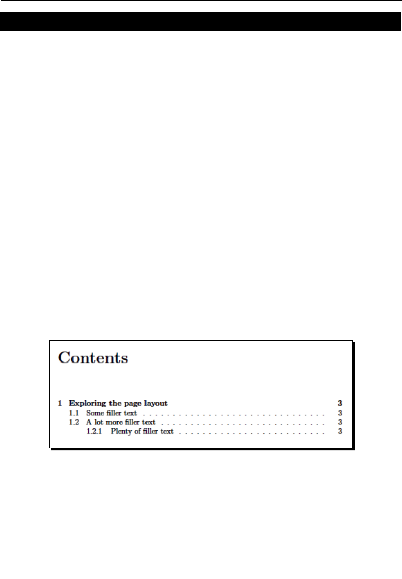
Chapter 3
[ 85 ]
Time for action – adding a table of contents
We shall create a table of contents based on our numbered headings.
1. Let's remove the opons landscape and twocolumn. We also don't load
the setspace package. Add the command\tableofcontents right aer
\begin{document}. Our code shall now be:
\documentclass[a4paper,12pt]{book}
\usepackage[english]{babel}
\usepackage{blindtext}
\usepackage[a4paper, inner=1.5cm, outer=3cm, top=2cm,
bottom=3cm, bindingoffset=1cm]{geometry}
\begin{document}
\tableofcontents
\chapter{Exploring the page layout}
In this chapter we will study the layout of pages.
\section{Some filler text}
\blindtext
\section{A lot more filler text}
More dummy text will follow.
\subsection{Plenty of filler text}
\blindtext[10]
\end{document}
2. Typeset twice. Aerwards, the rst page of your output will contain this table:
What just happened?
The command \tableofcontents tells LaTeX to produce a le with the extension .toc.
This le will be used to generate a table of contents. We had to typeset twice: in the rst run,
the .toc le was wrien and in the second run, LaTeX read it and processed it.
The entries are created by the seconing commands. We used \chapter, \section, and
\subsection, and we've got an entry for each.
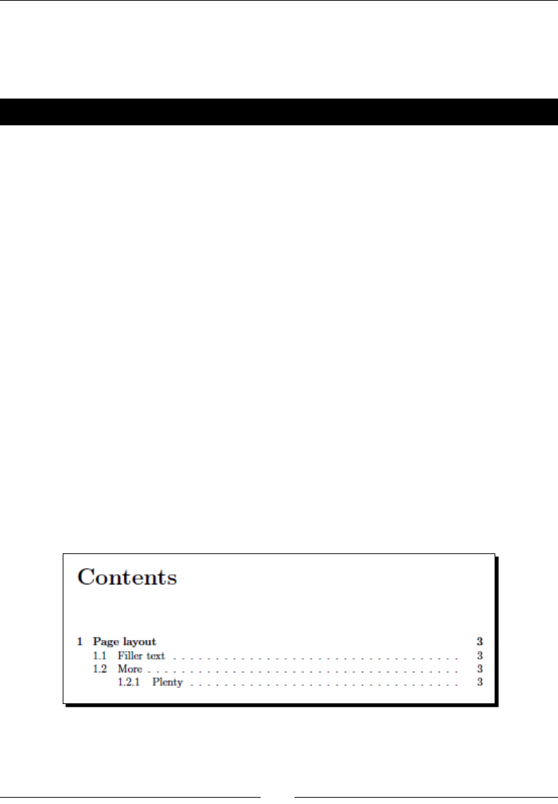
Designing Pages
[ 86 ]
Sectioning and the contents
A heading might be very long; it could span over two or more lines. In that case, we might
wish to shorten its corresponding table of contents entry. Let's see how.
Time for action – shortening the table of content entries
We will use the oponal argument of the seconing commands to produce shorter entries,
dierent to the actual headings:
1. Take our example and modify the seconing commands as shown in the
highlighted lines:
\documentclass[a4paper,12pt]{book}
\usepackage[english]{babel}
\usepackage{blindtext}
\usepackage[a4paper, inner=1.5cm, outer=3cm, top=2cm,
bottom=3cm, bindingoffset=1cm]{geometry}
\begin{document}
\tableofcontents
\chapter[Page layout]{Exploring the page layout}
In this chapter we will study the layout of pages.
\section[Filler text]{Some filler text}
\blindtext
\section[More]{A lot more filler text}
More blindtext will follow.
\subsection[Plenty]{Plenty of filler text}
\blindtext[10]
\end{document}
2. Typeset twice and look at the modied table of contents:

Chapter 3
[ 87 ]
What just happened?
Besides the mandatory argument producing the heading, each seconing command
understands an oponal argument. If this is given, it will be used instead of the mandatory
heading for the table of contents entry.
Again, we had to typeset twice to noce a change. This is not unusual. You will encounter
more situaons when several LaTeX runs would be necessary, like creang an index or
a bibliography.
In Chapter 7, Lisng Content and References, we shall take a further look and learn how
to customize the table of contents. Let's look again at the seconing commands of book,
report, and article. There are seven levels in those base classes:
\part: For dividing the document in major units. The numbering of other seconal
units is independent of \part. A part heading will use a whole page in book and
report documents.
\chapter: A large heading that will start at a new page, available in the book and
report classes.
\section, \subsection, \subsubsection: Bold headings available in all classes,
the following text comes below.
\paragraph, \subparagraph: Available in all classes, produces a run-in heading.
Except \part, all seconing commands reset the counter of the secon that's one level
below in the hierarchy. For instance, \chapter resets the secon counter. This way, the
secons will be numbered per chapter.
To sum up, though these commands are easy to use, they do a lot, such as:
Cause a page break (\part and \chapter with book and report classes)
Generate a number and a presentaon for it, some depending on the higher-level
counters (like 2.1)
Reset the counter of the next-level seconal unit (except \part)
Produce a table of contents entry storing it in the .toc le
Format the heading, usually bold-faced and the larger the higher in the hierarchy
If needed, save the heading for use in a page header
All seconing commands provide a starred form, as follows:
\section*{title}
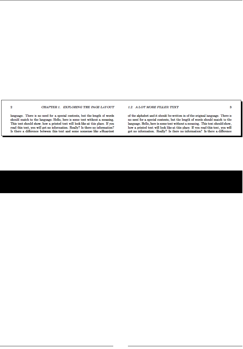
Designing Pages
[ 88 ]
If you use this form, the numbering will be suppressed and there won't be an entry in the
table of contents or in a header. Look at the heading Contents in our example; this has
actually been typeset by \chapter* inside the \tableofcontents macro.
As page headers have been menoned, let's explore them now.
Designing headers and footers
Already during tesng of the rst version of our example, you might have noced that except
for the page where the chapter started, all pages already showed the page number, chapter
tle, and secon tle in their header:
Though these standard headers are already quite useful, we shall see how to customize them
to meet our individual requirements.
Time for action – customizing headers with the
fancyhdr package
The default shape of the page headings is slanted. Furthermore, they are wrien in capital
leers. We shall use bold typeface instead and we will use capital leers only for the chapter
tle. We will load the fancyhdr package and use its commands to achieve that:
1. Load the rst version of our example. Insert the highlighted lines:
\documentclass[a4paper,12pt]{book}
\usepackage[english]{babel}
\usepackage{blindtext}
\usepackage{fancyhdr}
\fancyhf{}
\fancyhead[LE]{\leftmark}
\fancyhead[RO]{\nouppercase{\rightmark}}
\fancyfoot[LE,RO]{\thepage}
\pagestyle{fancy}
\begin{document}
\chapter{Exploring the page layout}
In this chapter we will study the layout of pages.
\section{Some filler text}
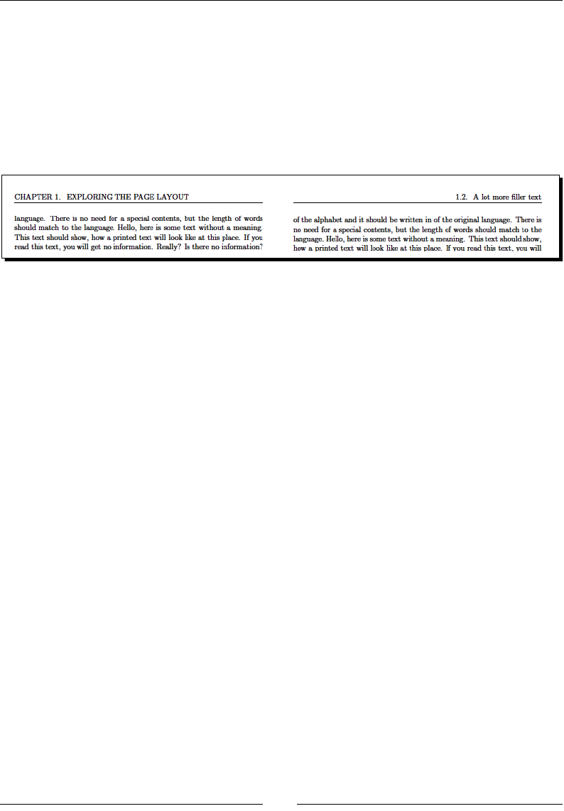
Chapter 3
[ 89 ]
\blindtext
\section{A lot more filler text}
More dummy text will follow.
\subsection{Plenty of filler text}
\blindtext[10]
\end{document}
2. Typeset—the footers will contain the page number on their outer side and the
headers should look like the following:
What just happened?
We loaded the fancyhdr package. Our rst acon was calling \fancyhf{}; this command
clears the headers and footers. Further, we used the following:
\leftmark: Used by the book class to store the chapter tle together with the
chapter number. Capital leers are used as default.
\rightmark: Used by the book class to store the secon tle together with its
number. Capital leers are used as well.
We used the command \fancyhead with the oponal argument LE to put the chapter tle
into the header. LE stands for le-even and means that this chapter tle will be put on the
le side of the header on even-numbered pages.
Analogous, we called the command \fancyhead with RO to put the secon tle into the
header. RO stands for right-odd and means that this secon heading shall be displayed on
right side of the header on odd-numbered pages.
Aerwards, we used \fancyfoot to display the page number in the footer. This me, we
used LE and RO that showed the page number on even as well as on odd pages, always on
the outer side. The command \thepage prints the page number.
All those commands are used to modify a page style provided by fancyhdr; this
style is called fancy. We had to tell LaTeX to use this style and we did it through
\pagestyle{fancy}.

Designing Pages
[ 90 ]
Emphasizing by wring all leers capitalized, like fancyhdr does by default,
is called all caps. It is widely regarded as a quesonable style. If it's used at
all, then it's recommended to slightly increase the spacing between the capital
leers. For adjusng this so called leerspacing, you can use the microtype
package or the soul package.
Understanding page styles
LaTeX and its base classes provide four page styles:
empty: Neither a header nor a footer is shown.
plain: No header. The page number will be printed and centered in the footer.
headings: The header contains tles of chapters, secons, and/or subsecons,
depending on the class and also the page number. The footer is empty.
myheadings: The header contains a user-dened text and the page number;
the footer is empty.
fancyhdr adds one page style:
fancy: Both the header and footer may be customized by the user.
Two commands may be used to choose the page style:
\pagestyle{name}: Switches to the page style name from this point onwards.
\thispagestyle{name}: Chooses the page style name only or the current page;
the following pages will have the style that's been used before.
You have seen that where a chapter starts, the page style is dierent to the style of other
pages. Such pages will have plain style. If you thought all pages should use the same style,
look into some books: it's very common that chapter beginnings dier in style. They usually
have a blank header. \thispagestyle could be used to override that.
Customizing header and footer
Let's divide the header and footer into six pieces: le, center, and right (l, c, r) both for the
header and footer. The commands to modify those areas are as follows:
For the header: \lhead, \chead, \rhead
For the footer: \lfoot, \cfoot, \rfoot
Each of these commands requires a mandatory argument, like \chead{User's guide}
or \cfoot{\thepage}. This argument will be put into the corresponding area of the page.
Chapter 3
[ 91 ]
Alternavely, you could use these versale commands:
For the header: \fancyhead[code]{text}
For the footer: \fancyfoot[code]{text}
Here, code may consist of one or more leers:
Symbol Meaning
L le
Ccenter
R right
E even page
O odd page
H header
F footer
It doesn't maer if we choose uppercase or lowercase leers. We already used such
combinaons in our example.
Using decorative lines in header or footer
We can introduce or delete lines between header and body text and body text and footer,
respecvely, with these two commands:
\renewcommand{\headrulewidth}{width}
\renewcommand{\footrulewidth}{width}
Where width may be a value like 1pt, 0.5mm, and so on. Just set it to 0pt if you don't like
such a line. The default is 0.4pt for the header line and 0pt for the footer line.
\renewcommand works exactly like \newcommand, except that the command must already
exist. It will get the new meaning. Incidentally, we've got to know a new concept: a lot of
LaTeX commands may be redened in this way. We shall take advantage of it from now on.
There are starred versions-\newcommand, and \renewcommand,
respecvely. They are called short commands. Their arguments must not contain
paragraph breaks. This limitaon eases troubleshoong, as TeX would be able to
pick up an error earlier. That's why many people use them whenever possible.
Designing Pages
[ 92 ]
Changing LaTeX's header marks
As we already know, LaTeX classes and packages store seconing numbers and headings
in the macros \leftmark and \rightmark automacally. It will be done when we call
\chapter, \section, or \subsection. So, we could just use \leftmark and
\rightmark in the arguments of the fancyhdr commands.
We will somemes want to change those entries manually, even if we rely on this
automasm. For instance, the starred seconing commands like \chapter* and
\section* won't produce a header entry, like indicated earlier. In such a case, two
commands will help us:
\markright{right head} sets the right heading
\markboth{left head}{right head} sets both le and right heading
The default style headings is easy-to-use and gives good results. myheadings can be
used together with \markright and \markboth. However, the most exible way is
given by fancy, especially in combinaon with \markright and \markboth.
There's a very good alternave to fancyhdr, which is a package
called scrpage2. It belongs to KOMA-Script, but works with other
classes as well. It provides a similar funconality and oers even
more features.
Breaking pages
As you've seen in our example, LaTeX took care of the page breaking. There might be
occasions where we'd like to insert a page break ourselves. LaTeX oers several commands
to do it; with vercal balance or without.
Time for action – inserting page breaks
We will go back to the rst version of our example and we shall manually insert a page break
right before the subsecon 1.2.1.
1. Insert the highlighted line into our example:
\documentclass[a4paper,12pt]{book}
\usepackage[english]{babel}
\usepackage{blindtext}
\begin{document}
\chapter{Exploring the page layout}
In this chapter we will study the layout of pages.
\section{Some filler text}
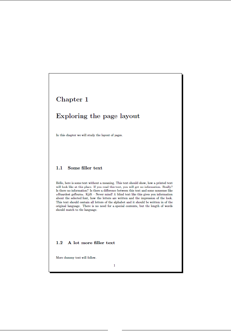
Chapter 3
[ 93 ]
\blindtext
\section{A lot more filler text}
More dummy text will follow.
\pagebreak
\subsection{Plenty of filler text}
\blindtext[10]
\end{document}
2. Typeset and have a look:
3. Replace \pagebreak by \newpage.
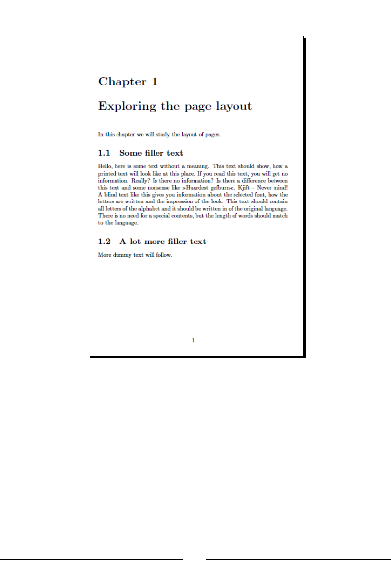
Designing Pages
[ 94 ]
4. Typeset and compare:
What just happened?
At rst, we inserted the command \pagebreak. Like its name suggests, it causes a page
break. Furthermore, the text has been stretched to ll the page down to the boom.
Aerwards, because of the obviously unpleasant whitespace between the paragraphs and
the headings, we replaced \pagebreak with \newpage. This command breaks the page
as well, but it doesn't stretch the text: the remaining space of the page will stay empty.
So, \pagebreak behaves like \linebreak and \newpage works like \newline, for
pages instead of lines. There's even a command \nopagebreak that's analogous to
\nolinebreak and forbids page breaking.
Chapter 3
[ 95 ]
\pagebreak won't break a line. Furthermore, \nopagebreak doesn't refer to the middle
of a line: both commands apply at the end of the current line. Of course, they immediately
have eect when used between paragraphs.
If you use the two-column format, both \pagebreak and \newpage would begin on a new
column instead of a new page.
There are two further variants: \clearpage works like \newpage,
except that it will start on a new page, even in two-column mode.
\cleardoublepage does the same, but causes the following text to start
on a right-hand page, inserng a blank page if necessary. The laer is useful
for two-sided documents.
More importantly, both commands cause all gures and tables that LaTeX has
in its memory to be printed out immediately.
Somemes you may noce large gaps between headings and paragraphs. Those could be
the result of a bad page break like in our example. In that case, you could assist LaTeX by
such a page break command or you switch o vercal juscaon by the command
\raggedbottom. Its counterpart \flushbottom will switch it on, which is the default
in the book class.
What we learned about line breaking is valid for page breaking as well: don't worry about it
while your work is sll in progress. Only when you're done with your document and you're
preparing the nal version, will it be me to tweak the page breaks.
Have a go hero – exploring page breaking options
Remember the oponal arguments for \linebreak and \nolinebreak. \pagebreak and
\nopagebreak are able to take an oponal argument as well, an integer between 0 and 4.
While 0 recommends, 4 demands. Again, try the previous example. This me use an oponal
argument for \pagebreak. Test with 0, 1, 2, 3, 4. Only \pagebreak[4] will cause the page
break because the necessary stretching is so much that LaTeX doesn't like to follow either a
weak or a strong request.
Enlarging a page
LaTeX's rules are not set in stone; they also apply to page balancing. There may be occasions
where we want to put a lile more text onto a page, even if the text would be squeezed a bit
or the text height increases. There's a command that will help us out: \enlargethispage.
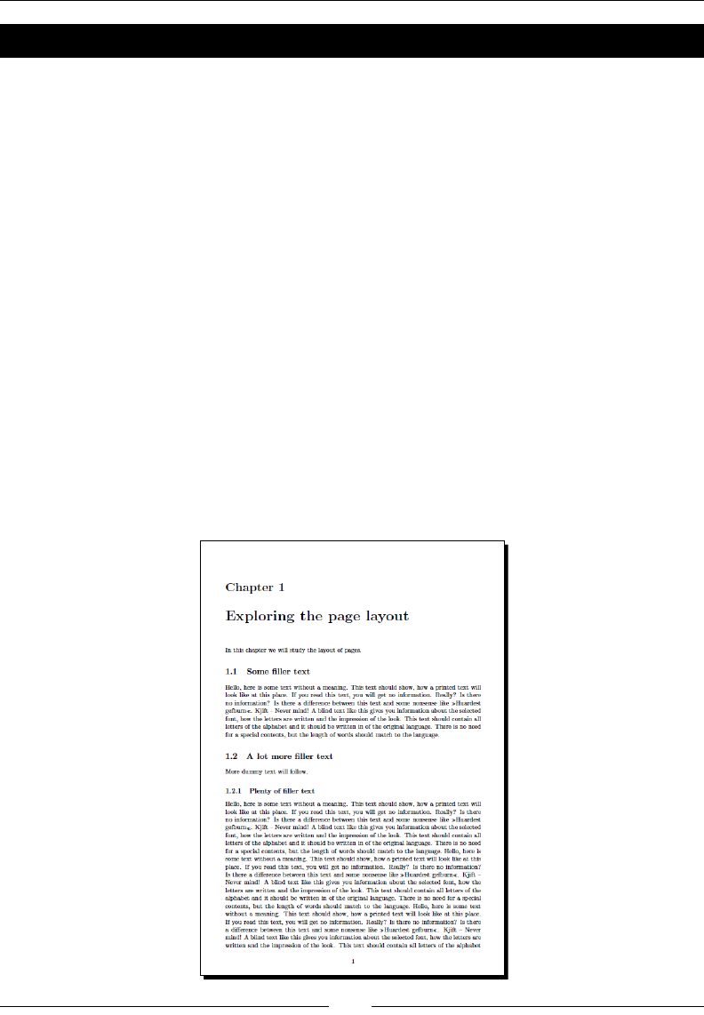
Designing Pages
[ 96 ]
Time for action – sparing an almost empty page
We shall modify our example a bit. This me, we will try to avoid a nearly empty page by
squeezing their text to the preceding page.
1. Remove the command \newpage from our example and switch to 11pt base font.
This me, use less ller text in the subsecon:
\documentclass[a4paper,11pt]{book}
\usepackage[english]{babel}
\usepackage{blindtext}
\usepackage[a4paper, inner=1.5cm, outer=3cm, top=2cm,
bottom=3cm, bindingoffset=1cm]{geometry}
\begin{document}
\chapter{Exploring the page layout}
In this chapter we will study the layout of pages.
\section{Some filler text}
\blindtext
\section{A lot more filler text}
More dummy text will follow.
\subsection{Plenty of filler text}
\blindtext[3]
\end{document}
2. Typeset, and the result will consist of two pages:
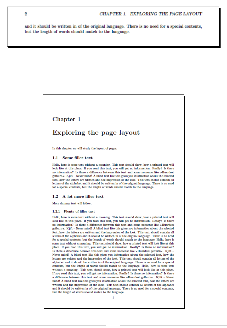
Chapter 3
[ 97 ]
3. Insert this command right aer the \subsection line:
\enlargethispage{\baselineskip}
4. Typeset. Now our document ts in only one page:
Designing Pages
[ 98 ]
What just happened?
We used the command \enlargethispage to squeeze more text onto a page. This
command takes the addionally requested height as its argument. The command
\baselineskip returns the height of a text line that we used as the argument. So,
LaTeX could put one extra line onto the page, and even the remaining line ed in as
well because LaTeX compressed some whitespace.
We could use factors: write \enlargethispage{2\baselineskip} to get two more lines
on a page. It doesn't even need to be an integer value. Like always, when you state a length,
you could use other units such as 10pt, 0.5in, 1cm, or 5mm, and even negave values.
Only the current page will be aected by this command.
There's a starred version: \enlargethispage* would
addionally shrink all vercal spaces on the page to their minimum.
Using footnotes
As briey menoned in Chapter 2, Formang Words, Lines, and Paragraphs, LaTeX provides
a command to typeset footnotes. Let's see it in acon.
Time for action – using footnotes in text and in headings
Let's go back to the very rst example of this chapter. We shall insert one footnote in the
body text and one in a secon heading:
1. Modify the example inserng a footnote, as shown in the highlighted line:
\documentclass[a4paper,12pt]{book}
\usepackage[english]{babel}
\usepackage{blindtext}
\begin{document}
\chapter{Exploring the page layout}
In this chapter we will study the layout of pages.
\section{Some filler text}
\blindtext
\section{A lot more filler text}
More dummy text\footnote{serving as a placeholder} will follow.
\subsection{Plenty of filler text}
\blindtext[10]
\end{document}
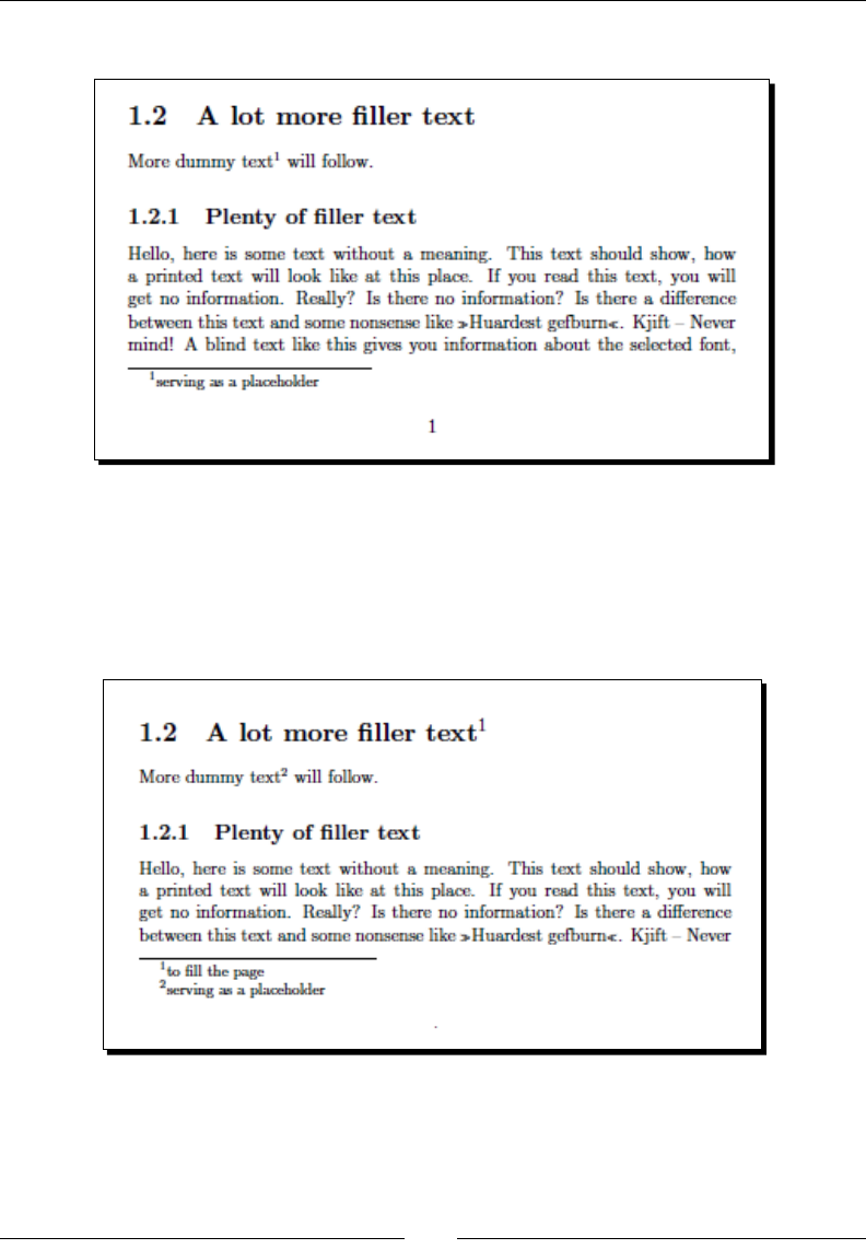
Chapter 3
[ 99 ]
2. Typeset to see how the footnote looks in print:
3. Insert a footnote in the second secon header. This me, put \protect right
before:
\section{A lot more filler text\protect\footnote{to fill the
page}}
4. Typeset to check that it works:

Designing Pages
[ 100 ]
What just happened?
The command \footnote{text} placed a superscripted number at the current posion.
Further, it prints its argument text into the boom of the page, marked by the same
number. As we've seen, such notes are separated from the main text by a horizontal line.
The other \footnote command has been preceded by the command \protect. If we
omied that, an error would be raised—try it. Such an error may occur when we use
\footnote inside an argument, where it's being further processed. \protect simply
prevents this processing error. As a rule of thumb, if a command causes an error when
it's used inside an argument, like in headings, try to x it by pung \protect right
before that command. Cases where \protect would hurt instead of helping are rare.
Generally, a heading might not be a good place for footnotes. If you simply use \footnote in
headings, be aware that they would appear in the table of contents and perhaps also in page
headers. If you want to avoid that, use the oponal parameter of the seconing commands
without \footnote, that is, \section[title without footnote]{title with
footnote}. The same applies to \chapter, and so on, and even further to \caption.
The complete denion of \footnote is:
\footnote[number]{text} produces a footnote marked by this oponal
number, an integer. If we don't give the oponal number, an internal counter would
be stepped and used. This would be done automacally; we don't need to worry.
Nevertheless, if we encounter dicules in placing footnotes, there are two commands
that help us:
\footnotemark[number] produces a superscripted number in the text as a
footnote mark. If the oponal argument wasn't given, it's also stepping and using
the internal footnote counter. No footnote will be generated.
\footnotetext[number]{text} generates a footnote without pung a
footnote mark into the text without stepping the internal footnote counter.
Both the commands may be used together in circumstances when \footnote would fail.
Set a footnote command right aer the related text. Don't leave a space in-between.
Otherwise, you would get a gap between the text and the following footnote mark.
Modifying the dividing line
The line that separates footnotes from the text is produced by the command
\footnoterule. If we wish to omit that line or if we want to modify it, we must
redene it. We learned about \renewcommand—so, let's use it.
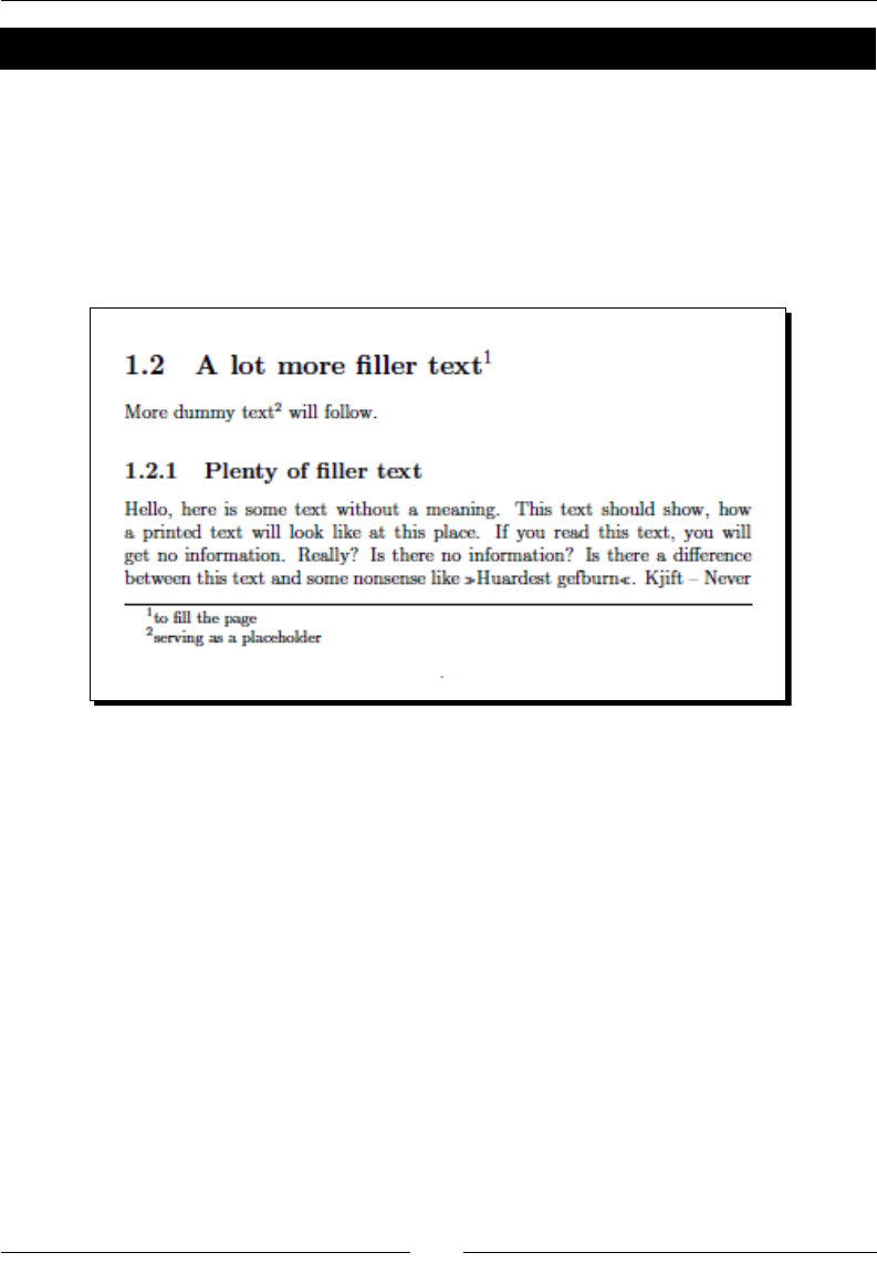
Chapter 3
[ 101 ]
Time for action – redening the footnote line
We will use \renewcommand to override the default \footnoterule command:
1. Take the previous example and add the following lines to the preamble:
\renewcommand{\footnoterule}
{\noindent\smash{\rule[3pt]{\textwidth}{0.4pt}}}
2. Typeset and see how the line has changed:
What just happened?
Remember the denion of \newcommand—here it's analogous. The exisng command
\footnoterule will be replaced by a new denion that we wrote in the second line. The
command \rule[raising]{width}{height} draws a line, here 0.4 pt thick, and as
wide as the text, raised a bit by 3 pt. Through the command \smash, we let our line pretend
to have a height and a depth of zero, so it's occupying no vercal space at all. This way,
the page balancing will not be aected. You already know \noindent, which avoids the
paragraph indentaon.
If you want to omit that line completely, you just need to write:
\renewcommand{\footnoterule}{}
Now the command is dened to do nothing.

Designing Pages
[ 102 ]
Using packages to expand footnote styles
There are dierent habits for seng footnotes. Some styles require footnotes numbered
per page, they might have to be placed in the document as so called endnotes, and symbols
instead of numbers may be used. More demands exist and therefore several packages have
been developed to comply with them. Here's a selecon:
endnotes: Places footnotes at the end of the document
manyfoot: Allows nested footnotes
bigfoot: Replaces and extends manyfoot, improves page break handling with
footnotes
savefnmark: Useful when you need to use footnotes several mes
footmisc: All-round package; introduces numbering per page, is able to save space
when many short footnotes are used, oers symbols instead of numbers as footnote
marks, provides hanging indentaon and other styles
Have a look at the respecve package documentaon to learn more—now you know how to
obtain it.
Pop quiz
1. According to the text, which of the following points should be the goal when
designing the page layout?
a. Fill the page as much as possible
b. Achieve an arsc design
c. Improve readability
d. Disnguish the work from other publicaons
2. Which opons are preset by the book class?
a. openright and twoside
b. openany and twoside
c. openright and oneside
d. openany and oneside
3. Which page style is used as default on the rst page of a chapter?
a. empty
b. plain
c. headings
d. myheadings
e. fancy

Chapter 3
[ 103 ]
4. One of these page breaking commands is able to stretch the text to the boom to
ll the page. Which one?
a. \newpage
b. \clearpage
c. \cleardoublepage
d. \pagebreak
5. We would like to put a footnote into a chapter heading. Choose the best way!
a. \chapter{title\footnote{text}}
b. \chapter*{title\footnote{text}}
c. \chapter{title\protect\footnote{text}}
d. \chapter[title]{title\footnote{text}}
Summary
In this chapter, we have worked out how to design the overall layout of a document.
Specically, we learned about:
Adjusng the page dimensions and margins
Using landscape orientaon and two-column layout
Modifying the spacing between lines
Breaking pages and paying aenon to the vercal juscaon
Designing headers and footers with tles and page numbers
Using footnotes
Further, we covered some general topics:
Obtaining documentaon of packages in several ways
Changing document properes by choosing class opons
Redening exisng commands
Now it's me to deal with further text structures. In the next chapter, we shall learn how to
create lists for presenng text in an easy-to-read way.
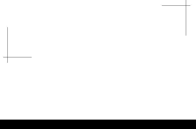
4
Creating Lists
Arranging text in the form of a list can be very reader-friendly. You can present
several ideas by a clear structure which is easy to survey. Commonly, three
types of lists are used:
1. Bulleted lists
2. Numbered lists
3. Denion lists
In this chapter, we shall learn how to create such lists.
Building a bulleted list
We shall start with the simplest kind of list. It contains just the items without numbers. Each
item is marked by a bullet.
Time for action – listing LaTeX packages
We shall create a list of packages that we got to know in the previous chapter:
1. Begin a new document and enter the following code:
\documentclass{article}
\begin{document}
\section*{Useful packages}
LaTeX provides several packages for designing the layout:
\begin{itemize}
\item geometry
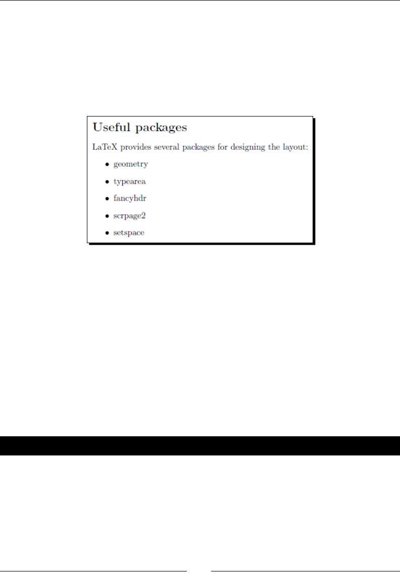
Creang Lists
[ 106 ]
\item typearea
\item fancyhdr
\item scrpage2
\item setspace
\end{itemize}
\end{document}
2. Typeset and have a look at the output:
What just happened?
It was not necessary to load any package. We began with a heading followed by some
text. For the actual list, we used an environment called itemize. As we know about
environments, \begin{itemize} starts it and \end{itemize} ends it. The command
\item tells LaTeX that a new item to the list follows. Each item may contain text of any
length and even paragraph breaks. Well, that's prey easy, isn't it?
Nesting lists
When a list gets longer, we could make it clearer by dividing it. We just create lists in a
list. It's advisable to use dierent bullets to keep the list levels apart easily. LaTeX does
it for us automacally.
Time for action – listing packages by topic
We shall rene the package list by introducing categories:
1. Rene the aforemenoned highlighted itemize environment of our
example in the following way:
\begin{itemize}
\item Page layout
\begin{itemize}
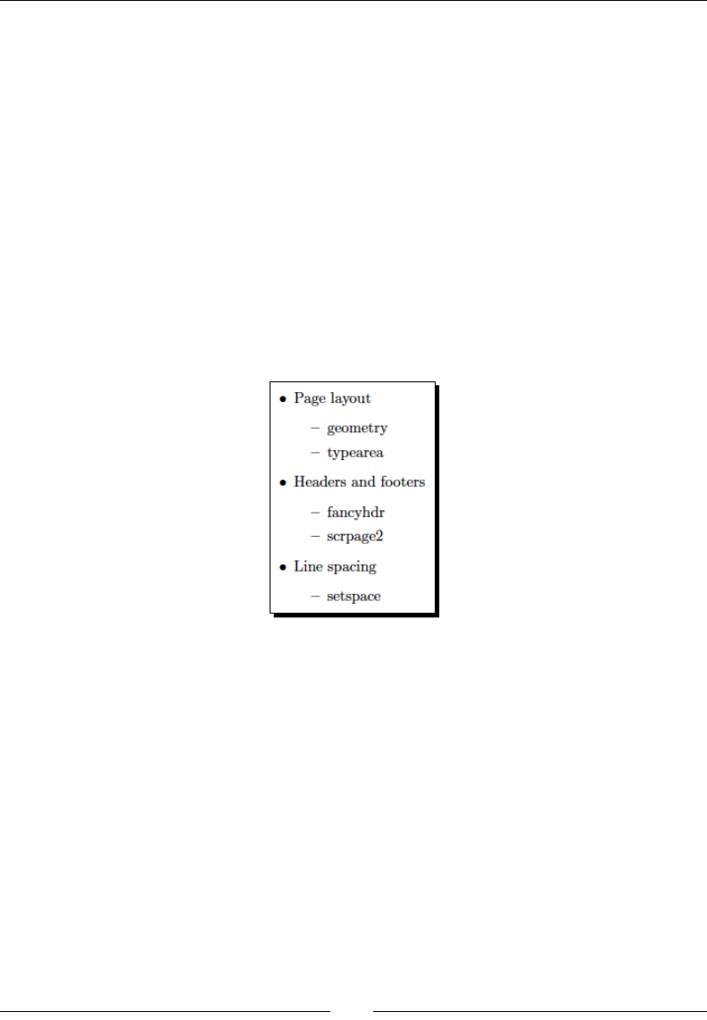
Chapter 4
[ 107 ]
\item geometry
\item typearea
\end{itemize}
\item Headers and footers
\begin{itemize}
\item fancyhdr
\item scrpage2
\end{itemize}
\item Line spacing
\begin{itemize}
\item setspace
\end{itemize}
\end{itemize}
2. Typeset to see the new list:
What just happened?
We simply inserted another list inside the list. Up to four levels are possible, otherwise LaTeX
would stop and print out the error message ! LaTeX Error: Too deeply nested. As we saw, the
rst level is marked by a bullet, and the second by an en dash. A third level item would start
with an asterisk symbol *. The fourth and last level would be marked by a centered dot.
Deeply nested lists can rarely be seen; such complicated structures might be hard to read.
In such cases, it could be a good idea to revise the text structure or at least split the list.
Creating a numbered list
Bulleted lists are useful if the order of the items doesn't maer. However, if the order is
important, we could organize the items by giving them numbers and creang a sorted list.
That would allow a reader to follow our thoughts easily.
Creang Lists
[ 108 ]
Time for action – writing a step-by-step tutorial
Let's prepare a ny "how-to" about designing the page layout:
1. Start with a new document and enter the following code:
\documentclass{article}
\begin{document}
\begin{enumerate}
\item State the paper size by an option to the document class
\item Determine the margin dimensions using one of these
packages:
\begin{itemize}
\item geometry
\item typearea
\end{itemize}
\item Customize header and footer by one of these packages:
\begin{itemize}
\item fancyhdr
\item scrpage2
\end{itemize}
\item Adjust the line spacing for the whole document
\begin{itemize}
\item by using the setspace package
\item or by the command \verb|\linespread{factor}|
\end{itemize}
\end{enumerate}
\end{document}
2. Typeset to generate the «how-to»:
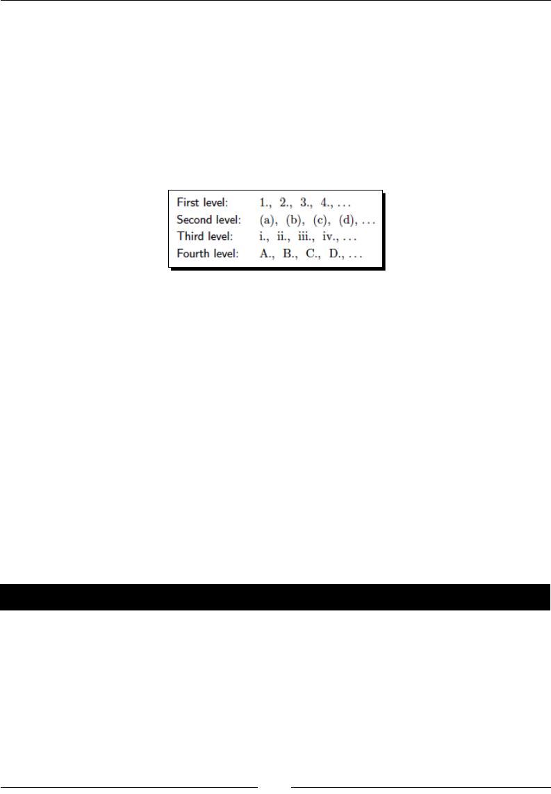
Chapter 4
[ 109 ]
What just happened?
We used an enumerate environment. Except for the name, we use it just like the itemize
environment; each list item is introduced by the command \item. Again, we nested two
lists, but this me the lists are of a dierent kind. As we saw, that's no problem. Even though
the unnumbered list is embedded within a numbered list, it's marked by bullets, because it's
the rst unnumbered level. Mixed nesng could go further than four levels, but four is the
maximum for each kind and six in general.
The default numbering scheme for the enumerate environment is as follows:
\item understands an oponal argument; if you write \item[text], then text will be
printed instead of a number or a bullet. This way, you could use any numbering and any
symbol for the bullet.
Customizing lists
The default appearance of lists is meaningful regarding spacing, indentaon, and symbols.
Nevertheless, it may be required to use another scheme for the enumeraon, for the bullets,
or to modify the line spacing or their indentaon. There are packages helping us both to save
space and to customize the symbols; let's start with the spacing.
Saving space with compact lists
A frequently arising queson is how to reduce the space. LaTeX's lists are oen regarded as
being too spacious. We shall see how to implement that.
Time for action – shrinking our tutorial
We shall remove the white space around the list items and before and aer the whole list
as well:
1. In the previous example, load the package paralist and replace
enumerate with compactenum and itemize with compactitem:
\documentclass{article}
\usepackage{paralist}
\begin{document}
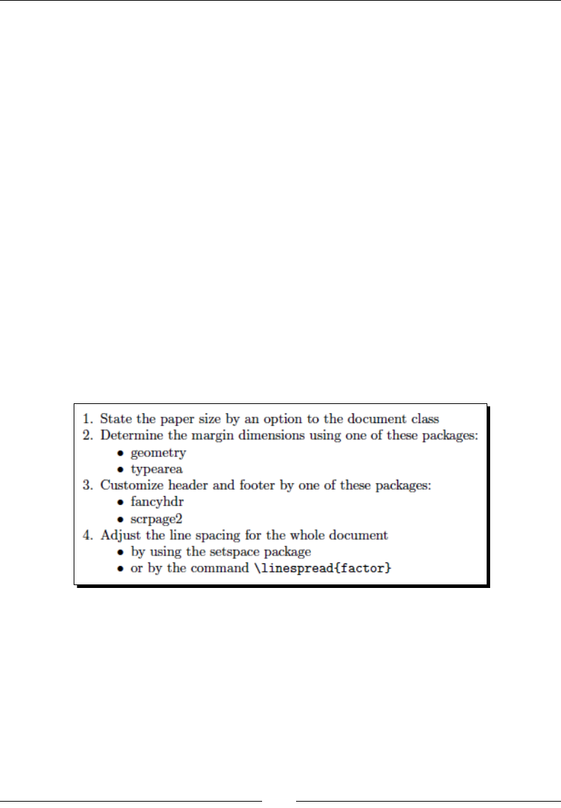
Creang Lists
[ 110 ]
\begin{compactenum}
\item State the paper size by an option to the document class
\item Determine the margin dimensions using one of these
packages:
\begin{compactitem}
\item geometry
\item typearea
\end{compactitem}
\item Customize header and footer by one of these packages:
\begin{compactitem}
\item fancyhdr
\item scrpage2
\end{compactitem}
\item Adjust the line spacing for the whole document
\begin{compactitem}
\item by using the setspace package
\item or by the command \verb|\linespread{factor}|
\end{compactitem}
\end{compactenum}
\end{document}
2. Typeset and compare the spacing:
3. Now extend the highlighted list item for setspace as follows:
\item by using the setspace package and one of its options:
\begin{inparaenum}
\item singlespacing
\item onehalfspacing
\item double spacing
\end{inparaenum}
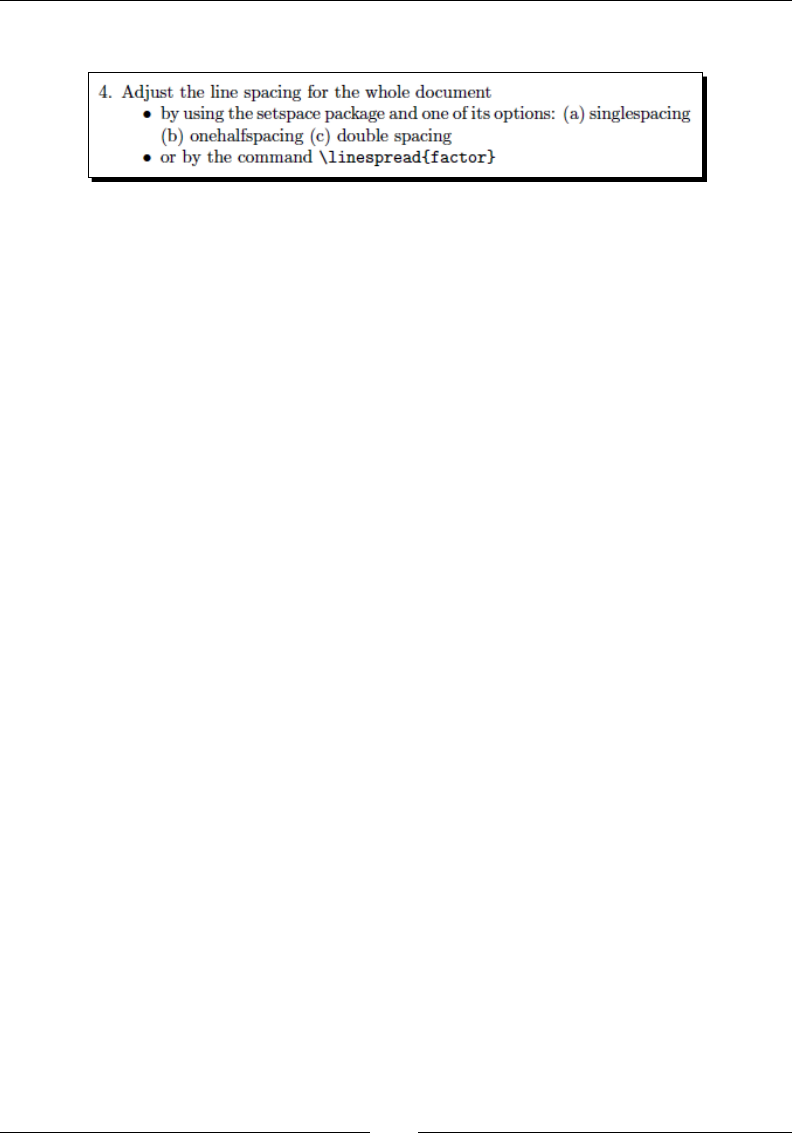
Chapter 4
[ 111 ]
2. Typeset and look at the change in the line spacing subject:
What just happened?
The used package paralist provides several new list environments designed to be
typeset within paragraphs or in a very compact look. We loaded this package and replaced
the standard environments with their compact counterparts. In step 3, we used a new
environment, where the items are enumerated but stay within the same paragraph.
For each standard environment, paralist adds three corresponding environments:
Numbered lists:
compactenum: Compact version of the enumerate environment without any
vercal space before or aer the list or its items
inparaenum: An enumerated list typeset within a paragraph
asparaenum: Every list item is formaed like a separate common LaTeX paragraph,
but numbered
Bulleted lists:
compactitem: Compact version of the itemize environment like compactenum
inparaitem: An itemized list typeset within a paragraph, rarely seen in print
asparaitem: Like asparaenum, but with symbols instead of numbers
Choosing bullets and numbering format
To follow language specic habits or certain requirements, we might wish to enumerate
by Roman numbers or alphabecally; parentheses or dots might be required. Some may
prefer dashes instead of bullets. The package enumitem provides sophiscated features to
implement such requirements.

Creang Lists
[ 112 ]
Time for action – modifying lists using enumitem
Let's change the numbering scheme. We shall number alphabecally using circled leers.
Furthermore, we will replace bullets by dashes:
1. We shall discard paralist and load the package enumitem instead. We will turn
away from the compact environments returning to the standard list notaon:
\documentclass{article}
\usepackage{enumitem}
\setlist{nolistsep}
\setitemize[1]{label=---}
\setenumerate[1]{label=\textcircled{\scriptsize\Alph*},
font=\sffamily}
\begin{document}
\begin{enumerate}
\item State the paper size by an option to the document class
\item Determine the margin dimensions using one of these
packages:
\begin{itemize}
\item geometry
\item typearea
\end{itemize}
\item Customize header and footer by one of these packages:
\begin{itemize}
\item fancyhdr
\item scrpage2
\end{itemize}
\item Adjust the line spacing for the whole document
\begin{itemize}
\item by using the setspace package
\item or by the command \verb|\linespread{factor}|
\end{itemize}
\end{enumerate}
\end{document}
2. Typeset and see the output:
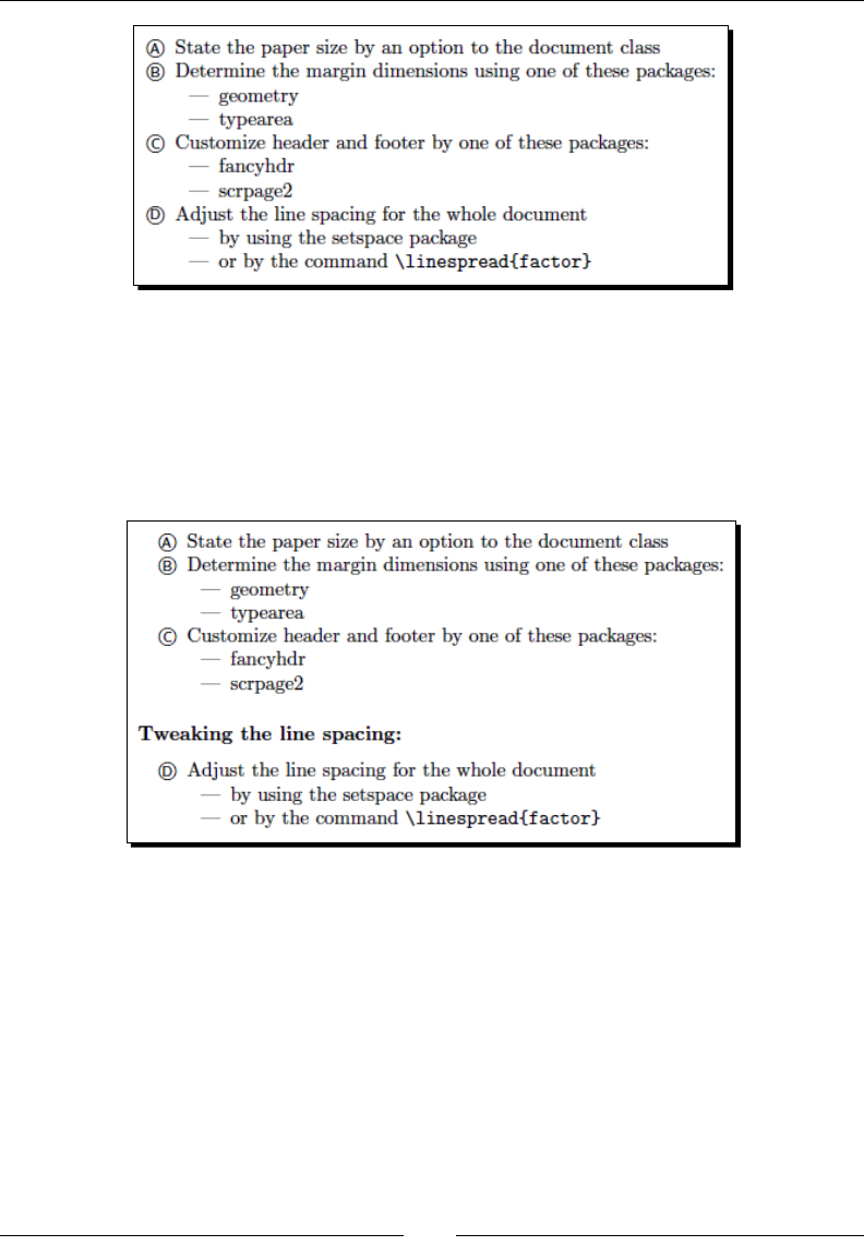
Chapter 4
[ 113 ]
3. Right above the highlighted line, insert the following lines:
\end{enumerate}
\subsubsection*{Tweaking the line spacing:}
\begin{enumerate}[resume*]
4. Typeset to see the change:
What just happened?
We used the enumitem command to specify list properes. Let's take a closer look:
\setlist{nolistsep}: \setlist sets properes valid for all types of lists. Here
we specied nolistsep to achieve very compact lists analogous to the compact
paralist environment.
\setitemize[1]{label=–--}: \setitemize modies properes of bulleted
lists. Here we chose an em dash as the label to get a leading wide dash.

Creang Lists
[ 114 ]
\setenumerate[1]{label=\textcircled{\scriptsize\Alph*},font=\
sffamily}: \setenumerate sets properes valid for numbered lists. We used it
to set a label and a font for the label. The command \Alph* stands for enumeraon
in capital leers.
All of those three commands allow arguments of the form key=value. Some useful
parameters are as follows:
Parameter Meaning Values Example
font Modies the label font Any font command font=\bfseries
label Sets the label for the
current level
May contain
\arabic*,
\alph*, \Alph*, \
roman*, \Roman*
label=\emph\
alph*)
label* Like label but
appended to the
current label
Like label label*=\arabic)
align Alignment of the label left or right align=right
start Number of the rst
item
Integer start=10
resume,
resume*
Let's the counter
continue from the
previous lists value
resume
noitemsep No extra space
between items and
paragraphs
noitemsep
nolistsep No extra vertical
spacing at all
nolistsep
These opons may be set globally like \setenumerate[level]{key=value list}.
If the oponal argument level is missing, this global command will apply to all levels.
Those opons may be used locally like we did with resume*. Other examples are:
\begin{itemize}[noitemsep] for a compact bulleted list
\begin{enumerate}[label=\Roman*.,start=3] numbered by III., IV., ...
\begin{enumerate}[label=\alph*)],nolistsep] for a very compact list
numbered a), b), c), ...

Chapter 4
[ 115 ]
The labeling commands would achieve a numbering as follows:
\arabic* 1, 2, 3, 4, …
\alph* a, b, c, d, …
\Alph* A, B, C, D, …
\roman* i, ii, iii, iv, …
\Roman* I, II, III, IV, …
The * has been added to disnguish those commands from LaTeX commands with the same
name. Parentheses and punctuaon may be used as wished. Later in the book, you will learn
how to choose between thousands of symbols for labels and bullets.
There's even a short form: if you load enumitem with the opon shortlabels, you may
use a compact syntax like \begin{enumerate}[(i)], \begin{enumerate}[(1)] where
1, a, A, i, I stand for \arabic*, \alph*, \Alph*, \roman*, \Roman* respecvely. This
allows customizaon quickly and easily. However, consider using global commands to keep
formang consistent.
Suspending and continuing lists
In step 3 of our example, we interrupted the list. We connued wring normal text unl we
restarted the list by \begin{enumerate}[resume*]. The resume opon tells enumitem
to connue the list with the next number. The starred variant resume* does it with the
same formang like before. If you would like to complete the document, note that a \
subsubsection command should be preceded by a \subsection command. This should
follow a \section command. Just using a lower-level heading without a parent heading
could result in numbering like 0.0.1.
Producing a denition list
We shall proceed to the third kind of list, namely, denion lists, also called descripon lists.
Every list item consists of a term followed by its descripon.
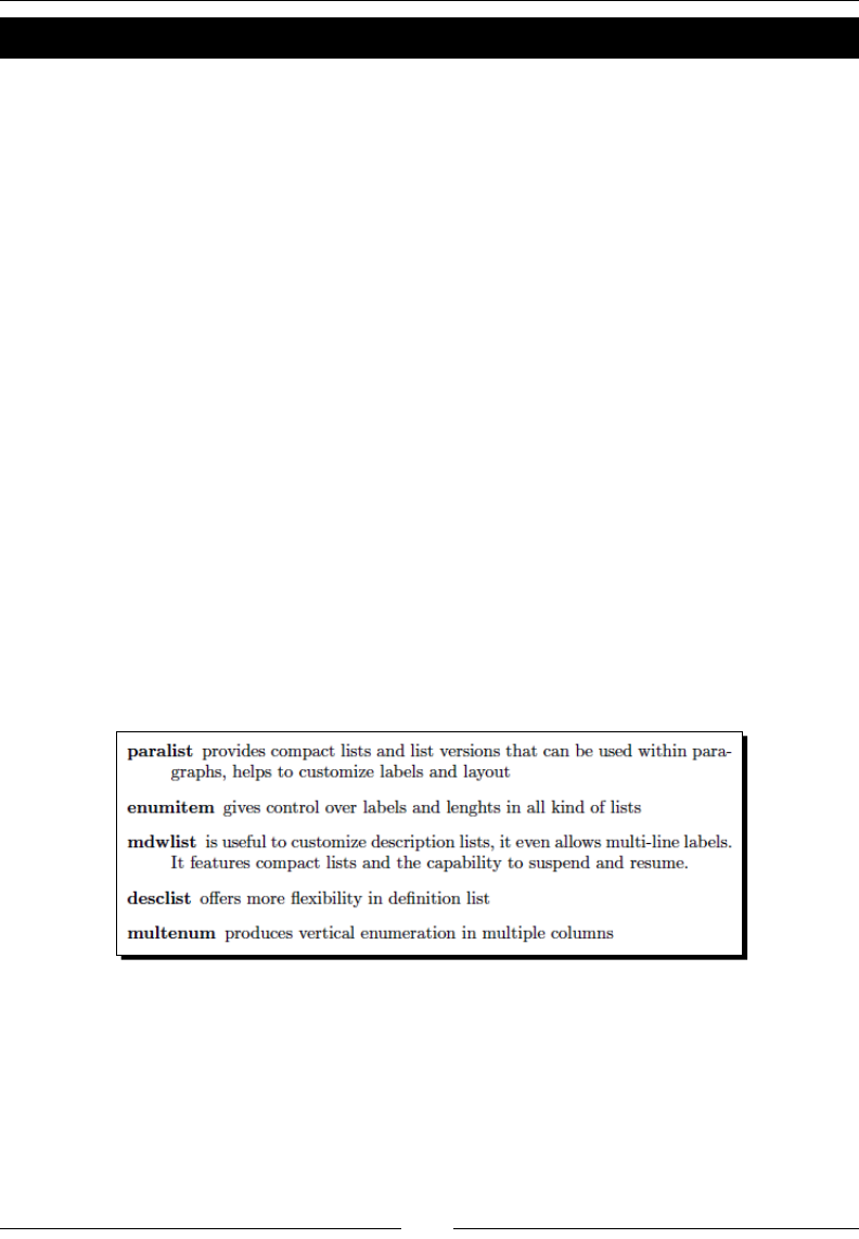
Creang Lists
[ 116 ]
Time for action – explaining capabilities of packages
Now that we know some packages for creang lists, we shall write a short overview to show
their capabilies. Let's choose some addional packages listed on http://texcatalogue.
sarovar.org:
1. We will use a descripon environment. Create a document with the following code:
\documentclass{article}
\begin{document}
\begin{description}
\item[paralist] provides compact lists and list versions that
can be used within paragraphs, helps to customize labels and
layout
\item[enumitem] gives control over labels and lengths
in all kind of lists
\item[mdwlist] is useful to customize description lists, it
even allows multi-line labels. It features compact lists and
the capability to suspend and resume.
\item[desclist] offers more flexibility in definition list
\item[multenum] produces vertical enumeration in multiple
columns
\end{description}
\end{document}
2. Typeset to get the denion list:

Chapter 4
[ 117 ]
What just happened?
We used the descripon environment like the other lists, except that we used the oponal
argument of \item. In the description environment, \item is dened such that the
oponal parameter will be typeset in the bold typeface.
The package paralist supports the description environment as well; there are
the compactdesc, inparadesc, and asparadesc versions working analogous to
the other lists.
The same is valid for enumitem: there's the global command \setdescription{format}
working like \setitemize and \setenumerate. Furthermore, it also extends the
descripon environment to accept oponal formang arguments of the form key=value,
supporng the short form as well.
Have a go hero – adjusting the dimensions of lists
LaTeX's lists have a meaningful layout. However, there might be occasions when you would
like to modify this layout, for instance, to change the margins or the item indentaon. All
layout dimensions are determined by LaTeX macros, so called lengths.
There's a package which is really great for visualizing layouts, which presents these length
macros. It's called layouts and it has been wrien by Peter Wilson. Let's use it to examine
LaTeX's list dimensions. We will use this small document:
\documentclass[12pt]{article}
\usepackage{layouts}
\begin{document}
\listdiagram
\end{document}
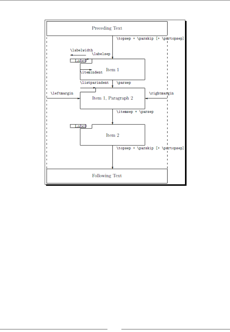
Creang Lists
[ 118 ]
By simply typeseng it, we will get the following diagram:
Isn't it fantasc? The layouts package can do even more, which you can read about in its
documentaon. For now, we stay on topic regarding lists.
Though there are LaTeX commands for customizing those lengths, for example,
\setlength{\labelwidth}{2cm}, applying them to individual lists and certain
nesng depths is hard. If you need to modify the list layout, the enumitem package
comes handy again. Its commands like \setlist and its key=value interface may be
used also for adjusng the values of the lengths you could see in the previous diagram.
For example, if we would like to remove the space between list items in the
description environment and to reduce the le margin, we could load
enumitem and write the following:
\setdescription{itemsep=0cm,parsep=0cm,leftmargin=0.5cm}
Note, we don't use the backslash for keys. Similarly, \setitemize, \setenumerate, and
\setlist can be used for ne-tuning. Try assigning values by yourself, and test the eect on
our examples. If you would like to learn more, have a look at the enumitem documentaon.

Chapter 4
[ 119 ]
Pop quiz
1. A list environment may be nested to up to how many levels?
a. Two
b. Three
c. Four
d. Any number, just depending on the memory
2. All but one of these packages understand opons in the form key=value. Which
does not?
a. geometry
b. paralist
c. enumitem
3. In which environment should \item be used with an oponal argument?
a. itemize
b. enumerate
c. description
d. inparaenum
Summary
In this chapter, we got to know a new way to structure our text—lists. Specically, we
learned to create:
Bulleted lists using the itemize environment
Numbered lists using the enumerate environment
Denion lists using the description environment
Furthermore, we worked with compact versions of such lists provided by the packages
paralist and enumitem. Those packages allowed us to customize our lists at will.
You may regard those lists as an addional possibility to structure your text. Use it to clarify
your ideas. Though you may design the layout of lists as you wish, it's highly recommended
to use the same bullets and numbering scheme respecvely for the same nesng level.
5
Creating Tables and Inserting
Pictures
Scienc documents and others do not just contain plain text; they also present
informaon and data in tables and use diagrams and drawings to visualize
them. We shall become familiar with that.
In this chapter, we will learn how to perform the following:
Lining up text and data in columns
Typeseng complex tables
Including pictures in our documents
Adding capons to pictures and tables
Controlling the placement of gures and tables
Let's tackle these tasks!
Writing in columns
Remember the me of the typewriter and early word processing soware? When we
needed to line up some text in columns, we could use tab stops. LaTeX provides a similar
way to easily align text in columns, namely, the tabbing environment.
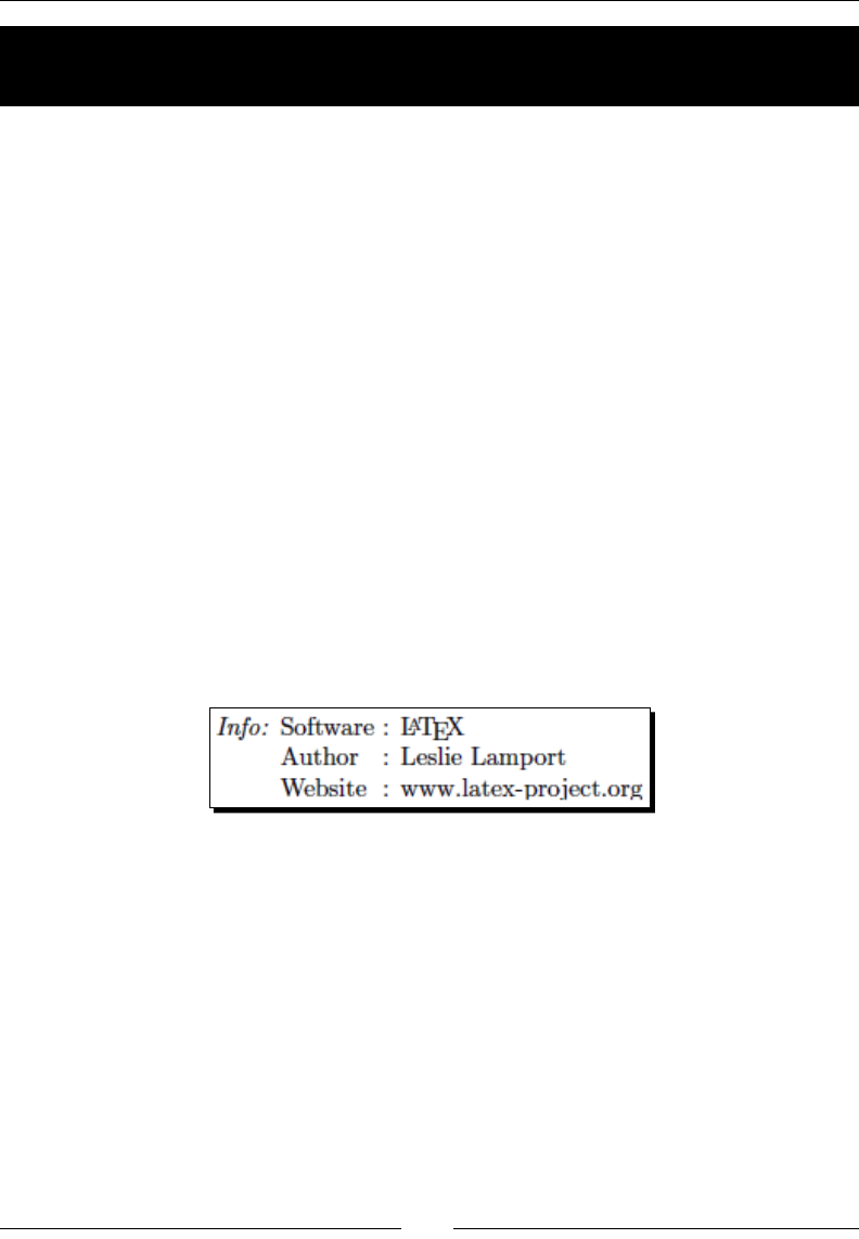
Creang Tables and Inserng Pictures
[ 122 ]
Time for action – lining up information using the tabbing
environment
We would like to present a quick overview regarding LaTeX. We shall present one point on
each line, aligned at words and double colons:
1. Begin a new document and open a tabbing environment:
\documentclass{article}
\begin{document}
\begin{tabbing}
2. Write the text, set tab stops by \=, and end the line by \\:
\emph{Info:} \= Software \= : \= \LaTeX \\
3. Add further lines, move to the next tab stop by \>, and again end lines by \\:
\> Author \> : \> Leslie Lamport \\
\> Website \> : \> www.latex-project.org
4. Close the tabbing environment and end the document:
\end{tabbing}
\end{document}
5. Typeset to get the output:
What just happened?
The tabbing environment that we used begins a new line. We used three simple tags
for markup:
\= sets a tab stop. We could put several tab stops on a line. If we use \=
later, the next awaited tab stop would be reset to this posion.
\\ ends a row.
\> goes to the next tab stop. This could also mean to go backwards.
This way, we can quickly produce columns containing le-aligned text. If the rows of the
tabbing environment would reach the end of a page, it could connue on the next page.
What if a column is too long, running over the tab stop? Let's see how to solve that.
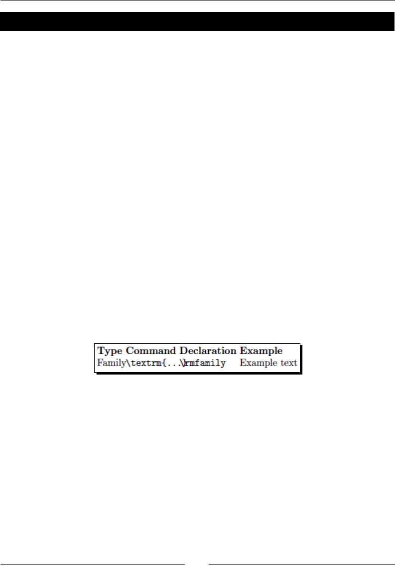
Chapter 5
[ 123 ]
Time for action – lining up font commands
In Chapter 2, Formang Words, Lines, and Paragraphs, we've got to know a lot of font
commands and declaraons. We saw a table containing those commands and example
output. Now we shall create such a table ourselves:
1. Begin a new document, like the one in step 1 of our previous example,
but dene a command for seng the font of our header:
\documentclass{article}
\newcommand{\head}[1]{\textbf{#1}}
\begin{document}
\begin{tabbing}
2. Write the rst row set tab stops by \= and use \> to move to the tab stops.
Use the command \verb|…| to typeset the LaTeX commands:
\begin{tabbing}
Family \= \verb|\textrm{...}| \= \head{Declaration} \= \kill
\> \head{Command} \> \head{Declaration} \> \head{Example}\\
Family \> \verb|\textrm{...}| \> \verb|\rmfamily|
\> \rmfamily Example text\\
\> \verb|\textsf{...}| \> \verb|\sffamily|
\> \sffamily Example text\\
\> \verb|\texttt{...}| \> \verb|\ttfamily|
\> \ttfamily Example text
\end{tabbing}
3. Typeset and examine:
4. As we can see, the tab stops are too narrow. We shall correct it. Create a new head
row containing the tab stops; this me, we will mark the line by \kill to hide that
line. Use ller text to specify the width between the tab stops. Complete it with
further font commands:
\begin{tabbing}
Family \= \verb|\textrm{...}| \= \head{Declaration} \= \kill
\> \head{Command} \> \head{Declaration} \> \head{Example}\\
Family \> \verb|\textrm{...}| \> \verb|\rmfamily|
\> \rmfamily Example text\\
\> \verb|\textsf{...}| \> \verb|\sffamily|
\> \sffamily Example text\\
\> \verb|\texttt{...}| \> \verb|\ttfamily|
\> \ttfamily Example text
\end{tabbing}
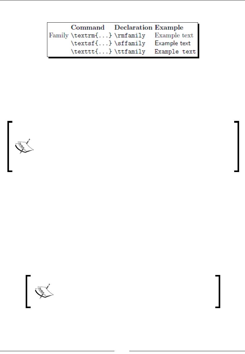
Creang Tables and Inserng Pictures
[ 124 ]
5. Typeset to get the result:
What just happened?
Aer we noced that our tab stops have been set too narrow, we constructed a new rst row
containing the tab stops. It consists of words represenng the widest entries of each column.
To hide this auxiliary row, we used the command \kill right at the end of the line; \kill
at the end of a line causes this line to have no output.
Like in this example, the command \verb|code| typesets code "as it is",
without interpreng commands within. Instead of |, any character may be
chosen as the delimiter. \verb cannot be used in arguments of commands
including \section and \footnote, and not in table heads.
For longer, verbam text, use the environment with the same name:
verbatim.
There are further useful commands:
\+ at the end of a line causes each subsequent line to start at the rst tab.
Use it twice \+\+ to start at the second tab and so on.
\- cancels a preceding \+; also using mulply has cumulave eect.
\< at the beginning of a line cancels the eect of one previous \+ command
for that line.
The menoned commands already allow a good use of the tabbing environment. Even more
commands can be found in the reference manual: http://texblog.net/help/latex/
tabbing.html.
Inside tabbing environments, declaraons are local to the
current item. A following \=, \>, \\, or \kill command
would stop the eect.
Tabbing environments cannot be nested.
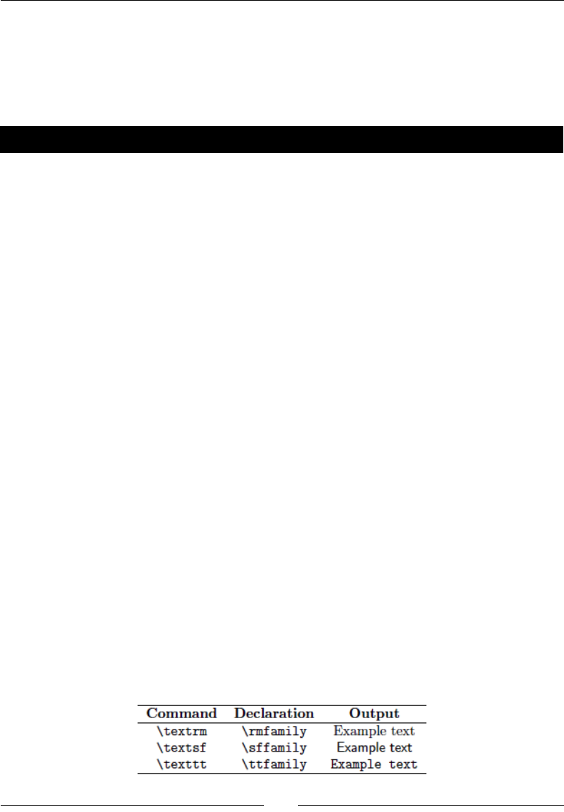
Chapter 5
[ 125 ]
Typesetting tables
We might need more complicated structures and formang, like centering in columns,
dividing lines, or even nested structures. LaTeX provides the tabular environment for
typeseng simple and complex tables which can be nested.
Time for action – building a table of font family commands
We shall create a table like in the previous example, but this me, we would like to make all
entries in a column horizontally centered to each other. We will also add some horizontal
lines to mark the border and the header of the table:
1. Create a new document. Dene a command for seng the font for the head row:
\documentclass{article}
\newcommand{\head}[1]{\textnormal{\textbf{#1}}}
\begin{document}
2. Begin a tabular environment. As a mandatory argument, provide ccc standing
for three centered columns:
\begin{tabular}{ccc}
3. Write the table head row, write & to separate column entries, and \\ to end rows.
Use \hline to insert horizontal lines:
\hline
\head{Command} & \head{Declaration} & \head{Output}\\
\hline
4. Connue with the table body and end the environment and the document. For
typeseng LaTeX commands, write \verb|\command|:
\verb|\textrm| & \verb|\rmfamily| & \rmfamily Example text\\
\verb|\textsf| & \verb|\sffamily| & \sffamily Example text\\
\verb|\texttt| & \verb|\ttfamily| & \ttfamily Example text\\
\hline
\end{tabular}
\end{document}
5. Typeset to see the table:

Creang Tables and Inserng Pictures
[ 126 ]
What just happened?
In the mandatory argument, we wrote a list of characters. Each character stands for a
formang opon. As we used three characters, we've got three columns. c stands for
centered alignment. Therefore, the entries of all columns have been centered.
Column entries are separated by &, while rows are terminated by \\. Don't end the last
line by \\ unless you further wish to write a line below. It's also a good idea to align the
ampersands in our source code to keep it readable.
Inside the entries, you may use ordinary text as well as LaTeX commands. As in the tabbing
environment, declaraons are local to the entry, like if each entry was surrounded by curly
braces.
Furthermore, tabular has an oponal alignment argument just like minipage. So, the
complete denion is:
\begin{tabular}[position]{column specifiers}
row 1 col 1 entry & row 1 col 2 entry ... & row 1 col n entry\\
...
\end{tabular}
In the oponal argument, t means alignment at the top row and b means alignment at the
boom row. The default is vercally centered alignment. This may come in handy if you
would like to place two tables next to each other or within further text.
Drawing lines in tables
Within tabular, three types of lines may be used:
\hline draws a horizontal line over the whole width of the table
\cline{m-n} draws a horizontal line starng at the beginning of column m and
ending at the end of column n
\vline draws a vercal line over the full height and depth of the current row
Understanding formatting arguments
Of course, further formang is possible. Have a look at this example table:
\begin{tabular}{|l|c|r|p{1.7cm}|}
\hline
left & centered & right & a fully justified paragraph cell\\
\hline
l & c & r & p\\
\hline
\end{tabular}
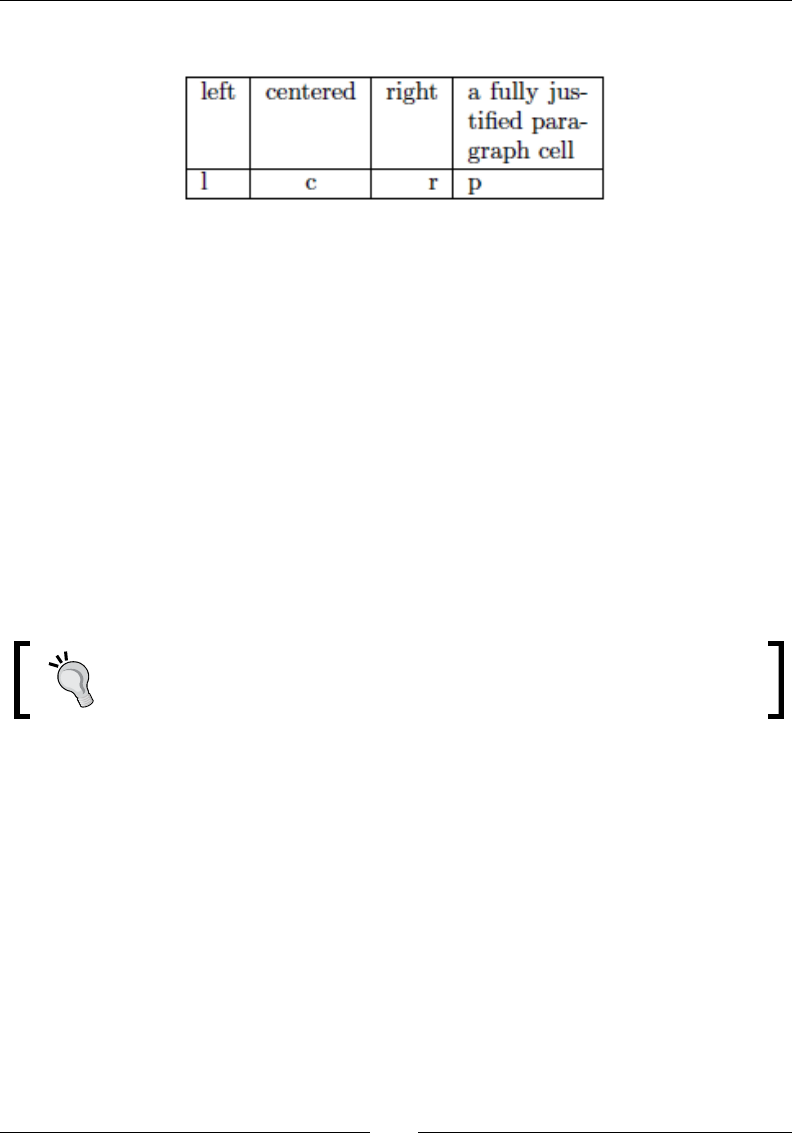
Chapter 5
[ 127 ]
This code would produce the following table:
The opons understood by the tabular environment are as follows:
l for le alignment.
c for centered alignment.
r for right alignment.
p{width} for a "paragraph" cell of a certain width. . If you place several p cells
next to each other, they will be aligned at their top line. It's equivalent to using
\parbox[t]{width} within a cell.
@{code} inserts code instead of empty space before or aer a column. This might
also be some text or it could be le empty to avoid this space.
| stands for a vercal line.
*{n}{options} is equivalent to n copies of options, where n is a posive integer
and options may consist of one or more column speciers including * as well.
It is very advisable to avoid vercal lines in tables. Lines should subtly support
your informaon but not make reading dicult.
Aer loading the array package by \usepackage{array} you may use some opons,
such as:
m{width} is similar to\parbox{width}: the base line is at the middle
b{width} is like \parbox[b]{width}: the base line is at the boom
!{code} can be used like | but inserts code instead of a vercal line.
In contrast to @{…}, the space between columns will not be suppressed.
>{code} can be used before an l, c, r, p, m, or b opon and inserts code right at
the beginning of each entry of that column
<{code} can be used aer an l, c, r, p, m, or b opon and inserts code at the end
of the entry of that column
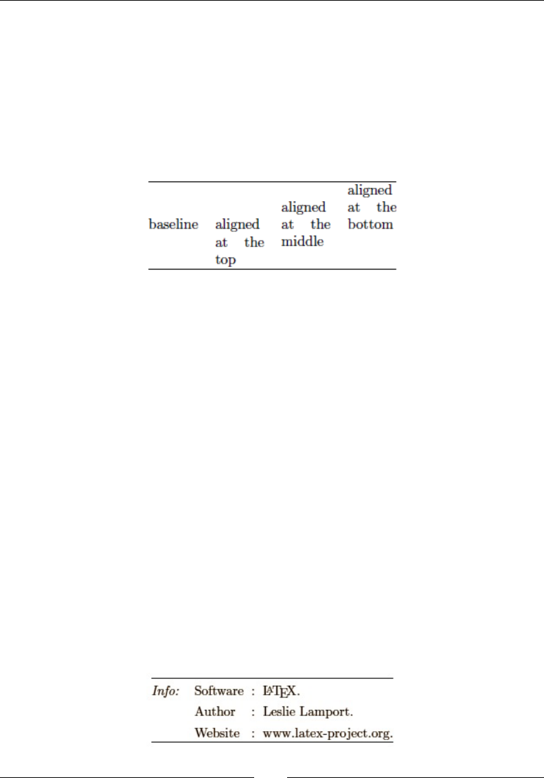
Creang Tables and Inserng Pictures
[ 128 ]
This example shows the eect of @{} and the alignment arguments p, m, and b:
\begin{tabular}{@{}lp{1.2cm}m{1.2cm}b{1.2cm}@{}}
\hline
baseline & aligned at the top & aligned at the middle
& aligned at the bottom\\
\hline
\end{tabular}
The output table is as follows:
Increasing the row height
You may have noced that horizontal lines nearly touch the leers in the cells, especially
capital leers. The array package introduces a length called \extrarowheight. If it has a
posive value, this will be added to the height of every row of the table.
The next example, following the very rst example of this chapter, shows how to extend
the row height and shows the eect of the remaining array opons:
\documentclass{article}
\usepackage{array}
\setlength{\extrarowheight}{4pt}
\begin{document}
\begin{tabular}{@{}>{\itshape}ll!{:}l<{.}@{}}
\hline
Info: & Software & \LaTeX\\
& Author & Leslie Lamport\\
& Website & www.latex-project.org\\
\hline
\end{tabular}
\end{document}
The output is as follows:

Chapter 5
[ 129 ]
Here, >{\itshape} has been used to change the font of a row to italic. >{} is oen used
to insert an alignment declaraon, but there's a piall: such declaraons might change the
internal meaning of \\, which is a shortcut for \tabularnewline within tables. But the
array package oers a command to repair it; in such cases, just add \arraybackslash, for
example:
\begin{tabular}{>{\centering\arraybackslash}p{5cm}}
Otherwise, the content of paragraph cells stated by p, m, or b will be fully jused.
Aer a specic row, you can add vercal space by the oponal argument of \\, such as
\\[10pt].
You may even stretch a whole table: the macro \arraystretch contains a stretching factor
with a default value of 1. Just redene it. For example, \renewcommand{\arraystretch}
{1.5} will increase the height of the rows by 50 percent. You could use it inside a group or
an environment to keep the eect local.
Beautifying tables
Sll our tables don't look as perfect as they look in good books. Especially, the lines and their
distances to the text might need improvement. The booktabs package comes to the rescue;
aer loading it, you can enhance the quality of your tables by new line commands replacing
\hline and \cline.
Time for action – adding nicer horizontal lines with the
booktabs package
We shall use the new commands introduced by booktabs:
1. In the previous example, load the package booktabs:
\usepackage{booktabs}
2. Use \toprule, \midrule, and \bottomrule instead of \hline. Specify a
thickness as an oponal argument:
\begin{tabular}{ccc}
\toprule[1.5pt]
\head{Command} & \head{Declaration} & \head{Output}\\
\midrule
\verb|\textrm| & \verb|\rmfamily| & \rmfamily Example text\\
\verb|\textsf| & \verb|\sffamily| & \sffamily Example text\\
\verb|\texttt| & \verb|\ttfamily| & \ttfamily Example text\\
\bottomrule[1.5pt]
\end{tabular}
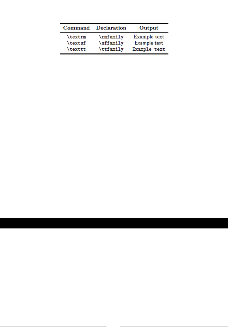
Creang Tables and Inserng Pictures
[ 130 ]
3. Typeset to see the dierence:
What just happened?
Brish typeseers call a line a rule. The booktabs developer chose this terminology for
the new commands. We used three of them. These are their denions:
\toprule[thickness] may be used to draw a horizontal line at the top of the
table. If desired, a thickness may be specied, like 1pt or 0.5mm.
\midrule[thickness] draws a horizontal dividing line between rows of a table.
\bottomrule[thickness] draws a horizontal line to nish o a table.
\cmidrule[thickness](trim){m–n} draws a horizontal line from column m to
column n. (trim) is oponal like thickness, it could be (l) or (r) to trim the
line at its le or right end. Write (lr) to trim at both ends. Even adding {width},
like in (l{10pt}), is possible and species the trim width.
The package does not dene vercal lines. They are not advisable anyway. The same applies
to double rules. Neither vercal nor double rules are recommended. They are even widely
considered to be bad typographic style.
Consider using \toprule and the other line commands without oponal arguments—let's
gure out how.
Have a go hero – adjusting lengths
We briey introduced the command \setlength. Instead of specifying a line thickness by
an oponal argument to \toprule, \midrule, \cmidrule, or \bottomrule, always omit
it. Instead, specify it once for your whole document by \setlength in the preamble.
These are the lengths that may be adjusted:
\heavyrulewidth for the thickness of the top and boom lines
\lightrulewidth for the thickness of the middle lines by \midrule
\cmidrulewidth for the thickness of \cmidrule
\cmidrulekern for the trimming in \cmidrule
\abovetopsep is the space above the top rule; the default is 0pt
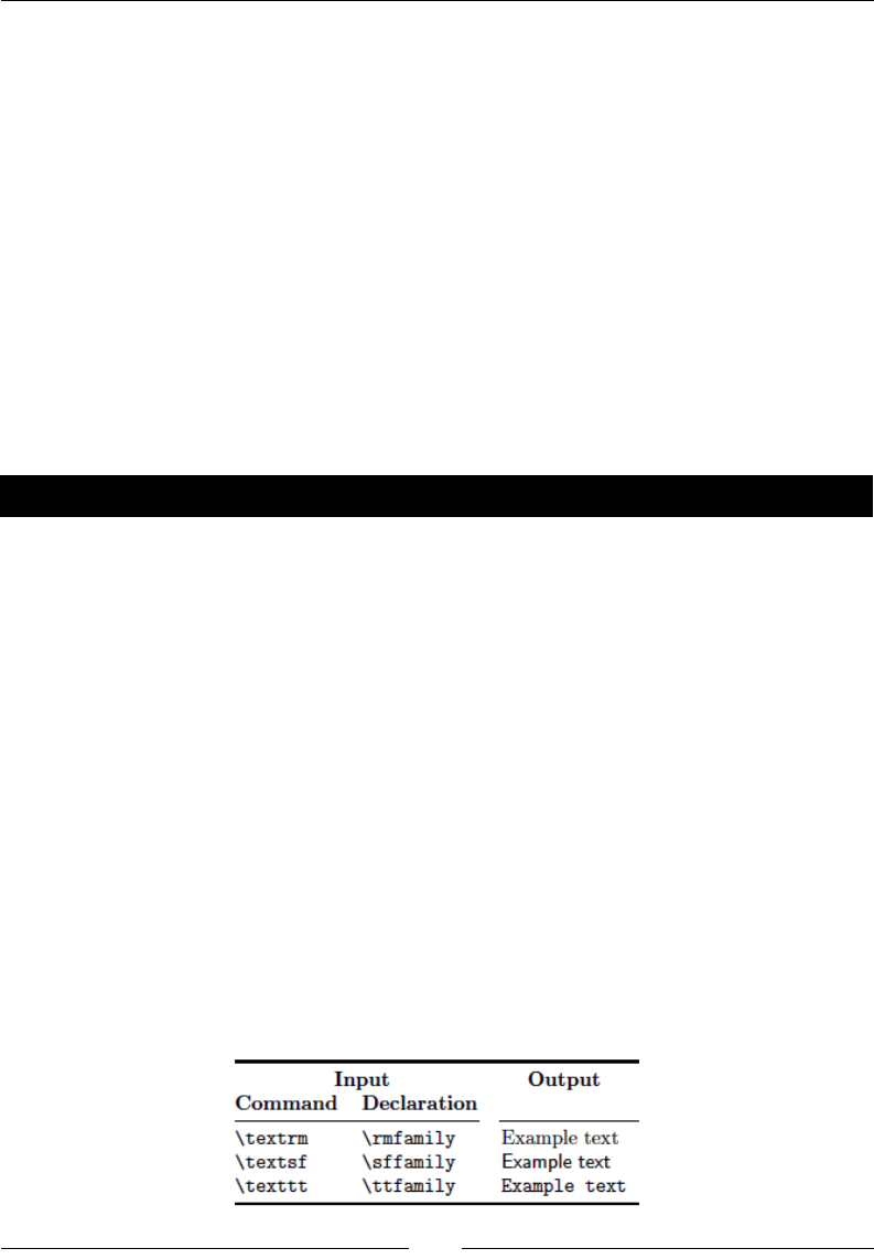
Chapter 5
[ 131 ]
\belowbottomsep is the space below the boom rule; the default is 0pt
\aboverulesep species the space above \midrule, \cmidrule, and
\bottomrule
\belowrulesep stands for the space below \midrule, \cmidrule, and
\toprule
Try to change the thickness of the lines. The lengths already have reasoned values, but
you may change them. So, the adjustment in your preamble would improve all tables in
your document.
Spanning entries over multiple columns
Columns concerning the same subject might be grouped by a common header. In such
a case, two cells in the header should be merged. The command \multicolumn does it
for us.
Time for action – merging cells
Regarding our example table, commands and declaraons are both input, whereas, the
remaining column contains output. We shall emphasize that in our header:
1. In our example, insert another header row. Use \multicolumn to merge cells. Alter
the column formang argument and the middle rule. Changes are highlighted:
\begin{tabular}{@{}*3l@{}}
\toprule[1.5pt]
\multicolumn{2}{c}{\head{Input}} &
\multicolumn{1}{c}{\head{Output}}\\
\head{Command} & \head{Declaration} & \\
\cmidrule(r){1-2}\cmidrule(l){3-3}
\verb|\textrm| & \verb|\rmfamily| & \rmfamily Example text\\
\verb|\textsf| & \verb|\sffamily| & \sffamily Example text\\
\verb|\texttt| & \verb|\ttfamily| & \ttfamily Example text\\
\bottomrule[1.5pt]
\end{tabular}
2. Typeset and see the output:

Creang Tables and Inserng Pictures
[ 132 ]
What just happened?
We used the command \multicolumn twice; once to merge two cells and surprisingly
another me just for one cell. Let's rst look at its denion:
\multicolumn{number of columns}{formatting options}{entry text}
The number of columns to be spanned may be a posive integer or just 1. The formang
opons will be applied instead of the opons specied in the tabular denion for this cell.
We took advantage of this when we used \multicolumn{1}{c}{…}, overriding the l
opon of the column by a c opon to get just this cell centered.
The other change we made concerns \cmidrule. We used it instead of \midrule together
with the trimming argument to get a gap between the input and the output column.
Inserting code column-wise
There are many more font commands that we would like to add to the table. Wring
\verb|…| in each cell is resome. We shall exploit the >{…} feature of the array package
to dene the formang of the entries once for the column.
Time for action – using the array package
We shall modify the table denion to set our input columns in the typewriter font. At the
same me, we will insert a column on the le, standing for our command type:
1. Extend the preamble of our example by dening a command \normal. It shall use
\multicolumn to produce an l cell, no maer what the column formang is:
\documentclass{article}
\usepackage{array}
\usepackage{booktabs}
\newcommand{\head}[1]{\textnormal{\textbf{#1}}}
\newcommand{\normal}[1]{\multicolumn{1}{l}{#1}}
\begin{document}
2. As \verb cannot be used in table headers, we shall use \ttfamily. Preceding it
with \textbackslash is enough for our purposes. Use >{…} to insert it twice.
Then add <{Example text} to the last column to save typing work:
\begin{tabular}{@{}l*2{>{\textbackslash\ttfamily}l}l%
<{Example text}@{}}
\toprule[1.5pt]
& \multicolumn{2}{c}{\head{Input}} &
\multicolumn{1}{c}{\head{Output}}\\
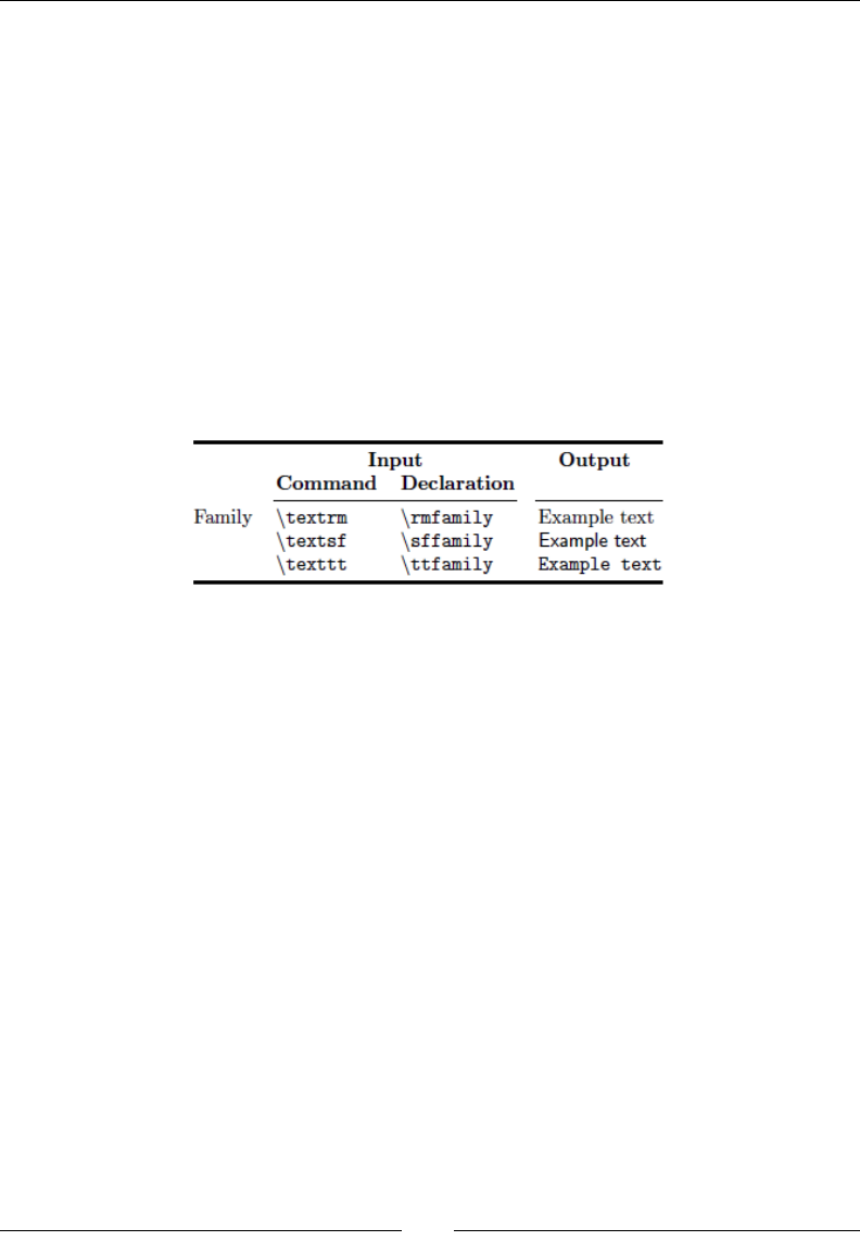
Chapter 5
[ 133 ]
3. We'll use the \normal command to avoid the typewriter formang in the header:
& \normal{\head{Command}} & \normal{\head{Declaration}}
& \normal{}\\
\cmidrule(lr){2-3}\cmidrule(l){4-4}
4. Now we may connue lisng the font command names:
Family & textrm&rmfamily & \rmfamily\\
& textsf & sffamily & \sffamily\\
& texttt & ttfamily & \ttfamily\\
\bottomrule[1.5pt]
\end{tabular}
\end{document}
5. Typeset and look at the result:
What just happened?
Using >{\textbackslash\ttfamily}l denes a le aligned row, where each entry is
preceded by a backslash and by switching to typewriter font. We wrote *2{…} to dene two
columns of this style. Because the example text has been inserted according to our table
denion with <{…}, we just had to put the declaraons into the last column without the
text.
Spanning entries over multiple rows
We already know how to span text over several columns. But what if text should cross over
several rows? LaTeX doesn't dene a command for it. However, the package mulrow does.
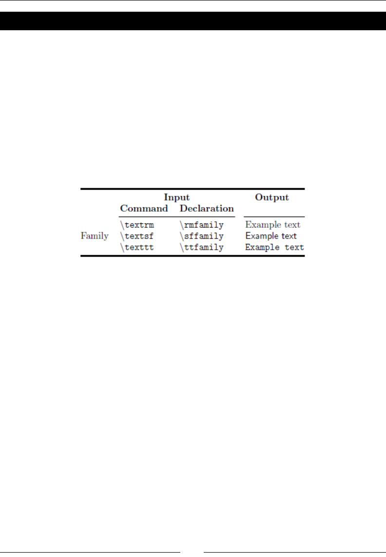
Creang Tables and Inserng Pictures
[ 134 ]
Time for action – merging cells using the multirow package
Before we complement the font table, we would like to center the command type "Family"
vercally, that is, span this cell over three columns. If we gured this out, we could use it
later on:
1. In our previous example, addionally load multirow:
\usepackage{multirow}
2. Replace the word «Family»:
\multirow{3}{*}{Family} & textrm & rmfamily & \rmfamily & \\
3. Typeset to see the small change:
What just happened?
We used the command \multirow to span three rows. Its denion is:
\multirow{number of rows}{width}{entry text}
The entry will span that number of rows from the row on which \multirow has been used.
If the number is negave, it will span the rows above.
You can specify a width or just write * for the natural width. If a width has been specied,
the text would be wrapped accordingly.
multirow understands further oponal arguments for ne tuning. They are described in
its documentaon.
Adding captions to tables
Especially with longer text, we would like to add capons and numbers to our tables.
Numbering the tables allows referring to them, whereas capons are informave, if the
table is not exactly placed where we refer to it. LaTeX has built-in features to achieve that.

Chapter 5
[ 135 ]
Time for action – adding a caption to our font table
Now it's me to complete our table. We shall list the remaining font commands. We'll use
the rst column to describe the category of the font commands: Family, Weight, Shape, and
so on. Then we will add another column to show the eect of combining font commands.
To nish, we shall center the table and provide a number and a capon:
1. Put a table environment around our example table, use \centering inside, and
insert a \caption command at the end of the table environment. Add more font
commands and add another column at the right containing more examples:
\documentclass{article}
\usepackage{array}
\usepackage{booktabs}
\usepackage{multirow}
\newcommand{\head}[1]{\textnormal{\textbf{#1}}}
\newcommand{\normal}[1]{\multicolumn{1}{l}{#1}}
\pagestyle{empty}
\begin{document}
\begin{table}
\centering
\begin{tabular}{@{}l*2{>{\textbackslash\ttfamily}l}%
l<{Example text}l@{}}
\toprule[1.5pt]
& \multicolumn{2}{c}{\head{Input}}
& \multicolumn{2}{c}{\head{Output}}\\
& \normal{\head{Command}} & \normal{\head{Declaration}}
& \normal{\head{Single use}} & \head{Combined}\\
\cmidrule(lr){2-3}\cmidrule(l){4-5}
\multirow{3}{*}{Family} & textrm & rmfamily & \rmfamily & \\
& textsf & sffamily & \sffamily& \\
& texttt & ttfamily & \ttfamily& \\
\cmidrule(lr){2-3}\cmidrule(lr){4-4}
\multirow{2}{1.1cm}{Weight} & textbf & bfseries & \bfseries
& \multirow{2}{1.8cm}{\sffamily\bfseries Bold and sans-serif} \\
& textmd & mdseries & \mdseries & \\
\cmidrule(lr){2-3}\cmidrule(lr){4-4}
\multirow{4}{*}{Shape} & textit & itshape & \itshape & \\
& textsl & slshape & \slshape &
\multirow{2}{1.8cm}{\sffamily\slshape Slanted and sans-serif}\\
& textsc & scshape & \scshape & \\
& textup & upshape & \upshape & \\
\cmidrule(lr){2-3}\cmidrule(lr){4-4}
Default & textnormal & normalfont & \normalfont & \\
\bottomrule[1.5pt]
\end{tabular}
\caption{\LaTeX\ font selection}
\end{table}
\end{document}
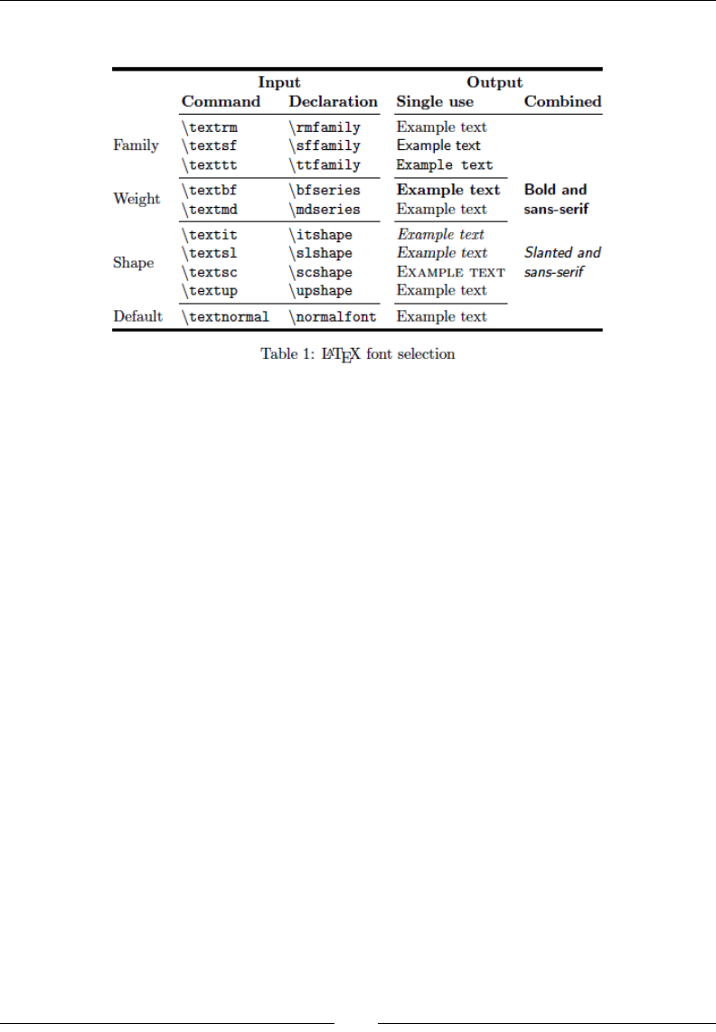
Creang Tables and Inserng Pictures
[ 136 ]
2. Typeset and our table is now ready:
What just happened?
We put the tabular environment in a table environment. It's used in this way together
with the \caption command:
\begin{table}[placement options]
table body
\caption{table title}
\end{table}
The table environment is a so-called oang environment. Unlike normal text, they might
appear somewhere else other than what is dened by their posion in the source code. The
oponal placement argument determines where the table might appear. However, LaTeX
decides it. We shall discuss this at the end of this chapter together with the placement of
graphics.
\caption understands an oponal argument as well: if you write \caption[short
text]{long text}, then short text will appear in a list of tables and long text
in the document body. That's useful if you need very long descripve capons.
Tables are automacally numbered.
Placing captions above
In typeseng, it's very common to place capons above the tables instead of below. This can
be achieved by wring \caption before the table body. However, LaTeX expects capon to
always be below, resulng in a cramped look to the table. There's too lile space between
the capon and the following table. You might wish to add some space, for instance, by
entering \vspace{10pt} directly aer a top capon.

Chapter 5
[ 137 ]
Remember booktabs? If you begin tables with \toprule, just specify the length
\abovetopskip, for example:
\setlength{\abovetopsep}{10pt}
By pung this line into your preamble, 10pt space would be added below the capon and
above the top line of the table.
Have a go hero – customizing captions
By default, the capons look like normal body text; there's no visual dierence. Would you
like to have a slight change in font size, a dierent formang of the label, some margins or
indentaon, or any other customizaon? The capon package is the answer to most needs.
By using a few opons, you could enhance the visual appearance of all of your capons. Try:
\usepackage[font=small,labelfont=bf,margin=1cm]{caption}
This way, your capons will be smaller than normal text, the label with number will be
bold, and it will not be as wide as normal text. The package oers a lot of features, both for
document wide sengs and ne-tuning. It's very well documented. So, have a look at its
documentaon.
Auto-tting columns to the table width
l, c, and r columns have the width of their content. For p columns, you specify the width.
This way, it's hard to nd out the actual width of the table. Wouldn't it be a good idea to
specify the table width and let LaTeX decide how wide the columns may be? The tabularx
package allows that. Using it looks like:
\usepackage{tabularx}
...
\begin{tabularx}{width}{column specifiers}
...
\end{tabularx}
The new environment tabularx requires an addional argument: the width of the table. It
introduces a new column type X. X columns behave like p columns, but they use all available
space. One X column would take all of the available space. If you use several X columns, they
would share the space equally. So you could write, for instance:
\begin{tabularx}{0.6\textwidth}{lcX}
This way you would get a table occupying 60 percent of the text width, a le aligned and a
centered column as wide as their content, and a paragraph column as wide as possible unl
60 percent is reached.

Creang Tables and Inserng Pictures
[ 138 ]
Though it's easy to use, the tabularx documentaon gives further examples, informs about
the derived types, and gives advice like this: don't let \multicolumn entries cross any X
column.
There are two similar approaches:
LaTeX provides a starred version of the tabular environment:
\begin{tabular*}{width}[position]{column specifiers}
The table is set to width, but by modifying the inter-column space. tabularx has
been developed sasfying the need for a more useful way.
The tabulary package provides another sophiscated tabular environment taking
the total width. It's weighng each column width according to the natural width of
the widest cell in the column.
Generating multi-page tables
All tabular environments we've got to know unl now cannot cross page boundaries.
The tabbing environment is an excepon due to its dierent nature.
As tables might contain a lot of data, we need a soluon. There are several packages:
longtable provides an environment with the same name that's like a mul-page
version of tabular. It provides commands to set table capons, connued
capons, and special headers and footers when a page break occurs. It's probably
the easiest way for mul-page tables and therefore the most popular. The package
documentaon describes all you need. In combinaon with the booktabs package,
you will get very good results.
ltxtable provides a combinaon of longtable and tabularx.
ltablex is another approach to combine the features of longtable and tabularx.
supertabular oers another mul-page extension of the internally used tabular
environment, providing oponal table tails and heads where page breaks occur.
xtab extends supertabular and reduces some of its weaknesses.
stabular implements a simple way to use page breaks in tabular without
much ado.
Example tables and links to documentaon can be found at
http://texblog.net/beginners-guide/tables/.

Chapter 5
[ 139 ]
Coloring tables
We didn't even color text yet, as this usually isn't what we do rst with LaTeX. But of course,
this can be done with text as well as with tables. For coloring text, use the color package
or, beer, the extension xcolor. For coloring tables, use the package colortbl. All can be
combined by using:
\usepackage[table]{xcolor}
The package allows coloring columns, rows, single entries, and lines in many ways. The
package documentaon may tell you more.
Using landscape orientation
Very wide tables could be typeset in landscape orientaon. The rotang package oers an
environment called sidewaystable that you could use instead of the table environment.
Both table and capon would be rotated +-90 degrees and placed on a separate page. The
package provides further rotaon-related environments and commands.
Aligning columns at the decimal point
Columns containing numbers are more readable when the entries are aligned at the
decimal marker and perhaps at an exponent. Several packages support this:
siunitx is primarily intended for typeseng values with units in a consistent way
according to scienc convenons. However, it provides a tabular column type
for such decimal alignment of numbers.
dcolumn oers a column type for aligning at a comma, a period, or another single
character.
rccol denes a column type where numbers are "right-centered", that is, they are
centered with respect to other entries but ushed right to each other. This way
corresponding digits are aligned along the column.
In contrast to dcolumn and rccol, the siunitx package is very new and powerful.
Handling narrow columns
Text in very narrow columns might require special aenon because juscaon is dicult
if there's lile space. Here's some advice:
Have a look at the correct hyphenaon. If necessary, improve it like we did in
Chapter 2.

Creang Tables and Inserng Pictures
[ 140 ]
TeX doesn't hyphenate the rst word of a line, a box, or a table entry. So, a long
word may cross the column boundary. To enable hyphenaon, insert an empty
word: write \hspace{0pt} directly at the beginning.
Load microtype to improve juscaon, it shows the best eect in narrow
columns.
Full juscaon in p columns and the like may look bad because of big gaps.
Consider using >{\raggedright\arraybackslash} for such columns.
From the ragged2e package, using the command \RaggedRight can do even
beer and doesn't need \arraybackslash.
Pop quiz – tables
1. Which of these environments cannot cross page boundaries?
a. tabular
b. longtable
c. tabbing
2. If you would like to format one entry dierent from the specicaon of its column,
which command may be used?
a. >{…}
b. @{…}
c. \multirow
d. \multicolumn
Inserting pictures
Documents may not consist of just text and tables. You might wish to include pictures,
diagrams, or drawings made with other programs. The graphicx package is dedicated to this.
Time for action – including a picture
We shall create a short document. Between two paragraphs, we would like to insert a
picture. If there's no picture le available, we will use the demo mode of graphicx:
1. Begin a new document and load babel and blindtext to print some ller text:
\documentclass[a5paper]{article}
\usepackage[english]{babel}
\usepackage{blindtext}
\usepackage[demo]{graphicx}
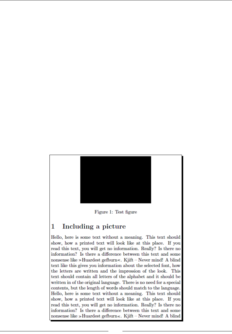
Chapter 5
[ 141 ]
\pagestyle{empty}
\begin{document}
\section{Including a picture}
\blindtext
2. Open a figure environment and declare centering:
\begin{figure}
\centering
3. Use the command \includegraphics with the lename as the argument:
\includegraphics{test}
4. Declare a capon, close the figure environment, and end the document with
ller text:
\caption{Test figure}
\end{figure}
\blindtext
\end{document}
5. Typeset and have a look at the output:

Creang Tables and Inserng Pictures
[ 142 ]
What just happened?
The most important command is \includegraphics. We specied a lename. This le
would be loaded if it exists. Otherwise an error would occur. LaTeX supports the following
le types:
PNG, JPG, and PDF if you directly compile to PDF (pdfLaTeX)
EPS if you compile to DVI and convert to PS and PDF (tradional LaTeX)
To clarify, PS means PostScript, EPS means Encapsulated PostScript, and DVI means Device
Independent Format. The laer was the rst output format to be supported by TeX. You
denitely know the very popular picture formats PNG and JPG, oen used for screenshots
or photos.
You don't need to specify a lename extension, it will be automacally added. Put the le
into the same directory as your document; otherwise specify a full or relave path name:
\includegraphics{appendix/figure1}
Don't use blanks in the lename or path! Blanks and special characters may cause problems
with \includegraphics. If such symbols in lenames are required, load the package
grle to try to x it. Also, in lenames, use slashes / instead of backslashes \, as the laer
begin a LaTeX command.
Because we specied the demo opon, graphicx doesn't require a le test.png or any other
le; instead it's just prinng a black lled rectangle. This is useful for tesng or if you would like
to discuss a LaTeX problem in an online forum, but don't wish to publish your pictures.
Go ahead; copy a picture of your choice into your document directory, give
\includegraphics its lename, and compile. The picture will be embedded with
its original size.
Scaling pictures
You may choose a dierent size. For this, let's look at the denion of includegraphics:
\includegraphics[key=value list]{file name}
The graphicx documentaon lists all keys and possible values. Here are the most
popular ones:
width: The graphic would be resized to this width. Example: width=
0.9\textwidth.
height: The graphic would be resized to this height. Example: height=3cm.
scale: The graphic would be scaled by this factor. Example: scale=0.5.
angle: The graphic would be turned by this angle. Example: angle=90.
Chapter 5
[ 143 ]
There are opons for clipping, but such post processing can be easily done with any graphics
soware.
Instead of turning a gure by 90 degrees, you could use the sidewaysfigure environment of
the rotating package. It's analogous to sidewaystable that has been menoned before.
Choosing the optimal le type
If you've got the nal picture, well, just use this format and include it. However, if you are
free to choose a le format, you could think about it for a moment.
EPS and PDF are both vector graphics format. They are scalable, also looking good at high
resoluon or if you zoom in. So, whenever possible, PDF (or EPS) should be preferred, for
instance, when you export drawings or diagrams out of other oce soware. For such
graphics, vector formats are common.
PNG and JPG are bitmap formats, also called raster graphics, commonly used for photos. If
you zoom in, you would noce a loss of quality. PNG uses a lossless compression, whereas
JPG pictures may lose quality when they are saved. So, if you make screenshots, use PNG or
at least ensure that there's no loss compression if you choose JPG.
Besides supporng vector graphics, both EPS and PDF may contain bitmap
graphics. They are also called container formats.
There are a lot of tools to convert between graphic formats. These three are especially useful
and included in both TeX Live and MiKTeX:
dvips converts DVI les to the PostScript format
ps2pdf converts PostScript les to PDF
epstopdf converts EPS les to PDF, a package with the same name does it on-the-y
These are command line tools. Some editors like TeXnicCenter use them to automate the
way TEX => DVI => PS => PDF.
epstopdf is especially useful if you have to include Postscript pictures, but wish to benet
from pdfLaTeX features like font expansion and character protrusion accessible by
microtype.
For further working with graphics, ImageMagick and GIMP are very capable open
source programs.

Creang Tables and Inserng Pictures
[ 144 ]
Including whole pages
How can we include pictures wider or higher than the text area? \includegraphics
could do it, but LaTeX would complain about width or size and might put it o to the next
page. Oversized images and even whole pages can be included using the pdfpages package.
It provides a command, \includepdf, which is able to include a complete page and
even a mul-page PDF document at once. Despite its name and not even menoned in its
otherwise good documentaon, it's capable of including PNG and JPG les, not just PDF.
pdfpages could also be used to resize several PDF pages and to arrange them on a
single sheet.
Putting images behind the text
Do you need watermarks? Background images? Textboxes posioned at arbitrary posions
on the page, preferably not interfering with the other text? The package eso-pic does it
for you.
Another approach is oered by the textpos package, developed for placing boxes with text
or graphics at absolute posions on a page.
Managing oating environments
When a page break occurs, normal text can be broken to connue on the next page.
However, pictures cannot be divided. Simple tables cannot be split either. That's why LaTeX
provides two oang environments, namely, figure and table. They are briey called
oats. Their content may oat to a place where it's the opmum for the page layout. Let's
gure out how to deal with it.
Time for action – letting a gure oat
Both the figure and the table environment take an oponal argument aecng the nal
placement of the gure or the table. We shall test the eect in our graphics example:
1. Go back to the previous example. This me, add the opons h and t:
\begin{figure}[ht]
\centering
\includegraphics{test}
\caption{Test figure}
\end{figure}
Chapter 5
[ 145 ]
2. Typeset, noce the change in the output.
3. Change the opons into !b:
\begin{figure}[!b]
4. Typeset, the gure is now forced to oat to the boom. Compare both results:
What just happened?
Just by adding some characters standing for placement opons, we could force the gure to
appear where we wanted it to.
Understanding oat placement options
The oponal argument of the figure and table environment tells LaTeX where it's allowed
to place the gure or the table. Four leers stand for four possible places:
h stands for here. The oat may appear where it's been wrien in the source code.
t stands for top. Placing at the top of a page is permied.
b stands for boom. The oat may appear at the boom of a page.
p stands for page. The oat is allowed to appear on a separate page, where only
oats may reside but no normal text.

Creang Tables and Inserng Pictures
[ 146 ]
A h opon might come in handy:
! tells LaTeX to try harder! Some constraints may be ignored, easing the placement.
If you don't specify any opon, the oat could be placed far away. New LaTeX users might
be surprised. Specifying more opons would help to place it as near as possible. The most
exible is using the placement [!htbp], allowing a oat everywhere. You sll could consider
removing a placement specier if you don't like it.
Forcing the output of oats
If you would like to stop LaTeX from pung the oats, there's a way; the \clearpage
command ends the current page and causes all already dened gures and tables to be
printed out. You can use \cleardoublepage that does the same but in a two-sided layout
it ensures that the next non-oat page is a right-hand page. . If necessary, a blank page
would be inserted.
Immediately ending the page might not be the best thing to do. It could leave a lot of empty
space on the current page. The aerpage package oers a clever possibility; this package
allows deferring the execuon of \clearpage unl the current page has ended:
\usepackage{afterpage}
...
body text
\afterpage{\clearpage}
Limiting oating
It may happen that tables and gures oat far away, perhaps even into another secon. The
placeins package provides a useful command to restrict the oang. If you load placeins
with \usepackage{placeins} and write \FloatBarrier somewhere in your document,
no table or gure could oat past it. This macro keeps oats in their place.
A very convenient way to prevent oats from crossing secon boundaries is stang the
secon opon:
\usepackage[section]{placeins}
This opon causes an implicit \FloatBarrier to be used at the beginning of each secon.
Two further opons, namely, above and below, allow you to lower the restricons,
prevenng oats from appearing above the start of the current secon or below the start
of the next secon.
Figures don't oat into the next chapter because \chapter implicitly uses \clearpage.

Chapter 5
[ 147 ]
Avoiding oating at all
Would you like to place a oat exactly where you want it? The obvious answer is: don't use
a oang environment! Even a capon doesn't have the same importance if the table or
gure is placed at the current point. However, if you really need a capon, you may use the
\captionof command without a oat. Both the capon package , KOMA-Script classes,
and the ny capt-of package provide that command:
\usepackage{capt-of}% or caption
…
\begin{center}
\begin{minipage}{\linewidth}%
\centering%
\includegraphics{test}%
\captionof{figure}{Test figure}%
\end{minipage}
\end{center}
The minipage keeps a picture and capon together. Furthermore, it's centered. Use
\captionof within a group or environment like minipage or center. The denion is
the same as \caption, except there is the addional argument specifying the oat type:
\captionof{figure}[short text]{long text}
\captionof{table}[short text]{long text}
Be aware that the numbering could get wrong if you mix real oats and xed gures or
tables. As you don't benet from LaTeX's posioning capabilies, you have to take care that
pages are sll properly lled.
The oat package provides a convenient and consistent looking approach. It introduces the
placement opon H causing the oat to appear right there:
\usepackage{float}
…
\begin{figure}[H]
\centering
\includegraphics{test}
\caption{Test figure}
\end{figure}
You may choose between these two opons. If you wish to exploit further features of
the float package, load it. Otherwise, consider using the one-liner capt-of. Perhaps
not even that is necessary, assuming that you're already using the caption package or
a KOMA-Script class.

Creang Tables and Inserng Pictures
[ 148 ]
Spanning gures and tables over text columns
There are starred forms of oats, namely, figure* and table*. In a two-column layout,
they put the oat into a single column. In one-column mode, there's no dierence to the
non-starred form.
Letting text ow around gures
Though it's a bit playful, you might wish to let text ow around a table or a gure. This can
be achieved using the wrapg package and its environments wrapfigure and wraptable.
Time for action – embedding a picture within text
We shall modify our picture embedding an example. We would like the picture to appear on
the le side, accompanied by the body text on the right side:
1. In our example, addionally load the wrapfig package:
\documentclass[a5paper]{article}
\usepackage[english]{babel}
\usepackage{blindtext}
\usepackage[demo]{graphicx}
\usepackage{wrapfig}
\pagestyle{empty}
\begin{document}
2. Begin an unnumbered secon, place a wrapfig environment within some ller
text:
\section*{Text flowing around a picture}
\blindtext
\begin{wrapfigure}{l}{4.4cm}
\includegraphics[width=4.4cm]{test}
\caption{Test figure}
\end{wrapfigure}
\blindtext
\end{document}
Chapter 5
[ 149 ]
3. Typeset and look:
What just happened?
The wrapfigure environment understands parameters other than the figure
environment. We used just two of them. If you need more, here's the complete denion:
\begin{wrapfigure}[number of lines]{placement}[overhang] {width}
The rst oponal argument states the number of wrapped text lines. If omied, it would be
automacally calculated from the height. placement can be one of the characters r, l, i, o
for right, le, inner, or outer side or the corresponding uppercase leers R, L, I, O with the
same meaning, but allowing the gure to oat. Only one character for specifying the opon
is allowed. The other oponal argument, overhang, may specify a width that the gure
might sck into the margin. The nal and mandatory argument gives the width of the gure.
The wraptable environment works analogous.

Creang Tables and Inserng Pictures
[ 150 ]
Breaking gures and tables into pieces
For grouping several sub gures or sub tables with capons within a single gure or table,
there are several supporng packages you can choose from:
subg is a sophiscated package supporng inclusion of small gures and tables.
It takes care of posioning, labeling, and caponing within single oats.
subcapon is another package for this purpose and belongs to the
caption package.
subgure is sll available, but considered as obsolete since subfig has appeared.
Pop quiz – pictures and oats
1. This chapter listed all graphic formats supported by LaTeX. Now, idenfy from the
following le types which is not directly supported by LaTeX!
a. jpg
b. gif
c. png
d. eps
e. pdf
2. If you would like a gure or a table to oat but to appear as near as possible to its
source, which of the following oat placement opons would be appropriate?
a. h
b. H
c. htbp
d. !htbp
Summary
In this chapter, we have learned to create tables and gures, and how to place them within
our document. Specically, we dealt with:
Pung text into columns
Typeseng tables with capons
Spanning columns and rows in tables
Using packages to auto-t columns and to create colored, landscape, and even
mul-page tables

Chapter 5
[ 151 ]
Including pictures with capons
Controlling and tuning placement of gures and tables
LaTeX is able to generate lists of tables and gures like a table of contents. We shall deal
with such lists in Chapter 7, Lisng Contents and References.
As our gures and tables are numbered, we can use these numbers to refer to them within
the text. In the next chapter, we shall gure out how to do this, beneng from LaTeX's
cross-referencing capabilies.

6
Cross-Referencing
Our documents contain a lot of numbered things such as pages, secons, list
items, gures, and tables. There's even more we have not covered yet. For
instance, if you would like to write a mathemacal text, you may number
equaons, theorems, denions, and many more.
We number things not just to count them, but to refer to them in other places
of our document. If you want to point the reader to the ninth gure in the third
chapter, you might write "See gure 3.9". LaTeX automacally enumerates the
gures for you. If you insert another gure, LaTeX will automacally adjust the
numbering of all gures aer it. But what's with the references?
LaTeX is able to take care of all of our cross-references. This is the subject of this chapter.
We shall learn how to:
Set labels that we shall use to refer to
Refer to secons, footnotes, list items, tables, and more
Refer to page numbers and ranges
Make LaTeX refer verbosely to adjacent pages
Automate naming of references
Create references to external documents
Let's gure out how to do all this.
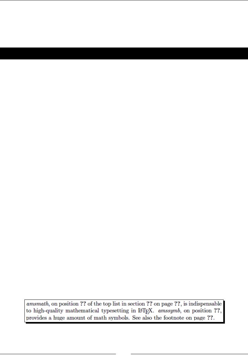
Cross-Referencing
[ 154 ]
Setting labels and referencing
To be able to refer to a certain point, we have to mark it by a label. The name of that label
will serve us aerwards.
Time for action – referencing items of a top list
We shall typeset a list of the most used packages for papers on the e-print archive site
http://arXiv.org. Through the command \label, we will mark items that we can
later refer to with the command \ref.
1. Create a new document with this code:
\documentclass{book}
\begin{document}
\chapter{Statistics}
\section{Most used packages on arXiv.org}\label{sec:packages}
The Top Five packages, used on arXiv.org\footnote{according
to the arXMLiv project\label{fn:project}}:
\begin{enumerate}
\item graphicx
\item amssymb \label{item:amssymb}
\item amsmath \label{item:amsmath}
\item epsfig
\item amsfonts
\end{enumerate}
\chapter{Mathematics}
\emph{amsmath}, on position \ref{item:amsmath} of the top list
in section~\ref{sec:packages} on page~\pageref{sec:packages},
is indispensable to high-quality mathematical typesetting in
\LaTeX.\emph{amssymb}, on position \ref{item:amssymb},
provides a huge amount of math symbols.
See also the footnote on page~\pageref{fn:project}.
\end{document}
2. Typeset and have a look at the text on page 3:
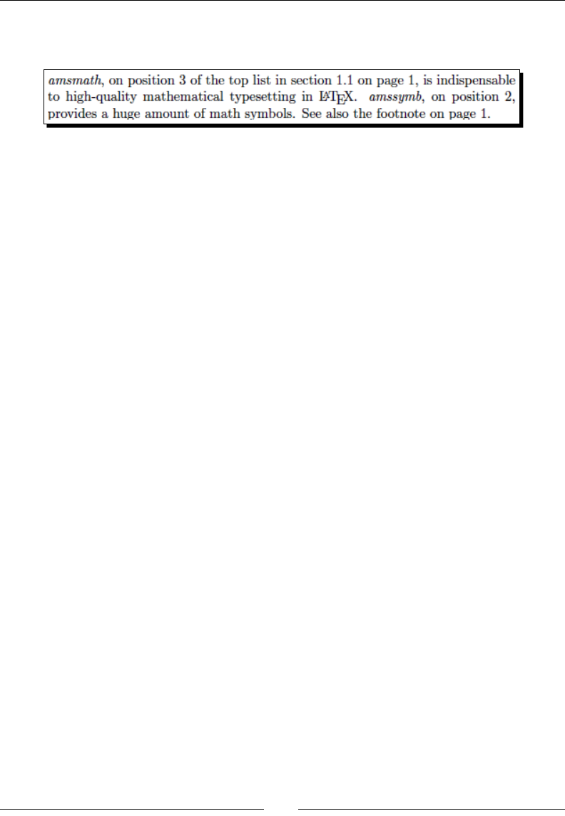
Chapter 6
[ 155 ]
3. Do you see the queson marks? The references are sll missing! Typeset again
and compare:
What just happened?
We created cross-references with just three commands: \label marks the posion, \ref
prints the number of the element we refer to, and \pageref prints the page number of
that element. Each command takes the name of the element as argument. Any name may
be chosen by us.
We had to Typeset twice because LaTeX needs one run to produce the references that can
be read in during the next compiler run. If LaTeX cannot resolve a reference, it prints two
queson marks instead.
Let's have a closer look.
Assigning a key
The command \label{name} assigns the current posion to the key name. Specically:
If the \label command appeared in ordinary text, then the current seconal unit,
like the chapter or the secon, would be assigned.
If the \label would be placed within a numbered environment, that environment
would be assigned to the key.
So, we cannot mark a secon within a table environment. To avoid any problem because of
a possible unsuitable posioning, a good rule of thumb is to place the \label command
right aer the posion we would like to mark. For instance, place it directly aer the
corresponding \chapter or aer \section—not before, of course.
In the gure or table environments, \caption is responsible for the numbering. That's
why \label has to be placed aer \caption, not before. Therefore, typical oang
environments look like the following:
\begin{figure}[htp]
\centering
\includegraphics{filename}
\caption{Test figure}\label{fig:name}
\end{figure}

Cross-Referencing
[ 156 ]
Or as follows:
\begin{table}[hbp]
\centering
\caption{table descripion}\label{tab:name}
\begin{tabular}{cc}
…
\end{tabular}
\end{table}
A key may consist of leers, digits, or punctuaon characters. Keys are case-sensive.
If you write larger documents, the number of keys could become very high. Imagine, you
have a secon dealing with fonts and a font table—how to disnguish their keys? We could
prex them with the type of environment. It has become common pracce to label gures
with fig:name, tables with tab:name, secons with sec:name, and similar in other cases.
Referring to a key
Once a label has been set and given a name, we may refer to that name. For this, we use
\ref{name}: this command prints the number that belongs to name. It could already be
used before the corresponding \label command appears in your code.
Even though it's that simple, it's powerful. Each me we Typeset a document, LaTeX checks
the keys and reassigns the numbers, responding to all changes. If LaTeX noced that labels
have been changed, it would inform you that a second Typeset run would be required to
update the corresponding labels. If in doubt Typeset twice.
Referring to a page
The command \pageref{name} works analogous to \ref, except that it prints the
corresponding page number.
Would all the references stay correct if we changed the secon and page numbers?
Let's put it to the test! Insert a secon and a page break at the beginning:
\chapter{Statistics}
\section{Introduction}
\newpage
\section{Most used packages on arXiv.org}\label{sec:packages}
Typeset once. LaTeX will compile it, but it will show a message: LaTeX Warning: Label(s) may
have changed. Rerun to get cross-references right. That's what we shall do! Typeset a second
me, now all the numbers have been correctly adjusted:
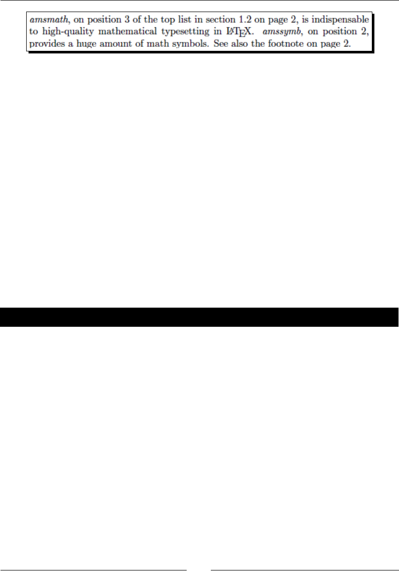
Chapter 6
[ 157 ]
Using a reference together with the page number reference, you may write:
See figure~\ref{fig:name} on page~\pageref{fig:name}.
As you know how to dene a command, you could make such referencing easier:
\newcommand{\fullref}[1]{\ref{#1} on page~\pageref{#1}}
…
See figure~\fullref{fig:name}.
This way, you would get a full reference like "See gure 4.2 on page 32". However, if the
reference appears on the same page, like the gure, wring out the page number looks
a bit odd. How can we avoid that? The varioref package provides a way.
Producing intelligent page references
The varioref package oers a command being able to add "on the preceding page", "on
the following page", or on the page number to a reference, depending on the context.
Time for action – introducing variable references
We will use the varioref commands, \vref and \vpageref, to achieve enhanced
reference texts:
1. Open our current example. Add the package varioref to your preamble:
\usepackage{varioref}
2. Edit the content of the second chapter:
\emph{amsmath}, on position \ref{item:amsmath} of the top list
in section~\vref{sec:packages}, is indispensable to high-quality
mathematical typesetting in \LaTeX. \emph{amssymb}, on position
\ref{item:amssymb}, provides a huge amount of math symbols.
See also the footnote \vpageref{fn:project}.
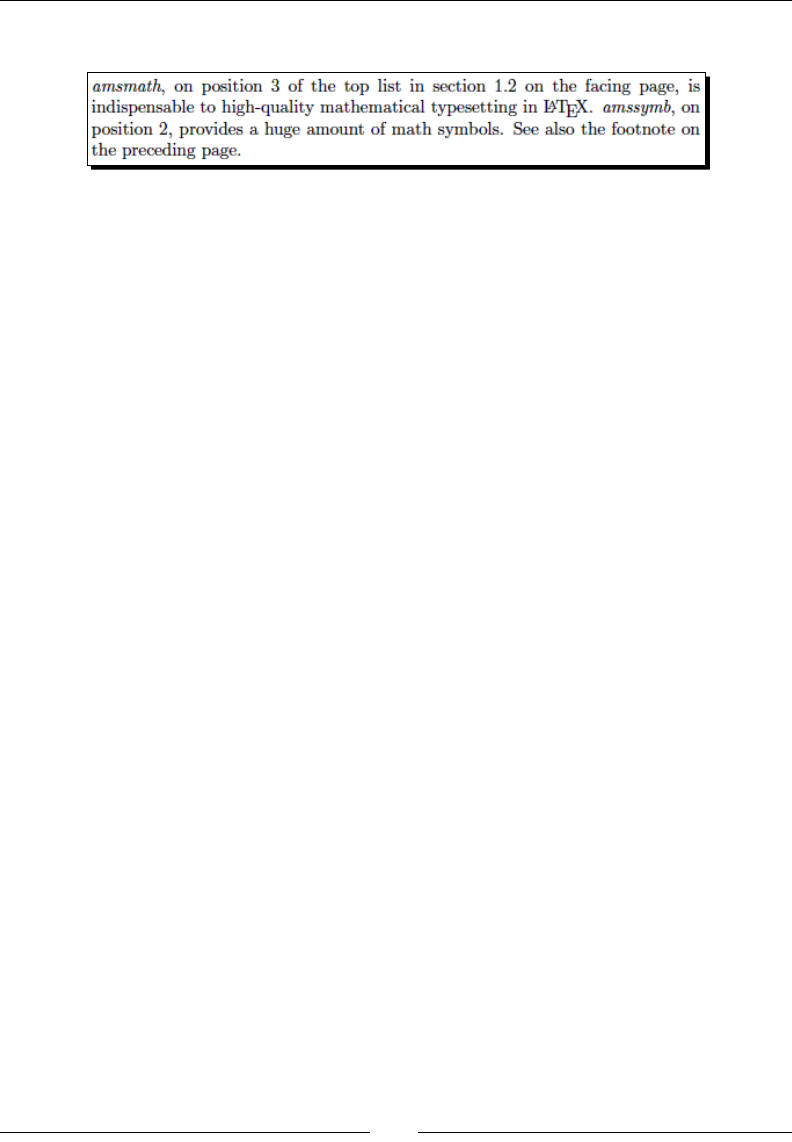
Cross-Referencing
[ 158 ]
3. Typeset twice and look at the result:
What just happened?
The command \vref checked the distance to the referenced secon. As it's on the facing
page, that is, on the preceding page in a two-sided layout, it wrote "1.2 on the facing page".
Similar for \vpageref, it refers to "the preceding page".
\vref{name} acts in the following way:
If the reference and \label{name} are on the same page, it behaves exactly
like \ref. The page number will not be printed.
If the reference and the corresponding \label are on two successive pages, \vref
prints the referred number and addionally "on the preceding page" or "on the
following page", or "on the facing page". The laer will be chosen if the document
is two-sided, that is, if \label and the reference fall onto a double-page spread.
Otherwise it will print both \ref and \pageref.
\vpageref is equivalent to \pageref, but behaves like \vref concerning the page
reference.
Even though varioref denes new commands, you may sll use the common \ref
and \pageref.
Fine-tuning page references
If label and reference are very close to each other, they would probably fall on the same
page, but not necessarily. In such cases, we usually know if the label comes before or aer
the reference. It allows specifying an oponal argument to \vpageref:
see the figure \vpageref[above]{fig:name}
This will print:
"see the gure above" if the gure is on the same page
"see the gure on the page before" if the gure is on the preceding page

Chapter 6
[ 159 ]
Whereas, with the following:
see the footnote \vpageref[below]{fn:name}
This will print:
"see the footnote below" if the footnote is on the same page
"see the footnote on the following page" if the footnote is on the next page
In fact, \vpageref understands two oponal arguments. The second oponal argument
would be used if the label and reference would fall on dierent pages. So, we could even
write:
see the figure \vpageref[above figure][figure]{fig:name}
This would print:
"see the above gure" if the gure is on the same page
"see the gure on the page before" if the gure is on the preceding page
Actually, reversing the word order to "above gure" if necessary.
Sounds complicated? Well, your demands might increase over me, requiring more
sophiscated features, so these features might come in handy some day.
Referring to page ranges
varioref oers two more commands:
\vpagerefrange[opt]{key1}{key2}, where key1 and key2 denote a range
(like a sequence of gures from fig:a to fig:c). If both labels fall onto the same
page, the result is the same as with \vpageref. Otherwise, the output will be a
range like "on pages 32-36". opt would be used if both labels fall onto the current
page.
\vpageref [opt]{key1}{key2}is analogous, but similar to \vref: see
figures \vpageref{fig:a}{fig:c} may result in "see gures 4.2 to 4.4 on
pages 36-37".
\vref, \vpageref, and \vpagerefrange have been implemented to remove any space to
their le before they insert space of their own. For example, \vref inserts a nonbreakable
space like we did before with ~. If this is not desired, use starred forms \vref*, \
vpageref*, or \vpagerefrange*.
More informaon regarding customizaon may be found in the package manual.

Cross-Referencing
[ 160 ]
Using automatic reference names
Tired of wring figure~\ref{fig:name} and table~\ref{fig:name}again and
again? Wouldn't it be great if LaTeX knew what type is meant by \ref{name} wring type
and number? What if we desire to abbreviate, say, fig.~\ref{fig:name}in the whole
document? The cleverev package eases the work: it automacally determines the type of
cross-reference and the context in which it's used.
Basically, you could just use \cref instead of \ref or \Cref if you wish to capitalize.
The corresponding range commands are \crefrange and \Crefrange.
Time for action – referring cleverly
We shall rewrite our rst example using cleveref. To verify that the package acts cleverly,
we consciously omit prexes in key names to \label and \cref.
1. Modify our rst example in this way:
\documentclass{book}
\usepackage{cleveref}
\crefname{enumi}{position}{positions}
\begin{document}
\chapter{Statistics}\label{stats}
\section{Most used packages on arXiv.org}\label{packages}
The Top Five packages, used on arXiv.org\footnote{according
to the arXMLiv project\label{project}}:
\begin{enumerate}
\item graphicx
\item amssymb \label{amssymb}
\item amsmath \label{amsmath}
\item epsfig
\item amsfonts
\end{enumerate}
\begin{table}[tp]
\centering
(Identify obsolete packages on CTAN)
\caption{Obsolete packages}\label{obsolete}
\end{table}
\chapter{Mathematics}
\emph{amsmath}, on \cref{amsmath} of the top list in
\cref{packages} of \cref{stats}, is indispensable to high-quality
Mathematical typesetting in \LaTeX. \emph{amssymb}, on
\cref{amssymb}, provides a huge amount of math symbols.
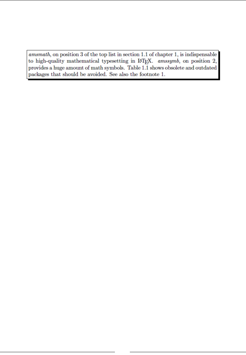
Chapter 6
[ 161 ]
\Cref{obsolete} shows obsolete and outdated packages that
should be avoided. See also the \cref{project}.
\end{document}
2. Typeset twice and check the references for having the correct names:
What just happened?
As we can see, we never needed to specify which object we refer to. \cref always chooses
the right name and the correct number for us. That's really comfortable!
We used the command \crefname to tell cleveref which name it should use for
enumerated items. The denion of \crefname is:
\crefname{type}{singular}{plural}
type may be one of chapter, section, figure, table, enumi, equation, theorem,
or many other types we did not encounter yet. The singular version will be used for
single references and the plural version for mulple. If you need capitalized versions, use
\Crefname. So, a typical use may be:
\crefname{figure}{fig.}{figs.}
\Crefname{figure}{Fig.}{Figs.}
To sum up your benets:
You save much typing.
You could use arbitrary labels. The package fancyref does a similar job but relies
on prexes like chap, g, tab, and so on.
If you decide to change wordings, it could be done easily by doing this once in the
preamble, having the desired eect in the whole document.
However, it's recommended to use a prex like fig: or sec: to disnguish the kind of
referenced object; your code would become more understandable—it's common.

Cross-Referencing
[ 162 ]
Combing cleveref and varioref
As cleveref fully supports varioref, you may use both to get the most out of them.
cleveref redenes the commands of varioref to use \cref internally. So, you could
use the good page referencing features of varioref together with the clever naming
automasm!
Just load varioref before cleveref:
\usepackage{varioref}
\usepackage{cleveref}
Now, you may use \vref, \cref, \ref, or the other commands—whichever seems
appropriate.
Referring to labels in other documents
If you write several related documents that refer to each other, you might want to
use references to labels of another document. The package with the short name
xr (standing for eXternal References) implements it. First load the package:
\usepackage{xr}
If you need to refer to secons or environments in an external document called, say,
doc.tex, insert this command into your preamble:
\externaldocument{doc}
This enables you to addionally refer to anything that has been given a label in doc.tex.
You may do this for several documents. If you need to avoid conicts when an external
document uses the same \label like the main document, declare a prex using the oponal
argument of \externaldocument:
\externaldocument[D-]{doc}
This way, all references from doc.tex would be prexed by D- and you could write
\ref{D-name} to refer to name in doc.tex. Instead of D- you may choose any prex
that transforms your labels such that they become unique.
Have a go hero – turning references into hyperlinks
PDF documents oer bookmarks and hyperlink capabilies. How about exploing that
ourselves? There's an outstanding package oering hyperlink support; it's called hyperref.
Try it: load hyperref right before cleveref. This order is important for the references to
work. Even without any opons or commands, your document will be hyperlinked as much
as possible:

Chapter 6
[ 163 ]
All references become hyperlinks. Click any of those numbers to jump to the
referred table, list item, secon, or page.
Each footnote marker is a hyperlink to the footnote text. Click it to jump down.
If you insert \tableofcontents, you will get a bookmark list for the document,
chapters, and secons listed in a navigaon bar of you PDF reader.
hyperref can do even more for you: linking index entries to text passages, back-referencing
of bibliography entries, and more. You can nely customize the behavior using opons, for
instance, choosing color or frames for hyperlinks. So, you could keep that valuable package
in mind. In Chapter 11, Enhancing Your Documents Further, we shall return to this topic.
Pop quiz
1. For a reference to a table, at which posion should the \label be placed?
a. Before \caption
b. Aer \caption
c. Aer\end{table}
2. What should we do if we see two unexpected consecuve queson marks in
the output?
a. Load the hyperref package.
b. Look out for an undened command. Check the syntax at that point.
c. Typeset again. If the queson marks stay, check the key to the reference
at that point.
Summary
In this chapter, we learned how to reference chapters, secons, footnotes, and environments
by their number or by the number of the corresponding page.
We even got to know some ways of clever and context dependent referencing.
In the next chapter, we shall deal with lists, which consist mainly of references: table of
contents, lists of gures and tables, and bibliographies.
7
Listing Content and References
LaTeX makes it very easy to create lists for many purposes. For example, we've
seen that just the simple command \tableofcontents creates a nice looking
table of contents. Let's just call it the TOC from now on. It simply takes the
entries from the headings and from the numbers of the pages they fall on.
In this chapter, we will perform the following:
Decide which headings at which numbering level go to the TOC
Create and customize a list of gures (LOF) and a list of tables (LOT)
Insert arbitrary text and commands into the TOC and into other lists
Cite books and create a bibliography
Create an index
Modify the headings for all those lists
We shall start with the content.
Customizing the table of contents
Besides just calling \tableofcontents to get a pre-designed list of content, LaTeX provides
basic ways to modify it. Let's use some.

Lisng Content and References
[ 166 ]
Time for action – rening an extensive table of contents
We shall build the frame of a document containing some headings. We will modify the
automacally created table of contents to be ner and to contain addional entries.
In Chapter 3, Designing Pages, we saw the eect of \tableofcontents. The entries have
been collected from the headings. We shall use this down to the subsubsecon level.
Then we shall extend the TOC further. We will manually add entries for some headings:
1. Create a new document with the following code:
\documentclass{book}
\setcounter{tocdepth}{3}
\begin{document}
\tableofcontents
\part{First Part}
\chapter*{Preface}
\addcontentsline{toc}{chapter}{Preface}
\chapter{First main chapter}
\section{A section}
\section{Another section}
\subsection{A smaller section}
\subsubsection[Deeper level]{This section has an even deeper
level}
\chapter{Second main chapter}
\part{Second part}
\chapter{Third main chapter}
\appendix
\cleardoublepage
\addtocontents{toc}{\bigskip}
\addcontentsline{toc}{part}{Appendix}
\chapter{Glossary}
\chapter{Symbols}
\end{document}
2. Typeset. The rst page will just show Contents but no entries.
3. Typeset a second me. Now the table of contents will be displayed:
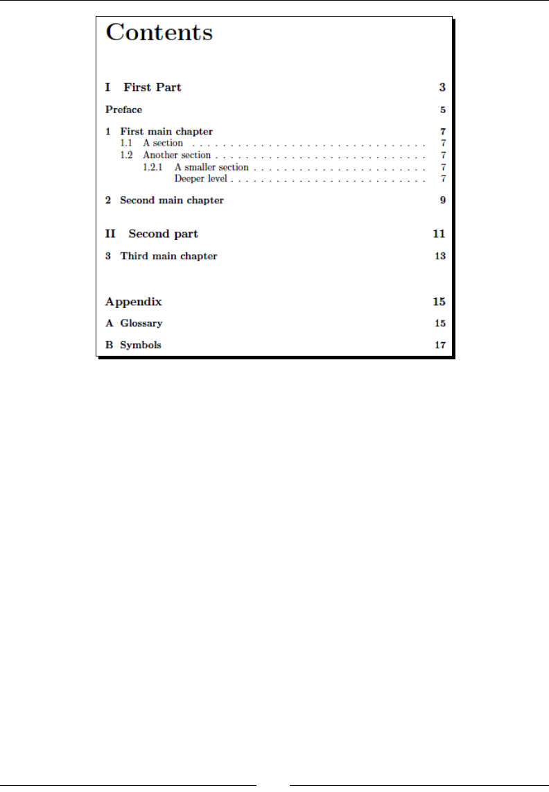
Chapter 7
[ 167 ]
What just happened?
We structured a document using several seconing commands. In the rst run, LaTeX read
all of our seconing commands and created a le with the extension .toc. This le contains
the commands and the tles for all entries in the table of contents. During the rst run, that
le didn't exist yet, thus the TOC remained empty.
During the second run, the command \tableofcontents read the .toc le and printed
the TOC.
In this example, we raised the depth of the TOC by one level. We added a chapter-like entry
for the preface and inserted a part-like heading showing the beginning of the appendix, using
\addcontentsline. Through \addtocontents, we inserted some space before the laer
heading. Let's look at these commands in detail.
Lisng Content and References
[ 168 ]
Adjusting the depth of the TOC
These are the standard seconing commands and their so called TOC level:
Command Level
\part -1 (book and report class)
\chapter 0 (not available in article class)
\section 1
\subsection 2
\subsubsection 3
\paragraph 4
\subparagraph 5
In the book and in the report class, LaTeX creates TOC entries unl level 2, in the article
class unl level 3. In a book, this means, for example, \subsubsection doesn't generate
a TOC entry. There's a variable represenng the level, namely, \tocdepth. It's an integer
variable which we call a counter. To tell LaTeX to include subsubsecons in the TOC, we
would have to raise this counter. There are two basic ways to adjust a counter value:
\setcounter{name}{n} species an integer value of n for the counter name
\addtocounter{name}{n} adds the integer value of n to value of the counter
name. n may be negave
Thus, the following command would ensure that even \subparagraph gives a TOC entry:
\setcounter{tocdepth}{5}
Using \addcounter instead you may raise or lower the level without knowing its number.
In contrast to commands, counter names don't begin with a backslash.
Shortening entries
As you have already learned in Chapter 3, you may choose a text for the TOC that's dierent
to the heading in the body text. Each seconing command understands an oponal
argument for the TOC entry, which is especially useful if you wish to use very long headings,
but a shorter TOC entry would be sucient. In our example, we did this by:
\subsubsection[Deeper level]{This section has an even deeper level}

Chapter 7
[ 169 ]
The body text shows the long heading while the TOC shows the short one. Running tles in
the headings would use the short entry as well, as the space in headings is very limited.
Adding entries manually
Starred commands like \chapter* and \section* don't produce a TOC entry. In our
example, we did that manually using this command:
\addcontentsline{file extension}{sectional unit}{text}
This command can be used in several contexts: the file extension may be:
toc for the table of contents le
lof for the list of gures le
lot for the list of tables le
Or, any another extension of such a le type known to LaTeX.
The sectional unit determines the formang of the entry. Specify chapter to create
an entry that's formaed like normal chapter entries and similar for other seconal units like
part, secon, or subsecon.
The third argument contains the text for the entry. This text may contain commands. Do
you remember the \protect command? For a macro inside the entries, it's usually a good
idea to write \protect right before it.
You may insert text or commands more directly with:
\addtocontents{file extension}{entry}
In contrary to \addcontentsline, the argument entry is wrien directly to the le
without any addional formang. You may choose any formang you like.
This command may even be used for some customizaon, for example:
\addtocontents{toc}{\protect\enlargethispage{\baselineskip}}
extends the text height such that one addional line ts to the contents page.
\addtocontents{toc}{\protect\newpage} causes a page break in the TOC.
For instance, if the automac page break happens aer a chapter entry and before
the following secon entries, you might wish to force a page break already before
the chapter entry.
\addtocontents{toc}{\protect\thispagestyle{fancy}} changes the
page style of the current TOC page to fancy. As the rst page of a chapter is of
plain style by default, the rst page of the TOC would be plain as well, even if you
specied \pagestyle{fancy}. This command overrides it.

Lisng Content and References
[ 170 ]
Place such commands where they should be eecve. To aect the rst TOC page, place it
at the beginning of your document. To cause a page break before a certain chapter, place it
right before the corresponding \chapter call.
Creating and customizing lists of gures
As briey menoned in the previous chapter, the two commands for creang lists of gures
and tables are \listoffigures and \listoftables. Depending on the class, they produce
a ne list of all capons together with the gure respecvely the table number and the
corresponding page numbers. As with the TOC, all can be done automacally. However, we
may use the same techniques, like with the TOC, to customize the other lists. Let's try that.
Time for action – creating a list of diagrams
Suppose all of our gures are diagrams. We shall avoid the term gure and we will typeset a
list of diagrams:
1. Open our current example. Add these lines to your preamble:
\renewcommand{\figurename}{Diagram}
\renewcommand{\listfigurename}{List of Diagrams}
2. Right aer \tableofcontents, add:
\listoffigures
3. Add a diagram somewhere in Chapter 1:
\begin{figure}
\centering
\fbox{Diagram placeholder}
\caption{Enterprize Organizational Chart}
\end{figure}
4. In the second part, in the third chapter, we'd like to add network design diagrams.
Let's mark that in the LOF and let the diagrams follow:
\addtocontents{lof}{Network Diagrams:}
\begin{figure}
\centering
\fbox{Diagram placeholder}
\caption{Network overview}
\end{figure}
\begin{figure}
\centering
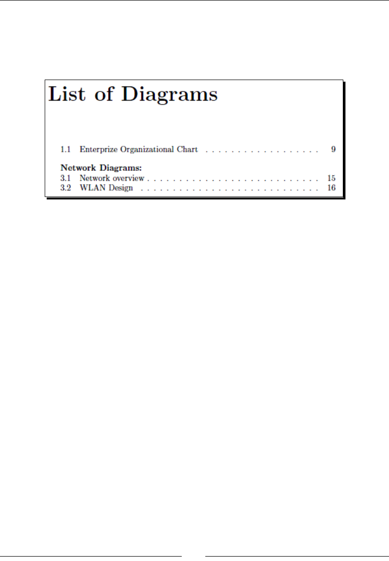
Chapter 7
[ 171 ]
\fbox{Diagram placeholder}
\caption{WLAN Design}
\end{figure}
5. Typeset twice to get the document and the list:
What just happened?
We renamed the gures and the list heading by redening LaTeX macros. At the end of
the chapter, you will get a list of names used by LaTeX classes that you may redene.
Like with the TOC, we used the command \addtocontents; this me to insert a bold
heading into the .lof le where LaTeX collects the capons. It works similar to the TOC.
Creating a list of tables
You already know all you need to create and customize a list of tables! The le, where LaTeX
collects the capons of the tables, has the extension .lot, and that's why the rst argument
of \addtocontents would be lot. Everything works analogous, like \listoftables,
\tablename, and \listtablename.
Using packages for customization
Besides the described simple methods, there are packages providing sophiscated features
for customizing the table of contents and the lists of gures and tables:
toclo gives extensive control over the typography of TOC, LOF, and LOT. You may
even dene new kinds of such lists.
tletoc oers convenient handling of entries and is the companion to tlesec,
a very good package for customizing seconing headings.

Lisng Content and References
[ 172 ]
multoc oers a layout in two or more columns using the mulcol package.
minitoc can create small TOCs for each part, chapter, or secon.
tocbibind can automacally add bibliography, index, TOC, LOF, and LOT to the table
of contents. It's even capable of using numbered headings instead of the default
unnumbered ones.
Let's connue with the announced index and the bibliography.
Generating an index
Extensive documents oen contain an index. It is a list of words or phrases and page
numbers poinng to where related material can be found in the document. In contrary
to a full-text search feature, the index provides selecve pointers to relevant informaon.
While it's our turn to idenfy and to mark the words for the index, LaTeX will collect this
informaon and is able to typeset the index for us.
Time for action – marking words and building the index
Suppose our example would contain informaon about an enterprise and its structure and
further about its network structure and design. We shall mark places in the text where these
concepts occur. Finally, we will order LaTeX to typeset the index:
1. Go back to our example. In the preamble, load the index package and add the
command to create the index:
\usepackage{index}
\makeindex
2. In the capon of our enterprise diagram, index this point with the keyword
enterprise:
\caption{\index{enterprise}Enterprise Organizational Chart}
3. In the third chapter, which contains our diagrams, index by the keyword network:
\index{network}
4. Directly before \end{document}, create an entry for the index for the table of
contents. To ensure that it shows the correct page number, end the page before:
\clearpage
\addcontentsline{toc}{chapter}{Index}
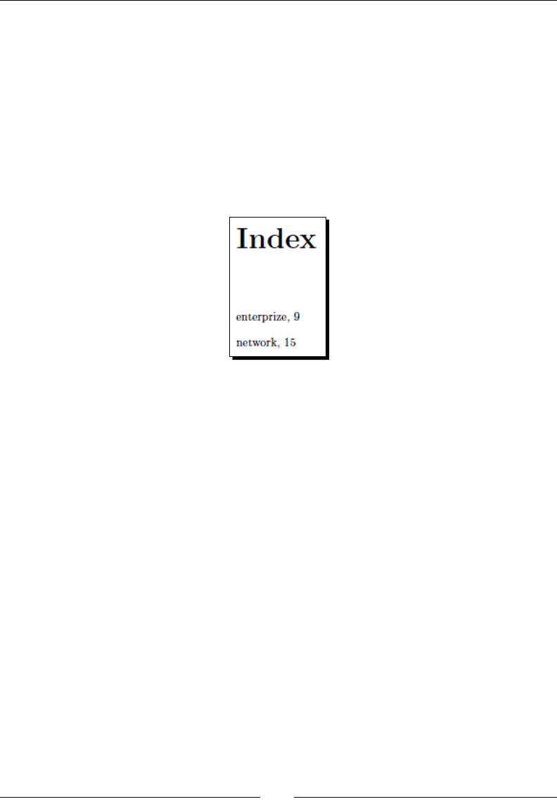
Chapter 7
[ 173 ]
5. In the next line, order LaTeX to typeset the index:
\printindex
6. If you're using TeXworks, choose MakeIndex instead of pdfLaTeX in the drop-down
box next to the typeset buon. Then click typeset. If you use another editor, use its
MakeIndex feature or type the following at the command prompt in the document
directory:
makeindex documentname
7. Switch back to pdfLaTeX, Typeset, and look at the last page:
What just happened?
We loaded the index package, which improves LaTeX's built-in indexing capabilies.
Alternavely, you could use the makeidx package which is part of standard LaTeX. The
command \makeindex prepared the index. Both commands must be put into the preamble.
The command \index takes just one argument, namely, the word or the phrase to be
indexed. This will be wrien to a le with the extension .idx. If you look into this le,
you will nd lines like the following:
\indexentry {enterprise}{9}
\indexentry {network}{15}
These stand for the index entries and the corresponding page numbers.
The external program makeindex takes that .idx le and produces an .ind le. The
laer consists of LaTeX code for the index creaon. Specically, it contains the index list
environment together with the items and looks like the following:
\begin{theindex}
\item enterprise, 9
\indexspace
\item network, 15
\end{theindex}

Lisng Content and References
[ 174 ]
More complex indexes may contain subitems, page ranges, and references to other items.
Let's see how to produce such an index.
Dening index entries and subentries
We already created simple index entries with:
\index{phrase}
Subentries are produced by specifying the main entry followed by the subentry, separated
by an exclamaon mark, for example:
\index{network!overview}
Also subentries may have subentries; just use another ! symbol, for example:
\index{enterprise!organization}
\index{enterprise!organization!sales}
\index{enterprise!organization!controlling}
\index{enterprise!organization!operation}
Up to three levels are possible.
Specifying page ranges
If several pages deal with the same concept, you may specify a page range for the index
entry. Sux the entry with |( where the range starts and add |) where it ends, as follows:
\index{network|(}
at the beginning of the network chapter and:
\index{network|)}
at the end of this chapter. This results in an entry of the form Network, 15-17.
Using symbols and macros in the index
makeindex sorts the entries alphabecally. If you would like to include symbols in the index,
for example, Greek leers, chemical formulas, or math symbols, you could face the problem
of integrang them into the sorng. For this purpose, \index understands a sort key. Use
this key as prex for the entry, separated by an @ symbol, for instance:
\index{Gamma@$\Gamma$}

Chapter 7
[ 175 ]
Using macros for index entries is generally not really recommended. Macros would be sorted
according to the macro name including the backslash, though it would be expanded when
the index is typeset. Imagine, you've got a macro \group standing for TeX Users Group. If
you write the following, then the entry TeX Users Group would be treated like \group in the
sorng and won't appear among the entries beginning with T:
\index{\group}
However, you could repair such issues by adding a sort key:
\index{TeX@\group}
\index{schon@sch\"{o}n}
What if you wish to use the symbols |, @, and ! within index entries? Quote them by using
a preceding ":
\index{exclamation ("!)!loud}
And don't worry, " itself may be used within verbam text as follows:
\index{quote (\verb|""|)}
Referring to other index entries
Dierent words may stand for the same concept. For such cases, it's possible to add a cross-
reference to the main phrase without a page number. Adding the code |see{entry list}
achieves that, for example:
\index{network|see{WLAN}}
\index{WLAN}
As such references don't print a page number, their posion in the text doesn't maer. You
could collect them in one place of your document.
Fine-tuning page numbers
If an index entry refers to several pages, you might want to emphasize one page number to
indicate it as the primary reference. You could dene a command for emphasizing as follows:
\newcommand{\main}[1]{\emph{#1}}
And for the index entry, add a pipe symbol and the command name:
\index{WLAN|main}
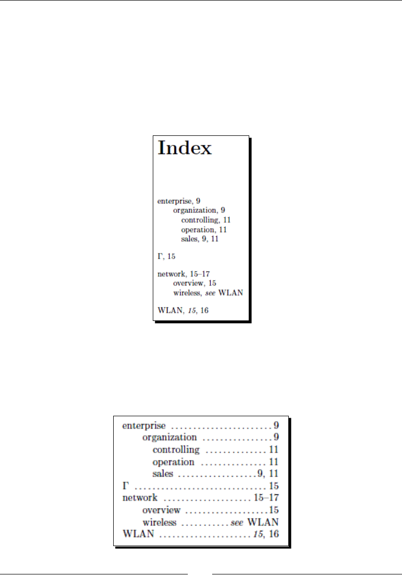
Lisng Content and References
[ 176 ]
Thus, the corresponding page number would be emphasized. Simply wring
\index{WLAN|emph} or \index{WLAN|texbf} is possible as well. However, dening
your own macro is more consistent—remember the concept of separang form and content.
Designing the index layout
If we extend our example document with the aforemenoned example commands,
\printindex gives us this layout, containing subentries, ranges, references, and
emphasized entries:
LaTeX provides some index styles called latex (the default), gind, din, and iso. To use
another style, specify it using the –s opon of the makeindex program, for example:
makeindex –s iso documentname
If you typeset aer this call, the index layout would be changed to:
Chapter 7
[ 177 ]
You could even dene your own styles. To learn more about indexing and makeindex, use
texdoc at the command prompt:
texdoc index
texdoc makeindex
Though it seems natural to generate the index while wring the
document, this might lead to inconsistencies in the index. It's
recommendable rst to nish wring and aerwards to work out what
should appear in the index.
Creating a bibliography
Especially in scienc documents, a list of references or bibliography is very common.
We shall work out how to typeset a bibliography and how to refer to its entries.
Time for action – citing texts and listing the references
Using LaTeX's standard features, we shall create a small list of references containing a book
and an arcle by Donald E. Knuth, the creator of TeX. In our body text, we will refer to both:
1. Create a new document as follows:
\documentclass{article}
\begin{document}
\section*{Recommended texts}
To study \TeX\ in depth, see \cite{DK86}. For writing math texts,
see \cite{DK89}.
\begin{thebibliography}{8}
\bibitem{DK86} D.E. Knuth, \emph{The {\TeX}book}, 1986
\bibitem{DK89} D.E. Knuth, \emph{Typesetting Concrete
Mathematics}, 1989
\end{thebibliography}
\end{document}
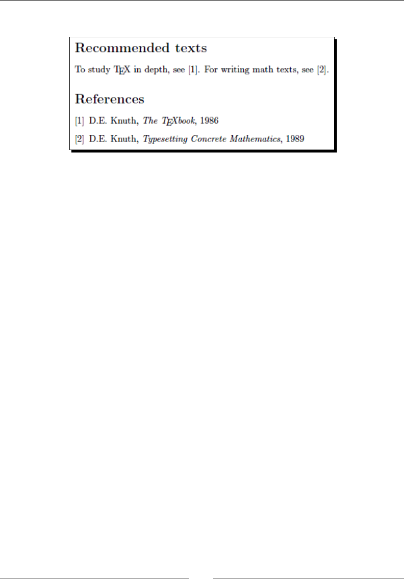
Lisng Content and References
[ 178 ]
2. Typeset and view the output:
What just happened?
We used an environment called thebibliography to typeset the list of references, which is
similar to a descripon list as we've seen in Chapter 4, Creang Lists. Each item of this list
has got a key. For cing in the body text, we referred to that key using the \cite command.
Let's look at these commands in detail.
Using the standard bibliography environment
LaTeX's standard environment for bibliographies has the following form:
\begin{thebibliography}{widest label}
\bibitem[label]{key} author, title, year etc.
\bibitem…
…
\end{thebibliography}
Each item is specied using the command \bibitem. This command requires a mandatory
argument determining the key. We may simply refer to this key by \cite{key} or
\cite{key1,key2}. \cite accepts an oponal argument stang a page range, for
example, \cite[p.\,18--20]{key}. You may choose a label by the oponal argument
of \bibitem. If no label has been given, LaTeX will number the items consecuvely in
square brackets, as we've seen.
Using labels, the environment could look as follows:
\begin{thebibliography}{Knuth89}
\bibitem[Knuth86]{DK86} D.E. Knuth, \emph{The {\TeX}book}, 1986
\bibitem[Knuth89]{DK89} D.E. Knuth, \emph{Typesetting Concrete
Mathematics}, 1989
\end{thebibliography}
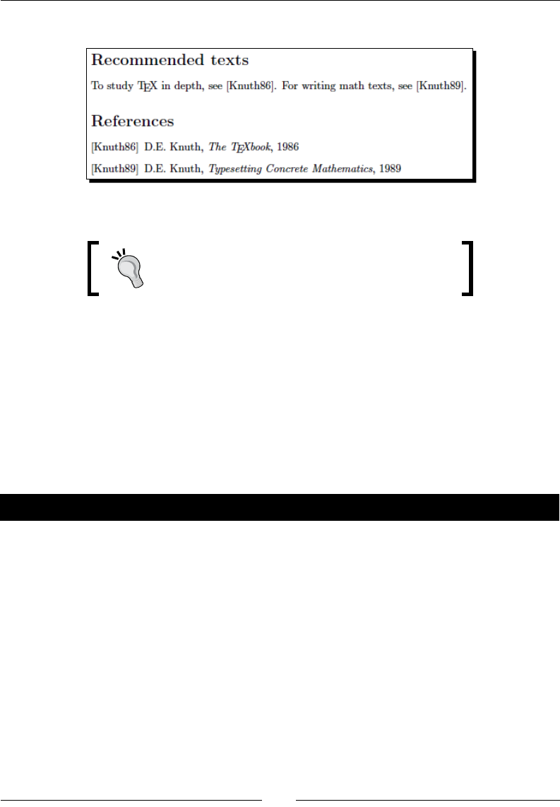
Chapter 7
[ 179 ]
And the output would then be as follows:
As you can see, the output of \cite has been automacally adjusted to the new labels.
The cite package oers compressed and sorted lists
of numerical citaons, like [2,4-6], and further
formang opons for in-text citaons.
The mandatory item of the environment should contain the widest label for the alignment
of the items. So, for instance, if you have more than 9 but fewer than a 100 items, you may
write two digits into the argument.
Using bibliography databases with BibTeX
Manually creang the bibliography is laborious. Especially, if you use references in
several documents, it would be benecial to use a database and let a program create
the bibliography for you. This sounds more complicated than it really is. We will try this.
Time for action – creating and using a BibTeX database
We shall create a separate database le containing the references of our previous example.
We will modify our example to use that database. To make this database usable, we have to
call the external program BibTeX:
1. Create a new document. Begin with wring the entry for the TeXbook:
@book{DK86,
author = "D.E. Knuth",
title = "The {\TeX}book",
publisher = "Addison Wesley",
year = 1986
}
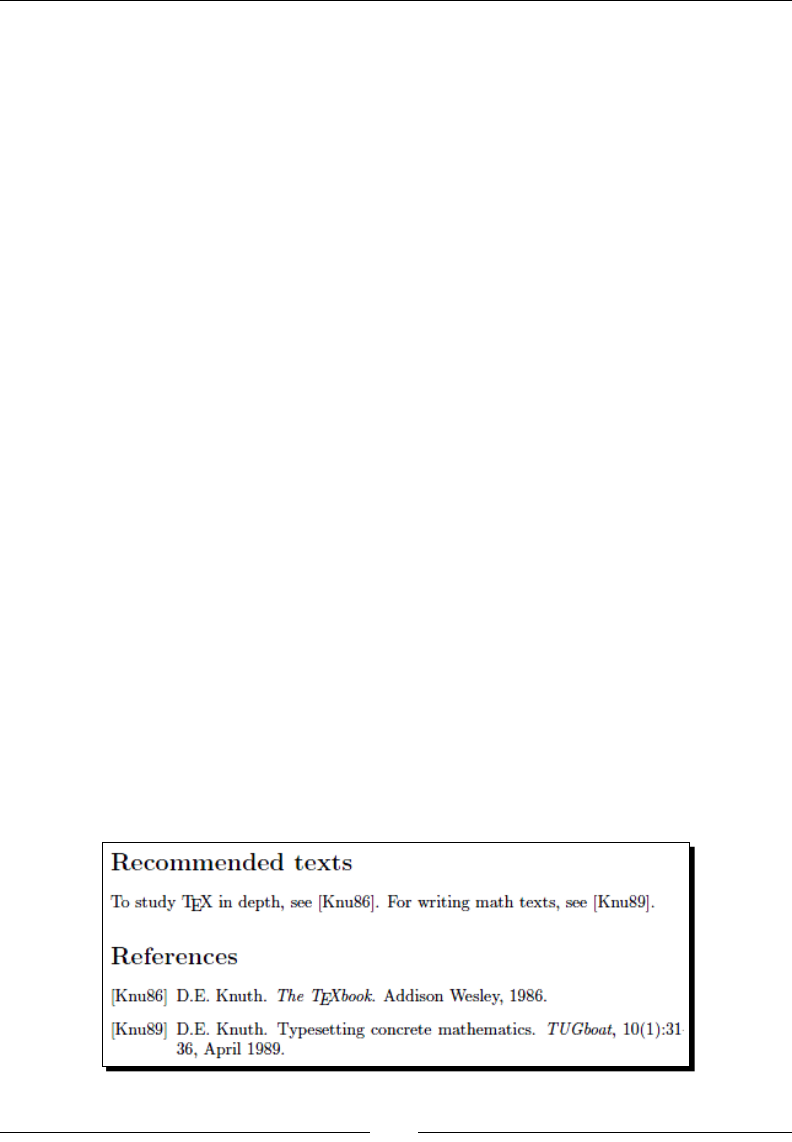
Lisng Content and References
[ 180 ]
2. For the next entry, that is, the arcle, we will specify even more elds:
@article{DK89,
author = "D.E. Knuth",
title = "Typesetting Concrete Mathematics",
journal = "TUGboat",
volume = 10,
number = 1,
pages = "31--36",
month = apr,
year = 1989
}
3. Save the le and give it the name tex.bib. Open our example tex document and
modify it as follows:
\documentclass{article}
\begin{document}
\section*{Recommended texts}
To study \TeX\ in depth, see \cite{DK86}. For writing math texts,
see \cite{DK89}.
\bibliographystyle{alpha}
\bibliography{tex}
\end{document}
4. Typeset one me with pdfLaTeX.
5. If you're using TeXworks, choose BibTeX instead of pdfLaTeX, present in the
drop-down box next to the Typeset buon, and then click on Typeset. If you
write with another editor, use its BibTeX opon or type at the command
prompt in the document directory as follows:
bibtex documentname
6. Typeset twice with pdfLaTeX. Here's the result:

Chapter 7
[ 181 ]
What just happened?
We created a text le containing all bibliography entries. In the next secon, we shall look
at its format in depth. In our document, we chose a style called alpha, which sorts entries
according to the author's name and uses a shortcut consisng of author and year as label.
Then we told LaTeX to load the bibliography le called tex. The extension .bib has been
automacally added.
Aerwards, we called the external program BibTeX. This program knows from the example
.tex le that tex.bib has to be translated. Thus out of this .bib le, it creates a .bbl
le, which contains a LaTeX thebibliography environment and the nal entries.
Finally, we had to Typeset twice, to ensure that all cross-references are correct.
Though we need some more steps to generate the bibliography, there are benets: we don't
need to ne-tune each entry. We can easily switch between styles. We can then reuse the
.bib le.
So, let's look at the .bib le format. It supports various entry types like book and article.
Furthermore, these entries contain elds like author, title, and year. Let's rst look at
the supported elds, and aerwards we shall talk about the dierent kinds of entries.
Looking at the BibTeX entry elds
Here's a list of the standard elds. Some elds are common, some are rarely used—we just
list them in alphabecal order, following the BibTeX documentaon:
address Usually the address of the publisher. At least for small publishers, this
informaon might be useful.
annote An annotaon, not used by the standard bibliography styles. Other styles or
macros might use this.
author The name(s) of the author(s).
booktle The tle of a book, if you cite a part of that. For a book, use the title eld
instead.
chapter A chapter number.
crossref The key of the database entry being cross referenced.
edion The edion (First, Second, and alike) of a book. Commonly it's capitalized.
editor The name(s) of the editor(s).
howpublished The way of publishing, especially if it's unusual. Capitalize the rst word.
instuon Could be a sponsoring instuon.
journal A journal name; you may use common abbreviaons.
Lisng Content and References
[ 182 ]
key Used for alphabezing, cross-referencing, and labeling if the author informaon
is missing. Don't confuse it with the key used in the \cite command which
corresponds to the beginning of the entry.
month The month in which the work was published or wrien if it's not yet published.
Usually a three leer abbreviaon is used.
note Any addional useful informaon. Capitalize the rst word.
number The number of a journal or another kind of work in a series.
organizaon Might be a sponsoring organizaon.
pages A page number or range of page numbers, like 12-18 or 22+.
publisher The name of the publisher.
school Could be the name of the school where the document was wrien.
series The name of a series of books or its number of a mul-volume set.
tle The tle of the work.
type The type of the publicaon.
volume The volume of a journal or mul-volume book.
year The year of the publicaon or the year when it was wrien if it hasn't been
published yet. Commonly four numerals are used, such as 2010.
You may use any elds possibly supported by other styles and ignored by standard styles.
Referring to Internet resources
Today we oen refer to online sources. To put Internet addresses into BibTeX
elds, use the \url command of the url or hyperref package, for example,
howpublished = {\url{http://texblog.net}}. Some styles oer
a url eld.
Understanding BibTeX entry types
Firstly, you decide which type of entry you want to add and then you ll in the elds.
Dierent types may support dierent elds. Some elds are required, some are oponal
and may be omied, and some are simply ignored.

Chapter 7
[ 183 ]
Usually the name of the entry tells you its meaning. These are the standard entry types and
their required and oponal elds, according to the BibTeX reference:
Type Required elds Oponal elds
arcle author, title, journal,
year
volume, number, pages, month, note
book author or editor,
title, publisher, year
volume or number, series, address,
edition, month, note
booklet title author, howpublished, address,
month, year, note
conference author, title,
booktitle, year
editor, volume or number, series,
pages, address, month, organization,
publisher, note
manual title author, organization, address,
edition, month, year, note
mastersthesis author, title, school,
year
type, address, month, note
misc none author, title, howpublished, month,
year, note
phdthesis author, title, school,
year
type, address, month, note
proceedings title, year editor, volume or number, series,
address, month, organization,
publisher, note
techreport author, title,
institution, year
type, number, address, month, note
unpublished author, title, note month, year
Have a look at the BibTeX reference for more details:
texdoc bibtex
If no other entry ts, choose misc. It doesn't maer if you use capitals or small leers;
@ARTICLE is understood the same as @article. As the example showed, entries have
the following form:
@entrytype{keyword,
fieldname = {field text},
fieldname = {field text},
…
}
Lisng Content and References
[ 184 ]
Use braces around the field text. Straight quotes instead like in "field text" are
supported as well. For numbers, you may omit the braces.
Some styles change the capitalizaon, which might lead to undesired
lowercase leers. To protect leers or words from becoming lowercase, put
addional braces around them. Preferably around a word instead of just the
leer to keep ligatures and kerning improvement, that is, {WAL} looks beer
than {W}AL as TeX moves an A closer to a preceding W. Separang braces
hampers TeX's micro-typographic improvements.
Choosing the bibliography style
Standard styles are as follows:
plain Arabic numbers for the labels, sorted according to the names of the authors. The number
is wrien in square brackets, which also appear with \cite.
unsrt No sorng. All entries appear like they were cited in the text, otherwise it looks like
plain.
alpha Sorng is according to the names of the authors, the labels are shortcuts made of the
authors name and the year of publicaon. Also here, square brackets are used.
abbrv Like plain, but rst names and other eld entries are abbreviated.
The style should be chosen aer \begin{document} and before \bibliography. You
may write \bibliographystyle right before \bibliography to keep it together.
There are more styles available in TeX distribuons and on the Internet. For instance, the
natbib package provides styles and the capability to cite in a nice author-year scheme. This
package further adds some elds, like ISBN, ISSN, and URL.
The package biblatex provides a complete reimplementaon of the
bibliographic features oered by BibTeX and LaTeX. Without learning the BibTeX
language, you could create new styles just by using your LaTeX knowledge.
Listing references without citing
BibTeX takes only those references from the database that are cited in the text, and prints
them out. However, you may specify keys for references, which should appear nevertheless
the following for a single reference. Just write the following for a single reference:
\nocite{key}

Chapter 7
[ 185 ]
Or write the following to list the complete database
\nocite{*}
Changing the headings
Like in our diagram example, if you don't like the heading Contents, you could easily change
it. The text of the heading is stored in the text macro \contentsname. So, just redene it
as follows:
\renewcommand{\contentsname}{Table of Contents}
Here's a list of all those headings:
List Heading command Default heading
Table of contents \contentsname Contents
List of gures \listfigurename List of gures
List of tables \listtablename List of tables
Bibliography \bibname in book and report
\refname in article
Bibliography in book and report
References in article
Index \indexname Index
Furthermore, as promised, here's a list of further macros for names used by LaTeX:
Name Command Default value
gure \figurename Figure
table \tablename Table
part \partname Part
chapter \chaptername Chapter
abstract \abstractname Abstract
appendix \appendixname Appendix
Not really surprising! Using name macros is especially useful when another language will be
used. For instance, the babel package takes a language opon and redenes all those name
macros according to those languages.
However, they are also useful to choose abbreviaons like Fig. or Appendices instead
of Appendix.
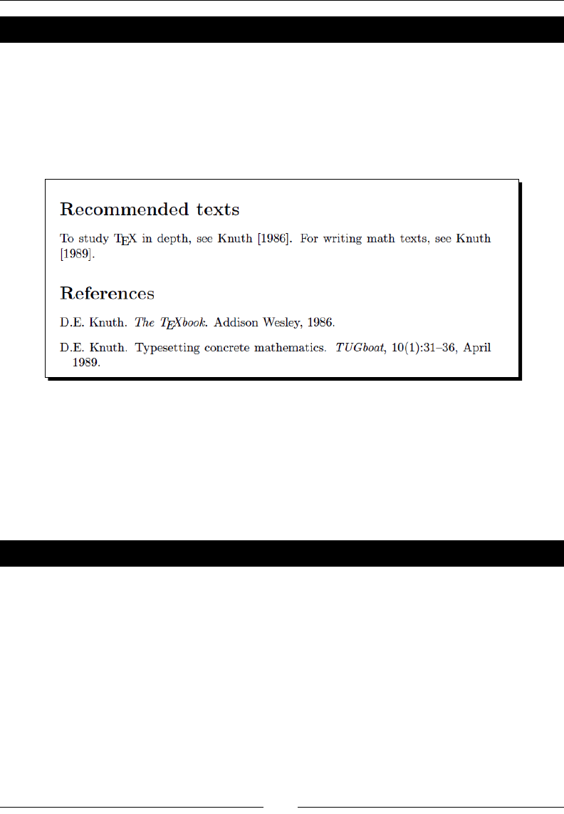
Lisng Content and References
[ 186 ]
Have a go hero – using natbib
Load the already menoned natbib package and try its new styles plainnat, abbrvnat, and
unsrtnat, for instance:
\usepackage{natbib}
\bibliographystyle{plainnat}
Our example would change as follows:
natbib reimplemented the \cite command and oers variaons to it, with the main
purpose of supporng author-year citaons. It works with most other available styles.
natbib introduces the citaon command \citet for textual citaons and the command
\citep for parenthecal citaons. There are starred variants prinng the full author list,
and oponal arguments allow adding text before and aer.
Check out the documentaon if you would like to benet from this ne package.
Pop quiz
1. Which of these commands should be used for adding unnumbered headings to the
table of contents?
a. \addtocontents
b. \addcontentsline
c. \contentsname
2. Which of the following indexing commands has to come before \begin{document}?
a. \index
b. \printindex
c. \makeindex

Chapter 7
[ 187 ]
3. Which command generates the bibliography?
a. \bibliography
b. \bibliographystyle
c. \bibitem
Summary
In this chapter, we dealt with many kinds of lists. Specically, we learned about:
Generang and customizing the table of contents and lists of gures and tables
Producing an index poinng to relevant informaon for keywords and phrases
Creang bibliographies, both manually and using a bibliography database
These lists are intended to guide the reader to the informaon he's/she's looking for; they
aren't just for lisng and summarizing. That's why the headings of the list of gures and the
list of tables usually don't appear in the TOC, as they commonly directly follow the TOC.
Somemes there's even the strange requirement to list the table of contents within itself. If
you are not sure with a design or a requirement, have a look at a good book in your special
eld, to see how exemplary tables of contents, lists, and indexes might look.
In the next chapter, we shall look at scienc wring in depth.
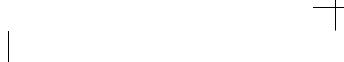
8
Typing Math Formulas
Chapter 1, Geng started with LaTeX, claimed that LaTeX oers excellent
quality for mathemacal typeseng. Now it's me to prove this.
To make the most of LaTeX's capabilies, we shall learn how to perform the following:
Wring basic formulas
Embedding formulas within text and text within formulas
Centering and numbering equaons
Aligning mul-line equaons
Typeseng math symbols such as roots, operators, Greek leers, and arrows
Building fracons
Stacking expressions
Building matrices
That's a great undertaking—let's tackle it!

Typing Math Formulas
[ 190 ]
Writing basic formulas
LaTeX knows three general modes:
The paragraph mode: The text is typeset as a sequence of words in lines,
paragraphs, and pages. That's what we used unl now.
The le-to-right mode: The text is also considered to be a sequence of words,
but LaTeX typesets it from le to right without breaking the line. For instance,
the argument of \mbox will be typeset in this mode; that's why \mbox prevents
hyphenaon.
The math mode: Leers are treated as math symbols. That's why they're typeset
in italic shape, which is common for variables. A lot of symbols can be used, most
of them exclusively in this mode. Such symbols are roots, sum signs, relaon
signs, math accents, arrows, and various delimiters like brackets and braces. Space
characters between leers and symbols are ignored. Instead, the spacing depends
on the type of symbols—distances to relaon signs are dierent from distances to
opening or closing delimiters. This mode is required for all math expressions.
Now we shall enter the math mode for the rst me.
Time for action – discussing quadratic equations and roots
Our rst small math text shall deal with the soluons of quadrac equaons. We need to
typeset formulas with constants, variables, superscripts for the square, and subscripts for
the soluons. The soluon itself needs a root symbol. Finally, we will use cross-references to
formulas.
1. Start a new document. For now, we don't need any package:
\documentclass{article}
\begin{document}
\section*{Quadratic equations}
2. State the quadrac equaon with its condions. Use an equaon environment
for it. Surround small pieces of math within text by \( … \):
The quadratic equation
\begin{equation}
\label{quad}
ax^2 + bx + c = 0,
\end{equation}
where \( a, b \) and \( c \) are constants and \( a \neq 0 \),
has two solutions for the variable \( x \):
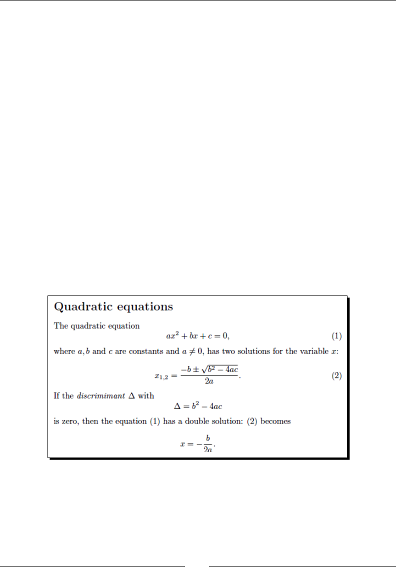
Chapter 8
[ 191 ]
3. Use another equaon for the soluons. The command for the square root is
\sqrt. The command for a fracon is \frac:
\begin{equation}
\label{root}
x_{1,2} = \frac{-b \pm \sqrt{b^2-4ac}}{2a}.
\end{equation}
4. Let's introduce the discriminant and discuss the case zero. To get an
unnumbered displayed equaon, we surround the formula with \[ … \]:
If the \emph{discrimimant} \( \Delta \) with
\[
\Delta = b^2 - 4ac
\]
is zero, then the equation (\ref{quad}) has a double solution:
(\ref{root}) becomes
\[
x = - \frac{b}{2a}.
\]
\end{document}
5. Typeset twice and look at the result:

Typing Math Formulas
[ 192 ]
What just happened?
Just as we said in Chapter 1, wring formulas also looks a lot like programming. However,
this chapter will help you master it, and the results are worth the eort. The formulas have
been built with commands: there are commands with arguments, like for roots and fracons,
and simple commands for symbols, like for the Greek leer. Most symbols have to be within
a math environment and don't simply work within normal text.
The equaon environment created a displayed formula; that formula has been horizontally
centered, some vercal space has been added before and aer, further these formulas are
consecuvely numbered.
However, \[ … \] and \( … \) are also, in truth, environments. Let's sort this out.
Embedding math expressions within text
LaTeX provides the math environment in-text formulas:
\begin{math}
expression
\end{math}
Since it's very laborious to write this environment for each small expression or symbol, LaTeX
oers an alias that's doing the same:
\(
expression
\)
You may write it without line breaks, such as \(expression\).
A third way is by using a shortcut, coming from TeX:
$expression$
A disadvantage of the laer is that the commands for beginning and ending the math
environment are the same, which may easily lead to errors. However, it's much easier to
type, which may be the reason why it's sll popular among LaTeX users.
\( … \) might cause problems in moving arguments like in headings. To
prevent any such problems, just load the package xltx2e, which xes this as
well as other issues.

Chapter 8
[ 193 ]
Displaying formulas
For displayed formulas, which have to be centered, LaTeX oers the displaymath
environment:
\begin{displaymath}
expression
\end{displaymath}
The eect of this environment is that the paragraph will be ended, some vercal space
follows, then the centered formula plus the following vercal space. As this math
environment takes care of the spacing, don't leave empty lines before and aer it! This
would cause addional vercal space because of the superuous paragraph breaks.
Also for this environment there's a shortcut. We already used it:
\[
expression
\]
In this case, pung the shortcuts \[ and \] on separate lines commonly improves the
readability as the formula is also kind of displayed in the source code.
There's also a TeX low level command:
$$
expression
$$
However, it's strongly recommended to use\[ … \], because this LaTeX environment
handles vercal spacing beer.
For the rest of this chapter, all pieces of code use math mode. Either we explicitly use a math
environment or we imagine that we are already in math mode, for short pieces of code.
Numbering equations
Equaons and formulas in general may be numbered. However, this applies only to displayed
formulas. The equation environment is responsible for this:
\begin{equation}
\label{key}
expression
\end{equation}
It looks similar to displaymath but numbered this me. The number will be displayed in
parentheses on the right side of the equaon.
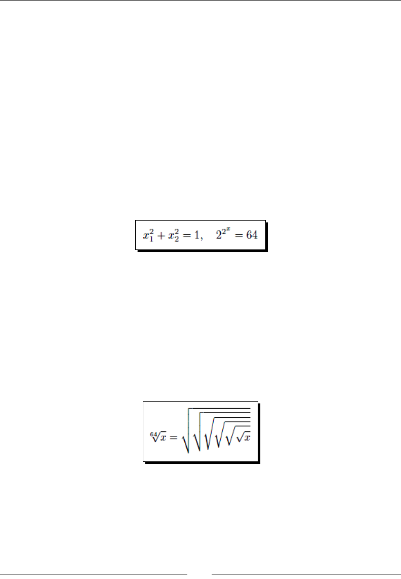
Typing Math Formulas
[ 194 ]
Adding subscripts and superscripts
As exponents and indexes are frequently used, there are very short commands for
typeseng them, for example, _ gives an index or subscript, ^ produces an exponent
or superscript. Use braces to mark the concerned expression. So, the common forms are
as follows:
{expression}_{subscript}
And:
{expression}^{superscript}
This may be nested. If you use subscripts and superscripts to the same expression, the order
of ^ and _ is not important. In the case of single leers, numerals, or symbols, you can omit
the braces. Let's look at an example:
\[ x_1^2 + x_2^2 = 1, \quad 2^{2^x} = 64 \]
Extracting roots
Our example contained a square root: \sqrt{value}. As there are roots of higher order,
this command accepts an oponal argument for the order. The complete denion is:
\sqrt[order]{value}
The size of the root symbol will be automacally adjusted to the height and the width of
the value expression. Roots may be nested. Both can be seen in this example:
\sqrt[64]{x} = \sqrt{\sqrt{\sqrt{\sqrt{\sqrt{\sqrt{x}}}}}}
Writing fractions
Within text formulas, you may just write / to denote fracons, such as \( (a+b)/2 \).
For larger fracons, there's the \frac command:
\frac{numerator}{denumerator}
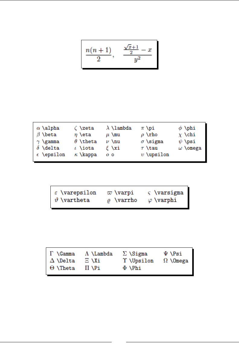
Chapter 8
[ 195 ]
This command may also be used for in-text formulas. However, the line spacing could
increase.
\[ \frac{n(n+1)}{2}, \quad \frac{\frac{\sqrt{x}+1}{2}-x}{y^2} \]
Greek letters
Mathemacians like to use Greek leers, for instance, to denote constants. To get a
lowercase Greek leer, just write the name with a backslash for the command. Here
are the lowercase Greek leers with their corresponding LaTeX commands:
For some leers, variants are available:
As the omicron just looks like an o, there's no command for it. It's similar for most uppercase
Greek leers, which are equal to Roman leers. The remaining uppercase Greek leers are
produced as follows:
For upright Greek leers, you may use the upgreek package.
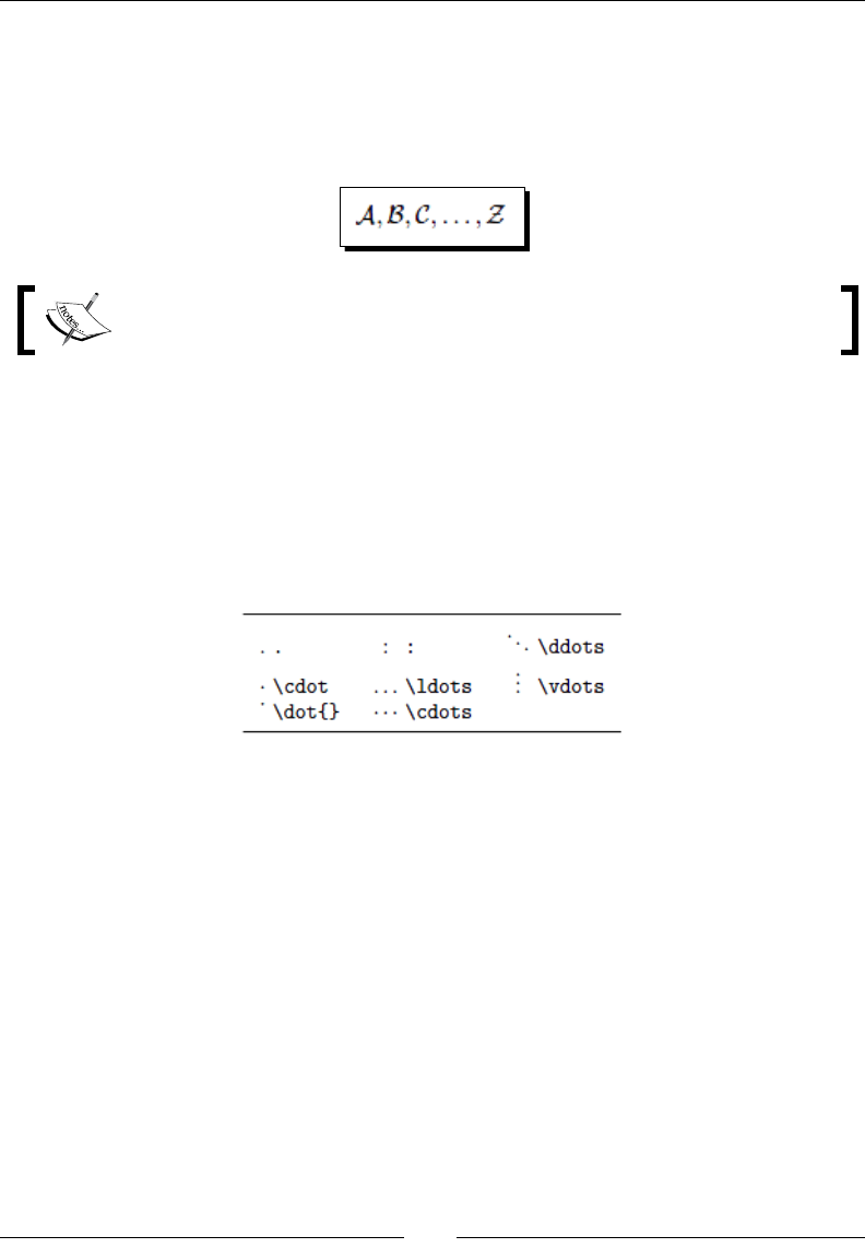
Typing Math Formulas
[ 196 ]
Script letters
For the twenty-six uppercase leers A, B, C, … , Z, there's a calligraphic shape, produced
by \mathcal:
\[ \mathcal{A}, \mathcal{B}, \mathcal{C}, \ldots, \mathcal{Z} \]
There are packages oering dierent calligraphic fonts, such as zapno and xits.
Producing an ellipsis
You already know \ldots for a low ellipsis. It also works in math mode. We use the low
ellipsis mainly between leers and commas. Between operaon and relaon symbols, a
centered ellipsis is commonly used. Furthermore, a matrix may require a vercal ellipsis.
Here's how all of them may be produced:
Comparing in-line formulas to displayed formulas
Wring formulas in-line saves space and allows uent explanaons. This is recommendable
for short math expressions within text.
Formulas in the displayed style are outstanding; they are centered and require more space.
Furthermore, they can be numbered and you may refer to them using the \label and \ref
techniques that you learned in Chapter 5, Creang Tables and Inserng Pictures.
Choose the style that is opmal for the readability of your text.
Changing the font, style, and size
In Chapter 2, Formang Words, Lines, and Paragraphs, we learned how to modify the font
of common text. There are further commands changing the font style in math mode:
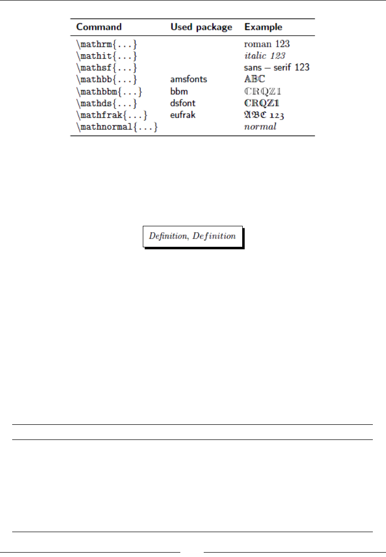
Chapter 8
[ 197 ]
Though leers in math mode are italic, they are considered to be separate symbols, which
results in a dierent spacing than that of an italic word. For instance, in math mode, may
be the product of the variables f and i, but not the ligature . Compare:
\textit{Definition}, \(Definition\)
Also, \mathit treats the argument as text in italic math font. So, for text within formulas,
use a text or math font command, or even beer: use \text{…} of amsmath—we will
return to this very soon.
If you wish to switch to bold typeface for a complete math expression, you can use the
declaraon \boldmath before the expression, that is, already outside math mode. The
declaraon \unboldmath switches back to the normal typeface. The laer has to be used
outside math mode as well.
To make parts of a formula bold, you can switch to the le-to-right mode by \mbox and by
using \boldmath in its argument.
Four math styles are available, determining the way of typeseng and the font size:
Style Command Meaning
display \displaystyle Default for leers and symbols in displayed
formulas
text \textstyle Default for leers and symbols within in-text
formulas
script \scriptstyle Smaller font size, used for subscripts and for
superscripts
scriptscript \scriptscriptstyle Even smaller font size, for nested script style

Typing Math Formulas
[ 198 ]
The textstyle diers from the displaystyle in mainly two ways; in textstyle,
variable sized symbols are smaller and subscripts and superscripts are usually placed beside
the expression instead of below and above, respecvely. Otherwise the font size is the same.
LaTeX switches the style automacally; if you write a simple exponent, it will be typeset in
script style, that is, with a smaller font size.
You may force a desired style using one of the commands in the aforemenoned table.
This allows you, for instance, to:
Type formulas within the text exactly like they would appear in a displayed formula:
bigger fracon, bigger sum signs, further subscripts are set below, and superscripts
are set above. Note, all of this increases the line spacing.
Write exponents or indexes with bigger symbols.
Customizing displayed formulas
There are two opons that modify the way the formulas are displayed:
fleqn "le equaon numbers" This causes all displayed formulas to be aligned at
the le margin.
leqno "le equaon numbers" All numbered formulas would get the numbers on
the le side instead of the right.
Oen, formulas are not displayed just standalone. We may encounter situaons where:
A formula is too long to t on one line
Several formulas are listed row-by-row
An equaon shall be transformed step-by-step
A chain of inequalies spans over more than one line
Several formulas shall be aligned at relaon symbols
We may also encounter similar situaons, where we have to write mul-line formulas, oen
with some kind of alignment. The amsmath package oers specialized environments for
nearly every such need.
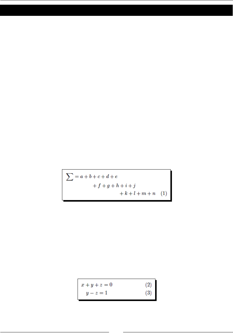
Chapter 8
[ 199 ]
Time for action – typesetting multi-line formulas
We shall use the amsmath package to experiment with a very long formula and with a
system of equaons:
1. Start a new document on an A6 paper and load the amsmath package.
\documentclass{article}
\usepackage[a6paper]{geometry}
\usepackage{amsmath}
\begin{document}
2. Use the multline environment to span a long equaon over three lines.
End the lines with\\:
\begin{multline}
\sum = a + b + c + d + e \\
+ f + g + h + i + j \\
+ k + l + m + n
\end{multline}
\end{document}
3. Typeset and look at the formula:
4. Now we handle a system of equaons. Use the gather environment
to add these equaons. Again, end lines with \\:
\begin{gather}
x + y + z = 0 \\
y - z = 1
\end{gather}
5. Typeset and look at the equaons:
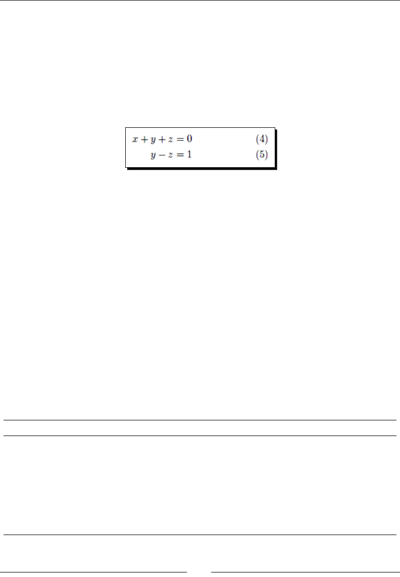
Typing Math Formulas
[ 200 ]
6. Commonly, equaon systems are aligned at the equal sign. Let's do this. Use the
& symbol to mark the point that we wish to align:
\begin{align}
x + y + z &= 0 \\
y - z &= 1
\end{align}
7. Typeset; now the equaons are aligned as desired:
What just happened?
Because we loaded the amsmath package, we have access to several mul-line math
environments.
Each line in such an environment is ended by \\, except the last one. The alignment depends
on the environment, as we've seen:
multline: The rst line is le-aligned, the last line right-aligned, and all
other lines in between are centered
gather: All lines are centered
align: The lines are aligned at marked relaon signs
Let's have a closer look.
Aligning multi-line equations
Here's a list of the amsmath mul-line environments:
Name Meaning
multline First line is le-aligned, last line is right-aligned, all others are centered.
gather Each line is centered.
align Use & to mark a symbol where the formulas shall be aligned. Use another
& to end a column, if you need several aligned columns.
flalign Similar to align with more than one column, but the columns are ushed
to the le and the right margin, respecvely.
alignat Alignment at several places, each has to be marked by &.

Chapter 8
[ 201 ]
Name Meaning
split Similar to align, but within another math environment, thus
unnumbered.
aligned,
gathered,
alignedat
Used for an aligned block within a math environment. This can be
displayed math or in-line math.
Numbering rows in multi-line formulas
In mul-line math environments, each line would be numbered like a normal equaon.
If you wish to suppress the numbering of a line, write \notag before the end of the line.
Use the starred variant like align*, or gather*, if you would like to avoid numbering
completely.
Inserting text into formulas
To insert some text into a formula, standard LaTeX provides the \mbox command. amsmath
oers further commands:
\text{words} inserts text within a math formula. The size is adjusted according
to the current math style, that is, \text produces smaller text within subscripts or
superscripts.
\intertext{text} suspends the formula, the text follows in a separate
paragraph, then the mul-line formula is resumed, keeping the alignment.
Use it for longer text.
These commands are the best choice, when you would like to use text within math
environments.
Fine-tuning formulas
If we go beyond wring variables and basic math operators, we may need many symbols for
special purposes: certain relaon signs, unary and binary operators, funcon-like operators,
sum and integral symbols and variants of the laer, arrows, and many more. LaTeX and
addional packages oer thousands of symbols for many purposes. We shall have a look at
some of them. But rstly, let's gure out how to write funcons.
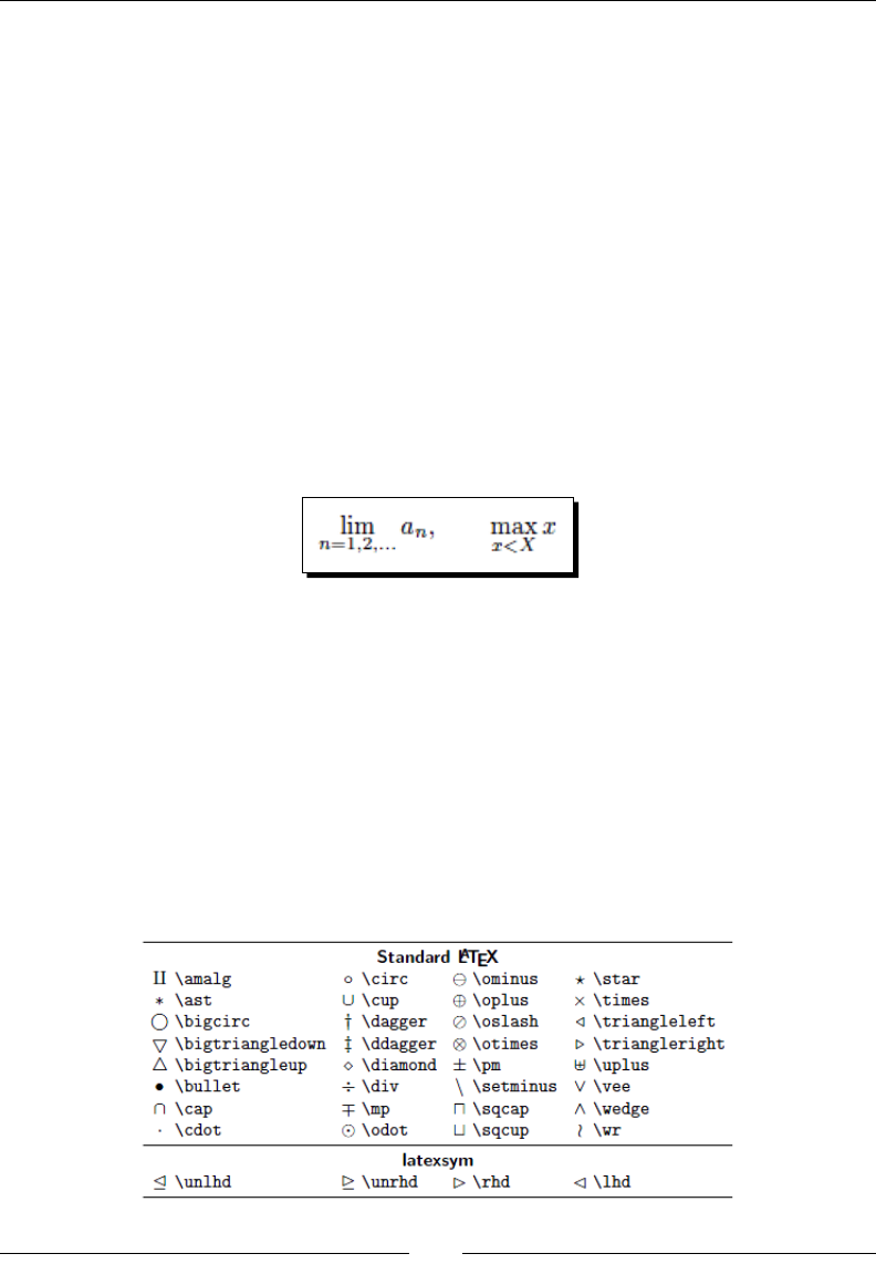
Typing Math Formulas
[ 202 ]
Using operators
Trigonometric funcons, logarithm funcons, and other analyc and algebraic funcons are
commonly wrien with upright Roman leers. Simply typing log would otherwise look like a
product of the three variables, namely, l, o, and g. To ease the input, there are commands for
many common funcons or so called operators. Here's an alphabecal list of the predened
ones:
\arccos, \arcsin, \arctan, \arg, \cos, \cosh, \cot, \coth, \scs, \deg, \det, \dim,
\exp, \gcd, \hom, \inf, \ker, \lg, \lim, \liminf, \limsup, \ln, \log, \max, \min,
\Pr, \sec, \sin, \sinh, \sup, \tan, \tanh
The modulo funcon may be wrien in two ways, either by using \bmod for a binary relaon
or by using \pmod{argument} for a modulo expression in parentheses.
Some operators support subscripts which are set as follows:
\[ \lim_{n=1, 2, \ldots} a_n, \qquad \max_{x<X} x \]
Superscripts would be set above then.
Exploring the wealth of math symbols
Now, let's look at some math symbols and the commands for producing them. We shall
cover many standard LaTeX symbols, some addional symbols are provided by the latexsym
package. Even more symbols are accessible using, for instance, the amssymb package.
Binary operation symbols
Besides plus and minus, there are a few more operaons:
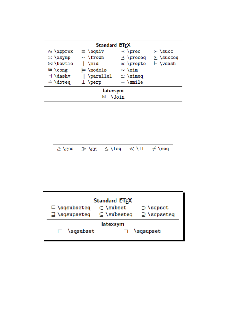
Chapter 8
[ 203 ]
Binary relation symbols
Values of expressions might be equal, but there are more possible relaons, for example,
they may be congruent, parallel, or they might stand in any other relaon:
Inequality relation symbols
If expressions are not equal, the inequality might be expressed in dierent ways:
Subset and superset symbols
For comparing sets and expressing relaons between them, there are many symbols:
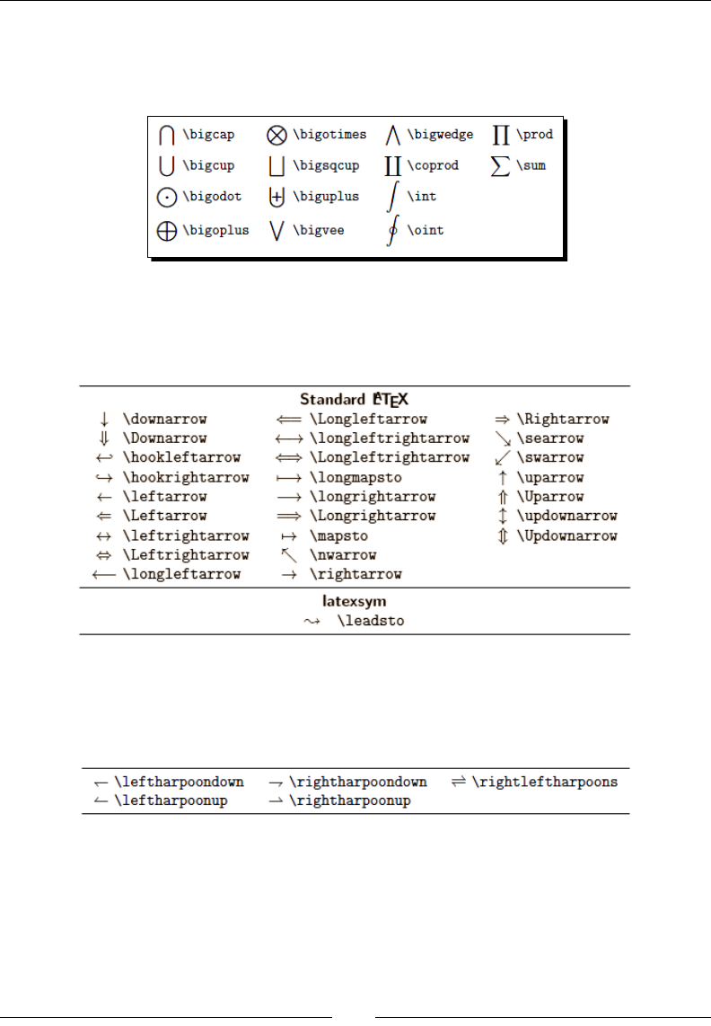
Typing Math Formulas
[ 204 ]
Variable sized operators
For sums, products, and set operaons, for example, we can use operator symbols
which are variable in size: bigger in display style and smaller in text style.
Arrows
Arrows are used for implicaons, maps, or descripve expressions:
Harpoons
There are special arrows called harpoons:
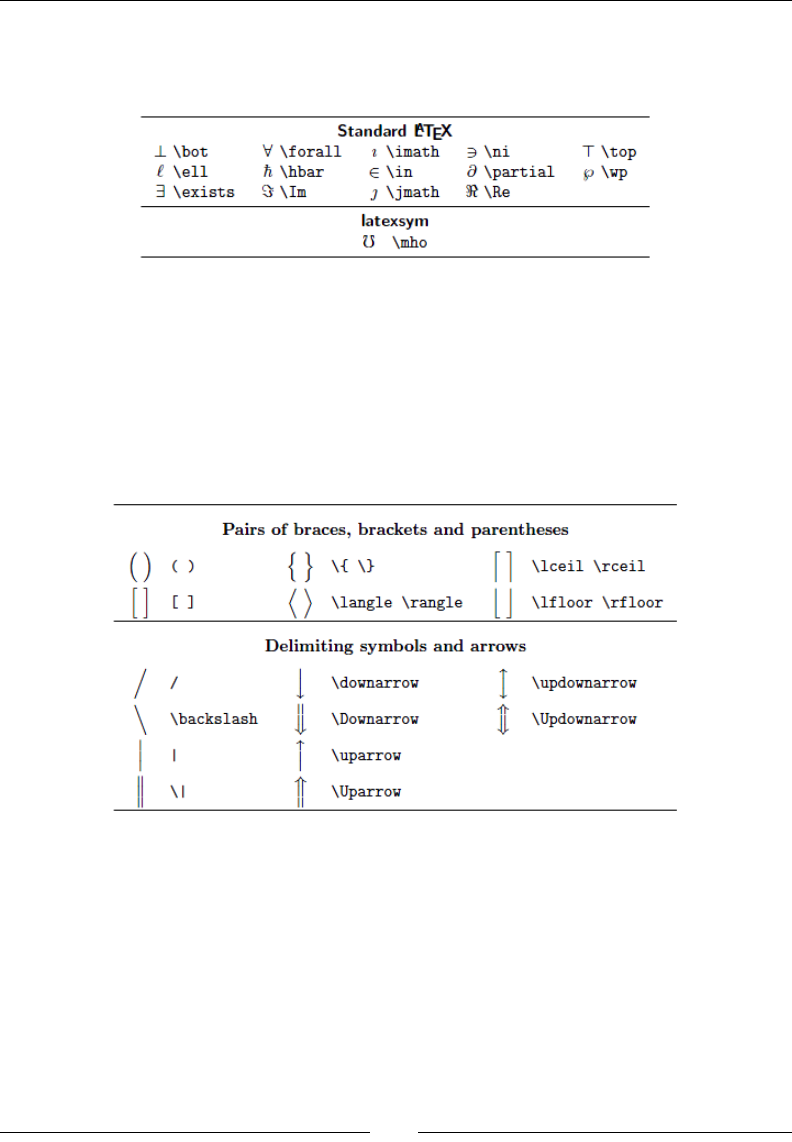
Chapter 8
[ 205 ]
Symbols derived from letters
Some leer-like symbols are used in math:
Variable sized delimiters
Also, delimiters such as parentheses, brackets, and braces can vary in size. If you write \left
or \right before such a delimiter, its size will be automacally matched to the size of the
inner expression. These size macros have to be used in pairs. To match a pair, if you don't
wish to match a delimiter, use\left. or\right. to get an invisible delimiter.
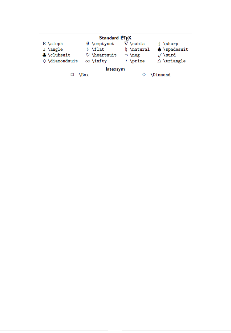
Typing Math Formulas
[ 206 ]
Miscellaneous symbols
Here are more LaTeX symbols that do not match the menoned categories:
"The Comprehensive LaTeX Symbol List" lists about 5000 symbols sorted in categories. If you
need to search for a symbol, have a look at this document. As usual, with TeX Live, you could
open this document by using the following at the command prompt:
texdoc symbols
You can nd it on CTAN as well.
Writing units
If you use units in text, they should not look like variables: 'm' for meters should not look
exactly like a variable m. Similarly, analogous 's' may stand for seconds, but not for a variable.
A typographical convenon is to use an upright font shape for units. Furthermore, it's
common to use a thin space between the value and the dimension. So, for 10 meters, you
may write 10\,\mathrm{m}. However, this is very me-consuming. That's why several
packages have been developed supporng correct and nice typeseng of units, for example,
units, fancyunits, and siunits.
The most modern and comprehensive units package is siunitx, providing features of all the
other packages and even more. It requires reading some documentaon before use, but it's
worth the eort.
Building math structures
Variables and constants are simple. But there are more complex objects, like binomial
coecients, vectors, and matrices. We shall gure out how to typeset such structures.
Let's begin with simple arrays.
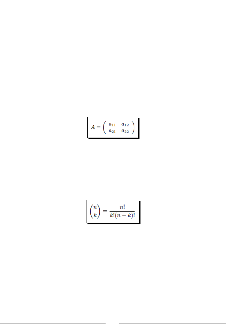
Chapter 8
[ 207 ]
Creating arrays
For arranging math expressions within a surrounding expression, there's the array
environment. We use it exactly like a tabular environment. However, it requires math
mode and all of its entries are made using the math mode as well.
For example, by using variable sized parentheses around the array:
\[
A = \left(
\begin{array}{cc}
a_{11} & a_{12} \\
a_{21} & a_{22}
\end{array}
\right)
\]
Writing binomial coefcients:
Binomial coecients and matrices may be typeset using an array together with delimiters.
However, the amsmath package provides shorter commands, for instance, \binom for
binomial coecients:
\binom{n}{k} = \frac{n!}{k!(n-k)!}
Typesetting matrices
As you might expect now of amsmath, there are many special matrix environments. A
standard matrix can be typeset by the pmatrix environment:
\documentclass{article}
\usepackage{amsmath}
\begin{document}
\[
A = \begin{pmatrix}
a_{11} & a_{12} \\
a_{21} & a_{22}
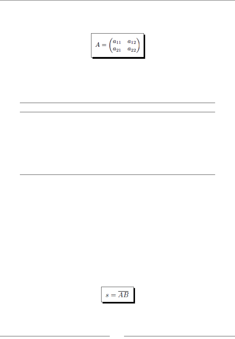
Typing Math Formulas
[ 208 ]
\end{pmatrix}
\]
\end{document}
You may noce that the parentheses are closer to the matrix entries than in the array
example.
These are amsmath's matrix environments:
Name Delimiters of the matrix
matrix without delimiters
pmatrix parentheses ( )
bmatrix square brackets [ ]
Bmatrix braces { }
vmatrix | |
Vmatrix || ||
smallmatrix without delimiters, add them if needed, more compact
The compact smallmatrix environment is useful for matrices within running text.
Stacking expressions
Formulas may become complex: we might need to put one symbol above another one or
above whole expressions, or we wish to put lines, braces, or dots above symbols. There are
several ways.
Underlining and overlining
\overline puts a line above its argument, which may be nested:
s = \overline{AB}
The counterpart is \underline.
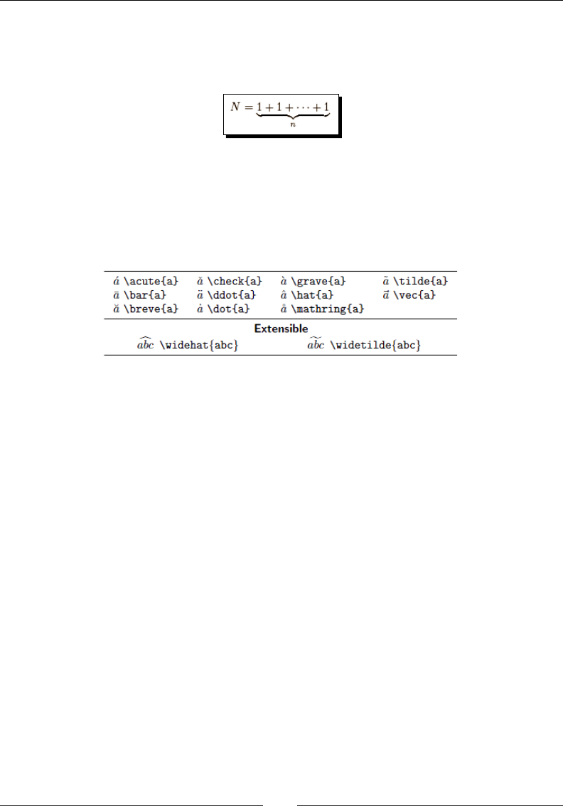
Chapter 8
[ 209 ]
It doesn't have to be a line; braces are popular too. The commands are \underbrace and
\overbrace. You may use subscripts and superscripts:
N = \underbrace{1 + 1 + \cdots + 1}_n
Setting accents
We've already seen accents in text mode. For the math mode, we need dierent commands.
They may be applied to any leer. Here's the list of math accents using the lowercase leer
'a' as an example:
The extensible ones are also called wide accents; they try to t the width of their argument.
Putting a symbol above another
Besides the array environment, there are amsmath commands to directly stack expressions:
\underset{expression below}{expression} puts an expression below
another, using the subscript size below.
\overset{expression above}{expression} puts an expression above
another, using the subscript size above.
Writing theorems and denitions
LaTeX provides environment for theorems, denions, and alike. Returning to our rst
example in this chapter, we could dene a theorem environment by:
\newtheorem{thm}{Theorem}
Then, we declare a denion environment, using an oponal argument stang an exisng
environment with which we would like to share the numbering:
\newtheorem{dfn}[thm]{Definition}
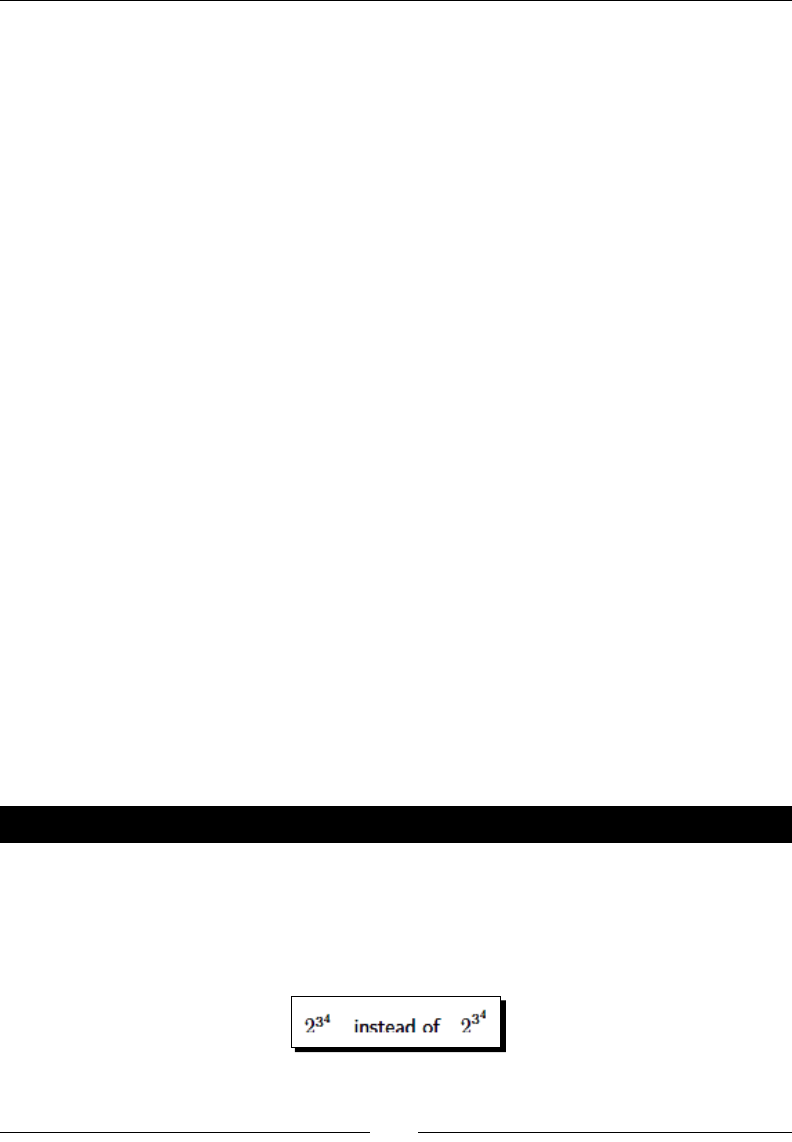
Typing Math Formulas
[ 210 ]
And in this simple way, we may use these environments:
\begin{dfn}
A quadratic equation is an equation of the form
\begin{equation}
\label{quad}
ax^2 + bx + c = 0,
\end{equation}
where \( a, b \) and \( c \) are constants and \( a \neq 0 \).
\end{dfn}
\begin{thm}
A quadratic equation (\ref{quad}) has two solutions for the variable
\( x \):
\begin{equation}
\label{root}
x_{1,2} = \frac{-b \pm \sqrt{b^2-4ac}}{2a}.
\end{equation}
\end{thm}
In the output, such environments are numbered and labeled "Theorem" and "Denion",
respecvely. In Chapter 10, Developing Large Documents, when we are going to develop
large documents, we will use this to create a complete document containing denions,
theorems, and lemmas.
There are two remarkable packages oering much more exibility:
amsthm provides several styles, allows ne customizaon, and includes a proof
environment.
ntheorem does similar work, but handles end marks in a beer way.
If you would like to use such environments, have a look at their documentaon, and
compare the features to decide which package is the best for you.
Have a go hero – checking out the mathtools package
The mathtools package extends amsmath. If you need a certain feature and cannot nd it,
neither in standard LaTeX nor in amsmath, always look rst at mathtools. Here are some of
its features with examples:
Tools for ne-tuning math typeseng, for example, compact styles:
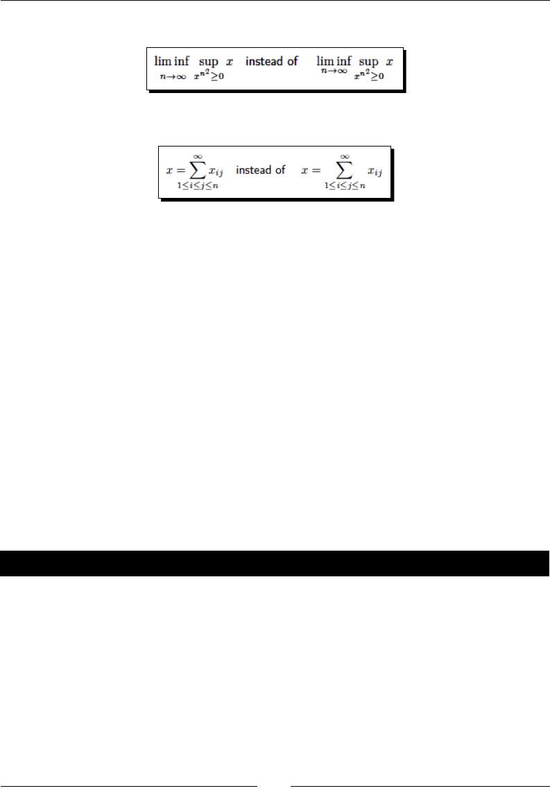
Chapter 8
[ 211 ]
Aligning limits of operators:
Adjusng the width of operators:
Beer control over tags; modifying their appearance and showing only tags for
equaons that have been actually referenced
Extensible symbols; more arrows and being able to automacally adjust their
width, also extensible brackets and braces to be set under or over expressions
New math environments for more exible matrices, cases, improved mul-line
formulas, and arrows between aligned formulas
Less spacing for shorter inter text
Declaraon of paired delimiters
Addional symbols such as a vercally centered colon, combinaons of relaon
symbols with colons, shortcuts for auto-sized parentheses
Techniques such as spreading lines in mul-line formulas, seng le sub- and
superscripts, typeseng math within italic text, and producing mul-line fracons
Try to typeset these examples rst without mathtools. You will noce some dicules.
Have a look into the documentaon of this valuable package and nd out which commands
can be applied to achieve the aforemenoned styles and alignments.
Pop quiz
1. Which environment produces a displayed formula?
a. \begin{math} … \end{math}
b. \[ … \]
c. \( … \)
2. Which of these environments has to be used within math mode?
a. align
b. aligned
c. alignat

Typing Math Formulas
[ 212 ]
3. The following commands may be used to insert text within math formulas.
According to this chapter, which command would generally be the most
appropriate?
a. \mbox
b. \mathrm
c. \textrm
d. \text
Summary
Now that we've got the necessary tools to write scienc texts, we are able to write
complex math formulas, ne-tune math expressions, align and number equaons, and
access thousands of math symbols.
In the next chapter, we will not only deal further with math fonts, but also with fonts in
general.
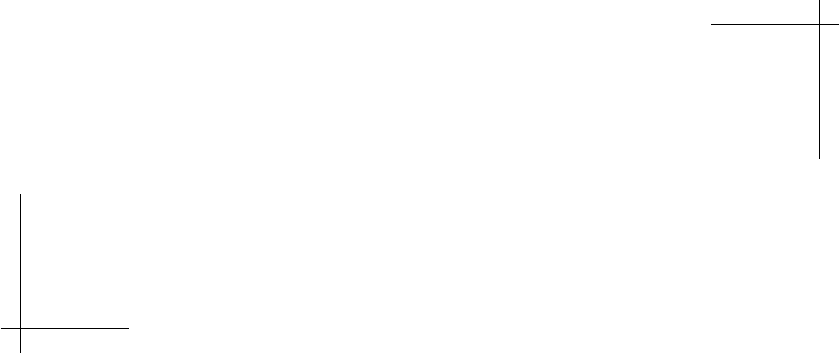
9
Using Fonts
The appearance of your text is signicantly determined by the base font. You
may choose a font that's especially clear and readable for a long piece of
wring, or a fancy font for a greeng card. Your job applicaon leer might
use a very clear and serious font, whereas a mathemacal arcle requires
fonts with a lot of symbols and a text font that ts well with them.
Unl now, we have been covering the logical properes of fonts. Though we
always used the LaTeX standard font, we switched, for instance, from roman to
sans-serif, or to typewriter, learned how to make text bold, italic, or slanted, but
we never le the standard set of fonts.
In this chapter, we shall learn how to:
Choose other sets of fonts for the whole document
Load font packages for specic shapes
During this, we will also:
See how to install addional fonts
Look at various fonts and learn how to use them
Speak about encoding of input text and of fonts in the output
Let's start discussing the encodings.
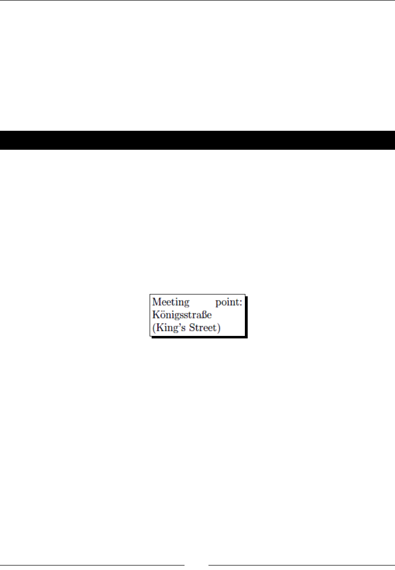
Using Fonts
[ 214 ]
Preparing the encoding
Do you remember the ASCII code? All operang systems are able to understand it. However,
when it comes to special characters like German umlauts or diacrics in general, currency
symbols, and non-lan language characters, some systems work dierently. We shall see
how to deal with that.
Also, the output needs some kind of encoding. We shall gure out how to perfect that.
Time for action – directly using special characters
In a TeX document, we would like to use the German name of a street. It contains diacrics,
so called umlauts. Let's check out how to make it work right.
1. Start a new document. Within a small parbox, write the text:
\documentclass{article}
\begin{document}
\parbox{3cm}{Meeting point: K\"onigsstra\ss e (King's Street)}
\end{document}
2. Typeset and have a rst look:
3. Try babel instead! It provides shortcuts for German umlauts, if you state the
ngerman opon. Use "u for ü, a for ä, and s for ß":
\usepackage[ngerman]{babel}
…
\parbox{3cm}{Meeting point: K"onigsstra"se (King'sStreet)}
4. The output would be the same. Sll the hyphenaon remains as a problem: TeX
cannot use hyphenaon rules if macros are inside the words.
5. As babel is required for good hyphenaon, we keep that. But we use Unicode
encoding and another called T1 font encoding:
\documentclass{article}
\usepackage[ngerman]{babel}
\usepackage[utf8]{inputenc}
\usepackage[T1]{fontenc}
Chapter 9
[ 215 ]
\begin{document}
\parbox{3cm}{Meeting point: Königsstraße (King's Street)}
\end{document}
6. Typeset. Now we've got the correct hyphenaon:
What just happened?
Firstly, using accent macros, or babel shortcut macros to construct diacrics, makes the TeX
code less readable and hard to type. Furthermore, it creates a problem with hyphenaon: for
macros, hyphenaon rules cannot be applied. That's why the juscaon has been so bad.
Two packages solve those problems:
inputenc takes care of the input and translates special characters into TeX macros.
It understands an opon to mark the encoding. This depends on the editor and
the operang system. As a rule of thumb: on Linux and Mac OS X, use utf8;
on Windows, use latin1, except with TeXworks. Also, on Windows, TeXworks
understands utf8, which is an implementaon of Unicode.
fontenc is responsible for the output encoding: TeX macros are translated into
special characters. For instance, ö is no longer constructed of o and dots, but it's
the glyph ö of the current font. Thus, hyphenaon rules can be applied, the search
feature of a PDF reader works with those characters, even copy and paste works
ne. With standard encoding, copying and pasng ö would result in dots and an o.
Unicode is an industry standard for text encoding, which hugely extends
the ASCII code. Unicode supports more than 100,000 characters of
many languages. It's become more and more supported by modern
operang systems and editors.
To be able to benet from those packages, you should know the encoding and you
should use a font supporng the T1 encoding, also known as Cork encoding. Take it
just as a name—we don't need to care further about encoding for now.
To see what happens with and without fontenc, use:
\showhyphens{Königsstraße}
Using Fonts
[ 216 ]
Use it together with babel and inputenc and examine the log le. With standard font
encoding, called OT1, you would read:
\OT1/cmr/m/n/10 K^^?onigsstra^^Ye
However, with T1 encoding, the log le would show:
\T1/cmr/m/n/10 Kö-nigs-straße
Installing additional fonts
TeX distribuons usually install a lot of fonts. A package manager allows the installaon of
further fonts, like mpm with MiKTeX or tlmgr with TeX Live.
TeX Live includes only freely licensed fonts. Non-free fonts may be installed using a separate
program. It's called getnonfreefonts. If it's not already installed with your version of TeX Live,
you can download it from http://www.tug.org/fonts/getnonfreefonts/.
getnonfreefonts –l
This command lists all addionally available non-free fonts. If you wish to install a font,
give its name as the argument or just type the following to install all available fonts:
getnonfreefonts –a
Type the following to get a brief documentaon:
getnonfreefonts
getnonfreefonts would install the fonts in your TeX home directory. To make the fonts
available for the complete local system, use getnonfreefonts-sys instead.
Progams ending with -sys work system wide. Further examples are: updmap-
sys, which updates font map les, and fmtutil-sys for (re)creaon of
so-called format les. Such programs require administrator privileges, so run it
as via sudo or as root on Linux or Mac OS X, on Windows use an administrator
account if you ever need it. Normally the TeX distribuon calls them
automacally during installaon and updates if required.
If you use T1 font encoding, which is strongly recommended, you might noce a decreased
font quality. Don't worry this could happen if you don't have good T1 supporng standard
fonts installed, thus bitmap fonts were used as replacement. It can be easily repaired by
installing the cm-super package, which contains the European Computer Modern fonts,
which are enhanced versions of the default Computer Modern fonts, with T1 support, in
high quality. Alternavely, use one of the following fonts.
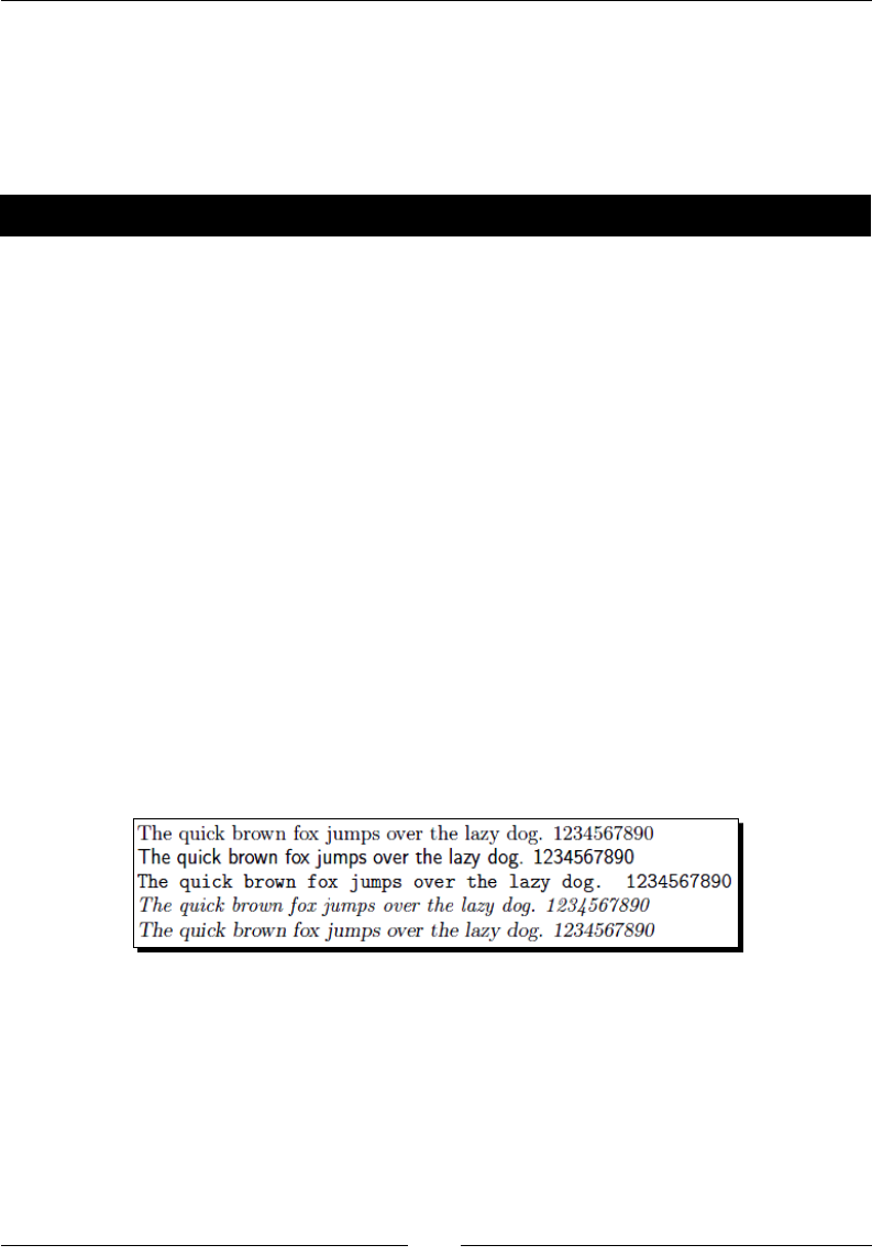
Chapter 9
[ 217 ]
Choosing the main font
We shall explore some TeX fonts. To test fonts, we may use a pangram. This word has a
Greek origin: "pan gramma" meaning "every leer". It stands for a sentence that uses every
leer of the alphabet. Thus, a pangram is very convenient for displaying fonts.
Time for action – comparing Computer Modern to Latin Modern
We shall print out a very famous pangram phrase, once using the standard font Computer
Modern and once using the Lan Modern font. Because Lan Modern is very similar to
the standard font, but supports diacrics much beer, while providing very high quality,
it is widely considered that it will become the successor to the standard font. We will just
compare serif and sans-serif typefaces:
1. Start a new document. Create a macro for the pangram plus numerals and use it:
\documentclass{article}
\newcommand{\pangram}[1][\rmfamily]{{#1 The quick brown fox jumps
over the lazy dog. 1234567890}\par}
\usepackage[T1]{fontenc}
\begin{document}
\large
\pangram
\pangram[\sffamily]
\pangram[\ttfamily]
\pangram[\itshape]
\pangram[\slshape]
\end{document}
2. Typeset and look at the font shapes:
3. Add this line to the preamble:
\usepackage{lmodern}
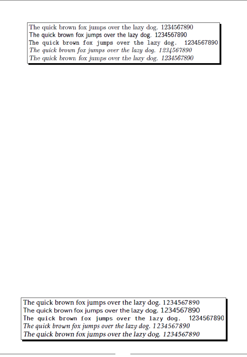
Using Fonts
[ 218 ]
4. Typeset again and compare:
What just happened?
You might noce that the fonts are indeed looking the same. So, why use lmodern?
Let's see.
Loading font packages
There are packages which provide fonts for all standards, shapes and weights, and more.
Just load one to change all at once.
Latin Modern – a replacement for the standard font
Lan Modern has been designed to look like Computer Modern, but the encoding and
manual ne-tuning has been improved. Lan Modern contains a huge amount of diacric
characters, whereas with Computer Modern such characters are built from leers and
accents.
If you use lmodern, you don't need to install the big cm-super package anymore.
Kp-fonts – a full set of fonts
This font collecon from the Johannes Kepler project provides Roman, sans-serif, and
monospaced fonts as well as mathemacs symbol fonts in dierent shapes and weights.
Even bold extended and combinaons like slanted Roman small caps are present.
Just load the package to use those fonts:
\usepackage{kpfonts}
The previous example will change to:
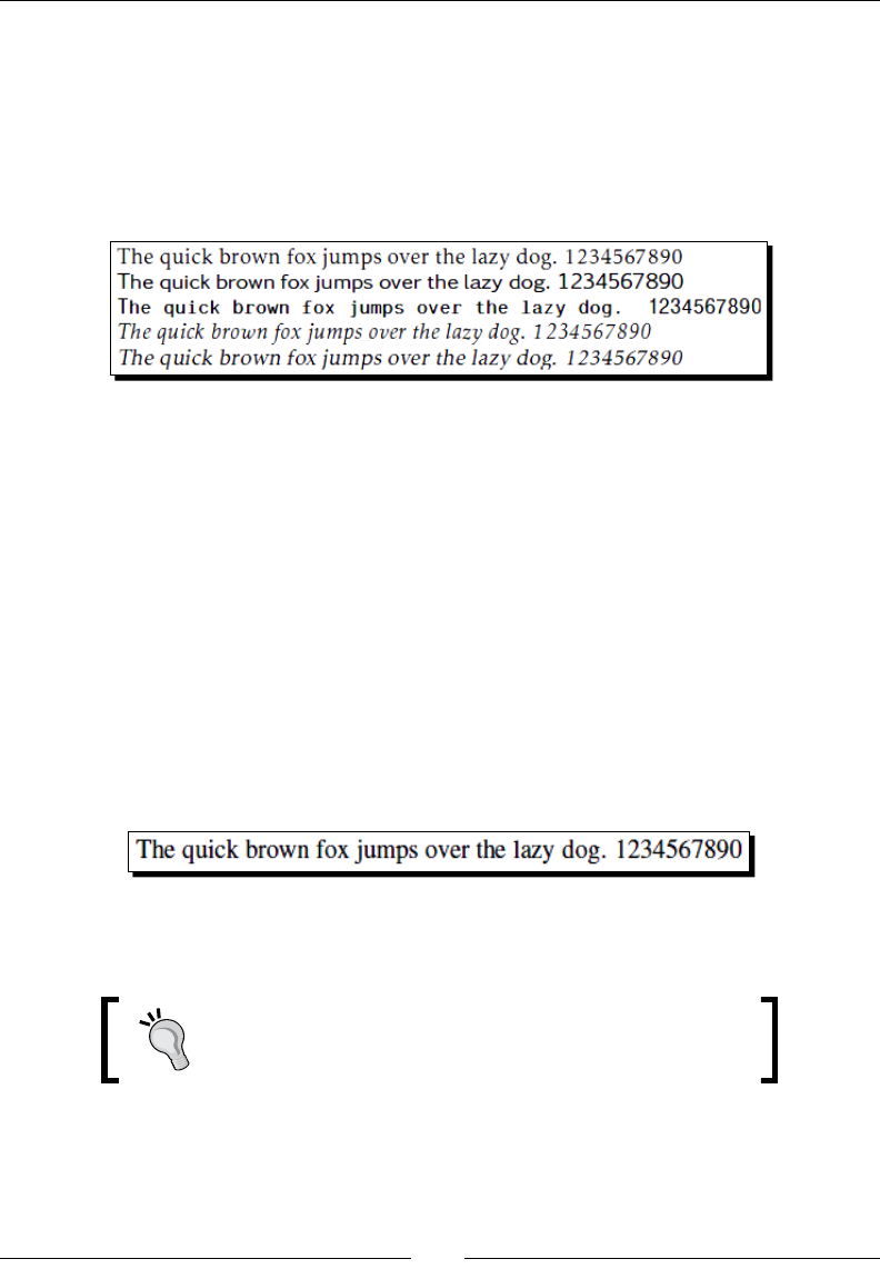
Chapter 9
[ 219 ]
Kp-fonts oers light versions with the same font metrics. They might look nice in print, but
they aren't recommended for reading on screen.
To switch to the light font set, load the package with the opon light:
\usepackage[light]{kpfonts}
The look will be dierent:
Now let's look at specialized font packages.
Serif fonts
The standard serif font is called Computer Modern Roman. Lan Modern provides a very
similar font, and you already know the Kp-fonts serif font. Further packages are specialized
in serif fonts.
Times Roman
The package mathptmx denes a Times Roman text font. Addionally, it provides math
support using suitable symbols of the standard Computer Modern symbol font together
with Times Roman leers and more glyphs of further fonts. It supersedes the mes package.
\usepackage{mathptmx}
As you can see, Times is a very narrow font that's suitable for mul-column text like in
newspapers, but not recommended for single-column text. Wide lines would be less readable.
The txfonts package is a good alternave, especially if you
use Greek characters.
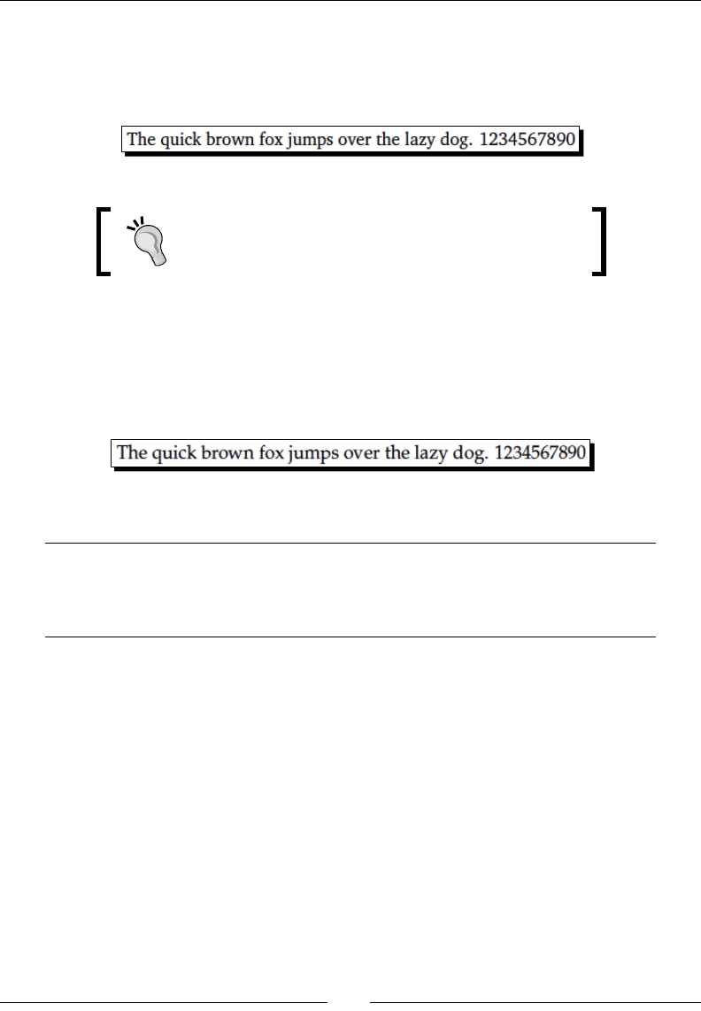
Using Fonts
[ 220 ]
Charter
Charter is similar to Computer Modern, but a bit bolder:
\usepackage{charter}
For suitable math support, it's recommended to load
the mathdesign package with the charter opon:
\usepackage[charter]{mathdesign}.
Palatino
The package mathpazo provides the Pazo math fonts, which are suitable for the Palano
text font. It may be loaded by:
\usepackage{mathpazo}
Two opons are recommended for mathpazo:
sc "small caps" Loads Palano with "real" small caps instead of
producing fake small caps by scaling capital leers.
osf "old style gures" Load Palano with old style gures which would be
used in text mode, not in math mode
Call texdoc psnfss2e to learn more. This opens the document Using common PostScript
fonts with LaTeX by Walter Schmidt. Among others, it describes how to use mathpazo and
mathptmx.
For Palano, a slightly higher line spacing is recommended. So, a typical way to load Palano
together with Pazo is:
\usepackage[sc]{mathpazo}
\linespread{1.05}
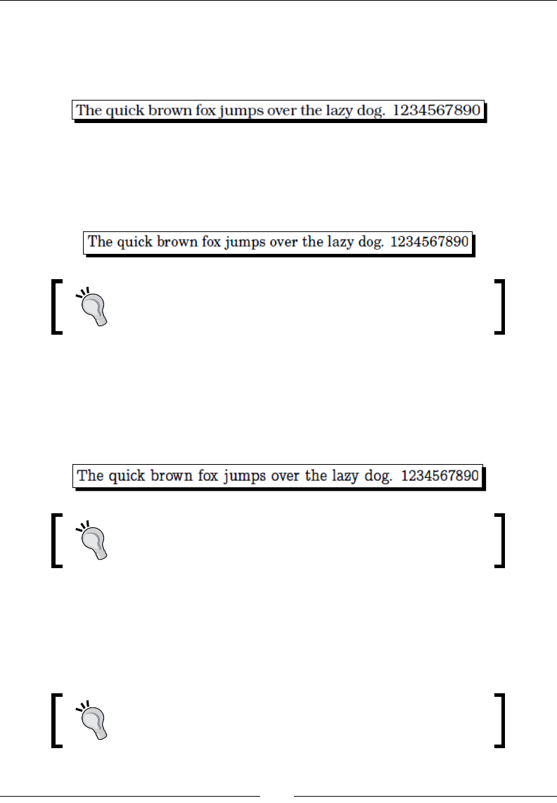
Chapter 9
[ 221 ]
Bookman
This is an old style serif font, provided by the bookman package:
\usepackage{bookman}
New Century Schoolbook
The newcent package provides this easy-to-read serif typeface:
\usepackage{newcent}
For a suitable math font, you might load the fourier math fonts:
\usepackage{fouriernc}.
Concrete Roman
The Concrete font doesn't look well on screen, but oers a high quality in print. Just load the
concrete package:
\usepackage{concrete}
Also for Concrete Roman, there's a matching math font package:
\usepackage{concmath}.
Sans-serif fonts
We already talked about sans-serif fonts: they might be appropriate for headings,
but many believe that running text with tradional serifs is much more readable.
If required, the main body font could be made sans-serif by \
renewcommand{\familydefault}{\sfdefault}.
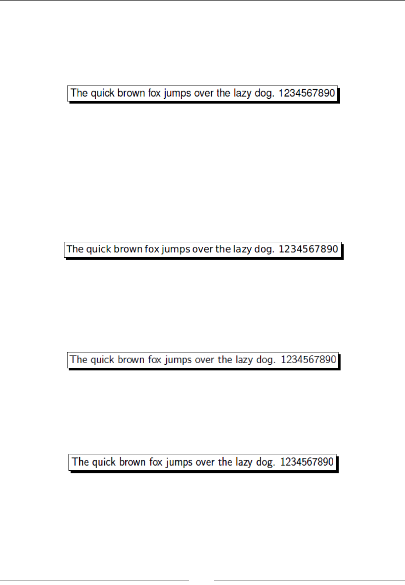
Using Fonts
[ 222 ]
Helvetica
The classical sans-serif font Helveca is simple and clean. You probably know a
descendant: Arial.
\usepackage{helvet}
Use the opon scaled if the font looks too big, especially when used together with a serif
font. For instance, if you also use times or mathptmx, you might write:
\usepackage[scaled=0.92]{helvet}
Bera Sans
Another nice sans-serif font is oered by berasans. It has been derived from Fruger.
\usepackage{berasans}
Computer Modern Bright
CM Bright has been derived from Computer Modern Sans Serif. The package cmbright
provides this font together with a lighter typewriter font and a sans-serif math font.
\usepackage{cmbright}
Kurier
Kurier is a bit dierent; look at the leer g:
\usepackage{kurier}
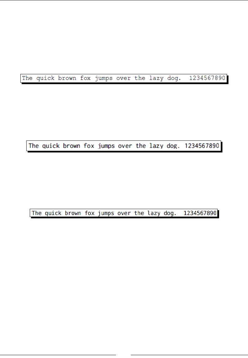
Chapter 9
[ 223 ]
Typewriter fonts
Typewriter, a.k.a. monospaced, fonts are widely used for source codes. We've seen it already.
Courier
Courier is a very wide running typewriter font, provided by the package with the same name.
\usepackage{courier}
Inconsolata
Inconsolata is a very nice monospaced font designed for source code lisngs. It's very
readable and not as wide as Courier.
\usepackage{inconsolata}
Bera Mono
Bera Mono is another font of the Bera family, consisng of Bera Serif, Bera Sans, and Bera
Mono. Originally, they had been developed under the name Bitstream Vera.
\usepackage{beramono}
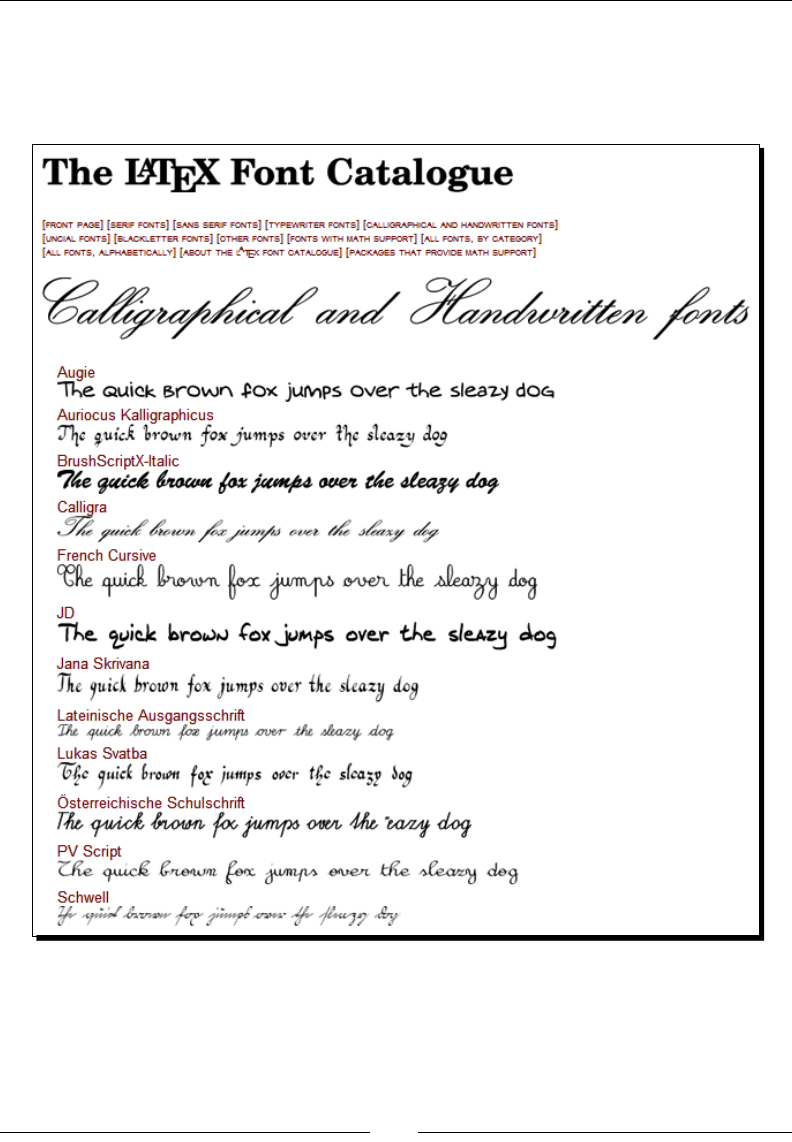
Using Fonts
[ 224 ]
Exploring the world of LaTeX fonts
Probably the best place to browse LaTeX fonts is The LaTeX Font Catalogue.
Visit http://www.tug.dk/FontCatalogue/:
Just choose a category, click on a font to see some examples, usage, and sources.

Chapter 9
[ 225 ]
Pop quiz
1. Which package allows us to type ä, ü, ü, ß, and other such characters directly
in the editor?
a. babel
b. inputenc
c. fontenc
2. All but one of the following packages improves full juscaon. Which one
does not?
a. babel
b. microtype
c. inputenc
d. fontenc
Summary
Now we are able to use dierent body text fonts. Our documents doesn't need to look like
standard LaTeX wrings anymore.
We learned about:
Specifying the encoding for source and output
Installing and choosing font sets and specic fonts
You probably know Truetype fonts: though they generally oer lower quality, there's a lot,
and they may be used with XeTeX, XeLaTeX, LuaTeX, and LuaLaTeX. These compilers even
support the OpenType font standard. All these compilers are supported by TeX Live and
TeXworks as well which are enhanced versions of TeX, LaTeX respecvely.
Now let's go back to LaTeX; we shall learn how to develop and manage bigger documents in
the next chapter.
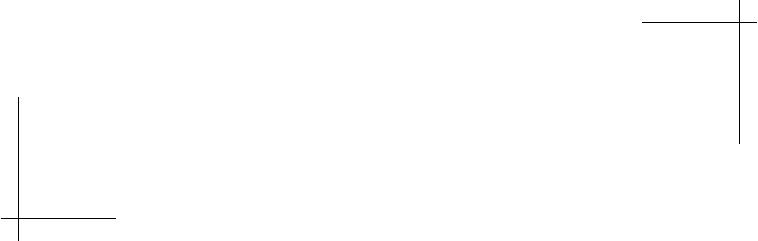
10
Developing Large Documents
The rst chapter of this book claimed that LaTeX handles large documents
easily. When you create extensive documents, you will noce that LaTeX keeps
on doing its job reliably. For the computer, it doesn't maer how the source
code is formaed. But for you, as the developer, it's important to keep your
source document manageable. Aer all, it may consist of hundreds of pages
with thousands of lines, possibly containing a lot of external pictures.
In this chapter, we shall learn how to:
Split a document into several les
Input and reuse pieces of code
Swap out document-wide sengs
Compile just a part of a document
Create a main document built upon sub-les
A bigger document requires a more complex structure, so we shall gure out how to:
Design a tle page
Use Roman page numbers in the front maer
Add a back maer without seconing numbers
We will work it out while developing a book, using separate les for the preamble and for
each chapter.

Developing Large Documents
[ 228 ]
Bigger documents require more work, so we shall nd out how to:
Work more eecve using templates
Acquire and evaluate templates
That's a big step forward on the way to wring a thesis, a book, or an extensive report.
Let's go on with it.
Splitting the input
Divide and conquer—this could be our moo now. We shall gure out how to break down
a document into several sub-documents. Thus, while we are wring, we will be able to
manage a huge project consisng of many chapters in separate les.
Firstly, we shall separate sengs and body text by swapping out the preamble. Secondly,
we shall write chapters in separate les and include them aerwards.
Time for action – swapping out preamble and chapter contents
We begin to write an extensive document about equaons and equaon systems.
The result should be in the style of a thesis or a book. We can use the last example in
Chapter 8, TypingMath Formulas, where we dealt with theorems concerning equaons.
1. Create a new document. Inside this, load all the packages and specify the opons,
like we did in our preambles before. Use all the benecial packages that we already
learned about:
\usepackage[english]{babel}
\usepackage[utf8]{inputenc}
\usepackage[T1]{fontenc}
\usepackage{lmodern}
\usepackage{microtype}
\usepackage{natbib}
\usepackage{tocbibind}
\usepackage{amsmath}
\usepackage{amsthm}
\newtheorem{thm}{Theorem}[chapter]
\newtheorem{lem}[thm]{Lemma}
\theoremstyle{definition}
\newtheorem{dfn}[thm]{Definition}
2. Save this document under the name preamble.tex.

Chapter 10
[ 229 ]
3. Start another new document and copy the contents of the chapter Equations in
the theorem example of Chapter 8 into it:
\chapter{Equations}
\section{Quadratic equations}
\begin{dfn}
A quadratic equation is an equation of the form
\begin{equation}
\label{quad}
ax^2 + bx + c = 0
\end{equation}
where \( a, b \) and \( c \) are constants and \( a \neq 0 \).
\end{dfn}
4. Save this document under the name chapter1.tex.
5. Create another document for the next chapter, write something, and save it as
chapter2.tex:
\chapter{Equation Systems}
\section{Linear Systems}
…
\section{Non-linear Systems}
…
6. Now we shall construct the top-level document. Create another le called
equations.tex. This one starts with the documentclass and lists the
preamble and the chapters for inclusion:
\documentclass{book}
\input{preamble}
\begin{document}
\tableofcontents
\include{chapter1}
\include{chapter2}
\end{document}
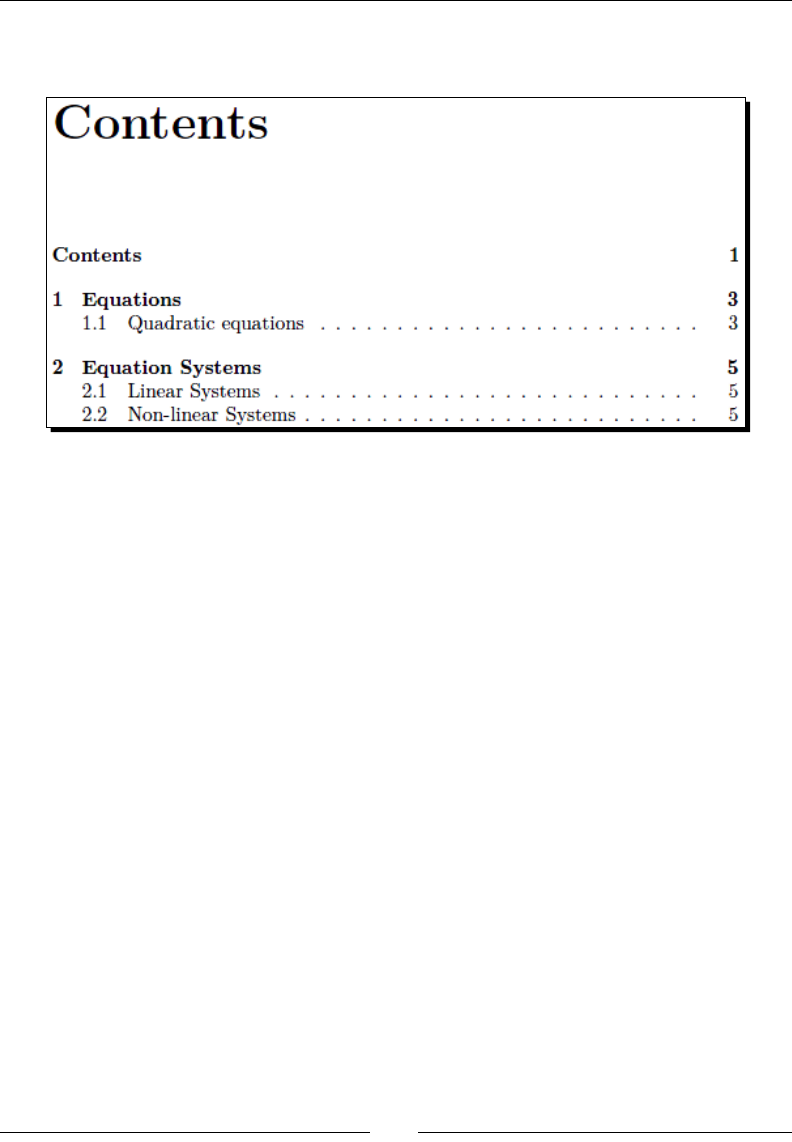
Developing Large Documents
[ 230 ]
7. Typeset the document twice. Remember, this acon is necessary to get the table
of contents. For now, check the contents, to see if everything is in its place:
What just happened?
We constructed a top-level document that we called equations.tex. It's tempng to just
call it main.tex or something similar. However, as this lename determines the name of the
resulng PDF document, we chose a meaningful name.
This is the framework of our project. It's an ordinary LaTeX document, but we reduced it as
much as possible and used two commands to import external .tex les:
\input reads in another le, just as if it had been typed in.
\include also reads in an external le, but automacally inserts \clearpage
before and aer.
The laer oers more to you, so let's have a closer look—we shall treat the simpler
command rst.
Including small pieces of code
The simplest command to read in a le is:
\input{filename}
When LaTeX encounters this command, it reads in the le with the name filename exactly
as if its contents have been typed at that point. Accordingly, all commands in this le would
be processed by the LaTeX compiler. You can even nest \input—this command may be used
inside an included le.

Chapter 10
[ 231 ]
If the lename doesn't have an extension, the extension .tex will be added automacally,
thus filename.tex would be inserted. You may also specify a path, relave or absolute. As a
backslash begins a command, use slashes / instead of backslashes \ in paths, also in Windows.
Using relave path names makes moving and copying of a
project easier.
Use \input if you wish to put your preamble into a separate le. Besides keeping your root
document clean, a separate preamble can easily be copied and adjusted for use in another
document.
However, simply spling and inpung is not yet considered document management. For
instance, though you could comment out selected \input lines for paral compilaon, the
numbering of pages, secons, and so on may be ruined, and cross-referencing to omied
document parts would fail.
There's a beer way—so let's look at the other command.
Including bigger parts of a document
When it comes to including one or more pages, this command proves to be useful:
\include{filename}
The argument is treated the same way as \input. However, there are some important
dierences:
1. \include implicitly starts new pages.\include{filename} behaves like:
\clearpage
\include{filename}
\clearpage
2. This makes it useful for page ranges such as chapters or secons. One consequence
is that you may use \include only aer \begin{document}.
3. \include cannot be nested. You could sll use \input within included
documents, though it might not be a good idea to complicate the structure further.
4. Most importantly, \include supports a mechanism of choosing which parts of
the document you wish to compile—so we come to another command, namely,
\includeonly.
Let's see how the laer command works.

Developing Large Documents
[ 232 ]
Compiling parts of a document
Such a paral document, which is intended for \input or \include, cannot be compiled
standalone: you need a root document that species the document class.
However, once you swapped out parts of the document using \include, while compiling
your root document, you may specify which parts are actually included by this command:
\includeonly{file list}
The argument may be a comma-separated list of lenames. If a le, name.tex, is not
specied within this argument, \include{name} would not insert this le but just behave
like \clearpage instead. This allows excluding chunks or whole chapters from compiling. If
you work on a huge document, this speeds up compilaon if you choose to include just your
current chapter while keeping the labels and references of the excluded chapter this way.
You may noce that LaTeX produces an .aux le for each included .tex le. LaTeX sll
reads in all those .aux les containing informaon such as chapter and page numbers. Of
course, the included les need to be Typeset at least once. This way, cross-referencing the
numbering of pages, chapters, secons, and so on will remain intact even if you temporarily
exclude the chapters.
Try it out—add the following:
\includeonly{chapter2}
Add it to your preamble in equation.tex and compile. The result will be just the second
chapter keeping the correct numbering.
You can use \include without \includeonly. Finally, when you nish your work, just
comment the laer command out to typeset your complete document.
Creating front and back matter
In contrast to reports, books oen begin with introductory material such as copyright
informaon, a foreword, acknowledgements, or a dedicaon. This part, including the tle
page and the table of contents, is called the front maer.
At the end, a book might include an aerword and supporng material like a bibliography,
and an index. This part is called the back maer.
The book class and some other classes like scrbook and memoir support this kind of
seconing directly. Oen, desired consequences of this seconing are dierences in the
numbering of pages and chapters. Let's see how it works.

Chapter 10
[ 233 ]
Time for action – adding a dedication and an appendix
Our book shall begin with a dedicaon. The front maer shall consist of the table of
contents, lists of tables and gures, and a dedicaon. All the pages of the front maer shall
be numbered with Roman leers. Finally, we add an appendix providing supplementary
proofs which we like to present outside the main chapters:
1. Create a le dedication.tex:
\chapter{Dedication}
This book is dedicated to one of the greatest mathematicians of
all time: Carl Friedrich Gauss. Without him, this book wouldn't
have been possible.
2. Create a le proofs.tex:
\chapter{Proofs}
...
3. Extend the main le equation.tex by the highlighted lines:
\documentclass{book}
\input{preamble}
\begin{document}
\frontmatter
\include{dedication}
\tableofcontents
\listoftables
\listoffigures
\mainmatter
\include{chapter1}
\include{chapter2}
\backmatter
\include{proofs}
\nocite{*}
\bibliographystyle{plainnat}
\bibliography{tex}
\end{document}
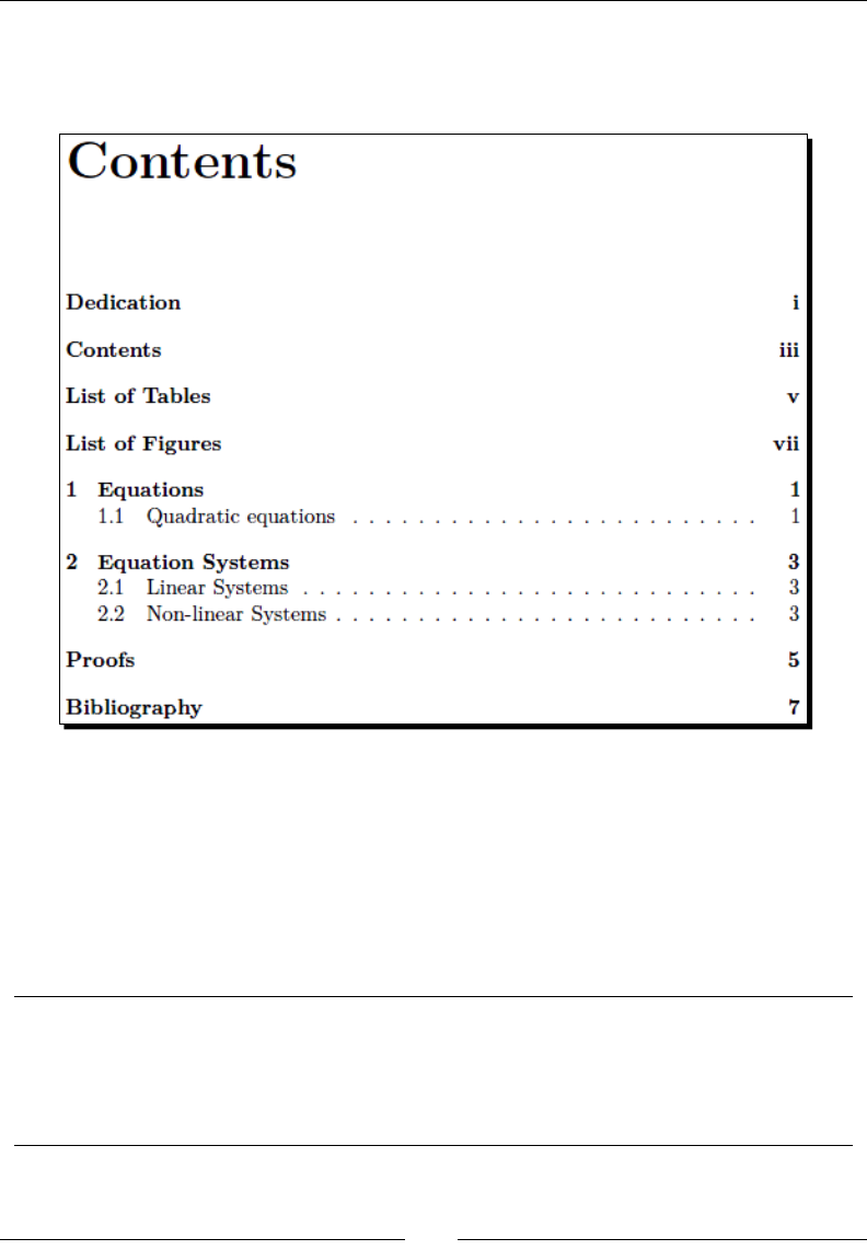
Developing Large Documents
[ 234 ]
4. As you can see in the last highlighted line, we re-used the le tex.bib from
Chapter 7, Lisng Contents and References. Typeset, run BibTeX, and Typeset
again. Check out the numbering within the table of contents:
What just happened?
We saw that the page number of the contents page has been typeset in Roman numbers.
This applies to all front maer pages. Further, all the chapters in front and back maer are
unnumbered even though we did not use the starred command \chapter*.
The three commands \frontmatter, \mainmatter, and \backmatter are responsible.
They modied both the page and chapter numbering in the following way:
\frontmatter Pages are numbered with lowercase Roman numbers.
Chapters generate a table of contents entry but don't get a number.
\mainmatter Pages are numbered with Arabic numbers.
Chapters are numbered and produce a table of contents entry.

Chapter 10
[ 235 ]
\backmatter Pages are numbered with Arabic numbers.
Chapters generate a table of contents entry but don't get a number.
Besides that, \frontmatter and \mainmatter call \cleardoublepage. \backmatter
calls \cleardoublepage in openright mode, that is, if chapters start on right hand pages,
otherwise it's using just \clearpage.
Like the book class, the classes scrbook and memoir provide the same command with very
similar behavior.
Designing a title page
A good looking tle page can quickly be created using \maketitle as we did in Chapter 2,
Formang Words, Lines, and Paragraphs. Document classes usually oer this command
to generate a suitable pre-formaed tle page. Alternavely, you could use a titlepage
environment to freely design its layout. So, let's design a nice tle page for our book of
equaons.
Time for action – creating a title page
In Chapter 2, we have already used some formang commands such as \centering and
font size and shape commands such as \Huge and \bfseries to format a tle. We shall do
it similarly within a titlepage environment:
1. Create a le title.tex with the following content:
\begin{titlepage}
\raggedleft
{\Large The Author\\[1in]}
{\large The Big Book of\\}
{\Huge\scshape Equations\\[.2in]}
{\large Packed with hundreds of examples and solutions\\}
\vfill
{\itshape 2011, Publishing company}
\end{titlepage}
2. Our nal book shall have A5 format, and so shall the tle page. Therefore, let's add
that to the preamble:
\usepackage[a5paper]{geometry}
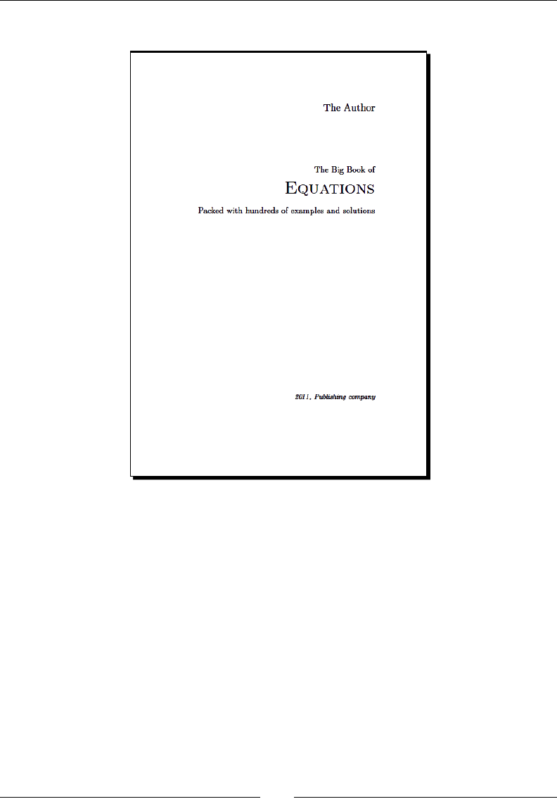
Developing Large Documents
[ 236 ]
3. Typeset. Now we've got a tle page:
What just happened?
The titlepage environment typesets its contents on a separate page. Though this tle
page will be numbered like any other page, the page number won't be printed on that page.
Within this environment, we used some basic LaTeX font commands to modify the font
size and shape. By grouping with curly braces, we limited those commands. Line breaks like
\\[.2in] just cause some more space before the following line. \vfill inserts an elasc
vercal space which stretches as much as possible such that the page is lled. This way we
put the last line o to the end of the page.
Note, this page has the same page dimensions as the other pages in the document. That
means, in a double-sided book it's a right-hand page. Thus, you may noce unequal le and
right margins, which might look undesirable especially, if your tle is in the center. But the
explanaon is simple: this tle page is intended to be an inner tle, not the cover page. The
inner tle page is of course a right-hand page.

Chapter 10
[ 237 ]
A cover page is a dierent thing. This should be one-side and thus it should have equal le
and right margins. A cover page is oen produced as a stand-alone document, printed out
separately. For a electronic document, you may use the pdfpages package or a tool like
pdam to merge PDF documents.
The tling package oers features to create sophiscated tle pages. To
get some ideas how tle pages may be designed, you could have a look at
Some Examples of Title Pages by Peter Wilson, available from texdoc
titlepages and at http://ctan.org/pkg/titlepages.
Working with templates
When we start to develop a document, we specify the document class, choose meaningful
packages and opons, and create a frame for the contents. To repeat these steps for each
document would be too laborious.
If we plan to write several documents of the same type, we may create a template.
This could be a .tex le containing:
Declaraon of a suitable document class together with a set of meaningful opons
Rounely-used packages and packages which are most eligible for our document
type
A predened layout for header, footer, and body of the text
Self-made macros to ease our work
A framework of seconing commands, where we ll in the headings and the
body text
Or a framework containing \include or \input commands, for which we create
the body text chunks later on.
While we improve our LaTeX knowledge, such templates might grow and become beer
and more sophiscated. Many users publish their elaborate templates on the Internet.
Many universies, instutes, journals, and publishers do the same, oering templates for
documents such as thesis, papers, journal arcles, and books, meeng their requirements.
You will nd a collecon of templates, arranged by document type such as thesis,
reports, leers, and presentaons, accompanied by sample output, in a template
gallery at http://texblog.net/latex/templates.
You may download a template and start to ll in your text. Alternavely, you could start a
document with a pre-dened template oered by your editor. Let's try that.
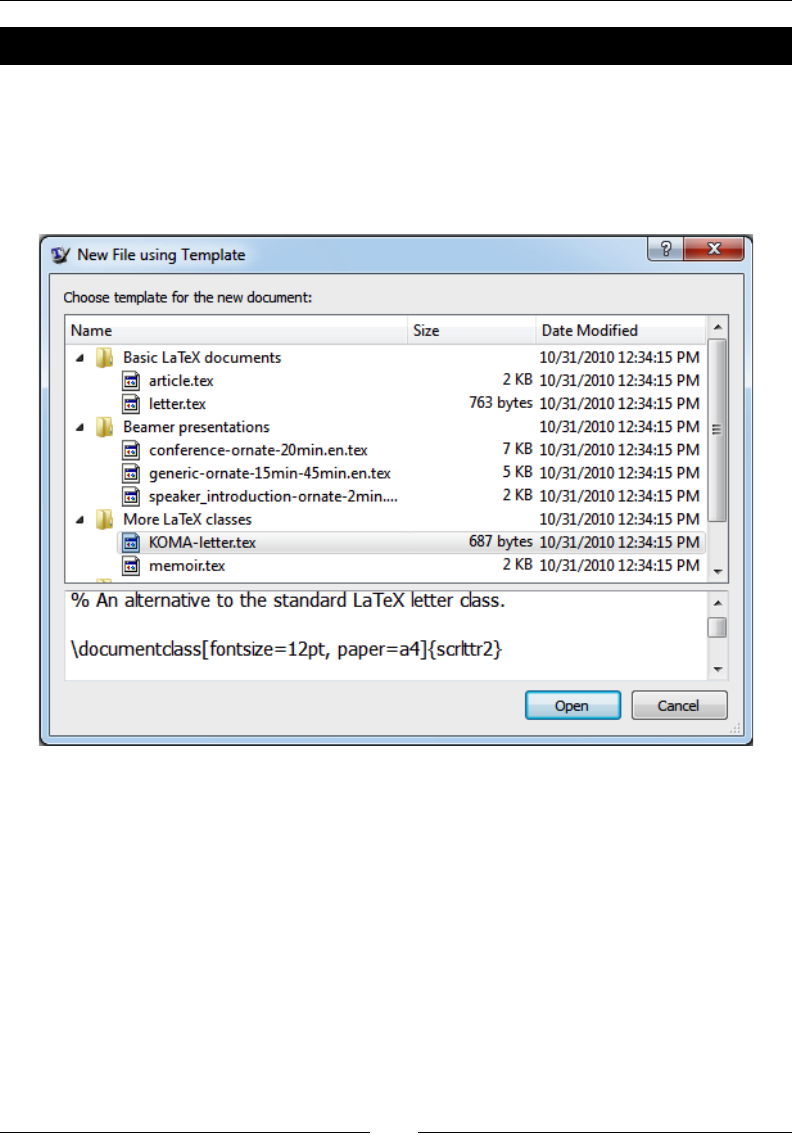
Developing Large Documents
[ 238 ]
Time for action – starting with a template
LaTeX editors oen provide templates to start with. TeXworks oers some as well. So we
shall test this feature, let's take one, open it, modify it, and Typeset:
1. In the TeXworks main menu, click on File and then on New from template. A
window will open allowing you to choose a template:
2. In the lower part of the window, you can read the template's source. Here's an
example of KOMA-Script (KOMA-letter.tex):
% !TEX TS-program = pdflatex
% !TEX encoding = UTF-8 Unicode
% An alternative to the standard LaTeX letter class.
\documentclass[fontsize=12pt, paper=a4]{scrlttr2}
% Don't forget to read the KOMA-Script documentation, scrguien.pdf
\usepackage[utf8]{inputenc}
\setkomavar{fromname}{} % your name
\setkomavar{fromaddress}{Address \\ of \\ Sender}
\setkomavar{signature}{} % printed after the \closing

Chapter 10
[ 239 ]
\renewcommand{\raggedsignature}{\raggedright} % make the signature
ragged right
\setkomavar{subject}{} % subject of the letter
\begin{document}
\begin{letter}{Name and \\ Address \\ of \\ Recipient}
\opening{} % eg. Hello
\closing{} %eg. Regards
\end{letter}
\end{document}
3. Click on Open. Fill in the gaps and edit the ller text of the example:
\documentclass[fontsize=12pt, paper=a4]{scrlttr2}
\usepackage[utf8]{inputenc}
\setkomavar{fromname}{My name} % your name
\setkomavar{fromaddress}{Street, City}
\setkomavar{signature}{Name} % printed after the \closing
\setkomavar{subject}{Invoice 1/2011} % subject of the letter
\setkomavar{place}{Place}
\setkomavar{date}{January 1, 2011 }
\begin{document}
\begin{letter}{Customer Name\\ Street No. X \\ City \\ Zipcode}
\opening{To whom it may concern} % eg. Hello
Text follows \ldots
\bigskip
\closing{With kind regards} %eg. Regards
\end{letter}
\end{document}
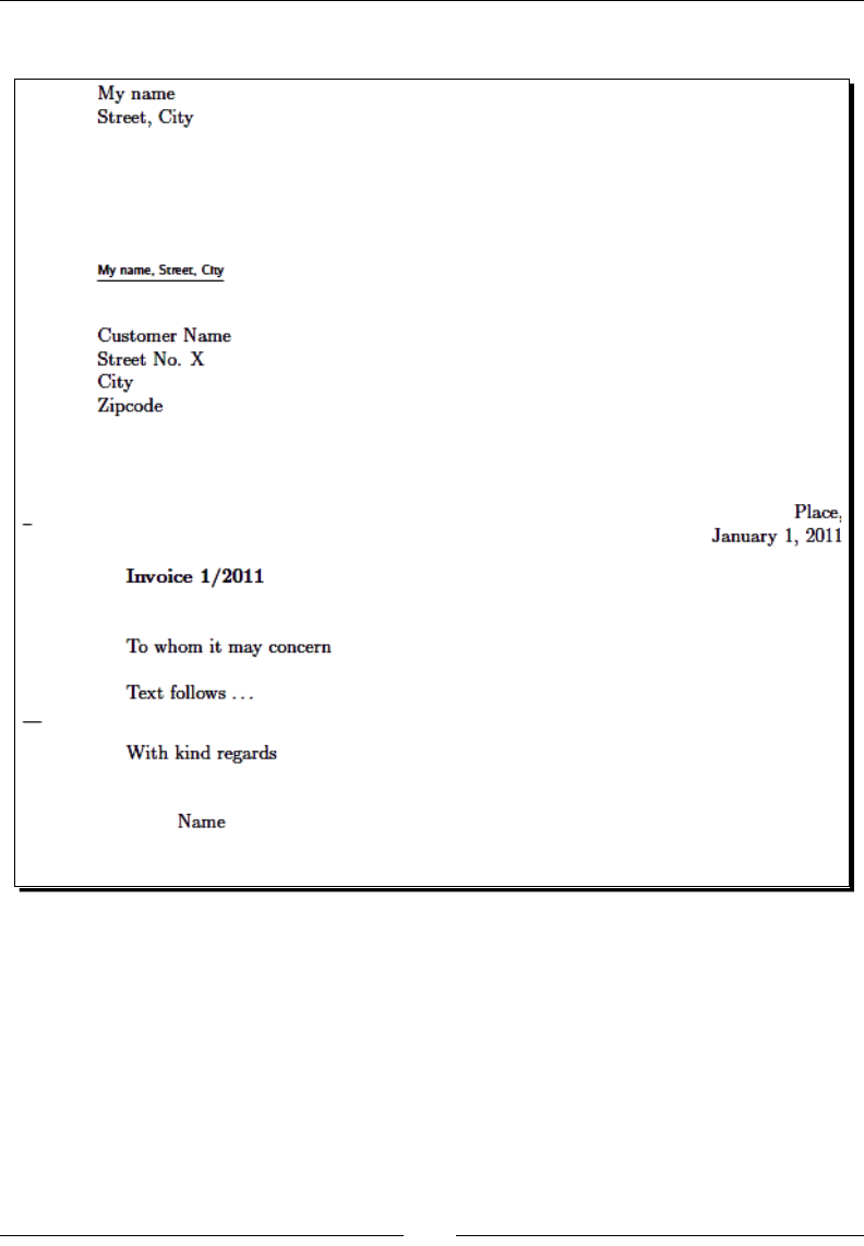
Developing Large Documents
[ 240 ]
4. Typeset. Have a look at our test leer:
What just happened?
That was easy! We just opened the template and modied the ller texts. Reading the
KOMA-Script documentaon, we can learn that the command \setkomavar is used for
specifying values for template parameters such as name, address, and subject. We used
that to declare the date and the place as well.
Once we have wrien our personal data into this template, we may save that for later use
instead of typing our address for each leer.

Chapter 10
[ 241 ]
The KOMA-Script documentaon (texdoc scrguien) describes the features of this leer
class well. Using this, you would be able to create your personal professional-looking leer
template for business use.
Imagine pung a job applicaon leer created with the LaTeX layout and fonts together
with microtype next to an applicaon leer produced with some other word processing
soware—which one will use to create a beer impression!
Have a go hero – evaluating and enhancing templates
While looking for LaTeX templates, code, and ps on the internet, you will nd a lot of
informaon and code. This code might be outdated and this informaon might be obsolete.
When you develop your own template, you probably would like to be sure to use the best
packages, opons, and soluons available today. How can you be sure?
Both quesons can be answered by studying l2tabu. This is the common shortcut for
An essenal guide to LaTeX2e usage, a document focusing on obsolete commands and
packages, which also demonstrates the most common and severe mistakes that LaTeX user's
tend to make. As LaTeX has developed over many years, some packages and techniques are
sll available and described in online resources, but it may not be recommendable any more.
Read this guide. It will help you to evaluate templates and code found on the Internet, but
also to ensure that you produce opmal code yourself.
Just type:
texdoc l2tabuen
At the command prompt or visit http://ctan.org/pkg/l2tabu.
To test a template, you may use the blindtext package and its command
\Blinddocument. This command generates dummy content for a big
document, which would demonstrate the output quality of a template. This
package is required to load babel. If you don't like that, you may use the
lipsum package instead.

Developing Large Documents
[ 242 ]
Pop quiz
1. Which of these commands can be used both in the preamble and body text?
a. \input
b. \include
c. \includeonly
2. All but one of the following commands may cause a page break. Which is the one
that doesn't?
a. \include
b. \input
c. \mainmatter
d. \begin{titlepage}
Summary
The techniques we learned in this chapter will help us to develop and maintain bigger
projects. Though enthusiasc users prefer LaTeX also to write small documents, many people
learn LaTeX because they plan to write longer texts. However, spling documents and the
use of templates are useful as well for small wrings such as leers—just think of header,
footer, address elds, and so on.
In this chapter, we dealt with:
Creang and managing large documents consisng of several les
Structuring documents with front maer and back maer
Designing a separate tle page
Using, creang, and evaluang templates
Now that we're able to develop and handle large documents, we shall see how to improve
them further.
11
Enhancing Your Documents Further
By now, you're capable of wring structured documents in ne typographical
quality. You are able to meet high expectaons for classic publicaons such as
books, journal arcles, or a university thesis.
What about presentaons? They are usually more colorful than prints. Perhaps
you would like to publish your documents online? Such electronic documents or
e-books usually require some kind of navigaon.
This chapter shall provide us with tools for such enhancements. We shall gure out
how to perform the following:
Adding hyperlinks to the table of contents, lists of gures and tables, and to any
cross-reference
Creang bookmarks for a navigaon bar
Designing headings
Using color with LaTeX
Let's implement this by using packages that are dedicated to these subjects.
Using hyperlinks and bookmarks
There's a sophiscated package called hyperref, which does nearly all basic hyper-linking
automacally. That's great! Let's check it out.
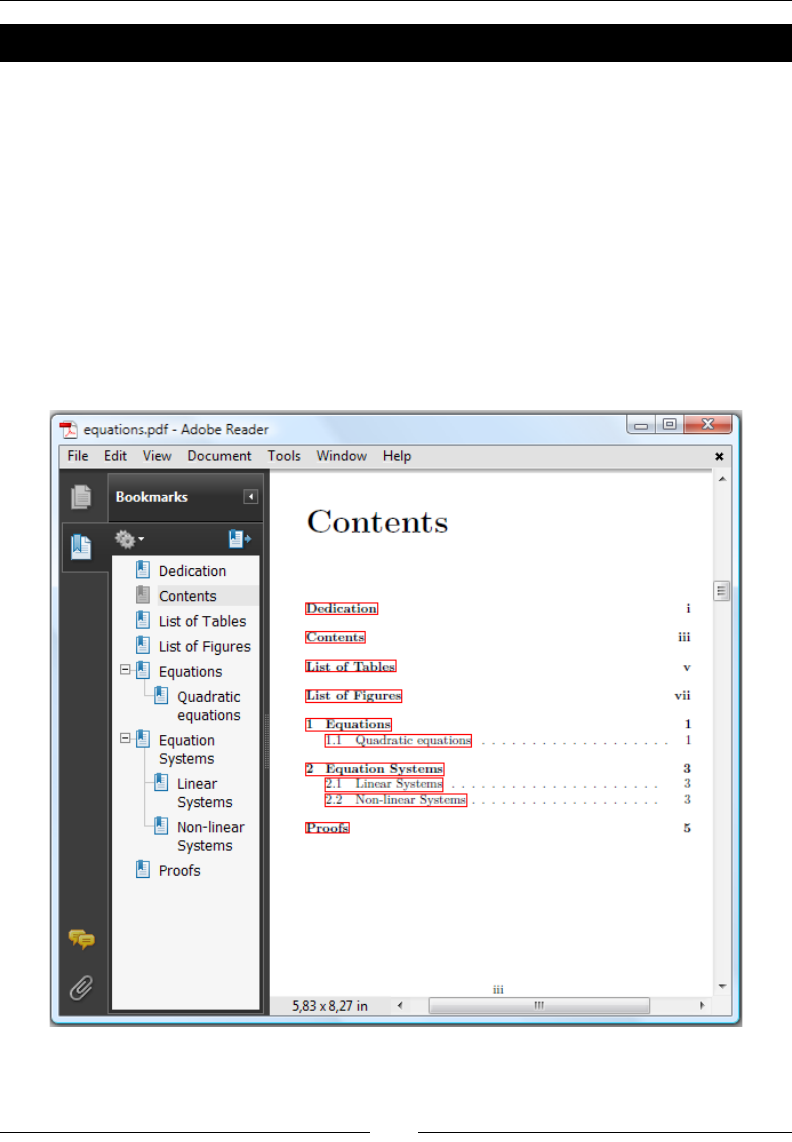
Enhancing Your Documents Further
[ 244 ]
Time for action – adding hyperlinks
We shall load the hyperref package and inspect its eect:
1. Open the le preamble.tex, which we used in the previous chapter. At its end,
add this line:
\usepackage{hyperref}
2. Save this document under the same name.
3. Open our book of equaons from the previous chapter; we called it equations.
tex.
4. Typeset the document twice without making any changes. Let's see how the
document now appears!
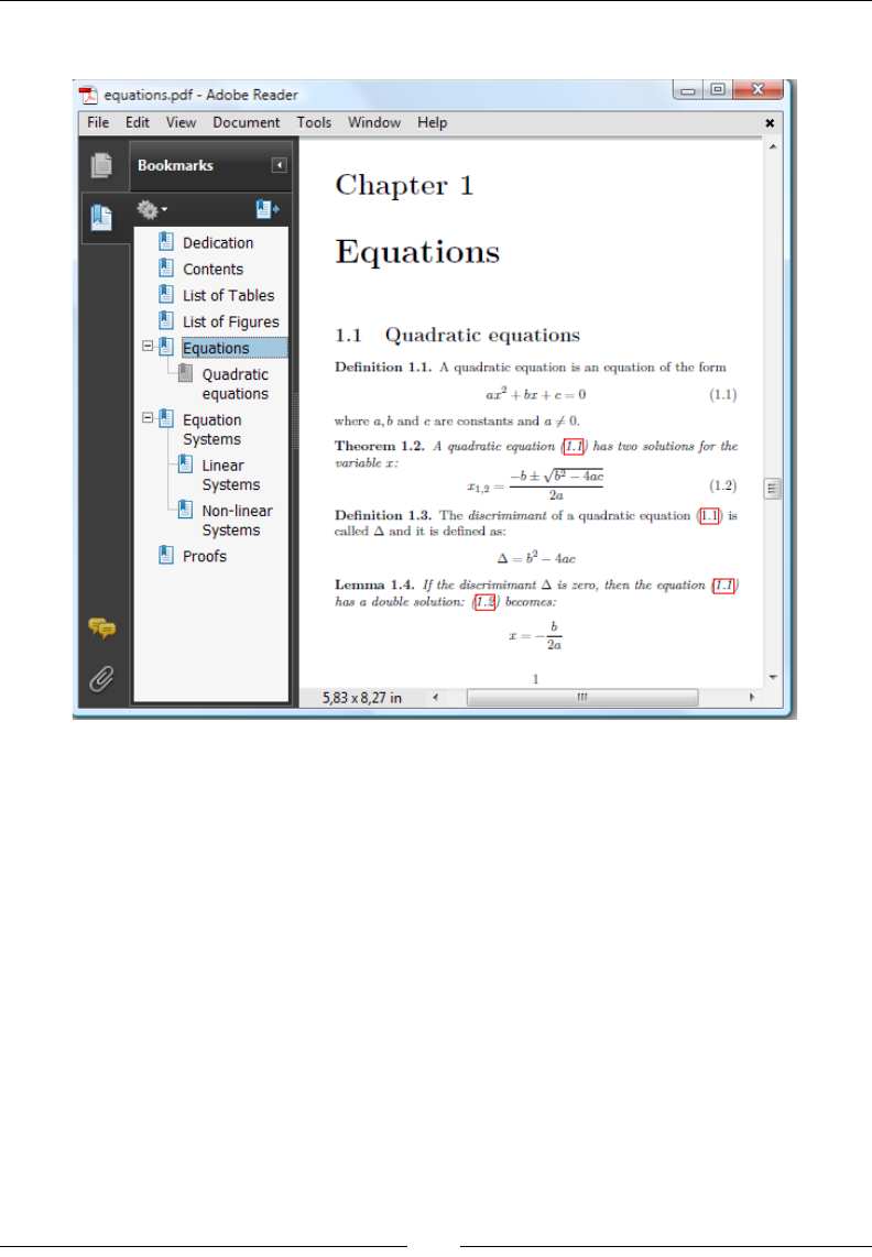
Chapter 11
[ 245 ]
5. The Chapter 1 looks like the following screenshot:
What just happened?
By just loading the hyperref package, our document has signicantly changed:
We got a bookmark bar, which allows us to easily navigate through the document.
Each entry in the table of contents has become a hyperlink to the beginning of the
corresponding chapter respecvely. Hyperlinks are marked by red frames.
All cross-references have become hyperlinks.
This is a great improvement for electronic versions of our documents! The print version
would not be aected—neither the bookmarks nor those red frames would be printed.
If you don't like the default look of the hyperlinks, it can easily be changed by eding the
opons to hyperref. Let's try this.
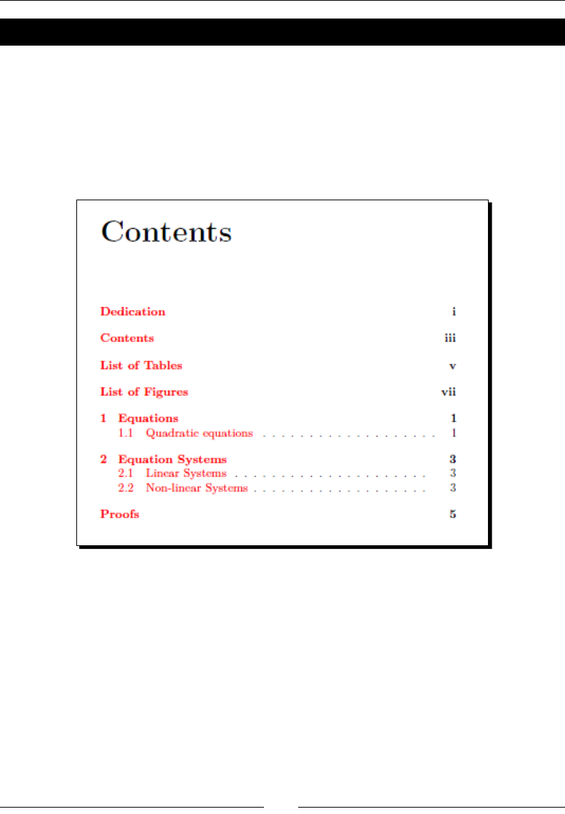
Enhancing Your Documents Further
[ 246 ]
Time for action – customizing the hyperlink appearance
We shall pass opons to hyperref aecng the way hyperlinks are emphasized:
1. Open the le preamble.tex again. This me, specify the opons for hyperref:
\usepackage[colorlinks=true,linkcolor=red]{hyperref}
2. Save this document, go to the main document equations.tex, and compile it
twice. The table of contents is changed:
What just happened?
Instead of frames, we now got a red color for emphasized links. The color can be seen
in a printed document.
hyperref oers ways to set up the opons. The rst one we used is:
\usepackage[key=value list]{hyperref}
Alternavely, we could just write \usepackage{hyperref} and set the opons
aerwards:
\hypersetup{key=value list}

Chapter 11
[ 247 ]
Our example would do the same with:
\hypersetup{colorlinks=true,linkcolor=red}
These methods may be combined. Here's a selecon of especially useful opons:
Opon Type Default Eect
draft boolean false Turns o all hypertext opons
final boolean true Turns all hypertext opons on
debug boolean false Prints extra diagnosc messages into the log
le
raiselinks boolean true Fits the height of links to the real size of
objects such as text or graphics
breaklinks boolean false Links may be broken across lines (true by
default with pdex)
pageanchor boolean true Gives pages implicit anchors, needed for the
index
backref boolean false Adds back links to bibliography items
hyperindex boolean true Links page numbers in the index, the
pageanchor opon should be set
hyperfootnotes boolean true Converts footnote markers into hyperlinks
linktocpage boolean false In TOC, LOF and LOT page numbers would be
linked instead of the text
colorlinks boolean false Writes links and anchors in color, depending
on the type of link such as page references,
URLs, le references, and citaons
linkcolor color red Color for internal links
anchorcolor color black Color for anchor texts
citecolor color green Color for citaons of bibliography items
filecolor color cyan Color for links to local les
urlcolor color magenta Color for URLs
frenchlinks boolean false Uses small caps for links instead of color
bookmarks boolean true Writes bookmarks for the Acrobat Reader
bookmarksopen boolean false Shows all bookmarks in an expanded view
bookmarksnumbered boolean false Includes the secon number in bookmarks
pdfstartpage text 1 Species which page would be shown when
the PDF le is opened

Enhancing Your Documents Further
[ 248 ]
There are many more opons for customizing link borders, PDF page size, anchors, bookmark
appearance, and PDF page display style. The hyperref documentaon lists them all. Have a
look at it—it's a really valuable document! Many PDF and hypertext-related quesons in web
forums just arise because users did not know that they have already got an extensive manual
on their own hard disk, namely, texdoc hyperref.
hyperref supports more than just pdfLaTeX, which most users choose today. If you, for
instance, use XeTeX, you may give the xetex opon to hyperref. If you typeset to DVI
and use dvips to convert to Postscript and to PDF aerwards, use the dvips opon. There
are more than a dozen of such driver opons; you can read about those backend drivers in
the manual. If no driver is specied, the hypertex driver would be used, which is, in most
mes, the appropriate driver.
Some text opons allow us to specify the metadata of PDF les, such as the author name,
tle, and keywords. This informaon is shown if you inspect the document properes with
the PDF reader. Even more benecial, Internet search engines are able to nd and classify
your PDF document according to this meta informaon. If you publish on the Internet, this
improves the chances of the readers nding your publicaon!
Time for action – editing PDF metadata
We shall add PDF metadata to our book of equaons. Besides choosing sensible keywords,
we will set the tle and the author's name. During development, why not choose the great
mathemacian to whom we dedicated our book. So, let's do it!
1. Open the le preamble.tex and add the following lines:
\hypersetup{pdfauthor={Carl Friedrich Gauss},
pdftitle={The Big Book of Equations},
pdfsubject={Solving Equations and Equation Systems},
pdfkeywords={equations,mathematics}}
2. Save that le. Go to the main document equations.tex and Typeset. Let's inspect
the document properes! So, if you use the Acrobat Reader, click on the File menu
and then Properes:
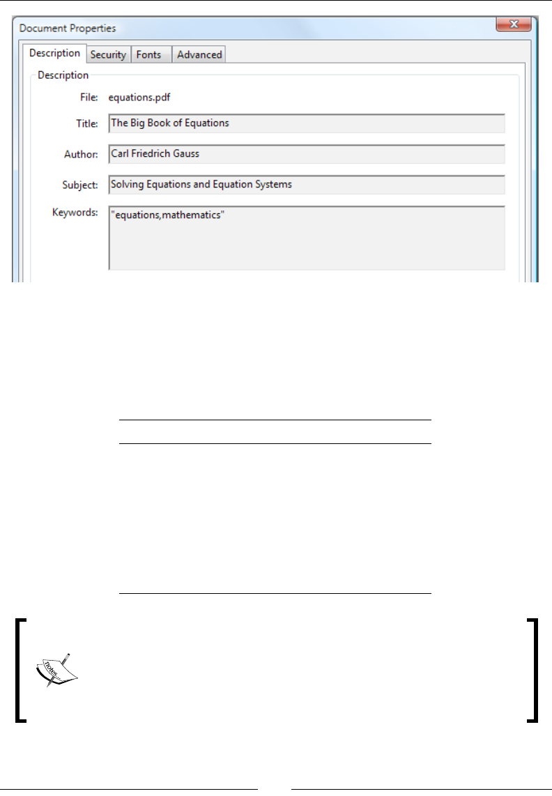
Chapter 11
[ 249 ]
What just happened?
Well, that was easy. We provided all document properes by using the hyperref opon.
We just had to take care to enclose each entry in curly braces.
The most commonly used meta-informaon opons are:
Opon PDF meta-informaon eld
pdftitle Sets the tle
pdfauthor Sets the author
pdfsubject Sets the subject
pdfcreator Sets the creator
pdfproducer Sets the producer
pdfkeywords Sets the keywords
As hyperref redenes many commands of other packages in order to
add hyperlink funconality, it has to be loaded aer those packages. A good
rule of thumb is to load the package as the last package in your preamble. A
few packages are excepons to that rule, namely, algorithm, amsrefs,
bookmark, chappg, cleveref, glossaries, hypernat, linguex,
sidecap, and tabularx are known to be excepons.

Enhancing Your Documents Further
[ 250 ]
Creating hyperlinks manually
As hyperref already creates links for nearly all kinds of references, it's rarely necessary to
create links by oneself. But of course, it's possible. hyperref provides user commands for
that:
\href{URL}{text} makes text to a hyperlink, which points to the URL address
\url{URL} prints the URL and links it
\nolinkurl{URL} prints the URL without linking it
\hyperref{label}{text} changes text to a hyperlink, which links to the place
where the label has been set, thus to the same place \ref{label} would point to
\hypertarget{name}{text} creates a target name for potenal hyperlinks with
text as the anchor
\hyperlink{name}{text} makes text to a hyperlink, which points to the target
name
Somemes you might need just an anchor, for instance, if you use \addcontentsline,
which creates a hyperlinked TOC entry, but there hasn't been a seconing command seng
the anchor. The TOC entry would point to the previously set anchor, thus to the wrong place!
The command \phantomsection comes to the rescue; it's just seng an anchor like
\hypertarget{}{} would do. It's mostly used this way for creang a TOC entry for the
bibliography while linking to the correct page as follows:
\cleardoublepage
\phantomsection
\addcontentsline{toc}{chapter}{\bibname}
\bibliography{name}
This ny command has been the answer to a lot of quesons on online forums. Well, not
everybody reads manuals.
Creating bookmarks manually
Your bookmark panel might already be full of chapter and secon entries. But what if you
wish to add bookmarks by yourself? That's been foreseen.
\pdfbookmark[level]{text}{name} creates a bookmark with text at the oponally
specied level. The default level is 0. Treat name just as\label; it should be unique
because it stands for the internal anchor.
Chapter 11
[ 251 ]
You can also create bookmarks relave to the current level:
\currentpdfbookmark{text}{name} puts a bookmark at the current level
\belowpdfbookmark{text}{name} creates a bookmark one level deeper
\subpdfbookmark{text}{name} increases the level and creates a bookmark at
that deeper level
The bookmarks package oers more features for customizing bookmarks.
Moreover, it requires just one compiler run in contrary to hyperref; thus its
use is recommended.
Math formulas and special symbols in bookmarks
Due to PDF restricons, math and special symbols cannot be used in PDF bookmarks. This
might cause a problem, for instance, in seconing commands with math symbols in their
tle or font commands which would be passed to the bookmark. There's a soluon though:
\texorpdfstring{string with TeX code}{text string}
It returns the argument depending on the context to avoid such problems. It can be used
like this:
\section{The equation \texorpdfstring{$y=x^2$}{y=x\texttwosuperior}}
That may come handy sooner than you might guess.
If you load hyperref with unicode opon, you could use Unicode characters
in bookmarks, such as in \section{\texorpdfstring{$\gamma$}{\
textgamma} radiation}.
Benetting from other packages
There's a huge amount of LaTeX packages. For nearly every possible task, somebody has
wrien a package either solving or supporng it. Nearly all packages are stored on CTAN.
But how can we nd what we need? Let's have a look at an online catalogue.
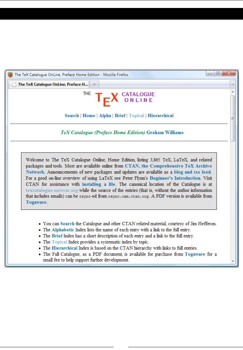
Enhancing Your Documents Further
[ 252 ]
Time for action – visiting the TeX Catalogue Online
We shall browse for PDF-related packages in the online catalogue to nd something that's
useful for us:
1. Open your favorite Internet browser and go to the address
http://texcatalogue.sarovar.org/ :
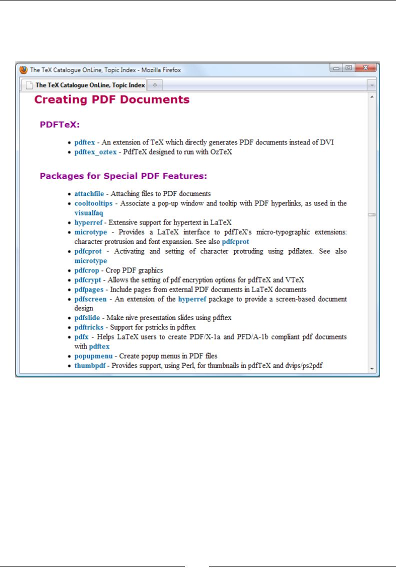
Chapter 11
[ 253 ]
2. We can see dierent indexes. The systemac topical index is oen the most useful
when you're looking for some subject, So, let's click on Topical. We get a huge list. In
the overview, click on Creang PDF documents. Then it scrolls down to that category:
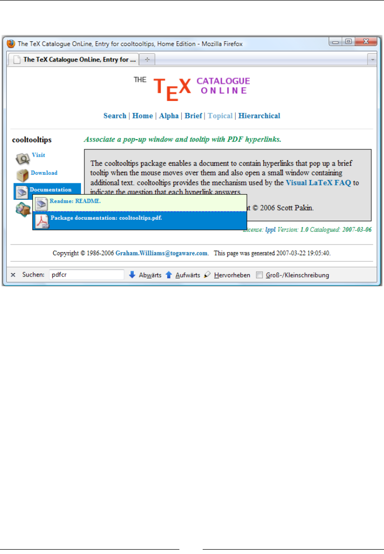
Enhancing Your Documents Further
[ 254 ]
3. Well, we found some packages! cooltoolps sounds fancy, so let's click it:
4. Now we may read the brief descripon and open the documentaon to learn more
about that package.
What just happened?
The TeX Catalogue is a really valuable source. Its category view is especially useful if you
are looking for a package but don't know its exact name. It's also an easy way to locate
and download documentaon if texdoc doesn't work for you.
So, you found cooltooltips, and now you can enhance your PDF document by
mouse-over eects and pop-ups.
If the package you desire is not yet on your computer, then you need to install it.
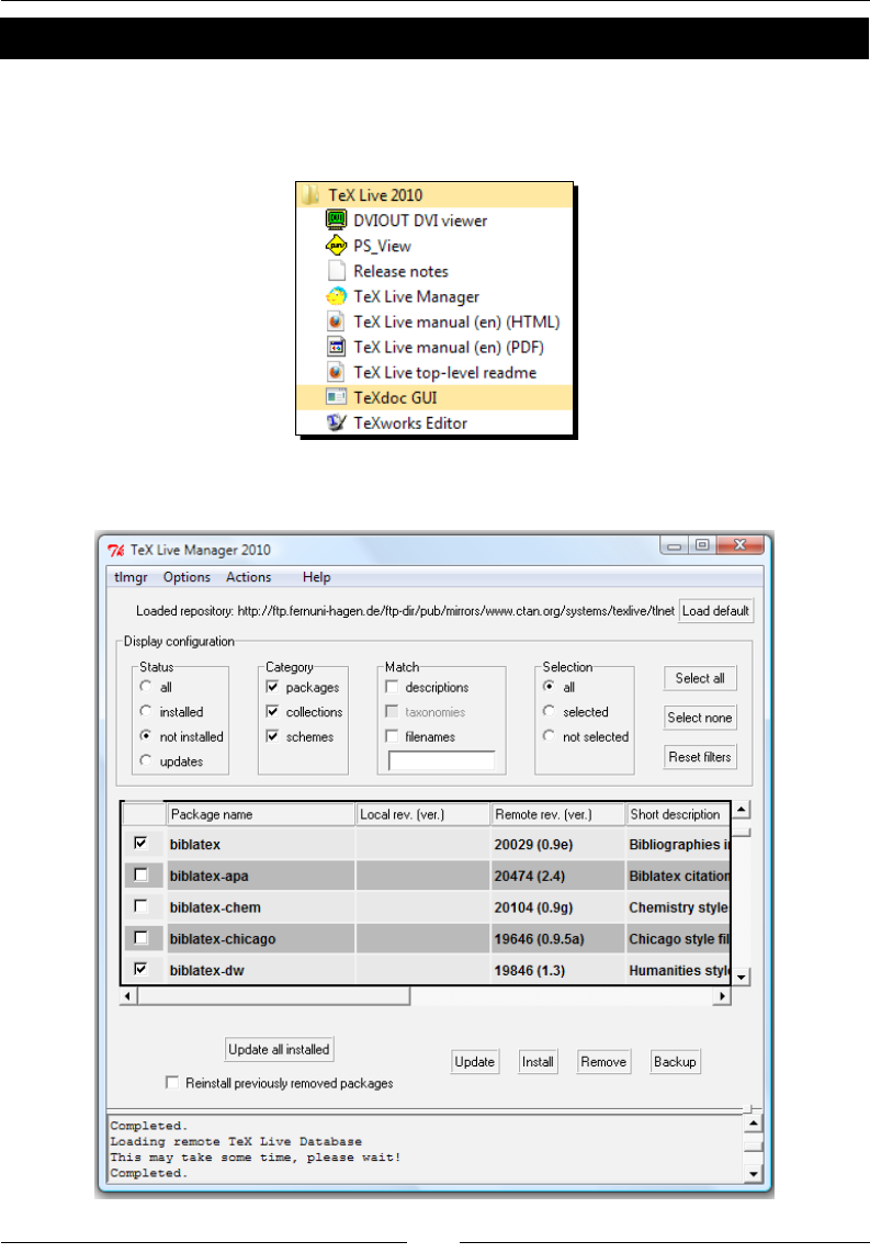
Chapter 11
[ 255 ]
Time for action – installing a LaTeX package
The prey new biblatex package is oen not yet installed. So, let's catch up on it!
1. Go to the Start menu and look for the TeX Live Manager:
2. Launch the TeX Live Manager with a mouse click:

Enhancing Your Documents Further
[ 256 ]
If you installed TeX Live on Linux or without a Start menu group, you
may start the TeX Live Manager at the command prompt. The name of
the executable le is tlmgr. So, type tlmgr –help to get a summary
of the available opons and acons.
3. In the menu, click on tlmgr and then Load default net repository to get the most
recent repository. The status bar at the boom will inform you about the success.
4. Choose the package you desire! Perhaps lter the Status to make it easier. Then click
on Install. Done!
What just happened?
Though you could just download packages to your computer, it's very recommendable to use
a package manager instead. That's what we did! With TeX Live, use the TeX Live Manager
a.k.a. tlmgr, and with MiKTeX, use the MiKTeX package manager a.k.a. mpm. If you use
Linux and installed TeX Live using your operang system's repositories instead of tlmgr, then
use your OS package manager for adding LaTeX packages; this might be Synapc, aptude,
apt-get, YaST, rpm, or any other, depending on your kind of Linux distribuon—you will
know it for sure if you use Linux.
Package managers are usually easy to handle: choose, install, or update plus some further
useful features. A manual installaon could be hard, at least if a package consists of more
than a .sty le—there might be documented source les needing compilaon or various
font les requiring some know-how regarding the TeX lesystem structure. The UK TeX FAQ,
listed among the online resources in the last chapter, oers detailed informaon about
package installaon.
Use a package manager, if available, so that you are on the safe side.
Designing headings
In Chapter 2, Formang Words, Lines, and Paragraphs, we encountered the problem of
customizing headings. There has to be a consistent way to modify the font of the headings,
their spacing, and their numbering for the whole document. Fortunately, there’s a handy
package for that, it’s called tlesec. We shall use it now.
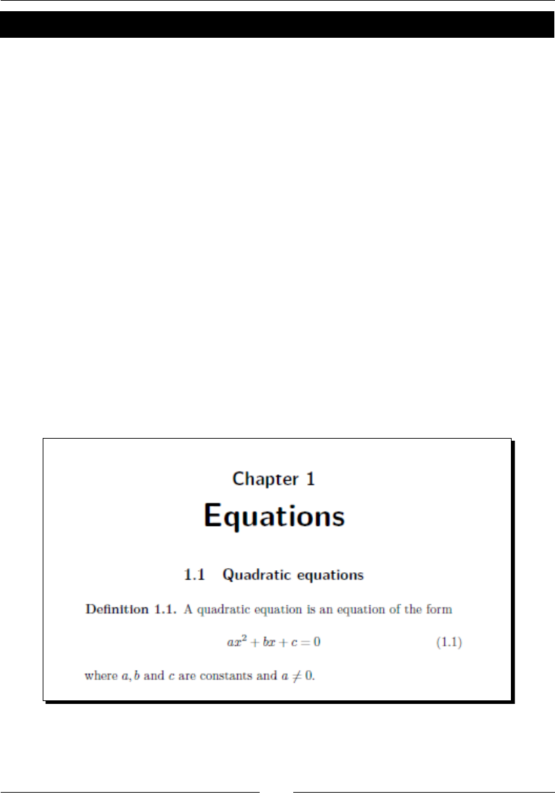
Chapter 11
[ 257 ]
Time for action – designing chapter and section headings
We return to our example that we used in this chapter. Our goal is to create centered
headings. The font size should be smaller, further we reduce the space above and below.
Finally, we switch to a sans serif font which is a good choice for bold headings:
1. Open the le preamble.tex which we already used in this chapter. Insert this line
to load the titlesec package:
\usepackage{titlesec}
2. Add this command to specify layout and font of the chapter headings:
\titleformat{\chapter}[display]
{\normalfont\sffamily\Large\bfseries\centering}
{\chaptertitlename\ \thechapter}{0pt}{\Huge}
3. Now dene the secon heading by calling \titleformat again:
\titleformat{\section}
{\normalfont\sffamily\large\bfseries\centering}
{\thesection}{1em}{}
4. Add this line to adjust the chapter headings spacing:
\titlespacing*{\chapter}{0pt}{30pt}{20pt}
5. Save preamble.tex and Typeset the main document equation.tex.
Let’s see how the headings have changed:

Enhancing Your Documents Further
[ 258 ]
What just happened?
We loaded the package titlesec, which provides a comprehensive interface for
customizing headings, of parts, chapters, secons, and even smaller seconing parts down
to subparagraphs.
In step 2 we chose displayed style, which means that numbering and actual tle use separate
lines. Firstly, we used \normalfont to switch to the base font, to be on the safe side. By \
sffamily we switched to sans-serif font, chose size and weight and nally declared that
the complete heading shall be centered. In step 3 we did this very similar, we just omied
[display] to get number and tle on the same line.
To understand the remaining arguments, have a look at the \titleformat denion:
\titleformat{cmd}[shape]{format}{label}{sep}{before}[after]
The meaning of the arguments is as follows:
cmd stands for the seconing command we redene, that is, \part, \chapter, \
section, \subsection, \subsubsection, \paragraph, or \subparagraph
shape species the paragraph shape. The eect of the possible values is:
display puts the label into a separate paragraph
hang creates a hanging label like in standard secons and is the default
opon
runin produces a run-in tle like \paragraph does by default
leftmargin sets the tle into the le margin
rightmargin puts the tle into the right margin
drop wraps the text around the tle, requires care to avoid overlapping
wrap works like drop but adjusts the space for the tle to match the
longest text line
frame works like display and addionally frames the tle
format may contains commands which will be applied to label and text of the tle.
label prints the label, that is, the number.
sep is a length which species the separaon between label and tle text. With
display opon, it’s the vercal separaon, with frame opon it means the
distance between text and frame, otherwise it’s the horizontal separaon between
label and tle.

Chapter 11
[ 259 ]
before can contain code which comes before the tle body. The last command of it
is allowed to take an argument, which should then be the tle text.
after can contain code which comes aer the tle body.
That’s a lot of opons! Have a look at the titlesec documentaon to learn even more.
We used the titlesec command \chaptertitlename, which is \chaptername by
default, that is, it defaults to Chapter. In an appendix, it changes to \appendixname.
By the remaining command we customized the spacing of all chapter headings:
\titlespacing*{cmd}{left}{beforesep}{aftersep}[right]
left works dierently depending on the shape: with drop, leftmargin and
rightmargin it’s the tle width. With wrap, it’s the maximum width. With
runin, it sets the indentaon before the tle. Otherwise it increases the le
margin. If negave, it decreases, which means overhanging into the margin.
beforesep sets the vercal space before the tle.
aftersep sets the separaon between tle and text. With hang, block, and
display, it’s has a vercal meaning. With runin, drop, wrap, leftmargin,
and rightmargin, it’s a horizontal width. Again, it may be a negave value.
right increases the right margin when hang, block or display shape is used.
If you use the star, the indentaon of the following paragraph would be removed as you
know of secons. With drop, wrap and run-in the starred version has no meaning.
In our example, we avoided the indentaon of the paragraph which follows a chapter
heading, and we specied a space of 30 pt before the heading and 20 pt aer it. That’s
less than before, standard classes use 50 pt above chapter headings.
It’s very recommendable to read the titlesec documentaon to get the most out of it.
In its appendix, it shows how the headings in standard classes would be dened by
\titleformat and \titlesec. That’s a great point to start o by copying these
denions and beginning to modify them.
Using sans-serif headings is very common today. They don’t have such a heavy and ancient
appearance like bold serif headings. However, serif text oers the best readability for body
test. Now it’s up to you to choose—you’ve got the tools!

Enhancing Your Documents Further
[ 260 ]
Coloring your document
We could enhance our texts further by colors. We didn't deal with it yet, because most
people use LaTeX for wring serious books and arcles, or leers where too much color may
harm the appearance. But why not try something fancy? For instance, diagrams and tables in
presentaons are oen colorful.
We just need to load the color package:
\usepackage{color}
From now on, we have to use a command to set the text color:
\color{name} is a declaraon that switches to the color name. Just try
\color{blue}.
\textcolor{name}{text} is the corresponding command form, coloring just
text. That's like {\color{name}}, not new for you.
The package oers the command \definecolor. Use this to mix your own colors. You may
read it in the documentaon of the color package or of the graphicx package, if needed.
But much beer is to use the xcolor package, which extends the color facilies. It oers
a lot of readily mixed colors; you just need to call it by its name and it has powerful
capabilies regarding color denion. If only for the huge color samples table, look at
the package documentaon.
Have a go hero – creating colorful tables
Now you're able to do everything with the color you like. Now think of diagrams in nancial
journals or tables of sports tournaments using rounded corners, shading, and fading. Is LaTeX
capable of that? Yes, it is!
The following presentaon slide has been created with LaTeX— can you believe it?
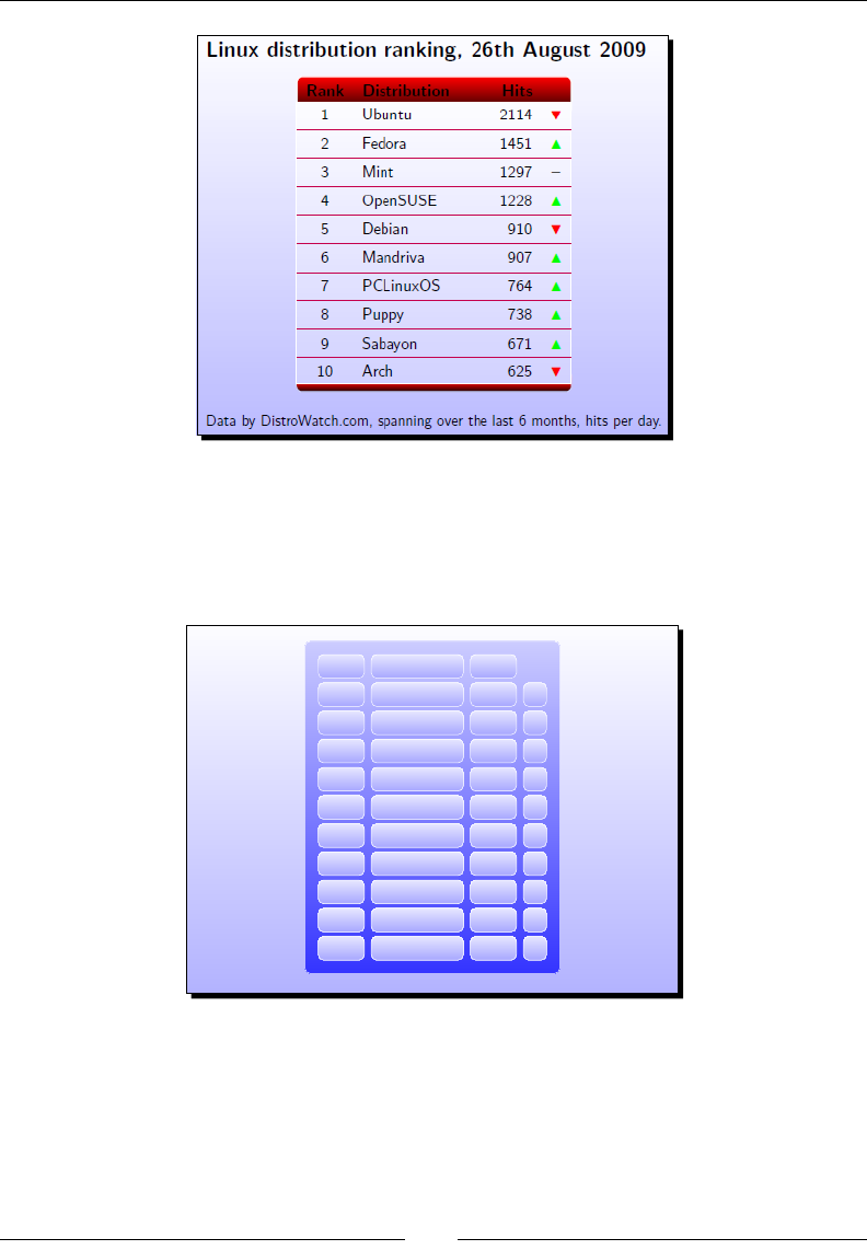
Chapter 11
[ 261 ]
The code for this presentaon can be found on http://texblog.net and in the book's
example archive.
Oponally, you can have a look at this dierently designed table, before we come to its
source code:
Rank Distribution Hits
1 Ubuntu 2114
2 Fedora 1451
3 Mint 1297 –
4 OpenSUSE 1228
5 Debian 910
6 Mandriva 907
7 PCLinuxOS 764
8 Puppy 738
9 Sabayon 671
10 Arch 625

Enhancing Your Documents Further
[ 262 ]
The document is not very long, but it contains some new subjects:
\documentclass[svgnames]{beamer}
\setbeamertemplate{background canvas}[vertical shading]%
[top=blue!1,bottom=blue!30]
\setbeamertemplate{navigation symbols}{}
\usepackage{tikz}
\usetikzlibrary{matrix}
\newcommand{\up}{\textcolor{YellowGreen}{$\blacktriangle$}}
\newcommand{\down}{\textcolor{Red}{$\blacktriangledown$}}
\newcommand{\const}{\textcolor{darkgray}{\textbf{--}}}
\newcommand{\head}[1]{\textbf{#1}}
\newenvironment{matrixtable}[4]{%
\begin{tikzpicture}[matrix of nodes/.style={
execute at begin cell=\node\bgroup\strut,
execute at end cell=\egroup;}]
\matrix (m) [matrix of nodes,top color=blue!20,
bottom color=blue!80,draw=white,
nodes={draw,top color=blue!10,bottom color=blue!35,
draw,innersep=2pt,minimum height=3.1ex},
columnsep=1ex,row sep=0.6ex,inner sep=2ex,
roundedcorners,column 1/.style={minimum width=#1},
column 2/.style={minimum width=#2},
column 3/.style={minimum width=#3},
column 4/.style={minimum width=#4}]}%
{;\end{tikzpicture}}
\begin{document}
\begin{frame}[fragile,bg=lightgray]
\begin{center}
\begin{matrixtable}{1.2cm}{2.4cm}{1.2cm}{0.6cm}{
\head{Rank} & \head{Distribution} & \head{Hits} & \\
1 & Ubuntu & 2114 & \down \\
2 & Fedora & 1451 & \up \\
3 & Mint & 1297 & \const \\
4 &OpenSUSE& 1228 & \up \\
5 &Debian& 910 & \down \\
6 &Mandriva& 907 & \up \\
7 &PCLinuxOS& 764 & \up \\
8 & Puppy & 738 & \up \\
9 & Sabayon & 671 & \up \\
10 & Arch & 625 & \down \\
}
\end{matrixtable}
\end{center}
\end{frame}
\end{document}

Chapter 11
[ 263 ]
Indeed, this looks a bit dierent than what we've done before. However, as you are a hero,
you may check out the magic behind it! We used the following:
The beamer class—this is a feature-rich presentaon class for producing slides.
It oers many predesigned colorful themes. More can be found on the Internet.
There's a user's guide with many examples on more than 200 pages—and it's
probably already on your hard drive! texdoc, you know.
The xcolor package—the beamer class loads it implicitly, so we did not have to do
this. We just gave beamer the svgnames opon to pass it along to xcolor, which
provides us with a color naming scheme.
The TikZ package—that's a jewel! TikZ is an enormously capable package for
creang graphics. Our small example just used a ny feature of it: a matrix of nodes.
The manual is twice as large as the beamer documentaon. However, this benets
you—a free book about producing graphics with LaTeX. You can learn to create
diagrams, charts, plots, trees, and arbitrary graphics using coordinates, nodes,
shapes, layers, transparency, shadings, transformaons, and shadings.
That's heavy stu. But check it out—you will see that there's more in the LaTeX world than
dry scienc or technical texts!
Pop quiz
1. By which command could you create an anchor, to which a hyperlink can point?
a. \href
b. \hyperlink
c. \hyperref
d. \hypertarget
e. \hypersetup
2. According to the text, which characters are allowed in bookmarks?
a. only leers
b. only leers and numbers
c. only leers and Unicode characters including numbers
d. leers and math symbols without line breaks

Enhancing Your Documents Further
[ 264 ]
Summary
This chapter started with easy and comfortable hyper-linking and ended with an outlook
to a very powerful graphic package, namely, TikZ.
By reading this chapter, we are now capable of:
Enhancing our document with a hypertext structure
Designing visually dierent styles for dierent types of links
Providing a navigaon bar for the reader by adding bookmarks
Eding the PDF metadata
Designing font and layout of headings
Adding color to our texts
Now that we've got most of the tools we need for successful wring, what's ahead is
specialized advanced classes and packages. However, this won't be dicult for you. Since you
have mastered the fundamental LaTeX challenges, you're now able to use any other package
together with reading its documentaon. The vast majority of classes and packages are very
well documented. And there are no secrets—everything is open source.
During our work, we may encounter errors and warnings. That's common, also for advanced
LaTeX users. The following chapter will prepare us for troubleshoong.
12
Troubleshooting
During typeseng, it may happen that LaTeX prints out warning messages. It's
even possible that LaTeX doesn't produce the desired output but shows error
messages instead. That's absolutely normal and can be caused, for example,
by small typos in command names or by unbalanced braces. Even professional
LaTeX typeseers have to deal with errors—they just know how to do it
eciently.
Don't worry too much about the potenal errors—let LaTeX check it for you.
Then you just need to do the correcons at the places pointed out by LaTeX.
This chapter prepares us to:
Understand error messages and to x them
Deal with warnings
Use all the informaon LaTeX produces during typeseng
Let's rst tackle the error handling.
Understanding and xing errors
If the LaTeX typeseng engine encounters a problem, it will issue an error message. This is
informave and it's intended to help you. So, read the messages carefully. Besides the line
number, where the error occurred, a diagnosc message is also provided.
Concentrate on the very rst error message. If you connue typeseng, further errors might
be just a consequence of the rst one that confused the compiler.
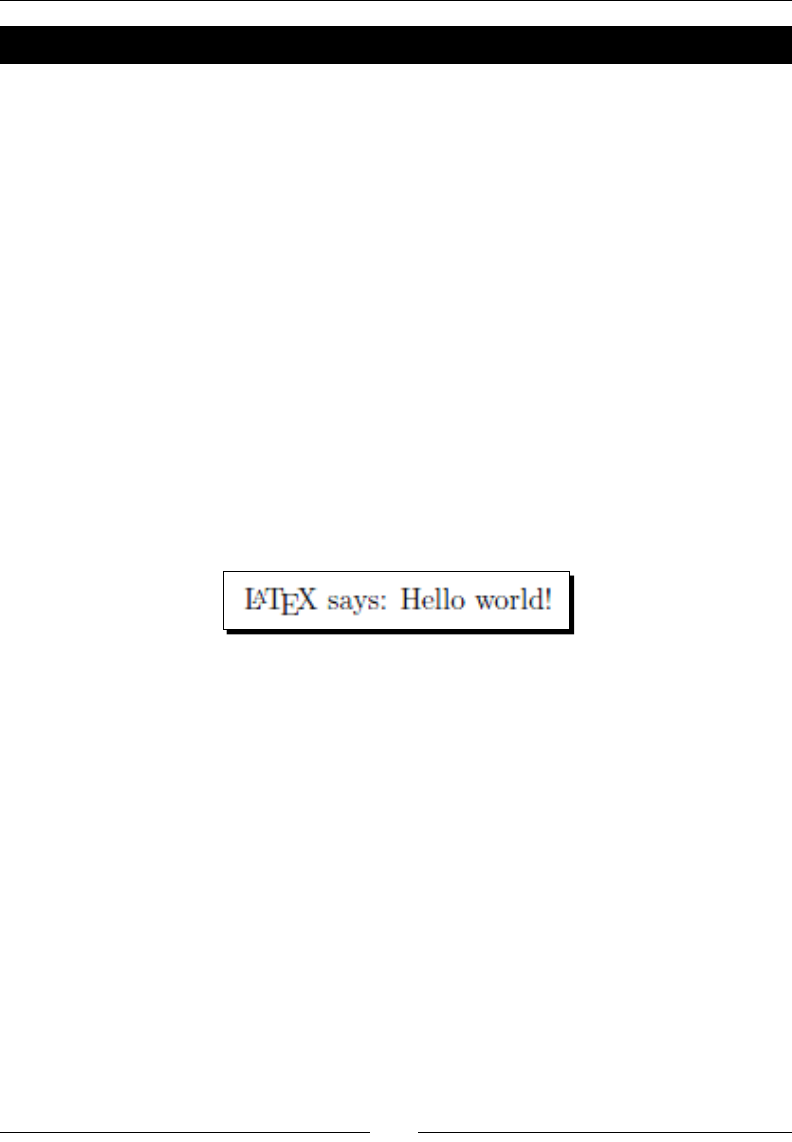
Troubleshoong
[ 266 ]
Time for action – interpreting and xing an error
Let's create a ny test document. For sure you know those "Hello world!" prinng
programs—we shall write one in LaTeX. Though we are used to the uncommon capitalizaon
used in the words TeX and LaTeX, we will now try if \Latex works as well.
1. Create a new document containing these lines:
\documentclass{article}
\begin{document}
\Latex\ says: Hello world!
\end{document}
2. Typeset. LaTeX will stop and print out the following message:
! Undened control sequence.
l.3 \Latex
\ says: Hello world!
3. Click on the cancel icon in the upper-le corner of TeXworks to stop typeseng.
Go to line 3, correct \Latex into \LaTeX and Typeset again. Now LaTeX produces
output without an error:
What just happened?
LaTeX commands are case-sensive. Because we did not respect that, LaTeX had to deal
with a macro called \Latex, which is just unknown. As a command is also called a control
sequence, we got the error Undened control sequence.
If TeX encounters an error, it stops typeseng and asks for user input. You could press the
Enter key to connue typeseng though or cancel and correct the error immediately.
Let's analyze the three parts of the error output:
An error message begins with an exclamaon mark, which is followed by a short
descripon of the problem.
Then LaTeX prints out the number of the input line where the error was raised
and the part of the line unl the problem occurred.
Aer a line break, the remaining part of the input line is printed out.

Chapter 12
[ 267 ]
So you are not on your own without a clue! LaTeX tells you exactly:
The kind of error
The exact locaon of the error
Most editors show you the line number or allow jumping to the line number you enter. As
you are now at the problemac place, you only need to know why LaTeX complains—if you
don't see it yourself immediately. Leslie Lamport's LaTeX book and documentaon lists error
messages alphabecally together with some background informaon. You may choose that
for look-up.
We shall now have a closer look at frequent TeX and LaTeX error messages. In this book,
let's do that by topic.
Using commands and environments
Command names might easily be misspelled or just misused. Let's check out LaTeX's
common complaints.
Undened control sequence: As in our example, TeX stumbled across an unknown
command name. There are two possible reasons:
The command name might be misspelled. In that case, you just need to
correct it and restart the typeseng.
The command name is correct, but it's dened by a package you didn't
load. Add a \usepackage command to your preamble, which loads that
package.
Environment undened: That's similar to Undened control sequence, but this
me you began an environment which is unknown. Again, this may be caused by
misspelling or by a missing package—you know how to correct it.
Command already dened: This happens when you create a command with a name
that's already used, for example, with \newcommand or \newenvironment. Just
choose a dierent name. If you really would like to override that command, use
\renewcommand or \renewenvironment instead.
Missing control sequence inserted: A control sequence has been expected but
didn't appear. A common cause is using \newcommand, \renewcommand, or
\providecommand, but not specifying a command name as its rst argument.
\verb illegal in command argument: The \verb command for producing verbam
text is a delicate one; it cannot be used within arguments of commands or
environments. The examplep package oers commands for using verbam text in
such places.

Troubleshoong
[ 268 ]
Writing math formulas
The most frequent mistake is forgeng to enter math mode. The rst of the following errors
would be raised then:
Missing $ inserted: There are a lot of commands which may only be used in math
mode. Just think of symbols; most of them require math mode. If TeX is not in math
mode, but encounters such a symbol, it stops and prints out that error. Usually it can
be repaired by inserng that missing $, possibly several. Remember that you cannot
use paragraph breaks inside a math expression. This means that blank lines within a
math expression are illegal; the math mode has to be ended before the blank line.
Command invalid in math mode: Some commands are not applicable within math
formulas. In that case, use the command outside the math mode.
Double subscript, double superscript: Two subsequent subscripts, superscripts
respecvely such as in $a_n_1$ cannot be typeset. To correct that, group by braces,
like in $a_{n_1}$ or $a_{n_{1}}$.
Bad math environment delimiter: This can be a consequence of illegally nesng
math mode. You must not start math mode if you are already inside math mode, for
example, don't use \[ within an equation environment. Similarly, you must not
end the math mode before you started it. Ensure that your math mode delimiters
match and that braces are balanced.
Handling the preamble and document body
The preamble is intended for document-wide sengs like class, packages, opons, and
command denions. Aer the preamble has ended, output may be produced in the
document body. If these rules are broken, one of the following errors would occur:
Missing \begin{document}: It seems to be obvious; you might have forgoen
the command \begin{document}. But the error may occur even if you did not
forget that! In that case, there may be a problem in the preamble. Specically, if a
character or a command within the preamble produces output, that error would be
raised. Just remember: output is not allowed before \begin{document}.
Can be used only in preamble: This error message belongs to a command which is
only allowed to be used in the preamble, not aer \begin{document}. Move that
command upwards into your preamble, or remove it. For example, \usepackage
can only be used in the preamble.

Chapter 12
[ 269 ]
Opon clash for package: An opon clash happens if you load a package twice
but with dierent opons. If you did that, it's usually beer to reduce it to one
\usepackage call with the desired opons. But the cause might be hidden.
Imagine that a class or a package implicitly loads a certain package together
with some opons. If you want to load the package too but with dierent opons,
there's a problem!
You could try to x an opon clash by oming reloading the package while
specifying the desired opons to the document class. Remember, class
opons are inherited by packages. Some packages and classes even oer
commands to set opons aer loading. For example, the hyperref package
provides \hypersetup{options}, and similarly the caption package
oers \captionsetup. KOMA classes support such late opons and are
described in their manual.
Working with les
The most common errors regarding les are mistakes in lename or path. Then the rst
of the following errors would be raised:
File not found: LaTeX tried to open a le that doesn't exist. Possibly you:
Used \include or \input to include a .tex le but a le with the
specied name doesn't exist
Tried to use a non-exisng package or misspelled the package's name.
Packages can be recognized by the le extension .sty.
Used a document class that doesn't exist or just has a dierent name.
Class les have the extension .cls.
Well, just correct the lename in your input document or rename the le.
\include cannot be nested: We learned in Chapter 10, Developing Large Documents,
that we cannot use \include within les that are being included by themselves.
Instead, use \input within such les.

Troubleshoong
[ 270 ]
Creating tables and arrays
Admiedly, tabular and array environments don't have the simplest syntax. Those & and
\\ might easily be misplaced, which causes LaTeX to complain. Further, we have to be careful
with the formang arguments. Let's start with the arguments to the environment:
Illegal character in array arg: In the argument to a tabular or an array
environment, you may specify the column formang. You line up characters such
as l, c, r, p, @, and width arguments such as {1cm}. If you use any character that
doesn't have such a meaning, LaTeX will tell you that. The same applies to the
formang argument of \multicolumn.
Missing p-arg in array arg: A bit more specic than the previous message, it tells us
that the width argument to the p opon is missing. Supplement the p with a width
such as {1cm} or change the p into another opon such as l, c, or r.
Missing @-exp in array arg: That's similar to the error; the expression aer the @
opon is missing. You just need to add it, in curly braces, or remove the @ opon.
Now we shall take a look at the potenal error messages concerning the table body.
Misplaced alignment tab character &: As you know, the ampersand character
has the special meaning of separang columns in a row of a tabular or array
environment. If you accidentally use it in normal text, this error will appear.
Type \& if you desire an ampersand symbol in the output.
Extra alignment tab has been changed to \cr: This happens if you use more
separaon characters & than the dened columns. For example, the \\ ending
a row could have been forgoen.
Working with lists
Lists follow a certain structure and cannot be endlessly nested. At some point, LaTeX would
complain:
Too deeply nested: As menoned in Chapter 4, Creang Lists, you can nest four
levels of a list. If you mix list types, you could go up to six. But if you go further than
what LaTeX accepts, you would get this error message.
Think over if you really need a deep nesng. If this is the case, you could
consider using seconing commands like \paragraph or \subsubsection
for outer levels.

Chapter 12
[ 271 ]
Working with oating gures and tables
In Chapter 5, Creang Tables and Inserng Pictures, we learned about inserng gures and
tables, and how to adjust their placement. If you use a lot of gures or tables, you might
encounter the following error:
Too many unprocessed oats: If you use many oang objects and LaTeX saves
them because it doesn't nd an appropriate place, LaTeX's room for that might get
full, so this error appears. There might even be just one non-ng oat blocking
those who follow. It may be solved as follows:
By adding placement opons to the gure and table environment
respecvely, thus lowering their placement requirements.
By inserng a \clearpage to ush out the oats at a suitable place,
or perhaps even cleverer: \afterpage{clearpage} with the
aerpage package.
General syntax errors
Just like with any markup or programming language, LaTeX's documents have to follow a
syntax. For example, braces and delimiters have to match. If there's a mistake, LaTeX would
point to it:
Missing { inserted, missing } inserted: Though it reads its like caused by unbalanced
braces, it may be because of a confusion of TeX, which could be caused before the
place where the error occurred. Well, check the used syntax thoroughly.
Extra }, or forgoen $: This me there's a problem with unbalanced braces,
or math mode delimiters don't match correctly. You need to correct the matching.
There's no line here to end: Using \\ or \newline between paragraphs in
vercal mode, is not meaningful and causes this error. Don't try to get more
vercal space by wring \\. Use \vspace instead or other skip commands
like \bigskip, \medskip, or \smallskip. For instance, a blank line may be
produced by \vspace{\baselineskip}.
Somemes, the cause of the error might be a bit hidden to the user: TeX might
be in vercal mode when you don't expect it to be. In such cases, you could force
the \\ to work if you write \leavevmode directly before it. Inserng some
whitespace before, like using ~, works too.
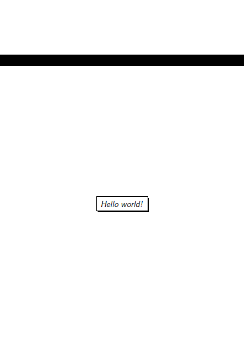
Troubleshoong
[ 272 ]
Handling warnings
Warning messages are just for your informaon. They don't need to point to a serious
problem, but oen it's a good idea to read these ps carefully and to act accordingly. This
may improve your document.
Time for action – emphasizing on a sans-serif font
We shall write our complete document using a sans-serif font. As we did not yet see how
emphasizing without serifs looks, we will try that:
1. Take our "Hello world!" example and modify it this way:
\documentclass{article}
\renewcommand{\familydefault}{\sfdefault}
\begin{document}
\emph{Hello world!}
\end{document}
2. Typeset. LaTeX will print out a warning:
LaTeX Font Warning: Font shape `OT1/cmss/m/it' in size <10> not available
(Font) Font shape `OT1/cmss/m/sl' tried instead on input line 4.
3. Check the output:
What just happened?
The macro \familydefault stands for the default font family which shall be used in the
LaTeX document. For this macro, we specied the value \sfdefault, which means the default
sans-serif font. This means simply that sans-serif is now default, no maer which font has been
chosen. As you can imagine, other possible values are \rmdefault and \ttdefault. By
changing \familydefault, we don't have to write \sffamily again and again.
But then we emphasized our text and got a warning! The message means that simply there's
no Computer Modern Sans Serif font (cmss) in OT1 encoding (just standard), in medium
weight (m) and italic shape (it) in 10pt size. Further, LaTeX told us how it tried to repair that;
instead of italic it chose a slanted shape. That's not too bad; at least it looks similar and the
output is produced.
Chapter 12
[ 273 ]
This is basically what happens when warnings occur: LaTeX informs about a potenal
problem or disadvantage, but it tries to choose the best alternave and connues
typeseng. It's not uncommon that a longer document produces dozens of warnings,
most oen dealing with horizontal or vercal juscaon.
Oen, it doesn't hurt if you ignore warnings, which don't seem very serious. Though
following them up is a good habit. Who desires to have a perfect document, xes all
warnings. This way you cannot overlook a potenal real problem.
Let's have a look at very common warning messages, what they mean, and how we could
x them.
Justifying text
These warnings are the most frequently occurring:
Overfull \hbox: A line is too long and doesn't t to the text width. This may result in
text extending past the margin. This may be caused by hyphenaon problems, which
can be xed by using \hyphenation, as you already learned, or by inserng \-.
You could break the line manually or polish your words otherwise.
Underfull \hbox: The opposite to the previous warning; a line is not wide enough
to t to the text width. This could be caused by \linebreak, if there's not enough
text on the line. Also, \\or \newline may cause it, such as \\\\.
Overfull \vbox: The page is too long because TeX could not break it accordingly.
The text might hang out past the boom margin.
Underfull \vbox: There's not enough text on the page. TeX had to break the page
too early.
In Chapter 2, Formang Words, Lines, and Paragraphs, we learned how to improve the
juscaon, reducing such warnings. Remember, already loading the microtype package
may help a bit.
The declaraon\sloppy switches to a prey relaxed typeseng, thus
avoiding many such warnings. It's counterpart is \fuzzy, switching back
to the default behavior. If you ever use \sloppy, maybe in a kind of
emergency, it's beer to keep it local by grouping or use the respecve
environment—\begin{sloppypar} … \end{sloppypar}.
Addionally, check out recommendaons and alternaves regarding \
sloppy in l2tabu, which has been menoned in Chapter 10.
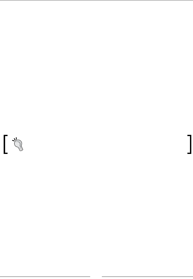
Troubleshoong
[ 274 ]
Referencing
Many warnings deal with referencing. Common mistakes are missing label or cite keys or
keys that have been used twice. Somemes LaTeX just tells you that another typeset run
is required.
Label mulply dened: \label or \bibitem has been used with a label name
that's already been used. Make label names unique.
There were mulply-dened labels: Like the previous warning, but aer processing
the complete document; a label has been dened by two \label commands.
Labels may have changed. Rerun to get cross-references right: Just typeset again to
let LaTeX correct the referencing.
Reference ... on page ... undened: \ref or \pageref has been used without a
corresponding \label denion. Insert a \label command at a suitable place.
Citaon ... on page ... undened: A \cite command did not have a corresponding
\bibitem command.
There were undened references or citaons: Summarizing aer processing—any
\ref or \cite command did not have a corresponding \label or \bibitem
command.
Whenever you get warnings regarding referencing, it’s a good idea to simply
rerun typeseng. Oen, such warnings then disappear, because LaTeX couldn’t
resolve all references in the rst run itself.
Choosing fonts
We already encountered the rst of the following warnings in our example:
Font shape … in size <…> not available: You chose a font that's not available. This
may be a result of combining font commands that results in a non-exisng font.
Also, it could just be of an unavailable size. LaTeX would choose a dierent font or
size and inform you about that choice in detail.
Some font shapes were not available, defaults substuted: LaTeX prints this aer
processing the enre document if any of the chosen fonts had been unavailable.
Placing gures and tables
We already encountered the rst of the following warnings in our example:
Float too large for page: A gure or table is too large to t the page.
It would be output, but on an oversize page.

Chapter 12
[ 275 ]
h oat specier changed to ht: If you specied an h opon to a oang gure or
table which doesn't t there, it would be placed on top of the next page and that
warning would be issued. The same can occur for !h and !ht.
Customizing the document class
A warning may be issued if you use an illegal class opon:
Unused global opon(s): You specied an opon to \documentclass, which
is unknown to the class and to any loaded package. This could be, for example,
a base font size which is not supported. Just check the opon which LaTeX
complains about.
Also packages may print out warnings if they foresee any problem. All these warnings are
intended to help you in designing your document.
Avoiding obsolete classes and packages
At the end of Chapter 10, we talked about the dangers of outdated informaon. LaTeX exists
since decades, and so do tutorials, examples, packages, and templates. Many are totally
outdated and some even refer to the old LaTeX standard 2.09, where even document classes
didn't exist. In Chapter 10, we pointed to the denive guide l2tabu that comes to the rescue.
Many problems just occur because of the use of obsolete packages. For example, some that
aren't maintained any more may conict with newer packages. Oen, you just need to nd
the recommended successor of an obsolete package and use that.
Here's a short list for helping you in that maer:
Obsolete packages Recommended successors
a4, a4wide, anysize geometry, typearea
backrefx backref
bitfield bytefield
caption2 caption
dinat natdin
doublespace setspace
dropping lettrine
eps, epsfig graphicx

Troubleshoong
[ 276 ]
Obsolete packages Recommended successors
euler eulervm
eurotex inputenx
fancyheadings fancyhdr
floatfig floatflt
glossary glossaries
here float
isolatin, isolatin1 inputenc
mathpple mathpazo
mathptm mathptmx
nthm ntheorem
palatino mathpazo
picinpar floatflt, picins,
wrapfig
prosper, HA-prosper powerdot, beamer
ps4pdf pst-pdf
raggedr ragged2e
scrlettr scrlttr2
scrpage scrpage2
seminar powerdot, beamer
subfigure subfig, subcaption
t1enc fontenc
times mathptmx
utopia fourier
vmargin geometry, typearea
That's not set in stone. Of course, you may sll use the so-called obsolete packages. They
may work well even today. But check out their descripon on their CTAN package home
page; usually there are comments regarding up-to-dateness and related packages.

Chapter 12
[ 277 ]
An up-to-date version of that list can also be found on http://texblog.net/packages.
There's an ongoing discussion at http://mrunix.de on the creaon and maintenance of
such a list.
General troubleshooting
There may be situaons where we cannot solve a problem simply by reading and acng
on warnings or error messages. Imagine a mysterious error, an untraceable error locaon,
irresolvable references, or just unclear messages from classes or packages.
Locang the cause by the line number which LaTeX printed out or by knowing what we've
done since the previous typeseng run, usually helps. Once a problemac line or chunk is
located, it could be removed or xed. Otherwise, it might become dicult.
Here are the general rst steps we might go through then:
Compile several mes. This may be necessary for correct referencing, posioning
of oang gures, and creaon of table of contents, bibliography, and lists of tables
and gures.
Check the order in which you load the packages. Some packages, like hyperref,
don't work well if loaded before or aer certain packages. You may just swap some
lines to correct or to test that.
Remove auxiliary les. If anything strange happens, it's somemes a good idea to
remove all les created by LaTeX during typeseng. These les have the same name
as the main document but have extensions such as .aux, .toc, .lot, .lof, .bbl,
.idx, or .nav, just to name some examples.
If the problem persists, we could try to isolate the cause.
1. Create a copy of your document. If necessary, copy the complete folder. From now
on, work on the copy.
2. Remove a part of the document which probably is not involved in the problem.
3. Typeset, to ensure that the problem persists. If this is the case, go back to step 2. If
the problem is gone, you isolated the problem within the part you just removed. In
this laer case, restore the deleted part, you may delete other parts.
4. Aer some repeons, you located the problem. If you didn't already, reduce the
number of loaded packages, repeang step 2 and typeseng.
5. You end up with a really ny but complete example document which reproduces
the error.

Troubleshoong
[ 278 ]
Removing or rewring that idened part of your document could help. What if you really
want to use that part and would like to x that error? Now that your problem can be shown
with such a very small example code, you could post that problem to an online LaTeX forum
and ask for help.
Have a go hero – examining LaTeX's log les
You are not dependent on just the errors and warnings that your editor shows to you! LaTeX
keeps track of any informaon, each warning, and every error. All of these will be collected
in a le with the same name like your document but carrying the extension .log. This is an
ordinary text le and may be opened with any editor, including your LaTeX editor.
For instance, the log le for our second example looks like the following:
This is pdfTeX, Version 3.1415926-1.40.10 (Web2C 2009)
(format=pdflatex 2010.6.25) 20JAN 2011 23:16
entering extended mode
%&-line parsing enabled.
**helloworld.tex
(./helloworld.tex
LaTeX2e <2009/09/24>
Babel <v3.8l> and hyphenation patterns for english, ... loaded.
(c:/texlive/2009/texmf-dist/tex/latex/base/article.cls
Document Class: article 2007/10/19 v1.4h Standard LaTeX document class
(c:/texlive/2009/texmf-dist/tex/latex/base/size10.clo
File: size10.clo 2007/10/19 v1.4h Standard LaTeX file (size option)
)
\c@part=\count79
\c@section=\count80
\c@subsection=\count81
\c@subsubsection=\count82
\c@paragraph=\count83
\c@subparagraph=\count84
\c@figure=\count85
\c@table=\count86
\abovecaptionskip=\skip41
\belowcaptionskip=\skip42
\bibindent=\dimen102
) (./warning.aux)
\openout1 = `warning.aux'.
LaTeX Font Info: Checking defaults for OML/cmm/m/it on input line 3.
LaTeX Font Info: ... okay on input line 3.
...

Chapter 12
[ 279 ]
LaTeX Font Warning: Font shape `OT1/cmss/m/it' in size <10> not
available
(Font) Font shape `OT1/cmss/m/sl' tried instead on input line 4.
[1
{c:/Users/guest/.texlive2009/texmf-var/fonts/map/pdftex/updmap/pdftex.
map}]
(./helloworld.aux) )
Output written on helloworld.pdf (1 page, 17376 bytes).
Check out the log les of some documents you produced unl now. The informaon therein
makes a very technical impression, but this might help you a lot in troubleshoong.
Pop quiz – troubleshooting
1. If you get several error messages during one typeseng run, which one is the most
important, according to the text?
a. The rst
b. The last
c. All error messages should be dealt with before another typeseng run
2. Which it the extension of the le containing errors, warnings, and informaon?
a. aux
b. toc
c. log
d. lof
Summary
This chapter prepared us to solve problems that might occur.
Specically, we have learned about:
Locang and xing errors
Understanding warning messages
Analyzing LaTeX's typeseng log
Correcng errors is absolutely necessary. Dealing with warnings is a valuable bonus.

Troubleshoong
[ 280 ]
If you encounter any problem which you aren't able to solve on your own, don't hesitate to
ask for help on a LaTeX Internet forum. You've got the tools within this chapter, and also:
You know how to create a ny but complete example which demonstrates the
problem
You are able to report an error message
You know about the log le and could provide its informaon
For LaTeX friends online, it's oen an easy task to use this informaon in solving your
problem, and denitely a lot of LaTeX enthusiasts have fun in helping other LaTeX users.
The next chapter will point the way to LaTeX web forums and also to many other
online resources.
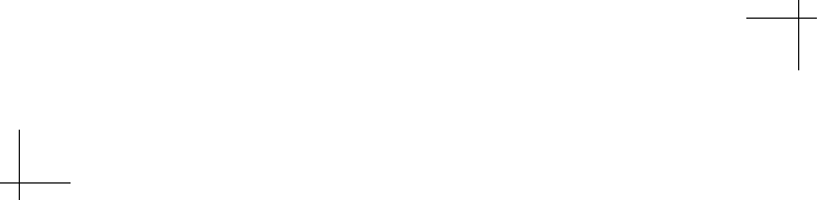
13
Using Online Resources
There's a vast amount of LaTeX informaon and material on the Internet,
and it has grown over many years. Today, thanks to the virtues of free and
open source soware, a huge TeX community exists, sharing knowledge and
experse.
On the Internet, you can nd:
Soware archives oering nearly all LaTeX material available
Web forums, where LaTeX users talk about problems and soluons
Homepages of user groups, TeX distribuons, and free editors
Blogs of individual LaTeX users
LaTeX mailing lists you may subscribe to
As you know how to navigate through the World Wide Web, this chapter does not contain
praccal examples. Instead, let's take a walk through the Internet.
Web forums, discussion boards, and Q&A sites
Before we proceed to soware archives and homepages, let's go where the online world
takes place!

Using Online Resources
[ 282 ]
Usenet groups
It all began with the Usenet. Around 1980, a long me before the World Wide Web
was born, this discussion network emerged. It consists of many thousands of groups,
so-called newsgroups, each dedicated to a certain subject. Not to our surprise, there's
a TeX newsgroup!
comp.text.tex
http://groups.google.com/group/comp.text.tex/topics
The easiest way is just to access this URL hosted by Google. Just browse it using its web
interface. Alternavely, you could install a Usenet reader program and connect to a Usenet
web server. At this point, you should familiarize yourself beer with Usenet. A great starng
point is its Wikipedia entry at http://en.wikipedia.org/wiki/Usenet. There you
would nd an introducon, links to necessary soware, and further reading.
comp.text.tex is the classic TeX discussion board. Then and now, there are disnguished
experts reading and posng messages. You can search and browse an archive reaching
back over more than 20 years.
Newsgroups in other languages
If you understand the language, you could check out the German or French Usenet
TeX groups:
http://groups.google.de/group/de.comp.text.tex/topics
http://groups.google.de/group/fr.comp.text.tex/topics
Web forums
During the last few years, web forums emerged. They oer an easier and more user-friendly
access to discussion groups. Inially, LaTeX has been the topic in sub forums of more general
computer forums, among other soware. Aer LaTeX became more and more popular,
websites dedicated to it have been founded.
LaTeX-Community.org
http://www.latex-community.org/
In January 2007, the originator of the LaTeX editor TeXnicCenter—Sven Wiegand, founded
the web forum LaTeX Community. This site has been the rst forum with the single topic
LaTeX. It is split into many sub forums, each dealing with a certain LaTeX topic, such as
Math and Science or Fonts and Character Sets, with a certain LaTeX distribuon or a
specic LaTeX editor.

Chapter 13
[ 283 ]
Today it's supplemented by a news secon and a know-how secon containing arcles and
essays of the community.
The author of this book supports the fellow community members as a moderator on
that site.
Parcipang is as easy as in any other web forum. You don't need to register for reading, as
it's freely available. Just for wring, you need to register once, choosing a login name and
a password. Then you may ask quesons yourself or support other users who turned there
looking for help.
Quesons are very welcome! They are the foundaon of the site. You may increase the
chance of receiving helpful answers by:
Choosing a meaningful header
Describing your problem clearly
Quong the error or warning messages you've got
Including a code example, which allows others to reproduce the problem
The laer is the opmal approach. There's even a website explaining why and how at
http://www.minimalbeispiel.de, in English and German. Once a problem could be
reproduced, it's nearly solved, even if it seems to be dicult at rst sight. Experienced users
who are familiar with the source code of the LaTeX kernel and packages can explain how
something works and are able to create soluons for nearly any problem.
TeX and LaTeX on Stack Exchange
http://tex.stackexchange.com/
There are queson and answer sites, which are dierent to classical web forums. While in
the web forums, people talk and discuss, these Q&A sites have a simpler structure. There's
a queson, followed by answers. There's no discussion, besides comments.
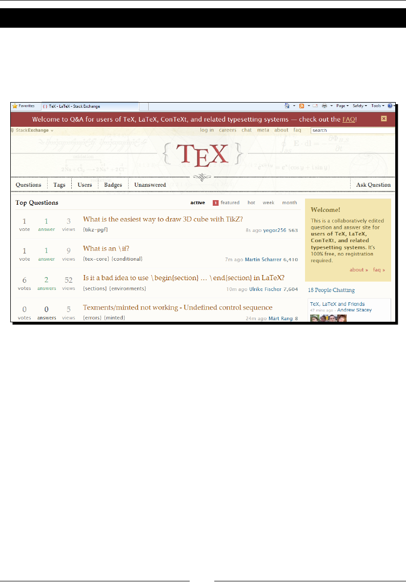
Using Online Resources
[ 284 ]
Time for action – asking a question online
Is there anything you wanted to know about LaTeX? Did you encounter any serious problem
you could not solve? Then post a queson on http://tex.stackexchange.com/:
1. Visit http://tex.stackexchange.com :
Chapter 13
[ 285 ]
2. In the upper-right corner, click on Ask Queson:
3. Fill out the Title eld and type in your queson, and choose some meaningful
keywords for the Tags eld. When you are done, click on Post Your Queson.
The nal queson will look like the following:

Using Online Resources
[ 286 ]
What just happened?
That wasn't really hard! Besides eding our queson we:
Chose a meaningful tle to get readers interested in checking out our queson
Specied some keywords, so called tags, which are used to lter the site's contents
Stack Exchange is a network of free, community-driven Q&A sites. The TeX site, oen briey
called TeX.SE, was founded in 2010 specically for users of TeX and LaTeX.
You don't have to register to post quesons and answers—you could simply start o just
as we saw! Like in the LaTeX Community web forum, nearly all quesons will be answered,
because on this site also, TeX users are happy to share their experse with everybody. It's
extremely rare that a queson would not get a sasfactory answer. Unl now, that happened
only with very unclear quesons without details which nobody could answer at all. If you
think of the advice aforemenoned regarding formulang good quesons, this won't happen
to you.
This TeX Q&A site is developed to an easily accessible knowledge base, because:
Quesons are tagged. For each queson, one or more tags should be chosen,
describing the subject. For example, if your queson is about a problem with
\label and \ref for equaons, choose the tags cross-referencing and equaons.
This makes it easy to nd answers to certain subjects. Specialized experts watch
their favorite tags.
Answers are voted on. Users vote helpful and meaningful answers up, while
misinformaon is voted down. This way, the best answer oats to the top.
So you don't have to read through an enre mul-page thread to nd the best
soluon, like it's necessary in classical web forums.
Both tagging and vong enhance the informaon access. They may be used for sorng and
rening search results.
There's another concept called reputaon. You don't need to care about that, but perhaps
you would like to know what it means. Users who post good quesons and useful answers
earn reputaon points depending on the votes on their quesons and answers. A certain
amount of reputaon points allows going beyond simply asking and answering, for example:
You can leave comments
You can create new tags or retag quesons
Adversing is reduced
You are able to edit other users posts
You could even have access to moderaon tools

Chapter 13
[ 287 ]
The reputaon is a rough measurement for the user status in the community. A user with
high reputaon is so trusted by the community that we can be sure he/she would act
carefully. Thus, the site is community-moderated and shows aspects of a collaborave Wiki.
The site oers a list of frequently asked quesons that explain all the details—check it out.
Such lists are common, so let's have a look at LaTeX-specic lists next.
Frequently Asked Questions
Now you know where to ask for help. However, during the long existence of online LaTeX
communies, the probability that another user has had the same problem like you is very
high! There's a bunch of quesons which appear again and again. If you post such a queson,
the community member might point you to a FAQ. This is an abbreviaon for "Frequently
Asked Quesons" and refers to a list of such quesons that also contains answers to them.
UK TeX FAQ
http://www.tex.ac.uk/cgi-bin/texfaq2html?introduction=yes
This is a FAQ site maintained by the UK TeX Users' Group, especially by Robin Fairbairns.
It is regularly posted to comp.text.tex. It contains several hundred frequently asked
quesons and well-thought answers. They are sorted by topic, and that list is sll growing
and is connuously being improved.
Visual LaTeX FAQ
http://www.ctan.org/tex-archive/help/Catalogue/entries/visualfaq.html
This is a very dierent approach: the Visual FAQ is a PDF document containing hundreds of
text and graphic elements, such as tables, gures, lists, footnotes, and math formulas: thirty
pages full of samples. At all these objects, key posions are marked and hyperlinked. Just
click on any marked object and you will be lead to the corresponding UK TeX FAQ entry. Take
a look—it's a fancy interface.
MacTeX FAQ
http://tug.org/mactex/faq/
Are you a Mac user? Then this FAQ is made for you. It covers installaon and use of the
MacTeX LaTeX distribuon and the popular Mac LaTeX editor TeXShop.

Using Online Resources
[ 288 ]
AMS-Math FAQ
http://www.ams.org/tex/amsmath-faq.html
As you know, amsmath is the most recommended math package. There's a list of quesons
and answers to amsmath and AMS classes and packages on the website of the American
Mathemacal Society.
LaTeX Picture FAQ
http://ctan.org/pkg/l2picfaq
As a lot of quesons are about including pictures, this How-to has been developed. It deals,
for example, with the various image le formats, conversion tools, picture manipulaon, and
placement of oang gures. The document contains a lot of small code examples and is a
very useful small resource for a LaTeX beginner.
As it originates in a German LaTeX forum, http://mrunix.de, it's been wrien in German.
It has been translated into English, but the translaon is not yet published on CTAN.
Mailing lists
Now we come again to a classic media: electronic mailing lists. They are both used
for announcements and for discussion. If you subscribe to such a list, you will receive
announcements and discussion contribuons by other subscribers. You could silently
receive and read all the messages, and you could send e-mails to the list address which
would then be sent to all other subscribers. Now you know you should read an FAQ before.
Today many people prefer easier accessible media, such as web forums. However, these
lists sll exist and might be as long as e-mail is popular.
texhax
http://tug.org/mailman/listinfo/texhax
This is a list for general TeX discussion, a companion to comp.text.tex, established in the
1980s. It has hundreds of subscribers and there are many experts among them.
tex-live
http://tug.org/mailman/listinfo/tex-live
The name says it all: it deals with the TeX Live collecon. If you installed this soware
distribuon, you might be interested in subscribing to get the latest news and to read
and write about issues with it.

Chapter 13
[ 289 ]
texworks
http://tug.org/mailman/listinfo/texworks
This list supports the user of the LaTeX editor—TeXworks, that we used in the rst chapter.
If you decided to use that editor later on and you are interested in the latest builds, tricks,
scripts, and news, you may subscribe.
List collections
Aforemenoned were some especially useful examples matching the soware used in this
book. There's a lot more that you can nd here:
http://tug.org/mailman/listinfo : More than 50 mailing lists for TeX and
LaTeX-specic subjects such as bibliographies, hyphenaon, PostScript, pdfTeX,
and development.
http://gmane.org/lists.php : A collecon of mailing lists; some of them
are (La)TeX related.
TeX user groups as well as developers of LaTeX editors and other soware oen provide
mailing lists, especially for announcements. You can read about that on their homepages.
We shall now look at some of them.
TeX user group sites
TeX user groups are organizaons for people interested in TeX and LaTeX. They provide
support for their members, but also for TeX and LaTeX users in general.
TUG – the TeX users group
http://www.tug.org/
That's a big instuon. It was founded in 1980 and has always had a great inuence on the
development and popularity of TeX. Their homepage is a portal to the TeX world with links
to support, documentaon, and soware.
The LaTeX project
http://www.latex-project.org/
The LaTeX3 project team maintains the LaTeX 2e standard and develops the next version
of LaTeX, called LaTeX3. This website informs about their work and about LaTeX in general.

Using Online Resources
[ 290 ]
UK TUG – TeX in the United Kingdom
http://uk.tug.org/
This user group supports and promotes TeX in the UK. Also this site is a good starng point
to explore TeX resources but specically those oered by the UK TUG.
Local user groups
http://www.tug.org/usergroups.html
http://www.ntg.nl/lug/
These pages list local TeX user groups from many countries in the world. Their websites
oen contain material in naonal languages and further informaon on the TeX world.
Homepages of LaTeX software and editors
Like most soware manufacturers and distributors, free and open source soware projects
oer informaon on their homepages.
LaTeX distributions
Today there are two big LaTeX distribuons, both very modern and comprehensive, plus
some descendants:
TeX Live: http://tug.org/texlive/ is a cross-plaorm LaTeX soware
collecon. It runs on Windows, Mac OS X, Linux, and Unix.
MiKTeX: http://www.miktex.org/ is a very user-friendly and popular LaTeX
distribuon specically for the Windows operang system.
proTeXt: http://www.tug.org/protext/ is a MiKTeX-based distribuon for
Windows that especially focuses on easy installaon.
MacTeX: http://www.tug.org/mactex/ is derived from TeX Live and has been
customized specically for Mac OS X.
LaTeX editors
There are many LaTeX editors available, from easy-to-use to complex and professional.

Chapter 13
[ 291 ]
Cross-platform
These editors support many systems including Windows, Mac OS X, Linux, and Unix:
TeXworks: http://tug.org/texworks/ is light-weight and comfortable.
Texmaker: http://www.xm1math.net/texmaker/ oers many features.
TexmakerX: http://texmakerx.sourceforge.net/ is derived from Texmaker
and provides many addional capabilies.
Emacs: http://www.tug.org/mactex/ is extensible and very customizable,
though not easy-to-use for everybody. However, it's great together with AUCTeX:
http://www.gnu.org/software/auctex/.
vim: http://www.vim.org/ is based on commands given in a text interface. It's
enhanced by the vim LaTeX-suite: http://vim-latex.sourceforge.net/.
Windows
These editors are specically for the Windows operang system, running on most versions:
TeXnicCenter: http://www.texniccenter.org/ is an enormously feature-rich
editor, a great tool for developing complex TeX projects.
LEd: http://www.latexeditor.org/ is a free-to-use mullingual LaTeX editor
with project management.
WinShell: http://www.winshell.de/ is a free and mullingual customizable
editor, also with project management and wizards.
MeWa LaTeX editor: http://www.meshwalk.com/latexeditor/ is another
LaTeX editor with a graphical user interface similar to TeXnicCenter.
WinEdt: http://www.winedt.com/ is powerful and very popular. This
one is distributed as shareware. Also see the WinEdt community site on
http://www.winedt.org/.
Linux
Besides the cross-plaorm editors, TeXworks, Texmaker, TexmakerX, Emacs, and vim
there are:
Kile: http://kile.sourceforge.net/ is very powerful and designed for
the KDE window system, but also runs on other window managers like GNOME,
if KDE libraries are installed. Just this editor is worth using KDE also on GNOME.
gedit: http://www.gnome.org/projects/gedit/ is the light-weight GNOME
standard editor and there's a LaTeX plugin: http://live.gnome.org/Gedit/
LaTeXPlugin.

Using Online Resources
[ 292 ]
Mac OS X
Though cross-plaorm editors run on Macs, there's one very popular Mac LaTeX editor:
TeXshop: http://www.uoregon.edu/~koch/texshop/ is believed to have led
many new users to LaTeX because of its outstanding usability.
LaTeX archives and catalogs
There are websites archiving and sharing LaTeX tools and packages and providing catalogs
for easy look-up.
CTAN – the Comprehensive TeX Archive Network
http://ctan.org/
This network consists of many servers world-wide, which store the biggest collecon
of TeX-related material. Nearly every serious LaTeX package can be found in this archive.
On the homepage, you will nd search features or you may just start browsing the
archive directories.
The TeX Catalogue Online
http://texcatalogue.sarovar.org/
This catalog oers a topical, a hierarchical, a brief, and an alphabecal index to nearly 4,000
TeX and LaTeX packages and tools. It is closely related to CTAN, which actually stores the
soware. This site is great for browsing especially if you work on a topic, but don't know
which packages may exist for that purpose.
The LaTeX Font Catalogue
http://www.tug.dk/FontCatalogue/
Nearly all fonts available for use with LaTeX are listed here. About a dozen categories, such
as Sans-Serif, Typewriter, and Calligraphy fonts, assist in nding the right font. The fonts
are displayed both briey in overviews but also extensively with several style and math
examples. The cherries on the cake are concrete code examples.

Chapter 13
[ 293 ]
TeX Resources on the Web
http://www.tug.org/interest.html
This extensive collecon of TeX-related Internet resources is maintained by the TeX users
group. An index and a substanal amount of links point you the way to helpful material on
the Internet.
Friends of LaTeX
Some soware builds on LaTeX or is closely related and oers dierent interesng
approaches.
XeTeX
http://scripts.sil.org/xetex
XeTeX extends TeX by Unicode support and modern font technologies for using OpenType
and TrueType fonts and Apple Advanced Typography. It navely supports Unicode.
The LaTeX version is called XeLaTeX.
Inially developed for Mac OS X, XeTeX is now available for Windows and Linux/Unix as
well. For example, you can use it with TeXworks by choosing XeTeX, XeLaTeX respecvely,
as typesetng engine
LuaTeX
http://www.luatex.org/
LuaTeX is an extended version of pdfTeX. It uses Lua as its scripng language. The LuaTeX
project aims to develop an enhanced TeX version while keeping downward compability.
Lua is a fast and powerful but light-weight and portable scripng language. You can read
about it at http://www.lua.org/.
ConTeXt
http://wiki.contextgarden.net/
Like LaTeX, ConTeXt is a document markup language based on TeX. Unlike LaTeX, it oers a
direct interface for handling typography giving the user more control over the formang.
It supports both pdfTeX and LuaTeX.

Using Online Resources
[ 294 ]
LyX
http://www.lyx.org/
LyX looks and feels like word processor soware, but is built on LaTeX. It combines an
easy-to-use graphical user interface with the power and structure of LaTeX. You can
develop documents mainly using LyX's toolbars and menus, but you may insert LaTeX
code at any point.
The LyX wiki oers an extensive documentaon at http://www.lyx.org/.
On one of the LyX homepage's, you will nd links for download, news, and support. As LyX is
very popular, it's also the subject of discussions at http://www.latex-community.org/.
Quesons about LyX are also welcome at http://tex.stackexchange.com/.
LaTeX blogs
Are you interested in LaTeX news and expert opinions? Then LaTeX blogs may supply you
with current LaTeX reading.
The TeXblog
http://texblog.net/
This is the blog of the author of this book. It regularly brings LaTeX-related news, oers a lot
of ps and tricks, and provides a structured link collecon, sorted by subject. And of course,
it contains all code examples of this book, plus supplementary material.
Some TeX Developments
http://www.texdev.net/
Joseph Wright, a member of the LaTeX project and author of LaTeX tools, writes this blog.
LaTeX Alive
http://latex-alive.tumblr.com/
This is the blog of the LaTeX developer Will Robertson. It provides interesng insights.
LaTeX for Humans
http://latexforhumans.wordpress.com/
This blog supports LaTeX in the humanies, with a special focus on Middle Eastern Studies.

Chapter 13
[ 295 ]
The TeX community aggregator
http://www.texample.net/community/
This page summarizes about 30 TeX and LaTeX-related blogs and may keep you updated.
Summary
While you have learned about the LaTeX fundamentals in this book, this chapter gave an
overview about further reading online.
Now you know about:
Finding and downloading LaTeX soware
Accessing the world wide LaTeX community knowledge
Geng the latest news from blogs
Asking quesons online if you would encounter any problem that you cannot solve
alone.
TeX friends will welcome you on any community website. As you have learned much in this
book, you may soon become an experienced LaTeX user who supports LaTeX novices. At
some me, you might be the advisor who answers quesons on LaTeX web forums.

Pop Quiz Answers
Chapter 2: Formatting Words, Lines, and Paragraphs
Commands
Queson Answer
1 d.
2 b.
Lines and paragraphs
Queson Answer
1c.
2c.
3b.
Chapter 3: Designing Pages
Queson Answer
1c.
2 a.
3b.
4 d.
5d.

Pop Quiz Answers
[ 298 ]
Chapter 4: Creating Lists
Queson Answer
1c.
2 b.
3 c.
Chapter 5: Creating Tables and Inserting Pictures
Tables
Queson Answer
1 a.
2 d.
Pictures and oats
Queson Answer
1 b.
2 d.
Chapter 6: Cross-Referencing
Queson Answer
1 b.
2c.
Chapter 7: Listing Content and References
Queson Answer
1 a.
2c.
3a.

Appendix
[ 299 ]
Chapter 8: Typing Math Formulas
Queson Answer
1 b.
2 b.
3d.
Chapter 9: Using Fonts
Queson Answer
1 b.
2c.
Chapter 10: Developing Large Documents
Queson Answer
1 a.
2 b.
Chapter 11: Enhancing Your Documents Further
Queson Answer
1 d.
2c.
Chapter 12: Troubleshooting
Queson Answer
1 a.
2c.
Index
Symbols
\aboverulesep 131
\abovetopsep 130
\addcontentsline command 167, 250
\addtocontents command 167, 171
\backmaer command 234
\belowboomsep 131
\belowpdookmark command 251
\belowrulesep 131
\bfseries declaraon 39
\bigskip command 39
\boomrule command 130
\centering 63
\centering command 235
\chapter command 168
\cline 126
\cmidrule command 130
\cmidrulekern 130
\cmidrulewidth 130
\color command 260
\crefname 161
\currentpdookmark command 251
\denecolor command 260
\documentclass command 43
\emph 33
\extrarowheight 128
\fancyfoot command 89
\fancyhead command 89
\fancyhf{} command 89
\FloatBarrier 146
\footnotesize 38
\frontmaer command 234
\heavyrulewidth 130
\hline 126
\huge command 39
\hyphenaon command 51
\intertext{text} command 201
\label command 155
\lemark command 89
\lightrulewidth 130
\listogures command 170
\listoables command 170
\mainmaer command 234
\maketle command 235
\mbox command 51
\midrule command 130
\mulcolumn command 131
\newcommand
about 40
denion 44
\noindent 38
\normalfont command 258
\overbrace command 209
\overline command 208
\overset command 209
\paragraph command 168
\parbox
about 46
common denion 46
features 48
\part command 168
\phantomsecon command 250
\raggedright 62
\rightmark command 89
\scriptsize 38
\secon command 73, 168
\setenumerate, enumitem commands 114
\setemize, enumitem commands 113
\setlength command 130
\setlist, enumitem commands 113
\subparagraph command 168

[ 302 ]
\subpdookmark command 251
\subsecon command 73, 168
\TeX command 40
\textbf command 32
\text command 32
\text{words} command 201
\today 63
\toprule command 130
\underbrace command 209
\underset command 209
\usepackage 52
\vline 126
\vpagerefrange, varioref commands 159
\vpageref, varioref commands 157, 159
\vref, varioref commands 157
\xspace command 41
A
accents, ligatures
experimenng with 60
seng 60
using 61
aerpage package 146
all caps 90
alpha 181
AMS-Math FAQ
about 288
URL 288
amsmath matrix environments
about 208
bmatrix 208
Bmatrix 208
matrix 208
pmatrix 208
smallmatrix 208
vmatrix 208
Vmatrix 208
amsmath package 198
amssymb package 202
arguments 28
arrays
creang 207
arrows 204
asparaenum, numbered lists 111
asparaitem, bulleted lists 111
automac line breaking
division points, stang for words 51
hyphenaon, improving 50
hyphenat package, exploing 52
improving 50
juscaon further, improving 52, 53
microtype package, using 52
automac reference names
cleveref, using 160, 161
using 160
B
babel package 73, 185
back maer, document
about 232
appendix, adding 233, 234
creang 232
backck 65
beamer class 263
Bera Mono, typewriter fonts 223
Bera Sans, sans-serif fonts 222
biblatex package 255
bibliography
bibliography databases, using with BibTeX 179
bibliography style, selecng 184
BibTeX entry elds 181
BibTeX entry types 182
creang 177
references, lisng 177, 184
standard bibliography environment, using
178, 179
texts, cing 177
bibliography style
abbrv 184
alpha 184
plain 184
selecng 184
unsrt 184
BibTeX 179
BibTeX database
creang 179, 181
using 179, 181
BibTeX entry elds
address 181
annote 181
author 181

[ 303 ]
booktle 181
chapter 181
crossref 181
edion 181
editor 181
howpublished 181
instuon 181
journal 181
key 182
month 182
note 182
number 182
organizaon 182
pages 182
publisher 182
school 182
series 182
tle 182
type 182
volume 182
year 182
BibTeX entry types
arcle 183
book 183
booklet 183
conference 183
manual 183
mastersthesis 183
misc 183
phdthesis 183
proceedings 183
techreport 183
unpublished 183
BibTeX reference 183
binary operaon symbols 202
binary relaon symbols 203
binomial coecients
wring 207
bitmap formats 143
blindtext package 241
bookman package 221
Bookman, serif fonts 221
bookmarks
adding, to documents 243-245
creang manually 250
math formulas 251
special symbols 251
booktabs package 129
bulleted list
asparaitem 111
building 105
compactem 111
inparaitem 111
LaTeX packages, lisng 105, 106
nesng 106
packages, lisng by topic 106, 107
C
caponof command 147
capons
adding, to font table 135, 136
adding, to tables 134
customizing 137
placing above 136, 137
cells
merging, \mulcolumn used 131
merging, mulrow used 134
center environment 64
Charter, serif fonts 220
cite package 179
class 27
class opons
using, for document style conguraon 82
cleveref
combining with, varioref 162
using 160, 161
cleverev package 160
cmbright package 222
cm-super package 216
color package 260
colortbl package 139
command 27
comment 30
common complaints 267
compactenum, numbered lists 111
compactem, bulleted lists 111
comp.text.tex 282
Computer Modern
comparing, to Lan Modern 217, 218
Computer Modern Bright, sans-serif fonts 222
Computer Modern Roman 219
concrete package 221
Concrete Roman, serif fonts 221

[ 304 ]
control sequence 266
Cork encoding 215
counter 168
Courier, typewriter fonts 223
cross-referencing
about 153
intelligent page references, creang 157
labels, seng 154
referencing, seng 154
top list items, referencing 154, 155
custom commands
creang 39, 40
intelligent spacing, adding 41
keywords, marking with oponal formang
43, 44
macro, creang for formang keywords 42
oponal arguments, using 43
universal commands, creang 42
D
dcolumn package 139
declaraon 35
denion list
creang 115
dimensions, adjusng 117, 118
packages capabilies, explaining 116, 117
delimiters 205
descripon environment 116
displayed formulas, customizing
eqn 198
leqno 198
mul-line equaons, aligning 200
mul-line formulas, typeseng 199, 200
opons 198
rows in mul-line formulas, numbering 201
text, inserng into formulas 201
displaymath environment 193
document
chapter and secon headings, designing
257-259
headings, designing 256
documentclass 229
document page layout
construcng, typearea used 79
dening 71
geometry package, using 75, 76
line spacing, changing 79
margins, dening 74
margins, specifying 74, 75
package documentaon, obtaining 78
documents
oang environments, managing 144
picture, inserng 140
pictures, inserng 140
table, typeseng 125
text, inserng in columns 121
documents, developing
about 227
back maer, creang 232
codes, including 230
front maer, creang 232
input, spling 228
one or more pages, including 231
paral document, compiling 232
preamble and chapter contents, swapping
out 228-230
templates, working with 237
tle page, designing 235
documents, enhancing
bookmarks, adding 243-245
bookmarks, creang manually 250
colorful tables, creang 260-263
hyperlink appearance, customizing 246, 248
hyperlinks, adding 243-245
hyperlinks, creang manually 250
PDF metadata, eding 248, 249
texts, coloring 260
document style
conguring, class opons used 82
two-column landscape document,
creang 82, 83
dots, ligatures
comparing, to ellipsis 59
dierently spaced dots, using 58, 59
seng 57
doublespace 81
dvips 143
E
ellipsis, math formulas
producing 196

[ 305 ]
entries, in TOC
adding manually 169
shortening 168
enumerate environment 109
enumitem commands
\setenumerate 114
\setemize 113
\setlist 113
parameters 114
enumitem package 111
environment 27
environments
using, for adjusng font size 38, 39
epstopdf 143
errors
commands and environments, using 267
les, working with 269
xing 265, 266
oang gures and tables, working with 271
interpreng 266
lists, working with 270
math formulas, wring 268
preamble and document body, handling 268
syntax errors 271
tables and arrays, creang 270
eso-pic package 144
expressions
accents, seng 209
overlining 208, 209
stacking 208
symbol, pung above another 209
underlining 208, 209
F
fancy 89
fancyhdr package 88
fancyref package 161
fancyunits 206
FAQs
about 287
AMS-Math FAQ 288
LaTeX Picture FAQ 288
MacTeX FAQ 287
UK TeX FAQ 287
Visual LaTeX FAQ 287
xltx2e package 192
oang
liming 146
oang environments
about 136
gures and tables, grouping 150
gures and tables, spanning over text
columns 148
oang, avoiding 147
oang, liming 146
oat output, forcing 146
oat placement opons 145
managing 144
picture, embedding within text 148, 149
tesng 144, 145
text, owing around gures 148
oats 144
ushle 65
ushright 65
fontenc 215
font, math formulas
modifying 196
font packages
Kp-fonts 218, 219
Lan Modern 218
fonts, LaTeX
addional fonts, installing 216
encoding, preparing 214
exploring 224
main font, selecng 217
reference link 224
special characters, using 214, 215
footnotes
dividing line, modifying 100
expanding, packages used 102
footnote line, redening 101
using 98
using, in text and headings 98, 99
fourier math fonts 221
fracons, math formulas
wring 194
front maer, documents
about 232
creang 232
dedicaon, adding 233, 234
full juscaon
disabling 62
environments, using 63

[ 306 ]
paragraph, jusfying to le 62
ragged-le text, creang 62
tle, centering 63
verses, centering 64
G
general modes, LaTeX
le-to-right mode 190
math mode 190
paragraph mode 190
geometry package, document page layout
margins, seng 77
paper size, selecng 76
text area, specifying 76
using 75
German umlauts
working 214
getnonfreefonts 216
graphicx package 140
Greek leers, math formulas 195
grle package 142
group 37
H
harpoons 204
headers
customizing, fancyhdr package used 88, 89
headers and footers, designing
customizing 90
decorave lines, using 91
header marks, changing 92
headers, customizing with fancyhdr package
88, 89
page styles 90
headings
chapter and secon headings, designing
257-259
designing 256
changing 185
changing, natbib using 186
Helvec, sans-serif fonts 222
homepage, TeX Live
demo 12
horizontal lines
adding, to table 129
hyperlink appearance
customizing 246
hyperlinks
adding, to documents 243-245
creang manually 250
hyperref 162, 163
hyperref package
about 243
loading 244
meta-informaon opons 249
opons 247
user commands 250
hyperref package, opons
anchorcolor 247
backref 247
bookmarks 247
bookmarksnumbered 247
bookmarksopen 247
breaklinks 247
citecolor 247
colorlinks 247
debug 247
dra 247
lecolor 247
nal 247
frenchlinks 247
hyperfootnotes 247
hyperindex 247
linkcolor 247
linktocpage 247
pageanchor 247
pdfstartpage 247
raiselinks 247
urlcolor 247
hyphenat package
exploing 52
I
Imagemagick 143
Inconsolata, typewriter fonts 223
index, generang
cross-reference 175
index entries, dening 174
index layout, designing 176, 177
page numbers, emphasizing 175, 176
page ranges, specifying 174

[ 307 ]
subentries, dening 174
symbols and macros, using 174
words, marking 172-174
inequality relaon symbols 203
in-line formulas
comparing, to displayed formulas 196
inparaenum, numbered lists 111
inparaitem, bulleted lists 111
inputenc 215
inputenc package 61
input, LaTeX
line breaks, inserng 29
source text, commenng 30
spaces, inserng 29
special characters, wring 31
special symbols, prinng out 30
installaon, LaTex
about 12
oine installaon 20
TeX Live, installing using net installer wizard
14-18
intelligent page references
automac reference names, using 160
cleveref and varioref, combining 162
creang 157
labels, referring to 162
page ranges, referring to 159
page references, ne-tuning 158, 159
references, turning into hyperlinks 162, 163
variable references, introducing 157, 158
itemize environment 109
K
Kile
about 23
URL 23
KOMA-Script classes 84
KOMA-Script documentaon 241
kpathsea library 82
Kp-fonts 218, 219
kpsewhich tool 82
Kurier, sans-serif fonts 222
L
l2tabu 241
labels and referencing, cross-referencing
key, assigning 155, 156
key, referring to 156
page, referring to 156, 157
seng 154
top list items, referencing 154, 155
landscape orientaon
using 139
LaTeX
about 9
basic formulas, wring 190
basic principle 11
benets 10
bibliography, creang 177
book, wring with chapters 72, 73
bulleted list 105
challenges 12
classes 11
common complaints 267
comparing, with word processor soware 12
cross-referencing 153
default page layout, reviewing 73, 74
denion list 115
documents, enhancing 243
empty page, sparing 96-98
features 10, 11
fonts 213
footnotes, using 98
full juscaon, disabling 62
general modes 190
headings, changing 185
index, generang 172
input, reading 28
installing 12
large documents, developing 227
ligatures, exploring 55
line breaking 50
list of tables, creang 171
lists, customizing 109
lists of gures, creang 170
lists of gures, customizing 170
logical formang 25
macros, creang 39
mathemacal typeseng 189
mathtools package 210
merits 10
numbered list 107

[ 308 ]
overview 9
packages 11
packages, for customizaon 171
page breaking 92
page, enlarging 95
paragraph width, liming 45
portability 11
protecon, for work 11
quotes, displaying 65
reference link 9
text formang 31
TOC, customizing 165
troubleshoong 277, 278
Usenet groups 282
warning messages, handling 272
web forums 281, 282
LaTeX base classes
arcle 83
beamer 83
book 83
leer 83
opons 83, 84
powerdot 83
report 83
slides 83
LaTeX commands 28
LaTeX-Community.org
about 282
URL 282
LaTeX distribuons
about 290
MacTeX 290
MiKTeX 290
proTeXt 290
TeX Live 12, 290
LaTeX document
creang, TeXworks used 21, 22
LaTeX editors
about 23
Cross-plaorm 291
Kile 23
Linux 291
Mac OS X 292
Texmaker 23
TeXShop 23
Windows 291
LaTeX environments 49
LaTeX fonts. See fonts, LaTeX
LaTeX macros 117
LaTeX packages
installing 255, 256
lisng 105, 106
LaTeX Picture FAQ
about 288
URL 288
LaTeX project
about 289
URL 289
latexsym package 202
LaTeX typeseng
errors 265
Lan Modern 218
layouts 117
le-to-right mode 190
length macros 117
leer-like symbols 205
leerspacing 90
ligatures
accents, seng 60
dash, selecng 57
dots, seng 57
exploring 55, 56
special characters, using in editor 61
understanding 57
line breaking, manually
line breaking opons, exploring 54
linebreaks, managing 55
linebreaks, prevenng 54
line breaks, using 53, 54
line spacing, document page layout
changing 79
increasing 80, 81
package source le, examining 81
lipsum package 241
list of diagrams
creang 170, 171
list of tables
creang 171
lists, customizaon
about 109
bullets and numbering format, selecng
111-115
compact lists, saving space with 109-111
enumitem, using 112, 113

[ 309 ]
lists, connuing 115
lists, suspending 115
local user groups
URLs 290
logical formang
about 25
document structure, exploring 27
document, lng 26
longtable package 138
ltablex package 138
ltxtable package 138
M
Mac OS X
LaTex, installing 20
macros 39
MacTeX
about 290
URL 290
MacTeX FAQ
about 287
URL 287
mailing lists
about 288
reference links 289
texhax 288
tex-live 288
texworks 289
main font
Computer Modern, comparing to Lan Modern
217, 218
font packages, loading 218
sans-serif fonts 221
selecng 217
serif fonts 219
typewriter fonts 223
margins, geometry package
seng 77
math accents 209
math expressions
embedding, within text 192
math formulas
displayed formulas, customizing 198
displaying 193
ellipsis, producing 196
equaons, numbering 193
ne-tuning 201
font, modifying 196
fracons, wring 194
general modes 190
Greek leers 195
in-line formulas, comparing to displayed formu-
las 196
math expressions, embedding within text 192
math symbols, exploring 202
operators, using 202
quadrac equaons and roots 190, 191
roots, extracng 194
Script leers 196
size, modifying 198
style, modifying 197
subscripts, adding 194
superscripts, adding 194
theorems and denions, wring 209
units 206
wring 190
math mode 190
mathpazo package 220
mathptmx package 219
math structures
arrays, creang 207
binomial coecients, wring 207
building 206
matrices, typeseng 207, 208
math styles
display 197
script 197
scriptscript 197
text 197
math symbols
about 202
arrows 204
binary operaon symbols 202
binary relaon symbols 203
delimiters 205
harpoons 204
inequality relaon symbols 203
leer-like symbols 205
miscellaneous symbols 206
subset and superset symbols 203
variable sized operators 204
mathtools package
about 210

[ 310 ]
features 210, 211
matrices
typeseng 207, 208
memoir class 232
meta-informaon opons, hyperref package
pdfauthor 249
pdfcreator 249
pdeywords 249
pdfproducer 249
pdfsubject 249
pditle 249
microtype package 52
MiKTeX
about 12, 290
URL 290
minipage environment
footnote, creang 49
using 48
miscellaneous symbols 206
monospaced font 34
mulcols package 83
mul-line equaons
aligning 200
mul-line formulas
typeseng 199, 200
mul-page tables
generang 138
N
natbib package 184
newcent package 221
New Century Schoolbook, serif fonts 221
numbered list
asparaenum 111
compactenum 111
creang 107
inparaenum 111
step-by-step tutorial, wring 108, 109
O
onehalfspace 81
onehalfspacing 80
operators 202
oponal arguments
marking 43
P
package documentaon
geometry package manual, searching 78
obtaining 78
packages, for customizaon
minitoc 172
multoc 172
tletoc 171
tocbibind 172
toclo 171
using 171
page breaking 92
page breaking opons
exploring 95
page breaks
inserng 92-95
page styles 90
Palano, serif fonts 220
pangram 217
paper size, geometry package
selecng 76
paragraph mode 190
paragraph mode, basic formulas 190
paragraph width, liming
common paragraph boxes 46
footnote, creang inside a minipage 49
minipage environment, using 48, 49
narrow text column, creaing 46
parameters, enumitem commands
align 114
font 114
label 114
noitemsep 114
nolistsep 114
resume 114
resume* 114
start 114
parskip package 68
pdam 237
PDF metadata
eding 248, 249
pdfpages package 237
pictures
inserng in tables 140, 142
opmal le type, selecng 143
pung, behind text 144

[ 311 ]
scaling 142
whole pages, including 144
placeins package 146
preamble 27
proTeXt
about 290
URL 290
ps2pdf 143
Q
quotaon environment 66
quote environment 66
quotes
longer text, quong 66
paragraphs, seperang by vercal space 67
scienst, quong 65
TeX benets, quong 66
R
raster graphics 143
rccol package 139
reputaon 286
Roman fonts 34
roots, math formulas
extracng 194
rotang package 139
row height, table
increasing 128
rows, in mul-line formulas
numbering 201
S
sans-serif fonts
about 34
Bera Sans 222
Computer Modern Bright 222
Helveca 222
Kurier 222
scope 37
scrbook class 232
Script leers, math formulas 196
semanc markup 33
serif fonts
about 219
Bookman 221
Charter 220
Concrete Roman 221
New Century Schoolbook 221
Palano 220
Times Roman 219
setspace package 80
singlespace 81
siunits 206
siunitx package 139, 206
size, math formulas
modifying 197, 198
smallmatrix environment 208
special characters
using 214
stabular package 138
Stack Exchange
about 283, 286
queson, asking online 284-286
standard bibliography environment
using 178, 179
style le 81
style, math formulas
modifying 197
subcapon package 150
subg package 150
subset and superset symbols 203
supertabular package 138
syntax errors 271
T
T1 font encoding 214
tabbing environment
using 122
tables
coloring 139
tables, typeseng
about 125
arguments, formang 126, 127
array package, using 132
capons, adding 134
capons, adding to font table 135, 136
capons, customizing 137
capons, placing above 136
cells, merging 131, 132
cells, merging using mulrow package 134
code, inserng column-wise 132

[ 312 ]
columns, aligning at decimal point 139
columns, auto-ng to table width 137
entries, spanning over mulple columns 131
entries, spanning over mulple rows 133
horizontal lines, adding with booktabs package
129, 130
landscape orientaon, using 139
lengths, adjusng 130, 131
lines, drawing 126
mul-page tables, generang 138
narrow columns, handling 139
row height, increasing 128, 129
table, building 125, 126
tables, coloring 139
tabular environment 125
tabularx package 137
tabulary package 138
templates
creang 237-240
enhancing 241
evaluang 241
working with 237
TeX Catalogue
vising online 252-254
TeX discussion board
comp.text.tex 282
TeX distribuons 11
texdoc 79
texhax
about 288
URL 288
TeX Live
about 11, 12, 288, 290
homepage 12
installing, net installer wizard used 14-18
installing, on other operang systems 20
oine installaon 20
URL 12, 288, 290
TeX Live 2010
DVIOUT DVI viewer 18
PS_VIEW 19
TeXdoc GUI 19
TeX Live documentaon 19
TeX Live Manager 19
TeXworks editor 19
Texmaker
about 23
URL 23
TeXnicCenter 143
TeX Q&A site 286
TeX.SE 286
TeXShop
about 23
URL 23
text
inserng, into formulas 201
text, aligning in columns
font commands, lining up 123, 124
informaon, lining up using tabbing
environment 122
text area, geometry package
specifying 76
text formang
command eect, deliming 36
declaraons, summarizing 36
font commands, summarizing 36
font family, selecng 33
font family, switching 35
font shape, tuning 32, 33
font sizes, adjusng using environments 38, 39
font sizes, exploring 37, 38
fonts, switching 34
grouping, exploring by braces 36, 37
monospaced font 34
Roman fonts 34
sans-serif font 34
sans-serif, switching to 33, 34
serifs fonts 34
typewriter font 34
typewriter fonts, switching to 33, 34
textpos package 144
TeX user group sites
about 289
LaTeX project 289
local user groups 290
TUG 289
UK TUG 290
TeX users group
about 289
URL 289
Texworks
about 11
URL 289
thebibliography environment 178

[ 313 ]
theorems and denions
wring 209
TikZ package 263
mes package 219
Times Roman, serif fonts 219
tle page, document
creang 235, 236
designing 235
tlepage environment 236
tlesec 256
tling package 237
TOC
creang 84, 85
customizing 165
depth, adjusng 168
entries, adding manually 169
entries, shortening 86, 87, 168
rening 166, 167
troubleshoong
about 277, 278
log les, examining 278, 279
TUG
URL 289
tutorial, lists
shrinking 109-111
two-column landscape document
creang 82, 83
txfonts package 219
typearea package 79
typewriter fonts
Bera Mono 223
Courier 223
Inconsolata 223
U
UK TeX FAQ
about 287
URL 287
UK TUG
about 290
URL 290
unicode 215
unicode encoding 214
units
about 206
wring 206
Usenet groups
about 282
comp.text.tex 282
German or French Usenet TeX group 282
user commands, hyperref package
\href 250
\hyperlink 250
\hyperref 250
\hypertarget 250
\nolinkurl 250
\url 250
V
variable sized operators 204
varioref commands
\vpageref 157, 159
\vpagerefrange 159
\vref 157
varioref package 157
combining with, cleveref 162
vector graphics format 143
verbam text 124
Visual LaTeX FAQ
about 287
URL 287
W
warning messages
document class, customizing 275
gures and tables, placing 274
fonts, selecng 274
handling 272
obsolete packages, avoiding 275, 276
referencing 274
sans-serif font, emphasizing 272
text, jusfying 273
web forums, LaTeX
about 282
LaTeX-Community.org 282, 283
Stack Exchange 283
wide accents 209
wrapg package 148
wrapgure environment 149


Thank you for buying
LaTeX Beginner's Guide
About Packt Publishing
Packt, pronounced 'packed', published its rst book "Mastering phpMyAdmin for Eecve
MySQL Management" in April 2004 and subsequently connued to specialize in publishing
highly focused books on specic technologies and soluons.
Our books and publicaons share the experiences of your fellow IT professionals in adapng
and customizing today's systems, applicaons, and frameworks. Our soluon based books
give you the knowledge and power to customize the soware and technologies you're
using to get the job done. Packt books are more specic and less general than the IT books
you have seen in the past. Our unique business model allows us to bring you more focused
informaon, giving you more of what you need to know, and less of what you don't.
Packt is a modern, yet unique publishing company, which focuses on producing quality,
cung-edge books for communies of developers, administrators, and newbies alike. For
more informaon, please visit our website: www.packtpub.com.
About Packt Open Source
In 2010, Packt launched two new brands, Packt Open Source and Packt Enterprise, in order
to connue its focus on specializaon. This book is part of the Packt Open Source brand,
home to books published on soware built around Open Source licences, and oering
informaon to anybody from advanced developers to budding web designers. The Open
Source brand also runs Packt's Open Source Royalty Scheme, by which Packt gives a royalty
to each Open Source project about whose soware a book is sold.
Writing for Packt
We welcome all inquiries from people who are interested in authoring. Book proposals
should be sent to author@packtpub.com. If your book idea is sll at an early stage and you
would like to discuss it rst before wring a formal book proposal, contact us; one of our
commissioning editors will get in touch with you.
We're not just looking for published authors; if you have strong technical skills but no wring
experience, our experienced editors can help you develop a wring career, or simply get
some addional reward for your experse.
Linux Shell Scripting Cookbook
ISBN: 978-1-849513-76-0 Paperback: 360 pages
Solve real-world shell scripng problems with over
110 simple but incredibly eecve recipes
1. Master the art of craing one-liner command
sequence to perform tasks such as text processing,
digging data from les, and lot more
2. Praccal problem solving techniques adherent to
the latest Linux plaorm
3. Packed with easy-to-follow examples to exercise all
the features of the Linux shell scripng language
OpenVPN 2 Cookbook
ISBN: 978-1-849510-10-3 Paperback: 356 pages
100 simple and incredibly eecve recipes for
harnessing the power of the OpenVPN 2 network
1. Set of recipes covering the whole range of tasks for
working with OpenVPN
2. The quickest way to solve your OpenVPN problems!
3. Set up, congure, troubleshoot and tune OpenVPN
4. Uncover advanced features of OpenVPN and even
some undocumented opons
Please check www.PacktPub.com for information on our titles
OGRE 3D 1.7 Beginner's Guide
ISBN: 978-1-849512-48-0 Paperback: 300 pages
Create real me 3D applicaons using OGRE 3D from
scratch
1. Easy-to-follow introducon to OGRE 3D
2. Create excing 3D applicaons using OGRE 3D
3. Create your own scenes and monsters, play with the
lights and shadows, and learn to use plugins
4. Get challenged to be creave and make fun and
addicve games on your own
Agile Web Application Development with Yii1.1
and PHP5
ISBN: 978-1-847199-58-4 Paperback: 368 pages
Fast-track your Web applicaon development by
harnessing the power of the Yii PHP framework
1. A step-by-step guide to creang a modern,
sophiscated web applicaon using an incremental
and iterave approach to soware development
2. Build a real-world, user-based, database-driven
project task management applicaon using the Yii
development framework
3. Take a test-driven design (TDD) approach to
soware development ulizing the Yii tesng
framework
Please check www.PacktPub.com for information on our titles
