Lab Manual
User Manual:
Open the PDF directly: View PDF ![]() .
.
Page Count: 23

MEAN-DG
Mixed Elements Applications with Nodal Discontinuous Galerkin
methods
Lab Manual
by
Subodh Joshi, Tapan Mankodi, Prof. S. Gopalakrishnan
Indian Institute of Technology, Bombay
Mumbai
2018
Contents
1 Introduction 2
1.1 What....................................... 2
1.2 Why ....................................... 2
1.3 Who ....................................... 3
1.4 How to refer this manual ............................. 3
2 Mathematical Background 4
2.1 Introduction................................... 4
2.2 Mapping on the Reference Element . . . . . . . . . . . . . . . . . . . . . . 5
2.2.1 Hexahedralcells............................. 5
2.3 Mapping onto the Reference Face . . . . . . . . . . . . . . . . . . . . . . . 8
2.3.1 QuadrilateralFaces........................... 8
2.4 Modal and Nodal Basis Functions . . . . . . . . . . . . . . . . . . . . . . . 12
2.4.1 Modal Basis Functions . . . . . . . . . . . . . . . . . . . . . . . . . 12
2.4.2 Nodal Basis Functions . . . . . . . . . . . . . . . . . . . . . . . . . 13
2.4.3 Multidimensional Interpolation . . . . . . . . . . . . . . . . . . . . 14
3 Code Structure 15
3.1 Codestructure ................................. 16
3.1.1 Tensor.................................. 16
3.1.2 Point................................... 16
3.1.3 Cell ................................... 16
3.1.4 Face ................................... 17
3.1.5 GeometryIO............................... 17
3.1.6 FunctionalSpace ............................ 17
3.1.7 Mathfunctions ............................. 17
3.1.8 Gasdynamics, Riemann solvers etc. . . . . . . . . . . . . . . . . . . 18
3.1.9 DG.................................... 18
4 Applications 19
5 License 20
5.1 LICENSE .................................... 20
i
List of Figures
2.1 a. Reference cell and faces relative numbering b. Reference cell and
verticesnumbering ............................... 8
2.2 First 9Legendrepolynomials ......................... 12
2.3 First 9Chebyshev polynomials . . . . . . . . . . . . . . . . . . . . . . . . . 13
3.1 Class dependency (crudely) . . . . . . . . . . . . . . . . . . . . . . . . . . 15
ii
List of Tables
1
Chapter 1
Introduction
1.1 What
MEAN-DG (Mixed Elements Applications with Nodal Discontinuous Galerkin method)
aims to be a versatile, industry-applications oriented efficient Discontinuous Galerkin
code. However, all efforts have been taken to keep it as a flexible framework such that
in addition to the Galerkin family of schemes, other schemes such as the FV scheme,
spectral methods etc. can be written as required. The code in its finished form is ex-
pected to cater four types of 3D elements: hexahedral, tetrahedral, prism and pyramid
cells. It can be customized for a wide array of equations ranging from as simple as the
linear advection equation, Laplace equation to as complicated as the Navier Stokes (N-S)
equations and Magnetohydrodynamics (MHD) equations. The code is mostly a c++ code
with some utilities written in Python language. The data-structure and the file reading
format is inspired from the OpenFOAM file format. Thus, test-cases and applications for
OpenFOAM can be readily solved using MEAN-DG (depending on the solvers coded).
After the current phase the code will have following features:
•Solve advection dominated flows efficiently
•Achieve arbitrary higher-order accuracy in space
•Open-MP parallelization
•Capability to handle flexible geometries and different mesh element types
•Capability to code other systems of equations
1.2 Why
Higher-order accuracy in space is extremely important for many applications such as
boundary layer flows, vortex dominated flows, linear propagating waves (such as in elec-
tromagnetics and aeroacoustics) etc. Finite volume (FV) methods are well established
and mature enough to cater to the industry demands. However, FV methods suffer from
certain limitations, such as:
•Poor hardware scalability and parallelization capacity (because of wider stencils
used and the inter-cell communications it demands)
2
•Limitations on order of accuracy because of non-compact nature of the reconstruc-
tion
•Difficult boundary treatments
On the other hand the spectral methods and global collocation methods are extremely
accurate but lack flexibility and simplicity of the finite volume methods. The DG methods
fall right in the sweet spot between the element based Galerkin methods and the finite
volume methods. As of now, not many large-scale codes are available based on the DG
framework. A few codes are available such as,
1. Deal.II (http://www.dealii.org/)
2. Dune (https://www.dune-project.org/about/dune/)
3. Fenix (https://fenicsproject.org/documentation/)
The idea behind MEAN-DG is to have a DG code similar to the OpenFOAM FV code
for industry level applications. It also serves the purpose of capacity building, indigenous
technology building and have an in-house computation-platform.
1.3 Who
The PI of the project is Prof. S. Gopalakrishnan. Primary contributions to the project
are made by Tapan Mankodi and Subodh Joshi. The project is funded by Siemens Tech-
nologies, Bangalore.
1.4 How to refer this manual
Chapter 2 covers the necessary mathematical background to get started with the code.
Chapter 3 explains the structure of the code. Chapter 4 explains the work-flow for a few
applications solved with MEAN-DG. Chapter 5 consists of the license. User is strongly
recommended to go through it before using the code.
3

Chapter 2
Mathematical Background
2.1 Introduction
Discontinuous Galerkin finite element method is an amalgamation of the element based
Galerkin schemes and the finite volume method. It is a compact, higher-order accurate
scheme where the solution can be discontinuous between two elements. The DG scheme
requires the physical domain (Ω) discretized with N e finite elements (written as Ωk). The
finite element cells are assumed to be one of the following types.
1. Hexahedral (8edges, 8nodes, 6faces)
2. Tetrahedral (6edges, 4nodes, 4faces)
3. Prism (9edges, 6nodes, 5faces)
4. Pyramid (8edges, 5nodes, 5faces)
The solution is assumed to be continuous (along with continuous derivatives depending on
the governing equations) inside the element. However, the solution can be discontinuous
at the edges and faces. The value of the conserved variable (and the numerical fluxes) at
the faces and edges are found out by solving the Riemann problem which arises because
of the discontinuity.
The DG method essentially starts with the ‘variational’ formulation of the problem.
Consider a differential equation given by,
L(u) = f(u), u ∈H1(Ω) (2.1)
(and suitable boundary conditions, not mentioned here). For example, L=d
dx and
f(u) = uresults in,
du
dx =u(2.2)
We will be using the general notation given by equation 2.1 henceforth. Then, if ukis the
approximate solution inside of the element, then instead of the solving equation 2.1 with
uk, we solve the following variational formulation of equation 2.1.
ZΩk
φL(uk)dΩ = ZΩk
φf(uk)dΩ(2.3)
4

φis the test function. The approximate solution ukis obtained by polynomial approx-
imation of uinside Ωk. A modal interpolation (basis functions consisting of modes, i.e.
frequencies) or a nodal interpolation (basis functions consist of the cardinal polynomials
such as the Lagrange polynomials) can be used for this. In the DG methods, the basis
functions serve as the test functions. The integrations in equation 2.2 are solved numer-
ically using quadrature formulas. The resulting algebraic system is solved iteratively (or
ODE is solved numerically if time dependant). This process is repeated till convergence
(for steady state problems) or till the final time is reached (for transient problems). It
is easier to solve the problem on a reference cell (canonical element) and then map the
solution on to the physical cell. This requires a mapping to be defined between the refer-
ence cell and the physical cell. Based on this general process, the following mathematical
concepts are revised in this chapter.
1. Mapping functions (Jacobian (J) of transformation, inverse Jacobian (J−1) and
(|J|))
2. Modal and nodal basis functions
3. Polynomial interpolation and differentiation
4. Numerical quadrature (integration)
5. Cell matrices (Vandermonde matrix, Mass matrix, differentiation matrix and flux
matrix)
6. Other mathematical functions
The discussion is kept brief and concise and only those concepts concerned with MEAN-
DG are discussed. The user is encouraged to go through the references for in-depth theory
of DG schemes.
Note 2.1. We use the c++ style indexing. i.e. indices start at 0(not 1).
2.2 Mapping on the Reference Element
Corresponding to each physical cell, there exists a canonical (reference) element. The
physical cell is expressed in terms of the physical coordinate system (x, y, z). The reference
coordinate system is written in terms of (r, s, t). Thus, each of the physical coordinates
can be written in terms of the (r, s, t)coordinate system. In the code, we describe the
physical coordinate system as XY Z, and the reference system as RST . The mapping from
the physical coordinate system to the reference coordinate system is characterized by the
Jacobian of transformation J. In this section, we describe the Jacobian of transformation
for the four types of the cells.
2.2.1 Hexahedral cells
Hexahedral, or Hex in short, cells are mapped to a cube in 3D. The Hex cell has 8nodes
given by the array, ((x0, y0, z0),(x1, y1, z1), ..., (x7, y7, z7)). We define the linear shape
functions on the reference element as follows:
N0=1
8(1 −r)(1 −s)(1 −t),{r, s, t ∈V|∀v∈V⊂R, v ∈[−1,1]}(2.4)
5

N1=1
8(1 + r)(1 −s)(1 −t)(2.5)
N2=1
8(1 + r)(1 + s)(1 −t)(2.6)
N3=1
8(1 −r)(1 + s)(1 −t)(2.7)
N4=1
8(1 −r)(1 −s)(1 + t)(2.8)
N5=1
8(1 + r)(1 −s)(1 + t)(2.9)
N6=1
8(1 + r)(1 + s)(1 + t)(2.10)
N7=1
8(1 −r)(1 + s)(1 + t)(2.11)
The mapping then is simply given as,
x(r, s, t) =
7
X
i=0
Nixi(2.12)
y(r, s, t) =
7
X
0
Niyi(2.13)
z(r, s, t) =
7
X
0
Nizi(2.14)
Definition 1. The Jacobian of transformation (J) is defined as :
J=
∂x
∂r
∂x
∂s
∂x
∂t
∂y
∂r
∂y
∂s
∂y
∂t
∂z
∂r
∂z
∂s
∂z
∂t
=
J00 J01 J02
J10 J11 J12
J20 J21 J22
(2.15)
The partial derivatives in equation 2.15 can be easily computed from equations 2.4-2.11
and 2.12, 2.13, 2.14. In the code, the above implementation is found in Cell.cpp.
Cell::calculateJacobian3DTensor(double r,double s,double t)
Note 2.2. The first name indicates the name of the class (Cell), the second symbol (::)
indicates the scope (in this case, indicating ’belongs to Cell’ the third name is the name of
the class method (calculateJacobian3DTensor) and terms in the bracket being arguments
passed to this function.
It is to be noted that the name ‘Tensor’ in the above function indicates that the functional
space for a Hex cell is obtained by a tensor product (outer product) of 1D functional
spaces.
The inverse of the Jacobian is found out by the standard process of inversion of a
matrix.
6
J−1=
∂r
∂x
∂r
∂y
∂r
∂z
∂s
∂x
∂s
∂y
∂s
∂z
∂t
∂x
∂t
∂y
∂t
∂z
(2.16)
These are given as:
∂r
∂x =1
|J|(J22J11 −J21J12)(2.17)
∂r
∂y =−1
|J|(J22J01 −J21J02)(2.18)
∂r
∂z =1
|J|(J12J01 −J11J02)(2.19)
∂s
∂x =−1
|J|(J22J10 −J20J12)(2.20)
∂s
∂y =1
|J|(J22J00 −J20J02)(2.21)
∂s
∂z =−1
|J|(J12J00 −J10J02)(2.22)
∂t
∂x =1
|J|(J21J10 −J20J11)(2.23)
∂t
∂y =−1
|J|(J21J00 −J20J01)(2.24)
∂t
∂z =1
|J|(J11J00 −J10J01)(2.25)
where, the determinant of the Jacobian |J|is calculated as:
|J|=J00(J22J11 −J21J12)−J01(J22J10 −J20J12) + J02(J21J10 −J20J11)(2.26)
The inverse of Jacobian is implemented in
Cell::calculateInverseJacobianMatrix3DTensor(arguments)
Note 2.3. The inverse of Jacobian is called as dRST_by_dXYZ in the code. Each
cell stores these matrices for all the quadrature points within that cell. The metric terms
given by 2.17–2.25 are used in computations involving derivatives as seen in the subsequent
sections and chapters.
The inverse Jacobian is stored for all the quadrature points for all the cells. It is an
attribute of the cell (i.e. Cell::dRST_by_dXYZ) and has dimensions nQuad ×3×3.
Use of the Jacobian Consider the following integration:
I=ZΩk
φ(x, y, z)dΩk(2.27)
7
The integration can be written as,
I=ZΩs
φ(r, s, t)|J|dΩs(2.28)
where, Ωsis a reference element and Jis the Jacobian matrix. The main benefit of
performing the above conversion is that, the function φ(r, s, t)needs to be computed only
once for the standard element, each cell will have its own Jacobian matrix, so number of
computations reduce drastically.
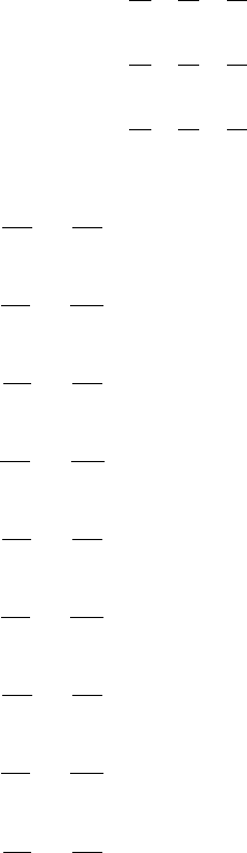
In the current code, the vertices and faces are numbered in a standardized fashion as
shown in Fig.2.1.
0 Base
1 Top
2 Front
4 Back
3 LHS
5 RHS
0
12
3
4
5
7
6
Figure 2.1: a. Reference cell and faces relative numbering b. Reference cell and vertices
numbering
The corresponding implementation can be found in:
Cell::orderDefiningPoints()
2.3 Mapping onto the Reference Face
DG method involves evaluation of surface integrations in order to find the numerical flux
at the cell-interface. The surface integrations in turn require mapping of a given arbitrary
surface on the reference surface. The parameterization of a plane surface requires two
parameters rand s.
2.3.1 Quadrilateral Faces
For a quadrilateral faces, the parameters assume the following values: (r, s)∈[−1,1].
However, the given surface can be arbitrarily oriented in the space, and thus requires
(x, y, z)position to be completely defined. We thus need to orient the surface such as one
of the variables becomes redundant. This means rotating the surface such as to make it
parallel to xy plane, for example. Thus, each surface needs to be re-oriented in space such
that the face normal ˆnbecomes parallel to the zaxis. After the we can map the rotated
face onto the standard element. Let θzbe the angle made by the face normal with the z
8

axis and θxbe the angle made by the face normal with the xaxis. The rotation matrix
rotates the face through θxfirst (counterclockwise) and the through θzcounterclockwise.
The resulting rotation matrix Ris given as:
R=< Rz, Rx>(2.29)
where,
Rx=
cos(θx)sin(θx) 0
−sin(θx)cos(θx) 0
0 0 1
;Rz=
cos(θz) 0 −sin(θz)
0 1 0
sin(θz) 0 cos(θz)
;(2.30)
and < a, b > indicates the dot product between matrices aand b. Matrix R−1indicates
the reverse transformation. The rotation matrix is calculated in,
Face::calculateRotationMatrixParallelToXY()
and the inverse matrix is computed in,
Face::calculateInverseRotationMatrix()
In order to describe the procedure to compute the Jacobian of transformation (|Jf|) for
face, we use the following nomencleture:
•(x, y, z): physical coordinate system (actual coordinates)
•(x0, y0, z0): Rotated coordinates such that the face is || to the xy plane
•(r, s): Reference coordinates such that r, s ∈[−1,1]
There are two ways the Jacobian can be computed.
Method 1
First, rotate each vertex of the face using R. i.e.
x0
i
y0
i
z0
i
=R
xi
yi
zi
, i ∈ {0,1,2,3}(2.31)
Each of the rotated points is then mapped to the standard element. After rotation of the
face, ∂z0
∂r = 0,∂z0
∂s = 0 since z0remains constant. The mapping from the rotated face f0to
the standard face fscan be defined through the shape functions.
N0=1
4(1 −r)(1 −s),{r, s ∈V|∀v∈V⊂R, v ∈[−1,1]}(2.32)
N1=1
4(1 + r)(1 −s)(2.33)
9
N2=1
4(1 + r)(1 + s)(2.34)
N3=1
4(1 −r)(1 + s)(2.35)
Then,
x0=
3
X
i=0
Nix0
i, y0=
3
X
i=0
Niy0
i,(2.36)
Equation2.36 can be used to find partial derivatives of x0and y0with respect to rand s.
The required face Jacobian is:
Jf=
∂x
∂r
∂x
∂s
∂y
∂r
∂y
∂s
∂z
∂r
∂z
∂s
(2.37)
which can be written as,
Jf=
x
y
z
.h∂
∂r
∂
∂s i=R−1
x0
y0
z0
.h∂
∂r
∂
∂s i(2.38)
i.e.
Jf=R−1Jf0(2.39)
where,
Jf0=
∂x0
∂r
∂x0
∂s
∂y0
∂r
∂y0
∂s
0 0
(2.40)
The procedure is summarized as,
1. Rotate the face so as to make it parallel to the xy plane.
2. Find the Jacobian of transformation from the rotated face to the standard face (Jf0).
3. Find the Jacobian of the face as given by equation 2.39.
4. |Jf|is given as q|(Jf)T(Jf)|
Method 2
In this method, we parametarize the surface x, y, z with parameters r, s. Let
X=xˆ
i+yˆ
j+zˆ
k
We use the standard shape functions to map the physical element to parameters r, s. i.e.
x=
3
X
i=0
Nixi, y =
3
X
i=0
Niyi, z =
3
X
i=0
Nizi,(2.41)
10

where same shape functions are used as earlier.
Note 2.4. In order to find the vertex mapping of a randomly oriented face with the
standard element, it would be advisable to first rotate the face to make it parallel to the xy
plane and then find the vertex mapping. Then find the shape function and proceed with
equation 2.41. However, we do not use the coordinates of the rotated face here.
After that, we find ∂X
∂r and ∂X
∂s . Then |Jf|is simply
∂X
∂r ×∂X
∂s
Both of these methods
are implemented in
Face::calculateJacobianQuadFace(double r, double s)
Any given quadrature point (r, s)can be mapped into (x, y, z)space using the two oper-
ations:
1. First find mapping from (r, s)to (x0, y0, z0)using equations 2.32-2.35 and 2.36.
2. Then map from (x0, y0, z0)to physical coordinates using R−1.
The global positioning of all the quadrature points on each face is stored in array
Face::quadPointsGlobalLocation
Index iruns over the surface quadrature points and index jruns over the x, y, z axes.
Note 2.5. Some of the volume quadrature points coincide with the surface quadrature
points. Function
DG::mapFaceQuadPointsToCellQuadPoints()
performs the mapping by direct comparison of global positioning of surface and volume
quadrature points.
The mapping of surface to volume quadrature points is stored in arrays
Face::mapOwnerQuadPoints[ ] and Face::mapNeighbourQuadPoints[ ].
Thus, if we are finding a 2nd-order polynomial for a face, then it should have 9quadra-
ture points (QP). The corresponding cell will meanwhile have 27 quadrature points, 9of
which will coincide with the face QP. Then if
Face::mapOwnerQuadPoints = [3, 2, 21, 14, ... , 7]
Then, it means the 0th quad point on face is same as the 3rd quad point of owner cell and
so on.
Note 2.6. In the improved version of the code, the face-vertex numbering is standardized,
such that the vertex numbering follows the right-hand rule. i.e. if the curled fingers
indicate the sequence of vertices, then the stretched thumb points in the direction of hte
face-normal. In that case, the rotation matrices are not required. i.e. both method 1 and
method 2 are obsolete. Refer:
Face::orderDefiningPoints()
11
2.4 Modal and Nodal Basis Functions
Basis functions are the independant dimensions on which any function can be projected.
In this chapter, we present a few modal and nodal basis functions.
2.4.1 Modal Basis Functions
These are the set of basis functions, where each dimension corresponds to a ‘mode’ or
frequency. A simple example is a set of monomials defined on the interval [a, b]
Note 2.7. This is just an example, in reality xcould be valid over (−∞,∞)
VK
mono ={1, x, x2, x3, ..., xK−1}, x ∈C0[a, b](2.42)
A polynomial up to order K−1can be represented exactly using Kmodal functions.
Thus, any general polynomial can be written as
PK(x) =
i=K−1
X
i=0
αixi, , x ∈C0[a, b](2.43)
The monomials is not a ‘good’ choice of the basis functions as we will see later, thus
we need a set of basis functions where each of the functions is ‘orthogonal’ (or better
‘orthonormal’) to every other functions. One such important set of orthogonal functions
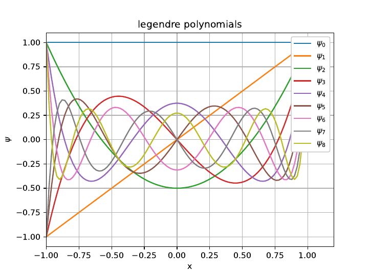
is called as ‘Jacobi’ polynomials. A special case of ‘Jacobi’ polynomials is ‘Legendre’
polynomials. In our code, we have extensively used Legendre polynomials. A general ith
modal basis function is indicated by symbol ψi. Other popular example of modal basis
functions is a set of Chebyshev polynomials.
Figure 2.2: First 9Legendre polynomials
12

Fig.2.2 shows first 9Legendre polynomials. Observe that the ‘frequency’ of the polyno-
mials increases (for increasing count) indicating higher modes. Fig.2.3 shows Chebyshev
polynomials.
Figure 2.3: First 9Chebyshev polynomials
The 1D modal functions are implemented in:
FunctionalSpace::monomials1D(args),
FunctionalSpace::legendrePolynomial1D(args),
FunctionalSpace::chebyshevPolynomial1D(args) and
FunctionalSpace::jacobiPolynomial1D(args)
It is indeed difficult to comprehend how the polynomials shown in Fig.2.2 and Fig.2.3 be
‘orthogonal’. The main reason for this is that we try to stick to our understanding of the
3D space and the notion of orthogonality that comes with it, however, the polynomial
space is essentially ∞dimensional space. For this space, the definition of orthogonality
depends on the definition of the Inner-Product and ‘metric’ of that space. For L2space,
the orthogonality is defined as,
ZΩ
ψiψjdΩ = αδij ,∀ψi, ψj∈L2{Ω}&α∈R(2.44)
where, δij is a ‘Kronecker Delta’ which means δij = 1 if i=jand 0otherwise. The
functions ψiand ψjare orthonormal if α= 1.
2.4.2 Nodal Basis Functions
The ‘nodal’ basis functions are the set of functions which are ‘Cardinal’ in nature. What
that means is, at the interpolation point, the basis function will have value 1and for all
13

other collocation points, the value of the basis function will be zero. Thus, the interpolated
value of the function agrees perfectly at the collocation points but may have some error
at other places. The general symbol used for nodal basis functions is φ. The interpolation
itself is given as,
fN(x) =
N−1
X
i=0
f(xi)φi(x), x ∈C0[a, b](2.45)
and, φi(xj) = δij . We use Lagrange polynomials as the nodal basis functions. The
polynomials in 1D are give as,
φi(x) =
N−1
Y
j=0,j6=i
(x−xj)
(xi−xj)(2.46)
it is clear that at x=xi,φi(xi) = 1. One crucial point that needs to be taken care
of is selection of the collocation points [x0, x1, ..., xN−1]. It is seen that the equi-spaced
arrangement of collocation points gives poor interpolation for very high orders of accura-
cies. Therefore we take these points as roots of orthonormal modal polynomials. Popu-
lar choices for collocation points are Gauss-Legendre (LG) collocation points, Legendre-
Gauss-Lobatto (LGL) points or Chebyshev points. An important distinction between LG
and LGL points is that, LGL points include the ‘end-points’ whereas LG points include
only the internal points. For DG methods, this doesn’t have a significant difference since
solving a Riemann problem at the face remains unchanged.
2.4.3 Multidimensional Interpolation
For number of dimensions greater than 1, the interpolating polynomials are obtained
depending on the type of the element we wish to interpolate on. For hex elements, these
are obtained using tensor product of 1D polynomials. i.e.
φ(x, y, z) = φ1D(x)φ1D(y)φ1D(z)(2.47)
Whereas, for other types of elements, special multidimensional polynomials are used.
However, the concept of modal and nodal basis functions remains essentially the same
irrespective of the number of dimensions.
14

Chapter 3
Code Structure
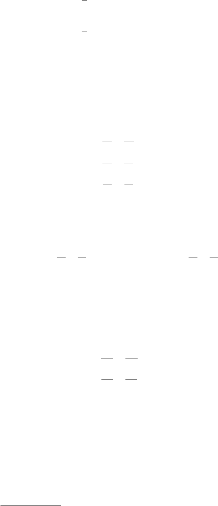
Roughly the code structure is displayed in Fig.3.1. For more accurate and detailed de-
scription, run Doxygen utility and refer the generated documentation.
Point
Cell
Face
DG
Functional Space
Math Functions
OF Input
GeometryIO Tensor
Figure 3.1: Class dependency (crudely)
Each of the the constituent elements are briefly described next.
15
3.1 Code structure
3.1.1 Tensor
MEANDG has a central datastructure called as ‘Tensor’, which forms all the important
arrays, matrices, multidimensional storage lists etc. Refer ‘include/Tensor’ for details.
Tensor class is made of 4 sub-classes.
TensorO1<dType>, TensorO2<dType>, TensorO3<dType>, Matrix<dType>
From these, O(1), O(2), O(3) tensors can be created of arbitrary dimensions. The tensor
objects interact with one another and have several in-build methods such as L1, L2, L∞
norms etc. All the maths functions accept objects of Tensor library.
Following example code shows usage of tensor class:
TensorO1<double> A(5); // creates a O(1) tensor of size 5 with
// data-members of the type double
TensorO1<double> C(5);
for (int i=0; i<5; i++){
// generate a random number between 0 and 100
double valueA = getRandom(0.0,100.0);
// generate another random number between 0 and 100
double valueC = getRandom(0.0,100.0);
// set value at ith index
A.setValue(i, valueA);
C.setValue(i, valueC);
};
// now A and C have random values
double dotAnswer = Math::dot(A,C); // perform math product between two arrays
cout << dotAnswer << endl; // print the answer
For further details and the available functions, refer the code documentation.
3.1.2 Point
Point is a physical point in (x, y, z)coordiante system. It has a unique id, and description
of its location.
3.1.3 Cell
If the domain is indicated by Ω, then the descritization of the domain (Ωh) is described
as,
Ωh=
n
[
l=1
Si(3.1)
16
where Siare the finite volume cells. These are non-overlapping pieces of the domain.
Each cell has the following important attributes (among others):
•Vertices (of the type ‘Point’)
•Faces (i.e. boundary of the cell)
•Degrees of Freedom (i.e. locations where unkowns are evaluated)
•Data (such as the conserved variables)
•Volume
•Mathematical constructs (Mass matrix, Stiffness matrix etc.)
•Mapping onto the standart cell (Jacobian etc.)
Thus, each of these parameters (among others) can be accessed using the accessor
(get, set) functions of the class ‘Cell’. For further details, refer Cell.h and Cell.cpp.
3.1.4 Face
A face is the boundary of a Cell. The face has following important attributes:
•Geometrical information (area, normal, vertices etc.)
•Neighbour and Owner cells
•Data (numerical flux and variables)
•Mapping (Jacobian etc.)
3.1.5 GeometryIO
This module reads the input file in the OpenFOAM format and fills the data arrays.
Refer:
GeometryIO::fillDataArrays(args)
3.1.6 Functional Space
This module is responsible for everything related to L2, H1functional spaces. It contains
nodal, modal basis functions and derivatives. It also computes various matrices used in
DG formulation.
3.1.7 Math functions
These are various mathematical functions.
17

3.1.8 Gasdynamics, Riemann solvers etc.
Depending on the system of equations which one wants to solve, include the physics-
specific functions and files. For example, for Euler’s equations of Gasdynamics, we have
Gasdyanmics.cpp module and corresponding Riemann solvers. Apart from these, there
are test functions, display functions etc. Refer the code files in ‘include/’ and ‘src/’ folders.
3.1.9 DG
This is the core (central) module of the code. It performs following operations:
•Memory management
•Cells, faces creation
•Calling appropriate functions for computation of cell matrices
•Time integration
•PDE solving
Currently it is configured to solve the hyperbolic system of PDEs of the type:
∂Q
∂t +∇.F(Q)=0 (3.2)
18
Chapter 4
Applications
19
Chapter 5
License
MEANDG is licensed under BSD-3 clause license. Refer:
https://en.wikipedia.org/wiki/BSD_licenses
The library Eigen which is used in this software (see ./include/Eigen/) is licensed under
MPL2 (see ./include/Eigen/COPYING.README).
Use preprocessor flag -DEIGEN_MPL2_ONLY to ensure that only MPL2 (and possibly
BSD) licensed code from Eigen is compiled. Refer
http://eigen.tuxfamily.org/index.php?title=Main\_Page#License
for details. No files of the Eigen library are modified for use with MEANDG.
5.1 LICENSE
Copyright (c) 2018, Subodh Joshi, Tapan Mankodi, Shivasubramanian Gopalakrishnan
All rights reserved.
Redistribution and use in source and binary forms, with or without modification, are
permitted provided that the following conditions are met:
1. Redistributions of source code must retain the above copyright notice, this list of
conditions and the following disclaimer.
2. Redistributions in binary form must reproduce the above copyright notice, this list
of conditions and the following disclaimer in the documentation and/or other materials
provided with the distribution.
3. Neither the name of the copyright holder nor the names of its contributors may be used
to endorse or promote products derived from this software without specific prior written
permission.
THIS SOFTWARE IS PROVIDED BY THE COPYRIGHT HOLDERS AND CONTRIBUTORS "AS IS" AND ANY
EXPRESS OR IMPLIED WARRANTIES, INCLUDING, BUT NOT LIMITED TO, THE IMPLIED WARRANTIES OF
MERCHANTABILITY AND FITNESS FOR A PARTICULAR PURPOSE ARE DISCLAIMED. IN NO EVENT SHALL
THE COPYRIGHT HOLDER OR CONTRIBUTORS BE LIABLE FOR ANY DIRECT, INDIRECT, INCIDENTAL, SPE-
CIAL, EXEMPLARY, OR CONSEQUENTIAL DAMAGES (INCLUDING, BUT NOT LIMITED TO, PROCUREMENT
OF SUBSTITUTE GOODS OR SERVICES; LOSS OF USE, DATA, OR PROFITS; OR BUSINESS INTERRUPTION)
HOWEVER CAUSED AND ON ANY THEORY OF LIABILITY, WHETHER IN CONTRACT, STRICT LIABILITY,
OR TORT (INCLUDING NEGLIGENCE OR OTHERWISE) ARISING IN ANY WAY OUT OF THE USE OF THIS
SOFTWARE, EVEN IF ADVISED OF THE POSSIBILITY OF SUCH DAMAGE.
20
