Lab Manual 1
User Manual:
Open the PDF directly: View PDF ![]() .
.
Page Count: 24

Page | 1
Ahsanullah University of Science and Technology
Department of Computer Science and Engineering
Course No: CSE 4228
Course Title: Digital Image Processing Lab
LAB MANUAL – 1
Objective:
The objective of this lab session is to getting familiar with MATLAB. This will cover the following topics –
1) MATLAB workspace, Command Window, Variable panel
2) Working with variables, vectors and function
3) Working with library functions.
4) Getting started with MATLAB plotting tools.
Software: MATLAB (any version higher than 2009a)
Pre-requisite: Vector, Matrix, Linear Algebra, Geometry, C, C++.
References:
[1] https://www.mathworks.com/help/matlab/learn_matlab/desktop.html
[2] https://www.mathworks.com/help/matlab/elementary-math.html
[3] https://www.mathworks.com/help/matlab/learn_matlab/matrices-and-arrays.html
[4] https://www.mathworks.com/help/matlab/functionlist.html?s_cid=doc_ftr
[5] https://www.mathworks.com/help/matlab/2-and-3d-plots.html
___________________________________________________________________________________
Page | 2
Figure 1
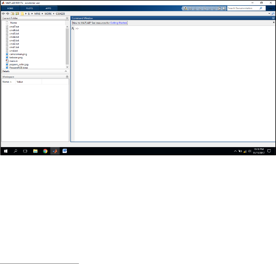
The desktop includes these panels (Figure 1): [1]
Current Folder — Access your files.
Command Window — Enter commands at the command line, indicated by the prompt (>>).
Workspace — Explore data that you create or import from files.
Variables and the workspace:
Let’s start with variable.
a = 2
After entering, the immediate next line will display the variable with the assigned value.
a =
2
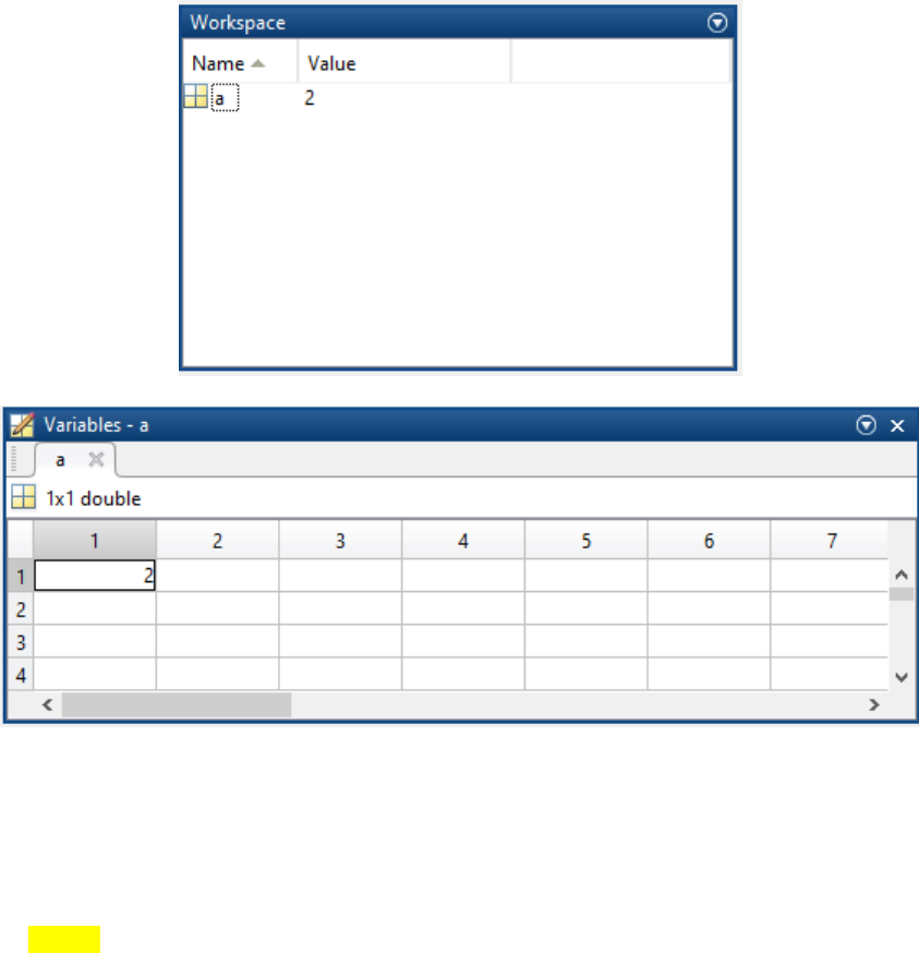
And you can see that, the variable is appeared in the workplace (Figure 2 a). If you double click on that
variable icon, a panel named ‘Variables’ will popup (Figure 2 b).
Page | 3
MATLAB stores everything as matrix. You can note the indication of 1 x 1 double in the variable
panel. It mean a is a 1 by 1 matrix (eventually a matrix with only one element), which is double type.
By default any numerical data is double type. There are other data types as well such as uint8
(unsigned integer 8 bit), char (character), logical (boolean).
(a)
(b)
Figure 2
Note that, throughout this manual, to make it more readable, we will highlight the commands, and the
prompted output will not be highlighted. For example, the following is a command.
b = 3
And the following is the immediate prompt.
b =
3
Let’s start with type casting.

Page | 4
a = 1
a =
1
d = logical(a)
d =
1
You can see that, d will be stored as 1 x 1 logical variable in the workspace.
Now, Let’s work more with variables and arithmetic operations. Let’s play with some simple arithmetic
operations. Assume that we have already have a and b in our workspace.
a + b
ans =
5
Observe that, ans is a default variable that stores the result of a + b, and it is stored in workspace. If
you simply use ans as a command, the value inside ans will be prompted.
ans
ans =
5
But, we can store the result in a different variable as well.
c = a + b
c =
5
c = a * b
c =
6
c = b^3 % power of 3

Page | 5
c =
27
You can observe that, % is used for commenting in MATLAB.
There are some special variables.
pi
ans =
3.1416
c = a*pi
c =
6.2832
Some library functions:
Some useful library functions for trigonometric operations are shown below.
c = cos(30) % take radian as input
c =
0.1543
c = cos(2*pi)
c =
1
c = cosd(30) % take degree as input
c =
0.8660
acosd(c) % inverse cosine (in degree)
ans =
30.0000
You can also try sin(), tan() etc.

Page | 6
Some other important functions are provided below.
c = mod(10,3) % remainder
c =
1
c = exp(2) % exponential
c =
7.3891
d = ceil(c) % ceiling (there is floor() and round() as well)
d =
8
c = log(10) %natural logarithm
c =
2.3026
c = log10(10) % 10 base logarithm
c =
1
There is a huge collection of functions dedicated for elementary math. You can find them here [1].
Let’s see some other useful command.
pwd : to print the current directory
clc : to clean command prompt history
clear : to delete all the variables from the workspace. You can delete a particular variable
from the workspace by the clear command followed by the variable name. For example,
clear c

Page | 7
Using / not using semicolon:
Semicolons (;) can be used after each command. If used, the output prompt will be suppressed. For
example, if you use the following command without a semicolon at the end, the output will be
prompted.
d = cos(pi)
d =
-1
But, if you use the following command with a semicolon at the end, the output will not be prompted.
d = cos(pi);
Working with vector and matrix:
Defining a row vector –
v = [1, 2, 3, 4]
v =
1 2 3 4
You can also omit the commas (,) in between the elements. This will give you the same vector.
v = [1 2 3 4]
v =
1 2 3 4
We are going to follow this approach throughout this manual.
Now, Defining a column vector –
v = [1; 2; 3; 4]
v =
1
2
3
4

Page | 8
Having the idea of row and column vector, now we can easily define a matrix –
M = [1 2 3 4; 5 6 7 8; 9 1 2 3]
M =
1 2 3 4
5 6 7 8
9 1 2 3
In MATLAB, the matrix element indices start from the top left corner. As we traverse right, we go
through each column. And as we traverse down, we go through each row.
1 2 3 4
5 6 7 8
9 1 2 3
Accessing elements of a matrix:
Now let’s see how to access elements from a matrix. To access we use the following format of the
command: Matrix (which_row, which_column). For example, Let’s assume that we have
matrix M in our workspace.
m = M(1,1) % accessing 1st row, 1st column from M
m =
1
m = M(2,3) % accessing 2nd row, 3rd column from M
m =
7
You can use end to access the last element in a row or column.
M(1, end) % 1st row, last column
ans =
4
1st row ->
3rd row ->
1st column
|
˅
4th column
|
˅

Page | 9
M(end, end) % last row, last column
ans =
3
Assigning elements of a matrix:
M(2,2) = 99
M =
1 2 3 4
5 99 7 8
9 1 2 3
Some library functions to generate matrix:
eye (m) : Generating an identity matrix, For example, for m = 5
I = eye(5) % identity matrix of 5 x 5
I =
1 0 0 0 0
0 1 0 0 0
0 0 1 0 0
0 0 0 1 0
0 0 0 0 1
ones (m) : Generating a matrix that contains only 1 (one). For example, m = 5
I = ones(5)
I =
1 1 1 1 1
1 1 1 1 1
1 1 1 1 1
1 1 1 1 1
1 1 1 1 1
You can also generate matrix rather than square shape. You can use ones (m,n) to define rows and
columns. For example,

Page | 10
I = ones(3,5) % 3 rows and 4 columns
I =
1 1 1 1 1
1 1 1 1 1
1 1 1 1 1
Similarly,
I = zeros(3,5)
I =
0 0 0 0 0
0 0 0 0 0
0 0 0 0 0
I = rand(3,5)
I =
0.8147 0.9134 0.2785 0.9649 0.9572
0.9058 0.6324 0.5469 0.1576 0.4854
0.1270 0.0975 0.9575 0.9706 0.8003
I = ceil(rand(3,2))
I =
1 1
1 1
1 1
Let’s apply matrix operations of two matrices A and B.
A = [1 2 3; 4 5 6; 7 8 9]
A =
1 2 3
4 5 6
7 8 9
B = [9 8 7; 6 5 4; 3 2 1]

Page | 11
B =
9 8 7
6 5 4
3 2 1
C = A + B
C =
10 10 10
10 10 10
10 10 10
C = A - B
C =
-8 -6 -4
-2 0 2
4 6 8
C = A * B
C =
30 24 18
84 69 54
138 114 90
C = 2*A
C =
2 4 6
8 10 12
14 16 18
C = A^2
C =
30 36 42
66 81 96
102 126 150
Q.1: Now, can you generate a matrix with random numbers greater than or equal to 1 using one single
line of command?
Page | 12
We can apply element wise operations. To perform that, we need to put a dot(.) in front of the operator.
For example, the following command will do element wise multiplication, that means 1st element of A
will be multiplied with the 1st element of B, 2nd of A will be multiplied with 2nd element of B, and so on.
C = A .* B
C =
9 16 21
24 25 24
21 16 9
Q.2: Now, can you square every element of the matrix A using one single line of command?
Q.3: Also, can you square each elements of both A and B, add the squared elements of A with the
squared elements B and store them in the matrix C? (Again, using one single line of command)
Using colon operator:
Let’s take the matrix A in previous examples.
A = [1 2 3; 4 5 6; 7 8 9]
A =
1 2 3
4 5 6
7 8 9
Say, we want to access all the columns at 1st row, that is 1, 2 and 3
c1 = A(1,:)
c1 =
1 2 3
Moreover,
c1 = A(2,:) % 2nd row, all columns
c1 =
4 5 6
Similarly, to get all rows at 3rd columns -

Page | 13
r1 = A(:,3)
r1 =
3
6
9
We can use colon operator to convert a matrix into a column vector.
v = A(:)
v =
1
4
7
2
5
8
3
6
9
Colon operator is very useful to access a range of elements from a matrix. To give an example, let’s take
a bigger matrix.
R = floor(rand(7)*10)
R =
1 5 0 4 1 0 0
2 9 0 0 6 2 4
6 2 5 3 2 9 1
4 7 7 1 6 1 9
3 7 9 7 6 8 0
8 3 1 3 7 5 7
5 5 5 5 4 9 8
Say, we want to access 2nd row to 5th row of 1st column.
s = R(2:5, 1)
s =
2
6
4
3

Page | 14
Similarly,
s = R(1, 2:5) % column 2 to 5 of row 1
s =
5 0 4 1
We can crop a region using the same concept. For example, row 2 to 5 and column 3 to 6.
S = R(2:5, 3:6)
S =
0 0 6 2
5 3 2 9
7 1 6 1
9 7 6 8
For better understanding, the elements of S accessed from R are gray-shaded below.
1 5 0 4 1 0 0
2 9 0 0 6 2 4
6 2 5 3 2 9 1
4 7 7 1 6 1 9
3 7 9 7 6 8 0
8 3 1 3 7 5 7
5 5 5 5 4 9 8
We can assign as well.
R(2:5, 3:6) = 99
R =
1 5 0 4 1 0 0
2 9 99 99 99 99 4
6 2 99 99 99 99 1
4 7 99 99 99 99 9
3 7 99 99 99 99 0
8 3 1 3 7 5 7
5 5 5 5 4 9 8
The colon operator is useful to generate a range of values. Say, we want to create a vector named data
with values from 1 to 10.
data = 1:10

Page | 15
data =
1 2 3 4 5 6 7 8 9 10
data = 1:2:10 % increment by 2 steps
data =
1 3 5 7 9
Q.4: Can you generate a vector containing 10 values stating from pi to 2*pi with equal steps in between?
Some library function for matrix/ vector:
Transpose of Vector:
t = transpose(data)
t =
1
3
5
7
9
Same thing can be done using a single quote (‘) operator.
t = data'
t =
1
3
5
7
9
Sorting a vector:
t = sort(data)

Page | 16
t =
1 3 5 7 9
Many MATLAB functions can be overloaded.
t = sort(data, 'descend')
t =
9 7 5 3 1
Sum of all the elements of a vector:
k = sum(data)
k =
25
Mean, median:
k = mean(data)
k =
4.1429
k = median(data)
k =
4
Transpose of Matrixr:
R = floor(rand(5)*10)
R =
2 2 3 5 7
6 7 4 3 0
6 2 6 4 6
1 8 8 7 4
4 8 6 8 4
r = R'

Page | 17
r =
2 6 6 1 4
2 7 2 8 8
3 4 6 8 6
5 3 4 7 8
7 0 6 4 4
Sorting a Matrix:
R = floor(rand(5)*10)
R =
8 4 1 8 0
0 9 8 6 2
3 1 5 3 1
2 2 5 5 1
8 1 1 4 2
By default, MATLAB sorts row-wise. That means it treats every column as an individual vector
and sort them.
s = sort(R)
s =
0 1 1 3 0
2 1 1 4 1
3 2 5 5 1
8 4 5 6 2
8 9 8 8 2
However, if you want to perform colum-wise, just pass 2 as parameter.
s = sort(R,2)
s =
0 1 4 8 8
0 2 6 8 9
1 1 3 3 5
1 2 2 5 5
1 1 2 4 8
This concept works for other functions as well.

Page | 18
Sum of Matrix:
k = sum(R) % row-wise
k =
21 17 20 26 6
k = sum(R,2) % column-wise
k =
21
25
13
15
16
k = sum(R(:)) %sum of all the values.
k =
90
Mean of Matrix:
k = mean(R) % row-wise
k =
4.2000 3.4000 4.0000 5.2000 1.2000
k = mean(R,2) % column-wise
k =
4.2000
5.0000
2.6000
3.0000
3.2000
k = mean(R(:))% mean of all
k =
3.6000
Page | 19
More functions can be found here [4].
Plotting:
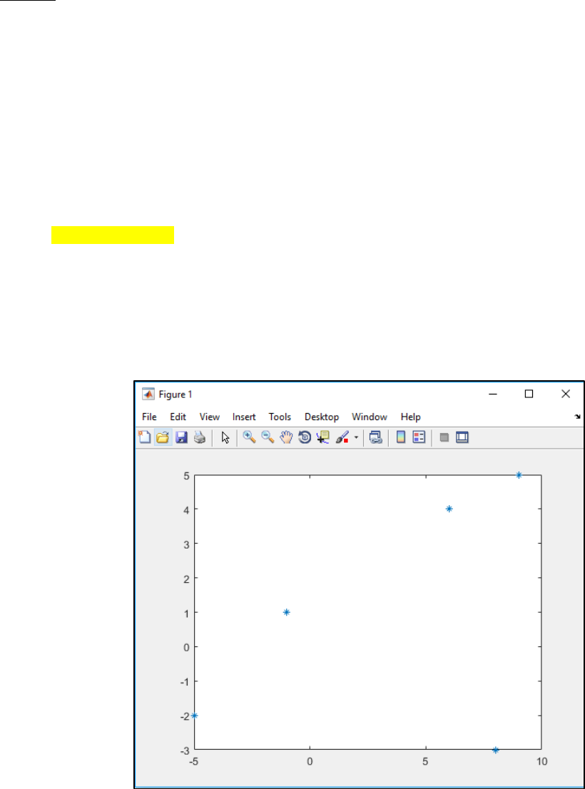
Assume that, we want to plot five 2-D points. The (x, y) coordinates are (-5, -2), (6, 4),
(8, -3), (9, 5) and (-1, 1). Now, let’s store this coordinate data in two vectors X and Y,
where X contains all x-coordinates and Y contains all the y-coordinates.
X = [-5 6 8 9 -1];
Y = [-2 4 -3 5 1];
To plot them, we can simply call the plot() function.
Plot(X,Y,’*’)
A window will pop up (Figure 3) showing the axis and the plotted points. Points will be plotted with (*)
as we pass this as the third parameter. These are called markers. You can use ‘.’, ‘O’, ‘o’, ‘X’,
‘x’ etc. as markers.
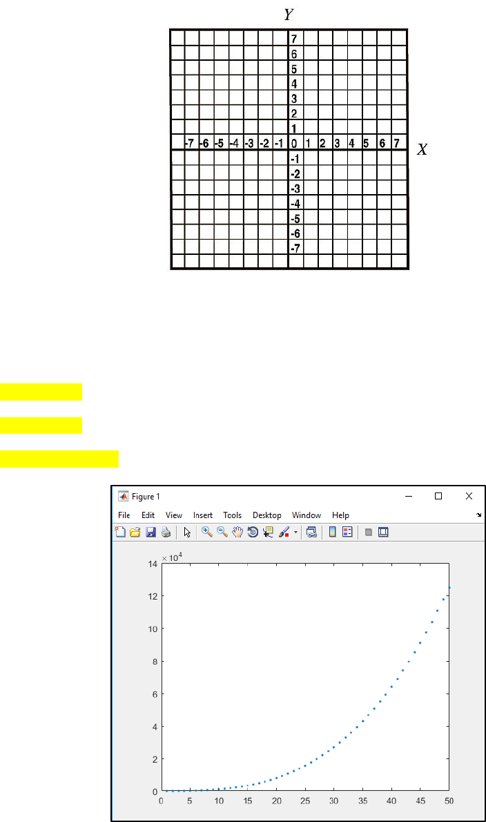
Note that, MATLAB plotting axis system follows the conventional Cartesian coordinates (Figure 4).
Figure 3
Page | 20
Figure 4
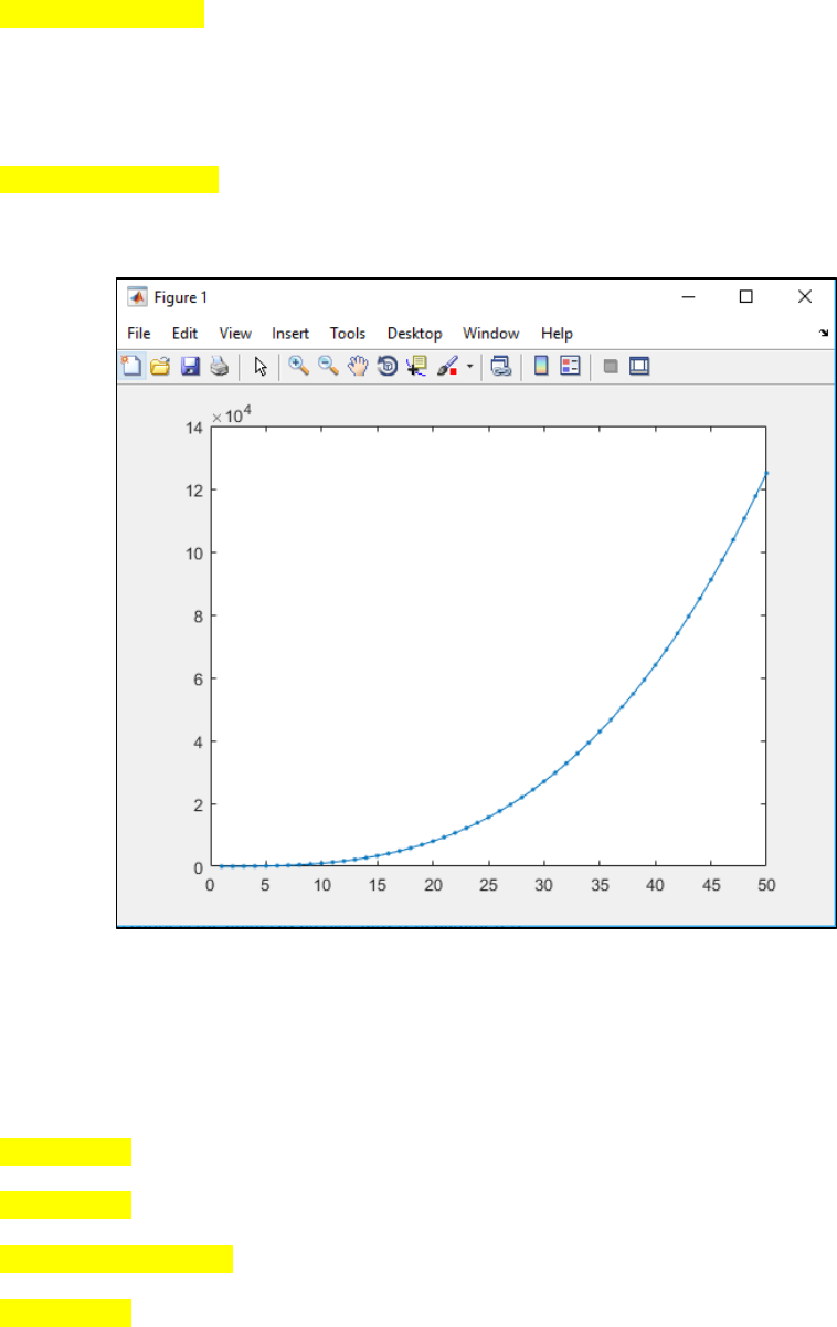
Let’s plot y = x3 equation. We define 50 points for x. Then obtain the y from y = x3 equation (Figure
5).
x = 1:50;
y = x.^3;
plot(x,y,'.')
Figure 5
Page | 21
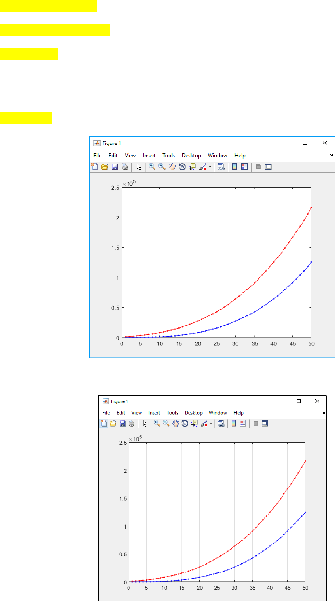
We can connect the points by passing different parameter.
plot(x,y,'.-')
A hyphen after the dot means to connect the dots with a continuous line (Figure 6).
You can also change the colors of the markers.
plot(x,y,'.-r') % r stands for red.
Figure 6
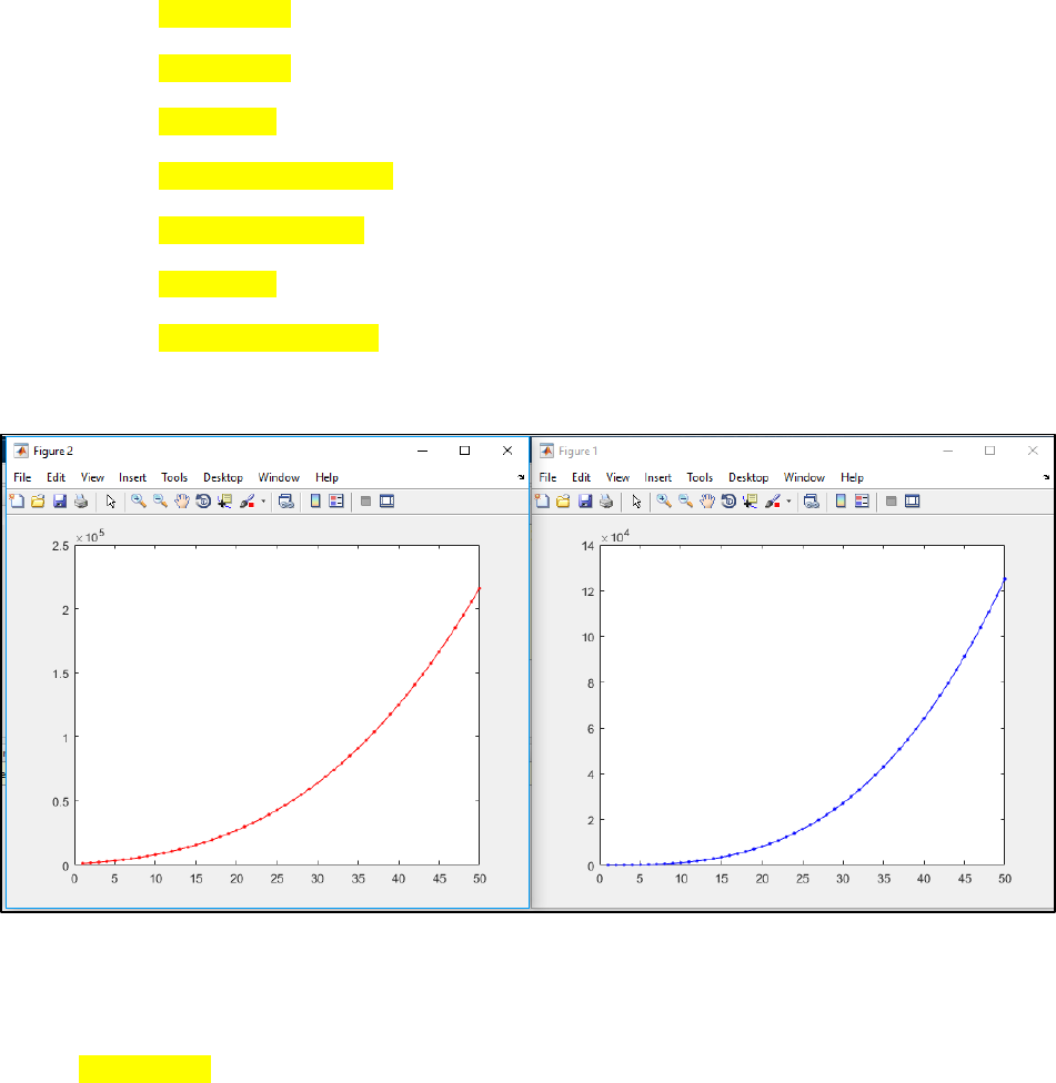
MATLAB allows you to redraw on a current figure. Say, we want to plot y = (x+10)3 along with the y
= x3. That means you want to plot on top each other. In that case, we use hold on command to let
the figure window wait for next plotting.
x = 1:50;
y = x.^3;
plot(x,y,'.-b'); % plotting the first equation
hold on; % holding the figure to wait.
Page | 22
y = (x+10).^3; % deriving the y for the second equation
plot(x,y,'.-r'); % plotting the first equation
hold off; % do not wait any more
See output in figure 7a. You can introduce grid lines on the current figure (Figure 7b). To do this, keep
the current figure opened and enter the command –
grid on;
(a)
(b)
Page | 23
Figure 7
Also, you can have multiple figures for multiple plotting. Say, we want the previous two equations to be
plotted in two different figure windows. In that case, enter figure command to open a new figure
(Figure 8).
x = 1:50;
y = x.^3;
figure; % new window
plot(x,y,'.-b');
y = (x+10).^3;
figure; % new window
plot(x,y,'.-r');
Figure 8
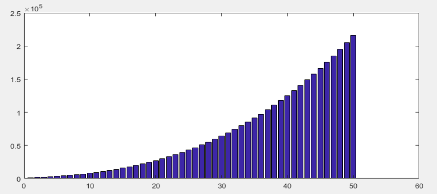
Another useful plotting function is bar(). For example,
bar(x, y)
Figure 9 shows the output.
Page | 24
Figure 9
More about MATLAB plotting is available here [5].
[END]
___________________________________________________________________________________
Prepared by-
Mohammad Imrul Jubair