Linear Mixed S: A Practical Guide Using Statistical Software, Second Edition S Stat Softw 2014
User Manual:
Open the PDF directly: View PDF ![]() .
.
Page Count: 434 [warning: Documents this large are best viewed by clicking the View PDF Link!]
- Front Cover
- Dedication
- Contents
- List of Tables
- List of Figures
- Preface to the Second Edition
- Preface to the First Edition
- The Authors
- Acknowledgments
- 1. Introduction
- 2. Linear Mixed Models: An Overview
- 3. Two-Level Models for Clustered Data: The Rat Pup Example
- 4. Three-Level Models for Clustered Data: The Classroom Example
- 5. Models for Repeated-Measures Data: The Rat Brain Example
- 6. Random Coefficient Models for Longitudinal Data: The Autism Example
- 7. Models for Clustered Longitudinal Data: The Dental Veneer Example
- 8. Models for Data with Crossed Random Factors: The SAT Score Example
- A. Statistical Software Resources
- B. Calculation of the Marginal Variance-Covariance Matrix
- C. Acronyms/Abbreviations
- Bibliography

K15924
Highly recommended by JASA, Technometrics, and other journals, the rst
edition of this bestseller showed how to easily perform complex linear mixed
model (LMM) analyses via a variety of software programs. Linear Mixed Models:
A Practical Guide Using Statistical Software, Second Edition continues to
lead you step by step through the process of tting LMMs. This second edition
covers additional topics on the application of LMMs that are valuable for data
analysts in all elds. It also updates the case studies using the latest versions
of the software procedures and provides up-to-date information on the options
and features of the software procedures available for tting LMMs in SAS, SPSS,
Stata, R/S-plus, and HLM.
New to the Second Edition
• A new chapter on models with crossed random effects that uses a case
study to illustrate software procedures capable of tting these models
• Power analysis methods for longitudinal and clustered study designs,
including software options for power analyses and suggested approaches
to writing simulations
• Use of the lmer() function in the lme4 R package
• New sections on tting LMMs to complex sample survey data and Bayesian
approaches to making inferences based on LMMs
• Updated graphical procedures in the software packages
• Substantially revised index to enable more efcient reading and easier
location of material on selected topics or software options
• More practical recommendations on using the software for analysis
• A new R package (WWGbook) that contains all of the data sets used in the
examples
Ideal for anyone who uses software for statistical modeling, this book eliminates
the need to read multiple software-specic texts by covering the most popular
software programs for tting LMMs in one handy guide. The authors illustrate the
models and methods through real-world examples that enable comparisons of
model-tting options and results across the software procedures.
West, Welch, and Gałecki
SECOND
EDITION
LINEAR MIXED MODELS
Statistics
K15924_cover.indd 1 6/13/14 3:30 PM
SECOND EDITION
LINEAR MIXED MODELS
A Practical Guide Using Statistical Software
This page intentionally left blankThis page intentionally left blank

Brady T. West
Kathleen B. Welch
Andrzej T. Gałecki
University of Michigan
Ann Arbor, USA
with contributions from Brenda W. Gillespie
SECOND EDITION
LINEAR MIXED MODELS
A Practical Guide Using Statistical Software
First edition published in 2006.
CRC Press
Taylor & Francis Group
6000 Broken Sound Parkway NW, Suite 300
Boca Raton, FL 33487-2742
© 2015 by Taylor & Francis Group, LLC
CRC Press is an imprint of Taylor & Francis Group, an Informa business
No claim to original U.S. Government works
Version Date: 20140326
International Standard Book Number-13: 978-1-4665-6102-1 (eBook - PDF)
This book contains information obtained from authentic and highly regarded sources. Reasonable efforts have been made to
publish reliable data and information, but the author and publisher cannot assume responsibility for the validity of all materials
or the consequences of their use. The authors and publishers have attempted to trace the copyright holders of all material repro-
duced in this publication and apologize to copyright holders if permission to publish in this form has not been obtained. If any
copyright material has not been acknowledged please write and let us know so we may rectify in any future reprint.
Except as permitted under U.S. Copyright Law, no part of this book may be reprinted, reproduced, transmitted, or utilized in any
form by any electronic, mechanical, or other means, now known or hereafter invented, including photocopying, microfilming,
and recording, or in any information storage or retrieval system, without written permission from the publishers.
For permission to photocopy or use material electronically from this work, please access www.copyright.com (http://www.copy-
right.com/) or contact the Copyright Clearance Center, Inc. (CCC), 222 Rosewood Drive, Danvers, MA 01923, 978-750-8400.
CCC is a not-for-profit organization that provides licenses and registration for a variety of users. For organizations that have been
granted a photocopy license by the CCC, a separate system of payment has been arranged.
Trademark Notice: Product or corporate names may be trademarks or registered trademarks, and are used only for identifica-
tion and explanation without intent to infringe.
Visit the Taylor & Francis Web site at
http://www.taylorandfrancis.com
and the CRC Press Web site at
http://www.crcpress.com
To Laura and Carter
To all of my mentors, advisors, and teachers, especially my parents and grandparents
—B.T.W.
To Jim, my children, and grandchildren
To the memory of Fremont and June
—K.B.W.
To Viola, my children, and grandchildren
To my teachers and mentors
In memory of my parents
—A.T.G.
This page intentionally left blankThis page intentionally left blank

Contents
List of Tables xv
List of Figures xvii
Preface to the Second Edition xix
Preface to the First Edition xxi
The Authors xxiii
Acknowledgments xxv
1 Introduction 1
1.1 WhatAreLinearMixedModels(LMMs)?.................. 1
1.1.1 Models with Random Effects for Clustered Data . . . . . . . . . 2
1.1.2 Models for Longitudinal or Repeated-Measures Data . . . . . . 2
1.1.3 ThePurposeofThisBook ..................... 3
1.1.4 OutlineofBookContents ...................... 4
1.2 ABriefHistoryofLMMs ........................... 5
1.2.1 KeyTheoreticalDevelopments ................... 5
1.2.2 KeySoftwareDevelopments..................... 7
2 Linear Mixed Models: An Overview 9
2.1 Introduction .................................. 9
2.1.1 TypesandStructuresofDataSets ................. 9
2.1.1.1 Clustered Data vs. Repeated-Measures and Longitudinal
Data ............................ 9
2.1.1.2 LevelsofData ....................... 11
2.1.2 Types of Factors and Their Related Effects in an LMM . . . . . 12
2.1.2.1 FixedFactors ....................... 12
2.1.2.2 RandomFactors ...................... 12
2.1.2.3 FixedFactorsvs.RandomFactors............ 13
2.1.2.4 FixedEffectsvs.RandomEffects ............ 13
2.1.2.5 Nested vs. Crossed Factors and Their Corresponding Ef-
fects ............................ 14
2.2 SpecificationofLMMs ............................. 15
2.2.1 General Specification for an Individual Observation . . . . . . . . 15
2.2.2 GeneralMatrixSpecification .................... 16
2.2.2.1 Covariance Structures for the DMatrix......... 19
2.2.2.2 Covariance Structures for the RiMatrix ........ 20
2.2.2.3 Group-Specific Covariance Parameter Values for the D
and RiMatrices ...................... 21
2.2.3 Alternative Matrix Specification for All Subjects . . . . . . . . . 21
vii
viii Contents
2.2.4 Hierarchical Linear Model (HLM) Specification of the LMM . . 22
2.3 TheMarginalLinearModel .......................... 22
2.3.1 SpecificationoftheMarginalModel ................ 23
2.3.2 TheMarginalModelImpliedbyanLMM ............. 23
2.4 EstimationinLMMs ............................. 25
2.4.1 MaximumLikelihood(ML)Estimation .............. 25
2.4.1.1 Special Case: Assume θIsKnown ............ 26
2.4.1.2 General Case: Assume θIsUnknown .......... 26
2.4.2 REMLEstimation .......................... 27
2.4.3 REMLvs.MLEstimation...................... 28
2.5 ComputationalIssues ............................. 29
2.5.1 Algorithms for Likelihood Function Optimization . . . . . . . . . 29
2.5.2 Computational Problems with Estimation of Covariance Parame-
ters .................................. 31
2.6 ToolsforModelSelection ........................... 33
2.6.1 BasicConceptsinModelSelection ................. 34
2.6.1.1 NestedModels ....................... 34
2.6.1.2 Hypotheses: Specification and Testing . . . . . . . . . . 34
2.6.2 LikelihoodRatioTests(LRTs) ................... 34
2.6.2.1 Likelihood Ratio Tests for Fixed-Effect Parameters . . . 35
2.6.2.2 Likelihood Ratio Tests for Covariance Parameters . . . 35
2.6.3 AlternativeTests........................... 36
2.6.3.1 Alternative Tests for Fixed-Effect Parameters . . . . . . 36
2.6.3.2 Alternative Tests for Covariance Parameters . . . . . . 38
2.6.4 InformationCriteria ......................... 38
2.7 Model-BuildingStrategies ........................... 39
2.7.1 TheTop-DownStrategy....................... 39
2.7.2 TheStep-UpStrategy ........................ 40
2.8 CheckingModelAssumptions(Diagnostics) ................. 41
2.8.1 ResidualDiagnostics......................... 41
2.8.1.1 RawResiduals ....................... 41
2.8.1.2 Standardized and Studentized Residuals . . . . . . . . . 42
2.8.2 Influence Diagnostics . . . . . . . . . . . . . . . . . . . . . . . . . 42
2.8.3 DiagnosticsforRandomEffects................... 43
2.9 OtherAspectsofLMMs ............................ 46
2.9.1 Predicting Random Effects: Best Linear Unbiased Predictors . . 46
2.9.2 IntraclassCorrelationCoefficients(ICCs) ............. 47
2.9.3 ProblemswithModelSpecification(Aliasing)........... 47
2.9.4 MissingData ............................. 49
2.9.5 CenteringCovariates......................... 50
2.9.6 Fitting Linear Mixed Models to Complex Sample Survey Data . 50
2.9.6.1 Purely Model-Based Approaches . . . . . . . . . . . . . 51
2.9.6.2 Hybrid Design- and Model-Based Approaches . . . . . 52
2.9.7 BayesianAnalysisofLinearMixedModels ............ 55
2.10 PowerAnalysisforLinearMixedModels .................. 56
2.10.1 DirectPowerComputations .................... 56
2.10.2 ExaminingPowerviaSimulation .................. 57
2.11 ChapterSummary ............................... 58
Contents ix
3 Two-Level Models for Clustered Data: The Rat Pup Example 59
3.1 Introduction .................................. 59
3.2 TheRatPupStudy .............................. 60
3.2.1 StudyDescription .......................... 60
3.2.2 DataSummary ............................ 62
3.3 OverviewoftheRatPupDataAnalysis .................. 65
3.3.1 AnalysisSteps ............................ 66
3.3.2 ModelSpecification ......................... 68
3.3.2.1 GeneralModelSpecification ............... 68
3.3.2.2 HierarchicalModelSpecification ............. 69
3.3.3 HypothesisTests ........................... 72
3.4 AnalysisStepsintheSoftwareProcedures ................. 75
3.4.1 SAS .................................. 75
3.4.2 SPSS ................................. 84
3.4.3 R................................... 91
3.4.3.1 Analysis Using the lme() Function ........... 91
3.4.3.2 Analysis Using the lmer() Function .......... 96
3.4.4 Stata ................................. 98
3.4.5 HLM ................................. 102
3.4.5.1 DataSetPreparation ................... 102
3.4.5.2 Preparing the Multivariate Data Matrix (MDM) File . 103
3.5 ResultsofHypothesisTests ......................... 107
3.5.1 LikelihoodRatioTestsforRandomEffects ............ 107
3.5.2 LikelihoodRatioTestsforResidualVariance ........... 107
3.5.3 F-tests and Likelihood Ratio Tests for Fixed Effects . . . . . . . 108
3.6 ComparingResultsacrosstheSoftwareProcedures ............ 109
3.6.1 ComparingModel3.1Results ................... 109
3.6.2 ComparingModel3.2BResults .................. 114
3.6.3 ComparingModel3.3Results ................... 114
3.7 Interpreting Parameter EstimatesintheFinalModel ........... 115
3.7.1 Fixed-EffectParameterEstimates ................. 115
3.7.2 CovarianceParameterEstimates .................. 118
3.8 Estimating the Intraclass Correlation Coefficients (ICCs) . . . . . . . . . 118
3.9 CalculatingPredictedValues ......................... 120
3.9.1 Litter-Specific (Conditional) Predicted Values . . . . . . . . . . 120
3.9.2 Population-Averaged (Unconditional) Predicted Values . . . . . 121
3.10 DiagnosticsfortheFinalModel ....................... 122
3.10.1 ResidualDiagnostics ........................ 122
3.10.1.1 ConditionalResiduals ................... 122
3.10.1.2 Conditional Studentized Residuals . . . . . . . . . . . . 124
3.10.2 Influence Diagnostics . . . . . . . . . . . . . . . . . . . . . . . . 126
3.10.2.1 Overall Influence Diagnostics . . . . . . . . . . . . . . 126
3.10.2.2 Influence on Covariance Parameters . . . . . . . . . . . 128
3.10.2.3 Influence on Fixed Effects . . . . . . . . . . . . . . . . 129
3.11 SoftwareNotesandRecommendations ................... 130
3.11.1 DataStructure ............................ 130
3.11.2 Syntaxvs.Menus .......................... 130
3.11.3 Heterogeneous Residual Variances for Level 2 Groups . . . . . . 130
3.11.4 Display of the Marginal Covariance and Correlation Matrices . . 130
3.11.5 DifferencesinModelFitCriteria .................. 131
3.11.6 DifferencesinTestsforFixedEffects ............... 131
xContents
3.11.7 Post-Hoc Comparisons of Least Squares (LS) Means (Estimated
MarginalMeans ........................... 133
3.11.8 Calculation of Studentized Residuals and Influence Statistics . . 133
3.11.9 CalculationofEBLUPs ....................... 133
3.11.10 TestsforCovarianceParameters .................. 133
3.11.11 Reference Categories for Fixed Factors . . . . . . . . . . . . . . 134
4 Three-Level Models for Clustered Data: The Classroom Example 135
4.1 Introduction .................................. 135
4.2 TheClassroomStudy ............................. 137
4.2.1 StudyDescription .......................... 137
4.2.2 DataSummary ............................ 139
4.2.2.1 DataSetPreparation ................... 139
4.2.2.2 Preparing the Multivariate Data Matrix (MDM) File . 139
4.3 OverviewoftheClassroomDataAnalysis ................. 142
4.3.1 AnalysisSteps ............................ 142
4.3.2 ModelSpecification ......................... 146
4.3.2.1 GeneralModelSpecification ............... 146
4.3.2.2 HierarchicalModelSpecification ............. 146
4.3.3 HypothesisTests ........................... 148
4.4 AnalysisStepsintheSoftwareProcedures ................. 151
4.4.1 SAS .................................. 151
4.4.2 SPSS ................................. 157
4.4.3 R................................... 162
4.4.3.1 Analysis Using the lme() Function ........... 162
4.4.3.2 Analysis Using the lmer() Function .......... 165
4.4.4 Stata ................................. 168
4.4.5 HLM ................................. 171
4.5 ResultsofHypothesisTests ......................... 177
4.5.1 LikelihoodRatioTestsforRandomEffects ............ 177
4.5.2 Likelihood Ratio Tests and t-Tests for Fixed Effects . . . . . . . 177
4.6 ComparingResultsacrosstheSoftwareProcedures ............ 179
4.6.1 ComparingModel4.1Results ................... 179
4.6.2 ComparingModel4.2Results ................... 181
4.6.3 ComparingModel4.3Results ................... 181
4.6.4 ComparingModel4.4Results ................... 181
4.7 Interpreting Parameter EstimatesintheFinalModel ........... 185
4.7.1 Fixed-EffectParameterEstimates ................. 185
4.7.2 CovarianceParameterEstimates .................. 186
4.8 Estimating the Intraclass Correlation Coefficients (ICCs) . . . . . . . . . 187
4.9 CalculatingPredictedValues ......................... 189
4.9.1 Conditional and Marginal Predicted Values . . . . . . . . . . . . 189
4.9.2 PlottingPredictedValuesUsingHLM ............... 190
4.10 DiagnosticsfortheFinalModel ....................... 191
4.10.1 PlotsoftheEBLUPs ........................ 191
4.10.2 ResidualDiagnostics ........................ 193
4.11 SoftwareNotes ................................ 195
4.11.1 REMLvs.MLEstimation ..................... 195
4.11.2 SettingupThree-LevelModelsinHLM .............. 195
4.11.3 Calculation of Degrees of Freedom for t-TestsinHLM ...... 196
4.11.4 AnalyzingCaseswithCompleteData ............... 196
Contents xi
4.11.5 MiscellaneousDifferences ...................... 197
4.12 Recommendations ............................... 198
5 Models for Repeated-Measures Data: The Rat Brain Example 199
5.1 Introduction .................................. 199
5.2 TheRatBrainStudy ............................. 199
5.2.1 StudyDescription .......................... 199
5.2.2 DataSummary ............................ 202
5.3 OverviewoftheRatBrainDataAnalysis ................. 204
5.3.1 AnalysisSteps ............................ 204
5.3.2 ModelSpecification ......................... 206
5.3.2.1 GeneralModelSpecification ............... 206
5.3.2.2 HierarchicalModelSpecification ............. 207
5.3.3 HypothesisTests ........................... 210
5.4 AnalysisStepsintheSoftwareProcedures ................. 212
5.4.1 SAS .................................. 213
5.4.2 SPSS ................................. 215
5.4.3 R................................... 218
5.4.3.1 Analysis Using the lme() Function ........... 219
5.4.3.2 Analysis Using the lmer() Function .......... 221
5.4.4 Stata ................................. 223
5.4.5 HLM ................................. 226
5.4.5.1 DataSetPreparation ................... 226
5.4.5.2 PreparingtheMDMFile ................. 227
5.5 ResultsofHypothesisTests ......................... 231
5.5.1 LikelihoodRatioTestsforRandomEffects ............ 231
5.5.2 LikelihoodRatioTestsforResidualVariance ........... 231
5.5.3 F-TestsforFixedEffects ...................... 232
5.6 ComparingResultsacrosstheSoftwareProcedures ............ 232
5.6.1 ComparingModel5.1Results ................... 233
5.6.2 ComparingModel5.2Results ................... 233
5.7 Interpreting Parameter EstimatesintheFinalModel ........... 233
5.7.1 Fixed-EffectParameterEstimates ................. 233
5.7.2 CovarianceParameterEstimates .................. 239
5.8 The Implied Marginal Variance-Covariance Matrix for the Final Model . 240
5.9 DiagnosticsfortheFinalModel ....................... 241
5.10 SoftwareNotes ................................ 243
5.10.1 Heterogeneous Residual Variances for Level 1 Groups . . . . . . 243
5.10.2 EBLUPsforMultipleRandomEffects ............... 244
5.11 OtherAnalyticApproaches ......................... 244
5.11.1 Kronecker Product for More Flexible Residual Covariance Struc-
tures.................................. 244
5.11.2 FittingtheMarginalModel ..................... 246
5.11.3 Repeated-MeasuresANOVA .................... 247
5.12 Recommendations ............................... 247
6 Random Coefficient Models for Longitudinal Data: The Autism Example 249
6.1 Introduction .................................. 249
6.2 TheAutismStudy .............................. 249
6.2.1 StudyDescription .......................... 249
6.2.2 DataSummary ............................ 251
xii Contents
6.3 OverviewoftheAutismDataAnalysis ................... 255
6.3.1 AnalysisSteps ............................ 255
6.3.2 ModelSpecification ......................... 257
6.3.2.1 GeneralModelSpecification ............... 257
6.3.2.2 HierarchicalModelSpecification ............. 260
6.3.3 HypothesisTests ........................... 261
6.4 AnalysisStepsintheSoftwareProcedures ................. 263
6.4.1 SAS .................................. 263
6.4.2 SPSS ................................. 267
6.4.3 R................................... 270
6.4.3.1 Analysis Using the lme() Function ........... 271
6.4.3.2 Analysis Using the lmer() Function .......... 273
6.4.4 Stata ................................. 276
6.4.5 HLM ................................. 278
6.4.5.1 DataSetPreparation ................... 278
6.4.5.2 PreparingtheMDMFile ................. 279
6.5 ResultsofHypothesisTests ......................... 284
6.5.1 LikelihoodRatioTestforRandomEffects ............. 284
6.5.2 LikelihoodRatioTestsforFixedEffects .............. 285
6.6 ComparingResultsacrosstheSoftwareProcedures ............ 285
6.6.1 ComparingModel6.1Results ................... 285
6.6.2 ComparingModel6.2Results ................... 289
6.6.3 ComparingModel6.3Results ................... 289
6.7 Interpreting Parameter EstimatesintheFinalModel ........... 289
6.7.1 Fixed-EffectParameterEstimates ................. 289
6.7.2 CovarianceParameterEstimates .................. 291
6.8 CalculatingPredictedValues ......................... 293
6.8.1 MarginalPredictedValues ..................... 293
6.8.2 ConditionalPredictedValues .................... 295
6.9 DiagnosticsfortheFinalModel ....................... 297
6.9.1 ResidualDiagnostics ........................ 297
6.9.2 Diagnostics for the Random Effects . . . . . . . . . . . . . . . . 298
6.9.3 ObservedandPredictedValues................... 300
6.10 Software Note: Computational Problems with the DMatrix ....... 301
6.10.1 Recommendations .......................... 302
6.11 An Alternative Approach: Fitting the Marginal Model with an Unstruc-
turedCovarianceMatrix ........................... 302
6.11.1 Recommendations .......................... 305
7 Models for Clustered Longitudinal Data: The Dental Veneer Example 307
7.1 Introduction .................................. 307
7.2 TheDentalVeneerStudy ........................... 309
7.2.1 StudyDescription .......................... 309
7.2.2 DataSummary ............................ 310
7.3 OverviewoftheDentalVeneerDataAnalysis ............... 312
7.3.1 AnalysisSteps ............................ 312
7.3.2 ModelSpecification ......................... 314
7.3.2.1 GeneralModelSpecification ............... 314
7.3.2.2 HierarchicalModelSpecification ............. 317
7.3.3 HypothesisTests ........................... 320
Contents xiii
7.4 AnalysisStepsintheSoftwareProcedures ................. 322
7.4.1 SAS .................................. 322
7.4.2 SPSS ................................. 327
7.4.3 R................................... 330
7.4.3.1 Analysis Using the lme() Function ........... 331
7.4.3.2 Analysis Using the lmer() Function .......... 334
7.4.4 Stata ................................. 337
7.4.5 HLM ................................. 341
7.4.5.1 DataSetPreparation ................... 341
7.4.5.2 Preparing the Multivariate Data Matrix (MDM) File . 342
7.5 ResultsofHypothesisTests ......................... 346
7.5.1 LikelihoodRatioTestsforRandomEffects ............ 346
7.5.2 LikelihoodRatioTestsforResidualVariance ........... 347
7.5.3 LikelihoodRatioTestsforFixedEffects .............. 347
7.6 ComparingResultsacrosstheSoftwareProcedures ............ 348
7.6.1 ComparingModel7.1Results ................... 348
7.6.2 Comparing Results for Models 7.2A, 7.2B, and 7.2C . . . . . . . 348
7.6.3 ComparingModel7.3Results ................... 349
7.7 Interpreting Parameter EstimatesintheFinalModel ........... 355
7.7.1 Fixed-EffectParameterEstimates ................. 355
7.7.2 CovarianceParameterEstimates .................. 356
7.8 The Implied Marginal Variance-Covariance Matrix for the Final Model . 357
7.9 DiagnosticsfortheFinalModel ....................... 359
7.9.1 ResidualDiagnostics ........................ 359
7.9.2 Diagnostics for the Random Effects . . . . . . . . . . . . . . . . 360
7.10 SoftwareNotesandRecommendations ................... 363
7.10.1 MLvs.REMLEstimation ..................... 363
7.10.2 The Ability to Remove Random Effects from a Model . . . . . . 364
7.10.3 Considering Alternative Residual Covariance Structures . . . . . 364
7.10.4 AliasingofCovarianceParameters ................. 365
7.10.5 Displaying the Marginal Covariance and Correlation Matrices . 365
7.10.6 MiscellaneousSoftwareNotes .................... 366
7.11 OtherAnalyticApproaches ......................... 366
7.11.1 ModelingtheCovarianceStructure ................ 366
7.11.2 The Step-Up vs. Step-Down Approach to Model Building . . . . 367
7.11.3 Alternative Uses of Baseline Values for the Dependent Variable 367
8 Models for Data with Crossed Random Factors: The SAT Score Example 369
8.1 Introduction .................................. 369
8.2 TheSATScoreStudy ............................. 369
8.2.1 StudyDescription .......................... 369
8.2.2 DataSummary ............................ 371
8.3 OverviewoftheSATScoreDataAnalysis ................. 373
8.3.1 ModelSpecification ......................... 374
8.3.1.1 GeneralModelSpecification ............... 374
8.3.1.2 HierarchicalModelSpecification ............. 374
8.3.2 HypothesisTests ........................... 375
8.4 AnalysisStepsintheSoftwareProcedures ................. 376
8.4.1 SAS .................................. 376
8.4.2 SPSS ................................. 378
8.4.3 R................................... 380
xiv Contents
8.4.4 Stata ................................. 382
8.4.5 HLM ................................. 384
8.4.5.1 DataSetPreparation ................... 384
8.4.5.2 PreparingtheMDMFile ................. 385
8.4.5.3 ModelFitting ....................... 385
8.5 ResultsofHypothesisTests ......................... 387
8.5.1 LikelihoodRatioTestsforRandomEffects ............ 387
8.5.2 TestingtheFixedYearEffect.................... 387
8.6 ComparingResultsacrosstheSoftwareProcedures ............ 387
8.7 Interpreting Parameter EstimatesintheFinalModel ........... 389
8.7.1 Fixed-EffectParameterEstimates ................. 389
8.7.2 CovarianceParameterEstimates .................. 390
8.8 The Implied Marginal Variance-Covariance Matrix for the Final Model . 391
8.9 RecommendedDiagnosticsfortheFinalModel .............. 392
8.10 Software Notes and Additional Recommendations . . . . . . . . . . . . . 393
A Statistical Software Resources 395
A.1 Descriptions/Availability of Software Packages . . . . . . . . . . . . . . . 395
A.1.1 SAS .................................. 395
A.1.2 IBMSPSSStatistics......................... 395
A.1.3 R.................................... 395
A.1.4 Stata.................................. 396
A.1.5 HLM.................................. 396
A.2 UsefulInternetLinks ............................. 396
B Calculation of the Marginal Variance-Covariance Matrix 397
C Acronyms/Abbreviations 399
Bibliography 401
Index 407

List of Tables
2.1 Hierarchical Structures of the Example Data Sets Considered in Chapters 3
through7 ..................................... 10
2.2 Multiple Levels of the Hierarchical Data Sets Considered in Each Chapter . 12
2.3 Examples of the Interpretation of Fixed and Random Effects in an LMM
BasedontheAutismDataAnalyzedinChapter6 .............. 14
2.4 Computational Algorithms Used by the Software Procedures for Estimation
oftheCovarianceParametersinanLMM ................... 31
2.5 Summary of Influence Diagnostics for LMMs . . . . . . . . . . . . . . . . . 44
3.1 Examples of Two-Level Data in Different Research Settings . . . . . . . . . 60
3.2 SampleoftheRatPupDataSet ........................ 61
3.3 Selected Models Considered in the Analysis of the Rat Pup Data . . . . . . 70
3.4 SummaryofHypothesesTestedintheRatPupAnalysis........... 73
3.5 Summary of Hypothesis Test Results for the Rat Pup Analysis . . . . . . . 108
3.6 ComparisonofResultsforModel3.1...................... 110
3.7 ComparisonofResultsforModel3.2B ..................... 112
3.8 ComparisonofResultsforModel3.3...................... 116
4.1 Examples of Three-Level Data in Different Research Settings . . . . . . . . 136
4.2 SampleoftheClassroomDataSet ....................... 138
4.3 Summary of Selected Models Considered for the Classroom Data . . . . . . 147
4.4 SummaryofHypothesesTestedintheClassroomAnalysis.......... 149
4.5 Summary of Hypothesis Test Results for the Classroom Analysis . . . . . . 178
4.6 ComparisonofResultsforModel4.1...................... 180
4.7 ComparisonofResultsforModel4.2...................... 182
4.8 ComparisonofResultsforModel4.3...................... 183
4.9 ComparisonofResultsforModel4.4...................... 184
5.1 Examples of Repeated-Measures Data in Different Research Settings . . . . 200
5.2 The Rat Brain Data in the Original “Wide” Data Layout. Treatments are
“Carb” and “Basal”; brain regions are BST, LS, and VDB . . . . . . . . . . 201
5.3 Sample of the Rat Brain Data Set Rearranged in the “Long” Format . . . . 201
5.4 SummaryofSelectedModelsfortheRatBrainData............. 208
5.5 Summary of Hypotheses Tested in the Analysis of the Rat Brain Data . . . 211
5.6 Summary of Hypothesis Test Results for the Rat Brain Analysis . . . . . . 232
5.7 ComparisonofResultsforModel5.1...................... 234
5.8 ComparisonofResultsforModel5.2...................... 236
6.1 Examples of Longitudinal Data in Different Research Settings . . . . . . . . 250
6.2 SampleoftheAutismDataSet......................... 251
6.3 Summary of Selected Models Considered for the Autism Data . . . . . . . . 258
6.4 SummaryofHypothesesTestedintheAutismAnalysis ........... 262
xv
xvi List of Tables
6.5 Summary of Hypothesis Test Results for the Autism Analysis . . . . . . . . 284
6.6 ComparisonofResultsforModel6.1...................... 286
6.7 ComparisonofResultsforModel6.2...................... 288
6.8 ComparisonofResultsforModel6.3...................... 290
7.1 Examples of Clustered Longitudinal Data in Different Research Settings . . 308
7.2 SampleoftheDentalVeneerDataSet ..................... 310
7.3 Summary of Models Considered for the Dental Veneer Data . . . . . . . . . 318
7.4 Summary of Hypotheses Tested for the Dental Veneer Data . . . . . . . . . 321
7.5 Summary of Hypothesis Test Results for the Dental Veneer Analysis . . . . 347
7.6 ComparisonofResultsforModel7.1...................... 350
7.7 Comparison of Results for Models 7.2A, 7.2B (Both with Aliased Covariance
Parameters),and7.2C.............................. 352
7.8 ComparisonofResultsforModel7.3...................... 354
8.1 Sample of the SAT Score Data Set in the “Long” Format . . . . . . . . . . 370
8.2 ComparisonofResultsforModel8.1...................... 388

List of Figures
3.1 Box plots of rat pup birth weights for levels of treatment by sex. . . . . . . 64
3.2 Litter-specific box plots of rat pup birth weights by treatment level and sex.
Boxplotsareorderedbylittersize........................ 65
3.3 Model selection and related hypotheses for the analysis of the Rat Pup data. 66
3.4 Histograms for conditional raw residuals in the pooled high/low and control
treatmentgroups,basedonthefitofModel3.3................. 123
3.5 Normal Q–Q plots for the conditional raw residuals in the pooled high/low
and control treatment groups, based on the fit of Model 3.3. . . . . . . . . . 124
3.6 Scatter plots of conditional raw residuals vs. predicted values in the pooled
high/low and control treatment groups, based on the fit of Model 3.3. . . . 125
3.7 Box plot of conditional studentized residuals by new litter ID, based on the
fitofModel3.3................................... 126
3.8 Effect of deleting each litter on the REML likelihood distance for Model 3.3. 127
3.9 Effects of deleting one litter at a time on summary measures of influence for
Model3.3...................................... 127
3.10 Effects of deleting one litter at a time on measures of influence for the co-
varianceparametersinModel3.3. ....................... 128
3.11 Effect of deleting each litter on measures of influence for the fixed effects in
Model3.3...................................... 129
4.1 Nesting structure of a clustered three-level data set in an educational setting. 136
4.2 Box plots of the MATHGAIN responses for students in the selected class-
roomsinthefirsteightschoolsfortheClassroomdataset........... 143
4.3 Model selection and related hypotheses for the Classroom data analysis. . . 144
4.4 Marginal predicted values of MATHGAIN as a function of MATHKIND and
MINORITY, based on the fit of Model 4.2 in HLM3. . . . . . . . . . . . . . 191
4.5 EBLUPs of the random classroom effects from Model 4.2, plotted using SPSS. 192
4.6 EBLUPs of the random school effects from Model 4.2, plotted using SPSS. . 193
4.7 Normal quantile–quantile (Q–Q) plot of the residuals from Model 4.2, plotted
usingSPSS..................................... 194
4.8 Residualvs.fittedplotfromSPSS........................ 195
5.1 Line graphs of activation for each animal by region within levels of treatment
fortheRatBraindata. ............................. 203
5.2 Model selection and related hypotheses for the analysis of the Rat Brain data. 204
5.3 DistributionofconditionalresidualsfromModel5.2.............. 243
5.4 Scatter plot of conditional residuals vs. conditional predicted values based on
thefitofModel5.2. ............................... 244
6.1 Observed VSAE values plotted against age for children in each SICD group. 254
6.2 Mean profiles of VSAE values for children in each SICD group. . . . . . . . 255
6.3 Model selection and related hypotheses for the analysis of the Autism data. 256
xvii
xviii List of Figures
6.4 Marginal predicted VSAE trajectories in the three SICDEGP groups for
Model6.3...................................... 294
6.5 Conditional (dashed lines) and marginal (solid lines) trajectories, for the first
12childrenwithSICDEGP=3. ........................ 296
6.6 Residual vs. fitted plot for each level of SICDEGP, based on the fit of Model
6.3.......................................... 297
6.7 PlotofconditionalrawresidualsversusAGE.2................. 298
6.8 Normal Q–Q Plots of conditional residuals within each level of SICDEGP. . 299
6.9 Normal Q–Q Plots for the EBLUPs of the random effects. . . . . . . . . . . 299
6.10 Scatter plots of EBLUPs for age-squared vs. age by SICDEGP. . . . . . . . 300
6.11 Agreement of observed VSAE scores with conditional predicted VSAE scores
foreachlevelofSICDEGP,basedonModel6.3................. 301
7.1 Structure of the clustered longitudinal data for the first patient in the Dental
Veneerdataset................................... 307
7.2 Raw GCF values for each tooth vs. time, by patient. Panels are ordered by
patientage. .................................... 312
7.3 Guide to model selection and related hypotheses for the analysis of the Dental
Veneerdata..................................... 315
7.4 Residual vs. fitted plot based on the fit of Model 7.3. . . . . . . . . . . . . . 360
7.5 Normal Q–Q plot of the standardized residuals based on the fit of Model 7.3. 361
7.6 Normal Q–Q plots for the EBLUPs of the random patient effects. . . . . . . 362
8.1 Box plots of SAT scores by year of measurement. . . . . . . . . . . . . . . . 372
8.2 Box plots of SAT scores for each of the 13 teachers in the SAT score data set. 372
8.3 Box plots of SAT scores for each of the 122 students in the SAT score data
set.......................................... 373
8.4 Predicted SAT math score values by YEAR based on Model 8.1. . . . . . . 390

Preface to the Second Edition
Books attempting to serve as practical guides on the use of statistical software are always
at risk of becoming outdated as the software continues to develop, especially in an area of
statistics and data analysis that has received as much research attention as linear mixed
models. In fact, much has changed since the first publication of this book in early 2007, and
while we tried to keep pace with these changes on the web site for this book, the demand
for a second edition quickly became clear. There were also a number of topics that were
only briefly referenced in the first edition, and we wanted to provide more comprehensive
discussions of those topics in a new edition. This second edition of Linear Mixed Models: A
Practical Guide Using Statistical Software aims to update the case studies presented in the
first edition using the newest versions of the various software procedures, provide coverage
of additional topics in the application of linear mixed models that we believe valuable for
data analysts from all fields, and also provide up-to-date information on the options and
features of the sofware procedures currently available for fitting linear mixed models in SAS,
SPSS, Stata, R/S-plus, and HLM.
Based on feedback from readers of the first edition, we have included coverage of the
following topics in this second edition:
•Models with crossed random effects, and software procedures capable of fitting these
models (see Chapter 8 for a new case study);
•Power analysis methods for longitudinal and clustered study designs, including software
options for power analyses and suggested approaches to writing simulations;
•Use of the lmer() function in the lme4 package in R;
•Fitting linear mixed models to complex sample survey data;
•Bayesian approaches to making inferences based on linear mixed models; and
•Updated graphical procedures in the various software packages.
We hope that readers will find the updated coverage of these topics helpful for their
research activities.
We have substantially revised the subject index for the book to enable more efficient
reading and easier location of material on selected topics or software options. We have
also added more practical recommendations based on our experiences using the software
throughout each of the chapters presenting analysis examples. New sections discussing over-
all recommendations can be found at the end of each of these chapters. Finally, we have
created an Rpackage named WWGbook that contains all of the data sets used in the example
chapters.
We will once again strive to keep readers updated on the web site for the book, and also
continue to provide working, up-to-date versions of the software code used for all of the
analysis examples on the web site. Readers can find the web site at the following address:
http://www.umich.edu/~bwest/almmussp.html.
xix
This page intentionally left blankThis page intentionally left blank

Preface to First Edition
The development of software for fitting linear mixed models was propelled by advances in
statistical methodology and computing power in the late twentieth century. These devel-
opments, while providing applied researchers with new tools, have produced a sometimes
confusing array of software choices. At the same time, parallel development of the method-
ology in different fields has resulted in different names for these models, including mixed
models, multilevel models, and hierarchical linear models. This book provides a reference
on the use of procedures for fitting linear mixed models available in five popular statis-
tical software packages (SAS, SPSS, Stata, R/S-plus, and HLM). The intended audience
includes applied statisticians and researchers who want a basic introduction to the topic
and an easy-to-navigate software reference.
Several existing texts provide excellent theoretical treatment of linear mixed models
and the analysis of variance components (e.g., McCulloch & Searle, 2001; Searle, Casella,
& McCulloch, 1992; Verbeke & Molenberghs, 2000); this book is not intended to be one
of them. Rather, we present the primary concepts and notation, and then focus on the
software implementation and model interpretation. This book is intended to be a refer-
ence for practicing statisticians and applied researchers, and could be used in an advanced
undergraduate or introductory graduate course on linear models.
Given the ongoing development and rapid improvements in software for fitting linear
mixed models, the specific syntax and available options will likely change as newer versions
of the software are released. The most up-to-date versions of selected portions of the syntax
associated with the examples in this book, in addition to many of the data sets used in
the examples, are available at the following web site: http://www.umich.edu/~bwest/
almmussp.html.
xxi
This page intentionally left blankThis page intentionally left blank

The Authors
Brady T. West is a research assistant professor in the Survey Methodology Program,
located within the Survey Research Center at the Institute for Social Research (ISR) on the
University of Michigan–Ann Arbor campus. He also serves as a statistical consultant at the
Center for Statistical Consultation and Research (CSCAR) on the University of Michigan–
Ann Arbor campus. He earned his PhD from the Michigan program in survey methodology
in 2011. Before that, he received an MA in applied statistics from the University of Michi-
gan Statistics Department in 2002, being recognized as an Outstanding First-Year Applied
Masters student, and a BS in statistics with Highest Honors and Highest Distinction from
the University of Michigan Statistics Department in 2001. His current research interests
include applications of interviewer observations in survey methodology, the implications of
measurement error in auxiliary variables and survey paradata for survey estimation, survey
nonresponse, interviewer variance, and multilevel regression models for clustered and lon-
gitudinal data. He has developed short courses on statistical analysis using SPSS, R,and
Stata, and regularly consults on the use of procedures in SAS, SPSS, R, Stata, and HLM
for the analysis of longitudinal and clustered data. He is also a coauthor of a book enti-
tled Applied Survey Data Analysis (with Steven Heeringa and Patricia Berglund), which
was published by Chapman Hall in April 2010. He lives in Dexter, Michigan with his wife
Laura, his son Carter, and his American Cocker Spaniel Bailey.
Kathy Welch is a senior statistician and statistical software consultant at the Center for
Statistical Consultation and Research (CSCAR) at the University of Michigan–Ann Ar-
bor. She received a BA in sociology (1969), an MPH in epidemiology and health education
(1975), and an MS in biostatistics (1984) from the University of Michigan (UM). She reg-
ularly consults on the use of SAS, SPSS, Stata, and HLM for analysis of clustered and
longitudinal data, teaches a course on statistical software packages in the University of
Michigan Department of Biostatistics, and teaches short courses on SAS software. She has
also codeveloped and cotaught short courses on the analysis of linear mixed models and
generalized linear models using SAS.
Andrzej Galecki is a research professor in the Division of Geriatric Medicine, Department
of Internal Medicine, and Institute of Gerontology at the University of Michigan Medical
School, and has a joint appointment in the Department of Biostatistics at the University of
Michigan School of Public Health. He received a MSc in applied mathematics (1977) from
the Technical University of Warsaw, Poland, and an MD (1981) from the Medical Academy
of Warsaw. In 1985 he earned a PhD in epidemiology from the Institute of Mother and
Child Care in Warsaw (Poland). Since 1990, Dr. Galecki has collaborated with researchers
in gerontology and geriatrics. His research interests lie in the development and application of
statistical methods for analyzing correlated and overdispersed data. He developed the SAS
macro NLMEM for nonlinear mixed-effects models, specified as a solution of ordinary differ-
ential equations. His research (Galecki, 1994) on a general class of covariance structures for
two or more within-subject factors is considered to be one of the very first approaches to the
xxiii
xxiv The Authors
joint modeling of multiple outcomes. Examples of these structures have been implemented
in SAS proc mixed. He is also a co-author of more than 90 publications.
Brenda Gillespie is the associate director of the Center for Statistical Consultation and
Research (CSCAR) at the University of Michigan in Ann Arbor. She received an AB
in mathematics (1972) from Earlham College in Richmond, Indiana, an MS in statistics
(1975) from The Ohio State University, and earned a PhD in statistics (1989) from Temple
University in Philadelphia, Pennsylvania. Dr. Gillespie has collaborated extensively with
researchers in health-related fields, and has worked with mixed models as the primary
statistician on the Collaborative Initial Glaucoma Treatment Study (CIGTS), the Dialysis
Outcomes Practice Pattern Study (DOPPS), the Scientific Registry of Transplant Recip-
ients (SRTR), the University of Michigan Dioxin Study, and at the Complementary and
Alternative Medicine Research Center at the University of Michigan.

Acknowledgments
First and foremost, we wish to thank Brenda Gillespie for her vision and the many hours she
spent on making the first edition of this book a reality. Her contributions were invaluable.
We sincerely wish to thank Caroline Beunckens at the Universiteit Hasselt in Belgium,
who patiently and consistently reviewed our chapters, providing her guidance and insight.
We also wish to acknowledge, with sincere appreciation, the careful reading of our text
and invaluable suggestions for its improvement provided by Tomasz Burzykowski at the
Universiteit Hasselt in Belgium; Oliver Schabenberger at the SAS Institute; Douglas Bates
and Jos´e Pinheiro, codevelopers of the lme() and gls() functions in R; Sophia Rabe-
Hesketh, developer of the gllamm procedure in Stata; Chun-Yi Wu, Shu Chen, and Carrie
Disney at the University of Michigan–Ann Arbor; and John Gillespie at the University of
Michigan–Dearborn.
We would also like to thank the technical support staff at SAS and SPSS for promptly
responding to our inquiries about the mixed modeling procedures in those software packages.
We also thank the anonymous reviewers provided by Chapman & Hall/CRC Press for their
constructive suggestions on our early draft chapters. The Chapman & Hall/CRC Press staff
has consistently provided helpful and speedy feedback in response to our many questions,
and we are indebted to Kirsty Stroud for her support of this project in its early stages. We
especially thank Rob Calver at Chapman & Hall /CRC Press for his support and enthusiasm
for this project, and his deft and thoughtful guidance throughout.
We thank our colleagues from the University of Michigan, especially Myra Kim and
Julian Faraway (now at the University of Bath), for their perceptive comments and useful
discussions. Our colleagues at the University of Michigan Center for Statistical Consultation
and Research (CSCAR) have been wonderful, particularly Ed Rothman, who has provided
encouragement and advice. We are very grateful to our clients who have allowed us to use
their data sets as examples.
We are also thankful to individuals who have participated in our statistics.com course
on mixed-effects modeling over the years, and provided us with feedback on the first edition
of this book. In particular, we acknowledge Rickie Domangue from James Madison Univer-
sity, Robert E. Larzelere from the University of Nebraska, and Thomas Trojian from the
University of Connecticut. We also gratefully acknowledge support from the Claude Pepper
Center Grants AG08808 and AG024824 from the National Institute of Aging.
The transformation of the first edition of this book from Microsoft Word to L
A
T
E
Xwas
not an easy one. This would not have been possible without the careful work and attention
to detail provided by Alexandra Birg, who is currently a graduate student at Ludwig Max-
imilians University in Munich, Germany. We are extremely grateful to Alexandra for her
extraordinary L
A
T
E
X skills and all of her hard work. We would also like to acknowledge the
CRC Press / Chapman and Hall typesetting staff for their hard work and careful review of
the new edition.
As was the case with the first edition of this book, we are once again especially indebted
to our families and loved ones for their unconditional patience and support. It has been a
long and sometimes arduous process that has been filled with hours of discussions and many
late nights. The time we have spent writing this book has been a period of great learning
and has developed a fruitful exchange of ideas that we have all enjoyed.
Brady, Kathy, and And rzej
xxv
This page intentionally left blankThis page intentionally left blank

1
Introduction
1.1 What Are Linear Mixed Models (LMMs)?
LMMs are statistical models for continuous outcome variables in which the residuals are
normally distributed but may not be independent or have constant variance. Study designs
leading to data sets that may be appropriately analyzed using LMMs include (1) studies with
clustered data, such as students in classrooms, or experimental designs with random blocks,
such as batches of raw material for an industrial process, and (2) longitudinal or repeated-
measures studies, in which subjects are measured repeatedly over time or under different
conditions. These designs arise in a variety of settings throughout the medical, biological,
physical, and social sciences. LMMs provide researchers with powerful and flexible analytic
tools for these types of data.
Although software capable of fitting LMMs has become widely available in the past
three decades, different approaches to model specification across software packages may
be confusing for statistical practitioners. The available procedures in the general-purpose
statistical software packages SAS, SPSS, R, and Stata take a similar approach to model
specification, which we describe as the “general” specification of an LMM. The hierarchical
linear model (HLM) software takes a hierarchical approach (Raudenbush & Bryk, 2002),
in which an LMM is specified explicitly in multiple levels, corresponding to the levels of
a clustered or longitudinal data set. In this book, we illustrate how the same models can
be fitted using either of these approaches. We also discuss model specification in detail in
Chapter 2 and present explicit specifications of the models fitted in each of our six example
chapters (Chapters 3 through 8).
The name linear mixed models comes from the fact that these models are linear in the
parameters, and that the covariates, or independent variables, may involve a mix of fixed
and random effects. Fixed effects may be associated with continuous covariates, such as
weight, baseline test score, or socioeconomic status, which take on values from a continuous
(or sometimes a multivalued ordinal) range, or with factors, such as gender or treatment
group, which are categorical. Fixed effects are unknown constant parameters associated
with either continuous covariates or the levels of categorical factors in an LMM. Estimation
of these parameters in LMMs is generally of intrinsic interest, because they indicate the
relationships of the covariates with the continuous outcome variable. Readers familiar with
linear regression models but not LMMs specifically may know fixed effects as regression
coefficients.
When the levels of a categorical factor can be thought of as having been sampled from
a sample space, such that each particular level is not of intrinsic interest (e.g., classrooms
or clinics that are randomly sampled from a larger population of classrooms or clinics),
the effects associated with the levels of those factors can be modeled as random effects
in an LMM. In contrast to fixed effects, which are represented by constant parameters
in an LMM, random effects are represented by (unobserved) random variables, which are
1
2Linear Mixed Models: A Practical Guide Using Statistical Software
usually assumed to follow a normal distribution. We discuss the distinction between fixed
and random effects in more detail and give examples of each in Chapter 2.
With this book, we illustrate (1) a heuristic development of LMMs based on both gen-
eral and hierarchical model specifications, (2) the step-by-step development of the model-
building process, and (3) the estimation, testing, and interpretation of both fixed-effect
parameters and covariance parameters associated with random effects. We work through
examples of analyses of real data sets, using procedures designed specifically for the fitting
of LMMs in SAS, SPSS, R, Stata, and HLM. We compare output from fitted models across
the software procedures, address the similarities and differences, and give an overview of
the options and features available in each procedure.
1.1.1 Models with Random Effects for Clustered Data
Clustered data arise when observations are made on subjects within the same randomly
selected group. For example, data might be collected from students within the same class-
room, patients in the same clinic, or rat pups in the same litter. These designs involve units
of analysis nested within clusters. If the clusters can be considered to have been sampled
from a larger population of clusters, their effects can be modeled as random effects in an
LMM. In a designed experiment with blocking, such as a randomized block design, the
blocks are crossed with treatments, meaning that each treatment occurs once in each block.
Block effects are usually considered to be random. We could also think of blocks as clusters,
where treatment is a factor with levels that vary within clusters.
LMMs allow for the inclusion of both individual-level covariates (such as age and sex)
and cluster-level covariates (such as cluster size), while adjusting for the random effects
associated with each cluster. Although individual cluster-specific coefficients are not explic-
itly estimated, most LMM software produces cluster-specific “predictions” (EBLUPs, or
empirical best linear unbiased predictors) of the random cluster-specific effects. Estimates
of the variability of the random effects associated with clusters can then be obtained, and
inferences about the variability of these random effects in a greater population of clusters
can be made.
We note that traditional approaches to analysis of variance (ANOVA) models with
both fixed and random effects used expected mean squares to determine the appropriate
denominator for each F-test. Readers who learned mixed models under the expected mean
squares system will begin the study of LMMs with valuable intuition about model building,
although expected mean squares per se are now rarely mentioned.
We examine a two-level model with random cluster-specific intercepts for a two-level
clustered data set in Chapter 3 (the Rat Pup data). We then consider a three-level model
for data from a study with students nested within classrooms and classrooms nested within
schools in Chapter 4 (the Classroom data).
1.1.2 Models for Longitudinal or Repeated-Measures Data
Longitudinal data arise when multiple observations are made on the same subject or unit of
analysis over time. Repeated-measures data may involve measurements made on the same
unit over time, or under changing experimental or observational conditions. Measurements
made on the same variable for the same subject are likely to be correlated (e.g., measure-
ments of body weight for a given subject will tend to be similar over time). Models fitted
to longitudinal or repeated-measures data involve the estimation of covariance parameters
to capture this correlation.
The software procedures (e.g., the GLM, or General Linear Model, procedures in SAS
and SPSS) that were available for fitting models to longitudinal and repeated-measures
Introduction 3
data prior to the advent of software for fitting LMMs accommodated only a limited range
of models. These traditional repeated-measures ANOVA models assumed a multivariate
normal (MVN) distribution of the repeated measures and required either estimation of
all covariance parameters of the MVN distribution or an assumption of “sphericity” of the
covariance matrix (with corrections such as those proposed by Geisser & Greenhouse (1958)
or Huynh & Feldt (1976) to provide approximate adjustments to the test statistics to correct
for violations of this assumption). In contrast, LMM software, although assuming the MVN
distribution of the repeated measures, allows users to fit models with a broad selection
of parsimonious covariance structures, offering greater efficiency than estimating the full
variance-covariance structure of the MVN model, and more flexibility than models assuming
sphericity. Some of these covariance structures may satisfy sphericity (e.g., independence or
compound symmetry), and other structures may not (e.g., autoregressive or various types
of heterogeneous covariance structures). The LMM software procedures considered in this
book allow varying degrees of flexibility in fitting and testing covariance structures for
repeated-measures or longitudinal data.
Software for LMMs has other advantages over software procedures capable of fitting
traditional repeated-measures ANOVA models. First, LMM software procedures allow sub-
jects to have missing time points. In contrast, software for traditional repeated-measures
ANOVA drops an entire subject from the analysis if the subject has missing data for a
single time point, known as complete-case analysis (Little & Rubin, 2002). Second, LMMs
allow for the inclusion of time-varying covariates in the model (in addition to a covariate
representing time), whereas software for traditional repeated-measures ANOVA does not.
Finally, LMMs provide tools for the situation in which the trajectory of the outcome varies
over time from one subject to another. Examples of such models include growth curve
models, which can be used to make inference about the variability of growth curves in the
larger population of subjects. Growth curve models are examples of random coefficient
models (or Laird–Ware models), which will be discussed when considering the longitudinal
data in Chapter 6 (the Autism data).
In Chapter 5, we consider LMMs for a small repeated-measures data set with two within-
subject factors (the Rat Brain data). We consider models for a data set with features of both
clustered and longitudinal data in Chapter 7 (the Dental Veneer data). Finally, we consider
a unique educational data set with repeated measures on both students and teachers over
time in Chapter 8 (the SAT score data), to illustrate the fitting of models with crossed
random effects.
1.1.3 The Purpose of This Book
This book is designed to help applied researchers and statisticians use LMMs appropriately
for their data analysis problems, employing procedures available in the SAS, SPSS, Stata,
R, and HLM software packages. It has been our experience that examples are the best
teachers when learning about LMMs. By illustrating analyses of real data sets using the
different software procedures, we demonstrate the practice of fitting LMMs and highlight
the similarities and differences in the software procedures.
We present a heuristic treatment of the basic concepts underlying LMMs in Chapter
2. We believe that a clear understanding of these concepts is fundamental to formulating
an appropriate analysis strategy. We assume that readers have a general familiarity with
ordinary linear regression and ANOVA models, both of which fall under the heading of
general (or standard) linear models. We also assume that readers have a basic working
knowledge of matrix algebra, particularly for the presentation in Chapter 2.
Nonlinear mixed models and generalized LMMs (in which the dependent variable may
be a binary, ordinal, or count variable) are beyond the scope of this book. For a discussion of
4Linear Mixed Models: A Practical Guide Using Statistical Software
nonlinear mixed models, see Davidian & Giltinan (1995), and for references on generalized
LMMs, see Diggle et al. (2002) or Molenberghs & Verbeke (2005). We also do not consider
spatial correlation structures; for more information on spatial data analysis, see Gregoire
et al. (1997). A general overview of current research and practice in multilevel modeling
for all types of dependent variables can be found in the recently published (2013) edited
volume entitled The Sage Handbook of Multilevel Modeling.
This book should not be substituted for the manuals of any of the software packages
discussed. Although we present aspects of the LMM procedures available in each of the five
software packages, we do not present an exhaustive coverage of all available options.
1.1.4 Outline of Book Contents
Chapter 2 presents the notation and basic concepts behind LMMs and is strongly recom-
mended for readers whose aim is to understand these models. The remaining chapters are
dedicated to case studies, illustrating some of the more common types of LMM analyses
with real data sets, most of which we have encountered in our work as statistical consul-
tants. Each chapter presenting a case study describes how to perform the analysis using
each software procedure, highlighting features in one of the statistical software packages in
particular.
In Chapter 3, we begin with an illustration of fitting an LMM to a simple two-level
clustered data set and emphasize the SAS software. Chapter 3 presents the most detailed
coverage of setting up the analyses in each software procedure; subsequent chapters do not
provide as much detail when discussing the syntax and options for each procedure. Chapter
4 introduces models for three-level data sets and illustrates the estimation of variance com-
ponents associated with nested random effects. We focus on the HLM software in Chapter 4.
Chapter 5 illustrates an LMM for repeated-measures data arising from a randomized block
design, focusing on the SPSS software. Examples in the second edition of this book were
constructed using IBM SPSS Statistics Version 21, and all SPSS syntax presented should
work in earlier versions of SPSS.
Chapter 6 illustrates the fitting of a random coefficient model (specifically, a growth
curve model), and emphasizes the Rsoftware. Regarding the Rsoftware, the examples have
been constructed using the lme() and lmer() functions, which are available in the nlme
and lme4 packages, respectively. Relative to the lme() function, the lmer() function offers
improved estimation of LMMs with crossed random effects. More generally, each of these
functions has particular advantages depending on the data structure and the model being
fitted, and we consider these differences in our example chapters. Chapter 7 highlights
the Stata software and combines many of the concepts introduced in the earlier chapters
by introducing a model for clustered longitudinal data, which includes both random effects
and correlated residuals. Finally, Chapter 8 discusses a case study involving crossed random
effects, and highlights the use of the lmer() function in R.
The analyses of examples in Chapters 3, 5, and 7 all consider alternative, heterogeneous
covariance structures for the residuals, which is a very important feature of LMMs that
makes them much more flexible than alternative linear modeling tools. At the end of each
chapter presenting a case study, we consider the similarities and differences in the results
generated by the software procedures. We discuss reasons for any discrepancies, and make
recommendations for use of the various procedures in different settings.
Appendix A presents several statistical software resources. Information on the back-
ground and availability of the statistical software packages SAS (Version 9.3), IBM SPSS
Statistics (Version 21), Stata (Release 13), R(Version 3.0.2), and HLM (Version 7) is pro-
vided in addition to links to other useful mixed modeling resources, including web sites for
important materials from this book. Appendix B revisits the Rat Brain analysis from Chap-

Introduction 5
ter 5 to illustrate the calculation of the marginal variance-covariance matrix implied by one
of the LMMs considered in that chapter. This appendix is designed to provide readers with
a detailed idea of how one models the covariance of dependent observations in clustered
or longitudinal data sets. Finally, Appendix C presents some commonly used abbreviations
and acronyms associated with LMMs.
1.2 A Brief History of LMMs
Some historical perspective on this topic is useful. At the very least, while LMMs might
seem difficult to grasp at first, it is comforting to know that scores of people have spent over
a hundred years sorting it all out. The following subsections highlight many (but not nearly
all) of the important historical developments that have led to the widespread use of LMMs
today. We divide the key historical developments into two categories: theory and software.
Some of the terms and concepts introduced in this timeline will be discussed in more detail
later in the book. For additional historical perspective, we refer readers to Brown & Prescott
(2006).
1.2.1 Key Theoretical Developments
The following timeline presents the evolution of the theoretical basis of LMMs:
1861: The first known formulation of a one-way random-effects model (an LMM with one
random factor and no fixed factors) is that by Airy, which was further clarified by Scheff´e
in 1956. Airy made several telescopic observations on the same night (clustered data)
for several different nights and analyzed the data separating the variance of the random
night effects from the random within-night residuals.
1863: Chauvenet calculated variances of random effects in a simple random-effects model.
1925: Fisher’s book Statistical Methods for Research Workers outlined the general method
for estimating variance components, or partitioning random variation into components
from different sources, for balanced data.
1927: Yule assumed explicit dependence of the current residual on a limited number of the
preceding residuals in building pure serial correlation models.
1931: Tippett extended Fisher’s work into the linear model framework, modeling quantities
as a linear function of random variations due to multiple random factors. He also clarified
an ANOVA method of estimating the variances of random effects.
1935: Neyman, Iwaszkiewicz, and Kolodziejczyk examined the comparative efficiency of
randomized blocks and Latin squares designs and made extensive use of LMMs in their
work.
1938: The seventh edition of Fisher’s 1925 work discusses estimation of the intraclass
correlation coefficient (ICC).
1939: Jackson assumed normality for random effects and residuals in his description of
an LMM with one random factor and one fixed factor. This work introduced the term
effect in the context of LMMs. Cochran presented a one-way random-effects model for
unbalanced data.
1940: Winsor and Clarke, and also Yates, focused on estimating variances of random effects
in the case of unbalanced data. Wald considered confidence intervals for ratios of variance
components. At this point, estimates of variance components were still not unique.
6Linear Mixed Models: A Practical Guide Using Statistical Software
1941: Ganguli applied ANOVA estimation of variance components associated with random
effects to nested mixed models.
1946: Crump applied ANOVA estimation to mixed models with interactions. Ganguli and
Crump were the first to mention the problem that ANOVA estimation can produce
negative estimates of variance components associated with random effects. Satterthwaite
worked with approximate sampling distributions of variance component estimates and
defined a procedure for calculating approximate degrees of freedom for approximate
F-statistics in mixed models.
1947: Eisenhart introduced the “mixed model” terminology and formally distinguished
between fixed- and random-effects models.
1950: Henderson provided the equations to which the BLUPs of random effects and fixed
effects were the solutions, known as the mixed model equations (MMEs).
1952: Anderson and Bancroft published Statistical Theory in Research, a book providing
a thorough coverage of the estimation of variance components from balanced data and
introducing the analysis of unbalanced data in nested random-effects models.
1953: Henderson produced the seminal paper “Estimation of Variance and Covariance
Components” in Biometrics, focusing on the use of one of three sums of squares methods
in the estimation of variance components from unbalanced data in mixed models (the
Type III method is frequently used, being based on a linear model, but all types are
available in statistical software packages). Various other papers in the late 1950s and
1960s built on these three methods for different mixed models.
1965: Rao was responsible for the systematic development of the growth curve model, a
model with a common linear time trend for all units and unit-specific random intercepts
and random slopes.
1967: Hartley and Rao showed that unique estimates of variance components could be
obtained using maximum likelihood methods, using the equations resulting from the
matrix representation of a mixed model (Searle et al., 1992). However, the estimates of
the variance components were biased downward because this method assumes that fixed
effects are known and not estimated from data.
1968: Townsend was the first to look at finding minimum variance quadratic unbiased
estimators of variance components.
1971: Restricted maximum likelihood (REML) estimation was introduced by Patterson &
Thompson (1971) as a method of estimating variance components (without assuming
that fixed effects are known) in a general linear model with unbalanced data. Likelihood-
based methods developed slowly because they were computationally intensive. Searle
described confidence intervals for estimated variance components in an LMM with one
random factor.
1972: Gabriel developed the terminology of ante-dependence of order p to describe a model
in which the conditional distribution of the current residual, given its predecessors, de-
pends only on its ppredecessors. This leads to the development of the first-order autore-
gressive AR(1) process (appropriate for equally spaced measurements on an individual
over time), in which the current residual depends stochastically on the previous residual.
Rao completed work on minimum-norm quadratic unbiased equation (MINQUE) esti-
mators, which demand no distributional form for the random effects or residual terms
(Rao, 1972). Lindley and Smith introduced HLMs.
1976: Albert showed that without any distributional assumptions at all, ANOVA estima-
tors are the best quadratic unbiased estimators of variance components in LMMs, and
the best unbiased estimators under an assumption of normality.
Introduction 7
Mid-1970s onward: LMMs are frequently applied in agricultural settings, specifically
split-plot designs (Brown & Prescott, 2006).
1982: Laird and Ware described the theory for fitting a random coefficient model in a
single stage (Laird & Ware, 1982). Random coefficient models were previously handled
in two stages: estimating time slopes and then performing an analysis of time slopes for
individuals.
1985: Khuri and Sahai provided a comprehensive survey of work on confidence intervals
for estimated variance components.
1986: Jennrich and Schluchter described the use of different covariance pattern models
for analyzing repeated-measures data and how to choose between them (Jennrich &
Schluchter, 1986). Smith and Murray formulated variance components as covariances
and estimated them from balanced data using the ANOVA procedure based on quadratic
forms. Green would complete this formulation for unbalanced data. Goldstein introduced
iteratively reweighted generalized least squares.
1987: Results from Self & Liang (1987) and later from Stram & Lee (1994) made testing
the significance of variance components feasible.
1990: Verbyla and Cullis applied REML in a longitudinal data setting.
1994: Diggle, Liang, and Zeger distinguished between three types of random variance com-
ponents: random effects and random coefficients, serial correlation (residuals close to
each other in time are more similar than residuals farther apart), and random measure-
ment error (Diggle et al., 2002).
1990s onward: LMMs become increasingly popular in medicine (Brown & Prescott, 2006)
and in the social sciences (Raudenbush & Bryk, 2002), where they are also known as
multilevel models or hierarchical linear models (HLMs).
1.2.2 Key Software Developments
Some important landmarks are highlighted here:
1982: Bryk and Raudenbush first published the HLM computer program.
1988: Schluchter and Jennrich first introduced the BMDP5-V software routine for unbal-
anced repeated-measures models.
1992: SAS introduced proc mixed as a part of the SAS/STAT analysis package.
1995: StataCorp released Stata Release 5, which offered the xtreg procedure for fitting
models with random effects associated with a single random factor, and the xtgee
procedure for fitting models to panel data using the Generalized Estimation Equations
(GEE) methodology.
1998: Bates and Pinheiro introduced the generic linear mixed-effects modeling function
lme() for the Rsoftware package.
2001: Rabe-Hesketh et al. collaborated to write the Stata command gllamm for fitting
LMMs (among other types of models). SPSS released the first version of the MIXED
procedure as part of SPSS version 11.0.
2005: Stata made the general LMM command xtmixed available as a part of Stata Release
9, and this would later become the mixed command in Stata Release 13. Bates introduced
the lmer() function for the Rsoftware package.
This page intentionally left blankThis page intentionally left blank

2
Linear Mixed Models: An Overview
2.1 Introduction
Alinear mixed model (LMM) is a parametric linear model for clustered, longitudinal, or
repeated-measures data that quantifies the relationships between a continuous dependent
variable and various predictor variables. An LMM may include both fixed-effect parame-
ters associated with one or more continuous or categorical covariates and random effects
associated with one or more random factors. The mix of fixed and random effects gives the
linear mixed model its name. Whereas fixed-effect parameters describe the relationships of
the covariates to the dependent variable for an entire population, random effects are specific
to clusters or subjects within a population. Consequently, random effects are directly used
in modeling the random variation in the dependent variable at different levels of the data.
In this chapter, we present a heuristic overview of selected concepts important for an
understanding of the application of LMMs. In Subsection 2.1.1, we describe the types and
structures of data that we analyze in the example chapters (Chapters 3 through 8). In
Subsection 2.1.2, we present basic definitions and concepts related to fixed and random
factors and their corresponding effects in an LMM. In Sections 2.2 through 2.4, we specify
LMMs in the context of longitudinal data, and discuss parameter estimation methods. In
Sections 2.5 through 2.10, we present other aspects of LMMs that are important when
fitting and evaluating models.
We assume that readers have a basic understanding of standard linear models, including
ordinary least-squares regression, analysis of variance (ANOVA), and analysis of covariance
(ANCOVA) models. For those interested in a more advanced presentation of the theory and
concepts behind LMMs, we recommend Verbeke & Molenberghs (2000).
2.1.1 Types and Structures of Data Sets
2.1.1.1 Clustered Data vs. Repeated-Measures and Longitudinal Data
In the example chapters of this book, we illustrate fitting linear mixed models to clustered,
repeated-measures, and longitudinal data. Because different definitions exist for these types
of data, we provide our definitions for the reader’s reference.
We define clustered data as data sets in which the dependent variable is measured
once for each subject (the unit of analysis), and the units of analysis are grouped into, or
nested within, clusters of units. For example, in Chapter 3 we analyze the birth weights
of rat pups (the units of analysis) nested within litters (clusters of units). We describe the
Rat Pup data as a two-level clustered data set. In Chapter 4 we analyze the math scores
of students (the units of analysis) nested within classrooms (clusters of units), which are
in turn nested within schools (clusters of clusters). We describe the Classroom data as a
three-level clustered data set.
We define repeated-measures data quite generally as data sets in which the dependent
variable is measured more than once on the same unit of analysis across levels of a repeated-
9

10 Linear Mixed Models: A Practical Guide Using Statistical Software
measures factor (or factors). The repeated-measures factors, which may be time or other
experimental or observational conditions, are often referred to as within-subject factors. For
example, in the Rat Brain example in Chapter 5, we analyze the activation of a chemical
measured in response to two treatments across three brain regions within each rat (the unit
of analysis). Both brain region and treatment are repeated-measures factors. Dropout of
subjects is not usually a concern in the analysis of repeated-measures data, although there
may be missing data because of an instrument malfunction or due to other unanticipated
reasons.
By longitudinal data, we mean data sets in which the dependent variable is measured
at several points in time for each unit of analysis. We usually conceptualize longitudinal
data as involving at least two repeated measurements made over a relatively long period of
time. For example, in the Autism example in Chapter 6, we analyze the socialization scores
of a sample of autistic children (the subjects or units of analysis), who are each measured
at up to five time points (ages 2, 3, 5, 9, and 13 years). In contrast to repeated-measures
data, dropout of subjects is often a concern in the analysis of longitudinal data.
In some cases, when the dependent variable is measured over time, it may be difficult
to classify data sets as either longitudinal or repeated-measures data. In the context of
analyzing data using LMMs, this distinction is not critical. The important feature of both
of these types of data is that the dependent variable is measured more than once for each
unit of analysis, with the repeated measures likely to be correlated.
Clustered longitudinal data sets combine features of both clustered and longitudinal
data. More specifically, the units of analysis are nested within clusters, and each unit is
measured more than once. In Chapter 7 we analyze the Dental Veneer data, in which teeth
TABLE 2.1: Hierarchical Structures of the Example Data Sets Considered in Chapters 3
through 7
Data Type
Clustered Repeated-Measures/
Data Longitudinal Data
Two-Level Three-
Level
Repeated-
Measures
Longitu-
dinal
Clustered
Longitudinal
Data set
(Chap.)
Rat Pup
(Chap. 3)
Classroom
(Chap. 4)
Rat Brain
(Chap. 5)
Autism
(Chap. 6)
Dental Veneer
(Chap. 7)
Repeated/
longitudinal
measures (t)
Spanned by
brain
region and
treatment
Age in
years
Time in
months
Subject/unit
of analysis (i)
Rat Pup Student Rat Child Tooth
Cluster of
units (j)
Litter Classroom Patient
Cluster of
clusters (k)
School
Note: Italicized terms in boxes indicate the unit of analysis for each study; (t, i, j, k) indices
shown here are used in the model notation presented later in this book.
Linear Mixed Models: An Overview 11
(the units of analysis) are nested within a patient (a cluster of units), and each tooth is
measured at multiple time points (i.e., at 3 months and 6 months post-treatment).
We refer to clustered, repeated-measures, and longitudinal data as hierarchical data
sets, because the observations can be placed into levels of a hierarchy in the data. In Ta-
ble 2.1, we present the hierarchical structures of the example data sets. The distinction
between repeated-measures/longitudinal data and clustered data is reflected in the pres-
ence or absence of a blank cell in the row of Table 2.1 labeled “Repeated/Longitudinal
Measures.”
In Table 2.1 we also introduce the index notation used in the remainder of the book. In
particular, we use the index tto denote repeated/longitudinal measurements, the index i
to denote subjects or units of analysis, and the index jto denote clusters. The index kis
used in models for three-level clustered data to denote “clusters of clusters.”
We note that Table 2.1 does not include the example data set from Chapter 8, which
features crossed random factors. In these cases, there is not an explicit hierarchy present in
the data. We discuss crossed random effects in more detail in Subsection 2.1.2.5.
2.1.1.2 Levels of Data
We can also think of clustered, repeated-measures, and longitudinal data sets as multilevel
data sets, as shown in Table 2.2. The concept of “levels” of data is based on ideas from the
hierarchical linear modeling (HLM) literature (Raudenbush & Bryk, 2002). All data sets
appropriate for an analysis using LMMs have at least two levels of data. We describe the
example data sets that we analyze as two-level or three-level data sets, depending on
how many levels of data are present. One notable exception is data sets with crossed random
factors (Chapter 8), which do not have an explicit hierarchy due to the fact that levels of one
random factor are not nested within levels of other random factors (see Subsection 2.1.2.5).
We consider data with at most three levels (denoted as Level 1,Level 2,orLevel 3)
in the examples illustrated in this book, although data sets with additional levels may be
encountered in practice:
Level 1 denotes observations at the most detailed level of the data. In a clustered data set,
Level 1 represents the units of analysis (or subjects) in the study. In a repeated-measures
or longitudinal data set, Level 1 represents the repeated measures made on the same
unit of analysis. The continuous dependent variable is always measured at Level 1 of
the data.
Level 2 represents the next level of the hierarchy. In clustered data sets, Level 2 observa-
tions represent clusters of units. In repeated-measures and longitudinal data sets, Level
2 represents the units of analysis.
Level 3 represents the next level of the hierarchy, and generally refers to clusters of units
in clustered longitudinal data sets, or clusters of Level 2 units (clusters of clusters) in
three-level clustered data sets.
We measure continuous and categorical variables at different levels of the data, and we
refer to the variables as Level 1,Level 2,orLevel 3 variables (with the exception of
models with crossed random effects, as in Chapter 8).
The idea of levels of data is explicit when using the HLM software, but it is implicit
when using the other four software packages. We have emphasized this concept because
we find it helpful to think about LMMs in terms of simple models defined at each level
of the data hierarchy (the approach to specifying LMMs in the HLM software package),
instead of only one model combining sources of variation from all levels (the approach to
LMMs used in the other software procedures). However, when using the paradigm of levels
12 Linear Mixed Models: A Practical Guide Using Statistical Software
TABLE 2.2: Multiple Levels of the Hierarchical Data Sets Considered in Each Chapter
Data Type
Clustered Repeated-Measures/
Data Longitudinal Data
Two-Level Three-
Level
Repeated-
Measures
Longitu-
dinal
Clustered
Longitudinal
Data set Rat Pup Classroom Rat Brain Autism Dental Veneer
(Chap.) (Chap. 3) (Chap. 4) (Chap. 5) (Chap. 6) (Chap. 7)
Level 1 Rat Pup Student Repeated
measures
(spanned
by brain
region and
treatment)
Longitudinal
measures
(age in
years)
Longitudinal
measures
(time in
months)
Level 2 Litter Classroom Rat Child Tooth
Level 3 School Patient
Note: Italicized terms in boxes indicate the units of analysis for each study.
of data, the distinction between clustered vs. repeated-measures/longitudinal data becomes
less obvious, as illustrated in Table 2.2.
2.1.2 Types of Factors and Their Related Effects in an LMM
The distinction between fixed and random factors and their related effects on a dependent
variable is critical in the context of LMMs. We therefore devote separate subsections to
these topics.
2.1.2.1 Fixed Factors
The concept of a fixed factor is most commonly used in the setting of a standard ANOVA
or ANCOVA model. We define a fixed factor as a categorical or classification variable,
for which the investigator has included all levels (or conditions) that are of interest in
the study. Fixed factors might include qualitative covariates, such as gender; classification
variables implied by a survey sampling design, such as region or stratum, or by a study
design, such as the treatment method in a randomized clinical trial; or ordinal classification
variables in an observational study, such as age group. Levels of a fixed factor are chosen
so that they represent specific conditions, and they can be used to define contrasts (or sets
of contrasts) of interest in the research study.
2.1.2.2 Random Factors
Arandom factor is a classification variable with levels that can be thought of as being
randomly sampled from a population of levels being studied. All possible levels of the
random factor are not present in the data set, but it is the researcher’s intention to make
inferences about the entire population of levels. The classification variables that identify the
Linear Mixed Models: An Overview 13
Level 2 and Level 3 units in both clustered and repeated-measures/longitudinal data sets
are often considered to be random factors. Random factors are considered in an analysis so
that variation in the dependent variable across levels of the random factors can be assessed,
and the results of the data analysis can be generalized to a greater population of levels of
the random factor.
2.1.2.3 Fixed Factors vs. Random Factors
In contrast to the levels of fixed factors, the levels of random factors do not represent
conditions chosen specifically to meet the objectives of the study. However, depending on
the goals of the study, the same factor may be considered either as a fixed factor or a
random factor, as we note in the following paragraph.
In the Dental Veneer data analyzed in Chapter 7, the dependent variable (Gingival
Crevicular Fluid, or GCF) is measured repeatedly on selected teeth within a given patient,
and the teeth are numbered according to their location in the mouth. In our analysis, we
assume that the teeth measured within a given patient represent a random sample of all
teeth within the patient, which allows us to generalize the results of the analysis to the
larger hypothetical “population” of “teeth within patients.” In other words, we consider
“tooth within patient” to be a random factor. If the research had been focused on the
specific differences between the selected teeth considered in the study, we might have treated
“tooth within patient” as a fixed factor. In this latter case, inferences would have only been
possible for the selected teeth in the study, and not for all teeth within each patient.
2.1.2.4 Fixed Effects vs. Random Effects
Fixed effects, called regression coefficients or fixed-effect parameters, describe the re-
lationships between the dependent variable and predictor variables (i.e., fixed factors or
continuous covariates) for an entire population of units of analysis, or for a relatively small
number of subpopulations defined by levels of a fixed factor. Fixed effects may describe
contrasts or differences between levels of a fixed factor (e.g., between males and females)
in terms of mean responses for the continuous dependent variable, or they may describe
the relationship of a continuous covariate with the dependent variable. Fixed effects are
assumed to be unknown fixed quantities in an LMM, and we estimate them based on our
analysis of the data collected in a given research study.
Random effects are random values associated with the levels of a random factor (or
factors) in an LMM. These values, which are specific to a given level of a random factor,
usually represent random deviations from the relationships described by fixed effects. For
example, random effects associated with the levels of a random factor can enter an LMM
as random intercepts (representing random deviations for a given subject or cluster from
the overall fixed intercept), or as random coefficients (representing random deviations
for a given subject or cluster from the overall fixed effects) in the model. In contrast to fixed
effects, random effects are represented as random variables in an LMM.
In Table 2.3, we provide examples of the interpretation of fixed and random effects in an
LMM, based on the analysis of the Autism data (a longitudinal study of socialization among
autistic children) presented in Chapter 6. There are two covariates under consideration
in this example: the continuous covariate AGE, which represents a child’s age in years at
which the dependent variable was measured, and the fixed factor SICDEGP, which identifies
groups of children based on their expressive language score at baseline (age 2). The fixed
effects associated with these covariates apply to the entire population of children. The
classification variable CHILDID is a unique identifier for each child, and is considered to be
a random factor in the analysis. The random effects associated with the levels of CHILDID
apply to specific children.

14 Linear Mixed Models: A Practical Guide Using Statistical Software
TABLE 2.3: Examples of the Interpretation of Fixed and Random Effects in an LMM Based
on the Autism Data Analyzed in Chapter 6
Effect
Type
Predictor Vari-
ables Associated
with Each Effect
Effect Applies to Possible Interpre-
tation of Effects
Fixed Variable
corresponding to the
intercept (i.e., equal to
1 for all observations)
Entire population Mean of the
dependent variable
when all covariates are
equal to zero
AGE Entire population Fixed slope for AGE
(i.e., expected change
in the dependent
variable for a 1-year
increase in AGE)
SICDEGP1,
SICDEGP2
(indicators for baseline
expressive language
groups; reference level
is SICDEGP3)
Entire population
within each
subgroup of
SICDEGP
Contrasts for different
levels of SICDEGP
(i.e., mean differences
in the dependent
variable for children in
Level 1 and Level 2 of
SICDEGP, relative to
Level 3)
Random Variable
corresponding to the
intercept
CHILDID
(individual child)
Child-specific random
deviation from the
fixed intercept
AGE CHILDID
(individual child)
Child-specific random
deviation from the
fixed slope for AGE
2.1.2.5 Nested vs. Crossed Factors and Their Corresponding Effects
When a particular level of a factor (random or fixed) can only be measured within a single
level of another factor and not across multiple levels, the levels of the first factor are said
to be nested within levels of the second factor. The effects of the nested factor on the
response are known as nested effects. For example, in the Classroom data set analyzed in
Chapter 4, both schools and classrooms within schools were randomly sampled. Levels of
classroom (one random factor) are nested within levels of school (another random factor),
because each classroom can appear within only one school.
When a given level of a factor (random or fixed) can be measured across multiple levels of
another factor, one factor is said to be crossed with another, and the effects of these factors
on the dependent variable are known as crossed effects. For example, in the analysis of
the Rat Pup data in Chapter 3, we consider two crossed fixed factors: TREATMENT and
SEX. Specifically, levels of TREATMENT are crossed with the levels of SEX, because both
male and female rat pups are studied for each level of treatment.

Linear Mixed Models: An Overview 15
We consider crossed random factors and their associated random effects in Chapter 8
of this book. In this chapter, we analyze a data set from an educational study in which
there are multiple measures collected over time on a random sample of students within a
school, and multiple students are instructed by the same randomly sampled teacher at a
given point in time. A reasonable LMM for these data would include random student effects
and random teacher effects, and the levels of the random student and teacher factors are
crossed with each other.
Software Note: Estimation of the parameters in LMMs with crossed random effects is
more computationally intensive than for LMMs with nested random effects, primarily
due to the fact that the design matrices associated with the crossed random effects
are no longer block-diagonal; see Chapter 15 of Galecki & Burzykowski (2013) for
more discussion of this point. The lmer() function in R, which is available in the
lme4 package, was designed to optimize the estimation of parameters in LMMs with
crossed random effects via the use of sparse matrices (see http://pages.cs.wisc.
edu/~bates/reports/MixedEffects.pdf, or Fellner (1987)), and we recommend its
use for such problems. SAS proc hpmixed also uses sparse matrices when fitting these
models. Each of these procedures in SAS and Rcan increase the efficiency of model-
fitting algorithms for larger data sets with crossed random factors; models with crossed
random effects can also be fitted using SAS proc mixed. We present examples of fitting
models with crossed random effects in the various software packages in Chapter 8.
Crossed and nested effects also apply to interactions of continuous covariates and cat-
egorical factors. For example, in the analysis of the Autism data in Chapter 6, we discuss
the crossed effects of the continuous covariate, AGE, and the categorical factor, SICDEGP
(expressive language group), on children’s socialization scores.
2.2 Specification of LMMs
The general specification of an LMM presented in this section refers to a model for a
longitudinal two-level data set, with the first index, t, being used to indicate a time point,
and the second index, i, being used for subjects. We use a similar indexing convention (index
tfor Level 1 units, and index ifor Level 2 units) in Chapters 5 through 7, which illustrate
analyses involving repeated-measures and longitudinal data.
In Chapters 3 and 4, in which we consider analyses of clustered data, we specify the
models in a similar way but follow a modified indexing convention. More specifically, we use
the first index, i, for Level 1 units, the second index, j, for Level 2 units (in both chapters),
and the third index, k, for Level 3 units (in Chapter 4 only). Refer to Table 2.1 for more
details.
In both of these conventions, the unit of analysis is indexed by i. We define the index
notation in Table 2.1 and in each of the chapters presenting example analyses.
2.2.1 General Specification for an Individual Observation
We begin with a simple and general formula that indicates how most of the components
of an LMM can be written at the level of an individual observation in the context of a
longitudinal two-level data set. The specification of the remaining components of the LMM,

16 Linear Mixed Models: A Practical Guide Using Statistical Software
which in general requires matrix notation, is deferred to Subsection 2.2.2. In the example
chapters we proceed in a similar manner; that is, we specify the models at the level of an
individual observation for ease of understanding, followed by elements of matrix notation.
For the sake of simplicity, we specify an LMM in (2.1) for a hypothetical two-level
longitudinal data set. In this specification, Yti represents the measure of the continuous
response variable Ytaken on the t-th occasion for the i-th subject.
Yti =β1×X(1)
ti +β2×X(2)
ti +β3×X(3)
ti +···+βp×X(p)
ti (fixed)
+u1i×Z(1)
ti +···+uqi ×Z(q)
ti +εti (random) (2.1)
The value of t(t=1,...,n
i), indexes the nilongitudinal observations of the depen-
dent variable for a given subject, and i(i=1,...,m) indicates the i-th subject (unit of
analysis). We assume that the model involves two sets of covariates, namely the Xand
Zcovariates. The first set contains pcovariates, X(1),...,X(p), associated with the fixed
effects β1,...,β
p. The second set contains qcovariates, Z(1),...,Z(q), associated with the
random effects u1i,...,u
qi that are specific to subject i.TheXand/or Zcovariates may
be continuous or indicator variables. The indices for the X and Z covariates are denoted
by superscripts so that they do not interfere with the subscript indices, tand i,forthe
elements in the design matrices, Xiand Zi, presented in Subsection 2.2.2.1For each Xco-
variate, X(1),...,X(p), the elements X(1)
ti ,...,X(p)
ti represent the t-th observed value of the
corresponding covariate for the i-th subject. We assume that the pcovariates may be either
time-invariant characteristics of the individual subject (e.g., gender) or time-varying for
each measurement (e.g., time of measurement, or weight at each time point).
Each βparameter represents the fixed effect of a one-unit change in the corresponding
Xcovariate on the mean value of the dependent variable, Y, assuming that the other
covariates remain constant at some value. These βparameters are fixed effects that we
wish to estimate, and their linear combination with the Xcovariates defines the fixed
portion of the model.
The effects of the Zcovariates on the response variable are represented in the random
portion of the model by the qrandom effects,u1i,...,u
qi, associated with the i-th subject.
In addition, εti represents the residual associated with the t-th observation on the i-th
subject. The random effects and residuals in (2.1) are random variables, with values drawn
from distributions that are defined in (2.3) and (2.4) in the next section using matrix
notation. We assume that for a given subject, the residuals are independent of the random
effects.
The individual observations for the i-th subject in (2.1) can be combined into vectors
and matrices, and the LMM can be specified more efficiently using matrix notation as shown
in the next section. Specifying an LMM in matrix notation also simplifies the presentation
of estimation and hypothesis tests in the context of LMMs.
2.2.2 General Matrix Specification
We now consider the general matrix specification of an LMM for a given subject i,by
stacking the formulas specified in Subsection 2.2.1 for individual observations indexed by t
into vectors and matrices.
1In Chapters 3 through 7, in which we analyze real data sets, our superscript notation for the covariates
in (2.1) is replaced by actual variable names (e.g., for the Autism data in Chapter 6, X(1)
ti might be replaced
by AGEti,thet-th age at which child iis measured).

Linear Mixed Models: An Overview 17
Yi=Xiβ
fixed
+Ziui+εi
random
ui∼N(0,D)
εi∼N(0,Ri)
(2.2)
In (2.2), Yirepresents a vector of continuous responses for the i-th subject. We present
elements of the Yivector as follows, drawing on the notation used for an individual obser-
vation in (2.1):
Yi=⎛
⎜
⎜
⎜
⎝
Y1i
Y2i
.
.
.
Ynii
⎞
⎟
⎟
⎟
⎠
Note that the number of elements, ni, in the vector Yimay vary from one subject to
another.
The Xiin (2.2) is an ni×pdesign matrix, which represents the known values of the p
covariates, X(1),...,X(p), for each of the niobservations collected on the i-th subject:
Xi=⎛
⎜
⎜
⎜
⎜
⎝
X(1)
1iX(2)
1i··· X(p)
1i
X(1)
2iX(2)
2i··· X(p)
2i
.
.
..
.
.....
.
.
X(1)
niiX(2)
nii··· X(p)
nii
⎞
⎟
⎟
⎟
⎟
⎠
In a model including an intercept term, the first column would simply be equal to 1 for
all observations. Note that all elements in a column of the Ximatrix corresponding to a
time-invariant (or subject-specific) covariate will be the same. For ease of presentation, we
assume that the Ximatrices are of full rank; that is, none of the columns (or rows) is a
linear combination of the remaining ones. In general, Ximatrices may not be of full rank,
and this may lead to an aliasing (or parameter identifiability) problem for the fixed effects
stored in the vector β(see Subsection 2.9.3).
The βin (2.2) is a vector of punknown regression coefficients (or fixed-effect parameters)
associated with the pcovariates used in constructing the Ximatrix:
β=⎛
⎜
⎜
⎜
⎝
β1
β2
.
.
.
βp
⎞
⎟
⎟
⎟
⎠
The ni×qmatrix Ziin (2.2) is a design matrix that represents the known values of
the qcovariates, Z(1),...,Z(q),forthei-th subject. This matrix is very much like the Xi
matrix in that it represents the observed values of covariates; however, it usually has fewer
columns than the Ximatrix:
Zi=⎛
⎜
⎜
⎜
⎜
⎝
Z(1)
1iZ(2)
1i··· Z(q)
1i
Z(1)
2iZ(2)
2i··· Z(q)
2i
.
.
..
.
.....
.
.
Z(1)
niiZ(2)
nii··· Z(q)
nii
⎞
⎟
⎟
⎟
⎟
⎠

18 Linear Mixed Models: A Practical Guide Using Statistical Software
The columns in the Zimatrix represent observed values for the qpredictor variables for
the i-th subject, which have effects on the continuous response variable that vary randomly
across subjects. In many cases, predictors with effects that vary randomly across subjects
are represented in both the Ximatrix and the Zimatrix. In an LMM in which only the
intercepts are assumed to vary randomly from subject to subject, the Zimatrix would
simply be a column of 1’s.
The uivector for the i-th subject in (2.2) represents a vector of qrandom effects
(defined in Subsection 2.1.2.4) associated with the qcovariates in the Zimatrix:
ui=⎛
⎜
⎜
⎜
⎝
u1i
u2i
.
.
.
uqi
⎞
⎟
⎟
⎟
⎠
Recall that by definition, random effects are random variables. We assume that the q
random effects in the uivector follow a multivariate normal distribution, with mean vector
0and a variance-covariance matrix denoted by D:
ui∼N(0,D) (2.3)
Elements along the main diagonal of the Dmatrix represent the variances of each
random effect in ui, and the off-diagonal elements represent the covariances between two
corresponding random effects. Because there are qrandom effects in the model associated
with the i-th subject, Dis a q×qmatrix that is symmetric and positive-definite.2Elements
of this matrix are shown as follows:
D=Var(ui)=⎛
⎜
⎜
⎜
⎝
Var(u1i)cov(u1i,u
2i)··· cov(u1i,u
qi)
cov(u1i,u
2i)Var(u2i)··· cov(u2i,u
qi)
.
.
..
.
.....
.
.
cov(u1i,u
qi)cov(u2i,u
qi)··· Var(uqi)
⎞
⎟
⎟
⎟
⎠
The elements (variances and covariances) of the Dmatrix are defined as functions of a
(usually) small set of covariance parameters stored in a vector denoted by θD. Note that the
vector θDimposes structure (or constraints) on the elements of the Dmatrix. We discuss
different structures for the Dmatrix in Subsection 2.2.2.1.
Finally, the εivector in (2.2) is a vector of niresiduals, with each element in εidenoting
the residual associated with an observed response at occasion tfor the i-th subject. Because
some subjects might have more observations collected than others (e.g., if data for one or
more time points are not available when a subject drops out), the εivectors may have a
different number of elements.
εi=⎛
⎜
⎜
⎜
⎝
ε1i
ε2i
.
.
.
εnii
⎞
⎟
⎟
⎟
⎠
In contrast to the standard linear model, the residuals associated with repeated observa-
tions on the same subject in an LMM can be correlated. We assume that the niresiduals in
the εivector for a given subject, i, are random variables that follow a multivariate normal
2For more details on positive-definite matrices, interested readers can visit http://en.wikipedia.org/
wiki/Positive-definite_matrix.
Linear Mixed Models: An Overview 19
distribution with a mean vector 0and a positive-definite symmetric variance-covariance
matrix Ri:
εi∼N(0,Ri) (2.4)
We also assume that residuals associated with different subjects are independent of each
other. Further, we assume that the vectors of residuals, ε1,...,εm, and random effects,
u1,...,um, are independent of each other. We represent the general form of the Rimatrix
as shown below:
Ri=Var(εi)=⎛
⎜
⎜
⎜
⎝
Var(ε1i)cov(ε1i,ε
2i)··· cov(ε1i,ε
nii)
cov(ε1i,ε
2i)Var(ε2i)··· cov(ε2i,ε
nii)
.
.
..
.
.....
.
.
cov(ε1i,ε
nii)cov(ε2i,ε
nii)··· Var(εnii)
⎞
⎟
⎟
⎟
⎠
The elements (variances and covariances) of the Rimatrix are defined as functions of
another (usually) small set of covariance parameters stored in a vector denoted by θR.
Many different covariance structures are possible for the Rimatrix; we discuss some of
these structures in Subsection 2.2.2.2.
To complete our notation for the LMM, we introduce the vector θused in subsequent
sections, which combines all covariance parameters contained in the vectors θDand θR.
2.2.2.1 Covariance Structures for the DMatrix
We consider different covariance structures for the Dmatrix in this subsection.
ADmatrix with no additional constraints on the values of its elements (aside from
positive-definiteness and symmetry) is referred to as an unstructured (or general)D
matrix. This structure is often used forrandom coefficient models (discussedinChap-
ter 6). The symmetry in the q×qmatrix Dimplies that the θDvector has q×(q+1)/2
parameters. The following matrix is an example of an unstructured Dmatrix, in the case
of an LMM having two random effects associated with the i-th subject.
D=Var(ui)=σ2
u1σu1,u2
σu1,u2σ2
u2
In this case, the vector θDcontains three covariance parameters:
θD=⎛
⎝σ2
u1
σu1,u2
σ2
u2⎞
⎠
We also define other more parsimonious structures for Dby imposing certain constraints
on the structure of D. A very commonly used structure is the variance components (or
diagonal) structure, in which each random effect in uihas its own variance, and all covari-
ances in Dare defined to be zero. In general, the θDvector for the variance components
structure requires qcovariance parameters, defining the variances on the diagonal of the
Dmatrix. For example, in an LMM having two random effects associated with the i-th
subject, a variance component Dmatrix has the following form:
D=Var(ui)=σ2
u10
0σ2
u2
In this case, the vector θDcontains two parameters:
θD=σ2
u1
σ2
u2
20 Linear Mixed Models: A Practical Guide Using Statistical Software
The unstructured Dmatrix and variance components structures for the matrix are the
most commonly used in practice, although other structures are available in some software
procedures. For example, the parameters representing the variances and covariances of the
random effects in the vector θDcould be allowed to vary across different subgroups of cases
(e.g., males and females in a longitudinal study), if greater between-subject variance in
selected effects was to be expected in one subgroup compared to another (e.g., males have
more variability in their intercepts); see Subsection 2.2.2.3. We discuss the structure of the
Dmatrices for specific models in the example chapters.
2.2.2.2 Covariance Structures for the RiMatrix
In this section, we discuss some of the more commonly used covariance structures for the
Rimatrix.
The simplest covariance matrix for Riis the diagonal structure, in which the residuals
associated with observations on the same subject are assumed to be uncorrelated and to
have equal variance. The diagonal Rimatrix for each subject ihas the following structure:
Ri=Var(εi)=σ2Ini=⎛
⎜
⎜
⎜
⎝
σ20··· 0
0σ2··· 0
.
.
..
.
.....
.
.
00··· σ2
⎞
⎟
⎟
⎟
⎠
The diagonal structure requires one parameter in θR, which defines the constant variance
at each time point:
θR=(σ2)
All software procedures that we discuss use the diagonal structure as the default struc-
ture for the Rimatrix.
The compound symmetry structure is frequently used for the Rimatrix. The general
form of this structure for each subject iis as follows:
Ri=Var(εi)=⎛
⎜
⎜
⎜
⎝
σ2+σ1σ1··· σ1
σ1σ2+σ1··· σ1
.
.
..
.
.....
.
.
σ1σ1··· σ2+σ1
⎞
⎟
⎟
⎟
⎠
In the compound symmetry covariance structure, there are two parameters in the θR
vector that define the variances and covariances in the Rimatrix:
θR=σ2
σ1
Note that the niresiduals associated with the observed response values for the i-th
subject are assumed to have a constant covariance, σ1, and a constant variance, σ2+σ1,
in the compound symmetry structure. This structure is often used when an assumption of
equal correlation of residuals is plausible (e.g., repeated trials under the same condition in
an experiment).
The first-order autoregressive structure, denoted by AR(1), is another commonly
used covariance structure for Rithe matrix. The general form of the Rimatrix for this
covariance structure is as follows:
Linear Mixed Models: An Overview 21
Ri=Var(εi)=⎛
⎜
⎜
⎜
⎜
⎝
σ2σ2ρ··· σ2ρni−1
σ2ρσ
2··· σ2ρni−2
.
.
..
.
.....
.
.
σ2ρni−1σ2ρni−2··· σ2
⎞
⎟
⎟
⎟
⎟
⎠
The AR(1) structure has only two parameters in the θRvector that define all the
variances and covariances in the Rimatrix: a variance parameter, σ2, and a correlation
parameter, ρ.
θR=σ2
ρ
Note that σ2must be positive, whereas ρcan range from −1 to 1. In the AR(1) covariance
structure, the variance of the residuals, σ2, is assumed to be constant, and the covariance
of residuals of observations that are wunits apart is assumed to be equal to σ2ρw.This
means that all adjacent residuals (i.e., the residuals associated with observations next to
each other in a sequence of longitudinal observations for a given subject) have a covariance
of σ2ρ, and residuals associated with observations two units apart in the sequence have a
covariance of σ2ρ2,andsoon.
The AR(1) structure is often used to fit models to data sets with equally spaced longi-
tudinal observations on the same units of analysis. This structure implies that observations
closer to each other in time exhibit higher correlation than observations farther apart in
time.
Other covariance structures, such as the Toeplitz structure, allow more flexibility in
the correlations, but at the expense of using more covariance parameters in the θRvector.
In any given analysis, we try to determine the structure for the Rimatrix that seems
most appropriate and parsimonious, given the observed data and knowledge about the
relationships between observations on an individual subject.
2.2.2.3 Group-Specific Covariance Parameter Values for the Dand Ri
Matrices
The Dand Ricovariance matrices can also be specified to allow heterogeneous variances
for different groups of subjects (e.g., males and females). Specifically, we might assume
the same structures for the matrices in different groups, but with different values for the
covariance parameters in the θDand θRvectors. Examples of heterogeneous Rimatrices
defined for different groups of subjects and observations are given in Chapter 3, Chapter 5,
and Chapter 7. We do not consider examples of heterogeneity in the Dmatrix. For a
recently published example of this type of heterogeneity (many exist in the literature),
interested readers can refer to West & Elliott (Forthcoming in 2014).
2.2.3 Alternative Matrix Specification for All Subjects
In (2.2), we presented a general matrix specification of the LMM for a given subject i.An
alternative specification, based on all subjects under study, is presented in (2.5):

22 Linear Mixed Models: A Practical Guide Using Statistical Software
Y=Xβ
fixed
+Zu+ε
random
(2.5)
u∼N(0,G)
ε∼N(0,R)
In (2.5), the n×1 vector Y,wheren=ini, is the result of “stacking” the Yivectors
for all subjects vertically. The n×pdesign matrix Xis obtained by stacking all Ximatrices
vertically as well. In two-level models or models with nested random effects, the Zmatrix
is a block-diagonal matrix, with blocks on the diagonal defined by the Zimatrices. The
uvector stacks all uivectors vertically, and the vector εstacks all εivectors vertically.
The Gmatrix is a block-diagonal matrix representing the variance-covariance matrix for all
random effects (not just those associated with a single subject i), with blocks on the diagonal
defined by the Dmatrix. The n×nmatrix Ris a block-diagonal matrix representing the
variance-covariance matrix for all residuals, with blocks on the diagonal defined by the Ri
matrices.
This “all subjects” specification is used in the documentation for SAS proc mixed and
the MIXED command in SPSS, but we primarily refer to the Dand Rimatrices for a single
subject (or cluster) throughout the book.
2.2.4 Hierarchical Linear Model (HLM) Specification of the LMM
It is often convenient to specify an LMM in terms of an explicitly defined hierarchy of
simpler models, which correspond to the levels of a clustered or longitudinal data set.
When LMMs are specified in such a way, they are often referred to as hierarchical linear
models (HLMs),ormultilevel models (MLMs). The HLM software is the only program
discussed in this book that requires LMMs to be specified in a hierarchical manner.
The HLM specification of an LMM is equivalent to the general LMM specification in-
troduced in Subsection 2.2.2, and may be implemented for any LMM. We do not present a
general form for the HLM specification of LMMs here, but rather introduce examples of the
HLM specification in Chapters 3 through 8. The levels of the example data sets considered
in the HLM specification of models for these data sets are displayed in Table 2.2.
2.3 The Marginal Linear Model
In Section 2.2, we specified the general LMM. In this section, we specify a closely related
marginal linear model. The key difference between the two models lies in the presence
or absence of random effects. Specifically, random effects are explicitly used in LMMs to
explain the between-subject or between-cluster variation, but they are not used in the
specification of marginal models. This difference implies that the LMM allows for subject-
specific inference, whereas the marginal model does not. For the same reason, LMMs are
often referred to as subject-specific models, and marginal models are called population-
averaged models. In Subsection 2.3.1, we specify the marginal model in general, and in
Subsection 2.3.2, we present the marginal model implied by an LMM.

Linear Mixed Models: An Overview 23
2.3.1 Specification of the Marginal Model
The general matrix specification of the marginal model for subject iis
Yi=Xiβ+ε∗
i(2.6)
where
ε∗
i∼N(0,V∗
i)
In (2.6), the ni×pdesign matrix Xiis constructed the same way as in an LMM. Similarly,
βis a vector of fixed effects. The vector ε∗
irepresents a vector of marginal residual errors.
Elements in the ni×nimarginal variance-covariance matrix V∗
iare usually defined by a
small set of covariance parameters, which we denote as θ∗. All structures used for the Ri
matrix in LMMs (described in Subsection 2.2.2.2) can be used to specify a structure for
V∗
i. Other structures for V∗
i, such as those shown in Subsection 2.3.2, are also allowed.
Note that the entire random part of the marginal model is described in terms of the
marginal residuals ε∗
ionly. In contrast to the LMM, the marginal model does not involve
the random effects, ui, so inferences cannot be made about them and consequently this
model is not a mixed model.
Software Note: Several software procedures designed for fitting LMMs, including the
procedures in SAS, SPSS, R, and Stata, also allow users to specify a marginal model
directly. The most natural way to specify selected marginal models in these procedures
is to make sure that random effects are not included in the model, and then specify an
appropriate covariance structure for the Rimatrix, which in the context of the marginal
model will be used for V∗
i. A marginal model of this form is not an LMM, because no
random effects are included in the model. This type of model cannot be specified using
the HLM software, because HLM generally requires the specification of at least one set
of random effects (e.g., a random intercept). Examples of fitting a marginal model by
omitting random effects and using an appropriate Rimatrix are given in alternative
analyses of the Rat Brain data at the end of Chapter 5, and the Autism data at the
end of Chapter 6.
2.3.2 The Marginal Model Implied by an LMM
The LMM introduced in (2.2) implies the following marginal linear model:
Yi=Xiβ+ε∗
i(2.7)
where
ε∗
i∼N(0,Vi)
and the variance-covariance matrix, Vi, is defined as
Vi=ZiDZ
i+Ri
A few observations are in order. First, the implied marginal model is an example of the
marginal model defined in Subsection 2.3.1. Second, the LMM in (2.2) and the corresponding
implied marginal model in (2.7) involve the same set of covariance parameters θ(i.e., the
θDand θRvectors combined). The important difference is that there are more restrictions
imposed on the covariance parameter space in the LMM than in the implied marginal model.
In general, the Dand Rimatrices in LMMs have to be positive-definite, whereas the only

24 Linear Mixed Models: A Practical Guide Using Statistical Software
requirement in the implied marginal model is that the Vimatrix be positive-definite. Third,
interpretation of the covariance parameters in a marginal model is different from that in an
LMM, because inferences about random effects are no longer valid.
The concept of the implied marginal model is important for at least two reasons. First,
estimation of fixed-effect and covariance parameters in the LMM (see Subsection 2.4.1.2) is
carried out in the framework of the implied marginal model. Second, in the case in which a
software procedure produces a nonpositive-definite (i.e., invalid) estimate of the Dmatrix
in an LMM, we may be able to fit the implied marginal model, which has fewer restrictions.
Consequently, we may be able to diagnose problems with nonpositive-definiteness of the D
matrix or, even better, we may be able to answer some relevant research questions in the
context of the implied marginal model.
The implied marginal model defines the marginal distribution of the Yivector:
Yi∼N(Xiβ,ZiDZ
i+Ri) (2.8)
The marginal mean (or expected value) and the marginal variance-covariance matrix of
the vector Yiare equal to
E(Yi)=Xiβ(2.9)
and
Var(Yi)=Vi=ZiDZ
i+Ri
The off-diagonal elements in the ni×nimatrix Virepresent the marginal covariances of
the Yivector. These covariances are in general different from zero, which means that in the
case of a longitudinal data set, repeated observations on a given individual iare correlated.
We present an example of calculating the Vimatrix for the marginal model implied by an
LMM fitted to the Rat Brain data (Chapter 5) in Appendix B. The marginal distribution
specified in (2.8), with mean and variance defined in (2.9), is a focal point of the likelihood
estimation in LMMs outlined in the next section.
Software Note: The software discussed in this book is primarily designed to fit LMMs.
In some cases, we may be interested in fitting the marginal model implied by a given
LMM using this software:
1. For some fairly simple LMMs, it is possible to specify the implied marginal
model directly using the software procedures in SAS, SPSS, R, and Stata,
as described in Subsection 2.3.1. As an example, consider an LMM with
random intercepts and constant residual variance. The Vimatrix for the
marginal model implied by this LMM has a compound symmetry structure
(see Appendix B), which can be specified by omitting the random intercepts
from the model and choosing a compound symmetry structure for the Ri
matrix.
2. Another very general method available in the LMM software procedures is
to “emulate” fitting the implied marginal model by fitting the LMM itself.
By emulation, we mean using the same syntax as for an LMM, i.e., including
specification of random effects, but interpreting estimates and other results
as if they were obtained for the marginal model. In this approach, we simply
take advantage of the fact that estimation of the LMM and of the implied
marginal model are performed using the same algorithm (see Section 2.4).

Linear Mixed Models: An Overview 25
3. Note that the general emulation approach outlined in item 2 has some lim-
itations related to less restrictive constraints in the implied marginal model
compared to LMMs. In most software procedures that fit LMMs, it is diffi-
cult to relax the positive-definiteness constraints on the Dand Rimatrices
as required by the implied marginal model. The nobound option in SAS
proc mixed is the only exception among the software procedures discussed
in this book that allows users to remove the positive-definiteness constraints
on the Dand Rimatrices and allows user-defined constraints to be imposed
on the covariance parameters in the θDand θRvectors. An example of us-
ing the nobound option to relax the constraints on covariance parameters
applicable to the fitted linear mixed model is given in Subsection 6.4.1.
2.4 Estimation in LMMs
In the LMM, we estimate the fixed-effect parameters, β, and the covariance parameters,
θ(i.e., θDand θRfor the Dand Rimatrices, respectively). In this section, we discuss
maximum likelihood (ML) and restricted maximum likelihood (REML) estimation, which
are methods commonly used to estimate these parameters.
2.4.1 Maximum Likelihood (ML) Estimation
In general, maximum likelihood (ML) estimation is a method of obtaining estimates
of unknown parameters by optimizing a likelihood function. To apply ML estimation,
we first construct the likelihood as a function of the parameters in the specified model,
based on distributional assumptions. The maximum likelihood estimates (MLEs) of
the parameters are the values of the arguments that maximize the likelihood function (i.e.,
the values of the parameters that make the observed values of the dependent variable most
likely, given the distributional assumptions). See Casella & Berger (2002) for an in-depth
discussion of ML estimation.
In the context of the LMM, we construct the likelihood function of βand θby referring to
the marginal distribution of the dependent variable Yidefined in (2.8). The corresponding
multivariate normal probability density function,f(Yi|β,θ), is:
f(Yi|β,θ)=(2π)
−ni
2det(Vi)−1
2exp(−0.5×(Yi−Xiβ)V−1
i(Yi−Xiβ)) (2.10)
where det refers to the determinant. Recall that the elements of the Vimatrix are functions
of the covariance parameters in θ.
Based on the probability density function (pdf) defined in (2.10), and given the observed
data Yi=yi, the likelihood function contribution for the i-th subject is defined as follows:
Li(β,θ;yi)=(2π)
−ni
2det(Vi)−1
2exp(−0.5×(yi−Xiβ)V−1
i(yi−Xiβ)) (2.11)
We write the likelihood function,L(β,θ) as the product of the mindependent con-
tributions defined in (2.11) for the individuals (i= 1, ..., m):

26 Linear Mixed Models: A Practical Guide Using Statistical Software
L(β,θ)=iLi(β,θ)=i(2π)
−ni
2det(Vi)−1
2exp(−0.5×(yi−Xiβ)V−1
i(yi−Xiβ))
(2.12)
The corresponding log-likelihood function,(β,θ), is defined using (2.12) as
(β,θ)=lnL(β,θ)=−0.5n×ln(2π)−0.5×
i
ln(det(Vi))
−0.5×
i
(yi−Xiβ)V−1
i(yi−Xiβ) (2.13)
where n(= ni) is the number of observations (rows) in the data set, and “ln” refers to
the natural logarithm.
Although it is often possible to find estimates of βand θsimultaneously, by optimization
of (β,θ) with respect to both βand θ, many computational algorithms simplify the opti-
mization by profiling out the βparameters from (β,θ), as shown in Subsections 2.4.1.1
and 2.4.1.2.
2.4.1.1 Special Case: Assume θIs Known
In this section, we consider a special case of ML estimation for LMMs, in which we assume
that θ, and as a result the matrix Vi, are known. Although this situation does not occur in
practice, it has important computational implications, so we present it separately.
Because we assume that θis known, the only parameters that we estimate are the fixed
effects, β. The log-likelihood function, (β,θ), thus becomes a function of βonly, and its
optimization is equivalent to finding a minimum of an objective function q(β), defined by
the last term in (2.13):
q(β)=0.5×
i
(yi−Xiβ)V−1
i(yi−Xiβ) (2.14)
The function in (2.14) looks very much like the matrix formula for the sum of squared
errors that is minimized in the standard linear model, but with the addition of the nondi-
agonal “weighting” matrix V−1
i.
Note that optimization of q(β) with respect to βcan be carried out by applying the
method of generalized least squares (GLS). The optimal value of βcan be obtained
analytically:
β=
i
X
i
V−1
iXi−1
i
X
i
V−1
iyi(2.15)
The estimate
βhas the desirable statistical property of being the best linear unbiased
estimator (BLUE) of β.
The closed-form formula in (2.15) also defines a functional relationship between the
covariance parameters, θ, and the value of βthat maximizes (β,θ). We use this relationship
in the next section to profile out the fixed-effect parameters, β, from the log-likelihood,
and make it strictly a function of θ.
2.4.1.2 General Case: Assume θIs Unknown
In this section, we consider ML estimation of the covariance parameters, θ,andthefixed
effects, β, assuming θis unknown.
Linear Mixed Models: An Overview 27
First, to obtain estimates for the covariance parameters in θ,weconstructaprofile log-
likelihood function ML(θ). The function ML(θ) is derived from (β,θ) by replacing the
βparameters with the expression defining
βin (2.15). The resulting function is
ML(θ)=−0.5n×ln(2π)−0.5×
i
ln(det(Vi)) −0.5×
i
r
iV−1
iri(2.16)
where
ri=yi−Xi⎛
⎝
i
X
iV−1
iXi−1
i
X
iV−1
iyi⎞
⎠(2.17)
In general, maximization of ML(θ), as shown in (2.16), with respect to θis an example
of a nonlinear optimization, with inequality constraints imposed on θso that positive-
definiteness requirements on the Dand Rimatrices are satisfied. There is no closed-form
solution for the optimal θ, so the estimate of θis obtained by performing computational
iterations until convergence (see Subsection 2.5.1).
After the ML estimates of the covariance parameters in θ(and consequently, estimates of
the variances and covariances in Dand Ri) are obtained through an iterative computational
process, we are ready to calculate
β.This can be done without an iterative process, using
(2.18) and (2.19). First, we replace the Dand Rimatrices in (2.9) by their ML estimates,
Dand
Ri,tocalculate
Vi, an estimate of Vi:
Vi=Zi
DZ
i+
Ri(2.18)
Then, we use the generalized least-squares formula, (2.15), for
β, with Vireplaced by
its estimate defined in (2.18) to obtain
β:
β=
i
X
i
V−1
iXi−1
i
X
i
V−1
iyi(2.19)
Because we replaced Viby its estimate,
Vi,we say that
βis the empirical best linear
unbiased estimator (EBLUE) of β.
Thevarianceof
β,var(
β), is a p×pvariance-covariance matrix calculated as follows:
var(
β)=
i
X
i
V−1
iXi−1
(2.20)
We discuss issues related to the estimates of var(
β) in Subsection 2.4.3, because they
apply to both ML and REML estimation.
The ML estimates of θare biased because they do not take into account the loss of
degrees of freedom that results from estimating the fixed-effect parameters in β(see Verbeke
& Molenberghs (2000) for a discussion of the bias in ML estimates of θin the context of
LMMs). An alternative form of the maximum likelihood method known as REML estimation
is frequently used to eliminate the bias in the ML estimates of the covariance parameters.
We discuss REML estimation in Subsection 2.4.2.
2.4.2 REML Estimation
REML estimation is an alternative way of estimating the covariance parameters in θ.
REML estimation (sometimes called residual maximum likelihood estimation) was intro-
duced in the early 1970s by Patterson & Thompson (1971) as a method of estimating
28 Linear Mixed Models: A Practical Guide Using Statistical Software
variance components in the context of unbalanced incomplete block designs. Alternative
and more general derivations of REML are given by Harville (1977), Cooper & Thompson
(1977), and Verbyla (1990).
REML is often preferred to ML estimation, because it produces unbiased estimates of
covariance parameters by taking into account the loss of degrees of freedom that results
from estimating the fixed effects in β.
The REML estimates of θare based on optimization of the following REML log-
likelihood function:
REML(θ)=−0.5×(n−p)×ln(2π)−0.5×
i
ln(det(Vi))
−0.5×
i
r
iV−1
iri−0.5×
i
ln(det(X
iV−1
iXi)) (2.21)
In the function shown in (2.21), riis defined as in (2.17). Once an estimate,
Vi,of
the Vimatrix has been obtained, REML-based estimates of the fixed-effect parameters,
β,
and var(
β) can be computed. In contrast to ML estimation, the REML method does not
provide a formula for the estimates. Instead, we use (2.18) and (2.19) from ML estimation
to estimate the fixed-effect parameters and their standard errors.
Although we use the same formulas in (2.18) and (2.19) for REML and ML estimation of
the fixed-effect parameters, it is important to note that the resulting
βand corresponding
var(
β) from REML and ML estimation are different, because the
Vimatrix is different in
each case.
2.4.3 REML vs. ML Estimation
In general terms, we use maximum likelihood methods (either REML or ML estimation) to
obtain estimates of the covariance parameters in θin an LMM. We then obtain estimates
of the fixed-effect parameters in βusing results from generalized least squares. However,
ML estimates of the covariance parameters are biased, whereas REML estimates are not.
When used to estimate the covariance parameters in θ, ML and REML estimation are
computationally intensive; both involve the optimization of some objective function, which
generally requires starting values for the parameter estimates and several subsequent iter-
ations to find the values of the parameters that maximize the likelihood function (iterative
methods for optimizing the likelihood function are discussed in Subsection 2.5.1). Statis-
tical software procedures capable of fitting LMMs often provide a choice of either REML
or ML as an estimation method, with the default usually being REML. Table 2.4 provides
information on the estimation methods available in the software procedures discussed in
this book.
Note that the variances of the estimated fixed effects, i.e., the diagonal elements in
var(
β) as presented in (2.20), are biased downward in both ML and REML estimation,
because they do not take into account the uncertainty introduced by replacing Viwith
Vi
in (2.15). Consequently, the standard errors of the estimated fixed effects, se(
β), are also
biased downward. In the case of ML estimation, this bias is compounded by the bias in the
estimation of θand hence in the elements of Vi. To take this bias into account, approximate
degrees of freedom are estimated for the t-tests or F-tests that are used for hypothesis
tests about the fixed-effect parameters (see Subsection 2.6.3.1). Kenward & Roger (1997)
proposed an adjustment to account for the extra variability in using
Vias an estimator of
Vi, which has been implemented in SAS proc mixed.

Linear Mixed Models: An Overview 29
The estimated variances of the estimated fixed-effect parameters contained in var(
β)
depend on how close
Viis to the “true” value of Vi.Togetthebestpossibleestimateof
Viin practice, we often use REML estimation to fit LMMs with different structures for
the Dand Rimatrices and use model selection tools (discussed in Section 2.6) to find the
best estimate for Vi. We illustrate the selection of appropriate structures for the Dand Ri
variance-covariance matrices in detail for the LMMs that we fit in the example chapters.
Although we dealt with estimation in the LMM in this section, a very similar algorithm
can be applied to the estimation of fixed effects and covariance parameters in the marginal
model specified in Section 2.3.
2.5 Computational Issues
2.5.1 Algorithms for Likelihood Function Optimization
Having defined the ML and REML estimation methods, we briefly introduce the computa-
tional algorithms used to carry out the estimation for an LMM.
The key computational difficulty in the analysis of LMMs is estimation of the covariance
parameters, using iterative numerical optimization of the log-likelihood functions intro-
duced in Subsection 2.4.1.2 for ML estimation and in Subsection 2.4.2 for REML estimation,
subject to constraints imposed on the parameters to ensure positive-definiteness of the D
and Rimatrices. The most common iterative algorithms used for this optimization prob-
lem in the context of LMMs are the expectation-maximization (EM) algorithm,the
Newton–Raphson (N–R) algorithm (the preferred method), and the Fisher scoring
algorithm.
The EM algorithm is often used to maximize complicated likelihood functions or to
find good starting values of the parameters to be used in other algorithms (this latter
approach is currently used by the procedures in R, Stata, and HLM, as shown in Table 2.4).
General descriptions of the EM algorithm, which alternates between expectation (E) and
maximization (M) steps, can be found in Dempster et al. (1977) and Laird et al. (1987). For
“incomplete” data sets arising from studies with unbalanced designs, the E-step involves,
at least conceptually, creation of a “complete” data set based on a hypothetical scenario,
in which we assume that data have been obtained from a balanced design and there are no
missing observations for the dependent variable. In the context of the LMM, the complete
data set is obtained by augmenting observed values of the dependent variable with expected
values of the sum of squares and sum of products of the unobserved random effects and
residuals. The complete data are obtained using the information available at the current
iteration of the algorithm, i.e., the current values of the covariance parameter estimates and
the observed values of the dependent variable. Based on the complete data, an objective
function called the complete data log-likelihood function is constructed and maximized
in the M-step, so that the vector of estimated θparameters is updated at each iteration. The
underlying assumption behind the EM algorithm is that optimization of the complete data
log-likelihood function is simpler than optimization of the likelihood based on the observed
data.
The main drawback of the EM algorithm is its slow rate of convergence. In addition,
the precision of estimators derived from the EM algorithm is overly optimistic, because the
estimators are based on the likelihood from the last maximization step, which uses complete
data instead of observed data. Although some solutions have been proposed to overcome
30 Linear Mixed Models: A Practical Guide Using Statistical Software
these shortcomings, the EM algorithm is rarely used to fit LMMs, except to provide starting
values for other algorithms.
The N–R algorithm and its variations are the most commonly used algorithms in ML
and REML estimation of LMMs. The N–R algorithm minimizes an objective function de-
fined as –2 times the log-likelihood function for the covariance parameters specified in
Subsection 2.4.1.2 for ML estimation or in Subsection 2.4.2 for REML estimation. At ev-
ery iteration, the N–R algorithm requires calculation of the vector of partial derivatives
(the gradient), and the second derivative matrix with respect to the covariance param-
eters (the observed Hessian matrix). Analytical formulas for these matrices are given
in Jennrich & Schluchter (1986) and Lindstrom & Bates (1988). Owing to Hessian matrix
calculations, N–R iterations are more time consuming, but convergence is usually achieved
in fewer iterations than when using the EM algorithm. Another advantage of using the N–R
algorithm is that the Hessian matrix from the last iteration can be used to obtain an asymp-
totic variance-covariance matrix for the estimated covariance parameters in θ, allowing for
calculation of standard errors of
θ.
The Fisher scoring algorithm can be considered as a modification of the N–R algorithm.
The primary difference is that Fisher scoring uses the expected Hessian matrix rather
than the observed one. Although Fisher scoring is often more stable numerically, more likely
to converge, and calculations performed at each iteration are simplified compared to the
N–R algorithm, Fisher scoring is not recommended to obtain final estimates. The primary
disadvantage of the Fisher scoring algorithm, as pointed out by Little & Rubin (2002), is
that it may be difficult to determine the expected value of the Hessian matrix because of
difficulties with identifying the appropriate sampling distribution. To avoid problems with
determining the expected Hessian matrix, use of the N–R algorithm instead of the Fisher
scoring algorithm is recommended.
To initiate optimization of the N–R algorithm, a sensible choice of starting values for
the covariance parameters is needed. One method for choosing starting values is to use a
noniterative method based on method-of-moment estimators (Rao, 1972). Alternatively, a
small number of EM iterations can be performed to obtain starting values. In other cases,
initial values may be assigned explicitly by the analyst.
The optimization algorithms used to implement ML and REML estimation need to
ensure that the estimates of the Dand Rimatrices are positive-definite. In general, it
is preferable to ensure that estimates of the covariance parameters in θ, updated from
one iteration of an optimization algorithm to the next, imply positive-definiteness of D
and Riat every step of the estimation process. Unfortunately, it is difficult to meet these
requirements, so software procedures set much simpler conditions that are necessary, but not
sufficient, to meet positive-definiteness constraints. Specifically, it is much simpler to ensure
that elements on the diagonal of the estimated Dand Rimatrices are greater than zero
during the entire iteration process, and this method is often used by software procedures
in practice. At the last iteration, estimates of the Dand Rimatrices are checked for being
positive-definite, and a warning message is issued if the positive-definiteness constraints are
not satisfied. See Subsection 6.4.1 for a discussion of a nonpositive-definite Dmatrix (called
the Gmatrix in SAS), in the analysis of the Autism data using proc mixed in SAS.
An alternative way to address positive-definiteness constraints is to apply a log-Cholesky
decomposition (or other transformations) to the Dand/or Rimatrices, which results in
substantial simplification of the optimization problem. This method changes the problem
from a constrained to an unconstrained one and ensures that the D,Ri,or both matrices are
positive-definite during the entire estimation process (see Pinheiro & Bates, 1996, for more
details on the log-Cholesky decomposition method). Table 2.4 details the computational
algorithms used to implement both ML and REML estimation by the LMM procedures in
the five software packages presented in this book.

Linear Mixed Models: An Overview 31
TABLE 2.4: Computational Algorithms Used by the Software Procedures for Estimation of
the Covariance Parameters in an LMM
Software
Procedures
Available Esti-
mation Methods,
Default Method
Computational
Algorithms
SAS proc mixed ML, REML Ridge-stabilized N–R,a
Fisher scoring
SPSS MIXED ML, REML N–R, Fisher scoring
R:lme() function ML, REML EMbalgorithm,cN–R
R:lmer() function ML, REML EMbalgorithm,cN–R
Stata: mixed
command
ML, REML EM algorithm, N–R (default)
HLM: HLM2
(Chapters 3, 5, 6)
ML, REML EM algorithm, Fisher scoring
HLM: HLM3 (Chapter
4)
ML EM algorithm, Fisher scoring
HLM: HMLM2
(Chapter 7)
ML EM algorithm, Fisher scoring
HLM: HCM2
(Chapter 8)
ML EM algorithm, Fisher scoring
aN–R denotes the Newton–Raphson algorithm (see Subsection 2.5.1).
bEM denotes the Expectation-Maximization algorithm (see Subsection 2.5.1).
cThe lme() function in Ractually use the ECME (expectation conditional maximization
either) algorithm, which is a modification of the EM algorithm. For details, see Liu and
Rubin (1994).
2.5.2 Computational Problems with Estimation of Covariance
Parameters
The random effects in the uivector in an LMM are assumed to arise from a multivari-
ate normal distribution with variances and covariances described by the positive-definite
variance-covariance matrix D. Occasionally, when one is using a software procedure to fit
an LMM, depending on (1) the nature of a clustered or longitudinal data set, (2) the degree
of similarity of observations within a given level of a random factor, or (3) model misspecifi-
cation, the iterative estimation routines converge to a value for the estimate of a covariance
parameter in θDthat lies very close to or outside the boundary of the parameter space.
Consequently, the estimate of the Dmatrix may not be positive-definite.
Note that in the context of estimation of the Dmatrix, we consider positive-definiteness
in a numerical, rather than mathematical, sense. By numerical, we mean that we take into
account the finite numeric precision of a computer.
Each software procedure produces different error messages or notes when computational
problems are encountered in estimating the Dmatrix. In some cases, some software pro-
cedures (e.g., proc mixed in SAS, or MIXED in SPSS) stop the estimation process, assume
that an estimated variance in the Dmatrix lies on a boundary of the parameter space,
32 Linear Mixed Models: A Practical Guide Using Statistical Software
and report that the estimated Dmatrix is not positive-definite (in a numerical sense). In
other cases, computational algorithms elude the positive-definiteness criteria and converge
to an estimate of the Dmatrix that is outside the allowed parameter space (a nonpositive-
definite matrix). We encounter this type of problem when fitting Model 6.1 in Chapter 6
(see Subsection 6.4.1).
In general, when fitting an LMM, analysts should be aware of warning messages indicat-
ing that the estimated Dmatrix is not positive-definite and interpret parameter estimates
with extreme caution when these types of messages are produced by a software procedure.
We list some alternative approaches for fitting the model when problems arise with
estimation of the covariance parameters:
1. Choose alternative starting values for covariance parameter estimates:
If a computational algorithm does not converge or converges to possibly subop-
timal values for the covariance parameter estimates, the problem may lie in the
choice of starting values for covariance parameter estimates. To remedy this prob-
lem, we may choose alternative starting values or initiate computations using a
more stable algorithm, such as the EM algorithm (see Subsection 2.5.1).
2. Rescale the covariates: In some cases, covariance parameters are very different
in magnitude and may even be several orders of magnitude apart. Joint estimation
of covariance parameters may cause one of the parameters to become extremely
small, approaching the boundary of the parameter space, and the Dmatrix may
become nonpositive-definite (within the numerical tolerance of the computer be-
ing used). If this occurs, one could consider rescaling the covariates associated
with the small covariance parameters. For example, if a covariate measures time
in minutes and a study is designed to last several days, the values on the covariate
could become very large and the associated variance component could be small
(because the incremental effects of time associated with different subjects will be
relatively small). Dividing the time covariate by a large number (e.g., 60, so that
timewouldbemeasuredinhoursinsteadofminutes)mayenablethecorrespond-
ing random effects and their variances to be on a scale more similar to that of
the other covariance parameters. Such rescaling may improve numerical stability
of the optimization algorithm and may circumvent convergence problems. We do
not consider this alternative in any of the examples that we discuss.
3. Based on the design of the study, simplify the model by removing ran-
dom effects that may not be necessary: In general, we recommend removing
higher-order terms (e.g., higher-level interactions and higher-level polynomials)
from a model first for both random and fixed effects. This method helps to ensure
that the reduced model remains well formulated (Morrell et al., 1997).
However, in some cases, it may be appropriate to remove lower-order random
effects first, while retaining higher-order random effects in a model; such an ap-
proach requires thorough justification. For instance, in the analysis of the longi-
tudinal data for the Autism example in Chapter 6, we remove the random effects
associated with the intercept (which contribute to variation at all time points for
a given subject) first, while retaining random effects associated with the linear
and quadratic effects of age. By doing this, we assume that all variation between
measurements of the dependent variable at the initial time point is attributable
to residual variation (i.e., we assume that none of the overall variation at the first
time point is attributable to between-subject variation). To implement this in an
LMM, we define additional random effects (i.e., the random linear and quadratic
effects associated with age) in such a way that they do not contribute to the vari-

Linear Mixed Models: An Overview 33
ation at the initial time point, and consequently, all variation at this time point is
due to residual error. Another implication of this choice is that between-subject
variation is described using random linear and quadratic effects of age only.
4. Fit the implied marginal model: AsmentionedinSection2.3,onecansome-
times fit the marginal model implied by a given LMM. The important difference
when fitting the implied marginal model is that there are fewer restrictions on
the covariance parameters being estimated. We present two examples of this ap-
proach:
(a) If one is fitting an LMM with random intercepts only and a homogeneous
residual covariance structure, one can directly fit the marginal model implied
by this LMM by fitting a model with random effects omitted, and with a
compound symmetry covariance structure for the residuals. We present an
example of this approach in the analysis of the Dental Veneer data in Sub-
section 7.11.1.
(b) Another approach is to “emulate” the fit of an implied marginal model by
fitting an LMM and, if needed, removing the positive-definiteness constraints
on the Dand the Rimatrices. The option of relaxing constraints on the D
and Rimatrices is currently only available in SAS proc mixed, via use of
the nobound option. We consider this approach in the analysis of the Autism
data in Subsection 6.4.1.
5. Fit the marginal model with an unstructured covariance matrix: In some
cases, software procedures are not capable of fitting an implied marginal model,
which involves less restrictive constraints imposed on the covariance parameters.
If measurements are taken at a relatively small number of prespecified time points
for all subjects, one can instead fit a marginal model (without any random effects
specified) with an unstructured covariance matrix for the residuals. We consider
this alternative approach in the analysis of the Autism data in Chapter 6.
Note that none of these alternative methods guarantees convergence to the optimal and
properly constrained values of covariance parameter estimates. The methods that involve
fitting a marginal model (items 4 and 5 in the preceding text) shift a more restrictive re-
quirement for the Dand Rimatrices to be positive-definite to a less restrictive requirement
for the matrix Vi(or V∗
i) to be positive-definite, but they still do not guarantee conver-
gence. In addition, methods involving marginal models do not allow for inferences about
random effects and their variances.
2.6 Tools for Model Selection
When analyzing clustered and repeated-measures/longitudinal data sets using LMMs, re-
searchers are faced with several competing models for a given data set. These competing
models describe sources of variation in the dependent variable and at the same time allow
researchers to test hypotheses of interest. It is an important task to select the “best” model,
i.e., a model that is parsimonious in terms of the number of parameters used, and at the
same time is best at predicting (or explaining variation in) the dependent variable.
In selecting the best model for a given data set, we take into account research objectives,
sampling and study design, previous knowledge about important predictors, and important
subject matter considerations. We also use analytic tools, such as the hypothesis tests

34 Linear Mixed Models: A Practical Guide Using Statistical Software
and the information criteria discussed in this section. Before we discuss specific hypothesis
tests and information criteria in detail, we introduce the basic concepts of nested models
and hypothesis specification and testing in the context of LMMs. For readers interested in
additional details on current practice and research in model selection techniques for LMMs,
we suggest Steele (2013).
2.6.1 Basic Concepts in Model Selection
2.6.1.1 Nested Models
An important concept in the context of model selection is to establish whether, for any
given pair of models, there is a “nesting” relationship between them. Assume that we have
two competing models: Model A and Model B. We define Model A to be nested in Model
B if Model A is a “special case” of Model B. By special case, we mean that the parameter
space for the nested Model A is a subspace of that for the more general Model B. Less
formally, we can say that the parameters in the nested model can be obtained by imposing
certain constraints on the parameters in the more general model. In the context of LMMs, a
model is nested within another model if a set of fixed effects and/or covariance parameters
in a nested model can be obtained by imposing constraints on parameters in a more general
model (e.g., constraining certain parameters to be equal to zero or equal to each other).
2.6.1.2 Hypotheses: Specification and Testing
Hypotheses about parameters in an LMM are specified by providing null (H0) and alterna-
tive (HA) hypotheses about the parameters in question. Hypotheses can also be formulated
in the context of two models that have a nesting relationship. A more general model encom-
passes both the null and alternative hypotheses, and we refer to it as a reference model.
A second simpler model satisfies the null hypothesis, and we refer to this model as a nested
(null hypothesis) model. Briefly speaking, the only difference between these two mod-
els is that the reference model contains the parameters being tested, but the nested (null)
model does not.
Hypothesis tests are useful tools for making decisions about which model (nested vs.
reference) to choose. The likelihood ratio tests presented in Subsection 2.6.2 require analysts
to fit both the reference and nested models. In contrast, the alternative tests presented in
Subsection 2.6.3 require fitting only the reference model.
We refer to nested and reference models explicitly in the example chapters when testing
various hypotheses. We also include a diagram in each of the example chapters (e.g., Fig-
ure 3.3) that indicates the nesting of models, and the choice of preferred models based on
results of formal hypothesis tests or other considerations.
2.6.2 Likelihood Ratio Tests (LRTs)
LRTs are a class of tests that are based on comparing the values of likelihood functions for
two models (i.e., the nested and reference models) defining a hypothesis being tested. LRTs
can be employed to test hypotheses about covariance parameters or fixed-effect parameters
in the context of LMMs. In general, LRTs require that both the nested (null hypothesis)
model and reference model corresponding to a specified hypothesis are fitted to the same
subset of the data. The LRT statistic is calculated by subtracting –2 times the log-likelihood
for the reference model from that for the nested model, as shown in the following equation:
−2lnLnested
Lreference =−2ln(Lnested)−(−2ln(Lreference)) ∼χ2
df (2.22)
Linear Mixed Models: An Overview 35
In (2.22), Lnested refers to the value of the likelihood function evaluated at the ML or
REML estimates of the parameters in the nested model, and Lreference refers to the value
of the likelihood function in the reference model. Likelihood theory states that under mild
regularity conditions the LRT statistic asymptotically follows a χ2distribution, in which
the number of degrees of freedom, df, is obtained by subtracting the number of parameters
in the nested model from the number of parameters in the reference model.
Using the result in (2.22), hypotheses about the parameters in LMMs can be tested.
The significance of the likelihood ratio test statistic can be determined by referring it to a
χ2distribution with the appropriate degrees of freedom. If the LRT statistic is sufficiently
large, there is evidence against the null hypothesis model and in favor of the reference model.
If the likelihood values of the two models are very close, and the resulting LRT statistic is
small, we have evidence in favor of the nested (null hypothesis) model.
2.6.2.1 Likelihood Ratio Tests for Fixed-Effect Parameters
The likelihood ratio tests that we use to test linear hypotheses about fixed-effect parameters
in an LMM are based on ML estimation; using REML estimation is not appropriate in this
context (Morrell, 1998; Pinheiro & Bates, 2000; Verbeke & Molenberghs, 2000). For LRTs of
fixed effects, the nested and reference models have the same set of covariance parameters but
different sets of fixed-effect parameters. The test statistic is calculated by subtracting the –2
ML log-likelihood for the reference model from that for the nested model. The asymptotic
null distribution of the test statistic is a χ2with degrees of freedom equal to the difference
in the number of fixed-effect parameters between the two models.
2.6.2.2 Likelihood Ratio Tests for Covariance Parameters
When testing hypotheses about covariance parameters in an LMM, REML estimation should
be used for both the reference and nested models, especially in the context of small sample
size. REML estimation has been shown to reduce the bias inherent in ML estimates of
covariance parameters (Morrell, 1998). We assume that the nested and reference models
have the same set of fixed-effect parameters, but different sets of covariance parameters.
To carry out a REML-based likelihood ratio test for covariance parameters, the –2 REML
log-likelihood value for the reference model is subtracted from that for the nested model.
The null distribution of the test statistic depends on whether the null hypothesis values for
the covariance parameters lie on the boundary of the parameter space for the covariance
parameters or not.
Case 1: The covariance parameters satisfying the null hypothesis do not lie on the bound-
ary of the parameter space.
When carrying out a REML-based likelihood ratio test for covariance parameters in
which the null hypothesis does not involve testing whether any parameters lie on the bound-
ary of the parameter space (e.g., testing a model with heterogeneous residual variance vs.
a model with constant residual variance, or testing whether a covariance between two ran-
dom effects is equal to zero), the test statistic is asymptotically distributed as a χ2with
degrees of freedom calculated by subtracting the number of covariance parameters in the
nested model from that in the reference model. An example of such a test is given in Sub-
section 5.5.2, in which we test a heterogeneous residual variance model vs. a model with
constant residual variance (Hypothesis 5.2 in the Rat Brain example).
Case 2: The covariance parameters satisfying the null hypothesis lie on the boundary of
the parameter space.
36 Linear Mixed Models: A Practical Guide Using Statistical Software
Tests of null hypotheses in which covariance parameters have values that lie on the
boundary of the parameter space often arise in the context of testing whether a given
random effect should be kept in a model or not. We do not directly test hypotheses about
the random effects themselves. Instead, we test whether the corresponding variances and
covariances of the random effects are equal to zero.
In the case in which we have a single random effect in a model, we might wish to test
the null hypothesis that the random effect can be omitted. Self & Liang (1987), Stram &
Lee (1994), and Verbeke & Molenberghs (2000) have shown that the test statistic in this
case has an asymptotic null distribution that is a mixture of χ2
0and χ2
1distributions, with
each having an equal weight of 0.5. Note that the χ2
0distribution is concentrated entirely
at zero, so calculations of p-values can be simplified and effectively are based on the χ2
1
distribution only. An example of this type of test is given in the analysis of the Rat Pup
data, in which we test whether the variance of the random intercepts associated with litters
is equal to zero in Subsection 3.5.1 (Hypothesis 3.1).
In the case in which we have two random effects in a model and we wish to test whether
one of them can be omitted, we need to test whether the variance for the given random
effect that we wish to test and the associated covariance of the two random effects are
both equal to zero. The asymptotic null distribution of the test statistic in this case is a
mixture of χ2
1and χ2
2distributions, with each having an equal weight of 0.5 (Verbeke &
Molenberghs, 2000). An example of this type of likelihood ratio test is shown in the analysis
of the Autism data in Chapter 6, in which we test whether the variance associated with the
random quadratic age effects and the associated covariance of these random effects with the
random linear age effects are both equal to zero in Subsection 6.5.1 (Hypothesis 6.1).
Because most statistical software procedures capable of fitting LMMs provide the option
of using either ML estimation or REML estimation for a given model, one can choose to
use REML estimation to fit the reference and nested models when testing hypotheses about
covariance parameters, and ML estimation when testing hypotheses about fixed effects.
Finally, we note that Crainiceanu & Ruppert (2004) have defined the exact null dis-
tribution of the likelihood ratio test statistic for a single variance component under more
general conditions (including small samples), and software is available in Rimplementing
exact likelihood ratio tests based on simulations from this distribution (the exactLRT()
function in the RLRsim package). Galecki & Burzykowski (2013) present examples of the
use of this function. Appropriate null distributions of likelihood ratio test statistics for mul-
tiple covariance parameters have not been derived to date, and classical likelihood ratio
tests comparing nested models with multiple variance components constrained to be 0 in
the reduced model should be considered conservative. The mixed command in Stata, for
example, makes explicit note of this when users fit models with multiple random effects (for
example, see Section 5.4.4).
2.6.3 Alternative Tests
In this section we present alternatives to likelihood ratio tests of hypotheses about the
parameters in a given LMM. Unlike the likelihood ratio tests discussed in Subsection 2.6.2,
these tests require fitting only a reference model.
2.6.3.1 Alternative Tests for Fixed-Effect Parameters
At-test is often used for testing hypotheses about a single fixed-effect parameter (e.g.,
H0:β=0vs.H
A:β= 0) in an LMM. The corresponding t-statistic is calculated as
follows:

Linear Mixed Models: An Overview 37
t=
β
se(
β)(2.23)
In the context of an LMM, the null distribution of the t-statistic in (2.23) does not in
general follow an exact tdistribution. Unlike the case of the standard linear model, the
number of degrees of freedom for the null distribution of the test statistic is not equal to
n−p(where pis the total number of fixed-effect parameters estimated). Instead, we use
approximate methods to estimate the degrees of freedom. The approximate methods for
degrees of freedom for both t-tests and F-tests are discussed later in this section.
Software Note: The mixed command in Stata calculates z-statistics for tests of single
fixed-effect parameters in an LMM using the same formula as specified for the t-test in
(2.23). These z-statistics assume large sample sizes and refer to the standard normal
distribution, and therefore do not require the calculation of degrees of freedom to derive
ap-value.
An F-test can be used to test linear hypotheses about multiple fixed effects in an LMM.
For example, we may wish to test whether any of the parameters associated with the levels
of a fixed factor are different from zero. In general, when testing a linear hypothesis of the
form
H0:Lβ =0vs. HA:Lβ =0
where Lis a known matrix, the F-statistic defined by
F=
βL⎛
⎝L
i
X
iV−1
iXi−1
L⎞
⎠
−1
L
β
rank(L)(2.24)
follows an approximate Fdistribution, with numerator degrees of freedom equal to the rank
of the matrix L(recall that the rank of a matrix is the number of linearly independent rows
or columns), and an approximate denominator degrees of freedom that can be estimated
using various methods (Verbeke & Molenberghs, 2000).
Similar to the case of the t-test, the F-statistic in general does not follow an exact F
distribution, with known numerator and denominator degrees of freedom. Instead, the de-
nominator degrees of freedom are approximated. The approximate methods that apply to
both t-tests and F-tests take into account the presence of random effects and correlated
residuals in an LMM. Several of these approximate methods (e.g., the Satterthwaite method,
or the “between-within” method) involve different choices for the degrees of freedom used
in the approximate t-tests and F-tests. The Kenward–Roger method goes a step further. In
addition to adjusting the degrees of freedom using the Satterthwaite method, this method
also modifies the estimated covariance matrix to reflect uncertainty in using
Vias a substi-
tute for Viin (2.19) and (2.20). We discuss these approximate methods in more detail in
Subsection 3.11.6.
Different types of F-tests are often used in practice. We focus on Type I F-tests and
Type III F-tests. Briefly, Type III F-tests are conditional on the effects of all other terms
in a given model, whereas Type I (sequential) F-tests are conditional on just the fixed
effects listed in the model prior to the effects being tested. Type I and Type III F-tests are
therefore equivalent only for the term entered last in the model (except for certain models
38 Linear Mixed Models: A Practical Guide Using Statistical Software
for balanced data). We compare these two types of F-tests in more detail in the example
chapters.
An omnibus Wald test can also be used to test linear hypotheses of the form H0:
Lβ =0vs. HA:Lβ =0. The test statistic for a Wald test is the numerator in (2.24), and
it asymptotically follows a χ2distribution with degrees of freedom equal to the rank of the
Lmatrix. We consider Wald tests for fixed effects using the Stata and HLM software in the
example chapters.
2.6.3.2 Alternative Tests for Covariance Parameters
A simple test for covariance parameters is the Wald z-test. In this test, a z-statistic is
computed by dividing an estimated covariance parameter by its estimated standard error.
The p-value for the test is calculated by referring the test statistic to a standard normal
distribution. The Wald z-test is asymptotic, and requires that the random factor with which
the random effects are associated has a large number of levels. This test statistic also has
unfavorable properties when a hypothesis test about a covariance parameter involves values
on the boundary of its parameter space. Because of these drawbacks, we do not recommend
using Wald z-tests for covariance parameters, and instead recommend the use of likelihood
ratio tests, with p-values calculated using appropriate χ2distributions or mixtures of χ2
distributions.
The procedures in the HLM software package by default generate alternative chi-square
tests for covariance parameters in an LMM (see Subsection 4.7.2 for an example). These
tests are described in detail in Raudenbush & Bryk (2002).
2.6.4 Information Criteria
Another set of tools useful in model selection are referred to as information criteria.The
information criteria (sometimes referred to as fit criteria) provide a way to assess the fit of a
model based on its optimum log-likelihood value, after applying a penalty for the number of
parameters that are estimated in fitting the model. A key feature of the information criteria
discussed in this section is that they provide a way to compare any two models fitted to the
same set of observations; i.e., the models do not need to be nested. We use the “smaller is
better” form for the information criteria discussed in this section; that is, a smaller value
of the criterion indicates a “better” fit.
The Akaike information criterion (AIC) may be calculated based on the (ML or
REML) log-likelihood, (β,θ), of a fitted model as follows (Akaike, 1973):
AIC =−2×(
β,
θ)+2p(2.25)
In (2.25), prepresents the total number of parameters being estimated in the model
for both the fixed and random effects. Note that the AIC in effect “penalizes” the fit of a
model for the number of parameters being estimated by adding 2pto the –2 log-likelihood.
Some software procedures calculate the AIC using slightly different formulas, depending on
whether ML or REML estimation is being used (see Subsection 3.6.1 for a discussion of the
calculation formulas used for the AIC in the different software procedures).
The Bayes information criterion (BIC) is also commonly used and may be calcu-
lated as follows:
BIC =−2×(
β,
θ)+p×ln(n) (2.26)

Linear Mixed Models: An Overview 39
The BIC in (2.26) applies a greater penalty for models with more parameters than does
the AIC, because we multiply the number of parameters being estimated by the natural
logarithm of n,wherenis the total number of observations used in estimation of the model.
Recent work (Steele, 2013; Gurka, 2006) suggests that no one information criterion
stands apart as the best criterion to be used when selecting LMMs, and that more work
still needs to be done in understanding the role that information criteria play in the selection
of LMMs. Consistent with Steele (2013), we recommend that analysts compute a variety of
information criteria when choosing among competing models, and identify models favored
by multiple criteria.
2.7 Model-Building Strategies
A primary goal of model selection is to choose the simplest model that provides the best
fit to the observed data. There may be several choices concerning which fixed and random
effects should be included in an LMM. There are also many possible choices of covariance
structures for the Dand Rimatrices. All of these considerations have an impact on both
the estimated marginal mean (Xiβ) and the estimated marginal variance-covariance matrix
Vi(= ZiDZ
i+Ri) for the observed responses in Yibased on the specified model.
The process of building an LMM for a given set of longitudinal or clustered data is an
iterative one that requires a series of model-fitting steps and investigations, and selection of
appropriate mean and covariance structures for the observed data. Model building typically
involves a balance of statistical and subject matter considerations; there is no single strategy
that applies to every application.
2.7.1 The Top-Down Strategy
The following broadly defined steps are suggested by Verbeke & Molenberghs (2000) for
building an LMM for a given data set. We refer to these steps as a top-down strategy for
model building, because they involve starting with a model that includes the maximum
number of fixed effects that we wish to consider in a model.
1. Start with a well-specified mean structure for the model: This step typ-
ically involves adding the fixed effects of as many covariates (and interactions
between the covariates) as possible to the model to make sure that the systematic
variation in the responses is well explained before investigating various covariance
structures to describe random variation in the data. In the example chapters we
refer to this as a model with a loaded mean structure.
2. Select a structure for the random effects in the model: This step involves
the selection of a set of random effects to include in the model. The need for in-
cluding the selected random effects can be tested by performing REML-based like-
lihood ratio tests for the associated covariance parameters (see Subsection 2.6.2.2
for a discussion of likelihood ratio tests for covariance parameters).
3. Select a covariance structure for the residuals in the model: Once fixed
effects and random effects have been added to the model, the remaining variation
in the observed responses is due to residual error, and an appropriate covariance
structure for the residuals should be investigated.
40 Linear Mixed Models: A Practical Guide Using Statistical Software
4. Reduce the model: This step involves using appropriate statistical tests (see
Subsections 2.6.2.1 and 2.6.3.1) to determine whether certain fixed-effect param-
eters are needed in the model.
In general, one would iterate between Steps 2 and 4 when building a model. We use this
top-down approach to model building for the data sets that we analyze in Chapter 3, and
Chapters 5 through 7.
2.7.2 The Step-Up Strategy
An alternative approach to model building, which we refer to as the step-up strategy, has
been developed in the literature on HLMs. We use the step-up model-building strategy in the
analysis of the Classroom data in Chapter 4. This approach is outlined in both Raudenbush
& Bryk (2002) and Snijders & Bosker (1999), and is described in the following text:
1. Start with an “unconditional” (or means-only) Level 1 model for the
data: This step involves fitting an initial Level 1 model having the fixed intercept
as the only fixed-effect parameter. The model also includes random effects asso-
ciated with the Level 2 units, and Level 3 units in the case of a three-level data
set. This model allows one to assess the variation in the response values across
the different levels of the clustered or longitudinal data set without adjusting for
the effects of any covariates.
2. Build the model by adding Level 1 covariates to the Level 1 model. In
the Level 2 model, consider adding random effects to the equations for
the coefficients of the Level 1 covariates: In this step, Level 1 covariates
and their associated fixed effects are added to the Level 1 model. These Level
1 covariates may help to explain variation in the residuals associated with the
observations on the Level 1 units. The Level 2 model can also be modified by
adding random effects to the equations for the coefficients of the Level 1 covari-
ates. These random effects allow for random variation in the effects of the Level
1 covariates across Level 2 units.
3. Build the model by adding Level 2 covariates to the Level 2 model.
For three-level models, consider adding random effects to the Level 3
equations for the coefficients of the Level 2 covariates: In this step, Level
2 covariates and their associated fixed effects can be added to the Level 2 model.
These Level 2 covariates may explain some of the random variation in the effects
of the Level 1 covariates that is captured by the random effects in the Level 2
models. In the case of a three-level data set, the effects of the Level 2 covariates
in the Level 2 model might also be allowed to vary randomly across Level 3 units.
After appropriate equations for the effects of the Level 1 covariates have been
specified in the Level 2 model, one can assess assumptions about the random
effects in the Level 2 model (e.g., normality and constant variance). This process
is then repeated for the Level 3 model in the case of a three-level analysis (e.g.,
Chapter 4).
The model-building steps that we present in this section are meant to be guidelines
and are not hard-and-fast rules for model selection. In the example chapters, we illustrate
aspects of the top-down and step-up model-building strategies when fitting LMMs to real
data sets. Our aim is to illustrate specific concepts in the analysis of longitudinal or clustered
data, rather than to construct the best LMM for a given data set.

Linear Mixed Models: An Overview 41
2.8 Checking Model Assumptions (Diagnostics)
After fitting an LMM, it is important to carry out model diagnostics to check whether
distributional assumptions for the residuals are satisfied and whether the fit of the model
is sensitive to unusual observations. The process of carrying out model diagnostics involves
several informal and formal techniques.
Diagnostic methods for standard linear models are well established in the statistics
literature. In contrast, diagnostics for LMMs are more difficult to perform and interpret,
because the model itself is more complex, due to the presence of random effects and different
covariance structures. In this section, we focus on the definitions of a selected set of terms
related to residual and influence diagnostics in LMMs. We refer readers to Claeskens (2013)
and Schabenberger (2004) for more detailed descriptions of existing diagnostic methods for
LMMs.
In general, model diagnostics should be part of the model-building process throughout
the analysis of a clustered or longitudinal data set. We consider diagnostics only for the
final model fitted in each of the example chapters for simplicity of presentation.
2.8.1 Residual Diagnostics
Informal techniques are commonly used to check residual diagnostics; these techniques rely
on the human mind and eye, and are used to decide whether or not a specific pattern exists
in the residuals. In the context of the standard linear model, the simplest example is to
decide whether a given set of residuals plotted against predicted values represents a random
pattern or not. These residual vs. fitted plots are used to verify model assumptions and to
detect outliers and potentially influential observations.
In general, residuals should be assessed for normality, constant variance, and outliers.
In the context of LMMs, we consider conditional residuals and their “studentized” versions,
as described in the following subsections.
2.8.1.1 Raw Residuals
Aconditional residual is the difference between the observed value and the conditional
predicted value of the dependent variable. For example, we write an equation for the vector
of conditional residuals for a given individual iin a two-level longitudinal data set as follows
(refer to Subsection 2.9.1 for the calculation of ui):
εi=yi−Xi
β−Zi
ui(2.27)
In general, conditional residuals in their basic form in (2.27) are not well suited for
verifying model assumptions and detecting outliers. Even if the true model residuals are
uncorrelated and have equal variance, conditional residuals will tend to be correlated and
their variances may be different for different subgroups of individuals. The shortcomings of
raw conditional residuals apply to models other than LMMs as well. We discuss alternative
forms of the conditional residuals in Subsection 2.8.1.2.
In contrast to conditional residuals, marginal residuals are based on models that do
not include explicit random effects:
ε∗
i=yi−Xi
β(2.28)
Although we consider diagnostic tools for conditional residuals in this section, a separate
class of diagnostic tools exists for the marginal residuals defined in (2.28) (see Galecki &
42 Linear Mixed Models: A Practical Guide Using Statistical Software
Burzykowski, 2013, for more details). We consider examples of different covariance structures
for marginal residuals in later chapters.
2.8.1.2 Standardized and Studentized Residuals
To alleviate problems with the interpretation of conditional residuals that may have unequal
variances, we consider scaling (i.e., dividing) the residuals by their true or estimated stan-
dard deviations. Ideally, we would like to scale residuals by their true standard deviations
to obtain standardized residuals. Unfortunately, the true standard deviations are rarely
known in practice, so scaling is done using estimated standard deviations instead. Residuals
obtained in this manner are called studentized residuals.
Another method of scaling residuals is to divide them by the estimated standard de-
viation of the dependent variable. The resulting residuals are called Pearson residuals.
Pearson-type scaling is appropriate if we assume that variability of
βcan be ignored. Other
scaling choices are also possible, although we do not consider them.
The calculation of a studentized residual may also depend on whether the observation
corresponding to the residual in question is included in the estimation of the standard
deviation or not. If the corresponding observation is included, we refer to it as internal
studentization. If the observation is excluded, we refer to it as external studentization.
We discuss studentized residuals in the model diagnostics section in the analysis of the
Rat Pup data in Chapter 3. Studentized residuals are directly available in SAS proc mixed,
but are not readily available in the other software that we feature, and require additional
calculation.
2.8.2 Influence Diagnostics
Likelihood-based estimation methods (both ML and REML) are sensitive to unusual obser-
vations. Influence diagnostics are formal techniques that allow one to identify observa-
tions that heavily influence estimates of the parameters in either βor θ.
Influence diagnostics for LMMs is an active area of research. The idea of influence di-
agnostics for a given observation (or subset of observations) is to quantify the effect of
omission of those observations on the results of the analysis of the entire data set. Scha-
benberger discusses several influence diagnostics for LMMs in detail (Schabenberger, 2004),
and a recent review of current practice and research in this area can be found in Claeskens
(2013).
Influence diagnostics may be used to investigate various aspects of the model fit. Because
LMMs are more complicated than standard linear models, the influence of observations
on the model fit can manifest itself in more varied and complicated ways. It is generally
recommended to follow a top-down approach when carrying out influence diagnostics in
mixed models. First, check overall influence diagnostics. Assuming that there are influential
sets of observations based on the overall influence diagnostics, proceed with other diagnostics
to see what aspect of the model a given subset of observations affects: fixed effects, covariance
parameters, the precision of the parameter estimates, or predicted values.
Influence diagnostics play an important role in the interpretation of the results. If a
given subset of data has a strong influence on the estimates of covariance parameters, but
limited impact on the fixed effects, then it is appropriate to interpret the model with respect
to prediction. However, we need to keep in mind that changes in estimates of covariance
parameters may affect the precision of tests for fixed effects and, consequently, confidence
intervals.

Linear Mixed Models: An Overview 43
We focus on a selected group of influence diagnostics, which are summarized in Table 2.5.
Following Schabenberger’s notation, we use the subscript (U) to denote quantities calculated
based on the data having a subset, U, excluded from calculations. For instance, consider the
overall influence calculations for an arbitrarily chosen vector of parameters, ψ(which can
include parameters in βor θ). The vector
ψuused in the calculation formulas denotes an
estimate of ψcomputed based on the reduced “leave-U-out” data. These methods include,
but are not limited to, overall influence, change in parameter estimates, change in precision
of parameter estimates, and effect on predicted values.
All methods for influence diagnostics presented in Table 2.5 clearly depend on the sub-
set, U, of observations that is being considered. The main difference between the Cook’s
distance statistic and the MDFFITS statistic shown in Table 2.5 is that the MDFFITS
statistic uses “externalized” estimates of var(
β), which are based on recalculated covari-
ance estimates using the reduced data, whereas Cook’s distance does not recalculate the
covariance parameter estimates in var(
β) (see (2.20)).
Calculations for influence statistics can be performed using either noniterative or iter-
ative methods. Noniterative methods are based on explicit (closed-form) updated formulas
(not shown in Table 2.5). The advantage of noniterative methods is that they are more time
efficient than iterative methods. The disadvantage is that they require the rather strong as-
sumption that all covariance parameters are known, and thus are not updated, with the
exception of the profiled residual variance. Iterative influence diagnostics require refitting
the model without the observations in question; consequently, the covariance parameters
are updated at each iteration, and computational execution time is much longer.
Software Note: All the influence diagnostic methods presented in Table 2.5 are cur-
rently supported by proc mixed in SAS. A class of leverage-based methods is also
available in proc mixed, but we do not discuss them in the example chapters. In Chap-
ter 3, we present and interpret several influence diagnostics generated by proc mixed
for the final model fitted to the Rat Pup data. Selected influence diagnostics can also
be computed when using the nlmeU and HLMdiag packages in R(see Section 20.3 of
Galecki & Burzykowski, 2013, or Loy & Hofmann, 2014, for computational details). To
our knowledge, influence diagnostic methods are not currently available in the other
software procedures. The theory behind these and other diagnostic methods is outlined
in more detail by Claeskens (2013).
2.8.3 Diagnostics for Random Effects
The natural choice to diagnose random effects is to consider the empirical Bayes (EB)
predictors defined in Subsection 2.9.1. EB predictors are also referred to as random-effects
predictors or, due to their properties, empirical best linear unbiased predictors (EBLUPs).
We recommend using standard diagnostic plots (e.g., histograms, quantile–quantile (Q–
Q) plots, and scatter-plots) to investigate EBLUPs for potential outliers that may warrant
further investigation. In general, checking EBLUPs for normality is of limited value, because
their distribution does not necessarily reflect the true distribution of the random effects.
We consider informal diagnostic plots for EBLUPs in the example chapters.

44 Linear Mixed Models: A Practical Guide Using Statistical Software
TABLE 2.5: Summary of Influence Diagnostics for LMMs
Group Name Par. of
Interest
Formula Descriptiona
Overall
influence
Likelihood
distance /
displacement
ψLD(u)=2{(
ψ)−(
ψ(u))}Change in ML log-likelihood
for all data with ψestimated
for all data vs. reduced data
Restricted
likelihood distance
/ displacement
ψRLD(u)=2{R(
ψ)−R(
ψ(u))}Change in REML log-likelihood
for all data with ψestimated
for all data vs. reduced data
Change in
parameter
estimates
Cook’s D βD(β)=(
β−
β(u))var[
β]−1(
β−
β(u))/rank(X) Scaled change in entire
estimated βvector
θD(θ)=(
θ−
θ(u))var[
θ]−1(
θ−
θ(u)) Scaled change in entire
estimated θvector
Multivariate
DFFITS statistic
βMDFFITS(β)=
(
β−
β(u))var[
β(u)]−1(
β−
β(u))/rank(X)
Scaled change in entire
estimated βvector, using
externalized estimates of var
(
β)
θMDFFITS(θ)=(
θ−
θ(u))var[
θ(u)]−1(
θ−
θ(u)) Scaled change in entire
estimated θvector, using
externalized estimates of var
(
θ)

Linear Mixed Models: An Overview 45
TABLE 2.5: (Continued)
Group Name Par. of
Interest
Formula Descriptiona
Change in
precision of
parameter
estimates
Trace of
covariance matrix
βCOV TRACE(β)=
|trace(var[
β]−1var[
β(u)]) −rank(X)|
Change in precision of
estimated βvector, based on
trace of var (
β)
θCOV TRACE(θ)=|trace(var[
θ]−1var[
θ(u)]) −q|Change in precision of
estimated θvector, based on
trace of var (
θ)
Covariance ratiobβCOV RATIO(β)= detns(var[
β(u)])
detns(var[
β]) Change in precision of
estimated βvector, based on
determinant of var (
β)
θCOV RATIO(θ)=detns(var[
θ(u)])
detns(var[
θ]) Change in precision of
estimated θvector, based on
determinant of var (
θ)
Effect on
predicted
value
Sum of squared
PRESS residuals
N/A PRESS
(u)=
i∈u
(yi−x
i
β(u)) Sum of PRESS residuals
calculated by deleting
observations in U
aThe “change” in the parameters estimates for each influence statistic is calculated by using
all data compared to the reduced “leave-U-out” data.
bdetns means the determinant of the nonsingular part of the matrix.

46 Linear Mixed Models: A Practical Guide Using Statistical Software
2.9 Other Aspects of LMMs
In this section, we discuss additional aspects of fitting LMMs that may be considered when
analyzing clustered or longitudinal data sets.
2.9.1 Predicting Random Effects: Best Linear Unbiased Predictors
One aspect of LMMs that is different from standard linear models is the prediction of the
values in the random-effects vector, ui. The values in uiare not fixed, unknown parameters
that can be estimated, as is the case for the values of βin a linear model. Rather, they are
random variables that are assumed to follow some multivariate normal distribution. As a
result, we predict the values of these random effects, rather than estimate them (Carlin &
Louis, 2009).
Thus far, we have discussed the variances and covariances of the random effects in the
Dmatrix without being particularly interested in predicting the values that these random
effects may take. However, in some research settings, it may be useful to predict the values
of the random effects associated with specific levels of a random factor.
Unlike fixed effects, we are not interested in estimating the mean (i.e., the expected value)
of a set of random effects, because we assume that the expected value of the multivariate
normal distribution of random effects is a vector of zeroes. However, assuming that the
expected value of a random effect is zero does not make any use of the observed data. In the
context of an LMM, we take advantage of all the data collected for those observations sharing
the same level of a particular random factor and use that information to predict the values
of the random effects in the LMM. To do this, we look at the conditional expectations of the
random effects, given the observed response values, yi,inYi. The conditional expectation
for uiis
ui=E(ui|Yi=yi)=
DZ
i
V−1
i(yi−Xi
β) (2.29)
The predicted values in (2.29) are the expected values of the random effects, ui, associ-
ated with the i-th level of a random factor, given the observed data in yi. These conditional
expectations are known as best linear unbiased predictors (BLUPs) of the random
effects. We refer to them as EBLUPs (or empirical BLUPs), because they are based on
the estimates of the βand θparameters.
The variance-covariance matrix of the EBLUPs can be written as follows:
Var(
ui)=
DZ
i(
V−1
i−
V−1
iXi(
i
Xi
V−1
iXi)−1Xi
V−1
i)Zi
D(2.30)
EBLUPs are “linear” in that they are linear functions of the observed data, yi.Theyare
“unbiased” in that their expectation is equal to the expectation of the random effects for a
single subject i. They are “best” in that they have minimum variance (see (2.30)) among
all linear unbiased estimators (i.e., they are the most precise linear unbiased estimators;
Robinson (1991)). And finally, they are “predictions” of the random effects based on the
observed data.
EBLUPs are also known as shrinkage estimators because they tend to be closer to
zero than the estimated effects would be if they were computed by treating a random factor
as if it were fixed. We include a discussion of shrinkage estimators on the web page for the
book (see Appendix A).
Linear Mixed Models: An Overview 47
2.9.2 Intraclass Correlation Coefficients (ICCs)
In general, the intraclass correlation coefficient (ICC) is a measure describing the
similarity (or homogeneity) of the responses on the dependent variable within a cluster (in
a clustered data set) or a unit of analysis (in a repeated-measures or longitudinal data set).
We consider different forms of the ICC in the analysis of a two-level clustered data set (the
Rat Pup data) in Chapter 3, and the analysis of a three-level data set (the Classroom data)
in Chapter 4.
2.9.3 Problems with Model Specification (Aliasing)
In this subsection we informally discuss aliasing (and related concepts) in general terms.
We then illustrate these concepts with two hypothetical examples. In our explanation, we
follow the work of Nelder (1977).
We can think of aliasing as an ambiguity that may occur in the specification of a para-
metric model (e.g., an LMM), in which multiple parameter sets (aliases) imply models that
are indistinguishable from each other. There are two types of aliasing:
1. Intrinsic aliasing: Aliasing attributable to the model formula specification.
2. Extrinsic aliasing: Aliasing attributable to the particular characteristics of a
given data set.
Nonidentifiability and overparameterization are other terms often used to refer to
intrinsic aliasing. In this section we use the term aliasing to mean intrinsic aliasing; however,
most of the remarks apply to both intrinsic and extrinsic aliasing.
Aliasing should be detected by the researcher at the time that a model is specified;
otherwise, if unnoticed, it may lead to difficulties in the estimation of the model parameters
and/or incorrect interpretation of the results.
Aliasing has important implications for parameter estimation. More specifically, aliasing
implies that only certain linear combinations of parameters are estimable and other combi-
nations of the parameters are not. “Nonestimability” due to aliasing is caused by the fact
that there are infinitely many sets of parameters that lead to the same set of predicted
values (i.e., imply the same model). Consequently, each value of the likelihood function
(including the maximum value) can be obtained with infinitely many sets of parameters.
To resolve a problem with aliasing so that a unique solution in a given parameter space
can be obtained, the common practice is to impose additional constraints on the parameters
in a specified model. Although constraints can be chosen arbitrarily out of infinitely many,
some choices are more natural than others. We choose constraints in such a way as to
facilitate interpretation of parameters in the model. At the same time, it is worthwhile to
point out that the choice of constraints does not affect the meaning (or interpretation) of
the model itself. It should also be noted that constraints imposed on parameters should not
be considered as part of the model specification. Rather, constraints are a convenient way
to resolve the issue of nonestimability caused by aliasing.
In the case of aliasing of the βparameters in standard linear models (Example 1 fol-
lowing), many software packages by default impose constraints on the parameters to avoid
aliasing, and it is the user’s responsibility to determine what constraints are used. In Ex-
ample 2, we consider aliasing of covariance parameters.
Example 1. A linear model with an intercept and a gender factor (Model E1).
Most commonly, intrinsic aliasing is encountered in linear models involving categorical fixed
factors as covariates. Consider for instance a hypothetical linear model, Model E1, with
an intercept and gender considered as a fixed factor. Suppose that this model involves three
48 Linear Mixed Models: A Practical Guide Using Statistical Software
corresponding fixed-effect parameters: μ(the intercept), μFfor females, and μMfor males.
The Xdesign matrix for this model has three columns: a column containing an indicator
variable for the intercept (a column of ones), a column containing an indicator variable
for females, and a column containing an indicator variable for males. Note that this design
matrix is not of full rank.
Consider transformation T1of the fixed-effect parameters μ,μF,andμM, such that
a constant Cis added to μand the same constant is subtracted from both μFand from
μM. Transformation T1is artificially constructed in such a way that any transformed set
of parameters μ=μ+C,μ
F=μF−C,andμ
M=μM−Cgenerates predicted values that
are the same as in Model E1. In other words, the model implied by any transformed set of
parameters is indistinguishable from Model E1.
Note that the linear combinations μ+μF,μ+μM,orC1×μF+C2×μM,whereC1+C2=
0, are not affected by transformation T1, because μ+μ
F=μ+μF,μ
+μ
M=μ+μM,and
C1×μ
F+C2×μ
M=C1×μF+C2×μM.All linear combinations of parameters unaffected
by transformation T1are estimable. In contrast, the individual parameters μ, μF,andμM
are affected by transformation T1and, consequently, are not estimable.
To resolve this issue of nonestimability, we impose constraints on μ,μF,andμM.Out
of an infinite number of possibilities, we arbitrarily constrain μto be zero. This constraint
was selected so that it allows us to directly interpret μFand μMas the means of a depen-
dent variable for females and males, respectively. In SAS proc mixed, for example, such
a constraint can be accomplished by using the noint option in the model statement. By
default, using the solution option in the model statement of proc mixed would constrain
μMto be equal to zero, meaning that μwould be interpreted as the mean of the dependent
variable for males, and μFwould represent the difference in the mean for females compared
to males.
Example 2. An LMM with aliased covariance parameters (Model E2). Consider
an LMM (Model E2) with the only fixed effect being the intercept, one random effect
associated with the intercept for each subject (resulting in a single covariance parameter,
σ2
int), and a compound symmetry covariance structure for the residuals associated with re-
peated observations on the same subject (resulting in two covariance parameters, σ2and σ1;
see the compound symmetry covariance structure for the Rimatrix in Subsection 2.2.2.2).
In the marginal Vimatrix for observations on subject ithat is implied by this model,
the diagonal elements (i.e., the marginal variances) are equal to σ2+σ1+σ2
int,and the
off-diagonal elements (i.e., the marginal covariances) are equal to σ1+σ2
int.
Consider transformation T2, such that a constant Cis added to σ2
int,and the same con-
stant Cis subtracted from σ1. We assume that the possible values of Cin transformation
T2should be constrained to those for which the matrices Dand Riremain positive-definite.
Transformation T2is constructed in such a way that any transformed set of parameters
σ2
int +Cand σ1−Cimplies the same marginal variance-covariance matrix, Vi, and con-
sequently, the marginal distribution of the dependent variable is the same as in Model E2,
which means that all these models are indistinguishable. Moreover, after applying transfor-
mation T2,thematrixRiremains compound symmetric, as needed.
The linear combinations of covariance parameters σ2+σ1+σ2
int and σ1+σ2
int (i.e., the
elements in the Vimatrix) are not affected by transformation T2. In other words, these
linear combinations are estimable. Due to aliasing, the individual parameters σ2
int and σ1
are not estimable.
To resolve this issue of nonestimability, we impose constraints on σ2
int and σ1.One
possible constraint to consider, out of infinitely many, is σ1= 0, which is equivalent to
assuming that the residuals are not correlated and have constant variance (σ2). In other
Linear Mixed Models: An Overview 49
words, the Rimatrix no longer has a compound symmetry structure, but rather has a
structure with constant variance on the diagonal and all covariances equal to zero.
If such a constraint is not defined by the user, then the corresponding likelihood function
based on all parameters has an infinite number of ML solutions. Consequently, the algorithm
used for optimization in software procedures may not converge to a solution at all, or it
may impose arbitrary constraints on the parameters and converge. In such a case, software
procedures will generally issue a warning, such as “Invalid likelihood” or “Hessian not
positive-definite” or “Convergence not achieved” (among others). In all these instances,
parameter estimates and their standard errors may be invalid and should be interpreted
with caution. We discuss aliasing of covariance parameters and illustrate how each software
procedure handles it in the analysis of the Dental Veneer data in Chapter 7.
2.9.4 Missing Data
In general, analyses using LMMs are carried out under the assumption that missing data
in clustered or longitudinal data sets are missing at random (MAR) (see Little &
Rubin, 2002, or Allison, 2001, for a more thorough discussion of missing data patterns
and mechanisms). Under the assumption that missing data are MAR, inferences based on
methods of ML estimation in LMMs are valid (Verbeke & Molenberghs, 2000).
The MAR pattern means that the probability of having missing data on a given variable
may depend on other observed information, but does not depend on the data that would
have been observed but were in fact missing. For example, if subjects in a study do not
report their weight because the actual (unobserved or missing) weights are too large or too
small, then the missing weight data are not MAR. Likewise, if a rat pup’s birth weight is
not collected because it is too small or too large for a measurement device to accurately
detect it, the information is not MAR. However, if a subject’s current weight is not related
to the probability that he or she reports it, but rather the likelihood of failing to report
it depends on other observed information (e.g., illness or previous weight), then the data
can be considered MAR. In this case, an LMM for the outcome of current weight should
consider the inclusion of covariates, such as previous weight and illness, which are related
to the nonavailability of current weight.
Missing data are quite common in longitudinal studies, often due to dropout. Multi-
variate repeated-measures ANOVA models are often used in practice to analyze repeated-
measures or longitudinal data sets, but LMMs offer two primary advantages over these
multivariate approaches when there are missing data.
First, they allow subjects being followed over time to have unequal numbers of mea-
surements (i.e., some subjects may have missing data at certain time points). If a subject
does not have data for the response variable present at all time points in a longitudinal
or repeated-measures study, the subject’s entire set of data is omitted in a multivariate
ANOVA (this is known as listwise deletion); the analysis therefore involves complete
cases only. In an LMM analysis, all observations that are available for a given subject are
used in the analysis.
Second, when analyzing longitudinal data with repeated-measures ANOVA techniques,
time is considered to be a within-subject factor, where the levels of the time factor are
assumed to be the same for all subjects. In contrast, LMMs allow the time points when
measurements are collected to vary for different subjects.
Because of these key differences, LMMs are much more flexible analytic tools for longitu-
dinal data than repeated-measures ANOVA models, under the assumption that any missing
data are MAR. We advise readers to inspect longitudinal data sets thoroughly for problems
with missing data. If the vast majority of subjects in a longitudinal study have data present
at only a single time point, an LMM approach may not be warranted, because there may not
50 Linear Mixed Models: A Practical Guide Using Statistical Software
be enough information present to estimate all of the desired covariance parameters in the
model. In this situation, simpler regression models should probably be considered because
issues of within-subject dependency in the data may no longer apply.
When analyzing clustered data sets (such as students nested within classrooms), clusters
may be of unequal sizes, or there may be data within clusters that are MAR. These problems
result in unbalanced data sets, in which an unequal number of observations are collected
for each cluster. LMMs can be fitted to unbalanced clustered data sets, again under the
assumption that any missing data are MAR. Quite similar to the analysis of longitudinal
data sets, multivariate techniques or techniques requiring balanced data break down when
attempting to analyze unbalanced clustered data. LMMs allow one to make valid inferences
when modeling these types of clustered data, which arise frequently in practice.
2.9.5 Centering Covariates
Centering covariates at specific values (i.e., subtracting a specific value, such as the mean,
from the observed values of a continuous covariate) has the effect of changing the intercept
in the model, so that it represents the expected value of the dependent value at a specific
value of the covariate (e.g., the mean), rather than the expected value when the covariate is
equal to zero (which is often outside the range of the observed data). This type of centering
is often known as grand mean centering. We consider grand mean centering of covariates
in the analysis of the Autism data in Chapter 6.
An alternative centering procedure is to center continuous covariates at the mean values
of the higher-level clusters or groups within which the units measured on the continuous
covariates are nested. This type of centering procedure, sometimes referred to as group
mean centering, changes the interpretation of both the intercept and the estimated fixed
effects for the centered covariates, unlike grand mean centering. This type of centering
requires an interpretation of the fixed effects associated with the centered covariates that
is relative to other units within a higher-level group (or cluster). A fixed effect in this case
now reflects the expected change in the dependent variable for a one-unit within-cluster
increase in the centered covariate.
A thorough overview of these centering options in the context of LMMs can be found
in Enders (2013). We revisit this issue in Chapter 6.
2.9.6 Fitting Linear Mixed Models to Complex Sample Survey Data
In many applied fields, scientific advances are driven by secondary analyses of large survey
data sets. Survey data are often collected from large, representative probability samples
of specified populations, where a formal sample design assigns a known probability of se-
lection to all individual elements (people, households, establishments, etc.) in the target
population. Many of the larger, nationally representative survey data sets that survey or-
ganizations make available for public consumption (e.g., the National Health and Nutrition
Examination Survey, or NHANES, in the United States; see http://www.cdc.gov/nchs/
nhanes/about_nhanes.htm) are collected from probability samples with so-called “com-
plex” designs, giving rise to the term complex sample survey data. These complex
sample designs generally have the following features (Heeringa et al., 2010):
•The sampling frame, or list of population elements (or clusters of population elements,
e.g., schools where students will be sampled and surveyed) is stratified into mutually
exclusive divisions of elements that are homogeneous within (in terms of the features
of survey interest) and heterogeneous between. This stratification serves to increase the
precision of survey estimates and ensure that the sample is adequately representative
Linear Mixed Models: An Overview 51
of the target population. Public-use survey data sets will sometimes include a variable
containing unique codes for each stratum of the population.
•To reduce the costs associated with data collection, naturally-occurring clusters of ele-
ments (e.g., schools, hospitals, neighborhoods, Census blocks, etc.) are randomly sampled
within strata, rather than randomly sampling individual elements. This is often done
because sampling frames only contain clusters, rather than the individual elements of in-
terest. This type of cluster sampling gives rise to a hierarchical structure in the data set,
where sampled elements nested within the sampled clusters tend to have similar values
on the survey features of interest (e.g., similar attitudes within a neighborhood, or similar
test performance within a school). This intracluster correlation needs to be accounted
for in analyses, so that standard errors of parameter estimates appropriately reflect this
dependency among the survey respondents. Public-use survey data sets will sometimes
include a variable containing unique codes for each sampled cluster.
•The known probabilities of selection assigned to each case in the target population need
not be equal (as in the case of a simple random sample), and these probabilities are
inverted to compute what is known as a design weight for each sampled case. These
design weights may also be adjusted to account for differential nonresponse among different
subgroups of the sample, and further calibrated to produce weighted sample distributions
that match known population distributions (Valliant et al., 2013). Public-use survey data
sets will include variables containing the final survey weight values for responding cases in
a survey, and these weights enable analysts to compute unbiased estimates of population
quantities.
Analysts of complex sample survey data are therefore faced with some decisions when
working with data sets containing variables that reflect these sampling features. When
fitting linear mixed models to complex sample survey data that recognize the hierarchical
structures of these data sets (given the cluster sampling), how exactly should these complex
design features be accounted for? Completely ignoring these design features when fitting
linear mixed models can be problematic for inference purposes, especially if the design
features are predictive of (or informative about) the dependent variable of interest. The
existing literature generally suggests two approaches that could be used to fit linear mixed
models to survey data sets, and we discuss implementation of these two approaches using
existing software in the following subsections.
2.9.6.1 Purely Model-Based Approaches
The majority of the analyses discussed in this book can be thought of as “model-based” ap-
proaches to data analysis, where a probability model is specified for a dependent variable of
interest, and one estimates the parameters defining that probability model. The probability
models in this book are defined by fixed effects and covariance parameters associated with
random effects, and the dependent variables considered have marginal normal distributions
defined by these parameters. When analyzing survey data following this framework, the key
complex sample design features outlined above are simply thought of as additional relevant
information for the dependent variable that should be accounted for in the specification of
a given probability model.
First, the sampling strata are generally thought of as categorical characteristics of the
randomly sampled clusters (which may define Level 2 or Level 3 units, depending on the
sample design), and the effects of the strata (or recoded versions of the original stratum
variable, to reduce the number of categories) are considered as fixed effects. The reason
that the effects of strata enter into linear mixed models as fixed effects is that all possible
52 Linear Mixed Models: A Practical Guide Using Statistical Software
strata (or divisions of the population) will be included in each hypothetical replication
of the sample; there is no sampling variability introduced by having different strata in
different samples. The effects associated with the different strata are therefore considered
as fixed. The fixed effects of strata can be incorporated into models by following the standard
approaches for categorical fixed factors discussed in detail in this book.
Second, the intracluster correlations in the survey data introduced by the cluster sam-
pling are generally accounted for by including random effects of the randomly sampled
clusters in the specification of a given linear mixed model. In this sense, the data hierarchy
of a given survey data set needs to be carefully considered. For example, an analyst may be
interested in modeling between-school variance when fitting a linear mixed model, but the
cluster variable in that survey data set may represent a higher-level unit of clustering (such
as a county, where multiple schools may be included in the sample from a given county).
In this example, the analyst may need to consider a three-level linear mixed model, where
students are nested within schools, and schools are nested within clusters (or counties).
Model-based approaches to fitting linear mixed models will be most powerful when the
models are correctly specified, and correctly accounting for the different possible levels of
clustering in a given data set therefore becomes quite important, so that important random
effects are not omitted from a model.
Third, when following a purely model-based approach to the analysis of complex sample
survey data using linear mixed models, the weights (or characteristics of sample units used to
form the weights, e.g., ethnicity in a survey that over-samples minority ethnic groups relative
to known population distributions) are sometimes considered as covariates associated with
the sampled units. As discussed by Gelman (2007), model-based approaches to the analysis
of survey data arising from complex samples need to account for covariates that affect sample
selection or nonresponse (and of course also potentially predict the dependent variable of
interest). Gelman (2007) proposed a model-based approach to estimating population means
and differences in population means (which can be estimated using regression) based on
the ideas of post-stratification weighting, which is a technique commonly used to adjust
for differences between samples and populations in survey data. In this approach, implicit
adjustment weights for survey respondents are based on regression models that condition
on variables defining post-stratification cells, where corresponding population distributions
across those cells are also known. Gelman (2007) called for more work to develop model-
based approaches to fitting regression models (possibly with random cluster effects) that
simultaneously adjust for these differences between samples and populations using the ideas
of post-stratification.
Other purely model-based approaches to accounting for sampling weights in multilevel
models for survey data are outlined by Korn & Graubard (1999) and Heeringa et al. (2010).
In general, these model-based approaches to accounting for survey weights can be readily
implemented using existing software capable of fitting multilevel models, given that the
weights (or features of respondents used to define the weights) can be included as covariates
in the specified models.
2.9.6.2 Hybrid Design- and Model-Based Approaches
In contrast to the purely model-based approaches discussed above, an alternative approach
is to incorporate complex sampling weights into the estimation of the parameters in a
linear mixed model. We refer to this as a “hybrid” approach, given that it includes fea-
tures of model-based approaches (where the models include random effects of sampling
clusters and fixed effects of sampling strata) and design-based approaches (incorporating
sampling weights into the likelihood functions used for estimation, in an effort to compute
design-unbiased estimates of model parameters). It is well known that if sampling weights
Linear Mixed Models: An Overview 53
informative about a dependent variable in a linear mixed model are not accounted for when
estimating that model, estimates of the parameters may be biased (Carle, 2009). These
“hybrid” approaches offer analysts an advantage over purely model-based approaches, in
that the variables used to compute sampling weights may not always be well-known (or
well-communicated by survey organizations in the documentation for their surveys) for in-
clusion in models. Incorporating the sampling weights into estimation of the parameters
in a linear mixed model will generally lead to unbiased estimates of the parameters defin-
ing the larger population model that is the objective of the estimation, even if the model
has been misspecified in some way. In this sense, unbiased estimates of the parameters in
a poorly-specified model would be preferred over biased estimates of the parameters in a
poorly-specified model.
What is critical for these “hybrid” approaches is that software be used that correctly
implements the theory of weighted estimation for multilevel models. Initial theory for param-
eter estimation and variance estimation in this context was communicated by Pfeffermann
et al. (1998), and later elaborated on by Rabe-Hesketh & Skrondal (2006), who have imple-
mented the theory in the Stata software procedure gllamm (available at www.gllamm.org).
This theory requires that conditional weights be used for estimation at lower levels of the
data hierarchy; for example, in a two-level cross-sectional data set with people nested within
clusters, the weights associated with individual people need to be conditional on their clus-
ter having been sampled. Making this more concrete, suppose that the weight provided in
a survey data set for a given individual is 100, meaning that (ignoring possible nonresponse
and post-stratification adjustments for illustration purposes), their probability of selection
into the sample was 1/100. This probability of selection was actually determined based on
the probability that their cluster was selected into the sample (say, 1/20), and then the
conditional probability that the individual was selected given that the cluster was sampled
(say, 1/5). In this sense, the appropriate “Level-1 weight” for implementing this theory for
that individual would be 5, or the inverse of their conditional selection probability. Fur-
thermore, the “Level-2 weight” of 20 for the sampled cluster is also needed in the data set;
this is because this theory requires these two components of the overall weight at different
places in the likelihood function.
There are two important issues that arise in this case. First, survey agencies seldom
release these conditional weights (or the information needed to compute them) in public-use
data files, and cluster-level weights are also seldom released; in general, only weights for the
ultimate Level-1 units accounting for the final probabilities of selection across all stages of
sampling are released. Second, these weights need to be scaled for inclusion in the likelihood
function used to estimate the model parameters. Scaling becomes most important when an
analyst only has access to final weights (as opposed to conditional weights) for Level-1 and
Level-2 units, and the final Level-1 weights (representing overall probabilities of selection)
need to be appropriately re-scaled to remove their dependence on the Level-2 weights (for
the clusters). Scaling can still be important even if the conditional Level-1 weights are in
fact provided in a data set (Rabe-Hesketh & Skrondal, 2006). Carle (2009) presents the
results of simulation studies examining the performance of the two most popular scaling
methods that have emerged in this literature, concluding that they do not tend to differ in
performance and still provide better inference than ignoring the weights entirely. Based on
this work, we recommend that analysts following these “hybrid” approaches use existing
software to examine the sensitivity of their inferences to the different scaling approaches
(and differences in inference compared to unweighted analyses).
At the time of the writing for the second edition of this book, two of the software
procedures emphasized in this book implement the appropriate theory for this hybrid type
of analysis approach: the mixed command in Stata, and the various procedures in the HLM
software package. When using the mixed command, the appropriate scaling approaches are
54 Linear Mixed Models: A Practical Guide Using Statistical Software
only currently implemented for two-level models, and in general, conditional weights need
to be computed at each level for higher-level models. The following syntax indicates the
general setup of the mixed command, for a two-level cross-sectional survey data set with
individuals nested within sampling clusters:
. mixed depvar indvar1 i.strata ... [pw = finwgt] || cluster:,
pweight(level2wgt) pwscale(size)
In this syntax, we assume that finwgt is the final weight associated with Level-1 respon-
dents, and reflects the overall probability of selection (including the conditional probability
of selection for the individuals and the cluster probability of selection). This is the type
of weight that is commonly provided in survey data sets. The pwscale(size) option is
then a tool for re-scaling these weights to remove their dependence on the cluster-level
weights, which reflect the probabilities of selection for the clusters (level2wgt). If condi-
tional Level-1 weights were available in the data set, the pwscale(gk) scaling option could
also be used. In general, all three scaling options (including pwscale(effective)) should
be considered in a given analysis, to examine the sensitivity of the results to the different
scaling approaches. We note that random cluster intercepts are included in the model to
reflect the within-cluster dependency in values on the dependent variable, and fixed effects
of the categorical strata are included as well (using i.strata).
Obviously the use of these options requires the presence of cluster weights and possibly
conditional Level-1 weights in the survey data set. In the absence of cluster weights, one
would have to assume that the weights associated with each cluster were 1 (essentially, a
simple random sample of clusters was selected). This is seldom the case in practice, and
would likely lead to biased parameter estimates.
In the HLM software, the conditional lower-level weights and the higher-level cluster
weights can be selected by clicking on the Other Settings menu, and then Estimation
Settings. Next, click on the button for Weighting, and select the appropriate weight
variables at each level. If weights are only available at Level 1 and are not conditional (the
usual case), HLM will automatically normalize the weights so that they have a mean of 1.
If Level-1 and Level-2 weights are specified, HLM will assume that the Level-1 weights are
conditional weights, and normalize these weights so that they sum to the size of the sample
within each Level-2 unit (or cluster). In this sense, HLM automatically performs scaling of
the weights. See http://www.ssicentral.com/hlm/example6-2.html for more details for
higher-level models.
Although the approaches above are described for two-level, cross-sectional, clustered
survey data sets, there are also interesting applications of these hybrid modeling approaches
for longitudinal survey data, where repeated measures are nested within individuals, and
individuals may be nested within sampling clusters. The same basic theory with regard to
weighting at each level still holds, but the longitudinal data introduce the possibility for
unique error covariance structures at Level 1. Heeringa et al. (2010) present an example of
fitting a model to data from the longitudinal Health and Retirement Study (HRS) using this
type of hybrid approach (as implemented in the gllamm procedure of Stata), and review some
of the literature that has advanced the use of these methods for longitudinal survey data.
More recently, Veiga et al. (2014) described the theory and methods required to fit multilevel
models with specific error covariance structures for the repeated measures at Level 1, and
showed how accounting for the survey weights at each level can make a difference in terms
of inferences related to trends over time. These authors also make software available that
implements this hybrid approach for this specific class of multilevel models. The analysis
of data from longitudinal surveys is a ripe area for future research, and we anticipate more
developments in this area in the near future.
Linear Mixed Models: An Overview 55
Other software packages that currently implement the theory for this hybrid approach
include Mplus (see Asparouhov, 2006, 2008), the gllamm add-on command for Stata (Rabe-
Hesketh & Skrondal, 2006; see www.gllamm.org for examples) and the MLwiN software
package (http://www.bristol.ac.uk/cmm/software/mlwin/). We are hopeful that these
approaches will become available in more of the general-purpose software packages in the
near future, and we will provide any updates in this regard on the web page for this book.
2.9.7 Bayesian Analysis of Linear Mixed Models
In general, we present a frequentist approach to the analysis of linear mixed models in
this book. These approaches involve the specification of a likelihood function corresponding
to a given linear mixed model, and subsequent application of the various numerical opti-
mization algorithms discussed earlier in this chapter to find the parameter estimates that
maximize that likelihood function. In contrast, one could also take a Bayesian approach
to the analysis of linear mixed models. Heuristically speaking, this approach makes use of
Bayes’ Theorem, and defines a posterior distribution foraparametervectorθgiven data
denoted by y,f(θ|y), as a function of the product of a prior distribution for that param-
eter vector, f(θ), and the likelihood function defined by the model of interest and the
observed data, f(y|θ). The Bayesian approach treats the data yas fixed and the parameter
vector θas random, allowing analysts to ascribe uncertainty to the parameters of interest
based on previous investigations via the prior distributions. Another important distinction
between the Bayesian and frequentist approaches is that uncertainty in estimates of variance
components describing distributions of random coefficients is incorporated into inferential
procedures, as described below.
Given a prior distribution for the vector of parameters θ(specified by the analyst)
and the likelihood function defined by the data and a given model, various computational
methods (e.g., Markov Chain Monte Carlo (MCMC) methods) can be used to simulate
draws from the resulting posterior distribution for the parameters of interest. The prior
distribution is essentially “updated” by the likelihood defined by a given data set and
model to form the posterior distribution. Inferences for the parameters are then based on
many simulated draws from the posterior distribution; for example, a 95% credible set for
a parameter of interest could be defined by the 0.025 and 0.975 percentiles of the simulated
draws from the posterior distribution for that parameter. This approach to inference is
considered by Bayesians to be much more “natural” than frequentist inferences based on
confidence intervals (which would suggest, for example, that 95% of intervals computed a
certain way will cover a true population parameters across hypothetical repeated samples).
With the Bayesian approach, which essentially treats parameters of interest as random
variables, one could suggest that the probability that a parameter takes a value between
the limits defined by a 95% credible set is actually 0.95.
Bayesian approaches also provide a natural method of inference for data sets having a
hierarchical structure, such as those analyzed in the case studies in this book, given that
the parameters of interest are treated as random variables rather than fixed constants. For
example, in a two-level cross-sectional clustered data set, observations on the dependent
variable at Level 1 (the “data”) may arise from a normal distribution governed by ran-
dom coefficients specific to a higher-level cluster; the coefficients in this model define the
likelihood function. The random cluster coefficients themselves may arise from a normal
distribution governed by mean and variance parameters. Then, these parameters may be
governed by some prior distribution, reflecting uncertainty associated with those parameters
based on prior studies. Following a Bayesian approach, one can then simulate draws from
the posterior distribution for all of the random coefficients and parameters that is defined

56 Linear Mixed Models: A Practical Guide Using Statistical Software
by these conditional distributions, making inference about either the random coefficients or
the parameters of interest.
There is a vast literature on Bayesian approaches to fitting linear mixed models; we only
provide a summary of the approach in this section. General texts providing very accessible
overviews of this topic with many worked examples using existing software include Gelman
et al. (2004), Carlin & Louis (2009), and Jackman (2009). Gelman & Hill (2006) provide a
very practical overview of using Bayesian approaches to fit multilevel models using the R
software in combination with the BUGS software. We will aim to include additional examples
using other software on the book’s web page as the various software packages covered in
this book progress in making Bayesian approaches more available and accessible. At the
time of this writing, fully Bayesian analysis approaches are only available in proc mixed in
SAS, and we will provide examples of these approaches on the book’s web page.
2.10 Power Analysis for Linear Mixed Models
At the stage where researchers are designing studies that will produce longitudinal or clus-
tered data, a power analysis is often necessary to ensure that sample sizes at each level
of the data hierarchy will be large enough to permit detection of effects (or parameters) of
scientific interest. In this section, we review methods that can be used to perform power
analyses for linear mixed models. We focus on aprioripower calculations, which would be
performed at the stage of designing a given study. We first consider direct power compu-
tations based on known analytic results. Readers interested in more details with regard to
study design considerations for LMMs should review van Breukelen & Moerbeek (2013).
2.10.1 Direct Power Computations
Methods and software for performing apriori power calculations for a study that will
employ linear mixed models are readily available, and much of the available software can
fortunately be obtained free of charge. Helms (1992) and Verbeke & Molenberghs (2000)
describe power calculations for linear mixed models based on known analytic formulas, and
Spybrook et al. (2011) provide a detailed account of power analysis methods for linear mixed
models that do not require simulations.
In terms of existing software, Galecki & Burzykowski (2013) describe the use of avail-
able tools in the freely available Rsoftware for performing aprioripower calculations for
linear mixed models. Spybrook et al. (2011) have developed the freely available Optimal
Design software package, which can be downloaded from http://sitemaker.umich.edu/
group-based/optimal_design_software. The documentation for this software, which can
also be downloaded free-of-charge from the same web site, provides several detailed exam-
ples of aprioripower calculations using known analytic results for linear mixed models that
are employed by this software. We find these tools to be extremely valuable for researchers
designing studies that will collect longitudinal or clustered data sets, and we urge readers
to consult these references when designing such studies.
For some study designs where closed-form results for power calculations are not readily
available, simulations will likely need to be employed. In the next section, we discuss a
general approach to the use of simulations to perform power analyses for studies that will
employ linear mixed models.
Linear Mixed Models: An Overview 57
2.10.2 Examining Power via Simulation
In general, there are three steps involved in using simulations to compute the power of a
given study design to detect specified parameters of interest in a linear mixed model:
1. Specify the model of interest, using actual values for the parameters of interest
which correspond to the values that the research team would like to be able
to detect at a specified level of significance. For example, in a simple random
intercept model for a continuous outcome variable in a two-level clustered data set
with one binary covariate at Level 1 (e.g., treatment), there are four parameters
to be estimated: the fixed intercept (or the mean for the control group), the fixed
treatment effect, the variance of the random intercepts, and the variance of the
errors at Level 1. A researcher may wish to detect a mean difference of 5 units
between the treatment and control groups, where the control group is expected
to have a mean of 50 on the continuous outcome. The researcher could also use
estimated values of the variance of the random intercepts and the variance of the
errors at Level 1 based on pilot studies or previous publications.
2. Randomly generate a predetermined number of observations based on the spec-
ified model, at each level of the data hierarchy. In the context of the two-level
data set described above, the researcher may be able afford data collection in 30
clusters, with 20 observations per cluster. This would involve randomly selecting
30 random effects from the specified distribution, and then randomly selecting
20 draws of values for the outcome variable conditional on each selected ran-
dom effect (based on the prespecified values of the fixed-effect parameters and 20
random draws of residuals from the specified distribution for the errors).
3. After generating a hypothetical data set, fit the linear mixed model of interest, and
use appropriate methods to test the hypothesis of interest or generate inference
regarding the target parameter(s). Record the result of the hypothesis test, and
repeat these last two steps several hundred (or even thousands) of times, recording
the proportion of simulated data sets where the effect of interest can be detected
at a specified level of significance. This proportion is the power of the proposed
design to detect the effect of interest.
We now present an example of a macro in SAS that illustrates this three-step simulation
methodology, in the case of a fairly simple linear mixed model. We suppose that a researcher
is interested in being able to detect a between-cluster variance component in a two-level
cross-sectional design, where individual observations on a continuous dependent variable
are nested within clusters. The research question is whether the between-cluster variance
component is greater than zero. Based on previous studies, the researcher estimates that
the dependent variable has a mean of 45, and a within-cluster variance (error variance) of
64. We do not consider any covariates in this example, meaning that 64 would be the “raw”
(or unconditional) variance of the dependent variable within a given cluster.
The researcher would like to be able to detect a between-cluster variance component of
2 as being significantly greater than zero with at least 80 percent power when using a 0.05
level of significance. This variance component corresponds to a within-cluster correlation (or
ICC) of 0.03. The 80 percent power means that if this ICC exists in the target population,
the researcher would be able to detect it 80 times out of 100 when using a significance
level of 0.05 and a likelihood ratio test based on a mixture of chi-square distributions (see
Subsection 2.6.2.2). The researcher needs to know how many clusters to sample, and how
many individuals to sample within each cluster.
We have prepared a SAS program on the book’s web page (see Appendix A) for per-
forming this simulation. We use proc glimmix in SAS to fit the linear mixed model to

58 Linear Mixed Models: A Practical Guide Using Statistical Software
each simulated data set, which enables the appropriate likelihood ratio test of the null hy-
pothesis that the between-cluster variance is equal to zero based on a mixture of chi-square
distributions (via the covtest glm statement). We also take advantage of the ods output
functionality in SAS to save the likelihood ratio test p-values in a SAS data file (lrtresult)
that can be analyzed further. This program requests 100 simulated data sets, where 40 ob-
servations are sampled from each of 30 clusters. One run of this macro results in a computed
power value of 0.91, suggesting that these choices for the number of clusters and the number
of observations per cluster would result in sufficient power (and that the researcher may be
able to sample fewer clusters or observations, given that a power value of 0.8 was desired).
This simple example introduces the idea of using simulation for power analysis when
fitting linear mixed models and designing longitudinal studies or cluster samples. With a
small amount of SAS code, these simulations are straightforward to implement, and similar
macros can be written using other languages (SPSS, Stata, R, etc.). For additional reading
on the use of simulations to conduct power analyses for linear mixed models, we refer readers
to Gelman & Hill (2006) and Galecki & Burzykowski (2013), who provide worked examples
of writing simulations for power analysis using the freely available Rsoftware. We also refer
readers to the freely available MLPowSim software that can be used for similar types of
simulation-based power analyses (http://www.bristol.ac.uk/cmm/software/mlpowsim/).
2.11 Chapter Summary
LMMs are flexible tools for the analysis of clustered and repeated-measures/longitudinal
data that allow for subject-specific inferences. LMMs extend the capabilities of standard
linear models by allowing:
1. Unbalanced and missing data, as long as the missing data are MAR;
2. The fixed effects of time-varying covariates to be estimated in models for repeated-
measures or longitudinal data sets;
3. Structured variance-covariance matrices for both the random effects (the Dma-
trix) and the residuals (the Rimatrix).
In building an LMM for a specific data set, we aim to specify a model that is appropriate
both for the mean structure and the variance-covariance structure of the observed responses.
The variance-covariance structure in an LMM should be specified in light of the observed
data and a thorough understanding of the subject matter. From a statistical point of view,
we aim to choose a simple (or parsimonious) model with a mean and variance-covariance
structure that reflects the basic relationships among observations, and maximizes the like-
lihood of the observed data. A model with a variance-covariance structure that fits the
data well leads to more accurate estimates of the fixed-effect parameters and to appropriate
statistical tests of significance.

3
Two-Level Models for Clustered Data:
The Rat Pup Example
3.1 Introduction
In this chapter, we illustrate the analysis of a two-level clustered data set. Such data
sets typically include randomly sampled clusters (Level 2) and units of analysis (Level
1), which are randomly selected from each cluster. Covariates can measure characteristics
of the clusters or of the units of analysis, so they can be either Level 2 or Level 1 variables.
The dependent variable, which is measured on each unit of analysis, is always a Level 1
variable.
The models fitted to clustered data sets with two or more levels of data (or to longitudinal
data) are often called multilevel models (see Subsection 2.2.4). Two-level models are
the simplest examples of multilevel models and are often used to analyze two-level data
sets. In this chapter, we consider two-level random intercept models that include only
a single random effect associated with the intercept for each cluster. We formally define an
example of a two-level random intercept model in Subsection 3.3.2.
Study designs that can result in two-level clustered data sets include observational
studies on units within clusters, in which characteristics of both the clusters and the units
are measured; cluster-randomized trials, in which a treatment is randomly assigned to
all units within a cluster; and randomized block design experiments,inwhichthe
blocks represent clusters and treatments are assigned to units within blocks. Examples of
two-level data sets and related study designs are presented in Table 3.1.
This is the first chapter in which we illustrate the analysis of a data set using the five
software procedures discussed in this book: proc mixed in SAS, the MIXED command in
SPSS, the lme() and lmer() functions in R,themixed command in Stata, and the HLM2
procedure in HLM. We highlight the SAS software in this chapter. SAS is used for the initial
data summary, and for the model diagnostics at the end of the analysis. We also go into
the modeling steps in more detail in SAS.
59

60 Linear Mixed Models: A Practical Guide Using Statistical Software
TABLE 3.1: Examples of Two-Level Data in Different Research Settings
Level of Data
Research Setting/Study Design
Sociology Education Toxicology
Observational
Study
Cluster-
Randomized
Tri al
Cluster-
Randomized
Tri al
Level 2 Cluster
(random
factor)
City Block Classroom Litter
Covariates Urban vs. rural
indicator,
percentage
single-family
dwellings
Teaching method,
teacher years of
experience
Treatment, litter
size
Level 1 Unit of
analysis
Household Student Rat Pup
Dependent
variable
Household income Test score Birth weight
Covariates Number of people
in household, own
or rent home
Gender, age Sex
3.2 The Rat Pup Study
3.2.1 Study Description
Jose Pinheiro and Doug Bates, authors of the lme() function in R, provide the Rat Pup data
in their book Mixed-Effects Models in S and S-PLUS (2000). The data come from a study
in which 30 female rats were randomly assigned to receive one of three doses (high, low,
or control) of an experimental compound. The objective of the study was to compare the
birth weights of pups from litters born to female rats that received the high- and low-dose
treatments to the birth weights of pups from litters that received the control treatment.
Although 10 female rats were initially assigned to receive each treatment dose, three of the
female rats in the high-dose group died, so there are no data for their litters. In addition,
litter sizes varied widely, ranging from 2 to 18 pups. Because the number of litters per
treatment and the number of pups per litter were unequal, the study has an unbalanced
design.
The Rat Pup data is an example of a two-level clustered data set obtained from a
cluster-randomized trial: each litter (cluster) was randomly assigned to a specific level of
treatment, and rat pups (units of analysis) were nested within litters. The birth weights of
rat pups within the same litter are likely to be correlated because the pups shared the same
maternal environment. In models for the Rat Pup data, we include random litter effects
(which imply that observations on the same litter are correlated) and fixed effects associated

Two-Level Models for Clustered Data:The Rat Pup Example 61
TABLE 3.2: Sample of the Rat Pup Data Set
Litter (Level 2) Rat Pup (Level 1)
Dependent
Cluster ID Covariates Unit ID Variable Covariate
LITTER TREATMENT LITSIZE PUP ID WEIGHT SEX
1 Control 12 1 6.60 Male
1 Control 12 2 7.40 Male
1 Control 12 3 7.15 Male
1 Control 12 4 7.24 Male
1 Control 12 5 7.10 Male
1 Control 12 6 6.04 Male
1 Control 12 7 6.98 Male
1 Control 12 8 7.05 Male
1 Control 12 9 6.95 Female
1 Control 12 10 6.29 Female
...
11 Low 16 132 5.65 Male
11 Low 16 133 5.78 Male
...
21 High 14 258 5.09 Male
21 High 14 259 5.57 Male
21 High 14 260 5.69 Male
21 High 14 261 5.50 Male
...
Note: “...” indicates that a portion of data is not displayed.
with treatment. Our analysis uses a two-level random intercept model to compare the mean
birth weights of rat pups from litters assigned to the three different doses, after taking into
account variation both between litters and between pups within the same litter.
A portion of the 322 observations in the Rat Pup data set is shown in Table 3.2, in the
“long”1format appropriate for a linear mixed model (LMM) analysis using the procedures
in SAS, SPSS, R, and Stata. Each data row represents the values for an individual rat pup.
The litter ID and litter-level covariates TREATMENT and LITSIZE are included, along
with the pup-level variables WEIGHT and SEX. Note that the values of TREATMENT
and LITSIZE are the same for all rat pups within a given litter, whereas SEX and WEIGHT
vary from pup to pup.
Each variable in this data set is classified as either a Level 2 or Level 1 variable, as
follows:
Litter (Level 2) Variables
•LITTER = Litter ID number
1The HLM software requires a different data setup, which will be discussed in Subsection 3.4.5.

62 Linear Mixed Models: A Practical Guide Using Statistical Software
•TREATMENT = Dose level of the experimental compound assigned to the litter
(high, low, control)
•LITSIZE = Litter size (i.e., number of pups per litter)
Rat Pup (Level 1) Variables
•PUP ID = Unique identifier for each rat pup
•WEIGHT = Birth weight of the rat pup (the dependent variable)
•SEX = Sex of the rat pup (male, female)
3.2.2 Data Summary
The data summary for this example was generated using SAS Release 9.3. A link to the
syntax and commands that can be used to carry out a similar data summary in the other
software packages is included on the web page for the book (see Appendix A).
We first create the ratpup data set in SAS by reading in the tab-delimited raw data
file, rat_pup.dat, assumed to be located in the C:\temp directory of a Windows machine.
Note that SAS users can optionally import the data directly from a web site (see the second
filename statement that has been “commented out”):
filename ratpup "C:\temp\rat_pup.dat";
*filename ratpup url "http://www-personal.umich.edu/~bwest/rat_pup.dat";
data ratpup;
infile ratpup firstobs = 2 dlm = "09"X;
input pup_id weight sex $ litter litsize treatment $;
if treatment = "High" then treat = 1;
if treatment = "Low" then treat = 2;
if treatment = "Control" then treat = 3;
run;
We skip the first row of the raw data file, containing variable names, by using the
firstobs = 2 option in the infile statement. The dlm = "09"X option tells SAS that
tabs, having the hexadecimal code of 09, are the delimiters in the data file.
We create a new numeric variable, TREAT, that represents levels of the original charac-
ter variable, TREATMENT, recoded into numeric values (High = 1, Low = 2, and Control
= 3). This recoding is carried out to facilitate interpretation of the parameter estimates
for TREAT in the output from proc mixed in later analyses (see Subsection 3.4.1 for an
explanation of how this recoding affects the output from proc mixed).
Next we create a user-defined format, trtfmt, to label the levels of TREAT in the
output. Note that assigning a format to a variable can affect the order in which levels of the
variable are processed in different SAS procedures; we will provide notes on the ordering of
the TREAT variable in each procedure that we use.
proc format;
value trtfmt 1 = "High"
2 = "Low"
3 = "Control";
run;

Two-Level Models for Clustered Data:The Rat Pup Example 63
The following SAS syntax can be used to generate descriptive statistics for the birth
weights of rat pups at each level of treatment by sex. The maxdec = 2 option specifies
that values displayed in the output from proc means are to have only two digits after the
decimal.
Software Note: By default the levels of the class variable, TREAT, are sorted by
their numeric (unformatted) values in the proc means output, rather than by their
alphabetic (formatted) values. The values of SEX are ordered alphabetically, because
no format is applied.
title "Summary statistics for weight by treatment and sex";
proc means data = ratpup maxdec = 2;
class treat sex;
var weight;
format treat trtfmt.;
run;
The SAS output displaying descriptive statistics for each level of treatment and sex are
shown in the Analysis Variable: weight table below.
'
&
$
%
Analysis Variable : weight
-------------------------------------------------------------
N
Treat Sex Obs N Mean Std Dev Minimum Maximum
High Female 32 32 5.85 0.60 4.48 7.68
Male 33 33 5.92 0.69 5.01 7.70
Low Female 65 65 5.84 0.45 4.75 7.73
Male 61 61 6.03 0.38 5.25 7.13
Control Female 54 54 6.12 0.69 3.68 7.57
Male 77 77 6.47 0.75 4.57 8.33
The experimental treatments appear to have a negative effect on mean birth weight: the
sample means of birth weight for pups born in litters that received the high- and low-dose
treatments are lower than the mean birth weights of pups born in litters that received the
control dose. We note this pattern in both female and male rat pups. We also see that the
sample mean birth weights of male pups are consistently higher than those of females within
all levels of treatment.
We use box plots to compare the distributions of birth weights for each treatment by sex
combination graphically. We generate these box plots using the sgpanel procedure, creating
panels for each treatment and showing box plots for each sex within each treatment:
title "Boxplots of rat pup birth weights (Figure 3.1)";
ods listing style = journal2;
proc sgpanel data = ratpup;
panelby treat / novarname columns=3;
vbox weight / category = sex;
format treat trtfmt.;
run;
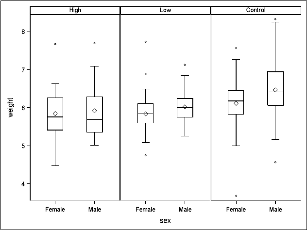
64 Linear Mixed Models: A Practical Guide Using Statistical Software
FIGURE 3.1: Box plots of rat pup birth weights for levels of treatment by sex.
The pattern of lower birth weights for the high- and low-dose treatments compared
to the control group is apparent in Figure 3.1. Male pups appear to have higher birth
weights than females in both the low and control groups, but not in the high group. The
distribution of birth weights appears to be roughly symmetric at each level of treatment
and sex. The variances of the birth weights are similar for males and females within each
treatment but appear to differ across treatments (we will check the assumption of constant
variance across the treatment groups as part of the analysis). We also note potential outliers,
which are investigated in the model diagnostics (Section 3.10). Because each box plot pools
measurements for rat pups from several litters, the possible effects of litter-level covariates,
such as litter size, are not shown in this graph.
In Figure 3.2, we use box plots to illustrate the relationship between birth weight and
litter size. Each panel shows the distributions of birth weights for all litters ranked by size,
within a given level of treatment and sex. We first create a new variable, RANKLIT, to
order the litters by size. The smallest litter has a size of 2 pups (RANKLIT = 1), and the
largest litter has a size of 18 pups (RANKLIT = 27). After creating RANKLIT, we create
box plots as a function of RANKLIT for each combination of TREAT and SEX by using
proc sgpanel:
proc sort data=ratpup;
by litsize litter;
run;
data ratpup2;
set ratpup;
by litsize litter;
if first.litter then ranklit+1;
label ranklit = "New Litter ID (Ordered by Size)";
run;
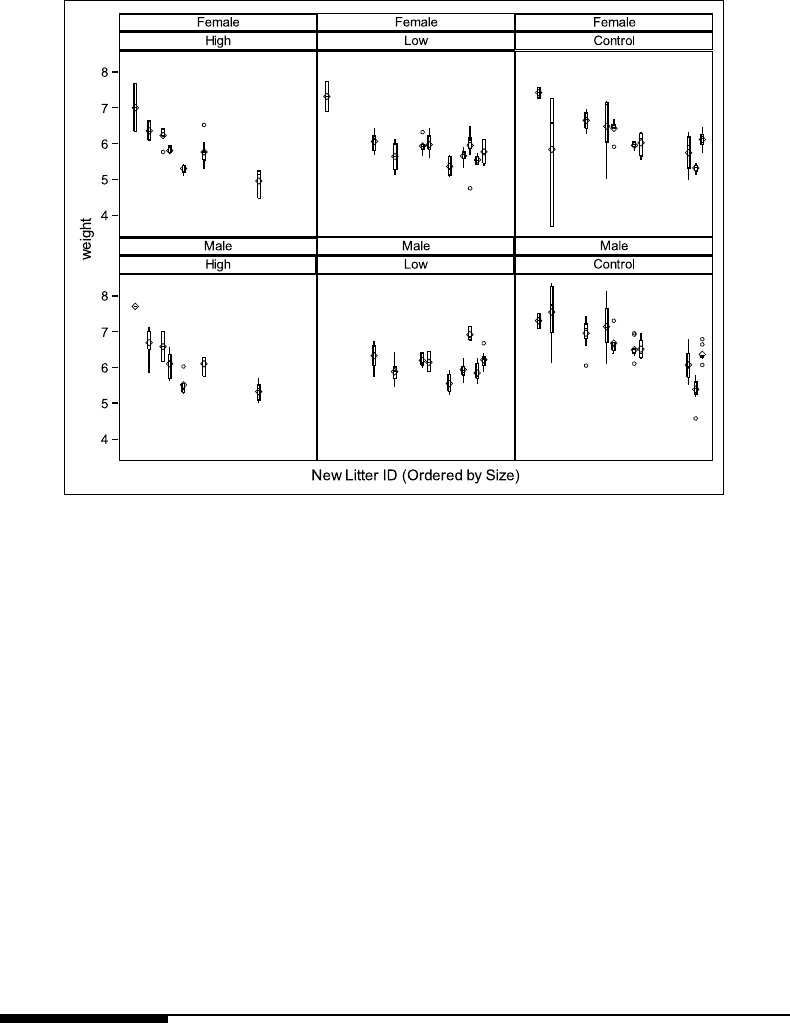
Two-Level Models for Clustered Data:The Rat Pup Example 65
FIGURE 3.2: Litter-specific box plots of rat pup birth weights by treatment level and sex.
Box plots are ordered by litter size.
/* Box plots for weight by litsize, for each level of treat and sex */
proc sgpanel data=ratpup2;
panelby sex treat / novarname columns=3 ;
vbox weight / category = ranklit meanattrs=(size=6) ;
format treat trtfmt.;
colaxis display=(novalues noticks);
run;
Figure 3.2 shows a strong tendency for birth weights to decrease as a function of litter
size in all groups except males from litters in the low-dose treatment. We consider this
important relationship in our models for the Rat Pup data.
3.3 Overview of the Rat Pup Data Analysis
For the analysis of the Rat Pup data, we follow the “top-down” modeling strategy outlined
in Subsection 2.7.1. In Subsection 3.3.1 we outline the analysis steps, and informally intro-
duce related models and hypotheses to be tested. Subsection 3.3.2 presents a more formal
specification of selected models that are fitted to the Rat Pup data, and Subsection 3.3.3
details the hypotheses tested in the analysis. To follow the analysis steps outlined in this
section, we refer readers to the schematic diagram presented in Figure 3.3.
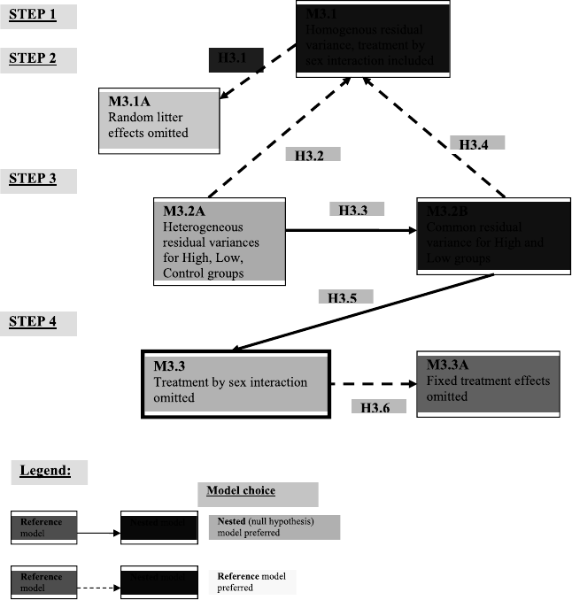
66 Linear Mixed Models: A Practical Guide Using Statistical Software
FIGURE 3.3: Model selection and related hypotheses for the analysis of the Rat Pup data.
3.3.1 Analysis Steps
Step 1: Fit a model with a “loaded” mean structure (Model 3.1).
Fit a two-level model with a “loaded” mean structure and random litter-specific
intercepts.
Model 3.1 includes the fixed effects of treatment, sex, litter size, and the interaction
between treatment and sex. The model also includes a random effect associated with the
intercept for each litter and a residual associated with each birth weight observation. The
residuals are assumed to be independent and identically distributed, given the random and
fixed effects, with constant variance across the levels of treatment and sex.
Step 2: Select a structure for the random effects (Model 3.1 vs. Model 3.1A).
Decide whether to keep the random litter effects in Model 3.1.
In this step we test whether the random litter effects associated with the intercept should
be omitted from Model 3.1 (Hypothesis 3.1), by fitting a nested model omitting the random
effects (Model 3.1A) and performing a likelihood ratio test. Based on the result of this test,
we decide to retain the random litter effects in all subsequent models.

Two-Level Models for Clustered Data:The Rat Pup Example 67
Step 3: Select a covariance structure for the residuals (Models 3.1, 3.2A, or
3.2B).
Decide whether the model should have homogeneous residual variances (Model
3.1), heterogeneous residual variances for each of the treatment groups (Model
3.2A), or grouped heterogeneous residual variances (Model 3.2B).
We observed in Figure 3.2 that the within-litter variance in the control group appears
to be larger than the within-litter variance in the high and low treatment groups, so we
investigate heterogeneity of residual variance in this step.
In Model 3.1, we assume that the residual variance is homogeneous across all treatment
groups. In Model 3.2A, we assume a heterogeneous residual variance structure, i.e., that the
residual variance of the birth weight observations differs for each level of treatment (high,
low, and control). In Model 3.2B, we specify a common residual variance for the high and
low treatment groups, and a different residual variance for the control group.
We test Hypotheses 3.2, 3.3, and 3.4 (specified in Section 3.3) in this step to decide
which covariance structure to choose for the residual variance. Based on the results of these
tests, we choose Model 3.2B as our preferred model at this stage of the analysis.
Step 4: Reduce the model by removing nonsignificant fixed effects, test the main
effects associated with treatment, and assess model diagnostics.
Decide whether to keep the treatment by sex interaction in Model 3.2B (Model
3.2B vs. Model 3.3).
Test the significance of the treatment effects in our final model, Model 3.3
(Model 3.3 vs. Model 3.3A).
Assess the assumptions for Model 3.3.
We first test whether we wish to keep the treatment by sex interaction in Model 3.2B
(Hypothesis 3.5). Based on the result of this test, we conclude that the treatment by sex
interaction is not significant, and can be removed from the model. Our new model is Model
3.3. The model-building process is complete at this point, and Model 3.3 is our final model.
We now focus on testing the main hypothesis of the study: whether the main effects
of treatment are equal to zero (Hypothesis 3.6). We use ML estimation to refit Model 3.3
and to fit a nested model, Model 3.3A, excluding the fixed treatment effects. We then carry
out a likelihood ratio test for the fixed effects of treatment. Based on the result of the test,
we conclude that the fixed effects of treatment are significant. The estimated fixed-effect
parameters indicate that, controlling for sex and litter size, treatment lowers the mean birth
weight of rat pups in litters receiving the high and low dose of the drug compared to the
birth weight of rat pups in litters receiving the control dose.
Finally, we refit Model 3.3 using REML estimation to reduce the bias of the estimated
covariance parameters, and carry out diagnostics for Model 3.3 using SAS (see Section 3.10
for diagnostics).
Software Note: Steps 3 and 4 of the analysis are carried out using proc mixed in
SAS, the GENLINMIXED procedure in SPSS, the lme() function in R,andthemixed
command in Stata only. The other procedures discussed in this book do not allow us
to fit models that have heterogeneous residual variance for groups defined by Level 2
(cluster-level) factors.
In Figure 3.3, we summarize the model selection process and hypotheses considered in
the analysis of the Rat Pup data. Each box corresponds to a model and contains a brief
description of the model. Each arrow corresponds to a hypothesis and connects two models
68 Linear Mixed Models: A Practical Guide Using Statistical Software
involved in the specification of that hypothesis. The arrow starts at the box representing
the reference model for the hypothesis and points to the simpler (nested) model. A dashed
arrow indicates that, based on the result of the hypothesis test, we chose the reference model
as the preferred one, and a solid arrow indicates that we chose the nested (null) model. The
final model is included in a bold box.
3.3.2 Model Specification
In this section we specify selected models considered in the analysis of the Rat Pup data.
We summarize the models in Table 3.3.
3.3.2.1 General Model Specification
The general specification of Model 3.1 for an individual birth weight observation
(WEIGHTij ) on rat pup iwithin the j-th litter is shown in (3.1). This specification corre-
sponds closely to the syntax used to fit the model using the procedures in SAS, SPSS, R,
and Stata.
WEIGHTij =β0+β1×TREAT1j+β2×TREAT2j+β3×SEX1ij
+β4×LITSIZEj+β5×TREAT1j×SEX1ij
+β6×TREAT2j×SEX1ij
⎫
⎪
⎬
⎪
⎭fixed
+uj+εij }random (3.1)
In Model 3.1 WEIGHTij is the dependent variable, and TREAT1jand TREAT2jare
Level 2 indicator variables for the high and low levels of treatment, respectively. SEX1ij is
a Level 1 indicator variable for female rat pups.
In this model, WEIGHTij depends on the βparameters (i.e., the fixed effects) in a linear
fashion. The fixed intercept parameter, β0, represents the expected value of WEIGHTij for
the reference levels of treatment and of sex (i.e., males in the control group) when LITSIZEj
is equal to zero. We do not interpret the fixed intercept, because a litter size of zero is outside
the range of the data (alternatively, the LITSIZE variable could be centered to make the
intercept interpretable; see Subsection 2.9.5).
The parameters β1and β2represent the fixed effects of the dummy variables (TREAT1j
and TREAT2j) for the high and low treatment levels vs. the control level, respectively. The
β3parameter represents the effect of SEX1ij (female vs. male), and β4represents the fixed
effect of LITSIZEj. The two parameters, β5and β6, represent the fixed effects associated
with the treatment by sex interaction.
The random effect associated with the intercept for litter jis indicated by uj,whichis
assumed to have a normal distribution with mean of 0 and constant variance σ2
litter .We
write the distribution of these random effects as:
uj∼N(0,σ
2
litter )
where σ2
litter represents the variance of the random litter effects.
In Model 3.1, the distribution of the residual εij , associated with the observation on an
individual rat pup iwithin litter j, is assumed to be the same for all levels of treatment:
εij ∼N(0,σ
2)
In Model 3.2A, we allow the residual variances for observations at different levels of
treatment to differ:
Two-Level Models for Clustered Data:The Rat Pup Example 69
High Treatment: εij ∼N(0,σ
2
high)
Low Treatment: εij ∼N(0,σ
2
low)
Control Treatment: εij ∼N(0,σ
2
control)
In Model 3.2B, we consider a separate residual variance for the combined high/low
treatment group and for the control group:
High/Low Treatment: εij ∼N(0,σ
2
high/low )
Control Treatment: εij ∼N(0,σ
2
control)
In Model 3.3, we include the same residual variance structure as in Model 3.2B, but
remove the fixed effects, β5and β6, associated with the treatment by sex interaction from
the model. In all models, we assume that the random effects, uj, associated with the litter-
specific intercepts and the residuals, εij , are independent.
3.3.2.2 Hierarchical Model Specification
We now present Model 3.1 in the hierarchical form used by the HLM software, with the
same notation as in (3.1). The correspondence between this notation and the HLM software
notation is defined in Table 3.3.
The hierarchical model has two components, reflecting two sources of variation: namely
variation between litters, which we attempt to explain using the Level 2 model and
variation between pups within a given litter, which we attempt to explain using the Level
1model. We write the Level 1 model as:
Level 1 Model (Rat Pup)
WEIGHTij =b
0j+b
1j×SEX1ij +εij (3.2)
where
εij ∼N(0,σ
2)
The Level 1 model in (3.2) assumes that WEIGHTij , i.e., the birth weight of rat pup i
within litter j, follows a simple ANOVA-type model defined by the litter-specific intercept,
b0jand the litter-specific effect of SEX1ij ,b
1j.
Both b0jand b1jare unobserved quantities that are defined as functions of Level 2
covariates in the Level 2 model:
Level 2 Model (Litter)
b0j=β0+β1×TREAT1j+β2×TREAT1j+β4×LITSIZEj+uj
b1j=β3+β5×TREAT1j+β6×TREAT2j(3.3)
where
uj∼N(0,σ
2
litter)

70 Linear Mixed Models: A Practical Guide Using Statistical Software
TABLE 3.3: Selected Models Considered in the Analysis of the Rat Pup Data
Term/Vari ab le General HLM Model
Notation Notation 3.1 3.2Aa3.2Ba3.3a
Fixed effects Intercept β0γ00 √√√√
TREAT1
(High vs. control) β1γ02 √√√√
TREAT2
(Low vs. control) β2γ03 √√√√
SEX1
(Female vs. male) β3γ10 √√√√
LITSIZE β4γ01 √√√√
TREAT1 ×SEX1 β5γ11 √√√
TREAT2 ×SEX1 β6γ12 √√√
Random
effects
Litter (j)Intercept ujuj√√√√
Residuals Rat pup
(pup iin
litter j)
εij rij √√√√
Covariance
parame-
ters (θD)
for D
matrix
Litter
level
Variance of
intercepts
σ2
litter τ√√√√

Two-Level Models for Clustered Data:The Rat Pup Example 71
TABLE 3.3: (Continued)
Term/Vari ab le General HLM Model
Notation Notation 3.1 3.2Aa3.2Ba3.3a
Covariance
parame-
ters (θR)
for Ri
matrix
Rat pup
level
Variances of
residuals
σ2
high
σ2
low
σ2
control
σ2σ2σ2
high
σ2
low
σ2
control
σ2
high/low,
σ2
control
σ2
high/low,
σ2
control
aModels 3.2A, 3.2B, and 3.3 (with heterogeneous residual variances) can only be fit using selected procedures in
SAS (proc mixed), SPSS (GENLINMIXED), R(the lme() function), and Stata (mixed).
72 Linear Mixed Models: A Practical Guide Using Statistical Software
The Level 2 model in (3.3) assumes that b0j, the intercept for litter j, depends on the
fixed intercept, β0, and for pups in litters assigned to the high- or low-dose treatments, on
the fixed effect associated with their level of treatment vs. control (β1or β2, respectively).
The intercept also depends on the fixed effect of litter size, β4, and a random effect, uj,
associated with litter j.
The effect of SEX1 within each litter, b1j, depends on an overall fixed SEX1 effect,
denoted by β3, and an additional fixed effect of either the high or low treatment vs. control
(β5or β6, respectively). Note that the effect of sex varies from litter to litter only through
the fixed effect of the treatment assigned to the litter; there is no random effect associated
with sex.
By substituting the expressions for b0jand b1jfrom the Level 2 model into the Level 1
model, we obtain the general LMM specified in (3.1). The fixed treatment effects, β5and
β6, for TREAT1jand TREAT2jin the Level 2 model for the effect of SEX1 correspond to
the interaction effects for treatment by sex (TREAT1j×SEX1ij and TREAT2j×SEX1ij)
in the general model specification.
3.3.3 Hypothesis Tests
Hypothesis tests considered in the analysis of the Rat Pup data are summarized in Table
3.4.
Hypothesis 3.1. The random effects, uj, associated with the litter-specific intercepts can
be omitted from Model 3.1.
We do not directly test the significance of the random litter-specific intercepts, but
rather test a hypothesis related to the variance of the random litter effects. We write the
null and alternative hypotheses as follows:
H0:σ2
litter =0
HA:σ2
litter >0
To test Hypothesis 3.1, we use a REML-based likelihood ratio test. The test statistic
is calculated by subtracting the –2 REML log-likelihood value for Model 3.1 (the reference
model) from the value for Model 3.1A (the nested model, which omits the random litter
effects). The asymptotic null distribution of the test statistic is a mixture of χ2distributions,
with 0 and 1 degrees of freedom, and equal weights of 0.5.
Hypothesis 3.2. The variance of the residuals is the same (homogeneous) for the three
treatment groups (high, low, and control).
The null and alternative hypotheses for Hypothesis 3.2 are:
H0:σ2
high =σ2
low =σ2
control =σ2
HA: At least one pair of residual variances is not equal to each other
We use a REML-based likelihood ratio test for Hypothesis 3.2. The test statistic is
obtained by subtracting the –2 REML log-likelihood value for Model 3.2A (the reference
model, with heterogeneous variances) from that for Model 3.1 (the nested model). The
asymptotic null distribution of this test statistic is a χ2with 2 degrees of freedom, where
the 2 degrees of freedom correspond to the 2 additional covariance parameters (i.e., the 2
additional residual variances) in Model 3.2A compared to Model 3.1.
Hypothesis 3.3. The residual variances for the high and low treatment groups are equal.

Two-Level Models for Clustered Data:The Rat Pup Example 73
TABLE 3.4: Summary of Hypotheses Tested in the Rat Pup Analysis
Hypothesis Specification Hypothesis Test
Models Compared
Label Null (H0)Alternative(HA) Test Nested
Model
(H0)
Ref.
Model
(HA)
Est.
Method
Test Stat.
Dist.
under H0
3.1 Drop ujRetain ujLRT Model Model REML 0.5χ2
0+0.5χ2
1
(σ2
litter =0) (σ2
litter >0) 3.1 A 3.1
3.2 Homogeneous Residual LRT Model Model REML χ2
2
residual variance variances are not 3.1 3.2A
(σ2
high =σ2
low =
σ2
control =σ2)
all equal
3.3 Grouped (σ2
high =σ2
low)LRT Model Model REML χ2
1
heterogeneous 3.2B 3.2A
residual variance
(σ2
high =σ2
low)
3.4 Homogeneous Grouped LRT Model Model REML χ2
1
residual variance heterogeneous 3.1 3.2B
(σ2
high/low =σ2
control =
σ2)
residual variance
(σ2
high/low =σ2
control)
3.5 Drop TREATMENT
×SEX effects
β5=0,or β6=0 Type III
F-test
N/A Model
3.2B
REML F(2,194)a
(β5=β6=0)
3.6 Drop TREATMENT β1=0,orβ2=0 LRT Model Model ML χ2
2
Effects 3.3A 3.3
(β1=β2=0) Type III N/A REML F(2,24.3)
aDifferent methods for calculating denominator degrees of freedom are available in the software procedures; we
report the Satterthwaite estimate of degrees of freedom calculated by proc mixed in SAS.
74 Linear Mixed Models: A Practical Guide Using Statistical Software
The null and alternative hypotheses are as follows:
H0:σ2
high =σ2
low
HA:σ2
high =σ2
low
We test Hypothesis 3.3 using a REML-based likelihood ratio test. The test statistic is
calculated by subtracting the –2 REML log-likelihood value for Model 3.2A (the reference
model) from the corresponding value for Model 3.2B (the nested model, with pooled residual
variance for the high and low treatment groups). The asymptotic null distribution of this test
statistic is a χ2with 1 degree of freedom, where the single degree of freedom corresponds
to the one additional covariance parameter (i.e., the one additional residual variance) in
Model 3.2A compared to Model 3.2B.
Hypothesis 3.4. The residual variance for the combined high/low treatment group is
equal to the residual variance for the control group.
In this case, the null and alternative hypotheses are:
H0:σ2
high/low =σ2
control =σ2
HA:σ2
high/low =σ2
control
We test Hypothesis 3.4 using a REML-based likelihood ratio test. The test statistic is
obtained by subtracting the –2 REML log-likelihood value for Model 3.2B (the reference
model) from that for Model 3.1 (the nested model). The asymptotic null distribution of this
test statistic is a χ2with 1 degree of freedom, corresponding to the one additional variance
parameter in Model 3.2B compared to Model 3.1.
Hypothesis 3.5. The fixed effects associated with the treatment by sex interaction are
equal to zero in Model 3.2B.
The null and alternative hypotheses are:
H0:β5=β6=0
HA:β5=0orβ6=0
We test Hypothesis 3.5 using an approximate F-test, based on the results of the REML
estimation of Model 3.2B. Because this test is not significant, we remove the treatment by
sex interaction term from Model 3.2B and obtain Model 3.3.
Hypothesis 3.6. The fixed effects associated with treatment are equal to zero in Model
3.3.
This hypothesis differs from the previous ones, in that it is not being used to select a
model, but is testing the primary research hypothesis. The null and alternative hypotheses
are:
H0:β1=β2=0
HA:β1=0orβ2=0
We test Hypothesis 3.6 using an ML-based likelihood ratio test. The test statistic is cal-
culated by subtracting the –2 ML log-likelihood value for Model 3.3 (the reference model)
from that for Model 3.3A (the nested model excluding the fixed treatment effects). The
asymptotic null distribution of this test statistic is a χ2with 2 degrees of freedom, cor-
responding to the two additional fixed-effect parameters in Model 3.3 compared to Model
3.3A.
Alternatively, we can test Hypothesis 3.6 using an approximate F-test for TREAT-
MENT, based on the results of the REML estimation of Model 3.3.
For the results of these hypothesis tests see Section 3.5.

Two-Level Models for Clustered Data:The Rat Pup Example 75
3.4 Analysis Steps in the Software Procedures
In this section, we illustrate fitting the LMMs for the Rat Pup example using the software
procedures in SAS, SPSS, R, Stata, and HLM. Because we introduce the use of the software
procedures in this chapter, we present a more detailed description of the steps and options
for fitting each model than we do in Chapters 4 through 8. We compare results for selected
models across the software procedures in Section 3.6.
3.4.1 SAS
Step 1: Fit a model with a “loaded” mean structure (Model 3.1).
We assume that the ratpup data set has been created in SAS, as illustrated in the data
summary (Subsection 3.2.2). The SAS commands used to fit Model 3.1 to the Rat Pup data
using proc mixed are as follows:
ods output fitstatistics = fitl;
title "Model 3.1";
proc mixed data = ratpup order = internal covtest;
class treat sex litter;
model weight = treat sex litsize treat*sex /
solution ddfm = sat;
random int / subject= litter;
format treat trtfmt.;
run;
The ods statement is used to create a data set, fit1, containing the –2 REML log-
likelihood and other fit statistics for Model 3.1. We will use the fit1 data set later to
perform likelihood ratio tests for Hypotheses 3.1, 3.2, and 3.4.
The proc mixed statement invokes the analysis, using the default REML estimation
method. We use the covtest option to obtain the standard errors of the estimated covari-
ance parameters for comparison with the results from the other software procedures. The
covtest option also causes SAS to display a Wald z-test of whether the variance of the
random litter effects equals zero (i.e., Hypothesis 3.1), but we do not recommend using this
test (see the discussion of Wald tests for covariance parameters in Subsection 2.6.3.2). The
order = internal option requests that levels of variables declared in the class statement
be ordered based on their (unformatted) internal numeric values and not on their formatted
values.
The class statement includes the two categorical factors, TREAT and SEX, which
will be included as fixed predictors in the model statement, as well as the classification
factor, LITTER, that defines subjects in the random statement.
The model statement sets up the fixed effects. The dependent variable, WEIGHT, is
listed on the left side of the equal sign, and the covariates having fixed effects are included
on the right of the equal sign. We include the fixed effects of TREAT, SEX, LITSIZE, and
the TREAT ×SEX interaction in this model. The solution option follows a slash (/), and
instructs SAS to display the fixed-effect parameter estimates in the output (they are not
displayed by default). The ddfm = option specifies the method used to estimate denominator
degrees of freedom for F-tests of the fixed effects. In this case, we use ddfm = sat for the
Satterthwaite approximation (see Subsection 3.11.6 for more details on denominator degrees
of freedom options in SAS).

76 Linear Mixed Models: A Practical Guide Using Statistical Software
Software Note: By default, SAS generates an indicator variable for each level of a
class variable included in the model statement. This typically results in an overpa-
rameterized model, in which there are more columns in the Xmatrix than there are
degrees of freedom for a factor or an interaction term involving a factor. SAS then
uses a generalized inverse (denoted by –in the following formula) to calculate the
fixed-effect parameter estimates (see the SAS documentation for proc mixed for more
information):
β=(X
V−1X)−X
V−1y
In the output for the fixed-effect parameter estimates produced by requesting the
solution option as part of the model statement, the estimate for the highest level of a
class variable is by default set to zero; and the level that is considered to be the highest
level for a variable will change depending on whether there is a format associated with
the variable or not.
In the analysis of the Rat Pup data, we wish to contrast the effects of the high- and
low-dose treatments to the control dose, so we use the order = internal option to
order levels of TREAT. This results in the parameter for Level 3 of TREAT (i.e., the
control dose, which is highest numerically) being set to zero, so the parameter estimates
for the other levels of TREAT represent contrasts with TREAT = 3 (control). This
corresponds to the specification of Model 3.1 in (3.1). The value of TREAT = 3 is
labeled “Control” in the output by the user-defined format.
We refer to TREAT = 3 as the reference category throughout our discussion. In
general, we refer to the highest level of a class variable as the “reference” level when we
estimate models using proc mixed throughout the book. For example, in Model 3.1,
the “reference category” for SEX is “Male” (the highest level of SEX alphabetically),
which corresponds to our specification in (3.1).
The random statement specifies that a random intercept, int, is to be associated with
each litter, and litters are specified as subjects by using the subject = litter option.
Alternative syntax for the random statement is:
random litter ;
This syntax results in a model that is equivalent to Model 3.1, but is much less efficient
computationally. Because litter is specified as a random factor, we get the same block-
diagonal structure for the variance-covariance matrix for the random effects, which SAS
refers to as the Gmatrix, as when we used subject = litter in the previous syntax (see
Subsection 2.2.3 for a discussion of the Gmatrix). However, all observations are assumed to
be from one “subject,” and calculations for parameter estimation use much larger matrices
and take more time than when subject = litter is specified.
The format statement attaches the user-defined format, trtfmt., to values of the vari-
able TREAT.
Step 2: Select a structure for the random effects (Model 3.1 vs. Model 3.1A).
To test Hypothesis 3.1, we first fit Model 3.1A without the random effects associated with
litter, by using the same syntax as for Model 3.1 but excluding the random statement:
title "Model 3.1A";
ods output fitstatistics = fitla;
proc mixed data = ratpup order = internal covtest;

Two-Level Models for Clustered Data:The Rat Pup Example 77
class treat sex litter;
model weight = treat sex treat*sex litsize /
solution ddfm = sat;
format treat trtfmt.;
run;
The SAS code below can be used to calculate the likelihood ratio test statistic for
Hypothesis 3.1, compute the corresponding p-value, and display the resulting p-value in the
SAS log. To apply this syntax, the user has to manually extract the –2 REML log-likelihood
value for the reference model, Model 3.1 (–2 REML log-likelihood = 401.1), and for the
nested model, Model 3.1A (–2 REML log-likelihood = 490.5), from the output and include
these values in the code. Recall that the asymptotic null distribution of the test statistic
for Hypothesis 3.1 is a mixture of χ2
0and χ2
1distributions, each having equal weight of 0.5.
Because the χ2
0has all of its mass concentrated at zero, its contribution to the p-value is
zero, so it is not included in the following code.
title "P-value for Hypothesis 3.1: Simple syntax";
data _null_;
lrtstat = 490.5 - 401.1;
df=1;
pvalue = 0.5*(1 - probchi(lrtstat,df));
format pvalue 10.8;
put lrtstat = df = pvalue = ;
run;
Alternatively, we can use the data sets fit1 and fit1a, containing the fit statistics for
Models 3.1 and 3.1A, respectively, to perform this likelihood ratio test. The information
contained in these two data sets is displayed below, along with more advanced SAS code
to merge the data sets, derive the difference of the –2 REML log-likelihoods, calculate the
appropriate degrees of freedom, and compute the p-value for the likelihood ratio test. The
results of the likelihood ratio test will be included in the SAS log.
title "Fit 1";
proc print data = fit1;
run;
title "Fit 1a";
proc print data = fit1a;
run; '
&
$
%
Fit 1
Obs Descr Value
1 -2 Res Log Likelihood 401.1
2 AIC (smaller is better) 405.1
3 AICC (smaller is better) 405.1
4 BIC (smaller is better) 407.7
Fit 1a
Obs Descr Value
1 -2 Res Log Likelihood 490.5
2 AIC (smaller is better) 492.5
3 AICC (smaller is better) 492.5
4 BIC (smaller is better) 496.3

78 Linear Mixed Models: A Practical Guide Using Statistical Software
title "p-value for Hypothesis 3.1: Advanced syntax";
data _null_;
merge fit1(rename = (value = reference)) fit1a(rename = (value = nested));
retain loglik_diff;
if descr = "-2 Res Log Likelihood" then
loglik_diff = nested - reference;
if descr = "AIC (smaller is better)" then do;
df = floor((loglik_diff - nested + reference)/2);
pvalue = 0.5*(1 - probchi(loglik_diff,df));
put loglik_diff = df = pvalue = ;
format pvalue 10.8;
end;
run;
The data _null_ statement causes SAS to execute the data step calculations without
creating a new data set. The likelihood ratio test statistic for Hypothesis 3.1 is calculated
by subtracting the –2 REML log-likelihood value for the reference model (contained in the
data set fit1) from the corresponding value for the nested model (contained in fit1a). To
calculate degrees of freedom for this test, we take advantage of the fact that SAS defines the
AIC statistic as AIC = –2 REML log-likelihood + 2 ×number of covariance parameters.
Software Note: When a covariance parameter is estimated to be on the boundary of
a parameter space by proc mixed (e.g., when a variance component is estimated to be
zero), SAS will not include it when calculating the number of covariance parameters
for the AIC statistic. Therefore, the advanced SAS code presented in this section for
computing likelihood ratio tests for covariance parameters is only valid if the estimates
of the covariance parameters being tested do not lie on the boundaries of their respective
parameter spaces (see Subsection 2.5.2).
Results from the likelihood ratio test of Hypothesis 3.1 and other hypotheses are pre-
sented in detail in Subsection 3.5.1.
Step 3: Select a covariance structure for the residuals (Models 3.1, 3.2A, or
3.2B).
The following SAS commands can be used to fit Model 3.2A, which allows unequal residual
variance for each level of treatment. The only change in these commands from those used
for Model 3.1 is the addition of the repeated statement:
title "Model 3.2A";
proc mixed data = ratpup order = internal covtest;
class treat litter sex;
model weight = treat sex treat*sex litsize /
solution ddfm = sat;
random int / subject = litter;
repeated / group = treat;
format treat trtfmt.;
run;
In Model 3.2A, the option group = treat in the repeated statement allows a hetero-
geneous variance structure for the residuals, with each level of treatment having its own
residual variance.

Two-Level Models for Clustered Data:The Rat Pup Example 79
Software Note: In general, the repeated statement in proc mixed specifies the struc-
ture of the Rjmatrix, which contains the variances and covariances of the residuals for
the j-th cluster (e.g., litter). If no repeated statement is used, the default covariance
structure for the residuals is employed, i.e., Rj=σ2Inj,whereInjis an nj×njidentity
matrix, with njequal to the number of observations in a cluster (e.g., the number of
rat pups in litter j). In other words, the default specification is homogeneous residual
variance. Because this default Rjmatrix is used for Model 3.1, we do not include a
repeated statement for this model.
To test Hypothesis 3.2, we calculate a likelihood ratio test statistic by subtracting the
value of the –2 REML log-likelihood for Model 3.2A (the reference model with heterogeneous
variance, –2 REML LL = 359.9) from that for Model 3.1 (the nested model, –2 REML LL =
401.1). The simple SAS syntax used to calculate this likelihood ratio test statistic is similar
to that used for Hypothesis 3.1. The p-value is calculated by referring the test statistic
to a χ2distribution with two degrees of freedom, which correspond to the two additional
variance parameters in Model 3.2A compared to Model 3.1. We do not use a mixture of
χ2
0and χ2
1distributions, as in Hypothesis 3.1, because we are not testing a null hypothesis
with values of the variances on the boundary of the parameter space:
title "p-value for Hypothesis 3.2";
data _null_;
lrtstat = 401.1 - 359.9;
df=2;
pvalue = 1 - probchi(lrtstat,df);
format pvalue 10.8;
put lrtstat = df = pvalue = ;
run;
The test result is significant (p<0.001), so we choose Model 3.2A, with heterogeneous
residual variance, as our preferred model at this stage of the analysis.
Before fitting Model 3.2B, we create a new variable named TRTGRP that combines the
high and low treatment groups, to allow us to test Hypotheses 3.3 and 3.4. We also define
a new format, TGRPFMT, for the TRTGRP variable.
title "RATPUP3 dataset";
data ratpup3;
set ratpup2;
if treatment in ("High", "Low") then TRTGRP = 1;
if treatment = "Control" then TRTGRP = 2;
run;
proc format;
value tgrpfmt 1 = "High/Low"
2 = "Control";
run;
We now fit Model 3.2B using the new data set, ratpup3, and the new group variable
in the repeated statement (group = trtgrp). We also include TRTGRP in the class
statement so that SAS will properly include it as the grouping variable for the residual
variance.
80 Linear Mixed Models: A Practical Guide Using Statistical Software
title "Model 3.2B";
proc mixed data = ratpup3 order = internal covtest;
class treat litter sex trtgrp;
model weight = treat sex treat*sex litsize / solution ddfm = sat;
random int / subject = litter;
repeated / group = trtgrp;
format treat trtfmt. trtgrp tgrpfmt.;
run;
We use a likelihood ratio test for Hypothesis 3.3 to decide if we can use a common
residual variance for both the high and low treatment groups (Model 3.2B) rather than
different residual variances for each treatment group (Model 3.2A). For this hypothesis
Model 3.2A is the reference model and Model 3.2B is the nested model. To calculate the
test statistic we subtract the –2 REML log-likelihood for Model 3.2A from that for Model
3.2B (–2 REML LL = 361.1). This test has 1 degree of freedom, corresponding to the one
fewer covariance parameter in Model 3.2B compared to Model 3.2A.
title "p-value for Hypothesis 3.3";
data _null_;
lrtstat = 361.1 - 359.9;
df=1;
pvalue = 1 - probchi(lrtstat, df);
format pvalue 10.8;
put lrtstat = df = pvalue = ;
run;
The likelihood ratio test statistic for Hypothesis 3.3 is not significant (p=0.27), so we
choose the simpler grouped residual variance model, Model 3.2B, as our preferred model at
this stage of the analysis.
To test Hypothesis 3.4, and decide whether we wish to have a grouped heterogeneous
residual variance structure vs. a homogeneous variance structure, we subtract the –2 REML
log-likelihood of Model 3.2B (= 361.1) from that of Model 3.1 (= 401.1). The test statistic
has 1 degree of freedom, corresponding to the 1 additional covariance parameter in Model
3.2B as compared to Model 3.1. The syntax for this comparison is not shown here. Based
on the significant result of this likelihood ratio test (p<0.001), we conclude that Model
3.2B (with grouped heterogeneous variances) is our preferred model.
Step 4: Reduce the model by removing nonsignificant fixed effects (Model 3.2B
vs.3.3,andModel3.3vs.3.3A).
We test Hypothesis 3.5 to decide whether we can remove the treatment by sex interaction
term, making use of the default Type III F-test for the TREAT ×SEX interaction in Model
3.2B. Because the result of this test is not significant (p=0.73), we drop the TREAT ×
SEX interaction term from Model 3.2B, which gives us Model 3.3.
We now test Hypothesis 3.6 to decide whether the fixed effects associated with treatment
are equal to zero, using a likelihood ratio test. This test is not used as a tool for possible
model reduction but as a way of assessing the impact of treatment on birth weights. To
carry out the test, we first fit the reference model, Model 3.3, using maximum likelihood
(ML) estimation:
title "Model 3.3 using ML";
proc mixed data = ratpup3 order = internal method = ml;

Two-Level Models for Clustered Data:The Rat Pup Example 81
class treat litter sex trtgrp;
model weight = treat sex litsize / solution ddfm = sat;
random int / subject = litter;
repeated / group = trtgrp;
format treat trtfmt.;
run;
The method = ml option in the proc mixed statement requests maximum likelihood
estimation.
To complete the likelihood ratio test for Hypothesis 3.6, we fit a nested model, Model
3.3A, without the fixed treatment effects, again requesting ML estimation, by making the
following modifications to the SAS code for Model 3.3:
title "Model 3.3A using ML";
proc mixed data = ratpup3 order = internal method = ml;
...
model weight = sex litsize / solution ddfm = sat;
...
The likelihood ratio test statistic used to test Hypothesis 3.6 is calculated by subtracting
the –2 ML log-likelihood for Model 3.3 (the reference model) from that for Model 3.3A (the
nested model without the fixed effects associated with treatment). The SAS code for this
test is not shown here.
Because the result of this test is significant (p<0.001), we conclude that treatment has
an effect on rat pup birth weights, after adjusting for the fixed effects of sex and litter size
and the random litter effects.
We now refit Model 3.3, our final model, using the default REML estimation method
to get unbiased estimates of the covariance parameters. We also add a number of options
to the SAS syntax. We request diagnostic plots in the proc mixed statement by adding a
plots= option. We add options to the model statement to get output data sets containing
the conditional predicted and residual values (outpred = pdat1) and we get another data
set containing the marginal predicted and residual values (outpredm = pdat2). We also re-
quest that estimates of the implied marginal variance-covariance and correlation matrices,
vand vcorr, for the third litter be displayed in the output by adding the options v=3and
vcorr = 3 to the random statement. Post-hoc tests for all estimated differences among treat-
ment means using the Tukey–Kramer adjustment for multiple comparisons are requested
by adding the lsmeans statement. Finally, we request that the EBLUPs for the random
intercept for each litter be saved in a new file called eblupsdat,byusinganods output
statement. We first sort the ratpup3 data set by PUP ID, because the diagnostic plots
identify individual points by row numbers in the data set, and the sorting will make the
PUP ID variable equal to the row number in the data set for ease in reading the graphical
output.
proc sort data = ratpup3;
by pup_id;
run;
ods graphics on;
ods rtf file = "c:\temp\ratpup_diagnostics.rtf" style = journal;
ods exclude influence;
title "Model 3.3 using REML. Model diagnostics";
proc mixed data = ratpup3 order = internal covtest

82 Linear Mixed Models: A Practical Guide Using Statistical Software
plots = (residualpanel boxplot influencestatpanel);
class treat litter sex trtgrp;
model weight = treat sex litsize / solution ddfm = sat
residual outpred = pdat1 outpredm = pdat2
influence (iter = 5 effect = litter est) ;
id pup_id litter treatment trtgrp ranklit litsize;
random int / subject=litter solution v = 3 vcorr = 3 ;
repeated / group=trtgrp ;
lsmeans treat / adjust = tukey ;
format treat trtfmt. trtgrp tgrpfmt. ;
ods output solutionR = eblupsdat ;
run;
ods graphics off;
ods rtf close;
Software Note: In earlier versions of SAS, the default output mode was “Listing,”
which produced text in the Output window. ODS (Output Delivery System) graphics
were not automatically produced. However, in Version 9.3, the default output mode
has changed to HTML, and ODS graphics are automatically produced. When you
use the default HTML output, statistical tables and graphics are included together
in the Results Viewer Window. You can change these default behaviors through SAS
commands, or by going to To o ls >Options >Preferences and clicking on the
Results tab. By selecting “Create listing,” you will add text output to the Output
window, as in previous versions of SAS. This will be in addition to the HTML output,
which can be turned off by deselecting “Create HTML.” To turn off ODS graphics,
which can become cumbersome when running large jobs, deselect “Use ODS graphics.”
Click “OK” to confirm these changes. These same changes can be accomplished by the
following commands:
ods listing;
ods html close;
ods graphics off;
The type of output that is produced can be modified by choosing an output type
(e.g., .rtf) and sending the output and SAS ODS graphics to that file. There are a
number of possible styles, with Journal being a black-and-white option suitable for
a manuscript. If no style is selected, the default will be used, which includes color
graphics. The .rtf file can be closed when the desired output has been captured.
ods graphics on;
ods rtf file="example.rtf" style=journal;
proc mixed ...;
run;
ods rtf close;
Any portion of the SAS output can be captured in a SAS data set, or can be excluded
from the output by using ODS statements. For example, in the SAS code for Model
3.3, we used ods exclude influence. This prevents the influence statistics for each
individual observation from being printed in the output, which can get very long if
there are a large number of cases, but it still allows the influence diagnostic plots to be

Two-Level Models for Clustered Data:The Rat Pup Example 83
displayed. We must also request that the influence statistics be calculated by including
an influence option as part of the model statement.
Output that we wish to save to a SAS data set can be requested by using an
ods output statement. The statement below requests that the solutions for the random
effects (the SolutionR table from the output) be output to a new data set called
eblupsdat.
ods output solutionR = eblupsdat;
To view the names of SAS output tables so that they can be captured in a data set,
use the following code, which will place the names of each portion of the output in the
SAS log.
ods trace on;
proc mixed ...;
run;
ods trace off;
The proc mixed statement for Model 3.3 has been modified by the addition of the
plots = option, with the specific ODS plots that are requested listed within parentheses:
(residualpanel boxplot influencestatpanel).Theresidualpanel suboption gener-
ates diagnostic plots for both conditional and marginal residuals. Although these residual
plots were requested, we do not display them here, because these plots are not broken down
by TRTGRP. Histograms and normal quantile–quantile (Q–Q) plots of residuals for each
treatment group are displayed in Figures 3.4, 3.5, and 3.6. The model statement has also
been modified by adding the residual option, to allow the generation of panels of resid-
ual diagnostic plots as part of the ODS graphics output. The boxplot suboption requests
box plots of the marginal and conditional residuals by the levels of each class variable,
including class variables specified in the subject = and group = options, to be created in
the ODS graphics output. SAS also generates box plots for levels of the “subject” vari-
able (LITTER), but only if we do not use nesting specification for litter in the random
statement (i.e., we must use subject = litter rather than subject = litter(treat)).
Box plots showing the studentized residuals for each litter are shown in Figure 3.7. The
influencestatpanel suboption requests that influence plots for the model fit (REML dis-
tance), overall model statistics, covariance parameters, and fixed effects be produced. These
plots are illustrated in Figures 3.8 through 3.11. Diagnostic plots generated for Model 3.3
are presented in Section 3.10.
The influence option has also been added to the model statement for Model 3.3 to
obtain influence plots as part of the ODS graphics output (see Subsection 3.10.2). The
inclusion of the iter = suboption is used to produce iterative updates to the model, by
removing the effect of each litter, and then re-estimating all model parameters (including
both fixed-effect and random-effect parameters). The option effect = specifies an effect
according to which observations are grouped, i.e., observations sharing the same level of the
effect are removed as a group when calculating the influence diagnostics. The effect must
contain only class variables, but these variables do not need to be contained in the model.
Without the effect = suboption, influence statistics would be created for the values for the
individual rat pups and not for litters. The influence diagnostics are discussed in Subsection
3.10.2.

84 Linear Mixed Models: A Practical Guide Using Statistical Software
We caution readers that running proc mixed with these options (e.g., iter = 5 and
effect = litter) can cause the procedure to take considerably longer to finish running.
In our example, with 27 litters and litter-specific subset deletion, the longer execution time
is a result of the fact that proc mixed needs to fit 28 models, i.e., the initial model and the
model corresponding to each deleted litter, with up to five iterations per model. Clearly,
this can become very time-consuming if there are a large number of levels of a variable that
is being checked for influence.
The outpred = option in the model statement causes SAS to output the predicted values
and residuals conditional on the random effects in the model. In this example, we output
the conditional residuals and predicted values to a data set called pdat1 by specifying
outpred = pdat1.Theoutpredm = option causes SAS to output the marginal predicted
and residual values to another data set. In this case, we request that these variables be
output to the pdat2 data set by specifying outpredm = pdat2. We discuss these residuals
in Subsection 3.10.1.
The id statement allows us to place variables in the output data sets, pdat1 and pdat2,
that identify each observation. We specify that PUP ID, LITTER, TREATMENT, TRT-
GRP, RANKLIT, and LITSIZE be included, so that we can use them later in the residual
diagnostics.
The random statement has been modified to include the v=and vcorr = options, so that
SAS displays the estimated marginal Vjmatrix and the corresponding marginal correlation
matrix implied by Model 3.3 for birth weight observations from the third litter (v=3and
vcorr = 3). We chose the third litter in this example because it has only four rat pups, to
keep the size of the estimated Vjmatrix in the output manageable (see Section 3.8 for a
discussion of the implied marginal covariance matrix). We also include the solution option,
to display the EBLUPs for the random litter effects in the output.
The lsmeans statement allows us to obtain estimates of the least-squares means of
WEIGHT for each level of treatment, based on the fixed-effect parameter estimates for
TREAT. The least-squares means are evaluated at the mean of LITSIZE, and assuming
that there are equal numbers of rat pups for each level of SEX. We also carry out post-hoc
comparisons among all pairs of the least-squares means using the Tukey–Kramer adjust-
ment for multiple comparisons by specifying adjust = tukey. Many other adjustments
for multiple comparisons can be obtained, such as Dunnett’s and Bonferroni. Refer to the
SAS documentation for proc mixed for more information on post-hoc comparison methods
available in the lsmeans statement.
Diagnostics for this final model using the REML fit for Model 3.3 are presented in
Section 3.10.
3.4.2 SPSS
Most analyses in SPSS can be performed using either the menu system or SPSS syntax. The
syntax for LMMs can be obtained by specifying a model using the menu system and then
pasting the syntax into the syntax window. We recommend pasting the syntax for any LMM
that is fitted using the menu system, and then saving the syntax file for documentation. We
present SPSS syntax throughout the example chapters for ease of presentation, although
the models were usually set up using the menu system. A link to an example of setting up
an LMM using the SPSS menus is included on the web page for this book (see Appendix A).
For the analysis of the Rat Pup data, we first read in the raw data from the tab-delimited
file rat pup.dat (assumed to be located in the C:\temp folder) using the following syntax.
This SPSS syntax was pasted after reading in the data using the SPSS menu system.
* Read in Rat Pup data.
GET DATA
Two-Level Models for Clustered Data:The Rat Pup Example 85
/TYPE = TXT
/FILE = "C:\temp\rat_pup.dat"
/DELCASE = LINE
/DELIMITERS = "\t"
/ARRANGEMENT = DELIMITED
/FIRSTCASE = 2
/IMPORTCASE = ALL
/VARIABLES =
pup_id F2.1
weight F4.2
sex A6
litter F1.
litsize F2.1
treatment A7
.
CACHE.
EXECUTE.
Because the MIXED command in SPSS sets the fixed-effect parameter associated with
the highest-valued level of a fixed factor to 0 by default, to prevent overparameterization
of models (similar to proc mixed in SAS; see Subsection 3.4.1), the highest-valued levels
of fixed factors can be thought of as “reference categories” for the factors. As a result,
we recode TREATMENT into a new variable named TREAT, so that the control group
(TREAT = 3) will be the reference category.
* Recode TREATMENT variable .
RECODE
Treatment
("High"=1) ("Low"=2) ("Control"=3) INTO treat .
EXECUTE .
VARIABLE LABEL treat "Treatment" .
VALUE LABELS treat 1 "High" 2 "Low" 3 "Control" .
Step 1: Fit a model with a “loaded” mean structure (Model 3.1).
The following SPSS syntax can be used to fit Model 3.1:
* Model 3.1.
MIXED
weight BY treat sex WITH litsize
/CRITERIA = CIN(95) MXITER(100) MXSTEP(5) SCORING(1)
SINGULAR(0.000000000001) HCONVERGE(0, ABSOLUTE)
LCONVERGE(0, ABSOLUTE) PCONVERGE(0.000001, ABSOLUTE)
/FIXED = treat sex litsize treat*sex | SSTYPE(3)
/METHOD = REML
/PRINT = SOLUTION
/RANDOM INTERCEPT | SUBJECT(litter) COVTYPE(VC)
/SAVE = PRED RESID .
The first variable listed after invoking the MIXED command is the dependent variable,
WEIGHT. The BY keyword indicates that the TREAT and SEX variables are to be consid-
ered as categorical factors (they can be either fixed or random). Note that we do not need

86 Linear Mixed Models: A Practical Guide Using Statistical Software
to include LITTER as a factor, because this variable is identified as a SUBJECT variable
later in the code. The WITH keyword identifies continuous covariates, and in this case, we
specify LITSIZE as a continuous covariate.
The CRITERIA subcommand specifies default settings for the convergence criteria ob-
tained by specifying the model using the menu system.
In the FIXED subcommand, we include terms that have fixed effects associated with them
inthemodel:TREAT,SEX,LITSIZEandtheTREAT×SEX interaction. The SSTYPE(3)
option after the vertical bar indicates that the default Type III analysis is to be used when
calculating F-statistics. We also use the METHOD = REML subcommand, which requests that
the REML estimation method (the default) be used.
The SOLUTION keyword in the PRINT subcommand specifies that the estimates of the
fixed-effect parameters, covariance parameters, and their associated standard errors are to
be included in the output.
The RANDOM subcommand specifies that there is a random effect in the model associated
with the INTERCEPT for each level of the SUBJECT variable (i.e., LITTER). The information
about the “subject” variable is specified after the vertical bar (|). Note that because we
included LITTER as a “subject” variable, we did not need to list it after the BY keyword
(including LITTER after BY does not affect the analysis if LITTER is also indicated as a
SUBJECT variable). The COVTYPE(VC) option indicates that the default Variance Components
(VC) covariance structure for the random effects (the Dmatrix) is to be used. We did not
need to specify a COVTYPE here because only a single variance associated with the random
effects is being estimated.
Conditional predicted values and residuals are saved in the working data set by specifying
PRED and RESID in the SAVE subcommand. The keyword PRED saves litter-specific predicted
values that incorporate both the estimated fixed effects and the EBLUPs of the random
litter effects for each observation. The keyword RESID saves the conditional residuals that
represent the difference between the actual value of WEIGHT and the predicted value for
each rat pup, based on the estimated fixed effects and the EBLUP of the random effect
for each observation. The set of population-averaged predicted values, based only on the
estimated fixed-effect parameters, can be obtained by adding the FIXPRED keyword to the
SAVE subcommand, as shown later in this chapter (see Section 3.9 for more details):
/SAVE = PRED RESID FIXPRED
Software Note: There is currently no option to display or save the predicted values of
the random litter effects (EBLUPs) in the output in SPSS. However, because all models
considered for the Rat Pup data contain a single random intercept for each litter, the
EBLUPs can be calculated by simply taking the difference between the “population-
averaged” and “litter-specific” predicted values. The values of FIXPRED from the first
LMM can be stored in a variable called FIXPRED 1, and the values of PRED from
the first model can be stored as PRED 1. We can then compute the difference between
these two predicted values and store the result in a new variable that we name EBLUP:
COMPUTE eblup = pred_1 - fixpred_1 .
EXECUTE .
The values of the EBLUP variable, which are constant for each litter, can then be
displayed in the output by using this syntax:
SORT CASES BY litter.
SPLIT FILE

Two-Level Models for Clustered Data:The Rat Pup Example 87
LAYERED BY litter.
DESCRIPTIVES
VARIABLES = eblup
/STATISTICS=MEAN STDDEV MIN MAX.
SPLIT FILE OFF.
Step 2: Select a structure for the random effects (Model 3.1 vs. Model 3.1A).
We now use a likelihood ratio test of Hypothesis 3.1 to decide if the random effects associated
with the intercept for each litter can be omitted from Model 3.1. To carry out the likelihood
ratio test we first fit a nested model, Model 3.1A, using the same syntax as for Model 3.1
but with the RANDOM subcommand omitted:
* Model 3.1A .
MIXED
weight BY treat sex WITH litsize
/CRITERIA = CIN(95) MXITER(100) MXSTEP(5) SCORING(l)
SINGULAR(0.000000000001) HCONVERGE(0, ABSOLUTE) LCONVERGE(0,
ABSOLUTE) PCONVERGE(0.000001, ABSOLUTE)
/FIXED = treat sex litsize treat*sex | SSTYPE(3)
/METHOD = REML
/PRINT = SOLUTION
/SAVE = PRED RESID FIXPRED .
The test statistic for Hypothesis 3.1 is calculated by subtracting the –2 REML log-
likelihood value associated with the fit of Model 3.1 (the reference model) from that for
Model 3.1A (the nested model). These values are displayed in the SPSS output for each
model. The null distribution for this test statistic is a mixture of χ2
0and χ2
1distributions,
each with equal weight of 0.5 (see Subsection 3.5.1). Because the result of this test is
significant (p<0.001), we choose to retain the random litter effects.
Step 3: Select a covariance structure for the residuals (Models 3.1, 3.2A, or
3.2B).
To fit Model 3.2A, with heterogeneous error variances as a function of the TREAT factor,
we need to use the GENLINMIXED command in IBM SPSS Statistics (Version 21). This
command can fit linear mixed models in addition to generalized linear mixed models, which
are not covered in this book. Models with heterogeneous error variances for different groups
of clusters cannot be fitted using the MIXED command.
We use the following syntax to fit Model 3.2A using the GENLINMIXED command:
* Model 3.2A.
GENLINMIXED
/DATA_STRUCTURE SUBJECTS=litter REPEATED_MEASURES=pup_id
GROUPING=treat COVARIANCE_TYPE=IDENTITY
/FIELDS TARGET=weight TRIALS=NONE OFFSET=NONE
/TARGET_OPTIONS DISTRIBUTION=NORMAL LINK=IDENTITY
/FIXED EFFECTS=sex litsize treat sex*treat USE_INTERCEPT=TRUE
/RANDOM USE_INTERCEPT=TRUE SUBJECTS=litter
COVARIANCE_TYPE=VARIANCE_COMPONENTS

88 Linear Mixed Models: A Practical Guide Using Statistical Software
/BUILD_OPTIONS TARGET_CATEGORY_ORDER=ASCENDING
INPUTS_CATEGORY_ORDER=ASCENDING MAX_ITERATIONS=100
CONFIDENCE_LEVEL=95 DF_METHOD=SATTERTHWAITE COVB=MODEL
/EMMEANS_OPTIONS SCALE=ORIGINAL PADJUST=LSD.
There are several important notes to consider when fitting this type of model using the
GENLINMIXED command:
•First, the LITTER variable (or the random factor identifying clusters of observations, more
generally) needs to be declared as a Nominal variable in the SPSS Variable View, under the
“Measure” column. Continuous predictors with fixed effects included in the model (e.g.,
LITSIZE) need to be declared as Scale variables in Variable View, and categorical fixed
factors with fixed effects included in the model should be declared as Nominal variables.
•Second, heterogeneous error variance structures for clustered data can only be set up if
some type of repeated measures index is defined for each cluster. We arbitrarily defined
thevariablePUPID, which has a unique value for each pup within a litter, as this index
(in the REPEATED_MEASURES option of the DATA_STRUCTURE subcommand). This index
variable should be a Scale variable.
•Third, the grouping factor that defines cases that will have different error variances is
defined in the GROUPING option (TREAT).
•Fourth, if we desire a simple error covariance structure for each TREAT group of litters,
defined only by a constant error variance, we need to use COVARIANCE_TYPE=IDENTITY.
Other error covariance structures are possible, but in models for cross-sectional clustered
data that already include random cluster effects, additional covariance among the errors
(that is not already accounted for by the random effects) is generally unlikely.
•Fifth, note that the dependent variable is identified as the TARGET variable, the marginal
distribution of the dependent variable is identified as NORMAL,andtheIDENTITY link is
used (in the context of generalized linear mixed models, these options set up a linear
mixed model).
•Sixth, the RANDOM subcommand indicates random intercepts for each litter by
USE_INTERCEPT=TRUE, with SUBJECTS=litter and COVARIANCE_TYPE=VARIANCE
_COMPONENTS.
After submitting this syntax, SPSS will generate output for the model in the output
viewer. The output generated by the GENLINMIXED command is fairly unusual relative to
the other procedures. By default, most of the output appears in “graphical” format, and
users need to double-click on the “Model Viewer” portion of the output to open the full
set of output windows. To test Hypothesis 3.2, we first need to find the –2 REML log-
likelihood value for this model (Model 3.2A). This value can be found in the very first
“Model Summary” window, in the footnote (359.9). We subtract this value from the –2
REML log-likelihood value of 401.1 for Model 3.1 (with constant error variance across the
treatment groups), and compute a p-value for the resulting chi-square test statistic using
the following syntax:
COMPUTE hyp32a = SIG.CHISQ(401.1 - 359.9, 2) .
EXECUTE .
We use two degrees of freedom given the two additional error variance parameters in
Model 3.2A relative to Model 3.1. The resulting p-value will be shown in the last column of

Two-Level Models for Clustered Data:The Rat Pup Example 89
the SPSS data set, and suggests that we reject the null hypothesis (Model 3.1, with equal
error variance across treatment groups) and proceed with Model 3.2A (p<0.001).
Before fitting Model 3.2B, we recode the original TREAT variable into a new variable,
TRTGRP, that combines the high and low treatment groups (for testing Hypotheses 3.3
and 3.4):
RECODE treat (1 = 1) (2 = 1) (3 = 2) into trtgrp .
EXECUTE .
VALUE LABELS trtgrp 1 "High/Low" 2 "Control".
We now fit Model 3.2B using the GENLINMIXED command once again:
* Model 3.2B .
GENLINMIXED
/DATA_STRUCTURE SUBJECTS=litter REPEATED_MEASURES=pup_id
GROUPING=trtgrp COVARIANCE_TYPE=IDENTITY
/FIELDS TARGET=weight TRIALS=NONE OFFSET=NONE
/TARGET_OPTIONS DISTRIBUTION=NORMAL LINK=IDENTITY
/FIXED EFFECTS=sex litsize treat sex*treat USE_INTERCEPT=TRUE
/RANDOM USE_INTERCEPT=TRUE SUBJECTS=litter
COVARIANCE_TYPE=VARIANCE_COMPONENTS
/BUILD_OPTIONS TARGET_CATEGORY_ORDER=ASCENDING
INPUTS_CATEGORY_ORDER=ASCENDING MAX_ITERATIONS=100
CONFIDENCE_LEVEL=95 DF_METHOD=SATTERTHWAITE COVB=MODEL
/EMMEANS_OPTIONS SCALE=ORIGINAL PADJUST=LSD.
Note that the only difference from the syntax used for Model 3.2A is the use of the
newly recoded TRTGRP variable in the GROUPING option, which will define a common
error variance for the high and low treatment groups, and a different error variance for the
control group. The resulting –2 REML log-likelihood value for this model is 361.1, and we
compute a likelihood ratio test p-value to test this model against Model 3.2A:
COMPUTE hyp33 = SIG.CHISQ(361.1 - 359.9, 1) .
EXECUTE .
The resulting p-value added to the data set (p=0.27) suggests that we choose the
simpler model (Model 3.2B) moving forward. To test Hypothesis 3.4, and compare the fit
of Model 3.2B with Model 3.1, we perform another likelihood ratio test:
COMPUTE hyp34 = SIG.CHISQ(401.1 - 359.9, 1) .
EXECUTE .
This test result (p<0.001) indicates that we should reject the null hypothesis of constant
error variance across the treatment groups, and proceed with Model 3.2B, allowing for
different error variances in the high/low treatment group and the control group.
Software Note: When processing the GENLINMIXED output for Model 3.2B, SPSS
users can navigate the separate windows within the “Model Viewer” window. In win-
dows showing the tests for the fixed effects and the estimated fixed effects themselves,
we recommend changing the display style to “Table” in the lower left corner of each
window. This will show the actual tests and estimates rather than a graphical display.

90 Linear Mixed Models: A Practical Guide Using Statistical Software
In the window showing estimates of the covariance parameters, users can change the
“Effect” being shown to examine the estimated variance of the random litter effects
or the estimates of the error variance parameters, and when examining the estimates
of the error variance parameters, users can toggle the (treatment) group being shown
in the lower left corner of the window.
Step 4: Reduce the model by removing nonsignificant fixed effects (Model 3.2B
vs.3.3,andModel3.3vs.3.3A).
We test Hypothesis 3.5 to decide whether we can remove the treatment by sex interaction
term, making use of the default Type III F-test for the TREAT ×SEX interaction in Model
3.2B. The result of this test can be found in the “Model Viewer” window for Model 3.2B,
in the window entitled “Fixed Effects.” Because the result of this test is not significant
(p=0.73), we drop the TREAT ×SEX interaction term from Model 3.2B, which gives us
Model 3.3.
We now test Hypothesis 3.6 to decide whether the fixed effects associated with treatment
are equal to 0 (in the model omitting the interaction term). While we illustrate the use of
likelihood ratio tests based on maximum likelihood estimation to test this hypothesis in
the other procedures, we do not have the option of fitting a model using ML estimation
when using GENLINMIXED. This is because this command takes the general approach of
using penalized quasi-likelihood (PQL) estimation, which can be used for a broad class of
generalized linear mixed models. For this reason, we simply refer to the Type III F-test for
treatment based on Model 3.3. Here is the syntax to fit Model 3.3:
* Model 3.3 .
GENLINMIXED
/DATA_STRUCTURE SUBJECTS=litter REPEATED_MEASURES=pup_id
GROUPING=trtgrp COVARIANCE_TYPE=IDENTITY
/FIELDS TARGET=weight TRIALS=NONE OFFSET=NONE
/TARGET_OPTIONS DISTRIBUTION=NORMAL LINK=IDENTITY
/FIXED EFFECTS=sex litsize treat USE_INTERCEPT=TRUE
/RANDOM USE_INTERCEPT=TRUE SUBJECTS=litter
COVARIANCE_TYPE=VARIANCE_COMPONENTS
/BUILD_OPTIONS TARGET_CATEGORY_ORDER=ASCENDING
INPUTS_CATEGORY_ORDER=ASCENDING MAX_ITERATIONS=100
CONFIDENCE_LEVEL=95 DF_METHOD=SATTERTHWAITE COVB=MODEL
/EMMEANS_OPTIONS SCALE=ORIGINAL PADJUST=LSD.
Note that the interaction term has been dropped from the FIXED subcommand. The
resulting F-test for TREAT in the “Fixed Effects” window suggests that TREAT is strongly
significant. Pairwise comparisons of the marginal means for each treatment group along with
fitted values and residuals (for diagnostic purposes) can be generated using the following
syntax:
* Model 3.3, pairwise comparisons and diagnostics .
GENLINMIXED
/DATA_STRUCTURE SUBJECTS=litter REPEATED_MEASURES=pup_id
GROUPING=trtgrp COVARIANCE_TYPE=IDENTITY
/FIELDS TARGET=weight TRIALS=NONE OFFSET=NONE
/TARGET_OPTIONS DISTRIBUTION=NORMAL LINK=IDENTITY
/FIXED EFFECTS=sex litsize treat USE_INTERCEPT=TRUE

Two-Level Models for Clustered Data:The Rat Pup Example 91
/RANDOM USE_INTERCEPT=TRUE SUBJECTS=litter
COVARIANCE_TYPE=VARIANCE_COMPONENTS
/BUILD_OPTIONS TARGET_CATEGORY_ORDER=ASCENDING
INPUTS_CATEGORY_ORDER=ASCENDING MAX_ITERATIONS=100
CONFIDENCE_LEVEL=95 DF_METHOD=SATTERTHWAITE COVB=MODEL
/EMMEANS TABLES=treat COMPARE=treat CONTRAST=PAIRWISE
/EMMEANS_OPTIONS SCALE=ORIGINAL PADJUST=SEQBONFERRONI
/SAVE PREDICTED_VALUES(PredictedValue)
PEARSON_RESIDUALS(PearsonResidual) .
Note the two new EMMEANS subcommands: the first requests a table showing pairwise
comparisons of the means for TREAT, while the second indicates a sequential Bonferroni
adjustment for the multiple comparisons. The resulting comparisons can be found in the
“Estimated Means” window of the “Model Viewer” output (where we again recommend
using a Table style for the display). In addition, the new SAVE subcommand generates fitted
values and residuals based on this model in the data set, which can be used for diagnostic
purposes (see Section 3.10).
3.4.3 R
Before starting the analysis in R, we first import the tab-delimited data file, rat_pup.dat
(assumed to be located in the C:\temp directory), into a data frame object in Rnamed
ratpup.2
> ratpup <- read.table("c:\\temp\\rat_pup.dat", h = T)
> attach(ratpup)
The h=Targument in the read.table() function indicates that the first row (the
header) in the rat_pup.dat file contains variable names. After reading the data, we “attach”
the ratpup data frame to R’s working memory so that the columns (i.e., variables) in the
data frame can be easily accessed as separate objects. Note that we show the “>”prompt
for each command as it would appear in R, but this prompt is not typed as part of the
commands.
To facilitate comparisons with the analyses performed using the other software proce-
dures, we recode the variable SEX into SEX1, which is an indicator variable for females, so
that males will be the reference group:
> ratpup$sex1[sex == "Female"] <- 1
> ratpup$sex1[sex == "Male"] <- 0
We first consider the analysis using the lme() function (from the nlme package), and
then replicate as many steps of the analysis as possible using the newer lmer() function
(from the lme4 package).
3.4.3.1 Analysis Using the lme() Function
Step 1: Fit a model with a “loaded” mean structure (Model 3.1).
We first load the nlme package, so that the lme() function will be available for model fitting:
> library(nlme)
2The Rat Pup data set is also available as a data frame object in the nlme package. After loading the
package, the name of the data frame object is RatPupWeight.
92 Linear Mixed Models: A Practical Guide Using Statistical Software
We next fit the initial LMM, Model 3.1, to the Rat Pup data using the lme() function:
> # Model 3.1.
> model3.1.fit <- lme(weight ~ treatment + sex1 + litsize +
treatment:sex1, random =~1|litter,
data = ratpup, method = "REML")
We explain each part of the syntax used for the lme() function below:
•model3.1.fit is the name of the object that will contain the results of the fitted model.
•The first argument of the function, weight ~ treatment + sex1 + litsize +
treatment:sex1, defines a model formula. The response variable, WEIGHT, and the
terms that have associated fixed effects in the model (TREATMENT, SEX1, LITSIZE,
and the TREATMENT ×SEX1 interaction), are listed. The factor() function is not
necessary for the categorical variable TREATMENT, because the original treatment vari-
able has string values High, Low, and Control, and will therefore be considered as a factor
automatically. We also do not need to declare SEX1 as a factor, because it is an indicator
variable having only values of 0 and 1.
•The second argument, random =~1|litter, includes a random effect for each level
of LITTER in the model. These random effects will be associated with the intercept, as
indicated by ~1.
•The third argument of the function, ratpup, indicates the name of the data frame object
to be used in the analysis.
•The final argument, method = "REML", specifies that the default REML estimation
method is to be used.
By default, the lme() function treats the lowest level (alphabetically or numerically)
of a categorical fixed factor as the reference category. This means that “Control” will be
the reference category of TREATMENT because “Control” is the lowest level of treatment
alphabetically. The relevel() function can also be used to change the reference categories
of factors. For example, if one desired “High” to be the reference category of treatment,
they could use the following function:
> treatment <- relevel(treatment, ref = "High")
We obtain estimates from the model fit by using the summary() function:
> summary(model3.1.fit)
Additional results for the fit of Model 3.1 can be obtained by using other functions in
conjunction with the mode13.1.fit object. For example, we can obtain F-tests for the fixed
effects in the model by using the anova() function:
> anova(model3.1.fit)
The anova() function performs a series of Type I (or sequential) F-tests for the fixed
effects in the model, each of which are conditional on the preceding terms in the model
specification. For example, the F-test for SEX1 is conditional on the TREATMENT effects,
but the F-test for TREATMENT is not conditional on the SEX1 effect.
The random.effects() function can be used to display the EBLUPs for the random
litter effects:
> # Display the random effects (EBLUPs) from the model.
> random.effects(model3.1.fit)
Two-Level Models for Clustered Data:The Rat Pup Example 93
Step 2: Select a structure for the random effects (Model 3.1 vs. Model 3.1A).
We now test Hypothesis 3.1 to decide whether the random effects associated with the
intercept for each litter can be omitted from Model 3.1, using a likelihood ratio test. We do
this indirectly by testing whether the variance of the random litter effects, σ2
litter,is zero vs.
the alternative that the variance is greater than zero. We fit Model 3.1A, which is nested
within Model 3.1, by excluding the random litter effects.
Because the lme() function requires the specification of at least one random effect,
we use the gls() function, which is also available in the nlme package, to fit Model 3.1,
excluding the random litter effects. The gls() function fits marginal linear models using
REML estimation. We fit Model 3.1A using the gls() function and then compare the –2
REML log-likelihood values for Models 3.1 and 3.1A using the anova() function:
> # Model 3.1A.
> model3.la.fit <- gls(weight ~ treatment + sex1 + litsize +
treatment:sex1, data = ratpup)
> anova(model3.1.fit, model3.la.fit) # Test Hypothesis 3.1.
The anova() function performs a likelihood ratio test by subtracting the –2 REML log-
likelihood value for Model 3.1 (the reference model) from the corresponding value for Model
3.1A (the nested model) and referring the difference to a χ2distribution with 1 degree of
freedom. The result of this test (p<0.001) suggests that the random litter effects should
be retained in this model.
To get the correct p-value for Hypothesis 3.1, however, we need to divide the p-value
reported by the anova() function by 2; this is because we are testing the null hypothesis
that the variance of the random litter effects equals zero, which is on the boundary of the
parameter space for a variance. The null distribution of the likelihood ratio test statistic for
Hypothesis 3.1 follows a mixture of χ2
0and χ2
1distributions, with equal weight of 0.5 (see
Subsection 3.5.1 for more details). Based on the significant result of this test (p<0.0001),
we keep the random litter effects in this model and in all subsequent models.
Step 3: Select a covariance structure for the residuals (Models 3.1, 3.2A, or
3.2B).
We now fit Model 3.2A, with a separate residual variance for each treatment group
(σ2
high,σ
2
low,and σ2
control).
> # Model 3.2A.
> model3.2a.fit <- lme(weight ~ treatment + sex1 + litsize
+ treatment:sex1, random = ~1 | litter, ratpup, method = "REML",
weights = varIdent(form = ~1 | treatment))
The arguments of the lme() function are the same as those used to fit Model 3.1, with the
addition of the weights argument. The weights = varIdent(form = ~ 1 | treatment)
argument sets up a heterogeneous residual variance structure, with observations at differ-
ent levels of TREATMENT having different residual variance parameters. We apply the
summary() function to review the results of the model fit:
> summary(model3.2a.fit)
In the Variance function portion of the following output, note the convention used by
the lme() function to display the heterogeneous variance parameters:

94 Linear Mixed Models: A Practical Guide Using Statistical Software
'
&
$
%
Random effects:
Formula: ~1 | litter
(Intercept) Residual
StdDev: 0.3134714 0.5147866
Variance function:
Structure: Different standard deviations per stratum
Formula: ~ 1 | treatment
Parameter estimates:
Control Low High
1.0000000 0.5650369 0.6393779
We first note in the Random effects portion of the output that the estimated Residual
standard deviation is equal to 0.5147866. The Parameter estimates specify the values by
which the residual standard deviation should be multiplied to obtain the estimated standard
deviation of the residuals in each treatment group. This multiplier is 1.0 for the control group
(the reference group). The multipliers reported for the low and high treatment groups are
very similar (0.565 and 0.639, respectively), suggesting that the residual standard deviation
is smaller in these two treatment groups than in the control group. The estimated residual
variance for each treatment group can be obtained by squaring their respective standard
deviations.
To test Hypothesis 3.2, we subtract the –2 REML log-likelihood for the heterogeneous
residual variance model, Model 3.2A, from the corresponding value for the model with
homogeneous residual variance for all treatment groups, Model 3.1, by using the anova()
function.
> # Test Hypothesis 3.2.
> anova(model3.1.fit, model3.2a.fit)
We do not need to adjust the p-value returned by the anova() function for Hypothesis
3.2, because the null hypothesis (stating that the residual variance is identical for each
treatment group) does not set a covariance parameter equal to the boundary of its parameter
space, as in Hypothesis 3.1. Because the result of this likelihood ratio test is significant
(p<0.001), we choose the heterogeneous variances model (Model 3.2A) as our preferred
model at this stage of the analysis.
We next test Hypothesis 3.3 to decide if we can pool the residual variances for the high
and low treatment groups. To do this, we first create a pooled treatment group variable,
TRTGRP:
> ratpup$trtgrp[treatment == "Control"] <- 1
> ratpup$trtgrp[treatment == "Low" | treatment == "High"] <- 2
We now fit Model 3.2B, using the new TRTGRP variable in the weights = argument
to specify the grouped heterogeneous residual variance structure:
> model3.2b.fit <- lme(weight ~ treatment + sex1 + litsize + treatment:sex1,
random = ~ 1 | litter, ratpup, method = "REML",
weights = varIdent(form = ~1 | trtgrp))
We test Hypothesis 3.3 using a likelihood ratio test, by applying the anova() function
to the objects containing the fits for Model 3.2A and Model 3.2B:
Two-Level Models for Clustered Data:The Rat Pup Example 95
> # Test Hypothesis 3.3.
> anova(model3.2a.fit, model3.2b.fit)
The null distribution of the test statistic in this case is a χ2with one degree of freedom.
Because the test is not significant (p=0.27), we select the nested model, Model 3.2B, as
our preferred model at this stage of the analysis.
We use a likelihood ratio test for Hypothesis 3.4 to decide whether we wish to retain
the grouped heterogeneous error variances in Model 3.2B or choose the homogeneous error
variance model, Model 3.1. The anova() function is also used for this test:
> # Test Hypothesis 3.4.
> anova(model3.1.fit, model3.2b.fit)
The result of this likelihood ratio test is significant (p<0.001), so we choose the pooled
heterogeneous residual variances model, Model 3.2B, as our preferred model. We can view
the parameter estimates from the fit of this model using the summary() function:
> summary(model3.2b.fit)
Step 4: Reduce the model by removing nonsignificant fixed effects (Model 3.2B
vs. Model 3.3, and Model 3.3 vs. Model 3.3A).
We test Hypothesis 3.5 to decide whether the fixed effects associated with the treatment by
sex interaction are equal to zero in Model 3.2B, using a Type I F-test in R. To obtain the
resultsofthistest(alongwithTypeIF-tests for all of the other fixed effects in the model),
we apply the anova() function to the model3.2b.fit object:
> # Test Hypothesis 3.5.
> anova(model3.2b.fit)
Based on the nonsignificant Type I F-test (p=0.73), we delete the TREATMENT ×
SEX1 interaction term from the model and obtain our final model, Model 3.3.
We test Hypothesis 3.6 to decide whether the fixed effects associated with treatment
are equal to zero in Model 3.3, using a likelihood ratio test based on maximum likeli-
hood (ML) estimation. We first fit the reference model, Model 3.3, using ML estimation
(method = "ML"), and then fit a nested model, Model 3.3A, without the TREATMENT
term, also using ML estimation.
> model3.3.ml.fit <- lme(weight ~ treatment + sexl + litsize,
random = ~1 | litter, ratpup, method = "ML",
weights = varIdent(form = ~1 | trtgrp))
> model3.3a.ml.fit <- lme(weight ~ sex1 + litsize,
random = ~1 | litter, ratpup, method = "ML",
weights = varIdent(form = ~1 | trtgrp))
We then use the anova() function to carry out the likelihood ratio test of Hypothesis
3.6:
> # Test Hypothesis 3.6.
> anova(model3.3.ml.fit, model3.3a.ml.fit)
The likelihood ratio test result is significant (p<0.001), so we retain the significant
fixed treatment effects in the model. We keep the fixed effects associated with SEX1 and
LITSIZE without testing them, to adjust for these fixed effects when assessing the treatment
96 Linear Mixed Models: A Practical Guide Using Statistical Software
effects. See Section 3.5 for a discussion of the results of all hypothesis tests for the Rat Pup
data analysis.
We now refit our final model, Model 3.3, using REML estimation to get unbiased es-
timates of the variance parameters. Note that we now specify TREATMENT as the last
term in the fixed-effects portion of the model, so the Type I F-test reported for TREAT-
MENT by the anova() function will be comparable to the Type III F-test reported by SAS
proc mixed.
> # Model 3.3: Final Model.
> model3.3.reml.fit <- lme(weight ~ sex1 + litsize + treatment,
random = ~1 | litter, ratpup, method = "REML",
weights = varIdent(form = ~1 | trtgrp))
> summary(model3.3.reml.fit)
> anova(model3.3.reml.fit)
3.4.3.2 Analysis Using the lmer() Function
Step 1: Fit a model with a “loaded” mean structure (Model 3.1).
We first load the lme4 package, so that the lmer() function will be available for model
fitting:
> library(lme4)
We next fit the initial LMM, Model 3.1, to the Rat Pup data using the lmer() function:
> # Model 3.1.
> model3.1.fit.lmer <- lmer(weight ~ treatment + sex1 + litsize +
treatment:sex1 + (1 | litter),
ratpup, REML = T)
We explain each part of the syntax used for the lmer() function below:
•model3.1.fit.lmer is the name of the object that will contain the results of the fitted
model.
•The first portion of the first argument of the function, weight ~ treatment + sex1 +
litsize + treatment:sex1, partly defines the model formula. The response variable,
WEIGHT, and the terms that have associated fixed effects in the model (TREATMENT,
SEX1, LITSIZE, and the TREATMENT ×SEX1 interaction), are listed. The factor()
function is not necessary for the categorical variable TREATMENT, because the original
treatment variable has string values High, Low, and Control, and will therefore be consid-
ered as a factor automatically. We also do not need to declare SEX1 as a factor, because
it is an indicator variable having only values of 0 and 1.
•The model formula also includes the term (1 | litter), which includes a random effect
associated with the intercept (1) for each unique level of LITTER. This is a key difference
from the lme() function, where there is a separate random argument needed to specify
the random effects in a given model.
•The third argument of the function, ratpup, indicates the name of the data frame object
to be used in the analysis.
•The final argument, REML = T, specifies that the default REML estimation method is to
be used.
Two-Level Models for Clustered Data:The Rat Pup Example 97
Like the lme() function, the lmer() function treats the lowest level (alphabetically or
numerically) of a categorical fixed factor as the reference category by default. This means
that “Control” will be the reference category of TREATMENT because “Control” is the
lowest level of treatment alphabetically. The relevel() functioncanalsobeusedincon-
junction with the lmer() function to change the reference categories of factors.
We obtain estimates from the model fit by using the summary() function:
> summary(model3.1.fit.lmer)
In the resulting output, we see that the lmer() function only produces t-statistics for the
fixed effects, with no corresponding p-values. This is primarily due to the lack of agreement
in the literature over appropriate degrees of freedom for these test statistics. The anova()
function also does not provide p-values for the F-statistics when applied to a model fit object
generated by using the lmer() function. In general, we recommend use of the lmerTest
package in Rfor users interested in testing hypotheses about parameters estimated using
the lmer() function. In this chapter and others, we illustrate likelihood ratio tests using
selected functions available in the lme4 and lmerTest packages.
The ranef() function can be used to display the EBLUPs for the random litter effects:
> # Display the random effects (EBLUPs) from the model.
> ranef(model3.1.fit.lmer)
Step 2: Select a structure for the random effects (Model 3.1 vs. Model 3.1A).
For this step, we first load the lmerTest package, which enables likelihood ratio tests of
hypotheses concerning the variances of random effects in models fitted using the lmer()
function (including models with only a single random effect, such as Model 3.1). As an
alternative to loading the lme4 package, Rusers may also simply load the lmerTest package
first, which includes all related packages required for its use.
> library(lmerTest)
We once again employ the lmer() function and fit Model 3.1 to the Rat Pup data, after
loading the lmerTest package:
> # Model 3.1.
> model3.1.fit.lmer <- lmer(weight ~ treatment + sex1 + litsize +
treatment:sex1 + (1 | litter),
ratpup, REML = T)
We then apply the summary() function to this model fit object:
> summary(model3.1.fit.lmer)
We note that the lmer() function now computes p-values for all of the fixed effects
included in this model, using a Satterthwaite approximation of the degrees of freedom for
this test (similar to the MIXED command in SPSS). For testing Hypothesis 3.1 (i.e., is the
variance of the random litter effects greater than zero?), we can use the rand() function to
perform a likelihood ratio test:
> rand(model3.1.fit.lmer)
In this case, the rand() function fits Model 3.1A (without the random litter effects) and
computes the appropriate likelihood ratio test statistic, representing the positive difference
in the –2 REML log-likelihood values of the two models (89.4). The corresponding p-value
based on a mixture of chi-square distributions (p<0.001) suggests a strong rejection of the
null hypothesis, and we therefore retain the random litter effects in all subsequent models.
98 Linear Mixed Models: A Practical Guide Using Statistical Software
Step 3: Select a covariance structure for the residuals (Models 3.1, 3.2A, or
3.2B).
At the time of this writing, the lmer() function does not allow users to fit models with
heterogeneous error variance structures. We therefore do not consider Models 3.2A or 3.2B
in this analysis. The fixed effects in the model including the random litter effects and
assuming constant error variance across the treatment groups (Model 3.1) can be tested
using the lmerTest package, and the lme() function can be used to test for the possibility
of heterogeneous error variances, as illustrated in Section 3.4.3.1.
3.4.4 Stata
We begin by importing the tab-delimited version of the Rat Pup data set into Stata, as-
suming that the rat_pup.dat data file is located in the C:\temp directory. Note that we
present the Stata commands including the prompt (.), which is not entered as part of the
commands.
. insheet using "C:\temp\rat_pup.dat", tab
Alternatively, users of web-aware Stata can import the Rat Pup data set directly from
the book’s web site:
. insheet using http://www-personal.umich.edu/~bwest/rat_pup.dat, tab
We now utilize the mixed command to fit the models for this example.
Step 1: Fit a model with a “loaded” mean structure (Model 3.1).
Because string variables cannot be used as categorical factor variables in Stata, we first
recode the TREATMENT and SEX variables into numeric format:
. gen female = (sex == "Female")
. gen treatment2 = 1 if treatment == "Control"
. replace treatment2 = 2 if treatment == "Low"
. replace treatment2 = 3 if treatment == "High"
The mixed command used to fit Model 3.1 (in Version 13+ of Stata) is then specified
as follows:
. * Model 3.1 fit .
. mixed weight ib1.treatment2 female litsize ib1.treatment2#c.female
|| litter:, covariance(identity) variance reml
The mixed command syntax has three parts. The first part specifies the dependent
variable and the fixed effects, the second part specifies the random effects, and the third
part specifies the covariance structure for the random effects, in addition to miscellaneous
options. We note that although we have split the single command onto two lines, readers
should attempt to submit the command on a single line in Stata. We discuss these parts of
the syntax in detail below.
The first variable listed after the mixed command is the continuous dependent variable,
WEIGHT. The variables following the dependent variable are the terms that will have
associated fixed effects in the model. We include fixed effects associated with TREATMENT
(where ib1. indicates that the recoded variable TREATMENT2 is a categorical factor, with
Two-Level Models for Clustered Data:The Rat Pup Example 99
the category having value 1 (Control) as the reference, or baseline category), the FEMALE
indicator, LITSIZE, and the interaction between TREATMENT2 and FEMALE (indicated
using #). We note that even though FEMALE is a binary indicator, it needs to be specified
as “continuous” in the interaction term using c., because it has not been specified as a
categorical factor previously in the variable list using i..
The two vertical bars (||) precede the variable that defines clusters of observations
(litter:) in this two-level data set. The absence of additional variables after the colon
indicates that there will only be a single random effect associated with the intercept for
each level of LITTER in the model.
The covariance option after the comma specifies the covariance structure for the ran-
dom effects (or the Dmatrix). Because Model 3.1 includes only a single random effect
associated with the intercept (and therefore a single variance parameter associated with the
random effects), it has an identity covariance structure. The covariance option is actually
not necessary in this simple case.
Finally, the variance option requests that the estimated variances of the random effects
and the residuals be displayed in the output, rather than their estimated standard devia-
tions, which is the default. The mixed procedure also uses ML estimation by default, so we
also include the reml option to request REML estimation for Model 3.1.
The AIC and BIC information criteria for this model can be obtained by using the
following command after the mixed command has finished running:
. * Information criteria.
. estat ic
By default, the mixed command does not display F-tests for the fixed effects in the
model. Instead, omnibus Wald chi-square tests for the fixed effects in the model can be
performed using the test command. For example, to test the overall significance of the
fixed treatment effects, the following command can be used:
. * Test overall significance of the fixed treatment effects.
. test 2.treatment2 3.treatment2
The two terms listed after the test command are the dummy variables automatically
generated by Stata for the fixed effects of the Low and High levels of treatment (as indicated
in the estimates of the fixed-effect parameters). The test command is testing the null
hypothesis that the two fixed effects associated with these dummy variables are both equal
to zero (i.e., the null hypothesis that the treatment means are all equal for males, given that
the interaction between TREATMENT2 and FEMALE has been included in this model).
Similar omnibus tests may be obtained for the fixed FEMALE effect, the fixed LITSIZE
effect, and the interaction between TREATMENT2 and SEX:
. * Omnibus tests for FEMALE, LITSIZE and the
. * TREATMENT2*FEMALE interaction.
. test female
. test litsize
. test 2.treatment2#c.female 3.treatment2#c.female
Once a model has been fitted using the mixed command, EBLUPs of the random effects
associated with the levels of the random factor (LITTER) can be saved in a new variable
(named EBLUPS) using the following command:
. predict eblups, reffects
The saved EBLUPs can then be used to check for random effects that may be outliers.

100 Linear Mixed Models: A Practical Guide Using Statistical Software
Step 2: Select a structure for the random effects (Model 3.1 vs. Model 3.1A).
We perform a likelihood ratio test of Hypothesis 3.1 to decide whether the random effects
associated with the intercept for each litter can be omitted from Model 3.1. In the case
of two-level models with random intercepts, the mixed command performs the appropriate
likelihood ratio test automatically. We read the following output after fitting Model 3.1:
LR test vs. linear regression: chibar2(01) = 89.41 Prob >= chibar2 = 0.0000
Stata reports chibar2(01), indicating that it uses the correct null hypothesis distribu-
tion of the test statistic, which in this case is a mixture of χ2
0and χ2
1distributions, each
with equal weight of 0.5 (see Subsection 3.5.1). The likelihood ratio test reported by the
mixed command is an overall test of the covariance parameters associated with all random
effects in the model. In models with a single random effect for each cluster, as in Model 3.1,
it is appropriate to use this test to decide if that random effect should be included in the
model. The significant result of this test (p<0.001) suggests that the random litter effects
should be retained in Model 3.1.
Step 3: Select a covariance structure for the residuals (Models 3.1, 3.2A, or
3.2B).
We now fit Model 3.2A, with a separate residual variance for each treatment group
(σ2
high,σ
2
low,and σ2
control).
. * Model 3.2A.
. mixed weight ib1.treatment2 female litsize ib1.treatment2#c.female
|| litter:, covariance(identity) variance reml
residuals(independent, by(treatment2))
We use the same mixed command that was used to fit Model 3.1, with one additional op-
tion: residuals(independent, by(treatment2)). This option specifies that the residuals
in this model are independent of each other (which is reasonable for two-level clustered data
if a random effect associated with each cluster has already been included in the model), and
that residuals associated with different levels of TREATMENT2 have different variances.
The resulting output will provide estimates of the residual variance for each treatment
group.
To test Hypothesis 3.2, we subtract the –2 REML log-likelihood for the heterogeneous
residual variance model, Model 3.2A, from the corresponding value for the model with
homogeneous residual variance for all treatment groups, Model 3.1. We can do this auto-
matically by fitting both models and saving the results from each model in new objects.
We first save the results from Model 3.2A in an object named model32Afit, refit Model 3.1
and save those results in an object named model31fit, and then use the lrtest command
to perform the likelihood ratio test using the two objects (where Model 3.1 is nested within
Model 3.2A, and listed second):
. est store model32Afit
. mixed weight ib1.treatment2 female litsize ib1.treatment2#c.female
|| litter:, covariance(identity) variance reml
. est store model31fit
. lrtest model32Afit model31fit
We do not need to modify the p-value returned by the lrtest command for Hypothesis
3.2, because the null hypothesis (stating that the residual variance is identical for each
treatment group) does not set a covariance parameter equal to the boundary of its parameter
Two-Level Models for Clustered Data:The Rat Pup Example 101
space, as in Hypothesis 3.1. Because the result of this likelihood ratio test is significant
(p<0.001), we choose the heterogeneous variances model (Model 3.2A) as our preferred
model at this stage of the analysis.
We next test Hypothesis 3.3 to decide if we can pool the residual variances for the high
and low treatment groups. To do this, we first create a pooled treatment group variable,
TRTGRP:
. gen trtgrp = 1 if treatment2 == 1
. replace trtgrp = 2 if treatment2 == 2 | treatment2 == 3
We now fit Model 3.2B, using the new TRTGRP variable to specify the grouped hetero-
geneous residual variance structure and saving the results in an object named model32Bfit:
. * Model 3.2B.
. mixed weight ib1.treatment2 female litsize ib1.treatment2#c.female
|| litter:, covariance(identity) variance reml
residuals(independent, by(trtgrp))
. est store model32Bfit
We test Hypothesis 3.3 using a likelihood ratio test, by applying the lrtest command
to the objects containing the fits for Model 3.2A and Model 3.2B:
. lrtest model32Afit model32Bfit
The null distribution of the test statistic in this case is a χ2with one degree of freedom.
Because the test is not significant (p=0.27), we select the nested model, Model 3.2B, as
our preferred model at this stage of the analysis.
We use a likelihood ratio test for Hypothesis 3.4 to decide whether we wish to retain
the grouped heterogeneous error variances in Model 3.2B or choose the homogeneous error
variance model, Model 3.1. The lrtest command is also used for this test:
. * Test Hypothesis 3.4.
. lrtest model32Bfit model31fit
The result of this likelihood ratio test is significant (p<0.001), so we choose the pooled
heterogeneous residual variances model, Model 3.2B, as our preferred model at this stage.
Step 4: Reduce the model by removing nonsignificant fixed effects (Model 3.2B
vs. Model 3.3, and Model 3.3 vs. Model 3.3A).
We test Hypothesis 3.5 to decide whether the fixed effects associated with the treatment by
sex interaction are equal to zero in Model 3.2B, using a Type III F-test in Stata. To obtain
the results of this test, we execute the test command below after fitting Model 3.2B:
. * Test Hypothesis 3.5.
. test 2.treatment2#c.female 3.treatment2#c.female
Based on the nonsignificant Type III F-test (p=0.73), we delete the TREATMENT2
×FEMALE interaction term from the model and obtain our final model, Model 3.3.
We test Hypothesis 3.6 to decide whether the fixed effects associated with treatment are
equal to zero in Model 3.3, using a likelihood ratio test based on maximum likelihood (ML)
estimation. We first fit the reference model, Model 3.3, using ML estimation (the default
of the mixed command, meaning that we drop the reml option along with the interaction
term), and then fit a nested model, Model 3.3A, without the TREATMENT2 term, also
using ML estimation. We then use the lrtest command to carry out the likelihood ratio
test of Hypothesis 3.6:

102 Linear Mixed Models: A Practical Guide Using Statistical Software
. * Test Hypothesis 3.6.
. mixed weight ib1.treatment2 female litsize
|| litter:, covariance(identity) variance
residuals(independent, by(trtgrp))
. est store model33fit
. mixed weight female litsize
|| litter:, covariance(identity) variance
residuals(independent, by(trtgrp))
. est store model33Afit
. lrtest model33fit model33Afit
The likelihood ratio test result is significant (p<0.001), so we retain the significant
fixed treatment effects in the model. We keep the fixed effects associated with FEMALE
and LITSIZE without testing them, to adjust for these fixed effects when assessing the
treatment effects. See Section 3.5 for a discussion of the results of all hypothesis tests for
the Rat Pup data analysis.
We now refit our final model, Model 3.3, using REML estimation to get unbiased esti-
mates of the variance parameters:
. * Model 3.3: Final Model.
. mixed weight ib1.treatment2 female litsize
|| litter:, covariance(identity) variance reml
residuals(independent, by(trtgrp))
3.4.5 HLM
3.4.5.1 Data Set Preparation
To perform the analysis of the Rat Pup data using the HLM software package, we need to
prepare two separate data sets.
1. The Level 1 (pup-level) data set contains a single observation (row of data)
for each rat pup. This data set includes the Level 2 cluster identifier variable,
LITTER, and the variable that identifies the units of analysis, PUP ID. The re-
sponse variable, WEIGHT, which is measured for each pup, must also be included,
along with any pup-level covariates. In this example, we have only a single pup-
level covariate, SEX. In addition, the data set must be sorted by the cluster-level
identifier, LITTER.
2. The Level 2 (litter-level) data set contains a single observation for each
LITTER. The variables in this data set remain constant for all rat pups within a
given litter. The Level 2 data set needs to include the cluster identifier, LITTER,
and the litter-level covariates, TREATMENT and LITSIZE. This data set must
also be sorted by LITTER.
Because the HLM program does not automatically create dummy variables for categor-
ical predictors, we need to create dummy variables to represent the nonreference levels of
the categorical predictors prior to importing the data into HLM. We first need to add an
indicator variable for SEX to represent female rat pups in the Level 1 data set, and we
need to create two dummy variables in the Level 2 data set for TREATMENT, to repre-
sent the high and low dose levels. If the input data files were created in SPSS, the SPSS
syntax to create these indicator variables in the Level 1 and Level 2 data files would look
like this:
Two-Level Models for Clustered Data:The Rat Pup Example 103
Level 1 data
COMPUTE sexl = (sex = "Female") .
EXECUTE .
Level 2 data
COMPUTE treat1 = (treatment = "High") .
EXECUTE .
COMPUTE treat2 = (treatment = "Low") .
EXECUTE .
3.4.5.2 Preparing the Multivariate Data Matrix (MDM) File
We create a new MDM file, using the Level 1 and Level 2 data sets described earlier. In the
main HLM menu, click File,Make new MDM file,andthenStat package input.Inthe
window that opens, select HLM2 to fit a two-level hierarchical linear model, and click OK.
In the Make MDM window that opens, select the Input File Type as SPSS/Windows.
Now, locate the Level-1 Specification area of the MDM window, and Browse to the
location of the Level 1 SPSS data set. Once the data file has been selected, click on the
Choose Variables button and select the following variables from the Level 1 file: LITTER
(check “ID” for the LITTER variable, because this variable identifies the Level 2 units),
WEIGHT (check “in MDM” for this variable, because it is the dependent variable), and
the indicator variable for females, SEX1 (check “in MDM”).
Next, locate the Level-2 Specification area of the MDM window and Browse to the
location of the Level 2 SPSS data set that has one record per litter. Click on the Choose
Variables button to include LITTER (check “ID”), TREAT1 and TREAT2 (check “in
MDM” for each indicator variable), and finally LITSIZE (check “in MDM”).
After making these choices, check the cross sectional (persons within groups)
option for the MDM file, to indicate that the Level 1 data set contains measures on individual
rat pups (“persons” in this context), and that the Level 2 data set contains litter-level
information (the litters are the “groups”). Also, select No for Missing Data? in the Level
1 data set, because we do not have any missing data for any of the litters in this example.
Enter a name for the MDM file with an .mdm extension (e.g., ratpup.mdm) in the upper
right corner of the MDM window. Finally, save the .mdmt template file under a new name
(click Save mdmt file), and click the Make MDM button.
After HLM has processed the MDM file, click the Check Stats button to see descriptive
statistics for the variables in the Level 1 and Level 2 data sets (HLM 7+ will show these
automatically). This step, which is required prior to fitting a model, allows you to check
that the correct number of records has been read into the MDM file and that there are
no unusual values for the variables included in the MDM file (e.g., values of 999 that were
previously coded as missing data; such values would need to be set to system-missing in
SPSS prior to using the data file in HLM). Click Done to proceed to the model-building
window.
Step 1: Fit a model with a loaded mean structure (Model 3.1).
In the model-building window, select WEIGHT from the list of variables, and click Out-
come variable. The initial “unconditional” (or “means-only”) model for WEIGHT, broken
down into Level 1 and Level 2 models, is now displayed in the model-building window. The
initial Level 1 model is:
104 Linear Mixed Models: A Practical Guide Using Statistical Software
Model 3.1: Level 1 Model (Initial)
WEIGHT = β0+r
To add more informative subscripts to the models (if they are not already shown), click
File and Preferences,andchooseUse level subscripts. The Level 1 model now includes
the subscripts iand j,whereiindexes individual rat pups and jindexes litters, as follows:
Model 3.1: Level 1 Model (Initial) With Subscripts
WEIGHTij =β0j+rij
This initial Level 1 model shows that the value of WEIGHTij for an individual rat pup
i, within litter j, depends on the intercept, β0j, for litter j, plus a residual, rij , associated
with the rat pup.
The initial Level 2 model for the litter-specific intercept, β0j, is also displayed in the
model-building window.
Model 3.1: Level 2 Model (Initial)
β0j=γ00 +u0j
This model shows that at Level 2 of the data set, the litter-specific intercept depends
on the fixed overall intercept, γ00, plus a random effect, u0j, associated with litter j. In this
“unconditional” model, β0jis allowed to vary randomly from litter to litter. After clicking
the Mixed button for this model (in the lower-right corner of the model-building window),
the initial means-only mixed model is displayed.
Model 3.1: Overall Mixed Model (Initial)
WEIGHTij =γ00 +u0j+rij
To complete the specification of Model 3.1, we add the pup-level covariate, SEX1. Click
the Level 1 button in the model-building window and then select SEX1. Choose add
variable uncentered. SEX1 is then added to the Level 1 model along with a litter-specific
coefficient, β1j, for the effect of this covariate.
Model 3.1: Level 1 Model (Final)
WEIGHTij =β0j+β1j(SEX1ij )+rij
The Level 2 model now has equations for both the litter-specific intercept, β0j,andfor
β1j, the litter-specific coefficient associated with SEX1.
Model 3.1: Level 2 Model (Intermediate)
β0j=γ00 +u0j
β1j=γ10
The equation for the litter-specific intercept is unchanged. The value of β1jis defined as
a constant (equal to the fixed effect γ10) and does not include any random effects, because
we assume that the effect of SEX1 (i.e., the effect of being female) does not vary randomly
from litter to litter.
Two-Level Models for Clustered Data:The Rat Pup Example 105
To finish the specification of Model 3.1, we add the uncentered versions of the two litter-
level dummy variables for treatment, TREAT1 and TREAT2, to the Level 2 equations for
the intercept, β0j, and for the effect of being female, β1j. We add the effect of the uncentered
version of the LITSIZE covariate to the Level 2 equation for the intercept only, because we
do not wish to allow the effect of being female to vary as a function of litter size. Click the
Level 2 button in the model-building window. Then, click on each Level 2 equation and
click on the specific variables (uncentered) to add.
Model 3.1: Level 2 Model (Final)
β0j=γ00 +γ01(LITSIZEj)+γ02(TREAT1j)+γ03(TREAT2j)+u0j
β1j=γ10 +γ11(TREAT1j)+γ12(TREAT2j)
In this final Level 2 model, the main effects of TREAT1 and TREAT2, i.e., γ02 and γ03,
enter the model through their effect on the litter-specific intercept, β0j. The interaction
between treatment and sex enters the model by allowing the litter-specific effect for SEX1,
β1j, to depend on fixed effects associated with TREAT1 and TREAT2 (γ11 and γ12,re-
spectively). The fixed effect associated with LITSIZE, γ01, is only included in the equation
for the litter-specific intercept and is not allowed to vary by sex (i.e., our model does not
include a LITSIZE ×SEX1 interaction).
We can view the final LMM by clicking the Mixed button in the HLM model-building
window:
Model 3.1: Overall Mixed Model (Final)
WEIGHTij =γ00 +γ01 ∗LITSIZEj+γ02 ∗TREAT1j
+γ03 ∗TREAT2j+γ10 ∗SEX1ij
+γ11 ∗TREAT1j∗SEX1ij +γ12 ∗TREAT2j∗SEX1ij
+u0j+rij
The final mixed model in HLM corresponds to Model 3.1 as it was specified in (3.1),
but with somewhat different notation. Table 3.3 shows the correspondence of this notation
with the general LMM notation used in (3.1).
After specifying Model 3.1, click Basic Settings to enter a title for this analysis (such
as “Rat Pup Data: Model 3.1”) and a name for the output (.html) file. Note that the default
outcome variable distribution is Normal (Continuous), so we do not need to specify it. The
HLM2 procedure automatically creates two residual data files, corresponding to the two
levels of the model. The “Level-1 Residual File” contains the conditional residuals, rij ,and
the “Level-2 Residual File” contains the EBLUPs of the random litter effects, u0j. To change
the names and/or file formats of these residual files, click on either of the two buttons for
the files in the Basic Settings window. Click OK to return to the model-building window.
Click File ... Save As to save this model specification to a new .hlm file. Finally, click
Run Analysis to fit the model. HLM2 by default uses REML estimation for two-level
models such as Model 3.1. Click on File ... View Output to see the estimates for this
model.
Step 2: Select a structure for the random effects (Model 3.1 vs. Model 3.1A).
In this step, we test Hypothesis 3.1 to decide whether the random effects associated with
the intercept for each litter can be omitted from Model 3.1. We cannot perform a likelihood
ratio test for the variance of the random litter effects in this model because HLM does not
106 Linear Mixed Models: A Practical Guide Using Statistical Software
allow us to remove the random effects in the Level 2 model (there must be at least one
random effect associated with each level of the data set in HLM). Because we cannot use a
likelihood ratio test for the variance of the litter-specific intercepts, we instead use the χ2
tests for the covariance parameters provided by HLM2. These χ2statistics are calculated
using methodology described in Raudenbush & Bryk (2002) and are displayed near the
bottom of the output file.
Step 3: Select a covariance structure for the residuals (Models 3.1, 3.2A, or
3.2B).
Models 3.2A, 3.2B and 3.3, which have heterogeneous residual variance for different levels of
treatment, cannot be fitted using HLM2, because this procedure does not allow the Level 1
variance to depend on a factor measured at Level 2 of the data. However, HLM does provide
an option labeled Test homogeneity of Level 1 variance under the Hypothesis Test-
ing settings, which can be used to obtain a test of whether the assumption of homogeneous
residual variance is met [refer to Raudenbush & Bryk (2002) for more details].
Step 4: Reduce the model by removing nonsignificant fixed effects (Model 3.2B
vs. Model 3.3, and Model 3.3 vs. Model 3.3A).
We can set up general linear hypothesis tests for the fixed effects in a model in HLM by
clicking Other Settings,andthenHypothesis Testing prior to fitting a model. In the
hypothesis-testing window, each numbered button corresponds to a test of a null hypothesis
that Cγ =0,whereCis a known matrix for a given hypothesis, and γis a vector of fixed-
effect parameters. This specification of the linear hypothesis in HLM corresponds to the
linear hypothesis specification, Lβ =0, described in Subsection 2.6.3.1. For each hypothesis,
HLM computes a Wald-type test statistic, which has a χ2null distribution, with degrees of
freedom equal to the rank of C[see Raudenbush & Bryk (2002) for more details].
For example, to test the overall effect of treatment in Model 3.1, which has seven fixed-
effect parameters (γ00, associated with the intercept term; γ01, with litter size; γ02 and γ03,
with the treatment dummy variables TREAT1 and TREAT2; γ10,withsex;andγ11 and
γ12, with the treatment by sex interaction terms), we would need to set up the following C
matrix and γvector:
C=0010000
0001000
,γ=
⎛
⎜
⎜
⎜
⎜
⎜
⎜
⎜
⎜
⎝
γ00
γ01
γ02
γ03
γ10
γ11
γ12
⎞
⎟
⎟
⎟
⎟
⎟
⎟
⎟
⎟
⎠
This specification of Cand γcorresponds to the null hypothesis H0:γ02 =0and
γ03 = 0. Each row in the Cmatrix corresponds to a column in the HLM Hypothesis Testing
window.
To set up this hypothesis test, click on the first numbered button under Multivariate
Hypothesis Tests in the Hypothesis Testing window. In the first column of zeroes,
corresponding to the first row of the Cmatrix, enter a 1 for the fixed effect γ02.Inthe
second column of zeroes, enter a 1 for the fixed effect γ03. To complete the specification
of the hypothesis, click on the third column, which will be left as all zeroes, and click
OK. Additional hypothesis tests can be obtained for the fixed effects associated with other
terms in Model 3.1 (including the interaction terms) by entering additional Cmatrices
under different numbered buttons in the Hypothesis Testing window. After setting up
all hypothesis tests of interest, click OK to return to the main model-building window.

Two-Level Models for Clustered Data:The Rat Pup Example 107
3.5 Results of Hypothesis Tests
The hypothesis test results reported in Table 3.5 were derived from output produced by SAS
proc mixed. See Table 3.4 and Subsection 3.3.3 for more information about the specification
of each hypothesis.
3.5.1 Likelihood Ratio Tests for Random Effects
Hypothesis 3.1. The random effects, u0j, associated with the litter-specific intercepts
can be omitted from Model 3.1.
To test Hypothesis 3.1, we perform a likelihood ratio test. The test statistic is calculated
by subtracting the –2 REML log-likelihood value of the reference model, Model 3.1, from the
corresponding value for a nested model omitting the random effects, Model 3.1A. Because a
variance cannot be less than zero, the null hypothesis value of σ2
litter = 0 is at the boundary
of the parameter space, and the asymptotic null distribution of the likelihood ratio test
statisticisamixtureofχ2
0and χ2
1distributions, each with equal weight of 0.5 (Verbeke
& Molenberghs, 2000). We illustrate calculation of the p-value for the likelihood ratio test
statistic:
p-value = 0.5×P(χ2
0>89.4) + 0.5×P(χ2
1>89.4) <0.001
The resulting test statistic is significant (p<0.001), so we retain the random effects
associated with the litter-specific intercepts in Model 3.1 and in all subsequent models. As
noted in Subsection 3.4.1, the χ2
0distribution has all of its mass concentrated at zero, so
its contribution to the p-value is zero and the first term can be omitted from the p-value
calculation.
3.5.2 Likelihood Ratio Tests for Residual Variance
Hypothesis 3.2. The variance of the residuals is the same (homogeneous) for the three
treatment groups (high, low, and control).
We use a REML-based likelihood ratio test for Hypothesis 3.2. The test statistic is calcu-
lated by subtracting the value of the –2 REML log-likelihood for Model 3.2A (the reference
model) from that for Model 3.1 (the nested model). Under the null hypothesis, the variance
parameters are not on the boundary of their parameter space (i.e., the null hypothesis does
not specify that they are equal to zero). The test statistic has a χ2distribution with 2
degrees of freedom because Model 3.2A has 2 more covariance parameters (i.e., the 2 ad-
ditional residual variances) than Model 3.1. The test result is significant (p<0.001). We
therefore reject the null hypothesis and decide that the model with heterogeneous residual
variances, Model 3.2A, is our preferred model at this stage of the analysis.
Hypothesis 3.3. The residual variances for the high and low treatment groups are equal.
To test Hypothesis 3.3, we again carry out a REML-based likelihood ratio test. The test
statistic is calculated by subtracting the value of the –2 REML log-likelihood for Model
3.2A (the reference model) from that for Model 3.2B (the nested model).
Under the null hypothesis, the test statistic has a χ2distribution with 1 degree of
freedom. The nested model, Model 3.2B, has one fewer covariance parameter (i.e., one less
residual variance) than the reference model, Model 3.2A, and the null hypothesis value of

108 Linear Mixed Models: A Practical Guide Using Statistical Software
TABLE 3.5: Summary of Hypothesis Test Results for the Rat Pup Analysis
Hypo-
thesis
Label
Test Estima-
tion
Method
Models
Compared
(Nested vs.
Reference)
Test Statistic
Values
(Calculation)
p-value
3.1 LRT REML 3.1A vs. 3.1 χ2(0 : 1) = 89.4<.001
(490.5 – 401.1)
3.2 LRT REML 3.1 vs. 3.2A χ2(2) = 41.2<.001
(401.1 – 359.9)
3.3 LRT REML 3.2B vs. 3.2A χ2(1) = 1.2 0.27
(361.1 – 359.9)
3.4 LRT REML 3.1 vs. 3.2B χ2(1) = 40.0<.001
(401.1 – 361.1)
3.5 Type III REML 3.2BaF(2,194) = 0.3 0.73
F-test
3.6 LRT ML 3.3A vs. 3.3 χ2(2) = 18.6<.001
(356.4 – 337.8)
Type III REML 3.3bF(2,24.3) = 11.4<.001
F-test
Note: See Table 3.4 for null and alternative hypotheses, and distributions of test statistics
under H0.
aWe use an F-test for the fixed effects associated with TREATMENT ×SEX based on the
fit of Model 3.2B only.
bWe use an F-test for the fixed effects associated with TREATMENT based on the fit of
Model 3.3 only.
the parameter does not lie on the boundary of the parameter space. The test result is not
significant (p=0.27). We therefore do not reject the null hypothesis, and decide that Model
3.2B, with pooled residual variance for the high and low treatment groups, is our preferred
model.
Hypothesis 3.4. The residual variance for the combined high/low treatment group is
equal to the residual variance for the control group.
To test Hypothesis 3.4, we carry out an additional REML-based likelihood ratio test.
The test statistic is calculated by subtracting the value of the –2 REML log-likelihood for
Model 3.2B (the reference model) from that of Model 3.1 (the nested model).
Under the null hypothesis, the test statistic has a χ2distribution with 1 degree of
freedom: the reference model has 2 residual variances, and the nested model has 1. The test
result is significant (p<0.001). We therefore reject the null hypothesis and choose Model
3.2B as our preferred model.
3.5.3 F-tests and Likelihood Ratio Tests for Fixed Effects
Hypothesis 3.5. The fixed effects, β5and β6, associated with the treatment by sex in-
teraction are equal to zero in Model 3.2B.

Two-Level Models for Clustered Data:The Rat Pup Example 109
We test Hypothesis 3.5 using a Type III F-test for the treatment by sex interaction in
Model 3.2B. The results of the test are not significant (p=0.73). Therefore, we drop the
fixed effects associated with the treatment by sex interaction and select Model 3.3 as our
final model.
Hypothesis 3.6. The fixed effects associated with treatment, β1and β2, are equal to zero
in Model 3.3.
Hypothesis 3.6 is not part of the model selection process but tests the primary hypothesis
of the study. We would not remove the effect of treatment from the model even if it proved
to be nonsignificant because it is the main focus of the study.
The Type III F-test, reported by SAS for treatment in Model 3.3, is significant
(p<0.001), and we conclude that the mean birth weights differ by treatment group, after
controlling for litter size, sex, and the random effects associated with litter.
We also carry out an ML-based likelihood ratio test for Hypothesis 3.6. To do this, we
refit Model 3.3 using ML estimation. We then fit a nested model without the fixed effects
of treatment (Model 3.3A), again using ML estimation. The test statistic is calculated by
subtracting the –2 log-likelihood value for Model 3.3 from the corresponding value for Model
3.3A. The result of this test is also significant (p<0.001).
3.6 Comparing Results across the Software Procedures
3.6.1 Comparing Model 3.1 Results
Table 3.6 shows selected results generated using each of the six software procedures to
fit Model 3.1 to the Rat Pup data. This model is “loaded” with fixed effects, has random
effects associated with the intercept for each litter, and has a homogeneous residual variance
structure.
All five procedures agree in terms of the estimated fixed-effect parameters and their
estimated standard errors for Model 3.1. They also agree on the estimated variance compo-
nents (i.e., the estimates of σ2
litter and σ2) and their respective standard errors, when they
are reported.
Portions of the model fit criteria differ across the software procedures. Reported values
of the –2 REML log-likelihood are the same for the procedures in SAS, SPSS, R,and
Stata. However, the reported value in HLM (indicated as the deviance statistic in the
HLM output) is lower than the values reported by the other four procedures. According to
correspondence with HLM technical support staff, the difference arising in this illustration
is likely due to differences in default convergence criteria between HLM and the other
procedures, or in implementation of the iterative REML procedure within HLM. This minor
difference is not critical in this case.
We also note that the values of the AIC and BIC statistics vary because of the different
computing formulas being used (the HLM2 procedure does not compute these information
criteria). SAS and SPSS compute the AIC as –2 REML log-likelihood + 2 ×(# covariance
parameters in the model). Stata and Rcompute the AIC as –2 REML log-likelihood +
2×(# fixed effects + # covariance parameters in the model). Although the AIC and
BIC statistics are not always comparable across procedures, they can be used to compare
the fits of models within any given procedure. For details on how the computation of the
BIC criteria varies from the presentation in Subsection 2.6.4 across the different software
procedures, refer to the documentation for each procedure.

110 Linear Mixed Models: A Practical Guide Using Statistical Software
TABLE 3.6: Comparison of Results for Model 3.1
SAS: proc SPSS: R:lme() R:lmer() Stata: HLM2
mixed MIXED function function mixed
Estimation Method REML REML REML REML REML REML
Fixed-Effect Parameter Estimate (SE) Estimate (SE) Estimate (SE) Estimate (SE) Estimate (SE) Estimate (SE)a
β0(Intercept) 8.32(0.27) 8.32(0.27) 8.32(0.27) 8.32(0.27) 8.32(0.27) 8.32(0.27)
β1(High vs. Control) −0.91(0.19) −0.91(0.19) −0.91(0.19) −0.91(0.19) −0.91(0.19) −0.91(0.19)
β2(Low vs. Control) −0.47(0.16) −0.47(0.16) −0.47(0.16) −0.47(0.16) −0.47(0.16) −0.47(0.16)
β3(Female vs. male) −0.41(0.07) −0.41(0.07) −0.41(0.07) −0.41(0.07) −0.41(0.07) −0.41(0.07)
β4(Litter size) −0.13(0.02) −0.13(0.02) −0.13(0.02) −0.13(0.02) −0.13(0.02) −0.13(0.02)
β5(High ×Female) 0.11(0.13) 0.11(0.13) 0.11(0.13) 0.11(0.13) 0.11(0.13) 0.11(0.13)
β6(Low ×Female) 0.08(0.11) 0.08(0.11) 0.08(0.11) 0.08(0.11) 0.08(0.11) 0.08(0.11)
Covariance Parameter Estimate (SE) Estimate (SE) Estimate (n.c.) Estimate (n.c.) Estimate (SE) Estimate (n.c.)
σ2
litter 0.10(0.03) 0.10(0.03) 0.10b0.10 0.10(0.03) 0.10
σ2(Residual variance) 0.16(0.01) 0.16(0.01) 0.16 0.16 0.16(0.01) 0.16
Model Information Criteria
–2 REML log-likelihood 401.1 401.1 401.1 401.1 401.1 399.3
AIC 405.1c405.1c419.1d419.1d419.1dn.c.
BIC 407.7 412.6 452.9 453.1 453.1 n.c.
Tests for Fixed Effects Type III Type III Type I Type I Wald Wald
F-Tests F-Tests F-Tests F-Tests χ2-Tests χ2-Tests
Intercept t(32.9) = 30.5F(1,34.0) = 1076.2F(1,292) = 9093.8N/AeZ=30.5χ2(1) = 927.3
p<.01 p<.01 p<.01 p<.01 p<.01
TREATMENT F(2,24.3) = 11.5F(2,24.3) = 11.5F(2,23.0) = 5.08 F(2,xx) = 5.08eχ2(2) = 23.7χ2(2) = 23.7
p<.01 p<.01 p=0.01 p<.01 p<.01

Two-Level Models for Clustered Data:The Rat Pup Example 111
TABLE 3.6: (Continued)
SAS: proc SPSS: R:lme() R:lmer() Stata: HLM2
mixed MIXED function function mixed
Estimation Method REML REML REML REML REML REML
SEX F(1,303) = 47.0F(1,302.9) = 47.0F(1,292) = 52.6F(1,xx) = 52.6eχ2(1) = 31.7χ2(l)=31.7
p<.01 p<.01 p<.01 p<.01 p<.01
LITSIZE F(1,31.8) = 46.9F(1,31.8) = 46.9F(1,23.0) = 47.4F(1,xx) = 47.4eχ2(l)=46.9χ2(1) = 46.9
p<.01 p<.01 p<.01 p<.01 p<.01
TREATMENT ×SEX F(2,302.0) = 0.5F(2,302.3) = 0.5F(2,292.0) = 0.5F(2,xx) = 0.5eχ2(2) = 0.9χ2(2) = 0.9
p=.63 p=.63 p=.63 p=.63 p>.50
EBLUPs Output Computed Can be Can be Can be Saved by
(w/sig. tests) (Subsection 3.3.2) saved saved saved default
Note: (n.c.) = not computed
Note: 322 Rat Pups at Level 1; 27 Litters at Level 2
aHLM2 also reports “robust” standard errors for the estimated fixed effects in the output by default. We report the model-based
standard errors here.
bUsers of the lme() function in Rcan use the function intervals(model3.1.ratpup) to obtain approximate 95% confidence
intervals for covariance parameters. The estimated standard deviations reported by the summary() function have been squared
to obtain variances.
cSAS and SPSS compute the AIC as –2 REML log-likelihood + 2 ×(# covariance parameters in the model).
dStata and Rcompute the AIC as –2 REML log-likelihood + 2 ×(# fixed effects + # covariance parameters in the model).
eLikelihood ratio tests are recommended for making inferences about fixed effects when using the lmer() function in R,given
that denominator degrees of freedom for the test statistics are not computed by default. Satterthwaite approximations of the
denominator degrees of freedom are computed when using the lmerTest package.

112 Linear Mixed Models: A Practical Guide Using Statistical Software
TABLE 3.7: Comparison of Results for Model 3.2B
SAS: proc SPSS: R:lme() Stata:
mixed GENLINMIXED function mixed
Estimation Method REML REML REML REML
Fixed-Effect Parameter Estimate (SE) Estimate (SE) Estimate (SE) Estimate (SE)
β0(Intercept) 8.35(0.28) 8.35(0.28) 8.35(0.28) 8.35(0.28)
β1(High vs. control) −0.90(0.19) −0.90(0.19) −0.90(0.19) −0.90(0.19)
β2(Low vs. control) −0.47(0.16) −0.47(0.16) −0.47(0.16) −0.47(0.16)
β3(Female vs. male) −0.41(0.09) −0.41(0.09) −0.41(0.09) −0.41(0.09)
β4(Litter size) −0.13(0.02) −0.13(0.02) −0.13(0.02) −0.13(0.02)
β5(High ×female) 0.09(0.12) 0.09(0.12) 0.09(0.12) 0.09(0.12)
β6(Low ×female) 0.08(0.11) 0.08(0.11) 0.08(0.11) 0.08(0.11)
Covariance Parameter Estimate (SE) Estimate (SE) Estimate (n.c.) Estimate (SE)
σ2
litter 0.10(0.03) 0.10(0.03) 0.10 0.10(0.03)
σ2
high/low 0.09(0.01) 0.09(0.01) 0.09 0.09(0.01)
σ2
control 0.27(0.03) 0.27(0.03) 0.27 0.27(0.03)
Tests for Fixed Effects Type III Type III Type I Wald
F-Tests F-Tests F-Tests χ2-Tests
Intercept t(34) = 30.29,t(34) = 30.29,F(1,292) = 9027.94,t(34) = 30.30,
p<.001 p<.001 p<.001 p<.001
TREATMENT F(2,24.4) = 11.18,F(2,24.4) = 11.18,F(2,23.0) = 4.24,χ
2(2) = 22.9,
p<.001 p<.001 p=.027 p<.01

Two-Level Models for Clustered Data:The Rat Pup Example 113
TABLE 3.7: (Continued)
SAS: proc SPSS: R:lme() Stata:
mixed GENLINMIXED function mixed
Estimation Method REML REML REML REML
SEX F(1,29.6) = 59.17,F(1,296) = 59.17,F(1,292) = 61.57,χ
2(1) = 19.3,
p<.001 p<.001 p<.001 p<.01
LITSIZE F(1,31.2) = 49.33,F(1,31.0) = 49.33,F(1,23.0) = 49.58,χ
2(1) = 49.33,
p<.001 p<.001 p<.001 p<.01
TREATMENT ×SEX F(2,194) = 0.32,F(2,194) = 0.32,F(2,292) = 0.32,χ
2(2) = 0.63,
p=.73 p=.73 p=.73 p=.73
Model Information Criteria
–2 REML log-likelihood 361.1 361.1 361.1 361.1
AIC 367.1 367.2 381.1 381.1
BIC 371.0 378.3 418.6 418.8
Note: (n.c.) = not computed
Note: 322 Rat Pups at Level 1; 27 Litters at Level 2
114 Linear Mixed Models: A Practical Guide Using Statistical Software
The significance tests for the fixed intercept are also different across the software pro-
cedures. SPSS and Rreport F-tests and t-tests for the fixed intercept, whereas SAS only
reports a t-test by default (an F-test can be obtained for the intercept in SAS by specifying
the intercept option in the model statement of proc mixed), Stata reports a z-test, and
the HLM2 procedure can optionally report a Wald chi-square test in addition to the default
t-test.
The procedures that report F-tests for fixed effects (other than the intercept) differ
in the F-statistics that they report. Type III F-tests are reported in SAS and SPSS, and
Type I (sequential) F-tests are reported in R. There are also differences in the denominator
degrees of freedom used for the F-tests (see Subsection 3.11.6 for a discussion of different
denominator degrees of freedom options in SAS). Using the test command for fixed effects
in Stata or requesting general linear hypothesis tests for fixed effects in HLM (as illustrated
in Subsection 3.4.5) results in Type III Wald chi-square tests being reported for the fixed
effects. The p-values for all tests of the fixed effects are similar for this model across the
software packages, despite differences in the tests being used.
3.6.2 Comparing Model 3.2B Results
Table 3.7 shows selected results for Model 3.2B, which has the same fixed effects as Model
3.1, random effects associated with the intercept for each litter, and heterogeneous residual
variances for the combined high/low treatment group and the control group.
We report results for Model 3.2B generated by proc mixed in SAS, GENLINMIXED in
SPSS, the lme() function in R,andthemixed command in Stata, because these are the only
procedures that currently accommodate models with heterogeneous residual (i.e., Level 1)
variances in different groups defined by categorical Level 2 variables.
The estimated variance of the random litter effects and the estimated residual variances
for the pooled high/low treatment group and the control treatment group are the same
across these procedures. However, these parameters are displayed differently in R;Rdisplays
multipliers of a single parameter estimate (see Subsection 3.4.3 for an example of the R
output for covariance parameters, and Table 3.7 for an illustration of how to calculate the
covariance parameters based on the Routput in Subsection 3.4.3).
In terms of tests for fixed effects, only the F-statistics reported for the treatment by sex
interaction are similar in R. This is because the other procedures are using Type III tests
by default (considering all other terms in the model), and Ronly produces Type I F-tests.
TheTypeIandTypeIIIF-test results correspond only for the last term entered into the
modelformula.TypeIF-tests can also be obtained in proc mixed by using the htype = 1
option in the model statement. Stata uses Wald chi-square tests when the test command
is used to perform these tests.
The values of the –2 REML log-likelihoods for the fitted models are the same across these
procedures. Again, we note that the information criteria (AIC and BIC) differ because of
different calculation formulas being used by the two procedures.
3.6.3 Comparing Model 3.3 Results
Table 3.8 shows selected results from the fit of Model 3.3 (our final model) using the pro-
cedures in SAS, SPSS, R, and Stata. This model has fixed effects associated with sex,
treatment and litter size, and heterogeneous residual variances for the high/low vs. control
treatment groups.
These four procedures agree on the reported values of the estimated fixed-effect param-
eters and their standard errors, as well as the estimated covariance parameters and their
standard errors. We note the same differences between the procedures in Table 3.8 that
were discussed for Table 3.7, for the model fit criteria (AIC and BIC) and the F-tests for
the fixed effects.

Two-Level Models for Clustered Data:The Rat Pup Example 115
3.7 Interpreting Parameter Estimates in the Final Model
The results discussed in this section were obtained from the fit of Model 3.3 using SAS
proc mixed. Similar results can be obtained when using the GENLINMIXED procedure in
SPSS, the lme() function in R,orthemixed command in Stata.
3.7.1 Fixed-Effect Parameter Estimates
The SAS output below displays the fixed-effect parameter estimates and their corresponding
t-tests.
'
&
$
%
Solution for Fixed Effects
-------------------------------------------------------------------------
Standard
Effect Sex Treat Estimate Error DF t Value Pr<|t|
Intercept 8.3276 0.27410 33.3 30.39 <.0001
treat High - 0.8623 0.18290 25.7 - 4.71 <.0001
treat Low - 0.4337 0.15230 24.3 - 2.85 .0088
treat Control 0.0000
sex Female - 0.3434 0.04204 256.0 - 8.17 <.0001
sex Male 0.0000
litsize - 0.1307 0.01855 31.1 - 7.04 <.0001
The main effects of treatment (high vs. control and low vs. control) are both negative
and significant (p<0.01). We estimate that the mean birth weights of rat pups in the high
and low treatment groups are 0.86 g and 0.43 g lower, respectively, than the mean birth
weight of rat pups in the control group, adjusting for sex and litter size. Note that the
degrees of freedom (DF) reported for the t-statistics are computed using the Satterthwaite
method (requested by using the ddfm = sat option in proc mixed).
The main effect of sex on birth weight is also negative and significant (p<0.001). We
estimate that the mean birth weight of female rat pups is 0.34 g less than that of male rat
pups, after adjusting for treatment level and litter size.
The main effect of litter size is also negative and significant (p<0.001). We estimate
that the mean birth weight of a rat pup in a litter with one additional pup is decreased
by 0.13 g, adjusting for treatment and sex. The relationship between litter size and birth
weight confirms our impression based on Figure 3.2, and corresponds with our intuition
that larger litters would on average tend to have smaller pups.
Post-hoc comparisons of the least-squares means, using the Tukey–Kramer adjustment
method to compute p-values for all pairwise comparisons, are shown in the SAS output
below. These comparisons are obtained by including the lsmeans statement in proc mixed:
lsmeans treat / adjust = tukey;
#
"
!
Differences of Least-Squares Means
--------------------------------------------------------------------------------------------
Effect treat _treat Estimate Std Error DF t Value Pr t Adjustment Adj P
treat High Low - 0.4286 0.1755 23.4 2.44 .0225 Tukey--Kramer .0558
treat High Control - 0.8623 0.1829 25.7 4.71 <.0001 Tukey--Kramer .0002
treat Low Control - 0.4337 0.1523 24.3 2.85 .0088 Tukey--Kramer .0231

116 Linear Mixed Models: A Practical Guide Using Statistical Software
TABLE 3.8: Comparison of Results for Model 3.3
SAS: proc SPSS: R:lme() Stata:
mixed GENLINMIXED function mixed
Estimation Method REML REML REML REML
Fixed-Effect Parameter Estimate (SE) Estimate (SE) Estimate (SE) Estimate (SE)
β0(Intercept) 8.33(0.27) 8.33(0.27) 8.33(0.27) 8.33(0.27)
β1(High vs. Control) −0.86(0.18) −0.86(0.18) −0.86(0.18) −0.86(0.18)
β2(Low vs. Control) −0.43(0.15) −0.43(0.15) −0.43(0.15) −0.43(0.15)
β3(Female vs. Male) −0.34(0.04) −0.34(0.04) −0.34(0.04) −0.34(0.04)
β4(Litter size) −0.13(0.02) −0.13(0.02) −0.13(0.02) −0.13(0.02)
Covariance Parameter Estimate (SE) Estimate (SE) Estimate (n.c.) Estimate (SE)
σ2
litter 0.10(0.03) 0.10(0.03) 0.10 0.10(0.03)
σ2
high/low 0.09(0.01) 0.09(0.01) 0.09 0.09(0.01)
σ2
control 0.26(0.03) 0.26(0.03) 0.26 0.26(0.03)
Model Information Criteria
–2 REML log-likelihood 356.3 356.3 356.3 356.3
AIC 362.3 362.3 372.3 372.3
BIC 366.2 373.6 402.3 402.5
Tests for Fixed Effects Type III Type III Type I Wald
F-Tests F-Tests F-Tests χ2-Tests
Intercept t(33.3) = 30.4, t(33.0) = 30.4, F(1,294) = 9029.6, Z=30.39,
p<.01 p<.01 p<.01 p<.01

Two-Level Models for Clustered Data:The Rat Pup Example 117
TABLE 3.8: (Continued)
SAS: proc SPSS: R:lme() Stata:
mixed GENLINMIXED function mixed
Estimation Method REML REML REML REML
SEX F(1,256) = 66.7, F(1,256) = 66.7, F(1,294) = 63.6, χ2(1) = 66.7,
p<.01 p<.01 p<.01 p<.01
LITSIZE F(1,31.1) = 49.6, F(1,31.1) = 49.6, F(1,23) = 33.7, χ2(1) = 49.6,
p<.01 p<.01 p<.01 p<.01
TREATMENT F(2,24.3) = 11.4, F(2,24) = 11.4, F(2,23) = 11.4, χ2(2) = 22.8,
p<.01 p<.01 p<.01 p<.01
Note: (n.c.) = not computed
Note: 322 Rat Pups at Level 1; 27 Litters at Level 2

118 Linear Mixed Models: A Practical Guide Using Statistical Software
Both the high and low treatment means of birth weight are significantly different from
the Control mean at α=0.05 (p=.0002 and p=.0231, respectively), and the high and
low treatment means are not significantly different (p=.0558).
3.7.2 Covariance Parameter Estimates
The SAS output below displays the covariance parameter estimates reported by proc mixed
for the REML-based fit of Model 3.3.
Covariance Parameter Estimates
--------------------------------------------------------------------------------
Cov Parm Subject Group Estimate Std Error Z Value Pr Z
Intercept litter 0.09900 0.03288 3.01 .0013
Residual TRTGRP High/low 0.09178 0.009855 9.31 <.0001
Residual TRTGRP control 0.2646 0.03395 7.79 <.0001
The estimated variance of the random effects associated with the intercept for litters
is 0.099. The estimated residual variances for the high/low and control treatment groups
are 0.092 and 0.265, respectively. That is, the estimated residual variance for the combined
high/low treatment group is only about one-third as large as that of the control group.
Based on this result, it appears that treatment not only lowers the mean birth weights of
rat pups, but reduces their within-litter variance as well. The difference in variability based
on treatment groups is apparent in the box plots in Figure 3.2.
We do not consider the Wald z-tests for the covariance parameters included in this
output, but rather recommend the use of likelihood ratio tests for testing the covariance
parameters, as discussed in Subsections 3.5.1 and 3.5.2.
3.8 Estimating the Intraclass Correlation Coefficients (ICCs)
In the context of a two-level model specification with random intercepts, the intraclass
correlation coefficient (ICC) is a measure describing the similarity (or homogeneity) of
the responses within a cluster (e.g., litter) and can be defined as a function of the variance
components in the model. For the models investigated in this chapter, the litter-level ICC is
defined as the proportion of the total random variation in the responses (the denominator
in (3.4)) that is due to the variance of the random litter effects (the numerator in (3.4)):
ICClitter =σ2
litter
σ2
litter +σ2(3.4)
ICClitter will be high if the total random variation in the denominator is dominated
by the variance of the random litter effects. Because variance components are by definition
greater than or equal to zero, the ICCs derived using (3.4) are also greater than or equal to
zero.
Although the classical definition of an ICC arises from a variance components model,
in which there are only random intercepts and no fixed effects, we illustrate the calculation
of adjusted ICCs in this chapter (Raudenbush & Bryk, 2002). The definition of an ad-
justed ICC is based on the variance components used in the model containing both random
intercepts and fixed effects.

Two-Level Models for Clustered Data:The Rat Pup Example 119
We obtain an estimate of the ICC by substituting the estimated variance components
from a fitted model into (3.4). The variance component estimates are clearly labeled in the
output provided by each software procedure and can be used for this calculation.
Another way to think about the intraclass correlation is in the context of a marginal
model implied by a mixed model with random intercepts, which has a marginal variance-
covariance matrix with a compound symmetry structure (see Subsection 2.3.2). In the
marginal model, the ICC can be defined as a correlation coefficient between responses,
common for any pair of individuals within the same cluster. For the Rat Pup example, the
marginal ICC is defined as the correlation of observed birth weight responses on any two
rat pups iand iwithin the same litter j, i.e., corr (WEIGHTij ,WEIGHT
ij).
Unlike the ICC calculated in (3.4), an ICC calculated using the marginal model approach
could be either positive or negative. A negative marginal correlation between the weights
of pairs of rat pups within the same litter would result in a negative intraclass correlation.
This could occur, for example, in the context of competition for maternal resources in the
womb, where rat pups that grow to be large might do so at the expense of other pups in
the same litter.
In practice, there are arguments for and against using each form of the ICC. The ICC
in (3.4) is easy to understand conceptually, but is restricted to be positive by the definition
of variance components. The ICC estimated from the marginal model allows for negative
correlations, but loses the nice interpretation of the variance components made possible
with random intercepts. In general, models with explicitly specified random effects and the
corresponding ICC definition in (3.4) are preferred when the pairwise correlations within
clusters are positive. However, we advise fitting a marginal model without random effects
and with a compound symmetry variance-covariance structure for the residuals (see Subsec-
tion 2.3.1) to check for a negative ICC. If the ICC is in fact negative, a marginal model must
be used. We illustrate fitting marginal models in Chapters 5 and 6, and discuss marginal
models in more detail in Section 2.3.
In this section, we calculate ICCs using the estimated variance components from Model
3.3 and also show how to obtain the intraclass correlations from the variance-covariance
matrix of the marginal model implied by Model 3.3. Recall that Model 3.3 has a hetero-
geneous residual variance structure, with one residual variance for the control group and
another for the pooled high/low treatment group. As a result, the observations on rat pups
in the control group also have a different estimated intraclass correlation than observations
on rat pups in the high/low treatment group. Equation (3.5) shows the estimated ICC for
the control group, and (3.6) shows the estimated ICC for the pooled high/low treatment
group. Because there is more within-litter variation in the control group, as noted in Figure
3.2, the estimated ICC is lower in the control group than in the pooled high/low group.
Control: I
CClitter =σ2
litter
σ2
litter +σ2
control
=0.0990
0.0990 + 0.2646 =0.2722 (3.5)
High/Low: I
CClitter =σ2
litter
σ2
litter +σ2
high/low
=0.0990
0.0990 + 0.0918 =0.5189 (3.6)
We can also obtain estimates of the ICC for a single litter from the marginal variance-
covariance matrix (Vj) implied by Model 3.3. When we specify v=3in the random state-
ment in proc mixed in SAS, the estimated marginal variance-covariance matrix for the
observations on the four rat pups in litter 3 (V3) is displayed in the following output. Note
that this litter was assigned to the control treatment.

120 Linear Mixed Models: A Practical Guide Using Statistical Software
'
&
$
%
Estimated V Correlation Matrix for litter 3
Row Col1 Col2 Col3 Col4
------------------------------------------
1 0.3636 0.0990 0.0990 0.0990
2 0.0990 0.3636 0.0990 0.0990
3 0.0990 0.0990 0.3636 0.0990
4 0.0990 0.0990 0.0990 0.3636
The marginal variance-covariance matrices for observations on rat pups within every
litter assigned to the control dose would have the same structure, with constant variance
on the diagonal and constant covariance in the off-diagonal cells. The size of the matrix for
each litter would depend on the number of pups in that litter. Observations on rat pups
from different litters would have zero marginal covariance because they are assumed to be
independent.
The estimated marginal correlations of observations collected on rat pups in litter 3
can be derived using the SAS output obtained from the vcorr = 3 option in the random
statement. The estimated marginal correlation matrix for rat pups within litter 3, which
received the control treatment, is as follows:
'
&
$
%
Estimated V Correlation Matrix for litter 3
Row Col1 Col2 Col3 Col4
------------------------------------------
1 1.0000 0.2722 0.2722 0.2722
2 0.2722 1.0000 0.2722 0.2722
3 0.2722 0.2722 1.0000 0.2722
4 0.2722 0.2722 0.2722 1.0000
We see the same estimates of the marginal within-litter correlation for control litters,
0.2722, that was found when we calculated the ICC using the estimated variance compo-
nents.
Similar estimates of the marginal variance-covariance matrices implied by Model 3.3 can
be obtained in Rusing the getVarCov() function:
> getVarCov(model3.3.reml.fit, individual="3", type="marginal")
Estimates for litters in different treatment groups can be obtained by changing the value
of the “individual” argument in the preceding function in R, or by specifying different litter
numbers in the v=and vcorr = options in SAS proc mixed. The option of displaying
these marginal variance-covariance matrices is currently not available in the other three
software procedures.
3.9 Calculating Predicted Values
3.9.1 Litter-Specific (Conditional) Predicted Values
Using the estimates obtained from the fit of Model 3.3, a formula for the predicted birth
weight of an individual observation on rat pup ifrom litter jis written as:
Two-Level Models for Clustered Data:The Rat Pup Example 121
WEI
GHTij =8.33 −0.36 ×TREAT1j−0.43 ×TREAT2j
−0.34 ×SEXij −0.13 ×LITSIZEj+ˆuj(3.7)
Recall that TREAT1jand TREAT2jin (3.7) are dummy variables, indicating whether
or not an observation is for a rat pup in a litter that received the high or low dose treatment,
SEX1ij is a dummy variable indicating whether or not a particular rat pup is a female, and
LITSIZEjis a continuous variable representing the size of litter j. The predicted value of uj
is the realization (or EBLUP) of the random litter effect for the j-th litter. This equation
can also be used to write three separate equations for predicting birth weight in the three
treatment groups:
High: WEI
GHTij =7.47 −0.34 ×SEX1ij −0.13 ×LITSIZEj+ˆuj
Low: WEI
GHTij =7.90 −0.34 ×SEX1ij −0.13 ×LITSIZEj+ˆuj
Control: WEI
GHTij =8.33 −0.34 ×SEX1ij −0.13 ×LITSIZEj+ˆuj
For example, after fitting Model 3.3 using proc mixed,weseetheEBLUPsofthe
random litter effects displayed in the SAS output. The EBLUP of the random litter effect
for litter 7 (assigned to the control dose) is 0.3756, suggesting that pups in this litter tend to
have higher birth weights than expected. The formula for the predicted birth weight values
in this litter is:
WEI
GHTij =8.33 −0.34 ×SEX1ij −0.13 ×LITSIZEj+0.3756
=8.71 −0.34 ×SEX1ij −0.13 ×18
=6.37 −0.34 ×SEX1ij
We present this calculation for illustrative purposes only. The conditional predicted
values for each rat pup can be placed in an output data set by using the outpred = option
in the model statement in proc mixed, as illustrated in the final syntax for Model 3.3 in
Subsection 3.4.1.
3.9.2 Population-Averaged (Unconditional) Predicted Values
Population-averaged (unconditional) predicted values for birth weight in the three treatment
groups, based only on the estimated fixed effects in Model 3.3, can be calculated using the
following formulas:
High: WEI
GHTij =7.47 −0.34 ×SEX1ij −0.13 ×LITSIZEj
Low: WEI
GHTij =7.90 −0.34 ×SEX1ij −0.13 ×LITSIZEj
Control: WEI
GHTij =8.33 −0.34 ×SEX1ij −0.13 ×LITSIZEj
Note that these formulas, which can be used to determine the expected values of birth
weight for rat pups of a given sex in a litter of a given size, simply omit the random
litter effects. These population-averaged predicted values represent expected values of birth
weight based on the marginal distribution implied by Model 3.3 and are therefore sometimes
referred to as marginal predicted values.
The marginal predicted values for each rat pup can be placed in an output data set by
using the outpredm = option in the model statement in proc mixed, as illustrated in the
final syntax for Model 3.3 in Subsection 3.4.1.

122 Linear Mixed Models: A Practical Guide Using Statistical Software
3.10 Diagnostics for the Final Model
The model diagnostics considered in this section are for the final model, Model 3.3, and
are based on REML estimation of this model using SAS proc mixed. The syntax for this
model is shown in Subsection 3.4.1.
3.10.1 Residual Diagnostics
We first examine conditional raw residuals in Subsection 3.10.1.1, and then discuss stu-
dentized conditional raw residuals in Subsection 3.10.1.2. The conditional raw residuals are
not as well suited to detecting outliers as are the studentized conditional residuals
(Schabenberger, 2004).
3.10.1.1 Conditional Residuals
In this section, we examine residual plots for the conditional raw residuals,whichare
the realizations of the residuals, εij , based on the REML fit of Model 3.3. They are the
differences between the observed values and the litter-specific predicted values for birth
weight, based on the estimated fixed effects and the EBLUPs of the random effects. Similar
plots for the conditional residuals are readily obtained for this model using the other soft-
ware procedures. Instructions on how to obtain these diagnostic plots in the other software
procedures are included on the book’s web page (see Appendix A).
The conditional raw residuals for Model 3.3 were saved in a new SAS data set (pdat1)by
using the outpred = option in the model statement of proc mixed in Subsection 3.4.1. To
check the assumption of normality for the conditional residuals, a histogram and a normal
quantile–quantile plot (Q–Q plot) are obtained separately for the high/low treatment group
and the control treatment group. To do this, we first use proc sgpanel with the histogram
keyword, and then use proc univariate with the qqplot keyword:
/* Figure 3.4: Histograms of residuals by treatment group */
title;
proc sgpanel data=pdat1;
panelby trtgrp / novarname rows=2;
histogram resid;
format trtgrp tgrpfmt.;
run;
/* Figure 3.5: Normal Q-Q plots of residuals by treatment group */
proc univariate data=pdat1;
class trtgrp ;
var resid;
qqplot / normal(mu=est sigma=est);
format trtgrp tgrpfmt.;
run;
We look at separate graphs for the high/low and control treatment groups. It would
be inappropriate to combine these graphs for the conditional raw residuals, because of the
differences in the residual variances for levels of TRTGRP in Model 3.3.
The plots in Figures 3.4 and 3.5 show that there are some outliers at the low end of the
distribution of the conditional residuals and potentially negatively skewed distributions for
both the high/low treatment and control groups. However, the skewness is not severe.
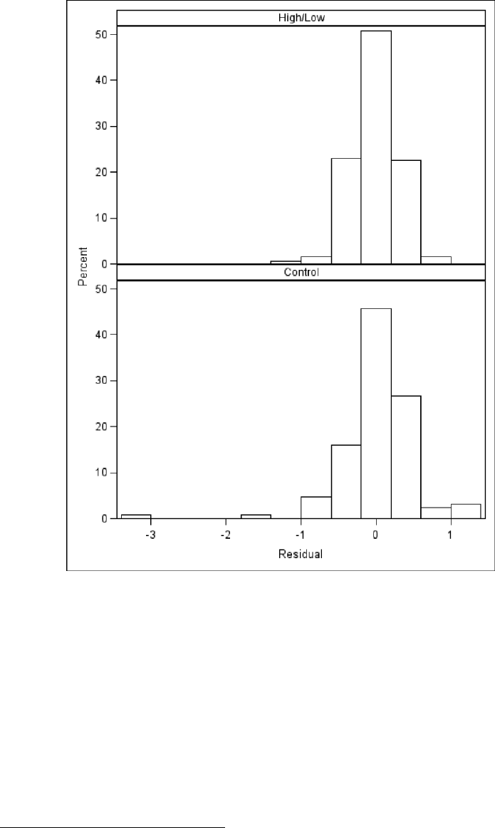
Two-Level Models for Clustered Data:The Rat Pup Example 123
FIGURE 3.4: Histograms for conditional raw residuals in the pooled high/low and control
treatment groups, based on the fit of Model 3.3.
The Shapiro–Wilk test of normality for the conditional residuals reported by
proc univariate (with the normal option) reveals that the assumption of normality for
the conditional residuals is violated in both the pooled high/low treatment group (Shapiro–
Wilk W = 0.982, p=0.015)3and the control group (W = 0.868, p<0.001). These results
suggest that the model still requires some additional refinement (e.g., transformation of the
response variable, or further investigation of outliers).
A plot of the conditional raw residuals vs. the predicted values by levels of TRTGRP
can be generated using the following syntax:
3SAS proc univariate also reports three additional tests for normality (including Kolmogorov–
Smirnov), the results of which indicate that we would not reject a null hypothesis of normality for the
conditional residuals in the high/low group (KS p>.15).
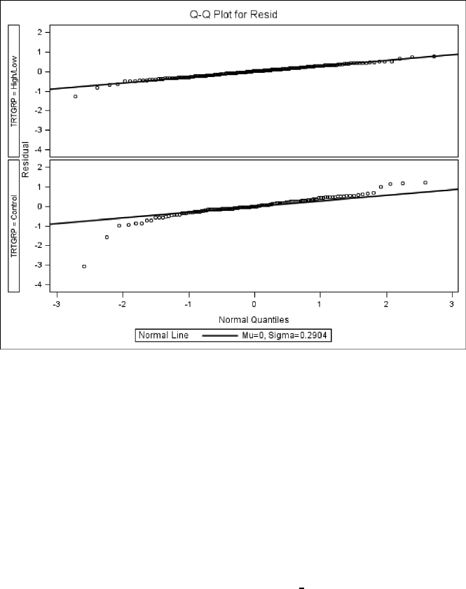
124 Linear Mixed Models: A Practical Guide Using Statistical Software
FIGURE 3.5: Normal Q–Q plots for the conditional raw residuals in the pooled high/low
and control treatment groups, based on the fit of Model 3.3.
/* Figure 3.6: Plot of conditional raw residuals vs. predicted values */
proc sgpanel data = pdat1;
panelby trtgrp / novarname rows=2;
scatter y = resid x = pred ;
format trtgrp tgrpfmt.;
run;
We do not see strong evidence of nonconstant variance for the pooled high/low group in
Figure 3.6. However, in the control group, there is evidence of an outlier, which after some
additional investigation was identified as being for PUP ID = 66. An analysis without the
values for this rat pup resulted in similar estimates for each of the fixed effects included in
Model 3.3, suggesting that this observation, though poorly fitted, did not have a great deal
of influence on these estimates.
3.10.1.2 Conditional Studentized Residuals
The conditional studentized residual for an observation is the difference between the
observed value and the predicted value, based on both the fixed and random effects in the
model, divided by its estimated standard error. The standard error of a residual depends on
both the residual variance for the treatment group (high/low or control), and the leverage
of the observation. The conditional studentized residuals are more appropriate to examine
model assumptions and to detect outliers and potentially influential points than are the raw
residuals because the raw residuals may not come from populations with equal variance, as
was the case in this analysis. Furthermore, if an observation has a large conditional residual,
we cannot know if it is large because it comes from a population with a larger variance, or
if it is just an unusual observation (Schabenberger, 2004).

Two-Level Models for Clustered Data:The Rat Pup Example 125
FIGURE 3.6: Scatter plots of conditional raw residuals vs. predicted values in the pooled
high/low and control treatment groups, based on the fit of Model 3.3.
We first examine the distribution of the conditional studentized residuals by obtaining
box plots of the distribution of these residuals for each litter. These box plots are produced
as a result of the boxplot option being used in the plots = specification of proc mixed,
or they can be obtained by using the following syntax:
proc sgplot data = pdat1 noautolegend;
vbox studentresid / category=litter;
run;
In Figure 3.7, we notice that the rat pup in row 66 of the data set (corresponding to
PUP ID = 66, from litter 6, because we sorted the ratpup3 data set by PUP ID before
fitting Model 3.3) is an outlier. These box plots also show that the distribution of the
conditional studentized residuals is approximately homogeneous across litters, unlike the
raw birth weight observations displayed in Figure 3.2. Note that there is no need to plot
studentized residuals separately for different treatments as there was for the raw conditional
residuals. This plot gives us some confidence in the appropriateness of Model 3.3.
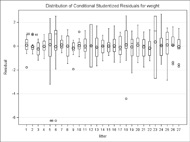
126 Linear Mixed Models: A Practical Guide Using Statistical Software
FIGURE 3.7: Box plot of conditional studentized residuals by new litter ID, based on the
fit of Model 3.3.
3.10.2 Influence Diagnostics
In this section, we examine influence diagnostics generated by proc mixed for the rat pups
and their litters.
3.10.2.1 Overall Influence Diagnostics
The graphs displayed here were obtained by using the influence (iter = 5 effect =
litter est) option in the model statement. The iter = suboption controls the maximum
number of additional iterations that will be performed by proc mixed to update the pa-
rameter estimates when a given litter is deleted. The est suboption causes SAS to display
a graph of the effects of each litter on the estimates of the fixed effects (shown in Figure
3.11).
model weight = treat sex litsize / solution ddfm=sat
influence(iter=5 effect=litter est) ;
Figure 3.8 shows the effect of deleting one litter at a time on the restricted (REML)
likelihood distance, a measure of the overall fit of the model. Based on this graph, litter
6 is shown to have a very large influence on the REML likelihood. In the remaining part
of the model diagnostics, we will investigate which aspect of the model fit is influenced by
individual litters (and litter 6 in particular).
Figure 3.9 shows the effect of deleting each litter on selected model summary statistics
(Cook’s D and Covratio). The upper left panel, Cook’s D Fixed Effects,showstheoverall
effect of the removal of each litter on the vector of fixed-effect parameter estimates. Litter
6 does not have a high value of Cook’s D statistic, indicating that it does not have a large
effect on the fixed-effect parameter estimates, even though it has a large influence on the
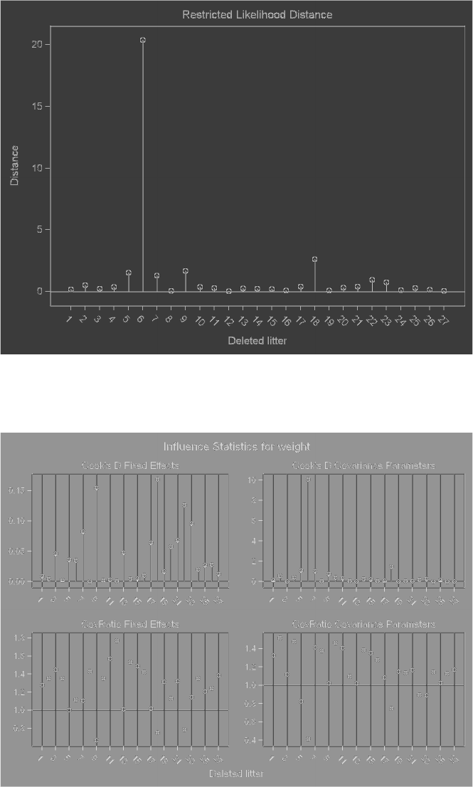
Two-Level Models for Clustered Data:The Rat Pup Example 127
FIGURE 3.8: Effect of deleting each litter on the REML likelihood distance for Model 3.3.
FIGURE 3.9: Effects of deleting one litter at a time on summary measures of influence for
Model 3.3.
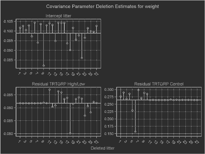
128 Linear Mixed Models: A Practical Guide Using Statistical Software
FIGURE 3.10: Effects of deleting one litter at a time on measures of influence for the
covariance parameters in Model 3.3.
REML likelihood. However, deletion of litter 6 has a very large influence on the estimated
covariance parameters, as shown in the Cook’s D Covariance Parameters panel. The
Covratio Fixed Effects panel illustrates the change in the precision of the fixed-effect
parameter estimates brought about by deleting the j-th litter. A reference line is drawn at
1.0 for this graph. A litter with a value of covratio = 1.0 indicates that deletion of that
litter has “no effect” on the precision of the fixed-effect parameter estimates, and a value of
covratio substantially below 1.0 indicates that deleting that litter will improve the precision
of the fixed-effect parameter estimates. A litter that greatly affects the covratio for the fixed
effects could have a large influence on statistical tests (such as t-tests and F-tests). There
do not appear to be any litters that have a large influence on the precision of the estimated
fixed effects (i.e., much lower covratio than the others). However, the very small value of
covratio = 0.4 for litter 6 in the panel of Covratio for Covariance Parameters indicates
that the precision of the estimated covariance parameters can be substantially improved by
removing litter 6.
3.10.2.2 Influence on Covariance Parameters
The ODS graphics output from SAS also produces influence diagnostics for the covariance
parameter estimates. These can be useful in identifying litters that may have a large effect
on the estimated between-litter variance (σ2
litter ),or on the residual variance estimates for
the two treatment groups (high/low and control). We have included the panel of plots
displaying the influence of each litter on the covariance parameters in Figure 3.10.
Each panel of Figure 3.10 depicts the influence of individual litters on one of the covari-
ance parameters in the model. There is a horizontal line showing the estimated value of the
covariance parameter when all litters are used in the model. For example, in the first panel
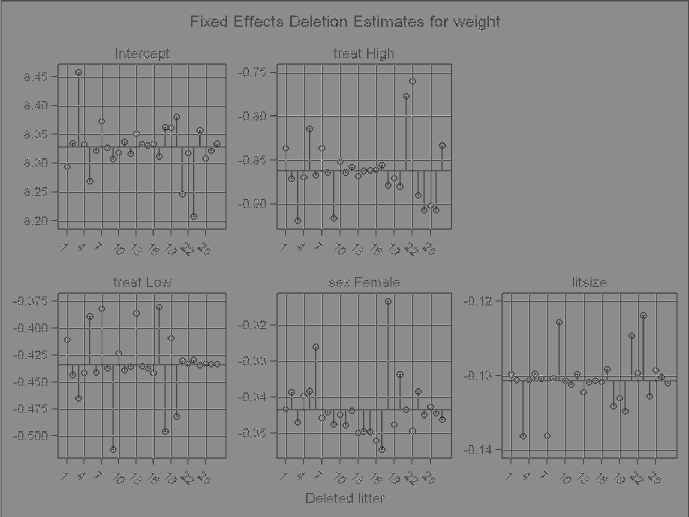
Two-Level Models for Clustered Data:The Rat Pup Example 129
FIGURE 3.11: Effect of deleting each litter on measures of influence for the fixed effects in
Model 3.3.
of the graph (labeled Intercept litter), the between-litter variance is displayed, with a
horizontal line at 0.099, the estimated between-litter variance from Model 3.3. The change
in the between-litter variance that would result from deletion of each litter is depicted.
Litter 6 has little influence on the between-litter variance estimate. The two lower panels
depict the residual variance estimates for the high/low treatment group (labeled Resid-
ual TRTGRP HIGH/LOW), and for the control group (labeled Residual TRTGRP
Control). This graph shows that deletion of litter 6 would decrease the residual variance
estimated for the control group from 0.2646 (as in Model 3.3) to about 0.155. We refitted
Model 3.3 excluding litter 6, and found that this was in fact the case, with the residual
variance for the control group decreasing from 0.2646 to 0.1569.
3.10.2.3 Influence on Fixed Effects
Figure 3.11 shows the effect of the deletion of each litter on the fixed-effect parameter
estimates, with one panel for each fixed effect. A horizontal line is drawn to represent the
value of the parameter estimate when all cases are used in the analysis, and the effect of
deleting each litter is depicted. For example, there is very little effect of litter 6 on the
estimated intercept in the model (because litter 6 is a control litter, its effect would be
included in the intercept).
We refitted Model 3.3 excluding litter 6, and found that the estimated fixed effects
were very similar (litter 6 received the control treatment). The residual variance for the
control group is much smaller without the presence of this litter, as discussed in Subsection
3.10.2.2. The likelihood ratio test for Hypothesis 3.4 was still significant after deleting litter
6(p<0.001), which suggested retaining the heterogeneous residual variance model (Model
3.2B) rather than assuming homogeneous residual variance (Model 3.1).

130 Linear Mixed Models: A Practical Guide Using Statistical Software
3.11 Software Notes and Recommendations
3.11.1 Data Structure
SAS proc mixed,theMIXED and GENLINMIXED commands in SPSS, the lme() and lmer()
functions in R,andthemixed command in Stata all require a single data set in the “long”
format, containing both Level 1 and Level 2 variables. See Table 3.2 for an illustration of
the Rat Pup data set in the “long” format.
The HLM2 procedure requires the construction of two data sets for a two-level analysis: a
Level 1 data set containing information on the dependent variable, and covariates measured
at Level 1 of the data (e.g., rat pups); and a Level 2 data set containing information on the
clusters (e.g., litters). See Subsection 3.4.5 for more details on setting up the two data sets
for HLM.
3.11.2 Syntax vs. Menus
SAS proc mixed and the lme() and lmer() functions in Rrequire users to create syntax to
specify an LMM. The MIXED and GENLINMIXED procedures in SPSS allows users to specify
a model using the menu system and then paste the syntax into a syntax window, where it
can be saved or run later. Stata allows users to specify a model either through the menu
system or by typing syntax for the mixed command. The HLM program works mainly by
menus (although batch processing of syntax for fitting HLM models is possible; see the
HLM documentation for more details).
3.11.3 Heterogeneous Residual Variances for Level 2 Groups
In the Rat Pup analysis we considered models (e.g., Model 3.2A, Model 3.2B, and Model
3.3) in which rat pups from different treatment groups were allowed to have different residual
variances. In other words, the Level 1 (residual) variance was allowed to vary as a function
of a Level 2 variable (TREATMENT, which is a characteristic of the litter). The option of
specifying a heterogeneous structure for the residual variance matrix, Rj, based on groups
defined by Level 2 variables, is currently only available in SAS proc mixed,theGENLINMIXED
command in SPSS, the lme() function in R,andthemixed command in Stata. The HLM2
procedure currently allows the residual variance at Level 1 of a two-level data set to be a
function of Level 1 variables, but not of Level 2 variables.
The ability to fit models with heterogeneous residual variance structures for different
groups of observations can be very helpful in certain settings and was found to improve
the fits of the models in the Rat Pup example. In some analyses, fitting a heterogeneous
residual variance structure could make a critical difference in the results obtained and in
the conclusions for the fixed effects in a model.
3.11.4 Display of the Marginal Covariance and Correlation Matrices
SAS proc mixed and the lme() function in Rallow users to request that the marginal
covariance matrix implied by a fitted model be displayed. The option of displaying the
implied marginal covariance matrix is currently not available in the other three software
procedures. We have found that it is helpful to investigate the implied marginal variance-
covariance and correlation matrices for a linear mixed model to see whether the estimated
variance-covariance structure is appropriate for the data set being analyzed.

Two-Level Models for Clustered Data:The Rat Pup Example 131
3.11.5 Differences in Model Fit Criteria
The –2 REML log-likelihood values obtained by fitting the two-level random intercept mod-
els discussed in this chapter are nearly identical across the software procedures (See Tables
3.6to3.8).However,therearesomeminordifferences in this statistic, as calculated by the
HLM2 procedure, which are perhaps due to computational differences. The AIC statistic
differs across the software procedures that calculate it, because of differences in the formulas
used (see Subsection 3.6.1 for a discussion of the different calculation formulas for AIC).
3.11.6 Differences in Tests for Fixed Effects
SAS proc mixed,theanova() function in R,andtheMIXED and GENLINMIXED commands
in SPSS all compute F-tests for the overall effects of fixed factors and covariates in the
model, in addition to t-tests for individual fixed-effect parameters. In contrast, the mixed
command in Stata calculates z-tests for individual fixed-effect parameters, or alternatively,
Wald chi-square tests for fixed effects via the use of the test command. The HLM2 program
calculates t-tests for fixed-effect parameters, or alternatively, Wald chi-square tests for sets
of fixed effects.
By default, the procedures in SAS and SPSS both calculate Type III F-tests, in which
the significance of each term is tested conditional on the fixed effects of all other terms in
the model. When the anova() function in Ris applied to a model fit object, it returns Type
I(sequential)F-tests, which are conditional on just the fixed effects listed in the model
prior to the effects being tested. The Type III and Type I F-tests are comparable only for
the term entered last in the model (except for certain models for balanced data). When
making comparisons between the F-test results for SAS and R,weusedtheF-tests only for
the last term entered in the model to maintain comparability. Note that SAS proc mixed
can calculate Type I F-tests by specifying the htype = 1 option in the model statement.
The programs that calculate F-tests and t-tests use differing methods to calculate de-
nominator degrees of freedom (or degrees of freedom for t-tests) for these approximate tests.
SAS allows the most flexibility in specifying methods for calculating denominator degrees
of freedom, as discussed below.
The MIXED command in SPSS and the lmerTest package in Rboth use the Satterthwaite
approximation when calculating denominator degrees of freedom for these tests and do not
provide other options.
A note on denominator degrees of freedom (df) methods for F-tests in SAS
The containment method is the default denominator degrees of freedom method for
proc mixed when a random statement is used, and no denominator degrees of freedom
method is specified. The containment method can be explicitly requested by using
the ddfm = contain option. The containment method attempts to choose the correct
degrees of freedom for fixed effects in the model, based on the syntax used to define
the random effects. For example, the df for the variable TREAT would be the df for
the random effect that contains the word “treat” in it. The syntax
random int / subject = litter(treat);
would cause SAS to use the degrees of freedom for litter(treat) as the denominator
degrees of freedom for the F-test of the fixed effects of TREAT. If no random effect
syntactically includes the word “treat,” the residual degrees of freedom would be used.
The Satterthwaite approximation (ddfm = sat) is intended to produce a more ac-
curate F-test approximation, and hence a more accurate p-value for the F-test. The

132 Linear Mixed Models: A Practical Guide Using Statistical Software
SAS documentation warns that the small-sample properties of the Satterthwaite ap-
proximation have not been thoroughly investigated for all types of models implemented
in proc mixed.
The Kenward–Roger method (ddfm = kr) is an attempt to make a further adjust-
ment to the F-statistics calculated by SAS, to take into account the fact that the
REML estimates of the covariance parameters are in fact estimates and not known
quantities. This method inflates the marginal variance-covariance matrix and then uses
the Satterthwaite method on the resulting matrix.
The between-within method (ddfm = bw) is the default for repeated-measures de-
signs, and may also be specified for analyses that include a random statement. This
method divides the residual degrees of freedom into a between-subjects portion and a
within-subjects portion. If levels of a covariate change within a subject (e.g., a time-
dependent covariate), then the degrees of freedom for effects associated with that co-
variate are the within-subjects df. If levels of a covariate are constant within subjects
(e.g., a time-independent covariate), then the degrees of freedom are assigned to the
between-subjects df for F-tests.
The residual method (ddfm = resid) assigns n−rank(X) as the denominator de-
grees of freedom for all fixed effects in the model. The rank of Xis the number of
linearly independent columns in the Xmatrixforagivenmodel.Thisisthesameas
the degrees of freedom used in ordinary least squares (OLS) regression (i.e., n−p,where
nis the total number of observations in the data set and pis the number of fixed-effect
parameters being estimated).
In R, when applying the summary() or anova() functions to the object containing the
results of an lme() fit, denominator degrees of freedom for tests associated with specific
fixed effects are calculated as follows:
Denominator degrees of freedom (df) methods for F-tests in R
Level 1: df = # of Level 1 observations – # of Level 2 clusters – # of Level
1 fixed effects
Level 2: df = # of Level 2 clusters – # of Level 2 fixed effects
For example, in the Type I F-test for TREATMENT from Rreported in Table 3.8,
the denominator degrees of freedom is 23, which is calculated as 27 (the number of litters)
minus 4 (the number of fixed-effect parameters associated with the Level 2 variables). In
theTypeIF-test for SEX, the denominator degrees of freedom is 294, which is calculated
as 322 (the number of pups in the data set) minus 27 (the number of litters), minus 1 (the
number of fixed-effect parameters associated with the Level 1 variables).
In general, the differences in the denominator degrees of freedom calculations are not
critical for the t-tests and F-tests when working with data sets and relatively large (>100)
samples at each level (e.g., rat pups at Level 1 and litters at Level 2) of the data set. However,
more attention should be paid when working with small samples, and these cases are best
handled using the different options provided by proc mixed in SAS. We recommend using
the Kenward–Roger method in these situations (Verbeke & Molenberghs, 2000).
We also remind readers that denominator degrees of freedom are not computed by
default when using the lme4 package version of the lmer() function in R,andp-values for
computed test statistics are not displayed as a result. Users of the lmer() function can
Two-Level Models for Clustered Data:The Rat Pup Example 133
consider loading the lmerTest package to compute Satterthwaite approximations of these
degrees of freedom (and p-values for the corresponding test statistics).
3.11.7 Post-Hoc Comparisons of Least Squares (LS) Means (Estimated
Marginal Means)
A very useful feature of SAS proc mixed and the MIXED and GENLINMIXED commands in
SPSS is the ability to obtain post-hoc pairwise comparisons of the least-squares means
(called estimated marginal means in SPSS) for different levels of a fixed factor, such as
TREATMENT. This can be accomplished by the use of the lsmeans statement in SAS
and the EMMEANS subcommand in SPSS. Different adjustments are available for multiple
comparisons in these two software procedures. SAS has the wider array of choices (e.g.,
Tukey–Kramer, Bonferroni, Dunnett, Sidak, and several others). SPSS currently offers only
the Bonferroni and Sidak methods. Post-hoc comparisons can also be computed in Rwith
some additional programming (Faraway, 2005), and users of Stata can apply the margins
command after fitting a model using mixed to explore alternative differences in marginal
means (see help margins in Stata).
3.11.8 Calculation of Studentized Residuals and Influence Statistics
Whereas each software procedure can calculate both conditional and marginal raw residuals,
SAS proc mixed is currently the only program that automatically provides studentized
residuals, which are preferred for model diagnostics (detection of outliers and identification
of influential observations).
SAS has also developed powerful and flexible influence diagnostics that can be used
to explore the potential influence of individual observations or clusters of observations on
both fixed-effect parameter estimates and covariance parameter estimates, and we have
illustrated the use of these diagnostic tools in this chapter.
3.11.9 Calculation of EBLUPs
The procedures in SAS, R, Stata, and HLM all allow users to generate and save the EBLUPs
for any random effects (and not just random intercepts, as in this example) included in an
LMM. In general, the current version of SPSS does not allow users to extract the values
of the EBLUPs. However, for models with a single random intercept for each cluster, the
EBLUPs can be easily calculated in SPSS, as illustrated for Model 3.1 in Subsection 3.4.2.
3.11.10 Tests for Covariance Parameters
By default, the procedures in SAS and SPSS do not report Wald tests for covariance pa-
rameters, but they can be requested as a means of obtaining the standard errors of the
estimated covariance parameters. We do not recommend the use of Wald tests for testing
hypotheses about the covariance parameters.
REML-based likelihood ratio tests for covariance parameters can be carried out (with a
varying amount of effort by the user) in proc mixed in SAS, the MIXED and GENLINMIXED
commands in SPSS, and by using the anova() function after fitting an LMM with the
either the lme() or the lmer() function in R. The syntax to perform these likelihood ratio
tests is most easily implemented using R, although the user may need to adjust the p-value
obtained, to take into account mixtures of χ2distributions when appropriate.
The default likelihood ratio test reported by the mixed command in Stata for the covari-
ance parameters is an overall test of the covariance parameters associated with all random
134 Linear Mixed Models: A Practical Guide Using Statistical Software
effects in the model. In models with a single random effect for each cluster, as in Model 3.1,
it is appropriate to use this test to decide if that effect should be included in the model.
However, the likelihood ratio test reported by Stata should be considered conservative in
models including multiple random effects.
The HLM procedures utilize alternative chi-square tests for covariance parameters asso-
ciated with random effects, the definition of which depend on the number of levels of data
(e.g., whether one is studying a two-level or three-level data set). For details on these tests
in HLM, refer to Raudenbush & Bryk (2002).
3.11.11 Reference Categories for Fixed Factors
By default, proc mixed in SAS and the MIXED and GENLINMIXED commands in SPSS both
prevent overparameterization of LMMs with categorical fixed factors by setting the fixed
effects associated with the highest-valued levels of the factors to zero. This means that when
using these procedures, the highest-valued level of a fixed factor can be thought of as the
“reference” category for the factor. The lme() and lmer() functions in Rand the mixed
command in Stata both use the lowest-valued levels of factors as the reference categories,
by default. These differences will result in different parameterizations of the model being
fitted in the different software procedures unless recoding is carried out prior to fitting the
model. However, the choice of parameterization will not affect the overall model fit criteria,
predicted values, hypothesis tests, or residuals.
Unlike the other four procedures, the HLM procedures in general (e.g., HLM2 for two-
level models, HLM3 for three-level models, etc.) do not automatically generate dummy
variables for levels of categorical fixed factors to be included in a mixed model. Indicator
variables for the nonreference levels of fixed factors need to be generated first in another
software package before importing the data sets into HLM. This leaves the choice of the
reference category to the user.

4
Three-Level Models for Clustered Data:
The Classroom Example
4.1 Introduction
In this chapter, we illustrate models for clustered study designs having three levels of data.
In three-level clustered data sets, the units of analysis (Level 1) are nested within randomly
sampled clusters (Level 2), which are in turn nested within other larger randomly sampled
clusters (Level 3). Such study designs allow us to investigate whether covariates measured at
each level of the data hierarchy have an impact on the dependent variable, which is always
measured on the units of analysis at Level 1.
Designs that lead to three-level clustered data sets can arise in many fields of research, as
illustrated in Table 4.1. For example, in the field of education research, as in the Classroom
data set analyzed in this chapter, students’ math achievement scores are studied by first
randomly selecting a sample of schools, then sampling classrooms within each school, and
finally sampling students from each selected classroom (Figure 4.1). In medical research,
a study to evaluate treatments for blood pressure may be carried out in multiple clinics,
with several doctors from each clinic selected to participate and multiple patients treated
by each doctor participating in the study. In a laboratory research setting, a study of birth
weights in rat pups similar to the Rat Pup study that we analyzed in Chapter 3 might have
replicate experimental runs, with several litters of rats involved in each run, and several rat
pups in each litter.
In Table 4.1, we provide possible examples of three-level clustered data sets in different
research settings. In these studies, the dependent variable is measured on one occasion for
each Level 1 unit of analysis, and covariates may be measured at each level of the data
hierarchy. For example, in a study of student achievement, the dependent variable, math
achievement score, is measured once for each student. In addition, student characteristics
such as age, classroom characteristics such as class size, and school characteristics such as
neighborhood poverty level are all measured. In the multilevel models that we fit to three-
level data sets, we relate the effects of covariates measured at each level of the data to the
dependent variable. Thus, in an analysis of the study of student achievement, we might
use student characteristics to help explain between-student variability in math achievement
scores, classroom characteristics to explain between-classroom variability in the classroom-
specific average math scores, and school-level covariates to help explain between-school
variation in school-specific mean math achievement scores.
Figure 4.1 illustrates the hierarchical structure of the data for an educational study sim-
ilar to the Classroom study analyzed in this chapter. This figure depicts the data structure
for a single (hypothetical) school with two randomly selected classrooms.
Models applicable for data from such sampling designs are known as three-level hier-
archical linear models (HLMs) and are extensions of the two-level models introduced in
135
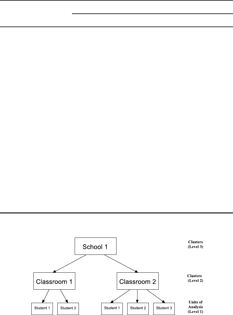
136 Linear Mixed Models: A Practical Guide Using Statistical Software
TABLE 4.1: Examples of Three-Level Data in Different Research Settings
Level of Data Research Setting
Education Medicine Biology
Level 3 Cluster of
clusters
(random
factor)
School Clinic Replicate
Covariates School size,
poverty level of
neighborhood
surrounding the
school
Number of
doctors in the
clinic, clinic type
(public or private)
Experimental run,
instrument
calibration,
ambient
temperature, run
order
Level 2 Cluster of
units
(random
factor)
Classroom Doctor Litter
Covariates Class size, years
of experience of
teacher
Specialty, years of
experience
Litter size, weight
of mother rat
Level 1 Unit of
analysis
Student Patient Rat Pup
Dependent
variable
Test scores Blood pressure Birth weight
Covariates Sex, age Age, illness
severity
Sex
FIGURE 4.1: Nesting structure of a clustered three-level data set in an educational setting.

Three-Level Models for Clustered Data:The Classroom Example 137
Chapter 3. Two-level, three-level, and higher-level models are generally referred to as mul-
tilevel models. Although multilevel models in general may have random effects associated
with both the intercept and with other covariates, in this chapter we restrict our discussion
to random intercept models, in which random effects at each level of clustering are
associated with the intercept. The random effects associated with the clusters at Level 2 of
a three-level data set are often referred to as nested random effects, because the Level 2
clusters are nested within the clusters at Level 3. In the absence of fixed effects associated
with covariates, a three-level HLM is also known as a variance components model.The
HLM software (Raudenbush et al., 2005; Raudenbush & Bryk, 2002), which we highlight
in this chapter, was developed specifically for analyses involving these and related types of
models.
4.2 The Classroom Study
4.2.1 Study Description
The Study of Instructional Improvement,1or SII (Anderson et al., 2009), was carried out
by researchers at the University of Michigan to study the math achievement scores of first-
and third-grade students in randomly selected classrooms from a national U.S. sample of
elementary schools. In this example, we analyze data for 1,190 first-grade students sampled
from 312 classrooms in 107 schools. The dependent variable, MATHGAIN, measures change
in student math achievement scores from the spring of kindergarten to the spring of first
grade.
The SII study design resulted in a three-level data set, in which students (Level 1) are
nested within classrooms (Level 2), and classrooms are nested within schools (Level 3).
We examine the contribution of selected student-level, classroom-level and school-level
covariates to the variation in students’ math achievement gain. Although one of the original
study objectives was to compare math achievement gain scores in schools participating in
comprehensive school reforms (CSRs) to the gain scores from a set of matched comparison
schools not participating in the CSRs, this comparison is not considered here.
A sample of the Classroom data is shown in Table 4.2. The first two rows in the table
are included to distinguish between the different types of variables; in the actual electronic
data set, the variable names are defined in the first row. Each row of data in Table 4.2
contains the school ID, classroom ID, student ID, the value of the dependent variable, and
values of three selected covariates, one at each level of the data.
The layout of the data in the table reflects the hierarchical nature of the data set. For
instance, the value of MATHPREP, a classroom-level covariate, is the same for all students
in the same classroom, and the value of HOUSEPOV, a school-level covariate, is the same
for all students within a given school. Values of student-level variables (e.g., the dependent
variable, MATHGAIN, and the covariate, SEX) vary from student to student (row to row)
in the data.
1Work on this study was supported by grants from the U.S. Department of Education to the Consortium
for Policy Research in Education (CPRE) at the University of Pennsylvania (Grant # OERI-R308A60003),
the National Science Foundation’s Interagency Educational Research Initiative to the University of Michigan
(Grant #s REC-9979863 & REC-0129421), the William and Flora Hewlett Foundation, and the Atlantic
Philanthropies. Opinions expressed in this book are those of the authors and do not reflect the views
of the U.S. Department of Education, the National Science Foundation, the William and Flora Hewlett
Foundation, or the Atlantic Philanthropies.

138 Linear Mixed Models: A Practical Guide Using Statistical Software
TABLE 4.2: Sample of the Classroom Data Set
School Classroom Student
(Level 3) (Level 2) (Level 1)
Cluster ID Covariate Cluster ID Covariate Unit ID Dependent
Variable
Covariate
SCHOOLID HOUSEPOV CLASSID MATHPREP CHILDID MATHGAIN SEX
1 0.0817 160 2.00 1 32 1
1 0.0817 160 2.00 2 109 0
1 0.0817 160 2.00 3 56 1
1 0.0817 217 3.25 4 83 0
1 0.0817 217 3.25 5 53 0
1 0.0817 217 3.25 6 65 1
1 0.0817 217 3.25 7 51 0
1 0.0817 217 3.25 8 66 0
1 0.0817 217 3.25 9 88 1
1 0.0817 217 3.25 10 7 0
1 0.0817 217 3.25 11 60 0
2 0.0823 197 2.50 12 2 1
2 0.0823 197 2.50 13 101 0
2 0.0823 211 2.33 14 30 0
2 0.0823 211 2.33 15 65 0
...
Note: “...” indicates portion of the data not displayed.
The following variables are considered in the analysis of the Classroom data:
School (Level 3) Variables
•SCHOOLID =SchoolIDnumber
a
•HOUSEPOV = Percentage of households in the neighborhood of the school below
the poverty level
Classroom (Level 2) Variables
•CLASSID = Classroom ID numbera
•YEARSTEAb= First-grade teacher’s years of teaching experience
•MATHPREP = First-grade teacher’s mathematics preparation: number of mathe-
matics content and methods courses
•MATHKNOWb= First-grade teacher’s mathematics content knowledge; based on
a scale based composed of 30 items (higher values indicate higher content knowledge)

Three-Level Models for Clustered Data:The Classroom Example 139
Student (Level 1) Variables
•CHILDID = Student ID numbera
•MATHGAIN = Student’s gain in math achievement score from the spring of kinder-
garten to the spring of first grade (the dependent variable)
•MATHKINDb= Student’s math score in the spring of their kindergarten year
•SEX = Indicator variable (0 = boy, 1 = girl)
•MINORITYb= Indicator variable (0 = non-minority student, 1 = minority student)
•SESb= Student socioeconomic status
aThe original ID numbers in the study were randomly reassigned for the data set used
in this example.
bNot shown in Table 4.2.
4.2.2 Data Summary
The descriptive statistics and plots for the Classroom data presented in this section are
obtained using the HLM software (Version 7). Syntax to carry out these descriptive analyses
using the other software packages is included on the web page for the book (see Appendix A).
4.2.2.1 Data Set Preparation
To perform the analyses for the Classroom data set using the HLM software, we need to
prepare three separate data sets:
1. The Level 1 (student-level) Data Set has one record per student, and contains
variables measured at the student level, including the response variable, MATH-
GAIN, the student-level covariates, and the identifying variables: SCHOOLID,
CLASSID, and CHILDID. The Level 1 data set is sorted in ascending order by
SCHOOLID, CLASSID, and CHILDID.
2. The Level 2 (classroom-level) Data Set has one record per classroom, and contains
classroom-level covariates, such as YEARSTEA and MATHKNOW, that are mea-
sured for the teacher. Each record contains the identifying variables SCHOOLID
and CLASSID, and the records are sorted in ascending order by these variables.
3. The Level 3 (school-level) Data Set has one record per school, and contains school-
level covariates, such as HOUSEPOV, and the identifying variable, SCHOOLID.
The data set is sorted in ascending order by SCHOOLID.
The Level 1, Level 2, and Level 3 data sets can easily be derived from a single data set
having the “long” structure illustrated in Table 4.2. All three data sets should be stored in
a format readable by HLM, such as ASCII (i.e., raw data in text files), or a data set specific
to a statistical software package. For ease of presentation, we assume that the three data
sets for this analysis have been set up in SPSS format (Version 21+).
4.2.2.2 Preparing the Multivariate Data Matrix (MDM) File
We prepare two MDM files for this initial data summary. One includes only variables that
do not have any missing values (i.e., it excludes MATHPREP and MATHKNOW), and

140 Linear Mixed Models: A Practical Guide Using Statistical Software
consequently, all students (n= 1190) are included. The second MDM file contains all
variables, including MATHPREP and MATHKNOW, and thus includes complete cases
(n= 1081) only.
We create the first Multivariate Data Matrix (MDM) file using the Level 1, Level
2, and Level 3 data sets defined earlier. After starting HLM, locate the main menu, and
click on File,Make new MDM file,andthenStat package input. In the dialog box
that opens, select HLM3 to fit a three-level hierarchical linear model with nested random
effects, and click OK. In the next window, choose the Input File Type as SPSS/Windows.
In the Level-1 Specification area of this window, we select the Level 1 data set.
Browse to the location of the student-level file. Click Choose Variables, and select the
following variables: CLASSID (check “L2id,” because this variable identifies clusters of
students at Level 2 of the data), SCHOOLID (check “L3id,” because this variable identifies
clusters of classrooms at Level 3 of the data), MATHGAIN (check “in MDM,” because this is
the dependent variable), and the student-level covariates MATHKIND, SEX, MINORITY,
and SES (check “in MDM” for all of these variables). Click OK when finished selecting
these variables.
In the Missing Data? box, select “Yes,” because some students may have missing values
on some of the variables. Then choose Delete missing level-1 data when: running
analyses, so that observations with missing data will be deleted from individual analyses
and not from the MDM file.
In the Level-2 Specification area of this window, select the Level 2 (classroom-level)
data set defined above. Browse to the location of the classroom-level data set. In the
Choose Variables dialog box, choose the CLASSID variable (check “L2id”) and the
SCHOOLID variable (check “L3id”). In addition, select the classroom-level covariate that
has complete data for all classrooms,2which is YEARSTEA (check “in MDM”). Click OK
when finished selecting these variables.
In the Level-3 Specification area of this window, select the Level 3 (school-level) data
set defined earlier. Browse to the location of the school-level data set, and choose the
SCHOOLID variable (click on “L3id”) and the HOUSEPOV variable, which has complete
data for all schools (check “in MDM”). Click OK when finished.
Once all three data sets have been identified and the variables have been selected, go
to the MDM template file portion of the window, where you will see a white box for
an MDM File Name (withan.mdmsuffix).EnteranamefortheMDMfile(suchas
classroom.mdm), including the .mdm suffix, and then click Save mdmt file to save an
MDM Template file that can be used later when creating the second MDM file. Finally,
click on Make MDM to create the MDM file using the three input files.
After HLM finishes processing the MDM file, click Check Stats to view descriptive
statistics for the selected variables at each level of the data, as shown in the following HLM
output:
2We do not select the classroom-level variables MATHPREP and MATHKNOW when setting up the
first MDM file, because information on these two variables is missing for some classrooms, which would
result in students from these classrooms being omitted from the initial data summary.

Three-Level Models for Clustered Data:The Classroom Example 141
'
&
$
%
LEVEL-1 DESCRIPTIVE STATISTICS
VARIABLE NAME N MEAN SD MINIMUM MAXIMUM
SEX 1190 0.51 0.50 0.00 1.00
MINORITY 1190 0.68 0.47 0.00 1.00
MATHKIND 1190 466.66 41.46 290.00 629.00
MATHGAIN 1190 57.57 34.61 -110.00 253.00
SES 1190 -0.01 0.74 -1.61 3.21
LEVEL-2 DESCRIPTIVE STATISTICS
VARIABLE NAME N MEAN SD MINIMUM MAXIMUM
YEARSTEA 312 12.28 9.65 0.00 40.00
LEVEL-3 DESCRIPTIVE STATISTICS
VARIABLE NAME N MEAN SD MINIMUM MAXIMUM
HOUSEPOV 107 0.19 0.14 0.01 0.56
Because none of the selected variables in the MDM file have any missing data, this is
a descriptive summary for all 1190 students, within the 312 classrooms and 107 schools.
We note that 51% of the 1190 students are female and that 68% of them are of minority
status. The average number of years teaching for the 312 teachers is 12.28, and the mean
proportion of households in poverty in the neighborhoods of the 107 schools is 0.19 (19%).
We now construct the second MDM file. After closing the window containing the de-
scriptive statistics, click Choose Variables in the Level-2 Specification area. At this
point, we add the MATHKNOW and MATHPREP variables to the MDM file by checking
“in MDM” for each of these variables; click OK after selecting them. Then, save the .mdm
file and the .mdmt template file under different names and click Make MDM to generate
a new MDM file containing these additional Level 2 variables. After clicking Check Stats,
the following output is displayed:
'
&
$
%
LEVEL-1 DESCRIPTIVE STATISTICS
VARIABLE NAME N MEAN SD MINIMUM MAXIMUM
SEX 1081 0.50 0.50 0.00 1.00
MINORITY 1081 0.67 0.47 0.00 1.00
MATHKIND 1081 467.15 42.00 290.00 629.00
MATHGAIN 1081 57.84 34.70 -84.00 253.00
SES 1081 -0.01 0.75 -1.61 3.21
LEVEL-2 DESCRIPTIVE STATISTICS
VARIABLE NAME N MEAN SD MINIMUM MAXIMUM
YEARSTEA 285 12.28 9.80 0.00 40.00
MATHKNOW 285 -0.08 1.00 -2.50 2.61
MATHPREP 285 2.58 0.96 1.00 6.00
LEVEL-3 DESCRIPTIVE STATISTICS
VARIABLE NAME N MEAN SD MINIMUM MAXIMUM
HOUSEPOV 105 0.20 0.14 0.01 0.56

142 Linear Mixed Models: A Practical Guide Using Statistical Software
Note that 27 classrooms have been dropped from the Level 2 file because of missing data
on the additional Level 2 variables, MATHKNOW and MATHPREP. Consequently, there
were two schools (SCHOOLID = 48 and 58) omitted from the Check Stats summary,
because none of the classrooms in these two schools had information on MATHKNOW and
MATHPREP. This resulted in only 1081 students being analyzed in the data summary
based on the second MDM file, which is 109 fewer than were included in the first summary.
We close the window containing the descriptive statistics and click Done to proceed to the
HLM model-building window.
In the model-building window we continue the data summary by examining box plots of
the observed MATHGAIN responses for students in the selected classrooms from the first
eight schools in the first (complete) MDM file. Select File,Graph Data,andbox-whisker
plots. To generate these box plots, select MATHGAIN as the Y-axis variable and select
Group at level-3 to generate a separate panel of box plots for each school. For Number
of groups, we select First ten groups (corresponding to the first 10 schools). Finally,
click OK. HLM produces box plots for the first 10 schools, and we display the plots for the
first eight schools in Figure 4.2.
In Figure 4.2, we note evidence of both between-classroom and between-school variability
in the MATHGAIN responses. We also see differences in the within-classroom variability,
which may be explained by student-level covariates. By clicking Graph Settings in the
HLM graph window, one can select additional Level 2 (e.g., YEARSTEA) or Level 3 (e.g.,
HOUSEPOV) variables as Z-focus variables that color-code box plots, based on values of
the classroom- and school-level covariates. Readers should refer to the HLM manual for
more information on additional graphing features.
4.3 Overview of the Classroom Data Analysis
For the analysis of the Classroom data, we follow the “step-up” modeling strategy outlined
in Subsection 2.7.2. This approach differs from the strategy used in Chapter 3, in that
it starts with a simple model, containing only a single fixed effect (the overall intercept),
random effects associated with the intercept for classrooms and schools, and residuals, and
then builds the model by adding fixed effects of covariates measured at the various levels.
In Subsection 4.3.1 we outline the analysis steps, and informally introduce related models
and hypotheses to be tested. In Subsection 4.3.2 we present the specification of selected
models that will be fitted to the Classroom data, and in Subsection 4.3.3 we detail the
hypotheses tested in the analysis. To follow the analysis steps outlined in this section, we
refer readers to the schematic diagram presented in Figure 4.3.
4.3.1 Analysis Steps
Step 1: Fit the initial “unconditional” (variance components) model (Model
4.1).
Fit a three-level model with a fixed intercept, and random effects associated with
the intercept for classrooms (Level 2) and schools (Level 3), and decide whether
to keep the random intercepts for classrooms (Model 4.1 vs. Model 4.1A).
Because Model 4.1 does not include fixed effects associated with any covariates, it is
referred to as a “means-only” or “unconditional” model in the HLM literature and is known
as a variance components model in the classical ANOVA context. We include the term
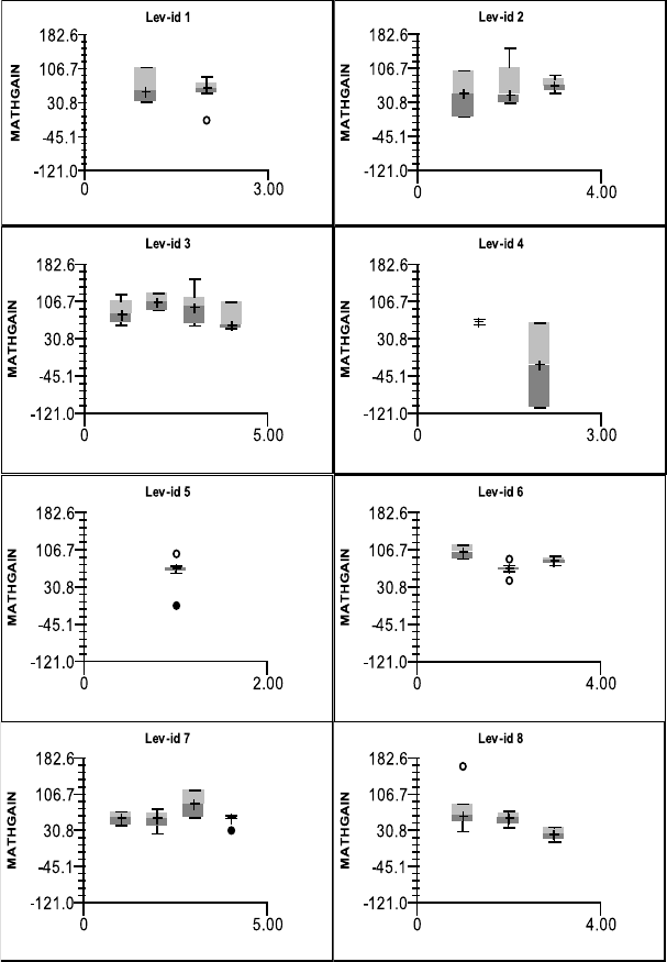
Three-Level Models for Clustered Data:The Classroom Example 143
FIGURE 4.2: Box plots of the MATHGAIN responses for students in the selected classrooms
in the first eight schools for the Classroom data set.
“unconditional” in quotes because it indicates a model that is not conditioned on any fixed
effects other than the intercept, although it is still conditional on the random effects. The
model includes a fixed overall intercept, random effects associated with the intercept for
classrooms within schools, and random effects associated with the intercept for schools.
After fitting Model 4.1, we obtain estimates of the initial variance components, i.e., the
variances of the random effects at the school level and the classroom level, and the residual
variance at the student level. We use the variance component estimates from the Model
4.1 fit to estimate intraclass correlation coefficients (ICCs) of MATHGAIN responses at the
school level and at the classroom level (see Section 4.8).
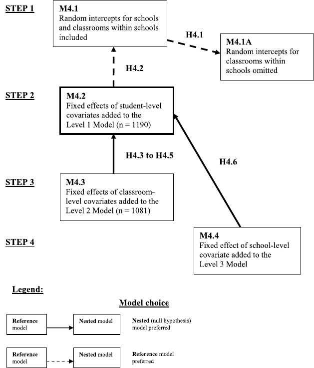
144 Linear Mixed Models: A Practical Guide Using Statistical Software
FIGURE 4.3: Model selection and related hypotheses for the Classroom data analysis.
We also test Hypothesis 4.1 to decide whether the random effects associated with the
intercepts for classrooms nested within schools can be omitted from Model 4.1. We fit a
model without the random classroom effects (Model 4.1A) and perform a likelihood ratio
test. We decide to retain the random intercepts associated with classrooms nested within
schools, and we also retain the random intercepts associated with schools in all subsequent
models, to preserve the hierarchical structure of the data. Model 4.1 is preferred at this
stage of the analysis.
Step 2: Build the Level 1 Model by adding Level 1 Covariates (Model 4.1 vs.
Model 4.2).
Add fixed effects associated with covariates measured on the students to the
Level 1 Model to obtain Model 4.2, and evaluate the reduction in the residual
variance.
In this step, we add fixed effects associated with the four student-level covariates
(MATHKIND, SEX, MINORITY, and SES) to Model 4.1 and obtain Model 4.2. We in-
Three-Level Models for Clustered Data:The Classroom Example 145
formally assess the related reduction in the between-student variance (i.e., the residual
variance).
We also test Hypothesis 4.2, using a likelihood ratio test, to decide whether we should
add the fixed effects associated with all of the student-level covariates to Model 4.1. We
decide to add these fixed effects and choose Model 4.2 as our preferred model at this stage
of the analysis.
Step 3: Build the Level 2 Model by adding Level 2 covariates (Model 4.3).
Add fixed effects associated with the covariates measured on the Level 2 clusters
(classrooms) to the Level 2 model to create Model 4.3, and decide whether to
retain the effects of the Level 2 covariates in the model.
We add fixed effects associated with the three classroom-level covariates (YEARSTEA,
MATHPREP, and MATHKNOW) to Model 4.2 to obtain Model 4.3. At this point, we would
like to assess whether the Level 2 component of variance (i.e., the variance of the nested
random classroom effects) is reduced when we include the effects of these Level 2 covariates
in the model. However, Models 4.2 and 4.3 are fitted using different sets of observations,
owing to the missing values on the MATHPREP and MATHKNOW covariates, and a simple
comparison of the classroom-level variance components obtained from these two models is
therefore not appropriate.
We also test Hypotheses 4.3, 4.4, and 4.5, to decide whether we should keep the fixed
effects associated with YEARSTEA, MATHPREP, and MATHKNOW in Model 4.3, using
individual t-tests for each hypothesis. Based on the results of the t-tests, we decide that none
of the fixed effects associated with these Level 2 covariates should be retained and choose
Model 4.2 as our preferred model at this stage. We do not use a likelihood ratio test for
the fixed effects of all Level 2 covariates at once, as we did for all Level 1 covariates in Step
2, because different sets of observations were used to fit Models 4.2 and 4.3. A likelihood
ratio test is only possible if both models were fitted using the same set of observations. In
Subsection 4.11.4, we illustrate syntax that could be used to construct a “complete case”
data set in each software package.
Step 4: Build the Level 3 Model by adding the Level 3 covariate (Model 4.4).
Add a fixed effect associated with the covariate measured on the Level 3 clusters
(schools) to the Level 3 model to create Model 4.4, and evaluate the reduction
in the variance component associated with the Level 3 clusters.
In this last step, we add a fixed effect associated with the only school-level covariate,
HOUSEPOV, to Model 4.2 and obtain Model 4.4. We assess whether the variance component
at the school level (i.e., the variance of the random school effects) is reduced when we include
this fixed effect at Level 3 of the model. Because the same set of observations was used to
fit Models 4.2 and 4.4, we informally assess the relative reduction in the between-school
variance component in this step.
We also test Hypothesis 4.6 to decide whether we should add the fixed effect associated
with the school-level covariate to Model 4.2. Based on the result of a t-test for the fixed
effect of HOUSEPOV in Model 4.4, we decide not to add this fixed effect, and choose Model
4.2 as our final model. We consider diagnostics for Model 4.2 in Section 4.9, using residual
files generated by the HLM software.
Figure 4.3 provides a schematic guide to the model selection process and hypotheses
considered in the analysis of the Classroom data. See Subsection 3.3.1 for a detailed inter-
pretation of the elements of this figure. Table 4.3 provides a summary of the various models
considered in the Classroom data analyses.
146 Linear Mixed Models: A Practical Guide Using Statistical Software
4.3.2 Model Specification
4.3.2.1 General Model Specification
We specify Model 4.3 in (4.1), because it is the model with the most fixed effects that we
consider in the analysis of the Classroom data. Models 4.1, 4.1A, and 4.2 are simplifications
of this more general model. Selected models are summarized in Table 4.3.
The general specification for Model 4.3 is:
MATHGAINijk =β0+β1×MATHKINDijk +β2×SEXijk
+β3×MINORITYijk +β4×SESijk +β5×YEARSTEAjk
+β6×MATHPREPjk +β7×MATHKNOWjk
⎫
⎪
⎬
⎪
⎭fixed
+uk+uj|k+εijk }random
(4.1)
In this specification, MATHGAINijk represents the value of the dependent variable for
student iin classroom jnested within school k;β0through β7represent the fixed intercept
and the fixed effects of the covariates (e.g., MATHKIND,. . . , MATHKNOW); ukis the
random effect associated with the intercept for school k;uj|kis the random effect associated
with the intercept for classroom jwithin school k;andεijk represents the residual. To obtain
Model 4.4, we add the fixed effect (β8) of the school-level covariate HOUSEPOV and omit
the fixed effects of the classroom-level covariates (β5through β7).
The distribution of the random effects associated with the schools in Model 4.3 is written
as
uk∼N(0,σ
2
int:school)
where σ2
int:school represents the variance of the school-specific random intercepts.
The distribution of the random effects associated with classrooms nested within a given
school is
uj|k∼N(0,σ
2
int:classroom)
where σ2
int:classroom represents the variance of the random classroom-specific intercepts at
any given school. This between-classroom variance is assumed to be constant for all schools.
The distribution of the residuals associated with the student-level observations is
εijk ∼N(0,σ
2)
where σ2represents the residual variance.
We assume that the random effects, uk, associated with schools, the random effects, uj|k,
associated with classrooms nested within schools, and the residuals, εijk,are all mutually
independent.
The general specification of Model 4.3 corresponds closely to the syntax that is used to
fit the model in SAS, SPSS, Stata, and R. In Subsection 4.3.2.2 we provide the hierarchical
specification that more closely corresponds to the HLM setup of Model 4.3.
4.3.2.2 Hierarchical Model Specification
We now present a hierarchical specification of Model 4.3. The following model is in the form
used in the HLM software, but employs the notation used in the general specification of
Model 4.3 in (4.1), rather than the HLM notation. The correspondence between the notation
used in this section and that used in the HLM software is shown in Table 4.3.

Three-Level Models for Clustered Data:The Classroom Example 147
TABLE 4.3: Summary of Selected Models Considered for the Classroom Data
Term/Vari ab le General HLM Model
Notation Notation 4.1 4.2 4.3 4.4
Fixed effects Intercept β0γ000 √√√√
MATHKIND β1γ300 √√√
SEX β2γ100 √√√
MINORITY β3γ200 √√√
SES β4γ400 √√√
YEARSTEA β5γ010 √
MATHPREP β6γ030 √
MATHKNOW β7γ020 √
HOUSEPOV β8γ001 √
Random Classroom (j)Intercept uj|krjk √√√√
effects School (k)Intercept uku00k√√√√
Residuals Student (i)εijk eijk √√√√
Covariance
parameters
(θD)forD
matrix
Classroom
level
Variance of
intercepts
σ2
int:class τπ√√√√
School level Variance of
intercepts
σ2
int:school τβ√√√√
Covariance
parameters
(θR)forRi
matrix
Student level Residual variance σ2σ2√√√√
148 Linear Mixed Models: A Practical Guide Using Statistical Software
The hierarchical model has three components, reflecting contributions from the three
levels of data shown in Table 4.2. First, we write the Level 1 component as
Level 1 Model (Student)
MATHGAINijk =b0j|k+β1×MATHKINDijk +β2×SEXijk
+β3×MINORITYijk +β4×SESijk +εijk (4.2)
where
εijk ∼N(0,σ
2)
The Level 1 model (4.2) shows that at the student level of the data, we have a set of
simple classroom-specific linear regressions of MATHGAIN on the student-level covariates.
The unobserved classroom-specific intercepts, b0j|k, are related to several other fixed and
random effects at the classroom level, and are defined in the following Level 2 model.
The Level 2 model for the classroom-specific intercepts can be written as
Level 2 Model (Classroom)
b0j|k=b0k+β5×YEARSTEAjk +β6×MATHPREPjk
+β7×MATHKNOWjk +uj|k(4.3)
where
uj|k∼N(0,σ
2
int:classroom)
The Level 2 model (4.3) assumes that the intercept, b0j|k, for classroom jnested within
school k, depends on the unobserved intercept specific to the k-th school, b0k, the classroom-
specific covariates associated with the teacher for that classroom (YEARSTEA, MATH-
PREP, and MATHKNOW), and a random effect, uj|k, associated with classroom jwithin
school k.
The Level 3 model for the school-specific intercepts in Model 4.3 is:
Level 3 Model (School)
b0k=β0+uk(4.4)
where
uk∼N(0,σ
2
int:school)
The Level 3 model in (4.4) shows that the school-specific intercept in Model 4.3 depends
on the overall fixed intercept, β0, and the random effect, uk, associated with the intercept
for school k.
By substituting the expression for b0kfrom the Level 3 model into the Level 2 model,
and then substituting the resulting expression for b0j|kfrom the Level 2 model into the
Level 1 model, we recover Model 4.3 as it was specified in (4.1).
We specify Model 4.4 by omitting the fixed effects of the classroom-level covariates from
Model 4.3, and adding the fixed effect of the school-level covariate, HOUSEPOV, to the
Level 3 model.
4.3.3 Hypothesis Tests
Hypothesis tests considered in the analysis of the Classroom data are summarized in Ta-
ble 4.4.

Three-Level Models for Clustered Data:The Classroom Example 149
TABLE 4.4: Summary of Hypotheses Tested in the Classroom Analysis
Hypothesis Specification Hypothesis Test
Models Compared
Label Null (H0)Alternative(HA) Test Nested
Model
(H0)
Ref.
Model
(HA)
Est.
Method
Test Stat.
Dist.
under H0
4.1 Drop uj|kRetain uj|kLRT Model Model REML 0.5χ2
0+0.5χ2
1
(σ2
int:classroom =0) (σ2
int:classroom >0) 4.1A 4.1
4.2 Fixed effects of
student-level
covariates are all zero
(β1=β2=β3
At least one fixed
effect at the student
level is different from
zero
LRT Model
4.1
Model
4.2
ML χ2
4
=β4=0)
4.3 Fixed effect of
YEARSTEA is zero
(β5=0)
β5=0 t-test N/A Model
4.3
REML/
ML
ta
177
4.4 Fixed effect of
MATHPREP is zero
(β6=0)
β6=0 t-test N/A Model
4.3
REML/
ML
ta
177
4.5 Fixed effect of
MATHKNOW is zero
(β7=0)
β7=0 t-test N/A Model
4.3
REML/
ML
ta
177
4.6 Fixed effect of
HOUSEPOV is zero
(β8=0)
β8=0 t-test N/A Model
4.4
REML/
ML
ta
105
aDegrees of freedom for the t-statistics are those reported by the HLM3 procedure.
150 Linear Mixed Models: A Practical Guide Using Statistical Software
Hypothesis 4.1. The random effects associated with the intercepts for classrooms nested
within schools can be omitted from Model 4.1.
We do not directly test the significance of the random classroom-specific intercepts, but
rather test null and alternative hypotheses about the variance of the classroom-specific
intercepts. The null and alternative hypotheses are:
H0:σ2
int:classroom =0
HA:σ2
int:classroom >0
We use a REML-based likelihood ratio test for Hypothesis 4.1 in SAS, SPSS, R,and
Stata. The test statistic is calculated by subtracting the –2 REML log-likelihood for Model
4.1 (the reference model, including the nested random classroom effects) from the corre-
sponding value for Model 4.1A (the nested model). To obtain a p-value for this test statistic,
we refer it to a mixture of χ2distributions, with 0 and 1 degrees of freedom and equal weight
0.5.
The HLM3 procedure does not use REML estimation and is not able to fit a model
without any random effects at a given level of the model, such as Model 4.1A. Therefore,
an LRT cannot be performed, so we consider an alternative chi-square test for Hypothesis
4.1 provided by HLM in Subsection 4.7.2.
We decide that the random effects associated with the intercepts for classrooms nested
within schools should be retained in Model 4.1. We do not explicitly test the variance of
the random school-specific intercepts, but we retain them in Model 4.1 and all subsequent
models to reflect the hierarchical structure of the data.
Hypothesis 4.2. The fixed effects associated with the four student-level covariates should
be added to Model 4.1.
The null and alternative hypotheses for the fixed effects associated with the student-level
covariates, MATHKIND, SEX, MINORITY, and SES, are:
H0:β1=β2=β3=β4=0
HA: At least one fixed effect is not equal to zero
We test Hypothesis 4.2 using a likelihood ratio test, based on maximum likelihood (ML)
estimation. The test statistic is calculated by subtracting the –2 ML log-likelihood for Model
4.2 (the reference model with the fixed effects of all student-level covariates included) from
that for Model 4.1 (the nested model). Under the null hypothesis, the distribution of this
test statistic is asymptotically a χ2with 4 degrees of freedom.
We decide that the fixed effects associated with the Level 1 covariates should be added
and select Model 4.2 as our preferred model at this stage of the analysis.
Hypotheses 4.3, 4.4, and 4.5. The fixed effects associated with the classroom-level
covariates should be retained in Model 4.3.
The null and alternative hypotheses for the fixed effects associated with the classroom-
level covariates YEARSTEA, MATHPREP, and MATHKNOW are written as follows:
•Hypothesis 4.3 for the fixed effect associated with YEARSTEA:
H0:β5=0
HA:β5=0
•Hypothesis 4.4 for the fixed effect associated with MATHPREP:
H0:β6=0
HA:β6=0

Three-Level Models for Clustered Data:The Classroom Example 151
•Hypothesis 4.5 for the fixed effect associated with MATHKNOW:
H0:β7=0
HA:β7=0
We test each of these hypotheses using t-tests based on the fit of Model 4.3. We de-
cide that none of the fixed effects associated with the classroom-level covariates should be
retained, and keep Model 4.2 as our preferred model at this stage of the analysis.
Because there are classrooms with missing values for the classroom-level covariate
MATHKNOW, there are different sets of observations used to fit Models 4.2 and 4.3. In
this case, we cannot use a likelihood ratio test to decide if we should keep the fixed effects
of all covariates at Level 2 of the model, as we did for the fixed effects of the covariates at
Level 1 of the model when we tested Hypothesis 4.2.
To perform a likelihood ratio test for the effects of all of the classroom-level covariates,
we would need to fit both Models 4.2 and 4.3 using the same cases (i.e., those cases with
no missing data on all covariates would need to be considered for both models). See Sub-
section 4.11.4 for a discussion of how to set up the necessary data set, with complete data
for all covariates, in each of the software procedures.
Hypothesis 4.6. The fixed effect associated with the school-level covariate HOUSEPOV
should be added to Model 4.2.
The null and alternative hypotheses for the fixed effect associated with HOUSEPOV are
specified as follows:
H0:β8=0
HA:β8=0
We test Hypothesis 4.6 using a t-test for the significance of the fixed effect of HOUSE-
POV in Model 4.4. We decide that the fixed effect of this school-level covariate should not
be added to the model, and choose Model 4.2 as our final model. For the results of these
hypothesis tests, see Section 4.5.
4.4 Analysis Steps in the Software Procedures
We compare results for selected models across the software procedures in Section 4.6.
4.4.1 SAS
We begin by reading the comma-delimited data file, classroom.csv (assumed to have the
“long” data structure displayed in Table 4.2, and located in the C:\temp directory) into a
temporary SAS data set named classroom:
proc import out = WORK.classroom
datafile = "C:\temp\classroom.csv";
dbms = csv replace;
getnames = YES;
datarow = 2;
guessingrows = 20;
run;

152 Linear Mixed Models: A Practical Guide Using Statistical Software
Step 1: Fit the initial “unconditional” (variance components) model (Model
4.1), and decide whether to omit the random classroom effects (Model 4.1 vs.
Model 4.1A).
Prior to fitting the models in SAS, we sort the data set by SCHOOLID and CLASSID.
Although not necessary for fitting the models, this sorting makes it easier to interpret
elements in the marginal variance-covariance and correlation matrices that we display later.
proc sort data = classroom;
by schoolid classid;
run;
The SAS code for fitting Model 4.1 using REML estimation is shown below. Because
the only fixed effect in Model 4.1 is the intercept, we use the model statement with no
covariates on the right-hand side of the equal sign; the intercept is included by default. The
two random statements specify that a random intercept should be included for each school
and for each classroom nested within a school.
title "Model 4.1";
proc mixed data = classroom noclprint covtest;
class classid schoolid;
model mathgain = / solution;
random intercept / subject = schoolid v vcorr;
random intercept / subject = classid(schoolid);
run;
We specify two options in the proc mixed statement. The noclprint option suppresses
listing of levels of the class variables in the output to save space; we recommend using this
option only after an initial examination of the levels of the class variablestobesurethe
data set is being read correctly. The covtest option is specified to request that the standard
errors of the estimated variance components be included in the output. The Wald tests of
covariance parameters that are reported when the covtest option is specified should not
be used to test hypotheses about the variance components.
The solution option in the model statement causes SAS to print estimates of the fixed-
effect parameters included in the model, which for Model 4.1 is simply the overall intercept.
We use the voption to request that a single block (corresponding to the first school)
of the estimated Vmatrix for the marginal model implied by Model 4.1 be displayed
in the output (see Subsection 2.2.3 for more details on the Vand Zmatrices in SAS). In
addition, we specify the vcorr option to request that the corresponding marginal correlation
matrix be displayed. The vand vcorr options can be added to one or both of the random
statements, with the same results. We display the SAS output from these commands in
Section 4.8.
Software Note: When the proc mixed syntax above is used, the overall subject is
considered by SAS to be SCHOOLID. Because CLASSID is specified in the class
statement, SAS sets up the same number of columns in the Zmatrix for each school.
The SAS output below, obtained by fitting Model 4.1 to the Classroom data, indicates

Three-Level Models for Clustered Data:The Classroom Example 153
that there are 107 subjects included in this model (corresponding to the 107 schools).
SAS sets up 10 columns in the Zmatrix for each school, which corresponds to the
maximum number of classrooms in any given school (9) plus a single column for the
school. The maximum number of students in any school is 31.
'
&
$
%
Dimensions
Covariance Parameters 3
Columns in X 1
Columns in Z Per Subject 10
Subjects 107
Max Obs Per Subject 31
This syntax for Model 4.1 allows SAS to fit the model efficiently, by taking blocks
of the marginal Vmatrix into account. However, it also means that if EBLUPs are
requested by specifying the solution option in the corresponding random statements,
as illustrated below, SAS will display output for 10 classrooms within each school, even
for schools that have fewer than 10 classrooms. This results in extra unwanted output
being generated. We present alternative syntax to avoid this potential problem below.
Alternative syntax for Model 4.1 may be specified by omitting the subject = option in
the random statement for SCHOOLID. By including the solution option in one or both
random statements, we obtain the predicted values of the EBLUPs for each school, followed
by the EBLUPs for the classrooms, with no extra output being produced.
title "Model 4.1: Alternative Syntax";
proc mixed data = classroom noclprint covtest;
class classid schoolid;
model mathgain = / solution;
random schoolid / solution;
random int / subject = classid(schoolid);
run;
The resulting “Dimensions” output for this model specification is as follows:
'
&
$
%
Dimensions
Covariance Parameters 3
Columns in x 1
Columns in Z Per Subject 419
Subjects 1
Max obs Per Subject 1190
SAS now considers there to be only one subject in this model, even though we specified
asubject = option in the second random statement. In this case, the Zmatrix has 419
columns, which correspond to the total number of schools (107) plus classrooms (312).
A portion of the resulting output for the EBLUPs is as follows:

154 Linear Mixed Models: A Practical Guide Using Statistical Software
'
&
$
%
Solution for Random Effects
---------------------------------------------------------------------
Std Err
Effect Classid Schoolid Estimate Pred DF t Value pr > |t|
---------------------------------------------------------------------
schoolid 1 0.94110 7.1657 878 0.13 0.8955
schoolid 2 2.54710 7.0625 878 0.36 0.7184
schoolid 3 13.67300 6.6390 878 2.06 0.0397
...
Intercept 160 1 1.63800 8.9188 878 0.18 0.8543
Intercept 217 1 -0.43260 8.1149 878 -0.05 0.9575
Intercept 197 2 -1.69390 9.1905 878 -0.18 0.8538
Intercept 211 2 2.51290 8.6881 878 0.29 0.7725
Intercept 307 2 2.44330 8.6881 878 0.28 0.7786
Intercept 11 3 3.86990 8.6607 878 0.45 0.6551
Intercept 137 3 5.56300 9.1818 878 0.61 0.5448
Intercept 145 3 8.10160 8.4622 878 0.96 0.3386
Intercept 228 3 -0.02247 8.8971 878 -0.00 0.9980
Note that the standard error, along with a t-test, is displayed for each EBLUP. The test
statistic is calculated by dividing the predicted EBLUP by its estimated standard error,
with the degrees of freedom being the same as indicated by the ddfm = option. If no ddfm =
option is specified, SAS will use the default “containment” method (see Subsection 3.11.6
for a discussion of different methods of calculating denominator degrees of freedom in SAS).
Although it may not be of particular interest to test whether the predicted random effect
for a given school or classroom is equal to zero, large values of the t-statistic may indicate
an outlying value for a given school or classroom.
To suppress the display of the EBLUPs in the output, but obtain them in a SAS data
set, we use the following ODS statements prior to invoking proc mixed:
ods exclude solutionr;
ods output solutionr=eblupdat;
The first ods statement prevents the EBLUPs from being displayed in the output. The
second ods statement requests that the EBLUPs be placed in a new SAS data set named
eblupdat. The distributions of the EBLUPs contained in the eblupdat data set can be
investigated graphically to check for possible outliers (see Subsection 4.10.1 for diagnostic
plots of the EBLUPs associated with Model 4.2). Note that the eblupdat data set is only
created if the solution option is added to either of the random statements.
We recommend that readers be cautious about including options, such as vand vcorr,
for displaying the marginal variance-covariance and correlation matrices when using ran-
dom statements with no subject = option, as shown in the first random statement in the
alternative syntax for Model 4.1. In this case, SAS will display matrices that are of the
same dimension as the total number of observations in the entire data set. In the case of
the Classroom data, this would result in a 1190 ×1190 matrix being displayed for both the
marginal variance-covariance and correlation matrices.
We now fit Model 4.1A using REML estimation (the default), so that we can perform
a likelihood ratio test of Hypothesis 4.1 to decide if we need the nested random class-
room effects in Model 4.1. We omit the random classroom-specific intercepts in Model
4.1A by adding an asterisk at the beginning of the second random statement, to comment
it out:
Three-Level Models for Clustered Data:The Classroom Example 155
title "Model 4.1A";
proc mixed data = classroom noclprint covtest;
class classid schoolid;
model mathgain = / solution;
random intercept / subject = schoolid;
*random intercept / subject = classid(schoolid);
run;
Results of the REML-based likelihood ratio test for Hypothesis 4.1 are discussed in
detail in Subsection 4.5.1.
We decide to retain the nested random classroom effects in Model 4.1 based on the
significant (p<0.001) result of this test. We also keep the random school-specific intercepts
in the model to reflect the hierarchical structure of the data.
Step 2: Build the Level 1 Model by adding Level 1 Covariates (Model 4.1 vs.
Model 4.2).
To fit Model 4.2, again using REML estimation, we modify the model statement to add the
fixed effects of the student-level covariates MATHKIND, SEX, MINORITY, and SES:
title "Model 4.2";
proc mixed data = classroom noclprint covtest;
class classid schoolid;
model mathgain = mathkind sex minority ses / solution;
random intercept / subject = schoolid;
random intercept / subject = classid(schoolid);
run;
Because the covariates SEX and MINORITY are indicator variables, having values of 0
and 1, they do not need to be identified as categorical variables in the class statement.
We formally test Hypothesis 4.2 (whether any of the fixed effects associated with the
student-level covariates are different from zero) by performing an ML-based likelihood ratio
test, subtracting the –2 ML log-likelihood of Model 4.2 (the reference model) from that of
Model 4.1 (the nested model, excluding the four fixed effects being tested), and referring the
difference to a χ2distribution with 4 degrees of freedom. Note that the method = ML option
is used to request maximum likelihood estimation of both models (see Subsection 2.6.2.1
for a discussion of likelihood ratio tests for fixed effects):
title "Model 4.1: ML Estimation";
proc mixed data = classroom noclprint covtest method = ML;
class classid schoolid;
model mathgain = / solution;
random intercept / subject = schoolid;
random intercept / subject = classid(schoolid);
run;
title "Model 4.2: ML Estimation";
proc mixed data = classroom noclprint covtest method = ML;
class classid schoolid;
model mathgain = mathkind sex minority ses / solution;
random intercept / subject = schoolid;
random intercept / subject = classid(schoolid);
run;
156 Linear Mixed Models: A Practical Guide Using Statistical Software
We reject the null hypothesis that all fixed effects associated with the student-level
covariates are equal to zero, based on the result of this test (p<0.001), and choose Model
4.2 as our preferred model at this stage of the analysis.
The significant result for the test of Hypothesis 4.2 suggests that the fixed effects of the
student-level covariates explain at least some of the variation at the student level of the
data. Informal examination of the estimated residual variance in Model 4.2 suggests that
the Level 1 (student-level) residual variance is substantially reduced compared to that for
Model 4.1 (see Section 4.6).
Step 3: Build the Level 2 Model by adding Level 2 Covariates (Model 4.3).
To fit Model 4.3, we add the fixed effects of the classroom-level covariates YEARSTEA,
MATHPREP, and MATHKNOW to the model statement that we specified for Model 4.2:
title "Model 4.3";
proc mixed data = classroom noclprint covtest;
class classid schoolid;
model mathgain = mathkind sex minority ses yearstea mathprep
mathknow / solution;
random intercept / subject = schoolid;
random intercept / subject = classid(schoolid);
run;
We consider t-tests of Hypotheses 4.3, 4.4, and 4.5, for the individual fixed effects of
the classroom-level covariates added to the model in this step. The results of these t-tests
indicate that none of the fixed effects associated with the classroom-level covariates are
significant, so we keep Model 4.2 as the preferred model at this stage of the analysis. Note
that results of the t-tests are based on an analysis with 109 observations omitted.
Step 4: Build the Level 3 Model by adding the Level 3 Covariate (Model 4.4).
To fit Model 4.4, we add the fixed effect of the school-level covariate, HOUSEPOV, to the
model statement for Model 4.2:
title "Model 4.4";
proc mixed data = classroom noclprint covtest;
class classid schoolid;
model mathgain = mathkind sex minority ses housepov / solution;
random intercept / subject = schoolid;
random intercept / subject = classid(schoolid);
run;
To test Hypothesis 4.6, we carry out a t-test for the fixed effect of HOUSEPOV, based
on the REML fit of Model 4.4. The result of the t-test indicates that the fixed effect for
this school-level covariate is not significant (p=0.25). We also note that the estimated
variance of the random school effects in Model 4.4 has not been reduced compared to that
of Model 4.2. We therefore do not retain the fixed effect of the school-level covariate and
choose Model 4.2 as our final model.
We now refit our final model, using REML estimation:
title "Model 4.2 (Final)";
proc mixed data = classroom noclprint covtest;
class classid schoolid;
Three-Level Models for Clustered Data:The Classroom Example 157
model mathgain = mathkind sex minority ses / solution outpred = pdatl;
random intercept / subject = schoolid solution;
random intercept / subject = classid(schoolid);
run;
The data set pdat1 (requested with the outpred = option in the model statement)
contains the conditional predicted values for each student (based on the estimated fixed
effects in the model, and the EBLUPs for the random school and classroom effects) and
the conditional residuals for each observation. This data set can be used to visually assess
model diagnostics (see Subsection 4.10.2).
4.4.2 SPSS
We first import the comma-delimited data file named classroom.csv, which has the “long”
format displayed in Table 4.2, using the following SPSS syntax:
GET DATA /TYPE = TXT
/FILE = "C:\temp\classroom.csv"
/DELCASE = LINE
/DELIMITERS = ","
/ARRANGEMENT = DELIMITED
/FIRSTCASE = 2
/IMPORTCASE = ALL
/VARIABLES =
sex F1.0
minority F1.0
mathkind F3.2
mathgain F4.2
ses F5.2
yearstea F5.2
mathknow F5.2
housepov F5.2
mathprep F4.2
classid F3.2
schoolid F1.0
childid F2.1
.
CACHE.
EXECUTE.
Now that we have a data set in SPSS in the “long” form appropriate for fitting linear
mixed models, we proceed with the analysis.
Step 1: Fit the initial “unconditional” (variance components) model (Model
4.1), and decide whether to omit the random classroom effects (Model 4.1 vs.
Model 4.1A).
There are two ways to set up a linear mixed model with nested random effects using SPSS
syntax. We begin by illustrating how to set up Model 4.1 without specifying any “subjects”
in the RANDOM subcommands:
158 Linear Mixed Models: A Practical Guide Using Statistical Software
* Model 4.1 (more efficient syntax).
MIXED
mathgain BY classid schoolid
/CRITERIA = CIN(95) MXITER(100) MXSTEP(5) SCORING(l)
SINGULAR(0.000000000001) HCONVERGE(0, ABSOLUTE) LCONVERGE (0, ABSOLUTE)
PCONVERGE(0.000001, ABSOLUTE)
/FIXED = | SSTYPE(3)
/METHOD = REML
/PRINT = SOLUTION
/RANDOM classid(schoolid) | COVTYPE(VC)
/RANDOM schoolid | COVTYPE(VC) .
The first variable listed after invoking the MIXED command is the dependent variable,
MATHGAIN. The two random factors (CLASSID and SCHOOLID) have been declared as
categorical factors by specifying them after the BY keyword. The CRITERIA subcommand
specifies the estimation criteria to be used when fitting the model, which are the defaults.
The FIXED subcommand has no variables on the right-hand side of the equal sign before
the vertical bar (|), which indicates that an intercept-only model is requested (i.e., the only
fixed effect in the model is the overall intercept). The SSTYPE(3) option after the vertical
bar specifies that SPSS should use the default “Type 3” analysis, in which the tests for the
fixed effects are adjusted for all other fixed effects in the model. This option is not critical
for Model 4.1, because the only fixed effect in this model is the intercept.
We use the default REML estimation method by specifying REML in the METHOD sub-
command.
The PRINT subcommand specifies that the printed output should include the estimated
fixed effects (SOLUTION).
Note that there are two RANDOM subcommands: the first identifies CLASSID nested
within SCHOOLID as a random factor, and the second specifies SCHOOLID as a random
factor. No “subject” variables are specified in either of these RANDOM subcommands. The
COVTYPE(VC) option specified after the vertical bar indicates that a variance components
(VC) covariance structure for the random effects is desired.
In the following syntax, we show an alternative specification of Model 4.1 that is less
efficient computationally for larger data sets. We specify INTERCEPT before the vertical bar
and a SUBJECT variable after the vertical bar for each RANDOM subcommand. This syntax
means that for each level of the SUBJECT variables, we add a random effect to the model
associated with the INTERCEPT:
* Model 4.1 (less efficient syntax).
MIXED
mathgain
/CRITERIA = CIN(95) MXITER(100) MXSTEP(5) SCORING(l)
SINGULAR(0.000000000001) HCONVERGE(0, ABSOLUTE) LCONVERGE (0, ABSOLUTE)
PCONVERGE(0.000001, ABSOLUTE)
/FIXED = | SSTYPE(3)
/METHOD = REML
/PRINT = SOLUTION
/RANDOM INTERCEPT | SUBJECT(classid*schoolid) COVTYPE(VC)
/RANDOM INTERCEPT | SUBJECT(schoolid) COVTYPE(VC) .
There is no BY keyword in this syntax, meaning that the random factors in this model
are not identified initially as categorical factors.

Three-Level Models for Clustered Data:The Classroom Example 159
The first RANDOM subcommand declares that there is a random effect associated with
the INTERCEPT for each subject identified by a combination of the classroom ID and school
ID variables (CLASSID*SCHOOLID). Even though this syntax appears to be setting up a
crossed effect for classroom by school, it is equivalent to the nested specification for these two
random factors that was seen in the previous syntax (CLASSID(SCHOOLID)). The asterisk is
necessary because nested SUBJECT variables cannot currently be specified when using the
MIXED command. The second RANDOM subcommand specifies that there is a random effect
in the model associated with the INTERCEPT for each subject identified by the SCHOOLID
variable.
Software Note: Fitting Model 4.1 using the less efficient SPSS syntax takes a relatively
long time compared to the time required to fit the equivalent model using the other
packages; and it also takes longer compared to the more efficient version of the SPSS
syntax. We use the more computationally efficient syntax for the remainder of the
analysis in SPSS.
We now carry out a likelihood ratio test of Hypothesis 4.1 to decide if we wish to omit
the nested random effects associated with classrooms from Model 4.1. To do this, we fit
Model 4.1A by removing the first RANDOM subcommand from the more efficient syntax for
Model 4.1:
* Model 4.1A .
MIXED
mathgain BY classid schoolid
/CRITERIA = CIN(95) MXITER(100) MXSTEP(5) SCORING(l)
SINGULAR(0.000000000001) HCONVERGE(0, ABSOLUTE) LCONVERGE
(0, ABSOLUTE) PCONVERGE(0.000001, ABSOLUTE)
/FIXED = | SSTYPE(3)
/METHOD = REML
/PRINT = SOLUTION
/RANDOM schoolid | COVTYPE(VC) .
To calculate the test statistic for Hypothesis 4.1, we subtract the –2 REML log-likelihood
value for the reference model, Model 4.1, from the corresponding value for Model 4.1A (the
nested model). We refer the resulting test statistic to a mixture of χ2distributions, with
0 and 1 degrees of freedom, and equal weight of 0.5 (see Subsection 4.5.1 for a discussion
of this test). Based on the significant result of this test (p=0.002), we decide to retain
the nested random classroom effects in Model 4.1 and all future models. We also retain the
random effects associated with schools in all models without testing their significance, to
reflect the hierarchical structure of the data in the model specification.
Step 2: Build the Level 1 Model by adding Level 1 Covariates (Model 4.1 vs.
Model 4.2).
Model 4.2 adds the fixed effects of the student-level covariates MATHKIND,SEX,MINOR-
ITY, and SES to Model 4.1, using the following syntax:
* Model 4.2 .
MIXED
mathgain WITH mathkind sex minority ses BY classid schoolid
/CRITERIA = CIN (95) MXITER(100) MXSTER(5) SCORING(1)

160 Linear Mixed Models: A Practical Guide Using Statistical Software
SINGULAR (0.000000000001) HCONVERGE (0,ABSOLUTE) LCONVERGE
(0,ABSOLUTER) PCONVERGE (0.000001,ABSOLUTE)
/FIXED = mathkind sex minority ses | SSTYPE(3)
/METHOD = REML
/PRINT = SOLUTION
/RANDOM classid(schoolid) | COVTYPE(VC)
/RANDOM schoolid | COVTYPE(VC) .
Note that the four student-level covariates have been identified as continuous by listing
them after the WITH keyword. This is an acceptable approach for SEX and MINORITY,
even though they are categorical, because they are both indicator variables having values 0
and 1. All four student-level covariates are also listed in the FIXED = subcommand, so that
fixed effect parameters associated with each covariate will be added to the model.
Software Note: If we had included SEX and MINORITY as categorical factors by
listing them after the BY keyword, SPSS would have used the highest levels of each
of these variables as the reference categories (i.e., SEX = 1, girls; and MINORITY
= 1, minority students). The resulting parameter estimates would have given us the
estimated fixed effect of being a boy, and of being a nonminority student, respectively,
on math achievement score. These parameter estimates would have had the opposite
signs of the estimates resulting from the syntax that we used, in which MINORITY
and SEX were listed after the WITH keyword.
We test Hypothesis 4.2 to decide whether all fixed effects associated with the Level 1
(student-level) covariates are equal to zero, by performing a likelihood ratio test based on
ML estimation (see Subsection 2.6.2.1 for a discussion of likelihood ratio tests for fixed
effects). The test statistic is calculated by subtracting the –2 ML log-likelihood for Model
4.2 (the reference model) from the corresponding value for Model 4.1 (the nested model,
excluding all fixed effects associated with the Level 1 covariates). We use the /METHOD = ML
subcommand to request Maximum Likelihood estimation of both models:
* Model 4.1 (ML Estimation).
MIXED
mathgain BY classid schoolid
/CRITERIA = CIN(95) MXITER(100) MXSTEP(5) SCORING(l)
SINGULAR(0.000000000001) HCONVERGE(0, ABSOLUTE) LCONVERGE
(0, ABSOLUTE) PCONVERGE(0.000001, ABSOLUTE)
/FIXED = | SSTYPE(3)
/METHOD = ML
/PRINT = SOLUTION
/RANDOM classid(schoolid) | COVTYPE(VC)
/RANDOM schoolid | COVTYPE(VC) .
* Model 4.2 (ML Estimation).
MIXED
mathgain WITH mathkind sex minority ses BY classid schoolid
/CRITERIA = CIN(95) MXITER(100) MXSTEP(5) SCORING(l)
SINGULAR(0.000000000001) HCONVERGE(0, ABSOLUTE)
LCONVERGE (0, ABSOLUTE) PCONVERGE(0.000001, ABSOLUTE)
/FIXED = mathkind sex minority ses | SSTYPE(3)
/METHOD = ML
Three-Level Models for Clustered Data:The Classroom Example 161
/PRINT = SOLUTION
/RANDOM classid(schoolid) | COVTYPE(VC)
/RANDOM schoolid | COVTYPE(VC) .
We reject the null hypothesis (p<0.001) and decide to retain all fixed effects associated
with the Level 1 covariates. This result suggests that the Level 1 fixed effects explain at least
some of the variation at Level 1 (the student level) of the data, which we had previously
attributed to residual variance in Model 4.1.
Step 3: Build the Level 2 Model by adding Level 2 Covariates (Model 4.3).
We fit Model 4.3 using the default REML estimation method by adding the Level 2
(classroom-level) covariates YEARSTEA, MATHPREP, and MATHKNOW to the SPSS
syntax. We add these covariates to the WITH subcommand, so that they will be treated as
continuous covariates, and we also add them to the FIXED subcommand:
* Model 4.3 .
MIXED
mathgain WITH mathkind sex minority ses yearstea mathprep mathknow
BY classid schoolid
/CRITERIA = CIN(95) MXITER(100) MXSTEP(5) SCORING(l)
SINGULAR(0.000000000001) HCONVERGE(0, ABSOLUTE) LCONVERGE
(0, ABSOLUTE) PCONVERGE(0.000001, ABSOLUTE)
/FIXED = mathkind sex minority ses
yearstea mathprep mathknow | SSTYPE(3)
/METHOD = REML
/PRINT = SOLUTION
/RANDOM classid(schoolid) | COVTYPE(VC)
/RANDOM schoolid | COVTYPE(VC) .
We cannot perform a likelihood ratio test of Hypotheses 4.3 through 4.5, owing to the
presence of missing data on some of the classroom-level covariates; we instead use t-tests
for the fixed effects of each of the Level 2 covariates added at this step. The results of these
t-tests are reported in the SPSS output for Model 4.3. Because none of these t-tests are
significant, we do not add these fixed effects to the model, and select Model 4.2 as our
preferred model at this stage of the analysis.
Step 4: Build the Level 3 Model by adding the Level 3 Covariate (Model 4.4).
We fit Model 4.4 using REML estimation, by updating the syntax used to fit Model 4.2.
We add the Level 3 (school-level) covariate, HOUSEPOV, to the WITH subcommand and to
the FIXED subcommand, as shown in the following syntax:
* Model 4.4.
MIXED
mathgain WITH mathkind sex minority ses housepov BY classid schoolid
/CRITERIA = CIN(95) MXITER(100) MXSTEP(5) SCORING(l)
SINGULAR(0.000000000001) HCONVERGE(0, ABSOLUTE) LCONVERGE
(0, ABSOLUTE) PCONVERGE(0.000001, ABSOLUTE)
/FIXED = mathkind sex minority ses housepov | SSTYPE(3)
/METHOD = REML
/PRINT = SOLUTION
/RANDOM classid(schoolid) | COVTYPE(VC)
/RANDOM schoolid | COVTYPE(VC) .
162 Linear Mixed Models: A Practical Guide Using Statistical Software
We use a t-test for Hypothesis 4.6, to decide whether we wish to add the fixed effect of
HOUSEPOV to the model. The result of this t-test is reported in the SPSS output, and
indicates that the fixed effect of HOUSEPOV is not significant (p=0.25). We therefore
choose Model 4.2 as our final model.
4.4.3 R
We begin by reading the comma-delimited raw data file, having the structure described in
Table 4.2 and with variable names in the first row, into a data frame object named class.
The h=Toption instructs Rto read a header record containing variable names from the
first row of the raw data:
> class <- read.csv("c:\\temp\\classroom.csv", h = T)
4.4.3.1 Analysis Using the lme() Function
We first load the nlme package, so that the lme() function can be used in the analysis:
> library(nlme)
We now proceed with the analysis steps.
Step 1: Fit the initial “unconditional” (variance components) model (Model
4.1), and decide whether to omit the random classroom effects (Model 4.1 vs.
Model 4.1A).
We fit Model 4.1 to the Classroom data using the lme() function as follows:
> # Model 4.1.
> model4.1.fit <- lme(mathgain ~ 1, random = ~ 1 | schoolid/classid,
class, method = "REML")
We describe the syntax used in the lme() function below:
•model4.1.fit is the name of the object that will contain the results of the fitted model.
•The first argument of the function, mathgain ~ 1, defines the response variable, MATH-
GAIN, and the single fixed effect in this model, which is associated with the intercept
(denoted by a 1 after the ~).
•The second argument, random =~1|schoolid/classid, indicates the nesting struc-
ture of the random effects in the model. The random = ~ 1 portion of the argument
indicates that the random effects are to be associated with the intercept. The first vari-
able listed after the vertical bar (|) is the random factor at the highest level (Level 3)
of the data (i.e., SCHOOLID). The next variable after a forward slash (/) indicates the
random factor (i.e., CLASSID) with levels nested within levels of the first random factor.
This notation for the nesting structure is known as the Wilkinson–Rogers notation.
•The third argument, class, indicates the name of the data frame object to be used in the
analysis.
•The final argument of the function, method = "REML", tells Rthat REML estimation
should be used for the variance components in the model. REML is the default estimation
method in the lme() function.

Three-Level Models for Clustered Data:The Classroom Example 163
Estimates saved in the model fit object can be obtained by applying the summary()
function:
> summary(mode14.1.fit)
Software Note: The getVarCov() function, which can be used to display blocks of
the estimated marginal Vmatrix for a two-level model, currently does not have the
capability of displaying blocks of the estimated Vmatrix for the models considered in
this example, due to the multiple levels of nesting in the Classroom data set.
The EBLUPs of the random school effects and the nested random classroom effects in
the model can be obtained by using the random.effects() function:
> random.effects(model4.1.fit)
At this point we perform a likelihood ratio test of Hypothesis 4.1, to decide if we need
the nested random classroom effects in the model. We first fit a nested model, Model 4.1A,
omitting the random effects associated with the classrooms. We do this by excluding the
CLASSID variable from the nesting structure for the random effects in the lme() function:
> # Model 4.1A.
> model4.1A.fit <- lme(mathgain ~ 1, random = ~1 | schoolid,
data = class, method = "REML")
The anova() function can now be used to carry out a likelihood ratio test for Hypothesis
4.1, to decide if we wish to retain the nested random effects associated with classrooms.
> anova(model4.1.fit, model4.1A.fit)
The anova() function subtracts the –2 REML log-likelihood value for Model 4.1 (the
reference model) from that for Model 4.1A (the nested model), and refers the resulting test
statistic to a χ2distribution with 1 degree of freedom. However, because the appropriate
null distribution for the likelihood ratio test statistic for Hypothesis 4.1 is a mixture of two
χ2distributions, with 0 and 1 degrees of freedom and equal weights of 0.5, we multiply the
p-value provided by the anova() function by 0.5 to obtain the correct p-value. Based on
the significant result of this test (p<0.01), we retain the nested random classroom effects
in Model 4.1 and in all future models. We also retain the random school effects as well, to
reflect the hierarchical structure of the data in the model specification.
Step 2: Build the Level 1 Model by adding Level 1 Covariates (Model 4.1 vs.
Model 4.2).
After obtaining the estimates of the fixed intercept and the variance components in Model
4.1, we modify the syntax to fit Model 4.2, which includes the fixed effects of the four Level
1 (student-level) covariates MATHKIND, SEX, MINORITY, and SES. Note that these
covariates are added on the right-hand side of the ~in the first argument of the lme()
function:
> # Model 4.2.
> model4.2.fit <- lme(mathgain ~ mathkind + sex + minority + ses,
random = ~1 | schoolid/classid, class,
na.action = "na.omit", method = "REML")

164 Linear Mixed Models: A Practical Guide Using Statistical Software
Because some of the students might have missing data on these covariates (which is
actually not the case for the Level 1 covariates in the Classroom data set), we include the
argument na.action = "na.omit", to tell the two functions to drop cases with missing
data from the analysis.
Software Note: Without the na.action = "na.omit" specification, the lme() func-
tion will not run if there are missing data on any of the variables input to the function.
The 1that was used to identify the intercept in the fixed part of Model 4.1 does not need
to be specified in the syntax for Model 4.2, because the intercept is automatically included
in any model with at least one fixed effect.
We assess the results of fitting Model 4.2 using the summary() function:
> summary(mode14.2.fit)
We now test Hypothesis 4.2, to decide whether the fixed effects associated with all Level
1 (student-level) covariates in Model 4.2 are equal to zero, by carrying out a likelihood
ratio test using the anova() function. To do this we refit the nested model, Model 4.1, and
the reference model, Model 4.2, using ML estimation. The test statistic is calculated by
the anova() function by subtracting the –2 ML log-likelihood for Model 4.2 (the reference
model) from that for Model 4.1 (the nested model), and referring the test statistic to a χ2
distribution with 4 degrees of freedom.
> # Model 4.1: ML estimation with lme().
> model4.1.ml.fit <- lme(mathgain ~ 1,
random = ~1 | schoolid/classid, class, method = "ML")
> # Model 4.2: ML estimation with lme().
> model4.2.ml.fit <- lme(mathgain ~ mathkind + sex + minority + ses,
random = ~1 | schoolid/classid, class,
na.action = "na.omit", method = "ML")
> anova(model4.1.ml.fit, model4.2.ml.fit)
We see that at least one of the fixed effects associated with the Level 1 covariates is
significant, based on the result of this test (p<0.001); Subsection 4.5.2 presents details on
testing Hypothesis 4.2. We therefore proceed with Model 4.2 as our preferred model.
Step 3: Build the Level 2 Model by adding Level 2 Covariates (Model 4.3).
We fit Model 4.3 by adding the fixed effects of the Level 2 (classroom-level) covariates,
YEARSTEA, MATHPREP, and MATHKNOW, to Model 4.2:
> # Model 4.3.
> model4.3.fit <- update(model4.2.fit,
fixed = ~ mathkind + sex + minority + ses + yearstea + mathprep + mathknow)
We investigate the resulting parameter estimates and standard errors for the estimated
fixed effects by applying the summary() function to the model fit object:
> summary(model4.3.fit)
We cannot consider a likelihood ratio test for the fixed effects added to Model 4.2,
because some classrooms have missing data on the MATHKNOW variable, and Models 4.2
Three-Level Models for Clustered Data:The Classroom Example 165
and 4.3 are fitted using different observations as a result. Instead, we test the fixed effects
associated with the classroom-level covariates (Hypotheses 4.3 through 4.5) using t-tests.
None of these fixed effects are significant based on the results of these t-tests (provided by
the summary() function), so we choose Model 4.2 as the preferred model at this stage of
the analysis.
Step 4: Build the Level 3 Model by adding the Level 3 Covariate (Model 4.4).
Model 4.4 can be fitted by adding the Level 3 (school-level) covariate to the formula for
the fixed-effects portion of the model in the lme() function. We add the fixed effect of the
HOUSEPOV covariate to the model by updating the fixed = argument for Model 4.2:
> # Model 4.4.
> model4.4.fit <- update(model4.2.fit, fixed = ~ mathkind + sex + minority
+ ses + housepov)
We apply the summary() function to the model fit object to obtain the resulting param-
eter estimates and t-tests for the fixed effects (in the case of model4.4.fit):
> summary(model4.4.fit)
The t-test for the fixed effect of HOUSEPOV is not significant, so we choose Model 4.2
as our final model for the Classroom data set.
4.4.3.2 Analysis Using the lmer() Function
We begin by loading the lme4 package, so that the lmer() function can be used in the
analysis:
> library(lme4)
We now proceed with the analysis steps.
Step 1: Fit the initial “unconditional” (variance components) model (Model
4.1), and decide whether to omit the random classroom effects (Model 4.1 vs.
Model 4.1A).
We fit Model 4.1 to the Classroom data using the lmer() function as follows:
> # Model 4.1.
> model4.1.fit.lmer <- lmer(mathgain ~ 1 + (1|schoolid) + (1|classid),
class, REML = T)
We describe the syntax used in the lmer() function below:
•model4.1.fit.lmer is the name of the object that will contain the results of the fitted
model.
•Like the lme() function, the first argument of the function, mathgain ~ 1, defines the re-
sponse variable, MATHGAIN, and the single fixed effect in this model, which is associated
with the intercept (denoted by a 1 after the ~).
•Next, random intercepts associated with each level of SCHOOLID and CLASSID are
added to the model formula (using +notation), using the syntax (1|schoolid) and
(1|classid). Note that a specific nesting structure does not need to be indicated here.
166 Linear Mixed Models: A Practical Guide Using Statistical Software
•The third argument, class, once again indicates the name of the data frame object to be
used in the analysis.
•The final argument of the function, REML = T, tells Rthat REML estimation should be
used for the variance components in the model. REML is also the default estimation
method in the lmer() function.
Estimates from the model fit can be obtained using the summary() function:
> summary(mode14.1.fit.lmer)
The EBLUPs of the random school effects and the nested random classroom effects in
the model can be obtained using the ranef() function:
> ranef(model4.1.fit.lmer)
At this point we perform a likelihood ratio test of Hypothesis 4.1, to decide if we need
the nested random classroom effects in the model. We first fit a nested model, Model
4.1A, omitting the random effects associated with the classrooms. We do this by excluding
(1|CLASSID) from the model formula for the lmer() function:
> # Model 4.1A.
> model4.1A.fit.lmer <- lmer(mathgain ~ 1 + (1|schoolid),
class, REML = T)
The anova() function can now be used to carry out a likelihood ratio test for Hypothesis
4.1, to decide if we wish to retain the nested random effects associated with classrooms.
> anova(model4.1.fit.lmer, model4.1A.fit.lmer)
The anova() function subtracts the –2 REML log-likelihood value for Model 4.1 (the
reference model) from that for Model 4.1A (the nested model), and refers the resulting test
statistic to a χ2distribution with 1 degree of freedom. However, because the appropriate
null distribution for the likelihood ratio test statistic for Hypothesis 4.1 is a mixture of two
χ2distributions, with 0 and 1 degrees of freedom and equal weights of 0.5, we multiply the
p-value provided by the anova() function by 0.5 to obtain the correct p-value. Based on
the significant result of this test (p<0.01), we retain the nested random classroom effects
in Model 4.1 and in all future models. We also retain the random school effects as well, to
reflect the hierarchical structure of the data in the model specification.
Step 2: Build the Level 1 Model by adding Level 1 Covariates (Model 4.1 vs.
Model 4.2).
After obtaining the estimates of the fixed intercept and the variance components in Model
4.1, we modify the syntax to fit Model 4.2, which includes the fixed effects of the four Level
1 (student-level) covariates MATHKIND, SEX, MINORITY, and SES. Note that these
covariates are added on the right-hand side of the ~in the first argument of the lmer()
function:
> # Model 4.2.
> model4.2.fit.lmer <- lmer(mathgain ~ mathkind + sex + minority + ses
+ (1|schoolid) + (1|classid),
class, na.action = "na.omit", REML = T)

Three-Level Models for Clustered Data:The Classroom Example 167
Because some of the students might have missing data on these covariates (which is
actually not the case for the Level 1 covariates in the Classroom data set), we include the
argument na.action = "na.omit", to tell the two functions to drop cases with missing
data from the analysis.
Software Note: Without the na.action = "na.omit" specification, the lmer() func-
tion will not run if there are missing data on any of the variables input to the function.
Software Note: The version of the lmer() function in the lme4 package does not
automatically compute p-values for the t-statistics that are generated by dividing the
fixed-effect parameter estimates by their standard errors (for testing the hypothesis
that a given fixed-effect parameter is equal to zero). This is primarily due to the lack of
agreement in the literature over an appropriate distribution for this test statistic under
the null hypothesis. Instead, approximate tests available in the lmerTest package can
be used; see Chapter 3 for an example using two-level models. When possible, we use
likelihood ratio tests for the fixed-effect parameters in this chapter.
The 1that was used to identify the intercept in the fixed part of Model 4.1 does not need
to be specified in the syntax for Model 4.2, because the intercept is automatically included
by the two functions in any model with at least one fixed effect.
We assess the results of fitting Model 4.2 using the summary() function:
> summary(model4.2.fit.lmer)
We now test Hypothesis 4.2, to decide whether the fixed effects associated with all Level
1 (student-level) covariates in Model 4.2 are equal to zero, by carrying out a likelihood ratio
test using the anova() function. To do this, we refit the nested model, Model 4.1, and the
reference model, Model 4.2, using ML estimation (note the REML = F arguments below).
The test statistic is calculated by the anova() function by subtracting the –2 ML log-
likelihood for Model 4.2 (the reference model) from that for Model 4.1 (the nested model),
and referring the test statistic to a χ2distribution with 4 degrees of freedom.
> # Model 4.1: ML estimation with lmer().
> model4.1.lmer.ml.fit <- lmer(mathgain ~ 1 + (1|schoolid) + (1|classid),
class, REML = F)
> # Model 4.2: ML estimation with lmer().
> model4.2.lmer.ml.fit <- lmer(mathgain ~ mathkind + sex + minority + ses
+ (1|schoolid) + (1|classid),
class, REML = F)
> anova(model4.1.lmer.ml.fit, model4.2.lmer.ml.fit)
We see that at least one of the fixed effects associated with the Level 1 covariates is
significant, based on the result of this test (p<0.001); Subsection 4.5.2 presents details on
testing Hypothesis 4.2. We therefore proceed with Model 4.2 as our preferred model.
Step 3: Build the Level 2 Model by adding Level 2 Covariates (Model 4.3).
We fit Model 4.3 by adding the fixed effects of the Level 2 (classroom-level) covariates,
YEARSTEA, MATHPREP, and MATHKNOW, to Model 4.2:
168 Linear Mixed Models: A Practical Guide Using Statistical Software
> # Model 4.3.
> model4.3.fit.lmer <- lmer(mathgain ~ mathkind + sex + minority + ses
+ yearstea + mathprep + mathknow
+ (1|schoolid) + (1|classid),
class, na.action = "na.omit", REML = T)
We investigate the resulting parameter estimates and standard errors for the estimated
fixed effects by applying the summary() function to the model fit object:
> summary(model4.3.fit.lmer)
We cannot consider a likelihood ratio test for the fixed effects added to Model 4.2,
because some classrooms have missing data on the MATHKNOW variable, and Models 4.2
and 4.3 are fitted using different observations as a result. Instead, we can refer the test
statistics provided by the summary() function to standard normal distributions to make
approximate inferences about the importance of the effects (where a test statistic larger
than 1.96 in absolute value would suggest a significant fixed effect at the 0.05 significance
level, under asymptotic assumptions). These tests would suggest that none of these fixed
effects are significant, so we would not retain them in this model.
Step 4: Build the Level 3 Model by adding the Level 3 Covariate (Model 4.4).
Model 4.4 can be fitted by adding the Level 3 (school-level) covariate HOUSEPOV to the
formula for the fixed-effects portion of Model 4.2:
> # Model 4.4.
> model4.4.fit.lmer <- lmer(mathgain ~ mathkind + sex + minority + ses
+ housepov + (1|schoolid) + (1|classid),
class, na.action = "na.omit", REML = T)
We apply the summary() function to the model fit object to obtain the resulting param-
eter estimates and standard errors:
> summary(mode14.4.fit.lmer)
Based on the test statistic for the fixed effect of HOUSEPOV (−1.151), we once again
do not have enough evidence to say that this effect is different from 0 (at the 0.05 level), so
we choose Model 4.2 as our final model for the Classroom data set.
4.4.4 Stata
First, we read the raw comma-delimited data into Stata using the insheet command:
. insheet using "C:\temp\classroom.csv", comma clear
Users of web-aware Stata can also import the data directly from the book’s web page:
. insheet using http://www-personal.umich.edu/~bwest/classroom.csv
The mixed command can then be used to fit three-level hierarchical models with nested
random effects.

Three-Level Models for Clustered Data:The Classroom Example 169
Step 1: Fit the initial “unconditional” (variance components) model (Model
4.1), and decide whether to omit the random classroom effects (Model 4.1 vs.
Model 4.1A).
We first specify the mixed syntax to fit Model 4.1, including the random effects of schools
and of classrooms nested within schools:
. * Model 4.1.
. mixed mathgain || schoolid: || classid:, variance reml
The first variable listed after invoking mixed is the continuous dependent variable,
MATHGAIN. No covariates are specified after the dependent variable, because the only
fixed effect in Model 4.1 is the intercept, which is included by default.
After the first clustering indicator (||), we list the random factor identifying clusters
at Level 3 of the data set, SCHOOLID, followed by a colon (:). We then list the nested
random factor, CLASSID, after a second clustering indicator. This factor identifies clusters
at Level 2 of the data set, and is again followed by a colon.
Software Note: If a multilevel data set is organized by a series of nested groups, such
as classrooms nested within schools as in this example, the random effects structure
of the mixed model is specified in mixed by listing the random factors defining the
structure, separated by two vertical bars (||). The nesting structure reads left to right;
e.g., SCHOOLID is the highest level of clustering, with levels of CLASSID nested within
each school.
If no variables are specified after the colon at a given level of the nesting structure,
the model will only include a single random effect (associated with the intercept) for
each level of the random factor. Additional covariates with random effects at a given
level of the nesting structure can be specified after the colon.
Finally, the variance and reml options specified after a comma request that the esti-
mated variances of the random school and classroom effects, rather than their estimated
standard deviations, should be displayed in the output, and that REML estimation should
be used to fit this model (ML estimation is the default in Stata 12+).
Information criteria, including the REML log-likelihood, can be obtained by using the
estat ic command after submitting the mixed command:
. estat ic
In the output associated with the fit of Model 4.1, Stata automatically reports a like-
lihood ratio test, calculated by subtracting the –2 REML log-likelihood of Model 4.1 (in-
cluding the random school effects and nested random classroom effects) from the –2 REML
log-likelihood of a simple linear regression model without the random effects. Stata reports
the following note along with the test:
Note: LR test is conservative and provided only for reference
Stata performs a classical likelihood ratio test here, where the distribution of the test
statistic (under the null hypothesis that both variance components are equal to zero) is
asymptotically χ2
2(where the 2 degrees of freedom correspond to the two variance compo-
nents in Model 4.1). Appropriate theory for testing a model with multiple random effects
(e.g., Model 4.1) vs. a model without any random effects has yet to be developed, and Stata
170 Linear Mixed Models: A Practical Guide Using Statistical Software
discusses this issue in detail if users click on the LR test is conservative note. The p-
value for this test statistic is known to be larger than it should be (making it conservative).
We recommend testing the need for the random effects by using individual likelihood
ratio tests, based on REML estimation of nested models. To test Hypothesis 4.1, and decide
whether we want to retain the nested random effects associated with classrooms in Model
4.1, we fit a nested model, Model 4.1A, again using REML estimation:
. * Model 4.1A.
. mixed mathgain || schoolid:, variance reml
The test statistic for Hypothesis 4.1 can be calculated by subtracting the –2 REML log-
likelihood for Model 4.1 (the reference model) from that of Model 4.1A (the nested model).
The p-value for the test statistic (7.9) is based on a mixture of χ2distributions with 0 and
1 degrees of freedom, and equal weight 0.5. Because of the significant result of this test
(p=0.002), we retain the nested random classroom effects in Model 4.1 and in all future
models (see Subsection 4.5.1 for a discussion of this test). We also retain the random effects
associated with schools, to reflect the hierarchical structure of the data set in the model.
Step 2: Build the Level 1 Model by adding Level 1 Covariates (Model 4.1 vs.
Model 4.2).
We fit Model 4.2 by adding the fixed effects of the four student-level covariates, MATH-
KIND, SEX, MINORITY, and SES, using the following syntax:
. * Model 4.2.
. mixed mathgain mathkind sex minority ses || schoolid: || classid:,
variance reml
Information criteria associated with the fit of this model can be obtained by using the
estat ic command after the mixed command has finished running.
We test Hypothesis 4.2 to decide whether the fixed effects that were added to Model 4.1
to form Model 4.2 are all equal to zero, using a likelihood ratio test. We first refit the nested
model, Model 4.1, and the reference model, Model 4.2, using ML estimation. We specify
the mle option to request maximum likelihood estimation for each model. The est store
command is then used to store the results of each model fit in new objects.
. * Model 4.1: ML Estimation.
. mixed mathgain || schoolid: || classid:, variance mle
. est store model4_1_ml_fit
. * Model 4.2: ML Estimation.
. mixed mathgain mathkind sex minority ses || schoolid: || classid:,
variance mle
. est store model4_2_ml_fit
We use the lrtest command to perform the likelihood ratio test. The likelihood ratio
test statistic is calculated by subtracting the –2 ML log-likelihood for Model 4.2 from that
for Model 4.1, and referring the difference to a χ2distribution with 4 degrees of freedom.
The likelihood ratio test requires that both models are fitted using the same cases.
. lrtest model4_1_ml_fit model4_2_ml_fit
Based on the significant result (p<0.001) of this test, we choose Model 4.2 as our pre-
ferred model at this stage of the analysis. We discuss the likelihood ratio test for Hypothesis
4.2 in more detail in Subsection 4.5.2.
Three-Level Models for Clustered Data:The Classroom Example 171
Step 3: Build the Level 2 Model by adding Level 2 Covariates (Model 4.3).
To fit Model 4.3, we modify the mixed command used to fit Model 4.2 by adding the fixed
effects of the classroom-level covariates, YEARSTEA, MATHPREP, and MATHKNOW,
to the fixed portion of the command. We again use the default REML estimation for this
model, and obtain the model information criteria by using the post-estimation command
estat ic.
. * Model 4.3.
. mixed mathgain mathkind sex minority ses yearstea mathprep mathknow
|| schoolid: || classid:, variance reml
. estat ic
We do not consider a likelihood ratio test for the fixed effects added to Model 4.2 to
form Model 4.3, because Model 4.3 was fitted using different cases, owing to the presence
of missing data on some of the classroom-level covariates. Instead, we consider the z-tests
reported by Stata for Hypotheses 4.3 through 4.5. None of the z-tests reported for the fixed
effects of the classroom-level covariates are significant. Therefore, we do not retain these
fixed effects in Model 4.3, and choose Model 4.2 as our preferred model at this stage of the
analysis.
Step 4: Build the Level 3 Model by adding the Level 3 Covariate (Model 4.4).
To fit Model 4.4, we add the fixed effect of the school-level covariate, HOUSEPOV, to the
model, by updating the mixed command that was used to fit Model 4.2. We again use
the default REML estimation method, and use the estat ic post-estimation command to
obtain information criteria for Model 4.4.
. * Model 4.4.
. mixed mathgain mathkind sex minority ses housepov
|| schoolid: || classid:, variance reml
. estat ic
To test Hypothesis 4.6, we use the z-test reported by the mixed command for the fixed
effect of HOUSEPOV. Because of the nonsignificant test result (p=0.25), we do not retain
this fixed effect, and choose Model 4.2 as our final model for the analysis of the Classroom
data.
4.4.5 HLM
We assume that the first MDM file discussed in the initial data summary (Subsection 4.2.2)
has been generated using HLM3, and proceed to the model-building window.
Step 1: Fit the initial “unconditional” (variance components) model (Model
4.1), and decide whether to omit the random classroom effects (Model 4.1 vs.
Model 4.1A).
We begin by specifying the Level 1 (student-level) model. In the model-building window,
click on MATHGAIN, and identify it as the Outcome variable.GototheBasic Settings
menu and identify the outcome variable as a Normal (Continuous) variable. Choose a title
for this analysis (such as “Classroom Data: Model 4.1”), and choose a location and name
for the output (.html) file that will contain the results of the model fit. Click OK to return
to the model-building window. Under the File menu, click Preferences, and then click
Use level subscripts to display subscripts in the model-building window.

172 Linear Mixed Models: A Practical Guide Using Statistical Software
Three models will now be displayed. The Level 1 model describes the “means-only”
model at the student level. We show the Level 1 model below as it is displayed in the HLM
model-building window:
Model 4.1: Level 1 Model
MATHGAINijk =π0jk +eijk
The value of MATHGAIN for an individual student i, within classroom jnested in
school k, depends on the intercept for classroom jwithin school k, π0jk, plus a residual,
eijk , associated with the student.
The Level 2 model describes the classroom-specific intercept in Model 4.1 at the
classroom level of the data set:
Model 4.1: Level 2 Model
π0jk =β00k+r0jk
The classroom-specific intercept, π0jk, depends on the school-specific intercept, β00k,
and a random effect, r0jk, associated with the j-th classroom within school k.
The Level 3 model describes the school-specific intercept in Model 4.1:
Model 4.1: Level 3 Model
β00k=γ000 +u00k
The school-specific intercept, β00k, depends on the overall (grand) mean, γ000,plusa
random effect, u00kassociated with the school.
The overall “means-only” mixed model derived from the preceding Level 1, Level 2, and
Level 3 models can be displayed by clicking on the Mixed button:
Model 4.1: Overall Mixed Model
MATHGAINijk =γ000 +r0jk +u00k+eijk
An individual student’s MATHGAIN depends on an overall fixed intercept, γ000 (which
represents the overall mean of MATHGAIN across all students), a random effect associated
with the student’s classroom, r0jk, a random effect associated with the student’s school,
u00k, and a residual, eijk .Table 4.3 shows the correspondence of this HLM notation with
the general notation used in (4.1).
To fit Model 4.1, click Run Analysis, and select Save as and Run to save the .hlm
command file. You will be prompted to supply a name and location for this .him file. After
the estimation has finished, click on File, and select View Output to see the resulting
parameter estimates and fit statistics.
At this point, we test the significance of the random effects associated with classrooms
nested within schools (Hypothesis 4.1). However, because the HLM3 procedure does not
allow users to remove all random effects from a given level of a hierarchical model (in this
example, the classroom level, or the school level), we cannot perform a likelihood ratio test
of Hypothesis 4.1, as was done in the other software procedures. Instead, HLM provides
chi-square tests that are calculated using methodology described in Raudenbush & Bryk
(2002). The following output is generated by HLM3 after fitting Model 4.1:
'
&
$
%
Final estimation of level-1 and level-2 variance components:
--------------------------------------------------------------------
Random Effect Standard Variance df Chi- P-value
Deviation Component square
--------------------------------------------------------------------
INTRCPT1, r0 10.02212 100.44281 205 301.95331 <0.001
level-1, e 32.05828 1027.73315

Three-Level Models for Clustered Data:The Classroom Example 173
'
&
$
%
Final estimation of level-3 variance components:
--------------------------------------------------------------------
Random Effect Standard Variance df Chi- P-value
Deviation Component square
--------------------------------------------------------------------
INTRCPT1/ u00 8.66240 75.03712 106 165.74813 <0.001
INTRCPT2,
The chi-square test statistic for the variance of the nested random classroom effects
(301.95) is significant (p<0.001), so we reject the null hypothesis for Hypothesis 4.1 and
retain the random effects associated with both classrooms and schools in Model 4.1 and all
future models. We now proceed to fit Model 4.2.
Step 2: Build the Level 1 Model by adding Level 1 Covariates (Model 4.1 vs.
Model 4.2).
We specify the Level 1 Model for Model 4.2 by clicking on Level 1 toaddfixedeffects
associated with the student-level covariates to the model. We first select the variable MATH-
KIND, choose add variable uncentered, and then repeat this process for the variables
SEX, MINORITY, and SES. Notice that as each covariate is added to the Level 1 model,
the Level 2 and Level 3 models are also updated. The new Level 1 model is as follows:
Model 4.2: Level 1 Model
MATHGAINijk =π0jk +π1jk(SEXijk )+π2jk(MINORITYijk )
+π3jk(MATHKINDijk )+π4jk(SESijk )+eijk
This updated Level 1 model shows that a student’s MATHGAIN now depends on the
intercept specific to classroom j,π0jk, the classroom-specific effects (π1jk,π
2jk,π
3jk and
π4jk) of each of the student-level covariates, and a residual, eijk.
The Level 2 portion of the model-building window displays the classroom-level equa-
tions for the student-level intercept (π0jk) and for each of the student-level effects (π1jk
through π4jk) defined in this model. The equation for each effect from HLM is as follows:
Model 4.2: Level 2 Model π0jk =β00k+r0jk
π1jk =β10k
π2jk =β20k
π3jk =β30k
π4jk =β40k
The equation for the student-level intercept (π0jk) has the same form as in Model 4.1. It
includes an intercept specific to school k,β00k, plus a random effect, r0jk, associated with
each classroom in school k. Thus, the student-level intercepts are allowed to vary randomly
from classroom to classroom within the same school.
The equations for each of the effects associated with the four student-level covariates
(π1jk through π4jk) are all constant at the classroom level. This means that the effects of
being female, being a minority student, kindergarten math achievement, and student-level
SES are assumed to be the same for students within all classrooms (i.e., these coefficients
do not vary across classrooms within a given school).
The Level 3 portion of the model-building window shows the school-level equations for
the school-specific intercept, β00k, and for each of the school-specific effects in the classroom-
level model, β10kthrough β40k:

174 Linear Mixed Models: A Practical Guide Using Statistical Software
Model 4.2: Level 3 Model β00k=γ000 +u00k
β10k=γ100
β20k=γ200
β30k=γ300
β40k=γ400
The equation for the school-specific intercept includes a parameter for an overall fixed
intercept, γ000, plus a random effect, u00k, associated with the school. Thus, the inter-
cepts are allowed to vary randomly from school to school, as in Model 4.1. However, the
effects (β10kthrough β40k) associated with each of the covariates measured at the student
level are not allowed to vary from school to school. This means that the effects of being
female, being a minority student, of kindergarten math achievement, and of student-level
SES (socioeconomic status) are assumed to be the same across all schools.
Click the Mixed button to view the overall linear mixed model specified for Model 4.2:
Model 4.2: Overall Mixed Model
MATHGAINijk =γ000 +γ100 ∗SEXijk +γ200 ∗MINORITYijk
+γ300 ∗MATHKINDijk +γ400 ∗SESijk +r0jk +u00k+eijk
The HLM specification of the model at each level results in the same overall linear
mixed model (Model 4.2) that is fitted in the other software procedures. Table 4.3 shows
the correspondence of the HLM notation with the general model notation used in (4.1).
At this point we wish to test Hypothesis 4.2, to decide whether the fixed effects associated
with the Level 1 (student-level) covariates should be added to Model 4.1. We set up the
likelihood ratio test for Hypothesis 4.2 in HLM before running the analysis for Model 4.2.
To set up a likelihood ratio test of Hypothesis 4.2, click on Other Settings and select
Hypothesis Testing.EntertheDeviance (or –2 ML log-likelihood)3displayed in the
output for Model 4.1 (deviance = 11771.33) and the Number of Parameters from Model
4.1 (number of parameters = 4: the fixed intercept, and the three variance components) in
the Hypothesis Testing window. After fitting Model 4.2, HLM calculates the appropriate
likelihood ratio test statistic and corresponding p-value for Hypothesis 4.2 by subtracting
the deviance statistic for Model 4.2 (the reference model) from that for Model 4.1 (the
nested model).
After setting up the analysis for Model 4.2, click Basic Settings, and enter a new title
for this analysis, in addition to a new file name for the saved output. Finally, click Run
Analysis,andchooseSave as and Run to save a new .hlm command file for this model.
After the analysis has finished running, click File and View Output to see the results.
Based on the significant (p<0.001) result of the likelihood ratio test for the student-
level fixed effects, we reject the null for Hypothesis 4.2 and conclude that the fixed effects
at Level 1 should be retained in the model. The results of the test of Hypothesis 4.2 are
discussed in more detail in Subsection 4.5.2.
The significant test result for Hypothesis 4.2 also indicates that the fixed effects at Level
1 help to explain residual variation at the student level of the data. A comparison of the
estimated residual variance for Model 4.2 vs. that for Model 4.1, both calculated using
ML estimation in HLM3, provides evidence that the residual variance at Level 1 is in fact
substantially reduced in Model 4.2 (as discussed in Subsection 4.7.2). We retain the fixed
effects of the Level 1 covariates in Model 4.2 and proceed to consider Model 4.3.
3HLM reports the value of the –2 ML log-likelihood for a given model as the model deviance.
Three-Level Models for Clustered Data:The Classroom Example 175
Step 3: Build the Level 2 Model by adding Level 2 covariates (Model 4.3).
Before fitting Model 4.3, we need to add the MATHPREP and MATHKNOW variables to
the MDM file (as discussed in Subsection 4.2.2). We then need to recreate Model 4.2 in the
model-building window.
We obtain Model 4.3 by adding the Level 2 (classroom-level) covariates to Model 4.2. To
do this, first click on Level 2, then click on the Level 2 model for the intercept term (π0jk);
include the nested random classroom effects, r0jk, and add the uncentered versions of the
classroom-level variables, YEARSTEA, MATHPREP, and MATHKNOW, to the Level 2
model for the intercept. This results in the following Level 2 model for the classroom-specific
intercepts:
Model 4.3: Level 2 Model for Classroom-Specific Intercepts
π0jk =β00k+β01k(YEARSTEAjk)+β02k(MATHKNOWjk)
+β03k(MATHPREPjk)+r0jk
We see that adding the classroom-level covariates to the model implies that the randomly
varying intercepts at Level 1 (the values of π0jk) depend on the school-specific intercept
(β00k), the classroom-level covariates, and the random effect associated with each classroom
(i.e., the value of r0jk).
The effects of the student-level covariates (π1jk through π4jk) have the same expressions
as in Model 4.2 (they are again assumed to remain constant from classroom to classroom).
Adding the classroom-level covariates to the Level 2 model for the intercept causes HLM
to include additional Level 3 equations for the effects of the classroom-level covariates in
the model-building window, as follows:
Model 4.3: Level 3 Model (Additional Equations)
β01k=γ010
β02k=γ020
β03k=γ030
These equations show that the effects of the Level 2 (classroom-level) covariates are
constant at the school level. That is, the classroom-level covariates are not allowed to have
effects that vary randomly at the school level, although we could set up the model to allow
this.
Click the Mixed button in the HLM model-building window to view the overall mixed
model for Model 4.3:
Model 4.3: Overall Mixed Model
MATHGAINijk =γ000 +γ010 ∗YEARSTEAjk +γ020 ∗MATHKNOWjk
+γ030 ∗MATHPREPjk +γ100 ∗SEXijk +γ200 ∗MINORITYijk
+γ300 ∗MATHKINDijk +γ400 ∗SESijk +r0jk +u00k+eijk
We see that the linear mixed model specified here is the same model that is being fit
using the other software procedures. Table 4.3 shows the correspondence of the HLM model
parameters with the parameters that we use in (4.1).
After setting up Model 4.3, click Basic Settings to enter a new name for this analysis
and a new name for the .html output file. Click OK, and then click Run Analysis,and
176 Linear Mixed Models: A Practical Guide Using Statistical Software
choose Save as and Run to save a new .html command file for this model before fitting
the model. After the analysis has finished running, click File and View Output to see the
results.
We use t-tests for Hypotheses 4.3 through 4.5 to decide if we want to keep the fixed
effects associated with the Level 2 covariates in Model 4.3 (a likelihood ratio test based on
the deviance statistics for Models 4.2 and 4.3 is not appropriate, due to the missing data on
the classroom-level covariates). Based on the nonsignificant t-tests for each of the classroom-
level fixed effects displayed in the HLM output, we choose Model 4.2 as our preferred model
at this stage of the analysis.
Step 4: Build the Level 3 Model by adding the Level 3 covariate (Model 4.4).
In this step, we add the school-level covariate to Model 4.2 to obtain Model 4.4. We first
open the .hlm file corresponding to Model 4.2 from the model-building window by clicking
File,andthenEdit/Run old command file. After locating the .hlm file saved for Model
4.2, open the file, and click the Level 3 button. Click on the first Level 3 equation for the
intercept that includes the random school effects (u00k).Add the uncentered version of the
school-level covariate, HOUSEPOV, to this model for the intercept. The resulting Level 3
modelisasfollows:
Model 4.4: Level 3 Model for School-Specific Intercepts
β00k=γ000 +γ001(HOUSEPOVk)+u00k
The school specific intercepts, β00k, in this model now depend on the overall fixed in-
tercept, γ000, the fixed effect, γ001, of HOUSEPOV, and the random effect, u00k, associated
with school k.
After setting up Model 4.4, click Basic Settings to enter a new name for this analysis
and a new name for the .html output file. Click OK, and then click Run Analysis,and
choose Save as and Run to save a new .html command file before fitting the model. After
the analysis has finished running, click File and View Output to see the results.
We test Hypothesis 4.6 using a t-test for the fixed effect associated with HOUSEPOV
in Model 4.4. Based on the nonsignificant result of this t-test (p=0.25), we do not retain
the fixed effect of HOUSEPOV, and choose Model 4.2 as our final model in the analysis of
the Classroom data set.
We now generate residual files to be used in checking model diagnostics (discussed in
Section 4.10) for Model 4.2. First, open the .hlm file for Model 4.2, and click Basic Settings.
In this window, specify names and file types (we choose to save SPSS-format data files in
this example) for the Level 1, Level 2, and Level 3 “Residual” files (click on the buttons
for each of the three files). The Level 1 file will contain the Level 1 residuals in a variable
named l1resid, and the conditional predicted values of the dependent variable in a variable
named fitval. The Level 2 residual file will include a variable named ebintrcp,andthe
Level 3 residual file will include a variable named eb00; these variables will contain the
Empirical Bayes (EB) predicted values (i.e., the EBLUPs) of the random classroom and
school effects, respectively. These three files can be used for exploration of the distributions
of the EBLUPs and the Level 1 residuals.
Covariates measured at the three levels of the Classroom data set can also be included
in the three files, although we do not use that option here. Rerun the analysis for Model
4.2 to generate the residual files, which will be saved in the same folder where the .html
output file was saved. We apply SPSS syntax to the resulting residual files in Section 4.10,
to check the diagnostics for Model 4.2.

Three-Level Models for Clustered Data:The Classroom Example 177
4.5 Results of Hypothesis Tests
4.5.1 Likelihood Ratio Tests for Random Effects
When the “step-up” approach to model building is used for three-level random intercept
models, as for the Classroom data, random effects are usually retained in the model, regard-
less of the results of significance tests for the associated covariance parameters. However,
when tests of significance for random effects are desired, we recommend using likelihood
ratio tests, which require fitting a nested model (in which the random effects in question
are omitted) and a reference model (in which the random effects are included). Both the
nested and reference models should be fitted using REML estimation.
Likelihood ratio tests for the random effects in a three-level random intercept model
are not possible when using the HLM3 procedure, because (1) HLM3 uses ML rather than
REML estimation, and (2) HLM in general will not allow models to be specified that do
not include random effects at each level of the data. Instead, HLM implements alternative
chi-square tests for the variance of random effects, which are discussed in more detail in
Raudenbush & Bryk (2002).
In this section, we present the results of a likelihood ratio test for the random effects in
Model 4.1, based on fitting the reference and nested models using SAS.
Hypothesis 4.1. The random effects associated with classrooms nested within schools
can be omitted from Model 4.1.
We calculate the likelihood ratio test statistic for Hypothesis 4.1 by subtracting the
value of the –2 REML log-likelihood for Model 4.1 (the reference model) from the value for
Model 4.1A (the nested model excluding the random classroom effects). The resulting test
statistic is equal to 7.9 (see Table 4.5). Because a variance cannot be less than zero, the null
hypothesis value of σ2
int:classroom = 0 is at the boundary of the parameter space, and the
null distribution of the likelihood ratio test statistic is a mixture of χ2
0and χ2
1distributions,
each having equal weight 0.5 (Verbeke & Molenberghs, 2000). The calculation of the p-value
for the likelihood ratio test statistic is as follows:
p-value = 0.5×p(χ2
0>7.9) + 0.5×p(χ2
1>7.9) <0.01
Based on the result of this test, we conclude that there is significant variance in the
MATHGAIN means between classrooms nested within schools, and we retain the random
effects associated with classrooms in Model 4.1 and in all subsequent models. We also retain
the random school effects, without testing them, to reflect the hierarchical structure of the
data in the model specification.
4.5.2 Likelihood Ratio Tests and t-Tests for Fixed Effects
Hypothesis 4.2. The fixed effects, β1,β2,β3,andβ4, associated with the four student-
level covariates, MATHKIND, SEX, MINORITY, and SES, should be added to Model 4.1.
We test Hypothesis 4.2 using a likelihood ratio test, based on ML estimation. We calcu-
late the likelihood ratio test statistic by subtracting the –2 ML log-likelihood for Model 4.2
(the reference model including the four student-level fixed effects) from the corresponding
value for Model 4.1 (the nested model excluding the student-level fixed effects). The distri-
bution of the test statistic, under the null hypothesis that the four fixed-effect parameters
are all equal to zero, is asymptotically a χ2with 4 degrees of freedom. Because the p-value

178 Linear Mixed Models: A Practical Guide Using Statistical Software
TABLE 4.5: Summary of Hypothesis Test Results for the Classroom Analysis
Hypo-
thesis
Label
Test Mo del s
Compared
(Nested vs.
Reference)a
Estima-
tion
Methodb
Test Statistic
Values
(Calculation)
p-value
4.1 LRT 4.1A vs. 4.1 REML χ2(0 : 1) = 7.9<0.01
(11776.7–11768.8)
4.2 LRT 4.1 vs. 4.2 ML χ2(4) = 380.4<0.01
(11771.3–11390.9)
4.3 t-test 4.3 REML t(792) = 0.34 0.73
ML t(177) = 0.35 0.72
4.4 t-test 4.3 REML t(792) = 0.97 0.34
ML t(177) = 0.97 0.34
4.5 t-test 4.3 REML t(792) = 1.67 0.10
ML t(177) = 1.67 0.10
4.6 t-test 4.4 REML t(873) = −1.15 0.25
ML t(105) = −1.15 0.25
Note: See Table 4.4 for null and alternative hypotheses, and distributions of test statistics
under H0.
aNested models are not necessary for the t-test of Hypotheses 4.4 through 4.6.
bThe HLM3 procedure uses ML estimation only; we also report results based on REML
estimation from SAS proc mixed.
is significant (p<0.001), we add the fixed effects associated with the four student-level
covariates to the model and choose Model 4.2 as our preferred model at this stage of the
analysis.
Recall that likelihood ratio tests are only valid if both the reference and nested models
are fitted using the same observations, and the fits of these two models are based on all
1190 cases in the data set.
Hypotheses 4.3, 4.4, and 4.5. The fixed effects, β5,β6,andβ7, associated with the
classroom-level covariates, YEARSTEA, MATHKNOW, and MATHPREP, should be re-
tained in Model 4.3.
We are unable to use a likelihood ratio test for the fixed effects of all the Level 2
(classroom-level) covariates, because cases are lost due to missing data on the MATHKNOW
variable. Instead, we consider individual t-tests for the fixed effects of the classroom-level
covariates in Model 4.3.
To illustrate testing Hypothesis 4.3, we consider the t-test reported by HLM3 for the
fixed effect, β5, of YEARSTEA in Model 4.3. Note that HLM used ML estimation for all
models fitted in this chapter, so the estimates of the three variance components will be
biased and, consequently, the t-tests calculated by HLM will also be biased (see Subsec-
tion 2.4.1). However, under the null hypothesis that β5= 0, the test statistic reported
by HLM approximately follows a t-distribution with 177 degrees of freedom (see Subsec-

Three-Level Models for Clustered Data:The Classroom Example 179
tion 4.11.3 for a discussion of the calculation of degrees of freedom in HLM3). Because the
t-test for Hypothesis 4.3 is not significant (p=0.724), we decide not to include the fixed ef-
fect associated with YEARSTEA in the model and conclude that there is not a relationship
between the MATHGAIN score of the student and the years of experience of their teacher.
Similarly, we use t-statistics to test Hypotheses 4.4 and 4.5. Because neither of these
tests is significant (see Table 4.5), we conclude that there is not a relationship between the
MATHGAIN score of the student and the math knowledge or math preparation of their
teacher, as measured for this study. Because the results of hypothesis tests 4.3 through 4.5
were not significant, we do not add the fixed effects associated with any classroom-level
covariates to the model, and proceed with Model 4.2 as our preferred model at this stage
of the analysis.
Hypothesis 4.6. The fixed effect, β8, associated with the school-level covariate, HOUSE-
POV, should be retained in Model 4.4.
We consider a t-test for Hypothesis 4.6. Under the null hypothesis, the t-statistic re-
ported by HLM3 for the fixed effect of HOUSEPOV in Model 4.4 approximately follows a
t-distribution with 105 degrees of freedom (see Table 4.5). Because this test is not significant
(p= 0.253), we do not add the fixed effect associated with HOUSEPOV to the model, and
conclude that the MATHGAIN score of a student is not related to the poverty level of the
households in the neighborhood of their school. We choose Model 4.2 as our final model for
the Classroom data analysis.
4.6 Comparing Results across the Software Procedures
In Tables 4.6 to 4.9, we present comparisons of selected results generated by the five software
procedures after fitting Models 4.1, 4.2, 4.3, and 4.4, respectively, to the Classroom data.
4.6.1 Comparing Model 4.1 Results
The initial model fitted to the Classroom data, Model 4.1, is variously described as an
unconditional, variance components, or “means-only” model. It has a single fixed-effect
parameter, the intercept, which represents the mean value of MATHGAIN for all students.
Despite the fact that HLM3 uses ML estimation, and the other five software procedures
use REML estimation for this model, all six procedures produce the same estimates for the
intercept and its standard error.
The REML estimates of the variance components and their standard errors are very
similar across the procedures in SAS, SPSS, R, and Stata, whereas the ML estimates
from HLM are somewhat different. Looking at the REML estimates, the estimated vari-
ance of the random school effects (σ2
int:school) is 77.5, the estimated variance of the
nested random classroom effects (σ2
int:classroom) is 99.2, and the estimated residual vari-
ance (σ2) is approximately 1028.2; the largest estimated variance component is the residual
variance.
Table 4.6 also shows that the –2 REML log-likelihood values calculated for Model 4.1
agree across the procedures in SAS, SPSS, R, and Stata. The AIC and BIC information
criteria based on the –2 REML log-likelihood values disagree across the procedures that
compute them, owing to the different formulas that are used to calculate them (as discussed
in Subsection 3.6.1). The HLM3 procedure does not calculate these information criteria.

180 Linear Mixed Models: A Practical Guide Using Statistical Software
TABLE 4.6: Comparison of Results for Model 4.1
SAS: proc SPSS: R:lme() R:lmer() Stata: HLM3
mixed MIXED function function mixed
Estimation Method REML REML REML REML REML ML
Fixed-Effect Parameter Estimate (SE) Estimate (SE) Estimate (SE) Estimate (SE) Estimate (SE) Estimate (SE)
β0(intercept) 57.43(1.44) 57.43(1.44) 57.43(1.44) 57.43(1.44) 57.43(1.44) 57.43(1.44)a
Covariance Parameter Estimate (SE) Estimate (SE) Estimate (SE)bEstimate (n.c.) Estimate (SE) Estimate (SE)
σ2
int:school 77.44(32.61) 77.49(32.62) 77.49c77.49 77.50(32.62) 75.04(31.70)
σ2
int:classroom 99.19(41.80) 99.23(41.81) 99.23 99.23 99.23(41.81) 100.44(38.45)
σ2(residual variance) 1028.28(49.04) 1028.23(49.04) 1028.23 1028.23 1028.23(49.04) 1027.73(48.06)
Model Information Criteria
–2 RE/ML log-likelihood 11768.8 11768.8 11768.8 11768 11768.8 11771.3
AIC 11774.8 11774.8 11776.8 11777 11776.8 n.c.
BIC 11782.8 11790.0 11797.1 11797 11797.1 n.c.
Note: (n.c.) = not computed
Note: 1190 Students at Level 1; 312 Classrooms at Level 2; 107 Schools at Level 3.
aModel-based standard errors are presented for the fixed-effect parameter estimates in HLM; robust (sandwich-type)
standard errors are also produced in HLM by default.
bStandard errors for the estimated covariance parameters are not reported in the output generated by the summary()
function in R; 95% confidence intervals for the parameter estimates can be generated by applying the intervals()
function in the nlme package to the object containing the results of an lme() fit (e.g., intervals(model4.1.fit)).
cThese are squared values of the estimated standard deviations reported by the nlme version of the lme() function
in R.
Three-Level Models for Clustered Data:The Classroom Example 181
4.6.2 Comparing Model 4.2 Results
Model 4.2 includes four additional parameters, representing the fixed effects of the four
student-level covariates. As Table 4.7 shows, the estimates of these fixed-effect parameters
and their standard errors are very similar across the six procedures. The estimates produced
using ML estimation in HLM3 are only slightly different from the estimates produced by
the other four procedures.
The estimated variance components in Table 4.7 are all smaller than the estimates in
Table 4.6, across the six procedures, owing to the inclusion of the fixed effects of the Level
1 (student-level) covariates in Model 4.2. The estimate of the variance between schools was
the least affected, while the residual variance was the most affected (as expected).
Table 4.7 also shows that the –2 REML log-likelihood values agree across the procedures
that use REML estimation, as was noted for Model 4.1.
4.6.3 Comparing Model 4.3 Results
Table 4.8 shows that the estimates of the fixed-effect parameters in Model 4.3 (and their
standard errors) are once again nearly identical across the five procedures that use REML
estimation of the variance components (SAS, SPSS, R, and Stata). The parameter estimates
are slightly different when using HLM3, due to the use of ML estimation (rather than
REML) by this procedure.
The five procedures that use REML estimation agree quite well (with small differences
likely due to rounding error) on the values of the estimated variance components. The
variance component estimates from HLM3 are somewhat smaller.
The –2 REML log-likelihood values agree across the procedures in SAS, SPSS, R,and
Stata. The AIC and BIC model fit criteria calculated using the –2 REML log-likelihood val-
ues for each program differ, due to the different calculation formulas used for the information
criteria across the software procedures.
We have included the t-tests and z-tests reported by five of the six procedures for
the fixed-effect parameters associated with the classroom-level covariates in Table 4.8, to
illustrate the differences in the degrees of freedom computed by the different procedures for
the approximate t-statistics. Despite the different methods used to calculate the approximate
degrees of freedom for the t-tests (see Subsections 3.11.6 or 4.11.3), the results are nearly
identical across the procedures. Note that the z-statistics calculated by Stata do not involve
degrees of freedom; Stata refers these test statistics to a standard normal distribution to
calculate p-values, and this methodology yields very similar test results. We remind readers
that p-values for the t-statistics are not computed when using the lme4 package version of
the lmer() function in Rto fit the model, because of the different approaches that exist for
defining the reference distribution.
4.6.4 Comparing Model 4.4 Results
The comparison of the results produced by the software procedures in Table 4.9 is similar
to the comparisons in the other three tables. Test statistics calculated for the fixed effect
of HOUSEPOV again show that the procedures that compute the test statistics agree in
terms of the results of the tests, despite the different degrees of freedom calculated for the
approximate t-statistics.

182 Linear Mixed Models: A Practical Guide Using Statistical Software
TABLE 4.7: Comparison of Results for Model 4.2
SAS: proc SPSS: R:lme() R:lmer() Stata: HLM3
mixed MIXED function function mixed
Estimation Method REML REML REML REML REML ML
Fixed-Effect Parameter Estimate (SE) Estimate (SE) Estimate (SE) Estimate (SE) Estimate (SE) Estimate (SE)
β0(Intercept) 282.79(10.85) 282.79(10.85) 282.79(10.85) 282.79(10.85) 282.79(10.85) 282.73(10.83)
β1(MATHKIND) −0.47(0.02) −0.47(0.02) −0.47(0.02) −0.47(0.02) −0.47(0.02) −0.47(0.02)
β2(SEX) −1.25(1.66) −1.25(1.66) −1.25(1.66) −1.25(1.66) −1.25(1.66) −1.25(1.65)
β3(MINORITY) −8.26(2.34) −8.26(2.34) −8.26(2.34) −8.26(2.34) −8.26(2.34) −8.25(2.33)
β4(SES) 5.35(1.24) 5.35(1.24) 5.35(1.24) 5.35(1.24) 5.35(1.24) 5.35(1.24)
Covariance Parameter Estimate (SE) Estimate (SE) Estimate (n.c.) Estimate (n.c.) Estimate (SE) Estimate (SE)
σ2
int:school 75.22(25.92) 75.20(25.92) 75.20 75.20 75.20(25.92) 72.88(26.10)
σ2
int:classroom 83.24(29.37) 83.28(29.38) 83.28 83.29 83.28(29.38) 82.98(28.82)
σ2(residual variance) 734.59(34.70) 734.57(34.70) 734.57 734.57 734.57(34.70) 732.22(34.30)
Model Information Criteria
–2 RE/ML log-likelihood 11385.8 11385.8 11385.8 11386 11385.8 11390.9
AIC 11391.8 11391.8 11401.8 11402 11401.8 n.c.
BIC 11399.8 11407.0 11442.4 11442 11442.5 n.c.
Note: (n.c.) = not computed
Note: 1190 Students at Level 1; 312 Classrooms at Level 2; 107 Schools at Level 3.

Three-Level Models for Clustered Data:The Classroom Example 183
TABLE 4.8: Comparison of Results for Model 4.3
SAS: proc SPSS: R:lme() R:lmer() Stata: HLM3
mixed MIXED function function mixed
Estimation Method REML REML REML REML REML ML
Fixed-Effect Parameter Estimate (SE) Estimate (SE) Estimate (SE) Estimate (SE) Estimate (SE) Estimate (SE)
β0(Intercept) 282.02(11.70) 282.02(11.70) 282.02(11.70) 282.02(11.70) 282.02(11.70) 281.90(11.65)
β1(MATHKIND) −0.48(0.02) −0.48(0.02) −0.48(0.02) −0.48(0.02) −0.48(0.02) −0.47(0.02)
β2(SEX) −1.34(1.72) −1.34(1.72) −1.34(1.72) −1.34(1.72) −1.34(1.72) −1.34(1.71)
β3(MINORITY) −7.87(2.42) −7.87(2.42) −7.87(2.42) −7.87(2.42) −7.87(2.42) −7.83(2.40)
β4(SES) 5.42(1.28) 5.42(1.28) 5.42(1.28) 5.42(1.28) 5.42(1.28) 5.43(1.27)
β5(YEARSTEA) 0.04(0.12) 0.04(0.12) 0.04(0.12) 0.04(0.12) 0.04(0.12) 0.04(0.12)
β6(MATHPREP) 1.09(1.15) 1.09(1.15) 1.09(1.15) 1.09(1.15) 1.09(1.15) 1.10(1.14)
β7(MATHKNOW) 1.91(1.15) 1.91(1.15) 1.91(1.15) 1.91(1.15) 1.91(1.15) 1.89(1.14)
Covariance Parameter Estimate (SE) Estimate (SE) Estimate (n.c.) Estimate (n.c.) Estimate (SE) Estimate (SE)
σ2
int:school 75.24(27.35) 75.19(27.35) 75.19 75.19 75.19(27.35) 72.16(27.44)
σ2
int:classroom 86.52(31.39) 86.68(31.43) 86.68 86.68 86.68(31.43) 82.69(30.32)
σ2(residual variance) 713.91(35.47) 713.83(35.47) 713.83 713.83 713.83(35.47) 711.50(35.00)
Model Information Criteria
–2 RE/ML log-likelihood 10313.0 10313.0 10313.0 10312.0 10313.0 10320.1
AIC 10319.0 10319.0 10335.0 10335.0 10335.0 n.c.
BIC 10327.0 10333.9 10389.8 10390.0 10389.8 n.c.
Tests for Fixed Effects t-tests t-tests t-tests N/A z-tests t-tests
β5(YEARSTEA) t(792.0) = 0.34, t(227.7) = 0.34, t(177.0) = 0.34, Z=0.34, t(177.0) = 0.35,
p=0.73 p=0.74 p=0.73 p=0.73 p=0.72
β6(MATHPREP) t(792.0) = 0.95, t(206.2) = 0.95, t(177.0) = 0.95, Z=0.95, t(177.0) = 0.97,
p=0.34 p=0.34 p=0.34 p=0.34 p=0.34
β7(MATHKNOW) t(792.0) = 1.67, t(232.3) = 1.67, t(177.0) = 1.67, Z=1.67, t(177.0=1.67,)
p=0.10 p=0.10 p=0.10 p=0.10 p=0.10
Note: (n.c.) = not computed
Note: 1081 Students at Level 1; 285 Classrooms at Level 2; 105 Schools at Level 3.

184 Linear Mixed Models: A Practical Guide Using Statistical Software
TABLE 4.9: Comparison of Results for Model 4.4
SAS: proc SPSS: R:lme() R:lmer() Stata: HLM3
mixed MIXED function function mixed
Estimation Method REML REML REML REML REML ML
Fixed-Effect Parameter Estimate (SE) Estimate (SE) Estimate (SE) Estimate (SE) Estimate (SE) Estimate (SE)
β0(Intercept) 285.06(11.02) 285.06(11.02) 285.06(11.02) 285.06(11.02) 285.06(11.02) 284.92(10.99)
β1(MATHKIND) −0.47(0.02) −0.47(0.02) −0.47(0.02) −0.47(0.02) −0.47(0.02) −0.47(0.02)
β2(SEX) −1.23(1.66) −1.23(1.66) −1.23(1.66) −1.23(1.66) −1.23(1.66) −1.23(1.65)
β3(MINORITY) −7.76(2.39) −7.76(2.38) −7.76(2.38) −7.76(2.38) −7.76(2.38) −7.74(2.37)
β4(SES) 5.24(1.25) 5.24(1.25) 5.24(1.25) 5.24(1.25) 5.24(1.25) 5.24(1.24)
β8(HOUSEPOV) −11.44(9.94) −11.44(9.94) −11.44(9.94) −11.44(9.94) −11.44(9.94) −11.30(9.83)
Covariance Parameter Estimate (SE) Estimate (SE) Estimate (n.c.) Estimate (n.c.) Estimate (SE) Estimate (SE)
σ2
int:school 77.77(25.99) 77.76(25.99) 77.76 77.76 77.76(25.99) 74.14(26.16)
σ2
int:classroom 81.52(29.07) 81.56(29.07) 81.56 81.56 81.56(29.07) 80.96(28.61)
σ2(residual variance) 734.44(34.67) 734.42(34.67) 734.42 734.42 734.42(34.67) 732.08(34.29)
Model Information Criteria
–2 RE/ML log-likelihood 11378.1 11378.1 11378.1 11378 11378.1 11389.6
AIC 11384.1 11384.1 11396.1 11396 11396.1 n.c.
BIC 11392.1 11399.3 11441.8 11442.0 11441.8 n.c.
Tests for Fixed Effects t-tests t-tests t-tests N/A z-tests t-tests
β8(HOUSEPOV) t(873.0) = −1.15, t(119.5) = −1.15, t(105.0) = −1.15, Z=−1.15, t(105.0) = −1.15,
p=0.25 p=0.25 p=0.25 p=0.25 p=0.25
Note: (n.c.) = not computed
Note: 1190 Students at Level 1; 312 Classrooms at Level 2; 107 Schools at Level 3.

Three-Level Models for Clustered Data:The Classroom Example 185
4.7 Interpreting Parameter Estimates in the Final Model
We consider results generated by the HLM3 procedure in this section.
4.7.1 Fixed-Effect Parameter Estimates
Based on the results from Model 4.2, we see that gain in math score in the spring of first
grade (MATHGAIN) is significantly related to math achievement score in the spring of
kindergarten (MATHKIND), minority status (MINORITY), and student SES. The portion
of the HLM3 output for Model 4.2 presented below shows that the individual tests for each
of these fixed-effect parameters are significant (p<0.05). The estimated fixed effect of SEX
(females relative to males) is the only nonsignificant fixed effect in Model 4.2 (p=0.45).
'
&
$
%
The outcome variable is MATHGAIN
Final estimation of fixed effects:
-------------------------------------------------------------------------------
Standard Approx.
Fixed Effect Coefficient Error T-ratio d.f. P-value
-------------------------------------------------------------------------------
For INTRCPT1, P0
For INTRCPT2, B00
INTRCPT3, G000 282.726785 10.828453 26.110 106 0.000
For SEX slope, P1
For INTRCPT2, B10
INTRCPT3, G100 -1.251422 1.654663 -0.756 767 0.450
For MINORITY slope, P2
For INTRCPT2, B20
INTRCPT3, G200 -8.253782 2.331248 -3.540 767 0.001
For MATHKIND slope, P3
For INTRCPT2, B30
INTRCPT3, G300 -0.469668 0.022216 -21.141 767 0.000
For SES slope, P4
For INTRCPT2, B40
INTRCPT3, G400 5.348526 1.238400 4.319 767 0.000
-------------------------------------------------------------------------------
The Greek letters for the fixed-effect parameters in the HLM version of Model 4.2 (see
Table 4.3 and Subsection 4.4.5) are shown in the left-most column of the output, in their
Latin form, along with the name of the variable whose fixed effect is included in the table.
For example, G100 represents the overall fixed effect of SEX (γ100 in HLM notation). This
fixed effect is actually the intercept in the Level 3 equation for the school-specific effect of
SEX (hence, the INTRCPT3 notation). The column labeled “Coefficient” contains the fixed-
effect parameter estimate for each of these covariates. The standard errors of the parameter
estimates are also provided, along with the T-ratios (t-test statistics), approximate degrees
of freedom (d.f.) for the T-ratios, and the p-value. We describe the HLM calculation of
degrees of freedom for these approximate t-tests in Subsection 4.11.3.
The estimated fixed effect of kindergarten math score, MATHKIND, on math achieve-
ment score in first grade, MATHGAIN, is negative (−0.47), suggesting that students with
higher math scores in the spring of their kindergarten year have a lower predicted gain in
math achievement in the spring of first grade, after adjusting for the effects of other covari-

186 Linear Mixed Models: A Practical Guide Using Statistical Software
ates (i.e., SEX, MINORITY, and SES). That is, students doing well in math in kindergarten
will not improve as much over the next year as students doing poorly in kindergarten.
Minority students are predicted to have a mean MATHGAIN score that is 8.25 units
lower than their nonminority counterparts, after adjusting for the effects of other covariates.
In addition, students with higher SES are predicted to have higher math achievement gain
than students with lower SES, controlling for the effects of the other covariates in the model.
4.7.2 Covariance Parameter Estimates
The HLM output below presents the estimated variance components for Model 4.2, based
on the HLM3 fit of this model.
'
&
$
%
Final estimation of level-1 and level-2 variance components:
--------------------------------------------------------------------
Random Effect Standard Variance df Chi-square P-value
Deviation Component
--------------------------------------------------------------------
INTRCPT1, r0 9.10959 82.98470 205 298.96800 0.000
Level-1, e 27.05951 732.21715
Final estimation of level-3 variance components:
---------------------------------------------------------------------------
Random Effect Standard Variance df Chi-square P-value
Deviation Component
---------------------------------------------------------------------------
INTRCPT1/INTRCPT2, u00 8.53721 72.88397 106 183.59757 0.000
---------------------------------------------------------------------------
The variance components in this three-level model are reported in two blocks of output.
The first block of output contains the estimated standard deviation of the nested random
effects associated with classrooms (labeled r0, and equal to 9.11), and the corresponding
estimated variance component (equal to 82.98). In addition, a chi-square test (discussed
in the following text) is reported for the significance of this variance component. The first
block of output also contains the estimated standard deviation of the residuals (labeled e,
and equal to 27.06), and the corresponding estimated variance component (equal to 732.22).
No test of significance is reported for the residual variance.
The second block of output above contains the estimated standard deviation of the
random effects associated with schools (labeled u00), and the corresponding estimated vari-
ance component (equal to 72.88). HLM also reports a chi-square test of significance for the
variance component at the school level.
The addition of the fixed effects of the student-level covariates to Model 4.1 (to produce
Model 4.2) reduced the estimated residual variance by roughly 29% (estimated residual
variance = 1027.73 in Model 4.1, vs. 732.22 in Model 4.2). The estimates of the classroom-
and school-level variance components were also reduced by the addition of the fixed ef-
fects associated with the student-level covariates, although not substantially (the estimated
classroom-level variance was reduced by roughly 17.4%, and the estimated school-level vari-
ance was reduced by about 2.9%). This suggests that the four student-level covariates are
effectively explaining some of the random variation in the response values at the different
levels of the data set, especially at the student level (as expected).
The magnitude of the variance components in Model 4.2 (and the significant chi-square
tests reported for the variance components by HLM3) suggests that there is still unexplained
random variation in the response values at all three levels of this data set.

Three-Level Models for Clustered Data:The Classroom Example 187
We see in the output above that HLM3 produces chi-square tests for the variance com-
ponents in the output (see Raudenbush & Bryk (2002) for details on these tests). These
tests suggest that the variances of the random effects at the school level (u00) and the
classroom level (r0) in Model 4.2 are both significantly greater than zero, even after the
inclusion of the fixed effects of the student-level covariates. These test results indicate that a
significant amount of random variation in the response values at all three levels of this data
set remains unexplained. At this point, fixed effects associated with additional covariates
could be added to the model, to see if they help to explain random variation at the different
levels of the data.
4.8 Estimating the Intraclass Correlation Coefficients (ICCs)
In the context of a three-level hierarchical model with random intercepts, the intraclass
correlation coefficient (ICC) is a measure describing the similarity (or homogeneity) of
observed responses within a given cluster. For each level of clustering (e.g., classroom or
school), an ICC can be defined as a function of the variance components. For brevity in
this section, we represent the variance of the random effects associated with schools as σ2
s
(instead of σ2
int:school), and the variance of the random effects associated with classrooms
nested within schools as σ2
c(instead of σ2
int:classroom).
The school-level ICC is defined as the proportion of the total random variation in the
observed responses (the denominator in (4.5)) due to the variance of the random school
effects (the numerator in (4.5)):
ICCschool =σ2
s
σ2
s+σ2
c+σ2(4.5)
The value of ICCschool is high if the total random variation is dominated by the variance
of the random school effects. In other words, the ICCschool is high if the MATHGAIN scores
of students in the same school are relatively homogeneous, but the MATHGAIN scores
across schools tend to vary widely.
Similarly, the classroom-level ICC is defined as the proportion of the total random
variation (the denominator in (4.6)) due to random between-school and between-classroom
variation (the numerator in (4.6)):
ICCclassroom =σ2
s+σ2
c
σ2
s+σ2
c+σ2(4.6)
This ICC is high if there is little variation in the responses of students within the same
classroom (σ2is low) compared to the total random variation.
The ICCs for classrooms and for schools are estimated by substituting the estimated
variance components from a random intercept model into the preceding formulas. Because
variance components are positive or zero by definition, the resulting ICCs are also positive
or zero.
The software procedures discussed in this chapter provide clearly labeled variance com-
ponent estimates in the computer output when fitting a random intercepts model, allowing
for easy calculation of estimates of these ICCs. We can use the estimated variance compo-
nents from Model 4.1 to compute estimates of the intraclass correlation coefficients (ICCs)
defined in (4.5) and (4.6). We estimate the ICC of observations on students within the same
school to be 77.5/(77.5 + 99.2 + 1028.2) = 0.064, and we estimate the ICC of observations
on students within the same classroom nested within a school to be (77.5 + 99.2)/(77.5 +

188 Linear Mixed Models: A Practical Guide Using Statistical Software
99.2 + 1028.2) = 0.147. Observations on students in the same school are modestly corre-
lated, while observations on students within the same classroom have a somewhat higher
correlation.
To further illustrate ICC calculations, we consider the marginal variance-covariance
matrix Vkimplied by Model 4.1 for a hypothetical school, k, having two classrooms, with
the first classroom having two students, and the second having three students. The first
two rows and columns of this matrix correspond to observations on the two students from
the first classroom, and the last three rows and columns correspond to observations on the
three students from the second classroom:
Vk=⎛
⎜
⎜
⎜
⎜
⎝
σ2
s+σ2
c+σ2σ2
s+σ2
c
σ2
s+σ2
cσ2
s+σ2
c+σ2σ2
sσ2
sσ2
s
σ2
sσ2
sσ2
s
σ2
sσ2
s
σ2
sσ2
s
σ2
sσ2
s
⎛
⎝σ2
s+σ2
c+σ2σ2
s+σ2
cσ2
s+σ2
c
σ2
s+σ2
cσ2
s+σ2
c+σ2σ2
s+σ2
c
σ2
s+σ2
cσ2
s+σ2
cσ2
s+σ2
c+σ2⎞
⎠
⎞
⎟
⎟
⎟
⎟
⎠
The corresponding marginal correlation matrix for these observations can be calculated
by dividing all elements in the matrix above by the total variance of a given observation,
[var(yijk )=σ2
s+σ2
c+σ2],as shown below. The ICCs defined in (4.5) and (4.6) can easily
be identified in this implied correlation matrix:
Vk(corr)=
⎛
⎜
⎜
⎜
⎜
⎜
⎜
⎜
⎜
⎜
⎝
⎛
⎝1σ2
s+σ2
c
σ2
s+σ2
c+σ2
σ2
s+σ2
c
σ2
s+σ2
c+σ21⎞
⎠
σ2
s
σ2
s+σ2
c+σ2
σ2
s
σ2
s+σ2
c+σ2
σ2
s
σ2
s+σ2
c+σ2
σ2
s
σ2
s+σ2
c+σ2
σ2
s
σ2
s+σ2
c+σ2
σ2
s
σ2
s+σ2
c+σ2
σ2
s
σ2
s+σ2
c+σ2
σ2
s
σ2
s+σ2
c+σ2
σ2
s
σ2
s+σ2
c+σ2
σ2
s
σ2
s+σ2
c+σ2
σ2
s
σ2
s+σ2
c+σ2
σ2
s
σ2
s+σ2
c+σ2
⎛
⎜
⎜
⎜
⎝
1σ2
s+σ2
c
σ2
s+σ2
c+σ2
σ2
s+σ2
c
σ2
s+σ2
c+σ2
σ2
s+σ2
c
σ2
s+σ2
c+σ21σ2
s+σ2
c
σ2
s+σ2
c+σ2
σ2
s+σ2
c
σ2
s+σ2
c+σ2
σ2
s+σ2
c
σ2
s+σ2
c+σ21
⎞
⎟
⎟
⎟
⎠
⎞
⎟
⎟
⎟
⎟
⎟
⎟
⎟
⎟
⎟
⎠
We obtain estimates of the ICCs from the marginal variance-covariance matrix for the
MATHGAIN observations implied by Model 4.1 by using the voption in the random state-
ment in SAS proc mixed. The estimated 11 ×11 V1matrix for the observations on the 11
students from school 1 is displayed as follows:
'
&
$
%
Estimated V Matrix for schoolid 1
Row Col1 Col2 Col3 Col4 Col5 Col6 Col7 Col8 Col9 Col10 Col11
---------------------------------------------------------------------------------------------------------
1 1204.910 176.630 176.630 77.442 77.442 77.442 77.442 77.442 77.442 77.442 77.442
2 176.630 1204.910 176.630 77.442 77.442 77.442 77.442 77.442 77.442 77.442 77.442
3 176.630 176.630 1204.910 77.442 77.442 77.442 77.442 77.442 77.442 77.442 77.442
4 77.442 77.442 77.442 1204.910 176.630 176.630 176.630 176.630 176.630 176.630 176.630
5 77.442 77.442 77.442 176.630 1204.910 176.630 176.630 176.630 176.630 176.630 176.630
6 77.442 77.442 77.442 176.630 176.630 1204.910 176.630 176.630 176.630 176.630 176.630
7 77.442 77.442 77.442 176.630 176.630 176.630 1204.910 176.630 176.630 176.630 176.630
8 77.442 77.442 77.442 176.630 176.630 176.630 176.630 1204.910 176.630 176.630 176.630
9 77.442 77.442 77.442 176.630 176.630 176.630 176.630 176.630 1204.910 176.630 176.630
10 77.442 77.442 77.442 176.630 176.630 176.630 176.630 176.630 176.630 1204.910 176.630
11 77.442 77.442 77.442 176.630 176.630 176.630 176.630 176.630 176.630 176.630 1204.910
The 3 ×3 submatrix in the upper-left corner of this matrix corresponds to the marginal
variances and covariances of the observations for the three students in the first classroom,
and the 8 ×8 submatrix in the lower-right corner represents the corresponding values for
the eight students from the second classroom.

Three-Level Models for Clustered Data:The Classroom Example 189
We note that the estimated covariance of observations collected on students in the
same classroom is 176.63. This is the sum of the estimated variance of the nested random
classroom effects, 99.19, and the estimated variance of the random school effects, 77.44.
Observations collected on students attending the same school but having different teachers
are estimated to have a common covariance of 77.44, which is the variance of the random
school effects. Finally, all observations have a common estimated variance, 1204.91, which
is equal to the sum of the three estimated variance components in the model (99.19 + 77.44
+ 1028.28 = 1204.91), and is the value along the diagonal of this matrix.
The marginal variance-covariance matrices for observations on students within any given
school would have the same structure, but would be of different dimensions, depending on
the number of students within the school. Observations on students in different schools will
have zero covariance, because they are assumed to be independent of each other.
The estimated marginal correlations of observations for students within school 1 implied
by Model 4.1 can be derived by using the vcorr option in the random statement in SAS
proc mixed. Note in the corresponding SAS output below that observations on different
students within the same classroom in this school have an estimated marginal correlation
of 0.1466, and observations on students in different classrooms within this school have an
estimated correlation of 0.06427. These results match our initial ICC calculations based on
the estimated variance components.
Covariates are not considered in the classical definitions of the ICC, either based on the
random intercept model or the marginal model; however, covariates can easily be accommo-
dated in the mixed model framework in either model setting. The ICC may be calculated
from a model without fixed effects of other covariates (e.g., Model 4.1) or for a model in-
cluding these fixed effects (e.g., Models 4.2 or 4.3). In either case, we can obtain the ICCs
from the labeled variance component estimates or from the estimated marginal correlation
matrix, as described earlier.
'
&
$
%
Estimated V Correlation Matrix for schoolid 1
Row Col1 Col2 Col3 Col4 Col5 Col6 Col7 Col8 Col9 Col10 Col11
-------------------------------------------------------------------------------
1 1.000 0.147 0.147 0.064 0.064 0.064 0.064 0.064 0.064 0.064 0.064
2 0.147 1.000 0.147 0.064 0.064 0.064 0.064 0.064 0.064 0.064 0.064
3 0.147 0.147 1.000 0.064 0.064 0.064 0.064 0.064 0.064 0.064 0.064
4 0.064 0.064 0.064 1.000 0.147 0.147 0.147 0.147 0.147 0.147 0.147
5 0.064 0.064 0.064 0.147 1.000 0.147 0.147 0.147 0.147 0.147 0.147
6 0.064 0.064 0.064 0.147 0.147 1.000 0.147 0.147 0.147 0.147 0.147
7 0.064 0.064 0.064 0.147 0.147 0.147 1.000 0.147 0.147 0.147 0.147
8 0.064 0.064 0.064 0.147 0.147 0.147 0.147 1.000 0.147 0.147 0.147
9 0.064 0.064 0.064 0.147 0.147 0.147 0.147 0.147 1.000 0.147 0.147
10 0.064 0.064 0.064 0.147 0.147 0.147 0.147 0.147 0.147 1.000 0.147
11 0.064 0.064 0.064 0.147 0.147 0.147 0.147 0.147 0.147 0.147 1.000
4.9 Calculating Predicted Values
4.9.1 Conditional and Marginal Predicted Values
In this section, we use the estimated fixed effects in Model 4.2, generated by the HLM3 pro-
cedure, to write formulas for calculating predicted values of MATHGAIN. Recall that three
190 Linear Mixed Models: A Practical Guide Using Statistical Software
different sets of predicted values can be generated: conditional predicted values including
the EBLUPs of the random school and classroom effects, and marginal predicted values
based only on the estimated fixed effects. For example, considering the estimates for the
fixed effects in Model 4.2, we can write a formula for the conditional predicted values
of MATHGAIN for a student in a given classroom:
MAT
HGAINijk = 282.73 −0.47 ×MATHKINDijk −1.25 ×SEXijk
−8.25 ×MINORITYijk +5.35 ×SESijk +uk+uj|k(4.7)
This formula includes the EBLUPs of the random effect for this student’s school, uk,
and the random classroom effect for this student, uj|k. Residuals calculated based on these
conditional predicted values should be used to assess assumptions of normality and constant
variance for the residuals (see Subsection 4.10.2). A formula similar to (4.7) that omits the
EBLUPs of the random classroom effects (uj|k) could be written for calculating a second
set of conditional predicted values specific to schools (4.8):
MAT
HGAINijk = 282.73 −0.47 ×MATHKINDijk −1.25 ×SEXijk
−8.25 ×MINORITYijk +5.35 ×SESijk +ˆuk(4.8)
Athirdsetof marginal predicted values, based on the marginal distribution of
MATHGAIN responses implied by Model 4.2, can be calculated based only on the estimated
fixed effects:
MAT
HGAINijk = 282.73 −0.47 ×MATHKINDijk −1.25 ×SEXijk
−8.25 ×MINORITYijk +5.35 ×SESijk
These predicted values represent average values of the MATHGAIN response (across
schools and classrooms) for all students having given values on the covariates.
We discuss how to obtain both conditional and marginal predicted values based on
the observed data using SAS, SPSS, R, and Stata in Chapter 3 and Chapters 5 through
7, respectively. Readers can refer to Subsection 4.4.5 for details on obtaining conditional
predicted values in HLM.
4.9.2 Plotting Predicted Values Using HLM
The HLM software has several convenient graphical features that can be used to visualize
the fit of a linear mixed model. For example, after fitting Model 4.2 in HLM, we can plot
the marginal predicted values of MATHGAIN as a function of MATHKIND for each level
of MINORITY, based on the estimated fixed effects in Model 4.2. In the model-building
window of HLM, click File,Graph Equations,andthenModel graphs. In the Equation
Graphing window, we set the parameters of the plot. First, set the Level 1 Xfocusto be
MATHKIND, which will set the horizontal axis of the graph. Next, set the first Level 1 Z
focus to be MINORITY. Finally, click on OK in the main Equation Graphing window to
generate the graph in Figure 4.4.
We can see the significant negative effect of MATHKIND on MATHGAIN in Figure 4.4,
along with the gap in predicted MATHGAIN for students with different minority status.
The fitted lines are parallel because we did not include an interaction between MATHKIND
and MINORITY in Model 4.2. We also note that the values of SES and SEX are held fixed
at their mean when calculating the marginal predicted values in Figure 4.4.

Three-Level Models for Clustered Data:The Classroom Example 191
FIGURE 4.4: Marginal predicted values of MATHGAIN as a function of MATHKIND and
MINORITY, based on the fit of Model 4.2 in HLM3.
We can also generate a graph displaying the fitted conditional MATHGAIN values as
a function of MATHKIND for a sample of individual schools, based on both the estimated
fixed effects and the predicted random school effects (i.e., EBLUPs) resulting from the fit
of Model 4.2. In the HLM model-building window, click File,Graph Equations,and
then Level 1 equation graphing.First,chooseMATHKINDastheLevel1Xfocus.For
Number of groups (Level 2 units or Level 3 units), select First ten groups. Finally, set
Grouping to be Group at level 3, and click OK. This plots the conditional predicted
values of MATHGAIN as a function of MATHKIND for the first ten schools in the data
set, in separate panels (not displayed here).
4.10 Diagnostics for the Final Model
In this section we consider diagnostics for our final model, Model 4.2, fitted using ML
estimation in HLM.
4.10.1 Plots of the EBLUPs
Plots of the EBLUPs for the random classroom and school effects from Model 4.2 were
generated by first saving the EBLUPs from the HLM3 procedure in SPSS data files (see
Subsection 4.4.5), and then generating the plots in SPSS. Figure 4.5 below presents a normal
Q–Q plot of the EBLUPs for the random classroom effects. This plot was created using the
EBINTRCP variable saved in the Level 2 residual file by the HLM3 procedure:
PPLOT
/VARIABLES=ebintrcp
/NOLOG
/NOSTANDARDIZE
/TYPE=Q-Q
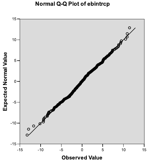
192 Linear Mixed Models: A Practical Guide Using Statistical Software
FIGURE 4.5: EBLUPs of the random classroom effects from Model 4.2, plotted using SPSS.
/FRACTION=BLOM
/TIES=MEAN
/DIST=NORMAL.
We do not see evidence of any outliers in the random classroom effects, and the distri-
bution of the EBLUPs for the random classroom effects is approximately normal. In the
next plot (Figure 4.6), we investigate the distribution of the EBLUPs for the random school
effects, using the EB00 variable saved in the Level 3 residual file by the HLM3 procedure:
PPLOT
/VARIABLES=eb00
/NOLOG
/NOSTANDARDIZE
/TYPE=Q-Q
/FRACTION=BLOM
/TIES=MEAN
/DIST=NORMAL.
We do not see any evidence of a deviation from a normal distribution for the EBLUPs
of the random school effects, and more importantly, we do not see any extreme outliers.
Plots such as these can be used to identify EBLUPs that are potential outliers, and further
investigate the clusters (e.g., schools or classrooms) associated with the extreme EBLUPs.
Note that evidence of a normal distribution in these plots does not always imply that the
distribution of the random effects is in fact normal (see Subsection 2.8.3).
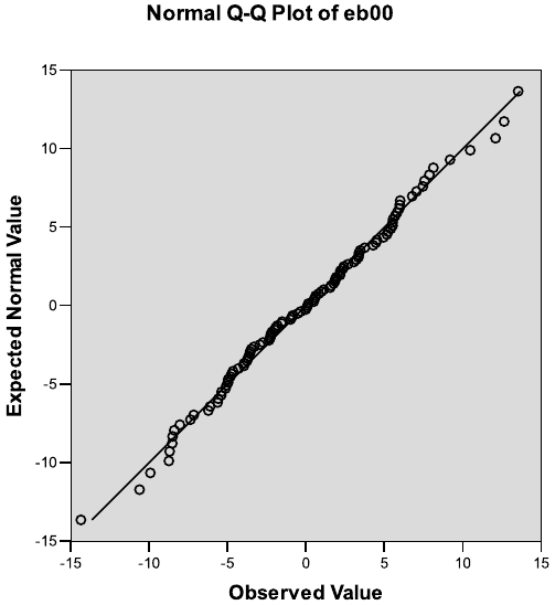
Three-Level Models for Clustered Data:The Classroom Example 193
FIGURE 4.6: EBLUPs of the random school effects from Model 4.2, plotted using SPSS.
4.10.2 Residual Diagnostics
In this section, we investigate the assumptions of normality and constant variance for the
residuals, based on the fit of Model 4.2. These plots were created in SPSS, using the Level
1 residual file generated by the HLM3 procedure. We first investigate a normal Q–Q plot
for the residuals:
PPLOT
/VARIABLES=l1resid
/NOLOG
/NOSTANDARDIZE
/TYPE=Q-Q
/FRACTION=BLOM
/TIES=MEAN
/DIST=NORMAL.
If the residuals based on Model 4.2 followed an approximately normal distribution, all
of the points in Figure 4.7 would lie on or near the straight line included in the figure.
We see a deviation from this line at the tails of the distribution, which suggests a long-
tailed distribution of the residuals (since only the points at the ends of the distribution
deviate from normality). There appear to be small sets of extreme negative and positive
residuals that may warrant further investigation. Transformations of the response variable
(MATHGAIN) could also be performed, but the scale of the MATHGAIN variable (where
some values are negative) needs to be considered; for example, a log transformation of the
response would not be possible without first adding a constant to each response to produce
a positive value.
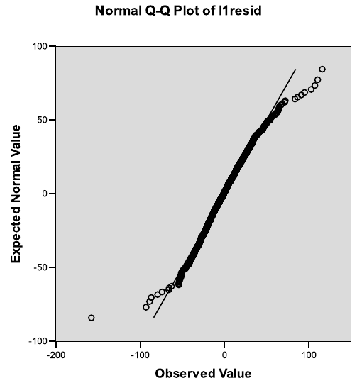
194 Linear Mixed Models: A Practical Guide Using Statistical Software
FIGURE 4.7: Normal quantile–quantile (Q–Q) plot of the residuals from Model 4.2, plotted
using SPSS.
Next, we investigate a scatter plot of the conditional residuals vs. the fitted MATHGAIN
values, which include the EBLUPs of the random school effects and the nested random
classroom effects. These fitted values are saved by the HLM3 procedure in a variable named
FITVAL in the Level 1 residual file. We investigate this plot to get a visual sense of whether
or not the residuals have constant variance:
GRAPH
/SCATTERPLOT(BIVAR) = fitval WITH llresid
/MISSING = LISTWISE .
We have edited the scatter plot in SPSS (Figure 4.8) to include the fit of a smooth Loess
curve, indicating the relationship of the fitted values with the residuals, in addition to a
dashed reference line set at zero.
We see evidence of nonconstant variance in the residuals in Figure 4.8. We would expect
there to be no relationship between the fitted values and the residuals (a line fitted to the
points in this plot should look like the reference line, representing the zero mean of the
residuals), but the Loess smoother shows that the residuals tend to get larger for larger
predicted values of MATHGAIN.
This problem suggests that the model may be misspecified; there may be omitted covari-
ates that would explain the large positive values and the low negative values of MATHGAIN
that are not being well fitted. Scatter plots of the residuals against other covariates would
be useful to investigate at this point, as there might be nonlinear relationships of the co-
variates with the MATHGAIN response that are not being captured by the strictly linear
fixed effects in Model 4.2.
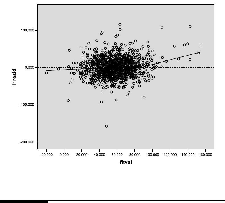
Three-Level Models for Clustered Data:The Classroom Example 195
FIGURE 4.8: Residual vs. fitted plot from SPSS.
4.11 Software Notes
4.11.1 REML vs. ML Estimation
The procedures in SAS, SPSS, R, and Stata use restricted maximum likelihood (REML)
estimation as the default estimation method for fitting models with nested random effects to
three-level data sets. These four procedures estimate the variance and covariance parameters
using REML (where ML estimation is also an option), and then use the estimated marginal
Vmatrix to estimate the fixed-effect parameters in the models using generalized least
squares (GLS). The procedure available in HLM (HLM3) utilizes ML estimation when
fitting three-level models with nested random effects.
4.11.2 Setting up Three-Level Models in HLM
In the following text, we note some important differences in setting up three-level models
using the HLM software as opposed to the other four packages:
•Three data sets, corresponding to the three levels of the data, are required to fit an LMM
to a three-level data set. The other procedures require that all variables for each level of
the data be included in a single data set, and that the data be arranged in the “long”
format displayed in Table 4.2.
196 Linear Mixed Models: A Practical Guide Using Statistical Software
•Models in HLM are specified in multiple parts. For a three-level data set, Level 1, Level
2, and Level 3 models are identified. The Level 2 models are for the effects of covariates
measured on the Level 1 units and specified in the Level 1 model; and the Level 3 models
are for the effects of covariates measured on the Level 2 units and specified in the Level
2models.
•In models for three-level data sets, the effects of any of the Level 1 predictors (including
the intercept) are allowed to vary randomly across Level 2 and Level 3 units. Similarly, the
effects of Level 2 predictors (including the intercept) are allowed to vary randomly across
Level 3 units. In the models fitted in this chapter, we have allowed only the intercepts to
vary randomly at different levels of the data.
4.11.3 Calculation of Degrees of Freedom for t-Tests in HLM
The degrees of freedom for the approximate t-statistics calculated by the HLM3 procedure,
and reported for Hypotheses 4.3 through 4.6, are described in this subsection.
Level 1 Fixed Effects: df = number of Level 1 observations (i.e., number of students) –
number of random effects at Level 2 – number of random effects at Level 3 – number of
fixed-effect parameters associated with the covariates at Level 1.
For example, for the t-tests for the fixed effects associated with the Level 1 (student-level)
covariates in Model 4.2, we have df = 1190 – 312 – 107 – 4 = 767.
Level 2 Fixed Effects: df = number of random effects at Level 2 – number of random
effects at Level 3 – number of fixed effects at Level 2.
For example, in Model 4.3, we have df = 285 – 105 – 3 = 177 for the t-tests for the fixed
effects associated with the Level 2 (classroom-level) covariates, as shown in Table 4.5.
Note that there are three fixed effects at Level 2 (the classroom level) in Model 4.3.
Level 3 Fixed Effects: df = number of random effects at Level 3 – number of fixed effects
at Level 3.
Therefore, in Model 4.4, we have df = 107 – 2 = 105 for the t-test for the fixed effect as-
sociated with the Level 3 (school-level) covariate, as shown in Table 4.5. The fixed intercept
is considered to be a Level 3 fixed effect, and there is one additional fixed effect at Level 3.
4.11.4 Analyzing Cases with Complete Data
We mention in the analysis of the Classroom data that likelihood ratio tests are not possible
for Hypotheses 4.3 through 4.5, due to the presence of missing data for some of the Level 2
covariates.
An alternative way to approach the analyses in this chapter would be to begin with a
data set having cases with complete data for all covariates. This would make either likelihood
ratio tests or alternative tests (e.g., t-tests) appropriate for any of the hypotheses that we
test. In the Classroom data set, MATHKNOW is the only classroom-level covariate with
missing data. Taking that into consideration, we include the following syntax for each of the
software packages that could be used to derive a data set where only cases with complete
data on all covariates are included.
In SAS, the following data step could be used to create a new SAS data set,
classroom_nomiss, which contains only observations with complete data:
Three-Level Models for Clustered Data:The Classroom Example 197
data classroom_nomiss;
set classroom;
if mathknow ne .;
run;
In SPSS, the following syntax can be used to select cases that do not have missing data
on MATHKNOW (the resulting data set should be saved under a different name):
FILTER OFF.
USE ALL.
SELECT IF (not MISSING (mathknow)).
EXECUTE.
In R, we could create a new data frame object excluding those cases with missing data
on MATHKNOW:
> class.nomiss <- subset(class, !is.na(mathknow))
In Stata, the following command could be used to delete cases with missing data on
MATHKNOW:
. keep if mathknow ! = .
Finally, in HLM, this can be accomplished by selecting Delete data when ... making
MDM (rather than when running the analysis) when setting up the MDM file.
4.11.5 Miscellaneous Differences
Less critical differences between the five software procedures in terms of fitting three-level
models are highlighted in the following text:
•Procedures in the HLM software package automatically generate both model-based stan-
dard errors and robust (or sandwich-type) standard errors for estimated fixed effects. The
two different sets of standard errors are clearly distinguished in the HLM output. The
robust standard errors are useful to report if one is unsure about whether the marginal
variance-covariance matrix for the data has been correctly specified; if the robust standard
errors differ substantially from the model-based standard errors, we would recommend re-
porting the robust standard errors (for more details see Raudenbush & Bryk (2002)).
Robust standard errors can be obtained in SAS by using the empirical option when
invoking proc mixed.
•EBLUPs for random effects cannot be calculated in SPSS when fitting models to data
sets with multiple levels of clustering, such as the Classroom data.
•Fitting three-level random intercept models using the MIXED command in SPSS tends to
be computationally intensive, and can take longer than in the other software procedures.
•The mixed command in Stata reports z-tests for the fixed effects, rather than the t-tests
reported by the other four procedures. The z-tests are asymptotic, and thus require large
sample sizes at all three levels of the data.

198 Linear Mixed Models: A Practical Guide Using Statistical Software
4.12 Recommendations
Three-level models for cross-sectional data introduce the possibility of extremely complex
random-effects structures. In the example analyses presented in this chapter, we only con-
sidered models with random intercepts; we could have allowed the relationships of selected
covariates at Level 1 (students) of the Classroom data to randomly vary across classrooms
and schools, and the relationships of selected covariates at Level 2 (classrooms) to vary
across schools. The decision to include many additional random effects in a three-level
model will result in a much more complex implied covariance structure for the dependent
variable, including several covariance parameters (especially if an unstructured Dmatrix
is used, which is the default random-effects covariance structure in HLM and the two R
functions). This may result in estimation difficulties, or the software appearing to “hang”
or “freeze” when attempting to estimate a model. For this reason, we only recommend in-
cluding a large number of random effects (above and beyond random intercepts) at higher
levels if there is explicit research interest in empirically describing (and possibly attempt-
ing to explain) the variance in the relationships of selected covariates with the dependent
variable across higher-level units. Including random intercepts at Level 2 and Level 3 of a
given three-level data set will typically result in a reasonable implied covariance structure
for a given continuous dependent variable in a cross-sectional three-level data set.
Because three-level models do introduce the possibility of allowing many relationships
to vary across higher levels of the data hierarchy (e.g., the relationship of student-level SES
with mathematical performance varying across schools), the ability to graphically explore
variance in both the means of a dependent variable and the relationships of key independent
variables with the dependent variable across higher-level units becomes very important when
analyzing three-level data. For this reason, having good graphical tools “built in” to a given
software package becomes very important. We find that the HLM software provides users
with a useful set of “point-and-click” graphing procedures for exploring random coefficients
without too much additional work (see Subsection 4.2.2.2). Creating similar graphs and
figures in the other software tends to take more work and some additional programming,
but is still possible.

5
Models for Repeated-Measures Data:
The Rat Brain Example
5.1 Introduction
This chapter introduces the analysis of repeated-measures data, in which multiple mea-
surements are made on the same subject (unit of analysis) under different conditions or
across time. Repeated-measures data sets can be considered to be a type of two-level data,
in which Level 2 represents the subjects and Level 1 represents the repeated measurements
made on each subject. Covariates measured at Level 2 of the data (the subject level) de-
scribe between-subject variation and Level 1 covariates describe within-subject variation.
The data that we analyze are from an experimental study of rats in which the dependent
variable was measured in three brain regions for two levels of a drug treatment. Brain region
and treatment are crossed within-subject factors; measurements were made for the same
brain regions and the same treatments within each rat. Between-subject factors (e.g.,
sex or genotype) are not considered in this example.
Repeated-measures data typically arise in an experimental setting, and often involve
measurements made on the same subject over time, although time is not a within-subject
factor in this example. In Table 5.1, we present examples of repeated-measures data in
different research settings.
In this chapter we highlight the SPSS software.
5.2 The Rat Brain Study
5.2.1 Study Description
The data used in this example were originally reported by Douglas et al. (2004).1The aim of
their experiment was to examine nucleotide activation (guanine nucleotide bonding) in seven
different brain nuclei (i.e., brain regions) among five adult male rats. The basal nucleotide
activation, measured after treatment with saline solution, was compared to activation in
the same region after treatment with the drug carbachol. Activation was measured as the
mean optical density produced by autoradiography. We compare activation in a subset of
three of the original seven brain regions studied by the authors: the bed nucleus of the stria
terminalis (BST), the lateral septum (LS), and the diagonal band of Broca (VDB). The
original data layout for this study is shown in Table 5.2.
1Data from this study are used with permission of the authors and represent a part of their larger study.
Experiments were conducted in accordance with the National Institutes of Health Policy on Humane Care
and Use of Laboratory Animals.
199

200 Linear Mixed Models: A Practical Guide Using Statistical Software
TABLE 5.1: Examples of Repeated-Measures Data in Different Research Settings
Level of Data Research Setting
Linguistics Medicine Anesthesiology
Unit of
analysis
(Level 2)
Subject
variable
(random
factor)
Person Patient Rat
Subject-
level
covariates
Age, native
language
Sex, severity
score
Sex, genotype
Repeated
measures
(Level 1)
Within-
subject
factors
Word type,
context
Time (minutes
after
administration
of drug)
Brain region,
treatment
Dependent
variable
Vowel duration
(msec)
Pain relief
(visual analog
scale)
Nucleotide
activation
(optical
density)
The following SPSS syntax can be used to read in the tab-delimited raw data from the
original ratbrain.dat file, assumed to be in the C:\temp directory:
GET DATA /TYPE = TXT
/FILE = "C:\temp\ratbrain.dat"
/DELCASE = LINE
/DELIMITERS = "\t"
/ARRANGEMENT = DELIMITED
/FIRSTCASE = 2
/IMPORTCASE = ALL
/VARIABLES =
animal A7
Carb.BST F6.2
Carb.LS F6.2
Carb.VDB F6.2
Basal.BST F6.2
Basal.LS F6.2
Basal.VDB F6.2
.
CACHE.
EXECUTE.
Before we carry out an analysis of the Rat Brain data using SAS, SPSS, R, Stata, or
HLM, we need to restructure the data set into the “long” format. The SPSS syntax to
restructure the data is shown as follows. A portion of the restructured Rat Brain data is
shown in Table 5.3.

Models for Repeated-Measures Data:The Rat Brain Example 201
TABLE 5.2: The Rat Brain Data in the Original “Wide” Data Layout. Treatments are
“Carb” and “Basal”; brain regions are BST, LS, and VDB
Animal Carb BST Carb LS Carb VDB Basal BST Basal LS Basal VDB
R111097 371.71 302.02 449.70 366.19 199.31 187.11
R111397 492.58 355.74 459.58 375.58 204.85 179.38
R100797 664.72 587.10 726.96 458.16 245.04 237.42
R100997 515.29 437.56 604.29 479.81 261.19 195.51
R110597 589.25 493.93 621.07 462.79 278.33 262.05
VARSTOCASES
/MAKE activate FROM Basal BST Basal LS Basal VDB Carb BST
Carb LS Carb VDB
/INDEX = treatment(2) region(3)
/KEEP = animal
/NULL = KEEP.
VALUE LABELS treatment 1 ’Basal’ 2 ’Carbachol’
/ region 1 ‘BST’ 2 ‘LS’ 3 ’VDB’.
The following variables are included in the Rat Brain data set (note that there are no
Level 2 covariates included in this study):
TABLE 5.3: Sample of the Rat Brain Data Set Rearranged in the “Long” Format
Rat Repeated Measures
(Level 2) (Level 1)
Unit ID Within-Subject Fixed Factors Dependent Variable
ANIMAL TREATMENT REGION ACTIVATE
R111097 1 1 366.19
R111097 1 2 199.31
R111097 1 3 187.11
R111097 2 1 371.71
R111097 2 2 302.02
R111097 2 3 449.70
R111397 1 1 375.58
R111397 1 2 204.85
R111397 1 3 179.38
R111397 2 1 492.58
R111397 2 2 355.74
R111397 2 3 459.58
R100797 1 1 458.16
R100797 1 2 245.04
R100797 1 3 237.42
...
Note: “...” indicates portion of the data not displayed.

202 Linear Mixed Models: A Practical Guide Using Statistical Software
Rat(Level2)Variable
•ANIMAL = Unique identifier for each rat
Repeated-Measures (Level 1) Variables
•TREATMENT = Level of drug treatment (1 = basal, 2 = carbachol)
•REGION = Brain nucleus (1 = BST, 2 = LS, 3 = VDB)
•ACTIVATE = Nucleotide activation (the dependent variable)
We recommend sorting the data in ascending order by ANIMAL and then by TREAT-
MENT and REGION within each level of ANIMAL prior to running the analysis. Although
this sorting is not necessary for the analysis, it makes the output displayed later (e.g.,
marginal variance-covariance matrices) easier to read.
5.2.2 Data Summary
The following SPSS syntax will generate descriptive statistics for the dependent variable,
ACTIVATE, for each level of REGION by TREATMENT:
MEANS
TABLES = activate BY treatment BY region
/CELLS MEAN COUNT STDDEV MIN MAX.
The following table displays the SPSS output generated by submitting the syntax above.
'
&
$
%
Report
activate
treatment region Mean N Std. Deviation Minimum Maximum
Basal BST 428.5060 5 53.31814 366.19 479.81
LS 237.7440 5 34.67477 199.31 278.33
VDB 212.2940 5 35.72899 179.38 262.05
Total 292.8480 15 107.21452 179.38 479.81
Carbachol BST 526.7100 5 109.86160 371.71 664.72
LS 435.2700 5 112.44907 302.02 587.10
VDB 572.3200 5 117.32236 449.70 726.96
Total 511.4333 15 120.30398 302.02 726.96
Total BST 477.6080 10 96.47086 366.19 664.72
LS 336.5070 10 130.35415 199.31 587.10
VDB 392.3070 10 206.61591 179.38 726.96
Total 402.1407 30 157.77534 179.38 726.96
The mean activation level is generally higher for carbachol than for the basal treatment
in each region. The mean activation also appears to differ by region, with BST having the
highest mean activation in the basal condition and VDB having the highest mean activation
in the carbachol condition. The standard deviations of activation appear to be much larger
for the carbachol treatment than for the basal treatment.
We investigate the data by creating line graphs of the activation in the three brain
regions for each animal for both the basal and carbachol treatments:
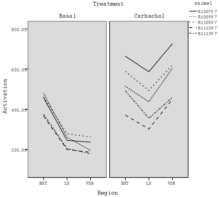
Models for Repeated-Measures Data:The Rat Brain Example 203
FIGURE 5.1: Line graphs of activation for each animal by region within levels of treatment
for the Rat Brain data.
GRAPH
/LINE(MULTIPLE) MEAN(activate) BY region BY animal
/PANEL COLVAR = treatment COLOP = CROSS.
The effects of treatment and region on the activation within each animal are clear
in Figure 5.1. Activation values are consistently higher in the carbachol treatment than
in the basal treatment across all regions, and the LS region has a lower mean than the
BST region for both carbachol and basal treatments. There also appears to be a greater
effect of carbachol treatment in the VDB region than in either the BST or LS region.
These observations suggest that the fixed effects of TREATMENT and REGION and the
TREATMENT ×REGION interaction are likely to be significant in a mixed model for the
data.
In Figure 5.1, we also note characteristics of these data that will be useful in specifying
the random effects in a mixed model. First, between-animal variation is apparent in the basal
treatment, but is even greater in the carbachol treatment. To capture the between-animal
variation in both treatments, we initially include in the model a random effect associated
with the intercept for each rat. To address the greater between-animal variation in the car-
bachol treatment, we include a second random animal effect associated with TREATMENT
(carbachol vs. basal). This results in each animal having two random intercepts, one for the
basal condition and another for the carbachol treatment.
204 Linear Mixed Models: A Practical Guide Using Statistical Software
Legend:
Reference
model
Nested model
Reference
model
Nested model
Model preference
Nested (null hypothesis)
model preferred
Reference model
preferred
M5.2 with fixed treatment
by region interaction,
random intercepts, and
random treatment effects
M5.1 with fixed treatment
by region interaction, and
random intercepts
Model obtained by
removing fixed effects of
treatment by region
interaction from Model 5.2
M5.3 with heterogeneous
residual variances for
Basal and Carbachol
treatments
H5.1
H5.2
H5.3
STEP 1
STEP 2
STEP 3
FIGURE 5.2: Model selection and related hypotheses for the analysis of the Rat Brain data.
5.3 Overview of the Rat Brain Data Analysis
We apply the “top-down” modeling strategy discussed in Chapter 2 (Subsection 2.7.1) to the
analysis of the Rat Brain data. Subsection 5.3.1 outlines the analysis steps and informally
introduces the related models and hypotheses to be tested. Subsection 5.3.2 presents a
more formal specification of selected models, and Subsection 5.3.3 presents details about
the hypotheses tested. The analysis steps outlined in this section are shown schematically
in Figure 5.2. See Subsection 5.3.3 for details on the interpretation of Figure 5.2.
5.3.1 Analysis Steps
Step 1: Fit a model with a “loaded” mean structure (Model 5.1).
Fit a two-level model with a loaded mean structure and random animal-specific
intercepts.
Model 5.1 includes fixed effects associated with region, treatment, and the interaction
between region and treatment. This model also includes a random effect associated with
the intercept for each animal and a residual associated with each observation. The residuals
are assumed to be independent and to have the same variance across all levels of region
and treatment. The assumption of homogeneous variance for the residuals, in conjunction
Models for Repeated-Measures Data:The Rat Brain Example 205
with the single random effect associated with the intercept for each animal, implies that
the six observations on each animal have the same marginal variance and that all pairs
of observations have the same (positive) marginal covariance (i.e., a compound symmetry
covariance structure).
Step 2: Select a structure for the random effects (Model 5.1 vs. Model 5.2).
Fit Model 5.2 by adding random animal-specific effects of treatment to Model
5.1, and decide whether to retain them in the model.
(Note: In this step we do not carry out a formal test of whether the random intercepts
should be retained in Model 5.1, but assume that they should be kept, based on the study
design.)
We observed in Figure 5.1 that the between-animal variation was greater for the carba-
chol treatment than for the basal treatment. To accommodate this difference in variation,
we add a random animal-specific effect of treatment to Model 5.1 to obtain Model 5.2. The
effect of treatment is fixed in Model 5.1 and therefore constant across all animals. The ad-
ditional random effect associated with treatment included in Model 5.2 allows the implied
marginal variance of observations for the carbachol treatment to differ from that for the
basal treatment. Model 5.2 can also be interpreted as having two random intercepts per
rat, i.e., one for the carbachol treatment and an additional one for the basal treatment.
We test Hypothesis 5.1 to decide if the random treatment effects should be kept in Model
5.2. Based on the test result, we retain the random treatment effects and keep Model 5.2
as the preferred model at this stage of the analysis.
Step 3: Select a covariance structure for the residuals (Model 5.2 vs. Model
5.3).
Fit Model 5.3 with heterogeneous residual variances for the basal and carbachol
treatments and decide whether the model should have homogeneous residual
variances (Model 5.2) or heterogeneous residual variances (Model 5.3)
We observed in Figure 5.1 that the variance of individual measurements appeared to
be greater for the carbachol treatment than for basal treatment. In Step 2, we explored
whether this difference can be attributed to between-subject variation by considering ran-
dom treatment effects in addition to random intercepts. In this step, we investigate whether
there is heterogeneity in the residual variances.
In Model 5.2, we assume that the residual variance is constant across all levels of region
and treatment. Model 5.3 allows a more flexible specification of the residual variance; i.e., it
allows the variance of the residuals to differ across levels of treatment. We test Hypothesis
5.2 to decide if the residual variance is equal for the carbachol and basal treatments. Based
on the results of this test, we keep Model 5.2, with homogeneous residual variance, as our
preferred model.
Step 4: Reduce the model by removing nonsignificant fixed effects and assess
model diagnostics for the final model (Model 5.2).
Decide whether to keep the fixed effects of the region by treatment interaction
in Model 5.2.
Based on the result of the test for Hypothesis 5.3, we conclude that the region by
treatment interaction effects are significant and consider Model 5.2 to be our final model.
We carry out diagnostics for the fit of Model 5.2 using informal graphical methods in SPSS
in Section 5.9.
206 Linear Mixed Models: A Practical Guide Using Statistical Software
5.3.2 Model Specification
5.3.2.1 General Model Specification
We specify Models 5.2 and 5.3 in this subsection. We do not explicitly specify the simpler
Model 5.1. All three models are summarized in Table 5.4. The general specification of Model
5.2 corresponds closely to the syntax used to fit this model in SAS, SPSS, Stata, and R.
The value of ACTIVATEti for a given observation indexed by t(t= 1, 2, ..., 6) on the
i-th animal (i= 1, 2, ..., 5) can be written as follows:
ACTIVATEti =β0+β1×REGION1ti +β2×REGION2ti
+β3×TREATMENTti +β4×REGION1ti ×TREATMENTti
+β5×REGION2ti ×TREATMENTti
⎫
⎪
⎬
⎪
⎭fixed
+u0i+u3i×TREATMENTti +εti }random
(5.1)
In Model 5.2, we include two indicator variables for region, REGION1ti and REGION2ti,
whichrepresenttheBSTandLSregions, respectively. TREATMENTti is an indicator
variable that indicates the carbachol treatment. In our parameterization of the model, we
assume that fixed effects associated with REGION=“VDB” and TREATMENT=“Basal”
are set to zero.
The fixed-effect parameters are represented by β0through β5. The fixed intercept β0
represents the expected value of ACTIVATEti for the reference levels of region and treat-
ment (i.e., the VDB region under the basal treatment). The parameters β1and β2represent
the fixed effects of the BST and LS regions vs. the VDB region, respectively, for the basal
treatment (given that the model includes an interaction between region and treatment).
The parameter β3represents the fixed effect associated with TREATMENTti (carbachol
vs. basal) for the VDB region. The parameters β4and β5represent the fixed effects associ-
ated with the region by treatment interaction. These parameters can either be interpreted
as changes in the carbachol effect for the BST and LS regions relative to the VDB region,
or changes in the BST and LS region effects for the carbachol treatment relative to the
basal treatment.
The u0iterm represents the random intercept associated with animal i,andu3irepre-
sents the random effect associated with treatment (carbachol vs. basal) for animal i. We
denote the random treatment effect as u3ibecause this random effect is coupled with the
fixed effect of TREATMENT (β3). We assume that the distribution of the random effects
associated with animal i,u0iand u3i, is bivariate normal:
ui=u0i
u3i∼N(0,D)
A set of three covariance parameters, σ2
int,σ
2
treat,and σint,treat,defines the Dmatrix of
variances and covariances for the two random effects in Model 5.2, as follows:
D=σ2
int σint,treat
σint,treat σ2
treat
In the Dmatrix, σ2
int is the variance of the random intercepts, σint,treat is the covariance
of the two random effects, and σ2
treat is the variance of the random treatment effects.
The residuals associated with the six observations on animal iare assumed to follow a
multivariate normal distribution:
Models for Repeated-Measures Data:The Rat Brain Example 207
εi=
⎛
⎜
⎜
⎜
⎜
⎜
⎜
⎝
ε1i
ε2i
ε3i
ε4i
ε5i
ε6i
⎞
⎟
⎟
⎟
⎟
⎟
⎟
⎠∼N(0,Ri)
where Riis a 6 ×6 covariance matrix. We assume that the six components of the εivector
are ordered in the same manner as in Table 5.3: The first three residuals are associated with
the basal treatment in the BST, LS, and VDB regions, and the next three are associated
with the carbachol treatment in the same three regions.
InModel5.2,theRimatrix is simply σ2I6. The diagonal elements of the 6 ×6matrix
represent the variances of the residuals, all equal to σ2(i.e., the variances are homogeneous).
The off-diagonal elements represent the covariances of the residuals, which are all zero:
Ri=⎛
⎜
⎜
⎜
⎝
σ20··· 0
0σ2··· 0
.
.
..
.
.....
.
.
00··· σ2
⎞
⎟
⎟
⎟
⎠=σ2I6
In Model 5.3, we allow the residual variances to differ for each level of treatment, by in-
cluding separate residual variances (σ2
basal and σ2
carb) for the basal and carbachol treatments.
This heterogeneous structure for the 6 ×6Rimatrix is as follows:
Ri=σ2
basalI30
0σ2
carbI3
The upper-left 3 ×3 submatrix corresponds to observations for the three regions in the
basal treatment, and the lower right submatrix corresponds to the regions in the carbachol
treatment. The treatment-specific residual variance is on the diagonal of the two 3 ×3
submatrices, and zeroes are off the diagonal. We assume that the residuals, εti (t=1, ..., 6),
conditional on a given animal i, are independent in both Models 5.2 and 5.3.
5.3.2.2 Hierarchical Model Specification
We now present an equivalent hierarchical specification of Model 5.2, using the same no-
tation as in Subsection 5.3.2.1. The correspondence between this notation and the HLM
software notation is shown in Table 5.4. The hierarchical model has two components that
reflect contributions from the two levels of the data: the repeated measures at Level 1 and
the rats at Level 2. We write the Level 1 component as:
Level 1 Model (Repeated Measures)
ACTIVATEti =b0i+b1i×REGION1ti +b2i×REGION2ti +b3i×TREATMENTti
+b4i×REGION1ti ×TREATMENTti
+b5i×REGION2ti ×TREATMENTti +εti (5.2)
where the residuals εti have the distribution defined in the general specification of Model
5.2 in Subsection 5.3.2.1, with constant variance and zero covariances in the Rimatrix.

208 Linear Mixed Models: A Practical Guide Using Statistical Software
TABLE 5.4: Summary of Selected Models for the Rat Brain Data
Term/Vari ab le General HLM Model
Notation Notation 5.1 5.2 5.3
Fixed effects Intercept β0β00 √√√
REGION1 (BST vs.
VDB)
β1β10 √√√
REGION2 (LS vs.
VDB)
β2β20 √√√
TREATMENT
(carbachol vs. basal)
β3β30 √√√
REGION1 ×
TREATMENT
β4β40 √√√
REGION2 ×
TREATMENT
β5β50 √√√
Random
effects
Rat (i)Intercept u0ir0i√√√
TREATMENT
(carbachol vs. basal)
u3ir3i√√
Residuals Measure
(t)onrat
(i)
εti eti √√√
Covariance
parameters
(θD)forD
matrix
Rat level Variance of
intercepts
σ2
int τ[1,1] √√√

Models for Repeated-Measures Data:The Rat Brain Example 209
TABLE 5.4: (Continued)
Term/Vari ab le General HLM Model
Notation Notation 5.1 5.2 5.3
Covariance of
intercepts and
treatment effects
σint,treat τ[2,1] √√
Variance of
treatment effects
σ2
treat τ[2,2] √√
Covariance
parameters
(θR)forRi
matrix
Repeated
measures
Variances of
residuals
σ2
basal,σ
2
carb σ2σ2
basal =
σ2
carb =
σ2
σ2
basal =
σ2
carb =
σ2
σ2
basal =
σ2
carb
Structure Riσ2I6σ2I6Heta
aHeterogeneous residual variance across treatments (see Subsection 5.3.2.1).
210 Linear Mixed Models: A Practical Guide Using Statistical Software
In the Level 1 model shown in (5.2), we assume that ACTIVATEti, the nucleotide acti-
vation for an individual observation ton rat i, follows a linear model, defined by the animal-
specific intercept b0i, the animal-specific effects b1iand b2iof REGION1ti and REGION2ti
(BST and LS relative to the VDB region, respectively), the animal-specific effect b3iof
TREATMENTti (carbachol vs. basal treatment), and the animal-specific interaction effects
b4iand b5i.
The Level 2 model describes variation between animals in terms of the animal-specific
intercepts (b0i) and the remaining animal-specific effects (b1ithrough b5i). Although the
Level 2 model has six equations (which is consistent with the HLM software specification),
there is a simple expression for each one:
Level 2 Model (Rat)
b0i=β0+u0i
b1i=β1
b2i=β2
b3i=β3+u3i
b4i=β4
b5i=β5
(5.3)
where
ui=u0i
u3i∼N(0,D)
In this Level 2 model, the intercept b0ifor rat idepends on the fixed intercept β0(i.e.,
the ACTIVATE mean for the VDB region in the basal treatment), and a random effect, u0i,
associated with rat i. The effect of treatment for rat i,b3i, also depends on a fixed effect
(β3) and a random effect associated with rat i(u3i). All remaining animal-specific effects
(bli,b2i,b4i,andb5i) are defined only by their respective fixed effects β1,β
2,β
4,andβ5.
By substituting the expressions for b0ithrough b5ifrom the Level 2 model into the Level
1 model, we obtain the general linear mixed model (LMM) as specified in (5.1).
In Model 5.3, the residuals in the Level 1 model have the heterogeneous variance struc-
ture that was defined in Subsection 5.3.2.1.
5.3.3 Hypothesis Tests
Hypothesis tests considered in the analysis of the Rat Brain data are summarized in Ta-
ble 5.5.
Hypothesis 5.1. The random effects (u3i) associated with treatment for each animal can
be omitted from Model 5.2.
Model 5.1 has a single random effect (u0i) associated with the intercept for each animal,
and Model 5.2 includes an additional random effect (u3i) associated with treatment for each
animal. We do not directly test the significance of the random animal-specific treatment
effects in Model 5.2, but rather, we test a null version of the Dmatrix (for Model 5.1) vs.
an alternative version for Model 5.2 (Verbeke & Molenberghs, 2000).
The null hypothesis Dmatrix has a single positive element, σ2
int,which is the variance of
the single random effect (u0i). The alternative hypothesis Dmatrix is positive semidefinite
and contains two additional parameters: σ2
treat >0,which is the variance of the random
treatment effects (u3i), and σint,treat,which is the covariance of the two random effects, u0i
and u3i, associated with each animal.

Models for Repeated-Measures Data:The Rat Brain Example 211
TABLE 5.5: Summary of Hypotheses Tested in the Analysis of the Rat Brain Data
Models Compared
Label Null (H0)Alternative(HA) Test Nested
Model
(H0)
Ref.
Model
(HA)
Est.
Method
Test Stat.
Dist.
under H0
5.1 Drop u3iRetain u3iLRT Model
5.1
Model
5.2
REML 0.5χ2
1+0.5χ2
2
5.2 Homogeneous residual
variance
(σ2
carb =σ2
basal)
Heterogeneous
residual variances
(σ2
carb =σ2
basal)
LRT Model
5.2
Model
5.3
REML χ2
1
5.3 Drop TREATMENT
×REGION effects
(β4=β5=0)
Retain TREATMENT
×REGION effects
(β4=0,orβ5=0)
Type III
F-test
Wald
χ2test
N/A Model
5.2
REML F(2, 16)a
χ2
2
Note: N/A = Not applicable.
aWe report the distribution of the F-statistic used by the MIXED command in SPSS, with the Satterthwaite approx-
imation used to compute the denominator degrees of freedom.

212 Linear Mixed Models: A Practical Guide Using Statistical Software
H0:D=σ2
int 0
00
HA:D=σ2
int σint,treat
σint,treat σ2
treat
We use a REML-based likelihood ratio test for Hypothesis 5.1. The test statistic is
calculated by subtracting the –2 REML log-likelihood value for Model 5.2 (the reference
model) from that for Model 5.1 (the nested model). The asymptotic null distribution of
the test statistic is a mixture of χ2
1and χ2
2distributions, with equal weights of 0.5 (see
Subsection 2.6.2.2).
Note that likelihood ratio tests, such as the one used for Hypothesis 5.1, rely on asymp-
totic (large-sample) theory, so we would not usually carry out this type of test for such a
small data set (five rats). Rather, in practice, the random effects would probably be retained
without testing, so that the appropriate marginal variance-covariance structure would be
obtained for the data set. We present the calculation of this likelihood ratio test for the
random effects (and those that follow in this chapter) strictly for illustrative purposes.
Hypothesis 5.2. The variance of the residuals is constant across both treatments. The
null and alternative hypotheses are
H0:σ2
basal =σ2
carb
HA:σ2
basal =σ2
carb
We test Hypothesis 5.2 using a REML-based likelihood ratio test. The test statistic is
calculated by subtracting the –2 REML log-likelihood value for Model 5.3 (the reference
model with heterogeneous residual variances) from that for Model 5.2 (the nested model).
The asymptotic distribution of the test statistic under the null hypothesis is a χ2
1,and not a
mixture of χ2distributions, as in the case of Hypothesis 5.1. This is because we are testing
whether two variances are equal, which does not involve testing any parameter values that
are on the boundary of a parameter space. The single degree of freedom corresponds to the
one additional variance parameter in Model 5.3.
Hypothesis 5.3. The fixed effects associated with the region by treatment interaction
can be omitted from Model 5.2.
The null and alternative hypotheses are
H0:β4=β5=0
HA:β4=0orβ5=0
We test Hypothesis 5.3 using F-tests in the software procedures that provide them (SAS,
SPSS, and R), based on REML estimation of the parameters in Model 5.2. By default, the
procedures in SAS and SPSS both calculate Type III F-tests, whereas Rprovides a Type I
F-test only. In this case, because the interaction term is the last one added to the model, the
Type III and Type I F-tests for the fixed interaction effects are comparable. We consider
Wald chi-square tests for the fixed interaction effects in Stata and HLM.
For the results of these hypothesis tests, see Section 5.5.
5.4 Analysis Steps in the Software Procedures
The modeling results for all software procedures are presented and compared in Section 5.6.

Models for Repeated-Measures Data:The Rat Brain Example 213
5.4.1 SAS
We first read in the raw data from the tab-delimited file, which we assume is stored in
the C:\temp folder. Note that the data actually begin on the second row of the file, so we
use the firstobs=2 option in the infile statement. We also use the dlm="09"X option to
specify that the raw data file is tab-delimited. In addition, we create an indicator variable
TREAT for the carbachol treatment:
data ratbrain;
infile "c:\temp\rat brain.dat" firstobs=2 dlm="09"X;
input animal $ treatment region activate;
if treatment = 1 then treat = 0;
if treatment = 2 then treat = 1;
run;
We now proceed with the model-fitting steps.
Step 1: Fit a model with a “loaded” mean structure (Model 5.1).
The SAS syntax to fit Model 5.1 using proc mixed is as follows:
title "Model 5.1";
proc mixed data = ratbrain covtest;
class region animal;
model activate = region treat region*treat / solution;
random int / subject = animal type = vc solution v vcorr;
run;
We have specified the covtest option in the proc mixed statement to obtain the stan-
dard errors of the estimated variance components in the output for comparison with the
other software procedures. This option also causes SAS to display a Wald test for the vari-
ance of the random effects associated with the animals, which we do not recommend for use
in testing whether to include random effects in a model (see Subsection 2.6.3.2).
The class statement identifies the categorical variables that are required to specify
the model. We include the fixed factor, REGION, and the random factor, ANIMAL, in
the class statement. The variable TREAT is an indicator variable with a value of one for
carbachol and zero for basal treatment, and therefore does not need to be included in the
class statement.
The model statement sets up the fixed-effects portion of Model 5.1. We specify that
the dependent variable, ACTIVATE, is a linear function of the fixed effects associated with
the REGION factor, the TREAT indicator, and the REGION ×TREAT interaction. The
solution option requests that the estimate of each fixed-effect parameter be displayed in
the output, along with its standard error and a t-test for the parameter.
Software Note: Because REGION is included in the class statement, SAS creates
three indicator variables for REGION in the model: the first variable is for the BST
region (REGION = l), the second is for the LS region (REGION = 2), and the third is
for the VDB region (REGION = 3). The solution option in the model statement sets
the fixed-effect parameter for the highest level of REGION (the VDB region) to zero,
and consequently, VDB becomes the reference category.
214 Linear Mixed Models: A Practical Guide Using Statistical Software
The random statement sets up the random-effects structure for the model. In this case,
ANIMAL is identified as the subject, indicating that it is a random factor. By specifying
random int, we include a random effect associated with the intercept for each animal.
We have included several options after the slash (/) in the random statement. The type=
option defines the structure of the Dcovariance matrix for random effects. Because there
is only one random effect specified in Model 5.1, the Dmatrix is 1 ×1, and defining its
structure is not necessary. Although proc mixed uses a variance components structure by
default, we specify it explicitly using the type=vc option. The type option becomes more
important later when we specify models with two random effects, one associated with the
intercept and another associated with the effect of treatment (Models 5.2 and 5.3).
We have also requested that the estimated marginal covariance matrix Viand the es-
timated marginal correlation matrix be displayed in the output for the first animal, by
specifying the vand vcorr options in the random statement.
The solution option in the random statement requests that the predicted random effect
(i.e., the EBLUP) associated with each animal also be displayed in the output.
Step 2: Select a structure for the random effects (Model 5.1 vs. Model 5.2).
We now fit Model 5.2 by including an additional random effect associated with the treatment
(carbachol vs. basal) for each animal.
title "Model 5.2";
proc mixed data = ratbrain covtest;
class animal region;
model activate = region treat region*treat / solution;
random int treat / subject = animal type = un solution v vcorr;
run;
The random statement from Model 5.1 has been updated to include TREAT. The type =
option has also been changed to type = un, which specifies an “unstructured” covariance
structure for the 2 ×2Dmatrix.
The SAS syntax for an alternative random effects specification of Model 5.2 is as follows:
title "Alternative Random Effects Specification for Model 5.2";
proc mixed data = ratbrain covtest;
class region animal treatment;
model activate = region treatment region*treatment / solution;
random treatment / subject=animal type=un solution v vcorr;
lsmeans region*treatment / slice=region;
run;
Because we include the original TREATMENT variable in the class statement, SAS
generates two dummy variables that will be used in the Zimatrix, one for carbachol and
the other for basal treatment. This has the effect of requesting two random intercepts, one
for each level of treatment.
The first syntax for Model 5.2, in which a dummy variable, TREAT, was used for
treatment, was specified to facilitate comparisons across software procedures. Specifically,
the HLM2 procedure cannot directly accommodate categorical variables as predictors, unless
they are specified as dummy variables.
We also include an lsmeans statement for the region*treatment interaction term to
create a comparison of the effects of treatment within each region (/slice=region). We
do not display these results generated by the lsmeans statement. Similar results obtained
using SPSS are presented in Section 5.7.
Models for Repeated-Measures Data:The Rat Brain Example 215
To test Hypothesis 5.1, we use a REML-based likelihood ratio test. See the SAS section
in Chapter 3 (Subsection 3.4.1) for two different versions of the syntax to carry out a
likelihood ratio test for random effects, and Subsection 5.5.1 for the results of the test.
Step 3: Select a covariance structure for the residuals (Model 5.2 vs. Model
5.3).
To fit Model 5.3, which has heterogeneous residual variances for the two levels of TREAT-
MENT, we add a repeated statement to the syntax used for Model 5.2 and include the
original TREATMENT variable in the class statement:
title "Model 5.3";
proc mixed data = ratbrain;
class animal region treatment;
model activate = region treat region*treat / solution;
random int treat / subject = animal type = un solution v vcorr;
repeated region / subject = animal*treatment group = treatment;
run;
The subject = animal*treatment option in the repeated statement defines two 3 ×3
blocks on the diagonal of the 6 ×6Rimatrix, with each block corresponding to a level
of treatment (see Subsection 5.3.2.1). Because the type= option is omitted, the default
“variance component” structure for each block is used. The group = treatment option
specifies that the variance components defining the blocks of the Rimatrix be allowed to
vary for each level of TREATMENT.
We carry out a likelihood ratio test of Hypothesis 5.2 to decide whether to retain the
heterogeneous residual variance structure for the two treatments in Model 5.3. SAS syntax
for this test is not shown here; refer to Subsection 3.4.1 for examples of relevant SAS
syntax. Based on the nonsignificant result of this test (p=0.66), we decide not to include
the heterogeneous residual variances, and keep Model 5.2 as our preferred model at this
stage of the analysis.
Step 4: Reduce the model by removing nonsignificant fixed effects (Model 5.2).
The result of the F-test for Hypothesis 5.3 in Model 5.2 is reported in Sections 5.5 and
5.6. The fixed effects associated with the REGION ×TREAT interaction are significant
(p<0.001), so we retain these fixed effects and keep Model 5.2 as our final model.
5.4.2 SPSS
We assume that the data set created to carry out the data summary in Subsection 5.2.2
is currently open in SPSS. Prior to fitting any models we generate TREAT, an indicator
variable for the carbachol treatment:
IF (treatment = 1) treat = 0.
IF (treatment = 2) treat = 1.
EXECUTE .
Step 1: Fit a model with a “loaded” mean structure (Model 5.1).
We begin the SPSS analysis by setting up the syntax to fit Model 5.1 using the MIXED
command:
216 Linear Mixed Models: A Practical Guide Using Statistical Software
* Model 5.1.
MIXED
activate BY region WITH treat
/CRITERIA = CIN(95) MXITER(100) MXSTEP(5) SCORING(l)
SINGULAR(0.000000000001) HCONVERGE(0, ABSOLUTE)
LCONVERGE(0, ABSOLUTE) PCONVERGE(0.000001, ABSOLUTE)
/FIXED = region treat region*treat | SSTYPE(3)
/METHOD = REML
/PRINT = SOLUTION
/RANDOM INTERCEPT | SUBJECT(animal) COVTYPE(VC).
In this syntax, ACTIVATE is listed as the dependent variable. The variable REGION
is specified as a categorical factor because it appears after the BY keyword. This causes
SPSS to generate the appropriate indicator variables for the REGION factor and for any
interactions involving REGION. The variable TREAT is specified as a covariate because it
appears after the WITH keyword.
The /FIXED subcommand lists the variables and interactions that have associated fixed
effects in Model 5.1. These terms include REGION, TREAT, and the REGION ×TREAT
interaction.
The /METHOD subcommand specifies the REML estimation method, which is the default.
The /PRINT subcommand requests that the SOLUTION for the estimated fixed-effect
parameters in the model be displayed in the output.
The /RANDOM subcommand indicates that the only random effect for each level of the
SUBJECT variable (ANIMAL) is associated with the INTERCEPT. The covariance structure for
the random effects is specified as variance components (the default), using the COVTYPE(VC)
syntax. Because there is only a single random effect for each animal included in Model 5.1,
there is no need to use a different covariance structure (Dis a 1 ×1matrix).
Step 2: Select a structure for the random effects (Model 5.1 vs. Model 5.2).
We now fit Model 5.2, which adds a random effect associated with treatment for each animal.
This allows the effect of the carbachol treatment (vs. basal) to vary from animal to animal.
* Model 5.2.
MIXED
activate BY region WITH treat
/CRITERIA = CIN(95) MXITER(100) MXSTEP(5) SCORING(l)
SINGULAR(0.000000000001) HCONVERGE(0, ABSOLUTE)
LCONVERGE(0, ABSOLUTE) PCONVERGE(0.000001, ABSOLUTE)
/FIXED = region treat region*treat | SSTYPE(3)
/METHOD = REML
/PRINT = SOLUTION G
/RANDOM INTERCEPT treat | SUBJECT(animal) COVTYPE(UN).
The /RANDOM subcommand has been updated by adding TREAT, which adds a random
treatment effect to the model for each animal. The option COVTYPE(UN) specifies that the
2×2Dmatrix defined in Subsection 5.3.2.1 for Model 5.2 is “unstructured.” We request
that the estimated Dmatrix be displayed in the output by including the Goption in the
/PRINT subcommand. Note that the Goption requests that a single block of the estimated
Gmatrix (defined in Subsection 2.2.3) be displayed in the output.
To test Hypothesis 5.1, and determine whether the random treatment effects can be
omitted from Model 5.2, we perform a likelihood ratio test. We decide to retain the random
Models for Repeated-Measures Data:The Rat Brain Example 217
treatment effects as a result of this significant test (see Subsection 5.5.1) and keep Model
5.2 as the preferred one at this stage of the analysis.
Step 3: Select a covariance structure for the residuals (Model 5.2 vs. Model
5.3).
In this step of the analysis we fit Model 5.3, in which the residual variances in the Rimatrix
are allowed to vary for the different treatments.
* Model 5.3.
MIXED
activate BY region WITH treat
/CRITERIA = CIN(95) MXITER(100) MXSTEP(5) SCORING(1)
SINGULAR(0.000000000001) HCONVERGE(0, ABSOLUTE)
LCONVERGE(0, ABSOLUTE) PCONVERGE(0.000001, ABSOLUTE)
/FIXED = region treat region*treat | SSTYPE(3)
/METHOD = REML
/PRINT = SOLUTION
/RANDOM INTERCEPT treat | SUBJECT(animal) COVTYPE(UN)
/REPEATED = treatment | SUBJECT(animal*region) COVTYPE(DIAG).
The /REPEATED subcommand specifies that repeated measures, uniquely indexed by lev-
els of the TREATMENT variable, are collected for each combination of levels of the ANI-
MAL and REGION variables, by including the SUBJECT(ANIMAL*REGION) option. Note that
this specification of the /REPEATED subcommand is different from that used for proc mixed
in SAS. This setup is required in SPSS to model heterogenous residual variances for each
level of TREATMENT via the DIAG covariance structure.
A diagonal covariance structure for the Rimatrix is specified by COVTYPE(DIAG).The
DIAG covariance type in SPSS means that there are heterogeneous variances for each level
of TREATMENT on the diagonal of the 6 ×6Rimatrix and that the residuals are not
correlated (see Subsection 5.3.2.1). This specification allows observations at different levels
of treatment on the same animal to have different residual variances.
After fitting Model 5.3, we test Hypothesis 5.2 using a likelihood ratio test to decide
whether we should retain the heterogeneous residual variance structure. Based on the non-
significant result of this test, we keep the simpler model (Model 5.2) at this stage of the
analysis as our preferred model. See Subsection 5.5.2 for the result of this likelihood ratio
test.
Step 4: Reduce the model by removing nonsignificant fixed effects (Model 5.2).
We use a Type III F-test to test Hypothesis 5.3 to decide if we wish to retain the fixed
effects associated with the REGION ×TREAT interaction in Model 5.2. Because this test
(shown in the SPSS output for Model 5.2) is significant, we retain these fixed effects and
select Model 5.2 is our final model (see Table 5.8).
We refit Model 5.2 in SPSS, and add syntax to generate pairwise comparisons of the
means at each brain region for each treatment to aid interpretation of the significant region
by treatment interaction:
* Model 5.2 (w/ interaction means).
MIXED
activate BY region WITH treat
/CRITERIA = CIN(95) MXITER(100) MXSTEP(5) SCORING(1)
SINGULAR(0.000000000001) HCONVERGE(0, ABSOLUTE)

218 Linear Mixed Models: A Practical Guide Using Statistical Software
LCONVERGE(0, ABSOLUTE) PCONVERGE(0.000001, ABSOLUTE)
/FIXED = region treat region*treat | SSTYPE(3)
/METHOD = REML
/PRINT = SOLUTION G
/RANDOM INTERCEPT treat | SUBJECT(animal) COVTYPE(UN)
/EMMEANS = TABLES(region) WITH(treat=1) COMPARE ADJ(BON)
/EMMEANS = TABLES(region) WITH(treat=0) COMPARE ADJ(BON).
Note that there are two instances of the /EMMEANS subcommand in the preceding syntax.
These subcommands request pairwise comparisons of the estimated marginal activation
means for each brain region, first for the carbachol treatment (treat=l) and then for the
basal treatment (treat=0). A Bonferroni adjustment for multiple comparisons is requested
with the ADJ(BON) option.
We consider diagnostics for Model 5.2 using SPSS in Section 5.9.
5.4.3 R
We begin the analysis of the Rat Brain data using Rby reading the tab-delimited raw data
set (having the “long” structure described in Table 5.3 and variable names in the first row
of the raw data) into a data frame object. Recall that the h=Toption tells Rthat the raw
data file has a header (first row) containing variable names.
> rat.brain <- read.table("C:\\temp\\rat brain.dat", h = T)
We then attach the vectors (or variables) in the rat.brain data frame object to R’s
working memory:
> attach(rat.brain)
Because Rby default treats the lowest category (alphabetically or numerically) of a
categorical fixed factor as the reference category in a model, we recode the REGION and
TREATMENT variables to obtain results consistent with those in SAS, SPSS, and Stata.
We first create a new factor REGION.F, which has VDB (REGION = 3) as the lowest value
(equal to zero). We then create TREAT, which is an indicator variable for the carbachol
treatment (TREAT = 1 for carbachol, TREAT = 0 for basal).
> region.f <- region
> region.f[region == 1] <- 1
> region.f[region == 2] <- 2
> region.f[region == 3] <- 0
> region.f <- factor(region.f)
> treat <- treatment
> treat[treatment == 1] <- 0
> treat[treatment == 2] <- 1
We add these new recoded variables to the rat.brain data frame object:
> rat.brain <- data.frame(rat.brain, region.f, treat)
Now that the appropriate variables in the Rat Brain data set have been attached to
memory, we can analyze the data using the available functions in the nlme and lme4 pack-
ages.
Models for Repeated-Measures Data:The Rat Brain Example 219
5.4.3.1 Analysis Using the lme() Function
The nlme package first needs to be loaded, so that the lme() functioncanbeusedinthe
analysis:
> library(nlme)
Step 1: Fit a model with a “loaded” mean structure (Model 5.1).
Model 5.1 is fitted to the data using the lme() function:
> # Model 5.1.
> model5.1.fit <- lme(activate ~ region.f*treat,
random = ~1 | animal, method = "REML", data = rat.brain)
We describe each part of this specification of the lme() function:
•model5.1.fit is the name of the object that contains the results of the fitted linear mixed
model.
•The first argument of the function, activate ~ region.f*treat, is the model formula,
which defines the response variable (activate), and the terms with associated fixed effects
in the model (region.f and treat). The asterisk (*) requests that the main effects
associated with each variable (the REGION factor and the TREAT indicator) be included
in the model, in addition to the fixed effects associated with the interaction between the
variables.
•The second argument of the function, random = ~1 | animal, includes a random effect
associated with the intercept (~1) for each level of the categorical random factor (animal).
•The third argument of the function, method = "REML", tells Rthat REML estimation
should be used for the desired covariance parameters in the model. This is the default
estimation method for the lme() function.
•The final argument of the function, data = rat.brain, indicates the name of the data
frame object to be used.
After the function is executed, estimates from the model fit can be obtained using the
summary() function:
> summary(model5.1.fit)
Additional results of interest for this LMM fit can be obtained by using other functions in
conjunction with the model5.1.fit object. For example, one can look at Type I (sequential)
F-tests for the fixed effects in this model using the anova() function:
> anova(model5.1.fit)
Step 2: Select a structure for the random effects (Model 5.1 vs. Model 5.2).
We now fit Model 5.2 by updating Model 5.1 to include a second animal-specific random
effect associated with the treatment (carbachol vs. basal):
> # Model 5.2.
> model5.2.fit <- update(model5.1.fit, random = ~ treat | animal)
220 Linear Mixed Models: A Practical Guide Using Statistical Software
Note that we use the update() function to specify Model 5.2, by modifying the random
effects specification in Model 5.1 to include random TREAT effects associated with each
animal. The random effects associated with the intercept for each animal will be included
in the model by default, and an “unstructured” covariance structure for the Dmatrix will
also be used by default (see Subsection 5.3.2.1 for specification of the Dmatrix for Models
5.2 and 5.3). We use the summary() function to display results generated by fitting Model
5.2:
> summary(model5.2.fit)
We also use the anova() function to obtain Type I F-tests of the fixed effects in Model
5.2:
> anova(model5.2.fit)
We test Hypothesis 5.1 to decide if we need the random treatment effects, using a like-
lihood ratio test. This would typically not be done with such a small sample of animals
(given the asymptotic nature of likelihood ratio tests), but we perform this test for illus-
trative purposes. The test statistic is calculated by subtracting the –2 REML log-likelihood
value for Model 5.2 (the reference model) from that for Model 5.1 (the value of the test
statistic is 275.3−249.2=26.1). The –2 REML log-likelihood values can be obtained from
the output provided by the summary() function for each model. The test statistic has a null
distribution that is a mixture of χ2
1and χ2
2distributions with equal weights of 0.5, so the
anova() function cannot be used for the p-value. Instead, we calculate a p-value for the test
statistic as follows:
> 0.5*(1 - pchisq(26.1,1)) + 0.5*(1 - pchisq(26.1,2))
[1] 1.237138e-06
See Subsection 5.5.1 for details. The test statistic is significant (p<0.001), so we decide
to reject the null hypothesis and retain the random treatment effects in the model; Model
5.2 is our preferred model at this stage of the analysis.
Step 3: Select a covariance structure for the residuals (Model 5.2 vs. Model
5.3).
We now fit Model 5.3, which has a heterogeneous variance structure for the Rimatrix (i.e.,
it allows the residual variances to differ for the two levels of TREAT). This is accomplished
by using the weights argument, as shown in the following syntax:
> # Model 5.3.
> model5.3.fit <- lme(activate ~ region.f*treat,
random = ~ treat | animal,
weights = varIdent(form = ~ 1 | treat),
data = rat.brain)
We use the summary() function to obtain estimates of the parameters in Model 5.3:
> summary(model5.3.fit)
We now test Hypothesis 5.2 with a likelihood ratio test, to decide if we wish to retain
the heterogeneous residual variance structure. To calculate the test statistic, we subtract
the –2 REML log-likelihood of Model 5.3 (the reference model, with heterogeneous residual
variances) from that for Model 5.2 (the nested model), using the anova() function:

Models for Repeated-Measures Data:The Rat Brain Example 221
> # Likelihood ratio test for Hypothesis 5.2.
> anova(model5.2.fit, model5.3.fit)
The result of this test is not significant (p=0.66), so we keep Model 5.2 as our preferred
model at this stage of the analysis (see Subsection 5.5.2).
Step 4: Reduce the model by removing nonsignificant fixed effects (Model 5.2).
The Type I F-tests reported for the fixed effects in Model 5.2 (see Section 5.6) indicate
that the fixed effects associated with the REGION ×TREAT interaction are significant
(p<0.05), so we reject the null hypothesis for Hypothesis 5.3. We therefore retain these
fixed effects, and select Model 5.2 as our final model.
Software Note: The Type I F-test in Rfor the fixed effects associated with the
REGION ×TREAT interaction is comparable to the Type III F-tests performed in
SAS and SPSS because the interaction is added last to the model, and the test is
therefore conditional on the main fixed effects of REGION and TREAT (which is also
the case for the Type III F-tests reported by SAS and SPSS).
5.4.3.2 Analysis Using the lmer() Function
The lme4 package first needs to be loaded, so that the lmer() function can be used in the
analysis:
> library(lme4)
Step 1: Fit a model with a “loaded” mean structure (Model 5.1).
Model 5.1 is fitted to the data using the lmer() function:
> # Model 5.1.
> model5.1.fit.lmer <- lmer(activate ~ region.f*treat + (1|animal),
data = rat.brain, REML = T)
We describe each part of this specification of the lmer() function:
•model5.1.fit.lmer is the name of the object that contains the results of the fitted linear
mixed model.
•The first argument of the function, activate ~ region.f*treat + (1|animal),isthe
model formula, which defines the response variable (activate), and the terms with asso-
ciated fixed effects in the model (region.f and treat). The asterisk (*) requests that the
main effects associated with each variable (the REGION factor and the TREAT indicator)
be included in the model, in addition to the fixed effects associated with the interaction
between the variables.
•The (1|animal) term in the model formula indicates that a random effect associated with
the intercept should be included for each level of the categorical random factor animal.
•The third argument of the function, data = rat.brain, indicates the name of the data
frame object to be used.
•The final argument of the function, REML = T, tells Rthat REML estimation should be
used for the desired covariance parameters in the model. This is the default estimation
method for the lmer() function.

222 Linear Mixed Models: A Practical Guide Using Statistical Software
After the function is executed, estimates from the model fit can be obtained using the
summary() function:
> summary(model5.1.fit.lmer)
Additional results of interest for this LMM fit can be obtained by using other functions
in conjunction with the model5.1.fit.lmer object. For example, one can look at Type I
(sequential) F-tests for the fixed effects in this model using the anova() function:
> anova(model5.1.fit.lmer)
Software Note: Applying the summary() and anova() functions to model fit objects
produced by the lme4 package version of the lmer() function does not result in p-
values for the computed t-statistics and F-statistics. This is primarily due to the lack
of consensus in the literature over appropriate degrees of freedom for these test statistics
under the null hypothesis. In general, we recommend use of the lmerTest package in R
for users interested in testing hypotheses about parameters estimated using the lmer()
function. In this chapter, we illustrate likelihood ratio tests using selected functions
available in the lme4 package. See Chapter 3 for an example of using the lmerTest
package, in the case of a random intercept model.
EBLUPs of the random effects for each animal can also be displayed:
> ranef(model5.1.fit.lmer)
Step 2: Select a structure for the random effects (Model 5.1 vs. Model 5.2).
We now fit Model 5.2 by updating Model 5.1 to include a second animal-specific random
effect associated with the treatment (carbachol vs. basal):
> # Model 5.2.
> model5.2.fit.lmer <- lmer(activate ~ region.f*treat + (treat|animal),
data = rat.brain, REML = T)
Note that we modify the random-effects specification in Model 5.1 to include random
TREAT effects associated with each animal. The random effects associated with the in-
tercept for each animal will be included in the model by default, and an “unstructured”
covariance structure for the Dmatrix will also be used by default (see Subsection 5.3.2.1
for specification of the Dmatrix for Models 5.2 and 5.3). We use the summary() function
to display results generated by fitting Model 5.2:
> summary(model5.2.fit.lmer)
We next test Hypothesis 5.1 to decide if we need the random treatment effects, using a
likelihood ratio test. This would typically not be done with such a small sample of animals
(given the asymptotic nature of likelihood ratio tests), but we perform this test for illus-
trative purposes. The test statistic is calculated by subtracting the –2 REML log-likelihood
value for Model 5.2 (the reference model) from that for Model 5.1 (the value of the test
statistic is 275.3−249.2=26.1). The –2 REML log-likelihood values can be obtained from
the output provided by the summary() function for each model. The test statistic has a null
distribution that is a mixture of χ2
1and χ2
2distributions with equal weights of 0.5, so the
anova() function cannot be used for the p-value. Instead, we calculate a p-value for the test
statistic as follows:

Models for Repeated-Measures Data:The Rat Brain Example 223
> 0.5*(1 - pchisq(26.1,1)) + 0.5*(1 - pchisq(26.1,2))
[1] 1.237138e-06
See Subsection 5.5.1 for details. The test statistic is significant (p<0.001), so we decide
to reject the null hypothesis and retain the random treatment effects in the model; Model
5.2 is our preferred model at this stage of the analysis.
Step 3: Select a covariance structure for the residuals (Model 5.2 vs. Model
5.3).
Unfortunately, we cannot fit models with heterogeneous residual variances when using the
current implementation of the lmer() function. See Section 5.4.3.1 for an example of how
this model can be fitted using the lme() function, and the results of the corresponding
hypothesis tests.
Step 4: Reduce the model by removing nonsignificant fixed effects (Model 5.2).
TheTypeIF-tests reported for the fixed effects in Model 5.2 (see Section 5.6) suggest
that the fixed effects associated with the REGION ×TREAT interaction are significant
(given the large F-statistics, despite the absence of computed p-values), so we reject the
null hypothesis for Hypothesis 5.3. We remind readers that ML-based likelihood ratio tests
could also be performed at this point to test fixed effects for significance (given larger sample
sizes), by fitting a model without the interaction using ML estimation (using the REML = F
argument in lmer()),andthenusingtheanova() function to compare the two models (see,
for example, Section 4.4.3.2). We therefore retain these fixed effects, and select Model 5.2
as our final model.
5.4.4 Stata
We begin the analysis in Stata by reading the tab-delimited raw data file (having the “long”
structure) into Stata’s working memory from the C:\temp folder:
. insheet using "C:\temp\rat brain.dat", tab
Users of web-aware Stata can also import the data directly from the book’s web page:
. insheet using http://www-personal.umich.edu/~bwest/rat brain.dat
Next, we generate an indicator variable (TREAT) for the carbachol treatment:
. gen treat = 0 if treatment == 1
. replace treat = 1 if treatment == 2
We now proceed with the analysis steps.
Step 1: Fit a model with a “loaded” mean structure (Model 5.1).
We first fit Model 5.1 using the mixed command. Because Stata by default treats the lowest-
valued level (alphabetically or numerically) of a categorical factor as the reference category
(i.e., REGION = l, or the BST region), we explicitly declare the value 3 for REGION to be
the reference region, using the ib3. modifier as indicated below:
. * Model 5.1.
. mixed activate ib3.region treat ib3.region#c.treat
|| animal:, covariance(identity) variance reml
224 Linear Mixed Models: A Practical Guide Using Statistical Software
The mixed command has three parts. The first part specifies the fixed effects; the second
part, the random effects; and the third part (after a comma), the covariance structure for
the random effects, together with miscellaneous options. We describe each portion of the
mixed syntax for Model 5.1 in the following paragraphs.
The first variable listed after the mixed command is the continuous dependent vari-
able, ACTIVATE. In this particular command, we then include fixed effects associated with
values 1 and 2 of the categorical factor REGION (using ib3.region), a fixed effect asso-
ciated with value 1 of TREAT, and fixed effects associated with the interaction between
REGION and TREAT (using ib3.region#c.treat). We note the use of c.treat,which
more generally indicates that TREAT is a “continuous” variable in this specification of the
interaction (we did not indicate factor variable coding for the TREAT effect included in
the model). Although the indicator variable for TREAT is of course not strictly continuous,
this simplifies the specification of the random effects in Model 5.2, which we will explain
shortly.
After the dependent variable and the fixed effects have been identified, two vertical bars
(||) precede the specification of the random effects in the model. We list the ANIMAL vari-
able (animal:) as the variable that defines clusters of observations. Because no additional
variables are listed after the colon, there will only be a single random effect in the model,
associated with the intercept for each animal.
The covariance structure for the random effects is specified after the comma following the
random effects. The covariance(identity) option tells Stata that an identity covariance
structureistobeusedforthesinglerandomeffect associated with the intercept in Model
5.1 (this option is not necessary for models that only include a single random effect, because
the Dmatrix will only have a single variance component).
Finally, the variance option requests that the estimated variances of the random animal
effects and the residuals be displayed in the output (rather than the default estimated
standard deviations), and the reml option requests REML estimation (as opposed to ML
estimation, which is the default).
Information criteria associated with the model fit (i.e., the AIC and BIC statistics) can
be obtained by using the following command:
. estat ic
Once a model has been fitted using the mixed command, EBLUPs of the random effects
associated with the levels of the random factor (ANIMAL) can be saved in a new variable
(named EBLUPS) using the following command:
. predict eblups, reffects
The saved EBLUPs can then be used to check for random animal effects that appear to
be outliers.
Step 2: Select a structure for the random effects (Model 5.1 vs. Model 5.2).
We now fit Model 5.2, including a second random effect associated with each animal that
allows the animals to have unique treatment effects (carbachol vs. basal):
. * Model 5.2.
. mixed activate ib3.region treat ib3.region#c.treat,
|| animal: treat, covariance(unstruct) variance reml
The random-effects portion of the model specified after the two vertical bars (||)has
been changed. We have added the TREAT variable after the colon (animal: treat)to

Models for Repeated-Measures Data:The Rat Brain Example 225
indicate that there will be an additional random effect in the model for each animal, asso-
ciated with the effect of the carbachol treatment. Stata includes a random effect associated
with the intercept for each level of ANIMAL by default.
The covariance structure of the random effects has also been changed to
covariance(unstruct). This will fit a model with an unstructured Dmatrix, as defined
in Subsection 5.3.2.1. Alternatively, we could have used the following command to try and
fit Model 5.2 (and also Model 5.1, minus the random treatment effects):
. * Model 5.2.
. mixed activate ib3.region ib0.treat ib3.region#ib0.treat,
|| animal: R.treat, covariance(unstruct) variance reml
Note in this command that we identify treat as a categorical factor, with 0 as the
reference category, when including the fixed effect of TREAT in addition to the interaction
term. Because we have specified TREAT as a categorical factor, and we wish to allow
the TREAT effects to randomly vary across levels of ANIMAL, we need to use R.treat
in the random effects specification (use of ib0.treat after the colon would produce an
error message). Unfortunately, when random effects associated with the nonreference levels
of a categorical factor are included in a model, Stata does not allow the user to specify
an unstructured covariance structure (most likely to prevent the estimation of too many
covariance parameters for the random effects of categorical factors with several levels). This
is the reason that we decided to specify the TREAT indicator as if it were a “continuous”
predictor, which is perfectly valid for binary predictor variables.
After fitting Model 5.2 (using the first command above), Stata automatically displays
the following output, which is a likelihood ratio test for the two random effects in the model:
LR test vs. linear regression: chi2(3) = 42.07 Prob > chi2 = 0.0000
Note: LR test is conservative and provided only for reference
This likelihood ratio test is a conservative test of the need for both random effects
associated with each animal in Model 5.2. The test statistic is calculated by subtracting the
–2 REML log-likelihood value for Model 5.2 from that for a linear regression model with no
random effects. The p-value for the test is obtained by referring the test statistic to a χ2
distribution with 3 degrees of freedom, displayed as chi2(3), because the reference model
contains 3 more covariance parameters than the nested model.
Software Note: Stata uses a standard likelihood ratio test, which is a conservative
approach. The appropriate theory for testing a model with multiple random effects
(e.g., Model 5.2) vs. a nested model without any random effects (i.e., an ordinary
linear regression model) has not yet been developed. Stata users can click on the link
LR test is conservative in the Stata output for a detailed explanation, including
references. We do not consider this test in any of the other software procedures.
We can now perform a likelihood ratio test of Hypothesis 5.1, to decide if we need the
random treatment effects in Model 5.2, by subtracting the –2 REML log-likelihood for Model
5.2 (the reference model) from that for Model 5.1 (the nested model). The asymptotic null
distribution of the test statistic is a mixture of χ2
1and χ2
2distributions with equal weights
of 0.5. Because the test is significant at α= 0.05, we choose Model 5.2 as our preferred
model at this stage of the analysis (see Subsection 5.5.1 for a discussion of this test and its
results).
226 Linear Mixed Models: A Practical Guide Using Statistical Software
Step 3: Select a covariance structure for the residuals (Model 5.2 vs. Model
5.3).
We now fit Model 5.3, allowing the variance of the residuals to vary depending on the level
of the TREAT variable:
. mixed activate ib3.region treat ib3.region#c.treat,
|| animal: treat, covariance(unstruct)
residuals(independent, by(treat)) variance reml
Note the addition of residuals(independent, by(treat)) in the command above.
This option indicates that the residuals remain independent, but that the residual variance
should be allowed to vary across levels of the TREAT variable. In preparation for testing
Hypothesis 5.2 and the need for heterogeneous residual variance, we save the results from
this model fit in a new object:
. est store model53
We now fit Model 5.2 once again, save the results from that model fit in a separate
object, and perform the likelihood ratio test using the lrtest command (where Model 5.2
is the nested model):
. mixed activate ib3.region treat ib3.region#c.treat,
|| animal: treat, covariance(unstruct) variance reml
. est store model52
. lrtest model53 model52
The resulting likelihood ratio test statistic suggests that the null hypothesis (i.e., the
nested model with constant residual variance across the treatment groups) should not be
rejected, and we therefore proceed with Model 5.2.
Step 4: Reduce the model by removing nonsignificant fixed effects (Model 5.2).
We now test Hypothesis 5.3 to decide whether we need to retain the fixed effects associated
with the REGION ×TREAT interaction in Model 5.2. To do this, we first refit Model 5.2,
and then use the test command to generate a Wald χ2test:
. mixed activate ib3.region treat ib3.region#c.treat,
|| animal: treat, covariance(unstruct) variance reml
. test 1.region#c.treat 2.region#c.treat
The two terms following the test command are the indicator variables generated by
StatatorepresenttheREGION×TREAT interaction (the products of the indicator vari-
ables for the nonreference categories of each factor). These product terms are listed in the
output displayed for the estimated fixed effects, where the values of REGION associated
with the coefficients for the interaction term (1 and 2) indicate the values that should be
used in the specification of the test statement above. The result of this test is significant
(p<0.05), so we retain the fixed interaction effects and select Model 5.2 as our final model.
5.4.5 HLM
5.4.5.1 Data Set Preparation
To perform the analysis of the Rat Brain data using the HLM software, two separate data
sets need to be prepared:

Models for Repeated-Measures Data:The Rat Brain Example 227
1. The Level 1 (repeated-measures) data set: Each row in this data set cor-
responds to an observation for a given level of REGION and TREATMENT on
a given rat. This data set is similar in structure to the data set displayed in
Table 5.3. The Level 1 data set includes ANIMAL, the REGION variable, the
TREATMENT variable, and the response variable, ACTIVATE. This data set
should be sorted by ANIMAL, TREATMENT, and REGION.
2. The Level 2 (rat-level) data set: This contains a single observation for each
level of ANIMAL. The variables in this file represent measures that remain con-
stant for a given rat. HLM requires that the Level 2 data set must include AN-
IMAL and at least one other variable measured at the rat level for the purpose
of generating the MDM file. In this example, we do not have any covariates that
remain constant for a given rat, so we include a variable (NOBS) representing the
number of repeated measures for each rat (six). This data set should be sorted
by ANIMAL.
To fit the LMMs used for this example in HLM, we need to create several new indica-
tor variables and add them to the Level 1 data set. First, we need to create an indicator
variable, TREAT, for the carbachol treatment. We also need to add two indicator vari-
ables representing the nonreference levels of REGION and two variables representing the
interaction between REGION and TREAT. These new variables need to be created in the
software package used to create the input data files prior to importing the data into HLM.
We import the Level 1 and Level 2 data sets from SPSS to HLM for this example and show
the SPSS syntax to create these five variables in the following Level 1 file:
IF (treatment = 1) treat = 0 .
IF (treatment = 2) treat = 1 .
EXECUTE .
COMPUTE region1 = (region = 1) .
COMPUTE region2 = (region = 2) .
EXECUTE .
COMPUTE reg1 tre = region1 * treat .
COMPUTE reg2 tre = region2 * treat .
EXECUTE .
After these two data sets have been created, we can proceed to create the multivariate
data matrix (MDM), and fit Model 5.1.
5.4.5.2 Preparing the MDM File
In the main HLM menu, click File,Make new MDM file and then Stat Package Input.
In the window that opens, select HLM2 to fit a two-level hierarchical linear model, and
click OK. Select the Input File Type as SPSS/Windows.
To prepare the MDM file for Model 5.1, locate the Level 1 Specification area, and
Browse to the location of the Level 1 data set. Click Open after selecting the Level 1
SPSS file, click the Choose Variables button, and select the following variables: ANIMAL
(click “ID” for the ANIMAL variable, because this variable identifies the Level 2 units),
REGION1, REGION2, TREAT, REG1 TRT, and REG2 TRT (click “in MDM” for each
of these variables). Check “in MDM” for the continuous response variable, ACTIVATE, as
well. Click OK when finished.

228 Linear Mixed Models: A Practical Guide Using Statistical Software
Next, locate the Level 2 Specification area, and Browse to the location of the Level 2
SPSS data set. Click Open after selecting the file, and click the Choose Variables button
to include ANIMAL (click on “ID”) and the variable indicating the number of repeated
measures on each animal, NOBS (click on “in MDM”).
Software Note: Specifying at least one variable to be included in the MDM file at
Level 2 (besides the ID variable) is not optional. This can be any variable, as long as
it has nonmissing values for all levels of the ID variable (i.e., ANIMAL). This variable
does not need to be included in the analysis and is not part of the analysis for this
example.
After making these choices, check the longitudinal (occasions within persons) op-
tion for this repeated-measures data set (we use this option, although we actually have
measures within rats; this selection will not affect the analysis, and only determines the
notation that HLM uses to display the model). Select No for Missing Data? in the Level
1 data set, because we do not have any missing data in this analysis. In the upper-right
corner of the MDM window, enter a name with a .mdm extension for the MDM file. Save the
.mdmt template file under a new name (click Save mdmt file), and click Make MDM.
After HLM has processed the MDM file, click the Check Stats button to display
descriptive statistics for the variables in the Level 1 and Level 2 files (this is not optional).
Click Done to begin building Model 5.1.
Step 1: Fit a model with a “loaded” mean structure (Model 5.1).
In the model-building window, identify ACTIVATE as the Outcome variable.Toadd
more informative subscripts to the models, click File and Preferences andthenchoose
Use level subscripts.
To complete the specification of Model 5.1, we first add the effects of the uncentered
Level 1 indicator variables TREAT, REGION1, and REGION2 to the model, in addition
to the effects of the interaction variables REG1 TRE and REG2 TRE. The Level 1 model
is displayed in HLM as follows:
Model 5.1: Level 1 Model
ACTIVATEti =π0i+π1i(TREATti)+π2i(REGION1ti)+π3i(REGION2ti)
+π4i(REG1 TREti)+π5i(REG2 TREti)+eti
The Level 2 equation for the rat-specific intercept (π0i) includes a constant fixed ef-
fect (β00) and a random effect associated with the rat (r0i), which allows the intercept
to vary randomly from rat to rat. The Level 2 equations for the five rat-specific coeffi-
cients for TREAT, REGION1, REGION2, REG1 TRE, and REG2 TRE (π1ithrough π5i
respectively) are simply defined as constant fixed effects (β10 through β50):
Model 5.1: Level 2 Model π0i=β00 +r0i
π1i=β10
π2i=β20
...
π5i=β50
We display the overall LMM by clicking the Mixed button in the model building win-
dow:

Models for Repeated-Measures Data:The Rat Brain Example 229
Model 5.1: Overall Mixed Model
ACTIVATEti =β00 +β10 ∗TREATti +β20 ∗REGION1ti +β30 ∗REGION2ti
+β40 ∗REG1 TREti +β50 ∗REG2 TREti +r0i+eti
This model is the same as the general specification of Model 5.1 introduced in Subsection
5.3.2.1, although the notation is somewhat different. The correspondence between the HLM
notation and the notation used in Subsection 5.3.2.1 is shown in Table 5.4.
After specifying Model 5.1, click Basic Settings to enter a title for this analysis (such as
“Rat Brain Data: Model 5.1”) and a name for the output (.html) file that HLM generates
when fitting this model. Note that the default outcome variable distribution is Normal
(Continuous).
Click OK to return to the model-building window, and then click Other Settings
and Hypothesis Testing to set up multivariate hypothesis tests for the fixed effects in
Model 5.1 (see Subsection 3.4.5 for details). Set up the appropriate general linear hypothesis
tests for the fixed effects associated with REGION, TREAT, and the REGION ×TREAT
interaction.
After setting up the desired tests for the fixed effects in the model, return to the model-
building window, and click File and Save As to save this model specification in a new .hlm
file. Finally, click Run Analysis to fit the model. After the estimation of the parameters
in Model 5.1 has finished, click on File and View Output to see the resulting estimates.
Step 2: Select a structure for the random effects (Model 5.1 vs. Model 5.2).
We now fit Model 5.2, including a second random effect associated with each animal that
allows for animal-specific treatment effects (carbachol vs. basal). We include this second
random effect by clicking on the shaded r1iterm in the Level 2 equation for the rat-specific
effect of TREAT.
Model 5.2: Level 2 Equation for Treatment Effects
π1i=β10 +r1i
The Level 2 equation for TREAT now implies that the rat-specific effect of TREAT
(π1i) depends on an overall fixed effect (β10) and a random effect (r1i) associated with rat i.
After adding the random effect to this equation, click Basic Settings to enter a different
title for the analysis and change the name of the associated output file. HLM will again
perform the same general linear hypothesis tests for the fixed effects in the model that were
specified for Model 5.1. Save the .hlm file under a different name (File,Save As ...), and
click Run Analysis to fit the model. Click File and View Output to see the resulting
parameter estimates and significance tests when HLM has finished processing the model.
To test Hypothesis 5.1 (to decide if we need the random treatment effects), we subtract
the –2 REML log-likelihood for Model 5.2 (reported as the deviance in the Model 5.2
output) from that for Model 5.1 and refer the difference to the appropriate mixture of χ2
distributions (see Subsection 5.5.1 for more details).
Step 3: Select a covariance structure for the residuals (Model 5.2 vs. Model
5.3).
We now fit Model 5.3, which has the same fixed and random effects as Model 5.2 but allows
different residual variances for the basal and carbachol treatments. To specify a model with
heterogeneous residual variances at Level 1, click Other Settings in the menu of the
model-building window, and then click Estimation Settings.

230 Linear Mixed Models: A Practical Guide Using Statistical Software
In the estimation settings window, click the Heterogeneous sigma2button, which
allows us to specify variables measured at Level 1 of the data set that define the Level 1
residual variance. In the window that opens, double-click on TREAT to identify it as a
predictor of the Level 1 residual variance. Click OK to return to the estimation settings
window, and then click OK to return to the model-building window.
Note that HLM has added another equation to the Level 1 portion of the model, shown
as follows:
Model 5.3: Level 1 Model (Heterogeneous Residual Variance)
Var(eti)=σ2
ti and log(σ2
ti)=α0+α1(TREATti)
This equation defines the parameterization of the heterogeneous residual variance at
Level 1: two parameters (α0and α1) are estimated, which define the variance as a function
of TREAT. Because HLM2 models a log-transformed version of the residual variance, both
sides of the preceding equation need to be exponentiated to calculate the estimated residual
variance for a given level of treatment. For example, once estimates of α0and α1have
been computed and displayed in the HLM output, the estimated residual variance for the
carbachol treatment can be calculated as exp(α0+α1).
We enter a new title and a new output file name for Model 5.3 under Basic Settings,
and then save the .hlm file under a different name. Click Run Analysis to fit the new
model. HLM divides the resulting output into two sections: a section for Model 5.2 with
homogeneous variance and a section for Model 5.3 with heterogeneous residual variance for
observations from the carbachol and basal treatments.
Software Note: The current version of HLM only allows models with heterogeneous
variances for residuals defined by groups at Level 1 of the data. In addition, REML
estimation for models with heterogeneous residual variances is not available, so ML
estimation is used instead.
In the output section for Model 5.3, HLM automatically performs a likelihood ratio test
of Hypothesis 5.2. The test statistic is obtained by subtracting the –2 ML log-likelihood
(i.e., the deviance statistic) of Model 5.3 (the reference model) from that of Model 5.2 (the
nested model). This test is a helpful guide to ascertaining whether specifying heterogeneous
residual variance improves the fit of the model; however, it is based on ML estimation,
which results in biased estimates of variance parameters:
'
&
$
%
Summary of Model Fit
------------------------------------------------------------------
Model Number of Parameters Deviance
1. Homogeneous sigma squared 10 292.72297
2. Heterogeneous sigma squared 11 292.53284
------------------------------------------------------------------
Model Comparison Chi-square df P-value
Model 1 vs Model 2 0.19012 1 >.500
The resulting likelihood ratio test statistic is not significant when referred to a χ2dis-
tribution with 1 degree of freedom (corresponding to the extra covariance parameter, α1,
in Model 5.3). This nonsignificant result suggests that we should not include heterogeneous
residual variances for the two treatments in the model. At this stage, we keep Model 5.2
as our preferred model. Although HLM uses an estimation method (ML) different from the

Models for Repeated-Measures Data:The Rat Brain Example 231
procedures in SAS, SPSS, R, and Stata (see Subsection 5.5.2 for more details), the choice
of the final model based on the likelihood ratio test is consistent with the other procedures.
Step 4: Reduce the model by removing nonsignificant fixed effects (Model 5.2).
We return to the output for Model 5.2 to investigate tests for the fixed effects of the region
by treatment interaction (Hypothesis 5.3). Specifically, locate the “Results of General Linear
Hypothesis Testing” in the HLM output. Investigation of the Wald chi-square tests reported
for the REGION by TREATMENT interaction in Model 5.2 indicates that Hypothesis
5.3 should be rejected, because the fixed effects associated with the REGION ×TREAT
interaction are significant. See Sections 5.5 and 5.6 for more details.
5.5 Results of Hypothesis Tests
Table 5.6 presents results of the hypothesis tests carried out in the analysis of the Rat Brain
data. The test results reported in this section were calculated based on the analysis in SPSS.
5.5.1 Likelihood Ratio Tests for Random Effects
Hypothesis 5.1. The random effects (u3i) associated with treatment for each animal can
be omitted from Model 5.2.
The likelihood ratio test statistic for Hypothesis 5.1 is calculated by subtracting the –2
REML log-likelihood for Model 5.2 (the reference model including the random treatment
effects) from that for Model 5.1 (the nested model without the random treatment effects).
This difference is calculated as 275.3 – 249.2 = 26.1. Because the null hypothesis value for
the variance of the random treatment effects is on the boundary of the parameter space
(i.e., zero), the asymptotic null distribution of this test statistic is a mixture of χ2
1and χ2
2
distributions, each with equal weights of 0.5 (Verbeke & Molenberghs, 2000). To evaluate
the significance of the test, we calculate the p-value as follows:
p-value = 0.5×P(χ2
2>26.1) + 0.5×P(χ2
1>26.1) <0.001
We reject the null hypothesis and retain the random effects associated with treatment
in Model 5.2 and all subsequent models.
5.5.2 Likelihood Ratio Tests for Residual Variance
Hypothesis 5.2. The residual variance is homogeneous for both the carbachol and basal
treatments.
We use a likelihood ratio test for Hypothesis 5.2. The test statistic is calculated by sub-
tracting the –2 REML log-likelihood for Model 5.3, the reference model with heterogeneous
residual variances, from that for Model 5.2, the nested model with homogeneous residual
variance. The asymptotic null distribution of the test statistic is a χ2with one degree
of freedom. The single degree of freedom is a consequence of the reference model having
one additional covariance parameter (i.e., the additional residual variance for the carbachol
treatment) in the Rimatrix. We do not reject the null hypothesis in this case (p=0.66),
so we conclude that Model 5.2, with homogeneous residual variance, is our preferred model.

232 Linear Mixed Models: A Practical Guide Using Statistical Software
TABLE 5.6: Summary of Hypothesis Test Results for the Rat Brain Analysis
Hypo-
thesis
Label
Test Estima-
tion
Method
Models
Compared
(Nested vs.
Reference)
Test Statistic
Values
(Calculation)
p-Value
5.1 LRTaREML 5.1 vs. 5.2 χ2(1 : 2) = 26.1<.001
(275.3 – 249.2)
5.2 LRT REML 5.2 vs. 5.3 χ2(1) = 0.2 0.66
(249.2 – 249.0)
5.3 Type-III
F-test
REML F(2,16) = 81.0<.001
Wald
χ2-test
5.2bχ2(1) = 162.1<.001
Note: See Table 5.5 for null and alternative hypotheses and distributions of test statistics
under H0.
aLikelihood ratio test; the test statistic is calculated by subtracting the –2 REML log-
likelihood for the reference model from that of the nested model.
bThe use of an F-test (SAS, SPSS, or R)oraWaldχ2-test (Stata or HLM) does not require
fitting a nested model.
5.5.3 F-Tests for Fixed Effects
Hypothesis 5.3. The REGION by TREATMENT interaction effects can be omitted from
Model 5.2.
To test Hypothesis 5.3, we use an F-test based on the results of the REML estimation
ofModel5.2.WepresenttheTypeIIIF-test results based on the SPSS output in this
section. This test is significant at α=0.05(p<.001), which indicates that the fixed effect
of the carbachol treatment on nucleotide activation differs by region, as we noted in our
original data summary. We retain the fixed effects associated with the region by treatment
interaction and select Model 5.2 as our final model.
5.6 Comparing Results across the Software Procedures
Table 5.7 shows a comparison of selected results obtained by using the five software pro-
cedures to fit Model 5.1 to the Rat Brain data. This model is “loaded” with fixed effects,
has a random effect associated with the intercept for each animal, and has homogeneous
residual variance across levels of TREATMENT and REGION.

Models for Repeated-Measures Data:The Rat Brain Example 233
Table 5.8 presents a comparison of selected results from the five procedures for Model
5.2, which has the same fixed and random effects as Model 5.1, and an additional random
effect associated with treatment for each animal.
5.6.1 Comparing Model 5.1 Results
Table 5.7 shows that results for Model 5.1 agree across the software procedures in terms of
the fixed-effect parameter estimates and their estimated standard errors. They also agree on
the values of the estimated variances, σ2
int and σ2, and their standard errors, when reported.
The value of the –2 REML log-likelihood is the same across all five software procedures.
However, there is some disagreement in the values of the information criteria (AIC and
BIC) because of different calculation formulas that are used (see Subsection 3.6.1).
There are also differences in the types of tests reported for the fixed-effect parameters
and, thus, in the results for these tests. SAS and SPSS report Type III F-tests, Rreports
Type I F-tests, and Stata and HLM report Wald χ2tests (see Subsection 2.6.3.1 for a
detailed discussion of the differences in these tests of fixed effects). The values of the test
statistics for the software procedures that report the same tests agree closely.
We note that the lmer() function in Rdoes not compute denominator degrees of freedom
for F-test statistics or degrees of freedom for t-statistics, primarily due to the variability in
methods that are available for approximating these degrees of freedom and the absence of
an accepted standard. As noted in the footnotes for Table 5.7, users of this function can use
the lmerTest package to compute approximate degrees of freedom for these test statistics,
along with p-values.
5.6.2 Comparing Model 5.2 Results
Table 5.8 shows that the estimated fixed-effect parameters and their respective standard
errors for Model 5.2 agree across all five software procedures.
The estimated covariance parameters differ slightly, likely due to rounding differences.
It is also noteworthy that Rreports the estimated correlation of the two random effects in
Model 5.2, as opposed to the covariances reported by the other four software procedures.
There are also differences in the types of the F-tests for fixed effects computed in SAS,
SPSS, and R. These differences are discussed in general in Subsections 2.6.3.1 and 3.11.6.
5.7 Interpreting Parameter Estimates in the Final Model
The results that we present in this section were obtained by fitting the final model (Model
5.2) to the Rat Brain data, using REML estimation in SPSS.
5.7.1 Fixed-Effect Parameter Estimates
The fixed-effect parameter estimates, standard errors, significance tests (t-tests with Sat-
terthwaite approximations for the degrees of freedom), and 95% confidence intervals ob-
tained by fitting Model 5.2 to the Rat Brain data in SPSS are reported in the following
SPSS output:

234 Linear Mixed Models: A Practical Guide Using Statistical Software
TABLE 5.7: Comparison of Results for Model 5.1
SAS: proc SPSS: R:lme() R:lmer() Stata: HLM:
mixed MIXED function function mixed HLM2
Estimation Method REML REML REML REML REML REML
Fixed-Effect Parameter Estimate (SE) Estimate (SE) Estimate (SE) Estimate (SE) Estimate (SE) Estimate (SE)
β0(Intercept) 212.29(38.21) 212.29(38.21) 212.29(38.21) 212.29(38.21) 212.29(38.21) 212.29(38.21)
β1(BST vs. VDB) 216.21(31.31) 216.21(31.31) 216.21(31.31) 216.21(31.31) 216.21(31.31) 216.21(31.31)
β2(LS vs. VDB) 25.45(31.31) 25.45(31.31) 25.45(31.31) 25.45(31.31) 25.45(31.31) 25.45(31.31)
β3(TREATMENT) 360.03(31.31) 360.03(31.31) 360.03(31.31) 360.03(31.31) 360.03(31.31) 360.03(31.31)
β4(BST ×TREATMENT) −261.82(44.27) −261.82(44.27) −261.82(44.27) −261.82(44.27) −261.82(44.27) −261.82(44.28)
β5(LS ×TREATMENT) −162.50(44.27) −162.50(44.27) −162.50(44.27) −162.50(44.27) −162.50(44.27) −162.50(44.28)
Covariance Parameter Estimate (SE) Estimate (SE) Estimate (n.c.)aEstimate (n.c.) Estimate (SE) Estimate (n.c.)
σ2
int 4849.81(3720.35) 4849.81(3720.35) 4849.81b4849.8 4849.81(3720.35) 4849.74
σ2(Residual variance) 2450.29(774.85) 2450.30(774.85) 2450.30 2450.30 2450.30(774.85) 2450.38
Model Information Criteria
–2 RE/ML log-likelihood 275.3 275.3 275.3 275.3 275.3 275.3
AIC 279.3 279.3 291.3 291.3 291.3 n.c.
BIC 278.5 281.6 300.7 302.5 302.5 n.c.
Tests for Fixed Effects Type III Type III Type I Type I Wald Wald
F-TestscF-Tests F-Tests F-Tests χ2-Testscχ2-Testsc
Intercept t(4) = 5.6, F(1,4.7) = 75.7, F(1,20) = 153.8, t=5.6Z=5.6, t(4) = 5.6,
p<.01 p<.01 p<.01 (no d.f.)dp<.01 p<.01
REGION F(2,20) = 28.5, F(2,20) = 28.5, F(2,20) = 20.6, F(1,no d.f.) = 20.6χ2(2) = 57.0, χ2(2) = 57.0,
p<.01 p<.01 p<.01 p<.01 p<.01
TREATMENT F(1,20) = 146.3, F(1,20) = 146.2, F(1,20) = 146.2, F(1,no d.f.) = 146.2χ2(1) = 132.3, χ2(1) = 132.2,

Models for Repeated-Measures Data:The Rat Brain Example 235
TABLE 5.7: (Continued)
SAS: proc SPSS: R:lme() R:lmer() Stata: HLM:
mixed MIXED function function mixed HLM2
Estimation Method REML REML REML REML REML REML
p<.01 p<.01 p<.01 p<.01 p<.01
REGION ×F(2,20) = 17.8, F(2,20) = 17.8, F(2,20) = 17.8, F(2,no d.f.) = 17.8χ2(2) = 35.7, χ2(2) = 35.7,
TREATMENT p<.01 p<.01 p<.01 p<.01 p<.01
Note: (n.c.) = not computed
Note: 30 Repeated Measures at Level 1; 5 Rats at Level 2
aThe nlme version of the lme() function in Rreports the estimated standard deviations of the random
effects and the residuals; these estimates are squared to get the estimated variances.
bUsers of the lme() function in Rcan use the function intervals(model5.1.fit) to obtain approximate
(i.e., large-sample) 95% confidence intervals for covariance parameters.
cThe test reported for the intercept differs from the tests for the other fixed effects in the model.
dUsers of the lmer() function in Rcan use the lmerTest package to obtain approximate degrees of
freedom for these test statistics based on a Satterthwaite approximation (which enables the computation
of p-values for the test statistics).

236 Linear Mixed Models: A Practical Guide Using Statistical Software
TABLE 5.8: Comparison of Results for Model 5.2
SAS: proc SPSS: R:lme() R:lmer() Stata: HLM:
mixed MIXED function function mixed HLM2
Estimation Method REML REML REML REML REML REML
Fixed-Effect Parameter Estimate (SE) Estimate (SE) Estimate (SE) Estimate (SE) Estimate (SE) Estimate (SE)
β0(Intercept) 212.29(19.10) 212.29(19.10) 212.29(19.10) 212.29(19.10) 212.29(19.10) 212.29(19.10)
β1(BST vs. VDB) 216.21(14.68) 216.21(14.68) 216.21(14.68) 216.21(14.68) 216.21(14.68) 216.21(14.68)
β2(LS vs. VDB) 25.45(14.68) 25.45(14.68) 25.45(14.68) 25.45(14.68) 25.45(14.68) 25.45(14.68)
β3(TREATMENT) 360.03(38.60) 360.03(38.60) 360.03(38.60) 360.03(38.60) 360.03(38.60) 360.03(38.60)
β4(BST ×TREATMENT) −261.82(20.76) −261.82(20.76) −261.82(20.76) −261.82(20.76) −261.82(20.76) −261.82(20.76)
β5(LS ×TREATMENT) −162.50(20.76) −162.50(20.76) −162.50(20.76) −162.50(20.76) −162.50(20.76) −162.50(20.76)
Covariance Parameter Estimate (SE) Estimate (SE) Estimate (n.c.)aEstimate (n.c.) Estimate (SE) Estimate (n.c.)
σ2
int 1284.32(1037.12)1284.32(1037.12) 1284.29 1284.30 1284.32(1037.12)1284.30
σint,treat 2291.22(1892.63)2291.22(1892.63) 0.80(corr.)0.80(corr.) 2291.23(1892.63)2291.25
σ2
treat 6371.33(4760.94)6371.33(4760.94) 6371.25 6371.30 6371.34(4760.95)6371.29
σ2538.90(190.53) 538.90(190.53) 538.90 538.90 538.90(190.53) 538.90
Model Information Criteria
–2 RE/ML log-likelihood 249.2 249.2 249.2 249.2 249.2 249.2
AIC 257.2 257.2 269.2 269.2 269.2 n.c.
BIC 255.6 261.9 281.0 283.2 283.2 n.c.
Tests for Fixed Effects Type III Type III Type I Type I Wald Wald
F-TestsaF-Tests F-Tests F-Tests χ2-Testsaχ2-Testsa
Intercept t(4) = 11.1, F(1,4) = 292.9, F(1,20) = 313.8, t(no d.f.) = 11.1Z=11.1, t(4) = 11.1,
p<.01 p<.01 p<.01 p<.01 p<.01
REGION t(2,16) = 129.6, t(2,16) = 129.6, t(2,20) = 93.7, F(2,no d.f.) = 93.7χ2(2) = 259.1, χ2(2) = 259.1,

Models for Repeated-Measures Data:The Rat Brain Example 237
TABLE 5.8: (Continued)
SAS: proc SPSS: R:lme() R:lmer() Stata: HLM:
mixed MIXED function function mixed HLM2
Estimation Method REML REML REML REML REML REML
p<.01 p<.01 p<.01 p<.01 p<.01
TREATMENT F(1,4) = 35.5, F(1,4) = 35.5, F(1,20) = 35.5, F(1,no d.f.) = 35.1χ2(1) = 87.0, χ2(1) = 87.0,
p<.01 p<.01 p<.01 p<.01 p<.01
REGION ×F(2,16) = 81.1, F(2,16) = 81.0, F(2,20) = 81.0, F(2,no d.f.) = 81.0χ2(2) = 162.1, χ2(2) = 162.1,
TREATMENT p<.01 p<.01 p<.01 p<.01 p<.01
Note: (n.c.) = not computed
Note: 30 Repeated Measures at Level 1; 5 Rats at Level 2
aThe test used for the intercept differs from the tests for the other fixed effects in the model.

238 Linear Mixed Models: A Practical Guide Using Statistical Software
'
&
$
%
Estimates of Fixed Effects (a)
95% Confidence Interval
Parameter Estimate Std. Error df t Sig. Lower Bound Upper Bound
Intercept 212.294000 19.095630 6.112 11.117 .000 165.775675 258.812325
[region=1] 216.212000 14.681901 16 14.726 .000 185.087761 247.336239
[region=2] 25.450000 14.681901 16 1.733 .102 -5.674239 56.574239
[region=3] 0(b) 0 . . . . .
treat 360.026000 38.598244 4.886 9.328 .000 260.103863 459.948137
[region=1]*treat -261.822000 20.763343 16 -12.610 .000 -305.838322 -217.805678
[region=2]*treat -162.500000 20.763343 16 -7.826 .000 -206.516322 -118.483678
[region=3]*treat 0(b) 0 . . . . .
a. Dependent Variable: activate.
b. This parameter is set to zero because it is redundant.
Because of the presence of the REGION ×TREAT interaction in the model, we need
to be careful when interpreting the main effects associated with these variables. To aid
interpretation of the results in the presence of the significant interaction, we investigate
the estimated marginal means (EMMEANS) of activation for each region within each level of
treatment, requested in the SPSS syntax for Model 5.2:
'
&
$
%
Estimates (a)
95% Confidence Interval
region Mean Std. Error df Lower Bound Upper Bound
BST 526.710(b) 50.551 4.234 389.364 664.056
LS 435.270(b) 50.551 4.234 297.924 572.616
VDB 572.320(b) 50.551 4.234 434.974 709.666
a. Dependent Variable: activate.
b. Covariates appearing in the model are evaluated at the following
values: treat = 1.00.
These are the estimated means for activation at the three regions when TREAT = 1
(carbachol). The estimated marginal means are calculated using the estimates of the fixed
effects displayed earlier. SPSS also performs pairwise comparisons of the estimated marginal
means for the three regions for carbachol treatment, requested with the COMPARE option in
the /EMMEANS subcommand:
'
&
$
%
Pairwise Comparisons (a)
Mean
Difference 95% Confidence Interval
(I) region (J) region (I-J) Std. Error df Sig.(c) Lower Bound Upper Bound
BST LS 91.440* 14.682 16 .000 52.195 130.685
VDB -45.610* 14.682 16 .020 -84.855 -6.365
LS BST -91.440* 14.682 16 .000 -130.685 -52.195
VDB -137.050* 14.682 16 .000 -176.295 -97.805
VDB BST 45.610* 14.682 16 .020 6.365 84.855
LS 137.050* 14.682 16 .000 97.805 176.295
Based on estimated marginal means
*. The mean difference is significant at the .05 level.
a. Dependent Variable: activate.
c. Adjustment for multiple comparisons: Bonferroni.
We see that all of the estimated marginal means are significantly different at α= 0.05
after performing a Bonferroni adjustment for the multiple comparisons. We display similar
tables for the basal treatment (TREAT = 0):

Models for Repeated-Measures Data:The Rat Brain Example 239
'
&
$
%
Estimates (a)
95% Confidence Interval
region Mean Std. Error df Lower Bound Upper Bound
BST 428.506(b) 19.096 6.112 381.988 475.024
LS 237.744(b) 19.096 6.112 191.226 284.262
VDB 212.294(b) 19.096 6.112 165.776 258.812
a. Dependent Variable: activate.
b. Covariates appearing in the model are evaluated at the following
values: treat = .00.
Note that the activation means at the LS and VDB regions are not significantly different
for the basal treatment (p=0.307):
'
&
$
%
Pairwise Comparisons (a)
Mean
Difference 95% Confidence Interval
(I) region (J) region (I-J) Std. Error df Sig.(c) Lower Bound Upper Bound
BST LS 190.762* 14.682 16 .000 151.517 230.007
VDB 216.212* 14.682 16 .000 176.967 255.457
LS BST -190.762* 14.682 16 .000 -230.007 -151.517
VDB 25.450 14.682 16 .307 -13.795 64.695
VDB BST -216.212* 14.682 16 .000 -255.457 -176.967
LS -25.450* 14.682 16 .307 -64.695 13.795
Based on estimated marginal means
*. The mean difference is significant at the .05 level.
a. Dependent Variable: activate.
c. Adjustment for multiple comparisons: Bonferroni.
These results are in agreement with what we observed in our initial graph of the data
(Figure 5.1), in which the LS and VDB regions had very similar activation means for the
basal treatment, but different activation means for the carbachol treatment.
5.7.2 Covariance Parameter Estimates
The estimated covariance parameters obtained by fitting Model 5.2 to the Rat Brain data
using the MIXED command in SPSS with REML estimation are reported in the following
output: '
&
$
%
Estimates of Covariance Parameters (a)
Parameter Estimate Std. Error
Residual 538.895532 190.528343
Intercept + treat UN (1,1) 1284.319876 1037.116565
[subject = animal] UN (2,1) 2291.223258 1892.631626
UN (2,2) 6371.331082 4760.943896
a. Dependent Variable: activate.
The first part of the output contains the estimated residual variance, which has a value
of 538.9. The next part of the output, labeled “Intercept + treat [subject=animal],” lists
the three elements of the estimated Dcovariance matrix for the two random effects in
the model. These elements are labeled according to their position (row, column) in the D
matrix. We specified the Dmatrix to be unstructured by using the COVTYPE(UN) option in
the /RANDOM subcommand of the SPSS syntax.

240 Linear Mixed Models: A Practical Guide Using Statistical Software
The variance of the random intercepts, labeled UN(1,1) in this unstructured matrix, is
estimated to be 1284.32, and the variance of the random treatment effects, labeled UN(2,2),
is estimated to be 6371.33. The positive estimated covariance between the random intercepts
and random treatment effects, denoted by UN(2,1) in the output, is 2291.22.
The estimated Dmatrix, referred to as the Gmatrix by SPSS, is shown as follows in
matrix form. This output was requested by using the /PRINT G subcommand in the SPSS
syntax for Model 5.2.
'
&
$
%
Random Effect Covariance Structure (G) (a)
Intercept | animal treat | animal
Intercept | animal 1284.319876 2291.223258
treat | animal 2291.223258 6371.331082
Unstructured
a. Dependent Variable: activate.
5.8 The Implied Marginal Variance-Covariance Matrix for
the Final Model
The current version of the MIXED command in SPSS does not provide an option to display the
estimated Vicovariance matrix for the marginal model implied by Model 5.2 in the output,
so we use output from SAS and Rin this section. The matrices of marginal covariances and
marginal correlations for an individual subject can be obtained in SAS by including the v
and vcorr options in the random statement in the proc mixed syntax for Model 5.2:
random int treat / subject = animal type = un v vcorr;
By default, SAS displays the marginal variance-covariance and corresponding correlation
matrices for the first subject in the data file (in this case the matrices displayed correspond
to animal R100797). Note that these matrices have the same structure for any given animal.
Both the marginal Vimatrix and the marginal correlation matrix are of dimension 6 ×6,
corresponding to the values of activation for each combination of region by treatment for a
given rat i.
The “Estimated V Matrix for animal R100797” displays the estimated marginal vari-
ances of activation on the diagonal and the estimated marginal covariances off the diagonal.
The 3 ×3 submatrix in the upper-left corner represents the marginal covariance matrix
for observations on the BST, LS, and VDB regions in the basal treatment, and the 3 ×3
submatrix in the lower-right corner represents the marginal covariance matrix for observa-
tions on the three brain regions in the carbachol treatment. The remainder of the Vimatrix
represents the marginal covariances of observations on the same rat across treatments.
'
&
$
%
Estimated V Matrix for animal R100797
Row Col1 Col2 Col3 Col4 Col5 Col6
1 1823.22 1284.32 1284.32 3575.54 3575.54 3575.54
2 1284.32 1823.22 1284.32 3575.54 3575.54 3575.54
3 1284.32 1284.32 1823.22 3575.54 3575.54 3575.54
4 3575.54 3575.54 3575.54 12777 12238 12238
5 3575.54 3575.54 3575.54 12238 12777 12238
6 3575.54 3575.54 3575.54 12238 12238 12777

Models for Repeated-Measures Data:The Rat Brain Example 241
The inclusion of the random treatment effects in Model 5.2 implies that the marginal
variances and covariances differ for the carbachol and basal treatments. We see in the
estimated Vimatrix that observations for the carbachol treatment have a much larger
estimated marginal variance (12777) than observations for the basal treatment (1823.22).
This result is consistent with the initial data summary and with Figure 5.1, in which we
noted that the between-rat variability in the carbachol treatment is greater than in the
basal treatment.
The implied marginal covariances of observations within a given treatment are assumed
to be constant, which might be viewed as a fairly restrictive assumption. We consider
alternative models that allow these marginal covariances to vary in Section 5.11.
The 6 ×6 matrix of estimated marginal correlations implied by Model 5.2 (taken from
the SAS output) is displayed below. The estimated marginal correlations of observations in
the basal treatment and the carbachol treatment are both very high (.70 and .96, respec-
tively). The estimated marginal correlation of observations for the same rat across the two
treatments is also high (.74).
'
&
$
%
Estimated V Correlation Matrix for animal R100797
Row Col1 Col2 Col3 Col4 Col5 Col6
1 1.0000 0.7044 0.7044 0.7408 0.7408 0.7408
2 0.7044 1.0000 0.7044 0.7408 0.7408 0.7408
3 0.7044 0.7044 1.0000 0.7408 0.7408 0.7408
4 0.7408 0.7408 0.7408 1.0000 0.9578 0.9578
5 0.7408 0.7408 0.7408 0.9578 1.0000 0.9578
6 0.7408 0.7408 0.7408 0.9578 0.9578 1.0000
In R, the estimated marginal variance-covariance matrix can be displayed by applying
the getVarCov() function to a model fit object produced by the lme() function:
> getVarCov(model5.2.fit, individual = "R100797", type = "marginal")
These findings support our impressions in the initial data summary (Figure 5.1), in which
we noted that observations on the same animal appeared to be very highly correlated (i.e.,
the level of activation for a given animal tended to “track” across regions and treatments).
We present a detailed example of the calculation of the implied marginal variance-
covariance matrix for the simpler Model 5.1 in Appendix B.
5.9 Diagnostics for the Final Model
In this section we present an informal graphical assessment of the diagnostics for our final
model (Model 5.2), fitted using REML estimation in SPSS.
The syntax in the following text was used to refit Model 5.2 with the MIXED command
in SPSS, using REML estimation to get unbiased estimates of the covariance parameters.
The /SAVE subcommand requests that the conditional predicted values, PRED, and the
conditional residuals, RESID, be saved in the current working data set. The predicted
values and the residuals are conditional on the random effects in the model and are saved in
two new variables in the working SPSS data file. Optionally, marginal predicted values can
be saved in the data set, using the FIXPRED option in the /SAVE subcommand. See Section
3.10 for a more general discussion of conditional predicted values and conditional residuals.

242 Linear Mixed Models: A Practical Guide Using Statistical Software
Software Note: The variable names used for the conditional predicted values and the
conditional residuals saved by SPSS depend on how many previously saved versions of
these variables already exist in the data file. If the current model is the first for which
these variables have been saved, they will be named PRED 1 and RESID 1 by default.
SPSS numbers successively saved versions of these variables as PRED nand RESID n,
where nincrements by one for each new set of conditional predicted and residual values.
* Model 5.2 (Diagnostics).
MIXED
activate BY region WITH treat
/CRITERIA = CIN(95) MXITER(100) MXSTEP(5) SCORING(1)
SINGULAR(0.000000000001) HCONVERGE(0, ABSOLUTE)
LCONVERGE(0, ABSOLUTE) PCONVERGE(0.000001, ABSOLUTE)
/FIXED = region treat region*treat | SSTYPE(3)
/METHOD = REML
/PRINT = SOLUTION G
/RANDOM INTERCEPT treat | SUBJECT(animal) COVTYPE(UN)
/SAVE = PRED RESID .
We include the following syntax to obtain a normal Q–Q plot of the conditional residuals:
PPLOT
/VARIABLES=RESID_1
/NOLOG
/NOSTANDARDIZE
/TYPE=Q-Q
/FRACTION=BLOM
/TIES=MEAN
/DIST=NORMAL.
The conditional residuals from this analysis appear to follow a normal distribution fairly
well (see Figure 5.3). However, it is difficult to assess the distribution of the conditional
residuals, because there are only 30 total observations (= 5 rats ×6 observations per rat).
A Kolmogorov–Smirnov test for normality of the conditional residuals can be carried out
using the following syntax:
NPAR TESTS
/K-S(NORMAL)= RESID_1
/MISSING ANALYSIS.
The result of the Kolmogorov–Smirnov test for normality2is not significant (p=0.95).
We consider normality of the residuals to be a reasonable assumption for this model.
We also investigate the assumption of equal residual variance in both treatments by
examining a scatter plot of the conditional residuals vs. the conditional predicted values:
GRAPH
/SCATTERPLOT(BIVAR)=PRED_1 WITH RESID_1 BY treatment
/MISSING=LISTWISE .
2In general, the Shapiro–Wilk test for normality is more powerful than the Kolmogorov–Smirnov test
when working with small sample sizes. Unfortunately, this test is not available in SPSS.
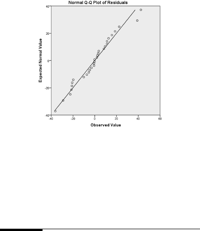
Models for Repeated-Measures Data:The Rat Brain Example 243
FIGURE 5.3: Distribution of conditional residuals from Model 5.2.
Figure 5.4 suggests that the residual variance is fairly constant across treatments (there
is no pattern, and the residuals are symmetric). We formally tested the assumption of equal
residual variances across treatments in Hypothesis 5.2, and found no significant difference
in the residual variance for the carbachol treatment vs. the basal treatment in Model 5.2
(see Subsection 5.5.2).
The distributions of the EBLUPs of the random effects should also be investigated to
check for possible outliers. Unfortunately, EBLUPs for the two random effects associated
with each animal in Model 5.2 cannot be generated in the current version of the MIXED
command in IBM SPSS Statistics (Version 21). Because we have a very small number of
animals, we do not investigate diagnostics for the EBLUPs for this model.
5.10 Software Notes
5.10.1 Heterogeneous Residual Variances for Level 1 Groups
Recall that in Chapter 3 we used a heterogeneous residual variance structure for groups
defined by a Level 2 variable (treatment) in Model 3.2B. The ability to fit such models
is available only in proc mixed in SAS, the GENLINMIXED command in SPSS, the lme()
function in R,andthemixed command in Stata. When we fit Model 5.3 to the Rat Brain
data in this chapter, we defined a heterogeneous residual variance structure for different
values of a Level 1 variable (TREATMENT). We were able to fit this model using all of the
software procedures, with the exception of the lmer() function in R.
The HLM2 procedure only allows maximum likelihood estimation for models that are
fitted with a heterogeneous residual variance structure. SAS, SPSS, the the lme() function
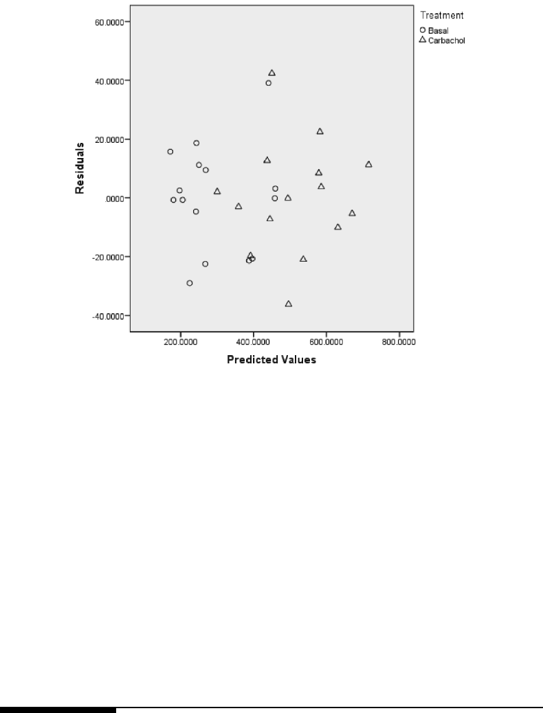
244 Linear Mixed Models: A Practical Guide Using Statistical Software
FIGURE 5.4: Scatter plot of conditional residuals vs. conditional predicted values based on
the fit of Model 5.2.
in R,andthemixed command in Stata all allow ML or REML (default) estimation for these
models. The parameterization of the heterogeneous residual variances in HLM2 employs a
logarithmic transformation, so the parameter estimates for the variances from HLM2 need
to be exponentiated before they can be compared with results from the other software
procedures (see Subsection 5.4.5).
5.10.2 EBLUPs for Multiple Random Effects
Model 5.2 specified two random effects for each animal: one associated with the intercept and
a second associated with treatment. The EBLUPs for multiple random effects per subject
can be displayed using SAS, R, Stata, and HLM. However, it is not possible to obtain
separate estimates of the EBLUPs for more than one random effect per subject when using
the MIXED command in the current version of IBM SPSS Statistics (Version 21).
5.11 Other Analytic Approaches
5.11.1 Kronecker Product for More Flexible Residual Covariance
Structures
Most residual covariance structures (e.g., AR(1) or compound symmetry) are designed for
one within-subject factor (e.g., time). In the Rat Brain example, we have two within-subject

Models for Repeated-Measures Data:The Rat Brain Example 245
factors: brain region and treatment. With such data, one can consider modeling a resid-
ual covariance structure using the Kronecker Product of the underlying within-subject
factor-specific covariance matrices (Galecki, 1994). This method adds flexibility in building
residual covariance structures and has an attractive interpretation in terms of independent
within-subject factor-specific contributions to the overall within-subject covariance struc-
ture. Examples of this general methodology are implemented in SAS proc mixed.
The SAS syntax that implements an example of this methodology for the Rat Brain
data is provided below:
title "Kronecker Product Covariance Structure";
proc mixed data = ratbrain;
class animal region treatment;
model activate = region treatment region*treatment / s;
random int / subject = animal type=vc v vcorr solution;
repeated region treatment / subject=animal type=un@un r rcorr;
run;
Note that both REGION and TREATMENT must be listed in the class statement. In
the random statement we retain the random intercept but omit the random animal-specific
treatment effects to avoid overparameterization of the model. The repeated statement in-
cludes the option type=un@un, which specifies the Kronecker product of the two matrices
for the REGION and TREATMENT factors, with three and two levels, respectively. The
syntax implies that REGION contributes an unstructured 3 ×3 matrix and TREATMENT
contributes an unstructured 2 ×2 matrix to the overall 6 ×6matrixRi. To ensure identi-
fiability of the matrices, we assume that the upper-left element in the matrix contributed
by TREATMENT is equal to 1 (which is automatically done by the software).
This syntax results in the following estimates of the elements of the underlying factor-
specific matrices for both REGION and TREATMENT.
'
&
$
%
Covariance Parameter Estimates
--------------------------------------
Cov Parm Subject Estimate
--------------------------------------
Intercept animal 7637.3000
region UN(1,1) animal 2127.7400
UN(2,1) animal 1987.2900
UN(2,2) animal 2744.6600
UN(3,1) animal 1374.5100
UN(3,2) animal 2732.2200
UN(3,3) animal 3419.7000
treatment UN(1,1) animal 1.0000
UN(2,1) animal -0.4284
UN(2,2) animal 0.6740
We can use these estimates to determine the unstructured variance-covariance matrices
for the residuals contributed by the REGION and TREATMENT factors:
RREGION =⎛
⎝2127.74 1987.29 1374.51
1987.29 2744.66 2732.22
1374.51 2732.22 3419.70 ⎞
⎠
RTREATMENT =1.00 −0.43
−0.43 0.67

246 Linear Mixed Models: A Practical Guide Using Statistical Software
The Kronecker product of these two factor-specific residual variance-covariance matrices
implies the following overall estimated Ricorrelation matrix for a given rat:
'
&
$
%
Estimated R Correlation Matrix for animal R100797
Row Col1 Col2 Col3 Col4 Col5 Col6
1 1.0000 0.8224 0.5096 -0.5219 -0.4292 -0.2659
2 0.8224 1.0000 0.8918 -0.4292 -0.5219 -0.4654
3 0.5096 0.8918 1.0000 -0.2659 -0.4654 -0.5219
4 -0.5219 -0.4292 -0.2659 1.0000 0.8224 0.5096
5 -0.4292 -0.5219 -0.4654 0.8224 1.0000 0.8918
6 -0.2659 -0.4654 -0.5219 0.5096 0.8918 1.0000
The implied marginal correlation matrix of observations for a given rat based on this
model is as follows. The structure of this marginal correlation matrix reveals a high level
of correlation among observations on the same animal, as was observed for the implied
marginal correlation matrix based on the fit of Model 5.2:
'
&
$
%
Estimated V Correlation Matrix for animal R100797
Row Col1 Col2 Col3 Col4 Col5 Col6
1 1.0000 0.9559 0.8673 0.7146 0.7050 0.7153
2 0.9559 1.0000 0.9678 0.6992 0.6511 0.6365
3 0.8673 0.9678 1.0000 0.7038 0.6314 0.5887
4 0.7146 0.6992 0.7038 1.0000 0.9676 0.9017
5 0.7050 0.6511 0.6314 0.9676 1.0000 0.9760
6 0.7153 0.6365 0.5887 0.9017 0.9760 1.0000
The AIC for this model is 258.0, which is very close to the value for Model 5.2 (AIC =
257.2) and better (i.e., smaller) than the value for Model 5.1 (AIC = 279.3).
Note that covariance structures based on Kronecker products can also be used for stud-
ies involving multiple dependent variables measured longitudinally (not considered in this
book).
5.11.2 Fitting the Marginal Model
We can also take a strictly marginal approach (in which random animal effects are not
considered) to modeling the Rat Brain data. However, there are only 5 animals and 30
observations; therefore, fitting a marginal model with an unstructured residual covariance
matrix is not recommended, because the unstructured Rimatrix would require the esti-
mation of 21 covariance parameters. When attempting to fit a marginal model with an
unstructured covariance structure for the residuals using REML estimation in SPSS, the
MIXED command issues a warning and does not converge to a valid solution.
We can consider marginal models with more restrictive residual covariance structures.
For example, we can readily fit a model with a heterogeneous compound symmetry Ri
matrix, which requires the estimation of seven parameters: six variances, i.e., one for each
combination of treatment and region, and a constant correlation parameter (note that these
are also a lot of parameters to estimate for this small data set). We use the following syntax
in SPSS:
* Marginal model with heterogeneous compound symmetry R(i) matrix.
MIXED
activate BY region treatment

Models for Repeated-Measures Data:The Rat Brain Example 247
/CRITERIA = CIN(95) MXITER(100) MXSTEP(5) SCORING(1)
SINGULAR(0.000000000001) HCONVERGE(0, ABSOLUTE)
LCONVERGE(0, ABSOLUTE) PCONVERGE(0.000001, ABSOLUTE)
/FIXED = region treatment region*treatment | SSTYPE(3)
/METHOD = REML
/PRINT = SOLUTION R
/REPEATED Region Treatment | SUBJECT(animal) COVTYPE(CSH) .
In this syntax for the marginal model, note that the /RANDOM subcommand is not in-
cluded. The structure of the Rimatrix is specified as CSH (compound symmetric hetero-
geneous), which means that the residual marginal variance is allowed to differ for each
combination of REGION and TREATMENT, although the correlation between observa-
tions on the same rat is constant (estimated to be 0.81). The AIC for this model is 267.8,
as compared to the value of 257.2 for Model 5.2. So, it appears that we have a better fit
using the LMM with explicit random effects (Model 5.2).
5.11.3 Repeated-Measures ANOVA
A more traditional approach to repeated-measures ANOVA (Winer et al., 1991) starts with
a data set in the wide format shown in Table 5.2. This type of analysis could be carried out,
for example, using the GLM procedures in SPSS and SAS. However, if any missing values
occur for a given subject (e.g., animal), that subject is dropped from the analysis altogether
(complete case analysis). Refer to Subsection 2.9.4 for more details on the problems with
this approach when working with missing data.
The correlation structure assumed in a traditional repeated-measures ANOVA is spheri-
cal (i.e., compound symmetry with homogeneous variance), with adjustments (Greenhouse–
Geisser or Huynh–Feldt) made to the degrees of freedom used in the denominator for the
F-tests of the within-subject effects when the assumption of sphericity is violated. There are
no explicit random effects in this approach, but a separate mean square error is estimated
for each within-subject factor, which is then used in the F-tests for that factor. Thus, in an
analysis of the Rat Brain data, there would be a separate residual variance estimated for
REGION, for TREATMENT, and for the REGION ×TREATMENT interaction.
In general, the LMM approach to the analysis of repeated-measures data allows for much
more flexible correlation structures than can be specified in a traditional repeated-measures
ANOVA model.
5.12 Recommendations
This chapter has illustrated some important points with respect to how categorical fixed
factors are handled in the specification of random-effects structures for linear mixed models
in the different software procedures. If, for example, a categorical fixed factor has four levels,
a standard reference (or “dummy variable”) parameterization of the model is used (where
fixed effects of indicators for the nonreference categories are included in the model), and
there are multiple measurements at each level of the categorical factor within each of the
higher-level units (as was the case for the two treatments in the Rat Brain example), then
technically one could include random effects associated with each of the indicator variables.
However, because some of the software procedures (e.g., R,HLM)useanunstructured co-
variance matrix for the random effects included in the model by default, analysts need to
248 Linear Mixed Models: A Practical Guide Using Statistical Software
be wary of how many covariance parameters are being included when specifying random
effects associated with categorical factors. Allowing the effects of the three nonreference lev-
els of the four-category fixed factor to randomly vary across higher-level units, for example,
not only introduces three additional variance components that need to be estimated, but
several additional covariances as well (e.g., the covariance of the random effects associated
with nonreference levels 1 and 2 of the categorical fixed factor). Analysts need to be careful
when specifying these random effects, and the approach that we took in the Stata exam-
ple in this chapter underscores this issue (where Stata does not allow for the estimation
of covariances of random effects when the effects associated with a categorical fixed factor
are allowed to randomly vary at higher levels). For this reason, we recommend “manual”
indicator coding for fixed factors, enabling more control over exactly what random effects
covariance structure is being estimated. We illustrated this approach with our handling of
the TREATMENT variable in the Rat Brain example.
We also illustrated the ability of the different software procedures to allow the error
variances to vary depending on the levels of categorical factors at Level 1 of the data
hierarchy in a repeated measures design (i.e., within-subject factors). While allowing the
error variances to vary across the two treatments did not improve the fits of the models to
the Rat Brain data, we recommend that analysts always consider this possibility, beginning
with graphical exploration of the data. It has been our experience that many real-world
data sets have this feature, and the fits of models (and corresponding tests for various
parameters) can be greatly improved by correctly modeling this aspect of the covariance
structure for a given data set.
Finally, we illustrated various likelihood ratio tests in this chapter, and we remind readers
that likelihood ratio tests rely on asymptotic theory (i.e., large sample sizes at each of the
levels of the data hierarchy, and especially at Level 2 in repeated measures designs). The
Rat Brain data set is certainly not large enough to make these tests valid in an asymptotic
sense, and the likelihood ratio tests are only included for illustration purposes. For smaller
data sets, analysts might consider Bayesian methods for hypothesis testing, as was discussed
in Chapter 2.

6
Random Coefficient Models for Longitudinal Data:
The Autism Example
6.1 Introduction
This chapter illustrates fitting random coefficient models to data arising from a lon-
gitudinal study of the social development of children with autism, whose socialization
scores were observed at ages 2, 3, 5, 9 and 13 years. We consider models that allow the
child-specific coefficients describing individual time trajectories to vary randomly. Random
coefficient models are often used for the analysis of longitudinal data when the researcher
is interested in modeling the effects of time and other time-varying covariates at Level 1 of
the model on a continuous dependent variable, and also wishes to investigate the amount of
between-subject variance in the effects of the covariates across Level 2 units (e.g., subjects
in a longitudinal study). In the context of growth and development over time, random coef-
ficient models are often referred to as growth curve models. Random coefficient models
may also be employed in the analysis of clustered data, when the effects of Level 1 covari-
ates, such as student’s socioeconomic status, tend to vary across clusters (e.g., classrooms
or schools). Table 6.1 illustrates some examples of longitudinal data that may be analyzed
using linear mixed models with random coefficients.
We highlight the Rsoftware in this chapter.
6.2 The Autism Study
6.2.1 Study Description
The data used in this chapter were collected by researchers at the University of Michigan
(Anderson et al., 2009) as part of a prospective longitudinal study of 214 children. The
children were divided into three diagnostic groups when they were 2 years old: autism,
pervasive developmental disorder (PDD), and nonspectrum children. We consider a subset
of 158 autism spectrum disorder (ASD) children, including autistic and PDD children, for
this example. The study was designed to collect information on each child at ages 2, 3, 5,
9, and 13 years, although not all children were measured at each age. One of the study
objectives was to assess the relative influence of the initial diagnostic category (autism or
PDD), language proficiency at age 2, and other covariates on the developmental trajectories
of the socialization of these children.
Study participants were children who had had consecutive referrals to one of two autism
clinics before the age of 3 years. Social development was assessed at each age using the
Vineland Adaptive Behavior Interview survey form, a parent-reported measure of social-
ization. The dependent variable, VSAE (Vineland Socialization Age Equivalent), was a
249

250 Linear Mixed Models: A Practical Guide Using Statistical Software
TABLE 6.1: Examples of Longitudinal Data in Different Research Settings
Level of Data Research Setting
Substance
Abuse
Business Autism
Research
Subject
(Level 2)
Subject
variable
(random
factor)
College Company Child
Covariates Geographic
region, public/
private,
rural/urban
Industry,
geographic
region
Gender,
baseline
language level
Time
(Level 1)
Time
variable
Year Quarter Age
Dependent
variable
Percent of
students
Stock value in
each
Socialization
score at
who use
marijuana
during each
academic year
quarter each age
Covariates School ranking,
cost of tuition
Quarterly sales,
workforce size
Amount of
therapy
received
combined score that included assessments of interpersonal relationships, play/leisure time
activities, and coping skills. Initial language development was assessed using the Sequenced
Inventory of Communication Development (SICD) scale; children were placed into one of
three groups (SICDEGP) based on their initial SICD scores on the expressive language
subscale at age 2.
Table 6.2 displays a sample of cases from the Autism data in the “long” form appropriate
for analysis using the LMM procedures in SAS, SPSS, Stata, and R. The data have been
sorted in ascending order by CHILDID and by AGE within each level of CHILDID. This
sorting is helpful when interpreting analysis results, but is not required for the model-fitting
procedures.
Note that the values of the subject-level variables, CHILDID and SICDEGP, are the
same for each observation within a child, whereas the value of the dependent variable
(VSAE) is different at each age. We do not consider any time-varying covariates other than
AGE in this example. The variables that will be used in the analysis are defined below:
Subject (Level 2) Variables
•CHILDID = Unique child identifier
•SICDEGP =Sequenced Inventory of Communication Development Expressive

Random Coefficient Models for Longitudinal Data: The Autism Example 251
TABLE 6.2: Sample of the Autism Data Set
Child Longitudinal Measures
(Level 2) (Level 1)
Subject Covariate Time Dependent
ID Variable Variable
CHILDID SICDEGP AGE VSAE
132 6
133 7
13518
13925
1 3 13 27
212 6
213 7
215 7
219 8
2 1 13 14
33217
33318
33512
33918
3 3 13 24
...
Group: categorized expressive language score at age 2 years (1 = low, 2 = medium,
3=high)
Time-Varying (Level 1) Variables
•AGE = Age in years (2, 3, 5, 9, 13); the time variable
•VSAE =Vineland Socialization Age Equivalent: parent-reported socialization, the
dependent variable, measured at each age
6.2.2 Data Summary
The data summary for this example is carried out using the Rsoftware package. A link
to the syntax and commands that can be used to perform similar analyses in the other
software packages is included on the book’s web page (see Appendix A).
We begin by reading the comma-separated raw data file (autism.csv) into Rand “at-
taching” the data set to memory, so that shorter versions of the variable names can be used
in Rfunctions (e.g., age rather than autism$age).
> autism <- read.csv("c:\\temp\\autism.csv", h = T)
> attach(autism)

252 Linear Mixed Models: A Practical Guide Using Statistical Software
Alternatively, Rusers can import text data files directly from a web site:
> file <- "http://www-personal.umich.edu/~bwest/autism.csv"
> autism <- read.csv(file, h = T)
> attach(autism)
Next, we apply the factor() function to the numeric variables SICDEGP and AGE to
create categorical versions of these variables (SICDEGP.F and AGE.F), and add the new
variables to the data frame.
> sicdegp.f <- factor(sicdegp)
> age.f <- factor(age)
> # Add the new variables to the data frame object.
> autism.updated <- data.frame(autism, sicdegp.f, age.f)
After creating these factors, we request descriptive statistics for both the continuous
and factor variables included in the analysis using the summary() function. Note that the
summary() function produces different output for the continuous variable, VSAE, than for
the factor variables.
> # Number of Observations at each level of AGE
> summary(age.f)
235913
156 150 91 120 95
> # Number of Observations at each level of AGE within each group
> # defined by the SICDEGP factor
> table(sicdegp.f, age.f)
age.f
sicdegp.f 235913
15048293728
26664364841
34038263526
> # Overall summary for VSAE
> summary(vsae)
Min. 1st Qu. Median Mean 3rd Qu. Max. NA’s
1.00 10.00 4.00 26.41 27.00 198.00 2.00
> # VSAE means at each AGE
> tapply(vsae, age.f, mean, na.rm=TRUE)
235913
9.089744 15.255034 21.483516 39.554622 60.600000
> # VSAE minimum values at each AGE

Random Coefficient Models for Longitudinal Data: The Autism Example 253
> tapply(vsae, age.f, min, na.rm=TRUE)
235913
1443 7
> # VSAE maximum values at each AGE
> tapply(vsae, age.f, max, na.rm=TRUE)
235 913
20 63 77 171 198
The number of children examined at each age differs due to attrition over time. We also
have fewer children at age 5 years because one of the clinics did not schedule children to be
examined at that age. There were two children for whom VSAE scores were not obtained
at age 9, although the children were examined at that age (missing values of VSAE are
displayed as NAs in the output).
Overall, VSAE scores ranged from 1 to 198, with a mean of 26.41. The minimum values
changed only slightly at each age, but the means and maximum values increased markedly
at later ages.
We next generate graphs that show the observed VSAE scores as a function of age for
each child within levels of SICDEGP (Figure 6.1). We also display the mean VSAE profiles
by SICDEGP (Figure 6.2). The Rsyntax that can be used to generate these graphs is
provided below:
> library(lattice) # Load the library for trellis graphics.
> trellis.device(color=F) # Color is turned off.
> # Load the nlme library, which is required for the
> # plots as well as for subsequent models.
> library(nlme)
We generate Figure 6.1 using the Rcode below. We use the model formula
vsae ~ age | childid as an argument in the groupedData() function to create a
“grouped” data frame object, autism.g1, in which VSAE is the y-axis variable, AGE is the
x-axis variable, and CHILDID defines the grouping of the observations (one line for each
child in the plot). The one-sided formula ~ sicdegp.f in the outer = argument defines the
outer groups for the plot (i.e., requests one plot per level of the SICDEGP factor).
> autism.gl <- groupedData(vsae ~ age | childid,
outer = ~ sicdegp.f, data = autism.updated)
> # Generate individual profiles in Figure 6.1.
> plot(autism.gl, display = "childid", outer = TRUE, aspect = 2,
key = F, xlab = "Age (Years)", ylab = "VSAE",
main = "Individual Data by SICD Group")
For Figure 6.2, we create a grouped data frame object, autism.g2, where VSAE
and AGE remain the y-axis and x-axis variables, respectively. However, by replacing
“| childid”with“| sicdegp.f”, all children with the same value of SICDEGP are de-
fined as a group and used to generate mean profiles. The argument order.groups = F
preserves the numerical order of the SICDEGP levels.
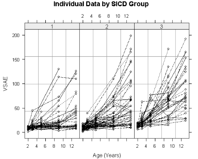
254 Linear Mixed Models: A Practical Guide Using Statistical Software
FIGURE 6.1: Observed VSAE values plotted against age for children in each SICD group.
> autism.g2 <- groupedData(vsae ~ age | sicdegp.f,
order.groups = F, data = autism.updated)
> # Generate mean profiles in Figure 6.2.
> plot(autism.g2, display = "sicdegp", aspect = 2, key = F,
xlab = "Age (Years)", ylab = "VSAE",
main = "Mean Profiles by SICD Group")
The plots of the observed VSAE values for individual children in Figure 6.1 show sub-
stantial variation from child to child within each level of SICD group; the VSAE scores
of some children tend to increase as the children get older, whereas the scores for other
children remain relatively constant. On the other hand, we do not see much variability in
the initial values of VSAE at age 2 years for any of the levels of SICD group. Overall, we
observe increasing between-child variability in the VSAE scores at each successive year of
age. The random coefficient models fitted to the data account for this important feature,
as we shall see later in this chapter.
The mean profiles displayed in Figure 6.2 show that the mean VSAE scores generally
increase with age. There may also be a quadratic trend in VSAE scores, especially in SICD
group two. This suggests that a model to predict VSAE should include both linear and
quadratic fixed effects of age, and possibly interactions between the linear and quadratic
effects of age and SICD group.
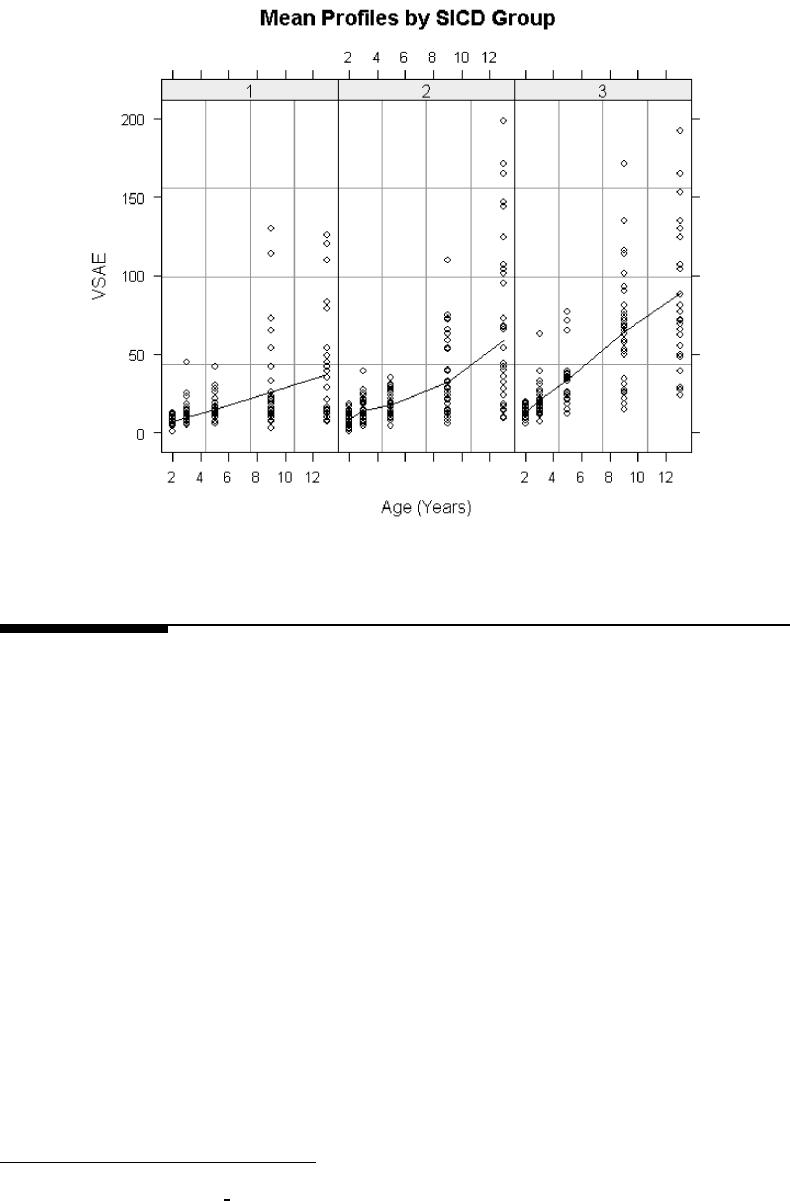
Random Coefficient Models for Longitudinal Data: The Autism Example 255
FIGURE 6.2: Mean profiles of VSAE values for children in each SICD group.
6.3 Overview of the Autism Data Analysis
For the analysis of the Autism data, we follow the “top-down” modeling strategy outlined
in Subsection 2.7.1 of Chapter 2. In Subsection 6.3.1 we outline the analysis steps, and
informally introduce related models and hypotheses to be tested. Subsection 6.3.2 presents
a more formal specification of selected models that are fitted to the Autism data, and
Subsection 6.3.3 details the hypotheses tested in the analysis. To follow the analysis steps
outlined in this section, refer to the schematic diagram presented in Figure 6.3.
6.3.1 Analysis Steps
Step 1: Fit a model with a “loaded” mean structure (Model 6.1).
Fit an initial random coefficient model with a “loaded” mean structure and
random child-specific coefficients for the intercept, age, and age-squared.
In Model 6.1, we fit a quadratic regression model for each child, which describes their
VSAE as a function of age. This initial model includes the fixed effects of age1, age-squared,
SICD group, the SICD group by age interaction, and the SICD group by age-squared interac-
tion. We also include three random effects associated with each child: a random intercept, a
random age effect, and a random age-squared effect. This allows each child to have a unique
parabolic trajectory, with coefficients that vary randomly around the fixed effects defining
1To simplify interpretation of the intercept, we subtract two from the value of AGE and create an
auxiliary variable named AGE 2. The intercept can then be interpreted as the predicted VSAE score at age
2, rather than at age zero, which is outside the range of our data.
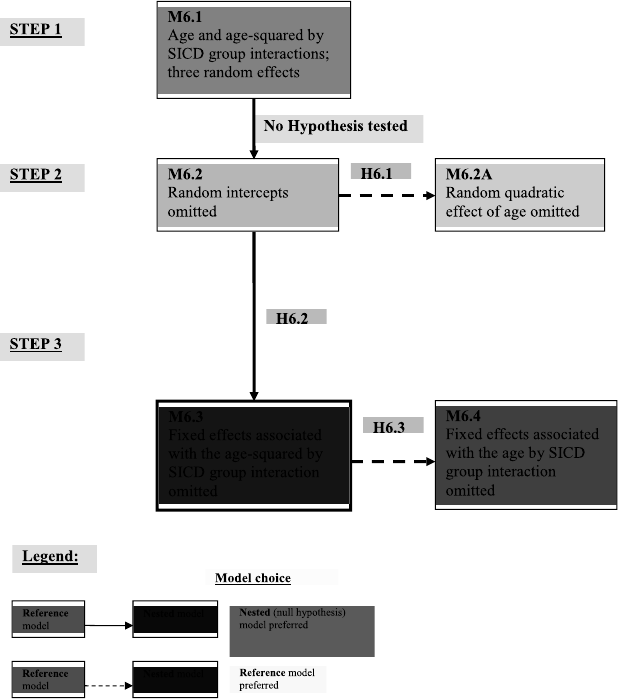
256 Linear Mixed Models: A Practical Guide Using Statistical Software
FIGURE 6.3: Model selection and related hypotheses for the analysis of the Autism data.
the mean growth curve for each SICD group. We use REML to estimate the variances and
covariances of the three random effects. Model 6.1 also includes residuals associated with
the VSAE observations, which conditional on a given child are assumed to be independent
and identically distributed.
We encounter some estimation problems when we fit Model 6.1 using the software pro-
cedures. SAS proc mixed reports problems with estimating the covariance parameters for
the random effects; the procedures in SPSS and Rdo not achieve convergence; the mixed
command in Stata converges to a solution, but encounters difficulties in estimating the stan-
dard errors of the covariance parameters; and HLM2 requires more than 1000 iterations to
converge to a solution. As a result, the estimates of the covariance parameters defined in
Model 6.1 differ widely across the packages.
Step 2: Select a structure for the random effects (Model 6.2 vs. Model 6.2A).
Fit a model without the random child-specific intercepts (Model 6.2), and test
whether to keep the remaining random effects in the model.
We noted in the initial data summary (Figures 6.1 and 6.2) that there was little vari-
ability in the VSAE scores at age 2, and therefore in Model 6.2 we attribute this variation

Random Coefficient Models for Longitudinal Data: The Autism Example 257
entirely to random error rather than to between-subject variability. Compared to Model
6.1, we remove the random child-specific intercepts, while retaining the same fixed effects
and the child-specific random effects of age and age-squared. Model 6.2 therefore implies
that the children-specific predicted trajectories within a given level of SICD group have a
common VSAE value at age 2 (i.e., there is no between-child variability in VSAE scores
at age 2). We also assume for Model 6.2 that the age-related linear and quadratic random
effects describe the between-subject variation.
We formally test the need for the child-specific quadratic effects of age (Hypothesis 6.1)
by using a REML-based likelihood ratio test. To perform this test, we fit a nested model
(Model 6.2A) that omits the random quadratic effects. Based on the significant result of
this test, we decide to retain both the linear and quadratic child-specific random effects in
all subsequent models.
Step 3: Reduce the model by removing nonsignificant fixed effects (Model 6.2
vs. Model 6.3), and check model diagnostics.
In this step, we test whether the fixed effects associated with the AGE-squared ×SICDEGP
interaction can be omitted from Model 6.2 (Hypothesis 6.2). We conclude that these fixed
effects are not significant, and we remove them to form Model 6.3. We then test whether
the fixed effects associated with the AGE ×SICDEGP interaction can be omitted from
Model 6.3 (Hypothesis 6.3), and find that these fixed effects are significant and should be
retained in the model.
Finally, we refit Model 6.3 (our final model) using REML estimation to obtain unbi-
ased estimates of the covariance parameters. We check the assumptions for Model 6.3 by
examining the distribution of the residuals and of the EBLUPs for the random effects. We
also investigate the agreement of the observed VSAE values with the conditional predicted
values based on Model 6.3 using scatter plots. The diagnostic plots are generated using the
Rsoftware package (Section 6.9).
In Figure 6.3 we summarize the model selection process and hypotheses considered in
the analysis of the Autism data. Refer to Subsection 3.3.1 for details on the notation in this
figure.
6.3.2 Model Specification
Selected models considered in the analysis of the Autism data are summarized in Table 6.3.
6.3.2.1 General Model Specification
The general form of Model 6.1 for an individual response, VSAEti, on child iat the t-th
visit (t=1,2,3,4,5,correspondingtoages2,3,5,9and13),isshownin(6.1).This
specification corresponds closely to the syntax used to fit the model using the procedures
in SAS, SPSS, R, and Stata.
VSAEti =β0+β1×AGE 2ti +β2×AGE 2SQti +β3×SICDEGP1i
+β4×SICDEGP2i+β5×AGE 2ti ×SICDEGP1i
+β6×AGE 2ti ×SICDEGP2i×β7×AGE 2SQti ×SICDEGP1i
+β8×AGE 2SQti ×SICDEGP2i
⎫
⎪
⎪
⎪
⎬
⎪
⎪
⎪
⎭
fixed
+u0i+u1i×AGE 2ti +u2i×AGE 2SQti +εti }random
(6.1)
258 Linear Mixed Models: A Practical Guide Using Statistical Software
TABLE 6.3: Summary of Selected Models Considered for the Autism Data
Term/Variable General HLM Model
Notation Notation 6.1 6.2 6.3
Fixed effects Intercept β0β00 √√√
AGE 2β1β10 √√√
AGE 2SQ β2β20 √√√
SICDEGP1 β3β01 √√√
SICDEGP2 β4β02 √√√
AGE 2×SICDEGP1 β5β11 √√√
AGE 2×SICDEGP2 β6β12 √√√
AGE 2SQ ×SICDEGP1 β7β21 √√
AGE 2SQ ×SICDEGP2 β8β22 √√
Random Child (i)Intercept u0ir0i√
effects AGE 2u1ir1i√√√
AGE 2SQ u2ir2i√√√
Residuals Time (t)εti eti √√√
Covariance
Parameters (θD)
for DMatrix
Child level Variance of intercepts σ2
int τ[1,1] √
Covariance of intercepts, AGE 2
effects
σint,age τ[1,2] √
Covariance of intercepts, AGE 2SQ
effects
σint,age-sq τ[1,3] √
Variance of AGE 2effects σ2
age τ[2,2] √√√
Covariance of AGE 2effects,
AGE 2SQ effects
σage,age-sq τ[2,3] √√√
Variance of AGE 2SQ effects σage-sq τ[3,3] √√√
Covariance
Parameters (θR)
for RiMatrix
Time level Residual variance σ2σ2√√√

Random Coefficient Models for Longitudinal Data: The Autism Example 259
In (6.1), the AGE 2 variable represents the value of AGE minus 2, and AGE 2SQ rep-
resents AGE 2 squared. We include two dummy variables, SICDEGP1 and SICDEGP2,
to indicate the first two levels of the SICD group. Because we set the fixed effect for the
third level of the SICD group to 0, we consider SICDEGP = 3 as the “reference category.”
There are two variables that represent the interaction between age and SICD group: AGE 2
×SICDEGP1 and AGE 2×SICDEGP2. There are also two variables that represent the
interaction between age-squared and SICD group: AGE 2SQ ×SICDEGP1 and AGE 2SQ
×SICDEGP2.
The parameters β0through β8represent the fixed effects associated with the intercept,
the covariates, and the interaction terms in the model. Because the fixed intercept, β0,
corresponds to the predicted VSAE score when all covariates, including AGE 2, are equal
to zero, the intercept can be interpreted as the mean predicted VSAE score for children at
2 years of age in the reference category of the SICD group (SICDEGP = 3).
The parameters β1and β2represent the fixed effects of age and age-squared for the
reference category of the SICD group (SICDEGP = 3). The fixed effects β3and β4represent
the difference in the intercept for the first two levels of the SICD group vs. the reference
category.
The fixed effects β5and β6represent the differences in the linear effect of age between
the first two levels of SICD group and the linear effect of age in the reference category of the
SICD group. Similarly, the fixed effects β7and β8represent the differences in the quadratic
effect of age between the first two levels of the SICD group and the quadratic effect of age
in the reference category.
The terms u0i,u1i,andu2iin (6.1) represent the random effects associated with the
intercept, linear effect of age, and quadratic effect of age for child i. The distribution of the
vector of the three random effects, ui, associated with child iis assumed to be multivariate
normal:
ui=⎛
⎝u0i
u1i
u2i⎞
⎠∼N(0,D)
Each of the three random effects has a mean of 0, and the variance-covariance matrix,
D, for the random effects is:
D=⎛
⎝
σ2
int σint,age σint,age-squared
σint,age σ2
age σage,age-squared
σint,age-squared σage,age-squared σ2
age-squared
⎞
⎠
The term εti in (6.1) represents the residual associated with the observation at time t
on child i. The distribution of the residuals can be written as
εti ∼N(0,σ
2)
We assume that the residuals are independent and identically distributed, conditional
on the random effects, and that the residuals are independent of the random effects.
We do not include the specification of other models (e.g., Models 6.2 and 6.3) in this
section. These models can be obtained by simplification of Model 6.1. For example, the D
matrix in Model 6.2 has the following form, because the random intercepts are omitted from
the model:
D=σ2
age σage,age-squared
σage,age-squared σ2
age-squared

260 Linear Mixed Models: A Practical Guide Using Statistical Software
6.3.2.2 Hierarchical Model Specification
We now present Model 6.1 in hierarchical form, using the same notation as in (6.1). The
correspondence between this notation and the HLM software notation is defined in Table 6.3.
The hierarchical model has two components, reflecting contributions from the two levels
of the Autism data: Level 1 (the time level), and Level 2 (the child level).
Level 1 Model (Time)
VSAEti =b0i+b1i×AGE 2ti +b2i×AGE 2SQti +εti (6.2)
where
εti ∼N(0,σ
2)
This model shows that at Level 1 of the data, we have a set of child-specific quadratic
regressions of VSAE on AGE 2andAGE2SQ. The intercept (b0i),the linear effect of
AGE 2(b1i),and the quadratic effect of AGE 2SQ (b2i) defined in the Level 2 model are
allowed to vary between children, who are indexed by i.
The unobserved child-specific coefficients for the intercept, linear effect of age, and
quadratic effect of age (b0i,b
1i,and b2i) in the Level 1 model depend on fixed effects as-
sociated with Level 2 covariates and random child effects, as shown in the Level 2 model
below:
Level 2 Model (Child)
b0i=β0+β3×SICDEGP1i+β4×SICDEGP2i+u0i
b1i=β1+β5×SICDEGP1i+β6×SICDEGP2i+u1i
b2i=β2+β7×SICDEGP1i+β8×SICDEGP2i+u2i
(6.3)
where
ui=⎛
⎝u0i
u1i
u2i⎞
⎠∼N(0,D)
The Level 2 model in (6.3) shows that the intercept (b0i) for child idepends on the fixed
overall intercept (β0), the fixed effects (β3and β4) of the child-level covariates SICDEGP1
and SICDEGP2, and a random effect (u0i) associated with child i.
The child-specific linear effect of age (b1i) depends on the overall fixed effect of age
(β1), the fixed effect of SICDEGP1 (β5), the fixed effect of SICDEGP2 (β6), and a random
effect (u1i) associated with child i. The equation for the child-specific quadratic effect of
age (b2i) for child iis defined similarly. The random effects in the Level 2 model allow the
child-specific intercepts, linear effects of age, and quadratic effects of age to vary randomly
between children. The variance-covariance matrix (D) of the random effects is defined as
in the general model specification.
The hierarchical specification of Model 6.1 is equivalent to the general specification for
this model presented in Subsection 6.3.2.1. We can derive the model as specified in (6.1) by
substituting the expressions for b0i,b1i,and b2ifrom the Level 2 model (6.3) into the Level

Random Coefficient Models for Longitudinal Data: The Autism Example 261
1 model (6.2). The fixed effects associated with the child-specific covariates SICDEGP1 and
SICDEGP2 in the Level 2 equations for b1iand b2irepresent interactions between these
covariates and AGE 2andAGE2SQ in the general model specification.
6.3.3 Hypothesis Tests
Hypothesis tests considered in the analysis of the Autism data are summarized in Table 6.4.
Hypothesis 6.1. The random effects associated with the quadratic effect of AGE can be
omitted from Model 6.2.
We indirectly test whether these random effects can be omitted from Model 6.2. The
null and alternative hypotheses are:
H0:D=σ2
age 0
00
HA:D=σ2
age σage,age-squared
σage,age-squared σ2
age-squared
To test Hypothesis 6.1, we use a REML-based likelihood ratio test. The test statistic is
the value of the –2 REML log-likelihood value for Model 6.2A (the nested model excluding
the random quadratic age effects) minus the value for Model 6.2 (the reference model). To
obtain a p-value for this statistic, we refer it to a mixture of χ2distributions, with 1 and 2
degrees of freedom and equal weight 0.5.
Hypothesis 6.2. The fixed effects associated with the AGE-squared ×SICDEGP inter-
action are equal to zero in Model 6.2.
The null and alternative hypotheses in this case are specified as follows:
H0:β7=β8=0
HA:β7=0orβ8=0
We test Hypothesis 6.2 using an ML-based likelihood ratio test. The test statistic is the
value of the –2 ML log-likelihood for Model 6.3 (the nested model excluding the fixed effects
associated with the interaction) minus the value for Model 6.2 (the reference model). To
obtain a p-value for this statistic, we refer it to a χ2distribution with 2 degrees of freedom,
corresponding to the 2 additional fixed-effect parameters in Model 6.2.
Hypothesis 6.3. The fixed effects associated with the AGE ×SICDEGP interaction are
equal to zero in Model 6.3.
The null and alternative hypotheses in this case are specified as follows:
H0:β5=β6=0
HA:β5=0orβ6=0
We test Hypothesis 6.3 using an ML-based likelihood ratio test. The test statistic is the
value of the –2 ML log-likelihood for Model 6.4 (the nested model excluding the fixed effects
associated with the interaction) minus the value for Model 6.3 (the reference model). To
obtain a p-value for this statistic, we refer it to a χ2distribution with 2 degrees of freedom,
corresponding to the 2 additional fixed-effect parameters in Model 6.3.
For the results of these hypothesis tests, see Section 6.5.

262 Linear Mixed Models: A Practical Guide Using Statistical Software
TABLE 6.4: Summary of Hypotheses Tested in the Autism Analysis
Models Compared
Label Null (H0)Alternative(HA) Test Nested
Model
(H0)
Ref.
Model
(HA)
Est.
Method
Test Stat.
Dist.
under H0
6.1 Drop u2i(random
effects associated with
AGE-squared)
Retain u2iLRT Model 6.2A Model 6.2 REML 0.5χ2
1+0.5χ2
2
6.2 Drop fixed effects
associated with AGE-
squared by SICDEGP
interaction
(β7=β8=0)
Either β7=0,or
β8=0
LRT Model 6.3 Model 6.2 ML χ2
2
6.3 Drop fixed effects
associated with AGE
by SICDEGP
interaction
(β5=β6=0)
Either β5=0,or
β6=0
LRT Model 6.4 Model 6.3 ML χ2
2

Random Coefficient Models for Longitudinal Data: The Autism Example 263
6.4 Analysis Steps in the Software Procedures
In general, when fitting an LMM to longitudinal data using the procedures discussed in this
book, all observations available for a subject at any time point are included in the analysis.
For this approach to yield correct results, we assume that missing values are missing at
random, or MAR (Little & Rubin, 2002). See Subsection 2.9.4 for a further discussion of
the MAR concept, and how missing data are handled by software procedures that fit LMMs.
We compare results for selected models across the software procedures in Section 6.6.
6.4.1 SAS
We first import the comma-separated data file (autism.csv, assumed to be located in the
C:\temp directory) into SAS, and create a temporary SAS data set named autism.
PROC IMPORT OUT = WORK.autism
DATAFILE="C:\temp\autism.csv"
DBMS=CSV REPLACE;
GETNAMES=YES;
DATAROW=2;
RUN;
Next, we generate a data set named autism2 that contains the new variable AGE 2
(equal to AGE minus 2), and its square, AGE 2SQ.
data autism2;
set autism;
age_2 = age - 2;
age_2sq = age_2*age_2;
run;
Step 1: Fit a model with a “loaded” mean structure (Model 6.1).
The SAS syntax for Model 6.1 is as follows:
title "Model 6.1";
proc mixed data = autism2 covtest;
class childid sicdegp;
model vsae = age_2 age_2sq sicdegp age_2*sicdegp
age_2sq*sicdegp / solution ddfm = sat;
random int age_2 age_2sq / subject = childid type = un g v solution;
run;
The model statement specifies the dependent variable, VSAE, and lists the terms that
have fixed effects in the model. The ddfm = sat option is used to request the Satterthwaite
degrees of freedom approximation for the denominator in the F-tests of fixed effects (see
Subsection 3.11.6 for a discussion of denominator degrees of freedom options in SAS).
The random statement lists the child-specific random effects associated with the intercept
(int), the linear effect of age (age_2), and the quadratic effect of age (age_2sq). We specify
the structure of the variance-covariance matrix of the random effects (called the Gmatrix
by SAS; see Subsection 2.2.3) as unstructured (type = un). The goption requests that a
single block of the estimated Gmatrix (the 3 ×3Dmatrix in our notation) be displayed in

264 Linear Mixed Models: A Practical Guide Using Statistical Software
the output, while the voption requests that the estimate of the implied marginal variance-
covariance matrix for observations on the first child (the subject variable) be displayed as
well. The solution option in the random statement instructs SAS to display the EBLUPs
of the three random effects associated with each level of CHILDID. This option can be
omitted to shorten the output.
Software Note: The following note is displayed in the SAS log after fitting Model 6.1:
NOTE: Estimated G matrix is not positive-definite.
This message is important, and should not be disregarded (even though SAS does
not generate an error, which would cause the model fitting to terminate). When such
a message is generated in the log, results of the model fit should be interpreted with
extreme caution, and the model may need to be simplified or respecified.
The NOTE means that proc mixed has converged to an estimated solution for the
covariance parameters in the Gmatrix that results in Gbeing nonpositive-definite. One
reason for Gbeing nonpositive-definite is that a variance parameter estimate might be
either very small (close to zero), or lie outside the parameter space (i.e., is estimated to
be negative). There can be nonpositive-definite Gmatrices in which this is not the case
(i.e., there are cases in which all variance estimates are positive, but the matrix is still
not positive-definite). We note in the SAS output that the estimate for the variance of
the random intercepts (σ2
int) is set to zero.
One way to investigate the problem encountered with the estimation of the Gmatrix
is to relax the requirement that it be positive-definite by using the nobound option in
the proc mixed statement:
proc mixed data=autism2 nobound;
A single block of the Gmatrix obtained after specifying the nobound option (cor-
responding to the Dmatrix introduced in Subsection 6.3.2) is:
#
"
!
Estimated G Matrix
Row Effect childid Col1 Col2 Col3
1 Intercept 1 -10.5406 4.2760 0.1423
2 age_2 1 4.2760 11.9673 -0.4038
3 age_2sq 1 0.1423 -0.4038 0.1383
Note that this block of the estimated Gmatrix is symmetric as needed, but that the
value of the entry that corresponds to the estimated variance of the random intercepts
is negative (-10.54); Gis therefore not a variance-covariance matrix. Consequently, we
are not able to make a valid statement about the variance of the child-specific intercepts
in the context of Model 6.1.
If we are not interested in making inferences about the between-child variability, this
Gmatrix is valid in the context of the marginal model implied by Model 6.1. As long
as the overall Vmatrix is positive-definite, we can use the marginal model to make valid
inferences about the fixed-effect parameters. This alternative approach, which does not
apply constraints to the Dmatrix (i.e., does not force it to be positive-definite) is not
presently available in the other software procedures.

Random Coefficient Models for Longitudinal Data: The Autism Example 265
In spite of the problems encountered in fitting Model 6.1, we consider the results gener-
ated by proc mixed (using the original syntax, without the nobound option) in Section 6.6
so that we can make comparisons across the software procedures.
Step 2: Select a structure for the random effects (Model 6.2 vs. Model 6.2A).
We now fit Model 6.2, which has the same fixed effects as Model 6.1 but omits the random
effects associated with the child-specific intercepts. We then decide whether to keep the
remaining random effects in the model. The syntax for Model 6.2 is as follows:
title "Model 6.2";
proc mixed data = autism2 covtest;
class childid sicdegp;
model vsae = age_2 age_2sq sicdegp age_2*sicdegp
age_2sq*sicdegp / solution ddfm = sat;
random age_2 age_2sq / subject = childid type = un g;
run;
Note that the int (intercept) term has been removed from the random statement, which
is the only difference between the syntax for Model 6.1 and Model 6.2. SAS does not indicate
any problems with the estimation of the Gmatrix for Model 6.2.
We next carry out a likelihood ratio test of Hypothesis 6.1, to decide whether we need to
keep the random effects associated with age-squared in Model 6.2. To test Hypothesis 6.1,
we fit a nested model (Model 6.2A) using syntax much like the syntax for Model 6.1, but
omitting the AGE 2SQ term from the random statement, as shown in the following text.
We retain the type = un and goptions below:
random age_2 / subject = childid type = un g;
We calculate a likelihood ratio test statistic for Hypothesis 6.1 by subtracting the –2
REML log-likelihood of Model 6.2 (the reference model, –2 REML LL = 4615.3) from that
of Model 6.2A (the nested model, –2 REML LL = 4699.2). The p-value for the resulting
test statistic is derived by referring it to a mixture of χ2distributions, with 1 and 2 degrees
of freedom and weights equal to 0.5, as shown in the syntax that follows below. The p-value
for this test will be displayed in the SAS log. Based on the significant result of this test
(p<0.001), we retain both the random linear and quadratic effects of age in Model 6.2.
title "p-value for Hypothesis 6.1";
data _null_;
lrtstat = 4699.2 - 4615.3;
pvalue = 0.5*(1 - probchi(lrtstat,1)) + 0.5*(1 - probchi(lrtstat,2));
format pvalue 10.8;
put pvalue =;
run;
Step 3: Reduce the model by removing nonsignificant fixed effects (Model 6.2
vs. Model 6.3).
In this step, we investigate whether we can reduce the number of fixed effects in Model 6.2
while maintaining the random linear and quadratic age effects. To test Hypothesis 6.2 (where
the null hypothesis is that there is no AGE-squared ×SICDEGP interaction), we fit Model
6.2 and Model 6.3 using maximum likelihood estimation, by including the method = ML
option in the proc mixed statement:

266 Linear Mixed Models: A Practical Guide Using Statistical Software
title "Model 6.2 (ML)";
proc mixed data = autism2 covtest method = ML;
class childid sicdegp;
model vsae = age_2 age_2sq sicdegp age_2*sicdegp
age_2sq*sicdegp / solution ddfm = sat;
random age_2 age_2sq / subject = childid type = un;
run;
To fit a nested model, Model 6.3 (also using ML estimation), we remove the interaction
term SICDEGP ×AGE 2SQ from the model statement:
title "Model 6.3 (ML)";
proc mixed data = autism2 covtest method = ML;
class childid sicdegp;
model vsae = age_2 age_2sq sicdegp age_2*sicdegp
/ solution ddfm = sat;
random age_2 age_2sq / subject = childid type = un;
run;
We then compute a likelihood ratio test statistic for Hypothesis 6.2 by subtracting the
−2 ML log-likelihood of Model 6.2 (the reference model, –2 LL = 4610.4) from that of
Model 6.3 (the nested model, –2 LL = 4612.3). The SAS code for this likelihood ratio test
is shown in the syntax that follows. Based on the nonsignificant test result (p=0.39), we
drop the fixed effects associated with the SICDEGP ×AGE 2SQ interaction from Model
6.2 and obtain Model 6.3. Additional hypothesis tests for fixed effects (i.e., Hypothesis 6.3)
do not suggest any further reduction of Model 6.3.
title "P-value for Hypothesis 6.2";
data _null_;
lrtstat = 4612.3 - 4610.4;
df=2;
pvalue = 1 - probchi(lrtstat,df);
format pvalue 10.8;
put lrtstat= df= pvalue= ;
run;
We now refit Model 6.3 (our final model) using REML estimation. The ods output
statement is included to capture the EBLUPs of the random effects in a data set, eblup_dat,
and to get the conditional studentized residuals in another data set, inf_dat. The captured
data sets can be used for checking model diagnostics.
title "Model 6.3 (REML)";
ods output influence = inf_dat solutionR = eblup_dat;
ods exclude influence solutionR;
proc mixed data = autism2 covtest;
class childid sicdegp;
model vsae = sicdegp age_2 age_2sq age_2*sicdegp
/ solution ddfm = sat influence;
random age_2 age_2sq / subject = childid solution g v vcorr type = un;
run;
The ods exclude statement requests that SAS not display the influence statistics for
each observation or the EBLUPs for the random effects in the output, to save space. The

Random Coefficient Models for Longitudinal Data: The Autism Example 267
ods exclude statement does not interfere with the ods output statement; influence statis-
tics and EBLUPs are still captured in separate data sets, but they are omitted from the out-
put. We must also include the influence option in the model statement and the solution
option in the random statement for these data sets to be created. See Chapter 3 (Subsection
3.10.2) for information on obtaining influence statistics and graphics for the purposes of
checking model diagnostics using SAS.
6.4.2 SPSS
We first imp ort the raw comma-separated data file, autism.csv,fromtheC:\temp folder
into SPSS:
GET DATA /TYPE = TXT
/FILE ’C:\temp\autism.csv’
/DELCASE = LINE
/DELIMITERS = ","
/ARRANGEMENT = DELIMITED
/FIRSTCASE = 2
/IMPORTCASE = ALL
/VARIABLES =
age F2.1
vsae F3.2
sicdegp F1.0
childid F2.1
.
CACHE.
EXECUTE.
Next, we compute the new AGE variable (AGE 2) and the squared version of this new
variable, AGE 2SQ:
COMPUTE age_2 = age-2.
EXECUTE .
COMPUTE age_2sq = age_2*age_2 .
EXECUTE.
We now proceed with the analysis steps.
Step 1: Fit a model with a “loaded” mean structure (Model 6.1).
The SPSS syntax for Model 6.1 is as follows:
* Model 6.1 .
MIXED
vsae WITH age_2 age_2sq BY sicdegp
/CRITERIA = CIN(95) MXITER(100) MXSTEP(5) SCORING(l)
SINGULAR(0.000000000001) HCONVERGE(0, ABSOLUTE)
LCONVERGE(0, ABSOLUTE) PCONVERGE(0.000001, ABSOLUTE)
/FIXED = age_2 age_2sq sicdegp age_2*sicdegp
age_2sq*sicdegp | SSTYPE(3)
/METHOD = REML
/PRINT = G SOLUTION
/RANDOM INTERCEPT age_2 age_2sq | SUBJECT(CHILDID) COVTYPE(UN) .

268 Linear Mixed Models: A Practical Guide Using Statistical Software
The dependent variable, VSAE, is listed first after invocation of the MIXED command.
The continuous covariates (AGE 2andAGE2SQ) appear after the WITH keyword. The
categorical fixed factor, SICDEGP, appears after the BY keyword. The convergence criteria
(listed after the /CRITERIA subcommand) are the defaults obtained when the model is set
up using the SPSS menu system.
The FIXED subcommand identifies the terms with associated fixed effects in the model.
The METHOD subcommand identifies the estimation method for the covariance parameters
(the default REML method is used). The PRINT subcommand requests that the estimated G
matrix be displayed (the displayed matrix corresponds to the Dmatrix that we defined for
Model 6.1 in Subsection 6.3.2). We also request that estimates of the fixed effects (SOLUTION)
be displayed in the output.
The RANDOM subcommand specifies that the model should include random effects asso-
ciated with the intercept (INTERCEPT), the linear effect of age (AGE_2), and the quadratic
effect of age (AGE_2SQ)foreachlevelofCHILDID.TheSUBJECT is specified as CHILDID
in the RANDOM subcommand. The structure of the Gmatrix of variances and covariances of
the random effects (COVTYPE) is specified as unstructured (UN) (see Subsection 6.3.2).
When we attempt to fit Model 6.1 in IBM SPSS Statistics (Version 21), the following
warning message appears in the SPSS output:
Warnings
Iteration was terminated but convergence has not been achieved.
The MIXED procedure continues despite this warning. Subsequent results
produced are based on the last iteration. Validity of the model fit
is uncertain.
Although this is a warning message and does not appear to be a critical error (which
would cause the model fitting to terminate), it should not be ignored and the model fit
should be viewed with caution. It is always good practice to check the SPSS output for
similar warnings when fitting a linear mixed model. Investigation of the “Estimates of
Covariance Parameters” table in the SPSS output reveals problems.
'
&
$
%
Estimates of Covariance Parameters (a)
Parameter Estimate Std. Error
Residual 36.945035 2.830969
Intercept + age_2 + UN (1,1) 0.000000 (b) 0.000000
age_2sq [subject = UN (2,1) -15.014722 2.406356
childid] UN (2,2) 15.389867 3.258686
UN (3,1) 3.296464 0.237604
UN (3,2) -0.676210 0.254689
UN (3,3) 0.135217 0.028072
a. Dependent Variable: vsae.
b. This covariance parameter is redundant.
The second footnote states that the variance of the random effects associated with the
INTERCEPT for each child (labeled UN(1,1) in the table) is “redundant.” This variance
estimate is set to a value of 0.000000, with a standard error of zero. In spite of the estimation
problems encountered, we display results fromthefitofModel6.1inSPSSinSection6.6,
for comparison with the other software procedures.

Random Coefficient Models for Longitudinal Data: The Autism Example 269
Step 2: Select a structure for the random effects (Model 6.2 vs. Model 6.2A).
We now fit Model 6.2, which includes the same fixed effects as Model 6.1, but omits the
random effects associated with the intercept for each CHILDID. The only change is in the
RANDOM subcommand:
* Model 6.2 .
MIXED
vsae WITH age 2 age 2sq BY sicdegp
/CRITERIA = CIN(95) MXITER(100) MXSTEP(5) SCORING(l)
SINGULAR(0.000000000001) HCONVERGE(0, ABSOLUTE)
LCONVERGE(0, ABSOLUTE) PCONVERGE(0.000001, ABSOLUTE)
/FIXED = age 2 age 2sq sicdegp age 2*sicdegp
age 2sq*sicdegp | SSTYPE(3)
/METHOD = REML
/PRINT = G SOLUTION
/RANDOM age 2 age 2sq | SUBJECT(CHILDID) COVTYPE(UN) .
Note that the INTERCEPT term has been omitted from the RANDOM subcommand in the
preceding code. The fit of Model 6.2 does not generate any warning messages.
To test Hypothesis 6.1, we fit a nested model (Model 6.2A) by modifying the RANDOM
subcommand for Model 6.2 as shown:
* Model 6.2A modified RANDOM subcommand.
/RANDOM age 2 | SUBJECT(CHILDID).
Note that the AGE 2SQ term has been omitted. A likelihood ratio test can now be
carried out by subtracting the –2 REML log-likelihood for Model 6.2 (the reference model)
from that of Model 6.2A (the reduced model). The p-value for the test statistic is derived
by referring it to a mixture of χ2distributions, with equal weight 0.5 and 1 and 2 degrees
of freedom (see Section 6.5.1). Based on the significant result (p<0.001) of this test, we
retain the random effects associated with the quadratic (and therefore linear) effects of age
in Model 6.2.
Step 3: Reduce the model by removing nonsignificant fixed effects (Model 6.2
vs. Model 6.3).
We now proceed to reduce the number of fixed effects in the model, while maintaining the
random-effects structure specified in Model 6.2. To test Hypothesis 6.2, we first refit Model
6.2 using ML estimation (/METHOD = ML):
* Model 6.2 (ML) .
MIXED
vsae WITH age 2 age 2sq BY sicdegp
/CRITERIA = CIN(95) MXITER(100) MXSTEP(5) SCORING(l)
SINGULAR(0.000000000001) HCONVERGE(0, ABSOLUTE)
LCONVERGE(0, ABSOLUTE) PCONVERGE(0.000001, ABSOLUTE)
/FIXED = age 2 age 2sq sicdegp age 2*sicdegp
age 2sq*sicdegp | SSTYPE(3)
/METHOD = ML
/PRINT = G SOLUTION
/RANDOM age 2 age 2sq | SUBJECT(CHILDID) COVTYPE(UN) .

270 Linear Mixed Models: A Practical Guide Using Statistical Software
Next, we fit a nested model (Model 6.3) by removing the term representing the inter-
action between SICDEGP and the quadratic effect of age, SICDEGP ×AGE 2SQ, from
the /FIXED subcommand. We again use /METHOD = ML (the other parts of the full MIXED
command are not shown here):
/FIXED = age_2 age_2sq sicdegp age_2*sicdegp | SSTYPE(3)
/METHOD = ML
Based on the nonsignificant likelihood ratio test (p=0.39; see Subsection 6.5.2), we con-
clude that the fixed effects associated with this interaction can be dropped from Model 6.2,
and we proceed with Model 6.3. Additional likelihood ratio tests (e.g., a test of Hypothesis
6.3) suggest no further reduction of Model 6.3.
We now fit Model 6.3 (the final model in this example) using REML estimation:
* Model 6.3 (REML).
MIXED
vsae WITH age_2 age_2sq BY sicdegp
/CRITERIA = CIN(95) MXITER(100) MXSTEP(5) SCORING(l)
SINGULAR(0.000000000001) HCONVERGE(0, ABSOLUTE)
LCONVERGE(0, ABSOLUTE) PCONVERGE(0.000001, ABSOLUTE)
/FIXED = age_2 age_2sq sicdegp age_2*sicdegp | SSTYPE(3)
/METHOD = REML
/PRINT = G SOLUTION
/SAVE = PRED RESID
/RANDOM age_2 age_2sq | SUBJECT(CHILDID) COVTYPE(UN) .
The SAVE subcommand is added to the syntax to save the conditional predicted values
(PRED) in the data set. These predicted values are based on the fixed effects and the EBLUPs
of the random AGE 2andAGE2SQ effects. We also save the conditional residuals (RESID)
in the data set. These variables can be used for checking assumptions about the residuals
for this model.
6.4.3 R
We start with the same data frame object (autism.updated) that was used for the initial
data summary in R(Subsection 6.2.2), but we first create additional variables that will be
used in subsequent analyses. Note that we create the new variable SICDEGP2, which has
a value of zero for SICDEGP = 3, so that SICD group 3 will be considered the reference
category (lowest value) for the SICDEGP2.F factor.Wedothistobeconsistentwiththe
output from the other software procedures.
> # Compute age.2 (AGE minus 2) and age.2sq (AGE2 squared).
> age.2 <- age - 2
> age.2sq <- age.2*age.2
> # Recode the SICDEGP factor for model fitting.
> sicdegp2 <- sicdegp
> sicdegp2[sicdegp == 3] <- 0
> sicdegp2[sicdegp == 2] <- 2
> sicdegp2[sicdegp == 1] <- 1
> sicdegp2.f <- factor(sicdegp2)

Random Coefficient Models for Longitudinal Data: The Autism Example 271
> # Omit two records with VSAE = NA, and add the recoded
> # variables to the new data frame object.
> autism.updated <- subset(data.frame(autism, sicdegp2.f, age.2),
!is.na(vsae))
Alternatively, the new variable SICDEGP2 can be obtained using this syntax:
> sicdegp2 <- cut(sicdegp, breaks = 0:3, labels= FALSE)
6.4.3.1 Analysis Using the lme() Function
We first load the nlme library, so that we can utilize the nlme version of the lme() function
for this example:
> library(nlme)
Next, we create a “grouped” data frame object named autism.grouped,usingthe
groupedData() function, to define the hierarchical structure of the Autism data set. The
arguments of this function indicate that (1) VSAE is the dependent variable, (2) AGE 2is
the primary covariate, and (3) CHILDID defines the “groups” of observations with which
random effects are associated when fitting the models. Note that the groupedData() func-
tion is only available after loading the nlme library:
> autism.grouped <- groupedData(vsae ~ age.2 | childid,
data = autism.updated, order.groups = F)
The order.groups = F argument is specified to preserve the original order of the
children in the input data set (children are sorted in descending order by SICDEGP, so
SICDEGP = 3 is the first group in the data set). We now continue with the analysis steps.
Step 1: Fit a model with a loaded mean structure (Model 6.1).
We first fit Model 6.1 using the lme() function (note that the modified version of the AGE
variable, AGE 2, is used):
> model6.1.fit <- lme(vsae ~ age.2 + I(age.2^2) + sicdegp2.f +
age.2:sicdegp2.f + I(age.2^2):sicdegp2.f,
random = ~ age.2 + I(age.2^2), method= "REML",
data = autism.grouped)
This specification of the lme() function is described as follows:
•The name of the created object that contains the results of the fitted model is
model6.1.fit.
•The model formula, vsae ~ age.2 + I(age.2^2) + sicdegp2.f +age.2:sicdegp2.f +
I(age.2^2):sicdegp2.f, defines the continuous response variable (VSAE) and the terms
that have fixed effects in the model (including the interactions). The lme() function auto-
matically creates the appropriate dummy variables for the categories of the SICDEGP2.F
factor, treating the lowest-valued category (which corresponds to the original value of
SICDEGP=3) as the reference. The I() function is used to inhibit Rfrom interpreting
the “^” character as an operator in the fixed-effects formula (as opposed to an arithmetic
operator meaning “raised to the power of”). A fixed intercept is included by default.

272 Linear Mixed Models: A Practical Guide Using Statistical Software
•The second argument of the function, random = ~ age.2 + I(age.2^2), indicates the
variables that have random effects associated with them. A random effect associated with
the intercept for each level of CHILDID is included by default. These random effects are
associated with each level of CHILDID because of the definition of the grouped data frame
object.
•The third argument of the function, method= "REML", requests that the default REML
estimation method is to be used.
•The fourth argument of the function, data = autism.grouped, indicates the “grouped”
data frame object to be used.
By default, the lme() function uses an unstructured Dmatrix for the variance-
covariance matrix of the random effects.
After fitting Model 6.1, the following message is displayed:
Error in lme.formula(vsae) ~ age.2 + I(age.2^2) +
sicdegp2.f + age.2:sicdegp2.f + :
nlminb problem, convergence error code = 1
iteration limit reached without convergence (10)
The estimation algorithm did not converge to a solution for the parameter estimates. As
a result, the model6.1.fit object is not created, and estimates of the parameters in Model
6.1 cannot be obtained using the summary() function. We proceed to consider Model 6.2 as
an alternative.
Step 2: Select a structure for the random effects (Model 6.2 vs. Model 6.2A).
We now fit Model 6.2, which includes the same fixed effects as in Model 6.1, but omits the
random effects associated with the intercept for each child. We omit these random effects
by including a -1 in the random-effects specification:
> model6.2.fit <- lme(vsae ~ age.2 + I(age.2^2) + sicdegp2.f +
age.2:sicdegp2.f + I(age.2^2):sicdegp2.f,
random = ~ age.2 + I(age.2^2) - 1, method= "REML",
data = autism.grouped)
Results from the fit of Model 6.2 are accessible using summary(model6.2.fit).
To decide whether to keep the random effects associated with the quadratic effects of
age in Model 6.2, we test Hypothesis 6.1 using a likelihood ratio test. To do this, we fit
a nested model (Model 6.2A) by removing AGE 2SQ (specifically, I(age.2^2))fromthe
random portion of the syntax:
> model6.2a.fit <- update(model6.2.fit, random = ~ age.2 - 1)
A likelihood ratio test is performed by subtracting the –2 REML log-likelihood for Model
6.2 (4615.3) from that of Model 6.2A (4699.2). This difference (83.9) follows a mixture of
χ2distributions, with equal weight 0.5 and 1 and 2 degrees of freedom; more details for this
test are included in Subsection 6.5.1. We calculate a p-value for this test statistic in Rby
making use of the pchisq() function:
> h6.1.pvalue <- 0.5*(1-pchisq(83.9,1)) + 0.5*(1-pchisq(83.9,2))
> h6.1.pvalue
The significant (p<0.001) likelihood ratio test for Hypothesis 6.1 indicates that the
random effects associated with the quadratic (and therefore linear) effects of age should be
retained in Model 6.2 and in all subsequent models.

Random Coefficient Models for Longitudinal Data: The Autism Example 273
Step 3: Reduce the model by removing nonsignificant fixed effects (Model 6.2
vs. Model 6.3).
To test the fixed effects associated with the age-squared by SICD group interaction (Hypoth-
esis 6.2), we first refit Model 6.2 (the reference model) using maximum likelihood estimation
(method = "ML"):
> model6.2.ml.fit <- update(model6.2.fit, method = "ML")
Next, we consider a nested model (Model 6.3), with the interaction between age-squared
and SICD group omitted. To fit Model 6.3 using ML estimation, we update the fixed
part of Model 6.2 by omitting the interaction between the squared version of AGE 2and
SICDEGP2.F:
> model6.3.ml.fit <- update(model6.2.ml.fit,
fixed = ~ age.2 + I(age.2^2) + sicdegp2.f + age.2:sicdegp2.f)
We use the anova() function to perform a likelihood ratio test for Hypothesis 6.2:
> anova(model6.2.ml.fit, model6.3.ml.fit)
Based on the p-value for the test of Hypothesis 6.2 (p=0.39; see Subsection 6.5.2), we
drop the fixed effects associated with this interaction and obtain Model 6.3. An additional
likelihood ratio test for the fixed effects associated with the age by SICD group interaction
(i.e., Hypothesis 6.3) does not suggest that these fixed effects should be dropped from Model
6.3. We therefore refit our final model, Model 6.3, using REML estimation. To obtain Model
6.3 we update Model 6.2 with a previously used specification of the fixed argument:
> model6.3.fit <- update(model6.2.fit,
fixed = ~ age.2 + I(age.2^2) + sicdegp2.f + age.2:sicdegp2.f)
The results obtained by applying the summary() function to the model6.3.fit object
are displayed in Section 6.6. Section 6.9 contains Rsyntax for checking the Model 6.3
diagnostics.
6.4.3.2 Analysis Using the lmer() Function
We first load the lme4 library, so that we can utilize the lmer() function for this example:
> library(lme4)
Step 1: Fit a model with a loaded mean structure (Model 6.1).
Next, we fit Model 6.1 using the lmer() function (note that the modified version of the
AGE variable, AGE 2, is used):
> model6.1.fit.lmer <- lmer(vsae ~ age.2 + I(age.2^2) + sicdegp2.f +
age.2*sicdegp2.f + I(age.2^2)*sicdegp2.f + (age.2 + I(age.2^2) | childid),
REML = T, data = autism.updated)
This specification of the lmer() function is described as follows:
•The name of the created object that contains the results of the fitted model is
model6.1.fit.lmer.

274 Linear Mixed Models: A Practical Guide Using Statistical Software
•The first portion of the model formula, vsae ~ age.2 + I(age.2^2) + sicdegp2.f +
age.2*sicdegp2.f + I(age.2^2)*sicdegp2.f, defines the continuous response variable
(VSAE), and the terms that have fixed effects in the model (including the interactions).
The lmer() function automatically creates the appropriate dummy variables for the cate-
gories of the SICDEGP2.F factor, treating the lowest-valued category (which corresponds
to the original value of SICDEGP = 3) as the reference. The I() function is used to in-
hibit Rfrom interpreting the “^” character as an operator in the fixed-effects formula (as
opposed to an arithmetic operator meaning “raised to the power of”). A fixed intercept
is included by default.
•The second portion of the model formula, + (age.2 + I(age.2^2) | childid), indi-
cates the variables that have random effects associated with them (in parentheses). A
random effect associated with the intercept for each level of CHILDID is included by
default. These random effects are associated with each level of CHILDID by the use of
| childid to “condition” the effects on CHILDID.
•The third argument of the function, REML = T, requests that the REML estimation method
is to be used.
•The fourth argument of the function, data = autism.updated, indicates the “updated”
data frame object to be used.
By default, the lmer() function uses an unstructured Dmatrix for the variance-
covariance matrix of the random effects.
After fitting Model 6.1, we do not see an error message indicating lack of convergence,
as was the case when performing the analysis using the lme() function. However, when
applying the summary() function to the model fit object to examine the estimates of the
parameters in this model, the estimate of the variance of the random CHILDID intercepts
is displayed as 1.9381e−10, which indicates that this estimate is essentially equal to 0.
Estimates of variance components that are set to zero generally indicate that the random-
effects specification of a model should be reconsidered. We proceed to consider Model 6.2
as an alternative.
Step 2: Select a structure for the random effects (Model 6.2 vs. Model 6.2A).
We now fit Model 6.2, which includes the same fixed effects as in Model 6.1, but omits the
random effects associated with the intercept for each child. We omit these random effects
by including a -1 in the random-effects specification:
> model6.2.fit.lmer <- lmer(vsae ~ age.2 + I(age.2^2) + sicdegp2.f +
age.2*sicdegp2.f + I(age.2^2)*sicdegp2.f +
(age.2 + I(age.2^2) - 1 | childid),
REML = T, data = autism.updated)
Results from the fit of Model 6.2 are accessible using summary(model6.2.fit.lmer).
To decide whether to keep the random effects associated with the quadratic effects of
age in Model 6.2, we test Hypothesis 6.1 using a likelihood ratio test. To do this, we fit
a nested model (Model 6.2A) by removing AGE 2SQ (specifically, I(age.2^2))fromthe
random portion of the syntax:
> model6.2a.fit.lmer <- lmer(vsae ~ age.2 + I(age.2^2) + sicdegp2.f +
age.2*sicdegp2.f + I(age.2^2)*sicdegp2.f +
(age.2 - 1 | childid),
REML = T, data = autism.updated)
Random Coefficient Models for Longitudinal Data: The Autism Example 275
A likelihood ratio test is performed by subtracting the –2 REML log-likelihood for Model
6.2 (4615.3) from that of Model 6.2A (4699.2). This difference (83.9) follows a mixture of
χ2distributions, with equal weight 0.5 and 1 and 2 degrees of freedom; more details for this
test are included in Subsection 6.5.1. We calculate a p-value for this test statistic in Rby
making use of the pchisq() function:
> h6.1.pvalue <- 0.5*(1-pchisq(83.9,1)) + 0.5*(1-pchisq(83.9,2))
> h6.1.pvalue
The significant (p<0.001) likelihood ratio test for Hypothesis 6.1 indicates that the
random effects associated with the quadratic (and therefore linear) effects of age should be
retained in Model 6.2 and in all subsequent models.
Step 3: Reduce the model by removing nonsignificant fixed effects (Model 6.2
vs. Model 6.3).
To test the fixed effects associated with the age-squared by SICD group interaction (Hypoth-
esis 6.2), we first refit Model 6.2 (the reference model) using maximum likelihood estimation
(note the use of REML = F):
> model6.2.ml.fit.lmer <- lmer(vsae ~ age.2 + I(age.2^2) + sicdegp2.f +
age.2*sicdegp2.f + I(age.2^2)*sicdegp2.f +
(age.2 + I(age.2^2) - 1 | childid),
REML = F, data = autism.updated)
Next, we consider a nested model (Model 6.3), with the interaction between age-squared
and SICD group omitted. To fit Model 6.3 using ML estimation, we update the fixed part
of Model 6.2 by omitting the interaction between these two terms:
> model6.3.ml.fit.lmer <- lmer(vsae ~ age.2 + I(age.2^2) + sicdegp2.f +
age.2*sicdegp2.f +
(age.2 + I(age.2^2) - 1 | childid),
REML = F, data = autism.updated)
We then use the anova() function to perform a likelihood ratio test for Hypothesis 6.2:
> anova(model6.2.ml.fit.lmer, model6.3.ml.fit.lmer)
Based on the p-value for the test of Hypothesis 6.2 (p=0.39; see Subsection 6.5.2), we
drop the fixed effects associated with this interaction and obtain Model 6.3. An additional
likelihood ratio test for the fixed effects associated with the age by SICD group interaction
(i.e., Hypothesis 6.3) does not suggest that these tested fixed effects should be dropped
from Model 6.3. We therefore refit our final model, Model 6.3, using REML estimation
(REML = T). To obtain Model 6.3, we update Model 6.2 with a previously used specification
of the fixed effects:
> model6.3.fit.lmer <- lmer(vsae ~ age.2 + I(age.2^2) + sicdegp2.f +
age.2*sicdegp2.f + (age.2 + I(age.2^2) - 1 | childid),
REML = T, data = autism.updated)
The results obtained by applying the summary() function to the model6.3.fit.lmer
object are displayed in Section 6.6. Section 6.9 contains Rsyntax for checking the Model
6.3 diagnostics.

276 Linear Mixed Models: A Practical Guide Using Statistical Software
6.4.4 Stata
We begin the analysis by importing the comma-separated values file (autism.csv) contain-
ing the Autism data into Stata:
. insheet using "C:\temp\autism.csv", comma
We generate the variable AGE 2 by subtracting 2 from AGE, and then square this new
variable to generate AGE 2SQ:
. gen age_2 = age - 2
. gen age_2sq = age_2 * age_2
We now proceed with the analysis.
Step 1: Fit a model with a “loaded” mean structure (Model 6.1).
We first fit Model 6.1 using the mixed command, with the reml estimation option:
. * Model 6.1 (REML)
. mixed vsae ib3.sicdegp age_2 age_2sq
ib3.sicdegp#c.age_2 ib3.sicdegp#c.age_2sq
|| childid: age_2 age_2sq, covariance(unstruct) variance reml
The ib3. notation causes Stata to generate the appropriate indicator variables for the
SICDEGP factor, using the highest level of SICDEGP (3) as the reference category. The
terms listed after the dependent variable (VSAE) represent the fixed effects that we wish to
include in this model, and include the two-way interactions between SICDEGP (treated as
a categorical variable with level 3 as the reference category, using ib3.)andbothAGE2
and AGE 2SQ (both specified as continuous variables in the interaction terms using the c.
notation, which is necessary for correct specification of these interactions).
The random effects portion of the model is specified following the fixed effects portion,
after two vertical lines (||), as follows:
|| childid: age_2 age_2sq, covariance(unstruct) variance
We specify CHILDID as the grouping variable that identifies the Level 2 units. The
variables listed after the colon (:) are the Level 1 (time-varying) covariates with effects
that vary randomly between children. We list AGE 2andAGE2SQ to allow both the
linear and quadratic effects of age to vary from child to child. A random effect associated
with the intercept for each child will be included by default, and does not need to be
explicitly specified.
The structure of the variance-covariance matrix of the random effects (D) is specified
as unstructured, by using the option covariance(unstruct).Thevariance option is used
so that Stata will display the estimated variances of the random effects and their standard
errors in the output, rather than the default standard deviations of the random effects.
When attempting to fit this model in Stata, the following error message appears in red
in the output:
Hessian is not negative semidefinite
conformability error
r(503)

Random Coefficient Models for Longitudinal Data: The Autism Example 277
While this error message is slightly cryptic, recall from Chapter 2 that the Hessian matrix
is used to compute standard errors of the estimated parameters in a linear mixed model.
This error message therefore indicates that there are problems with the Hessian matrix
that was computed based on the specified model, and that these problems are preventing
estimation of the standard errors (Stata does not provide any output for this model). This
message should be considered seriously when it is encountered, and the model will need to
be simplified or respecified. We now consider Model 6.2 as an alternative.
Step 2: Select a structure for the random effects (Model 6.2 vs. Model 6.2A).
We now fit Model 6.2, which includes the same fixed effects as Model 6.1, but excludes the
random effects associated with the intercept for each child, by using the noconst option:
. * Model 6.2
. mixed vsae ib3.sicdegp age_2 age_2sq
ib3.sicdegp#c.age_2 ib3.sicdegp#c.age_2sq
|| childid: age_2 age_2sq, noconst covariance(unstruct) variance reml
The resulting output does not indicate a problem with the computation of the standard
errors. The information criteria associated with the fit of Model 6.2 can be obtained by
submitting the estat ic command after estimation of the model has finished:
. estat ic
A likelihood ratio test of Hypothesis 6.1 is performed by fitting a nested model (Model
6.2A) that omits the random effects associated with AGE 2SQ:
. * Model 6.2A
. mixed vsae ib3.sicdegp age_2 age_2sq
ib3.sicdegp#c.age_2 ib3.sicdegp#c.age_2sq
|| childid: age_2, noconst covariance(unstruct) variance reml
We calculate a test statistic by subtracting the –2 REML log-likelihood for Model 6.2
from that for Model 6.2A. We then refer this test statistic to a mixture of χ2distributions,
with equal weight 0.5 and 1 and 2 degrees of freedom:
. di (-2 * -2349.6013) - (-2 * -2307.6378)
83.927
. di 0.5 * chi2tail(1,83.927) + 0.5 * chi2tail(2,83.927)
3.238e-19
The significant result (p<0.001) of this likelihood ratio test indicates that the variance
of the random effects associated with the quadratic effect of age (Hypothesis 6.1) is signif-
icant in Model 6.2, so both the quadratic and the linear random effects are retained in all
subsequent models (see Subsection 6.5.1 for more details).
Step 3: Reduce the model by removing nonsignificant fixed effects (Model 6.2
vs. Model 6.3).
We now refit Model 6.2 using maximum likelihood estimation, so that we can carry out
likelihood ratio tests for the fixed effects in the model (starting with Hypothesis 6.2). This
is accomplished by specifying the mle option:

278 Linear Mixed Models: A Practical Guide Using Statistical Software
. * Model 6.2 (ML)
. mixed vsae ib3.sicdegp age_2 age_2sq
ib3.sicdegp#c.age_2 ib3.sicdegp#c.age_2sq
|| childid: age_2 age_2sq, noconst covariance(unstruct) variance mle
After fitting Model 6.2 with ML estimation, we store the results in an object named
model6_2_ml:
. est store model6_2_ml
We now omit the two fixed effects associated with the SICDEGP ×AGE 2SQ interac-
tion, and fit a nested model (Model 6.3):
. * Model 6.3 (ML)
. mixed vsae ib3.sicdegp age_2 age_2sq ib3.sicdegp#c.age_2
|| childid: age_2 age_2sq, noconst covariance(unstruct) variance mle
We store the results from the Model 6.3 fit in a second object named model6_3_ml:
. est store model6_3_ml
Finally, we perform a likelihood ratio test of Hypothesis 6.2 using the lrtest command:
. lrtest model6_2_ml model6_3_ml
The resulting test statistic (which follows a χ2distribution with 2 degrees of freedom,
corresponding to the 2 fixed effects omitted from Model 6.2) is not significant (p=0.39).
We therefore simplify the model by excluding the fixed effects associated with the SICD
group by age-squared interaction, and obtain Model 6.3.
Additional likelihood ratio tests can be performed for the remaining fixed effects in the
model, beginning with the SICD group by age interaction (Hypothesis 6.3). No further
model reduction is indicated; all remaining fixed effects are significant at the 0.05 level, and
are retained. We fit the final model (Model 6.3) using REML estimation, and obtain the
model fit criteria:
. * Model 6.3 (REML)
. mixed vsae ib3.sicdegp age_2 age_2sq ib3.sicdegp#c.age_2
|| childid: age_2 age_2sq, noconst covariance(unstruct) variance reml
. estat ic
6.4.5 HLM
6.4.5.1 Data Set Preparation
To perform the analysis of the Autism data using the HLM software package, two separate
data sets need to be prepared:
1. The Level 1 (time-level) data set contains a single observation (row of data)
for each observed age on each child, and is similar in structure to Table 6.2.
The data set should include CHILDID, the time variable (i.e., AGE), a variable
representing AGE-squared, and any other variables of interest measured over
time for each child, including the response variable, VSAE. This data set must
be sorted by CHILDID and by AGE within CHILDID.

Random Coefficient Models for Longitudinal Data: The Autism Example 279
2. The Level 2 (child-level) data set contains a single observation (row of data)
for each level of CHILDID. The variables in this file represent measures that
remain constant for a given child. This includes variables collected at baseline
(e.g., SICDEGP) or demographic variables (e.g., GENDER) that do not change
as the child gets older. This data set must also include the CHILDID variable,
and be sorted by CHILDID.
Because the HLM program does not automatically create indicator variables for the
levels of categorical predictors, we need to create two indicator variables representing the
two nonreference levels of SICDEGP in the Level 2 data file prior to importing the data
into HLM. For example, if the input data files were created in SPSS, the syntax used to
compute the two appropriate indicator variables in the Level 2 file would look like this:
COMPUTE sicdegp1 = (sicdegp = 1) .
EXECUTE .
COMPUTE sicdegp2 = (sicdegp = 2) .
EXECUTE .
We also create a variable AGE 2, which is equal to the original AGE variable minus two
(i.e., AGE 2 is equal to zero when the child is 2 years old), and create the squared version
of this new variable (AGE 2SQ). Both of these variables are created in the Level 1 data
set prior to importing it into HLM. SPSS syntax to compute these new variables is shown
below:
COMPUTE age 2=age-2.
EXECUTE .
COMPUTE age 2sq = age 2 * age 2.
EXECUTE .
Once the Level 1 and Level 2 data sets have been created, we can proceed to prepare
the multivariate data matrix (MDM) file in HLM.
6.4.5.2 Preparing the MDM File
We start by creating a new MDM file using the Level 1 and Level 2 data sets described
above. In the main HLM menu, click File,Make new MDM file,andthenStat package
input. In the window that opens, select HLM2 to fit a two-level hierarchical linear model
with random coefficients, and click OK. Select the Input File Type as SPSS/Windows.
TomaketheMDMfileforModel6.1,locatetheLevel 1 Specification area and
Browse to the location of the Level 1 data set. Click the Choose Variables button
and select the following variables in the Level 1 file to be used in the Model 6.1 analysis:
CHILDID (click on “ID” for the CHILDID variable), AGE 2 (click “in MDM” for this time-
varying variable), AGE 2SQ (click “in MDM”), and the time-varying dependent variable,
VSAE (click “in MDM”).
Next, locate the Level 2 Specification area, and Browse to the location of the Level 2
data set. Click the Choose Variables button to include CHILDID (click “ID”) and the two
indicator variables for the nonreference levels of SICDEGP (SICDEGP1 and SICDEGP2)
in the MDM file. Click “in MDM” for these two indicator variables.
After making these choices, select the longitudinal (occasions within persons) radio
option for the structure of this longitudinal data set (for notation purposes only). Also, select
Yes for Missing Data? in the Level 1 data set (because some children have missing data),
and make sure that the option to Delete missing data when: running analyses is
selected. Enter a name for the MDM file with a .mdm extension in the upper-right corner

280 Linear Mixed Models: A Practical Guide Using Statistical Software
of the MDM window, save the .mdmt template file under a new name (click Save mdmt
file), and click Make MDM.
After HLM has processed the MDM file, click the Check Stats button to view descrip-
tive statistics for the variables in the Level 1 and Level 2 files (this is not optional). Be sure
that the desired number of records has been read into the MDM file and that there are no
unusual values for the variables. Click Done to begin building Model 6.1.
Step 1: Fit a model with a loaded mean structure (Model 6.1).
In the model-building window, select VSAE from the list of variables, and then click on
Outcome variable. This will cause the initial “unconditional” model without covariates
(or with intercepts only) to be displayed, broken down into the Level 1 and the Level
2 models. To add more informative subscripts to the model specification, click File and
Preferences,andthenchooseUse level subscripts.
We now set up the Level 1 portion of Model 6.1 by adding the effects of the time-varying
covariates AGE 2andAGE2SQ. Click the Level 1 button in the model-building window,
and then click the AGE 2variable.Chooseadd variable uncentered. The Level 1 model
shows that the AGE 2 covariate has been added, along with its child-specific coefficient,
π1i. Repeat this process, adding the uncentered version of the AGE 2SQ variable to the
Level 1 model:
Model 6.1: Level 1 Model
VSAEti =π0i+π1i(AGE 2ti)+π2i(AGE 2SQti)+eti
At this point, the Level 2 equation for the child-specific intercept (π0i) contains a random
effect for each child (r0i).However, the coefficients for AGE 2andAGE2SQ (π1iand π2i,
respectively) are simply defined as constants, and do not include any random effects. We
can change this by clicking the r1iand r2iterms in the Level 2 model to add random
child-specific effects to the coefficients of AGE 2andAGE2SQ, as shown in the following
preliminary Level 2 model:
Model 6.1: Level 2 Model (Preliminary)
π0i=β00 +r0i
π1i=β10 +r1i
π2i=β20 +r2i
This specification implies that the child-specific intercept (π0i) depends on the overall
intercept (β00) and the child-specific random effect associated with the intercept (r0i).The
effects of AGE 2andAGE 2SQ (π1iand π2i, respectively) depend on the overall fixed effects
of AGE 2andAGE2SQ (β10 and β20) and the random effects associated with each child
(r1iand r2i, respectively). As a result, the initial VSAE value at age 2 and the trajectory
of VSAE are both allowed to vary randomly between children.
To complete the specification of Model 6.1, we need to add the uncentered versions of
the indicator variables for the first two levels of SICDEGP to the Level 2 equations for the
intercept (π0i), the linear effect of age (π1i), and the quadratic effect of age (π2i). Click
the Level 2 button in the model-building window. Then, click on each Level 2 equation,
and click on the two indicator variables to add them to the equations (uncentered). The
completed Level 2 model now appears as follows:

Random Coefficient Models for Longitudinal Data: The Autism Example 281
Model 6.1: Level 2 Model (Final)
π0i=β00 +β01(SICDEGP1i)+β02(SICDEGP2i)+r0i
π1i=β10 +β11(SICDEGP1i)+β12(SICDEGP2i)+r1i
π2i=β20 +β21(SICDEGP1i)+β22(SICDEGP2i)+r2i
Adding SICDEGP1iand SICDEGP2ito the Level 2 equation for the child-specific in-
tercept (π0i) shows that the main effects (β01 and β02) of these indicator variables represent
changes in the intercept (i.e., the expected VSAE response at age 2) for SICDEGP groups
1 and 2 relative to the reference category (SICDEGP = 3).
By including the SICDEGP1iand SICDEGP2iindicator variables in the Level 2 equa-
tions for the effects of AGE 2andAGE2SQ (π1iand π2i), we imply that the interactions
between these indicator variables and AGE 2andAGE2SQ will be included in the overall
linear mixed model, as shown below. We can view the overall linear mixed model by clicking
the Mixed button in the model-building window:
Model 6.1: Overall Mixed Model
VSAEti =β00 +β01 ∗SICDEGP1i+β02 ∗SICDEGP2i+β10 ∗AGE 2ti
+β11 ∗SICDEGP1i∗AGE 2ti +β12 ∗SICDEGP2i∗AGE 2ti
+β20 ∗AGE 2SQti +β21 ∗SICDEGP1i∗AGE 2SQti
+β22 ∗SICDEGP2i∗AGE 2SQti
+r0i+r1i∗AGE 2ti +r2i∗AGE 2SQti +e
ti
This model is the same as the general specification of Model 6.1 (see (6.1)) introduced
in Subsection 6.3.2.1, although the notation is somewhat different. The correspondence
between the HLM notation and the general notation that we used in Subsection 6.3.2 is
displayed in Table 6.3. Note that we can also derive this form of the overall linear mixed
model by substituting the expressions for the child-specific effects in the Level 2 model into
the Level 1 model.
After specifying Model 6.1, click Basic Settings to enter a title for this analysis (such
as “Autism Data: Model 6.1”) and a name for the output (.html) file that HLM generates
when it fits this model. We do not need to alter the outcome variable distribution setting,
because the default is Normal (Continuous). Click OK to return to the model-building
window, and then click File and Save As to save this model specification in a new .hlm
file. Finally, click Run Analysis to fit the model. HLM by default uses REML estimation
to estimate the covariance parameters in Model 6.1.
We see the following message generated by HLM when it attempts to fit Model 6.1:
The maximum number of iterations has been reached, but the analysis has
not converged.
Do you want to continue until convergence?
At this point, one can request that the iterative estimation procedure continue by typing
a “y” and hitting enter. After roughly 1600 iterations, the analysis finishes running. The
large number of iterations required for the REML estimation algorithm to converge to a
solution indicates a potential problem in fitting the model. We can click on File and View
Output to see the results from this model fit.

282 Linear Mixed Models: A Practical Guide Using Statistical Software
Despite the large number of iterations required to fit Model 6.1, the HLM results for
this model are displayed in Section 6.6 for comparison with the other software procedures.
Step 2: Select a structure for the random effects (Model 6.2 vs. Model 6.2A).
We now fit Model 6.2, which includes the same fixed effects as Model 6.1 but does not
have child-specific random effects associated with the intercept. To remove the random
effects associated with the intercept from the model, simply click the r0iterm in the Level
2 equation for the child-specific intercept. The new Level 2 equation for the intercept is:
Model 6.2: Level 2 Equation for Child-Specific Intercept
π0i=β00 +β01(SICDEGP1i)+β02(SICDEGP2i)
Model 6.2 implies that the intercept for a given child is a function of their SICD group,
but does not vary randomly from child to child. Click Basic Settings to enter a different
title for this analysis (such as “Autism Data: Model 6.2”) and to change the name of the
output file. Then click File and Save As to save the new model specification in a different
.hlm file, so that the previous .hlm file is not overwritten.
Click Run Analysis to fit Model 6.2. The REML algorithm converges to a solution
in only 19 iterations. The default χ2tests for the covariance parameters reported by HLM
in the output for Model 6.2 suggest that there is significant variability in the child-specific
linear and quadratic effects of age (rejecting the null hypothesis for Hypothesis 6.1), so we
retain the random effects associated with AGE 2andAGE2SQ in all subsequent models.
Note that the tests reported by HLM are not likelihood ratio tests, with p-values based on
amixtureofχ2distributions, as we reported in the other software procedures; see pages
63-64 of Raudenbush & Bryk (2002) for more details on these tests.
We do not illustrate how to carry out a REML-based likelihood ratio test of Hypothesis
6.1 using HLM2.2We can perform this likelihood ratio test (with a p-value based on a
mixture of χ2distributions) in HLM2 by calculating the difference in the deviance statistics
reported for a reference (Model 6.2) and a nested (Model 6.2A) model, as long as at least
one random effect is retained in the Level 2 models that are being compared. Subsection
6.5.1 provides more detail on the likelihood ratio test for the random quadratic age effects
considered in this example.
Step 3: Reduce the model by removing nonsignificant fixed effects (Model 6.2
vs. Model 6.3).
In this step, we test the fixed effects in the model, given that the random child effects
associated with the linear and quadratic effects of age are included. We begin by testing
the SICD group by age-squared interaction (Hypothesis 6.2) in Model 6.2.
We first refit Model 6.2 using maximum likelihood (ML) estimation. To do this, click
Other Settings and then Estimation Settings in the model-building window. Select the
Full maximum likelihood option (as opposed to REML estimation, which is the default),
and click OK. Then click Basic Settings, save the output file under a different name, and
enter a different title for the analysis (such as “Model 6.2: Maximum Likelihood”). Save
the .hlm file under a new name, and click Run Analysis to refit the Model 6.2 using ML
estimation.
2HLM uses chi-square tests for covariance parameters by default (see Chapter 3). Likelihood ratio tests
may also be calculated, as long as at least one random effect is retained in the Level 2 model for both the
reference and nested models.

Random Coefficient Models for Longitudinal Data: The Autism Example 283
We now fit a nested model (Model 6.3) that omits the fixed effects associated with
the SICD group by age-squared interaction. To do this, we remove the SICDEGP1 and
SICDEGP2 terms from the Level 2 model for the child-specific effect of AGE 2SQ (π2i).
Click on this Level 2 equation in the model-building window, click the SICDEGP1 variable
in the variable list, and then select Delete variable from model. Do the same for the
SICDEGP2 variable. The equation for the child-specific quadratic effect of age (i.e., the
effect of AGE 2SQ) now appears as follows:
Model 6.3: Level 2 Equation for Child-Specific Quadratic Effect of Age
π2i=β20 +r2i
This reduced model implies that the child-specific effect of AGE 2SQ depends on an
overall fixed effect (β20) and a random effect associated with the child (r2i). The child-
specific effect of AGE 2SQ no longer depends on the SICD group of the child in this reduced
model.
After removing these fixed effects, click on Basic Settings, and save the output in
a different file, so that the original ML fit of Model 6.2 is not overwritten. To perform a
likelihood ratio test comparing the fit of the nested model (Model 6.3) to the fit of Model 6.2,
we locate the deviance (i.e., the –2 ML log-likelihood) and number of parameters associated
with the ML fit of Model 6.2 in the previous output file (4610.44 and 13, respectively). Click
Other Settings, and then click Hypothesis Testing. Enter the deviance and number of
parameters from the ML fit of Model 6.2 (deviance = 4610.44 and number of parameters =
13) in the window that opens, and click OK. HLM will now compare the deviance associated
with the ML fit of Model 6.3 to the deviance of the ML fit of Model 6.2, and perform the
appropriate likelihood ratio test. Save the .hlm file under a new name, and fit the model by
clicking Run Analysis.
HLM provides the result of the likelihood ratio test for Hypothesis 6.2 at the bottom
of the resulting output file, which can be viewed by clicking File and View Output.The
test is not significant in this case (HLM reports p>.50 for the resulting χ2statistic),
suggesting that the fixed effects associated with the SICDEGP ×AGE 2SQ interaction
can be dropped from the model. We refer to the model obtained after removing these fixed
effects as Model 6.3. Additional likelihood ratio tests can be performed for other fixed effects
(e.g., Hypothesis 6.3) in a similar manner. Based on these tests, we conclude that the Model
6.3 is our final model.
We now refit Model 6.3 using REML estimation. This model has the same setup as
Model 6.2, but without the fixed effects associated with the SICD group by age-squared
interaction. To do this, the Estimation Settings need to be reset to REML, and the title
of the output, as well as the output file name, should also be reset.
In the Basic Settings window, files containing the Level 1 and Level 2 residuals can
be generated for the purpose of checking assumptions about the residuals and random child
effects in the model, by clicking the Level 1 Residual File and Level 2 Residual File
buttons. We choose to generate SPSS versions of these residual files. The Level 1 residual
file will contain the conditional residuals associated with the longitudinal measures (labeled
L1RESID) and the conditional predicted values (labeled FITVAL). The Level 2 residual file
will contain the EBLUPs for the child-specific random effects associated with AGE 2and
AGE 2SQ (labeled EBAGE 2 and V9, because EBAGE 2SQ is more than eight characters
long).

284 Linear Mixed Models: A Practical Guide Using Statistical Software
TABLE 6.5: Summary of Hypothesis Test Results for the Autism Analysis
Hypo-
thesis
Label
Test Est ima-
tion
Method
Models
Compared
(Nested vs.
Reference)
Test Statistic
Values
(Calculation)
p-Value
6.1 LRT REML 6.2A vs. 6.2 χ2(1 : 2) = 83.9<.001
(4699.2 – 4615.3)
6.2 LRT ML 6.3 vs. 6.2 χ2(2) = 1.90.39
(4612.3 – 4610.4)
6.3 LRT ML 6.4 vs. 6.3 χ2(2) = 23.4<.001
(4635.7 – 4612.3)
Note: See Table 6.4 for null and alternative hypotheses and distributions of test statistics
under H0.
6.5 Results of Hypothesis Tests
6.5.1 Likelihood Ratio Test for Random Effects
In Step 2 of the analysis we used a likelihood ratio test to test Hypothesis 6.1, and decide
whether to retain the random quadratic (and therefore linear) effects of age in Model 6.2.
These likelihood ratio tests were carried out based on REML estimation in all software
packages except HLM.
Hypothesis 6.1. The child-specific quadratic random effects of age can be omitted from
Model 6.2.
We tested the need for the quadratic random effects of age indirectly, by carrying out
tests for the corresponding elements in the Dmatrix. The null and alternative hypotheses
for Hypothesis 6.1 are defined in terms of the Dmatrix, and shown in Subsection 6.3.3.
We calculated the likelihood ratio test statistic for Hypothesis 6.1 by subtracting the –2
REML log-likelihood value for Model 6.2 (the reference model) from the value for Model
6.2A (the nested model). The resulting test statistic is equal to 83.9 (see Table 6.5). The
asymptotic distribution of the likelihood ratio test statistic under the null hypothesis is
amixtureofχ2
1and χ2
2distributions with equal weights of 0.5 rather than the usual χ2
2
distribution, because the null hypothesis value of one of the parameters (σ2
age-squared =0)
is on the boundary of the parameter space (Verbeke & Molenberghs, 2000).
The p-value for this test statistic is computed as follows:
p-value = 0.5×P(χ2
2>83.9) + 0.5×P(χ2
1>83.9) <0.001
We therefore decided to retain the random quadratic age effects in this model and in all
subsequent models. We also retain the random linear age effects as well, so that the model
is well formulated in a hierarchical sense (Morrell et al., 1997). In other words, because we
keep the higher-order quadratic effects, the lower-order linear effects are also kept in the
model.

Random Coefficient Models for Longitudinal Data: The Autism Example 285
The child-specific linear and quadratic effects of age are in keeping with what we observed
in Figure 6.1 in our initial data summary, in which we noted marked differences in the
individual VSAE trajectories of children as they grew older. The random effects in the
model capture the variability between these trajectories.
6.5.2 Likelihood Ratio Tests for Fixed Effects
In Step 3 of the analysis we carried out likelihood ratio tests for selected fixed effects using
ML estimation in all software packages. Specifically, we tested Hypotheses 6.2 and 6.3.
Hypothesis 6.2. The age-squared by SICD group interaction effects can be dropped from
Model 6.2 (β7=β8=0).
To perform a test of Hypothesis 6.2, we used maximum likelihood (ML) estimation to
fit Model 6.2 (the reference model) and Model 6.3 (the nested model with the AGE 2SQ
×SICDEGP interaction term omitted). The likelihood ratio test statistic was calculated
by subtracting the –2 ML log-likelihood for Model 6.2 from the value for Model 6.3. The
asymptotic null distribution of the test statistic is a χ2with 2 degrees of freedom. The 2
degrees of freedom arise from the two fixed effects omitted in Model 6.3. The result of the
test was not significant (p=0.39), so we dropped the AGE 2SQ ×SICDEGP interaction
term from Model 6.2.
Hypothesis 6.3. The age by SICD group interaction effects can be dropped from Model
6.3 (β5=β6=0).
To test Hypothesis 6.3 we used ML estimation to fit Model 6.3 (the reference model) and
Model 6.4 (a nested model without the AGE 2×SICDEGP interaction). The test statistic
was calculated by subtracting the –2 ML log-likelihood for Model 6.3 from that of Model
6.4. The asymptotic null distribution of the test statistic again was a χ2with 2 degrees of
freedom. The p-value for this test was significant (p<0.001). We concluded that the linear
effect of age on VSAE does differ for different levels of SICD group, and we kept the AGE 2
×SICDEGP interaction term in Model 6.3.
6.6 Comparing Results across the Software Procedures
6.6.1 Comparing Model 6.1 Results
Table 6.6 shows a comparison of selected results obtained by fitting Model 6.1 to the Autism
data, using four of the six software procedures (results were not available when using the
lme() function in Ror the mixed command in Stata, because of problems encountered when
fitting this model). We present results for SAS, SPSS, the lmer() function in R,andHLM,
despite the problems encountered when fitting Model 6.1 using each of the procedures, to
highlight the differences and similarities across the procedures. Both warning and error
messages were produced by the procedures in SAS, SPSS, R, and Stata, and a large number
of iterations were required to fit this model when using the HLM2 procedure. See the
data analysis steps for each software procedure in Section 6.4 for details on the problems
encountered when fitting Model 6.1. Because of the estimation problems, the results in
Table 6.6 should be regarded with a great deal of caution.

286 Linear Mixed Models: A Practical Guide Using Statistical Software
TABLE 6.6: Comparison of Results for Model 6.1
SAS: proc SPSS: R:lmer() HLM2
mixed MIXED function
Estimation Method REML REML REML REML
Warning Message G Matrix Not Lack of None 1603
Positive-Definite Convergence Iterations
Fixed-Effect Parameter Estimate (SE) Estimate (SE) Estimate (SE) Estimate (SE)
β0(Intercept) 13.78(0.81) 13.76(0.79) 13.77(0.81) 13.79(0.82)
β1(AGE 2) 5.61(0.79) 5.60(0.80) 5.60(0.79) 5.60(0.79)
β2(AGE 2SQ) 0.20(0.09) 0.21(0.08) 0.20(0.08) 0.20(0.09)
β3(SICDEGP1) −5.43(1.10) −5.41(1.07) −5.42(1.09) −5.44(1.11)
β4(SICDEGP2) −4.03(1.03) −4.01(1.01) −4.04(1.03) −4.04(1.05)
β5(AGE 2×SICDEGP1) −3.29(1.08) −3.25(1.10) −3.30(1.09) −3.28(1.08)
β6(AGE 2×SICDEGP2) −2.77(1.02) −2.76(1.03) −2.75(1.03) −2.75(1.02)
β7(AGE 2SQ ×
SICDEGP1)
−0.14(0.12) −0.14(0.11) −0.13(0.11) −0.14(0.12)
β8(AGE 2SQ ×
SICDEGP2)
−0.13(0.11) −0.13(0.11) −0.13(0.11) −0.13(0.11)
Covariance Parameter Estimate (SE) Estimate (SE) Estimate (n.c.) Estimate (n.c.)
σ2
int 0.00(n.c.)0.00(0.00)a0.00 1.48
σint,age 0.62(2.29) −15.01(2.41) 0.00 0.25
σint,age-sq 0.57(0.22) 3.30(0.24) 0.00 0.42
σ2
age 14.03(3.09) 15.39(3.26) 14.67 14.27
σage,age-sq −0.64(0.26) −0.68(0.25) −0.32(corr.)−0.59
σ2
age-sq 0.17(0.03) 0.14(0.03) 0.13 0.16
σ238.71 36.95 38.50 37.63

Random Coefficient Models for Longitudinal Data: The Autism Example 287
TABLE 6.6: (Continued)
SAS: proc SPSS: R:lmer() HLM2
mixed MIXED function
Estimation Method REML REML REML REML
Model Information Criteria
–2 REML log-likelihood 4604.7 4618.8 4610.0 4606.2
AIC 4616.7 4632.8 4647.0 n.c.
BIC 4635.1 4663.6 4718.0 n.c.
Note: (n.c.) = not computed
Note: 610 Longitudinal Measures at Level 1; 158 Children at Level 2
aThis covariance parameter is reported to be “redundant” by the MIXED command in SPSS.

288 Linear Mixed Models: A Practical Guide Using Statistical Software
TABLE 6.7: Comparison of Results for Model 6.2
SAS: proc SPSS: R:lme() R:lmer() Stata: HLM:
mixed MIXED function function mixed HLM2
Estimation Method REML REML REML REML REML REML
Fixed-Effect Parameter Estimate (SE) Estimate (SE) Estimate (SE) Estimate (SE) Estimate (SE) Estimate (SE)
β0(Intercept) 13.77(0.81) 13.77(0.81) 13.77(0.81) 13.77(0.81) 13.77(0.81) 13.77(0.81)
β1(AGE 2) 5.60(0.79) 5.60(0.79) 5.60(0.79) 5.60(0.79) 5.60(0.79) 5.60(0.79)
β2(AGE 2SQ) 0.20(0.08) 0.20(0.08) 0.20(0.08) 0.20(0.08) 0.20(0.08) 0.20(0.08)
β3(SICDEGP1) −5.42(1.09) −5.42(1.09) −5.42(1.09) −5.42(1.09) −5.42(1.09) −5.42(1.09)
β4(SICDEGP2) −4.04(1.03) −4.04(1.03) −4.04(1.03) −4.04(1.03) −4.04(1.03) −4.04(1.03)
β5(AGE 2×SICDEGP1) −3.30(1.09) −3.30(1.09) −3.30(1.09) −3.30(1.09) −3.30(1.09) −3.30(1.09)
β6(AGE 2×SICDEGP2) −2.75(1.03) −2.75(1.03) −2.75(1.03) −2.75(1.03) −2.75(1.03) −2.75(1.03)
β7(AGE 2SQ ×
SICDEGP1)
−0.13(0.11) −0.13(0.11) −0.13(0.11) −0.13(0.11) −0.13(0.11) −0.13(0.11)
β8(AGE 2SQ ×
SICDEGP2)
−0.13(0.11) −0.13(0.11) −0.13(0.11) −0.13(0.11) −0.13(0.11) −0.13(0.11)
Covariance Parameter Estimate (SE) Estimate (SE) Estimate (n.c.) Estimate (n.c.) Estimate (SE) Estimate (n.c.)
σ2
age 14.67(2.63) 14.67(2.63) 14.67 14.67 14.67(2.63) 14.67
σage,age-sq −0.44(0.21) −0.44(0.21) −0.32(corr.)−0.32 −0.44(0.21) −0.44
σ2
age-sq 0.13(0.03) 0.13(0.03) 0.13 0.13 0.13(0.03) 0.13
σ238.50 38.50 38.50 38.50 38.50 38.50
Model Information Criteria
–2 RE/ML log-likelihood 4615.3 4615.3 4615.3 4615.3 4615.3 4613.4
AIC 4623.3 4623.3 4641.3 4641.0 4641.3 n.c.
BIC 4635.5 4640.9 4698.5 4699.0 4698.7 n.c.
Note: (n.c.) = not computed
Note: 610 Longitudinal Measures at Level 1; 158 Children at Level 2

Random Coefficient Models for Longitudinal Data: The Autism Example 289
The major differences in the results for Model 6.1 across the software procedures are
in the covariance parameter estimates and their standard errors. These differences are due
to the violation of positive-definite constraints for the Dmatrix. Despite these differences,
the fixed-effect parameter estimates and their standard errors are similar. The –2 REML
log-likelihoods, which are a function of the fixed-effect and covariance parameter estimates,
also differ across the software procedures.
In general, warning messages that can result in these types of discrepancies depending on
the software used should never be ignored when fitting linear mixed models with multiple
random effects. Given the likely lack of variability in the intercepts in this particular model,
we consider results from Model 6.2 (with random intercepts excluded) next.
6.6.2 Comparing Model 6.2 Results
Selected results obtained by fitting Model 6.2 to the Autism data using each of the six
software procedures are displayed in Table 6.7. The only difference between Models 6.1 and
6.2 is that the latter does not contain the random child-specific effects associated with the
intercept. The difficulties in estimating the covariance parameters that were encountered
when fitting Model 6.1 were not experienced when fitting this model.
The five procedures agree very closely in terms of the estimated fixed effects, the covari-
ance parameter estimates, and their standard errors. The –2 REML log-likelihoods reported
by the procedures in SAS, SPSS, R, and Stata all agree. The –2 REML log-likelihood re-
ported by HLM differs, perhaps because of differences in default convergence criteria (see
Subsection 3.6.1). The other model information criteria (AIC and BIC), not reported by
HLM, differ because of differences in the calculation formulas used across the software pro-
cedures (see Section 3.6 for a discussion of these differences).
6.6.3 Comparing Model 6.3 Results
Table 6.8 compares the results obtained by fitting the final model, Model 6.3, across the
six software procedures. As we noted in the comparison of the Model 6.2 results, there is
agreement between the six procedures in terms of both the fixed-effect and covariance pa-
rameter estimates and their standard errors (when reported). The –2 REML log-likelihoods
agree across the procedures in SAS, SPSS, Rand Stata. The HLM value of the –2 REML
log-likelihood is again different from that reported by the other procedures. Other differ-
ences in the model information criteria (e.g., AIC and BIC) are due to differences in the
calculation formulas, as noted in Subsection 6.6.2.
6.7 Interpreting Parameter Estimates in the Final Model
We now use the results obtained by using the lme() function in Rto interpret the parameter
estimates for Model 6.3.
6.7.1 Fixed-Effect Parameter Estimates
We show a portion of the output for Model 6.3 below. This output includes the fixed-effect
parameter estimates, their corresponding standard errors, the degrees of freedom, the t-test
values, and the corresponding p-values. The output is obtained by applying the summary()
function to the object model6.3.fit, which contains the results of the model fit.

290 Linear Mixed Models: A Practical Guide Using Statistical Software
TABLE 6.8: Comparison of Results for Model 6.3
SAS: proc SPSS: R:lme() R:lmer() Stata: HLM:
mixed MIXED function function mixed HLM2
Estimation Method REML REML REML REML REML REML
Fixed-Effect Parameter Estimate (SE) Estimate (SE) Estimate (SE) Estimate (SE) Estimate (SE) Estimate (SE)
β0(Intercept) 13.46(0.78) 13.46(0.78) 13.46(0.78) 13.46(0.78) 13.46(0.78) 13.46(0.78)
β1(AGE 2) 6.15(0.69) 6.15(0.69) 6.15(0.69) 6.15(0.69) 6.15(0.69) 6.15(0.69)
β2(AGE 2SQ) 0.11(0.04) 0.11(0.04) 0.11(0.04) 0.11(0.04) 0.11(0.04) 0.11(0.04)
β3(SICDEGP1) −4.99(1.04) −4.99(1.04) −4.99(1.04) −4.99(1.04) −4.99(1.04) −4.99(1.04)
β4(SICDEGP2) −3.62(0.98) −3.62(0.98) −3.62(0.98) −3.62(0.98) −3.62(0.98) −3.62(0.98)
β5(AGE 2×SICDEGP1) −4.07(0.88) −4.07(0.88) −4.07(0.88) −4.07(0.88) −4.07(0.88) −4.07(0.88)
β6(AGE 2×SICDEGP2) −3.50(0.83) −3.50(0.83) −3.50(0.83) −3.50(0.83) −3.50(0.83) −3.50(0.83)
Covariance Parameter Estimate (SE) Estimate (SE) Estimate (n.c.) Estimate (n.c.) Estimate (SE) Estimate (n.c.)
σ2
age 14.52(2.61) 14.52(2.61) 14.52 14.52 14.52(2.61) 14.52
σage,age-sq −0.42(0.20) −0.42(0.20) −0.31a−0.31 −0.42(0.20) −0.42
σ2
age-squared 0.13(0.03) 0.13(0.03) 0.13 0.13 0.13(0.03) 0.13
σ238.79 38.79 38.79 38.79 38.79 38.79
Model Information Criteria
–2 RE/ML log-likelihood 4611.6 4611.6 4611.6 4612.0 4611.6 4609.7
AIC 4619.6 4619.6 4633.6 4634.0 4633.6 n.c.
BIC 4631.8 4637.2 4682.0 4682.0 4682.2 n.c.
Note: (n.c.) = not computed
Note: 610 Longitudinal Measures at Level 1; 158 Children at Level 2
a(correlation).

Random Coefficient Models for Longitudinal Data: The Autism Example 291
'
&
$
%
Fixed effects: vsae ~ age.2 + I(age.2 ^ 2) + sicdegp2.f + age.2:sicdegp2.f
Value Std.Error DF t-value p-value
(Intercept) 13.463533 0.7815177 448 17.227419 0.0000
age.2 6.148750 0.6882638 448 8.933711 0.0000
I(age.2 ^ 2) 0.109008 0.0427795 448 2.548125 0.0112
sicdegp2.f1 -4.987639 1.0379064 155 -4.805480 0.0000
sicdegp2.f2 -3.622820 0.9774516 155 -3.706394 0.0003
age.2:sicdegp2.f1 -4.068041 0.8797676 448 -4.623995 0.0000
age.2:sicdegp2.f2 -3.495530 0.8289509 448 -4.216812 0.0000
The (Intercept) (= 13.46) represents the estimated mean VSAE score for children at
2 years of age in the reference category of SICDEGP2.F (i.e., Level 3 of SICDEGP: the
children who had the highest initial expressive language scores). The value reported for
sicdegp2.f1 represents the estimated difference between the mean VSAE score for 2-year-
oldchildreninLevel1ofSICDEGPvs.thereference category. In this case, the estimate
is negative (−4.99), which means that the mean initial VSAE score for children in Level 1
of SICDEGP is 4.99 units lower than that of children in the reference category. Similarly,
the effect of sicdegp2.f2 represents the estimated difference in the mean VSAE score for
children at age 2 in Level 2 of SICDEGP vs. Level 3. Again, the value is negative (−3.62),
which means that the children in Level 2 of SICDEGP are estimated to have an initial
mean VSAE score at age 2 years that is 3.62 units lower than children in the reference
category.
The parameter estimates for age.2 and I(age.2^2) (6.15 and 0.11, respectively) in-
dicate that both coefficients defining the quadratic regression model for children in the
reference category of SICD group (SICDEGP = 3) are positive and significant, which sug-
gests a trend in VSAE scores that is consistently accelerating as a function of age. The
value associated with the interaction term age2:sicdegp2.f1 represents the difference in
the linear effect of age for children in Level 1 of SICDEGP vs. Level 3. The linear coefficient
of age for children in SICDEGP = 1 is estimated to be 4.07 units less than that of children
in SICDEGP = 3. However, the estimated linear effect of age for children in SICDEGP =
1 is still positive: 6.15 −4.07=2.08. The value for the interaction term age2:sicdegp2.f2
represents the difference in the linear coefficient of age for children in Level 2 of SICDEGP
vs. Level 3, which is again negative. Despite this, the linear trend for age for children in
Level 2 of SICDEGP is also estimated to be positive and very similar to that for children
in SICDEGP Level 1: 6.15 −3.50 = 2.65.
6.7.2 Covariance Parameter Estimates
In this subsection, we discuss the covariance parameter estimates for the child-specific linear
and quadratic age effects for Model 6.3. Notice in the output from Rbelow that the estimated
standard deviations (StdDev) and correlation (Corr) of the two random effects are reported
in the Routput, rather than their variances and covariances, as shown in Table 6.8. We
remind readers that this output is based on the lme() function in R; when using the lmer()
function, estimates of the variances and corresponding standard deviations will be displayed
by the summary() function.

292 Linear Mixed Models: A Practical Guide Using Statistical Software
'
&
$
%
Random effects:
Formula: ~age.2 + I(age.2 ^ 2) - 1 | childid
Structure: General positive-definite, Log-Cholesky
parametrization
StdDev Corr
age.2 3.8110274 age.2
I(age.2 ^ 2) 0.3556805 -0.306
Residual 6.2281389
To calculate the estimated variance of the random linear age effects, we square the
reported StdDev value for AGE.2 (3.81×3.81 = 14.52). We also square the reported StdDev
of the random quadratic effects of age to obtain their estimated variance (0.36×0.36 = 0.13).
The correlation of the random linear age effects and the random quadratic age effects is
estimated to be −0.31. The residual variance is estimated to be 6.23 ×6.23 = 38.81. There
is no entry in the Corr column for the Residual, because we assume that the residuals are
independent of the random effects in the model.
We use the intervals() function to obtain the estimated standard errors for the covari-
ance parameter estimates, and approximate 95% confidence intervals for the parameters. R
calculates these estimates for the standard deviations and correlation of the random effects,
rather than for their variances and covariance.
> intervals(model6.3.fit)
The approximate 95% confidence intervals for the standard deviations of the random
linear and quadratic age effects do not contain zero. However, these confidence intervals
are based on the asymptotic normality of the covariance parameter estimates, as are the
Wald tests for covariance parameters produced by SAS and SPSS. Because these confidence
intervals are only approximate, they should be interpreted with caution.
For formal tests of the need for the random effects in the model (Hypothesis 6.1), we rec-
ommend likelihood ratio tests, with p-values calculated using a mixture of χ2distributions,
as discussed in Subsection 6.5.1. Based on the likelihood ratio test results, we concluded
that there is significant between-child variability in the quadratic effects of age on VSAE
score.
We noted in the initial data summary (Figure 6.2) that the variability of the individual
VSAE scores increased markedly with age. The marginal Vimatrix (= ZiDZ
i+Ri)for
the i-th child implied by Model 6.3 can be obtained for the first child by using the Rsyntax
shown below. We note in this matrix that the estimated marginal variances of the VSAE
scores (shown on the diagonal of the matrix) increase dramatically with age.
> getVarCov(model6.3.fit, individual= "1", type= "marginal")
'
&
$
%
CHILDID1
Marginal variance covariance matrix
123 45
1 38.79 0.000 0.000 0.000 0.00
2 0.00 52.610 39.728 84.617 120.27
3 0.00 39.728 157.330 273.610 425.24
4 0.00 84.617 273.610 769.400 1293.00
5 0.00 120.270 425.240 1293.000 2543.20
The fact that the implied marginal covariances associated with age 2 years (in the first
row and first column of the Vimatrix) are zero is a direct result of our choice to delete
the random effects associated with the intercepts from Model 6.3, and to use AGE – 2 as a

Random Coefficient Models for Longitudinal Data: The Autism Example 293
covariate. The values in the first row of the Zimatrix correspond to the values of AGE –
2 and AGE – 2 squared for the first measurement (age 2 years). Because we used AGE – 2
as a covariate, the Zimatrix has values of 0 in the first row.
Zi=⎛
⎜
⎜
⎜
⎜
⎝
00
11
39
749
11 121
⎞
⎟
⎟
⎟
⎟
⎠
In addition, because we did not include a random intercept in Model 6.3, the only
nonzero component corresponding to the first time point (age = 2) in the upper-left corner
of the Vimatrix is contributed by the Rimatrix, which is simply σ2Ini (see Subsection
6.3.2 in this example). This means that the implied marginal variance at age 2 is equal
to the estimated residual variance (38.79), and the corresponding marginal covariances are
zero. This reflects our decision to attribute all the variance in VSAE scores at age 2 to
residual variance.
6.8 Calculating Predicted Values
6.8.1 Marginal Predicted Values
Using the estimates of the fixed-effect parameters obtained by fitting Model 6.3 in R(Ta-
ble 6.8), we can write a formula for the marginal predicted VSAE score at visit tfor child
i, as shown in (6.4):
VSAEti =13.46 + 6.15 ×AGE 2ti +0.11 ×AGE 2SQti
−4.99 ×SICDEGP1i−3.62 ×SICDEGP2i−4.07 ×AGE 2ti ×SICDEGP1i
−3.50 ×AGE 2ti ×SICDEGP2i(6.4)
We can use the values in (6.4) to write three separate formulas for predicting the marginal
VSAE scores for children in the three levels of SICDEGP. Recall that SICDEGP1 and
SICDEGP2 are dummy variables that indicate whether a child is in the first or second level
of SICDEGP. The marginal predicted values are the same for all children at a given age
who share the same level of SICDEGP.
FOR SICDEGP = 1:
VSAEti =(13.46 −4.99) + (6.15 −4.07) ×AGE 2ti +0.11 ×AGE 2SQti
=8.47 + 2.08 ×AGE 2ti +0.11 ×AGE 2SQti
FOR SICDEGP = 2:
VSAEti =(13.46 −3.62) + (6.15 −3.50) ×AGE 2ti +0.11 ×AGE 2SQti
=9.84 + 2.65 ×AGE 2ti +0.11 ×AGE 2SQti
FOR SICDEGP = 3:
VSAEti =13.46 + 6.15 ×AGE 2ti +0.11 ×AGE 2SQti
294 Linear Mixed Models: A Practical Guide Using Statistical Software
0246810
0 20406080100
AGE minus 2
Marginal Predicted VSAE
SICDEGP = 1
SICDEGP = 2
SICDEGP = 3
FIGURE 6.4: Marginal predicted VSAE trajectories in the three SICDEGP groups for
Model 6.3.
The marginal intercept for children in the highest expressive language group at 2 years
of age (SICDEGP = 3) is higher than that of children in group 1 or group 2. The marginal
linear effect of age is also less for children in SICDEGP Level 1 and Level 2 than for children
in Level 3 of SICDEGP, but the quadratic effect of age is assumed to be the same for the
three levels of SICDEGP.
Figure 6.4 graphically shows the marginal predicted values for children in each of the
three levels of SICDEGP at each age, obtained using the following Rsyntax:
> curve(0.ll*x^2 + 6.15*x + 13.46, 0, 11,
xlab = "AGE minus 2", ylab = "Marginal Predicted VSAE",
lty = 3, ylim=c(0,100), lwd = 2)
> curve(0.ll*x^2+ 2.65*x + 9.84, 0, 11, add=T, lty = 2, lwd = 2)
> curve(0.ll*x^2 + 2.08*x + 8.47, 0, 11, add=T, lty = 1, lwd = 2)
> # Add a legend to the plot; Rwill wait for the user to click
> # on the point in the plot where the legend is desired.
> legend(locator(1),
c("SICDEGP = 1", "SICDEGP = 2", "SICDEGP = 3"),
lty = c(l, 2, 3), lwd = c(2, 2, 2))
The different intercepts for each level of SICDEGP are apparent in Figure 6.4, and the
differences in the predicted trajectories for each level of SICDEGP can be easily visualized.

Random Coefficient Models for Longitudinal Data: The Autism Example 295
Children in SICDEGP = 3 are predicted to start at a higher initial level of VSAE at age 2
years, and also have predicted mean VSAE scores that increase more quickly as a function
of age than children in the first or second SICD group.
6.8.2 Conditional Predicted Values
We can also write a formula for the predicted VSAE score at visit tfor child i, conditional
on the random linear and quadratic age effects in Model 6.3, as follows:
VSAEti =13.46 + 6.15 ×AGE 2ti +0.11 ×AGE 2SQti
−4.99 ×SICDEGP1i−3.62 ×SICDEGP2i(6.5)
−4.07 ×AGE 2ti ×SICDEGP1i−3.50 ×AGE 2ti ×SICDEGP2i
+ˆu1i×AGE 2ti +ˆu2i×AGE 2SQti
In general, the intercept will be the same for all children in a given level of SICDEGP,
but their individual trajectories will differ, because of the random linear and quadratic
effects of age that were included in the model.
For the i-th child, the predicted values of u1iand u2iare the realizations of the EBLUPs
of the random linear and quadratic age effects, respectively. The formula below can be used
to calculate the conditional predicted values for a given child iin SICDEGP = 3:
VSAEti =13.46 + 6.15 ×AGE 2ti +0.11 ×AGE 2SQti
+ˆu1i×AGE 2ti +ˆu2i×AGE 2SQti (6.6)
For example, we can write a formula for the predicted value of VSAE at visit tfor
CHILDID = 4 (who is in SICDEGP = 3) by substituting the predicted values of the EBLUPs
generated by Rusing the random.effects() function for the fourth child into the formula
above. The EBLUP for u14 is 2.31, and the EBLUP for u24 is 0.61:
VSAEt4=13.46 + 6.15 ×AGE 2t4+0.11 ×AGE 2SQt4
+2.31 ×AGE 2t4+0.61 ×AGE 2SQt4(6.7)
=13.46 + 8.46 ×AGE 2t4+0.72 ×AGE 2SQt4
The conditional predicted VSAE value for child 4 at age 2 is 13.46, which is the same for
all children in SICDEGP = 3. The predicted linear effect of age specific to child 4 is positive
(8.46), and is larger than the predicted marginal effect of age for all children in SICDEGP
= 3 (6.15). The quadratic effect of age for this child (0.72) is also much larger than the
marginal quadratic effect of age (0.11) for all children in SICDEGP = 3. See the third panel
in the bottom row of Figure 6.5 for a graphical depiction of the individual trajectory of
CHILDID = 4.
We graph the child-specific predicted values of VSAE for the first 12 children in
SICDEGP = 3, along with the marginal predicted values for children in SICDEGP = 3,
using the following Rsyntax:
> # Load the lattice package.
> # Set the trellis graphics device to have no color.
> library(lattice)
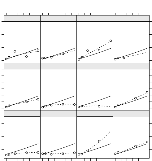
296 Linear Mixed Models: A Practical Guide Using Statistical Software
AGE minus 2
Predicted VSAE
0
50
100
150
200
250
0246810
13
0246810
419
21 27 36
0
50
100
150
200
250
42
0
50
100
150
200
250
46
0246810
48 49
0246810
51
marginal mean profile subject−specific profile
FIGURE 6.5: Conditional (dashed lines) and marginal (solid lines) trajectories, for the first
12 children with SICDEGP = 3.
> trellis.device(color=F)
> # Use the augPred function in the nlme package to plot
> # conditional predicted values for the first twelve children
> # with SICDEGP = 3, based on the fit of Model 6.3 (note that
> # this requires the autism.csv data set to be sorted
> # in descending order by SICDEGP, prior to
> # being imported into R).
> plot(augPred(model6.3.fit, level = 0:1),
layout = c(4, 3, 1), xlab = "AGE minus 2", ylab = "Predicted VSAE",
key = list(
lines = list(lty = c(1, 2), col = c(1, 1), lwd = c(1, 1) ),
text = list(c("marginal mean profile", "subject-specific profile")),
columns = 2))
We can clearly see the variability in the fitted trajectories for different children in the
third level of SICDEGP in Figure 6.5.
In general, the fitted() function can be applied to a model fit object (e.g.,
model6.3.fit) to obtain conditional predicted values in the Rsoftware, and the
random.effects() function (in the nlme package) can be applied to a model fit object
to obtain EBLUPs of random effects. Refer to Section 6.9 for additional Rsyntax that can
be used to obtain and plot conditional predicted values.
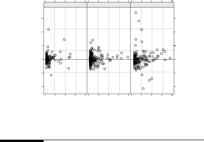
Random Coefficient Models for Longitudinal Data: The Autism Example 297
Fitted values
Standardized residuals
−4
−2
0
2
4
6
0 50 100 150 200
1
0 50 100 150 200
2
0 50 100 150 200
3
FIGURE 6.6: Residual vs. fitted plot for each level of SICDEGP, based on the fit of Model
6.3.
6.9 Diagnostics for the Final Model
We now check the assumptions for Model 6.3, fitted using REML estimation, using informal
graphical procedures in the Rsoftware. Similar plots can be generated in the other four
software packages after saving the conditional residuals, the conditional predicted values,
and the EBLUPs of the random effects based on the fit of Model 6.3 (see the book’s web
page in Appendix A).
6.9.1 Residual Diagnostics
We first assess the assumption of constant variance for the residuals in Model 6.3. Figure
6.6 presents a plot of the standardized conditional residuals vs. the conditional predicted
values for each level of SICDEGP.
> library(lattice)
> trellis.device(color= F)
> plot(model6.3.fit,
resid(., type = "p") ~ fitted(.) | factor(sicdegp),
layout=c(3,1), aspect=2, abline=0)
The variance of the residuals appears to decrease for larger fitted values, and there are
some possible outliers that may warrant further investigation. The preceding syntax may be
modified by adding the id = 0.05 argument to produce a plot (not shown) that identifies
outliers at the 0.05 significance level:
> plot(model6.3.fit,
resid(., type= "p") ~ fitted(.) | factor(sicdegp),
id = 0.05, layout = c(3,1), aspect = 2, abline = 0)
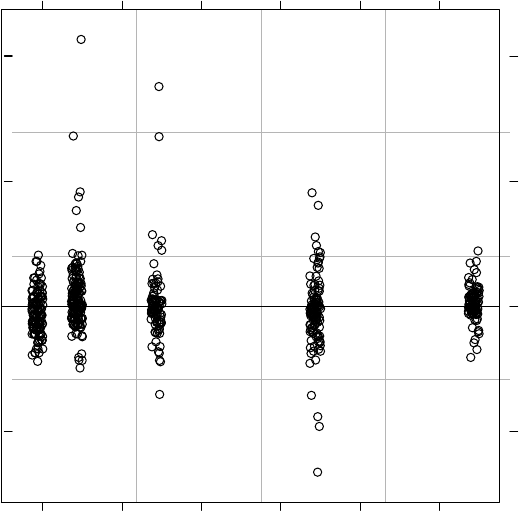
298 Linear Mixed Models: A Practical Guide Using Statistical Software
age.2
Residuals
−20
0
20
40
0246810
FIGURE 6.7: Plot of conditional raw residuals versus AGE.2.
Next, we investigate whether the residual variance is constant as a function of AGE.2.
> plot(model6.3.fit, resid(.) ~ age.2, abline = 0)
Figure 6.7 suggests that the variance of the residuals is fairly constant across the values
of AGE – 2. We again note the presence of outliers.
Next, we assess the assumption of normality of the residuals using Q–Q plots within
each level of SICDEGP, and request that unusual points be identified by CHILDID using
the id = 0.05 argument:
> qqnorm(model6.3.fit,
~resid(.) | factor(sicdegp) ,
layout = c(3,1), aspect = 2, id = 0.05)
Figure 6.8 suggests that the assumption of normality for the residuals seems accept-
able. However, the presence of outliers in each level of SICDEGP (e.g., CHILDID = 46 in
SICDEGP = 3) may warrant further investigation.
6.9.2 Diagnostics for the Random Effects
We now check the distribution of the random effects (EBLUPs) generated by fitting Model
6.3 to the Autism data. Figure 6.9 presents Q–Q plots for the two sets of random effects.
Significant outliers at the 0.10 level of significance are identified by CHILDID in this graph
(id = 0.10):
> qqnorm(model6.3.fit, ~ranef(.) , id = 0.10)
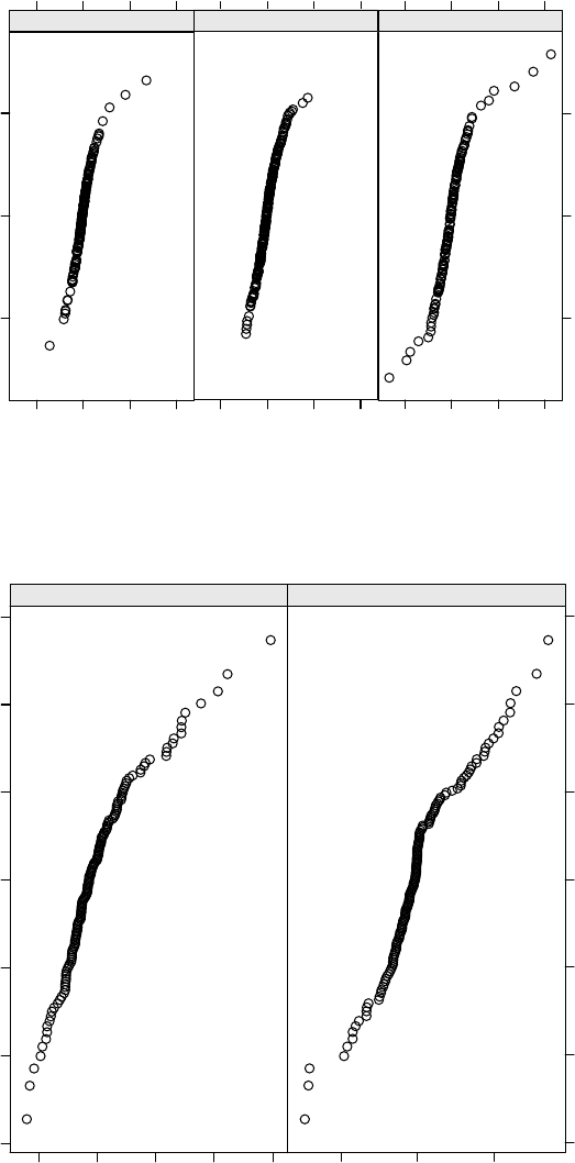
Random Coefficient Models for Longitudinal Data: The Autism Example 299
Residuals
Quantiles of standard normal
−2
0
2
−20 0 20 40
77
80
124
1
−20 0 20 40
87
193
2
−20 0 20 40
46
46
49
49
97
100
106
131
18
0
180
3
FIGURE 6.8: Normal Q–Q Plots of conditional residuals within each level of SICDEGP.
Random effects
Quantiles of standard normal
−2
−1
0
1
2
−5 0 5 10 15
9
80
91
105
110
124
155
156
193
210
age.2
−0.5 0.0 0.5
4
77
100
105
110
124
139
155
I(age.2^2)
FIGURE 6.9: Normal Q–Q Plots for the EBLUPs of the random effects.
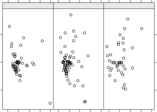
300 Linear Mixed Models: A Practical Guide Using Statistical Software
age.2
I(age.2^2)
−0.5
0.0
0.5
−5 0 5 10 15
12
4
1
−5 0 5 10 15
2
−5 0 5 10 15
3
FIGURE 6.10: Scatter plots of EBLUPs for age-squared vs. age by SICDEGP.
We note that CHILDID = 124 is an outlier in terms of both random effects. The children
indicated as outliers in these plots should be investigated in more detail to make sure that
there is nothing unusual about their observations.
Next, we check the joint distribution of the random linear and quadratic age effects
across levels of SICDEGP using the pairs() function:
> pairs(model6.3.fit,
~ranef(.) | factor(sicdegp),
id = ~childid == 124, layout = c(3, 1), aspect = 2)
The form of these plots is not suggestive of a very strong relationship between the
random effects for age and age-squared, although Rreported a modest negative correlation
(r=−0.31) between them in Model 6.3 (see Table 6.8).
The distinguishing features of these plots are the outliers, which give the overall shape
of the plots a rather unusual appearance. The EBLUPs for CHILDID = 124 are again
unusual in Figure 6.10. Investigation of the values for children with unusual EBLUPs would
be useful at this point, and might provide insight into the reasons for the outliers; we do
not pursue such an investigation here.
We also remind readers (from Chapter 2) that selected influence diagnostics can also be
computed when using the nlmeU or HLMdiag packages in R; see Section 20.3 of Galecki &
Burzykowski (2013) or Loy & Hofmann (2014) for additional details on the computational
steps involved.
6.9.3 Observed and Predicted Values
Finally, we check for agreement between the conditional predicted values based on the fit
of Model 6.3 and the actual observed VSAE scores. Figure 6.11 displays scatter plots of the
observed VSAE scores vs. the conditional predicted VSAE scores for each level of SICDEGP,
with possible outliers once again identified:
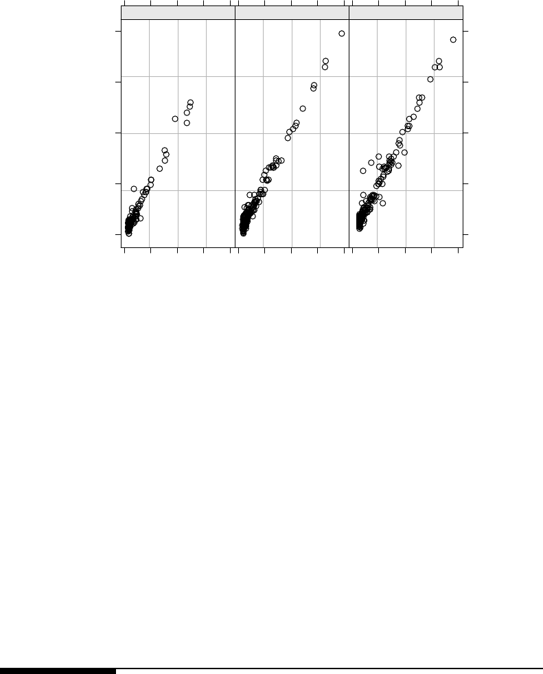
Random Coefficient Models for Longitudinal Data: The Autism Example 301
Fitted values
vsae
0
50
100
150
200
0 50 100 150 200
77
80
124
1
0 50 100 150 200
87
193
2
0 50 100 150 200
46
46
49 49
97
100
106
131
180 180
3
FIGURE 6.11: Agreement of observed VSAE scores with conditional predicted VSAE scores
for each level of SICDEGP, based on Model 6.3.
> plot(model6.3.fit, vsae ~ fitted(.) | factor(sicdegp),
id = 0.05, layout = c(3,1) , aspect = 2)
We see relatively good agreement between the observed and predicted values within each
SICDEGP group, with the exception of some outliers.
We refit Model 6.3 after excluding the observations for CHILDID = 124 (in SICDEGP
= 1) and CHILDID = 46 (in SICDEGP = 3):
> autism.grouped2 <- autism.grouped[(autism.grouped$childid != 124 &
autism.grouped$childid != 46),]
> model6.3.fit.out <- update(model6.3.fit, data = autism.grouped2)
Applying the summary() and intervals() functions to the model6.3.fit.out object
indicates that the primary results in Model 6.3 did not change substantially after excluding
the outliers.
6.10 Software Note: Computational Problems with the DMatrix
The major differences between the software procedures in this analysis were encountered
when attempting to estimate the variance-covariance matrix of the random effects (the D
matrix) in Model 6.1. This model included three random effects for each child, associated
with the intercept, the linear effect of age, and the quadratic effect of age. Each software pro-
cedure reacted differently to the estimation problems that occurred when fitting Model 6.1.
We summarize these differences in Table 6.6. SAS proc mixed produced a note in the
log stating that the estimated Gmatrix (i.e., the block-diagonal matrix with blocks defined

302 Linear Mixed Models: A Practical Guide Using Statistical Software
by the 3 ×3Dmatrix for a single child) was not positive-definite. The estimated value of
σ2
int was reported to be zero in the output, and its standard error was not reported. SPSS
MIXED produced a warning in the output stating that model convergence was not achieved,
and that the validity of the model fit was uncertain. SPSS also reported the estimated
value of σ2
int and its standard error to be zero. The lme() function in Rreported problems
with convergence of the estimation algorithm, and estimates of the parameters in the model
were not available. Similar to the procedures in SAS and SPSS, the lmer() function in R
reported an estimate of 0 for σ2
int.Themixed command in Stata reported an error message
and did not produce any output. HLM did not report any problems in fitting the model,
but required more than 1600 iterations to converge.
To investigate the estimation problems encountered in fitting Model 6.1, we used the
nobound option in SAS proc mixed. This option allowed us to fit the implied marginal
model without requiring that the Gmatrix be positive-definite. We found that the estimated
value for what would have been σ2
int in the unconstrained matrix was actually negative
(−10.54). Subsequent models were simplified by omitting the random effect associated with
the intercept. SAS proc mixed is currently the only software procedure that provides an
option to relax the requirement that the Dmatrix be positive-definite.
6.10.1 Recommendations
We recommend carefully checking the covariance parameter estimates and their standard
errors. Models with multiple random effects, like those fitted in this chapter, may need to be
simplified or respecified if problems are encountered. For this analysis, we decided to remove
the child-specific random effects associated with the intercept from Model 6.1 because of
the estimation problems, and because there was little variability in the initial VSAE scores
for these autistic children at 2 years of age, as illustrated in our initial data summary (see
Figures 6.1 and 6.2). This had implications for the marginal covariance matrix, as illustrated
in Subsection 6.7.2. But the remedies for this problem will depend on the subject matter
under study and the model specification. We find that this issue arises quite often when
analysts attempt to include too many random effects in a given linear mixed model (and
accordingly request that the software provide estimates of several variances and covariances).
Careful examination of the covariance parameter estimates and possible reduction of the
number of random effects included in the model (for example, were we really interested in
the variance of the intercepts in the model for the Autism data?) will generally prevent
these estimation issues.
6.11 An Alternative Approach: Fitting the Marginal Model with
an Unstructured Covariance Matrix
Fitting a marginal model with an “unstructured” covariance matrix is a plausible alternative
for the Autism data, because a relatively small number of observations are made on each
child, and the observations are made at the same ages. We use the gls() function in Rto
fit a marginal model having the same fixed effects as in Model 6.3, but with no random
effects, and an “unstructured” covariance structure for the marginal residuals.
To fit a marginal model with an unstructured covariance matrix (i.e., an unstructured
Rimatrix) for the residuals using the Rsoftware, we need to specify a “General” corre-
lation structure within each level of CHILDID. This correlation structure (specified with

Random Coefficient Models for Longitudinal Data: The Autism Example 303
the correlation = corSymm() argument) is characterized by completely general (uncon-
strained) correlations. In order to have general (unconstrained) variances as well (resulting
in a specification consistent with the “unstructured” covariance structure in SAS and SPSS),
we also need to make use of the weights = argument.
The correlation = corSymm() argument requires the specification of an index variable
with consecutive integer values, to identify the ordering of the repeated measures in a
longitudinal data set. We first create this variable as follows:
> index <- age.2
> index[age.2 == 0] <- 1
> index[age.2 == 1] <- 2
> index[age.2 == 3] <- 3
> index[age.2 == 7] <- 4
> index[age.2 == 11] <- 5
We then add the index variable to the original autism data frame object:
> autism.updated <- subset(data.frame(
autism, sicdegp2.f, age.2, index), !is.na(vsae))
We now specify this correlation structure in the gls() function using the
correlation=corSymm(form = ~ index | childid) argument in the following syn-
tax, and allow for unequal variances at each level of AGE 2byusingthe
weights = varIdent(form = ~ 1 | age.2) argument. Refer to Pinheiro & Bates (1996)
for more information about this structure; the SAS and SPSS procedures allow users to
select this “unstructured” covariance structure for the Rimatrix directly as opposed to
specifying correlation and weights arguments separately.
> marg.model.fit <- gls(
vsae ~ age. 2 + I(age.2^2) + sicdegp2.f + age.2:sicdegp2.f,
correlation=corSymm(form = ~ index | childid),
weights = varIdent(form =~1|age.2) , autism.updated)
The estimated fixed effects in the marginal model can be obtained by applying the
summary() function to the model fit object:
> summary(marg.model.fit)
'
&
$
%
Coefficients
Value Std.Error t-value p-value
(Intercept) 12.471584 0.5024636 24.820869 0.000
age.2 7.373850 0.6042509 12.203293 0.000
I(age.2^2) -0.004881 0.0373257 -0.130761 0.896
sicdegp2.f1 -5.361092 0.6691472 -8.011828 0.000
sicdegp2.f2 -3.725960 0.6307950 -5.906769 0.000
age.2:sicdegp2.f1 -4.332097 0.7787670 -5.562764 0.000
age.2:sicdegp2.f2 -3.867433 0.7334745 -5.272757 0.000
We note that the effect of AGE 2squared(I(age.2^2)) for the reference SICD group
(SICDEGP = 3) is not significant in the marginal model (p=0.896), whereas it is positive
and significant (p=0.01) in Model 6.3. In general, the estimates of the fixed effects and
their standard errors in the marginal model are different from those estimated for Model
6.3, because the estimated Vimatrix for the marginal model differs from the implied Vi
matrix for Model 6.3.
The covariance matrix from the marginal model is also part of the output generated by
the summary() function:

304 Linear Mixed Models: A Practical Guide Using Statistical Software
'
&
$
%
Correlation Structure: General
Formula: ~index | childid
Parameter estimate(s):
Correlation:
123 4
2 0.365
3 0.214 0.630
4 0.263 0.448 0.574
5 0.280 0.543 0.664 0.870
The correlations of the marginal residuals at time 1 (corresponding to 2 years of age)
with residuals at later times are in general smaller (ranging from about 0.21 to 0.37) than
the correlations of the residuals at times 2 through 5 with the residuals for later time
points. Recall that the marginal correlations of observations at 2 years of age with other
observations implied by Model 6.3 were zero (see Subsection 6.7.2), because we had omitted
the random intercept and used AGE – 2 as a predictor (resulting in zeroes for the Zimatrix
values corresponding to 2 years of age).
We report the estimated marginal variance-covariance matrix Vifor a single child ias
follows, using additional Rcode that can be found on the book’s web page (see Appendix A):
'
&
$
%
013711
[1,] 10.811330 8.858858 8.310693 24.59511 43.05836
[2,] 8.858858 54.509537 55.123024 94.33787 187.58256
[3,] 8.310693 55.123024 140.582610 194.00964 368.23192
[4,] 24.595114 94.337868 194.009635 811.74023 1160.52408
[5,] 43.058363 187.582559 368.231923 1160.52408 2191.80398
Software Note: The getVarCov() function, when applied to the marg.model.fit
object obtained by using gls(), returns an incorrect result for the estimated Vimatrix
(not shown). This function was primarily designed to work with model fit objects ob-
tained using the lme() function. According to the Rdocumentation, this function should
also work for a gls() object. However, in our example, which involves the weights argu-
ment, the getVarCov() function does not return a correct marginal variance-covariance
matrix.
The estimated marginal variances, indicated on the diagonal of the matrix above, in-
crease with age, similar to the marginal variances implied by Model 6.3 (see Subsection
6.7.2).
We can also fit the preceding marginal model using the following syntax in SAS:
title "Marginal Model w/ Unstructured Covariance Matrix";
proc mixed data = autism2 noclprint covtest;
class childid sicdegp age;
model vsae = sicdegp age_2 age_2sq age_2*sicdegp / solution;
repeated age / subject = childid type = un r rcorr;
run;
The repeated statement indicates that observations on the same CHILDID are indexed
by the original AGE variable (identified in the class statement), and that an unstructured
covariance matrix (type = un)istobeused.Theroption requests that SAS display the
estimated marginal variance-covariance matrix in the output, and the rcorr option requests
the corresponding correlation matrix. SPSS users can also fit a similar model using only a
REPEATED statement in the MIXED syntax.
Random Coefficient Models for Longitudinal Data: The Autism Example 305
6.11.1 Recommendations
Fitting the marginal model directly with an “unstructured” residual covariance matrix
allows us to get a better sense of the marginal variances and covariances in the observed data
than from the marginal model implied by the random coefficient model (Model 6.3). When
analyzing data sets from longitudinal studies with balanced designs (i.e., where all subjects
are measured at the same time points), we recommend fitting the marginal model in this
manner, because it allows us to get an idea of whether the random coefficient model being
fitted implies a reasonable marginal covariance structure for the data. However, fitting the
marginal model directly does not allow us to answer research questions about the between-
child variability in the VSAE trajectories, because the marginal model does not explicitly
include any random child effects.
Because these models do not include explicit random effects, they should not be referred
to as linear mixed models. Linear mixed models, by definition, include a mix of fixed and
random effects. When describing these models in technical reports or academic publications,
they should be referred to as general linear models with correlated errors, and the type of
covariance structure used for the errors should be clearly defined.
This page intentionally left blankThis page intentionally left blank
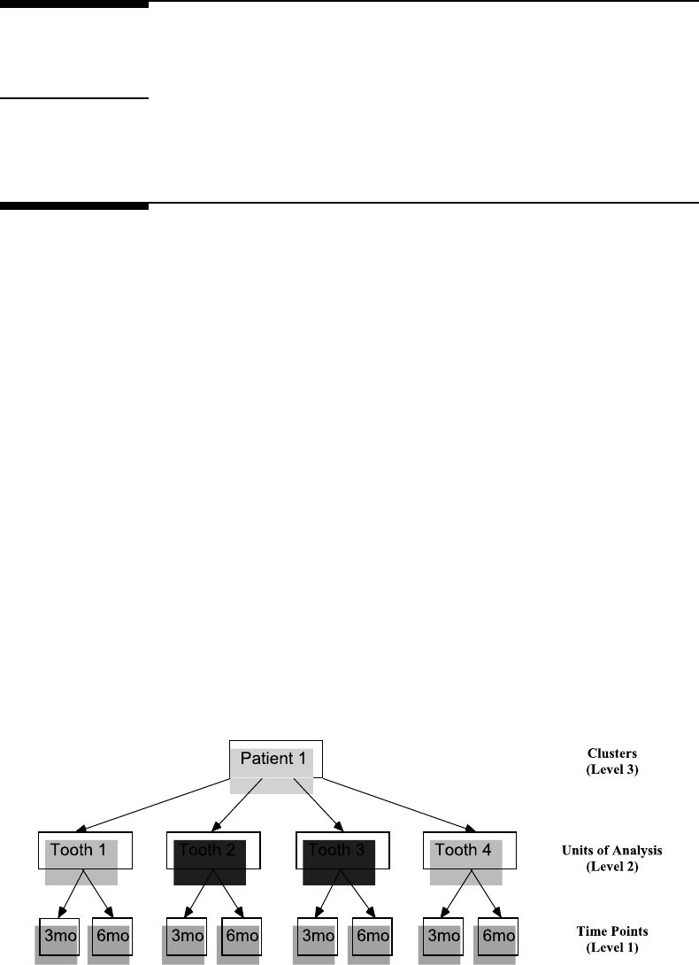
7
Models for Clustered Longitudinal Data:
The Dental Veneer Example
7.1 Introduction
In this chapter we illustrate fitting linear mixed models (LMMs) to clustered longitudinal
data,inwhichunits of analysis are nested within clusters,andrepeated measures
are collected on the units of analysis over time. Each cluster may have a different number
of units of analysis, and the time points at which the dependent variable is measured can
differ for each unit of analysis. Such data sets can be considered to have three levels. Level
3 represents the clusters of units, Level 2 the units of analysis, and Level 1 represents the
longitudinal (repeated) measures made over time.
In Table 7.1 we illustrate examples of clustered longitudinal data in different research
settings. Such data structures might arise in an educational setting when student achieve-
ment scores are measured over time, with students clustered within a sample of classrooms.
A clustered longitudinal data structure might also be encountered in an environmental set-
ting in a study of the weekly oxygen yield for a sample of trees measured over the course of
a growing season. In this case, trees are clustered within a sample of plots, and the trees are
measured repeatedly over time. In the Dental Veneer data set analyzed in this chapter, the
dependent variable, gingival crevicular fluid (GCF), was measured at two post-treatment
time points for each tooth, with teeth clustered within patients.
Figure 7.1 illustrates an example of the structure of a clustered longitudinal data set,
using the first patient in the Dental Veneer data set. Note that patient 1 (who represents
a cluster of units) had four teeth (the units of analysis) included in the study, but other
patients could have a different number of treated teeth. Measurements were made on each
tooth at two follow-up time points (3 months and 6 months).
FIGURE 7.1: Structure of the clustered longitudinal data for the first patient in the Dental
Veneer data set.
307

308 Linear Mixed Models: A Practical Guide Using Statistical Software
TABLE 7.1: Examples of Clustered Longitudinal Data in Different Research Settings
Research Setting
Level of Data Environment Education Dentistry
Cluster
of Units
(Level 3)
Cluster ID
variable
(random
factor)
Plot Classroom Patient
Covariates Soil minerals,
tree crown
density in the
plot
Teacher’s years
of experience,
classroom size
Gender, age
Unit of
Analysis
(Level 2)
Unit of
Analysis ID
variable
(random
factor)
Tree Student Tooth
Covariates Tree size Gender, age,
baseline score
Treatment,
tooth type
Time
(Level 1)
Time
variable
Week Marking
period
Month
Dependent
variable
Oxygen yield Test score Gingival
crevicular fluid
(GCF)
Time-
varying
covariates
Sunlight
exposure,
precipitation
Attendance Frequency of
tooth brushing
LMMs for clustered longitudinal data are “hybrids” of the models that we have used for
the examples in previous chapters. Specifically, these models include random effects associ-
ated with both the clusters (e.g., plots, classrooms, and patients) and the units of analysis
nested within these clusters (e.g., trees, students, and teeth) to take the clustered struc-
ture of the data into account, and also allow the residuals associated with the longitudinal
measures on the same unit of analysis to be correlated.
The variables indicating the units of analysis (Level 2) and the clusters of units (Level
3) are assumed to be random factors, with levels (e.g., students and classrooms) sampled
from a larger population. However, convenience samples, which are easy to obtain but do
not arise from a probability sample, are commonly used in practice. The time variable itself
can be considered to be either a categorical fixed factor or a continuous predictor. If each
unit is measured at the same time points, time is crossed with the random factors defined
at Level 2 and Level 3. However, we do not necessarily require each unit of analysis to be
measured at the same time points.
In this chapter, we highlight features in the Stata software package.

Models for Clustered Longitudinal Data:The Dental Veneer Example 309
7.2 The Dental Veneer Study
7.2.1 Study Description
The Dental Veneer data were collected by researchers at the University of Michigan Dental
School, in a study investigating the impact of veneer placement on subsequent gingival (gum)
health among adult patients (Ocampo, 2005). Ceramic veneers were applied to selected teeth
to hide discoloration. The treatment process involved removing some of the surface of each
treated tooth, and then attaching the veneer to the tooth with an adhesive. The veneer was
placed to match the original contour of the tooth as closely as possible. The investigators
were interested in studying whether varying amounts of contour difference (CDA) due to
placement of the veneer might affect gingival health in the treated teeth over time. One
measure of gingival health was the amount of GCF in pockets of the gum adjacent to the
treated teeth. GCF was measured for each tooth at visits 3 months and 6 months post-
treatment.
A total of 88 teeth in 17 patients were prepared for veneer placement, and a baseline
measure of GCF was collected for each tooth. We consider only the 55 treated teeth located
in the maxillary arches of 12 patients in this example to avoid duplication of results from
the original authors. Each patient could have different numbers of treated teeth, and the
particular teeth that were treated could differ by patient. Table 7.2 presents a portion of
the Dental Veneer data set in the “long” format appropriate for analysis using the mixed
command in Stata, and the LMM procedures in SAS, SPSS, and R.
The following variables are included in the Dental Veneer data set:
Patient (Level 3) Variables
•PATIENT = Patient ID variable (Level 3 ID)
•AGE = Age of patient when veneer was placed; constant for all observations on the
same patient
To oth ( Level 2) Varia bles
•TOOTH = Tooth number (Level 2 ID)
•BASE GCF = Baseline measure of GCF for the tooth; constant for all observations
on the same tooth
•CDA = Average contour difference in the tooth after veneer placement; constant for
all observations on the same tooth
Time-Varying (Level 1) Variables
•TIME = Time points of longitudinal measures (3 = 3 Months, 6 = 6 Months)
•GCF = Gingival crevicular fluid adjacent to the tooth, collected at each time point
(dependent variable)

310 Linear Mixed Models: A Practical Guide Using Statistical Software
TABLE 7.2: Sample of the Dental Veneer Data Set
Patient Tooth Longitudinal Measures
(Level 3) (Level 2) (Level 1)
Cluster
ID
Co-
variate
Unit ID Covariate Time
Variable
Dependent
Variable
PATIENT AGE TOOTH BASE GCF CDA TIME GCF
1466174.67311
1466174.67668
1467224.67313
1467224.67647
...
1 4611175.673 11
1 4611175.676 53
3326 37.67328
3326 37.67623
3 32 7 4 11.00 3 17
3 32 7 4 11.00 6 15
...
Note: “...” indicates portion of the data not displayed.
7.2.2 Data Summary
The data summary for this example was generated using Stata (Release 13). A link to the
syntax and commands that can be used to perform similar analyses in the other software
packages is included on the book’s web page (see Appendix A).
We begin by importing the tab-delimited raw data file (veneer.dat) into Stata from the
C:\temp directory:
. insheet using "C:\temp\veneer.dat", tab
We create line graphs of the GCF values across time for all teeth within each patient.
To create these graphs, we need to restructure the data set to a “wide” format using the
reshape wide command:
. keep patient tooth age time gcf
. reshape wide gcf, i(patient time) j(tooth)
Software Note: The Dental Veneer data set is restructured here only for the purpose
of generating Figure 7.2. The original data set in the “long” form displayed in Table 7.2
will be used for all mixed model analyses in Stata.
The following output is generated as a result of applying the reshape command to the
original data set. As indicated in this output, the restructured data set contains just 24
observations (2 per patient, corresponding to the 2 time points) and 9 variables: PATIENT,
TIME, AGE, and GCF6 through GCF11. The new GCF variables are indexed by levels of
the original TOOTH variable (GCF6 corresponds to tooth 6, etc.).

Models for Clustered Longitudinal Data:The Dental Veneer Example 311
'
&
$
%
(note: j = 6 7 8 9 10 11)
Data long -> wide
-----------------------------------------------------------------------------
Number of obs. 110 -> 24
Number of variables 5 -> 9
j variable (6 values) tooth -> (dropped)
xij variables:
gcf -> gcf6 gcf7 ... gcf11
-----------------------------------------------------------------------------
The first four observations in the restructured data set are as follows:
. list in 1/4
'
&
$
%
+------------------------------------------------------------------+
| patient time gcf6 gcf7 gcf8 gcf9 gcf10 gcf11 age |
|------------------------------------------------------------------|
1.| 1 311131410 14 1146|
2.| 1 668475857 44 5346|
3.| 3 328171934 54 3832|
4.| 3 623153246 39 1932|
+------------------------------------------------------------------+
We now label the six new GCF variables to indicate the tooth numbers to which they
correspond and label the AGE variable:
. label var gcf6 "6"
. label var gcf7 "7"
. label var gcf8 "8"
. label var gcf9 "9"
. label var gcf10 "10"
. label var gcf11 "11"
. label var age "Patient Age"
Next, we generate Figure 7.2 using the twoway line plotting command to create a single
figure containing multiple line graphs:
. twoway line gcf6 gcf7 gcf8 gcf9 gcf10 gcf11 time, ///
lcolor(black black black black black black) ///
lpattern(solid dash longdash vshortdash shortdash dash_dot) ///
ytitle(GCF) by(age)
We use the /// symbols in this command because we are splitting a long command into
multiple lines.
The lcolor option is used to set the color of the six possible lines (corresponding to
teeth within a given patient) within a single graph to be black. The pattern of the lines
is set with the lpattern option. The plots in this graph are ordered by the age of each
patient, displayed at the top of each panel.
In Figure 7.2, we observe that the GCF values for all teeth within a given patient tend
to follow the same trend over time (the lines for the treated teeth appear to be roughly
parallel within each patient). In some patients, the GCF levels tend to increase, whereas
in others the GCF levels tend to decrease or remain relatively constant over time. This
pattern suggests that an appropriate model for the data might include random patient-
specific time slopes. The GCF levels of the teeth also tend to differ by patient, suggesting
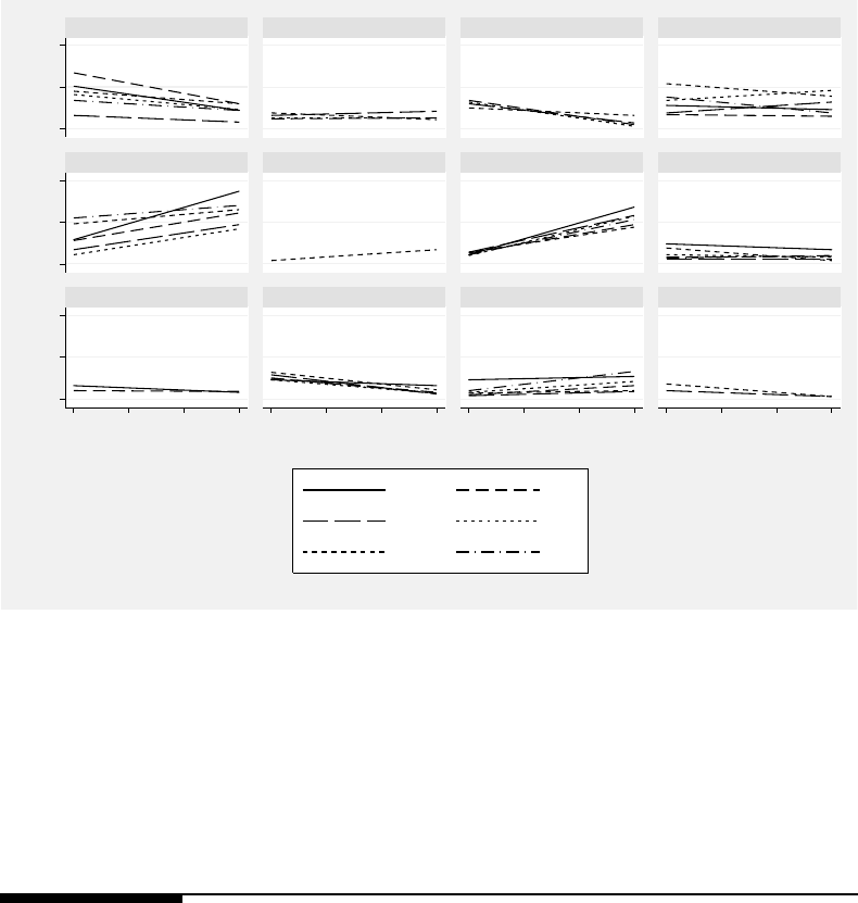
312 Linear Mixed Models: A Practical Guide Using Statistical Software
0 50 1000 50 1000 50 100
3 4 5 6 3 4 5 6 3 4 5 6 3 4 5 6
21 25 28 32
36 41 46 47
50 51 53 62
67
89
10 11
GCF
time
Graphs by Patient Age
FIGURE 7.2: Raw GCF values for each tooth vs. time, by patient. Panels are ordered by
patient age.
that a model should also include random patient-specific intercepts. There is also evidence
in most patients that the level of GCF tends to differ by tooth, suggesting that we may
want to include random tooth-specific intercepts in the model.
7.3 Overview of the Dental Veneer Data Analysis
For the analysis of the Dental Veneer data, we use the “top-down” modeling strategy dis-
cussed in Subsection 2.7.1 of Chapter 2. In Subsection 7.3.1, we outline the analysis steps
and informally introduce related models and hypotheses to be tested. In Subsection 7.3.2
we present more detailed specifications of selected models. The hypotheses tested are de-
tailed in Subsection 7.3.3. To follow the analysis steps outlined in this section, refer to the
schematic diagram presented in Figure 7.3.
7.3.1 Analysis Steps
Step 1: Fit a model with a “loaded” mean structure (Model 7.1).
Fit a three-level model with a “loaded” mean structure, and random effects
associated with both the intercept and slope for patients and with individual
teeth within patients.

Models for Clustered Longitudinal Data:The Dental Veneer Example 313
In Model 7.1, we include fixed effects associated with all covariates under consideration
(TIME, BASE CGF, CDA, and AGE) and the two-way interactions between TIME and
each of the other covariates. We consider TIME to be a continuous predictor in all models,
even though it only has two levels; this allows us to interpret the fixed effect of TIME as
the expected change in GCF over a one-month period. Based on inspection of the initial
graphs in Figure 7.2, we add the following random components to this model: random
patient-specific effects associated with both the intercept and slope (i.e., the effect of time)
for each patient, and random effects associated with the intercept for each tooth nested
within a patient. We assume that the residuals in Model 7.1 are independent and identically
distributed, with constant variance across the time points.
Step 2: Select a structure for the random effects (Model 7.1 vs. Model 7.1A).
Decide whether to keep the random tooth-specific intercepts in the model.
In this step we fit Model 7.1A, which excludes the random intercepts associated with
teeth nested within patients, and test whether we need to keep these random effects in the
model (Hypothesis 7.1). Based on the results of this hypothesis test, we decide to retain
the nested random tooth effects in the model (and therefore the random patient effects as
well, to preserve the hierarchical structure of the data in the model specification) and keep
Model 7.1 as our preferred model at this stage.
Step 3: Select a covariance structure for the residuals (Models 7.1, 7.2A, 7.2B,
or 7.2C).
Fit models with different covariance structures for the residuals associated with
observations on the same tooth.
In this step, we investigate different covariance structures for the residuals, while main-
taining the same fixed and random effects as in Model 7.1. Because there are only two
repeated measures on each tooth, we can only consider a limited number of residual covari-
ance structures, and we will note that parameters in some of these covariance structures
are aliased (or not identifiable; see Subsection 2.9.3). In short, the tooth-specific random
intercepts are inducing marginal correlations between the repeated measures on each tooth,
so an additional correlation parameter for the residuals is not needed.
Model 7.2A: Unstructured covariance matrix for the residuals.
The most flexible residual covariance structure involves three parameters: different residual
variances at 3 and 6 months, and the covariance between the residuals at the two visits.
This is an appropriate structure to use if GCF at 3 months has a residual variance different
from that at 6 months. We include a residual covariance because we expect the two
residuals for a given tooth to be positively related.
Unfortunately, specifying an unstructured covariance matrix for the residuals together
with the variance for the random tooth intercepts leads to an aliasing problem with the
covariance parameters. Preferably, aliasing should be detected during model specification.
If aliasing is unnoticed during model specification it leads to an estimation problem and
usually can be indirectly detected during estimation of model parameters, as will be shown
in the software-specific sections.
Although in practice we would not consider this model, we present it (and Model 7.2B fol-
lowing) to illustrate what happens in each software procedure when aliasing of covariance
parameters occurs.

314 Linear Mixed Models: A Practical Guide Using Statistical Software
Model 7.2B: Compound symmetry covariance structure for the residuals.
We next fitted a simpler model with equal (homogeneous) residual variances at 3 months
and at 6 months, and correlated residuals. This residual covariance structure has only two
parameters, but the residual covariance parameter is again aliased with the variance of
the random tooth-specific intercepts in this model.
Model 7.2C: Heterogeneous (unequal) residual variances at each time point,
with zero covariance for the residuals.
This residual covariance structure also has two parameters, representing the different
residual variances at 3 months and at 6 months. However, the covariance of the residuals
at the two time points is constrained to be zero. In this model, the residual covariance
parameters are no longer aliased with the variance of the random tooth-specific intercepts.
In Model 7.1, we assume that the residuals have constant variance at each time point,
but this restriction is relaxed in Model 7.2C. We test Hypothesis 7.2 in this step to decide
whether to use a heterogeneous residual covariance structure, Model 7.2C, or retain the
simpler residual covariance structure of Model 7.1. Because of the nonsignificant result
of this hypothesis test, we keep Model 7.1 as our preferred model at this stage of the
analysis.
Step 4: Reduce the model by removing fixed effects associated with the two-way
interactions (Model 7.1 vs. Model 7.3) and check model diagnostics.
We now fit Model 7.3, which omits the fixed effects associated with the two-way interactions
between TIME and the other fixed covariates, using maximum likelihood (ML) estimation.
We test the significance of these fixed effects (Hypothesis 7.3) and decide that Model 7.3
is our preferred model. We decide to retain all the main fixed effects associated with the
covariates in our final model, so that the primary research questions can be addressed.
We refit the final model using REML estimation to obtain unbiased estimates of the
covariance parameters. We informally examine diagnostics for Model 7.3 in Section 7.10,
using Stata.
Figure 7.3 provides a schematic guide to the model selection process in the analysis of
the Dental Veneer data (see Section 3.3.1 for details on how to interpret this figure).
7.3.2 Model Specification
The general specification of the models in Subsection 7.3.2.1 corresponds closely to the
syntax used to fit the models in SAS, SPSS, Stata, and R. In Subsection 7.3.2.2, we discuss
the hierarchical specification of the models, which corresponds closely to the model setup in
HLM. Selected models considered in the analysis of the Dental Veneer data are summarized
in Figure 7.3.
7.3.2.1 General Model Specification
The general form of Models 7.1 through 7.2C for an individual GCF response at visit t(t
= 1, 2, corresponding to months 3 and 6) on tooth inested within patient j(denoted by
GCFtij )isasfollows:
GCFtij =β0+β1×TIMEt+β2×BASE GCFij
+β3×CDAij +β4×AGEj+β5×TIMEt×BASE GCFij
+β6×TIMEt×CDAij +β7×TIMEt×AGEj
⎫
⎪
⎬
⎪
⎭fixed
+u0j+u1j×TIMEt+u0i|j+εtij }random (7.1)

Models for Clustered Longitudinal Data:The Dental Veneer Example 315
FIGURE 7.3: Guide to model selection and related hypotheses for the analysis of the Dental
Veneer data.
The parameters β0through β7represent the fixed effects associated with the intercept,
TIME, the patient-level and tooth-level covariates, and their two-way interactions; u0jand
u1jare random patient effects associated with the intercept and time slope, respectively;
u0i|jis the random effect associated with a tooth nested within a patient; and εtij represents
a residual. We write the joint distribution of the two random effects associated with patient
jas:
uj=u0j
u1j∼N(0,D(2))
where the variance-covariance matrix D(2) is defined as:
D(2) =Var(u0j)cov(u0j,u
1j)
cov(u0j,u
1j)Var(u1j)
For all models considered in this analysis, we specify an unstructured D(2) matrix defined
by three covariance parameters, σ2
int:patient ,σ
int,time:patient ,andσ2
time:patient ,as shown in
the following matrix:
316 Linear Mixed Models: A Practical Guide Using Statistical Software
D(2) =σ2
int:patient σint,time:patient
σint,time:patient σ2
time:patient
The distribution of the random effects associated with tooth inested within patient jis
u0i|j∼N(0,D(1)),
where the 1 ×1matrixD(1) contains the variance, σ2
int:tooth(patient), of the nested random
tooth effects u0i|j.
D(1) =Var(u0i|j)=σ2
int:tooth(patient)
The distribution of the residuals, εij , associated with observations on the same tooth is
εij =ε1ij
ε2ij ∼N(0,Rij )
where the variance-covariance matrix Rij for the residuals is defined as
Rij =Var(ε1ij )cov(ε1ij ,ε
2ij )
cov(ε1ij ,ε
2ij )Var(ε2ij )
Different structures for Rij will be specified for different models in the analysis.
We assume that the random effects associated with patients, u0jand u1j, are indepen-
dent of the random effects associated withteethnestedwithinpatients,u0i|j, and that all
random effects are independent of the residuals.
In Model 7.1, the Rij matrix is equal to σ2I2and involves only one parameter, σ2,as
shown below:
Rij =σ20
0σ2=σ2I2
In this structure, the residual variance at 3 months is equal to that at 6 months, and
there is no covariance between the residuals at 3 and at 6 months (they are independent).
In Model 7.2A, we have an unstructured (UN) Rij matrix
Rij =σ2
t1σt1,t2
σt1,t2σ2
t2
defined by three covariance parameters: σ2
t1,σ
2
t2,and σt1,t2. In this structure, the residual
variance is allowed to be different at 3 and at 6 months, and we allow the covariance
between the residuals at 3 and at 6 months to be different from zero (i.e., the residuals are
not independent).
In Model 7.2B, we have a compound symmetric (CS) Rij matrix involving two covariance
parameters, σ2and σtl,t2:
Rij =σ2+σt1,t2σt1,t2
σt1,t2σ2+σt1,t2
In this structure, the residual variance is equal at 3 and at 6 months, and there is a
covariance between the residuals at the two time points.
In Model 7.2C, we have a heterogeneous (HET) Rij matrix with two parameters, σ2
t1
and σ2
t2:
Rij =σ2
t10
0σ2
t2

Models for Clustered Longitudinal Data:The Dental Veneer Example 317
In this structure, the residual variances are different at 3 and at 6 months, and the
covariance is assumed to be zero.
Finally, Model 7.3 has the same random effects and residual covariance structure as in
Model 7.1, but omits the fixed effects associated with the two-way interactions.
7.3.2.2 Hierarchical Model Specification
We now consider an equivalent specification of the model defined in (7.1), corresponding
to the hierarchical specification in the HLM software. The correspondence between the
notation used in HLM and our notation is defined in Table 7.3.
The hierarchical model has three components, reflecting contributions from the three
levels of the Dental Veneer data (time, tooth, and patient). First, we write the Level 1
component as:
Level 1 Model (Time)
GCFtij =b0i|j+b1i|j×TIMEt+εtij (7.2)
where ε1ij
ε2ij ∼N(0,Rij )
The model in (7.2) implies that at the most basic level of the data set (the GCF measures
at each time point), we have a set of simple linear regressions of GCF on TIME. The
unobserved regression coefficients, i.e., the tooth-specific intercepts (b0i|j)andTIMEslopes
(b1i|j), depend on other fixed and random effects, as shown in the Level 2 model below:
Level 2 Model (Tooth)
b0i|j=b0j+β2×BASE GCFij +β3×CDAij +u0i|j
b1i|j=b1j+β5×BASE GCFij +β6×CDAij (7.3)
where
u0i|j∼N(0,σ
2
int:tooth(patient))
The Level 2 model in (7.3) implies that the intercept, b0i|j, for tooth inested within
patient jdepends on the intercept specific to the j-th patient, b0j, the tooth-specific co-
variates (BASE GCF and CDA), and a random effect associated with the tooth, u0i|j.The
tooth-specific slope for time, b1i|j, depends on the patient-specific time effect, b1j,andthe
tooth-specific covariates. Note that we do not include a random effect for the tooth-specific
slope for TIME.
The Level 3 model for the patient-specific contributions to the intercept and slope is
shown below:
Level 3 Model (Patient)
b0j=β0+β4×AGEj+u0j
b1j=β1+β7×AGEj+u1j(7.4)
where
uj=u0j
u1j∼N(0,D(2))

318 Linear Mixed Models: A Practical Guide Using Statistical Software
TABLE 7.3: Summary of Models Considered for the Dental Veneer Data
Term/Vari ab le General HLM Model
Notation Notation 7.1 7.2Aa7.2Ba7.2C 7.3
Fixed effects Intercept β0γ000 √√√ √√
TIME β1γ100 √√√ √√
BASE GCF β2γ010 √√√ √√
CDA β3γ020 √√√ √√
AGE β4γ001 √√√ √√
TIME ×BASE GCF β5γ110 √√√ √
TIME ×CDA β6γ120 √√√ √
TIME ×AGE β7γ101 √√√ √
Random
effects
Patient
(j)
Intercept u0ju00k√√√ √√
TIME u1ju10k√√√ √√
To oth (i)
within
Patient
(j)
Intercept u0i|jr0jk √√√ √√
Residuals Visit (t)εtij εijk √√√ √√
Covariance
Parame-
ters (θD)
for D
Matrix
Patient
level
Variance of
intercepts
σ2
int:pat τβ[1,1] √√√ √√
Variance of slopes σ2
time:pat τβ[2,2] √√√ √√
Covariance of
intercepts, slopes
σint,time:pat τβ[2,1] √√√ √√

Models for Clustered Longitudinal Data:The Dental Veneer Example 319
TABLE 7.3: (Continued)
Term/Vari ab le General HLM Model
Notation Notation 7.1 7.2Aa7.2Ba7.2C 7.3
StructurebD(2) τβUN UN UN UN UN
To oth
Level
Variance of
intercepts
σ2
int:tooth(pat)τπ√√√ √√
Covariance
Parame-
ters (θR)
for Rij
Matrix
Time
Level
Variances at Time 1,
Time 2
σ2
t1
σ2
t2
σ2
1
σ2
2
Equal Unequal Equal Unequal Equal
Covariance of Time
1, Time 2
σt1,t2Variesc0√√ 00
StructurebRij Sσ
2I2UN CS HET σ2I2
aIn Models 7.2A and 7.2B, the residual covariance parameters are aliased with the variance of the random tooth-level
intercepts.
bUN = unstructured, CS = compound symmetry, HET = diagonal with heterogeneous variances.
cThe notation for this covariance parameter varies in HLM, depending on the structure specified.
320 Linear Mixed Models: A Practical Guide Using Statistical Software
The Level 3 model in (7.4) implies that the unobserved patient-specific intercept, b0j,
depends on the overall fixed intercept, β0, the single covariate measured at the patient level
(AGE), and a random effect, u0j, associated with patient j. The Level 3 model also implies
that the patient-specific TIME effect, b1j, depends on the overall fixed TIME effect, β1,the
patient’s age, and the random effect of TIME, u1j, associated with patient j.
By substituting the values for b0jand b1jfrom the Level 3 model back into the Level 2
model, and then substituting the values for b0i|jand b1i|jfrom the Level 2 model into the
Level 1 model, we obtain the general LMM specified in (7.1).
7.3.3 Hypothesis Tests
Hypothesis tests considered in the analysis of the Dental Veneer data are summarized in
Table 7.4.
We consider three-level models for the Dental Veneer data, with random effects at Level
3 (the patient level) and at Level 2 (the tooth level). To preserve the hierarchy of the data,
we first test the significance of the random effects beginning at Level 2 (the tooth level),
while retaining those at Level 3 (the patient level).
Hypothesis 7.1. The nested random effects, u0i|j, associated with teeth within the same
patient can be omitted from Model 7.1.
We decide whether we can remove the random effects associated with teeth indirectly
by testing null and alternative hypotheses about the variance of these random effects, as
follows:
H0:σ2
int:tooth(patient)=0
HA:σ2
int:tooth(patient)>0
We use a REML-based likelihood ratio test for Hypothesis 7.1. The test statistic is
calculated by subtracting the –2 REML log-likelihood for Model 7.1 (the reference model)
from that of Model 7.1A (the nested model, excluding the nested random tooth effects). To
obtain a p-value for this test statistic, we refer it to a mixture of χ2distributions, with 0
and 1 degrees of freedom, and equal weights of 0.5.
Based on the significant result of this test, we retain the nested random tooth effects
in the model. Having made this choice, we do not test for the need of the random patient
effects, u0jand u1j, to preserve the hierarchical structure of the data.
Hypothesis 7.2. The variance of the residuals is constant (homogeneous) across the time
points in Model 7.2C.
We test Hypothesis 7.2 to decide whether we should include heterogeneous residual
variances at the two time points (Model 7.2C) vs. having homogeneous residual variances.
We write the null and alternative hypotheses as follows:
H0:σ2
t1=σ2
t2
HA:σ2
t1=σ2
t2
The test statistic is calculated by subtracting the –2 REML log-likelihood for Model 7.2C
(the reference model, with heterogeneous residual variances) from that of Model 7.1 (the
nested model, with homogeneous residual variance). The distribution of the test statistic
under the null hypothesis is a χ2with 1 degree of freedom.
Hypothesis 7.3. The fixed effects associated with the two-way interactions between
TIME and the patient- and tooth-level covariates can be omitted from Model 7.1.

Models for Clustered Longitudinal Data:The Dental Veneer Example 321
TABLE 7.4: Summary of Hypotheses Tested for the Dental Veneer Data
Hypothesis Specification Hypothesis Test
Models Compared
Label Null (H0)Alternative(HA) Test Nested
Model
(H0)
Ref.
Model
(HA)
Est.
Method
Test Stat.
Dist.
under H0
7.1 Drop u0i|j, random
tooth-specific
intercepts
(σ2
int:tooth(pat)=0)
Retain u0i|j
(σ2
int:tooth(pat)>0)
LRT Model 7.1A Model 7.1 REML 0.5χ2
0+0.5χ2
1
7.2 Constant residual
variance: σ2
t1=σ2
t2
σ2
t1=σ2
t2LRT Model 7.1 Model
7.2C
REML χ2
1
7.3 Dropfixedeffects
associated with all
two-way interactions
(β5=β6=β7=0)
β5=0,or β6=0,or
β7=0
LRT Model 7.3 Model 7.1 ML χ2
3

322 Linear Mixed Models: A Practical Guide Using Statistical Software
In Hypothesis 7.3, we test whether the fixed effects associated with the two-way interac-
tions between TIME and the covariates BASE CGF, CDA, and AGE are all equal to zero.
The null and alternative hypotheses are specified as follows:
H0:β5=β6=β7=0
HA:β5=0,or β6=0,or β7=0
We test Hypothesis 7.3 using a likelihood ratio test, based on ML estimation. The test
statistic is calculated by subtracting the –2 ML log-likelihood for Model 7.1 (the reference
model) from that of Model 7.3 (the nested model, excluding the fixed effects associated with
the two-way interactions). The distribution of the test statistic under the null hypothesis
is a χ2with 3 degrees of freedom, corresponding to the 3 fixed effects set to zero under the
null hypothesis.
For the results of these hypothesis tests, see Section 7.5.
7.4 Analysis Steps in the Software Procedures
In this section, we demonstrate the analysis steps described earlier in the chapter using
the procedures in SAS, SPSS, R, Stata, and HLM. We compare results for selected models
across the procedures in Section 7.6.
7.4.1 SAS
Step 1: Fit a model with a “loaded” mean structure (Model 7.1).
To fit Model 7.1 using SAS proc mixed, we use a temporary SAS data set named veneer,
assumed to have the data structure shown in Table 7.2. Note that we sort the data by levels
of PATIENT, TOOTH, and TIME before fitting the model, to make portions of the output
easier to read (this sorting is optional and does not affect the analysis):
proc sort data = veneer;
by patient tooth time;
run;
title "Model 7.1";
proc mixed data = veneer noclprint covtest;
class patient tooth;
model gcf = time base_gcf cda age time*base_gcf
time*cda time*age / solution outpred = resids;
random intercept time / subject = patient type = un solution
v = 1 vcorr = 1;
random intercept / subject = tooth(patient) solution;
run;
We include the noclprint option in the proc mixed statement to save space by pre-
venting SAS from displaying all levels of the class variables in the output. The covtest
option is only used to display the estimated standard errors of the covariance parameters in
the output for comparison with the estimates from the other software procedures. Because
no estimation method is specified, the default REML method will be used.

Models for Clustered Longitudinal Data:The Dental Veneer Example 323
The class statement identifies the categorical variables used in the random statements.
PATIENT denotes clusters of units, and TOOTH denotes the units of analysis.
The model statement specifies the terms that have associated fixed effects in the model.
We include TIME, BASE GCF, CDA, AGE, and the two-way interactions between TIME
and the other covariates. The solution option is specified so that SAS displays the esti-
mated values of the fixed-effect parameters in the output. The outpred = option is used
to obtain conditional residuals (conditional on the values of all of the appropriate random
effects) for each observation in a new data set called resids.
The first random statement (random intercept time / subject = patient)identi-
fies the intercept and the slope for TIME as two random effects associated with each patient.
The solution option requests that the EBLUPs for the random effects be displayed in the
output. The type = un option specifies that the individual 2 ×2blocksoftheGcovari-
ance matrix of random effects for each subject (which we denote as the D(2) matrix) are
unstructured. We also request that the variance-covariance matrix and the corresponding
correlation matrix for the marginal model implied by Model 7.1 be displayed for the first
subject by using the v=1and vcorr = 1 options.
The second random statement (random intercept / subject = tooth(patient))
specifies that we wish to include a random effect associated with the intercept for each tooth
nested within a patient. We also use the solution option to request that the EBLUPs for
these random effects be displayed in the output.
Because we do not include a repeated statement in the syntax for Model 7.1, SAS
assumes that the residuals associated with all observations, εtij , are independent and iden-
tically distributed, with constant variance σ2.
Step 2: Select a structure for the random effects (Model 7.1 vs. Model 7.1A).
To test Hypothesis 7.1, we fit Model 7.1A, which omits the random effects associated with
the intercept for each tooth nested within a patient. To do this, we remove the second
random statement from the syntax for Model 7.1. We then subtract the –2 REML log-
likelihood for Model 7.1 (the reference model) from the –2 REML log-likelihood for Model
7.1A (the nested model, excluding the nested random tooth effects). The p-value for the
resulting test statistic (858.3−847.1=11.2) can be obtained in the SAS log by using the
following syntax:
data _null_;
p_value = 0.5*(1-probchi(11.2,1));
put p_value;
run;
We use the probchi() function to obtain the appropriate p-value for the χ2
1distribution
and weight it by 0.5. Note that the χ2
0distribution is not included in the syntax, because
it contributes zero to the resulting p-value.
We keep Model 7.1 as our preferred model at this stage of the analysis based on the
result of this test.
Step 3: Select a covariance structure for the residuals (Model 7.1 and Models
7.2A through 7.2C).
Next, we investigate different covariance structures for the residuals associated with obser-
vations on the same tooth, by adding a repeated statement to the SAS syntax. We first
create a new variable in the veneer data set named CATTIME, which has the same values
as the original TIME variable and will be used to index the repeated measures:

324 Linear Mixed Models: A Practical Guide Using Statistical Software
data veneer;
set veneer;
cattime = time;
run;
We fit Model 7.2A, which has an unstructured covariance matrix for the residuals
associated with observations on the same tooth:
title "Model 7.2A";
proc mixed data = veneer noclprint covtest;
class patient tooth cattime;
model gcf = time base gcf cda age time*base gcf
time*cda time*age / solution outpred = resids;
random intercept time / subject = patient type = un solution
v = 1 vcorr = 1;
random intercept / subject = tooth(patient) solution;
repeated cattime / subject = tooth(patient) type = un r rcorr;
run;
Note that the proc mixed code used to fit this model is similar to the code used for
Model 7.1; the only differences are the presence of the repeated statement and the inclusion
of CATTIME in the class statement.
The repeated statement specifies CATTIME as an index for the time points, allowing
SAS to identify the repeated measures on a given tooth correctly and to identify appro-
priately the row and column elements in the Rij matrix. The subject = option identifies
the units of analysis on which repeated observations were measured and, in this case, the
subject is each tooth nested within a patient: subject = tooth(patient). We specify the
covariance structure (or type) of the Rij matrix as unstructured by using the type = un
option. We also request that the estimated 2 ×2Rij matrix for the first tooth in the data
set be displayed in the output along with the corresponding correlation matrix by specifying
the rand rcorr options.
Software Note: proc mixed requires that the variable used to define the index for
thetimepointsintherepeated statement be included in the class statement, so that
proc mixed considers the variable as categorical. As long as there are no missing values
on any of the repeated measures for any subjects and the data have been sorted (e.g.,
by PATIENT, TOOTH, and TIME), the use of such an index variable is not necessary.
Index variables are also not necessary if a covariance structure that does not require
ordering of the repeated measures, such as compound symmetry, is specified for the
Rij matrix.
The following note is produced in the SAS log after fitting Model 7.2A using SAS
Release 9.3:
NOTE: Convergence criteria met but final Hessian is not
positive-definite.

Models for Clustered Longitudinal Data:The Dental Veneer Example 325
The Hessian matrix is used to compute the standard errors of the estimated covariance
parameters. Because we specified the covtest option in the syntax, we can inspect the esti-
mated standard errors of the covariance parameters. As shown in the following SAS output,
the estimated standard error of covariance parameter UN(2,2) for TOOTH(PATIENT) is
zero. This is the estimated standard error of the estimated residual variance at time 2.
'
&
$
%
Covariance Parameter Estimates
Standard Z
Cov Parm Subject Estimate Error Value Pr Z
UN(1,1) PATIENT 546.61 279.34 1.96 0.0252
UN(2,1) PATIENT -148.64 74.3843 -2.00 0.0457
UN(2,2) PATIENT 44.6420 21.0988 2.12 0.0172
Intercept TOOTH(PATIENT) 7.7452 18.4261 0.42 0.3371
UN(1,1) TOOTH(PATIENT) 101.55 26.4551 3.84 <.0001
UN(2,1) TOOTH(PATIENT) 39.1711 15.2980 2.56 0.0105
UN(2,2) TOOTH(PATIENT) 76.1128 0 . .
The nonpositive-definite Hessian matrix encountered in fitting Model 7.2A is a conse-
quence of the aliasing of the residual covariance parameters and the variance of the random
tooth effects.
We fit Model 7.2B by modifying the repeated statement to specify that residuals associ-
ated with observations on the same tooth have a simpler compound symmetry covariance
structure:
repeated cattime / subject = tooth(patient) type = cs rcorr r;
The only difference in the SAS syntax here is the specification of type = cs in the
repeated statement, which requests a compound symmetry structure for the Rij matrix.
When attempting to fit Model 7.2B in SAS Version 9.3, we see the following warning in the
SAS log:
NOTE: Stopped because of too many likelihood evaluations.
The REML estimation procedure does not converge to a valid solution, and this is
another consequence of the aliasing of the residual covariance and the variance of the random
tooth effects. We do not see any estimates printed in the SAS output as a result.
We now fit Model 7.2C, which has a diagonal Rij matrix that allows the variance of
the residuals at 3 and at 6 months to differ, and has zero covariance between the two time
points. We use the following repeated statement for this model:
repeated cattime / subject = tooth(patient) type = un(l) rcorr r;
The option type = un(1) specifies that the residuals in the Rij matrix are uncorrelated
and that the residual variances differ for observations at different time points. This model
now has no accompanying error messages, and the covariance parameter estimates and their
standard errors seem appropriate. There is no apparent problem with aliasing of covariance
parameters in this model.

326 Linear Mixed Models: A Practical Guide Using Statistical Software
'
&
$
%
Covariance Parameter Estimates
Standard Z
Cov Parm Subject Estimate Error Value Pr Z
UN(1,1) PATIENT 546.60 279.33 1.96 0.0252
UN(2,1) PATIENT -148.64 74.3839 -2.00 0.0457
UN(2,2) PATIENT 44.6417 21.0987 2.12 0.0172
Intercept TOOTH(PATIENT) 46.9155 16.5274 2.84 0.0023
UN(1,1) TOOTH(PATIENT) 62.3774 18.8107 3.32 0.0005
UN(2,1) TOOTH(PATIENT) 0 . . .
UN(2,2) TOOTH(PATIENT) 36.9482 15.3006 2.41 0.0079
Note in the output above that the UN(2,1) parameter equals zero, because it is con-
strained to be zero by the specification of the type = un(1) structure for the Rij matrix.
Model 7.2C is the only possible model other than Model 7.1 to consider at this stage of the
analysis, because the other models have problems with aliasing of the covariance parameters.
We use a likelihood ratio test for Hypothesis 7.2 to decide if we wish to keep the hetero-
geneous residual variances, as in Model 7.2C, or if we should have constant residual variance
as in Model 7.1. We calculate the test statistic by subtracting the –2 REML log-likelihood
for Model 7.2C (the reference model with heterogeneous residual variances) from that of
Model 7.1 (the nested model). The test statistic is equal to 0.9. The p-value for this test is
calculated by referring the test statistic to a χ2distribution with 1 degree of freedom. We
do not use a mixture of χ2distributions for this test, because the null hypothesis value of
the test statistic is not at the boundary of the parameter space. SAS code for computing
the p-value for this test and displaying it in the log is as follows:
data _null_;
p_value = 1 - probchi(0.9, 1);
put p_value;
run;
Because the test is not significant (p=0.34), we keep Model 7.1, with homogeneous
residual variance, as our preferred model at this stage of the analysis.
Step 4: Reduce the model by removing nonsignificant fixed effects (Model 7.1
vs. Model 7.3).
We test Hypothesis 7.3 to decide whether we want to keep the fixed effects of the two-way
interactions between TIME and the other covariates in Model 7.1. We first refit Model 7.1,
using ML estimation, by including the method = ml option in the prox mixed statement,
as shown in the following code:
title "Model 7.1: ML Estimation";
proc mixed data = veneer noclprint covtest method = ml;
class patient tooth;
model gcf = time base gcf cda age time*base gcf
time*cda time*age / solution outpred = resids;
random intercept time / subject = patient type = un solution
v = 1 vcorr = 1;
random intercept / subject = tooth(patient) solution;
run;

Models for Clustered Longitudinal Data:The Dental Veneer Example 327
Next, we fit Model 7.3, also using ML estimation, by removing all two-way interactions
from the model statement and refitting the model:
model gcf = time base gcf cda age / solution outpred = resids;
We calculate a likelihood ratio test statistic by subtracting the –2 ML log-likelihood
for Model 7.1 (the reference model) from that for Model 7.3 (the nested model, without
any two-way interactions). The test statistic has a value of 1.84, and the null distribution
of this test statistic is a χ2with 3 degrees of freedom, corresponding to the 3 fixed-effect
parameters that we omitted from Model 7.1. The p-value for this likelihood ratio test is
calculated and displayed in the log using the following SAS syntax:
data _null_;
p_value = 1 - probchi(1.84, 3);
put p_value;
run;
Because this test statistic is not significant, we conclude that we can omit the fixed
effects associated with the two-way interactions from the model, and select Model 7.3 as
our final model.
We now refit Model 7.3 using the default REML estimation method, to obtain unbiased
estimates of the covariance parameters:
title "Model 7.3: REML Estimation";
proc mixed data = veneer noclprint covtest;
class patient tooth;
model gcf = time base_gcf cda age / solution outpred = resids;
random intercept time / solution subject = patient type = un
v = 1 vcorr = 1;
random intercept / solution subject = tooth(patient);
run;
7.4.2 SPSS
Step 1: Fit a model with a “loaded” mean structure (Model 7.1).
We assume that an SPSS data set having the format displayed in Table 7.2 is currently
open, and begin by specifying the SPSS syntax to set up Model 7.1:
* Model 7.1 .
MIXED
gcf WITH time base gcf cda age
/CRITERIA = CIN(95) MXITER(100) MXSTEP(5) SCORING(1)
SINGULAR(0.000000000001) HCONVERGE(0, ABSOLUTE) LCONVERGE(0,
ABSOLUTE) PCONVERGE(0.000001, ABSOLUTE)
/FIXED = time base gcf cda age time*base gcf time*cda time*age | SSTYPE(3)
/METHOD = REML
/PRINT = G SOLUTION TESTCOV
/SAVE = PRED RESID
/RANDOM INTERCEPT time | SUBJECT(Patient) COVTYPE(UN)
/RANDOM INTERCEPT | SUBJECT(tooth*Patient) .

328 Linear Mixed Models: A Practical Guide Using Statistical Software
This syntax is very similar to that used to fit the three-level models discussed in Chap-
ter 4. The first RANDOM subcommand sets up the two random effects for each patient: IN-
TERCEPT and TIME. The subject is specified as PATIENT, and the covariance structure
for the patient-specific random effects is unstructured, as indicated by the COVTYPE(UN)
option.
The second RANDOM subcommand sets up the random effects associated with
the INTERCEPT for each tooth. The subject identified in this subcommand is
(TOOTH*PATIENT), which actually indicates tooth nested within patient, although the
syntax appears to be specifying TOOTH crossed with PATIENT. We would run this syntax
to fit Model 7.1.
Step 2: Select a structure for the random effects (Model 7.1 vs. Model 7.1A).
To test Hypothesis 7.1, we fit a nested model, Model 7.1A, which excludes the random
effects associated with the teeth nested within patients, by omitting the second RANDOM
subcommand entirely from the syntax used for Model 7.1:
* Model 7.1A .
MIXED
gcf WITH time base gcf cda age
/CRITERIA = CIN(95) MXITER(100) MXSTEP(5) SCORING(1)
SINGULAR(0.000000000001) HCONVERGE(0, ABSOLUTE)
LCONVERGE(0,ABSOLUTE) PCONVERGE(0.000001, ABSOLUTE)
/FIXED = time base gcf cda age time*base gcf time*cda time*age | SSTYPE(3)
/METHOD = REML
/PRINT = G SOLUTION TESTCOV
/SAVE = PRED RESID
/RANDOM INTERCEPT time | SUBJECT(Patient) COVTYPE(UN) .
The likelihood ratio test statistic is calculated by subtracting the –2 REML log-likelihood
for Model 7.1 (reported in the SPSS output) from that of Model 7.1A. The p-value is
calculated by referring the test statistic to a mixture of χ2distributions with degrees of
freedom of 0 and 1, and equal weights of 0.5 (see Section 7.5).
Step 3: Select a covariance structure for the residuals (Model 7.1, and Models
7.2A through 7.2C).
Once the structure for the random effects has been set up, we consider different covariance
structures for the residuals. But before fitting these models, we sort the data set in ascending
order by PATIENT, TOOTH, and TIME to ensure that all desired covariance structures
will be displayed in a way that is easy to read in the output (this sorting is recommended
but not essential for the analysis):
SORT CASES BY
patient (A) tooth (A) time (A) .
We first fit Model 7.2A with an unstructured covariance structure for the residuals
associated with observations over time on the same tooth:
* Model 7.2A .
MIXED
gcf WITH time base gcf cda age
/CRITERIA = CIN(95) MXITER(100) MXSTEP(5) SCORING(1)

Models for Clustered Longitudinal Data:The Dental Veneer Example 329
SINGULAR(0.000000000001) HCONVERGE(0, ABSOLUTE)
LCONVERGE(0, ABSOLUTE) PCONVERGE(0.000001, ABSOLUTE)
/FIXED = time base gcf cda age time*base gcf time*cda time*age | SSTYPE(3)
/METHOD = REML
/PRINT = G R SOLUTION TESTCOV
/SAVE = PRED RESID
/RANDOM INTERCEPT time | SUBJECT(Patient) COVTYPE(UN)
/RANDOM INTERCEPT | SUBJECT(tooth*Patient)
/REPEATED time | SUBJECT(tooth*Patient) COVTYPE(UN) .
This syntax is identical to that used to fit Model 7.1, with the exception of the PRINT and
REPEATED subcommands. In the PRINT subcommand, we have requested that the estimated
2×2Rij variance-covariance matrix be displayed in the SPSS output by using the Rkeyword
(the corresponding correlation matrix is not available).
The REPEATED subcommand is used to identify the units of analysis (or subjects) that
have measurements made on them over time, the time index (TIME), and the structure
of the covariance matrix for the residuals. In this case, we again specify the subject as
(TOOTH*PATIENT), which denotes teeth nested within patients, and identify the covari-
ance structure as UN (i.e., unstructured).
After fitting Model 7.2A, the following warning message is displayed in the SPSS output:
Warnings
Iteration was terminated but convergence has not been achieved. The MIXED
procedure continues despite this warning. Subsequent results produced are
based on the last iteration. Validity of the model fit is uncertain.
The MIXED command fails to converge to a solution because the residual covariance
parameters are aliased with the variance of the random tooth effects in Model 7.2A. Results
from the model fit should not be interpreted if this warning message appears.
Next, we use SPSS syntax to fit Model 7.2B, which has a compound symmetry residual
covariance structure. The REPEATED subcommand in the syntax used to fit Model 7.2A is
modified to include the COVTYPE(CS) option:
/REPEATED time | SUBJECT(tooth*patient) COVTYPE(CS) .
Model 7.2B also has a problem with aliasing of the covariance parameters, and the same
warning message about the model failing to converge is displayed in the output. The results
of this model fit should also not be interpreted.
We now fit Model 7.2C using the COVTYPE(DIAG) option, which specifies that the two
residuals associated with observations on the same tooth are independent and have different
variances:
/REPEATED time | SUBJECT(tooth*patient) COVTYPE(DIAG) .
In the diagonal covariance structure defined for the Rij matrix in this model, the co-
variance between observations on the same tooth is set to zero, and the residual variances
along the diagonal of the matrix are heterogeneous.
We test Hypothesis 7.2 by carrying out a likelihood ratio test to decide if we wish to have
heterogeneous residual variances in the model. The test statistic is calculated by subtracting
the –2 REML log-likelihood for Model 7.2C (the reference model with heterogeneous residual
variances) from that of Model 7.1 (the nested model). The appropriate p-value for the test
statistic is based on a χ2distribution with 1 degree of freedom. Because this test is not
significant, we keep Model 7.1 (with homogeneous residual variance) as our preferred model
at this stage of the analysis.

330 Linear Mixed Models: A Practical Guide Using Statistical Software
Step 4: Reduce the model by removing nonsignificant fixed effects (Model 7.1
vs. Model 7.3).
Finally, we test Hypothesis 7.3 to see if we can remove the fixed effects associated with
all the two-way interactions from the model. To do this, we first refit Model 7.1 using ML
estimation by including the /METHOD = ML subcommand:
* Model 7.1 (ML) .
MIXED
gcf WITH time base gcf cda age
/CRITERIA = CIN(95) MXITER(100) MXSTEP(5) SCORING(1)
SINGULAR(0.000000000001) HCONVERGE(0, ABSOLUTE)
LCONVERGE(0, ABSOLUTE) PCONVERGE(0.000001, ABSOLUTE)
/FIXED = time base gcf cda age time*base gcf time*cda time*age | SSTYPE(3)
/METHOD = ML
/PRINT = G SOLUTION TESTCOV
/SAVE = PRED RESID
/RANDOM INTERCEPT time | SUBJECT(Patient) COVTYPE(UN)
/RANDOM INTERCEPT | SUBJECT(tooth*Patient) .
Next, we fit Model 7.3 by removing all two-way interactions listed in the FIXED subcom-
mand:
/FIXED = time base gcf cda age | SSTYPE(3)
We can now carry out a likelihood ratio test for Hypothesis 7.3. To do this, we subtract
the –2 ML log-likelihood for Model 7.1 (the reference model) from that of Model 7.3 (the
nested model). Because this test is not significant (see Subsection 7.5.3), we choose Model
7.3 as our preferred model at this stage of the analysis.
Finally, we refit Model 7.3 using the default REML estimation method, to obtain unbi-
ased estimates of the covariance parameters:
* Model 7.3 .
MIXED
gcf WITH time base gcf cda age
/CRITERIA = CIN(95) MXITER(100) MXSTEP(5) SCORING(1)
SINGULAR(0.000000000001) HCONVERGE(0, ABSOLUTE)
LCONVERGE(0, ABSOLUTE) PCONVERGE(0.000001, ABSOLUTE)
/FIXED = time base gcf cda age | SSTYPE(3)
/METHOD = REML
/PRINT = G SOLUTION TESTCOV
/SAVE = PRED RESID
/RANDOM INTERCEPT time | SUBJECT(Patient) COVTYPE(UN)
/RANDOM INTERCEPT | SUBJECT(tooth*Patient) .
7.4.3 R
We begin the analysis of the Dental Veneer data using Rby reading the tab-delimited raw
data file, which has the structure described in Table 7.2 with variable names in the first
row,intoadataframeobject:
> veneer <- read.delim("c:\\temp\\veneer.dat", h = T)

Models for Clustered Longitudinal Data:The Dental Veneer Example 331
7.4.3.1 Analysis Using the lme() Function
We first load the nlme package, so that the lme() function can be used in the analysis:
> library(nlme)
Step 1: Fit a model with a “loaded” mean structure (Model 7.1).
We now fit Model 7.1 using the lme() function:
> model7.1.fit <- lme(gcf ~ time + base gcf + cda + age +
time:base gcf + time:cda + time:age,
random = list(patient = ~time, tooth = ~1),
data = veneer, method = "REML")
The syntax used for the lme() function is discussed in detail below:
•model7.1.fit is the name of the object that contains the results from the fit of Model
7.1.
•The first argument of the function is a formula, which defines the continuous response
variable (GCF), and the covariates and interaction terms that have fixed effects in the
model.
•The second argument of the function, random = list(patient = ~time, tooth = ~1),
indicates the random effects to be included in the model. Note that a “list” has been
declared to identify the specific structure of the random effects, and each random factor
(i.e., PATIENT and TOOTH) in the list needs to have at least one associated random
effect. This syntax implies that levels of the TOOTH variable are nested within levels
of the PATIENT variable, because the PATIENT variable is the first argument of the
list function. We include a patient-specific TIME slope (listed after the ~symbol), and
a random intercept associated with patients is included by default. Next, we explicitly
specify that a random effect associated with the intercept (1) should be included for each
level of TOOTH. By default, the lme() function chooses an unstructured 2 ×2D(2)
matrix for the random patient-specific effects.
•The third argument of the function, data = veneer, indicates the name of the data frame
object to be used.
•The final argument, method = "REML", specifies that REML estimation, which is the
default method for the lme() function, should be used.
The estimates from the model fit can be obtained by using the summary() function:
> summary(model7.1.fit)
Confidence intervals for the covariance parameters in Model 7.1 can be obtained using
the intervals() function:
> intervals(model7.1.fit)
The EBLUPs for each of the random effects in the model associated with the patients
and the teeth within patients are obtained by using the random.effects() function:
> random.effects(model7.1.fit)
Unfortunately, the getVarCov() function cannot be used to obtain the estimated
marginal variance-covariance matrices for given individuals in the data set, because this
function has not yet been implemented in the nlme package for analyses with multiple
levels of nested random effects.

332 Linear Mixed Models: A Practical Guide Using Statistical Software
Step 2: Select a structure for the random effects (Model 7.1 vs. Model 7.1A).
We carry out a likelihood ratio test of Hypothesis 7.1 by fitting Model 7.1 and Model 7.1A
using REML estimation. Model 7.1 was fitted in Step 1 of the analysis. Model 7.1A is
specified by omitting the random tooth effects from Model 7.1:
> model7.1A.fit <- lme(gcf ~ time + base gcf + cda + age +
time:base gcf + time:cda + time:age,
random = list(patient = ~ time),
data = veneer, method = "REML")
We then subtract the –2 REML log-likelihood for Model 7.1 from that of the nested
model, Model 7.1A. The p-value for the resulting test statistic can be obtained by referring
it to a mixture of χ2distributions with degrees of freedom of 0 and 1, and equal weights of
0.5. Users of Rcan use the anova() function to calculate the likelihood ratio test statistic for
Hypothesis 7.1, but the reported p-value should be divided by 2, because of the distribution
that the statistic follows under the null hypothesis.
> anova(model7.1.fit, model7.1A.fit)
We have strong evidence in favor of retaining the nested random tooth effects in the
model.
Step 3: Select a covariance structure for the residuals (Model 7.1, and Models
7.2A through 7.2C).
Next, we fit models with less restrictive covariance structures for the residuals associated
with observations on the same tooth. We first attempt to fit a model with an unstructured
residual covariance matrix (Model 7.2A). We have included additional arguments in the
lme() function, as shown in the following syntax:
> model7.2A.fit <- lme(gcf ~ time + base gcf + cda + age +
time:base gcf + time:cda + time:age,
random = list(patient = ~ time, tooth = ~1),
corr = corCompSymm(0.5, form = ~1 | patient/tooth),
weights = varIdent(form = ~1 | time),
data = veneer, method = "REML")
We specify the unstructured residual covariance structure in two parts: the correla-
tion of the residuals and their variances. First, we specify that the correlation structure is
compound symmetric, by using the corr=corCompSymm() argument. An arbitrary starting
value of 0.5 is used to estimate the correlation; the patient/tooth argument is used to
identify the units of analysis to which the correlation structure applies (i.e., teeth nested
within patients). Next, we use the weights = varIdent(form = ~1 | time) argument, to
identify a covariance structure for the residuals that allows the residuals at the two time
points to have different variances.
We obtain results from this model fit by using the summary() function:
> summary(model7.2A.fit)
Rdoes not produce a warning message when fitting this model. We attempt to use the
intervals() function to obtain 95% confidence intervals for the covariance parameters:
> intervals(model7.2A.fit)

Models for Clustered Longitudinal Data:The Dental Veneer Example 333
Unlike the other software procedures, the lme() function in Rcomputes approximate
confidence intervals for each of the parameters being estimated (including the covariance
parameters). However, we see that the estimated standard deviation of the residuals at Time
3is8.39 ×1.000 = 8.39, with a 95% confidence interval of (0.0008, 90591.87), while the
estimated standard deviation of the residuals at Time 6 is 8.39 ×0.799 = 6.70, with a 95%
confidence interval of (0.004, 143.73) (see Section 3.4.3 for more details about how these
estimates are reported by the lme() function). Furthermore, the 95% confidence interval
for the correlation of the two random effects at the patient level is (−1, 1). These results
suggest that the estimates are extremely unstable, despite the apparently valid solution.
We therefore consider simpler versions of this model.
Next, we specify Model 7.2B with a more parsimonious compound symmetry covari-
ance structure for the residuals associated with observations on the same tooth:
> model7.2B.fit <- lme(gcf ~ time + base gcf + cda + age +
time:base gcf + time:cda + time:age,
random = list(patient = ~ time, tooth = ~1),
corr = corCompSymm(0.5, form = ~1 | patient/tooth),
data = veneer, method = "REML")
This syntax is changed from that used to fit Model 7.2A by omitting the weights()
argument, so that the residual variances at the two time points are constrained to be equal.
We obtain results for this model fit by using the summary() function and attempt to obtain
confidence intervals for the covariance parameters by using the intervals() function:
> summary(model7.2B.fit)
> intervals(model7.2B.fit)
We once again see extremely wide intervals suggesting that the estimates of the covari-
ance parameters are very unstable, despite the fact that the solution appears to be valid.
This is due to the fact that the covariance of the residuals associated with the same tooth
is aliased with the variance of the random tooth effects.
We now fit Model 7.2C, which allows the residuals to have different variances at the
two time points but assumes that the residuals at the two time points are uncorrelated (the
heterogeneous, or diagonal, structure):
> model7.2C.fit <- lme(gcf ~ time + base gcf + cda + age +
time:base gcf + time:cda + time:age,
random = list(patient = ~ time, tooth = ~1),
weights = varIdent(form = ~1 | time),
data = veneer, method = "REML")
In this syntax, we omit the corr = corCompSymm() option and include the
weights option, which specifies that the residual variances at each time point differ
(form = ~1 | time). We obtain results of the model fit by using the summary() func-
tion, and we no longer see extremely wide confidence intervals when using the intervals()
function to obtain approximate 95% confidence intervals for the covariance parameters:
> summary(model7.2C.fit)
> intervals(model7.2C.fit)
We test Hypothesis 7.2 by subtracting the –2 REML log-likelihood for Model 7.2C (the
reference model, with heterogeneous residual variances) from that of Model 7.1 (the nested
model). This likelihood ratio test can be easily implemented using the anova() function
within R:

334 Linear Mixed Models: A Practical Guide Using Statistical Software
> anova(model7.2C.fit, model7.1.fit)
Because the test is not significant (p=0.33), we keep Model 7.1 as our preferred model
at this stage of the analysis.
Step 4: Reduce the model by removing nonsignificant fixed effects (Model 7.1
vs. Model 7.3).
We test whether we can omit the fixed effects associated with the two-way interactions
between TIME and the other covariates in the model (Hypothesis 7.3) using a likelihood
ratio test. First, we refit Model 7.1 using maximum likelihood estimation by including the
method = "ML" option in the following syntax:
> model7.1.ml.fit <- lme(gcf ~ time + base gcf + cda + age +
time:base gcf + time:cda + time:age,
random = list(patient = ~ time, tooth = ~1),
data = veneer, method = "ML")
Next, we fit Model 7.3, without the fixed effects of any of the two-way interactions, also
using ML estimation:
> model7.3.ml.fit <- lme(gcf ~ time + base gcf + cda + age,
random = list(patient = ~ time, tooth = ~1),
data = veneer, method = "ML")
After fitting these two models using ML estimation, we use the anova() function to
perform a likelihood ratio test of Hypothesis 7.3:
> anova(model7.1.ml.fit, model7.3.ml.fit)
The likelihood ratio test is nonsignificant (p=0.61), so we keep Model 7.3 as our final
model.
We now refit Model 7.3 using REML estimation to obtain unbiased estimates of the
covariance parameters.
> model7.3.fit <- lme(gcf ~ time + base gcf + cda + age,
random = list(patient = ~ time, tooth = ~1),
data = veneer, method = "REML")
> summary(model7.3.fit)
7.4.3.2 Analysis Using the lmer() Function
We first load the lme4 package, so that the lmer() function can be used in the analysis:
> library(lme4)
Next, because the values of the TOOTH variable are not unique to a given patient and
we need to specify that teeth are nested within patients, we create a new version of the
TOOTH variable, TOOTH2, that does have unique values for each patient:
> veneer$tooth2 <- as.numeric(paste(factor(veneer$patient),
factor(veneer$tooth),sep=""))

Models for Clustered Longitudinal Data:The Dental Veneer Example 335
Because of the way that models are specified when using the lmer() function, a failure
to do this recoding would result in the random effects of TOOTH being crossed with the
random patient effects (i.e., TOOTH = 6 for the first patient and TOOTH = 6 for the
second patient would be interpreted as the same tooth for model-fitting purposes). This
would result in unnecessary estimation complications, and incorrectly capture the nested
structure of these data. We now proceed with model fitting using this recoded version of
the TOOTH variable.
Step 1: Fit a model with a “loaded” mean structure (Model 7.1).
We first fit Model 7.1 using the lmer() function:
> model7.1.fit.lmer <- lmer(gcf ~ time + base gcf + cda + age +
time*base gcf + time*cda + time*age +
(time | patient) + (1 | tooth2),
data = veneer, REML = T)
The syntax used for the lmer() function is discussed in detail below:
•model7.1.fit.lmer is the name of the object that contains the results from the fit of
Model 7.1.
•The first argument of the function is a formula, which first defines the continuous response
variable (GCF), and the covariates and interaction terms that have fixed effects in the
model. Note that asterisks are used to indicate the interaction terms.
•The formula also defines the random effects that are included in this model. The first set of
random effects is specified with (time | patient), which indicates that the effect of time
on GCF is allowed to randomly vary across levels of patient, in addition to the intercept
(where random intercepts are once again included by default when the effect of a covariate
is allowed to randomly vary). The covariance structure for these two random patient
effects will be unstructured. The next random effect is specified with (1 | tooth2),
which indicates that the intercept (represented by the constant value of 1) is also allowed
to randomly vary across teeth within a patient (given that the recoded TOOTH2 identifier
is being used).
•The second argument of the function, data = veneer, indicates the name of the data
frame object to be used.
•The final argument, REML = T, specifies that REML estimation should be used.
The estimates from the model fit can be obtained by using the summary() function:
> summary(model7.1.fit.lmer)
The intervals() function that was available for objects created using the lme() func-
tion is not available for objects created using the lmer() function, so we do not generate
approximate 95% confidence intervals for the parameters in Model 7.1 here.
The EBLUPs for each of the random effects in the model associated with the patients
and the teeth within patients are obtained by using the ranef() function:
> ranef(model7.1.fit.lmer)$patient
> ranef(model7.1.fit.lmer)$tooth2

336 Linear Mixed Models: A Practical Guide Using Statistical Software
Step 2: Select a structure for the random effects (Model 7.1 vs. Model 7.1A).
We carry out a likelihood ratio test of Hypothesis 7.1 by fitting Model 7.1 and Model 7.1A
using REML estimation. Model 7.1 was fitted in Step 1 of the analysis. Model 7.1A is
specified by omitting the random tooth effects from Model 7.1:
> model7.1A.fit.lmer <- lmer(gcf ~ time + base gcf + cda + age +
time*base gcf + time*cda + time*age +
(time | patient),
data = veneer, REML = T)
We then subtract the –2 REML log-likelihood for Model 7.1 from that of the nested
model, Model 7.1A. The p-value for the resulting test statistic can be obtained by referring
it to a mixture of χ2distributions with degrees of freedom of 0 and 1, and equal weights of
0.5. Users of Rcan use the anova() function to calculate the likelihood ratio test statistic for
Hypothesis 7.1, but the reported p-value should be divided by 2, because of the distribution
that the statistic follows under the null hypothesis.
> anova(model7.1.fit.lmer, model7.1A.fit.lmer)
We have strong evidence in favor of retaining the nested random tooth effects in the
model.
Step 3: Select a covariance structure for the residuals (Model 7.1, and Models
7.2A through 7.2C).
The current implementation of the lmer() function does not allow users to fit models with
specified covariance structures for the conditional residuals, and assumes that residuals
have constant variance and zero covariance (conditional on the random effects included in a
given model). Given the problems with aliasing that we encountered when attempting to fit
Models 7.2A through 7.2C in the other software procedures, this is not a serious limitation
for this case study; however, some models may be improved by allowing for heterogeneous
residual variances across groups, and this could be a limitation in other studies (e.g., Chap-
ter 3). We therefore proceed with testing the fixed effects of the interactions in the model
that retains all of the random effects associated with the patients and the teeth within
patients.
Step 4: Reduce the model by removing nonsignificant fixed effects (Model 7.1
vs. Model 7.3).
We test whether we can omit the fixed effects associated with the two-way interactions
between TIME and the other covariates in the model (Hypothesis 7.3) using a likelihood
ratio test. First, we refit Model 7.1 using maximum likelihood estimation by including the
REML = F option in the following syntax:
> model7.1.ml.fit.lmer <- lmer(gcf ~ time + base_gcf + cda + age +
time*base_gcf + time*cda + time*age +
(time | patient) + (1 | tooth2),
data = veneer, REML = F)
Next, we fit Model 7.3, without the fixed effects of any of the two-way interactions, also
using ML estimation:
Models for Clustered Longitudinal Data:The Dental Veneer Example 337
> model7.3.ml.fit.lmer <- lmer(gcf ~ time + base_gcf + cda + age +
(time | patient) + (1 | tooth2),
data = veneer, REML = F)
After fitting these two models using ML estimation, we use the anova() function to
perform a likelihood ratio test of Hypothesis 7.3:
> anova(model7.1.ml.fit.lmer, model7.3.ml.fit.lmer)
The likelihood ratio test is nonsignificant (p=0.61), so we keep Model 7.3 as our final
model.
We now refit Model 7.3 using REML estimation to obtain unbiased estimates of the
covariance parameters.
> model7.3.fit.lmer <- lmer(gcf ~ time + base_gcf + cda + age +
(time | patient) + (1 | tooth2),
data = veneer, REML = T)
> summary(model7.3.fit.lmer)
As mentioned in earlier chapters, we recommend use of the lmerTest package in Rfor
users interested in testing hypotheses about individual fixed-effect parameters estimated
using the lmer() function. Likelihood ratio tests can be used, as demonstrated here, but
these tests rely on asymptotic assumptions that may not apply for smaller data sets like
the Dental Veneer data.
7.4.4 Stata
Before we begin the analysis using Stata, we illustrate how to import the raw tab-delimited
Dental Veneer data from the web site for the book, using web-aware Stata (where there is
an active connection to the Internet):
. insheet using http://www-personal.umich.edu/~bwest/veneer.dat
Next, we generate variables representing the two-way interactions between TIME and
the other continuous covariates, BASE GCF, CDA, and AGE:
. gen time base gcf = time * base gcf
. gen time cda = time * cda
. gen time age = time * age
Step 1: Fit a model with a “loaded” mean structure (Model 7.1).
Now, we fit Model 7.1 using the mixed command:
. * Model 7.1.
. mixed gcf time base_gcf cda age time_base_gcf time_cda time_age
|| patient: time, cov(unstruct) || tooth: , variance reml
The first variable listed is the dependent variable, GCF. Next, we list the covariates
(including the two-way interactions) with associated fixed effects in the model.
The random effects are specified after the fixed part of the model. If a multilevel data set
is organized by a series of nested groups, such aspatientsandteethnestedwithinpatients,
then the random-effects structure of the mixed model is specified by a series of equations,

338 Linear Mixed Models: A Practical Guide Using Statistical Software
each separated by ||. The nesting structure reads from left to right, with the first cluster
identifier (PATIENT in this case) indicating the highest level of the data set.
For Model 7.1, we specify the random factor identifying clusters at Level 3 of the data
set (PATIENT) first. We indicate that the effect of TIME is allowed to vary randomly by
PATIENT. A random patient-specific intercept is included by default and is not listed. We
also specify that the covariance structure for the random effects at the patient level (the
D(2), matrix following our notation) is unstructured, with the option cov(unstruct).
Because TOOTH follows the second clustering indicator ||, Stata assumes that levels of
TOOTH are nested within levels of PATIENT. We do not list any variables after TOOTH, so
Stata assumes that the only random effect for each tooth is associated with the intercept. A
covariance structure for the single random effect associated with each tooth is not required,
because only a single variance will be estimated. Finally, the variance option requests that
the estimated variances of the random patient and tooth effects, rather than their estimated
standard deviations, be displayed in the output (along with the estimated variance of the
residuals), and the reml option requests REML estimation.
After running the mixed command, Stata displays a summary of the clustering structure
of the data set implied by this model specification:
#
"
!
-----------------------------------------------------------
| No. of Observations per Group
Group Variable | Groups Minimum Average Maximum
----------------+------------------------------------------
patient | 12 2 9.2 12
tooth | 55 2 2.0 2
-----------------------------------------------------------
This summary is useful to determine whether the clustering structure has been identified
correctly to Stata. In this case, Stata notes that there are 12 patients and 55 teeth nested
within the patients. There are from 2 to 12 observations per patient, and 2 observations per
tooth.
After the command has finished running, the parameter estimates appear in the out-
put. We can obtain information criteria associated with the fit of the model by using the
estat ic command, and then save these criteria in a model fit object (model71) for later
analyses:
. estat ic
. est store model71
Step 2: Select a structure for the random effects (Model 7.1 vs. Model 7.1A).
In the output associated with the fit of Model 7.1, Stata automatically reports an omnibus
likelihood ratio test for all random effects at once vs. no random effects. The test statistic is
calculated by subtracting the −2 REML log-likelihood for Model 7.1 from that of a simple
linear regression model without any random effects. Stata reports the following note along
with the test:
Note: LR test is conservative and provided only for reference.
The test is conservative because appropriate theory for the distribution of this test
statistic for multiple random effects has not yet been developed (users can click on the
LR test is conservative statement in the Stata Results window for an explanation of
this issue). We recommend testing the variance components associated with the random
Models for Clustered Longitudinal Data:The Dental Veneer Example 339
effects one by one (e.g., Hypothesis 7.1), using likelihood ratio tests based on REML esti-
mation. While this is generally appropriate for larger samples, we now illustrate this process
using the Dental Veneer data.
To test Hypothesis 7.1 using an LRT, we fit Model 7.1A. We specify this model by
removing the portion of the random effects specification from Model 7.1 involving teeth
nested within patients (i.e., || tooth: ,):
. * Model 7.1A.
. mixed gcf time base_gcf cda age time_base_gcf time_cda time_age
|| patient: time, cov(unstruct) variance reml
To obtain a test statistic for Hypothesis 7.1, the –2 REML log-likelihood for Model
7.1 (the reference model) is subtracted from that of Model 7.1A (the nested model); both
values are calculated by multiplying the reported log-restricted likelihood in the output by
–2. The resulting test statistic (11.2) is referred to a mixture of χ2distributions with degrees
of freedom of 0 and 1, and equal weights of 0.5. We calculate the appropriate p-value for
this test statistic as follows:
. display 0.5*chiprob(1,11.2)
.00040899
The test is significant (p=0.0004), so we retain the nested random tooth effects in the
model. We retain the random patient effects without testing them to reflect the hierarchical
structure of the data in the model specification.
Step 3: Select a covariance structure for the residuals (Model 7.1, and Models
7.2A through 7.2C).
We now consider alternative covariance structures for the residuals, given that we have
repeated measures on the teeth nested within each patient. We begin with Model 7.2A, and
specify an unstructured covariance structure for the residuals associated with each tooth
within a patient:
. mixed gcf time base_gcf cda age time_base_gcf time_cda time_age
|| patient: time, cov(unstruct) || tooth: ,
residuals(un,t(time)) variance reml
We note the inclusion of the option residuals(un,t(time)) after the random tooth
effects have been specified. This option indicates that at the lowest level of the data set (the
repeated measures on each tooth), the residuals have an unstructured covariance structure
(indicated by un), and the residuals should be ordered within unique teeth by values on the
variable TIME (indicated by t(time)).
When fitting this model, Stata does not generate any warnings or error messages, but
we see red flags in the output similar to those noted when performing this analysis using the
lme() function in R. The estimated standard errors for the estimated variance of the random
tooth effects and the three residual covariance parameters (the residual variances at the two
time points and the covariance of the two residuals) are all extremely large and nearly equal
(about 2416), suggesting an identifiability problem with these four covariance parameters.
The corresponding approximate confidence intervals for these covariance parameters are
defined by entirely unrealistic limits that are either extremely large or extremely small,
so we would view these results with some suspicion and consider alternative covariance
structures.
We now consider Model 7.2B, with a compound symmetry covariance structure for the
residuals associated with each tooth within a patient:
340 Linear Mixed Models: A Practical Guide Using Statistical Software
. mixed gcf time base_gcf cda age time_base_gcf time_cda time_age
|| patient: time, cov(unstruct) || tooth: ,
residuals(exchangeable) variance reml
The only difference between this code and the code for Model 7.2A is the specification of
an exchangeable, or compound symmetry, covariance structure for the residuals associated
with each tooth (where no time ordering is needed given this covariance structure). When
fitting this model, Stata does not converge to a solution after several hundred iterations,
and the estimation algorithm needs to be stopped manually. This is due to the fact that the
covariance of the residuals and the variance of the random tooth effects in this structure
are perfectly aliased with each other, and Stata is unable to generate parameter estimates.
We therefore consider Model 7.2C, which removes the covariance of the residuals and
allows the variances of the residuals at each time point to be unique:
. mixed gcf time base_gcf cda age time_base_gcf time_cda time_age
|| patient: time, cov(unstruct) || tooth: ,
residuals(ind, by(time)) variance reml
We now specify that the residuals are independent (using the option ind), meaning that
the residuals have a diagonal covariance structure, and allow the residuals at each time point
to have unique variances (using the by(time) option). We do not encounter any problems
or red flags when fitting this model, and we save the information criteria in a second model
fit object, enabling a likelihood ratio test of Hypothesis 7.2 (that the residual variances at
each time point are equal):
. est store model72C
We now perform a formal test of Hypothesis 7.2 using the lrtest command:
. lrtest model72C model71
The resulting test statistic is not significant (p=0.33), suggesting that we would fail to
reject the null hypothesis that the residual variance is constant at the two time points. We
therefore proceed with Model 7.1.
Step 4: Reduce the model by removing nonsignificant fixed effects (Model 7.1
vs. Model 7.3).
We now test Hypothesis 7.3 using a likelihood ratio test based on ML estimation to de-
cide whether we want to retain the fixed effects associated with the interactions between
TIME and the other covariates in the model. To do this, we first refit Model 7.1 using ML
estimation for all parameters in the model (note that the reml option has been removed):
. * Model 7.1.
. mixed gcf time base_gcf cda age time_base_gcf time_cda time_age
|| patient: time, cov(unstruct) || tooth: , variance
We view the model fit criteria by using the estat ic command and store the model
estimates and fit criteria in a new object named model7_l_ml:
. estat ic
. est store model7_l_ml
Next, we fit a nested model (Model 7.3), again using ML estimation, by excluding the
two-way interaction terms from the model specification:

Models for Clustered Longitudinal Data:The Dental Veneer Example 341
. * Model 7.3.
. mixed gcf time base_gcf cda age
|| patient: time, cov(unstruct) || tooth: , variance
We display the model information criteria for this nested model, and store the model fit
criteria and related estimates in another new object named model7_3_ml:
. estat ic
. est store model7_3_ml
The appropriate likelihood ratio test for Hypothesis 7.3 can now be carried out by
applying the lrtest command to the two objects containing the model fit information:
. lrtest model7_l_ml model7_3_ml
The results of this test are displayed in the Stata output:
Likelihood-ratio test LR chi2(3) = 1.84
(Assumption: model7_3_ml nested in model7_1_ml) Prob > chi2 = 0.6060
Because the test is not significant (p=0.61), we omit the two-way interactions and
choose Model 7.3 as our preferred model.
Additional tests could be performed for the fixed effects associated with the four covari-
ates in the model, but we stop at this point (so that we can interpret the main effects of
the covariates) and refit our final model (Model 7.3) using REML estimation:
. * Model 7.3 (REML).
. mixed gcf time base_gcf cda age
|| patient: time, cov(unstruct) || tooth: , variance reml
We carry out diagnostics for Model 7.3 using informal graphical procedures in Stata in
Section 7.10.
7.4.5 HLM
We use the HMLM2 (Hierarchical Multivariate Linear Model 2) procedure to fit the models
for the Dental Veneer data set, because this procedure allows for specification of alterna-
tive residual covariance structures (unlike the HLM3 procedure). We note that only ML
estimation is available in the HMLM2 procedure.
7.4.5.1 Data Set Preparation
To fit the models outlined in Section 7.3 using the HLM software, we need to prepare three
separate data sets:
1. The Level 1 (longitudinal measures) data set: This data set has two ob-
servations (rows) per tooth and contains variables measured at each time point
(such as GCF and the TIME variable). It also contains the mandatory TOOTH
and PATIENT variables. In addition, the data set needs to include two indicator
variables, one for each time point. We create two indicator variables: TIME3 has
a value of 1 for all observations at 3 months, and 0 otherwise, whereas TIME6
equals 1 for all observations at 6 months, and 0 otherwise. These indicator vari-
ables must be created prior to importing the data set into HLM. The data must
be sorted by PATIENT, TOOTH, and TIME.

342 Linear Mixed Models: A Practical Guide Using Statistical Software
2. The Level 2 (tooth-level) data set: This data set has one observation (row)
per tooth and contains variables measured once for each tooth (e.g., TOOTH,
CDA, and BASE GCF). This data set must also include the PATIENT variable.
The data must be sorted by PATIENT and TOOTH.
3. The Level 3 (patient-level) data set: This data set has one observation (row)
per patient and contains variables measured once for each patient (e.g., PATIENT
and AGE). The data must be sorted by PATIENT.
The Level 1, Level 2, and Level 3 data sets can easily be derived from a single data set
having the “long” structure shown in Table 7.2. For this example, we assume that all three
data sets are stored in SPSS for Windows format.
7.4.5.2 Preparing the Multivariate Data Matrix (MDM) File
In the main HLM window, click File,Make new MDM file,andthenStat package
input. In the dialog box that opens, select HMLM2 to fit a Hierarchical (teeth nested
within patients), Multivariate (repeated measures on the teeth) Linear Model, and click
OK.IntheMake MDM window, choose the Input File Type as SPSS/Windows.
Locate the Level 1 Specification,Browse to the location of the Level 1 data set
defined earlier, and open the file. Now, click on the Choose Variables button, and select
the following variables: PATIENT (check “L3id,” because this variable identifies Level 3
units), TOOTH (check “L2id,” because this variable identifies the Level 2 units), TIME
(check “MDM” to include this variable in the MDM file), the response variable GCF (check
“MDM”), and finally, TIME3 and TIME6 (check “ind” for both, because they are indicators
for the repeated measures). Click OK when finished selecting these six variables.
Next, locate the Level 2 Specification area, Browse to the Level 2 data set defined
earlier,andopenit.IntheChoose Variables dialog box, select the following variables:
PATIENT (check “L3id”), TOOTH (check “L2id”), CDA (check “MDM” to include this
tooth-level variable in the MDM file), and BASE GCF (check “MDM”). Click OK when
finished selecting these four variables.
Now, in the Level 3 Specification area, Browse to the Level 3 data set defined
earlier, and open it. Select the PATIENT variable (check “L3id”) and the AGE variable
(check “MDM”). Click on OK to continue.
Next, select “longitudinal” as the structure of the data. As the MDM template window
indicates, this selection will only affect the notation used when the models are displayed in
the HLM model-building window.
Once all three data sets have been identified and the variables of interest have been
selected, type a name for the MDM file (with an .mdm extension), and go to the MDM
template file portion of the window. Click on Save mdmt file to save this setup as
an MDM template file for later use (you will be prompted to supply a file name with an
.mdmt suffix). Finally, click on the Make MDM button to create the MDM file using
the three input files. You should briefly see a screen displaying descriptive statistics and
identifying the number of records processed in each of the three input files. After this screen
disappears, you can click on the Check Stats button to view descriptive statistics for the
selected MDM variables at each level of the data. Click on the Done button to proceed to
the model specification window.
In the following model-building steps, we use notation from the HLM software. Table 7.3
shows the correspondence between the HLM notation and that used in (7.1) through (7.4).
Step 1: Fit a model with a “loaded” mean structure (Model 7.1).
We begin by specifying the Level 1 model, i.e., the model for the longitudinal measures
collected on the teeth. The variables in the Level 1 data set are displayed in a list at the

Models for Clustered Longitudinal Data:The Dental Veneer Example 343
left-hand side of the model specification window. Click on the outcome variable (GCF), and
identify it as the Outcome variable.GototheBasic Settings menu, and click on Skip
Unrestricted (the “unrestricted” model in HMLM2 refers to a model with no random
effects and an unstructured covariance matrix for the residuals, which will be considered in
the next step), and click on Homogeneous (to specify that the residual variance will be
constant and that the covariance of the residuals will be zero in this initial model). Choose
a title for this analysis (such as “Veneer Data: Model 7.1”), and choose a location and name
for the output (.html) file that will contain the results of the model fit. Click on OK to
return to the model-building window. Click on File and Preferences, and then select Use
level subscripts, to display subscripts in the model-building window.
Three models will now be displayed. The initial Level 1 model, as displayed in the HLM
model specification window, is as follows:
Model 7.1: Level 1 Model (Initial)
GCF*tij =π0ij +εtij
In this simplest specification of the Level 1 model, the GCFtij for an individual measure-
ment on a tooth depends on the tooth-specific intercept, denoted by π0ij , and a residual for
the individual measure, denoted by εtij .We now add the TIME variable from the Level 1
data set to this model, by clicking on the TIME variable and then clicking on “Add variable
uncentered.” The Level 1 model now has the following form:
Model 7.1: Level 1 Model (Final)
GCF*tij =π0ij +π1ij (TIMEtij )+εtij
The Level 2 model describes the equations for the tooth-specific intercept, π0ij ,and
the tooth-specific time effect, π1ij . The simplest Level 2 model is given by the following
equations:
Model 7.1: Level 2 Model (Initial)
π0ij =β00j+r0ij
π1ij =β10j
The tooth-specific intercept, π0ij , depends on the patient-specific intercept, β00j,anda
random effect associated with the tooth, r0ij .The tooth-specific time effect, π1ij ,doesnot
vary from tooth to tooth within the same patient and is simply equal to the patient-specific
time effect, β10j. If we had more than two time points, this random effect could be included
by clicking on the shaded r1ij term in the model for π1ij .
We now include the tooth-level covariates by clicking on the Level 2 button, and then
selecting the Level 2 equations for π0ij and π1ij , in turn. We add the uncentered versions of
CDA and BASE GCF to both equations to get the completed version of the Level 2 model:
Model 7.1: Level 2 Model (Final)
π0ij =β00j+β01j(BASE GCFij )+β02j(CDAij )+r0ij
π1ij =β10j+β11j(BASE GCFij )+β12j(CDAij )
After defining the Level 1 and Level 2 models, HLM displays the combined Level 1 and
Level 2 model in the model specification window. It also shows how the marginal variance-
covariance matrix will be calculated based on the random tooth effects and the residuals

344 Linear Mixed Models: A Practical Guide Using Statistical Software
currently specified in the Level 1 and Level 2 models. By choosing the Homogeneous
option in the Basic Settings menu earlier, we specified that the residuals are assumed to
be independent with constant variance.
The Level 3 portion of the model specification window shows the equations for the
patient-specific intercept, β00j, the patient-specific time slope, β10j, and the patient-specific
effects of BASE GCF and CDA, which were defined in the Level 2 model. The simplest
Level 3 equations for the patient-specific intercepts and slopes include only the overall fixed
effects, γ000 and γ100, and the patient-specific random effects for the intercept, u00j,and
slope, u10j, respectively (one needs to click on the shaded u10jterm to include it in the
model). We add the patient-level covariate AGE to these equations:
Model 7.1: Level 3 Model (Final)
β00j=γ000 +γ001(AGEj)+u00j
β10j=γ100 +γ101(AGEj)+u10j
The patient-specific intercept, β00j, depends on the overall fixed intercept, γ000,the
patient-level covariate AGE, and a random effect for the intercept associated with the
patient, u00j. The patient-specific time slope, β10j, depends on the fixed overall time slope,
γ100, the patient-level covariate AGE, and a random effect for TIME associated with the
patient,u10j.The expressions for the Level 3, Level 2, and Level 1 models defined earlier can
be combined to obtain the LMM defined in (7.1). The correspondence between the HLM
notation and the notation we use for (7.1) can be found in Table 7.3.
To fit Model 7.1, click on Run Analysis, and select Save and Run to save the .hlm
command file. HLM will prompt you to supply a name and location for this file. After
the estimation of the model has finished, click on File and select View Output to see
the resulting parameter estimates and fit statistics. Note that HLM automatically displays
the fixed-effect parameter estimates with model-based standard errors (“Final estimation
of fixed effects”). The estimates of the covariance parameters associated with the random
effects at each level of the model are also displayed.
Step 2: Select a structure for the random effects (Model 7.1 vs. Model 7.1A).
At this stage of the analysis, we wish to test Hypothesis 7.1 using a likelihood ratio test.
However, HLM cannot fit models in which all random effects associated with units at a given
level of a clustered data set have been removed. Because Model 7.1A has no random effects
at the tooth level, we cannot consider a likelihood ratio test of Hypothesis 7.1 in HLM,
and we retain all random effects in Model 7.1, as we did when using the other software
procedures.
Step 3: Select a covariance structure for the residuals (Model 7.1, and Models
7.2A through 7.2C).
We are unable to specify Model 7.2A, having random effects at the patient and tooth levels
and an unstructured covariance structure for the residuals, using the HMLM2 procedure.
However, we can fit Model 7.2B, which has random effects at the patient- and tooth-level and
acompound symmetry covariance structure for the residuals. To do this, we use a first-
order autoregressive, or AR(1), covariance structure for the Level 1 (or residual) variance. In
this case, the AR(1) covariance structure is equivalent to the compound symmetry structure,
because there are only two time points for each tooth in the Dental Veneer data set.
Open the .hlm file saved in the process of fitting Model 7.1, and click Basic Settings.
Choose the 1st order autoregressive covariance structure option, make sure that the

Models for Clustered Longitudinal Data:The Dental Veneer Example 345
“unrestricted” model is still being skipped, enter a new title for the analysis and a different
name for the output (.html) file to save, and click on OK to continue. We recommend
saving the .hlm file under a different name as well when making these changes. Next, click
on Run Analysis to fit Model 7.2B. In the process of fitting the model, HLM displays the
following message:
Invalid info, score, or likelihood
This warning message arises because the residual covariance parameters are aliased with
the variance of the nested random tooth effects in this model.
The output for Model 7.2B has two parts. The first part is essentially a repeat of the out-
put for Model 7.1, which had a homogeneous residual variance structure (under the header
OUTPUT FOR RANDOM EFFECTS MODEL WITH HOMOGENEOUS LEVEL-1 VARI-
ANCE). The second part (under the header OUTPUT FOR RANDOM EFFECTS MODEL
FIRST-ORDER AUTOREGRESSIVE MODEL FOR LEVEL-1 VARIANCE) does not in-
clude any estimates of the fixed-effect parameters, due to the warning message indicated
above. Because of the problems encountered in fitting Model 7.2B, we do not consider these
results.
Next, we fit Model 7.2C, which has a heterogeneous residual variance structure.
In this model, the residuals at time 1 and time 2 are allowed to have different residual
variances, but they are assumed to be uncorrelated. Click on the Basic Settings menu in
the model-building window, and then click on the Heterogeneous option for the residual
variance (make sure that “Skip unrestricted” is still checked). Enter a different title for this
analysis (e.g., “Veneer Data: Model 7.2C”) and a new name for the output file, and then
click on OK to proceed with the analysis. Next, save the .hlm file under a different name,
and click on Run Analysis to fit this model and investigate the output.
No warning messages are generated when Model 7.2C is fitted. However, because HLM
only fits models of this type using ML estimation, we cannot carry out the REML-based
likelihood ratio test of Hypothesis 7.2. The HMLM2 procedure by default performs an
ML-based likelihood ratio test, calculating the difference in the deviance (or –2 ML log-
likelihood) statistics from Model 7.1 and Model 7.2C, and displays the result of this test
at the bottom of the output for the heterogeneous variances model (Model 7.2C). This
nonsignificant likelihood ratio test (p=0.31) suggests that the simpler nested model (Model
7.1) is preferable at this stage of the analysis.
Step 4: Reduce the model by removing nonsignificant fixed effects (Model 7.1
vs. Model 7.3).
We now fit Model 7.3, which omits the fixed effects associated with the two-way interactions
between TIME and the other covariates from Model 7.1. In HLM, this is accomplished by
removing the effects of the covariates in question from the Level 2 and Level 3 equations
for the effects of TIME.
First, the fixed effects associated with the tooth-level covariates, BASE GCF and CDA,
are removed from the Level 2 equation for the tooth-specific effect of TIME, π1ij , as follows:
Model 7.1: Level 2 Equation for the Effect of Time
π1ij =β10j+β11j(BASE GCFij )+β12j(CDAij )
Model 7.3: Level 2 Equation for the Effect of Time with Covariates Removed
π1ij =β10j

346 Linear Mixed Models: A Practical Guide Using Statistical Software
We also remove the patient-level covariate, AGE, from the Level 3 model for the patient-
specific effect of TIME, β10j:
Model 7.1: Level 3 Equation for the Effect of Time
β10j=γ100 +γ101(AGEj)+u10j
Model 7.3: Level 3 Equation for the Effect of Time with Covariates Removed
β10j=γ100 +u10j
To accomplish this, open the .hlm file defining Model 7.1. In the HLM model specification
window, click on the Level 2 equation for the effect of TIME, click on the BASE GCF
covariate in the list of covariates at the left of the window, and click on Delete variable
from model. Repeat this process for the CDA variable in the Level 2 model. Then, click
on the Level 3 equation for the effect of TIME, and delete the AGE variable.
After making these changes, click on Basic Settings to change the title for this analysis
and the name of the text output file, and click OK. To set up a likelihood ratio test
of Hypothesis 7.3, click Other Settings and Hypothesis Testing. Enter the deviance
reported for Model 7.1 (843.65045) and the number of parameters in Model 7.1 (13), and
click OK. Save the .hlm file associated with the Model 7.3 specification under a different
name, and then click Run Analysis. The results of the likelihood ratio test for the fixed-
effect parameters that have been removed from this model (Hypothesis 7.3) can be viewed
at the bottom of the output for Model 7.3.
7.5 Results of Hypothesis Tests
The results of the hypothesis tests reported in this section were based on the analysis of
the Dental Veneer data using Stata, and are summarized in Table 7.5.
7.5.1 Likelihood Ratio Tests for Random Effects
Hypothesis 7.1. The nested random effects, u0i|j, associated with teeth within the same
patient can be omitted from Model 7.1.
The likelihood ratio test statistic for Hypothesis 7.1 is calculated by subtracting the value
of the –2 REML log-likelihood associated with Model 7.1 (the reference model including the
random tooth-specific intercepts) from that of Model 7.1A (the nested model excluding the
random tooth effects). Because the null hypothesis value of the variance of the random tooth-
specific intercepts is at the boundary of the parameter space (H0:σ2
int :tooth(patient)=0),
the null distribution of the test statistic is a mixture of χ2
0and χ2
1distributions, each with
equal weight 0.5 (Verbeke & Molenberghs, 2000). To evaluate the significance of the test
statistic, we calculate the p-value as follows:
p-value = 0.5×P(χ2
0>11.2) + 0.5×P(χ2
1>11.2) <0.001
We reject the null hypothesis and retain the random effects associated with teeth nested
within patients in Model 7.1 and all subsequent models.

Models for Clustered Longitudinal Data:The Dental Veneer Example 347
TABLE 7.5: Summary of Hypothesis Test Results for the Dental Veneer Analysis
Hypo-
thesis
Label
Test Estima-
tion
Method
Models
Compared
(Nested vs.
Reference)
Test Statistic
Values
(Calculation)
p-Value
7.1 LRT REML 7.1A vs. 7.1 χ2(0 : 1) = 11.2<.001
(858.3 – 847.1)
7.2 LRT REML 7.1 vs. 7.2C χ2(1) = 0.90.34
(847.1 – 846.2)
7.3 LRT ML 7.3 vs. 7.1 χ2(3) = 1.80.61
(845.5 – 843.7)
Note: See Table 7.4 for null and alternative hypotheses, and distributions of test statistics
under H0.
The presence of the random tooth-specific intercepts implies that different teeth within
the same patient tend to have consistently different GCF values over time, which is in
keeping with what we observed in the initial data summary. To preserve the hierarchical
nature of the model, we do not consider fitting a model without the random patient-specific
effects, u0jand u1j.
7.5.2 Likelihood Ratio Tests for Residual Variance
Hypothesis 7.2. The variance of the residuals is constant (homogeneous) across the time
points in Model 7.2C.
To test Hypothesis 7.2, we use a REML-based likelihood ratio test. The test statistic is
calculated by subtracting the –2 REML log-likelihood value for Model 7.2C, the reference
model with heterogeneous residual variances, from that for Model 7.1, the nested model.
Because Model 7.2C has one additional variance parameter compared to Model 7.1, the
asymptotic null distribution of the test statistic is a χ2
1distribution. We do not reject the
null hypothesis in this case (p=0.34) and decide to keep a homogeneous residual variance
structure in Model 7.1 and all of the subsequent models.
7.5.3 Likelihood Ratio Tests for Fixed Effects
Hypothesis 7.3. The fixed effects associated with the two-way interactions between
TIME and the patient- and tooth-level covariates can be omitted from Model 7.1.
To test Hypothesis 7.3, we use an ML-based likelihood ratio test. We calculate the test
statistic by subtracting the –2 ML log-likelihood for Model 7.1 from that for Model 7.3.
The asymptotic null distribution of the test statistic is a χ2with 3 degrees of freedom,
corresponding to the 3 fixed-effect parameters that are omitted in the nested model (Model
7.3) compared to the reference model (Model 7.1). There is not enough evidence to reject
the null hypothesis for this test (p=0.61), so we remove the two-way interactions involving
TIME from the model.

348 Linear Mixed Models: A Practical Guide Using Statistical Software
We do not attempt to reduce the model further, because the research is focused on the
effects of the covariates on GCF. Model 7.3 is the final model that we consider for the
analysis of the Dental Veneer data.
7.6 Comparing Results across the Software Procedures
7.6.1 Comparing Model 7.1 Results
Table 7.6 shows a comparison of selected results obtained using the six software procedures
to fit the initial three-level model, Model 7.1, to the Dental Veneer data. This model is
“loaded” with fixed effects, has two patient-specific random effects (associated with the
intercept and with the effect of time), has a random effect associated with each tooth
nested within a patient, and has residuals that are independent and identically distributed.
Model 7.1 was fitted using REML estimation in SAS, SPSS, R, and Stata, and was fitted
using ML estimation in HLM (the current version of the HMLM2 procedure does not allow
models to be fitted using REML estimation).
Table 7.6 demonstrates that the procedures in SAS, SPSS, R, and Stata agree in terms
of the estimated fixed-effect parameters and their standard errors for Model 7.1. The proce-
dures in all of these software packages use REML estimation by default. REML estimation
is not available in HMLM2, so HMLM2 uses ML estimation instead. Consequently, the
fixed-effect estimates from HMLM2 are not comparable to those from the other software
procedures. As expected, the fixed-effect estimates from HMLM2 differ somewhat from those
for the other software procedures. Most notably, the estimated standard errors reported by
HMLM2 are smaller in almost all cases than those reported in the other software proce-
dures. We expect this because of the bias in the estimated covariance parameters when ML
estimation is used instead of REML (see Subsection 2.4.1).
The estimated covariance parameters generated by HMLM2 differ more markedly from
those in the other five software procedures. Although the results generated by the procedures
in SAS, SPSS, R, and Stata are the same, the covariance parameters estimated by HMLM2
tend to be smaller and to have smaller standard errors than those reported by the other
software procedures. Again, this is anticipated, in view of the bias in the ML estimates of
the covariance parameters. The difference is most apparent in the variance of the random
patient-specific intercepts, σ2
int:patient, which is estimated to be 555.39 with a standard error
of 279.75 by the mixed procedure in Stata, and is estimated to be 447.13 with a standard
error of 212.85 by HMLM2.
There are also differences in the information criteria reported across the software pro-
cedures. The programs that use REML estimation agree in terms of the –2 REML log-
likelihoods, but disagree in terms of the other information criteria, because of different
calculation formulas that are used (see Section 3.6 for a discussion of these differences). The
–2 log-likelihood reported by HMLM2 (referred to as the deviance) is not comparable with
the other software procedures, because it is calculated using ML estimation.
7.6.2 Comparing Results for Models 7.2A, 7.2B, and 7.2C
Table 7.7 presents a comparison of selected results across the procedures in SAS, SPSS, R,
Stata, and HLM for Models 7.2A, 7.2B, and 7.2C. Recall that each of these models has a
Models for Clustered Longitudinal Data:The Dental Veneer Example 349
different residual covariance structure, and that there were problems with aliasing of the
covariance parameters in Models 7.2A and 7.2B. We do not display results for the lmer()
procedure in R, given that one cannot currently fit models with conditional errors that are
correlated and/or have nonconstant variance when using this procedure.
In Table 7.7 we present the information criteria calculated by the procedures in SAS,
SPSS, R, and Stata for Model 7.2A, Model 7.2B, and Model 7.2C. Because the covariance
parameters in Model 7.2A and Model 7.2B are aliased, we do not compare their results with
those for Model 7.2C, but present brief descriptions of how the problem might be detected
in the software procedures. We note that the –2 REML log-likelihoods are virtually the
same for a given model across the procedures. The other information criteria (AIC and
BIC) differ because of different calculation formulas.
We report the model information criteria and covariance parameter estimates for Model
7.2C, which has a heterogeneous residual variance structure and is the only model in Ta-
ble 7.7 that does not have an aliasing problem. The estimated covariance parameters and
their respective standard errors are comparable across the procedures in SAS, SPSS, R,
and Stata, each of which use REML estimation. The covariance parameter estimates re-
ported by the HMLM2 procedure, which are calculated using ML estimation, are in general
smaller than those reported by the other procedures, and their estimated standard errors
are smaller as well. We expect this because of the bias in the ML estimation of the covari-
ance parameters. We do not present the estimates of the fixed-effect parameters for Model
7.2C in Table 7.7.
7.6.3 Comparing Model 7.3 Results
Table 7.8 shows results from fitting the final model, Model 7.3, using REML estimation
in SAS, SPSS, R, and Stata, and using ML estimation in HLM. This model has the same
random effects and residual covariance structure as in Model 7.1, but omits the fixed effects
associated with the two-way interactions between TIME and the other covariates from the
model.
The fixed-effect parameter estimates and their estimated standard errors are nearly
identical across the five procedures (proc mixed in SAS, MIXED in SPSS, lme() in R,lmer()
in R,andmixed in Stata) that use REML estimation. Results from the HMLM2 procedure
again differ because HMLM2 uses ML estimation. In general, the estimated standard errors
of the fixed-effect parameter estimates are smaller in HMLM2 than in the other software
procedures.
As noted in the comparison of results for Model 7.1, the –2 REML log-likelihood val-
ues agree very well across the procedures. The AIC and BIC differ because of differ-
ent computational formulas. The information criteria are not computed by the HMLM2
procedure.
The estimated covariance parameters and their estimated standard errors are also very
similar across the procedures in SAS, SPSS, R, and Stata. Again, we note that these es-
timated parameters and their standard errors are consistently smaller in HMLM2, which
uses ML estimation.

350 Linear Mixed Models: A Practical Guide Using Statistical Software
TABLE 7.6: Comparison of Results for Model 7.1
SAS: proc SPSS: R:lme() R:lmer() Stata: HMLM2
mixed MIXED function function mixed
Estimation Method REML REML REML REML REML ML
Fixed-Effect Parameter Estimate (SE) Estimate (SE) Estimate (SE) Estimate (SE) Estimate (SE) Estimate (SE)
β0(Intercept) 69.92(28.40) 69.92(28.40) 69.92(28.40) 69.92(28.40) 69.92(28.40) 70.47(26.11)
β1(Time) −6.02(7.45) −6.02(7.45) −6.02(7.45) −6.02(7.45) −6.02(7.45) −6.11(6.83)
β2(Baseline GCF) −0.32(0.29) −0.32(0.29) −0.32(0.29) −0.32(0.29) −0.32(0.29) −0.32(0.28)
β3(CDA) −0.88(1.08) −0.88(1.08) −0.88(1.08) −0.88(1.08) −0.88(1.08) −0.88(1.05)
β4(Age) −0.97(0.61) −0.97(0.61) −0.97(0.61) −0.97(0.61) −0.97(0.61) −0.98(0.55)
β5(Time ×Base GCF) 0.07(0.06) 0.07(0.06) 0.07(0.06) 0.07(0.06) 0.07(0.06) 0.07(0.06)
β6(Time ×CDA) 0.13(0.22) 0.13(0.22) 0.13(0.22) 0.13(0.22) 0.13(0.22) 0.13(0.21)
β7(Time ×Age) 0.11(0.17) 0.11(0.17) 0.11(0.17) 0.11(0.17) 0.11(0.17) 0.11(0.15)
Covariance Parameter Estimate (SE) Estimate (SE) Estimate (n.c.) Estimate (n.c.) Estimate (SE) Estimate (SE)
σ2
int:patient 555.39a(279.75) 555.39a(279.75) 555.39b,c 555.39c555.39(279.75) 447.13d(212.85)
σint,time:patient −149.76(74.55)e−149.76(74.55)e−0.95(corr.)−0.95(corr.)−149.77(74.55) −122.23(57.01)
σ2
time:patient 44.72(21.15)f44.72(21.15)f44.72c44.72c44.72(21.15) 36.71(16.21)
σ2
int:tooth(patient)46.96(16.67) 46.96(16.67) 46.96c46.96c46.96(16.67) 45.14(15.66)
σ249.69(10.92) 49.69(10.92) 49.69 49.69 49.69(10.92) 47.49(10.23)
Model Information Criteria
–2 RE/ML log-likelihood 847.1 847.1 847.1 847.1 847.1 843.7g
AIC 857.1 857.1 873.1 873.1 873.1 n.c.
BIC 859.5 870.2 907.2 908.2 908.2 n.c.
Note: (n.c.) = not computed
Note: 110 Longitudinal Measures at Level 1; 55 Teeth at Level 2; 12 Patients at Level 3.
aReported as UN(1,1) in SAS and SPSS.
Models for Clustered Longitudinal Data:The Dental Veneer Example 351
bThe nlme version of the lme() function reports the estimated standard deviations of the random effects and
residuals by default; these estimates have been squared in Tables 7.6, 7.7, and 7.8. The intervals() function can
be applied to obtain CIs for the parameters.
cStandard errors are not reported.
dHLM reports the four covariance parameters associated with the random effects in the 2 ×2 Tau(beta) matrix and
the scalar Tau(pi), respectively.
eReported as UN(2,1) in SAS and SPSS.
fReported as UN(2,2) in SAS and SPSS.
gThe –2 ML log-likelihood associated with the model fit is referred to in the HLM output as the model deviance.

352 Linear Mixed Models: A Practical Guide Using Statistical Software
TABLE 7.7: Comparison of Results for Models 7.2A, 7.2B (Both with Aliased Covariance Parameters), and 7.2C
SAS: proc SPSS: R:lme() Stata: HMLM2
mixed MIXED function mixed
Estimation Method REML REML REML REML ML
Model 7.2A (Unstructured)
Software Notes Warning: Hessian Warning: validity of Wide intervals Extremely large SEs Cannot be
not positive-definite the fit uncertain for cov. parms. for cov. parms. fitted
–2 REML log-likelihood 846.2 846.7 846.2 846.2
AIC (smaller the better) 860.2 860.7 876.2 876.2
BIC (smaller the better) 863.6 879.0 915.5 916.7
Model 7.2B (Comp. Symm.)
Software Notes Stopped: Too many Warning: validity Wide intervals Failure to Invalid
likelihood evaluations of the fit uncertain for cov. parms. converge likelihood
–2 REML/ML log-likelihood N/A 847.1 847.1N/AN/A
AIC N/A 859.1 875.1N/AN/A
BIC N/A 874.9 911.9N/AN/A
Model 7.2C (Heterogeneous)
–2 REML/ML log-likelihood 846.2 846.2 846.2 846.2 842.6
AIC 858.2 858.2 874.2 874.2n.c.
BIC 861.1 873.9 910.9 912.0n.c.
Covariance Parameters (Model 7.2C)
Estimate (SE) Estimate (SE) Estimate (SE) Estimate (SE) Estimate (SE)
σ2
int:patient 546.60(279.33) 546.61(279.34) 546.61a,b 546.61(279.34) 438.18(212.68)
σint,time:patient −148.64(74.38) −148.64(74.38) −0.95(corr.)−148.64(74.38) −121.14(56.90)

Models for Clustered Longitudinal Data:The Dental Veneer Example 353
TABLE 7.7: (Continued)
SAS: proc SPSS: R:lme() Stata: HMLM2
mixed MIXED function mixed
Estimation Method REML REML REML REML ML
σ2
time:patient 44.64(21.10) 44.64(21.10) 44.64b44.64(21.10) 36.65(16.16)
σ2
int:tooth(patient)46.92(16.53) 46.92(16.53) 46.92b46.92(16.53) 45.12(15.54)
σ2
t162.38(18.81) 62.38(18.81) 62.38b62.38(18.81) 59.93(17.70)
σ2
t236.95(15.30) 36.95(15.30) 36.95b,c 36.95(15.30) 35.06(14.32)
Note: SE = Standard error, (n.c.) = not computed
Note: 110 Longitudinal Measures at Level 1; 55 Teeth at Level 2; 12 Patients at Level 3.
aUsers of Rcan employ the function intervals(model7.2c.fit) to obtain approximate 95% confidence
intervals for the covariance parameters.
bStandard errors are not reported.
cSee Subsection 3.4.3 for a discussion of the lme() function output from models with heterogeneous
residual variance.

354 Linear Mixed Models: A Practical Guide Using Statistical Software
TABLE 7.8: Comparison of Results for Model 7.3
SAS: proc SPSS: R:lme() R:lmer() Stata: HMLM2
mixed MIXED function function mixed
Estimation Method REML REML REML REML REML ML
Fixed-Effect Parameter Estimate (SE) Estimate (SE) Estimate (SE) Estimate (SE) Estimate (SE) Estimate (SE)
β0(Intercept) 45.74(12.55) 45.74(12.55) 45.74(12.55) 45.74(12.55) 45.74(12.55) 46.02(11.70)
β1(Time) 0.30(1.94) 0.30(1.94) 0.30(1.94) 0.30(1.94) 0.30(1.94) 0.29(1.86)
β2(Baseline GCF) −0.02(0.14) −0.02(0.14) −0.02(0.14) −0.02(0.14) −0.02(0.14) −0.02(0.14)
β3(CDA) −0.33(0.53) −0.33(0.53) −0.33(0.53) −0.33(0.53) −0.33(0.53) −0.31(0.51)
β4(Age) −0.58(0.21) −0.58(0.21) −0.58(0.21) −0.58(0.21) −0.58(0.21) −0.58(0.19)
Covariance Parameter Estimate (SE) Estimate (SE) Estimate (n.c.) Estimate (n.c.) Estimate (SE) Estimate (SE)
σ2
int:patient 524.95(252.99) 524.98(253.02) 524.99 524.98 524.99(253.02) 467.74(221.98)
σint,time:patient −140.42(66.57) −140.42(66.58) −0.95(corr.)−0.95(corr.)−140.42(66.58) −127.80(59.45)
σ2
time:patient 41.89(18.80) 41.89(18.80) 41.89 41.89 41.89(18.80) 38.23(16.86)
σ2
int:tooth(patient)47.45(16.63) 47.46(16.63) 47.46 47.46 47.46(16.63) 44.57(15.73)
σ248.87(10.51) 48.87(10.51) 48.87 48.87 48.87(10.51) 48.85(10.52)
Model Information Criteria
–2 log-likelihood 841.9 841.9 841.9 841.9 841.9 845.5
AIC 851.9 851.9 861.9 861.9 861.9 n.c.
BIC 854.3 865.1 888.4 888.9 888.9 n.c.
Note: SE = Standard error, (n.c.) = not computed
Note: 110 Longitudinal Measures at Level 1; 55 Teeth at Level 2; 12 Patients at Level 3.

Models for Clustered Longitudinal Data:The Dental Veneer Example 355
7.7 Interpreting Parameter Estimates in the Final Model
Results in this section were obtained by fitting Model 7.3 to the Dental Veneer data using
the mixed command in Stata.
7.7.1 Fixed-Effect Parameter Estimates
The Stata output for the fixed-effect parameter estimates and their estimated standard
errors is shown below.
'
&
$
%
Wald chi2(4) = 7.48
Log restricted-likelihood = -420.92761 Prob > chi2 = 0.1128
gcf Coef. Std. Err. z P > |z| [95% Conf. Interval]
--------------------------------------------------------------------------
time 0.3009815 1.9368630 0.16 0.877 -3.4952000 4.0971630
base_gcf -0.0183127 0.1433094 -0.13 0.898 -0.2991940 0.2625685
cda -0.3293040 0.5292525 -0.62 0.534 -1.3666190 0.7080128
age -0.5773932 0.2139656 -2.70 0.007 -0.9967582 -0.1580283
_cons 45.7386200 12.5549700 3.64 0.000 21.1313300 70.3459100
The first part of the output above shows the value of the REML log-likelihood for Model
7.3. Note that in Table 7.8 we report the –2 REML log-likelihood value for this model
(841.9). The Wald chi-square statistic and corresponding p-value reported at the top of the
output represent an omnibus test of all fixed effects (with the exception of the intercept).
The null distribution of the test statistic is a χ2with 4 degrees of freedom, corresponding to
the 4 fixed effects in the model. This test statistic is not significant (p=0.11), suggesting
that these covariates do not explain a significant amount of variation in the GCF measures.
The mixed command reports z-tests for the fixed-effect parameters, which are asymp-
totic (i.e., they assume large sample sizes). The z-tests suggest that the only fixed-effect
parameter significantly different from zero is the one associated with AGE (p=0.007).
There appears to be a negative effect of AGE on GCF, after controlling for the effects
of time, baseline GCF, and CDA. Patients who are one year older are predicted to have
an average value of GCF that is 0.58 units lower than similar patients who are one year
younger. There is no significant fixed effect of TIME on GCF overall. This result is not
surprising, given the initial data summary in Figure 7.2, in which we saw that the GCF for
some patients went up over time, whereas that for other patients decreased over time.
The effect of contour difference (CDA) is also not significant, indicating that a greater
discrepancy in tooth contour after veneer placement is not necessarily associated with a
higher mean value of GCF.
Earlier, when we tested the two-way interactions between TIME and the other covari-
ates (Hypothesis 7.3), we found that none of the fixed effects associated with the two-way
interactions were significant (p=0.61; see Table 7.5). As a result, all two-way interactions
between TIME and the other covariates were dropped from the model. The fact that there
were no significant interactions between TIME and the other covariates suggests that the
effect of TIME on GCF does not tend to differ for different values of AGE, baseline GCF,
or contour difference.

356 Linear Mixed Models: A Practical Guide Using Statistical Software
7.7.2 Covariance Parameter Estimates
The Stata output below displays the estimates of the covariance parameters associated with
the random effects in Model 7.3, reported by the mixed command.
'
&
$
%
Random-effects Parameters Estimate Std. Err. [95% Conf. Interval]
------------------------------------------------------------------------------
patient: Unstructured
var(time) 41.88772 524.98510 -140.42290 18.799970
var(_cons) 253.02050 66.57623 17.38009 204.128700
cov(time, _cons) -270.90990 100.95350 1350.17500 -9.935907
tooth: Identity
var(_cons) 47.45738 16.63034 23.87920 94.31650
var(Residual) 48.86704 10.50523 32.06479 74.47382
LR test vs. linear regression: chi2(4) = 91.12 Prob > chi2 = 0.0000
Note: LR test is conservative and provided only for reference.
Stata reports the covariance parameter estimates, their standard errors, and approxi-
mate 95% confidence intervals. The output table divides the parameter estimates into three
groups. The top group corresponds to the patient level (Level 3) of the model, where the
Unstructured covariance structure produces three covariance parameter estimates. These
include the variance of the random patient-specific time effects, var(time), the variance of
the random patient-specific intercepts, var(_cons), and the covariance between these two
random effects, cov(time, _cons). We note that the covariance between the two patient-
specific random effects is negative. This means that patients with a higher (lower) time 1
value for their GCF tend to have a lower (higher) time 2 value.
Because there is only a single random effect at the tooth level of the model (Level 2), the
variance-covariance matrix for the nested random tooth effects (which only has one element)
has an Identity covariance structure. The single random tooth effect is associated with
the intercept, and the estimated covariance parameter at the tooth level represents the
estimated variance of these nested random tooth effects.
At the lowest level of the data (Level 1), there is a single covariance parameter associated
with the variance of the residuals, labeled var(Residual).
Stata also displays approximate 95% confidence intervals for the covariance parameters
based on their standard errors, which can be used to get an impression of whether the
true covariance parameters in the population of patients and teeth are equal to zero. We
note that none of the reported confidence intervals cover zero. However, Stata does not
automatically generate formal tests for any of these covariance parameters. Readers should
note that interpreting these 95% confidence intervals for covariance parameters can be
problematic, especially when estimates of variances are small. See Bottai & Orsini (2004)
for more details.
Finally, we note an omnibus likelihood ratio test for all covariance parameters. Stata
generates a test statistic by calculating the difference in the –2 REML log-likelihood of
Model 7.3 (the reference model) and that of a linear regression model with the same fixed
effects but without any random effects (the nested model, which has four fewer covariance
parameters). The result of this conservative test suggests that some of the covariance pa-
rameters are significantly different from zero, which is in concordance with the approximate
95% confidence intervals for the parameters. Stata allows users to click on the note about
the likelihood ratio test in the output, for additional information about the reason why this

Models for Clustered Longitudinal Data:The Dental Veneer Example 357
test should be considered conservative (see Subsection 5.4.4 for more details on this type of
test).
Based on these results and the formal test of Hypothesis 7.1, we have evidence of
between-patient variance and between-tooth variance within the same patient that is not
being explained by the fixed effects of the covariates included in Model 7.3.
7.8 The Implied Marginal Variance-Covariance Matrix for
the Final Model
In this section, we present the estimated Vjmatrix for the marginal model implied by
Model 7.3 for the first patient in the Dental Veneer data set. We use SAS proc mixed to
generate this output, because the post-estimation commands associated with the current
implementation of the mixed command in Stata 13 do not allow one to display blocks of
the estimated Vjmatrix in the output.
Recall that prior to fitting the models in SAS, we first sorted the data by PATIENT,
TOOTH, and TIME, as shown in the following syntax. This was done to facilitate reading
the output for the marginal variance-covariance and correlation matrices.
proc sort data = veneer;
by patient tooth time;
run;
The estimated Vjmatrix for patient 1 shown in the SAS output that follows can be
generated by using the v=1option in either of the random statements in the proc mixed
syntax for Model 7.3 (see Subsection 7.4.1). The following output displays an 8 ×8matrix,
because there are eight observations for the first patient, corresponding to measurements
at 3 months and at 6 months for each of the patient’s four treated teeth. If another patient
had three teeth, we would have had a 6 ×6 marginal covariance matrix.
The estimated marginal variances and covariances for each tooth are represented by 2×2
blocks, along the diagonal of the Vjmatrix. Note that the 2 ×2 tooth-specific covariance
matrix has the same values across all teeth. The estimated marginal variance for a given
observation on a tooth at 3 months is 155.74, whereas that at 6 months is 444.19. The
estimated marginal covariance between observations on the same tooth at 3 and at 6 months
is 62.60.
'
&
$
%
Estimated V Matrix for PATIENT 1
Row Col1 Col2 Col3 Col4 Col5 Col6 Col7 Col8
----------------------------------------------------------------------------------
1 155.7400 62.6020 59.4182 15.1476 59.4182 15.1476 59.4182 15.1476
2 62.6020 444.1900 15.1476 347.8600 15.1476 347.8600 15.1476 347.8600
3 59.4182 15.1476 155.7400 62.6020 59.4182 15.1476 59.4182 15.1476
4 15.1476 347.8600 62.6020 444.1900 15.1476 347.8600 15.1476 347.8600
5 59.4182 15.1476 59.4182 15.1476 155.7400 62.6020 59.4182 15.1476
6 15.1476 347.8600 15.1476 347.8600 62.6020 444.1900 15.1476 347.8600
7 59.4182 15.1476 59.4182 15.1476 59.4182 15.1476 155.7400 62.6020
8 15.1476 347.8600 15.1476 347.8600 15.1476 347.8600 62.6020 444.1900

358 Linear Mixed Models: A Practical Guide Using Statistical Software
The following SAS output shows the estimated marginal correlation matrix for patient 1
generated by proc mixed, obtained by using the vcorr = 1 option in either of the random
statements in the syntax for Model 7.3. The 2 ×2 submatrices along the diagonal represent
the marginal correlations between the two measurements on any given tooth at 3 and at 6
months.
'
&
$
%
Estimated V Correlation Matrix for PATIENT 1
Row Col1 Col2 Col3 Col4 Col5 Col6 Col7 Col8
---------------------------------------------------------------------------
1 1.00000 0.23800 0.38150 0.05759 0.38150 0.05759 0.38150 0.05759
2 0.23800 1.00000 0.05759 0.78310 0.05759 0.78310 0.05759 0.78310
3 0.38150 0.05759 1.00000 0.23800 0.38150 0.05759 0.38150 0.05759
4 0.05759 0.78310 0.23800 1.00000 0.05759 0.78310 0.05759 0.78310
5 0.38150 0.05759 0.38150 0.05759 1.00000 0.23800 0.38150 0.05759
6 0.05759 0.78310 0.05759 0.78310 0.23800 1.00000 0.05759 0.78310
7 0.38150 0.05759 0.38150 0.05759 0.38150 0.05759 1.00000 0.23800
8 0.05759 0.78310 0.05759 0.78310 0.05759 0.78310 0.23800 1.00000
We note in this matrix that the estimated covariance parameters for Model 7.3 imply that
observations on the same tooth are estimated to have a rather small marginal correlation
of approximately 0.24.
If we re-sort the data by PATIENT, TIME, and TOOTH and refit Model 7.3 using SAS
proc mixed, the rows and columns in the correlation matrix are reordered correspondingly,
and we can more readily view the blocks of marginal correlations among observations on
all teeth at each time point.
proc sort data = veneer;
by patient time tooth;
run;
We run identical syntax to fit Model 7.3 and display the resulting marginal correlation
matrix for patient 1:
'
&
$
%
Estimated V Correlation Matrix for PATIENT 1
Row Col1 Col2 Col3 Col4 Col5 Col6 Col7 Col8
---------------------------------------------------------------------------
1 1.00000 0.38150 0.38150 0.38150 0.23800 0.05759 0.05759 0.05759
2 0.38150 1.00000 0.38150 0.38150 0.05759 0.23800 0.05759 0.05759
3 0.38150 0.38150 1.00000 0.38150 0.05759 0.05759 0.23800 0.05759
4 0.38150 0.38150 0.38150 1.00000 0.05759 0.05759 0.05759 0.23800
5 0.23800 0.05759 0.05759 0.05759 1.00000 0.78310 0.78310 0.78310
6 0.05759 0.23800 0.05759 0.05759 0.78310 1.00000 0.78310 0.78310
7 0.05759 0.05759 0.23800 0.05759 0.78310 0.78310 1.00000 0.78310
8 0.05759 0.05759 0.05759 0.23800 0.78310 0.78310 0.78310 1.00000
In this output, we focus on the 4 ×4 blocks that represent the correlations among the
four teeth for patient 1 at time 1 and at time 2. It is readily apparent that the marginal
correlation at time 1 is estimated to have a constant value of 0.38, whereas the marginal
correlation among observations on the four teeth at time 2 is estimated to have a higher
value of 0.78.
As noted earlier, the estimated marginal correlation between the observations on tooth
1 at time 1 and time 2 (displayed in this output in row 1, column 5) is 0.24. We also note

Models for Clustered Longitudinal Data:The Dental Veneer Example 359
that the estimated marginal correlation of observations on tooth 1 at time 1 and the other
three teeth at time 2 (displayed in this output in row 1, columns 6 through 8) is rather low,
not surprisingly, and is estimated to be 0.06.
7.9 Diagnostics for the Final Model
In this section, we check the assumptions for the REML-based fit of Model 7.3, using infor-
mal graphical procedures available in Stata. Similar plots can be generated using the other
four software packages by saving the conditional residuals, conditional predicted values,
and EBLUPs of the random effects based on the fit of Model 7.3. We include syntax for
performing these diagnostics in the other software packages on the book’s web page (see
Appendix A).
7.9.1 Residual Diagnostics
We first assess the assumption of constant variance for the residuals in Model 7.3. Figure 7.4
presents a plot of the standardized conditional residuals vs. the conditional predicted values
(based on the fit of Model 7.3) to assess whether the variance of the residuals is constant.
The final command used to fit Model 7.3 in Stata is repeated from Subsection 7.4.4 as
follows:
. * Model 7.3 (REML).
. mixed gcf time base_gcf cda age
|| patient: time, cov(unstruct) || tooth: , variance reml
After fitting Model 7.3, we save the standardized residuals in a new variable named
ST RESID, by using the predict post-estimation command in conjunction with the
rstandard option (this option requests that standardized residuals be saved in the data
set):
. predict st resid, rstandard
We also save the conditional predicted GCF values (including the EBLUPs) in a new
variable named PREDVALS, by using the fitted option:
. predict predvals, fitted
We then use the two new variables to generate the fitted-residual scatter plot in Fig-
ure 7.4, with a reference line at zero on the y-axis:
. twoway (scatter st resid predvals), yline(0)
The plot in Figure 7.4 suggests nonconstant variance in the residuals as a function of the
predicted values, and that a variance-stabilizing transformation of the GCF response vari-
able (such as the square-root transformation) may be needed, provided that no important
fixed effects of relevant covariates have been omitted from the model.
Analysts interested in generating marginal predicted values for various subgroups defined
by the covariates and factors included in a given model, in addition to plots of those marginal
predicted values, can make use of the post-estimation commands margins and marginsplot
(where the latter command needs to directly follow the former command) to visualize these
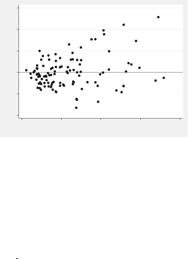
360 Linear Mixed Models: A Practical Guide Using Statistical Software
−2 −1 0 1 2 3
Standardized residuals
0 20 40 60 80
Fitted values: xb + Zu
FIGURE 7.4: Residual vs. fitted plot based on the fit of Model 7.3.
predicted values. For example, to plot marginal predicted values of GCF at TIME = 0,
TIME = 3, and TIME = 6 in addition to 95% confidence intervals for the predicted values,
the following two commands can be used (plot not shown):
. margins, at(time=(0,3,6))
. marginsplot
These plots can be useful for illustrating predicted values of the dependent variable based
on a given model, and can be especially useful for interpreting more complex interactions.
Stata users can submit the command help margins for more details.
The assumption of normality for the conditional residuals can be checked by using the
qnorm command to generate a normal Q–Q plot:
. qnorm st resid
The resulting plot in Figure 7.5 suggests that the distribution of the conditional residuals
deviates from a normal distribution. This further suggests that a transformation of the
response variable may be warranted, provided that no fixed effects of important covariates
or interaction terms have been omitted from the final model. In this example, a square-root
transformation of the response variable (GCF) prior to model fitting was found to improve
the appearance of both of these diagnostic plots, suggesting that such a transformation
would be recommended before making any final inferences about the parameters in this
model.
7.9.2 Diagnostics for the Random Effects
We now check the distributions of the predicted values (EBLUPs) for the three random
effects in Model 7.3. After refitting Model 7.3, we save the EBLUPs of the two random
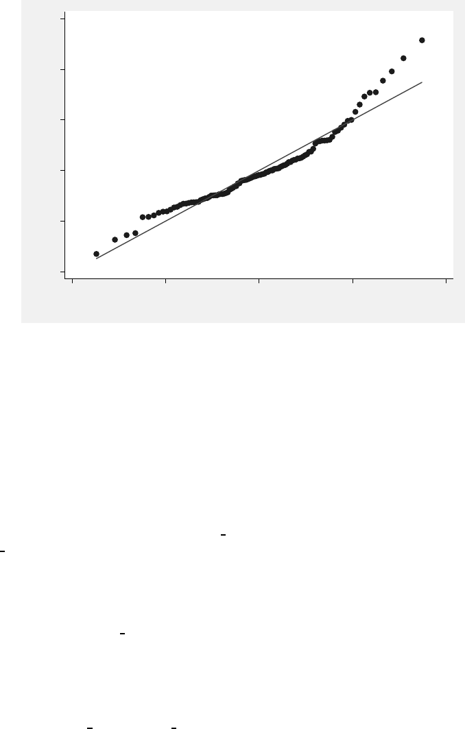
Models for Clustered Longitudinal Data:The Dental Veneer Example 361
−2 −1 0 1 2 3
Standardized residuals
−2 −1 0 1 2
Inverse Normal
FIGURE 7.5: Normal Q–Q plot of the standardized residuals based on the fit of Model 7.3.
patient effects and the nested random tooth effects in three new variables, again using the
predict command:
. predict pat_eblups*, reffects level(patient)
. predict tooth_eblups, reffects level(tooth)
The first command saves the predicted random effects (EBLUPs) for each level of
PATIENT in new variables named PAT EBLUPS1 (for the random TIME effects) and
PAT EBLUPS2 (for the random effects associated with the intercept) in the data set. The
asterisk (*) requests that a single new variable be created for each random effect associated
with the levels of PATIENT. In this case, two new variables are created, because there are
two random effects in Model 7.3 associated with each patient. The second command saves
the EBLUPs of the random effects associated with the intercept for each tooth in a new
variable named TOOTH EBLUPS.
After saving these three new variables, we generate a new data set containing a single
case per patient, and including the individual patient EBLUPs (the original data set should
be saved before creating this collapsed data set):
. save "C:\temp\veneer.dta", replace
. collapse pat eblups1 pat eblups2, by(patient)
We then generate normal Q–Q plots for each set of patient-specific EBLUPs and check
for outliers:
. qnorm pat_eblups1, ytitle(EBLUPs of Random Patient TIME Effects)
. graph save "C:\temp\figure76_part1.gph"
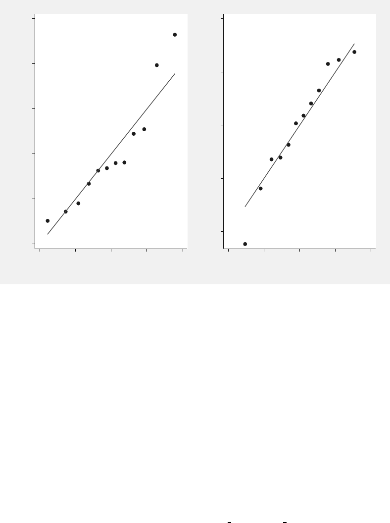
362 Linear Mixed Models: A Practical Guide Using Statistical Software
−10 −5 0 5 10 15
EBLUPs of Random Patient TIME Effects
−10 −5 0 5 10
Inverse Normal
−40 −20 0 20 40
EBLUPs of Random Patient Intercepts
−40 −20 0 20 40
Inverse Normal
FIGURE 7.6: Normal Q–Q plots for the EBLUPs of the random patient effects.
. qnorm pat_eblups2, ytitle(EBLUPs of Random Patient Intercepts)
. graph save "C:\temp\figure76_part2.gph"
. graph combine "C:\temp\figure76_part1.gph"
"C:\temp\figure76_part2.gph"
Note that we make use of the graph save and graph combine commands to save the
individual plots and then combine them into a single figure.
Figure 7.6 suggests that there are two positive outliers in terms of the random TIME
effects (EBLUPs greater than 5) associated with the patients (left panel). We can investigate
selected variables for these patients after opening the original data set (including the saved
EBLUPs) once again:
. use "C:\temp\veneer.dta", clear
. list patient tooth gcf time age cda base gcf if pat eblups1 > 5

Models for Clustered Longitudinal Data:The Dental Veneer Example 363
'
&
$
%
+-------------------------------------------------+
patient tooth gcf time age cda base_gcf
---------------------------------------------------
1. 1 6 11 3 46 4.666667 17
2. 1 6 68 6 46 4.666667 17
3. 1 7 13 3 46 4.666667 22
4. 1 7 47 6 46 4.666667 22
5. 1 8 14 3 46 5.000000 18
---------------------------------------------------
6. 1 8 58 6 46 5.000000 18
7. 1 9 10 3 46 3.333333 12
8. 1 9 57 6 46 3.333333 12
9. 1 10 14 3 46 8.666667 10
10. 1 10 44 6 46 8.666667 10
---------------------------------------------------
11. 1 11 11 3 46 5.666667 17
12. 1 11 53 6 46 5.666667 17
85. 10 6 29 3 36 2.333333 27
86. 10 6 87 6 36 2.333333 27
87. 10 7 28 3 36 8.666667 10
---------------------------------------------------
88. 10 7 61 6 36 8.666667 10
89. 10 8 17 3 36 6.333333 25
90. 10 8 47 6 36 6.333333 25
91. 10 9 11 3 36 6.666667 7
92. 10 9 42 6 36 6.666667 7
---------------------------------------------------
93. 10 10 48 3 36 6.333333 15
94. 10 10 65 6 36 6.333333 15
95. 10 11 55 3 36 4.666667 19
96. 10 11 70 6 36 4.666667 19
+-------------------------------------------------+
As expected, these two patients (PATIENT = 1 and 10) consistently have large increases
in GCF as a function of TIME for all of their teeth, and their data should be checked for
validity.
The tooth-specific random effects can be assessed in a similar manner by first creating
a tooth-specific data set containing only the PATIENT, TOOTH, and TOOTH EBLUP
variables (after generating predicted values of the random effects in the original data set,
as shown above), and then generating a normal Q–Q plot:
. collapse tooth eblups, by(patient tooth)
. qnorm tooth eblups, ytitle(EBLUPs of Random Tooth Effects)
The resulting plot (not displayed) does not provide any evidence of extremely unusual
random tooth effects.
7.10 Software Notes and Recommendations
7.10.1 ML vs. REML Estimation
In this chapter, we introduce for the first time the HMLM2 (hierarchical multivariate linear
models) procedure, which was designed for analyses of clustered longitudinal data sets in
364 Linear Mixed Models: A Practical Guide Using Statistical Software
HLM. Unlike the LMM procedures in SAS, SPSS, R, and Stata, this procedure only uses
ML estimation. The procedures in SAS, SPSS, R, and Stata provide users with a choice of
either REML or ML estimation when fitting these models.
This difference could have important consequences when developing a model. We rec-
ommend using likelihood ratio tests based on REML estimation when testing hypotheses,
such as Hypotheses 7.1 and 7.2, involving covariance parameters. This is not possible if the
models are fitted using ML estimation.
A second important consequence of using ML estimation is that the covariance parameter
estimates are known to be biased. This can result in smaller estimated standard errors for
the estimates of the fixed effects in the model and also has implications for the fixed-
effect parameters that are estimated. Some of these differences were apparent in Tables 7.6
through 7.8.
7.10.2 The Ability to Remove Random Effects from a Model
The HMLM2 procedure requires that at least one random effect be specified in the model
at Level 3 and at Level 2 of the data. The procedures in SAS, SPSS, R, and Stata all allow
more flexibility in specifying and testing which levels of the data (e.g., patient or teeth
nested within patients) should have random effects included in the model.
Although the HMLM2 procedure is more restrictive than some of the other software
procedures in this sense, it also ensures that the hierarchy of the data is maintained in the
analysis. Users of SAS, SPSS, R, and Stata must think carefully about how the hierarchy of
the data is specified in the model, and then correctly specify the appropriate random effects
in the syntax. HMLM2 forces the hierarchical structure of these data sets to be taken into
consideration.
7.10.3 Considering Alternative Residual Covariance Structures
With the exception of the lmer() function in R, all of the other LMM procedures considered
in this chapter allow users to fit models with nonidentity residual covariance (Rij ) matrices.
The unstructured residual covariance matrix (Model 7.2A) is not available in HMLM2
when random effects are also considered simultaneously, and we had to use an alternative
setup of the model to allow us to fit the compound symmetry structure (Model 7.2B) using
HMLM2 (see Subsection 7.4.5).
In this analysis, we found that the identity residual covariance structure was the better
and more parsimonious choice for our models, but this would not necessarily be the case
in analyses of other data sets. Heterogeneity of variances and correlation of residuals is a
common feature in longitudinal data sets, and the ability to accommodate a wide range of
residual covariance structures is very important. We recommend that analysts of clustered
longitudinal data sets with more than two longitudinal observations consider alternative
covariance structures for the residuals, and attempt to identify the structures that provide
the best fit to a given set of data. The information criteria (AIC, BIC, etc.) can be useful
in this regard.
In the Dental Veneer example, there were only a small number of residual covariance
structures that could be considered for the 2×2Rij matrix, because it contained only three
parameters, at the most, and aliasing with other covariance parameters was involved. In
other data sets with more longitudinal observations, a wider variety of residual covariance
structures could (and should) be considered. The procedures in SAS, SPSS, Stata, HLM,
and the lme() function in Roffer flexibility in this regard, with proc mixed in SAS having
the largest list of available residual covariance structures.
Models for Clustered Longitudinal Data:The Dental Veneer Example 365
7.10.4 Aliasing of Covariance Parameters
We had difficulties when fitting Models 7.2A and 7.2B because of aliasing (nonidentifia-
bility) of the covariance parameters. The problems with these models arose because we
were specifying random effects at two levels of the data (patient and teeth within patients),
as well as an additional residual covariance at the tooth level. If we had more than two
observations per tooth, this would have been a problem for Model 7.2B only.
The symptoms of aliasing of covariance parameters manifest themselves in different
fashions in the different software programs. For Model 7.2A, SAS complained in a NOTE in
the log that the estimated Hessian matrix (which is used to compute the standard errors
of the estimated covariance parameters) was not positive-definite. Users of SAS need to be
aware of these types of messages in the log file. SAS also reported a value of zero for the
UN(2,2) covariance parameter (i.e., the residual variance at time 2) and did not report a
standard error for this parameter estimate in the output. For Model 7.2B, SAS did not
provide estimates due to too many likelihood evaluations.
SPSS produced a warning message in the output window about lack of convergence for
both Models 7.2A and 7.2B. In this case, results from SPSS should not be interpreted,
because the estimation algorithm has not converged to a valid solution for the parameter
estimates.
After fitting Models 7.2A and 7.2B with the lme() function in R, attempts to use the
intervals() function to obtain confidence intervals for the estimated covariance parameters
resulted in extremely wide and unrealistic intervals. Simply fitting these two models in R
did not indicate any problems with the model specification, but the intervals for these
parameters provide an indication of instability in the estimates of the standard errors for
these covariance parameter estimates. Similar problems were apparent when fitting Model
7.2A in Stata, and Model 7.2B could not be fitted in Stata due to a lack of convergence
(similar to the procedures in SAS and SPSS).
We were not able to fit Model 7.2A using HMLM2, because the unstructured residual
covariance matrix is not available as an option in a model that also includes random effects.
In addition, HMLM2 reported a generic message for Model 7.2B that stated “Invalid info,
score, or likelihood” and did not report parameter estimates for this model.
In general, users of these software procedures need to be very cautious about interpret-
ing the output for covariance parameters. We recommend always examining the estimated
covariance parameters and their standard errors to see if they are reasonable. The pro-
cedures in SAS, SPSS and Stata make this relatively easy to do. In R,theintervals()
function is helpful (when using the lme() function). HMLM2 is fairly direct and obvious
about problems that occur, but it is not very helpful in diagnosing this particular problem.
Readers should be aware of potential problems when fitting models to clustered longitu-
dinal data, pay attention to warnings and notes produced by the software, and check model
specification carefully. We considered three possible structures for the residual covariance
matrix in this example to illustrate potential problems with aliasing. We advise exercising
caution when fitting these models so as not to overspecify the covariance structure.
7.10.5 Displaying the Marginal Covariance and Correlation Matrices
The ability to examine implied marginal covariance matrices and their associated correlation
matrices can be very helpful in understanding an LMM that has been fitted (see Section 7.8).
SAS makes it easy to do this for any subject desired, by using the v=and vcorr = options
in the random statement. In fact, proc mixed in SAS is currently the only procedure that
allows users to examine the marginal covariance matrix implied by a LMM fitted to a
clustered longitudinal data set with three levels.

366 Linear Mixed Models: A Practical Guide Using Statistical Software
7.10.6 Miscellaneous Software Notes
1. SPSS: The syntax to set up the subject in the RANDOM subcommand for
TOOTH nested within PATIENT is (TOOTH*PATIENT), which appears to
be specifying TOOTH crossed with PATIENT, but is actually the syntax used
for nesting. Alternatively, one could use a RANDOM subcommand of the form
/RANDOM tooth(patient), without any SUBJECT variable(s), to include nested
random tooth effects in the model; however, this would not allow one to specify
multiple random effects at the tooth level.
2. HMLM2: This procedure requires that the Level 1 data set include an indicator
variable for each time point. For instance, in the Dental Veneer example, the
Level 1 data set needs to include two indicator variables: one for observations at
3 months, and a second for observations at 6 months. These indicator variables
are not necessary when using the procedures in SAS, SPSS, R, and Stata.
7.11 Other Analytic Approaches
7.11.1 Modeling the Covariance Structure
In Section 7.8 we examined the marginal covariance of observations on patient 1 implied
by the random effects specified for Model 7.3. As discussed in Chapter 2, we can model
the marginal covariance structure directly by allowing the residuals for observations on the
same tooth to be correlated.
For the Dental Veneer data, we can model the tooth-level marginal covariance struc-
ture implied by Model 7.3 by removing the random tooth-level effects from the model and
specifying a compound symmetry covariance structure for the residuals, as shown in the
following SAS syntax for Model 7.3A:
title "Alternative Model 7.3A";
proc mixed data = veneer noclprint covtest;
class patient tooth cattime;
model gcf = time base gcf cda age / solution outpred = resids;
random intercept time / subject = patient type = un solution
v = 1 vcorr = 1;
repeated cattime / subject = tooth(patient) type=cs;
run;
We can view the estimated covariance parameters for Model 7.3A in the following output:
'
&
$
%
Covariance Parameter Estimates (Model 7.3A)
Standard Z
Cov Parm Subject Estimate Error Value Pr Z
UN(l,l) PATIENT 524.9700 253.0100 2.07 0.0190
UN(2,1) PATIENT -140.4200 66.5737 -2.11 0.0349
UN(2,2) PATIENT 41.8869 18.7993 2.23 0.0129
CS TOOTH (PATIENT) 47.4573 16.6304 2.85 0.0043
Residual 48.8675 10.5053 4.65 <0.0001

Models for Clustered Longitudinal Data:The Dental Veneer Example 367
The analogous syntax and output for Model 7.3 are shown below for comparison. Note
that the output for the models is nearly identical, except for the labels assigned to the
covariance parameters in the output. The −2 REML log-likelihood values are the same for
the two models, as are the AIC and BIC.
title "Model 7.3";
proc mixed data = data.veneer noclprint covtest;
class patient tooth cattime;
model gcf = time base gcf cda age / solution outpred = resids;
random intercept time / subject = patient type = un
v = 1 vcorr = 1;
random intercept / subject = tooth(patient) solution;
run; '
&
$
%
Covariance Parameter Estimates (Model 7.3)
Standard Z
Cov Parm Subject Estimate Error Value Pr Z
UN(l,l) PATIENT 524.9500 252.9900 2.07 0.0190
UN(2,1) PATIENT -140.4200 66.5725 -2.11 0.0349
UN(2,2) PATIENT 41.8874 18.7998 2.23 0.0129
Intercept TOOTH (PATIENT) 47.4544 16.6298 2.85 0.0022
Residual 48.8703 10.5059 4.65 <0.0001
It is important to note that the model setup used for Model 7.3 only allows for positive
marginal correlations among observations on the same tooth over time, because the im-
plied marginal correlations are a result of the variance of the random intercepts associated
with each tooth. The specification of Model 7.3A allows for negative correlations among
observations on the same tooth.
7.11.2 The Step-Up vs. Step-Down Approach to Model Building
The step-up approach to model building commonly used in the HLM literature (Rauden-
bush & Bryk, 2002) begins with an “unconditional” model, containing only the intercept
and random effects. The reduction in the estimated variance components at each level of the
data is then monitored as fixed effects are added to the model. The mean structure is consid-
ered complete when adding fixed-effect terms provides no further reduction in the variance
components. This step-up approach to model building (see Chapter 4, or Subsection 2.7.2)
could also be considered for the Dental Veneer data.
The step-down (or top-down) approach involves starting the analysis with a “loaded”
mean structure and then working on the covariance structure. One advantage of this ap-
proach is that the covariances can then be truly thought of as measuring “variance” and not
simply variation due to fixed effects that have been omitted from the model. An advantage
of using the step-up approach is that the effect of each covariate on reducing the model
“variance” can be viewed for each level of the data. If we had used the step-up approach
and adopted a strategy of only including significant main effects in the model, our final
model for the Dental Veneer data might have been different from Model 7.3.
7.11.3 Alternative Uses of Baseline Values for the Dependent Variable
The baseline (first) value of the dependent variable in a series of longitudinal measures may
be modeled as simply one of the repeated outcome measures, or it can be considered as a
baseline covariate, as we have done in the Dental Veneer example.
368 Linear Mixed Models: A Practical Guide Using Statistical Software
There are strong theoretical reasons for treating the baseline value as another measure
of the outcome. If the subsequent measures represent values on the dependent variable,
measured with error, then it is difficult to argue that the first of the series is “fixed,” as
required for covariates. In this sense it is more natural to consider the entire sequence,
including the baseline values, as having a multivariate normal distribution. However, when
using this approach, if a treatment is administered after the baseline measurement, the
treatment effect must be modeled as a treatment by time interaction if treatment groups are
similar at baseline. A changing treatment effect over time may lead to a complex interaction
between treatment and a function of time.
Those who consider the baseline value as a covariate argue that the baseline value
is inherently different from other values in the series. The baseline value is often taken
prior to a treatment or intervention, as in the Dental Veneer data. There is a history
of including baseline values as covariates, particularly in clinical trials. The inclusion of
baseline covariates in a model may substantially reduce the residual variance (because of
strong correlations with the subsequent values), thus increasing the power of tests for other
covariates. The inclusion of baseline covariates also allows an appropriate adjustment for
baseline imbalance between groups.
Finally, the values in the subsequent series of response measurements may be a function
of the initial value. This can happen in instances when there is large room for improvement
when the baseline level is poor, but little room for improvement when the baseline level is
already good. This situation is easily modeled with an interaction between time and the
baseline covariate, but more difficult to handle in the model considering the baseline value
as one of the outcome measures.
In summary, we find both model frameworks to be useful in different settings. The
longitudinal model, which includes baseline values as measures on the dependent variable,
is more elegant; the model considering the first outcome measurement as a baseline covariate
is often more practical.

8
Models for Data with Crossed Random Factors:
The SAT Score Example
8.1 Introduction
This chapter introduces the analysis of data sets with crossed random factors,where
there are multiple random factors with levels that are crossed with each other, rather
than having an explicit nesting structure. For example, in Chapter 4, we analyzed a data
set where students were nested in classrooms, and classrooms were nested within schools.
The classroom and school ID variables were both random factors, where the levels of these
variables were randomly selected from larger populations of classrooms and schools. Further,
the levels of the classroom factor were nested within levels of the school factor; a given
classroom could not exist in multiple schools. In this chapter, we consider an example
data set where there are repeated measurements of math scores on an SAT test (Student
Aptitude Test) collected on randomly sampled students within a given school, and those
students have multiple teachers from the school over time. As a result, both students and
teachers have multiple measures on the dependent variable associated with them, but the
levels of these two random factors (student ID and teacher ID) are crossed with each other.
Linear mixed models with crossed random effects enable the potential correlations of
the repeated observations associated with each level of these crossed random factors to be
modeled simultaneously. For example, we might expect between-student variance in math
performance over time; at the same time, we might expect that some teachers are better
math instructors, resulting in between-teacher variance in the math scores. These models
enable simultaneous estimation of the components of variance associated with the levels of
the crossed random factors, and assessment of which random factor tends to contribute the
most to variability in measures on the dependent variable.
As discussed in Chapter 2, models with crossed random effects tend to be more difficult
to estimate. Estimation is facilitated by the use of sparse matrices in model specification
and maximum likelihood estimation, but different software procedures will tend to use
different algorithms when fitting these types of models. We do not highlight one package in
particular in this chapter, and discuss some of the notable differences between the software
procedures in Section 8.10.
8.2 The SAT Score Study
8.2.1 Study Description
The data used in this example have been borrowed from the example data sets provided by
the developers of the HLM software. Specifically, we analyze a subset of the data from an
369

370 Linear Mixed Models: A Practical Guide Using Statistical Software
TABLE 8.1: Sample of the SAT Score Data Set in the “Long” Format
STUDID TCHRID MATH YEAR
13099 14433 631 −1
13100 14433 596 −1
13100 14484 575 0
13100 14755 591 1
13101 14433 615 −1
13101 14494 590 0
13102 14433 621 −1
13102 14494 624 0
13102 14545 611 1
...
Note: “...” indicates portion of the data not
displayed.
educational study, focusing on one of the original 67 schools in the study, and the teachers
and students within that school. In this study, students were given a math test in grades
3, 4, and 5 that was similar to the SAT math test used to evaluate college applicants.
While different treatments were applied in some years for randomly sampled students, we
do not consider treatment effects in the analysis in this chapter. We focus mainly on the
components of variance in the math scores associated with students and teachers, in addition
to change over time in the scores. The subset of the original data set that we work with
in this chapter features 234 repeated measures collected from 122 students who have been
instructed by a total of 12 teachers.
Before we carry out an analysis of the SAT score data using the procedures in SAS,
SPSS, R, Stata, or HLM, we need to make sure that the data set has been restructured into
the “long” format (similar to the other case studies presented in the book). A portion of
the SAT score data in the “long” format is shown in Table 8.1.
The portion of the SAT score data set presented in Table 8.1 demonstrates some key
features of both this specific data set and data sets with crossed random factors more
generally. First, note that the YEAR variable represents a centered version of the grade in
which the student was measured (centered at Grade 4). Second, note that there are repeated
measures on both students and teachers; students are measured repeatedly over time (with
not all students measured in each of the three years), and different students might have had
the same teacher in a given year. For example, teacher ID 14433 instructed all four of the
students in Table 8.1 in grade 3. Students are therefore not nested within teachers. This
crossed structure, illustrated in the matrix below, introduces multiple levels of potentially
correlated observations in the data set, and linear mixed models including random effects
for both students and teachers enable decomposition of the components of variance due to
each of these crossed random factors.
Teacher ID
Student ID 14433 14484 14494 14545 14755 ...
13099 X
13100 X X X
13101 X X
13102 X X X
...

Models for Data with Crossed Random Factors:The SAT Score Example 371
We note below how this crossed structure, where an “X” indicates an observation on the
dependent variable measuring math achievement on the SAT for a given student–teacher
pairing, results in a matrix with several empty cells, where a particular student was not
instructed by a particular teacher.Thisiswhymethodsusingsparse matrices for estimation
are the most efficient when fitting these types of models.
In the analysis in this chapter, we consider models including a fixed effect of YEAR
(enabling assessment of change over time in the mean math score) and random effects for
the levels of TCHRID (teachers) and STUDID (students), to see whether the variation in
math scores is being driven by students or teachers.
To summarize, the following variables are included in the SAT score data set:
•STUDID = Unique Student ID
•TCHRID = Unique Teacher ID
•MATH = Score on SAT Math Test
•YEAR = Year of Measurement (−1 = Grade 3, 0 = Grade 4, 1 = Grade 5)
Sorting the data set by STUDID or TCHRID is not required for using the software
procedures that enable fitting models with crossed random effects.
8.2.2 Data Summary
In this section, we consider some exploratory graphical analyses of the SAT score data, using
the Rsoftware. These plots can easily be generated using the other four software packages
as well.
We first consider the distribution of the SAT scores as a function of the year (or grade)
in which the data were collected. The following Rsyntaxcanbeusedtoreadinthedata
(with variable names in the first row) from the C:\temp directory, and then generate the
side-by-side box plots in Figure 8.1.
> sat <- read.csv("C:\\temp\\school_data_final.csv", h=T)
> attach(sat)
> plot(math ~ factor(year), xlab = "Year (Centered at Grade 4)",
ylab = "SAT Math Score")
Figure 8.1 shows evidence of a fairly clear linear increase in performance on the math
portion of the SAT among these students as a function of year of measurement. These plots
result in an expectation that the fixed effect of YEAR (representing a linear rate of change
in the SAT math scores) will likely be positive and significant in our analysis. We also see
evidence of fairly constant variance in the scores as a function of YEAR.
We now consider variability in the math scores among the teachers and students. First,
we examine side-by-side box plots for the teachers, using the following Rsyntax to generate
Figure 8.2.
> plot(math ~ factor(tchrid), xlab = "Teacher ID",
ylab = "SAT Math Score")
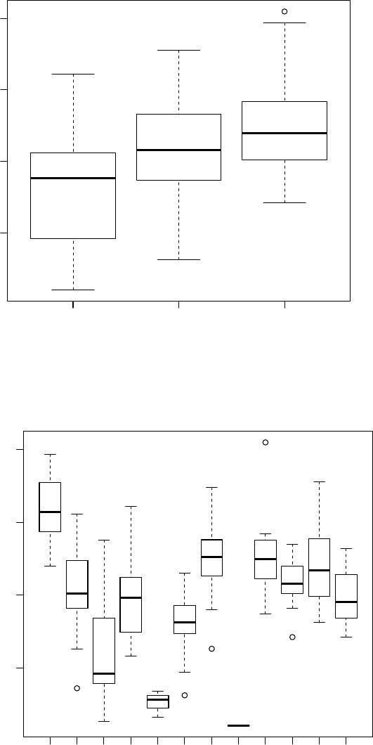
372 Linear Mixed Models: A Practical Guide Using Statistical Software
−1 0 1
550 600 650 700
Year (Centered at Grade 4)
SAT Math Score
FIGURE 8.1: Box plots of SAT scores by year of measurement.
14405 14443 14473 14494 14545 14694
550 600 650 700
Teacher ID
SAT Math Score
FIGURE 8.2: Box plots of SAT scores for each of the 13 teachers in the SAT score data set.
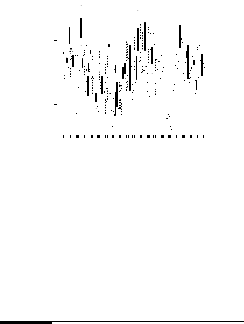
Models for Data with Crossed Random Factors:The SAT Score Example 373
13099 13116 13133 13150 13168 13195 13315 13344
550 600 650 700
Student ID
SAT Math Score
FIGURE 8.3: Box plots of SAT scores for each of the 122 students in the SAT score data
set.
Figure 8.2 provides evidence of substantial variability in performance on the math por-
tion of the SAT among these 13 teachers, suggesting that a model for these data should
include random teacher effects.
Finally, we consider variability among the students, using the following Rsyntax to
generate Figure 8.3.
> plot(math ~ factor(studid), xlab = "Student ID",
ylab = "SAT Math Score")
We also note a fair amount of variability among the students in terms of the SAT scores
in Figure 8.3, and that several students have only been measured once. These results suggest
that random effects associated with the students should also be included in a model for these
data (meaning that the random effects of students would be crossed with the random effects
of teachers, given the structure of these data).
We now consider the model that we will fit to the SAT score data.
8.3 Overview of the SAT Score Data Analysis
In this chapter, we do not consider explicit model-building steps for the SAT score data.
Instead, we simply fit a single model in each of the different software procedures that includes
all of the fixed effects and crossed random effects that we are interested in evaluating. We
then compare the methods and syntax used to fit the model across the software procedures,
in addition to the resulting estimates produced by the procedures.
374 Linear Mixed Models: A Practical Guide Using Statistical Software
8.3.1 Model Specification
8.3.1.1 General Model Specification
We specify Model 8.1 in this subsection. The general specification of Model 8.1 corresponds
closely to the syntax used to fit this model when using the procedures in SAS, SPSS, Stata,
and R.
The value of MATHtij in a given year indexed by t(t=1,2,3)forthei-th student (i
= 1, 2, ..., 122) being instructed by the j-th teacher (j= 1, 2, ..., 13) can be written as
follows:
MATHtij =β0+β1×YEARtij fixed
+ui+vj+εtij }random (8.1)
The fixed-effect parameters are represented by β0and β1. The fixed intercept β0rep-
resents the expected value of MATHtij when YEARtij in equal to zero (or Grade 4, given
the centering). The parameter β1represents the fixed effect of the YEAR variable, which
can be interpreted as the linear rate of change in the expected math score associated with
a one-year increase.
The uiterm represents the random effect associated with student i,andvjrepresents
the random effect associated with teacher j. We assume that the random effects arise from
two independent normal distributions:
ui∼N(0,σ
2
i),v
j∼N(0,σ
2
j)
We have a total of 135 random effects in this model, corresponding to the 122 students
and the 13 teachers. The overall resulting Dmatrix corresponding to this type of model
with crossed random effects is a diagonal matrix with 122+13 = 135 columns and 135 rows,
corresponding to the 135 random effects of the students and teachers. The first 122 ×122
block-diagonal portion of the matrix will have the variance of the random student effects, σ2
i,
on the diagonal, and zeroes off the diagonal. The remaining 13 ×13 block-diagonal portion
of this matrix will have the variance of the random teacher effects, σ2
j, on the diagonal, and
zeroes off the diagonal.
The residuals associated with the math score observations are assumed to be independent
of the two random effects, and follow a normal distribution:
εtij ∼N(0,σ
2)
We next consider the hierarchical specification of a model with crossed random effects.
8.3.1.2 Hierarchical Model Specification
We now present an equivalent hierarchical specification of Model 8.1, using the same nota-
tion as in Subsection 8.3.1.1. The hierarchical model has two components, reflecting contri-
butions from the two levels of the data: the repeated measures at Level 1, and the crossing
of students and teachers at Level 2 (i.e., the repeated measures of the dependent variable
are associated with both students and teachers simultaneously). We write the Level 1
component as
Level 1 Model (Repeated Measures)
MATHtij =b0ij +b1ij ×YEARtij +εtij (8.2)
where the residuals (εtij ) have the distribution defined in the general specification of
Model 8.1 in Subsection 8.3.1.1, with constant variance.
Models for Data with Crossed Random Factors:The SAT Score Example 375
In the Level 1 model, we assume that MATHtij , the math SAT score for an individual
combination of student iand teacher jat time t, follows a linear model, defined by the
intercept specific to the student–teacher combination, b0ij , and the effect of YEAR specific
to the student–teacher combination, b1ij .
The Level 2 model then describes variation between the various student–teacher com-
binations in terms of the random intercepts and time effects, using the crossed random
effects:
Level 2 Model (Student–Teacher Combination)
b0ij =β0+ui+vj
b1ij =β1(8.3)
where
ui∼N(0,σ
2
i),v
j∼N(0,σ
2
j)
In this Level 2 model, the intercept b0ij for student iand teacher jdepends on the
overall fixed intercept, β0, the random effect associated with student i,ui, and the random
effect associated with teacher j,vj. We note that crossed random effects associated with the
students and teachers are not included in the Level 2 equation for the effect of YEAR in this
simple example (although they could be more generally, if one wished to test hypotheses
about variance among students or teachers in terms of the YEAR effects). As a result, the
YEAR effect specific to a student–teacher combination is simply defined by the overall fixed
effect of YEAR, β1.
By substituting the expressions for b0ij and b1ij from the Level 2 model into the Level 1
model, we obtain the general linear mixed model (LMM) with crossed random effects that
was specified in (8.1).
8.3.2 Hypothesis Tests
We test a simple set of three hypotheses in this case study, related to the two crossed random
effects and the overall fixed effect of YEAR on the SAT math scores for these students.
Hypothesis 8.1. The random effects associated with students (ui) can be omitted from
Model 8.1.
Model 8.1 has a single random effect, ui, associated with the intercept for each student.
To test Hypothesis 8.1, we fit a model (Model 8.2) excluding the random student effects
(i.e., a two-level model with repeated measures nested within teachers), and use a REML-
based likelihood ratio test. The test statistic is calculated by subtracting the –2 REML
log-likelihood value for Model 8.1 (the reference model) from that for Model 8.2 (the nested
model). The asymptotic null distribution of the test statistic is a mixture of χ2
0and χ2
1
distributions, with equal weights of 0.5 (see Subsection 2.6.2.2).
We once again remind readers that likelihood ratio tests, such as the one used for
Hypothesis 8.1, rely on asymptotic (large-sample) theory, so we would not usually carry out
this type of test for such a small data set. Rather, in practice, the random effects would
probably be retained without testing, so that the appropriate marginal variance-covariance
structure would be obtained for the data set. We present the calculation of this likelihood
ratio test for the random effects (and those that follow in this chapter) strictly for illustrative
purposes.
Hypothesis 8.2. The random effects associated with teachers (vj) can be omitted from
Model 8.1.

376 Linear Mixed Models: A Practical Guide Using Statistical Software
We test Hypothesis 8.2 using a similar REML-based likelihood ratio test. The test statis-
tic is calculated by subtracting the –2 REML log-likelihood value for Model 8.1 from that
for a new nested model, Model 8.3, excluding the random teacher effects (i.e., a two-level
model with repeated measures nested within students). The asymptotic distribution of the
test statistic under the null hypothesis is once again a mixture of χ2
0and χ2
1distributions,
with equal weights of 0.5.
Hypothesis 8.3. The fixed effects associated with the YEAR variable can be omitted
from Model 8.1.
The null and alternative hypotheses are
H0:β1=0
HA:β1=0
We test Hypothesis 8.3 using the standard test statistics for single fixed-effect param-
eters that are computed automatically by the various software procedures. We talk about
differences in the test statistics reported and the test results in the next section (Section
8.4). For more detail on the results of these hypothesis tests, see Section 8.5.
8.4 Analysis Steps in the Software Procedures
The modeling results for all software procedures are presented and compared in Section 8.6.
8.4.1 SAS
We first import the comma-separated data file (school_data_final.csv, assumed to be
located in the C:\temp directory) into SAS, and create a temporary SAS data set named
satmath.
PROC IMPORT OUT = WORK.satmath
DATAFILE="C:\temp\school_data_final.csv"
DBMS=CSV REPLACE;
GETNAMES=YES;
DATAROW=2;
RUN;
We now proceed with fitting Model 8.1 and testing the hypotheses outlined in Section
8.3.2. The SAS syntax to fit Model 8.1 using proc mixed is as follows:
title "Model 8.1";
proc mixed data = satmath covtest;
class studid tchrid;
model math = year / solution;
random int / subject = studid;
random int / subject = tchrid;
run;
We have specified the covtest option in the proc mixed statement to obtain the stan-
dard errors of the estimated variance components in the output for comparison with the
other software procedures. Recall that this option also causes SAS to display a Wald test
Models for Data with Crossed Random Factors:The SAT Score Example 377
for the variance of the random effects associated with the teachers and students, which we
do not recommend for use in testing whether to include random effects in a model (see
Subsection 2.6.3.2).
The class statement identifies the categorical variables that are required to specify
the model. We include the two crossed random factors, STUDID and TCHRID, in the
class statement; as shown in earlier chapters, random factors (crossed or nested) need to
be specified here. The dependent variable, MATH, and the predictor variable, YEAR, are
both treated as continuous variables in this model.
The model statement sets up the fixed-effects portion of Model 8.1. We specify that the
dependent variable, MATH, is a linear function of a fixed intercept (included by default) and
the fixed effect of the YEAR variable. The solution option requests that the estimates of
the two fixed-effect parameters be displayed in the output, along with their standard errors
and a t-test for each parameter.
The two random statements set up the crossed random effects structure for this model.
In this case, STUDID is identified as the subject in the first random statement, indicating
that it is a random factor. By specifying random int, we include a random effect associated
with the intercept for each unique student. The second random statement with a different
subject variable specified (TCHRID) also includes a random effect associated with the
intercept for each teacher, and indicates that the levels of these two subject variables may
potentially cross with each other. We note the difference in these two random statements
from those used in Chapter 4, for example; there is no nesting relationship indicated for the
random factors.
We now test Hypothesis 8.1 by removing the random student effects from Model 8.1,
and performing a likelihood ratio test. We first refit Model 8.1 without the first random
statement:
title "Hypothesis 8.1";
proc mixed data = satmath covtest;
class studid tchrid;
model math = year / solution;
random int / subject = tchrid;
run;
The –2 REML log-likelihood value for this reduced two-level model is 2170.3, and the
corresponding value for Model 8.1 was 2123.6. We compute the p-value for the likelihood
ratio test using the following syntax:
title "p-value for Hypothesis 8.1";
data _null_;
lrtstat = 2170.3 - 2123.6;
df=1;
pvalue = 0.5 * (1 - probchi(lrtstat, df));
format pvalue 10.8;
put lrtstat = df = pvalue = ;
run;
We have very strong evidence (p<0.001) against the null hypothesis in this case, and
would choose to retain the random student effects in the model; there is clear evidence of
substantial between-student variance in performance on the math test, as was apparent in
the initial data summary.
We test Hypothesis 8.2 using a similar approach. We first fit a reduced model without
the random teacher effects, and then compute the likelihood ratio test statistic and p-value:
378 Linear Mixed Models: A Practical Guide Using Statistical Software
title "Hypothesis 8.2";
proc mixed data = satmath covtest;
class studid tchrid;
model math = year / solution;
random int / subject = studid;
run;
title "p-value for Hypothesis 8.2";
data _null_;
lrtstat = 2203.1 - 2123.6;
df=1;
pvalue = 0.5 * (1 - probchi(lrtstat, df));
format pvalue 10.8;
put lrtstat = df = pvalue = ;
run;
We have even stronger evidence against the null hypothesis in this case, and would also
choose to retain the random teacher effects in this model. Collectively, we can conclude
that there is substantial variance among both students and teachers in performance on the
math test. The solution option can be added to both random statements for Model 8.1
to examine predicted values of the random effects (EBLUPs) for individual students or
teachers:
title "Model 8.1, EBLUPs";
proc mixed data = satmath covtest;
class studid tchrid;
model math = year / solution;
random int / subject = studid solution;
random int / subject = tchrid solution;
run;
Finally, we test Hypothesis 8.3 with regard to the fixed effect of YEAR by examining
the t-test for the fixed year effect included in the SAS output for Model 8.1. The resulting
p-value (p=0.0032) suggests that the fixed effect of YEAR is significantly different from
zero, and the positive estimated coefficient suggests that the average performance of the
students is increasing significantly over time. At this point, the model diagnostics examined
in other chapters could also be examined for Model 8.1.
8.4.2 SPSS
We assume that the .csv data set used to carry out the data summary in Subsection 8.2.2
has been imported into SPSS. We begin the SPSS analysis by setting up the syntax to fit
Model 8.1 using the MIXED command:
* Model 8.1 .
MIXED math WITH year
/CRITERIA=CIN(95) MXITER(100) MXSTEP(10) SCORING(1)
SINGULAR(0.000000000001) HCONVERGE(0, ABSOLUTE)
LCONVERGE(0, ABSOLUTE) PCONVERGE(0.000001, ABSOLUTE)
/FIXED=year | SSTYPE(3)
/METHOD=REML
/PRINT=SOLUTION TESTCOV
Models for Data with Crossed Random Factors:The SAT Score Example 379
/RANDOM=INTERCEPT | SUBJECT(studid) COVTYPE(VC)
/RANDOM=INTERCEPT | SUBJECT(tchrid) COVTYPE(VC).
In this syntax, MATH is listed as the dependent variable. The /FIXED subcommand
then lists the variable that has an associated fixed effect in Model 8.1 (YEAR). Note that
YEAR is being treated as a continuous covariate, given that it is specified following the
WITH keyword in the MIXED command. A fixed intercept term is included in the model by
default.
The /METHOD subcommand then specifies the REML estimation method, which is the
default. The /PRINT subcommand requests that the SOLUTION for the estimated parameters
in the model be displayed in the output. Furthermore, we request simple Wald tests of the
two variance components with the TESTCOV option, to get an initial sense of the importance
of the between-student variance and the between-teacher variance.
We then include two separate /RANDOM subcommands, indicating that crossed random
effects associated with each level of STUDID and TCHRID should be included in Model
8.1. The covariance structure for the random effects is specified as variance components (the
default), using the COVTYPE(VC) syntax. We note that this specification of the two /RANDOM
subcommands does not identify any type of nesting relationship between the two random
effects.
After fitting Model 8.1 and generating the parameter estimates and model information
criteria in the SPSS output viewer, we now test Hypothesis 8.1 by removing the random
student effects from Model 8.1, and performing a likelihood ratio test. We first refit Model
8.1 without the first /RANDOM subcommand:
* Hypothesis 8.1 .
MIXED math WITH year
/CRITERIA=CIN(95) MXITER(100) MXSTEP(10) SCORING(1)
SINGULAR(0.000000000001) HCONVERGE(0, ABSOLUTE)
LCONVERGE(0, ABSOLUTE) PCONVERGE(0.000001, ABSOLUTE)
/FIXED=year | SSTYPE(3)
/METHOD=REML
/PRINT=SOLUTION TESTCOV
/RANDOM=INTERCEPT | SUBJECT(tchrid) COVTYPE(VC).
The –2 REML log-likelihood value for this reduced two-level model is 2170.3, and the
corresponding value for Model 8.1 was 2123.6 (a difference of 46.7). We compute the p-value
for the likelihood ratio test using the following syntax:
* Hypothesis 8.1 .
COMPUTE hyp81pvalue = 0.5 * (1 - CDF.CHISQ(46.7,1)).
EXECUTE.
This syntax will compute a new variable in the SPSS data set, containing the p-value
associated with this test as a constant value for all cases in the data set. We have very strong
evidence (p<0.001) against the null hypothesis in this case, and would choose to retain the
random student effects in the model; there is clear evidence of substantial between-student
variance in performance on the math test, as was apparent in the initial data summary.
We test Hypothesis 8.2 using a similar approach. We first fit a reduced model without
the random teacher effects, and then compute the likelihood ratio test statistic and p-value:
* Hypothesis 8.2 .
MIXED math WITH year
380 Linear Mixed Models: A Practical Guide Using Statistical Software
/CRITERIA=CIN(95) MXITER(100) MXSTEP(10) SCORING(1)
SINGULAR(0.000000000001) HCONVERGE(0, ABSOLUTE)
LCONVERGE(0, ABSOLUTE) PCONVERGE(0.000001, ABSOLUTE)
/FIXED=year | SSTYPE(3)
/METHOD=REML
/PRINT=SOLUTION TESTCOV
/RANDOM=INTERCEPT | SUBJECT(studid) COVTYPE(VC).
COMPUTE hyp82pvalue = 0.5 * (1 - CDF.CHISQ(79.5,1)).
EXECUTE.
We have even stronger evidence against the null hypothesis in this case, and would also
choose to retain the random teacher effects in this model. Collectively, we can conclude
that there is substantial variance among both students and teachers in performance on the
math test. Unfortunately, there are no easy ways to extract the predicted random effects
(EBLUPs) associated with teachers and students when using the MIXED command to fit
models with crossed random effects in the current version of SPSS.
Finally, we test Hypothesis 8.3 with regard to the fixed effect of YEAR by examining
the t-test for the fixed year effect included in the SPSS output for Model 8.1. The resulting
p-value (p=0.016, based on a Satterthwaite approximation of the denominator degrees
of freedom) suggests that the fixed effect of YEAR is significantly different from zero, and
the positive estimated coefficient suggests that the average performance of the students is
increasing significantly over time. At this point, the model diagnostics examined in other
chapters could (and should) also be examined for Model 8.1.
8.4.3 R
We assume that the sat data frame object created in the initial data summary (Subsection
8.2.2) has been attached to R’s working memory. Importantly, the lme() function in the R
package nlme cannot fit models with crossed random effects, so we only fit Model 8.1 and
test the three hypotheses using the lmer() function in the Rpackage lme4 in this section.
Assuming that it has already been installed from a Comprehensive RArchive Network
(CRAN) mirror, the lme4 package first needs to be loaded, so that the lmer() function can
be used in the analysis:
> library(lme4)
We then fit Model 8.1 to the SAT score data using the lmer() function:
> # Model 8.1.
> model8.1.fit <- lmer(math ~ year + (1|studid) + (1|tchrid), REML = T)
We describe each part of this specification of the lmer() function:
•model8.1.fit is the name of the object that contains the results of the fitted linear mixed
model with crossed random effects.
•The first argument of the function, math ~ year + (1|studid) + (1|tchrid),isthe
model formula, which defines the response variable (math), and the terms with associated
fixed effects in the model (year).
•The (1|studid) and (1|tchrid) terms in the model formula indicate that a random
effect associated with the intercept should be included for each level of the categorical

Models for Data with Crossed Random Factors:The SAT Score Example 381
random factor studid, and each level of the random factor tchrid.Thelmer() function
will automatically recognize whether the levels of these random factors are crossed or
nested when estimating the variances of the random effects.
•The final argument of the function, REML = T, tells Rthat REML estimation should be
used for the desired covariance parameters in the model. This is the default estimation
method for the lmer() function.
After the function is executed, estimates from the model fit can be obtained using the
summary() function:
> summary(model8.1.fit)
Additional results of interest for this LMM fit can be obtained by using other functions
in conjunction with the model8.1.fit object. For example, predicted values (EBLUPs) of
the random effects for each student and each teacher can be displayed using the ranef()
function:
> ranef(model8.1.fit)
Software Note: As noted in earlier chapters, the lmer() function only produces t-
statistics for the fixed effects, with no corresponding p-values. This is primarily due to
the lack of agreement in the literature over appropriate degrees of freedom for these
test statistics. In general, we recommend use of the lmerTest package in Rfor users
interested in testing hypotheses about parameters estimated using the lmer() function,
and we illustrate the use of this package later in this analysis.
We now test Hypothesis 8.1 by fitting a reduced form of Model 8.1 without the random
student effects:
> # Hypothesis 8.1.
> model8.1.fit.nostud <- lmer(math ~ year + (1|tchrid), REML = T)
> summary(model8.1.fit.nostud)
The likelihood test statistic is calculated by subtracting the –2 REML log-likelihood
value for Model 8.1 (the reference model) from that for this reduced model (the value of the
test statistic, based on the output provided by the summary() function, is 2170−2124 = 46).
The test statistic has a null distribution that is a mixture of χ2
1and χ2
2distributions with
equal weights of 0.5, so the anova() function cannot be used for the p-value. Instead, we
calculate a p-value for the test statistic as follows:
> 0.5*(1 - pchisq(46,0)) + 0.5*(1 - pchisq(46,1))
See Subsection 8.5.1 for details. The test statistic is significant (p<0.001), so we decide
to reject the null hypothesis and retain the random student effects in the model.
We use a similar approach for testing Hypothesis 8.2, extracting the –2 REML log-
likelihood (or REMLdev)fromthesummary() function output for this reduced model exclud-
ing the random teacher effects:
> # Hypothesis 8.2.
> model8.1.fit.notchr <- lmer(math ~ year + (1|studid), REML = T)
> summary(model8.1.fit.notchr)

382 Linear Mixed Models: A Practical Guide Using Statistical Software
The value of this test statistic, based on the output provided by the summary() function,
is 2203 −2124 = 79. We compute the asymptotic p-value for this test statistic:
> 0.5*(1 - pchisq(79,0)) + 0.5*(1 - pchisq(79,1))
The resulting p-value (p<0.0001) provides strong evidence for retaining the random
teacher effects in the model. There is clear evidence of substantial variation among both
students and teachers.
Finally, we load the lmerTest package, which enables approximate t-tests of fixed-effect
parameters in models fitted using the lmer() function.
> library(lmerTest)
We once again fit Model 8.1:
> # Model 8.1.
> model8.1.fit <- lmer(math ~ year + (1|studid) + (1|tchrid), REML = T)
We then apply the summary() function to the new model fit object:
> summary(model8.1.fit)
In the resulting output, the p-value computed for the approximate t-statistic (p=0.016,
based on a Satterthwaite approximation of the denominator degrees of freedom) suggests
that the fixed effect of YEAR is significantly different from zero, and the positive estimated
coefficient suggests that the average performance of the students is increasing significantly
over time. At this point, the model diagnostics examined in other chapters could (and
should) also be examined for Model 8.1.
8.4.4 Stata
We begin the analysis by importing the comma-separated values file containing the SAT
score data (school_data_final.csv) into Stata:
. insheet using "C:\temp\school data final.csv", comma
We now proceed with fitting Model 8.1. We use the following mixed command to fit
Model 8.1 to the SAT score data:
. * Model 8.1.
. mixed math year || _all: R.studid || _all: R.tchrid, variance reml
. estat ic
In this mixed command, MATH is listed as the dependent variable, followed by the
predictor variable that has an associated fixed effect in Model 8.1 (YEAR). Note that YEAR
is being treated as a continuous covariate, given that it is not preceded by i. (Stata’s factor
notation). A fixed intercept term is included in the model by default.
We next indicate the crossed random effects using two successive || symbols in the
command. The first random factor, STUDID, follows the first || symbol, and is specified
in a unique fashion. The _all: notation indicates that the entire data set is treated as one
“cluster,” and R.studid indicates that STUDID is a categorical random factor, where the
effects of the levels of that factor randomly vary for the one “cluster.” We then indicate
the second random factor crossed with STUDID following a second || symbol, using the
Models for Data with Crossed Random Factors:The SAT Score Example 383
same general concept with the categorical TCHRID factor. We note that this command
does not specify an explicit nesting structure, given that the entire data set is treated as
one “subject.”
Finally, after a comma, we specify the variance option, which requests estimates of the
variances of the random effects in the output (rather than estimates of standard deviations),
and the reml option, requesting REML estimation of the parameters in this model (rather
than the default ML estimation). The subsequent estat ic command requests that Stata
compute selected information criteria (e.g., AIC, BIC) for this model and display them in
the output.
After fitting Model 8.1 and generating the parameter estimates and model information
criteria in the Stata results window, we now test Hypothesis 8.1 by removing the random
student effects from Model 8.1, and performing a likelihood ratio test. We first refit Model
8.1 without the random student effects:
. * Model 8.1, no random student effects.
. mixed math year || _all: R.tchrid, variance reml
. estat ic
This reduced model could also be fitted using this command, shown in earlier chapters
for simple two-level models:
. * Model 8.1, no random student effects.
. mixed math year || tchrid:, variance reml
. estat ic
The –2 REML log-likelihood value for this reduced two-level model (found by multiplying
the REML log-likelihood displayed by the estat ic command by –2) is 2170.3, and the
corresponding value for Model 8.1 was 2123.6 (a difference of 46.7). We compute the p-value
for the likelihood ratio test using the following syntax:
. * Hypothesis 8.1 .
. di 0.5*chi2tail(1,46.7)
Based on the resulting p-value, we have very strong evidence (p<0.001) against the
null hypothesis in this case, and would choose to retain the random student effects in the
model; there is clear evidence of substantial between-student variance in performance on
the math test, as was apparent in the initial data summary.
We test Hypothesis 8.2 using a similar approach. We first fit a reduced model without
the random teacher effects, and then compute the likelihood ratio test statistic and p-value:
. * Model 8.1, no random teacher effects.
. mixed math year || _all: R.studid, variance reml
. estat ic
. * Hypothesis 8.2 .
. di 0.5*chi2tail(1,79.5)
We have even stronger evidence against the null hypothesis in this case, and would also
choose to retain the random teacher effects in this model. Collectively, we can conclude that
there is substantial variance among both students and teachers in performance on the math
test.
Once a model with crossed random effects has been fitted using the mixed command, the
predict post-estimation command can be used to generate new variables in the Stata data

384 Linear Mixed Models: A Practical Guide Using Statistical Software
set containing predicted values of each random effect. For example, we save the EBLUPs of
the random school and teacher effects, respectively, in two new variables (b1 and b2)using
the following predict command (after fitting Model 8.1):
. * Model 8.1.
. mixed math year || _all: R.studid || _all: R.tchrid, variance reml
. predict b*, reffects
Finally, we test Hypothesis 8.3 with regard to the fixed effect of YEAR by examining the
z-statistic for the fixed year effect included in the Stata output for Model 8.1. The resulting
p-value (p=0.003) suggests that the fixed effect of YEAR is significantly different from
zero, and the positive estimated coefficient suggests that the average performance of the
students is increasing significantly over time. At this point, the model diagnostics examined
in other chapters could (and should) also be examined for Model 8.1.
8.4.5 HLM
8.4.5.1 Data Set Preparation
When using the HLM software to fit linear mixed models with crossed random effects to
data sets with two crossed random factors like the SAT score data, three separate data sets
need to be prepared:
1. The Level-1 data set: Each row in this data set corresponds to an observation
on a unit of analysis (including a unique measurement on the dependent variable)
for a given combination of the two crossed random factors. In the context of the
present SAT score study, each row of the Level-1 data set represents a measure-
ment on a student–teacher combination in a given year. This data set is similar
in structure to the data set displayed in Table 8.1. The Level-1 data set for this
example includes STUDID, TCHRID, the dependent variable (MATH), and the
predictor variable of interest (YEAR).
2. The Row-Level data set: When thinking about the crossed random factors in
a data set like the SAT score data, one can think of a matrix like that shown in
Section 8.2.1, where the unique levels of one random factor define the rows, and
the unique levels of the second random factor define the columns. This distinction
between the row factor and the column factor is essentially arbitrary in HLM, but
the row-level data set contains one row per unique level of one of the two random
factors. In this example, we consider STUDID as the random factor defining
the “rows” of this cross-tabulation, and this data set therefore has one row per
student. We include the unique student ID (STUDID), in addition to a variable
recording the number of measures collected on each student (MEASURES), and
we sort the data set is ascending order by STUDID. Although we don’t actually
analyze the MEASURES variable in this example, HLM requires at least one non-
ID variable to be included in this data set. In general, additional student-level
covariates of interest in the analysis would be included in the row-level data set.
3. The Column-Level data set: This data set has one row per unique level of
the second random factor. In this example, this data set has one row per unique
level of TCHRID, or per teacher. We include the TCHRID variable in this data
set, along with a variable recording the number of measures collected on each
teacher (MEASURES T), and sort the data set in ascending order by TCHRID.
Similar to the row-level data set, the column-level data set needs to have at least

Models for Data with Crossed Random Factors:The SAT Score Example 385
one non-ID variable for the teachers, and additional teacher-level covariates could
also be included in this data set.
After these three data sets have been created, we can proceed to create the multivariate
data matrix (MDM), and fit Model 8.1.
8.4.5.2 Preparing the MDM File
In the main HLM menu, click File, Make new MDM file and then Stat package
input. In the window that opens, select HCM2 to fit a hierarchical linear model with
crossed random effects associated with two (2) random factors, and click OK. Select the
Input File Type as SPSS/Windows.
To prepare the MDM file for Model 8.1, locate the Level-1 Specification area, and
Browse to the location of the Level-1 data set. Click Open after selecting the Level 1
SPSS file, click the Choose Variables button, and select the following variables: STUDID
(click “rowid” for the STUDID variable, because this random factor identifies the “rows”
in the cross-classification), TCHRID (click “colid” for the TCHRID variable, because this
random factor identifies the “columns” in the cross-classification), and both MATH and
YEAR (click “in MDM” for each of these variables). Click OK when finished.
Next, locate the Row-Level Specification area, and Browse to the location of the
row-level (student-level) SPSS data set. Click Open after selecting the file, and click the
Choose Variables button to include STUDID (click “rowid”) and the variable indicating
the number of measures on each student, MEASURES (click “in MDM”). Again, although
we don’t analyze the MEASURES variable in this example, HLM requires that at least one
numeric variable be included in the MDM file from both the row and column data sets.
Click OK when finished.
Next, locate the Column-Level Specification area, and Browse to the location of the
column-level (teacher-level) SPSS data set. Click Open after selecting the file, and click the
Choose Variables button to include TCHRID (click “colid”) and the variable indicating
the number of measures on each teacher, MEASURES T (click “in MDM”). Again, although
we don’t analyze the MEASURES T variable in this example, HLM requires that at least
one numeric variable be included in the MDM file from both the row and column data sets.
Click OK when finished.
After making these choices, select No for Missing Data? in the Level-1 data set,
because we do not have any missing data in this analysis. In the upper-right corner of the
MDM window, enter a name with a .mdm extension for the MDM file (e.g., SAT.mdm).
Save the .mdmt template file under a new name (click Save mdmt file), and click Make
MDM.
After HLM has processed the MDM file, click the Check Stats button to display
descriptive statistics for the variables in the Level-1, row, and column data files (this is not
optional). Click Done to begin building Model 8.1.
8.4.5.3 Model Fitting
In the model building window, identify MATH as the Outcome variable.Toaddmore
informative subscripts to the models (if they do not already appear), click File and Pref-
erences,andthenchooseUse level subscripts.
To complete the specification of Model 8.1, we first add the fixed effect of the uncentered
YEAR variable to the model. We choose uncentered because this variable has already been
centered at the data management stage. The Level 1 model is displayed in HLM as follows
(where iis an index for the individual observations, jis an index for students, and kis an
index for teachers):
386 Linear Mixed Models: A Practical Guide Using Statistical Software
Model 8.1: Level 1 Model
MATHijk =π0jk +π1jk(YEARijk )+eijk
The Level 2 equation for the random intercept specific to a given observation (π0jk)
includes a constant fixed effect, θ0, a random effect associated with the student (b00j), which
allows the intercept to vary randomly across students, and a random effect associated with
the teacher (c00k), which allows the intercept to vary randomly across teachers. The Level
2 equation for the random coefficient for YEAR specific to a student–teacher combination,
π1jk, is simply defined by a constant fixed effect (θ1), although we could allow the effect of
year to randomly vary across both students and teachers:
Model 8.1: Level 2 Model
π0jk =θ0+b00j+c00k
π1jk =θ1
We display the overall LMM by clicking the Mixed button in the model building win-
dow:
Model 8.1: Overall Mixed Model
MATHijk =θ0+θ1∗YEARijk +b00j+c00k+eijk
This model is the same as the general specification of Model 8.1 introduced in Subsection
8.3.1.1, although the notation is somewhat different.
After specifying Model 8.1, click Basic Settings to enter a title for this analysis (such as
“SAT Score Data: Model 8.1”) and a name for the output (.html) file that HLM generates
when fitting this model. Note that the default outcome variable distribution is Normal
(Continuous).
Click OK to return to the model-building window. We note that there is not an option to
choose either REML or ML estimation under Other Settings and Estimation Settings;
HLM only provides ML estimation as an option for models with crossed random effects.
Click File and Save As to save this model specification in a new .hlm file. Finally,
click Run Analysis to fit the model. After the estimation of the parameters in Model 8.1
has finished (one may need to enter “y” for estimation to proceed past the predetermined
maximum number of iterations), click File and View Output to see the resulting estimates
if they do not automatically appear in a new browser window.
In the other software procedures, we tested Hypotheses 8.1 and 8.2 by fitting nested
models that excluded either the random student effects or the random teacher effects, and
then performed likelihood ratio tests. HLM automatically produces tests of the null hypoth-
esis that the variance of the random effects associated with a given random factor is zero,
and in the case of a model with crossed random effects, two of these hypothesis tests are
displayed in the output [see Raudenbush & Bryk (2002) for details]. These two tests strongly
suggest that the null hypothesis of zero variance in the random effects should be rejected for
both students and teachers, indicating that we should retain both crossed random effects
in the model.
Hypothesis 8.3 can be tested by examining the p-value for the fixed effect of YEAR (θ1
in the HLM notation). We have strong evidence against the null hypothesis (p=0.001),
and conclude that there is a significant positive increase in the expected math score as a
function of YEAR.

Models for Data with Crossed Random Factors:The SAT Score Example 387
At this point, fixed effects of additional covariates could be added to the model in an
effort to explain variance in the two sets of random effects, and residual diagnostics could
be examined. As illustrated in earlier chapters, HLM enables users to save external residual
files in the format of a statistical package of their choosing (e.g., SPSS, Stata) in the Basic
Settings window.
8.5 Results of Hypothesis Tests
The test results reported in this section were calculated based on the analysis in R.
8.5.1 Likelihood Ratio Tests for Random Effects
Hypothesis 8.1. The random effects (ui) associated with the intercept for each student
can be omitted from Model 8.1.
The likelihood ratio test statistic for Hypothesis 8.1 is calculated by subtracting the –2
REML log-likelihood for Model 8.1 from that for a reduced version of Model 8.1 excluding
the random student effects. This difference is calculated as 2170 −2124 = 46. Because the
null hypothesis value for the variance of the random student effects is on the boundary of
the parameter space (i.e., zero), the asymptotic null distribution of this test statistic is a
mixture of χ2
0and χ2
1distributions, each with equal weights of 0.5 (Verbeke & Molenberghs,
2000). To evaluate the significance of the test, we calculate the p-value as follows:
p-value = 0.5×P(χ2
0>46) + 0.5×P(χ2
1>46) <0.001
We reject the null hypothesis and retain the random effects associated with students in
Model 8.1. We perform a similar test of Hypothesis 8.2 for the random teacher effects,
and arrive at a similar conclusion.
We noted earlier that the HLM software provides slightly different chi-square tests of
these hypotheses, each of which led to the same conclusions; interested readers can consult
Raudenbush & Bryk (2002) for more details.
8.5.2 Testing the Fixed Year Effect
Hypothesis 8.3. The fixed effect of YEAR can be omitted from Model 8.1.
In this chapter, we tested this hypothesis using t-orz-statistics produced in the output
by the various software procedures, which are computed using the ratio of the estimated
fixed effect to its estimated standard error. Regardless of the slight variance in these statis-
tics (and their degrees of freedom, if applicable) across the procedures in SAS, SPSS, R,
Stata, and HLM, we arrived at the same conclusion, rejecting the null hypothesis and con-
cluding that the fixed effect of YEAR is positive and significant.
8.6 Comparing Results across the Software Procedures
Table 8.2 shows that the results for Model 8.1 generally agree across the software procedures,
in terms of the fixed-effect parameter estimates and their estimated standard errors. The

388 Linear Mixed Models: A Practical Guide Using Statistical Software
TABLE 8.2: Comparison of Results for Model 8.1
SAS: proc SPSS: R: lmer() Stata: HLM:
mixed MIXED function mixed HCM2
Estimation Method REML REML REML REML ML
Fixed-Effect Parameter Estimate (SE) Estimate (SE) Estimate (SE) Estimate (SE) Estimate (SE)
β0(Intercept) 597.38(8.38) 597.38(8.38) 597.38(8.38) 597.38(8.38) 597.71(7.53)
β1(YEAR) 29.05(9.63) 29.05(9.63) 29.05(9.63) 29.05(9.63) 28.56(8.64)
Covariance Parameter Estimate (SE) Estimate (SE) Estimate (n.c.) Estimate (SE) Estimate (n.c.)
σ2
i(Students) 338.41(67.84) 338.41(67.84) 338.41 338.41(67.84) 340.79
σ2
j(Teachers) 762.90(396.09) 762.94(396.12) 762.94 762.94(396.12) 604.90
σ2(Residuals) 238.30 238.30 238.30 238.30 237.91
Model Information Criteria
–2 REML log-likelihood 2123.6 2123.6 2124.0 2123.6 2135.9
AIC 2129.6 2129.6 2134.0 2133.6n.c.
BIC 2123.6 2140.0 2151.0 2150.9n.c.
Note: (n.c.) = not computed
Note: 234 Measures at Level 1; 122 students and 12 teachers

Models for Data with Crossed Random Factors:The SAT Score Example 389
five software procedures also generally agree in terms of the values of the estimated variance
components for the two sets of crossed random effects, σ2
iand σ2
j, and their standard errors,
when reported.
We note that the value of the –2 REML log-likelihood is the same across the four software
procedures using REML estimation (with the difference in Rjust due to rounding). The
Hierarchical Cross-Classified Model (HCM2) procedure in HLM uses ML estimation only,
leading to the different estimates in Table 8.2 and the different value of the –2 ML log-
likelihood. We also once again note that there is some disagreement in the values of the
information criteria (AIC and BIC), because of different calculation formulas that are used
in the different procedures.
We also note that the lmer() function in Rand the HLM procedure do not compute
standard errors for the estimated variance components. The various methods discussed in
this chapter for testing hypotheses about the variance components can be used to make
inferences about the variance components in these cases.
8.7 Interpreting Parameter Estimates in the Final Model
The results that we present in this section were obtained by fitting Model 8.1 to the SAT
score data, using REML estimation in Stata.
8.7.1 Fixed-Effect Parameter Estimates
The fixed-effect parameter estimates, standard errors, significance tests, and 95% confidence
intervals obtained by fitting Model 8.1 to the SAT score data in Stata are reported in the
following output:
'
&
$
%
Wald chi2(1) = 9.11
Log restricted-likelihood = -1061.8139 Prob > chi2 = 0.0025
----------------------------------------------------------------------
gcf Coef. Std. Err. z P > |z| [95 pct Conf. Interval]
----------------------------------------------------------------------
year 29.04963 9.626692 3.02 0.003 10.18166 47.9176
_cons 597.3811 8.378181 71.30 0.000 580.96020 613.8021
Based on these estimates, we would conclude that the expected value of the SAT math
score at Grade 4 for the individuals in this school is 597.38, with a 95% confidence interval
for this mean of (580.96, 613.80). We would also conclude that the fixed effect of YEAR on
the SAT score is significant (p=0.003), with a one-year (or one-grade) increase resulting
in an expected change of 29.05 in the SAT score.
We can use the margins and marginsplot post-estimation commands in Stata to visu-
alize this relationship. Note that these commands need to be submitted immediately after
fitting Model 8.1.
. * Model 8.1, with plots of marginal predicted values.
. mixed math year || _all: R.studid || _all: R.tchrid, variance reml
. margins, at(year = (-1,0,1))
. marginsplot
We note that we are using the margins command to plot expected values of the depen-
dent variable (SAT math score) at values −1, 0, and 1 on the predictor variable YEAR.
390 Linear Mixed Models: A Practical Guide Using Statistical Software
550 600 650
Linear Prediction, Fixed Portion
−1 0 1
year
Adjusted Predictions with 95% CIs
FIGURE 8.4: Predicted SAT math score values by YEAR based on Model 8.1.
We then immediately follow the margins command, which displays the marginal predicted
values in the output, with the marginsplot command to plot the predicted values (in ad-
dition to 95% confidence intervals for the predicted values). The resulting plot is shown in
Figure 8.4.
8.7.2 Covariance Parameter Estimates
The estimated covariance parameters obtained by fitting Model 8.1 to the SAT score data
using the mixed command in Stata with REML estimation are reported in the following
output:
'
&
$
%
Random-effects Parameters Estimate Std. Err. [95 pct Conf. Interval]
--------------------------------------------------------------------------
_all: Identity
var(R.studid) 338.4091 67.8428 228.453 501.2879
_all: Identity
var(R.tchrid) 762.9415 396.1218 275.7685 2110.7560
var(Residual) 238.2957 32.8589 181.8624 312.2407
LR test vs. linear regression: chi2(4) = 162.50 Prob > chi2 = 0.0000
Note: LR test is conservative and provided only for reference.
We first see that the variance of the random student effects, var(R.studid),isestimated
to be 338.4091. The 95% confidence interval suggests that this parameter is in fact greater
than zero; we illustrated the use of a likelihood ratio test for a more formal (and asymptotic)
test of this hypothesis earlier in the chapter. We next see that the estimated variance of
the random teacher effects, var(R.tchrid), is 762.9415. The 95% confidence interval for
this variance component also suggests that the variance is greater than zero. Finally, we

Models for Data with Crossed Random Factors:The SAT Score Example 391
see the estimated residual variance (238.2957). Based on these results, it is fairly clear that
between-student and between-teacher variance represent substantial portions of the overall
variance in the SAT math scores.
8.8 The Implied Marginal Variance-Covariance Matrix for
the Final Model
In this section, we capitalize on the ability of proc mixed in SAS to compute the implied
marginal variance-covariance matrix for observations in the SAT score data set based on
Model 8.1, and examine the unique structure of this matrix. The matrix of implied marginal
variances and covariances for the SAT score observations (and the corresponding correlation
matrix) can be obtained in SAS by including the vand vcorr options in either of the two
random statements for Model 8.1:
random int / subject = studid v vcorr;
In models with crossed random effects, the default in SAS is no longer to display the
implied marginal variance-covariance matrix for the first “subject” in the data set (e.g.,
Chapter 5), given that there are now multiple “subject” variables crossed with each other.
When fitting these models, proc mixed will display this matrix for all observations in the
data set, which can be prohibitive when working with larger data sets (in this case, we
would see a 234 ×234 matrix). In this illustration, examination of this matrix is instructive
for understanding how the estimated variance components in a model with crossed random
effects determine the marginal variances and covariances of observations in the data set
with crossed random factors.
In the table below, we consider the 6 ×6 submatrix in the upper-left corner of the full
matrix. This submatrix represents the first six observations in the SAT score data set, shown
earlier in Table 8.1, where we have three unique students (with 1, 3, and 2 observations,
respectively), and four unique teachers. We first see that the estimated marginal variance
of a given observation (on the diagonal of the submatrix below) is simply defined by the
sum of the three estimated variance components (338.41 + 762.90 + 238.30 = 1339.61). The
implied marginal covariance of observations on the same teacher (e.g., observations 1 and 2)
is defined by the estimated variance of the random teacher effects (762.90). The estimated
covariance of observations on the same student (e.g., observations 2 and 3) is defined by
the estimated variance of the random student effects (338.41). The matrix then has empty
cells where there were no covariances, due to the fact that a given pair of observations was
collected on unique students and teachers (e.g., observations 1 and 4).
'
&
$
%
Row Col1 Col2 Col3 Col4 Col5 Col6
------------------------------------------------------------
1 1339.61 762.90 762.90
2 762.90 1339.61 338.41 338.41 762.90
3 338.41 1339.61 338.41
4 338.41 338.41 1339.61
5 762.90 762.90 1339.61 338.41
6 338.41 1339.61
The “blank” cells in this matrix indicate the need to use estimation algorithms for sparse
matrices that was discussed in Chapter 2 when fitting models with crossed random effects.

392 Linear Mixed Models: A Practical Guide Using Statistical Software
For example, in order to compute estimates of standard errors for the estimated fixed effects
in this model, we need to invert the “sparse” implied marginal variance-covariance shown
above.
The implied marginal correlation matrix is simply determined by dividing all cells in
the implied marginal variance-covariance matrix by the estimated total variance on the
diagonal. The implied intraclass correlation of observations on the same student is simply
the proportion of the total variance due to students, while the implied intraclass correlation
of observations on the same teacher is simply the proportion of the total variance due to
teachers. The implied marginal correlation matrix for the SAT score data set is shown in
the output below.
'
&
$
%
Row Col1 Col2 Col3 Col4 Col5 Col6
------------------------------------------------------
1 1.0000 0.5695 0.5695
2 0.5695 1.0000 0.2526 0.2526 0.5695
3 0.2526 1.0000 0.2526
4 0.2526 0.2526 1.0000
5 0.5695 0.5695 1.0000 0.2526
6 0.2526 1.0000
We see that there is a stronger correlation of observations on the same teacher compared
to observations from the same student, suggesting that the teacher tends to be a stronger
determinant of performance on the test.
8.9 Recommended Diagnostics for the Final Model
Using the procedures outlined in earlier chapters in the various software packages, we recom-
mend performing the following set of diagnostic analyses when fitting models with crossed
random effects:
•Generate predicted values (EBLUPs) of the two (or more) crossed random effects, and
examine the distributions of the random effects using normal Q–Q plots. For example,
when adding the solution option to each of the two random statements using to fit Model
8.1 in SAS proc mixed, we identify several students and teachers with extreme values,
and the data for these “subjects” could be examined in more detail to make sure that
there are not any extreme outliers or data entry errors.
•Generate residuals and fitted values for the dependent variable based on the final model,
and use normal Q–Q plots and scatter plots to examine assumptions of normality and
constant variance for the residuals. Consider whether important covariates (or functions
of covariates) have been omitted if these assumptions seem violated, and consider trans-
forming the dependent variable if needed. Alternative generalized linear mixed models for
non-normal outcomes (outside of the scope of this book) may be needed if these suggested
remedies do not fix apparent violations of these assumptions.
•Plot the residuals as a function of each of the continuous predictor variables included
in the model, to make sure that there are no systematic patterns in the residuals as a
function of the predictors (indicating possible model misspecification).
The sensitivity of model estimates (and the corresponding inferences) to removing ex-
treme subjects or extreme observations should also be examined.

Models for Data with Crossed Random Factors:The SAT Score Example 393
8.10 Software Notes and Additional Recommendations
We noted some important differences between the five software procedures in this chapter
when fitting models with crossed random effects:
1. There are no straightforward ways to extract the predicted random effects
(EBLUPs) associated with teachers and students when using the MIXED com-
mand to fit models with crossed random effects in the current version of SPSS.
The other four procedures discussed in this chapter provide options for computing
these EBLUPs.
2. To fit models with crossed random effects in R, we need to use the lmer() function
in the lme4 package.
3. The lme4 package version of the lmer() function in Rdoes not provide p-values
for computed test statistics based on fitted models. As a result, we recommend
using the lmerTest package in Rto test hypotheses about parameters estimated
using the lmer() function.
4. When using the HLM package to fit models with crossed random effects, only ML
estimation is allowed. This will lead to slight differences in parameter estimates
relative to other procedures that may be using REML by default.
Because fitting models with crossed random effects can be more intensive computa-
tionally than fitting models with nested random effects, we recommend that analysts only
include random intercepts associated with the various levels of crossed random factors. This
will capture essential features of the dependence of observations based on the multiple ran-
dom factors, and enable estimation of components of variance due to the random factors.
Additional (crossed) random effects (e.g., random coefficients associated with a given pre-
dictor variable) can be included in models and tested if there is explicit research interest
in between-subject (or between-cluster) variance in these coefficients, but this can lead to
computational difficulties, especially when attempting to fit models to larger data sets than
the one considered in this chapter.
This page intentionally left blankThis page intentionally left blank

A
Statistical Software Resources
A.1 Descriptions/Availability of Software Packages
A.1.1 SAS
SAS is a comprehensive software package produced by the SAS Institute, Inc., which has
its headquarters in Cary, North Carolina. SAS is used for business intelligence, scientific
applications, and medical research. SAS provides tools for data management, reporting,
and analysis. proc mixed is a procedure located within the SAS/STAT software package,
a collection of procedures that implement statistical analyses. The current version of the
SAS/STAT software package at the time of this publication is SAS Release 9.3, which is
available for many different computing platforms, including Windows and UNIX. Additional
information on ordering and availability can be obtained by calling 1-800-727-0025 (United
States), or visiting the following web site: http://www.sas.com/nextsteps/index.html.
A.1.2 IBM SPSS Statistics
IBM SPSS Statistics (referred to simply as “SPSS” in this book) is a comprehensive sta-
tistical software package produced by International Business Machines (IBM) Corporation,
headquartered in Armonk, New York. SPSS’s statistical software, or the collection of pro-
cedures available in the Base version of SPSS and several add-on modules, is used primarily
for data mining, data management and database analysis, market and survey research, and
research of all types in general. The Linear Mixed Models (MIXED)procedureinSPSSis
part of the Advanced Statistics module that can be used in conjunction with the Base
SPSS software. The current version of the SPSS software package at the time of this publi-
cation (Version 22) is available for Windows, MacOS, and Linux desktop platforms. Addi-
tional information on ordering and availability can be obtained by calling 1-800-543-2185,
or visiting the following web site: http://www-01.ibm.com/software/analytics/spss/
products/statistics/.
A.1.3 R
Ris a free software environment for statistical computing and graphics, which is available for
Windows, UNIX, and MacOS platforms. Ris an open source software package, meaning that
the code written to implement the various functions can be freely examined and modified.
The lme() function for fitting linear mixed models can be found in the nlme package, which
automatically comes with the Rsoftware, and the newer lmer() function for fitting linear
mixed models can be found in the lme4 package, which needs to be downloaded by users.
The newest version of Rat the time of this publication is 3.1.0 (April 2014), and all analyses
in this book were performed using at least Version 2.15.1. To download the base Rsoftware
or any contributed packages (such as the lme4 package) free of charge, readers can visit any
395

396 Linear Mixed Models: A Practical Guide Using Statistical Software
of the Comprehensive RArchive Network (CRAN) mirrors listed at the following web site:
http://www.r-project.org/.
This web site provides a variety of additional information about the Rsoftware environ-
ment.
A.1.4 Stata
Stata is a statistical software package for research professionals of all disciplines, offering a
completely integrated set of commands and procedures for data analysis, data management,
and graphics. Stata is produced by StataCorp LP, which is headquartered in College Station,
Texas. The mixed procedure for fitting linear mixed models was first available in Stata
Release 13, which is currently available for Windows, Macintosh, and UNIX platforms. For
more information on sales or availability, call 1-800-782-8272, or visit: http://www.stata.
com/order/.
A.1.5 HLM
The HLM software program is produced by Scientific Software International, Inc. (SSI),
headquartered in Lincolnwood, Illinois, and is designed primarily for the purpose of fitting
hierarchical linear models. HLM is not a general-purpose statistical software package similar
to SAS, SPSS, R, or Stata, but offers several tools for description, graphing and analysis of
hierarchical (clustered and/or longitudinal) data. The current version of HLM (HLM 7) can
fit a wide variety of hierarchical linear models, including generalized HLMs for non-normal
response variables (not covered in this book). A free student edition of HLM 7 is available
at the following web site: http://www.ssicentral.com/hlm/student.html.
More information on ordering the full commercial version of HLM 7, which is currently
available for Windows, UNIX systems, and Linux servers, can be found at the following web
site: http://www.ssicentral.com/ordering/index.html.
A.2 Useful Internet Links
The web site for this book, which contains links to electronic versions of the data sets,
output, and syntax discussed in each chapter, in addition to syntax in the various software
packages for performing the descriptive analyses and model diagnostics discussed in the
example chapters, can be found at the following link: http://www.umich.edu/~bwest/
almmussp.html.
A very helpful web site introducing matrix algebra operations that are useful for un-
derstanding the calculations presented in Chapter 2 and Appendix B can be found at the
following link: http://www.sosmath.com/matrix/matrix.html.
In this book, we have focused on procedures capable of fitting linear mixed models in
the HLM software package and four general-purpose statistical software packages. To the
best of our knowledge, these five software tools are in widespread use today, but these by
no means are the only statistical software tools available for the analysis of linear mixed
models. The following web site provides an excellent survey of the procedures available
in these and other popular statistical software packages, including MLwiN: http://www.
bristol.ac.uk/cmm/learning/mmsoftware/.

B
Calculation of the Marginal Variance-Covariance
Matrix
In this appendix, we present the detailed calculation of the marginal variance-covariance
matrix, Vi, implied by Model 5.1 in Chapter 5 (the analysis of the Rat Brain data). This
calculation assumes knowledge of simple matrix algebra.
Vi=ZiDZ
i+Ri
=
⎛
⎜
⎜
⎜
⎜
⎜
⎜
⎝
1
1
1
1
1
1
⎞
⎟
⎟
⎟
⎟
⎟
⎟
⎠
(σ2
int)(111111)+
⎛
⎜
⎜
⎜
⎜
⎜
⎜
⎝
σ200000
0σ20000
00σ2000
000σ200
0000σ20
00000σ2
⎞
⎟
⎟
⎟
⎟
⎟
⎟
⎠
Note that the Zidesign matrix has a single column of 1s (for the random intercept
for each animal in Model 5.1). Multiplying the Zimatrix by the Dmatrix,wehavethe
following:
ZiD=
⎛
⎜
⎜
⎜
⎜
⎜
⎜
⎜
⎝
σ2
int
σ2
int
σ2
int
σ2
int
σ2
int
σ2
int
⎞
⎟
⎟
⎟
⎟
⎟
⎟
⎟
⎠
Then, multiplying the above result by the transpose of the Zimatrix, we have
ZiDZ
i=
⎛
⎜
⎜
⎜
⎜
⎜
⎜
⎜
⎝
σ2
int
σ2
int
σ2
int
σ2
int
σ2
int
σ2
int
⎞
⎟
⎟
⎟
⎟
⎟
⎟
⎟
⎠
(111111)=
⎛
⎜
⎜
⎜
⎜
⎜
⎜
⎜
⎝
σ2
int σ2
int σ2
int σ2
int σ2
int σ2
int
σ2
int σ2
int σ2
int σ2
int σ2
int σ2
int
σ2
int σ2
int σ2
int σ2
int σ2
int σ2
int
σ2
int σ2
int σ2
int σ2
int σ2
int σ2
int
σ2
int σ2
int σ2
int σ2
int σ2
int σ2
int
σ2
int σ2
int σ2
int σ2
int σ2
int σ2
int
⎞
⎟
⎟
⎟
⎟
⎟
⎟
⎟
⎠
For the final step, we add the 6 ×6Rimatrix to the above result to obtain the Vi
matrix:
Vi=ZiDZ
i+Ri
=
⎛
⎜
⎜
⎜
⎜
⎜
⎜
⎜
⎝
σ2
int +σ2‘σ2
int σ2
int σ2
int σ2
int σ2
int
σ2
int σ2
int +σ2σ2
int σ2
int σ2
int σ2
int
σ2
int σ2
int σ2
int +σ2σ2
int σ2
int σ2
int
σ2
int σ2
int σ2
int σ2
int +σ2σ2
int σ2
int
σ2
int σ2
int σ2
int σ2
int σ2
int +σ2σ2
int
σ2
int σ2
int σ2
int σ2
int σ2
int σ2
int +σ2
⎞
⎟
⎟
⎟
⎟
⎟
⎟
⎟
⎠397
398 Linear Mixed Models: A Practical Guide Using Statistical Software
We see how the small sets of covariance parameters defining the Dand Rimatrices (σ2
int
and σ2, respectively) are used to obtain the implied marginal variances (on the diagonal of
the Vimatrix) and covariances (off the diagonal) for the six observations on an animal i.
Note that this marginal Vimatrix implied by Model 5.1 has a compound symmetry
covariance structure (see Subsection 2.2.2.2), where the marginal covariances are restricted
to be positive due to the constraints on the Dmatrix in the LMM (σ2
int >0). We could fit
a marginal model without random animal effects and with a compound symmetry variance-
covariance structure for the marginal residuals to allow the possibility of negative marginal
covariances.

C
Acronyms/Abbreviations
Definitions for selected acronyms and abbreviations used in the book:
AIC = Akaike Information Criterion
ANOVA = Analysis of Variance
AR(1) = First-order Autoregressive (covariance structure)
BIC = Bayes Information Criterion
CS = Compound Symmetry (covariance structure)
DIAG = Diagonal (covariance structure)
det = Determinant
df = Degrees of freedom
(E)BLUE = (Empirical) Best Linear Unbiased Estimator
(E)BLUP = (Empirical) Best Linear Unbiased Predictor (for random effects)
EM = Expectation-Maximization (algorithm)
EMMEANS = Estimated Marginal MEANS (from SPSS)
GLS = Generalized Least Squares
HET = Heterogeneous Variance Structure
HLM = Hierarchical Linear Model
ICC = Intraclass Correlation Coefficient
LL = Log-likelihood
LMM = Linear Mixed Model
LRT = Likelihood Ratio Test
LSMEANS = Least Squares MEANS (from SAS)
MAR = Missing at Random
ML = Maximum Likelihood
MLM = Multilevel Model
N–R = Newton–Raphson (algorithm)
ODS = Output Delivery System (in SAS)
OLS = Ordinary Least Squares
REML = Restricted Maximum Likelihood
UN = Unstructured (covariance structure)
VC = Variance Components (covariance structure)
399
This page intentionally left blankThis page intentionally left blank

Bibliography
Akaike, H. (1973). Information theory and an extension of the maximum likelihood principle.
In E. Petrov, & F. Csaki (eds.), Second International Symposium on Information Theory
and Control, pp. 267–281. Akademiai Kiado.
Allison, P. (2001). Missing Data: Quantitative Applications in the Social Sciences. Newbury
Park, CA: Sage Publications.
Anderson, D., Oti, R., Lord, C., & Welch, K. (2009). Patterns of growth in adaptive social
abilities among children with autism spectrum disorders. Journal of Abnormal Child
Psychology,37 (7), 1019–1034.
Asparouhov, T. (2006). General multi-level modeling with sampling weights. Communica-
tions in Statistics, Theory and Methods,35 (3), 439–460.
Asparouhov, T. (2008). Scaling of sampling weights for two-level models in Mplus 4.2.
Available at http://www.statmodel.com/download/Scaling3.pdf.
Bottai, M., & Orsini, N. (2004). A new stata command for estimating confidence intervals
for the variance components of random-effects linear models. Presented at the United
Kingdom Stata Users’ Group Meetings, London, United Kingdom, June 28–29.
Brown, H., & Prescott, R. (2006). Applied Mixed Models in Medicine, Second Edition. New
York, NY: John Wiley and Sons.
Carle, A. (2009). Fitting multilevel models in complex survey data with design weights:
Recommendations. BMC Medical Research Methodology,9(49), 1–13.
Carlin, B. P., & Louis, T. A. (2009). Bayesian Methods for Data Analysis, Third Edition.
London: Chapman & Hall / CRC Press.
Casella, G., & Berger, R. (2002). Statistical Inference. North Scituate, MA: Duxbury Press.
Claeskens, G. (2013). Lack of fit, graphics, and multilevel model diagnostics. In M. Scott,
J. Simonoff, & B. Marx (eds.), The Sage Handbook of Multilevel Modeling, pp. 425–443.
London: Sage Publications.
Cooper, D., & Thompson, R. (1977). A note on the estimation of the parameters of the
autoregressive-moving average process. Biometrika,64 (3), 625–628.
Crainiceanu, C., & Ruppert, D. (2004). Likelihood ratio tests in linear mixed models with
one variance component. Journal of the Royal Statistical Society, Series B,66 , 165–185.
Davidian, M., & Giltinan, D. (1995). Nonlinear Models for Repeated Measurement Data.
London: Chapman & Hall.
Dempster, A., Laird, N., & Rubin, D. (1977). Maximum likelihood from incomplete data
via the EM algorithm. Journal of the Royal Statistical Society, Series B ,39 (1), 1–38.
With discussion.
401
402 Bibliography
Diggle, P. J., Heagerty, P. J., Liang, K.-Y., & Zeger, S. L. (2002). Analysis of Longitudi-
nal Data, Second Edition, vol. 25 of Oxford Statistical Science Series. Oxford: Oxford
University Press.
Douglas, C., Demarco, G., Baghdoyan, H., & Lydic, R. (2004). Pontine and basal forebrain
cholinergic interaction: Implications for sheep and breathing. Respiratory Physiology and
Neurobiology,143 (2-3), 251–262.
Enders, C. (2013). Centering predictors and contextual effects. In M. Scott, J. Simonoff,
&B.Marx(eds.),The Sage Handbook of Multilevel Modeling, pp. 89–107. London: Sage
Publications.
Faraway, J. (2005). Linear Models with R. London: Chapman & Hall / CRC Press.
Fellner, W. (1987). Sparse matrices, and the estimation of variance components by likelihood
equations. Communications in Statistics-Simulation,16 (2), 439–463.
Galecki, A. (1994). General class of covariance structures for two or more repeated factors
in longitudinal data analysis. Communications in Statistics-Theory and Methods,23 (11),
3105–3119.
Galecki, A., & Burzykowski, T. (2013). Linear Mixed-Effects Models using R: A Step-by-Step
Approach. New York, NY: Springer.
Geisser, S., & Greenhouse, S. (1958). An extension of box’s results on the use of the f
distribution in multivariate analysis. The Annals of Mathematical Statistics,29 (3), 885–
891.
Gelman, A. (2007). Struggles with survey weighting and regression modeling. Statistical
Science,22 (2), 153–164.
Gelman, A., Carlin, J., Stern, H., & Rubin, D. (2004). Bayesian Data Analysis. London:
Chapman and Hall / CRC Press.
Gelman, A., & Hill, J. (2006). Data Analysis Using Regression and Multilevel / Hierarchical
Models. New York, NY: Cambridge University Press.
Gregoire, T., Brillinger, D., Diggle, P., Russek-Cohen, E., Warren, W., & Wolfinger, R.
(1997). Modeling Longitudinal and Spatially Correlated Data: Methods, Applications and
Future Directions . New York, NY: Springer-Verlag.
Gurka, M. (2006). Selecting the best linear mixed model under reml. The American Statis-
tician,60 (1), 19–26.
Harville, D. A. (1977). Maximum likelihood approaches to variance component estimation
and to related problems. Journal of the American Statistical Association,72 (358), 320–
340. With a comment by J. N. K. Rao and a reply by the author.
Heeringa, S., West, B., & Berglund, P. (2010). Applied Survey Data Analysis.NewYork,
NY: Chapman & Hall / CRC Press.
Helms, R. (1992). Intentionally incomplete longitudinal designs: 1. Methodology and com-
parison of some full span designs. Statistics in Medicine,11 (14–15), 1889–1913.
Huynh, H., & Feldt, L. (1976). Estimation of the box correction for degrees of freedom
from sample data in the randomized block and split plot designs. Journal of Educational
Statistics,1(1), 69–82.
Bibliography 403
Jackman, S. (2009). Bayesian Analysis for the Social Sciences. New York, NY: Wiley.
Jennrich, R. I., & Schluchter, M. D. (1986). Unbalanced repeated-measures models with
structured covariance matrices. Biometrics,42 (4), 805–820.
Kenward, M., & Roger, J. (1997). Small sample inference for fixed effects from restricted
maximum likelihood. Biometrics,53 (3), 983–997.
Korn, E., & Graubard, B. (1999). Analysis of Health Surveys. New York, NY: Wiley.
Laird, N., Lange, N., & Stram, D. (1987). Maximum likelihood computations with re-
peated measures: Application of the EM algorithm. Journal of the American Statistical
Association,82 (397), 97–105.
Laird, N., & Ware, J. (1982). Random-effects models for longitudinal data. Biometrics,
38 (4), 963–974.
Lindstrom, M. J., & Bates, D. M. (1988). Newton-Raphson and EM algorithms for linear
mixed-effects models for repeated-measures data. Journal of the American Statistical
Association,83 (404), 1014–1022.
Little, R. J. A., & Rubin, D. B. (2002). Statistical Analysis with Missing Data, Second
Edition. Wiley Series in Probability and Statistics. Hoboken, NJ: Wiley-Interscience
[John Wiley & Sons].
Liu, C., & Rubin, D. (1994). The ECME algorithm: A simple extension of EM and ECM
with faster monotone convergence. Biometrika,81 (4), 633–648.
Loy, A., & Hofmann, H. (2014). Hlmdiag: A suite of diagnostics for hierarchical linear
models in r. Journal of Statistical Software,56 (5), 1–28.
McCulloch, C. E., Searle, S. R., & Neuhaus, J. M. (2008). Generalized, Linear, and Mixed
Models, Second Edition. Wiley.
Molenberghs, G., & Verbeke, G. (2005). Models for Discrete Longitudinal Data. Berlin:
Springer-Verlag.
Morrell, C. (1998). Likelihood ratio testing of variance components in the linear mixed-
effects model using restricted maximum likelihood. Biometrics,54 (4), 1560–1568.
Morrell, C., Pearson, J., & Brant, L. (1997). Linear transformations of linear mixed-effects
models. The American Statistician,51 (4), 338–343.
Nelder, J. (1977). A reformulation of linear models. Journal of the Royal Statistical Society,
Series A,140 (1), 48–77.
Ocampo, J. (2005). Effect of porcelain laminate contour on gingival inflammation. Master’s
thesis, University of Michigan School of Dentistry.
Patterson, H. D., & Thompson, R. (1971). Recovery of inter-block information when block
sizes are unequal. Biometrika,58 , 545–554.
Pfeffermann, D., Skinner, C., Holmes, D., Goldstein, H., & Rasbash, J. (1998). Weighting
for unequal selection probabilities in multilevel models. Journal of the Royal Statistical
Society, Series B,60 (1), 23–40.
Pinheiro, J., & Bates, D. (1996). Unconstrained parameterizations for variance-covariance
matrices. Statistics and Computing,6, 289–296.
404 Bibliography
Pinheiro, J., & Bates, D. (2000). Mixed-Effects Models in S and S-PLUS . Berlin: Springer-
Verlag.
Rabe-Hesketh, S., & Skrondal, A. (2006). Multilevel modeling of complex survey data.
Journal of the Royal Statistical Society, Series A,169 , 805–827.
Rao, C. (1972). Estimation of variance of covariance components in linear models. Journal
of the American Statistical Association,67 (337), 112–115.
Raudenbush, S., & Bryk, A. (2002). Hierarchical Linear Models: Applications and Data
Analysis Methods. Newbury Park, CA: Sage Publications.
Raudenbush, S., Bryk, A., & Congdon, R. (2005). HLM 6: Hierarchical Linear and Non-
linear Modeling. Lincolnwood, IL: Scientific Software International.
Robinson, G. (1991). That blup is a good thing: The estimation of random effects. Statistical
Science,6(1), 15–32. Discussion: pp. 32-51.
Schabenberger, O. (2004). Mixed model influence diagnostics. Presented at the Twenty-
Ninth Annual SAS Users Group International Conference, Montreal, Canada; May 9–12.
Paper 189-29.
Searle, S., Casella, G., & McCulloch, C. (1992). Variance Components. New York, NY:
John Wiley.
Self, S. G., & Liang, K.-Y. (1987). Asymptotic properties of maximum likelihood estima-
tors and likelihood ratio tests under nonstandard conditions. Journal of the American
Statistical Association,82 (398), 605–610.
Snijders, T., & Bosker, R. (1999). Multilevel Analysis: An Introduction to Basic and Ad-
vanced Multilevel Modeling. Newbury Park, CA: Sage Publications.
Spybrook, J., Bloom, H., Congdon, R., Hill, C., Martinez, A., & Raudenbush, S. (2011). Op-
timal design plus empirical evidence: Documentation for the “Optimal Design” software
version 3.0. Available from www.wtgrantfoundation.org.
Steele, R. (2013). Model selection for multilevel models. In M. Scott, J. Simonoff, &
B. Marx (eds.), The Sage Handbook of Multilevel Modeling, pp. 109–125. London: Sage
Publications.
Stram, D., & Lee, J. (1994). Variance components testing in the longitudinal mixed effects
model. Biometrics,50 (4), 1171–1177.
Valliant, R., Dever, J., & Kreuter, F. (2013). Practical Tools for Designing and Weighting
Survey Samples. New York, NY: Springer.
van Breukelen, G., & Moerbeek, M. (2013). Design considerations in multilevel studies. In
M. Scott, J. Simonoff, & B. Marx (eds.), The Sage Handbook of Multilevel Modeling, pp.
183–199. London: Sage Publications.
Veiga, A., Smith, P., & Brown, J. (2014). The use of sample weights in multivariate multi-
level models with an application to income data collected using a rotating panel survey.
Journal of the Royal Statistical Society, Series C (Applied Statistics),63 (1), 65–84.
Verbeke, G., & Molenberghs, G. (2000). Linear Mixed Models for Longitudinal Data.New
York, NY: Springer-Verlag.
Bibliography 405
Verbyla, A. (1990). A conditional derivation of residual maximum likelihood. The Australian
Journal of Statistics,32 (2), 227–230.
West, B., & Elliott, M. (Forthcoming in 2014). Frequentist and bayesian approaches for
comparing interviewer variance components in two groups of survey interviewers. Survey
Methodology.
Winer, B., Brown, D., & Michels, K. (1991). Statistical Principles in Experimental Design.
New York, NY: McGraw-Hill.
This page intentionally left blankThis page intentionally left blank

K15924
Highly recommended by JASA, Technometrics, and other journals, the rst
edition of this bestseller showed how to easily perform complex linear mixed
model (LMM) analyses via a variety of software programs. Linear Mixed Models:
A Practical Guide Using Statistical Software, Second Edition continues to
lead you step by step through the process of tting LMMs. This second edition
covers additional topics on the application of LMMs that are valuable for data
analysts in all elds. It also updates the case studies using the latest versions
of the software procedures and provides up-to-date information on the options
and features of the software procedures available for tting LMMs in SAS, SPSS,
Stata, R/S-plus, and HLM.
New to the Second Edition
• A new chapter on models with crossed random effects that uses a case
study to illustrate software procedures capable of tting these models
• Power analysis methods for longitudinal and clustered study designs,
including software options for power analyses and suggested approaches
to writing simulations
• Use of the lmer() function in the lme4 R package
• New sections on tting LMMs to complex sample survey data and Bayesian
approaches to making inferences based on LMMs
• Updated graphical procedures in the software packages
• Substantially revised index to enable more efcient reading and easier
location of material on selected topics or software options
• More practical recommendations on using the software for analysis
• A new R package (WWGbook) that contains all of the data sets used in the
examples
Ideal for anyone who uses software for statistical modeling, this book eliminates
the need to read multiple software-specic texts by covering the most popular
software programs for tting LMMs in one handy guide. The authors illustrate the
models and methods through real-world examples that enable comparisons of
model-tting options and results across the software procedures.
West, Welch, and Gałecki
SECOND
EDITION
LINEAR MIXED MODELS
Statistics
K15924_cover.indd 1 6/13/14 3:30 PM
