MALG Manual
User Manual:
Open the PDF directly: View PDF ![]() .
.
Page Count: 23
0.1 Framework of the macroalgae module
Macroalgae, kelp, or seaweed, are macroscopic multicellular marine algae that cover a large
range of taxonomic groups. They are of interest from an ecological point of view as they
provide habitat for marine animals. They are also interesting from an economic point of view
as they can be cultivated and harvested while offering a bio-remediating service to marine
waters. There specifically is interest in the use of macroalgae as a bioremediator in integrated
multitrophic aquaculture (IMTA) systems, where they can convert excess farm nutrients into
biomass and value added products such as alginate.
The macroalgae module (MALG) in DELWAQ models the the dynamics of the kelp Saccharina
latissima and is based almost entirely on the model described in Ole Jacob Broch (2012). Its
applicability to seaweed in general is not known at this time and up to the user to determine.
Note that numerous changes have been made to the equations in Ole Jacob Broch (2012) to
allow for compatibility with DELWAQ’s mass based systems, and also to allow for the inclusion
of MALG in 3D models, whereby the size of the seaweed needs to be modelled in addition to
the biomass. The primary motivation for this development is for application in the assessment
of IMTA systems.
The general model organization will be described here, specifically the implementation in the
DELWAQ library. For further details of the derivation of the model equations please refer to
Ole Jacob Broch (2012).
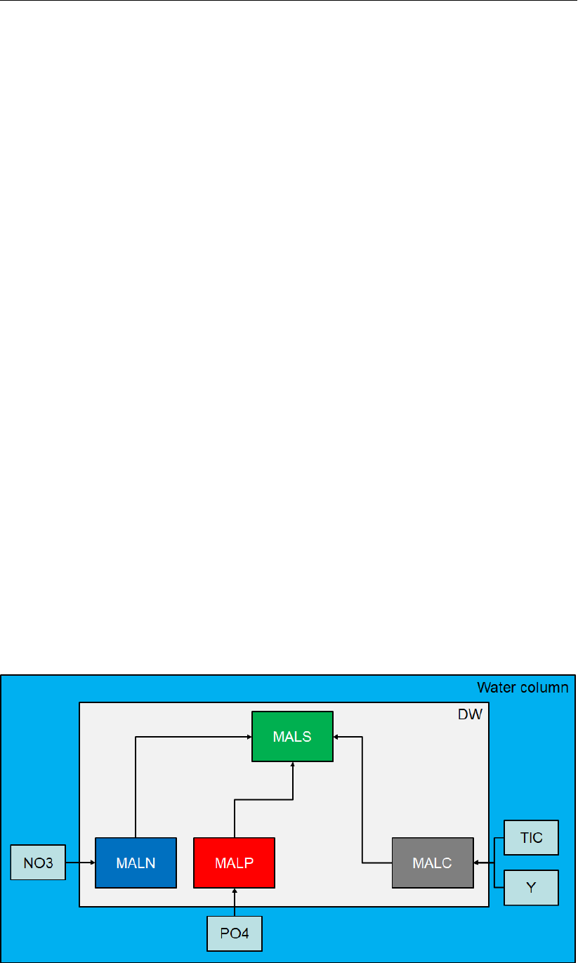
Macroalgae can be idealized as 4 distinct state variable components:
MacroALgae Structural mass (MALS, gDM m2)
MacroALgae Nitrogen storage mass (MALN, gN m2)
MacroALgae Phosphorous storage mass (MALP, gP m2)
MacroALgae Carbon storage mass (MALC, gC m2)
Collectively these components represent the entire macroalgae "frond", where frond is the
term used to describe the macro structure of the algae visible to the naked eye, including the
foot (attachment organ). Each component of the frond exhibits its own growth dynamics and
interacts with the surrounding water independently. The relationships between the variables
is shown in Figure 1.
Figure 1: Relationship between the state variables in MALG
1

The structural mass represents the part of the macroalgae that increases the area and length
of the total front when it grows. Its surface area dictates that which is available to capture solar
energy. It does not take nutrients from the water, does not photosynthesize, and produces
detritus when it decays/erodes. It grows by taking nutrients (N/P/C) from its storage and
has its own fixed carbon, nitrogen, and phosphorous ratios that it must satisfy to grow. The
structural mass has units of dry matter (DM m−2) and is similar to the common notion of
’dry matter’. However, it is less than the true dry matter content of the frond that would be
measured because it represents only the dry weight of the plant minus the weight of water,
nutrient stores, and carbon stores. The model does also compute dry weight (DW), which is
the structural weight including the mass of nutrient stores, and wet weight (WW), which is the
structural weight including the mass of nutrient stores with water. Both of these are model
outputs and not state variables.
The nitrogen and phosphorous storage (or reserves) uptake dissolved inorganic nutrients
(NO−
3, PO3−
4) from the ambient water and store them for use by the structural mass during
growth periods. In this model it is assumed the phosphorous storage dynamics are analagous
to the nitrogen, but in reality the behaviour of phosphorous storage is not well known.
The carbon storage is the part of the plant responsible for photosynthesizing, producing ex-
udate, and respiring. It produces carbon stores (carbohydrates) by taking up dissolved inor-
ganic carbon and producing oxygen via photosynthesis. It provides carbon to the structural
mass during growth periods.
It is assumed that there is constant relationship between volume and area of a macroalgae
frond. This means that the density of the macroalgae does not change, even if the ratio
of structural mass to stored material changes. Additionally, the C:N and C:P ratios of each
component are fixed, but because the ratio of stored mass to structural mass changes, the
C:N and C:P ratios of the entire frond, and thus the dry matter, will change due to changes in
the environment.
2
0.1.1 Distribution of macroalgae biomass in the water column
PROCESS: MALDIS
The physiological equations described in Ole Jacob Broch (2012) do not mention any phys-
ical description of the seaweed fronds in space aside from their area. Area (m2) is actually
the main state variable in the Broch model. The translation from an area based model to a
mass based model is straightforward because Broch uses a constant conversion factor be-
tween area and mass (called ArDenMAL in MALG), and employs this factor in many of
the model equations where mass rates concerning the structual mass are involved. Therefore
application of Broch’s area based equations to DELWAQ’s mass based system is not trivial
but possible given Broch’s fixed mass to surface area frond ratio and a DELWAQ segment sur-
face area. In most cases the equations involving MALS in MALG are simply not multiplied
by ArDenMAL as the units are already in mass and not area. The largest implications of
the difference between Broch and MALG relate to photosynthesis, which is proportional to the
frond area in both model implementations. For these calculations, the MALS mass is simply
multiplied by the segment surface area and divided by the ArDenMAL to obtain the frond
area in the segment. For fluxes a conversion is made to obtain the units of g m−2or g m−3.
However, implementation in DELWAQ also requires knowledge of the vertical space occupied
by the frond, which is not given by Broch. Thus, the algorithms for distributing the frond mass
in space have been developed independently of the physiological formulations in Broch.
A simple approach is taken, whereby fronds (typically) only grow in length and retain a con-
stant length:area ratio. The exception to this rule is when a frond is able to reach the end of
the water column (i.e. the bed or the water surface) while it still has the capacity to grow. In
these situations only the area will increase and not the length. The case for a single frond per
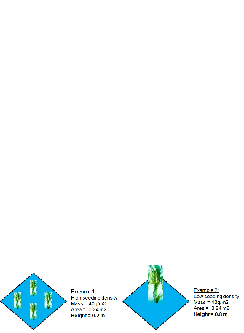
computational cell is simple. However, the code must be able to deal with any seeding density,
which cannot be uniquely defined in a 3D model by the mass per m2in DELWAQ alone. For
example, consider two cases whereby there exists 40g of dry matter per m2as is shown in
Figure 2.
Figure 2: Two situations that have identical mass but non-identical position of the mass
in the vertical axis
In the first example there are 4 fronds in a 1 m2square. They each weigh 10 g, have a
combined area of 0.24 m2and are each 0.2 m long. In a second example, there is a single
frond in a 1 m2square. It weighs 40 g, has an area of 0.24 m2, and is 0.8 m long. In a 3D
model with grid cells that are <0.8 m thick, the nutrient uptake will take place in different cells
in each of the two cases even though the mass per m2is identical in DELWAQ. To avoid this
ambiguity the user must prescribe a set of parameters to describe the spatial characteristics
of the culture. These are as follows:
3

F ootDepth The depth below the water surface that the foot of the frond is attached.
The frond begins growing from the segment that intersects this depth, and the segment
it resides in within a sigma layer model can change with a variable water level as it is
assigned each time step.
LmaxMAL The maximum length of the frond measured in the vertical (z) axis from the
foot to the tip of the frond.
SwGroMAL Switch for an upwards (>0) or downwards (<0) growing frond.
LinDenMal The linear density of the culture. This describes the amount of mass it
takes a m2of culture to grow 1 m. Four small fronds require more mass to increase their
collective length by 1 m compared to a single long frond. All fronds in a single segment
change length at the same rate.
ArDenMal The area density of the culture. This is the ratio between surface area and
dry weight.
The model does not explicitly model individual plants in a given segment, and so the collective
mass per segment is generally referred to as a culture in this model. However, for most
purposes the model can be understood by idealizing the culture as a single frond with variable
girth. Thus, the word ’frond’ pertains to the physical structure of the culture (length, area), and
may represent one or more individual plants depending on the settings of the parameters just
described.
Using these parameters the culture’s position can be completely described in 3 dimensions.
To determine the position of the frond in the water column each time step, the process first
calculates the length and the area of the culture in this column of segments:
LenMAL =MALS ×LinDenCor
LinDenMAL ×Nfrond
(1)
AreMAL =MALS ×Surf
ArDenMAL (2)
Where:
LenMAL Length of culture in the column (m)
Surf Surface area of the bottom segment (m2)
MALS structural mass (gDM m−2)
LinDenMAL The linear density of a single frond (g m−3)
LinDenCor Frond length correction factor for low biomass density (−)
Nfrond Number of fronds per m2 (must be ≥1)
ArDenMAL The area density of the culture (g m−2)
Note that Nfrond is said to be ≥1even though there are certainly situations where it is
not the case. The reason that Nfrond must be specified is to act as a scaling factor on
LinDenMAL and mrtMAL (see process FLMALS), since they are defined on the basis
of a single frond growing 1m in a 1m2box. When there are more than 1 fronds in that box
then the biomass required to increase the length of the culture increases. When biomass
densities are extremely low due to perhaps large grid sizes, then it is not meaningful to think
of anything other than an equal distribution of fronds across each m2of the grid cell, be-
cause any frond will always experience itself. Additionally this is a central assumption of the
model (well mixed within a single segment). In these situations a very low biomass density
multiplied by LinDenMAL will yeild a very short plant. The exchange with the ambient
4

water will be correct but the vertical discretization will not be. To correct for this the parameter
LinDenCor can be specified to make the frond much skinnier in order to have it posess the
desired length.The correction factor for situations where the number of fronds per m2is <1 for
segment ishould be set to:
LinDenCori=18
MALSi
(3)
To further adjust this length beyond correcting for biomass density, i.e. to incorporate the effect
of ropes, you can adjust the factor F rondStrech. This will simply multiply the computed
length by a constant to elongate the frond and spread the biomass and the fluxes over more
segments.
LenMAL is then used to check which segments the frond biomass should be present in,
and which fraction of the frond exists in each segment. This fraction is communicated to
each segment for all other computations involving biomass and fluxes. As all MALG param-
eters are non-transportable (g m−2), only the bottom segment can truly contain any MALG
mass. However, depending on the ratio of segment depths to frond length, the culture can
exhibit fluxes affecting segments other than the bottom segment. To achieve this effect with-
out actually storing any mass in segments above the bottom segment, MALDIS tells each
segment what fraction of the biomass in the water column resides in any particular segment
(F rBmLay), and also the mass of this biomass as the parameter BmLayMAL. All mass
actually administratively resides in the bottom segment however.
The calculation of this biomass fraction depends firstly on whether the frond grows upwards
or downwards.
Zm =SwGroDir < 0 : LenMAL +F ootDepth
SwGroDir > 0 : F ootDepth −LenMAL (4)
Where:
Zm Distance from water surface to tip of frond (positive down) (m)
Z1Distance from water surface to top of segment (positive down) (m)
Z2Distance from water surface to bottom of segment (positive down) (m)
The segment top depth Z1and segment bottom depth Z2are then checked against Zm to
see if the frond resides entirely within, entirely outside, or partially within the current segment
in the segment loop. The fraction of the biomass allocated to the current segment is then the
ratio of the segment depth to LenMAL in the column for segments in which the frond com-
pletely resides, or the ratio of the difference between Zm and either Z1or Z2to LenMAL
for segments in which the tip or foot of the frond is found.
Experiments done by Sjøtun (1993) show that the length of Saccharina can vary between 0.8
m and 1.6 m, and the growth in length of the fronds varied between 0.1 and 1.2 cm d−1. The
length to width ratios of the new frond material varied quite a bit, but during periods of high
growth it was approximately 0.5. Thus, we assume for every cm gained in length there are 2
cm gained in width. Note that the overall shape of the plant is such that the L/W ratio is >1,
because it is only new material that grows at a ratio less than 1. Taking the Ole Jacob Broch
(2012) value of 0.6 g sw dm−2(60 g)as the area density, it is found that the plant is expected
5

to require 0.003 g sw cm−1of growth in length. Thus, the default value for LinDenMAL is
set to 0.3 g sw m−1.
Note that this module is somewhat different than other DELWAQ modules because of the
notion of ghost mass. This means that although state variables are written to the bottom seg-
ment, outputs are written to segments that the mass should otherwise in 3D space reside.
This means that there are some values that are written to individual segments only if the seg-
ments have biomass, and some values that are written to all segments in a water column that
has some biomass in the bottom layer. The clarification of which is which is now described:
Type 1. State variables strictly always exist only in bottom segments:
MALS
MALN
MALP
MALC
Type 2. Outputs that reflect what is happening in the specific segment and is = 0 for segments
without biomss, including bottom segment if FrBmLay == 0:
Generally all variables with the prefix ’Loc’
LocGroC
LocGroN
LocGroPS
LocUpC
but NOT LocAreaMAL
All variables with the prefix ’Lim’
biomass based output such as MALCDMS
Wet and Dry weight
Type 3. Outputs that reflect what is happening in the column, and all segments in the column
have the same value:
LengthMAL
LocAreaMAL
6

0.1.2 Flux of Macroalgae structural biomass
PROCESS: FLMALS
The structural component of the macroalgae is the dry material that gives shape and structure
to the macroalgae frond. It does not include N, P, or C stores, but has a fixed N, P, and C
component, meaning that these nutrients are required for growth of the structural mass and
there is a minimum amount of N,P and C in the structural mass regardless of the reserve
nutrient level. As the structural mass grows it increases the length and area of the entire
frond. Growth of other components of the frond (nutrient reserves) do not have any effect on
the frond length, volume, density, or surface area.
The net growth of the structural mass is the resulting rate of structural biomass production and
frond erosion (considered to be analagous to mortality used in other DELWAQ processes).
This balance can be defined by the following equation:
dGrowMALS =MALS ×(µ−φ)(5)
Where:
µspecific growth rate of macroalgae sturctural mass (d−1)
φmortality/erosion rate (d−1)
The growth rate µof MALS is dependent firstly on the available nutrient stores (MALN,
MALP , and MALC). The growth rate is defined as follows:
µ=fdensityfphotoperiodftemperature ×min1−Nmin
MALN ,1−Pmin
MALP ,1−Cmin
MALC (6)
Where:
fdensity biomass density limitation function (-)
fphotoperiod photoperiod limitation function (-)
ftemperature temperature limitation function (-)
Nmin minimum N storage (gN gDM−1)
MALN nitrogen storage (gN/m2)
Pmin minimum phosphorous storage (gP gDM−1)
MALP phosphorous storage (gP/m2)
Cmin minimum carbon storage (gC gDM−1)
MALC carbon storage (gC/m2)
Note that in the code the storage terms are temporarily converted to gX/gDMstructural by
dividing by MALS to comply with the formulations and units outlined in Ole Jacob Broch
(2012) where they have units of gX/gDMstructural. In MALG formulations, the storage state
variable terms are (must be) g m−2as per all non-transportable DELWAQ substances, and
this is reflected in the fluxes, which are back calculated to g m−2d−1. As the substances
are non transportable they reside in the bottom segment. However, depending on the user
defined variables, it is possible for the mass and associated fluxes to have no effect in the
bottom segment, such as in the case where the algae grow from the water surface downward.
This is discussed in MALDIS.
7

gDMstructural is not equivalent to dry matter, ad it does not include the nutrient stores. Dry
weight and wet weight are calculated by the model according to the following equations:
W dry =MALS(1+kN(MALN−(MALNmin))+MALNmin+kC(MALC−MALCmin)+MALCmin)
(7)
W wet =MALS(1
kD
+kN(MALN−(MALNmin))+MALNmin+kC(MALC−MALCmin)+MALCmin)
(8)
Where:
kCcarbon:dry matter ratio in structural mass (gC gDM−1)
kNnitrogen:carbon ratio in structural mass (gN gC−1)
kWdry weight to wet weight ratio in structural mass (g g−1)
The growth rate of the struc-
tural mass is dependent on a density limitation, a photoperiod limitation, and a temperature
limitation. These limitations differ from conventional DELWAQ limitations for algae growth in
that they do not range strictly between 0 and 1 and alter a pre-defined growth rate. Instead
Broch has tuned them such that their product is equal to the maximum growth rate when
conditions are optimal (0.18 d−1).
The density limitation represents the ability of the frond to only grow so big, and the bigger it
gets the lower its growth rate will become. The formulation is as follows:
fdensity =m1exp−(AreaLoc
MALS0×Nfrond
)2+m2(9)
Where:
m1growth rate parameter 1 (-)
m2growth rate parameter 2 (-)
AreaLoc local frond area in this segment (m2)
MALS0critical biomass area (m2)
This formulation is designed to allow small fronds to grow faster than bigger fronds, and as
such the value in broch describes the area above which a frond will stuggle to grow. This has
large implications for the DELWAQ model in contrast to the Broch model which is ’individual
based’ and thus can integrate this formulation seamlessly. The frond area LocArea in a
DELWAQ segment does not represent a single frond, but the sum of all frond areas in a
segment. This means that the default value for MALS0cannot be used in the case where
the DELWAQ user expects more than one frond per segment. It could be possible to require
that the user specify LinDenMAL and MALS0based on their knowledge of how many
fronds they expect there to be in a segment. However, it is thought that knowledge of the
number of fronds per m2is a better confined value. Thus, the following formulations are used
in the code.
LinDenMAL = 100 ×Nf rondm2(10)
and
MALS0= 0.06 ×Nfrondm2(11)
8

Where 100 g m−3is derived from the relationship between mass gain and length increase
seen in Sjøtun (1993), and 0.06 m−1is taken from Ole Jacob Broch (2012). These formula-
tions describe how as the number of fronds m−2increases, the area limit within the segment
increases and the amount of carbon required to increase the length of the culture in the seg-
ment increases, and both are proportional to what is known about the behaviour of a single
frond.
Some examples are shown below:
The photoperiod limitation is similar to the daylength limitation used in BLOOM and DYNAMO,
but instead considers the normalized change in daylength compared to the previous day in-
stead of the actual current daylength. In this context, ’normalized’ means that the change in
daylength is relative to the maximum change in daylength (i.e. the daylength change at the
equinoxes). This response to normalized daylength change is due to the fact that Saccharina
latissima is a seasonal anticipator and will grow and store nutrients in accordance with the
change in the season as determined by how much longer or shorter the days become. This
formulation is given by:
fphotoperiod =a1(1 + sin(τ(n)|τ(n)|1
2)) + a2(12)
Where:
a1photoperiod parameter 1 (-)
a2photoperiod parameter 2 (-)
and τis a function describing the normalized difference in day length between current day and
previous day. This function is calculated by the process DAYLP which essentially identical
to the standard DELWAQ process DAYL. The parameters a1and a2are chosen such that
0.3> fphotoperiod <2at the given latitude. In future implementations it is hoped that the
code will calculate this for the user, but it currently requires an iterative approach before the
simulation to define the correct values for the given latitude to ensure 0.3> fphotoperiod <2.
The temperature limitation is a simple piece wise function that identifies an optimal growth
between temperatures 10-150C, no growth above 190C, and linear growth increasing between
-1.8 and 100C. The temperature limitation is therefore:
ftemperature =
0.08T+ 0.2−1.8<10
1 10 ≤T≤15
19/4−T/4 15 ≤T≤19
0T > 19
(13)
The specific erosion (mortality) rate φof the structural biomass is proportional to the area of
the frond and the erosion parameter. The formulation is as follows:
φ=10−6exp(×LocArea
Nf rond )
1 + 10−6exp((×LocArea
Nf rond )−1) (14)
Where:
erosion parameter (m−2)
LocArea Area of frond per m2of segment (m−2)
9

The structural growth process occurs over all segments which have a biomass fraction >0.
This is in spite of the fact that the biomass administratively resides in the bottom segment.
During each time step, all segments with a non-zero biomass fraction receive ’ghost’ structural
and storage mass according to the biomass allocated to it in MALDIS. The local inorganic
nutrient, gas, and particulate fluxes are calculated using this mass and the local ambient
conditions. The fluxes are then locally applied to ambient state variables exogenous to MALG,
but not the MALG parameters (MALS, MALN, MALP, MALC). Instead, the fluxes of MALG
state variables are communicated to the bottom segment in a cumulative way, whereby the
local fluxes of all segments that share the same bottom segment are summed to compute
the net total change in MALS,MALN,MALP , and MALC resulting from the net
growth in the column. Once the bottom segment is reached in the segment loop, the fluxes
for each column of segments have been accumulated and the net change in mass of each
administrative bottom segment is known. The culture will then become longer or shorter in the
next time step to reflect this new state, which again is kept track of by the bottom segment in
the column. The consequence of applying this technique is that the local per segment ’ghost
reserve masses’ adopt the reserve ratio of the whole column. Another way to say this is that
all segments with a non-zero biomass fraction belonging to a given water column have a fixed
structural mass to storage mass ratio, and consequently all reserves are equally distributed
along the frond.
10

0.1.3 Flux of Macroalgae nutrient storage
PROCESS: FLMALN
The nutrient storage component(s) of the macroalgae (also referred to as reserves) are those
that supply nutrients for growth of the structural mass. The storage is also responsible for
taking up dissolved inorganic nutrients from the ambient water. The reserves consist of a
nitrogen (MALN) and a phosphorous (MALP ) storage component, which are both dealt
with in the same nutrient storage subroutine. Note that Ole Jacob Broch (2012) does not
include a phosphorous component to the nutrient storage, but it is included in this model for
flexibility should new information about phosphorous storage become available. Currently the
model is written such that the culture cannot be P limited and no P flux will occur.
The change in a nutrient storage mass is given by the following equations:
dUptMALN =JN−µ(kC×kN×MALS +MALN)(15)
dUptMALP =JP−µ(kC×kP×MALS +MALP )(16)
Where the state variables MALN and MALP are in the units given by Broch (gX/gDM),
which is achieved in MALG by dividing MALX by MALS at the begining of the subroutine.
This is valid because the storage is distributed equally along the frond. This equation repre-
sents the balance between uptake Jand utilization for growth of the frond’s structural mass µ.
The uptake is dependent on flow velocity, the amount of stores compared to the minimum and
maximum possible, and the ambient nutrient concentration. The formulation for both nitrogen
and phosphorus is described as follows:
JN=fvelocityJNmax(NO−
3
Ksn +NO−
3
)( MALNmax −MALN
MALNmax −MALNmin
)(17)
JP=fvelocityJP max(P O3−
4
Ksp +P O3−
4
)( MALPmax −MALP
MALPmax −MALPmin
)(18)
fvelocity = 1 −exp(−U
U0.65
)(19)
Where:
kPphosphorous:carbon ratio in structural mass (gN gC−1)
JNmax maximum uptake rate nitrogen (gN m−2d−1)
Ksn half saturation for inorganic nitrogen uptake
NO−
3ambient nitrate concentration (gN m−3)
MALNmax maximum nitrogen storage (gN gDM−1)
MALNmin minimum nitrogen storage (gN gDM−1)
JP max maximum uptake rate nitrogen gP m−2d−1)
Ksp half saturation for inorganic nitrogen uptake (gP m−3)
P O3−
4ambient phosphate concentration (gP m−3)
MALPmax maximum phosphorous storage (gP gDM−1)
MALNmin minimum phosphorous storage (gP gDM−1)
Uwater velocity (m s−1)
U0.65 water velocity at which uptake rate is 65 of maximum (m s−1)
11

The first term in JNand JPpertains to the uptake of nutrients and the second term to the
utilization of stores by the structural mass during growth. Note how the nutrient requirement
(quota) is dependent on the combined quota for structural mass and storage mass. The
uptake of nutrients is dependent on the ambient concentration according to Michaelis-Menten
kinetics. It is dependent on velocity such that high velocities make it easier for the frond to
uptake the nutrients. This is related to an improved mass transfer coefficient. At sufficiently
high ambient concentrations and water velocities the uptake rate is Jmax.
12
0.1.4 Flux of Macroalgae carbon storage
PROCESS: FLMALC
The carbon storage component of the macroalgae (MALC) supplies carbohydrates for
growth of the structural mass. The carbon storage is also responsible for photosynthesis,
respiration and exudation. The change in a carbon storage mass is given by the following
equation:
dUptMALC =P(1 −E)−R−µ(kC×MALS +MALC)(20)
Where:
PGross photosynthetic rate (gCm−3d−1)
EFraction exudation (-)
RMaintenance respiration rate (gCm−3d−1)
Where the first term relates to the net of production, respiration and exudation, and the second
term pertains to the utilization of carbon stores by the structural mass. The state variables
MALC is given here in the units used by Broch (gC/gDM), which is achieved in MALG by
dividing MALC by MALS at the begining of the subroutine. This is valid because the
storage is distributed equally along the frond.
The carbon production rate (i.e. photosynthesis) is given by the following set of equations:
P(T, I) = Ps(1 −exp(−α×I
Ps
))exp(−β×I
Ps
)(21)
Ps(T) = α×Isat
ln(1 + α
β)(22)
Pmax(β) = ( α×Isat
ln(1 + α
β
)( α
α+β)( β
α+β)β
α(23)
Pmax(T) = P1exp(TAP
TP1)
1 + exp(TAP L
T−TAP L
TP L ) + exp(TAP H
TP H −TAP H
T)(24)
Where:
13

PPhotosynthetic rate (gC dm−2h−1)
Ps(T)Saturation photosynthetic rate (gC dm−2h−1)
IIncident radiation (W m−2)
Isat Saturation radiation (W m−2)
αPhotosynthetic efficiency (gC dm−2h−1(µmolpm−2s−1)−1)
β(T)Photosynthetic light inhibition (gC dm−2h−1(µmolpm−2s−1)−1)
P1Reference photosynthetic rate at T1(0K)
P2Reference photosynthetic rate at T2(0K)
TWater temperature (0K)
TP1temp for reference photosynthetic rate 1 (0K)
TP2temp for reference photosynthetic rate 2 (0K)
TAP Arrhenius temperature for photosynthesis (0K)
TAP H Arrhenius temp for photosynthesis high end (0K)
TAP L Arrhenius temp for photosynthesis low end (0K)
Note the use of unconventional DELWAQ units dm2,µmol (photons), and hours. These have
been maintained to allow easy comparisons to Broch and to emphasize the fact that photo-
synthesis is proportional to frond surface area and not segment surface area in MALG. There
is an internal conversion in the code from W, the unit of DELWAQ radiation, to µmol s−1,
the unit of irradiance in the formulations, which is 4.57 µmols−1
W. After production, respiration
and exudation have been calculated, all rates are converted to gC m−2d−1by multiplying by
2400. Recall that this is still in m2 of frond per segment, and this is further multiplied by the
total area of frond in the segment, which is later divided by the segment surface area to get
the gross production flux.
It would be possible for this routine to receive information about the light environment in the
water column from the process CALCRAD. However, the first implementation of the MALG
module was meant to be independent of other DELWAQ processes, hence the creation of
DAY LP instead of simply editing DAY L. For integration into DELWAQ, the previous day
length and the light environment should be provided to MALG processes instead of being cal-
culated by MALG processes. The irradiance in MALG is calculated using the same equations
as is used in DYNAMO, using the surface irradiance, the extinction of visible light, and the
water depth, while integrating the Lambert-Beer equation over the current segment using the
following equation:
I=−I0e−ExtV l×LocalDepth
ExtV l ×Depth −e−ExtV l×(LocalDepth−Depth)(25)
Where:
I0Irradiance at the surface (W m−2)
ExtV l Extinction of visible light (m−1)
Depth Thickness of segment (m)
LocalDepth Depth of bottom of segment below water surface (m)
Currently the macroalgae do not attenuate light in the water column.
This set of equations describes a photo inhibitory effect for I > Isat. The structural mass
is strictly unable to grow above T > 190. Although the structural mass cannot grow, pho-
tosynthesis production can still occur in the range >−10CT emp < 230C. These two
temperature controls are fixed for the species and the user cannot flexibly change this unless
the code is edited. To adapt the model to tropical species or species that have a different opti-
14
mal temperature photosynthesis range, both the temperature function and the photosynthetic
range parameters have to be edited in addition to the code for the piece-wise temperature
growth function for MALS.
The formulations also show that maximum production rate Pmax can be expressed in two
ways. The first is only a function of temperature and describes photosynthesis at I=Isat.
The second production rate Pmax is the actual maximum production rate taking into account
the effect of temperature on the response of growth to light. This means that growth is non-
linear in temperature, as it effects both growth directly and also the way in which growth is
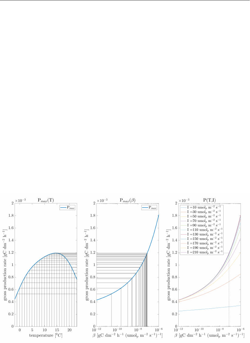
affected by light. βis solved for using Newton’s method in Broch by differentiating Pmax(β).
This involves solving for the value βsuch that Pmax(T)equals the Pmax(β)obtained from
the temperature relationship at the current temperature and at I=Isat. Newton’s method
is not used in the DELWAQ code and instead βis pre-calculated for all temperatures in the
photosynthetic range -20C to 230C at an interval of 0.10C. This is hard coded into the FLMALC
subroutine and constitutes a linear approximation of β. Due to this the model should only be
used for temperature ranges −20C < T < 230C. Currently:
β(T)for T < −20C=β(−20C)and β(T)forT > 230C=β(230C).
Consequently, temperatures above or below the photosynthetic temperature range will result
in a production rate equivalent to the rate at the closest temperature in the range. The rela-
tionship between temperature, beta, irradiance and gross production is shown in Figure 3
Figure 3: Relationship between temperature, β, irradiance and gross production. Here
the black lines demonstrate the process by which for a given temperature
Pmax(T)is calculated, and the corresponding βvalue required to achieve
Pmax(T) = Pmax(β)is derived, and used to calculate the response of growth
rate to irradiance, where P=Pmax when I=Isat
15

0.1.5 Harvesting of macroalgae
PROCESS: HRVMAL
To be filled in.
16

0.2 Model validation
This section briefly outlines the test cases for the application of the MALG model. Two test
cases have been outlined:
Broch 1DV model
A simple (large) 3D flume model with tidal currents
0.2.1 Testcase: Broch 2012
This testcase involves the reproduction of the model as it was demonstrated in Ole Ja-
cob Broch (2012). The testcase involves a single frond growing off the coast of Nowrway
in 250m deep water at approximately 5 m below the surface, although the depth of the frond
in Ole Jacob Broch (2012) is never explicitly stated. The kelp grows in a 0D model (a box) with
temperature, nitrogen, and light climate forcing derived from measurements and local models.
These forcing functions are shown in Figure 4.
17
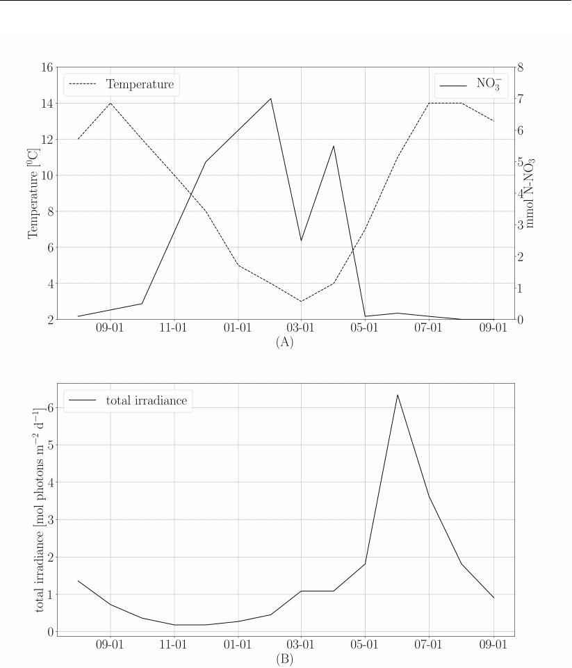
Figure 4: (A) Temperature and NO3forcing used in the model. (B) 10 m irradiance forcing
used in the model. All forcing is adapted from Ole Jacob Broch (2012)
Only MALG processes and processes relating to reaeration of CO2and O2and pH are ac-
tivated in this model. All model constants are set to the default values described in Ole Ja-
cob Broch (2012). There are however a few exceptions:
Broch states that the maximum growth rate of the structural mass is 0.18 d−1. Broch
also states that the contribution to the growth rate from MALN = 1−= 0.65. As
MALNmax is stated as = 0.022, it must be the case that 1− ≤ 0.565. Thus, the µin
MALG is up to 13 percent lower than in Ole Jacob Broch (2012). The has been changed
from the default 0.22 m−1to 0.18 m−1to counteract this effect.
Broch checks the gross production formulation at I = 10 µmol m−2s−1and T = 120and
arrives at a value of 2.95 ×10⁻⁴gCdm−2h−1. This is lower than the value computed
by MALG under the same conditions (3.21 ×10⁻⁴gCdm−2h−1). It is at least partially
due to the different method of approximating β, but it was also found that Pmax(Tpl)6=
3.394 ×10⁻⁴gCdm−2h−1in contrast to what was stated in the paper. This discrepancy
18

may be due to discrepancies in Tapl and Taph, which were stated to be 27,7740Kand
25,9240Krespectively in the paper but could not be reproduced using the high and low
end temperatures and production rates. Thus the gross production is higher in MALG than
in Ole Jacob Broch (2012).
ExtV L is set to 0.07 m−1in Broch, but the depth is not known. In the test case the
model is 10 m deep and ExtV l = 0.18 m−1. this means the frond likely received less
light than in Broch, counteracting the increased production rate.
The model settings specifically for the MALG processes are listed in Table 1:
parameter value unit description
K0HrvMALS 0.00000 (gDM/m2/d) zero order harvesting rate Macroalgae
K1HrvMALS 0.00000 (1/d) first order harvesting rate Macroalgae
MALCmin 0.100000E-01 (gC/gDM) minimum C in storage
CDRatMALS 0.200000 (gC/gDM) C to structural dry mass ratio in MALS
ArDenMAL 60.0000 (gDM/m2) Area density frond (grams/m2 surface area)
R1 0.278500E-03 (gC/dm2/h) Reference respiration rate at T1
R2 0.542900E-03 (gC/dm2/h) Reference respiration rate at T2
Tr1 285.000 (degK) reference temperature 1 for respiration
Tr2 290.000 (degK) reference temperature 2 for respiration
P1 0.122000E-02 (gC/dm2/h) Reference photosynthetic rate at T1
P2 0.144000E-02 (gC/dm2/h) Reference photosynthetic rate at T2
Tp1 285.000 (degK) temp for reference photosynthetic rate 1
Tp2 288.000 (degK) temp for reference photosynthetic rate 2
Tap 1694.00 (degK) Arrhenius temperature for photosynthesis
Taph 25924.0 (degK) Arrhenius temp for photosynthesis high end
Tapl 27774.0 (degK) Arrhenius temp for photosynthesis low end
Tar 11033.0 (degK) Arrhenius temp for respiration
ExtVl 0.180000 (1/m) total extinction coefficient visible light
alpha0 0.375000E-04 (...) photosynthetic efficiency MALC
Isat 43.7630 (W/m2) light intensity where photosynthesis is max
exuMALC 0.500000 (gC/gC) exudation parameter
MALNmin 0.100000E-01 (-) minimum N in storage
MALNmax 0.220000E-01 (gN/gDM) maximum N in MALN
MALPmin 0.100000E-02 (gP/gDM) minimum P in storage
MALPmax 0.220000E-02 (gP/gDM) maximum P in MALP
NCRatMALS 0.500000E-01 (gN/gC) N:C ratio in MALS
PCRatMALS 0.500000E-02 (gP/gC) P:C ratio in MALS
Ksn 0.560000E-01 (gN/m3) half saturation MALN N uptake
Ksp 0.126000E-01 (gP/m3) half saturation MALN P uptake
JNmax 0.336000 (gN/m2/d) maximum MALN N uptake rate (per area frond)
JPmax 0.336000 (gP/m2/d) maximum MALP P uptake rate (per area frond)
Vel 0.150000 (m/s) velocity
Vel65 0.300000E-01 (m/s) current speed at which J = 0.65Jmax
Latitude 52.0000 (degrees) latitude of study area
m1 0.108500 (-) growth rate parameter 1
m2 0.300000E-01 (1/d) growth rate parameter 2
MALS0 0.600000E-01 (m2) growth rate parameter 3
a1 1.02000 (-) photoperiod parameter 1
a2 0.120000 (-) photoperiod parameter 2
mrtMAL 0.180000 (1/dm2) epsilon erosion/mortality parameter macro
CDRatMAL 0.200000 (-) C:DM ratio in MALS
NCRatMAL 0.500000E-01 (-) N:C ratio in MALS
PCRatMAL 0.500000E-02 (-) P:C ratio in MALS
19

Kn 2.72000 (gN/gN) mass of nitrogen reserves per gram nitrogen
Kc 2.12130 (gC/gC) mass of carbon reserves per gram carbon
Kdw 0.785000E-01 (-) structural dry weight per unit frond area
FrPO1MAL 0.750000 (-) fraction of MALS that goes to POC1 in decay
FrPO2MAL 0.250000 (-) fraction of MALS that goes to POC2 in decay
TotalDepth 10.0000 (m) total depth water column
FootDepth -999.999 (m) location of frond attachment in the water columns
LmaxMAL 10.0000 (m) Maximum length MALG
SWGroDir 1.00000 (-) grow direction MALG(1 = up -1 = down )
LinDenMAL 100.000 (g/m3) linear density of macroalgae
Velocity 0.500000 (m/s) horizontal flow velocity
Table 1: List of parameters used in the Broch test case. All except are the default value.
Figure 5and Figure 6demonstrate the performance of the MALG implementation compared to
measurements used in Ole Jacob Broch (2012), which originate from Sjøtun (1993). Deviation
with respect to Broch are mostly due to the uncertainties described in the exceptions to the
Broch model.
20
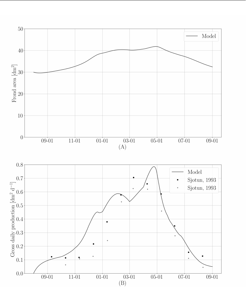
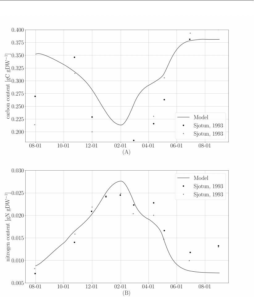
Figure 6: (A) Carbon content expressed as a fraction of dry weight. Solid line, model
results. Circles, Sjøtun (1993) proximal/meristematic tissue. Crosses, apical
frond tissue. (B) Nitrogen content expressed as fraction dry weight. Solid line,
model results. Circles, Sjøtun (1993) 2-year plants. Crosses, Sjøtun (1993),
3-year plants.
22
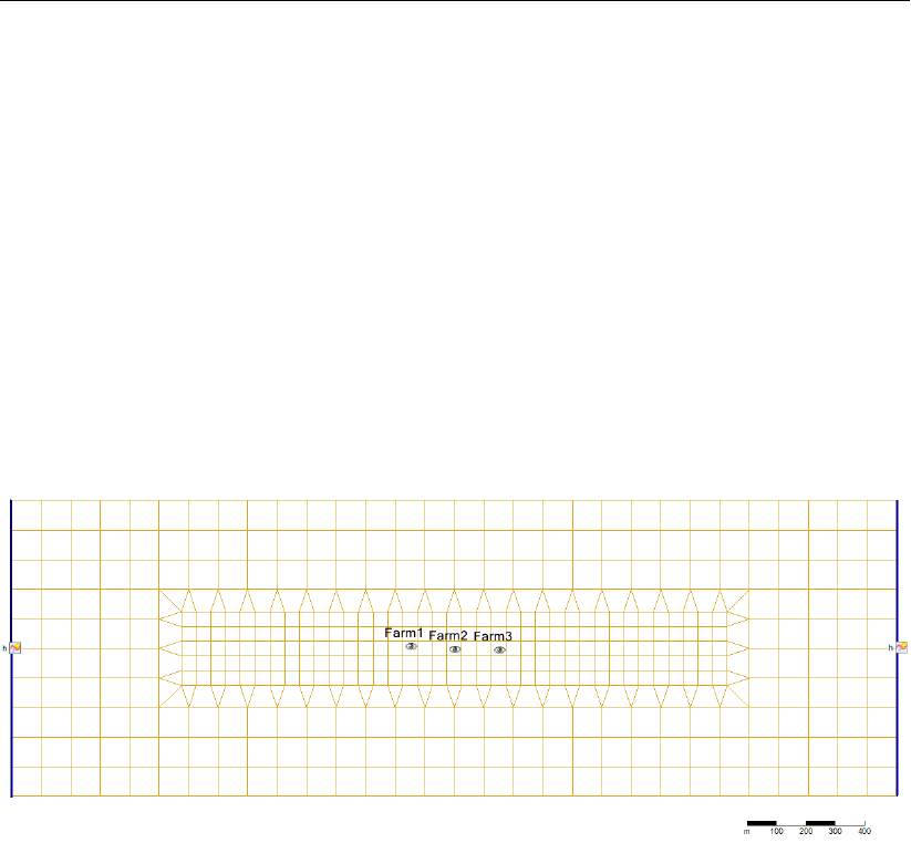
0.2.2 Testcase: Tidal flume farm
The tidal flume farm test case is a synthetic case used to test the 3D performance of the
model in Delft3D flexible mesh with sigma layers. It is designed to demonstrate that the
biomass allocation works with variable sigma layer thickness in time due to tidal variation.
The test case consists of a 10x30 cell grid with 100 m resolution containing a factor 2 refine-
ment in the center to obtain a 50m resolution. The model is thus 1km x 3km. It has a uniform
depth of 10 m and 20 sigma layers, meaning each layer is 0.5 m deep. The tidal amplitude
applied is 2 m and velocities vary between 0.0-0.1 m/s. The flow switches direction approxi-
mately every 6 hours. The oscillation of the layer thickness means each layer will be between
0.4 m (low water) and 0.6 m (high water). Thus as long as the plant is at least 0.4 m long
and grows a minimum of 0.4 m, the segments within which it resides will vary within a single
tidal period due to water level variations alone. Multiple farms are located within this higher
resolution area. The layout is shown in Figure 7
Figure 7: Layout of the tidal flume farm test case
0.3 References
Ole Jacob Broch, D. S., 2012. “Modelling seasonal growth and composition of the kelp Sac-
charina latissima.” Journal of Applied Phycology 24: 259-776.
Sjøtun, I. K., 1993. “Seasonal Lamina Growth in two Age Groups of Laminaria saccharina (L.)
Lamour. in Western Norway.” Botanica Marina 36: 433-441.
23
